/


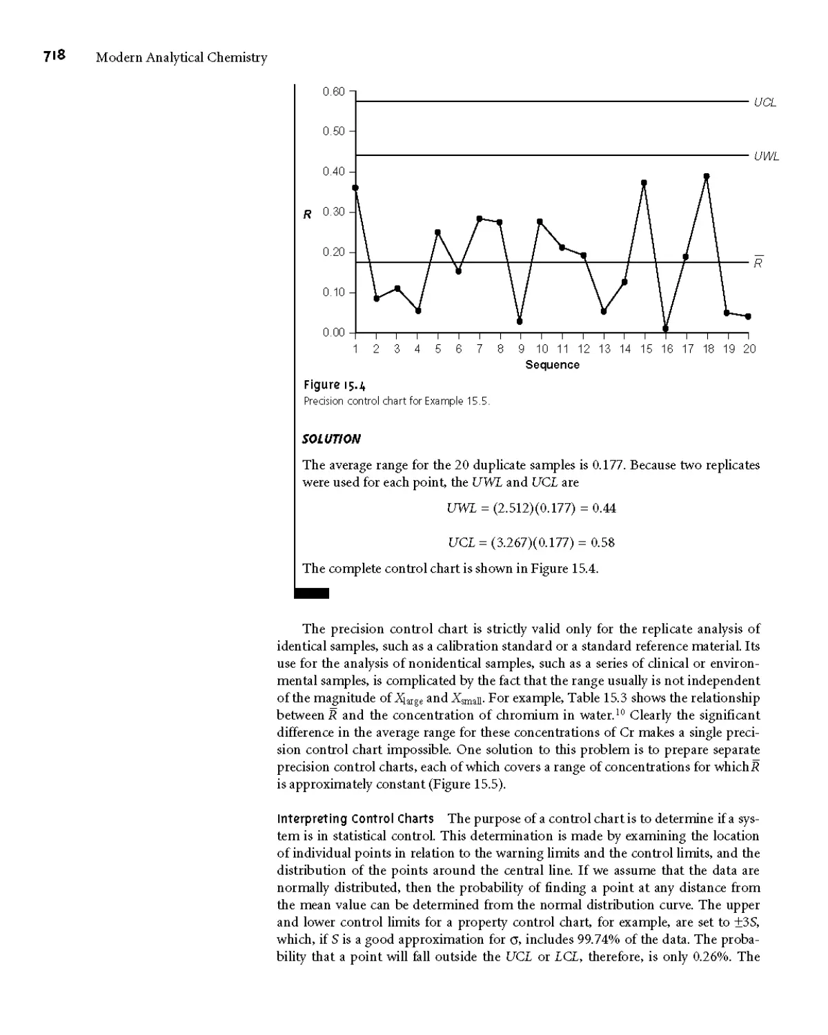


Текст
Modern Analytical Chemistry
David Harvey
DePauw University
Boston Burr Ridge, IL Dubuque, IA Madison, WI New York San Francisco St Louis
Bangkok Bogota Caracas Lisbon London Madrid
Mexico City Milan New Delhi Seoul Singapore Sydney Taipei Toronto
McGraw-Hill Higher Education
A Division of The McGraw-Hill Companies
MODERN ANALYTICAL CHEMISTRY
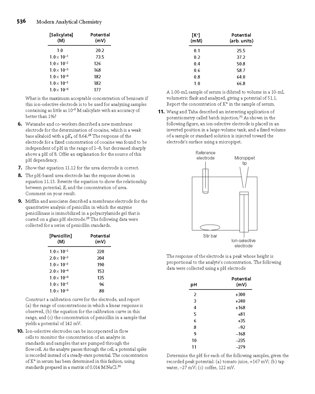
Copyright © 2000 by The McGraw-Hill Companies, Inc All rights reserved. Printed in
the United States of America. Except as permitted under the United States Copyright Act of
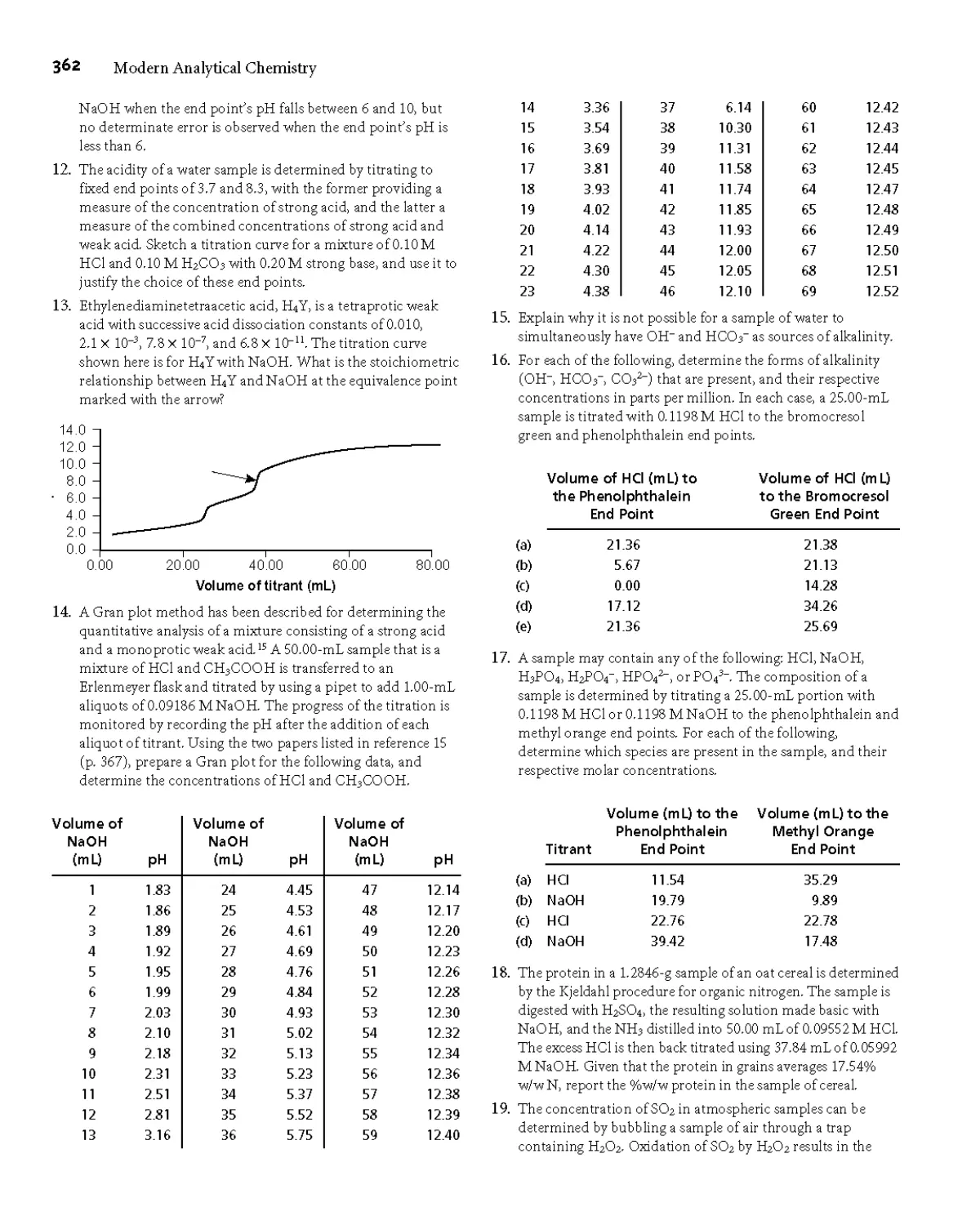
1976, no part of this publication maybe reproduced or distributed in any form or by any
means, or stored in a database or retrievalsystem, without the prior written permission of the
publisher.
This book is printed on acid-free paper.
1234567390 KGP/KGP 0937654321 0
ISBN 0-07-237547-7
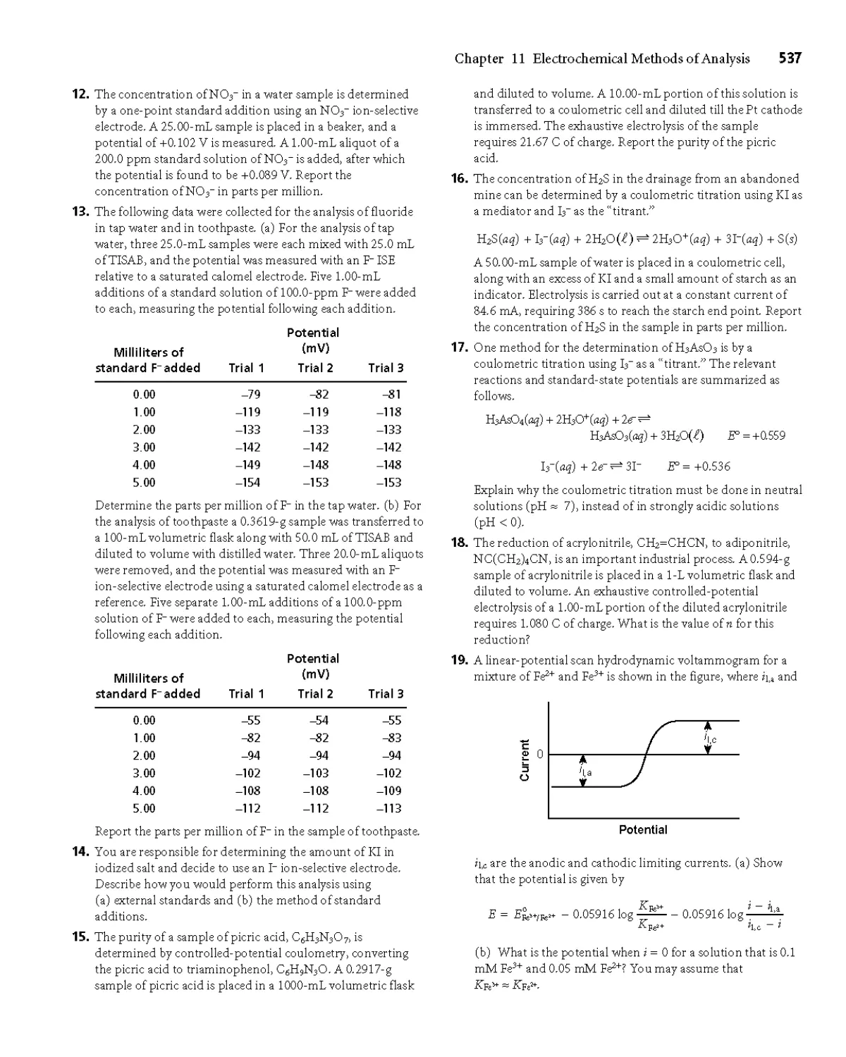
Vice president and editorial directo r T. Kane
Publisher: James M. Smith
Sponsoring editor: A. Peterson
Edi to rial ass is tant: Je nnifer L. Be nsin к
D eve lopmen tai e d ito r: Shx rley P.Oberbro eckling
Senio r marketing manager: Martin J. Lange
Senior project manager Jayne Kkin
Production supervisor: Laura Fuller
Coordinate r of freelance design: Michelle D. Whitaker
Senior photo research coordinator: Lori Hancock
Senior supplement coordinator: Audrey A. Peiter
Compositor: Shepherd, Inc.
Typeface: 10/12 Minion
Printer: Quebecor Printing Book Group/Kingsport
Freelance cover/interior designer: Lansdon
Cover image: © George Diebold/The Stock Market
Photo res e arch: R ob erta Sp ie ck erm an Associates
Colorplates: Colorplates 1-6, 3,10: © David Harvey/Marilyn E Culler, photographer;
Colorplate 7: Richard Megna/Fundamental Photographs; Colorplate 9: ©Alfred P as ieka/Science
Photo Library/Photo Researchers, Inc.; Colorplate 11: From H. Black, Environ. Set. Technol.,
1996, 30124A. Photos courtesy D. Pesiri and W. Tumas, Los Alamos National Laboratory;
Colorplate 12: Courtesy of Hewlett-Packard Company; Colorplate 13: © David Harvey.
Library of Congress Cataloging-in-Publication Data
Harvey, David, 1956-
Modern analytical chemistry / David Harvey. — 1st ed.
p. cm.
Includes bibliographical references and index
ISBN 0-07-237547-7
1. Chemistry, Analytic. I. Title.
QD75.2.H374 2000
543—dc21 99-15120
CIP
INTERNATIONAL EDITION ISBN 0-07-116953-9
Copyright ©2000. Exclusive rights by The McGraw-Hill Companies, Inc. for manufacture
and export. This book cannot be re-exported from the country to which it is consigned by
McGraw-Hill. The International Edition is not available in North America.
www.mhhe.com
Contents
Preface xii
Introduction
1A What is Analytical Chemistry? 2
1В The Analytical Perspective 5
1C Common Analytical Problems 8
ID Key Terms 9
IE Summary 9
IF Problems 9
1G Suggested Readings 10
1H References 10
Basic Tools of Analytical Chemistry n
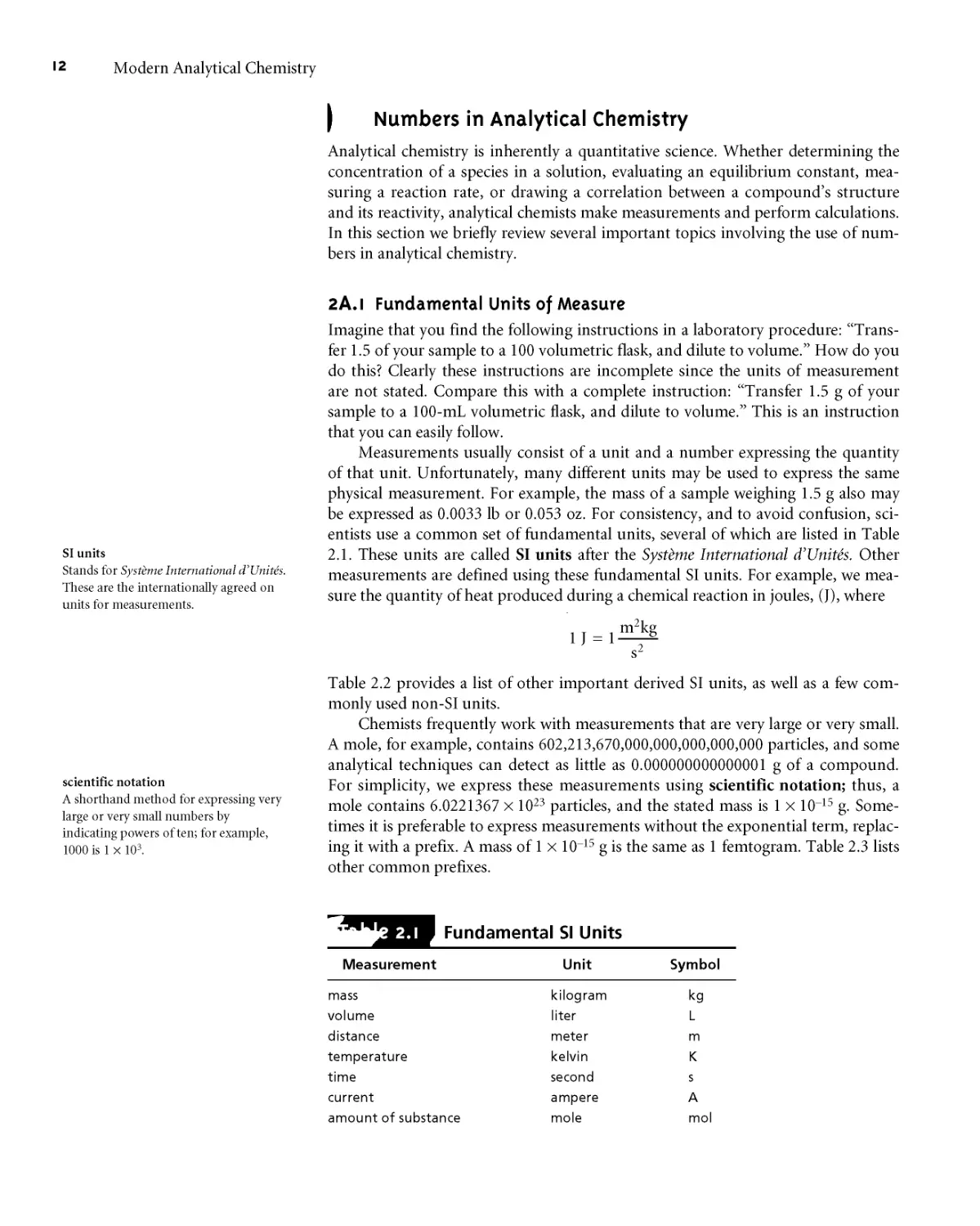
2A Numbers in Analytical Chemistry 12
2 AT Fundamental Units of Measure 12
2A.2 Significant Figures 13
2B Units for Expressing Concentration 15
2B.1 Molarity and Formality 15
2B.2 Normality 16
2B.3 Molality 18
2B.4 Weight, Volume, and Weight-to-Volume
Ratios 18
2B.5 Converting Between Concentration Units 18
2B.6 p-Functions 19
2C Stoichiometric Calculations 20
2C. 1 Conservation of Mass 22
2C.2 Conservation of Charge 22
2C.3 Conservation of Protons 22
2C.4 Conservation of Electron Pairs 23
2C.5 Conservation of Electrons 23
2C.6 Using Conservation Principles in
Stoichiometry Problems 23
2D Basic Equipment and Instrumentation 25
2D.1 Instrumentation for Measuring Mass 25
2D.2 Equipment for Measuring Volume 26
2D3 Equipment for Drying Samples 29
2E Preparing Solutions 30
2E. 1 Preparing Stock Solutions 30
2E.2 Preparing Solutions by Dilution 31
2F The Laboratory Notebook 32
2G Key Terms 32
2H Summary 33
21 Problems 33
2J Suggested Readings 34
2K References 34
The Language of Analytical Chemistry 35
ЗА Analysis, Determination, and Measurement 36
3B Techniques, Methods, Procedures, and
Protocols 36
3 C Classifying Analytical Techniques 3 7
3D Selecting an Analytical Method 38
3D.1 Accuracy 38
3D.2 Precision 39
3D.3 Sensitivity 39
3D.4 Selectivity 40
3D.5 Robustness and Ruggedness 42
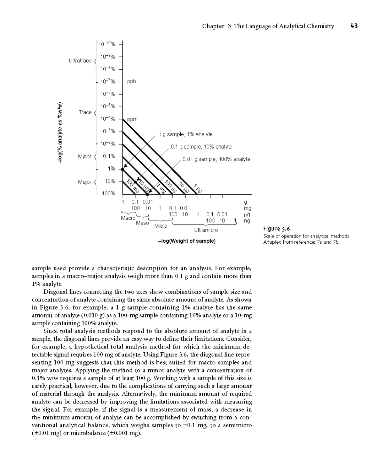
3D.6 Scale of Operation 42
3D.7 Equipment, Time, and Cost 44
3D.8 Making the Final Choice 44
iv
Modern Analytical Chemistry
3E Developing the Procedure 45
ЗЕД Compensating for Interferences 45
3E.2 Calibration and Standardization 47
3E.3 Sampling 47
3E.4 Validation 47
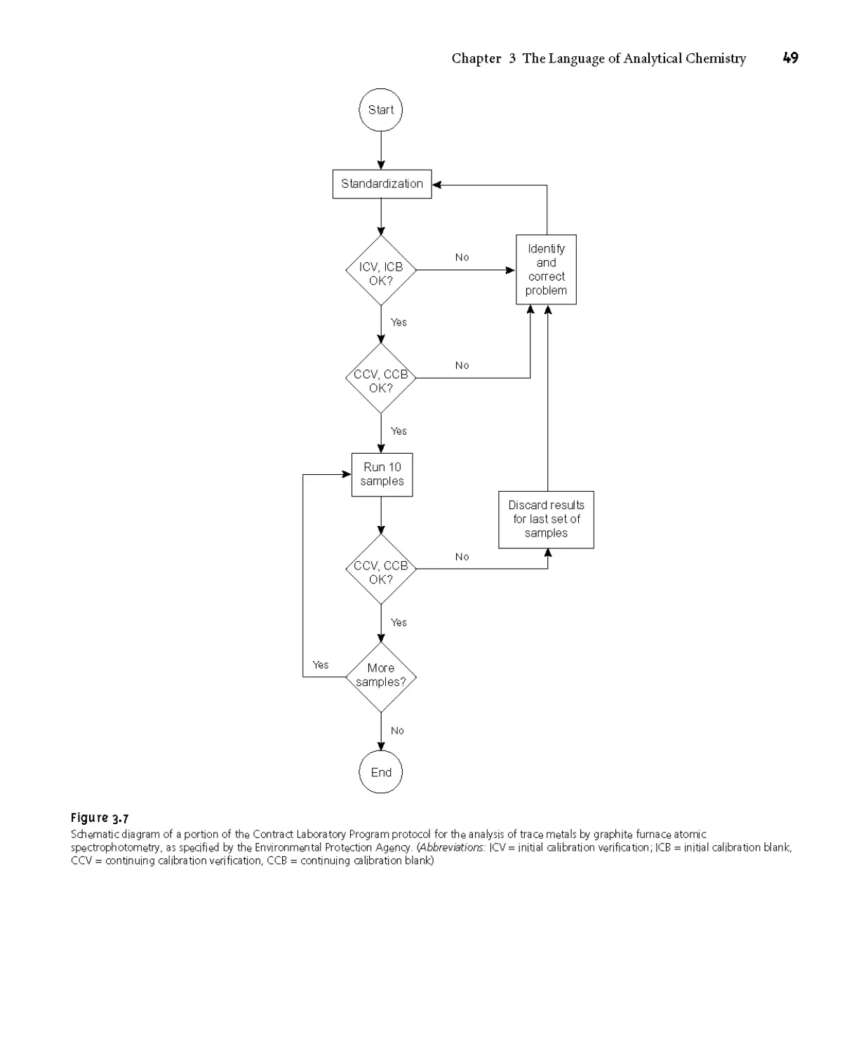
3F Protocols 48
3G The Importance of Analytical Methodology 48
3H Key Terms 50
31 Summary 50
3J Problems 51
3K Suggested Readings 52
3L References 52
Evaluating Analytical Data 53
4A Characterizing Measurements and Results 54
4A. 1 Measures of Central Tendency 54
4A.2 Measures of Spread 55
4B Characterizing Experimental Errors 57
4ВД Accuracy 57
4B.2 Precision 62
4B.3 Error and Uncertainty 64
4C Propagation of Uncertainty 64
401 A Few Symbols 65
402 Uncertainty When Adding or Subtracting 65
403 Uncertainty When Multiplying or
Dividing 66
404 Uncertainty for Mixed Operations 66
405 Uncertainty for Other Mathematical
Functions 67
406 Is Calculating Uncertainty Actually Useful? 68
4D The Distribution of Measurements and
Results 70
4D.I Populations and Samples 71
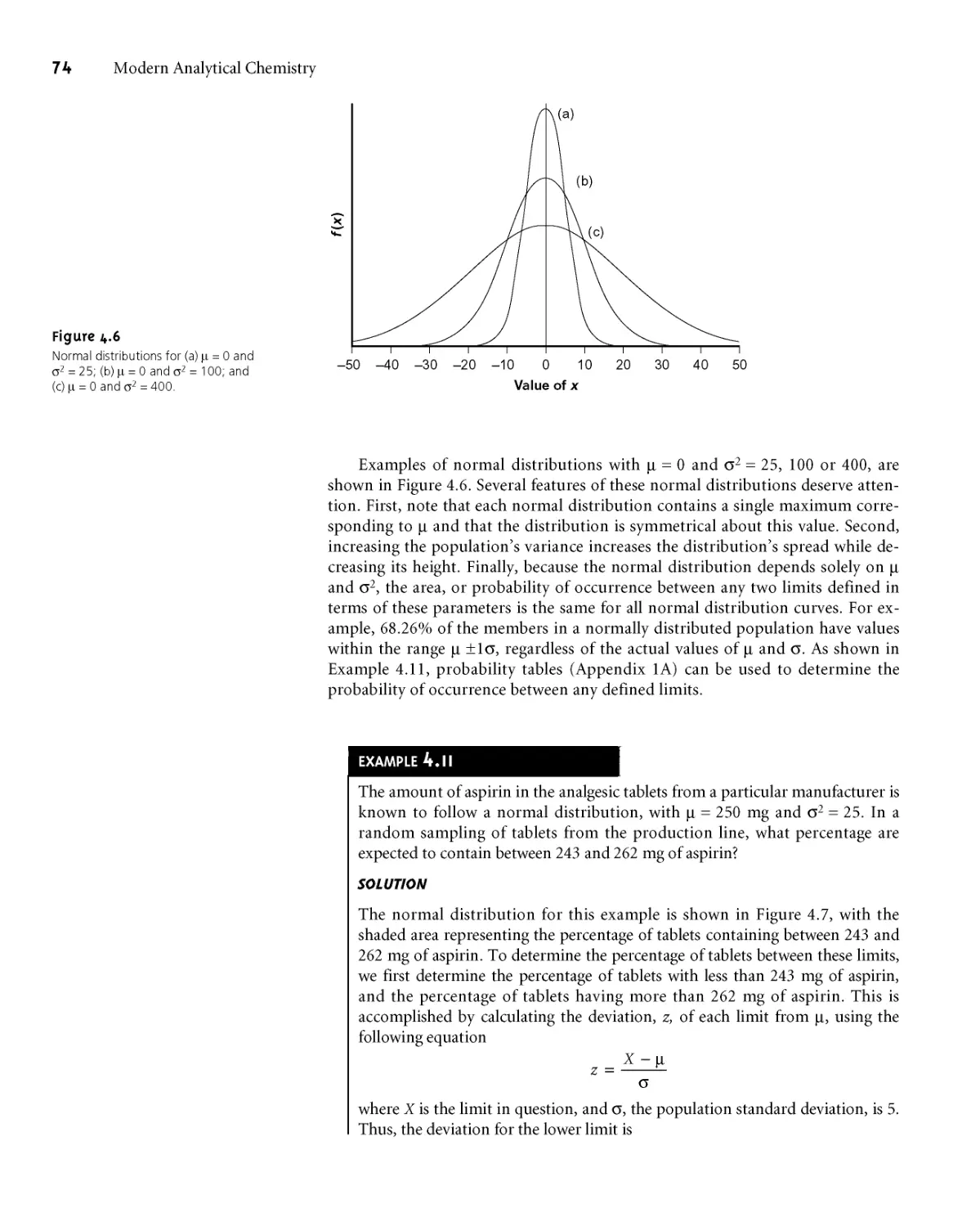
4D.2 Probability Distributions for Populations 71
4D.3 Confidence Intervals for Populations 75
4D.4 Probability Distributions for Samples 77
4D.5 Confidence Intervals for Samples 80
4D.6 A Cautionary Statement 81
4E Statistical Analysis of Data 82
4ЕД Significance Testing 82
4E.2 Constructing a Significance Test 83
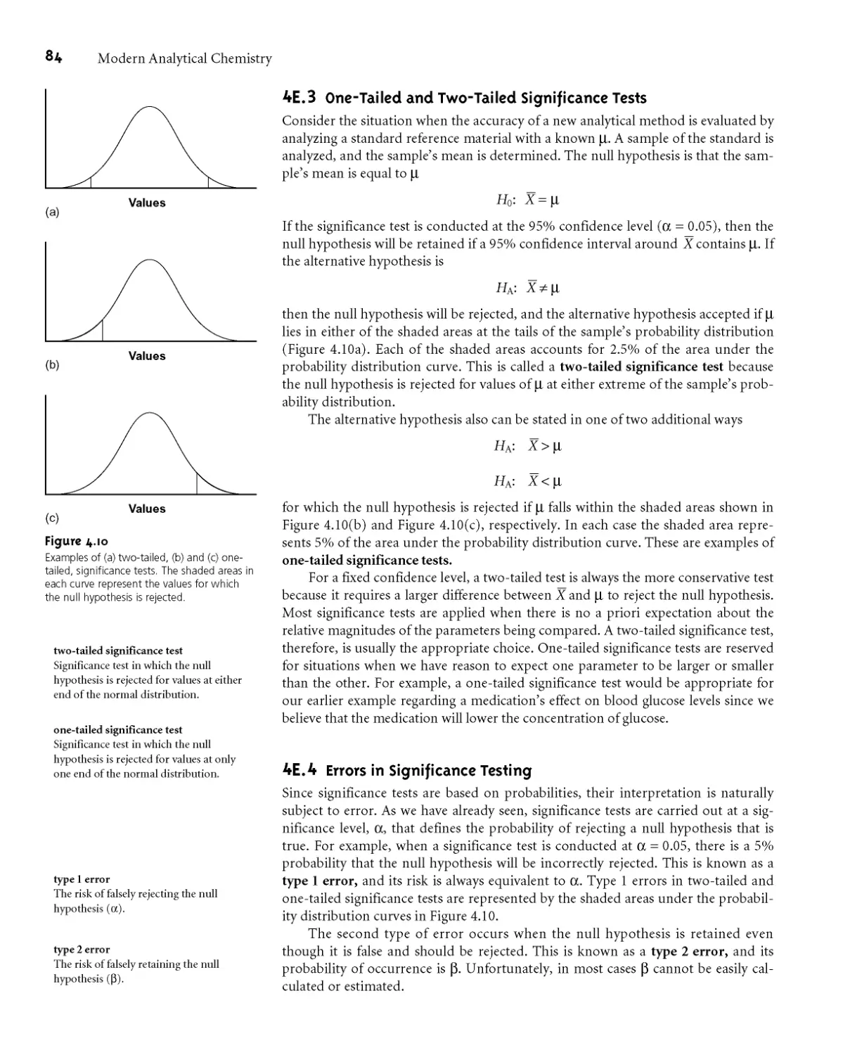
4E.3 One-Tailed and Two-Tailed Significance
Tests 84
4E.4 Errors in Significance Testing 84
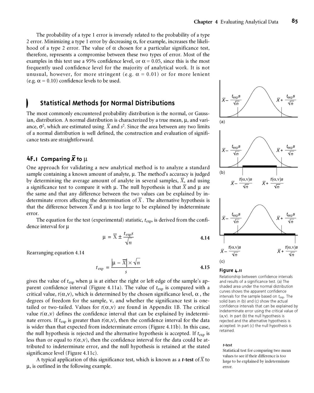
4F Statistical Methods for Normal Distributions 85
4E1 Comparing X to Ц 85
4E2 Comparing s2 to a2 87
4E3 Comparing Two Sample Variances 88
4E4 Comparing Two Sample Means 88
4E5 Outliers 93
4G Detection Limits 95
4H Key Terms 96
41 Summary 96
4J Suggested Experiments 97
4K Problems 98
4L Suggested Readings 102
4M References 102
Calibrations, Standardizations,
and Blank Corrections 104
5A Calibrating Signals 105
5B Standardizing Methods 106
5ВД Reagents Used as Standards 106
5B.2 Single-Point versus Multiple-Point
Standardizations 108
5B.3 External Standards 109
5B.4 Standard Additions 110
5B.5 Internal Standards 115
5C Linear Regression and Calibration Curves 117
501 Linear Regression of Straight-Line Calibration
Curves 118
502 Unweighted Linear Regression with Errors
in у 119
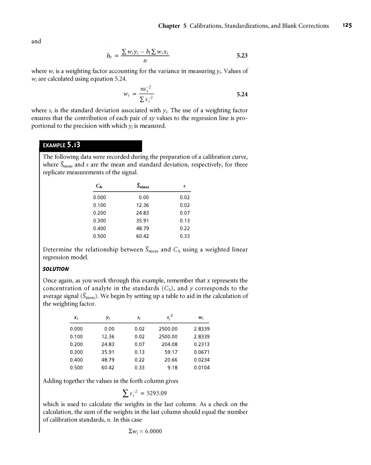
503 Weighted Linear Regression with Errors
in у 124
504 Weighted Linear Regression with Errors
in Both x and у 127
505 Curvilinear and Multivariate
Regression 127
5D Blank Corrections 128
5E Key Terms 130
5F Summary 130
5G Suggested Experiments 130
5H Problems 131
51 Suggested Readings 133
5 J References 134
Contents
V
Equilibrium Chemistry 135
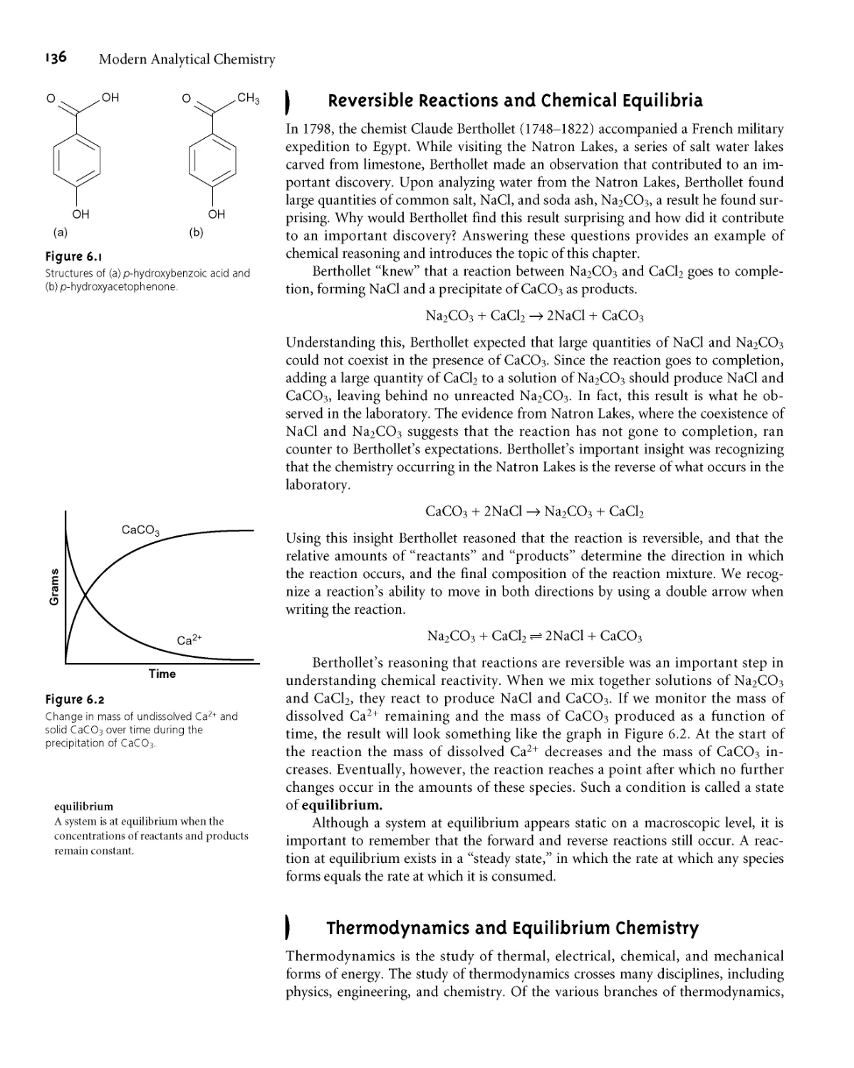
6A Reversible Reactions and Chemical
Equilibria 136
6B Thermodynamics and Equilibrium
Chemistry 136
6C Manipulating Equilibrium Constants 138
6D Equilibrium Constants for Chemical
Reactions 139
6D.1 Precipitation Reactions 139
6D.2 Acid-Base Reactions 140
6D.3 Complexation Reactions 144
6D.4 Oxidation-Reduction Reactions 145
6E Le Chatelier’s Principle 148
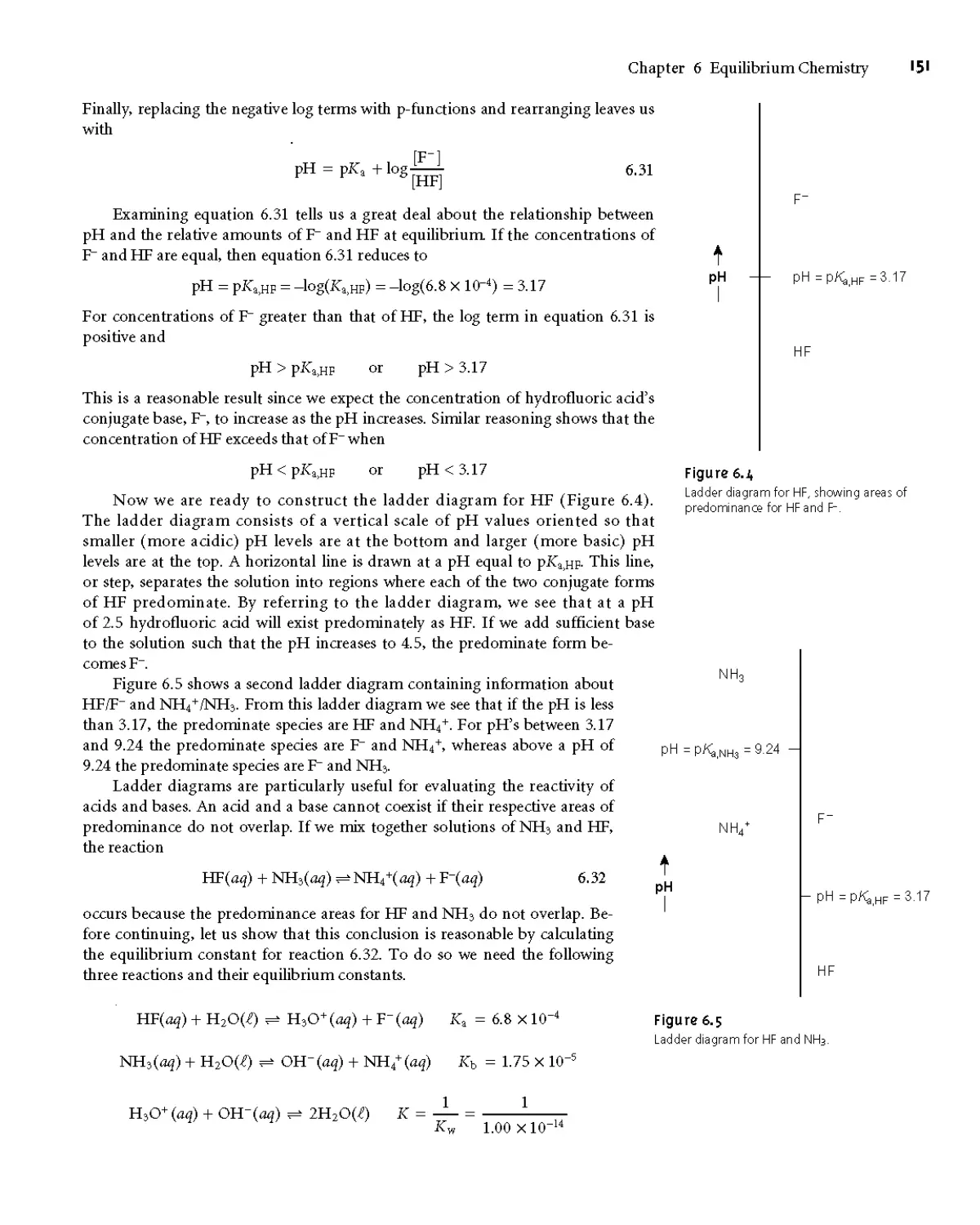
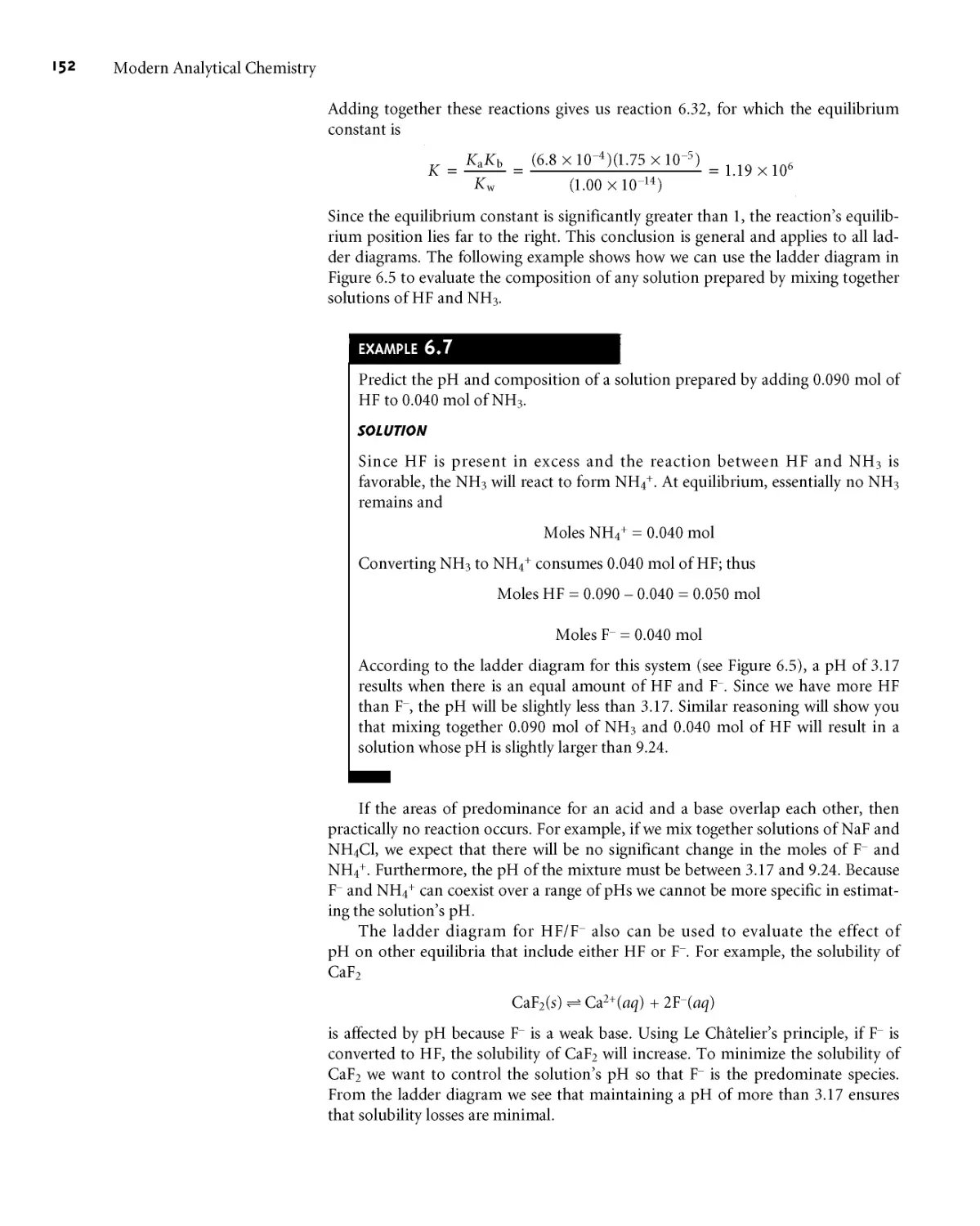
6F Ladder Diagrams 150
6E 1 Ladder Diagrams for Acid-Base Equilibria 150
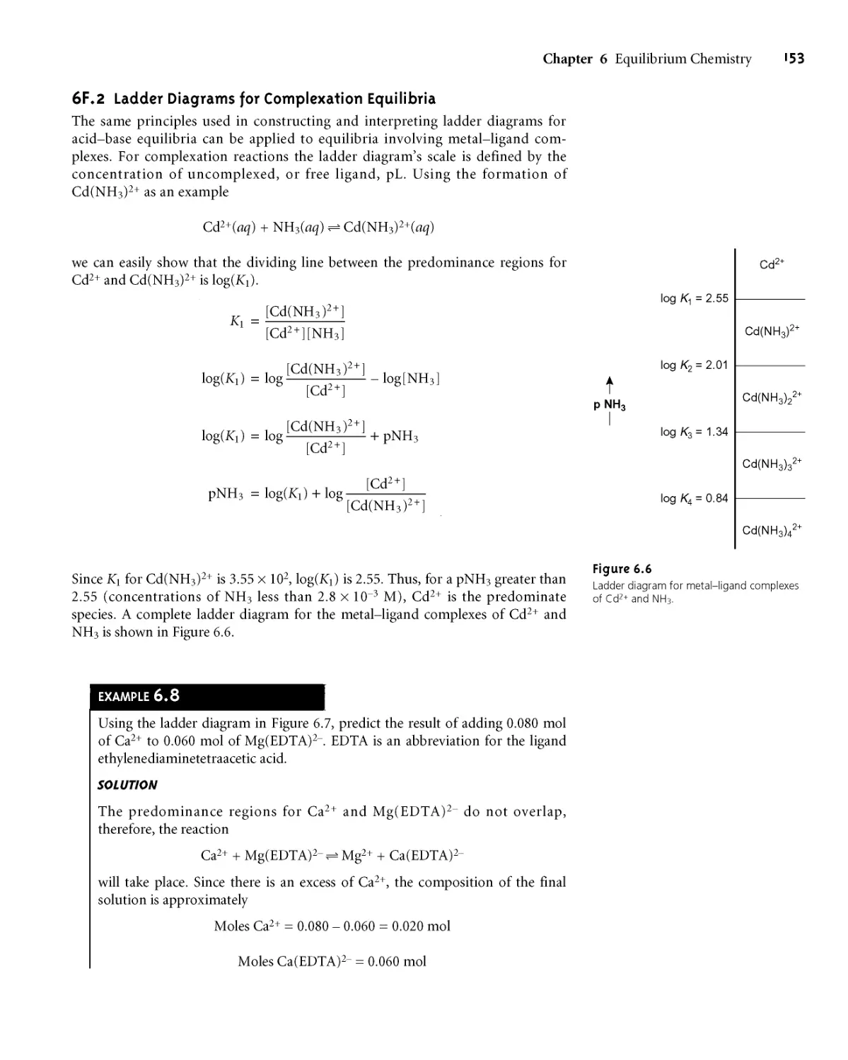
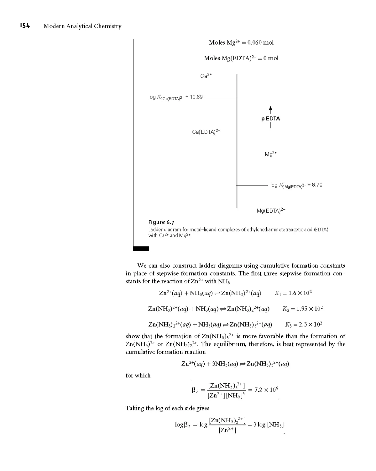
6E2 Ladder Diagrams for Complexation
Equilibria 153
6E3 Ladder Diagrams for Oxidation-Reduction
Equilibria 155
6G Solving Equilibrium Problems 156
6G.1 A Simple Problem: Solubility of РЬ(Юз)2 in
Water 156
6G.2 A More Complex Problem: The Common Ion
Effect 157
6G.3 Systematic Approach to Solving Equilibrium
Problems 159
6G.4 pH of a Monoprotic Weak Acid 160
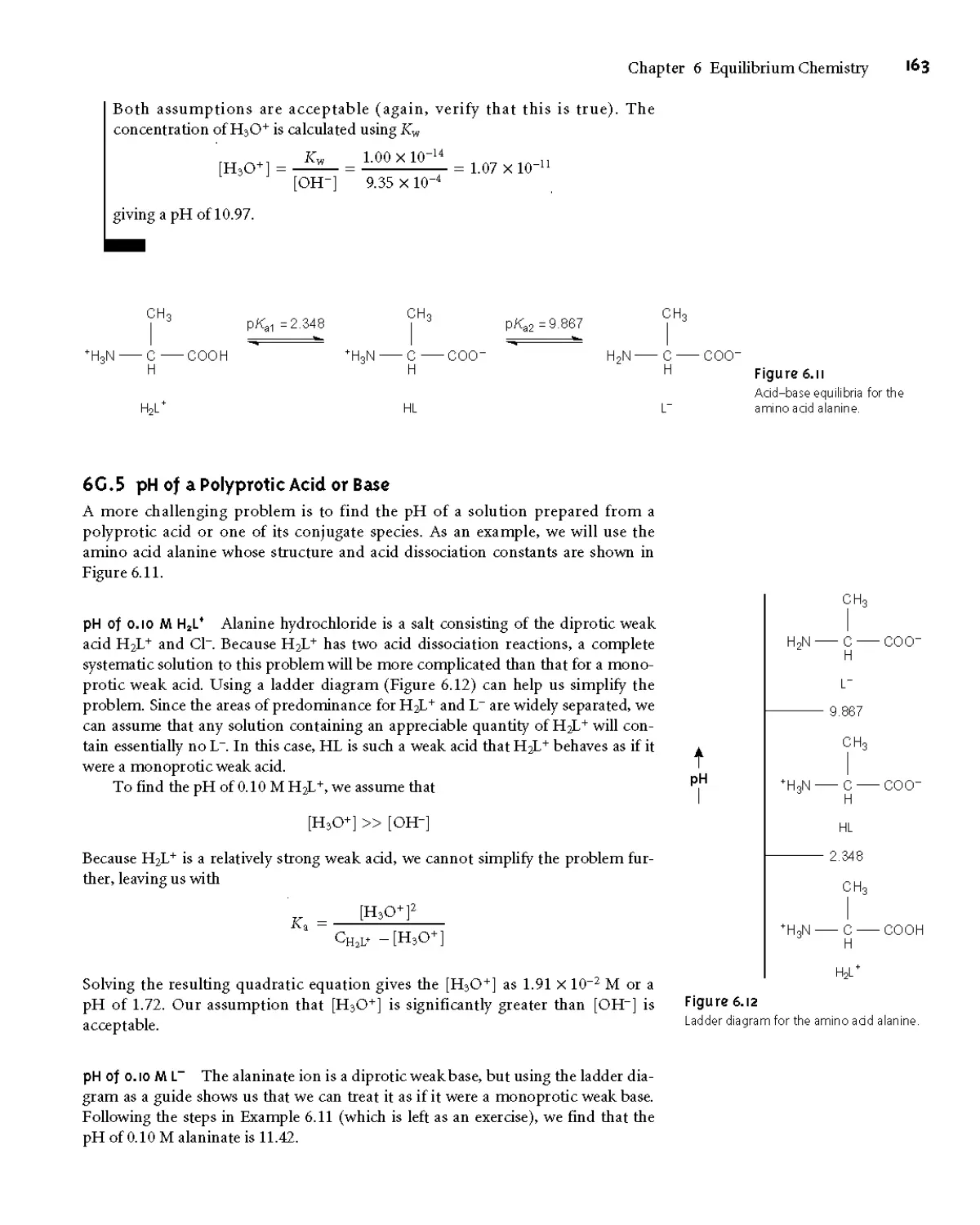
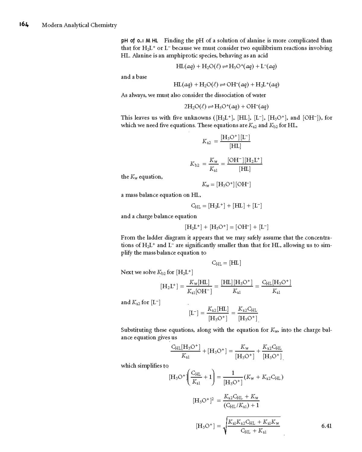
6G.5 pH of a Polyprotic Acid or Base 163
6G.6 Effect of Complexation on Solubility 165
6H Buffer Solutions 167
6НД Systematic Solution to Buffer
Problems 168
6H.2 Representing Buffer Solutions with
Ladder Diagrams 170
61 Activity Effects 171
6J Two Final Thoughts About Equilibrium
Chemistry 175
6K Key Terms 175
6L Summary 175
6M Suggested Experiments 176
6N Problems 176
60 Suggested Readings 178
6P References 178
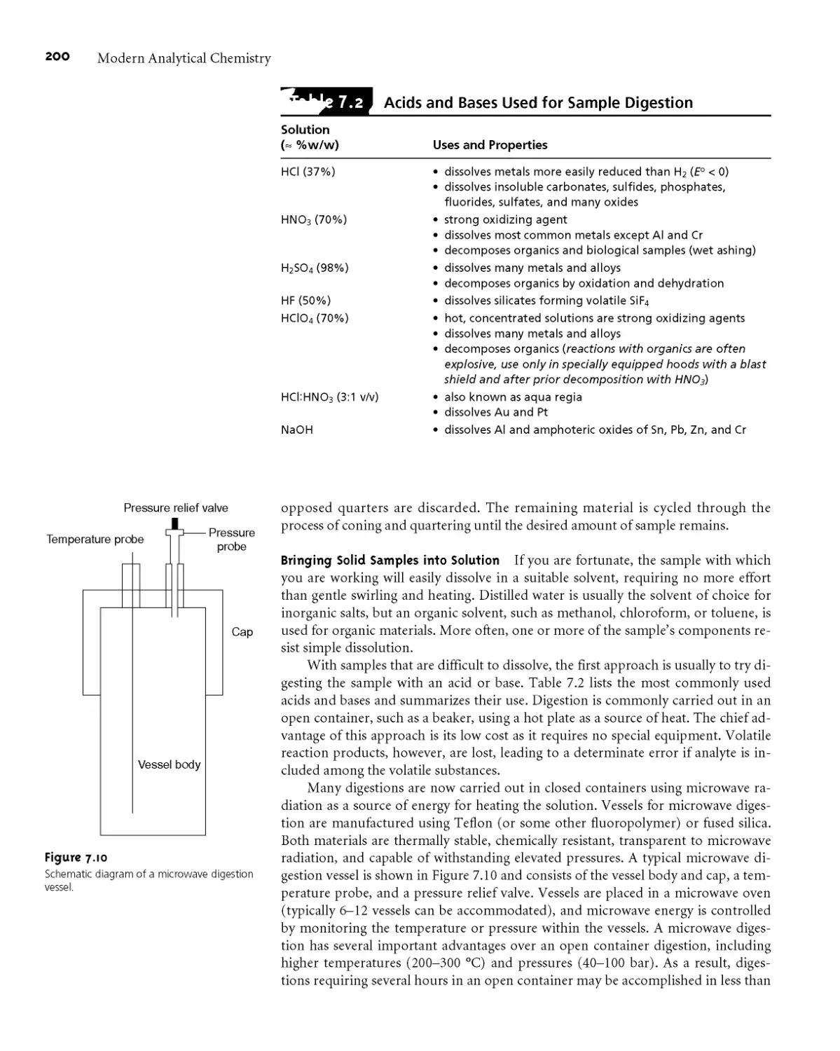
Obtaining and Preparing Samples
for Analysis 179
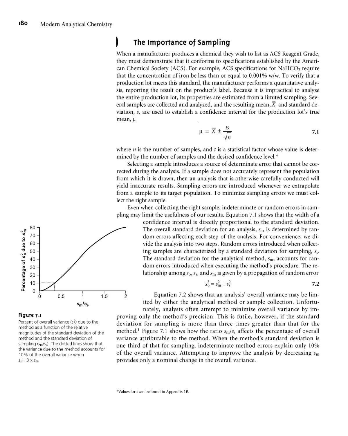
7A The Importance of Sampling 180
7B Designing a Sampling Plan 182
7B. 1 Where to Sample the Target
Population 182
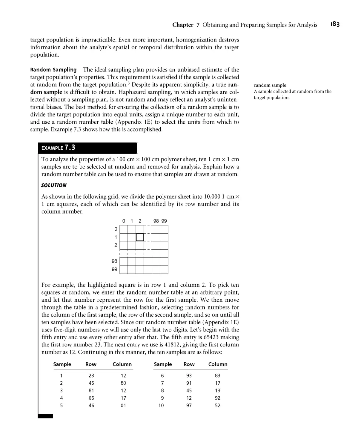
7B.2 What Type of Sample to Collect 185
7B.3 How Much Sample to Collect 187
7B.4 How Many Samples to Collect 191
7B.5 Minimizing the Overall Variance 192
7C Implementing the Sampling Plan 193
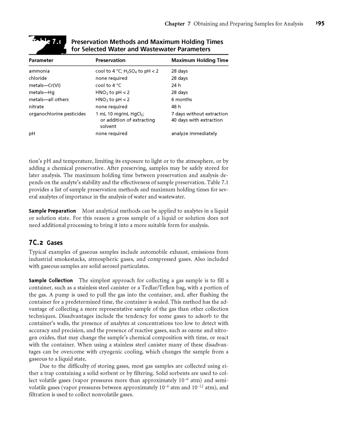
7G1 Solutions 193
7G2 Gases 195
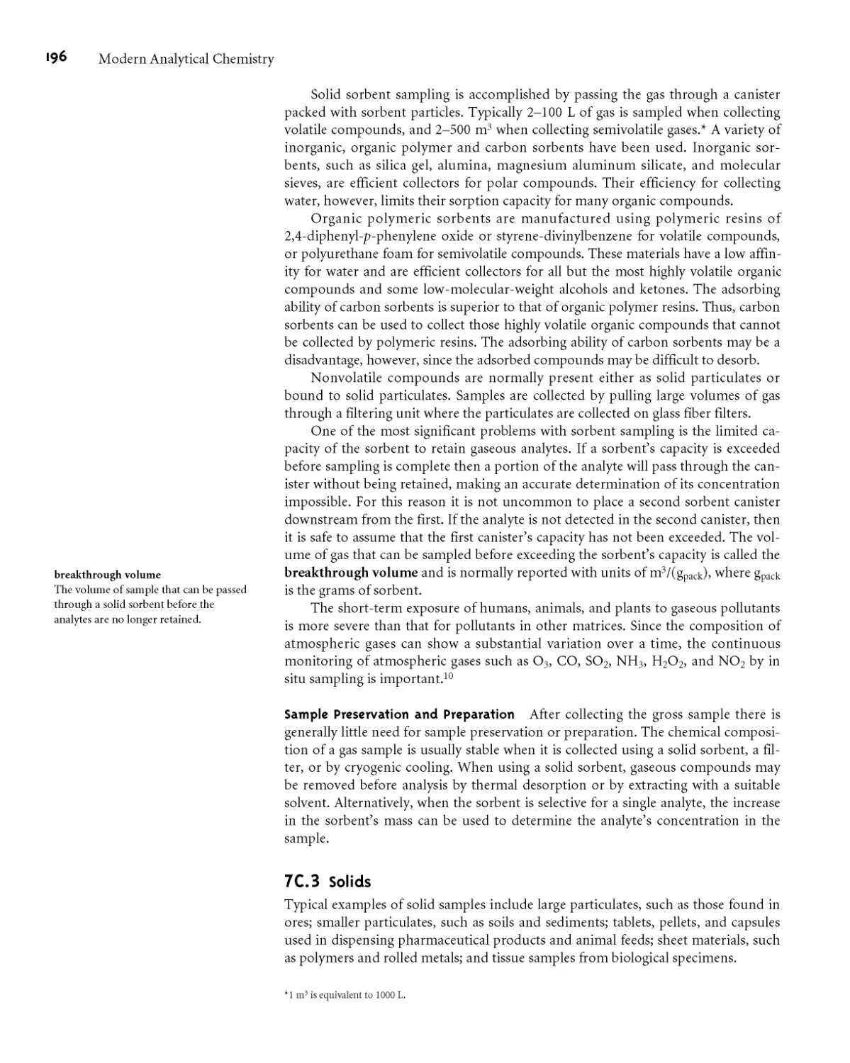
7G3 Solids 196
7D Separating the Analyte from
Interferents 201
7E General Theory of Separation
Efficiency 202
7F Classifying Separation Techniques 205
7E1 Separations Based on Size 205
7E2 Separations Based on Mass or Density 206
7E3 Separations Based on Complexation
Reactions (Masking) 207
7E4 Separations Based on a Change
of State 209
7E5 Separations Based on a Partitioning Between
Phases 211
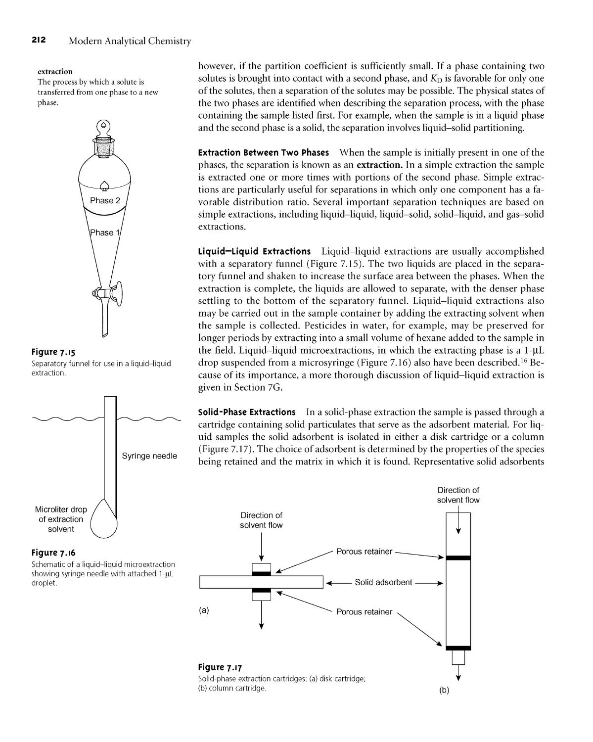
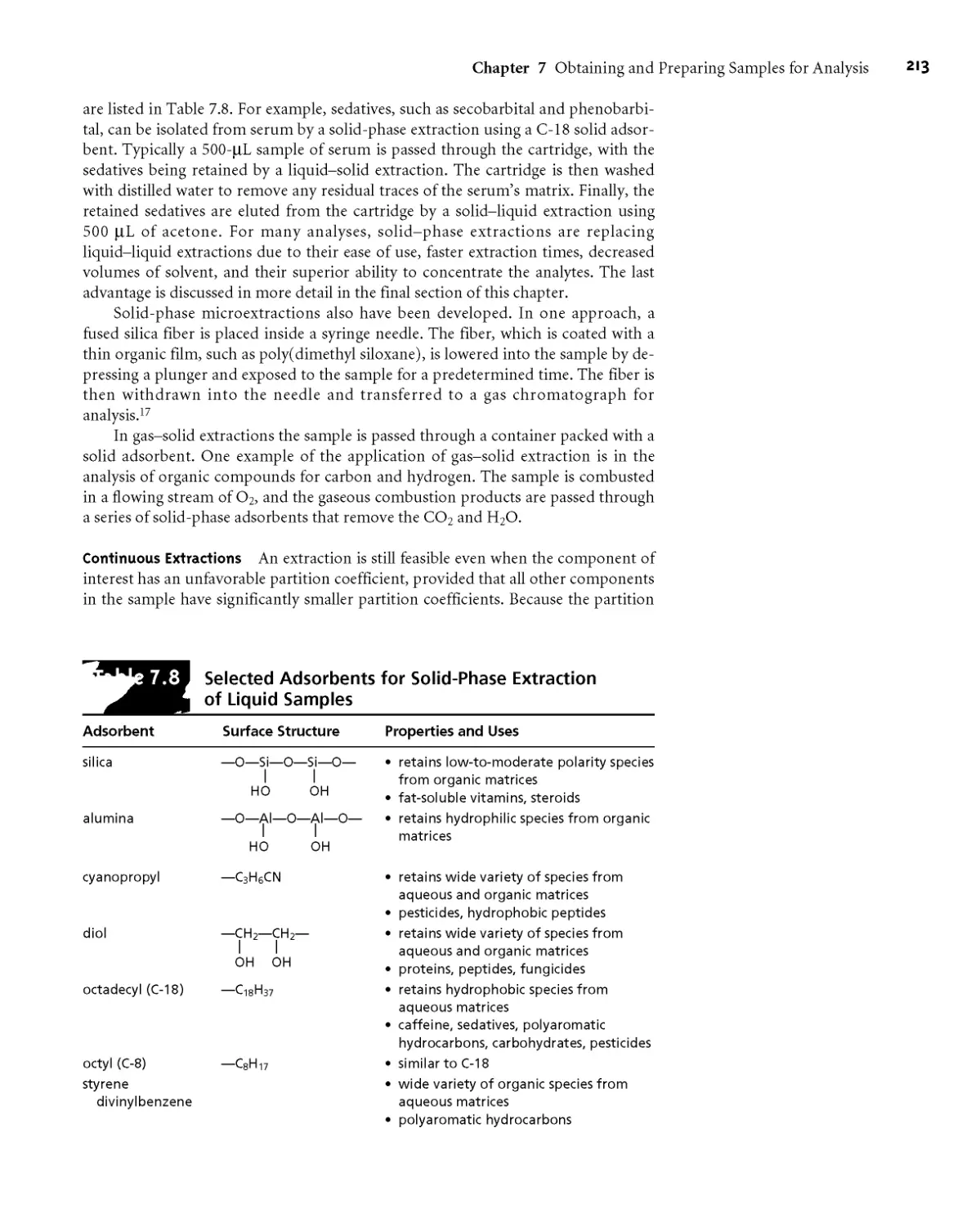
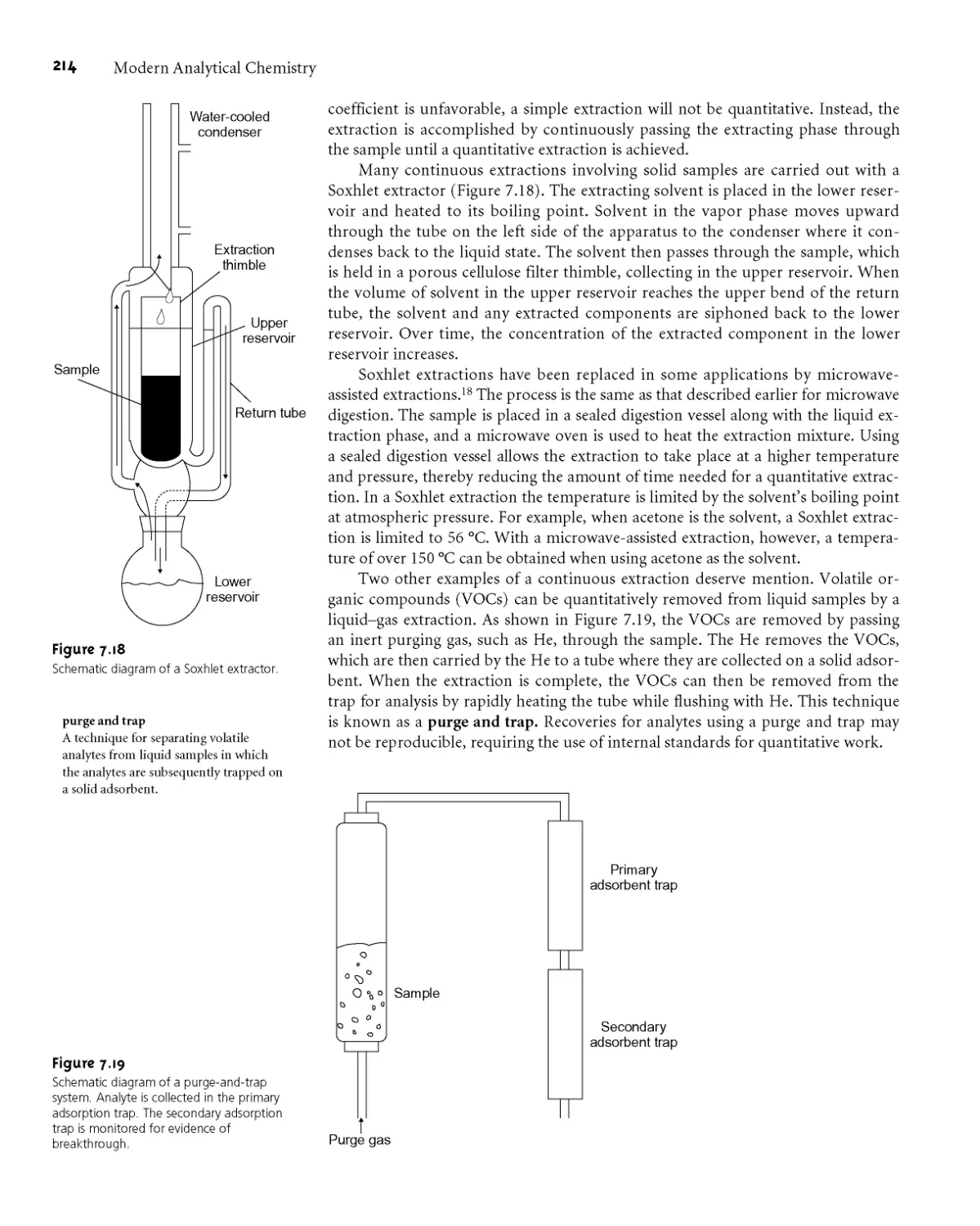
7G Liquid-Liquid Extractions 215
7G. 1 Partition Coefficients and Distribution
Ratios 216
7G.2 Liquid-Liquid Extraction with No Secondary
Reactions 216
7G.3 Liquid-Liquid Extractions Involving
Acid-Base Equilibria 219
7G.4 Liquid-Liquid Extractions Involving Metal
Chelators 221
7H Separation versus Preconcentration 223
71 Key Terms 224
7J Summary 224
7K Suggested Experiments 225
7L Problems 226
7M Suggested Readings 230
7N References 231
vi
Modern Analytical Chemistry
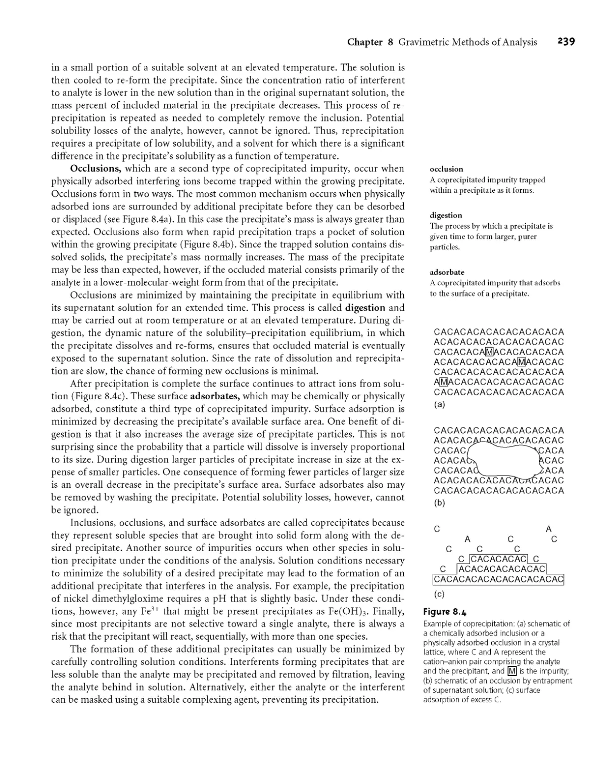
8
Gravimetric Methods of Analysis 232
8A Overview of Gravimetry 233
8A. 1 Using Mass as a Signal 233
8A.2 Types of Gravimetric Methods 234
8A.3 Conservation of Mass 234
8A.4 Why Gravimetry Is Important 235
8B Precipitation Gravimetry 235
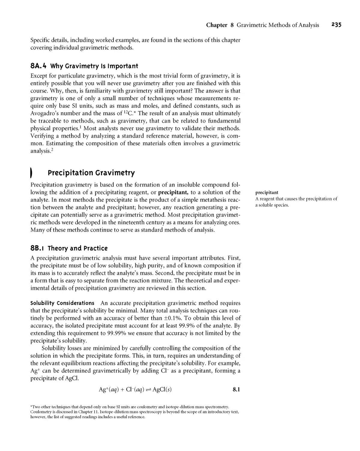
8ВД Theory and Practice 235
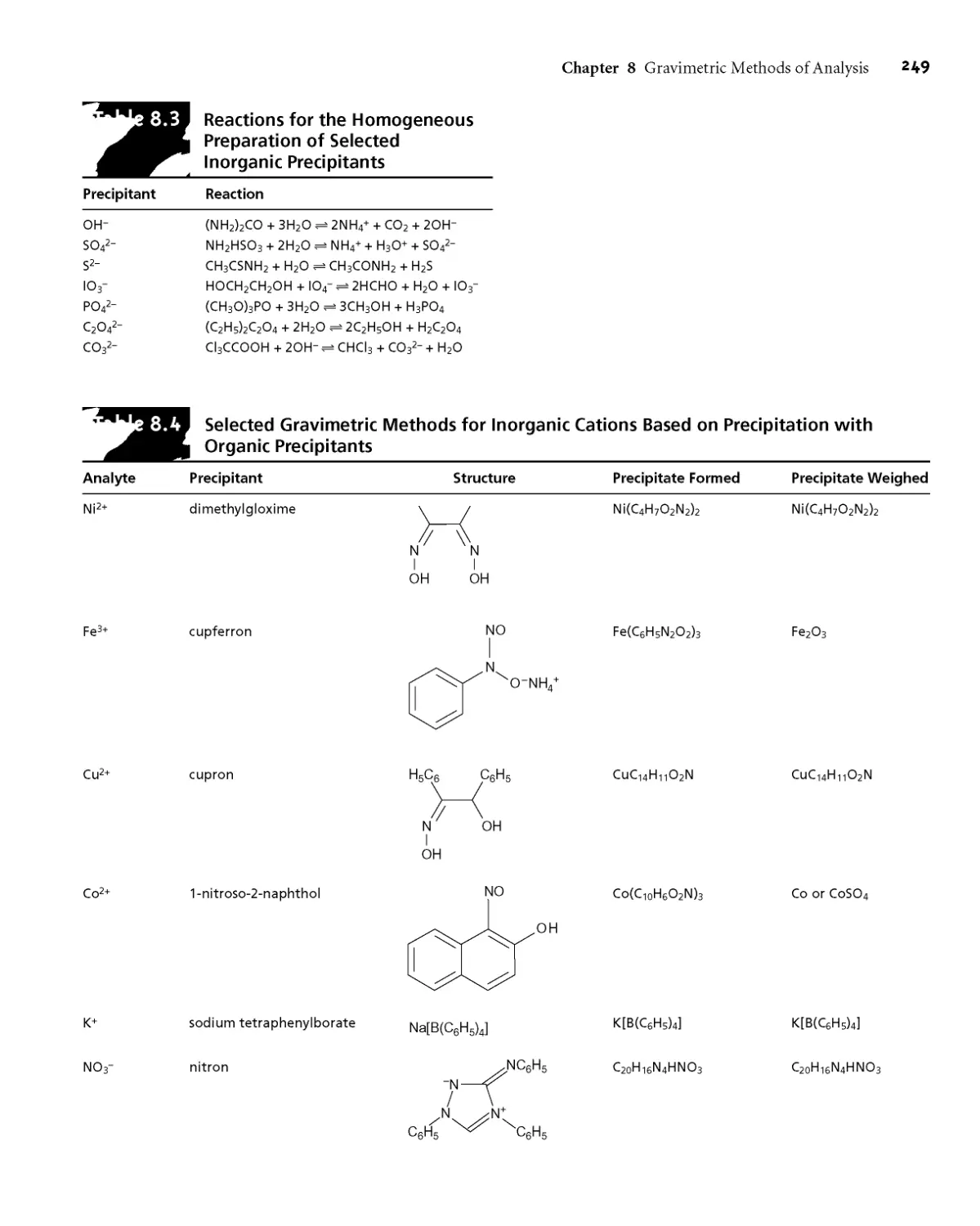
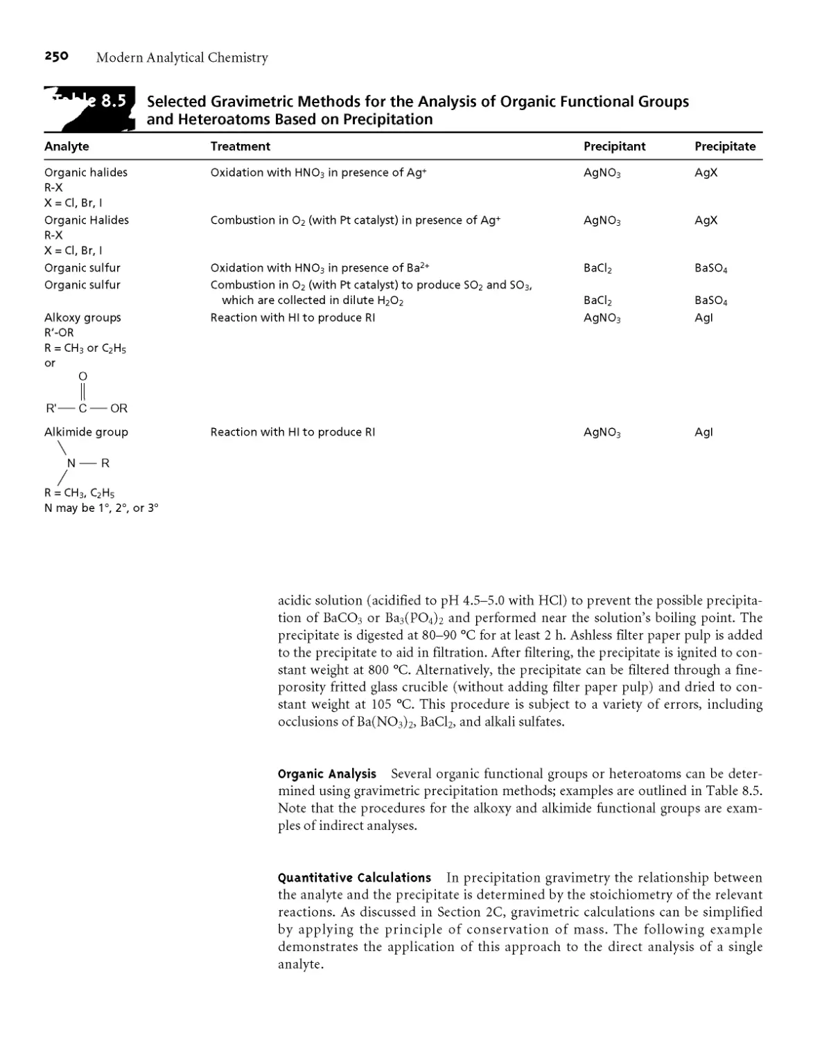
8B.2 Quantitative Applications 247
8B.3 Qualitative Applications 254
8B.4 Evaluating Precipitation Gravimetry 254
8C Volatilization Gravimetry 255
8G1 Theory and Practice 255
8G2 Quantitative Applications 259
8G3 Evaluating Volatilization Gravimetry 262
8D Particulate Gravimetry 262
8D.1 Theory and Practice 263
8D.2 Quantitative Applications 264
8D.3 Evaluating Precipitation Gravimetry 265
8E Key Terms 265
8F Summary 266
8G Suggested Experiments 266
8H Problems 267
81 Suggested Readings 271
8J References 272
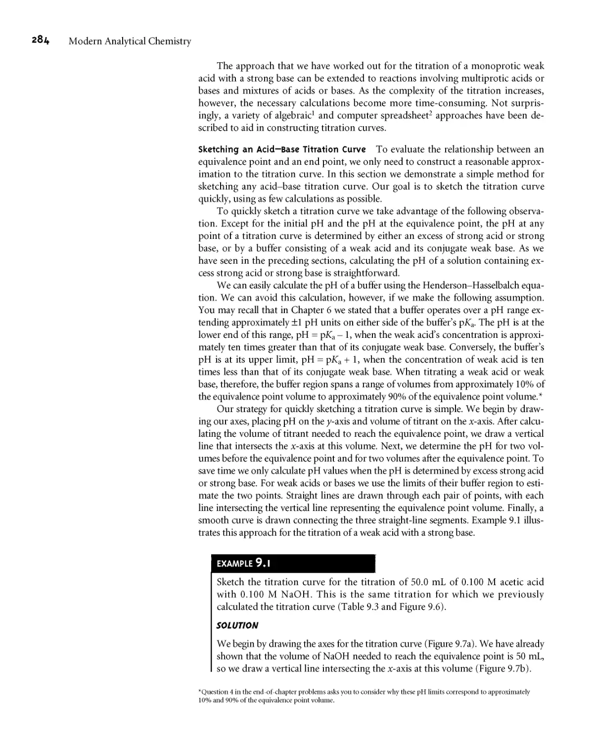
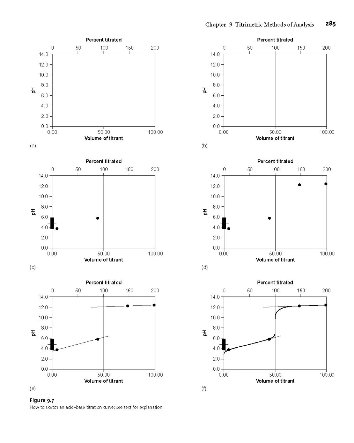
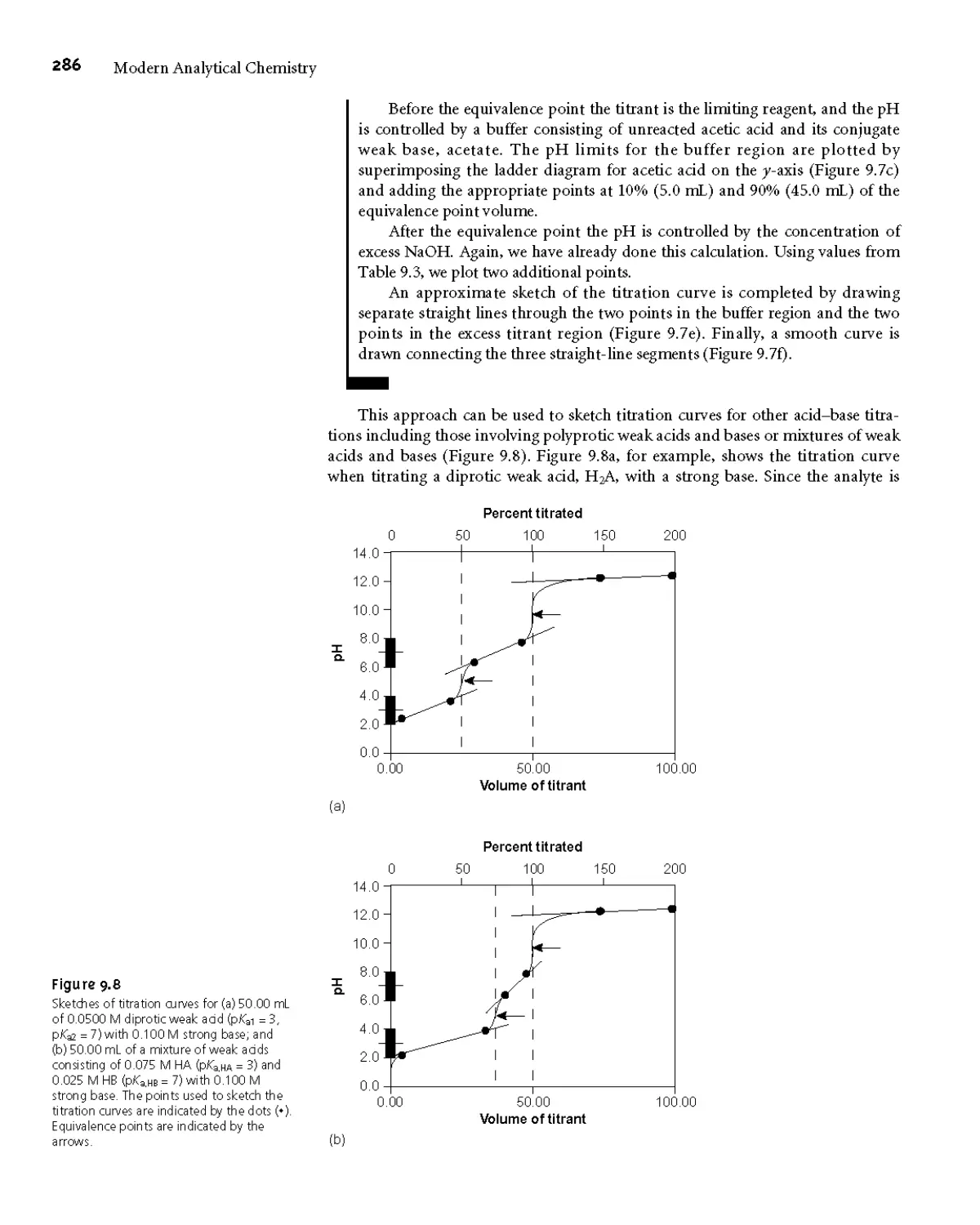
9
Titrimetric Methods of Analysis 273
9A Overview of Titrimetry 274
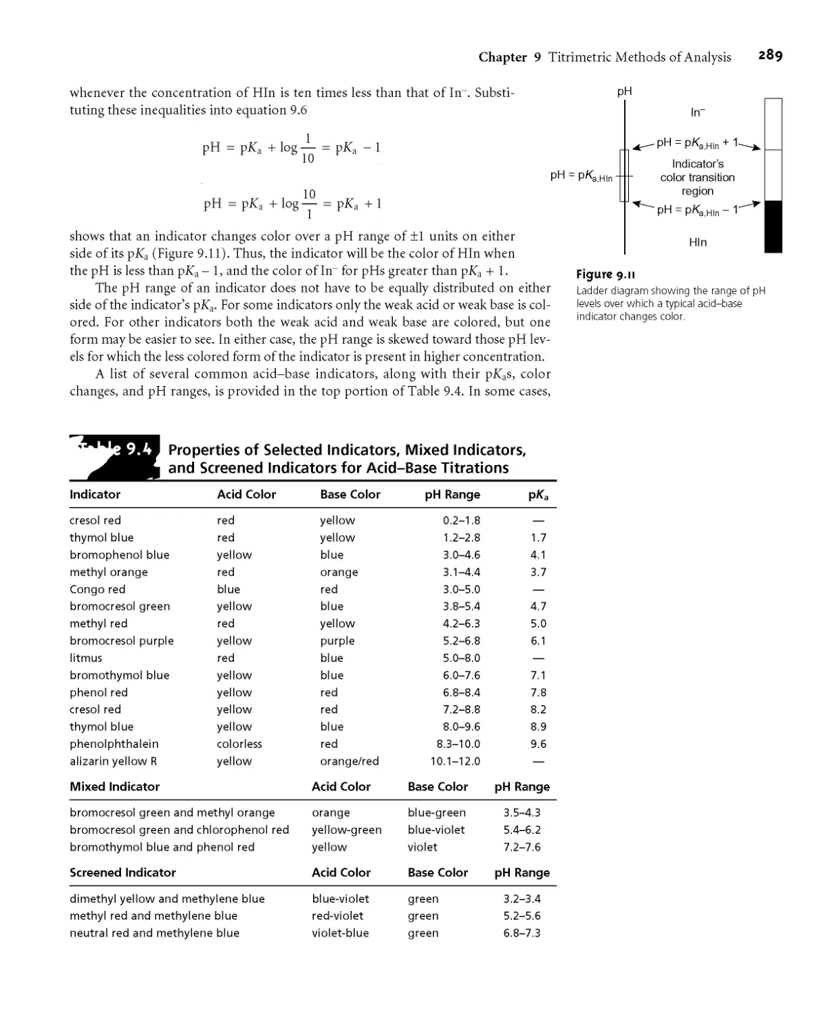
9АД Equivalence Points and End Points 274
9A.2 Volume as a Signal 274
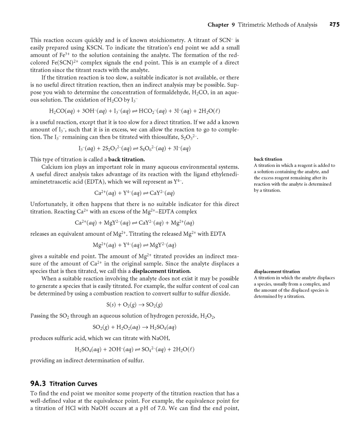
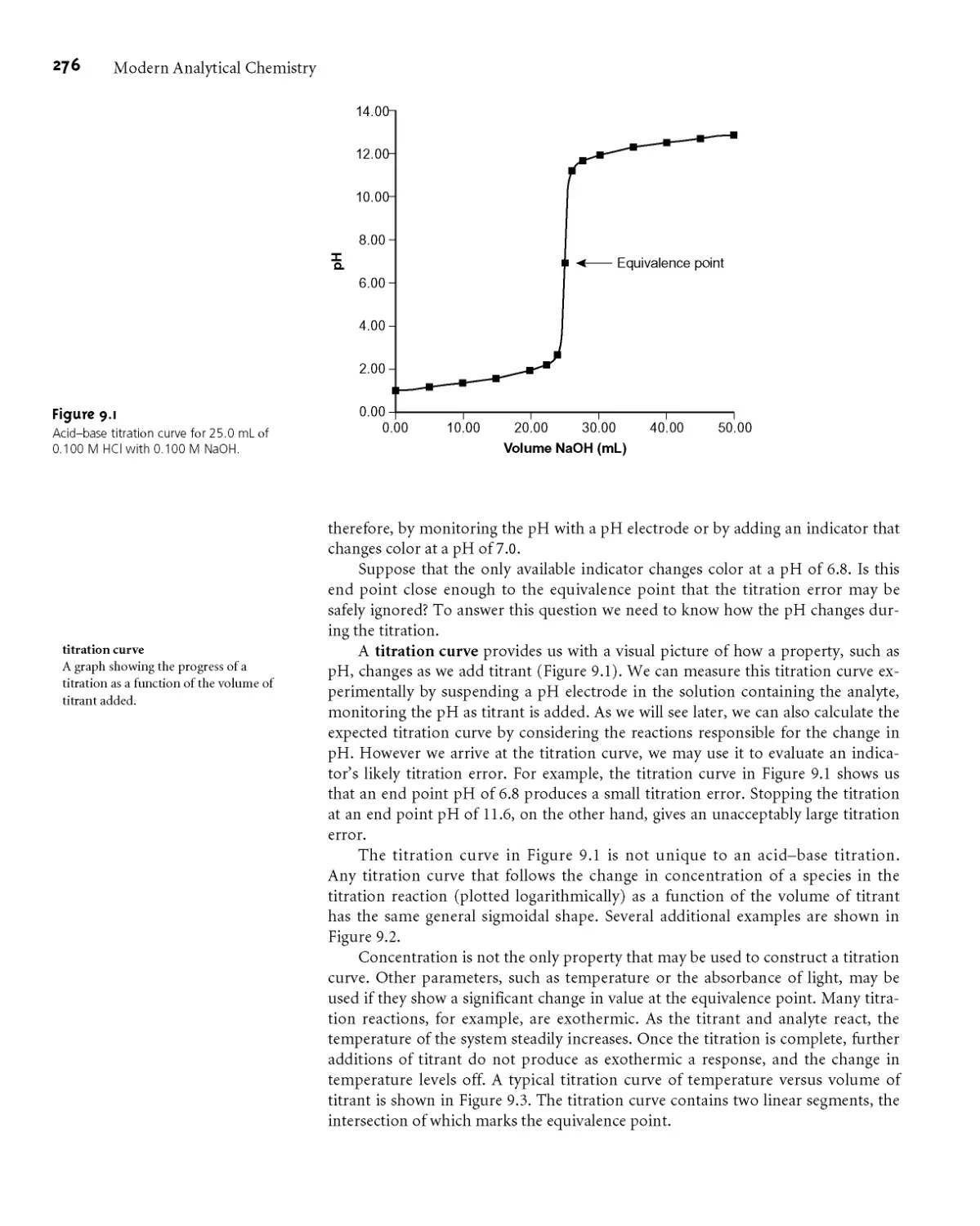
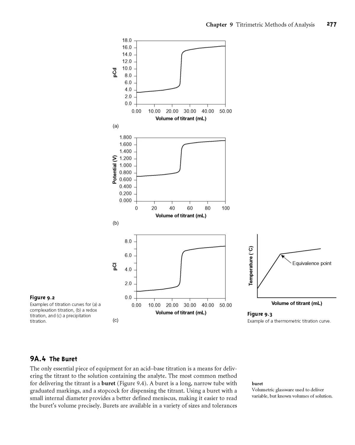
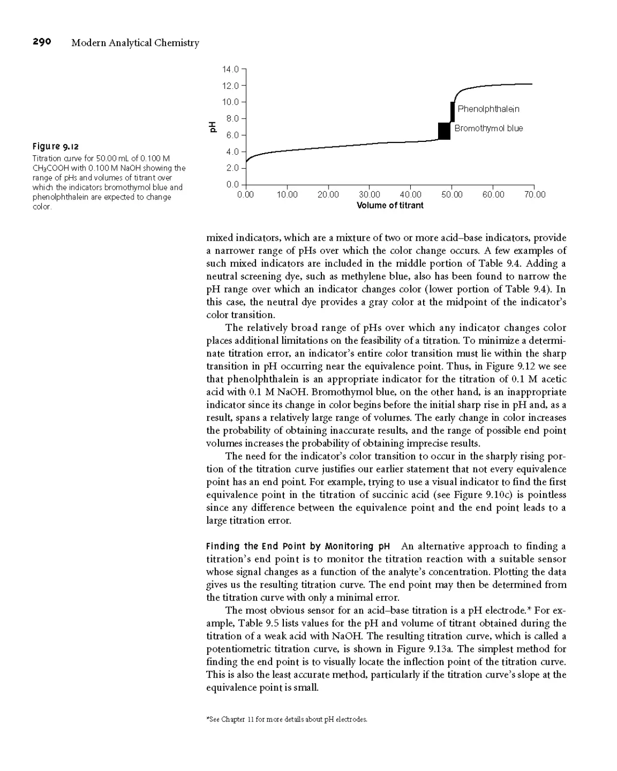
9A.3 Titration Curves 275
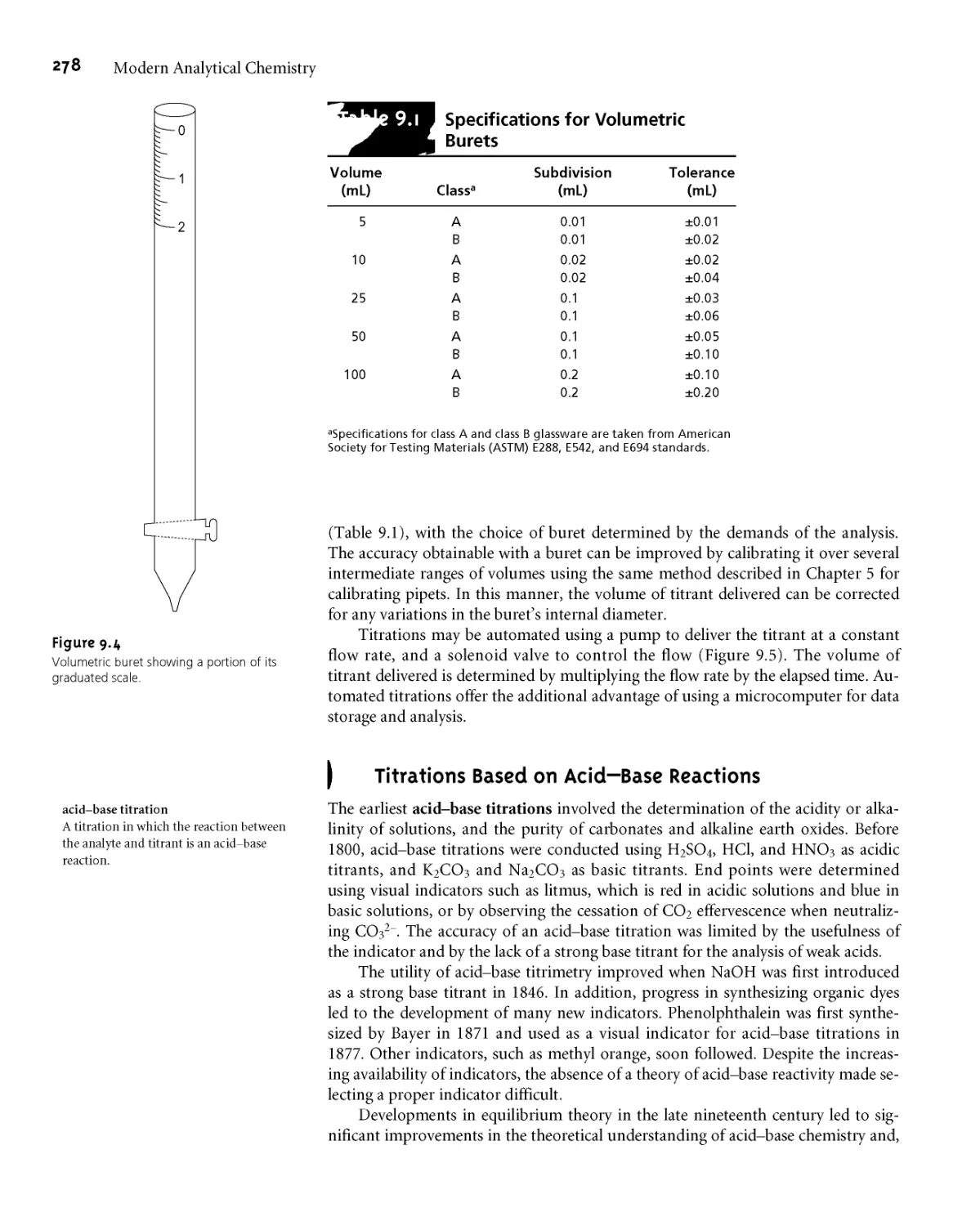
9A.4 The Buret 277
9B Titrations Based on Acid-Base Reactions 278
9ВД Acid-Base Titration Curves 279
9B.2 Selecting and Evaluating the
End Point 287
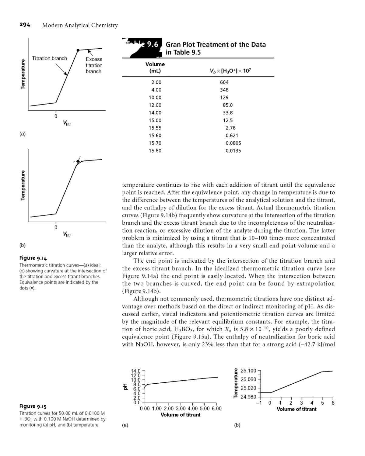
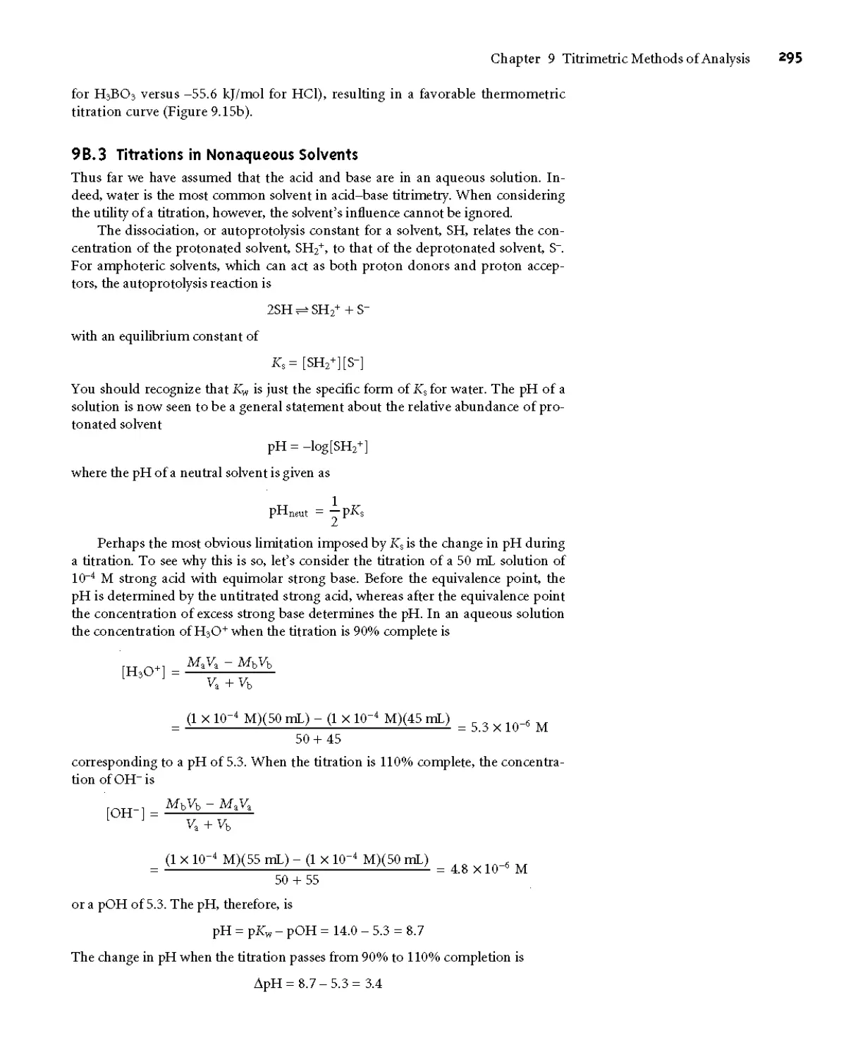
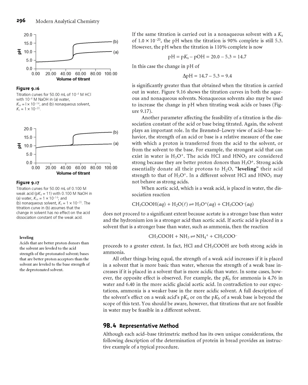
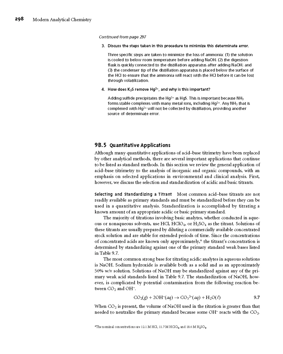
9B.3 Titrations in Nonaqueous Solvents 295
9B.4 Representative Method 296
9B.5 Quantitative Applications 298
9B.6 Qualitative Applications 308
9B.7 Characterization Applications 309
9B.8 Evaluation of Acid-Base Titrimetry 311
9C Titrations Based on Complexation Reactions 314
9G 1 Chemistry and Properties of EDTA 315
9G2 Complexometric EDTA Titration Curves 317
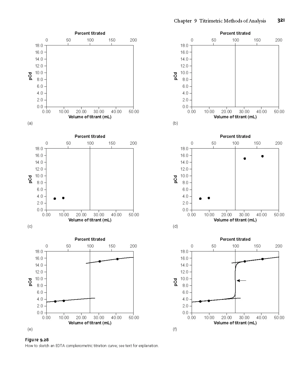
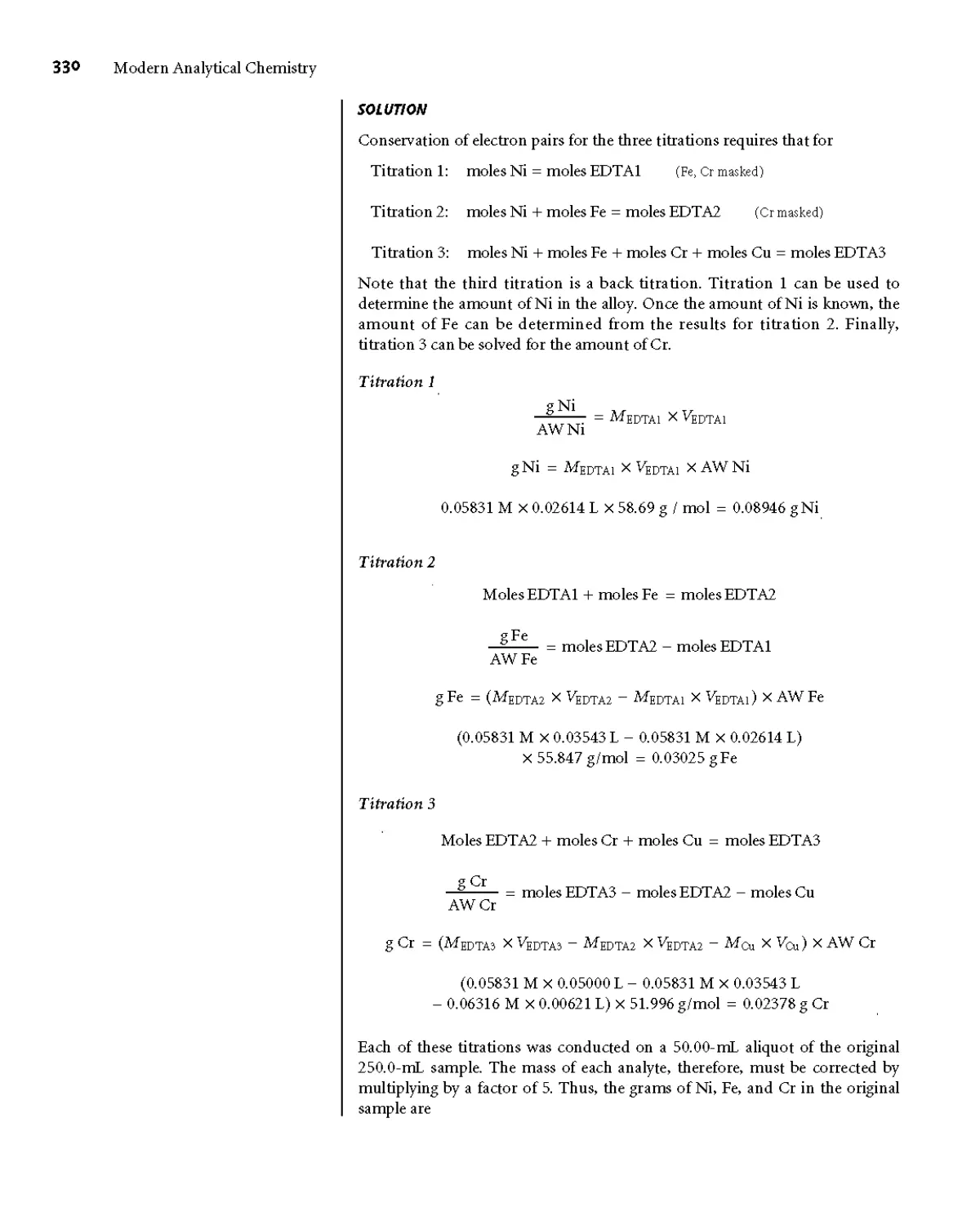
9G3 Selecting and Evaluating the End Point 322
9G4 Representative Method 324
9G5 Quantitative Applications 327
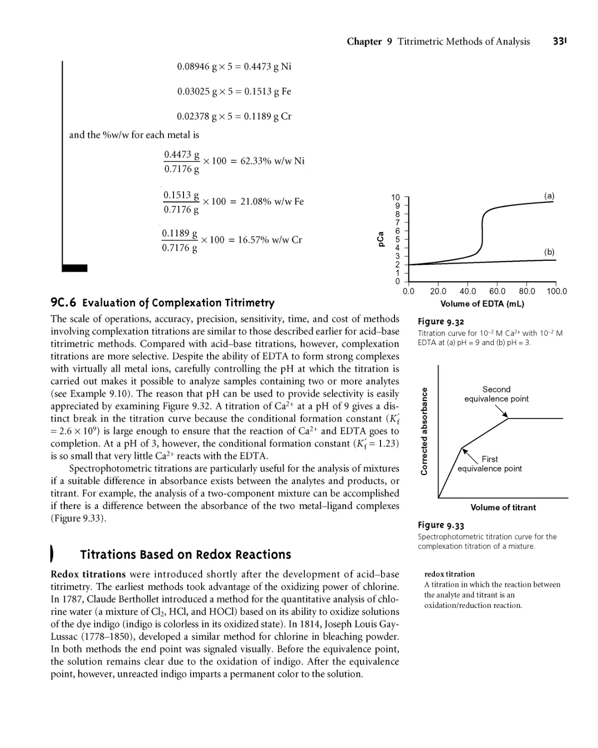
9G6 Evaluation of Complexation Titrimetry 331
9D Titrations Based on Redox Reactions 331
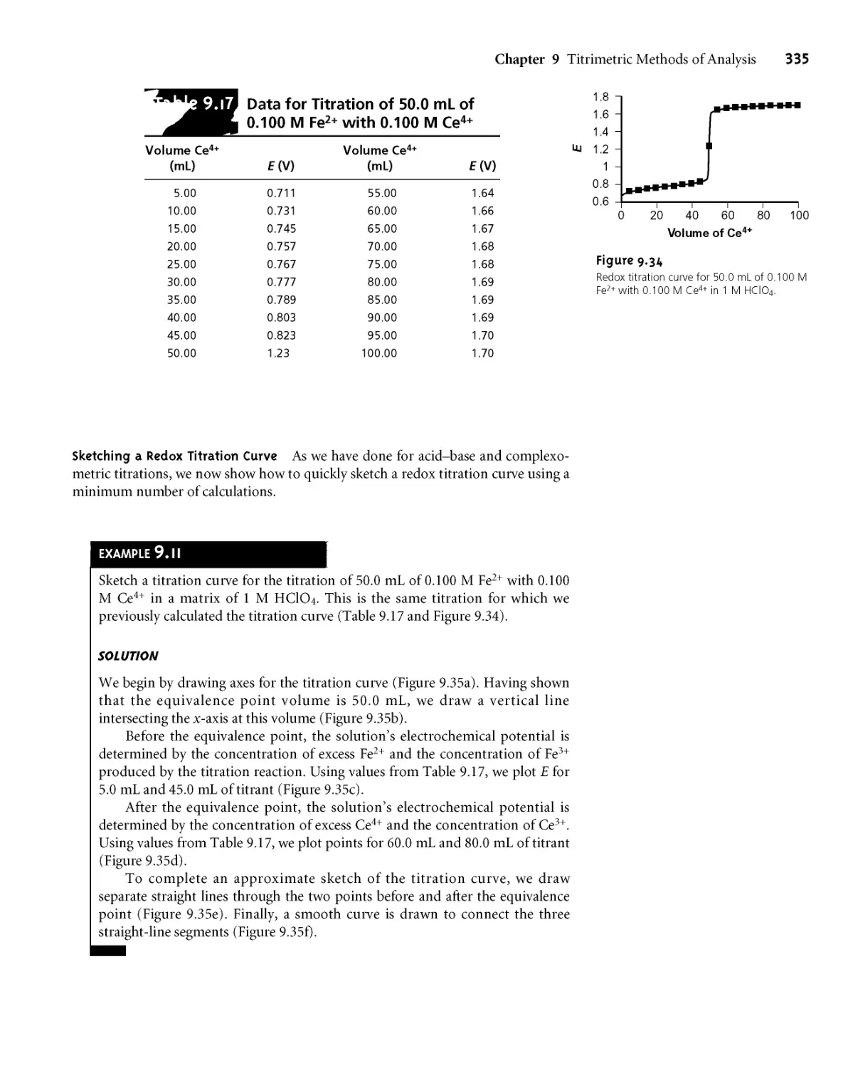
9D.1 Redox Titration Curves 332
9D.2 Selecting and Evaluating the End Point 337
9D.3 Representative Method 340
9D.4 Quantitative Applications 341
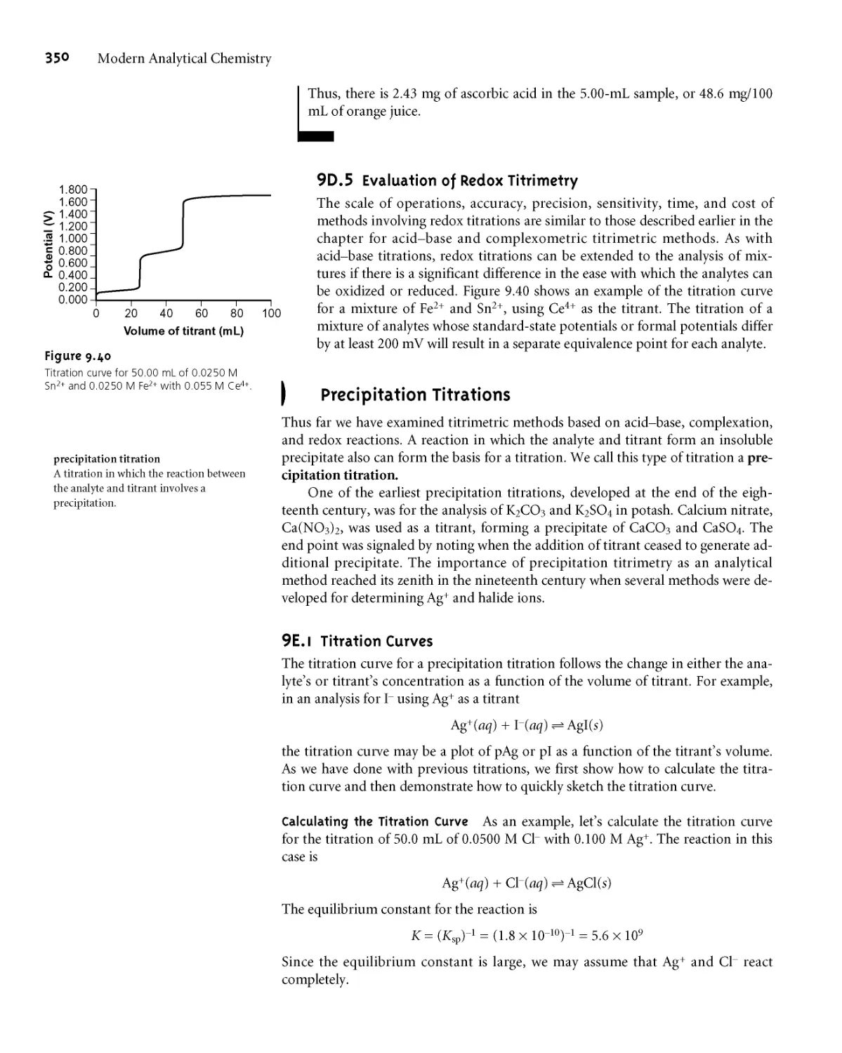
9D.5 Evaluation of Redox Titrimetry 350
9E Precipitation Titrations 350
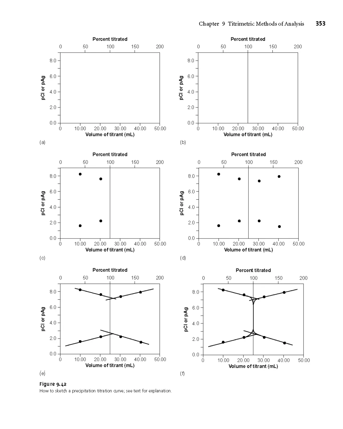
9ЕД Titration Curves 350
9E.2 Selecting and Evaluating the End Point 354
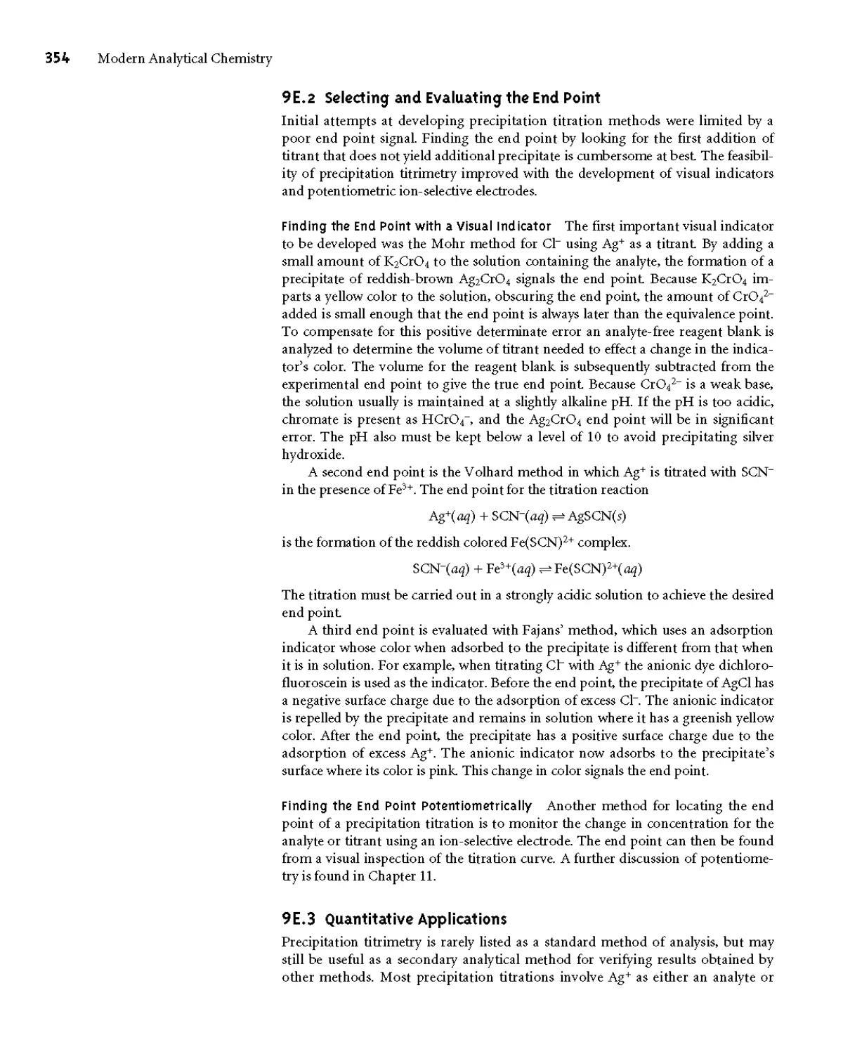
9E.3 Quantitative Applications 354
9E.4 Evaluation of Precipitation Titrimetry 357
9F Key Terms 357
9G Summary 357
9H Suggested Experiments 3 58
91 Problems 360
9J Suggested Readings 366
9K References 367
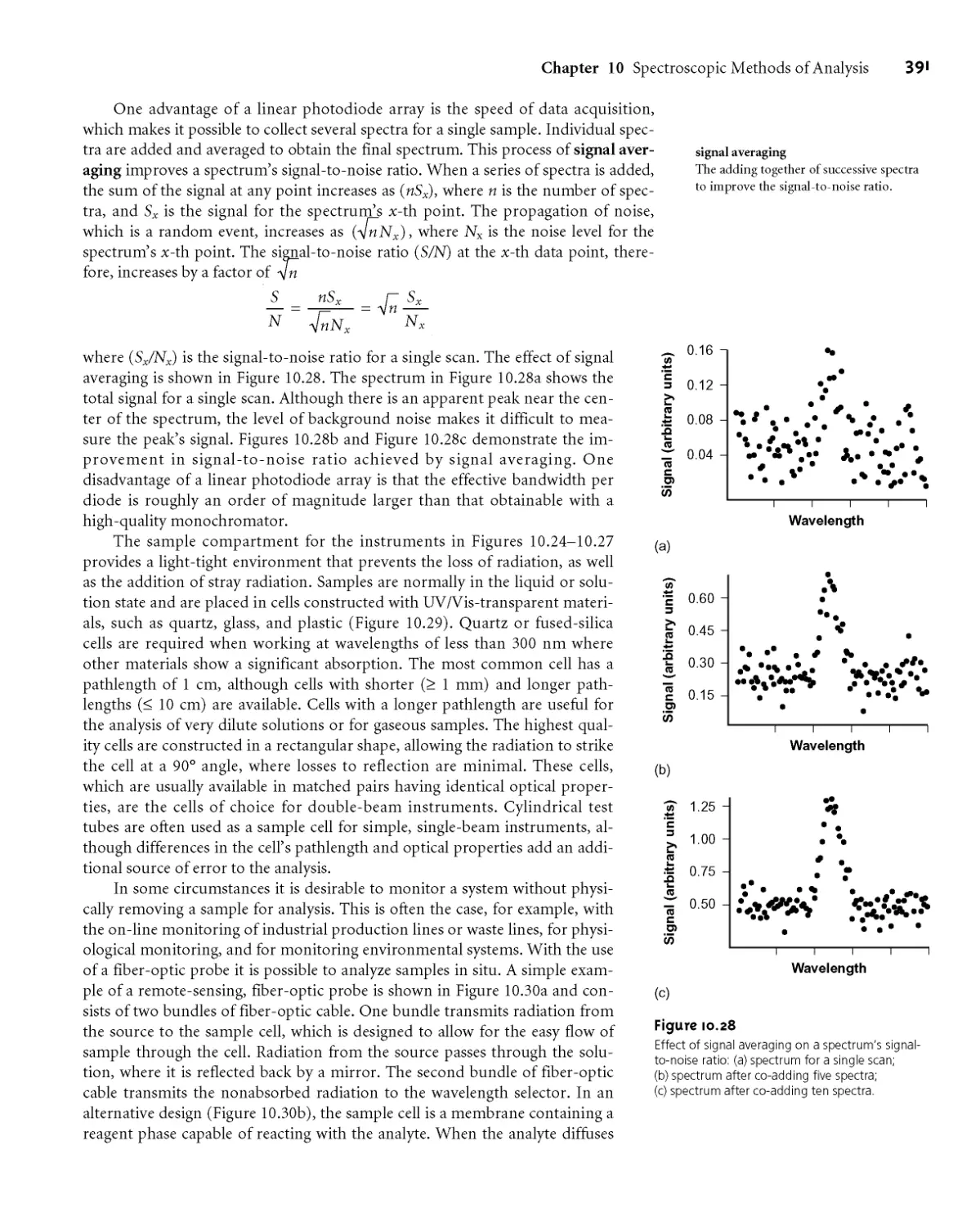
Spectroscopic Methods
of Analysis 368
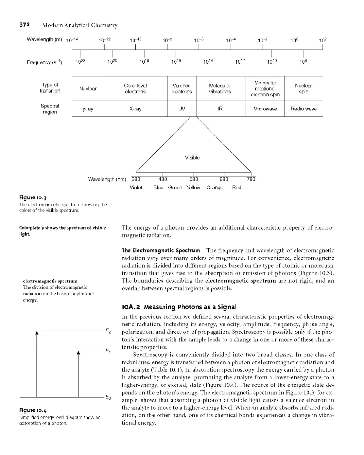
10A Overview of Spectroscopy 369
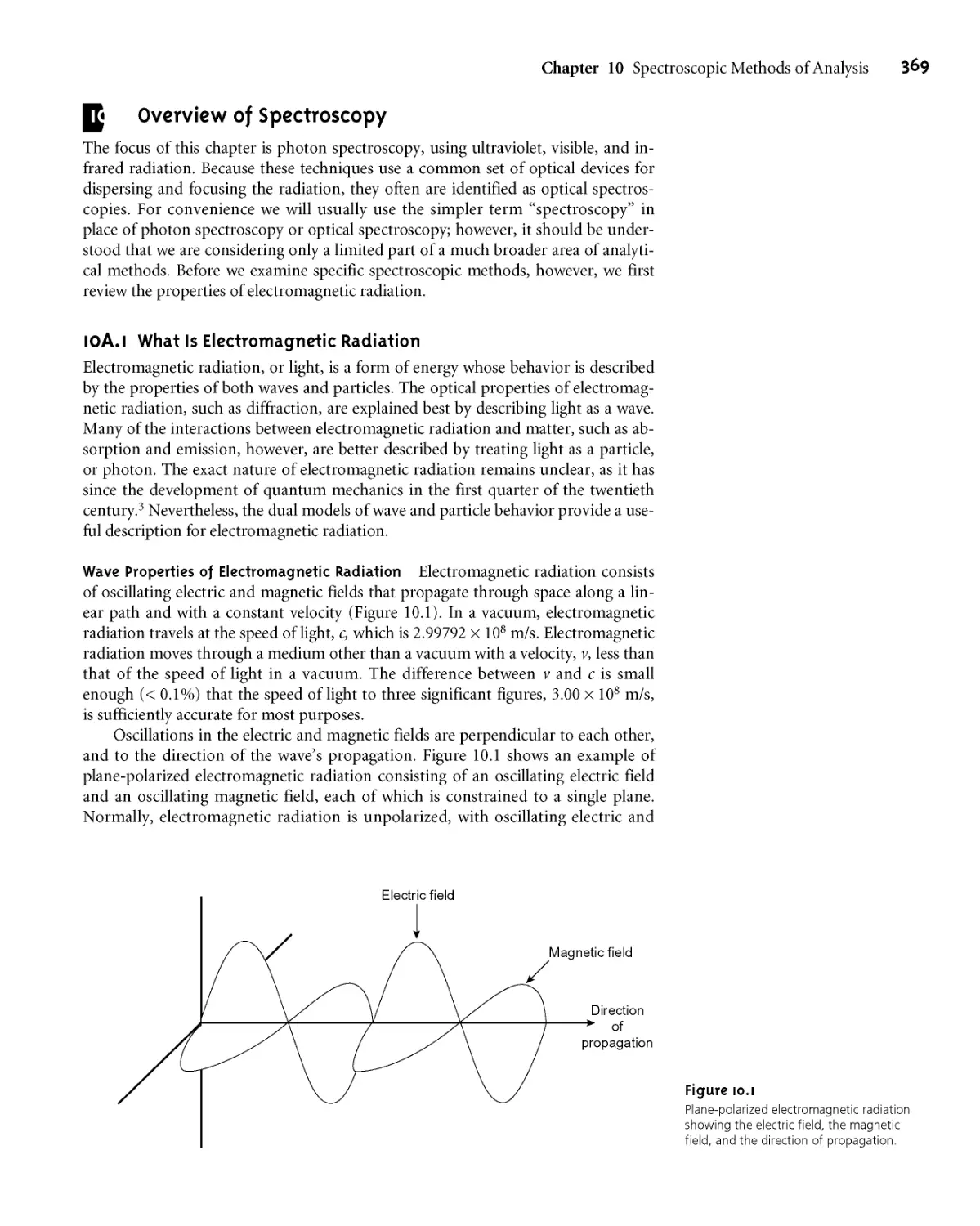
10A. 1 What Is Electromagnetic Radiation 369
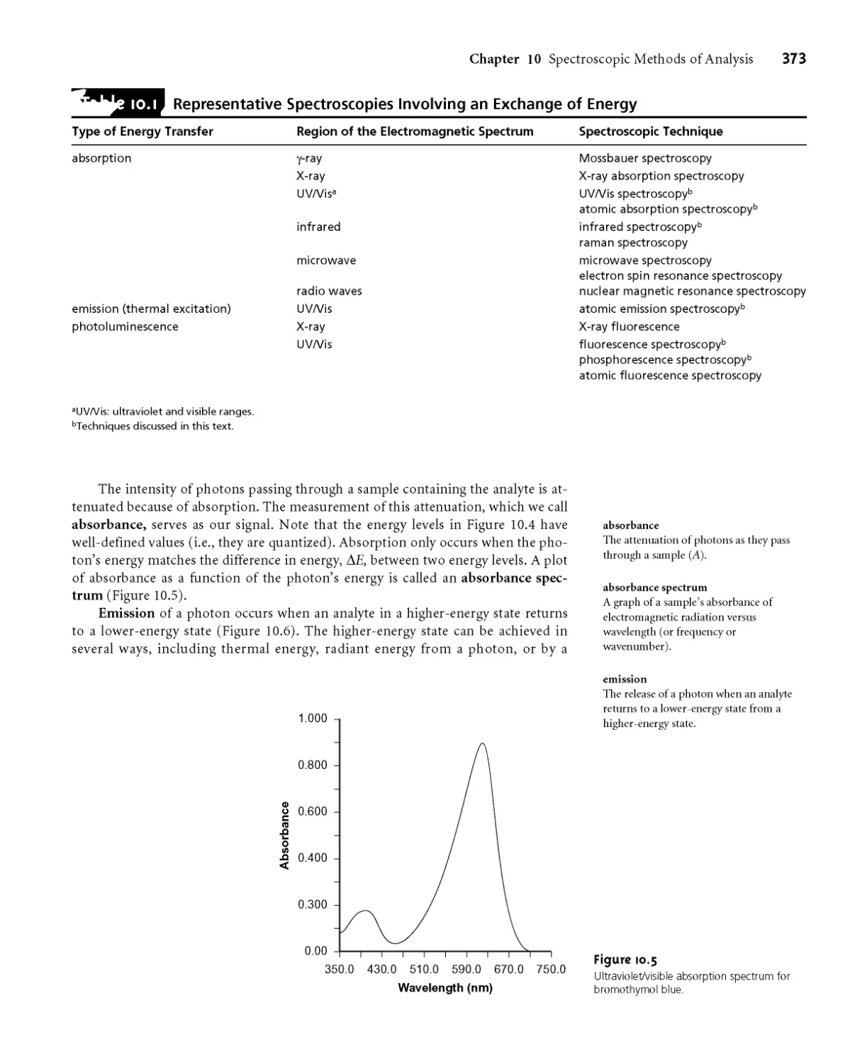
10A.2 Measuring Photons as a Signal 372
10B Basic Components of Spectroscopic
Instrumentation 374
I0B.I Sources of Energy 375
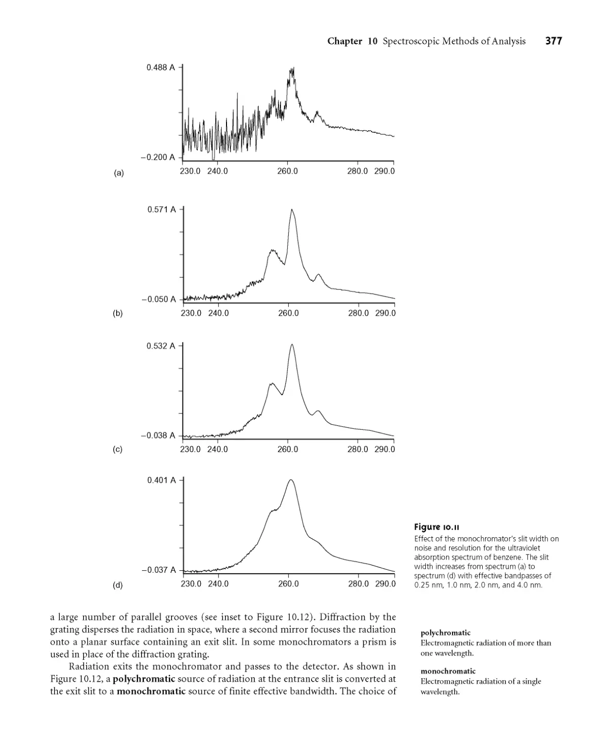
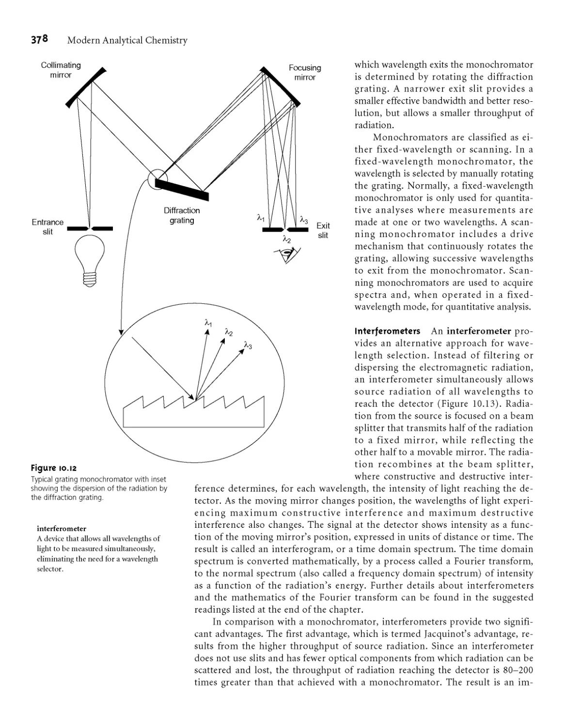
10B.2 Wavelength Selection 376
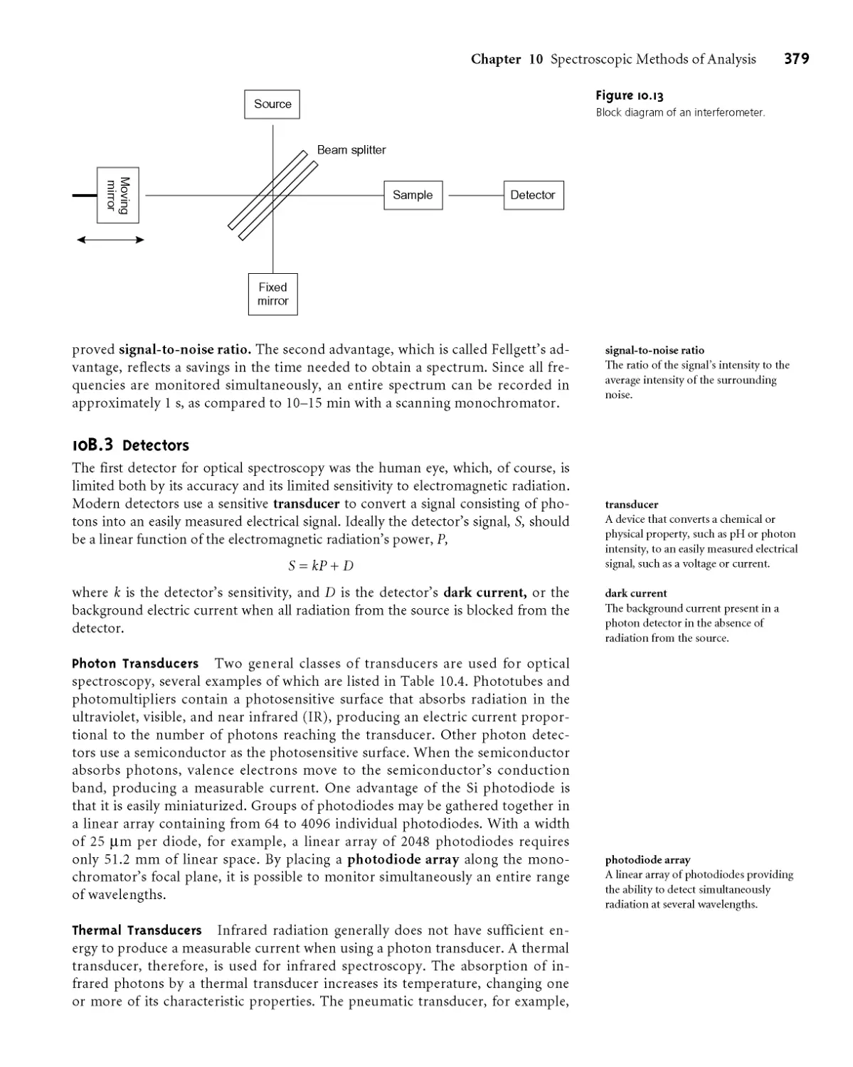
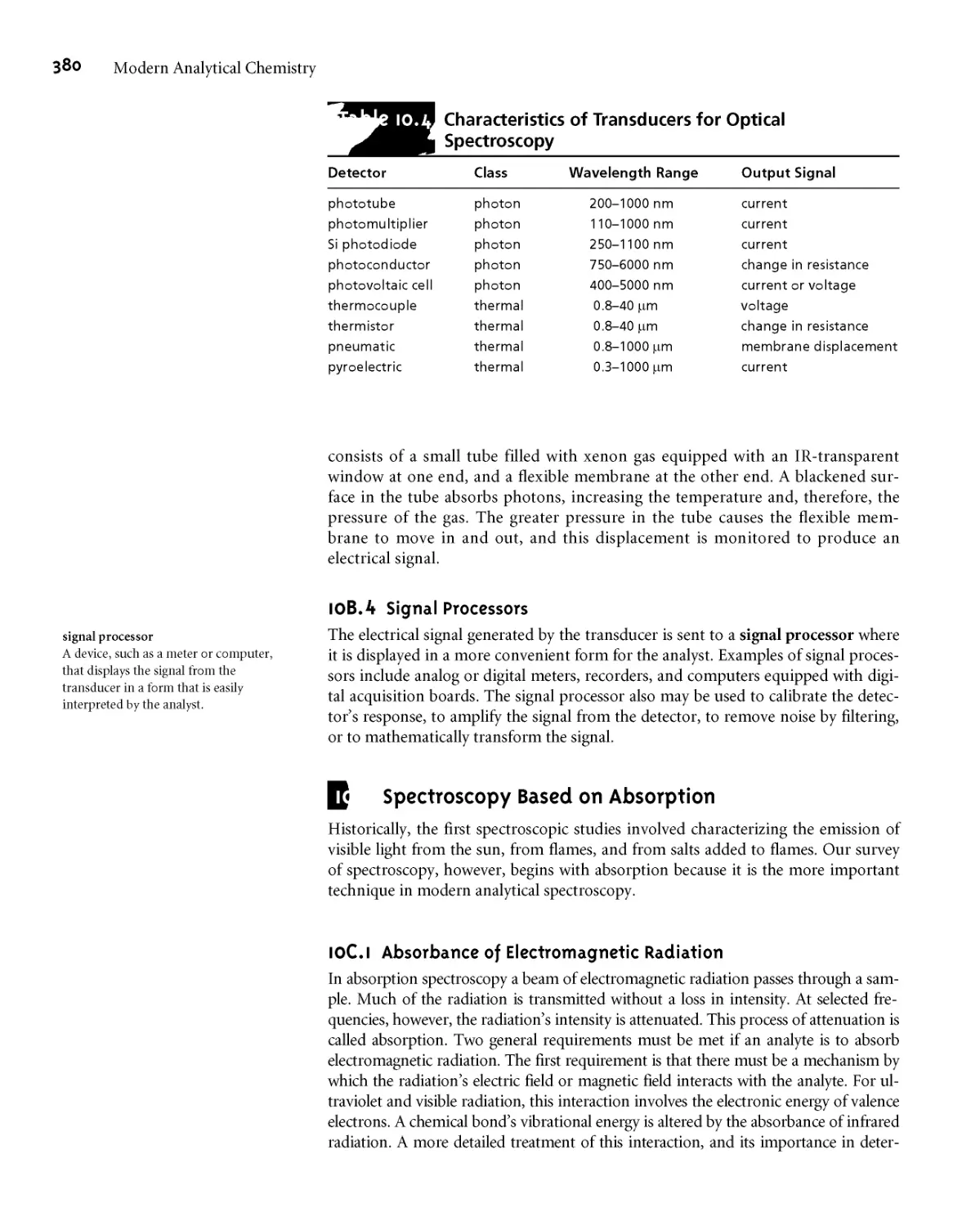
10B.3 Detectors 379
10B.4 Signal Processors 380
10C Spectroscopy Based on Absorption 380
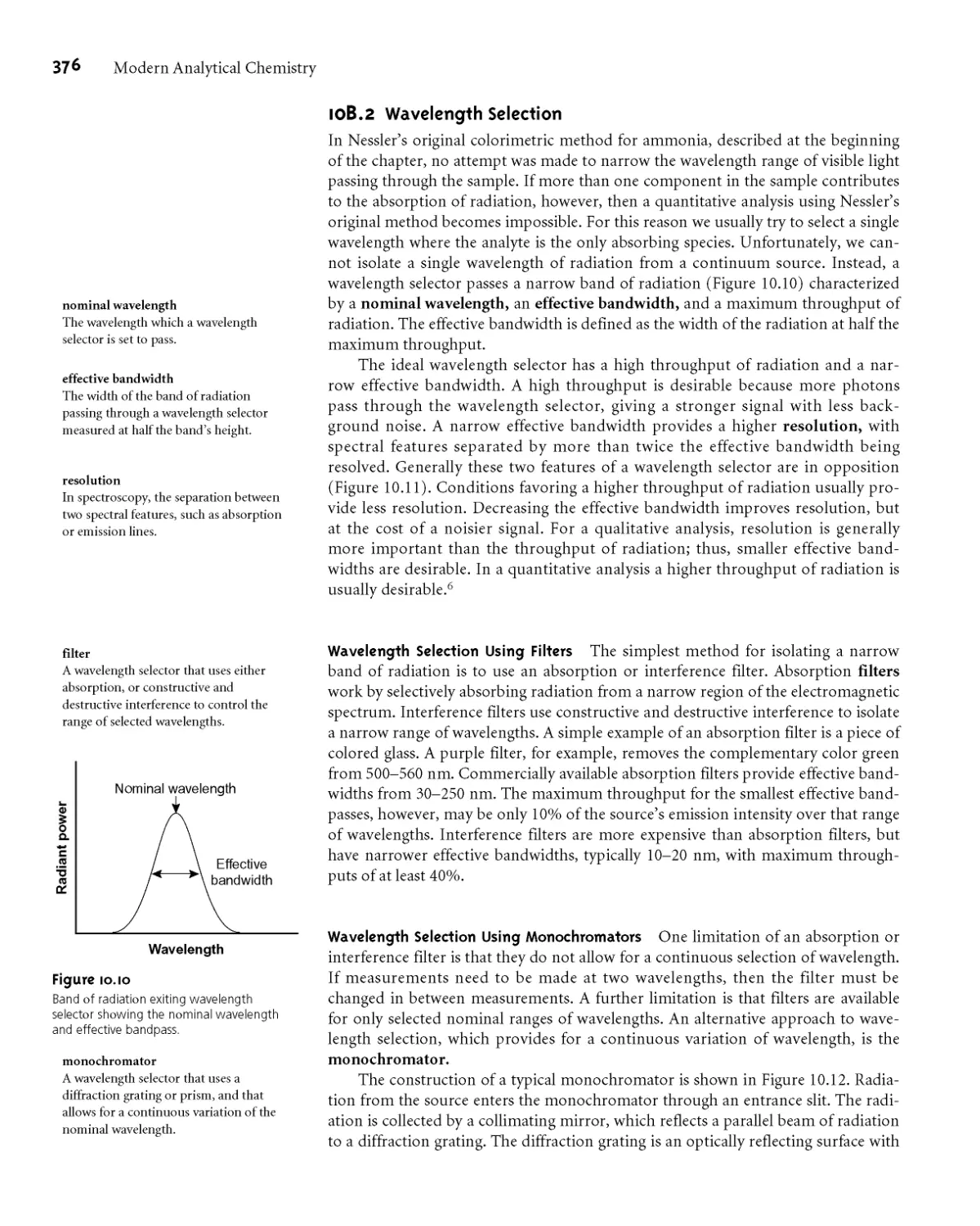
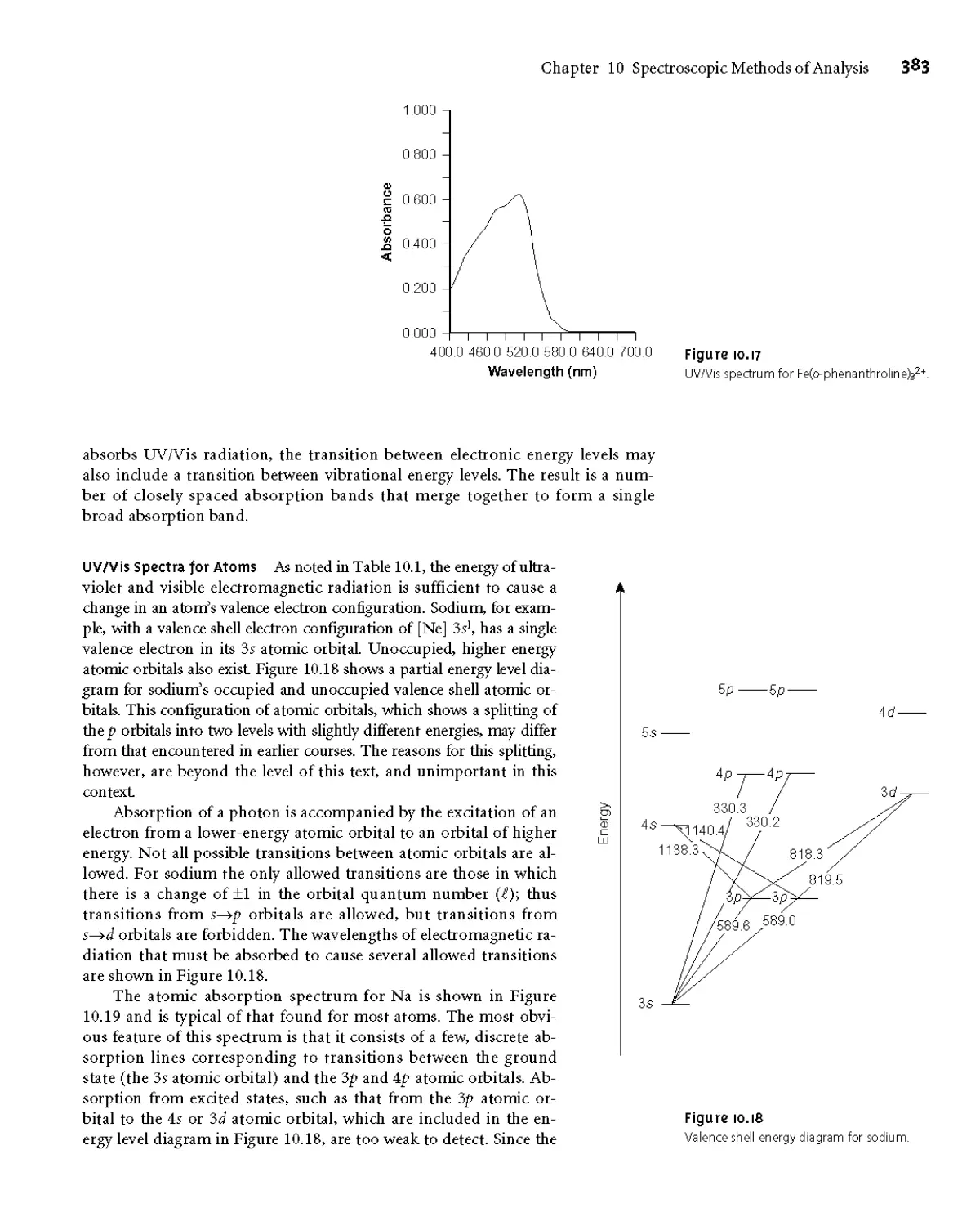
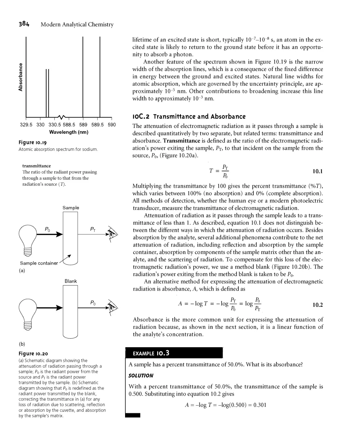
1 ОС. 1 Absorbance of Electromagnetic Radiation 380
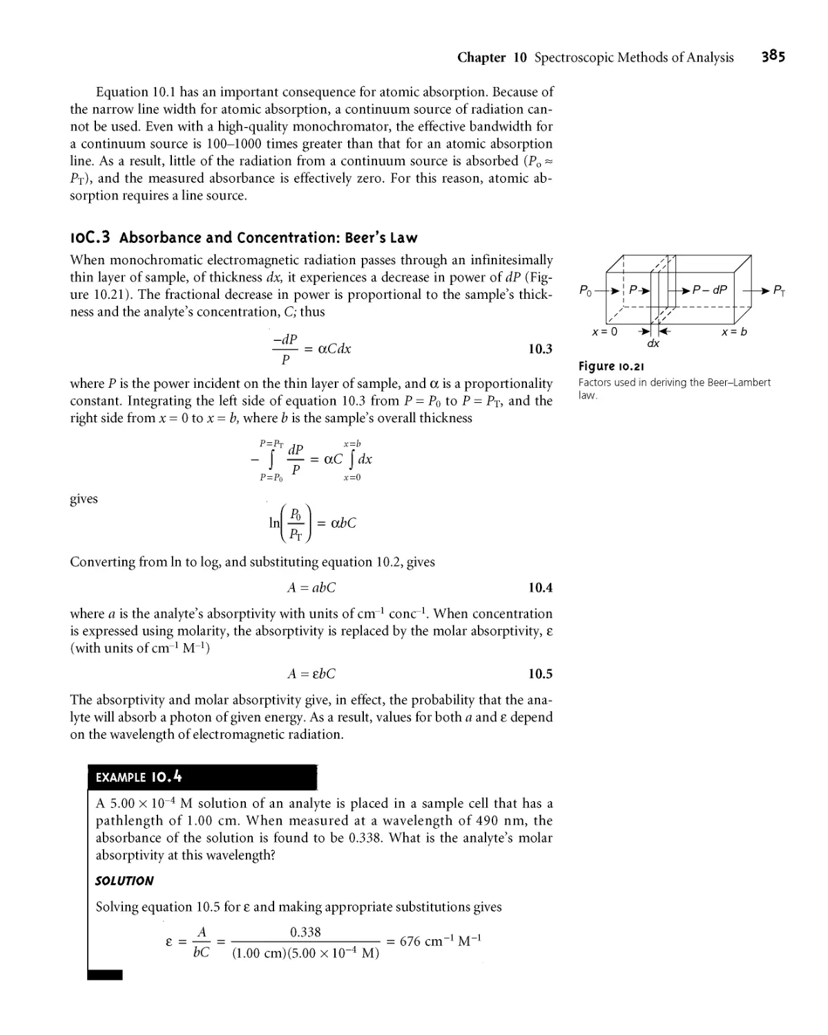
I0G2 Transmittance and Absorbance 384
I0G3 Absorbance and Concentration: Beer’s
Law 385
* *
VII
Contents
10C.4 Beer’s Law and Multicomponent
Samples 386
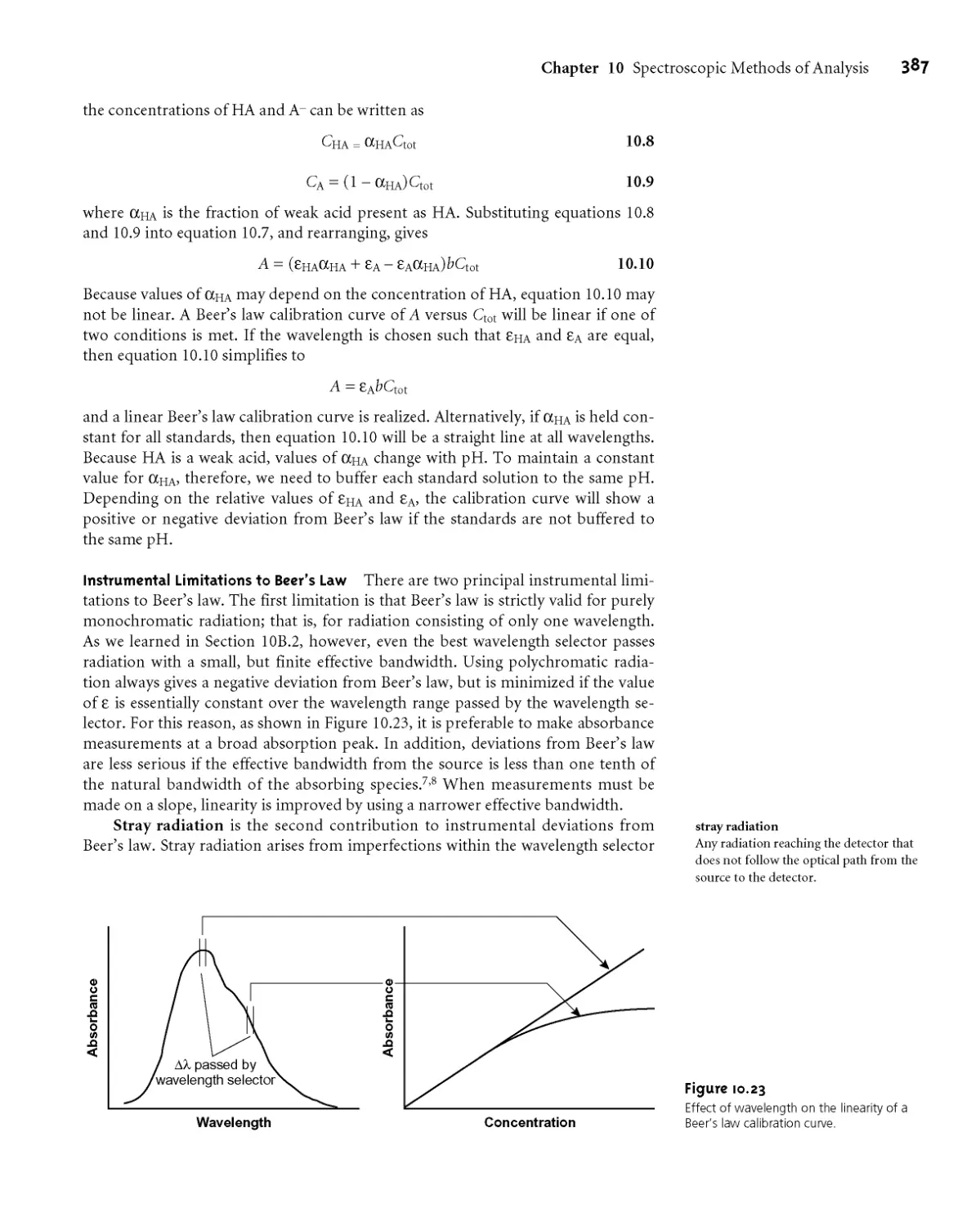
10C.5 Limitations to Beer’s Law 386
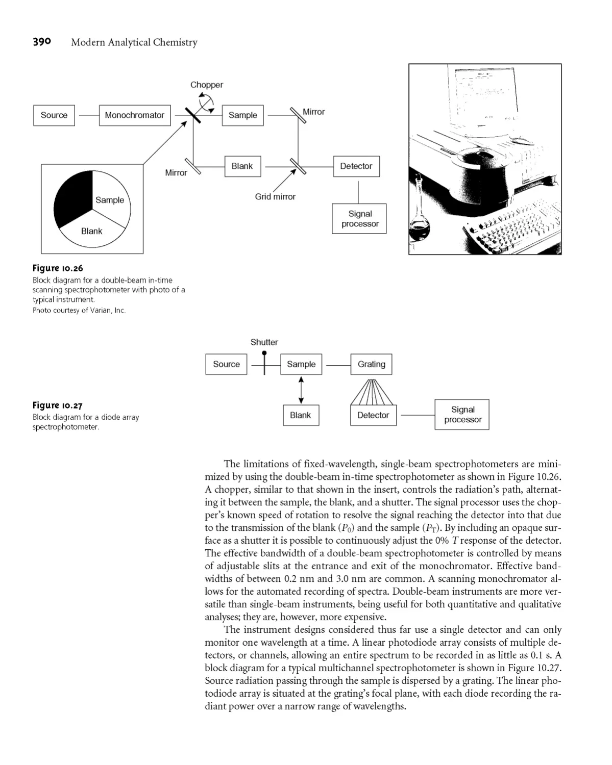
10D Ultraviolet-Visible and Infrared
Spectrophotometry 388
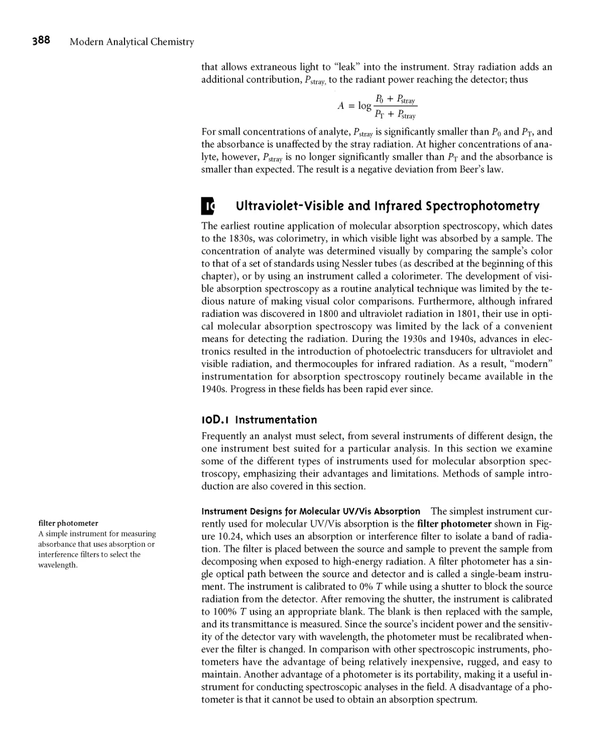
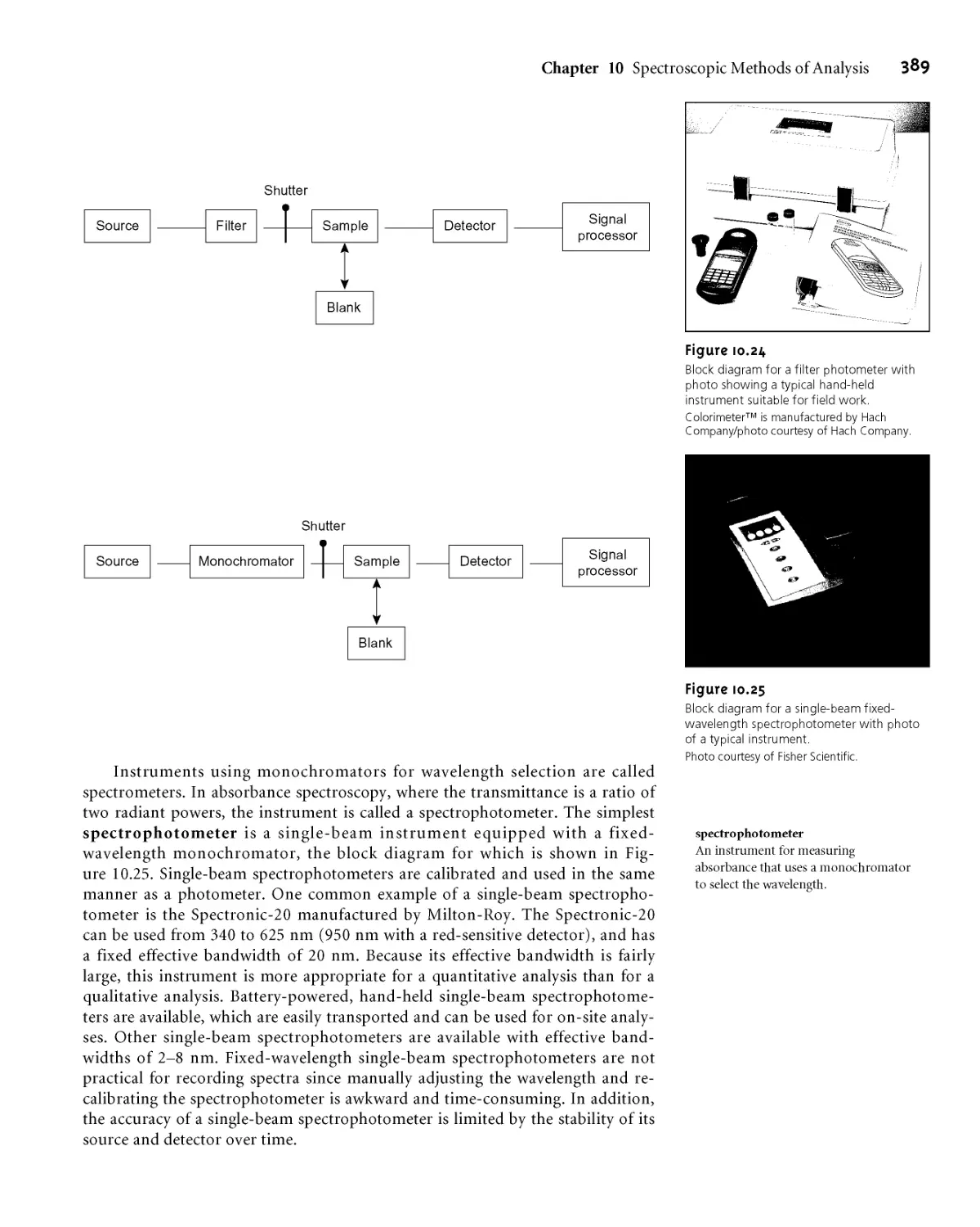
10D.1 Instrumentation 388
10D.2 Quantitative Applications 394
10D.3 Qualitative Applications 402
10D.4 Characterization Applications 403
10D.5 Evaluation 409
10E Atomic Absorption Spectroscopy 412
10E. 1 Instrumentation 412
10E.2 Quantitative Applications 415
10E.3 Evaluation 422
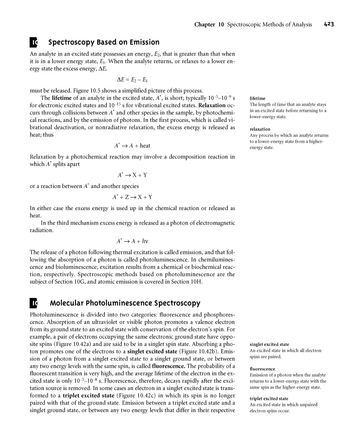
10F Spectroscopy Based on Emission 423
10G Molecular Photoluminescence
Spectroscopy 423
10G.1 Molecular Fluorescence and
Phosphorescence Spectra 424
10G.2 Instrumentation 42 7
10G.3 Quantitative Applications Using Molecular
Luminescence 429
10G.4 Evaluation 432
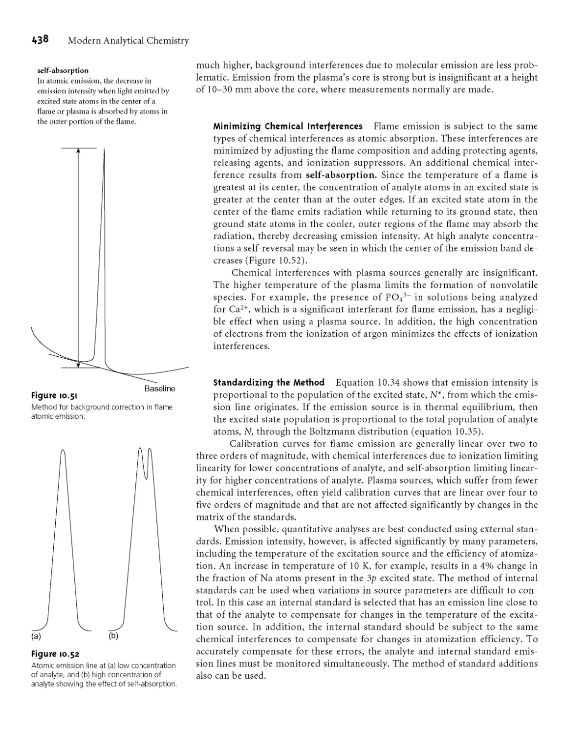
10H Atomic Emission Spectroscopy 434
I OH. I Atomic Emission Spectra 434
10H.2 Equipment 435
10H.3 Quantitative Applications 437
10H.4 Evaluation 440
101 Spectroscopy Based on Scattering 441
101.1 Origin of Scattering 441
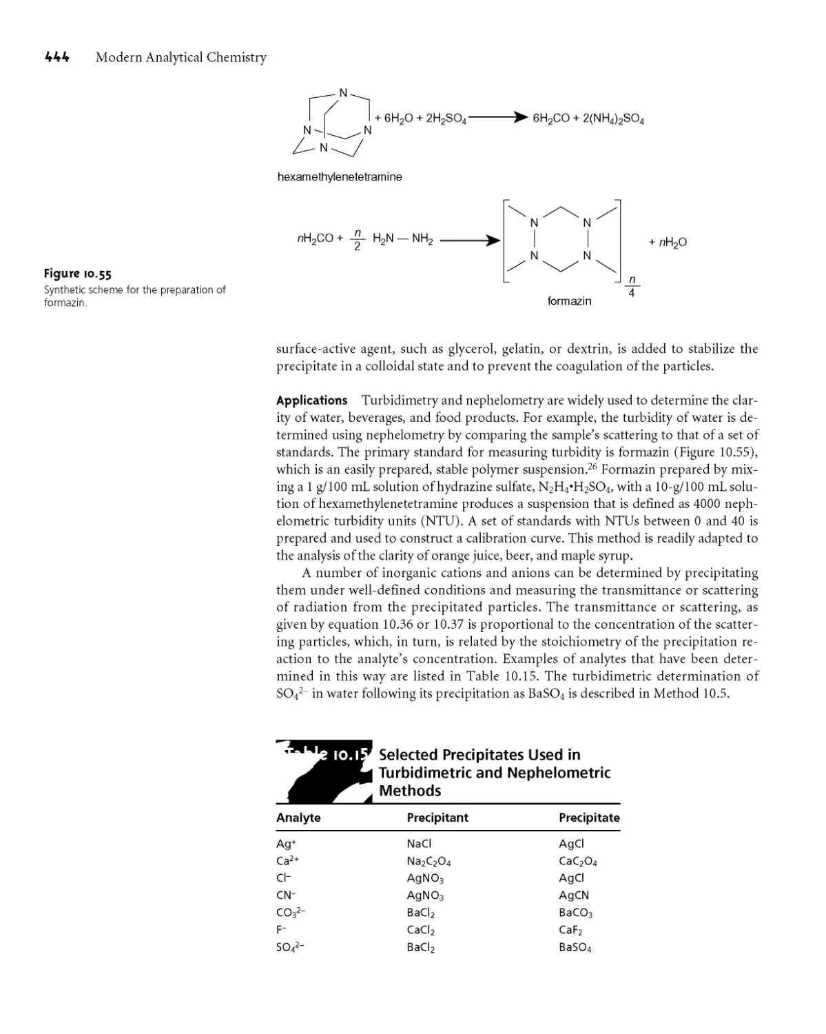
101.2 Turbidimetry and Nephelometry 441
10J Key Terms 446
1 OK Summary 446
10L Suggested Experiments 447
10M Problems 450
10N Suggested Readings 458
10 О References 459
Electrochemical Methods of Analysis 461
11A Classification of Electrochemical Methods 462
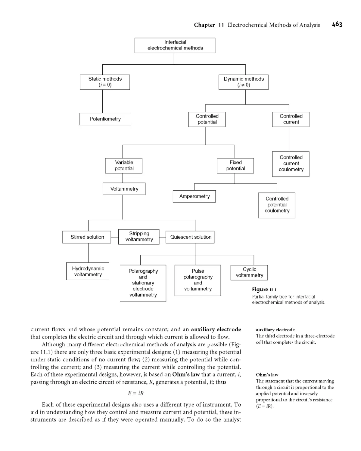
11A.1 Interfacial Electrochemical Methods 462
11 A.2 Controlling and Measuring Current and
Potential 462
1 IB Potentiometric Methods of Analysis 465
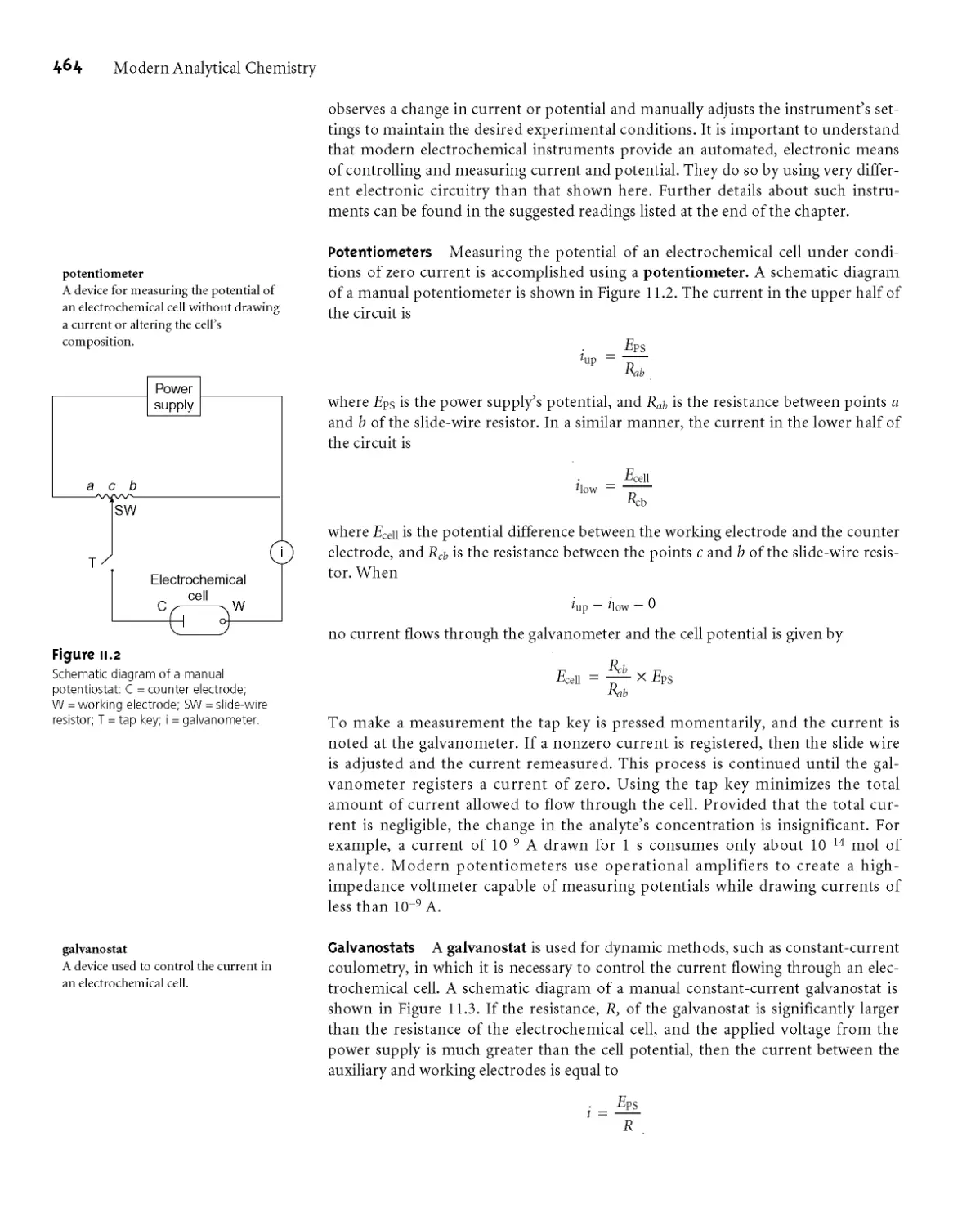
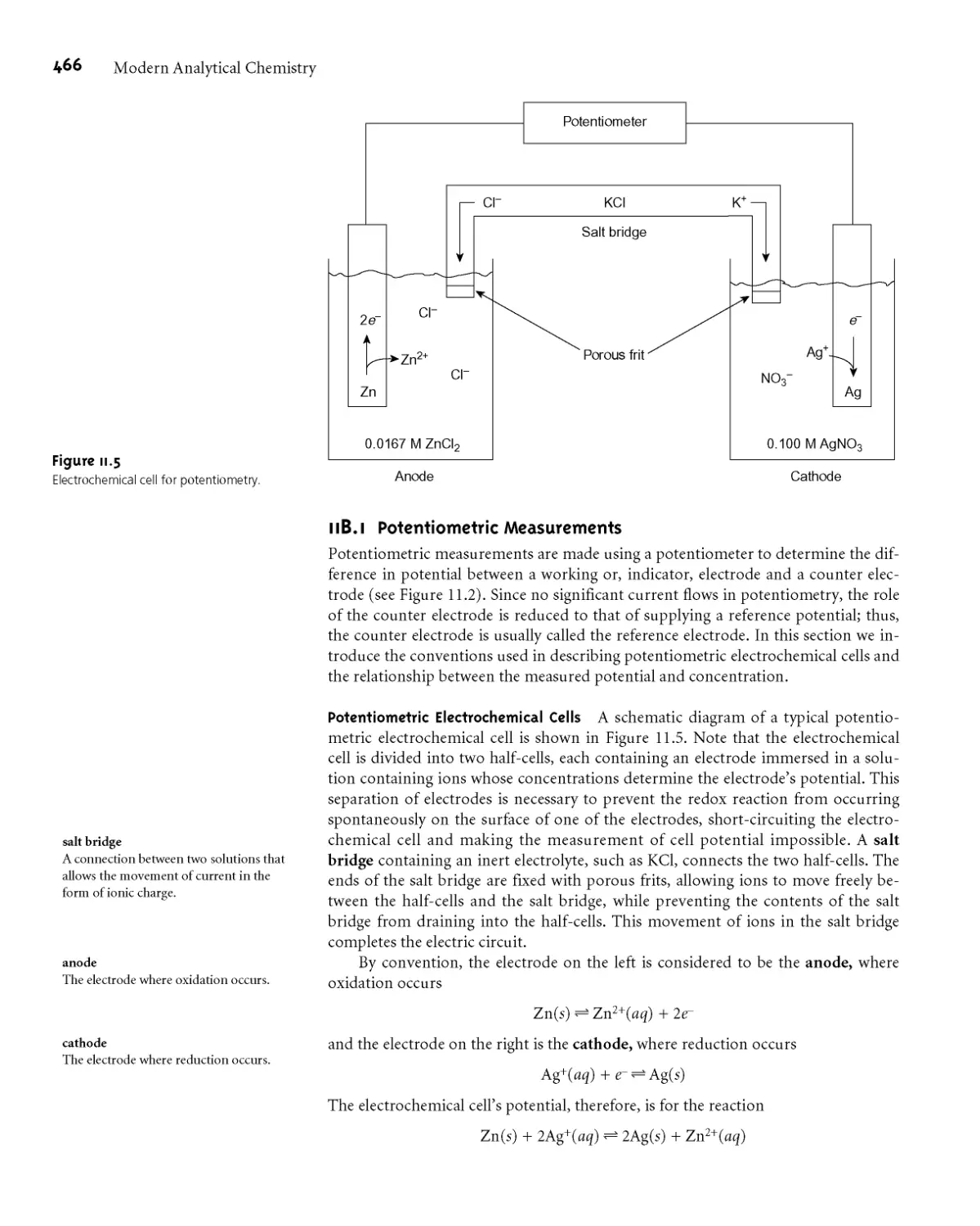
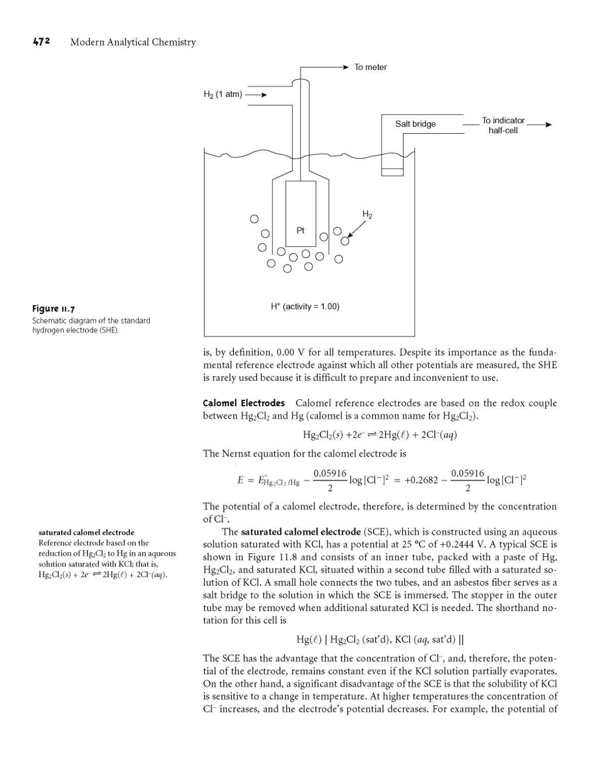
11B.1 Potentiometric Measurements 466
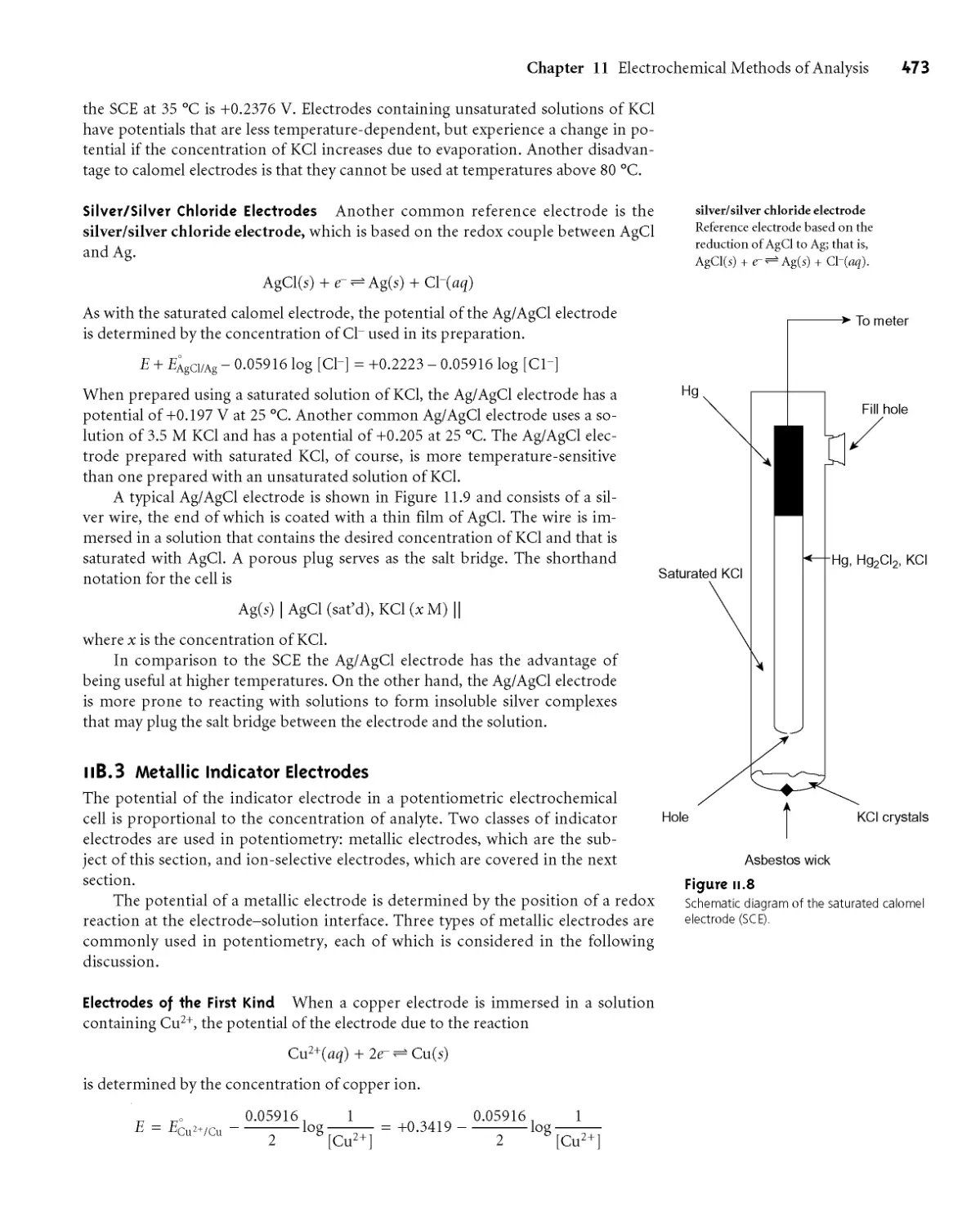
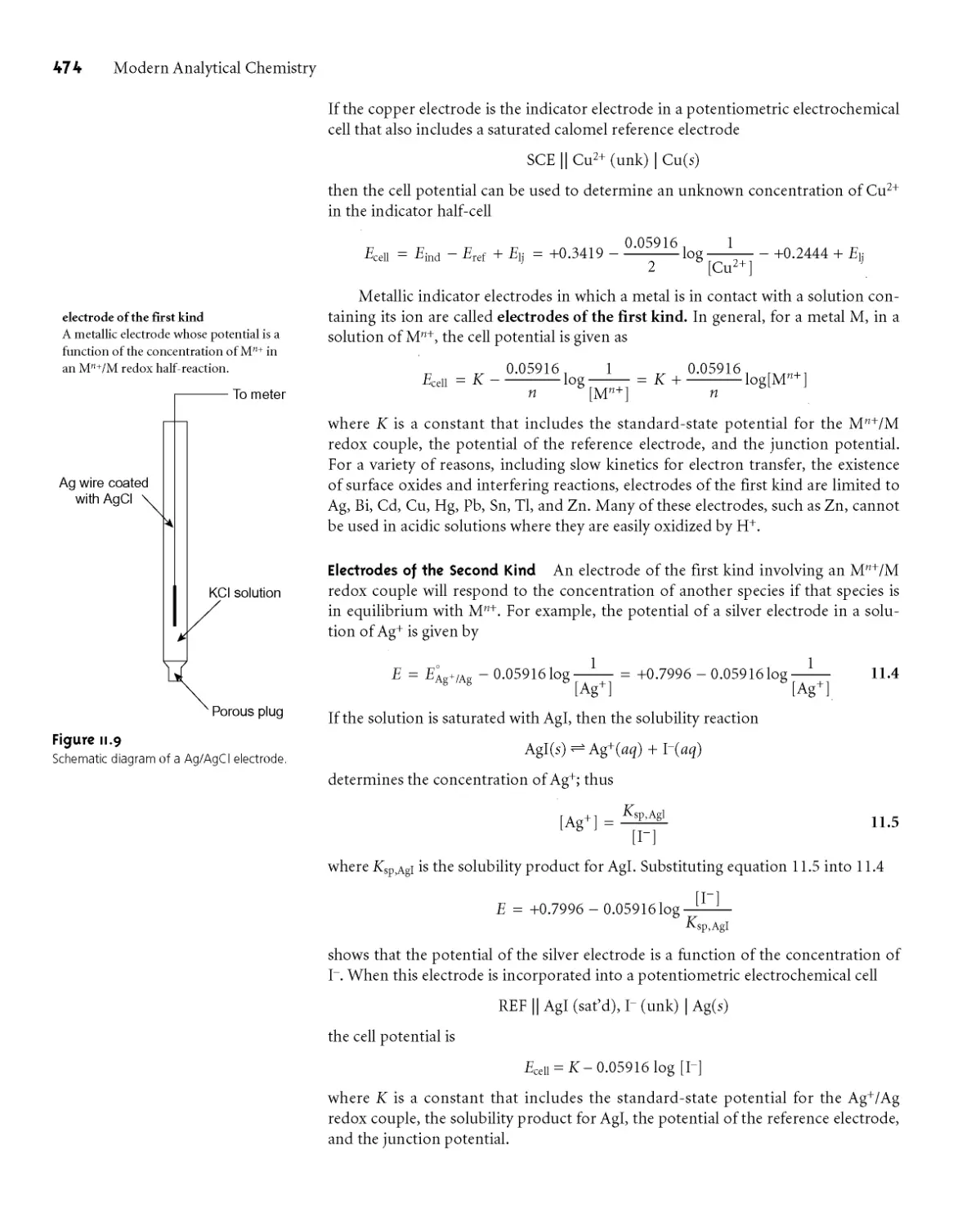
11B.2 Reference Electrodes 471
11B.3 Metallic Indicator Electrodes 473
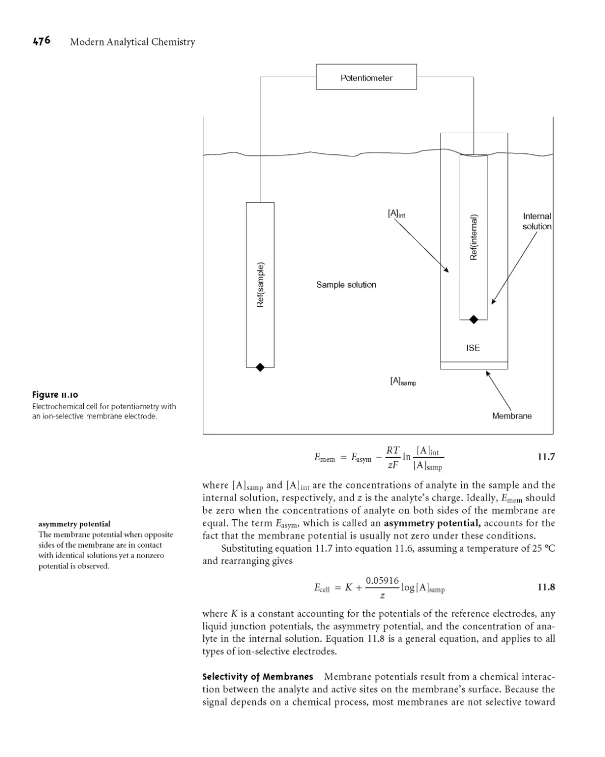
11B.4 Membrane Electrodes 475
1 IB.5 Quantitative Applications 485
1 IB.6 Evaluation 494
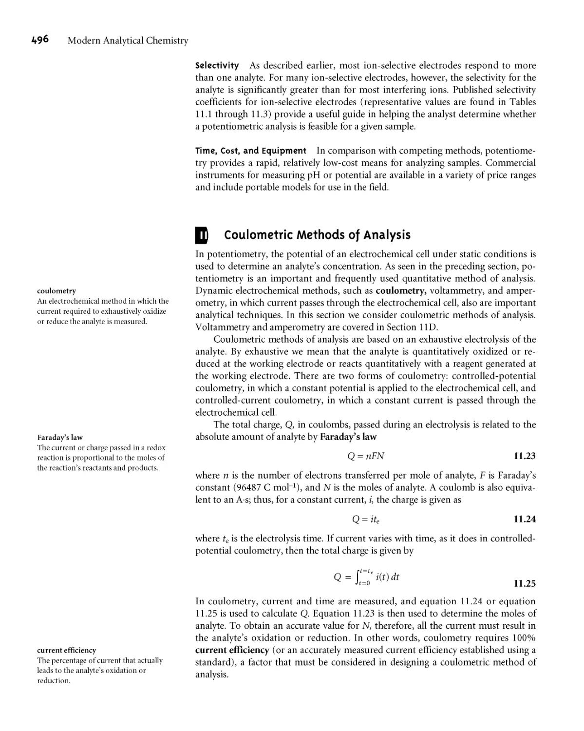
11C Coulometric Methods of Analysis 496
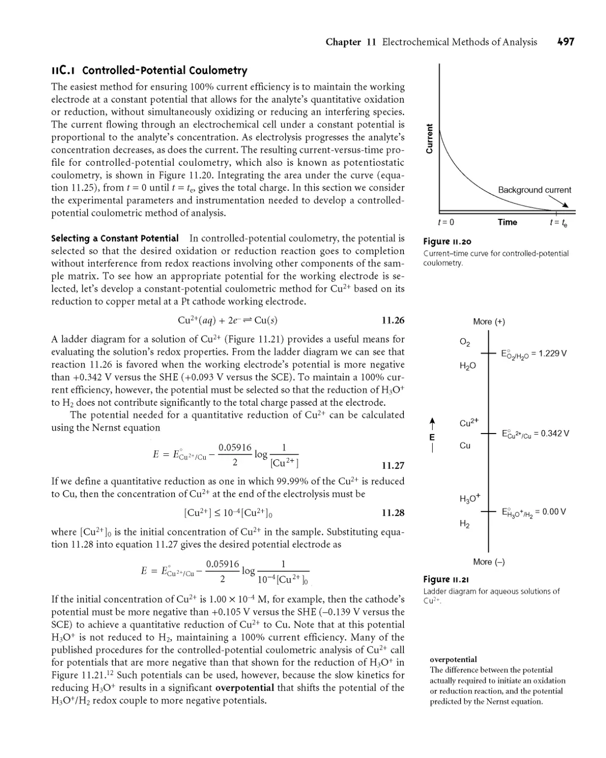
11C.1 Controlled-Potential Coulometry 497
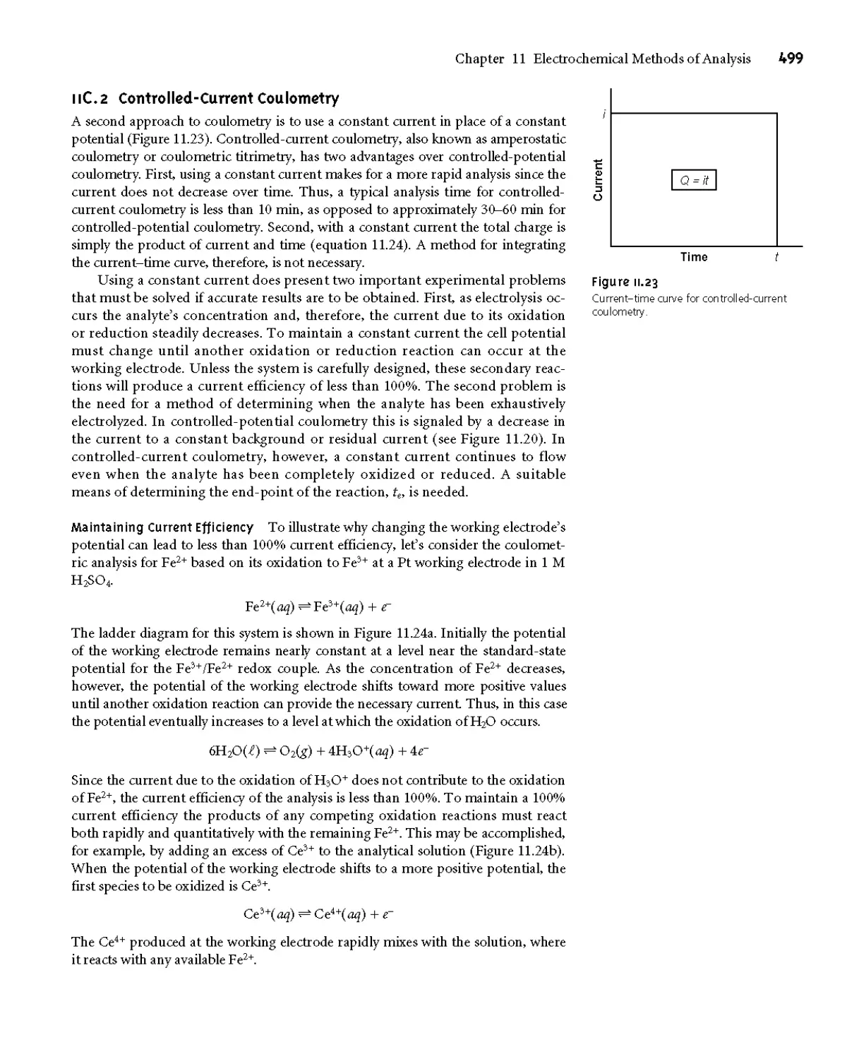
11C.2 Controlled-Current Coulometry 499
11C.3 Quantitative Applications 501
11 C.4 Characterization Applications 506
11C.5 Evaluation 507
1 ID Voltammetric Methods of Analysis 508
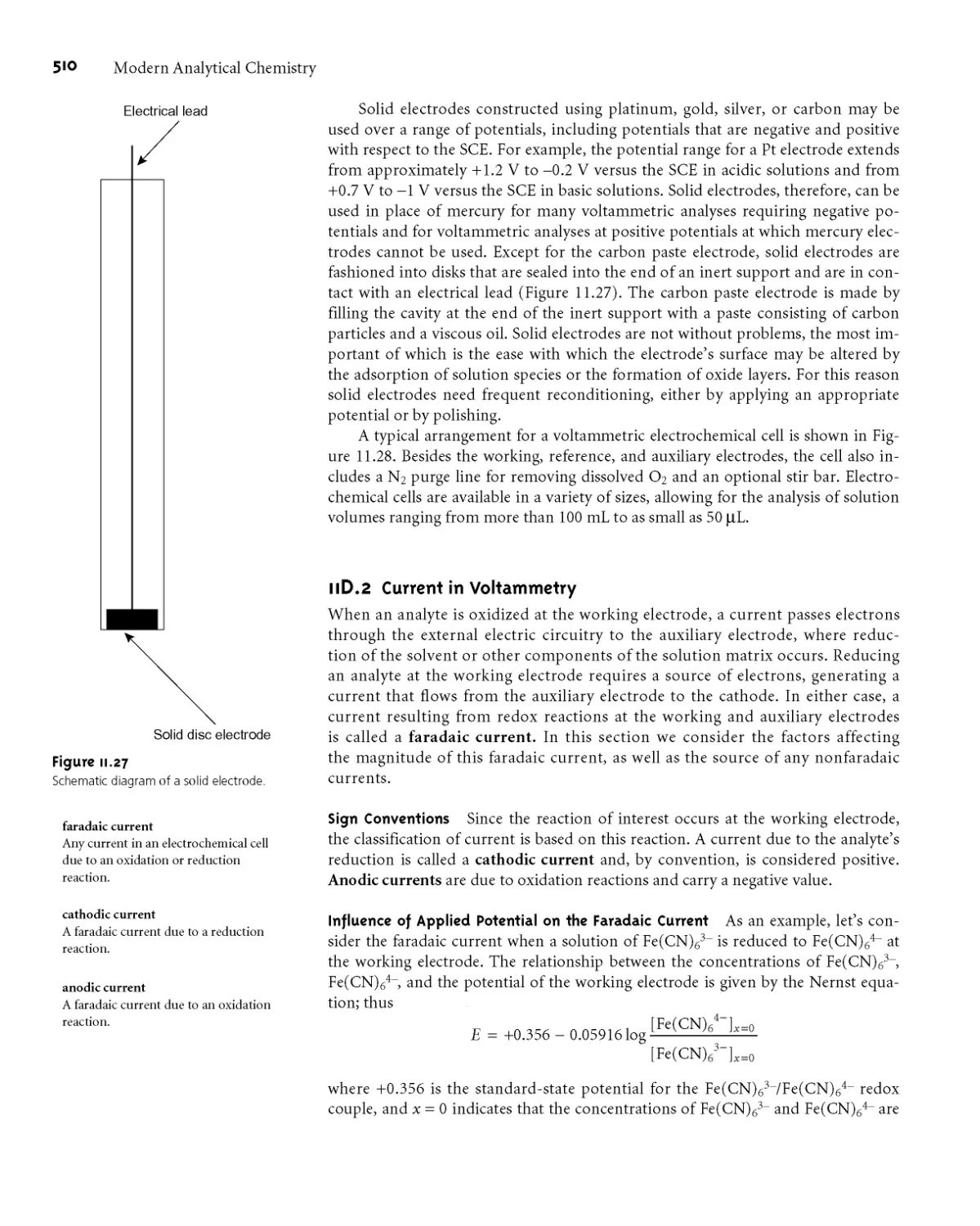
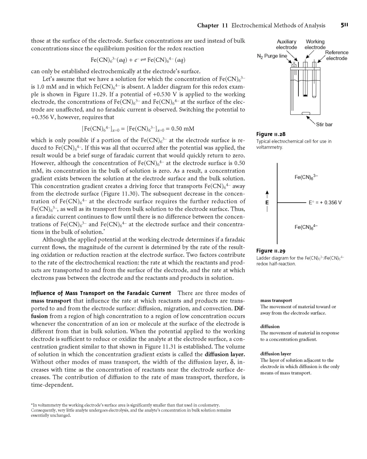
11D.1 Voltammetric Measurements 509
1 ID.2 Current in Voltammetry 510
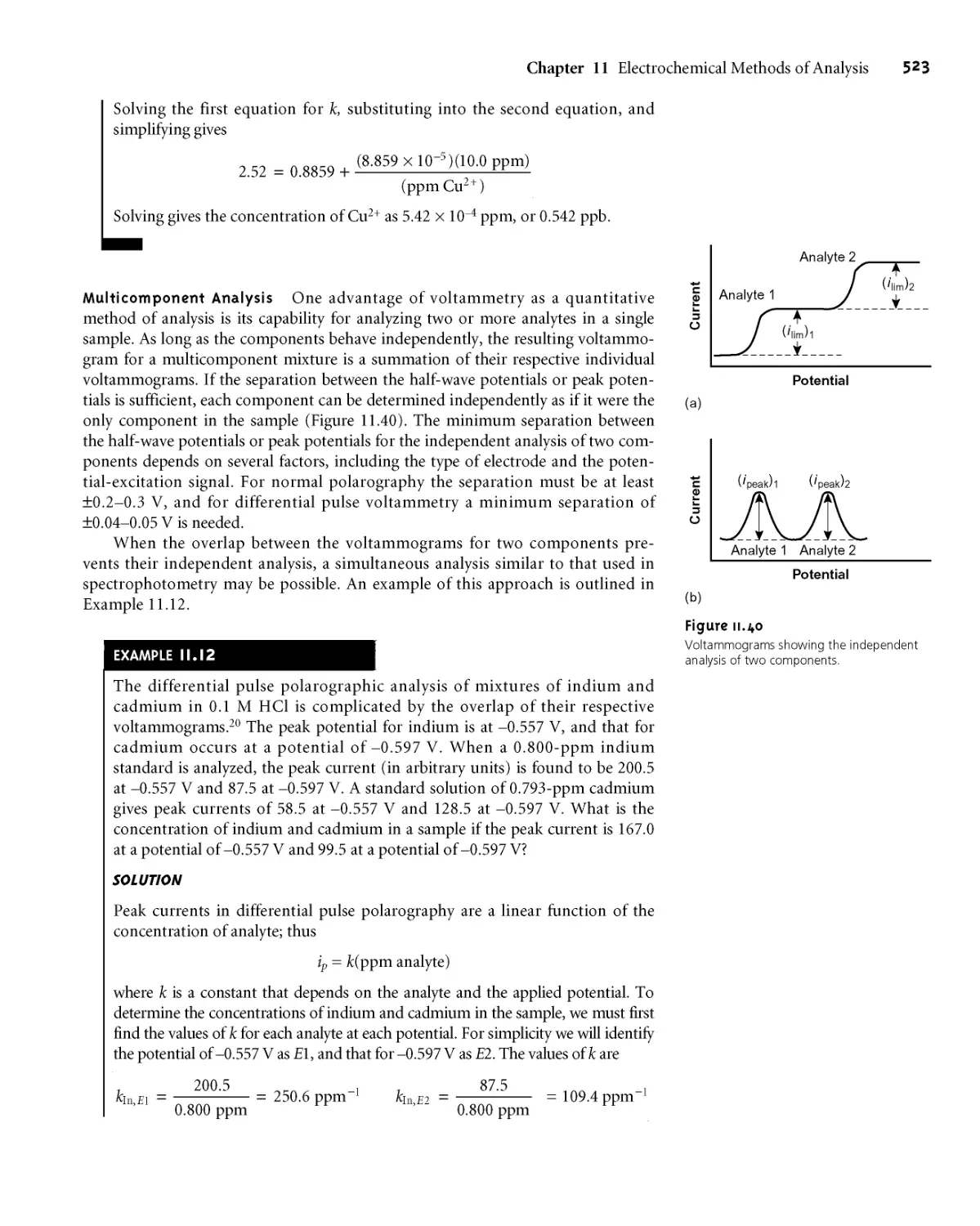
11D. 3 Shape of Voltammograms 513
1 ID.4 Quantitative and Qualitative Aspects
of Voltammetry 514
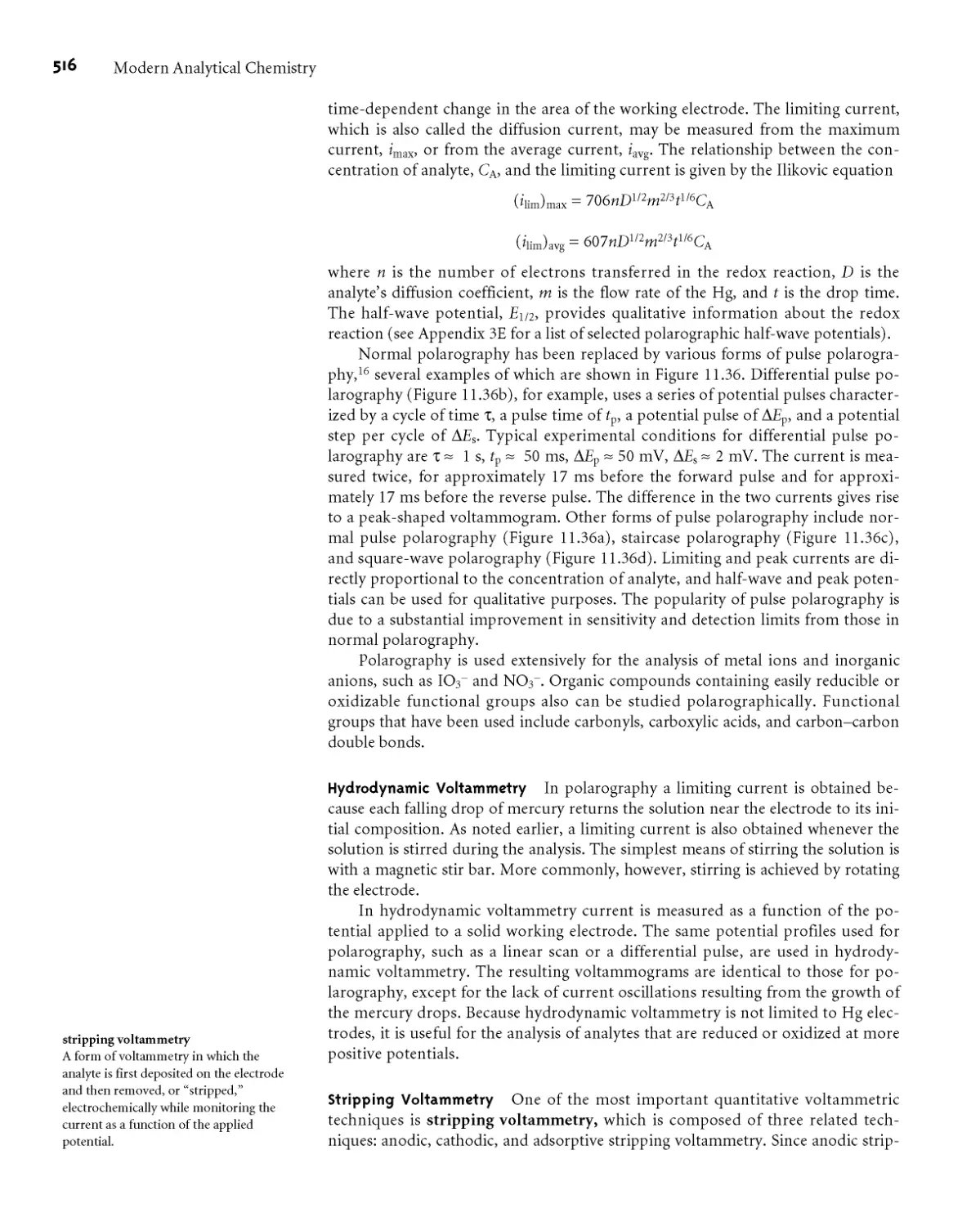
1 ID.5 Voltammetric Techniques 515
1 ID.6 Quantitative Applications 520
1 ID.7 Characterization Applications 527
1 ID.8 Evaluation 531
HE Key Terms 532
11F Summary 532
11G Suggested Experiments 533
11H Problems 535
111 Suggested Readings 540
11J References 541
Chromatographic and Electrophoretic
Methods 543
12A Overview of Analytical Separations 544
12A. 1 The Problem with Simple
Separations 544
12A.2 A Better Way to Separate Mixtures 544
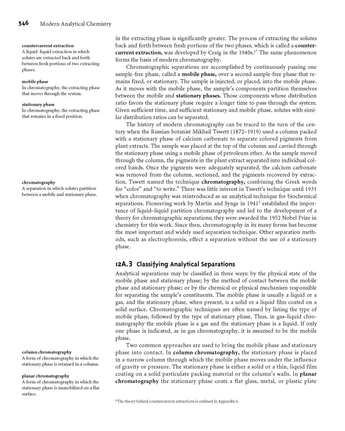
12A.3 Classifying Analytical Separations 546
12B General Theory of Column
Chromatography 547
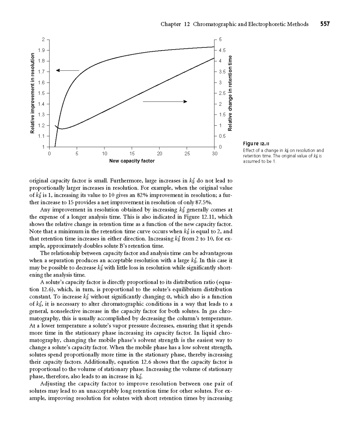
12B.1 Chromatographic Resolution 549
12B.2 Capacity Factor 550
12B.3 Column Selectivity 552
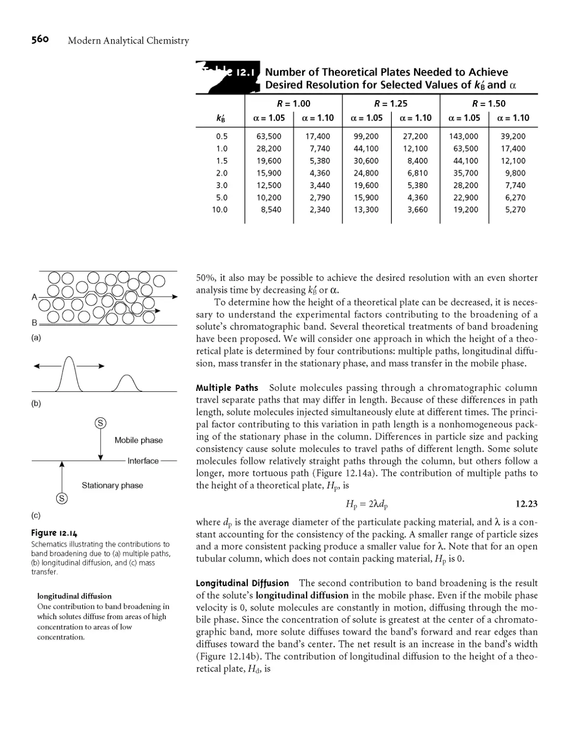
12B.4 Column Efficiency 552
* * *
VIII
Modern Analytical Chemistry
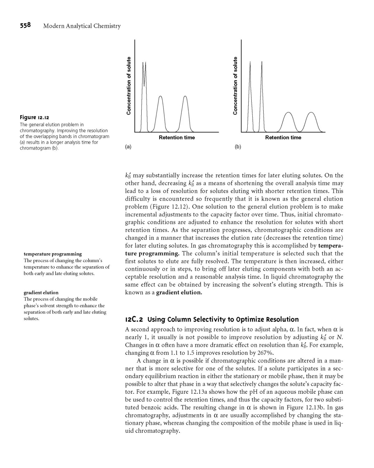
12B J Peak Capacity 554
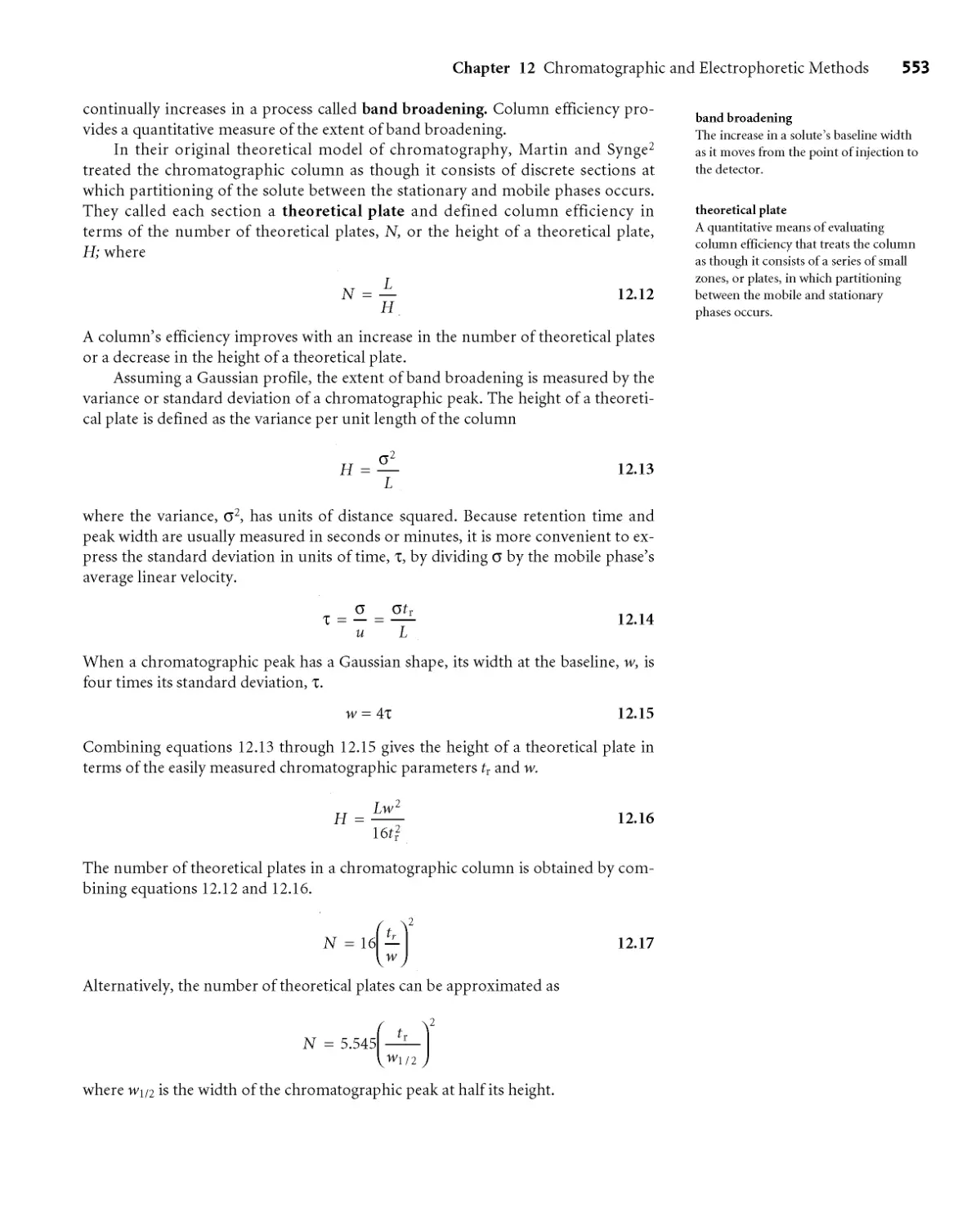
12B.6 Nonideal Behavior 555
12C Optimizing Chromatographic Separations 556
12СЛ Using the Capacity Factor to Optimize
Resolution 556
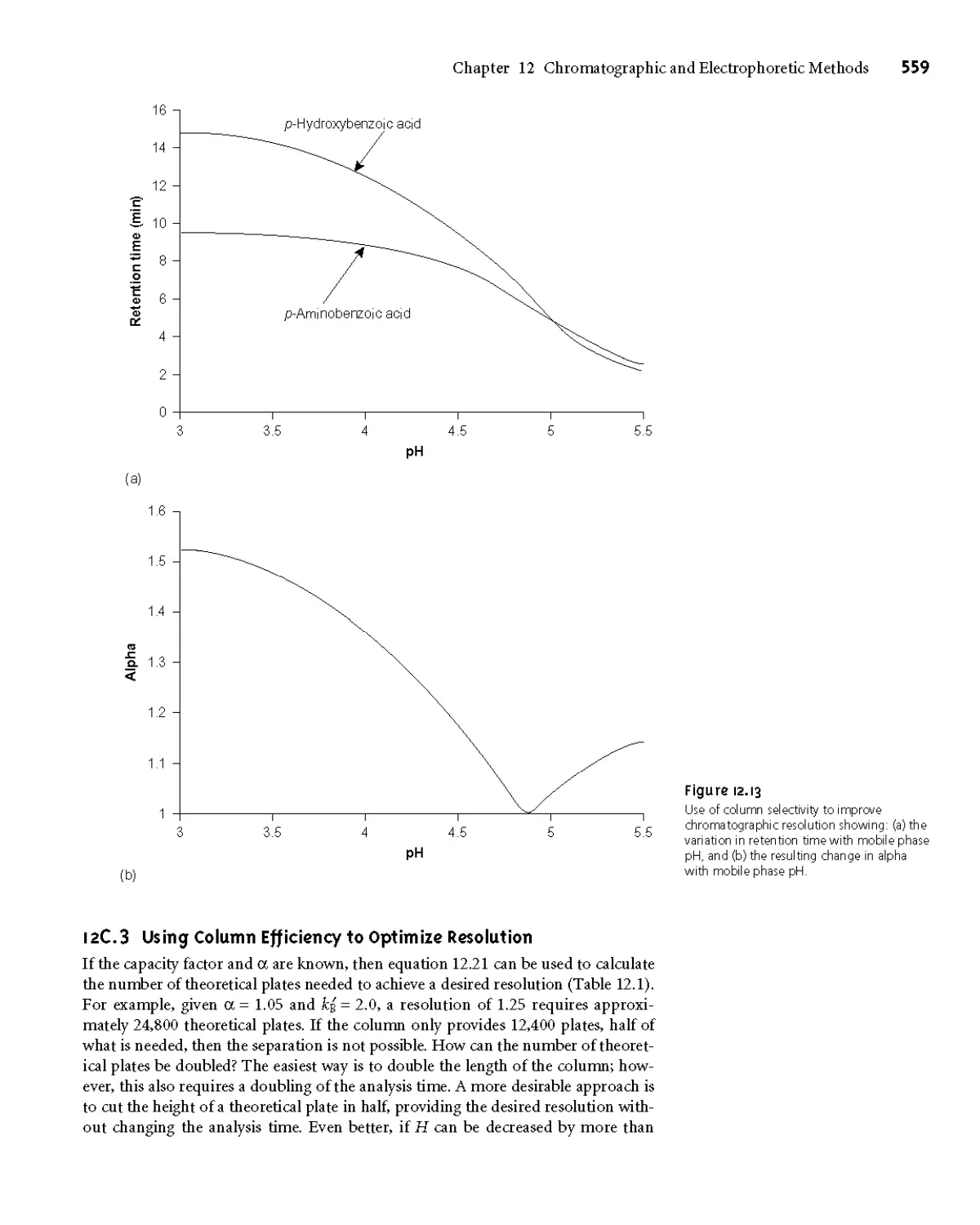
12C.2 Using Column Selectivity to Optimize
Resolution 558
12C.3 Using Column Efficiency to Optimize
Resolution 559
12D Gas Chromatography 563
12DT Mobile Phase 563
12D.2 Chromatographic Columns 564
12D J Stationary Phases 565
12D.4 Sample Introduction 567
12D.5 Temperature Control 568
12D.6 Detectors for Gas Chromatography 569
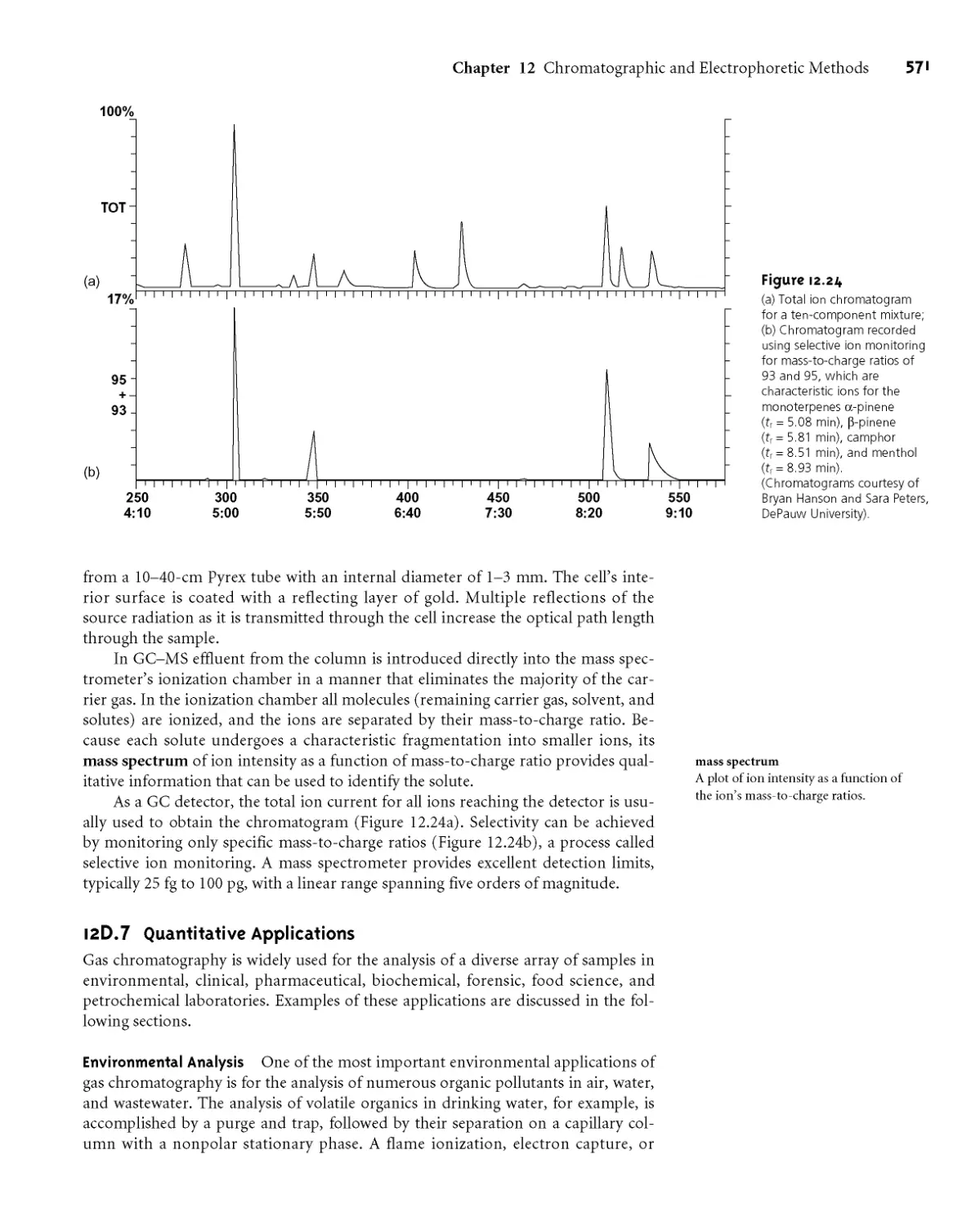
12D.7 Quantitative Applications 571
12D.8 Qualitative Applications 575
12D.9 Representative Method 576
12 D Л 0 Evaluatio n 577
12E High-Performance Liquid
Chromatography 578
12ЕЛ HPLC Columns 578
12E.2 Stationary Phases 579
12EJ Mobile Phases 580
12E.4 HPLC Plumbing 583
12E.5 Sample Introduction 584
I2E.6 Detectors for HPLC 584
I2E.7 Quantitative Applications 586
I2E.8 Representative Method 588
I2E.9 Evaluation 589
12F Liquid-Solid Adsorption Chromatography 590
12G Ion-Exchange Chromatography 590
12H Size-Exclusion Chromatography 593
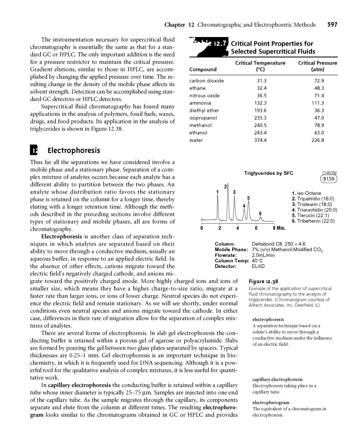
121 Supercritical Fluid Chromatography 596
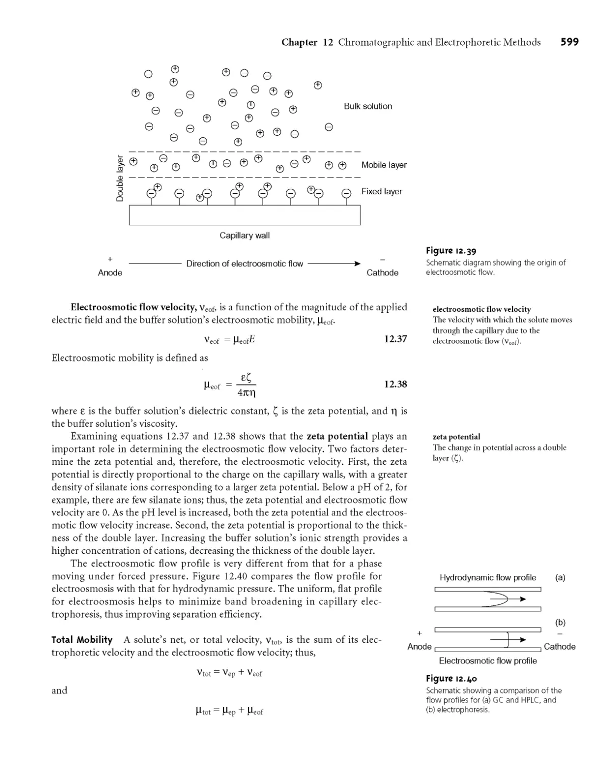
12J Electrophoresis 597
12 J Л Theory of Capillary Electrophoresis 598
I2J.2 Instrumentation 601
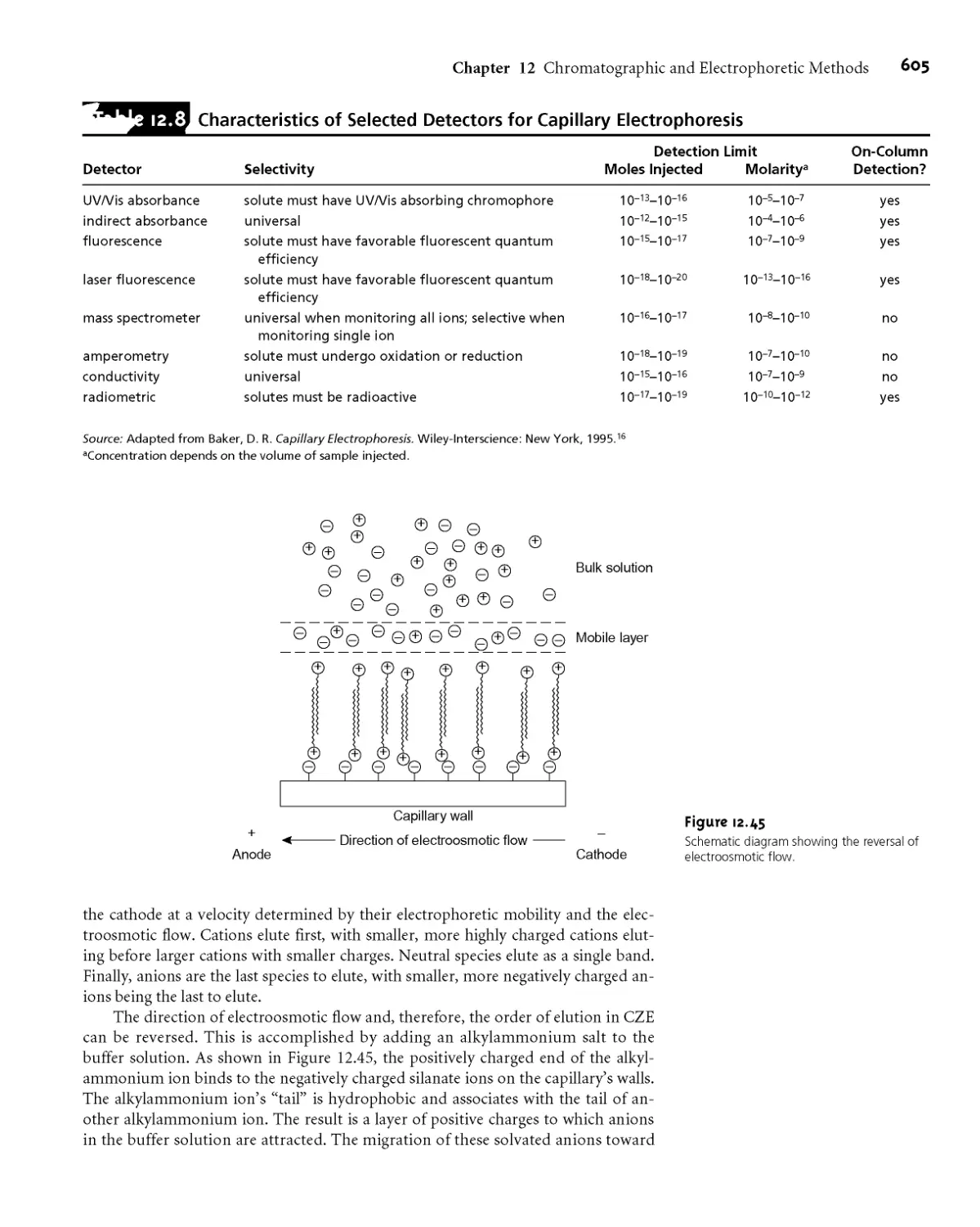
I2J3 Capillary Electrophoresis Methods 604
12J.4 Representative Method 607
12J.5 Evaluation 609
12K Key Terms 609
12L Summary 610
12M Suggested Experiments 610
12N Problems 615
120 Suggested Readings 620
12P References 620
13
Kinetic Methods of Analysis 622
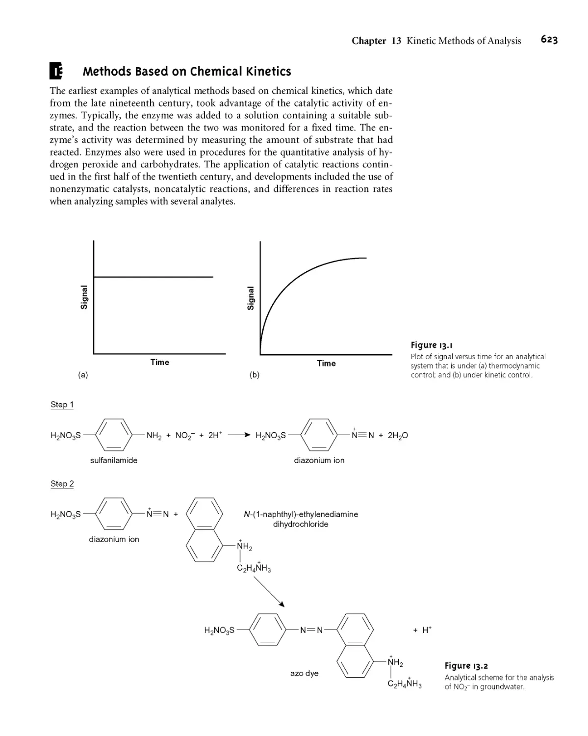
13A Methods Based on Chemical Kinetics 623
13АЛ Theory and Practice 624
13 A.2 Instrumentation 634
13AJ Quantitative Applications 636
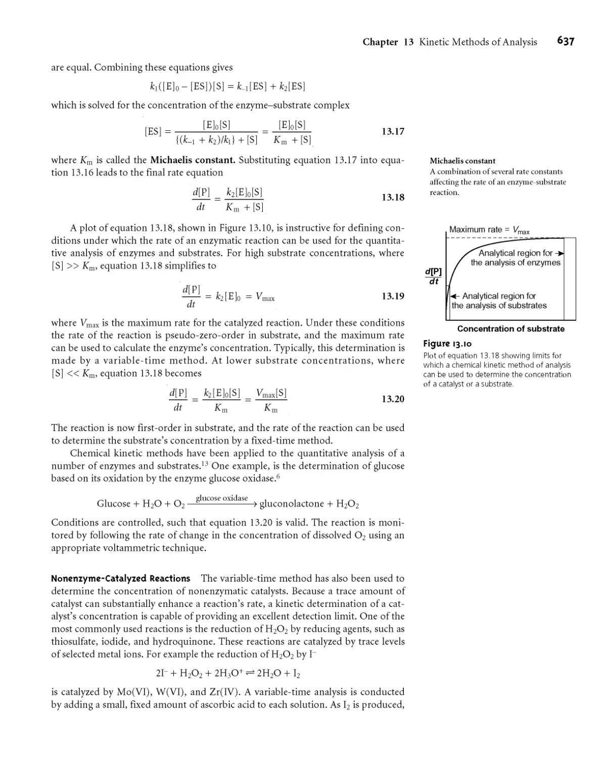
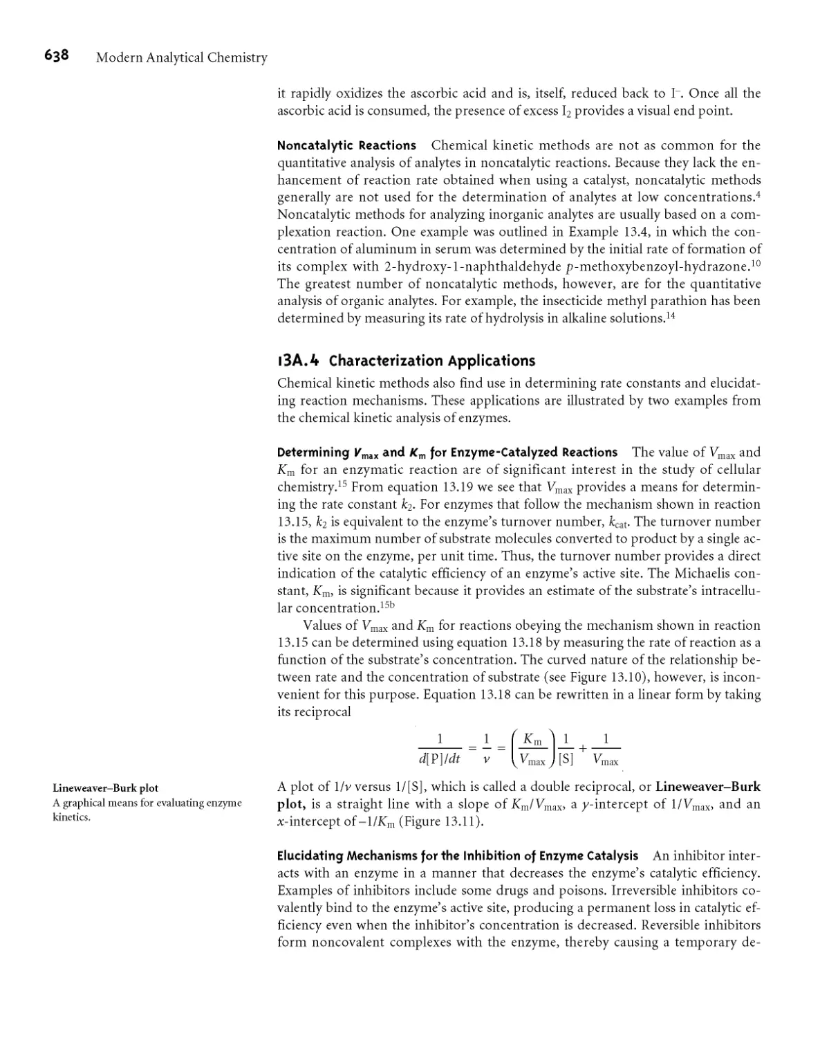
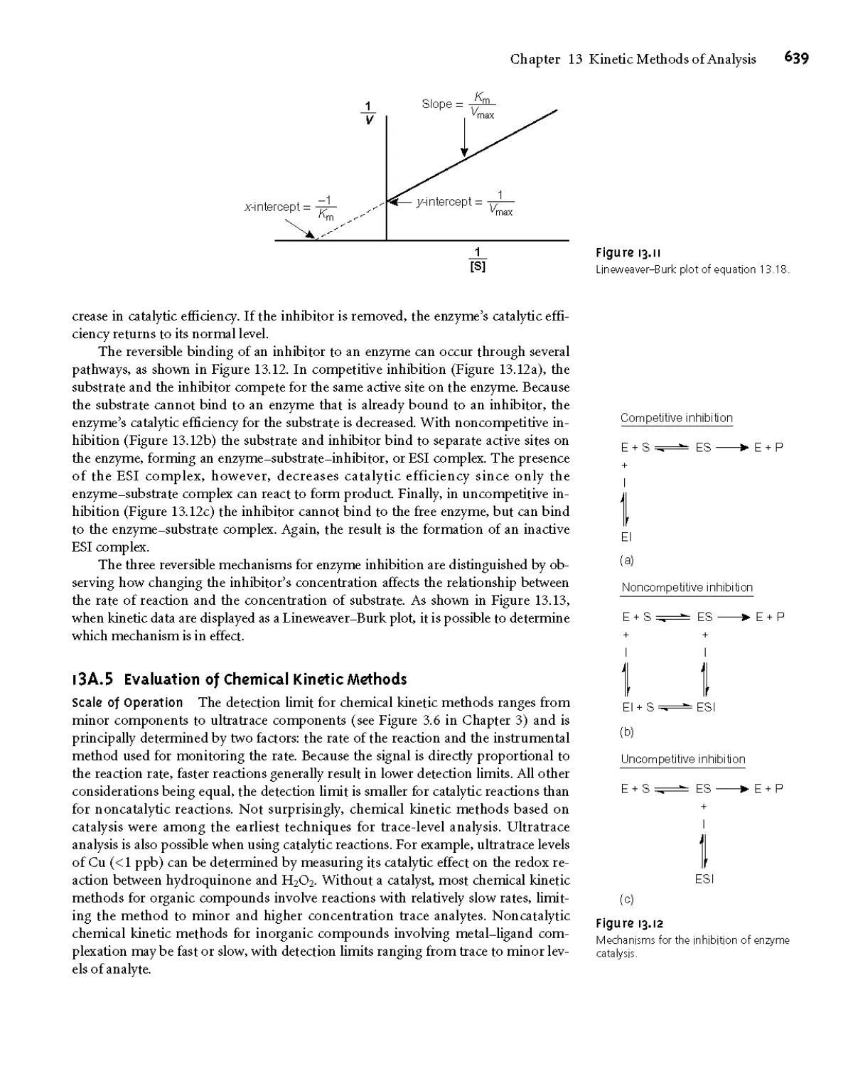
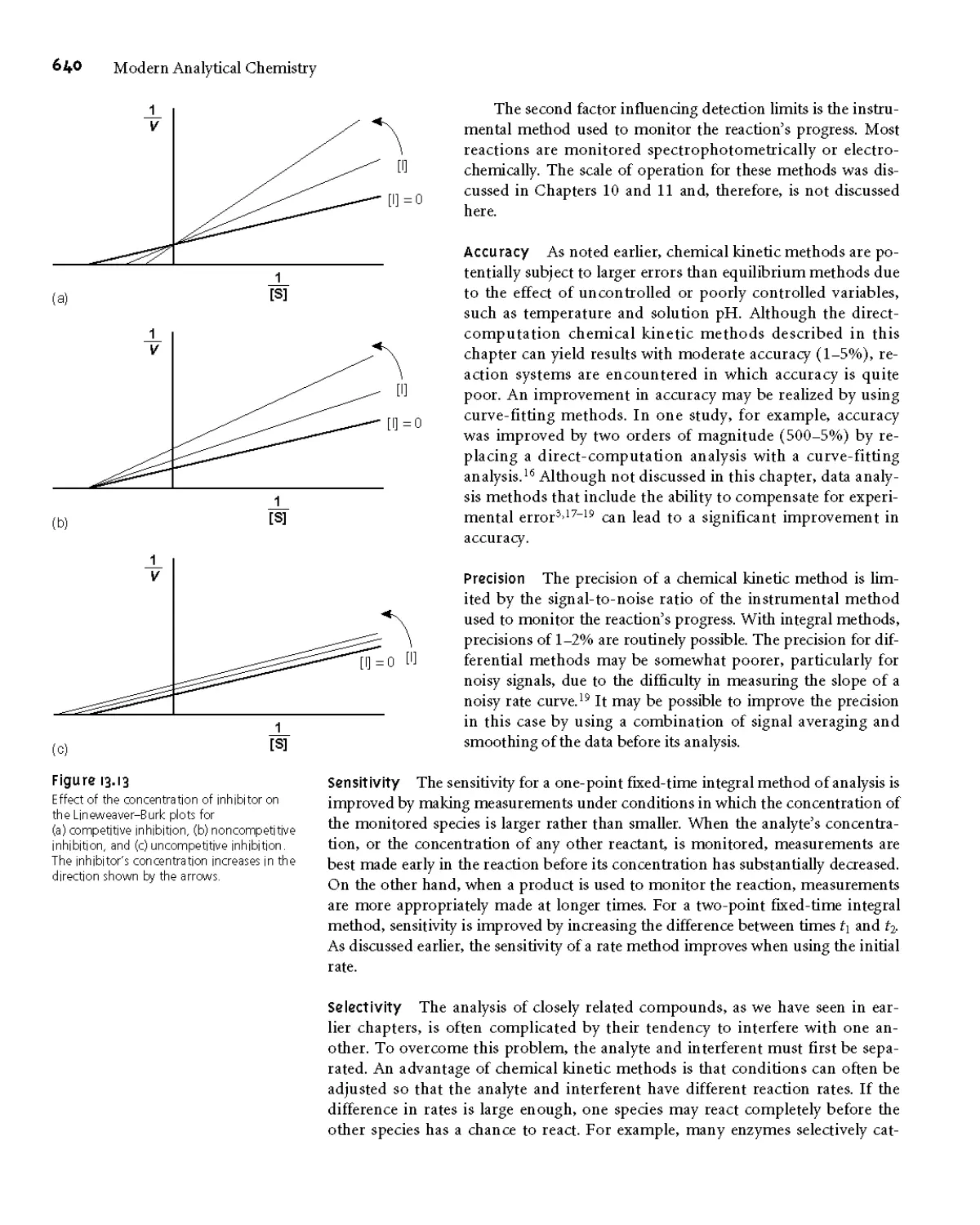
I3A.4 Characterization Applications 638
I3A.5 Evaluation of Chemical Kinetic
Methods 639
13B Radiochemical Methods of Analysis 642
13ВЛ Theory and Practice 643
I3B.2 Instrumentation 643
I3B3 Quantitative Applications 644
I3B.4 Characterization Applications 647
I3B.5 Evaluation 648
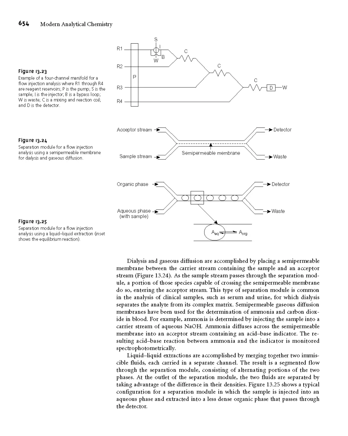
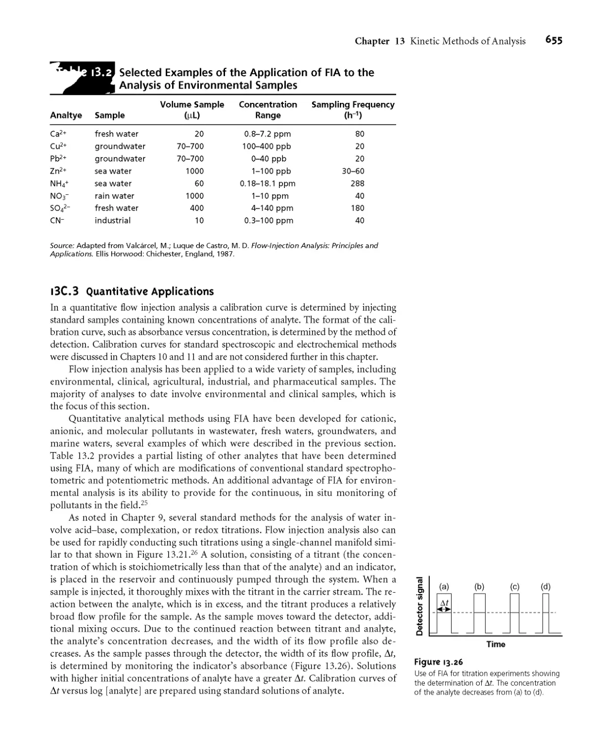
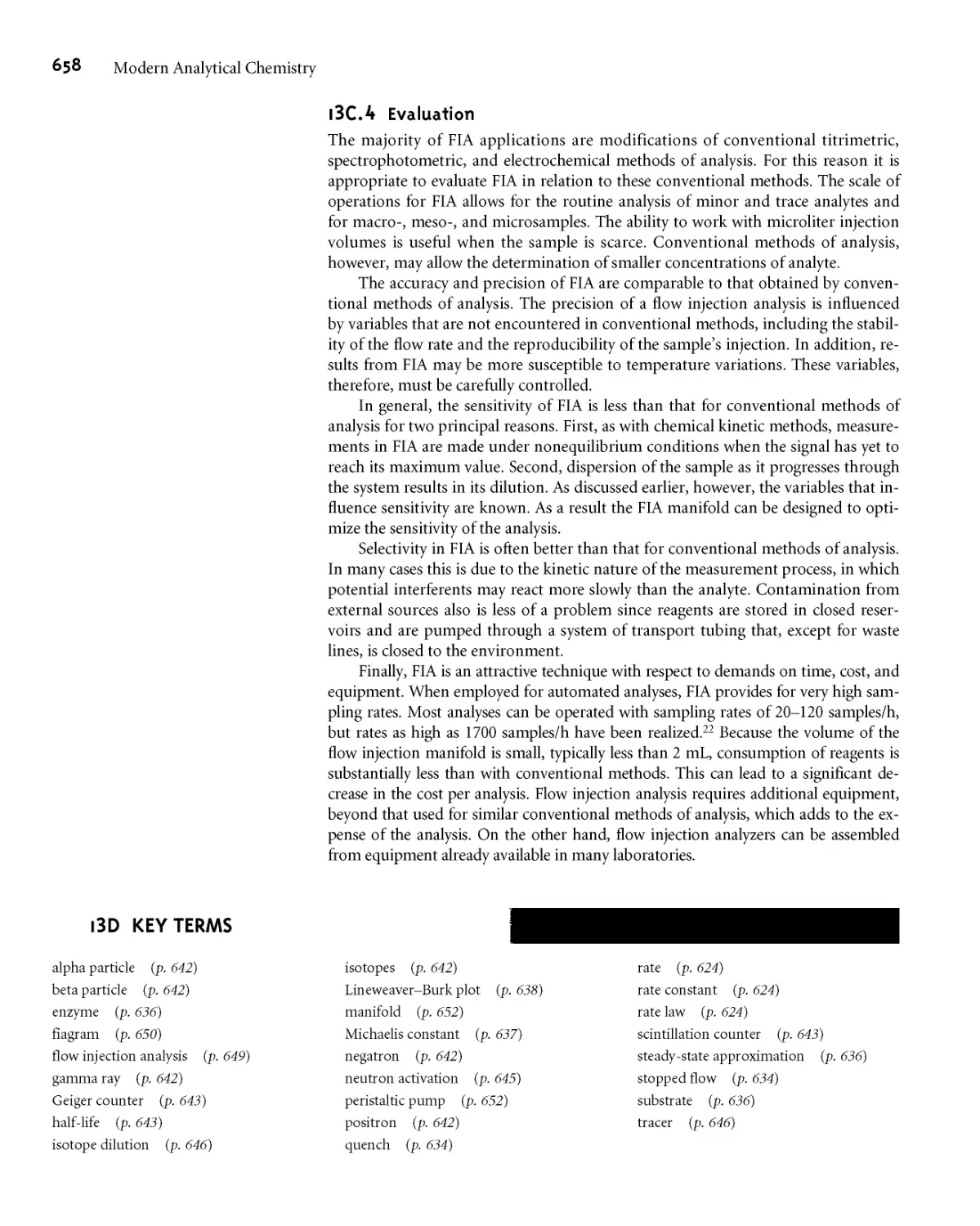
13C Flow Injection Analysis 649
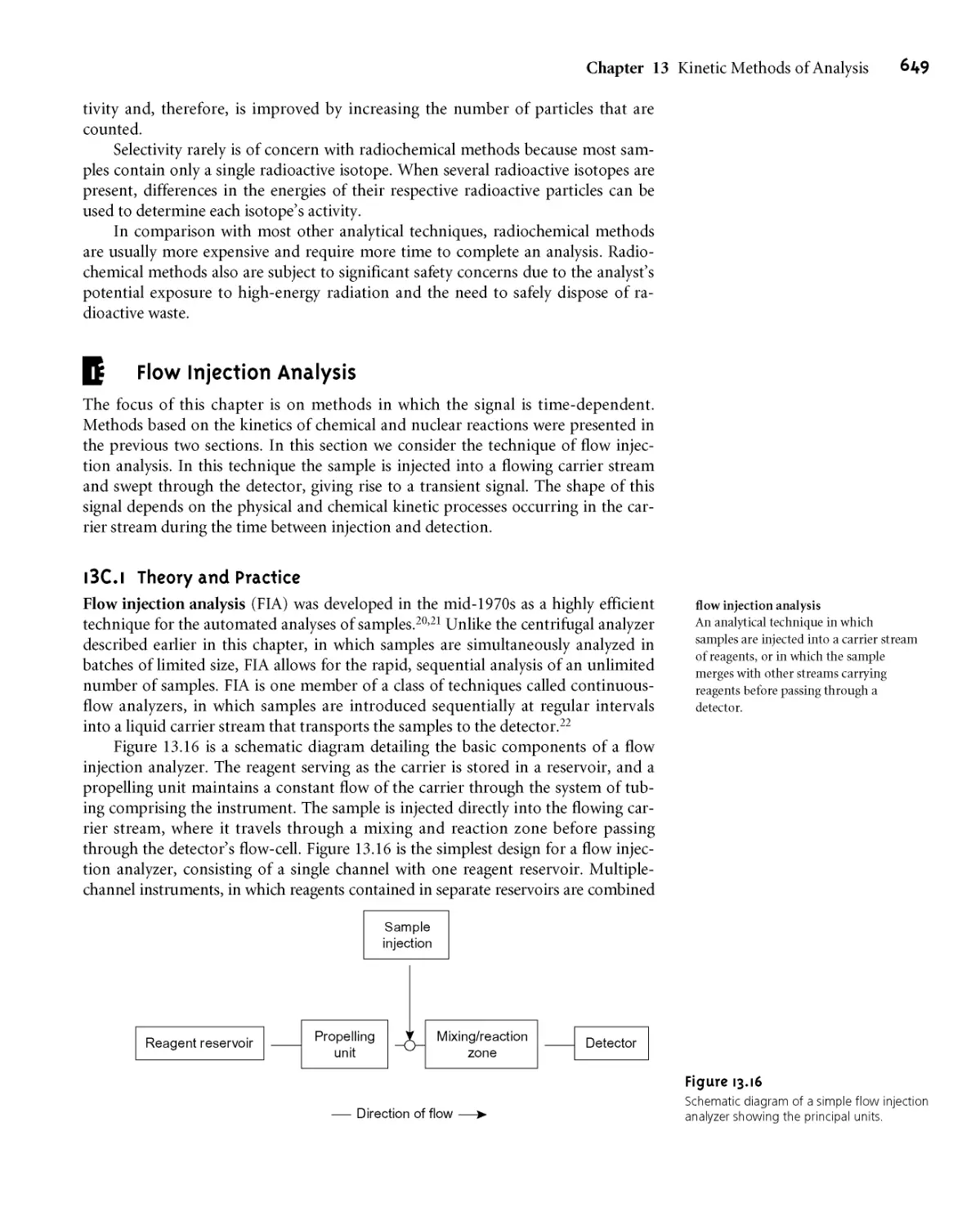
13СЛ Theory and Practice 649
13C.2 Instrumentation 651
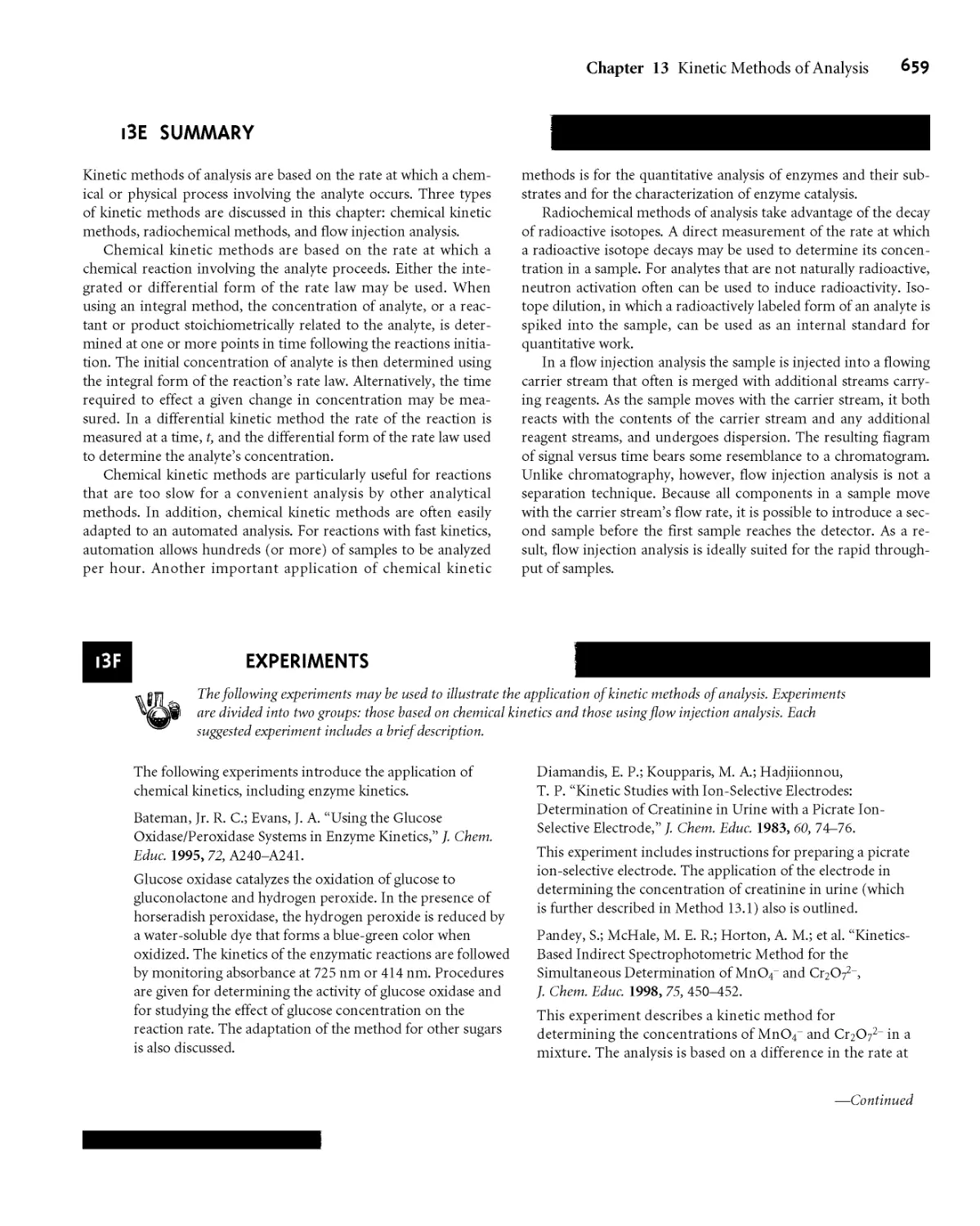
13G3 Quantitative Applications 655
I3G4 Evaluation 658
13D Key Terms 658
13E Summary 659
13F Suggested Experiments 659
13G Problems 661
13H Suggested Readings 664
131 References 665
14
Developing a Standard Method 666
14A Optimizing the Experimental Procedure 667
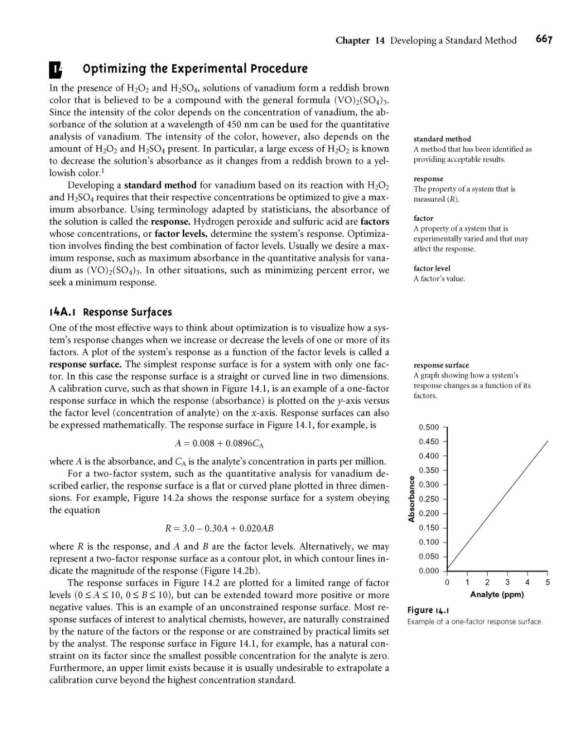
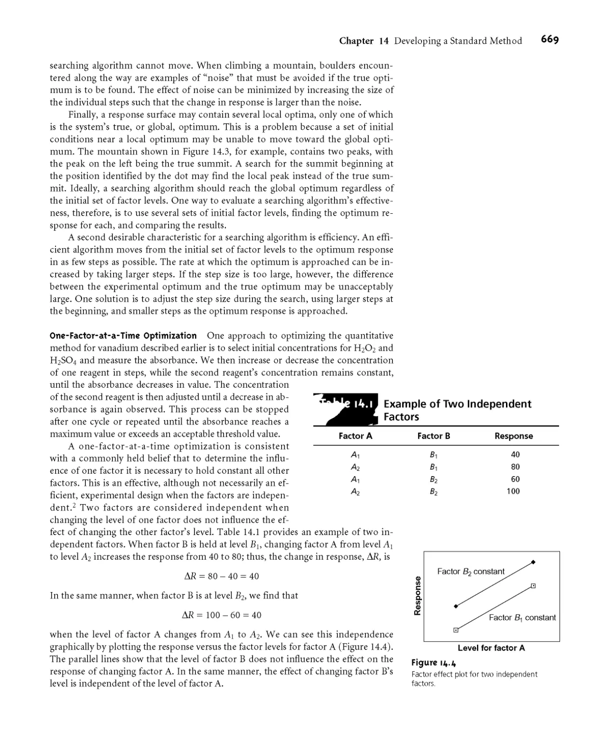
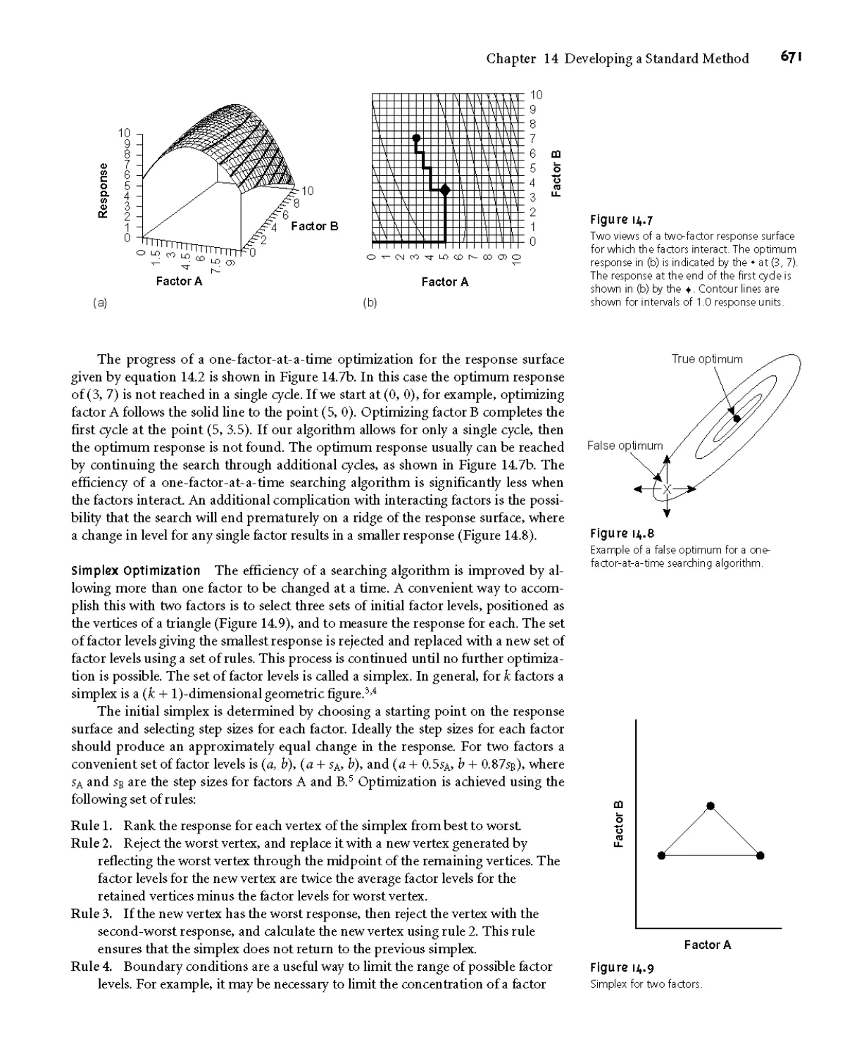
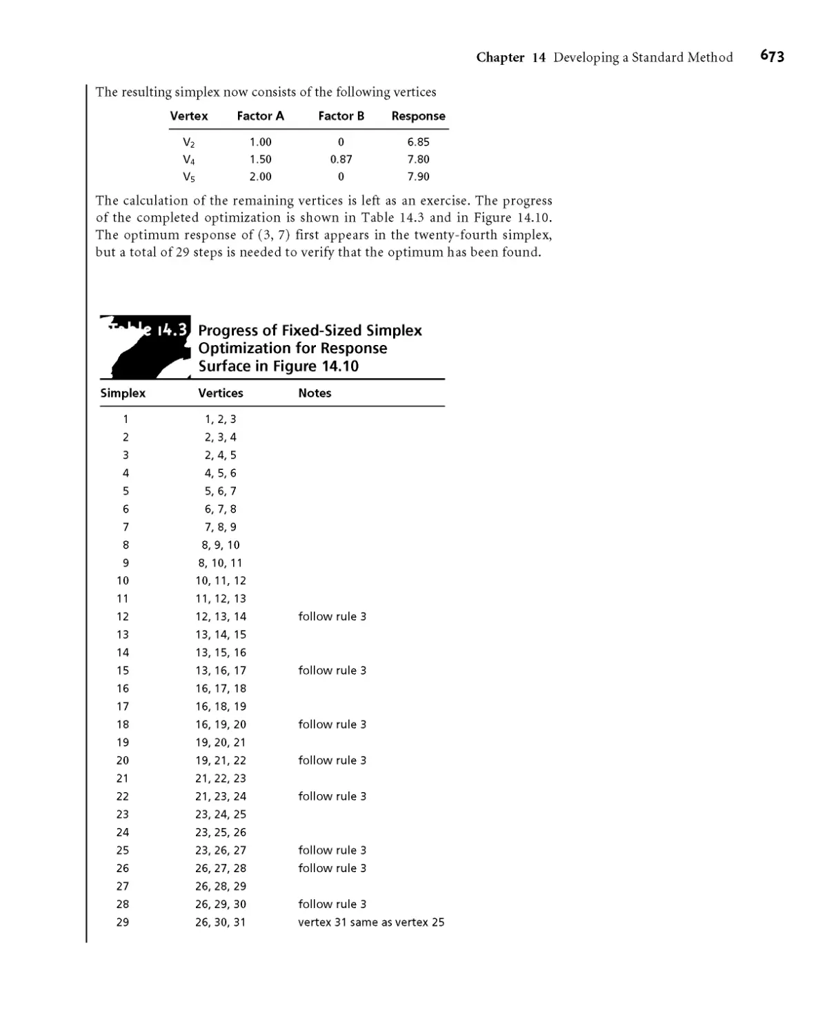
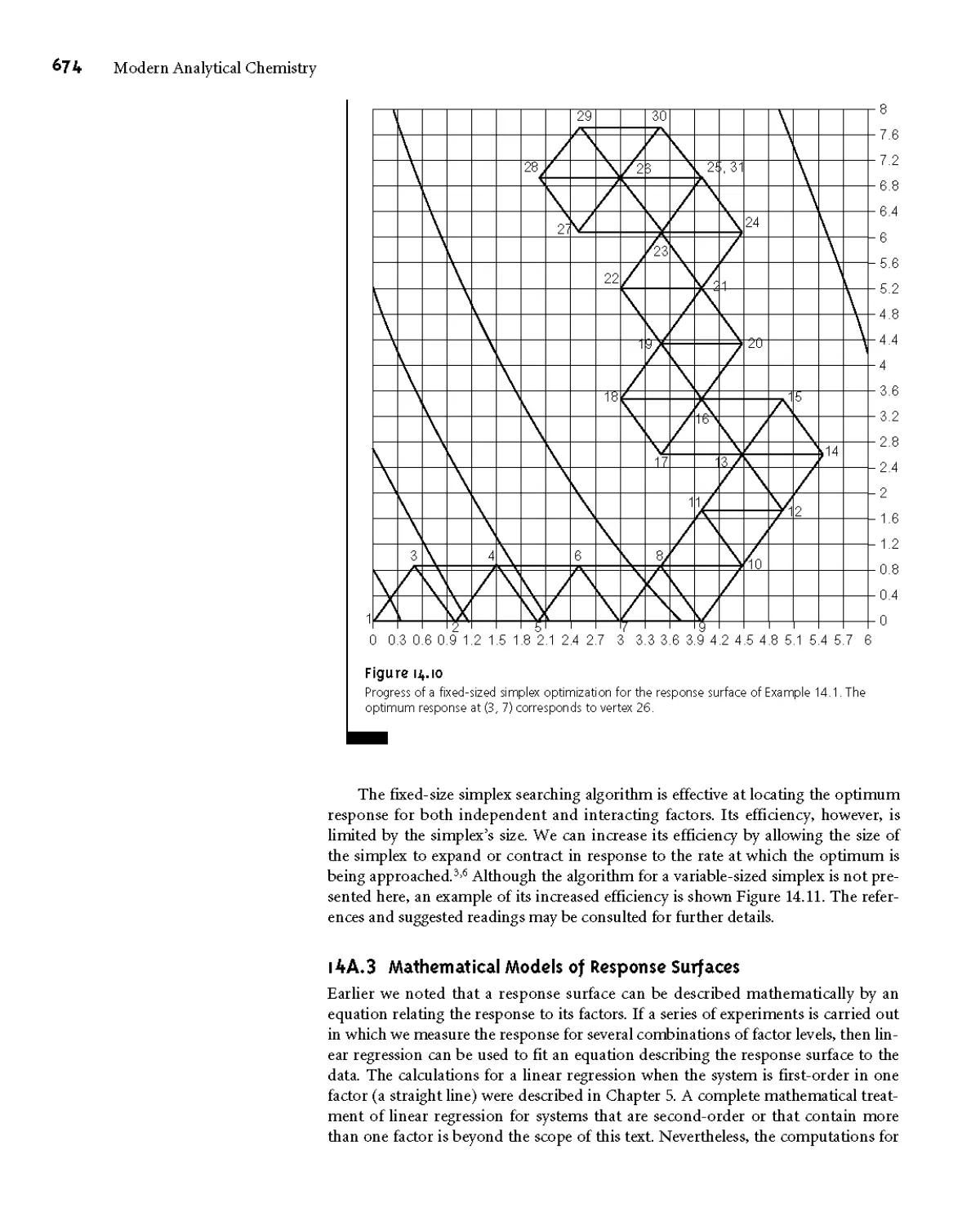
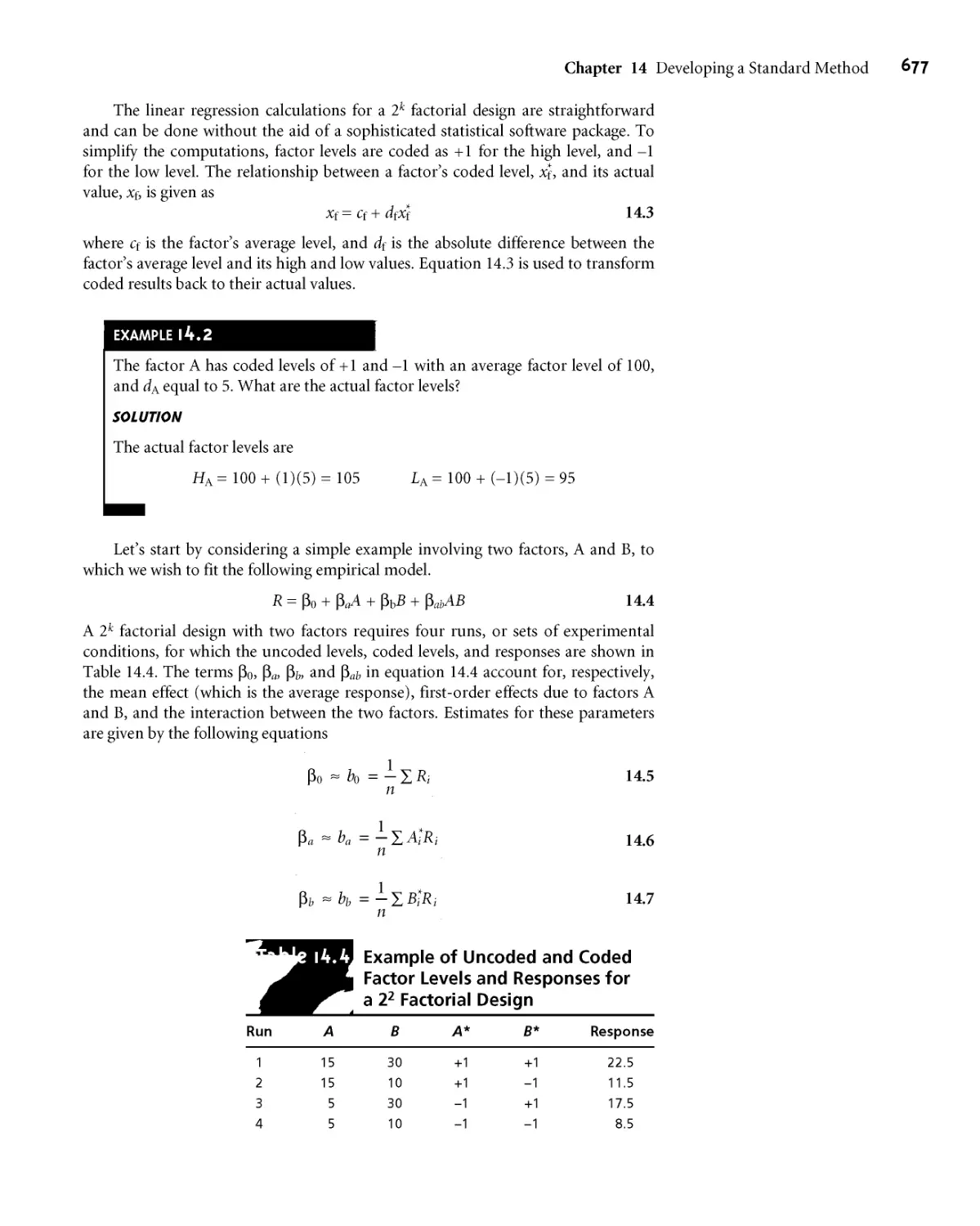
МАЛ Response Surfaces 667
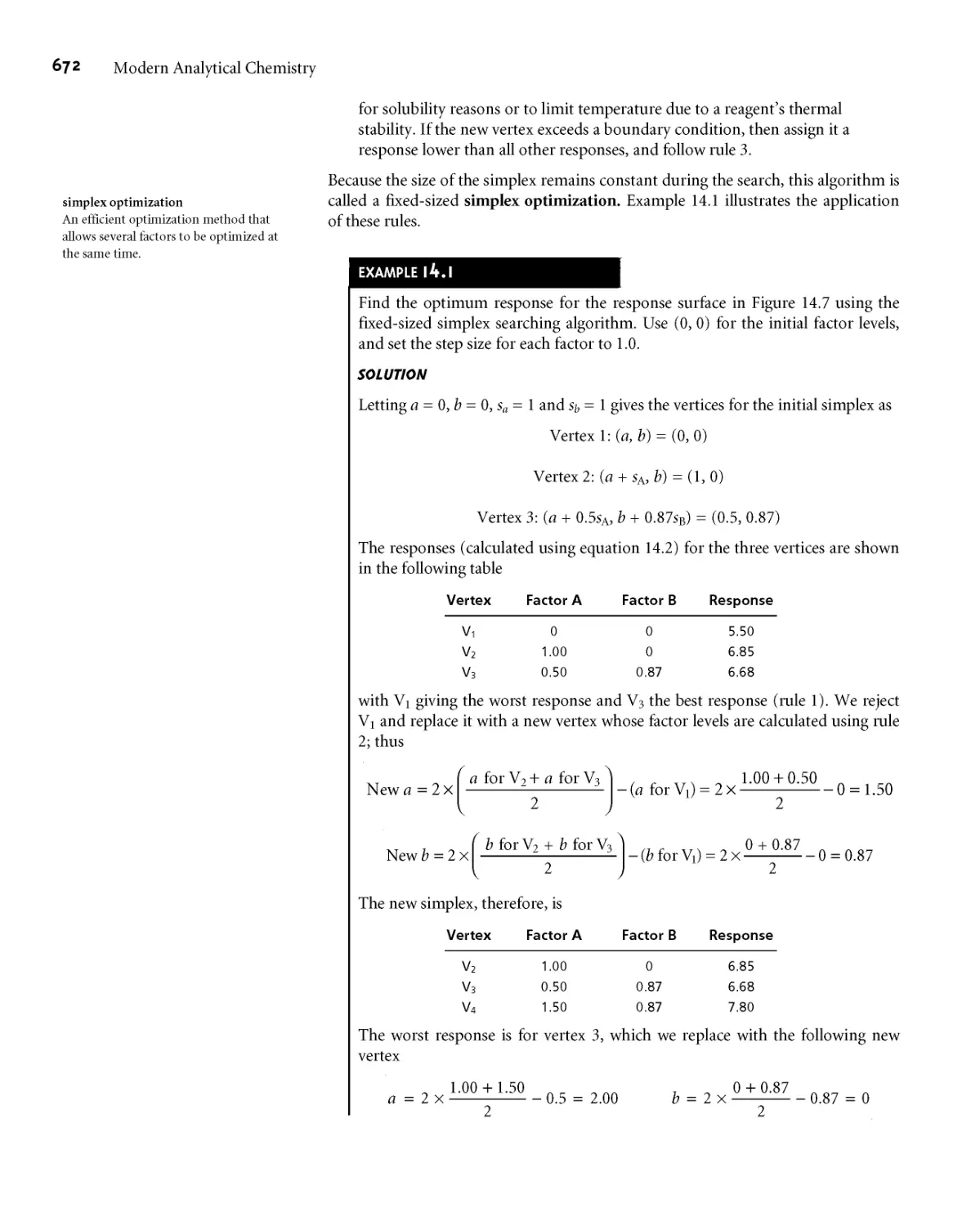
MAJ Searching Algorithms for Response
Surfaces 668
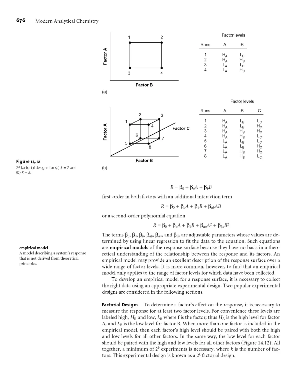
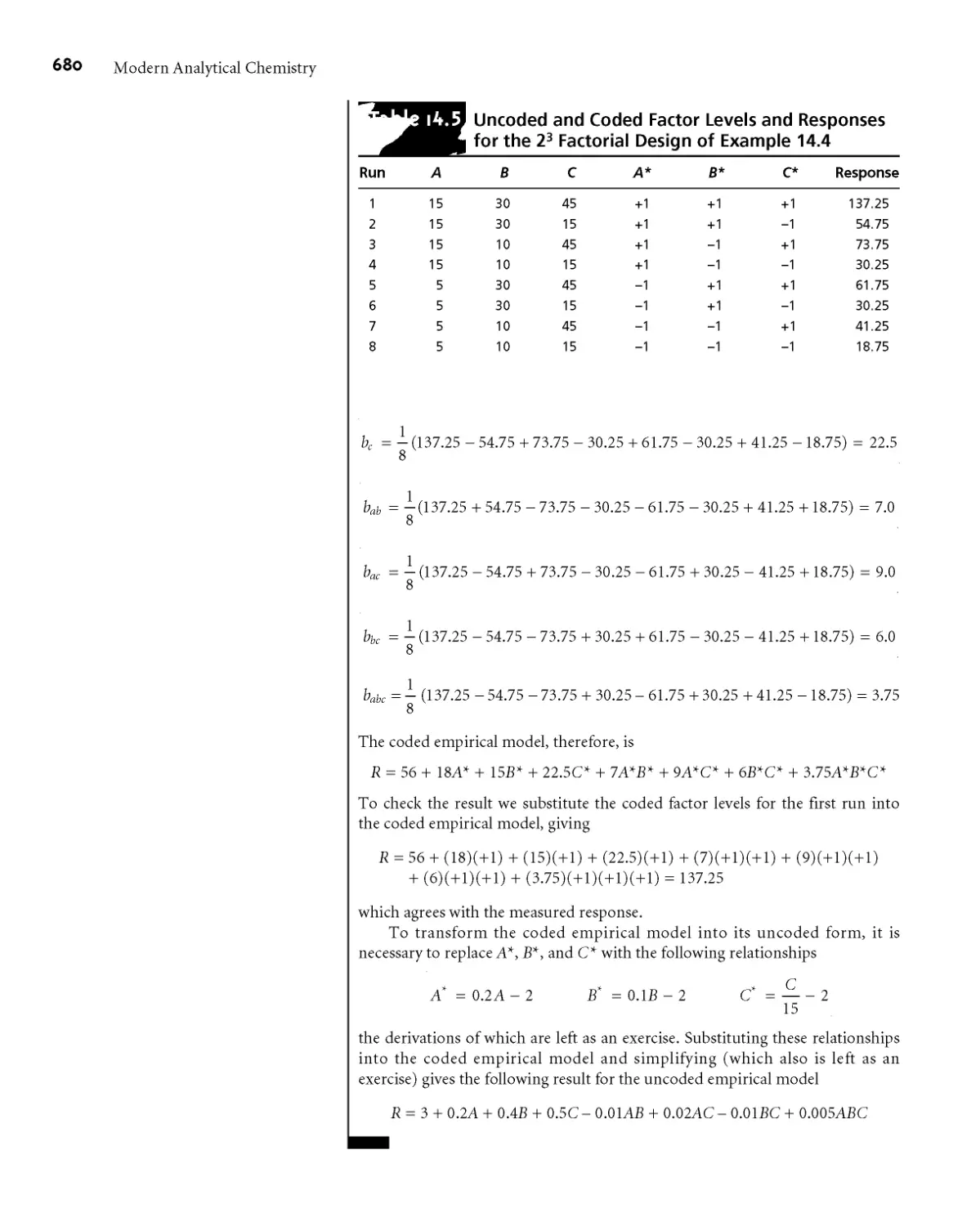
MAJ Mathematical Models of Response
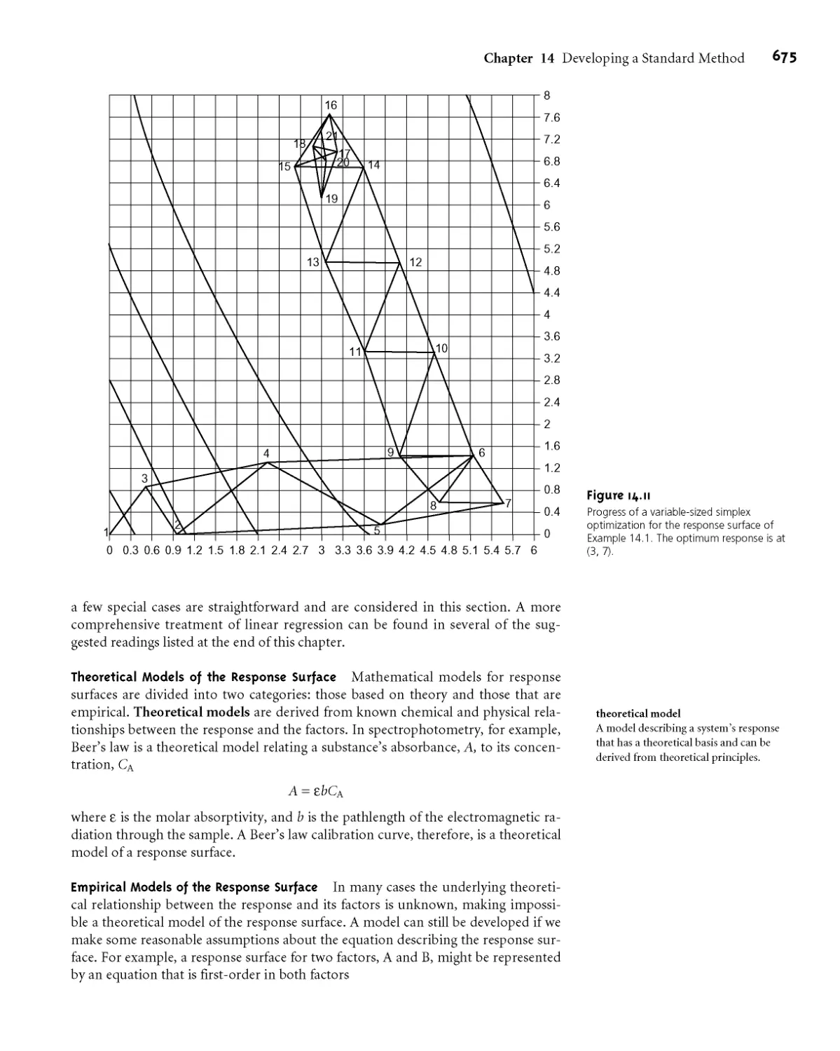
Surfaces 674
14B Verifying the Method 683
14ВЛ Single-Operator Characteristics 683
I4B.2 Blind Analysis of Standard Samples 683
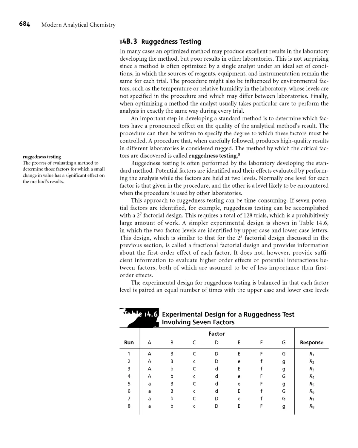
14B J Ruggedness Testing 684
I4B.4 Equivalency Testing 687
Contents
ix
14C Validating the Method as a Standard
Method 687
14C.1 Two-Sample Collaborative Testing 688
14C.2 Collaborative Testing and Analysis of
Variance 693
14C.3 What Is a Reasonable Result for a
Collaborative Study? 698
14D Key Terms 699
14E Summary 699
14F Suggested Experiments 699
14G Problems 700
14H Suggested Readings 704
141 References 704
15
Quality Assurance 705
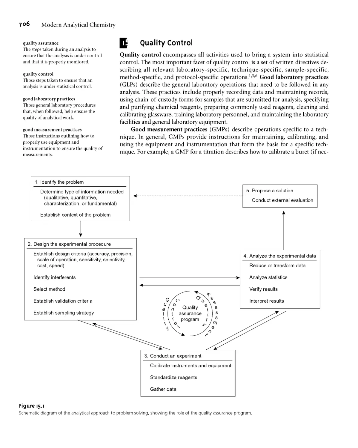
15A Quality Control 706
15B Quality Assessment 708
15ВД Internal Methods of Quality
Assessment 708
I5B.2 External Methods of Quality
Assessment 711
15C Evaluating Quality Assurance Data 712
I5C.I Prescriptive Approach 712
I5C.2 Performance-Based Approach 714
15D Key Terms 721
15E Summary 722
15F Suggested Experiments 722
15G Problems 722
15H Suggested Readings 724
151 References 724
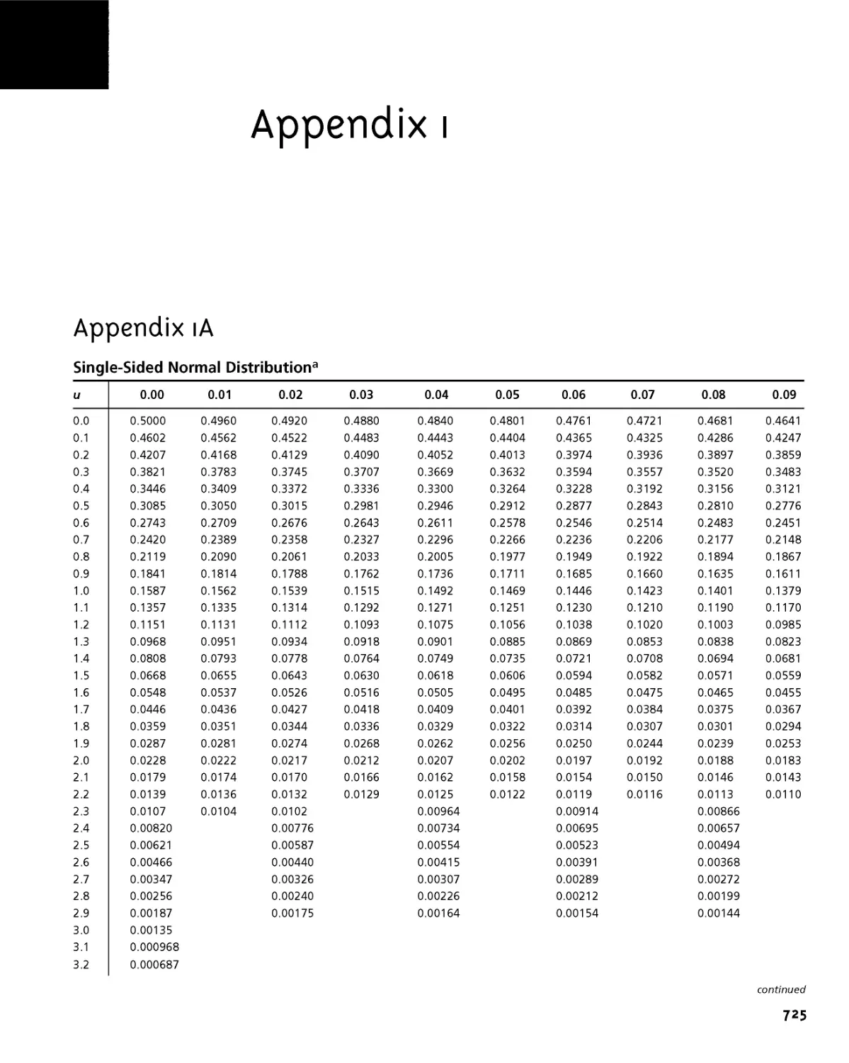
Appendix 1A Single-Sided Normal Distribution 725
Appendix IB t-Table 726
Appendix 1C F-Table 727
Appendix ID Critical Values for Q-Test 728
Appendix IE Random Number Table 728
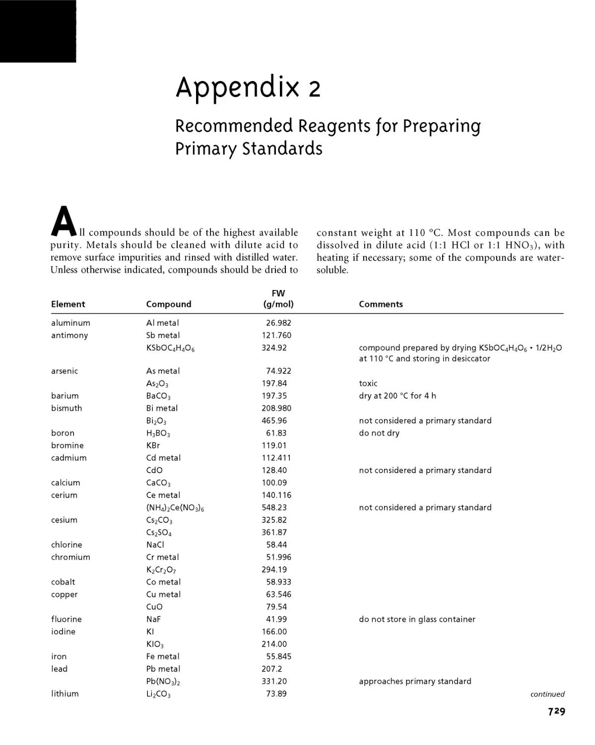
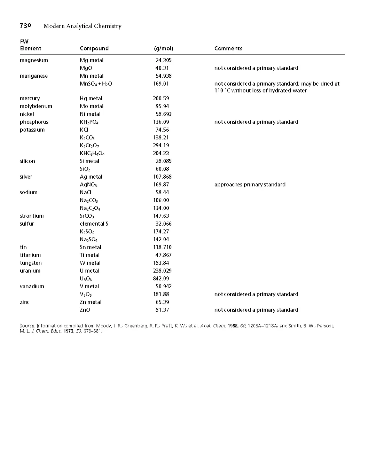
Appendix 2 Recommended Reagents for Preparing Primary
Standards 729
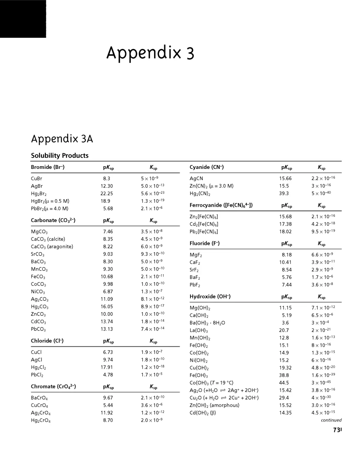
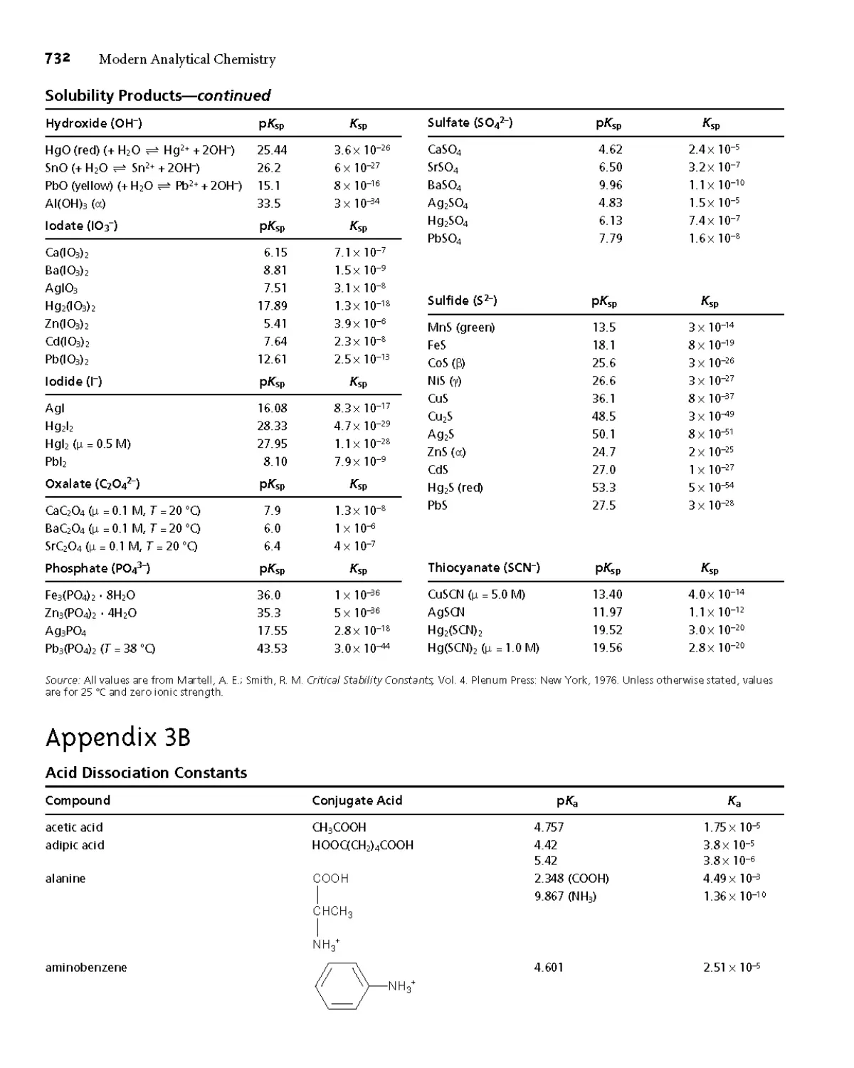
Appendix ЗА Solubility Products 731
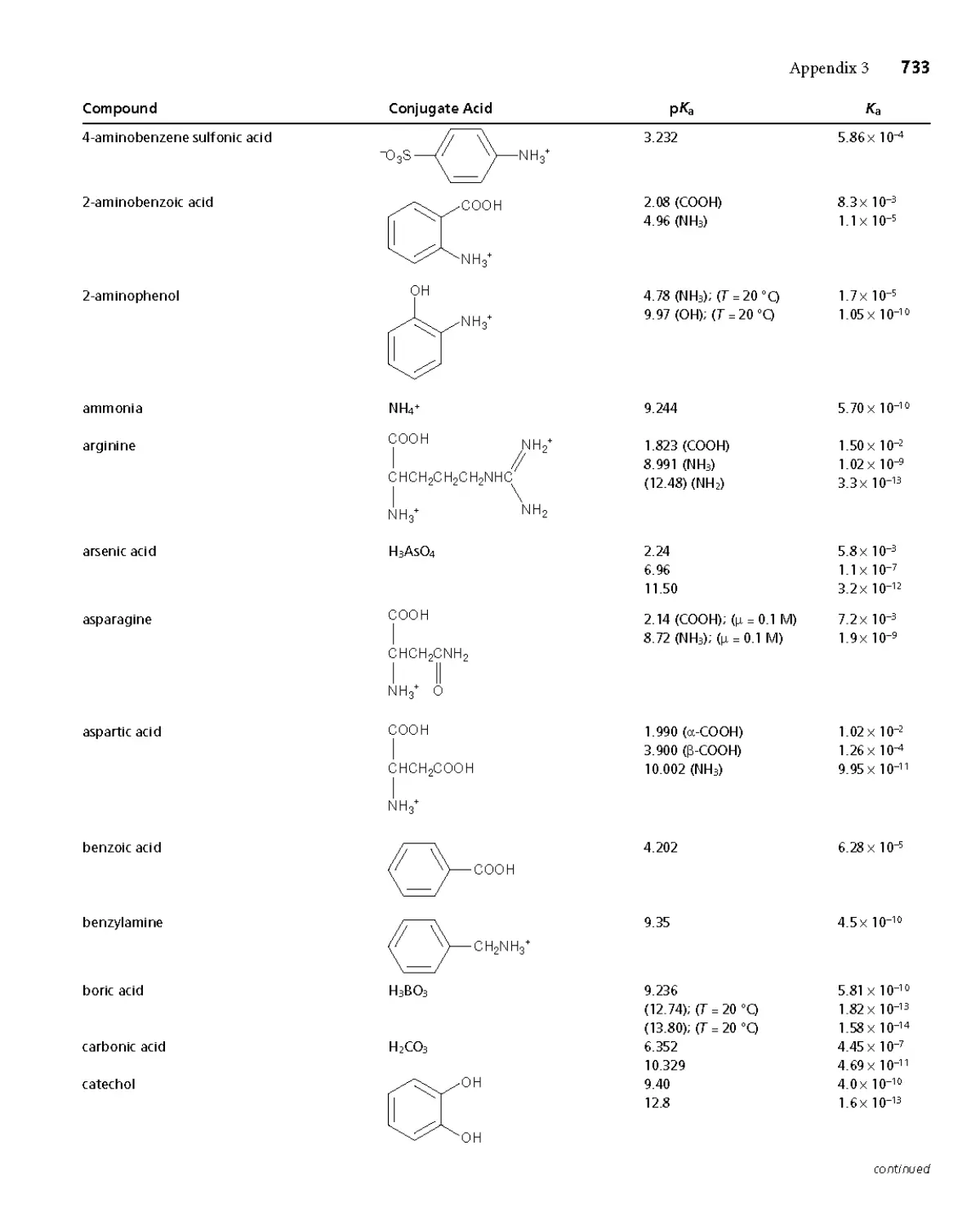
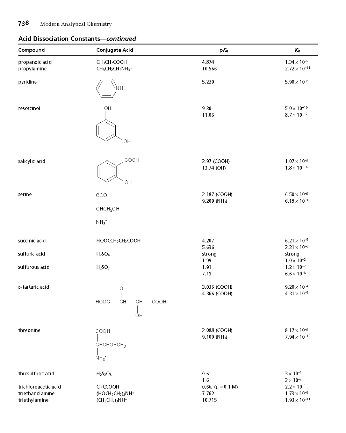
Appendix 3B Acid Dissociation Constants 732
Appendix 3C Metal-Ligand Formation Constants 739
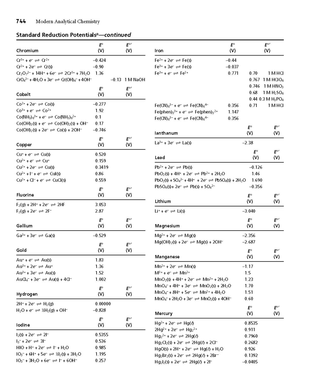
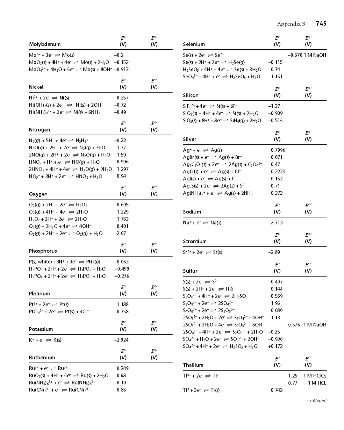
Appendix 3D Standard Reduction Potentials 743
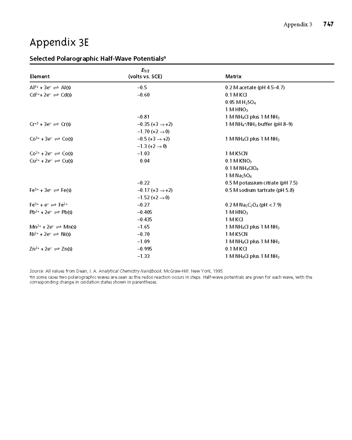
Appendix 3E Selected Polarographic Half-Wave Potentials 747
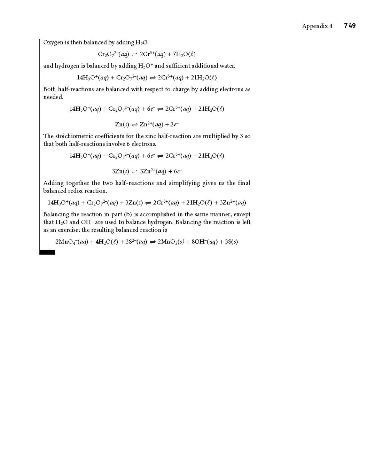
Appendix 4 Balancing Redox Reactions 748
Appendix 5 Review of Chemical Kinetics 750
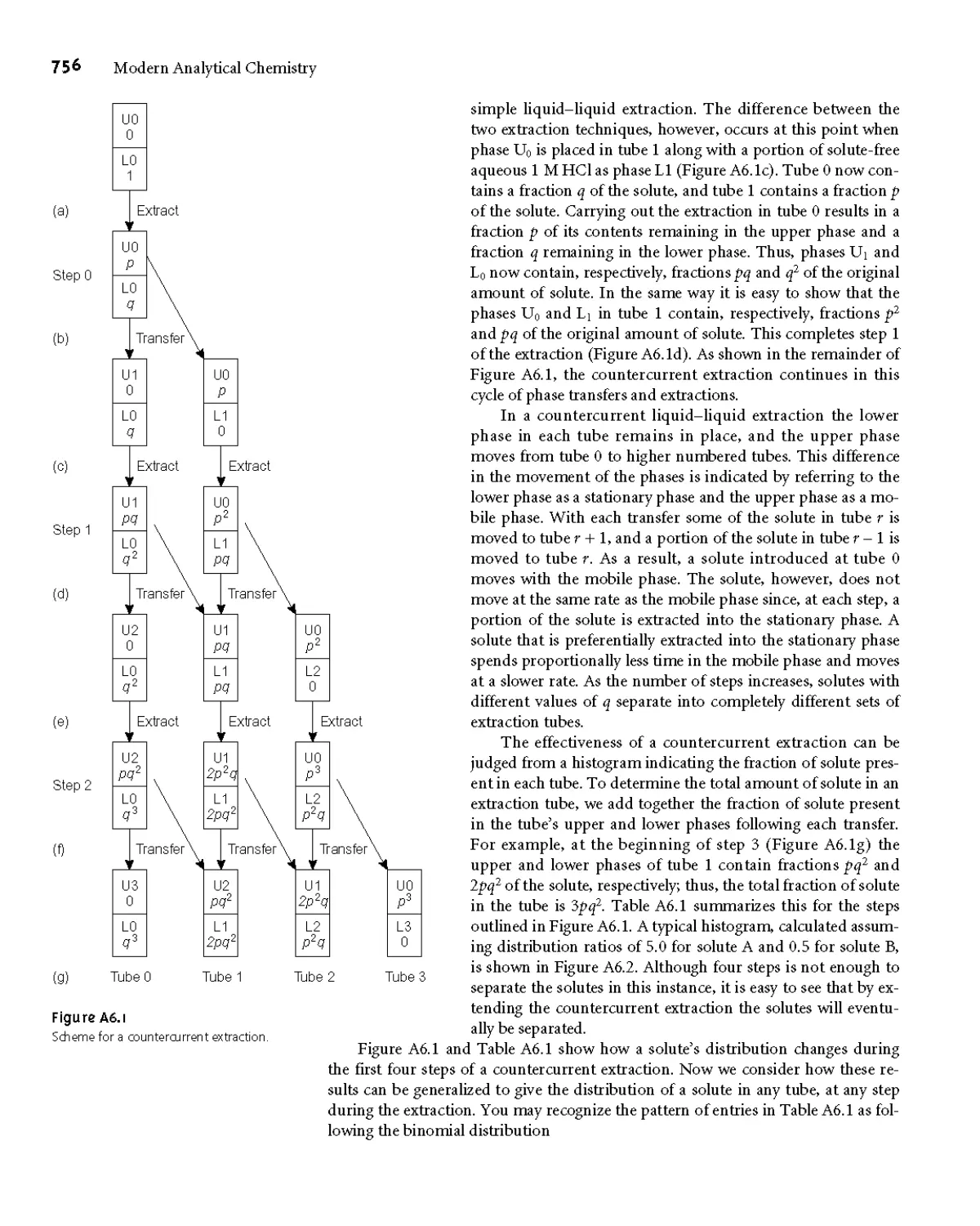
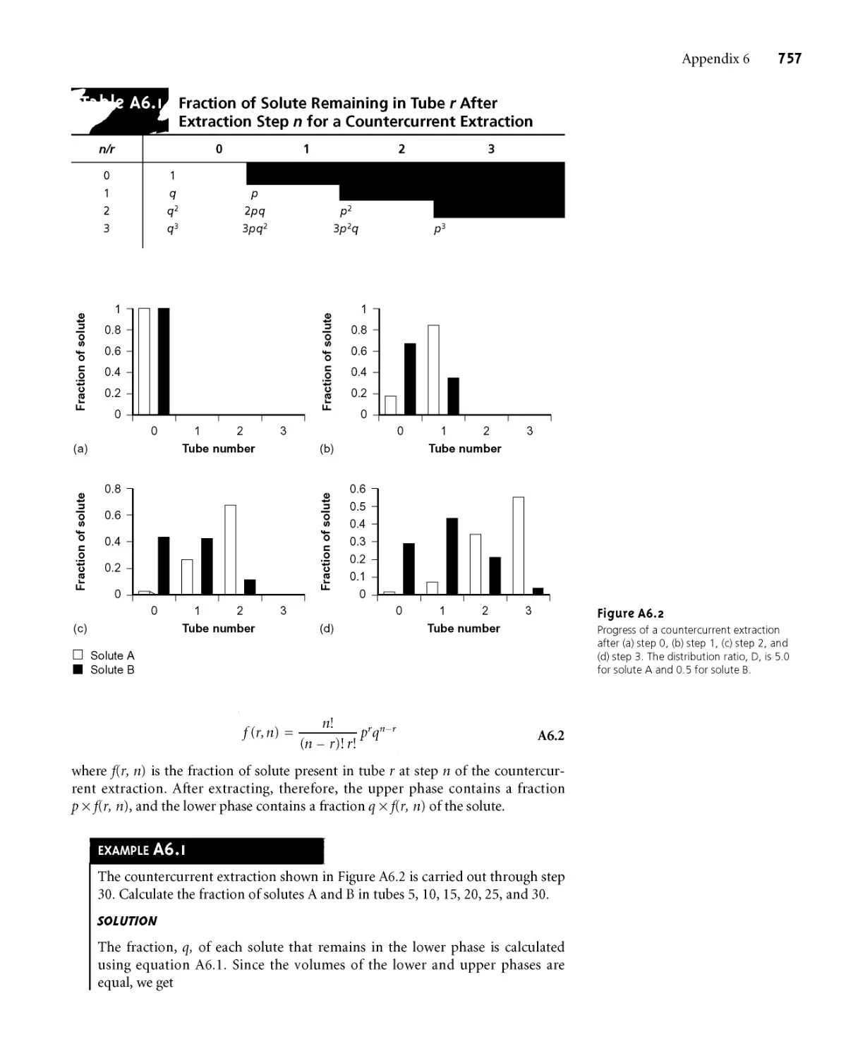
Appendix 6 Countercurrent Separations 755
Appendix 7 Answers to Selected Problems 762
Glossary 769
Index 781
A Guide to Using This Text
... in Chapter
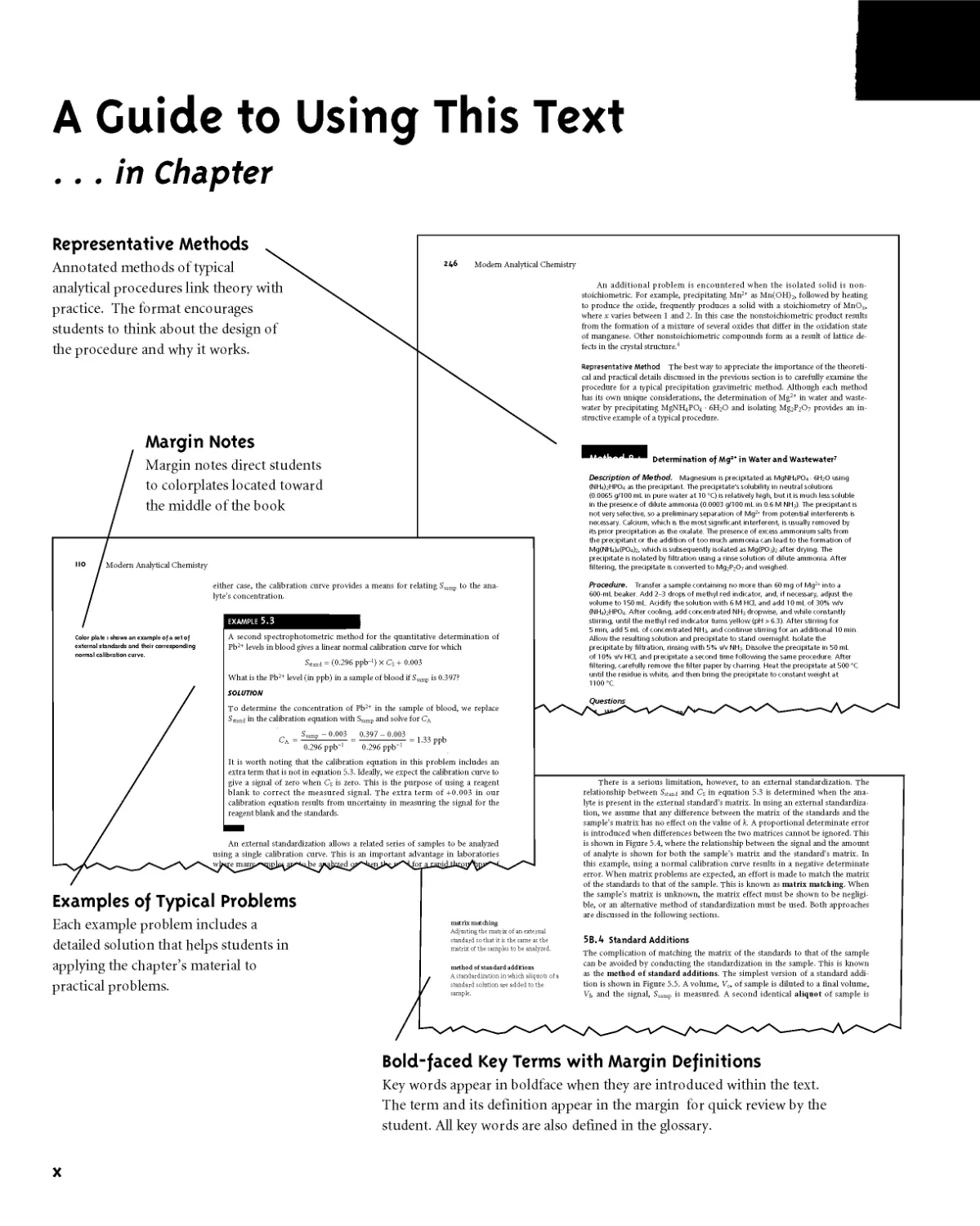
Representative Methods
Annotated methods of typical
analytical procedures link theory with
practice. The format encourages
students to think about the design of
the procedure and why it works.
Margin Notes
Margin notes direct students
to colorplates located toward
the middle of the book
Modern Analytical Chemistry
Color plate i shows an example of a set of
external standards and their corresponding
normal calibration curve.
Modem Analytical Chemistry
An additional problem is encountered when the isolated solid is non-
stoichiometric* For example, precipitating Mn2+ as Mn(OH)?, followed by heating
to produce the oxide, frequently produces a solid with a stoichiometry of MnOD
where x varies between 1 and 2* In this case the nonstoichiometric product results
from the formation of a mixture of several oxides that differ in the oxidation state
of manganese* Other nonstoichiometric compounds form as a result of lattice de-
fects in the crystal structure*6
Representative Method The best way to appreciate the importance of the theoreti-
cal and practical details discussed in the previous section is to carefully examine the
procedure for a typical precipitation gravimetric method* Although each method
has its own unique considerations, the determination of Mg2+ in water and waste-
water by precipitating MgNH4PO4 бН^О and isolating MgJ^Oy provides an in-
structive example of a typical procedure*
Determination of Mg2* in Water and Wastewater7
Description of Method. Magnesium is precipitated as MgNH4PO4 6H2O using
(NH4)2HPO4 as the precipitant The precipitate's solubility in neutral solutions
(0.0065 g/100 mL in pure water at 10 °C) is relatively high, but it is much less soluble
in the presence of dilute ammonia (0.0003 g/100 mL in 0.6 M NH3). The precipitant is
not very selective, so a preliminary separation of Mg2+ from potential interferents is
necessary. Calcium, which is the most significant interferent, is usually removed by
its prior precipitation as the oxalate. The presence of excess ammonium salts from
the precipitant or the addition of too much ammonia can lead to the formation of
Mg(NH4)4(PO4)2, which is subsequently isolated as Мд(РОз)2 after drying. The
precipitate is isolated by filtration using a rinse solution of dilute ammonia. After
filtering, the precipitate is converted to Mg2P2O7 and weighed.
either case, the calibration curve provides a means for relating Ssamp to the ana-
lyte’s concentration*
EXAMPLE 5.3
A second spectrophotometric method for the quantitative determination of
Pb2+ levels in blood gives a linear normal calibration curve for which
Sstand = (0*296 ppb-1) x Cs + 0*003
What is the Pb2+ level (in ppb) in a sample of blood if Ssamp is 0*397?
Procedure. Transfer a sample containing no more than 60 mg of Mg2+ into a
600-mL beaker. Add 2-3 drops of methyl red indicator, and, if necessary, adjust the
volume to 150 mL. Acidify the solution with 6 M HCI, and add 10 mL of 30% w/v
(NH4)2HPO4. After cooling, add concentrated NH3 dropwise, and while constantly
stirring, until the methyl red indicator turns yellow (pH > 6.3). After stirring for
5 min, add 5 mL of concentrated ЫНз, and continue stirring for an additional 10 min.
Allow the resulting solution and precipitate to stand overnight. Isolate the
precipitate by filtration, rinsing with 5% v/v NH3. Dissolve the precipitate in 50 mL
of 10% v/v HCI, and precipitate a second time following the same procedure. After
filtering, carefully remove the filter paper by charring. Heat the precipitate at 500 °C
until the residue is white, and then bring the precipitate to constant weight at
1100 °C.
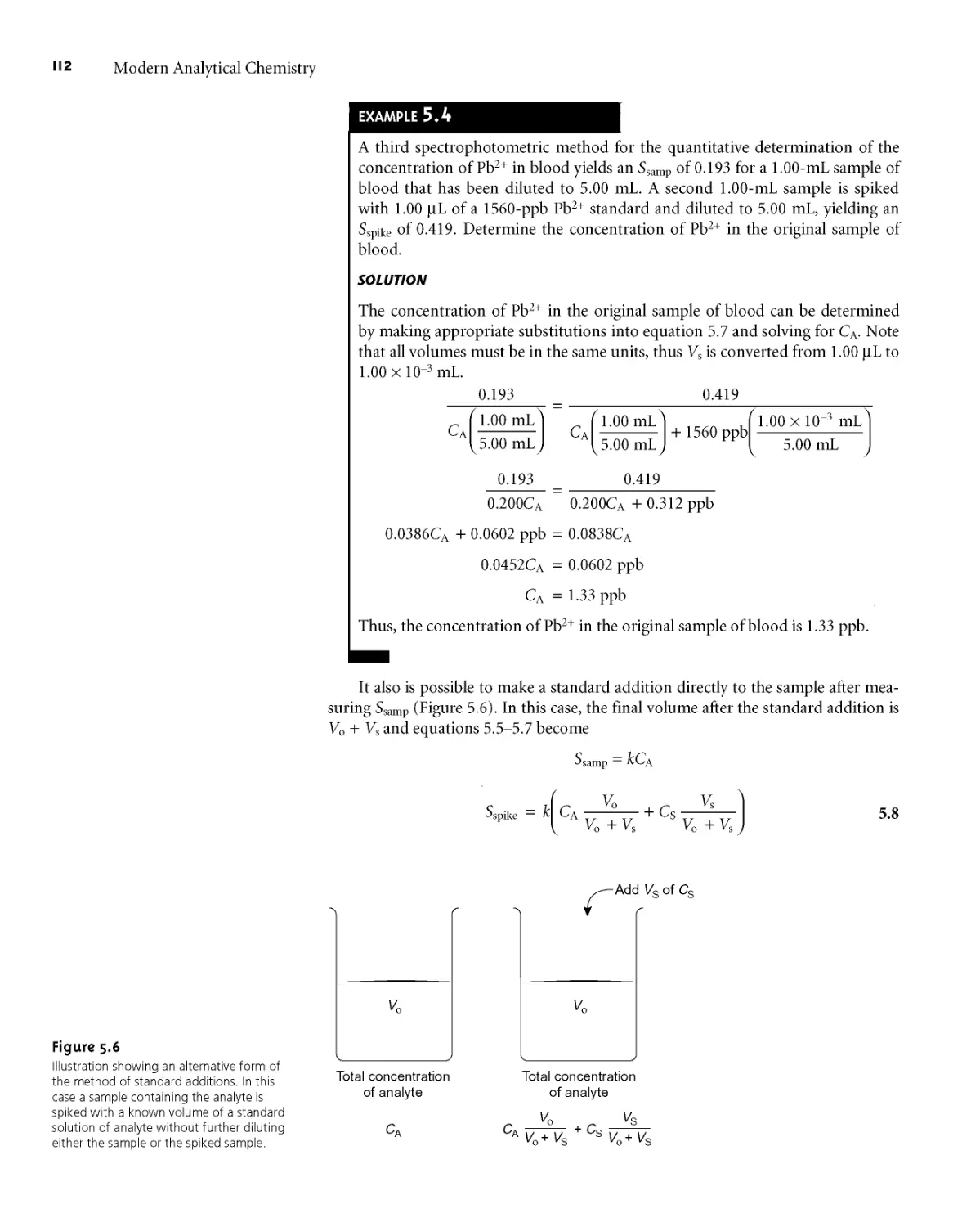
An external standardization allows a related series of samples to be analyzed
using a single calibration curve* This is an important advantage in laboratories
be
e man
Questions
To determine the concentration of Pb2+ in the sample of blood, we replace
Sstand in the calibration equation with Ssamp and solve for
Ssamp - 0*003 0*397 - 0*003 1 .
CA =------------— =-------------— = 1*33 ppb
0*296 ppb 1 0*296 ppb 1
It is worth noting that the calibration equation in this problem includes an
extra term that is not in equation 5*3* Ideally, we expect the calibration curve to
give a signal of zero when Cs is zero* This is the purpose of using a reagent
blank to correct the measured signal* The extra term of +0*003 in our
calibration equation results from uncertainty in measuring the signal for the
reagent blank and the standards*
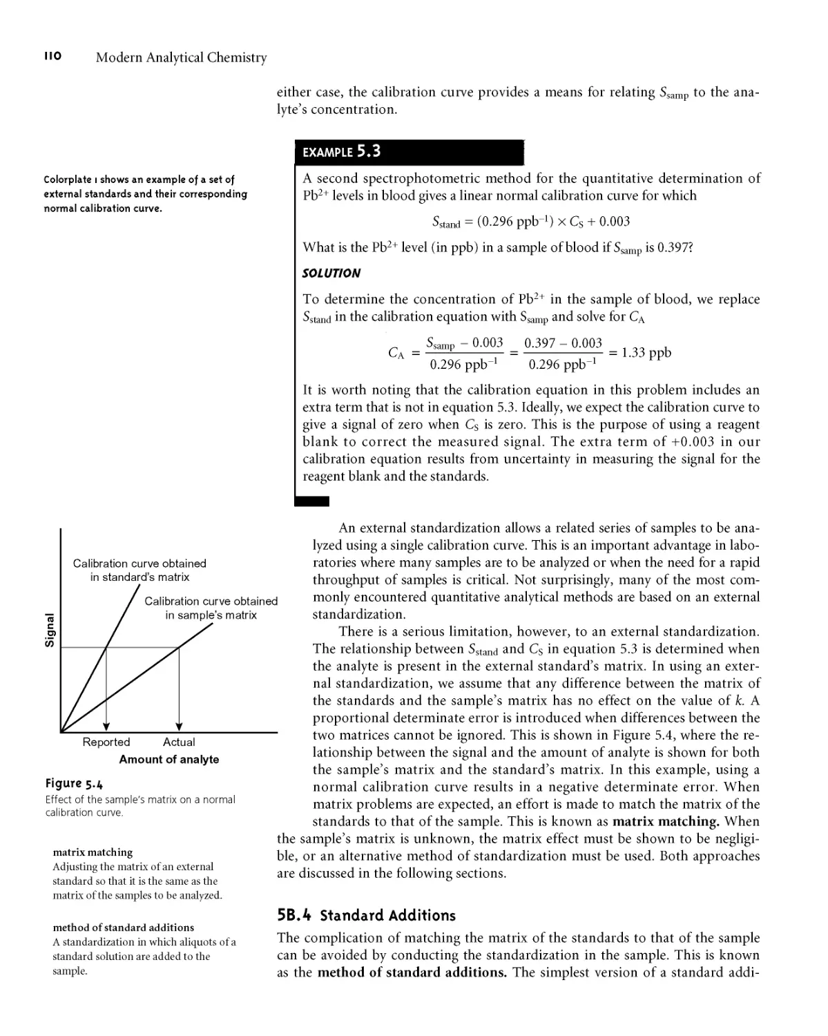
There is a serious limitation, however, to an external standardization* The
relationship between Sstand and Cs in equation 5*3 is determined when the ana-
lyte is present in the external standard’s matrix* In using an external standardiza-
tion, we assume that any difference between the matrix of the standards and the
sample’s matrix has no effect on the value of fc. A proportional determinate error
is introduced when differences between the two matrices cannot be ignored* This
is shown in Figure 5*4, where the relationship between the signal and the amount
of analyte is shown for both the sample’s matrix and the standard’s matrix* In
this example, using a normal calibration curve results in a negative determinate
error* When matrix problems are expected, an effort is made to match the matrix
of the standards to that of the sample* This is known as matrix matching* When
Examples of Typical Problems
Each example problem includes a
detailed solution that helps students in
applying the chapter’s material to
practical problems.
matrix matching
Adjusting the matrix of an external
standard so that it is the same as the
matrix of the samples to be analyzed.
method of standard additions
Astandardization in which aliquots of a
standard solution are added to the
sample.
the sample’s matrix is unknown, the matrix effect must be shown to be negligi-
ble, or an alternative method of standardization must be used* Both approaches
are discussed in the following sections*
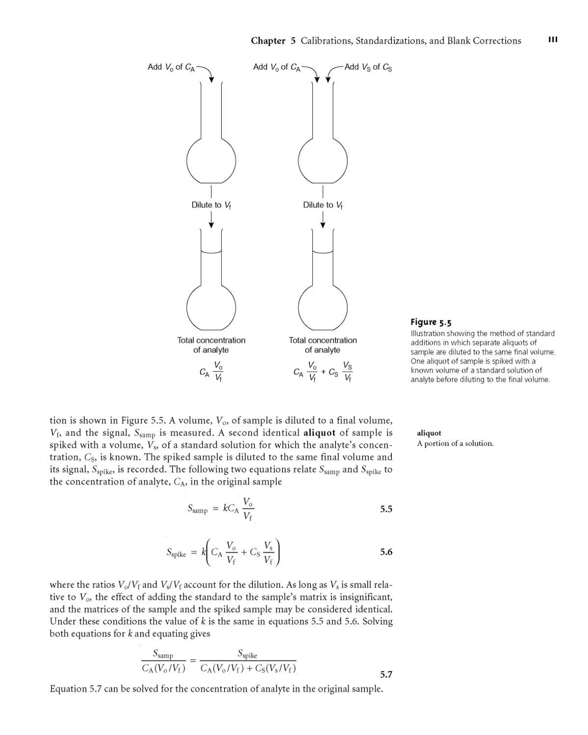
5B.4 Standard Additions
The complication of matching the matrix of the standards to that of the sample
can be avoided by conducting the standardization in the sample* This is known
as the method of standard additions* The simplest version of a standard addi-
tion is shown in Figure 5*5* A volume, Vo, of sample is diluted to a final volume,
Vf, and the signal, SSamp is measured* A second identical aliquot of sample is
Bold-faced Key Terms with Margin Definitions
Key words appear in boldface when they are introduced within the text.
The term and its definition appear in the margin for quick review by the
student. All key words are also defined in the glossary.
X
... End of Chapter
5E KEY TERMS
aliquot (p. Ill)
external standard (p. 109)
internal standard (p. 116)
linear regression (p. 118)
matrix matching (p. 110)
method of standard additions (p. 110)
normal calibration curve (p. 109)
single-point standardization (p. 108)
primary reagent (p. 106)
reagent grade (p. 107)
residual error (p. 118)
standard deviation about the
regression (p. 121)
total Youden blank (p. 129)
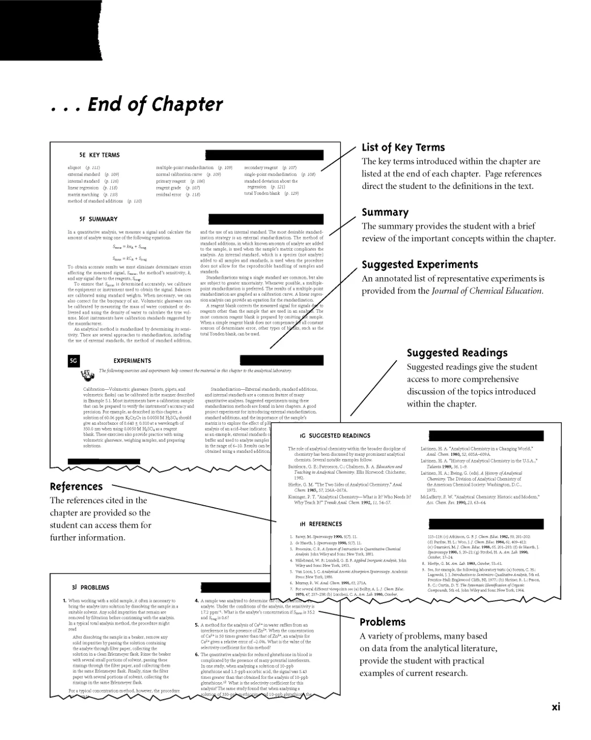
List of Key Terms
The key terms introduced within the chapter are
listed at the end of each chapter. Page references
direct the student to the definitions in the text.
5F SUMMARY
In a quantitative analysis, we measure a signal and calculate the
amount of analyte using one of the following equations.
Smsas ^-^A + ^reag
Smsas — + Sx
To obtain accurate results we must eliminate determinate errors
affecting the measured signal, Smsas, the method’s sensitivity, k,
and any signal due to the reagents, ST^
To ensure that Smsas is determined accurately, we calibrate
the equipment or instrument used to obtain the signal. Balances
are calibrated using standard weights. When necessary, we can
also correct for the buoyancy of air. Volumetric glassware can
be calibrated by measuring the mass of water contained or de-
livered and using the density of water to calculate the true vol-
ume. Most instruments have calibration standards suggested by
the manufacturer.
An analytical method is standardized by determining its sensi-
tivity. There are several approaches to standardization, including
the use of external standards, the method of standard addition,
and the use of an internal standard. The most desirable standard-
ization strategy is an external standardization. The method of
standard additions, in which known amounts of analyte are added
to the sample, is used when the sample’s matrix complicates the
analysis. An internal standard, which is a species (not analyte)
added to all samples and standards, is used when the procedure
does not allow for the reproducible handling of samples and
standards.
Standardizations using a single standard are common, but also
are subject to greater uncertainty. Whenever possible, a multiple-
point standardization is preferred. The results of a multiple-point
standardization are graphed as a calibration curve. A linear regres-
sion analysis can provide an equation for the standardization.
A reagent blank corrects the measured signal for signals d
reagents other than the sample that are used in an anal
most common reagent blank is prepared by omitting
When a simple reagent blank does not compensate
sources of determinate error, other types of b
total Youden blank, can be used.
to
e sample,
all constant
ks, such as the
1 The
5G
EXPERIMENTS
The following exercises and experiments help connect the material in this chapter to the analytical laboratory.
Calibration—Volumetric glassware (burets, pipets, and
volumetric flasks) can be calibrated in the manner described
in Example 5.1. Most instruments have a calibration sample
that can be prepared to verify the instrument’s accuracy and
precision. For example, as described in this chapter, a
solution of 60.06 ppm К2СГ2О7 in 0.0050 M H2SO4 should
give an absorbance of 0.640 ± 0.010 at a wavelength of
550.0 nm when using 0.0050 M H2SO4 as a reagent
blank. These exercises also provide practice with using
volumetric glassware, weighingsamples, and preparing
solutions.
References
The references cited in the
chapter are provided so the
student can access them for
Summary
The summary provides the student with a brief
review of the important concepts within the chapter
Suggested Experiments
An annotated list of representative experiments is
provided from the Journal of Chemical Education.
Standardization—External standards, standard additions,
and internal standards are a common feature of many
quantitative analyses. Suggested experiments using these
standardization methods are found in later chapters. A good
project experiment for introducing external standardization,
standard additions, and the importance of the sample’s
matrix is to explore the effect of pH
analysis of an acid-base indicator. I
as an example, external standards ct
buffer and used to analyze samples
in the range of 6-10. Results can be
obtained using a standard addition.
Suggested Readings
Suggested readings give the student
access to more comprehensive
discussion of the topics introduced
within the chapter.
iC SUGGESTED READINGS
The role of analytical chemistry within the broader discipline of
chemistry has been discussed by many prominent analytical
chemists. Several notable examples follow.
Baiulescu, G. E.; Patroescu, Cc, Chalmers, R. A. Education and
Teaching in Analytical Chemistry. Ellis Horwood; Chichester,
1982.
Hieftje, G. M. 'The Two Sides of Analytical Chemistry,” Anal
Chem. 198557, 256A-267A.
Kissinger, P. T. “Analytical Chemistry—What is It? Who Needs It?
Why Teach It?” Trends Anal. Chem. 1992, 11, 54-57.
Laitinen, H. A. “Analytical Chemistry in a Changing World,”
Anal. Chem. 1980, 52, 605A-609A.
Laitinen, H. A. “History of Analytical Chemistry in the U.S.A.,”
Taianta 1989, 3b, 1-9.
Laitinen, H. Ac, Ewing, G. (eds). A H^toty of Analytical
Chemistry. The Division of Analytical Chemistry of
the American Chemical Society; Washington, D.C.,
1972.
McLafferty, F. W. “Analytical Chemistry: Historic and Modern;
Acc. Chem. Res. 1990,23, 63-64.
iH REFERENCES
113-119; (c) Atkinson, G. FJ. Chem.Educ. 1982,59, 201-202;
(d) Pardue, H. L.; Woo, J J. Chem. Educ. 1984, 61, 409-412;
(e) Guarnieri, M.f. Chem. Educ. 1988, 65, 201-203; (f) de Haseth, J.
Spectroscopy 1990, 5, 20-21; (g) Strobel, H. A. Am. Lab. 1990,
October, 17-24.
8. Hieftje, G. M. Am. Lab. 1993, October, 53-61.
9. See, for example, the foil owing lab oratory texts: (a) Sorum, C.H.;
Lagowski, J. J. Introduction to Semimicro Qualitative Analysis, 5th ed.
Prentice-Hall: Englewood Cliffs, NJ, 1977.; (b) Shriner, R. L.; Fuson,
R. C.; Curtin, D. Y. The Systematic Identification of Organic
Compounds, 5th ed. John Wiley and Sons: New York, 1964.
further information
31 PROBLEMS
1. When working with a solid sample, it often is necessary to
bring the analyte into solution by dissolving the sample in a
suitable solvent. Any solid impurities that remain are
removed by filtration before continuing with the analysis.
In a typical total analysis method, the procedure might
read
After dissolving the sample in a beaker, remove any
solid impurities by passing the solution containing
the analyte through filter paper, collecting the
solution in a clean Erlenmeyer flask. Rinse the beaker
with several small portions of solvent, passing these
rinsings through the filter paper, and collecting them
in the same Erlenmeyer flask. Finally, rinse the filter
paper with several portions of solvent, collecting the
rinsings in the same Erlenmeyer flask.
For a typical concentration method, however, the procedure
1. Ravey, M. Spectroscopy 1990, 5(7), 11.
2. de Haseth, J. Spectroscopy 1990, 5(7), 11.
3. Fresenius, C. R. A System cf Instruction in Quantitative Chemical
Analysis. John Wiley and Sons: New York, 1881.
4. Hill eb rand, W. F.; Lundell, G. E F. Applied Inorganic Analysis, John
Wiley and Sons: New York, 1953.
5. Van Loon, J. C. Analytical Atomic Absorption Spectroscopy. Academic
Press: New York, 1980.
6. Murray, R. W. Anal. Chem. 1991, 63, 271A
7. For several different viewpoints see (a) Beilby, A. L./. Chem. Educ.
1970, 47, 237-238; (b) Lucchesi, C. A. Am. Lab. 1980, October,
10
4. A sample was analyzed to determine ffie'c
analyte. Under the conditions of the analysis, the sensitivity is
17.2 ppm-1. What is the analyte’s concentration if Smsas is 35.2
and Srsa? is 0.6?
5. A method for the analysis of Ca2+ in water suffers from an
interference in the presence ofZn2+. When the concentration
of Ca2+ is 50 times greater than that of Zn2+, an analysis for
Ca2+ gives a relative error of-2.0%. What is the value of the
selectivity coefficient for this method?
6. The quantitative analysis for reduced glutathione in blood is
complicated by the presence of many potential interferents.
In one study, when analyzing a solution of 10-ppb
glutathione and 1.5-ppb ascorbic acid, the signal was 5.43
times greater than that obtained for the analysis of 10-ppb
glutathione.12 What is the selectivity coefficient for this
analysis? The same study found that when analyzing a
olution of 350-p ethi d 10-ppb glutalhio
Problems
A variety of problems, many based
on data from the analytical literature,
provide the student with practical
examples of current research.
XI
Preface
A
« >s currently taught, the introductory course in analytical chemistry emphasizes
quantitative (and sometimes qualitative) methods of analysis coupled with a heavy
dose of equilibrium chemistry. Analytical chemistry, however, is more than equilib-
rium chemistry and a collection of analytical methods; it is an approach to solving
chemical problems. Although discussing different methods is important, that dis-
cussion should not come at the expense of other equally important topics. The intro-
ductory analytical course is the ideal place in the chemistry curriculum to explore
topics such as experimental design, sampling, calibration strategies, standardization,
optimization, statistics, and the validation of experimental results. These topics are
important in developing good experimental protocols, and in interpreting experi-
mental results. If chemistry is truly an experimental science, then it is essential that
all chemistry students understand how these topics relate to the experiments they
conduct in other chemistry courses.
Currently available textbooks do a good job of covering the diverse range of wet
and instrumental analysis techniques available to chemists. Although there is some
disagreement about the proper balance between wet analytical techniques, such as
gravimetry and titrimetry, and instrumental analysis techniques, such as spec-
trophotometry, all currently available textbooks cover a reasonable variety of tech-
niques. These textbooks, however, neglect, or give only brief consideration to,
obtaining representative samples, handling interferents, optimizing methods, ana-
lyzing data, validating data, and ensuring that data are collected under a state of sta-
tistical control.
In preparing this textbook, I have tried to find a more appropriate balance
between theory and practice, between “classical” and “modern” methods of analysis,
between analyzing samples and collecting and preparing samples for analysis, and
between analytical methods and data analysis. Clearly, the amount of material in this
textbook exceeds what can be covered in a single semester; it’s my hope, however,
that the diversity of topics will meet the needs of different instructors, while, per-
haps, suggesting some new topics to cover.
The anticipated audience for this textbook includes students majoring in chem-
istry, and students majoring in other science disciplines (biology, biochemistry,
environmental science, engineering, and geology, to name a few), interested in
obtaining a stronger background in chemical analysis. It is particularly appropriate
for chemistry majors who are not planning to attend graduate school, and who often
do not enroll in those advanced courses in analytical chemistry that require physical
chemistry as a pre-requisite. Prior coursework of a year of general chemistry is
assumed. Competence in algebra is essential; calculus is used on occasion, however,
its presence is not essential to the material’s treatment.
* *
XII
Preface
xiii
Key Features of This Textbook
Key features set this textbook apart from others currently available.
• A stronger emphasis on the evaluation of data. Methods for characterizing
chemical measurements, results, and errors (including the propagation of
errors) are included. Both the binomial distribution and normal distribution
are presented, and the idea of a confidence interval is developed. Statistical
methods for evaluating data include the f-test (both for paired and unpaired
data), the F-test, and the treatment of outliers. Detection limits also are
discussed from a statistical perspective. Other statistical methods, such as
ANOVA and ruggedness testing, are presented in later chapters.
• Standardizations and calibrations are treated in a single chapter. Selecting the
most appropriate calibration method is important and, for this reason, the
methods of external standards, standard additions, and internal standards are
gathered together in a single chapter. A discussion of curve-fitting, including
the statistical basis for linear regression (with and without weighting) also is
included in this chapter.
• More attention to selecting and obtaining a representative sample. The design of a
statistically based sampling plan and its implementation are discussed earlier,
and in more detail than in other textbooks. Topics that are covered include
how to obtain a representative sample, how much sample to collect, how many
samples to collect, how to minimize the overall variance for an analytical
method, tools for collecting samples, and sample preservation.
• The importance of minimizing interferents is emphasized. Commonly used
methods for separating interferents from analytes, such as distillation, masking,
and solvent extraction, are gathered together in a single chapter.
• Balanced coverage of analytical techniques. The six areas of analytical
techniques—gravimetry, titrimetry, spectroscopy, electrochemistry,
chromatography, and kinetics—receive roughly equivalent coverage, meeting
the needs of instructors wishing to emphasize wet methods and those
emphasizing instrumental methods. Related methods are gathered together in a
single chapter encouraging students to see the similarities between methods,
rather than focusing on their differences.
• An emphasis on practical applications. Throughout the text applications from
organic chemistry, inorganic chemistry, environmental chemistry, clinical
chemistry, and biochemistry are used in worked examples, representative
methods, and end-of-chapter problems.
• Representative methods link theory with practice. An important feature of this
text is the presentation of representative methods. These boxed features present
typical analytical procedures in a format that encourages students to think
about why the procedure is designed as it is.
• Separate chapters on developing a standard method and quality assurance. Two
chapters provide coverage of methods used in developing a standard method
of analysis, and quality assurance. The chapter on developing a standard
method includes topics such as optimizing experimental conditions using
response surfaces, verifying the method through the blind analysis of
standard samples and ruggedness testing, and collaborative testing using
Youden’s two-sample approach and ANOVA. The chapter on quality
assurance covers qualify control and internal and external techniques for
quality assessment, including the use of duplicate samples, blanks, spike
recoveries, and control charts.
xiv
Preface
• Problems adapted from the literature. Many of the in-chapter examples and end-
of-chapter problems are based ondatafromthe analytical literature, providing
students with practical examples of current research in analytical chemistry.
• An emphasis on critical thinking. Critical thinking is encouraged through
problems in which students are asked to explain why certain steps in an
analytical procedure are included, or to determine the effect of an experimental
error on the results of an analysis.
* Suggested experiments from the Journal of Chemical Education. Rather than
including a short collection of experiments emphasizing the analysis of
standard unknowns, an annotated list of representative experiments from the
Journal of Chemical Education is included at the conclusion of most chapters.
These experiments may serve as stand alone experiments, or as starting points
for individual or group projects.
The Role of Equilibrium Chemistry in Analytical Chemistry
Equilibrium chemistry often receives a significant emphasis in the introductory ana-
lytical chemistry course. While an important topic, its overemphasis can cause stu-
dents to confuse analytical chemistry with equilibrium chemistry. Although atten-
tion to solving equilibrium problems is important, it is equally important for stu-
dents to recognize when such calculations are impractical, or when a simpler, more
qualitative approach is all that is needed. For example, in discussing the gravimetric
analysis of Ag+ as AgCl, there is little point in calculating the equilibrium solubility
of AgCl since the concentration of Cl- at equilibrium is rarely known. It is impor-
tant, however, to qualitatively understand that a large excess of Cl- increases the sol-
ubility of AgCl due to the formation of soluble silver-chloro complexes. Balancing
the presentation of a rigorous approach to solving equilibrium problems, this text
also introduces the use of ladder diagrams as a means for providing a qualitative pic-
ture of a system at equilibrium Students are encouraged to use the approach best
suited to the problem at hand.
Computer Software
Many of the topics covered in analytical chemistry benefit from the availability of
appropriate computer software. In preparing this text, however, I made a conscious
decision to avoid a presentation tied to a single computer platform or software pack-
age. Students and faculty are increasingly experienced in the use of computers,
spreadsheets, and data analysis software; their use is, I think, best left to the person-
al choice of each student and instructor.
Organization
The textbook’s organization can be divided into four parts. Chapters 1-3 serve as an
introduction, providing an overview of analytical chemistry (Chapter 1); a review of
the basic tools of analytical chemistry, including significant figures, units, and stoi-
chiometry (Chapter 2); and an introduction to the terminology used by analytical
chemists (Chapter 3). Familiarity with the material in these chapters is assumed
throughout the remainder of the text
Chapters 4-7 cover a number of topics that are important in understanding how
a particular analytical method works. Later chapters are mostly independent of the
material in these chapters. Instructors may pick and choose from among the topics
Preface
XV
of these chapters, as needed, to support individual course goals. The statistical analy-
sis of data is covered in Chapter 4 ata level that is more complete than that found in
other introductory analytical textbooks. Methods for calibrating equipment, stan-
dardizing methods, and linear regression are gathered together in Chapter 5. Chapter
6 provides an introduction to equilibrium chemistry, stressing both the rigorous
solution to equilibrium problems, and the use of semi-quantitative approaches, such
as ladder diagrams. The importance of collecting the right sample, and methods for
separating analytes and interferents are covered in Chapter 7.
Chapters 8-13 cover the major areas of analysis, including gravimetry
(Chapter 8), titrimetry (Chapter 9), spectroscopy (Chapter 10), electrochemistry
(Chapter 11), chromatography and electrophoresis (Chapter 12), and kinetic meth-
ods (Chapter 13). Related techniques, such as acid-base titrimetry and redox
titrimetry, or potentiometry and voltammetry, are gathered together in single chap-
ters. Combining related techniques together encourages students to see the similar-
ities between methods, rather than focusing on their differences. The first technique
presented in each chapter is generally that which is most commonly covered in the
introductory course.
Finally, the textbook concludes with two chapters discussing the design and
maintenance of analytical methods, two topics of importance to analytical chemists.
Chapter 14 considers the development of an analytical method, including its opti-
mization, verification, and validation. Quality control and quality assessment are
discussed in Chapter 15.
Acknowledgments
Before beginning an academic career I was, of course, a student My interest in
chemistry and teaching was nurtured by many fine teachers at Westtown Friends
School, Knox College, and the University of North Carolina at Chapel Hill; their col-
lective influence continues to bear fruit In particular, I wish to recognize David
Madnnes, Alan Hiebert, Robert Kooser, and Richard Linton.
I have been fortunate to work with many fine colleagues during my nearly 17
years of teaching undergraduate chemistry at Stockton State College and DePauw
University. I am particularly grateful for the friendship and guidance provided by
Jon Griffiths and Ed Paul during my four years at Stockton State College. At DePauw
University, Jim George and Bryan Hanson have willingly shared their ideas about
teaching, while patiently listening to mine.
Approximately 300 students have joined me in thinking and learning about ana-
lytical chemistry; their questions and comments helped guide the development of
this textbook I realize that working without a formal textbook has been frustrating
and awkward; all the more reason why I appreciate their effort and hard work
The following individuals reviewed portions of this textbook at various stages
during its development
David Ballantine
Northern Illinois University
John E. Bauer
Illinois State University
Ali Bazzi
University of Michigan-Dearborn
Steven D. Brown
University of Delaware
Wendy Clevenger
University of Tennessee-Chattanooga
Cathy Cobb
Augusta State University
Paul Flowers
University of North Carolina-Pembroke
Nancy Gordon
University of Southern Maine
xvi
Preface
Virginia M. Indivero
Swarthmore College
Michael Janusa
Nicholls State University
J. David Jenkins
Georgia Southern University
Richard S. Mitchell
Arkansas State University
George A. Pearse, Jr.
Le Moyne College
Gary Rayson
New Mexico State University
David Redfield
NW Nazar ene University
Vincent Remcho
West Virginia University
Jeanette K. Rice
Georgia Southern University
Martin W. Rowe
Texas A&M University
Alexander Scheeline
Un iversity of Illinois
James D. Stuart
Un iversity of Connecticut
Thomas J. Wenzel
Bates College
David Zax
Cornell University
lam particularly grateful for their detailed written comments and suggestions for
improving the manuscript Much of what is good in the final manuscript is the result
of their interest and ideas. George Foy (York College of Pennsylvania), John McBride
(Hofstra University), and David Karpovich (Saginaw Valley State University) checked
the accuracy of problems in the textbook Gary Kinsel (University of Texas at
Arlington) reviewed the page proofs and provided additional suggestions.
This project began in the summer of 1992 with the support of a course develop-
ment grant from DePauw University’s Faculty Development Fund. Additional finan-
cial support from DePauw University’s Presidential Discretionary Fund also is
acknowledged. Portions of the first draft were written during a sabbatical leave in the
Fall semester of the 1993/94 academic year. A Fisher Fellowship provided release
time during the Fall 1995 semester to complete the manuscript’s second draft
Alite ch and Associates (Deerfield, IL) graciously provided permission to use the
chromatograms in Chapter 12; the assistance of Jim Anderson, Vice-President,
and Julia Poncher, Publications Director, is greatly appreciated. Fred Soster and
Marilyn Culler, both of DePauw University, provided assistance with some of the
photographs.
The editorial staff at McGraw-Hill has helped guide a novice through the
process of developing this text I am particularly thankful for the encouragement and
confidence shown by Jim Smith, Publisher for Chemistry, and Kent Peterson,
Sponsoring Editor for Chemistry. Shirley Oberbroeckling, Developmental Editor for
Chemistry, and Jayne Klein, Senior Project Manager, patiently answered my ques-
tions and successfully guided me through the publishing process.
Finally, I would be remiss if I did not recognize the importance of my family’s
support and encouragement, particularly that of my parents. A very special thanks to
my daughter, Devon, for gifts too numerous to detail.
How to Contact the Author
Writing this textbook has been an interesting (and exhausting) challenge. Despite
my efforts, I am sure there are a few glitches, better examples, more interesting end-
of-chapter problems, and better ways to think about some of the topics. I welcome
your comments, suggestions, and data for interesting problems, which may be
addressed to me atDePauwUniversity, 602 S. College St, Greencastle, IN 46135, or
electronically at harvey@depauw.edu.
Introduction
V^hemistry is the study of matter, including its composition,
structure, physical properties, and reactivity. There are many
approaches to studying chemistry, but, for convenience, we
traditionally divide it into five fields: organic, inorganic, physical,
biochemical, and analytical. Although this division is historical and
arbitrary, as witnessed by the current interest in interdisciplinary areas
such as bioanalytical and organometallic chemistry, these five fields
remain the simplest division spanning the discipline of chemistry.
Training in each of these fields provides a unique perspective to the
study of chemistry. Undergraduate chemistry courses and textbooks
are more than a collection of facts; they are a kind of apprenticeship. In
keeping with this spirit, this text introduces the field of analytical
chemistry and the unique perspectives that analytical chemists bring to
the study of chemistry.
i
2
Modern Analytical Chemistry
) What Is Analytical Chemistry?
"'Analytical chemistry is what analytical chemists do.”*
We begin this section with a deceptively simple question. What is analytical chem-
istry? Like all fields of chemistry, analytical chemistry is too broad and active a disci-
pline for us to easily or completely define in an introductory textbook. Instead, we
will try to say a little about what analytical chemistry is, as well as a little about what
analytical chemistry is not.
Analytical chemistry is often described as the area of chemistry responsible for
characterizing the composition of matter, both qualitatively (what is present) and
quantitatively (how much is present). This description is misleading. After all, al-
most all chemists routinely make qualitative or quantitative measurements. The ar-
gument has been made that analytical chemistry is not a separate branch of chem-
istry, but simply the application of chemical knowledge.1 In fact, you probably have
performed quantitative and qualitative analyses in other chemistry courses. For ex-
ample, many introductory courses in chemistry include qualitative schemes for
identifying inorganic ions and quantitative analyses involving titrations.
Unfortunately, this description ignores the unique perspective that analytical
chemists bring to the study of chemistry. The craft of analytical chemistry is not in
performing a routine analysis on a routine sample (which is more appropriately
called chemical analysis), but in improving established methods, extending existing
methods to new types of samples, and developing new methods for measuring
chemical phenomena.2
Here’s one example of this distinction between analytical chemistry and chemi-
cal analysis. Mining engineers evaluate the economic feasibility of extracting an ore
by comparing the cost of removing the ore with the value of its contents. To esti-
mate its value they analyze a sample of the ore. The challenge of developing and val-
idating the method providing this information is the analytical chemist’s responsi-
bility. Once developed, the routine, daily application of the method becomes the
job of the chemical analyst.
Another distinction between analytical chemistry and chemical analysis is
that analytical chemists work to improve established methods. For example, sev-
eral factors complicate the quantitative analysis of Ni2+ in ores, including the
presence of a complex heterogeneous mixture of silicates and oxides, the low con-
centration of Ni2+ in ores, and the presence of other metals that may interfere in
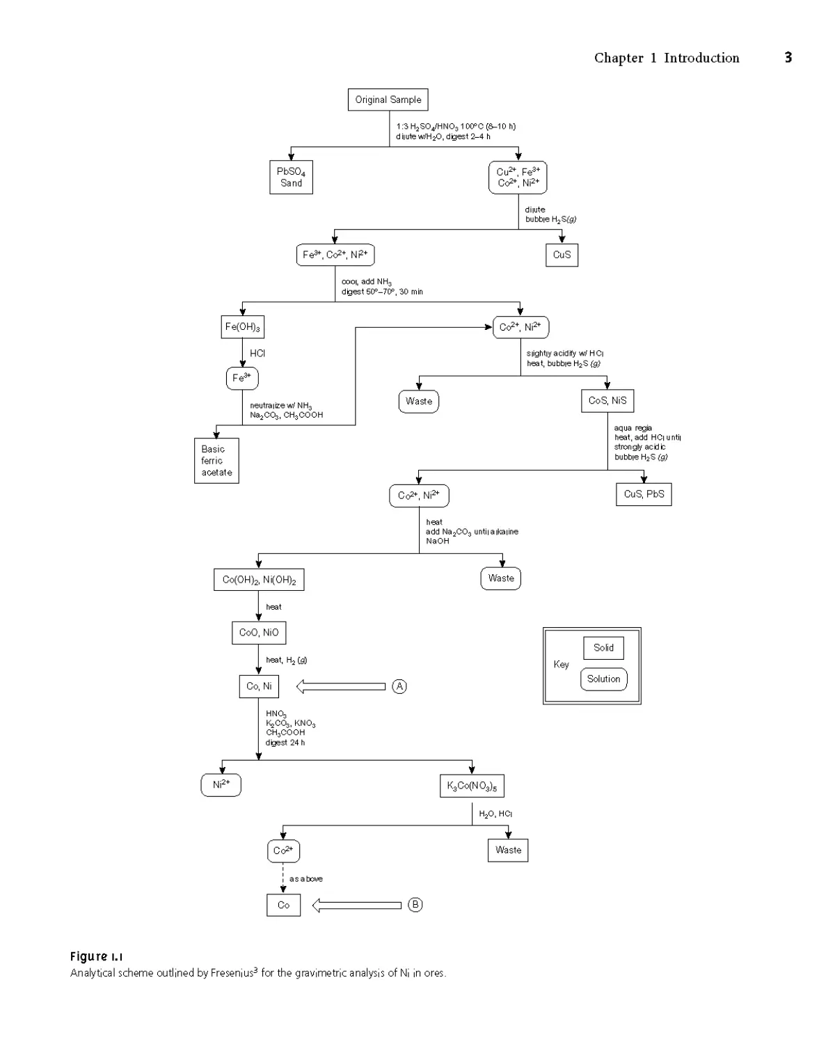
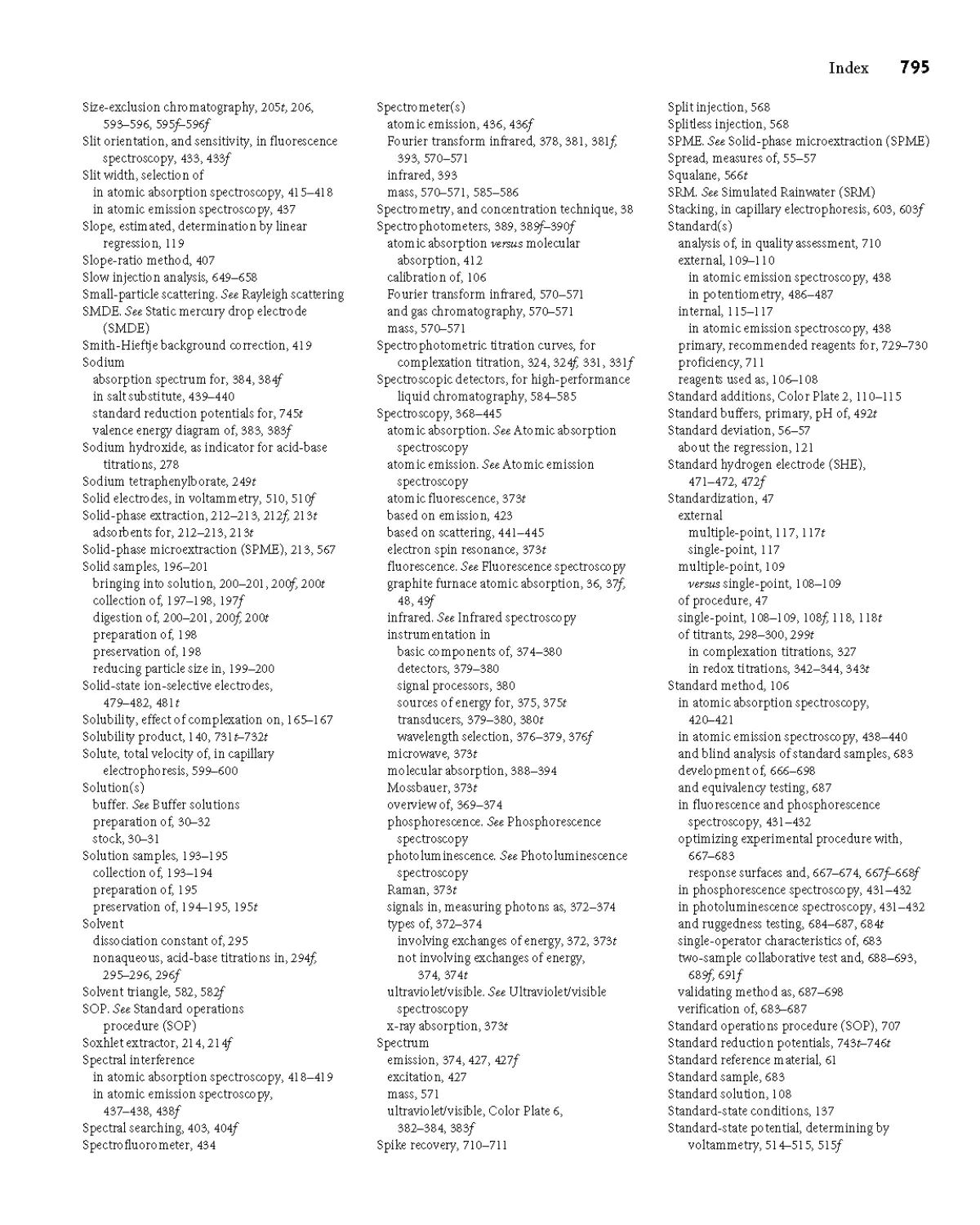
the analysis. Figure 1.1 is a schematic outline of one standard method in use dur-
ing the late nineteenth century.3 After dissolving a sample of the ore in a mixture
of H2SO4 and HNO3, trace metals that interfere with the analysis, such as Pb2+,
Cu2+ and Fe3+, are removed by precipitation. Any cobalt and nickel in the sample
are reduced to Co and Ni, isolated by filtration and weighed (point A). After
dissolving the mixed solid, Co is isolated and weighed (point B). The amount
of nickel in the ore sample is determined from the difference in the masses at
points A and B.
л/ ^T. mass point A - mass point В
%Ni =------------------------------x 100
mass sample
* Attributed to C. N. Reilley (1925-1981) on receipt of the 1965 Fisher Award in Analytical Chemistry. Reilley, who was
a professor of chemistry at the University of North Carolina at Chapel Hill, was one of the most influential analytical
chemists of the last half of the twentieth century.
Chapter 1 Introduction
3
। asabove
t
сЛ < I ®
Figure 1.1
Analytical scheme outlined by Fresenius3 for the gravimetric analysis of Ni in ores.
4
Modern Analytical Chemistry
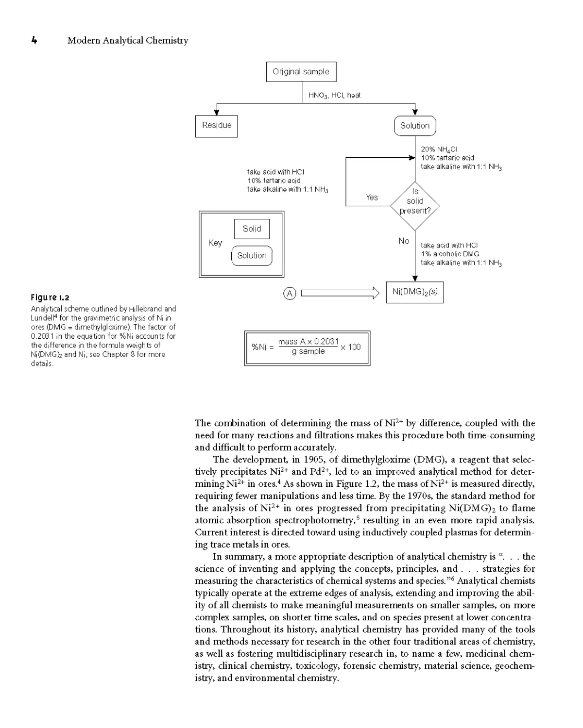
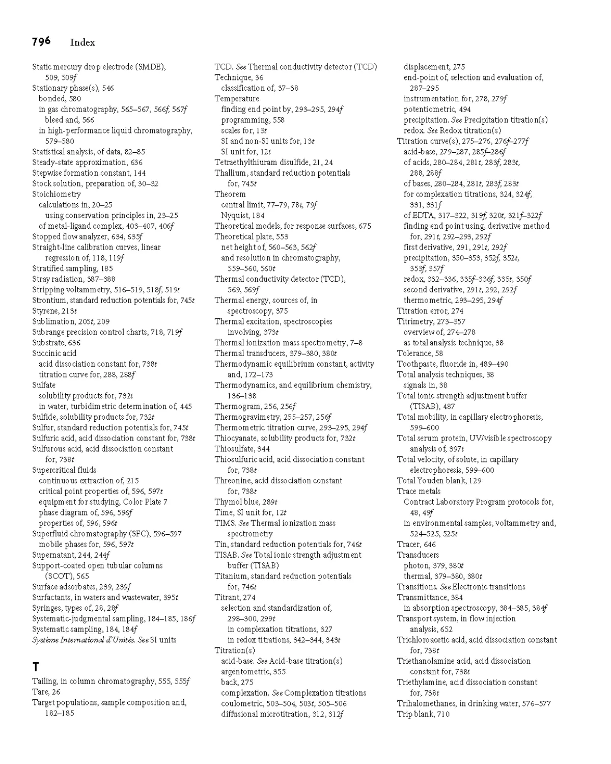
Figure 1.2
Analytical scheme outlined by Hillebrand and
Lun del I4 for the gravimetric analysis of Ni in
ores (DMG = dimethylgloxime). The factor of
0.2031 in the equation for %Ni accounts for
the difference in the formula weights of
Ni(DMGk and Mi; see Chapter 8 for more
details.
n/hl. mass Ax 0.2031
%N| = g sample x 100
The combination of determining the mass of Ni2+ by difference, coupled with the
need for many reactions and filtrations makes this procedure both time-consuming
and difficult to perform accurately.
The development, in 1905, of dimethylgloxime (DMG), a reagent that selec-
tively precipitates Ni2+ and Pd2+, led to an improved analytical method for deter-
mining Ni2+ in ores.4 As shown in Figure 1.2, the mass of Ni2+ is measured directly,
requiring fewer manipulations and less time. By the 1970s, the standard method for
the analysis of Ni2+ in ores progressed from precipitating Ni(DMG)2 to flame
atomic absorption spectrophotometry,5 resulting in an even more rapid analysis.
Current interest is directed toward using inductively coupled plasmas for determin-
ing trace metals in ores.
In summary, a more appropriate description of analytical chemistry is . .the
science of inventing and applying the concepts, principles, and . . . strategies for
measuring the characteristics of chemical systems and species.”6 Analytical chemists
typically operate at the extreme edges of analysis, extending and improving the abil-
ity of all chemists to make meaningful measurements on smaller samples, on more
complex samples, on shorter time scales, and on species present at lower concentra-
tions. Throughout its history, analytical chemistry has provided many of the tools
and methods necessary for research in the other four traditional areas of chemistry,
as well as fostering multidisciplinary research in, to name a few, medicinal chem-
istry, clinical chemistry, toxicology, forensic chemistry, material science, geochem-
istry, and environmental chemistry.
Chapter 1 Introduction
5
You will come across numerous examples of qualitative and quantitative meth-
ods in this text, most of which are routine examples of chemical analysis. It is im-
portant to remember, however, that nonroutine problems prompted analytical
chemists to develop these methods. Whenever possible, we will try to place these
methods in their appropriate historical context. In addition, examples of current re-
search problems in analytical chemistry are scattered throughout the text.
The next time you are in the library, look through a recent issue of an analyti-
cally oriented journal, such as Analytical Chemistry. Focus on the titles and abstracts
of the research articles. Although you will not recognize all the terms and methods,
you will begin to answer for yourself the question “What is analytical chemistry”?
| The Analytical Perspective
Having noted that each field of chemistry brings a unique perspective to the study
of chemistry, we now ask a second deceptively simple question. What is the “analyt-
ical perspective”? Many analytical chemists describe this perspective as an analytical
approach to solving problems.7 Although there are probably as many descriptions
of the analytical approach as there are analytical chemists, it is convenient for our
purposes to treat it as a five-step process:
1. Identify and define the problem.
2. Design the experimental procedure.
3. Conduct an experiment, and gather data.
4. Analyze the experimental data.
5. Propose a solution to the problem.
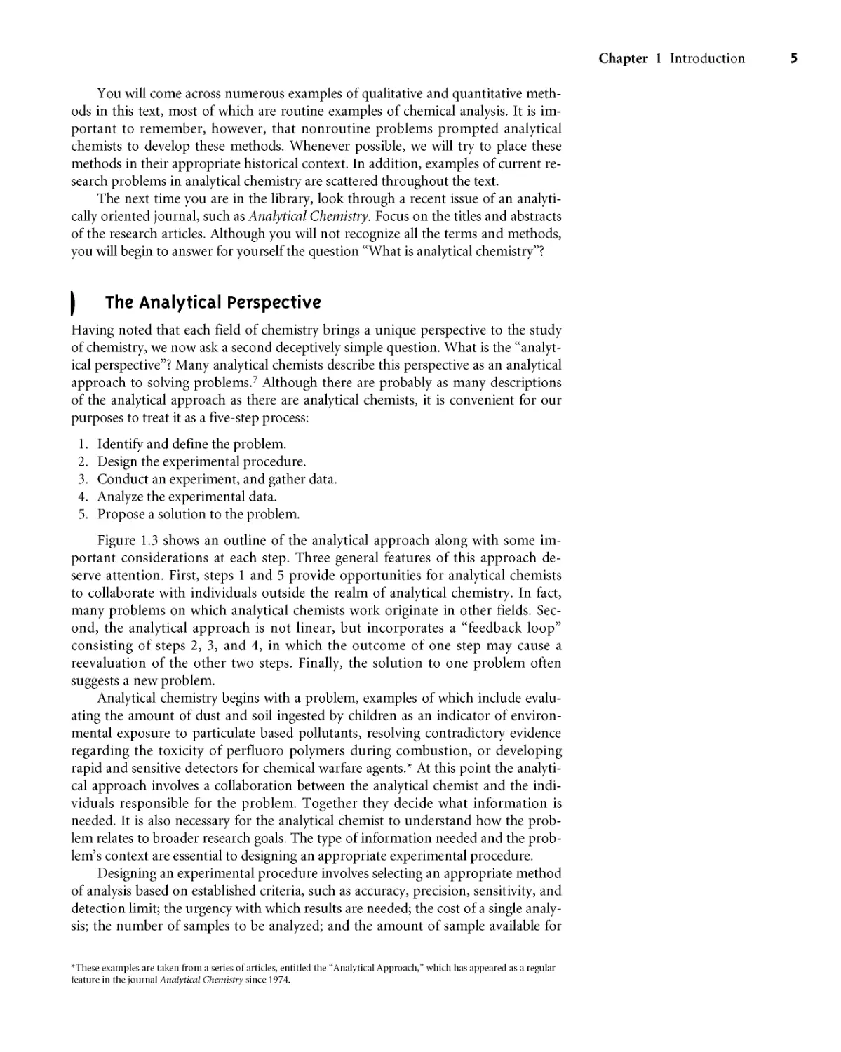
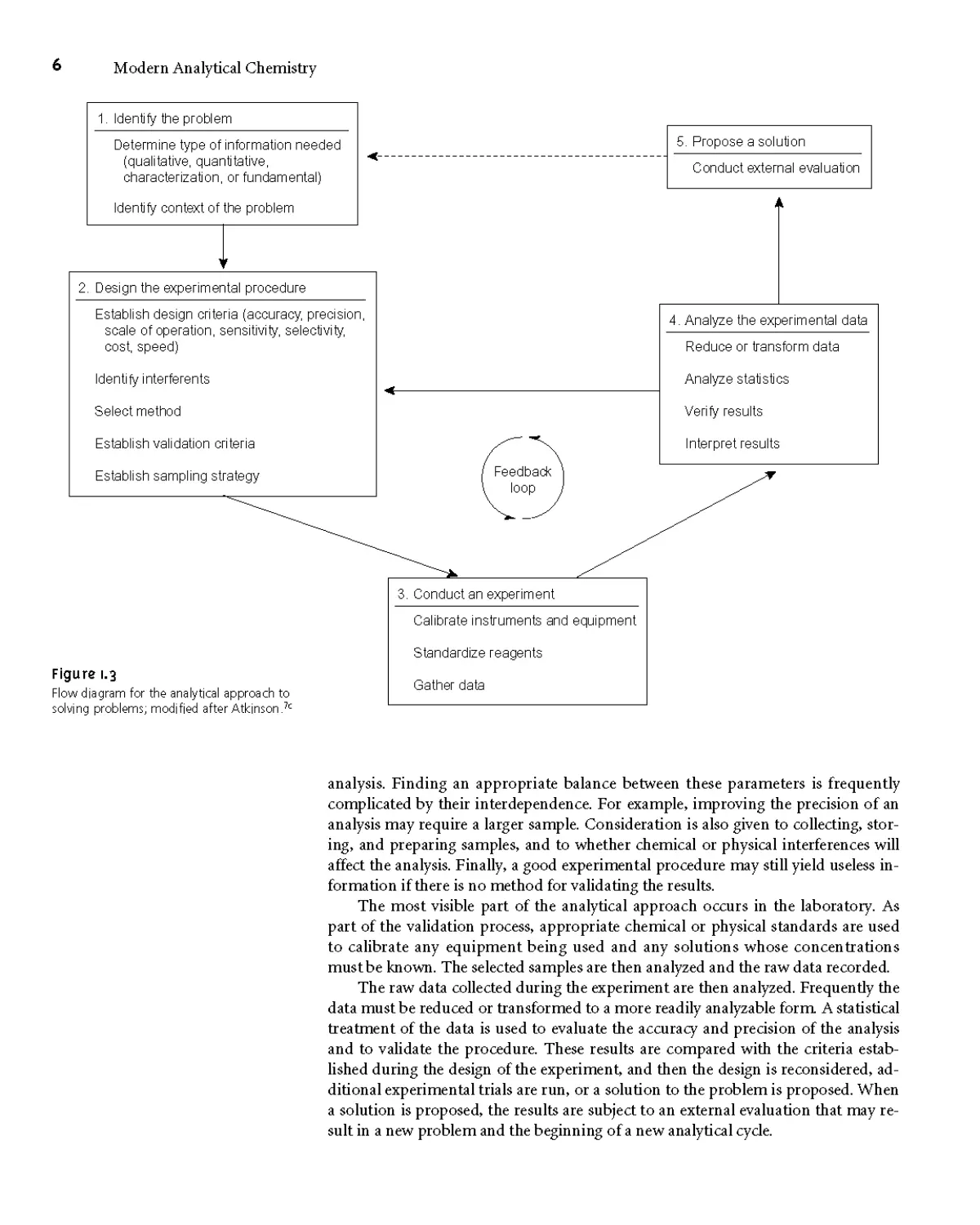
Figure 1.3 shows an outline of the analytical approach along with some im-
portant considerations at each step. Three general features of this approach de-
serve attention. First, steps 1 and 5 provide opportunities for analytical chemists
to collaborate with individuals outside the realm of analytical chemistry. In fact,
many problems on which analytical chemists work originate in other fields. Sec-
ond, the analytical approach is not linear, but incorporates a “feedback loop”
consisting of steps 2, 3, and 4, in which the outcome of one step may cause a
reevaluation of the other two steps. Finally, the solution to one problem often
suggests a new problem.
Analytical chemistry begins with a problem, examples of which include evalu-
ating the amount of dust and soil ingested by children as an indicator of environ-
mental exposure to particulate based pollutants, resolving contradictory evidence
regarding the toxicity of perfluoro polymers during combustion, or developing
rapid and sensitive detectors for chemical warfare agents? At this point the analyti-
cal approach involves a collaboration between the analytical chemist and the indi-
viduals responsible for the problem. Together they decide what information is
needed. It is also necessary for the analytical chemist to understand how the prob-
lem relates to broader research goals. The type of information needed and the prob-
lem’s context are essential to designing an appropriate experimental procedure.
Designing an experimental procedure involves selecting an appropriate method
of analysis based on established criteria, such as accuracy, precision, sensitivity, and
detection limit; the urgency with which results are needed; the cost of a single analy-
sis; the number of samples to be analyzed; and the amount of sample available for
*These examples are taken from a series of articles, entitled the “Analytical Approach,” which has appeared as a regular
feature in the journal Analytical Chemistry since 1974.
6
Modern Analytical Chemistry
analysis. Finding an appropriate balance between these parameters is frequently
complicated by their interdependence. For example, improving the precision of an
analysis may require a larger sample. Consideration is also given to collecting, stor-
ing, and preparing samples, and to whether chemical or physical interferences will
affect the analysis. Finally, a good experimental procedure may still yield useless in-
formation if there is no method for validating the results.
The most visible part of the analytical approach occurs in the laboratory. As
part of the validation process, appropriate chemical or physical standards are used
to calibrate any equipment being used and any solutions whose concentrations
must be known. The selected samples are then analyzed and the raw data recorded.
The raw data collected during the experiment are then analyzed. Frequently the
data must be reduced or transformed to a more readily analyzable form A statistical
treatment of the data is used to evaluate the accuracy and precision of the analysis
and to validate the procedure. These results are compared with the criteria estab-
lished during the design of the experiment, and then the design is reconsidered, ad-
ditional experimental trials are run, or a solution to the problem is proposed. When
a solution is proposed, the results are subject to an external evaluation that may re-
sult in a new problem and the beginning of a new analytical cycle.
Chapter 1 Introduction
7
As an exercise, let’s adapt this model of the analytical approach to a real prob-
lem For our example, we will use the determination of the sources of airborne pol-
lutant particles. A description of the problem can be found in the following article:
“Tracing Aerosol Pollutants with Rare Earth Isotopes” by
Ondov, J. M.; Kelly, W. R. Anal. Chem. 1991, 63, 691A-697A.
Before continuing, take some time to read the article, locating the discussions per-
taining to each of the five steps outlined in Figure 1.3. In addition, consider the fol-
lowing questions:
1. What is the analytical problem?
2. What type of information is needed to solve the problem?
3. How will the solution to this problem be used?
4. What criteria were considered in designing the experimental procedure?
5. Were there any potential interferences that had to be eliminated? If so, how
were they treated?
6. Is there a plan for validating the experimental method?
7. How were the samples collected?
8. Is there evidence that steps 2, 3, and 4 of the analytical approach are repeated
more than once?
9. Was there a successful conclusion to the problem?
According to our model, the analytical approach begins with a problem The
motivation for this research was to develop a method for monitoring the transport
of solid aerosol particulates following their release from a high-temperature com-
bustion source. Because these particulates contain significant concentrations of
toxic heavy metals and carcinogenic organic compounds, they represent a signifi-
cant environmental hazard.
An aerosol is a suspension of either a solid or a liquid in a gas. Fog, for exam-
ple, is a suspension of small liquid water droplets in air, and smoke is a suspension
of small solid particulates in combustion gases. In both cases the liquid or solid par-
ticulates must be small enough to remain suspended in the gas for an extended
time. Solid aerosol particulates, which are the focus of this problem, usually have
micrometer or sub micro me ter diameters. Over time, solid particulates settle out
from the gas, falling to the Earth’s surface as dry deposition.
Existing methods for monitoring the transport of gases were inadequate for
studying aerosols. To solve the problem, qualitative and quantitative information
were needed to determine the sources of pollutants and their net contribution to
the total dry deposition at a given location. Eventually the methods developed in
this study could be used to evaluate models that estimate the contributions of point
sources of pollution to the level of pollution at designated locations.
Following the movement of airborne pollutants requires a natural or artificial
tracer (a species specific to the source of the airborne pollutants) that can be exper-
imentally measured at sites distant from the source. Limitations placed on the
tracer, therefore, governed the design of the experimental procedure. These limita-
tions included cost, the need to detect small quantities of the tracer, and the ab-
sence of the tracer from other natural sources. In addition, aerosols are emitted
from high-temperature combustion sources that produce an abundance of very re-
active species. The tracer, therefore, had to be both thermally and chemically stable.
On the basis of these criteria, rare earth isotopes, such as those of Nd, were selected
as tracers. The choice of tracer, in turn, dictated the analytical method (thermal
ionization mass spectrometry, or UMS) for measuring the isotopic abundances of
8
Modern Analytical Chemistry
Nd in samples. Unfortunately, mass spectrometry is not a selective technique. A
mass spectrum provides information about the abundance of ions with a given
mass. It cannot distinguish, however, between different ions with the same mass.
Consequently, the choice of TIMS required developing a procedure for separating
the tracer from the aerosol particulates.
Validating the final experimental protocol was accomplished by running a
model study in which 148Nd was released into the atmosphere from a I00-MW coal
utility boiler. Samples were collected at 13 locations, all of which were 20 km from
the source. Experimental results were compared with predictions determined by the
rate at which the tracer was released and the known dispersion of the emissions.
Finally, the development of this procedure did not occur in a single, linear pass
through the analytical approach. As research progressed, problems were encoun-
tered and modifications made, representing a cycle through steps 2, 3, and 4 of the
analytical approach.
Others have pointed out, with justification, that the analytical approach out-
lined here is not unique to analytical chemistry, but is common to any aspect of sci-
ence involving analysis.8 Here, again, it helps to distinguish between a chemical
analysis and analytical chemistry. For other analytically oriented scientists, such as
physical chemists and physical organic chemists, the primary emphasis is on the
problem, with the results of an analysis supporting larger research goals involving
fundamental studies of chemical or physical processes. The essence of analytical
chemistry, however, is in the second, third, and fourth steps of the analytical ap-
proach. Besides supporting broader research goals by developing and validating an-
alytical methods, these methods also define the type and quality of information
available to other research scientists. In some cases, the success of an analytical
method may even suggest new research problems.
qualitative analysis
An analysis in which we determine the
identity of the constituent species in a
sample.
| Common Analytical Problems
In Section 1A we indicated that analytical chemistry is more than a collection of
qualitative and quantitative methods of analysis. Nevertheless, many problems on
which analytical chemists work ultimately involve either a qualitative or quantita-
tive measurement. Other problems may involve characterizing a sample’s chemical
or physical properties. Finally, many analytical chemists engage in fundamental
studies of analytical methods. In this section we briefly discuss each of these four
areas of analysis.
Many problems in analytical chemistry begin with the need to identify what is
present in a sample. This is the scope of a qualitative analysis, examples of which
include identifying the products of a chemical reaction, screening an athlete’s urine
for the presence of a performance-enhancing drug, or determining the spatial dis-
tribution of Pb on the surface of an airborne particulate. Much of the early work in
analytical chemistry involved the development of simple chemical tests to identify
the presence of inorganic ions and organic functional groups. The classical labora-
tory courses in inorganic and organic qualitative analysis,9 still taught at some
schools, are based on this work. Currently, most qualitative analyses use methods
such as infrared spectroscopy, nuclear magnetic resonance, and mass spectrometry.
These qualitative applications of identifying organic and inorganic compounds are
covered adequately elsewhere in the undergraduate curriculum and, so, will receive
no further consideration in this text.
Chapter 1 Introduction
9
Perhaps the most common type of problem encountered in the analytical lab is
a quantitative analysis. Examples of typical quantitative analyses include the ele-
mental analysis of a newly synthesized compound, measuring the concentration of
glucose in blood, or determining the difference between the bulk and surface con-
centrations of Cr in steel Much of the analytical work in clinical, pharmaceutical,
environmental, and industrial labs involves developing new methods for determin-
ing the concentration of targeted species in complex samples. Most of the examples
in this text come from the area of quantitative analysis.
Another important area of analytical chemistry, which receives some attention
in this text, is the development of new methods for characterizing physical and
chemical properties. Determinations of chemical structure, equilibrium constants,
particle size, and surface structure are examples of a characterization analysis.
The purpose of a qualitative, quantitative, and characterization analysis is to
solve a problem associated with a sample. A fundamental analysis, on the other
hand, is directed toward improving the experimental methods used in the other
areas of analytical chemistry. Extending and improving the theory on which a
method is based, studying a method’s limitations, and designing new and modify-
ing old methods are examples of fundamental studies in analytical chemistry.
quantitative analysis
An analysis in which we determine how
much of a constituent species is present
in a sample.
characterization analysis
An analysis in which we evaluate a
sample’s chemical or physical properties.
fundamental analysis
An analysis whose purpose is to improve
an analytical method’s capabilities.
ID KEY TERMS
characterization analysis (p. 9)
fundamental analysis (p. 9)
qualitative analysis (p. 8)
quantitative analysis (p. 9)
IE SUMMARY
Analytical chemists work to improve the ability of all chemists to
make meaningful measurements. Chemists working in medicinal
chemistry, clinical chemistry, forensic chemistry, and environ-
mental chemistry, as well as the more traditional areas of chem-
istry, need better tools for analyzing materials. The need to work
with smaller quantities of material, with more complex materi-
als, with processes occurring on shorter time scales, and with
species present at lower concentrations challenges analytical
chemists to improve existing analytical methods and to develop
new analytical techniques.
Typical problems on which analytical chemists work include
qualitative analyses (what is present?), quantitative analyses
(how much is present?), characterization analyses (what are
the material’s chemical and physical properties?), and funda-
mental analyses (how does this method work and how can it be
improved?).
IF PROBLEMS
1. For each of the following problems indicate whether its
solution requires a qualitative, quantitative, characterization,
or fundamental study. More than one type of analysis may be
appropriate for some problems.
a. A hazardous-waste disposal site is believed to be leaking
contaminants into the local groundwater.
b. An art museum is concerned that a recent acquisition is a
forgery.
c. A more reliable method is needed by airport security for
detecting the presence of explosive materials in luggage.
d. The structure of a newly discovered virus needs to be
determined.
e. A new visual indicator is needed for an acid-base titration.
f. A new law requires a method for evaluating whether
automobiles are emitting too much carbon monoxide.
2. Read a recent article from the column “Analytical Approach,”
published in Analytical Chemistry, or an article assigned by
your instructor, and write an essay summarizing the nature of
the problem and how it was solved. As a guide, refer back to
Figure 1.3 for one model of the analytical approach.
10
Modern Analytical Chemistry
iG SUGGESTED READINGS
The role of analytical chemistry within the broader discipline of
chemistry has been discussed by many prominent analytical
chemists. Several notable examples follow.
Baiulescu, G. E.; Patroescu, C.; Chalmers, R. A. Education and
Teaching in Analytical Chemistry. Ellis Horwood: Chichester,
1982.
Hieftje, G. M. “The Two Sides of Analytical Chemistry,” Anal.
Chem. 1985,57, 256A-267A.
Kissinger, P. T. “Analytical Chemistry—What is It? Who Needs It?
Why Teach It?” Trends Anal. Chem. 1992,11, 54-57.
Laitinen, H. A. “Analytical Chemistry in a Changing World,”
Anal. Chem. 1980, 52, 605A-609A.
Laitinen, H. A. “History of Analytical Chemistry in the U.S.A.,”
Taianta 1989, 55, 1-9.
Laitinen, H. A.; Ewing, G. (eds). A History of Analytical
Chemistry. The Division of Analytical Chemistry of the
American Chemical Society: Washington, D.C., 1972.
McLafferty, F. W. “Analytical Chemistry: Historic and Modern,”
Ace. Chem. Res. 1990, 25, 63-64.
Mottola, H. A. “The Interdisciplinary and Multidisciplinary
Nature of Contemporary Analytical Chemistry and Its Core
Components,” Anal. Chim. Acta 1991,242, 1-3.
Tyson, J. Analysis: What Analytical Chemists Do. Royal Society of
Chemistry: Cambridge, England, 1988.
Several journals are dedicated to publishing broadly in the
field of analytical chemistry, including Analytical Chemistry,
Analytica Chimica Acta, Analyst, and Taianta. Other journals, too
numerous to list, are dedicated to single areas of analytical
chemistry.
Current research in the areas of quantitative analysis, qualitative
analysis, and characterization analysis are reviewed biannually
(odd-numbered years) in Analytical Chemistry's “Application
Reviews.”
Current research on fundamental developments in analytical
chemistry are reviewed biannually (even-numbered years) in
Analytical Chemistry's “Fundamental Reviews.”
113-119; (c) Atkinson, G. F. J. Chem. Educ. 1982, 59, 201-202;
(d) Pardue, H. L.; Woo, J. J. Chem. Educ. 1984, 61, 409-412;
(e) Guarnieri, M. J. Chem. Educ. 1988, 65, 201-203; (f) de Haseth, J.
Spectroscopy 1990, 5, 20-21; (g) Strobel, H. A. Am. Lab. 1990,
October, 17-24.
8. Hieftje, G. M. Am. Lab. 1993, October, 53-61.
9. See, for example, the following laboratory texts: (a) Sorum, С. H.;
Lagowski, J. J. Introduction to Semimicro Qualitative Analysis, 5th ed.
Prentice-Hall: Englewood Cliffs, NJ, 1977.; (b) Shriner, R. L.; Fuson,
R. C.; Curtin, D. Y. The Systematic Identification of Organic
Compounds, 5th ed. John Wiley and Sons: New York, 1964.
IH REFERENCES
1. Ravey, M. Spectroscopy 1990, 5(7), 11.
2. de Haseth, J. Spectroscopy 1990, 5(7), 11.
3. Fresenius, C. R. A System of Instruction in Quantitative Chemical
Analysis. John Wiley and Sons: New York, 1881.
4. Hillebrand, W. F.; Lundell, G. E. F. Applied Inorganic Analysis, John
Wiley and Sons: New York, 1953.
5. Van Loon, J. C. Analytical Atomic Absorption Spectroscopy. Academic
Press: New York, 1980.
6. Murray, R. W. Anal. Chem. 1991, 63, 271A.
7. For several different viewpoints see (a) Beilby, A. L. J. Chem. Educ.
1970, 47, 237-238; (b) Lucchesi, C. A. Am. Lab. 1980, October,
Basic Tools of Analytical Chemistry
I n the chapters that follow we will learn about the specifics of
analytical chemistry. In the process we will ask and answer questions
such as "How do we treat experimental data?” "How do we ensure that
our results are accurate?” "How do we obtain a representative
sample?” and "How do we select an appropriate analytical technique?”
Before we look more closely at these and other questions, we will first
review some basic numerical and experimental tools of importance to
analytical chemists.
и
12
Modern Analytical Chemistry
SI units
Stands for Systeme International cTUnites.
These are the internationally agreed on
units for measurements.
scientific notation
A shorthand method for expressing very
large or very small numbers by
indicating powers often; for example,
1000 is 1 x 10³.
) Numbers in Analytical Chemistry
Analytical chemistry is inherently a quantitative science. Whether determining the
concentration of a species in a solution, evaluating an equilibrium constant, mea-
suring a reaction rate, or drawing a correlation between a compound’s structure
and its reactivity, analytical chemists make measurements and perform calculations.
In this section we briefly review several important topics involving the use of num-
bers in analytical chemistry.
2A.I Fundamental Units of Measure
Imagine that you find the following instructions in a laboratory procedure: “Trans-
fer 1.5 of your sample to a 100 volumetric flask, and dilute to volume.” How do you
do this? Clearly these instructions are incomplete since the units of measurement
are not stated. Compare this with a complete instruction: “Transfer 1.5 g of your
sample to a 100-mL volumetric flask, and dilute to volume.” This is an instruction
that you can easily follow.
Measurements usually consist of a unit and a number expressing the quantity
of that unit. Unfortunately, many different units may be used to express the same
physical measurement. For example, the mass of a sample weighing 1.5 g also may
be expressed as 0.0033 lb or 0.053 oz. For consistency, and to avoid confusion, sci-
entists use a common set of fundamental units, several of which are listed in Table
2.1. These units are called SI units after the Systeme International d'Unites. Other
measurements are defined using these fundamental SI units. For example, we mea-
sure the quantity of heat produced during a chemical reaction in joules, (J), where
1 T = 1 m2kg
s2
Table 2.2 provides a list of other important derived SI units, as well as a few com-
monly used non-SI units.
Chemists frequently work with measurements that are very large or very small.
A mole, for example, contains 602,213,670,000,000,000,000,000 particles, and some
analytical techniques can detect as little as 0.000000000000001 g of a compound.
For simplicity, we express these measurements using scientific notation; thus, a
mole contains 6.0221367 x IO23 particles, and the stated mass is 1 x IO-15 g. Some-
times it is preferable to express measurements without the exponential term, replac-
ing it with a prefix. A mass of 1 x IO-15 g is the same as 1 femtogram. Table 2.3 lists
other common prefixes.
Fundamental SI Units
Measurement
Unit
Symbol
mass kilogram kg
volume liter L
distance meter m
temperature kelvin К
time second s
current ampere A
amount of substance mole mol
Chapter 2 Basic Tools of Analytical Chemistry
13
Other SI and Non-SI Units
Measurement Unit Symbol Equivalent SI units
length angstrom 0 A 1 A = 1 x 10⁻¹⁰ m
force newton N 1 N = 1 m • kg/s2
pressure pascal Pa 1 Pa = 1 N/m2 = 1 kg/(m • s2)
atmosphere atm 1 atm = 101,325 Pa
energy, work, heat joule J 1 J = 1 N • m = 1 m2 • kg/s2
power watt W 1 W = 1 J/s = 1 m2 • kg/s3
charge coulomb C 1C=1 A • s
potential volt V 1 V = 1 W/A = 1 m2 • kg/(s3 • A)
temperature degree Celsius °C °C = K-273.15
degree Fahrenheit °F °F = 1,8(K - 273.15) + 32
Exponential
Common Prefixes for Exponential
Notation
Prefix
Symbol
1012 tera "I"
109 giga G
106 mega M
103 kilo к
io-1 deci d
IO"2 centi c
10-3 milli m
10"6 micro F
10"9 nano n
10-12 pico P
10-15 femto f
10"18 atto a
2A.2 Significant Figures
Recording a measurement provides information about both its magnitude and un-
certainty. For example, if we weigh a sample on a balance and record its mass as
1.2637 g, we assume that all digits, except the last, are known exactly. We assume
that the last digit has an uncertainty of at least ±1, giving an absolute uncertainty of
at least ±0.0001 g, or a relative uncertainty of at least
±0.0001 g
1.2637 g
X 100 = ±0.0079%
Significant figures are a reflection of a measurement’s uncertainty. The num-
ber of significant figures is equal to the number of digits in the measurement, with
the exception that a zero (0) used to fix the location of a decimal point is not con-
sidered significant. This definition can be ambiguous. For example, how many sig-
nificant figures are in the number 100? If measured to the nearest hundred, then
there is one significant figure. If measured to the nearest ten, however, then two
significant figures
The digits in a measured quantity,
including all digits known exactly and
one digit (the last) whose quantity is
uncertain.
14
Modern Analytical Chemistry
significant figures are included. To avoid ambiguity we use scientific notation. Thus,
1 X10² has one significant figure, whereas 1.0X10² has two significant figures.
For measurements using logarithms, such as pH, the number of significant
figures is equal to the number of digits to the right of the decimal, including all
zeros. Digits to the left of the decimal are not included as significant figures since
they only indicate the power of 10. A pH of 2.45, therefore, contains two signifi-
cant figures.
Exact numbers, such as the stoichiometric coefficients in a chemical formula or
reaction, and unit conversion factors, have an infinite number of significant figures.
A mole of CaCl2, for example, contains exactly two moles of chloride and one mole
of calcium In the equality
1000 mL = 1 L
both numbers have an infinite number of significant figures.
Recording a measurement to the correct number of significant figures is im-
portant because it tells others about how precisely you made your measurement.
For example, suppose you weigh an object on a balance capable of measuring
mass to the nearest ±0.1 mg, but record its mass as 1.762 g instead of 1.7620 g.
By failing to record the trailing zero, which is a significant figure, you suggest to
others that the mass was determined using a balance capable of weighing to only
the nearest ±1 mg. Similarly, a buret with scale markings every 0.1 mL can be
read to the nearest ±0.01 mL. The digit in the hundredth’s place is the least sig-
nificant figure since we must estimate its value. Reporting a volume of 12.241
mL implies that your buref s scale is more precise than it actually is, with divi-
sions every 0.01 mL.
Significant figures are also important because they guide us in reporting the re-
sult of an analysis. When using a measurement in a calculation, the result of that
calculation can never be more certain than that measurement’s uncertainty. Simply
put, the result of an analysis can never be more certain than the least certain mea-
surement included in the analysis.
As a general rule, mathematical operations involving addition and subtraction
are carried out to the last digit that is significant for all numbers included in the cal-
culation. Thus, the sum of 135.621, 0.33, and 21.2163 is 157.17 since the last digit
that is significantfor all three numbers is in the hundredth’s place.
135.621 ±0.33 ±21.2163 = 157.1673 = 157.17
When multiplying and dividing, the general rule is that the answer contains the
same number of significant figures as that number in the calculation having the
fewest significant figures. Thus,
22.91 X 0.152
----------= = 0.21361 = 0.214
16.302 ---
It is important to remember, however, that these rules are generalizations.
What is conserved is not the number of significant figures, but absolute uncertainty
when adding or subtracting, and relative uncertainty when multiplying or dividing.
For example, the following calculation reports the answer to the correct number of
significant figures, even though it violates the general rules outlined earlier.
= 1.02
99
Chapter 2 Basic Tools of Analytical Chemistry
15
Since the relative uncertainty in both measurements is roughly 1% (101 ±1, 99 ±1),
the relative uncertainty in the final answer also must be roughly 1%. Reporting the
answer to only two significant figures (1.0), as required by the general rules, implies
a relative uncertainty of 10%. The correct answer, with three significant figures,
yields the expected relative uncertainty. Chapter 4 presents a more thorough treat-
ment of uncertainty and its importance in reporting the results of an analysis.
Finally, to avoid “round-off ” errors in calculations, it is a good idea to retain at
least one extra significant figure throughout the calculation. This is the practice
adopted in this textbook. Better yet, invest in a good scientific calculator that allows
you to perform lengthy calculations without recording intermediate values. When
the calculation is complete, the final answer can be rounded to the correct number
of significant figures using the following simple rules.
1. Retain the least significant figure if it and the digits that follow are less than
halfway to the next higher digit; thus, rounding 12.442 to the nearest tenth
gives 12.4 since 0.442 is less than halfway between 0.400 and 0.500.
2. Increase the least significant figure by 1 if it and the digits that follow are more
than halfway to the next higher digit; thus, rounding 12.476 to the nearest tenth
gives 12.5 since 0.476 is more than halfway between 0.400 and 0.500.
3. If the least significant figure and the digits that follow are exactly halfway to the
next higher digit, then round the least significant figure to the nearest even
number; thus, rounding 12.450 to the nearest tenth gives 12.4, but rounding
12.550 to the nearest tenth gives 12.6. Rounding in this manner prevents us
from introducing a bias by always rounding up or down.
) Units for Expressing Concentration
Concentration is a general measurement unit stating the amount of solute present
in a known amount of solution
. amount of solute
Concentration =------------------- 2.1
amount of solution
Although the terms “solute” and “solution” are often associated with liquid sam-
ples, they can be extended to gas-phase and solid-phase samples as well. The actual
units for reporting concentration depend on how the amounts of solute and solu-
tion are measured. Table 2.4 lists the most common units of concentration.
2B.1 Molarity and Formality
Both molarity and formality express concentration as moles of solute per liter of solu-
tion. There is, however, a subtle difference between molarity and formality. Molarity
is the concentration of a particular chemical species in solution. Formality, on the
other hand, is a substance’s total concentration in solution without regard to its spe-
cific chemical form. There is no difference between a substance’s molarity and for-
mality if it dissolves without dissociating into ions. The molar concentration of a so-
lution of glucose, for example, is the same as its formality.
For substances that ionize in solution, such as NaCl, molarity and formality are
different. For example, dissolving 0.1 mol of NaCl in 1 L of water gives a solution
containing 0.1 mol of Na+ and 0.1 mol of Cl-. The molarity of NaCl, therefore,
is zero since there is essentially no undissociated NaCl in solution. The solution,
concentration
An expression stating the relative
amount of solute per unit volume or
unit mass of solution.
molarity
The number of moles of solute per liter
of solution (M).
formality
The number of moles of solute,
regardless of chemical form, per liter of
solution (F).
6 Modern Analytical Chemistry
Common Units for Reporting
Concentration
Name Units3 Symbol
molarity moles solute liters solution M
formality number FWs solute liters solution F
normality number EWs solute liters solution N
molality moles solute kg solvent m
weight % g solute 100 g solution % w/w
volume % mL solute 100 mL solution % v/v
weight-to-volume % g solute 100 mL solution % w/v
parts per million g solute 106 g solution ppm
parts per billion g solute 109 g solution ppb
aFW = formula weight; EW = equivalent weight.
normality
The number of equivalents of solute per
liter of solution (N).
instead, is 0.1 M in Na+ and 0.1 M in Ch. The formality of NaCl, however, is 0.1 F
because it represents the total amount of NaCl in solution. The rigorous definition
of molarity, for better or worse, is largely ignored in the current literature, as it is in
this text. When we state that a solution is 0.1 M NaCl we understand it to consist of
Na+ and Ch ions. The unit of formality is used only when it provides a clearer de-
scription of solution chemistry.
Molar concentrations are used so frequently that a symbolic notation is often
used to simplify its expression in equations and writing. The use of square brackets
around a species indicates that we are referring to that species’ molar concentration.
Thus, [Na+] is read as the “molar concentration of sodium ions.”
2B.2 Normality
Normality is an older unit of concentration that, although once commonly used, is
frequently ignored in today’s laboratories. Normality is still used in some hand-
books of analytical methods, and, for this reason, it is helpful to understand its
meaning. For example, normality is the concentration unit used in Standard Meth-
ods for the Examination of Water and Wastewater J a commonly used source of ana-
lytical methods for environmental laboratories.
Normality makes use of the chemical equivalent, which is the amount of one
chemical species reacting stoichiometrically with another chemical species. Note
that this definition makes an equivalent, and thus normality, a function of the
chemical reaction in which the species participates. Although a solution of H2SO4
has a fixed molarity, its normality depends on how it reacts.
Chapter 2 Basic Tools of Analytical Chemistry
17
The number of equivalents, n, is based on a reaction unit, which is that part of
a chemical species involved in a reaction. In a precipitation reaction, for example,
the reaction unit is the charge of the cation or anion involved in the reaction; thus
for the reaction
equivalent
The moles of a species that can donate
one reaction unit.
Pb2+(Aq) + 2I_(aq) Pbl2(s)
/7 = 2 for Pb2+ and и = 1 for Г. In an acid-base reaction, the reaction unit is the
number of H+ ions donated by an acid or accepted by a base. For the reaction be-
tween sulfuric acid and ammonia
H2SO4(^) + 2NH3(aq) 2NH4+(^) + SO42 (^)
we find that /7 = 2 for H2SO4 and n = 1 for NH3. For a complexation reaction, the
reaction unit is the number of electron pairs that can be accepted by the metal or
donated by the ligand. In the reaction between Ag+ and NH3
Ag+(tiq) + 2NH3(aq) Ag(NH3)2+(^)
the value of n for Ag+ is 2 and that for NH3 is 1. Finally, in an oxidation-reduction
reaction the reaction unit is the number of electrons released by the reducing agent
or accepted by the oxidizing agent; thus, for the reaction
2Fe3+(Aq) + Sn2+(Aq) Sn4+(Aq) + 2Fe2+(Aq)
n = 1 for Fe3+ and n = 2 for Sn2+. Clearly, determining the number of equivalents
for a chemical species requires an understanding of how it reacts.
Normality is the number of equivalent weights (EW) per unit volume and,
like formality, is independent of speciation. An equivalent weight is defined as the
ratio of a chemical species’ formula weight (FW) to the number of its equivalents
EW =
FW
n
Consequently, the following simple relationship exists between normality and
molarity.
equivalent weight
The mass of a compound containing one
equivalent (EW).
formula weight
The mass of a compound containing one
mole (FW).
N = n x M
Example 2.1 illustrates the relationship among chemical reactivity, equivalent
weight, and normality.
EXAMPLE 2.1
Calculate the equivalent weight and normality for a solution of 6.0 M H3PO4
given the following reactions:
(а) Н3РО4(ш?) + ЗОН-(^) РО43-(ш?) + 3H2O(f)
(b) Н3РО4(ш?) + 2NH3(^q) HPO42"H) + 2NH4+(^)
(c) H3PO4(Aq) + H2PO4“(Aq) + HF(Aq)
SOLUTION
For phosphoric acid, the number of equivalents is the number of H+ ions
donated to the base. For the reactions in (a), (b), and (c) the number of
equivalents are 3, 2, and 1, respectively. Thus, the calculated equivalent weights
and normalities are
i8
Modern Analytical Chemistry
/ x FW
(a) EW =-----
n
(b) EW =-----
n
, . FW
97.994
3
97.994
2
n
97.994
1
= 32.665
= 48.997
= 97.994
N = nxM = 3x6.0 = 18N
N = nxM = 2x6.0 = 12N
N = и x M = 1 x 6.0 = 6.0 N
2B.3 Molality
molality
The number of moles of solute per
kilogram of solvent (m).
Molality is used in thermodynamic calculations where a temperature independent
unit of concentration is needed. Molarity, formality and normality are based on the
volume of solution in which the solute is dissolved. Since density is a temperature de-
pendent property a solution’s volume, and thus its molar, formal and normal concen-
trations, will change as a function of its temperature. By using the solvent’s mass in
place of its volume, the resulting concentration becomes independent of temperature.
weight percent
Grams of solute per 100 g of solution.
(% w/w).
volume percent
Milliliters of solute per 100 mL of
solution (% v/v).
weight-to-volume percent
Grams of solute per 100 mL of solution
(% w/v).
parts per million
Micrograms of solute per gram of
solution; for aqueous solutions the units
are often expressed as milligrams of
solute per liter of solution (ppm).
2B.4 Weight, Volume, and Weight-to-Volume Ratios
Weight percent (% w/w), volume percent (% v/v) and weight-to-volume percent
(% w/v) express concentration as units of solute per 100 units of sample. A solution in which
a solute has a concentration of 23% w/v contains 23 g of solute per 100 mL of solution.
Parts per million (ppm) and parts per billion (ppb) are mass ratios of grams of
solute to one million or one billion grams of sample, respectively. For example, a steel
that is 450 ppm in Mn contains 450 |LLg of Mn for every gram of steel. If we approxi-
mate the density of an aqueous solution as 1.00 g/mL, then solution concentrations can
be expressed in parts per million or parts per billion using the following relationships.
mg fig
ppm = —— = ——
liter mL
ppb = i
liter mL
For gases a part per million usually is a volume ratio. Thus, a helium concentration
of 6.3 ppm means that one liter of air contains 6.3 |11L of He.
parts per billion
Nanograms of solute per gram of
solution; for aqueous solutions the units
are often expressed as micrograms of
solute per liter of solution (ppb).
2B.5 Converting Between Concentration Units
The units of concentration most frequently encountered in analytical chemistry are
molarity, weight percent, volume percent, weight-to-volume percent, parts per mil-
lion, and parts per billion. By recognizing the general definition of concentration
given in equation 2.1, it is easy to convert between concentration units.
EXAMPLE 2.2
A concentrated solution of aqueous ammonia is 28.0% w/w NH3 and has a
density of 0.899 g/mL. What is the molar concentration of NH3 in this solution?
SOLUTION
28.0 gNH3 0.899 g solution 1 moleNH3 1000 mL _
100 g solution mL solution 17.04 g NH3 liter
Chapter 2 Basic Tools of Analytical Chemistry
19
EXAMPLE 2.3
The maximum allowed concentration of chloride in a municipal drinking
water supply is 2.50 x 10² ppm Cl-. When the supply of water exceeds this
limit, it often has a distinctive salty taste. What is this concentration in moles
Cl/liter?
SOLUTION
2-50 X 102 mg Cl- 1g 1 mole Cl" = 3
L 1000 mg 35.453 gCC
2B.6 p-Functions
Sometimes it is inconvenient to use the concentration units in Table 2.4. For exam-
ple, during a reaction a reactant’s concentration may change by many orders of mag-
nitude. If we are interested in viewing the progress of the reaction graphically, we
might wish to plot the reactant’s concentration as a function of time or as a function
of the volume of a reagent being added to the reaction. Such is the case in Figure 2.1,
where the molar concentration of H+ is plotted (у-axis on left side of figure) as a
function of the volume of NaOH added to a solution of HC1. The initial [H+] is 0.10
M, and its concentration after adding 75 mL of NaOH is 5.0 x 10⁻¹³ M. We can easily
follow changes in the [H+] over the first 14 additions of NaOH. For the last ten addi-
tions of NaOH, however, changes in the [H+] are too small to be seen.
When working with concentrations that span many orders of magnitude, it is
often more convenient to express the concentration as a p-function. The p-func-
tion of a number X is written as pX and is defined as
pX = -log(X)
p-function
A function of the form pX, where
pX = -log(X).
Thus, the pH of a solution that is 0.10 M H+ is
pH = -log[H+] = -log(O.lO) = 1.00
and the pH of 5.0 x 10⁻¹³ M H+ is
pH = -log[H+] = -log(5.0 x IO-13) = 12.30
Figure 2.1 shows how plotting pH in place of [H+] provides more detail about how
the concentration of H+ changes following the addition of NaOH.
EXAMPLE 2. 4
What is pNa for a solution of 1.76 x 10’’ M Na3PO4?
SOLUTION
Since each mole of Na3PC>4 contains three moles of Na+, the concentration of
Na+ is
[Na+] = 3 mo1 Na+ x 1.76 x 10⁻³ M = 5.28 x 10⁻³ M
mol Na3PC>4
and pNa is
pNa = -log[Na+] = -log(5.28 X IQ-3) = 2.277
20
Modern Analytical Chemistry
Figure 2.1
Graph of [H+] versus volume of NaOH and
pH versus volume of NaOH for the reaction
of 0.10 M HCI with 0.10 M NaOH.
EXAMPLE 2. 5
What is the [H+] in a solution that has a pH of 5.16?
SOLUTION
The concentration of H+ is
pH=-log[H+] =5.16
log[H+] =-5.16
[H+] = antilog(-5.16) = 10~516 = 6.9 X IQ-6 M
) Stoichiometric Calculations
A balanced chemical reaction indicates the quantitative relationships between the
moles of reactants and products. These stoichiometric relationships provide the
basis for many analytical calculations. Consider, for example, the problem of deter-
mining the amount of oxalic acid, H2C2O4, in rhubarb. One method for this analy-
sis uses the following reaction in which we oxidize oxalic acid to CO2.
2Fe3+(Aq) + H2C2O4H) + 2H2O(f) 2Fe2+(Aq) + 2CO2(g) + 2Н3О+(ш?) 2.2
The balanced chemical reaction provides the stoichiometric relationship between
the moles of Fe3+ used and the moles of oxalic acid in the sample being analyzed—
specifically, one mole of oxalic acid reacts with two moles of Fe3+. As shown in Ex-
ample 2.6, the balanced chemical reaction can be used to determine the amount of
oxalic acid in a sample, provided that information about the number of moles of
Fe3+ is known.
Chapter 2 Basic Tools of Analytical Chemistry
21
EXAMPLE 2. 6
The amount of oxalic acid in a sample of rhubarb was determined by reacting
with Fe3+ as outlined in reaction 2.2. In a typical analysis, the oxalic acid in
10.62 g of rhubarb was extracted with a suitable solvent. The complete
oxidation of the oxalic acid to CO2 required 36.44 mL of 0.0130 M Fe3+. What
is the weight percent of oxalic acid in the sample of rhubarb?
SOLUTION
We begin by calculating the moles of Fe3+ used in the reaction
0.0130 mol Fe3+
X 0.03644 L = 4.737 X 10“4 mol Fe3+
The moles of oxalic acid reacting with the Fe3+, therefore, is
4.737 x 10“4 mol Fe3+ X 1 mo1 C2H2°4 = 2.369 X 10“4 mol C2H2O4
2 mol Fe3+
Converting moles of oxalic acid to grams of oxalic acid
2.369 x 10 4 mol C2H2O4 x g C2H2O4 _ 2432 x 10 2 g oxalic acid
molC2H2O4 6
and converting to weight percent gives the concentration of oxalic acid in the
sample of rhubarb as
2.132 x 10~2 g С2Н2О4
10.62 g rhubarb
X 100 = 0.201% w/wC2H2O4
In the analysis described in Example 2.6 oxalic acid already was present in the
desired form. In many analytical methods the compound to be determined must be
converted to another form prior to analysis. For example, one method for the quan-
titative analysis of tetraethylthiuram disulfide (C10H20N2S4), the active ingredient in
the drug Antabuse (disulfiram), requires oxidizing the S to SO2, bubbling the SO2
through H2O2 to produce H2SO4, followed by an acid-base titration of the H2SO4
with NaOH. Although we can write and balance chemical reactions for each of these
steps, it often is easier to apply the principle of the conservation of reaction units.
A reaction unit is that part of a chemical species involved in a reaction. Con-
sider, for example, the general unbalanced chemical reaction
A + В Products
Conservation of reaction units requires that the number of reaction units associated
with the reactant A equal the number of reaction units associated with the reactant
B. Translating the previous statement into mathematical form gives
Number of reaction units per A x moles A 23
= number of reaction units per В x moles В
If we know the moles of A and the number of reaction units associated with A and
B, then we can calculate the moles of B. Note that a conservation of reaction units,
as defined by equation 2.3, can only be applied between two species. There are five
important principles involving a conservation of reaction units: mass, charge, pro-
tons, electron pairs, and electrons.
22
Modern Analytical Chemistry
2C.1 Conservation of Mass
The easiest principle to appreciate is conservation of mass. Except for nuclear reac-
tions, an element’s total mass at the end of a reaction must be the same as that pres-
ent at the beginning of the reaction; thus, an element serves as the most fundamen-
tal reaction unit Consider, for example, the combustion of butane to produce CO2
and H2O, for which the unbalanced reaction is
C4H10(g) + O2(g) CO2(g) + H2O(g)
All the carbon in CO2 comes from the butane, thus we can select carbon as a reac-
tion unit Since there are four carbon atoms in butane, and one carbon atom in
CO2, we write
4 X moles СДо = 1 X moles CO2
Hydrogen also can be selected as a reaction unit since all the hydrogen in butane
ends up in the H2O produced during combustion. Thus, we can write
10 X moles C4H10 = 2 X moles H2O
Although the mass of oxygen is conserved during the reaction, we cannot apply
equation 2.3 because the O2 used during combustion does not end up in a single
product
Conservation of mass also can, with care, be applied to groups of atoms. For
example, the ammonium ion, NH4+, can be precipitated as Fe(NH4)2(SO4)2 6H2O.
Selecting NH4+ as the reaction unit gives
2 X molesFe(NH4)2(SO4)2 6H2O = 1 X moles NH4+
2C.2 Conservation of Charge
The stoichiometry between two reactants in a precipitation reaction is governed by
a conservation of charge, requiring that the total cation charge and the total anion
charge in the precipitate be equal. The reaction units in a precipitation reaction,
therefore, are the absolute values of the charges on the cation and anion that make
up the precipitate. Applying equation 2.3 to a precipitate of Саэ(РО4)2 formed from
the reaction of Ca2+ and PO43-, we write
2 X moles Ca2+ = 3 X moles PO43-
2С.З Conservation of Protons
In an acid—base reaction, the reaction unit is the proton. For an acid, the num-
ber of reaction units is given by the number of protons that can be donated
to the base; and for a base, the number of reaction units is the number of
protons that the base can accept from the acid. In the reaction between HyPO4
and NaOH, for example, the weak acid HyPO4 can donate all three of its pro-
tons to NaOH, whereas the strong base NaOH can accept one proton. Thus,
we write
3 X moles Н^РО4 = 1 X moles NaOH
Care must be exercised in determining the number of reaction units associ-
ated with the acid and base. The number of reaction units for an acid, for in-
stance, depends not on how many acidic protons are present, but on how many
Chapter 2 Basic Tools of Analytical Chemistry
23
of the protons are capable of reacting with the chosen base. In the reaction be-
tween H3PO4 and NH3
H3PO4H) + 2NH3(aq) HPO4-(^) + 2NH4+(^)
a conservation of protons requires that
2 x moles H3PO4 = moles of NH3
2C.4 Conservation of Electron Pairs
In a complexation reaction, the reaction unit is an electron pair. For the metal, the
number of reaction units is the number of coordination sites available for binding
ligands. For the ligand, the number of reaction units is equivalent to the number of
electron pairs that can be donated to the metal. One of the most important analyti-
cal complexation reactions is that between the ligand ethylenediaminetetracetic acid
(EDTA), which can donate 6 electron pairs and 6 coordinate metal ions, such as
Cu2+; thus
6 x mole Cu2+ = 6 x moles EDTA
2C.5 Conservation of Electrons
In a redox reaction, the reaction unit is an electron transferred from a reducing
agent to an oxidizing agent. The number of reaction units for a reducing agent is
equal to the number of electrons released during its oxidation. For an oxidizing
agent, the number of reaction units is given by the number of electrons needed to
cause its reduction. In the reaction between Fe3+ and oxalic acid (reaction 2.2), for
example, Fe3+ undergoes a 1-electron reduction. Each carbon atom in oxalic acid is
initially present in a +3 oxidation state, whereas the carbon atom in CO2 is in a +4
oxidation state. Thus, we can write
1 x moles Fe3+ = 2 x moles of H2C2O4
Note that the moles of oxalic acid are multiplied by 2 since there are two carbon
atoms, each of which undergoes a 1-electron oxidation.
2C.6 Using Conservation Principles in Stoichiometry Problems
As shown in the following examples, the application of conservation principles sim-
plifies stoichiometric calculations.
EXAMPLE 2.7
Rework Example 2.6 using conservation principles.
SOLUTION
Conservation of electrons for this redox reaction requires that
moles Fe3+ = 2 x moles H2C2O4
which can be transformed by writing moles as the product of molarity and
volume or as grams per formula weight.
24
Modern Analytical Chemistry
Solving for g H2C2O4 gives
MFe3+ x VFe3+ x FW H2C2O4 _ (0.0130 M)(0.03644 L)(90.03 g/mole)
2 2
= 2.132 x 10 2 gH2C2O4
and the weight percent oxalic acid is
2.132X10⁻² gC2H2O4
10.62 g rhubarb
X 100 = 0.201% w/wC2H2O4
EXAMPLE 2.8
One quantitative analytical method for tetraethylthiuram disulfide, C10H20N2S4
(Antabuse), requires oxidizing the sulfur to SO2, and bubbling the resulting
SO2 through H2O2 to produce H2SO4. The H2SO4 is then reacted with NaOH
according to the reaction
H2SO4(^) + 2NaOH(^q) Na2SO4(^) + 2H2O(f)
Using appropriate conservation principles, derive an equation relating the
moles of C10H20N2S4 to the moles of NaOH. What is the weight percent
C10H20N2S4 in a sample of Antabuse if the H2SO4 produced from a 0.4613-g
portion reacts with 34.85 mL of 0.02500 M NaOH?
SOLUTION
The unbalanced reactions converting C10H20N2S4 to H2SO4 are
C10H20N2S4 —> SO2
SO2 H2SO4
Using a conservation of mass we have
4 x moles C10H20N2S4 = moles SO2 = moles H2SO4
A conservation of protons for the reaction of H2SO4 with NaOH gives
2 x moles H2SO4 = moles of NaOH
Combining the two conservation equations gives the following stoichiometric
equation between C10H20N2S4 and NaOH
8 x moles C10H20N2S4 = moles NaOH
Now we are ready to finish the problem. Making appropriate substitutions for
moles of C10H20N2S4 and moles of NaOH gives
8 x g C10H20N2S4
FW C10H20N2S4
- X УмаОН
Solving for g C10H20N2S4 gives
g C10H20N2S4 - — X MNaOH X VNaOH x FW C10H20N2S4
- (0.02500 M)(0.03485 L)(296.54 g/mol) = 0.032295 g C10H20N2S4
Chapter 2 Basic Tools of Analytical Chemistry
25
The weight percent C10H20N2S4 in the sample, therefore, is
0.32295 gCioH2oN2S4
0.4613 g sample
X 100 = 7.001% w/w C10H20N2S4
) Basic Equipment and Instrumentation
Measurements are made using appropriate equipment or instruments. The array of
equipment and instrumentation used in analytical chemistry is impressive, ranging
from the simple and inexpensive, to the complex and costly. With two exceptions,
we will postpone the discussion of equipment and instrumentation to those chap-
ters where they are used. The instrumentation used to measure mass and much of
the equipment used to measure volume are important to all analytical techniques
and are therefore discussed in this section.
2D J Instrumentation for Measuring Mass
An object’s mass is measured using a balance. The most common type of balance
is an electronic balance in which the balance pan is placed over an electromagnet
(Figure 2.2). The sample to be weighed is placed on the sample pan, displacing the
pan downward by a force equal to the product of the sample’s mass and the acceler-
ation due to gravity. The balance detects this downward movement and generates a
counterbalancing force using an electromagnet. The current needed to produce this
force is proportional to the object’s mass. A typical electronic balance has a capacity
of 100-200 g and can measure mass to the nearest ±0.01 to ±1 mg.
Another type of balance is the single-pan, unequal arm balance (Figure 2.3). In
this mechanical balance the balance pan and a set of removable standard weights on
one side of a beam are balanced against a fixed counterweight on the beam’s other
side. The beam itself is balanced on a fulcrum consisting of a sharp knife edge. Adding
a sample to the balance pan tilts the beam away from its balance point. Selected stan-
dard weights are then removed until the beam is brought back into balance. The com-
bined mass of the removed weights equals the sample’s mass. The capacities and mea-
surement limits of these balances are comparable to an electronic balance.
balance
An apparatus used to measure mass.
(a)
(b)
Figure 2.2
(a) Photo of a typical electronic balance.
(b) Schematic diagram of electronic balance;
adding a sample moves the balance pan
down, allowing more light to reach the
detector. The control circuitry directs the
electromagnetic servomotor to generate an
opposing force, raising the sample up until
the original intensity of light at the detector
is restored.
Photo courtesy of Fisher Scientific.
26
Modern Analytical Chemistry
Figure 2.3
Schematic diagram of single-arm mechanical
balance.
Counterweight
Removable weights
Balance pan
The mass of a sample is determined by difference. If the material being weighed
is not moisture-sensitive, a clean and dry container is placed on the balance. The
mass of this container is called the tare. Most balances allow the tare to be automat-
ically adjusted to read a mass of zero. The sample is then transferred to the con-
tainer, the new mass is measured and the sample’s mass determined by subtracting
the tare. Samples that absorb moisture from the air are weighed differently. The
sample is placed in a covered weighing bottle and their combined mass is deter-
mined. A portion of the sample is removed, and the weighing bottle and remaining
sample are reweighed. The difference between the two masses gives the mass of the
transferred sample.
Several important precautions help to minimize errors in measuring an object’s
mass. Balances should be placed on heavy surfaces to minimize the effect of vibra-
tions in the surrounding environment and should be maintained in a level position.
Analytical balances are sensitive enough that they can measure the mass of a finger-
print. For this reason, materials placed on a balance should normally be handled
using tongs or laboratory tissues. Volatile liquid samples should be weighed in a
covered container to avoid the loss of sample by evaporation. Air currents can sig-
nificantly affect a sample’s mass. To avoid air currents, the balance’s glass doors
should be closed, or the balance’s wind shield should be in place. A sample that is
cooler or warmer than the surrounding air will create convective air currents that
adversely affect the measurement of its mass. Finally, samples dried in an oven
should be stored in a desiccator to prevent them from reabsorbing moisture from
the atmosphere.
volumetric flask
Glassware designed to contain a specific
volume of solution when filled to its
calibration mark.
2D.2 Equipment for Measuring Volume
Analytical chemists use a variety of glassware to measure volume, several examples
of which are shown in Figure 2.4. The type of glassware used depends on how exact
the volume needs to be. Beakers, dropping pipets, and graduated cylinders are used
to measure volumes approximately, typically with errors of several percent.
Pipets and volumetric flasks provide a more accurate means for measuring vol-
ume. When filled to its calibration mark, a volumetric flask is designed to contain a
specified volume of solution at a stated temperature, usually 20 °C. The actual vol-
Chapter 2 Basic Tools of Analytical Chemistry
27
Figure 2.4
Common examples of glassware
used to measure volume:
(a) beaker; (b) graduated cylinder;
(c) volumetric flask; (d) pipet;
(e) dropping pipet.
Photos courtesy of Fisher Scientific.
~
1 00 30 70 60 50 40 30 20 IO Г
у \
(b)
(c)
ume contained by the volumetric flask is usually within 0.03-0.2% of the stated
value. Volumetric flasks containing less than 100 mL generally measure volumes to
the hundredth of a milliliter, whereas larger volumetric flasks measure volumes to
the tenth of a milliliter. For example, a 10-mL volumetric flask contains 10.00 mL,
but a 250-mL volumetric flask holds 250.0 mL (this is important when keeping
track of significant figures).
Because a volumetric flask contains a solution, it is useful in preparing solu-
tions with exact concentrations. The reagent is transferred to the volumetric flask,
and enough solvent is added to dissolve the reagent. After the reagent is dissolved,
additional solvent is added in several portions, mixing the solution after each addi-
tion. The final adjustment of volume to the flask’s calibration mark is made using a
dropping pipet. To complete the mixing process, the volumetric flask should be in-
verted at least ten times.
A pipet is used to deliver a specified volume of solution. Several different
styles of pipets are available (Figure 2.5). Transfer pipets provide the most accurate
means for delivering a known volume of solution; their volume error is similar to
that from an equivalent volumetric flask. A 250-mL transfer pipet, for instance,
will deliver 250.0 mL. To fill a transfer pipet, suction from a rubber bulb is used to
pull the liquid up past the calibration mark {never use your mouth to suck a solu-
tion into a pipet). After replacing the bulb with your finger, the liquid’s level is ad-
justed to the calibration mark, and the outside of the pipet is wiped dry. The
pipet’s contents are allowed to drain into the receiving container with the tip of the
pipet touching the container walls. A small portion of the liquid remains in the
pipet’s tip and should not be blown out. Measuring pipets are used to deliver vari-
able volumes, but with less accuracy than transfer pipets. With some measuring
(d)
A
i
-
pipet
Glassware designed to deliver a specific
volume of solution when filled to its
calibration mark.
28
Modern Analytical Chemistry
(b)
J
Figure 2.5
Common types of pipets and syringes: (a) transfer pipet; (b) measuring pipet;
(c) digital pipet; (d) syringe.
Photos courtesy of Fisher Scientific.
Calibration
mark
Figure 2.6
Proper means of reading the meniscus on a
volumetric flask or pipet.
pipets, delivery of the calibrated volume requires that any solution remaining in
the tip be blown out. Digital pipets and syringes can be used to deliver volumes as
small as a microliter.
Three important precautions are needed when working with pipets and
volumetric flasks. First, the volume delivered by a pipet or contained by a volu-
metric flask assumes that the glassware is clean. Dirt and grease on the inner
glass surface prevents liquids from draining evenly, leaving droplets of the liquid
on the container’s walls. For a pipet this means that the delivered volume is
less than the calibrated volume, whereas drops of liquid above the calibration
mark mean that a volumetric flask contains more than its calibrated volume.
Commercially available cleaning solutions can be used to clean pipets and volu-
metric flasks.
Chapter 2 Basic Tools of Analytical Chemistry
29
Second, when filling a pipet or volumetric flask, set the liquid’s level exactly
at the calibration mark. The liquid’s top surface is curved into a meniscus, the
bottom of which should be exactly even with the glassware’s calibration mark
(Figure 2.6). The meniscus should be adjusted with the calibration mark at eye
level to avoid parallax errors. If your eye level is above the calibration mark the
pipet or volumetric flask will be overfilled. The pipet or volumetric flask will be
underfilled if your eye level is below the calibration mark.
Finally, before using a pipet or volumetric flask you should rinse it with several
small portions of the solution whose volume is being measured. This ensures that
any residual liquid remaining in the pipet or volumetric flask is removed.
2D.3 Equipment for Drying Samples
Many materials need to be dried prior to their analysis to remove residual moisture.
Depending on the material, heating to a temperature of 110-140 °C is usually suffi-
cient. Other materials need to be heated to much higher temperatures to initiate
thermal decomposition. Both processes can be accomplished using a laboratory
oven capable of providing the required temperature.
Commercial laboratory ovens (Figure 2.7) are used when the maximum de-
sired temperature is 160-325 °C (depending on the model). Some ovens include the
ability to circulate heated air, allowing for a more efficient removal of moisture and
shorter drying times. Other ovens provide a tight seal for the door, allowing the
oven to be evacuated. In some situations a conventional laboratory oven can be re-
placed with a micro wave oven. Higher temperatures, up to 1700° C, can be achieved
using a muffle furnace (Figure 2.8).
After drying or decomposing a sample, it should be cooled to room tempera-
ture in a desiccator to avoid the readsorption of moisture. A desiccator (Figure 2.9)
is a closed container that isolates the sample from the atmosphere. A drying agent,
called a desiccant, is placed in the bottom of the container. Typical desiccants in-
clude calcium chloride and silica gel. A perforated plate sits above the desiccant,
providing a shelf for storing samples. Some desiccators are equipped with stopcocks
that allow them to be evacuated.
meniscus
The curved surface of a liquid contained
in a tube.
Figure 2.7
Conventional laboratory oven used for
drying materials.
Figure 2.8
Example of a muffle furnace used for
heating samples to maximum temperatures
of 1100-1700 °C.
Courtesy of Fisher Scientific.
desiccator
A closed container containing a
desiccant; used to store samples in a
moisture-free environment.
desiccant
A drying agent.
(a)
(b)
Figure 2.9
(a) Desiccator, (b) Desiccator with stopcock for evacuating the desiccator.
Photos courtesy of Fisher Scientific.
30
Modern Analytical Chemistry
) Preparing Solutions
Preparing a solution of known concentration is perhaps the most common activity
in any analytical lab. The method for measuring out the solute and solvent depend
on the desired concentration units, and how exact the solution’s concentration
needs to be known. Pipets and volumetric flasks are used when a solution’s concen-
tration must be exact; graduated cylinders, beakers, and reagent bottles suffice when
concentrations need only be approximate. Two methods for preparing solutions are
described in this section.
stock solution
A solution of known concentration from
which other solutions are prepared.
2E.I Preparing Stock Solutions
A stock solution is prepared by weighing out an appropriate portion of a pure solid
or by measuring out an appropriate volume of a pure liquid and diluting to a
known volume. Exactly how this is done depends on the required concentration
units. For example, to prepare a solution with a desired molarity you would weigh
out an appropriate mass of the reagent, dissolve it in a portion of solvent, and bring
to the desired volume. To prepare a solution where the solute’s concentration is
given as a volume percent, you would measure out an appropriate volume of solute
and add sufficient solvent to obtain the desired total volume.
EXAMPLE 2. 9
Describe how you would prepare the following three solutions: (a) 500 mL of
approximately 0.20 M NaOH using solid NaOH; (b) 1 L of 150.0 ppm Cu2+
using Cu metal; and (c) 2 L of 4% v/v acetic acid using concentrated glacial
acetic acid.
SOLUTION
(a) Since the concentration only needs to be known to two significant figures,
the mass of NaOH and volume of solution do not need to be measured
exactly. The desired mass of NaOH is
0.20 mol 40.0 g
--------X-------- X 0.50 L = 4.0 g
L mol
To prepare the solution we place 4.0 g of NaOH, weighed to the nearest tenth
of a gram, in a bottle or beaker and add approximately 500 mL of water.
(b) Since the concentration of Cu2+ needs to be exact, the mass of Cu metal
and the final solution volume must be measured exactly. The desired mass
of Cu metal is
15O'° mg x 1.000 L = 150.0 mg = 0.1500 g
quantitative transfer
The process of moving a sample from
one container to another in a manner
that ensures all material is transferred
To prepare the solution we measure out exactly 0.1500 g of Cu into a small
beaker. To dissolve the Cu we add a small portion of concentrated HNO3
and gently heat until it completely dissolves. The resulting solution is
poured into a 1-L volumetric flask. The beaker is rinsed repeatedly with
small portions of water, which are added to the volumetric flask. This
process, which is called a quantitative transfer, ensures that the Cu2+ is
completely transferred to the volumetric flask. Finally, additional water is
added to the volumetric flask’s calibration mark.
Chapter 2 Basic Tools of Analytical Chemistry
31
(c) The concentration of this solution is only approximate, so volumes do not
need to be measured exactly. The necessary volume of glacial acetic acid is
4 mL CH3COOH x 200() mL = 8() mL CH C0QH
100 mL
To prepare the solution we use a graduated cylinder to transfer 80 mL of
glacial acetic acid to a container that holds approximately 2 L, and we then
add sufficient water to bring the solution to the desired volume.
2E.2 Preparing Solutions by Dilution
Solutions with small concentrations are often prepared by diluting a more concen-
trated stock solution. A known volume of the stock solution is transferred to a new
container and brought to a new volume. Since the total amount of solute is the
same before and after dilution, we know that
Co x Vo = Cd x Vd
2.4
where Co is the concentration of the stock solution, Vo is the volume of the stock
solution being diluted, Cd is the concentration of the dilute solution, and Vj is the
volume of the dilute solution. Again, the type of glassware used to measure Vo and
Vd depends on how exact the solution’s concentration must be known.
dilution
The process of preparing a less
concentrated solution from a more
concentrated solution.
EXAMPLE 2.1 0
A laboratory procedure calls for 250 mL of an approximately 0.10 M solution
of NH3. Describe how you would prepare this solution using a stock solution of
concentrated NH3 (14.8 M).
SOLUTION
Substituting known volumes in equation 2.4
14.8 MX Vo = 0.10 MX 0.25 L
and solving for Vo gives 1.69 x 10 3 L, or 1.7 mL. Since we are trying to make a
solution that is approximately 0.10 M NH3, we can measure the appropriate
amount of concentrated NH3 using a graduated cylinder, transfer the NH3 to a
beaker, and add sufficient water to bring the total solution volume to
approximately 250 mL.
As shown in the following example, equation 2.4 also can be used to calculate a
solution’s original concentration using its known concentration after dilution.
EXAMPLE 2.1 1
A sample of an ore was analyzed for Cu2+ as follows. A 1.25-g sample of the ore
was dissolved in acid and diluted to volume in a 250-mL volumetric flask. A
20-mL portion of the resulting solution was transferred by pipet to a 50-mL
volumetric flask and diluted to volume. An analysis showed that the
concentration of Cu2+ in the final solution was 4.62 ppm. What is the weight
percent of Cu in the original ore?
32
Modern Analytical Chemistry
SOLUTION
Substituting known volumes (with significant figures appropriate for pipets
and volumetric flasks) into equation 2.4
(ppm Cu2+)o X 20.00 mL = 4.62 ppm X 50.00 mL
and solving for (ppm Cu2+)o gives the original solution concentration as 11.55
ppm. To calculate the grams of Cu2+ we multiply this concentration by the total
volume
11.55 HgCu + x 25() 0 mL x 1 g = 2 888 x 10-3 g Cu2+
mL 106 |Llg
The weight percent Cu is then given by
X 100 = 0.231% w/w Cu
) The Laboratory Notebook
Finally, we cannot end a chapter on the basic tools of analytical chemistry without
mentioning the laboratory notebook. Your laboratory notebook is your most im-
portant tool when working in the lab, providing a complete record of all your work.
If kept properly, you should be able to look back at your laboratory notebook sev-
eral years from now and reconstruct the experiments on which you worked.
Your instructor will probably provide you with detailed instructions on how he
or she wants you to maintain your notebook. Of course, you should expect to bring
your notebook to the lab. Everything you do, measure, or observe while working in
the lab should be recorded in your notebook as it takes place. Preparing data tables
to organize your data will help ensure that you record the data you need and that
you can find the data when it is time to calculate and analyze your results. Writing a
narrative to accompany your data will help you remember what you did, why you
did it, and why you thought it was significant. Reserve space for your calculations,
for analyzing your data, and for interpreting your results. Take your notebook with
you when you do research in the library.
Maintaining a laboratory notebook may seem like a great deal of effort, but if
you do it well you have a permanent record of your work. Scientists working in aca-
demic, industrial, and governmental research labs rely on their notebooks to pro-
vide a written record of their work. Questions about research carried out at some
time in the past can be answered by finding the appropriate pages in the laboratory
notebook. A laboratory notebook is also a legal document that helps establish
patent rights and proof of discovery.
2C KEY TERMS
balance (p. 25)
concentration (p. 15)
desiccant (p. 29)
desiccator (p. 29)
dilution (p. 31)
equivalent (p. 17)
equivalent weight (p. 17)
formality (p. 15)
formula weight (p. 17)
meniscus (p. 29)
molality (p. 18)
molarity (p. 15)
Chapter 2 Basic Tools of Analytical Chemistry
33
normality (p. 16)
parts per billion (p. 18)
parts per million (p. 18)
p-function (p. 19)
pipet (p. 27)
quantitative transfer (p. 30)
scientific notation (p. 12)
significant figures (p. 13)
SI units (p. 12)
stock solution (p. 30)
volume percent (p. 18)
volumetric flask (p. 26)
weight percent (p. 18)
weight-to-volume percent (p. 18)
2H SUMMARY
There are a few basic numerical and experimental tools with
which you must be familiar. Fundamental measurements in ana-
lytical chemistry, such as mass and volume, use base SI units, such
as the kilogram (kg) and the liter (L). Other units, such as power,
are defined in terms of these base units. When reporting measure-
ments, we must be careful to include only those digits that are sig-
nificant and to maintain the uncertainty implied by these signifi-
cant figures when transforming measurements into results.
The relative amount of a constituent in a sample is expressed as
its concentration. There are many ways to express concentration,
the most common of which are molarity, weight percent, volume
percent, weight-to-volume percent, parts per million, and parts per
billion. Concentrations also can be expressed using p-functions.
Stoichiometric relationships and calculations are important in
many quantitative analyses. The stoichiometry between the reac-
tants and products of a chemical reaction is given by the coeffi-
cients of a balanced chemical reaction. When it is inconvenient to
balance reactions, conservation principles can be used to establish
the stoichiometric relationships.
Balances, volumetric flasks, pipets, and ovens are standard
pieces of laboratory instrumentation and equipment that are
routinely used in almost all analytical work. You should be fa-
miliar with the proper use of this equipment. You also should
be familiar with how to prepare a stock solution of known con-
centration, and how to prepare a dilute solution from a stock
solution.
2l PROBLEMS
1. Indicate how many significant figures are in each of the
following numbers.
a. 903 b. 0.903 c. 1.0903
d. 0.0903 e. 0.09030 f. 9.03 x 101 2
2. Round each of the following to three significant figures.
a. 0.89377 b. 0.89328 c. 0.89350
d. 0.8997 e. 0.08907
3. Round each of the following to the stated number of
significant figures.
a. The atomic weight of carbon to four significant figures
b. The atomic weight of oxygen to three significant figures
c. Avogadro’s number to four significant figures
d. Faraday’s constant to three significant figures
4. Report results for the following calculations to the correct
number of significant figures.
a. 4.591 + 0.2309 + 67.1 =
b. 313 -273.15 =
c. 712x8.6 =
d. 1.43/0.026 =
e. (8.314x298)796485 =
f. log(6.53 x 10⁻⁵ *) =
g. 10-7‘14 =
h. (6.51 x 10⁻⁵) (8.14 x 10⁻⁹) =
5. A 12.1374-g sample of an ore containing Ni and Co was
carried through Fresenius’ analytical scheme shown in Figure
1.1. At point A the combined mass of Ni and Co was found to
be 0.2306 g, and at point В the mass of Co was found to be
0.0813 g. Report the weight percent Ni in the ore to the
correct number of significant figures.
6. Hillebrand and Lundell’s analytical scheme (see Figure 1.2)
for the analysis of Ni in ores involves precipitating Ni2+ using
dimethylgloxime. The formula for the precipitate is
Ni(C4H7N2O2)2. Calculate the precipitate’s formula weight to
the correct number of significant figures.
7. An analyst wishes to add 256 mg of Cl- to a reaction mixture.
How many milliliters of 0.217 M BaCb should be added?
8. A solution of 0.10 M SO42- is available. What is the normality
of this solution when used in the following reactions?
a. Pb2+(ag) + SO42-(ag) PbSO4(s)
b. HCl(ag) + SO42-(ag) HSO^aq) + Cl~(aq)
c. SO42- + 4H3O+(ag) + 2e_ H2SO3(ti^) + 5H2O(f?)
9. The concentration of lead in an industrial waste stream is 0.28
ppm. What is its molar concentration?
10. Commercially available concentrated hydrochloric acid is
37.0% w/w HCI. Its density is 1.18 g/mL. Using this
information calculate (a) the molarity of concentrated HCI,
and (b) the mass and volume (in milliliters) of solution
containing 0.315 mol of HCI.
11. The density of concentrated ammonia, which is 28.0% w/w NH3,
is 0.899 g/mL. What volume of this reagent should be diluted
to 1.0 x 10³ 4 mL to make a solution that is 0.036 M in NH3?
34
Modern Analytical Chemistry
12. A 250.0-mL aqueous solution contains 45.1 |LLg of a pesticide.
Express the pesticide’s concentration in weight percent, parts
per million, and parts per billion.
13. A city’s water supply is fluoridated by adding NaF. The
desired concentration of F- is 1.6 ppm. How many milligrams
of NaF should be added per gallon of treated water if the
water supply already is 0.2 ppm in F-?
14. What is the pH of a solution for which the concentration of
H+ is 6.92 x 10⁻⁶ M? What is the [H+] in a solution whose pH
is 8.923?
15. Using conservation principles, write stoichiometric
relationships for the following
a. The precipitation of Mg2+ as Mg2?2Oy
b. The acid-base reaction between СаСОз and HC1 in which
H2CO3 is formed
c. The reaction between AgCl and NH3 to form Ag(NH3)2+
d. The redox reaction between C^Oy2- and Fe2+ to form Cr3+
and Fe3+
16. Calculate the molarity of a potassium dichromate solution
prepared by placing 9.67 g of К2СГ2О7 in a 100-mL
volumetric flask, dissolving, and diluting to the calibration
mark.
17. For each of the following, explain how you would prepare 1.0
L of a solution that is 0.10 M in K+. Repeat for concentrations
of 1.0 x 10² ppm K+ and 1.0% w/v K+.
a. KC1 b. K2SO4 c. K3Fe(CN)6
18. A series of dilute NaCl solutions is prepared, starting with an
initial stock solution of 0.100 M NaCl. Solution A is prepared
by pipeting 10 mL of the stock solution into a 250-mL
volumetric flask and diluting to volume. Solution В is
prepared by pipeting 25 mL of solution A into a 100-mL
volumetric flask and diluting to volume. Solution C is
prepared by pipeting 20 mL of solution В into a 500-mL
volumetric flask and diluting to volume. What is the molar
concentration of NaCl in solutions A, B, and C?
19. Calculate the molar concentration of NaCl, to the correct
number of significant figures, if 1.917 g of NaCl is placed in a
beaker and dissolved in 50 mL of water measured with a
graduated cylinder. This solution is quantitatively transferred
to a 250-mL volumetric flask and diluted to volume. Calculate
the concentration of this second solution to the correct
number of significant figures.
20. What is the molar concentration of NCb- in a solution
prepared by mixing 50.0 mL of 0.050 M KNO3 with 40.0 mL
of 0.075 M NaNO3? What is pNO3 for the mixture?
21. What is the molar concentration of CL in a solution prepared
by mixing 25.0 mL of 0.025 M NaCl with 35.0 mL of 0.050 M
BaCl2? What is pCl for the mixture?
22. To determine the concentration of ethanol in cognac a 5.00-mL
sample of cognac is diluted to 0.500 L. Analysis of the diluted
cognac gives an ethanol concentration of 0.0844 M. What is the
molar concentration of ethanol in the undiluted cognac?
2j SUGGESTED READINGS
Two useful articles providing additional information on topics
covered in this chapter are
MacCarthy, P. “A Novel Classification of Concentration Units,”
J. Chem. Educ. 1983, 60, 187-189.
Schwartz, L. M. “Propagation of Significant Figures,” J. Chem.
Educ. 1985, 62, 693-697.
A useful resource for information on maintaining a useful
laboratory notebook is
Kan are, H. M. Writing the Laboratory Notebook, American
Chemical Society: Washington, DC; 1985.
2K REFERENCES
1. American Public Health Association. Standard Methods for the
Analysis of Waters and Wastewaters, 19th ed., Washington, DC. 1995.
The Language of
Analytical Chemistry
Д
^^Wnalytical chemists converse using terminology that conveys
specific meaning to other analytical chemists. To discuss and learn
analytical chemistry you must first understand its language. You are
probably already familiar with some analytical terms, such as
"accuracy” and "precision,” but you may not have placed them in their
appropriate analytical context. Other terms, such as "analyte” and
"matrix,” may be less familiar. This chapter introduces many important
terms routinely used by analytical chemists. Becoming comfortable
with these terms will make the material in the chapters that follow
easier to read and understand.
35
36 Modern Analytical Chemistry
analysis
A process that provides chemical or
physical information about the
constituents in the sample or the sample
itself
analytes
The constituents of interest in a sample.
matrix
All other constituents in a sample except
for the analytes.
determination
An analysis of a sample to find the
identity, concentration, or properties of
the analyte.
measurement
An experimental determination of an
analyte’s chemical or physical properties.
technique
A chemical or physical principle that can
be used to analyze a sample.
method
A means for analyzing a sample for a
specific analyte in a specific matrix.
procedure
Written directions outlining how to
analyze a sample.
) Analysis, Determination, and Measurement
The first important distinction we will make is among the terms “analysis,” “deter-
mination,” and “measurement.” An analysis provides chemical or physical infor-
mation about a sample. The components of interest in the sample are called ana-
lytes, and the remainder of the sample is the matrix. In an analysis we determine
the identity, concentration, or properties of the analytes. To make this determina-
tion we measure one or more of the analyte’s chemical or physical properties.
An example helps clarify the differences among an analysis, a determination,
and a measurement. In 1974, the federal government enacted the Safe Drinking
Water Act to ensure the safety of public drinking water supplies. To comply with
this act municipalities regularly monitor their drinking water supply for potentially
harmful substances. One such substance is coliform bacteria. Municipal water de-
partments collect and analyze samples from their water supply. To determine the
concentration of coliform bacteria, a portion of water is passed through a mem-
brane filter. The filter is placed in a dish containing a nutrient broth and incu-
bated. At the end of the incubation period the number of coliform bacterial
colonies in the dish is measured by counting (Figure 3.1). Thus, municipal water
departments analyze samples of water to determine the concentration of coliform
bacteria by measuring the number of bacterial colonies that form during a speci-
fied period of incubation.
| Techniques, Methods, Procedures, and Protocols
Suppose you are asked to develop a way to determine the concentration of lead in
drinking water. How would you approach this problem? To answer this question it
helps to distinguish among four levels of analytical methodology: techniques, meth-
ods, procedures, and protocols.1
A technique is any chemical or physical principle that can be used to study an
analyte. Many techniques have been used to determine lead levels.2 For example, in
graphite furnace atomic absorption spectroscopy lead is atomized, and the ability of
the free atoms to absorb light is measured; thus, both a chemical principle (atom-
ization) and a physical principle (absorption of light) are used in this technique.
Chapters 8-13 of this text cover techniques commonly used to analyze samples.
A method is the application of a technique for the determination of a specific
analyte in a specific matrix. As shown in Figure 3.2, the graphite furnace atomic ab-
sorption spectroscopic method for determining lead levels in water is different from
that for the determination of lead in soil or blood. Choosing a method for deter-
mining lead in water depends on how the information is to be used and the estab-
lished design criteria (Figure 3.3). For some analytical problems the best method
might use graphite furnace atomic absorption spectroscopy, whereas other prob-
lems might be more easily solved by using another technique, such as anodic strip-
ping voltammetry or potentiometry with a lead ion-selective electrode.
A procedure is a set of written directions detailing how to apply a method to a
particular sample, including information on proper sampling, handling of interfer-
ents, and validating results. A method does not necessarily lead to a single proce-
dure, as different analysts or agencies will adapt the method to their specific needs.
As shown in Figure 3.2, the American Public Health Agency and the American Soci-
ety for Testing Materials publish separate procedures for the determination of lead
levels in water.
Chapter 3 The Language of Analytical Chemistry
37
Figure 3.1
Membrane filter showing colonies of coliform
bacteria. The number of colonies are counted and
reported as colonies/100 mL of sample.
PourRite™ is a trademark of Hach Company/photo
courtesy of Hach Company.
Methods
Protocols
Techniques
Procedures
Figure 3.2
Chart showing hierarchical relationship among a technique, methods using that technique,
and procedures and protocols for one method. (Abbreviations: APHA = American Public
Health Association, ASTM = American Society for Testing Materials, EPA = Environmental
Protection Agency)
Finally, a protocol is a set of stringent written guidelines detailing the proce-
dure that must be followed if the agency specifying the protocol is to accept the re-
sults of the analysis. Protocols are commonly encountered when analytical chem-
istry is used to support or define public policy. For purposes of determining lead
levels in water under the Safe Drinking Water Act, labs follow a protocol specified
by the Environmental Protection Agency.
There is an obvious order to these four facets of analytical methodology. Ide-
ally, a protocol uses a previously validated procedure. Before developing and vali-
dating a procedure, a method of analysis must be selected. This requires, in turn, an
initial screening of available techniques to determine those that have the potential
for monitoring the analyte. We begin by considering a useful way to classify analyti-
cal techniques.
) Classifying Analytical Techniques
Analyzing a sample generates a chemical or physical signal whose magnitude is pro-
portional to the amount of analyte in the sample. The signal may be anything we
can measure; common examples are mass, volume, and absorbance. For our pur-
poses it is convenient to divide analytical techniques into two general classes based
on whether this signal is proportional to an absolute amount of analyte or a relative
amount of analyte.
Consider two graduated cylinders, each containing 0.01 M CtfiNCLh (Fig-
ure 3.4). Cylinder 1 contains 10 mL, or 0.0001 mol, of Cu2+; cylinder 2 contains
20 mL, or 0.0002 mol, of Cu2+. If a technique responds to the absolute amount of
analyte in the sample, then the signal due to the analyte, Sa, can be expressed as
Sa = Atia 3.1
where is the moles or grams of analyte in the sample, and A: is a proportionality
constant. Since cylinder 2 contains twice as many moles of Cu2+ as cylinder 1, an-
alyzing the contents of cylinder 2 gives a signal that is twice that of cylinder 1.
1. Identify the problem
Determine type of information
needed (qualitative,
quantitative, or characterization)
Identify context of the problem
2. Design the experimental
procedure
Establish design criteria
(accuracy, precision, scale of
operation, sensitivity,
selectivity, cost, speed)
Identify interferents
Select method
Establish validation criteria
Establish sampling strategy
Figure 3.3
Subsection of the analytical approach to
problem solving (see Figure 1.3), of
relevance to the selection of a method and
the design of an analytical procedure.
protocol
A set of written guidelines for analyzing
a sample specified by an agency.
signal
An experimental measurement that is
proportional to the amount of analyte (S).
38 Modern Analytical Chemistry
A second class of analytical techniques are those that respond to the relative
amount of analyte; thus
5д — kC.\
3.2
total analysis techniques
A technique in which the signal is
proportional to the absolute amount of
analyte; also called “classical” techniques.
concentration techniques
A technique in which the signal is
proportional to the analyte’s
concentration; also called “instrumental”
techniques.
Figure 3.4
Graduated cylinders containing 0.01 M
Cu(NO3)2. (a) Cylinder 1 contains 10 mL, or
0.0001 mol, of Cu2+. (b) Cylinder 2 contains
20 mL, or 0.0002 mol, of Cu2+.
© David Harvey/Marilyn Culler, photographer.
accuracy
A measure of the agreement between an
experimental result and its expected
value.
where Сд is the concentration of analyte in the sample. Since the solutions in both
cylinders have the same concentration of Cu2+, their analysis yields identical signals.
Techniques responding to the absolute amount of analyte are called total
analysis techniques. Historically, most early analytical methods used total analysis
techniques, hence they are often referred to as “classical” techniques. Mass, volume,
and charge are the most common signals for total analysis techniques, and the cor-
responding techniques are gravimetry (Chapter 8), titrimetry (Chapter 9), and
coulometry (Chapter 11). With a few exceptions, the signal in a total analysis tech-
nique results from one or more chemical reactions involving the analyte. These re-
actions may involve any combination of precipitation, acid-base, complexation, or
redox chemistry. The stoichiometry of each reaction, however, must be known to
solve equation 3.1 for the moles of analyte.
Techniques, such as spectroscopy (Chapter 10), potentiometry (Chapter 11),
and voltammetry (Chapter 11), in which the signal is proportional to the relative
amount of analyte in a sample are called concentration techniques. Since most
concentration techniques rely on measuring an optical or electrical signal, they also
are known as “instrumental” techniques. For a concentration technique, the rela-
tionship between the signal and the analyte is a theoretical function that depends on
experimental conditions and the instrumentation used to measure the signal. For
this reason the value of к in equation 3.2 must be determined experimentally.
) Selecting an Analytical Method
A method is the application of a technique to a specific analyte in a specific matrix.
Methods for determining the concentration of lead in drinking water can be devel-
oped using any of the techniques mentioned in the previous section. Insoluble lead
salts such as PbSCU and PbCrCU can form the basis for a gravimetric method. Lead
forms several soluble complexes that can be used in a complexation titrimetric
method or, if the complexes are highly absorbing, in a spectrophotometric
method. Lead in the gaseous free-atom state can be measured by an atomic ab-
sorption spectroscopic method. Finally, the availability of multiple oxidation states
(Pb, Pb2+, Pb4+) makes coulometric, potentiometric, and voltammetric methods
feasible.
The requirements of the analysis determine the best method. In choosing a
method, consideration is given to some or all the following design criteria: accuracy,
precision, sensitivity, selectivity, robustness, ruggedness, scale of operation, analysis
time, availability of equipment, and cost. Each of these criteria is considered in
more detail in the following sections.
3D.I Accuracy
Accuracy is a measure of how closely the result of an experiment agrees with the ex-
pected result. The difference between the obtained result and the expected result is
usually divided by the expected result and reported as a percent relative error
л/ obtained result - expected result
% Error =--------------------£-----------x 100
expected result
Chapter 3 The Language of Analytical Chemistry
39
Analytical methods may be divided into three groups based on the
magnitude of their relative errors.3 When an experimental result is
within 1% of the correct result, the analytical method is highly ac-
curate. Methods resulting in relative errors between 1% and 5%
are moderately accurate, but methods of low accuracy produce rel-
ative errors greater than 5%.
The magnitude of a method’s relative error depends on how
accurately the signal is measured, how accurately the value of к in
equations 3.1 or 3.2 is known, and the ease of handling the sample
without loss or contamination. In general, total analysis methods
produce results of high accuracy, and concentration methods range
from high to low accuracy. A more detailed discussion of accuracy
is presented in Chapter 4.
3D.2 Precision
X
XX X
X X X X X X
5.8 5.9 6.0 6.1 6.2
ppm K+
(a)
x
X XXX XXX X X
---------1--------1-------1--------1--------1-------
5.8 5.9 6.0 6.1 6.2
ppm K+
(b)
Figure 3.5
Two determinations of the concentration of
K+ in serum, showing the effect of precision
The data in (a) are less scattered and,
therefore, more precise than the data in (b).
When a sample is analyzed several times, the individual results are rarely the same.
Instead, the results are randomly scattered. Precision is a measure of this variability.
The closer the agreement between individual analyses, the more precise the results.
For example, in determining the concentration of K+ in serum, the results shown in
Figure 3.5(a) are more precise than those in Figure 3.5(b). It is important to realize
that precision does not imply accuracy. That the data in Figure 3.5(a) are more pre-
cise does not mean that the first set of results is more accurate. In fact, both sets of
results may be very inaccurate.
As with accuracy, precision depends on those factors affecting the relationship
between the signal and the analyte (equations 3.1 and 3.2). Of particular impor-
tance are the uncertainty in measuring the signal and the ease of handling samples
reproducibly. In most cases the signal for a total analysis method can be measured
with a higher precision than the corresponding signal for a concentration method.
Precision is covered in more detail in Chapter 4.
3D.3 Sensitivity
The ability to demonstrate that two samples have different amounts of analyte is an
essential part of many analyses. A method’s sensitivity is a measure of its ability to
establish that such differences are significant. Sensitivity is often confused with a
method’s detection limit.4 The detection limit is the smallest amount of analyte
that can be determined with confidence. The detection limit, therefore, is a statisti-
cal parameter and is discussed in Chapter 4.
Sensitivity is the change in signal per unit change in the amount of analyte and
is equivalent to the proportionality constant, k, in equations 3.1 and 3.2. If ASa is
the smallest increment in signal that can be measured, then the smallest difference
in the amount of analyte that can be detected is
A«a
ACa
(total analysis method)
ASa
к
(concentration method)
precision
An indication of the reproducibility of a
measurement or result.
sensitivity
A measure of a method’s ability to
distinguish between two samples;
reported as the change in signal per unit
change in the amount of analyte (k).
detection limit
A statistical statement about the smallest
amount of analyte that can be
determined with confidence.
Suppose that for a particular total analysis method the signal is a measurement
of mass using a balance whose smallest increment is ±0.0001 g. If the method’s
40
Modern Analytical Chemistry
sensitivity is 0.200, then the method can conceivably detect a difference of as
little as
д = ±00001 g = 000.
0.200
in the absolute amount of analyte in two samples. For methods with the same ASa,
the method with the greatest sensitivity is best able to discriminate among smaller
amounts of analyte.
3D.4 Selectivity
An analytical method is selective if its signal is a function of only the amount of an-
alyte present in the sample. In the presence of an interferent, equations 3.1 and 3.2
can be expanded to include a term corresponding to the interferent’s contribution
to the signal, Si,
Ssanip = Sa + Si = k.\ll.\ + kitli (total analysis method)
3.3
samp — 3 a + Si — +\C\ + Ki Ci
(concentration method)
3.4
selectivity
A measure of a method’s freedom from
interferences as defined by the method’s
selectivity coefficient.
selectivity coefficient
A measure of a method’s sensitivity for
an interferent relative to that for the
analyte (Кдд).
where Ssanip is the total signal due to constituents in the sample; k& and ki are the
sensitivities for the analyte and the interferent, respectively; and ni and Q are the
moles (or grams) and concentration of the interferent in the sample.
The selectivity of the method for the interferent relative to the analyte is de-
fined by a selectivity coefficient, Кад
3.5
which may be positive or negative depending on whether the interferent’s effect on
the signal is opposite that of the analyte? A selectivity coefficient greater than +1 or
less than -1 indicates that the method is more selective for the interferent than for
the analyte. Solving equation 3.5 for ki
ki = x
substituting into equations 3.3 and 3.4, and simplifying gives
Ssamp = Ы^А + Км X Hi) (total analysis method)
Ssamp = ^a(Ca + Ka.,1 X Ci) (concentration method)
3.6
3.7
3.8
The selectivity coefficient is easy to calculate if k& and ki can be independently
determined. It is also possible to calculate Кдд by measuring Ssanip in the presence
and absence of known amounts of analyte and interferent.
EXAMPLE 3.1
A method for the analysis of Ca2+ in water suffers from an interference in the
presence of Zn2+. When the concentration of Ca2+ is 100 times greater than
that of Zn2+, an analysis for Ca2+ gives a relative error of +0.5%. What is the
selectivity coefficient for this method?
* Although кл and ki are usually positive, they also may be negative. For example, some analytical methods work by
measuring the concentration of a species that reacts with the analyte. As the analyte’s concentration increases, the
concentration of the species producing the signal decreases, and the signal becomes smaller. If the signal in the absence
of analyte is assigned a value of zero, then the subsequent signals are negative.
Chapter 3 The Language of Analytical Chemistry
41
SOLUTION
Since only relative concentrations are reported, we can arbitrarily assign
absolute concentrations. To make the calculations easy, let Cca =100 (arbitrary
units) and Czn = L A relative error of +0.5% means that the signal in the
presence of Zn2+ is 0.5% greater than the signal in the absence of zinc. Again,
we can assign values to make the calculation easier. If the signal in the absence
of zinc is 100 (arbitrary units), then the signal in the presence of zinc is 100.5.
The value of fcca is determined using equation 3.2
1 SCa = ЮР = x
' CCa WO
In the presence of zinc the signal is
Ssamp = 100.5 = fcaCca + kZnCZn = (1) (100) + fen(D
Solving for kZn gives a value of 0.5. The selectivity coefficient, therefore, is
__________ kZn
J^Ca/Zn — ,
= 0.5
Knowing the selectivity coefficient provides a useful way to evaluate an inter-
ferent’s potential effect on an analysis. An interferent will not pose a problem as
long as the term КАд x ni in equation 3.7 is significantly smaller than nA, or КАд x Ci
in equation 3.8 is significantly smaller than CA.
EXAMPLE 3. 2
Barnett and colleagues5 developed a new method for determining the
concentration of codeine during its extraction from poppy plants. As part of
their study they determined the method’s response to codeine relative to that
for several potential interferents. For example, the authors found that the
method’s signal for 6-methoxycodeine was 6 (arbitrary units) when that for an
equimolar solution of codeine was 40.
(a) What is the value for the selectivity coefficient KA)I when
6-methoxycodeine is the interferent and codeine is the
analyte?
(b) If the concentration of codeine is to be determined with an
accuracy of ±0.50%, what is the maximum relative concentration
of 6-methoxycodeine (i.e., [6-methoxycodeine]/[codeine]) that
can be present?
SOLUTION
(a) The signals due to the analyte, SA> and the interferent, Si, are
SA = k\C\ Si = fciCi
Solving these two expressions for fcA and ki and substituting into equation
3.6 gives
42
Modern Analytical Chemistry
Since equimolar concentrations of analyte and interferent were used
(Сд = Ci), we have
(b) To achieve an accuracy of better than ±0.50% the term Кдд X Q in
equation 3.8 must be less than 0.50% of Сд; thus
0.0050 X CA > КдД X Q
Solving this inequality for the ratio q/Сд and substituting the value for
Кдд determined in part (a) gives
Q < 0.0050 = 0.0050 = Q
Сд “ Кдд 0.15
Therefore, the concentration of 6-methoxycodeine cannot exceed 3.3% of
codeine’s concentration.
Not surprisingly, methods whose signals depend on chemical reactivity are often
less selective and, therefore, more susceptible to interferences. Problems with selec-
tivity become even greater when the analyte is present at a very low concentration.6
3D. 5 Robustness and Ruggedness
robust
A method that can be applied to analytes
in a wide variety of matrices is
considered robust.
rugged
A method that is insensitive to changes
in experimental conditions is considered
rugged.
For a method to be useful it must provide reliable results. Unfortunately, methods
are subject to a variety of chemical and physical interferences that contribute uncer-
tainty to the analysis. When a method is relatively free from chemical interferences,
it can be applied to the determination of analytes in a wide variety of sample matri-
ces. Such methods are considered robust.
Random variations in experimental conditions also introduce uncertainty. If a
method’s sensitivity is highly dependent on experimental conditions, such as tem-
perature, acidity, or reaction time, then slight changes in those conditions may lead
to significantly different results. A rugged method is relatively insensitive to changes
in experimental conditions.
3D.6 Scale of Operation
Another way to narrow the choice of methods is to consider the scale on which the
analysis must be conducted. Three limitations of particular importance are the
amount of sample available for the analysis, the concentration of analyte in the
sample, and the absolute amount of analyte needed to obtain a measurable signal.
The first and second limitations define the scale of operations shown in Figure 3.6;
the last limitation positions a method within the scale of operations.7
The scale of operations in Figure 3.6 shows the analyte’s concentration in
weight percent on the у-axis and the sample’s size on the x-axis. For convenience,
we divide analytes into major (>1% w/w), minor (0.01% w/w - 1% w/w), trace
(10 7% w/w - 0.01% w/w) and ultratrace (<10-7% w/w) components, and we
divide samples into macro (>0.1 g), meso (10 mg - 100 mg), micro (0.1 mg-
10 mg) and ultramicro (<0.1 mg) sample sizes. Note that both the x-axis and the
у-axis use a logarithmic scale. The analyte’s concentration and the amount of
Chapter 3 The Language of Analytical Chemistry
43
100 10 1 0.1 0.01 mg
100 10 1 0.1 0.01 pig
:r°Mesol->________________________J°° 10 1 H9
Micro v
Ultramicro
-log(Weight of sample)
Figure 3.6
Scale of operation for analytical methods.
Adapted from references 7a and 7b.
sample used provide a characteristic description for an analysis. For example,
samples in a macro-major analysis weigh more than 0.1 g and contain more than
1% analyte.
Diagonal lines connecting the two axes show combinations of sample size and
concentration of analyte containing the same absolute amount of analyte. As shown
in Figure 3.6, for example, a 1-g sample containing 1% analyte has the same
amount of analyte (0.010 g) as a 100- mg sample containing 10% analyte or a 10- mg
sample containing 100% analyte.
Since total analysis methods respond to the absolute amount of analyte in a
sample, the diagonal lines provide an easy way to define their limitations. Consider,
for example, a hypothetical total analysis method for which the minimum de-
tectable signal requires 100 mg of analyte. Using Figure 3.6, the diagonal line repre-
senting 100 mg suggests that this method is best suited for macro samples and
major analytes. Applying the method to a minor analyte with a concentration of
0.1% w/w requires a sample of at least 100 g. Working with a sample of this size is
rarely practical, however, due to the complications of carrying such a large amount
of material through the analysis. Alternatively, the minimum amount of required
analyte can be decreased by improving the limitations associated with measuring
the signal. For example, if the signal is a measurement of mass, a decrease in
the minimum amount of analyte can be accomplished by switching from a con-
ventional analytical balance, which weighs samples to ±0.1 mg, to a semimicro
(±0.01 mg) or microbalance (±0.001 mg).
44
Modern Analytical Chemistry
Concentration methods frequently have both lower and upper limits for the
amount of analyte that can be determined. The lower limit is dictated by the small-
est concentration of analyte producing a useful signal and typically is in the parts
per million or parts per billion concentration range. Upper concentration limits
exist when the sensitivity of the analysis decreases at higher concentrations.
An upper concentration level is important because it determines how a sam-
ple with a high concentration of analyte must be treated before the analysis. Con-
sider, for example, a method with an upper concentration limit of 1 ppm (micro-
grams per milliliter). If the method requires a sample of 1 mL, then the upper
limit on the amount of analyte that can be handled is 1 |ig. Using Figure 3.6, and
following the diagonal line for 1 pig of analyte, we find that the analysis of an ana-
lyte present at a concentration of 10% w/w requires a sample of only 10 pig! Ex-
tending such an analysis to a major analyte, therefore, requires the ability to ob-
tain and work with very small samples or the ability to dilute the original sample
accurately. Using this example, analyzing a sample for an analyte whose concen-
tration is 10% w/w requires a 10,000-fold dilution. Not surprisingly, concentra-
tion methods are most commonly used for minor, trace, and ultratrace analytes,
in macro and meso samples.
3D.7 Equipment, Time, and Cost
Finally, analytical methods can be compared in terms of their need for equipment,
the time required to complete an analysis, and the cost per sample. Methods relying
on instrumentation are equip me nt-in tensive and may require significant operator
training. For example, the graphite furnace atomic absorption spectroscopic
method for determining lead levels in water requires a significant capital investment
in the instrument and an experienced operator to obtain reliable results. Other
methods, such as titrimetry, require only simple equipment and reagents and can be
learned quickly.
The time needed to complete an analysis for a single sample is often fairly simi-
lar from method to method. This is somewhat misleading, however, because much
of this time is spent preparing the solutions and equipment needed for the analysis.
Once the solutions and equipment are in place, the number of samples that can be
analyzed per hour differs substantially from method to method. This is a significant
factor in selecting a method for laboratories that handle a high volume of samples.
The cost of an analysis is determined by many factors, including the cost of
necessary equipment and reagents, the cost of hiring analysts, and the number of
samples that can be processed per hour. In general, methods relying on instruments
cost more per sample than other methods.
3D.8 Making the Final Choice
Unfortunately, the design criteria discussed earlier are not mutually independent8
Working with smaller amounts of analyte or sample, or improving selectivity, often
comes at the expense of precision. Attempts to minimize cost and analysis time may
decrease accuracy. Selecting a specific method requires a careful balance among
these design criteria. Usually, the most important design criterion is accuracy, and
the best method is that capable of producing the most accurate results. When the
need for results is urgent, as is often the case in clinical labs, analysis time may be-
come the critical factor.
The best method is often dictated by the sample’s properties. Analyzing a sam-
ple with a complex matrix may require a method with excellent selectivity to avoid
Chapter 3 The Language of Analytical Chemistry
45
interferences. Samples in which the analyte is present at a trace or ultratrace con-
centration usually must be analyzed by a concentration method. If the quantity of
sample is limited, then the method must not require large amounts of sample.
Determining the concentration of lead in drinking water requires a method
that can detect lead at the parts per billion concentrations. Selectivity is also im-
portant because other metal ions are present at significantly higher concentrations.
Graphite furnace atomic absorption spectroscopy is a commonly used method for
determining lead levels in drinking water because it meets these specifications. The
same method is also used in determining lead levels in blood, where its ability to
detect low concentrations of lead using a few microliters of sample are important
considerations.
| Developing the Procedure
After selecting a method, it is necessary to develop a procedure that will accomplish
the goals of the analysis. In developing the procedure, attention is given to compen-
sating for interferences, selecting and calibrating equipment, standardizing the
method, acquiring a representative sample, and validating the method.
3E.I Compensating for Interferences
The accuracy of a method depends on its selectivity for the analyte. Even the best
methods, however, may not be free from interferents that contribute to the mea-
sured signal. Potential interferents may be present in the sample itself or the
reagents used during the analysis. In this section we will briefly look at how to mini-
mize these two sources of interference.
In the absence of an interferent, the total signal measured during an analy-
sis, Smeas, is a sum of the signal due to the analyte, and the signal due to the rea-
gents, Sreag
meas — Зд "I” ^reag — KHa + Oreag
(total analysis method)
meas — Зд "I” 3reag — ^Сд + Sreag
(concentration method) 3.10
Without an independent determination of Sreag, equation 3.9 or 3.10 cannot be
solved for the moles or concentration of analyte. The contribution of Sreag is deter-
mined by measuring the signal for a reagent or method blank that does not contain
the sample. Consider, for example, a procedure in which a 0.1-g sample is dissolved
in 100 mL of solvent. After dissolving the sample, several reagents are added, and
the signal is measured. The reagent blank is prepared by omitting the sample and
adding the reagents to 100 mL of solvent. When the sample is a liquid, or is in solu-
tion, an equivalent volume of an inert solvent is substituted for the sample. Once
Sreag is known, it is easy to correct Smeas for the reagent’s contribution to the overall
signal.
Compensating for an interference in the sample’s matrix is more difficult. If the
identity and concentration of the interferent are known, then it can be added to the
reagent blank. In most analyses, however, the identity or concentration of matrix
interferents is not known, and their contribution to Smeas is not included in Sreag. In-
stead, the signal from the interferent is included as an additional term
method blank
A sample that contains all components
of the matrix except the analyte.
meas — "I" M/lj + Sreag
(total analysis method)
meas — ^аСд + /CjCi + Sreag
(concentration method)
3.12
& Modern Analytical Chemistry
Solving either equation 3.11 or 3.12 for the amount of analyte can be accomplished
by separating the analyte and interferent before the analysis, thus eliminating the
term for the interferent. Methods for effecting this separation are discussed in
Chapter 7.
Alternatively, equations 3.11 or 3.12 can be solved for the amounts of both the
analyte and the interferent. To do so, however, we must obtain two independent
values for Smeas. Using a concentration method as an example, gives two equations
meas,l — КддСд + MjCj + 5reag,l
3meas,2 — А\,2С\ + + Sreag,2
that can be solved simultaneously for Сд and CB This treatment is general. The
composition of a solution with a total of n analytes and interferents can be deter-
mined by measuring n independent signals, and solving n independent simultane-
ous equations of the general form of equation 3.11 or 3.12.
EXAMPLE 3. 3
A sample was analyzed for the concentration of two analytes, A and B, under
two sets of conditions. Under condition 1, the calibration sensitivities are
кдд = 26 ppm-1 kB,i = 186 ppm-1
and for condition 2
kA>2 = 33 ppm-1 fcB,2 = 243 ppm1
The signals under the two sets of conditions are
Smeas 1 = 33.4 Smeas2 = 29.7
111VCU) J. 111VUJ)
Determine the concentration of A and B. You may assume that Sreag is zero
under both conditions.
SOLUTION
Using equation 3.12, we write the following simultaneous equations
33.4 = (76 ррт_1)Сд + (186 ppm-1)CB
29.7 = (33 ррт_1)Сд + (243 ppm-1)CB
Multiplying the first equation by the ratio 33/76 gives the two equations as
14.5 = (33 ррт_1)Сд + (80.8 ppm-1)CB
29.7 = (33 ррт_1)Сд + (243 ppm-1)CB
Subtracting the first equation from the second gives
15.2 = (162.2 ppm-1)CB
Solving for CB gives the concentration of В as 0.094 ppm. Substituting this
concentration back into either of the two original equations gives the
concentration of А, Сд, as 0.21 ppm.
Chapter 3 The Language of Analytical Chemistry
47
3E.2 Calibration and Standardization
Analytical chemists make a distinction between calibration and standardization.9
Calibration ensures that the equipment or instrument used to measure the signal is
operating correctly by using a standard known to produce an exact signal. Balances,
for example, are calibrated using a standard weight whose mass can be traced to the
internationally accepted platinum-iridium prototype kilogram.
Standardization is the process of experimentally determining the relation-
ship between the signal and the amount of analyte (the value of к in equations
3.1 and 3.2). For a total analysis method, standardization is usually defined by
the stoichiometry of the chemical reactions responsible for the signal. For a con-
centration method, however, the relationship between the signal and the ana-
lyte’s concentration is a theoretical function that cannot be calculated without
experimental measurements. To standardize a method, the value of к is deter-
mined by measuring the signal for one or more standards, each containing a
known concentration of analyte. When several standards with different concen-
trations of analyte are used, the result is best viewed visually by plotting Smeas
versus the concentration of analyte in the standards. Such a plot is known as a
calibration curve. A more detailed discussion of calibration and standardization
is found in Chapter 5.
3E.3 Sampling
Selecting an appropriate method helps ensure that an analysis is accurate. It does
not guarantee, however, that the result of the analysis will be sufficient to solve the
problem under investigation or that a proposed answer will be correct. These latter
concerns are addressed by carefully collecting the samples to be analyzed.
A proper sampling strategy ensures that samples are representative of the mate-
rial from which they are taken. Biased or nonrepresentative sampling and contami-
nation of samples during or after their collection are two sources of sampling error
that can lead to significant errors. It is important to realize that sampling errors are
completely independent of analysis errors. As a result, sampling errors cannot be
corrected by evaluating a reagent blank. A more detailed discussion of sampling is
found in Chapter 7.
3E.4 Validation
Before a procedure can provide useful analytical information, it is necessary to
demonstrate that it is capable of providing acceptable results. Validation is an eval-
uation of whether the precision and accuracy obtained by following the procedure
are appropriate for the problem. In addition, validation ensures that the written
procedure has sufficient detail so that different analysts or laboratories following the
same procedure obtain comparable results. Ideally, validation uses a standard sam-
ple whose composition closely matches the samples for which the procedure was
developed. The comparison of replicate analyses can be used to evaluate the proce-
dure’s precision and accuracy. Intralaboratory and interlaboratory differences in the
procedure also can be evaluated. In the absence of appropriate standards, accuracy
can be evaluated by comparing results obtained with a new method to those ob-
tained using a method of known accuracy. Chapter 14 provides a more detailed dis-
cussion of validation techniques.
calibration
The process of ensuring that the signal
measured by a piece of equipment or an
instrument is correct.
standardization
The process of establishing the
relationship between the amount of
analtye and a method’s signal.
calibration curve
The result of a standardization showing
graphically how a method’s signal
changes with respect to the amount of
analyte.
validation
The process of verifying that a procedure
yields acceptable results.
48 Modern Analytical Chemistry
quality assurance and quality control
Those steps taken to ensure that the
work conducted in an analytical lab is
capable of producing acceptable results;
also known as QA/QC.
| Protocols
Earlier we noted that a protocol is a set of stringent written guidelines, specifying an
exact procedure that must be followed if results are to be accepted by the agency
specifying the protocol Besides all the considerations taken into account when de-
signing the procedure, a protocol also contains very explicit instructions regarding
internal and external quality assurance and quality control (QA/QC) procedures.10
Internal QA/QC includes steps taken to ensure that the analytical work in a given
laboratory is both accurate and precise. External QA/QC usually involves a process
in which the laboratory is certified by an external agency.
As an example, we will briefly outline some of the requirements in the Envi-
ronmental Protection Agency’s Contract Laboratory Program (CLP) protocol for
the analysis of trace metals in aqueous samples by graphite furnace atomic ab-
sorption spectrophotometry. The CLP protocol (Figure 3.7) calls for daily stan-
dardization with a reagent blank and three standards, one of which is at the labo-
ratory’s contract required detection limit. The resulting calibration curve is then
verified by analyzing initial calibration verification (ICV) and initial calibration
blank (ICB) samples. The reported concentration of the ICV sample must fall
within ±10% of the expected concentration. If the concentration falls outside this
limit, the analysis must be stopped and the problem identified and corrected be-
fore continuing.
After a successful analysis of the ICV and ICB samples, standardization is rever-
ified by analyzing a continuing calibration verification (CCV) sample and a contin-
uing calibration blank (CCB). Results for the CCV also must be within ±10% of the
expected concentration. Again, if the concentration of the CCV falls outside the es-
tablished limits, the analysis must be stopped, the problem identified and corrected,
and the system standardized as described earlier. The CCV and the CCB are ana-
lyzed before the first and after the last sample, and after every set of ten samples.
Whenever the CCV or the CCB is unacceptable, the results for the most recent set
of ten samples are discarded, the system is standardized, and the samples are reana-
lyzed. By following this protocol, every result is bound by successful checks on the
standardization. Although not shown in Figure 3.7, the CLP also contains detailed
instructions regarding the analysis of duplicate or split samples and the use of spike
testing for accuracy.
) The Importance of Analytical Methodology
The importance of analytical methodology is evident when examining the results
of environmental monitoring programs. The purpose of a monitoring program
is to determine the present status of an environmental system and to assess long-
term trends in the quality of the system. These are broad and poorly defined
goals. In many cases, such studies are initiated with little thought to the ques-
tions the data will be used to answer. This is not surprising since it can be hard
to formulate questions in the absence of initial information about the system.
Without careful planning, however, a poor experimental design may result in
data that has little value.
Chapter 3 The Language of Analytical Chemistry
49
Figure 3.7
Sdiematic diagram of a portion of the Contract Laboratory Program protocol for the analysis of trace metals by graphite furnace atomic
spectrophotometry, as specified by the Environmental Protection Agency. (Abbreviations: |CV= initial calibration verification; ICE = initial calibration blank.
CCV = continuing calibration verification. CCB = continuing calibration blank)
50
Modern Analytical Chemistry
These concerns are illustrated by the Chesapeake Bay monitoring program.
This research program, designed to study nutrients and toxic pollutants in the
Chesapeake Bay, was initiated in 1984 as a cooperative venture between the fed-
eral government, the state governments of Maryland, Virginia, and Pennsylvania,
and the District of Columbia. A 1989 review of some of the problems with this
program highlights the difficulties common to many monitoring programs.11
At the beginning of the Chesapeake Bay monitoring program, little attention
was given to the proper choice of analytical methods, in large part because the
intended uses of the monitoring data were not specified. The analytical methods
initially chosen were those standard methods already approved by the EP A. In
many cases these methods proved to be of little value for this monitoring project.
Most of the EPA-approved methods were designed to detect pollutants at their
legally mandated maximum allowed concentrations. The concentrations of these
contaminants in natural waters, however, are often well below the detection limit
of the EPA methods. For example, the EPA-approved standard method for phos-
phate had a detection limit of 7.5 ppb. Since actual phosphate concentrations in
Chesapeake Bay usually were below the EPA detection limit, the EPA method
provided no useful information. On the other hand, a nonapproved variant of
the EPA method commonly used in chemical oceanography had a detection limit
of 0.06 ppb. In other cases, such as the elemental analysis for particulate forms of
carbon, nitrogen, and phosphorus, EPA-approved procedures provided poorer
reproducibility than nonapproved methods.
3H KEY TERMS
accuracy (p. 38)
analysis (p. 36)
analytes (p. 36)
calibration (p. 47)
calibration curve (p. 47)
concentration techniques (p. 38)
detection limit (p. 39)
determination (p. 36)
matrix (p. 36)
measurement (p. 36)
method (p. 36)
method blank (p. 45)
precision (p. 39)
procedure (p. 36)
protocol (p. 37)
quality assurance and quality
control (p. 48)
robust (p. 42)
rugged (p. 42)
selectivity (p. 40)
selectivity coefficient (p. 40)
sensitivity (p. 39)
signal (p. 37)
standardization (p. 47)
technique (p. 36)
total analysis techniques (p. 38)
validation (p. 47)
31 SUMMARY
Every discipline has its own terminology. Your success in studying
analytical chemistry will improve if you master the language used
by analytical chemists. Be sure that you understand the difference
between an analyte and its matrix, a technique and a method, a
procedure and a protocol, and a total analysis technique and a
concentration technique.
An analytical method is selected on the basis of criteria such as
accuracy, precision, sensitivity, selectivity, robustness, ruggedness,
the amount of available sample, the amount of analyte in the sam-
ple, time, cost, and the availability of equipment. These criteria are
not mutually independent, and it often is necessary to find an ac-
ceptable balance among them.
In developing a procedure or protocol, consideration is given
to compensating for interferences, calibrating equipment and
standardizing the method, obtaining an appropriate sample, and
validating the analysis. Poorly designed procedures and protocols
produce results that are insufficient to meet the needs of the
analysis.
Chapter 3 The Language of Analytical Chemistry
51
3J PROBLEMS
1. When working with a solid sample, it often is necessary to
bring the analyte into solution by dissolving the sample in a
suitable solvent. Any solid impurities that remain are
removed by filtration before continuing with the analysis.
In a typical total analysis method, the procedure might
read
After dissolving the sample in a beaker, remove any
solid impurities by passing the solution containing
the analyte through filter paper, collecting the
solution in a clean Erlenmeyer flask. Rinse the beaker
with several small portions of solvent, passing these
rinsings through the filter paper, and collecting them
in the same Erlenmeyer flask. Finally, rinse the filter
paper with several portions of solvent, collecting the
rinsings in the same Erlenmeyer flask.
For a typical concentration method, however, the procedure
might state
After dissolving the sample in a beaker, remove
any solid impurities by filtering a portion of the
solution containing the analyte. Collect and discard
the first several milliliters of solution before collecting
a sample of approximately 5 mL for further analysis.
Explain why these two procedures are different.
2. A certain concentration method works best when the analyte’s
concentration is approximately 10 ppb.
a. If the sampling volume for the method is 0.5 mL, about
what mass of analyte is being measured?
b. If the analyte is present at 10% w/v, how would you
prepare the sample for analysis?
c. Repeat for the case in which the analyte is present at
10% w/w.
d. Based on your results, comment on the suitability of this
method for the analysis of a major analyte.
3. An analyst needs to evaluate the potential effect of an
interferent, I, on the quantitative analysis for an analyte, A. She
begins by measuring the signal for a sample in which the
interferent is absent and the analyte is present with a
concentration of 15 ppm, obtaining an average signal of 23.3
(arbitrary units). When analyzing a sample in which the
analyte is absent and the interferent is present with a
concentration of 25 ppm, she obtains an average signal of 13.7.
a. What is the analyte’s sensitivity?
b. What is the interferent’s sensitivity?
c. What is the value of the selectivity coefficient?
d. Is the method more selective for the analyte or the
interferent?
e. What is the maximum concentration of interferent relative
to that of the analyte (i.e., [interferent]/[analyte]), if the
error in the analysis is to be less than 1%?
4. A sample was analyzed to determine the concentration of an
analyte. Under the conditions of the analysis, the sensitivity is
17.2 ppm-1. What is the analyte’s concentration if Smeas is 35.2
and Sreag is 0.6?
5. A method for the analysis of Ca2+ in water suffers from an
interference in the presence of Zn2+. When the concentration
of Ca2+ is 50 times greater than that of Zn2+, an analysis for
Ca2+ gives a relative error of-2.0%. What is the value of the
selectivity coefficient for this method?
6. The quantitative analysis for reduced glutathione in blood is
complicated by the presence of many potential interferents.
In one study, when analyzing a solution of 10-ppb
glutathione and 1.5-ppb ascorbic acid, the signal was 5.43
times greater than that obtained for the analysis of 10-ppb
glutathione.12 What is the selectivity coefficient for this
analysis? The same study found that when analyzing a
solution of 350-ppb methionine and 10-ppb glutathione the
signal was 0.906 times less than that obtained for the analysis
of 10 ppb-glutathione. What is the selectivity coefficient for
this analysis? In what way do these interferents behave
differently?
7. Oungpipat and Alexander described a new method for
determining the concentration of glycolic acid (GA)
in a variety of samples, including physiological fluids
such as urine.13 In the presence of only GA, the signal
is given as
Ssamp,l — ^GaCgA
and in the presence of both glycolic acid and ascorbic acid
(AA), the signal is
^samp^ - ^gaCga + ^АаСда
When the concentration of glycolic acid is 1.0 x 10⁻⁴ M and
the concentration of ascorbic acid is 1.0 x 10⁻⁵ M, the ratio of
the two signals was found to be
SMmp,2 = L44
^samp, 1
a. Using the ratio of the two signals, determine the value of
the selectivity ratio
b. Is the method more selective toward glycolic acid or
ascorbic acid?
c. If the concentration of ascorbic acid is 1.0 x 10⁻⁵ M,
what is the smallest concentration of glycolic acid that
can be determined such that the error introduced by
failing to account for the signal from ascorbic acid is less
than 1%?
5 2 Modern Analytical Chemistry
8. Ibrahim and co-workers developed a new method for the
quantitative analysis of hypoxanthine, a natural compound of
some nucleic acids.14 As part of their study they evaluated the
method’s selectivity for hypoxanthine in the presence of
several possible interferents, including ascorbic acid.
a. When analyzing a solution of 1.12 x 10⁻⁶ M hypoxanthine,
the authors obtained a signal of 7.45 x 10⁻⁵ amperes (A).
What is the sensitivity for hypoxanthine? You may
assume that the signal has been corrected for the method
blank.
b. When a solution containing 1.12 x 10⁻⁶ M hypoxanthine
and 6.5 x 10⁻⁵ M ascorbic acid was analyzed a signal of
4.04 x 10⁻⁵ A was obtained. What is the selectivity
coefficient for this method?
c. Is the method more selective for hypoxanthine or for
ascorbic acid?
d. What is the largest concentration of ascorbic acid that may
be present if a concentration of 1.12 x 10⁻⁶ M
hypoxanthine is to be determined within ±1%?
9. A sample was analyzed for the concentration of two analytes,
C and D, under two sets of conditions. Under condition 1 the
calibration sensitivities are
кед = 23 ppm-1 к&д = 415 ppm-1
and for condition 2
fcc,2 =115 ppm-1 fcD>2 = 45 ppm-1
The signals under the two sets of conditions are
^meas,l = 78.6 ^meas,2 = 47.9
Determine the concentration of C and D. You may assume
that Sreag is zero under both conditions.
10. Examine a procedure from Standard Methods for the Analysis
of Waters and Wastewaters (or another manual of standard
analytical methods), and identify the steps taken to
compensate for interferences, to calibrate equipment and
instruments, to standardize the method, and to acquire a
representative sample.
3K SUGGESTED READINGS
The following papers provide alternative schemes for classifying
analytical methods
Booksh, K. S.; Kowalski, B. R. “Theory of Analytical Chemistry,”
Anal. Chem. 1994, 66, 782A-791A.
Phillips, J. B. “Classification of Analytical Methods,” Anal. Chem.
1981,53, 1463A-1470A.
Valcarcel, M.; Luque de Castro, M. D. “A Hierarchical Approach to
Analytical Chemistry,” Trends Anal. Chem., 1995,14, 242-250.
Further details on evaluating analytical methods may be found in
Wilson, A. L. “The Performance-Characteristics of Analytical
Methods,” Part I-Talanta, 1970,17, 21-29; Part II-Talanta,
1970,17, 31-44; Part Ш-Talanta, 1973,20, 725-732; Part IV-
Talanta, 1974,21, 1109-1121.
Several texts provide numerous examples of analytical procedures
for specific analytes in well-defined matrices.
Basset, J.; Denney, R. C.; Jeffery, G. H.; et al. Vogel’s Textbook of
Quantitative Inorganic Analysis, 4th ed. Longman: London, 1981.
Csuros, M. Environmental Sampling and Analysis for Technicians,
Lewis: Boca Raton, 1994.
Keith, L. H., ed. Compilation ofEPA’s Sampling and Analysis
Methods, Lewis: Boca Raton, 1996.
Rump, H. H.; Krist, H. Laboratory Methods for the Examination of
Water, Wastewater and Soil. VCH Publishers: New York, 1988.
Standard Methods for the Analysis of Waters and Wastewaters,
19th ed. American Public Health Association: Washington,
DC, 1995.
Chapter l,pp. 3-6; (b) Potts, L. W. Quantitative Analysis—Theory and
Practice. Harper and Row: New York, 1987, p. 12.
8. Valcarcel, M.; Rios, A. Anal. Chem. 1993, 65, 781A-787A.
9. Valcarcel, M.; Rios, A. Analyst, 1995, 120, 2291-2297.
10. (a) Amore, F. Anal. Chem. 1979, 51, 1105A-1110A; (b) Taylor, J. K.
Anal. Chem. 1981,53, 1588A-1593A.
11. D’Elia, C. F.; Sanders, J. G.; Capone, D. G. Environ. Sci. Technol. 1989,
23, 768-774.
12. Jimenez-Prieto, R.; Velasco, A.; Silva, M.; et al. Anal. Chim. Acta 1992,
269, 273-279.
13. Oungpipat, W.; Alexander, P. W. Anal. Chim. Acta 1994, 295, 36-46.
14. Ibrahim, M. S.; Ahmad, M. E.; Ternerk, Y. M.; et al. Anal. Chim. Acta
1996, 328, 47-52.
3L REFERENCES
1. Taylor, J. K. Anal. Chem. 1983,55, 600A-608A.
2. Fitch, A.; Wang, Y.; Mellican, S.; et al. Anal. Chem. 1996, 68,
727A-731A.
3. Basset, J.; Denney, R. C.; Jeffery, G. H.; et al. Vogels Textbook of
Quantitative Inorganic Analysis, 4th ed. Longman: London,
1981, p. 8.
4. Ingle, J. D.; Crouch, S. R. Spectrochemical Analysis. Prentice-Hall:
Englewood, NJ, 1988, pp. 171-172.
5. Barnett, N. W.; Bowser, T. A.; Gerardi, R. D.; et al. Anal. Chim. Acta
1996,318, 309-317.
6. Rogers, L. В. I. Chem. Ed. 1986, 63, 3-6.
7. (a) Sandell, E. B.; Elving, P. J. In Kolthoff, I. M.; Elving, P. J., eds.
Treatise on Analytical Chemistry, Interscience: New York; Part 1, Vol. 1,
Evaluating Analytical Data
Д
problem dictates the requirements we place on our
measurements and results. Regulatory agencies, for example, place
stringent requirements on the reliability of measurements and results
reported to them. This is the rationale for creating a protocol for
regulatory problems. Screening the products of an organic synthesis,
on the other hand, places fewer demands on the reliability of
measurements, allowing chemists to customize their procedures.
When designing and evaluating an analytical method, we usually
make three separate considerations of experimental error.1 First, before
beginning an analysis, errors associated with each measurement are
evaluated to ensure that their cumulative effect will not limit the utility
of the analysis. Errors known or believed to affect the result can then be
minimized. Second, during the analysis the measurement process is
monitored, ensuring that it remains under control. Finally, at the end
of the analysis the quality of the measurements and the result are
evaluated and compared with the original design criteria. This chapter
is an introduction to the sources and evaluation of errors in analytical
measurements, the effect of measurement error on the result of an
analysis, and the statistical analysis of data.
53
54
Modern Analytical Chemistry
) Characterizing Measurements and Results
Let’s begin by choosing a simple quantitative problem requiring a single measure-
ment. The question to be answered is—What is the mass of a penny? If you think
about how we might answer this question experimentally, you will realize that this
problem is too broad. Are we interested in the mass of United State pennies or Cana-
dian pennies, or is the difference in country of importance? Since the composition of
a penny probably differs from country to country, let’s limit our problem to pennies
minted in the United States. There are other considerations. Pennies are minted at
several locations in the United States (this is the meaning of the letter, or absence of a
letter, below the date stamped on the lower right corner of the face of the coin).
Since there is no reason to expect a difference between where the penny was minted,
we will choose to ignore this consideration. Is there a reason to expect a difference
between a newly minted penny not yet in circulation, and a penny that has been in
circulation? The answer to this is not obvious. Let’s simplify the problem by narrow-
ing the question to—What is the mass of an average United States penny in circula-
tion? This is a problem that we might expect to be able to answer experimentally.
A good way to begin the analysis is to acquire some preliminary data. Table 4.1
shows experimentally measured masses for seven pennies from my change jar at
home. Looking at these data, it is immediately apparent that our question has no
simple answer. That is, we cannot use the mass of a single penny to draw a specific
conclusion about the mass of any other penny (although we might conclude that all
pennies weigh at least 3 g). We can, however, characterize these data by providing a
measure of the spread of the individual measurements around a central value.
4A.I Measures of Central Tendency
One way to characterize the data in Table 4.1 is to assume that the masses of indi-
vidual pennies are scattered around a central value that provides the best estimate of
a penny’s true mass. Two common ways to report this estimate of central tendency
are the mean and the median.
mean
The average value of a set of data (X).
Mean The mean, X, is the numerical average obtained by dividing the sum of the
individual measurements by the number of measurements
n
П
where Xi is the zth measurement, and n is the number of independent measurements.
Masses of Seven United States
Pennies in Circulation
Penny
Mass (g)
1
2
3
4
5
6
7
3.080
3.094
3.107
3.056
3.112
3.174
3.198
Chapter 4 Evaluating Analytical Data
55
EXAMPLE 4. 1
What is the mean for the data in Table 4.1?
SOLUTION
To calculate the mean, we add the results for all measurements
3.080 + 3.094 + 3.107 + 3.056 + 3.112 + 3.174 + 3.198 = 21.821
and divide by the number of measurements
The mean is the most common estimator of central tendency. It is not consid-
ered a robust estimator, however, because extreme measurements, those much
larger or smaller than the remainder of the data, strongly influence the mean’s
value.2 For example, mistakenly recording the mass of the fourth penny as 31.07 g
instead of 3.107 g, changes the mean from 3.117 g to 7.112 g!
Median The median, Xmed, is the middle value when data are ordered from the
smallest to the largest value. When the data include an odd number of measure-
ments, the median is the middle value. For an even number of measurements, the
median is the average of the nil and the (nil) + 1 measurements, where n is the
number of measurements.
median
That value for a set of ordered data, for
which half of the data is larger in value
and half is smaller in value (Xmed).
EXAMPLE 4. 2
What is the median for the data in Table 4.1?
SOLUTION
To determine the median, we order the data from the smallest to the largest
value
3.056 3.080 3.094 3.107 3.112 3.174 3.198
Since there is a total of seven measurements, the median is the fourth value in
the ordered data set; thus, the median is 3.107.
As shown by Examples 4.1 and 4.2, the mean and median provide similar esti-
mates of central tendency when all data are similar in magnitude. The median,
however, provides a more robust estimate of central tendency since it is less sensi-
tive to measurements with extreme values. For example, introducing the transcrip-
tion error discussed earlier for the mean only changes the median’s value from
3.107 g to 3.112 g.
4A.2 Measures of Spread
If the mean or median provides an estimate of a penny’s true mass, then the spread of
the individual measurements must provide an estimate of the variability in the masses
of individual pennies. Although spread is often defined relative to a specific measure
of central tendency, its magnitude is independent of the central value. Changing all
5 6 Modern Analytical Chemistry
measurements in the same direction, by adding or subtracting a constant value,
changes the mean or median, but will not change the magnitude of the spread. Three
common measures of spread are range, standard deviation, and variance.
range
The numerical difference between the
largest and smallest values in a data set
(w).
Range The range, w, is the difference between the largest and smallest values in
the data set.
Range — w — A|;11gCS( — Xslll;1neS(
The range provides information about the total variability in the data set, but does
not provide any information about the distribution of individual measurements.
The range for the data in Table 4.1 is the difference between 3.198 g and 3.056 g;
thus
w = 3.198 g- 3.056 g = 0.142 g
standard deviation
A statistical measure of the “average”
deviation of data from the data’s mean
value (s).
Standard Deviation The absolute standard deviation, s, describes the spread of
individual measurements about the mean and is given as
where X/ is one of n individual measurements, and X is the mean. Frequently, the
relative standard deviation, sr, is reported.
The percent relative standard deviation is obtained by multiplying sr by 100%.
EXAMPLE 4. 3
What are the standard deviation, the relative standard deviation, and the
percent relative standard deviation for the data in Table 4.1?
SOLUTION
To calculate the standard deviation, we obtain the difference between the mean
value (3.117; see Example 4.1) and each measurement, square the resulting
differences, and add them to determine the sum of the squares (the numerator
of equation 4.1)
(3.080- 3.117)2 = (-0.037)2 = 0.00137
(3.094- 3.117)2 = (-0.023)2 = 0.00053
(3.107-3.117)2 = (-O.OlO)2 = 0.00010
(3.056- 3.117)2 = (-0.061)2 = 0.00372
(3.112 - 3.117)2 = (-0.005)2 = 0.00003
(3.174- 3.117)2 = (+0.057)2 = 0.00325
(3.198- 3.117)2 = (+0.081)2 = 0 0Q656
0.01556
The standard deviation is calculated by dividing the sum of the squares by
n - 1, where n is the number of measurements, and taking the square root.
lo.O1556
N 7-1
= 0.051
Chapter 4 Evaluating Analytical Data
57
The relative standard deviation and percent relative standard deviation are
0.051
3.117
= 0.016
sr (%) = 0.016 x 100% = 1.6%
It is much easier to determine the standard deviation using a scientific
calculator with built-in statistical functions?
Variance Another common measure of spread is the square of the standard devia-
tion, or the variance. The standard deviation, rather than the variance, is usually re-
ported because the units for standard deviation are the same as that for the mean
value.
variance
The square of the standard deviation (s2).
EXAMPLE 4. 4
What is the variance for the data in Table 4.1?
SOLUTION
The variance is just the square of the absolute standard deviation. Using the
standard deviation found in Example 4.3 gives the variance as
Variance = s2 = (0.051 )2 = 0.0026
) Characterizing Experimental Errors
Realizing that our data for the mass of a penny can be characterized by a measure of
central tendency and a measure of spread suggests two questions. First, does our
measure of central tendency agree with the true, or expected value? Second, why are
our data scattered around the central value? Errors associated with central tendency
reflect the accuracy of the analysis, but the precision of the analysis is determined by
those errors associated with the spread.
4B.I Accuracy
Accuracy is a measure of how close a measure of central tendency is to the true, or
expected value, ц? Accuracy is usually expressed as either an absolute error
E=X-p
4.2
or a percent relative error, Er.
£r = ——x 100
u
4.3
*Many scientific calculators include two keys for calculating the standard deviation, only one of which corresponds to
equation 4.3. Your calculator’s manual will help you determine the appropriate key to use.
fThe standard convention for representing experimental parameters is to use a Roman letter for a value calculated from
experimental data, and a Greek letter for the corresponding true value. For example, the experimentally determined
mean isX, and its underlying true value is u. Likewise, the standard deviation by experiment is given the symbol s, and
its underlying true value is identified as a.
58 Modern Analytical Chemistry
determinate error
Any systematic error that causes a
measurement or result to always be too
high or too small; can be traced to an
identifiable source.
sampling error
An error introduced during the process
of collecting a sample for analysis.
heterogeneous
Not uniform in composition.
method error
An error due to limitations in the
analytical method used to analyze a
sample.
measurement error
An error due to limitations in the
equipment and instruments used to
make measurements.
tolerance
The maximum determinate
measurement error for equipment or
instrument as reported by the
manufacturer.
Although the mean is used as the measure of central tendency in equations 4.2 and
4.3, the median could also be used.
Errors affecting the accuracy of an analysis are called determinate and are char-
acterized by a systematic deviation from the true value; that is, all the individual
measurements are either too large or too small. A positive determinate error results
in a central value that is larger than the true value, and a negative determinate error
leads to a central value that is smaller than the true value. Both positive and nega-
tive determinate errors may affect the result of an analysis, with their cumulative ef-
fect leading to a net positive or negative determinate error. It is possible, although
not likely, that positive and negative determinate errors may be equal, resulting in a
central value with no net determinate error.
Determinate errors may be divided into four categories: sampling errors,
method errors, measurement errors, and personal errors.
Sampling Errors We introduce determinate sampling errors when our sampling
strategy fails to provide a representative sample. This is especially important when
sampling heterogeneous materials. For example, determining the environmental
quality of a lake by sampling a single location near a point source of pollution, such
as an outlet for industrial effluent, gives misleading results. In determining the mass
of a U.S. penny, the strategy for selecting pennies must ensure that pennies from
other countries are not inadvertently included in the sample. Determinate errors as-
sociated with selecting a sample can be minimized with a proper sampling strategy,
a topic that is considered in more detail in Chapter 7.
Method Errors Determinate method errors are introduced when assumptions
about the relationship between the signal and the analyte are invalid. In terms of the
general relationships between the measured signal and the amount of analyte
Smeas = ^A + Sreag (total analysis method) 4.4
Smeas = + Sreag (concentration method) 4.5
method errors exist when the sensitivity, k, and the signal due to the reagent blank,
Sreag, are incorrectly determined. For example, methods in which Smeas is the mass of
a precipitate containing the analyte (gravimetric method) assume that the sensitiv-
ity is defined by a pure precipitate of known stoichiometry. When this assumption
fails, a determinate error will exist. Method errors involving sensitivity are mini-
mized by standardizing the method, whereas method errors due to interferents
present in reagents are minimized by using a proper reagent blank. Both are dis-
cussed in more detail in Chapter 5. Method errors due to interferents in the sample
cannot be minimized by a reagent blank. Instead, such interferents must be sepa-
rated from the analyte or their concentrations determined independently.
Measurement Errors Analytical instruments and equipment, such as glassware and
balances, are usually supplied by the manufacturer with a statement of the item’s
maximum measurement error, or tolerance. For example, a 25-mL volumetric
flask might have a maximum error of ±0.03 mL, meaning that the actual volume
contained by the flask lies within the range of 24.97-25.03 mL. Although expressed
as a range, the error is determinate; thus, the flask’s true volume is a fixed value
within the stated range. A summary of typical measurement errors for a variety of
analytical equipment is given in Tables 4.2-4.4.
Chapter 4 Evaluating Analytical Data
59
Measurement Errors for Selected Glassware3
Measurement Errors for
Glassware Volume (mL) Class A Glassware (±mL) Class В Glassware (±mL)
Transfer Pipets 1 0.006 0.012
2 0.006 0.012
5 0.01 0.02
10 0.02 0.04
20 0.03 0.06
25 0.03 0.06
50 0.05 0.10
Volumetric Flasks 5 0.02 0.04
10 0.02 0.04
25 0.03 0.06
50 0.05 0.10
100 0.08 0.16
250 0.12 0.24
500 0.20 0.40
1000 0.30 0.60
2000 0.50 1.0
Burets 10 0.02 0.04
25 0.03 0.06
50 0.05 0.10
Specifications for class A and class В glassware are taken from American Society for Testing and
Materials E288, E542 and E694 standards.
Measurement Errors
for Selected Balances
Measurement Errors
for Selected Digital Pipets
Balance Capacity (g) Measurement Error
Precisa 160M 160 ±1 mg
A & D ER 120M 120 ±0.1 mg
Metier H54 160 ±0.01 mg
Pipet Range Volume (mL or aL)a Measurement Error (±%)
10-100 |iLb 10 1.0
50 0.6
100 0.6
200-1000 pLc 200 1.5
1000 0.8
1-10 mLd 1 0.6
5 0.4
10 0.3
aUnits for volume same as for pipet range.
bData for Eppendorf Digital Pipet 4710.
cData for Oxford Benchmate.
dData for Eppendorf Maxipetter 4720 with Maxitip P.
6о
Modern Analytical Chemistry
personal error
An error due to biases introduced by the
analyst.
constant determinate error
A determinate error whose value is the
same for all samples.
Volumetric glassware is categorized by class. Class A glassware is manufactured
to comply with tolerances specified by agencies such as the National Institute of
Standards and Technology. Tolerance levels for class A glassware are small enough
that such glassware normally can be used without calibration. The tolerance levels
for class В glassware are usually twice those for class A glassware. Other types of vol-
umetric glassware, such as beakers and graduated cylinders, are unsuitable for accu-
rately measuring volumes.
Determinate measurement errors can be minimized by calibration. A pipet can
be calibrated, for example, by determining the mass of water that it delivers and
using the density of water to calculate the actual volume delivered by the pipet. Al-
though glassware and instrumentation can be calibrated, it is never safe to assume
that the calibration will remain unchanged during an analysis. Many instruments,
in particular, drift out of calibration over time. This complication can be minimized
by frequent recalibration.
Personal Errors Finally, analytical work is always subject to a variety of personal
errors, which can include the ability to see a change in the color of an indicator
used to signal the end point of a titration; biases, such as consistently overestimat-
ing or underestimating the value on an instrument’s readout scale; failing to cali-
brate glassware and instrumentation; and misinterpreting procedural directions.
Personal errors can be minimized with proper care.
Identifying Determinate Errors Determinate errors can be difficult to detect.
Without knowing the true value for an analysis, the usual situation in any analysis
with meaning, there is no accepted value with which the experimental result can be
compared. Nevertheless, a few strategies can be used to discover the presence of a
determinate error.
Some determinate errors can be detected experimentally by analyzing several
samples of different size. The magnitude of a constant determinate error is the
same for all samples and, therefore, is more significant when analyzing smaller sam-
ples. The presence of a constant determinate error can be detected by running sev-
eral analyses using different amounts of sample, and looking for a systematic change
in the property being measured. For example, consider a quantitative analysis in
which we separate the analyte from its matrix and determine the analyte’s mass.
Let’s assume that the sample is 50.0% w/w analyte; thus, if we analyze a 0.100-g
sample, the analyte’s true mass is 0.050 g. The first two columns of Table 4.5 give
the true mass of analyte for several additional samples. If the analysis has a positive
constant determinate error of 0.010 g, then the experimentally determined mass for
Effect of Constant Positive Determinate Error on Analysis
of Sample Containing 50% Analyte (%w/w)
Percent Analyte Reported
(% w/w)
Mass Sample True Mass of Analyte Constant Error Mass of Analyte Determined
(g) (g) (g) (g)
0.100 0.050 0.010 0.060 60.0
0.200 0.100 0.010 0.110 55.0
0.400 0.200 0.010 0.210 52.5
0.800 0.400 0.010 0.410 51.2
1.000 0.500 0.010 0.510 51.0
Chapter 4 Evaluating Analytical Data 61
any sample will always be 0.010 g, larger than its true mass (column four of Table
4.5). The analyte’s reported weight percent, which is shown in the last column of
Table 4.5, becomes larger when we analyze smaller samples. A graph of % w/w ana-
lyte versus amount of sample shows a distinct upward trend for small amounts of
sample (Figure 4.1). A smaller concentration of analyte is obtained when analyzing
smaller samples in the presence of a constant negative determinate error.
A proportional determinate error, in which the error’s magnitude depends on
the amount of sample, is more difficult to detect since the result of an analysis is in-
dependent of the amount of sample. Table 4.6 outlines an example showing the ef-
fect of a positive proportional error of 1.0% on the analysis of a sample that is
50.0% w/w in analyte. In terms of equations 4.4 and 4.5, the reagent blank, Sreag, is
an example of a constant determinate error, and the sensitivity, k, may be affected
by proportional errors.
Potential determinate errors also can be identified by analyzing a standard sam-
ple containing a known amount of analyte in a matrix similar to that of the samples
being analyzed. Standard samples are available from a variety of sources, such as the
National Institute of Standards and Technology (where they are called standard
reference materials) or the American Society for Testing and Materials. For exam-
ple, Figure 4.2 shows an analysis sheet for a typical reference material. Alternatively,
proportional determinate error
A determinate error whose value
depends on the amount of sample
analyzed.
standard reference material
A material available from the National
Institute of Standards and Technology
certified to contain known
concentrations of analytes.
the sample can be analyzed by an independent
method known to give accurate results, and the re-
sults of the two methods can be compared. Once
identified, the source of a determinate error can be
corrected. The best prevention against errors affect-
ing accuracy, however, is a well-designed procedure
that identifies likely sources of determinate errors,
coupled with careful laboratory work.
The data in Table 4.1 were obtained using a
calibrated balance, certified by the manufacturer to
have a tolerance of less than ±0.002 g. Suppose the
Treasury Department reports that the mass of a
1998 U.S. penny is approximately 2.5 g. Since the
mass of every penny in Table 4.1 exceeds the re-
ported mass by an amount significantly greater
than the balance’s tolerance, we can safely conclude
that the error in this analysis is not due to equip-
ment error. The actual source of the error is re-
vealed later in this chapter.
Figure 4.1
Effect of a constant determinate error on the reported concentration of
analyte.
Effect of Proportional Positive Determinate Error on Analysis
of Sample Containing 50% Analyte (%w/w)
Percent Analyte Reported
(% w/w)
Mass Sample True Mass of Analyte Proportional Error Mass of Analyte Determined
(g) (g) (%) (g)
0.200 0.100 1.00 0.101 50.5
0.400 0.200 1.00 0.202 50.5
0.600 0.300 1.00 0.303 50.5
0.800 0.400 1.00 0.404 50.5
1.000 0.500 1.00 0.505 50.5
62
Modern Analytical Chemistry
Figure 4.2
Analysis sheet for Simulated Rainwater (SRM
2694a). Adapted from NIST Special
Publication 260: Standard Reference
Materials Catalog 1995-96, p. 64; U.S.
Department of Commerce, Technology
Administration, National Institute of
Standards and Technology.
Simulated Rainwater (liquid form)
This SRM was developed to aid in the analysis of acidic rainwater by providing a stable,
homogeneous material at two levels of acidity.
SRM Type Unit of issue
2694a Simulated rainwater Set of 4: 2 of 50 mL at each of 2 levels
Constituent element parameter 2694a-l 2694a-ll
pH,25°C 4.30 3.60
Electrolytic Conductivity (S/cm, 25°C) 25.4 129.3
Acidity, meq/L 0.0544 0.283
Fluoride, mg/L 0.057 0.108
Chloride, mg/L (0.23)* (0.94)*
Nitrate, mg/L (0.53)* 7.19
Sulfate, mg/L 2.69 10.6
Sodium, mg/L 0.208 0.423
Potassium, mg/L 0.056 0.108
Ammonium, mg/L (0.12)* (1.06)*
Calcium, mg/L 0.0126 0.0364
Magnesium, mg/L 0.0242 0.0484
* Values in parentheses are not certified and are given for information only.
repeatability
The precision for an analysis in which
the only source of variability is the
analysis of replicate samples.
reproducibility
The precision when comparing results
for several samples, for several analysts
or several methods.
indeterminate error
Any random error that causes some
measurements or results to be too high
while others are too low.
4B .2 Precision
Precision is a measure of the spread of data about a central value and may be ex-
pressed as the range, the standard deviation, or the variance. Precision is commonly
divided into two categories: repeatability and reproducibility. Repeatability is the
precision obtained when all measurements are made by the same analyst during a
single period of laboratory work, using the same solutions and equipment. Repro-
ducibility, on the other hand, is the precision obtained under any other set of con-
ditions, including that between analysts, or between laboratory sessions for a single
analyst. Since reproducibility includes additional sources of variability, the repro-
ducibility of an analysis can be no better than its repeatability.
Errors affecting the distribution of measurements around a central value are
called indeterminate and are characterized by a random variation in both magni-
tude and direction. Indeterminate errors need not affect the accuracy of an analy-
sis. Since indeterminate errors are randomly scattered around a central value, posi-
tive and negative errors tend to cancel, provided that enough measurements are
made. In such situations the mean or median is largely unaffected by the precision
of the analysis.
Sources of Indeterminate Error Indeterminate errors can be traced to several
sources, including the collection of samples, the manipulation of samples during
the analysis, and the making of measurements.
When collecting a sample, for instance, only a small portion of the available
material is taken, increasing the likelihood that small-scale inhomogeneities in the
sample will affect the repeatability of the analysis. Individual pennies, for example,
are expected to show variation from several sources, including the manufacturing
process, and the loss of small amounts of metal or the addition of dirt during circu-
lation. These variations are sources of indeterminate error associated with the sam-
pling process.
Chapter 4 Evaluating Analytical Data 63
During the analysis numerous opportunities arise for random variations in the
way individual samples are treated. In determining the mass of a penny, for exam-
ple, each penny should be handled in the same manner. Cleaning some pennies but
not cleaning others introduces an indeterminate error.
Finally, any measuring device is subject to an indeterminate error in reading its
scale, with the last digit always being an estimate subject to random fluctuations, or
background noise. For example, a buret with scale divisions every 0.1 mL has an in-
herent indeterminate error of ±0.01 - 0.03 mL when estimating the volume to the
hundredth of a milliliter (Figure 4.3). Background noise in an electrical meter (Fig-
ure 4.4) can be evaluated by recording the signal without analyte and observing the
fluctuations in the signal over time.
Evaluating Indeterminate Error Although it is impossible to eliminate indetermi-
nate error, its effect can be minimized if the sources and relative magnitudes of the
indeterminate error are known. Indeterminate errors may be estimated by an ap-
propriate measure of spread. Typically, a standard deviation is used, although in
some cases estimated values are used. The contribution from analytical instruments
and equipment are easily measured or estimated. Inde-
terminate errors introduced by the analyst, such as in-
consistencies in the treatment of individual samples,
are more difficult to estimate.
To evaluate the effect of indeterminate error on
the data in Table 4.1, ten replicate determinations of
the mass of a single penny were made, with results
shown in Table 4.7. The standard deviation for the
data in Table 4.1 is 0.051, and it is 0.0024 for the
data in Table 4.7. The significantly better precision
when determining the mass of a single penny sug-
gests that the precision of this analysis is not limited
by the balance used to measure mass, but is due to a
significant variability in the masses of individual
pennies.
30
31
Figure 4.3
Close-up of buret, showing difficulty in
estimating volume. With scale divisions every
0.1 mL it is difficult to read the actual
volume to better than ±0.01 - 0.03 mL.
Replicate Determinations of the
Mass of a Single United States
Penny in Circulation
Replicate Number
Figure 4.4
Background noise in a meter obtained by
measuring signal over time in the absence of
analyte.
Mass
(g)
1
2
3
4
5
6
7
8
9
10
3.025
3.024
3.028
3.027
3.028
3.023
3.022
3.021
3.026
3.024
64 Modern Analytical Chemistry
error
A measure of bias in a result or
measurement.
uncertainty
The range of possible values for a
measurement.
4B.3 Error and Uncertainty
Analytical chemists make a distinction between error and uncertainty? Error is the
difference between a single measurement or result and its true value. In other
words, error is a measure of bias. As discussed earlier, error can be divided into de-
terminate and indeterminate sources. Although we can correct for determinate
error, the indeterminate portion of the error remains. Statistical significance testing,
which is discussed later in this chapter, provides a way to determine whether a bias
resulting from determinate error might be present.
Uncertainty expresses the range of possible values that a measurement or result
might reasonably be expected to have. Note that this definition of uncertainty is not
the same as that for precision. The precision of an analysis, whether reported as a
range or a standard deviation, is calculated from experimental data and provides an
estimation of indeterminate error affecting measurements. Uncertainty accounts for
all errors, both determinate and indeterminate, that might affect our result. Al-
though we always try to correct determinate errors, the correction itself is subject to
random effects or indeterminate errors.
To illustrate the difference between precision and un-
Experimentally Determined
Volumes Delivered by a 10-mL
Class A Pipet
Volume Volume
Delivered Delivered
Trial (mL) Trial (mL)
1 10.002 6 9.983
2 9.993 7 9.991
3 9.984 8 9.990
4 9.996 9 9.988
5 9.989 10 9.999
certainty, consider the use of a class A 10-mL pipet for de-
livering solutions. A pipet’s uncertainty is the range of
volumes in which its true volume is expected to lie. Sup-
pose you purchase a 10-mL class A pipet from a labora-
tory supply company and use it without calibration. The
pipet’s tolerance value of ±0.02 mL (see Table 4.2) repre-
sents your uncertainty since your best estimate of its vol-
ume is 10.00 mL ±0.02 mL. Precision is determined ex-
perimentally by using the pipet several times, measuring
the volume of solution delivered each time. Table 4.8
shows results for ten such trials that have a mean of 9.992
mL and a standard deviation of 0.006. This standard devi-
ation represents the precision with which we expect to be
able to deliver a given solution using any class A 10-mL
pipet. In this case the uncertainty in using a pipet is worse
than its precision. Interestingly, the data in Table 4.8 allow
us to calibrate this specific pipet’s delivery volume as 9.992 mL. If we use this vol-
ume as a better estimate of this pipet’s true volume, then the uncertainty is ±0.006.
As expected, calibrating the pipet allows us to lower its uncertainty.
Propagation of Uncertainty
Suppose that you need to add a reagent to a flask by several successive transfers
using a class A 10-mL pipet. By calibrating the pipet (see Table 4.8), you know that
it delivers a volume of 9.992 mL with a standard deviation of 0.006 mL. Since the
pipet is calibrated, we can use the standard deviation as a measure of uncertainty.
This uncertainty tells us that when we use the pipet to repetitively deliver 10 mL of
solution, the volumes actually delivered are randomly scattered around the mean of
9.992 mL.
If the uncertainty in using the pipet once is 9.992 ± 0.006 mL, what is the un-
certainty when the pipet is used twice? As a first guess, we might simply add the un-
certainties for each delivery; thus
(9.992 mL + 9.992 mL) ± (0.006 mL + 0.006 mL) = 19.984 ± 0.012 mL
Chapter 4 Evaluating Analytical Data 65
It is easy to see that combining uncertainties in this way overestimates the total un-
certainty. Adding the uncertainty for the first delivery to that of the second delivery
assumes that both volumes are either greater than 9.992 mL or less than 9.992 mL.
At the other extreme, we might assume that the two deliveries will always be on op-
posite sides of the pipet’s mean volume. In this case we subtract the uncertainties
for the two deliveries,
(9.992 mL ± 9.992 mL) ± (0.006 mL - 0.006 mL) = 19.984 ± 0.000 mL
underestimating the total uncertainty.
So what is the total uncertainty when using this pipet to deliver two successive
volumes of solution? From the previous discussion we know that the total uncer-
tainty is greater than ±0.000 mL and less than ±0.012 mL. To estimate the cumula-
tive effect of multiple uncertainties, we use a mathematical technique known as the
propagation of uncertainty. Our treatment of the propagation of uncertainty is
based on a few simple rules that we will not derive. A more thorough treatment can
be found elsewhere.4
4C.I A Few Symbols
Propagation of uncertainty allows us to estimate the uncertainty in a calculated re-
sult from the uncertainties of the measurements used to calculate the result. In the
equations presented in this section the result is represented by the symbol R and the
measurements by the symbols A, B, and C. The corresponding uncertainties are Sr,
Sa, Sb, and Sc- The uncertainties for A, B, and C can be reported in several ways, in-
cluding calculated standard deviations or estimated ranges, as long as the same form
is used for all measurements.
4C.2 Uncertainty When Adding or Subtracting
When measurements are added or subtracted, the absolute uncertainty in the result
is the square root of the sum of the squares of the absolute uncertainties for the in-
dividual measurements. Thus, for the equations K = A±B±C or K=A±B-C, or
any other combination of adding and subtracting A, B, and C, the absolute uncer-
tainty in R is
4.6
EXAMPLE 4. 5
The class A 10-mL pipet characterized in Table 4.8 is used to deliver two
successive volumes. Calculate the absolute and relative uncertainties for the
total delivered volume.
SOLUTION
The total delivered volume is obtained by adding the volumes of each delivery;
thus
Vtot = 9.992 mL ± 9.992 mL = 19.984 mL
Using the standard deviation as an estimate of uncertainty, the uncertainty in
the total delivered volume is
sR = ±0.006)2 + (0.006)2 = 0.0085
66
Modern Analytical Chemistry
Thus, we report the volume and its absolute uncertainty as 19.984 ± 0.008 mL.
The relative uncertainty in the total delivered volume is
0.0085
19.984
X 100 = 0.043%
4C.3 Uncertainty When Multiplying or Dividing
When measurements are multiplied or divided, the relative uncertainty in the result
is the square root of the sum of the squares of the relative uncertainties for the indi-
vidual measurements. Thus, for the equations R = AxBxC or R = A x B/C, or any
other combination of multiplying and dividing A, B, and C, the relative uncertainty
in R is
EXAMPLE 4. 6
The quantity of charge, Q, in coulombs passing through an electrical circuit is
Q = Ixt
where I is the current in amperes and t is the time in seconds. When a current
of 0.15 ± 0.01 A passes through the circuit for 120 ± 1 s, the total charge is
Q = (0.15 A) x (120 s) = 18 C
Calculate the absolute and relative uncertainties for the total charge.
SOLUTION
Since charge is the product of current and time, its relative uncertainty is
0.01
120
= ±0.0672
or ±6.7%. The absolute uncertainty in the charge is
sR = R x 0.0672 = (18) x (±0.0672) = ±1.2
Thus, we report the total charge as 18 C ± 1 C.
4C.4 Uncertainty for Mixed Operations
Many chemical calculations involve a combination of adding and subtracting, and
multiply and dividing. As shown in the following example, the propagation of un-
certainty is easily calculated by treating each operation separately using equations
4.6 and 4.7 as needed.
Chapter 4 Evaluating Analytical Data 67
EXAMPLE 4. 7
For a concentration technique the relationship between the measured signal
and an analyte’s concentration is given by equation 4.5
Smeas — ^C\ ± Sreag
Calculate the absolute and relative uncertainties for the analyte’s concentration
if Smeas is 24.37 ± 0.02, Sreag is 0.96 ± 0.02, and к is 0.186 ± 0.003 ppm-1.
lllVUv У J. Ч-CLJl x x
SOLUTION
Rearranging equation 4.5 and solving for Сд
meas Sreag 24.37 — 0.96
------------ =---------------= 125.9 ppm
к 0.186 ppm 1
gives the analyte’s concentration as 126 ppm. To estimate the uncertainty in
Сд, we first determine the uncertainty for the numerator, Smeas - Sreag, using
equation 4.6
sR = ±0.02)2 + (0.02)2 = 0.028
The numerator, therefore, is 23.41 ± 0.028 (note that we retain an extra
significant figure since we will use this uncertainty in further calculations). To
complete the calculation, we estimate the relative uncertainty in Сд using
equation 4.7, giving
= 0.0162
or a percent relative uncertainty of 1.6%. The absolute uncertainty in the
analyte’s concentration is
sR = (125.9 ppm) X (0.0162) = ±2.0 ppm
giving the analyte’s concentration as 126 ± 2 ppm.
4C.5 Uncertainty for Other Mathematical Functions
Many other mathematical operations are commonly used in analytical chemistry,
including powers, roots, and logarithms. Equations for the propagation of uncer-
tainty for some of these functions are shown in Table 4.9.
EXAMPLE 4. 8
The pH of a solution is defined as
pH = -log[H+]
where [H+] is the molar concentration of H+. If the pH of a solution is 3.72
with an absolute uncertainty of ±0.03, what is the [H+] and its absolute
uncertainty?
68
Modern Analytical Chemistry
SOLUTION
The molar concentration of H+ for this pH is
[H+] = 10-PH = 103-72 = 1.91 X 1(H M
or 1.9 X 10⁻⁴ M to two significant figures. From Table 4.9 the relative
uncertainty in [H+] is
— = 2.303 X sA = 2.303 X 0.03 = 0.069
R
and the absolute uncertainty is
(1.91 X 1(H M) X (0.069) = 1.3 X 10⁵ M
We report the [H+] and its absolute uncertainty as 1.9 (±0.1) X 10^ M.
Propagation of Uncertainty
for Selected Functions3
Function
Sr
R = kA
R = A + B
R = A-B
R = AxB
R = —
В
R = ln(A)
R = log(A)
R = eA
R = 10A
R = Ak
Sr = 0.4343 X---
A
2.303s a
aThese equations assume that the measurements A and В are
uncorrelated; that is, $д is independent of sb.
4C.6 Is Calculating Uncertainty Actually Useful?
Given the complexity of determining a result’s uncertainty when several mea-
surements are involved, it is worth examining some of the reasons why such cal-
culations are useful. A propagation of uncertainty allows us to estimate an ex-
Chapter 4 Evaluating Analytical Data 69
pected uncertainty for an analysis. Comparing the expected uncertainty to that
which is actually obtained can provide useful information. For example, in de-
termining the mass of a penny, we estimated the uncertainty in measuring mass
as ±0.002 g based on the balance’s tolerance. If we measure a single penny’s mass
several times and obtain a standard deviation of ±0.020 g, we would have reason
to believe that our measurement process is out of control. We would then try to
identify and correct the problem.
A propagation of uncertainty also helps in deciding how to improve the un-
certainty in an analysis. In Example 4.7, for instance, we calculated the concen-
tration of an analyte, obtaining a value of 126 ppm with an absolute uncertainty
of ±2 ppm and a relative uncertainty of 1.6%. How might we improve the analy-
sis so that the absolute uncertainty is only ±1 ppm (a relative uncertainty of
0.8%)? Looking back on the calculation, we find that the relative uncertainty is
determined by the relative uncertainty in the measured signal (corrected for the
reagent blank)
0.028
------= ±0.0012, or ± 0.12%
23.41
and the relative uncertainty in the method’s sensitivity, fc
= ±0.016, or ± 1.6%
0.186
Of these two terms, the sensitivity’s uncertainty dominates the total uncertainty.
Measuring the signal more carefully will not improve the overall uncertainty
of the analysis. On the other hand, the desired improvement in uncertainty
can be achieved if the sensitivity’s absolute uncertainty can be decreased to
±0.0015 ppm-1.
As a final example, a propagation of uncertainty can be used to decide which
of several procedures provides the smallest overall uncertainty. Preparing a solu-
tion by diluting a stock solution can be done using several different combina-
tions of volumetric glassware. For instance, we can dilute a solution by a factor
of 10 using a 10-mL pipet and a 100-mL volumetric flask, or by using a 25-mL
pipet and a 250-mL volumetric flask. The same dilution also can be accom-
plished in two steps using a 50-mL pipet and a 100-mL volumetric flask for the
first dilution, and a 10-mL pipet and a 50-mL volumetric flask for the second di-
lution. The overall uncertainty, of course, depends on the uncertainty of the
glassware used in the dilutions. As shown in the following example, we can use
the tolerance values for volumetric glassware to determine the optimum dilution
strategy.5
EXAMPLE 4. 9
Which of the following methods for preparing a 0.0010 M solution from a
1.0 M stock solution provides the smallest overall uncertainty?
(a) A one-step dilution using a 1-mL pipet and a 1000-mL volumetric
flask.
(b) A two-step dilution using a 20-mL pipet and a 1000-mL volumetric flask
for the first dilution and a 25-mL pipet and a 500-mL volumetric flask for
the second dilution.
70
Modern Analytical Chemistry
SOLUTION
Letting Ma and Mb represent the molarity of the final solutions from method
(a) and method (b), we can write the following equations
o.oow M^L0M)(1 000 mL)
1000.0 mL
Mb = 0.0010 M =
(1.0 M)(20.00 mL)(25.00 mL)
(1000.0 mL)(500.0 mL)
Using the tolerance values for pipets and volumetric flasks given in Table 4.2,
the overall uncertainties in Ma and Mb are
( 0.006?
0000.0 J
= 0.006
= 0.002
Since the relative uncertainty for Mb is less than that for Ma, we find that the
two-step dilution provides the smaller overall uncertainty.
) The Distribution of Measurements and Results
An analysis, particularly a quantitative analysis, is usually performed on several
replicate samples. How do we report the result for such an experiment when results
for the replicates are scattered around a central value? To complicate matters fur-
ther, the analysis of each replicate usually requires multiple measurements that,
themselves, are scattered around a central value.
Consider, for example, the data in Table 4.1 for the mass of a penny. Reporting
only the mean is insufficient because it fails to indicate the uncertainty in measuring
a penny’s mass. Including the standard deviation, or other measure of spread, pro-
vides the necessary information about the uncertainty in measuring mass. Never-
theless, the central tendency and spread together do not provide a definitive state-
ment about a penny’s true mass. If you are not convinced that this is true, ask
yourself how obtaining the mass of an additional penny will change the mean and
standard deviation.
How we report the result of an experiment is further complicated by the need
to compare the results of different experiments. For example, Table 4.10 shows re-
sults for a second, independent experiment to determine the mass of a U.S. penny
in circulation. Although the results shown in Tables 4.1 and 4.10 are similar, they
are not identical; thus, we are justified in asking whether the results are in agree-
ment. Unfortunately, a definitive comparison between these two sets of data is not
possible based solely on their respective means and standard deviations.
Developing a meaningful method for reporting an experiment’s result requires
the ability to predict the true central value and true spread of the population under
investigation from a limited sampling of that population. In this section we will take
a quantitative look at how individual measurements and results are distributed
around a central value.
Chapter 4 Evaluating Analytical Data
71
Results for a Second
Determination of the Mass of a
United States Penny in Circulation
Penny
Mass
(g)
1
2
3
4
5
s
3.052
3.141
3.083
3.083
3.048
3.081
0.037
4D. 1 Populations and Samples
In the previous section we introduced the terms “population” and “sample” in the
context of reporting the result of an experiment. Before continuing, we need to un-
derstand the difference between a population and a sample. A population is the set
of all objects in the system being investigated. These objects, which also are mem-
bers of the population, possess qualitative or quantitative characteristics, or values,
that can be measured. If we analyze every member of a population, we can deter-
mine the population’s true central value, Ц, and spread, G.
The probability of occurrence for a particular value, P( V), is given as
population
All members of a system.
where V is the value of interest, M is the value’s frequency of occurrence in the pop-
ulation, and N is the size of the population. In determining the mass of a circulating
United States penny, for instance, the members of the population are all United
States pennies currently in circulation, while the values are the possible masses that
a penny may have.
In most circumstances, populations are so large that it is not feasible to analyze
every member of the population. This is certainly true for the population of circulating
U.S. pennies. Instead, we select and analyze a limited subset, or sample, of the popula-
tion. The data in Tables 4.1 and 4.10, for example, give results for two samples drawn
at random from the larger population of all U.S. pennies currently in circulation.
sample
Those members of a population that we
actually collect and analyze.
4D.2 Probability Distributions for Populations
To predict the properties of a population on the basis of a sample, it is necessary to
know something about the population’s expected distribution around its central
value. The distribution of a population can be represented by plotting the frequency
of occurrence of individual values as a function of the values themselves. Such plots
are called probability distributions. Unfortunately, we are rarely able to calculate
the exact probability distribution for a chemical system. In fact, the probability dis-
tribution can take any shape, depending on the nature of the chemical system being
investigated. Fortunately many chemical systems display one of several common
probability distributions. Two of these distributions, the binomial distribution and
the normal distribution, are discussed next.
probability distribution
Plot showing frequency of occurrence
for members of a population.
72
Modern Analytical Chemistry
binomial distribution
Probability distribution showing chance
of obtaining one of two specific
outcomes in a fixed number of trials.
Binomial Distribution The binomial distribution describes a population in which
the values are the number of times a particular outcome occurs during a fixed num-
ber of trials. Mathematically, the binomial distribution is given as
P(.X, N) =
N!
X’.(N-X)’.
x px x (1 - p)N
where P(X,N) is the probability that a given outcome will occur X times during N
trials, and p is the probability that the outcome will occur in a single trial? If you
flip a coin five times, P(2,5) gives the probability that two of the five trials will turn
up “heads.”
A binomial distribution has well-defined measures of central tendency and
spread. The true mean value, for example, is given as
p = Np
and the true spread is given by the variance
o2 = Np(l -p)
homogeneous
Uniform in composition.
or the standard deviation
о = 7 Np(l - p)
The binomial distribution describes a population whose members have only
certain, discrete values. A good example of a population obeying the binomial dis-
tribution is the sampling of homogeneous materials. As shown in Example 4.10, the
binomial distribution can be used to calculate the probability of finding a particular
isotope in a molecule.
EXAMPLE 4.1 0
Carbon has two common isotopes, 12C and 13C, with relative isotopic
abundances of, respectively, 98.89% and 1.11%. (a) What are the mean and
standard deviation for the number of 13C atoms in a molecule of cholesterol?
(b) What is the probability of finding a molecule of cholesterol (C27H44O)
containing no atoms of 13C?
SOLUTION
The probability of finding an atom of 13C in cholesterol follows a binomial
distribution, where X is the sought for frequency of occurrence of 13C atoms, N
is the number of C atoms in a molecule of cholesterol, and p is the probability
of finding an atom of 13C.
(a) The mean number of 13C atoms in a molecule of cholesterol is
p = Np = 27x0.0111 = 0.300
with a standard deviation of
a = 7(27)(0.0111)(1 - 0.0111) =0.172
(b) Since the mean is less than one atom of 13C per molecule, most
molecules of cholesterol will not have any 13C. To calculate
*N! is read as X l acto rial and is the product Nx (N- 1) x (N- 2) x . . • x 1. For example, 4! is 4 x 3 x 2 x 1, or 24.
Your calculator probably has a key for calculating factorials.
Chapter
Evaluating Analytical Data 73
the probability, we substitute appropriate values into the binomial
equation
27!
P(0,27) =--------:---X (0.0111)° X (1-0.01 И)27’0 = 0.740
01(27-0)!
There is therefore a 74.0% probability that a molecule of cholesterol will
not have an atom of 13C.
A portion of the binomial distribution for atoms of 13C in cholesterol is
shown in Figure 4.5. Note in particular that there is little probability of finding
more than two atoms of 13C in any molecule of cholesterol.
Figure 4.5
Portion of the binomial distribution for the
number of naturally occurring 13C atoms in a
molecule of cholesterol.
Number of atoms of carbon-13 in a molecule of cholesterol
Normal Distribution The binomial distribution describes a population whose
members have only certain, discrete values. This is the case with the number of 13C
atoms in a molecule, which must be an integer number no greater then the number
of carbon atoms in the molecule. A molecule, for example, cannot have 2.5 atoms of
13C. Other populations are considered continuous, in that members of the popula-
tion may take on any value.
The most commonly encountered continuous distribution is the Gaussian, or
normal distribution, where the frequency of occurrence for a value, X, is given by
= -^=
Л/2ЯС2
normal distribution
“Bell-shaped” probability distribution
curve for measurements and results
showing the effect of random error.
The shape of a normal distribution is determined by two parameters, the first of
which is the population’s central, or true mean value, Ц, given as
n
where n is the number of members in the population. The second parameter is the
population’s variance, G2, which is calculated using the following equation*
n
*Note the difference between the equation for a population’s variance, which includes the term n in the denominator,
and the similar equation for the variance of a sample (the square of equation 4.3), which includes the term и - 1 in the
denominator. The reason for this difference is discussed later in the chapter.
74
Modern Analytical Chemistry
Figure 4.6
Normal distributions for (а) ц = 0 and
c>2 = 25; (b) 11 = 0 and c>2 = 100; and
(с) 11 = 0 and c>2 = 400.
Value of x
Examples of normal distributions with p = 0 and a2 = 25, 100 or 400, are
shown in Figure 4.6. Several features of these normal distributions deserve atten-
tion. First, note that each normal distribution contains a single maximum corre-
sponding to p and that the distribution is symmetrical about this value. Second,
increasing the population’s variance increases the distribution’s spread while de-
creasing its height. Finally, because the normal distribution depends solely on p
and a2, the area, or probability of occurrence between any two limits defined in
terms of these parameters is the same for all normal distribution curves. For ex-
ample, 68.26% of the members in a normally distributed population have values
within the range p ±la, regardless of the actual values of p and a. As shown in
Example 4.11, probability tables (Appendix 1A) can be used to determine the
probability of occurrence between any defined limits.
EXAMPLE 4.1 1
The amount of aspirin in the analgesic tablets from a particular manufacturer is
known to follow a normal distribution, with p = 250 mg and a2 = 25. In a
random sampling of tablets from the production line, what percentage are
expected to contain between 243 and 262 mg of aspirin?
SOLUTION
The normal distribution for this example is shown in Figure 4.7, with the
shaded area representing the percentage of tablets containing between 243 and
262 mg of aspirin. To determine the percentage of tablets between these limits,
we first determine the percentage of tablets with less than 243 mg of aspirin,
and the percentage of tablets having more than 262 mg of aspirin. This is
accomplished by calculating the deviation, 2, of each limit from p, using the
following equation
о
where X is the limit in question, and a, the population standard deviation, is 5.
Thus, the deviation for the lower limit is
Chapter 4 Evaluating Analytical Data
75
Figure 4.7
Normal distribution for population of
aspirin tablets with ц = 250 mg aspirin
and c+ = 25. The shaded area shows
the percentage of tablets containing
between 243 and 262 mg of aspirin.
Aspirin (mg)
243 - 250
^low — ~ —1*4
5
and the deviation for the upper limit is
262 - 250
zup — z — +2.4
5
Using the table in Appendix 1A, we find that the percentage of tablets with less
than 243 mg of aspirin is 8.08%, and the percentage of tablets with more than
262 mg of aspirin is 0.82%. The percentage of tablets containing between 243
and 262 mg of aspirin is therefore
100.00% - 8.08% - 0.82 % = 91.10%
4D.3 Confidence Intervals for Populations
If we randomly select a single member from a pop-
ulation, what will be its most likely value? This is an
important question, and, in one form or another, it is
the fundamental problem for any analysis. One of the
most important features of a population’s probability
distribution is that it provides a way to answer this
question.
Earlier we noted that 68.26% of a normally distrib-
uted population is found within the range of Ц ± 1G. Stat-
ing this another way, there is a 68.26% probability that a
member selected at random from a normally distributed
population will have a value in the interval of Ц ± 1G. In
general, we can write
Confidence Intervals for Normal
Distribution Curves Between
the Limits ц ± zg
Confidence Interval (%)
0.50 38.30
1.00 68.26
1.50 86.64
1.96 95.00
2.00 95.44
2.50 98.76
3.00 99.73
3.50 99.95
Xi = Ц ± ZG
4.9
where the factor z accounts for the desired level of confidence. Values reported
in this fashion are called confidence intervals. Equation 4.9, for example, is the
confidence interval for a single member of a population. Confidence intervals
can be quoted for any desired probability level, several examples of which are
shown in Table 4.11. For reasons that will be discussed later in the chapter, a
95% confidence interval frequently is reported.
confidence interval
Range of results around a mean value
that could be explained by random error.
76 Modern Analytical Chemistry
EXAMPLE 4.12
What is the 95% confidence interval for the amount of aspirin in a single
analgesic tablet drawn from a population where p is 250 mg and o2 is 25?
SOLUTION
According to Table 4.11, the 95% confidence interval for a single member of a
normally distributed population is
Xi = p± 1.96o = 250 mg ± (1.96)(5) = 250 mg ± 10 mg
Thus, we expect that 95% of the tablets in the population contain between 240
and 260 mg of aspirin.
Alternatively, a confidence interval can be expressed in terms of the popula-
tion’s standard deviation and the value of a single member drawn from the popu-
lation. Thus, equation 4.9 can be rewritten as a confidence interval for the popula-
tion mean
p = Xi ± 20 4.10
EXAMPLE 4. |3
The population standard deviation for the amount of aspirin in a batch of
analgesic tablets is known to be 7 mg of aspirin. A single tablet is randomly
selected, analyzed, and found to contain 245 mg of aspirin. What is the 95%
confidence interval for the population mean?
SOLUTION
The 95% confidence interval for the population mean is given as
p = Xi ± 20 = 245 ± (1.96)(7) = 245 mg ± 14 mg
There is, therefore, a 95% probability that the population’s mean, p, lies within
the range of 231-259 mg of aspirin.
Confidence intervals also can be reported using the mean for a sample of size u,
drawn from a population of known o. The standard deviation for the mean value,
Ox, which also is known as the standard error of the mean, is
The confidence interval for the population’s mean, therefore, is
yn
Chapter 4 Evaluating Analytical Data 77
EXAMPLE 4.14
What is the 95% confidence interval for the analgesic tablets described in
Example 4.13, if an analysis of five tablets yields a mean of 245 mg of aspirin?
SOLUTION
In this case the confidence interval is given as
(1*96) (7)
= 245 mg ± 6 mg
5
Thus, there is a 95% probability that the population’s mean is between 239 and
251 mg of aspirin. As expected, the confidence interval based on the mean of
five members of the population is smaller than that based on a single member.
4D.4 Probability Distributions for Samples
In Section 4D.2 we introduced two probability distributions commonly encoun-
tered when studying populations. The construction of confidence intervals for a
normally distributed population was the subject of Section 4D.3. We have yet to ad-
dress, however, how we can identify the probability distribution for a given popula-
tion. In Examples 4.11-4.14 we assumed that the amount of aspirin in analgesic
tablets is normally distributed. We are justified in asking how this can be deter-
mined without analyzing every member of the population. When we cannot study
the whole population, or when we cannot predict the mathematical form of a popu-
lation’s probability distribution, we must deduce the distribution from a limited
sampling of its members.
Sample Distributions and the Central Limit Theorem Let’s return to the problem
of determining a penny’s mass to explore the relationship between a population’s
distribution and the distribution of samples drawn from that population. The data
shown in Tables 4.1 and 4.10 are insufficient for our purpose because they are not
large enough to give a useful picture of their respective probability distributions. A
better picture of the probability distribution requires a larger sample, such as that
shown in Table 4.12, for which X is 3.095 ands2 is 0.0012.
The data in Table 4.12 are best displayed as a histogram, in which the fre-
quency of occurrence for equal intervals of data is plotted versus the midpoint of
each interval. Table 4.13 and Figure 4.8 show a frequency table and histogram for
the data in Table 4.12. Note that the histogram was constructed such that the mean
value for the data set is centered within its interval. In addition, a normal distribu-
tion curve using X and s2 to estimate p and o2 is superimposed on the histogram.
It is noteworthy that the histogram in Figure 4.8 approximates the normal dis-
tribution curve. Although the histogram for the mass of pennies is not perfectly
symmetrical, it is roughly symmetrical about the interval containing the greatest
number of pennies. In addition, we know from Table 4.11 that 68.26%, 95.44%,
and 99.73% of the members of a normally distributed population are within, re-
spectively, ±lo, ±2o, and ±3o. If we assume that the mean value, 3.095 g, and the
sample variance, 0.0012, are good approximations for p and o2, we find that 73%,
histogram
A plot showing the number of times an
observation occurs as a function of the
range of observed values.
7® Modern Analytical Chemistry
Individual Masses for a Large Sample of U.S. Pennies
in Circulation3
Penny Weight (g) Penny Weight (g) Penny Weight (g) Penny Weight (g)
1 3.126 26 3.073 51 3.101 76 3.086
2 3.140 27 3.084 52 3.049 77 3.123
3 3.092 28 3.148 53 3.082 78 3.115
4 3.095 29 3.047 54 3.142 79 3.055
5 3.080 30 3.121 55 3.082 80 3.057
6 3.065 31 3.116 56 3.066 81 3.097
7 3.117 32 3.005 57 3.128 82 3.066
8 3.034 33 3.115 58 3.112 83 3.113
9 3.126 34 3.103 59 3.085 84 3.102
10 3.057 35 3.086 60 3.086 85 3.033
11 3.053 36 3.103 61 3.084 86 3.112
12 3.099 37 3.049 62 3.104 87 3.103
13 3.065 38 2.998 63 3.107 88 3.198
14 3.059 39 3.063 64 3.093 89 3.103
15 3.068 40 3.055 65 3.126 90 3.126
16 3.060 41 3.181 66 3.138 91 3.111
17 3.078 42 3.108 67 3.131 92 3.126
18 3.125 43 3.114 68 3.120 93 3.052
19 3.090 44 3.121 69 3.100 94 3.113
20 3.100 45 3.105 70 3.099 95 3.085
21 3.055 46 3.078 71 3.097 96 3.117
22 3.105 47 3.147 72 3.091 97 3.142
23 3.063 48 3.104 73 3.077 98 3.031
24 3.083 49 3.146 74 3.178 99 3.083
25 3.065 50 3.095 75 3.054 100 3.104
aPennies are identified in the order in which they were sampled and weighed.
Interval
Frequency Distribution
for the Data in Table 4.12
Frequency
2.991-3.009 2
3.010-3.028 0
3.029-3.047 4
3.048-3.066 19
3.067-3.085 15
3.086-3.104 23
3.105-3.123 19
3.124-3.142 12
3.143-3.161 13
3.162-3.180 1
3.181-3.199 2
Chapter
Evaluating Analytical Data 79
3.009 3.028 3.047 3.066 3.085 3.104 3.123 3.142 3.161 3.180 3.199
Weight of pennies (g)
Figure 4.8
Histogram for data in Table 4.12. A normal
distribution curve for the data, based onX
and s2, is superimposed on the histogram.
95%, and 100% of the pennies fall within these limits. It is easy to imagine that in-
creasing the number of pennies in the sample will result in a histogram that even
more closely approximates a normal distribution.
We will not offer a formal proof that the sample of pennies in Table 4.12
and the population from which they were drawn are normally distributed; how-
ever, the evidence we have seen strongly suggests that this is true. Although we
cannot claim that the results for all analytical experiments are normally distrib-
uted, in most cases the data we collect in the laboratory are, in fact, drawn from
a normally distributed population. That this is generally true is a consequence of
the central limit theorem.6 According to this theorem, in systems subject to a
variety of indeterminate errors, the distribution of results will be approximately
normal. Furthermore, as the number of contributing sources of indeterminate
error increases, the results come even closer to approximating a normal distribu-
tion. The central limit theorem holds true even if the individual sources of in-
determinate error are not normally distributed. The chief limitation to the
central limit theorem is that the sources of indeterminate error must be indepen-
dent and of similar magnitude so that no one source of error dominates the final
distribution.
Estimating Ц and G2 Our comparison of the histogram for the data in Table 4.12
to a normal distribution assumes that the sample’s mean, X, and variance, s2, are
appropriate estimators of the population’s mean, Ц, and variance, G2. Why did we
select X and s2, as opposed to other possible measures of central tendency and
spread? The explanation is simple; X and s2 are considered unbiased estimators of Ц
and G2.7,8 If we could analyze every possible sample of equal size for a given popula-
tion (e.g., every possible sample of five pennies), calculating their respective means
and variances, the average mean and the average variance would equal Ц and G2. Al-
though X and s2 for any single sample probably will not be the same as Ц or G2, they
provide a reasonable estimate for these values.
central limit theorem
The distribution of measurements
subject to indeterminate errors is often a
normal distribution.
8о
Modern Analytical Chemistry
Degrees of Freedom Unlike the population’s variance, the variance of a sample in-
cludes the term n - 1 in the denominator, where n is the size of the sample
n - 1
4.12
degrees of freedom
The number of independent values on
which a result is based (v).
Defining the sample’s variance with a denominator of n, as in the case of the popu-
lation’s variance leads to a biased estimation of o2. The denominators of the vari-
ance equations 4.8 and 4.12 are commonly called the degrees of freedom for the
population and the sample, respectively. In the case of a population, the degrees of
freedom is always equal to the total number of members, n, in the population. For
the sample’s variance, however, substituting X for p removes a degree of freedom
from the calculation. That is, if there are n members in the sample, the value of the
nth member can always be deduced from the remaining n - 1 members and X. For
example, if we have a sample with five members, and we know that four of the
members are 1, 2, 3, and 4, and that the mean is 3, then the fifth member of the
sample must be
(X X n) - Xi - X2 - X3 - X4 = (3 X 5) - 1 - 2 - 3 - 4 = 5
4D.5 Confidence Intervals for Samples
Earlier we introduced the confidence interval as a way to report the most probable
value for a population’s mean, p, when the population’s standard deviation, o, is
known. Since s2 is an unbiased estimator of o2, it should be possible to construct
confidence intervals for samples by replacing о in equations 4.10 and 4.11 with s.
Two complications arise, however. The first is that we cannot define s2 for a single
member of a population. Consequently, equation 4.10 cannot be extended to situa-
tions in which s2 is used as an estimator of o2. In other words, when о is unknown,
we cannot construct a confidence interval for p by sampling only a single member
of the population.
The second complication is that the values of z shown in Table 4.11 are derived
for a normal distribution curve that is a function of o2, not s2. Although s2 is an un-
biased estimator of o2, the value of s2 for any randomly selected sample may differ
significantly from o2. To account for the uncertainty in estimating o2, the term z in
equation 4.11 is replaced with the variable where t is defined such that t > z at all
confidence levels. Thus, equation 4.11 becomes
— , ts
p = X ±-p
yn
4.13
Values for t at the 95% confidence level are shown in Table 4.14. Note that t be-
comes smaller as the number of the samples (or degrees of freedom) increase, ap-
proaching z as n approaches infinity. Additional values of t for other confidence lev-
els can be found in Appendix IB.
EXAMPLE 4.15
What is the 95% confidence interval for the data in Table 4.1?
SOLUTION
The mean and standard deviation for this sample are, respectively, 3.117 g and
0.051 g. Since the sample consists of seven measurements, there are six degrees
Chapter 4 Evaluating Analytical Data
81
of freedom. The value of t from Table 4.14, is 2.45. Substituting into equation
4.13 gives
— , ts , (2.45)(0.051)
Ц = X ± = 3.117 ± --------------- = 3.117 ± 0.047 g
Thus, there is a 95% probability that the population’s mean is between 3.070
and 3.164 g.
Values of tfor the 95%
Confidence Interval
Degrees of
Freedom
1
2
3
4
5
6
7
8
9
10
12
14
16
18
20
30
50
oo
12.71
4.30
3.18
2.78
2.57
2.45
2.36
2.31
2.26
2.23
2.18
2.14
2.12
2.10
2.09
2.04
2.01
1.96
4D.6 A Cautionary Statement
There is a temptation when analyzing data to plug numbers into an equation, carry
out the calculation, and report the result. This is never a good idea, and you should
develop the habit of constantly reviewing and evaluating your data. For example, if
analyzing five samples gives an analyte’s mean concentration as 0.67 ppm with a
standard deviation of 0.64 ppm, then the 95% confidence interval is
(2.78)(0.64)
= 0.64 ± 0.80 ppm
This confidence interval states that the analyte’s true concentration lies within the
range of-0.16 ppm to 1.44 ppm. Including a negative concentration within the con-
fidence interval should lead you to reevaluate your data or conclusions. On further
investigation your data may show that the standard deviation is larger than expected,
82
Modern Analytical Chemistry
making the confidence interval too broad, or you may conclude that the analyte’s
concentration is too small to detect accurately?
A second example is also informative. When samples are obtained from a nor-
mally distributed population, their values must be random. If results for several
samples show a regular pattern or trend, then the samples cannot be normally dis-
tributed. This may reflect the fact that the underlying population is not normally
distributed, or it may indicate the presence of a time-dependent determinate error.
For example, if we randomly select 20 pennies and find that the mass of each penny
exceeds that of the preceding penny, we might suspect that the balance on which
the pennies are being weighed is drifting out of calibration.
| Statistical Analysis of Data
In the previous section we noted that the result of an analysis is best expressed as a
confidence interval. For example, a 95% confidence interval for the mean of five re-
sults gives the range in which we expect to find the mean for 95% of all samples of
equal size, drawn from the same population. Alternatively, and in the absence of de-
terminate errors, the 95% confidence interval indicates the range of values in which
we expect to find the population’s true mean.
The probabilistic nature of a confidence interval provides an opportunity to ask
and answer questions comparing a sample’s mean or variance to either the accepted
values for its population or similar values obtained for other samples. For example,
confidence intervals can be used to answer questions such as “Does a newly devel-
oped method for the analysis of cholesterol in blood give results that are signifi-
cantly different from those obtained when using a standard method?” or “Is there a
significant variation in the chemical composition of rainwater collected at different
sites downwind from a coalburning utility plant?” In this section we introduce a
general approach to the statistical analysis of data. Specific statistical methods of
analysis are covered in Section 4F.
Values
Values
(b)
Values
(c)
Figure 4.9
Three examples of possible relationships
between the probability distributions for two
populations, (a) Completely separate
distributions; (b) Distributions with a great
deal of overlap; (c) Distributions with some
overlap.
4E.I Significance Testing
Let’s consider the following problem. Two sets of blood samples have been collected
from a patient receiving medication to lower her concentration of blood glucose.
One set of samples was drawn immediately before the medication was adminis-
tered; the second set was taken several hours later. The samples are analyzed and
their respective means and variances reported. How do we decide if the medication
was successful in lowering the patient’s concentration of blood glucose?
One way to answer this question is to construct probability distribution curves
for each sample and to compare the curves with each other. Three possible out-
comes are shown in Figure 4.9. In Figure 4.9a, the probability distribution curves
are completely separated, strongly suggesting that the samples are significantly dif-
ferent. In Figure 4.9b, the probability distributions for the two samples are highly
overlapped, suggesting that any difference between the samples is insignificant. Fig-
ure 4.9c, however, presents a dilemma. Although the means for the two samples ap-
pear to be different, the probability distributions overlap to an extent that a signifi-
cant number of possible outcomes could belong to either distribution. In this case
we can, at best, only make a statement about the probability that the samples are
significantly different.
*The topic of detection limits is discussed at the end of this chapter.
Chapter 4 Evaluating Analytical Data 83
The process by which we determine the probability that there is a significant
difference between two samples is called significance testing or hypothesis testing.
Before turning to a discussion of specific examples, however, we will first establish a
general approach to conducting and interpreting significance tests.
4E.2 Constructing a Significance Test
A significance test is designed to determine whether the difference between two
or more values is too large to be explained by indeterminate error. The first step
in constructing a significance test is to state the experimental problem as a yes-
or-no question, two examples of which were given at the beginning of this sec-
tion. A null hypothesis and an alternative hypothesis provide answers to the ques-
tion. The null hypothesis, Ho, is that indeterminate error is sufficient to explain
any difference in the values being compared. The alternative hypothesis, Нд, is
that the difference between the values is too great to be explained by random
error and, therefore, must be real. A significance test is conducted on the null hy-
pothesis, which is either retained or rejected. If the null hypothesis is rejected,
then the alternative hypothesis must be accepted. When a null hypothesis is not
rejected, it is said to be retained rather than accepted. A null hypothesis is re-
tained whenever the evidence is insufficient to prove it is incorrect. Because of the
way in which significance tests are conducted, it is impossible to prove that a null
hypothesis is true.
The difference between retaining a null hypothesis and proving the null hy-
pothesis is important. To appreciate this point, let us return to our example on de-
termining the mass of a penny. After looking at the data in Table 4.12, you might
pose the following null and alternative hypotheses
Hq: Any U.S. penny in circulation has a mass that falls in the range of
2.900-3.200 g
Ид: Some U.S. pennies in circulation have masses that are less than
2.900 g or more than 3.200 g.
To test the null hypothesis, you reach into your pocket, retrieve a penny, and deter-
mine its mass. If the mass of this penny is 2.512 g, then you have proved that the
null hypothesis is incorrect. Finding that the mass of your penny is 3.162 g, how-
ever, does not prove that the null hypothesis is correct because the mass of the next
penny you sample might fall outside the limits set by the null hypothesis.
After stating the null and alternative hypotheses, a significance level for the
analysis is chosen. The significance level is the confidence level for retaining the null
hypothesis or, in other words, the probability that the null hypothesis will be incor-
rectly rejected. In the former case the significance level is given as a percentage (e.g.,
95%), whereas in the latter case, it is given as ОС, where ОС is defined as
confidence level
ОС = 1------------------
100
Thus, for a 95% confidence level, ОС is 0.05.
Next, an equation for a test statistic is written, and the test statistic’s critical
value is found from an appropriate table. This critical value defines the breakpoint
between values of the test statistic for which the null hypothesis will be retained or
rejected. The test statistic is calculated from the data, compared with the critical
value, and the null hypothesis is either rejected or retained. Finally, the result of the
significance test is used to answer the original question.
significance test
A statistical test to determine if the
difference between two values is
significant.
null hypothesis
A statement that the difference between
two values can be explained by
indeterminate error; retained if the
significance test does not fail (Hq).
alternative hypothesis
A statement that the difference between
two values is too great to be explained by
indeterminate error; accepted if the
significance test shows that null
hypothesis should be rejected (Ид).
84 Modern Analytical Chemistry
Values
(a)
Values
(b)
Values
(c)
Figure 4.10
Examples of (a) two-tailed, (b) and (c) one-
tailed, significance tests. The shaded areas in
each curve represent the values for which
the null hypothesis is rejected.
two-tailed significance test
Significance test in which the null
hypothesis is rejected for values at either
end of the normal distribution.
one-tailed significance test
Significance test in which the null
hypothesis is rejected for values at only
one end of the normal distribution.
type 1 error
The risk of falsely rejecting the null
hypothesis (a).
type 2 error
The risk of falsely retaining the null
hypothesis (0).
4E.3 One-Tailed and Two-Tailed Significance Tests
Consider the situation when the accuracy of a new analytical method is evaluated by
analyzing a standard reference material with a known Ц. A sample of the standard is
analyzed, and the sample’s mean is determined. The null hypothesis is that the sam-
ple’s mean is equal to Ц
HQ: Х=Ц
If the significance test is conducted at the 95% confidence level (a = 0.05), then the
null hypothesis will be retained if a 95% confidence interval around X contains Ц. If
the alternative hypothesis is
HA:
then the null hypothesis will be rejected, and the alternative hypothesis accepted if Ц
lies in either of the shaded areas at the tails of the sample’s probability distribution
(Figure 4.10a). Each of the shaded areas accounts for 2.5% of the area under the
probability distribution curve. This is called a two-tailed significance test because
the null hypothesis is rejected for values of Ц at either extreme of the sample’s prob-
ability distribution.
The alternative hypothesis also can be stated in one of two additional ways
HA: X>|I
HA: X<|I
for which the null hypothesis is rejected if Ц falls within the shaded areas shown in
Figure 4.10(b) and Figure 4.10(c), respectively. In each case the shaded area repre-
sents 5% of the area under the probability distribution curve. These are examples of
one-tailed significance tests.
For a fixed confidence level, a two-tailed test is always the more conservative test
because it requires a larger difference between X and Ц to reject the null hypothesis.
Most significance tests are applied when there is no a priori expectation about the
relative magnitudes of the parameters being compared. A two-tailed significance test,
therefore, is usually the appropriate choice. One-tailed significance tests are reserved
for situations when we have reason to expect one parameter to be larger or smaller
than the other. For example, a one-tailed significance test would be appropriate for
our earlier example regarding a medication’s effect on blood glucose levels since we
believe that the medication will lower the concentration of glucose.
4E.4 Errors in Significance Testing
Since significance tests are based on probabilities, their interpretation is naturally
subject to error. As we have already seen, significance tests are carried out at a sig-
nificance level, ОС, that defines the probability of rejecting a null hypothesis that is
true. For example, when a significance test is conducted at ОС = 0.05, there is a 5%
probability that the null hypothesis will be incorrectly rejected. This is known as a
type 1 error, and its risk is always equivalent to ОС. Type 1 errors in two-tailed and
one-tailed significance tests are represented by the shaded areas under the probabil-
ity distribution curves in Figure 4.10.
The second type of error occurs when the null hypothesis is retained even
though it is false and should be rejected. This is known as a type 2 error, and its
probability of occurrence is p. Unfortunately, in most cases p cannot be easily cal-
culated or estimated.
Chapter 4 Evaluating Analytical Data 85
The probability of a type 1 error is inversely related to the probability of a type
2 error. Minimizing a type 1 error by decreasing a, for example, increases the likeli-
hood of a type 2 error. The value of a chosen for a particular significance test,
therefore, represents a compromise between these two types of error. Most of the
examples in this text use a 95% confidence level, or a = 0.05, since this is the most
frequently used confidence level for the majority of analytical work. It is not
unusual, however, for more stringent (e.g. a = 0.01) or for more lenient
(e.g. a = 0.10) confidence levels to be used.
I Statistical Methods for Normal Distributions
The most commonly encountered probability distribution is the normal, or Gauss-
ian, distribution. A normal distribution is characterized by a true mean, p, and vari-
ance, a2, which are estimated using X and s2. Since the area between any two limits
of a normal distribution is well defined, the construction and evaluation of signifi-
cance tests are straightforward.
(a)
4F.I Comparing X to Li
One approach for validating a new analytical method is to analyze a standard
sample containing a known amount of analyte, p. The method’s accuracy is judged
by determining the average amount of analyte in several samples, X, and using
a significance test to compare it with p. The null hypothesis is that X and p are
the same and that any difference between the two values can be explained by in-
determinate errors affecting the determination ofX. The alternative hypothesis is
that the difference between X and p is too large to be explained by indeterminate
error.
The equation for the test (experimental) statistic, texp, is derived from the confi-
dence interval for p
f(oc,v)s _ f(oc,v)s
— , t.
p = X±-
n
4.14
Rearranging equation 4.14
f(oc,v)s _ f(oc,v)s
(c)
Figure 4.11
Relationship between confidence intervals
and results of a significance test, (a) The
shaded area under the normal distribution
curves shows the apparent confidence
intervals for the sample based on texp- The
solid bars in (b) and (c) show the actual
confidence intervals that can be explained by
indeterminate error using the critical value of
(oc,vf In part (b) the null hypothesis is
rejected and the alternative hypothesis is
accepted. In part (c) the null hypothesis is
retained.
t-test
Statistical test for comparing two mean
values to see if their difference is too
large to be explained by indeterminate
error.
4.15
gives the value of texp when p is at either the right or left edge of the sample’s ap-
parent confidence interval (Figure 4.11a). The value of texp is compared with a
critical value, t(a,v), which is determined by the chosen significance level, a , the
degrees of freedom for the sample, v, and whether the significance test is one-
tailed or two-tailed. Values for t(a,v) are found in Appendix IB. The critical
value t(a,v) defines the confidence interval that can be explained by indetermi-
nate errors. If texp is greater than t(a,v), then the confidence interval for the data
is wider than that expected from indeterminate errors (Figure 4.11b). In this case,
the null hypothesis is rejected and the alternative hypothesis is accepted. If texp is
less than or equal to t(a,v), then the confidence interval for the data could be at-
tributed to indeterminate error, and the null hypothesis is retained at the stated
significance level (Figure 4.11c).
A typical application of this significance test, which is known as a t-test ofX to
p, is outlined in the following example.
86
Modern Analytical Chemistry
EXAMPLE 4.l6
Before determining the amount of Na2COs in an unknown sample, a student
decides to check her procedure by analyzing a sample known to contain
98.76% w/w Na2CC>3. Five replicate determinations of the %w/w Na2CC>3 in the
standard were made with the following results
98.71% 98.59% 98.62% 98.44% 98.58%
Is the mean for these five trials significantly different from the accepted value at
the 95% confidence level (a = 0.05)?
SOLUTION
The mean and standard deviation for the five trials are
X = 98.59 s = 0.0973
Since there is no reason to believe thatX must be either larger or smaller than
p, the use of a two-tailed significance test is appropriate. The null and
alternative hypotheses are
HA:
X ^p
The test statistic is
0.0973
The critical value for f(0.05,4), as found in Appendix IB, is 2.78. Since texp is
greater than f(0.05, 4), we must reject the null hypothesis and accept the
alternative hypothesis. At the 95% confidence level the difference between
X and p is significant and cannot be explained by indeterminate sources of
error. There is evidence, therefore, that the results are affected by a determinate
source of error.
If evidence for a determinate error is found, as in Example 4.16, its source
should be identified and corrected before analyzing additional samples. Failing to
reject the null hypothesis, however, does not imply that the method is accurate, but
only indicates that there is insufficient evidence to prove the method inaccurate at
the stated confidence level.
The utility of the f-test for X and p is improved by optimizing the conditions
used in determining X. Examining equation 4.15 shows that increasing the num-
ber of replicate determinations, n, or improving the precision of the analysis en-
hances the utility of this significance test. A f-test can only give useful results,
however, if the standard deviation for the analysis is reasonable. If the standard
deviation is substantially larger than the expected standard deviation, a, the con-
fidence interval around X will be so large that a significant difference between
X and p may be difficult to prove. On the other hand, if the standard deviation is
significantly smaller than expected, the confidence interval around X will be too
small, and a significant difference between X and p may be found when none ex-
ists. A significance test that can be used to evaluate the standard deviation is the
subject of the next section.
Chapter 4 Evaluating Analytical Data 87
4F.2 Comparing s2 to o2
When a particular type of sample is analyzed on a regular basis, it may be possible
to determine the expected, or true variance, a2, for the analysis. This often is the
case in clinical labs where hundreds of blood samples are analyzed each day. Repli-
cate analyses of any single sample, however, results in a sample variance, s2. A statis-
tical comparison of s2 to a2 provides useful information about whether the analysis
is in a state of “statistical control.” The null hypothesis is that s2 and a2 are identical,
and the alternative hypothesis is that they are not identical.
The test statistic for evaluating the null hypothesis is called an F-test, and is
given as either
or
exp
О 2
s2
4.16
F-test
Statistical test for comparing two
variances to see if their difference is too
large to be explained by indeterminate
error.
1 exp n
О 2
(s2 > G2)
(G2 > S2)
depending on whether s2 is larger or smaller than a2. Note that Fexp is defined such
that its value is always greater than or equal to 1.
If the null hypothesis is true, then Fexp should equal 1. Due to indeterminate er-
rors, however, the value for Fexp usually is greater than 1. A critical value, F(a, vnum,
Vden), gives the largest value of F that can be explained by indeterminate error. It is
chosen for a specified significance level, a, and the degrees of freedom for the vari-
ances in the numerator, vnum, and denominator, Vden. The degrees of freedom for s2
is n - 1, where n is the number of replicates used in determining the sample’s vari-
ance. Critical values of F for a = 0.05 are listed in Appendix 1C for both one-tailed
and two-tailed significance tests.
EXAMPLE 4.17
A manufacturer’s process for analyzing aspirin tablets has a known variance of
25. A sample of ten aspirin tablets is selected and analyzed for the amount of
aspirin, yielding the following results
254 249 252 252 249 249 250 247 251 252
Determine whether there is any evidence that the measurement process is not
under statistical control at a = 0.05.
SOLUTION
The variance for the sample of ten tablets is 4.3. A two-tailed significance test is
used since the measurement process is considered out of statistical control if
the sample’s variance is either too good or too poor. The null hypothesis and
alternative hypotheses are
Ho* s2 = G2 HA: s2 Ф o2
The test statistic is
F -A-21-5S
“ s2 “ 4.3 “
The critical value for F(0.05, <», 9) from Appendix 1C is 3.33. Since F is greater
than F(0.05,°o, 9), we reject the null hypothesis and accept the alternative
hypothesis that the analysis is not under statistical control. One explanation for
the unreasonably small variance could be that the aspirin tablets were not
selected randomly.
88
Modern Analytical Chemistry
4F.3 Comparing Two Sample Variances
The F-test can be extended to the comparison of variances for two samples, A and
B, by rewriting equation 4.16 as
s2
F = —
1 exp ?
where A and В are defined such that sA is greater than or equal to An example of
this application of the F-test is shown in the following example.
EXAMPLE 4.18
Tables 4.1 and 4.8 show results for two separate experiments to determine the
mass of a circulating U.S. penny. Determine whether there is a difference in the
precisions of these analyses at a = 0.05.
SOLUTION
Letting A represent the results in Table 4.1 and В represent the results in Table
4.8, we find that the variances are si = 0.00259 and si = 0.00138. A two-tailed
significance test is used since there is no reason to suspect that the results for
one analysis will be more precise than that of the other. The null and
alternative hypotheses are
Ho:
and the test statistic is
2 2 }I 2.2
% - Sb FTa: sa Ф sB
_ T _ 0.00259 _
— --- — -------- — 1.00
s2 0.00138
6, 4) is 9.197. Since F^ is less than F(0.05, 6
exp
The critical value for F(0.05,
the null hypothesis is retained. There is no evidence at the chosen significance
level to suggest that the difference in precisions is significant.
4F.4 Comparing Two Sample Means
unpaired data
Two sets of data consisting of results
obtained using several samples drawn
from a single source.
paired data
Two sets of data consisting of results
obtained using several samples drawn
from different sources.
The result of an analysis is influenced by three factors: the method, the sample, and
the analyst. The influence of these factors can be studied by conducting a pair of ex-
periments in which only one factor is changed. For example, two methods can be
compared by having the same analyst apply both methods to the same sample and
examining the resulting means. In a similar fashion, it is possible to compare two
analysts or two samples.
Significance testing for comparing two mean values is divided into two cate-
gories depending on the source of the data. Data are said to be unpaired when each
mean is derived from the analysis of several samples drawn from the same source.
Paired data are encountered when analyzing a series of samples drawn from differ-
ent sources.
Unpaired Data Consider two samples, A and B, for which mean values, XA andXB,
and standard deviations, sA and sB, have been measured. Confidence intervals for pA
and цв can be written for both samples
Chapter 4 Evaluating Analytical Data 89
Ha = XA ±
4.17
II - Y -L
Це - лЕ ± -=
4.18
where and are the number of replicate trials conducted on samples A and B. A
comparison of the mean values is based on the null hypothesis that X& and XE are
identical, and an alternative hypothesis that the means are significantly different
A test statistic is derived by letting Ha equal He, and combining equations 4.17
and 4.18 to give
XA ±
Solving for |Xa— XeI and using a propagation of uncertainty, gives
|xA - XE| =
,2 -2
У 72В
Finally, solving for t which we replace with fexp, leaves us with
|XA - XE|
fexp — j-----------------
у/(4^а) + (^е^е)
4.19
The value of f;xp is compared with a critical value, f(ct, V), as determined by the cho-
sen significance level, a, the degrees of freedom for the sample, V, and whether the
significance test is one-tailed or two-tailed.
It is unclear, however, how many degrees of freedom are associated with f(ct, V)
since there are two sets of independent measurements. If the variances and sj esti-
mate the same a2, then the two standard deviations can be factored out of equation
4.19 and replaced by a pooled standard deviation, Spool, which provides a better esti-
mate for the precision of the analysis. Thus, equation 4.19 becomes
fexp
______XA - XE|
Spool'y(l^A) + (1/72e )
with the pooled standard deviation given as
(«А - l)d + («в - l)sE
Spool “1 , ~
V 72A + 72e - 2
4.20
4.21
As indicated by the denominator of equation 4.21, the degrees of freedom for the
pooled standard deviation is 72a + t?e — 2.
If sa and se are significantly different, however, then fxP must be calculated
using equation 4.19. In this case, the degrees of freedom is calculated using the fol-
lowing imposing equation.
_________[(ФЯа)+(5в-М]2__________
[(s|/ha)2/(«a +1)] + [(se/«b)2/(«b +1)]
Since the degrees of freedom must be an integer, the value ofv obtained using
equation 4.22 is rounded to the nearest integer.
Regardless of whether equation 4.19 or 4.20 is used to calculate fexp, the null hy-
pothesis is rejected if fexp is greater than V), and retained if fexp is less than or
equal to t(af V).
90
Modern Analytical Chemistry
EXAMPLE 4.19
Tables 4.1 and 4.8 show results for two separate experiments to determine the
mass of a circulating U.S. penny. Determine whether there is a difference in the
means of these analyses at a = 0.05.
SOLUTION
To begin with, we must determine whether the variances for the two analyses
are significantly different. This is done using an F-test as outlined in Example
4.18. Since no significant difference was found, a pooled standard deviation
with 10 degrees of freedom is calculated
(nA - 1)$A + (»B - 1)$B
V /1А + ПЪ - 2
/(7 - l)(0.00259) + (5 - l)(0.00138)
V 7+5-2
= 0.0459
where the subscript A indicates the data in Table 4.1, and the subscript В
indicates the data in Table 4.8. The comparison of the means for the two
analyses is based on the null hypothesis
Ax = XB
and a two-tailed alternative hypothesis
ff.v Хд Ф Хв
Since the standard deviations can be pooled, the test statistic is calculated using
equation 4.20
3.117-3.081
-------. = 1.34
0.0459^(1/7 + 1/5)
The critical value for f(0.05, 10), from Appendix IB, is 2.23. Since texp is less than
f(0.05, 10) the null hypothesis is retained, and there is no evidence that the two
sets of pennies are significantly different at the chosen significance level.
EXAMPLE 4.20
The %w/w Na2CC>3 in soda ash can be determined by an acid-base titration.
The results obtained by two analysts are shown here. Determine whether the
difference in their mean values is significant at a = 0.05.
Analyst A Analyst В
86.82 81.01
87.04 86.15
86.93 81.73
87.01 83.19
86.20 80.27
87.00 83.94
Chapter 4 Evaluating Analytical Data
91
50£(/n(W
We begin by summarizing the mean and standard deviation for the data
reported by each analyst These values are
XA = 86.83%
sA = 0.32
XE = 82.71%
sE = 2.16
A two-tailed F-test of the following null and alternative hypotheses
ТГ 2 2 Tr 2.2
rfo- — sE cia- sa sb
is used to determine whether a pooled standard deviation can be calculated.
The test statistic is
F , A = = 45.6
sj (0.32)2
Since Fexp is larger than the critical value of 7.15 for F(0.05, 5, 5), the null
hypothesis is rejected and the alternative hypothesis that the variances are
significantly different is accepted. As a result, a pooled standard deviation
cannot be calculated.
The mean values obtained by the two analysts are compared using a two-
tailed f-test The null and alternative hypotheses are
Xa = ^e Ha: Xa^Xe
Since a pooled standard deviation could not be calculated, the test statistic, f^p,
is calculated using equation 4.19
|xA -XE| |86.83 — 82.71|
^(s1/ha) + (sb2Mb) -^[(0.32)2/6] + [(2.16)2/6]
and the degrees of freedom are calculated using equation 4.22
v = [(0.32г/6) + (2.162/6)]2 2 = 53=5
{(0.322/6)2/(6 + 1)} + {(2.162/6)2/(6 + 1)}
The critical value for f(0.05, 5) is 2.57. Since the calculated value of fexp is
greater than f(0.05, 5) we reject the null hypothesis and accept the alternative
hypothesis that the mean values for %w/w Na2COj reported by the two
analysts are significantly different at the chosen significance level.
Paired Data In some situations the variation within the data sets being compared
is more significant than the difference between the means of the two data sets. This
is commonly encountered in clinical and environmental studies, where the data
being compared usually consist of a set of samples drawn from several populations.
For example, a study designed to investigate two procedures for monitoring the
concentration of glucose in blood might involve blood samples drawn from ten pa-
tients. If the variation in the blood glucose levels among the patients is significantly
larger than the anticipated variation between the methods, then an analysis in which
the data are treated as unpaired will fail to find a significant difference between the
92
Modern Analytical Chemistry
methods. In general, paired data sets are used whenever the variation being investi-
gated is smaller than other potential sources of variation.
In a study involving paired data the difference, di, between the paired values for
each sample is calculated. The average difference, d, and standard deviation of the
differences, sj, are then calculated. The null hypothesis is that d is 0, and that there
is no difference in the results for the two data sets. The alternative hypothesis is that
the results for the two sets of data are significantly different, and, therefore, d is not
equal to 0.
The test statistic, texp, is derived from a confidence interval around d
0 = d ±
where n is the number of paired samples. Replacing t with texp and rearranging gives
texp —
Sd
paired t-test
Statistical test for comparing paired data
to determine if their difference is too
large to be explained by indeterminate
error.
The value of texp is then compared with a critical value, t(a, v), which is determined
by the chosen significance level, a, the degrees of freedom for the sample, v, and
whether the significance test is one-tailed or two-tailed. For paired data, the degrees
of freedom is n - I. If texp is greater than t(a, v), then the null hypothesis is rejected
and the alternative hypothesis is accepted. If texp is less than or equal to t(a, v), then
the null hypothesis is retained, and a significant difference has not been demon-
strated at the stated significance level. This is known as the paired t-test.
EXAMPLE 4.21
Marecek and colleagues developed a new electrochemical method for the rapid
quantitative analysis of the antibiotic monensin in the fermentation vats used
during its production.9 The standard method for the analysis, which is based
on a test for microbiological activity, is both difficult and time-consuming. As
part of the study, samples taken at different times from a fermentation
production vat were analyzed for the concentration of monensin using both
the electrochemical and microbiological procedures. The results, in parts per
thousand (ppt),* are reported in the following table.
Sample Microbiological Electrochemical
1 129.5 132.3
2 89.6 91.0
3 76.6 73.6
4 52.2 58.2
5 110.8 104.2
6 50.4 49.9
7 72.4 82.1
8 141.4 154.1
9 75.0 73.4
10 34.1 38.1
11 60.3 60.1
Determine whether there is a significant difference between the methods at
a = 0.05.
*1 ppt is equivalent to 0.1%.
Chapter 4 Evaluating Analytical Data
93
SOLUTION
This is an example of a paired data set since the acquisition of samples over an
extended period introduces a substantial time-dependent change in the
concentration of monensin. The comparison of the two methods must be done
with the paired t-test, using the following null and two-tailed alternative
hypotheses
Hq: d = 0 d Ф 0
Defining the difference between the methods as
micro
we can calculate the difference for each sample
Sample 1 2 3 4 5 6
d 2.8 1.4 -3.0 6.0 -6.6 -0.5
7 8 9 10 11
9.7 12.7 -1.6 4.0 -0.2
The mean and standard deviation for the differences are 2.25 and 5.63,
respectively. The test statistic is
Axp
Sd
5.63
which is smaller than the critical value of 2.23 for t(0.05, 10). Thus, the null
hypothesis is retained, and there is no evidence that the two methods yield
different results at the stated significance level.
A paired t-test can only be applied when the individual differences, d^ belong
to the same population. This will only be true if the determinate and indeterminate
errors affecting the results are independent of the concentration of analyte in the
samples. If this is not the case, a single sample with a larger error could result in a
value of d[ that is substantially larger than that for the remaining samples. Including
this sample in the calculation of d and leads to a biased estimate of the true mean
and standard deviation. For samples that span a limited range of analyte concentra-
tions, such as that in Example 4.21, this is rarely a problem. When paired data span
a wide range of concentrations, however, the magnitude of the determinate and in-
determinate sources of error may not be independent of the analyte’s concentra-
tion. In such cases the paired t-test may give misleading results since the paired data
with the largest absolute determinate and indeterminate errors will dominate d. In
this situation a comparison is best made using a linear regression, details of which
are discussed in the next chapter.
4F.5 Outliers
On occasion, a data set appears to be skewed by the presence of one or more data
points that are not consistent with the remaining data points. Such values are called
outliers. The most commonly used significance test for identifying outliers is Dixon’s
Q-test. The null hypothesis is that the apparent outlier is taken from the same popula-
tion as the remaining data. The alternative hypothesis is that the outlier comes from a
different population, and, therefore, should be excluded from consideration.
The Q-test compares the difference between the suspected outlier and its near-
est numerical neighbor to the range of the entire data set. Data are ranked from
smallest to largest so that the suspected outlier is either the first or the last data
outlier
Data point whose value is much larger or
smaller than the remaining data.
Dixon’s Q-test
Statistical test for deciding if an outlier
can be removed from a set of data.
94
Modern Analytical Chemistry
point. The test statistic, Qexp, is calculated using equation 4.23 if the suspected out-
lier is the smallest value (Xi)
4.23
or using equation 4.24 if the suspected outlier is the largest value (Xn)
n "W/ —1
4.24
where n is the number of members in the data set, including the suspected outlier.
It is important to note that equations 4.23 and 4.24 are valid only for the detection
of a single outlier. Other forms of Dixon’s Q-test allow its extension to the detection
of multiple outliers.10 The value of Qexp is compared with a critical value, Q(a, ri), at
a significance level of a. The Q-test is usually applied as the more conservative two-
tailed test, even though the outlier is the smallest or largest value in the data set.
Values for Q(a, n) can be found in Appendix ID. If Qexp is greater than Q(a, ri),
then the null hypothesis is rejected and the outlier may be rejected. When Qexp is
less than or equal to Q(a, n) the suspected outlier must be retained.
EXAMPLE 4.22
The following masses, in grams, were recorded in an experiment to determine
the average mass of a U.S. penny.
3.067 3.049 3.039 2.514 3.048 3.079 3.094 3.109 3.102
Determine if the value of 2.514 g is an outlier at a = 0.05.
SOLUTION
To begin with, place the masses in order from smallest to largest
2.514 3.039 3.048 3.049 3.067 3.079 3.094 3.102 3.109
and calculate Qexp
The critical value for Q(0.05, 9) is 0.493. Since Qexp > Q(0.05, 9) the value is
assumed to be an outlier, and can be rejected.
The Q-test should be applied with caution since there is a probability, equal to
a, that an outlier identified by the Q-test actually is not an outlier. In addition, the
Q-test should be avoided when rejecting an outlier leads to a precision that is un-
reasonably better than the expected precision determined by a propagation of un-
certainty. Given these two concerns it is not surprising that some statisticians cau-
tion against the removal of outliers.11 On the other hand, testing for outliers can
provide useful information if we try to understand the source of the suspected out-
lier. For example, the outlier identified in Example 4.22 represents a significant
change in the mass of a penny (an approximately 17% decrease in mass), due to a
change in the composition of the U.S. penny. In 1982, the composition of a U.S.
penny was changed from a brass alloy consisting of 95% w/w Cu and 5% w/w Zn, to
a zinc core covered with copper.12 The pennies in Example 4.22 were therefore
drawn from different populations.
Chapter 4 Evaluating Analytical Data
95
Detection Limits
The focus of this chapter has been the evaluation of analytical data, including the
use of statistics. In this final section we consider how statistics may be used to char-
acterize a method’s ability to detect trace amounts of an analyte.
A method’s detection limit is the smallest amount or concentration of analyte
that can be detected with statistical confidence. The International Union of Pure
and Applied Chemistry (IUPAC) defines the detection limit as the smallest concen-
tration or absolute amount of analyte that has a signal significantly larger than the
signal arising from a reagent blank. Mathematically, the analyte’s signal at the detec-
tion limit, (Sa)dl, is
detection limit
The smallest concentration or absolute
amount of analyte that can be reliably
detected.
(Sa)dL — Sreag "I" Z^reag
4.25
where Sreag is the signal for a reagent blank, oreag is the known standard devia-
tion for the reagent blank’s signal, and z is a factor accounting for the desired
confidence level. The concentration, (Сд)dl, or absolute amount of analyte,
(^a)dl, at the detection limit can be determined from the signal at the detection
limit.
Probability distribution
for blank Probability
(Ca)dl
($a)dl
к
z ч (Sa)dl
(ha)dl =---------
к
The value for z depends on the desired significance level for reporting the detection
limit. Typically, z is set to 3, which, from Appendix 1A, corresponds to a signifi-
cance level of a = 0.00135. Consequently, only 0.135% of measurements made on
the blank will yield signals that fall outside this range (Figure 4.12a). When are;lg is
unknown, the term zoreag may be replaced with tsreag, where t is the appropriate
value from a t-table for a one-tailed analysis.13
In analyzing a sample to determine whether an analyte is present, the signal
for the sample is compared with the signal for the blank. The null hypothesis is
that the sample does not contain any analyte, in which case (Sa)dl and Sreag are
identical. The alternative hypothesis is that the analyte is present, and (Sa)dl is
greater than Sreag. If (Sa)dl exceeds Sreag by za(or ts), then the null hypothesis is
rejected and there is evidence for the analyte’s presence in the sample. The proba-
bility that the null hypothesis will be falsely rejected, a type 1 error, is the same as
the significance level. Selecting z to be 3 minimizes the probability of a type 1
error to 0.135%.
Significance tests, however, also are subject to type 2 errors in which the null
hypothesis is falsely retained. Consider, for example, the situation shown in Figure
4.12b, where Sa is exactly equal to (Sa)dl. In this case the probability of a type 2
error is 50% since half of the signals arising from the sample’s population fall below
the detection limit. Thus, there is only a 50:50 probability that an analyte at the
IUPAC detection limit will be detected. As defined, the IUPAC definition for the
detection limit only indicates the smallest signal for which we can say, at a signifi-
cance level of a, that an analyte is present in the sample. Failing to detect the ana-
lyte, however, does not imply that it is not present.
An alternative expression for the detection limit, which minimizes both type 1
and type 2 errors, is the limit of identification, (Sa)lol which is defined as 14
^reag (^a)dl
Probability distribution Probability
r distribution
Figure 4.12
Normal distribution curves showing the
definition of detection limit and limit of
identification (LOI). The probability of a type
1 error is indicated by the dark shading, and
the probability of a type 2 error is indicated
by light shading.
(Sa)loi — Sreag + ZOreag + ZOsanip
limit of identification
The smallest concentration or absolute
amount of analyte such that the
probability of type 1 and type 2 errors
are equal (LOI).
9^ Modern Analytical Chemistry
As shown in Figure 4.12c, the limit of identification is selected such that there is an
equal probability of type 1 and type 2 errors. The American Chemical Society’s
Committee on Environmental Analytical Chemistry recommends the limit of
quantitation, (Sa)loq, which is defined as15
limit of quantitation
The smallest concentration or absolute
amount of analyte that can be reliably
determined (LOQ).
interval interval
Figure 4.13
Establishment of areas where the signal is
never detected, always detected, and where
results are ambiguous. The upper and lower
confidence limits are defined by the probability
of a type 1 error (darkshading), and the
probability of a type 2 error (light shading).
(Sa)loq - Sreag "I” 10<5reag
Other approaches for defining the detection limit have also been developed.16
The detection limit is often represented, particularly when used in debates over
public policy issues, as a distinct line separating analytes that can be detected from
those that cannot be detected.17 This use of a detection limit is incorrect. Defining
the detection limit in terms of statistical confidence levels implies that there may be
a gray area where the analyte is sometimes detected and sometimes not detected.
This is shown in Figure 4.13 where the upper and lower confidence limits are de-
fined by the acceptable probabilities for type 1 and type 2 errors. Analytes produc-
ing signals greater than that defined by the upper confidence limit are always de-
tected, and analytes giving signals smaller than the lower confidence limit are never
detected. Signals falling between the upper and lower confidence limits, however,
are ambiguous because they could belong to populations representing either the
reagent blank or the analyte. Figure 4.12c represents the smallest value of Sa for
which no such ambiguity exists.
4H KEY TERMS
alternative hypothesis (p. 83)
binomial distribution (p. 72)
central limit theorem (p. 79)
confidence interval (p. 75)
constant determinate error (p. 60)
degrees of freedom (p. 80)
detection limit (p. 95)
determinate error (p. 58)
Dixon’s Q-test (p. 93)
error (p. 64)
F-test (p. 87)
heterogeneous (p. 58)
histogram (p. 77)
homogeneous (p. 72)
indeterminate error (p. 62)
limit of identification (p. 95)
limit of quantitation (p. 96)
mean (p. 54)
measurement error (p. 58)
median (p. 55)
method error (p. 58)
normal distribution (p. 73)
null hypothesis (p. 83)
one-tailed significance test (p. 84)
outlier (p. 93)
paired data (p. 88)
paired t-test (p. 92)
personal error (p. 60)
population (p. 71)
probability distribution (p. 71)
proportional determinate error (p. 61)
range (p. 56)
repeatability (p. 62)
reproducibility (p. 62)
sample (p. 71)
sampling error (p. 58)
significance test (p. 83)
standard deviation (p. 56)
standard reference material (p. 61)
tolerance (p. 58)
t-test (p. 85)
two-tailed significance test (p. 84)
type 1 error (p. 84)
type 2 error (p. 84)
uncertainty (p. 64)
unpaired data (p. 88)
variance (p. 57)
41 SUMMARY
The data we collect are characterized by their central tendency
(where the values are clustered), and their spread (the variation of
individual values around the central value). Central tendency is re-
ported by stating the mean or median. The range, standard devia-
tion, or variance may be used to report the data’s spread. Data also
are characterized by their errors, which include determinate errors
affecting the data’s accuracy, and indeterminate errors affecting
the data’s precision. A propagation of uncertainty allows us to es-
timate the affect of these determinate and indeterminate errors on
results determined from our data.
The distribution of the results of an analysis around a central
value is often described by a probability distribution, two examples
Chapter 4 Evaluating Analytical Data
97
of which are the binomial distribution and the normal distribution.
Knowing the type of distribution allows us to determine the proba-
bility of obtaining results within a specified range. For a normal
distribution this range is best expressed as a confidence interval.
A statistical analysis allows us to determine whether our
results are significantly different from known values, or from
values obtained by other analysts, by other methods of analy-
sis, or for other samples. A t-test is used to compare mean val-
ues, and an F-test to compare precisions. Comparisons between
two sets of data require an initial evaluation of whether the data
is paired or unpaired. For unpaired data it is also necessary to
decide if the standard deviations can be pooled. A decision
about whether to retain an outlying value can be made using
Dixon’s Q-test.
Finally, we have seen that the detection limit is a statistical
statement about the smallest amount of analyte that can be de-
tected with confidence. A detection limit is not exact because its
value depends on how willing we are to falsely report the analyte’s
presence or absence in a sample. When reporting a detection
limit, you should clearly indicate how you arrived at its value.
EXPERIMENTS
The following experiments may be used to introduce the statistical analysis of data in the analytical chemistry
laboratory. Each experiment is annotated with a brief description of the data collected and the type of statistical
analysis used in evaluating the data.
Cunningham, С. C.; Brown, G. R.; St Pierre, L. E.
“Evaluation of Experimental Data,” J. Chem. Educ. 1981, 58,
509-511.
In this experiment students determine the density of glass
marbles and the radius of the bore of a glass capillary tube.
Density is determined by measuring a marble’s mass and
volume, the latter by measuring a marble’s diameter and
assuming a spherical shape. Results are compared with those
expected for a normal distribution. The radius of a glass
capillary tube is determined using Poiseuille’s equation by
measuring the volume flow rate of water as a function of the
hydrostatic head. In both experiments the experimentally
obtained standard deviation is compared with that estimated
by a propagation of uncertainty.
Gordus, A. A. “Statistical Evaluation of Class Data for Two
Buret Readings,” J. Chem. Educ. 1987, 64, 376-377.
The volumes of water in two burets are read, and the
difference between the volumes are calculated. Students
analyze the data by drawing histograms for each of the three
volumes, comparing results with those predicted for a normal
distribution.
Harvey, D. T. “Statistical Evaluation of Acid/Base
Indicators,” J. Chem. Educ. 1991, 68, 329-331.
In this experiment students standardize a solution of HC1 by
titration using several different indicators to signal the
titration’s end point. A statistical analysis of the data using t-
tests and F-tests allows students to compare results obtained
using the same indicator, with results obtained using different
indicators. The results of this experiment can be used later
when discussing the selection of appropriate indicators.
O’Reilley, J. E. “The Length of a Pestle,” J. Chem. Educ. 1986,
63, 894-896.
In this experiment students measure the length of a pestle
using a wooden meter stick, a stainless-steel ruler, and a
vernier caliper. The data collected in this experiment provide
an opportunity to discuss significant figures and sources of
error. Statistical analysis includes the Q-test, Ftest, and F-test.
Paselk, R. A. “An Experiment for Introducing Statistics to
Students of Analytical and Clinical Chemistry,” J. Chem.
Educ. 1985, 62, 536.
Students use a commercial diluter to prepare five sets of
dilutions of a stock dye solution (each set contains ten
replicates) using two different diluters. Results are compared
using Ftests and F-tests.
Richardson, T. H. “Reproducible Bad Data for Instruction in
Statistical Methods,” J. Chem. Educ. 1991, 68, 310-311.
This experiment uses the change in the mass of a U.S. penny
to create data sets with outliers. Students are given a sample
of ten pennies, nine of which are from one population. The
Q-test is used to verify that the outlier can be rejected. Class
data from each of the two populations of pennies are pooled
and compared with results predicted for a normal
distribution.
Sheeran, D. “Copper Content in Synthetic Copper
Carbonate: A Statistical Comparison of Experimental and
Expected Results,” J. Chem. Educ. 1998, 75, 453-456.
In this experiment students synthesize basic copper(II)
carbonate and determine the %w/w Cu by reducing the
copper to Cu. A statistical analysis of the results shows that
the synthesis does not produce СиСОз, the compound that
many predict to be the product (although it does not exist).
Results are shown to be consistent with a hemihydrate of
malachite, Си2(ОН)2(СО3) • 1/2H2O, or azurite,
Cu3(OH)2(CO3)2.
—Continued
98 Modern Analytical Chemistry
Continued from page 97
Spencer, R. D. “The Dependence of Strength in Plastics upon
Polymer Chain Length and Chain Orientation,” J. Chem.
Educ. 1984, 61, 555-563.
The stretching properties of polymers are investigated by
examining the effect of polymer orientation, polymer chain
length, stretching rate, and temperature. Homogeneity of
polymer films and consistency between lots of polymer films
also are investigated. Statistical analysis of data includes Q-
tests and t-tests.
Thomasson, K.; Lofthus-Merschman, S.; Humbert, M.; et al.
“Applying Statistics in the Undergraduate Chemistry
Laboratory: Experiments with Food Dyes,” J. Chem. Educ.
1998,75, 231-233.
The absorbance of solutions of food dyes is used to explore
the treatment of outliers and the application of the t-test for
comparing means.
Vitha, M. F.; Carr, P. W. “A Laboratory Exercise in Statistical
Analysis of Data,” J. Chem. Educ. 1997, 74, 998-1000.
Students determine the average weight of vitamin E pills using
several different methods (one at a time, in sets of ten pills,
and in sets of 100 pills). The data collected by the class are
pooled together, plotted as histograms, and compared with
results predicted by a normal distribution. The histograms and
standard deviations for the pooled data also show the effect of
sample size on the standard error of the mean.
4K PROBLEMS
1. The following masses were recorded for 12 different U.S.
quarters (all given in grams):
5.683 5.549 5.548 5.552
5.620 5.536 5.539 5.684
5.551 5.552 5.554 5.632
Report the mean, median, range, standard deviation, and
variance for these data.
2. Shown in the following rows are results for the determination
of acetaminophen (in milligrams) in ten separate tablets of
Excedrin Extra Strength Pain Reliever.18
224.3 240.4 246.3 239.4 253.1
261.7 229.4 255.5 235.5 249.7
(a) Report the mean, median, range, standard deviation, and
variance for these data, (b) Assuming that X and s2 are good
approximations for Ц and o2, and that the population is
normally distributed, what percentage of tablets are expected
to contain more than the standard amount of 250 mg
acetaminophen per tablet?
3. Salem and Galan have developed a new method for
determining the amount of morphine hydrochloride in
tablets.19 Results, in milligrams, for several tablets containing
different nominal dosages follow
100-mg 60-mg 30-mg 10-mg
tablets tablets tablets tablets
99.17 54.21 28.51 19.06
94.31 55.62 26.25 8.83
95.92 57.40 25.92 9.08
94.55 57.51 28.62
(a) For each dosage, calculate the mean and standard
deviation for the milligrams of morphine hydrochloride per
tablet, (b) Assuming that X and s2 are good approximations
for Ц and o2, and that the population is normally distributed,
what percentage of tablets at each dosage level are expected to
contain more than the nominal amount of morphine
hydrochloride per tablet?
4. Daskalakis and co-workers recently evaluated several
procedures for digesting the tissues of oysters and mussels
prior to analyzing the samples for silver.20 One of the
methods used to evaluate the procedure is a spike
recovery in which a known amount of silver is added
to the tissue sample and the percent of the added silver
found on analysis is reported. Ideally, spike recoveries
should fall within the range 100 ± 15%. The results
for one method are
106% 108% 92% 99% 104% 101% 93% 93%
Assuming that the spike recoveries are normally distributed,
what is the probability that any single spike recovery will be
within the accepted range?
5. The formula weight (FW) of a gas can be determined using
the following form of the ideal gas law
fw =
where g is the mass in grams, R is the gas constant, T is the
temperature in kelvins, P is the pressure in atmospheres, and
V is the volume in liters. In a typical analysis the following
data are obtained (with estimated uncertainties in
parentheses)
93.83
52.59 24.93
Chapter 4 Evaluating Analytical Data
99
g = 0.118 (±0.002)
R = 0.082056 (±0.000001)
T = 298.2 (±0.1)
P = 0.724 (±0.005)
V = 0.250 (±0.005)
(a) What is the compound's formula weight and its estimated
uncertainty? (b) To which variable(s) should you direct your
attention ifyou wish to improve the uncertainty in the
compound's molecular weight?
6. A standard solution ofMn2+was prepared by dissolving
0.250 g ofMn in 10 mL of concentrated HNOj (measured
with a graduated cylinder). The resulting solution was
quantitatively transferred to a 100-mL volumetric flask
and diluted to volume with distilled water. A 10-mL
aliquot of the solution was pipeted into a 500-mL volumetric
flask and diluted to volume, (a) Express the concentration
ofMn in parts per millionj and estimate uncertainty by a
propagation of uncertainty calculation, (b) Would the
uncertainty in the solution's concentration be improved
by using a pipet to measure the HNOjj instead of a
graduated cylinder?
7. Hydroscopic materials often are measured by the technique of
weighing by difference. In this technique the material is
placed in a sealed container and weighed. A portion of the
material is removed> and the container and the remaining
material are reweighed. The difference between the two
masses gives the amount of material that was sampled. A
solution of a hydroscopic material with a gram formula
weight of 121.34 (±0.01) was prepared in the following
manner. A sample of the compound and its container has a
mass of 23.5811 g. A portion of the compound was
transferred to a 100-mL volumetric flask and diluted to
volume. The mass of the compound and container after the
transfer is 22.1559 g. Calculate the molarity of the solution
and estimate its uncertainty by a propagation of uncertainty
calculation.
8. Show by a propagation of uncertainty calculation that the
standard error of the mean for n determinations is given as
9. What is the smallest mass that can be measured on an
analytical balance with a tolerance of ±0.1 mg> such that the
relative error is less than 0.1%?
10. Which of the following is the best way to dispense 100.0 mL
of a reagent: (a) use a 50-mL pipet twice; (b) usea25-mL
pipet four times; or (c) use a 10-mL pipet ten times?
11. A solution can be diluted by a factor of 200 using readily
available pipets (1-mL to 100-mL) and volumetric flasks
(10-mL to 1000-mL) in either one> two> or three steps.
Limiting yourself to glassware listed in Table 4,2> determine
the proper combination of glassware to accomplish each
dilution and rank them in order of their most probable
uncertainties.
12. Explain why changing all values in a data set by a constant
amount will changeX but will have no effect on s.
13. Obtain a sample of a metal from your instructor and
determine its density by one or both of the following
methods:
Method A: Obtain the sample's mass with a balance.
Calculate the sample's volume using appropriate linear
dimensions.
Method B: Obtain the sample's mass with a balance.
Calculate the sample's volume by measuring the amount of
water that it displaces. This can be done by adding water to a
graduated cylinder reading the volume> adding the object
and reading the new volume. The difference in volumes is
equal to the object's volume.
Determine the density at least five times, (a) Report the mean>
the standard deviation and the 95% confidence interval for
your results, (b) Find the accepted value for the density of
your metalj and determine the absolute and relative error for
your experimentally determined density, (c) Use the
propagation of uncertainty to determine the uncertainty for
your chosen method. Are the results of this calculation
consistent with your experimental results? Ifnot> suggest
some possible reasons for this disagreement.
14. How many carbon atoms must a molecule have if the mean
number of 9 10 11 12 1ЭС atoms per molecule is 1.00? What percent of
such molecules will have no atoms of 1ЭС?
15. In Example 4.10 we determined the probability that a
molecule of cholesterol C27H440j had no atoms of 1ЭС.
(a) Calculate the probability that a molecule of cholesterol
has one atom of 1ЭС. (b) What is the probability that a
molecule of cholesterol will have two or more atoms of 1ЭС?
16. Berglund and Wichart investigated the quantitative
determination of Cr in high-alloy steels by a potentiometric
titration of Cr61".21 Before titrating the steel was dissolved in
acid and the chromium oxidized to Cr61" by peroxy disulfate.
Following are their results (%w/w Cr) for the analysis of a
single reference steel.
16.968 16.922 16.840 16.883
16.887 16.977 16.857 16.728
Calculate the mean> the standard deviation and the 95%
confidence interval about the mean. What does this
confidence interval mean?
17. Ketkar and co-workers developed a new analytical method
for measuring trace levels of atmospheric gases.22 The
analysis of a sample containing 40.0 parts per thousand (ppt)
2-chloroethylsulfide yielded the following results
43.3 34.8 31.9 37.8 34.4 31.9 42.1 33.6 35.3
(a)Determine whether there is a significant difference between
the experimental mean and the expected value at a = 0.05.
(b) As part of this study a reagent blank was analyzed 12
timesj giving a mean of 0.16 ppt and a standard deviation of
1.20 ppt. What are the IUPAC detection limits the limit of
identificationj and limit of quantitation for this method
assuming a = 0.05?
100 Modern Analytical Chemistry
18. To test a spectrophotometer for its accuracy a solution of
60,06 ppm K2Cr2O7 in 5,0 mM H2SO4 is prepared and
analyzed. This solution has a known absorbance of 0,640 at
350,0 nm in a 1,0-cm cell when using 5,0 mM H2SO4 as a
reagent blank. Several aliquots of the solution are analyzed
with the following results
0.639 0.638 0.640 0.639 0.640 0.639 0.638
Determine whether there is a significant difference between
the experimental mean and the expected value at a = 0,01,
19. Mo nna and co-workers studied the use of radioactive isotopes
as a means of dating sediments collected from the bottom of
lakes and estuaries,25 To verify this method they analyzed a
Wo standard known to have an activity of 77,5 decays/min,
obtaining the following results
77.09 75.37 72.42 76.84 77.84 76.69
78.03 74.96 77.54 76.09 81.12 75.75
Determine whether there is a significant difference between
the mean and the expected value at a = 0,05,
20. A 2,6540-g sample of an iron ore known to contain 53,51%
w/w Fe is dissolved in a small portion of concentrated HC1
and diluted to volume in a 250-mL volumetric flask, A
spectrophotometric method is used to determine the
concentration ofFe in this solution yielding results of 5840,
5770, 5 65 0, and 5660 ppm. Determine whether there is a
significant difference between the experimental mean and the
expected value at a = 0,05,
21. Horvat and colleagues investigated the application ofatomic
absorption spectroscopy to the analysis of Hg in coal fly ash,24
Of particular interest was the development of an appropriate
procedure for digesting the samples in order to release the Hg
for analysis. As part of their study they tested several reagents for
digesting samples. Results obtained with HNO3 and with a 1 + 3
mixture of HNO3 and HC1 are shown here. All concentrations
are given as nanograms of Hgper gram of sample,
HNO3: 161 165 160 167 166
1+3HNO3-HQ: 159 145 140 147 143 156
Determine whether there is a significant difference between
these methods at a = 0,05,
22. Lord Rayleigh, John William Strutt (1842-1919) was one of
the most well-known scientists of the late nineteenth and
early twentieth centuries, publishing over 440 papers and
receiving the Nobel Prize in chemistry in 1904 for the
discovery of argon. An important turning point in the
discovery of Ar was Rayleigh's experimental measurements
of the density ofN2, Rayleigh approached this experiment in
two ways: first by taking atmospheric air and removing any
O2 and H2 that was present; and second, by chemically
producing N2 by decomposing nitrogen-containing
compounds (NO, N2O, and NH4NO3) and again removing
any O2 and H2, His results for the density ofN2, published in
Proc. Roy. Soo. 1894,LV, 340 (publication 210), follow (all
values are for grams of gas at equivalent volume, pressure,
and temperature).
Atmospheric Origin: 2.31017 2.31024 2.30986 2.31010 2.31010 2.31028 2.31001
Chemical 2.30143 2.29890 2.29816 2.30182
Origin: 2.29869 2.29940
2.29849 2.29889
Explain why these data led Rayleigh tolookforand discover Ar,
23. Gaos and Ferraroli reported a new method for monitoring the
concentration ofSO2 in air,25 They compared their method
with the standard method by sampling and analyzing urban
air from a single location. Air samples were collected by
drawing air through a collection solution for 6 min. Following
is a summary of their results with SO2 concentrations
reported in microliters per cubic meter.
Standard
method: 21.62 22.20 24.27 23.54 24.25 23.09 21.02
New
method: 21.54 20.51 22.31 21.30 24.62 25.72 21.54
Using an appropriate statistical test, determine whether there
is any significant difference between the standard and new
methods at «.= 0,05,
24. The accuracy of a spectrophotometer can be checked
by measuring absorbances for a series ofstandard
dichromate solutions that can be obtained in sealed
cuvettes from the National Institute of Standards and
Technology, Absorbances are measured at 257 nm and
compared with the accepted values. The results
obtained when testing a newly purchased
spectrophotometer are shown here. Determine if
the tested spectrophotometer is accurate at a = 0,05,
Standard: 1 2
Measured
absorbance: 0.2872 0.5773
3 4 5
0.8674 1.1623 1.4559
Accepted
absorbance:
0.2871 0.5760 0.8677 1.1608 1.4565
25. Maskarinec and associates investigated the stability of volatile
organics in environmental water samples,26 Of particular
interest was establishing proper conditions for maintaining
the sample's integrity between its collection and analysis. Two
preservatives were investigated (ascorbic acid and sodium
bisulfate), and maximum holding times were determined for
a number of volatile organics and water matrices. Results (in
days) for surface waters follow.
Ascorbic Sodium
acid bisulfate
methylene chloride 77 62
carbon disulfide 23 54
trichloroethane 52 51
benzene 62 42
1,1,2-trichloroethane
57 53
1,1,2,2-tetrachloroethane 33 85
tetrachloroethene 41 63
toluene 32 94
chlorobenzene
36
86
Chapter 4 Evaluating Analytical Data
101
Determine whether there is a significant difference in the
effectiveness of the two preservatives at a = 0,10,
26. Using X-ray diffraction Karstang and Kvalhein
reported a new method for determining the weight
percent of kalonite in complex clay minerals?7 To test the
method, nine samples containing known amounts of
kalonite were prepared and analyzed. The results (as
%w/w kalonite) are shown.
Actual: 5.0 10.0 20.0 40.0 50.0 60.0 80.0 90.0 95.0
Found: 6.8 11.7 19.8 40.5 53.6 61.7 78.9 91.7 94.7
Evaluate the accuracy of the method at a = 0.05.
27. Mizutani and colleagues reported the development of a new
method for the analysis of 1-malate,28 As part of their study
they analyzed a series of beverages using both their method
and a standard spectrophotometric procedure based on a
clinical kit purchased from Boerhinger Scientific, A summary
follows of their results (in parts per million).
Sample Electrode Spectrophotometric
Apple juice 1 34.0 33.4
Apple juice 2 22.6 28.4
Apple juice 3 29.7 29.5
Apple juice 4 24.9 24.8
Grape juice 1 17.8 18.3
Grape juice 2 14.8 15.4
Mixed fruit juice 1 8.6 8.5
Mixed fruit juice 2 31.4 31.9
White wine 1 10.8 11.5
White wine 2 17.3 17.6
White wine 3 15.7 15.4
White wine 4 18.4 18.3
29. The following data were collected during a study of the
concentration ofZn in samples drawn from several locations
in Lake Erie (all concentrations in parts per million).
Location [Zn2+] at the air-water interface [Zn2+] at the sediment-water interface
1 0.430 0.415
2 0.266 0.238
3 0.567 0.390
4 0.531 0.410
5 0.707 0.605
6 0.716 0.609
Determine whether there is a significant difference between
the concentration ofZn2+ at the air-water interface and the
sediment-water interface at a = 0,05,
30. Ten laboratories were asked to determine the concentration
of an analyte A in three standard test samples. Following are
the results, in parts per million?0
Laboratory Sample 1 Sample 2 Sample 3
1 22.6 13.6 16.0
2 23.0 14.2 15.9
3 21.5 13.9 16.3
4 21.9 13.9 16.9
5 21.3 13.5 16.7
6 22.1 13.5 17.4
7 23.1 13.9 17.5
8 21.7 13.5 16.8
9 22.2 12.9 17.2
10 21.7 13.8 16.7
Determine whether there is a significant difference between
the methods at a = 0,05,
28. Alexiev and associates describe an improved photometric
method for the determination of Fe3+ based on its
catalytic effect on the oxidation of sulphanilic acid by
KIO4,29 As part of their study the concentration of
Fe5+ in human serum samples was determined by the
proposed method and the standard method.
Following are the results, with concentrations in
micromoles/L
Sample Proposed Method Standard Method
1 8.25 8.06
2 9.75 8.84
3 9.75 8.36
4 9.75 8.73
5 10.75 13.13
6 11.25 13.65
7 13.88 13.85
8 14.25 13.43
Determine whether there is a significant difference between
the two methods at a = 0,05,
Determine if there are any potential outliers in Sample 1,
Sample 2, or Sample 3 at a significance level of a = 0,05,
31. When copper metal and powdered sulfur are placed in a
crucible and ignited, the product is a sulfide with an empirical
formula of CuxS, The value of x can be determined by
weighing theCu andS before ignition, and finding the mass
ofCuxSwhen the reaction is complete. Following are the Cu/S
ratios from 62 such experiments.
1.764 1.838 1.865 1.866 1.872 1.877 1.890 1.891 1.891
1.897 1.899 1.900 1.906 1.908 1.910 1.911 1.916 1.919
1.920 1.922 1.927 1.931 1.935 1.936 1.936 1.937 1.939
1.939 1.940 1.941 1.941 1.942 1.943 1.948 1.953 1.955
1.957 1.957 1.957 1.959 1.962 1.963 1.963 1.963 1.966
1.968 1.969 1.973 1.975 1.976 1.977 1.981 1.981 1.988
1.993 1.993 1.995 1.995 1.995 2.017 2.029 2.042
(a) Calculate the mean and standard deviation for these data,
(b) Construct a histogram for this data set. From a visual
inspection ofyour histogram, do the data appear to be
normally distributed? (c) In a normally distributed
population, 68,26% of all members lie within the range
Ц ± 1(5, What percentage of the data lies within the range
X ± Is? Does this support your answer to the previous
102
Modern Analytical Chemistry
question? (d) Assuming that X and О2 are good
approximations for ц and o2, what percentage of all
experimentally determined Cu/S ratios will be greater than 2?
How does this compare with the experimental data? Does this
support your conclusion about whether the data are normally
distributed? (e) It has been reported that this method for
preparing copper sulfide results in a nonstoichiometric
compound with a Cu/S ratio of less than 2. Determine if the
mean value for these data is significantly less than 2 at a
significance level of a = 0.01.
4L SUGGESTED READINGS
A more comprehensive discussion of the analysis of data, covering
all topics considered in this chapter as well as additional material,
can be found in any textbook on statistics or data analysis;
following are several such texts.
Anderson, R. L. Practical Statistics for Analytical Chemists. Van
Nostrand Reinhold: New York, 1987.
Graham, R. C. Data Analysis for the Chemical Sciences. VCH
Publishers: New York, 1993.
Mark, H.; Workman, J. Statistics in Spectroscopy. Academic Press:
Boston, 1991.
Mason, R. L.; Gunst, R. F.; Hess, J. L. Statistical Design and
Analysis of Experiments. Wiley: New York, 1989.
Miller, J. C.; Miller, J. N. Statistics for Analytical Chemistry, 3rd ed.
Ellis Horwood PTR Prentice-Hall: New York, 1993.
Sharaf, M. H.; Ulman, D. L.; Kowalski, B. R. Chemometrics. Wiley-
Interscience: New York, 1986.
The difference between precision and accuracy and a discussion of
indeterminate and determinate sources of error
is covered in the following paper.
Treptow, R. S. “Precision and Accuracy in Measurements,”
J. Chem. Educ. 1998, 75, 992-995.
The detection of outliers, particularly when working with a small
number of samples, is discussed in the following papers.
Efstathiou, C. “Stochastic Calculation of Critical Q-Test Values for
the Detection of Outliers in Measurements,” J. Chem. Educ.
1992, 69, 773-736.
Kelly, P. C. “Outlier Detection in Collaborative Studies,” Anal.
Chem. 1990, 73, 58-64.
Mitschele, J. “Small Sample Statistics,” J. Chem. Educ. 1991, 68,
470-473.
The following papers provide additional information on error and
uncertainty, including the propagation of uncertainty.
Andraos, J. “On the Propagation of Statistical Errors for a
Function of Several Variables,” J. Chem. Educ. 1996, 73,
150-154.
Donato, H.; Metz, C. “A Direct Method for the Propagation of
Error Using a Personal Computer Spreadsheet Program,”
J. Chem. Educ. 1988, 65, 867-868.
Gordon, R.; Pickering, M.; Bisson, D. “Uncertainty Analysis by the
Worst Case’ Method,” J. Chem. Educ. 1984, 61, 780-781.
Guare, C. J. “Error, Precision and Uncertainty,” J. Chem. Educ.
1991,68, 649-652.
Guedens, W. J.; Yperman, J.; Mullens, J.; et al. “Statistical Analysis
of Errors: A Practical Approach for an Undergraduate
Chemistry Lab,” Part 1. The Concept, ]. Chem. Educ. 1993, 70,
776-779; Part 2. Some Worked Examples, J. Chem. Educ. 1993,
70, 838-841.
Heydorn, K. “Detecting Errors in Micro and Trace Analysis by
Using Statistics,” Anal. Chim. Acta 1993,283, 494-499.
Taylor, B. N.; Kuyatt, С. E. “Guidelines for Evaluating and
Expressing the Uncertainty of NIST Measurement Results,”
NIST Technical Note 1297, 1994.
A further discussion of detection limits is found in
Currie, L. A., ed. Detection in Analytical Chemistry: Importance,
Theory and Practice. American Chemical Society: Washington,
DC, 1988.
4АЛ REFERENCES
1. Goedhart, M. J.; Verdonk, A. H. J. Chem. Educ. 1991, 68, 1005-1009.
2. Rousseeuw, P. J. J. Chemom. 1991, 5, 1-20.
3. Ellison, S.; Wegscheider, W.; Williams, A. Anal. Chem. 1997, 69,
607A-613A.
4. Shoemaker, D. P.; Garland, C. W.; Nibler, J. W. Experiments in
Physical Chemistry, 5th ed. McGraw-Hill: New York, 1989, pp. 55-63.
5. Lam, R. B.; Isenhour, T. L. Anal. Chem. 1980, 52, 1158-1161.
6. Mark, H.; Workman, J. Spectroscopy, 1988, 3(1), 44-48.
7. Winn, R. L. Statistics for Scientists and Engineers, Prentice-Hall:
Englewood Cliffs, NJ, 1964; pp. 165-174.
8. Mark, H.; Workman, J. Spectroscopy, 1989, 4(3), 56-58.
9. Marecek, V.; Janchenova, H.; Brezina, M.; et al. Anal. Chim. Acta
1991,244, 15-19.
10. Rorabacher, D. B. Anal. Chem. 1991, 63, 139-146.
11. Deming, W. E. Statistical Adjustment of Data. Wiley: New York, 1943
(republished by Dover: New York, 1961); p. 171.
12. Richardson, T. H. J. Chem. Educ. 1991, 68, 310-311.
13. Kirchner, C. J. “Estimation of Detection Limits for Environmental
Analytical Procedures,” In Currie, L. A., ed. Detection in Analytical
Chemistry: Importance, Theory and Practice. American Chemical
Society: Washington, DC, 1988.
14. Long, G. L.; Winefordner, J. D. Anal. Chem. 1983, 55, 712A-724A.
Chapter 4 Evaluating Analytical Data ЮЗ
15. “Guidelines for Data Acquisition and Data Quality Control Evaluation
in Environmental Chemistry,” Anal Chem. 1980,52, 2242-2249.
16. (a) Ferms, Rs Egea, M. R. Anal. Chim. Acta 1994,287, 119—145;
(b) Glaser, J. As Foerst, D. L.; McKee, G. D.; etal. Environ. Sci.
Technol. 1981,15, 1426—1435; (c) Boumans, P. W. J. M. Anal. Chem.
1994,66, 459A—467A; (d) Kimbrough, D. E.; Wakakuwa, J. Environ.
Sci. Technol. 1994,28, 333—345; (e) Currie, L. A. Anal. Chem. 1968,40,
536-593.
17. (a) Rogers, L. B. J. Chem. Educ. 1986, 63, 3-6; (b) Mark, H.;
Workman, J. Spectroscopy, 1989,4(1), 52—55.
13. Simonian, M. H.; Dinh, S.; Fray, L. A. Spectroscopy 1993, 8(6), 37-47.
19. Salem, 1.1.; Galan, A. C. Anal. Chim. Actal993f 283, 334-337.
20. Daskalakis, K. D.; O’Connor, T. P.; Crecelius,E. A. Environ. Sci.
Technol. 1997, 31,2303-2306.
21. В erglund, B.; Wichardt, C. Anal. Chim. Acta 1990,236, 399—410.
22. Ketkar, S. N.; Dulak, J. G.; Dheandhanou, S.; et al. Anal. Chim. Acta.
1991,245,267—270.
23. Monna, F.; Mathieu, D.; Marques Jr, etal. Anal. Chim. Acta 1996,
330, 107-1 16.
24. Horvat,M.; Lupsina, V.; Pihlar, B. Anal. Chim. Acta 1991,243, 71-79.
25. Gacs, I.; Ferraroli, R. Anal. Chim. Acta 1992,269, 177—135.
26. Maskarinec, M. P.; Johnson, L. H.; Holladay, S. K.; et al. Environ. Sci.
Technol. 1990,24, 1665-1670.
27. Karstang, T. V.; Kvalhein, О. M. Anal. Chem. 1991,63, 767-772.
23. Mizutani, F.; Yabuki, S.; Asai, M. Anal Chim. Acta. 1991,245,
145-150.
29. Alexiev, A.; Rubino, S.; Deyanova,M.; etal. Anal. Chem. Acta 1994,
295,211-219.
30. These data are adapted from Steiner, E. H. “Planning and Analysis of
Results of Collaborative Tests” published in Statistical Manual of the
Association cf Official Analytical Chemists, Association of Official
Analytical Chemists: Washington, DC, 1975.
Calibrations, Standardizations,
and Blank Corrections
In Chapter 3 we introduced a relationship between the measured signal,
5meas, and the absolute amount of analyte
meas — л^А + ^reag
or the relative amount of analyte in a sample
meas — + 5reag
5.1
5.2
where nA is the moles of analyte, CA is the analyte’s concentration, k is
the method’s sensitivity, and5Teag is the contribution to5meas from
constant errors introduced by the reagents used in the analysis. To
obtain an accurate value for nA or CA it is necessary to avoid
determinate errors affecting5meas, k, and5Teag. This is accomplished by
a combination of calibrations, standardizations, and reagent blanks.
104
Chapter 5 Calibrations, Standardizations, and Blank Corrections
105
Calibrating Signals
Signals are measured using equipment or instruments that must be properly cali-
brated if Smeas is to be free of determinate errors. Calibration is accomplished
against a standard, adjusting Smeas until it agrees with the standard’s known signal.
Several common examples of calibration are discussed here.
When the signal is a measurement of mass, Smeas is determined with an analyti-
cal balance. Before a balance can be used, it must be calibrated against a reference
weight meeting standards established by either the National Institute for Standards
and Technology or the American Society for Testing and Materials. With an elec-
tronic balance the sample’s mass is determined by the current required to generate
an upward electromagnetic force counteracting the sample’s downward gravita-
tional force. The balance’s calibration procedure invokes an internally programmed
calibration routine specifying the reference weight to be used. The reference weight
is placed on the balance’s weighing pan, and the relationship between the displace-
ment of the weighing pan and the counteracting current is automatically adjusted.
Calibrating a balance, however, does not eliminate all sources of determinate
error. Due to the buoyancy of air, an object’s weight in air is always lighter than its
weight in vacuum. If there is a difference between the density of the object being
weighed and the density of the weights used to calibrate the balance, then a correc-
tion to the object’s weight must be made.1 An object’s true weight in vacuo, Wv, is
related to its weight in air, Wa, by the equation
x 0.0012
where Do is the object’s density, Dw is the density of the calibration weight, and
0.0012 is the density of air under normal laboratory conditions (all densities are in
units of g/cm3). Clearly the greater the difference between Do and Dw the more seri-
ous the error in the object’s measured weight.
The buoyancy correction for a solid is small, and frequently ignored. It may be
significant, however, for liquids and gases of low density. This is particularly impor-
tant when calibrating glassware. For example, a volumetric pipet is calibrated by
carefully filling the pipet with water to its calibration mark, dispensing the water
into a tared beaker and determining the mass of water transferred. After correcting
for the buoyancy of air, the density of water is used to calculate the volume of water
dispensed by the pipet.
EXAMPLE 5.1
A 10-mL volumetric pipet was calibrated following the procedure just outlined,
using a balance calibrated with brass weights having a density of 8.40 g/cm3. At
25 °C the pipet was found to dispense 9.9736 g of water. What is the actual
volume dispensed by the pipet?
SOLUTION
At 25 °C the density of water is 0.99705 g/cm3. The water’s true weight,
therefore, is
1 1
Wv = 9.9736 g x 1 +
0.99705 8.40
X 0.0012 = 9.9842 g
I Об Modern Analytical Chemistry
and the actual volume of water dispensed by the pipet is
9 9842 2
-----:--------= 10.014 cm3 = 10.014 mL
0.99705 g/cm3
If the buoyancy correction is ignored, the pipet’s volume is reported as
9 9736 £
----------2---= 10.003 cm3 = 10.003 mL
0.99705 g/cm3
introducing a negative determinate error of-0.11 %.
Balances and volumetric glassware are examples of laboratory equipment. Lab-
oratory instrumentation also must be calibrated using a standard providing a
known response. For example, a spectrophotometer’s accuracy can be evaluated by
measuring the absorbance of a carefully prepared solution of 60.06 ppm K2Cr2O7 in
0.0050 M H2SO4, using 0.0050 M H2SO4 as a reagent blank.2 The spectrophotome-
ter is considered calibrated if the resulting absorbance at a wavelength of 350.0 nm
is 0.640 ± 0.010 absorbance units. Be sure to read and carefully follow the calibra-
tion instructions provided with any instrument you use.
| Standardizing Methods
The American Chemical Society’s Committee on Environmental Improvement de-
fines standardization as the process of determining the relationship between the
measured signal and the amount of analyte.3 A method is considered standardized
when the value of к in equation 5.1 or 5.2 is known.
In principle, it should be possible to derive the value of к for any method by
considering the chemical and physical processes responsible for the signal. Unfortu-
nately, such calculations are often of limited utility due either to an insufficiently
developed theoretical model of the physical processes or to nonideal chemical be-
havior. In such situations the value of к must be determined experimentally by ana-
lyzing one or more standard solutions containing known amounts of analyte. In
this section we consider several approaches for determining the value of k. For sim-
plicity we will assume that Sreag has been accounted for by a proper reagent blank,
allowing us to replace Smeas in equations 5.1 and 5.2 with the signal for the species
being measured.
5B.I Reagents Used as Standards
The accuracy of a standardization depends on the quality of the reagents and glass-
ware used to prepare standards. For example, in an acid-base titration, the amount
of analyte is related to the absolute amount of titrant used in the analysis by the
stoichiometry of the chemical reaction between the analyte and the titrant. The
amount of titrant used is the product of the signal (which is the volume of titrant)
and the titrant’s concentration. Thus, the accuracy of a titrimetric analysis can be
no better than the accuracy to which the titrant’s concentration is known.
primary reagent
A reagent of known purity that can be
used to make a solution of known
concentration.
Primary Reagents Reagents used as standards are divided into primary reagents
and secondary reagents. A primary reagent can be used to prepare a standard con-
taining an accurately known amount of analyte. For example, an accurately weighed
sample of 0.1250 g K2Cr2O7 contains exactly 4.249 x IO-4 mol of K2Cr2O7. If this
Chapter 5 Calibrations, Standardizations, and Blank Corrections >07
same sample is placed in a 250-mL volumetric flask and diluted to volume, the con-
centration of the resulting solution is exactly 1.700 X 10⁻³ M. A primary reagent
must have a known stoichiometry, a known purity (or assay), and be stable during
long-term storage both in solid and solution form. Because of the difficulty in es-
tablishing the degree of hydration, even after drying, hydrated materials usually are
not considered primary reagents. Reagents not meeting these criteria are called sec-
ondary reagents. The purity of a secondary reagent in solid form or the concentra-
tion of a standard prepared from a secondary reagent must be determined relative
to a primary reagent. Lists of acceptable primary reagents are available.4 Appendix 2
contains a selected listing of primary standards.
Other Reagents Preparing a standard often requires additional substances that are
not primary or secondary reagents. When a standard is prepared in solution, for ex-
ample, a suitable solvent and solution matrix must be used. Each of these solvents
and reagents is a potential source of additional analyte that, if unaccounted for,
leads to a determinate error. If available, reagent grade chemicals conforming to
standards set by the American Chemical Society should be used.5 The packaging
label included with a reagent grade chemical (Figure 5.1) lists either the maximum
allowed limit for specific impurities or provides the actual assayed values for the im-
purities as reported by the manufacturer. The purity of a reagent grade chemical
can be improved by purification or by conducting a more accurate assay. As dis-
cussed later in the chapter, contributions to Smeas from impurities in the sample ma-
trix can be compensated for by including an appropriate blank determination in the
analytical procedure.
secondary reagent
A reagent whose purity must be
established relative to a primary reagent.
reagent grade
Reagents conforming to standards set by
the American Chemical Society.
(a)
rtaNCOj
F.W. a4.CH
MEETS A. C S. SPECIFICATIONS
Maximum limits of Impurities
Ammonium (HHz) ...........0.0005%
Calcium, Magnesium and
K2C3 FpL ...............0.020 %
Chia ride (G) ............0.003 %
Heavy Melcls (ds Pb) .....0.0005%
Insoluble Matter .........0.015 %
Iron (fe) ................0.001 %
Phosphate (P0<} ..........ODfll %
Potassium (K) ............0.005 %
Sulfur Compounds [as SOjJ ...0,003 %
ASSAY (NaHC03)........99.7-100.3%
72а Prilled ir. U.S.A. TjiSSM
(b)
Figure 5.1
Examples of typical packaging labels from
reagent grade chemicals, Label (a) provides
the actual lot assay for the reagent as
determined by the manufacturer, Note that
potassium has been flagged with an asterisk
(*) because its assay exceeds the maximum
limit established by the American Chemical
Society (ACS), Label (b) does not provide
assayed values, but indicates that the
reagent meets the specifications of the ACS
for the listed impurities, An assay for the
reagent also is provided,
© David Harvey/Marilyn Culler, photographer.
(453.6 Gms.)
IO8 Modern Analytical Chemistry
Preparing Standard Solutions Solutions of primary standards generally are pre-
pared in class A volumetric glassware to minimize determinate errors. Even so, the
relative error in preparing a primary standard is typically ±0.1%. The relative error
can be improved if the glassware is first calibrated as described in Example 5.1. It
also is possible to prepare standards gravimetrically by taking a known mass of stan-
dard, dissolving it in a solvent, and weighing the resulting solution. Relative errors
of ±0.01% can typically be achieved in this fashion.
It is often necessary to prepare a series of standard solutions, each with a differ-
ent concentration of analyte. Such solutions may be prepared in two ways. If the
range of concentrations is limited to only one or two orders of magnitude, the solu-
tions are best prepared by transferring a known mass or volume of the pure stan-
dard to a volumetric flask and diluting to volume. When working with larger con-
centration ranges, particularly those extending over more than three orders of
magnitude, standards are best prepared by a serial dilution from a single stock solu-
tion. In a serial dilution a volume of a concentrated stock solution, which is the first
standard, is diluted to prepare a second standard. A portion of the second standard
is then diluted to prepare a third standard, and the process is repeated until all nec-
essary standards have been prepared. Serial dilutions must be prepared with extra
care because a determinate error in the preparation of any single standard is passed
on to all succeeding standards.
single-point standardization
Any standardization using a single
standard containing a known amount of
analyte.
5B.2 Single-Point versus Multiple-Point Standardizations*
The simplest way to determine the value of к in equation 5.2 is by a single-
point standardization. A single standard containing a known concentration
of analyte, Cs, is prepared and its signal, Sstand> is measured. The value of к is calcu-
lated as
5.3
Figure 5.2
Example showing how an improper use of
a single-point standardization can lead to a
determinate error in the reported
concentration of analyte,
A single-point standardization is the least desirable way to standardize
a method. When using a single standard, all experimental errors, both de-
terminate and indeterminate, are carried over into the calculated value for
k. Any uncertainty in the value of к increases the uncertainty in the ana-
lyte’s concentration. In addition, equation 5.3 establishes the standardiza-
tion relationship for only a single concentration of analyte. Extending
equation 5.3 to samples containing concentrations of analyte different
from that in the standard assumes that the value of к is constant, an as-
sumption that is often not true.6 Figure 5.2 shows how assuming a con-
stant value of к may lead to a determinate error. Despite these limitations,
single-point standardizations are routinely used in many laboratories when
the analyte’s range of expected concentrations is limited. Under these con-
ditions it is often safe to assume that к is constant (although this assump-
tion should be verified experimentally). This is the case, for example, in
clinical laboratories where many automated analyzers use only a single
standard.
The preferred approach to standardizing a method is to prepare a se-
ries of standards, each containing the analyte at a different concentration.
Standards are chosen such that they bracket the expected range for the
*The following discussion of standardizations assumes that the amount of analyte is expressed as a concentration. It
also applies, however, when the absolute amount of analyte is given in grams or moles.
Chapter 5 Calibrations, Standardizations, and Blank Corrections l09
analyte’s concentration. Thus, a multiple-point standardization should use at least
three standards, although more are preferable. A plot of Sstand versus Cs is known as
a calibration curve. The exact standardization, or calibration relationship, is deter-
mined by an appropriate curve-fitting algorithm? Several approaches to standard-
ization are discussed in the following sections.
multiple-point standardization
Any standardization using two or more
standards containing known amounts of
analyte.
5B.3 External Standards
The most commonly employed standardization method uses one or more external
standards containing known concentrations of analyte. These standards are identi-
fied as external standards because they are prepared and analyzed separately from
the samples.
A quantitative determination using a single external standard was described at
the beginning of this section, with к given by equation 5.3. Once standardized, the
concentration of analyte, Сд, is given as
external standard
A standard solution containing a known
amount of analyte, prepared separately
from samples containing the analyte.
samp
5.4
EXAMPLE 5.2
A spectrophotometric method for the quantitative determination of Pb2+ levels
in blood yields an Sstand of 0.474 for a standard whose concentration of lead is
1.75 ppb. How many parts per billion of Pb2+ occur in a sample of blood if
Ssanip is 0.361?
SOLUTION
Equation 5.3 allows us to calculate the value of к for this method using the data
for the standard
к = Sstand, = °-474 = 0 2709 ppb-1
Cs 1.75 ppb
Once к is known, the concentration of Pb2+ in the sample of blood can be
calculated using equation 5.4
samp _ 0.361
к 0.2709 ppb
A multiple-point external standardization is accomplished by constructing a
calibration curve, two examples of which are shown in Figure 5.3. Since this is
the most frequently employed method of standardization, the resulting relation-
ship often is called a normal calibration curve. When the calibration curve is a
linear (Figure 5.3a), the slope of the line gives the value of k. This is the most de-
sirable situation since the method’s sensitivity remains constant throughout the
standard’s concentration range. When the calibration curve is nonlinear, the
method’s sensitivity is a function of the analyte’s concentration. In Figure 5.3b,
for example, the value of к is greatest when the analyte’s concentration is small
and decreases continuously as the amount of analyte is increased. The value of
к at any point along the calibration curve is given by the slope at that point. In
Figure 5.3
Examples of (a) straight-line and (b) curved
normal calibration curves,
* Linear regression, also known as the method of least squares, is covered in Section 5C.
normal calibration curve
A calibration curve prepared using
several external standards.
но
Modern Analytical Chemistry
either case, the calibration curve provides a means for relating Ssamp to the ana-
lyte’s concentration.
Colorplate i shows an example of a set of
external standards and their corresponding
normal calibration curve.
A second spectrophotometric method for the quantitative determination of
Pb2+ levels in blood gives a linear normal calibration curve for which
Sstand = (0.296 ppb1) x Cs + 0.003
What is the Pb2+ level (in ppb) in a sample of blood if Ssanip is 0.397?
SOLUTION
To determine the concentration of Pb2+ in the sample of blood, we replace
Sstand in the calibration equation with Ssanip and solve for Сд
n _ Ssanip — 0.003
0.296 ppb 1
0.397 - 0.003
It is worth noting that the calibration equation in this problem includes an
extra term that is not in equation 5.3. Ideally, we expect the calibration curve to
give a signal of zero when Cs is zero. This is the purpose of using a reagent
blank to correct the measured signal. The extra term of +0.003 in our
calibration equation results from uncertainty in measuring the signal for the
reagent blank and the standards.
An external standardization allows a related series of samples to be ana-
lyzed using a single calibration curve. This is an important advantage in labo-
Calibration curve obtained
in standard’s matrix
ratories where many samples are to be analyzed or when the need for a rapid
throughput of samples is critical. Not surprisingly, many of the most com-
Calibration curve obtained
in sample’s matrix
monly encountered quantitative analytical methods are based on an external
standardization.
There is a serious limitation, however, to an external standardization.
The relationship between Sstand and Cs in equation 5.3 is determined when
the analyte is present in the external standard’s matrix. In using an exter-
nal standardization, we assume that any difference between the matrix of
the standards and the sample’s matrix has no effect on the value of k. A
proportional determinate error is introduced when differences between the
two matrices cannot be ignored. This is shown in Figure 5.4, where the re-
lationship between the signal and the amount of analyte is shown for both
Figure 5.4
Effect of the sample's matrix on a normal
calibration curve,
the sample’s matrix and the standard’s matrix. In this example, using a
normal calibration curve results in a negative determinate error. When
matrix problems are expected, an effort is made to match the matrix of the
matrix matching
Adjusting the matrix of an external
standard so that it is the same as the
matrix of the samples to be analyzed.
standards to that of the sample. This is known as matrix matching. When
the sample’s matrix is unknown, the matrix effect must be shown to be negligi-
ble, or an alternative method of standardization must be used. Both approaches
are discussed in the following sections.
5B.4 Standard Additions
method of standard additions
A standardization in which aliquots of a
standard solution are added to the
sample.
The complication of matching the matrix of the standards to that of the sample
can be avoided by conducting the standardization in the sample. This is known
as the method of standard additions. The simplest version of a standard addi-
Chapter 5 Calibrations, Standardizations, and Blank Corrections
III
Add Vo of CA
Add Vo of CA
Add l/s of Cs
Dilute to Ц
Dilute to Ц
Total concentration
of analyte
Total concentration
of analyte
l/0 Vs
Сд V+ Cs V
Figure 5.5
Illustration showing the method of standard
additions in which separate aliquots of
sample are diluted to the same final volume,
One aliquot of sample is spiked with a
known volume of a standard solution of
analyte before diluting to the final volume,
tion is shown in Figure 5.5. A volume, Vo, of sample is diluted to a final volume,
Vf, and the signal, Ssamp is measured. A second identical aliquot of sample is
spiked with a volume, Vs, of a standard solution for which the analyte’s concen-
tration, Cs, is known. The spiked sample is diluted to the same final volume and
its signal, SSpike, is recorded. The following two equations relate Ssamp and Sspike to
the concentration of analyte, CA, in the original sample
aliquot
A portion of a solution.
5.5
samp
where the ratios V0/Vf and Vs/Vf account for the dilution. As long as Vs is small rela-
tive to Vo, the effect of adding the standard to the sample’s matrix is insignificant,
and the matrices of the sample and the spiked sample may be considered identical.
Under these conditions the value of к is the same in equations 5.5 and 5.6. Solving
both equations for к and equating gives
S spike
^samp
Ca(V/V) Ca(Vo/V) + Cs(Vs/V)
5.7
Equation 5.7 can be solved for the concentration of analyte in the original sample.
112
Modern Analytical Chemistry
EXAMPLE 5. 4
A third spectrophotometric method for the quantitative determination of the
concentration of Pb2+ in blood yields an Ssanip of 0.193 for a 1.00-mL sample of
blood that has been diluted to 5.00 mL. A second 1.00-mL sample is spiked
with 1.00 pL of a 1560-ppb Pb2+ standard and diluted to 5.00 mL, yielding an
Sspike of 0.419. Determine the concentration of Pb2+ in the original sample of
blood.
SOLUTION
The concentration of Pb2+ in the original sample of blood can be determined
by making appropriate substitutions into equation 5.7 and solving for Сд. Note
that all volumes must be in the same units, thus Vs is converted from 1.00 pL to
1.00 ХЮ”3 mL.
0.193
0.419
CA
^1.00 mL '
^5.00 mLj
1.00 mL '
5.00 mLj
+ 1560 ppb
1.00 x 10“3 nd
5.00 mL
0.193
0.200Ca
0.419
0.200Ca +0.312 ppb
0.0386Ca + 0.0602 ppb = 0.0838CA
0.0452Ca = 0.0602 ppb
CA = 1.33 ppb
Thus, the concentration of Pb2+ in the original sample of blood is 1.33 ppb.
It also is possible to make a standard addition directly to the sample after mea-
suring Ssamp (Figure 5.6). In this case, the final volume after the standard addition is
Vo + Vs and equations 5.5-5.7 become
Ssanip — &Сд
Add Vs of Cs
5.8
Figure 5.6
Illustration showing an alternative form of
the method of standard additions, In this
case a sample containing the analyte is
spiked with a known volume of a standard
solution of analyte without further diluting
either the sample or the spiked sample,
Vo
Total concentration
of analyte
CA
Total concentration
of analyte
о
Chapter 5 Calibrations, Standardizations, and Blank Corrections
ИЗ
samp
EXAMPLE 5. 5
A fourth spectrophotometric method for the quantitative determination of the
concentration of Pb2+ in blood yields an Ssanip of 0.712 for a 5.00-mL sample of
blood. After spiking the blood sample with 5.00 pL of a 1560-ppb Pb2+
standard, an Sspike of 1.546 is measured. Determine the concentration of Pb2+ in
the original sample of blood.
SOLUTION
The concentration of Pb2+ in the original sample of blood can be determined
by making appropriate substitutions into equation 5.9 and solving for CA.
0.712 1.546
5.00 mL
(5.00 mL + 5.00 x 10 3 mL)
+ 1560 ppb
5.00 x 10 3 mL
(5.00 mL + 5.00 x 10“3 mL)
1.546
CA 0.9990CA + 1.558 ppb
0.7113CA + 1.109 ppb = 1.546Q
Thus, the concentration of Pb2+ in the original sample of blood is 1.33 ppb.
The single-point standard additions outlined in Examples 5.4 and 5.5 are easily
adapted to a multiple-point standard addition by preparing a series of spiked sam-
ples containing increasing amounts of the standard. A calibration curve is prepared
by plotting SSpike versus an appropriate measure of the amount of added standard.
Figure 5.7 shows two examples of a standard addition calibration curve based on
equation 5.6. In Figure 5.7(a) Sspike is plotted versus the volume of the standard so-
lution spikes, Vs. When к is constant, the calibration curve is linear, and it is easy to
show that the x-intercept’s absolute value is CaV0/Cs.
Colorplate 2 shows an example of a set of
standard additions and their corresponding
standard additions calibration curve.
EXAMPLE 5. 6
Starting with equation 5.6, show that the equations for the slope, /-intercept,
and x-intercept in Figure 5.7(a) are correct.
SOLUTION
We begin by rewriting equation 5.6 as
_ fcCAVo kQ
spike " Vf Vf
which is in the form of the linear equation
114
Modern Analytical Chemistry
Figure 5.7
Examples of calibration curves for the
method of standard additions, In (a) the
signal is plotted versus the volume of the
added standard, and in (b) the signal is
plotted versus the concentration of the
added standard after dilution,
(b)
where Y is Sspike and X is Vs. The slope of the line, therefore, is fcCs/Vf, and the
у-intercept is kCдУо/Vf. The x-intercept is the value ofX when Yis 0, or
fcCAV0 kC$ / • f fx
0 =----------1-----x (x-intercept)
Vf Vf
(fcCAV0/Vf) CAV0
x-intercept =----------------=----------
(fcCs/Vf) Cs
Thus, the absolute value of the x-intercept is CaV0/Cs.
Since both Vo and Cs are known, the x-intercept can be used to calculate the ana-
lyte’s concentration.
EXAMPLE 5. 7
A fifth spectrophotometric method for the quantitative determination of the
concentration of Pb2+ in blood uses a multiple-point standard addition based
on equation 5.6. The original blood sample has a volume of 1.00 mL, and the
standard used for spiking the sample has a concentration of 1560 ppb Pb2+. All
samples were diluted to 5.00 mL before measuring the signal. A calibration
curve of SSpike versus Vs is described by
Chapter 5 Calibrations, Standardizations, and Blank Corrections
115
Sspike = 0.266 + 312 mL-1 X Vs
Determine the concentration ofPb2+ in the original sample of blood.
SOLUTION
To find the x-intercept we let Sspike equal 0
0 = 0.266 + 312 mL-1 X (x-intercept)
and solve for the ^-intercept’s absolute value, giving a value of 8.526 X 10⁻⁴ mL.
Thus
T CAV0 CA X (1.00 mL)
%-intercept = 8.526 X 10 4 mL =---------=------------------
r Cs 1560 ppb
and the concentration of Pb2+ in the blood sample, CA, is 1.33 ppb.
Figure 5.7(b) shows the relevant relationships when S^ike is plotted versus the con-
centrations of the spiked standards after dilution. Standard addition calibration
curves based on equation 5.8 are also possible.
Since a standard additions calibration curve is constructed in the sample, it
cannot be extended to the analysis of another sample. Each sample, therefore, re-
quires its own standard additions calibration curve. This is a serious drawback to
the routine application of the method of standard additions, particularly in labora-
tories that must handle many samples or that require a quick turnaround time. For
example, suppose you need to analyze ten samples using a three-point calibration
curve. For a normal calibration curve using external standards, only 13 solutions
need to be analyzed (3 standards and 10 samples). Using the method of standard
additions, however, requires the analysis of 30 solutions, since each of the 10 sam-
ples must be analyzed three times (once before spiking and two times after adding
successive spikes).
The method of standard additions can be used to check the validity of an exter-
nal standardization when matrix matching is not feasible. To do this, a normal cali-
bration curve of Sstand versus Cs is constructed, and the value of к is determined
from its slope. A standard additions calibration curve is then constructed using
equation 5.6, plotting the data as shown in Figure 5.7(b). The slope of this standard
additions calibration curve gives an independent determination of к If the two val-
ues of к are identical, then any difference between the sample’s matrix and that of
the external standards can be ignored. When the values offc are different, a propor-
tional determinate error is introduced if the normal calibration curve is used.
5B.5 Internal Standards
The successful application of an external standardization or the method of standard
additions, depends on the analyst’s ability to handle samples and standards repro-
ducibly. When a procedure cannot be controlled to the extent that all samples and
standards are treated equally, the accuracy and precision of the standardization may
suffer. For example, if an analyte is present in a volatile solvent, its concentration
will increase if some solvent is lost to evaporation. Suppose that you have a sample
and a standard with identical concentrations of analyte and identical signals. If both
experience the same loss of solvent their concentrations of analyte and signals will
continue to be identical. In effect, we can ignore changes in concentration due to
evaporation provided that the samples and standards experience an equivalent loss
of solvent If an identical standard and sample experience different losses of solvent,
Il6
Modern Analytical Chemistry
internal standard
A standard, whose identity is different
from the analyte’s, that is added to all
samples and standards containing the
analyte.
however, their concentrations and signals will no longer be equal In this case, an
external standardization or standard addition results in a determinate error.
A standardization is still possible if the analyte’s signal is referenced to a signal
generated by another species that has been added at a fixed concentration to all
samples and standards. The added species, which must be different from the ana-
lyte, is called an internal standard.
Since the analyte and internal standard in any sample or standard receive the
same treatment, the ratio of their signals will be unaffected by any lack of repro-
ducibility in the procedure. If a solution contains an analyte of concentration Сд,
and an internal standard of concentration, Cis, then the signals due to the analyte,
Sa, and the internal standard, Sis, are
Sa — k\Q\
Sis - AjsCis
where k& and AjS are the sensitivities for the analyte and internal standard, respec-
tively. Taking the ratio of the two signals gives
5.10
Because equation 5.10 is defined in terms of a ratio, K, of the analyte’s sensitivity
and the internal standard’s sensitivity, it is not necessary to independently deter-
mine values for either k& or kIs.
In a single-point internal standardization, a single standard is prepared, and К
is determined by solving equation 5.10
к /V / stand
Once the method is standardized, the analyte’s concentration is given by
EXAMPLE 5.8
A sixth spectrophotometric method for the quantitative determination of Pb2+
levels in blood uses Cu2+ as an internal standard. A standard containing 1.75
ppb Pb2+ and 2.25 ppb Cu2+ yields a ratio of Sa/Sis of 2.37. A sample of blood is
spiked with the same concentration of Cu2+, giving a signal ratio of 1.80.
Determine the concentration of Pb2+ in the sample of blood.
SOLUTION
Equation 5.11 allows us to calculate the value of К using the data for the
standard
The concentration of Pb2+, therefore, is
= — xl.80 = 1.33 ppb Pb2+
3.05
samp
Chapter 5 Calibrations, Standardizations, and Blank Corrections
H7
A single-point internal standardization has the same limitations as a single-
point normal calibration. To construct an internal standard calibration curve, it is
necessary to prepare several standards containing different concentrations of ana-
lyte. These standards are usually prepared such that the internal standard’s concen-
tration is constant. Under these conditions a calibration curve of ($A/Sis)stand versus
Ca is linear with a slope of K/Ci$.
EXAMPLE 5.9
A seventh spectrophotometric method for the quantitative determination of
Pb2+ levels in blood gives a linear internal standards calibration curve for which
= (2.11ppb-1)x CA -0.006
/stand
What is the concentration (in ppb) of Pb2+ in a sample of blood if (SA/Sis)samp is 2.80?
SOLUTION
To determine the concentration of Pb2+ in the sample of blood, we replace
($A/Sis)stand in the calibration equation with (SA/Sis)samp and solve for Ca
(SA/Sis)samp + 0.006 2.80 + 0.006 1 K
CA =----------------------=----------—- = 133 ppb
2.11 ppb1 2.11 ppb1
The concentration of Pb2+ in the sample of blood is 1.33 ppb.
When the internal standard’s concentration cannot be held constant the data must
be plotted as ($A/Sis)stand versus Сд/Cis, giving a linear calibration curve with a slope
of К
) Linear Regression and Calibration Curves
In a single-point external standardization, we first determine the value of к by
measuring the signal for a single standard containing a known concentration of
analyte. This value of к and the signal for the sample are then used to calculate
the concentration of analyte in the sample (see Example 5.2). With only a single
determination of fc, a quantitative analysis using a single-point external stan-
dardization is straightforward. This is also true for a single-point standard addi-
tion (see Examples 5.4 and 5.5) and a single-point internal standardization (see
Example 5.8).
A multiple-point standardization presents a more difficult problem. Consider the
data in Table 5.1 for a multiple-point external standardiza-
tion. What is the best estimate of the relationship between
Smeas and Cs? It is tempting to treat this data as five separate
single-point standardizations, determining к for each stan-
dard and reporting the mean value. Despite its simplicity,
this is not an appropriate way to treat a multiple-point
standardization.
In a single-point standardization, we assume that
the reagent blank (the first row in Table 5.1) corrects for
all constant sources of determinate error. If this is not
the case, then the value of к determined by a single-
point standardization will have a determinate error.
0.000
0.100
0.200
0.300
0.400
0.500
Data for Hypothetical Multiple-
Point External Standardization
meas
0.00
12.36
24.83
35.91
48.79
60.42
н8
Modern Analytical Chemistry
(Л
<0
Effect of a Constant Determinate Error on the Value
of к Calculated Using a Single-Point Standardization
CA Smeas (true) к (true) Smeas (with constant error) к (apparent)
1.00 1.00 1.00 1.50 1.50
2.00 2.00 1.00 2.50 1.25
3.00 3.00 1.00 3.50 1.17
4.00 4.00 1.00 4.50 1.13
5.00 5.00 1.00 5.50 1.10
mean kftrue) = 1.00 mean к (apparent) = 1.23
0.0 0.1 0.2 0.3 0.4 0.5 0.6
Figure 5.8
Normal calibration plot of hypothetical data
from Table 5.1.
Table 5.2 demonstrates how an uncorrected constant error
affects our determination of k. The first three columns show
the concentration of analyte, the true measured signal (no
constant error) and the true value of к for five standards. As
expected, the value of к is the same for each standard. In the
fourth column a constant determinate error of +0.50 has
been added to the measured signals. The corresponding val-
ues of к are shown in the last column. Note that a different
value of к is obtained for each standard and that all values are
greater than the true value. As we noted in Section 5B.2, this
is a significant limitation to any single-point standardization.
How do we find the best estimate for the relationship be-
tween the measured signal and the concentration of analyte in
a multiple-point standardization? Figure 5.8 shows the data in
Table 5.1 plotted as a normal calibration curve. Although the
data appear to fall along a straight line, the actual calibration
curve is not intuitively obvious. The process of mathemati-
cally determining the best equation for the calibration curve is
called regression.
5C.I Linear Regression of Straight-Line Calibration Curves
A calibration curve shows us the relationship between the measured signal and the
analyte’s concentration in a series of standards. The most useful calibration curve is
a straight line since the method’s sensitivity is the same for all concentrations of an-
alyte. The equation for a linear calibration curve is
У = Po + Pl*
5.12
linear regression
A mathematical technique for fitting an
equation, such as that for a straight line,
to experimental data.
residual error
The difference between an experimental
value and the value predicted by a
regression equation.
where у is the signal and x is the amount of analyte. The constants p0 and Pi are
the true у-intercept and the true slope, respectively. The goal of linear regres-
sion is to determine the best estimates for the slope, bb and/-intercept, bo- This
is accomplished by minimizing the residual error between the experimental val-
ues, /;, and those values,/ь predicted by equation 5.12 (Figure 5.9). For obvious
reasons, a regression analysis is also called a least-squares treatment. Several ap-
proaches to the linear regression of equation 5.12 are discussed in the following
sections.
Chapter 5 Calibrations, Standardizations, and Blank Corrections
"9
5C.2 Unweighted Linear Regression with Errors in у
The most commonly used form of linear regression is based on three assump-
tions: (1) that any difference between the experimental data and the calculated
regression line is due to indeterminate errors affecting the values of y, (2) that
these indeterminate errors are normally distributed, and (3) that the indetermi-
nate errors in у do not depend on the value of x. Because we assume that indeter-
minate errors are the same for all standards, each standard contributes equally in
estimating the slope and у-intercept. For this reason the result is considered an
unweighted linear regression.
The second assumption is generally true because of the central limit theorem
outlined in Chapter 4. The validity of the two remaining assumptions is less cer-
tain and should be evaluated before accepting the results of a linear regression.
In particular, the first assumption is always suspect since there will certainly be
some indeterminate errors affecting the values of x. In preparing a calibration
curve, however, it is not unusual for the relative standard deviation of the mea-
sured signal (y) to be significantly larger than that for the concentration of ana-
lyte in the standards (x). In such circumstances, the first assumption is usually
reasonable.
Finding the Estimated Slope and у Intercept The derivation of equations for cal-
culating the estimated slope and у-intercept can be found in standard statistical
texts7 and is not developed here. The resulting equation for the slope is given as
nYxiyi Yyi
Total residual error = ^/у, - У,)2
Figure 5.9
Residual error in linear regression, where the
filled circle shows the experimental valuey,,
and the open circle shows the predicted
valuey,.
5.13
and the equation for the у-intercept is
, ХУ/ - bl
bQ = —------------- 5.14
n
Although equations 5.13 and 5.14 appear formidable, it is only necessary to evaluate
four summation terms. In addition, many calculators, spreadsheets, and other com-
puter software packages are capable of performing a linear regression analysis based
on this model. To save time and to avoid tedious calculations, learn how to use one
of these tools. For illustrative purposes, the necessary calculations are shown in de-
tail in the following example.
EXAMPLE 5.10
Using the data from Table 5.1, determine the relationship between Smeas and Cs
by an unweighted linear regression.
SOLUTION
Equations 5.13 and 5.14 are written in terms of the general variables x and y.
As you work through this example, remember that x represents the
concentration of analyte in the standards (Cs), and that у corresponds to the
signal (Smeas). We begin by setting up a table to help in the calculation of the
summation terms Xx,, Xyz, Xx2, and Xx^ which are needed for the calculation
of bo and bi
120
Modern Analytical Chemistry
Xj W Xjyj
0.000 0.00 0.000 0.000
0.100 12.36 0.010 1.236
0.200 24.83 0.040 4.966
0.300 35.91 0.090 10.773
0.400 48.79 0.160 19.516
0.500 60.42 0.250 30.210
Adding the values in each column gives
1.500 £уг = 182.31 S4= 0.550 Xx;y;= 66.701
Substituting these values into equations 5.12 and 5.13 gives the estimated slope
(6)(66.701) - (1.500) (182.31)
tq = ----------------------------- = 1ZU./UO
(6)(0.550) - (1.500)2
and the estimated y- intercept
= 182.31 - (120.706)(1.500) = 0 2()9
6
The relationship between the signal and the analyte, therefore, is
Smeas = 120.70 XQ + 0.21
Note that for now we keep enough significant figures to match the number of
decimal places to which the signal was measured. The resulting calibration
curve is shown in Figure 5.10.
Figure 5.10
Normal calibration curve for the hypothetical data in Table 5.1,
showing the regression line.
Uncertainty in the Regression Analysis As shown in Figure 5.10, the regression
line need not pass through the data points (this is the consequence of indeter-
minate errors affecting the signal). The cumulative deviation of the data from
the regression line is used to calculate the uncertainty in the regression due to
Chapter 5 Calibrations, Standardizations, and Blank Corrections
121
indeterminate error. This is called the standard deviation about the regression,
sr, and is given as
_ IS”=1 (.y, -y,)2
Sr — -t------------ 3.13
V n-2
standard deviation about the regression
The uncertainty in a regression analysis
due to indeterminate error (sr).
where yi is the zth experimental value, and yi is the corresponding value predicted by
the regression line
yi = bo + biXi
There is an obvious similarity between equation 5.15 and the standard deviation in-
troduced in Chapter 4, except that the sum of squares term for sr is determined rela-
tive to// instead of % and the denominator is n - 2 instead of n - 1; n - 2 indicates
that the linear regression analysis has only n-2 degrees of freedom since two pa-
rameters, the slope and the intercept, are used to calculate the values of yb
A more useful representation of uncertainty is to consider the effect of indeter-
minate errors on the predicted slope and intercept. The standard deviation of the
slope and intercept are given as
5 bo
5.16
sUx-
Sr^Xi
n^(Xi - x)2
5.17
These standard deviations can be used to establish confidence intervals for the true
slope and the true /-intercept
Pi = bi ± tsbi
Po — bo ± tsbQ
5.18
5.19
where t is selected for a significance level of a and for n - 2 degrees of freedom.
Note that the terms tsbl and tsb() do not contain a factor of (Vn)-1 because the con-
fidence interval is based on a single regression line. Again, many calculators, spread-
sheets, and computer software packages can handle the calculation of and sbl and
the corresponding confidence intervals for p0 and Pi. Example 5.11 illustrates the
calculations.
EXAMPLE 5.11
Calculate the 95% confidence intervals for the slope and /-intercept
determined in Example 5.10.
SOLUTION
Again, as you work through this example, remember that x represents the
concentration of analyte in the standards (Cs), and / corresponds to the signal
(Smeas)- To begin with, it is necessary to calculate the standard deviation about
the regression. This requires that we first calculate the predicted signals, /ь
using the slope and /-intercept determined in Example 5.10. Taking the first
standard as an example, the predicted signal is
yt = b0 + biX = 0.209 + (120.706) (0.100) = 12.280
122
Modern Analytical Chemistry
The results for all six solutions are shown in the following table.
К W (у -у/
0.000 0.00 0.209 0.0437
0.100 12.36 12.280 0.0064
0.200 24.83 24.350 0.2304
0.300 35.91 36.421 0.2611
0.400 48.79 48.491 0.0894
0.500 60.42 60.562 0.0202
Adding together the data in the last column gives the numerator of equation
5.15, Z(y,-y,)2, as 0.6512. The standard deviation about the regression,
therefore, is
= 0.4035
6-2
Next we calculate % and s&0 using equations 5.16 and 5.17. Values for the
summation terms Xx2 and Xx;- are found in Example 5.10.
I I (6)(0.4035)2
S&. = J------------------ = J----------------------- = 0.965
x2 - (У хг)2 у (6)(0.550) - (1.500)2
s, = I-------—--------- = I (0^35)2(0.550) = a292
'pyx2 -(Ухг)2 у (6)(0.550) - (1.500)2
Finally, the 95% confidence intervals (ct= 0.05, 4 degrees of freedom) for the
slope andy-intercept are
pi = bi ± tsbl = 120.706 ± (2.78)(0.965) = 120.7 ± 2.7
Po = b0 ± tsbo = 0.209 ± (2.78)(0.292) = 0.2 ± 0.8
The standard deviation about the regression, sr, suggests that the measured
signals are precise to only the first decimal place. For this reason, we report the
slope and intercept to only a single decimal place.
To minimize the uncertainty in the predicted slope and у-intercept, calibration
curves are best prepared by selecting standards that are evenly spaced over a wide
range of concentrations or amounts of analyte. The reason for this can be rational-
ized by examining equations 5.16 and 5.17. For example, both s&0 and Sbi can be
minimized by increasing the value of the termX(x; - x)2, which is present in the de-
nominators of both equations. Thus, increasing the range of concentrations used in
preparing standards decreases the uncertainty in the slope and the y-intercept Fur-
thermore, to minimize the uncertainty in the у-intercept, it also is necessary to de-
crease the value of the term Xx2 in equation 5.17. This is accomplished by spreading
the calibration standards evenly over their range.
Using the Regression Equation Once the regression equation is known, we can use
it to determine the concentration of analyte in a sample. When using a normal cali-
bration curve with external standards or an internal standards calibration curve, we
measure an average signal for our sample, Y# and use it to calculate the value of A
Chapter 5 Calibrations, Standardizations, and Blank Corrections
123
5.20
The standard deviation for the calculated value of X is given by the following
equation
(Yx - y)2
- x)2
5.21
where m is the number of replicate samples used to establish Yx, n is the number of
calibration standards, у is the average signal for the standards, and Xi and x are the
individual and mean concentrations of the standards.8 Once Sx is known the confi-
dence interval for the analyte’s concentration can be calculated as
fix- X ± tsx
where fix is the expected value of X in the absence of determinate errors, and the
value of t is determined by the desired level of confidence and for n - 2 degrees of
freedom. The following example illustrates the use of these equations for an analysis
using a normal calibration curve with external standards.
EXAMPLE 5.12
Three replicate determinations are made of the signal for a sample
containing an unknown concentration of analyte, yielding values of 29.32,
29.16, and 29.51. Using the regression line from Examples 5.10 and 5.11,
determine the analyte’s concentration, Сд, and its 95% confidence interval.
SOLUTION
The equation for a normal calibration curve using external standards is
Smeas — Ь$ + Ь]_ X Сд
thus, Yx is the average signal of 29.33, and X is the analyte’s concentra-
tion. Substituting the value of Yx into equation 5.20 along with the estimated
slope and the у-intercept for the regression line gives the analyte’s
concentration as
120.706
= 0.241
To calculate the standard deviation for the analyte’s concentration, we must
determine the values for у and X(x; - x)2. The former is just the average signal
for the standards used to construct the calibration curve. From the
data in Table 5.1, we easily calculate that у is 30.385. Calculating X(xi - x)2
looks formidable, but we can simplify the calculation by recognizing that this
sum of squares term is simply the numerator in a standard deviation equation;
thus,
S(x^-x)2 = 52(n — 1)
where s is the standard deviation for the concentration of analyte in the
standards used to construct the calibration curve. Using the data in Table 5.1,
we find that s is 0.1871 and
Х(хг-х)2 = (0.1871)2(6 - 1) = 0.175
124 Modern Analytical Chemistry
Substituting known values into equation 5.21 gives
0.4035 1 1 (29.33 - 30.385)2 1/2
sa - sx - 120.706 1 1 3 6 (120.706)2(0.175) = 0.0024
Finally, the 95% confidence interval for 4 degrees of freedom is
Ha = CA ± tsA = 0.241 ± (2.78)(0.0024) = 0.241 ± 0.007
In a standard addition the analyte’s concentration is determined by extrapolat-
ing the calibration curve to find the x-intercept In this case the value of X is
(c)
Figure 5.11
Plot of the residual error in у as a function
ofx The distribution of the residuals in
(a) indicates that the regression model
was appropriate for the data, and the
distributions in (b) and (c) indicate that the
model does not provide a good fit for the
data.
v . . -fro
X = %-intercept =-
fri
and the standard deviation in X is
,iJl+——
И « ^V(x<-x)2
where n is the number of standards used in preparing the standard additions cali-
bration curve (including the sample with no added standard), and у is the average
signal for the n standards. Because the analyte’s concentration is determined by ex-
trapolation, rather than by interpolation, sv for the method of standard additions
generally is larger than for a normal calibration curve.
A linear regression analysis should not be accepted without evaluating the
validity of the model on which the calculations were based. Perhaps the simplest
way to evaluate a regression analysis is to calculate and plot the residual error
for each value of x The residual error for a single calibration standard, гг, is given as
гг=уг-Л
If the regression model is valid, then the residual errors should be randomly distrib-
uted about an average residual error of 0, with no apparent trend toward either
smaller or larger residual errors (Figure 5.11a). Trends such as those shown in Fig-
ures 5.11b and 5.11c provide evidence that at least one of the assumptions on which
the regression model is based are incorrect For example, the trend toward larger
residual errors in Figure 5.11b suggests that the indeterminate errors affecting у are
not independent of the value of x In Figure 5.11c the residual errors are not ran-
domly distributed, suggesting that the data cannot be modeled with a straight-line
relationship. Regression methods for these two cases are discussed in the following
sections.
5C.3 Weighted Linear Regression with Errors in у
Equations 5.13 for the slope, fri, and 5.14 for the у-intercept, fro, assume that
indeterminate errors equally affect each value ofy. When this assumption is false, as
shown in Figure 5.11b, the variance associated with each value of у must be
included when estimating [% and In this case the predicted slope and inter-
cept are
fri =
П s w;x;yj - у 1Угхг- У
W;X2 - (Хвд)2
5.22
Chapter 5 Calibrations, Standardizations, and Blank Corrections
125
and
Ywiyi ~ bjYwiXj
n
5.23
where w, is a weighting factor accounting for the variance in measuring y,. Values of
wi are calculated using equation 5.24.
ns^1
w, = —— 5.24
W
where Si is the standard deviation associated with y^ The use of a weighting factor
ensures that the contribution of each pair of xy values to the regression line is pro-
portional to the precision with which y, is measured.
EXAMPLE 5. l3
The following data were recorded during the preparation of a calibration curve,
where Smeas and s are the mean and standard deviation, respectively, for three
replicate measurements of the signal.
Сд Smeas s
0.000 0.00 0.02
0.100 12.36 0.02
0.200 24.83 0.07
0.300 35.91 0.13
0.400 48.79 0.22
0.500 60.42 0.33
Determine the relationship between Smeas and Сд using a weighted linear
regression model.
SOLUTION
Once again, as you work through this example, remember that x represents the
concentration of analyte in the standards (Cs), and у corresponds to the
average signal (Smeas). We begin by setting up a table to aid in the calculation of
the weighting factor.
Уг Si si
0.000 0.00 0.02 2500.00 2.8339
0.100 12.36 0.02 2500.00 2.8339
0.200 24.83 0.07 204.08 0.2313
0.300 35.91 0.13 59.17 0.0671
0.400 48.79 0.22 20.66 0.0234
0.500 60.42 0.33 9.18 0.0104
Adding together the values in the forth column gives
£sy2 = 5293.09
which is used to calculate the weights in the last column. As a check on the
calculation, the sum of the weights in the last column should equal the number
of calibration standards, n. In this case
= 6.0000
126
Modern Analytical Chemistry
After the individual weights have been calculated, a second table is used to aid
in calculating the four summation terms in equations 5.22 and 5.23.
Уг wyi
0.000 0.00 2.8339 0.0000 0.0000 0.0000 0.0000
0.100 12.36 2.8339 0.2834 35.0270 0.0283 3.5027
0.200 24.83 0.2313 0.0463 5.7432 0.0093 1.1486
0.300 35.91 0.0671 0.0201 2.4096 0.0060 0.7229
0.400 48.79 0.0234 0.0094 1.1417 0.0037 0.4567
0.500 60.42 0.0104 0.0052 0.6284 0.0026 0.3142
Adding the values in the last four columns gives
Sw^ = 0.3644 = 44.9499 Sw^= 0.0499 = 6.1451
Substituting these values into the equations 5.22 and 5.23 gives the estimated
slope
(6)(6.1451) - (0.3644)(44.9499)
tq = ------------------------------ = 1ZZ.7OJ
(6)(0.0499) - (0.3644)2
and the estimated y- intercept
b0 = 44.9499 -(122.985)(0.3644) = Q
6
The relationship between the signal and the concentration of the analyte,
therefore, is
Smeas = 122.98 XCA+ 0.02
with the calibration curve shown in Figure 5.12.
Figure 5.12
Weighted normal calibration curve for the data in Example 5.13. The
lines through the data points show the standard deviation of the
signal for the standards. These lines have been scaled by a factor of
50 so that they can be seen on the same scale as the calibration
curve.
Chapter 5 Calibrations, Standardizations, and Blank Corrections
127
Equations for calculating confidence intervals for the slope, the y-intercept,
and the concentration of analyte when using a weighted linear regression are
not as easily defined as for an unweighted linear regression.9 The confidence in-
terval for the concentration of an analyte, however, will be at its optimum value
when the analyte’s signal is near the weighted centroid, y, of the calibration
curve
у = - S W
n
5C. 4 Weighted Linear Regression with Errors in Both x and у
If we remove the assumption that the indeterminate errors affecting a calibration
curve are found only in the signal (y), then indeterminate errors affecting the
preparation of standards containing known amounts of analyte (%) must be fac-
tored into the regression model. The solution for the resulting regression line is
computationally more involved than that for either the unweighted or weighted
regression lines, and is not presented in this text. The suggested readings at the
end of the chapter list several papers discussing algorithms for this regression
method.
SC5 Curvilinear and Multivariate Regression
Regression models based on a straight line, despite their apparent complexity, use
the simplest functional relationship between two variables. In many cases, calibra-
tion curves show a pronounced curvature at high concentrations of analyte (see Fig-
ure 5.3b). One approach to constructing a calibration curve when curvature exists is
to seek a transformation function that will make the data linear. Logarithms, expo-
nentials, reciprocals, square roots, and trigonometric functions have all been used
in this capacity. A plot ofy versus log x is a typical example. Such transformations
are not without complications. Perhaps the most obvious is that data that originally
has a uniform variance for the у values will not maintain that uniform variance
when the variable is transformed.
A more rigorous approach to developing a regression model for a nonlinear
calibration curve is to fit a polynomial equation such as у = a + bx + ex2 to the data.
Equations for calculating the parameters a, b? and c are derived in the same manner
as that described earlier for the straight-line model.10 When a single polynomial
equation cannot be fitted to the calibration data, it may be possible to fit separate
polynomial equations to short segments of the calibration curve. The result is a sin-
gle continuous calibration curve known as a spline function.
The regression models considered earlier apply only to functions containing a
single independent variable. Analytical methods, however, are frequently subject to
determinate sources of error due to interferents that contribute to the measured sig-
nal. In the presence of a single interferent, equations 5.1 and 5.2 become
Smeas = ^A^A + к\П\ + Sreag
Smeas — ^aCa + &lQ + S^ag
where k] is the interferent’s sensitivity, n\ is the moles of interferent, and Q is the in -
terferenfs concentration. Multivariate calibration curves can be prepared using
standards that contain known amounts of analyte and interferent11
128 Modern Analytical Chemistry
| Blank Corrections
In discussing ways to standardize a method, we assumed that an appropriate
reagent blank had been used to correct Smeas for signals originating from sources
other than the analyte. At that time we did not ask an important question—
“What constitutes an appropriate reagent blank?” Surprisingly, the answer is not
intuitively obvious.
In one study,12 analytical chemists were asked to evaluate a data set consist-
ing of a normal calibration curve, three samples of different size but drawn from
the same source, and an analyte-free sample (Table 5.3). At least four different
approaches for correcting the signals were used by the participants: (1) ignore
the correction entirely, which clearly is incorrect; (2) use the у-intercept of the
calibration curve as a calibration blank, CB; (3) use the analyte-free sample as a
reagent blank, RB; and (4) use both the calibration and reagent blanks. Equa-
tions for calculating the concentration of analyte using each approach are shown
in Table 5.4, along with the resulting concentration for the analyte in each of the
three samples.
That all four methods give a different result for the concentration of analyte
underscores the importance of choosing a proper blank but does not tell us
which of the methods is correct. In fact, the variation within each method for the
reported concentration of analyte indicates that none of these four methods has
adequately corrected for the blank. Since the three samples were drawn from the
same source, they must have the same true concentration of analyte. Since all
four methods predict concentrations of analyte that are dependent on the size of
the sample, we can conclude that none of these blank corrections has accounted
for an underlying constant source of determinate error.
To correct for all constant method errors, a blank must account for signals
due to the reagents and solvent used in the analysis and any bias due to interac-
Hypothetical Data Used to Study Procedures
for Method Blanks
Sample
l/l/sa Sstand N u m be r l/l/xb
samp
1.6667 0.2500 1 62.4746 0.8000
5.0000 0.5000 2 82.7915 1.0000
8.3333 0.7500 3 103.1085 1.2000
9.5507 0.8413
11.6667 1.0000 analyte-freec 0.1000
18.1600 1.4870
19.9333 1.6200
Calibration equation: Sstand = 0.0750 x l/l/s + 0.1250
Source: Modified from Cardone, M. J. Anal. Chem. 1986, 58, 433-438.
al/l/s = weight of analyte used to prepare standard solution by diluting to a fixed volume, V.
b|/|/x = weight of sample used to prepare sample solution by diluting to a fixed volume, V.
cAnalyte-free sample prepared in the same fashion as samples, but without the analyte being present.
Chapter 5 Calibrations, Standardizations, and Blank Corrections |29
tions between the analyte and the sample matrix. Both the calibration blank and
the reagent blank correct for signals due to the reagents and solvents. Any differ-
ence in their values is due to the number and composition of samples contribut-
ing to the determination of the blank.
Unfortunately, neither the calibration blank nor the reagent blank can cor-
rect for bias due to analyte-matrix interactions because the analyte is missing in
the reagent blank, and the sample’s matrix is missing from the calibration blank.
The true method blank must include both the matrix and the analyte and, conse-
quently, can only be determined using the sample itself. One approach is to mea-
sure the signal for samples of different size and determine the regression line
from a plot of signal versus the amount of sample. The resulting у-intercept gives
the signal for the condition of no sample and is known as the total Youden
blank.13 This is the true blank correction. The regression line for the sample data
in Table 5.3 is
Ssamo = 0.009844 X Wx + 0.185
total Youden blank
A blank that corrects the signal for
analyte-matrix interactions.
giving a true blank correction of 0.185. Using this value to correct the signals
gives identical values for the concentration of analyte in all three samples (see
Table 5.4, bottom row).
The total Youden blank is not encountered frequently in analytical work,
because most chemists rely on a calibration blank when using calibration curves
and rely on reagent blanks when using a single-point standardization. As long
as any constant bias due to analyte-matrix interactions can be ignored, which
is often the case, the accuracy of the method will not suffer. It is always a
good idea, however, to check for constant sources of error, by analyzing
samples of different sizes, before relying on either a calibration or reagent
blank.
Equations and Resulting Concentrations for Different Approaches to Correcting
for the Method Blank
Concentration of Analyte in
Approach for Correcting Method Blank
Equation3
Sample 1 Sample 2 Sample 3
Ignore blank corrections r. = wa s _ --'samp 0.1707 0.1610 0.1552
A wx kWx
Use calibration blank С Л = w* 5samp - CB 0.1441 0.1409 0.1390
A wx kWx
Use reagent blank С Л = w* ssamp - RB 0.1494 0.1449 0.1422
A Wx kWx
Use both calibration and reagent blank С Л = w* ssamp - CB - RB 0.1227 0.1248 0.1261
A Wx kWx
Use total Youden blank
И/а _ Ssamp — TYB
Й77 “ kW~x
0.1313
0.1313
0.1313
aCA = concentration of analyte; l/l/a = weight of analyte; l/l/x = weight of sample; к = slope of calibration curve = 0.075 (see Table 5.3).
Abbreviations: CB = calibration blank = 0.125 (see Table 5.3); RB = reagent blank = 0.100 (see Table 5.3); TYB = total Youden blank = 0.185 (see text).
130 Modern Analytical Chemistry
5E KEY TERMS
aliquot (p. Ill)
external standard (p. 109)
internal standard (p. 116)
linear regression (p. 118)
matrix matching (p. 110)
method of standard additions (p. 110)
multiple-point standardization (p. 109)
normal calibration curve (p. 109)
primary reagent (p. 106)
reagent grade (p. 107)
residual error (p. 118)
secondary reagent (p. 107)
single-point standardization (p. 108)
standard deviation about the
regression (p. 121)
total Youden blank (p. 129)
5F SUMMARY
In a quantitative analysis, we measure a signal and calculate the
amount of analyte using one of the following equations.
^meas — + ^reag
Smeas — + Sreag
To obtain accurate results we must eliminate determinate errors
affecting the measured signal, Smeas> the method’s sensitivity, k,
and any signal due to the reagents, Sreag.
To ensure that Smeas is determined accurately, we calibrate
the equipment or instrument used to obtain the signal. Balances
are calibrated using standard weights. When necessary, we can
also correct for the buoyancy of air. Volumetric glassware can
be calibrated by measuring the mass of water contained or de-
livered and using the density of water to calculate the true vol-
ume. Most instruments have calibration standards suggested by
the manufacturer.
An analytical method is standardized by determining its sensi-
tivity. There are several approaches to standardization, including
the use of external standards, the method of standard addition,
and the use of an internal standard. The most desirable standard-
ization strategy is an external standardization. The method of
standard additions, in which known amounts of analyte are added
to the sample, is used when the sample’s matrix complicates the
analysis. An internal standard, which is a species (not analyte)
added to all samples and standards, is used when the procedure
does not allow for the reproducible handling of samples and
standards.
Standardizations using a single standard are common, but also
are subject to greater uncertainty. Whenever possible, a multiple-
point standardization is preferred. The results of a multiple-point
standardization are graphed as a calibration curve. A linear regres-
sion analysis can provide an equation for the standardization.
A reagent blank corrects the measured signal for signals due to
reagents other than the sample that are used in an analysis. The
most common reagent blank is prepared by omitting the sample.
When a simple reagent blank does not compensate for all constant
sources of determinate error, other types of blanks, such as the
total Youden blank, can be used.
EXPERIMENTS
The following exercises and experiments help connect the material in this chapter to the analytical laboratory.
Calibration—Volumetric glassware (burets, pipets, and
volumetric flasks) can be calibrated in the manner described
in Example 5.1. Most instruments have a calibration sample
that can be prepared to verify the instrument’s accuracy and
precision. For example, as described in this chapter, a
solution of 60.06 ppm K2Cr2O7 in 0.0050 M H2SO4 should
give an absorbance of 0.640 ± 0.010 at a wavelength of
350.0 nm when using 0.0050 M H2SO4 as a reagent
blank. These exercises also provide practice with using
volumetric glassware, weighing samples, and preparing
solutions.
Standardization—External standards, standard additions,
and internal standards are a common feature of many
quantitative analyses. Suggested experiments using these
standardization methods are found in later chapters. A good
project experiment for introducing external standardization,
standard additions, and the importance of the sample’s
matrix is to explore the effect of pH on the quantitative
analysis of an acid-base indicator. Using bromothymol blue
as an example, external standards can be prepared in a pH 9
buffer and used to analyze samples buffered to different pHs
in the range of 6-10. Results can be compared with those
obtained using a standard addition.
Chapter 5 Calibrations, Standardizations, and Blank Corrections
131
5H PROBLEMS
1. In calibrating a 10-mL pipet, a measured volume of water was
transferred to a tared flask and weighed, yielding a mass of
9.9814 g. (a) Calculate, with and without correcting for
buoyancy, the volume of water delivered by the pipet. Assume
that the density of water is 0.99707 g/cm3 and that the density
of the weights is 8.40 g/cm3. (b) What are the absolute and
relative errors introduced by failing to account for the effect
of buoyancy? Is this a significant source of determinate error
for the calibration of a pipet? Explain.
2. Repeat the questions in problem 1 for the case when a
mass of 0.2500 g is measured for a solid that has a density
of 2.50 g/cm3.
3. Is the failure to correct for buoyancy a constant or
proportional source of determinate error?
4. What is the minimum density of a substance necessary to
keep the buoyancy correction to less than 0.01% when using
brass calibration weights with a density of 8.40 g/cm3?
5. Describe how you would use a serial dilution to prepare 100
mL each of a series of standards with concentrations of
1.000 x IO”5, 1.000 x IO”4, 1.000 x IO”3, and 1.000 x 10“2 M
from a 0.1000 M stock solution. Calculate the uncertainty for
each solution using a propagation of uncertainty, and
compare to the uncertainty if each solution was prepared by a
single dilution of the stock solution. Tolerances for different
types of volumetric glassware and digital pipets are found in
Tables 4.2 and 4.4. Assume that the uncertainty in the
molarity of the stock solution is ±0.0002.
6. Three replicate determinations of the signal for a standard
solution of an analyte at a concentration of 10.0 ppm give values
of 0.163, 0.157, and 0.161 (arbitrary units), respectively. The
signal for a method blank was found to be 0.002. Calculate the
concentration of analyte in a sample that gives a signal of 0.118.
7. A 10.00-g sample containing an analyte was transferred to a
250-rnL volumetric flask and diluted to volume. When a
10.00-mL aliquot of the resulting solution was diluted to 25.00
mL it was found to give a signal of 0.235 (arbitrary units). A
second 10.00-mL aliquot was spiked with 10.00 mL of a 1.00-
ppm standard solution of the analyte and diluted to 25.00 mL.
The signal for the spiked sample was found to be 0.502.
Calculate the weight percent of analyte in the original sample.
8. A 50.00-mL sample containing an analyte gives a signal of
11.5 (arbitrary units). A second 50-mL aliquot of the sample,
which is spiked with 1.00-mL of a 10.0-ppm standard solution
of the analyte, gives a signal of 23.1. What is the concentration
of analyte in the original sample?
9. An appropriate standard additions calibration curve based on
equation 5.8 plots SSpike(Vo + Vs) on they-axis and CSVS on
the x-axis. Clearly explain why you cannot plot Sspike on the y-
axis and CS[VS/(VO + Vs)] °n the x-axis. Derive equations for
the slope and у-intercept, and explain how the amount of
analyte in a sample can be determined from the calibration
curve.
10. A standard sample was prepared containing 10.0 ppm of an
analyte and 15.0 ppm of an internal standard. Analysis of the
sample gave signals for the analyte and internal standard of
0.155 and 0.233 (arbitrary units), respectively. Sufficient
internal standard was added to a sample to make it 15.0 ppm
in the internal standard. Analysis of the sample yielded signals
for the analyte and internal standard of 0.274 and 0.198,
respectively. Report the concentration of analyte in the
sample.
11. For each of the pairs of calibration curves in Figure 5.13
on page 132, select the calibration curve with the better
set of standards. Briefly explain the reasons for your
selections. The scales for the x-axes and у-axes are the same
for each pair.
12. The following standardization data were provided for a series
of external standards of Cd2+ that had been buffered to a pH
of 4.6.14
[Cd2+] (nM) 15.4 30.4 44.9 59.0 72.7 86.0
Smeas(nA) 4.8 11.4 18.2 26.6 32.3 37.7
(a) Determine the standardization relationship by a linear
regression analysis, and report the confidence intervals for the
slope and у-intercept, (b) Construct a plot of the residuals,
and comment on their significance.
At a pH of 3.7 the following data were recorded
[Cd2+] (nM) 15.4 30.4 44.9 59.0 72.7 86.0
Smeas (nA) 15.0 42.7 58.5 77.0 101 118
(c) How much more or less sensitive is this method at the
lower pH? (d) A single sample is buffered to a pH of 3.7 and
analyzed for cadmium, yielding a signal of 66.3. Report the
concentration of Cd2+ in the sample and its 95% confidence
interval.
13. To determine the concentration of analyte in a sample, a
standard additions was performed. A 5.00-mL portion
of the sample was analyzed and then successive
0.10-mL spikes of a 600.0-ppb standard of the analyte
w
N
Modern Analytical Chemistry
Chapter 5 Calibrations, Standardizations, and Blank Corrections
133
were added, analyzing after each spike. The following
results were obtained
Volume of Spike Signal
(mL) (arbitrary units)
0.00 0.119
0.10 0.231
0.20 0.339
0.30 0.442
Construct an appropriate standard additions calibration
curve, and use a linear regression analysis to determine the
concentration of analyte in the original sample and its 95%
confidence interval.
14. Troost and Olavesen investigated the application of an
internal standardization to the quantitative analysis of
polynuclear aromatic hydrocarbons.15 The following results
were obtained for the analysis of the analyte phenanthrene
using isotopically labeled phenanthrene as an internal
standard
$a/Sis
Сд/Cis Replicate 1 Replicate 2
0.50 0.514 0.522
1.25 0.993 1.024
2.00 1.486 1.471
3.00 2.044 2.080
4.00 2.342 2.550
(a) Determine the standardization relationship by a linear
regression, and report the confidence intervals for the slope
andy-intercept. (b) Based on your results, explain why the
authors of this paper concluded that the internal
standardization was inappropriate.
15. In Chapter 4 we used a paired t-test to compare two methods
that had been used to independently analyze a series of
samples of variable composition. An alternative approach is to
plot the results for one method versus those for the other. If
the two methods yield identical results, then the plot should
have a true slope (pi) of 1.00 and a true у-intercept (po) of
0.0. A t-test can be used to compare the actual slope and y-
intercept with these ideal values. The appropriate test statistic
for the у-intercept is found by rearranging equation 5.18
Rearranging equation 5.17 gives the test statistic for the slope
Pi - bi
$ bi
1.00 -
s bi
Reevaluate the data in problem 24 in Chapter 4 using the
same significance level as in the original problem.*
16. Franke and co-workers evaluated a standard additions
method for a voltammetric determination of Tl.16 A
summary of their results is tabulated here.
ppm Tl Instrument Response for Replicates
added
(pA)
0.000 2.53 2.50 2.70 2.63 2.70 2.80 2.52
0.387 8.42 7.96 8.54 8.18 7.70 8.34 7.98
1.851 29.65 28.70 29.05 28.30 29.20 29.95 28.95
5.734 84.8 85.6 86.0 85.2 84.2 86.4 87.8
Determine the standardization relationship using a weighted
linear regression.
51 SUGGESTED READINGS
In addition to the texts listed as suggested readings in Chapter 4,
the following text provides additional details on regression
Draper, N. R.; Smith, H. Applied Regression Analysis, 2nd. ed.
Wiley: New York, 1981.
Several articles providing more details about linear regression
follow.
Boque, R.; Rius, F. X.; Massart, D. L. “Straight Line Calibration:
Something More Than Slopes, Intercepts, and Correlation
Coefficients,” J. Chem. Educ. 1993, 70, 230-232.
Henderson, G. “Lecture Graphic Aids for Least-Squares Analysis,”
J. Chem. Educ. 1988, 65, 1001-1003.
Renman, L., Jagner, D. “Asymmetric Distribution of Results in
Calibration Curve and Standard Addition Evaluations,” Anal.
Chim. Acta 1997, 357, 157-166.
Two useful papers providing additional details on the method of
standard additions are
Bader, M. “A Systematic Approach to Standard Addition Methods
in Instrumental Analysis,” ]. Chem. Educ. 1980, 57, 703-706.
* Although this is a commonly used procedure for comparing two methods, it does violate one of the assumptions of an ordinary linear regression. Since both methods are
expected to have indeterminate errors, an unweighted regression with errors in у may produce a biased result, with the slope being underestimated and the /-intercept being
overestimated. This limitation can be minimized by placing the more precise method on the x--axis, using ten or more samples to increase the degrees of freedom in the analysis,
and by using samples that uniformly cover the range of concentrations. For more information see Miller, J. C.; Miller, J. N. Statistics for Analytical Chemistry, 3rd ed. Ellis
Horwood PTR Prentice-Hall: New York, 1993. Alternative approaches are discussed in Hartman, C.; Smeyers-Verbeke, J.; Penninckx, W.; Massart, D. L. Anal. Chim. Acta 1997,
338, 19-40 and Zwanziger, H. W.; Sarbu, C. Anal. Chem. 1998, 70, 1277-1280.
ЗА- Modern Analytical Chemistry
Nimura, Y.; Carr, M. R. “Reduction of the Relative Error in the
Standard Additions Method,” Analyst 1990,115, 1589-1595.
The following paper discusses the importance of weighting
experimental data when using linear regression
Karolczak, M. “To Weight or Not to Weight? An Analyst’s
Dilemma,” Curr. Separations 1995,13, 98-104.
Algorithms for performing a linear regression with errors in both
x and у are discussed in
Irvin, J. A.; Quicken den, T. L. “Linear Least Squares Treatment
When There Are Errors in Both x and y,” J. Chem. Educ. 1983,
60, 711-712.
Kalantar, A. H. “Kerrich’s Method for у = ctx Data When Bothy
and x Are Uncertain,” ]. Chem. Educ. 1991, 68, 368-370.
Macdonald, J. R.; Thompson, W. J. “Least-Squares Fitting When
Both Variables Contain Errors: Pitfalls and Possibilities,” Am.
J. Phys. 1992, 60, 66-73.
Ogren, P. J.; Norton, J. R. “Applying a Simple Linear Least-
Squares Algorithm to Data with Uncertainties in Both
Variables,” J. Chem. Educ. 1992, 69, A130-A131.
The following paper discusses some of the problems that may be
encountered when using linear regression to model data that have
been mathematically transformed into a linear form.
Chong, D. P. “On the Use of Least Squares to Fit Data in Linear
Form,” J. Chem. Educ. 1994, 71, 489-490.
The analysis of nonlinear data is covered in the following papers.
Harris, D. C. “Nonlinear Least-Squares Curve Fitting with
Microsoft Excel Solver,” J. Chem. Educ. 1998, 75, 119-121.
Lieb, S. G. “Simplex Method of Nonlinear Least-Squares—A
Logical Complementary Method to Linear Least-Squares
Analysis of Data,” J. Chem. Educ. 1997, 74, 1008-1011.
Machuca-Herrera, J. G. “Nonlinear Curve Fitting with
Spreadsheets,” J. Chem. Educ. 1997, 74, 448-449.
Zielinski, T. J.; Allendoerfer, R. D. “Least Squares Fitting of
Nonlinear Data in the Undergraduate Laboratory,” J. Chem.
Educ. 1997, 74, 1001-1007.
More information on multivariate regression can be found in
Lang, P. M.; Kalivas, J. H. “A Global Perspective on Multivariate
Calibration Methods,” J. Chemometrics 1993, 7, 153-164.
Kowalski, B. R.; Seasholtz, M. B. “Recent Developments in
Multivariate Calibration,” J. Chemometrics 1991, 5 129-145.
An additional discussion on method blanks is found in the
following two papers.
Cardone, M. J. “Detection and Determination of Error in
Analytical Methodology. Part II. Correction for Corrigible
Systematic Error in the Course of Real Sample Analysis,” J.
Assoc. Off. Anal. Chem. 1983, 66, 1283-1294.
Cardone, M. J. “Detection and Determination of Error in
Analytical Methodology. Part IIB. Direct Calculational
Technique for Making Corrigible Systematic Error
Corrections,” J. Assoc. Off. Anal. Chem. 1985, 68, 199-202.
9. Bonate, P.J. Anal. Chem. 1993, 65, 1367-1372.
10. (a) Sharaf, M. A.; Ulman, D. L.; Kowalski, B. R. Chemometrics,
Wiley-Interscience: New York, 1986; (b) Deming, S. N.; Morgan,
S. L. Experimental Design: A Chemometric Approach, Elsevier:
Amsterdam, 1987.
11. Beebe, K. R.; Kowalski, B. R. Anal. Chem. 1987, 59,
1007A-1017A.
12. Cardone, M. J. Anal. Chem. 1986, 58, 433-438.
13. Cardone, M. J. Anal. Chem. 1986, 58, 438-445.
14. Wojciechowski, M; Balcerzak, J. Anal. Chim. Acta 1991,249,
433-445.
15. Troost, J. R.; Olavesen, E. Y. Anal. Chem. 1996, 68, 708-711.
16. Franke, J. P.; de Zeeuw, R. A.; Hakkert, R. Anal. Chem. 1978,50,
1374-1380.
5J REFERENCES
1. Battino, R.; Williamson, A. G. J. Chem. Educ. 1984, 61, 51-52.
2. Ebel, S. Fresenius J. Anal. Chem. 1992, 342, 769.
3. ACS Committee on Environmental Improvement “Guidelines for
Data Acquisition and Data Quality Evaluation in Environmental
Chemistry,” Anal. Chem. 1980, 52, 2242-2249.
4. Moody, J. R.; Greenburg, P. R.; Pratt, K. W.; et al. Anal. Chem. 1988,
60, 1203A-1218A.
5. Committee on Analytical Reagents, Reagent Chemicals, 8th ed.,
American Chemical Society: Washington, DC, 1993.
6. Cardone, M. J.; Palmero, P. J.; Sybrandt, L. B. Anal. Chem. 1980, 52,
1187-1191.
7. Draper, N. R.; Smith, H. Applied Regression Analysis, 2nd ed. Wiley:
New York, 1981.
8. (a) Miller, J. N. Analyst 1991,116, 3-14; and (b) Sharaf, M. A.; Ulman,
D. L.; Kowalski, B. R. Chemometrics, Wiley-Interscience: New York,
1986; pp. 126-127.
Equilibrium Chemistry
D
regardless of the problem on which an analytical chemist is
working, its solution ultimately requires a knowledge of chemistry and
the ability to reason with that knowledge. For example, an analytical
chemist developing a method for studying the effect of pollution on
spruce trees needs to know, or know where to find, the structural
and chemical differences between p-hydroxybenzoic acid and
p-hydroxyacetophenone, two common phenols found in the needles of
spruce trees (Figure 6.1). Chemical reasoning is a product of experience
and is constructed from knowledge acquired in the classroom, the
laboratory, and the chemical literature.
The material in this text assumes familiarity with topics covered in
the courses and laboratory work you have already completed. This
chapter provides a review of equilibrium chemistry. Much of the
material in this chapter should be familiar to you, but other ideas are
natural extensions of familiar topics.
135
136 Modern Analytical Chemistry
OH OH
(a) (b)
Figure 6.1
Structures of (a)p-hydroxybenzoic acid and
(b) p-hydroxyacetophenone.
I Reversible Reactions and Chemical Equilibria
In 1798, the chemist Claude Berthollet (1748-1822) accompanied a French military
expedition to Egypt. While visiting the Natron Lakes, a series of salt water lakes
carved from limestone, Berthollet made an observation that contributed to an im-
portant discovery. Upon analyzing water from the Natron Lakes, Berthollet found
large quantities of common salt, NaCl, and soda ash, Na2COs, a result he found sur-
prising. Why would Berthollet find this result surprising and how did it contribute
to an important discovery? Answering these questions provides an example of
chemical reasoning and introduces the topic of this chapter.
Berthollet “knew” that a reaction between Na2COs and CaCb goes to comple-
tion, forming NaCl and a precipitate of СаСОз as products.
Na2CO3 + CaCl2 2NaCl + CaCO3
Figure 6.2
Change in mass of undissolved Ca2+ and
solid CaCO3 over time during the
precipitation of CaCO3.
Understanding this, Berthollet expected that large quantities of NaCl and Na2CC>3
could not coexist in the presence of СаСОз. Since the reaction goes to completion,
adding a large quantity of CaCb to a solution of Na2CO3 should produce NaCl and
СаСОз, leaving behind no unreacted Na2CO3. In fact, this result is what he ob-
served in the laboratory. The evidence from Natron Lakes, where the coexistence of
NaCl and Na2CO3 suggests that the reaction has not gone to completion, ran
counter to Berthollet’s expectations. Berthollet’s important insight was recognizing
that the chemistry occurring in the Natron Lakes is the reverse of what occurs in the
laboratory.
СаСОз + 2NaCl Na2CO3 + CaCl2
Using this insight Berthollet reasoned that the reaction is reversible, and that the
relative amounts of “reactants” and “products” determine the direction in which
the reaction occurs, and the final composition of the reaction mixture. We recog-
nize a reaction’s ability to move in both directions by using a double arrow when
writing the reaction.
Na2CO3 + CaCl2 2NaCl + CaCO3
equilibrium
A system is at equilibrium when the
concentrations of reactants and products
remain constant.
Berthollet’s reasoning that reactions are reversible was an important step in
understanding chemical reactivity. When we mix together solutions of Na2CC>3
and CaCb, they react to produce NaCl and СаСОз. If we monitor the mass of
dissolved Ca2+ remaining and the mass of СаСОз produced as a function of
time, the result will look something like the graph in Figure 6.2. At the start of
the reaction the mass of dissolved Ca2+ decreases and the mass of СаСОз in-
creases. Eventually, however, the reaction reaches a point after which no further
changes occur in the amounts of these species. Such a condition is called a state
of equilibrium.
Although a system at equilibrium appears static on a macroscopic level, it is
important to remember that the forward and reverse reactions still occur. A reac-
tion at equilibrium exists in a “steady state,” in which the rate at which any species
forms equals the rate at which it is consumed.
) Thermodynamics and Equilibrium Chemistry
Thermodynamics is the study of thermal, electrical, chemical, and mechanical
forms of energy. The study of thermodynamics crosses many disciplines, including
physics, engineering, and chemistry. Of the various branches of thermodynamics,
Chapter 6 Equilibrium Chemistry >37
the most important to chemistry is the study of the changes in energy occurring
during a chemical reaction.
Consider, for example, the general equilibrium reaction shown in equation 6.1,
involving the solutes А, В, C, and D, with stoichiometric coefficients a, b, c, and d.
ak + bB cC + dD
By convention, species to the left of the arrows are called reactants, and those on the
right side of the arrows are called products. As Berthollet discovered, writing a reac-
tion in this fashion does not guarantee that the reaction of A and В to produce C and
D is favorable. Depending on initial conditions, the reaction may move to the left, to
the right, or be in a state of equilibrium. Understanding the factors that determine
the final position of a reaction is one of the goals of chemical thermodynamics.
Chemical systems spontaneously react in a fashion that lowers their overall free
energy. At a constant temperature and pressure, typical of many bench-top chemi-
cal reactions, the free energy of a chemical reaction is given by the Gibb’s free en-
ergy function
AG = AH-TAS
6.2
where T is the temperature in kelvins, and AG, AH, and AS are the differences in the
Gibb’s free energy, the enthalpy, and the entropy between the products and reactants.
Enthalpy is a measure of the net flow of energy, as heat, during a chemical re-
action. Reactions in which heat is produced have a negative AH and are called
exothermic. Endothermic reactions absorb heat from their surroundings and have a
positive AH Entropy is a measure of randomness, or disorder. The entropy of an
individual species is always positive and tends to be larger for gases than for solids
and for more complex rather than simpler molecules. Reactions that result in a
large number of simple, gaseous products usually have a positive AS.
The sign of AG can be used to predict the direction in which a reaction moves
to reach its equilibrium position. A reaction is always thermodynamically favored
when enthalpy decreases and entropy increases. Substituting the inequalities AH < 0
and AS > 0 into equation 6.2 shows that AG is negative when a reaction is thermo-
dynamically favored. When AG is positive, the reaction is unfavorable as written
(although the reverse reaction is favorable). Systems at equilibrium have a AG
of zero.
As a system moves from a nonequilibrium to an equilibrium position, AG must
change from its initial value to zero. At the same time, the species involved in the
reaction undergo a change in their concentrations. The Gibb’s free energy, there-
fore, must be a function of the concentrations of reactants and products.
As shown in equation 6.3, the Gibb’s free energy can be divided into two terms.
AG = AG° + RTlnQ 6.3
The first term, AG°, is the change in Gibb’s free energy under standard-state condi-
tions; defined as a temperature of 298 K, all gases with partial pressures of 1 atm, all
solids and liquids pure, and all solutes present with 1 M concentrations. The second
term, which includes the reaction quotient, Q, accounts for nonstandard-state pres-
sures or concentrations. For reaction 6.1 the reaction quotient is
Q=l™i 6.4
|AF|B]‘
where the terms in brackets are the molar concentrations of the solutes. Note that
the reaction quotient is defined such that the concentrations of products are placed
Gibb’s free energy
A thermodynamic function for systems
at constant temperature and pressure
that indicates whether or not a reaction
is favorable (AG < 0), unfavorable
(AG > 0), or at equilibrium (AG = 0).
enthalpy
A change in enthalpy indicates the heat
absorbed or released during a chemical
reaction at constant pressure.
entropy
A measure of disorder.
standard state
Condition in which solids and liquids are
in pure form, gases have partial pressures
of 1 atm, solutes have concentrations of
1 M, and the temperature is 298 K.
138 Modern Analytical Chemistry
in the numerator, and the concentrations of reactants are placed in the denominator.
In addition, each concentration term is raised to a power equal to its stoichiometric
coefficient in the balanced chemical reaction. Partial pressures are substituted for
concentrations when the reactant or product is a gas. The concentrations of pure
solids and pure liquids do not change during a chemical reaction and are excluded
from the reaction quotient.
At equilibrium the Gibb’s free energy is zero, and equation 6.3 simplifies to
AG° = -RT In К
equilibrium constant
For a reaction at equilibrium, the
equilibrium constant determines the
relative concentrations of products and
reactants.
where К is an equilibrium constant that defines the reaction’s equilibrium posi-
tion. The equilibrium constant is just the numerical value obtained when substitut-
ing the concentrations of reactants and products at equilibrium into equation 6.4;
thus,
g _ [C]eq[D]eq
~ [A]eq[B]eq
where the subscript “eq” indicates a concentration at equilibrium. Although the
subscript “eq” is usually omitted, it is important to remember that the value of К is
determined by the concentrations of solutes at equilibrium.
As written, equation 6.5 is a limiting law that applies only to infinitely dilute
solutions, in which the chemical behavior of any species in the system is unaffected
by all other species. Corrections to equation 6.5 are possible and are discussed in
more detail at the end of the chapter.
I Manipulating Equilibrium Constants
We will use two useful relationships when working with equilibrium constants.
First, if we reverse a reaction’s direction, the equilibrium constant for the new reac-
tion is simply the inverse of that for the original reaction. For example, the equilib-
rium constant for the reaction
A + 2B AB2
[AB2]
[A] [B]I 2
is the inverse of that for the reaction
ab2
[A][B]2
2
[AB2]
Second, if we add together two reactions to obtain a new reaction, the equilibrium
constant for the new reaction is the product of the equilibrium constants for the
original reactions.
[AC]
[A] [C]
AC + C - AC2
K2
[AC2]
[AC] [C]
A + 2C AC2
K3 = KtK2
[AC] [AC2] [AC2]
[А] [С] [AC] [С] [A] [C]2
Chapter 6 Equilibrium Chemistry 139
EXAMPLE 6.1
Calculate the equilibrium constant for the reaction
2A + В C + 3D
given the following information
Ki = 0.40
/<2 = 0.10
K, = 2.0
Ki = 5.0
SOLUTION
The overall reaction is given as
If Rxn 3 is reversed, giving
— = 0.50
2.0
then the overall reaction is
Rxn 1 + Rxn 2 + Rxn 5 + Rxn 4
and the overall equilibrium constant is
^overall = /<! X /<2 X /<2 X /<1 = 0.40 X 0.10 X 0.50 X 5.0 = 0.10
) Equilibrium Constants for Chemical Reactions
Several types of reactions are commonly used in analytical procedures, either in
preparing samples for analysis or during the analysis itself. The most important of
these are precipitation reactions, acid-base reactions, complexation reactions, and
oxidation-reduction reactions. In this section we review these reactions and their
equilibrium constant expressions.
6D.I Precipitation Reactions
A precipitation reaction occurs when two or more soluble species combine to form
an insoluble product that we call a precipitate. The most common precipitation re-
action is a metathesis reaction, in which two soluble ionic compounds exchange
parts. When a solution of lead nitrate is added to a solution of potassium chloride,
for example, a precipitate of lead chloride forms. We usually write the balanced re-
action as a net ionic equation, in which only the precipitate and those ions involved
in the reaction are included. Thus, the precipitation of PbCl2 is written as
precipitate
An insoluble solid that forms when two
or more soluble reagents are combined.
Pb2+(Aq) + 2Cl_(aq) PbCl2(s)
In the equilibrium treatment of precipitation, however, the reverse reaction de-
scribing the dissolution of the precipitate is more frequently encountered.
PbCl2(s) Pb2+(Aq) + 2Cl_(aq)
!40 Modern Analytical Chemistry
solubility product
The equilibrium constant for a reaction
in which a solid dissociates into its ions
The equilibrium constant for this reaction is called the solubility product, Ksp, and
is given as
Ksp = [Pb2+] [Cl-]2 = 1.7 X 10⁻⁵
6.6
Note that the precipitate, which is a solid, does not appear in the Asp expression. It
is important to remember, however, that equation 6.6 is valid only if PbCl2(s) is
present and in equilibrium with the dissolved Pb2+ and Cl-. Values for selected solu-
bility products can be found in Appendix ЗА.
6D.2 Acid-Base Reactions
acid
A proton donor.
base
A proton acceptor.
A useful definition of acids and bases is that independently introduced by Jo-
hannes Bronsted (1879-1947) and Thomas Lowry (1874-1936) in 1923. In the
Bronsted-Lowry definition, acids are proton donors, and bases are proton accep-
tors. Note that these definitions are interrelated. Defining a base as a proton accep-
tor means an acid must be available to provide the proton. For example, in reac-
tion 6.7 acetic acid, CH3COOH, donates a proton to ammonia, NH3, which serves
as the base.
CH3COOH(a^) + NH3(a^) CH3COO-(a^) + NH4+(a^) 6.7
When an acid and a base react, the products are a new acid and base. For exam-
ple, the acetate ion, CH3COO_, in reaction 6.7 is a base that reacts with the acidic
ammonium ion, NH4+, to produce acetic acid and ammonia. We call the acetate ion
the conjugate base of acetic acid, and the ammonium ion is the conjugate acid of
ammonia.
Strong and Weak Acids The reaction of an acid with its solvent (typically water) is
called an acid dissociation reaction. Acids are divided into two categories based on
the ease with which they can donate protons to the solvent. Strong acids, such as
HC1, almost completely transfer their protons to the solvent molecules.
HCl(a^) + H2O(f) H3O+(a^) + Cl~(aq)
In this reaction H2O serves as the base. The hydronium ion, H3O+, is the conju-
gate acid of H2O, and the chloride ion is the conjugate base of HCL It is the hy-
dronium ion that is the acidic species in solution, and its concentration deter-
mines the acidity of the resulting solution. We have chosen to use a single arrow
(—>) in place of the double arrows (^) to indicate that we treat HC1 as if it were
completely dissociated in aqueous solutions. A solution of 0.10 M HC1 is effec-
tively 0.10 M in H3O+ and 0.10 M in Cl-. In aqueous solutions, the common
strong acids are hydrochloric acid (HC1), hydroiodic acid (HI), hydrobromic acid
(HBr), nitric acid (HNO3), perchloric acid (HC1O4), and the first proton of sulfu-
ric acid (H2SO4).
Weak acids, of which aqueous acetic acid is one example, cannot completely
donate their acidic protons to the solvent. Instead, most of the acid remains undis-
sociated, with only a small fraction present as the conjugate base.
acid dissociation constant
The equilibrium constant for a reaction
in which an acid donates a proton to the
solvent (Ka).
CH3COOH(a^) + H2O(f) H3O+(a^) + CH3COO-(a^)
The equilibrium constant for this reaction is called an acid dissociation constant,
Ka, and is written as
[H3O+][CH3COO-]
[CH3COOH]
= 1.75 X 10⁻⁵
Chapter 6 Equilibrium Chemistry
141
Note that the concentration of H2O is omitted from the IC} expression because its
value is so large that it is unaffected by the dissociation reaction.* The magnitude
of Кл provides information about the relative strength of a weak acid, with a
smaller Кл corresponding to a weaker acid. The ammonium ion, for example,
with a of 5.70 X IO-10, is a weaker acid than acetic acid.
Monoprotic weak acids, such as acetic acid, have only a single acidic proton
and a single acid dissociation constant. Some acids, such as phosphoric acid, can
donate more than one proton and are called polyprotic weak acids. Polyprotic acids
are described by a series of acid dissociation steps, each characterized by it own acid
dissociation constant. Phosphoric acid, for example, has three acid dissociation re-
actions and acid dissociation constants.
H3PO4(a^) + H2O(f) H3O+(a^) + H2PO4-(a^)
^al
[H2PO4-][H3O+]
[H3PO4]
Н2РО4-(а^) + H2O(£) Н3О+(Ч) + HPO42-(a<j)
[HPO42~] [H3O+]
[H2PO4-
HPO42-(a<j) + H2O(£) H3O+(aij) + PO43“(aq)
^-аЗ
[PO43-][H3O+] д r 1Л
1 4—— ------- = 4.5 X 10
[HPO42-]
The decrease in the acid dissociation constant from ICai to ICa3 tells us that each suc-
cessive proton is harder to remove. Consequently, H3PO4 is a stronger acid than
H2PO4~, and H2PO4- is a stronger acid than HPO42-.
Strong and Weak Bases Just as the acidity of an aqueous solution is a measure of
the concentration of the hydronium ion, H3O+, the basicity of an aqueous solution
is a measure of the concentration of the hydroxide ion, OH-. The most common
example of a strong base is an alkali metal hydroxide, such as sodium hydroxide,
which completely dissociates to produce the hydroxide ion.
NaOH(a^) Na+(aq) + OH-(a^)
Weak bases only partially accept protons from the solvent and are characterized by
a base dissociation constant, Кь. For example, the base dissociation reaction and
base dissociation constant for the acetate ion are
CH3COO-(a^) + H2O(f) ОН-(а^) + СН3СООН(а^)
base dissociation constant
The equilibrium constant for a reaction
in which a base accepts a proton from
the solvent (Хь).
[CH3COOH][OH-] _ 10
iCb = 11 = 5.71 X IO”10
[CH3COO-]
Polyprotic bases, like polyprotic acids, also have more than one base dissociation re-
action and base dissociation constant.
Amphiprotic Species Some species can behave as either an acid or a base. For ex-
ample, the following two reactions show the chemical reactivity of the bicarbonate
ion, HCO3-, in water.
*The concentration of pure water is approximately 55.5 M
I42 Modern Analytical Chemistry
amphiprotic
A species capable of acting as both an
acid and a base.
HCO3-(^) + H2O(£) Н3О+(ш?) + CO32 (^) 6.8
HCO3"(aq) + H2O(£) OH-(aq) + Н2СО3(ш?) 6.9
A species that can serve as both a proton donor and a proton acceptor is called am-
phiprotic. Whether an amphiprotic species behaves as an acid or as a base depends
on the equilibrium constants for the two competing reactions. For bicarbonate, the
acid dissociation constant for reaction 6.8
JCa2 = 4.69xlO-11
is smaller than the base dissociation constant for reaction 6.9.
Kb2 = 2.25 X IO’8
Since bicarbonate is a stronger base than it is an acid (kb2 > fca2), we expect that
aqueous solutions of HCO3_ will be basic.
Dissociation of Water Water is an amphiprotic solvent in that it can serve as an
acid or a base. An interesting feature of an amphiprotic solvent is that it is capable
of reacting with itself as an acid and a base.
H2O(£) + H2O(£) H3O+(Aq) + OH-(aq)
The equilibrium constant for this reaction is called water’s dissociation con-
stant,
^w=[H3O+][OH] 6.10
which has a value of 1.0000 x 10⁻¹⁴ at a temperature of 24 °C. The value of Kw varies
substantially with temperature. For example, at 20 °C, Kw is 6.809 x 10⁻¹⁵, but at
30 °C Kw is 1.469 x 10⁻¹⁴. At the standard state temperature of 25 °C, Kw is
1.008 x 10⁻¹⁴, which is sufficiently close to 1.00 x 10⁻¹⁴ that the latter value can be
used with negligible error.
The pH Scale An important consequence of equation 6.10 is that the concentra-
tions of H3O+ and OH- are related. If we know [H3O+] for a solution, then [OH ]
can be calculated using equation 6.10.
EXAMPLE 6. 2
What is the [OH] if the [H3O+] is 6.12 x IO-5 M?
SOLUTION
К 1 00 x 10-14
[OH-] = w = — = 1.63 x 10“10
[H3O+] 6.12 xio 5
PH
Defined as pH = -log[H30+].
Equation 6.10 also allows us to develop a pH scale that indicates the acidity of a so-
lution. When the concentrations of H3O+ and OH- are equal, a solution is neither
acidic nor basic; that is, the solution is neutral. Letting
[H3O+] = [OH]
and substituting into equation 6.10 leaves us with
Kw = [H3O+]2 = 1.00 x 10⁻¹⁴
Chapter 6 Equilibrium Chemistry 143
Solving for [H3O+] gives
[H3O+] = л/1.00 x 1014 = LOO x 107
A neutral solution has a hydronium ion concentration of LOO x 10-7 M and a pH of
7.00.* For a solution to be acidic, the concentration of H3O+ must be greater than
that for OH-, or
— Gastric juice
2 --
3 __ —Vinegar
4 --
[H3O+] > l.OOx 10-7M
The pH of an acidic solution, therefore, must be less than 7.00. A basic solution, on
the other hand, will have a pH greater than 7.00. Figure 6.3 shows the pH scale
along with pH values for some representative solutions.
Tabulating Values for Ka and Kb A useful observation about acids and bases is that
the strength of a base is inversely proportional to the strength of its conjugate acid.
Consider, for example, the dissociation reactions of acetic acid and acetate.
CH3COOH(^) + H2O(f) H3O+(Aq) + CH3COO-(^) 6.11
5
6
7
8
9
— “Pure” rain
!---Milk
— Neutral
1---Blood
— Seawater
10 -- — Milk of magnesia
12
13
Household bleach
CH3COO-(^) + H2O(f) CH3COOH(^) + OH-(^)
Adding together these two reactions gives
2H2O(£) H3O+(Aq) + OH-(aq)
6.12
6.13
Figure
6.3
pH scale showing values for representative
solutions.
The equilibrium constant for equation 6.13 is Aw. Since equation 6.13 is obtained
by adding together reactions 6.11 and 6.12, Kw may also be expressed as the product
of Ka for CH3COOH and Къ for CH3COO-. Thus, for a weak acid, HA, and its con-
jugate weak base, A-,
6.14
This relationship between A;1 and Къ simplifies the tabulation of acid and base dis-
sociation constants. Acid dissociation constants for a variety of weak acids are listed
in Appendix 3B. The corresponding values of Къ for their conjugate weak bases are
determined using equation 6.14.
EXAMPLE 6. 3
Using Appendix 3B, calculate the following equilibrium constants
(а) Къ for pyridine, C5H5N
(b) Кь for dihydrogen phosphate, H2POr
SOLUTION
(a)
fCa>C5H5NH+
1.00 x 10 14
5.90 x 10 6
= 1.69 x 10~9
(b) X,h2po/
^a,H3PO4
1.00 x 10 14
7.11 x 10’’
= 1.41 x 10 12
*The use of a p-function to express a concentration is covered in Chapter 2.
144
Modern Analytical Chemistry
ligand
A Lewis base that binds with a metal ion.
formation constant
The equilibrium constant for a reaction
in which a metal and a ligand bind to
form a metal-ligand complex (Kf).
dissociation constant
The equilibrium constant for a reaction
in which a metal-ligand complex
dissociates to form uncomplexed metal
ion and ligand (Ki).
stepwise formation constant
The formation constant for a
metal-ligand complex in which only one
ligand is added to the metal ion or to a
metal-ligand complex (Ki).
cumulative formation constant
The formation constant for a
metal-ligand complex in which two or
more ligands are simultaneously added
to a metal ion or to a metal-ligand
complex (pj.
6D.3 Complexation Reactions
A more general definition of acids and bases was proposed by G. N. Lewis
(1875-1946) in 1923. The Bronsted-Lowry definition of acids and bases focuses on
an acid’s proton-donating ability and a base’s proton-accepting ability. Lewis the-
ory, on the other hand, uses the breaking and forming of covalent bonds to describe
acid-base characteristics. In this treatment, an acid is an electron pair acceptor, and
a base is an electron pair donor. Although Lewis theory can be applied to the treat-
ment of acid-base reactions, it is more useful for treating complexation reactions
between metal ions and ligands.
The following reaction between the metal ion Cd2+ and the ligand NH3 is typi-
cal of a complexation reaction.
Cd2+(aq) + 4(:NH3)(tq) Cd(:NH3)42+(a^) 6.15
The product of this reaction is called a metal-ligand complex. In writing the equa-
tion for this reaction, we have shown ammonia as :NH3 to emphasize the pair of
electrons it donates to Cd2+. In subsequent reactions we will omit this notation.
The formation of a metal-ligand complex is described by a formation con-
stant, Kf. The complexation reaction between Cd2+ and NH3, for example, has the
following equilibrium constant
__ МЖЛ __ X 10? 6.16
|Cd“|[NH,|4
The reverse of reaction 6.15 is called a dissociation reaction and is characterized by
a dissociation constant, Kj, which is the reciprocal of Kf.
Many complexation reactions occur in a stepwise fashion. For example, the re-
action between Cd2+ and NH3 involves four successive reactions
Cd2+(aq) + NH3(a^) Cd(NH3)2+(a^) 6.17
Cd(NH3)2+(a^) + NH3(a^) Cd(NH3)22+H) 6.18
Cd(NH3)22+H) + NH3(a^) Cd(NH3)32+(a^) 6.19
Cd(NH3)32+(a^) + NH3(a^) Cd(NH3)42+(a^) 6.20
This creates a problem since it no longer is clear what reaction is described by a for-
mation constant. To avoid ambiguity, formation constants are divided into two cat-
egories. Stepwise formation constants, which are designated as K* for the /th step,
describe the successive addition of a ligand to the metal-ligand complex formed in
the previous step. Thus, the equilibrium constants for reactions 6.17-6.20 are, re-
spectively, Kf, K2, K3, and K4. Overall, or cumulative formation constants, which
are designated as p^, describe the addition of i ligands to the free metal ion. The
equilibrium constant expression given in equation 6.16, therefore, is correctly iden-
tified as p4, where
p4 = Xi x K2 x K3 x Kt
In general
₽, = XiXX2x- • -xK,
Stepwise and cumulative formation constants for selected metal-ligand complexes
are given in Appendix 3C.
Chapter 6 Equilibrium Chemistry
145
Equilibrium constants for complexation reactions involving solids are defined
by combining appropriate Asp and Kf expressions. For example, the solubility of
AgCl increases in the presence of excess chloride as the result of the following com-
plexation reaction
AgCl(s) + CU(aq) AgCl2 (flq) 6.21
This reaction can be separated into three reactions for which equilibrium constants
are known—the solubility of AgCl, described by its Asp
AgCl(s) Ag+(Aq) + Cl_(aq)
and the stepwise formation of AgCl2_, described by Ki and K2
Ag+(Aq) + CU(aq) AgClfAq)
AgCKAq) + Cl_(aq) AgCl2 (flq)
The equilibrium constant for reaction 6.21, therefore, is equal to Asp x Ki x K2.
EXAMPLE 6. 4
Determine the value of the equilibrium constant for the reaction
PbCl2(s) PbCl2(aq)
SOLUTION
This reaction can be broken down into three reactions. The first of these
reactions is the solubility of PbCl2, described by its Asp
PbCl2(s) Pb2+(Aq) + 2Cl_(aq)
and the second and third are the stepwise formation of PbCl2 (aq), described by
Ki and K2
Pb2+(aq) + Cl_(aq) PbCl+(Aq)
PbCl+(Aq) + Cl_(aq) PbCl2(Aq)
Using values for JCsp, Kly and K2 from Appendices ЗА and 3C, we find the
equilibrium constant to be
K= Ksp x Ki x K2 = (1.7 x 1 05)(38.9)(1.62) = 1.1 x 10³
6D.4 Oxidation-Reduction Reactions
In a complexation reaction, a Lewis base donates a pair of electrons to a Lewis acid.
In an oxidation-reduction reaction, also known as a redox reaction, electrons are
not shared, but are transferred from one reactant to another. As a result of this elec-
tron transfer, some of the elements involved in the reaction undergo a change in ox-
idation state. Those species experiencing an increase in their oxidation state are oxi-
dized, while those experiencing a decrease in their oxidation state are reduced. For
example, in the following redox reaction between Fe3+ and oxalic acid, Н2С2О4,
iron is reduced since its oxidation state changes from +3 to +2.
redox reaction
An electron-transfer reaction.
2Fe3+(^) + H2C2O4(^) + 2H2O(f) 2Fe2+(aq) + 2CO2(g) + 2Н3О+(ш?) 6.22
146 Modern Analytical Chemistry
oxidation
A loss of electrons.
reduction
A gain of electrons.
Oxalic acid, on the other hand, is oxidized since the oxidation state for carbon in-
creases from +3 in H2C2O4 to +4 in CO2.
Redox reactions, such as that shown in equation 6.22, can be divided into sepa-
rate half-reactions that individually describe the oxidation and the reduction
processes.
H2C2O4(a^) + 2H2O(f) 2CO2(g) + 2H3O+(a^) + 2e-
Fe3+(a^) + e- 'Fe2+(aq)
reducing agent
A species that donates electrons to
another species.
oxidizing agent
A species that accepts electrons from
another species.
It is important to remember, however, that oxidation and reduction reactions al-
ways occur in pairs.* This relationship is formalized by the convention of calling the
species being oxidized a reducing agent, because it provides the electrons for the re-
duction half-reaction. Conversely, the species being reduced is called an oxidizing
agent. Thus, in reaction 6.22, Fe3+ is the oxidizing agent and H2C2O4 is the reducing
agent.
The products of a redox reaction also have redox properties. For example, the
Fe2+ in reaction 6.22 can be oxidized to Fe3+, while CO2 can be reduced to H2C2O4.
Borrowing some terminology from acid-base chemistry, we call Fe2+ the conjugate
reducing agent of the oxidizing agent Fe3+ and CO2 the conjugate oxidizing agent of
the reducing agent H2C2O4.
Unlike the reactions that we have already considered, the equilibrium position
of a redox reaction is rarely expressed by an equilibrium constant. Since redox reac-
tions involve the transfer of electrons from a reducing agent to an oxidizing agent,
it is convenient to consider the thermodynamics of the reaction in terms of the
electron.
The free energy, AG associated with moving a charge, Q, under a potential, E,
is given by
AG = EQ
Charge is proportional to the number of electrons that must be moved. For a reac-
tion in which one mole of reactant is oxidized or reduced, the charge, in coulombs, is
Q = nF
where n is the number of moles of electrons per mole of reactant, and F is Faraday’s
constant (96,485 C • mol-1). The change in free energy (in joules per mole; J/mol)
for a redox reaction, therefore, is
AG = -nFE
6.23
where AG has units of joules per mole. The appearance of a minus sign in equation
6.23 is due to a difference in the conventions for assigning the favored direction for
reactions. In thermodynamics, reactions are favored when AG is negative, and
redox reactions are favored when E is positive.
The relationship between electrochemical potential and the concentrations
of reactants and products can be determined by substituting equation 6.23 into
equation 6.3
-nFE = -nFE° +RThQ
Nernst equation
An equation relating electrochemical
potential to the concentrations of
products and reactants.
where E° is the electrochemical potential under standard-state conditions. Dividing
through by -nF leads to the well-known Nernst equation.
^Separating a redox reaction into its half-re actio ns is useful if you need to balance the reaction. One method for
balancing redox reactions is reviewed in Appendix 4.
Chapter 6 Equilibrium Chemistry
147
E = E°----InQ
nF
Substituting appropriate values for R and F, assuming a temperature of 25 °C
(298 K), and switching from In to log* gives the potential in volts as
6.24
The standard-state electrochemical potential, E°, provides an alternative way of
expressing the equilibrium constant for a redox reaction. Since a reaction at equilib-
rium has a AG of zero, the electrochemical potential, E, also must be zero. Substi-
tuting into equation 6.24 and rearranging shows that
E° =
nF
6.25
Standard-state potentials are generally not tabulated for chemical reactions, but are
calculated using the standard-state potentials for the oxidation, E°ox, and reduction
half-reactions, E°red- By convention, standard-state potentials are only listed for re-
duction half-reactions, and E° for a reaction is calculated as
po ______ po _____ po
n reac — n red n ox
where both E°red and E°ox are standard-state reduction potentials.
Since the potential for a single half-reaction cannot be measured, a reference half-
reaction is arbitrarily assigned a standard-state potential of zero. All other reduction
potentials are reported relative to this reference. The standard half-reaction is
2H3O+H) + 2e^2H2O(G + H2(g)
Appendix 3D contains a listing of the standard-state reduction potentials for se-
lected species. The more positive the standard-state reduction potential, the more
favorable the reduction reaction will be under standard-state conditions. Thus,
under standard-state conditions, the reduction of Cu2+ to Cu (E° = +0.3419) is
more favorable than the reduction of Zn2+ to Zn (E° = -0.7618).
EXAMPLE 6. 5
Calculate (a) the standard-state potential, (b) the equilibrium constant, and
(c) the potential when [Ag+] = 0.020 M and [Cd2+] = 0.050 M, for the
following reaction taking place at 25 °C.
Cd(s) + 2Ag+(^q) Cd2+(^q) + 2Ag(s)
SOLUTION
(a) In this reaction Cd is undergoing oxidation, and Ag+ is undergoing
reduction. The standard-state cell potential, therefore, is
E° = FAg+/Ag - B°cd2+/cd = 0.7996 v - (-0.4030 V) = 1.2026 V
(b) To calculate the equilibrium constant, we substitute the values for the
standard-state potential and number of electrons into equation 6.25.
*ln(x) = 2.303 log(x)
148 Modern Analytical Chemistry
Solving for К gives the equilibrium constant as
log K= 40.6558
K= 4.527 X IO40
(c) The potential when the [Ag+] is 0.020 M and the [Cd2+] is 0.050 M is
calculated using equation 6.24 employing the appropriate relationship for
the reaction quotient Q.
_ co 0.05916, [Cd2+]
E = E------------log--------
n [Ag+]2
, . 0.05916 , (0.050)
= 1.2026 ----------log---------
2 (0.020)2
= 1.14V
Le Chatelier’s Principle
The equilibrium position for any reaction is defined by a fixed equilibrium con-
stant, not by a fixed combination of concentrations for the reactants and products.
This is easily appreciated by examining the equilibrium constant expression for the
dissociation of acetic acid.
[H3O+][CH3COO]
[CH3COOH]
Le Chatelier’s principle
When stressed, a system that was at
equilibrium returns to its equilibrium
state by reacting in a manner that
relieves the stress.
As a single equation with three variables, equation 6.26 does not have a unique so-
lution for the concentrations of CH3COOH, CH3COO_, and H3O+. At constant
temperature, different solutions of acetic acid may have different values for [H3O+],
[CH3COO ] and [CH3COOH], but will always have the same value of
If a solution of acetic acid at equilibrium is disturbed by adding sodium acetate,
the [CH3COO ] increases, suggesting an apparent increase in the value ofJCa. Since
Ka must remain constant, however, the concentration of all three species in equa-
tion 6.26 must change in a fashion that restores A;1 to its original value. In this case,
equilibrium is reestablished by the partial reaction of CH3COO_ and H3O+ to pro-
duce additional CH3COOH.
The observation that a system at equilibrium responds to a stress by reequili-
brating in a manner that diminishes the stress, is formalized as Le Chatelier’s prin-
ciple. One of the most common stresses that we can apply to a reaction at equilib-
rium is to change the concentration of a reactant or product. We already have seen,
in the case of sodium acetate and acetic acid, that adding a product to a reaction
mixture at equilibrium converts a portion of the products to reactants. In this in-
stance, we disturb the equilibrium by adding a product, and the stress is diminished
by partially reacting the excess product. Adding acetic acid has the opposite effect,
partially converting the excess acetic acid to acetate.
In our first example, the stress to the equilibrium was applied directly. It is also
possible to apply a concentration stress indirectly. Consider, for example, the fol-
lowing solubility equilibrium involving AgCl
6.27
AgCl(s) Ag+(aq) + Cl_(Aq)
Chapter 6 Equilibrium Chemistry 149
The effect on the solubility of AgCl of adding AgNO3 is obvious,* but what is the ef-
fect of adding a ligand that forms a stable, soluble complex with Ag+? Ammonia, for
example, reacts with Ag+ as follows
Ag+(aq) + 2NH3(aq) Ag(NH3)2+(aq)
6.28
Adding ammonia decreases the concentration of Ag+ as the Ag(NH3)2+ complex
forms. In turn, decreasing the concentration of Ag+ increases the solubility of AgCl
as reaction 6.27 reestablishes its equilibrium position. Adding together reactions
6.27 and 6.28 clarifies the effect of ammonia on the solubility of AgCl, by showing
that ammonia is a reactant.
AgCl(s) + 2NH3(flq) Ag(NH3)2+(flq) + Cl“(^)
6.29
What is the effect on the solubility of AgCl if HNO3 is added to the equilibrium
solution defined by reaction 6.29?
SOLUTION
Nitric acid is a strong acid that reacts with ammonia as shown here
HNO3(fzq) + NH3(fzq) NH4+(fzq) + NO3"(aq)
Adding nitric acid lowers the concentration of ammonia. Decreasing
ammonia’s concentration causes reaction 6.29 to move from products to
reactants, decreasing the solubility of AgCl.
Increasing or decreasing the partial pressure of a gas is the same as increasing
or decreasing its concentration.^ The effect on a reaction’s equilibrium position can
be analyzed as described in the preceding example for aqueous solutes. Since the
concentration of a gas depends on its partial pressure, and not on the total pressure
of the system, adding or removing an inert gas has no effect on the equilibrium po-
sition of a gas-phase reaction.
Most reactions involve reactants and products that are dispersed in a solvent.
If the amount of solvent is changed, either by diluting or concentrating the solu-
tion, the concentrations of all reactants and products either decrease or increase.
The effect of these changes in concentration is not as intuitively obvious as when
the concentration of a single reactant or product is changed. As an example, let’s
consider how dilution affects the equilibrium position for the formation of the
aqueous silver-amine complex (reaction 6.28). The equilibrium constant for this
reaction is
_ [Ag(NH3)2+]eq
[Ag+]eq[NH3]2q
6.30
* Adding AgNO3 decreases the solubility of AgCl.
f The relationship between pressure and concentration can be deduced from the ideal gas law. Starting with PV = 11RT, we
solve for the molar concentration
Molar concentration = — =-----
V RT
Of course, this assumes an ideal gas (which is usually a reasonable assumption under normal laboratory conditions).
50 Modern Analytical Chemistry
where the subscript “eq” is included for clarification. If a portion of this solution
is diluted with an equal volume of water, each of the concentration terms in equa-
tion 6.30 is cut in half. Thus, the reaction quotient becomes
Q = (0.5)[Ag(NH3)2+]eq
(0.5)[Ag+]eq(0.5)2[NH3]eq
which we can rewrite as
Q_f °-5 Y[Ag(NH3)2+]eqL п-в
((0.5)3 )( [Ag+] [NH3]2q J
Since Q is greater than |32, equilibrium must be reestablished by shifting the reac-
tion to the left, decreasing the concentration of Ag(NH3)2+. Furthermore, this new
equilibrium position lies toward the side of the equilibrium reaction with the
greatest number of solutes (one Ag+ ion and two molecules of NH3 versus the sin-
gle metal-ligand complex). If the solution of Ag(NH3)2+ is concentrated, by evapo-
rating some of the solvent, equilibrium is reestablished in the opposite direction.
This is a general conclusion that can be applied to any reaction, whether gas-phase,
liquid-phase, or solid-phase. Increasing volume always favors the direction pro-
ducing the greatest number of particles, and decreasing volume always favors the
direction producing the fewest particles. If the number of particles is the same on
both sides of the equilibrium, then the equilibrium position is unaffected by a
change in volume.
Ladder Diagrams
ladder diagram
A visual tool for evaluating systems at
equilibrium.
When developing or evaluating an analytical method, we often need to under-
stand how the chemistry taking place affects our results. We have already seen,
for example, that adding NH3 to a solution of Ag+ is a poor idea if we intend to
isolate the Ag+ as a precipitate of AgCl (reaction 6.29). One of the primary
sources of determinate method errors is a failure to account for potential chemi-
cal interferences.
In this section we introduce the ladder diagram as a simple graphical tool
for evaluating the chemistry taking place during an analysis.1 Using ladder dia-
grams, we will be able to determine what reactions occur when several reagents
are combined, estimate the approximate composition of a system at equilibrium,
and evaluate how a change in solution conditions might affect our results.
6F.I Ladder Diagrams for Acid-Base Equilibria
To see how a ladder diagram is constructed, we will use the acid-base equilibrium
between HF and F_
HF(aq) + H2O(£) H3O+(^q) + F~(aq)
for which the acid dissociation constant is
_ [H3O+][F~]
a,HF [HF]
Taking the log of both sides and multiplying through by -1 gives
- log Ka,HF = -log [H3o + ] - log22[
[HF]
Chapter 6 Equilibrium Chemistry
151
Finally, replacing the negative log terms with p-functions and rearranging leaves us
with
[F“]
pH = pKa+log— 6.31
[HF]
Examining equation 6.31 tells us a great deal about the relationship between
pH and the relative amounts of F- and HF at equilibrium If the concentrations of
F- and HF are equal, then equation 6.31 reduces to
pH = pKa:.HF = -log(Ka:.HF) = —log(6.8 X KT4) = 3.17
For concentrations of F- greater than that of HF, the log term in equation 6.31 is
positive and
pH > pIQ.HP or pH >3.17
This is a reasonable result since we expect the concentration of hydrofluoric acid’s
conjugate base, F-, to increase as the pH increases. Similar reasoning shows that the
concentration of HF exceeds that of F_ when
pH
pH = p/^HF = 3.17
HF
pH < pIQ.HP or pH < 3.17
Now we are ready to construct the ladder diagram for HF (Figure 6.4).
The ladder diagram consists of a vertical scale of pH values oriented so that
smaller (more acidic) pH levels are at the bottom and larger (more basic) pH
levels are at the top. A horizontal line is drawn at a pH equal to pKa>HF- This line,
or step, separates the solution into regions where each of the two conjugate forms
of HF predominate. By referring to the ladder diagram, we see that at a pH
of 2.5 hydrofluoric acid will exist predominately as HF. If we add sufficient base
to the solution such that the pH increases to 4.5, the predominate form be-
comes F".
Figure 6.5 shows a second ladder diagram containing information about
HF/F- and NH4+/NH> From this ladder diagram we see that if the pH is less
than 3.17, the predominate species are HF and NH4+. For pH’s between 3.17
and 9.24 the predominate species are F- and NH4+, whereas above a pH of
9.24 the predominate species are F- and NH>
Ladder diagrams are particularly useful for evaluating the reactivity of
acids and bases. An acid and a base cannot coexist if their respective areas of
predominance do not overlap. If we mix together solutions ofNHj and HF,
the reaction
HF(a<?) + NH^q) #NH4+(<<) + F_(a<?) 6.32
occurs because the predominance areas for HF and NH3 do not overlap. Be-
fore continuing, let us show that this conclusion is reasonable by calculating
the equilibrium constant for reaction 6.32. To do so we need the following
three reactions and their equilibrium constants.
HF(^) + H2O(^) H3O+(^) + F’(^) Ka = 6.8 X 1(T4
Figure 6.4
Ladder diagram for HF, showing areas of
predominance for HF and F-.
Figure 6.5
Ladder diagram for HF and NH3.
NH3H) + H2O(Z) OH-(^) + NH4+(^) Kb = 1-75 X IO’5
Н5О+(«д) + ОН-(йл) 2H2O«) К = 2- = -------------1-----
4 Kw 1.00 X10⁻¹⁴
152
Modern Analytical Chemistry
Adding together these reactions gives us reaction 6.32, for which the equilibrium
constant is
Since the equilibrium constant is significantly greater than 1, the reaction’s equilib-
rium position lies far to the right. This conclusion is general and applies to all lad-
der diagrams. The following example shows how we can use the ladder diagram in
Figure 6.5 to evaluate the composition of any solution prepared by mixing together
solutions of HF and NH3.
EXAMPLE 6.7
Predict the pH and composition of a solution prepared by adding 0.090 mol of
HF to 0.040 mol ofNH3.
SOLUTION
Since HF is present in excess and the reaction between HF and NH3 is
favorable, the NH3 will react to form NH4+. At equilibrium, essentially no NH3
remains and
Moles NH4+ = 0.040 mol
Converting NH3 to NH4+ consumes 0.040 mol of HF; thus
Moles HF = 0.090 - 0.040 = 0.050 mol
Moles F_ = 0.040 mol
According to the ladder diagram for this system (see Figure 6.5), a pH of 3.17
results when there is an equal amount of HF and F_. Since we have more HF
than F_, the pH will be slightly less than 3.17. Similar reasoning will show you
that mixing together 0.090 mol of NH3 and 0.040 mol of HF will result in a
solution whose pH is slightly larger than 9.24.
If the areas of predominance for an acid and a base overlap each other, then
practically no reaction occurs. For example, if we mix together solutions of NaF and
NH4C1, we expect that there will be no significant change in the moles of F_ and
NH4+. Furthermore, the pH of the mixture must be between 3.17 and 9.24. Because
F_ and NH4+ can coexist over a range of pHs we cannot be more specific in estimat-
ing the solution’s pH.
The ladder diagram for HF/F- also can be used to evaluate the effect of
pH on other equilibria that include either HF or F_. For example, the solubility of
CaF2
CaF2(s) Ca2+(^q) + 2F_(^q)
is affected by pH because F_ is a weak base. Using Le Chatelier’s principle, if F_ is
converted to HF, the solubility of CaF2 will increase. To minimize the solubility of
CaF2 we want to control the solution’s pH so that F_ is the predominate species.
From the ladder diagram we see that maintaining a pH of more than 3.17 ensures
that solubility losses are minimal.
Chapter 6 Equilibrium Chemistry
153
6F.2 Ladder Diagrams for Complexation Equilibria
The same principles used in constructing and interpreting ladder diagrams for
acid-base equilibria can be applied to equilibria involving metal-ligand com-
plexes. For complexation reactions the ladder diagram’s scale is defined by the
concentration of uncomplexed, or free ligand, pL. Using the formation of
Cd(NH3)2+ as an example
Cd2+(^) + NH3H) Cd(NH3)2+(^)
we can easily show that the dividing line between the predominance regions for
Cd2+ and Cd(NH3)2+ is logCKj).
K = [Cd(NH3)2+]
[Cd2 + ][NH3]
[Cd(NH3)2+]
-----10g|NH5l
1
pNH3
Cd2+
[Cd(NH3)2+]
[Cd2+]
+ pNH3
log Kj = 2.55 -----------
Cd(NH3)2+
log K2 = 2.01 -----------
Cd(NH3)22+
log K3= 1.34 ------------
Cd(NH3)32+
pNH3 = log(Ki) + log
[Cd2+]
[Cd(NH3)2+]
log K4 = 0.84
Cd(NH3)42+
Since Ki for Cd(NH3)2+ is 3.55 x 10², log(JCi) is 2.55. Thus, for a pNH3 greater than
2.55 (concentrations of NH3 less than 2.8 x 10⁻³ M), Cd2+ is the predominate
species. A complete ladder diagram for the metal-ligand complexes of Cd2+ and
NH3 is shown in Figure 6.6.
Figure 6.6
Ladder diagram for metal-ligand complexes
of Cd2+ and NH3.
EXAMPLE 6.8
Using the ladder diagram in Figure 6.7, predict the result of adding 0.080 mol
of Ca2+ to 0.060 mol of Mg(EDTA)2-. EDTA is an abbreviation for the ligand
ethylenediaminetetraacetic acid.
SOLUTION
The predominance regions for Ca2+ and Mg(EDTA)2- do not overlap,
therefore, the reaction
Ca2+ + Mg(EDTA)2Mg2+ + Ca(EDTA)2-
will take place. Since there is an excess of Ca2+, the composition of the final
solution is approximately
Moles Ca2+ = 0.080 - 0.060 = 0.020 mol
Moles Ca(EDTA)2- = 0.060 mol
154
Modern Analytical Chemistry
Moles Mg2+ = 0.060 mol
Moles Mg(EDTA)2- = 0 mol
Ca2+
lo9 ^f.Ca(EDTA)2- = 1 0.69
pEDTA
Ca(EDTA)2-
Mg2'
lo9 ^Mg(EDTA)2- - 8.79
Mg(EDTA)2-
Figure 6.7
Ladder diagram for metal-ligand complexes of ethylenediaminetetraacetic add (EDTA)
with Ca2+ and Mg2+
We can also construct ladder diagrams using cumulative formation constants
in place of stepwise formation constants. The first three stepwise formation con-
stants for the reaction ofZn2+ with NEE,
Zn2+(a<?) + NH3(^) ^Zn(NH3)2+(^) Ki = 1.6 X 10²
Zn(NH3)2+(a<?) + NH:3(^) ^Zn(NH:3)22+(^) K2 = 1.95 X 10²
Zn(NH3)22+(^) + NH3(^) ^Zn(NH3)?+(^) K3 =2.3 X 10²
show that the formation of Zn(NH3)32+ is more favorable than the formation of
Zn(NHj)2+ or Zn(NHj)22+. The equilibrium, therefore, is best represented by the
cumulative formation reaction
Zn2+(^) + 3NH3(a<?) ^Zn(NH3)?+(^)
for which
= [Zn(NH^ = 72xio6
[Zn2+][NH5]5
Taking the log of each side gives
log₽5 = log [Zn№V+]_3log [NH3]
[Znz+]
Chapter 6 Equilibrium Chemistry
155
or
pNH5 = |-logp5 + |log
[Zn2+]
[Zn(NH5)52+]
The concentrations of Zn2+ and Zn(NH3)32+, therefore, are equal when
pNH, = jlogpj = |log(7.2 X10s) = 2.29
A complete ladder diagram for the Zn2+—NH3 system is shown in Figure 6.8.
PNH3
Zn2+
— Уз log p3 = 2.29
Zn(NH3)32+
6F.3 Ladder Diagram for Oxidation-Reduction Equilibria
Ladder diagrams can also be used to evaluate equilibrium reactions in redox sys-
tems. Figure 6.9 shows a typical ladder diagram for two half-reactions in which
the scale is the electrochemical potential, E. Areas of predominance are defined by
the Nernst equation. Using the Fe3+/Fe2+ half-reaction as an example, we write
— log = 2.03
Zn(NH3)42+
E = E°
- 0.05916 log
[Fe2+ ]
[Fe5+]
+0.771V — 0.059161og
[Fe2+ ]
[Fe5+]
For potentials more positive than the standard-state potential, the predominate
species is Fe3+, whereas Fe2+ predominates for potentials more negative than E°.
When coupled with the step for the Sn4+/Sn2+ ha If-reaction, we see that Sn2+ can be
used to reduce Fe3+. If an excess of Sn2+ is added, the potential of the resulting solu-
Figure 6.8
Ladder diagram forZn2+, 7п(МНз)з2+, and
Zn(NH3)42+, showing how cumulative
formation constants are included.
tion will be near +0.154 V.
Using standard-state potentials to construct a ladder diagram can
present problems if solutes are not at their standard-state concentra-
tions. Because the concentrations of the reduced and oxidized species
are in a logarithmic term, deviations from standard-state concentra-
tions can usually be ignored if the steps being compared are separated
by at least 0.3 V.lb A trickier problem occurs when a ha If-reaction’s po-
tential is affected by the concentration of another species. For example,
the potential for the following half-reaction
Fe3+
Epe^/Fe2+ = +0.771 —
Fe2+
UO22+(<kj) +4HsO+(<^) +2e-^ U4+(«<?) + 6H2O(Z)
depends on the pH of the solution. To define areas of predominance in
this case, we begin with the Nernst equation
E = 0.327
0.059161 [U4+]
°S[UO22+][H3O+]4
and factor out the concentration of H3O+.
0.05916 гтт 0.05916 [U4+]
E = 0.327 +--------log H3O+ 4 ---------log—-------
2 6L 2 *[UO22+]
From this equation we see that the areas of predominance for UO22+
and U4+ are defined by a step whose potential is
Sn4+
“ ^sn4+/sn2+ = +0.154
Sn2+
Figure 6.9
Ladder diagram for the Fe^/Fe2* and Sn4+/SN2+ half-
reactions.
E = 0.327+ 0,°|916 log [НЭО+]4 = 0.327 -0.1183 pH
Figure 6.10 shows how a change in pH affects the step for the UO22+/U4+ half-reaction.
156 Modern Analytical Chemistry
uo22+
- +0.327 V (pH = 0)
E -------------- +0.209V(pH = 1)
) Solving Equilibrium Problems
Ladder diagrams are a useful tool for evaluating chemical reactivity, usually provid-
ing a reasonable approximation of a chemical system’s composition at equilibrium.
When we need a more exact quantitative description of the equilibrium condition, a
ladder diagram may not be sufficient. In this case we can find an algebraic solution.
Perhaps you recall solving equilibrium problems in your earlier coursework in
chemistry. In this section we will learn how to set up and solve equilibrium prob-
lems. We will start with a simple problem and work toward more complex ones.
- +0.090 V (pH =2)
U4+
Figure 6.10
Ladder diagram showing the effect of a
change in pH on the areas of predominance
for the UO22+/U4+ half-reaction.
6G.1 A Simple Problem: Solubility of Pb(lO3)2 in Water
When an insoluble compound such as РЬ(Юз)2 is added to a solution a small por-
tion of the solid dissolves. Equilibrium is achieved when the concentrations of Pb2+
and Юз" are sufficient to satisfy the solubility product for РЬ(Юз)2. At equilibrium
the solution is saturated with РЬ(Юз)2. How can we determine the concentrations
of Pb2+ and Юз", and the solubility of РЬ(Юз)2 in a saturated solution prepared by
adding Pb(IO3)2 to distilled water?
We begin by writing the equilibrium reaction
Pb(IO3)2(s) Pb2+(^) + 2IO3-(^)
and its equilibrium constant
Ksp = [Pb2+] [Ю3-]2 = 2.5 x IO-13 6.33
As equilibrium is established, two Юз" ions are produced for each ion of Pb2+. If we
assume that the molar concentration of Pb2+ at equilibrium is x then the molar con-
centration of Юз" is 2x To help keep track of these relationships, we can use the
following table.
Pbl2(s) v - Pb2+(aq) н h 2IO3-(aq)
Initial concentration solid 0 0
Change in concentration solid +x +2x
Equilibrium concentration solid 0 + x = x 0 + 2x = 2x
Substituting the equilibrium concentrations into equation 6.33
(x)(2x)2 = 2.5 x 10⁻¹³
and solving gives
4x3 = 2.5 X IO-13
x=3.97xI0-5
The equilibrium concentrations of Pb2+ and IO3 , therefore, are
[Pb2+] = x = 4.0 x IO-5 M
[I-] = 2x = 7.9 x IO’5 M
Since one mole of РЬ(Юз)2 contains one mole of Pb2+, the solubility of РЬ(Юз)2
is the same as the concentration of Pb2+; thus, the solubility of РЬ(Юз)2 is
4.0 x I0“5M.
Chapter 6 Equilibrium Chemistry 157
6C.2 A More Complex Problem: The Common Ion Effect
Calculating the solubility of РЬ(1ОЭ)2 in distilled water is a straightforward prob-
lem since the dissolution of the solid is the only source ofPb2+ orlO^-. How is the
solubility of Pb(IO3)2 affected if we add Pb(IO3)2 to a solution of 0.10 M
Pb(NOj)2? Before we set up and solve the problem algebraically, think about the
chemistry occurring in this system, and decide whether the solubility of РЬ(ЮЭ)2
will increase, decrease, or remain the same. This is a good habit to develop.
Knowing what answers are reasonable will help you spot errors in your calcula-
tions and give you more confidence that your solution to a problem is correct
We begin by setting up a table to help us keep track of the concentrations of
Pb2+ and IOj- in this system
Pbl2(s) Pb2+(aq) + 210з“(ад)
Initial concentration solid 0.10 0
Change in concentration solid +x +2x
Equilibrium concentration solid 0.10 + x=x Q + 2x=2x
Substituting the equilibrium concentrations into the solubility product expression
(equation 6.33)
(0.10 +x)(2x)2 = 2.5 X 1(TB
and multiplying out the terms on the left leaves us with
4x3 + 0.4 Ox2 = 2.5 X IO-13 6.34
This is a more difficult equation to solve than that for the solubility of РЬ(ЮЭ)2 in dis-
tilled water, and its solution is not immediately obvious. A rigorous solution to equa-
tion 6.34 can be found using available computer software packages and spreadsheets.
How might we solve equation 6.34 if we do not have access to a computer? One
possibility is that we can apply our understanding of chemistry to simplify the algebra.
FromLe Chatelier’s principle, we expect that the large initial concentration ofPb2+ will
significantly decrease the solubility ofPb(IOj)2. In this case we can reasonably expect the
equilibrium concentration of Pb2+ to be very close to its initial concentration; thus, the
following approximation for the equilibrium concentration ofPb2+ seems reasonable
[Pb2+] =0.10 +X:==: 0.10 M
Substituting into equation 6.34
(0.10)(2x)2 = 2.5 X 10-D
and solving for x gives
0.4 Ox2 = 2.5 X 10-D
x = 7.91 X 1(T7
Before accepting this answer, we check to see if our approximation was reasonable.
In this case the approximation 0.10 + x~ 0.10 seems reasonable since the difference
between the two values is negligible. The equilibrium concentrations of Pb2+ and
IОз-, therefore, are
[Pb2+] =0.10 +X:==: 0.10 M
[I-] = 2x = 1.6 X 1(Гб M
5® Modern Analytical Chemistry
common ion effect
The solubility of an insoluble salt
decreases when it is placed in a solution
already containing one of the salt’s ions.
The solubility of РЬ(Юз)2 is equal to the additional concentration of Pb2+ in solu-
tion, or 7.9 x 10 7 mol/L. As expected, the solubility of РЬ(Юз)2 decreases in the
presence of a solution that already contains one of its ions. This is known as the
common ion effect.
As outlined in the following example, the process of making and evaluating ap-
proximations can be extended if the first approximation leads to an unacceptably
large error.
EXAMPLE 6. 9
Calculate the solubility of РЬ(Юз)2 in 1.0 x 10⁻⁴ M РЬ(ЬЮз)2.
SOLUTION
Letting x equal the change in the concentration of Pb2+, the equilibrium
concentrations are
[Pb2+] = 1.0 x IO’4 + x [Юз"] = 2x
and
(1.0 x IO’4 + x)(2x)2 = 2.5 x 10¹³
We start by assuming that
[Pb2+] = 1.0 x 10⁴ + x~ 1.0 x 10“4M
and solve for x, obtaining a value of 2.50 x IO-5. Substituting back gives the
calculated concentration of Pb2+ at equilibrium as
[Pb2+] = 1.0 x IO”4 + 2.50 x IO”5 = 1.25 x 10“4M
a value that differs by 25% from our approximation that the equilibrium
concentration is 1.0 x 10⁻⁴ M. This error seems unreasonably large. Rather than
shouting in frustration, we make a new assumption. Our first assumption that
the concentration of Pb2+ is 1.0 x 10⁻⁴ M was too small. The calculated
concentration of 1.25 x 10⁻⁴ M, therefore, is probably a little too large. Let us
assume that
[Pb2+] = 1.0 x 10 4 + x~1.2 x 10 4M
Substituting into the solubility product equation and solving for x gives us
x = 2.28xl0-5
or a concentration of Pb2+ at equilibrium of
[Pb2+] = 1.0 x IO”4 + (2.28 x IO”5) = 1.23 x 10“4M
which differs from our assumed concentration of 1.2 x 10-4 M by 2.5%. This
seems to be a reasonable error since the original concentration of Pb2+ is
given to only two significant figures. Our final solution, to two significant
figures, is
[Pb2+] = 1.2 x IO”4 M [IO3-] = 4.6 x IO”5 M
and the solubility of РЬ(Юз)2 is 2.3 x IO-5 mol/L. This iterative approach to
solving an equation is known as the method of successive approximations.
Chapter 6 Equilibrium Chemistry ^59
6C.3 Systematic Approach to Solving Equilibrium Problems
Calculating the solubility of РЬ(1Оз)2 in a solution of Pb(NCh)2 was more com-
plicated than calculating its solubility in distilled water. The necessary calcula-
tions, however, were still relatively easy to organize, and the assumption used to
simplify the problem was fairly obvious. This problem was reasonably straight-
forward because it involved only a single equilibrium reaction, the solubility of
Pb(IO3)2. Calculating the equilibrium composition of a system with multiple
equilibrium reactions can become quite complicated. In this section we will
learn how to use a systematic approach to setting up and solving equilibrium
problems.
As its name implies, a systematic approach involves a series of steps:
1. Write all relevant equilibrium reactions and their equilibrium constant
expressions.
2. Count the number of species whose concentrations appear in the equilibrium
constant expressions; these are your unknowns. If the number of unknowns
equals the number of equilibrium constant expressions, then you have enough
information to solve the problem. If not, additional equations based on the
conservation of mass and charge must be written. Continue to add equations
until you have the same number of equations as you have unknowns.
3. Decide how accurate your final answer needs to be. This decision will influence
your evaluation of any assumptions you use to simplify the problem.
4. Combine your equations to solve for one unknown (usually the one you are
most interested in knowing). Whenever possible, simplify the algebra by
making appropriate assumptions.
5. When you obtain your final answer, be sure to check your assumptions. If any
of your assumptions prove invalid, then return to the previous step and
continue solving. The problem is complete when you have an answer that does
not violate any of your assumptions.
Besides equilibrium constant equations, two other types of equations are used
in the systematic approach to solving equilibrium problems. The first of these is a
mass balance equation, which is simply a statement of the conservation of matter.
In a solution of a monoprotic weak acid, for example, the combined concentrations
of the conjugate weak acid, HA, and the conjugate weak base, A-, must equal the
weak acid’s initial concentration, Cha-*
The second type of equation is a charge balance equation. A charge balance
equation is a statement of solution electroneutrality.
Total positive charge from cations = total negative charge from anions
Mathematically, the charge balance expression is expressed as
n
X 0+) .
x[Mz+],. = X(z-)7
j=l
x[Az-];
mass balance equation
An equation stating that matter is
conserved, and that the total amount of a
species added to a solution must equal
the sum of the amount of each of its
possible forms present in solution.
charge balance equation
An equation stating that the total
concentration of positive charge in a
solution must equal the total
concentration of negative charge.
where [Mz+]^ and [Az-]j are, respectively, the concentrations of the /th cation
and thejth anion, and (z+); and (z_)j are the charges of the /th cation and thejth
anion. Note that the concentration terms are multiplied by the absolute values
of each ion’s charge, since electroneutrality is a conservation of charge, not con-
centration. Every ion in solution, even those not involved in any equilibrium
*You may recall that this is the difference between a formal concentration and a molar concentration.
l6o Modern Analytical Chemistry
reactions, must be included in the charge balance equation. The charge balance
equation for an aqueous solution of Са(ИОз)2 is
2 x [Ca2+] + [H3O+] = [OH-] + [NO3-]
Note that the concentration of Ca2+ is multiplied by 2, and that the concentrations
of H3O+ and OH- are also included. Charge balance equations must be written
carefully since every ion in solution must be included. This presents a problem
when the concentration of one ion in solution is held constant by a reagent of un-
specified composition. For example, in many situations pH is held constant using a
buffer. If the composition of the buffer is not specified, then a charge balance equa-
tion cannot be written.
EXAMPLE 6.1 0
Write a mass balance and charge balance equations for a 0.10 M solution of
NaHCO3.
SOLUTION
It is easier to keep track of what species are in solution if we write down the
reactions that control the solution’s composition. These reactions are the
dissolution of a soluble salt
NaHCO3(s) Na+(^q) + HCO3"(^)
and the acid-base dissociation reactions of НСО3_ and H2O
НСОз’Н) + H2O(f) H3O+(flq) + CO32 H)
НСОз’Н) + H2O(f) OH-(aq) + Н2СОзН)
2H2O(f) H3O+(flq) + OH-(aq)
The mass balance equations are
0.10 M = [H2CO3] + [HCO3 ] + [СОз2 ]
0.10 M= [Na+]
The charge balance equation is
[Na+] + [H3O+] = [ОН-] + [HCO3-] + 2 x [CO32-]
6C.4 pH of a Monoprotic Weak Acid
To illustrate the systematic approach, let us calculate the pH of 1.0 M HF. Two
equilbria affect the pH of this system. The first, and most obvious, is the acid disso-
ciation reaction for HF
HF(aq) + H2O(f) H3O+(flq) + F"(aq)
for which the equilibrium constant expression is
K. = [H?O*][F-] = M x 10_4
[HF]
Chapter 6 Equilibrium Chemistry
l6l
The second equilibrium reaction is the dissociation of water, which is an obvious
yet easily disregarded reaction
2H2O(/) ^H:3O+(^) + ОН-(й^)
= [НЭО+] [OH-] = 1.00 X 10“14 6.36
Counting unknowns, we find four ([HF], [F-], [НЭО+], and [OH-]). To solve this
problem, therefore, we need to write two additional equations involving these un-
knowns. These equations are a mass balance equation
CHF = [HF] + [F-] 6.37
and a charge balance equation
[H3O+] = [F-] + [OH-] 6.38
We now have four equations (6.35, 6.36, 6.37, and 6.38) and four unknowns
([HF], [F-], [НЭО+], and [OH-]) and are ready to solve the problem Before doing
so, however, we will simplify the algebra by making two reasonable assumptions.
First, since HF is a weak acid, we expect the solution to be acidic; thus it is reason-
able to assume that
[H3O+] » [OH-]
simplifying the charge balance equation (6.38) to
[H3O+] = [F-] 6.39
Second, since HF is a weak acid we expect that very little dissociation occurs, and
[HF] » [F-]
Thus, the mass balance equation (6.36) simplifies to
CHF = [HF] 6.40
For this exercise we will accept our assumptions if the error introduced by each as-
sumption is less than ±5%.
Substituting equations 6.39 and 6.40 into the equilibrium constant expression
for the dissociation of HF (equation 6.35) and solving for the concentration of
НЭО+ gives us
_ [H5O+][H5O+]
a=
[H5O+] = i/КаСнр = -7(6.8 X l(T4)(1.0) = 2.6 X 1(T2 M
Before accepting this answer, we must verify that our assumptions are acceptable.
The first assumption was that the [OH-] is significantly smaller than the [НЭО+]. To
calculate the concentration of OH- we use the expression (6.36)
[OH’] = w
[Нэо+]
i.oo x io-14
2.6 X 10-2
= 3.8 X10’13 M
Clearly this assumption is reasonable. The second assumption was that the [F-] is
significantly smaller than the [HF]. From equation 6.39 we have
[F-] =2.6X 1(T2M
162 Modern Analytical Chemistry
Since the [F ] is 2.6% of Chf, this assumption is also within our limit that the error
be no more than ±5%. Accepting our solution for the concentration of H3O+, we
find that the pH of 1.0 M HF is 1.59.
How does the result of this calculation change if we require our assumptions to
have an error of less than ±1%. In this case we can no longer assume that [HF] »
[F-]. Solving the mass balance equation (6.37) for [HF]
[HF] = Chf-[F-]
and substituting into the A;1 expression along with equation 6.39 gives
K [H3O+]2
Chf - [H3O+]
Rearranging leaves us with a quadratic equation
[H3O+]2 = K.CW - JCa[H3O+]
[H3O+]2 + JCa[H3O+]-JCaCHF = 0
which we solve using the quadratic formula
2a
where a, b, and c are the coefficients in the quadratic equation ax2 + bx + c = 0.
Solving the quadratic formula gives two roots, only one of which has any chemical
significance. For our problem the quadratic formula gives roots of
-6.8 x 10 4 ± J(6.8 x 10 4)2 - (4)(l)(-6.8 x 10"4)(1.0)
x =----------------------------------------------------------
2(1)
_ -6.8 x 10~4 ± 5.22 x 10~2
2
= 2.57 x 10“2 or - 2.63 x 10“2
Only the positive root has any chemical significance since the negative root implies
that the concentration of H3O+ is negative. Thus, the [H3O+] is 2.6 x IO-2 M, and
the pH to two significant figures is still 1.59.
This same approach can be extended to find the pH of a monoprotic weak
base, replacing A;1 with Къ, Chf with the weak base’s concentration, and solving for
the [OH ] in place of [H3O+].
EXAMPLE 6.11
Calculate the pH of 0.050 M NH3. State any assumptions made in simplifying
the calculation, and verify that the error is less than 5%.
SOLUTION
Since NH3 is a weak base (Кь = 1.75 x 10⁻⁵), we assume that
[OH] » [H3O+] and CNh3 = 0.050 M
With these assumptions, we find (be sure to check the derivation)
[OH-] = AbcNH3 = -75 x 10 s )C0.050) = 9.35 X 10 1 M
Chapter 6 Equilibrium Chemistry l63
Both assumptions are acceptable (again, verify that this is true). The
concentration of НЭО+ is calculated using
[нэо+] = = 100x10 14 = 1.07 x l(Tn
[OH’] 9.35 X 1(T4
giving a pH of 10.97.
CH3 1 pKa1 =2.348 CH3 I pKa2 =9.867 CH3 I
H3N C COOH + H3N C COO- h2n— c — coo-
H H H Figure 6.11 Acid-base equilibria for the
H2L + HL L- amino acid alanine.
6C.5 pH of a Polyprotic Acid or Base
A more challenging problem is to find the pH of a solution prepared from a
polyprotic acid or one of its conjugate species. As an example, we will use the
amino acid alanine whose structure and acid dissociation constants are shown in
Figure 6.11.
pH of o.io M H2L* Alanine hydrochloride is a salt consisting of the diprotic weak
acid H2L+ and Cl-. Because H2L+ has two acid dissociation reactions, a complete
systematic solution to this problem will be more complicated than that for a mono-
protic weak acid. Using a ladder diagram (Figure 6.12) can help us simplify the
problem. Since the areas of predominance for H2L+ and L- are widely separated, we
can assume that any solution containing an appreciable quantify of H2L+ will con-
tain essentially no L-. In this case, HL is such a weak acid that H2L+ behaves as if it
were a mon opr otic weak acid.
To find the pH of 0.10 M H2L+, we assume that
[НзО+] » [OH-]
Because H2L+ is a relatively strong weak acid, we cannot simplify the problem fur-
ther, leaving us with
к [Нэо+]2
Свд* -[H5O+]
Solving the resulting quadratic equation gives the [НЭО+] as 1.91 X 10⁻² M or a
pH of 1.72. Our assumption that [НЭО+] is significantly greater than [OH-] is
acceptable.
CH3
I
h2n — c — coo-
H
L-
-----9.867
CH3
HL
-------- 2.348
CH3
I
+ H3N----C-----COOH
H
h2l+
Figure 6.12
Ladder diagram for the amino add alanine.
pH of 0.10 M L” The alaninate ion is a diprotic weakbase, but using the ladder dia-
gram as a guide shows us that we can treat it as if it were a monoprotic weak base.
Following the steps in Example 6.11 (which is left as an exercise), we find that the
pH of 0.10 M alaninate is 11.42.
164 Modern Analytical Chemistry
pH of o.i M HL Finding the pH of a solution of alanine is more complicated than
that for H2L+ or L- because we must consider two equilibrium reactions involving
HL. Alanine is an amphiprotic species, behaving as an acid
HL(^) + H2O(Z) ^H3O+(^) +L-(^)
and a base
HL(^) + H2O(^) ОН-(й^) + H2L+(^)
As always, we must also consider the dissociation of water
2H2O(/) ^H:3O+(^) + ОН-(й^)
This leaves us with five unknowns ([H2L+], [HL], [L-], [НЭО+], and [OH-]), for
which we need five equations. These equations areKa2 and Ktc for HL,
Ka2
[HaO+][L~]
[HL]
[OH-][H2L+]
Kai [HL]
the equation,
Kw = [H3O+] [OH-]
a mass balance equation on HL,
Chl=[H2L+] + [HL] + [L-]
and a charge balance equation
[H2L+] + [H3O+] = [OH-] + [L-]
From the ladder diagram it appears that we may safely assume that the concentra-
tions of H2L+ and L- are significantly smaller than that for HL, allowing us to sim-
plify the mass balance equation to
Chl= [HL]
Next we solve Ktc for [H2L+]
_+1 KW[HL] [HL][HjO+] CHL[H3O+]
Kal[OH-] Kai Kai
and Ka2 for [L-]
= Ka2[HL] = Ka2CHL
[НЭО+] [НЭО+]
Substituting these equations, along with the equation for Kv/, into the charge bal-
ance equation gives us
Chl[H5O+] Ka2CHL
------------г 1I —-------------1-------
Kai [Нэо+] [H3O+]
which simplifies tQ
[H5o+] + 1 =-----i--(Kvl + Ka2CHL)
l^al ) [H5O+]
[H5O+]2
Ка2Снь + Kw
(CHL/Kal) + 1
[Нэо+]
^Ка1К~а2Снь + Ка11<?/
ChL + Kai
6.41
Chapter 6 Equilibrium Chemistry 165
We can simplify this equation further if and if Kai << Chl,
giving
[H3O+] - ^KaiKa2
6.42
For a solution of 0.10 M alanine, the [H3O+] is
[H3O+] = Л/(4.487Х1О-3)(1.358 Х1О-10) = 7.807 X 10 7 M
or a pH of 6.11. Verifying that the assumptions are acceptable is left as an exercise.
Triprotic Acids and Bases, and Beyond The treatment of a diprotic acid or base is
easily extended to acids and bases having three or more acid-base sites. For a tripro-
tic weak acid such as H3PCU, for example, we can treat H3PCU as if it was a mono-
protic weak acid, H2PO4- and HPCU2- as if they were intermediate forms of diprotic
weak acids, and PCU3- as if it was a monoprotic weak base.
EXAMPLE 6.12
Calculate the pH of 0.10 M Na2HPO4.
SOLUTION
We treat H PO,2 as the intermediate form of a diprotic weak acid
h2po4-(«<?) — hpo42-(«<?) — РО43~(й<?)
where the equilibrium constants are Ka2 = 6.32 x 10s and Ka3 = 4.5 x 10 l3.
Since the value of Ka3 is so small, we use equation 6.41 instead of equation 6.42.
[H3O+]
(6.32 x 10~8)(4.5 x 10~13)(0.10) + (6.32 x 10~8)(1.00 x 10 11)
0.10 + 6.32 x 10 8
= 1.86 x 10 40
or a pH of 9.73.
6C.6 Effect of Complexation on Solubility
The solubility of a precipitate can be improved by adding a ligand capable of
forming a soluble complex with one of the precipitate’s ions. For example, the
solubility of Agl increases in the presence of NH3 due to the formation of the
soluble Ag(NH3)2+ complex. As a final illustration of the systematic approach
to solving equilibrium problems, let us find the solubility of Agl in 0.10 M
NH3.
We begin by writing the equilibria that we need to consider
Agl(s) Ag+(«q) + I-(oq)
Ag+(«q) + 2NH3(«q) Ag(NH3)2+(«q)
NH3(«q) + H2O(f) OH-(nq) + NH4+(«q)
2H2O(f) H3O+(«q) + OH-(nq)
166 Modern Analytical Chemistry
Counting unknowns, we find that there are seven—[Ag+], [I-], [Ag(NHs)2+],
[NHj], [NH4+], [OH-], and [НЭО+]. Four of the equations needed to solve this
problem are given by the equilibrium constant expressions
Ksp = [Ag+][I-] = 8.3 X 10-17
= [Ag(NH^]=17xl07
[Ag+][NH3]2
= [NH4+][OH-]=L75><10-5
[NH3]
= [H3O+][OH-] = 1.00 X IO-14
Three additional equations are needed. The first of these equations is a mass balance
for NH>
CNH3 = [NH3] + [NH4+] + 2 X [Ag(NH02+]
Note that in writing this mass balance equation, the concentration of Ag(NH3)2+
must be multiplied by 2 since two moles of NH3 occurs per mole of Ag(NH3)2+. The
second additional equation is a mass balance on iodide and silver. Since Agl is the
only source of I- and Ag+, every iodide in solution must have an associated silver
ion; thus
[I’] = [Ag+] + [Ag(NH5)2+]
Finally, the last equation is a charge balance equation
[Ag+] + [Ag(NH3)2+] + [NH4+] + [H3O+] = [I-] + [OH-]
Our problem looks challenging, but several assumptions greatly simplify the al-
gebra. First, since the formation of the Ag(NH3)2+ complex is favorable, we will as-
sume that
[Ag+] « [Ag(NH5)2+]
Second, since NH3 is a base, we will assume that
[H3O+] « [OH-]
[NH4+] « [NH3] + [Ag(NH3)2+]
Finally, since is significantly smaller than p2> it seems likely that the solubility of
Agl is small and
[Ag(NH3)2+] « [NH3]
Using these assumptions allows us to simplify several equations. The mass bal-
ance for NHj is now
Cnh3 = [NH3]
and the mass balance for I- is
[I-] = [Ag(NH02+]
Simplifying the charge balance expression by dropping [НЭО+] and [Ag+], and re-
placing [Ag(NHj)2+] with [I-] gives
Chapter 6 Equilibrium Chemistry 167
[NH4+] = [OH]
We continue by multiplying together the equations for Asp and £2, giving
= [Ag(NH3)2+][I ] = 14 x 10-9
[NH3]2
Substituting in the new mass balance equations for NH3 and U
(Cnh3)2
and solving for the [I ] gives
(0.10M)2
Before accepting this answer, we first check our assumptions. Using the Asp
equation we calculate the [Ag+] to be
sp
From the simplified mass balance equation for I , we have
Our first assumption that the [Ag+] is significantly smaller than the [Ag(NH3)2+],
therefore, is reasonable. Furthermore, our third assumption that the [Ag(NH3)2+] is
significantly less than the [NH3] also is reasonable. Our second assumption was
[NH4+] « [NH3] + [Ag(NH3)2+]
To verify this assumption, we solve the Кь equation for [NH4+]
[NH4+][OH-] = [NH4+P
[NH3] 0.10M
giving
[NH4+] = 1.3 x 10⁻³M
Although the [NH4+] is not significantly smaller than the combined concentrations
of NH3 and Ag(NH3)2+, the error is only about 1%. Since this is not an excessively
large error, we will accept this approximation as reasonable.
Since one mole of Agl produces one mole of I-, the solubility of Agl is the same
as the concentration of iodide, or 3.7 x IO-6 mol/L.
) Buffer Solutions
Adding as little as 0.1 mL of concentrated HCI to a liter of H2O shifts the pH from
7.0 to 3.0. The same addition of HCI to a liter solution that is 0.1 M in both a weak
acid and its conjugate weak base, however, results in only a negligible change in pH.
Such solutions are called buffers, and their buffering action is a consequence of the
relationship between pH and the relative concentrations of the conjugate weak
acid/weak base pair.
buffer
A solution containing a conjugate weak
acid/weak base pair that is resistant to a
change in pH when a strong acid or
strong base is added.
168
Modern Analytical Chemistry
A mixture of acetic acid and sodium acetate is one example of an acid/base
buffer. The equilibrium position of the buffer is governed by the reaction
СНзСООН(^) + H2O(/) ^H:3O+(^) + СНзСОО-(й^)
and its acid dissociation constant
H3O+ CH3COO- _
—--------------- = 1.75 X 10
[CH3COOH]
6.43
The relationship between the pH of an acid-base buffer and the relative amounts of
CH3COOH and CHjCOO- is derived by taking the negative log of both sides of
equation 6.43 and solving for the pH
pH = pl<a + log
[CH3COO-]
[CH3COOH]
4.76 + log
[CH3COO-]
[CH3COOH]
6.44
Buffering occurs because of the logarithmic relationship between pH and the ratio
of the weak base and weak acid concentrations. For example, if the equilibrium
concentrations of CH3COOH and CH^COO- are equal, the pH of the buffer is 4.76.
If sufficient strong acid is added such that 10% of the acetate ion is converted to
acetic acid, the concentration ratio [СНзСОО“]/[СНзСООН] changes to 0.818,
and the pH decreases to 4.67.
6H.1 Systematic Solution to Buffer Problems
Equation 6.44 is written in terms of the concentrations of CH3COOH and
CHjCOO- at equilibrium. A more useful relationship relates the buffer’s pH to the
initial concentrations of weak acid and weak base. A general buffer equation can be
derived by considering the following reactions for a weak acid, HA, and the salt of
its conjugate weak base, NaA.
NaA(a^) -4 Na+(a<?) + A~(aq)
HA(aq) + H2O(Z) ^H3O+(^) + A’(^)
2H2O(/) ^H:3O+(^) + ОН-(й^)
Since the concentrations of Na+, А-, НА, НЭО+, and OH- are unknown, five equa-
tions are needed to uniquely define the solution’s composition. Two of these equa-
tions are given by the equilibrium constant expressions
K _ [НЭО+][А-]
1 [HA]
=[H5O+][OH-]
The remaining three equations are given by mass balance equations on HA and
Na+
Cha + CNaA = [HA] + [A-] 6-45
CNaA=[Na+] 6.46
and a charge balance equation
[H3O+] + [Na+] = [ОН’] + [A-]
Chapter 6 Equilibrium Chemistry 169
Substituting equation 6.46 into the charge balance equation and solving for [A ]
gives
[A-] = CNaA- [OH-] + [H3O+]
6.47
which is substituted into equation 6.45 to give the concentration of HA
[HA] = Cha+[OH-]-[H3O+]
6.48
Finally, substituting equations 6.47 and 6.48 into the Кл equation for HA and solv-
ing for pH gives the general buffer equation
pH = pfCa + log
CNaA -[OH-] + [H3O+]
Cha +[OH-]-[H3O+]
If the initial concentrations of weak acid and weak base are greater than [H3O+] and
[OH ], the general equation simplifies to the Henderson-Hasselbalch equation.
pH = p V, + log
Ьцл
6.49
Henderson-Hasselbalch equation
Equation showing the relationship
between a buffer’s pH and the relative
amounts of the buffer’s conjugate weak
acid and weak base.
As in Example 6.13, the Henderson-Hasselbalch equation provides a simple way to
calculate the pH of a buffer and to determine the change in pH upon adding a
strong acid or strong base.
EXAMPLE 6.l3
Calculate the pH of a buffer that is 0.020 M in NH3 and 0.030 M in NH4C1.
What is the pH after adding 1.00 mL of 0.10 M NaOH to 0.10 L of this buffer?
SOLUTION
The acid dissociation constant for NH4+ is 5.70 x 10⁻¹⁰; thus the initial pH of
the buffer is
pH = 9.24 + log—= 9.24 + log^^ = 9.06
+ 0.030
nh4
Adding NaOH converts a portion of the NH4+ to NH3 due to the following
NH4+(^) + OH-(aq) NH3(^q) + H2O(f)
Since the equilibrium constant for this reaction is large, we may treat the
reaction as if it went to completion. The new concentrations of NH4+ and NH3
are therefore
_ moles NH4+ - moles OH-
Cnh4+ - -
Г tot
(0,030 M)(0,10L) - (O.lOMXl.OO x IQ-3 L) = 0 029M
0.101L
moles NH3 + moles OH
Cnh3 =--------------------------
Vtot
(0.020M)(0.10L) + (0.10M)(1.00 x 10 3 L)
0.101L
= 0.021 M
I?0 Modern Analytical Chemistry
Substituting the new concentrations into the Henderson—Hasselbalch equation
gives a pH of
pH = 9.24 + log 0'021 - 9до
r 0.029
Multiprotic weak acids can be used to prepare buffers at as many different pH’s
as there are acidic protons. For example, a diprotic weak acid can be used to prepare
buffers at two pH’s and a triprotic weak acid can be used to prepare three different
buffers. The Henderson—Ha sselb al ch equation applies in each case. Thus, buffers of
malonic acid (pl<ai = 2.85 and pKa2 = 5.70) can be prepared for which
pH = 2.85+ log 2™!.
Ch2m
pH = 5.70+ log
CHM-
where H2M, HM“, and M2- are the different forms of malonic acid.
The capacity of a buffer to resist a change in pH is a function of the absolute
concentration of the weak acid and the weak base, as well as their relative propor-
tions. The importance of the weak acid’s concentration and the weak base’s con-
centration is obvious. The more moles of weak acid and weak base that a buffer
has, the more strong base or strong acid it can neutralize without significantly
changing the buffer’s pH. The relative proportions of weak acid and weak base af-
fect the magnitude of the change in pH when adding a strong acid or strong base.
Buffers that are equimolar in weak acid and weak base require a greater amount of
strong acid or strong base to effect a change in pH of one unit2 Consequently,
buffers are most effective to the addition of either acid or base at pH values near
the pl<a of the weak acid.
Buffer solutions are often prepared using standard “recipes” found in the
chemical literature? In addition, computer programs have been developed to aid in
the preparation of other buffers.4 Perhaps the simplest means of preparing a buffer,
however, is to prepare a solution containing an appropriate conjugate weak acid
and weak base and measure its pH. The pH is easily adjusted to the desired pH by
adding small portions of either a strong acid or a strong base.
Although this treatment of buffers was based on acid-base chemistry, the idea
of a buffer is general and can be extended to equilibria involving complexation or
redox reactions. For example, the Nernst equation for a solution containing Fe2+
and Fe3+ is similar in form to the Henderson—Hasselbalch equation.
FFe2+1
E = Ерез+/Fe2+ — 0.05916 log----
[Fe3+]
Consequently, solutions of Fe2+ and Fe3+ are buffered to a potential near the
standard-state reduction potential for Fe3+.
6H.2 Representing Buffer Solutions with Ladder Diagrams
Ladder diagrams provide a simple graphical description of a solution’s predominate
species as a function of solution conditions. They also provide a convenient way to
show the range of solution conditions over which a buffer is most effective. For ex-
Chapter 6 Equilibrium Chemistry
171
4.17
2.17
pH
-P^,hf = 3.17
11.69
9.69
p EDTA
Sn4+
0.184
- l°gKf,Ca(EDTA)2- “ Ю-69
0.124
_^Sn4+/Sn2+ “ 0.154
Ca(EDTA)2-
Sn2+
(a)
(b)
(c)
Figure 6.13
Ladder diagrams showing buffer regions for
(a) HF/F~ acid-base buffer;
(b) Ca2+/Ca(EDTA)2~ metal-ligand
complexation buffer; and (c) SN4+/Sn2+
oxidation-reduction buffer.
ample, an acid-base buffer can only exist when the relative abundance of the weak
acid and its conjugate weak base are similar. For convenience, we will assume that
an acid-base buffer exists when the concentration ratio of weak base to weak acid is
between 0.1 and 10. Applying the Henderson-Hasselbalch equation
pH = pJCa + log— = pJCa - 1
pH = pJCa + log— = pJCa + 1
shows that acid-base buffer exists within the range of pH = pA;1 ± 1. In the same
manner, it is easy to show that a complexation buffer for the metal-ligand complex
ML„ exists when pL = log Kf ± 1, and that a redox buffer exists for
E = E° ± (0.05916/n). Ladder diagrams showing buffer regions for several equilibria
are shown in Figure 6.13.
Activity Effects
Suppose you need to prepare a buffer with a pH of 9.36. Using the Henderson-
Hasselbalch equation, you calculate the amounts of acetic acid and sodium acetate
needed and prepare the buffer. When you measure the pH, however, you find that
it is 9.25. If you have been careful in your calculations and measurements, what can
account for the difference between the obtained and expected pHs? In this section,
we will examine an important limitation to our use of equilibrium constants and
learn how this limitation can be corrected.
Careful measurements of the solubility of AglOs show that it increases in the
presence of KNO3, even though neither K+ or ЬЮз- participates in the solubility re-
action.5 Clearly the equilibrium position for the reaction
AgIO3(s) Ag+(aq) + KM^)
172
Modern Analytical Chemistry
depends on the composition of the solution. When the solubility product for AgICb
is calculated using the equilibrium concentrations of Ag+ and IO3-
Ksp= [Ag+][IO3-]
ionic strength
A quantitative method for reporting the
ionic composition of a solution that
takes into account the greater effect of
more highly charged ions (p).
its apparent value increases when an inert electrolyte such as KNO3 is added.
Why should adding an inert electrolyte affect the equilibrium position of a
chemical reaction? We can explain the effect of KNO3 on the solubility of AgIO3 by
considering the reaction on a microscopic scale. The solution in which equilibrium
is established contains a variety of cations and anions—K+, Ag+, H3O+, NO3-, IO3
and OH-. Although the solution is homogeneous, on the average, there are more
anions in regions near Ag+ ions, and more cations in regions near IO3- ions. Thus,
Ag+ and IO3- are surrounded by charged ionic atmospheres that partially screen the
ions from each other. The formation of AgIO3 requires the disruption of the ionic
atmospheres surrounding the Ag+ and IO3- ions. Increasing the concentrations of
ions in solution, by adding KNO3, increases the size of these ionic atmospheres.
Since more energy is now required to disrupt the ionic atmospheres, there is a
decrease in the formation of AgIO3, and an apparent increase in the equilibrium
constant.
The ionic composition of a solution frequently is expressed by its ionic
strength, p
where Ci and z\ are the concentration and charge of the zth ion.
EXAMPLE 6.14
Calculate the ionic strength of 0.10 M NaCl. Repeat the calculation for a
solution of 0.10 M Na2SO4.
SOLUTION
The ionic strength for 0.10 M NaCl is
Ll = —([Na+](+l)2 +[Cl-](-l)2) = - [(0.10X+1)2 + (0.10X-1)2] = 0.10M
2 2
For 0.10 M Na2SO4, the ionic strength is
Ll = I([Na+](+l)2 + [SO42“](-2)2) = i[(0.20)(+l)2 + (0.10)(-2)2] = 0.30M
2 2
activity
True thermodynamic constants use a
species activity in place of its molar
concentration (a).
activity coefficient
The number that when multiplied by a
species’ concentration gives that species’
activity (y).
Note that the unit for ionic strength is molarity, but that the molar ionic strength
need not match the molar concentration of the electrolyte. For a 1:1 electrolyte,
such as NaCl, ionic strength and molar concentration are identical. The ionic
strength of a 2:1 electrolyte, such as Na2SO4, is three times larger than the elec-
trolyte’s molar concentration.
The true thermodynamic equilibrium constant is a function of activity
rather than concentration. The activity of a species, aA, is defined as the prod-
uct of its molar concentration, [A], and a solution-dependent activity coeffi-
cient, уд
Oa = [A] Ya
Chapter 6 Equilibrium Chemistry 173
The true thermodynamic equilibrium constant, iCsp, for the solubility of AgIO3,
therefore, is
^sp - (^Ag+)(aio3 ) - [Ag+][IO3 ](YAg+)(Yio3 )
To accurately calculate the solubility of AgIO3, we must know the activity coeffi-
cients for Ag+ and IO3_.
For gases, pure solids, pure liquids, and nonionic solutes, activity coefficients
are approximately unity under most reasonable experimental conditions. For reac-
tions involving only these species, differences between activity and concentration
are negligible. Activity coefficients for ionic solutes, however, depend on the ionic
composition of the solution. It is possible, using the extended Debye-Hiickel the-
ory,* to calculate activity coefficients using equation 6.50
A Cl ~2 xz 1,1
6.50
where Za is the charge of the ion, OCa is the effective diameter of the hydrated ion in
nanometers (Table 6.1), Ц is the solution’s ionic strength, and 0.51 and 3.3 are con-
stants appropriate for aqueous solutions at 25 °C.
Several features of equation 6.50 deserve mention. First, as the ionic strength
approaches zero, the activity coefficient approaches a value of one. Thus, in a solu-
tion where the ionic strength is zero, an ion’s activity and concentration are identi-
cal. We can take advantage of this fact to determine a reaction’s thermodynamic
equilibrium constant. The equilibrium constant based on concentrations is mea-
sured for several increasingly smaller ionic strengths and the results extrapolated
Effective Diameters (oc) for Selected Inorganic
Cations and Anions
Ion
Effective Diameter
(nm)
H3O+ 0.9
Li+ 0.6
Na+, IO3-, HSO3-, HCO3-, H2PO4- 0.45
OH-, F-, SCN-, HS-, CIO3-, CIO4-, MnO4- 0.35
K+, CI-, Bn, I-, CN-, NO2-, NO3- 0.3
Cs+, Tl+, Ag+, NH4+ 0.25
Mg2+, Be2+ 0.8
Ca2+, Cu2+, Zn2+, Sn2+, Mn2+, Fe2+, Ni2+, Co2+ 0.6
Sr2+, Ba2+, Cd2+, Hg2+, S2- 0.5
Pb2+, CO32-, SO32- 0.45
Hg22+, SO42-, S2O32-, CrO42-, HPO42- 0.40
Al3+, Fe3+, Cr3+ 0.9
PO43-, Fe(CN)63“ 0.4
Zr4+, Ce4+, Sn4+ 1.1
Fe(CN)64-
0.5
Source: Values from Kielland, J. J. Am. Chem. Soc. 1937, 59, 1675.
*See any standard textbook on physical chemistry for more information on the Debye-Htickel theory and its
application to solution equilibrium
174 Modern Analytical Chemistry
Colorplate 3 provides a visual
demonstration of the effect of ionic
strength on the equilibrium reaction
Fe3*(^) + SCN-(^)^ Fe(SCN)2+(m?)
back to zero ionic strength to give the thermodynamic equilibrium constant. Sec-
ond, activity coefficients are smaller, and thus activity effects are more important,
for ions with higher charges and smaller effective diameters. Finally, the extended
Debye-Hiickel equation provides reasonable activity coefficients for ionic
strengths of less than 0.1. Modifications to the extended Debye-Hiickel equation,
which extend the calculation of activity coefficients to higher ionic strength, have
been proposed.6
EXAMPLE 6.15
Calculate the solubility of Pb(IO3)2 in a matrix of 0.020 M Mg(NO3)2.
SOLUTION
We begin by calculating the ionic strength of the solution. Since Pb(IO3)2 is
only sparingly soluble, we will assume that its contribution to the ionic strength
can be ignored; thus
Ц = |[(0.20М)(+2Я+(0.040 M)(-1)2] = 0.060M
Activity coefficients for Pb2+ and I are calculated using equation 6.50
- log уРЬ2+
0.51 x (+2)2 x -Vo.060 n
-----------------, = 0.366
1 +3.3 X 0.45 Хл/0.060
giving an activity coefficient for Pb2+ of 0.43. A similar calculation for IO3
gives its activity coefficient as 0.81. The equilibrium constant expression for the
solubility of Pbl2 is
^sp = [Pb2+] [IO3“]2YPb2+Yio3- = 2.5 x 10¹³
Letting
we have
[Pb2+] = x and [IO3] = 2x
(x)(2x)2(0.45)(0.81)2 = 2.5 X 10¹³
Solving for x gives a value of 6.0 x 10⁻⁵ or a solubility of 6.0 x 10⁻⁵ mol/L. This
compares to a value of 4.0 x IO-5 mol/L when activity is ignored. Failing to
correct for activity effects underestimates the solubility of Pbl2 in this case by
33%.
As this example shows, failing to correct for the effect of ionic strength can lead
to significant differences between calculated and actual concentrations. Neverthe-
less, it is not unusual to ignore activities and assume that the equilibrium constant
is expressed in terms of concentrations. There is a practical reason for this—in an
analysis one rarely knows the composition, much less the ionic strength of a sample
solution. Equilibrium calculations are often used as a guide when developing an an-
alytical method. Only by conducting the analysis and evaluating the results can we
judge whether our theory matches reality.
Chapter 6 Equilibrium Chemistry
175
I Two Final Thoughts About Equilibrium Chemistry
In this chapter we have reviewed and extended our understanding of equilibrium
chemistry. We also have developed several tools for evaluating the composition of a
system at equilibrium. These tools differ in how accurately they allow us to answer
questions involving equilibrium chemistry. They also differ in their ease of use. An
important part of having several tools available to you is knowing when to use
them. If you need to know whether a reaction is favorable, or the approximate pH
of a solution, a ladder diagram may be sufficient to meet your needs. On the other
hand, if you require an accurate estimate of a compound’s solubility, a rigorous cal-
culation using the systematic approach and activity coefficients is necessary.
Finally, a consideration of equilibrium chemistry can only help us decide what
reactions are favorable. Knowing that a reaction is favorable does not guarantee that
the reaction will occur. How fast a reaction approaches its equilibrium position
does not depend on the magnitude of the equilibrium constant. The rate of a chem-
ical reaction is a kinetic, not a thermodynamic, phenomenon. Kinetic effects and
their application in analytical chemistry are discussed in Chapter 13.
6K KEY TERMS
acid (p. 140)
acid dissociation constant (p. 140)
activity (p. 172)
activity coefficient (p. 172)
amphiprotic (p. 142)
base (p. 140)
base dissociation constant (p. 141)
buffer (p. 167)
charge balance equation (p. 159)
common ion effect (p. 158)
cumulative formation constant (p. 144)
dissociation constant (p. 144)
enthalpy (p. 137)
entropy (p. 137)
equilibrium (p. 136)
equilibrium constant (p. 138)
formation constant (p. 144)
Gibb’s free energy (p. 137)
Henderson-Hasselbalch
equation (p. 169)
ionic strength (p. 172)
ladder diagram (p. 150)
Le Chatelier’s principle (p. 148)
ligand (p. 144)
mass balance equation (p. 159)
Nernst equation (p. 146)
oxidation (p. 146)
oxidizing agent (p. 146)
pH (p. 142)
precipitate (p. 139)
redox reaction (p. 145)
reducing agent (p. 146)
reduction (p. 146)
solubility product (p. 140)
standard state (p. 137)
stepwise formation constant (p. 144)
6L SUMMARY
Analytical chemistry is more than a collection of techniques; it is
the application of chemistry to the analysis of samples. As you will
see in later chapters, almost all analytical methods use chemical re-
activity to accomplish one or more of the following—dissolve the
sample, separate analytes and interferents, transform the analyte
to a more useful form, or provide a signal. Equilibrium chemistry
and thermodynamics provide us with a means for predicting
which reactions are likely to be favorable.
The most important types of reactions are precipitation reac-
tions, acid-base reactions, metal-ligand complexation reactions,
and redox reactions. In a precipitation reaction two or more solu-
ble species combine to produce an insoluble product called a pre-
cipitate. The equilibrium properties of a precipitation reaction are
described by a solubility product.
Acid-base reactions occur when an acid donates a proton to a
base. The equilibrium position of an acid-base reaction is de-
scribed using either the dissociation constant for the acid, Ka, or
the dissociation constant for the base, Кь. The product of Ka and
Кь for an acid and its conjugate base is Kw (water’s dissociation
constant).
Ligands have electron pairs that they can donate to a metal ion,
forming a metal-ligand complex. The formation of the metal-
ligand complex ML2, for example, may be described by a stepwise
formation constant in which each ligand is added one at a time;
thus, Ki represents the addition of the first ligand to M, and K2
represents the addition of the second ligand to ML. Alternatively,
the formation of ML2 can be described by a cumulative, or overall
formation constant, p2, in which both ligands are added to M.
176 Modern Analytical Chemistry
In a redox reaction, one of the reactants is oxidized while an-
other reactant is reduced. Equilibrium constants are rarely used
when characterizing redox reactions. Instead, we use the electro-
chemical potential, positive values of which indicate a favorable
reaction. The Nernst equation relates this potential to the concen-
trations of reactants and products.
Le Chatelier’s principle provides a means for predicting how
systems at equilibrium respond to a change in conditions. When a
stress is applied to an equilibrium by adding a reactant or product,
by adding a reagent that reacts with one of the reactants or prod-
ucts, or by changing the volume, the system responds by moving
in the direction that relieves the stress.
You should be able to describe a system at equilibrium both
qualitatively and quantitatively. Rigorous solutions to equilibrium
problems can be developed by combining equilibrium constant
expressions with appropriate mass balance and charge balance
equations. Using this systematic approach, you can solve some
quite complicated equilibrium problems. When a less rigorous an-
swer is needed, a ladder diagram may help you decide the equilib-
rium system’s composition.
Solutions containing a weak acid and its conjugate base show
only a small change in pH upon the addition of small amounts of
strong acid or strong base. Such solutions are called buffers.
Buffers can also be formed using a metal and its metal-ligand
complex, or an oxidizing agent and its conjugate reducing agent.
Both the systematic approach to solving equilibrium problems
and ladder diagrams can be used to characterize a buffer.
A quantitative solution to an equilibrium problem may give an
answer that does not agree with the value measured experimen-
tally. This result occurs when the equilibrium constant based on
concentrations is matrix-dependent. The true, thermodynamic
equilibrium constant is based on the activities, a, of the reactants
and products. A species’ activity is related to its molar concentra-
tion by an activity coefficient, y, where ai = y[ ];. Activity coeffi-
cients often can be calculated, making possible a more rigorous
treatment of equilibria.
EXPERIMENTS
The following experiments involve the experimental determination of equilibrium constants and, in some cases,
demonstrate the importance of activity effects.
“The Effect of Ionic Strength on an Equilibrium Constant (A
Class Study).” In J. A. Bell, ed. Chemical Principles in Practice.
Addison-Wesley: Reading, MA, 1967.
In this experiment the equilibrium constant for the
dissociation of bromocresol green is measured at several
ionic strengths. Results are extrapolated to zero ionic strength
to find the thermodynamic equilibrium constant.
“Equilibrium Constants for Calcium Iodate Solubility and
Iodic Acid Dissociation.” In J. A. Bell, ed. Chemical Principles
in Practice. Addis on-Wesley: Reading, MA, 1967.
The effect of pH on the solubility of Са(Юз)2 is studied in
this experiment.
“The Solubility of Silver Acetate.” In J. A. Bell, ed. Chemical
Principles in Practice. Addison-Wesley: Reading, MA, 1967.
In this experiment the importance of the soluble silver
acetate complexes AgCH3COO(ag) and Ag(CH3COO)2“(ag)
in describing the solubility of AgCH3COO(s) is investigated.
Green, D. B.; Rechtsteiner, G.; Honodel, A. “Determination
of the Thermodynamic Solubility Product, /<sp, of Pbl2
Assuming Nonideal Behavior,” J. Chem. Educ. 1996, 73,
789-792.
The thermodynamic solubility product for Pbl2 is
determined in this experiment by measuring its solubility at
several ionic strengths.
6N PROBLEMS
1. Write equilibrium constant expressions for the following
reactions. Determine the value for the equilibrium constant
for each reaction using appropriate equilibrium constants
from Appendix 3.
а. МНз(ад) + HCl(ag) NH4+(ag) + Cl~(aq)
b. Pbl2(s) + S2-(ag) PbS(s) + 2I~ (aq)
c. CdY1 2 *-(ag) + 4CN“(ag) Cd(CN)42-(ag) + Y4“(ag)
[Y4- is EDTA]
d. AgCl(s) + 2NH3(ag) Ag(NH3)2+H) + Cl (a^)
e. ВаСОз(5) + 2НзО+(ад) Ba2+(ag) + ^CCEfaq) + 2H2O(f)
2. Using a ladder diagram, explain why the following reaction
H3PO4(ag) + F_(ag) HF(ag) + H2PO4_(ag)
is favorable, whereas
НзРО4(ад) + 2F_(ag) 2HF(ag) + H2PO42-(ag)
is unfavorable. Determine the equilibrium constant for these
reactions, and verify that they are consistent with your ladder
diagram.
Chapter 6 Equilibrium Chemistry 177
3. Calculate the potential for the following redox reaction when
the [Fe3+] = 0.050 M, [Fe^] = 0.030 M, [Sn2+] = 0.015 M and
[Sn4+] = 0.020 M
2Fe3+(a^) +Sn2+H) ^Sn4+H) + 2Fe2+(aq)
4. Balance the following redox reactions> and calculate the
standard-state potential and the equilibrium constant for
each. Assume that the [H5O+] is 1 M for acidic solutions> and
that the [OH-] is 1 M for basic solutions.
a. MnO4’(^) +Н230зЦ)#Мп2+(й£) +
(acidic solution)
b. IO5-(fli7) + I- (at?) I2(s) (acidic solution)
c. ClO-(fli7) + I-# IO5-(fli7) + Cl-(fli7) (basic solution)
5. Sulfur can be determined quantitatively by oxidizing to
SO42- and precipitating as BaSO4. The solubility reaction
for BaSO4 is
BaSO4(s) Ba2+(ci[?) + SO^fa^)
How will the solubility of BaSO4 be affected by (a) decreasing
the pH of the solution; (b) adding BaCl2; (c) decreasing the
volume of the solution?
6. Write charge balance and mass balance equations for the
following solutions
a. O.lMNaCl
b. 0.1 M HCI
c. 0.1 M HF
d. 0.1MNaH2PO4
e. MgCO5 (saturated solution)
f. 0.1 M Ag(CN)2- (from AgNO3 and KCN)
g. 0.1 M HCI and 0.050 MNaNO2
7. Using the systematic approach^ calculate the pH of the
following solutions
a. 0.050MHC104
b. 1.00 X 10⁻⁷M HCI
c. 0.025 MHC1O
d. 0.010 MHCOOH
e. 0.050 MBa(OH)2
f. 0.010 MC5H5N
8. Construct ladder diagrams for the following diprotic weak
acids (H2L)j and estimate the pH of 0.10 M solutions ofH2L>
HL- and L2-. Using the systematic approach^ calculate the pH
of each of these solutions.
a. maleic acid
b. malonic acid
c. succinic acid
9. Igno ring activity effectSj calculate the solubility of Hg^C^ in
the following
a. A saturated solution of Hg^C^
b. 0.025 M Hg2(NO3)2 saturated with Hg^C^
c. 0.050 M NaCl saturated with Hg^C^
10. The solubility of CaF2 is controlled by the following two
reactions
CaF2(s) Ca2+H) + F-(^)
HFH) + H2O(fl ^H3O+(^) +F-(^)
Calculate the solubility of CaF2 in a solution buffered to a pH
of 7.00. Use a ladder diagram to help simplify the calculations.
How would your approach to this problem change if the pH
is buffered to 2.00? What is the solubility of CaF2 at this pH?
11. Calculate the solubility ofMg(OH)2 in a solution buffered to
a pH of 7.00. How does this compare with its solubility in
unbuffered water?
12. Calculate the solubility of AgsPO4 in a solution buffered to a
pH of 9.00.
13. Determine the equilibrium composition of saturated solution
of AgCl. Assume that the solubility of AgCl is influenced by
the following reactions.
AgClfy) F^Ag+([2[?) + Cl-([2[?)
Ag+(ci[?) + Cl-([2[?) F^AgCl(a^)
AgCl(a^) + Cl-([2[?) AgCl2-(a[?)
14. Calculate the ionic strength of the following solutions
a. 0.050 M NaCl
b. 0.025 MCuCl2
c. 0.10MNa2S04
15. Repeat the calculations in problem 9> this time correcting for
activity effects.
16. With the permission of your instructor carry out the
following experiment. In a beaker> mix equal volumes of
0.001 M NH4SCN and 0.001 M FeCls (the latter solution
must be acidified with concentrated HNO3 at a ratio of 4
drops/L to prevent the precipitation ofFe(OH)j). Divide
solution in half, and add solid KNO3 to one portion at a
ratio of 4 g per 100 mL. Compare the colors of the two
solutions (see Color Plate 3)> and explain why thsy are
different. The relevant reaction is
Fe3+H) +SCN-(^MFe(SCN)2+(^)
17. Over what pH range do you expect Caj(PO4)2 to have its
minimum solubility?
18. Construct ladder diagrams for the following systems> and
describe the information that can be obtained from each
a. HF and H3PO4
b. Ag(CN)2- Ni(CN)4^ and Fe(CN)64“
c. Cr2O72-/Cr3+ and Fe^/Fe2*
19. Calculate the pH of the following acid-base buffers
a. 100 mL of 0.025 M formic acid and 0.015 M sodium
formate
b. 50.00 mL of 0.12 MNH3 and 3.50 mL of 1.0 M HCI
c. 5.00 g of Na2CO3 and 5.00 g ofNaHCO3 in 0.100 L
20. Calculate the pH of the buffers in problem 19 after adding
5.0 X 10^ mol of HCI.
21. Calculate the pH of the buffers in problem 19 after adding
5.0 X 10^ molofNaOH.
22. Consider the following hypothetical complexation reaction
between a metal> and a ligand, L
М(д[?) + L(ci[?) F^ML(a^)
7® Modern Analytical Chemistry
with a formation constant of 1.5 x 10⁸. Derive an equation,
similar to the Henderson-Hasselbalch equation, which relates
pM to the concentrations of L and ML. What will be the pM
for a solution containing 0.010 mol of M and 0.020 mol of L?
What will the pM be if 0.002 mol of M are added?
23. A redox buffer contains an oxidizing agent and its conjugate
reducing agent. Calculate the potential of a solution
containing 0.010 mol of Fe3+ and 0.015 mol of Fe2+. What is
the potential if sufficient oxidizing agent is added such that
0.002 mol of Fe2+ is converted to Fe3+?
60 SUGGESTED READINGS
A lucid discussion of Berthollet’s discovery of the reversibility of
reactions is found in
Gordus, A. A. “Chemical Equilibrium VI. Buffer Solutions,”
J. Chem. Educ. 1991, 68, 656-658.
Roots-Bernstein, R. S. Discovering. Harvard University Press:
Cambridge, MA, 1989.
The following texts and articles provide additional coverage of
equilibrium chemistry and the systematic approach to solving
equilibrium problems.
Butler, J. N. Ionic Equilibria: A Mathematical Approach. Addison-
Wesley: Reading, MA, 1964.
Butler, J. N. Solubility and pH Calculations. Addison-Wesley:
Reading, MA, 1973.
Chaston, S. “Calculating Complex Equilibrium Concentrations by
a Next Guess Factor Method,” J. Chem. Educ. 1993, 70,
622-624.
Fernando, Q.; Ryan, M. D. Calculations in Analytical Chemistry,
Harcourt Brace Jovanovich: New York, 1982.
Freis er, H. Concepts and Calculations in Analytical Chemistry, CRC
Press: Boca Raton, 1992.
Freiser, H.; Fernando, Q. Ionic Equilibria in Analytical Chemistry,
Wiley: New York, 1963.
Gordus, A. A. “Chemical Equilibrium I. The Thermodynamic
Equilibrium Concept,” J. Chem. Educ. 1991, 68, 138-140.
Gordus, A. A. “Chemical Equilibrum II. Deriving an Exact
Equilibrium Equation,” J. Chem. Educ. 1991, 68, 215-217.
Gordus, A. A. “Chemical Equilibrium III. A Few Math Tricks,”
J. Chem. Educ. 1991, 68, 291-293.
Gordus, A. A. “Chemical Equilibrium VII. Precipitates,” J. Chem.
Educ. 1991, 68, 927-930.
Gordus, A. A. Schaurns Outline of Analytical Chemistry. McGraw-
Hill: New York, 1985.
Olivieri, A. C. “Solution of Acid-Base Equilibria by Successive
Approximations,” J. Chem. Educ. 1990, 67, 229-231.
Ramette, R. W. Chemical Equilibrium and Analysis. Addison-
Wesley: Reading, MA, 1981.
Thomson, В. M.; Kessick, M. A. “On the Preparation of Buffer
Solutions,” J. Chem. Educ. 1981,58, 743-746.
Weltin, E. “Are the Equilibrium Concentrations for a Chemical
Reaction Always Uniquely Determined by the Initial
Concentrations?” J. Chem. Educ. 1990, 67, 548.
Weltin, E. “A Numerical Method to Calculate Equilibrium
Concentrations for Single-Equation Systems,” J. Chem. Educ.
1991,68, 486-487.
Weltin, E. “Calculating Equilibrium Concentrations,” J. Chem.
Educ. 1992, 69, 393-396.
Weltin, E. “Calculating Equilibrium Concentrations for Stepwise
Binding of Ligands and Polyprotic Acid-Base Systems,”
J. Chem. Educ. 1993, 70, 568-571.
Weltin, E. “Equilibrium Calculations are Easier Than You
Think— But You Do Have to Think!” J. Chem. Educ. 1993, 70,
571-573.
Gordus, A. A. “Chemical Equilibrium IV. Weak Acids and Bases,”
J. Chem. Educ. 1991, 68, 397-399.
(c) Bates, R. G. Determination of pH, 2nd ed. Wiley-Interscience: New
York, 1973, p. 73.
4. Lambert, W. J. J. Chem. Educ. 1990, 67, 150-153.
5. Kolthoff, I. M.; Lingane, J. J. Phys. Chem. 1938, 42, 133-140.
6. Davies, C. W. Ion Association. Butterworth: London, 1962.
6P REFERENCES
1. (a) Runo, J. R.; Peters, D. G. J. Chem. Educ. 1993, 70, 708-713;
(b) Vale, J.; Fernandez-Pereira, C.; Alcalde, M. J. Chem. Educ. 1993,
70, 790-795.
2. Van Slyke, D. D. J. Biol. Chem. 1922, 52, 525-570.
3. (a) Bower, V. E.; Bates, R. G. J. Res. Natl. Bur. Stand. (U. S.) 1955, 55,
197-200; (b) Bates, R. G. Ann. N. Y. Acad. Sci. 1961, 92, 341-356;
Obtaining and Preparing
Samples for Analysis
w
W w hen we first use an analytical method to solve a problem, it is
not unusual to find that our results are of questionable accuracy or so
imprecise as to be meaningless. Looking back we may find that
nothing in the method seems amiss. In designing the method we
considered sources of determinate and indeterminate error and took
appropriate steps, such as including a reagent blank and calibrating
our instruments, to minimize their effect. Why, then, might a carefully
designed method give such poor results? One explanation is that we
may not have accounted for errors associated with the sample. When
we collect the wrong sample or lose analyte while preparing the sample
for analysis, we introduce a determinate source of error. If we do not
collect enough samples or collect samples of the wrong size, the
precision of the analysis may suffer. In this chapter we consider how
collecting samples and preparing them for analysis can affect the
accuracy and precision of our results.
179
l8o Modern Analytical Chemistry
The Importance of Sampling
When a manufacturer produces a chemical they wish to list as ACS Reagent Grade,
they must demonstrate that it conforms to specifications established by the Ameri-
can Chemical Society (ACS). For example, ACS specifications for NaHCOs require
that the concentration of iron be less than or equal to 0.001% w/w. To verify that a
production lot meets this standard, the manufacturer performs a quantitative analy-
sis, reporting the result on the product’s label. Because it is impractical to analyze
the entire production lot, its properties are estimated from a limited sampling. Sev-
eral samples are collected and analyzed, and the resulting mean,X, and standard de-
viation, s, are used to establish a confidence interval for the production lot’s true
mean, p
Figure 7.1
Percent of overall variance (s£) due to the
method as a function of the relative
magnitudes of the standard deviation of the
method and the standard deviation of
sampling (sm/ss). The dotted lines show that
the variance due to the method accounts for
10% of the overall variance when
ss = 3xsm.
where n is the number of samples, and t is a statistical factor whose value is deter-
mined by the number of samples and the desired confidence level/
Selecting a sample introduces a source of determinate error that cannot be cor-
rected during the analysis. If a sample does not accurately represent the population
from which it is drawn, then an analysis that is otherwise carefully conducted will
yield inaccurate results. Sampling errors are introduced whenever we extrapolate
from a sample to its target population. To minimize sampling errors we must col-
lect the right sample.
Even when collecting the right sample, indeterminate or random errors in sam-
pling may limit the usefulness of our results. Equation 7.1 shows that the width of a
confidence interval is directly proportional to the standard deviation.
The overall standard deviation for an analysis, s0, is determined by ran-
dom errors affecting each step of the analysis. For convenience, we di-
vide the analysis into two steps. Random errors introduced when collect-
ing samples are characterized by a standard deviation for sampling, ss.
The standard deviation for the analytical method, sm, accounts for ran-
dom errors introduced when executing the method’s procedure. The re-
lationship among s0, ss, and sm is given by a propagation of random error
s2 = s2 + s2 7 2
Equation 7.2 shows that an analysis’ overall variance may be lim-
ited by either the analytical method or sample collection. Unfortu-
nately, analysts often attempt to minimize overall variance by im-
proving only the method’s precision. This is futile, however, if the standard
deviation for sampling is more than three times greater than that for the
method.1 Figure 7.1 shows how the ratio sm/ss affects the percentage of overall
variance attributable to the method. When the method’s standard deviation is
one third of that for sampling, indeterminate method errors explain only 10%
of the overall variance. Attempting to improve the analysis by decreasing sm
provides only a nominal change in the overall variance.
* Values for t can be found in Appendix IB.
Chapter 7 Obtaining and Preparing Samples for Analysis
181
EXAMPLE 7. 1
A quantitative analysis for an analyte gives a mean concentration of 12.6 ppm.
The standard deviation for the method is found to be 1.1 ppm, and that due to
sampling is 2.1 ppm. (a) What is the overall variance for the analysis? (b) By
how much does the overall variance change if sm is improved by 10% to 0.99
ppm? (c) By how much does the overall variance change if ss is improved by
10% to 1.9 ppm?
SOLUTION
(a) The overall variance is
s2 = si = (Id)2 + (2d)2 = 1.21 + 4.41 = 5.62 - 5.6
(b) Improving the method’s standard deviation changes the overall variance to
si = (0.99)2 + (2.1)2 = 0.98 + 4.41 = 5.39 - 5.4
Thus, a 10% improvement in the method’s standard deviation changes the
overall variance by approximately 4%.
(c) Changing the standard deviation for sampling
si = (1.1)2 + (1 9)2 = x 21 + 3.61 = 4.82 - 4.8
improves the overall variance by almost 15%. As expected, since ss is larger
than sm, a more significant improvement in the overall variance is realized
when we focus our attention on sampling problems.
To determine which step has the greatest effect on the overall variance, both
and sj must be known. The analysis of replicate samples can be used to estimate the
overall variance. The variance due to the method is determined by analyzing a stan-
dard sample, for which we may assume a negligible sampling variance. The variance
due to sampling is then determined by difference.
EXAMPLE 7. 2
The following data were collected as part of a study to determine the effect of
sampling variance on the analysis of drug animal-feed formulations.2
% Drug (w/w) % Drug (w/w)
0.0114 0.0099 0.0105 0.0105 0.0109 0.0107
0.0102 0.0106 0.0087 0.0103 0.0103 0.0104
0.0100 0.0095 0.0098 0.0101 0.0101 0.0103
0.0105 0.0095 0.0097
The data on the left were obtained under conditions in which random errors in
sampling and the analytical method contribute to the overall variance. The data
on the right were obtained in circumstances in which the sampling variance is
known to be insignificant. Determine the overall variance and the
contributions from sampling and the analytical method.
182 Modern Analytical Chemistry
SOLUTION
The overall variance, s£, is determined using the data on the left and is equal to
4.71 x IO7. The method’s contribution to the overall variance, s^, is
determined using the data on the right and is equal to 7.00 x 10 8. The variance
due to sampling, sj, is therefore
5? = So - Sm= 4.71 X 10⁻⁷ - 7.00 X 10-8 = 4.01 X 10⁻⁷
sampling plan
A plan that ensures that a representative
sample is collected.
) Designing A Sampling Plan
A sampling plan must support the goals of an analysis. In characterization studies a
sample’s purity is often the most important parameter. For example, a material sci-
entist interested in the surface chemistry of a metal is more likely to select a freshly
exposed surface, created by fracturing the sample under vacuum, than a surface that
has been exposed to the atmosphere for an extended time. In a qualitative analysis
the sample’s composition does not need to be identical to that of the substance
being analyzed, provided that enough sample is taken to ensure that all components
can be detected. In fact, when the goal of an analysis is to identify components
present at trace levels, it may be desirable to discriminate against major components
when sampling. In a quantitative analysis, however, the sample’s composition must
accurately represent the target population. The focus of this section, therefore, is on
designing a sampling plan for a quantitative analysis.
Five questions should be considered when designing a sampling plan:
1. From where within the target population should samples be collected?
2. What type of samples should be collected?
3. What is the minimum amount of sample needed for each analysis?
4. How many samples should be analyzed?
5. How can the overall variance be minimized?
Each of these questions is considered below in more detail.
7B.I Where to Sample the Target Population
Sampling errors occur when a sample’s composition is not identical to that of the
population from which it is drawn. When the material being sampled is homoge-
neous, individual samples can be taken without regard to possible sampling errors.
Unfortunately, in most situations the target population is heterogeneous in either
time or space. As a result of settling, for example, medications available as oral sus-
pensions may have a higher concentration of their active ingredients at the bottom
of the container. Before removing a dose (sample), the suspension is shaken to min-
imize the effect of this spatial heterogeneity. Clinical samples, such as blood or
urine, frequently show a temporal heterogeneity. A patient’s blood glucose level, for
instance, will change in response to eating, medication, or exercise. Other systems
show both spatial and temporal heterogeneities. The concentration of dissolved O2
in a lake shows a temporal heterogeneity due to the change in seasons, whereas
point sources of pollution may produce a spatial heterogeneity.
When the target population’s heterogeneity is of concern, samples must be ac-
quired in a manner that ensures that determinate sampling errors are insignificant.
If the target population can be thoroughly homogenized, then samples can be taken
without introducing sampling errors. In most cases, however, homogenizing the
Chapter 7 Obtaining and Preparing Samples for Analysis
target population is impracticable. Even more important, homogenization destroys
information about the analyte’s spatial or temporal distribution within the target
population.
Random Sampling The ideal sampling plan provides an unbiased estimate of the
target population’s properties. This requirement is satisfied if the sample is collected
at random from the target population.3 Despite its apparent simplicity, a true ran-
dom sample is difficult to obtain. Haphazard sampling, in which samples are col-
lected without a sampling plan, is not random and may reflect an analyst’s uninten-
tional biases. The best method for ensuring the collection of a random sample is to
divide the target population into equal units, assign a unique number to each unit,
and use a random number table (Appendix IE) to select the units from which to
sample. Example 7.3 shows how this is accomplished.
random sample
A sample collected at random from the
target population.
EXAMPLE 7.3
To analyze the properties of a 100 cm x 100 cm polymer sheet, ten 1 cm x 1 cm
samples are to be selected at random and removed for analysis. Explain how a
random number table can be used to ensure that samples are drawn at random.
SOLUTION
As shown in the following grid, we divide the polymer sheet into 10,000 1 cm x
1 cm squares, each of which can be identified by its row number and its
column number.
For example, the highlighted square is in row 1 and column 2. To pick ten
squares at random, we enter the random number table at an arbitrary point,
and let that number represent the row for the first sample. We then move
through the table in a predetermined fashion, selecting random numbers for
the column of the first sample, the row of the second sample, and so on until all
ten samples have been selected. Since our random number table (Appendix IE)
uses five-digit numbers we will use only the last two digits. Let’s begin with the
fifth entry and use every other entry after that. The fifth entry is 65423 making
the first row number 23. The next entry we use is 41812, giving the first column
number as 12. Continuing in this manner, the ten samples are as follows:
Sample Row Column Sample Row Column
1 23 12 6 93 83
2 45 80 7 91 17
3 81 12 8 45 13
4 66 17 9 12 92
5 46 01 10 97 52
!84 Modern Analytical Chemistry
A randomly collected sample makes no assumptions about the target popula-
tion, making it the least biased approach to sampling. On the other hand, random
sampling requires more time and expense than other sampling methods since a
greater number of samples are needed to characterize the target population.
judgmental sampling
Samples collected from the target
population using available information
about the analyte’s distribution within
the population.
Judgmental Sampling The opposite of random sampling is selective, or judg-
mental sampling, in which we use available information about the target popula-
tion to help select samples. Because assumptions about the target population are
included in the sampling plan, judgmental sampling is more biased than random
sampling; however, fewer samples are required. Judgmental sampling is common
when we wish to limit the number of independent variables influencing the re-
sults of an analysis. For example, a researcher studying the bioaccumulation of
polychlorinated biphenyls (PCBs) in fish may choose to exclude fish that are too
small or that appear diseased. Judgmental sampling is also encountered in many
protocols in which the sample to be collected is specifically defined by the regula-
tory agency.
Systematic Sampling Random sampling and judgmental sampling represent ex-
systematic sampling
Samples collected from the target
population at regular intervals in time or
space.
within the sampling grid.
Nyquist theorem
Statement that a periodic signal must be
sampled at least twice each period to
avoid a determinate error in measuring
its frequency.
systematic-judgmental sampling
A sampling plan that combines
judgmental sampling with systematic
sampling.
tremes in bias and the number of samples needed to accurately characterize the tar-
get population. Systematic sampling falls in between these extremes. In systematic
sampling the target population is sampled at regular intervals in space or time. For a
system exhibiting a spatial heterogeneity, such as the distribution of dissolved O2 in
a lake, samples can be systematically collected by dividing the system into discrete
Figure 7.2
Example of a systematic sampling plan for
collecting samples from a lake. Each solid
dot represents a sample collected from
units using a two- or three-dimensional grid pattern (Figure 7.2). Samples
are collected from the center of each unit, or at the intersection of grid
lines. When a heterogeneity is time-dependent, as is common in clinical
studies, samples are drawn at regular intervals.
When a target population’s spatial or temporal heterogeneity shows a
periodic trend, a systematic sampling leads to a significant bias if samples
are not collected frequently enough. This is a common problem when
sampling electronic signals, in which case the problem is known as alias-
ing. Consider, for example, a signal consisting of a simple sine wave. Fig-
ure 7.3a shows how an insufficient sampling frequency underestimates the
signal’s true frequency.
According to the Nyquist theorem, to determine a periodic signal’s true fre-
quency, we must sample the signal at a rate that is at least twice its frequency (Fig-
ure 7.3b); that is, the signal must be sampled at least twice during a single cycle or
period. When samples are collected at an interval of At, the highest frequency that
can be accurately monitored has a frequency of (2 At)-1. For example, if samples are
collected every hour, the highest frequency that we can monitor is 0.5 h-1, or a peri-
odic cycle lasting 2 h. A signal with a cycling period of less than 2 h (a frequency of
more than 0.5 h-1) cannot be monitored. Ideally, the sampling frequency should be
at least three to four times that of the highest frequency signal of interest. Thus, if
an hourly periodic cycle is of interest, samples should be collected at least every
15-20 min.
Systematic—Judgmental Sampling Combinations of the three primary approaches
to sampling are also possible.4 One such combination is systematic-judgmental
sampling, which is encountered in environmental studies when a spatial or tempo-
Chapter 7 Obtaining and Preparing Samples for Analysis >85
ral distribution of pollutants is anticipated. For example, a plume of waste
leaching from a landfill can reasonably be expected to move in the same di-
rection as the flow of groundwater. The systematic-judgmental sampling
plan shown in Figure 7.4 includes a rectangular grid for systematic sampling
and linear transects extending the sampling along the plume’s suspected
major and minor axes.5
Stratified Sampling Another combination of the three primary
approaches to sampling is judgmental-random, or stratified sampling.
Many target populations are conveniently subdivided into distinct units,
or strata. For example, in determining the concentration of particulate
Pb in urban air, the target population can be subdivided by particle size.
In this case samples can be collected in two ways. In a random sampling,
differences in the strata are ignored, and individual samples are collected
at random from the entire target population. In a stratified sampling
the target population is divided into strata, and random samples are
collected from within each stratum. Strata are analyzed separately, and
their respective means are pooled to give an overall mean for the target
population.
The advantage of stratified sampling is that the composition of each stra-
tum is often more homogeneous than that of the entire target population.
When true, the sampling variance for each stratum is less than that when the
target population is treated as a single unit. As a result, the overall sampling
variance for stratified sampling is always at least as good as, and often better
than, that obtained by simple random sampling.
Convenience Sampling One additional method of sampling deserves
brief mention. In convenience sampling, sample sites are selected using
criteria other than minimizing sampling error and sampling variance. In
a survey of groundwater quality, for example, samples can be collected
by drilling wells at randomly selected sites, or by making use of existing
wells. The latter method is usually the preferred choice. In this case, cost,
expedience, and accessibility are the primary factors used in selecting sam-
pling sites.
Figure 7.3
Effect of sampling frequency when monitoring
periodic signals. In (a) the sampling frequency is
1.2 samples per period. The dashed line shows the
apparent signal, while the solid line shows the
true signal. In (b) a sampling frequency of five
samples per period is sufficient to give an accurate
estimation of the true signal.
7B.2 What Type of Sample to Collect
After determining where to collect samples, the next step in designing a sampling
plan is to decide what type of sample to collect. Three methods are commonly used
to obtain samples: grab sampling, composite sampling, and in situ sampling. The
most common type of sample is a grab sample, in which a portion of the target
population is removed at a given time and location in space. A grab sample, there-
fore, provides a “snapshot” of the target population. Grab sampling is easily
adapted to any of the sampling schemes discussed in the previous section. If the tar-
get population is fairly uniform in time and space, a set of grab samples collected at
random can be used to establish its properties. A systematic sampling using grab
samples can be used to characterize a target population whose composition varies
over time or space.
stratified sampling
A sampling plan that divides the
population into distinct strata from
which random samples are collected.
convenience sampling
A sampling plan in which samples are
collected because they are easily obtained.
grab sample
A single sample removed from the target
population.
l86 Modern Analytical Chemistry
composite sample
Several grab samples combined to form a
single sample.
in situ sampling
Sampling done within the population
without physically removing the sample.
Figure 7-4
Systematic-judgmental sampling scheme for
monitoring the leaching of pollutants from a
landfill. Sites where samples are collected
are represented by the solid dots.
Direction of
groundwater flow
A composite sample consists of a set of grab samples that are combined to
form a single sample. After thoroughly mixing, the composite sample is analyzed.
Because information is lost when individual samples are combined, it is normally
desirable to analyze each grab sample separately. In some situations, however, there
are advantages to working with composite samples. One such situation is in deter-
mining a target population’s average composition over time or space. For example,
wastewater treatment plants are required to monitor and report the average compo-
sition of treated water released to the environment. One approach is to analyze a se-
ries of individual grab samples, collected using a systematic sampling plan, and av-
erage the results. Alternatively, the individual grab samples can be combined to
form a single composite sample. Analyzing a single composite sample instead of
many individual grab samples, provides an appreciable savings in time and cost.
Composite sampling is also useful when a single sample cannot supply sufficient
material for an analysis. For example, methods for determining PCBs in fish often
require as much as 50 g of tissue, an amount that may be difficult to obtain from a
single fish. Tissue samples from several fish can be combined and homogenized,
and a 50-g portion of the composite sample taken for analysis.
A significant disadvantage of grab samples and composite samples is the need to
remove a portion of the target population for analysis. As a result, neither type of sam-
ple can be used to continuously monitor a time-dependent change in the target popu-
lation. In situ sampling, in which an analytical sensor is placed directly in the target
population, allows continuous monitoring without removing individual grab samples.
For example, the pH of a solution moving through an industrial production line can be
continually monitored by immersing a pH electrode within the solution’s flow.
Chapter 7 Obtaining and Preparing Samples for Analysis 187
7B.3 How Much Sample to Collect
To minimize sampling errors, a randomly collected grab sample must be of an ap-
propriate size. If the sample is too small its composition may differ substantially
from that of the target population, resulting in a significant sampling error. Samples
that are too large, however, may require more time and money to collect and ana-
lyze, without providing a significant improvement in sampling error.
As a starting point, let’s assume that our target population consists of two types
of particles. Particles of type A contain analyte at a fixed concentration, and type В
particles contain no analyte. If the two types of particles are randomly distributed,
then a sample drawn from the population will follow the binomial distribution/ If
we collect a sample containing n particles, the expected number of particles con-
taining analyte, и a, is
Ha = Щ>
where p is the probability of selecting a particle of type A. The sampling standard
deviation is
The relative standard deviation for sampling, ss>r, is obtained by dividing equation
7.3 by иА. .-------
_ W(1 -p)
Solving for n allows us to calculate the number of particles that must be sampled to
obtain a desired sampling variance.
n =
2
Note that the relative sampling variance is inversely proportional to the number of
particles sampled. Increasing the number of particles in a sample, therefore, im-
proves the sampling variance.
EXAMPLE 7. 4
Suppose you are to analyze a solid where the particles containing analyte
represent only 1 x I0-7% of the population. How many particles must be
collected to give a relative sampling variance of 1%?
SOLUTION
Since the particles of interest account for 1 x I0-7% of all particles in the
population, the probability of selecting one of these particles is only 1 x IO-9.
Substituting into equation 7.4 gives
1 x IO’9 (0.01)
Thus, to obtain the desired sampling variance we need to collect I x IO13
particles.
*See Chapter 4 to review the properties of a binomial distribution.
188 Modern Analytical Chemistry
A sample containing 1013 particles can be fairly large. Suppose this is equivalent
to a mass of 80 g. Working with a sample this large is not practical; but does this
mean we must work with a smaller sample and accept a larger relative sampling
variance? Fortunately the answer is no. An important feature of equation 7.4 is that
the relative sampling variance is a function of the number of particles but not their
combined mass. We can reduce the needed mass by crushing and grinding the par-
ticles to make them smaller. Our sample must still contain 1013 particles, but since
each particle is smaller their combined mass also is smaller. If we assume that a par-
ticle is spherical, then its mass is proportional to the cube of its radius.
Mass oc r3
Decreasing a particle’s radius by a factor of 2, for example, decreases its mass by a fac-
tor of 23, or 8. Instead of an 80-g sample, a 10-g sample will now contain IO13 particles.
EXAMPLE 7. 5
Assume that the sample of 1013 particles from Example 7.4 weighs 80 g. By how
much must you reduce the radius of the particles if you wish to work with a
sample of 0.6 g?
SOLUTION
To reduce the sample from 80 g to 0.6 g you must change its mass by a factor of
80 •
— = 133 times
0.6
This can be accomplished by decreasing the radius of the particles by a factor of
x3 = 133
Decreasing the radius by a factor of approximately 5 allows you to decrease the
sample’s mass from 80 g to 0.6 g.
Treating a population as though it contains only two types of particles is a use-
ful exercise because it shows us that the relative sampling variance can be improved
by collecting more particles of sample. Furthermore, we learned that the mass of
sample needed can be reduced by decreasing particle size without affecting the rela-
tive sampling variance. Both are important conclusions.
Few populations, however, meet the conditions for a true binomial distribu-
tion. Real populations normally contain more than two types of particles, with the
analyte present at several levels of concentration. Nevertheless, many well-mixed
populations, in which the population’s composition is homogeneous on the scale at
which we sample, approximate binomial sampling statistics. Under these conditions
the following relationship between the mass of a randomly collected grab sample,
ш, and the percent relative standard deviation for sampling, R, is often valid.6
mR2 = Ks 7.5
where Ks is a sampling constant equal to the mass of sample producing a percent
relative standard deviation for sampling of ±1%.* The sampling constant is evalu-
*Problem 8 in the end-of-chapter problem set asks you to consider the relationship between equations 7.4 and 7.5.
Chapter 7 Obtaining and Preparing Samples for Analysis ^9
ated by determining R using several samples of similar mass. Once Ks is known, the
mass of sample needed to achieve a desired relative standard deviation for sampling
can be calculated.
EXAMPLE 7.6
The following data were obtained in a preliminary determination of the
amount of inorganic ash in a breakfast cereal.
Mass of Cereal
(g)
0.9956
0.9981
1.0036
0.9994
1.0067
Percentage Ash
(w/w)
1.34
1.29
1.32
1.26
1.28
Determine Ks and the amount of sample needed to give a relative standard
deviation for sampling of ±2.0%. Predict the percent relative standard
deviation and the absolute standard deviation if samples of 5 g are collected.
SOLUTION
To determine Ks we need to know the average mass of the cereal samples and
the relative standard deviation for the % (w/w) ash. The average mass of the five
cereal samples is 1.0007 g. The average %(w/w) ash and the absolute standard
deviation are, respectively, 1.298% and 0.03194. The percent relative standard
deviation, therefore, is
5^1 X 100 = 2.46%
1.298
Thus
The amount of sample needed to give a relative standard deviation of ±2%,
therefore, is
m
If we use 5.00-g samples, then the expected percent relative standard deviation is
R = J— = = 1.10%
V tn \ 5.00 g
and the expected absolute standard deviation is
RX = (1.10X1.298) = 0 Q143
100 100
19° Modern Analytical Chemistry
When the target population is segregated, or stratified, equation 7.5 provides a poor
estimate of the amount of sample needed to achieve a desired relative standard de-
viation for sampling. A more appropriate relationship, which can be applied to both
segregated and nonsegregated samples, has been proposed.7
9 A В
Ss = ------ + —
mns ns
where ns is the number of samples to be analyzed, m is the mass of each sample, A is
a homogeneity constant accounting for the random distribution of analyte in the
target population, and В is a segregation constant accounting for the nonrandom
distribution of analyte in the target population. Equation 7.6 shows that sampling
variance due to the random distribution of analyte can be minimized by increasing
either the mass of each sample or the total number of samples. Sampling errors due
to the nonrandom distribution of the analyte, however, can only be minimized by
increasing the total number of samples. Values for the homogeneity constant and
heterogeneity constant are determined using two sets of samples that differ signifi-
cantly in mass.
EXAMPLE 7.7
To develop a sampling plan for the determination of PCBs in lake sediments,
the following two experiments are conducted. First, 15 samples, each with a
mass of 1.00 g, are analyzed, giving a sampling variance of 0.0183. In a second
experiment, ten samples, each with a mass of 10.0 g, are analyzed, giving a
sampling variance of 0.0069. If samples weighing 5.00 g are to be collected, how
many are needed to give a sampling variance of 0.0100? If five samples are to be
collected, how much should each sample weigh?
SOLUTION
Substituting known values for the two experiments into equation 7.6 gives the
following pair of simultaneous equations
0.0183 =------------+ —
(1.00)(15) 15
Л AAZA 71 В
0.0069 =--------------1---
(10.0)(10) 10
Solving for A and В gives values of 0.228 and 0.0462, respectively. The number
of 5.00-g samples is determined by solving
0.0100 =
0.228 0.0462
(5.00)n n
for n, giving n = 9.2 ~
given by the equation
9 samples. When using five samples, the mass of each is
0.0100 =
0.228 ! 0.0462
ш(5) 5
for which m is 60.0 g.
Chapter 7 Obtaining and Preparing Samples for Analysis
191
7B.4 How Many Samples to Collect
In the previous section we considered the amount of sample needed to minimize
the sampling variance. Another important consideration is the number of samples
required to achieve a desired maximum sampling error. If samples drawn from the
target population are normally distributed, then the following equation describes
the confidence interval for the sampling error
77 ,
ns
where ns is the number of samples and ss is the sampling standard deviation. Rear-
ranging and substituting e for the quantity (ц -X), gives the number of samples as
where si and e2 are both expressed as absolute uncertainties or as relative uncertain-
ties. Finding a solution to equation 7.7 is complicated by the fact that the value of t
depends on ns. As shown in Example 7.8, equation 7.7 is solved iteratively.
EXAMPLE 7.8
In Example 7.6 we found that an analysis for the inorganic ash content of a
breakfast cereal required a sample of 1.5 g to establish a relative standard
deviation for sampling of ±2.0%. How many samples are needed to obtain a
relative sampling error of no more than 0.80% at the 95% confidence level?
SOLUTION
Because the value of t depends on ns, and the value of ns is not yet known, we
begin by letting ns = °° and use the associated value of t. From Appendix IB,
the value for t is 1.96. Substituting known values into equation 7.7
.96)2 (2.0)
(0.80)
Letting ns = 24, the value of t from Appendix IB is 2.075. Recalculating ns gives
(2.075)2(2.0)2
/Т =-------:---------
When ns = 27, the value of t is 2.066. Recalculating ns, we find
ns =
Since two successive calculations give the same value for ns, an iterative
solution has been found. Thus, T1 samples are needed to achieve the desired
sampling error.
Equation 7.7 only provides an estimate for the smallest number of samples ex-
pected to produce the desired sampling error. The actual sampling error may be
substantially higher if the standard deviation for the samples that are collected is
significantly greater than the standard deviation due to sampling used to calculate ns.
92 Modern Analytical Chemistry
This is not an uncommon problem. For a target population with a relative sampling
variance of 50 and a desired relative sampling error of ±5%, equation 7.7 predicts
that ten samples are sufficient. In a simulation in which 1000 samples of size 10
were collected, however, only 57% of the samples resulted in sampling errors of less
than ±5%.8 By increasing the number of samples to 17 it was possible to ensure that
the desired sampling error was achieved 95% of the time.
7B.5 Minimizing the Overall Variance
A final consideration in developing a sampling plan is to minimize the overall vari-
ance for the analysis. Equation 7.2 shows that the overall variance is a function of
the variance due to the method and the variance due to sampling. As we have seen,
we can improve the variance due to sampling by collecting more samples of proper
size. Increasing the number of times we analyze each sample improves the variance
due to the method. If $s is significantly greater than then the method’s variance
can be ignored and equation 7.7 used to estimate the number of samples to analyze.
Analyzing any sample more than once will not improve the overall variance, since
the variance due to the method is insignificant.
If $mis significantly greater than si, then we only need to collect and analyze a
single sample. The number of replicate analyses, nr, needed to minimize the error
due to the method is given by an equation similar to equation 7.7
Unfortunately, the simple situations just described are often the exception. In
many cases, both the sampling variance and method variance are significant, and
both multiple samples and replicate analyses of each sample are required. The over-
all error in this circumstance is given by
e = t
7.8
nsnr
Equation 7.8 does not have a unique solution because different combinations of ns
and nr give the same overall error. The choice of how many samples to collect and
how many times each sample should be analyzed is determined by other concerns,
such as the cost of collecting and analyzing samples, and the amount of available
sample.
EXAMPLE 7.9
A certain analytical method has a relative sampling variance of 0.40% and a
relative method variance of 0.070%. Evaluate the relative error (a = 0.05) if
(a) you collect five samples, analyzing each twice; and, (b) you collect two
samples, analyzing each five times.
SOLUTION
Both sampling strategies require a total of ten determinations. Using Appendix IB,
we find that the value of t is 2.26. Substituting into equation 7.8, we find that the
relative error for the first sampling strategy is
e = 2.26
0.40 । 0.070
5 (5)(2)
= 0.67%
Chapter 7 Obtaining and Preparing Samples for Analysis !93
and that for the second sampling strategy is
\l/2
0.070
(2)(5)>
= 1.0%
As expected, since the relative method variance is better than the relative
sampling variance, a sampling strategy that favors the collection of more
samples and few replicate analyses gives the better relative error.
| Implementing the Sampling Plan
After a sampling plan has been developed, it is put into action. Implementing a
sampling plan normally involves three steps: physically removing the sample from
its target population, preserving the sample, and preparing the sample for analysis.
Except for in situ sampling, the analysis of a sample occurs after removing it from
the target population. Since sampling exposes the target population to potential
contamination, the sampling device must be inert and clean.
Once a sample is withdrawn from a target population, there is a danger that it
may undergo a chemical or physical change. This is a serious problem since the
properties of the sample will no longer be representative of the target population.
For this reason, samples are often preserved before transporting them to the labora-
tory for analysis. Even when samples are analyzed in the field, preservation may still
be necessary.
The initial sample is called the primary, or gross sample and may be a single
increment drawn from the target population, or a composite of several increments.
In many cases the gross sample cannot be analyzed without further treatment. Pro-
cessing the gross sample may be used to reduce the sample’s particle size, to transfer
the sample into a more readily analyzable form, or to improve its homogeneity.
In the sections that follow, these three steps are considered for the sampling of
liquids (including solutions), gases, and solids.
7C.I Solutions
Typical examples of liquid samples include those drawn from containers of com-
mercial solvents; beverages, such as milk or fruit juice; natural waters, including
from lakes, streams, seawater, and rain; bodily fluids, such as blood and urine; and,
suspensions, such as those found in many oral medications.
Sample Collection Homogeneous solutions are easily sampled by siphoning, de-
canting, or by using a pipet or syringe. Unfortunately, few solutions are truly homo-
geneous. When the material to be sampled is of manageable size, manual shaking is
often sufficient to ensure homogeneity. Samples may then be collected with a pipet,
a syringe, or a bottle. The majority of solutions, however, cannot be sampled in this
manner. To minimize the effect of heterogeneity, the method for collecting the
gross sample must be adapted to the material being sampled.
The environmental sampling of waters and wastewaters provides a good illus-
tration of many of the methods used to sample solutions. The chemical composi-
tion of surface waters, such as streams, rivers, lakes, estuaries, and oceans, is influ-
enced by flow rate and depth. Rapidly flowing shallow streams and rivers, and
shallow (<5 m) lakes are usually well mixed and show little stratification with
gross sample
The initial sample, collected from the
target population without any
processing.
194 Modern Analytical Chemistry
depth. Grab samples are conveniently collected by submerging a capped bottle
below the surface and removing the cap. The air-water interface, which may be en-
riched with heavy metals9 or contaminated with oil, is avoided when collecting the
sample. After the sample bottle is filled, the cap is replaced and the bottle removed.
Slowly moving streams and rivers, lakes deeper than 5 m, estuaries, and oceans may
show substantial stratification. Grab samples from nearthe surface can be collected
as described earlier, whereas samples at greater depths are collected with a weighted
sample bottle that is lowered to the desired depth. Once it has reached the desired
depth, the sample bottle is opened, allowed to fill, and closed before retrieving.
Grab samples can be analyzed individually, giving information about changes in the
analyte’s concentration with depth. Alternatively, the grab samples may be pooled
to form a composite sample.
Wells used for collecting ground water samples must be purged before the sam-
ple is collected, since the chemical composition of water in the well-casing and in
the adjacent matrix may be significantly different from that of the surrounding
groundwater. These differences may result from contaminants introduced when
drilling the well, or differences in the ground water’s redox potential when exposed
to atmospheric oxygen. In general, wells are purged by pumping out a volume of
water equivalent to several we 11-casing volumes, or until the water’s temperature,
pH, or specific conductance are constant Samples collected from municipal water
supplies must also be purged since the chemical composition of water left standing
in pipes may differ significantly from the treated water supply. Samples are collected
at faucets after flushing the pipes for 2-3 min.
Samples from municipal waste water treatment plants and samples of industrial
discharges often are collected as 24-h composites. Samples are obtained using an
automatic sampler that periodically removes individual grab samples. The volume
of each sample increment and the frequency of sampling may be constant or may
vary in response to changes in flow rate.
Sample containers for collecting solutions are made from glass or plastic Con-
tainers made from Kimax or Pyrex brand borosilicate glass have the advantage of
being sterilizable, easy to clean, and inert to all solutions except those that are
strongly alkaline. The disadvantages of glass containers are cost, weight, and the
likelihood of breakage. Plastic containers are made from a variety of polymers, in-
cluding polyethylene, polypropylene, polycarbonate, polyvinyl chloride, and Teflon
(polytetrafluoroethylene). Plastic containers are lightweight, durable, and, except
for those manufactured from Teflon, inexpensive. In most cases glass or plastic bot-
tles may be used, although polyethylene bottles are generally preferred because of
their lower cost Glass containers are always used when collecting samples for the
analysis of pesticides, oil and grease, and organics because these species often inter-
act with plastic surfaces. Since glass surfaces easily adsorb metal ions, plastic bottles
are preferred when collecting samples for the analysis of trace metals.
In most cases the sample bottle has a wide mouth, making it easy to fill and re-
move the sample. A narrow-mouth sample bottle is used when exposing the sample
to the container cap or to the outside environment is undesirable. Unless exposure
to plastic is a problem, caps for sample bottles are manufactured from polyethylene.
When polyethylene must be avoided, the container cap includes an inert interior
liner of neoprene or Teflon.
Sample Preservation Once removed from its target population, a liquid sample’s
chemical composition may change as a result of chemical, biological, or physical
processes. Following its collection, samples are preserved by controlling the solu-
Chapter 7 Obtaining and Preparing Samples for Analysis 195
Parameter
Preservation Methods and Maximum Holding Times
for Selected Water and Wastewater Parameters
Preservation
Maximum Holding Time
ammonia
chloride
metals—Cr(VI)
metals—Hg
metals—all others
nitrate
organochlorine pesticides
cool to 4 °C; H2SO4 to pH < 2
none required
cool to 4 °C
HNO3to pH <2
HNO3to pH <2
none required
1 mL 10 mg/mL HgCI2;
or addition of extracting
solvent
28 days
28 days
24 h
28 days
6 months
48 h
7 days without extraction
40 days with extraction
pH
none required analyze immediately
tion’s pH and temperature, limiting its exposure to light or to the atmosphere, or by
adding a chemical preservative. After preserving, samples may be safely stored for
later analysis. The maximum holding time between preservation and analysis de-
pends on the analyte’s stability and the effectiveness of sample preservation. Table 7.1
provides a list of sample preservation methods and maximum holding times for sev-
eral analytes of importance in the analysis of water and wastewater.
Sample Preparation Most analytical methods can be applied to analytes in a liquid
or solution state. For this reason a gross sample of a liquid or solution does not
need additional processing to bring it into a more suitable form for analysis.
7C.2 Cases
Typical examples of gaseous samples include automobile exhaust, emissions from
industrial smokestacks, atmospheric gases, and compressed gases. Also included
with gaseous samples are solid aerosol particulates.
Sample Collection The simplest approach for collecting a gas sample is to fill a
container, such as a stainless steel canister or a Tedlar/Teflon bag, with a portion of
the gas. A pump is used to pull the gas into the container, and, after flushing the
container for a predetermined time, the container is sealed. This method has the ad-
vantage of collecting a more representative sample of the gas than other collection
techniques. Disadvantages include the tendency for some gases to adsorb to the
container’s walls, the presence of analytes at concentrations too low to detect with
accuracy and precision, and the presence of reactive gases, such as ozone and nitro-
gen oxides, that may change the sample’s chemical composition with time, or react
with the container. When using a stainless steel canister many of these disadvan-
tages can be overcome with cryogenic cooling, which changes the sample from a
gaseous to a liquid state.
Due to the difficulty of storing gases, most gas samples are collected using ei-
ther a trap containing a solid sorbent or by filtering. Solid sorbents are used to col-
lect volatile gases (vapor pressures more than approximately 10 6 atm) and semi-
volatile gases (vapor pressures between approximately 10-6 atm and 10-12 atm), and
filtration is used to collect nonvolatile gases.
!9б Modern Analytical Chemistry
breakthrough volume
The volume of sample that can be passed
through a solid sorbent before the
analytes are no longer retained.
Solid sorbent sampling is accomplished by passing the gas through a canister
packed with sorbent particles. Typically 2-100 L of gas is sampled when collecting
volatile compounds, and 2-500 m3 when collecting semivolatile gases.* A variety of
inorganic, organic polymer and carbon sorbents have been used. Inorganic sor-
bents, such as silica gel, alumina, magnesium aluminum silicate, and molecular
sieves, are efficient collectors for polar compounds. Their efficiency for collecting
water, however, limits their sorption capacity for many organic compounds.
Organic polymeric sorbents are manufactured using polymeric resins of
2,4-diphenyl-p-phenylene oxide or styrene-divinylbenzene for volatile compounds,
or polyurethane foam for semivolatile compounds. These materials have a low affin-
ity for water and are efficient collectors for all but the most highly volatile organic
compounds and some low-molecular-weight alcohols and ketones. The adsorbing
ability of carbon sorbents is superior to that of organic polymer resins. Thus, carbon
sorbents can be used to collect those highly volatile organic compounds that cannot
be collected by polymeric resins. The adsorbing ability of carbon sorbents may be a
disadvantage, however, since the adsorbed compounds maybe difficult to desorb.
Nonvolatile compounds are normally present either as solid particulates or
bound to solid particulates. Samples are collected by pulling large volumes of gas
through a filtering unit where the particulates are collected on glass fiber filters.
One of the most significant problems with sorbent sampling is the limited ca-
pacity of the sorbent to retain gaseous analytes. If a sorbenfs capacity is exceeded
before sampling is complete then a portion of the analyte will pass through the can-
ister without being retained, making an accurate determination of its concentration
impossible. For this reason it is not uncommon to place a second sorbent canister
downstream from the first. If the analyte is not detected in the second canister, then
it is safe to assume that the first canister’s capacity has not been exceeded. The vol-
ume of gas that can be sampled before exceeding the sorbenfs capacity is called the
breakthrough volume and is normally reported with units of m3/(gpacj<), where gpack
is the grams of sorbent.
The short-term exposure of humans, animals, and plants to gaseous pollutants
is more severe than that for pollutants in other matrices. Since the composition of
atmospheric gases can show a substantial variation over a time, the continuous
monitoring of atmospheric gases such as O3, CO, SO2, NH3, H2O2, and NO2 by in
situ sampling is important.10
Sample Preservation and Preparation After collecting the gross sample there is
generally little need for sample preservation or preparation. The chemical composi-
tion of a gas sample is usually stable when it is collected using a solid sorbent, a fil-
ter, or by cryogenic cooling. When using a solid sorbent, gaseous compounds may
be removed before analysis by thermal desorption or by extracting with a suitable
solvent. Alternatively, when the sorbent is selective for a single analyte, the increase
in the sorbenfs mass can be used to determine the analyte’s concentration in the
sample.
7C.3 Solids
Typical examples of solid samples include large particulates, such as those found in
ores; smaller particulates, such as soils and sediments; tablets, pellets, and capsules
used in dispensing pharmaceutical products and animal feeds; sheet materials, such
as polymers and rolled metals; and tissue samples from biological specimens.
*1 m3 is equivalent to 1000 L.
Chapter 7 Obtaining and Preparing Samples for Analysis 197
Figure 7.5
Schematic diagram of grab sampler. When
the sampler reaches the sediment, the jaws
of the grab sampler are closed, collecting a
sample of the sediment.
Sample Collection Solids are usually heteroge-
neous, and samples must be collected carefully if
they are to be representative of the target popula-
tion. As noted earlier, solids come in a variety of
forms, each of which is sampled differently.
Sediments from the bottom of streams, rivers,
lakes, estuaries, and oceans are collected with a bot-
tom grab sampler or with a corer. Grab samplers are
equipped with a pair of “jaws” that close when they
contact the sediment, scooping up sediment in the
process (Figure 7.5). Their principal advantages are
ease of use and the ability to collect a large sample.
Disadvantages include the tendency to lose finer-
grained sediment particles as water flows out of the
sampler and the loss of spatial information, both lat-
erally and with depth, due to mixing of the sample.
An alternative method for sampling sediments
uses a cylindrical coring device (Figure 7.6). The
corer is dropped into the sediment, collecting a col-
umn of sediment and the water in contact with the
sediment. With the possible exception of sediment
at the surface, which may experience mixing, sam-
ples collected with a corer maintain their vertical
profile. As a result, changes in the sediment’s com-
position with depth are preserved. The main disad-
Hauling in
Partial Full
Free fall penetration penetration
Trigger
weight
Sea bottom
vantage to a corer is that only a small surface area is
sampled. For this reason sampling with a corer usu-
ally requires more samples.
Soil samples collected at depths of up to 30 cm are easily collected with
scoops or shovels, although the sampling variance is generally high. A better
method for obtaining soil samples near the surface is to use a soil punch. This
thin-walled steel tube retains a core sample when it is pushed into the soil and
Figure 7.6
Schematic diagram of a piston corer in
operation. The weight of the corer is
sufficient to cause its penetration into the
sediment, while the upward motion of the
piston allows water pressure to help force
the sediment column into the barrel of the
removed. Soil samples collected at depths greater than 30 cm are obtained by corer,
digging a trench and collecting lateral samples with a soil punch. Alternatively,
19® Modern Analytical Chemistry
Figure 7.7
Example of a four-unit riffle. A sample
added through the top is divided into four
piles, two on each of the riffle's sides.
Figure 7-8
Schematic diagram of a sample thief.
Rotating the inner cylinder opens and closes
the openings along the outer cylinder's
shaft.
an auger may be used to drill a hole to the desired depth and the sample col-
lected with a soil punch.
The sampling of particulate material is often determined by the size of the par-
ticles. Large particulate solids, such as coals and ores, can be sampled by randomly
collecting samples with a shovel or by riffling. A riffle (Figure 7.7) is a trough con-
taining an even number of compartments with adjacent compartments emptying
on opposite sides of the riffle. Particulate material dumped into a riffle is divided
into two parts. By repeatedly passing half of the separated material back through the
riffle, a sample of any desired size may be collected. Smaller particulate materials,
such as powders, are best collected with a sample thief, which allows material to be
collected simultaneously from several locations (Figure 7.8). A typical sample thief
consists of two tubes that are nestled together. Each tube has an identical set of slots
aligned down their length. Before the sample thief is inserted into the material being
sampled, the inner tube is rotated so that slots are closed. When the sample thief is
in place, the inner tube is rotated to open the slots, allowing the powder to enter the
sample thief through each slot The inner tube is then rotated to the closed position
and the sample thief withdrawn.
When sampling a metal, it usually is necessary to obtain material from both the
surface and the interior. When the metal is in the form of a sheet, random samples
can be collected with a metal punch. Samples can be obtained from a metal wire by
randomly cutting off pieces of an appropriate length. Larger pieces of metal, such as
bars or bricks, are best sampled by sawing through the metal at randomly selected
points and collecting the “sawdust” or by drilling through the metal and collecting
the shavings. A surface coating can be sampled in situ or by dissolving the coating
with an appropriate solvent.
Sampling of biological tissue is done by removing the entire organ, which is
then homogenized before smaller portions are taken for analysis. Alternatively, sev-
eral small portions of tissue may be combined to form a composite sample. The
composite sample is then homogenized and analyzed.
Sample Preservation Without preservation, many solid samples are subject to
changes in chemical composition due to the loss of volatile material, biodegrada-
tion, and chemical reactivity (particularly redox reactions). Samples stored at re-
duced temperatures are less prone to biodegradation and the loss of volatile mate-
rial, but fracturing and phase separations may present problems. The loss of volatile
material is minimized by ensuring that the sample completely fills its container
without leaving a head space where gases can collect Samples collected from mate-
rials that have not been exposed to O2 are particularly susceptible to oxidation reac-
tions. For example, the contact of air with anaerobic sediments must be prevented.
Sample Preparation Unlike gases and liquids, which generally require little sample
preparation, solid samples usually need some processing before analysis. There are two
reasons for this. First, as discussed in Section 7B.3, sampling variance is a function of
the number of particles sampled, not their combined mass. For extremely heteroge-
neous populations consisting of large particulates, the gross sample maybe too large to
analyze. For example, a boxcar containing a load of a Ni-bearing ore with an average
particle size of 5 mm may require a sample weighing one ton to obtain a reasonable
sampling variance. Reducing the sample’s average particle size allows the same number
of particles to be sampled with a smaller, more manageable combined mass.
Second, the majority of analytical techniques, particularly those used for a
quantitative analysis, require that the analyte be in solution. Solid samples, or at
least the analytes in a solid sample, must be brought into solution.
Chapter 7 Obtaining and Preparing Samples for Analysis '99
(a)
(b)
Figure 7-9
Illustration showing the method of coning
and guartering as a means of reducing a
gross sample for subsampling, (a) The gross
sample is first piled into a cone and
(b) flattened. Looking down from above,
(c) the cone is divided into four guarters,
(d) which are then separated.
Reducing Particle Size A reduction in particle size is accomplished by a combina-
tion of crushing and grinding the gross sample. The resulting particulates are then
thoroughly mixed and divided into samples of smaller mass containing the appro-
priate number of particles. The process seldom occurs in a single step. Instead, sam-
ples are cycled through the process several times until a laboratory sample of de-
sired mass is obtained.
Crushing and grinding uses mechanical force to break larger particles into
smaller ones. A variety of tools are used depending on the particle’s size and hard-
ness. Large particles are crushed using jaw crushers capable of reducing particles to
diameters of a few millimeters. Ball mills, disk mills, and mortars and pestles are
used to further reduce particle size.
Significant changes in composition may occur during crushing and grinding.
Decreasing particle size increases available surface area. With more surface area
there is a greater risk of losing volatile components, a problem made worse by the
frictional heat accompanying the crushing and grinding. An increase in surface area
also means that portions of the sample are freshly exposed to the atmosphere where
oxidation may alter the sample’s composition. Other problems include contamina-
tion from the mechanical abrasion of the materials used to crush and grind the
sample, and differences in the ease with which particles are reduced in size. Softer
particles are reduced in size more easily and may be lost as dust before the rest of
the sample has been processed. This is a problem since the analyte’s distribution
may not be uniform between particles of different size.
To ensure that all particles are reduced to a uniform size, the sample is intermit-
tently passed through a sieve. Processing of those particles not passing through the
sieve continues until the entire sample is of uniform size. The sample is then mixed
thoroughly to ensure homogeneity, and a secondary sample obtained with a riffle or
by coning and quartering. The latter approach is outlined in Figure 7.9. The gross
sample is piled into a cone, flattened, divided into four quarters, and two diagonally
laboratory sample
Sample taken into the lab for analysis
after processing the gross sample.
coning and quartering
A process for reducing the size of a gross
sample.
200
Modern Analytical Chemistry
Solution
(« % w/w)
HCI (37%)
HNO3 (70%)
H2SO4 (98%)
HF (50%)
HCIO4 (70%)
HCI:HNO3 (3:1 v/v)
NaOH
Acids and Bases Used for Sample Digestion
Uses and Properties
• dissolves metals more easily reduced than H2 (£° < 0)
• dissolves insoluble carbonates, sulfides, phosphates,
fluorides, sulfates, and many oxides
• strong oxidizing agent
• dissolves most common metals except Al and Cr
• decomposes organics and biological samples (wet ashing)
• dissolves many metals and alloys
• decomposes organics by oxidation and dehydration
• dissolves silicates forming volatile SiF4
• hot, concentrated solutions are strong oxidizing agents
• dissolves many metals and alloys
• decomposes organics (reactions with organics are often
explosive, use only in specially equipped hoods with a blast
shield and after prior decomposition with HN03)
• also known as aqua regia
• dissolves Au and Pt
• dissolves Al and amphoteric oxides of Sn, Pb, Zn, and Cr
Figure 7.10
Schematic diagram of a microwave digestion
vessel.
opposed quarters are discarded. The remaining material is cycled through the
process of coning and quartering until the desired amount of sample remains.
Bringing Solid Samples into Solution If you are fortunate, the sample with which
you are working will easily dissolve in a suitable solvent, requiring no more effort
than gentle swirling and heating. Distilled water is usually the solvent of choice for
inorganic salts, but an organic solvent, such as methanol, chloroform, or toluene, is
used for organic materials. More often, one or more of the sample’s components re-
sist simple dissolution.
With samples that are difficult to dissolve, the first approach is usually to try di-
gesting the sample with an acid or base. Table 7.2 lists the most commonly used
acids and bases and summarizes their use. Digestion is commonly carried out in an
open container, such as a beaker, using a hot plate as a source of heat. The chief ad-
vantage of this approach is its low cost as it requires no special equipment. Volatile
reaction products, however, are lost, leading to a determinate error if analyte is in-
cluded among the volatile substances.
Many digestions are now carried out in closed containers using microwave ra-
diation as a source of energy for heating the solution. Vessels for microwave diges-
tion are manufactured using Teflon (or some other fluoropolymer) or fused silica.
Both materials are thermally stable, chemically resistant, transparent to microwave
radiation, and capable of withstanding elevated pressures. A typical microwave di-
gestion vessel is shown in Figure 7.10 and consists of the vessel body and cap, a tem-
perature probe, and a pressure relief valve. Vessels are placed in a microwave oven
(typically 6-12 vessels can be accommodated), and microwave energy is controlled
by monitoring the temperature or pressure within the vessels. A microwave diges-
tion has several important advantages over an open container digestion, including
higher temperatures (200-300 °C) and pressures (40-100 bar). As a result, diges-
tions requiring several hours in an open container maybe accomplished in less than
Chapter 7 Obtaining and Preparing Samples for Analysis
201
Common Fluxes for Decomposing Inorganic Samples
Flux Melting Temperature (°C) Crucible Typical Samples
Na2CO3 851 Pt silicates, oxides, phosphates, sulfides
Ы2В4О7 LiBO2 930 845 Pt, graphite aluminosilicates, carbonates
NaOH KOH 318 380 Au, Ag silicates, silicon carbide
Na2O2 — Ni silicates, chromium steel, Pt alloys
K2S2O7 300 Pt, porcelain oxides
B2O3 577 Pt silicates, oxides
30 min using microwave digestion. In addition, the closed container prevents the
loss of volatile gases. Disadvantages include the inability to add reagents during di-
gestion, limitations on the amount of sample that can be used (typically 1 g or less),
and safety concerns due to the use of high pressures and corrosive reagents. Appli-
cations include environmental and biological samples.
Inorganic samples that resist decomposition by digestion with acids or
bases often can be brought into solution by fusing with a large excess of an al-
kali metal salt, called a flux. The sample and flux are mixed together in a cru-
cible and heated till the substances fuse together in a molten state. The resulting
melt is allowed to cool slowly to room temperature. Typically the melt dissolves
readily in distilled water or dilute acid. Several common fluxes and their uses
are listed in Table 7.3. Fusion works when other methods of decomposition do
not because of the higher temperatures obtained and the high concentration of
the reactive flux in the molten liquid. Disadvantages include a greater risk of
contamination from the large quantity of flux and the crucible and the loss of
volatile materials.
Finally, organic materials may be decomposed by dry ashing. In this method
the sample is placed in a suitable crucible and heated over a flame or in a furnace.
Any carbon present in the sample is oxidized to CO2, and hydrogen, sulfur, and ni-
trogen are removed as H2O, SO2 and N2. These gases can be trapped and weighed to
determine their content in the organic material. Often the goal of dry ashing is the
removal of organic material, leaving behind an inorganic residue, or ash, that can be
further analyzed.
I Separating the Analyte from Interferents
When a method shows a high degree of selectivity for the analyte, the task of per-
forming a quantitative, qualitative, or characterization analysis is simplified. For ex-
ample, a quantitative analysis for glucose in honey is easier to accomplish if the
method is selective for glucose, even in the presence of other reducing sugars, such
as fructose. Unfortunately, analytical methods are rarely selective toward a single
species.
In the absence of interferents, the relationship between the sample’s signal,
Ssamp? and the concentration of analyte, Сд, is
samp
202
Modern Analytical Chemistry
where is the analyte’s sensitivity? In the presence of an interferent, equation 7.9
becomes
samp
7.10
where ki and Ci are the interferent’s sensitivity and concentration, respectively. A
method’s selectivity is determined by the relative difference in its sensitivity toward
the analyte and interferent. If is greater than Aq, then the method is more selec-
tive for the analyte. The method is more selective for the interferent if ki is greater
than kA.
Even if a method is more selective for an interferent, it can be used to deter-
mine an analyte’s concentration if the interferent’s contribution to Ssanip is insignifi-
cant. The selectivity coefficient, Кдд, was introduced in Chapter 3 as a means of
characterizing a method’s selectivity.
ir -
Аад ” T~
К A 7 11
Solving equation 7.11 for ki and substituting into equation 7.10 gives, after simplifying
samp
7.12
An interferent, therefore, will not pose a problem as long as the product of its con-
centration and the selectivity coefficient is significantly smaller than the analyte’s
concentration.
When an interferent cannot be ignored, an accurate analysis must begin by separat-
ing the analyte and interferent.
recovery
The fraction of analyte or interferent
remaining after a separation (R).
| General Theory of Separation Efficiency
The goal of an analytical separation is to remove either the analyte or the interferent
from the sample matrix. To achieve a separation there must be at least one signifi-
cant difference between the chemical or physical properties of the analyte and inter-
ferent. Relying on chemical or physical properties, however, presents a fundamental
problem—a separation also requires selectivity. A separation that completely re-
moves an interferent may result in the partial loss of analyte. Altering the separation
to minimize the loss of analyte, however, may leave behind some of the interferent.
A separation’s efficiency is influenced both by the failure to recover all the ana-
lyte and the failure to remove all the interferent. We define the analyte’s recovery,
Ra, as
(CA)o
where Сд is the concentration of analyte remaining after the separation, and (CA)O
is the analyte’s initial concentration. A recovery of 1.00 means that none of the ana-
lyte is lost during the separation. The recovery of the interferent, Ri, is defined in
the same manner
(G)o
7.13
*In equation 7.9, and the equations that follow, the concentration of analyte, Сд, can be replaced by the moles of
analyte, when considering a total analysis technique.
Chapter 7 Obtaining and Preparing Samples for Analysis 203
where Ci is the concentration of interferent remaining after the separation, and
(Ci)o is the interferent’s initial concentration. The degree of separation is given by a
separation factor, SI>A, which is the change in the ratio of interferent to analyte
caused by the separation.11
separation factor
A measure of the effectiveness of a
separation at separating an analyte from
an interferent ($рд).
(Ci)o /(CA)O
EXAMPLE 7.10
An analysis to determine the concentration of Cu in an industrial plating bath
uses a procedure for which Zn is an interferent. When a sample containing
128.6 ppm Cu is carried through a separation to remove Zn, the concentration
of Cu remaining is 127.2 ppm. When a 134.9-ppm solution of Zn is carried
through the separation, a concentration of 4.3 ppm remains. Calculate the
recoveries for Cu and Zn and the separation factor.
SOLUTION
The recoveries for the analyte and interferent are
flcu = 1272 ppm = 0.9891, or 98.91%
128.6 ppm
and
RZn = 43 ppm = 0.032, or 3.2%
134.9 ppm
The separation factor is
Szn,Cu —
R/.n
R'u
0.032
0.9891
= 0.032
In an ideal separation KA = 1, Ri = 0, and SpA = 0. In general, the separation factor
should be approximately IO 7 for the quantitative analysis of a trace analyte in the
presence of a macro interferent, and IO 3 when the analyte and interferent are pres-
ent in approximately equal amounts.
Recoveries and separation factors are useful ways to evaluate the effectiveness
of a separation. They do not, however, give a direct indication of the relative error
introduced by failing to remove all interferents or failing to recover all the analyte.
The relative error introduced by the separation, E, is defined as
S - S*
where Ssamp is the expected signal for an ideal separation when all the analyte is re-
covered.
7.14
Ssanip — WCa)o
Substituting equations 7.12 and 7.15 into 7.14 gives
^a(Ca + JCAj x Ci) - fcA(CA)o
к A (Ca )o
204 Modern Analytical Chemistry
which simplifies to
Сд + x Ci - (Сд)о
(CA)o
Ca _ (Ca)q + x Ci
(Ca)o (Ca)o (Ca)o
= (Ka - 1) +
7.16
A more useful equation for the relative error is obtained by solving equation 7.13
for Ci and substituting back into equation 7.16
E = (Ra - 1) +
*CA,i x (Ci)q
(CA)o
The first term of equation 7.17 accounts for the incomplete recovery of analyte, and
the second term accounts for the failure to remove all the interferent.
EXAMPLE 7.11
Following the separation outlined in Example 7.10, an analysis is to be carried
out for the concentration of Cu in an industrial plating bath. The concentration
ratio of Cu to Zn in the plating bath is 7:1. Analysis of standard solutions
containing only Cu or Zn give the following standardization equations
Scu = 1250 x (ppm Cu)
Szn = 2310 x (ppm Zn)
(a) What error is expected if no attempt is made to remove Zn before analyzing
for Cu? (b) What is the error if the separation is carried out? (c) What is the
maximum acceptable recovery for Zn if Cu is completely recovered and the
error due to the separation must be no greater than 0.10%?
SOLUTION
(a) If the analysis is carried out without a separation, then RCu and Rzn are
equal to 1.000, and equation 7.17 simplifies to
E = ^cu, zn x (ppmZn)o
(ppm Cu)o
From equation 7.11 the selectivity coefficient is
Kcu, Zn —
kzn
kcu
2310
1250
Although we do not know the actual concentrations of Zn or Cu in the sample,
we do know that the concentration ratio (ppm Zn)o/(ppm Cu)o is 1/7. Thus
P (1.85)(1) _ _.0/
E =----------- = 0.264, or 26.4%
(7)
(b) To calculate the error, we substitute the recoveries calculated in Example
7.10 into equation 7.17
Chapter 7 Obtaining and Preparing Samples for Analysis 205
E = (0.9891 - 1) +
(1.85)(1)
(7)
X 0.032
= (-0.0109) + (0.0085)
= -0.0024, or - 0.24%
Note that a negative determinate error introduced by failing to recover all
the analyte is partially offset by a positive determinate error due to a failure
to remove all the interferent.
(c) To determine the maximum allowed recovery for Zn, we make appropriate
substitutions into equation 7.17
0.0010 = (1.000 - 1) +
(1.85)(1)
(7)
x Rzn
and solve for Rzn, obtaining a recovery of 0.0038, or 0.38%. Thus, at least
99.62% of the Zn must be removed by the separation.
| Classifying Separation Techniques
An analyte and an interferent can be separated if there is a significant difference in
at least one of their chemical or physical properties. Table 7.4 provides a partial list
of several separation techniques, classified by the chemical or physical property that
is exploited.
7F.I Separations Based on Size
The simplest physical property that can be exploited in a
separation is size. The separation is accomplished using a
porous medium through which only the analyte or inter-
ferent can pass. Filtration, in which gravity, suction, or
pressure is used to pass a sample through a porous filter is
the most commonly encountered separation technique
based on size.
Particulate interferents can be separated from dis-
solved analytes by filtration, using a filter whose pore
size retains the interferent. This separation technique is
important in the analysis of many natural waters, for
which the presence of suspended solids may interfere in
the analysis. Filtration also can be used to isolate analytes
present as solid particulates from dissolved ions in the
sample matrix. For example, this is a necessary step in
gravimetry, in which the analyte is isolated as a precipi-
tate. A more detailed description of the types of available
filters is found in the discussion of precipitation
gravimetry and particulate gravimetry in Chapter 8.
Basis of Separation
Classification of Separation
Techniques
Separation Technique
size
mass and density
complex formation
change in physical state
change in chemical state
partitioning between phases
filtration
dialysis
size-exclusion chromatography
centrifugation
masking
distillation
sublimation
recrystallization
precipitation
ion exchange
electrodeposition
volatilization
extraction
chromatography
206 Modern Analytical Chemistry
Figure 7.11
Illustration of a dialysis membrane in action.
In (a) the sample solution is placed in the
dialysis tube and submerged in the solvent,
(b) Smaller particles pass through the
membrane, but larger particles remain
within the dialysis tube.
dialysis
A method of separation that uses a semi-
permeable membrane.
size-exclusion chromatography
A separation method in which a mixture
passes through a bed of porous particles,
with smaller particles taking longer to
pass through the bed due to their ability
to move into the porous structure.
Another example of a separation technique based on size is dialysis, in which a
semipermeable membrane is used to separate the analyte and interferent. Dialysis
membranes are usually constructed from cellulose, with pore sizes of 1-5 nm. The
sample is placed inside a bag or tube constructed from the membrane. The dialysis
membrane and sample are then placed in a container filled with a solution whose
composition differs from that of the sample. If the concentration of a particular
species is not the same on the two sides of the membrane, the resulting concentra-
tion gradient provides a driving force for its diffusion across the membrane. Al-
though small particles may freely pass through the membrane, larger particles are
unable to pass (Figure 7.11). Dialysis is frequently used to purify proteins, hormones,
and enzymes. During kidney dialysis, metabolic waste products, such as urea, uric
acid, and creatinine, are removed from blood by passing it over a dialysis membrane.
Size-exclusion chromatography, which also is called gel permeation or molecular-
exclusion chromatography, is a third example of a separation technique based on
size. In this technique a column is packed with small, approximately 10-цт, porous
particles of cross-linked dextrin or polyacrylamide. The pore size of the particles is
controlled by the degree of cross-linking, with greater cross-linking resulting in
smaller pore sizes. The sample to be separated is placed into a stream of solvent that
is pumped through the column at a fixed flow rate. Particles too large to enter the
pores are not retained and pass through the column at the same rate as the solvent.
Those particles capable of entering into the pore structure take longer to pass
through the column. Smaller particles, which penetrate more deeply into the pore
structure, take the longest time to pass through the column. Size-exclusion chro-
matography is widely used in the analysis of polymers and in biochemistry, where it
is used for the separation of proteins.
7F.2 Separations Based on Mass or Density
If there is a difference in the mass or density of the analyte and interferent, then a
separation using centrifugation may be possible. The sample, as a suspension, is
placed in a centrifuge tube and spun at a high angular velocity (high numbers of
revolutions per minute, rpm). Particles experiencing a greater centrifugal force have
faster sedimentation rates and are preferentially pulled toward the bottom of the
Chapter 7 Obtaining and Preparing Samples for Analysis 207
Conditions for the Separation of Selected Cellular
Components by Centrifugation
Components Centrifugal Force (xg) Time (min)
eukaryotic cell 1000 5
cell membranes, nuclei 4000 10
mitochondria, bacterial cells 15,000 20
lysosomes, bacterial membranes 30,000 30
ribosomes 100,000 180
Source: Adapted from Zubay G. Biochemistry, 2nd ed. Macmillan: New York, 1988, p. 120.
centrifuge tube. For particles of equal density the separation is based on mass, with
heavier particles having greater sedimentation rates. When the particles are of equal
mass, those with the highest density have the greatest sedimentation rate.
Centrifugation is of particular importance as a separation technique in biochem-
istry. As shown in Table 7.5, cellular components can be separated by centrifugation.12
For example, lysosomes can be separated from other cellular components by repeated
differential centrifugation, in which the sample is divided into a solid residue and a so-
lution called the supernatant. After destroying the cell membranes, the solution
is centrifuged at 15,000 Xg (a centrifugal field strength that is 15,000 times that
of the Earth’s gravitational field) for 20 min, leaving a residue of cell membranes
and mitochondria. The supernatant is isolated by decanting from the residue
and is centrifuged at 30,000 Xgfor 30 min, leaving a residue of lysosomes.
An alternative approach to differential centrifugation is equilibrium-
density-gradient centrifugation. The sample is either placed in a solution
with a preformed density gradient or in a solution that, when centrifuged,
forms a density gradient. For example, density gradients can be established
with solutions of sucrose or CsCL During centrifugation, the sample’s com-
ponents undergo sedimentation at a rate determined by their centrifugal
force. Because the solution’s density increases toward the bottom of the cen-
trifuge tube, the sedimentation rate for each component decreases as it moves
toward the bottom of the centrifuge tube. When a component reaches a posi-
tion where its density is equal to that of the solution, the centrifugal force
drops to zero and sedimentation stops. Each component, therefore, is isolated
as a separate band positioned where the density of the component is equal to
the density of the solution. For example, a mixture of proteins, RNA, and
DNA can be separated in this way since their densities are different. A density
gradient from 1.65 g/cm3 to 1.80 g/cm3 is established using CsCL Proteins, with
density of less than 1.3 g/cm3 experience no sedimentation, whereas RNA, with
density of greater than 1.8 g/cm3 collects as a residue at the bottom of the centrifuge
tube. The DNA, which has a density of approximately 1.7 g/cm3 separates as a band
near the middle of the centrifuge tube (Figure 7.12).
a
a
7F.3 Separations Based on Complexation Reactions (Masking)
One of the most widely used techniques for preventing an interference is to bind the
interferent as a soluble complex, preventing it from interfering in the analyte’s deter-
mination. This process is known as masking. Technically, masking is not a separation
Protein
DNA
RNA
Figure 7.12
Illustration showing separation by
equilibrium-density-gradient centrifugation.
The homogeneous mixture in (a) separates
into three bands (b) after applying
centrifugal force.
masking
A pseudo-separation method in which a
species is prevented from participating in
a chemical reaction by binding it with a
masking agent in an unreactive complex.
208 Modern Analytical Chemistry
Masking Agent
CN-
SCN-
NH3
F-
s2o32-
tartrate
oxalate
thioglycolic acid
Selected Masking Agents
Species Which Can Be Masked
Ag, Au, Cd, Co, Cu, Fe, Hg, Mn, Ni, Pd, Pt, Zn
Ag, Cd, Co, Cu, Fe, Ni, Pd, Pt, Zn
Ag, Co, Cu, Fe, Pd, Pt
Al, Co, Cr, Mg, Mn, Sn, Zn
Au, Cd, Co, Cu, Fe, Pb, Pd, Pt, Sb
Al, Ba, Bi, Ca, Ce, Co, Cr, Cu, Fe, Hg, Mn, Pb, Pd, Pt, Sb, Sn, Zn
Al, Fe, Mg, Mn, Sn
Cu, Fe, Sn
Source: Adapted from Meites, L. Handbook of Analytical Chemistry, McGraw-Hill: New York, 1963.
masking agent
The reagent used to bind the species to
be masked in an unreactive complex.
technique because the analyte and interferent are never physically separated from each
other. Masking can, however, be considered a pseudo-separation technique, and is in-
cluded here for that reason. A wide variety of ions and molecules have been used as
masking agents (Table 7.6), and, as a result, selectivity is usually not a problem.13
EXAMPLE 7.12
Suggest a masking agent for the analysis of Al in the presence of Fe. Repeat for
the analysis of Fe when Al is an interferent.
SOLUTION
To find a suitable masking agent, we look for a species that binds with the
interferent but does not bind with the analyte. Oxalate, for example, is an
inappropriate choice because it binds with both Al and Fe. From Table 7.6 we
find that thioglycolic acid is a selective masking agent for Fe in the presence of
Al and that F is a selective masking agent for Al in the presence of Fe.
As shown in Example 7.13, a masking agent’s effectiveness can be judged by
considering the equilibrium constants for the analytical and masking reactions.
EXAMPLE 7.l3
Show that CN_ is an appropriate masking agent for Ni2+ in a method in which
nickel’s complexation with EDTA is an interference.
SOLUTION
The relevant reactions and equilibrium constants from Appendix 3C are
Ni2+ + Y4 NiY2“ Kf = 4.2 x 10¹⁸
Ni2+ + 4CN“ Ni(CN)42“ p4 = 1.7 x IO30
in which Y1 is an abbreviation for ethylenediaminetetraacetic acid (EDTA).
Cyanide is an appropriate masking agent because the formation constant for
Chapter 7 Obtaining and Preparing Samples for Analysis 2^9
Ni(CN)42- is greater than that for the Ni-EDTA complex. In fact, the
equilibrium constant for the reaction in which EDTA displaces the masking
agent
Ni(CN)42- + Y4“ NiY2’ + 4CN“
₽4
4.2 X10¹⁸
1.7 X 1(P°
= 2.5 X IO’12
is very small, indicating that Ni(CN)42 is relatively inert in the presence of
EDTA.
7F.4 Separations Based on a Change of State
Since an analyte and interferent are usually in the same phase, a separation often
can be effected by inducing a change in one of their physical or chemical states.
Changes in physical state that have been exploited for the purpose of a separation
include liquid-to-gas and solid-to-gas phase transitions. Changes in chemical state
involve one or more chemical reactions.
Changes in Physical State When the analyte and interferent are mis-
cible liquids, a separation based on distillation maybe possible if their
boiling points are significantly different. The progress of a distillation
is outlined in Figure 7.13, which shows a plot of temperature versus
the vapor-phase and liquid-phase composition of a mixture consisting
of a low-boiling analyte and a high-boiling interferent The initial
mixture is indicated by the point labeled A. When this solution is
brought to its boiling point, a vapor phase with the composition indi-
cated by the point labeled В is in equilibrium with the original liquid
phase. This equilibrium is indicated by the horizontal tie-line between
points A and B. When the vapor phase at point В condenses, a new
liquid phase with the same composition as the vapor phase (point C)
results. The liquid phase at point C boils at a lower temperature, with an equilib-
rium established with the vapor-phase composition indicated by point D. This
0 Mole % interferent 100
100 Mole % analyte 0
Figure ? 13
Boiling points versus composition diagram
for a near-ideal solution, showing the
progress of a distillation.
process of repeated vaporization and condensation gradually separates the ana-
lyte and interferent
Two examples of the equipment used for distillations are shown in Figure 7.14.
The simple distillation apparatus shown in Figure 7.14a does not produce a very effi-
cient separation and is useful only for separating a volatile liquid from nonvolatile
liquids or for separating liquids with boiling points that differ by more than 150 °C.
A more efficient separation is achieved by a fractional distillation (Figure 7.14b).
Packing the distillation column with a high-surface-area material, such as a steel
sponge or glass beads, provides more opportunity for the repeated process of vapor-
ization and condensation necessary to effect a complete separation.
When the sample is a solid, a separation of the analyte and interferent by subli-
mation may be possible. The sample is heated at a temperature and pressure below
its triple point where the solid vaporizes without passing through the liquid state.
The vapor is then condensed to recover the purified solid. A good example of the
use of sublimation is in the isolation of amino acids from fossil mollusk shells and
deep-sea sediments.14
210 Modern Analytical Chemistry
(b) Thermometer
(a)
Thermometer
Distillation
adaptor
Condenser
Figure 7.14
Typical equipment for a
(a) simple distillation; and a
(b) fractional distillation.
Distillation
flask
Receiving flask
Condenser
Distillation
flask
Receiving flask
Another approach for purifying solids is recrystallization. The solid is dissolved
in a minimum volume of solvent, for which the analyte’s solubility is significant
when the solvent is hot, and minimal when the solvent is cold. The interferents
must be less soluble in the hot solvent than the analyte, or present in much smaller
amounts. A portion of the solvent is heated in an Erlenmeyer flask, and small
amounts of sample are added until undissolved sample is visible. Additional heated
solvent is added until the sample is again dissolved or until only insoluble impuri-
ties remain. The process of adding sample and solvent is repeated until the entire
sample has been added to the Erlenmeyer flask. If necessary, insoluble impurities
are removed by filtering the heated solution. The solution is allowed to cool slowly,
promoting the growth of large, pure crystals, and then cooled in an ice bath to min-
imize solubility losses. The purified sample is isolated by filtration and rinsed to re-
move soluble impurities. Finally, the sample is dried to remove any remaining
traces of the solvent. Further purification, if necessary, can be accomplished by ad-
ditional recrystallizations.
Changes in Chemical State Distillation, sublimation, and recrystallization use a
change in physical state as a means of separation. Chemical reactivity also can be
used in a separation by effecting a change in the chemical state of the analyte or in-
Selected Examples of the
Application of Distillation to the
Separation of Inorganic Ions
Analyte or Interferent
Treatment3
CO32-
NH4+
SO32-
CO32- + 2H3O+ CO2 + 3H2O
NH4+ + OH-^NH3 + H2O
SO32- + 2H3O+ S02 + 3H2O
S2- + 2H3O+^H2S + 2H2O
aUnderlined species is removed by distillation.
terferent. For example, SiC>2 can be separated from a
sample by reacting with HF. The volatile SiF4 that forms
is easily removed by evaporation. In other cases distilla-
tion may be used to remove a nonvolatile inorganic ion
after chemically converting it to a more volatile form. For
example, NH4+ can be separated from a sample by mak-
ing the solution basic, resulting in the formation of NH3.
The ammonia that is produced can then be removed by
distillation. Other examples are listed in Table 7.7.
Other types of reactions can be used to chemically
separate an analyte and interferent, including precipita-
tion, electrodeposition, and ion exchange. Two impor-
tant examples of the application of precipitation are the
Chapter 7 Obtaining and Preparing Samples for Analysis
211
pH-dependent solubility of metal oxides and hydroxides, and the solubility of
metal sulfides.
Separations based on the pH-dependent solubility of oxides and hydroxides are
usually accomplished using strong acids, strong bases, or NH3/NH4C1 buffers. Most
metal oxides and hydroxides are soluble in hot concentrated HNO3, although a few
oxides, such as WO3, SiC>2, and SnO2 remain insoluble even under these harsh con-
ditions. In determining the amount of Cu in brass, for example, an interference
from Sn is avoided by dissolving the sample with a strong acid. An insoluble residue
of SnO2 remains that can then be removed by filtration.
Most metals will precipitate as the hydroxide in the presence of concentrated
NaOH. Metals forming amphoteric hydroxides, however, remain soluble in concen-
trated NaOH due to the formation of higher-order hydroxo-complexes. For exam-
ple, Zn2+ and Al3+ will not precipitate in concentrated NaOH due to the formation
of Zn(OH)3“ and A1(OH)4“. The solubility of Al3+ in concentrated NaOH is used to
isolate aluminum from impure bauxite, an ore of A12O3. The ore is powdered and
placed in a solution of concentrated NaOH where the A12O3 dissolves to form
A1(OH)4“. Other oxides that may be present in the ore, such as Fe2O3 and SiO2, re-
main insoluble. After filtering, the filtrate is acidified to recover the aluminum as a
precipitate of A1(OH)3.
The pH of an NH3/NH4C1 buffer (piCa = 9.24) is sufficient to ensure the precip-
itation of most metals as the hydroxide. The alkaline earths and alkaline metals,
however, will not precipitate at this pH. In addition, metal ions that form soluble
complexes with NH3, such as Cu2+, Zn2+, Ni2+, and Co2+, also will not precipitate
under these conditions.
Historically, the use of S2- as a precipitating reagent is one of the earliest exam-
ples of a separation technique. In Fresenius’s 1881 text, A System of Instruction in
Quantitative Chemical Analysis,15 sulfide is frequently used as a means for separat-
ing metal ions from the remainder of the sample matrix. The importance of sulfide
as a precipitating reagent for separations is due to two factors: most metal ions, ex-
cept for the alkaline earths and alkaline metals, form insoluble sulfides; and the sol-
ubilities of these metal sulfides show a substantial variation. Since the concentration
of S2- is pH-dependent, control of pH was used to determine which metal ions
would precipitate. For example, in Fresenius’s gravimetric procedure for the deter-
mination of Ni in ore samples (see Figure 1.1 in Chapter 1 for a schematic diagram
of this procedure), sulfide is used three times as a means of separating Co2+ and
Ni2+ from Cu2+ and, to a lesser extent from Pb2+.
7F.5 Separations Based on a Partitioning Between Phases
The most important class of separation techniques is based on the selective parti-
tioning of the analyte or interferent between two immiscible phases. When a phase
containing a solute, S, is brought into contact with a second phase, the solute parti-
tions itself between the two phases.
phase 1
phase 2
7.18
The equilibrium constant for reaction 7.18
Kd
[Sphase 2 ]
1]
is called the distribution constant, or partition coefficient. If K& is sufficiently large,
then the solute will move from phase 1 to phase 2. The solute will remain in phase 1,
partition coefficient
An equilibrium constant describing the
distribution of a solute between two
phases; only one form of the solute is used
in defining the partition coefficient (Ko).
212
Modern Analytical Chemistry
extraction
The process by which a solute is
transferred from one phase to a new
phase.
Figure 7.15
Separatory funnel for use in a liquid-liquid
extraction.
Figure 7.16
Schematic of a liquid-liquid microextraction
showing syringe needle with attached 1-pL
droplet.
however, if the partition coefficient is sufficiently small. If a phase containing two
solutes is brought into contact with a second phase, and K-q is favorable for only one
of the solutes, then a separation of the solutes may be possible. The physical states of
the two phases are identified when describing the separation process, with the phase
containing the sample listed first. For example, when the sample is in a liquid phase
and the second phase is a solid, the separation involves liquid-solid partitioning.
Extraction Between Two Phases When the sample is initially present in one of the
phases, the separation is known as an extraction. In a simple extraction the sample
is extracted one or more times with portions of the second phase. Simple extrac-
tions are particularly useful for separations in which only one component has a fa-
vorable distribution ratio. Several important separation techniques are based on
simple extractions, including liquid-liquid, liquid-solid, solid-liquid, and gas-solid
extractions.
Liquid—Liquid Extractions Liquid-liquid extractions are usually accomplished
with a separatory funnel (Figure 7.15). The two liquids are placed in the separa-
tory funnel and shaken to increase the surface area between the phases. When the
extraction is complete, the liquids are allowed to separate, with the denser phase
settling to the bottom of the separatory funnel. Liquid-liquid extractions also
may be carried out in the sample container by adding the extracting solvent when
the sample is collected. Pesticides in water, for example, may be preserved for
longer periods by extracting into a small volume of hexane added to the sample in
the field. Liquid-liquid microextractions, in which the extracting phase is a 1 -pL
drop suspended from a microsyringe (Figure 7.16) also have been described.16 Be-
cause of its importance, a more thorough discussion of liquid-liquid extraction is
given in Section 7G.
Solid-Phase Extractions In a solid-phase extraction the sample is passed through a
cartridge containing solid particulates that serve as the adsorbent material. For liq-
uid samples the solid adsorbent is isolated in either a disk cartridge or a column
(Figure 7.17). The choice of adsorbent is determined by the properties of the species
being retained and the matrix in which it is found. Representative solid adsorbents
Direction of
solvent flow
Direction of
solvent flow
(b)
Figure 7.17
Solid-phase extraction cartridges: (a) disk cartridge;
(b) column cartridge.
Chapter 7 Obtaining and Preparing Samples for Analysis 2|3
are listed in Table 7.8. For example, sedatives, such as secobarbital and phenobarbi-
tal, can be isolated from serum by a solid-phase extraction using a C-18 solid adsor-
bent. Typically a 500-|LlL sample of serum is passed through the cartridge, with the
sedatives being retained by a liquid-solid extraction. The cartridge is then washed
with distilled water to remove any residual traces of the serum’s matrix. Finally, the
retained sedatives are eluted from the cartridge by a solid-liquid extraction using
500 pL of acetone. For many analyses, solid-phase extractions are replacing
liquid-liquid extractions due to their ease of use, faster extraction times, decreased
volumes of solvent, and their superior ability to concentrate the analytes. The last
advantage is discussed in more detail in the final section of this chapter.
Solid-phase microextractions also have been developed. In one approach, a
fused silica fiber is placed inside a syringe needle. The fiber, which is coated with a
thin organic film, such as poly(dimethyl siloxane), is lowered into the sample by de-
pressing a plunger and exposed to the sample for a predetermined time. The fiber is
then withdrawn into the needle and transferred to a gas chromatograph for
analysis.17
In gas-solid extractions the sample is passed through a container packed with a
solid adsorbent. One example of the application of gas-solid extraction is in the
analysis of organic compounds for carbon and hydrogen. The sample is combusted
in a flowing stream of O2, and the gaseous combustion products are passed through
a series of solid-phase adsorbents that remove the CO2 and H2O.
Continuous Extractions An extraction is still feasible even when the component of
interest has an unfavorable partition coefficient, provided that all other components
in the sample have significantly smaller partition coefficients. Because the partition
Selected Adsorbents for Solid-Phase Extraction
of Liquid Samples
Adsorbent Surface Structure Properties and Uses
silica —0—Si—0—Si—0— I I HO OH
alumina —0—Al—0—Al—0— I I HO OH
cyanopropyl —C3H6CN
diol —CH2—CH2— OH OH
octadecyl (C-18) —C18H37
octyl (C-8) styrene divinylbenzene —QH17
• retains low-to-moderate polarity species
from organic matrices
• fat-soluble vitamins, steroids
• retains hydrophilic species from organic
matrices
• retains wide variety of species from
aqueous and organic matrices
• pesticides, hydrophobic peptides
• retains wide variety of species from
aqueous and organic matrices
• proteins, peptides, fungicides
• retains hydrophobic species from
aqueous matrices
• caffeine, sedatives, polyaromatic
hydrocarbons, carbohydrates, pesticides
• similar to C-18
• wide variety of organic species from
aqueous matrices
• polyaromatic hydrocarbons
2|4 Modern Analytical Chemistry
Water-cooled
condenser
Figure 7.18
Schematic diagram of a Soxhlet extractor.
purge and trap
A technique for separating volatile
analytes from liquid samples in which
the analytes are subsequently trapped on
a solid adsorbent.
coefficient is unfavorable, a simple extraction will not be quantitative. Instead, the
extraction is accomplished by continuously passing the extracting phase through
the sample until a quantitative extraction is achieved.
Many continuous extractions involving solid samples are carried out with a
Soxhlet extractor (Figure 7.18). The extracting solvent is placed in the lower reser-
voir and heated to its boiling point. Solvent in the vapor phase moves upward
through the tube on the left side of the apparatus to the condenser where it con-
denses back to the liquid state. The solvent then passes through the sample, which
is held in a porous cellulose filter thimble, collecting in the upper reservoir. When
the volume of solvent in the upper reservoir reaches the upper bend of the return
tube, the solvent and any extracted components are siphoned back to the lower
reservoir. Over time, the concentration of the extracted component in the lower
reservoir increases.
Soxhlet extractions have been replaced in some applications by microwave-
assisted extractions.18 The process is the same as that described earlier for microwave
digestion. The sample is placed in a sealed digestion vessel along with the liquid ex-
traction phase, and a microwave oven is used to heat the extraction mixture. Using
a sealed digestion vessel allows the extraction to take place at a higher temperature
and pressure, thereby reducing the amount of time needed for a quantitative extrac-
tion. In a Soxhlet extraction the temperature is limited by the solvent’s boiling point
at atmospheric pressure. For example, when acetone is the solvent, a Soxhlet extrac-
tion is limited to 56 °C. With a microwave-assisted extraction, however, a tempera-
ture of over 150 °C can be obtained when using acetone as the solvent.
Two other examples of a continuous extraction deserve mention. Volatile or-
ganic compounds (VOCs) can be quantitatively removed from liquid samples by a
liquid-gas extraction. As shown in Figure 7.19, the VOCs are removed by passing
an inert purging gas, such as He, through the sample. The He removes the VOCs,
which are then carried by the He to a tube where they are collected on a solid adsor-
bent. When the extraction is complete, the VOCs can then be removed from the
trap for analysis by rapidly heating the tube while flushing with He. This technique
is known as a purge and trap. Recoveries for analytes using a purge and trap may
not be reproducible, requiring the use of internal standards for quantitative work.
Figure 7.19
Schematic diagram of a purge-and-trap
system. Analyte is collected in the primary
adsorption trap. The secondary adsorption
trap is monitored for evidence of
breakthrough.
Purge gas
Primary
adsorbent trap
Secondary
adsorbent trap
Chapter 7 Obtaining and Preparing Samples for Analysis
215
Continuous extractions also can be accomplished with supercritical fluids.19
When a substance is heated above its critical temperature and pressure, it forms a
supercritical fluid whose properties are between those of a gas and a liquid. Super-
critical fluids are better solvents than gases, making them a better reagent for ex-
tractions. In addition, the viscosity of a supercritical fluid is significantly less than
that of a liquid solvent, allowing it to pass more readily through particulate samples.
One example of a supercritical extraction is the determination of total petroleum
hydrocarbons (TPHs) in soils, sediments, and sludges with supercritical CO2. Ap-
proximately 3 g of sample is placed in a 10-mL stainless steel cartridge, and super-
critical CO2, at a pressure of 340 atm and a temperature of 80 °C, is passed through
the cartridge for 30 min at flow rate of 1-2 mL/min. The petroleum hydrocarbons
are collected by passing the effluent from the cartridge through 3 mL of tetra-
chloroethylene at room temperature. At this temperature the CO2 reverts to the gas
phase and is released to the atmosphere.20
Chromatographic Separations In an extraction, the sample is initially present in
one phase, and the component of interest is extracted into a second phase. Separa-
tions can also be accomplished by continuously passing one sample-free phase,
called the mobile phase, over a second sample-free phase that remains fixed or sta-
tionary. The sample is then injected or placed into the mobile phase. As the sam-
ple’s components move with the mobile phase, they partition themselves between
the mobile and stationary phases. Those components having the largest partition
coefficients are more likely to move into the stationary phase, taking longer to pass
through the system. This is the basis of all chromatographic separation techniques.
As currently practiced, modern chromatography provides a means both of separat-
ing analytes and interferents and of performing a qualitative or quantitative analysis
of the analyte. For this reason a more thorough treatment of chromatography is
found in Chapter 12.
) Liquid-Liquid Extractions
supercritical fluid
A state of matter where a substance is
held at a temperature and pressure that
exceeds its critical temperature and
pressure.
A liquid-liquid extraction is one of the most important separation techniques used
in environmental, clinical, and industrial laboratories. Two examples from envi-
ronmental analysis serve to illustrate its importance. Public drinking water supplies
are routinely monitored for trihalomethanes (CHCI3, CHBrCb, CHBr2Cl, and
CHBr3) because of their known or suspected carcinogeneity. Before their analysis
by gas chromatography, trihalomethanes are separated from their aqueous matrix
by a liquid-liquid extraction using pentane.21 A liquid-liquid extraction is also
used in screening orange juice for the presence of organophosphorous pesticides. A
sample of orange juice is mixed with acetonitrite and filtered. Any organophospho-
rous pesticides that might be present in the filtrate are extracted with petroleum
ether before a gas chromatographic analysis.22
In a simple liquid-liquid extraction the solute is partitioned between two im-
miscible phases. In most cases one of the phases is aqueous, and the other phase is
an organic solvent such as diethyl ether or chloroform. Because the phases are im-
miscible, they form two layers, with the denser phase on the bottom. The solute is
initially present in one phase, but after extraction it is present in both phases. The
efficiency of a liquid-liquid extraction is determined by the equilibrium constant
for the solute’s partitioning between the two phases. Extraction efficiency is also in-
fluenced by any secondary reactions involving the solute. Examples of secondary re-
actions include acid-base and complexation equilibria.
2|6 Modern Analytical Chemistry
distribution ratio
A ratio expressing the total
concentration of solute in one phase
relative to a second phase; all forms of
the solute are considered in defining the
distribution ratio (D).
7C.I Partition Coefficients and Distribution Ratios
Earlier we learned that the partitioning of a solute between two phases is described
by a partition coefficient. If the solute is initially in an aqueous phase and is ex-
tracted into an organic phase*
^aq SOrg
the partition coefficient is
_ [^org]
D “ICT
A large value for Kd indicates that the extraction of the solute into the organic phase
is favorable.
In evaluating the efficiency of an extraction, however, we must consider the
solute’s total concentration in each phase. We define the distribution ratio, D, to
be the ratio of the solute’s total concentration in each phase.
JJ _ [Sorg]tot
[^aqltot
When the solute exists in only one form in each phase, then the partition coefficient
and the distribution ratio are identical. If, however, the solute exists in more than
one form in either phase, then Kp and D usually have different values. For example,
if the solute exists in two forms in the aqueous phase, A and B, only one of which,
A, partitions itself between the two phases, then
[Sorg]A . v [Sorg]A
U = ---------------- S A p = ---------
[Saq]A + [$aq]B [^aq]A
This distinction between iCp and D is important. The partition coefficient is an
equilibrium constant and has a fixed value for the solute’s partitioning between the
two phases. The value of the distribution ratio, however, changes with solution con-
ditions if the relative amounts of forms A and В change. If we know the equilibrium
reactions taking place within each phase and between the phases, we can derive an
algebraic relationship between Kp and D.
Q
°org
t Organic
Aqueous
$aq
Figure 7.20
Scheme for a simple liquid-liquid extraction
without any secondary reactions.
7C.2 Liquid-Liquid Extraction with No Secondary Reactions
In the simplest form of liquid-liquid extraction, the only reaction affecting extrac-
tion efficiency, is the partitioning of the solute between the two phases (Figure 7.20).
In this case the distribution ratio and the partition coefficient are equal.
[SOrg]tot
[^aqltot
[SOrg
7.19
Conservation of mass requires that the moles of solute initially present in one
phase equal the combined moles of solute in the aqueous and organic phases after
the extraction; thus
(Moles aq)o = (moles aq)i + (moles org)i
7.20
* Although the following treatment assumes that the solute is initially present in the aqueous phase, the resulting
equations for the distribution of the solute between the two phases are independent of which phase originally contains
the solute.
Chapter 7 Obtaining and Preparing Samples for Analysis
2
where the subscript indicates the extraction number. The concentration of S in the
aqueous phase after the extraction is
rc 1 _ (m°les aq)i
iPaq J —
7.21
v aq
whereas the solute’s concentration in the organic phase is
(moles org)i
L^orgJ —
vOrg
where Vaq and VOrg are the volumes of the aqueous and organic phases. Solving
equation 7.20 for (moles org)i and substituting into equation 7.22 leave us with
j = (moles aq)0 - (moles aq)i 7 23
vOrg
Substituting equations 7.21 and 7.23 into equation 7.19, we obtain
_ [(moles aq)0 - (moles aq)i] / УОГё _ (moles aq)oyaq ~ (moles адЩд
(moles aq)i / Vaq (moles aq)i yorg
Rearranging and solving for the fraction of solute remaining in the aqueous phase
after one extraction, (qaq)i, gives
z . (moles aq)i Vaq
(<?aq)l = ---:------- = 7.24
(moles aq)0 DVorg + Vaq
The fraction present in the organic phase after one extraction, (qorg)i, is
( _ (moles org)i
(<?org)i - 7 : “
(moles org)0 v org aq
Example 7.14 shows how equation 7.24 is used to calculate the efficiency of a simple
liquid-liquid extraction.
org
EXAMPLE 7.14
A solute, S, has a JCD between water and chloroform of 5.00. A 50.00-mL
sample of a 0.050 M aqueous solution of the solute is extracted with 15.00 mL
of chloroform, (a) What is the extraction efficiency for this separation?
(b) What is the solute’s final concentration in each phase? (c) What volume of
chloroform is needed to extract 99.9% of the solute?
SOLUTION
For a simple liquid-liquid extraction, the distribution ratio, D, and the
partition coefficient, KD, are identical.
(a) The fraction of solute remaining in the aqueous phase after the extraction
is given by equation 7.24
G?aq )1
50.00 mL
(5.00)(15.00 mL) + 50.00 mL
= 0.400
The fraction of solute present in the organic phase is, therefore, 0.600.
Extraction efficiency is the percentage of solute successfully transferred
from its initial phase to the extracting phase. The extraction efficiency is,
therefore, 60.0%.
218 Modern Analytical Chemistry
(b) The moles of solute present in the aqueous phase before the extraction is
(Moles aq)o = [Saq]o x Vaq = mo x 0.05000 L = 0.0025 mol
Since 40.0% of the solute remains in the aqueous phase, and 60.0% has
been extracted into the organic phase, the moles of solute in the two
phases after extraction are
(Moles aq)i = (moles aq)o X (qaq)i = 0.0025 mol X (0.400) = 0.0010 mol
(Moles org)i = (moles aq)o - (moles aq)i = 0.0025 mol - 0.0010 mol = 0.0015 mol
The solute’s concentration in each phase is
, (moles aq)i 0.0010 mol „ ,
Saq i = =------------= 0.020 M
4 vaq 0.05000 L
= (moles org), = 0.0015 mol _ 0 10 M
g Vorg 0.01500 L
(c) To extract 99.9% of the solute (qaq)i must be 0.001. Solving equation 7.24
for Vorg, and making appropriate substitutions for (qaq)i and Vaq gives
- (gaq)iVaq 50.00 mL - (0.001)(50.00 mL) T
----------- =--------------------------------= 9990 mL
Gjaq)lD (0.001)(5.00)
Clearly, a single extraction is not reasonable under these conditions.
org
In Example 7.14 a single extraction results in an extraction efficiency of only
60%. If a second extraction is carried out, the fraction of solute remaining in the
aqueous phase, (qaq)2, is given by
_ (moles aq)2 _ Vaq
^aq 2 (moles aq)i DVorg + Vaq
Colorplate 4 shows an example of a
liquid—liquid extraction.
If the volumes of the aqueous and organic layers are the same for both extractions,
then the cumulative fraction of solute remaining in the aqueous layer after two ex-
tractions, (Qaq)2, is
(Qaq )2
z \2
(moles aq)2 _ ( w . Vaq
“ 7 1 X “ v?aq/lv?aq/2 -
(moles aq)0 ^DVorg + Vaq J
In general, for a series of n identical extractions, the fraction of analyte remaining in
the aqueous phase after the last extraction is
aq
.aq 7 и
org
EXAMPLE 7.15
For the extraction described in Example 7.14, determine (a) the extrac-
tion efficiency for two extractions and for three extractions; and
(b) the number of extractions required to ensure that 99.9% of the solute is
extracted.
Chapter 7 Obtaining and Preparing Samples for Analysis
21
SOLUTION
(a) The fraction of solute remaining in the aqueous phase after two and three
extractions is
50.00 mL ]
--------------------------- =0.160
(5.00)(15.00 mL) + 50.00 mL)
(Qaq)? —
(Qaqh —
0.001 =
50.00 mL ।
------------------------------ =0.064
(5.00)(15.00 mL) + 50.00 mL)
Thus, the extraction efficiencies are 84.0% with two extractions and 93.6%
with three extractions.
(b) To determine the minimum number of extractions for an efficiency of
99.9%, we set (Qaq)n to 0.001 and solve for n in equation 7.25
50.00 mL A
(5.00)(15.00 mL) + 50.00 mL J
Taking the log of both sides
log(0.001) = ralog(0.400)
and solving for n gives
77 = 7.54
Thus, a minimum of eight extractions is necessary.
An important observation from Examples 7.14 and 7.15 is that an extraction
efficiency of 99.9% can be obtained with less solvent when using multiple extrac-
tions. Obtaining this extraction efficiency with one extraction requires 9990 mL
of the organic solvent. Eight extractions using separate 15-mL portions of the or-
ganic solvent, however, requires only 120 mL. Although extraction efficiency in-
creases dramatically with the first few multiple extractions, the effect quickly di-
minishes as the number of extractions is increased (Figure 7.21). In most cases
there is little gain in extraction efficiency after five or six extractions. In Example
7.15 five extractions are needed to reach an extraction efficiency of 99%, and an
additional three extractions are required to obtain the extra 0.9% increase in ex-
traction efficiency.
Number of extractions
Figure ?-2i
Plot of extraction efficiency versus number
of extractions for the liquid-liquid extractio
scheme in Figure 7.20.
7C.3 Liquid-Liquid Extractions Involving Acid-Base Equilibria
In a simple liquid—liquid extraction the distribution ratio and the partition coeffi-
cient are identical. As a result, the distribution ratio is unaffected by any change in
the composition of the aqueous or organic phase. If the solute also partici-
pates in a single-phase equilibrium reaction, then the distribution ratio and
the partition coefficient may not be the same. For example, Figure 7.22
shows the equilibria occurring when extracting an aqueous solution contain-
ing a molecular weak acid, HA, with an organic phase in which ionic species
are not soluble. In this case the partition coefficient and the distribution
ratio are
HA
[HAprg]
[HAaq]
7.26
k Organ
- ------------------------------------
. Aqueoi
HA + H2O H3O+ + A-
Figure 7.22
Scheme for the liquid-liquid extraction of a
molecular weak add.
220
Modern Analytical Chemistry
[ H Aorg ] tot
[ H Aaq ]
[HAorg]
7.27
Since the position of an acid-base equilibrium depends on the pH, the distribution
ratio must also be pH-dependent. To derive an equation for D showing this depen-
dency, we begin with the acid dissociation constant for HA.
[H3OJq] [Aaq]
[HAaq]
Solving equation 7.28 for [Aaq]
and substituting into equation 7.27 gives
[HAorg]
[HAaq] + (JCa[HAaq]/[H3O:q])
Factoring [HAaq] from the denominator
& _ [ HAorg ]
" [HAaq]{i + cM[H3o:q])}
and substituting equation 7.26
i + (jca/[H3o:q])
gives, after simplifying, the sought-after relationship between the distribution ratio
and the pH of the aqueous solution
^1)1 HATig |
[H3o:q] + jca
7.29
The value for D given by equation 7.29 can be used in equation 7.25 to determine
extraction efficiency.
EXAMPLE 7.16
An acidic solute, HA, has an acid dissociation constant of 1.00 x IO-5, and a
partition coefficient between water and benzene of 3.00. Calculate the
extraction efficiency when 50.00 mL of a 0.025 M aqueous solution of HA
buffered to a pH of 3.00, is extracted with 50.00 mL of benzene. Repeat for
cases in which the pH of the aqueous solution is buffered to 5.00 and 7.00.
SOLUTION
When the pH is 3.00, the [H3O^] is 1.00 x 10⁻³, and the distribution ratio for
the extraction is
(З.ОО)(1.ООхЮ~3)
1.00 xlO-3 + 1.00 x 10“5
Chapter 7 Obtaining and Preparing Samples for Analysis
The fraction of solute remaining in the aqueous phase is
. . 50.00 mL
(Qaq )1 — ---------------------------- — 0.252
4 (2.97)(50.00 mL) + 50.00 mL
The extraction efficiency, therefore, is almost 75%. When the same calculation
is carried out at a pH of 5.00, the extraction efficiency is 60%, but the
extraction efficiency is only 3% at a pH of 7.00. As expected, extraction
efficiency is better at more acidic pHs when HA is the predominate species in
the aqueous phase. A graph of extraction efficiency versus pH for this system is
shown in Figure 7.23. Note that the extraction efficiency is greatest for pHs
more acidic than the weak acid’s pKa and decreases substantially at pHs more
basic than the рКд. A ladder diagram for HA is superimposed on the graph to
help illustrate this effect
Figure 7-23
Plot of extraction efficiency versus pH of the
aqueous phase for the liquid-liquid extractor
of the molecular weak acid in Example 7.16.
The same approach can be used to derive an equation for the distri-
bution ratio when the solute is a molecular weak base, B, (Figure 7.24).
The resulting distribution ratio is
p _ КрКа
Ka +[H3OJq]
В
where Ka is the acid dissociation constant for the weak base’s conjugate
weak acid.
-----Kb
В + H2O
Organ
AqueoL
Кь
OH" + HB’
7C.4 Liquid-Liquid Extractions Involving Metal Chelators
One of the most common applications of a liquid—liquid extraction is
the selective extraction of metal ions using a chelating agent. Unfor-
tunately, many chelating agents have a limited solubility in water or
are subject to hydrolysis or air oxidation in aqueous solutions. For
these reasons the chelating agent is added to the organic solvent in-
stead of the aqueous phase. The chelating agent is extracted into the
aqueous phase, where it reacts to form a stable metal—ligand complex
with the metal ion. The metal—ligand complex is then extracted into
the organic phase. A summary of the relevant equilibria is shown in
Figure 7.25.
If the ligand’s concentration is much greater than the metal ion’s
concentration, the distribution ratio is given as*
Figure 7-24
Scheme for the liquid-liquid extraction of a
molecular weak base.
'D.HL
HL
HL
ML„
Organ
AqueoL
рКр,сОД
D Kg>L[H5OJq]" + род
7.30
where Cl is the initial concentration of ligand in the organic phase be-
fore the extraction. The distribution ratio calculated using equation 7.30
can be substituted back into equation 7.25 to determine the extraction
efficiency. As shown in Example 7.17, the extraction efficiency for metal
ions shows a marked pH dependency.
n
*The derivation of equation 7.31 is considered in problem 33 in the end-of-chapter problem set.
H2O
J
L"
H3O
D£
+ hr
ML„
Figure 7-25
Scheme for the liquid-liquid extraction of a
metal ion by a metal chelator.
222
Modern Analytical Chemistry
A divalent metal ion, M2+, is to be extracted from an aqueous solution into an
organic solvent using a chelating agent, HL, dissolved in the organic solvent.
The partition coefficients for the chelating agent, and the metal-ligand
complex, KD>C, are 1.0 x 10⁴ and 7.0 x 10⁴, respectively. The acid dissociation
constant for the chelating agent, Ka, is 5.0 x IO-5, and the formation constant
for the metal-ligand complex, £, is 2.5 x 10¹⁶. Calculate the extraction
efficiency when 100.0 mL of a 1.0 x IO-6 M aqueous solution of M2+, buffered
to a pH of 1.00, is extracted with 10.00 mL of an organic solvent that is 0.1 mM
in the chelating agent. Repeat the calculation at a pH of 3.00.
SOLUTION
At a pH of 1.00 ([H3Oaq] = 0.10), the distribution ratio for the extraction is
D = (2.5 X 10¹⁶)(7.0 X 10⁴)(5.0 X IO"5)2(1.0 X 10~4)2 = Q
(1.0 x 10⁴)2(0.10)2 + (2.5 x 10¹⁶)(5.0 x 10“5)2(1.0 x 10“4)2
and the fraction of metal ion remaining in the aqueous phase is
100.0 mL
(0.0438)(10.00 mL) + 100.0 mL
Thus, at a pH of 1.00, only 0.40% of the metal is extracted. Changing the pH to
3.00, however, gives an extraction efficiency of 97.8%. A plot of extraction
efficiency versus the pH of the aqueous phase is shown in Figure 7.26.
100.0 0 -1 x-----------------
90.00 - /
> 80.00 - /
° /
5 70.00 - I
g 60.00 - /
ф I
c 50.00 - I
40.00 - /
i 30.00 - /
ш 20.00 - /
10.00- /
0.00
Figure 7.26
Typical plot of extraction efficiency versus
pH for the liquid-liquid extraction of a
metal ion by metal chelator.
3 4 5
pH
One of the advantages of using a chelating agent is the high degree of selec-
tivity that it brings to the extraction of metal ions. As shown in Example 7.17
and Figure 7.26, the extraction efficiency for a divalent cation increases from
approximately 0%-100% over a range of only 2 pH units. Furthermore, a
chelating agent’s metal-ligand formation constant varies substantially between
metal ions. As a result, significant differences arise in the pH range over which
different metal ions experience an increase in extraction efficiency from 0% to
100% (Figure 7.27).
Chapter 7 Obtaining and Preparing Samples for Analysis
22
Figure 7.27
Plot of extraction efficiency for selected
metals using dithizone in CCI4. The metal
ions are: (a) Cu2+; (b) Co2+; (c) Ni2+; (d) Sn2+
(e) Pb2+; and (f) Cd2+.
EXAMPLE 7.l8
Using Figure 7.27, explain how an aqueous mixture of Cu2+, Pb2+, and Cd2+
can be separated by extraction with dithizone in ССЦ.
SOLUTION
From Figure 7.27 we see that a quantitative separation of Cu2+ from Pb2+ and
Cd2+ can be accomplished if the aqueous phase is buffered to a pH of less than
5.5. After the extraction is complete, the pH can be buffered to approximately
9.5, allowing the selective extraction of Pb2+.
Liquid-liquid extractions using ammonium pyrrolidine dithiocarbamate
(APDC) as a metal chelating agent are commonly encountered in the analysis of
metal ions in aqueous samples. The sample and APDC are mixed together, and the
resulting metal-ligand complexes are extracted into methyl isobutyl ketone before
analysis.
) Separation Versus Preconcentration
Two frequently encountered analytical problems are: (1) the presence of matrix
components interfering with the analysis of the analyte; and (2) the presence of an-
alytes at concentrations too small to analyze accurately. We have seen how a separa-
tion can be used to solve the former problem. Interestingly, separation techniques
can often be used to solve the second problem as well. For separations in which a
complete recovery of the analyte is desired, it may be possible to transfer the analyte
in a manner that increases its concentration. This step in an analytical procedure is
known as a preconcentration.
Two examples from the analysis of water samples illustrate how a separation
and preconcentration can be accomplished simultaneously. In the gas chromato-
graphic analysis for organophosphorous pesticides in environmental waters, the an-
alytes in a 1000-mL sample may be separated from their aqueous matrix by a solid-
phase extraction using 15 mL of ethyl acetate.23 After the extraction, the analytes are
present in the ethyl acetate at a concentration that is 67 times greater than that in
preconcentration
The process of increasing an analyte’s
concentration before its analysis.
224 Modern Analytical Chemistry
the original sample (if the extraction is 100% efficient). The preconcentration of
metal ions is accomplished by a liquid-liquid extraction with a metal chelator. For
example, before their analysis by atomic absorption spectrophotometry, metal ions
in aqueous samples can be concentrated by extraction into methyl isobutyl ketone
(MIBK) using ammonium pyrrolidine dithiocarbamate (APDC) as a chelating
agent. Typically, a 100-mL sample is treated with 1 mL of APDC, and extracted with
ten mL of MIBK. The result is a ten-fold increase in the concentration of the metal
ions. This procedure can be adjusted to increase the concentrations of the metal
ions by as much as a factor of 40.
71 KEY TERMS
breakthrough volume (p. 196)
composite sample (p. 186)
coning and quartering (p. 199)
convenience sampling (p. 185)
dialysis (p. 206)
distribution ratio (p. 216)
extraction (p. 212)
grab sample (p. 185)
gross sample (p. 193)
in situ sampling (p. 186)
judgmental sampling (p. 184)
laboratory sample (p. 199)
masking (p. 207)
masking agent (p. 208)
Nyquist theorem (p. 184)
partition coefficient (p. 211)
preconcentration (p. 223)
purge and trap (p. 214)
random sample (p. 183)
recovery (p. 202)
sampling plan (p. 182)
separation factor (p. 203)
size-exclusion chromatography (p. 206)
stratified sampling (p. 185)
systematic-j udgmental
sampling (p. 184)
systematic sampling (p. 184)
supercritical fluid (p. 215)
7J SUMMARY
An analysis requires a sample, and how we acquire the sample is
critical. To be useful, the samples we collect must accurately repre-
sent their target population. Just as important, our sampling plan
must provide a sufficient number of samples of appropriate size so
that the variance due to sampling does not limit the precision of
our analysis.
A complete sampling plan requires several considerations,
including the type of sampling (random, judgmental, systematic,
systematic-judgmental, stratified, or convenience); whether to col-
lect grab samples, composite samples, or in situ samples; whether
the population is homogeneous or heterogeneous; the appropriate
size for each sample; and, the number of samples to collect.
Removing a sample from its population may induce a change
in its composition due to a chemical or physical process. For this
reason, samples are collected in inert containers and are often pre-
served at the time of collection.
When the analytical method’s selectivity is insufficient,
it may be necessary to separate the analyte from potential
interferents. Such separations can take advantage of physical
properties, such as size, mass or density, or chemical proper-
ties. Important examples of chemical separations include mask-
ing, distillation, and extractions.
In a solid-phase extraction the analytes are first extracted
from their solution matrix into a solid adsorbent. After wash-
ing to remove impurities, the analytes are removed from the
adsorbent with a suitable solvent. Alternatively, the extraction
can be carried out using a Soxhlet extractor.
In a liquid-liquid extraction, the analyte (or interferent) is ex-
tracted from one liquid phase into a second, immiscible liquid
phase. When the analyte is involved in secondary equilibrium re-
actions, it is often possible to improve selectivity by carefully ad-
justing the composition of one or both phases.
Chapter 7 Obtaining and Preparing Samples for Analysis
22
EXPERIMENTS
The following set of experiments introduce students to the important effect of sampling on the quality
of analytical results. Each experiment is annotated with a brief description of the principles that it
emphasizes.
Bauer, C. F. “Sampling Error Lecture Demonstration,” ].
Chem. Educ. 1985, 62, 253.
This short paper describes a demonstration suitable for
use in the classroom. Two populations of corks are sampled
to determine the concentration of labeled corks. The exercise
demonstrates how increasing the number of particles
sampled improves the standard deviation due to sampling.
Clement, R. E. “Environmental Sampling for Trace Analysis,”
Anal. Chem. 1992, 64, 1076A-1081A.
Sampling of a large population (n = 900) of colored
candies (M&M’s work well) is used to demonstrate the
importance of sample size in determining the concentration
of species at several different concentration levels. This
experiment is similar to the preceding one described by Bauer
but incorporates several analytes.
Guy, R. D.; Ramaley, L.; Wentzell, P. D. “An Experiment in
the Sampling of Solids for Chemical Analysis,” J. Chem. Educ.
1998, 75, 1028-1033.
This experiment uses the molybdenum-blue method to
determine the concentration of phosphate in a
phosphate/sodium chloride mixture. Flow-injection analysis
is used to increase the speed of analysis, allowing students to
collect a sufficient amount of data in a single laboratory
period. The overall variance of the analysis is partitioned into
components due to the method, to the preparation of
samples, and to sample collection. The validity of equation
7.5 is also evaluated.
Kratochvil, B.; Reid, R. S.; Harris, W. E. “Sampling Error in a
Particulate Mixture,” J. Chem. Educ. 1980,57, 518-520.
In this experiment the overall variance for the analysis of
potassium hydrogen phthalate (КНР) in a mixture of КНР
and sucrose is partitioned into that due to sampling and that
due to the analytical method (an acid-base titration). By
having individuals analyze samples with different % w/w
КНР, the relationship between sampling error and
concentration of analyte can be explored.
Lochmuler, C. “Atomic Spectroscopy—Determination of
Calcium and Magnesium in Sand with a Statistical Treatment
of Measurements” published on the web at
http://www.chem.duke.edu/~clochmul/exp4/exp4.html.
This experiment introduces random sampling. The
experiment’s overall variance is divided into that due to the
instrument, that due to sample preparation, and that due to
sampling.
The following experiments describe homemade sampling devices for collecting samples in the field.
Delumyea, R. D.; McCleary, D. L. “A Device to Collect
Sediment Cores,” J. Chem. Educ. 1993, 70, 172-173.
Directions are provided for preparing and using a simple
coring device using PVC pipe. This experiment also details a
procedure for determining the weight percent of organic
material in sediments as a function of depth.
Rockwell, D. M.; Hansen, T. “Sampling and Analyzing Air
Pollution,” J. Chem. Educ. 1994, 71, 318-322.
Two simple air samplers are described as well as their use
for determining particulates in air.
Saxena, S.; Upadhyay, R.; Upadhyay, P. “A Simple and Low-
Cost Air Sampler,” J. Chem. Educ. 1996, 73, 787-788.
This experiment describes the construction of an air
sampler using an aquarium pump, a flow meter, a filter
holder, and bottles that serve as traps for analytes.
Applications include the determinations of SO2, NO2,
HCHO, and suspended particulate matter.
Shooter, D. “Nitrogen Dioxide and Its Determination in the
Atmosphere,” J. Chem. Educ. 1993, 70, A133-A140.
This paper describes the construction and use of a
diffusion tube for sampling NO2 from the atmosphere.
Examples of its use include the determination of NO2
concentrations at various heights above ground level in an
urban environment and through a tree’s leaf canopy.
—Continued
226 Modern Analytical Chemistry
Continued from page 225
The following experiments introduce students to the importance of sample preparation and methods for extracting analytes from their
matrix. Each experiment includes a brief description of the sample and analyte, as well as the method of analysis used to measure the
analyte’s concentration.
Dunn, J. G.; Phillips, D. N.; von Bronswijk, W. “An Exercise
to Illustrate the Importance of Sample Preparation in
Chemical Analysis,” J. Chem. Educ. 1997, 74, 1188-1190.
Ore samples are analyzed for %w/w Ni. A jaw crusher is
used to break the original ore sample into smaller pieces that
are then sieved into 5 size fractions. A portion of each
fraction is reduced in size using a disk mill and samples taken
for analysis by coning and quartering. The effect of particle
size on the determination of %w/w Ni is evaluated.
“Extract-Clean SPE Sample Preparation Guide
Volume 1,” Bulletin No. 83, Alltech Associates, Inc.
Deerfield, IL.
This publication provides several examples of the
use of solid-phase extractions for separating analytes
from their matrices. Some of the examples included
are caffeine from coffee, polyaromatic hydrocarbons
from water, parabens from cosmetics, chlorinated
pesticides from water, and steroids from
hydrocortisone creams. Extracted analytes maybe
determined quantitatively by gas (GC) or liquid
chromatography (LC).
Freeman, R. G.; McCurdy, D. L. “Using Microwave Sample
Decomposition in Undergraduate Analytical Chemistry,”
J. Chem. Educ. 1998, 75, 1033-1032.
Although experimental details are not included, the
application of microwave digestion is discussed for the
determination of Na in food samples by flame atomic
emission spectroscopy, and the Kjeldahl analysis of
nitrogen is detailed.
Snow, N. H.; Dunn, M.; Patel, S. “Determination of Crude
Fat in Food Products by Supercritical Fluid Extraction
and Gravimetric Analysis,” J. Chem. Educ. 1997, 74,
1108-1111.
Supercritical CO2 is used to extract fat from candy bars.
Samples are placed in an extraction vessel and its weight
determined before and after extraction. The %w/w fat
content is determined by difference. The volume of CO2
needed to effect a complete extraction is determined
experimentally. Variations in results for different samples
illustrate the importance of sampling.
Yang, M. J.; Orton, M. L.; Pawliszyn, J. “Quantitative
Determination of Caffeine in Beverages Using a Combined
SPME-GC/MS Method,” J. Chem. Educ. 1997, 74,
1130-1132.
Caffeine is extracted from beverages by a solid-phase
microextraction using an uncoated fused silica fiber. The fiber
is suspended in the sample for 5 min and the sample stirred to
assist the mass transfer of analyte to the fiber. Immediately
after removing the fiber from the sample it is transferred to
the gas chromatograph’s injection port where the analyte is
thermally desorbed. Quantitation is accomplished by using a
13Сз caffeine solution as an internal standard.
7L PROBLEMS
1. Because of the risk of lead poisoning, the exposure of children
to lead-based paint is a significant public health concern. The
first step in the quantitative analysis of lead in dried paint
chips is to dissolve the sample. Corl evaluated several
dissolution techniques.24 In this study, samples of paint were
collected and pulverized with a Pyrex mortar and pestle.
Replicate portions of the powdered paint were then taken for
analysis. Results for an unknown paint sample and for a
standard reference material, in which dissolution was
accomplished by a 4-6-h digestion with HNO3 on a hot plate,
are shown in the following table.
Replicate % w/w Pb in Unknown %w/w Pb in Standard
1 5.09 11.48
2 6.29 11.62
3 6.64 11.47
4 4.63 11.86
(a) Determine the overall variance, the variance due to the
method, and the variance due to sampling, (b) What
percentage of the overall variance is due to sampling?
How might the variance due to sampling be decreased?
Chapter 7 Obtaining and Preparing Samples for Analysis
22
2. A shipment of 100 barrels of an organic solvent is to be
evaluated by collecting and analyzing single samples from 10
of the barrels, A random number table is used to determine
the barrels to be sampled. From which barrels should the
samples be drawn if the first barrel is given by the twelfth
entry in the random number table in Appendix 1E> with
subsequent barrels given by every third entry?
3. The concentration of dissolved O2 in a lake shows a daily cycle
due to the effect of photosynthesis and a yearly cycle due to
seasonal changes in temperature. Suggest an appropriate
systematic sampling plan for monitoring the daily changes in
dissolved O2, Suggest an appropriate systematic sampling plan
for monitoring the yearly changes in dissolved O2,
4. The following data were collected during a preliminary study
of the pH of an industrial wastewater stream
Time (h) pH Time (h) pH
0.5 4.4 9.0 5.7
1.0 4.8 9.5 5.5
1.5 5.2 10.0 6.5
2.0 5.2 10.5 6.0
2.5 5.6 11.0 5.8
3.0 5.4 11.5 6.0
3.5 5.4 12.0 5.6
4.0 4.4 12.5 5.6
4.5 4.8 13.0 5.4
5.0 4.8 13.5 4.9
5.5 4.2 14.0 5.2
6.0 4.2 14.5 4.4
6.5 3.8 15.0 4.0
7.0 4.0 15.5 4.5
7.5 4.0 16.0 4.0
8.0 3.9 16.5 5.0
8.5 4.7 17.0 5.0
Construct a graph of pH as a function of time> and suggest an
appropriate sampling frequency for a long-term monitoring
pro gram,
5. Suppose you have been asked to monitor the daily
fluctuations in atmospheric ozone levels in the downtown
area of a city to determine the relationship between daily
traffic patterns and ozone levels, (a) Describe the sampling
plan you would choose (random^ systematic judgmental
systematic-judgmentalj or stratified), (b) Would you choose
to collect and analyze a series of grab samples or form a
single composite sample? (c) How would your answers to
these questions change if the purpose of your work is to
determine if the average daily ozone level exceeds a threshold
value?
6. The best sampling plan for collecting samples depends
on whether the population is homogeneous or
heterogeneous, (a) Define homogeneous and heterogeneous,
(b) If you collect and analyze a single sample> can you
determine if the population is homogeneous or
heterogeneous?
7. Examine equation 7,6 for sampling a heterogeneous
population, (a) Explain why the contribution of heterogenef
to the overall sampling variance can be minimized by
increasing the number ofsamples> but not the mass of the
individual samples, (b) Explain why the contribution of
homogeneity to the overall sampling variance can be
minimized by increasing both the number ofsamples and th
mass of individual samples,
8. Show that equation 7,5 can be derived from equation 7,4,
Assume that the particles are spherical with a radius of r and
density of d.
9. The sampling constant for the radioisotope ^Na in a sample ।
homogenized human liver has been reported as approximate!
35 g,25 (a) What is the expected relative standard deviation fo
sampling if 1,0-g samples are analyzed? (b) How many 1,0-g
samples need to be analyzed to obtain a maximum sampling
error of ±5% at the 95% confidence level?
10. Engels and Ingamells reported the following results for the
%w/w K2O in a mixture of amphibolite and orthoclase,26
0.247 0.300 0.236 0.258 0.304 0.330
0.247 0.275 0.212 0.311 0.258 0.187
Each of the 12 samples had a nominal weight of 0,1 g.
Determine the approximate value for KS) and the mass of
sample needed to achieve a percent relative standard
deviation of 2%,
11. The following data have been reported for the determination
of KH2PO4 in a mixture of KH2PO4 and NaCl,27
Nominal Mass (g) Actual Mass (g) %w/w KH2PO4
0.10 0.1039 0.085
0.1015 1.078
0.1012 0.413
0.1010 1.248
0.1060 0.654
0.0997 0.507
0.25 0.2515 0.847
0.2465 0.598
0.2770 0.431
0.2460 0.842
0.2485 0.964
0.2590 1.178
0.50 0.5084 1.009
0.4954 0.947
0.5286 0.618
0.5232 0.744
0.4965 0.572
0.4995 0.709
228
Modern Analytical Chemistry
1.00 1.027 0.696
0.987 0.843
0.991 0.535
0.998 0.750
0.997 0.711
1.001 0.639
2.50 2.496 0.766
2.504 0.769
2.496 0.682
2.496 0.609
2.557 0.589
2.509 0.617
(a) Prepare a graph of %w/w KH2PO4 versus actual
sample mass, and discuss how this graph is consistent
with your understanding of factors affecting sampling
variance, (b) For each nominal mass, calculate the
percent relative standard deviation for the analysis.
The value of .K’s for this analysis has been estimated as
350. For each nominal mass, use K’s to determine the
percent relative standard deviation due to sampling.
Considering these two calculations, what conclusion
can you make about the importance of indeterminate
sampling errors for this analysis? (c) For each
nominal mass, convert the percent relative standard
deviation to an absolute standard deviation. Plot
points on your graph corresponding to ±1 absolute
standard deviation about the overall average %w/w
KH2PO4. Draw smooth curves through these two
sets of points. Considering these results, does the
sample appear to be homogeneous on the scale at
which it is sampled?
12. In this problem you will collect and analyze data in a
simulation of the sampling process. Obtain a pack of M&M/s
or other similar candy. Obtain a sample of five candies, and
count the number that are red. Report the result ofyour
analysis as % red. Return the candies to the bag, mix
thoroughly, and repeat the analysis for a total of 20
determinations. Calculate the mean and standard deviation
for your data. Remove all candies, and determine the true %
red for the population. Sampling in this exercise should
follow binomial statistics. Calculate the expected mean value
and expected standard deviation and compare to your
experimental results.
13. The following two experiments were conducted in developing
a sampling plan for determining the concentration of the
herbicide diaquat in soil. First, eight samples, each with a
mass of 1.50 g, were analyzed, giving a sampling variance of
0.013. In the second experiment, eight samples, each with a
mass of 3.00 g, were analyzed, giving a sampling variance of
0.0071. (a) If samples of 1.00 g are to be collected, how many
are needed to give a sampling variance of 0.0100? (b) If five
samples are to be collected, how much should each sample
weigh?
14. Determine the error («.= 0.05) for the following situations. In
each case, assume that the variance for a single determination
is 0.0025 and that the variance for collecting a single sample is
0.050. (a) Nine samples are collected, each of which is
analyzed once, (b) One sample is collected and analyzed nine
times, (c) Five samples are collected, each of which is analyzed
three times.
15. Which of the sampling schemes in problem 14 is best if you
wish to have an overall error of less than ±0.25, and the cost
of collecting a single sample is 1 (arbitrary units), and the cost
of analyzing a single sample is 10? Which is best if the cost of
collecting a single sample is 7, and the cost of analyzing a
single sample is 3?
16. Maw, Witry, and Emo nd evaluated a microwave digestion
method for Hg against the standard open-vessel digestion
method.28 The standard method requires a 2-h digestion and
is operator-intensive, whereas the microwave digestion is
complete in approximately 0.5 h and requires little
monitoring by the operator. Samples of baghouse dust from
air-pollution-control equipment were collected from a
hazardous waste incinerator and digested in triplicate by each
method before determining the concentration of Hg in parts
per million (ppm). Results are summarized in the following
table.
Parts per Million Hg Following
Microwave Digestion
Sample Replicate 1 Replicate 2 Replicate 3
1 7.12 7.66 7.17
2 16.1 15.7 15.6
3 4.89 4.62 4.28
4 9.64 9.03 8.44
5 6.76 7.22 7.50
6 6.19 6.61 7.61
7 9.44 9.56 10.7
8 30.8 29.0 26.2
Parts per million Hg Following
Standard Digestion
Sample Replicate 1 Replicate 2 Replicate
1 5.50 5.54 5.40
2 13.1 12.8 13.0
3 5.39 5.12 5.36
4 6.59 6.52 7.20
5 6.20 6.03 5.77
6 6.25 5.65 5.61
7 15.0 13.9 14.0
8 20.4 16.1 20.0
Evaluate whether the microwave digestion method yields
acceptable results in comparison with the standard digestion
method.
Chapter 7 Obtaining and Preparing Samples for Analysis
22
17. Simpson Apte> and Batley investigated methods for
preserving water samples collected from anoxic (O2-poor)
environments containing high concentrations of dissolved
sulfide?9 They found that preserving the water samples by
adding HNOj (which is a common preservation method for
aerobic samples) gave significant negative determinate errors
when analyzing for Cu2+, When samples were preserved by
adding H2O2 followed by HNO5) the concentration of Cu2+
was determined without a determinate error. Explain their
observations,
18. In a particular analysis the selectivity coefficient KXjj is 0,816,
When a standard sample known to contain an analyte-to-
interferent ratio of 5:1 is carried through the analysisj the
error in determining the analyte is +6,3%, (a) Determine the
apparent recovery for the analyte if = 0, (b) Determine the
apparent recovery for the interferent if Яд = 1,
19. The amount of Co in an ore sample is to be determined using
a procedure for which Fe is an interferent. To evaluate the
procedure’s accuracy5 a standard sample of ore known to have
a Co/Fe ratio of 10,2:1 is analyzed. When pure samples of Co
and Fe are taken through the procedure> the following
calibration relationships are obtained
^Co = 0,786 X number of grams Co
Sfe = 0,699 X number of grams Fe
When 278,3 mg of Co is taken through the separation step>
275,9 mg is recovered. Only 3,6 mg of Fe is recovered when a
184,9-mg sample of Fe is carried through the separation step.
Calculate (a) the recoveries for Co and Fe; (b) the separation
factor; (c) the error if no attempt is made to separate the Co
and Fe before the analysis; (d) the error if the separation step
is carried out; and (e) the maximum recovery for Fe if all the
Co is recovered and the maximum allowed error is 0,05%,
20. The amount of calcium in a sample of urine was determined
by a method for which magnesium is an interferent. The
selectivity coefficientj _Kca,Mgj for the method is 0,843, When a
sample with a Mg/Ca ratio of 0,50 was carried through the
procedurej an error of-3,7% was obtained. The error was
+5,5% when a sample with a Mg/Ca ratio of 2,0 was used,
(a) Determine the recoveries for Ca and Mg, (b) What is
the expected error for a urine sample in which the Mg/Ca
ratio is 10,0?
21. Show that F_ is an effective masking agent in preventing a
reaction of AP+ with EDTA, Assume that the only significant
forms of fluoride and EDTA are F_ and Y4-,
22. Cyanide is frequently used as a masking agent for metal ions.
The effectiveness of CN_ as a masking agent is generally better
in more basic solutions. Explain the reason for this pH
dependency,
23. Explain how an aqueous sample consisting of Cu2+j Sn4+j
Pb2+j and Zn2+ can be separated into its component parts by
adjusting the pH of the solution.
24. A solutej Sj has a distribution ratio between water and ether ।
7,5, Calculate the extraction efficiency if a 50,0-mL aqueous
sample of S is extracted using 50,0 mL of ether as (a) a single
portion of 50,0 mL; (b) two portions5 each of 25,0 mL;
(c) four portionsj each of 12,5 mL; and (d) five portions5 eac
of 10,0 mL, Assume that the solute is not involved in any
secondary equilibria,
25. What volume of ether is needed to extract 99,9% of the solut
in problem 24 when using (a) one extraction; (b) two
extractions; (c) four extractions; and (d) five extractions,
26. What must a solute's distribution ratio be if 99% of the solut
in a 50,0-mLsample is to be extracted with a single 50,0-mL
portion of an organic solvent? Repeat for the case where two
25,0-mL portions of the organic solvent are used,
27. A weak acid5 HA5 with a of 1,0 X IO-5, has a partition
coefficientj between water and an organic solvent of 120(
What restrictions on the sample’s pH are necessary to ensure
that a minimum of 99,9% of the weak acid is extracted in a
single step from 50,0 mL of water using 50,0 mL of the
organic solvent?
28. For problem 275 how many extractionswill be necessary if th
pH of the sample cannot be decreased below 7,0?
29. A weak base5 with a of 1,0 X 10⁻³j has a partition
coefficientj between water and an organic solvent of 500,
What restrictions on the pH of the sample are necessary to
ensure that a minimum of 99,9% of the weak base is extracts
from 50,0 mL of water using two 25,00-mL portions of the
organic solvent?
30. A sample contains a weak acid analyte5 НД and a weak acid
interferentj HB, The acid dissociation constants and partition
coefficients for the weak acids are as follows: = 1,0 X 10_-
КаЛВ = h0 X IO-? Хцяд = До.нв = 500, (a) Calculate the
extraction efficiency for HA and HB when 50,0 mL ofsampL
buffered to a pH of 7,05 is extracted with 50,0 mLof the
organic solvent, (b) Which phase is enriched in the analyte?
(c) What are the recoveries for the analyte and interferent in
this phase? (d) What is the separation factor? (e) A
quantitative analysis is conducted on the contents of the
phase enriched in analyte. What is the expected relative erroi
if the selectivity coefficientj ICha^Bj is 0,500 and the initial
ratio of HB/HA was 10,0?
31. The relevant equilibria for the extraction of I2 from an
aqueous solution of KI into an organic phase are shown in th
following diagram.
Organic
Aqueous
(a) Will the extraction efficiency for I2 be greater for higher c
lower concentrations of I”? (b) Derive an expression for
the distribution ratio for this extraction.
230 Modern Analytical Chemistry
32. The relevant equilibria for extracting a neutral metal-ligand
complex from an aqueous solution into an organic phase are
shown in the following diagram.
ML2
Organic
Aqueous
ml2
(a) Derive an expression for the distribution ratio for this
extraction, (b) Calculate the extraction efficiency when
50.0 mL of an aqueous solution that is 0.15 mM in M2+
and 0.12 M in L- is extracted with 25.0 mL of the organic
phase. Assume that KD is 10.3 and p2 is 560.
33. Derive equation 7.30.
34. The following information is available for the extraction of
Cu2+ into CC14 with dithizone: KD>C = 7xl04;p = 5x 10²²;
£a,HL = 3 x 10~5; KD’Hl = 1.1 x 10⁴; n = 2. What is the
extraction efficiency if 100 mL of an aqueous solution of
1.0 x 10 7 M Cu2+ that is 1 M in HCI is extracted with 10 mL
of CC14 containing 4.0 x 10⁻⁴ M HL?
35. Cupferron is a ligand whose strong affinity for metal ions
makes it useful as a chelating agent in liquid-liquid
extractions. The following distribution ratios are known for
the extraction of Hg2+, Pb2+, and Zn2+ from aqueous
solutions to an organic solvent.
Distribution Ratio for
pH Hg2+ Pb2+ Zn2+
1 3.3 0.0 0.0
2 10.0 0.43 0.0
3 32.3 999 0.0
4 32.3 9999 0.0
5 19.0 9999 0.18
6 4.0 9999 0.33
7 1.0 9999 0.82
8 0.54 9999 1.50
9 0.15 9999 2.57
10 0.05 9999 2.57
(a) Suppose that you have 50.0 mL of an aqueous solution
containing Hg2+, Pb2+, and Zn2+. Describe how you
would go about effecting a separation in which these
metal ions are extracted into separate portions of the
organic solvent, (b) Under the conditions you have
selected for extracting Hg2+, what percent of the Hg2+
remains in the aqueous phase after three extractions with
50.0 mL each of the organic solvent? (c) Under the
conditions you have chosen for extracting Pb2+, what is
the minimum volume of organic solvent needed to extract
99.5% of the Pb2+ in a single extraction? (d) Under the
conditions you have chosen for extracting Zn2+, how
many extractions are needed to remove 99.5% of the Zn2+
if each extraction is to use 25.0 mL of organic solvent?
7ЛЛ SUGGESTED READINGS
The following paper provides a general introduction to the
terminology used in describing sampling.
Majors, R. E. “Nomenclature for Sampling in Analytical
Chemistry.” LC-GC 1992,10, 500-506.
Further information on the statistics of sampling is covered in the
following papers.
Kratochvil, B.; Goewie, С. E.; Taylor, J. K. “Sampling Theory for
Environmental Analysis,” Trends Anal. Chem. 1986,5,
253-256.
Kratochvil, B.; Taylor, J. K. “Sampling for Chemical Analysis,”
Anal. Chem. 1981, 53, 924A-938A.
The following sources may be consulted for further details
regarding the collection of environmental samples. The paper
by Benoit and colleagues provides a good discussion of how
easily samples can be contaminated during collection and
preservation.
Barcelo, D.; Hennion, M. C. “Sampling of Polar Pesticides from
Water Matrices,” Anal. Chim. Acta 1997,338, 3-18.
Batley, G. E.; Gardner, D. “Sampling and Storage of Natural
Waters for Trace Metal Analysis”, Wat. Res. 1977,11, 745-756.
Benoit, G.; Hunter, K. S.; Rozan, T. F. “Sources of Trace Metal
Contamination Artifacts During Collection, Handling, and
Analysis of Freshwaters,” Anal. Chem. 1997, 69, 1006-1011.
Keith, L. H., ed. Principles of Environmental Sampling, American
Chemical Society: Washington, DC, 1988.
Keith, L. H. Environmental Sampling and Analysis—A Practical
Guide, Lewis Publishers, Boca Raton, FL, 1991.
The following sources provide additional information on
preparing samples for analysis, including the separation of
analytes and interferents.
Anderson, R. Sample Pretreatment and Separation, Wiley:
Chichester, 1987.
Baiulescu, G. E.; Dumitrescu, P.; Zuaravescu, P. G. Sampling. Ellis
Horwood: New York, 1991.
Compton, T. R. Direct Preconcentration Techniques. Oxford
Science Publications: Oxford, 1993.
Compton, T. R. Complex-Formation Preconcentration Techniques.
Oxford Science Publications: Oxford, 1993.
Gy, P. M. Sampling of Particulate Materials: Theory and Practice;
Elsevier: Amsterdam, 1979.
Chapter 7 Obtaining and Preparing Samples for Analysis
Gy, P. M. Sampling of Heterogeneous and Dynamic Materials:
Theories of Heterogeneity, Sampling and Homogenizing. Elsevier:
Amsterdam, 1992.
Gy, P. ed. Sampling for Analytical Purposes. Wiley: New York, 1998.
Karger, B. L.; Snyder, L. R.; Harvath, C. An Introduction to
Separation Science, Wiley-Interscience: New York, 1973.
Kingston, H. M.; Haswell, S. J., eds. Microwave-Enhanced
Chemistry: Fundamentals, Sample Preparation, and
Applications. American Chemical Society: Washington, DC,
1997.
Majors, R. E.; Raynie, D. E. “Sample Preparation and Solid-Phase
Extraction,” LC-GC 1997,15, 1106-1117.
Miller, J. M. Separation Methods in Chemical Analysis, Wiley-
Interscience: New York, 1975.
Morrison, G. H.; Freiser, H. Solvent Extraction in Analytical
Chemistry, John Wiley and Sons: New York, 1957.
Pawliszyn, J. Solid-Phase Micro extraction: Theory and Practice,
Wiley: New York, 1997.
Smith, R.; James, G. V. The Sampling of Bulk Materials. Royal
Society of Chemistry: London, 1981.
Sulcek, Z.; Povondra, P. Methods of Decomposition in Inorganic
Analysis. CRC Press: Boca Raton, FL, 1989.
Thurman, E. M.; Mills, M. S. Solid-Phase Extraction: Principles an
Practice, Wiley: New York, 1998.
A web-site dedicated to sample preparation, which contains usefi
information about acid digestion and microwave digestion, is
found at
http://www.sampleprep.duq.edu/sampleprep/
7N REFERENCES
1. Youden, Y. J. J. Assoc. Off. Anal. Chem. 1981,50, 1007-1013.
2. Fricke, G. H.; Mischler, P. G.; Staffieri, F. P.; et al. Anal. Chem. 1987,
59, 1213-1217.
3. (a) Cohen, R. D. /. Chem. Educ. 1991, 68, 902-903; (b) Cohen, R. D.
I. Chem. Educ. 1992, 69, 200-203.
4. Keith, L. H. Environ. Sci. Technol. 1990, 24, 610-617.
5. Flatman, G. T.; Englund, E. J.; Yfantis, A. A. In Keith, L. H., ed.
Principles of Environmental Sampling. American Chemical Society:
Washington, DC, 1988, 73-84.
6. Ingamells; С. O.; Switzer, P. Taianta 1973,20, 547-568.
7. Viseman, J. Mat. Res. Stds. 1969, 9(11), 8-13.
8. Blackwood, L. G. Environ. Sci. Technol. 1991,25, 1366-1367.
9. Duce, R. A.; Quinn, J. G.; Olney, С. E. et al. Science, 1972,176,
161-163.
10. Tanner, R. L. In Keith, L. H., ed. Principles of Environmental Sampling.
American Chemical Society: Washington, DC, 1988, 275-286.
11. (a) Sandell, E. B. Colorimetric Determination of Traces of Metals,
Interscience Publishers: New York, 1950, pp. 19-20; (b) Sandell, E. B.
Anal. Chem. 1968,40, 834-835.
12. Zubay, G. Biochemistry, 2nd ed. Macmillan: New York, 1988, p. 120.
13. Meites, L. Handbook of Analytical Chemistry, McGraw-Hill: New York,
1963.
14. Glavin, D. P.; Bada, J. L. Anal. Chem. 1998, 70, 3119-3122.
15. Fresenius, C. R. A System of Instruction in Quantitative Chemical
Analysis. John Wiley and Sons: New York, 1881.
16. Jeannot, M. A.; Cantwell, F. F. Anal. Chem. 1997, 69, 235-239.
17. Zhang, A.; Yang, M. J.; Pawliszyn, J. Anal. Chem. 1994, 66,
844A-853A.
18. Renoe, B. W. Am. Lab. August 1994, 34-40.
19. McNally, M. E. Anal. Chem. 1995, 67, 308A-315A.
20. “TPH Extraction by SFE”, ISCO, Inc., Lincoln, NE, Revised Nov. 199^
21. “The Analysis of Trihalomethanes in Drinking Water by Liquid
Extraction”; US Environmental Protection Agency, Environmental
Monitoring and Support Laboratory, Cincinnati, OH, 9 Sept. 1977.
22. Official Methods of Analysis, 11th ed., Association of Official Analytic
Chemists, Washington, DC, 1970, p. 475.
23. Aguilar, C.; Borrull, F.; Marce, R. M. LC*GC 1996,14, 1048-1054.
24. Corl, W. E. Spectroscopy 1991, 6(8), 40-43.
25. Kratochvil, B.; Taylor, J. K. Anal. Chem. 1981, 53, 924A-938A.
26. Engels, J. C.; Ingamells, С. O. Geochim. Cosmochim. Acta 1970, 34,
1007-1017.
27. Guy, R. D.; Ramaley, L.; Wentzell, P. D. J. Chem. Educ. 1998, 75,
1028-1033.
28. Maw, R.; Witry, L.; Emond, T. Spectroscopy 1994, 9, 39-41.
29. Simpson, S. L.; Apte, S. C.; Batley, G. E. Anal. Chem. 1998, 70,
4202-4205.
Gravimetric Methods
of Analysis
ravimetry encompasses all techniques in which we measure mass
or a change in mass. When you step on a scale after exercising you are
making, in a sense, a gravimetric determination of your mass.
Measuring mass is the most fundamental of all analytical
measurements, and gravimetry is unquestionably the oldest analytical
technique.
232
Chapter 8 Gravimetric Methods of Analysis 233
) Overview of Gravimetry
Before we look more closely at specific gravimetric methods and their applications,
let’s take a moment to develop a broad survey of gravimetry. Later, as you read
through the sections of this chapter discussing different gravimetric methods, this
survey will help you focus on their similarities. It is usually easier to understand a
new method of analysis when you can see its relationship to other similar methods.
gravimetry
Any method in which the signal is a mass
or change in mass.
8Aj Using Mass as a Signal
At the beginning of this chapter we indicated that in gravimetry we measure mass
or a change in mass. This suggests that there are at least two ways to use mass as an
analytical signal. We can, of course, measure an analyte’s mass directly by placing it
on a balance and recording its mass. For example, suppose you are to determine the
total suspended solids in water released from a sewage-treatment facility. Sus-
pended solids are just that; solid matter that has yet to settle out of its solution ma-
trix. The analysis is easy. You collect a sample and pass it through a preweighed fil-
ter that retains the suspended solids. After drying to remove any residual moisture,
you weigh the filter. The difference between the filter’s original mass and final mass
gives the mass of suspended solids. We call this a direct analysis because the analyte
itself is the object being weighed.
What if the analyte is an aqueous ion, such as Pb2+? In this case we cannot iso-
late the analyte by filtration because the Pb2+ is dissolved in the solution’s matrix.
We can still measure the analyte’s mass, however, by chemically converting it to a
solid form. If we suspend a pair of Pt electrodes in our solution and apply a suffi-
ciently positive potential between them for a long enough time, we can force the
reaction
Pb2+(^) + 4H2O(f) PbO2(s) + H2(g) + 2H3O+(^)
to go to completion. The Pb2+ ion in solution oxidizes to PbO2 and deposits on the
Pt electrode serving as the anode. If we weigh the Pt anode before and after applying
the potential, the difference in the two measurements gives the mass of PbO2 and,
from the reaction’s stoichiometry, the mass of Pb2+. This also is a direct analysis be-
cause the material being weighed contains the analyte.
Sometimes it is easier to remove the analyte and use a change in mass as the
analytical signal. Imagine how you would determine a food’s moisture content by
a direct analysis. One possibility is to heat a sample of the food to a temperature
at which the water in the sample vaporizes. If we capture the vapor in a
preweighed absorbent trap, then the change in the absorbent’s mass provides a di-
rect determination of the amount of water in the sample. An easier approach,
however, is to weigh the sample of food before and after heating, using the change
in its mass as an indication of the amount of water originally present. We call this
an indirect analysis since we determine the analyte by a signal representing its
disappearance.
The indirect determination of moisture content in foods is done by difference.
The sample’s initial mass includes the water, whereas the final mass is measured
after removing the water. We can also determine an analyte indirectly without its
ever being weighed. Again, as with the determination of Pb2+ as PbO2(s), we take
advantage of the analyte’s chemistry. For example, phosphite, PO33-, reduces Hg2+
to Hg22+. In the presence of Cl“ a solid precipitate of Hg2Cl2 forms.
2HgCl2(aq) + PO33(flq) + 3H2O(f) Hg2Cl2(s) + 2H3O+(^q) + 2Ck(^)+ РОЛ(^)
234 Modern Analytical Chemistry
precipitation gravimetry
A gravimetric method in which the
signal is the mass of a precipitate.
electrogravimetry
A gravimetric method in which the
signal is the mass of an electrodeposit on
the cathode or anode in an
electrochemical cell.
volatilization gravimetry
A gravimetric method in which the loss
of a volatile species gives rise to the
signal.
particulate gravimetry
A gravimetric method in which the mass
of a particulate analyte is determined
following its separation from its matrix.
If HgCl2 is added in excess, each mole of PO33- produces one mole of Hg2Cl2. The
precipitate’s mass, therefore, provides an indirect measurement of the mass of
PO33“ present in the original sample.
Summarizing, we can determine an analyte gravimetric ally by directly deter-
mining its mass, or the mass of a compound containing the analyte. Alternatively,
we can determine an analyte indirectly by measuring a change in mass due to its
loss, or the mass of a compound formed as the result of a reaction involving the
analyte.
8A.2 Types of Gravimetric Methods
In the previous section we used four examples to illustrate the different ways that
mass can serve as an analytical signal. These examples also illustrate the four gravi-
metric methods of analysis. When the signal is the mass of a precipitate, we call the
method precipitation gravimetry. The indirect determination of PO33- by precipi-
tating Hg2Cl2 is a representative example, as is the direct determination of Cl- by
precipitating AgCl.
In electrogravimetry the analyte is deposited as a solid film on one electrode in
an electrochemical cell. The oxidation of Pb2+, and its deposition as PbO2 on a Pt
anode is one example of electrogravimetry. Reduction also may be used in electro-
gravimetry. The electrodeposition of Cu on a Pt cathode, for example, provides a
direct analysis for Cu2+.
When thermal or chemical energy is used to remove a volatile species, we call
the method volatilization gravimetry. In determining the moisture content of
food, thermal energy vaporizes the H2O. The amount of carbon in an organic com-
pound may be determined by using the chemical energy of combustion to convert
C to CO2.
Finally, in particulate gravimetry the analyte is determined following its re-
moval from the sample matrix by filtration or extraction. The determination of sus-
pended solids is one example of particulate gravimetry.
8A.3 Conservation of Mass
An accurate gravimetric analysis requires that the mass of analyte present in a sam-
ple be proportional to the mass or change in mass serving as the analytical signal.
For all gravimetric methods this proportionality involves a conservation of mass.
For gravimetric methods involving a chemical reaction, the analyte should partici-
pate in only one set of reactions, the stoichiometry of which indicates how the pre-
cipitate’s mass relates to the analyte’s mass. Thus, for the analysis of Pb2+ and PO33“
described earlier, we can write the following conservation equations
Moles Pb2+ = moles PbO2
Moles PO33- = moles Hg2Cl2
Removing the analyte from its matrix by filtration or extraction must be complete.
When true, the analyte’s mass can always be found from the analytical signal; thus,
for the determination of suspended solids we know that
Filter’s final mass - filter’s initial mass = g suspended solid
whereas for the determination of the moisture content we have
Sample’s initial mass - sample’s final mass = g H2O
Chapter 8 Gravimetric Methods of Analysis 235
Specific details, including worked examples, are found in the sections of this chapter
covering individual gravimetric methods.
8A.4 Why Gravimetry Is Important
Except for particulate gravimetry, which is the most trivial form of gravimetry, it is
entirely possible that you will never use gravimetry after you are finished with this
course. Why, then, is familiarity with gravimetry still important? The answer is that
gravimetry is one of only a small number of techniques whose measurements re-
quire only base SI units, such as mass and moles, and defined constants, such as
Avogadro’s number and the mass of 12C.* The result of an analysis must ultimately
be traceable to methods, such as gravimetry, that can be related to fundamental
physical properties.1 Most analysts never use gravimetry to validate their methods.
Verifying a method by analyzing a standard reference material, however, is com-
mon. Estimating the composition of these materials often involves a gravimetric
analysis.2
) Precipitation Gravimetry
Precipitation gravimetry is based on the formation of an insoluble compound fol-
lowing the addition of a precipitating reagent, or precipitant, to a solution of the
analyte. In most methods the precipitate is the product of a simple metathesis reac-
tion between the analyte and precipitant; however, any reaction generating a pre-
cipitate can potentially serve as a gravimetric method. Most precipitation gravimet-
ric methods were developed in the nineteenth century as a means for analyzing ores.
Many of these methods continue to serve as standard methods of analysis.
8B.I Theory and Practice
A precipitation gravimetric analysis must have several important attributes. First,
the precipitate must be of low solubility, high purity, and of known composition if
its mass is to accurately reflect the analyte’s mass. Second, the precipitate must be in
a form that is easy to separate from the reaction mixture. The theoretical and exper-
imental details of precipitation gravimetry are reviewed in this section.
Solubility Considerations An accurate precipitation gravimetric method requires
that the precipitate’s solubility be minimal. Many total analysis techniques can rou-
tinely be performed with an accuracy of better than ±0.1%. To obtain this level of
accuracy, the isolated precipitate must account for at least 99.9% of the analyte. By
extending this requirement to 99.99% we ensure that accuracy is not limited by the
precipitate’s solubility.
Solubility losses are minimized by carefully controlling the composition of the
solution in which the precipitate forms. This, in turn, requires an understanding of
the relevant equilibrium reactions affecting the precipitate’s solubility. For example,
Ag+ can be determined gravimetrically by adding Cl- as a precipitant, forming a
precipitate of AgCl.
Ag+(Aq) ± Cl_(aq) AgCl(s) 8.1
precipitant
A reagent that causes the precipitation of
a soluble species.
*Two other techniques that depend only on base SI units are coulometry and isotope-dilution mass spectrometry.
Coulometry is discussed in Chapter 11.1 so tope-dilution mass spectroscopy is beyond the scope of an introductory text,
however, the list of suggested readings includes a useful reference.
236 Modern Analytical Chemistry
Figure 8.1
Solubility of AgCl as a function of pCl. The
dashed line shows the predicted SAgci,
assuming that only reaction 8.1 and
equation 8.2 affect the solubility of AgCl.
The solid line is calculated using equation
8.7, and includes the effect of reactions
83-8.5. A ladder diagram for the AgCl
complexation equilibria is superimposed on
the pCl axis.
If this is the only reaction considered, we would falsely conclude that the precipi-
tate’s solubility, SAgCb is given by
SAgCi = [Ag+] = 8.2
I ci |
and that solubility losses may be minimized by adding a large excess of Cl-. In fact,
as shown in Figure 8.1, adding a large excess of Cl- eventually increases the precipi-
tate’s solubility.
To understand why AgCl shows a more complex solubility relationship than
that suggested by equation 8.2, we must recognize that Ag+ also forms a series of
soluble ch loro-complexes
Ag+(aq) + С1-(й^) AgCl(a^) 8.3
B2
Ag+(aq) +2С1-(эд) AgCl2-(ti^) 8.4
Ag+(a^) + ЗС1-(й^) Д AgC132-(a<?) 8.5
The solubility of AgCl, therefore, is the sum of the equilibrium concentrations for
all soluble forms of Ag+.
^AgCi = [Ag+] + [AgCl(^)] + [AgCl2-] + [AgCb2-] 8.6
Substituting the equilibrium constant expressions for reactions 8.3-8.5 into equation
8.6 defines the solubility of AgCl in terms of the equilibrium concentration of Cl-.
SAgCi = 2a + [Cl- ] + psK^Cl-]2 8.7
[Cl ]
Equation 8.7 explains the solubility curve for AgCl shown in Figure 8.1. As Cl-
is added to a solution of Ag+, the solubility of AgCl initially decreases because of re-
action 8.1. Note that under these conditions, the final three terms in equation 8.7
are small, and that equation 8.1 is sufficient to describe the solubility of AgCl. In-
creasing the concentration of chloride, however, leads to an increase in the solubil-
ity of AgCl due to the soluble chloro-complexes formed in reactions 8.3-8.5/
*Also shown in Figure 8.1 is a ladder diagramfor this system. Note that the increase in solubility begins when the
higher-order soluble complexes, AgCk" and AgCb2-, become the dominant species.
Chapter 8 Gravimetric Methods of Analysis 237
pH
PO43-
HPO42-
14
77
HPO42- 8
h2po4- e
P^3 = 12-35
P^2 = 7.20
Figure 8.2
(a) Ladder diagram for phosphate;
(b) Solubility diagram for Ca^PO^
showing the predominate form of
phosphate for each segment of
the solubility curve.
Clearly the equilibrium concentration of chloride is an important parameter if the
concentration of silver is to be determined gravimetrically by precipitating AgCl. In
particular, a large excess of chloride must be avoided.
Another important parameter that may affect a precipitate’s solubility is the pH
of the solution in which the precipitate forms. For example, hydroxide precipitates,
such as Fe(OH)s, are more soluble at lower pH levels at which the concentration of
OH- is small. The effect of pH on solubility is not limited to hydroxide precipitates,
but also affects precipitates containing basic or acidic ions. The solubility of
Саэ(РО4)2 is pH-dependent because phosphate is a weak base. The following four
reactions, therefore, govern the solubility of Саэ(РО4)2.
Ca5(PO4)2(s) & 3Ca2+(«<?) + 2PO ?-(«<?) 8.8
PO?-(<kj) + H2O(^)^ HPO42-(<^) + OH-(a<j) 8.9
HPO42-(^) + H2O(^) H2PO4-((^) + ОН-(й^) 8.10
Н2РО4-(я<?) + H2O(^) HyPO4(fl<?) + OH-(^) 8.11
Depending on the solution’s pH, the predominate phosphate species is either PO43-,
HPO42-, H2PO4_, or HyPO4. The ladder diagram for phosphate, shown in Figure
8.2a, provides a convenient way to evaluate the pH-dependent solubility of phos-
phate precipitates. When the pH is greater than 12.4, the predominate phosphate
species is PO43-, and the solubility of Саэ(РО4)2 will be at its minimum because
only reaction 8.8 occurs to an appreciable extent (see Figure 8.2b). As the solution
becomes more acidic, the solubility of Саэ(РО4)2 increases due to the contributions
of reactions 8.9-8.11.
Solubility can often be decreased by using a nonaqueous solvent A precip-
itate’s solubility is generally greater in aqueous solutions because of the ability
of water molecules to stabilize ions through solvation. The poorer solvating
ability of nonaqueous solvents, even those that are polar, leads to a smaller solu-
bility product. For example, PbSO4 has а of 1.6 X 10⁻⁸ in H2O, whereas in a
50:50 mixture of H2O/ethanol the at 2.6 X 10⁻¹² is four orders of magnitude
smaller.
238 Modern Analytical Chemistry
Figure 8.3
Schematic model of AgCl showing
difference between bulk and surface atoms
of silver. Silver and chloride ions are not
shown to scale.
surrounded by 4 chloride ions
inclusion
A coprecipitated impurity in which the
interfering ion occupies a lattice site in
the precipitate.
Avoiding Impurities Precipitation gravimetry is based on a known stoichiometry
between the analyte’s mass and the mass of a precipitate. It follows, therefore, that
the precipitate must be free from impurities. Since precipitation typically occurs in
a solution rich in dissolved solids, the initial precipitate is often impure. Any impu-
rities present in the precipitate’s matrix must be removed before obtaining its
weight.
The greatest source of impurities results from chemical and physical interac-
tions occurring at the precipitate’s surface. A precipitate is generally crystalline,
even if only on a microscopic scale, with a well-defined lattice structure of cations
and anions. Those cations and anions at the surface of the precipitate carry, respec-
tively, a positive or a negative charge as a result of their incomplete coordination
spheres. In a precipitate of AgCl, for example, each Ag+ ion in the bulk of the pre-
cipitate is bound to six Cl- ions. Silver ions at the surface, however, are bound to no
more than five Cl- ions, and carry a partial positive charge (Figure 8.3).
Precipitate particles grow in size because of the electrostatic attraction between
charged ions on the surface of the precipitate and oppositely charged ions in solu-
tion. Ions common to the precipitate are chemically adsorbed, extending the crystal
lattice. Other ions may be physically adsorbed and, unless displaced, are incorpo-
rated into the crystal lattice as a coprecipitated impurity. Physically adsorbed ions
are less strongly attracted to the surface and can be displaced by chemically ad-
sorbed ions.
One common type of impurity is an inclusion. Potential interfering ions whose
size and charge are similar to a lattice ion may substitute into the lattice structure by
chemical adsorption, provided that the interferent precipitates with the same crystal
structure (Figure 8.4a). The probability of forming an inclusion is greatest when the
interfering ion is present at substantially higher concentrations than the dissolved
lattice ion. The presence of an inclusion does not decrease the amount of analyte
that precipitates, provided that the precipitant is added in sufficient excess. Thus,
the precipitate’s mass is always larger than expected.
Inclusions are difficult to remove since the included material is chemically part
of the crystal lattice. The only way to remove included material is through reprecip-
itation. After isolating the precipitate from the supernatant solution, it is dissolved
Chapter 8 Gravimetric Methods of Analysis 239
in a small portion of a suitable solvent at an elevated temperature. The solution is
then cooled to re-form the precipitate. Since the concentration ratio of interferent
to analyte is lower in the new solution than in the original supernatant solution, the
mass percent of included material in the precipitate decreases. This process of re-
precipitation is repeated as needed to completely remove the inclusion. Potential
solubility losses of the analyte, however, cannot be ignored. Thus, reprecipitation
requires a precipitate of low solubility, and a solvent for which there is a significant
difference in the precipitate’s solubility as a function of temperature.
Occlusions, which are a second type of coprecipitated impurity, occur when
physically adsorbed interfering ions become trapped within the growing precipitate.
Occlusions form in two ways. The most common mechanism occurs when physically
adsorbed ions are surrounded by additional precipitate before they can be desorbed
or displaced (see Figure 8.4a). In this case the precipitate’s mass is always greater than
expected. Occlusions also form when rapid precipitation traps a pocket of solution
within the growing precipitate (Figure 8.4b). Since the trapped solution contains dis-
solved solids, the precipitate’s mass normally increases. The mass of the precipitate
may be less than expected, however, if the occluded material consists primarily of the
analyte in a lower-molecular-weight form from that of the precipitate.
Occlusions are minimized by maintaining the precipitate in equilibrium with
its supernatant solution for an extended time. This process is called digestion and
may be carried out at room temperature or at an elevated temperature. During di-
gestion, the dynamic nature of the solubility-precipitation equilibrium, in which
the precipitate dissolves and re-forms, ensures that occluded material is eventually
exposed to the supernatant solution. Since the rate of dissolution and reprecipita-
tion are slow, the chance of forming new occlusions is minimal.
After precipitation is complete the surface continues to attract ions from solu-
tion (Figure 8.4c). These surface adsorbates, which maybe chemically or physically
adsorbed, constitute a third type of coprecipitated impurity. Surface adsorption is
minimized by decreasing the precipitate’s available surface area. One benefit of di-
gestion is that it also increases the average size of precipitate particles. This is not
surprising since the probability that a particle will dissolve is inversely proportional
to its size. During digestion larger particles of precipitate increase in size at the ex-
pense of smaller particles. One consequence of forming fewer particles of larger size
is an overall decrease in the precipitate’s surface area. Surface adsorbates also may
be removed by washing the precipitate. Potential solubility losses, however, cannot
be ignored.
Inclusions, occlusions, and surface adsorbates are called coprecipitates because
they represent soluble species that are brought into solid form along with the de-
sired precipitate. Another source of impurities occurs when other species in solu-
tion precipitate under the conditions of the analysis. Solution conditions necessary
to minimize the solubility of a desired precipitate may lead to the formation of an
additional precipitate that interferes in the analysis. For example, the precipitation
of nickel dimethylgloxime requires a pH that is slightly basic. Under these condi-
tions, however, any Fe3+ that might be present precipitates as Ре(ОН)з. Finally,
since most precipitants are not selective toward a single analyte, there is always a
risk that the precipitant will react, sequentially, with more than one species.
The formation of these additional precipitates can usually be minimized by
carefully controlling solution conditions. Interferents forming precipitates that are
less soluble than the analyte may be precipitated and removed by filtration, leaving
the analyte behind in solution. Alternatively, either the analyte or the interferent
can be masked using a suitable complexing agent, preventing its precipitation.
occlusion
A coprecipitated impurity trapped
within a precipitate as it forms.
digestion
The process by which a precipitate is
given time to form larger, purer
particles.
adsorbate
A coprecipitated impurity that adsorbs
to the surface of a precipitate.
CACACACACACACACACACA
ACACACACACACACACACAC
cacacacaSacacacacaca
АСАСАСАСАСАСА[М|АСАСАС
CACACACACACACACACACA
A0ACACACACACACACACAC
CACACACACACACACACACA
(a)
CACACACACACACACACACA
АСАСАСДСДСАСАСАСАСАС
САСАСЛ " 'ЛСАСА
АСАСАСх АСАС
САСАСАСД____ JJACA
ACACACACACACTfcACACAC
CACACACACACACACACACA
(b)
С A
ACC
C C______C
C |CACACACAC| C
C [ACACACACACACAC
CACACACACACACACACACAC
(c)
Figure 8.4
Example of coprecipitation: (a) schematic of
a chemically adsorbed inclusion or a
physically adsorbed occlusion in a crystal
lattice, where C and A represent the
cation-anion pair comprising the analyte
and the precipitant, and [m] is the impurity;
(b) schematic of an occlusion by entrapment
of supernatant solution; (c) surface
adsorption of excess C.
240 Modern Analytical Chemistry
Both of the above-mentioned approaches are illustrated in Fresenius’s analyti-
cal method for determining Ni and Co in ores containing Pb2+, Cu2+, and Fe3+ as
potential interfering ions (see Figure 1.1 in Chapter 1). The ore is dissolved in a so-
lution containing H2SO4, selectively precipitating Pb2+ as PbSO4. After filtering, the
supernatant solution is treated with H2S. Because the solution is strongly acidic,
however, only CuS precipitates. After removing the CuS by filtration, the solution is
made basic with ammonia until Fe(OH)3 precipitates. Cobalt and nickel, which
form soluble amine complexes, remain in solution.
In some situations the rate at which a precipitate forms can be used to separate
an analyte from a potential interferent. For example, due to similarities in their
chemistry, a gravimetric analysis for Ca2+ may be adversely affected by the presence
of Mg2+. Precipitates of Ca(OH)2, however, form more rapidly than precipitates of
Mg(OH)2. If Ca(OH)2 is filtered before Mg(OH)2 begins to precipitate, then a
quantitative analysis for Ca2+ is feasible.
Finally, in some cases it is easier to isolate and weigh both the analyte and the
interferent After recording its weight, the mixed precipitate is treated to convert at
least one of the two precipitates to a new chemical form This new mixed precipitate
is also isolated and weighed. For example, a mixture containing Ca2+ and Mg2+ can
be analyzed for both cations by first isolating a mixed precipitate of CaCOj and
MgCOj. After weighing, the mixed precipitate is heated, converting it to a mixture
ofCaO and MgO. Thus
Grams of mixed precipitate 1 = grams CaCOj + grams MgCOj
Grams of mixed precipitate 2 = grams CaO + grams MgO
Although these equations contain four unknowns (grams CaCO> grams MgCO>
grams CaO, and grams MgO), the stoichiometric relationships between CaCOj and
CaO
Moles СаСОз = moles CaO
and between MgCO3 and MgO
Moles MgCO3 = moles MgO
provide enough additional information to determine the amounts of both Ca2+ and
Mg2+ in the sample/
Controlling Particle Size Following precipitation and digestion, the precipitate
must be separated from the supernatant solution and freed of any remaining impu-
rities, including residual solvent These tasks are accomplished by filtering, rinsing,
and drying the precipitate. The size of the precipitate’s particles determines the ease
and success of filtration. Smaller, colloidal particles are difficult to filter because
they may readily pass through the pores of the filtering device. Large, crystalline
particles, however, are easily filtered.
By carefully controlling the precipitation reaction we can significantly increase
a precipitate’s average particle size. Precipitation consists of two distinct events: nu-
cleation, or the initial formation of smaller stable particles of precipitate, and the
subsequent growth of these particles. Larger particles form when the rate of particle
growth exceeds the rate of nucleation.
*Ex ample 8.2 shows how to solve this type of problem.
Chapter 8 Gravimetric Methods of Analysis
241
A solute’s relative supersaturation, I?SS, can be expressed as
=
8.12
where Q is the solute’s actual concentration, S is the solute’s expected concentra-
tion at equilibrium, and Q - S is a measure of the solute’s supersaturation when
precipitation begins.3 A large, positive value of indicates that a solution is
highly supersaturated. Such solutions are unstable and show high rates of nucle-
ation, producing a precipitate consisting of numerous small particles. When
is small, precipitation is more likely to occur by particle growth than by
nucleation.
Examining equation 8.12 shows that we can minimize by either decreasing
the solute’s concentration or increasing the precipitate’s solubility. A precipitate’s
solubility usually increases at higher temperatures, and adjusting pH may affect a
precipitate’s solubility if it contains an acidic or basic anion. Temperature and pH,
therefore, are useful ways to increase the value of S. Conducting the precipitation in
a dilute solution of analyte, or adding the precipitant slowly and with vigorous stir-
ring are ways to decrease the value of Q.
There are, however, practical limitations to minimizing I?SS. Precipitates that
are extremely insoluble, such as Ее(ОН)з and PbS, have such small solubilities that
a large cannot be avoided. Such solutes inevitably form small particles. In addi-
tion, conditions that yield a small may lead to a relatively stable supersaturated
solution that requires a long time to fully precipitate. For example, almost a month
is required to form a visible precipitate of BaSC>4 under conditions in which the ini-
tial is 5.4
An increase in the time required to form a visible precipitate under conditions
of low is a consequence of both a slow rate of nucleation and a steady decrease
in as the precipitate forms. One solution to the latter problem is to chemically
generate the precipitant in solution as the product of a slow chemical reaction. This
maintains the at an effectively constant level. The precipitate initially forms
under conditions of low I?SS, leading to the nucleation of a limited number of parti-
cles. As additional precipitant is created, nucleation is eventually superseded by par-
ticle growth. This process is called homogeneous precipitation.5
Two general methods are used for homogeneous precipitation. If the precipi-
tate’s solubility is pH-dependent, then the analyte and precipitant can be mixed
under conditions in which precipitation does not occur. The pH is then raised or
lowered as needed by chemically generating OH- or НзО+. For example, the hydrol-
ysis of urea can be used as a source of OH-.
CO(NH2)2(a^) + H2O(f) CO2(g) + 2NH3(^)
relative supersaturation
A measure of the extent to which a
solution, or a localized region of
solution, contains more dissolved solute
than that expected at equilibrium (RSS).
homogeneous precipitation
A precipitation in which the precipitant
is generated in situ by a chemical
reaction.
NH3(a^) + H2O(f) ^NH/H + OH-(^)
The hydrolysis of urea is strongly temperature-dependent, with the rate being negli-
gible at room temperature. The rate of hydrolysis, and thus the rate of precipitate
formation, can be controlled by adjusting the solution’s temperature. Precipitates of
BaCrO4, for example, have been produced in this manner.
In the second method of homogeneous precipitation, the precipitant itself is
generated by a chemical reaction. For example, Ba2+ can be homogeneously precipi-
tated as BaSC>4 by hydrolyzing sulphamic acid to produce SO42-.
NH2SO3H(a^) + 2H2O(f) ^NH4+(^) + H3O+(a^) + SO42-(a^)
Color Plate 5 shows the difference
between a precipitate formed by direct
precipitation and a precipitate formed
by a homogeneous precipitation.
21*2 Modern Analytical Chemistry
coagulation
The process of smaller particles of
precipitate clumping together to form
larger particles.
Figure 8.5
Schematic model of the solid-solution
interface at a particle of AgCl in a solution
containing excess AgNO3.
Homogeneous precipitation affords the dual advantages of producing large
particles of precipitate that are relatively free from impurities. These advantages,
however, may be offset by increasing the time needed to produce the precipitate,
and a tendency for the precipitate to deposit as a thin film on the container’s walls.
The latter problem is particularly severe for hydroxide precipitates generated using
urea.
An additional method for increasing particle size deserves mention. When a
precipitate’s particles are electrically neutral, they tend to coagulate into larger par-
ticles. Surface adsorption of excess lattice ions, however, provides the precipitate’s
particles with a net positive or negative surface charge. Electrostatic repulsion be-
tween the particles prevents them from coagulating into larger particles.
Consider, for instance, the precipitation of AgCl from a solution of AgNO3,
using NaCl as a precipitant. Early in the precipitation, when NaCl is the limiting
reagent, excess Ag+ ions chemically adsorb to the AgCl particles, forming a posi-
tively charged primary adsorption layer (Figure 8.5). Anions in solution, in this case
NO3- and OH-, are attracted toward the surface, forming a negatively charged sec-
ondary adsorption layer that balances the surface’s positive charge. The solution
outside the secondary adsorption layer remains electrically neutral. Coagulation
cannot occur if the secondary adsorption layer is too thick because the individual
particles of AgCl are unable to approach one another closely enough.
Coagulation can be induced in two ways: by increasing the concentration of the
ions responsible for the secondary adsorption layer or by heating the solution. One
way to induce coagulation is to add an inert electrolyte, which increases the concen-
tration of ions in the secondary adsorption layer. With more ions available, the
thickness of the secondary absorption layer decreases. Particles of precipitate may
now approach one another more closely, allowing the precipitate to coagulate. The
amount of electrolyte needed to cause spontaneous coagulation is called the critical
coagulation concentration.
Chapter 8 Gravimetric Methods of Analysis 243
(d)
Figure 8.6
Proper procedure for filtering solids using
filter paper. The filter paper circle in (a) is
folded in half (b), and folded in half again
(c). The filter paper is parted (d), and a small
corner is torn off (e). The filter paper is
opened up into a cone and placed in the
funnel (f). Note that the torn corner is placed
to the outside.
Heating the solution and precipitate provides a second way to induce coagula-
tion. As the temperature increases, the number of ions in the primary adsorption
layer decreases, lowering the precipitate’s surface charge. In addition, increasing the
particle’s kinetic energy may be sufficient to overcome the electrostatic repulsion
preventing coagulation at lower temperatures.
Filtering the Precipitate After precipitation and digestion are complete, the precip-
itate is separated from solution by filtration using either filter paper or a filtering cru-
cible. The most common filtering medium is cellulose-based filter paper, which is
classified according to its filtering speed, its size, and its ash content on ignition. Fil-
tering speed is a function of the paper’s pore size, which determines the particle sizes
retained by the filter. Filter paper is rated as fast (retains particles > 20—25 цт),
medium fast (retains particles > 16 цт), medium (retains particles > 8 цт), and
slow (retains particles > 2—3 цт). The proper choice of filtering speed is important
If the filtering speed is too fast, the precipitate may pass through the filter paper re-
sulting in a loss of precipitate. On the other hand, the filter paper can become
clogged when using a filter paper that is too slow.
Filter paper is hygroscopic and is not easily dried to a constant weight As a re-
sult, in a quantitative procedure the filter paper must be removed before weighing
the precipitate. This is accomplished by carefully igniting the filter paper. Following
ignition, a residue of non combustible inorganic ash remains that contributes a posi-
tive determinate error to the precipitate’s final mass. For quantitative analytical pro-
cedures a low-ash filter paper must be used. This grade of filter paper is pre treated
by washing with a mixture of HCI and HF to remove inorganic materials. Filter
paper classed as quantitative has an ash content of less than 0.010% w/w. Qualita-
tive filter paper typically has a maximum ash content of 0.06% w/w.
Filtering is accomplished by folding the filter paper into a cone, which is then
placed in a long-stem funnel (Figure 8.6). A seal between the filter cone and the
Modern Analytical Chemistry
supernatant
The solution that remains after a
precipitate forms.
Figure 8.7
Proper procedure for transferring the
supernatant to the filter paper cone.
funnel is formed by dampening the paper with water and pressing the paper to the
wall of the funnel. When properly prepared, the stem of the funnel will fill with the
solution being filtered, increasing the rate of filtration. Filtration is accomplished by
the force of gravity.
The precipitate is transferred to the filter in several steps (Figure 8.7). The first
step is to decant the majority of the supernatant through the filter paper without
transferring the precipitate. This is done to prevent the filter paper from becoming
clogged at the beginning of the filtration process. Initial rinsing of the precipitate is
done in the beaker in which the precipitation was performed. These rinsings are
also decanted through the filter paper. Finally, the precipitate is transferred onto the
filter paper using a stream of rinse solution. Any precipitate clinging to the walls of
the beaker is transferred using a rubber policeman (which is simply a flexible rubber
spatula attached to the end of a glass stirring rod).
An alternative method for filtering the precipitate is a filtering crucible (Fig-
ure 8.8). The most common is a fritted glass crucible containing a porous glass
disk filter. Fritted glass crucibles are classified by their porosity: coarse (retaining
particles > 40-60 |im), medium (retaining particles > 10-15 |im), and fine (re-
taining particles > 4-5.5 цт). Another type of filtering crucible is the Gooch cru-
cible, a porcelain crucible with a perforated bottom. A glass fiber mat is placed in
the crucible to retain the precipitate, which is transferred to the crucible in the
same manner described for filter paper. The supernatant is drawn through the
crucible with the assistance of suction from a vacuum aspirator or pump.
Rinsing the Precipitate Filtering removes most of the supernatant solution. Resid-
ual traces of the supernatant, however, must be removed to avoid a source of deter-
minate error. Rinsing the precipitate to remove this residual material must be done
carefully to avoid significant losses of the precipitate. Of greatest concern is the po-
tential for solubility losses. Usually the rinsing medium is selected to ensure that
solubility losses are negligible. In many cases this simply involves the use of cold
solvents or rinse solutions containing organic solvents such as ethanol. Precipitates
containing acidic or basic ions may experience solubility losses if the rinse solution’s
pH is not appropriately adjusted. When coagulation plays an important role in de-
Figure 8.8
Procedure for filtering through a filtering
crucible. The trap is used to prevent water
from a water aspirator from backwashing
into the suction flask.
Chapter 8 Gravimetric Methods of Analysis 245
termining particle size, a volatile inert electrolyte is often added to the rinse water to
prevent the precipitate from reverting into smaller particles that may not be re-
tained by the filtering device. This process of reverting to smaller particles is called
peptization. The volatile electrolyte is removed when drying the precipitate.
When rinsing a precipitate there is a trade-off between introducing positive de-
terminate errors due to ionic impurities from the precipitating solution and intro-
ducing negative determinate errors from solubility losses. In general, solubility
losses are minimized by using several small portions of the rinse solution instead of
a single large volume. Testing the used rinse solution for the presence of impurities
is another way to ensure that the precipitate is not overrinsed. This can be done by
testing for the presence of a targeted solution ion and rinsing until the ion is no
longer detected in a freshly collected sample of the rinse solution. For example,
when Cl- is known to be a residual impurity, its presence can be tested for by
adding a small amount of AgNO3 to the collected rinse solution. A white precipitate
of AgCl indicates that Cl- is present and additional rinsing is necessary. Additional
rinsing is not needed, however, if adding AgNO3 does not produce a precipitate.
Drying the Precipitate Finally, after separating the precipitate from its super-
natant solution the precipitate is dried to remove any residual traces of rinse solu-
tion and any volatile impurities. The temperature and method of drying depend on
the method of filtration, and the precipitate’s desired chemical form. A temperature
of 110 °C is usually sufficient when removing water and other easily volatilized im-
purities. A conventional laboratory oven is sufficient for this purpose. Higher tem-
peratures require the use of a muffle furnace, or a Bunsen or Meker burner, and are
necessary when the precipitate must be thermally decomposed before weighing or
when using filter paper. To ensure that drying is complete the precipitate is repeat-
edly dried and weighed until a constant weight is obtained.
Filter paper’s ability to absorb moisture makes its removal necessary before
weighing the precipitate. This is accomplished by folding the filter paper over the
precipitate and transferring both the filter paper and the precipitate to a porcelain
or platinum crucible. Gentle heating is used to first dry and then to char the filter
paper. Once the paper begins to char, the temperature is slowly increased. Although
the paper will often show traces of smoke, it is not allowed to catch fire as any pre-
cipitate retained by soot particles will be lost. After the paper is completely charred
the temperature is slowly raised to a higher temperature. At this stage any carbon
left after charring is oxidized to CO2.
Fritted glass crucibles cannot withstand high temperatures and, therefore,
should only be dried in an oven at temperatures below 200 °C. The glass fiber mats
used in Gooch crucibles can be heated to a maximum temperature of approxi-
mately 500 °C.
Composition of Final Precipitate The quantitative application of precipitation
gravimetry, which is based on a conservation of mass, requires that the final precipi-
tate have a well-defined composition. Precipitates containing volatile ions or sub-
stantial amounts of hydrated water are usually dried at a temperature that is suffi-
cient to completely remove the volatile species. For example, one standard
gravimetric method for the determination of magnesium involves the precipitation
of MgNH4PC>4 • 6H2O. Unfortunately, this precipitate is difficult to dry at lower
temperatures without losing an inconsistent amount of hydrated water and ammo-
nia. Instead, the precipitate is dried at temperatures above 1000 °C, where it decom-
poses to magnesium pyrophosphate, Mg2P2O7.
peptization
The reverse of coagulation in which a
coagulated precipitate reverts to smaller
particles.
246 Modern Analytical Chemistry
An additional problem is encountered when the isolated solid is non-
stoichiometric. For example, precipitating Mn2+ as Mn(OH)2, followed by heating
to produce the oxide, frequently produces a solid with a stoichiometry of MnOv,
where x varies between 1 and 2. In this case the nonstoichiometric product results
from the formation of a mixture of several oxides that differ in the oxidation state
of manganese. Other nonstoichiometric compounds form as a result of lattice de-
fects in the crystal structure.6
Representative Method The best way to appreciate the importance of the theoreti-
cal and practical details discussed in the previous section is to carefully examine the
procedure for a typical precipitation gravimetric method. Although each method
has its own unique considerations, the determination of Mg2+ in water and waste-
water by precipitating MgNH4PC>4 • 6H2O and isolating Mg2P2O7 provides an in-
structive example of a typical procedure.
Determination of Mg2* in Water and Wastewater7
Description of Method. Magnesium is precipitated as MgNH4PO4 • 6H2O using
(NH4)2HPO4 as the precipitant. The precipitate's solubility in neutral solutions
(0.0065 g/100 mL in pure water at 10 °C) is relatively high, but it is much less soluble
in the presence of dilute ammonia (0.0003 g/100 mL in 0.6 M NH3). The precipitant is
not very selective, so a preliminary separation of Mg2+ from potential interferents is
necessary. Calcium, which is the most significant interferent, is usually removed by
its prior precipitation as the oxalate. The presence of excess ammonium salts from
the precipitant or the addition of too much ammonia can lead to the formation of
Mg(NH4)4(PO4)2, which is subsequently isolated as Mg(PO3)2 after drying. The
precipitate is isolated by filtration using a rinse solution of dilute ammonia. After
filtering, the precipitate is converted to Mg2P2O7 and weighed.
Procedure. Transfer a sample containing no more than 60 mg of Mg2+ into a
600-mL beaker. Add 2-3 drops of methyl red indicator, and, if necessary, adjust the
volume to 1 50 mL. Acidify the solution with 6 M HCI, and add 10 mL of 30% w/v
(NH4)2HPO4. After cooling, add concentrated NH3 dropwise, and while constantly
stirring, until the methyl red indicator turns yellow (pH > 6.3). After stirring for
5 min, add 5 mL of concentrated NH3, and continue stirring for an additional 10 min.
Allow the resulting solution and precipitate to stand overnight. Isolate the
precipitate by filtration, rinsing with 5% v/v NH3. Dissolve the precipitate in 50 mL
of 10% v/v HCI, and precipitate a second time following the same procedure. After
filtering, carefully remove the filter paper by charring. Heat the precipitate at 500 °C
until the residue is white, and then bring the precipitate to constant weight at
1100 °C.
Questions
1. Why does the procedure call for a sample containing no more than 60 mg of
Mg2+?
A sample containing 60 mg of Mg2+ will generate approximately 600 mg, or
0.6 g, of MgNH4PO4 • 6H2O. This is a substantial amount of precipitate to work
with during the filtration step. Large quantities of precipitate may be difficult
to filter and difficult to adequately rinse free of impurities.
—Continued
Chapter 8 Gravimetric Methods of Analysis 247
2. Why is the solution acidified with HCl before the precipitant is added?
The HCI is added to ensure that MgNH4PO4 6H2O does not precipitate when
the precipitant is initially added. Because PO43- is a weak base, the precipitate is
soluble in a strongly acidic solution. If the precipitant is added under neutral or
basic conditions (high RSS), the resulting precipitate will consist of smaller, less
pure particles. Increasing the pH by adding base allows the precipitate of
MgNH4PO4 6H2O to form under more favorable (low RSS) conditions.
3. Why is the acid-base indicator methyl red added to the solution?
The indicator's color change, which occurs at a pH of approximately 6.3,
indicates when sufficient NH3 has been added to neutralize the HCI added at
the beginning of the procedure. The amount of NH3 added is crucial to this
procedure. If insufficient NH3 is added, the precipitate's solubility increases,
leading to a negative determinate error. If too much NH3 is added, the
precipitate may contain traces of Mg(NH4)4(PO4)2, which, on ignition, forms
Mg(PO3)2. This increases the mass of the ignited precipitate, giving a positive
determinate error. Once enough NH3 has been added to neutralize the HCI,
additional NH3 is added to quantitatively precipitate MgNH4PO4 6H2O.
4. Explain why the formation of Мд(РО3Ъ in place of Mg2P2O7 increases the mass
of precipitate.
The desired final precipitate, Mg2P2O7, contains two moles of Mg, and the
impurity, Mg(PO3)2, contains only one mole of Mg. Conservation of mass,
therefore, requires that two moles of Mg(PO3)2 must form in place of each mole
of Mg2P2O7. One mole of Mg2P2O7 weights 222.6 g. Two moles of Mg(PO3)2
weigh 364.5 g. Any replacement of Mg2P2O7with Mg(PO3)2 must increase the
precipitate's mass.
5. What additional steps in the procedure, beyond those discussed in questions 2
and 3, are taken to improve the precipitate's purity?
Two additional steps in the procedure help form a precipitate that is free of
impurities: digestion and reprecipitation.
6. Why is the precipitate rinsed with a solution of 5% v/v NH3?
This is done for the same reason that precipitation is carried out in an
ammonical solution; using dilute ammonia minimizes solubility losses when
rinsing the precipitate.
8B.2 Quantitative Applications
Although not in common use, precipitation gravimetry still provides a reliable
means for assessing the accuracy of other methods of analysis or for verifying the
composition of standard reference materials. In this section we review the general
application of precipitation gravimetry to the analysis of inorganic and organic
compounds.
Inorganic Analysis The most important precipitants for inorganic cations are
chromate, the halides, hydroxide, oxalate, sulfate, sulfide, and phosphate. A sum-
mary of selected methods, grouped by precipitant, is shown in Table 8.1. Many in-
organic anions can be determined using the same reactions by reversing the analyte
248 Modern Analytical Chemistry
Selected Gravimetric Method for Inorganic Cations
Based on Precipitation
Analyte Precipitant Precipitate Formed Precipitate Weighed
Ba2+ (NH4)2CrO4 BaCrO4 BaCrO4
Pb2+ K2CrO4 PbCrO4 PbCrO4
Ag+ HCI AgCl AgCl
Hg22+ HCI Hg2CI2 Hg2CI2
Al3+ NH3 AI(OH)3 AI2O3
Be2+ NH3 Be(OH)2 BeO
1=ез+ NH3 Fe(OH)3 Fe2O3
Ca2+ (NH4)2C2O4 CaC2O4 CaCO3 or CaO
Sb3+ H2S Sb2S3 Sb2S3
As3+ H2S As2S3 As2S3
Hg2+ H2S HgS HgS
Ba2+ H2SO4 BaSO4 BaSO4
Pb2+ H2SO4 PbSO4 PbSO4
S r^+ H2SO4 SrSO4 SrSO4
Be2+ (NH4)2HPO4 NH4BePO4 Be2P2O7
Mg2+ (NH4)2HPO4 NH4MgPO4 Mg2P2O7
S r^+ KH2PO4 SrHPO4 Sr2P2O7
Zn2+ (NH4)2HPO4 NH4ZnPO4 Zn2P2O7
Selected Gravimetric Methods for Inorganic Anions
Based on Precipitation
Analyte Precipitant Precipitate Formed Precipitate Weighed
CN- AgNO3 AgCN AgCN
1- AgNO3 Agl Agl
Br- AgNO3 AgBr AgBr
Cl- AgNO3 AgCl AgCl
CIO3- FeSOz/AgNOs AgCl AgCl
SCN- SO2/CuSO4 CuSCN CuSCN
SO42- BaCI2 BaSO4 BaSO4
and precipitant. For example, chromate can be determined by adding BaCl2 and
precipitating BaCrO4. Methods for other selected inorganic anions are summarized
in Table 8.2. Methods for the homogeneous generation of precipitants are shown in
Table 8.3.
The majority of inorganic precipitants show poor selectivity. Most organic pre-
cipitants, however, are selective for one or two inorganic ions. Several common or-
ganic precipitants are listed in Table 8.4.
Precipitation gravimetry continues to be listed as a standard method for the
analysis of Mg2+ and SO42- in water and wastewater analysis. A description of the
procedure for Mg2+ was discussed earlier in Method 8.1. Sulfate is analyzed by pre-
cipitating BaSO4, using BaCl2 as the precipitant. Precipitation is carried out in an
Chapter 8 Gravimetric Methods of Analysis 249
Reactions for the Homogeneous
Preparation of Selected
Inorganic Precipitants
Precipitant Reaction
OH-
(NH2)2CO + 3H2O 2NH4+ + CO2 + 2OH-
NH2HSO3 + 2H2O NH4+ + H3O+ + so42-
CH3CSNH2 + H2O CH3CONH2 + H2S
IO3- HOCH2CH2OH + IO4- 2HCHO + H2O + IO3-
PO42- (CH3O)3PO + 3H2O 3CH3OH + H3PO4
C2O42- (C2H5)2C2O4 + 2H2O 2C2H5OH + H2C2O4
CO32- CI3CCOOH + 2OH- CHCI3 + CO32- + H2O
Selected Gravimetric Methods for Inorganic Cations Based on Precipitation with
Organic Precipitants
Analyte Precipitant
Structure
Precipitate Formed Precipitate Weighed
Ni2+ dimethylgloxime
Ni(C4H7O2N2)2
Ni(C4H7O2N2)2
Cu2+
K+
NO3-
cupferron
cupron
1-nitroso-2-naphthol
sodium tetraphenylborate
nitron
Na[B(C6H5)4]
Fe(C6H3N2O2)3 Fe2O3
CuCi4HhO2N CuCi4HhO2N
Co(C10H6O2N)3 Co or CoSO4
K[B(C6H5)4]
C20H16N4HNO3
K[B(C6H5)4]
C20H16N4HNO3
25O Modern Analytical Chemistry
Analyte
Organic halides
Organic Halides
Organic sulfur
Organic sulfur
Alkoxy groups
R'-OR
R = CH3orC2H5
or
OR
Alkimide group
Selected Gravimetric Methods for the Analysis of Organic Functional Groups
and Heteroatoms Based on Precipitation
Treatment Precipitant Precipitate
Oxidation with HNO3 in presence of Ag+ AgNO3 AgX
Combustion in O2 (with Pt catalyst) in presence of Ag+ AgNO3 AgX
Oxidation with HNO3 in presence of Ba2+ BaCI2 ВаЗОд
Combustion in O2 (with Pt catalyst) to produce SO2 and SO3, which are collected in dilute H2O2 BaCI2 ВаЗОд
Reaction with HI to produce Rl AgNO3 Agl
Reaction with HI to produce Rl AgNO3 Agl
R = CH3, C2H5
N may be 1°, 2°, or 3°
N
acidic solution (acidified to pH 4.5-5.0 with HCI) to prevent the possible precipita-
tion of BaCO3 or Ваз(РС>4)2 and performed near the solution’s boiling point. The
precipitate is digested at 80-90 °C for at least 2 h. Ashless filter paper pulp is added
to the precipitate to aid in filtration. After filtering, the precipitate is ignited to con-
stant weight at 800 °C. Alternatively, the precipitate can be filtered through a fine-
porosity fritted glass crucible (without adding filter paper pulp) and dried to con-
stant weight at 105 °C. This procedure is subject to a variety of errors, including
occlusions of Ba(NO3)2, BaCl2, and alkali sulfates.
Organic Analysis Several organic functional groups or heteroatoms can be deter-
mined using gravimetric precipitation methods; examples are outlined in Table 8.5.
Note that the procedures for the alkoxy and alkimide functional groups are exam-
ples of indirect analyses.
Quantitative Calculations In precipitation gravimetry the relationship between
the analyte and the precipitate is determined by the stoichiometry of the relevant
reactions. As discussed in Section 2C, gravimetric calculations can be simplified
by applying the principle of conservation of mass. The following example
demonstrates the application of this approach to the direct analysis of a single
analyte.
Chapter 8 Gravimetric Methods of Analysis
251
EXAMPLE 8.1
An ore containing magnetite, Fe3O4, was analyzed by dissolving a 1.5419-g
sample in concentrated HCI, giving a mixture of Fe2+ and Fe3+. After adding
HNO3 to oxidize any Fe2+ to Fe3+, the resulting solution was diluted with water
and the Fe3+ precipitated as Fe(OH)3 by adding NH3. After filtering and
rinsing, the residue was ignited, giving 0.8525 g of pure Fe2O3. Calculate the
%w/w Fe3C>4 in the sample.
SOLUTION
This is an example of a direct analysis since the iron in the analyte, Fe3C>4, is
part of the isolated precipitate, Fe2O3. Applying a conservation of mass to Fe,
we write
3 x moles Fe3C>4 = 2 x moles Fe2O3
Using formula weights, FW, to convert from moles to grams in the preceding
equation leaves us with
3 x g Fe3O4 = 2 x gFe2O3
FWFe3O4 ” FWFe2O3
which can be solved for grams of Fe3C>4 and %w/w Fe3C>4 in the sample.
2xgFe2O3 xFWFe3O4 2 x 0.8525 g x 231.54 g/mol _ r n
---------------------- =--------------------------- = 0.82405 g Fe3O4
3 x FW Fe2O3 3 x 159.69 g/mol &
g Fe3O4
g sample
X100 =
0.82405 g
--------* x 100 = 53.44% w/w Fe
1.5419 g
As discussed earlier, the simultaneous analysis of samples containing two analytes
requires the isolation of two precipitates. As shown in Example 8.2, conservation of
mass can be used to write separate stoichiometric equations for each precipitate.
These equations can then be solved simultaneously for both analytes.
EXAMPLE 8.2
A 0.6113-g sample of Dow metal, containing aluminum, magnesium, and other
metals, was dissolved and treated to prevent interferences by the other metals. The
aluminum and magnesium were precipitated with 8-hydroxyquinoline. After
filtering and drying, the mixture of A1(C9H6NO)3 and Mg(Cc)H6NO)2 was found
to weigh 7.8154 g. The mixture of dried precipitates was then ignited, converting
the precipitate to a mixture of A12O3 and MgO. The weight of this mixed solid was
found to be 1.0022 g. Calculate the %w/w Al and %w/wMg in the alloy.
SOLUTION
This is an example of a direct analysis in which the two analytes are determined
without a prior separation. The weight of the original precipitate and the
ignited precipitate are given by the following two equations
g A1(C9H6NO)3 + gMg(C9H6NO)2 = 7.8154
gAl2O3 + gMgO= 1.0022
252 Modern Analytical Chemistry
containing four unknown terms. To solve this pair of equations, we must find
two additional equations relating the four unknowns to one another. These
additional equations describe the stoichiometric relationships between the two
compounds containing aluminum and the two compounds containing
magnesium and are based on the conservation of Al and Mg. Thus, for Al we
have
2 X g AI2O3
FWAI2O3
л1 gAl(C9H6NO)3 XFWAI2O3
2AI2O3 =---------------------
b 2 XFWA1(C9H6NO)3
2 X moles AbO?, = moles A^CsH^NO)^
Converting from moles to grams and solving yields an equation relating the
grams of А12Оз to the grams of A1(C9H6NO)3
gAl(C9H6NOh
FWA1(C9H6NO)3
g A1(C9H6NO)3 X 101.96 g/mol
2 X 459.45 g/mol
0.11096 X gAl(C9H6NO)3
For Mg we have
Moles MgO = moles Mg(C9H6NO)2
gMgO _ g Mg(C9H6NO)2
FW MgO ” FWMg(C9H6NO)2
gMgO =
g Mg(C9H6NO)2 X FW MgO
g Mg(C9H6NO)2 X 40.304 g/mol
FW Mg(C9H6NO)2
312.61 g/mol
= 0.12893 X g Mg(C9H6NO)2
Substituting the equations for g MgO and g AI2O3 into the equation for the
combined weights of MgO and AI2O3 leaves us with two equations and two
unknowns.
g A1(C9H6NO)3 + g Mg(C9H6NO)2 = 7.8154
0.11096 XgAl(C9H6NO)3 + 0.12893 XgMg(C9H6NO) 2= 1.0022
Multiplying the first equation by 0.11096 and subtracting the second equation
gives
-0.01797 X g Mg(C&H6NO)2 = -0.1350
which can be solved for the mass of Mg(C&H6NO)2.
g Mg(C9H6NO)2 = 7.5125 g
The mass of АЦС^Н^О)^ can then be calculated using the known combined
mass of the two original precipitates.
7.8154 g - g Mg(C9H6NO)2 = 7.8154 g - 7.5125 g = 0.3029 g А1(СЛбЫО)э
Using the conservation of Mg and Al, the %w/w Mg and %w/w Al in the
sample can now be determined as in Example 8.1, where AW is an atomic
weight
Chapter 8 Gravimetric Methods of Analysis 2 53
Moles Mg = moles Mg(C9H6NO)2
gMg = gMg(C9H6NO)2
AW Mg FW Mg(C9H6NO)2
gMg(C9H6NO)2 xAWMg
ё 8 FW Mg(C9H6NO)2
_ 7.5125 gx 24.305 g/mol
312.61 g/mol
= 0.5841 g
%Mg = gMg X100
g sample
0.5841 g
------2- X 100 = 95.55% w/w Mg
0.6113 g
Moles Al = moles A1(C9H6NO)3
gAl = gAl(C9H6NO)3
AW Al FWA1(C9H6NO)3
., gAl(C9H6NO)3 x AW Al
gAl = —-------------------
& FWA1(C9H6NO)3
_ 0.3029 gx 26.982 g/mol
459.45 g/mol
= 0.0178 g
g Al
%A1 = —2-----x 100
g sample
°'°178 g x 100 = 2.91% w/w Al
0.6113 g
In an indirect analysis the precipitate does not contain the analyte, but is the
product of a reaction involving the analyte. Despite the additional complexity, a
stoichiometric relationship between the analyte and the precipitate can be written
by applying the conservation principles discussed in Section 2C.
EXAMPLE 8.3
An impure sample of NasPOs weighing 0.1392 g was dissolved in 25 mL of
water. A solution containing 50 mL of 3% w/v mercury(II) chloride, 20 mL of
10% w/v sodium acetate and 5 mL of glacial acetic acid was then prepared. The
solution containing the phosphite was added dropwise to the second solution,
oxidizing РОз3- to PCfi3- and precipitating Hg2C12. After digesting, filtering,
and rinsing, the precipitated Hg2C12 was found to weigh 0.4320 g. Report the
purity of the original sample as %w/w ИазРОз.
SOLUTION
This is an example of an indirect analysis since the isolated precipitate, Hg2C12,
does not contain the analyte, ИазРОз. The stoichiometry of the redox reaction
in which ИазРОз is a reactant and Hg2C12 is a product was given earlier in the
chapter. It also can be determined by using the conservation of electrons.
Phosphorus has an oxidation state of +3 in РОз3- and +5 in PCU3-; thus,
oxidizing РОз3- to PCfi3- requires two electrons. The formation of Hg2C12 by
reduction of HgCl2 requires 2 electrons as the oxidation state of each mercury
changes from +2 to +1. Since the oxidation of РОз3- and the formation of
Hg2Cl2 both require two electrons, we have
Moles Na3PO3 = moles Hg2Cl2
Converting from moles to grams leaves us with
gNa3PO3 = gHg2Cl2
FWNa3PO3 ” FWHg2Cl2
254 Modern Analytical Chemistry
which can be solved for gNa^POj and %w/wNajPO3 in the sample.
g Hg2Cl2 X FWNa3PO3 04320 g X 147.94 g/mol
gNa3PO3 = Ё °г г---------—- =------2-----------= 0.1354 g
FW Hg2Cl2 472.09 g /mol
gNa3PO3 0.1354 g
£-------- X 100 =-----2- X 100 = 97.27% w/w Na^PO^
g sample 0.1392 g
8B.3 Qualitative Applications
Precipitation gravimetry can also be applied to the identification of inorganic and
organic analytes, using precipitants such as those outlined in Tables 8.1, 8.2, 8.4,
and 8.5. Since this does not require quantitative measurements, the analytical signal
is simply the observation that a precipitate has formed. Although qualitative appli-
cations of precipitation gravimetry have been largely replaced by spectroscopic
methods of analysis, they continue to find application in spot testing for the pres-
ence of specific analytes.8
8B.4 Evaluating Precipitation Gravimetry
Scale of Operation The scale of operation for precipitation gravimetry is governed
by the sensitivity of the balance and the availability of sample. To achieve an accu-
racy of ±0.1% using an analytical balance with a sensitivity of ±0.1 mg, the precipi-
tate must weigh at least 100 mg. As a consequence, precipitation gravimetry is usu-
ally limited to major or minor analytes, and macro or meso samples (see Figure 3.6
in Chapter 3). The analysis of trace level analytes or micro samples usually requires
a microan a lytical balance.
Accuracy For macro-major samples, relative errors of 0.1-0.2% are routinely
achieved. The principal limitations are solubility losses, impurities in the precipitate,
and the loss of precipitate during handling. When it is difficult to obtain a precipitate
free from impurities, an empirical relationship between the precipitate’s mass and
the mass of the analyte can be determined by an appropriate standardization.
Precision The relative precision of precipitation gravimetry depends on the
amount of sample and precipitate involved. For smaller amounts of sample or
precipitate, relative precisions of 1-2 ppt are routinely obtained. When working
with larger amounts of sample or precipitate, the relative precision can be ex-
tended to several parts per million. Few quantitative techniques can achieve this
level of precision.
Sensitivity For any precipitation gravimetric method, we can write the following
general equation relating the signal (grams of precipitate) to the absolute amount of
analyte in the sample
Grams precipitate = к X grams of analyte 8.13
where k, the method’s sensitivity, is determined by the stoichiometry between the
precipitate and the analyte. Note that equation 8.13 assumes that a blank has been
used to correct the signal for the reagent’s contribution to the precipitate’s mass.
Chapter 8 Gravimetric Methods of Analysis 255
Consider, for example, the determination of Fe as Fe2O3. Using a conservation
of mass for Fe we write
2 x moles Fe2O3 = moles Fe
Converting moles to grams and rearranging yields an equation in the form of 8.13
gFe2O3
1 FWFe2O3
- x--------x g Fe
2 AW Fe
where к is equal to
£ FW Fe2O3
2 AWFe
8.14
As can be seen from equation 8.14, we may improve a method’s sensitivity in two
ways. The most obvious way is to increase the ratio of the precipitate’s molar mass
to that of the analyte. In other words, it is desirable to form a precipitate with as
large a formula weight as possible. A less obvious way to improve the calibration
sensitivity is indicated by the term of 1/2 in equation 8.14, which accounts for the
stoichiometry between the analyte and precipitate. Sensitivity also may be improved
by forming precipitates containing fewer units of the analyte.
Selectivity Due to the chemical nature of the precipitation process, precipitants
are usually not selective for a single analyte. For example, silver is not a selective
precipitant for chloride because it also forms precipitates with bromide and iodide.
Consequently, interferents are often a serious problem that must be considered if
accurate results are to be obtained.
Time, Cost, and Equipment Precipitation gravimetric procedures are time-intensive
and rarely practical when analyzing a large number of samples. However, since much
of the time invested in precipitation gravimetry does not require an analyst’s immedi-
ate supervision, it may be a practical alternative when working with only a few sam-
ples. Equipment needs are few (beakers, filtering devices, ovens or burners, and bal-
ances), inexpensive, routinely available in most laboratories, and easy to maintain.
Volatilization Gravimetry
A second approach to gravimetry is to thermally or chemically decompose a solid
sample. The volatile products of the decomposition reaction may be trapped and
weighed to provide quantitative information. Alternatively, the residue remaining
when decomposition is complete may be weighed. In thermogravimetry, which is
one form of volatilization gravimetry, the sample’s mass is continuously monitored
while the applied temperature is slowly increased.
thermogravimetry
A form of volatilization gravimetry in
which the change in a sample’s mass is
monitored while it is heated.
8C.I Theory and Practice
Whether the analysis is direct or indirect, volatilization gravimetry requires that the
products of the decomposition reaction be known. This requirement is rarely a
problem for organic compounds for which volatilization is usually accomplished by
combustion and the products are gases such as CO2, H2O, and N2. For inorganic
compounds, however, the identity of the volatilization products may depend on the
temperature at which the decomposition is conducted.
256 Modern Analytical Chemistry
Figure 8.9
Thermogram for CaC2O4 • H2O.
thermogram
A graph showing change in mass as a
function of applied temperature.
Thermogravimetry The products of a thermal decomposition can be deduced by
monitoring the sample’s mass as a function of applied temperature. (Figure 8.9).
The loss of a volatile gas on thermal decomposition is indicated by a step in the
thermogram. As shown in Example 8.4, the change in mass at each step in a ther-
mogram can be used to identify both the volatilized species and the solid residue.
EXAMPLE 8.4
The thermogram in Figure 8.9 shows the change in mass for a sample of
calcium oxalate monohydrate, CaC2C>4 • H2O. The original sample weighed
24.60 mg and was heated from room temperature to 1000 °C at a rate of 5 °C
min. The following changes in mass and corresponding temperature ranges
were observed:
Loss of 3.03 mg from 100-250 °C
Loss of 4.72 mg from 400-500 °C
Loss of 7.41 mg from 700-850 °C
Determine the identities of the volatilization products and the solid residue at
each step of the thermal decomposition.
SOLUTION
The loss of 3.03 mg from 100-250 °C corresponds to a 12.32% decrease in the
original sample’s mass.
3'03 mg X 100 = 12.32%
24.60 mg
In terms of CaC2O4 • H2O, this corresponds to a loss of 18.00 g/mol.
0.1232 X 146.11 g/mol = 18.00 g/mol
Chapter 8 Gravimetric Methods of Analysis 257
The product’s molar mass, coupled with the temperature range, suggests that
this represents the loss of H2O. The residue is CaC2O4.
The loss of 4.72 mg from 400-500 °C represents a 19.19% decrease in the
original mass of 24.60 g, or a loss of
0.1919 X 146.11 g/mol = 28.04 g/mol
This loss is consistent with CO as the volatile product, leaving a residue of
CaCOj.
Finally, the loss of 7.41 mg from 700-850 °C is a 30.12% decrease in the
original mass of 24.60 g. This is equivalent to a loss of
0.3012 X 146.11 g/mol = 44.01 g/mol
suggesting the loss of CO2. The final residue is CaO.
Once the products of thermal decomposition have been determined, an analyt-
ical procedure can be developed. For example, the thermogram in Figure 8.9 shows
that a precipitate of CaC2O4 • H2O must be heated at temperatures above 250 °C,
but below 400 °C if it is to be isolated as CaC2O4. Alternatively, by heating the sam-
ple to 1000 °C, the precipitate can be isolated as CaO. Knowing the identity of the
volatilization products also makes it possible to design an analytical method in
which one or more of the gases are trapped. Thus, a sample of CaC2O4 • H2O could
be analyzed by heating to 1000 °C and passing the volatilized gases through a trap
that selectively retains H2O, CO, or CO2.
Equipment Depending on the method, the equipment for volatilization gravime-
try may be simple or complex. In the simplest experimental design, the weight of a
solid residue is determined following either thermal decomposition at a fixed tem-
perature or combustion. Thermal decomposition or combustion is accomplished
using a Bunsen or Meker burner, a laboratory oven or a muffle furnace, with the
volatile products vented to the atmosphere. The weight of the sample and the solid
residue are determined using an analytical balance.
Constant-temperature decomposition or combustion, followed by trapping
and weighing the volatilized gases, requires more specialized equipment Decom-
position of the sample is conducted in a closed container, and the volatilized
gases are carried by a purge-gas stream through one or more selective absorbent
traps.
In a thermogravimetric analysis, the sample is placed in a small weighing
boat attached to one arm of a specially designed electromagnetic balance and
placed inside an electric furnace. The temperature of the electric furnace is
slowly increased at a fixed rate of a few degrees per minute, and the sample’s
weight is monitored.
Representative Method Although each volatilization gravimetric procedure has its
own unique characteristics, the following indirect method for the determination of
Si in ores and alloys by formation of volatile SiF4 provides an instructive example of
a typical procedure.
258 Modern Analytical Chemistry
Determination of Si in Ores and Alloys9
Description of Method. Silicon is determined by dissolving the sample in acid.
Dehydration of the resulting solution precipitates silicon as SiC>2. Because a variety of
other insoluble oxides also form, the precipitate's mass does not provide a direct
measure of the amount of silicon in the sample. Treating the solid residue with HF
results in the formation of volatile SiF4. The decrease in mass following the loss of
SiF4 provides an indirect measure of the amount of silicon in the original sample.
Procedure. Transfer a sample of between 0.5 and 5 g to a platinum crucible along
with an excess of Na2CO3, and heat until a melt is formed. After cooling, dissolve the
residue in dilute HCI. Dehydrating silicon to SiO2 is accomplished by evaporating the
solution to dryness on a steam bath and heating the residue for 1 hour at 110 °C.
Moisten the residue with HCI, and repeat the dehydration. Remove any acid-soluble
materials from the residue by adding 50 mL of water and 5 mL of concentrated HCI.
Bring to a boil, and filter through #40 filter paper. Wash the residue with hot 2% v/v
HCI followed by hot water. Evaporate the filtrate to dryness twice, and, following
the same procedure, treat to remove any acid-soluble materials. Combine the two
precipitates, and dry and ignite to a constant weight at 1200 °C. After cooling, add 2
drops of 50% v/v H2SO4 and 10 mL of HF. Remove the volatile SiF4 by evaporating to
dryness on a hot plate. Finally, bring the residue to constant weight by igniting at
1200 °C.
Questions
1. According to the procedure, the sample should weigh between 0.5 and 5 g. On
what basis should a decision on the amount of sample be made?
In this procedure the critical measurement is the decrease in mass following the
volatilization of SiF4. The reaction that occurs is
SiO2(s) + 4HF(aq) SiF4(g) + 2H2O(/)
The water and any excess HF are removed during the final ignition and do not
contribute to the change in mass. The loss in weight, therefore, is equal to the
grams of SiO2 present after the dehydration step. For every 0.1 g of Si in the
original sample, a weight loss of 0.21 g is expected. The amount of sample used
is determined by how much Si is present. If a sample is 50% w/w Si, a 0.5-g
sample will give a respectable weight loss of 0.53 g. A 0.5-g sample that is only
5% w/w Si, however, will give a weight loss of only 0.053 g. In this case, a larger
sample is needed.
2. Why are acid-soluble materials removed before the dehydrated residue is
treated with HF?
Any acid-soluble materials present in the sample will react with HF or H2SO4. If
the products of these reactions are volatile or decompose at the ignition
temperature of 1200 °C, then the change in weight will not be due solely to the
volatilization of SiF4. The result is a positive determinate error.
3. Why is H2SO4 added with the HF?
Many samples containing silicon also contain aluminum and iron. After
dehydration, these metals are present as AI2O3 and Fe2O3. These oxides are
potential interferents since they also are capable of forming volatile fluorides.
In the presence of H2SO4, however, aluminum and iron form nonvolatile
sulfates. These sulfates decompose back to their respective oxides when ignited
to 1200 °C. As a result, the change in weight after treating with HF and H2SO4 is
due only to the loss of SiF4.
Chapter 8 Gravimetric Methods of Analysis 259
8C.2 Quantitative Applications
Unlike precipitation gravimetry, which is rarely used as a standard method of analy-
sis, gravimetric methods based on volatilization reactions continue to play an im-
portant role in chemical analysis. Several important examples are discussed in the
following sections.
Inorganic Analysis Determining the inorganic ash content of organic materials,
such as polymers and paper, is an example of a direct volatilization gravimetric
analysis. The sample is weighed, placed in an appropriate crucible, and the organic
material is carefully removed by combustion. The crucible containing the residue is
then heated to a constant weight using either a burner or an oven.
Another example of volatilization gravimetry is the determination of dissolved
solids in water and waste water. In this method a sample of the water is transferred
to a weighed dish and dried to a constant weight at either 103-105 °C, or at 180 °C.
Samples dried at the lower temperature retain some occluded water and lose some
carbonate as CO2. The loss of organic material, however, is minimal. At the higher
temperature, the residue is free from occluded water, but losses of carbonate are
greater. In addition, some chloride, nitrate, and organic material are lost through
thermal decomposition. The residue remaining after drying at either temperature
can be ignited to constant weight at 500 °C. The loss in weight on ignition provides
an indirect measure of the amount of volatile solids in the sample, and the weight of
the remaining residue gives the amount of fixed solids.
Indirect analyses based on the weight of the residue remaining after volatiliza-
tion are commonly used in determining moisture in a variety of products and in de-
termining silica in water, wastewater, and rocks. Moisture is determined by drying a
preweighed sample with an infrared lamp or in a low-temp er atu re oven. The differ-
ence between the original weight and the weight after drying equals the mass of
water lost.
The determination of silicon is commonly encountered in metallurgical and
mining laboratories responsible for the analysis of ores, slags, and alloys. The
volatilization gravimetric method, which is appropriate for samples containing high
concentrations of silicon, was described earlier in Method 8.2.
As a final example, the determination of carbon in steels and other metal alloys
can be determined by heating the sample. The carbon is converted to CO2, which is
collected in an appropriate absorbent trap, providing a direct measure of the
amount ofC in the original sample.
Organic Analysis The most important application of volatilization gravimetry to
the analysis of organic materials is an elemental analysis. When burned in a stream
of pure C>2, many elements, such as carbon and hydrogen, are released as gaseous
combustion products, such as CO2 and H2O. The combustion products are passed
through preweighed tubes containing appropriate absorbents. The increase in the
mass of these tubes provides a direct indication of the mass percent of carbon and
hydrogen in the organic material.
Alkaline metals and earths in organic materials can be determined by adding
H2SO4 to the sample before combustion. Following combustion, the metal remains
behind as a solid residue of metal sulfite. Silver, gold, and platinum can be deter-
mined by burning the organic sample, leaving a metallic residue of Ag, Au, or Pt.
Other metals are determined by adding HNO3 before combustion, leaving a residue
of the metal oxide.
2бО Modern Analytical Chemistry
Volatilization gravimetry is also used to determine biomass in water and waste-
water. Biomass is a water quality index, providing an indication of the total mass of
organisms contained within a sample of water. A known volume of the sample is
passed through a preweighed 0.45-цт membrane filter or a glass-fiber filter and
dried at 105 °C for 24 h. The residue’s mass provides a direct measure of biomass. If
samples are known to contain a substantial amount of dissolved inorganic solids,
the residue can be ignited at 500 °C for 1 h, thereby removing all organic materials.
The resulting residue is wetted with distilled water to rehydrate any clay minerals
and dried to a constant weight at 105 °C. The difference in weight before and after
ignition provides an indirect measure of biomass.
Quantitative Calculations When needed, the relationship between the analyte and
the analytical signal is given by the stoichiometry of any relevant reactions. Calcula-
tions are simplified, however, by applying the principle of conservation of mass.
The most frequently encountered example of a direct volatilization gravimetric
analysis is the determination of a compound’s elemental composition.
EXAMPLE 8.5
A 101.3-mg sample of an organic compound known to contain Cl is burned in
pure O2 and the combustion gases collected in absorbent tubes. The tube used
to trap CO2 increases in mass by 167.6 mg, and the tube for trapping H2O
shows a 13.7-mg increase. A second sample of 121.8 mg is treated with
concentrated HNO3 producing CI2, which subsequently reacts with Ag+,
forming 262.7 mg of AgCl. Determine the compound’s composition, as well as
its empirical formula.
SOLUTION
Applying the principle of conservation of mass to carbon, we write
Moles C = moles CO2
Converting from moles to grams, and rearranging to solve for milligrams of
carbon gives
g CO2 x AW С x 1000 mg/g _ 0Д676 g x 12.011 g/mol x 1000 mg/g
FWCO2 ” 44.011 g/mol
= 45.74 mg C
Thus, the %w/w C in the sample is
—mgC X 100 = 4574 mg X 100 = 45.15% w/wC
mg sample 101.3 mg
The calculation is then repeated for hydrogen
Moles H = 2 x moles H2O
2 X g H2O X AW H X 1000 mg/g _ 2 X 0.0137 g X 1.008 g/mol X 1000 mg/g
FWH2O " 18.015 g/mol
= 1.533 mg H
—— X 100 = 1533 mg X 100 = 1.51% w/w H
mg sample 101.3 mg
Chapter 8 Gravimetric Methods of Analysis
and for chlorine
Moles Cl = moles AgCl
g AgCl x AW Cl x 1000 mg/g _ 0,2627 g x 35,453 g/mol x 1000 mg/g
FW AgCl ” 143,32 g/mol
= 64,98 mg Cl
mg sample
X 100 = 53,35% w/w Cl
Adding together the weight percents for С, H, and Cl gives a total of 100,01%,
The compound, therefore, contains only these three elements. To determine the
compound’s empirical formula, we assume that we have 1 g of the compound,
giving 0,4515 g of C, 0,0151 g of H, and 0,5335 g of Cl, Expressing each element
in moles gives 0,0376 mol C, 0,0150 mol H, and 0,0150 mol Cl, Hydrogen and
chlorine are present in a 1:1 molar ratio. The molar ratio of C to moles of H or
Cl is
Moles C _ moles C _ 0,0376 -251-25
Moles H moles Cl 0,0150
Thus, the simplest, or empirical, formula for the compound is C5H2CI2.
In an indirect volatilization gravimetric analysis, the change in the sample’s
weight is proportional to the amount of analyte. Note that in the following example it
is not necessary to apply the conservation of mass to relate the analytical signal to the
analyte.
EXAMPLE 8.6
A sample of slag from a blast furnace is analyzed for SiC>2 by decomposing a 0,5003-g
sample with HCI, leaving a residue with a mass of 0,1414 g. After treating with HF
and H2SO4 and evaporating the volatile SiF4, a residue with a mass of 0,0183 g
remains. Determine the %w/w SiC>2 in the sample,
SOLUTION
In this procedure the difference in the residue’s mass before and after volatilizing
SiF4 gives the mass of SiC>2 in the sample. Thus the sample contained
0,1414 g - 0,0183 g = 0,1231 g SiO2
The %w/w SiC>2, therefore, is
gS1°2 X 100 = °'1231 ё X 100 = 24.61% w/wSiO2
g sample 0,5003 g
Finally, in some quantitative applications it is necessary to compare the result for a
sample with a similar result obtained using a standard.
262 Modern Analytical Chemistry
EXAMPLE 8.7
A 26.23-mg sample of MgC2C>4 • H2O and inert materials is heated to constant
weight at 1200 °C, leaving a residue weighing 20.98 mg. A sample of pure
MgC2O4 • H2O, when treated in the same fashion, undergoes a 69.08% change
in its mass. Determine the %w/w MgC2C>4 • H2O in the sample.
SOLUTION
The change in mass when analyzing the mixture is 5.25 mg, thus the grams of
MgC2C>4 • H2O in the sample is
5.25 mg lost x 100 mg МёС2°4 * H2° = 7.60 mg MgC2O4 • H2O
69.08 mg lost
The %w/w MgC2O4 • H2O, therefore, is
mg MgC2O4 ♦ H2O x 10() = 7.60 mg * 1Q() = 29 Q% w/wMgc2O4 • H2O
mg sample 26.23 mg
8C.3 Evaluating Volatilization Gravimetry
The scale of operation, accuracy, and precision of gravimetric volatilization
methods are similar to that described in Section 8B.4 for precipitation gravime-
try. The sensitivity for a direct analysis is fixed by the analyte’s chemical form
following combustion or volatilization. For an indirect analysis, however, sensi-
tivity can be improved by carefully choosing the conditions for combustion or
volatilization so that the change in mass is as large as possible. For example, the
thermogram in Figure 8.9 shows that an indirect analysis for CaC2C>4 • H2O
based on the weight of the residue following ignition at 1000 °C will be more
sensitive than if the ignition was done 300 °C. Selectivity does not present a
problem for direct volatilization gravimetric methods in which the analyte is a
gaseous product retained in an absorbent trap. A direct analysis based on the
residue’s weight following combustion or volatilization is possible when the
residue only contains the analyte of interest. As noted earlier, indirect analyses
are only feasible when the residue’s change in mass results from the loss of a sin-
gle volatile product containing the analyte.
Volatilization gravimetric methods are time- and labor-intensive. Equipment
needs are few except when combustion gases must be trapped or for a thermogravi-
metric analysis, which requires specialized equipment.
| Particulate Gravimetry
Gravimetric methods based on precipitation or volatilization reactions require that
the analyte, or some other species in the sample, participate in a chemical reaction
producing a change in physical state. For example, in direct precipitation gravime-
try, a soluble analyte is converted to an insoluble form that precipitates from solu-
tion. In some situations, however, the analyte is already present in a form that may
be readily separated from its liquid, gas, or solid matrix. When such a separation is
possible, the analyte’s mass can be directly determined with an appropriate balance.
In this section the application of particulate gravimetry is briefly considered.
Chapter 8 Gravimetric Methods of Analysis 263
8D J Theory and Practice
Two approaches have been used to separate the analyte from its matrix in particu-
late gravimetry. The most common approach is filtration, in which solid particu-
lates are separated from their gas, liquid, or solid matrix. A second approach uses a
liquid-phase or solid-phase extraction.
Filtration Liquid samples are filtered by pulling the liquid through an appropriate
filtering medium, either by gravity or by applying suction from a vacuum pump or
aspirator. The choice of filtering medium is dictated primarily by the size of the
solid particles and the sample’s matrix. Filters are constructed from a variety of ma-
terials, including cellulose fibers, glass fibers, cellulose nitrate, and polytetrafluo-
roethylene (PI FL). Particle retention depends on the size of the filter’s pores. Cellu-
lose fiber filters, commonly referred to as filter paper, range in pore size from 30 цт
to 2-3 цт Glass fiber filters, constructed from chemically inert borosilicate glass,
range in pore size from 2.5 цт to 0.3 цт. Membrane filters, which are made from a
variety of materials, including cellulose nitrate and PI FL, are available with pore
sizes from 5.0 цт to 0.1 цт.
Solid aerosol particulates in gas samples are filtered using either a single or
multiple stage. In a single-stage system the gas is passed through a single filter, re-
taining particles larger than the filter’s pore size. When sampling a gas line, the filter
is placed directly in line. Atmospheric gases are sampled with a high-volume sam-
pler that uses a vacuum pump to pull air through the filter at a rate of approxi-
mately 75 rrf/h. In either case, the filtering medium used for liquid samples also can
be used for gas samples. In a multiple-st age system, a series of filtering units is used
to separate the particles by size.
Solid samples are separated by particle size using one or more sieves. By select-
ing several sieves of different mesh size, particulates with a narrow size range can be
isolated from the solid matrix. Sieves are available in a variety of mesh sizes, ranging
from approximately 25 mm to 40 цт.
Extraction Filtering limits particulate gravimetry to solid particulate analytes that
are easily separated from their matrix. Particulate gravimetry can be extended to the
analysis of gas-phase analytes, solutes, and poorly filterable solids if the analyte can
be extracted from its matrix with a suitable solvent After extraction, the solvent can
be evaporated and the mass of the extracted analyte determined. Alternatively, the
analyte can be determined indirectly by measuring the change in a sample’s mass
after extracting the analyte. Solid-phase extractions, such as those described in
Chapter 7, also maybe used.
More recently, methods for particulate gravimetry have been developed in
which the analyte is separated by adsorption onto a metal surface, by absorption
into a thin polymer or chemical film coated on a solid support, or by chemically
binding to a suitable receptor covalently bound to a solid support (Figure 8.10). Ad-
sorption, absorption, and binding occur at the interface between the metal surface,
the thin film, or the receptor, and the solution containing the analyte. Conse-
quently, the amount of analyte extracted is minuscule, and the resulting change in
mass is too small to detect with a conventional balance. This problem is overcome
by using a quartz crystal microbalance as a support
The measurement of mass using a quartz crystal microbalance is based on the
piezoelectric effect.10 When a piezoelectric material, such as a quartz crystal, experi-
ences a mechanical stress, it generates an electrical potential whose magnitude is
proportional to the applied stress. Conversely, when an alternating electrical field is
(d)
Figure 8.10
Four possible mechanisms for solid-state
extraction: (a)adsorption onto a solid
substrate; (b) absorption into a thin polymer
or chemical film coated on a solid substrate;
(c) metal-ligand complexation in which the
ligand is covalently bound to the solid
substrate; and (d) antibody-antigen binding
in which the receptor is covalently bound to
the solid substrate.
264 Modern Analytical Chemistry
applied across a quartz crystal, an oscillatory vibrational motion is induced in the
crystal. Every quartz crystal vibrates at a characteristic resonant frequency that is a
function of the crystal’s properties, including the mass per unit area of any material
coated on the crystal’s surface. The change in mass following adsorption, absorption,
or binding of the analyte, therefore, can be determined by monitoring the change in
the quartz crystal’s characteristic resonant frequency. The exact relationship between
the change in frequency and mass is determined by a calibration curve.
8D.2 Quantitative Applications
Particulate gravimetry is commonly encountered in the environmental analysis
of water, air, and soil samples. The analysis for suspended solids in water samples, for
example, is accomplished by filtering an appropriate volume of a well-mixed sample
through a glass fiber filter and drying the filter to constant weight at 103-105 °C.
Microbiological testing of water also is accomplished by particulate gravimetry.
For example, in the analysis for coliform bacteria an appropriate volume of sample
is passed through a sterilized 0.45-цт membrane filter. The filter is then placed on
a sterilized absorbent pad saturated with a culturing medium and incubated for
22-24 h at 35 ±0.5 °C. Coliform bacteria are identified by the presence of individual
bacterial colonies that form during the incubation period. As with qualitative appli-
cations of precipitation gravimetry, the signal in this case is a visual observation
rather than a measurement of mass.
Total airborne particulates are determined using a high-volume air sampler
equipped with either cellulose fiber or glass fiber filters. Samples taken from urban
environments require approximately 1 h of sampling time, but samples from rural
environments require substantially longer times.
Grain size distributions for sediments and soils are used to determine the
amount of sand, silt, and clay present in a sample. For example, a grain size of 2 mm
serves as a boundary between gravel and sand. Grain size boundaries for sand-silt
and silt-clay are given as 1/16 mm and 1/256 mm, respectively.
Several standard methods for the quantitative analysis of food samples are
based on measuring the sample’s mass following a selective solvent extraction. For
example, the crude fat content in chocolate can be determined by extracting with
ether for 16 h in a Soxhlet extractor. After the extraction is complete, the ether is al-
lowed to evaporate, and the residue is weighed after drying at 100 °C. This analysis
has also been accomplished indirectly by weighing a sample before and after ex-
tracting with supercritical CO2.
Quartz crystal microbalances equipped with thin-film polymer or chemical
coatings have found numerous quantitative applications in environmental analysis.
Methods have been reported for the analysis of a variety of gaseous pollutants, in-
cluding ammonia, hydrogen sulfide, ozone, sulfur dioxide, and mercury.10 Bio-
chemical particulate gravimetric sensors also have been developed. For example, a
piezoelectric immunosensor has been developed that shows a high selectivity for
human serum albumin and is capable of detecting microgram quantities.11
Quantitative Calculations The result of a quantitative analysis by particulate
gravimetry is just the ratio, using appropriate units, of the amount of analyte to the
amount of sample.
Chapter 8 Gravimetric Methods of Analysis 265
EXAMPLE 8.8
A 200.0-mL sample of water was filtered through a preweighed glass fiber filter.
After drying to constant weight at 105 °C, the filter was found to have increased
in mass by 48.2 mg. Determine the total suspended solids for the sample in
parts per million.
SOLUTION
Parts per million is the same as milligrams of analyte per liter of solution; thus,
the total suspended solids for the sample is
48.2 mg
-------- = 241 ppm
0.2000 L
8D.3 Evaluating Particulate Gravimetry
The scale of operation and detection limit for particulate gravimetry can be ex-
tended beyond that of other gravimetric methods by increasing the size of the
sample taken for analysis. This is usually impossible for other gravimetric meth-
ods because of the difficulty of manipulating a larger sample through the indi-
vidual steps of the analysis. With particulate gravimetry, however, the part of
the sample that is not analyte is removed when filtering or extracting. Conse-
quently, particulate gravimetry is easily extended to the analysis of trace-level
analytes.
Except for methods relying on a quartz crystal microbalance, particulate
gravimetry uses the same balances as other gravimetric methods and is capable
of achieving similar levels of accuracy and precision. Since particulate gravime-
try is defined in terms of the mass of the particle itself, the sensitivity of the
analysis is given by the balance’s sensitivity. Selectivity, on the other hand, is de-
termined by either the filter’s pore size or the properties of the extracting phase.
Particulate gravimetric methods based on filtration are generally less time-,
labor-, and capital-intensive than other gravimetric methods since they require
only a filtration step.
8E KEY TERMS
adsorbate (p. 239)
coagulation (p. 242)
digestion (p. 239)
electrogravimetry (p. 234)
gravimetry (p. 233)
homogeneous precipitation (p. 241)
inclusion (p. 238)
occlusion (p. 239)
particulate gravimetry (p. 234)
peptization (p. 245)
precipitant (p. 235)
precipitation gravimetry (p. 234)
relative supersaturation (p. 241)
supernatant (p. 244)
thermogram (p. 256)
thermogravimetry (p. 255)
volatilization gravimetry (p. 234)
266 Modern Analytical Chemistry
8F SUMMARY
In a gravimetric analysis a measurement of mass or change in
mass provides quantitative information about the amount of ana-
lyte in a sample. The most common form of gravimetry uses a pre-
cipitation reaction to generate a product whose mass is propor-
tional to the analyte. In many cases the precipitate includes the
analyte; however, an indirect analysis in which the analyte causes
the precipitation of another compound also is possible. Precipita-
tion gravimetric procedures must be carefully controlled to pro-
duce precipitates that are easily filterable, free from impurities,
and of known stoichiometry.
In volatilization gravimetry, thermal or chemical energy is used
to decompose the sample containing the analyte. The mass of
residue remaining after decomposition, the mass of volatile prod-
ucts collected with a suitable trap, or a change in mass due to the
loss of volatile material are all gravimetric measurements.
When the analyte is already present in a particulate form that is
easily separated from its matrix, then a particulate gravimetric
analysis may be feasible. Examples include the determination of
dissolved solids and the determination of fat in foods.
8G
EXPERIMENTS
A number of gravimetric methods, such as the determination ofCl~ in a soluble salt, have been part of the
“standard" repertoire of experiments for introductory courses in analytical chemistry. Listed here are additional
experiments that may be used to provide practical examples of gravimetry.
Burrows, H. D.; Ellis, H. A.; Odilora, C. A. “The
Dehydrochlorination ofPVC,” J. Chem. Educ. 1995, 72,
448-450.
This experiment describes a simple gravimetric procedure
for determining the %w/w Cl in samples of poly(vinyl
chloride).
Carmosini, N.; Ghoreshy, S.; Koether, M. C. “The
Gravimetric Analysis of Nickel Using a Microwave Oven,”
J. Chem. Educ. 1997, 74, 986-987.
A procedure for using a microwave oven to digest samples
of Ni ore and to dry precipitates of nickel-dimethylgloxime is
described in this experiment.
Harris, T. M. “Revitalizing the Gravimetric Determination in
Quantitative Analysis Laboratory,” J. Chem. Educ. 1995, 72,
355-356.
This experiment investigates the accuracy of a gravimetric
analysis when modifying a standard procedure. The
gravimetric procedure is the determination of Ba2+ as BaSO4.
Modifications that are investigated include the addition of a
potential interferent (Ca2+), changing the pH at which
precipitation occurs, changing the rate at which the
precipitant is added, changing the conditions for digesting
the precipitate, and changing the procedure for filtering and
drying the precipitate. Errors introduced by modifying the
standard procedure can be explained by considering the
process by which precipitation occurs.
Henrickson, С. H.; Robinson, P. R. “Gravimetric
Determination of Calcium as CaC2C>4 • H2O,” J. Chem. Educ.
1979, 56, 341-342.
A procedure is provided for the analysis of calcium in
samples of СаСОз. Precipitation is done homogeneously
using urea and acidified ammonium oxalate. By acidifying
the ammonium oxalate, the oxalate is introduced as oxalic
acid and does not precipitate the Ca2+. Heating the solution
hydrolyzes the urea, forming NH3. As the NH3 neutralizes the
acid in solution, oxalate acid is converted to oxalate and
CaC2O4 • H2O precipitates. The acid-base indicator methyl
red is used to signal the completion of the precipitation.
Snow, N. H.; Dunn, M.; Patel, S. “Determination of Crude
Fat in Food Products by Supercritical Fluid Extraction and
Gravimetric Analysis,” J. Chem. Educ. 1997, 74, 1108-1 111.
The %w/w fat in candy bars is determined by an indirect
particulate gravimetric analysis. Supercritical CO2 is used to
extract the fat from the sample, and the change in the
sample’s weight is used to determine the fat content.
Thompson, R. Q.; Ghadiali, M. “Microwave Drying of
Precipitates for Gravimetric Analysis,” J. Chem. Educ. 1993,
70, 170-171.
This article describes conditions for using a household
microwave oven to dry precipitates for the determination of
Cl- as AgCl, the determination of SC>42_ as BaSC>4, and the
determination of Ca2+ as CaC2C>4 • H2O.
Chapter 8 Gravimetric Methods of Analysis 267
8H PROBLEMS
1. Starting with the equilibrium constant expressions for
reactions 8.1, and 8.3-8.5, verify that equation 8.7 is correct.
2. Equation 8.7 shows how the solubility of AgCl varies as a
function of the equilibrium concentration of Ch. Derive a
similar equation to describe the solubility of AgCl as a
function of the equilibrium concentration of Ag+. Graph the
resulting solubility function and compare it with that shown
in Figure 8.1.
3. Derive a solubility diagram (solubility versus pH) for
Zn(OH)2 that takes into account the following soluble zinc
hydroxide complexes: Zn(OH)+, Zn(OH)3_, Zn(OH)42-.
What is the optimum pH for the quantitative precipitation of
Zn(OH)2?
4. For what pH range will the following precipitates have their
lowest solubility?
a. CaC2O4
b. PbCrO4
c. BaSO4
d. SrCO3
e. ZnS
5. When solutions of 1.5 M KNO3 and 1.5 M HC1O4 are mixed,
a white precipitate of KC1O4 is formed. If traces of MnO4_ are
present, an inclusion of KMnO4 is possible. Impure
precipitates of KC1O4 are colored purple by the included
KMnO4. Following are the descriptions and results for two
experiments in which KC1O4 is precipitated in the presence of
MnO4_. Explain why the two experiments lead to different
results (see Color Plate 6).
Experiment 1. Place 1 mL of 1.5 M KNO3 in a test tube, add
3 drops of 0.1 M KMnO4, and swirl to mix. Add 1 mL of 1.5
M HC1O4 dropwise, agitating the solution between drops.
Destroy the excess KMnO4 by adding 0.1 M NaHSO3
dropwise. The resulting precipitate of KC1O4 has an intense
purple color.
Experiment 2. Place 1 mL of 1.5 M HC1O4 in a test tube, add
3 drops of 0.1 M KMnO4, and swirl to mix. Add 1 mL of 1.5
M KNO3 dropwise, agitating the solution between drops.
Destroy the excess KMnO4 by adding 0.1 M NaHSO3
dropwise. The resulting precipitate of KC1O4 is pale purple or
white in color.
6. When solutions of Ba(SCN)2 and MgSO4 are mixed, a
precipitate of BaSO4 forms. Following are the descriptions
and results for several experiments in which only the
concentrations of Ba(SCN)2 and MgSO4 are different. Explain
why these experiments produce different results.
Experiment 1. When equal volumes of 3.5 M Ba(SCN)2 and
3.5 M MgSO4 are mixed, a gelatinous precipitate immediately
forms.
Experiment 2. When equal volumes of 1.5 M Ba(SCN)2 and
1.5 M MgSO4 are mixed, a curdy precipitate immediately
forms. Individual particles of BaSO4 can be seen as points
under magnification at I500x.
Experiment 3. When equal volumes of 0.0005 M Ba(SCN)2
and 0.0005 M MgSO4 are mixed, the complete precipitation
of BaSO4 requires 2-3 h. Individual crystals of BaSO4 obtain
lengths of approximately 0.005 mm.
7. Aluminum can be determined gravimetrically by precipitating
as A1(OH)3 and isolating as A12O3. A sample containing
approximately 0.1 g of Al is dissolved in 200 mL of H2O and
5 g of NH4C1 and a few drops of methyl red indicator is added
(methyl red is red at pH levels below 4 and yellow at pH levels
above 6). The solution is heated to boiling, and 1:1 NH3 is
added dropwise till the indicator turns yellow, precipitating
A1(OH)3. The precipitate is held at the solution’s boiling point
for several minutes, filtered, and washed with a hot solution
of 2%, w/v NH4NO3. The precipitate is then ignited at
1000-1100 °C, forming A12O3.
(a) Cite two ways in which this procedure has been designed
to encourage the formation of larger particles of precipitate,
(b) The ignition step must be carried out carefully to ensure
that A1(OH)3 is quantitatively converted to A12O3. What effect
would an incomplete conversion have on the reported %w/w
Al? (c) What role do NH4C1 and methyl red indicator play in
this procedure? (d) An alternative procedure involves
isolating and weighing the precipitate as the 8-
hydroxyquinolate, Al(C9HgON)3. Why might this be a more
advantageous form of Al for a gravimetric analysis?
8. Calcium is determined gravimetrically by precipitating it as
CaC2O4 • H2O, followed by isolating the precipitate as CaCO3.
The sample to be analyzed is dissolved in 10 mL of water and
15 mL of 6 M HCI. After dissolution, the resulting solution is
heated to boiling, and a warm solution of excess ammonium
oxalate is added. The solution is maintained at 80 °C, and 6 M
NH3 is added dropwise, with stirring, until the solution is
faintly alkaline. The resulting precipitate and solution are
removed from the heat and allowed to stand for at least 1 h.
After testing the solution for completeness of precipitation, the
sample is filtered, washed with 0.1% w/v ammonium oxalate,
and dried at 100-120 °C for 1 h. The precipitate is then
transferred to a muffle furnace where it is converted to CaCO3
by drying at 500 ± 25 °C until a constant weight.
(a) Why is the precipitate of CaC2O4 • H2O converted to
CaCO3? (b) In the final step, if the sample is heated at too
high of a temperature, some CaCO3 may be converted to
CaO. What effect would this have on the reported %w/w Ca?
(c) Why is the precipitant, (NH4)2C2O4, added to a hot, acidic
solution rather than to a cold, alkaline solution?
268 Modern Analytical Chemistry
9. Iron can be determined gravimetrically by precipitating as
Fe(OH)5 and igniting to Fe2O5, The sample to be analyzed is
weighed and transferred to a 400-mL beaker where it is
dissolved in 50 mLof H2O and 10 mL of 6 M HCL Any Fe2+
that is present is oxidized to Fe5+ with 1-2 mL of concentrated
HN05, After boiling to remove the oxides of nitrogen, the
solution is diluted to 200 mL brought to boiling, and
Fe(OH)5 is precipitated by slowly adding 1:1 NH5 until the
odor of NH5 is detected. The solution is boiled for an
additional minute, and the precipitate is allowed to settle to
the bottom of the beaker. The precipitate is then filtered and
washed with several portions of hot 1% w/vNH4NO5
until no Ch is found in the wash water. Finally, the
precipitate is ignited to constant weight at 500-550 °C,
and weighed as Fe2O5,
(a) If the ignition is not carried out under oxidizing
conditions (plenty of O2 present), the final product will
contain some Fe5O4, What effect would this have on the
reported %w/w Fe? (b) The precipitate is washed with a dilute
solution of NH4NO3, Why isNH4NO3 added to the wash
water? (c) Why does the procedure call for adding NH5 until
the odor of ammonia is detected? (d) Describe how you might
test the filtrate for Cl-,
10. Sinha and Shome described a gravimetric method for
molybdenum in which it is precipitated with n-
benzoylphenylhydroxylamine, C15H11NO2) giving a
precipitate ofMoO2(C15H10NO2)2,12The precipitate is
weighed after igniting to MoO5, As part of their study they
determined the optimum conditions for the analysis.
Samples containing a known amount of Mo were taken
through the procedure while varying the temperature, the
amount of precipitant added, and the pH of the solution.
The solution volume was held constant at 300 mL for all
experiments, A summary of their results are shown in the
following table
g Mo taken Temperature (°C) g precipitant mL10 M HCI g MoO3
0.0770 30 0.20 0.9 0.0675
0.0770 30 0.30 0.9 0.1014
0.0770 30 0.35 0.9 0.1140
0.0770 30 0.42 0.9 0.1155
0.0770 30 0.42 0.3 0.1150
0.0770 30 0.42 18.0 0.1152
0.0770 30 0.42 48.0 0.1160
0.0770 30 0.42 75.0 0.1159
0.0770 50 0.42 0.9 0.1156
0.0770 75 0.42 0.9 0.1158
0.0770 80 0.42 0.9 0.1129
Considering these results, discuss the optimum conditions
for the determination of Mo by this method. Express
your results for the precipitant as the minimum
concentration in excess, as %w/v, needed to ensure a
quantitative precipitation.
11. A sample of an impure iron ore is believed to be
approximately 55% w/w Fe, The amount of Fe in the sample
is to be determined gravimetrically by isolating it as Fe2O5,
How many grams ofsample should be taken to ensure that
approximately 1 g of Fe2O5 will be isolated?
12. The concentration of arsenic in an insecticide can be
determined gravimetrically by precipitating it as
MgNH4AsO4, The precipitate is ignited and weighed as
Mg^As^y, Determine the %w/w As2O5 in a 1,627-g sample of
insecticide that yields 106,5 mg of Mg^As^y,
13. After preparing a sample of alum, K2SO4 • Al2(SO4)5 • 24H2O,
a student determined its purity gravimetrically, A 1,2931-g
sample was dissolved and the aluminum precipitated as
A1(OH)5, The precipitate was collected by filtration, washed,
and ignited to A12O5, yielding 0,1357 g. What is the purity of
the alum preparation?
14. To determine the amount of iron in a dietary supplement, a
random sample of 15 tablets weighing a total of 20,505 g was
ground into a fine powder, A 3,116-gsample of the powdered
tablets was dissolved and treated to precipitate the iron as
Fe(OH)5, The precipitate was collected, rinsed, and ignited to
a constant weight as Fe2O5, yielding 0,355 g. Report the iron
content of the dietary supplement as g FeSO4 * 7H2O per
tablet,
15. A 1,4639-gsample of limestone was analyzed for Fe, Ca, and
Mg, The iron was determined as Fe2O5i yielding 0,0357 g.
Calcium was isolated as CaSO4, yielding a precipitate of
1,4058 g, and Mg was isolated as 0,0672 gofMg^Oy, Report
the amount of Fe, Ca, and Mg in the limestone sample as
%w/w Fe2O5, %w/w CaO, and %w/wMgO,
16. The number of ethoxy groups (CH5CH2O-) in an organic
compound can be determined by the following sequence of
reactions
R(OCH2CH3)% + xHI -ч> R(OH)% + ^CH3CH2I
CH3CH2I + Ag+ + H2O -ч> Agl(s) + CH3CH2OH
A 36,92-mg sample of an organic compound with an
approximate molecular weight of 176 was treated in this
fashion, yielding 0,1478 g of AgL How many ethoxy groups
are there in each molecule?
17. A 516,7-mg sample containing a mixture of K2SO4 and
(NH4)2SO4 was dissolved in water and treated with BaCl2,
precipitating theSC^2- as BaSO4, The resulting precipitate was
isolated by filtration, rinsed free of impurities, and dried to a
constant weight, yielding 863,5 mg of BaSO4, What is the
%w/w K2SO4 in the sample?
18. The amount of iron and manganese in an alloy can be
determined by precipitating the metals with 8-
hydroxyquinoline, C9H7NO, After weighing the mixed
precipitate, the precipitate is dissolved and the amount of
8-hydroxyquinoline determined by another method. In a
typical analysis, a 127,3-mg sample of an alloy containing
iron, manganese, and other metals was dissolved in acid and
Chapter 8 Gravimetric Methods of Analysis 269
treated with appropriate masking agents to prevent an
interference from other metals. The iron and manganese were
precipitated and isolated as Ре(СдНбЬТО)з and
MnfCsHeNO^:, yielding a total mass of 867,8 mg. The
amount of 8-hydroxyquinolate in the mixed precipitate was
determined to be 5,276 mmol. Calculate the %w/w Fe and
%w/w Mn in the alloy,
19. A 0,8612-g sample of a mixture consisting ofNaBr, Nal, and
NaNOj was analyzed by adding AgNOj to precipitate the Br”
and I” yielding a 1,0186-g mixture of AgBr and AgL The
precipitate was then heated in a stream of Cb, converting it to
0,7125 g of AgCl, Calculate the %w/wNaNCh in the sample,
20. The earliest determinations of elemental atomic weights were
accomplished gravimetrically. In determining the atomic
weight of manganese, a carefully purified sample ofMnBr2
weighing 7,16539 g was dissolved and the Br- precipitated as
AgBr, yielding 12,53112 g. What is the atomic weight forMn
if the atomic weights for Ag and Br are taken to be 107,868
and 79,904, respectively?
21. While working as a laboratory assistant you prepared 0,4 M
solutions of AgNO^j РЬ(ЫОз)2> ВаСЬ, KI, and №2804,
Unfortunately, you became distracted and forgot to label the
solutions before leaving the laboratory. Realizing your error,
you labeled the solutions A-E and performed all possible
binary mixings of the five solutions. The following results
were obtained where NR means no reaction was observed, W
means a white precipitate formed, and Y means a yellow
precipitate formed,
ABODE
A NR Y NR W
В Y W W
C NR NR
D W
Identify solutions A-E,
22. A solid sample is known to consist of approximately equal
amounts of two or more of the following soluble salts,
AgNO3 ZnCl2 K2CO3 MgSO4 Ba(C2H3O2)2 NH4NO3
A sample of the solid, sufficient to give at least 0,04 mol of any
single salt, was added to 100 mL ofwater, yielding a white
precipitate and a clear solution. The precipitate was collected
and rinsed with water. When a portion of the precipitate was
placed in dilute HNOj, it completely dissolved, leaving a
colorless solution, A second portion of the precipitate was
placed in dilute HCI, yielding a precipitate and a clear
solution. Finally, the filtrate from the original precipitate was
treated with excess NHj, yielding a white precipitate. Indicate
which of the soluble salts must be present in the sample,
which must be absent and those for which there is insufficient
information to make this determination,15
23. Two methods have been proposed for the analysis of sulfur in
impure samples of pyrite, FeS2, Sulfur can be determined in a
direct analysis by oxidizing it to SO42- and precipitating as
BaSO4, An indirect analysis is also possible if the iron is
precipitated as Fe(OH)5 and isolated as Ре2О5, Which of these
methods will provide a more sensitive determination for
sulfur? What other factors should be considered in deciding
between these methods?
24. A sample of impure pyrite known to be approximately
90-95% w/w FeS2 is to be analyzed by oxidizing the sulfur to
SO42- and precipitating as BaSO4, How many grams of the
sample must be taken if a minimum of 1 g of BaSO4 is
desired?
25. A series ofsamples consisting of any possible combination of
KC1, NaCl, andNH^Cl is to be analyzed by adding AgNO3 to
precipitate AgCl, What is the minimum volume of 5% w/v
AgNOj necessary to completely precipitate the chloride in any
0,5-g sample?
26. When precipitation does not result in a “stoichiometric”
precipitate, a gravimetric analysis is still feasible if the
stoichiometric ratio between analyte and precipitate can be
established experimentally. Consider, for example, the
precipitation gravimetric analysis of Pb asPbCrO4, (a) For
each gram ofPb in a sample, how many grams ofPbCrO4 are
expected to form? (b) In a study of this procedure, Grote
found that 1,568 g of PbCrO4 formed per gram of Pb,14 What
is the apparent stoichiometry between Pb andPbCrO4?
(c) Does failing to account for the actual stoichiometry lead to
a positive or negative determinate error for the analysis?
27. Determine the uncertainty for the gravimetric analysis
described in Example 8,1, (a) How does your result compare
with the expected accuracy of 0,1-0,2% for precipitation
gravimetry? (b) What sources of error might account for any
discrepancy between the most probable measurement error
and the expected accuracy?
28. A 38,63-mg sample of potassium ozonide, KO3, was heated to
70 °C for 1 h, undergoing a weight loss of 7,10 mg. Write a
balanced chemical reaction describing this decomposition
reaction, A 29,6-mg sample of impure KO5 experiences a
4,86-mg weight loss when treated under similar condition.
What is the %w/w KO5 in the sample?
29. The water content of an 875,4-mg sample of cheese was
determined with a moisture analyzer. What is the %w/w H2O
in the cheese if the final mass was found to be 545,8 mg?
30. Method 8,2 describes a procedure for determining Si in ores
and alloys. In this analysis a weight loss of 0,21 g corresponds
to 0,1 g ofSi, Show that this relationship is correct,
31. The iron content of an organometallic compound was
determined by treating a 0,4873-g sample with HNO5 and
heating to volatilize the organic material. After ignition, the
residue of Ре2О5 was found to weigh 0,2091 g, (a) What is the
%w/w Fe in this compound? The carbon and hydrogen in a
second sample of the compound were determined by a
270 Modern Analytical Chemistry
combustion analysis. When a 0,5123-g sample was carried
through the analysis, 1,2119 g of CO2 and 0,2482 g of ЩО
were collected, (b) What are the %w/w C and % w/w H in
this compound? (c) What is the compound's empirical
formula?
32. A polymer’s ash content is determined by placing a weighed
sample in a Pt crucible that has been previously brought to a
constant weight. The polymer is melted under gentle heating
from a Bunsen burner until the volatile vapor ignites. The
polymer is allowed to burn until only a noncombustible
residue remains. The residue is then brought to constant
weight at 800 °C in a muffle furnace. The following data were
collected during the analysis of two samples of a polymer
resin:
Polymer A g crucible g crucible + polymer g crucible + ash
replicate 1 19.1458 21.2287 19.7717
replicate 2 15.9193 17.9522 16.5310
replicate 3 15.6992 17.6660 16.2909
Polymer В g crucible g crucible + polymer g crucible + ash
replicate 1 19.1457 21.0693 19.7187
replicate 2 15.6991 17.8273 16.3327
replicate 3 15.9196 17.9037 16.5110
(a) Determine the average and standard deviation for the
%w/w ash of each polymer resin, (b) Is there any evidence at
a = 0,05 for a significant difference between the two polymer
resins?
33. In the presence of water vapor the surface of zirconia, ZrC^,
chemically adsorbs ЩО, forming surface hydroxyls, ZrOH
(additional water is physically adsorbed as ЩО), When heated
above 200 °C the surface hydroxyls convert to tkOfg), with one
molecule of water released for every two surface hydroxyls.
Below 200 °C only physically absorbed water is lost, Nawrocki
and coworkers15 used thermogravimetry to determine the
density of surface hydroxyls on a sample of zirconia that was
heated to 700 °C and allowed to cool in a desiccator containing
humid N2j finding that 0,006 g H2O was lost between
200 °C and 900 °C for every gram of dehydroxylated ZrO2,
Given that the zirconia sample had a surface area of 33 m2/g
and that one molecule of H2O forms two surface hydroxyls,
calculate the density of surface hydroxyls in micromoles per
square meter.
34. Suppose that you have a mixture of СаС2О4, MgC2O4, and
some inert impurities, and that you wish to determine the
%w/w CaC2O4 in the sample. One way to accomplish this
analysis is by volatilization gravimetry. The following
information is available to you as the result of a
thermogravimetric study: CaC2O4 converts to CaCO5 at a
temperature of 500 °C; CaCO5 converts to CaO ata
temperature of 900 °C; and MgC2O4 converts to MgO at a
temperature of 500 °C, (a) Describe how you would carry out
this analysis, paying particular attention to the measurements
that you need to make, (b) How would you calculate the
%w/w CaC2O4 in the sample?
35. The concentration of airborne particulates in an industrial
workplace was determined by pulling the air through a single-
stage air sampler equipped with a glass fiber filter. The air was
sampled for 20 min at a rate of 75 m5/h. At the end of the
sampling period the glass fiber filter was found to have
increased in mass by 345,2 mg. What is the concentration of
particulates in the air sample in milligrams per cubic meter
and in milligrams per liter?
36. The fat content of potato chips can be determined indirectly
by weighing a sample before and after extracting the fat with
supercritical CO2, The following data were obtained for the
analysis of one sample of potato chips,16
Sample Number Initial Sample Weight (g) Final Sample Weight (g)
1 1.1661 0.9253
2 1.1723 0.9252
3 1.2525 0.9850
4 1.2280 0.9562
5 1.2837 1.0119
(a) Determine the average fat content (%w/w) for this sample
of potato chips, (b) This sample of potato chips is known to
have a fat content of 22,7% w/w. Is there any evidence for a
determinate error in the data at a = 0,05?
37. Delumyea and McCleary report data for the determination
of %w/w organic material in sediment samples collected at
different depths from a cove on the St, Johns River in
Jacksonville, FL,17 After collecting the sediment core it was
sectioned into a set of 2-cm increments. Each increment
was placed in 50 mL of deionized water and the slurry
filtered through a piece of preweighed filter paper. The
filter paper and sediment increment were then placed in a
preweighed evaporating dish and dried in an oven at
Chapter 8 Gravimetric Methods of Analysis
271
110 °C. After weighing, the filter paper and sediment were
transferred to a muffle furnace where the filter paper and
any organic material were removed by ashing. Finally, the
inorganic residue remaining after ashing was weighed.
Using the following data, determine the %w/w organic
material as a function of the average depth for each
increment.
Depth (cm) Weight of Paper Filter (g) Weight of Evaporating Dish (g) Weight After Drying (g) Weight After Ashing (g)
0-2 1.590 43.21 52.10 49.49
2-4 1.745 40.62 48.83 46.00
4-6 1.619 41.23 52.86 47.84
6-8 1.611 42.10 50.59 47.13
8-10 1.658 43.62 51.88 47.53
10-12 1.628 43.24 49.45 45.31
12-14 1.633 43.08 47.92 44.20
14-16 1.630 43.96 58.31 55.53
16-18 1.636 43.36 54.37 52.75
38. Yao and associates recently described a method for the
quantitative analysis of thiourea based on its reaction
with I2.18
CS(NH2)2 + 4I2 + 6H2O (NH4)2SO4 + 8 HI + CO2
The procedure calls for placing a lOO-pL aqueous sample
containing the thiourea in a 60-mL separatory funnel along
with 10 mL of a pH 7 buffer and 10 mL of a 12 pM solution of
I2 in CC14. The contents of the separatory funnel are shaken,
and the organic and aqueous layers are allowed to separate.
The organic layer, containing the excess I2, is transferred to
the surface of a piezoelectric crystal on which a thin layer of
Au has been deposited. After allowing the I2 to adsorb to the
Au, the CC14 is removed and the crystal’s frequency shift is
measured. The following data are reported for a series of
thiourea standards.
[thiourea] (M) Af (Hz)
3.00 x 10⁻⁷ 74.6
5.00 x10“7 120
7.00 x10“7 159
9.00 x10“7 205
1 5.00 x 10⁻⁷ 327
25.00 x 10“7 543
35.00 x 10“7 789
50.00 x 10“7 1089
(a) Characterize this method with respect to the scale of
operation shown in Figure 3.6 of Chapter 3. (b) Using a
regression analysis, determine the relationship between the
crystal’s frequency shift and the concentration of thiourea,
(c) A sample containing an unknown amount of thiourea is
taken through the procedure and gives a A/of 176 Hz. What
is the molar concentration of thiourea in the sample?
(d) What is the 95% confidence interval for the
concentration of thiourea in this sample assuming one
replicate?
81 SUGGESTED READINGS
The following resources provide a general history of gravimetry.
Beck, С. M. “Classical Analysis: A Look at the Past, Present, and
Future,” Anal. Chem. 1991, 63, 993A-1003A.
Laitinen, H. A.; Ewing, G. W., eds. A History of Analytical
Chemistry. The Division of Analytical Chemistry of the
American Chemical Society: Washington, DC, 1977,
pp. 10-24.
Sources providing additional examples of inorganic and organic
gravimetric methods include the following texts.
Bassett, J.; Denney, R. C.; Jeffery, G. H.; et aL Vogel's Textbook of
Quantitative Inorganic Analysis, 4th ed. Longman: London,
1981.
Erdey, L. Gravimetric Analysis, Pergamon: Oxford, 1965.
Steymark, A. Quantitative Organic Microanalysis, The Blakiston
Co.: New York, 1951.
The following text provides more information on
thermogravimetry.
Wendlandt, W. W. Thermal Methods of Analysis, 2nd ed. Wiley:
New York, 1986.
For a review of isotope dilution mass spectrometry see the
following article.
Fassett, J. D.; Paulsen, P. J. “Isotope Dilution Mass Spectrometry
for Accurate Elemental Analysis,” Anal. Chem. 1989, 61,
643A-649A.
272 Modern Analytical Chemistry
8J REFERENCES
1. Valcarcel, M.; Rios, A. Analyst 1995,120, 2291-2297.
2. (a) Moody, J. R.; Epstein, M. S. Spectrochim. Acta 1991, 46B,
1571-1575. (b) Epstein, M. S. Spectrochim. Acta 1991, 46B, 1583-1591.
3. Von Weimarn, P. P. Chem. Revs. 1925,2, 217.
4. Bassett, J.; Denney, R. C.; Jeffery, G. H.; et al. Vogel's Textbook of
Quantitative Inorganic Analysis, 4th ed. Longman: London, 1981,
p. 408.
5. Gordon, L; Salutsky, M. L.; Willard, H. H. Precipitation from
Homogeneous Solution, Wiley: New York, 1959.
6. Ward, R., ed. Non-Stoichiometric Compounds {Ad. Chem. Ser. 39f
American Chemical Society: Washington, DC, 1963.
7. Method 3500-Mg D as published in Standard Methods for the
Examination of Water and Wastewater, 18th ed. American Public
Health Association: Washington, DC, 1992, pp. 3-73 to 3-74.
8. Jungreis, E. Spot Test Analysis, 2nd ed. Wiley: New York, 1997.
9. Young, R. S. Chemical Analysis in Extractive Metallurgy, Griffen:
London, 1971, pp. 302-304.
10. (a) Ward, M. D.; Buttry, D. A. Science 1990, 249, 1000-1007;
(b) Grate, J. W.; Martin, S. J.; White, R. M. Anal. Chem. 1993, 65,
940A-948A; (c) Grate, J. W.; Martin, S. J.; White, R. M. Anal. Chem.
1993, 65, 987A-996A.
11. Muratsugu, M.; Ohta, F.; Miya, Y. et al. Anal. Chem. 1993, 65,
2933-2937.
12. Sinha, S. K.; Shome, S. C. Anal. Chim. Acta 1960,24, 33-36.
13. Adapted from So rum, С. H.; Lagowski, J. J. Introduction to Semimicro
Qualitative Analysis, 5th ed. Prentice-Hall: Englewood Cliffs, N. J.,
1977, p. 285.
14. Grote, Z. Anal. Chem. 1941,122, 395.
15. Nawrocki, J.; Carr, P. W.; Annen, M. J.; et al. Anal. Chim. Acta 1996,
327, 261-266.
16. Data taken from the pamphlet Fat Determination by SFE, ISCO, Inc.:
Lincoln, NE.
17. Delumyea, R. D.; McCleary, D. L. J. Chem. Educ. 1993, 70, 172-173.
18. Yao, S. F.; He, F. J.; Nie, L. H. Anal. Chim. Acta 1992,268, 311-314.
Titrimetric Methods of Analysis
itrimetry, in which we measure the volume of a reagent reacting
stoichiometrically with the analyte, first appeared as an analytical
method in the early eighteenth century. Unlike gravimetry, titrimetry
initially did not receive wide acceptance as an analytical technique.
Many prominent late-nineteenth century analytical chemists preferred
gravimetry over titrimetry and few of the standard texts from that era
include titrimetric methods. By the early twentieth century, however,
titrimetry began to replace gravimetry as the most commonly used
analytical method.
Interestingly, precipitation gravimetry developed in the absence of
a theory of precipitation. The relationship between the precipitate’s
mass and the mass of analyte, called a gravimetric factor, was
determined experimentally by taking known masses of analyte (an
external standardization). Gravimetric factors could not be calculated
using the precipitation reaction’s stoichiometry because chemical
formulas and atomic weights were not yet available! Unlike gravimetry,
the growth and acceptance of titrimetry required a deeper
understanding of stoichiometry, thermodynamics, and chemical
equilibria. By the early twentieth century the accuracy and precision of
titrimetric methods were comparable to that of gravimetry,
establishing titrimetry as an accepted analytical technique.
273
274 Modern Analytical Chemistry
titrimetry
Any method in which volume is the
signal.
titrant
The reagent added to a solution
containing the analyte and whose
volume is the signal.
| Overview of Titrimetry
Titrimetric methods are classified into four groups based on the type of reaction in-
volved. These groups are acid-base titrations, in which an acidic or basic titrant re-
acts with an analyte that is a base or an acid; complexometric titrations involving a
metal-ligand complexation reaction; redox titrations, where the titrant is an oxidiz-
ing or reducing agent; and precipitation titrations, in which the analyte and titrant
react to form a precipitate. Despite the difference in chemistry, all titrations share
several common features, providing the focus for this section.
equivalence point
The point in a titration where
stoichiometrically equivalent amounts of
analyte and titrant react.
9A.I Equivalence Points and End Points
For a titration to be accurate we must add a stoichiometrically equivalent amount
of titrant to a solution containing the analyte. We call this stoichiometric mixture
the equivalence point. Unlike precipitation gravimetry, where the precipitant is
added in excess, determining the exact volume of titrant needed to reach the equiv-
alence point is essential. The product of the equivalence point volume, Veq, and the
titrant’s concentration, Ст, gives the moles of titrant reacting with the analyte.
end point
The point in a titration where we stop
adding titrant.
indicator
A colored compound whose change in
color signals the end point of a titration.
Moles titrant = Veq x Cp
Knowing the stoichiometry of the titration reaction(s), we can calculate the moles
of analyte.
Unfortunately, in most titrations we usually have no obvious indication that
the equivalence point has been reached. Instead, we stop adding titrant when we
reach an end point of our choosing. Often this end point is indicated by a change in
the color of a substance added to the solution containing the analyte. Such sub-
stances are known as indicators. The difference between the end point volume and
the equivalence point volume is a determinate method error, often called the titra-
tion error. If the end point and equivalence point volumes coincide closely, then
the titration error is insignificant and can be safely ignored. Clearly, selecting an ap-
propriate end point is critical if a titrimetric method is to give accurate results.
titration error
The determinate error in a titration due
to the difference between the end point
and the equivalence point.
9A.2 Volume as a Signal*
Almost any chemical reaction can serve as a titrimetric method provided that
three conditions are met. The first condition is that all reactions involving the
titrant and analyte must be of known stoichiometry. If this is not the case, then
the moles of titrant used in reaching the end point cannot tell us how much ana-
lyte is in our sample. Second, the titration reaction must occur rapidly. If we add
titrant at a rate that is faster than the reaction’s rate, then the end point will ex-
ceed the equivalence point by a significant amount. Finally, a suitable method
must be available for determining the end point with an acceptable level of accu-
racy. These are significant limitations and, for this reason, several titration strate-
gies are commonly used.
A simple example of a titration is an analysis for Ag+ using thiocyanate, SCN-,
as a titrant.
Ag+(Aq) + SCN~(Aq) AgSCN(s)
Unstead of measuring the titranf s volume we also can measure its mass. Since the titrant’s density is a measure of its
mass per unit volume, the mass of titrant and volume of titrant are proportional.
Chapter 9 Titrimetric Methods of Analysis 275
This reaction occurs quickly and is of known stoichiometry. A titrant of SCN- is
easily prepared using KSCN. To indicate the titration’s end point we add a small
amount of Fe3+ to the solution containing the analyte. The formation of the red-
colored Fe(SCN)2+ complex signals the end point. This is an example of a direct
titration since the titrant reacts with the analyte.
If the titration reaction is too slow, a suitable indicator is not available, or there
is no useful direct titration reaction, then an indirect analysis maybe possible. Sup-
pose you wish to determine the concentration of formaldehyde, H2CO, in an aque-
ous solution. The oxidation of H2CO by 1з-
H2CO(a(?) + 3OH_(a^) + 1з“(а^) НСО2_(а^) + 3I~(aq) + 2Н2О(£)
is a useful reaction, except that it is too slow for a direct titration. If we add a known
amount of I3_, such that it is in excess, we can allow the reaction to go to comple-
tion. The I3_ remaining can then be titrated with thiosulfate, S2O32-.
1з“(а^) + 2S2O32-(a^) S^O^^aq) + 3I~(aq)
This type of titration is called a back titration.
Calcium ion plays an important role in many aqueous environmental systems.
A useful direct analysis takes advantage of its reaction with the ligand ethylenedi-
aminetetraacetic acid (EDTA), which we will represent as Y4-.
Ca2+(a^) + Y4-(a^) CaY2-(a^)
Unfortunately, it often happens that there is no suitable indicator for this direct
titration. Reacting Ca2+ with an excess of the Mg2+-EDTA complex
Ca2+(a^) + MgY2-(a^) CaY2-(a^) + Mg2+(a^)
releases an equivalent amount of Mg2+. Titrating the released Mg2+ with EDTA
Mg2+(a^) + Y4-(a^) ^MgY2~(aq)
gives a suitable end point. The amount of Mg2+ titrated provides an indirect mea-
sure of the amount of Ca2+ in the original sample. Since the analyte displaces a
species that is then titrated, we call this a displacement titration.
When a suitable reaction involving the analyte does not exist it may be possible
to generate a species that is easily titrated. For example, the sulfur content of coal can
be determined by using a combustion reaction to convert sulfur to sulfur dioxide.
S(s) + O2(g) SO2(g)
Passing the SO2 through an aqueous solution of hydrogen peroxide, H2O2,
SO2(g) + H2O2(a^) H2SO4(a^)
produces sulfuric acid, which we can titrate with NaOH,
H2SO4(a^) + 2OH(atj) SO42-(a^) + 2H2O(f)
providing an indirect determination of sulfur.
9A.3 Titration Curves
To find the end point we monitor some property of the titration reaction that has a
well-defined value at the equivalence point. For example, the equivalence point for
a titration of HCI with NaOH occurs at a pH of 7.0. We can find the end point,
back titration
A titration in which a reagent is added to
a solution containing the analyte, and
the excess reagent remaining after its
reaction with the analyte is determined
by a titration.
displacement titration
A titration in which the analyte displaces
a species, usually from a complex, and
the amount of the displaced species is
determined by a titration.
14.00-1
12.00-
10.00-
8.00-
Equivalence point
6.00-
4.00-
2.00-
Figure 9.1
Acid-base titration curve for 25.0 mL of
0.100 M HCI with 0.100 M NaOH.
0.00 —
0.00
10.00
20.00 30.00
Volume NaOH (mL)
40.00
50.00
therefore, by monitoring the pH with a pH electrode or by adding an indicator that
changes color at a pH of 7.0.
Suppose that the only available indicator changes color at a pH of 6.8. Is this
end point close enough to the equivalence point that the titration error may be
safely ignored? To answer this question we need to know how the pH changes dur-
ing the titration.
titration curve
A graph showing the progress of a
titration as a function of the volume of
titrant added.
A titration curve provides us with a visual picture of how a property, such as
pH, changes as we add titrant (Figure 9.1). We can measure this titration curve ex-
perimentally by suspending a pH electrode in the solution containing the analyte,
monitoring the pH as titrant is added. As we will see later, we can also calculate the
expected titration curve by considering the reactions responsible for the change in
pH. However we arrive at the titration curve, we may use it to evaluate an indica-
tor’s likely titration error. For example, the titration curve in Figure 9.1 shows us
that an end point pH of 6.8 produces a small titration error. Stopping the titration
at an end point pH of 11.6, on the other hand, gives an unacceptably large titration
error.
The titration curve in Figure 9.1 is not unique to an acid-base titration.
Any titration curve that follows the change in concentration of a species in the
titration reaction (plotted logarithmically) as a function of the volume of titrant
has the same general sigmoidal shape. Several additional examples are shown in
Figure 9.2.
Concentration is not the only property that maybe used to construct a titration
curve. Other parameters, such as temperature or the absorbance of light, may be
used if they show a significant change in value at the equivalence point. Many titra-
tion reactions, for example, are exothermic. As the titrant and analyte react, the
temperature of the system steadily increases. Once the titration is complete, further
additions of titrant do not produce as exothermic a response, and the change in
temperature levels off. A typical titration curve of temperature versus volume of
titrant is shown in Figure 9.3. The titration curve contains two linear segments, the
intersection of which marks the equivalence point.
Chapter 9 Titrimetric Methods of Analysis 277
18.0
0.00 10.00 20.00 30.00 40.00 50.00
Volume of titrant (mL)
(a)
Volume of titrant (mL)
(b)
Figure 9.2
Examples of titration curves for (a) a
complexation titration, (b) a redox
titration, and (c) a precipitation
titration.
Volume of titrant (mL)
(c)
9A.4 The Buret
The only essential piece of equipment for an acid-base titration is a means for deliv-
ering the titrant to the solution containing the analyte. The most common method
for delivering the titrant is a buret (Figure 9.4). A buret is a long, narrow tube with
graduated markings, and a stopcock for dispensing the titrant. Using a buret with a
small internal diameter provides a better defined meniscus, making it easier to read
the buref s volume precisely. Burets are available in a variety of sizes and tolerances
Figure 9.3
Example of a thermometric titration curve.
buret
Volumetric glassware used to deliver
variable, but known volumes of solution.
278 Modern Analytical Chemistry
Specifications for Volumetric
Burets
Figure 9.4
Volumetric buret showing a portion of its
graduated scale.
acid-base titration
A titration in which the reaction between
the analyte and titrant is an acid-base
reaction.
Volume Subdivision Tolerance
(mL) Class3 (mL) (mL)
5 A 0.01 ±0.01
В 0.01 ±0.02
10 A 0.02 ±0.02
В 0.02 ±0.04
25 A 0.1 ±0.03
В 0.1 ±0.06
50 A 0.1 ±0.05
В 0.1 ±0.10
100 A 0.2 ±0.10
В 0.2 ±0.20
Specifications for class A and class В glassware are taken from American
Society for Testing Materials (ASTM) E288, E542, and E694 standards.
(Table 9.1), with the choice of buret determined by the demands of the analysis.
The accuracy obtainable with a buret can be improved by calibrating it over several
intermediate ranges of volumes using the same method described in Chapter 5 for
calibrating pipets. In this manner, the volume of titrant delivered can be corrected
for any variations in the buret’s internal diameter.
Titrations may be automated using a pump to deliver the titrant at a constant
flow rate, and a solenoid valve to control the flow (Figure 9.5). The volume of
titrant delivered is determined by multiplying the flow rate by the elapsed time. Au-
tomated titrations offer the additional advantage of using a microcomputer for data
storage and analysis.
| Titrations Based on Acid-Base Reactions
The earliest acid-base titrations involved the determination of the acidity or alka-
linity of solutions, and the purity of carbonates and alkaline earth oxides. Before
1800, acid-base titrations were conducted using H2SO4, HCI, and HNO3 as acidic
titrants, and К2СОз and Ыа2СОз as basic titrants. End points were determined
using visual indicators such as litmus, which is red in acidic solutions and blue in
basic solutions, or by observing the cessation of CO2 effervescence when neutraliz-
ing СОз2-. The accuracy of an acid-base titration was limited by the usefulness of
the indicator and by the lack of a strong base titrant for the analysis of weak acids.
The utility of acid-base titrimetry improved when NaOH was first introduced
as a strong base titrant in 1846. In addition, progress in synthesizing organic dyes
led to the development of many new indicators. Phenolphthalein was first synthe-
sized by Bayer in 1871 and used as a visual indicator for acid-base titrations in
1877. Other indicators, such as methyl orange, soon followed. Despite the increas-
ing availability of indicators, the absence of a theory of acid-base reactivity made se-
lecting a proper indicator difficult.
Developments in equilibrium theory in the late nineteenth century led to sig-
nificant improvements in the theoretical understanding of acid-base chemistry and,
Chapter 9 Titrimetric Methods of Analysis 279
Figure 9.5
Typical instrumentation for performing an
automatic titration.
Courtesy of Fisher Scientific.
in turn, of acid-base titrimetry. Sorenson’s establishment of the pH scale in 1909
provided a rigorous means for comparing visual indicators. The determination of
acid-base dissociation constants made the calculation of theoretical titration curves
possible, as outlined by Bjerrum in 1914. For the first time a rational method ex-
isted for selecting visual indicators, establishing acid-base titrimetry as a useful al-
ternative to gravimetry.
9B.I Acid-Base Titration Curves
In the overview to this chapter we noted that the experimentally determined end
point should coincide with the titration’s equivalence point. For an acid-base titra-
tion, the equivalence point is characterized by a pH level that is a function of the
acid-base strengths and concentrations of the analyte and titrant. The pH at the end
point, however, may or may not correspond to the pH at the equivalence point. To
understand the relationship between end points and equivalence points we must
know how the pH changes during a titration. In this section we will learn how to
construct titration curves for several important types of acid-base titrations. Our
280
Modern Analytical Chemistry
approach will make use of the equilibrium calculations described in Chapter 6. We
also will learn how to sketch a good approximation to any titration curve using only
a limited number of simple calculations.
Titrating Strong Acids and Strong Bases For our first titration curve lef s consider
the titration of 50.0 mL of 0.100 M HCI with 0.200 M NaOH. For the reaction of a
strong base with a strong acid the only equilibrium reaction of importance is
НэО+(я<?) + OH-(^) 2H2O(^) 9.1
The first task in constructing the titration curve is to calculate the volume of NaOH
needed to reach the equivalence point At the equivalence point we know from re-
action 9.1 that
Moles HCI = moles NaOH
or
MaVa = MbVb
where the subscript caJ indicates the acid, HCI, and the subscript cbJ indicates the
base, NaOH. The volume of NaOH needed to reach the equivalence point there-
fore, is
v v MaVa (0.100 M)(50.0 mL)
q Mb (0.200 M)
Before the equivalence point HCI is present in excess and the pH is determined by
the concentration of excess HCI. Initially the solution is 0.100 M in HCI, which,
since HCI is a strong acid, means that the pH is
pH = -log[HjO+] = -log [HCI] = -log(0.100) = 1.00
The equilibrium constant for reaction 9.1 is (Kw)-1, or 1.00 X IO14. Since this is such
a large value we can treat reaction 9.1 as though it goes to completion. After adding
10.0 mL of NaOH, therefore, the concentration of excess HCI is
moles excess HCI MaVa - MbVb
total volume Va + Vb
(0.100 M)(50.0 mL) - (0.200 M)(10.0 mL) _ 0 050 M
50.0 mL + 10.0 mL
giving a pH of 1.30.
At the equivalence point the moles of HCI and the moles of NaOH are equal.
Since neither the acid nor the base is in excess, the pH is determined by the dissoci-
ation of water.
= 1.00 X 1(T14 = [H3O+] [OH-] = [H3O+]2
[нэо+] = i.oo x 1(г7м
Thus, the pH at the equivalence point is 7.00.
Finally, for volumes of NaOH greater than the equivalence point volume, the
pH is determined by the concentration of excess OH-. For example, after adding
30.0 mL of titrant the concentration of OH- is
Chapter 9 Titrimetric Methods of Analysis 28l
Data for Titration of 50.00 mL of
0.100 M HCI with 0.0500 M NaOH
Volume (mL) of Titrant
PH
0.00 1.00
5.00 1.14
10.00 1.30
15.00 1.51
20.00 1.85
22.00 2.08
24.00 2.57
25.00 7.00
26.00 11.42
28.00 11.89
30.00 12.50
35.00 12.37
40.00 12.52
45.00 12.62
50.00 12.70
[OH-] m°les excess NaOH
total volume
MbVb - MaVa
Va + Vb
(0.200 M)(30.0 mL) - (0.100 M)(50.0 mL)
50.0 mL + 30.0 mL
= 0.0125 M
To find the concentration of H3O+, we use the Kw expression
[H3O+] = —
[OH-]
1.00 X 10⁻¹⁴
8.00 X 10⁻¹³
0.0125
giving a pH of 12.10. Table 9.2 and Figure 9.1 show additional results for this titra-
tion curve. Calculating the titration curve for the titration of a strong base with a
strong acid is handled in the same manner, except that the strong base is in excess
before the equivalence point and the strong acid is in excess after the equivalence
point.
Titrating a Weak Acid with a Strong Base For this example let’s consider the titra-
tion of 50.0 mL of 0.100 M acetic acid, CH3COOH, with 0.100 M NaOH. Again, we
start by calculating the volume of NaOH needed to reach the equivalence point;
thus
Moles CH3COOH = moles NaOH
MaVa = MbVb
(0.100 M)(50.0 mL)
(0.100 M)
= 50.0 mL
282
Modern Analytical Chemistry
Before adding any NaOH the pH is that for a solution of 0.100 M acetic acid.
Since acetic acid is a weak acid, we calculate the pH using the method outlined in
Chapter 6.
СНзСООН(^) + H2O(/) ^H:3O+(^) + СНзСОО-(й^)
[H5O+] [CH5COO“] (x)(x)
Jx л — — A • / О X 1 v
[CH3COOH] 0.100 - x
x = [H3O+] = 1.32 X 10^
At the beginning of the titration the pH is 2.88.
Adding NaOH converts a portion of the acetic acid to its conjugate base.
СНзСООН(^) + OH-(^)#H2O(/) + СНзСОО-(й^) 9.2
Any solution containing comparable amounts of a weak acid, HA, and its conjugate
weak base. A-, is a buffer. As we learned in Chapter 6, we can calculate the pH of a
buffer using the Henderson-Hasselbalch equation.
pH=pJC.+logHd
The equilibrium constant for reaction 9.2 is large (I< = KJKV/ = 1.75 X 10⁹), so we
can treat the reaction as one that goes to completion. Before the equivalence point,
the concentration of unreacted acetic acid is
ггтт moles unreacted CH3COOH MaVa - MbVb
CH 3 CO OH] = ------------------------ = -----------
total volume Va + Vb
and the concentration of acetate is
r™ m/л-т molesNaOH added MbVb
[CHjCUU ] = ------------------ = ------
total volume Va + Vb
For example, after adding 10.0 mL of NaOH the concentrations of CH3COOH and
CHjCOO- are
[CH3COOH]
(0.100 M)(50.0 mL) - (0.100 M)(10.0 mL)
50.0 mL + 10.0 mL
= 0.0667 M
H = mOOMXlO^mL)
50.0 mL+10.0 mL
= 0.0167 M
giving a pH of
pH = 4.76 + log 0 0167 _ 16
r * 0.0667
A similar calculation shows that the pH after adding 20.0 mL of NaOH is 4.58.
At the equivalence point the moles of acetic acid initially present and the moles
of NaOH added are identical. Since their reaction effectively proceeds to comple-
tion, the predominate ion in solution is CH^COO-, which is a weak base. To calcu-
late the pH we first determine the concentration of CH^COO-.
r_T n molesCHjCOOH (0.100 M)(50.0 mL) ллглл„
СНзСОО" =--------------= 2-----1 = 0.0500 M
total volume 50.0 mL + 50.0 mL
The pH is then calculated as shown in Chapter 6 for a weak base.
Chapter 9 Titrimetric Methods of Analysis 283
СН3СОО-(а^) + H2O(f) ОН-(а^) + СН3СООН(а^)
[OH~][CH3COOH]
[СНзСОСГ]
(%)(Х) = 5.71 X КГ10
0.0500 - х
х = [ОН-] = 5.34 X 10⁻⁶М
The concentration of Н3О+, therefore, is 1.87 X IO-9, or a pH of 8.73.
After the equivalence point NaOH is present in excess, and the pH is deter-
mined in the same manner as in the titration of a strong acid with a strong base. For
example, after adding 60.0 mL of NaOH, the concentration of OH- is
[OH’] =
(0.100 M)(60.0 mL) - (0.100 M)(50.0 mL)
= 0.00909 M
50.0 mL + 60.0 mL
giving a pH of 11.96. Table 9.3 and Figure 9.6 show additional results for this titra-
tion. The calculations for the titration of a weak base with a strong acid are handled
in a similar manner except that the initial pH is determined by the weak base, the
pH at the equivalence point by its conjugate weak acid, and the pH after the equiva-
lence point by the concentration of excess strong acid.
Volume of NaOH
0.00 2.88
5.00 3.81
10.00 4.16
15.00 4.39
20.00 4.58
25.00 4.76
30.00 4.94
35.00 5.13
40.00 5.36
45.00 5.71
48.00 6.14
50.00 8.73
52.00 11.29
55.00 11.68
60.00 11.96
65.00 12.12
70.00 12.22
75.00 12.30
80.00 12.36
85.00 12.41
90.00 12.46
95.00 12.49
100.00 12.52
Data for Titration of 50.0 mL of
0.100 M Acetic Acid with 0.100 M
NaOH
Figure 9.6
Titration curve for 50.0 mL of 0.100 M acetic acid (p/Ca = 4.76) with
0.100 M NaOH.
284 Modern Analytical Chemistry
The approach that we have worked out for the titration of a monoprotic weak
acid with a strong base can be extended to reactions involving multiprotic acids or
bases and mixtures of acids or bases. As the complexity of the titration increases,
however, the necessary calculations become more time-consuming. Not surpris-
ingly, a variety of algebraic1 and computer spreadsheet2 approaches have been de-
scribed to aid in constructing titration curves.
Sketching an Acid—Base Titration Curve To evaluate the relationship between an
equivalence point and an end point, we only need to construct a reasonable approx-
imation to the titration curve. In this section we demonstrate a simple method for
sketching any acid-base titration curve. Our goal is to sketch the titration curve
quickly, using as few calculations as possible.
To quickly sketch a titration curve we take advantage of the following observa-
tion. Except for the initial pH and the pH at the equivalence point, the pH at any
point of a titration curve is determined by either an excess of strong acid or strong
base, or by a buffer consisting of a weak acid and its conjugate weak base. As we
have seen in the preceding sections, calculating the pH of a solution containing ex-
cess strong acid or strong base is straightforward.
We can easily calculate the pH of a buffer using the Henderson-Hasselbalch equa-
tion. We can avoid this calculation, however, if we make the following assumption.
You may recall that in Chapter 6 we stated that a buffer operates over a pH range ex-
tending approximately ±1 pH units on either side of the buffer’s pKP The pH is at the
lower end of this range, pH = pA;1 - 1, when the weak acid’s concentration is approxi-
mately ten times greater than that of its conjugate weak base. Conversely, the buffer’s
pH is at its upper limit, pH = pA;1 + 1, when the concentration of weak acid is ten
times less than that of its conjugate weak base. When titrating a weak acid or weak
base, therefore, the buffer region spans a range of volumes from approximately 10% of
the equivalence point volume to approximately 90% of the equivalence point volume?
Our strategy for quickly sketching a titration curve is simple. We begin by draw-
ing our axes, placing pH on the у-axis and volume of titrant on the x-axis. After calcu-
lating the volume of titrant needed to reach the equivalence point, we draw a vertical
line that intersects the x-axis at this volume. Next, we determine the pH for two vol-
umes before the equivalence point and for two volumes after the equivalence point. To
save time we only calculate pH values when the pH is determined by excess strong acid
or strong base. For weak acids or bases we use the limits of their buffer region to esti-
mate the two points. Straight lines are drawn through each pair of points, with each
line intersecting the vertical line representing the equivalence point volume. Finally, a
smooth curve is drawn connecting the three straight-line segments. Example 9.1 illus-
trates this approach for the titration of a weak acid with a strong base.
EXAMPLE 9.1
Sketch the titration curve for the titration of 50.0 mL of 0.100 M acetic acid
with 0.100 M NaOH. This is the same titration for which we previously
calculated the titration curve (Table 9.3 and Figure 9.6).
SOLUTION
We begin by drawing the axes for the titration curve (Figure 9.7a). We have already
shown that the volume of NaOH needed to reach the equivalence point is 50 mL,
so we draw a vertical line intersecting the x-axis at this volume (Figure 9.7b).
^Question 4 in the end-of-chapter problems asks you to consider why these pH limits correspond to approximately
10% and 90% of the equivalence point volume.
Chapter 9 Titrimetric Methods of Analysis 2^5
Percent titrated
0 50 100 150 200
12.0-
10.0-
8.0-
x
Q.
6.0-
4.0-
2.0-
0.0-|--------------------।---------------------
0.00 50.00 100.00
Volume of titrant
(a)
Percent titrated
Percent titrated
0 50 100 150 200
14.0 —I---------1----------------------1----------
12.0-
10.0-
8.0-
т
Q.
6.0-
4.0-
2.0-
0.0-|--------------------------------------------
0.00 50.00 100.00
Volume of titrant
(b)
Percent titrated
(c)
(d)
Percent titrated
Percent titrated
(e)
(f)
Figure 9.7
How to sketch an acid—base titration curve; see text for explanation.
286
Modern Analytical Chemistry
Before the equivalence point the titrant is the limiting reagent, and the pH
is controlled by a buffer consisting of unreacted acetic acid and its conjugate
weak base, acetate. The pH limits for the buffer region are plotted by
superimposing the ladder diagram for acetic acid on the у-axis (Figure 9.7c)
and adding the appropriate points at 10% (5.0 mL) and 90% (45.0 mL) of the
equivalence point volume.
After the equivalence point the pH is controlled by the concentration of
excess NaOH. Again, we have already done this calculation. Using values from
Table 9.3, we plot two additional points.
An approximate sketch of the titration curve is completed by drawing
separate straight lines through the two points in the buffer region and the two
points in the excess titrant region (Figure 9.7e). Finally, a smooth curve is
drawn connecting the three straight-line segments (Figure 9.7f).
This approach can be used to sketch titration curves for other acid-base titra-
tions including those involving polyprotic weak acids and bases or mixtures of weak
acids and bases (Figure 9.8). Figure 9.8a, for example, shows the titration curve
when titrating a diprotic weak acid, H2A, with a strong base. Since the analyte is
Percent titrated
Volume of titrant
(a)
Percent titrated
Figure 9.8
Sketches of titration curves for (a) 50.00 mL
of 0.0500 M diprotic weak add (p/Cai = 3,
= 7) with 0.100 M strong base; and
(b) 50.00 mL of a mixture of weak adds
consisting of 0.075 M HA (p/Ca.HA = 3) and
0.025 M НВ (рКа.нв = 7) with 0.100 M
strong base. The points used to sketch the
titration curves are indicated by the dots (*).
Equivalence points are indicated by the
arrows.
Volume of titrant
(b)
Chapter 9 Titrimetric Methods of Analysis 287
diprotic there are two equivalence points, each requiring the same volume of
titrant Before the first equivalence point the pH is controlled by a buffer consisting
of H2A and HA-, and the HA-/A2- buffer determines the pH between the two equiv-
alence points. After the second equivalence point, the pH reflects the concentration
of the excess strong base titrant
Figure 9.8b shows a titration curve for a mixture consisting of two weak acids:
HA and HB. Again, there are two equivalence points. In this case, however, the
equivalence points do not require the same volume of titrant because the concen-
tration of HA is greater than that for HB. Since HA is the stronger of the two weak
acids, it reacts first; thus, the pH before the first equivalence point is controlled by
the HA/A- buffer. Between the two equivalence points the pH reflects the titration
ofHB and is determined by the HB/B-buffer. Finally, after the second equivalence
point, the excess strong base titrant is responsible for the pH.
9B.2 Selecting and Evaluating the End Point
Earlier we made an important distinction between an end point and an equivalence
point. The difference between these two terms is important and deserves repeating.
The equivalence point occurs when stoich io metrically equal amounts of analyte and
titrant react. For example, if the analyte is a triprofic weak acid, a titration with
NaOH will have three equivalence points corresponding to the addition of one, two,
and three moles of OH- for each mole of the weak acid. An equivalence point,
therefore, is a theoretical not an experimental value.
An end point for a titration is determined experimentally and represents the
analyst’s best estimate of the corresponding equivalence point Any difference be-
tween an equivalence point and its end point is a source of determinate error. As we
shall see, it is even possible that an equivalence point will not have an associated end
point.
Where Is the Equivalence Point? We have already learned how to calculate the
equivalence point for the titration of a strong acid with a strong base, and for the
titration of a weak acid with a strong base. We also have learned to sketch a titra-
tion curve with a minimum of calculations. Can we also locate the equivalence
point without performing any calculations? The answer, as you may have guessed,
is often yes!
It has been shown3 that for most acid-base titrations the inflection point,
which corresponds to the greatest slope in the titration curve, very nearly coincides
with the equivalence point The inflection point actually precedes the equivalence
point, with the error approaching 0.1% for weak acids or weak bases with dissocia-
tion constants smaller than 1(T9, or for very dilute solutions. Equivalence points de-
termined in this fashion are indicated on the titration curves in Figure 9.8.
The principal limitation to using a titration curve to locate the equivalence
point is that an inflection point must be present Sometimes, however, an inflection
point may be missing or difficult to detect. Figure 9.9, for example, demonstrates
the influence of the acid dissociation constant, Ka, on the titration curve for a weak
acid with a strong base titrant. The inflection point is visible, even if barely so, for
acid dissociation constants larger than 1(T9, but is missing when Ka is 10-11.
Another situation in which an inflection point may be missing or difficult to
detect occurs when the analyte is a multi protic weak acid or base whose successive
dissociation constants are similar in magnitude. To see why this is true let’s con-
sider the titration of a diprotic weak acid, H2A, with NaOH. During the titration the
following two reactions occur.
14.0-1
J 4------i------i------i—
0.00 20.00 40.00 60.00
Volume oftitrant
Figure 9.9
Titration curves for 50.00 mL of 0.1 00 M
weak acid with 0.100 M strong base. The
pKas of the weak acids are (a) 1, (b) 3, (c) 5,
(d)7, (e)9, (f) 11.
288
Modern Analytical Chemistry
0.00 20.00 40.00 60.00
Volume of titrant
80.00
0.00 20.00 40.00 60.00
Volume of titrant
80.00
(b)
0.00 20.00 40.00 60.00
Volume of titrant
Figure 9.10
Titration curves for (a) maleic acid,
p/Cai = 1.91, = 6.33; (b) malonic add,
pK"ai = 2.85, pK"a2 = 5.70; (c) sucdnic acid,
pK"ai = 4.21, pK"a2 = 5.64. Titration curves are
for 50.00 mL of 0.0500 M acid with 0.100 M
strong base. Equivalence points for all three
titrations occur at 25.00 and 50.00 mL of
titrant.
80.00
(c)
H2A(^) + ОН-(й^) НА-(й^) + H2O(^)
НА-(й^) + ОН-(й^) A2-((^) + H2O(Z)
9.3
9.4
Two distinct inflection points are seen if reaction 9.3 is essentially complete
before reaction 9.4 begins.
Figure 9.10 shows titration curves for three diprotic weak acids. The titra-
tion curve for maleic acid, for which JCal is approximately 20,000 times larger
than Ka2, shows two very distinct inflection points. Malonic acid, on the other
hand, has acid dissociation constants that differ by a factor of approximately
690. Although malonic acid’s titration curve shows two inflection points, the
first is not as distinct as that for maleic acid. Finally, the titration curve for suc-
cinic acid, for which the two Ka values differ by a factor of only 27, has only a
single inflection point corresponding to the neutralization of HC4H4O4- to
C4H4O42-. In general, separate inflection points are seen when successive acid
dissociation constants differ by a factor of at least 500 (a ApKa of at least 2.7).
Finding the End Point with a Visual Indicator One interesting group of
weak acids and bases are derivatives of organic dyes. Because such com-
pounds have at least one conjugate acid-base species that is highly colored,
their titration results in a change in both pH and color. This change in color
can serve as a useful means for determining the end point of a titration, pro-
vided that it occurs at the titration’s equivalence point
The pH at which an acid-base indicator changes color is determined by
its acid dissociation constant For an indicator that is a monoprotic weak
acid, HIn, the following dissociation reaction occurs
HIn(a<?) + H2O(^) ^НэО+(й^) +1п~(ш?)
for which the equilibrium constant is
[In-][H3O+]
[HIn]
9.5
Taking the negative log of each side of equation 9.5, and rearranging to solve for pH
gives a familiar equation.
pH = pl<a + log
[In']
[HIn]
9.6
The two forms of the indicator, HIn and In , have different colors. The color of
a solution containing an indicator, therefore, continuously changes as the concen-
tration of HIn decreases and the concentration of In increases. If we assume that
both HIn and In- can be detected with equal ease, then the transition between the
two colors reaches its midpoint when their concentrations are identical or when the
pH is equal to the indicator’s pKa. The equivalence point and the end point coin-
cide, therefore, if an indicator is selected whose pKa is equal to the pH at the equiva-
lence point, and the titration is continued until the indicator’s color is exactly
halfway between that for HIn and In-. Unfortunately, the exact pH at the equiva-
lence point is rarely known. In addition, detecting the point where the concentra-
tions of HIn and In- are equal may be difficult if the change in color is subtle.
We can establish a range of pHs over which the average analyst will observe a
change in color if we assume that a solution of the indicator is the color of HIn
whenever its concentration is ten times more than that of In-, and the color of In-
Chapter 9 Titrimetric Methods of Analysis 289
whenever the concentration of HIn is ten times less than that of In-. Substi-
tuting these inequalities into equation 9.6
pH = pfCa + log -t- = pfCa - 1
10
PH = pKa.HIn
pH
In"
^-'PH = pKa,Hln + 'l
Indicator’s
— color transition
region
shows that an indicator changes color over a pH range of ±1 units on either
side of its p/<, (Figure 9.11). Thus, the indicator will be the color of HIn when
Figure 9.11
Ladder diagram showing the range of pH
levels over which a typical acid-base
indicator changes color.
the pH is less than piCa - 1, and the color of In- for pHs greater than piCa + 1.
The pH range of an indicator does not have to be equally distributed on either
side of the indicator’s piCa. For some indicators only the weak acid or weak base is col-
ored. For other indicators both the weak acid and weak base are colored, but one
form maybe easier to see. In either case, the pH range is skewed toward those pH lev-
els for which the less colored form of the indicator is present in higher concentration.
A list of several common acid-base indicators, along with their piCas, color
changes, and pH ranges, is provided in the top portion of Table 9.4. In some cases,
Indicator
Properties of Selected Indicators, Mixed Indicators,
and Screened Indicators for Acid-Base Titrations
Acid Color Base Color pH Range pKa
cresol red red yellow 0.2-1.8 —
thymol blue red yellow 1.2-2.8 1.7
bromophenol blue yellow blue 3.0-4.6 4.1
methyl orange red orange 3.1-4.4 3.7
Congo red blue red 3.0-5.0 —
bromocresol green yellow blue 3.8-5.4 4.7
methyl red red yellow 4.2-6.3 5.0
bromocresol purple yellow purple 5.2-6.8 6.1
litmus red blue 5.0-8.0 —
bromothymol blue yellow blue 6.0-7.6 7.1
phenol red yellow red 6.8-8.4 7.8
cresol red yellow red 7.2-8.8 8.2
thymol blue yellow blue 8.0-9.6 8.9
phenolphthalein colorless red 8.3-10.0 9.6
alizarin yellow R yellow orange/red 10.1-12.0 —
Mixed Indicator Acid Color Base Color pH Range
bromocresol green and methyl orange orange blue-green 3.5-4.3
bromocresol green and chlorophenol red yellow-green blue-violet 5.4-6.2
bromothymol blue and phenol red yellow violet 7.2-7.6
Screened Indicator
Acid Color Base Color pH Range
dimethyl yellow and methylene blue blue-violet green 3.2-3.4
methyl red and methylene blue red-violet green 5.2-5.6
neutral red and methylene blue violet-blue green 6.8-7.3
Modern Analytical Chemistry
Figure 9.12
Titration curve for 50.00 mL of 0.100 M
CH3COOH with 0.100 M NaOH showing the
range of pHs and volumes of titrant over
which the indicators bromothymol blue and
phenolphthalein are expected to change
col or.
Volume oftitrant
mixed indicators, which are a mixture of two or more acid-base indicators, provide
a narrower range of pHs over which the color change occurs. A few examples of
such mixed indicators are included in the middle portion of Table 9.4. Adding a
neutral screening dye, such as methylene blue, also has been found to narrow the
pH range over which an indicator changes color (lower portion of Table 9.4). In
this case, the neutral dye provides a gray color at the midpoint of the indicator’s
color transition.
The relatively broad range of pHs over which any indicator changes color
places additional limitations on the feasibility of a titration. To minimize a determi-
nate titration error, an indicator’s entire color transition must lie within the sharp
transition in pH occurring near the equivalence point. Thus, in Figure 9.12 we see
that phenolphthalein is an appropriate indicator for the titration of 0.1 M acetic
acid with 0.1 M NaOH. Bromothymol blue, on the other hand, is an inappropriate
indicator since its change in color begins before the initial sharp rise in pH and, as a
result, spans a relatively large range of volumes. The early change in color increases
the probability of obtaining inaccurate results, and the range of possible end point
volumes increases the probability of obtaining imprecise results.
The need for the indicator’s color transition to occur in the sharply rising por-
tion of the titration curve justifies our earlier statement that not every equivalence
point has an end point For example, trying to use a visual indicator to find the first
equivalence point in the titration of succinic acid (see Figure 9.10c) is pointless
since any difference between the equivalence point and the end point leads to a
large titration error.
Finding the End Point by Monitoring pH An alternative approach to finding a
titration’s end point is to monitor the titration reaction with a suitable sensor
whose signal changes as a function of the analyte’s concentration. Plotting the data
gives us the resulting titration curve. The end point may then be determined from
the titration curve with only a minimal error.
The most obvious sensor for an acid-base titration is a pH electrode/ For ex-
ample, Table 9.5 lists values for the pH and volume of titrant obtained during the
titration of a weak acid with NaOH. The resulting titration curve, which is called a
potentiometric titration curve, is shown in Figure 9.13a. The simplest method for
finding the end point is to visually locate the inflection point of the titration curve.
This is also the least accurate method, particularly if the titration curve’s slope at the
equivalence point is small.
*See Chapter 11 for more details about pH electrodes.
Chapter 9 Titrimetric Methods of Analysis 291
Data for the Titration of a Weak Acid with
0.100 M NaOH
Normal Titration First Derivative Second Derivative
Volume (mL) pH Volume (mL) ApH AU Volume (mL) A2 pH Д1/2
0.00 2.89 1.00 0.815
2.00 4.52 3.00 0.270 2.00 -0.273
4.00 5.06 7.00 0.138 5.00 -0.033
10.00 5.89 11.00 0.130 9.00 -0.002
12.00 6.15 13.00 0.240 12.00 0.055
14.00 6.63 14.50 0.450 13.75 0.140
15.00 7.08 15.25 1.34 14.88 1.19
15.50 7.75 15.55 6.50 15.40 17.2
15.60 8.40 15.65 8.90 15.60 24.0
15.70 9.29 15.75 7.80 15.70 -11.0
15.80 10.07 15.90 2.90 15.83 -32.8
16.00 10.65 16.50 0.690 16.20 -3.68
17.00 11.34 17.50 0.290 17.00 -0.400
18.00 11.63 19.00 0.185 18.25 -0.070
20.00 12.00 22.00 0.103 20.50 -0.027
24.00 12.41
Another method for finding the end point is to plot the first or second deriva-
tive of the titration curve. The slope of a titration curve reaches its maximum value
at the inflection point. The first derivative of a titration curve, therefore, shows a
separate peak for each end point. The first derivative is approximated as ApH/AV,
where ApH is the change in pH between successive additions of titrant. For exam-
ple, the initial point in the first derivative titration curve for the data in Table 9.5 is
ApH _ 4.52 - 2.89
AV ” 2.00 - 0.00
= 0.815
and is plotted at the average of the two volumes (1.00 mL). The remaining data for
the first derivative titration curve are shown in Table 9.5 and plotted in Figure 9.13b.
Modern Analytical Chemistry
Figure 9.13
Titration curves for a weak acid with
0.100 M NaOH—(a) normal titration
curve; (b) first derivative titration curve;
(c) second derivative titration curve;
(d) Gran plot.
40 и
30-
20-
10-
3 0 -i—ш—им—*—4-
? 2 4 6 8 10 12 14
Q. —10 -
< —20-
-30-
-40 J
Volume of titrant (mL)
(0
The second derivative of a titration curve may be more useful than the first de-
rivative, since the end point is indicated by its intersection with the volume axis.
The second derivative is approximated as A(ApH/AV)/AV, or A2pH/AV2. For the
titration data in Table 9.5, the initial point in the second derivative titration curve is
A2pH 0.270- 0.815
—-— =---------------= -0.273
AV2 3.00 - 1.00
and is plotted as the average of the two volumes (2.00 mL). The remainder of the
data for the second derivative titration curve are shown in Table 9.5 and plotted in
Figure 9.13c
Derivative methods are particularly well suited for locating end points in multi-
protic and multicomponent systems, in which the use of separate visual indicators
for each end point is impractical. The precision with which the end point may be
located also makes derivative methods attractive for the analysis of samples with
poorly defined normal titration curves.
Derivative methods work well only when sufficient data are recorded during
the sharp rise in pH occurring near the equivalence point This is usually not a
problem when the titration is conducted with an automatic titrator, particularly
when operated under computer control. Manual titrations, however, often contain
only a few data points in the equivalence point region, due to the limited range of
volumes over which the transition in pH occurs. Manual titrations are, however,
information-rich during the more gently rising portions of the titration curve be-
fore and after the equivalence point
Consider again the titration of a monoprotic weak acid, HA, with a strong base.
At any point during the titration the weak acid is in equilibrium with НЭО+ and A-
НА(й^) + H2O(/) ^H:3O+(^) + A’
Chapter 9 Titrimetric Methods of Analysis 293
for which
[H3O+][A~]
[HA]
Before the equivalence point, and for volumes of titrant in the titration curve’s
buffer region, the concentrations of HA and A- are given by the following equations.
г т т * и moles HA - moles OH added
[HA] =---------------------------
total volume
MaVa - MbVb
Va + Vb
r , . moles OH added
[A-] =----------------
total volume
MbVb
Va + Vb
Substituting these equations into the Ki} expression for HA, and rearranging gives
[H3O+](MbVb)/(Va + Vb)
(MaVa - MbVb)/(Va + Vb)
[H3O+]MbVb
MaVa - MbVb
JCaMaVa - KaMbVb = [H3O+]MbVb
Finally, recognizing that the equivalence point volume is
eq
МаУа
Mb
leaves us with the following equation.
Vb X [H3O+] = Ka X Veq — ICa X Vb
For volumes of titrant before the equivalence point, a plot of Vb X [H3O+] versus Vb
is a straight line with an x-intercept equal to the volume of titrant at the end point
and a slope equal to -Ka.* Results for the data in Table 9.5 are shown in Table 9.6
and plotted in Figure 9.13d. Plots such as this, which convert a portion of a titration
curve into a straight line, are called Gran plots.
Finding the End Point by Monitoring Temperature The reaction between an acid
and a base is exothermic. Heat generated by the reaction increases the temperature
of the titration mixture. The progress of the titration, therefore, can be followed by
monitoring the change in temperature.
An idealized thermometric titration curve (Figure 9.14a) consists of three
distinct linear regions. Before adding titrant, any change in temperature is due to
the cooling or warming of the solution containing the analyte. Adding titrant ini-
tiates the exothermic acid-base reaction, resulting in an increase in temperature.
This part of a thermometric titration curve is called the titration branch. The
Gran plot
A linearized form of a titration curve.
^Values of fo determined by this method may be in substantial error if the effect of activity is not considered.
294 Modern Analytical Chemistry
Gran Plot Treatment of the Data
in Table 9.5
Volume
(mL)
Vb x [H3O+] x 107
(b)
Figure 9.14
Thermometric titration curves—(a) ideal;
(b) showing curvature at the intersection of
the titration and excess titrant branches.
Equivalence points are indicated by the
dots (•).
2.00 604
4.00 348
10.00 129
12.00 85.0
14.00 33.8
15.00 12.5
15.55 2.76
15.60 0.621
15.70 0.0805
15.80 0.0135
temperature continues to rise with each addition of titrant until the equivalence
point is reached. After the equivalence point, any change in temperature is due to
the difference between the temperatures of the analytical solution and the titrant,
and the enthalpy of dilution for the excess titrant. Actual thermometric titration
curves (Figure 9.14b) frequently show curvature at the intersection of the titration
branch and the excess titrant branch due to the incompleteness of the neutraliza-
tion reaction, or excessive dilution of the analyte during the titration. The latter
problem is minimized by using a titrant that is 10-100 times more concentrated
than the analyte, although this results in a very small end point volume and a
larger relative error.
The end point is indicated by the intersection of the titration branch and
the excess titrant branch. In the idealized thermometric titration curve (see
Figure 9.14a) the end point is easily located. When the intersection between
the two branches is curved, the end point can be found by extrapolation
(Figure 9.14b).
Although not commonly used, thermometric titrations have one distinct ad-
vantage over methods based on the direct or indirect monitoring of pH. As dis-
cussed earlier, visual indicators and potentiometric titration curves are limited
by the magnitude of the relevant equilibrium constants. For example, the titra-
tion of boric acid, H3BO3, for which Кл is 5.8 X IO-10, yields a poorly defined
equivalence point (Figure 9.15a). The enthalpy of neutralization for boric acid
with NaOH, however, is only 23% less than that for a strong acid (-42.7 kj/mol
Figure 9.15
Titration curves for 50.00 mL of 0.0100 M
H3BO3 with 0.100 M NaOH determined by
monitoring (a) pH, and (b) temperature.
(a)
(b)
Volume oftitrant
Volume of titrant
Chapter 9 Titrimetric Methods of Analysis 295
for H3BO3 versus -55.6 kj/mol for HCI), resulting in a favorable thermometric
titration curve (Figure 9.15b).
9B.3 Titrations in Nonaqueous Solvents
Thus far we have assumed that the acid and base are in an aqueous solution. In-
deed, water is the most common solvent in acid-base titrimetry. When considering
the utility of a titration, however, the solvent’s influence cannot be ignored.
The dissociation, or autoprotolysis constant for a solvent, SH, relates the con-
centration of the protonated solvent, SH2+, to that of the deprotonated solvent, S_.
For amphoteric solvents, which can act as both proton donors and proton accep-
tors, the autoprotolysis reaction is
2SH SH2+ + S"
with an equilibrium constant of
Ks= [SH/][S-]
You should recognize that is just the specific form of Ks for water. The pH of a
solution is now seen to be a general statement about the relative abundance of pro-
tonated solvent
pH = -log[SH2+]
where the pH of a neutral solvent is given as
pHneut = — pKs
Perhaps the most obvious limitation imposed by Ks is the change in pH during
a titration. To see why this is so, lef s consider the titration of a 50 mL solution of
1(Г4 M strong acid with equimolar strong base. Before the equivalence point, the
pH is determined by the untitrated strong acid, whereas after the equivalence point
the concentration of excess strong base determines the pH. In an aqueous solution
the concentration of НЭО+ when the titration is 90% complete is
' = МЛ - MbVb
Va+Vb
= (1 X 10⁻⁴ M)(50 mL) - (1 X IO-4 M)(45 mL) = 5 3 * 1()_6 M
50 + 45
corresponding to a pH of 5.3. When the titration is 110% complete, the concentra-
tion of OH- is
MbVb - MaVa
Va + vb
(1 X 10⁻⁴ M)(55 mL) - (1 X IO-4 M)(50 mL) = ± g x 1()_б M
50 + 55
or a pOH of 5.3. The pH, therefore, is
pH = pl<w - pOH = 14.0 - 5.3 = 8.7
The change in pH when the titration passes from 90% to 110% completion is
ApH = 8.7-5.3= 3.4
29б Modern Analytical Chemistry
20.0 -1
' и--------1-------1--------1-------1--------1
0.00 20.00 40.00 60.00 80.00 100.00
Volume of titrant
Volume of titrant
Figure 9.17
Titration curves for 50.00 mL of 0.100 M
weak acid (p/Ca = 11) with 0.100 M NaOH in
(a) water, Kw = 1 x 10~14; and
(b) nonaqueous solvent, Ks = 1 x 10“20. The
titration curve in (b) assumes that the
If the same titration is carried out in a nonaqueous solvent with a Ks
of 1.0 X 10 20, the pH when the titration is 90% complete is still 5.3.
However, the pH when the titration is 110% complete is now
pH = piCs - pOH = 20.0 - 5.3 = 14.7
In this case the change in pH of
ЛрН = 14.7-5.3 = 9.4
is significantly greater than that obtained when the titration is carried
out in water. Figure 9.16 shows the titration curves in both the aque-
ous and nonaqueous solvents. Nonaqueous solvents also may be used
to increase the change in pH when titrating weak acids or bases (Fig-
ure 9.17).
Another parameter affecting the feasibility of a titration is the dis-
Figure 9.16
Titration curves for 50.00 mL of 10~4 M HCI
with 10“4 M NaOH in (a) water,
Kw = I x 10-14, and (b) nonaqueous solvent,
Ks = 1 x 10-20.
sociation constant of the acid or base being titrated. Again, the solvent
plays an important role. In the Bronsted-Lowry view of acid-base be-
havior, the strength of an acid or base is a relative measure of the ease
with which a proton is transferred from the acid to the solvent, or
from the solvent to the base. For example, the strongest acid that can
exist in water is H3OA The acids HCI and HNO3 are considered
strong because they are better proton donors than H3O+. Strong acids
essentially donate all their protons to H2O, "leveling” their acid
strength to that of НзО+. In a different solvent HCI and HNO3 may
not behave as strong acids.
When acetic acid, which is a weak acid, is placed in water, the dis-
sociation reaction
СНзСООН(а^) + H2O(f) H3O+(a^) + CH3COO~(aq)
change in solvent has no effect on the acid
dissociation constant of the weak acid.
does not proceed to a significant extent because acetate is a stronger base than water
and the hydronium ion is a stronger acid than acetic acid. If acetic acid is placed in a
solvent that is a stronger base than water, such as ammonia, then the reaction
leveling
Acids that are better proton donors than
the solvent are leveled to the acid
strength of the protonated solvent; bases
that are better proton acceptors than the
solvent are leveled to the base strength of
the deprotonated solvent.
CH3COOH + NH3 NH4+ + CH3COO-
proceeds to a greater extent. In fact, HCI and CH3COOH are both strong acids in
ammonia.
All other things being equal, the strength of a weak acid increases if it is placed
in a solvent that is more basic than water, whereas the strength of a weak base in-
creases if it is placed in a solvent that is more acidic than water. In some cases, how-
ever, the opposite effect is observed. For example, the p/% for ammonia is 4.76 in
water and 6.40 in the more acidic glacial acetic acid. In contradiction to our expec-
tations, ammonia is a weaker base in the more acidic solvent. A full description of
the solvent’s effect on a weak acid’s p or on the p/% of a weak base is beyond the
scope of this text. You should be aware, however, that titrations that are not feasible
in water maybe feasible in a different solvent.
9B.4 Representative Method
Although each acid-base titrimetric method has its own unique considerations, the
following description of the determination of protein in bread provides an instruc-
tive example of a typical procedure.
Chapter 9 Titrimetric Methods of Analysis 297
MHLr.Y.fcee Determination of Protein in Bread4
Description of the Method. This quantitative method of analysis for proteins
is based on a determination of the %w/w N in the sample. Since different cereal
proteins have similar amounts of nitrogen, the experimentally determined
%w/w N is multiplied by a factor of 5.7 to give the %w/w protein in the sample (on
average there are 5.7 g of cereal protein for every gram of nitrogen). As described
here, nitrogen is determined by the Kjeldahl method. The protein in a sample of
bread is oxidized in hot concentrated H2SO4, converting the nitrogen to NH4+. After
making the solution alkaline, converting NH4+ to NH3, the ammonia is distilled into
a flask containing a known amount of standard strong acid. Finally, the excess
strong acid is determined by a back titration with a standard strong base titrant.
Procedure. Transfer a 2.0-g sample of bread, which has previously been air
dried and ground into a powder, to a suitable digestion flask, along with 0.7 g of
HgO as a catalyst, 10 g of K2SO4, and 25 mL of concentrated H2SO4. Bring the
solution to a boil, and continue boiling until the solution turns clear, and for at
least an additional 30 min. After cooling to below room temperature, add 200 mL
of H2O and 25 mL of 4% w/v K2S to remove the Hg2+ catalyst. Add a few Zn
granules to serve as boiling stones, and 25 g of NaOH. Quickly connect the flask to
a distillation apparatus, and distill the NH3 into a collecting flask containing a
known amount of standardized HCI. The tip of the condenser should be placed
below the surface of the strong acid. After the distillation is complete, titrate the
excess strong acid with a standard solution of NaOH, using methyl red as a visual
indicator.
Questions
1. Oxidizing the protein converts the nitrogen to NH4+. Why is the amount of
nitrogen not determined by titrating the NH4+ with a strong base?
There are two reasons for not titrating the ammonium ion. First, NH4+ is a very
weak acid (Ka = 5.7x10⁻¹⁰) that yields a poorly defined end point when titrated
with a strong base. Second, even if the end point can be determined with
acceptable accuracy and precision, the procedure calls for adding a substantial
amount of H2SO4. After the oxidation is complete, the amount of excess H2SO4
will be much greater than the amount of NH4+ that is produced. The presence
of two acids that differ greatly in concentration makes for a difficult analysis. If
the titrant's concentration is similar to that of H2SO4, then the equivalence
point volume for the titration of NH4+ may be too small to measure reliably. On
the other hand, if the concentration of the titrant is similar to that of NH4+, the
volume needed to neutralize the H2SO4 will be unreasonably large.
2. Ammonia is a volatile compound as evidenced by the strong smell of even
dilute solutions. This volatility presents a possible source of determinate error.
Will this determinate error be negative or positive?
The conversion of N to NH3 follows the following pathway
N NH4+
NH4+ NH3
Any loss of NH3 is loss of analyte and a negative determinate error.
The photo in Colorplate 8a shows the
indicator’s color change for this titration.
—Continued
29® Modern Analytical Chemistry
Contirwetf from page 297
3. Discuss the steps taken in this procedure to minimize this determinate error.
Three specific steps are taken to minimize the loss of ammonia: (1) the solution
is cooled to below room temperature before adding NaOH; (2) the digestion
flask is quickly connected to the distillation apparatus after adding NaOH; and
(3) the condenser tip of the distillation apparatus is placed below the surface of
the HCI to ensure that the ammonia will react with the HCI before it can be lost
through volatilization.
4. How does K2S remove Hg2+, and why is this important?
Adding sulfide precipitates the Hg2+ as HgS. This is important because NH3
forms stable complexes with many metal ions, including Hg2+. Any NH3 that is
complexed with Hg2+ will not be collected by distillation, providing another
source of determinate error.
9B.5 Quantitative Applications
Although many quantitative applications of acid-base titrimetry have been replaced
by other analytical methods, there are several important applications that continue
to be listed as standard methods. In this section we review the general application of
acid-base titrimetry to the analysis of inorganic and organic compounds, with an
emphasis on selected applications in environmental and clinical analysis. First,
however, we discuss the selection and standardization of acidic and basic titrants.
Selecting and Standardizing a Titrant Most common acid-base titrants are not
readily available as primary standards and must be standardized before they can be
used in a quantitative analysis. Standardization is accomplished by titrating a
known amount of an appropriate acidic or basic primary standard.
The majority of titrations involving basic analytes, whether conducted in aque-
ous or nonaqueous solvents, use HCI, HC1O4, or H2SO4 as the titrant Solutions of
these titrants are usually prepared by diluting a commercially available concentrated
stock solution and are stable for extended periods of time. Since the concentrations
of concentrated acids are known only approximately,* the titrant’s concentration is
determined by standardizing against one of the primary standard weak bases listed
in Table 9.7.
The most common strong base for titrating acidic analytes in aqueous solutions
is NaOH. Sodium hydroxide is available both as a solid and as an approximately
50% w/v solution. Solutions of NaOH may be standardized against any of the pri-
mary weak acid standards listed in Table 9.7. The standardization of NaOH, how-
ever, is complicated by potential contamination from the following reaction be-
tween CO2 and OH-.
CO2(g) + 2OH-(^) СОз2-(^) + H2O(Z) 9.7
When CO2 is present, the volume of NaOH used in the titration is greater than that
needed to neutralize the primary standard because some OH- reacts with the CO2.
*The nominal concentrations are 121 M HCI, 11.7M HC1O4, and 18.0 M H2SO,
Chapter 9 Titrimetric Methods of Analysis 299
Primary Standard
Selected Primary Standards for the Standardization
of Strong Acid and Strong Base Titrants
Standardization of Acidic Titrants
Titration Reaction
Na2CO3
TRIS
Na2B4O7
Primary Standard
KHC8H4O4
C6H5COOH
KH(IO3)2
Na2CO3 + 2H3O+ H2CO3 + 2Na+ + 2H2O
(HOCH2)3CNH2 + H3O+ -^(HOCH2)3CNH3+ + H2O
Na2B4O7 + 2H3O+ + 3H2O 2Na+ + 4H3BO3
Standardization of Basic Titrants
Titration Reaction
Comment
Comment
a
b
KHC8H4O4 + OH- K+ + C8H4O42- + H2O
C6H5COOH + OH- C6H5COO- + H2O
d
KH(IO3)2 + OH- K+ + 2IO3- + H2O
aThe end point for this titration is improved by titrating to the second equivalence point, boiling the
solution to expel СО2, and retitrating to the second equivalence point. In this case the reaction is
Na2CO3 + 2H3O+ CO2 + 2Na+ + 3H2O
bTRIS stands for tr/s-(hydroxymethyl)aminomethane.
CKHC8H4O4 is also known as potassium hydrogen phthalate, or КНР.
dDue to its poor solubility in water, benzoic acid is dissolved in a small amount of ethanol before being
diluted with water.
The calculated concentration of OH-, therefore, is too small. This is not a problem
when titrations involving NaOH are restricted to an end point pH less than 6.
Below this pH any CO32- produced in reaction 9.7 reacts with НзО+ to form car-
bonic acid.
CO32 (arj) + 2H3O+(a^) H2CO3(a^) + 2H2O(f) 9.8
Combining reactions 9.7 and 9.8 gives an overall reaction of
CO2(g) + H2O(/)^H2CO3(^)
which does not include OH-. Under these conditions the presence of CO2 does not
affect the quantity of OH- used in the titration and, therefore, is not a source of de-
terminate error.
For pHs between 6 and 10, however, the neutralization of CO32- requires only
one proton
CO32-(a^) + H3O+(a^) HCO3-(^) + H2O(f)
and the net reaction between CO2 and OH- is
CO2(g) + OH-(a^) HCO3-(ag)
Under these conditions some OH- is consumed in neutralizing CO2. The result is a
determinate error in the titrant’s concentration. If the titrant is used to analyze an
analyte that has the same end point pH as the primary standard used during stan-
dardization, the determinate errors in the standardization and the analysis cancel,
and accurate results may still be obtained.
Solid NaOH is always contaminated with carbonate due to its contact with the
atmosphere and cannot be used to prepare carbonate-free solutions of NaOH. So-
lutions of carbonate-free NaOH can be prepared from 50% w/v NaOH since
Иа2СОз is very insoluble in concentrated NaOH. When CO2 is absorbed, Иа2СОз
300 Modern Analytical Chemistry
alkalinity
A measure of a water’s ability to
neutralize acid.
precipitates and settles to the bottom of the container, allowing access to the
carbonate-free NaOH. Dilution must be done with water that is free from dissolved
CO2. Briefly boiling the water expels CO2 and, after cooling, it may be used to pre-
pare carbonate-free solutions of NaOH. Provided that contact with the atmosphere
is minimized, solutions of carbonate-free NaOH are relatively stable when stored
in polyethylene bottles. Standard solutions of sodium hydroxide should not be
stored in glass bottles because NaOH reacts with glass to form silicate.
Inorganic Analysis Acid-base titrimetry is a standard method for the quantitative
analysis of many inorganic acids and bases. Standard solutions of NaOH can be
used in the analysis of inorganic acids such as H3PO4 or H3ASO4, whereas standard
solutions of HCI can be used for the analysis of inorganic bases such as Na2CCh.
Inorganic acids and bases too weak to be analyzed by an aqueous acid-base
titration can be analyzed by adjusting the solvent or by an indirect analysis. For ex-
ample, the accuracy in titrating boric acid, H3BO3, with NaOH is limited by boric
acid’s small acid dissociation constant of 5.8 X IO-10. The acid strength of boric acid,
however, increases when mannitol is added to the solution because it forms a com-
plex with the borate ion. The increase in to approximately 1.5 X 10⁻⁴ results in a
sharper end point and a more accurate titration. Similarly, the analysis of ammo-
nium salts is limited by the small acid dissociation constant of 5.7 X IO-10 for NH4T
In this case, NH4+ can be converted to NH3 by neutralizing with strong base. The
NH3, for which Кь is 1.8 X 10⁻⁵, is then removed by distillation and titrated with a
standard strong acid titrant.
Inorganic analytes that are neutral in aqueous solutions may still be analyzed if
they can be converted to an acid or base. For example, NO3- can be quantitatively
analyzed by reducing it to NH3 in a strongly alkaline solution using Devarda’s alloy,
a mixture of 50% w/w Cu, 45% w/w Al, and 5% w/w Zn.
3NO3-(a^) + 8Al(s) + 5OH(aq) + 2H2O(f) 8AlO2-(a^) + 3NH3(a^)
The NH3 is removed by distillation and titrated with HCI. Alternatively, NO3- can
be titrated as a weak base in an acidic nonaqueous solvent such as anhydrous acetic
acid, using HCIO4 as a titrant.
Acid-base titrimetry continues to be listed as the standard method for the de-
termination of alkalinity, acidity, and free CO2 in water and wastewater analysis. Al-
kalinity is a measure of the acid-neutralizing capacity of a water sample and is as-
sumed to arise principally from ОН-, HCO3-, and CO32-, although other weak
bases, such as phosphate, may contribute to the overall alkalinity. Total alkalinity is
determined by titrating with a standard solution of HCI or H2SO4 to a fixed end
point at a pH of 4.5, or to the bromocresol green end point. Alkalinity is reported as
milligrams CaCO3 per liter.
When the sources of alkalinity are limited to ОН-, HCO3-, and CO32-, titra-
tions to both a pH of 4.5 (bromocresol green end point) and a pH of 8.3 (phe-
nolphthalein or metacresol purple end point) can be used to determine which
species are present, as well as their respective concentrations. Titration curves for
ОН-, HCO3-, and CO32- are shown in Figure 9.18. For a solution containing only
OH- alkalinity, the volumes of strong acid needed to reach the two end points are
identical. If a solution contains only HCO3- alkalinity, the volume of strong acid
needed to reach the end point at a pH of 8.3 is zero, whereas that for the pH 4.5 end
point is greater than zero. When the only source of alkalinity is CO32-, the volume
of strong acid needed to reach the end point at a pH of 4.5 is exactly twice that
needed to reach the end point at a pH of 8.3.
Chapter 9 Titrimetric Methods of Analysis 301
14.0 -|
0.00 10.00 20.00 30.00 40.00 50.00 60.00 70.00
Volume of titrant
(a)
u.u и----------1--------1--------1--------1---------1--------1--------1
0.00 20.00 40.00 60.00 80.00 100.00 120.00 140.00
Volume of titrant
(b)
14.0 -i
12.0-
10.0-
J1---------1--------1--------1-------1--------1--------1-------1
0.00 10.00 20.00 30.00 40.00 50.00 60.00 70.00
Volume of titrant
(c)
Figure 9.18
Titration curves for (a) 50.00 mL of 0.100 M
NaOH with 0.100 M HCI; (b) 50.00 mLof
0.100 M Na2CO3 with 0.100 M HCI; and
(c) 50.00 mLof 0.100 M NaHCO3 with
M HCI. The dashed lines indicate the pH 8.3
and pH 4.5 end points.
Mixtures of OH- and CO32-, or HCO3_ and CO32- alkalinities also are possible.
Consider, for example, a mixture of OH- and CO32-. The volume of strong acid
needed to titrate OH- will be the same whether we titrate to the pH 8.3 or pH 4.5
end point. Titrating CO32- to the end point at a pH of 4.5, however, requires twice
as much strong acid as when titrating to the pH 8.3 end point. Consequently, when
titrating a mixture of these two ions, the volume of strong acid needed to reach the
pH 4.5 end point is less than twice that needed to reach the end point at a pH of 8.3.
For a mixture of HCO3_ and CO32-, similar reasoning shows that the volume of
strong acid needed to reach the end point at a pH of 4.5 is more than twice that
need to reach the pH 8.3 end point. Solutions containing OH- and HCO3_ alkalini-
ties are unstable with respect to the formation of CO32- and do not exist. Table 9.8
summarizes the relationship between the sources of alkalinity and the volume of
titrant needed to reach the two end points.
Acidity is a measure of a water sample’s capacity for neutralizing base and is
conveniently divided into strong acid and weak acid acidity. Strong acid acidity is
due to the presence of inorganic acids, such as HCI, HNO3, and H2SO4, and is com-
monly found in industrial effluents and acid mine drainage. Weak acid acidity
is usually dominated by the formation of H2CO3 from dissolved CO2, but also
acidity
A measure of a water’s ability to
neutralize base.
302 Modern Analytical Chemistry
Source of Alkalinity
Relationship Between End Point Volumes
and Sources of Alkalinity
Relationship Between End Point Volumes
Kjeldahl analysis
An acid-base titrimetric method for
determining the amount of nitrogen in
organic compounds.
OH-
CO32-
HCO3-
OH-and CO32-
CO32- and HCO3-
Vph 4.5 = Vph 8.3
Vph 4.5 = 2 x VpH 8.3
Vph 8.3 = 0; Vph 4.5 > 0
Урн 4.5 < 2 x VpH 8.3
Vph 4.5 > 2 x Vph 8.3
includes contributions from hydrolyzable metal ions such as Fe3+, Al3+, and Mn2+.
In addition, weak acid acidity may include a contribution from organic acids.
Acidity is determined by titrating with a standard solution of NaOH to fixed
end points at pH 3.7 and pH 8.3. These end points are located potentiometrically,
using a pH meter, or by using an appropriate indicator (bromophenol blue for
pH 3.7, and metacresol purple or phenolphthalein for pH 8.3). Titrating to a pH of
3.7 provides a measure of strong acid acidity,* and titrating to a pH of 8.3 provides
a measure of total acidity. Weak acid acidity is given indirectly as the difference be-
tween the total and strong acid acidities. Results are expressed as the milligrams of
СаСОз per liter that could be neutralized by the water sample’s acidity. An alterna-
tive approach for determining strong and weak acidity is to obtain a potentiometric
titration curve and use Gran plot methodology to determine the two equivalence
points. This approach has been used, for example, in determining the forms of acid-
ity in atmospheric aerosols.5
Water in contact with either the atmosphere or carbonate-bearing sediments
contains dissolved or free CO2 that exists in equilibrium with gaseous CO2 and the
aqueous carbonate species H2CO3, НСОз-, and СОз2-. The concentration of free
CO2 is determined by titrating with a standard solution of NaOH to the phenol-
phthalein end point, or to a pH of 8.3, with results reported as milligrams CO2 per
liter. This analysis is essentially the same as that for the determination of total acid-
ity, and can only be applied to water samples that do not contain any strong acid
acidity.
Organic Analysis The use of acid-base titrimetry for the analysis of organic com-
pounds continues to play an important role in pharmaceutical, biochemical, agri-
cultural, and environmental laboratories. Perhaps the most widely employed
acid-base titration is the Kjeldahl analysis for organic nitrogen, described earlier in
Method 9.1. This method continues to be used in the analysis of caffeine and sac-
charin in pharmaceutical products, as well as for the analysis of proteins, fertilizers,
sludges, and sediments. Any nitrogen present in the -3 oxidation state is quantita-
tively oxidized to NH4+. Some aromatic heterocyclic compounds, such as pyridine,
are difficult to oxidize. A catalyst, such as HgO, is used to ensure that oxidation is
complete. Nitrogen in an oxidation state other than -3, such as nitro- and azo-
nitrogens, is often oxidized to N2, resulting in a negative determinate error. Adding
a reducing agent, such as salicylic acid, reduces the nitrogen to a -3 oxidation state,
*This is sometimes referred to as “methyl orange acidity” since, at one time, methyl orange was the traditional indicator
of choice.
Chapter 9 Titrimetric Methods of Analysis 303
Selected Elemental Analyses Based on Acid-Base Titrimetry
Element Liberated as Reaction Producing Acid or Base to Be Titrated3 Titration
N NH3(g) NH3(g) + H3O+(ag) -> NH4+(ag) + H2O(€) excess H3O+ with strong base
S SO2(g) SO2(g) + H2O2(ag) -> H2SO4(ag) H2SO4 with strong base
C CO2(g) CO2(g) + Ba(OH)2(ag) -^BaCO3(s) + H2O(€) excess Ba(OH)2 with strong acid
Cl HCI(g) HCI(g) + H2O(€) -> H3O+(ag) + Cl-(ag) H3O+with strong base
F SiF4(g) 3SiF4(g) + 2H2O(€) -> 2H2SiF6(ag) + SiO2(s) H2SiF6 with strong base
aThe acid or base that is eventually titrated is indicated in bold.
Selected Acid-Base Titrimetric Procedures for Organic Functional Groups Based
on the Production or Consumption of Acid or Base
Functional Group Reaction Producing Acid or Base to Be Titrated3 Titration
ester
carbonyl
alcoholb
RCOOR'(aq) + OH-(aq) RCOQ-(aq) + HOR'(aq)
R2C = O(aq) + NH2OH • HCI(aq)
R2C = NOH(aq) + HCI(aq) + H2OU)
[1] (CH3CO)2O + ROH CH3COOR + CH3COOH
[2] (CH3CO)2O + H2O 2CH3COOH
excess OH-with strong acid
HCI with strong base
CH3COOH with strong base; ROH is determined
from the difference in the amount of titrant
needed to react with a blank consisting only of
acetic anhydride, and the amount reacting
with the sample.
aThe acid or base that is eventually titrated is indicated in bold.
bThe acetylation reaction, [1], is carried out in pyridine to avoid the hydrolysis of acetic anhydride by water. After the acetylation is complete, water is
added to convert the remaining acetic anhydride to acetic acid, [2].
eliminating this source of error. Other examples of elemental analyses based on the
conversion of the element to an acid or base are outlined in Table 9.9.
Several organic functional groups have weak acid or weak base properties that
allow their direct determination by an acid-base titration. Carboxylic (—COOH),
sulfonic (—SO3H), and phenolic (—C6H5OH) functional groups are weak acids
that can be successfully titrated in either aqueous or nonaqueous solvents. Sodium
hydroxide is the titrant of choice for aqueous solutions. Nonaqueous titrations are
often carried out in a basic solvent, such as ethylenediamine, using tetrabutylam-
monium hydroxide, (C4H9)4NOH, as the titrant. Aliphatic and aromatic amines are
weak bases that can be titrated using HCI in aqueous solution or HC1O4 in glacial
acetic acid. Other functional groups can be analyzed indirectly by use of a func-
tional group reaction that produces or consumes an acid or base. Examples are
shown in Table 9.10.
Many pharmaceutical compounds are weak acids or bases that can be analyzed
by an aqueous or nonaqueous acid-base titration; examples include salicylic acid,
phenobarbital, caffeine, and sulfanilamide. Amino acids and proteins can be ana-
lyzed in glacial acetic acid, using HC1O4 as the titrant. For example, a procedure for
determining the amount of nutritionally available protein has been developed that
is based on an acid-base titration of lysine residues.6
304 Modern Analytical Chemistry
Quantitative Calculations In acid-base titrimetry the quantitative relationship be-
tween the analyte and the titrant is determined by the stoichiometry of the relevant
reactions. As outlined in Section 2C, stoichiometric calculations may be simplified
by focusing on appropriate conservation principles. In an acid-base reaction the
number of protons transferred between the acid and base is conserved; thus
moles of H+ donated , ., moles of H+ accepted , ,
--------------------x moles acid =--------------------x moles base
mole acid mole base
The following example demonstrates the application of this approach in the direct
analysis of a single analyte.
EXAMPLE 9.2
A 50.00-mL sample of a citrus drink requires 17.62 mL of 0.04166 M NaOH to
reach the phenolphthalein end point (Figure 9.19a). Express the sample’s
acidity in terms of grams of citric acid, СбН8О7, per 100 mL.
SOLUTION
Since citric acid is a triprotic weak acid, we must first decide to which
equivalence point the titration has been carried. The three acid dissociation
constants are
pJCai = 3.13 p^ = 4.76 pJCa3 = 6.40
Chapter 9 Titrimetric Methods of Analysis 305
The phenolphthalein end point is basic, occurring at a pH of approximately 8.3
and can be reached only if the titration proceeds to the third equivalence point
(Figure 9.19b); thus, we write
3 x moles citric acid = moles NaOH
Making appropriate substitutions for the moles of citric acid and moles of
NaOH gives the following equation
3 x g citric acid
-----2-----------= Mb x Vb
FW citric acid
which can be solved for the grams of citric acid
Mb X Vb X FW citric acid _ (0.04166 M)(0.01762 L)(192.13 g/mol)
3 3
= 0.04701 g citric acid
Since this is the grams of citric acid in a 50.00-mL sample, the concentration of
citric acid in the citrus drink is 0.09402 g/100 mL.
In an indirect analysis the analyte participates in one or more preliminary reac-
tions that produce or consume acid or base. Despite the additional complexity, the
stoichiometry between the analyte and the amount of acid or base produced or con-
sumed may be established by applying the conservation principles outlined in Sec-
tion 2C. Example 9.3 illustrates the application of an indirect analysis in which an
acid is produced.
EXAMPLE 9.3
The purity of a pharmaceutical preparation of sulfanilamide, C6H4N2O2S, can
be determined by oxidizing the sulfur to SO2 and bubbling the SO2 through
H2O2 to produce H2SO4. The acid is then titrated with a standard solution of
NaOH to the bromothymol blue end point, where both of sulfuric acid’s acidic
protons have been neutralized. Calculate the purity of the preparation, given
that a 0.5136-g sample required 48.13 mL of 0.1251 M NaOH.
SOLUTION
Conservation of protons for the titration reaction requires that
2 x moles H2SO4 = moles NaOH
Since all the sulfur in H2SO4 comes from sulfanilamide, we use a conservation
of mass on sulfur to establish the following stoichiometric relationship.
Moles C6H4N2O2S = moles H2SO4
Combining the two conservation equations gives a single equation relating the
moles of analyte to the moles of titrant.
2 x moles C6H4N2O2S = moles NaOH
Making appropriate substitutions for the moles of sulfanilamide and moles of
NaOH gives
2 x g sulfanilamide
FW sulfanilamide
= Mb x Vb
ЗОб Modern Analytical Chemistry
which can be solved for the grams of sulfanilamide
Mb x Vb x FW sulfanilamide _ (0.1251 M)(0.04813 L)(168.18 g/mol)
2 2
= 0.5063 g sulfanilamide
Thus, the purity of the preparation is
g sulfanilamide 0.5063 g
—--------------x 100 =----------- x 100 = 98.58% w/w sulfanilamide
g sample 0.5136 g
This approach is easily extended to back titrations, as shown in the following
example.
EXAMPLE 9.4
The amount of protein in a sample of cheese is determined by a Kjeldahl
analysis for nitrogen. After digesting a 0.9814-g sample of cheese, the nitrogen
is oxidized to NH4+, converted to NH3 with NaOH, and distilled into a
collection flask containing 50.00 mL of 0.1047 M HCI. The excess HCI is then
back titrated with 0.1183 M NaOH, requiring 22.84 mL to reach the
bromothymol blue end point. Report the %w/w protein in the cheese given
that there is 6.38 g of protein for every gram of nitrogen in most dairy
products.
SOLUTION
In this procedure, the HCI reacts with two different bases; thus
Moles HCI = moles HCI reacting with NH3 + moles HCI reacting with NaOH
Conservation of protons requires that
Moles HCI reacting with NH3 = moles NH3
Moles HCI reacting with NaOH = moles NaOH
A conservation of mass on nitrogen gives the following equation.
Moles NH3 = moles N
Combining all four equations gives a final stoichiometric equation of
Moles HCI = moles N + moles NaOH
Making appropriate substitutions for the moles of HCI, N, and NaOH gives
g N
Ma x Va = -f— + Mb x Vb
AWN
which we solve for the grams of nitrogen.
gN=(MaxVa-Mbx Vb)xAWN
(0.1047 M X 0.05000 L - 0.1183 M X 0.02284 L) X 14.01 g/mol = 0.03549 g N
Chapter 9 Titrimetric Methods of Analysis 307
The mass of protein, therefore, is
6.38 g protein
X 0.03549 gN = 0.2264 g protein
and the %w/w protein is
g protein _ 0.2264 g _ 2здо/о w/w protein
g sample 0.9814 g
Earlier we noted that an acid-base titration may be used to analyze a mixture of
acids or bases by titrating to more than one equivalence point. The concentration of
each analyte is determined by accounting for its contribution to the volume of
titrant needed to reach the equivalence points.
EXAMPLE 9.5
The alkalinity of natural waters is usually controlled by ОН-, CO32-, and
HCO3-, which may be present singularly or in combination. Titrating a
100.0-mL sample to a pH of 8.3 requires 18.67 mL of a 0.02812 M solution of
HCI. A second 100.0-mL aliquot requires 48.12 mL of the same titrant to
reach a pH of 4.5. Identify the sources of alkalinity and their concentrations
in parts per million.
SOLUTION
Since the volume of titrant needed to reach a pH of 4.5 is more than twice that
needed to reach a pH of 8.3, we know, from Table 9.8, that the alkalinity of the
sample is controlled by CO32- and HCO32-.
Titrating to a pH of 8.3 neutralizes CO32- to HCO3-, but does not lead to a
reaction of the titrant with HCO3- (see Figure 9.14b). Thus
Moles HCI to pH 8.3 = moles CO32-
or
Ma X Va,pH8.3
g CO32-
FW CO32“
Solving for the grams of carbonate gives
g CO32- = Ma x Va, pH 8.3 x FW CO32~
0.02812 M X 0.01867 L X 60.01 g/mol = 0.03151 g CO32~
The concentration of CO32 , therefore, is
mg CO32- 31.51 mg 2_
—2------— =--------- = 315.1 ppmCO3
liter 0.1000 L
Titrating to the second end point at pH 4.5 neutralizes CO? to H2CO3, and
HCO >, to H2CO3 (see Figures 9.18b,c). The conservation of protons, therefore,
requires that
Moles HCI to pH 4.5 = 2 x moles CO? + moles HCO3
or
308 Modern Analytical Chemistry
Ma X pH 4.5
2 X g CO32 g HCO3
FW CO32“ FW HCO3“
Solving for the grams of bicarbonate gives
g HCO3 — Ma X Vh pH 4.5
2 X g CO32
FW CO32“
x FW HCO3“
0.02812 MX 0.04812 L-
2 X 0.03151g
60.01 g/mol
X 61.02 g/mol = 0.01849 g HCO32“
The concentration of HCO3_, therefore, is
mg HCO3 18.49 mg
liter ” 0.1000 L
= 184.9 ppm HCO3
9B.6 Qualitative Applications
We have already come across one example of the qualitative application of
acid-base titrimetry in assigning the forms of alkalinity in waters (see Example 9.5).
This approach is easily extended to other systems. For example, the composition of
solutions containing one or two of the following species
H3PO4 H2PO4- HPO42- PO43- NaOH HCI
can be determined by titrating with either a strong acid or a strong base to the
methyl orange and phenolphthalein end points. As outlined in Table 9.11, each
species or mixture of species has a unique relationship between the volumes of
titrant needed to reach these two end points.
Solution
Composition
Relationship Between End Point Volumes for Solutions of Phosphate Species
with HCI and NaOH
Relationship Between End Point
Volumes with Strong Base Titrant3
Relationship Between End Point
Volumes with Strong Acid Titrant3
H3PO4
h2po4-
HPO42-
PO43-
HCI
NaOH
HCI and H3PO4
H3PO4 and H2PO4-
H2PO4-and HPO42-
HPO42-and PO43-
PO43-and NaOH
Vph = 2 x Vmo
VpH > 0; Vmo = 0
Vph = Vmo
Vph < 2 x Vmo
VpH > 2 x VMo
Vph > 0; Vmo = 0
__b
Vmo > 0; Vph = 0
Vmo = 2 x Vph
Vmo = Vph
Vmo > 0; Vph = 0
Vmo > 2 x Vph
Vmo < 2 x Vph
aVMo and Vph are, respectively, the volume of titrant needed to reach the methyl orange and phenolphthalein end points.
bWhen no information is given, the volume of titrant needed to reach either end point is zero.
Chapter 9 Titrimetric Methods of Analysis 309
9B.7 Characterization Applications
Two useful characterization applications involving acid-base titrimetry are the de-
termination of equivalent weight, and the determination of acid-base dissociation
constants.
Equivalent Weights Acid-base titrations can be used to characterize the chemical
and physical properties of matter. One simple example is the determination of the
equivalent weight* of acids and bases. In this method, an accurately weighed sample
of a pure acid or base is titrated to a well-defined equivalence point using a mono-
protic strong acid or strong base. If we assume that the titration involves the trans-
fer of n protons, then the moles of titrant needed to reach the equivalence point is
given as
Moles titrant = n x moles analyte
and the formula weight is
FW = g апа1У*е
moles analyte
moles titrant
Since the actual number of protons transferred between the analyte and titrant is
uncertain, we define the analyte’s equivalent weight (EW) as the apparent formula
weight when n = I. The true formula weight, therefore, is an integer multiple of the
calculated equivalent weight.
FW = nx EW
Thus, if we titrate a monoprotic weak acid with a strong base, the EW and FW are
identical. If the weak acid is diprotic, however, and we titrate to its second equiva-
lence point, the FW will be twice as large as the EW.
EXAMPLE 9.6
A 0.2521-g sample of an unknown weak acid is titrated with a 0.1005 M
solution of NaOH, requiring 42.68 mL to reach the phenolphthalein end point.
Determine the compound’s equivalent weight. Which of the following
compounds is most likely to be the unknown weak acid?
ascorbic acid СбНзОб FW = 176.1 monoprotic
malonic acid C3H4O4 FW = 104.1 diprotic
succinic acid C4H6O4 FW = 118.1 diprotic
citric acid СбНзОу FW = 192.1 triprotic
SOLUTION
The moles of NaOH needed to reach the end point is
Mb X Vb = 0.1005 M X 0.04268 L = 4.289 X 10“3 mol NaOH
giving an equivalent weight of
g analyte 0.2521 g ™ ™ , i
EW = —------------- =------------------= 58.78 g/mol
moles titrant 4.289 x IO-3 mol
*See Section 2B.2 for a review of chemical equivalents and equivalent weights.
ЗЮ Modern Analytical Chemistry
The possible formula weights for the unknown weak acid are
for n = 1:
for n = 2:
for n = 3:
FW = EW = 58.78 g/mol
FW = 2xEW = 117.6 g/mol
FW = 3 X EW = 176.3 g/mol
If the weak acid is monoprotic, then the FW must be 58.78 g/mol, eliminating
ascorbic acid as a possibility. If the weak acid is diprotic, then the FW may be
either 58.78 g/mol or 117.6 g/mol, depending on whether the titration was to
the first or second equivalence point Succinic acid, with a formula weight of
118.1 g/mol is a possibility, but malonic acid is not. If the analyte is a triprotic
weak acid, then itsFW must be 58.78 g/mol, 117.6 g/mol, or 176.3 g/mol. None
of these values is close to the formula weight for citric acid, eliminating it as a
possibility. Only succinic acid provides a possible match.
9.9
Equilibrium Constants Another application of acid-base titrimetry is the determi-
nation of equilibrium constants. Consider, for example, the titration of a weak acid,
HA, with a strong base. The dissociation constant for the weak acid is
[A-][H5O+]
J\. я —
[HA]
When the concentrations of HA and A- are equal, equation 9.9 reduces to
Ka = [НЭО+], or pH = pKa. Thus, the pKa for a weak acid can be determined by
measuring the pH for a solution in which half of the weak acid has been neutralized.
On a titration curve, the point of ha If-neutralization is approximated by the volume
oftitrant that is half of that needed to reach the equivalence point As shown in Fig-
ure 9.20, an estimate of the weak acid’s pKa can be obtained directly from the titra-
tion curve.
This method provides a reasonable estimate of the pKa, provided that the weak
acid is neither too strong nor too weak These limitations are easily appreciated by
considering two limiting cases. For the first case let’s assume that the acid is strong
enough that it is more than 50% dissociated before the titration begins. As a result
the concentration of HA before the equivalence point is always less than the con-
centration of A-, and there is no point along the titration curve where [HA] = [A-].
At the other extreme, if the acid is too weak, the equilibrium constant for the titra-
tion reaction
HA(^) + OH-(^)#H2O(/) + A~(aq)
may be so small that less than 50% of HA will have reacted at the equivalence point
In this case the concentration of HA before the equivalence point is always greater
Figure 9.20
Estimating the p/Ca for a weak acid from its
titration curve with a strong base.
0.00 10.00 20.00 30.00 40.00 50.00 60.00 70.00
Volume oftitrant
Chapter 9 Titrimetric Methods of Analysis
311
than that of A-. Determining the pl<a by the ha If-equivalence point method overes-
timates its value if the acid is too strong and underestimates its value if the acid is
too weak
A second approach for determining the pKa of an acid is to replot the titration
curve in a linear form as a Gran plot For example, earlier we learned that the titra-
tion of a weak acid with a strong base can be plotted in a linear form using the fol-
lowing equation
Vb X [H3O+] = Ka X Veq - Ka X Vb
Plotting Vb X [НЭО+] versus Vb, for volumes less than the equivalence point volume
yields a straight line with a slope of -Ka. Other linearizations have been developed
that use all the points on a titration curve7 or require no assumptions.8 This ap-
proach to determining acidity constants has been used to study the acid-base prop-
erties of humic acids, which are naturally occurring, large-molecular-weight organic
acids with multiple acidic sites. In one study, a sample of humic acid was found to
have six titratable sites, three of which were identified as carboxylic acids, two of
which were believed to be secondary or tertiary amines, and one of which was iden-
tified as a phenolic group.9
9B.8 Evaluation of Acid-Base Titrimetry
Scale of Operation In an acid-base titration the volume of titrant needed to
reach the equivalence point is proportional to the absolute amount of analyte
present in the analytical solution. Nevertheless, the change in pH at the equiv-
alence point, and thus the utility of an acid-base titration, is a function of the
analyte’s concentration in the solution being titrated.
When the sample is available as a solution, the smallest concentration of
analyte that can be readily analyzed is approximately 1(ГЭ M (Figure 9.21). If
for example, the analyte has a gram formula weight of 120 g/mol, then the
lower concentration limit is 120 ppm. When the analyte is a solid, it must first
be placed into solution, the volume of which must be sufficient to allow the
titration’s end point to be monitored using a visual indicator or a suitable
probe. If we assume a minimum volume of 25 mL, and a lower concentration
limit of 120 ppm, then a sample containing at least 3 mg of analyte is re-
quired. Acid-base titrations involving solid or solution samples, therefore, are
generally limited to major and minor analytes (see Figure 3.6 in Chapter 3).
The analysis of gases can be extended to trace analytes by pulling a large vol-
ume of the gas through a suitable collection solution.
Efforts have been made to develop methods for conducting acid-base
titrations on a much smaller scale. In one experimental design, samples of
20-100 pL were held by capillary action between a flat-surface pH electrode
and a stainless steel rod.10 The titrant was added by using the oscillations of
a piezoelectric ceramic device to move an angled glass rod in and out of a
tube connected to a reservoir containing the titrant (see Figure 9.22). Each
time the glass tube was withdrawn an approximately 2-nL microdroplet of
titrant was released. The microdroplets were allowed to fall onto the steel
rod containing the sample, with mixing accomplished by spinning the rod
at 120 rpm. A total of 450 microdroplets, with a combined volume of
0.81-0.84 pL, was dispensed between each pH measurement. In this fashion
a titration curve was constructed. This method was used to titrate solutions
of 0.1 M HCI and 0.1 M CH3COOH with 0.1 M NaOH. Absolute errors
ranged from a minimum of +0.1% to a maximum of -4.1%, with relative
Volume of NaOH (mL)
Figure 9.21
Titration curves for (a) 10-1 M HCL
(b) 10-2 M HCL (c) 1 O-3 M HCL and
(d) 10-4 M HCI. In each case the titrant
is an equimolar solution of NaOH.
Titrant
Figure 9.22
Experimental design fora microdroplet
titration apparatus.
312 Modern Analytical Chemistry
Sample Heptane
(a)
(b)
Figure 9.23
(a) Experimental set-up for a diffusional
microtitration; (b) dose-ир showing the tip
of the diffusional microburet in contact with
the drop of sample.
standard deviations from 0.15% to 4.7%. The smallest volume of sample that was
successfully titrated was 20 |1L.
More recently, a method has been described in which the acid-base titration is
conducted within a single drop of solution.11 The titrant is added using a microbu-
ret fashioned from a glass capillary micropipet (Figure 9.23). The microburet has a
1-2 цт tip filled with an agar gel membrane. The tip of the microburet is placed
within a drop of the sample solution, which is suspended in heptane, and the titrant
is allowed to diffuse into the sample. The titration is followed visually using a col-
ored indicator, and the time needed to reach the end point is measured. The rate of
the titrant’s diffusion from the microburet must be determined by calibration.
Once calibrated, the end point time can be converted to an end point volume. Sam-
ples usually consisted of picoliter volumes (ICT12 L), with the smallest sample being
0.7 pL. The precision of the titrations was usually about 2%.
Titrations conducted with microliter or picoliter sample volumes require a
smaller absolute amount of analyte. For example, diffusional titrations have been
successfully conducted on as little as 29 femtomoles (ICT15 mol) of nitric acid. Nev-
ertheless, the analyte must still be present in the sample at a major or minor level
for the titration to be performed accurately and precisely.
Accuracy When working with macro-major and macro-minor samples,
acid-base titrations can be accomplished with relative errors of 0.1-0.2%. The prin-
cipal limitation to accuracy is the difference between the end point and the equiva-
lence point
Precision The relative precision of an acid-base titration depends primarily on the
precision with which the end point volume can be measured and the precision of
the end point signal. Under optimum conditions, an acid-base titration can be ac-
complished with a relative precision of 0.1-0.2%. The relative precision can be im-
proved by using the largest volume buret that is feasible and ensuring that most of
its capacity is used to reach the end point. Smaller volume burets are used when the
cost of reagents or waste disposal is of concern or when the titration must be com-
pleted quickly to avoid competing chemical reactions. Automatic titrators are par-
ticularly useful for titrations requiring small volumes of titrant, since the precision
with which the volume can be measured is significantly better (typically about
±0.05% of the buret’s volume).
The precision of the end point signal depends on the method used to locate the
end point and the shape of the titration curve. With a visual indicator, the precision
of the end point signal is usually between ±0.03 mL and 0.10 mL. End points deter-
mined by direct monitoring often can be determined with a greater precision.
Sensitivity For an acid-base titration we can write the following general analytical
equation
Volume of titrant = к X moles of analyte
where k, the sensitivity, is determined by the stoichiometric relationship between
analyte and titrant Note that this equation assumes that a blank has been analyzed
to correct the signal for the volume of titrant reacting with the reagents.
Consider, for example, the determination of sulfurous acid, H2SO> by titrating
with NaOH to the first equivalence point Using the conservation of protons, we write
Moles NaOH = moles H2SO3
Chapter 9 Titrimetric Methods of Analysis 3^3
Substituting the molarity and volume of titrant for moles, and rearranging gives
Vb = —— X moles H2SCS <
Mb
9.10
where к is equivalent to
к = —
Mb
There are two ways in which the sensitivity can be increased. The first, and most ob-
vious, is to decrease the concentration of the titrant, since it is inversely propor-
tional to the sensitivity, k. The second method, which only applies if the analyte is
multiprotic, is to titrate to a later equivalence point When H2SO3 is titrated to the
second equivalence point, for instance, equation 9.10 becomes
Vb = 2 X —— X moles H2SO3
Mb
where к is now equal to
к = —
Mb
In practice, however, any improvement in the sensitivity of an acid-base titration
due to an increase in к is offset by a decrease in the precision of the equivalence
point volume when the buret needs to be refilled. Consequently, standard analytical
procedures for acid-base titrimetry are usually written to ensure that titrations re-
quire 60-100% of the buret’s volume.
Selectivity Acid-base titrants are not selective. A strong base titrant, for example,
will neutralize any acid, regardless of strength. Selectivity, therefore, is determined
by the relative acid or base strengths of the analyte and the interferent Two limiting
situations must be considered. First, if the analyte is the stronger acid or base, then
the titrant will begin reacting with the analyte before reacting with the interferent
The feasibility of the analysis depends on whether the titrant5s reaction with the in-
terferent affects the accurate location of the analyte’s equivalence point If the acid
dissociation constants are substantially different, the end point for the analyte can
be accurately determined (Figure 9.24a). Conversely, if the acid dissociation con-
stants for the analyte and interferent are similar, then an accurate end point for the
analyte may not be found (Figure 9.24b). In the latter case, a quantitative analysis
for the analyte is not possible.
In the second limiting situation the analyte is a weaker acid or base than the in-
terferent In this case the volume of titrant needed to reach the analyte’s equivalence
point is determined by the concentration of both the analyte and the interferent To
account for the contribution from the interferent, an equivalence point for the in-
terferent must be present Again, if the acid dissociation constants for the analyte
and interferent are significantly different, the analyte’s determination is possible. If
however, the acid dissociation constants are similar, only a single equivalence point
is found, and the analyte’s and interferent’s contributions to the equivalence point
volume cannot be separated.
Time, Cost, and Equipment Acid-base titrations require less time than most gravi-
metric procedures, but more time than many instrumental methods of analysis,
particularly when analyzing many samples. With the availability of instruments for
314 Modern Analytical Chemistry
Figure 9.24
Titration curves for a 50.00 mL mixture of
0.100 M HAandO.100 M HB with 0.100 M
NaOH, where (а) р/Са,нд = 3 and р/Са,нв = 8;
and (b) р/Са,нд = 5 and р/Са,нв = 6. The
dashed lines indicate the location of the two
equivalence points.
0-0 H------1-------1—1—1----------1-------1-------1------1
0.00 20.00 40.00 60.00 80.00 100.00 120.00 140.00
Volume of titrant
(b)
complexation titration
A titration in which the reaction between
the analyte and titrant is a complexation
reaction.
performing automated titrations, however, concerns about analysis time are less of
a problem. When performing a titration manually the equipment needs are few (a
buret and possibly a pH meter), inexpensive, routinely available in most laborato-
ries, and easy to maintain. Instrumentation for automatic titrations can be pur-
chased for around $3000.
) Titrations Based on Complexation Reactions
The earliest titrimetric applications involving metal-ligand complexation were the
determinations of cyanide and chloride using, respectively, Ag+ and Hg2+ as titrants.
Both methods were developed by Justus Liebig (1803-1873) in the 1850s. The use of
a monodentate ligand, such as Cl- and CN_, however, limited the utility of com-
plexation titrations to those metals that formed only a single stable complex, such
as Ag(CN)2- and HgCb. Other potential metal-ligand complexes, such as Cdl42_,
were not analytically useful because the stepwise formation of a series of metal-
ligand complexes (Cdl+, Cdl2, Cdls-, and Cdl42 ) resulted in a poorly defined end
point.
The utility of complexation titrations improved following the introduction by
Schwarzenbach, in 1945, of aminocarboxylic acids as multidentate ligands capable
of forming stable 1:1 complexes with metal ions. The most widely used of these
new ligands was ethylenediaminetetraacetic acid, EDTA, which forms strong 1:1
complexes with many metal ions. The first use of EDTA as a titrant occurred in
Chapter 9 Titrimetric Methods of Analysis 3^5
1946, when Schwarzenbach introduced metallochromic dyes
as visual indicators for signaling the end point of a complexa-
tion titration.
CH2-
COO-
-00C — H2C
:N
9C.I Chemistry and Properties of EDTA
Ethylenediaminetetraacetic acid, or EDTA, is an aminocar-
boxylic acid. The structure of EDTA is shown in Figure 9.25a.
EDTA, which is a Lewis acid, has six binding sites (the four car-
boxylate groups and the two amino groups), providing six pairs
of electrons. The resulting metal-ligand complex, in which EDTA forms a cage-like
structure around the metal ion (Figure 9.25b), is very stable. The actual number of
coordination sites depends on the size of the metal ion; however, all metal-EDTA
complexes have a 1:1 stoichiometry.
N:
CH2-
COO-
-00C—H2C
(a)
Metal-EDTA Formation Constants To illustrate the formation of a metal-EDTA
complex consider the reaction between Cd2+ and EDTA
Cd2+(^) + Y4-^) CdY2-(a<?)
where Y4- is a shorthand notation for the chemical form of EDTA shown in Figure
9.25. The formation constant for this reaction
Kf = ^CdY ] = 2.9 X 10ls
[Cd2+][Y4“]
(b)
Figure 9.25
Structures of (a) EDTA, and (b) a six-
coordinate metal-EDTA complex.
9.11
is quite large, suggesting that the reaction’s equilibrium position lies far to the right.
Formation constants for other metal-EDTA complexes are found in Appendix 3C.
EDTA Is a Weak Acid Besides its properties as a ligand, EDTA is also a weak acid.
The fully protonated form of EDTA, H6Y2+, is a hexaprotic weak acid with succes-
sive pKa values of
pl<ai = 0.0 pKa2 = 1.5 pKa:3 = 2.0 pKa4 = 2.68 pKa5 = 6.11 pl<a6 = 10.17
The first four values are for the carboxyl protons, and the remaining two values are
for the ammonium protons. A ladder diagram for EDTA is shown in Figure 9.26.
The species Y4- becomes the predominate form of EDTA at pH levels greater than
10.17. It is only for pH levels greater than 12 that Y4- becomes the only significant
form of EDTA.
Conditional Metal-Ligand Formation Constants Recognizing EDTA’s acid-base
properties is important The formation constant for CdY2- in equation 9.11 as-
sumes that EDTA is present as Y4-. If we restrict the pH to levels greater than 12,
then equation 9.11 provides an adequate description of the formation of CdY2-. For
pH levels less than 12, however, Kf overestimates the stability of the CdY2- complex.
At any pH a mass balance requires that the total concentration of unbound
EDTA equal the combined concentrations of each of its forms.
CEDta = [H6Y2+] + [H5Y+] + [H4Y] + [H3Y-] + [H2Y2-] + [HY3-] + [Y4-]
Y4-
HY3-
10.17
6.11
pH
h2y2-
h5y+
Figure 9.26
Ladder diagram for EDTA.
To correct the formation constant for EDTA’s acid-base properties, we must ac-
count for the fraction, ctys of EDTA present as Y4-.
Ct у 4-
[Y4-]
Cedta
9.12
3^6 Modern Analytical Chemistry
Values of (zY4~ for Selected pHs
pH осу4- pH осу4-
2 3.7 x 10⁻¹⁴ 8 5.4 x 10⁻³
3 2.5 x 10-" 9 5.2 x 10’2
4 3.6 x IO-9 10 0.35
5 3.5 x 10⁻⁷ 11 0.85
6 2.2x10⁻⁹ 12 0.98
7 4.8 x 10⁻⁴ 13 1.00
Conditional Formation Constants
for CdY2-
pH Kl
pH
Ki
2
1.1 x 10³
8
1.6x10¹⁴
3 7.3x10s 9 1.5x10¹⁵
4 1.0x10⁸ 10 1.0x10¹⁶
5 1.0x10¹⁰ 11 2.5x10¹⁶
6 6.4x10" 12 2.8x10¹⁶
7 1.4x10¹³ 13 2.9x10¹⁶
Values of (Xy4- are shown in Table 9.12. Solving equation 9.12 for [Y4 ] and substi-
tuting into the equation for the formation constant gives
_ [CdY2~]
f ~ [Cd2+]ocY4- Cedta
If we fix the pH using a buffer, then (Ту4 is a constant. Combining СХу4 with Kf
gives
A?f = otY4- x A?f
[CdY2~]
[Cd2+]CEDTA
9.13
conditional formation constant
The equilibrium formation constant for
a metal-ligand complex for a specific set
of solution conditions, such as pH.
auxiliary complexing agent
A second ligand in a complexation
titration that initially binds with the
analyte but is displaced by the titrant.
where Kf is a conditional formation constant whose value depends on the pH. As
shown in Table 9.13 for CdY2-, the conditional formation constant becomes
smaller, and the complex becomes less stable at lower pH levels.
EDTA Must Compete with Other Ligands To maintain a constant pH, we must add
a buffering agent. If one of the buffer’s components forms a metal-ligand complex
with Cd2+, then EDTA must compete with the ligand for Cd2+. For example, an
NH4+/NHs buffer includes the ligand NH3, which forms several stable Cd2+-NH3
complexes. EDTA forms a stronger complex with Cd2+ and will displace NH3. The
presence of NH3, however, decreases the stability of the Cd2+-EDTA complex.
We can account for the effect of an auxiliary complexing agent, such as NH3,
in the same way we accounted for the effect of pH. Before adding EDTA, a mass
balance on Cd2+ requires that the total concentration of Cd2+, Ccd> be
Qd= [Cd2+] + [Cd(NH3)2+] + [Cd(NH3)22+] + [Cd(NH3)32+] + [Cd(NH3)42+]
Chapter 9 Titrimetric Methods of Analysis 31?
Values of cxm* for Selected Concentrations of Ammonia
[NH3] (M) ОСдд+ Otca2+ OtCd2+ OCco2+ Otcu2+ C^Mg2+ Ot|\|j2+ C^Zn2+
1 1.00 x 10⁻⁷ 5.50 x 10⁻¹ 6.09 x 10⁻⁸ 1.00 x 10~6 3.79 x 10⁻¹⁴ 1.76x10-’ 9.20x10-’° 3.95x10-’°
0.5 4.00 x 10⁻⁷ 7.36 x 10⁻¹ 1.05 x IO-6 2.22 x IO"5 6.86 x 10⁻¹³ 4.13 x 10-’ 3.44 x IO-8 6.27 x IO’9
0.1 9.98 x IO’6 9.39 x 10⁻¹ 3.51 x 10⁻⁴ 6.64 x IO’3 4.63 x 10⁻¹⁰ 8.48 x 10-’ 5.12 x IO-5 3.68 x 10-«
0.05 3.99 x IO-5 9.69 x 10⁻¹ 2.72 x IO-3 3.54 x IO’2 7.17 x 10⁻⁹ 9.22 x 10-’ 6.37 x IO-4 5.45 x IO-5
0.01 9.83 x 10”4 9.94 x 10“’ 8.81 x 10⁻² 3.55 x IO’1 3.22 x IO"6 9.84 x IO’1 4.32 x IO'2 1.82 x IO'2
0.005 3.86 x 10⁻³ 9.97 x 10⁻¹ 2.27 x 10⁻¹ 5.68 x 10⁻¹ 3.62 x 10⁻⁵ 9.92 x 10-’ 1.36 x 10-’ 1.27 x 10-’
0.001 7.95 x IO-2 9.99 x 10⁻¹ 6.90 x 10⁻¹ 8.84 x 10⁻¹ 4.15 x IO-3 9.98x10-’ 5.76 x 10-’ 7.48 x 10-’
The fraction, 0Ccd2+> present as uncomplexed Cd2+ is
[Cd2+]
«cd2+ = —----- 9.14
Ccd
Solving equation 9.14 for [Cd2+] and substituting into equation 9.13 gives
[CdY2-]
Af = oty4- x Af =----------------
0tcd2+ CcdCEDTA
If the concentration of NH3 is held constant, as it usually is when using a buffer,
then we can rewrite this equation as
— Ot Qd2+ X Ot y4- x A?f
[CdY2~]
GddCEDTA
9.15
where Ay is a new conditional formation constant accounting for both pH and the
presence of an auxiliary complexing agent. Values of 0Смп+ for several metal ions are
provided in Table 9.14.
9C.2 Complexometric EDTA Titration Curves
Now that we know something about EDTA’s chemical properties, we are ready to
evaluate its utility as a titrant for the analysis of metal ions. To do so we need to
know the shape of a complexometric EDTA titration curve. In Section 9B we saw
that an acid-base titration curve shows the change in pH following the addition of
titrant. The analogous result for a titration with EDTA shows the change in pM,
where M is the metal ion, as a function of the volume of EDTA. In this section we
learn how to calculate the titration curve. We then show how to quickly sketch the
titration curve using a minimum number of calculations.
Calculating the Titration Curve As an example, let’s calculate the titration curve
for 50.0 mL of 5.00 X IO-3 M Cd2+ with 0.0100 M EDTA at a pH of 10 and in the
presence of 0.0100 M NH3. The formation constant for Cd2+-EDTA is 2.9 X 10¹⁶.
Since the titration is carried out at a pH of 10, some of the EDTA is present
in forms other than Y4-. In addition, the presence of NH3 means that the EDTA
must compete for the Cd2+. To evaluate the titration curve, therefore, we must
use the appropriate conditional formation constant. From Tables 9.12 and
9.14 we find that CXy1 is 0.35 at a pH of 10, and that Otcd2+ is 0.0881 when the
Modern Analytical Chemistry
concentration of NH3 is 0.0100 M. Using these values, we calculate that the con-
ditional formation constant is
Kf = cty4-ссса2+xKf = (0.35)(0.0881)(2.9 X 10¹⁶) = 8.9 X10¹⁴
Because Kf is so large, we treat the titration reaction as though it proceeds to
completion.
The first task in calculating the titration curve is to determine the volume of
EDTA needed to reach the equivalence point At the equivalence point we know
that
Moles EDTA = moles Cd2+
or
^EDTaVedTA - AfcdVcd
Solving for the volume of EDTA
„ McaVcd (5.00 X 10⁻⁵ M)(50.0 mL)
Vfdta —---------- —------------------------ = Za.u mL
Medta 0.0100 M
shows us that 25.0 mL of EDTA is needed to reach the equivalence point
Before the equivalence point, Cd2+ is in excess, and pCd is determined by the
concentration of free Cd2+ remaining in solution. Not all the untitrated Cd2+ is free
(some is complexed with NHj), so we will have to account for the presence ofNH>
For example, after adding 5.0 mL of EDTA, the total concentration of Cd2+ is
moles excess Cd2+ McdVcd - MedtaVedta
C-Qd — ---------------- —------------------------
total volume Vcd + Vedta
_ (5.00 X 10⁻³ M)(50.0 mL) - (0.0100 M)(5.0 mL) _ 3 64 x 10-з M
50.0 mL + 5.0 mL
To calculate the concentration of free Cd2+ we use equation 9.14.
[Cd2+] = cccd2+ X CCd = (0.0881)(3.64 X 10-э M) = 3.21 X 10⁻⁴ M
Thus, pCd is
pCd = -log[Cd2+] = -log(3.21 X 1(H) = 3.49
At the equivalence point, all the Cd2+ initially present is now present as CdY2-.
The concentration of Cd2+, therefore, is determined by the dissociation of the CdY2-
complex. To find pCd we must first calculate the concentration of the complex.
[CdY2-] - moles c<*2+ _ McdVcd
total volume Vcd + Vedta
(5.00 X 10⁻³ M)(50.0 mL)
50.0 mL + 25.0 mL
= 3.33 X10’3 M
Letting the variable x represent the concentration of Cd2+ due to the dissociation of
the CdY2- complex, we have
K" = [CdY2 ] = 3.33X10 3 -x = 8 94 x 1()14
CcdCEDTA
X = Ccd = 1.93 X 10⁻⁹ M
Chapter 9 Titrimetric Methods of Analysis 3^9
Once again, to find the [Cd2+] we must account for the presence of thus
[Cd2+] = aCd2+ X CCd = (0.0881)(1.93 X 10⁻⁹ M) = 1.70 X 1(Г10 M
giving pCd as 9.77.
After the equivalence point, EDTA is in excess, and the concentration of Cd2+ is
determined by the dissociation of the CdY2- complex. Examining the equation for
the complex’s conditional formation constant (equation 9.15), we see that to calcu-
late Ccd we must first calculate [CdY2-] and Cedta- After adding 30.0 mL of EDTA
these concentrations are
[CdY2-] - moles c<*2+ _ McdVcd
total volume Vcd + ^edta
(5.00 X 10-э M)(50.0 mL) = * 1()_э M
50.0 mL + 30.0 mL
moles excess EDTA Medta^edta - MCdVcd
Cedta —-----------------—---------------------
total volume Vcd + Vedta
_ (0.0100 M)(30.0 mL) - (5.00 X 1(ГЭ M)(50.0 mL) _ 6 25 x lf)_4 M
50.0 mL + 30.0 mL
Substituting these concentrations into equation 9.15 and solving for Cca gives
[CdY2’] 3.13 X10⁻⁵ M
---------- =----------------- = 8.94 X 10¹⁴
CcdCEDTA Ccd(6.25 XlO’4)
CCd = 5.60 X10⁻¹⁵ M
Thus,
[Cd2+] = ctCd2+ x Ccd = (0.0881)(5.60 X 1(Г15 M) = 4.93 X 10-ls M
and pCd is 15.31. Figure 9.27 and Table 9.15 show additional results for this
titration.
Volume of EDTA (mL)
Figure 9.27
Complexometric titration curve for 50.0 mL
of 5.00 x 10⁻³ M Cd2+with 0.0100 M EDTA
at a pH of 10.0 in the presence of
0.0100 M NH3.
320 Modern Analytical Chemistry
Data for Titration of 5.00 x 10⁻³ M
Cd2+ with 0.0100 M EDTA
at a pH of 10.0 and in the
Presence of 0.0100 M NH3
Volume of EDTA
(mL)
pCd
0.00 3.36
5.00 3.49
10.00 3.66
15.00 3.87
20.00 4.20
23.00 4.62
25.00 9.77
27.00 14.91
30.00 15.31
35.00 15.61
40.00 15.78
45.00 15.91
50.00 16.01
Sketching an EDTA Titration Curve Our strategy for sketching an EDTA titration
curve is similar to that for sketching an acid-base titration curve. We begin by
drawing axes, placing pM on the у-axis and volume of EDTA on the x-axis. After
calculating the volume of EDTA needed to reach the equivalence point, we add a
vertical line intersecting the x-axis at this volume. Next we calculate and plot two
values of pM for volumes of EDTA before the equivalence point and two values of
pM for volumes after the equivalence point. Straight lines are drawn through each
pair of points. Finally, a smooth curve is drawn connecting the three straight-line
segments.
EXAMPLE 9.7
Sketch the titration curve for 50.0 mL of 5.00 x IO 3 M Cd2+ with 0.010 M
EDTA at a pH of 10, and in the presence of an ammonia concentration that is
held constant throughout the titration at 0.010 M. This is the same titration for
which we previously calculated the titration curve (Table 9.15 and Figure 9.27).
SOLUTION
We begin by drawing axes for the titration curve (Figure 9.28a). We have
already shown that the equivalence point is at 25.0 mL, so we draw a vertical
line intersecting the x-axis at this volume (Figure 9.28b).
Before the equivalence point, pCd is determined by the excess
concentration of free Cd2+. Using values from Table 9.15, we plot pCd for 5.0
mL and 10.0 mL of EDTA (Figure 9.28c).
After the equivalence point, pCd is determined by the dissociation of the
Cd2+-EDTA complex. Using values from Table 9.15, we plot pCd for 30.0 mL
and 40.0 mL of EDTA (Figure 9.28d).
Chapter 9 Titrimetric Methods of Analysis 321
200
(c)
18.0
16.0
14.0
12.0
10.0
8.0
6.0
4.0
2.0
0.0
0.00
Percent titrated
100 150
10.00 20.00 30.00 40.00
Volume oftitrant (mL)
50.00
200
200
(b)
18.0
16.0
14.0
12.0
10.0
8.0
6.0
4.0
2.0
0.0
0.00
Percent titrated
100 150
10.00 20.00 30.00 40.00
Volume oftitrant (mL)
50.00
(d)
200
18.0
16.0
14.0
12.0
10.0
8.0
6.0
4.0
2.0
0.0
0.00
Percent titrated
100 150
10.00 20.00 30.00 40.00
Volume oftitrant (mL)
50.00
200
18.0
16.0
14.0
12.0
10.0
8.0
6.0
4.0
2.0
0.0
0.00
Percent titrated
100 150
10.00 20.00 30.00 40.00
Volume oftitrant (mL)
50.00
Percent titrated
100 150
200
Percent titrated
100 150
18.0
16.0
14.0
12.0
10.0
8.0
6.0
4.0
2.0
0.0
0.00 10.00 20.00 30.00 40.00 50.00
Volume oftitrant (mL)
18.0
16.0
14.0
12.0
10.0
8.0
6.0
4.0
2.0
0.0
0.00 10.00 20.00 30.00 40.00 50.00
Volume oftitrant (mL)
(e)
(f)
Figure 9.28
How to sketch an EDTA complexometric titration curve; see text for explanation.
322 Modern Analytical Chemistry
An approximate sketch of the titration curve is completed by drawing
separate straight lines through the two points before and after the equivalence
point (Figure 9.28e). Finally, a smooth curve is drawn to connect the three
straight-line segments (Figure 9.28f). Additional examples of Cd2+-EDTA
titration curves are shown in Figure 9.29. Note in particular, that the change in
pCd near the equivalence point is not as great when the titration is carried out
at a lower pH or in the presence of a higher concentration of NH>
Volume titrant (mL)
Figure 9.29
Effect of pH and [NH3] on the titration curve for 50.0 mL of 5.00x 1 О-3 M
Cd2+ with 0.01 OOM EDTA. (a) pH = IO, [NH3] = 0; (b) pH = 1, [NH3] = 0;
(c) pH = 10,. [NH3] = 0.5 M.
9C.3 Selecting and Evaluating the End Point
The equivalence point of a complexation titration occurs when stoichiometri-
cally equivalent amounts of analyte and titrant have reacted. For titrations in-
volving metal ions and EDTA, the equivalence point occurs when Cm and Cedta
are equal and may be located visually by looking for the titration curve’s inflec-
tion point.
As with acid-base titrations, the equivalence point of a complexation titration
is estimated by an experimental end point A variety of methods have been used to
find the end point, including visual indicators and sensors that respond to a change
in the solution conditions. Typical examples of sensors include recording a poten-
tiometric titration curve using an ion-selective electrode (analogous to measuring
pH with a pH electrode),* monitoring the temperature of the titration mixture, and
monitoring the absorbance of electromagnetic radiation by the titration mixture.
*See Chapter 11 for a further discussion of ion-selective electrodes.
Chapter 9 Titrimetric Methods of Analysis 323
The first two sensors were discussed in Section 9B.3 for acid-base titrations and are
not considered further in this section.
Finding the End Point with a Visual Indicator Most indicators for complexation
titrations are organic dyes that form stable complexes with metal ions. These dyes
are known as metallochromic indicators. To function as an indicator for an
EDTA titration, the metal-indicator complex must possess a color different from
that of the uncomplexed indicator. Furthermore, the formation constant for the
metal-indicator complex must be less favorable than that for the metal-EDTA
complex.
The indicator, Inm-, is added to the solution of analyte, forming a colored
metal-indicator complex, Mln11111. As EDTA is added, it reacts first with the free an-
alyte, and then displaces the analyte from the metal-indicator complex, affecting a
change in the solution’s color. The accuracy of the end point depends on the
strength of the metal-indicator complex relative to that of the metal-EDTA com-
plex. If the metal-indicator complex is too strong, the color change occurs after the
equivalence point. If the metal-indicator complex is too weak, however, the end
point is signaled before reaching the equivalence point.
Most metallochromic indicators also are weak acids or bases. The condi-
tional formation constant for the metal-indicator complex, therefore, depends on
the solution’s pH. This provides some control over the indicator’s titration error.
The apparent strength of a metal-indicator complex can be adjusted by controlling
the pH at which the titration is carried out. Unfortunately, because they also are
acid-base indicators, the color of the uncomplexed indicator changes with pH. For
example, calmagite, which we may represent as Нз1п, undergoes a change in color
from the red of H2ln- to the blue of HIn2- at a pH of approximately 8.1, and from
the blue of HIn2- to the red-orange of In3- at a pH of approximately 12.4. Since the
color of calmagite’s metal-indicator complexes are red, it is only useful as a metal-
lochromic indicator in the pH range of 9-11, at which almost all the indicator is
present as HIn2-.
A partial list of metallochromic indicators, and the metal ions and pH condi-
tions for which they are useful, is given in Table 9.16. Even when a suitable indica-
tor does not exist, it is often possible to conduct an EDTA titration by introducing a
small amount of a secondary metal-EDTA complex, provided that the secondary
metal ion forms a stronger complex with the indicator and a weaker complex with
EDTA than the analyte. For example, calmagite can be used in the determination of
Indicator
metallochromic indicator
A visual indicator used to signal the end
point in a complexation titration.
Selected Metallochromic Indicators
Useful pH Range
Useful for
calmagite 9-11 Ba, Ca, Mg, Zn
Eriochrome Black T 7.5-10.5 Ba, Ca, Mg, Zn
Eriochrome Blue Black R 8-12 Ca, Mg, Zn, Cu
murexide 6-13 Ca, Ni, Cu
PAN 2-11 Cd, Cu, Zn
salicylic acid 2-3 Fe
324 Modern Analytical Chemistry
Ca2+ if a small amount of Mg2+-EDTA is added to the solution containing the ana-
lyte. The Mg2+ is displaced from the EDTA by Ca2+, freeing the Mg2+ to form the
red Mg2+-indicator complex. After all the Ca2+ has been titrated, Mg2+ is displaced
from the Mg2+-indicator complex by EDTA, signaling the end point by the pres-
ence of the uncomplexed indicator’s blue form
Finding the End Point by Monitoring Absorbance. An important limitation
when using a visual indicator is the need to observe the change in color signal-
ing the end point. This may be difficult when the solution is already colored.
For example, ammonia is used to adjust the pH of solutions containing Cu2+
before its titration with EDTA. The presence of the intensely colored
Cu(NH3)42+ complex obscures the indicator’s color, making an accurate deter-
mination of the end point difficult Other absorbing species present within the
sample matrix may also interfere in a similar fashion. This is often a problem
when analyzing clinical samples such as blood or environmental samples such
as natural waters.
As long as at least one species in a complexation titration absorbs electro-
magnetic radiation, the equivalence point can be located by monitoring the ab-
sorbance of the analytical solution at a carefully selected wavelength/ For ex-
ample, the equivalence point for the titration of Cu2+ with EDTA, in the
presence of NH> can be located by monitoring the absorbance at a wavelength
of 745 nm, where the Cu(NH3)42+ complex absorbs strongly. At the beginning
of the titration the absorbance is at a maximum. As EDTA is added, however,
the reaction
Cu(NH3)42+(^) + Y4-^) CuY2-(^) +4NH3(a<?)
occurs, decreasing both the concentration of Cu(NH3)42+ and the absorbance.
The absorbance reaches a minimum at the equivalence point and remains essen-
tially unchanged as EDTA is added in excess. The resulting spectrophotometric
titration curve is shown in Figure 9.30a. In order to keep the individual segments
of the titration curve linear, the measured absorbance, Ameas, is corrected for
dilution
, _ , „ Vedta + Vcu
лсогг — -^rneas л
Vcu
where Асогг is the corrected absorbance, and Vedta and Vcu are, respectively, the
volumes of EDTA and Cu. The equivalence point is given by the intersection of the
linear segments, which are extrapolated if necessary to correct for any curvature in
the titration curve. Other common spectrophotometric titration curves are shown
in Figures 9.30b-f.
9C.4 Representative Method
Although every complexation titrimetric method has its own unique considera-
tions, the following description for determining the hardness of water provides an
instructive example of a typical procedure.
*See Chapter 10 for a further discussion of absorbance and spectroscopy.
Chapter 9 Titrimetric Methods of Analysis 3^5
Corrected absorbance ..SL Corrected absorbance Corrected absorbance
(e)
Volume oftitrant
Volume oftitrant
or
Volume oftitrant
Figure 9.30
Spectrophotometric titration curves for the
titration of an analyte, A, with a titrant, T, to
form a product, P, in the presence of a visual
indicator. Titration curves are shown for
cases where (a) only A absorbs; (b) only T
absorbs; (c) only P absorbs; (d) A and T
absorb; (e) P and T absorb; and (f) only the
visual indicator absorbs.
326 Modern Analytical Chemistry
Determination of Hardness of Water and Wastewater12
Description of the Method. The operational definition of water hardness is the
total concentration of cations in a sample capable of forming insoluble complexes
with soap. Although most divalent and trivalent metal ions contribute to hardness,
the most important are Ca2+ and Mg2+. Hardness is determined by titrating with
EDTA at a buffered pH of 10. Eriochrome Black T or calmagite is used as a visual
indicator. Hardness is reported in parts per million СаСОз.
The photo in Colorplate 8b shows the
indicator’s color change for this titration.
Procedure. Select a volume of sample requiring less than 15 mL of titrant to keep
the analysis time under 5 min and, if necessary, dilute the sample to 50 mL with
distilled water. Adjust the pH by adding 1-2 mL of a pH 10 buffer containing a small
amount of Mg2+-EDTA. Add 1-2 drops of indicator, and titrate with a standard
solution of EDTA until the red-to-blue end point is reached.
Questions
1. Why is the sample buffered to a pH of 10? What problems might be expected
at higher or lower pHs?
Of the cations contributing to hardness, Mg2+ forms the weakest complex with
EDTA and is the last cation to be titrated. Calmagite was selected as the
indicator because it gives a distinct end point with Mg2+. Because of calmagite’s
acid-base properties the indicator is only useful in the pH range of 9-11 (see
Table 9.16). Figure 9.31 shows the titration curve for a solution of 10-3 M Mg2+
with 10-2 M EDTA at pHs of 9, 10, and 11. Superimposed on each titration curve
is the range of conditions in which the average analyst will find the end point.
At a pH of 9 an early end point is possible, leading to a negative determinate
error, and at a pH of 11 there is a chance of a late end point and a positive
determinate error.
Volume titrant (mL)
(a)
Volume titrant (mL)
(b)
Figure 9.31
Titration curves for 10-3 M Mg2+with 10-2 M
EDTA using calmagite as an indicator at
(a) pH = 9, (b) pH = 10, and (c) pH = 11. The
range of pMg and volume of titrant over
which the indicator is expected to change
color is shown for each titration curve.
10.0 -1
1.0 -
0.0 । । । । ।
0.00 2.00 4.00 6.00 8.00 10.00
Volume titrant (mL)
(c)
—Continued
Chapter 9 Titrimetric Methods of Analysis 3^7
2. Why is a small amount of Mg2+-EDTA complex added to the buffer?
The titration's end point is signaled by the indicator calmagite, which gives a
good end point with magnesium, but a poor end point with other cations such
as calcium. If the sample does not contain any Mg2+ as a source of hardness,
then the titration will have a poorly defined end point and inaccurate results
will be obtained. By adding a small amount of Mg2+-EDTA to the buffer, a
source of Mg2+ is ensured. When the buffer is added to the sample, the Mg2+ is
displaced by Ca2+. because Ca2+forms a stronger complex with EDTA. Since the
displacement is stoichiometric, the total concentration of hardness cations
remains unchanged, and there is no change in the amount of EDTA needed to
reach the equivalence point.
3. Why does the procedure specify that the titration take no longer than 5 min?
The presence of a time limitation suggests that there must be a kinetically
controlled interference, possibly arising from a competing chemical reaction. In
this case the interference is the possible precipitation of СаСОз.
9C.5 Quantitative Applications
With a few exceptions, most quantitative applications of complexation titrimetry
have been replaced by other analytical methods. In this section we review the gen-
eral application of complexation titrimetry with an emphasis on selected applica-
tions from the analysis of water and wastewater. We begin, however, with a discus-
sion of the selection and standardization of complexation titrants.
Selection and Standardization of Titrants EDTA is a versatile titrant that can be
used for the analysis of virtually all metal ions. Although EDTA is the most com-
monly employed titrant for complexation titrations involving metal ions, it cannot
be used for the direct analysis of anions or neutral ligands. In the latter case, stan-
dard solutions of Ag+ or Hg2+ are used as the titrant
Solutions of EDTA are prepared from the soluble disodium salt,
Na2H2Y • 2H2O. Concentrations can be determined directly from the known mass
of EDTA; however, for more accurate work, standardization is accomplished by
titrating against a solution made from the primary standard CaCO> Solutions of
Ag+ and Hg2+ are prepared from AgNOj and Hg(NO3)2, both of which are sec-
ondary standards. Standardization is accomplished by titrating against a solution
prepared from primary standard grade NaCl.
Inorganic Analysis Complexation titrimetry continues to be listed as a standard
method for the determination of hardness, Ca2+, CN_, and Cl- in water and waste-
water analysis. The evaluation of hardness was described earlier in Method 9.2. The
determination of Ca2+ is complicated by the presence of Mg2+, which also reacts
with EDTA. To prevent an interference from Mg2+, the pH is adjusted to 12-13,
precipitating any Mg2+ as Mg(OH)2. Titrating with EDTA using murexide or Eri-
ochrome Blue BlackR as a visual indicator gives the concentration of Ca2+.
Cyanide is determined at concentrations greater than 1 ppm by making the
sample alkaline with NaOH and titrating with a standard solution of AgNO>
forming the soluble Ag(CN)2_ complex. The end point is determined using
p-dimethylaminobenzalrhodamine as a visual indicator, with the solution turn-
ing from yellow to a salmon color in the presence of excess Ag+.
328 Modern Analytical Chemistry
Chloride is determined by titrating with Hg(NOs)2, forming soluble HgCfo
The sample is acidified to within the pH range of 2.3-3.8 where diphenylcarbazone,
which forms a colored complex with excess Hg2+, serves as the visual indicator. Xy-
lene cyanol FF is added as a pH indicator to ensure that the pH is within the desired
range. The initial solution is a greenish blue, and the titration is carried out to a
purple end point.
Quantitative Calculations The stoichiometry of complexation reactions is given by
the conservation of electron pairs between the ligand, which is an electron-pair
donor, and the metal, which is an electron-pair acceptor (see Section 2C); thus
moles of electron pairs donated . ..
------------------------------x moles ligand =
mole ligand
moles of electron pairs accepted
-------------------------------x moles metal
mole metal
This is simplified for titrations involving EDTA where the stoichiometry is always
1:1 regardless of how many electron pairs are involved in the formation of the
metal-ligand complex.
EXAMPLE 9.8
The concentration of a solution of EDTA was determined by standardizing
against a solution of Ca2+ prepared from the primary standard СаСОз. A
0.4071-g sample of СаСОз was transferred to a 500-mL volumetric flask,
dissolved using a minimum of 6 M HCI, and diluted to volume. A 50.00-mL
portion of this solution was transferred into a 250-mL Erlenmeyer flask and the
pH adjusted by adding 5 mL of a pH 10 NH3-NH4CI buffer containing a small
amount of Mg2+-EDTA. After adding calmagite as a visual indicator, the
solution was titrated with the EDTA, requiring 42.63 mL to reach the end
point. Report the molar concentration of the titrant.
SOLUTION
Conservation of electron pairs for the titration reaction requires that
Moles EDTA = moles Ca2+
Making appropriate substitution for the moles of EDTA and Ca2+ gives
ATedTA X VeDTA = Mza X Vca
The molarity of the Ca2+ solution is
moles СаСОз _ g СаСОз _ 0.4071 g
VW ” FW СаСОз x Vflask ” 100.09 g/mol x 0.5000 L
= 8.135 x 10⁻³ MCa2+
Substituting known values and solving for Media gives
McaVca (8.135 X IO’3 M) (50.00 mL) з^т^л
= 2-------------------------L = 9.541 X 10“3 M EDTA
Vedta 42.63 mL
Chapter 9 Titrimetric Methods of Analysis 329
The principle of the conservation of electron pairs is easily extended to other com-
plexation reactions, as shown in the following example.
EXAMPLE 9.9
The concentration of Cl- in a 100.0-mL sample of water drawn from a fresh
water acquifer suffering from encroachment of sea water, was determined by
titrating with 0.0516 M Hg(NOs)2. The sample was acidified and titrated to the
diphenylcarbazone end point, requiring 6.18 mL of the titrant. Report the
concentration of Cl- in parts per million.
SOLUTION
Conservation of electron pairs requires that
Moles Cl- = 2 x moles Hg2+
Making appropriate substitutions for the moles of Cl and Hg2+
gCl-
AW Cl
- 2 x MHg x VHg
and rearranging leaves us with
g Ch = 2 x MHg x VHg x AW Cl
Substituting known values and solving gives
2 X 0.0516 M X 0.00618 L X 35.453 g/mol = 0.0226 g Cl"
The concentration of Cl" in parts per million, therefore, is
mg Cl“ 22.6 mg
—2------=---------— = 226 ppm
liter 0.1000 L
Finally, quantitative problems involving multiple analytes and back titrations also
can be solved by applying the principle of conservation of electron pairs.
EXAMPLE 9.IO
An alloy of chromel containing Ni, Fe, and Cr was analyzed by a
complexation titration using EDTA as the titrant. A 0.7176-g sample of the
alloy was dissolved in HNO3 and diluted to 250 mL in a volumetric flask. A
50.00-mL aliquot of the sample, treated with pyrophosphate to mask the Fe
and Cr, required 26.14 mL of 0.05831 M EDTA to reach the murexide end
point. A second 50.00-mL aliquot was treated with hexamethylenetetramine
to mask the Cr. Titrating with 0.05831 M EDTA required 35.43 mL to reach
the murexide end point. Finally, a third 50.00-mL aliquot was treated with
50.00 mL of 0.05831 M EDTA, and back titrated to the murexide end point
with 6.21 mL of 0.06316 M Cu2+. Report the weight percents of Ni, Fe, and
Cr in the alloy.
33® Modern Analytical Chemistry
SOLUTION
Conservation of electron pairs for the three titrations requires that for
Titration 1: moles Ni = moles EDTA1 (Fe, Cr masked)
Titration 2: moles Ni + moles Fe = moles EDTA2 (Cr masked)
Titration 3: moles Ni + moles Fe + moles Cr + moles Cu = moles EDTA3
Note that the third titration is a back titration. Titration 1 can be used to
determine the amount of Ni in the alloy. Once the amount of Ni is known, the
amount of Fe can be determined from the results for titration 2. Finally,
titration 3 can be solved for the amount of Cr.
Titration 1
gNi
------7 = Medtai x Vedtai
AWNi
gNi = Medtai X Vedtai X AWNi
0.05831 M X 0.02614 L X 58.69 g / mol = 0.08946 gNi
Titration 2
Moles EDTA1 + moles Fe = moles EDTA2
g Fe
—----- = moles EDTA2 - moles EDTA 1
AWFe
gFe = (Medtas X Vedta? - Medtai X Vedtai) X AWFe
(0.05831 M X 0.03543 L - 0.05831 M X 0.02614 L)
X 55.847 g/mol = 0.03025 gFe
Titration 3
Moles EDTA2 + moles Cr + moles Cu = moles EDTA3
2 Cr
—-----= moles EDTA3 - moles EDTA2 - moles Cu
AWCr
g Cr = (Medtas x Vedtas - MEdta? X Vedta? - MC:U X Vcu) X AW Cr
(0.05831 M X 0.05000 L - 0.05831 M X 0.03543 L
- 0.06316 M X 0.00621 L) X 51.996 g/mol = 0.02378 g Cr
Each of these titrations was conducted on a 50.00-mL aliquot of the original
250.0-mL sample. The mass of each analyte, therefore, must be corrected by
multiplying by a factor of 5. Thus, the grams of Ni, Fe, and Cr in the original
sample are
Chapter 9 Titrimetric Methods of Analysis
331
0.08946 gx 5 = 0.4473 gNi
0.03025 gx 5 = 0.1513 g Fe
0.02378 gx 5 = 0.1189 gCr
and the %w/w for each metal is
0.4473 g
-------2 x 100 = 62.33% w/wNi
0.7176 g
0.1513 g
-------2 x 100 = 21.08% w/wFe
0.7176 g
°'1189 ё X 100 = 16.57% w/w Cr
0.7176 g
9C.6 Evaluation of Complexation Titrimetry
Figure 9.32
Titration curve for 10-2 M Ca2+ with 10-2 M
EDTA at (a) pH = 9 and (b) pH = 3.
The scale of operations, accuracy, precision, sensitivity, time, and cost of methods
involving complexation titrations are similar to those described earlier for acid-base
titrimetric methods. Compared with acid-base titrations, however, complexation
titrations are more selective. Despite the ability of EDTA to form strong complexes
with virtually all metal ions, carefully controlling the pH at which the titration is
carried out makes it possible to analyze samples containing two or more analytes
(see Example 9.10). The reason that pH can be used to provide selectivity is easily
appreciated by examining Figure 9.32. A titration of Ca2+ at a pH of 9 gives a dis-
tinct break in the titration curve because the conditional formation constant (K'f
= 2.6 x 10⁹) is large enough to ensure that the reaction of Ca2+ and EDTA goes to
completion. At a pH of 3, however, the conditional formation constant (K'f= 1.23)
is so small that very little Ca2+ reacts with the EDTA.
Spectrophotometric titrations are particularly useful for the analysis of mixtures
if a suitable difference in absorbance exists between the analytes and products, or
titrant. For example, the analysis of a two-component mixture can be accomplished
if there is a difference between the absorbance of the two metal-ligand complexes
(Figure 9.33).
Figure 9.33
Spectrophotometric titration curve for the
complexation titration of a mixture.
Titrations Based on Redox Reactions
Redox titrations were introduced shortly after the development of acid-base
titrimetry. The earliest methods took advantage of the oxidizing power of chlorine.
In 1787, Claude Berthollet introduced a method for the quantitative analysis of chlo-
rine water (a mixture of Cb, HCI, and HOC1) based on its ability to oxidize solutions
of the dye indigo (indigo is colorless in its oxidized state). In 1814, Joseph Louis Gay-
Lussac (1778-1850), developed a similar method for chlorine in bleaching powder.
In both methods the end point was signaled visually. Before the equivalence point,
the solution remains clear due to the oxidation of indigo. After the equivalence
point, however, unreacted indigo imparts a permanent color to the solution.
redox titration
A titration in which the reaction between
the analyte and titrant is an
oxidation/reduction reaction.
332 Modern Analytical Chemistry
The number of redox titrimetric methods increased in the mid-1800s with the
introduction of МпО4_, Сг2О72_ and I2 as oxidizing titrants, and Fe2+ and ЭгОз2- as
reducing titrants. Even with the availability of these new titrants, however, the rou-
tine application of redox titrimetry to a wide range of samples was limited by the
lack of suitable indicators. Titrants whose oxidized and reduced forms differ signifi-
cantly in color could be used as their own indicator. For example, the intensely pur-
ple MnO4- ion serves as its own indicator since its reduced form, Mn2+, is almost
colorless. The utility of other titrants, however, required a visual indicator that
could be added to the solution. The first such indicator was diphenylamine, which
was introduced in the 1920s. Other redox indicators soon followed, increasing the
applicability of redox titrimetry.
9D.I Redox Titration Curves
To evaluate a redox titration we must know the shape of its titration curve. In an
acid-base titration or a complexation titration, a titration curve shows the change
in concentration of H3O+ (as pH) or Mn+ (as pM) as a function of the volume of
titrant. For a redox titration, it is convenient to monitor electrochemical potential.
You will recall from Chapter 6 that the Nernst equation relates the electro-
chemical potential to the concentrations of reactants and products participating in a
redox reaction. Consider, for example, a titration in which the analyte in a reduced
state, Ared, is titrated with a titrant in an oxidized state, Tox. The titration reaction is
The electrochemical potential for the reaction is the difference between the reduc-
tion potentials for the reduction and oxidation half-reactions; thus,
Trxn ^Tox/Tred ^-Aox/Tred
After each addition of titrant, the reaction between the analyte and titrant reaches a
state of equilibrium. The reaction’s electrochemical potential, Erxn, therefore, is
zero, and
^Tox/Tred ^Aox/Ared
Consequently, the potential for either half-reaction may be used to monitor the
titration’s progress.
Before the equivalence point the titration mixture consists of appreciable quan-
tities of both the oxidized and reduced forms of the analyte, but very little unreacted
titrant. The potential, therefore, is best calculated using the Nernst equation for the
analyte’s half-reaction
i Mred]
-^4 ox red П
nF Uox
formal potential
The potential of a redox reaction for a
specific set of solution conditions, such
as pH and ionic composition.
Although ЕАох/Ared is the standard-state potential for the analyte’s half-reaction,
a matrix-dependent formal potential is used in its place. After the equivalence
point, the potential is easiest to calculate using the Nernst equation for the titrant’s
half-reaction, since significant quantities of its oxidized and reduced forms are
present.
^ox /Tred ^ox
RT b [rred]
nF П [Tox]
Chapter 9 Titrimetric Methods of Analysis 333
Calculating the Titration Curve As an example, let’s calculate the titration curve
for the titration of 50.0 mL of 0.100 M Fe2+ with 0.100 M Ce4+ in a matrix of 1 M
НСЮ4. The reaction in this case is
Fe2+(^) + Се4+(я<?) — Сеэ+(я<?) + Fe3+(a<?) 9.16
The equilibrium constant for this reaction is quite large (it is approximately
6 X 10¹⁵), so we may assume that the analyte and titrant react completely.
The first task is to calculate the volume of Ce4+ needed to reach the equivalence
point. From the stoichiometry of the reaction we know
Moles Fe2+ = moles Ce4+
or
MFeVFe = MCeVce
Solving for the volume of Ce4+
MFeVFe (0.100 M)(50.0 mL)
Vce =-------- =--------------------- = эи.и mL
MCe (0.100 M)
gives the equivalence point volume as 50.0 mL.
Before the equivalence point the concentration of unreacted Fe2+ and the con-
centration of Fe3+ produced by reaction 9.16 are easy to calculate. For this reason
we find the potential using the Nernst equation for the analyte’s half-reaction
ГРе2+1
E = - 0.05916 In L , J q 17
[Fei+] >,iZ
The concentrations of Fe2+ and Fe3+ after adding 5.0 mL of titrant are
r„ 2+i moles unreacted Fe2+ MFeVFe - MCeVce
[Fez+] =---------------------------- =-----------------
total volume VFe + Vce
= (0-100 M)(50.0 mL) - (0.100 M)(5.0 mL) = g lg x 1()_2 M
50.0 mL + 5.0 mL
r„ 3+1 moles Ce4+ added MCeVce
[Fe0+] =---------------=-----------
total volume VFe + Va
(0.100 M)(5.0mL) л _
= 1------------------ = 9.09 X 10"э M
50.0 ml + 5.0 mL
Substituting these concentrations into equation 9.17 along with the formal potential
for the Fe3+/Fe2+ half-reaction from Appendix 3D, we find that the potential is
\ 8 18 X IO"2 1
E = +0.767 V - 0.05916 log ----------- = 40.711 V
1^9.09 X10"3)
At the equivalence point, the moles of Fe2+ initially present and the moles of
Ce4+ added are equal. Because the equilibrium constant for reaction 9.16 is large,
the concentrations of Fe2+ and Ce4+ are exceedingly small and difficult to calculate
without resorting to a complex equilibrium problem Consequently, we cannot cal-
culate the potential at the equivalence point, £eq, using just the Nernst equation for
the analyte’s half-reaction or the titrant’s ha If-reaction. We can, however, calculate
334 Modern Analytical Chemistry
£eq by combining the two Nernst equations. To do so we recognize that the poten-
tials for the two half-reactions are the same; thus,
RFe2+1
Eeq = Epe5+/Fe2+ - 0.05916 log—-—
[FeJ+]
[Сеэ+1
=-Ece,+/Ce3+ - 0.05916 log y——
|Ce ]
Adding together these two Nernst equations leaves us with
[Fe2+1 ГСеэ+1
2£eq =£Fe3+/Fe2+ +£ce4+/Ce5+ ~ 0.05916 log —— 9.18
[Fe3 ][Ce4 ]
At the equivalence point, the titration reaction’s stoichiometry requires that
[Fe2+] = [Ce4+]
[Fe3+] = [Ce3+]
The ratio in the log term of equation 9.18, therefore, equals one and the log term is
zero. Equation 9.18 simplifies to
E;e3+/Fe2+ + Ec^/c^ 0.767 V + 1.70 V
Eeq =------------------------- =-------------------- = 1.23 V
After the equivalence point, the concentrations of Ce5+ and excess Ce4+ are easy
to calculate. The potential, therefore, is best calculated using the Nernst equation
for the titrant’s ha If-reaction.
E = Ece^/Ce^ - 0.05916 log
[Сеэ+]
[Ce4+],
9.19
For example, after adding 60.0 mL of titrant, the concentrations of Ce5+ and Ce4+
are
[C 3+] intial moles Fe2+ MFeVFe
total volume VFe + Vce
(0.100M)(50.0mL)= 455 ><i0_2M
50.0 mL + 60.0 mL
r_ 4 moles excess Ce4+ MCeVce - MFeVF(
[Ce ] =------------------ =------------------
total volume Vpe + Vce
(0.100 M)(60.0 mL) - (0.100 M)(50.0 mL) = 9 09 x 1()_з M
50.0 mL + 60.0 mL
Substituting these concentrations into equation 9.19 gives the potential as
E = +1.70 V - 0.05916 log 455 X 10 = 1.66 V
9.09 X 10’5
Additional results for this titration curve are shown in Table 9.17 and Figure 9.34.
Chapter 9 Titrimetric Methods of Analysis 335
Volume Ce4+ (mL) W Data for Titration of 50.0 mL of ( 0.100 M Fe2+ with 0.100 M Ce4+
F(V) Volume Ce4+ (mL) F(V)
5.00 0.711 55.00 1.64
10.00 0.731 60.00 1.66
15.00 0.745 65.00 1.67
20.00 0.757 70.00 1.68
25.00 0.767 75.00 1.68
30.00 0.777 80.00 1.69
35.00 0.789 85.00 1.69
40.00 0.803 90.00 1.69
45.00 0.823 95.00 1.70
50.00 1.23 100.00 1.70
Volume of Ce4+
Figure 9.34
Redox titration curve for 50.0 mL of 0.100 M
Fe2+with 0.100 M Ce4+ in 1 M HCIO4.
Sketching a Redox Titration Curve As we have done for acid-base and complexo-
metric titrations, we now show how to quickly sketch a redox titration curve using a
minimum number of calculations.
EXAMPLE 9.11
Sketch a titration curve for the titration of 50.0 mL of 0.100 M Fe2+ with 0.100
M Ce4+ in a matrix of 1 M HCIO4. This is the same titration for which we
previously calculated the titration curve (Table 9.17 and Figure 9.34).
SOLUTION
We begin by drawing axes for the titration curve (Figure 9.35a). Having shown
that the equivalence point volume is 50.0 mL, we draw a vertical line
intersecting the x-axis at this volume (Figure 9.35b).
Before the equivalence point, the solution’s electrochemical potential is
determined by the concentration of excess Fe2+ and the concentration of Fe3+
produced by the titration reaction. Using values from Table 9.17, we plot E for
5.0 mL and 45.0 mL of titrant (Figure 9.35c).
After the equivalence point, the solution’s electrochemical potential is
determined by the concentration of excess Ce4+ and the concentration of Ce3+.
Using values from Table 9.17, we plot points for 60.0 mL and 80.0 mL of titrant
(Figure 9.35d).
To complete an approximate sketch of the titration curve, we draw
separate straight lines through the two points before and after the equivalence
point (Figure 9.35e). Finally, a smooth curve is drawn to connect the three
straight-line segments (Figure 9.35f).
ззб Modern Analytical Chemistry
Percent titrated
Percent titrated
0 50 100 150 200
1.800 —I---------1-----------1-----------1---------
1.600 -
1.400 -
g 1.200 -
75 1.000 -
| 0.800 -
£ 0.600 -
0.400 -
0.200 -
0 000 -----------।-------।--------।--------।-------
0 20 40 60 80 100
Volume of titrant (mL)
(a)
0 50 100 150 200
1.800 —I--------1-----------------------1----------
1.600 -
1.400 -
g 1.200 -
75 1.000 -
| 0.800 -
£ 0.600 -
0.400 -
0.200 -
0000------------।-------।--------।---------।-------
0 20 40 60 80 100
Volume of titrant (mL)
(b)
(c)
1.800
1.600
1.400
1.200
1.000
0.800
0.600
0.400
0.200
0.000
Percent titrated
Volume of titrant (mL)
(d)
1.800
1.600
1.400
1.200
1.000
0.800
0.600
0.400
0.200
0.000
Percent titrated
Volume of titrant (mL)
Percent titrated
0 50 100 150 200
1.800 -i----------1-------------------- ' ,
1.600 - -----*
1.400 -
g 1.200 -
75 1.000 -
| 0.800 _______________________
£ 0.600 -
0.400 -
0.200 -
0 000 ----------।---------।--------।--------।--------
0 20 40 60 80 100
Volume of titrant (mL)
(e)
1.800
1.600
1.400
g 1.200
75 1.000
I 0.800
£ 0.600
0.400
0.200
0.000
Percent titrated
Volume of titrant (mL)
Figure 9.35
How to sketch a redox titration curve; see text for explanation.
Chapter 9 Titrimetric Methods of Analysis 337
9D.2 Selecting and Evaluating the End Point
The equivalence point of a redox titration occurs when stoichiometrically equiva-
lent amounts of analyte and titrant react. As with other titrations, any difference be-
tween the equivalence point and the end point is a determinate source of error.
Where Is the Equivalence Point? In discussing acid-base titrations and com-
plexometric titrations, we noted that the equivalence point is almost identical
with the inflection point located in the sharply rising part of the titration curve.
If you look back at Figures 9.8 and 9.28, you will see that for acid-base and com-
plexometric titrations the inflection point is also in the middle of the titration
curve’s sharp rise (we call this a symmetrical equivalence point). This makes it
relatively easy to find the equivalence point when you sketch these titration
curves. When the stoichiometry of a redox titration is symmetrical (one mole
analyte per mole of titrant), then the equivalence point also is symmetrical. If the
stoichiometry is not symmetrical, then the equivalence point will lie closer to the
top or bottom of the titration curve’s sharp rise. In this case the equivalence
point is said to be asymmetrical. Example 9.12 shows how to calculate the equiv-
alence point potential in this situation.
EXAMPLE 9.12
Derive a general equation for the electrochemical potential at the equivalence
point for the titration of Fe2+ with МпО4_; the reaction is
5Fe2+(^q) + MnO4"(aq) + 8Н3О+(ш?) 5Fe3+(^q) + Mn2+(^q) + 12H2O(f)
SOLUTION
The redox half-reactions for the analyte and the titrant are
Ve2+(aq) Ve3+(aq) + e_
MnOrH) + 8Н3О+(ш?) + 5e~^Mn2+(aq) + 12H2O(f)
for which the Nernst equations are
[Fe2+1
£eq = -Epe3-/Fe2- ~ 0-05916 log
E
MnO4“/Mn2+
0.05916, [Mn2+]
-------log---------------
5 [MnO4-][H3O+]8
Before adding together these two equations, the second equation must be
multiplied by 5 so that the log terms can be combined; thus
eq ^Fe /Fe
nncQ1Ai [Fe2+][Mn2+]
Mno4-/Mn2+ 0.05916 log
[Fe3+] [MnO4-] [H3O+]'
At the equivalence point, we know that
[Fe2+] = 5 x [MnO4-]
[Fe3+] = 5 x [Mn2+]
338 Modern Analytical Chemistry
Substituting these equalities into the equation for £eq and rearranging gives
+ 5E^n0(_/Mni+ 0.05916, 5[MnO4-][Mn2+]
Eeq =----------------------------------log-------------------------
6 6 5[Mn2+][MnO4-][H5O+]8
E;e3+/Fe2+ + 5E^n0 2+ 0.05916 , 1
6 6 [H5O+]8
£^2* + 5£^ (0.05916)(8), гтт ^+1
=--------------------------------------log[H5O ]
О о
= _ o.O7888pH
For this titration the electrochemical potential at the equivalence point consists
of two terms. The first term is a weighted average of the standard state or
formal potentials for the analyte and titrant, in which the weighting factors are
the number of electrons in their respective redox half-reactions. The second
term shows that £eq is pH-dependent. Figure 9.36 shows a typical titration
curve for the analysis of Fe2+ by titration with MnOf, showing the
asymmetrical equivalence point Note that the change in potential near the
equivalence point is sharp enough that selecting an end point near the middle
of the titration curve’s sharply rising portion does not introduce a significant
titration error.
Figure 9.36
Titration curve for Fe2+ with Mn04_ in 1 M
H2SO4; equivalence point is shown by the
symbol .
Finding the End Point with a Visual Indicator Three types of visual indicators
are used to signal the end point in a redox titration. A few titrants, such as
MnOf, have oxidized and reduced forms whose colors in solution are signifi-
cantly different. Solutions of MnOf are intensely purple. In acidic solutions,
however, permanganate’s reduced form, Mn2+, is nearly colorless. When MnO4“
is used as an oxidizing titrant, the solution remains colorless until the first drop
of excess MnOf is added. The first permanent tinge of purple signals the end
point
A few substances indicate the presence of a specific oxidized or reduced species.
Starch, for example, forms a dark blue complex with 1э_ and can be used to signal
the presence of excess 1э_ (color change: colorless to blue), or the completion of a
reaction in which 1э_ is consumed (color change: blue to colorless). Another exam-
ple of a specific indicator is thiocyanate, which forms a soluble red-colored com-
plex, Fe(SCN)2+, with Fe3+.
Chapter 9 Titrimetric Methods of Analysis 339
The most important class of redox indicators, however, are substances that
do not participate in the redox titration, but whose oxidized and reduced forms
differ in color. When added to a solution containing the analyte, the indicator im-
parts a color that depends on the solution’s electrochemical potential. Since the
indicator changes color in response to the electrochemical potential, and not to
the presence or absence of a specific species, these compounds are called general
redox indicators.
The relationship between a redox indicator’s change in color and the solution’s
electrochemical potential is easily derived by considering the half-reaction for the
indicator
redox indicator
A visual indicator used to signal the end
point in a redox titration.
Inox + пег Inred
where Inox and Inred are, respectively, the indicator’s oxidized and reduced
forms. The Nernst equation for this reaction is
E — Tlnox/Inred
0.059161 [Inred]
--------log-------
n [Inox]
If we assume that the indicator’s color in solution changes from that of Inox to
that of Inred when the ratio [Inred]/[In0X] changes from 0.1 to 10, then the end
point occurs when the solution’s electrochemical potential is within the range
1.800
1.600
ST 1.400
1.200
1.000
0.800
0.600
0.400
0.200
0.000
co
Ferroin
Diphenylamine
sulfonic acid
20 40 60 80 100
Volume of titrant (mL)
ф
о
0
0.05916
n
A partial list of general redox indicators is shown in Table 9.18. Examples of
appropriate and inappropriate indicators for the titration of Fe2+ with Ce4+
are shown in Figure 9.37.
Figure 9.37
Titration curve for 50.00 mL of 0.0500 M
Fe2+ with 0.0500 M Ce4+ showing the range
of E and volume of titrant over which the
indicators ferroin and diphenylamine sulfonic
acid are expected to change color.
Finding the End Point Potentiometrically Another method for locating the
end point of a redox titration is to use an appropriate electrode to monitor the
change in electrochemical potential as titrant is added to a solution of analyte.
The end point can then be found from a visual inspection of the titration
curve. The simplest experimental design (Figure 9.38) consists of a Pt indica-
tor electrode whose potential is governed by the analyte’s or titrant’s redox
half-reaction, and a reference electrode that has a fixed potential. A further
discussion of potentiometry is found in Chapter 11.
Selected General Redox Indicators
Indicator Oxidized Color Reduced Color E° (V)
indigo tetrasulfonate blue colorless 0.36
methylene blue blue colorless 0.53
diphenylamine violet colorless 0.75
diphenylamine sulfonic acid red-violet colorless 0.85
tris(2,2'-bipyridine)iron pale blue red 1.120
ferroin pale blue red 1.147
tris(5-nitro-1,10-phenanthroline)iron pale blue red-violet 1.25
Figure 9.38
Experimental arrangement for recording a
potentiometric redox titration curve.
340 Modern Analytical Chemistry
9D.3 Representative Method
Although every redox titrimetric method has its own unique considerations, the fol-
lowing description of the determination of total residual chlorine in water provides
an instructive example of a typical procedure.
Determination of Total Chlorine Residual13
The photo in Colorplate 8c shows the
indicator’s color change for this titration.
Description of the Method. The chlorination of public water supplies results in
the formation of several chlorine-containing species, the combined concentration of
which is called the total chlorine residual. Chlorine may be present in a variety of
states including free residual chlorine, consisting of Cl2, HOCI, and OCI-, and
combined chlorine residual, consisting of NH2CI, NHCI2, and NCI3. The total chlorine
residual is determined by using the oxidizing power of chlorine to convert I- to 1з-.
The amount of l3_ formed is then determined by a redox titration using S2O32- as a
titrant and starch as an indicator. Regardless of its form, the total chlorine residual is
calculated as if all the chlorine were available as Cl2, and is reported as parts per
million of Cl.
Procedure. Select a volume of sample requiring less than 20 mL of S2O32- to reach
the end point. Using glacial acetic acid, acidify the sample to a pH in the range of 3
to 4, and add about 1 g of KI. Titrate with Na2S2O3 until the yellow color due to l3_
begins to disappear. Add 1 mL of a starch indicator solution, and continue titrating
until the blue color of the starch-l3_ complex disappears. The volume of titrant
needed to reach the end point should be corrected for reagent impurities by
conducting a blank titration.
Questions
1. Is this an example of a direct or an indirect analysis?
This is an indirect method of analysis because the chlorine-containing species
do not react with the titrant. Instead the total chlorine residual oxidizes
I- to l3_, and the amount of l3_ is determined by the redox titration with
Na2S2O3.
2. Why is the procedure not carried out directly using KI as a titrant?
The redox half-reaction when I- is used as a titrant is
31-^ l3- + 2e-
Because the product of the reaction, l3_, is itself colored, the color of the
solution containing the analyte changes with each addition of titrant. For this
reason it is difficult to find a suitable visual indicator for the titration’s end
point.
3. Both oxidizing and reducing agents can interfere with this analysis. Explain
what effect each of these interferents will have on the result of an analysis.
An interferent that is an oxidizing agent will convert additional I- to l3_. This
extra l3" requires an additional volume of S2O32- to reach the end point,
overestimating the total chlorine residual. If the interferent is a reducing agent,
it reduces some of the l3_, produced by the reaction between the total chlorine
residual and iodide, back to I-. The result is an underestimation of the total
chlorine residual.
Chapter 9 Titrimetric Methods of Analysis 341
9D.4 Quantitative Applications
As with acid-base and complexation titrations, redox titrations are not frequently
used in modern analytical laboratories. Nevertheless, several important applications
continue to find favor in environmental, pharmaceutical, and industrial laborato-
ries. In this section we review the general application of redox titrimetry. We begin,
however, with a brief discussion of selecting and characterizing redox titrants, and
methods for controlling the analyte’s oxidation state.
Adjusting the Analyte’s Oxidation State If a redox titration is to be used in a
quantitative analysis, the analyte must initially be present in a single oxidation state.
For example, the iron content of a sample can be determined by a redox titration in
which Ce4+ oxidizes Fe2+ to Fe3+. The process of preparing the sample for analysis
must ensure that all iron is present as Fe2+. Depending on the sample and the
method of sample preparation, however, the iron may initially be present in both
the +2 and +3 oxidation states. Before titrating, any Fe3+ that is present must be re-
duced to Fe2+. This type of pretreatment can be accomplished with an auxiliary re-
ducing or oxidizing agent.
Metals that are easily oxidized, such as Zn, Al, and Ag, can serve as auxiliary re-
ducing agents. The metal, as a coiled wire or powder, is placed directly in the solu-
tion where it reduces the analyte. Of course any unreacted auxiliary reducing agent
will interfere with the analysis by reacting with the titrant. The residual auxiliary re-
ducing agent, therefore, must be removed once the analyte is completely reduced.
This can be accomplished by simply removing the coiled wire or by filtering.
An alternative approach to using an auxiliary reducing agent is to immobilize it
in a column. To prepare a reduction column, an aqueous slurry of the finely divided
metal is packed in a glass tube equipped with a porous plug at the bottom (Figure
9.39). The sample is placed at the top of the column and moves through the column
under the influence of gravity or vacuum suction. The length of the reduction col-
umn and the flow rate are selected to ensure the analyte’s complete reduction.
Two common reduction columns are used. In the Jones reductor the column
is filled with amalgamated Zn prepared by briefly placing Zn granules in a solution
of HgCl2 to form Zn(Hg). Oxidation of the amalgamated Zn
Zn(Hg)(s) ^Zn2+(aq) + Hg(f) + 2c
provides the electrons for reducing the analyte. In the Walden reductor the column
is filled with granular Ag metal. The solution containing the analyte is acidified with
HCI and passed through the column where the oxidation of Ag
Ag(s) + Cl~(aq) ^AgCl(s) + c
provides the necessary electrons for reducing the analyte. Examples of both reduc-
tion columns are shown in Table 9.19.
Several reagents are commonly used as auxiliary oxidizing agents, including
ammonium peroxydisulfate, (NH4)2S2O8, and hydrogen peroxide, H2O2. Ammo-
nium peroxydisulfate is a powerful oxidizing agent
Figure 9.39
Schematic diagram of a reductor column.
auxiliary reducing agent
A reagent used to reduce the analyte
before its analysis by a redox titration.
Jones reductor
A reduction column using a Zn amalgam
as a reducing agent.
Walden reductor
A reduction column using granular Ag as
a reducing agent.
auxiliary oxidizing agent
A reagent used to oxidize the analyte
before its analysis by a redox titration.
S2Os2 (ш/) + 2c^ 2SO42-(a^)
capable of oxidizing Mn2+ to MnO4_, Cr3+ to Сг2О72_, and Ce3+ to Ce4+. Excess per-
oxydisulfate is easily destroyed by briefly boiling the solution. The reduction of hy-
drogen peroxide in acidic solution
H2O2H) + 2H3O+(aq) + 2е^4Н2О(0
342 Modern Analytical Chemistry
Selected Reductions Using Metal Reductor Columns
Oxidized
Species Walden Reductor
Jones Reductor
Cu2+ + e- Cu+
TiO2+
MoO22+
VO2+
TiO2+ + 2H3O+ + e- Ti3+ + 3H2O
MoO22+ + e_ MoO2+ MoO22+ + 4НзО+ + 3e_ Mo3+ + 6H2O
VO2+ + 2H3O+ + e- VO2+ + 3H2O VO2+ + 4H3O+ + 3e~ V2+ + 6H2O
aNo reaction.
provides another method for oxidizing an analyte. Excess H2O2 also can be de-
stroyed by briefly boiling the solution.
Selecting and Standardizing a Titrant In quantitative work the titrant’s concen-
tration must remain stable during the analysis. Since titrants in a reduced state are
susceptible to air oxidation, most redox titrations are carried out using an oxidizing
agent as the titrant. The choice of which of several common oxidizing titrants is best
for a particular analysis depends on the ease with which the analyte can be oxidized.
Analytes that are strong reducing agents can be successfully titrated with a relatively
weak oxidizing titrant, whereas a strong oxidizing titrant is required for the analysis
of analytes that are weak reducing agents.
The two strongest oxidizing titrants are MnO4~ and Ce4+, for which the reduc-
tion half-reactions are
MnOy(^) + 8H3O+(a^) + 5e^Mn2+(azj) + 12H2O(f)
Ce4+(a^) + e Ce3+(a^)
Solutions of Ce4+ are prepared from the primary standard cerium ammonium ni-
trate, Ce(NO3)4 • 2NH4NO3, in 1 M H2SO4. When prepared from reagent grade
materials, such as Ce(OH)4, the solution must be standardized against a primary
standard reducing agent such as Na2C2O4 or Fe2+ (prepared using Fe wire). Ferroin
is a suitable indicator when standardizing against Fe2+ (Table 9.20). Despite its
availability as a primary standard and its ease of preparation, Ce4+ is not as fre-
quently used as MnO4~ because of its greater expense.
Solutions of MnO4- are prepared from KMnO4, which is not available as a pri-
mary standard. Aqueous solutions of permanganate are thermodynamically unsta-
ble due to its ability to oxidize water.
4MnO4-(a^) + 2H2O(f) ^4MnO2(s) + 3O2(g) + 4OH“(a^)
This reaction is catalyzed by the presence of MnO2, Mn2+, heat, light, and the pres-
ence of acids and bases. Moderately stable solutions of permanganate can be pre-
pared by boiling for an hour and filtering through a sintered glass filter to remove
any solid MnO2 that precipitates. Solutions prepared in this fashion are stable for
1-2 weeks, although the standardization should be rechecked periodically. Stan-
dardization maybe accomplished using the same primary standard reducing agents
that are used with Ce4+, using the pink color of MnO4~ to signal the end point
(Table 9.20).
Chapter 9 Titrimetric Methods of Analysis 343
Standardization Reactions for
Selected Redox Titrants
Titration Reaction
Ce4+ + Fe2+ Ce3+ + Fe3+
2Ce4+ + H2C2O4 + 2H2O 2Ce3+ + 2CO2 + 2H3O+
MnO4- + 5Fe2+ + 8H3O+ Mn2+ + 5Fe3+ + 12H2O
2MnO4- + 5H2C2O4 + 6H3O+ 2Mn2+ + 10CO2 + 14H2O
l3- + 2S2O32-^3|- + S4O62-
l2 + 2S2O32-^2|- + S4O62-
Potassium dichromate is a relatively strong oxidizing agent whose principal ad-
vantages are its availability as a primary standard and the long-term stability of its
solutions. It is not, however, as strong an oxidizing agent as MnO4~ or Ce4+, which
prevents its application to the analysis of analytes that are weak reducing agents. Its
reduction half-reaction is
Cr2O72-(a^) + 14H3O+(a^) + 6e^2Cr3+(azj) + 21H2O(f)
Although solutions of Cr2O72- are orange and those of Cr3+ are green, neither color
is intense enough to serve as a useful indicator. Diphenylamine sulfonic acid, whose
oxidized form is purple and reduced form is colorless, gives a very distinct end
point signal with Cr2O72-.
Iodine is another commonly encountered oxidizing titrant. In comparison with
MnO4_, Ce4+, and Cr2O72-, it is a weak oxidizing agent and is useful only for the
analysis of analytes that are strong reducing agents. This apparent limitation, how-
ever, makes I2 a more selective titrant for the analysis of a strong reducing agent in
the presence of weaker reducing agents. The reduction half-reaction for I2 is
I2(ag) + 2e 2I~(aq)
Because of iodine’s poor solubility, solutions are prepared by adding an excess
of I-. The complexation reaction
I2(a^) + I~(aq) I3“(^)
increases the solubility of I2 by forming the more soluble triiodide ion, T-. Even
though iodine is present as 1з- instead of I2, the number of electrons in the reduc-
tion half-reaction is unaffected.
1з“(а^) + 2c 3I_(a^)
Solutions of I3_ are normally standardized against Na2S2O3 (see Table 9.20) using
starch as a specific indicator for 1з-.
Oxidizing titrants such as MnO4_, Ce4+, Cr2O72- and I3_, are used to titrate ana-
lytes that are in a reduced state. When the analyte is in an oxidized state, it can be
reduced with an auxiliary reducing agent and titrated with an oxidizing titrant. Al-
ternatively, the analyte can be titrated with a suitable reducing titrant. Iodide is a
relatively strong reducing agent that potentially could be used for the analysis of an-
alytes in higher oxidation states. Unfortunately, solutions of I- cannot be used as a
direct titrant because they are subject to the air oxidation of I- to 1з-.
3I_(a^) 1з“(ад) + 2e~
344 Modern Analytical Chemistry
Instead, an excess of KI is added, reducing the analyte and liberating a stoichiomet-
ric amount of Is-. The amount of I3- produced is then determined by a back titra-
tion using Na2S2O3 as a reducing titrant
252Оз2-(й^) S4O62-(a<?) + 2t"
Solutions ofNa2S2Os are prepared from the pentahydrate and must be stan-
dardized before use. Standardization is accomplished by dissolving a carefully
weighed portion of the primary standard KIO3 in an acidic solution containing an
excess of KI. When acidified, the reaction between IO3- and I-
Юз-(^) + 8I-(^) + 6H3O+(^) 3Is-(^) + 9H2O(^)
liberates a stoichiometric amount of I3-. Titrating I3- using starch as a visual indica-
tor allows the determination of the titrant5s concentration.
Although thiosulfate is one of the few reducing titrants not readily oxidized
by contact with air, it is subject to a slow decomposition to bisulfite and ele-
mental sulfur. When used over a period of several weeks, a solution of thiosul-
fate should be restandardized periodically. Several forms of bacteria are able to
metabolize thiosulfate, which also can lead to a change in its concentration.
This problem can be minimized by adding a preservative such as Hgl2 to the
solution.
Another reducing titrant is ferrous ammonium sulfite, Fe(NH4)2(SO4)2 • 6H2O,
in which iron is present in the +2 oxidation state. Solutions of Fe2+ are normally
very susceptible to air oxidation, but when prepared in 0.5 M H2SO4 the solution
may remain stable for as long as a month. Periodic restandardization with K2Cr2O7
is advisable. The titrant can be used in either a direct titration in which the Fe2+ is
oxidized to Fe3+, or an excess of the solution can be added and the quantity of Fe3+
produced determined by a back titration using a standard solution of Ce4+ or
Cr2O72-.
Inorganic Analysis Redox titrimetry has been used for the analysis of a wide range
of inorganic analytes. Although many of these methods have been replaced by
newer methods, a few continue to be listed as standard methods of analysis. In this
section we consider the application of redox titrimetry to several important envi-
ronmental, public health, and industrial analyses. Other examples can be found in
the suggested readings listed at the end of this chapter.
One of the most important applications of redox titrimetry is in evaluating the
chlorination of public water supplies. In Method 9.3 an approach for determining
the total chlorine residual was described in which the oxidizing power of chlorine is
used to oxidize I- to Tr. The amount of I3- formed is determined by a back titration
with S2Os2-.
The efficiency of chlorination depends on the form of the chlorinating
species. For this reason it is important to distinguish between the free chlorine
residual, due to Cl2, HOC1, and OC1-, and the combined chlorine residual. The
latter form of chlorine results from the reaction of ammonia with the free chlo-
rine residual, forming NH2C1, NHC12, and NC1> When a sample of iodide-free
chlorinated water is mixed with an excess of the indicator N,N-diethyl-p-
phenylenediamine (DPD), the free chlorine oxidizes a stoichiometric portion of
DPD to its red-colored form. The oxidized DPD is then titrated back to its color-
less form with ferrous ammonium sulfate, with the volume of titrant being pro-
portional to the amount of free residual chlorine. Adding a small amount of KI
reduces monochloramine, NH2C1, forming I3-. The I3- then oxidizes a portion of
Chapter 9 Titrimetric Methods of Analysis 345
the DPD to its red-colored form Titrating the oxidized DPD with ferrous am-
monium sulfate yields the amount of NH2C1 in the sample. The amount of
dichloramine and trichloramine are determined in a similar fashion.
The methods described earlier for determining the total, free, or combined
chlorine residual also are used in establishing the chlorine demand of a water sup-
ply. The chlorine demand is defined as the quantity of chlorine that must be
added to a water supply to completely react with any substance that can be oxi-
dized by chlorine while also maintaining the desired chlorine residual. It is deter-
mined by adding progressively greater amounts of chlorine to a set of samples
drawn from the water supply and determining the total, free, or combined chlo-
rine residual.
Another important example of redox titrimetry that finds applications in both
public health and environmental analyses is the determination of dissolved oxygen.
In natural waters the level of dissolved O2 is important for two reasons: it is the
most readily available oxidant for the biological oxidation of inorganic and organic
pollutants; and it is necessary for the support of aquatic life. In wastewater treat-
ment plants, the control of dissolved O2 is essential for the aerobic oxidation of
waste materials. If the level of dissolved O2 falls below a critical value, aerobic bacte-
ria are replaced by anaerobic bacteria, and the oxidation of organic waste produces
undesirable gases such as CH4 and H2S.
One standard method for determining the dissolved O2 content of natural wa-
ters and wastewaters is the Winkler method. A sample of water is collected in a fash-
ion that prevents its exposure to the atmosphere (which might change the level of
dissolved O2). The sample is then treated with a solution of MnSO4, and then with a
solution of NaOH and KI. Under these alkaline conditions Mn2+ is oxidized to
MnO2by the dissolved oxygen.
2Mn2+(^) + 4OH-((^) + O2(aq) -> 2MnO2(s) + 2H2O(^)
After the reaction is complete, the solution is acidified with H2SO4. Under the now
acidic conditions I- is oxidized to 1э_ by MnO2.
MnO2(s) + 3U(^) + 4H3O+(^) Mn2+M +h"(^) + 6H2O(^)
The amount of 1Э_ formed is determined by titrating with S2Oj2- using starch as an
indicator. The Winkler method is subject to a variety of interferences, and several
modifications to the original procedure have been proposed. For example, NO2_ in-
terferes because it can reduce 1э_ to I- under acidic conditions. This interference is
eliminated by adding sodium azide, NaN> reducing NO2_ to N2. Other reducing
agents, such as Fe2+, are eliminated by pretreating the sample with KMnO4, and de-
stroying the excess permanganate with K2C2O4.
Another important example of a redox titration for inorganic analytes, which is
important in industrial labs, is the determination of water in nonaqueous solvents.
The titrant for this analysis is known as the Karl Fischer reagent and consists of a
mixture of iodine, sulfur dioxide, pyridine, and methanol. The concentration of
pyridine is sufficiently large so that I2 and SO2 are complexed with the pyridine (py)
as py • I2 and py • SO2. When added to a sample containing water, I2 is reduced to
I-, and SO2 is oxidized to SO>
py • I2 + py • SO2 + py + H2O -4 2py • HI + py • SO3
Methanol is included to prevent the further reaction of py • SO3 with water. The
titration’s end point is signaled when the solution changes from the yellow color of
the products to the brown color of the Karl Fischer reagent.
346 Modern Analytical Chemistry
Organic Analysis Redox titrimetric methods also are used for the analysis of or-
ganic analytes. One important example is the determination of the chemical oxygen
demand (COD) in natural waters and wastewaters. The COD provides a measure of
the quantity of oxygen necessary to completely oxidize all the organic matter in a
sample to CO2 and H2O. No attempt is made to correct for organic matter that can-
not be decomposed biologically or for which the decomposition kinetics are very
slow. Thus, the COD always overestimates a sample’s true oxygen demand. The de-
termination of COD is particularly important in managing industrial wastewater
treatment facilities where it is used to monitor the release of organic-rich wastes
into municipal sewer systems or the environment
The COD is determined by refluxing the sample in the presence of excess
K2Cr2O7, which serves as the oxidizing agent The solution is acidified with H2SO4,
and Ag2SO4 is added as a catalyst to speed the oxidation of low-molecular-weight
fatty acids. Mercuric sulfate, HgSO4, is added to complex any chloride that is pres-
ent, thus preventing the precipitation of the Ag+ catalyst as AgCl. Under these con-
ditions, the efficiency for oxidizing organic matter is 95-100%. After refluxing for
2h, the solution is cooled to room temperature, and the excess Cr2O7I 2- is deter-
mined by a back titration, using ferrous ammonium sulfate as the titrant and fer-
roin as the indicator. Since it is difficult to completely remove all traces of organic
matter from the reagents, a blank titration must be performed. The difference in the
amount of ferrous ammonium sulfate needed to titrate the blank and the sample is
proportional to the COD.
Iodine has been used as an oxidizing titrant for a number of compounds of
pharmaceutical interest Earlier we noted that the reaction of S2Oj2- with 1э_ pro-
duces the tetrathionate ion, S4O62-. The tetrathionate ion is actually a dimer consist-
ing of two thiosulfate ions connected through a disulfide (-S-S-) linkage. In the
same fashion, 1э_ can be used to titrate mercaptans of the general formula RSH,
forming the dimer RSSR as a product The amino acid cysteine also can be titrated
with Ij-. The product of this titration is cystine, which is a dimer of cysteine. Triio-
dide also can be used for the analysis of ascorbic acid (vitamin C) by oxidizing the
enediol functional group to an alpha diketone
and for the analysis of reducing sugars, such as glucose, by oxidizing the aldehyde
functional group to a carboxylate ion in a basic solution.
HC = O CO2-
I I
нс —OH HC—OH
I I
HO —CH HO—CH
I +3OH-----► I +2H2O + 2e-
HC —OH HC—OH
I I
HC —OH HC—OH
I I
CH2OH CH2OH
Chapter 9 Titrimetric Methods of Analysis 347
Organic compounds containing a hydroxyl, carbonyl, or amine functional
group adjacent to a hydoxyl or carbonyl group can be oxidized using metaperio-
date, IO4 , as an oxidizing titrant.
IO4-(aq) + H2O(f) + 2e- IO3"(aq) + 2OH"(aq)
A two-electron oxidation cleaves the C—C bond between the two functional
groups, with hydroxyl groups being oxidized to aldehydes or ketones, carbonyl
functional groups being oxidized to carboxylic acids, and amines being oxidized to
an aldehyde and an amine (ammonia if the original amine was primary). For exam-
ple, treatment of serine with IO4“ results in the following oxidation reaction
OH NH3+
I + 2OH-
H2C —CH —co2-
O О
I + || + NH4+ + H2O + 2e~
CH2 HC —CO2“
The analysis is conducted by adding a known excess of IOi to the solution contain-
ing the analyte and allowing the oxidation to take place for approximately 1 h at
room temperature. When the oxidation is complete, an excess of KI is added, which
reacts with the unreacted Юг to form IO3_ and I3_.
IO4_(aq) + 3I_(aq) + H2O(f) IO3_(aq) + I3_(^q) + 2OH_(^q)
The I3_ is then determined by titrating with S2O32- using starch as an indicator.
Quantitative Calculations The stoichiometry of a redox reaction is given by the con-
servation of electrons between the oxidizing and reducing agents (see Section 2C); thus
Moles of electrons lost
Mole reducing agent
x moles reducing agent
moles of electrons gained
mole oxidizing agent
x moles oxidizing agent
Example 9.13 shows how this equation is applied to an analysis based on a direct
titration.
EXAMPLE 9.l3
The amount of Fe in a 0.4891-g sample of an ore was determined by a redox
titration with K2Cr20y. The sample was dissolved in HCI and the iron brought
into the +2 oxidation state using a Jones reductor. Titration to the
diphenylamine sulfonic acid end point required 36.92 mL of 0.02153 M
K2Cr20y. Report the iron content of the ore as %w/w Fe2O3.
SOLUTION
In this titration the analyte is oxidized from Fe2+ to Fe3+, and the titrant is
reduced from Сг20у2- to Cr3+. Oxidation of Fe2+ requires only a single electron.
Reducing Cr2O72-, in which chromium is in the +6 oxidation state, requires a
total of six electrons. Conservation of electrons for the redox reaction,
therefore, requires that
Moles Fe2+ = 6 x moles Сг20у2_
A conservation of mass relates the moles of Fe2+ to the moles of Fe2O3
Moles Fe2+ = 2 x moles Fe2O3
348 Modern Analytical Chemistry
Combining the two conservation equations gives
2 x moles Ре20з = 6 x moles Cr2O72-
Making appropriate substitutions for the moles of Ре20з and Cr2O72- gives the
following equation
2 X grams Fe.O, _ 6 x v
FWFe2O3 Cr2°7 ’ Cr2°7
which we solve for the grams of Fe^CK
6xM 2_ xV 2_ xFW Fe2O3
Cr2O 7* 2 Cr2O 7 2
(6)(0.02153 M)(0.03692 L)(159.69 g/mol) n.,ono r
----------------------------------2------= 0.3808 g Fe2O3
Thus, the %w/w Fe2O3 in the sample of ore is
grams Fe2O3
grams sample
0.3808 g
-------z x 100 = 77.86% w/w Fe2O3
0.4891 g
As shown in the following two examples, this approach is easily extended to situa-
tions that require an indirect analysis or a back titration.
EXAMPLE 9.14
A 25.00-mL sample of a liquid bleach was diluted to 1000 mL in a volumetric
flask. A 25-mL portion of the diluted sample was transferred by pipet into an
Erlenmeyer flask and treated with excess KI, oxidizing the OC1- to Cl-, and
producing I3-. The liberated I3- was determined by titrating with 0.09892 M
Na2S2C>3, requiring 8.96 mL to reach the starch indicator end point. Report the
%w/v NaOCl in the sample of bleach.
SOLUTION
Reducing OC1- to Cl- requires two electrons, and oxidizing a single I- to I3-
requires 2/3 of an electron; thus, conservation of electrons requires that
2 x moles NaOCl = 2/3 x moles I-
In the titration, two electrons are needed when I3- is reduced, but oxidizing
520з2- releases one electron; thus
2 x moles I3- = moles 520з2-
These two equations can be combined by recognizing that a conservation of
mass for iodine requires that
Moles I- = 3 x moles I3-
Thus
2 x moles NaOCl = moles 520з2-
Substituting for moles of NaOCl and 520з2 leaves us with an equation
2 x grams NaOCl
----------------= M . xV
FW NaOCl S2°3 S2°3
Chapter 9 Titrimetric Methods of Analysis 349
that is solved for the grams of NaOCl.
ЛХо/ x vs2cy- x FW NaOCl _ (0,09892 M)(0.00896 L)(74.44 g/mol)
2 2
= 0.03299 g NaOCl
Thus, the %w/v NaOCl in the diluted sample is
Grams NaOCl x 100 = °-03299 g x 100 = 0.132% w/v NaOCl
mL sample 25.00 mL
Since the bleach was diluted by a factor of 40 (25 mL to 1000 mL), the
concentration of NaOCl in the bleach is 5.28% (w/v).
EXAMPLE 9.15
The amount of ascorbic acid, СбН8Об, in orange juice was determined by
oxidizing the ascorbic acid to dehydroascorbic acid, СбЩОб, with a known
excess of 1з“, and back titrating the excess 1з“ with ШоЗзОз. A 5.00-mL sample
of filtered orange juice was treated with 50.00 mL of excess 0.01023 M 1з-. After
the oxidation was complete, 13.82 mL of 0.07203 M ШоЗгОз was needed to
reach the starch indicator end point. Report the concentration of ascorbic acid
in milligrams per 100 mL.
SOLUTION
Oxidizing ascorbic acid requires two electrons, and reducing I3 to I also
requires two electrons. Thus
(Moles I3 )ascorbic acid — moles СбН8Об
For the back titration, the stoichiometric relationship between I3 and S2O32 is
(see Example 9.14)
(Moles Iз )ьаскtitration = 0.5 x moles S2O32“
The total moles of I3 used in the analysis is the sum of that reacting with
ascorbic acid and БгОз2-
(Moles I3 )tot = (moles Mascorbicacid + (moles 1з“)ьаск titration
or
Moles 1з- = moles СбН8Об + 0.5 x moles 520з2-
Making appropriate substitutions for the moles of I3_, СбН8Об, and 520з2-
M
13
g СбН80б
FW C6H8O6
+ 0.5 x Л4
2-
and solving for the grams of С8Н80б gives
(M. _ XV. -0.5xMSfi2_ XV..JXFW C6H8O6 =
I3 I3 ->2^3 ^2^3
[(0.01023 M)(0.0500 L) - (0.5)(0.07203 M)(0.01382 L)](176.13 g/mol)
= 0.00243 gC6H8O6
350 Modern Analytical Chemistry
Thus, there is 2.43 mg of ascorbic acid in the 5.00-mL sample, or 48.6 mg/100
mL of orange juice.
Potential (V)
1.800-1
1.600- r---------------
1.400"
1.200"
1.000,
0.800 _ J
0.600- \
0.400-
0.200 _______J
0.000 | —।------1------1-----1-----1
0 20 40 60 80 100
Volume of titrant (mL)
Figure 9.40
Titration curve for 50.00 mL of 0.0250 M
Sn2+ and 0.0250 M Fe2+with 0.055 M Ce4+.
9D.5 Evaluation of Redox Titrimetry
The scale of operations, accuracy, precision, sensitivity, time, and cost of
methods involving redox titrations are similar to those described earlier in the
chapter for acid-base and complexometric titrimetric methods. As with
acid-base titrations, redox titrations can be extended to the analysis of mix-
tures if there is a significant difference in the ease with which the analytes can
be oxidized or reduced. Figure 9.40 shows an example of the titration curve
for a mixture of Fe2+ and Sn2+, using Ce4+ as the titrant. The titration of a
mixture of analytes whose standard-state potentials or formal potentials differ
by at least 200 mV will result in a separate equivalence point for each analyte.
Precipitation Titrations
precipitation titration
A titration in which the reaction between
the analyte and titrant involves a
precipitation.
Thus far we have examined titrimetric methods based on acid-base, complexation,
and redox reactions. A reaction in which the analyte and titrant form an insoluble
precipitate also can form the basis for a titration. We call this type of titration a pre-
cipitation titration.
One of the earliest precipitation titrations, developed at the end of the eigh-
teenth century, was for the analysis of К2СОз and K2SO4 in potash. Calcium nitrate,
Са(ЬЮз)2, was used as a titrant, forming a precipitate of СаСОз and CaSO4. The
end point was signaled by noting when the addition of titrant ceased to generate ad-
ditional precipitate. The importance of precipitation titrimetry as an analytical
method reached its zenith in the nineteenth century when several methods were de-
veloped for determining Ag+ and halide ions.
9E.I Titration Curves
The titration curve for a precipitation titration follows the change in either the ana-
lyte’s or titrant’s concentration as a function of the volume of titrant. For example,
in an analysis for I- using Ag+ as a titrant
Ag+(^q) + I"(aq) Agl(s)
the titration curve may be a plot of pAg or pl as a function of the titrant’s volume.
As we have done with previous titrations, we first show how to calculate the titra-
tion curve and then demonstrate how to quickly sketch the titration curve.
Calculating the Titration Curve As an example, let’s calculate the titration curve
for the titration of 50.0 mL of 0.0500 M Cl- with 0.100 M Ag+. The reaction in this
case is
Ag+(Aq) + Cl"(aq) AgCl(s)
The equilibrium constant for the reaction is
K = (JQp)-1 = (1.8 x IO’10)-1 = 5.6 x 10⁹
Since the equilibrium constant is large, we may assume that Ag+ and Cl- react
completely.
Chapter 9 Titrimetric Methods of Analysis 351
By now you are familiar with our approach to calculating titration curves. The
first task is to calculate the volume of Ag+ needed to reach the equivalence point
The stoichiometry of the reaction requires that
Moles Ag+ = moles Cl-
or
= MciVci
Solving for the volume of Ag+
MciVci (0.0500 M)(50.0 mL)
Via =--------=-----------------------= Zo.u mL
* MAg (0.100 M)
shows that we need 25.0 mL of Ag+ to reach the equivalence point
Before the equivalence point Cl- is in excess. The concentration of unreacted
Cl- after adding 10.0 mL of Ag+, for example, is
[d-] moles excess Cl- MciVci
total volume Vci + ^Ag
_ (0.0500 M)(50.0mL)- (0.100 M)( 10.0 mL)
50.0 mL + 10.0 mL
= 2.50 X10⁻² M
If the titration curve follows the change in concentration for Cl-, then we calculate
pCl as
pCl = -log[Cl-] = -log(2.50 X 1(T2) = 1.60
However, if we wish to follow the change in concentration for Ag+ then we must
first calculate its concentration. To do so we use thelCp expression for AgCl
[Ag+][C1-] = 1.8 X10⁻¹⁰
Solving for the concentration of Ag+
= 7.2 X 1(Г9 M
[Cl-] 2.50 X10⁻²
gives a pAg of 8.14.
At the equivalence point, we know that the concentrations of Ag+ and Cl- are
equal. Using the solubility product expression
Ksp = [Ag+] [Cl-] = [Ag+]2 = 1.8 X IO-10
gives
[Ag+] = [Cl-] = 1.3 X 1(T5 M
At the equivalence point, therefore, pAg and pCl are both 4.89.
After the equivalence point, the titration mixture contains excess Ag+. The con-
centration ofAg+ after adding 35.0 mL of titrant is
r moles excess Ag+ MasVas _
Ag+ =-----------------— =------ss------------
total volume Vci + Vas
_ (0.100 M)(35.0 mL) - (0.0500 M)(50.0 mL)
50.0 mL + 35.0 mL
= 1.18 X 10⁻² M
352 Modern Analytical Chemistry
Volume AgNO3
(mL)
Volume AgNO3
Figure 9.41
Precipitation titration curve for 50.0 mL of
0.0500 M Ch with 0.100 M Ag+. (a) pCI
versus volume of titrant; (b) pAg versus
volume of titrant.
Data for Titration of 50.0 mL of
0.0500 M Ch with 0.100 M Ag+
pCI
pAg
0.00 1.30 —
5.00 1.44 8.31
10.00 1.60 8.14
15.00 1.81 7.93
20.00 2.15 7.60
25.00 4.89 4.89
30.00 7.54 2.20
35.00 7.82 1.93
40.00 7.97 1.78
45.00 8.07 1.68
50.00 8.14 1.60
or a pAg of 1.93. The concentration of Cl is
[C1-] = = 1-8 X 10 10 = 1.5 x IO-8 M
[Ag+] 1.18 x IO-2
or a pCI of 7.82. Additional results for the titration curve are shown in Table 9.21
and Figure 9.41.
Sketching the Titration Curve As we have done for acid-base, complexometric
titrations, and redox titrations, we now show how to quickly sketch a precipitation
titration curve using a minimum number of calculations.
EXAMPLE 9.l6
Sketch a titration curve for the titration of 50.0 mL of 0.0500 M Cl- with 0.100
M Ag+. This is the same titration for which we previously calculated the
titration curve (Table 9.21 and Figure 9.41).
SOLUTION
We begin by drawing axes for the titration curve (Figure 9.42a). Having shown
that the equivalence point volume is 25.0 mL, we draw a vertical line
intersecting the x-axis at this volume (Figure 9.42b).
Before the equivalence point, pCI and pAg are determined by the
concentration of excess Cl-. Using values from Table 9.21, we plot either pAg
or pCI for 10.0 mL and 20.0 mL oftitrant (Figure 9.42c).
After the equivalence point, pCI and pAg are determined by the
concentration of excess Ag+. Using values from Table 9.21, we plot points for
30.0 mL and 40.0 mL oftitrant (Figure 9.42d).
To complete an approximate sketch of the titration curve, we draw
separate straight lines through the two points before and after the equivalence
point (Figure 9.42e). Finally, a smooth curve is drawn to connect the three
straight-line segments (Figure 9.42f).
Chapter 9 Titrimetric Methods of Analysis 353
Percent titrated
50 100 150 200
8.0
6.0
4.0
2.0
0.0
0 10.00 20.00 30.00 40.00 50.00
Volume of titrant (mL)
Percent titrated
50 100 150 200
8.0
6.0
4.0
2.0
0.0
0 10.00 20.00 30.00 40.00 50.00
Volume of titrant (mL)
(a)
Percent titrated
50
100
150
200
6.0
4.0
2.0
0.0
10.00 20.00 30.00 40.00
Volume of titrant (mL)
50.00
Percent titrated
50 100 150
200
6.0
4.0
2.0
0.0
10.00 20.00 30.00 40.00
Volume of titrant (mL)
50.00
(c)
(d)
Percent titrated
Percent titrated
(ej
(f)
Figure 9.42
How to sketch a precipitation titration curve; see text for explanation.
354 Modern Analytical Chemistry
9E.2 Selecting and Evaluating the End Point
Initial attempts at developing precipitation titration methods were limited by a
poor end point signal. Finding the end point by looking for the first addition of
titrant that does not yield additional precipitate is cumbersome at best The feasibil-
ity of precipitation titrimetry improved with the development of visual indicators
and potentiometric ion-selective electrodes.
Finding the End Point with a Visual Indicator The first important visual indicator
to be developed was the Mohr method for Cl- using Ag+ as a titrant By adding a
small amount of K2CrO4 to the solution containing the analyte, the formation of a
precipitate of reddish-brown Ag2CrO4 signals the end point Because K2CrO4 im-
parts a yellow color to the solution, obscuring the end point, the amount of CrO42-
added is small enough that the end point is always later than the equivalence point.
To compensate for this positive determinate error an analyte-free reagent blank is
analyzed to determine the volume of titrant needed to effect a change in the indica-
tor’s color. The volume for the reagent blank is subsequently subtracted from the
experimental end point to give the true end point Because CrO42- is a weak base,
the solution usually is maintained at a slightly alkaline pH. If the pH is too acidic,
chromate is present as HCrO4-, and the Ag2CrO4 end point will be in significant
error. The pH also must be kept below a level of 10 to avoid precipitating silver
hydroxide.
A second end point is the Volhard method in which Ag+ is titrated with SCN-
in the presence of Fe3+. The end point for the titration reaction
Ag+(^) + SCN’(^) AgSCN(s)
is the formation of the reddish colored Fe(SCN)2+ complex.
SCN’(^) + Fe3+(^) ^Fe(SCN)2+(^)
The titration must be carried out in a strongly acidic solution to achieve the desired
end point
A third end point is evaluated with Fajans’ method, which uses an adsorption
indicator whose color when adsorbed to the precipitate is different from that when
it is in solution. For example, when titrating Cl- with Ag+ the anionic dye dichloro-
fluoroscein is used as the indicator. Before the end point, the precipitate of AgCl has
a negative surface charge due to the adsorption of excess Cl-. The anionic indicator
is repelled by the precipitate and remains in solution where it has a greenish yellow
color. After the end point, the precipitate has a positive surface charge due to the
adsorption of excess Ag+. The anionic indicator now adsorbs to the precipitate’s
surface where its color is pink This change in color signals the end point.
Finding the End Point Potentiometrically Another method for locating the end
point of a precipitation titration is to monitor the change in concentration for the
analyte or titrant using an ion-selective electrode. The end point can then be found
from a visual inspection of the titration curve. A further discussion of potentiome-
try is found in Chapter 11.
9E.3 Quantitative Applications
Precipitation titrimetry is rarely listed as a standard method of analysis, but may
still be useful as a secondary analytical method for verifying results obtained by
other methods. Most precipitation titrations involve Ag+ as either an analyte or
Chapter 9 Titrimetric Methods of Analysis 355
Representative Examples
of Precipitation Titrations
Analyte Titrant3 End Pointb
AsO43- AgNO3, KSCN Volhard
Br- AgNO3 Mohr or Fajans
AgNO3, KSCN Volhard
Cl- AgNO3 Mohr or Fajans
AgNO3, KSCN Volhard*
CO32- AgNO3, KSCN Volhard*
AgNO3, KSCN Volhard*
CrO42- AgNO3, KSCN Volhard*
1- AgNO3 Fajans
AgNO3, KSCN Volhard
PO43- AgNO3, KSCN Volhard*
52- AgNO3, KSCN Volhard*
SCN- AgNO3, KSCN Volhard
aWhen two reagents are listed, the analysis is by a back titration. The first
reagent is added in excess, and the second reagent is used to back titrate
the excess.
bFor Volhard methods identified by an asterisk (*) the precipitated silver
salt must be removed before carrying out the back titration.
titrant. Those titrations in which Ag+ is the titrant are called argentometric titra-
tions. Table 9.22 provides a list of several typical precipitation titrations.
Quantitative Calculations The stoichiometry of a precipitation reaction is given by
the conservation of charge between the titrant and analyte (see Section 2C); thus
Moles of charge . . moles of charge
---------: x moles titrant = x moles analyte
mole titrant-------------------------mole analyte
Example 9.17 shows how this equation is applied to an analysis based on a direct
titration.
argentometric titration
A precipitation titration in which Ag+ is
the titrant.
EXAMPLE 9. 17
A mixture containing only KC1 and NaBr is analyzed by the Mohr method. A
0.3172-g sample is dissolved in 50 mL of water and titrated to the Ag2CrC>4
end point, requiring 36.85 mL of 0.1120 M AgNOs. A blank titration requires
0.71 mL of titrant to reach the same end point. Report the %w/w KC1 and
NaBr in the sample.
SOLUTION
The volume of titrant reacting with the analytes is
VAg = 36.85 mL - 0.71 mL = 36.14 mL
Conservation of charge for the titration requires that
Moles Ag+ = moles KC1 + moles NaBr
356 Modern Analytical Chemistry
Making appropriate substitutions for the moles of Ag+, KC1, and NaBr gives the
following equation.
M,\gVAg —
g KC1 g NaBr
FW KC1 FW NaBr
Since the sample contains just KC1 and NaBr, we know that
gNaBr = 0.3172 g-gKCl
and
gKCl 0.3172 g- gKCl
FW KC1 FW NaBr
Solving, we find
(0.1120 M)(0.03614 L) =
gKCl 0.3172 g-gKCl
74.551 g/mol 102.89 g/mol
4.048 X IO’3 = 1.341 X IO’2 (g KC1) + 3.083 X IO’3 - 9.719 X IO’3 (g KC1)
3.691 x IO’3 (gKCl) = 9.650 x 10’4
gKCl = 0.2614 g
that there is 0.2614 g of KC1 and
g NaBr = 0.3172 g - 0.2614 g = 0.0558 g
0.0558 g of NaBr. The weight percents for the two analytes, therefore, are
0.2614 gKCl x wo = 82 41o/o w/wKC1
0.3172 g
0.0558 g NaBr x 100 = 17 59o/o w/wNaBr
0.3172 g
The analysis for I using the Volhard method requires a back titration. A typical
calculation is shown in the following example.
EXAMPLE 9. l8
The %w/w 1“ in a 0.6712-g sample was determined by a Volhard titration. After
adding 50.00 mL of 0.05619 M AgNOs and allowing the precipitate to form, the
remaining silver was back titrated with 0.05322 M KSCN, requiring 35.14 mL
to reach the end point. Report the %w/w 1“ in the sample.
SOLUTION
Conservation of charge for this back titration requires that
Moles Ag+ = moles I- + moles SCN-
Making appropriate substitutions for moles of Ag+, I-, and SCN- leaves us with
g I-
MAgVAg =----------1- MscnVscn
AW I"
Chapter 9 Titrimetric Methods of Analysis 357
Solving for the grams of I , we find
g I- = (AW I-)(MAgVAg - MscnVscn)
= (126.9 g/mol)[(0.05619 M)(0.05000 L) - (0.05322 M)(0.03514 L)]
= 0.1192 g
that there is 0.1192 g of iodide. The weight percent iodide, therefore, is
01192 2
-------2- X 100 = 17.76% w/w Г
0.6712 g
16.00
14.00
12.00
□) 10.00
< 8.00
°- 6.00
4.00
2.00
0.00
Volume AgNO3 (mL)
9E.4 Evaluation of Precipitation Titrimetry
The scale of operations, accuracy, precision, sensitivity, time, and cost of methods
involving precipitation titrations are similar to those described earlier in the chapter
for other titrimetric methods. Precipitation titrations also can be extended to the
analysis of mixtures, provided that there is a significant difference in the solubilities
of the precipitates. Figure 9.43 shows an example of the titration curve for a mixture
of I- and Cl- using Ag+ as a titrant.
Figure 9.43
Titration curve for a mixture of I- and Gl-
using AgNO3 as a titrant.
9F KEY TERMS
acid-base titration (p. 278)
acidity (p. 301)
alkalinity (p. 300)
argentometric titration (p. 355)
auxiliary complexing agent (p. 316)
auxiliary oxidizing agent (p. 341)
auxiliary reducing agent (p. 341)
back titration (p. 275)
buret (p. 277)
complexation titration (p. 314)
conditional formation constant (p. 316)
displacement titration (p. 275)
end point (p. 274)
equivalence point (p. 274)
formal potential (p. 332)
Gran plot (p. 293)
indicator (p. 274)
Jones reductor (p. 341)
Kjeldahl analysis (p. 302)
leveling (p. 296)
metallochromic indicator (p. 323)
precipitation titration (p. 350)
redox indicator (p. 339)
redox titration (p. 331)
titrant (p. 274)
titration curve (p. 276)
titration error (p. 274)
titrimetry (p. 274)
Walden reductor (p. 341)
9C SUMMARY
In a titrimetric method of analysis the volume of titrant reacting
stoichiometrically with the analyte provides quantitative infor-
mation about the amount of analyte in a sample. The volume of
titrant required to achieve this stoichiometric reaction is called
the equivalence point. Experimentally we determine the titra-
tion’s end point using a visual indicator that changes color near
the equivalence point. Alternatively, we can locate the end point
by recording a titration curve showing the titration reaction’s
progress as a function of the titrant’s volume. In either case,
the end point must closely match the equivalence point if a
titration is to be accurate. Knowing the shape of a titration
curve is critical to evaluating the feasibility of a proposed titri-
metric method.
Many titrations are direct, in which the titrant reacts with the
analyte. Other titration strategies may be used when a direct reac-
tion between the analyte and titrant is not feasible. In a back titra-
tion a reagent is added in excess to a solution containing the ana-
lyte. When the reaction between the reagent and the analyte is
complete, the amount of excess reagent is determined titrimetri-
cally. In a displacement titration the analyte displaces a reagent,
usually from a complex, and the amount of the displaced reagent
is determined by an appropriate titration.
358 Modern Analytical Chemistry
Titrimetric methods have been developed using acid-base,
complexation, redox, and precipitation reactions. Acid-base titra-
tions use a strong acid or strong base as a titrant. The most com-
mon titrant for a complexation titration is EDTA. Because of their
stability against air oxidation, most redox titrations use an oxidiz-
ing agent as a titrant. Titrations with reducing agents also are pos-
sible. Precipitation titrations usually involve Ag+ as either the ana-
lyte or titrant.
9H
EXPERIMENTS
The following experiments may be used to illustrate the application of titrimetry to quantitative, qualitative, or
characterization problems. Experiments are grouped into four categories based on the type of reaction
(acid-base, complexation, redox, and precipitation). A brief description is included with each experiment
providing details such as the type of sample analyzed, the method for locating end points, or the analysis of data.
Additional experiments emphasizing potentiometric electrodes are found in Chapter 11.
The first block of experiments cover acid-base titrimetry.
Castillo, C. A.; Jaramillo, A. “An Alternative Procedure for
Titration Curves of a Mixture of Acids of Different
Strengths,” J. Chem. Educ. 1989, 66, 341.
This short paper describes a modification to the
traditional Gran plot for determining the concentration of a
weak acid in the presence of a strong acid.
Clay, J. T.; Walters, E. A.; Brabson, G. D. “A Dibasic Acid
Titration for the Physical Chemistry Laboratory,” J. Chem.
Educ. 1995, 72, 665-667.
Values for Kai and for acids of the form H2A are
determined from a least-squares analysis of data from a
potentiometric titration.
Crossno, S. K; Kalbus, L. H.; Kalbus, G. E. “Determinations
of Carbon Dioxide by Titration,” ]. Chem. Educ. 1996, 73,
175-176.
Experiments are described for determining CO2 in
carbonated beverages, NaHCO3 in Alka-Seltzer tablets, and
the molecular weight of CO2. Carbon dioxide is collected in
NaOH and the concentrations of CO32- are determined by
titrating with a standard solution of HCI to the
phenolphthalein and methyl orange end points.
Flowers, P. A. “Potentiometric Measurement of Transition
Ranges and Titration Errors for Acid-Base Indicators,” J.
Chem. Educ. 1997, 74, 846-847.
Dilute solutions of nominally 0.001 M NaOH and HCI are
used to demonstrate the effect of an indicator’s color
transition range on titration error. Potentiometric titration
curves are measured, and the indicator’s color transition
range is noted. Titration errors are calculated using the
volume of titrant needed to effect the first color change and
for a complete color change.
Graham. R. C.; DePew, S. “Determination of Ammonia in
Household Cleaners,” J. Chem. Educ. 1983, 60, 765-766.
A quantitative analysis for NH3 in several household
cleaning products is carried out by titrating with a standard
solution of HCI. The titration’s progress is followed
thermo metrically by monitoring the temperature of the
titration mixture as a function of the volume of added titrant.
Household cleaning products may contain other basic
components, such as sodium citrate or sodium carbonate,
that will also be titrated by HCI. By comparing titration
curves for prepared samples of NH3 to titration curves for the
samples, it is possible to determine that portion of the
thermometric titration curve due to the neutralization of
NH3.
Kalbus, L. H.; Petrucci, R. H.; Forman, J. E.; et al. “Titration
of Chromate-Dichromate Mixtures,” J. Chem. Educ. 1991,
68, 677-678.
A known amount of HCI in excess is added to a mixture
of CrO4_ and Сг2О72“, with the HCI converting CrO42- to
HCrO4_. The resulting solution is then back titrated with a
standard solution of NaOH. The titration is followed
potentiometrically, showing two end points. Titration to the
first end point provides a quantitative measure of the excess
HCI, providing an indirect measure of the amount of CrO42-
in the sample. Titration to the second end point gives the
total amount of C^Oy2- and CrO42- in the sample.
Ophardt, С. E. “Acid Rain Analysis by Standard Addition
Titration,” J. Chem. Educ. 1985, 62, 257-258.
This experiment describes a method for determining the
acidity, reported as an equivalent molarity of H2SO4, of rain
water. Because the volume of standard base needed to titrate
a sample of rain water is small, the analysis is done by a
standard addition. A 10.00-mL sample of nominally 0.005 M
H2SCV is diluted with 100.0 mL of distilled water and
standardized by titrating with 0.0100 M NaOH. A second
10.00-mL sample of the sulfuric acid is mixed with 100.0 mL
of rain water and titrated with the same solution of NaOH.
The difference between the two equivalence point volumes
—Continued
Chapter 9 Titrimetric Methods of Analysis 359
gives the volume of NaOH needed to neutralize the acidity in
the rain water. Titration curves are measured
potentiometrically and the equivalence point determined
from a Gran plot.
Partanen, J. I.; Karki, M. H. “Determination of the
Thermodynamic Dissociation Constant of a Weak Acid by
Potentiometric Acid-Base Titration,” J. Chem. Educ. 1994,
71, A120-A122.
Directions are provided in this experiment for
determining the dissociation constant for a weak acid.
Potentiometric titration data are analyzed by a modified
Gran plot. The experiment is carried out at a variety of ionic
strengths and the thermodynamic dissociation constant
determined by extrapolating to zero ionic strength.
Thompson, R. Q. “Identification of Weak Acids and Bases by
Titration with Primary Standards,” J. Chem. Educ. 1988, 65,
179-180.
Potentiometric titration curves are used to determine the
molecular weight and IC} or Хь for weak acid or weak base
analytes. The analysis is accomplished using a nonlinear least
squares fit to the potentiometric curve. The appropriate
master equation can be provided, or its derivation can be left
as a challenge.
Tucker, S. A.; Acree, Jr., W. E. “A Student-Designed Analytical
Laboratory Method,” J. Chem. Educ. 1994,71, 71-74.
In this experiment the effect of a mixed aqueous-organic
solvent on the color transition range of common indicators
is investigated. One goal of the experiment is to design an
appropriate titrimetric method for analyzing sparingly
soluble acids and bases.
Tucker, S. A.; Amszi, V. L.; Acree, Jr., W. E. “Studying Acid-
Base Equilibria in Two-Phase Solvent Media,” J. Chem. Educ.
1993, 70, 80-82.
This experiment shows how modifying the matrix
of the solution containing the analyte can dramatically
improve the shape of the titration curve.
Trialkylammonium salts, such as lidocaine
hydrochloride, are titrated in an aqueous solution
containing a surfactant. The presence of the surfactant
increases the trialkylammonium salt’s Ka, giving a
titration curve with a more pronounced break. The
effect of adding an immiscible organic solvent, such as
methylene chloride or toluene, also is demonstrated.
Werner, J. A.; Werner, T. C. “Multifunctional Base
Unknowns in the Introductory Analytical Chemistry Lab,”
J. Chem. Educ. 1991, 68, 600-601.
A potentiometric titration is used to determine if an
unknown sample is pure Na2CC>3, a mixture of Na2CC>3 and
NaHCO3, pure Na3PO4, or a mixture of Na3PO4 and
Na2HPO4.
Three experiments involving complexometric titrations are described in this second block of experiments.
Fulton, R.; Ross, M.; Schroeder, K. “Spectrophotometric
Titration of a Mixture of Calcium and Magnesium,” J. Chem.
Educ. 1986, 63, 721-723.
In this experiment the concentrations of Ca2+ and Mg2+
in aqueous solutions are determined by titrating with EDTA.
The titration is followed spectrophotometrically by
measuring the absorbance of a visual indicator. The effect of
changing the indicator, the pH at which the titration is
carried out, and the relative concentrations of Ca2+ and Mg2+
are also investigated.
Novick, S. G. “Complexometric Titration of Zinc,” J. Chem.
Educ. 1997, 74, 1463.
Most experiments involving EDTA as a titrant use Ca2+
and Mg2+ as an analyte. This experiment describes a
quantitative analysis for Zn2+ in cold lozenges using EDTA
as a titrant and xylenol orange as a visual indicator.
Smith, R. L.; Popham, R. E. “The Quantitative Resolution of
a Mixture of Group II Metal Ions by Thermometric Titration
with EDTA,” J. Chem. Educ. 1983, 60, 1076-1077.
Binary mixtures of Ca2+ and Mg2+, and ternary mixtures
of Ca2+, Mg2+, and Ba2+ are determined by titrating with
EDTA. The progress of the titration is followed
thermometrically. Complexation of Ca2+ and Ba2+ with
EDTA is exothermic, whereas complexation of Mg2+ with
EDTA is endothermic. As EDTA is added, the temperature
initially rises due to the complexation of Ca2+. The
temperature then falls as Mg2+ is titrated, rising again as Ba2+
is titrated.
The following five experiments provide examples of redox titrimetric methods.
Guenther, W. B. “Supertitrations: High-Precision Methods,” The purity of ferrous ammonium sulfate is determined by
J. Chem. Educ. 1988, 65, 1097-1098. a redox titration with К2Сг2О7, using the weight of the
reagents as the signal in place of volume.
—Continued
360 Modern Analytical Chemistry
Continued from page 359
Haddad, P. “Vitamin C Content of Commercial Orange
Juices,” J* Chem. Educ. 1977,54, 192-193.
The content of ascorbic acid, in milligrams per
100 mL, in orange juice is determined by a redox
titration using either 2,6-dichlorophenolindephenol
or N-bromosuccinimide as the titrant.
Harris, D. C.; Hills, M. E.; Hewston, T. A. “Preparation,
Iodometric Analysis and Classroom Demonstration of
Superconductivity in YBa2Cu3O8-x>” J- Chem. Educ. 1987,
64, 847-850.
The superconductor УВа2СизО8-х contains copper in
both the +2 and +3 oxidation states. Procedures are
described for synthesizing the superconductor,
demonstrating the superconducting effect, and for
determining the amount of Cu2+ and Cu3+ in the prepared
material.
Phinyocheep, P.; Tang, I. M. “Determination of the Hole
Concentration (Copper Valency) in the High Tc
Superconductors,” J. Chem. Educ. 1994, 71, Al 15-Al 18.
This experiment outlines a potentiometric titration for
determining the valency of copper in superconductors in
place of the visual end point used in the preceding
experiment of Harris, Hill, and Hewston. The analysis of
several different superconducting materials is described.
Powell, J. R.; Tucker, S. A.; Acree, Jr., et al. “A
Student-Designed Potentiometric Titration: Quantitative
Determination of Iron(II) by Caro’s Acid Titration,”
J. Chem. Educ. 1996, 73, 984-986.
Caro’s acid, H2SO5 is used as a titrant for determining
Fe2+. Directions are given for exploring the method of end
point detection, the titrant’s shelf-life, the method’s accuracy
and precision, and the susceptibility of the method to
interference from other species.
Finally, the last experiment describes an unusual precipitation titration.
Ueno, K.; Kina, K. “Colloid Titration—A Rapid Method for
the Determination of Charged Colloid,” J. Chem. Educ.
1985, 62, 627-629.
The reaction of a positively charged polyelectrolyte with a
negatively charged polyelectrolyte produces a precipitate,
forming the basis for a precipitation titration. This paper
provides an overview of colloid titrations, discussing
compounds that can be used as positively charged titrants or
negatively charged titrants. Several methods for detecting the
end point, including the use of visual indicators or
potentiometric measurements, are discussed. Procedures for
titrating positive polyelectrolytes and negative
polyelectrolytes also are given.
91 PROBLEMS
1. Calculate or sketch (or both) qualitatively correct titration
curves for the following acid-base titrations.
(a) 25.0 mL of 0.100 M NaOH with 0.0500 M HCI
(b) 50.0 mL of 0.0500 M HCOOH with 0.100 M NaOH
(c) 50.0 mL of 0.100 M NH3 with 0.100 M HCI
(d) 50.0 mL of 0.0500 M ethylenediamine with 0.100 M HCI
(e) 50.0 mL of 0.0400 M citric acid with 0.120 M NaOH
(f) 50.0 mL of 0.0400 M H3PO4 with 0.120 M NaOH
2. Locate the equivalence point for each of the titration curves in
problem 1. What is the stoichiometric relationship between
the moles of acid and moles of base at each of these
equivalence points?
3. Suggest an appropriate visual indicator for each of the
titrations in problem 1.
4. In sketching the titration curve for a weak acid, we
approximated the pH at 10% of the equivalence point volume
as pKa - 1, and the pH at 90% of the equivalence point
volume as pKa + 1. Show that these assumptions are
reasonable.
5. Tartaric acid, H2C4H4O6, is a diprotic weak acid with a pKai
of 3.0 and a pKa2 of 4.4. Suppose you have a sample of
impure tartaric acid (%purity > 80) and that you plan to
determine its purity by titrating with a solution of 0.1 M
NaOH using a visual indicator to signal the end point.
Describe how you would carry out the analysis, paying
particular attention to how much sample you would use,
the desired pH range over which you would like the visual
indicator to operate, and how you would calculate the
%w/w tartaric acid.
6. The following data were collected with an automatic titrator
during the titration of a monoprotic weak acid with a strong
base. Prepare normal, first-derivative, second-derivative, and
Gran plot titration curves for this data, and locate the
equivalence point for each.
Chapter 9 Titrimetric Methods of Analysis 3^1
Volume NaOH (mL) pH Volume NaOH (mL) pH
0.25 3.0 49.97 8.0
0.86 3.2 49.98 8.2
1.63 3.4 49.99 8.4
2.72 3.6 50.00 8.7
4.29 3.8 50.01 9.1
6.54 4.0 50.02 9.4
9.67 4.2 50.04 9.6
13.79 4.4 50.06 9.8
18.83 4.6 50.10 10.0
24.47 4.8 50.16 10.2
30.15 5.0 50.25 10.4
35.33 5.2 50.40 10.6
39.62 5.4 50.63 10.8
42.91 5.6 51.01 11.0
45.28 5.8 51.61 11.2
46.91 6.0 52.58 11.4
48.01 6.2 54.15 11.6
48.72 6.4 56.73 11.8
49.19 6.6 61.11 12.0
49.48 6.8 68.83 12.2
49.67 7.0 83.54 12.4
49.79 7.2 116.14 12.6
49.87 7.4
49.92 7.6
49.95 7.8
7. Schwartz has published some hypothetical data for the titration
of a 1,02 X 1CH M solution of a monoprotic weak acid
(pXa = 8.16) with 1,004 X IO"3 M NaOH,14 A 50-mL pipet is
used to transfer a portion of the weak acid solution to the
titration vessel. Calibration of the pipet, however, shows that it
delivers a volume of only 49,94 mL, Prepare normal, first-
derivative, second-derivative, and Gran plot titration curves for
these data, and determine the equivalence point for each. How
do these equivalence points compare with the expected
equivalence point? Comment on the utility of each titration
curve for the analysis of very dilute solutions of very weak acids.
Volume Strong Base (mL) pH Volume Strong Base (mL) pH
0.03 6.212 4.79 8.858
0.09 6.504 4.99 8.926
0.29 6.936 5.21 8.994
0.72 7.367 5.41 9.056
1.06 7.567 5.61 9.118
1.32 7.685 5.85 9.180
1.53 7.776 6.05 9.231
1.76 7.863 6.28 9.283
1.97 7.938 6.47 9.327
2.18 8.009 6.71 9.374
2.38
8.077 6.92 9.414
2.60
8.146 7.15 9.451
2.79 8.208 7.36 9.484
8.273 7.56 9.514
3.19
8.332 7.79 9.545
8.398 7.99 9.572
3.60 8.458 8.21
9.599
8.521 8.44 9.624
3.99
8.584 8.64 9.645
8.650 8.84 9.666
4.40 8.720 9.07 9.688
8.784 9.27 9.706
8. Calculate or sketch (or both) the titration curves for 50,0 mL
of a 0,100 M solution of a mono protic weak acid (pXa = 8)
with 0,1 M strong base in (a) water; and (b) a non-aqueous
solvent with Ks = IO-20, You may assume that the change in
solvent does not affect the weak acid's p2Ca,
9. The titration of a mixture ofp-nitrophenol (p2Ca = 7,0) and
m-nitrophenol (p2Ca = 8,3) can be followed
spectro photometrically. Neither acid absorbs at a wavelength
of 545 nm, but their respective conjugate bases do absorb at
this wavelength. The m-nitrophenolate ion has a greater
absorbance than an equimolar solution of the
p-nitrophenolate ion. Sketch the spectrophotometric titration
curve for a 50,00-mL mixture consisting of 0,0500 M
p-nitrophenol and 0,0500 M m-nitrophenol with 0,100 M
NaOH, and compare the curve with the expected
potentiometric titration curves,
10. The quantitative analysis for aniline (C6H5NH2;
Хь = 3,94 X IO-10) can be carried out by an acid-base
titration, using glacial acetic acid as the solvent and НСЮ4 as
the titrant, A known volume ofsample containing 3-4 mmol
of aniline is transferred to a 250-mL Erlenmeyer flask and
diluted to approximately 75 mL with glacial acetic acid. Two
drops of a methyl violet visual indicator are added, and the
solution is titrated with previously standardized 0,1000 M
НСЮ4 (prepared in glacial acetic acid using anhydrous
НСЮ4) until the visual end point is reached. Results are
reported as parts per million of aniline,
(a) Explain why this titration is conducted using glacial acetic
acid as the solvent instead of water, (b) One problem with
using glacial acetic acid as solvent is its relatively high
coefficient of thermal expansion of 0,11%/°C, Thus, for
example, 100,00 mL of glacial acetic acid at 25 °C will
occupy 100,22 mL at 27 °C, What is the effect on the
reported parts per million of aniline if the standardization
of НСЮ4 was conducted at a lower temperature than the
analysis of the unknown? (c) The procedure calls for a
sample containing only 3-4 mmol of aniline. Why was this
requirement made?
11. Using a ladder diagram, explain why the presence of dissolved
CO2 leads to a determinate error in the standardization of
Зб2 Modern Analytical Chemistry
NaOH when the end point's pH falls between 6 and 10, but
no determinate error is observed when the end point's pH is
less than 6,
12. The acidity of a water sample is determined by titrating to
fixed end points of 3.7 and 8,3> with the former providing a
measure of the concentration ofstrong acid, and the latter a
measure of the combined concentrations of strong acid and
weak acid. Sketch a titration curve for a mixture of 0.10 M
HCI and 0.10 M H2CO3 with 0.20 M strong base, and use it to
justify the choice of these end points.
13. Ethylenediaminetetraacetic acid, H<Yj is a tetraprotic weak
acid with successive acid dissociation constants of 0,010,
2.1 X IO-3, 7.8 X 10”7, and 6.8 X 10⁻¹¹. The titration curve
shown here is for H4Y with NaOH. What is the stoichiometric
relationship between H4Y and NaOH at the equivalence point
marked with the arrow?
Volume of titrant (mL)
14. A Gran plot method has been described for determining the
quantitative analysis of a mixture consisting of a strong acid
and a mo no protic weak acid.15 A 50.00-mL sample that is a
mixture of HCI and CH3COOH is transferred to an
Erlenmeyer flask and titrated by using a pipet to add 1.00-mL
aliquots of 0.09186 MNaOH. The progress of the titration is
monitored by recording the pH after the addition of each
aliquot of titrant. Using the two papers listed in reference 15
(p. 367), prepare a Gran plot for the following data, and
determine the concentrations of HCI and CH3COOH.
14 3.36 37 6.14 60 12.42
15 3.54 38 10.30 61 12.43
16 3.69 39 11.31 62 12.44
17 3.81 40 11.58 63 12.45
18 3.93 41 11.74 64 12.47
19 4.02 42 11.85 65 12.48
20 4.14 43 11.93 66 12.49
21 4.22 44 12.00 67 12.50
22 4.30 45 12.05 68 12.51
23 4.38 46 12.10 69 12.52
15. Explain why it is not possible for a sample of water to
simultaneously have OH” and HCO3” as sources of alkalinity.
16. For each of the following, determine the forms of alkalinity
(ОН” HCO3” CO32”) that are present, and their respective
concentrations in parts per million. In each case, a 25.00-mL
sample is titrated with 0.1198 M HCI to the bromocresol
green and phenolphthalein end points.
Volume of HCI (mL)to the Phenolphthalein End Point Volume of HCI (m L) to the Bromocresol Green End Point
(a) 21.36 21.38
(b) 5.67 21.13
(c) 0.00 14.28
(d) 17.12 34.26
(e) 21.36 25.69
17. A sample may contain any of the following: HCI, NaOH,
H3PO4, H2PO4”, HPO42”, ОГРО43”. The composition of a
sample is determined by titrating a 25.00-mL portion with
0.1198 M HCI or 0.1198 MNaOH to the phenolphthalein and
methyl orange end points. For each of the following,
determine which species are present in the sample, and their
respective molar concentrations.
Volume of NaOH (mL) pH Volume of NaOH (mL) pH Volume of NaOH (mL) pH
1 1.83 24 4.45 47 12.14
2 1.86 25 4.53 48 12.17
3 1.89 26 4.61 49 12.20
4 1.92 27 4.69 50 12.23
5 1.95 28 4.76 51 12.26
6 1.99 29 4.84 52 12.28
7 2.03 30 4.93 53 12.30
8 2.10 31 5.02 54 12.32
9 2.18 32 5.13 55 12.34
10 2.31 33 5.23 56 12.36
11 2.51 34 5.37 57 12.38
12 2.81 35 5.52 58 12.39
13 3.16 36 5.75 59 12.40
Volume (mL) to the Volume (mL) to the
Phenolphthalein Methyl Orange
Titrant End Point End Point
(a) HCI 11.54 35.29
(b) NaOH 19.79
9.89
(c) HCI 22.76 22.78
(d) NaOH 39.42
17.48
18. The protein in a 1.2846-g sample of an oat cereal is determined
by the Kjeldahl procedure for organic nitrogen. The sample is
digested with H2SO4J the resulting solution made basic with
NaOH, and the NH3 distilled into 50.00 mL of 0.09552 M HCI.
The excess HCI is then back titrated using 37.84 mLof 0.05992
MNaOH. Given that the protein in grains averages 17.54%
w/w N, report the %w/w protein in the sample of cereal.
19. The concentration ofSO2 in atmospheric samples can be
determined by bubbling a sample of air through a trap
containing H2O2. Oxidation of SO2 by H2O2 results in the
Chapter 9 Titrimetric Methods of Analysis ЗбЗ
formation оГЩЗО^ the amount of which can be determined
by titrating with NaOH, In a typical analyst a sample of air
was passed through the peroxide trap at a rate of 1,25 L/min
for 60 min and required 10,08 mL of 0,0244 M NaOH to
reach the phenolphthalein end point. Calculate the parts per
million of SO2 (|1L/L) in the sample of air. The density ofSO2
at the temperature of the air sample is 2,86 mg/mL
20. The concentration of CO2 in air can be determined by an indirect
acid-base titration, A sample of the air is bubbled through a
solution containing an excess of Ba (OH)^ precipitating В aCO>
The excess Ba(OH)2 is back titrated with HCI, In a typical
analysis, a 3,5-L sample of air was bubbled through 50,00 mL
of 0,0200 M Ba(OH)2, Back titrating with 0,0316 M HCI
requires 38,58 mL to reach the end point. Determine the parts
per million of CO2 in the sample of air, given that the density
of CO2 at the temperature of the sample is 1,98 g/L,
21. The purity of a synthetic preparation of methylethyl ketone
(СЩеО) can be determined by reacting the ketone with
hydroxylamine hydro ch lor id e, liberating HCI (see Table 9,10),
In a typical analysis, a 3,00-mL sample was diluted to 50,00 mL
and treated with an excess of hydroxylamine hydrochloride.
The liberated HCI was titrated with 0,9989 MNaOH,
requiring 32,68 mL to reach the end point. Report the percent
purity of the sample, given that the density of methylethyl
ketone is 0,805 g/mL,
22. Animal fats and vegetable oils are triacylglycerols, or triesters,
formed from the reaction of glycerol (1, 2, 3-propanetriol) with
three long-chain fatty acids. One of the methods used to
characterize a fat or an oil is a determination of its saponification
number. When treated with boiling aqueous KOH, an ester is
saponified into the parent alcohol and fatty acids (as carboxylate
ions). The saponification number is the number of milligrams of
KOH required to saponify 1,000 g of the fat or oil. In a typical
analysis, a 2,085-g sample of butter is added to 25,00 mLof
0,5131 M KOH, After saponification is complete, the excess
KOH is back titrated with 10,26 mLof0,5000M HCI, What is
the saponification number for this sample of butter?
23. A 250,0-mg sample of an organic weak acid was dissolved in
an appropriate solvent and titrated with 0,0556 MNaOH,
requiring 32,58 mL to reach the end point. Determine the
compound's equivalent weight,
24. The potentiometric titration curve shown here was recorded
on a 0,4300-g sample of a purified amino acid that was
dissolved in 50,00 mL of water and titrated with 0,1036 M
NaOH, Identify the amino acid from the possibilities listed in
the following table.
14.0 -1
12.0- ------------
10.0- _______________
ze 8.0- ,______________________
Q- 6.0
4.0 -
2.0 -
°0 и------------i--------i----------i--------i-----------1
0.00 10.00 20.00 30.00 40.00 50.00
Volume of titrant (mL)
Amino Acid FW Ka Amino Acid FW Ka
alanine 89.1 1.36 x 10⁻¹⁰ asparagine 150 1.9x 10⁻⁹
glycine 75.1 1.67x 10⁻¹⁰ leucine 131.2 1.79x 10⁻¹⁰
methionine 149.2 8.9 x 10⁻¹⁰ phenylalanine 166.2 4.9 x 10⁻¹⁰
tau rine 125.2 1.8x 10⁻⁹ valine 117.2 1.91 x 10⁻¹⁰
Ajbjbrewat/on.’ FW=formula weight.
25. Using its titration curve, determine the acid dissociation
constant for the weak acid in problem 6,
26. Where in the scale of operations do the micro titration
techniques discussed in Section 9B,8 belong?
27. An acid-base titration can be used to determine an analyte’s
equivalent weighs but cannot be used to determine its
formula weight. Explain why,
28. Commercial washing soda contains approximately 30-40%
w/w Na2CO5, One procedure for the quantitative analysis of
washing soda contains the following instructions:
Transfer an approximately 4-g sample of the
washing soda to a 250-mL volumetric flask.
Dissolve the sample in about 100 mL of H2O, and
then dilute to the mark Using a pipet, transfer a
25-mL aliquot of this solution to a 125-mL
Erlenmeyer flask, and add 25-mL of H2O and
2 drops of bromocresol green indicator. Titrate the
sample with 0,1 M HCI to the indicator’s end point.
What modifications, if any, would need to be made to this
procedure if it were to be adapted for the evaluation of the
purity of commercial Na2CO5 (>98+% pure)?
29. When standardizing a solution of NaOH against potassium
hydrogen phthalate (КНР), a variety of systematic and
random errors are possible. Identify, with justification,
whether the following are systematic or random sources of
error, or if they have no effect. If the error is systematic, then
indicate whether the experimentally determined molarity for
NaOH will be too high or too low. The standardization
reaction is
C8H5O4- + OH- -+ СДОЛ + H2O
(a) The balance used to weigh the КНР is not properly
calibrated and always reads 0,15 g too low, (b) The visual
indicator selected for the standardization changes color
between a pH of 3 and 4, (c) An air bubble is lodged in the
tip of the buret at the beginning of the analysis, but is
dislodged during the titration, (d) Samples of КНР are
weighed into separate Erlenmeyer flasks, but the balance is
only tared with the first flask, (e) The КНР was not dried
before it was used, (f) The NaOH was not dried before it
was used, (g) The procedure calls for the sample of КНР
to be dissolved in 25 mL ofwater, but it is accidentally
dissolved in 35 mL,
30. The concentration ofc-phthalic acid in an organic solvent,
such as n-butanol, may be determined by an acid-base
titration using aqueous NaOH as the titrant. As the titrant is
added, the 0-phthalic acid is extracted into the aqueous
364 Modern Analytical Chemistry
solution, where it reacts with the titrant. The titrant must be
added slowly to allow sufficient time for the extraction to
occur, (a) What type of error would you expect if the titration
were to be carried out too quickly? (b) Propose an alternative
acid-base titration method that would allow for the more
rapid determination of the concentration of c-phthalic acid in
n-butano 1.
31. Calculate or sketch (or both) the titration curves for 50.00 mL
of 0.0500 М^+ with 0.0500 M EDTA at a pH of 7 and 10.
Locate the equivalence point for each titration curve.
32. Calculate or sketch (or both) the titration curves for 25.0 mL
of 0.0500 M Cu2+ with 0.025 M EDTA at a pH of 10 and in
the presence of 10-3 M and 10-1 MNH3, Locate the
equivalence point for each titration curve.
33. Sketch the spectrophotometric titration curve for the titration
of a mixture of 5.00 X 10⁻³ M Bi3+ and 5.00 X IO-3 M Cu2+
with 0.0100 M EDTA. Assume that only the Cu2+-EDTA
complex absorbs at the selected wavelength.
34. The EDTA titration of mixtures of Ca2+ and Mg24" can be
followed thermometrically because the formation of the
Ca2+-EDTA complex is exothermic but the formation of the
Mg2+-EDTA complex is endothermic. Sketch the
thermometric titration curve for a mixture of 5.00 X 10⁻³ M
Ca2+ with 5.00 X 10⁻³ MMg+ with 0.0100 M EDTA The heats
of formation for CaY2- and MgY2- are, respectively, -23.9
kj/mol and 23.0 kj/mol.
35. EDTA is one member of a class of aminocarboxylate ligands
that form very stable 1:1 complexes with metal ions. The
following table shows log Kf values for several ligands with
Ca2+ and Mg24". Which ligand is the best choice for the direct
titration of Ca2+ in the presence of Mg24"?
Mg2+ Ca2+
EDTA ethylenediaminetetraacetic acid 8.7 10.7
HEDTA N-hydroxy ethylene di amine tri acetic acid 7.0 8.0
EEDTA ethyletherdiaminetetraacetic acid 8.3 10.0
EGTA ethyleneglycol-bis(p-aminoethylether) -N,N -tetraacetic acid 5.4 10.9
DTPA diethylenetriaminepentaacetic acid 9.0 10.7
CyDTA cyclohexanediaminetetraacetic acid 10.3 12.3
36. The amount of calcium in physiologic fluids can be determined
by a complexometric titration with EDTA In one such analysis,
a 0.100-mLsample of blood serum was made basic by adding 2
drops of NaOH and titrated with 0.00119 M EDTA, requiring
0.268 mLto reach the end point. Report the concentration of
calcium in the sample asmiligrams ofCa per 100 mL.
37. After removing the membranes from an eggshell, the shell is
dried and its mass recorded as 5.613 g. The eggshell is
transferred to a 250-mL beaker and dissolved in 25 mL of 6M
HCI. After filtering, the solution containing the dissolved
eggshell is diluted to 250 mL in a volumetric flask. A 10.00-
mL aliquot is placed in a 125-mL Erlenmeyer flask and
buffered to a pH of 10. Titrating with 0.04988 M EDTA
requires 44.11 mL to reach the end point. Determine the
amount of calcium in the eggshell as %w/w CaCOj.
38. The concentration of cyanide, CN", in a copper electroplating
bath can be determined by a complexometric titration with
Ag+, forming the soluble Ag(CN)2- complex In a typical
analysis a 5.00-mLsample from an electroplating bath is
transferred to a 250-mL Erlenmeyer flask, and treated with
100 mL of H2O, 5 mL of 20% w/v NaOH, and 5 mL of 10%
w/v KI. The sample is titrated with 0.1012 M AgNОз,
requiring 27.36 mLto reach the end point as signaled by the
formation of a yellow precipitate of Agl. Report the
concentration of cyanide as parts per million ofNaCN.
39. Before the introduction of EDTA most complexation
titrations used Ag+ or CN” as the titrant. The analysis for
Cd2+, for example, was accomplished indirectly by adding an
excess of KCN to form CdfCN^2-, and back titrating the
excess CN” with Ag+, forming Ag(CN)2”. In one such analysis,
a 0.3000-g sample of an ore was dissolved and treated with
20.00 mL of 0.5000 M KCN. The excess CN- required 13.98
mL of 0.1518 M AgNOj to reach the end point. Determine the
%w/w Cd in the ore.
40. Solutions containing both Fe3+ and Al3+ can be selectively
analyzed for Fe34" by buffering to a pH of 2 and titrating with
EDTA. The pH of the solution is then raised to 5 and an
excess of EDTA added, resulting in the formation of the
A13+-EDTA complex. The excess EDTA is back titrated using
a standard solution of Fe3+, providing an indirect analysis
for Al3+.
(a) Show that at a pH of 2 the formation of the Fe3+-EDTA
complex is favorable, but the formation of the A13+-EDTA
complex is not favorable, (b) A 50.00-mL aliquot of a
sample containing Fe3+ and Al3+ is transferred to a 250-
mL Erlenmeyer flask and buffered to a pH of 2. A small
amount of salicylic acid is added, forming the soluble red-
colored Fe3+-salicylic acid complex The solution is
titrated with 0.05002 M EDTA, requiring 24.82 mLto
reach the end point as signaled by the disappearance of
the Fe3+-salicylic acid complex’s red color. The solution
is buffered to a pH of 5, and 50.00 mL of 0.05002
M EDTA is added. After ensuring that the formation
of the A13+-EDTA complex is complete, the excess
EDTA was back titrated with 0.04109 M Fe3+, requiring
17.84 mL to reach the end point as signaled by the
reappearance of the red-colored Fe3+-salicylic acid
complex Report the molar concentrations of Fe3+ and
Al3+ in the sample.
41. Prada and colleagues recently described a new indirect
method for determining sulfate in natural samples, such as sea
water and industrial effluents.16 The method is based on
(1) precipitating the sulfate asPbSO4. (2) dissolving the
PbSO4 in an ammonical solution of excess EDTA to form the
soluble PbY2- complex; and (3) titrating the excess EDTA
Chapter 9 Titrimetric Methods of Analysis 3^5
with a standard solution ofMg2+. The following reactions and
equilibrium constants are known
PbSO4(s) ^Pb2+ + SO42- Ks? = 1,6 X 10⁻⁸
Pb2++ Y^-^PbY2- Kf = MX 1018
Mg2+ +Y4-^MgY2- Kf=4,9x 10⁸
Zn2+ +Y^^ZnY2- Kf= 3.2 X IO16
(a) Show that a precipitate of PbSO4 will dissolve in a solution
of Y4-. (b) Sporek proposed a similar method using Zn2+
as a titrant and found that the accuracy was frequently
poor.17 One explanation is that Zn2+ might react with the
PbY2- complex, forming ZnY2-. Using the preceding
equilibrium constants, show that this might be a problem
when using Zn2+ as a titrant, but will not be a problem
when using Mg2+ as a titrant. Would such a displacement
ofPb2+ by Zn2+ lead to the reporting of too much or too
little sulfate? (c) In a typical analysis, a 25.00-mL sample
of an industrial effluent was carried through the procedure
using 50.00 mLof 0.05000 M EDTA Titrating the excess
EDTArequired 12.42 mL of 0.1000 MMg2+. Report the
molar concentration of SC^2- in the effluent sample.
42. Calculate or sketch (or both) titration curves for the following
(unbalanced) redox titration reactions at 25 °C. Assume that
the analyte is initially present at a concentration of 0.0100 M
and that a 25.0-mL sample is taken for analysis. The titrant,
which is the underlined species in each reaction, is 0.0100 M.
(a) V2+ + Ce4+ V3+ + Ce3+
(b) Ti2+ + Ff + -ч> Ti3+ + Fe24-
(c) Fe2+ + MnOj- -4> Fe3+ + Mn2+ (pH = 1)
43. What are the equivalence points for the titrations listed in
problem 42?
44. Suggest an appropriate indicator for each of the titrations in
problem 42.
45. The iron content of an ore can be determined by a redox
titration using K2Cr2O7 as the titrant. The ore sample is
dissolved in concentrated HCI using Sn2+ to speed the ore’s
dissolution by reducing the Fe34" to Fe24". After the sample is
dissolved, the Fe2+ and any excess Sn2+ are oxidized to Fe34"
and Sn4+, using MnO4_. The iron is then carefully reduced to
Fe2+ by adding a 2-3-drop excess of Sn2+. Asolution of HgCl2
is added and, if a white precipitate of Hg^C^ forms, the
analysis is continued by titrating with K2Cr2O7. The sample is
discarded without completing the analysis if no precipitate
forms, or if a gray precipitate (due to Hg) forms.
(a) Explain the role of the HgCl2 in the analysis, (b) Will a
determinate error be introduced into the analysis if the
analyst forgets to add Sn2+ in the step where the iron ore is
dissolved? (c) Will a determinate error be introduced if
the iron is not quantitatively oxidized back to Fe34" by the
MnO4-?
46. The amount of Cr3+ in inorganic salts can be determined by a
redox titration. A portion of sample containing
approximately 0.25 g of Cr3+ is accurately weighed and
dissolved in 50 mLofНэО. The Cr34" is oxidized to C^Oy2- by
adding 20 mL of 0.1 M AgNCA which serves as a catalyst, and
50 mL of 10% w/v (NHd)?S?Os, which serves as the oxidizing
agent. After the reaction is complete, the resulting solution is
boiled for 20 min to destroy the excess S2Og2-, cooled to room
temperature, and diluted to 250 mL in a volumetric flask. A
50-mL portion of the resulting solution is transferred to an
Erlenmeyer flask, treated with 50 mLof a standard solution of
Fe2+, and acidified with 200 mLof 1 M H?SQd. reducing the
C^Oy2- to Cr34". The excess Fe24" is then determined by a back
titration with a standard solution of K2Cr2O7, using an
appropriate visual indicator. The results are reported as %w/w
Cr3+.
(a) Several volume measurements are noted in this procedure
by underlining. Which of these measurements must be
made using a volumetric pipet? (b) The excess
peroxydisulfate, S2O g2-, which was used to oxidize the
Cr34" to C^Oy2-, is destroyed by boiling the solution. What
would be the effect on the reported %w/w Cr34" ifsome of
the 8,0 g2- was not destroyed during this step?
(c) Solutions of Fe2+ undergo slow air oxidation to Fe3+.
What would be the effect on the reported %w/w Cr34" if
the standard solution of Fe2+ had been inadvertently
allowed to partially oxidize?
47. The exact concentration of H2O2 in a solution that is
nominally 6% w/v H2O2 can be determined by a redox
titration withMnO4_. A25-mL aliquot of the sample is
transferred to a 250-mL volumetric flask and diluted to
volume with distilled water. A 25 mL aliquot of the diluted
sample is added to an Erlenmeyer flask, diluted with 200 mL
of distilled water, and acidified with 20 mLof 25% v/v H2SO4.
The resulting solution is then titrated with a standard solution
of KMnO4 until a faint pink color persists for 30 s. The results
are reported as %w/v H2O2.
(a) Many commercially available solutions of H2O2 contain
an inorganic or organic stabilizer to prevent the
autodecomposition of the peroxide to H2O and O2. What
effect would the presence of this stabilizer have on the
reported %w/v H2O2 if it also reacts with MnO4_?
(b) Laboratory distilled water often contains traces of
dissolved organic material that also can react with MnO4_.
Describe a simple method to correct for this potential
interference, (c) What modifications, if any, would need
to be made to this procedure if the sample to be analyzed
has a nominal concentration of 30% w/v H2O2.
48. The amount of iron in a meteorite was determined by a redox
titration using KMnO4 as the titrant. A 0.4185-g sample was
dissolved in acid and the liberated Fe34" quantitatively reduced
to Fe2+, using a reductor column. Titrating with 0.02500 M
KMnO4 requires41.27 mLto reach the end point. Determine
the %w/w Fe2O5 in the sample of meteorite.
49. Under basic conditions, MnO4_ can be used as a titrant for the
analysis of Mn2+, with both the analyte and the titrant ending
up as MnO2. In the analysis of a mineral sample for
збб Modern Analytical Chemistry
manganese, a 0.5165-g sample is dissolved, and the
manganese reduced to Mn2+. The solution is made basic and
titrated with 0.03358 M KMnO4, requiring 34.88 mL to reach
the end point. Calculate the %w/w Mn in the mineral sample.
50. The amount of uranium in an ore sample can be determined
by an indirect redox titration. The analysis is accomplished by
dissolving the ore in sulfuric acid and reducing the resulting
UO22+ to U4+ with a Walden reductor. The resulting solution
is treated with an excess of Fe3+, forming Fe2+ and U6+. The
Fe2+ is titrated with a standard solution of К2СГ2О7 to a visual
end point. In a typical analysis, a 0.315-g sample of ore is
passed through the Walden reductor and treated with an
excess of Fe3+. Titrating with 0.00987 M К2Сг2О7 requires
10.52 mL. What is the %w/w U in the sample?
51. The thickness of the chromium plate on an auto fender was
determined by dissolving a 30.0-cm2 section of the fender in
acid and oxidizing the liberated Cr3+ to CryOy2- with
peroxydisulfate. After removing the excess peroxydisulfate by
boiling, 500.0 mg of Fe(NH4)2(SO4)2 • 6H2O was added,
reducing the CryOy2- to Cr3+. The excess Fe2+ was back-
titrated, requiring 18.29 mL of 0.00389 M K2Cr2O7 to reach
the end point. Determine the average thickness of the
chromium plate given that the density of Cr is 7.20 g/cm3.
52. The concentration of CO in air can be determined by passing
a known volume of air through a tube containing I2O5,
resulting in the formation of CO2 and I2. The I2 is removed
from the tube by distillation and is collected in a solution
containing an excess of KI, producing I3_. The I3_ is titrated
with a standard solution of Na2S2O3. In a typical analysis, a
4.79-L sample of air was sampled as described here, requiring
7.17 mL of 0.00329 M NaySyO3 to reach the end point. If the
air has a density of 1.23 x 10⁻³ g/mL, determine the parts per
million of CO in the air.
53. The level of dissolved oxygen in a water sample can be
determined by the Winkler method. In a typical analysis, a
100.0-mL sample is made basic, and treated with a solution of
MnSO4, resulting in the formation of MnOy. An excess of KI
is added, and the solution is acidified, resulting in the
formation of Mn2+ and I2. The liberated I2 is titrated with a
solution of 0.00870 M Na2S2O3, requiring 8.90 mL to reach
the starch indicator end point. Calculate the concentration of
dissolved oxygen as parts per million of O2.
54. The analysis for CL using the Volhard method requires a back
titration. A known amount of AgNO3 in excess is added,
precipitating AgCl. The unreacted Ag+ is determined by back
titrating with KSCN. There is a complication, however,
because AgCl is more soluble than AgSCN. (a) Why do the
relative solubilities of AgCl and AgSCN lead to a titration
error? (b) Is the resulting titration error a positive or negative
determinate error? (c) How might you modify the procedure
described here to prevent this source of determinate error?
(d) Will this source of determinate error be of concern when
using the Volhard method to determine Br-?
55. Voncina and co-workers suggest that precipitation titrations
can be monitored by measuring pH as a function of the
volume of titrant if the titrant is a weak base.18 For example,
in titrating Pb2+ with CrO42- the solution containing the
analyte is initially acidified to a pH of 3.50 using HNO3.
Before the equivalence point, the concentration of CrO42- is
controlled by the solubility product of PbCrO4. After the
equivalence point, the concentration of CrO42- is determined
by the amount of excess titrant added. Considering the
reactions controlling the concentration of CrO42-, sketch the
expected titration curve of pH versus volume of titrant.
56. Calculate or sketch (or both) the titration curve for the
titration of 50.0 mL of 0.0250 M KI with 0.0500 M AgNO3.
Plot both pAg and pl.
57. Calculate or sketch (or both) the titration curve for the
titration of 25.0 mL of 0.0500 M KI and 0.0500 M KSCN with
0.0500 M AgNO3.
58. A 0.5131-g sample containing KBr is dissolved in 50 mL of
distilled water. Titrating with 0.04614 M AgNO3 requires
25.13 mL to reach the Mohr end point. A blank titration
requires 0.65 mL to reach the same end point. Report the
%w/w KBr in the sample.
59. A 0.1036-g sample containing only BaCl2 and NaCl is
dissolved in 50 mL of distilled water. Titrating with 0.07916
M AgNO3 requires 19.46 mL to reach the Fajans end point.
Report the %w/w BaCl2 in the sample.
60. A 0.1093-g sample of impure Na2CO3 was analyzed by the
Volhard method. After adding 50.00 mL of 0.06911 M
AgNO3, the sample was back titrated with 0.05781 M KSCN,
requiring 27.36 mL to reach the end point. Report the purity
of the Na2CO3 sample.
9J SUGGESTED READINGS
For a general history of titrimetry, see the following sources.
Kolthoff, I. M. “Analytical Chemistry in the USA in the First
Quarter of This Century,” Anal. Chem. 1994, 66, 241A-249A.
Laitinen, H. A.; Ewing, G. W., eds. A History of Analytical
Chemistry. The Division of Analytical Chemistry of the American
Chemical Society: Washington, DC, 1977, pp. 52-93.
The use of weight instead of volume as a signal for titrimetry is
reviewed in the following paper.
Kratochvil, B.; Maitra, C. “Weight Titrations: Past and Present,”
Am. Lab. 1983, January, 22-29.
A more thorough discussion of nonaqueous titrations, with
numerous practical examples, is provided in the following text.
Chapter 9 Titrimetric Methods of Analysis 3^7
Fritz, J. S. Acid-Base Titrations in Nonaqueous Solvents. Allyn and
Bacon: Boston, 1973.
The text listed below provides more details on how the
potentiometric titration data may be used to calculate equilibrium
constants. This text provides a number of examples and includes a
discussion of several computer programs that have been
developed to model equilibrium reactions.
Meloun, M.; Havel, J.; Hogfeldt, E. Computation of Solution
Equilibria. Ellis Horwood Limited: Chichester, England, 1988.
The following paper provides additional information about the
use of Gran plots.
Schwartz, L. M. “Advances in Acid-Base Gran Plot Methodology,”
J. Chem. Educ. 1987, 64, 947-950.
For a complete discussion of the application of complexation
titrimetry, see the following texts.
Pribil, R. Applied Complexometry. Pergamon Press: Oxford,
1982.
Ringbom, A. Complexation in Analytical Chemistry. John Wiley
and Sons, Inc.: New York, 1963.
Schwarzenbach, G. Complexometric Titrations. Methuen & Co.
Ltd: London, 1957.
A good source for additional examples of the application of all
forms of titrimetry is
Vogel's Textbook of Quantitative Inorganic Analysis, 4th ed.
Longman: London, 1981.
9K REFERENCES
1. (a) Willis, C. J.}. Chem. Educ. 1981, 58, 659-663; (b) Nakagawa, K.}.
Chem. Educ. 1990, 67, 673-676; (c) Gordus, A. A.}. Chem. Educ. 1991,
68, 759-761; (d) de Levie, R. J. Electroanal. Chem. 1992, 323, 347-355;
(e) de Levie, R. J. Chem. Educ. 1993, 70, 209-217; (f) Chaston, S. J.
Chem. Educ. 1993, 70, 878-880; (g) de Levie, R. Anal. Chem. 1996, 68,
585-590.
2. (a) Currie, J. O.; Whiteley, R. V. J. Chem. Educ. 1991, 68, 923-926;
(b) Breneman, G. L.; Parker, O. J.}. Chem. Educ. 1992, 69, 46-47;
(c) Carter, D. R.; Frye, M.S.; Mattson, W. A. J. Chem. Educ. 1993, 70,
67-71; (d) Freiser, H. Concepts and Calculations in Analytical
Chemistry, CRC Press: Boca Raton, FL, 1992.
3. Meites, L.; Goldman, J. A. Anal. Chim. Acta 1963,29, 472-479.
4. Method 13.86 as published in Official Methods of Analysis, 8th Ed.,
Association of Official Agricultural Chemists: Washington, DC, 1955,
p. 226.
5. Ferek, R. J.; Lazrus, A. L.; Haagenson, P. L.; et al. Environ. Sci. Technol.
1983,77,315-324.
6. (a) Molnar-Perl, I.; Pintee-Szakas, M. Anal. Chim. Acta 1987, 202, 159;
(b) Barbosa, J.; Bosch, E.; Cortina, J. L., et al. Anal. Chim. Acta 1992,
256, 177-181.
7. Gonzalez, A. G.; Asuero, A. G. Anal. Chim. Acta 1992,257, 29-33.
8. Papanastasiou, G.; Ziogas, L; Kokkinidis, G. Anal. Chim. Acta 1993,
277, 119-135.
9. Alexio, L. M.; Godinho, О. E. S.; da Costa, W. F. Anal. Chim. Acta
1992, 257, 35-39.
10. Steele, A. W.; Hieftje, G. M. Anal. Chem. 1984, 56, 2884-2888.
11. (a) Gratzl, M.; Yi, C. Anal. Chem. 1993, 65, 2085-2088; (b) Yi, C.;
Gratzl, M. Anal. Chem. 1994, 66, 1976-1982; (c) Hui, K. Y.; Gratzl. M.
Anal. Chem. 1997, 69, 695-698; (d) Yi, C.; Huang, D.; Gratzl, M. Anal.
Chem. 1996, 68, 1580-1584; (e) Xie, H.; Gratzl, M. Anal. Chem. 1996,
68, 3665-3669.
12. Method 2340 C as published in Standard Methods for the Examination
of Water and Wastewater, 20th ed. American Public Health
Association: Washington, DC, 1998, pp. 2-27 to 2-29.
13. Method 4500-C1A as published in Standard Methods for the
Examination of Water and Wastewater, 20th ed. American Public
Health Association: Washington, DC, 1998, pp. 4-53 to 4-55.
14. Schwartz, L. M. J. Chem. Educ. 1992, 69, 879-883.
15. (a) Boiani, J. A. J. Chem. Educ. 1986, 63, 724-726; (b) Castillo, C. A.;
Jaramillo, A. J. Chem. Educ. 1989, 66, 341.
16. Prada, S.; Guekezian, M.; Suarez-Iha, M. E. V. Anal. Chim. Acta 1996,
329, 197-202.
17. Sporek, K. F. Anal. Chem. 1958, 30, 1032.
18. Voncina, D. B.; Dobcnik, D.; Gomiscek, S. Anal. Chim. Acta 1992,
263, 147-153.
10
Spectroscopic Methods of Analysis
D
before the beginning of the twentieth century most quantitative
chemical analyses used gravimetry or titrimetry as the analytical method.
With these methods, analysts achieved highly accurate results, but were
usually limited to the analysis of major and minor analytes. Other
methods developed during this period extended quantitative analysis to
include trace level analytes. One such method was colorimetry.
One example of an early colorimetric analysis is Nessler’s method for
ammonia, which was first proposed in 1856. Nessler found that adding
an alkaline solution of Hgl2 and KI to a dilute solution of ammonia
produced a yellow to reddish brown colloid with the color determined by
the concentration of ammonia. A comparison of the sample’s color to
that for a series of standards was used to determine the concentration of
ammonia. Equal volumes of the sample and standards were transferred
to a set of tubes with flat bottoms. The tubes were placed in a rack
equipped at the bottom with a reflecting surface, allowing light to pass
through the solution. The colors of the samples and standards were
compared by looking down through the solutions. Until recently, a
modified form of this method was listed as a standard method for the
analysis of ammonia in water and wastewater.1
Colorimetry, in which a sample absorbs visible light, is one example
of a spectroscopic method of analysis. At the end of the nineteenth
century, spectroscopy was limited to the absorption, emission, and
scattering of visible, ultraviolet, and infrared electromagnetic
radiation. During the twentieth century, spectroscopy has been
extended to include other forms of electromagnetic radiation (photon
spectroscopy), such as X-rays, microwaves, and radio waves, as well as
energetic particles (particle spectroscopy), such as electrons and ions.2
368
Chapter 10 Spectroscopic Methods of Analysis 3^9
П Overview of Spectroscopy
The focus of this chapter is photon spectroscopy, using ultraviolet, visible, and in-
frared radiation. Because these techniques use a common set of optical devices for
dispersing and focusing the radiation, they often are identified as optical spectros-
copies. For convenience we will usually use the simpler term “spectroscopy” in
place of photon spectroscopy or optical spectroscopy; however, it should be under-
stood that we are considering only a limited part of a much broader area of analyti-
cal methods. Before we examine specific spectroscopic methods, however, we first
review the properties of electromagnetic radiation.
lOA.l What Is Electromagnetic Radiation
Electromagnetic radiation, or light, is a form of energy whose behavior is described
by the properties of both waves and particles. The optical properties of electromag-
netic radiation, such as diffraction, are explained best by describing light as a wave.
Many of the interactions between electromagnetic radiation and matter, such as ab-
sorption and emission, however, are better described by treating light as a particle,
or photon. The exact nature of electromagnetic radiation remains unclear, as it has
since the development of quantum mechanics in the first quarter of the twentieth
century.3 Nevertheless, the dual models of wave and particle behavior provide a use-
ful description for electromagnetic radiation.
Wave Properties of Electromagnetic Radiation Electromagnetic radiation consists
of oscillating electric and magnetic fields that propagate through space along a lin-
ear path and with a constant velocity (Figure 10.1). In a vacuum, electromagnetic
radiation travels at the speed of light, c, which is 2.99792 x 10⁸ m/s. Electromagnetic
radiation moves through a medium other than a vacuum with a velocity, v, less than
that of the speed of light in a vacuum. The difference between v and c is small
enough (< 0.1%) that the speed of light to three significant figures, 3.00 x 10⁸ m/s,
is sufficiently accurate for most purposes.
Oscillations in the electric and magnetic fields are perpendicular to each other,
and to the direction of the wave’s propagation. Figure 10.1 shows an example of
plane-polarized electromagnetic radiation consisting of an oscillating electric field
and an oscillating magnetic field, each of which is constrained to a single plane.
Normally, electromagnetic radiation is unpolarized, with oscillating electric and
Figure 10.1
Plane-polarized electromagnetic radiation
showing the electric field, the magnetic
field, and the direction of propagation.
370 Modern Analytical Chemistry
Figure 10.2
Electric field component of plane-polarized
electromagnetic radiation.
magnetic fields in all possible planes oriented perpendicular to the direction of
propagation.
The interaction of electromagnetic radiation with matter can be explained
using either the electric field or the magnetic field. For this reason, only the electric
field component is shown in Figure 10.2. The oscillating electric field is described by
a sine wave of the form
E = Ae sin(2TCVt + Ф)
frequency
The number of oscillations of an
electromagnetic wave per second (v).
where E is the magnitude of the electric field at time t, Ae is the electric field’s maxi-
mum amplitude, V is the frequency, or the number of oscillations in the electric
field per unit time, and Ф is a phase angle accounting for the fact that the electric
field’s magnitude need not be zero at t = 0. An identical equation can be written for
the magnetic field, M
M = Am sin(2juvt + Ф)
wavelength
The distance between any two
consecutive maxima or minima of an
electromagnetic wave (X).
where Am is the magnetic field’s maximum amplitude.
An electromagnetic wave, therefore, is characterized by several fundamental
properties, including its velocity, amplitude, frequency, phase angle, polarization,
and direction of propagation.4 Other properties, which are based on these funda-
mental properties, also are useful for characterizing the wave behavior of electro-
magnetic radiation. The wavelength of an electromagnetic wave, E, is defined as the
distance between successive maxima, or successive minima (see Figure 10.2). For
ultraviolet and visible electromagnetic radiation the wavelength is usually expressed
in nanometers (nm, 10-9 m), and the wavelength for infrared radiation is given in
microns (|Llm, 10-6 m). Unlike frequency, wavelength depends on the electromag-
netic wave’s velocity, where
У -v - c r ,
Л — — — — (in vacuum)
V V
wavenumber
The reciprocal of wavelength (v).
Thus, for electromagnetic radiation of frequency, V, the wavelength in vacuum is
longer than in other media. Another unit used to describe the wave properties of
electromagnetic radiation is the wavenumber, V, which is the reciprocal of wave-
length
Chapter 10 Spectroscopic Methods of Analysis 371
Wavenumbers are frequently used to characterize infrared radiation, with the units
given in reciprocal centimeter (cm1).
EXAMPLE 10 .1
In 1817, Josef Fraunhofer (1787-1826) studied the spectrum of solar radiation,
observing a continuous spectrum with numerous dark lines. Fraunhofer
labeled the most prominent of the dark lines with letters. In 1859, Gustav
Kirchhoff (1824-1887) showed that the “D” line in the solar spectrum was due
to the absorption of solar radiation by sodium atoms. The wavelength of the
sodium D line is 589 nm. What are the frequency and the wavenumber for this
line?
SOLUTION
The frequency and wavenumber of the sodium D line are
m
1 m
m 100 cm
cm
Two additional wave properties are power, P, and intensity, /, which give the flux
of energy from a source of electromagnetic radiation.
Particle Properties of Electromagnetic Radiation When a sample absorbs electro-
magnetic radiation it undergoes a change in energy. The interaction between the
sample and the electromagnetic radiation is easiest to understand if we assume that
electromagnetic radiation consists of a beam of energetic particles called photons.
When a photon is absorbed by a sample, it is “destroyed,” and its energy acquired
by the sample.5 The energy of a photon, in joules, is related to its frequency, wave-
length, or wavenumber by the following equations
E = hv
power
The flux of energy per unit time (P).
intensity
The flux of energy per unit time per area
(I).
photon
A particle of light carrying an amount of
energy equal to hv.
= hex
where h is Planck’s constant, which has a value of 6.626 x 10 34 J • s.
EXAMPLE IO .2
What is the energy per photon of the sodium D line (X = 589 nm)?
SOLUTION
The energy of the sodium D line is
_ he (6.626 x 10⁻³⁴ J . s) (3.00 x 10⁸ m/s) , . __19 T
E = — =--------------------------------------= 3.37 X 10 J
X 589 X 10“9 m
372 Modern Analytical Chemistry
Wavelength (m) ю-14 10“12 1O“10 10“8 10“6 10-4 10“2 10° 102
Frequency (s-1) 1022 102° 1018 1016 1014 1012 101° 108
Figure 10.3
The electromagnetic spectrum showing the
colors of the visible spectrum.
Colorplate 9 shows the spectrum of visible
light.
electromagnetic spectrum
The division of electromagnetic
radiation on the basis of a photon’s
energy.
------f---------------------------E2
-----------------------X----------
---------------------------------------Co
Figure 10.4
Simplified energy level diagram showing
absorption of a photon.
The energy of a photon provides an additional characteristic property of electro-
magnetic radiation.
The Electromagnetic Spectrum The frequency and wavelength of electromagnetic
radiation vary over many orders of magnitude. For convenience, electromagnetic
radiation is divided into different regions based on the type of atomic or molecular
transition that gives rise to the absorption or emission of photons (Figure 10.3).
The boundaries describing the electromagnetic spectrum are not rigid, and an
overlap between spectral regions is possible.
10A.2 Measuring Photons as a Signal
In the previous section we defined several characteristic properties of electromag-
netic radiation, including its energy, velocity, amplitude, frequency, phase angle,
polarization, and direction of propagation. Spectroscopy is possible only if the pho-
ton’s interaction with the sample leads to a change in one or more of these charac-
teristic properties.
Spectroscopy is conveniently divided into two broad classes. In one class of
techniques, energy is transferred between a photon of electromagnetic radiation and
the analyte (Table 10.1). In absorption spectroscopy the energy carried by a photon
is absorbed by the analyte, promoting the analyte from a lower-energy state to a
higher-energy, or excited, state (Figure 10.4). The source of the energetic state de-
pends on the photon’s energy. The electromagnetic spectrum in Figure 10.3, for ex-
ample, shows that absorbing a photon of visible light causes a valence electron in
the analyte to move to a higher-energy level. When an analyte absorbs infrared radi-
ation, on the other hand, one of its chemical bonds experiences a change in vibra-
tional energy.
Chapter 10 Spectroscopic Methods of Analysis 373
Representative Spectroscopies Involving an Exchange of Energy
Type of Energy Transfer
Region of the Electromagnetic Spectrum
Spectroscopic Technique
absorption y-ray
X-ray
UV/Visa
infrared
microwave
radio waves
emission (thermal excitation) UV/Vis
photoluminescence X-ray
UV/Vis
Mossbauer spectroscopy
X-ray absorption spectroscopy
UV/Vis spectroscopy6
atomic absorption spectroscopy6
infrared spectroscopy6
raman spectroscopy
microwave spectroscopy
electron spin resonance spectroscopy
nuclear magnetic resonance spectroscopy
atomic emission spectroscopy6
X-ray fluorescence
fluorescence spectroscopy6
phosphorescence spectroscopy6
atomic fluorescence spectroscopy
aUV/Vis: ultraviolet and visible ranges,
techniques discussed in this text.
The intensity of photons passing through a sample containing the analyte is at-
tenuated because of absorption. The measurement of this attenuation, which we call
absorbance, serves as our signal. Note that the energy levels in Figure 10.4 have
well-defined values (i.e., they are quantized). Absorption only occurs when the pho-
ton’s energy matches the difference in energy, AE, between two energy levels. A plot
of absorbance as a function of the photon’s energy is called an absorbance spec-
trum (Figure 10.5).
Emission of a photon occurs when an analyte in a higher-energy state returns
to a lower-energy state (Figure 10.6). The higher-energy state can be achieved in
several ways, including thermal energy, radiant energy from a photon, or by a
absorbance
The attenuation of photons as they pass
through a sample (A).
absorbance spectrum
A graph of a sample’s absorbance of
electromagnetic radiation versus
wavelength (or frequency or
wavenumber).
emission
The release of a photon when an analyte
returns to a lower-energy state from a
higher-energy state.
Wavelength (nm)
Figure 10.5
Ultraviolet/visible absorption spectrum for
bromothymol blue.
374 Modern Analytical Chemistry
Figure 10.6
Simplified energy level diagram showing
emission of a photon.
X-ray
UV/Visa
Representative Spectroscopies That Do Not Involve
an Exchange of Energy
Region of the
Electromagnetic Spectrum Type of Interaction Spectroscopic Technique
diffraction
refraction
scattering
dispersion
X-ray diffraction
refractometry
nephelometry6
turbidimetry6
optical rotary dispersion
aUV/Vis: Ultraviolet and visible ranges,
techniques covered in this text.
Figure 10.7
Photoluminescent spectra for
methyltetrahydrofolate and the enzyme
methyltransferase. When
methyltetrahydrofolate and
methyltransferase are mixed, the enzyme is
no longer photoluminescent, but the
photoluminescence of
methyltetrahydrofolate is enhanced.
(Spectra courtesy of Dave Roberts, DePauw
University.)
photoluminescence
Emission following absorption of a
photon.
chemiluminescence
Emission induced by a chemical
reaction.
chemical reaction. Emission following the absorption of a photon is also called
photoluminescence, and that following a chemical reaction is called chemilumi-
nescence. A typical emission spectrum is shown in Figure 10.7.
In the second broad class of spectroscopy, the electromagnetic radiation under-
goes a change in amplitude, phase angle, polarization, or direction of propagation
as a result of its refraction, reflection, scattering, diffraction, or dispersion by the
sample. Several representative spectroscopic techniques are listed in Table 10.2.
emission spectrum
A graph of emission intensity versus
wavelength (or frequency or
wavenumber).
R Basic Components of Spectroscopic Instrumentation
The instruments used in spectroscopy consist of several common components,
including a source of energy that can be input to the sample, a means for isolat-
ing a narrow range of wavelengths, a detector for measuring the signal, and a sig-
nal processor to display the signal in a form convenient for the analyst. In this
section we introduce the basic components used to construct spectroscopic in-
Chapter 10 Spectroscopic Methods of Analysis 375
Source
Common Sources of Electromagnetic Radiation for Spectroscopy
Wavelength Region
Useful for
H2 and D2 lamp continuum source from 160-380 nm
tungsten lamp continuum source from 320-2400 nm
Xe arc lamp continuum source from 200-1000 nm
Nernst glower continuum source from 0.4-20 цт
globar continuum source from 1-40 цт
nichrome wire continuum source from 0.75-20 цт
hollow cathode lamp line source in UV/Vis
Hg vapor lamp line source in UV/Vis
laser line source in UV/Vis
Abbreviations: UV: ultraviolet; Vis: visible; IR: infrared.
UV molecular absorption
Vis molecular absorption
molecular fluorescence
IR molecular absorption
IR molecular absorption
IR molecular absorption
atomic absorption
molecular fluorescence
atomic and molecular absorption, fluorescence and scattering
struments. A more detailed discussion of these components can be found in the
suggested end-of-chapter readings. Specific instrument designs are considered in
later sections.
ioB.i Sources of Energy
All forms of spectroscopy require a source of energy. In absorption and scattering
spectroscopy this energy is supplied by photons. Emission and luminescence spec-
troscopy use thermal, radiant (photon), or chemical energy to promote the analyte
to a less stable, higher energy state.
Sources of Electromagnetic Radiation A source of electromagnetic radiation must
provide an output that is both intense and stable in the desired region of the elec-
tromagnetic spectrum. Sources of electromagnetic radiation are classified as either
continuum or line sources. A continuum source emits radiation over a wide range
of wavelengths, with a relatively smooth variation in intensity as a function of wave-
length (Figure 10.8). Line sources, on the other hand, emit radiation at a few se-
lected, narrow wavelength ranges (Figure 10.9). Table 10.3 provides a list of the
most common sources of electromagnetic radiation.
Sources of Thermal Energy The most common sources of thermal energy are
flames and plasmas. Flame sources use the combustion of a fuel and an oxidant
such as acetylene and air, to achieve temperatures of 2000-3400 K. Plasmas, which
are hot, ionized gases, provide temperatures of 6000-10,000 K.
Chemical Sources of Energy Exothermic reactions also may serve as a source of
energy. In chemiluminescence the analyte is raised to a higher-energy state by
means of a chemical reaction, emitting characteristic radiation when it returns to a
lower-energy state. When the chemical reaction results from a biological or enzy-
matic reaction, the emission of radiation is called bioluminescence. Commercially
available “light sticks” and the flash of light from a firefly are examples of chemilu-
minescence and bioluminescence, respectively.
Figure io.8
Emission spectrum from a typical continuum
source.
continuum source
A source that emits radiation over a wide
range of wavelengths.
line source
A source that emits radiation at only
select wavelengths.
Figure 10.9
Emission spectrum from a typical line source.
37 6 Modern Analytical Chemistry
nominal wavelength
The wavelength which a wavelength
selector is set to pass.
effective bandwidth
The width of the band of radiation
passing through a wavelength selector
measured at half the band’s height.
resolution
In spectroscopy, the separation between
two spectral features, such as absorption
or emission lines.
10B.2 Wavelength Selection
In Nessler’s original colorimetric method for ammonia, described at the beginning
of the chapter, no attempt was made to narrow the wavelength range of visible light
passing through the sample. If more than one component in the sample contributes
to the absorption of radiation, however, then a quantitative analysis using Nessler’s
original method becomes impossible. For this reason we usually try to select a single
wavelength where the analyte is the only absorbing species. Unfortunately, we can-
not isolate a single wavelength of radiation from a continuum source. Instead, a
wavelength selector passes a narrow band of radiation (Figure 10.10) characterized
by a nominal wavelength, an effective bandwidth, and a maximum throughput of
radiation. The effective bandwidth is defined as the width of the radiation at half the
maximum throughput.
The ideal wavelength selector has a high throughput of radiation and a nar-
row effective bandwidth. A high throughput is desirable because more photons
pass through the wavelength selector, giving a stronger signal with less back-
ground noise. A narrow effective bandwidth provides a higher resolution, with
spectral features separated by more than twice the effective bandwidth being
resolved. Generally these two features of a wavelength selector are in opposition
(Figure 10.11). Conditions favoring a higher throughput of radiation usually pro-
vide less resolution. Decreasing the effective bandwidth improves resolution, but
at the cost of a noisier signal. For a qualitative analysis, resolution is generally
more important than the throughput of radiation; thus, smaller effective band-
widths are desirable. In a quantitative analysis a higher throughput of radiation is
usually desirable.6
filter
A wavelength selector that uses either
absorption, or constructive and
destructive interference to control the
range of selected wavelengths.
Figure 10.10
Band of radiation exiting wavelength
selector showing the nominal wavelength
and effective bandpass.
monochromator
A wavelength selector that uses a
diffraction grating or prism, and that
allows for a continuous variation of the
nominal wavelength.
Wavelength Selection Using Filters The simplest method for isolating a narrow
band of radiation is to use an absorption or interference filter. Absorption filters
work by selectively absorbing radiation from a narrow region of the electromagnetic
spectrum. Interference filters use constructive and destructive interference to isolate
a narrow range of wavelengths. A simple example of an absorption filter is a piece of
colored glass. A purple filter, for example, removes the complementary color green
from 500-560 nm. Commercially available absorption filters provide effective band-
widths from 30-250 nm. The maximum throughput for the smallest effective band-
passes, however, maybe only 10% of the source’s emission intensity over that range
of wavelengths. Interference filters are more expensive than absorption filters, but
have narrower effective bandwidths, typically 10-20 nm, with maximum through-
puts of at least 40%.
Wavelength Selection Using Monochromators One limitation of an absorption or
interference filter is that they do not allow for a continuous selection of wavelength.
If measurements need to be made at two wavelengths, then the filter must be
changed in between measurements. A further limitation is that filters are available
for only selected nominal ranges of wavelengths. An alternative approach to wave-
length selection, which provides for a continuous variation of wavelength, is the
mo no chromato r.
The construction of a typical monochromator is shown in Figure 10.12. Radia-
tion from the source enters the monochromator through an entrance slit. The radi-
ation is collected by a collimating mirror, which reflects a parallel beam of radiation
to a diffraction grating. The diffraction grating is an optically reflecting surface with
Chapter 10 Spectroscopic Methods of Analysis 377
(a)
(b)
Figure io.ii
Effect of the monochromator's slit width on
noise and resolution for the ultraviolet
absorption spectrum of benzene. The slit
width increases from spectrum (a) to
spectrum (d) with effective bandpasses of
0.25 nm, 1.0 nm, 2.0 nm, and 4.0 nm.
a large number of parallel grooves (see inset to Figure 10.12). Diffraction by the
grating disperses the radiation in space, where a second mirror focuses the radiation
onto a planar surface containing an exit slit. In some monochromators a prism is
used in place of the diffraction grating.
Radiation exits the monochromator and passes to the detector. As shown in
Figure 10.12, a polychromatic source of radiation at the entrance slit is converted at
the exit slit to a monochromatic source of finite effective bandwidth. The choice of
polychromatic
Electromagnetic radiation of more than
one wavelength.
monochromatic
Electromagnetic radiation of a single
wavelength.
37 8 Modern Analytical Chemistry
which wavelength exits the monochromator
is determined by rotating the diffraction
grating. A narrower exit slit provides a
smaller effective bandwidth and better reso-
lution, but allows a smaller throughput of
radiation.
Monochromators are classified as ei-
ther fixed-wavelength or scanning. In a
fixed-wavelength monochromator, the
wavelength is selected by manually rotating
the grating. Normally, a fixed-wavelength
monochromator is only used for quantita-
tive analyses where measurements are
made at one or two wavelengths. A scan-
ning monochromator includes a drive
mechanism that continuously rotates the
grating, allowing successive wavelengths
to exit from the monochromator. Scan-
ning monochromators are used to acquire
spectra and, when operated in a fixed-
Figure 10.12
Typical grating monochromator with inset
wavelength mode, for quantitative analysis.
Interferometers An interferometer pro-
vides an alternative approach for wave-
length selection. Instead of filtering or
dispersing the electromagnetic radiation,
an interferometer simultaneously allows
source radiation of all wavelengths to
reach the detector (Figure 10.13). Radia-
tion from the source is focused on a beam
splitter that transmits half of the radiation
to a fixed mirror, while reflecting the
other half to a movable mirror. The radia-
tion recombines at the beam splitter,
where constructive and destructive inter-
showing the dispersion of the radiation by
the diffraction grating.
ference determines, for each wavelength, the intensity of light reaching the de-
tector. As the moving mirror changes position, the wavelengths of light experi-
interfero meter
A device that allows all wavelengths of
light to be measured simultaneously,
eliminating the need for a wavelength
selector.
encing maximum constructive interference and maximum destructive
interference also changes. The signal at the detector shows intensity as a func-
tion of the moving mirror’s position, expressed in units of distance or time. The
result is called an interferogram, or a time domain spectrum. The time domain
spectrum is converted mathematically, by a process called a Fourier transform,
to the normal spectrum (also called a frequency domain spectrum) of intensity
as a function of the radiation’s energy. Further details about interferometers
and the mathematics of the Fourier transform can be found in the suggested
readings listed at the end of the chapter.
In comparison with a monochromator, interferometers provide two signifi-
cant advantages. The first advantage, which is termed lacquinot’s advantage, re-
sults from the higher throughput of source radiation. Since an interferometer
does not use slits and has fewer optical components from which radiation can be
scattered and lost, the throughput of radiation reaching the detector is 80-200
times greater than that achieved with a monochromator. The result is an im-
Chapter 10 Spectroscopic Methods of Analysis 379
Figure 10.13
Block diagram of an interferometer.
proved signal-to-noise ratio. The second advantage, which is called Fellgett’s ad-
vantage, reflects a savings in the time needed to obtain a spectrum. Since all fre-
quencies are monitored simultaneously, an entire spectrum can be recorded in
approximately 1 s, as compared to 10-15 min with a scanning monochromator.
ioB.3 Detectors
The first detector for optical spectroscopy was the human eye, which, of course, is
limited both by its accuracy and its limited sensitivity to electromagnetic radiation.
Modern detectors use a sensitive transducer to convert a signal consisting of pho-
tons into an easily measured electrical signal. Ideally the detector’s signal, S, should
be a linear function of the electromagnetic radiation’s power, P,
S = kP + D
where к is the detector’s sensitivity, and D is the detector’s dark current, or the
background electric current when all radiation from the source is blocked from the
detector.
Photon Transducers Two general classes of transducers are used for optical
spectroscopy, several examples of which are listed in Table 10.4. Phototubes and
photomultipliers contain a photosensitive surface that absorbs radiation in the
ultraviolet, visible, and near infrared (IR), producing an electric current propor-
tional to the number of photons reaching the transducer. Other photon detec-
tors use a semiconductor as the photosensitive surface. When the semiconductor
absorbs photons, valence electrons move to the semiconductor’s conduction
band, producing a measurable current. One advantage of the Si photodiode is
that it is easily miniaturized. Groups of photodiodes maybe gathered together in
a linear array containing from 64 to 4096 individual photodiodes. With a width
of 25 цт per diode, for example, a linear array of 2048 photodiodes requires
only 51.2 mm of linear space. By placing a photodiode array along the mono-
chromator’s focal plane, it is possible to monitor simultaneously an entire range
of wavelengths.
Thermal Transducers Infrared radiation generally does not have sufficient en-
ergy to produce a measurable current when using a photon transducer. A thermal
transducer, therefore, is used for infrared spectroscopy. The absorption of in-
frared photons by a thermal transducer increases its temperature, changing one
or more of its characteristic properties. The pneumatic transducer, for example,
signal-to-noise ratio
The ratio of the signal’s intensity to the
average intensity of the surrounding
noise.
transducer
A device that converts a chemical or
physical property, such as pH or photon
intensity, to an easily measured electrical
signal, such as a voltage or current.
dark current
The background current present in a
photon detector in the absence of
radiation from the source.
photodiode array
A linear array of photodiodes providing
the ability to detect simultaneously
radiation at several wavelengths.
38о Modern Analytical Chemistry
Detector Characteristic* Spectroscopy ; of Transducers for Optical
Class Wavelength Range Output Signal
phototube photon 200-1000 nm current
photomultiplier photon 110-1000 nm current
Si photodiode photon 250-1100 nm current
photoconductor photon 750-6000 nm change in resistance
photovoltaic cell photon 400-5000 nm current or voltage
thermocouple thermal 0.8-40 |Lim voltage
thermistor thermal 0.8-40 |Lim change in resistance
pneumatic thermal 0.8-1000 |Lim membrane displacement
pyroelectric thermal 0.3-1000 |Lim current
consists of a small tube filled with xenon gas equipped with an IR-transparent
window at one end, and a flexible membrane at the other end. A blackened sur-
face in the tube absorbs photons, increasing the temperature and, therefore, the
pressure of the gas. The greater pressure in the tube causes the flexible mem-
brane to move in and out, and this displacement is monitored to produce an
electrical signal.
IOB.4 Signal Processors
signal processor
A device, such as a meter or computer,
that displays the signal from the
transducer in a form that is easily
interpreted by the analyst.
The electrical signal generated by the transducer is sent to a signal processor where
it is displayed in a more convenient form for the analyst. Examples of signal proces-
sors include analog or digital meters, recorders, and computers equipped with digi-
tal acquisition boards. The signal processor also may be used to calibrate the detec-
tor’s response, to amplify the signal from the detector, to remove noise by filtering,
or to mathematically transform the signal.
ц Spectroscopy Based on Absorption
Historically, the first spectroscopic studies involved characterizing the emission of
visible light from the sun, from flames, and from salts added to flames. Our survey
of spectroscopy, however, begins with absorption because it is the more important
technique in modern analytical spectroscopy.
lOC.l Absorbance of Electromagnetic Radiation
In absorption spectroscopy a beam of electromagnetic radiation passes through a sam-
ple. Much of the radiation is transmitted without a loss in intensity. At selected fre-
quencies, however, the radiation’s intensity is attenuated. This process of attenuation is
called absorption. Two general requirements must be met if an analyte is to absorb
electromagnetic radiation. The first requirement is that there must be a mechanism by
which the radiation’s electric field or magnetic field interacts with the analyte. For ul-
traviolet and visible radiation, this interaction involves the electronic energy of valence
electrons. A chemical bond’s vibrational energy is altered by the absorbance of infrared
radiation. A more detailed treatment of this interaction, and its importance in deter-
Chapter 10 Spectroscopic Methods of Analysis 3^1
mining the intensity of absorption, is found in the suggested readings listed at the
end ofthe chapter.
The second requirement is that the energy of the electromagnetic radia-
tion must exactly equal the difference in energy, ДЕ, between two of the ana-
lytes quantized energy states. Figure 10.4 shows a simplified view of the ab-
sorption of a photon. The figure is useful because it emphasizes that the
photon’s energy must match the difference in energy between a lower-energy
state and a higher-energy state. What is missing, however, is information
about the types of energetic states involved, which transitions between states
are likely to occur, and the appearance of the resulting spectrum.
We can use the energy level diagram in Figure 10.14 to explain an ab-
sorbance spectrum. The thick lines labeled and Ei represent the analyte’s
ground (lowest) electronic state and its first electronic excited state. Superim-
posed on each electronic energy level is a series of lines representing vibra-
tional energy levels.
Infrared Spectra for Molecules and Polyatomic Ions The energy of infrared
radiation is sufficient to produce a change in the vibrational energy of a mole-
cule or polyatomic ion (see Table 10.1). As shown in Figure 10.14, vibrational
energy levels are quantized; that is, a molecule may have only certain, discrete
vibrational energies. The energy for allowed vibrational modes, K,, is
Figure 10.14
Energy level diagram showing difference
between the absorption of infrared radiation
(/eft) and ultraviolet-visible radiation (r/g/rf)-
where v is the vibrational quantum number, which may take values of 0, 1, 2,
. . ., and Vo is the bond’s fundamental vibrational frequency. Values for Vo
are determined by the bond’s strength and the mass at each end of the bond
and are characteristic of the type of bond. For example, a carbon^carbon sin-
gle bond (C—C) absorbs infrared radiation at a lower energy than a
carbon—carbon double bond (C=C) because a
C—C bond is weaker than a C=C bond.
At room temperature most molecules are in
their ground vibrational state (v = 0). A transi-
tion from the ground vibrational state to the
first vibrational excited state (v = 1) requires the
absorption of a photon with an energy of hVo.
Transitions in which Av is ±1 give rise to the
fundamental absorption lines. Weaker absorp-
tion lines, called overtones, are due to transi-
tions in which Av is ±2 or ±3. The number of
possible normal vibrational modes for a linear
molecule is 3N—5, and for a nonlinear mole-
cule is 3N —6, where N is the number of atoms
in the molecule. Not surprisingly, infrared spec-
tra often show a considerable number of ab-
sorption bands. Even a relatively simple mole-
cule, such as benzene (C6H6), for example, has
30 possible normal modes of vibration, al-
though not all of these vibrational modes give
rise to an absorption. A typical IR spectrum is
shown in Figure 10.15.
Figure 10.15
Fourier transform infrared (FT—IR) spectrum
of polyvinylchloride.
382 Modern Analytical Chemistry
Electronic Transitions Involving nt
g, and я Molecular Orbitals
Wavelength Range
Transition (nm) Examples
(5 ^>(5*
П —>C)*
Л 7Г*
n Л*
<200
160-260
200-500
250-600
C—C, C—H
H2O, CH3OH, CH3CI
C=C, C=O, C=N, C=C
C=O, C=N, N=N, N=O
chromophore
The specific bonds or functional groups in
a molecule responsible for the absorption
of a particular wavelength of light.
dz dx2_y2
Figure 10.16
Splitting of cf-orbitals in an octahedral field.
UV/Vis Spectra for Molecules and Ions When a molecule or ion absorbs ultravio-
let or visible radiation it undergoes a change in its valence electron configuration.
The valence electrons in organic molecules, and inorganic anions such as СОз2-, oc-
cupy quantized sigma bonding, G, pi bonding, я, and nonbonding, n, molecular or-
bitals. Unoccupied sigma antibonding, G*> and pi antibonding, я*, molecular or-
bitals often lie close enough in energy that the transition of an electron from an
occupied to an unoccupied orbital is possible.
Four types of transitions between quantized energy levels account for molecu-
lar UV/Vis spectra. The approximate wavelength ranges for these absorptions, as
well as a partial list of bonds, functional groups, or molecules that give rise to these
transitions is shown in Table 10.5. Of these transitions, the most important are the
n я* and я я*, because they involve functional groups that are characteristic
of the analyte and wavelengths that are easily accessible. The bonds and functional
groups that give rise to the absorption of ultraviolet and visible radiation are called
chromophores.
Many transition metal ions, such as Cu2+ and Co2+, form solutions that are
colored because the metal ion absorbs visible light. The transitions giving rise to
this absorption are due to valence electrons in the metal ion’s d-orbitals. For a
free metal ion, the five d-orbitals are of equal energy. In the presence of a com-
plexing ligand or solvent molecule, however, the d-orbitals split into two or
more groups that differ in energy. For example, in the octahedral complex
Си(Н2О)б2+ the six water molecules perturb the d-orbitals into two groups as
shown in Figure 10.16. The resulting d-d transitions for transition metal ions are
relatively weak.
A more important source of UV/Vis absorption for inorganic metal-ligand
complexes is charge transfer, in which absorbing a photon produces an excited state
species that can be described in terms of the transfer of an electron from the metal,
M, to the ligand, L.
M—L + hv M+—L~
Charge-transfer absorption is important because it produces very large absorbances,
providing for a much more sensitive analytical method. One important example of
a charge-transfer complex is that of o-phenanthroline with Fe2+, the UV/Vis spec-
trum for which is shown in Figure 10.17. Charge-transfer absorption in which the
electron moves from the ligand to the metal also is possible.
Comparing the IR spectrum in Figure 10.15 to the UV/Vis spectrum in Fig-
ure 10.17, we note that UV/Vis absorption bands are often significantly broader
than those for IR absorption. Figure 10.14 shows why this is true. When a species
Chapter 10 Spectroscopic Methods of Analysis 3&3
Wavelength (nm)
Figure 10.17
UVA/is spectrum for Fe(o-phenanthroline)32+.
absorbs UV/Vis radiation, the transition between electronic energy levels may
also include a transition between vibrational energy levels. The result is a num-
ber of closely spaced absorption bands that merge together to form a single
broad absorption band.
UV/Vis Spectra for Atoms As noted in Table 10.1, the energy of ultra-
violet and visible electromagnetic radiation is sufficient to cause a
change in an atom’s valence electron configuration. Sodium, for exam-
ple, with a valence shell electron configuration of [Ne] 3s1, has a single
valence electron in its 3s atomic orbital. Unoccupied, higher energy
atomic orbitals also exist Figure 10.18 shows a partial energy level dia-
gram for sodium’s occupied and unoccupied valence shell atomic or-
bitals. This configuration of atomic orbitals, which shows a splitting of
thep orbitals into two levels with slightly different energies, may differ
from that encountered in earlier courses. The reasons for this splitting,
however, are beyond the level of this text, and unimportant in this
context
Absorption of a photon is accompanied by the excitation of an
electron from a lower-energy atomic orbital to an orbital of higher
energy. Not all possible transitions between atomic orbitals are al-
lowed. For sodium the only allowed transitions are those in which
there is a change of ±1 in the orbital quantum number (Z); thus
transitions from s—>p orbitals are allowed, but transitions from
s—>d orbitals are forbidden. The wavelengths of electromagnetic ra-
diation that must be absorbed to cause several allowed transitions
are shown in Figure 10.18.
The atomic absorption spectrum for Na is shown in Figure
10.19 and is typical of that found for most atoms. The most obvi-
ous feature of this spectrum is that it consists of a few, discrete ab-
sorption lines corresponding to transitions between the ground
state (the 3s atomic orbital) and the 3p and 4p atomic orbitals. Ab-
sorption from excited states, such as that from the 3p atomic or-
bital to the 4s or 3d atomic orbital, which are included in the en-
ergy level diagram in Figure 10.18, are too weak to detect. Since the
Figure 10.18
Valence shell energy diagram for sodium.
384 Modern Analytical Chemistry
Wavelength (nm)
Figure 10.19
Atomic absorption spectrum for sodium.
lifetime of an excited state is short, typically IO7-10-8 s, an atom in the ex-
cited state is likely to return to the ground state before it has an opportu-
nity to absorb a photon.
Another feature of the spectrum shown in Figure 10.19 is the narrow
width of the absorption lines, which is a consequence of the fixed difference
in energy between the ground and excited states. Natural line widths for
atomic absorption, which are governed by the uncertainty principle, are ap-
proximately IO 5 nm. Other contributions to broadening increase this line
width to approximately IO 3 nm.
IOC.2 Transmittance and Absorbance
The attenuation of electromagnetic radiation as it passes through a sample is
described quantitatively by two separate, but related terms: transmittance and
absorbance. Transmittance is defined as the ratio of the electromagnetic radi-
ation’s power exiting the sample, Pt, to that incident on the sample from the
source, Pq, (Figure 10.20a).
transmittance
The ratio of the radiant power passing
through a sample to that from the
radiation’s source (T).
Sample
(a)
Blank
T = — 10.1
Po
Multiplying the transmittance by 100 gives the percent transmittance (%T),
which varies between 100% (no absorption) and 0% (complete absorption).
All methods of detection, whether the human eye or a modern photoelectric
transducer, measure the transmittance of electromagnetic radiation.
Attenuation of radiation as it passes through the sample leads to a trans-
mittance of less than 1. As described, equation 10.1 does not distinguish be-
tween the different ways in which the attenuation of radiation occurs. Besides
absorption by the analyte, several additional phenomena contribute to the net
attenuation of radiation, including reflection and absorption by the sample
container, absorption by components of the sample matrix other than the an-
alyte, and the scattering of radiation. To compensate for this loss of the elec-
tromagnetic radiation’s power, we use a method blank (Figure 10.20b). The
radiation’s power exiting from the method blank is taken to be Pq.
An alternative method for expressing the attenuation of electromagnetic
radiation is absorbance, A, which is defined as
10.2
Absorbance is the more common unit for expressing the attenuation of
radiation because, as shown in the next section, it is a linear function of
the analyte’s concentration.
(b)
Figure 10.20
(a) Schematic diagram showing the
attenuation of radiation passing through a
sample; Pq is the radiant power from the
source and Py is the radiant power
transmitted by the sample, (b) Schematic
diagram showing that Pq is redefined as the
radiant power transmitted by the blank,
correcting the transmittance in (a) for any
loss of radiation due to scattering, reflection
or absorption by the cuvette, and absorption
by the sample's matrix.
EXAMPLE IO.3
A sample has a percent transmittance of 50.0%. What is its absorbance?
SOLUTION
With a percent transmittance of 50.0%, the transmittance of the sample is
0.500. Substituting into equation 10.2 gives
A = -log T = -log(0.500) = 0.301
Chapter 10 Spectroscopic Methods of Analysis 385
Equation 10.1 has an important consequence for atomic absorption. Because of
the narrow line width for atomic absorption, a continuum source of radiation can-
not be used. Even with a high-quality monochromator, the effective bandwidth for
a continuum source is 100-1000 times greater than that for an atomic absorption
line. As a result, little of the radiation from a continuum source is absorbed (Po ~
Pt), and the measured absorbance is effectively zero. For this reason, atomic ab-
sorption requires a line source.
10С.З Absorbance and Concentration: Beer’s Law
When monochromatic electromagnetic radiation passes through an infinitesimally
thin layer of sample, of thickness dx, it experiences a decrease in power of dP (Fig-
ure 10.21). The fractional decrease in power is proportional to the sample’s thick-
ness and the analyte’s concentration, C; thus
-dP
----= aCdx
10.3
Figure 10.21
Factors used in deriving the Beer-Lambert
law.
where P is the power incident on the thin layer of sample, and a is a proportionality
constant. Integrating the left side of equation 10.3 from P = Po to P = Pt, and the
right side from x = 0 to x = b, where b is the sample’s overall thickness
P=P|- jn x=b
gives
In — = abC
Converting from In to log, and substituting equation 10.2, gives
10.4
where a is the analyte’s absorptivity with units of cm-1 cone-1. When concentration
is expressed using molarity, the absorptivity is replaced by the molar absorptivity, 8
(with units of cm-1 M-1)
10.5
The absorptivity and molar absorptivity give, in effect, the probability that the ana-
lyte will absorb a photon of given energy. As a result, values for both a and 8 depend
on the wavelength of electromagnetic radiation.
EXAMPLE IO.4
A 5.00 x 10⁻⁴ M solution of an analyte is placed in a sample cell that has a
pathlength of 1.00 cm. When measured at a wavelength of 490 nm, the
absorbance of the solution is found to be 0.338. What is the analyte’s molar
absorptivity at this wavelength?
SOLUTION
Solving equation 10.5 for 8 and making appropriate substitutions gives
A 0.338 -lw-1
8 = — =---------------------------- = 676 cm 1 M 1
bC (1.00 cm)(5.00 x 10⁻⁴ M)
386 Modern Analytical Chemistry
Beer’s law
The relationship between a sample’s
absorbance and the concentration of the
absorbing species (A = zbC).
Equations 10.4 and 10.5, which establish the linear relationship between absorbance
and concentration, are known as the Beer-Lambert law, or more commonly, as
Beer’s law. Calibration curves based on Beer’s law are used routinely in quantitative
analysis.
ioC.4 Beer’s Law and Multicomponent Samples
Beer’s law can be extended to samples containing several absorbing components
provided that there are no interactions between the components. Individual ab-
sorbances, A;, are additive. For a two-component mixture of X and Y, the total ab-
sorbance, Atot, is
Aot = Ax + Ay = + SybCy
Generalizing, the absorbance for a mixture of n components, Am, is given as
n n
Am = У A; = Xt-ibCi
i=l i=l
10.6
Absorbance
Concentration
Figure 10.22
Calibration curves showing positive and
negative deviations from Beer's law.
10C.5 Limitations to Beer’s Law
According to Beer’s law, a calibration curve of absorbance versus the concentration
of analyte in a series of standard solutions should be a straight line with an intercept
of 0 and a slope of ab or sb. In many cases, however, calibration curves are found to
be nonlinear (Figure 10.22). Deviations from linearity are divided into three cate-
gories: fundamental, chemical, and instrumental.
Fundamental Limitations to Beers Law Beer’s law is a limiting law that is valid
only for low concentrations of analyte. There are two contributions to this funda-
mental limitation to Beer’s law. At higher concentrations the individual particles of
analyte no longer behave independently of one another. The resulting interaction
between particles of analyte may change the value of £. A second contribution is
that the absorptivity, a, and molar absorptivity, £, depend on the sample’s refractive
index. Since the refractive index varies with the analyte’s concentration, the values
of a and г will change. For sufficiently low concentrations of analyte, the refractive
index remains essentially constant, and the calibration curve is linear.
Chemical Limitations to Beer’s Law Chemical deviations from Beer’s law can
occur when the absorbing species is involved in an equilibrium reaction. Consider,
as an example, an analysis for the weak acid, HA. To construct a Beer’s law calibra-
tion curve, several standards containing known total concentrations of HA, Ctot, are
prepared and the absorbance of each is measured at the same wavelength. Since HA
is a weak acid, it exists in equilibrium with its conjugate weak base, A-
HA + H2O H3O+ + A-
If both HA and A- absorb at the selected wavelength, then Beers law is written as
А = гндЬСнд + £дЬСд 10.7
where Cha and Ca are the equilibrium concentrations of HA and A-. Since the weak
acid’s total concentration, Ctot, is
Qot - Cha + Сд
Chapter 10 Spectroscopic Methods of Analysis 3^7
the concentrations of HA and A- can be written as
Cha = OtHAQot
10.8
Q — (1 0(ha) Ctot
10.9
where OCha is the fraction of weak acid present as HA. Substituting equations 10.8
and 10.9 into equation 10.7, and rearranging, gives
A = (ShaOChA + £ \ - £A0CHA)bCtot 10.10
Because values of OCha may depend on the concentration of HA, equation 10.10 may
not be linear. A Beer’s law calibration curve of A versus Ctot will be linear if one of
two conditions is met. If the wavelength is chosen such that Она and Од are equal,
then equation 10.10 simplifies to
A = ЕдЬСфд
and a linear Beer’s law calibration curve is realized. Alternatively, if OCha is held con-
stant for all standards, then equation 10.10 will be a straight line at all wavelengths.
Because HA is a weak acid, values of OCha change with pH. To maintain a constant
value for 0Cha> therefore, we need to buffer each standard solution to the same pH.
Depending on the relative values of Она and U\, the calibration curve will show a
positive or negative deviation from Beer’s law if the standards are not buffered to
the same pH.
Instrumental Limitations to Beer’s Law There are two principal instrumental limi-
tations to Beer’s law. The first limitation is that Beer’s law is strictly valid for purely
monochromatic radiation; that is, for radiation consisting of only one wavelength.
As we learned in Section 10B.2, however, even the best wavelength selector passes
radiation with a small, but finite effective bandwidth. Using polychromatic radia-
tion always gives a negative deviation from Beer’s law, but is minimized if the value
of г is essentially constant over the wavelength range passed by the wavelength se-
lector. For this reason, as shown in Figure 10.23, it is preferable to make absorbance
measurements at a broad absorption peak. In addition, deviations from Beer’s law
are less serious if the effective bandwidth from the source is less than one tenth of
the natural bandwidth of the absorbing species.7’8 When measurements must be
made on a slope, linearity is improved by using a narrower effective bandwidth.
Stray radiation is the second contribution to instrumental deviations from
Beer’s law. Stray radiation arises from imperfections within the wavelength selector
stray radiation
Any radiation reaching the detector that
does not follow the optical path from the
source to the detector.
Figure 10.23
Effect of wavelength on the linearity of a
Beer's law calibration curve.
Wavelength
Concentration
388 Modern Analytical Chemistry
that allows extraneous light to “leak” into the instrument. Stray radiation adds an
additional contribution, Pstray, to the radiant power reaching the detector; thus
For small concentrations of analyte, Pstray is significantly smaller than Po and Pp, and
the absorbance is unaffected by the stray radiation. At higher concentrations of ana-
lyte, however, Pstray is no longer significantly smaller than Pp and the absorbance is
smaller than expected. The result is a negative deviation from Beer’s law.
filter photometer
A simple instrument for measuring
absorbance that uses absorption or
interference filters to select the
wavelength.
Ultraviolet-Visible and Infrared Spectrophotometry
The earliest routine application of molecular absorption spectroscopy, which dates
to the 1830s, was colorimetry, in which visible light was absorbed by a sample. The
concentration of analyte was determined visually by comparing the sample’s color
to that of a set of standards using Nessler tubes (as described at the beginning of this
chapter), or by using an instrument called a colorimeter. The development of visi-
ble absorption spectroscopy as a routine analytical technique was limited by the te-
dious nature of making visual color comparisons. Furthermore, although infrared
radiation was discovered in 1800 and ultraviolet radiation in 1801, their use in opti-
cal molecular absorption spectroscopy was limited by the lack of a convenient
means for detecting the radiation. During the 1930s and 1940s, advances in elec-
tronics resulted in the introduction of photoelectric transducers for ultraviolet and
visible radiation, and thermocouples for infrared radiation. As a result, “modern”
instrumentation for absorption spectroscopy routinely became available in the
1940s. Progress in these fields has been rapid ever since.
lOD.l Instrumentation
Frequently an analyst must select, from several instruments of different design, the
one instrument best suited for a particular analysis. In this section we examine
some of the different types of instruments used for molecular absorption spec-
troscopy, emphasizing their advantages and limitations. Methods of sample intro-
duction are also covered in this section.
Instrument Designs for Molecular UV/Vis Absorption The simplest instrument cur-
rently used for molecular UV/Vis absorption is the filter photometer shown in Fig-
ure 10.24, which uses an absorption or interference filter to isolate a band of radia-
tion. The filter is placed between the source and sample to prevent the sample from
decomposing when exposed to high-energy radiation. A filter photometer has a sin-
gle optical path between the source and detector and is called a single-beam instru-
ment. The instrument is calibrated to 0% T while using a shutter to block the source
radiation from the detector. After removing the shutter, the instrument is calibrated
to 100% T using an appropriate blank. The blank is then replaced with the sample,
and its transmittance is measured. Since the source’s incident power and the sensitiv-
ity of the detector vary with wavelength, the photometer must be recalibrated when-
ever the filter is changed. In comparison with other spectroscopic instruments, pho-
tometers have the advantage of being relatively inexpensive, rugged, and easy to
maintain. Another advantage of a photometer is its portability, making it a useful in-
strument for conducting spectroscopic analyses in the field. A disadvantage of a pho-
tometer is that it cannot be used to obtain an absorption spectrum.
Chapter 10 Spectroscopic Methods of Analysis 389
Shutter
Figure 10.24
Block diagram for a filter photometer with
photo showing a typical hand-held
instrument suitable for field work.
Colorimeter™ is manufactured by Hach
Company/photo courtesy of Hach Company.
Shutter
Figure 10.25
Block diagram for a single-beam fixed-
wavelength spectrophotometer with photo
of a typical instrument.
Photo courtesy of Fisher Scientific.
Instruments using monochromators for wavelength selection are called
spectrometers. In absorbance spectroscopy, where the transmittance is a ratio of
two radiant powers, the instrument is called a spectrophotometer. The simplest
spectrophotometer is a single-beam instrument equipped with a fixed-
wavelength monochromator, the block diagram for which is shown in Fig-
ure 10.25. Single-beam spectrophotometers are calibrated and used in the same
manner as a photometer. One common example of a single-beam spectropho-
tometer is the Spectronic-20 manufactured by Milton-Roy. The Spectronic-20
can be used from 340 to 625 nm (950 nm with a red-sensitive detector), and has
a fixed effective bandwidth of 20 nm. Because its effective bandwidth is fairly
large, this instrument is more appropriate for a quantitative analysis than for a
qualitative analysis. Battery-powered, hand-held single-beam spectrophotome-
ters are available, which are easily transported and can be used for on-site analy-
ses. Other single-beam spectrophotometers are available with effective band-
widths of 2-8 nm. Fixed-wavelength single-beam spectrophotometers are not
practical for recording spectra since manually adjusting the wavelength and re-
calibrating the spectrophotometer is awkward and time-consuming. In addition,
the accuracy of a single-beam spectrophotometer is limited by the stability of its
source and detector over time.
spectro pho tometer
An instrument for measuring
absorbance that uses a monochromator
to select the wavelength.
390 Modern Analytical Chemistry
Chopper
Figure 10.26
Block diagram for a double-beam in-time
scanning spectrophotometer with photo of a
typical instrument.
Photo courtesy of Varian, Inc.
Figure 10.27
Block diagram for a diode array
spectrophotometer.
Shutter
The limitations of fixed-wavelength, single-beam spectrophotometers are mini-
mized by using the double-beam in-time spectrophotometer as shown in Figure 10.26.
A chopper, similar to that shown in the insert, controls the radiation’s path, alternat-
ing it between the sample, the blank, and a shutter. The signal processor uses the chop-
per’s known speed of rotation to resolve the signal reaching the detector into that due
to the transmission of the blank (Po) and the sample (Pt)- By including an opaque sur-
face as a shutter it is possible to continuously adjust the 0% T response of the detector.
The effective bandwidth of a double-beam spectrophotometer is controlled by means
of adjustable slits at the entrance and exit of the monochromator. Effective band-
widths of between 0.2 nm and 3.0 nm are common. A scanning monochromator al-
lows for the automated recording of spectra. Double-beam instruments are more ver-
satile than single-beam instruments, being useful for both quantitative and qualitative
analyses; they are, however, more expensive.
The instrument designs considered thus far use a single detector and can only
monitor one wavelength at a time. A linear photodiode array consists of multiple de-
tectors, or channels, allowing an entire spectrum to be recorded in as little as 0.1 s. A
block diagram for a typical multichannel spectrophotometer is shown in Figure 10.27.
Source radiation passing through the sample is dispersed by a grating. The linear pho-
todiode array is situated at the grating’s focal plane, with each diode recording the ra-
diant power over a narrow range of wavelengths.
Chapter 10 Spectroscopic Methods of Analysis 391
One advantage of a linear photodiode array is the speed of data acquisition,
which makes it possible to collect several spectra for a single sample. Individual spec-
tra are added and averaged to obtain the final spectrum. This process of signal aver-
aging improves a spectrum’s signal-to-noise ratio. When a series of spectra is added,
the sum of the signal at any point increases as (nSx), where n is the number of spec-
tra, and Sx is the signal for the spectrum’s x-th point. The propagation of noise,
which is a random event, increases as (^JnNx)y where Nx is the noise level for the
spectrum’s x-th point. The signal-to-noise ratio (S/N) at the x-th data point, there-
fore, increases by a factor of л/n
signal averaging
The adding together of successive spectra
to improve the signal-to-noise ratio.
iS nSx
N JnNx
where (Sx/Nx) is the signal-to-noise ratio for a single scan. The effect of signal
averaging is shown in Figure 10.28. The spectrum in Figure 10.28a shows the
total signal for a single scan. Although there is an apparent peak near the cen-
ter of the spectrum, the level of background noise makes it difficult to mea-
sure the peak’s signal. Figures 10.28b and Figure 10.28c demonstrate the im-
provement in signal-to-noise ratio achieved by signal averaging. One
disadvantage of a linear photodiode array is that the effective bandwidth per
diode is roughly an order of magnitude larger than that obtainable with a
high-quality monochromator.
The sample compartment for the instruments in Figures 10.24-10.27
provides a light-tight environment that prevents the loss of radiation, as well
as the addition of stray radiation. Samples are normally in the liquid or solu-
tion state and are placed in cells constructed with UV/Vis-transparent materi-
als, such as quartz, glass, and plastic (Figure 10.29). Quartz or fused-silica
cells are required when working at wavelengths of less than 300 nm where
other materials show a significant absorption. The most common cell has a
pathlength of 1 cm, although cells with shorter (> 1 mm) and longer path-
lengths (< 10 cm) are available. Cells with a longer pathlength are useful for
the analysis of very dilute solutions or for gaseous samples. The highest qual-
ity cells are constructed in a rectangular shape, allowing the radiation to strike
the cell at a 90° angle, where losses to reflection are minimal. These cells,
which are usually available in matched pairs having identical optical proper-
ties, are the cells of choice for double-beam instruments. Cylindrical test
tubes are often used as a sample cell for simple, single-beam instruments, al-
though differences in the cell’s pathlength and optical properties add an addi-
tional source of error to the analysis.
In some circumstances it is desirable to monitor a system without physi-
cally removing a sample for analysis. This is often the case, for example, with
the on-line monitoring of industrial production lines or waste lines, for physi-
ological monitoring, and for monitoring environmental systems. With the use
of a fiber-optic probe it is possible to analyze samples in situ. A simple exam-
ple of a remote-sensing, fiber-optic probe is shown in Figure 10.30a and con-
sists of two bundles of fiber-optic cable. One bundle transmits radiation from
the source to the sample cell, which is designed to allow for the easy flow of
sample through the cell. Radiation from the source passes through the solu-
tion, where it is reflected back by a mirror. The second bundle of fiber-optic
cable transmits the nonabsorbed radiation to the wavelength selector. In an
alternative design (Figure 10.30b), the sample cell is a membrane containing a
reagent phase capable of reacting with the analyte. When the analyte diffuses
(a)
Wavelength
Figure 10.28
Effect of signal averaging on a spectrum's signal-
to-noise ratio: (a) spectrum for a single scan;
(b) spectrum after со-adding five spectra;
(c) spectrum after со-adding ten spectra.
392 Modern Analytical Chemistry
Figure 10.30
Example of fiber-optic probes.
Figure 10.29
Typical cells used in UV/Vis spectroscopy.
Courtesy of Fisher Scientific.
(a)
(b)
Chapter 10 Spectroscopic Methods of Analysis 393
across the membrane, it reacts with the reagent phase, producing a product that ab-
sorbs UV or visible radiation. Nonabsorbed radiation from the source is reflected or
scattered back to the detector. Fiber-optic probes that show chemical selectivity are
called optrodes.910
Instrument Designs for Infrared Absorption The simplest instrument for IR ab-
sorption spectroscopy is a filter photometer similar to that shown in Figure 10.24
for UV/Vis absorption. These instruments have the advantage of portability and
typically are used as dedicated analyzers for gases such as HCN and CO.
Infrared instruments using a monochromator for wavelength selection are con-
structed using double-beam optics similar to that shown in Figure 10.26. Double-
beam optics are preferred over single-beam optics because the sources and detectors
for infrared radiation are less stable than that for UV/Vis radiation. In addition, it is
easier to correct for the absorption of infrared radiation by atmospheric CO2 and
H2O vapor when using double-beam optics. Resolutions of 1-3 cm-1 are typical for
most instruments.
In a Fourier transform, infrared spectrometer, or FT-IR, the monochromator
is replaced with an interferometer (see Figure 10.13). Because an FT-LR includes
only a single optical path, it is necessary to collect a separate spectrum to compen-
sate for the absorbance of atmospheric CO2 and H2O vapor. This is done by collect-
ing a background spectrum without the sample and storing the result in the instru-
ment’s computer memory. The background spectrum is removed from the sample’s
spectrum by ratioing the two signals. In comparison to other IR instruments, an
FT-LR provides for rapid data acquisition, allowing an enhancement in signal-to-
noise ratio through signal averaging.
Infrared spectroscopy is routinely used for the analysis of samples in the gas,
liquid, and solid states. Sample cells are made from materials, such as NaCl and
KBr, that are transparent to infrared radiation. Gases are analyzed using a cell with a
pathlength of approximately 10 cm. Longer pathlengths are obtained by using mir-
rors to pass the beam of radiation through the sample several times.
Liquid samples are analyzed in one of two ways. For nonvolatile liquids a suit-
able sample can be prepared by placing a drop of the liquid between two NaCl
plates, forming a thin film that typically is less than 0.01 mm thick Volatile liquids
must be placed in a sealed cell to prevent their evaporation.
The analysis of solution samples is limited by the solvent’s LR-absorbing prop-
erties, with CCI4, CS2, and CHCI3 being the most common solvents. Solutions are
placed in cells containing two NaCl windows separated by a Teflon spacer. By
changing the Teflon spacer, pathlengths from 0.015 to 1.0 mm can be obtained.
Sealed cells with fixed or variable pathlengths also are available.
The analysis of aqueous solutions is complicated by the solubility of the NaCl
cell window in water. One approach to obtaining infrared spectra on aqueous solu-
tions is to use attenuated total reflectance (ATR) instead of
transmission. Figure 10.31 shows a diagram of a typical
ATR sampler, consisting of an IR-transparent crystal of high-
refractive index, such as ZnSe, surrounded by a sample of
lower-refractive index. Radiation from the source enters the
ATR crystal, where it undergoes a series of total internal reflec-
tions before exiting the crystal. During each reflection, the ra-
diation penetrates into the sample to a depth of a few microns. The result is a selec-
tive attenuation of the radiation at those wavelengths at which the sample absorbs.
From
source
To
j detector
ATR crystal
Figure 10.31
Attenuated total reflectance (ATR) cell for
use in infrared spectroscopy.
394 Modern Analytical Chemistry
ATR spectra are similar, but not identical, to those obtained by measuring the
transmission of radiation.
Transparent solid samples can be analyzed directly by placing them in the IR
beam Most solid samples, however, are opaque and must be dispersed in a more
transparent medium before recording a traditional transmission spectrum. If a suit-
able solvent is available, then the solid can be analyzed by preparing a solution and
analyzing as described earlier. When a suitable solvent is not available, solid samples
may be analyzed by preparing a mull of the finely powdered sample with a suitable
oil. Alternatively, the powdered sample can be mixed with KBr and pressed into an
optically transparent pellet
Solid samples also can be analyzed by means of reflectance. The ATR sampler
(see Figure 10.31) described for the analysis of aqueous solutions can be used for
the analysis of solid samples, provided that the solid can be brought into contact
with the ATR crystal. Examples of solids that have been analyzed by ATR include
polymers, fibers, fabrics, powders, and biological tissue samples. Another re-
flectance method is diffuse reflectance, in which radiation is reflected from a rough
surface, such as a powder. Powdered samples are mixed with a nonabsorbing mate-
rial, such as powdered KBr, and the reflected light is collected and analyzed. As with
ATR, the resulting spectrum is similar to that obtained by conventional transmis-
sion methods. Further details about these and other methods for preparing solids
for infrared analysis can be found in the suggested readings listed at the end of the
chapter.
Percent transmittance
Figure 10.32
Method for determining absorbance from an
|R transmission spectrum.
10D.2 Quantitative Applications
The determination of an analyte’s concentration based on its absorption of ultravi-
olet or visible radiation is one of the most frequently encountered quantitative ana-
lytical methods. One reason for its popularity is that many organic and inorganic
compounds have strong absorption bands in the UV/Vis region of the electromag-
netic spectrum. In addition, analytes that do not absorb UV/Vis radiation, or that
absorb such radiation only weakly, frequently can be chemically coupled to a
species that does. For example, nonabsorbing solutions of Pb2+ can be reacted with
dithizone to form the red Pb-dithizonate complex. An additional advantage to
UV/Vis absorption is that in most cases it is relatively easy to adjust experimental
and instrumental conditions so that Beer’s law is obeyed.
Quantitative analyses based on the absorption of infrared radiation, although
important are less frequently encountered than those for UV/Vis absorption. One
reason is the greater tendency for instrumental deviations from Beer’s law when
using infrared radiation. Since infrared absorption bands are relatively narrow, de-
viations due to the lack of monochromatic radiation are more pronounced. In addi-
tion, infrared sources are less intense than sources of UV/Vis radiation, making
stray radiation more of a problem. Differences in pathlength for samples and stan-
dards when using thin liquid films or KBr pellets are a problem, although an inter-
nal standard can be used to correct for any difference in pathlength. Finally, estab-
lishing a 100% T (A = 0) baseline is often difficult since the optical properties of
NaCl sample cells may change significantly with wavelength due to contamination
and degradation. This problem can be minimized by determining absorbance rela-
tive to a baseline established for the absorption band. Figure 10.32 shows how this is
accomplished.
The applications of Beer’s law for the quantitative analysis of samples in envi-
ronmental chemistry, clinical chemistry, industrial chemistry and forensic chem-
istry are numerous. Examples from each of these fields follow.
Chapter 10 Spectroscopic Methods of Analysis 395
Analyte
Selected Examples of the Application of UV/Vis Molecular Absorption to the Analysis
of Waters and Wastewaters
Method
(nm)
Trace Metals
aluminum reaction with Eriochrome cyanide R dye at pH 6 produces red to pink complex 535
arsenic reduce to AsH3 using Zn and react with silver diethyldithiocarbamate to form red complex 535
cadmium extraction into CHCI3 containing dithizone from sample made basic with NaOH; pink to
red complex 518
chromium oxidize to Cr(VI) and react with diphenylcarbazide in acidic solution to give red-violet product 540
copper react with neocuprine in neutral to slightly acid solution; extract into CHCI3/CH3OH to give
yellow solution 457
iron react with o-phenanthroline in acidic solution to form orange-red complex 510
lead extraction into CHCI3 containing dithizone from sample made basic with ammoniacal buffer;
cherry red complex 510
manganese oxidize to MnO4“with persulfate 525
mercury extraction into CHCI3 containing dithizone from acidic sample; orange complex 492
zinc reaction with zincon at pH 9 to form blue complex 620
Inorganic Nonmetals
ammonia reaction with ammonia, hypochlorite, and phenol produces blue indophenol; catalyzed by
manganous salt 630
cyanide convert to CNCI by reaction with chloramine-T, followed by reaction with a pyridine-barbituric
acid to form red-blue dye 578
fluoride reaction with red Zr-SPADNS lake results in formation of ZrF62- and decrease in
concentration of the lake 570
chlorine (residual) oxidation of leuco crystal violet to form product with a bluish color 592
nitrate reduction to NO2“ by Cd, colored azo dye formed by reaction with sulfanilamide and
/V-(1-naphthyl)-ethelyenediamine 543
phosphate reaction with ammonium molybdate followed by reduction with stannous chloride to
form molybdenum blue 690
Organics
phenol reaction with 4-aminoantipyrine and K3Fe(CN)6 to form antipyrine dye 460
surfactants formation of blue ion pair between anionic surfactant and the cationic dye methylene blue,
which is extracted into CHCI3 652
Environmental Applications Methods for the analysis of waters and wastewaters
relying on the absorption of UV/Vis radiation are among some of the most fre-
quently employed analytical methods. Many of these methods are outlined in
Table 10.6, and a few are described later in more detail.
Although the quantitative analysis of metals in water and wastewater is ac-
complished primarily by atomic absorption or atomic emission spectroscopy,
many metals also can be analyzed following the formation of a colored metal-
ligand complex. One advantage to these spectroscopic methods is that they are
easily adapted to the field analysis of samples using a filter photometer. One lig-
and used in the analysis of several metals is diphenylthiocarbazone, also known as
dithizone. Dithizone is insoluble in water, but when a solution of dithizone in
CHC13 is shaken with an aqueous solution containing an appropriate metal ion, a
colored metal-dithizonate complex forms that is soluble in CHCI3. The selectivity
396 Modern Analytical Chemistry
of dithizone is controlled by adjusting the pH of the aqueous sample. For exam-
ple, Cd2+ is extracted from solutions that are made strongly basic with NaOH,
Pb2+ from solutions that are made basic with an ammoniacal buffer, and Hg2+
from solutions that are slightly acidic
When chlorine is added to water that portion available for disinfection is called
the chlorine residual. Two forms of the chlorine residual are recognized. The free
chlorine residual includes Cl2, HOC1, and OC1-. The combined chlorine residual,
which forms from the reaction of NH3 with HOC1, consists of monochloroamine,
NH2C1, dichlororamine, NHC12, and tri ch loro amine, NC1> Since the free chlorine
residual is more efficient at disinfection, analytical methods have been developed to
determine the concentration of both forms of residual chlorine. One such method
is the leuco crystal violet method. Free residual chlorine is determined by adding
leuco crystal violet to the sample, which instantaneously oxidizes giving a bluish
color that is monitored at 592 nm Completing the analysis in less than 5 min pre-
vents a possible interference from the combined chlorine residual. The total chlo-
rine residual (free + combined) is determined by reacting a separate sample with io-
dide, which reacts with both chlorine residuals to form HOI. When the reaction is
complete, leuco crystal violet is added and oxidized by HOI, giving the same bluish
colored product The combined chlorine residual is determined by difference.
The concentration of fluoride in drinking water may be determined indirectly
by its ability to form a complex with zirconium. In the presence of the dye
SPADNS,* solutions of zirconium form a reddish colored compound, called a “lake,”
that absorbs at 570 nm When fluoride is added, the formation of the stable ZrF62-
complex causes a portion of the lake to dissociate, decreasing the absorbance. A plot
of absorbance versus the concentration of fluoride, therefore, has a negative slope.
Spectroscopic methods also are used in determining organic constituents in
water. For example, the combined concentrations of phenol, and ortho- and meta-
substituted phenols are determined by using steam distillation to separate the phe-
nols from nonvolatile impurities. The distillate is reacted with 4-aminoantipyrine
at pH 7.9 ± 0.1 in the presence of KyFe(CN)6, forming a colored antipyrine dye.
The dye is extracted into CHC1> and the absorbance is monitored at 460 nm. A
calibration curve is prepared using only the unsubstituted phenol, C6H5OH. Be-
cause the molar absorptivities of substituted phenols are generally less than that for
phenol, the reported concentration represents the minimum concentration of phe-
nolic compounds.
Molecular absorption also can be used for the analysis of environmentally sig-
nificant airborne pollutants. In many cases the analysis is carried out by collecting
the sample in water, converting the analyte to an aqueous form that can be analyzed
by methods such as those described in Table 10.6. For example, the concentration
ofNO2 can be determined by oxidizing NO2 to NO^-. The concentration ofNO^- is
then determined by reducing to NO2_ with Cd and reacting the NO2_ with sulfanil-
amide and ЛЦ1-naphthyl)-ethylene di amine to form a brightly colored azo dye. An-
other important application is the determination of SO2, which is determined by
collecting the sample in an aqueous solution of HgCl42- where it reacts to form
Hg(SOj)22_. Addition of p-rosaniline and formaldehyde results in the formation of
a bright purple complex that is monitored at 569 nm. Infrared absorption has
proved useful for the analysis of organic vapors, includingHCN, SO^ nitrobenzene,
methyl mercaptan, and vinyl chloride. Frequently, these analyses are accomplished
using portable, dedicated infrared photometers.
*S PAD NS is the acronym for the sodium salt of 2-(4-sulfophenylazo)-1,8-dihy dr oxy-3,6-naphthalenedisulfonic add.
Chapter 10 Spectroscopic Methods of Analysis 397
Analyte
Selected Examples of the Application of UV/Vis
Molecular Absorption to the Analysis of Clinical
Samples
Method
(nm)
total serum protein
serum cholesterol
uric acid
serum barbiturates
glucose
protein-bound iodine
reaction with protein, NaOH, and Cu2+ produces
blue-violet complex 540
reaction with Fe3+ in presence of isopropanol, acetic
acid, and H2SO4 produces blue-violet complex 540
reaction with phosphotungstic acid produces
tungsten blue 710
barbiturates are extracted into CHCI3, and then into
0.45 M NaOH 260
reaction with o-toludine at 100 °C produces
blue-green complex 630
decompose protein to release iodide; I- determined
by its catalytic effect on redox reaction between
Ce4+ and As3+ 420
Clinical Applications UV/Vis molecular absorption is one of the most commonly
employed techniques for the analysis of clinical samples, several examples of which
are listed in Table 10.7.
The analysis of clinical samples is often complicated by the complexity of the
sample matrix, which may contribute a significant background absorption at the
desired wavelength. The determination of serum barbiturates provides one example
of how this problem is overcome. The barbiturates are extracted from a sample of
serum with CHC13, and extracted from the CHC13 into 0.45 M NaOH (pH ~ 13).
The absorbance of the aqueous extract is measured at 260 nm and includes contri-
butions from the barbiturates as well as other components extracted from the
serum sample. The pH of the sample is then lowered to approximately 10 by adding
NH4C1, and the absorbance remeasured. Since the barbiturates do not absorb at this
pH, the absorbance at pH 10 is used to correct the absorbance at pH 13; thus
Abarb — ApH 13
samp + Vnh4C1
ApH 10
samp
Industrial Analysis UV/Vis molecular absorption is used for the analysis of a di-
verse array of industrial samples, including pharmaceuticals, food, paint, glass, and
metals. In many cases the methods are similar to those described in Tables 10.6 and
10.7. For example, the iron content of food can be determined by bringing the iron
into solution and analyzing using the o-phenanthroline method listed in Table 10.6.
Many pharmaceutical compounds contain chromophores that make them suit-
able for analysis by UV/Vis absorption. Products that have been analyzed in this
fashion include antibiotics, hormones, vitamins, and analgesics. One example of the
use of UV absorption is in determining the purity of aspirin tablets, for which the
active ingredient is acetylsalicylic acid. Salicylic acid, which is produced by the hy-
drolysis of acetylsalicylic acid, is an undesirable impurity in aspirin tablets, and
should not be present at more than 0.01% w/w. Samples can be screened for unac-
ceptable levels of salicylic acid by monitoring the absorbance at a wavelength of
398 Modern Analytical Chemistry
312 nm. Acetylsalicylic acid absorbs at 280 nm, but absorbs poorly at 312 nm. Con-
ditions for preparing the sample are chosen such that an absorbance of greater than
0.02 signifies an unacceptable level of salicylic acid.
Forensic Applications UV/Vis molecular absorption is routinely used in the analy-
sis of narcotics and for drug testing. One interesting forensic application is the de-
termination of blood alcohol using the Breathalyzer test. In this test a 52.5-mL
breath sample is bubbled through an acidified solution of K2Cr2O7. Any ethanol
present in the breath sample is oxidized by the dichromate, producing acetic acid
and Cr3+ as products. The concentration of ethanol in the breath sample is deter-
mined from the decrease in absorbance at 440 nm where the dichromate ion ab-
sorbs. A blood alcohol content of 0.10%, which is the legal limit in most states, cor-
responds to 0.025 mg of ethanol in the breath sample.
Developing a Quantitative Method for a Single Component In developing a quan-
titative analytical procedure, the conditions under which Beer’s law is obeyed must
be established. First, the most appropriate wavelength for the analysis is determined
from an absorption spectrum. In most cases the best wavelength corresponds to an
absorption maximum because it provides greater sensitivity and is less susceptible
to instrumental limitations to Beer’s law due to the lack of monochromatic radia-
tion. Second, if an instrument with adjustable slits is being used, then an appropri-
ate slit width needs to be chosen. The absorption spectrum also aids in selecting a
slit width. Generally the slit width should be as wide as possible to increase the
throughput of radiation from the source, while being narrow enough to avoid in-
strumental limitations to Beer’s law. Finally, a calibration curve is constructed to
determine the range of concentrations for which Beer’s law is valid. Additional con-
siderations that are important in any quantitative method are the effect of potential
interferents and establishing an appropriate blank.
Determination of Iron in Water and Wastewater11
Description of Method. Iron in the +2 oxidation state reacts with
o-phenanthroline to form the orange-red Fe(o-phen)32+ complex (see Figure 10.17).
The intensity of the complex's color is independent of solution acidity between a pH
of 3 and 9. Due to a faster rate of complex formation in more acidic solutions, the
reaction is usually carried out within the pH range of 3.0-3.5. Any iron present in the
+3 oxidation state is reduced with hydroxylamine before adding o-phenanthroline.
The most important interferents are strong oxidizing agents; polyphosphates; and
metal ions, such as Cu2+, Zn2+, Ni2+, and Cd2+. Interferences from oxidizing agents are
minimized by adding an excess of hydroxylamine, whereas the interference from
polyphosphate is minimized by boiling the sample in the presence of acid. The
absorbance of samples and standards is measured at a wavelength of 510 nm using a
1-cm cell (longer-pathlength cells may be used as well). Beer's law is obeyed for
concentrations of iron within the range of 0.2-4.0 ppm.
o-Phenanthroline
—Continued
Chapter 10 Spectroscopic Methods of Analysis 399
Procedure. For samples containing less than 2 ppm Fe. directly transfer a 50-mL
portion to a 125-mL Erlenmeyer flask. Samples containing more than 2 ppm Fe
must be suitably diluted before acquiring the 50-mL portion. Add 2 mL of
concentrated HCI and 1 mL of hydroxylamine to the sample in the Erlenmeyer
flask. Heat the solution to boiling, and continue boiling until the solution's
volume is reduced to between 15 and 20 mL. After cooling to room temperature,
transfer the solution to a 50-mL volumetric flask, add 10 mL of an ammonium
acetate buffer. 2 mL of a 1000 ppm solution of o-phenanthroline. and dilute to
volume. Allow 10-15 min for color development before measuring the
absorbance, using distilled water to set 100% T. Calibration standards, including a
blank, are prepared by the same procedure using a stock solution containing a
known concentration of Fe2+.
Questions
1. Explain why strong oxidizing agents interfere with this analysis and
why an excess of hydroxylamine prevents such interferences from
occurring.
To obtain an accurate result it is necessary that only the Fe(o-phen)s2+ complex
be presenL Strong oxidizing agents interfere by oxidizing some of the Fe2+ to
Fe3+. producing the weakly absorbing Fe(o-phen)s3+ complex. The excess
hydroxylamine reacts with the oxidizing agents, removing them from the
solution.
2. The color intensity of the complex is stable between pH levels of 3 and 9.
What are some possible complications at more acidic or more basic
pHs?
As with EDTA. which we encountered in Chapter 9. o-phenanthroline is a ligand
possessing acid-base properties. The formation of the Fe(o-phen)s2+ complex,
therefore, is less favorable at lower pH levels, where o-phenanthroline is
protonated. The result is a decrease in absorbance. When the pH is greater than
9. competition for Fe2+ between OH- and o-phenanthroline also leads to a
decrease in absorbance. In addition, if the pH is sufficiently basic there is a risk
that the iron will precipitate as Fe(OH)2.
3. Cadmium is an interferant because it forms a precipitate with
o-phenanthroline. What effect would the formation of a Cd-o-phenanthroline
precipitate have on the determination of the parts per million of Fe in a
sample?
Since o-phenanthroline is present in large excess (2000 pig of o-phenanthroline
for 100 pig of Fe2+). it is not likely that the interference is due to an
insufficient amount of o-phenanthroline being available to react with
the Fe2+. The presence of a precipitate in the sample cell results in the
scattering of radiation and an apparent increase in absorbance. Since the
measured absorbance is too high, the reported concentration also is too
high.
4. Even high-quality ammonium acetate contains a significant amount of iron.
Why is this source of iron not a problem?
Since all samples and standards are prepared using the same volume of
ammonium acetate buffer, the contribution of this source of iron is accounted
for by the calibration curve's reagent blank.
400 Modern Analytical Chemistry
Quantitative Analysis for a Single Analyte The concentration of a single analyte is
determined by measuring the absorbance of the sample and applying Beer’s law
(equation 10.5) using any of the standardization methods described in Chapter 5.
The most common methods are the normal calibration curve and the method of
standard additions. Single-point standardizations also can be used, provided that
the validity of Beer’s law has been demonstrated.
EXAMPLE 10.5
The determination of Fe in an industrial waste stream was carried out by the
o-phenanthroline described in Method 10.1. Using the data shown in the
following table, determine the concentration of Fe in the waste stream.
ppm Fe
Absorbance
0.00
1.00
2.00
3.00
4.00
unknown
0.000
0.183
0.364
0.546
0.727
0.269
SOLUTION
Linear regression of absorbance versus the concentration of Fe in the standards
gives
A = 0.0006 + 0.1817 x (ppm Fe)
Substituting the unknown’s absorbance into the calibration expression gives
the concentration of Fe in the waste stream as 1.48 ppm.
Quantitative Analysis of Mixtures The analysis of two or more components in the
same sample is straightforward if there are regions in the sample’s spectrum in
which each component is the only absorbing species. In this case each component
can be analyzed as if it were the only species in solution. Unfortunately, UV/Vis ab-
sorption bands are so broad that it frequently is impossible to find appropriate
wavelengths at which each component of a mixture absorbs separately. Earlier we
learned that Beer’s law is additive (equation 10.6); thus, for a two-component mix-
ture of X and Y, the mixture’s absorbance, Am, is
(An)xi - (^x)xi^Cx + (Sy)xi^Cy
10.11
where Xl is the wavelength at which the absorbance is measured. Since equation 10.11
includes terms for both the concentrations of X and Y, the absorbance at one wave-
length does not provide sufficient information to determine either Cx or Cy. If we
measure the absorbance at a second wavelength, X2,
(An)x2 - (£x)x2^Cx + (£у)х2^Су
10.12
then Cx and Cy can be determined by solving equations 10.11 and 10.12. Of course,
it is necessary to determine values for 8 for each component at both wavelengths. In
general, for a mixture of n components, the absorbance must be measured at n dif-
ferent wavelengths.
Chapter 10 Spectroscopic Methods of Analysis 4©1
EXAMPLE 10.6
The concentrations of Fe3+ and Cu2+ in a mixture can be determined following
their reaction with hexacyanoruthenate (II), Ru(CN)64-, which forms a purple-
blue complex with Fe3+ (Xmax = 550 nm), and a pale green complex with Cu2+
(^max = 396 nm).12 The molar absorptivities (M-1 cm-1) for the metal
complexes at the two wavelengths are summarized in the following table.
E550 E396
9970 84
34 856
When a sample containing Fe3+ and Cu2+ is analyzed in a cell with a pathlength
of 1.00 cm, the absorbance at 550 nm is 0.183, and the absorbance at 396 nm is
0.109. What are the molar concentrations of Fe3+ and Cu2+ in the sample?
SOLUTION
Substituting known values into equations 10.11 and 10.12 gives
A55o = 0.183 = 9970CFe + 34CGu
A396 = 0.109 = 84CFe + 856CCu
To determine the CFe and Ccu we solve the first equation for Ccu
0.183 - 9970CFe
34
and substitute the result into the second equation.
0.109 = 84CFe +856
0.183 - 9970CFe
34
4.607 - (2.51 X 10⁵)CFe
Solving for CFe gives the concentration of Fe3+ as 1.80 x IO-5 M. Substituting
this concentration back into the equation for the mixture’s absorbance at a
wavelength of 396 nm gives the concentration of Cu2+ as 1.26 x IO-4 M.
To obtain results with good accuracy and precision the two wavelengths should
be selected so that Ex > £y at one wavelength and £y < £x at the other wavelength.
The optimum precision is obtained when the difference in molar absorptivities is as
large as possible. One method for locating the optimum wavelengths, therefore, is
to plot Ex/Ey as a function of wavelength and determine the wavelengths at which
Ex/Ey reaches maximum and minimum values.13
Two additional methods for determining the composition of a mixture deserve
mention. In multiwavelength linear regression analysis (MLRA) the absorbance of a
mixture is compared with that of standard solutions at several wavelengths.14 If ASx
and ASy are the absorbances of standard solutions of components X and Y at any
wavelength, then
Asx - £x^Csx
Asy - EyACsy
10.13
10.14
402 Modern Analytical Chemistry
where Csx and Csy are the known concentrations of X and Y in the standard solu-
tions. Solving equations 10.13 and 10.14 for £x and £y, substituting into equation
10.11 (the wavelength designation can be dropped), and rearranging gives
Am _ Cx + ( Cy A Agy
Asx Csx I^CsyjAsx
To determine Cx and Cy, the mixture’s absorbance and the absorbances of the stan-
dard solutions are measured at several wavelengths. Plotting Am/Asx versus Asy/Asx
gives a straight line with a slope ofCy/C^y and ay-intercept of Cx/Qx-
The generalized standard addition method (GSAM) extends the analysis of
mixtures to situations in which matrix effects prevent the determination of £x and
£y using external standards.15 When adding a known concentration of analyte to a
solution containing an unknown concentration of analyte, the concentrations usu-
ally are not additive (see question 9 in Chapter 5). Conservation of mass, however,
is always obeyed. Equation 10.11 can be written in terms of moles, n> by using the
relationship
n
C = — 10.15
V.
where V is the total solution volume. Substituting equation 10.15 into 10.11 and
10.12 gives
Qu = V(Am)xi = (£x)xi^x + (£y)xi^«y Ю.16
Qu. = V(Am)x2 = (£x)x2^^x + (£y)x2^«y 10.17
where Q is the volume-corrected absorbance. If a standard is added to the sample,
the moles of X and Y increase by the amount Attx and Атту, and the new volume-
corrected absorbances are
(Qxi)' = feOxiH^x + Аттх) + (£у)мЬ(яу + Атту) 10.18
(Qu)' = (£х)Л + Аттх) + ЙЛ + Атту) 10.19
Subtracting equation 10.16 from 10.18, and 10.17 from 10.19 gives
AQxi = (ex)xib A^< + (£y)xi^ Атту
AQu = (£x)u^ Аттх + (£yW? Атту
Values for (£x)u> (£y)u> (£x)u> and (£у)л2 are obtained by plotting AQ^i versus
Attx, AQxi versus Атту, AQq versus Аттх, and AQ^2 versus Атту and determining the
slopes. Equations 10.16 and 10.17 can then be solved to determine TTxand тту.
ioD.3 Qualitative Applications
As discussed earlier in Section 10C.1, ultraviolet, visible and infrared absorption
bands result from the absorption of electromagnetic radiation by specific valence
electrons or bonds. The energy at which the absorption occurs, as well as the inten-
sity of the absorption, is determined by the chemical environment of the absorbing
moiety. For example, benzene has several ultraviolet absorption bands due to
7Г —> тс* transitions. The position and intensity of two of these bands, 203.5 nm
(£ = 7400) and 254 nm (£ = 204), are very sensitive to substitution. For benzoic
acid, in which a carboxylic acid group replaces one of the aromatic hydrogens, the
Chapter 10 Spectroscopic Methods of Analysis 403
two bands shift to 230 nm (г = 11,600) and 273 nm (г = 970). Several rules have
been developed to aid in correlating UV/Vis absorption bands to chemical struc-
ture. Similar correlations have been developed for determining structures using in-
frared absorption bands. For example the carbonyl, C=O, stretch is very sensitive
to adjacent functional groups, occurring at 1650 cm-1 for acids, 1700 cm-1 for ke-
tones, and 1800 cm-1 for acid chlorides. The qualitative manual interpretation of
UV/Vis and IR spectra receives adequate coverage elsewhere in the chemistry cur-
riculum, notably in organic chemistry and is therefore not considered further in
this text.
With the availability of computerized data acquisition and storage it is possible
to build database libraries of standard reference spectra. When a spectrum of an un-
known compound is obtained, its identity can often be determined by searching
through a library of reference spectra. This process is known as spectral searching.
Comparisons are made by an algorithm that calculates the cumulative difference
between the absorbances of the sample and reference spectra. For example, one
simple algorithm uses the following equation
n
D = Х|(Л), -(Ar),
i=l
spectral searching
The matching of a spectrum for an
unknown compound to a reference
spectrum stored in a computer database.
where D is the cumulative difference, As is the absorbance of the sample at wave-
length or wavenumber i, Ar is the absorbance of the reference compound at the
same wavelength or wavenumber, and n is the number of points for which the spec-
tra were digitized. The cumulative difference is calculated for each reference spec-
trum. The reference compound with the smallest value of D provides the closest
match to the unknown compound. The accuracy of spectral searching is limited by
the number and type of compounds included in the library and by the effect of the
sample’s matrix on the spectrum.
Another advantage of computerized data acquisition is the ability to subtract
one spectrum from another. When coupled with spectral searching it may be pos-
sible, by repeatedly searching and subtracting reference spectra, to determine the
identity of several components in a sample without the need of a prior separation
step. An example is shown in Figure 10.33 in which the composition of a two-
component mixture consisting of mannitol and cocaine hydrochloride was identi-
fied by successive searching and subtraction. Figure 10.33a shows the spectrum of
the mixture. A search of the spectral library selects mannitol (Figure 10.33b) as a
likely component of the mixture. Subtracting mannitol’s spectrum from the mix-
ture’s spectrum leaves a result (Figure 10.33c) that closely matches the spectrum
of cocaine hydrochloride (Figure 10.33d) in the spectral library. Subtracting
leaves only a small residual signal (Figure Ю.ЗЗе).
ioD.4 Characterization Applications
Molecular absorption, particularly in the UV/Vis range, has been used for a variety
of different characterization studies, including determining the stoichiometry of
metal-ligand complexes and determining equilibrium constants. Both of these ex-
amples are examined in this section.
Stoichiometry of a Metal—Ligand Complex The stoichiometry for a metal-ligand
complexation reaction of the following general form
M + yL ML,,
404 Modern Analytical Chemistry
Figure 10.33
Spectral searching and stripping in the
analysis of a mixture of mannitol and
cocaine hydrochloride, (a) IR spectrum for
the mixture; (b) Library IR spectrum of
mannitol; (c) Result of subtracting mannitol's
IR spectrum from that of the mixture;
(d) Library IR spectrum for cocaine
hydrochloride; (e) Result of subtracting the
spectrum of cocaine hydrochloride from the
mixture's IR spectrum.
3500 3000 2500 2000 1800 1600 1400 1200 1000 800 600
Wavenumbers (cm-1)
method of continuous variations
A procedure for determining the
stoichiometry between two reactants by
preparing solutions containing different
mole fractions of one reactant; also
known as Job’s method.
can be determined by one of three methods: the method of continuous variations,
the mole-ratio method, and the slope-ratio method.
Of the three methods, the method of continuous variations, also called Job’s
method, is the most popular. In this method a series of solutions is prepared such
that the total moles of metal and ligand, ntQb in each solution is the same. Thus, if
(hm)z and (hl); are, respectively, the moles of metal and ligand in the /-th solution,
then
«tot = Wi + («l)>
The relative amount of ligand and metal in each solution is expressed as the mole
fraction of ligand, (Xl)z, and the mole fraction of metal, (Хм) л
(XL)Z =
(»l),
^tot
(xM), =i-(xl), =^k
^tot
The concentration of the metal-ligand complex is determined by the limiting
reagent, with the greatest concentration occurring when the metal and ligand are
mixed stoichiometrically. If the reaction is monitored at a wavelength where only
the metal-ligand complex absorbs, a plot of absorbance versus the mole fraction of
ligand will show two linear branches: one when the ligand is the limiting reagent
and a second when the metal is the limiting reagent. The intersection of these two
branches occurs when a stoichiometric mixing of metal and ligand is reached. The
Chapter 10 Spectroscopic Methods of Analysis 405
mole fraction of ligand at this intersection is used to determine the value of у for the
metal-ligand complex, ML}.
У = —
/1м
If there is no wavelength where only the metal-ligand complex absorbs, then the
measured absorbances must be corrected for the absorbance that would be exhib-
ited if the metal and ligand did not react to form MLr
corr
— Ameas Em&Cm - Sl&Cl
In essence, the corrected absorbance gives the change in absorbance due to the for-
mation of the metal-ligand complex. An example of the application of the method
of continuous variations is shown in Example 10.7.
EXAMPLE 10.7
To determine the formula for the complex between Fe2+ and o-phenanthroline,
a series of solutions was prepared in which the total concentration of metal and
ligand was held constant at 3.15 x IO-4 M. The absorbance of each solution was
measured at a wavelength of 510 nm. Using the following data, determine the
formula for the complex.
Colorplate io shows the solutions used to
generate this data.
Absorbance
Absorbance
0.0 0.000 0.6 0.693
0.1 0.116 0.7 0.809
0.2 0.231 0.8 0.693
0.3 0.347 0.9 0.347
0.4 0.462 1.0 0.000
0.5 0.578
SOLUTION
To determine the formula of the complex, we plot absorbance versus the mole
fraction of ligand, obtaining the result shown in the graph.
The maximum absorbance is determined by extrapolating the two linear
portions of the plot. The intersection of the extrapolated lines corresponds to a
mole fraction of ligand of 0.75. Solving for the value of у gives
0.75
1 - 0.75
and, the formula for the metal-ligand complex is Fe(o-phenanthroline)s2+.
JtOb Modern Analytical Chemistry
(a)
Figure 10.34
Mole-ratio plots used to determine the
stoichiometry of a metal-ligand
complexation reaction.
(b)
(c)
mole-ratio method
A procedure for determining the
stoichiometry between two reactants by
preparing solutions containing different
mole ratios of two reactants.
Several precautions are necessary when using the method of continuous varia-
tions. First, the method of continuous variations requires that a single metal-ligand
complex be formed. To determine if this condition is true, plots of absorbance ver-
sus Xl should be constructed for several different wavelengths and for several differ-
ent values of ntQt. If the maximum absorbance does not occur at the same value of
Xl for each set of conditions, then more than one metal-ligand complex must be
present. A second precaution is that the metal-ligand complex must obey Beer’s law
for the range of concentrations used in constructing the plot of absorbance versus
Xp. Third, if the metal-ligand complex’s formation constant is relatively small, the
plot of absorbance versus Xl may show significant curvature. In this case it is often
difficult to determine the stoichiometry by extrapolation. Finally, since the stability
of the metal-ligand complex may be influenced by solution conditions, the compo-
sition of the solutions must be carefully controlled. When the ligand is a weak base,
for example, the solutions must be buffered to the same pH.
In the mole-ratio method the moles of one reactant, usually the metal, are held
constant, while the moles of the other reactant are varied. The absorbance is moni-
tored at a wavelength at which the metal-ligand complex absorbs. A plot of ab-
sorbance as a function of the ligand-to-metal mole ratio (ир/идо) has two linear
branches that intersect at a mole ratio corresponding to the formula of the complex.
Figure 10.34a shows a mole-ratio plot for the formation of a 1:1 complex in which
the absorbance is monitored at a wavelength at which only the complex absorbs.
Figure 10.34b shows a mole-ratio plot for a 1:2 complex in which the metal, the
ligand, and the complex absorb at the selected wavelength. Unlike the method of
continuous variations, the mole-ratio method can be used for complexation reac-
tions that occur in a stepwise fashion, provided that the molar absorptivities of the
metal-ligand complexes differ and the formation constants are sufficiently differ-
ent. A typical mole-ratio plot for the stepwise formation of ML and ML2 is shown in
Figure 10.34c.
Both the method of continuous variations and the mole-ratio method rely on
an extrapolation of absorbance data collected under conditions in which a linear re-
lationship exists between absorbance and the relative amounts of metal and ligand.
When a metal-ligand complex is very weak, a plot of absorbance versus Xl or п^/пм
may be curved, making it impossible to determine the stoichiometry by extrapola-
tion. In this case the slope ratio maybe used.
Chapter 10 Spectroscopic Methods of Analysis 407
In the slope-ratio method two sets of solutions are prepared. The first set con-
sists of a constant amount of metal and a variable amount of ligand, chosen such
that the total concentration of metal, Cm> is much greater than the total concentra-
tion of ligand, Cl. Under these conditions we may assume that essentially all the
ligand is complexed. The concentration of a metal-ligand complex of the general
form MxLy is
[MxLy] = —
У
If absorbance is monitored at a wavelength where only MxLy absorbs, then
A = eb[MxLv] =
У
and a plot of absorbance versus Cl will be linear with a slope, $l> of
eb
Sl = --
У .
A second set of solutions is prepared with a fixed concentration of ligand that is
much greater than the variable concentration of metal; thus
[MxLy] = —
X
i гл т i вЬСм
A = sb[MxLJ =-------—
x
eb
5m - —
X
The mole ratio of ligand-to-metal is determined from the ratio of the two slopes.
_ &b/x _ у
$L &b/y X
An important assumption in the slope-ratio method is that the complexation reac-
tion continues to completion in the presence of a sufficiently large excess of metal
or ligand. The slope-ratio method also is limited to systems that obey Beer’s law and
in which only a single complex is formed.
Determination of Equilibrium Constants Another important application of molec-
ular absorption is the determination of equilibrium constants. Let’s consider, as a
simple example, an acid-base reaction of the general form
HIn + H2O H3O+ + In-
where HIn and In- are the conjugate weak acid and weak base forms of a visual
acid-base indicator. The equilibrium constant for this reaction is
K _ [H3O+] [In~]
' [HIn]
To determine the equilibrium constant’s value, we prepare a solution in which the
reaction exists in a state of equilibrium and determine the equilibrium concentration
of H3O+, HIn, and In-. The concentration of H3O+ is easily determined by measuring
slope-ratio method
A procedure for determining the
stoichiometry between two reactants by
measuring the relative change in
absorbance under conditions when each
reactant is the limiting reagent.
408 Modern Analytical Chemistry
the solution’s pH, whereas the concentration of HIn and In- may be determined by
measuring the solution’s absorbance.
If both HIn and In- absorb at the selected wavelength, then, from equation
10.6, we know that
A = 8Hmfe[HIn] + £infe[In-] 10.20
where eHin and £in are the molar absorptivities for HIn and In-. The total concentra-
tion of indicator, C, is given by a mass balance equation
C = [HIn] + [In] 10.21
Solving equation 10.21 for [HIn] and substituting into equation 10.20 gives
A = £HIn^(C- [In-]) + £infe[In-]
which simplifies to
A = £Hin^C - £Hin^[In-] + £in^[In-]
A - AHln + fe[In ] (£in - £н1п)
10.22
where AHin, which is equal to £шп^С, is the absorbance when the pH is acidic
enough that essentially all the indicator is present as HIn. Solving equation 10.22 for
the concentration of In- gives
[In-] =
bfeln “ SHIn)
10.23
Proceeding in the same fashion, we can derive a similar equation for the concentra-
tion of HIn; thus
[HIn] =
А-in ~ A
bfeln “ ^Hln)
10.24
where AIn, which is equal to £inbC, is the absorbance when the pH is basic enough
that only In- contributes to the absorbance. Substituting equations 10.23 and 10.24
into the equilibrium constant expression for HIn gives
10.25
Using equation 10.25, the value of A;1 can be determined in one of two ways. The
simplest approach is to prepare three solutions, each of which contains the same
amount, C, of indicator. The pH of one solution is made acidic enough that [HIn]
» [In-]. The absorbance of this solution gives AHin- The value of AIn is determined
by adjusting the pH of the second solution such that [In ] » [HIn]. Finally, the pH
of the third solution is adjusted to an intermediate value, and the pH and ab-
sorbance, A, are recorded. The value of A;1 can then be calculated by making appro-
priate substitutions into equation 10.25.
EXAMPLE IO.8
The acidity constant for an acid-base indicator was determined by preparing
three solutions, each of which has a total indicator concentration of 5.00 x IO-5 M.
The first solution was made strongly acidic with HCI and has an absorbance of
0.250. The second solution was made strongly basic and has an absorbance of
1.40. The pH of the third solution was measured at 2.91, with an absorbance of
0.662. What is the value of Кл for the indicator?
Chapter 10 Spectroscopic Methods of Analysis 4^9
SOLUTION
The value ofl<a is determined by making appropriate substitutions into 10.25;
thus
z 0.662- 0.250^ ,
Ka = (1.23 X 10’3) ------------- = 6.87 X 10’4
\ 1.40 - 0.662 )
A second approach is to prepare a series of solutions, each of which contains
the same amount of indicator. Two solutions are used to determine values for Anin
and Ain. Rewriting equation 10.25 in logarithmic form and rearranging
( A- AHin
i°g -------г = ph -
Ain - A J
shows that a plot of log [(А —Аны) /(An —21)] versus pH is linear, with a slope of+1
and ay-intercept of—pKa.
In developing this treatment for determining equilibrium constants, we have
considered a relatively simple system in which the absorbance of HIn and In- were
easily measured, and for which it is easy to determine the concentration of НЭО+. In
addition to acid-base reactions, the same approach can be applied to any reaction
of the general form
X + Y#Z.
including metal—ligand complexation and redox reactions, provided that the con-
centration of the product, Z, and one of the reactants can be determined spec-
trophotometrically and the concentration of the other reactant can be determined
by another method. With appropriate modifications, more-complicated systems, in
which one or more of these parameters cannot be measured, also can be treated.16
ioD.5 Evaluation
Scale of Operation Molecular UV/Vis absorption is routinely used for the analysis
of trace analytes in macro and meso samples. Major and minor analytes can be de-
termined by diluting samples before analysis, and concentrating a sample may allow
for the analysis of ultra trace analytes. The scale of operations for infrared absorp-
tion is generally poorer than that for UV/Vis absorption.
Accuracy Under normal conditions relative errors of 1—5% are easily obtained with
UV/Vis absorption. Accuracy is usually limited by the quality of the blank Examples
of the type of problems that may be encountered include the presence of particulates
in a sample that scatter radiation and interferents that react with analytical reagents.
In the latter case the interferant may react to form an absorbing species, giving rise to
a positive determinate error. Interferents also may prevent the analyte from reacting,
leading to a negative determinate error. With care, it may be possible to improve the
accuracy of an analysis by as much as an order of magnitude.
Precision In absorption spectroscopy, precision is limited by indeterminate er-
rors, or instrumental “noise,” introduced when measuring absorbance. Precision
is generally worse with very low absorbances due to the uncertainty of distin-
guishing a small difference between Po and Pt, and for very high absorbances
when Pt approaches 0. We might expect, therefore, that precision will vary with
transmittance.
4Ю Modern Analytical Chemistry
«1*1 Effect of Indeterminate Instrumental Errors on Relative Uncertainty in Concentration
Category Sources of Indeterminate Error Equation for Relative Uncertainty in Concentration
sT = k<\ %Treadout resolution, noise in thermal detectors Sc_ _ 0.434k, C “ 7 log 7
sr 0.434k? L 1
sT = k2yT2 + T noise in photon detectors — = -; J1 + — C log 7 \ 7
sT = k3T positioning of sample cell, fluctuations in source intensity sc _ 0.434k3 C log 7
We can derive an expression between precision and transmittance by applying
the propagation of uncertainty as described in Chapter 4. To do so we write Beer’s
law as
10.26
Using Table 4.9, the absolute uncertainty in the concentration, $c> is given as
0.434
10.27
where st is the absolute uncertainty for the transmittance. Dividing equation 10.27
by equation 10.26 gives the relative uncertainty in concentration, sq/C, as
sc _ 0.434st
~ = riogT
Thus, if st is known, the relative uncertainty in concentration can be determined for
any transmittance.
Calculating the relative uncertainty in concentration is complicated by the fact
that st may be a function of the transmittance. Three categories of indeterminate
instrumental error have been observed.17 Table 10.8 provides a summary of these
categories. A constant st is observed for the uncertainty associated with the reading
%T from a meter’s analog or digital scale. Typical values are ±0.2-0.3% (Jcr of
±0.002-0.003) for an analog scale, and ±0.001% of ±0.00001) for a digital scale.
A constant st also is observed for the thermal transducers used in infrared spec-
trophotometers. The effect of a constant st on the relative uncertainty in concen-
tration is shown by curve A in Figure 10.35. Note that the relative uncertainty is
very large for both high and low absorbances, reaching a minimum when the ab-
sorbance is 0.434. This source of indeterminate error is important for infrared
spectrophotometers and for inexpensive UV/Vis spectrophotometers. To obtain a
relative uncertainty in concentration of ±1-2%, the absorbance must be kept be-
tween 0.1 and 1.
Values of st are a complex function of transmittance when indeterminate er-
rors are dominated by the noise associated with photon transducers. Curve В in
Figure 10.35 shows that the relative uncertainty in concentration is very large for
low absorbances, but is less affected by higher absorbances. Although the relative
uncertainty reaches a minimum when the absorbance is 0.96, there is little change
in the relative uncertainty for absorbances between 0.5 and 2. This source of inde-
Chapter 10 Spectroscopic Methods of Analysis
411
Curve A
Figure 10.35
Relative uncertainties for absorption
spectrophotometry as a function of
absorbance for the three categories of
indeterminate instrumental errors
(see Table 10.8 for equations).
terminate error generally limits the precision of high-quality UV/Vis spectropho-
tometers for mid-to-high absorbances.
Finally, values of st are directly proportional to transmittance for indetermi-
nate errors due to fluctuations in source intensity and for uncertainty in positioning
the sample cell within the spectrometer. The latter is of particular importance since
the optical properties of any sample cell are not uniform As a result, repositioning
the sample cell may lead to a change in the intensity of transmitted radiation. As
shown by curve C in Figure 10.35, the effect of this source of indeterminate error is
only important at low absorbances. This source of indeterminate errors is usually
the limiting factor for high-quality UV/Vis spectrophotometers when the ab-
sorbance is relatively small.
When the relative uncertainty in concentration is limited by the %T readout res-
olution, the precision of the analysis can be improved by redefining the standards
used to define 100% T and 0% T. Normally 100% T is established using a blank, and
0% T is established while using a shutter to prevent source radiation from reaching
the detector. When the absorbance is too high, precision can be improved by reset-
ting 100% T using a standard solution of analyte whose concentration is less than
that of the sample (Figure 10.36a). For a sample whose absorbance is too low, preci-
sion can be improved by redefining 0% T> using a standard solution of analyte whose
concentration is greater than that of the analyte (Figure 10.36b). In this case a cali-
bration curve is required because a linear relationship between absorbance and con-
centration no longer exists. Precision can be further increased by combining these
two methods (Figure 10.36c). Again, a calibration curve is necessary because the rela-
tionship between absorbance and concentration is no longer linear.
Sensitivity The sensitivity of a molecular absorption analysis is equivalent to the
slope of a Beef s-law calibration curve and is determined by the product of the an-
alyte’s absorptivity and the pathlength of the sample cell. Sensitivity is improved by
selecting a wavelength when absorbance is at a maximum or by increasing the
pathlength.
0%T 100 %T
Sa St
(a)
0%T 100 %T
St Sa
(b)
0%T 100 %T
St Sa St
(0
Figure 10.36
Methods for improving the precision of
absorption measurements: (a) high-absorbance
method; (b) low-absorbance method; and
(c) maximum precision method. Abbreviations:
Sa = sample; St= standard.
412 Modern Analytical Chemistry
Figure 10.37
Photo of a typical atomic absorption
spectrophotometer.
Courtesy of Varian, Inc.
atomization
The process of converting an analyte into
a free atom.
Selectivity Selectivity is rarely a problem in molecular absorption spectrophotom-
etry. In many cases it is possible to find a wavelength at which only the analyte ab-
sorbs or to use chemical reactions in a manner such that the analyte is the only
species that absorbs at the chosen wavelength. When two or more species con-
tribute to the measured absorbance, a multicomponent analysis is still possible, as
shown in Example 10.6.
Time, Cost, and Equipment The analysis of a sample by molecular absorption spec-
troscopy is relatively rapid, although additional time may be required when it is nec-
essary to use a chemical reaction to transform a nonabsorbing analyte into an ab-
sorbing form. The cost of UV/Vis instrumentation ranges from several hundred
dollars for a simple, manually operated, single-beam instrument equipped with an
inexpensive grating, to as much as $50,000 for a computer-controlled, high-resolu-
tion, double-beam instrument equipped with variable slits and operating over an ex-
tended range of wavelengths. Fourier transform infrared spectrometers can be ob-
tained for as little as $15,000-$20,000, although more expensive models are available.
Д Atomic Absorption Spectroscopy
Atomic absorption, along with atomic emission, was first used by Guystav Kirch-
hoff and Robert Bunsen in 1859 and 1860, as a means for the qualitative identifica-
tion of atoms. Although atomic emission continued to develop as an analytical
technique, progress in atomic absorption languished for almost a century. Modern
atomic absorption spectroscopy was introduced in 1955 as a result of the indepen-
dent work of A. Walsh and С. T. J. Alkemade.18 Commercial instruments were in
place by the early 1960s, and the importance of atomic absorption as an analytical
technique was soon evident.
lOE.l Instrumentation
Atomic absorption spectrophotometers (Figure 10.37) are designed using either the
single-beam or double-beam optics described earlier for molecular absorption spec-
trophotometers (see Figures 10.25 and 10.26). There are, however, several impor-
tant differences that are considered in this section.
Atomization The most important difference between a spectrophotometer for
atomic absorption and one for molecular absorption is the need to convert the ana-
lyte into a free atom. The process of converting an analyte in solid, liquid, or solu-
tion form to a free gaseous atom is called atomization. In most cases the sample
containing the analyte undergoes some form of sample preparation that leaves the
analyte in an organic or aqueous solution. For this reason, only the introduction of
solution samples is considered in this text. Two general methods of atomization are
used: flame atomization and electrothermal atomization. A few elements are atom-
ized using other methods.
Flame Atomizers In flame atomization the sample is first converted into a fine
mist consisting of small droplets of solution. This is accomplished using a nebulizer
assembly similar to that shown in the inset to Figure 10.38. The sample is aspirated
into a spray chamber by passing a high-pressure stream consisting of one or more
combustion gases, past the end of a capillary tube immersed in the sample. The im-
pact of the sample with the glass impact bead produces an aerosol mist. The aerosol
Chapter 10 Spectroscopic Methods of Analysis 4^3
Optical
path
Figure 10.38
Flame atomization assembly equipped with
spray chamber and slot burner. The inset
shows the nebulizer assembly.
mist mixes with the combustion gases in the spray chamber before passing to the
burner where the flame’s thermal energy desolvates the aerosol mist to a dry aerosol
of small, solid particles. Subsequently, thermal energy volatilizes the particles, pro-
ducing a vapor consisting of molecular species, ionic species, and free atoms.
Thermal energy in flame atomization is provided by the combustion of a
fuel—oxidant mixture. Common fuels and oxidants and their normal temperature
ranges are listed in Table 10.9. Of these, the air—acetylene and nitrous oxide-a cetylene
flames are used most frequently. Normally, the fuel and oxidant are mixed in an ap-
proximately stoichiometric ratio; however, a fuel-rich mixture may be desirable for
atoms that are easily oxidized. The most common design for the burner is the slot
burner shown in Figure 10.38. This burner provides a long path length for monitoring
absorbance and a stable flame.
The burner is mounted on an adjustable stage that allows the entire burner as-
sembly to move horizontally and vertically. Horizontal adjustment is necessary to
ensure that the flame is aligned with the instrument5s optical path. Vertical adjust-
ments are needed to adjust the height within the flame from which absorbance is
414 Modern Analytical Chemistry
Fuels and Oxidants Used for
Flame Combustion
Fuel
Oxidant
Temperature Range
(°C)
natural gas
hydrogen
acetylene
acetylene
acetylene
air 1700-1900
air 2000-2100
air 2100-2400
nitrous oxide 2600-2800
oxygen 3050-3150
Figure 10.39
Absorbance profile for Ag and Cr in flame
atomic absorption spectroscopy.
monitored. This is important because two competing processes affect the concen-
tration of free atoms in the flame. An increased residence time in the flame results
in a greater atomization efficiency; thus, the production of free atoms increases with
height. On the other hand, longer residence times may lead to the formation of
metal oxides that absorb at a wavelength different from that of the atom. For easily
oxidized metals, such as Cr, the concentration of free atoms is greatest just above
the burner head. For metals, such as Ag, which are difficult to oxidize, the concen-
tration of free atoms increases steadily with height (Figure 10.39). Other atoms
show concentration profiles that maximize at a characteristic height.
The most common means for introducing samples into a flame atomizer is
continuous aspiration, in which the sample is continuously passed through the
burner while monitoring the absorbance. Continuous aspiration is sample-
intensive, typically requiring 2-5 mL of sample. Flame microsampling provides a
means for introducing a discrete sample of fixed volume and is useful when the
volume of sample is limited or when the sample’s matrix is incompatible with
the flame atomizer. For example, the continuous aspiration of a sample contain-
ing a high concentration of dissolved solids, such as sea water, may result in the
build-up of solid deposits on the burner head. These deposits partially obstruct
the flame, lowering the absorbance. Flame microsampling is accomplished using
a micropipet to place 50-250 |LlL of sample in a Teflon funnel connected to the
nebulizer, or by dipping the nebulizer tubing into the sample for a short time.
Dip sampling is usually accomplished with an automatic sampler. The signal for
flame microsampling is a transitory peak whose height or area is proportional to
the amount of analyte that is injected.
The principal advantage of flame atomization is the reproducibility with which
the sample is introduced into the spectrophotometer. A significant disadvantage to
flame atomizers is that the efficiency of atomization may be quite poor. This may
occur for two reasons. First, the majority of the aerosol mist produced during nebu-
lization consists of droplets that are too large to be carried to the flame by the com-
bustion gases. Consequently, as much as 95% of the sample never reaches the flame.
A second reason for poor atomization efficiency is that the large volume of combus-
tion gases significantly dilutes the sample. Together, these contributions to the effi-
ciency of atomization reduce sensitivity since the analyte’s concentration in the
flame may be only 2.5 X 10 6 of that in solution.19
graphite furnace
An electrothermal atomizer that relies on
resistive heating to atomize samples.
Electrothermal Atomizers A significant improvement in sensitivity is achieved by
using resistive heating in place of a flame. A typical electrothermal atomizer, also
known as a graphite furnace, consists of a cylindrical graphite tube approximately
Chapter 10 Spectroscopic Methods of Analysis 4^5
Optical
window
Optical
path
Sample
Optical
window
Inert
gas
Inert
gas
Optical
path
Figure 10.40
Diagram of an electrothermal analyzer.
1-3 cm in length, and 3-8 mm in diameter (Figure 10.40). The graphite tube is
housed in an assembly that seals the ends of the tube with optically transparent win-
dows. The assembly also allows for the passage of a continuous stream of inert gas,
protecting the graphite tube from oxidation, and removing the gaseous products
produced during atomization. A power supply is used to pass a current through the
graphite tube, resulting in resistive heating.
Samples between 5 and 50 pl are injected into the graphite tube through a
small-diameter hole located at the top of the tube. Atomization is achieved in three
stages. In the first stage the sample is dried using a current that raises the tempera-
ture of the graphite tube to about 110 °C. Desolvation leaves the sample as a solid
residue. In the second stage, which is called ashing, the temperature is increased to
350-1200 °C. At these temperatures, any organic material in the sample is con-
verted to CO2 and H2O, and volatile inorganic materials are vaporized. These gases
are removed by the inert gas flow. In the final stage the sample is atomized by
rapidly increasing the temperature to 2000-3000 °C. The result is a transient ab-
sorbance peak whose height or area is proportional to the absolute amount of ana-
lyte injected into the graphite tube. The three stages are complete in approximately
45^90 s, with most of this time used for drying and ashing the sample.
Electrothermal atomization provides a significant improvement in sensitivity
by trapping the gaseous analyte in the small volume of the graphite tube. The ana-
lyte’s concentration in the resulting vapor phase may be as much as 1000 times
greater than that produced by flame atomization.20 The improvement in sensitivity,
and the resulting improvement in detection limits, is offset by a significant decrease
in precision. Atomization efficiency is strongly influenced by the sample’s contact
with the graphite tube, which is difficult to control reproducibly.
Miscellaneous Atomization Methods A few elements may be atomized by a chemi-
cal reaction that produces a volatile product Elements such as As, Se, Sb, Bi, Ge, Sn,
Те, and Pb form volatile hydrides when reacted with NaBH4 in acid. An inert gas
carries the volatile hydrides to either a flame or to a heated quartz observation tube
situated in the optical path. Mercury is determined by the cold-vapor method in
which it is reduced to elemental mercury with SnCl2. The volatile Hg is carried by
an inert gas to an unheated observation tube situated in the instrument’s optical
path.
10E.2 Quantitative Applications
Atomic absorption using either flame or electrothermal atomization is widely used
for the analysis of trace metals in a variety of sample matrices. Using the atomic ab-
sorption analysis for zinc as an example, procedures have been developed for its de-
termination in samples as diverse as water and wastewater, air, blood, urine, muscle
4^6 Modern Analytical Chemistry
characteristic concentration
The concentration of analyte giving an
absorbance of 0.00436.
tissue, hair, milk, breakfast cereals, shampoos, alloys, industrial plating baths, gaso-
line, oil, sediments, and rocks.
Developing a quantitative atomic absorption method requires several consider-
ations, including choosing a method of atomization, selecting the wavelength and
slit width, preparing the sample for analysis, minimizing spectral and chemical in-
terferences, and selecting a method of standardization. Each of these topics is con-
sidered in this section.
Flame Versus Electrothermal Atomization The choice of atomization method is
determined primarily by the analyte’s concentration in the samples being analyzed.
Because of its greater sensitivity, detection limits for most elements are significantly
lower when using electrothermal atomization (Table 10.10). A better precision
when using flame atomization makes it the method of choice when the analyte’s
concentration is significantly greater than the detection limit for flame atomization.
In addition, flame atomization is subject to fewer interferences, allows for a greater
throughput of samples, and requires less expertise from the operator. Electrother-
mal atomization is the method of choice when the analyte’s concentration is lower
than the detection limit for flame atomization. Electrothermal atomization is also
useful when the volume of sample is limited.
Selecting the Wavelength and Slit Width The source for atomic absorption is a
hollow cathode lamp consisting of a cathode and anode enclosed within a glass tube
filled with a low pressure of Ne or Ar (Figure 10.41). When a potential is applied
across the electrodes, the filler gas is ionized. The positively charged ions collide
with the negatively charged cathode, dislodging, or “sputtering,” atoms from the
cathode’s surface. Some of the sputtered atoms are in the excited state and emit ra-
diation characteristic of the metal from which the cathode was manufactured. By
fashioning the cathode from the metallic analyte, a hollow cathode lamp provides
emission lines that correspond to the analyte’s absorption spectrum.
The sensitivity of an atomic absorption line is often described by its characteris-
tic concentration, which is the concentration of analyte giving an absorbance of
0.00436 (corresponding to a percent transmittance of 99%). For example, Table 10.11
shows a list of wavelengths and characteristic concentrations for copper.
Usually the wavelength providing the best sensitivity is used, although a less
sensitive wavelength may be more appropriate for a high concentration of analyte.
A less sensitive wavelength also may be appropriate when significant interferences
occur at the most sensitive wavelength. For example, atomizing a sample produces
atoms of not only the analyte, but also of other components present in the sam-
ple’s matrix. The presence of other atoms in the flame does not result in an inter-
ference unless the absorbance lines for the analyte and the potential interferant are
within approximately 0.01 nm. When this is a problem, an interference may be
Figure 10.41
Schematic diagram of a hollow cathode
lamp showing mechanism by which atomic
emission is obtained.
Element
Atomic Absorption Detection Limits for Selected
Elements
Detection Limits (ppb)
Flame Atomization Electrothermal Atomization
Ag 0.9 0.001
Al 20 0.01
Asa 20 0.08
Au 6 0.01
В 700 15
Ba 8 0.04
Be 1 0.003
Bia 20 0.1
Ca 0.5 0.01
Cd 0.5 0.0002
Co 2 0.008
Cr 2 0.004
Cs 8 0.04
Fe 3 0.01
Ga 50 0.01
Ge 50 0.1
Hgb 200 0.2
К 1 0.004
Li 0.3 0.01
Mg 0.1 0.0002
Mn 0.8 0.0006
Mo 10 0.02
Na 0.2 0.004
Ni 2 0.05
Pb 10 0.007
Pd 10 0.05
Pt 40 0.2
Sba 30 0.08
Sea 100 0.05
Si 20 0.005
Sn 10 0.03
Sr 2 0.01
Ti 10 0.3
V 20 0.1
Zn 0.8 0.0006
Source: Compiled from Parson, M. L.; Major, S.; Forster, A. R. Appl. Spectrosc. 1983,37, 411-418; Weitz,
B. Atomic Absorption Spectrometry, VCH: Deerfield Beach, FL, 1985.
aDetection limit by hydride vaporization method:
As 0.02 ppb
Bi 0.02 ppb
Sb 0.1 ppb
Se 0.02 ppb
bDetection limit by cold-vapor method:
Hg 0.001 ppb
417
418 Modern Analytical Chemistry
Absorption Lines and
Characteristic Concentrations
for Copper
Wavelength
(nm)
324.8
327.4
217.9
222.6
249.2
244.2
Characteristic Concentration
(ppm)
0.04
0.1
0.6
2.0
10
40
avoided by selecting another wavelength at which the analyte, but not the interfer-
ant, absorbs.
The emission spectrum from a hollow cathode lamp includes, besides emission
lines for the analyte, additional emission lines for impurities present in the metallic
cathode and the filler gas. These additional lines serve as a potential source of stray
radiation that may lead to an instrumental deviation from Beer’s law. Normally the
monochromator’s slit width is set as wide as possible, improving the throughput of
radiation, while being narrow enough to eliminate this source of stray radiation.
Preparing the Sample Flame and electrothermal atomization require that the
sample be in a liquid or solution form. Samples in solid form are prepared for
analysis by dissolving in an appropriate solvent. When the sample is not soluble, it
may be digested, either on a hot plate or by microwave, using HNO3, H2SO4, or
HCIO4. Alternatively, the analyte maybe extracted via a Soxhlet extraction. Liquid
samples may be analyzed directly or may be diluted or extracted if the matrix is in-
compatible with the method of atomization. Serum samples, for instance, may be
difficult to aspirate when using flame atomization and may produce unacceptably
high background absorbances when using electrothermal atomization. A
liquid-liquid extraction using an organic solvent containing a chelating agent is
frequently used to concentrate analytes. Dilute solutions of Cd2+, Co2+, Cu2+, Fe3+,
Pb2+, Ni2+, and Zn2+, for example, can be concentrated by extracting with a solu-
tion of ammonium pyrrolidine dithiocarbamate in methyl isobutyl ketone.
Minimizing Spectral Interference A spectral interference occurs when an analyte’s
absorption line overlaps with an interferant’s absorption line or band. As noted pre-
viously, the overlap of two atomic absorption lines is seldom a problem. On the
other hand, a molecule’s broad absorption band or the scattering of source radia-
tion is a potentially serious spectral interference.
An important question to consider when using a flame as an atomization
source, is how to correct for the absorption of radiation by the flame. The prod-
ucts of combustion consist of molecular species that may exhibit broad-band ab-
sorption, as well as particulate material that may scatter radiation from the
source. If this spectral interference is not corrected, then the intensity of the
transmitted radiation decreases. The result is an apparent increase in the sam-
Chapter 10 Spectroscopic Methods of Analysis 4^9
pie’s absorbance. Fortunately, absorption and scattering of radiation by the
flame are corrected by analyzing a blank.
Spectral interferences also occur when components of the sample’s matrix
react in the flame to form molecular species, such as oxides and hydroxides. Ab-
sorption and scattering due to components in the sample matrix other than the
analyte constitute the sample’s background and may present a significant prob-
lem, particularly at wavelengths below 300 nm, at which the scattering of radia-
tion becomes more important. If the composition of the sample’s matrix is
known, then standards can be prepared with an identical matrix. In this case the
background absorption is the same for both the samples and standards. Alterna-
tively, if the background is due to a known matrix component, then that compo-
nent can be added in excess to all samples and standards so that the contribution
of the naturally occurring interferant is insignificant. Finally, many interferences
due to the sample’s matrix can be eliminated by adjusting the flame’s composi-
tion. For example, by switching to a higher temperature flame it may be possible
to prevent the formation of interfering oxides and hydroxides.
When the identity of the matrix interference is unknown, or when it is impossi-
ble to adjust the flame to eliminate the interference, then other means must be used
to compensate for the background interference. Several methods have been devel-
oped to compensate for matrix interferences, and most atomic absorption spec-
trophotometers include one or more of these methods.
One of the most common methods for background correction is the use of
a continuum source, such as a D2 lamp. Since the D2 lamp is a continuum
source, the absorbance of its radiation by the analyte’s narrow absorption line is
negligible. Any absorbance of radiation from the D2 lamp, therefore, is due to
the background. Absorbance of radiation from the hollow cathode lamp, how-
ever, is due to both the analyte and the background. Subtracting the absorbance
for the D2 lamp from that for the hollow cathode lamp gives an absorbance that
has been corrected for the background interference. Although this method of
background correction may be quite effective, it assumes that the background
absorbance is constant over the range of wavelengths passed by the monochro-
mator. When this is untrue, subtracting the two absorbances may under- or
over-correct for the background.
Other methods of background correction have been developed, including Zee-
man effect background correction and Smith-Hieftje background correction, both
of which are included in some commercially available atomic absorption spec-
trophotometers. Further details about these methods can be found in several of the
suggested readings listed at the end of the chapter.
Minimizing Chemical Interferences The quantitative analysis of some elements
is complicated by chemical interferences occurring during atomization. The two
most common chemical interferences are the formation of nonvolatile com-
pounds containing the analyte and ionization of the analyte. One example of a
chemical interference due to the formation of nonvolatile compounds is ob-
served when PO43- or Al3+ is added to solutions of Ca2+. In one study, for exam-
ple, adding 100 ppm Al3+ to a solution of 5 ppm Ca2+ decreased the calcium
ion’s absorbance from 0.50 to 0.14, whereas adding 500 ppm PO43- to a similar
solution of Ca2+ decreased the absorbance from 0.50 to 0.38.21 These interfer-
ences were attributed to the formation of refractory particles of Саз(РО4)2 and
an Al-Ca-O oxide.
background correction
In atomic absorption spectroscopy, the
correction of the net absorbance from
that due to the sample matrix.
420 Modern Analytical Chemistry
releasing agent
A reagent whose reaction with an
interferant is more favorable than the
interferant’s reaction with the analyte.
protecting agent
A reagent that reacts with the analyte,
preventing it from transforming into a
nonanalyzable form.
ionization suppressor
A reagent that is more easily ionizable
than the analyte.
The formation of nonvolatile compounds often can be minimized by increas-
ing the temperature of the flame, either by changing the fuel-to-oxidant ratio or
by switching to a different combination of fuel and oxidant. Another approach is
to add a releasing agent or protecting agent to solutions containing the analyte. A
releasing agent is a species whose reaction with the interferent is more favorable
than that of the analyte. Adding Sr2+ or La3+ to solutions of Ca2+, for example,
minimizes the effect of PCV- and Al3+ by reacting in place of the analyte. Thus,
adding 2000 ppm SrCh to the Са2+/РС>43_ and Ca2+/Al3+ mixtures discussed in the
preceding paragraph gave absorbances for each of 0.48, whereas a solution of
2000 ppm SrCl2 and Ca2+ alone gave an absorbance of 0.49. Protecting agents
react with the analyte to form a stable volatile complex. Adding 1% w/w EDTA to
the Са2+/РС>43_ solution discussed in the preceding paragraph gave an absorbance
of 0.52, compared with an absorbance of 0.55 for just the Ca2+ and EDTA. On
the other hand, EDTA does not serve as a protecting agent for solutions of Ca2+
and Al3+.
Ionization interferences occur when thermal energy from the flame or elec-
trothermal atomizer is sufficient to ionize the analyte
M^M+ + e- 10.28
where M is the analyte in atomic form, and M+ is the cation of the analyte formed
by ionization. Since the absorption spectra for M and M+ are different, the position
of the equilibrium in reaction 10.28 affects absorbance at wavelengths where M ab-
sorbs. If another species is present that ionizes more easily than M, then the equilib-
rium in reaction 10.28 shifts to the left. Variations in the concentration of easily
ionized species, therefore, may have a significant effect on a sample’s absorbance,
resulting in a determinate error. The effect of ionization can be minimized by
adding a high concentration of an ionization suppressor, which is simply another
species that ionizes more easily than the analyte. If the concentration of the ioniza-
tion suppressor is sufficient, then the increased concentration of electrons in the
flame pushes reaction 10.28 to the left, preventing the analyte’s ionization. Potas-
sium and cesium are frequently used as ionization suppressors because of their low
ionization energy.
Standardizing the Method Because Beer’s law also applies to atomic absorp-
tion, we might expect atomic absorption calibration curves to be linear. In prac-
tice, however, most atomic absorption calibration curves are nonlinear, or linear
for only a limited range of concentrations. Nonlinearity in atomic absorption is a
consequence of instrumental limitations, including stray radiation from the hol-
low cathode lamp and a nonconstant molar absorptivity due to the narrow width
of the absorption line. Accurate quantitative work, therefore, often requires a
suitable means for computing the calibration curve from a set of standards. Non-
linear calibration curves may be fit using quadratic and cubic equations, al-
though neither works well over a broad range of concentrations. More accurate
results maybe obtained using some of the methods mentioned in Section 5C.5 in
Chapter 5.
When possible, a quantitative analysis is best conducted using external stan-
dards. Unfortunately, matrix interferences are a frequent problem, particularly when
using electrothermal atomization. For this reason the method of standard additions
is often used. One limitation to this method of standardization, however, is the re-
quirement that there be a linear relationship between absorbance and concentration.
Chapter 10 Spectroscopic Methods of Analysis 421
Determination of Cu and Zn in Tissue Samples22
Description of Method. Copper and zinc are isolated by digesting tissue samples
after extracting any fatty tissue. The concentration of copper and zinc in the
supernatant are determined by atomic absorption using an air-acetylene flame.
Procedure. Tissue samples are obtained by a muscle needle biopsy and are dried for
24-30 hours at 105 °C to remove all traces of moisture. The fatty tissue in the dried
samples is removed by extracting overnight with anhydrous ether. After removing the
ether, the sample is dried to obtain the fat-free dry tissue weight (FFDT). The sample is
digested at 68 °C for 20-24 h using 3 mL of 0.75 M HNO3. After centrifuging at 2500 rpm
for 10 min, the supernatant is transferred to a 5-mL volumetric flask. The digestion is
repeated two more times, for 2-4 h each, using 0.9-mL aliquots of 0.75 M HNO3. These
supernatants are added to the 5-mL volumetric flask, which is diluted to volume with
0.75 M HNO3. The concentration of Cu and Zn in the diluted supernatant is determined
by atomic absorption spectroscopy using an air-acetylene flame and external standards.
Copper is analyzed at a wavelength of 324.8 nm with a slit width of 0.5 nm, and zinc is
analyzed at 213.9 nm with a slit width of 1.0 nm. Background correction is used for zinc.
Results are reported as micrograms of Cu or Zn per gram of FFDT.
Questions
1. What is the proper matrix for the external standards and the blank?
The matrix for the standards and the blank should match that of the samples;
thus, an appropriate matrix is 0.75 M HNO3. Any interferences from other
components of the sample matrix are minimized by background correction.
2. Why is background correction necessary for the analysis of Zn, but not for the
analysis of Cu?
Background correction is used to compensate for background absorption and
scattering due to interferents in the sample. Such interferences are most severe
for analytes, such as Zn, that absorb at wavelengths of less than 300 nm.
3. The following absorbances were obtained for a set of Cu calibration standards
ppm Cu Absorbance
0.000
0.100
0.200
0.300
0.400
0.500
0.600
0.700
1.000
0.000
0.006
0.013
0.020
0.026
0.033
0.039
0.046
0.066
What is the concentration of copper, in micrograms per gram FFDT, for a 11.23-
mg FFDT tissue sample that yields an absorbance of 0.023?
Linear regression of the calibration standards gives the relationship between
absorbance and concentration as
A =-0.0002 + 0.0661 (ppm Cu)
Substituting the sample's absorbance into the preceding equation gives the
concentration of copper in solution as 0.351 ppm. The concentration in the
tissue sample, therefore, is
(0.351 |Lig/mL)(5 mL)
0.01123 g
= 156 цд Cu/g FFDT
422 Modern Analytical Chemistry
10Е.З Evaluation
Scale of Operation Atomic absorption spectroscopy is ideally suited for the analy-
sis of trace and ultratrace analytes, particularly when using electrothermal atomiza-
tion. By diluting samples, atomic absorption also can be applied to minor and
major analytes. Most analyses use macro or meso samples. The small volume re-
quirement for electrothermal atomization or flame micro samp ling, however, allows
the use of micro, or even ultramicro samples.
Accuracy When spectral and chemical interferences are minimized, accuracies of
0.5^5% are routinely possible. With nonlinear calibration curves, higher accuracy is
obtained by using a pair of standards whose absorbances closely bracket the sam-
ple’s absorbance and assuming that the change in absorbance is linear over the lim-
ited concentration range. Determinate errors for electrothermal atomization are
frequently greater than that obtained with flame atomization due to more serious
matrix interferences.
Precision For absorbances greater than 0.1-0.2, the relative standard deviation for
atomic absorption is 0.3-1% for flame atomization, and 1-5% for electrothermal
atomization. The principal limitation is the variation in the concentration of free-
analyte atoms resulting from a nonuniform rate of aspiration, nebulization, and at-
omization in flame atomizers, and the consistency with which the sample is heated
during electrothermal atomization.
Sensitivity The sensitivity of an atomic absorption analysis with flame atom-
ization is influenced strongly by the flame’s composition and the position in the
flame from which absorption is monitored. Normally the sensitivity for an
analysis is optimized by aspirating a standard and adjusting operating condi-
tions, such as the fuel-to-oxidant ratio, the nebulizer flow rate, and the height of
the burner, to give the greatest absorbance. With electrothermal atomization,
sensitivity is influenced by the drying and ashing stages that precede atomiza-
tion. The temperature and time used for each stage must be worked out for each
type of sample.
Sensitivity is also influenced by the sample’s matrix. We have already noted, for
example, that sensitivity can be decreased by chemical interferences. An increase in
sensitivity can often be realized by adding a low-molecular-weight alcohol, ester, or
ketone to the solution or by using an organic solvent
Selectivity Due to the narrow width of absorption lines, atomic absorption pro-
vides excellent selectivity. Atomic absorption can be used for the analysis of over 60
elements at concentrations at or below the level of parts per million.
Time, Cost, and Equipment The analysis time when using flame atomization is
rapid, with sample throughputs of 250-350 determinations per hour when using a
fully automated system Electrothermal atomization requires substantially more
time per analysis, with maximum sample throughputs of 20-30 determinations
per hour. The cost of a new instrument ranges from $10,000 to $50,000 for flame
atomization and $18,000 to $70,000 for electrothermal atomization. The more ex-
pensive instruments in each price range include double-beam optics and auto-
matic samplers, are computer controlled, and can be programmed for multiele-
mental analysis by allowing the wavelength and hollow cathode lamp to be
changed automatically.
Chapter 10 Spectroscopic Methods of Analysis 423
Ц Spectroscopy Based on Emission
An analyte in an excited state possesses an energy, £2? that is greater than that when
it is in a lower energy state, Ep When the analyte returns, or relaxes to a lower en-
ergy state the excess energy, ЛЕ,
AE = E2 - Ei
must be released. Figure 10.5 shows a simplified picture of this process.
The lifetime of an analyte in the excited state, A*, is short; typically 10-5—10-9 s
for electronic excited states and IO15 s for vibrational excited states. Relaxation oc-
curs through collisions between A* and other species in the sample, by photochemi-
cal reactions, and by the emission of photons. In the first process, which is called vi-
brational deactivation, or nonradiative relaxation, the excess energy is released as
heat; thus
A* A + heat
lifetime
The length of time that an analyte stays
in an excited state before returning to a
lower-energy state.
relaxation
Any process by which an analyte returns
to a lower-energy state from a higher-
energy state.
Relaxation by a photochemical reaction may involve a decomposition reaction in
which A* splits apart
A+^X + Y
or a reaction between A* and another species
A* + Z X + Y
In either case the excess energy is used up in the chemical reaction or released as
heat.
In the third mechanism excess energy is released as a photon of electromagnetic
radiation.
A* A + hv
The release of a photon following thermal excitation is called emission, and that fol-
lowing the absorption of a photon is called photoluminescence. In chemilumines-
cence and bioluminescence, excitation results from a chemical or biochemical reac-
tion, respectively. Spectroscopic methods based on photoluminescence are the
subject of Section 10G, and atomic emission is covered in Section 10H.
Ц Molecular Photoluminescence Spectroscopy
Photoluminescence is divided into two categories: fluorescence and phosphores-
cence. Absorption of an ultraviolet or visible photon promotes a valence electron
from its ground state to an excited state with conservation of the electron’s spin. For
example, a pair of electrons occupying the same electronic ground state have oppo-
site spins (Figure 10.42a) and are said to be in a singlet spin state. Absorbing a pho-
ton promotes one of the electrons to a singlet excited state (Figure 10.42b). Emis-
sion of a photon from a singlet excited state to a singlet ground state, or between
any two energy levels with the same spin, is called fluorescence. The probability of a
fluorescent transition is very high, and the average lifetime of the electron in the ex-
cited state is only IO-5-IO-8 s. Fluorescence, therefore, decays rapidly after the exci-
tation source is removed. In some cases an electron in a singlet excited state is trans-
formed to a triplet excited state (Figure 10.42c) in which its spin is no longer
paired with that of the ground state. Emission between a triplet excited state and a
singlet ground state, or between any two energy levels that differ in their respective
singlet excited state
An excited state in which all electron
spins are paired.
fluorescence
Emission of a photon when the analyte
returns to a lower-energy state with the
same spin as the higher-energy state.
triplet excited state
An excited state in which unpaired
electron spins occur.
Modern Analytical Chemistry
(a)
Singlet
ground state
Singlet
excited state
(b)
(c)
Triplet
excited state
Figure 10.42
Difference between singlet and triplet states.
phosphorescence
Emission of a photon when the analyte
returns to a lower-energy state with the
opposite spin as the higher-energy state.
spin states, is called phosphorescence. Because the average lifetime for phosphores-
cence ranges from 10-4 to 104 s, phosphorescence may continue for some time after
removing the excitation source.
The use of molecular fluorescence for qualitative analysis and semiquantitative
analysis can be traced to the early to mid-1800s, with more accurate quantitative
methods appearing in the 1920s. Instrumentation for fluorescence spectroscopy
using filters and monochromators for wavelength selection appeared in, respec-
tively, the 1930s and 1950s. Although the discovery of phosphorescence preceded
that of fluorescence by almost 200 years, qualitative and quantitative applications of
molecular phosphorescence did not receive much attention until after the develop-
ment of fluorescence instrumentation.
vibrational relaxation
A form of radiationless relaxation in
which an analyte moves from a higher
vibrational energy level to a lower
vibrational energy level in the same
electronic level.
10C.1 Molecular Fluorescence and Phosphorescence Spectra
To appreciate the origin of molecular fluorescence and phosphorescence, we must
consider what happens to a molecule following the absorption of a photon. Let’s as-
sume that the molecule initially occupies the lowest vibrational energy level of its
electronic ground state. The ground state, which is shown in Figure 10.43, is a sin-
glet state labeled So. Absorption of a photon of correct energy excites the molecule
to one of several vibrational energy levels in the first excited electronic state, Si, or
the second electronic excited state, S2, both of which are singlet states. Relaxation to
the ground state from these excited states occurs by a number of mechanisms that
are either radiationless, in that no photons are emitted, or involve the emission of a
photon. These relaxation mechanisms are shown in Figure 10.43. The most likely
pathway by which a molecule relaxes back to its ground state is that which gives the
shortest lifetime for the excited state.
Radiationless Deactivation One form of radiationless deactivation is vibra-
tional relaxation, in which a molecule in an excited vibrational energy level loses
energy as it moves to a lower vibrational energy level in the same electronic state.
Vibrational relaxation is very rapid, with the molecule’s average lifetime in an
excited vibrational energy level being 10-12 s or less. As a consequence, molecules
that are excited to different vibrational energy levels of the same excited elec-
tronic state quickly return to the lowest vibrational energy level of this excited
state.
Chapter 10 Spectroscopic Methods of Analysis 425
S2
Fluorescence Phosphorescence
Figure 10.43
Energy level diagram for a molecule showing
pathways for deactivation of an excited
state: vr is vibrational relaxation; ic is internal
conversion; ec is external conversion, and isc
is intersystem crossing. The lowest
vibrational energy level for each electronic
state is indicated by the thicker line.
Another form of radiationless relaxation is internal conversion, in which a
molecule in the ground vibrational level of an excited electronic state passes directly
into a high vibrational energy level of a lower energy electronic state of the same
spin state. By a combination of internal conversions and vibrational relaxations, a
molecule in an excited electronic state may return to the ground electronic state
without emitting a photon. A related form of radiationless relaxation is external
conversion in which excess energy is transferred to the solvent or another compo-
nent in the sample matrix.
A final form of radiationless relaxation is an intersystem crossing in which a
molecule in the ground vibrational energy level of an excited electronic state passes
into a high vibrational energy level of a lower energy electronic energy state with a
different spin state. For example, an intersystem crossing is shown in Figure 10.43
between a singlet excited state, Si, and a triplet excited state, T\.
Fluorescence Fluorescence occurs when a molecule in the lowest vibrational en-
ergy level of an excited electronic state returns to a lower energy electronic state by
emitting a photon. Since molecules return to their ground state by the fastest mech-
anism, fluorescence is only observed if it is a more efficient means of relaxation than
the combination of internal conversion and vibrational relaxation. A quantitative
expression of the efficiency of fluorescence is the fluorescent quantum yield, Of,
which is the fraction of excited molecules returning to the ground state by fluores-
cence. Quantum yields range from 1, when every molecule in an excited state un-
dergoes fluorescence, to 0 when fluorescence does not occur.
The intensity of fluorescence, If, is proportional to the amount of the radiation
from the excitation source that is absorbed and the quantum yield for fluorescence
If = Wf(P0 - ft) 10.29
internal conversion
A form of radiationless relaxation in
which the analyte moves from a higher
electronic energy level to a lower
electronic energy level.
external conversion
A form of radiationless relaxation in
which energy is transferred to the solvent
or sample matrix.
intersystem crossing
A form of radiationless relaxation in
which the analyte moves from a higher
electronic energy level to a lower
electronic energy level with a different
spin state.
quantum yield
The fraction of absorbed photons that
produce a desired event, such as
fluorescence or phosphorescence (Ф).
426 Modern Analytical Chemistry
where к is a constant accounting for the efficiency of collecting and detecting the
fluorescent emission. From Beefs law we know that
V10 Ю-30
where C is the concentration of the fluorescing species. Solving equation 10.30 for
Pt and substituting into equation 10.29 gives, after simplifying
Jf = M>fP0(l -10-£&c) 10.31
For low concentrations of the fluorescing species, where sbC is less than 0.01, this
equation simplifies to
Jf = 2.303^fP0£bC 10.32
The intensify of fluorescence therefore, increases with an increase in quantum effi-
ciency, incident power of the excitation source, and the molar absorptivity and con-
centration of the fluorescing species.
Fluorescence is generally observed with molecules where the lowest energy ab-
sorption is а тс —> тс* transition, although some n transitions show weak fluo-
rescence. Most unsubstituted, nоnheterocyclic aromatic compounds show favorable
fluorescence quantum yields, although substitution to the aromatic ring can have a
significant effect on For example, the presence of an electron-withdrawing
group, such as —NO2, decreases whereas adding an electron-donating group,
such as —OH, increases Ф^ Fluorescence also increases for aromatic ring systems
and for aromatic molecules with rigid planar structures.
A molecule’s fluorescence quantum yield is also influenced by external vari-
ables such as temperature and solvent Increasing temperature generally decreases
Фf because more frequent collisions between the molecule and the solvent increases
external conversion. Decreasing the solvent’s viscosity decreases Фf for similar rea-
sons. For an analyte with acidic or basic functional groups, a change in pH may
change the analyte’s structure and, therefore, its fluorescent properties. Changes in
both the wavelength and intensify of fluorescence may be affected.
As shown in Figure 10.43, fluorescence may return the molecule to any of sev-
eral vibrational energy levels in the ground electronic state. Fluorescence, therefore,
occurs over a range of wavelengths. Because the change in energy for fluorescent
emission is generally less than that for absorption, a molecule’s fluorescence spec-
trum is shifted to higher wavelengths than its absorption spectrum.
Phosphorescence A molecule in the lowest vibrational energy level of an excited
triplet electronic state normally relaxes to the ground state by an intersystem cross-
ing to a singlet state or by external conversion. Phosphorescence is observed when
relaxation occurs by the emission of a photon. As shown in Figure 10.43, phospho-
rescence occurs over a range of wavelengths, all of which are at a lower energy than
the molecule’s absorption band. The intensify of phosphorescence, Jp, is given by an
equation similar to equation 10.32 for fluorescence
Jp = 2.303Ы>рР0£ЬС 10.33
where Фр is the quantum yield for phosphorescence.
Phosphorescence is most favorable for molecules that have n тс* transitions,
which have a higher probability for an intersystem crossing than do тс —> тс* transi-
tions. For example, phosphorescence is observed with aromatic molecules contain-
ing carbonyl groups or heteroatoms. Aromatic compounds containing halide atoms
Chapter 10 Spectroscopic Methods of Analysis 427
also have a higher efficiency for phosphorescence. In general, an increase in phos-
phorescence corresponds to a decrease in fluorescence.
Since the average lifetime for phosphorescence is very long, ranging from 10-4
to 104 s, the quantum yield for phosphorescence is usually quite small. An improve-
ment in Фр is realized by decreasing the efficiency of external conversion. This may
be accomplished in several ways, including lowering the temperature, using a more
viscous solvent, depositing the sample on a solid substrate, or trapping the molecule
in solution.
Excitation Versus Emission Spectra Photoluminescence spectra are recorded by
measuring the intensity of emitted radiation as a function of either the excitation
wavelength or the emission wavelength. An excitation spectrum is obtained by
monitoring emission at a fixed wavelength while varying the excitation wavelength.
Figure 10.44 shows the excitation spectrum for the hypothetical system described by
the energy level diagram in Figure 10.43. When corrected for variations in source
intensity and detector response, a sample’s excitation spectrum is nearly identical to
its absorbance spectrum. The excitation spectrum provides a convenient means for
excitation spectrum
A fluorescence or phosphorescence
spectrum in which the emission intensity
at a fixed wavelength is measured as a
function of the wavelength used for
excitation.
selecting the best excitation wavelength for a quantitative or qualitative analysis.
In an emission spectrum a fixed wavelength is used to excite the mol-
ecules, and the intensity of emitted radiation is monitored as a function of
wavelength. Although a molecule has only a single excitation spectrum, it
has two emission spectra, one for fluorescence and one for phosphores-
cence. The corresponding emission spectra for the hypothetical system in
Figure 10.43 are shown in Figure 10.44.
10C.2 Instrumentation
The basic design of instrumentation for monitoring molecular fluores-
cence and molecular phosphorescence is similar to that found for other
spectroscopies. The most significant differences are discussed in the fol-
lowing sections.
Molecular Fluorescence A typical instrumental block diagram for molec-
ular fluorescence is shown in Figure 10.45. In contrast to instruments for
absorption spectroscopy, the optical paths for the source and detector are
usually positioned at an angle of 90°.
Fluorescent
emission
Figure 10.44
Example of molecular excitation and
emission spectra.
Chopper
Detector
Signal
processor
Figure 10.45
Block diagram for molecular fluorescence
spectrometer.
428 Modern Analytical Chemistry
fluorometer
An instrument for measuring
fluorescence that uses filters to select the
excitation and emission wavelengths.
sp ectro fluo r om eter
An instrument for measuring
fluorescence that uses a
monochromator to select the excitation
and emission wavelengths.
Two basic instrumental designs are used for measuring molecular fluorescence.
In a fluorometer the excitation and emission wavelengths are selected with absorp-
tion or interference filters. The excitation source for a fluorometer is usually a low-
pressure mercury vapor lamp that provides intense emission lines distributed
throughout the ultraviolet and visible region (254, 312, 365, 405, 436, 546, 577, 691,
and 773 nm). When a monochromator is used to select the excitation and emission
wavelengths, the instrument is called a spectrofluorometer. With a monochroma-
tor, the excitation source is usually a high-pressure Xe arc lamp, which has a contin-
uum emission spectrum. Either instrumental design is appropriate for quantitative
work, although only a spectrofluorometer can be used to record an excitation or
emission spectrum.
The sample cells for molecular fluorescence are similar to those for optical
molecular absorption. Remote sensing with fiber-optic probes (see Figure 10.30)
also can be adapted for use with either a fluorometer or spectrofluorometer. An an-
alyte that is fluorescent can be monitored directly. For analytes that are not fluores-
cent, a suitable fluorescent probe molecule can be incorporated into the tip of the
fiber-optic probe. The analyte’s reaction with the probe molecule leads to an in-
crease or decrease in fluorescence.
Molecular Phosphorescence Instrumentation for molecular phosphorescence
must discriminate between phosphorescence and fluorescence. Since the lifetime
for fluorescence is much shorter than that for phosphorescence, discrimination is
easily achieved by incorporating a delay between exciting and measuring phospho-
rescent emission. A typical instrumental design is shown in Figure 10.46. As shown
Figure 10.46
Block diagram for molecular
phosphorescence spectrometer with inset
showing how choppers are used to isolate
excitation and emission.
Chapter 10 Spectroscopic Methods of Analysis 4^9
in the inset, the two choppers are rotated out of phase, such that fluorescent emis-
sion is blocked from the detector when the excitation source is focused on the sam-
ple, and the excitation source is blocked from the sample when measuring the phos-
phorescent emission.
Because phosphorescence is such a slow process, provision must be made to
prevent deactivation of the excited state by external conversion. Traditionally, this
has been accomplished by dissolving the sample in a suitable organic solvent, usu-
ally a mixture of ethanol, isopentane, and diethyl ether. The resulting solution is
frozen at liquid-N2 temperatures, forming an optically clear solid. The solid matrix
minimizes external conversion due to collisions between the analyte and the sol-
vent External conversion also is minimized by immobilizing the sample on a solid
substrate, allowing the measurement of phosphorescence at room temperature. One
approach is to place a drop of solution containing the analyte on a small filter paper
disk mounted on a sample probe. After drying the sample under a heat lamp, the
sample probe is placed in the spectrofluorometer for analysis. Other solid surfaces
that have been used include silica gel, alumina, sodium acetate, and sucrose. This
approach is particularly useful for the analysis of thin-layer chromatography plates.
ioC.3 Quantitative Applications Using Molecular Luminescence
Molecular fluorescence and, to a lesser extent, phosphorescence have been used for
the direct or indirect quantitative analysis of analytes in a variety of matrices. A di-
rect quantitative analysis is feasible when the analyte’s quantum yield for fluores-
cence or phosphorescence is favorable. When the analyte is not fluorescent or phos-
phorescent or when the quantum yield for fluorescence or phosphorescence is
unfavorable, an indirect analysis may be feasible. One approach to an indirect
analysis is to react the analyte with a reagent, forming a product with fluorescent
properties. Another approach is to measure a decrease in fluorescence when the an-
alyte is added to a solution containing a fluorescent molecule. A decrease in fluores-
cence is observed when the reaction between the analyte and the fluorescent species
enhances radiationless deactivation, or produces a non flu or escent product The ap-
plication of fluorescence and phosphorescence to inorganic and organic analytes is
considered in this section.
Inorganic Analytes Except for a few metal ions, most notably UO2+, most inor-
ganic ions are not sufficiently fluorescent to allow a direct analysis. Many metal
ions can be determined indirectly by reacting with an organic ligand to form a
fluorescent, or less commonly, a phosphorescent metal—ligand complex. One ex-
ample of a chelating ligand is the sodium salt of 2,4,3'-trihydroxy azobenzene-5'-
sulfonic acid, also known as alizarin garnet R, which forms a fluorescent
metal—ligand complex with AP+ (Figure 10.47). The analysis is carried out using
an excitation wavelength of 470 nm, with fluorescence monitored at 500 nm.
Other examples of chelating reagents that form fluorescent metal—ligand com-
plexes with metal ions are listed in Table 10.12. A few inorganic non meta Is are
determined by their ability to decrease, or quench, the fluorescence of another
species. One example is the analysis for F-, which is based on its ability to quench
the fluorescence of the AP+—alizarin garnet R complex.
Organic Analytes As noted earlier, organic compounds containing aromatic
rings generally are fluorescent, but aromatic heterocycles are often phosphores-
cent Many important biochemical, pharmaceutical, and environmental com-
pounds are aromatic and, therefore, can be analyzed quantitatively by fluorometry
OH HO
(a)
fluorescent complex
(b)
Figure 10.47
Structure of (a) alizarin garnet R, and (b) its
metal-ligand complex with Al3+.
430 Modern Analytical Chemistry
Chelating Agent
Selected Chelating Agents for the Fluorometric
Analysis of Inorganic Metal Ions
Metal Ions
8-hydroxyquinoline
flavonal
benzoin
2',3,4',5,7-pentahydroxyflavone
2-(o-hydroxyphenyl) benzoxazole
Al3+, Be2+, Zn2+, Li+, Mg2+ (and others)
Zr2+, Sn4+
B4O72- Zn2+
Be2+
Cd2+
Class
Selected Examples of Organic Compounds of
Biochemical, Pharmaceutical, and Environmental
Significance That Show Natural Fluorescence or
Phosphorescence
Compounds3
aromatic amino acids
vitamins
catecholamines
pharmaceuticals and drugs
environmental pollutants
phenylalanine (F)
tyrosine (F)
tryptophan (F, P)
vitamin A (F)
vitamin B2 (F)
vitamin B6 (F)
vitamin B12 (F)
vitamin E (F)
folic acid (F)
dopamine (F)
norepinephrine (F)
quinine (F)
salicylic acid (F, P)
morphine (F)
barbiturates (F)
LSD (F)
codeine (P)
caffeine (P)
sulfanilamide (P)
polycyclic aromatic hydrocarbons:
pyrene (F)
benzo[a]pyrene (F)
organothiophosphorous pesticides (F)
carbamate insecticides (F)
DDT (P)
abbreviations: F = fluorescence, P= phosphorescence, LSD = lysergic acid diethylamide,
DDT = dichlorodiphenyltrichloroethane.
or phosphorometry. Several examples are listed in Table 10.13. When an organic ana-
lyte is not naturally fluorescent or phosphorescent, it may be possible to incorporate it
into a chemical reaction that produces a fluorescent or phosphorescent product. For
example, the enzyme creatine phosphokinase can be determined by using it to catalyze
the formation of creatine from phosphocreatine. The creatine that is formed reacts
with ninhydrin, producing a fluorescent product of unknown structure.
Chapter 10 Spectroscopic Methods of Analysis 431
Standardizing the Method Equations 10.32 and 10.33 show that the intensity of
fluorescent or phosphorescent emission is proportional to the concentration of the
photoluminescent species, provided that the absorbance of radiation from the exci-
tation source (A = гЬС) is less than approximately 0.01. Quantitative methods are
usually standardized using a set of external standards. Calibration curves are linear
over as much as four to six orders of magnitude for fluorescence and two to four
orders of magnitude for phosphorescence. Calibration curves become nonlinear for
high concentrations of the photoluminescent species at which the intensity of emis-
sion is given by equation 10.31. Nonlinearity also may be observed at low concen-
trations due to the presence of fluorescent or phosphorescent contaminants. As dis-
cussed earlier, the quantum efficiency for emission is sensitive to temperature and
sample matrix, both of which must be controlled if external standards are to be
used. In addition, emission intensity depends on the molar absorptivity of the pho-
toluminescent species, which is sensitive to the sample matrix.
Determination of Quinine in Urine23
Description of Method. Quinine is an alkaloid used in treating malaria (it also is
found in tonic water). It is a strongly fluorescent compound in dilute solutions of
H2SO4 (Of = 0.55). The excitation spectrum of quinine shows two absorption bands
at 250 nm and 350 nm, and the emission spectrum shows a single emission band at
450 nm. Quinine is rapidly excreted from the body in urine and is easily determined
by fluorescence following its extraction from the urine sample.
Procedure. Transfer a 2.00-mL sample of urine to a 1 5-mL test tube, and adjust
the pH to between 9 and 10 using 3.7 M NaOH. Add 4 mL of a 3:1 (v/v) mixture of
chloroform and isopropanol, and shake the contents of the test tube for 1 min.
Allow the organic and aqueous (urine) layers to separate, and transfer the organic
phase to a clean test tube. Add 2.00 mL of 0.05 M H2SO4 to the organic phase, and
shake the contents for 1 min. Allow the organic and aqueous layers to separate, and
transfer the aqueous phase to the sample cell. Measure the fluorescent emission at
450 nm, using an excitation wavelength of 350 nm. Determine the concentration of
quinine in the urine sample using a calibration curve prepared with a set of external
standards in 0.05 M H2SO4 and a distilled water blank. The external standards are
prepared from a 100.0-ppm solution of quinine in 0.05 M H2SO4.
Questions
1. Chloride ion is known to quench the intensity of quinine's fluorescent
emission. For example, the presence of 100 ppm NaCl (61 ppm Cl-) gives an
emission intensity that is only 83% of that without chloride, whereas the
presence of 1000 ppm NaCl (610 ppm Cl-) gives a fluorescent emission that is
only 29% as intense. The concentration of chloride in urine typically ranges
from 4600 to 6700 ppm Cl-. How is an interference from chloride avoided in
this procedure?
Extracting the aqueous urine sample with a mixture of chloroform and
isopropanol separates the quinine and chloride, with the chloride remaining in
the urine sample.
2. Samples of urine that do not contain quinine still contain a small amount of
fluorescent material after the extraction steps. How can the quantitative
procedure described earlier be modified to take this into account?
—Continued
432 Modern Analytical Chemistry
Contirwetf from page 431
One approach is to prepare a sample blank using urine known to be free of
quinine. The fluorescent signal for the sample blank is subtracted from the
urine sample's measured fluorescence.
3. The fluorescent emission for quinine at 450 nm can be induced using an
excitation frequency of either 250 nm or 350 nm. The fluorescent quantum
efficiency is known to be the same for either excitation wavelength, and the
UV absorption spectrum shows that £2ю is greater than &35o- Nevertheless,
fluorescent emission intensity is greater when using 350 nm as the excitation
wavelength. Speculate on why this is the case.
From equation 10.32, /f is a function of P& &, b, and C. Since Ф{, b, and C
are the same for either excitation wavelength, and & is larger for a wavelength
of 250 nm, the greater /f for an excitation wavelength of 350 nm must be due to
larger values for or к ata wavelength of 350 nm. In fact, R. at 350 nm for a
high-pressure Xe arc lamp is about 170% of that at 250 nm. In addition, the
sensitivity of a typical photomultiplier transducer (which contributes to the
value of k) at 350 nm is about 140% of that at 250 nm.
ioC.4 Evaluation
Scale of Operation Molecular photoluminescence can be used for the routine
analysis of trace and ultra trace analytes in macro and meso samples. Detection limits
for fluorescence spectroscopy are strongly influenced by the analyte’s quantum yield.
For analytes with d>f > 0.5, detection limits in the picomolar range are possible when
using a high-quality spectrofluorometer. As an example, the detection limit for qui-
nine sulfate, for which d>f is 0.55, is generally between 1 ppb and 1 ppTr (part per
trillion). Detection limits for phosphorescence are somewhat poorer than those for
fluorescence, with typical values in the nanomolar range for low-temperature ph os-
pho rometry and in the micromolar range for room-temperature phosph or ometry
using a solid substrate.
Accuracy The accuracy of a fluorescence method is generally 1—5% when spectral
and chemical interferences are insignificant Accuracy is limited by the same types
of problems affecting other spectroscopic methods. In addition, accuracy is affected
by interferences influencing the fluorescent quantum yield. The accuracy of phos-
phorescence is somewhat greater than that for fluorescence.
Precision When the analyte’s concentration is well above the detection limit, the
relative standard deviation for fluorescence is usually 0.5—2%. The limiting instru-
mental factor affecting precision is the stability of the excitation source. The preci-
sion for phosphorescence is often limited by reproducibility in preparing samples
for analysis, with relative standard deviations of 5—10% being common.
Sensitivity From equations 10.32 and 10.33 we can see that the sensitivity of a flu-
orescent or phosphorescent method is influenced by a number of parameters. The
importance of quantum yield and the effect of temperature and solution composi-
tion on d>f and Фр already have been considered. Besides quantum yield, the sensi-
tivity of an analysis can be improved by using an excitation source that has a greater
Chapter 10 Spectroscopic Methods of Analysis 433
Figure 10.46
Use of slit orientation to change thevolume
from which fluorescence is measured:
(a) normal; (b) rotated 90°.
emission intensity (Po) at the desired wavelength and by selecting an excitation
wavelength that corresponds to an absorption maximum (s). Another approach
that can be used to increase sensitivity is to increase the volume in the sample from
which emission is monitored. Figure 10.48 shows how a 90° rotation of the slits
used to focus the excitation source on the sample and to collect emission from the
sample can produce a 5—30-fold increase in the signal.
Selectivity The selectivity of molecular fluorescence and phosphorescence is
superior to that of absorption spectrophotometry for two reasons: first, not
every compound that absorbs radiation is fluorescent or phosphorescent, and,
second, selectivity between an analyte and an interferant is possible if there is a
difference in either their excitation or emission spectra. In molecular lumines-
cence the total emission intensity is a linear sum of that from each fluorescent
or phosphorescent species. The analysis of a sample containing n components,
therefore, can be accomplished by measuring the total emission intensity at n
wavelengths.
Time, Cost, and Equipment As with other optical spectroscopic methods, fluores-
cent and phosphorescent methods provide a rapid means of analysis and are capa-
ble of automation. Fluorometers are relatively inexpensive, ranging from several
434 Modern Analytical Chemistry
hundred to several thousand dollars, and often are very satisfactory for quantitative
work. Spectrofluorometers are more expensive, with some models costing as much
as $50,000.
Д Atomic Emission Spectroscopy
In principle, emission spectroscopy can be applied to both atoms and molecules.
Molecular infrared emission, or blackbody radiation played an important role in
the early development of quantum mechanics and has been used for the analysis of
hot gases generated by flames and rocket exhausts. Although the availability of
FT-IR instrumentation extended the application of IR emission spectroscopy to a
wider array of samples, its applications remain limited. For this reason IR emission
is not considered further in this text. Molecular UV/Vis emission spectroscopy is of
little importance since the thermal energies needed for excitation generally result in
the sample’s decomposition.
The focus of this section is the emission of ultraviolet and visible radiation fol-
lowing thermal or electrical excitation of atoms. Atomic emission spectroscopy has
a long history. Qualitative applications based on the color of flames were used in the
smelting of ores as early as 1550 and were more fully developed around 1830 with
the observation of atomic spectra generated by flame emission and spark emis-
sion.24 Quantitative applications based on the atomic emission from electrical
sparks were developed by Norman Lockyer (1836-1920) in the early 1870s, and
quantitative applications based on flame emission were pioneered by H. G. Lunde-
gardh in 1930. Atomic emission based on emission from a plasma was introduced
in 1964.
lOH.l Atomic Emission Spectra
Atomic emission occurs when a valence electron in a higher-energy atomic orbital
returns to a lower-energy atomic orbital. Figure 10.23 shows a portion of the energy
level diagram for sodium used earlier to discuss atomic absorption spectra. An
atomic emission spectrum, therefore, consists of a series of discrete lines at wave-
lengths corresponding to the difference in energy between two atomic orbitals.
The intensity, I, of an emission line is proportional to the number of atoms,
N*, populating the excited state
I = kN* 10.34
where к is a constant related to the efficiency of the transition. For a system in ther-
mal equilibrium, the population of the excited state is related to the total concentra-
tion of atoms, N, by the Boltzmann distribution. For many elements at tempera-
tures of less than 5000 К the Boltzmann distribution for the zth excited state is
approximated as
« = 44~“' 10.35
where g, and go are statistical factors accounting for the number of equivalent
energy levels for the excited state and ground state, Ei is the energy of the ex-
cited state relative to that of the ground state (Eo = 0), к is Boltzmann’s constant
Chapter 10 Spectroscopic Methods of Analysis 435
(1.3807 X 10⁻²³ J/K), and T is the temperature in kelvin. From equation 10.35
we can see that excited states with lower energies have larger populations and,
therefore, the most intense emission lines. Furthermore, emission intensity in-
creases with temperature.
ioH.2 Equipment
Instrumentation for atomic emission spectroscopy is similar in design to that used
for atomic absorption. In fact, most flame atomic absorption spectrometers are eas-
ily adapted for use as flame atomic emission spectrometers by turning off the hol-
low cathode lamp and monitoring the difference between the intensity of radiation
emitted when aspirating the sample and that emitted when aspirating a blank. Many
atomic emission spectrometers, however, are dedicated instruments designed to
take advantage of features unique to atomic emission, including the use of plasmas,
arcs, sparks, and lasers, as atomization and excitation sources and have an enhanced
capability for multielemental analysis.
Atomization and Excitation Atomic emission requires a means for converting an
analyte in solid, liquid, or solution form to a free gaseous atom. The same source of
thermal energy usually serves as the excitation source. The most common methods
are flames and plasmas, both of which are useful for liquid or solution samples.
Solid samples may be analyzed by dissolving in solution and using a flame or
plasma atomizer.
Flame Sources Atomization and excitation in flame atomic emission is accom-
plished using the same nebulization and spray chamber assembly used in atomic
absorption (see Figure 10.38). The burner head consists of single or multiple slots
or a Meker-style burner. Older atomic emission instruments often used a total con-
sumption burner in which the sample is drawn through a capillary tube and in-
jected directly into the flame.
Plasma Sources A plasma consists of a hot, partially ionized gas, containing an
abundant concentration of cations and electrons that make the plasma a conductor.
The plasmas used in atomic emission are formed by ionizing a flowing stream of
argon, producing argon ions and electrons. The high temperatures in a plasma re-
sult from resistive heating that develops due to the movement of the electrons and
argon ions. Because plasmas operate at much higher temperatures than flames, they
provide better atomization and more highly populated excited states. Besides neu-
tral atoms, the higher temperatures of a plasma also produce ions of the analyte.
A schematic diagram of the inductively coupled plasma (ICP) torch is shown
in Figure 10.49. The ICP torch consists of three concentric quartz tubes, sur-
rounded at the top by a radio-frequency induction coil. The sample is mixed
with a stream of Ar using a spray chamber nebulizer similar to that used for
flame emission and is carried to the plasma through the torch’s central tube.
Plasma formation is initiated by a spark from a Tesla coil. An alternating radio-
frequency current in the induction coils creates a fluctuating magnetic field that
induces the argon ions and electrons to move in a circular path. The resulting
collisions with the abundant unionized gas give rise to resistive heating, provid-
plasma
A hot, ionized gas containing an
abundance of ions and electrons.
Figure 10.49
Diagram of an inductively coupled plasma
torch.
436 Modern Analytical Chemistry
Figure 10.50
Schematicdiagram of a multichannel atomic
emission spectrometer, showing the
arrangement of multiple exit slits and
detectors for the simultaneous analysis of
several elements.
ing temperatures as high as 10,000 К at the base of the plasma, and between 6000
and 8000 К at a height of 15-20 mm above the coil, where emission is usually
measured. At these high temperatures the outer quartz tube must be thermally
isolated from the plasma. This is accomplished by the tangential flow of argon
shown in the schematic diagram
Multielemental Analysis Atomic emission spectroscopy is ideally suited for multi-
elemental analysis because all analytes in a sample are excited simultaneously. A
scanning monochromator can be programmed to move rapidly to an analyte’s de-
sired wavelength, pausing to record its emission intensity before moving to the next
analyte’s wavelength. Proceeding in this fashion, it is possible to analyze three or
four analytes per minute.
Another approach to multielemental analysis is to use a multichannel instru-
ment that allows for the simultaneous monitoring of many analytes. A simple de-
sign for a multichannel spectrometer consists of a standard diffraction grating
and 48-60 separate exit slits and detectors positioned in a semicircular array
around the diffraction grating at positions corresponding to the desired wave-
lengths (Figure 10.50).
Chapter 10 Spectroscopic Methods of Analysis 437
10Н.З Quantitative Applications
Atomic emission is used for the analysis of the same types of samples that may be
analyzed by atomic absorption. The development of a quantitative atomic emission
method requires several considerations, including choosing a source for atomiza-
tion and excitation, selecting a wavelength and slit width, preparing the sample for
analysis, minimizing spectral and chemical interferences, and selecting a method of
standardization.
Choice of Atomization and Excitation Source Except
for the alkali metals, detection limits when using an ICP
are significantly better than those obtained with flame
emission (Table 10.14). Plasmas also are subject to
fewer spectral and chemical interferences. For these rea-
sons a plasma emission source is usually the better
choice.
Selecting the Wavelength and Slit Width The choice
of wavelength is dictated by the need for sensitivity
and freedom from interference due to unresolved emis-
sion lines from other constituents in the sample. Be-
cause an atomic emission spectrum usually has an abun-
dance of emission lines, particularly when using a high-
temperature plasma source, it is inevitable that some
overlap will occur between emission lines. For example,
an analysis for Ni using the atomic emission line at
349.30 nm is complicated by the atomic emission line
for Fe at 349.06 nm. Narrower slit widths provide for
better resolution. The easiest approach to selecting a
wavelength is to obtain an emission spectrum for the
sample and then to look for an emission line for the an-
alyte that provides an intense signal and is resolved
from other emission lines.
Preparing the Sample Flame and plasma sources are
best suited for the analysis of samples in solution and
liquid form. Although solids can be analyzed by direct
insertion into the flame or plasma, they usually are first
brought into solution by digestion or extraction.
Minimizing Spectral Interferences The most impor-
tant spectral interference is a continuous source of
background emission from the flame or plasma and
emission bands from molecular species. This back-
ground emission is particularly severe for flames in
which the temperature is insufficient to break down re-
fractory compounds, such as oxides and hydroxides.
Background corrections for flame emission are made by
scanning over the emission line and drawing a baseline
(Figure 10.51). Because the temperature of a plasma is
Atomic Emission Detection
Limits for Selected Elements
Detection Limits
(ppb)
Element Flame Emission ICP
Ag 2 0.2
Al 3 0.2
As 2000 2
Au 500 0.9
В 50 0.1
Ba 1 0.01
Be 100 0.003
Bi 1000 10
Ca 0.1 0.0001
Cd 300 0.07
Co 5 0.1
Cr 1 0.08
Cs 0.02 —
Fe 10 0.09
Ga 5 0.6
Ge 400 0.5
Hg 150 1
К 0.01 30
Li 0.001 0.02
Mg 1 0.003
Mn 1 0.01
Mo 10 0.2
Na 0.01 0.1
Ni 10 0.2
Pb 0.2 1
Pd 40 2
Pt 2000 0.9
Sb 100 10
Se — 1
Si — 2
Sn 100 3
Sr 0.1 0.002
Ti 30 0.03
V 7 0.06
Zn 1000 0.1
Source: Compiled from Parsons, M. L.; Major, S.; Forster, A. R., App.
Spectrosc. 1983,37, 411-418.
438 Modern Analytical Chemistry
self-absorption
In atomic emission, the decrease in
emission intensity when light emitted by
excited state atoms in the center of a
flame or plasma is absorbed by atoms in
the outer portion of the flame.
Method for background correction in flame
atomic emission.
Figure 10.52
Atomic emission line at (a) low concentration
of analyte, and (b) high concentration of
analyte showing the effect of self-absorption.
much higher, background interferences due to molecular emission are less prob-
lematic. Emission from the plasma’s core is strong but is insignificant at a height
of 10-30 mm above the core, where measurements normally are made.
Minimizing Chemical Interferences Flame emission is subject to the same
types of chemical interferences as atomic absorption. These interferences are
minimized by adjusting the flame composition and adding protecting agents,
releasing agents, and ionization suppressors. An additional chemical inter-
ference results from self-absorption. Since the temperature of a flame is
greatest at its center, the concentration of analyte atoms in an excited state is
greater at the center than at the outer edges. If an excited state atom in the
center of the flame emits radiation while returning to its ground state, then
ground state atoms in the cooler, outer regions of the flame may absorb the
radiation, thereby decreasing emission intensity. At high analyte concentra-
tions a self-reversal may be seen in which the center of the emission band de-
creases (Figure 10.52).
Chemical interferences with plasma sources generally are insignificant.
The higher temperature of the plasma limits the formation of nonvolatile
species. For example, the presence of PC>43_ in solutions being analyzed
for Ca2+, which is a significant interferant for flame emission, has a negligi-
ble effect when using a plasma source. In addition, the high concentration
of electrons from the ionization of argon minimizes the effects of ionization
interferences.
Standardizing the Method Equation 10.34 shows that emission intensity is
proportional to the population of the excited state, N*, from which the emis-
sion line originates. If the emission source is in thermal equilibrium, then
the excited state population is proportional to the total population of analyte
atoms, N, through the Boltzmann distribution (equation 10.35).
Calibration curves for flame emission are generally linear over two to
three orders of magnitude, with chemical interferences due to ionization limiting
linearity for lower concentrations of analyte, and self-absorption limiting linear-
ity for higher concentrations of analyte. Plasma sources, which suffer from fewer
chemical interferences, often yield calibration curves that are linear over four to
five orders of magnitude and that are not affected significantly by changes in the
matrix of the standards.
When possible, quantitative analyses are best conducted using external stan-
dards. Emission intensity, however, is affected significantly by many parameters,
including the temperature of the excitation source and the efficiency of atomiza-
tion. An increase in temperature of 10 K, for example, results in a 4% change in
the fraction of Na atoms present in the 3p excited state. The method of internal
standards can be used when variations in source parameters are difficult to con-
trol. In this case an internal standard is selected that has an emission line close to
that of the analyte to compensate for changes in the temperature of the excita-
tion source. In addition, the internal standard should be subject to the same
chemical interferences to compensate for changes in atomization efficiency. To
accurately compensate for these errors, the analyte and internal standard emis-
sion lines must be monitored simultaneously. The method of standard additions
also can be used.
Chapter 10 Spectroscopic Methods of Analysis 439
Determination of Sodium in a Salt Substitute25
Description of Method. Salt substitutes, which are used in place of table salt for
individuals on a low-sodium diet, contain KCI. Depending on the brand, fumaric acid,
calcium hydrogen phosphate, or potassium tartrate also may be present. Typically,
the concentration of sodium in a salt substitute is about 100 ppm. The concentration
of sodium is easily determined by flame atomic emission. Because it is difficult to
match the matrix of the standards to that of the sample, the analysis is accomplished
by the method of standard additions.
Procedure. A sample is prepared by placing an approximately 10-g portion of the
salt substitute in 10 mL of 3 M HCI and 100 mL of distilled water. After dissolving the
sample, it is transferred to a 250-mL volumetric flask and diluted to volume with
distilled water. A series of standard additions is prepared by placing 25-mL portions
of the diluted sample into separate 50-mL volumetric flasks, spiking each with a
known amount of an approximately 10-ppm standard solution of Na+ and diluting to
volume. After zeroing the instrument with an appropriate blank, the instrument is
optimized at a wavelength of 589.0 nm while aspirating the standard solution of
Na+. The emission intensity is measured for each of the standard addition samples,
and the concentration of sodium in the salt substitute is reported in parts per
million.
Questions
1. What type of chemical interference in the sample necessitates the use of the
method of standard additions?
Potassium is more easily ionized than sodium. The high concentration of
potassium in the sample suppresses the ionization of sodium, increasing its
emission relative to that of a standard of equal concentration that does not
contain potassium.
2. Why is it inadvisable to match the matrix of the standards to the sample by
adding KCI to each standard?
Sodium is a common contaminant found in many chemicals. Reagent grade KCI,
for example, may contain 40-50 ppm sodium. This is a significant source of
sodium, given that its concentration in the salt substitute is about 100 ppm.
3. One problem with the analysis of salt samples is their tendency to clog the
aspirator and burner assembly. What effect would this have on the analysis?
Clogging the aspirator and burner assembly decreases the rate of aspiration,
decreasing the analyte's concentration in the flame. The result is a decrease in
the signal and the introduction of a determinate error.
4. The following results were obtained for the analysis of a 10.0077-g sample of
salt substitute that was analyzed by the procedure described earlier.
Concentration of Added Sodium
(ppm) Emission
0.000 1.79
0.420 2.63
1.051 3.54
2.102 4.94
3.153 6.18
—Continued
440 Modern Analytical Chemistry
Contirwetf from page 439
What is the concentration of sodium, in parts per million, in the salt substitute?
A standard addition calibration curve of emission versus the concentration of
added sodium gives, by linear regression, an equation of
/ = 1.97 + 1.37 x (ppm Na)
The concentration of sodium in the standard addition samples is determined
from the absolute value of thex-intercept(see Figure 5.7b); thus, substituting
zero for the emission intensity gives the concentration of sodium as 1.44 ppm.
The concentration of sodium in the salt substitute, therefore, is
(1.44 pig Na+ /mLsolution) x (50.00 mL/25.00 mL) x 250.0 mL _ ..
-----------------------ТоЖт!--------------------------= 719 ppm Na
loH.4 Evaluation
Scale of Operation The scale of operations for atomic emission is ideal for the
direct analysis of trace and ultratrace analytes in macro and meso samples. With
appropriate dilutions, atomic emission also can be applied to major and minor
analytes.
Accuracy When spectral and chemical interferences are insignificant, atomic
emission is capable of producing quantitative results with accuracies of 1-5%. Ac-
curacy in flame emission frequently is limited by chemical interferences. Because
the higher temperature of a plasma source gives rise to more emission lines, accu-
racy when using plasma emission often is limited by stray radiation from overlap-
ping emission lines.
Precision For samples and standards in which the concentration of analyte ex-
ceeds the detection limit by at least a factor of 50, the relative standard deviation for
both flame and plasma emission is about 1-5%. Perhaps the most important factor
affecting precision is the stability of the flame’s or plasma’s temperature. For exam-
ple, in a 2500 К flame a temperature fluctuation of ±2.5 К gives a relative standard
deviation of 1% in emission intensity. Significant improvements in precision may
be realized when using internal standards.
Sensitivity Sensitivity in flame atomic emission is strongly influenced by the tem-
perature of the excitation source and the composition of the sample matrix. Nor-
mally, sensitivity is optimized by aspirating a standard solution and adjusting the
flame’s composition and the height from which emission is monitored until the
emission intensity is maximized. Chemical interferences, when present, decrease the
sensitivity of the analysis. With plasma emission, sensitivity is less influenced by the
sample matrix. In some cases, for example, a plasma calibration curve prepared
using standards in a matrix of distilled water can be used for samples with more
complex matrices.
Selectivity The selectivity of atomic emission is similar to that of atomic absorp-
tion. Atomic emission has the further advantage of rapid sequential or simultane-
ous analysis.
Chapter 10 Spectroscopic Methods of Analysis 441
Time, Cost, and Equipment Sample throughput with atomic emission is very
rapid when using automated systems capable of multielemental analysis. For exam-
ple, sampling rates of 3000 determinations per hour have been achieved using an
ICP with simultaneous analysis, and 300 determinations per hour with a sequential
ICP. Flame emission is often accomplished using an atomic absorption spectrome-
ter, which typically costs $10,000-50,000. Sequential ICPs range in price from
$55,000 to $150,000, whereas an ICP capable of simultaneous multielemental analy-
sis costs $80,000-200,000. Combination ICPs that are capable of both sequential
and simultaneous analysis range in price from $150,000 to $300,000. The cost of Ar,
which is consumed in significant quantities, cannot be overlooked when consider-
ing the expense of operating an ICP.
Д Spectroscopy Based on Scattering
The blue color of the sky during the day and the red color of the sun at sunset result
from the scattering of light by small particles of dust, molecules of water, and other
gases in the atmosphere. The efficiency with which light is scattered depends on its
wavelength. The sky is blue because violet and blue light are scattered to a greater
extent than other, longer wavelengths of light. For the same reason, the sun appears
to be red when observed at sunset because red light is less efficiently scattered and,
therefore, transmitted to a greater extent than other wavelengths of light. The scat-
tering of radiation has been studied since the late 1800s, with applications begin-
ning soon thereafter. The earliest quantitative applications of scattering, which date
from the early 1900s, used the elastic scattering of light to determine the concentra-
tion of colloidal particles in a suspension.
lOLl Origin of Scattering
A focused, monochromatic beam of radiation of wavelength X, passing through a
medium containing particles whose largest dimensions are less than у X is ob-
served to scatter in all directions. For example, visible radiation of 500 nm is scat-
tered by particles as large as 750 nm in the longest dimension. With larger parti-
cles, radiation also may be reflected or refracted. Two general categories of
scattering are recognized. In elastic scattering, radiation is absorbed by the analyte
and re-emitted without a change in the radiation’s energy. When the radiation is
re-emitted with a change in energy, the scattering is said to be inelastic. Only elas-
tic scattering is considered in this text.
Elastic scattering is divided into two types: Rayleigh, or small-particle scatter-
ing, and large-particle scattering. Rayleigh scattering occurs when the scattering
particles largest dimension is less than 5% of the radiation’s wavelength. The inten-
sity of the scattered radiation is symmetrically distributed (Figure 10.53a) and is
proportional to its frequency to the fourth power (v4), accounting for the greater
scattering of blue light compared with red light. For larger particles, the distribution
of scattered light increases in the forward direction and decreases in the backward
direction as the result of constructive and destructive interferences (Figure 10.53b).
IOI.2 Turbidimetry and Nephelometry
Turbidimetry and nephelometry are two related techniques in which an incident
source of radiation is elastically scattered by a suspension of colloidal particles. In
turbidimetry, the detector is placed in line with the radiation source, and the
(a)
(b)
Figure 10.53
Distribution of radiation for (a) Rayleigh
scattering and (b) large-particle scattering.
turbidimetry
A method in which the decrease in
transmitted radiation due to scattering is
measured.
Modern Analytical Chemistry
nephelometry
A method in which the intensity of
scattered radiation is measured at an
angle of 90° to the source.
decrease in the radiation’s transmitted power is measured. In nephelometry, scat-
tered radiation is measured at an angle of 90° to the radiation source. The similarity
of the measurement of turbidimetry to absorbance, and of nephelometry to fluores-
cence, is evident in the block instrumental designs shown in Figure 10.54. In fact,
turbidity can be measured using a UV/Vis spectrophotometer, such as a Spectronic-
20, whereas a spectrofluorometer is suitable for nephelometry.
Turbidimetry Versus Nephelometry Choosing between turbidimetry and neph-
elometry is determined by two principal factors. The most important consideration
is the intensity of the transmitted or scattered radiation relative to the intensity of
radiation from the source. When the solution contains a small concentration of
scattering particles, the intensity of the transmitted radiation, It, will be very similar
to the intensity of the radiation source, Io. As we learned earlier in the section on
molecular absorption, determining a small difference between two intense signals is
subject to a substantial uncertainty. Thus, nephelometry is a more appropriate
choice for samples containing few scattering particles. On the other hand, tur-
bidimetry is a better choice for samples containing a high concentration of scatter-
ing particles.
The second consideration in choosing between turbidimetry and nephelometry
is the size of the scattering particles. For nephelometry, the intensity of scattered ra-
diation at 90° will be greatest if the particles are small enough that Rayleigh scatter-
ing is in effect. For larger particles, as shown in Figure 10.37, scattering intensity is
diminished at 90°. When using an ultraviolet or visible source of radiation, the opti-
mum particle size is 0.1-1 цт. The size of the scattering particles is less important
for turbidimetry, in which the signal is the relative decrease in transmitted radia-
tion. In fact, turbidimetric measurements are still feasible even when the size of the
scattering particles results in an increase in reflection and refraction (although a lin-
ear relationship between the signal and the concentration of scattering particles may
no longer hold).
Determining Concentration by Turbidimetry In turbidimetry the measured trans-
mittance, T, is the ratio of the transmitted intensity of the source radiation, It, to
the intensity of source radiation transmitted by a blank, Io.
Chapter 10 Spectroscopic Methods of Analysis 443
The relationship between transmittance and the concentration of the scattering par-
ticles is similar to that given by Beer’s law
-\ogT = kbC 10.36
where C is the concentration of the scattering particles in mass per unit volume
(w/v), b is the pathlength, and к is a constant that depends on several factors, in-
cluding the size and shape of the scattering particles and the wavelength of the
source radiation. As with Beer’s law, equation 10.36 may show appreciable devia-
tions from linearity. The exact relationship is established by a calibration curve pre-
pared using a series of standards of known concentration.
Determining Concentration by Nephelometry In nephelometry, the relationship
between the intensity of scattered radiation, 7$, and the concentration (% w/v) of
scattering particles is given as
7з = Ы)С 10.37
where is an empirical constant for the system, and A is the intensity of the inci-
dent source radiation. The value of &s is determined from a calibration curve pre-
pared using a series of standards of known concentration.
Selecting a Wavelength for the Incident Radiation Selecting a wavelength for the
incident radiation is based primarily on the need to minimize potential interfer-
ences. For turbidimetry, where the incident radiation is transmitted through the
sample, it is necessary to avoid radiation that is absorbed by the sample. Since ab-
sorption is a common problem, the wavelength must be selected with some care,
using a filter or monochromator for wavelength selection. For nephelometry, the
absorption of incident radiation is not a problem unless it induces fluorescence
from the sample. With a non flu or escent sample there is no need for wavelength se-
lection, and a source of white light may be used as the incident radiation. When
using a filter or monochromator, other considerations include the dependence of
scattering intensity, transducer sensitivity, and source intensity on the wavelength.
For example, many common photon transducers are more sensitive to radiation at
400 nm than at 600 nm.
Preparing the Sample Although equations 10.36 and 10.37 relate scattering to the
concentration of scattering particles, the intensity of scattered radiation is also in-
fluenced strongly by the particle’s size and shape. For example, samples containing
the same number of scattering particles may show significantly different values for
-logT or 7S depending on the average diameter of the particles. For a quantitative
analysis, therefore, it is necessary to maintain a uniform distribution of particle sizes
throughout the sample and between samples and standards.
Most turbidimetric and nephelometric methods rely on the formation of the
scattering particles by precipitation. As we learned in the discussion of precipitation
gravimetry (Chapter 8), the properties of a precipitate are determined by the condi-
tions used to effect the precipitation. To maintain a reproducible distribution of
particle sizes between samples and standards, it is necessary to control parameters
such as the concentration of reagents, order of adding reagents, pH, temperature,
agitation or stirring rate, ionic strength, and time between the precipitate’s initial
formation and the measurement of transmittance or scattering. In many cases a
444 Modern Analytical Chemistry
+ 6H2O + 2H2SO4
hexamethylenetetramine
6H2CO + 2(NH4)2SO4
Figure 10.55
Synthetic scheme for the preparation of
formazin.
nH2CO + H2N — NH2
surface-active agent, such as glycerol, gelatin, or dextrin, is added to stabilize the
precipitate in a colloidal state and to prevent the coagulation of the particles.
Applications Turbidimetry and nephelometry are widely used to determine the clar-
ity of water, beverages, and food products. For example, the turbidity of water is de-
termined using nephelometry by comparing the sample’s scattering to that of a set of
standards. The primary standard for measuring turbidity is formazin (Figure 10.55),
which is an easily prepared, stable polymer suspension.26 Formazin prepared by mix-
ing a 1 g/100 mL solution ofhydrazine sulfate, IShH^FbSCh, with a 10-g/100 mL solu-
tion of hexamethylenetetramine produces a suspension that is defined as 4000 neph-
elometric turbidity units (NTU). A set of standards with NTUs between 0 and 40 is
prepared and used to construct a calibration curve. This method is readily adapted to
the analysis of the clarity of orange juice, beer, and maple syrup.
A number of inorganic cations and anions can be determined by precipitating
them under well-defined conditions and measuring the transmittance or scattering
of radiation from the precipitated particles. The transmittance or scattering, as
given by equation 10.36 or 10.37 is proportional to the concentration of the scatter-
ing particles, which, in turn, is related by the stoichiometry of the precipitation re-
action to the analyte’s concentration. Examples of analytes that have been deter-
mined in this way are listed in Table 10.15. The turbidimetric determination of
SO42- in water following its precipitation as BaSO4 is described in Method 10.5.
Analyte
Selected Precipitates Used in
Turbidimetric and Nephelometric
Methods
Precipitant
Precipitate
Ag+ NaCl AgCl
Ca2+ Ыа2С20д CaC2O4
ci- AgNO3 AgCl
CN- AgNO3 AgCN
CO32- BaCI2 ВаСОз
F- CaCI2 CaF2
SO42- BaCI2 BaSO4
Chapter 10 Spectroscopic Methods of Analysis 445
ГЛГЗЬтеТевгемл Turbidimetric Determination of Sulfate in Water27
Description of Method. Adding BaCI2 to an acidified sample precipitates SO42- as
BaSO4. The concentration of SO42- may be determined either by turbidimetry or
nephelometry using an incident source of radiation of 420 nm. External standards
containing known concentrations of SO42- are used to standardize the method.
Procedure. A 100-mL sample is transferred to a 250-mL Erlenmeyer flask along
with 5.00 mL of a conditioning reagent. The composition of the conditioning
reagent is 50 mL glycerol, 30 mL concentrated HCI, 300 mL distilled water, 100 mL
95% ethyl or isopropyl alcohol, and 75 g NaCl. The sample and conditioning
reagent are placed on a magnetic stirrer that is operated at the same speed for all
samples and standards. A portion of crystalline BaCI2 is added using a measuring
spoon whose capacity is 0.2-0.3 mL, precipitating the SO42- as Ba$O4. Timing begins
when the BaCI2 is added and the solution and precipitate are allowed to stir for
exactly 1 min. At the end of the stirring period a portion of the suspension is
poured into the turbidimeter or nephelometer cell, and the transmittance or
scattering intensity measured at 30-s intervals for 4 min. The minimum
transmittance or maximum scattering intensity recorded during this period is the
analytical signal. Calibration curves over the range 0-40 ppm SO42- are prepared by
diluting a 100-ppm SO42- standard. The standards and a reagent blank must be
treated in exactly the same fashion as samples.
Questions
1. What is the role of the conditioning reagent?
The conditioning reagent is used to stabilize the precipitate of Ba$O4. The high
ionic strength and acidity, due to NaCl and HCI, prevent the formation of
microcrystalline particles of Ba$O4, and glycerol and alcohol help stabilize the
precipitate's suspension.
2. Why is it important to use the same stirring rate and time for all samples and
standards?
The stirring speed and time influence the size of the precipitate's particles, as
well as their suspension in solution.
3. The following results were obtained for the turbidimetric analysis of a set of
standard SO42- solutions using the procedure described earlier
ppm SO42"
Transmittance
(T)
0.00
10.00
20.00
30.00
40.00
1.00
0.646
0.417
0.269
0.174
When a sample of a surface water was carried through this procedure, the
transmittance was found to be 0.538. What is the concentration of sulfate in
the sample?
A calibration curve of -log(7) versus concentration gives a standardization
equation of
-log(T) = -1.04x 10⁻⁵ + 0.0190(ppm SO42~)
Substituting the sample's transmittance into the standardization equation gives
the concentration of sulfate in the sample as 14.2 ppm.
Modern Analytical Chemistry
IO] KEY TERMS
absorbance (p. 373)
absorbance spectrum (p. 373)
atomization (p. 412)
background correction (p. 419)
Beer’s law (p. 386)
characteristic concentration (p. 416)
chemiluminescence (p. 374)
chromophore (p. 382)
continuum source (p. 375)
dark current (p. 379)
effective bandwidth (p. 376)
electromagnetic spectrum (p. 372)
emission (p. 373)
emission spectrum (p. 374)
excitation spectrum (p. 427)
external conversion (p. 425)
filter (p. 376)
filter photometer (p. 388)
fluorescence (p. 423)
fluorometer (p. 428)
frequency (p. 370)
graphite furnace (p. 414)
intensity (p. 371)
interferometer (p. 378)
internal conversion (p. 425)
intersystem crossing (p. 425)
ionization suppressor (p. 420)
lifetime (p. 423)
line source (p. 375)
method of continuous
variations (p. 404)
mole-ratio method (p. 406)
monochromatic (p. 377)
monochromator (p. 376)
nephelometry (p. 442)
nominal wavelength (p. 376)
phosphorescence (p. 424)
photodiode array (p. 379)
pho to luminescence (p. 374)
photon (p. 371)
plasma (p. 435)
polychromatic (p. 377)
power (p. 371)
protecting agent (p. 420)
quantum yield (p. 425)
relaxation (p. 423)
releasing agent (p. 420)
resolution (p. 376)
self-absorption (p. 438)
signal averaging (p. 391)
signal processor (p. 380)
signal-to-noise ratio (p. 379)
singlet excited state (p. 423)
slope-ratio method (p. 407)
spectral searching (p. 403)
spectrofluorometer (p. 428)
spectrophotometer (p. 389)
stray radiation (p. 387)
transducer (p. 379)
transmittance (p. 384)
triplet excited state (p. 423)
turbidimetry (p. 441)
vibrational relaxation (p. 424)
wavelength (p. 370)
wavenumber (p. 370)
lOK SUMMARY
Spectroscopic methods of analysis covered in this chapter include
those based on the absorption, emission, or scattering of electro-
magnetic radiation. When a molecule absorbs UV/Vis radiation, it
undergoes a change in its valence shell configuration, whereas a
change in vibrational energy results for the absorption of IR radia-
tion. Experimentally we measure the fraction of radiation trans-
mitted (T) through the sample. Instrumentation for molecular ab-
sorption requires a source of electromagnetic radiation, a means
for selecting the wavelength for which transmittance is measured,
and a detector for measuring the transmittance. Beer’s law relates
absorbance to both transmittance and the concentration of the ab-
sorbing species (A = -logT = гЬС).
In atomic absorption we measure the absorption of radiation
by gaseous atoms. Samples are atomized using thermal energy
from either a flame or a graphite furnace. Because the width of an
atom’s absorption band is so narrow, the continuum sources com-
mon for molecular absorption cannot be used. Instead, a hollow
cathode lamp provides the necessary line source of radiation.
Atomic absorption suffers from a number of spectral and chemical
interferences. The absorption or scattering of radiation from the
sample’s matrix is an important spectral interference that may be
minimized by background correction. Chemical interferences in-
clude the formation of nonvolatile forms of the analyte in the
flame and ionization of the analyte. The former interference is
minimized by using a releasing agent or a protecting agent, and an
ionization suppressor helps minimize the latter interference.
When a molecule absorbs radiation, it moves from a lower-
energy state to a higher-energy state. In returning to the lower-
energy state the molecule may emit radiation. This process is
called photoluminescence. One form of photoluminescence
is fluorescence, in which the analyte emits a photon without un-
dergoing a change in its spin state. In phosphorescence, emission
occurs with a change in the analyte’s spin state. For low concen-
trations of analyte, both fluorescent and phosphorescent emission
intensities are a linear function of the analyte’s concentration.
Thermally excited atoms also emit radiation, forming the basis
for atomic emission spectroscopy. Thermal excitation is achieved
using either a flame or a plasma.
Spectroscopic measurements may also involve the scattering of
light by a particulate form of the analyte. In turbidimetry, the de-
crease in the radiation’s transmittance through the sample is mea-
sured and related to the analyte’s concentration through Beer’s
law. In nephelometry we measure the intensity of scattered radia-
tion, which varies linearly with the analyte’s concentration.
Chapter 10 Spectroscopic Methods of Analysis 447
EXPERIMENTS
The following experiments may be used to illustrate the application of spectroscopy to quantitative or
characterization problems. Experiments are divided into four groups: those using UV/Vis absorption, those
using IR absorption, those using atomic absorption or atomic emission, and those using fluorescence. Other
experiments are described in the highlighted method sections. A brief description is included with each
experiment providing details such as the type of sample analyzed and the method of standardization.
The first group of experiments are for the analysis of samples
using UV/Vis absorption.
Allen, H. C.; Brauers, T.; Finlayson-Pitts, B. J. “Illustrating
Deviations in the Beer-Lambert Law in an Instrumental
Analysis Laboratory: Measuring Atmospheric Pollutants by
Differential Optical Absorption Spectrometry,” J. Chem.
Educ. 1997,74, 1459-1462.
This experiment demonstrates the chemical limitations to
Beer’s law using the NO2-N2O4 equilibrium as an example.
Blanco, M.; Iturriaga, H.; Maspoch, S.; et aL “A Simple
Method for Spectrophotometric Determination of Two-
Components with Overlapped Spectra,” J. Chem. Educ. 1989,
66, 178-180.
This experiment describes the application of multiwavelength
linear regression to the analysis of two-component mixtures.
Directions are given for the analysis of
permanganate-dichromate mixtures, Ti(IV)-V(V) mixtures
and Cu(II)-Zn(II) mixtures.
Bruneau, E.; Lavabre, D.; Levy, G.; et aL “Quantitative
Analysis of Continuous-Variation Plots with a Comparison
of Several Methods,” J. Chem. Educ. 1992, 69, 833-837.
In this experiment the method of continuous variations is used
to determine the stoichiometry and equilibrium constant for
the organic complex of 3-aminopyridine with picric acid in
CHC13, and the inorganic complex of Fe3+with salicylic acid.
Crisp, P. T.; Eckert, J. M.; Gibson, N. A. “The Determination
of Anionic Surfactants in Natural and Waste Waters,” J.
Chem. Educ. 1983, 60, 236-238.
The concentration of anionic surfactants at the sub-ppm level
in natural waters and industrial waters are determined
spectrophotometrically. The anionic surfactants are extracted
into a nonaqueous solvent following the formation of an ion
association complex with a suitable cation.
Dominguez, A.; Fernandez, A.; Gonzalez, N.; et al.
“Determination of Critical Micelle Concentration of Some
Surfactants by Three Techniques,” J. Chem. Educ. 1997, 74,
1227-1231.
Surfactants are long-chain compounds containing a
hydrophobic tail and an ionic head. In polar solvents the
surfactants arrange themselves in a “spherical” structure
known as a micelle in which the hydrophobic tails form the
core. The concentration of surfactant needed to form
micelles is called the critical micelle concentration (CMC).
This experiment describes both a UV absorption and a
fluorescence method for determining the CMC. Directions
also are given for determining the CMC by measuring
electrical conductivity.
Hill, Z. D.; MacCarthy, P. “Novel Approach to Job’s
Method,” J. Chem. Educ. 1986, 63, 162-167.
Data from the spectrophotometric titrations of Fe3+ with
SCN-, and of Cu2+ with EDTA are used to determine the
stoichiometry of the resulting complexes using the method of
continuous variations.
Long, J. R.; Drago, R. S. “The Rigorous Evaluation of
Spectrophotometric Data to Obtain an Equilibrium
Constant,” J. Chem. Educ. 1982, 59, 1037-1039.
Although this experiment is written as a “dry-lab,” it can
be adapted to the laboratory. Details are given for the
determination of the equilibrium constant for the
binding of the Lewis base 1-methylimidazole to the
Lewis acid cobalt(II)4-trifluoromethyl-o-phenylene-4,6-
methoxysalicylideniminate in toluene. The equilibrium
constant is found by a linear regression analysis of the
absorbance data to a theoretical equilibrium model.
McDevitt, V. L.; Rodriquez, A.; Williams, K. R. “Analysis of
Soft Drinks: UV Spectrophotometry, Liquid
Chromatography, and Capillary Electrophoresis,” 1998, 75,
625-629.
Procedures for determining the concentrations of caffeine,
benzoic acid and aspartame in soda by these three methods
are provided. In the example provided in this paper, the
concentrations of caffeine and benzoic acid in Mello Yellow
are determined spectrophotometrically.
Mehra, M. C.; Rioux, J. “An Analytical Chemistry
Experiment in Simultaneous Spectrophotometric
Determination of Fe(III) and Cu(II) with
Hexacyanoruthenate(II) Reagent,” J. Chem. Educ. 1982,59,
688-689.
This experiment describes a standard multicomponent
analysis for two analytes based on measuring the absorbance
at two wavelengths. Hexacyanoruthenate(II) is used as a
complexing agent, forming a purple-blue complex with
Fe(III) and a pale green complex with Cu(II).
Continued
448 Modern Analytical Chemistry
Continued from page 447
Orstan, A.; Wojcik, J. F. “Spectroscopic Determination of
Protein-Ligand Binding Constants,” J. Chem. Educ. 1987, 64,
814-816.
This experiment provides a nice example of the application of
spectroscopy to biochemistry. After presenting the basic
theory for the spectroscopic treatment of protein-ligand
interactions, a procedure for characterizing the binding of
methyl orange to bovine serum albumin is described.
Pandey, S.; Powell, J. R.; McHale, M. E. R.; et al.
“Quantitative Determination of Cr(III) and Co(II) Using a
Spectroscopic H-Point Standard Addition,” J. Chem. Educ.
1997, 74, 848-850.
Another nice example of a multicomponent analysis based on
current research is presented in this experiment. Although the
H-point standard addition is not discussed in this text, this
paper provides adequate theory and references to the original
literature.
Raymond, M.; Jochum, C.; Kowalski, B. R. “Optimal
Multicomponent Analysis Using the Generalized Standard
Addition Method,” J. Chem. Educ. 1983, 60, 1072-1073.
This experiment demonstrates the application of the
generalized standard additions method for the analysis of
mixtures of K2Cr2O7 and KMnO4.
Tucker, S.; Robinson, R.; Keane, C.; et al. “Colorimetric
Determination of pH,” J. Chem. Educ. 1989, 66,
769-771.
In this experiment mixtures of dyes are used to provide a
means for determining spectrophotometrically a sample’s pH.
Walmsley, F. “Aggregation in Dyes: A Spectrophotometric
Study,” J. Chem. Educ. 1992, 69, 583.
A dye used in the coloration of materials, such as fibers,
must be present as the monomer if it is to adsorb to the
material’s surface. This experiment describes how
spectrophotometry can be used to determine the equilibrium
constant between a monomer and a dimer for the dye
pinacyanol iodide in water.
Williams, K. R.; Cole, S. R.; Boyette, S. E.; et al. “The Use of
Dristan Nasal Spray as the Unknown for Simultaneous
Spectrophotometric Analysis of a Mixture,” J. Chem. Educ.
1990, 67, 535.
The analysis of a pharmaceutical preparation for
pheniramine maleate and phenylephrine hydrochloride is
described in this experiment.
Yarnelle, M. K.; West, K. J. “Modification of an Ultraviolet
Spectrophotometric Determination of the Active Ingredients
in APC Tablets,” J. Chem. Educ. 1989, 66, 601-602.
The analysis of APC tablets (a mixture of aspirin,
phenacetin, and caffeine) has been a common undergraduate
laboratory experiment. This experiment describes
modifications to the standard analysis for APC tablets in
which paracetamol (also known as acetaminophen) replaces
phenacetin.
The second block of experiments provide examples of the application of infrared spectroscopy.
Frohlich, H. “Using Infrared Spectroscopy Measurements to
Study Intermolecular Hydrogen Bonding,” J. Chem. Educ.
1993, 70, A3-A6.
This experiment describes a characterization analysis in
which the degree of association, equilibrium constant, and
hydrogen bond energy are measured for benzyl alcohol and
phenol in CCI4.
Mathias, L. J.; Hankins, M. G.; Bertolucci, С. M.; et al.
“Quantitative Analysis by FT-IR: Thin Films of Copolymers
of Ethylene and Vinyl Acetate,” J. Chem. Educ. 1992, 69,
A217-A219.
The % w/w vinyl acetate in a copolymer is determined using
a ratio of the peak at 1020 cm-1 due to C—О and the
polyethylene C—H peak at 720 cm-1.
Seasholtz, M. B.; Pence, L. E.; Moe Jr., O. A.
“Determination of Carbon Monoxide in Automobile
Exhaust by FT-IR Spectroscopy,” J. Chem. Educ. 1988, 65,
820-823.
Samples of car exhaust are collected using a 4-L glass bottle
evacuated to a level of less than 2 torr. A normal calibration
curve using external standards of known Pco is used to
determine the Pco in the exhaust samples.
The next set of experiments describe suitable applications of atomic absorption spectroscopy.
Gilles de Pelichy, L. D.; Adams, C.; Smith, E. T. “Analysis of
the Essential Nutrient Strontium in Marine Aquariums by
Atomic Absorption Spectroscopy,” J. Chem. Educ. 1997, 74,
1192-1194.
The concentration of strontium in a sea water aquarium is
determined by atomic absorption using the method of
standard additions. The effect of adding La3+ as a releasing
agent also is explored.
Hoskins, L. C.; Reichardt, P. B.; Stolzberg, R. J.
“Determination of the Extraction Constant for Zinc
Pyrrolidinecarbodithioate,” J. Chem. Educ. 1981,58, 580-581.
—Continued
Chapter 10 Spectroscopic Methods of Analysis 449
Aqueous solutions buffered to a pH of 5.2 and containing
known total concentrations ofZn2+ are prepared. A solution
containing ammonium pyrrolidinecarbodithioate (APCD) is
added along with methyl isobutyl ketone (MIBK). The
mixture is shaken briefly and then placed on a rotary shaker
table for 30 min. At the end of the extraction period the
aqueous and organic phases are separated and the
concentration of zinc in the aqueous layer determined by
atomic absorption. The concentration of zinc in the organic
phase is determined by difference and the equilibrium
constant for the extraction calculated.
Lehman, T. A.; Everett, W. W. “Solubility of Lead Sulfate in
Water and in Sodium Sulfate Solutions,” J. Chem. Educ. 1982,
59, 797.
Saturated solutions are prepared by adding PbSO4 to
solutions containing 0 - 2 x 10⁻³ M Na2SO4. After allowing
time for equilibration, the aqueous solution is isolated by
decantation and analyzed by atomic absorption for the
concentration of Pb2+. The apparent Ksp for PbSO4 is
calculated, showing the effect of ionic strength on solubility
products.
Markow, P. G. “Determining the Lead Content of Paint
Chips,” J. Chem. Educ. 1996, 73, 178-179.
The %w/w lead in a lead-based paint Standard Reference
Material and in unknown paint chips is determined by
atomic absorption using external standards.
Masina, M. R.; Nkosi, P. A.; Rasmussen, P. W.; et aL
“Determination of Metal Ions in Pineapple Juice and Effluent
of a Fruit Canning Industry,” J. Chem. Educ. 1989, 66,
342-343.
The concentrations of iron, lead, tin, and aluminum are
determined using the method of standard additions.
Quigley, M. N. “Determination of Calcium in Analgesic
Tablets Using Atomic Absorption Spectrophotometry,”
J. Chem. Educ. 1994, 71, 800.
Analgesic tablets are ground into a fine powder, dissolved in
HCI, and analyzed for calcium by atomic absorption. A
releasing agent of La3+ is used to prevent an interference due
to the formation of calcium pyrophosphate.
Quigley, M. N.; Vernon, F. “Determination of Trace Metal
Ion Concentrations in Seawater,” J. Chem. Educ. 1996, 73,
671-675.
Trace metals in sea water are preconcentrated either by
coprecipitating with Fe(OH)3 and recovering by
dissolving the precipitate or by ion exchange. The
concentrations of several trace metals are determined by
standard additions using graphite furnace atomic
absorption spectrometry.
Rheingold, A. L.; Hues, S.; Cohen, M. N. “Strontium and
Zinc Content in Bones as an Indication of Diet,” J. Chem.
Educ., 1983, 60, 233-234.
Samples of animal bones weighing approximately 3 g are
ashed at 600 °C until the entire bone is ash-white. Samples
are then crushed in a mortar and pestle. A portion of the
sample is digested in HCI and diluted to a known volume.
The concentrations of zinc and strontium are determined by
atomic absorption. The analysis for strontium illustrates the
use of a protecting agent as La(NO3)3 is added to prevent an
interference due to the formation of refractory strontium
phosphate.
Rocha, F. R. P.; Nobrega, J. A. “Effects of Solution Physical
Properties on Copper and Chromium Signals in Flame
Atomic Absorption Spectrometry,” J. Chem. Educ. 1996, 73,
982-984.
A nice experiment illustrating the importance of a
sample’s matrix. The effect on the absorbance of copper
for solutions with different %v/v ethanol, and the
effect on the absorbance of chromium for solutions
with different concentrations of added surfactants are
evaluated.
The last set of experiments illustrate the use of fluorescence spectroscopy.
Buccigross, J. M.; Bedell, С. M.; Suding-Moster, H. L.
“Fluorescent Measurement of TNS Binding to Calmodulin,” J.
Chem. Educ. 1996, 73, 275-278.
Although intended for the biochemistry lab, this experiment
provides analytical students with a practical characterization
analysis. Of particular interest is the use of Job’s method to
determine the number of TNS (2-p-toludinylnaphthalene-6-
sulfonate) binding sites on calmodulin. Fluorescence is
measured at 475 nm using an excitation wavelength of 330 nm.
Henderleiter, J. A.; Hyslopo, R. M. “The Analysis of
Riboflavin in Urine by Fluorescence,” J. Chem. Educ. 1996,
73, 563-564.
Samples of urine are analyzed for riboflavin before and
after taking a vitamin tablet containing riboflavin.
Concentrations are determined using external standards or
by the method of standard additions. Fluorescence is
monitored at 525 nm using an excitation wavelength of
280 nm.
450 Modern Analytical Chemistry
10M PROBLEMS
1. Provide the missing information in the following table
Wavelength Frequency Wavenumber Energy
(m) (s’1) (cm-1) (J/molecule)
4.50x10⁻⁹
1.33x10¹⁵
3215
7.20 x10“19
2. Provide the missing information in the following table
[Analyte] (M) Absorb- ance % Trans- mittance Molor absorptivity (M"1cm-1) Pathlength (cm)
1.40 хЮ-4 1120 1.00
0.563 750 1.00
2.56 хЮ-4 0.225 440
1.55x10⁻³ 0.167 5.00
33.3 565 1.00
4.35x10’3 21.2 1550
1.20 хЮ-4 81.3 10.00
3. The transmittance of a solution is found to be 35.0%. What is
the transmittance if the solution is diluted in half?
4. The transmittance of a solution is found to be 85.0% when
measured in a cell whose pathlength is 1.00 cm. What is the
percent transmittance if the pathlength is increased to 10.00
cm?
5. The accuracy of a spectrophotometer can be evaluated by
preparing a solution of 60.06-ppm К2СГ2О7 in 0.0050 M
H2SO4 and measuring its absorbance at a wavelength of 350
nm using a cell with a pathlength of 1.00 cm. The absorbance
should be 0.640. What is the molar absorptivity of К2СГ2О7 at
this wavelength?
6. Chemical deviations to Beer’s law may occur when the
concentration of an absorbing species is affected by the
position of an equilibrium reaction. Consider a weak acid,
HA, for which /<n is 2 x IO-5. Construct Beer’s law
calibration curves of absorbance versus the total
concentration of weak acid (Ctot = [HA] + [A-]), using
values for Ctot of 1.0 x 10“5 6 7 *, 3.0 x 10“5, 5.0 x 10“5, 9.0 x 10“5,
11 x IO-5, and 13 x IO-5 M for the following sets of
conditions: (a) Ена = Ед- = 2000, and solution is not
buffered; (b) Eha = 2000 and Ед- = 500, and solution is not
buffered; and, (c) Eha = 2000 and ea- = 500, and solution is
buffered to a pH of 4.50. Assume a constant pathlength of
1.00 cm for all samples. All values of £ have units of M-1cm_1.
7. One instrumental limitation to Beer’s law is the use of
polychromatic radiation instead of monochromatic radiation.
Consider a radiation source that emits two wavelengths of
radiation, Az and X". When treated separately, the absorbances
at these wavelengths, A' and A", are
A' = log = г'ЬС
ft'
A" = iOg = е"ЪС
When both wavelengths are measured simultaneously, the
absorbance is given as
A = log
(Pr + P? )
(a) Show that when the molar absorptivity at Az and X" are the
same (ez = e" = e), the absorbance is equivalent to
A = zbC
(b) Construct Beer’s law calibration curves over the
concentration range of zero to 1 x IO-4 M using ez = 1000
and ezz = 1000, and ez = 1900 and ezz = 100. Assume a
value of 1.00 cm for the pathlength and that Po = Po-
Explain the difference between the two curves.
8. A second instrumental limitation to Beer’s law is stray
radiation. The following data were obtained using a cell with a
pathlength of 1.00 cm, when stray light is insignificant
(Tstray — 0)*
[Analyte]
(M) Absorbance
0.000 0.00
0.002 0.40
0.004 0.80
0.006 1.20
0.008 1.60
0.010 2.00
Calculate the absorbance of each solution when Pstray is 5% of
Po> and plot Beer’s law calibration curves for both sets of data.
Explain any differences between the two curves. (Hint:
Assume that Po is 100).
9. In the process of performing a spectrophotometric
determination of Fe, an analyst prepares a calibration curve
using a single-beam spectrometer, such as a Spec-20. After
preparing the calibration curve, the analyst drops the cuvette
used for the method blank and the standards. The analyst
acquires a new cuvette, measures the absorbance of the
sample, and determines the %w/w Fe in the sample. Will the
change in cuvette lead to a determinate error in the analysis?
Explain.
Chapter 10 Spectroscopic Methods of Analysis 451
10. О ne method for the analysis ofFe34" that can be used with a
variety of sample matrices, is to form the highly colored
Fe3+-thioglycolic acid complex The complex absorbs strongly
at 535 nm, Standardizing the method is accomplished using
external standards, A 10,00 ppm Fe3+ working standard is
prepared by transferring a 10-mL aliquot of a 100,0 ppm
stock solution of Fe34" to a 100-mL volumetric flask and
diluting to volume. Calibration standards of 1,00, 2,00, 3,00,
4,00, and 5,00 ppm are then prepared by transferring
appropriate amounts of the 100,0-ppm working solution into
separate 50-mL volumetric flasks, each containing 5 mL of
thioglycolic acid, 2 mLof20% w/v ammonium citrate, and
5 mL of 0,22 M NH5, After diluting to volume and mixing,
the absorbances of the external standards are measured
against an appropriate blank. Samples are prepared for
analysis by taking a portion known to contain approximately
0,1 g of Fe3+, dissolving in a minimum amount of HNO3, and
diluting to volume in a 1-Lvolumetric flask, A 1,00-mL
aliquot of this solution is transferred to a 50-mL volumetric
flask, along with 5 mL of thioglycolic acid, 2 mL of 20% w/v
ammonium citrate, and 5 mL of 0,22 MNH? and diluted to
volume. The absorbance of this solution is used to determine
the concentration of Fe3+ in the sample,
(a) What is an appropriate blank for this procedure?
(b) Ammonium citrate is added to prevent the
precipitation of Al3+, What effect would the presence of
trace amount of Fe3+ in the ammonium citrate have on
the reported concentration of iron in the sample? (c) Why
does the procedure call for taking an amount ofsample
containing approximately 0,1 grams of Fe34"?
(d) Unbeknownst to the analyst, the 100-mL volumetric
flask used to prepare the 10,00 ppm working standard of
Fe3+ has a volume that is significantly smaller than
100,0mL, What effect will this have on the reported
concentration of iron in the sample?
11. A spectrophotometric method for the analysis of iron has a
linear calibration curve for standards of 0,00, 5,00, 10,00,
15,00, and 20,00 ppm. An iron ore sample with an expected
iron content of 40-60% w/w is to be analyzed by this method.
An approximately 0,5-g sample is taken, dissolved in a
minimum of concentrated HCI, and diluted to 1 L in a
volumetric flask using distilled water, A5,00-mL aliquot is
removed with a pipet. To what volume (10, 25, 50, 100, 250,
500, or 1000 mL) should it be diluted to minimize the
uncertainty in the analysis? Explain,
12. In a recent paper, Lozano-Calero and colleagues describe a
new method for the quantitative analysis of phosphorus in
cola beverages,28 The method is based on the formation of an
intensely blue-colored phosphomolybdate complex,
(ЫН4)э[РО4(МоОэ)12], The complexis formed by adding
(NH^gMoyO^ to the sample in the presence of a reducing
agent, such as ascorbic acid. The concentration of the
complex is determined spectrophotometrically at a
wavelength of 830 nm, using a normal calibration curve as a
method ofstandardization.
In a typical analysis, a set of standard solutions
containing known amounts of phosphorus was prepared by
placing appropriate volumes of a 4,00-ppm solution of P2O5
in a 5-mL volumetric flask, adding 2 mL of the ascorbic acid
reducing solution, and diluting to volume with distilled water.
Cola beverages were prepared for analysis by pouring a
sample into a beaker and allowing it to stand for 24 h to expel
the dissolved gases (CO2), A 2,50-mL sample of the degassed
sample was transferred to a 50-mLvolumetric flask and
diluted to volume, A 25O-|1L aliquot of the diluted sample was
then transferred to a 5-mL volumetric flask, treated with 2 mL
of the ascorbic acid reducing solution, and diluted to volume
with distilled water,
(a) The authors note that this method only can be applied to
noncolored cola beverages, such as Crystal Pepsi, Clearly
explain why this is the case, (b) How might you modify
this method so that it could be applied to any cola
beverage? (c) Why is it necessary to ensure that the
dissolved gases have been removed? (d) How would you
prepare a blank for this method? (e) The calibration curve
reported by the authors yields a regression line of
Abs = -0,02 + 0,72(ppm P2O5)
Asample of Crystal Pepsi, analyzed as described here,
yields an absorbance of 0,565, What is the concentration
of phosphorus, reported as parts per million of P, in the
original sample of Crystal Pepsi?
13. EDTA forms colored complexes with a variety of metal ions
that may serve as the basis for a quantitative
spectrophotometric method of analysis. The molar
absorptivities of the EDTA complexes of Cu2+, Co2+, andNi2+
at three wavelengths are summarized in the following table
(all values ofs are in M-1 cm-1)
Metal £462.9 £732.0 £378.7
Co2+ 15.8 2.11 3.11
Cu2+ 2.32 95.2 7.73
Ni2+ 1.79 3.03 13.5
Using this information, determine (a) the concentration of
Cu2+ in a solution that has an absorbance of 0,338 at a
wavelength of 732,0 nm; (b) the concentrations of Cu2+ and
Co2+ in a solution that has an absorbance of 0,453 at a
wavelength of 732,0 nm and 0,107 at a wavelength of 462,9
nm; and (c) the concentrations of Cu2+, Co2+, andNi2+ in a
sample that has an absorbance of 0,423 at a wavelength of
732,0 nm, 0,184 at a wavelength of 462,9 nm, and 0,291 at a
wavelength of 378,7 nm. The pathlength, b> for all
measurements is 1,00 cm,
14. The concentration of phenol in a water sample is determined
by separating the phenol from nonvolatile impurities by
steam distillation, followed by reacting with 4-
aminoantipyrine and K?Fe(CN)6 at pH 7,9 to form a colored
antipyrine dye, A phenol standard with a concentration of
452 Modern Analytical Chemistry
4,00 ppm has an absorbance of 0,424 at a wavelength of460
nm using a 1,00-cm cell, A water sample is steam-distilled,
and a 50,00-mL aliquot of the distillate is placed in a 100-mL
volumetric flask and diluted to volume with distilled water.
The absorbance of this solution is found to be 0,394, What is
the concentration of phenol (in parts per million) in the water
sample?
15. Saito described a quantitative spectrophotometric procedure
for iron based on a solid-phase extraction using
batho phenanthroline in a poly(vinyl chloride) membrane,29
In the absence of Fe2+, the membrane is colorless, but when
immersed in a solution of Fe24" and I” the membrane
develops a red color as a result of the formation of a
Fe2+-bathophenanthroline complex A calibration curve
determined using a set of external standards with known
molar concentrations of Fe2+ gave a standardization
relationship of
A = (8,60 X 10³ M-1)[Fe2+]
What is the concentration of iron in parts per million for a
sample with an absorbance of 0,100?
16. In the DPD colorimetric method for the free chlorine
residual, which is reported as parts per million of the
oxidizing power of free chlorine converts the colorless amine
W,W-diethyl-p-phenylenediamine to a colored dye that
absorbs strongly over the wavelength range of 440-580 nm.
Analysis of a set of calibration standards gave the following
results
ppm Ch absorbance
0 0.000
0.50 0.270
1.00 0.543
1.50 0.813
2.00 1.084
A sample from a public water supply is analyzed to determine
the free chlorine residual, giving an absorbance of 0,113,
What is the free chlorine residual for the sample in parts per
million CU?
17. Brown and Lin reported a quantitative method for
methanol based on its effect on the visible spectrum of
methylene blue,30 In the absence of methanol, the visible
spectrum for methylene blue shows two prominent
absorption bands centered at approximately 610 nm
and 660 nm, corresponding to the monomer and dimer,
respectively. In the presence of methanol, the intensity
of the dimebs absorption band decreases, and that of the
monomer increases. For concentrations of methanol
between 0 and 30% v/v, the ratio of the absorbance
at 663 nm, Аббз> to that at 610 nmMeiO) is a linear
function of the amount of methanol. Using the following
standardization data, determine the %v/v methanol in a
sample for which Agio is 0,75 andAeej is 1,07,
% Methanol (v/v) Agio
0 1.21
5.0 1.29
10.0 1.42
15.0 1.52
20.0 1.62
25.0 1.74
30.0 1.84
18. The concentration of the barbiturate barbital in a blood
sample was determined by extracting 3,00 mLof the blood
with 15 mLofCHCb, The chloroform, which now contains
the bar bi tai j is then extracted with 10,0 mL of 0,045 M NaOH
(pH ~ 13), A 3,00-mL sample of the aqueous extract is placed
in a 1,00-cm cell, and an absorbance of 0,115 is measured.
The pH of the sample in the absorption cell is then adjusted
to approximately 10 by adding 0,5 mL of 16% w/vNHjCl,
giving an absorbance of 0,023, When 3,00 mL of a standard
barbital solution with a concentration of 3,0 mg/100 mL is
taken through the same procedure, the absorbance at pH 13 is
0,295, whereas that at a pH of 10 is 0,002, Report the
concentration of barbital, (milligrams per 100 mL), in the
sample,
19. Jones and Thatcher developed a spectrophotometric method
for analyzing analgesic tablets containing aspirin, phenacetin,
and caffeine,31 The sample is dissolved in CHCb and
extracted with an aqueous solution of NaHCOj to remove the
aspirin. After the extraction is complete, the chloroform is
then transferred to a 250-mLvolumetric flask and diluted to
volume with CHCI3, A 2,00-mL portion of this solution is
diluted to volume in a 200-mL volumetric flask with CHCI3,
The absorbance of the final solution is measured at
wavelengths of 250 nm and 275 nm, at which the
absorptivities, in ppm-1 cm"1, for caffeine and phenacetin are
caffeine: ^250 = 0,0131 and = 0,0485
phenacetin: ^250 = 0,0702 and ^75 = 0,0159
Aspirin is determined by neutralizing the NaHCOj in the
aqueous solution and extracting the aspirin into CHCI3, The
combined extracts are diluted to 500 mL in a volumetric flask,
A 20,00-mL portion of the solution is placed in a 100-mL
volumetric flask and diluted to volume with CHCI3, The
absorbance of this solution is measured at 277 nm, where the
absorptivity of aspirin is 0,00682 ppm-1 cm-1. An analgesic
tablet treated by this procedure is found to have absorbances
of 0,466 at 250 nm, 0,164 at 275 nm, and 0,600 at 277 nm
when using a cell with a 1,00-cm pathlength. Report the
milligrams of aspirin, caffeine, and phenacetin in the analgesic
tablet,
20. The concentration ofSO2 in a sample of air was determined
by thep-rosaniline method, TheSO2 was collected in a 10,00-
mL solution of HgCk2", where it forms HgfSOj^2-, by pulling
the air through the solution for 75 min at a rate of 1,6 L/min,
Chapter 10 Spectroscopic Methods of Analysis 453
After adding p-rosaniline and formaldehydcj the colored
solution was diluted to 25 mL in a volumetric flask. The
absorbance was measured at 569 nm in a 1-cm cell, yielding a
value of 0,485, A standard sample was prepared by
substituting a 1,00-mLsample of a standard solution
containing the equivalent of 15,00 ppm SO2 for the air
sample. The absorbance of the standard was found to be
0,181, Report the concentration ofSO2 in the air in parts per
million. The density of air may be taken as 1,18 g/L
21. Seasholtz and colleagues describe a method for the
quantitative analysis of CO in automobile exhaust based on
the measurement of infrared radiation at 2170 cm-1?2 A
calibration curve was prepared by filling a 10-cm infrared gas
cell with a known pressure of CO and measuring the
absorbance using an FT-IR, The standardization relationship
was found to be
A = -1,1 X 10^ + 9,9 X 10⁻⁴CPco in torr)
Samples were prepared by using a vacuum manifold to fill the
gas cell. After measuring the total pressure> the absorbance of
the sample at 2170 cm-1 was measured. Results are reported as
%CO (Fco/Aot)' Five exhaust samples were obtained from a
1973 coupej yielding the following results
Pfot
(torr) Absorbance
595 0.1146
354 0.0642
332 0.0591
233 0.0412
143 0.0254
Determine the %CO for each sample> and report the mean
value and the 95% confidence interval,
22. A recent innovation in IR sample preparation is the use of
disposable sample cards made from thin sheets of either
polyethylene (PE) or polytetrafluoroethylene (PTFE),
Samples of analyte are dissolved in a suitable solvent and
placed on the IR card. After the solvent evaporates> the
sample's spectrum is obtained. Because the thickness of the
PE or PTFE film is not uniform^ the primary use for IR cards
has been for qualitative analysis, Zhao and Malinowski
showed how a quantitative analysis for polystyrene could be
performed by adding an internal standard of KSCN to the
sample?5 Polystyrene was monitored at 1494 cm-1 and KSCN
at 2064 cm-1. Standard solutions were prepared by placing
weighed portions of polystyrene in a 10-mL volumetric flask
and diluting to volume with a solution of 10 g/L KSCN in
methyl isobutyl ketone. Results obtained with a PE card are
shown below
When a 0,8006-g sample of a poly(styrene/maleic anhydride)
copolymer was prepared in the same manner > the following
results were obtained
Replicate A1494 cmr1 Агнете1
1 0.2729 0.3582
2 0.2074 0.2820
3 0.2785 0.3642
What is the %w/w polystyrene in the copolymer? Given that
the reported %w/w polystyrene is 67%> is there any evidence
for a determinate error at a = 0,05?
23. The following table lists the molar absorptivities for the
Arsenazo complexes of copper and barium at selected
wavelengths54 Determine the optimum wavelengths for the
analysis of a mixture of copper and barium.
Wavelength (nm) £Cu £Ba
595 11900 7100
600 15500 7200
607 18300 7400
611 19300 6900
614 19300 7000
620 17800 7100
626 16300 8400
635 10900 9900
641 7500 10500
645 5300 10000
650 3500 8600
655 2200 6600
658 1900 6500
665 1500 3900
670 1500 2800
680 1800 1500
24. Blanco and co-workers14 reported several examples of the
application of multiwavelength linear regression analysis for
the simultaneous determination of mixtures containing two
components with overlapping spectra. For each of the
followingj determine the molar concentration of each analyte
in the mixture,
(a) A mixture ofMnOdT and C^O?2^ and standards of
1,0 X IO"4 M KMnO4 and 1,0 X 10^ M К2СГ2О7 gave the
following results
Wavelength Absorbances
(nm) МпОд" standard СггО?2-standard Mixture
266 0.042 0.410 0.766
g polystyrene 0.1609 0.3290 0.4842 0.6402 0.8006
Ai494cnr1 0.0452 0.1138 0.1820 0.3275 0.3195
Агоиспг1 0.1948 0.2274 0.2525 0.3580 0.2703
288 0.082 0.283 0.571
320 0.168 0.158 0.422
350 0.125
360 0.056
0.318
0.181
0.672
0.366
454 Modern Analytical Chemistry
(b) Titanium and vanadium were determined by forming the
H2O2 complexes. Results for a mixture ofTi(IV) and V(V)
and standards of 63,1 ppm Ti(IV) and 96,4 ppm V(V) are
listed in the following table
Mole fraction M Mole fraction L Absorbance
1.0 0.0 0.001
0.9 0.1 0.126
0.8 0.2 0.260
Wavelength Absorbances
(nm) Ti(IV) standard V(V) standard Mixture
390 0.895 0.326 0.651
430 0.884 0.497 0.743
450 0.694 0.528 0.665
470 0.481
510 0.173
0.512 0.547
0.374 0.314
(c) Copper andzinc were determined by forming colored
complexes with 2-pyridyl-azo-resorcinol (PAR). The
absorbances forPARj a mixture ofCu2+ and Zu21"> and
standards of 1.0-ppm Cu2+ and 1.0-ppm Zn2+ are listed in
the following table. Note that you must correct the
absorbances for the metal for the absorbance due to the PAR.
Wavelength Absorbances
(nm) PAR Cu2+ standard Zn2+ standard Mixture
480 0.211 0.698 0.971 0.656
496 0.137 0.732 1.018 0.668
510 0.100 0.732 0.891 0.627
526 0.072 0.602 0.672 0.498
540 0.056 0.387 0.306 0.290
25. Jochum and associates155 reported the following results for
the analysis of Ni2+ and Cu2+ by the generalized standard
addition method
(mol) Ancu (mol) AQ<1 AQ<2
1.00x IO"5 0 0.174 0.058
2.00x IO"5 0 0.345 0.093
3.00x IO"5 0 0.532 0.198
4.00x IO"5 0 0.732 0.266
4.00x IO"5 2.00 x 10⁻⁵ 1.11 1.81
4.00x IO"5 4.00 x 10⁻⁵ 1.49 3.28
4.00x IO"5 6.00 x10“5 1.89 4.88
4.00x IO"5 8.00 x 10⁻⁵ 2.31 6.44
0.7 0.3 0.389
0.6 0.4 0.515
0.5 0.5 0.642
0.4 0.6 0.775
0.3 0.7 0.771
0.2 0.8 0.513
0.1 0.9 0.253
0.0 1.0 0.000
27. The stoichiometry of a metal-ligand complex was
determined by the mole-ratio method. A series ofsolutions
was prepared in which the concentration of the metal was
held constant at 3.65 X 1CH and the concentration of the
ligand varied from 1 X 1CH M to 1 X 10⁻⁵ M. Using the
following data> determine the stoichiometry of the
metal-ligand complex.
[Ligand]
(M) Absorbance
I.Ox 10^ 0.122
2.Ox 10^ 0.251
3.0x 10^ 0.376
4.Ox 10^ 0.496
5.Ox 10^ 0.625
6.Ox 10^ 0.752
7.Ox 10^ 0.873
8.Ox 10^ 0.937
9.Ox 10^ 0.962
I.Ox IO"3 1.001
28. The stoichiometry of a metal-ligand complex was
determined by the slope-ratio method. Two sets ofsolutions
were prepared. For the first set ofsolutions the concentration
of the metal was held constant at 0.010 and the
concentration of the ligand was varied. When the absorbance
of these solutions was measured at a wavelength at which
only the metal-ligand complex absorbs the following data
were obtained.
Determine the moles ofNi2+ and Cu2+ in a sample if the
volume corrected absorbances at and Z2 are> respective^
0.442 and 0.869 before the standard additions.
26. The stoichiometry for a metal-ligand complex was
determined by the method of continuous variations. A series
ofsolutions was prepared in which the combined
concentrations of the metal and ligand were held constant at
5.15 X 10^ M. The absorbances of these solutions were
measured at a wavelength at which only the metal-ligand
complex absorbs. Using the following data> determine the
formula of the complex.
[Ligand]
(M) Absorbance
I.Ox IO"5 0.012
2.0x IO"5 0.029
3.0x IO"5 0.042
4.0x IO"5 0.055
5.0x IO"5 0.069
For the second set ofsolutions the concentration of the ligand
was held constant at 0.010 and the concentration of the
metal was varied> yielding the following absorbances.
Chapter 10 Spectroscopic Methods of Analysis 455
[Metal] (M) Absorbance
I.Ox IO"5 0.040
2.0 x IO"5 0.085
3.0x IO"5 0.125
4.0x IO"5 0.162
5.0x IO"5 0.206
Using this data, determine the stoichiometry of the
metal-ligand complex
29. Kawakami and Igarash?5 developed a new
spectrophotometric method for nitrite based on its reaction
with 5)10)15j20-tetrakis(4-aminophenyl)porphrine (TAPP),
As part of their study, they investigated the stoichiometry of
the reaction between TAPP and NCW; the following data are
derived from a figure in their paper.
[TAPP] (M) [NO 2-] (M) Absorbance
8.0x IO"7 1.6 x 10⁻⁷ 0.227
8.0x IO"7 3.2x IO"7 0.192
8.0x IO"7 4.8x IO"7 0.158
8.0x IO"7 8.0x IO"7 0.126
8.0x IO"7 1.6x 10⁻⁶ 0.065
8.0x IO"7 2.4x IO"6 0.047
8.0x IO"7 3.2x IO"6 0.042
8.0x IO"7 4.0x IO"6 0.042
What is the stoichiometry of the reaction?
30. The equilibrium constant for an acid-base indicator is
determined by preparing three solutions, each ofwhich has a
total indicator concentration of 1,35 X IO-5 M, The pH of the
first solution is adjusted until it is acidic enough to ensure
that only the acid form of the indicator is present, yielding an
absorbance of 0,673, The absorbance of the second solution
whose pH was adjusted to give only the base form of the
indicator was measured at 0,118, The pH of the third
solution was adjusted to 4,17 and had an absorbance of 0,439,
What is the acidity constant for the acid-base indicator?
31. The acidity constant for an organic weak acid was determined
by measuring its absorbance as a function of pH while
maintaining a constant total concentration of the acid. Using
the data in the following table, determine the acidity constant
for the organic weak acid.
pH Absorbance
1.53 0.010
2.20 0.010
3.66 0.035
4.11 0.072
4.35 0.103
4.75 0.169
4.88 0.193
5.09 0.227
5.69 0.288
7.20 0.317
7.78 0.317
32. When using a spectrophotometer for which the precision of
absorbance measurements is limited by the uncertainty of
reading %T, the analysis of highly absorbing solutions can
lead to an unacceptable level of indeterminate errors. Consider
the analysis of a sample for which the molar absorptivity is
1,0 X 10⁴ M-1 cm_1j and the pathlength is 1,00 cm, (a) What is
the relative uncertainty in concentration for an analyte whose
concentration is 2,0 X 10"4 M ifs? is +0,002? (b) What is the
relative uncertainty in the concentration if the
spectrophotometer is calibrated using a blank consisting of a
1,0 X 10"4 M solution of the analyte?
33. Hobbins reported the following calibration data for the flame
atomic absorption analysis for phosphorus?6
ppm P Absorbance
2130 0.048
4260 0.110
6400 0.173
8530 0.230
To determine the purity of a sample ofNa2HPO4, a 2,469-g
sample is dissolved and diluted to volume in a 100-mL
volumetric flask. Analysis of the resulting solution gives an
absorbance of 0,135, What is the purity of the Na2HPC>4?
34. Bonert and Pohl reported results for the atomic absorption
analysis of several metals in caustic suspensions produced
during the manufacture ofsoda by the ammonia-soda
process?7 (a) The concentration of Cu was determined by
acidifying a 200-mL sample of the caustic solution with 20 mL
of concentrated HNOj, adding 1 mLof 27% w/v H2O2 and
boiling for 30 min. The resulting solution was diluted to 500
mL, filtered, and analyzed by flame atomic absorption using
matrix-matched standards. The results for a typical analysis
are shown in the following table.
Solution ppm Cu Absorbance
blank 0 0.007
standard 1 0.200 0.014
standard 2 0.500 0.036
standards 1.000 0.072
standard 4 2.000 0.146
sample
0.027
Determine the concentration of Cu in the caustic suspension,
(b) The determination of Cr was accomplished by acidifying a
200-mLsample of the caustic solution with 20 mL of
concentrated HNOj, adding 0,2 g ofNa2SOj and boiling for
30 min. The Cr was isolated from the sample by adding 20 mL
456 Modern Analytical Chemistry
ofNHjj producing a precipitate that includes the chromium
as well as other oxides. The precipitate was isolated by
filtration, washed, and transferred with wash water to a
beaker. After acidifying with lOmLofHNOj, the solution
was evaporated to dryness. The residue was redissolved in a
combination of HNOj and HCI and evaporated to dryness.
Finally, the residue was dissolved in 5 mL of HCI, filtered,
diluted to volume in a 50-mL volumetric flask, and analyzed
by atomic absorption using the method ofstandard additions.
The atomic absorption results are summarized in the
following table.
Sample
ppm CracH Absorbance
blank 0.001
sample 0.045
standard addition 1 0.200 0.083
standard addition 2 0.500
standard addition 3 1.000
0.118
0.192
Report the concentration of Cr in the caustic suspension,
35. Quigley and Vernon report results for the determination of
trace metals in sea water using a graphite furnace atomic
absorption spectrophotometer?8 Calibration was achieved by
the method ofstandard additions. The trace metals were first
separated from their complex, high-salt matrix by
coprecipitating with Fe34 35 36 * *", In a typical analysis a 5,00-mL
portion of 2000-ppm Fe3+ was added to 1,00 L of sea water.
The pH was adjusted to 9 using КЩОН, and the precipitate
of Fe(OH)j allowed to stand overnight. After isolating and
rinsing the precipitate, the Fe(OH)j and coprecipitated metals
were dissolved in 2 mL of concentrated HNO3 and diluted to
volume in a 50-mL volumetric flask To analyze for Mn2+, a
1,00-mL sample of this solution was diluted to 100 mL in a
volumetric flask. The following samples were injected into the
graphite furnace and analyzed
Absorbance
2.5-pL sample + 2.5 pL of 0-ppb Mn2+ standard 0.223
2.5-pLsample + 2.5 pL of 2.5-ppb Mn2 + standard 0.294
2.5-pLsample + 2.5 pL of 5.0-ppb Mn2+ standard 0.361
Report the parts per billion ofMn21" in the sample of sea water,
36. The concentration ofNa in plant materials may be
determined by flame atomic emission. The material to be
analyzed is prepared by grinding, homogenizing, and drying
at 103 °C, Asample of approximately 4 g is transferred to a
quartz crucible and heated on a hot plate to char the organic
material. The sample is heated in a muffle furnace at 550 °C
for several hours. After cooling to room temperature the
residue is dissolved by adding 2 mL of 1:1 HNO3 and
evaporated to dryness. The residue is redissolved in 10 mL of
1:9 HNOj, filtered, and diluted to 50 mLin a volumetric flask.
The following data were obtained during a typical analysis for
the concentration of Na in a 4,0264-g sample of oat bran
Emission
Sample ppm Na (arbitrary units)
blank 0 0
standard 1 2.00 90.3
standard 2 4.00 181
standard 3 6.00 272
standard 4 8.00 363
standards 10.00 448
sample
238
Determine the parts per million Na in the sample of oat bran,
37. Gluodenis describes the use of ICP to analyze samples
containing Pb and Ni in brass,39 The analysis for Pb uses
external standards prepared from brass samples containing
known amounts of lead. Results are shown in the following
table.
%w/w Pb Emission Intensity
0.000 4.29x 10⁴
0.0100 1.87x 10⁵
0.0200 3.20x 10⁵
0.0650 1.28x 10⁶
0.350 6.22x 10⁶
0.700 1.26x 10⁷
1.04 1.77x 10⁷
2.24 3.88x 10⁷
3.15 5.61 x 10⁷
9.25 1.64x 10s
What is the %w/w Pb in a sample of brass that gives an
emission intensity of 9,25 X 10⁴?
The analysis for Ni uses an internal standard. Results for
a typical calibration are shown in the following table.
%w/w Ni Ratio of Emission Intensity
0.000 0.00267
0.0140 0.00154
0.0330 0.00312
0.130 0.120
0.280 0.246
0.280 0.247
0.560 0.533
1.30 1.20
4.82 4.44
What is the %w/wNi in a sample for which the ratio of
emission intensity is 1,10 X 10⁻³?
38. Yan and associates developed a method for the analysis of
iron based on its formation of a fluorescent metal-ligand
complex with the ligand 5-(4-methylphenylazo)-8-
aminoquinoline,40 In the presence of the surfactant
cetyltrimethyl ammonium bromide the analysis is carried out
Chapter 10 Spectroscopic Methods of Analysis 457
using an excitation wavelength of 316 nm with emission
monitored at 528 nm. Standardization with external
standards gives
I = -0,03 + 1.594(ppm Fe3+)
A 0,5113-g sample of dry dog food was ashed to remove
organic material and the residue dissolved in a small amount
of HCI and diluted to volume in a 50-mLvolumetric flask.
Analysis of the resulting solution gave a fluorescent emission
intensity of 5,72, Determine the parts per million of Fe in the
sample of dog food,
39. A solution of 5,00 X IO-5 M L3-dihydroxynaphthelene in 2 M
NaOH has a fluorescence intensity of4,85 at a wavelength of
459 nm. What is the concentration of 1> 3-
dihydroxynaphthelene in a solution with a fluorescence
intensity of 3,74 under identical conditions?
40. The following data was recorded for the phosphorescence
intensity for several standard solutions of benzo [a] pyrene.
Molar Concentration
benzo [a] pyrene
Intensity of
Phosphorescent Emission
1.00 xio-5 0.98
3.00 x10“5 3.22
6.00 xio-5 6.25
1.00x10^ 10.21
What is the concentration of benzo [д] pyrene in a sample
yielding a phosphorescent emission intensity of4,97?
41. The concentration of acetylsalicylic acid> in aspirin
tablets can be determined by hydrolyzing to the salicylate
ion> C7H5O2C and determining the concentration of the
salicylate ion spectrofluorometrically, A stock standard
solution is prepared by weighing 0,0774 g of salicylic acid>
С?НбО2) into a 1-L volumetric flask and diluting to volume
with distilled water, A set of calibration standards is prepared
by pipeting 0j 2,00, 4,00, 6,00, 8,00, and 10,00 mL of the
stock solution into separate 100-mL volumetric flasks
containing 2,00 mLof4 M NaOH and diluting to volume
with distilled water. The fluorescence of the calibration
standards was measured at an emission wavelength of 400
nm using an excitation wavelength of 310 nm; results are
listed in the following table.
Milliliters of stock Fluorescence
standard solution emission intensity
0 0
2.00 3.02
4.00 5.98
6.00 9.18
8.00 12.13
10.00 14.96
Several aspirin tablets are ground to a fine powder in a mortar
and pestle, A 0,1013-g portion of the powder is placed in a 1-L
volumetric flask and diluted to volume with distilled water, A
portion of this solution is filtered to remove insoluble
binder and a 10,00-mL aliquot transferred to a 100-mL
volumetric flask containing 2,00 mL of4 MNaOH, After
diluting to volume the fluorescence of the resulting solution is
found to be 8,69, What is the %w/w acetylsalicylic acid in the
aspirin tablets?
42. Selenium (IV) in natural waters can be determined
by complexing with ammonium pyrrolidine
dithiocarbamate and extracting into CHCI3, This step serves
to concentrate the Se(IV) and to separate it from Se(VI), The
Se(IV) is then extracted back into an aqueous matrix using
HNO3, After complexing with 2j3-diaminonaphthelenej the
complex is extracted into cyclohexane. Fluorescence is
measured at 520 nm following its excitation at 380 nm.
Calibration is by adding known amounts ofSe(IV) to the
water sample before beginning the analysis. Given the
following resultSj what is the concentration ofSe(IV) in the
sample?
Concentration of
Se(IV) Added Fluorescence
(nM) Intensity
0 323
2.00 597
4.00 862
6.00 1123
43. Fibrinogen is a protein found in human plasma that is
produced by the liver. Its concentration in plasma is
clinically important to blood clotting. Many of the
analytical methods used to determine the concentration of
fibrinogen in plasma are based on light scattering
following its precipitation, da Silva5 and colleagues
describe such a method in which fibrinogen precipitates in
the presence of ammonium sulfate in a guanidine
hydrochloride buffer,41 Light scattering is measured
nephelometrically at a wavelength of 340 nm. Analysis of a set
of external calibration standards gives the following
calibration equation,
1= -4p 66 + 9907,63
where I is the intensity ofscattered light, and Ca is the
concentration of fibrinogen in grams per liter, A 9,00-mL
sample of plasma was collected from a patient and mixed with
1,00-mL of an anticoagulating agent, A 1,00-mL aliquot was
then diluted to 250 mL in a volumetric flask. Analysis of the
resulting solution gave a scattering intensity of44,70. What is
the concentration of fibrinogen (in grams per liter) in the
plasma sample?
458 Modern Analytical Chemistry
ION SUGGESTED READINGS
The history of spectroscopy is discussed in the following
sources.
Laitenen, H. A.; Ewing, G. W., eds. A History of Analytical Chemistry,
The Division of Analytical Chemistry of the American Chemical
Society: Washington, D.C., 1977, pp. 103-243.
Thomas, N. C. “The Early History of Spectroscopy,” J. Chem.
Educ. 1991,68, 631-633.
An explanation of the many units used to describe the energy of
electromagnetic radiation is provided in the following paper.
Ball, D. W. “Units! Units! Units!” Spectroscopy 1995,10(8),
44-47.
The following sources present a theoretical treatment of the
interaction of electromagnetic radiation with matter.
Ingle, J. D.; Crouch, S. R. Spectr о chemical Analysis. Prentice Hall,
Englewood Cliffs, N.J., 1988.
Macomber, R. S. “A Unifying Approach to Absorption
Spectroscopy at the Undergraduate Level,” J. Chem. Educ.
1997, 74, 65-67.
Orchin, M.; Jaffe, H. H. Symmetry, Orbitals and Spectra. Wiley-
Interscience: New York, 1971.
Two noncalculus-based approaches to discovering the
Beer-Lambert law are found in the following papers.
Lykos, P. “The Beer-Lambert Law Revisited: A Development
without Calculus,” J. Chem. Educ. 1992, 69, 730-732.
Ricci, R. W.; Ditzler, M. A.; Nestor, L. P. “Discovering the
Beer-Lambert Law,” J. Chem. Educ. 1994, 71, 983-985.
The following sources provide further information on the
optical characteristics of gratings and their method of
production.
Grossman, W. E. L. “The Optical Characteristics and Production
of Diffraction Gratings,” J. Chem. Educ. 1993, 70, 741-748.
Palmer, C. “Diffraction Gratings,” Spectroscopy 1995,10(2),
14-15.
The evaluation of instrumentation for molecular UV/Vis
spectroscopy is reviewed in the following pair of papers.
Altermose, I. R. “Evolution of Instrumentation for UV-Visible
Spectrophotometry: Part I,” J. Chem. Educ. 1986, 63,
A216-A223.
Altermose, I. R. “Evolution of Instrumentation for UV-Visible
Spectrophotometry: Part II,” J. Chem. Educ. 1986, 63,
A262-A266.
Listed below is a two-part series on the application of photodiode
arrays in UV/Vis spectroscopy.
Jones, D. G. “Photodiode Array Detectors in UV-Vis
Spectroscopy: Part I,” Anal. Chem. 1985,57, 1057A-1073A.
Jones, D. G. “Photodiode Array Detectors in UV-Vis
Spectroscopy: Part II,” Anal. Chem. 1985,11, 1207A-1214A.
There is an abundant literature covering the Fourier transform
and its application in spectroscopy, several examples of which are
listed here.
Bracewell, R. N. “The Fourier Transform,” Sei. American 1989,
260(6), 85-95.
Glasser, L. “Fourier Transforms for Chemists: Part I. Introduction
to the Fourier Transform,” J. Chem. Educ. 1987, 64,
A228-A233.
Glasser, L. “Fourier Transforms for Chemists: Part II. Fourier
Transforms in Chemistry and Spectroscopy,” J. Chem. Educ.
1987, 64, A260-A266.
Glasser, L. “Fourier Transforms for Chemists: Part III. Fourier
Transforms in Data Treatment,” J. Chem. Educ. 1987, 64,
A306-A313.
Graff, D. K. “Fourier and Hadamard: Transforms in
Spectroscopy,” J. Chem. Educ. 1995, 72, 304-309.
Griffiths, P. R. Chemical Fourier Transform Spectroscopy. Wiley-
Interscience: New York, 1975.
Griffiths, P. R. ed. Transform Techniques in Chemistry. Plenum
Press: New York, 1978.
Perkins, W. E. “Fourier Transform Infrared Spectroscopy: Part I.
Instrumentation,” J. Chem. Educ. 1986, 63, A5-A10.
Perkins, W. E. “Fourier Transform Infrared Spectroscopy: Part II.
Advantages ofFT-IR,” J. Chem. Educ. 1987, 64, A269-A271.
Perkins, W. E. “Fourier Transform Infrared Spectroscopy: Part III.
Applications,” J. Chem. Educ. 1987, 64, A296-A305.
Strong III, F. C. “How the Fourier Transform Infrared
Spectrophotometer Works,” J. Chem. Educ. 1979,56, 681-684.
Consult the following sources for more information about
reflectance techniques for IR spectroscopy.
Leyden, D. E.; Shreedhara Murthy, R. S. “Surface-Selective
Sampling Techniques in Fourier Transform Infrared
Spectroscopy,” Spectroscopy 1987,2(2), 28-36.
Optical Spectroscopy: Sampling Techniques Manual. Harrick
Scientific Corporation: Ossining, N.Y., 1987.
Porro, T. J.; Pattacini, S. C. “Sample Handling for Mid-Infrared
Spectroscopy, Part I: Solid and Liquid Sampling,” Spectroscopy
1993, 8(7), 40-47.
Porro, T. J.; Pattacini, S. C. “Sample Handling for Mid-Infrared
Spectroscopy, Part II: Specialized Techniques,” Spectroscopy
1993, 8(8), 39-44.
A thorough treatment of the multicomponent quantitative
analysis of samples based on Beer’s law, and the analysis of
samples for which the pathlength is indeterminate is found in the
following review article.
Brown, C. W.; Obremski, R. J. “Multicomponent Quantitative
Analysis,” Appl. Spectrosc. Rev. 1984,20, 373-418.
Chapter 10 Spectroscopic Methods of Analysis 459
For more information on optical luminescence spectroscopy, see
the following sources.
Guilbault, G. G. Practical Fluorescence. Decker: New York,
1990.
Schenk, G. “Historical Overview of Fluorescence Analysis to
1980,” Spectroscopy 1997,12, 47-56.
Vo-Dinh, T. Room-Temperature Phosphorimetry for Chemical
Analysis. Wiley-Interscience: New York, 1984.
Winefordner, J. D.; Schulman, S. G.; O’Haver, T. C. Luminescence
Spectroscopy in Analytical Chemistry. Wiley-Interscience: New
York, 1969.
The following sources provide additional information on atomic
absorption and atomic emission.
Blades, M. W.; Weir, D. G. “Fundamental Studies of the
Inductively Coupled Plasma,” Spectroscopy 1994,
9, 14-21.
Hieftje, G. M. “Atomic Absorption Spectrometry—Has It
Gone or Where Is It Going?” J. Anal. At. Spectrom. 1989, 4,
117-122.
Koirtyohann, S. R. “A History of Atomic Absorption
Spectrometry from an Academic Perspective,” Anal. Chem.
1991,63, 1024A-1031A.
L’Vov, В. V. “Graphite Furnace Atomic Absorption
Spectrometry,” Anal. Chem. 1991, 63, 924A-931A.
Slavin, W. “A Comparison of Atomic Spectroscopic Analytical
Techniques,” Spectroscopy 1991, 6, 16-21.
Van Loon, J. C. Analytical Atomic Absorption Spectroscopy.
Academic Press: New York, 1980.
Walsh, A. “The Development of Atomic Absorption Methods of
Elemental Analysis 1952-1962,” Anal. Chem. 1991,63,
933A-941A.
Welz, B. Atomic Absorption Spectroscopy. VCH: Deerfield Beach,
FL, 1985.
Several texts may be consulted for further examples of
spectroscopic methods of analysis.
Christian, G. D.; Callis, J. B. eds. Trace Analysis and Spectroscopic
Methods for Molecules. Wiley-Interscience: New York, 1986.
Skoog, D. A.; Holler, F. J.; Nieman, T. A. Principles of Instrumental
Analysis. Saunders College Publishing: Philadelphia, 1998.
Vandecasteele, C.; Block, С. B. Modern Methods for Trace Element
Determination. Wiley: Chichester, England, 1994.
Van Loon, J. C. Selected Methods of Trace Metal Analysis: Biological
and Environmental Samples. Wiley-Interscience: New York,
1985.
IOO REFERENCES
1. Method 417B in Standard Methods for the Analysis of Water and
Wastewater, American Public Health Association: Washington, D.C.;
15 ed., 1981, pp. 356-360.
2. (a) Sheppard, N. In Andrews, D. L. Ed. Perspectives in Modern
Chemical Spectroscopy. Springer-Verlag: Berlin, 1990, pp. 1-41;
(b) Tyson, J. Analysis: What Analytical Chemists Do. Royal Society of
Chemistry: Letchworth, England, 1988, pp. 49-52.
3. Home, D.; Gribbin, J. New Scientist 1991, 2 November, 30-33.
4. Ball, D. W. Spectroscopy 1994, 9(5), 24-25.
5. Ball, D. W. Spectroscopy 1994, 9(6), 20-21.
6. Jiang, S; Parker, G. A. Am. Lab. 1981, October, 38-43.
7. Strong, F. C., Ill Anal. Chem. 1976, 48, 2155-2161.
8. Gilbert, D. D. J. Chem. Educ. 1991, 68, A278-A281.
9. Seitz, W. R. Anal. Chem. 1984, 56, 16A-34A.
10. Angel, S. M. Spectroscopy 1987,2(2), 38-48.
11. Method 3500-Fe-B as published in Standard Methods for the Analysis
of Water and Wastewater. American Public Health Association:
Washington, D.C., 19th ed., 1998, pp. 3-76 to 3-78.
12. DiTusa, M. R.; Schilt, A. A. J. Chem. Educ. 1985, 62, 541-542.
13. Mehra, M. C.; Rioux, J. J. Chem. Educ. 1982, 59, 688-689.
14. Blanco, M.; Iturriaga, H.; Maspoch, S.; et al. Chem. Educ. 1989, 66,
178-180.
15. (a) Saxberg, В. E. H.; Kowalski, B. R. Anal. Chem. 1979, 51,
1031-1038; (b) Jochum, C.; Jochum, P.; Kowalski, B. R. Anal. Chem.
1981, 53, 85-92; (c) Gerlach, R. W.; Kowalski, B. R. Anal. Chim. Acta.
1982, 134, 119; (d) Kalivas, J. H.; Kowalski, B. R. Anal. Chem. 1981,
53, 2207-2212; Raymond, M.; Jochum, C.; Kowalski, B. R. J. Chem.
Educ. 1983, 60, 1072-1073.
16. Ramette, R. W. Chemical Equilibrium and Analysis. Addison-Wesley:
Reading, MA, 1981, Chapter 13.
17. Rothman, L. D.; Crouch, S. R.; Ingle, J. D. Jr. Anal. Chem. 1975, 47,
1226-1233.
18. (a) Walsh, A. Anal. Chem. 1991, 63, 933A-941A; (b) Koirtyohann,
S. R. Anal. Chem. 1991, 63, 1024A-1031A; (c) Slavin, W. Anal. Chem.
1991,63, 1033A-1038A.
19. Ingle, J. D.; Crouch, S. R. Spectrochemical Analysis. Prentice-Hall:
Englewood Cliffs, N.J., 1988; p. 275.
20. Parsons, M. L.; Major, S.; Forster, A. R. Appl. Spectrosc. 1983, 37,
411-418.
21. Hosking, J. W.; Snell, N. B.; Sturman, В. T. J. Chem. Educ. 1977, 54,
128-130.
22. (a) Bhattacharya, S. K.; Goodwin, T. G.; Crawford, A. J. Anal. Lett.
1984, 17, 1567-1593;(b) Crawford, A. J.; Bhattacharya, S. K.
“Microanalysis of Copper and Zinc in Biopsy-Sized Tissue Specimens
by Atomic Absorption Spectroscopy Using a Stoichiometric
Air-Acetylene Flame”; Varian Instruments at Work, Number AA-46,
April 1985.
23. (a) Mule, S. J.; Hushin, P. L. Anal. Chem. 1971, 43, 708-711;
(b) O’Reilly, J. E. J. Chem. Educ. 1975, 52, 610-612.
24. Dawson, J. B.}. Anal. At. Spectrosc. 1991, 6, 93-98.
25. Goodney, D. E. J. Chem. Educ. 1982, 59, 875-876.
460 Modern Analytical Chemistry
26. Hach, С. C.; Bryant, M. “Turbidity Standards”; Technical Information
Series-Booklet No. 12, Hach Company: Loveland, CO, 1995.
2 7. Me th о d 4 50 0 - SO4 ^-E in Standard Methods for the An alysis of Wate r
and Wastewater, American Public Health Association: Washington,
D.C.; 20th ed., 1993, pp. 4-173 to 4-179.
23. Lozano-Calero, D.;Martin-Palomeque, P.; Maduefto-Loriguillo, S. J.
Chem. Educ. 1996, 73, 1173-1174.
29. Saito, T. Anal. Chim. Acta 1992,268, 351-355.
30. Lin, J.; Brown, C. W. Spectroscopy 1995,10(5), 43—51.
31. Jones, Mo Thatcher, R L. Anal. Chem. 1951,23, 957—960.
32. Seaholtz,M. B.; Pence, L. E.;Moe, O. A. Jr. / Chem. Educ. 1988, 65,
320-323.
33. Zhao, Z.; Malinowski, E. R. Spectroscopy 1996,11(7), 44-49.
34. Grossman, O.; Turanov, A. N. Anal. Chim. Acta. 1992,257,195—202.
35. Kawakami, To Igarashi, S. Anal. Chim. Acta 1996, 333, 175—130.
36. Hobbins, W. B. “Direct Determination of Phosphorus in Aqueous
Matri ces b у A to m ic Abs о rp ti о n ”; Varian I ns tru m e nts at Wo rk,
Number AA-19, February 1932.
37. Bonert, К.; Pohl, B. “The Determination of Cd, Cr, Cu, Ni, and Pb in
Concentrated CaCl/NaCl Solutions by AAS”; AA Instruments at
Work (Vartan), Number 93, November 1990.
33. Quigley, M. No Vernon, F. J. Chem. Educ. 1996, 73, 671-673.
39. Gluodenis, Jr.,T. J. Am. Lab. November 1998,245-275.
40. Yan, Go Shi, G; Liu, Y. Anal. Chim. Acta. 1992,264, 121—124.
41. daSilva, M. P.; Fernandez-Romero, J. M.; Luque de Castro, M. D.
Anal. Chim. Acta. 1996, 327, 101-106.
Electrochemical Methods of Analysis
I n Chapter io we examined several analytical methods based on the
interaction of electromagnetic radiation with matter. In this chapter we
turn our attention to analytical methods in which a measurement of
potential, current, or charge in an electrochemical cell serves as the
analytical signal.
461
462 Modern Analytical Chemistry
Q Classification of Electrochemical Methods
Although there are only three principal sources for the analytical signal—potential,
current, and charge—a wide variety of experimental designs are possible; too many,
in fact, to cover adequately in an introductory textbook. The simplest division is be-
tween bulk methods, which measure properties of the whole solution, and interfa-
cial methods, in which the signal is a function of phenomena occurring at the inter-
face between an electrode and the solution in contact with the electrode. The
measurement of a solution’s conductivity, which is proportional to the total con-
centration of dissolved ions, is one example of a bulk electrochemical method. A
determination of pH using a pH electrode is one example of an interfacial electro-
chemical method. Only interfacial electrochemical methods receive further consid-
eration in this text.
llA.l Interfacial Electrochemical Methods
The diversity of interfacial electrochemical methods is evident from the partial
family tree shown in Figure 11.1. At the first level, interfacial electrochemical
methods are divided into static methods and dynamic methods. In static methods
no current passes between the electrodes, and the concentrations of species in the
electrochemical cell remain unchanged, or static. Potentiometry, in which the po-
tential of an electrochemical cell is measured under static conditions, is one of the
most important quantitative electrochemical methods, and is discussed in detail in
Section 11B.
The largest division of interfacial electrochemical methods is the group of dy-
namic methods, in which current flows and concentrations change as the result of a
redox reaction. Dynamic methods are further subdivided by whether we choose to
control the current or the potential. In controlled-current coulometry, which is
covered in Section 11C, we completely oxidize or reduce the analyte by passing a
fixed current through the analytical solution. Controlled-potential methods are
subdivided further into controlled-potential coulometry and amperometry, in
which a constant potential is applied during the analysis, and voltammetry, in
which the potential is systematically varied. Controlled-potential coulometry is dis-
cussed in Section 11C, and amperometry and voltammetry are discussed in Section
11D.
indicator electrode
The electrode whose potential is a
function of the analyte’s concentration
(also known as the working electrode).
counter electrode
The second electrode in a two-electrode
cell that completes the circuit.
reference electrode
An electrode whose potential remains
constant and against which other
potentials can be measured.
llA.2 Controlling and Measuring Current and Potential
Electrochemical measurements are made in an electrochemical cell, consisting of
two or more electrodes and associated electronics for controlling and measuring the
current and potential. In this section the basic components of electrochemical in-
strumentation are introduced. Specific experimental designs are considered in
greater detail in the sections that follow.
The simplest electrochemical cell uses two electrodes. The potential of one of
the electrodes is sensitive to the analyte’s concentration and is called the working, or
indicator electrode. The second electrode, which is called the counter electrode,
serves to complete the electric circuit and provides a reference potential against
which the working electrode’s potential is measured. Ideally the counter electrode’s
potential remains constant so that any change in the overall cell potential is attrib-
uted to the working electrode. In a dynamic method, where the passage of current
changes the concentration of species in the electrochemical cell, the potential of the
counter electrode may change over time. This problem is eliminated by replacing
the counter electrode with two electrodes: a reference electrode, through which no
Chapter 11 Electrochemical Methods of Analysis 463
current flows and whose potential remains constant; and an auxiliary electrode
that completes the electric circuit and through which current is allowed to flow.
Although many different electrochemical methods of analysis are possible (Fig-
ure 11.1) there are only three basic experimental designs: (1) measuring the potential
under static conditions of no current flow; (2) measuring the potential while con-
trolling the current; and (3) measuring the current while controlling the potential.
Each of these experimental designs, however, is based on Ohm’s law that a current, i,
passing through an electric circuit of resistance, R, generates a potential, E; thus
E = iR
Each of these experimental designs also uses a different type of instrument. To
aid in understanding how they control and measure current and potential, these in-
struments are described as if they were operated manually. To do so the analyst
auxiliary electrode
The third electrode in a three-electrode
cell that completes the circuit.
Ohm’s law
The statement that the current moving
through a circuit is proportional to the
applied potential and inversely
proportional to the circuit’s resistance
(E = iR).
Modern Analytical Chemistry
observes a change in current or potential and manually adjusts the instrument’s set-
tings to maintain the desired experimental conditions. It is important to understand
that modern electrochemical instruments provide an automated, electronic means
of controlling and measuring current and potential. They do so by using very differ-
ent electronic circuitry than that shown here. Further details about such instru-
ments can be found in the suggested readings listed at the end of the chapter.
Potentiometers Measuring the potential of an electrochemical cell under condi-
tions of zero current is accomplished using a potentiometer. A schematic diagram
of a manual potentiometer is shown in Figure 11.2. The current in the upper half of
the circuit is
potentiometer
A device for measuring the potential of
an electrochemical cell without drawing
a current or altering the cell’s
composition.
Figure 11.2
Schematic diagram of a manual
potentiostat: C = counter electrode;
W = working electrode; SW = slide-wire
resistor; T = tap key; i = galvanometer.
galvanostat
A device used to control the current in
an electrochemical cell.
fop
where Eps is the power supply’s potential, and Ray is the resistance between points a
and b of the slide-wire resistor. In a similar manner, the current in the lower half of
the circuit is
ffoell
how — “
where Есец is the potential difference between the working electrode and the counter
electrode, and Rcb is the resistance between the points c and b of the slide-wire resis-
tor. When
fop — how — 0
no current flows through the galvanometer and the cell potential is given by
^cb
-^ab
To make a measurement the tap key is pressed momentarily, and the current is
noted at the galvanometer. If a nonzero current is registered, then the slide wire
is adjusted and the current remeasured. This process is continued until the gal-
vanometer registers a current of zero. Using the tap key minimizes the total
amount of current allowed to flow through the cell. Provided that the total cur-
rent is negligible, the change in the analyte’s concentration is insignificant. For
example, a current of IO-9 A drawn for 1 s consumes only about IO-14 mol of
analyte. Modern potentiometers use operational amplifiers to create a high-
impedance voltmeter capable of measuring potentials while drawing currents of
less than IO-9 A.
Galvanostats A galvanostat is used for dynamic methods, such as constant-current
coulometry, in which it is necessary to control the current flowing through an elec-
trochemical cell. A schematic diagram of a manual constant-current galvanostat is
shown in Figure 11.3. If the resistance, R, of the galvanostat is significantly larger
than the resistance of the electrochemical cell, and the applied voltage from the
power supply is much greater than the cell potential, then the current between the
auxiliary and working electrodes is equal to
Chapter 11 Electrochemical Methods of Analysis 4^5
The potential of the working electrode, which changes as the composition of the
electrochemical cell changes, is monitored by including a reference electrode and a
high-impedance potentiometer.
Potentiostats A potentiostat is used for dynamic methods when it is necessary to
control the potential of the working electrode. Figure 11.4 shows a schematic dia-
gram for a manual potentiostat that can be used to maintain a constant cell poten-
tial. The potential of the working electrode is monitored by a reference electrode
connected to the working electrode through a high-impedance potentiometer. The
desired potential is achieved by adjusting the slide-wire resistor connected to the
auxiliary electrode. If the working electrode’s potential begins to drift from the de-
sired value, then the slide-wire resistor is manually readjusted, returning the poten-
tial to its initial value. The current flowing between the auxiliary and working elec-
trodes is measured with a galvanostat. Modern potentiostats include waveform
generators allowing a time-dependent potential profile, such as a series of potential
pulses, to be applied to the working electrode.
Q Potentiometric Methods of Analysis
In potentiometry the potential of an electrochemical cell is measured under static
conditions. Because no current, or only a negligible current, flows while measuring
a solution’s potential, its composition remains unchanged. For this reason, poten-
tiometry is a useful quantitative method. The first quantitative potentiometric ap-
plications appeared soon after the formulation, in 1889, of the Nernst equation re-
lating an electrochemical cell’s potential to the concentration of electroactive
species in the cell.1
When first developed, potentiometry was restricted to redox equilibria at
metallic electrodes, limiting its application to a few ions. In 1906, Cremer discov-
ered that a potential difference exists between the two sides of a thin glass mem-
brane when opposite sides of the membrane are in contact with solutions contain-
ing different concentrations of H3O+. This discovery led to the development of the
glass pH electrode in 1909. Other types of membranes also yield useful potentials.
Kolthoff and Sanders, for example, showed in 1937 that pellets made from AgCl
could be used to determine the concentration of Ag+. Electrodes based on mem-
brane potentials are called ion-selective electrodes, and their continued develop-
ment has extended potentiometry to a diverse array of analytes.
potentiostat
A device used to control the potential in
an electrochemical cell.
Power
supply
Figure 11.3
Schematic diagram of a galvanostat:
R = resistor; i = galvanometer; A = auxiliary
electrode; W = working electrode;
R = reference electrode; V = voltmeter or
potentiometer (optional).
Power
supply
Figure 11.4
Schematic diagram of a manual
potentiostat: SW = slide-wire resistor;
A = auxiliary electrode; R = reference
electrode; W = working electrode;
V = voltmeter or potentiometer;
i = galvanometer.
466 Modern Analytical Chemistry
Figure 11.5
Electrochemical cell for potentiometry.
11B.1 Potentiometric Measurements
Potentiometric measurements are made using a potentiometer to determine the dif-
ference in potential between a working or, indicator, electrode and a counter elec-
trode (see Figure 11.2). Since no significant current flows in potentiometry, the role
of the counter electrode is reduced to that of supplying a reference potential; thus,
the counter electrode is usually called the reference electrode. In this section we in-
troduce the conventions used in describing potentiometric electrochemical cells and
the relationship between the measured potential and concentration.
salt bridge
A connection between two solutions that
allows the movement of current in the
form of ionic charge.
anode
The electrode where oxidation occurs.
cathode
The electrode where reduction occurs.
Potentiometric Electrochemical Cells A schematic diagram of a typical potentio-
metric electrochemical cell is shown in Figure 11.5. Note that the electrochemical
cell is divided into two half-cells, each containing an electrode immersed in a solu-
tion containing ions whose concentrations determine the electrode’s potential. This
separation of electrodes is necessary to prevent the redox reaction from occurring
spontaneously on the surface of one of the electrodes, short-circuiting the electro-
chemical cell and making the measurement of cell potential impossible. A salt
bridge containing an inert electrolyte, such as KC1, connects the two half-cells. The
ends of the salt bridge are fixed with porous frits, allowing ions to move freely be-
tween the half-cells and the salt bridge, while preventing the contents of the salt
bridge from draining into the half-cells. This movement of ions in the salt bridge
completes the electric circuit.
By convention, the electrode on the left is considered to be the anode, where
oxidation occurs
Zn(s) ^Zn2+(aq) + 2e~
and the electrode on the right is the cathode, where reduction occurs
Ag+(a^) + e-^Ag(s)
The electrochemical cell’s potential, therefore, is for the reaction
Zn(s) + 2Ag+(a^) 2Ag(s) + Zn2+(a^)
Chapter 11 Electrochemical Methods of Analysis 4^7
Also, by convention, potentiometric electrochemical cells are defined such that the
indicator electrode is the cathode (right half-cell) and the reference electrode is the
anode (left half-cell).
Shorthand Notation for Electrochemical Cells Although Figure 11.5 provides a
useful picture of an electrochemical cell, it does not provide a convenient repre-
sentation. A more useful representation is a shorthand, or schematic, notation
that uses symbols to indicate the different phases present in the electrochemical
cell, as well as the composition of each phase. A vertical slash (|) indicates a
phase boundary where a potential develops, and a comma (,) separates species in
the same phase, or two phases where no potential develops. Shorthand cell nota-
tions begin with the anode and continue to the cathode. The electrochemical cell
in Figure 11.5, for example, is described in shorthand notation as
Zn(s) | ZnCl2 (aq, 0.0167 M) || AgNO3 (aq, 0.100 M) | Ag(s)
The double vertical slash (||) indicates the salt bridge, the contents of which are nor-
mally not indicated. Note that the double vertical slash implies that there is a poten-
tial difference between the salt bridge and each half-cell.
EXAMPLE 11.1
What are the anodic, cathodic, and overall reactions responsible for the
potential in the electrochemical cell shown here? Write the shorthand notation
for the electrochemical cell.
SOLUTION
The oxidation of Ag to Ag+ occurs at the anode (the left-hand cell). Since the
solution contains a source of Cl-, the anodic reaction is
Ag(s) + Cl-(^q) AgCl(5) + e-
468 Modern Analytical Chemistry
The cathodic reaction (the right-hand cell) is the reduction ofFe3+ to Fe2+
Fe3+(a<?) + e_ ^Fe2+(^)
The overall cell reaction, therefore, is
Ag(s) + Fe3+(a<?) + С1_(й^) AgCl(s) + Fe2+(ti^)
The electrochemical cell’s shorthand notation is
Ag(s) | HCl(a# 0.100 M), AgCl (sat’d) ||
FeCl2 (aq, 0.0100 M), FeCl3 (aq> 0.0500 M) | Pt
Note that the Pt cathode is an inert electrode that carries electrons to the
reduction half-reaction. The electrode itself does not undergo oxidation or
reduction.
Potential and Concentration—The Nernst Equation The potential of a potentio-
metric electrochemical cell is given as
Fcell = Ec - £a 11.1
where Ec and £a are reduction potentials for the reactions occurring at the
cathode and anode. These reduction potentials are a function of the concentrations
of those species responsible for the electrode potentials, as given by the Nernst
equation
E = E° InQ
nF
where E° is the standard-state reduction potential, Й is the gas constant, T is the
temperature in Kelvins, n is the number of electrons involved in the reduction
reaction, F is Faraday’s constant, and Q is the reaction quotient/ Under typical
laboratory conditions (temperature of 25 °C or 298 K) the Nernst equation
becomes
n 0.05916
E = E-------------logQ 11-2
77
where E is given in volts.
Using equation 11.2 the potential of the anode and cathode in Figure 11.5 are
n 0.05916 1
£a = F2n2+/Zn------------log
2 [Znz+]
£c = “ 0.05916 log
Note, again, that the Nernst equations for both £c and £a are written for reduction
reactions. The cell potential, therefore, is
£ce]l -
0.05916 log—1—
[Ag I
0.05916, 1 V,.
--------log------- 11.3
2 [Zn2+]J
*See Chapter 6 for a review of the Nernst equation.
Chapter 11 Electrochemical Methods of Analysis 4^9
Substituting known values for the standard-state reduction potentials (see Appen-
dix 3D) and the concentrations of Ag+ and Zn2+, gives a potential for the electro-
chemical cell in Figure 11.5 of
Ecell = +0.7996 - 0.05916 log——
_0.7(>18_^
2
0.0167
= +1.555 V
EXAMPLE 11.2
What is the potential of the electrochemical cell shown in Example 11.1?
SOLUTION
The potential for the electrochemical cell is
Tcell —
Fe3+/Fe2+
0.05916 log
[Fe2+P
[Fe3+];
-CElgci/Ag - 0.05916 log [Cl-])
+0.771 - 0.05916 log
0.0100 3
0.0500 ;
- [+0.2223 - 0.05916log (0.100)]
= +0.531 V
In potentiometry, the concentration of analyte in the cathodic half-cell is gen-
erally unknown, and the measured cell potential is used to determine its concentra-
tion. Thus, if the potential for the cell in Figure 11.5 is measured at +1.50 V, and the
concentration of Zn2+ remains at 0.0167 M, then the concentration of Ag+ is deter-
mined by making appropriate substitutions to equation 11.3
Feel I — +1-50 V
+0.7996 - 0.05916 log
-0.7618
0.05916
0.0167
2
Solving for [Ag+] gives its concentration as 0.0118 M.
EXAMPLE 11.3
What is the concentration of Fe3+ in an electrochemical cell similar to that
shown in Example 11.1 if the concentration of HCI in the left-hand cell is
1.0 M, the concentration of FeCb in the right-hand cell is 0.0151 M and the
measured potential is +0.546 V?
SOLUTION
Making appropriate substitutions into the Nernst equation for the
electrochemical cell (see Example 11.2)
Eceii = +0.546 =
+0.771 - 0.05916 log
0.015?
[Fe3+];
- [+0.2223 - 0.05916log(l.O)]
and solving for [Fe3+] gives its concentration as 0.0136 M.
470 Modern Analytical Chemistry
I_l+
П 0.1 M HCI Cl- 0.01 M HCI
(a)
0.1 M HCI — + + + + + 0.01 M HCI
(b)
Excess of H+
Excess of Cl-
Figure 11.6
Origin of liquid junction potential between
solutions of 0.1 M HCI and 0.01 M HCI.
liquid junction potential
A potential that develops at the interface
between two ionic solutions that differ in
composition, because of a difference in
the mobilities of the ions (Ejj).
Despite the apparent ease of determining an analyte’s concentration using the
Nernst equation, several problems make this approach impractical. One problem is
that standard-state potentials are temperature-dependent, and most values listed in
reference tables are for a temperature of 25 °C. This difficulty can be overcome by
maintaining the electrochemical cell at a temperature of 25 °C or by measuring the
standard-state potential at the desired temperature.
Another problem is that the Nernst equation is a function of activities, not con-
centrations.* As a result, cell potentials may show significant matrix effects. This
problem is compounded when the analyte participates in additional equilibria. For
example, the standard-state potential for the Fe3+/Fe2+ redox couple is +0.767 V in
1 M HC1O4, +0.70 V in 1 M HCI, and +0.53 in 10 M HCI. The shift toward more
negative potentials with an increasing concentration of HCI is due to chloride’s
ability to form stronger complexes with Fe3+ than with Fe2+. This problem can be
minimized by replacing the standard-state potential with a matrix-dependent for-
mal potential. Most tables of standard-state potentials also include a list of selected
formal potentials (see Appendix 3D).
A more serious problem is the presence of additional potentials in the electro-
chemical cell, not accounted for by equation 11.1. In writing the shorthand nota-
tion for the electrochemical cell in Figure 11.5, for example, we use a double slash
(||) for the salt bridge, indicating that a potential difference exists at the interface
between each end of the salt bridge and the solution in which it is immersed. The
origin of this potential, which is called a liquid junction potential, and its signifi-
cance are discussed in the following section.
Liquid Junction Potentials A liquid junction potential develops at the interface
between any two ionic solutions that differ in composition and for which the mo-
bility of the ions differs. Consider, for example, solutions of 0.1 M HCI and 0.01 M
HCI separated by a porous membrane (Figure 11.6a). Since the concentration of
HCI on the left side of the membrane is greater than that on the right side of the
membrane, there is a net diffusion of H+ and Cl- in the direction of the arrows. The
mobility of H+, however, is greater than that for Cl-, as shown by the difference in the
* See Chapter 6 for a review of activity.
Chapter 11 Electrochemical Methods of Analysis 471
lengths of their respective arrows. As a result, the solution on the right side of the
membrane develops an excess of H+ and has a positive charge (Figure 11.6b). Simul-
taneously, the solution on the left side of the membrane develops a negative charge
due to the greater concentration of Cl-. The difference in potential across the mem-
brane is called a liquid junction potential, Ец.
The magnitude of the liquid junction potential is determined by the ionic com-
position of the solutions on the two sides of the interface and may be as large as
30-40 mV. For example, a liquid junction potential of 33.09 mV has been measured
at the interface between solutions of 0.1 M HCI and 0.1 M NaCl.2 The magnitude of
a salt bridge’s liquid junction potential is minimized by using a salt, such as KCI, for
which the mobilities of the cation and anion are approximately equal. The magni-
tude of the liquid junction potential also is minimized by incorporating a high con-
centration of the salt in the salt bridge. For this reason salt bridges are frequently
constructed using solutions that are saturated with KCI. Nevertheless, a small liquid
junction potential, generally of unknown magnitude, is always present.
When the potential of an electrochemical cell is measured, the contribution of
the liquid junction potential must be included. Thus, equation 11.1 is rewritten as
Since the junction potential is usually of unknown value, it is normally impossible
to directly calculate the analyte’s concentration using the Nernst equation. Quanti-
tative analytical work is possible, however, using the standardization methods dis-
cussed in Chapter 5.
11B.2 Reference Electrodes
Potentiometric electrochemical cells are constructed such that one of the half-cells
provides a known reference potential, and the potential of the other half-cell indi-
cates the analyte’s concentration. By convention, the reference electrode is taken to
be the anode; thus, the shorthand notation for a potentiometric electrochemical
cell is
Reference || Indicator
and the cell potential is
The ideal reference electrode must provide a stable potential so that any change in
Ecell is attributed to the indicator electrode, and, therefore, to a change in the ana-
lyte’s concentration. In addition, the ideal reference electrode should be easy to
make and to use. Three common reference electrodes are discussed in this section.
Standard Hydrogen Electrode The standard hydrogen electrode (SHE) is rarely
used for routine analytical work, but is important because it is the reference elec-
trode used to establish standard-state potentials for other half-reactions. The SHE
consists of a Pt electrode immersed in a solution in which the hydrogen ion activity
is 1.00 and in which H2 gas is bubbled at a pressure of 1 atm (Figure 11.7). A con-
ventional salt bridge connects the SHE to the indicator half-cell. The shorthand no-
tation for the standard hydrogen electrode is
standard hydrogen electrode
Reference electrode based on the
reduction of H+(ng) to H2(g)
at a Pt electrode; that is,
+ e~^ lH2(g).
Pt(s), H2 (g 1 atm) I H+ (aq, a = 1.00) ||
and the standard-state potential for the reaction
2EL+(aq) + e^H2(g)
47 2 Modern Analytical Chemistry
Figure 11.7
Schematic diagram of the standard
hydrogen electrode (SHE).
is, by definition, 0.00 V for all temperatures. Despite its importance as the funda-
mental reference electrode against which all other potentials are measured, the SHE
is rarely used because it is difficult to prepare and inconvenient to use.
Calomel Electrodes Calomel reference electrodes are based on the redox couple
between Hg2Cl2 and Hg (calomel is a common name for Hg2Cl2).
Hg2Cl2(s) +2e-^2Hg(f) + 2Cl~(aq)
The Nernst equation for the calomel electrode is
0.05916 n 0.05916 n
E = £Hg2ci2/Hg------------log [Cl ]2 = +0.2682 -----------log [Cl ]2
saturated calomel electrode
Reference electrode based on the
reduction of Hg2Cl2 to Hg in an aqueous
solution saturated with KC1; that is,
Hg2Cl2(s) + 2e_^2Hg(f) + 2Cl_(ng).
The potential of a calomel electrode, therefore, is determined by the concentration
ofCl"
The saturated calomel electrode (SCE), which is constructed using an aqueous
solution saturated with KC1, has a potential at 25 °C of +0.2444 V. A typical SCE is
shown in Figure 11.8 and consists of an inner tube, packed with a paste of Hg,
Hg2Cl2, and saturated KC1, situated within a second tube filled with a saturated so-
lution of KC1. A small hole connects the two tubes, and an asbestos fiber serves as a
salt bridge to the solution in which the SCE is immersed. The stopper in the outer
tube may be removed when additional saturated KC1 is needed. The shorthand no-
tation for this cell is
Hg(f) I Hg2Cl2 (sat’d), KC1 (a^, sat’d) ||
The SCE has the advantage that the concentration of Cl-, and, therefore, the poten-
tial of the electrode, remains constant even if the KC1 solution partially evaporates.
On the other hand, a significant disadvantage of the SCE is that the solubility of KC1
is sensitive to a change in temperature. At higher temperatures the concentration of
Cl- increases, and the electrode’s potential decreases. For example, the potential of
Chapter 11 Electrochemical Methods of Analysis 473
the SCE at 35 °C is +0.2376 V. Electrodes containing unsaturated solutions of KC1
have potentials that are less temperature-dependent, but experience a change in po-
tential if the concentration of KC1 increases due to evaporation. Another disadvan-
tage to calomel electrodes is that they cannot be used at temperatures above 80 °C.
Silver/Silver Chloride Electrodes Another common reference electrode is the
silver/silver chloride electrode, which is based on the redox couple between AgCl
and Ag.
silver/silver chloride electrode
Reference electrode based on the
reduction of AgCl to Ag; that is,
AgCl(s) + e_^Ag(s) + Cl_(ng).
AgCl(s) + e_^Ag(s) + Cl~(aq)
As with the saturated calomel electrode, the potential of the Ag/AgCl electrode
is determined by the concentration of Cl- used in its preparation.
E + Elgci/Ag - 0.05916 log [C1-] = +0.2223 - 0.05916 log [Cl"]
> To meter
When prepared using a saturated solution of KC1, the Ag/AgCl electrode has a
potential of +0.197 V at 25 °C. Another common Ag/AgCl electrode uses a so-
lution of 3.5 M KC1 and has a potential of +0.205 at 25 °C. The Ag/AgCl elec-
trode prepared with saturated KC1, of course, is more temperature-sensitive
than one prepared with an unsaturated solution of KC1.
A typical Ag/AgCl electrode is shown in Figure 11.9 and consists of a sil-
ver wire, the end of which is coated with a thin film of AgCl. The wire is im-
mersed in a solution that contains the desired concentration of KC1 and that is
saturated with AgCl. A porous plug serves as the salt bridge. The shorthand
notation for the cell is
Ag(s) | AgCl (sat’d), KC1 (xM) ||
where x is the concentration of KC1.
In comparison to the SCE the Ag/AgCl electrode has the advantage of
being useful at higher temperatures. On the other hand, the Ag/AgCl electrode
is more prone to reacting with solutions to form insoluble silver complexes
that may plug the salt bridge between the electrode and the solution.
nB.3 Metallic Indicator Electrodes
The potential of the indicator electrode in a potentiometric electrochemical
cell is proportional to the concentration of analyte. Two classes of indicator
electrodes are used in potentiometry: metallic electrodes, which are the sub-
ject of this section, and ion-selective electrodes, which are covered in the next
Hole
Asbestos wick
KCI crystals
section.
The potential of a metallic electrode is determined by the position of a redox
reaction at the electrode-solution interface. Three types of metallic electrodes are
commonly used in potentiometry, each of which is considered in the following
discussion.
Figure n.8
Schematic diagram of the saturated calomel
electrode (SCE).
Electrodes of the First Kind When a copper electrode is immersed in a solution
containing Cu2+, the potential of the electrode due to the reaction
Cu2+(a^) + 2e~ Cu(s)
is determined by the concentration of copper ion.
0.05916 п 1
E = £Cu2+/Cu------------log = +0.3419
2 [Cuz+]
0.05916, 1
--------log-------
2 & [Cu2+]
474 Modern Analytical Chemistry
If the copper electrode is the indicator electrode in a potentiometric electrochemical
cell that also includes a saturated calomel reference electrode
electrode of the first kind
A metallic electrode whose potential is a
function of the concentration of Mn+ in
an Mn+/M redox half-reaction.
Figure 11.9
Schematic diagram of a Ag/AgCI electrode.
SCE || Cu2+ (unk) I Cu(s)
then the cell potential can be used to determine an unknown concentration of Cu2+
in the indicator half-cell
л л 0.05916 , 1
-Ecell = £ind “ ^ref + Aj = +0.3419---------log - +0.2444 + E]j
Metallic indicator electrodes in which a metal is in contact with a solution con-
taining its ion are called electrodes of the first kind. In general, for a metal M, in a
solution of Mn+, the cell potential is given as
_ 0.05916, 1 _ 0.05916
bcdl = К-----------log"----— = К + ---------
n [Mn+] n
where К is a constant that includes the standard-state potential for the Mn+/M
redox couple, the potential of the reference electrode, and the junction potential.
For a variety of reasons, including slow kinetics for electron transfer, the existence
of surface oxides and interfering reactions, electrodes of the first kind are limited to
Ag, Bi, Cd, Cu, Hg, Pb, Sn, Tl, and Zn. Many of these electrodes, such as Zn, cannot
be used in acidic solutions where they are easily oxidized by H+.
Electrodes of the Second Kind An electrode of the first kind involving an Mn+/M
redox couple will respond to the concentration of another species if that species is
in equilibrium with Mn+. For example, the potential of a silver electrode in a solu-
tion of Ag+ is given by
E = E°Asvas ~ 0.059161og—— = +0.7996 - 0.059161og—— 11.4
[Ag+] [Ag+]
If the solution is saturated with Agl, then the solubility reaction
Agl(s) — Ag+(a<j) + I~(aq)
determines the concentration of Ag+; thus
[A +] = ^Mgi n>5
[I’]
where iCsp>Agi is the solubility product for Agl. Substituting equation 11.5 into 11.4
E = +0.7996 - 0.05916 log-+_L
^sp,AgI
shows that the potential of the silver electrode is a function of the concentration of
I-. When this electrode is incorporated into a potentiometric electrochemical cell
REF || Agl (sat’d), I- (unk) | Ag(s)
the cell potential is
Eceii = K- 0.05916 log [I-]
where К is a constant that includes the standard-state potential for the Ag+/Ag
redox couple, the solubility product for Agl, the potential of the reference electrode,
and the junction potential.
Chapter 11 Electrochemical Methods of Analysis 475
When the potential of an electrode of the first kind responds to the potential of
another ion that is in equilibrium with Mn+, it is called an electrode of the second
kind. Two common electrodes of the second kind are the calomel and silver/silver
chloride reference electrodes. Electrodes of the second kind also can be based on
complexation reactions. For example, an electrode for EDTA is constructed by cou-
pling a Hg2+/Hg electrode of the first kind to EDTA by taking advantage of its for-
mation of a stable complex with Hg2+.
Redox Electrodes Electrodes of the first and second kind develop a potential as the
result of a redox reaction in which the metallic electrode undergoes a change in its
oxidation state. Metallic electrodes also can serve simply as a source of, or a sink for,
electrons in other redox reactions. Such electrodes are called redox electrodes. The
Pt cathode in Example 11.1 is an example of a redox electrode because its potential
is determined by the concentrations of Fe2+ and Fe3+ in the indicator half-cell. Note
that the potential of a redox electrode generally responds to the concentration of
more than one ion, limiting their usefulness for direct potentiometry.
nB.4 Membrane Electrodes
If metallic electrodes were the only useful class of indicator electrodes, poten-
tiometry would be of limited applicability. The discovery, in 1906, that a thin
glass membrane develops a potential, called a membrane potential, when oppo-
site sides of the membrane are in contact with solutions of different pH led to the
eventual development of a whole new class of indicator electrodes called ion-
selective electrodes (ISEs). Following the discovery of the glass pH electrode, ion-
selective electrodes have been developed for a wide range of ions. Membrane
electrodes also have been developed that respond to the concentration of molecu-
lar analytes by using a chemical reaction to generate an ion that can be monitored
with an ion-selective electrode. The development of new membrane electrodes
continues to be an active area of research.
Membrane Potentials Ion-selective electrodes, such as the glass pH electrode,
function by using a membrane that reacts selectively with a single ion. Figure 11.10
shows a generic diagram for a potentiometric electrochemical cell equipped with an
ion-selective electrode. The shorthand notation for this cell is
electrode of the second kind
A metallic electrode whose potential is a
function of the concentration of X in an
MX„/M redox half-reaction.
redox electrode
An inert electrode that serves as a source
or sink for electrons for a redox half-
reaction.
membrane potential
A potential developing across a
conductive membrane whose opposite
sides are in contact with solutions of
different composition.
ion-selective electrode
An electrode in which the membrane
potential is a function of the
concentration of a particular ion in
solution.
Ref(samp) || [A]samp | [A]int || Ref(int)
where the membrane is represented by the vertical slash (|) separating the two solu-
tions containing analyte. Two reference electrodes are used; one positioned within
the internal solution, and one in the sample solution. The cell potential, therefore, is
sam
mem
11.6
where Emem is the potential across the membrane. Since the liquid junction poten-
tial and reference electrode potentials are constant, any change in the cell’s potential
is attributed to the membrane potential.
Interaction of the analyte with the membrane results in a membrane potential
if there is a difference in the analyte’s concentration on opposite sides of the mem-
brane. One side of the membrane is in contact with an internal solution containing
a fixed concentration of analyte, while the other side of the membrane is in contact
with the sample. Current is carried through the membrane by the movement of ei-
ther the analyte or an ion already present in the membrane’s matrix. The membrane
potential is given by a Nernst-like equation
476 Modern Analytical Chemistry
asymmetry potential
The membrane potential when opposite
sides of the membrane are in contact
with identical solutions yet a nonzero
potential is observed.
Figure 11.10
Electrochemical cell for potentiometry with
an ion-selective membrane electrode.
mem
'asym
RTln [A]int
zf [A]Samp
where [A]samp and [A]jnt are the concentrations of analyte in the sample and the
internal solution, respectively, and z is the analyte’s charge. Ideally, Emem should
be zero when the concentrations of analyte on both sides of the membrane are
equal. The term Easym, which is called an asymmetry potential, accounts for the
fact that the membrane potential is usually not zero under these conditions.
Substituting equation 11.7 into equation 11.6, assuming a temperature of 25 °C
and rearranging gives
0.05916, rA1
--------log LA J samp
Z
11.8
where К is a constant accounting for the potentials of the reference electrodes, any
liquid junction potentials, the asymmetry potential, and the concentration of ana-
lyte in the internal solution. Equation 11.8 is a general equation, and applies to all
types of ion-selective electrodes.
Selectivity of Membranes Membrane potentials result from a chemical interac-
tion between the analyte and active sites on the membrane’s surface. Because the
signal depends on a chemical process, most membranes are not selective toward
Chapter 11 Electrochemical Methods of Analysis 477
a single analyte. Instead, the membrane potential is proportional to the concen-
tration of all ions in the sample solution capable of interacting at the mem-
brane’s active sites. Equation 11.8 can be generalized to include the contribution
of an interferent, I,
Ecell = к + °'05916 log([A] + Xa>i[I]Za/zi)
where zA and z\ are the charges of the analyte and interferent, and Кдд is a selectivity
coefficient accounting for the relative response of the interferent.* The selectivity
coefficient is defined as
[A]£
[I]fA/ZI
where [A]^ and [I]^ are the concentrations of analyte and interferent yielding
identical cell potentials. When the selectivity coefficient is 1.00, the membrane
responds equally to the analyte and interferent. A membrane shows good se-
lectivity for the analyte when Кдд is significantly less than 1.00.
Selectivity coefficients for most commercially available ion-selective elec-
trodes are provided by the manufacturer. If the selectivity coefficient is un-
known, it can be determined experimentally. The easiest method for deter-
mining Кад is to prepare a series of solutions, each of which contains the same
concentration of interferent, [I]add> but a different concentration of analyte. A
plot of cell potential versus the log of the analyte’s concentration has two dis-
tinct linear regions (Figure 11.11). When the analyte’s concentration is signif-
icantly larger than Клд[1]ааа, the potential is a linear function of log [A], as
given by equation 11.8. If Клд[1]ааа is significantly larger than the analyte’s
concentration, however, the cell potential remains constant. The concentra-
tion of analyte and interferent at the intersection of these two linear regions is
used to calculate Кдд.
log[A]
Figure ii.ii
Plot of cell potential versus the log of the
analyte's concentration in the presence of a
fixed concentration of interferent, showing
the determination of the selectivity
coefficient.
Class Ion-Selective Electrodes The first commercial glass electrodes were manu-
factured using Corning 015, a glass with a composition of approximately 22%
Na2O, 6% CaO, and 72% SiC>2. When immersed in an aqueous solution, the outer
approximately 10 nm of the membrane becomes hydrated over the course of sev-
eral hours. Hydration of the glass membrane results in the formation
of negatively charged sites, G_, that are part of the glass membrane’s silica
framework. Sodium ions, which are able to move through the hydrated layer, serve
as the counterions. Hydrogen ions from solution diffuse into the membrane and,
since they bind more strongly to the glass than does Na+, displace the sodium ions
H+(a^) + G--Na+(s) G“-H+(s) + Na+(a^)
glass electrode
An ion-selective electrode based on a
glass membrane in which the potential
develops from an ion-exchange reaction
on the membrane’s surface.
giving rise to the membrane’s selectivity for H+. The transport of charge across the
membrane is carried by the Na+ ions. The potential of glass electrodes using Corn-
ing 015 obeys the equation
£cell = K+ 0.05916 log [H+]
over a pH range of approximately 0.5-9. Above a pH of 9-10, the glass membrane
may become more responsive to other cations, such as Na+ and K+.
*Note that this treatment of sensitivity is similar to that introduced in Chapter 3.
478 Modern Analytical Chemistry
AgCl, KCI
Figure 11.12
Schematic diagram of a combination glass
electrode for measuring pH.
EXAMPLE 11 .4
The selectivity coefficient ^CH+/Na+ for Corning 015 is approximately 10-11.
What error in pH is expected for a solution of 0.05 M NaOH.
SOLUTION
A solution of 0.05 M NaOH has an actual H+, [H+]act, concentration of
2 x 10 13 M and a pH of 12.7. The electrode responds, however, to both H+ and
Na+, with the apparent concentration of H+, [H+]app, given by
[H+]app= [H+]act + JCH+/Na+[Na+] = 2 x 10-13 + (10-11)(0.05)
= 7xl0-13
The apparent concentration of H+ corresponds to a pH of 12.2, giving an error
of-0.5 pH units.
Replacing Na2O and CaO with Ы2О and BaO extends the useful pH range of glass
membrane electrodes to pH levels greater than 12.
Glass membrane pH electrodes are often available in a combination form that
includes both the indicator and the reference electrode. The use of a single electrode
greatly simplifies the measurement of pH. An example of a typical combination
electrode is shown in Figure 11.12.
Chapter 11 Electrochemical Methods of Analysis 479
Analyte
Representative Examples of Glass Membrane
Ion-Selective Electrodes
Membrane Composition
Selectivity Coefficients3
Na+ 11% Na2O, 18% AI2O3, 71% SiO2
Li+ 15% Li2O, 25% AI2O3, 60% SiO2
K+ 27% Na2O, 5% AI2O3, 68% SiO2
KNa+/H+ = 1000
^Na+/K+ = ^Na+/Li+ = 1 0”3
^Li+/Na+ = 0.3
KLi+/K+ = 1 O’3
/<K+/Na+ = 0.05
Selectivity constants are approximate, and those found experimentally may vary substantially from
the listed values.3
The response of the Corning 015 glass membrane to monovalent cations other
than H+ at high pH led to the development of glass membranes possessing a greater
selectivity for other cations. For example, a glass membrane with a composition of
11% Na2O, 18% A12O3> and 71% SiO2 is used as a Na+ ion-selective electrode. Other
glass electrodes have been developed for the analysis of Li+, K+, Rb+, Cs+, NH4+,
Ag+, and Tl+. Several representative examples of glass membrane electrodes are
listed in Table 11.1.
Since the typical thickness of the glass membrane in an ion-selective electrode
is about 50 gm, they must be handled carefully to prevent the formation of cracks
or breakage. Before a glass electrode can be used it must be conditioned by soaking
for several hours in a solution containing the analyte. Glass electrodes should not be
allowed to dry out, as this destroys the membrane’s hydrated layer. If a glass elec-
trode has been allowed to dry out, it must be reconditioned before it can be used.
The composition of a glass membrane changes over time, affecting the electrode’s
performance. The average lifetime for a glass electrode is several years.
Crystalline Solid-State Ion-Selective Electrodes Solid-state ion-selective elec-
trodes use membranes fashioned from polycrystalline or single-crystal inorganic
salts. Polycrystalline ion-selective electrodes are made by forming a thin pellet of
Ag2S, or a mixture of Ag2S and either a second silver salt or another metal sulfide.
The pellet, which is 1-2 mm in thickness, is sealed into the end of a nonconducting
plastic cylinder, and an internal solution containing the analyte and a reference
electrode are placed in the cylinder. Charge is carried across the membrane by
Ag+ ions.
The membrane potential for a Ag2S pellet develops as the result of a difference
in the equilibrium position of the solubility reaction
Ag2S(s) 2Ag+(a^) + S2~(aq)
solid-state ion-selective electrode
An ion-selective electrode based on a
sparingly soluble inorganic crystalline
material.
on the two sides of the membrane. When used to monitor the concentration of Ag+
ions, the cell potential is
БсеП = IC + 0.05916 log [Ag+]
The membrane also responds to the concentration of S2-, with the cell potential
given as
0.05916 r , 1
log[S2-]
Дсе11 — К
480 Modern Analytical Chemistry
If a mixture of an insoluble silver salt and Ag2S is used to make the membrane,
then the membrane potential also responds to the concentration of the anion of the
added silver salt. Thus, pellets made from a mixture of Ag2S and AgCl can serve as a
Cl- ion-selective electrode, with a cell potential of
Been = ^-0.05916 log [C1-]
Membranes fashioned from a mixture of Ag2S with CdS, CuS, or PbS are used to
make ion-selective electrodes that respond to the concentration of Cd2+, Cu2+, or
Pb2+. In this case the cell potential is
Ecell — К +
0.05916, глуг2 + 1
—------log[M2+]
where [M2+] is the concentration of the appropriate metal ion.
Several examples of polycrystalline, Ag2S-based ion-selective electrodes are
listed in Table 11.2. The selectivity of these ion-selective electrodes is determined by
solubility. Thus, a Cl- ion-selective electrode constructed using a Ag2S/AgCl mem-
brane is more selective for Br~ (Xci-/Br- = Ю2) and I- (Kci-/i- = Ю6) since AgBr and
Agl are less soluble than AgCl. If the concentration of Br~ is sufficiently high, the
AgCl at the membrane-solution interface is replaced by AgBr, and the electrode’s
response to Cl- decreases substantially. Most of the ion-selective electrodes listed in
Table 11.2 can be used over an extended range of pH levels. The equilibrium be-
tween S2- and HS~ limits the analysis for S2- to a pH range of 13-14. Solutions of
CN~, on the other hand, must be kept basic to avoid the release of HCN.
The membrane of a F_ ion-selective electrode is fashioned from a single crystal
of LaF3 that is usually doped with a small amount of EuF2 to enhance the mem-
brane’s conductivity. Since EuF2 provides only two F~ ions, compared with three for
LaF3, each EuF2 produces a vacancy in the crystal lattice. Fluoride ions move
through the membrane by moving into adjacent vacancies. The LaF3 membrane is
sealed into the end of a nonconducting plastic tube, with a standard solution of F~,
typically 0.1 M NaF, and a Ag/AgCl reference electrode.
The membrane potential for a F~ ion-selective electrode results from a difference
in the solubility of LaF3 on opposite sides of the membrane, with the potential given by
Ecell = ^-0.05916 log [F-]
One advantage of the F~ ion-selective electrode is its freedom from interference.
The only significant exception is OH- (Wr/oii = 0.1), which imposes a maximum
pH limit for a successful analysis.
EXAMPLE 11 .5
What is the maximum pH that can be tolerated in the analysis of a 1 x IO-5 M
solution of F_ if the error is to be less than 1%?
SOLUTION
To achieve an error of less than 1%, the difference between the actual, [F~]act,
and apparent, [F“]app, concentrations of F" must be less than 1%; thus
[F ]app— [F ] act — 0.01 [F ]act
([F-]act + ^f-/oh-[OH-]) - [F-]act < 0.01[F-]act
F7OH-[OH-]<0.01[F-]act
Chapter 11 Electrochemical Methods of Analysis 481
Solving for [OH ], and making appropriate substitutions gives
0.01[F-]act
F" /ОН-
0.1
corresponding to a pH of less than 8.
Analyte
Representative Examples of Polycrystalline
Ion-Selective Electrodes
Membrane Composition
Selectivity Coefficients3
Ag+ Ag2S
Cd2+ CdS/Ag2S
Cu2+ CuS/Ag2S
Pb2+ PbS/Ag2S
Br~ AgBr/Ag2S
Cl- AgCI/Ag2S
CN- Agl/Ag2S
I- Agl/Ag2S
SCN- AgSCN/Ag2S
Ag2S
^Ag+/Cu2+ = 1 0-6
^Ag+/Pb2+ = 1 0-10
Hg2+ interferes
^Cd2+/Fe2+ = 200
Kcd2+/Pb2+ = 6
Ag+, Hg2+, Cu2+ must be absent
^Cu2+/Fe3+ =10
Kcu2+/Cu+ = 1
Ag+, Hg2+ must be absent
Kpb2+/Fe3+ = 1
Kpb2+/Cd2+ = 1
Ag+, Hg2+, Cu2+ must be absent
/Свг_/|_ = 5000
Квг-ZCN- =100
Квг7С|- =5x10⁻³
Квг-/ОН- = 1 х 1 О-5
S2- must be absent
Kci-/r = 1 x 10⁶
Kcr/CN- = 1 x 10⁴
/Cci-/Br- =100
^cr/он- = 0.01
S2- must be absent
^cn-/i- =100
KCN-/Br-=1 X10-4
Kcn-/ci- =1 X 1 0"6
KcN-/OH- = 1 X 10⁻⁸
S2- must be absent
K\-/S2- = 30
K|-/cn- =0.01
/Cr/Br_=1 x10-4
/Cr/cr = 1x10^
K|-/oh-=1 x10-7
^scn-/i- =1000
KsCN-/Br- =100
KsCN-/CN- =100
KsCN-/CI" = 0.1
KsCN-/OH- =0.01
S2- must be absent
Hg2+ interferes
Selectivity constants are approximate, and those found experimentally may vary substantially from
the listed values.3
482 Modern Analytical Chemistry
(C10H21O)2PO2
Figure 11.13
Structure and formula of d I-(n-decyl)
phosphate.
Figure 11.14
Schematic diagram of a Ca2+
liquid-based ion-selective electrode.
ionophore
A neutral ligand whose exterior is
hydrophobic and whose interior is
hydrophilic.
liquid-based ion-selective electrode
An ion-selective electrode in which a
chelating agent is incorporated into a
hydrophobic membrane.
Below a pH of 4 the predominate form of fluoride in solution is HF, which, unlike
F_, does not contribute to the membrane potential. For this reason, an analysis for
total fluoride must be carried out at a pH greater than 4.
Unlike ion-selective electrodes using glass membranes, crystalline solid-state
ion-selective electrodes do not need to be conditioned before use and maybe stored
dry. The surface of the electrode is subject to poisoning, as described earlier for a
Cl- ISE in contact with an excessive concentration of Br_. When this happens, the
electrode can be returned to its original condition by sanding and polishing the
crystalline membrane.
Liquid-Based Ion-Selective Electrodes Another approach to constructing an
ion-selective electrode is to use a hydrophobic membrane containing a selective,
liquid organic complexing agent. Three types of organic liquids have been used:
cation exchangers, anion exchangers, and neutral ionophores. When the ana-
lyte’s concentration on the two sides of the membrane is different, a membrane
potential is the result. Current is carried through the membrane by the analyte.
One example of a liquid-based ion-selective electrode is that for Ca2+, which
uses a porous plastic membrane saturated with di-(и-decyl) phosphate (Figure
11.13). As shown in Figure 11.14, the membrane is placed at the end of a noncon-
ducting cylindrical tube and is in contact with two reservoirs. The outer reservoir
contains di-(n-decyl) phosphate in di-n-octylphenylphosphonate, which soaks into
the porous membrane. The inner reservoir contains a standard aqueous solution of
Ca2+ and a Ag/AgCl reference electrode. Calcium ion-selective electrodes are also
available in which the di-(и-decyl) phosphate is immobilized in a polyvinyl chloride
Chapter 11 Electrochemical Methods of Analysis 483
Representative Examples of Liquid-Based
Ion-Selective Electrodes
Analyte Membrane Composition
Selectivity Coefficients3
Ca2+
K+
Li+
NH4+
CIO4-
NO3-
di-(n-decyl) phosphate in PVC
Valinomycin in PVC
ETH 149 in PVC
Nonactin and monactin in PVC
Fe(o-phen)33+ in p-nitrocymene with
porous membrane
tetradodecyl ammonium nitrate in PVC
Kca2+/Zn2+ = 1-5
^Ca2+/AI3+ = 0.90
Kca2+/Mn2+ = 0.38
^Ca2+/Cu2+ = 0.070
Kca2+/Mg2+ = 0.032
Kx+/Rb+ = 1- 9
K«+/cs+ = 0.38
K«+/Li + = 1 X 1 О"4
K«+/Na+ = 1 X 1 0-5
K|_i+/H+ = 1
^Li+/Na+ = 0.05
/C|_i+/<+ = 7x1 0“3
Knh4+/k+ = 0.12
Knh4+/h+ = 0.016
^NH4+/Li+ = 4.2 x 10⁻³
^NH4+/Na+ = 2 X 1 0-3
KciO4-/OH- = 1
Kcio4-/r = 0.012
Kcio4-/no3- = 1.5 x 10⁻³
Kcio4-/Br-= 5.6x10⁻⁴
Kcio4-/ci- = 2-2x10⁻⁴
Kno3-/ci- = 6 x 10⁻³
KNo3-/f-= 9x10⁻⁴
Selectivity constants are approximate, and those found experimentally may vary substantially from
the listed values.3
(PVC) membrane, eliminating the need for a reservoir containing di-(и-decyl)
phosphate.
A membrane potential develops as the result of a difference in the equilibrium
position of the complexation reaction
Ca2+(a^) + 2(C10H21O)2PO2- (m) Ca[(C10H21O)2PO2]2(m)
on the two sides of the membrane, where (m) indicates that the species is present in
the membrane. The cell potential for the Ca2+ ion-selective electrode is
0.05916 n r _ 9.
--------log[Ca2+]
The selectivity of the electrode for Ca2+ is very good, with only Zn2+ showing
greater selectivity.
The properties of several representative liquid-based ion-selective electrodes
are presented in Table 11.3. An electrode using a liquid reservoir can be stored in a
dilute solution of analyte and needs no additional conditioning before use. The life-
time of an electrode with a PVC membrane, however, is proportional to its expo-
sure to aqueous solutions. For this reason these electrodes are best stored by cover-
ing the membrane with a cap containing a small amount of wetted gauze to
484 Modern Analytical Chemistry
Figure 11.15
Schematic diagram of a gas-sensing
membrane electrode.
maintain a humid environment. The electrode must then be conditioned be-
fore use by soaking in a solution of analyte for 30-60 min.
Cas-Sensing Electrodes A number of membrane electrodes have been devel-
oped that respond to the concentration of dissolved gases. The basic design of
these electrodes is shown in Figure 11.15 and consists of a thin membrane sepa-
rating the sample from an inner solution containing an ion-selective electrode.
The membrane is permeable to the gaseous analyte, but is not permeable to
nonvolatile components in the sample matrix. Once the gaseous analyte passes
through the membrane, it reacts in the inner solution, producing a species
whose concentration can be monitored by an appropriate ion-selective elec-
trode. For example, in the CO2 electrode, CO2 reacts in the inner solution to
produce НзО+.
CO2(a^) + 2H2O(f) HCO3 (a^) + H3O+(a^)
11.10
The change in the concentration of H3O+ is monitored with a pH ion-selective
electrode, for which the cell potential is given by equation 11.9. The relation-
ship between the concentration of H3O+ and CO2 is given by rearranging the
equilibrium constant expression for reaction 11.10; thus
[H3o+] = К
[CO2]
11.11
[HCO3- ]
where К is the equilibrium constant. If the amount of HCO3 in the internal solu-
tion is sufficiently large, then its concentration is unaffected by the presence of CO2
and remains constant. Substituting equation 11.11 into equation 11.9 gives
Бсец = Г + 0.05916 log [CO2]
where K' is a constant that includes the constant for the pH ion-selective electrode,
the equilibrium constant for reaction 11.10, and the concentration of HCO3_.
Gas-sensing electrodes have been developed for a variety of gases, the charac-
teristics for which are listed in Table 11.4. The composition of the inner solution
changes with use, and both it and the membrane must be replaced periodically.
Gas-sensing electrodes are stored in a solution similar to the internal solution to
minimize their exposure to atmospheric gases.
enzyme electrodes
An electrode that responds to the
concentration of a substrate by reacting
the substrate with an immobilized
enzyme, producing an ion that can be
monitored with an ion-selective
electrode.
Potentiometric Biosensors Potentiometric electrodes for the analysis of molecules
of biochemical importance can be constructed in a fashion similar to that used for
gas-sensing electrodes. The most common class of potentiometric biosensors are
the so-called enzyme electrodes, in which an enzyme is trapped or immobilized at
the surface of an ion-selective electrode. Reaction of the analyte with the enzyme
produces a product whose concentration is monitored by the ion-selective elec-
trode. Potentiometric biosensors have also been designed around other biologi-
cally active species, including antibodies, bacterial particles, tissue, and hormone
receptors.
One example of an enzyme electrode is the urea electrode, which is based on
the catalytic hydrolysis of urea by urease
CO(NH2)2(^^) + 2H2O(f) ^2NH4+(arj) + CO32-(a^)
In one version of the urea electrode, shown in Figure 11.16, an NH3 electrode is
modified by adding a dialysis membrane that physically traps a pH 7.0 buffered so-
lution of urease between the dialysis membrane and the gas-permeable
Chapter 11 Electrochemical Methods of Analysis 485
Characteristics of Gas-Sensing Membrane Electrodes
Analyte Reaction in Inner Solution Inner Solution Ion-Selective Electrode
CO2 CO2 + 2H2O HCO3- + H3O+ 0.01 M NaHCO3, 0.01 M NaCl glass pH electrode
HCN HCN + H2O^CN- + H3O+ 0.01 M KAg(CN)2 Ag2S membrane electrode
HF hf + h2o^f- + h3o+ 1 M H3O+ F" electrode
H2S H2S + H2O^HS- + H3O+ pH 5 citrate buffer Ag2S membrane electrode
NH3 NH3 + H2O^NH4+ + OH- 0.01 M NH4CI, 0.1 M KNO3 glass pH electrode
no2 2NO2 + 3H2O NO3- + NO2- + 2H3O+ 0.02 M NaNO2, 0.1 M KNO3 glass pH electrode
SO2 SO2 + 2H2O HSO3- + H3O+ 0.001 M NaHSO3, pH 5 glass pH electrode
Source: Data compiled from Cammann, K. Working with Ion-Selective Electrodes. Springer-Ver lag: Berlin, 1977.
membrane.4 When immersed in the sample, urea diffuses through the dialy-
sis membrane, where it reacts with the enzyme urease. The NH4+ that is pro-
duced is in equilibrium with NH3
NH4+(a^) + H2O(f) H3O+(a^) + NH3(a^)
which, in turn, diffuses through the gas-permeable membrane, where it is de-
tected by a pH electrode. The response of the electrode to the concentration
of urea is given by
Been = K-0.05916 log [urea] 11.12
Another version of the urea electrode (Figure 11.17) immobilizes the enzyme
in a polymer membrane formed directly on the tip of a glass pH electrode.5 In
this case, the electrode’s response is
pH=IC[urea] 11.13
Few potentiometric biosensors are commercially available. As shown in
Figures 11.16 and 11.17, however, available ion-selective and gas-sensing elec-
trodes may be easily converted into biosensors. Several representative exam-
ples are described in Table 11.5, and additional examples can be found in sev-
eral reviews listed in the suggested readings at the end of the chapter.
Figure 11.16
Schematic diagram of an enzyme-based
potentiometric biosensor for urea in which
urease is trapped between two membranes.
nB.5 Quantitative Applications
The potentiometric determination of an analyte’s concentration is one of the most
common quantitative analytical techniques. Perhaps the most frequently employed,
routine quantitative measurement is the potentiometric determination of a solu-
tion’s pH, a technique considered in more detail in the following discussion. Other
areas in which potentiometric applications are important include clinical chemistry,
environmental chemistry, and potentiometric titrations. Before considering these
applications, however, we must first examine more closely the relationship between
cell potential and the analyte’s concentration, as well as methods for standardizing
potentiometric measurements.
Activity Versus Concentration In describing metallic and membrane indicator elec-
trodes, the Nernst equation relates the measured cell potential to the concentration of
analyte. In writing the Nernst equation, we often ignore an important detail—the
486 Modern Analytical Chemistry
To meter
potential of an electrochemical cell is a function of activity, not concen-
tration. Thus, the Nernst equation for a metallic electrode of the first
kind is more appropriately written as
Internal reference (Ag/AgCl)
Sample reference (Ag/AgCl)
pH electrode
Salt bridge
Urease immobilized in
polymer membrane
Figure 11.17
Schematic diagrams of a second enzyme-
based potentiometric biosensor for urea in
which urease is immobilized in a polymer
matrix.
_ 0.05916, 1
Ecell = К-----------log------ Ц.14
и n+
where ам«+ is the activity of the metal ion. As described in Chapter 6,
the activity of an ion is equal to the product of its concentration,
[Mn+], and a matrix-dependent activity coefficient, Умп+-
амп+ = [Мп+]умп+ 11.15
Substituting equation 11.15 into equation 11.14 and rearranging gives
_ 0.05916, 1 0.05916, 1
bcdi = К------------log-----------------log ----— 11.16
n yM«+ n [Mn+]
Equation 11.16 can be solved for the metal ion’s concentration if its ac-
tivity coefficient is known. This presents a serious complication since
the activity coefficient may be difficult to determine. If, however, the
standards and samples have an identical matrix, then Умп+ remains
constant, and equation 11.16 simplifies to
0.05916, 1
bcell = К-----------log"----—
П [Mn+]
where K' includes the activity coefficient.
Quantitative Analysis Using External Standards To determine the
concentration of analyte in a sample, it is necessary to standardize
the electrode. If the electrode’s response obeys the Nernst equation,
Analyte
Biologically Active Phase3
Substance Determined
5'-adenosinemonophosphate (5'-AMP)
L-arginine
asparagine
L-cysteine
L-glutamate
L-glutamine
oxalate
penicillin
L-phenylalanine
sugars
urea
AMP-deaminase (E)
arginase + urease (E)
asparaginase (E)
Proteus morganii (B)
yellow squash (T)
Sarcina flava (B)
oxalate decarboxylase (E)
penicillinase (E)
L-amino acid oxidase and horseradish peroxidase (E)
bacteria from human dental plaque (B)
urease (E)
NH3
NH3
NH4+
H2S
CO2
NH3
CO2
H3O+
I-
H3O+
NH3 or H3O+
Source: Compiled from Cammann, K. Working with Ion-Selective Electrodes. Springer-Ver lag: Berlin, 1977; and Lunte, С. E.; Heineman, W. R.
"Electrochemical Techniques in Bioanalysis." In Steckham, E., ed. Topics in Current Chemistry, Vol. 143, Springer-Verlag: Berlin, 1988, p. 8.3'6
abbreviations: E = enzyme; В = bacterial particle; T = tissue.
Chapter 11 Electrochemical Methods of Analysis 487
then only the constant К need be determined, and standardizing with a single ex-
ternal standard is possible. Since small deviations from the ideal “Nerstian” slope
of ±RT/nF or +RT/zF are frequently observed, standardization is usually accom-
plished using two or more external standards.
In most quantitative analyses we are interested in determining the concen-
tration, not the activity, of the analyte. As noted earlier, however, the electrode’s
response is a function of the analyte’s activity. In the absence of interferents,
a calibration curve of potential versus activity is a straight line. A plot of poten-
tial versus concentration, however, may be curved at higher concentrations
of analyte due to changes in the analyte’s activity coefficient. A curved calibra-
tion curve may still be used to determine the analyte’s concentration if the stan-
dard’s matrix matches that of the sample. When the exact composition of the
sample matrix is unknown, which often is the case, matrix matching becomes
impossible.
Another approach to matrix matching, which does not rely on knowing
the exact composition of the sample’s matrix, is to add a high concentration
of inert electrolyte to all samples and standards. If the concentration of added
electrolyte is sufficient, any difference between the sample’s matrix and that of
the standards becomes trivial, and the activity coefficient remains essentially
constant. The solution of inert electrolyte added to the sample and standards
is called a total ionic strength adjustment buffer (TISAB).
EXAMPLE 11 .6
The concentration of Ca2+ in a water sample was determined by the method of
external standards. The ionic strength of the samples and standards was
maintained at a nearly constant level by making each solution 0.5 M in KNO3.
The measured cell potentials for the external standards are shown in the
following table.
[Ca2+] ECeii
(M) (V)
total ionic strength adjustment buffer
A solution containing a relatively high
concentration of inert electrolytes such
that its composition fixes the ionic
concentration of all solutions to which it
is added.
1.00x 10⁻⁵
5.00 x 10⁻⁵
1.00x IO-4
5.00 x IO-4
1.00x 10⁻³
5.00 x IO-3
1.00x 10⁻²
-0.125
-0.103
-0.093
-0.072
-0.065
-0.043
-0.033
What is the concentration of Ca2+ in a water sample if its cell potential is found
to be -0.084 V?
SOLUTION
Linear regression gives the equation for the calibration curve as
Eceii = 0.027 + 0.0303 log [Ca2+]
Substituting the cell potential for the sample gives the concentration of Ca2+ as
2.17 x IO-4 M. Note that the slope of the calibration curve is slightly different
from the ideal value of 0.05916/2 = 0.02958.
488 Modern Analytical Chemistry
Quantitative Analysis Using the Method of Standard Additions Because of the dif-
ficulty of maintaining a constant matrix for samples and standards, many quantita-
tive potentiometric methods use the method of standard additions. A sample of vol-
ume, Vx, and analyte concentration, Cx, is transferred to a sample cell, and the
potential, (ECeii)x, measured. A standard addition is made by adding a small volume,
Vs? of a standard containing a known concentration of analyte, Cs, to the sample,
and the potential, (ECeii)s, measured. Provided that Vs is significantly smaller than
Vx, the change in sample matrix is ignored, and the analyte’s activity coefficient re-
mains constant. Example 11.7 shows how a one-point standard addition can be
used to determine the concentration of an analyte.
EXAMPLE 11.7
The concentration of Ca2+ in a sample of sea water is determined using a Ca
ion-selective electrode and a one-point standard addition. A 10.00-mL sample
is transferred to a 100-mL volumetric flask and diluted to volume. A 50.00-mL
aliquot of sample is placed in a beaker with the Ca ion-selective electrode and a
reference electrode, and the potential is measured as -0.05290 V. A 1.00-mL
aliquot of a 5.00 x IO-2 M standard solution of Ca2+ is added, and a potential of
-0.04417 V is measured. What is the concentration of Ca2+ in the sample of sea
water?
SOLUTION
To begin, we write Nernst equations for the two measured cell potentials. The
cell potential for the sample is
0.05916
2
and that following the standard addition is
4 0.05916,
(Tcell)s = К + ---------log
Vf
Vs
Vp
where Vp is the total volume (Vs + Vx) after the standard addition. Subtracting
the first equation from the second equation gives
0.05916
2
Vp
Vs
Vp
0.05916
2
Replacing (Eceu)s - (£ceii)x with ЛЕ and rearranging yields
2ЛЕ , Г(УХ/УТ)СХ + (Vs/Ws 1 , fv
0.05916
Vf
VpCx
2(0.00873)
0.05916
Substituting known values for ДЕ, Vx, Vs, Vr, and Cs,
50.00 mL (1.00 mL)(5.00 X 10~2 M)
51.00 mL (51.00 mL)Cx
0.2951 = log 0.9804 +
9.804 X 1O~4>
Chapter 11 Electrochemical Methods of Analysis 489
and taking the inverse log of both sides gives
1.973 = 0.9804 +
9.804 X IO’4
Finally, solving for Cx gives the concentration of Ca2+ as 9.88 x 10⁻⁴ M. Since
the original sample of sea water was diluted by a factor of 10, the concentration
of Ca2+ in the sea water sample is 9.88 x 10⁻³ M.
Free Ions Versus Complexed Ions In discussing the F_ ion-selective electrode, we
noted that the membrane potential is influenced by the concentration of F_, but not
the concentration of HF. An analysis for fluoride, therefore, is pH-dependent.
Below a pH of approximately 4, fluoride is present predominantly as HF, and a
quantitative analysis for total fluoride is impossible. If the pH is increased to greater
than 4, however, the equilibrium
HF(aq) + H2O(£) H3O+(flq) + F"(^)
shifts to the right, and a quantitative analysis for total fluoride is possible.
Most potentiometric electrodes are selective for only the free, uncomplexed
analyte and do not respond to complexed forms of the analyte. Solution condi-
tions, therefore, must be carefully controlled if the purpose of the analysis is to de-
termine the analyte’s total concentration. On the other hand, this selectivity pro-
vides a significant advantage over other quantitative methods of analysis when it is
necessary to determine the concentration of free ions. For example, calcium is
present in urine both as free Ca2+ ions and as protein-bound Ca2+ ions. If a urine
sample is analyzed by atomic absorption spectroscopy, the signal is proportional to
the total concentration of Ca2+, since both free and bound calcium are atomized.
Analysis with a Ca2+ ISE, however, gives a signal that is a function of only free Ca2+
ions since the protein-bound ions cannot interact with the electrode’s membrane.
Representative Method Ion-selective electrodes find application in numerous quan-
titative analyses, each of which has its own unique considerations. The following pro-
cedure for the analysis of fluoride in toothpaste provides an instructive example.
Determination of Fluoride in Toothpaste7
Description of the Method. The concentration of fluoride in toothpastes
containing soluble F_ may be determined with a F_ ion-selective electrode, using a
calibration curve prepared with external standards. Although the F_ ISE is very
selective (only OH- with Kf-/oh- of 0.1 is a significant interferent), Fe3+ and Al3+
interfere with the analysis by forming soluble fluoride complexes that do not
interact with the ion-selective electrode's membrane. This interference is minimized
by reacting any Fe3+ and Al3+with a suitable complexing agent.
Procedure. Prepare 1 L of a standard solution of 1.00% w/v SnF2, and transfer
to a plastic bottle for storage. Using this solution, prepare 100 mL each of
standards containing 0.32%, 0.36%, 0.40%, 0.44%, and 0.48% w/v SnF2, adding
—Continued
49° Modern Analytical Chemistry
Contirwetf from page 489
400 mg of malic acid to each solution as a stabilizer. Transfer the standards to
plastic bottles for storage. Prepare a total ionic strength adjustment buffer
(TISAB) by mixing 500 mL of water, 57 mL of glacial acetic acid, 58 g of NaCl, and
4 g of the disodium salt of DCTA (trans- 1,2-cydohexanetetraacetic acid) in a
1-L beaker, stirring until dissolved. Cool the beaker in a water bath, and add
5 M NaOH until the pH is between 5 and 5.5. Transfer the contents of the beaker
to a 1-L volumetric flask, and dilute to volume. Standards are prepared by placing
approximately 1 g of a fluoride-free toothpaste, 30 mL of distilled water, and
1.00 mL of the standard into a 50-mL plastic beaker and stirring vigorously for
2 min with a stir bar. The resulting suspension is quantitatively transferred to a
100-mL volumetric flask along with 50 mL of TISAB and diluted to volume with
distilled water. The entire standard solution is then transferred to a 250-mL
plastic beaker until its potential is measured. Samples of toothpaste are prepared
for analysis by using approximately 1 -g portions and treating in the same manner
as the standards. The cell potential for the standards and samples are measured
using a F_ ion-selective electrode and an appropriate reference electrode. The
solution is stirred during the measurement, and 2-3 min is allowed for
equilibrium to be reached. The concentration of F_ in the toothpaste is reported
as %w/w SnF2.
Questions
1. The total ionic strength adjustment buffer serves several purposes in this
procedure. Identify these purposes.
The composition of the TISAB accomplishes three things: (1) The high
concentration of NaQ (approximately 1 M) ensures that the ionic strength of
the standards and samples are essentially identical. Since the activity coefficient
for fluoride will be the same in all solutions, the Nernst equation can be written
using the concentration of F_ in place of its activity; (2) Glacial acetic acid and
NaOH are used to prepare an acetic acid/acetate buffer of pH 5-5.5. The pH of
this buffer is high enough to ensure that the predominant form of fluoride is F_
instead of HF; and (3) DCTA is added as a complexing agent for any Fe3+ or Al3+
that might be present, preventing the formation of FeFe3-or AIF63_.
2. Why is a fluoride-free toothpaste added to the standard solutions?
Fluoride-free toothpaste is added as a precaution against any matrix effects
that might influence the ion-selective electrode's response. This assumes, of
course, that the matrices of the two toothpastes are otherwise similar.
3. The procedure specifies that the standard and sample solutions should be
stored in plastic containers. Why is it not a good idea to store the solutions in
glass containers?
The fluoride ion is capable of reacting with glass to form SIF4.
4. The slope of the calibration curve is found to be -57.98 mV per tenfold change
in the concentration of F_, compared with the expected slope of -59.16 mV per
tenfold change in concentration. What effect does this have on the
quantitative analysis for %w/w SnF2 in the toothpaste samples?
No effect at all—this is the reason for preparing a calibration curve with
multiple standards.
Chapter 11 Electrochemical Methods of Analysis 49^
11.17
11.18
Measurement of pH With the availability of inexpensive glass pH electrodes and
pH meters, the determination of pH has become one of the most frequent quantita-
tive analytical measurements. The potentiometric determination of pH, however, is
not without complications, several of which are discussed in this section.
One complication is the meaning of pH.8 9 The conventional definition of pH
as presented in most introductory texts is
pH = -log [H+]
The pH of a solution, however, is defined by the response of an electrode to the H
ion and, therefore, is a measure of its activity.
pH = -log(«H+)
Calculating the pH of a solution using equation 11.17 only approximates the true
pH. Thus, a solution of 0.1 M HCI has a calculated pH of 1.00 using equation 11.17,
but an actual pH of 1.1 as defined by equation 11.18.8 The difference between the
two values occurs because the activity coefficient for H+ is not unity in a matrix of
0.1 M HCI. Obviously the true pH of a solution is affected by the composition of its
matrix. As an extreme example, the pH of 0.01 M HCI in 5 m Li Cl is 0.8, a value
that is more acidic than that of 0.1 M HCI!8
A second complication in measuring pH results from uncertainties in the rela-
tionship between potential and activity. For a glass membrane electrode, the cell po-
tential, Ex, for a solution of unknown pH is given as
ЯТ, 1 2.303ЯТ
Ex = к - — In---- = К----------pHx
F дн + F
11.19
where К includes the potential of the reference electrode, the asymmetry potential
of the glass membrane and any liquid junction potentials in the electrochemical cell.
All the contributions to К are subject to uncertainty and may change from day to
day, as well as between electrodes. For this reason a pH electrode must be calibrated
using a standard buffer of known pH. The cell potential for the standard, Eg, is
Es = -fe-
2.303ЯТ
---F---PHs
г
11.20
where pHs is the pH of the standard. Subtracting equation 11.20 from equation
11.19 and solving for pH gives
„ „ (Ex - Es)F
pHx = pHs-------------
r r 2.303ЯТ
ll. 21
which is the operational definition of pH adopted by the International Union of
Pure and Applied Chemistry/
*Equations 11.19-11.21 are definedfor a potentiometric electrochemical cell in which the pH electrode is the cathode.
In this case an increase in pH decreases the cell potential. Many pH meters are designed with the pH electrode as the
anode so that an increase in pH increases the cell potential. The operational definition of pH then becomes
pHx = pH& - ~
F F 2.303ЙТ
This difference, however, doesnot affect the operation of a pH meter.
492 Modern Analytical Chemistry
pH Values for Selected NIST Primary Standard Buffers3
Temperature (°C) Saturated (25 °C) KHC4H4O6 (tartrate) 0.05 m KH2C6H5O7 (citrate) 0.05 m KHC8H4O4 (phthalate) 0.025 m KH2PO4, 0.025 m Na2HPO4 0.008695 m KH2PO4, 0.03043 m Na2HPO4 0.01 m Na4B4O7 (borax) 0.025 m NaHCO3, 0.025 m Na2CO3
0 — 3.863 4.003 6.984 7.534 9.464 10.317
5 — 3.840 3.999 6.951 7.500 9.395 10.245
10 — 3.820 3.998 6.923 7.472 9.332 10.179
15 — 3.802 3.999 6.900 7.448 9.276 10.118
20 — 3.788 4.002 6.881 7.429 9.225 10.062
25 3.557 3.776 4.008 6.865 7.413 9.180 10.012
30 3.552 3.766 4.015 6.854 7.400 9.139 9.966
35 3.549 3.759 4.024 6.844 7.389 9.102 9.925
40 3.547 3.753 4.035 6.838 7.380 9.068 9.889
45 3.547 3.750 4.047 6.834 7.373 9.038 9.856
50 3.549 3.749 4.060 6.833 7.367 9.011 9.828
Source: Values taken from Bates, R. G. Determination of pH: Theory and Practice, 2nd ed. Wiley: New York, 1973.10
aConcentrations are given in molality (moles solute per kilograms solvent).
Calibrating the electrode presents a third complication since a standard with an
accurately known activity for H+ needs to be used. Unfortunately, it is not possible
to calculate rigorously the activity of a single ion. For this reason pH electrodes are
calibrated using a standard buffer whose composition is chosen such that the de-
fined pH is as close as possible to that given by equation 11.18. Table 11.6 gives pH
values for several primary standard buffer solutions accepted by the National Insti-
tute of Standards and Technology.
A pH electrode is normally standardized using two buffers: one near a pH of 7
and one that is more acidic or basic depending on the sample’s expected pH. The
pH electrode is immersed in the first buffer, and the “standardize” or “calibrate”
control is adjusted until the meter reads the correct pH. The electrode is placed in
the second buffer, and the “slope” or “temperature” control is adjusted to the-
buffer’s pH. Some pH meters are equipped with a temperature compensation fea-
ture, allowing the pH meter to correct the measured pH for any change in tempera-
ture. In this case a thermistor is placed in the sample and connected to the pH
meter. The “temperature” control is set to the solution’s temperature, and the pH
meter is calibrated using the “calibrate” and “slope” controls. If a change in the
sample’s temperature is indicated by the thermistor, the pH meter adjusts the slope
of the calibration based on an assumed Nerstian response of 2.303RT/F.
Clinical Applications Perhaps the area in which ion-selective electrodes receive the
widest use is in clinical analysis, where their selectivity for the analyte in a complex
matrix provides a significant advantage over many other analytical methods. The
most common analytes are electrolytes, such as Na+, K+, Ca2+, H+, and Ch, and dis-
solved gases, such as CO2. For extracellular fluids, such as blood and urine, the analy-
sis can be made in vitro with conventional electrodes, provided that sufficient sample
is available. Some clinical analyzers place a series of ion-selective electrodes in a flow
Chapter 11 Electrochemical Methods of Analysis 493
Schematic diagram for the Kodak Ektachem
analyzer for K+: (a) support base; (b) silver;
(c) silver chloride; (d) potassium chloride film;
(e) ion-selective membrane containing
valinomycin; (f) paper salt bridge; (g) well for
sample solution; (h) well for standard
solution.
cell, allowing several analytes to be monitored simultaneously. Standards, samples,
and rinse solutions are pumped through the flow cell and across the surface of the
electrodes. For smaller volumes of sample the analysis can be conducted using dis-
posable ion-selective systems, such as the Kodak Ektachem analyzer for K+ shown in
Figure 11.18. The analyzer consists of separate electrodes for the sample and refer-
ence solutions. Each electrode is constructed from several thin films, consisting of a
Ag/AgCl reference electrode, a salt bridge and an ion-selective membrane, deposited
on a support base. The two electrodes are connected by a paper salt bridge saturated
with the sample and reference solutions. The overall dimensions of the analyzer are
2.8 cm X 2.4 cm with a thickness of 150 цт and require only 10 pL each of sample
and reference solution. Similar analyzers are available for the determination of Na+,
Cl-, and CO2.
The analysis of intercellular fluids requires an ion-selective electrode that
can be inserted directly into the desired cell. Liquid-based membrane microelec-
trodes with tip diameters of less than 1 цт are constructed by heating and draw-
ing out a hard-glass capillary tube with an initial diameter of approximately
1-2 mm (Figure 11.19). The tip of the microelectrode is made hydrophobic by
dipping in dichlorodimethyl silane. An inner solution appropriate for the desired
analyte and a Ag/AgCl wire reference electrode are placed within the microelec-
trode. The tip of the micro elect rode is then dipped into a solution containing the
liquid complexing agent The small volume of liquid complexing agent entering
the microelectrode is retained within the tip by capillary action, eliminating the
need for a solid membrane. Potentiometric microelectrodes have been developed
for a number of clinically important analytes, including H+, K+, Na+, Ca2+, Cl-,
and I-.
Wk Modern Analytical Chemistry
< 1 pim
Figure 11.19
Schematicdiagram of a liquid-based ion-
selective microelectrode.
Environmental Applications Although ion-selective electrodes find use in envi-
ronmental analysis, their application is not as widespread as in clinical analysis.
Standard methods have been developed for the analysis of CN-, F-, NH> and NO3-
in water and wastewater. Except for F-, however, other analytical methods are con-
sidered superior. By incorporating the ion-selective electrode into a flow cell, the
continuous monitoring of waste water streams and other flow systems is possible.
Such applications are limited, however, by the electrode’s response to the analyte’s
activity, rather than its concentration. Considerable interest has been shown in the
development of biosensors for the field screening and monitoring of environmental
samples for a number of priority pollutants.11
Potentiometric Titrations In Chapter 9 we noted that one method for determining
the equivalence point of an acid-base titration is to follow the change in pH with a
pH electrode. The potentiometric determination of equivalence points is feasible for
acid-base, complexation, redox, and precipitation titrations, as well as for titrations
in aqueous and nonaqueous solvents. Acid-base, complexation, and precipitation
potentiometric titrations are usually monitored with an ion-selective electrode that
is selective for the analyte, although an electrode that is selective for the titrant or a
reaction product also can be used. A redox electrode, such as a Pt wire, and a refer-
ence electrode are used for potentiometric redox titrations. More details about po-
tentiometric titrations are found in Chapter 9.
11B.6 Evaluation
Scale of Operation The working range for most ion-selective electrodes is
from a maximum concentration of 0.1-1 M to a minimum concentration of
10-5 - IO-10 M. This broad working range extends from major to ultratrace ana-
lytes, and is significantly greater than many other analytical methods. For conven-
tional ion-selective electrodes, macro-sized samples with minimum volumes of
0.05-10 mL are necessary. Micro electrodes and specially designed analyzers, such
as the Kodak Ektachem analyzer for K+ shown in Figure 11.18, may be used with
ultramicro-sized samples provided that the sample taken for analysis is suffi-
ciently large to be representative of the original sample.
Accuracy The accuracy of a potentiometric analysis is limited by the measure-
ment error for the cell’s potential. Several factors contribute to this measurement
error, including the contribution to the potential from interfering ions, the finite
current drawn through the cell while measuring the potential, differences in the
analyte’s activity coefficient in the sample and standard solutions, and liquid
junction potentials. Errors in accuracy due to interfering ions often can be elimi-
nated by including a separation step before the potentiometric analysis. Modern
high-impedance potentiometers minimize errors due to the passage of current
through the electrochemical cell. Errors due to activity coefficients and liquid
junction potentials are minimized by matching the matrix of the standards to
that of the sample. Even in the best circumstances, however, a difference in po-
tential of approximately ±1 mV is observed for samples and standards at equal
concentration.
Chapter 11 Electrochemical Methods of Analysis 495
The effect of an uncertainty in potential on the accuracy of a potentiometric
method of analysis is evaluated using a propagation of uncertainty. For a membrane
ion-selective electrode the general expression for potential is given as
f±ell — FC -I —In [A]
zF
where z is the charge of the analyte. From Table 4.9 in Chapter 4, the error in the
cell potential, ЛЕсец is
AEcell —
RT A[A]
zF [A]
Rearranging and multiplying through by 100 gives the percent relative error in con-
centration as
% relative error = X 100 = ^cel1 X 100 11.22
[A] RT/zF
The relative measurement error in concentration, therefore, is determined by the
magnitude of the error in measuring the cell’s potential and by the charge of the an-
alyte. Representative values are shown in Table 11.7 for ions with charges of ±1 and
±2, at a temperature of 25 °C. Accuracies of 1-5% for monovalent ions and 2-10%
for divalent ions are typical. Although equation 11.22 was developed for membrane
electrodes, it also applies to metallic electrodes of the first and second kind when z is
replaced by n.
Precision The precision of a potentiometric measurement is limited by variations
in temperature and the sensitivity of the potentiometer. Under most conditions,
and with simple, general-purpose potentiometers, the potential can be measured
with a repeatability of ±0.1 mV. From Table 11.7 this result corresponds to an un-
certainty of ±0.4% for monovalent analytes, and ±0.8% for divalent analytes. The
reproducibility of potentiometric measurements is about a factor of 10 poorer.
Sensitivity The sensitivity of a potentiometric analysis is determined by the
term RT/nF or RT/zF in the Nernst equation. Sensitivity is best for smaller values
of n or z.
Error in Potential
(±mV)
Relationship Between Measurement Error in
Potential and Relative Error in Concentration
Relative Error in Concentration
0.1 ±0.4 ±0.8
0.5 ±1.9 ±3.9
1.0 ±3.9 ±7.8
1.5 ±5.8 ±11.1
2.0 ±7.8 ±15.6
496 Modern Analytical Chemistry
Selectivity As described earlier, most ion-selective electrodes respond to more
than one analyte. For many ion-selective electrodes, however, the selectivity for the
analyte is significantly greater than for most interfering ions. Published selectivity
coefficients for ion-selective electrodes (representative values are found in Tables
11.1 through 11.3) provide a useful guide in helping the analyst determine whether
a potentiometric analysis is feasible for a given sample.
Time, Cost, and Equipment In comparison with competing methods, potentiome-
try provides a rapid, relatively low-cost means for analyzing samples. Commercial
instruments for measuring pH or potential are available in a variety of price ranges
and include portable models for use in the field.
coulometry
An electrochemical method in which the
current required to exhaustively oxidize
or reduce the analyte is measured.
Faraday’s law
The current or charge passed in a redox
reaction is proportional to the moles of
the reaction’s reactants and products.
Q Coulometric Methods of Analysis
In potentiometry, the potential of an electrochemical cell under static conditions is
used to determine an analyte’s concentration. As seen in the preceding section, po-
tentiometry is an important and frequently used quantitative method of analysis.
Dynamic electrochemical methods, such as coulometry, voltammetry, and amper-
ometry, in which current passes through the electrochemical cell, also are important
analytical techniques. In this section we consider coulometric methods of analysis.
Voltammetry and amperometry are covered in Section 1 ID.
Coulometric methods of analysis are based on an exhaustive electrolysis of the
analyte. By exhaustive we mean that the analyte is quantitatively oxidized or re-
duced at the working electrode or reacts quantitatively with a reagent generated at
the working electrode. There are two forms of coulometry: controlled-potential
coulometry, in which a constant potential is applied to the electrochemical cell, and
controlled-current coulometry, in which a constant current is passed through the
electrochemical cell.
The total charge, Q, in coulombs, passed during an electrolysis is related to the
absolute amount of analyte by Faraday’s law
Q = nFN 11.23
where n is the number of electrons transferred per mole of analyte, F is Faraday’s
constant (96487 C mol-1), and N is the moles of analyte. A coulomb is also equiva-
lent to an A s; thus, for a constant current, z, the charge is given as
Q = ite
11.24
where te is the electrolysis time. If current varies with time, as it does in controlled-
potential coulometry, then the total charge is given by
11.25
current efficiency
The percentage of current that actually
leads to the analyte’s oxidation or
reduction.
In coulometry, current and time are measured, and equation 11.24 or equation
11.25 is used to calculate Q. Equation 11.23 is then used to determine the moles of
analyte. To obtain an accurate value for N, therefore, all the current must result in
the analyte’s oxidation or reduction. In other words, coulometry requires 100%
current efficiency (or an accurately measured current efficiency established using a
standard), a factor that must be considered in designing a coulometric method of
analysis.
Chapter 11 Electrochemical Methods of Analysis 497
liC.i Controlled-Potential Coulometry
The easiest method for ensuring 100% current efficiency is to maintain the working
electrode at a constant potential that allows for the analyte’s quantitative oxidation
or reduction, without simultaneously oxidizing or reducing an interfering species.
The current flowing through an electrochemical cell under a constant potential is
proportional to the analyte’s concentration. As electrolysis progresses the analyte’s
concentration decreases, as does the current. The resulting current-versus-time pro-
file for controlled-potential coulometry, which also is known as potentiostatic
coulometry, is shown in Figure 11.20. Integrating the area under the curve (equa-
tion 11.25), from t = 0 until t = te, gives the total charge. In this section we consider
the experimental parameters and instrumentation needed to develop a controlled-
potential coulometric method of analysis.
Selecting a Constant Potential In controlled-potential coulometry, the potential is
selected so that the desired oxidation or reduction reaction goes to completion
without interference from redox reactions involving other components of the sam-
ple matrix. To see how an appropriate potential for the working electrode is se-
lected, let’s develop a constant-potential coulometric method for Cu2+ based on its
reduction to copper metal at a Pt cathode working electrode.
Figure 11.20
Current-time curve for controlled-potential
coulometry.
Cu2+(a^) + 2c Cu(s)
11.26
More (+)
A ladder diagram for a solution of Cu2+ (Figure 11.21) provides a useful means for
evaluating the solution’s redox properties. From the ladder diagram we can see that
reaction 11.26 is favored when the working electrode’s potential is more negative
than +0.342 V versus the SHE (+0.093 V versus the SCE). To maintain a 100% cur-
rent efficiency, however, the potential must be selected so that the reduction of НзО+
to H2 does not contribute significantly to the total charge passed at the electrode.
The potential needed for a quantitative reduction of Cu2+ can be calculated
using the Nernst equation
O2
H2O
Eq^h^ = 1.229 V
c 0.05916. 1
— ^Cu2+/Cu ~
If we define a quantitative reduction as one in which 99.99% of the Cu2+ is reduced
to Cu, then the concentration of Cu2+ at the end of the electrolysis must be
[Cu2+] < 10^[Cu2+]0 11.28
where [Cu2+]o is the initial concentration of Cu2+ in the sample. Substituting equa-
tion 11.28 into equation 11.27 gives the desired potential electrode as
4 Cu2+
E ----E^u2+/Cu = 0.342 V
I Cu
H3O+
--------Eh 0+/H2 = 0-00 V
H2
о 0.05916, 1
E = hC1]2+/C1]------------log--------------
Z 2 610-4[Cu2+]0
If the initial concentration of Cu2+ is 1.00 X 10^ M, for example, then the cathode’s
potential must be more negative than +0.105 V versus the SHE (-0.139 V versus the
SCE) to achieve a quantitative reduction of Cu2+ to Cu. Note that at this potential
НзО+ is not reduced to H2, maintaining a 100% current efficiency. Many of the
published procedures for the controlled-potential coulometric analysis of Cu2+ call
for potentials that are more negative than that shown for the reduction of H3O+ in
Figure 11.21.12 Such potentials can be used, however, because the slow kinetics for
reducing НзО+ results in a significant overpotential that shifts the potential of the
НзО+/Н2 redox couple to more negative potentials.
More (-)
Figure 11.21
Ladder diagram for aqueous solutions of
Cu2+.
overpotential
The difference between the potential
actually required to initiate an oxidation
or reduction reaction, and the potential
predicted by the Nernst equation.
498 Modern Analytical Chemistry
Minimizing Electrolysis Time The current-time curve for controlled-potential
coulometry in Figure 11.20 shows that the current decreases continuously
throughout electrolysis. An exhaustive electrolysis, therefore, may require a long
time. Since time is an important consideration in choosing and designing analyt-
ical methods, the factors that determine the analysis time need to be considered.
The change in current as a function of time in controlled-potential coulometry
is approximated by an exponential decay; thus, the current at time t is
i = wrkt 11.29
where is the initial current, and к is a constant that is directly proportional to the
area of the working electrode and the rate of stirring and inversely proportional to
the volume of the solution. For an exhaustive electrolysis in which 99.99% of the
analyte is oxidized or reduced, the current at the end of the analysis, ter may be ap-
proximated as
I < (10-4)/0 11.30
Substituting equation 11.30 into equation 11.29 and solving for te gives the mini-
mum time for an exhaustive electrolysis as
1 9 21
te =--ln(10-4) = —
к к
From this equation we see that increasing к leads to a shorter analysis time. For this
reason controlled-potential coulometry is carried out in small-volume electrochem-
ical cells, using electrodes with large surface areas and with high stirring rates. A
quantitative electrolysis typically requires approximately 30-60 min, although
shorter or longer times are possible.
Charge
Figure 11.22
Charge-time curve obtained by integrating
the current-time curve in Figure 11.20.
Instrumentation The potential in controlled-potential coulometry is set using a
three-electrode potentiostat. Two types of working electrodes are commonly
used: a Pt electrode manufactured from platinum-gauze and fashioned into a
cylindrical tube, and an Hg pool electrode. The large overpotential for reducing
НЭО+ at mercury makes it the electrode of choice for analytes requiring negative
potentials. For example, potentials more negative than -1 V versus the SCE are
feasible at an Hg electrode (but not at a Pt electrode), even in very acidic solu-
tions. The ease with which mercury is oxidized, however, prevents its use at po-
tentials that are positive with respect to the SHE. Platinum working electrodes
are used when positive potentials are required. The auxiliary electrode, which is
often a Pt wire, is separated by a salt bridge from the solution containing the an-
alyte. This is necessary to prevent electrolysis products generated at the auxiliary
electrode from reacting with the analyte and interfering in the analysis. A satu-
rated calomel or Ag/AgCl electrode serves as the reference electrode.
The other essential feature of instrumentation for controlled-potential coulom-
etry is a means of determining the total charge passed during electrolysis. One
method is to monitor the current as a function of time and determine the area
under the curve (see Figure 11.20). Modern instruments, however, use electronic
integration to monitor charge as a function of time. The total charge at the end of
the electrolysis then can be read directly from a digital readout or from a plot of
charge versus time (Figure 11.22).
Chapter 11 Electrochemical Methods of Analysis 499
I iC. 2 Control led-Current Coulometry
A second approach to coulometry is to use a constant current in place of a constant
potential (Figure 11.23). Con trolled-current coulometry, also known as amperostatic
coulometry or coulometric titrimetry, has two advantages over controlled-potential
coulometry. First, using a constant current makes for a more rapid analysis since the
current does not decrease over time. Thus, a typical analysis time for controlled-
current coulometry is less than 10 min, as opposed to approximately 30-60 min for
controlled-potential coulometry. Second, with a constant current the total charge is
simply the product of current and time (equation 11.24). A method for integrating
the current-time curve, therefore, is not necessary.
Using a constant current does present two important experimental problems
that must be solved if accurate results are to be obtained. First, as electrolysis oc-
curs the analyte’s concentration and, therefore, the current due to its oxidation
or reduction steadily decreases. To maintain a constant current the cell potential
must change until another oxidation or reduction reaction can occur at the
working electrode. Unless the system is carefully designed, these secondary reac-
tions will produce a current efficiency of less than 100%. The second problem is
the need for a method of determining when the analyte has been exhaustively
electrolyzed. In controlled-potential coulometry this is signaled by a decrease in
the current to a constant background or residual current (see Figure 11.20). In
controlled-current coulometry, however, a constant current continues to flow
even when the analyte has been completely oxidized or reduced. A suitable
means of determining the end-point of the reaction, ter is needed.
Maintaining Current Efficiency To illustrate why changing the working electrode’s
potential can lead to less than 100% current efficiency, let’s consider the coulomet-
ric analysis for Fe2+ based on its oxidation to Fe3+ at a Pt working electrode in 1 M
H2SO4.
Fe2+(<^) ^Fe-'+Gu) +
The ladder diagram for this system is shown in Figure 11.24a. Initially the potential
of the working electrode remains nearly constant at a level near the standard-state
potential for the Fe3+/Fe2+ redox couple. As the concentration of Fe2+ decreases,
however, the potential of the working electrode shifts toward more positive values
until another oxidation reaction can provide the necessary current Thus, in this case
the potential eventually increases to a level at which the oxidation ofH2O occurs.
6H2O(^) O2(g) + 4H3O+(^) + 4e-
Since the current due to the oxidation of НЭО+ does not contribute to the oxidation
of Fe2+, the current efficiency of the analysis is less than 100%. To maintain a 100%
current efficiency the products of any competing oxidation reactions must react
both rapidly and quantitatively with the remaining Fe2+. This may be accomplished,
for example, by adding an excess of Сеэ+ to the analytical solution (Figure 11.24b).
When the potential of the working electrode shifts to a more positive potential, the
first species to be oxidized is Сеэ+.
Сеэ+(й^) Се4+(й^) + e~
The Ce4+ produced at the working electrode rapidly mixes with the solution, where
it reacts with any available Fe2+.
Time f
Figure 11.23
Current-time curve for controlled-current
coulometry.
500 Modern Analytical Chemistry
2
More (+)
2
More (+)
Ece4+/Ce3+ = + 1-44 V
Fe3+
EFe3+/Fe:
EFe3+/Fe:
3
3
Figure 11.24
Ladder diagrams for the controlled-current
coulometric analysis of Fe2+ (a) without the
addition of Ce3+, and (b) with the addition
of Ce3+. The matrix is 1 M H2SO4 in both
cases.
H2
More (-)
H2
More (-)
(a)
(b)
Ce4+(a^) + Fe2+(a^) Fe3+(a^) + Ce3+(a^)
11.31
Combining these reactions gives the desired overall reaction of
Fe2+(a^) Fe3+(a^) + e-
mediator
A species that transfers electrons from
the electrode to the analyte.
In this manner, a current efficiency of 100% is maintained. Furthermore, since the
concentration of Ce3+ remains at its initial level, the potential of the working elec-
trode remains constant as long as any Fe2+ is present. This prevents other oxidation
reactions, such as that for H2O, from interfering with the analysis. A species, such as
Ce3+, which is used to maintain 100% current efficiency, is called a mediator.
End Point Determination Adding a mediator solves the problem of maintaining
100% current efficiency, but does not solve the problem of determining when the
analyte’s electrolysis is complete. Using the same example, once all the Fe2+ has
been oxidized current continues to flow as a result of the oxidation of Ce3+ and,
eventually, the oxidation of H2O. What is needed is a means of indicating when the
oxidation of Fe2+ is complete. In this respect it is convenient to treat a controlled-
current coulometric analysis as if electrolysis of the analyte occurs only as a result of
its reaction with the mediator. A reaction between an analyte and a mediator, such
as that shown in reaction 11.31, is identical to that encountered in a redox titration.
Thus, the same end points that are used in redox titrimetry (see Chapter 9), such as
visual indicators, and potentiometric and conductometric measurements, may be
used to signal the end point of a controlled-current coulometric analysis. For exam-
ple, ferroin may be used to provide a visual end point for the Ce3+-mediated coulo-
metric analysis for Fe2+.
Instrumentation Controlled-current coulometry normally is carried out using a
galvanostat and an electrochemical cell consisting of a working electrode and a
counterelectrode. The working electrode, which often is constructed from Pt, is also
Chapter 11 Electrochemical Methods of Analysis 501
called the generator electrode since it is where the mediator reacts to generate the
species reacting with the analyte. The counterelectrode is isolated from the analyti-
cal solution by a salt bridge or porous frit to prevent its electrolysis products from
reacting with the analyte. Alternatively, oxidizing or reducing the mediator can be
carried out externally, and the appropriate products flushed into the analytical solu-
tion. Figure 11.25 shows one simple method by which oxidizing and reducing
agents can be generated externally. A solution containing the mediator flows under
the influence of gravity into a small-volume electrochemical cell. The products gen-
erated at the anode and cathode pass through separate tubes, and the appropriate
oxidizing or reducing reagent can be selectively delivered to the analytical solution.
For example, external generation of Ce4+ can be obtained using an aqueous solution
of Ce3+ and the products generated at the anode.
The other necessary instrumental component for controlled-current coulometry
is an accurate clock for measuring the electrolysis time, te, and a switch for starting
and stopping the electrolysis. Analog clocks can read time to the nearest ±0.01 s, but
the need to frequently stop and start the electrolysis near the end point leads to a net
uncertainty of ±0.1 s. Digital clocks provide a more accurate measurement of time,
with errors of ±1 ms being possible. The switch must control the flow of current and
the clock, so that an accurate determination of the electrolysis time is possible.
Mediator solution
Cathode Anode
Glass wool
Source of Source of
reducing agent oxidizing agent
Figure 11.25
Method for the external generation of
oxidizing and reducing agents in coulometric
titrations.
Coulometric Titrations Controlled-current coulometric methods commonly are
called coulometric titrations because of their similarity to conventional titrations.
We already have noted, in discussing the controlled-current coulometric determi-
nation of Fe2+, that the oxidation of Fe2+ by Ce4+ is identical to the reaction used in
a redox titration. Other similarities between the two techniques also exist. Combin-
ing equations 11.23 and 11.24 and solving for the moles of analyte gives
coulometric titrations
A titration in which the equivalence
point is the time required for a constant
current to completely oxidize or reduce
the analyte.
11.32
Compare this equation with the relationship between the moles of strong acid, N,
titrated with a strong base of known concentration.
AT — (Mbase)(VbaSe)
The titrant in a conventional titration is replaced in a coulometric titration by a
constant-current source whose current is analogous to the titrant’s molarity. The
time needed for an exhaustive electrolysis takes the place of the volume of titrant,
and the switch for starting and stopping the electrolysis serves the same function as
a buret’s stopcock.
nC.3 Quantitative Applications
Coulometry maybe used for the quantitative analysis of both inorganic and organic
compounds. Examples of controlled-potential and controlled-current coulometric
methods are discussed in the following sections.
Controlled-potential Coulometry The majority of controlled-potential coulometric
analyses involve the determination of inorganic cations and anions, including trace
metals and halides. Table 11.8 provides a summary of several of these methods.
The ability to control selectivity by carefully selecting the working electrode’s
potential, makes controlled-potential coulometry particularly useful for the analysis
of alloys. For example, the composition of an alloy containing Ag, Bi, Cd, and Sb
502 Modern Analytical Chemistry
Representative Examples for the Controlled-
Potential Coulometric Analysis of Inorganic Ions
Analyte
Electrolytic Reaction3
Electrode
Antimony
Arsenic
Cadmium
Cobalt
Copper
Halides
Iron
Lead
Nickel
Plutonium
Silver
Tin
Uranium
Zinc
Sb(lll) + 3e-^Sb
As(lll)^As(V) + 2e-
Cd(ll) + 2e-^Cd
Co(ll) + 2e-^Co
Cu(ll) + 2e-^Cu
Ag + X~ AgX + e~
Fe(ll)^Fe(lll) + e-
Pb(ll) + 2e- Pb
Ni(ll) + 2e~Ni
Pu(lll) Pu(IV) + e-
Ag(l) + e-^ Ag
Sn(ll) + 2e_^Sn
U(VI) + 2e-^U(IV)
Zn(ll) + 2e-^Zn
Pt
Pt
Pt or Hg
Pt or Hg
Pt or Hg
Ag
Pt or Hg
Pt or Hg
Pt
Pt
Pt
Pt or Hg
Pt or Hg
Source: Compiled from Rechnitz, G. A. Controlled-Potential Analysis. Macmillan: New York, 1963, p. 49.
aElectrolytic reactions are written in terms of the change in oxidation state. The actual species in
solution depend on the composition of the sample matrix.
can be determined by dissolving the sample and placing it in a matrix of 0.2 M
H2SO4. A platinum working electrode is immersed in the solution and held at a
constant potential of +0.40 V versus the SCE. At this potential Ag(I) deposits on the
Pt electrode as Ag, and the other metal ions remain in solution. When electrolysis is
complete, the total charge is used to determine the amount of silver in the alloy.
The potential of the platinum electrode is then shifted to -0.08 V versus the SCE,
depositing Bi on the working electrode. When the coulometric analysis for bismuth
is complete, antimony is determined by shifting the working electrode’s potential to
-0.33 V versus the SCE, depositing Sb. Finally, cadmium is determined following its
electrodeposition on the Pt electrode at a potential of-0.80 V versus the SCE.
Another area where controlled-potential coulometry has found application is
in nuclear chemistry, in which elements such as uranium and polonium can be de-
termined at trace levels. For example, microgram quantities of uranium in a
medium of H2SO4 can be determined by reducing U(VI) to U(IV) at a mercury
working electrode.
Controlled-potential coulometry also can be applied to the quantitative analy-
sis of organic compounds, although the number of applications is significantly less
than that for inorganic analytes. One example is the six-electron reduction of a
nitro group, -NO2, to a primary amine, -NH2, at a mercury electrode. Solutions of
picric acid, for instance, can be analyzed by reducing to triaminophenol.
OH
OH
O2N
NO2
+ 18H3O++ 18e"
nh2
+ 24H2O
nh2
Chapter 11 Electrochemical Methods of Analysis 5^3
Л Representative Examples of Coulometric Redox Titrations Electrochemically Generator-Electrode
Mediator Generated Reagent Reaction Representative Application3
Ag+ Br- Ce3+ ci- Ag2+ Ag+^Ag2+ + e- H2C2O4 + 2Ag2+ + 2H2O 2CO2 + 2Ag+ + 2H3O+ Br2 2Br_ Br2 + 2e_ H2S + Br2 + 2H2O S + 2Br~ + 2H3O+ Ce4+ Ce3+ Ce4+ + e- Fe(CN)64- + Ce4+ Fe(CN)63- + Ce3+ Cl2 2CI- Cl2 + 2e- Tl(l) + Cl2 Tl(lll) + 2C|- Fe2+ Fe3+ + e-^Fe2+ Cr2O72- + 6Fe2+ + 14H3O+ 2Cr3+ + 6Fe3+ + 21H2O
1- Mn2+ l3- 3|-^l3- + 2e- 2S2O32-+I3-^S4O62- + 3|- Mn3+ Mn2+ ^Mn3+ + e~ As(lll) + 2Mn3+^As(V) + 2Mn2+
aThe analyte is the underlined species in each reaction.
Another example is the successive reduction of trichloroacetate to dichloroac-
etate, and of dichloroacetate to monochloroacetate
Cl3CCOO-(a^) + H3O+(a^) + 2e ^ Cl2HCCOO (azj) + Cl~(aq) + H2O(f)
Cl2HCCOO-(a^) + H3O+(a^) + 2e ^ ClH2CCOO (azj) + Cl~(aq) + H2O(f)
Mixtures of trichloroacetate and dichloroacetate are analyzed by selecting an initial
potential at which only the more easily reduced trichloroacetate is reduced. When
its electrolysis is complete, the potential is switched to a more negative potential at
which dichloroacetate is reduced. The total charge for the first electrolysis is used to
determine the amount of trichloroacetate, and the difference in total charge be-
tween the first and second electrolyses gives the amount of dichloroacetate.
Controlled-Current Coulometry The use of a mediator makes controlled-current
coulometry a more versatile analytical method than controlled-potential coulome-
try. For example, the direct oxidation or reduction of a protein at the working elec-
trode in controlled-potential coulometry is difficult if the protein’s active redox site
lies deep within its structure. The controlled-current coulometric analysis of the
protein is made possible, however, by coupling its oxidation or reduction to a medi-
ator that is reduced or oxidized at the working electrode. Controlled-current coulo-
metric methods have been developed for many of the same analytes that may be de-
termined by conventional redox titrimetry. These methods, several of which are
summarized in Table 11.9, also are called coulometric redox titrations.
Coupling the mediator’s oxidation or reduction to an acid-base, precipitation,
or complexation reaction involving the analyte allows for the coulometric titration
of analytes that are not easily oxidized or reduced. For example, when using H2O as
a mediator, oxidation at the anode produces H3O+
6H2O(f) 4H3O+(a^) + O2(g) + de-
while reduction at the cathode produces OH-.
2H2O(f) + 2e ^ 2OH (arj) + H2(g)
If the oxidation or reduction of H2O is carried out externally using the generator
cell shown in Figure 11.25, then H3O+ or OH- can be dispensed selectively into a
solution containing a basic or acidic analyte. The resulting reaction is identical to
that in an acid-base titration. Coulometric acid-base titrations have been used for
504 Modern Analytical Chemistry
41.10
Representative Examples of Coulometric Titrations Using Acid-Base, Complexation,
and Precipitation Reactions
Type of Electrochemically Generator-Electrode
Reaction Mediator Generated Reagent Reaction Representative Reaction3
Acid-Base H2O H3O+ 6H2O 4H3O+ + O2 + 4e OH~+ H3O+^2H2O
H2O OH- 2H2O + 2e-^2OH~+ H2 H3O+ + OH~^2H2O
Complexation HgNH3Y2- EDTA (HY3-) HgNH3Y2~ + NH4++ 2e~ Ca2++ HY3’ +H2O CaY2’ + H3O+
^HY3‘+Hg+2NH3
Precipitation Ag Ag+ Ag Ag+ + e- F + Ag+ Agl
Hg Hg22+ 2Hg Hg22+ + 2e_ 2CI~ + Hg22+ Hg2CI2
Fe(CN)63- Fe(CN)64- Fe(CN)63- + e- Fe(CN)64- 3Zn2+ + 2K++ 2Fe(CN)64-^ K2Zn3[Fe(CN)6]2
aThe analyte is the underlined species in each reaction.
the analysis of strong and weak acids and bases, in both aqueous and nonaqueous
matrices. Examples of coulometric titrations involving acid-base, complexation,
and precipitation reactions are summarized in Table 11.10.
In comparison with conventional titrimetry, there are several advantages to the
coulometric titrations listed in Tables 11.9 and 11.10. One advantage is that the
electrochemical generation of a “titrant” that reacts immediately with the analyte al-
lows the use of reagents whose instability prevents their preparation and storage as a
standard solution. Thus, highly reactive reagents such as Ag2+ and Mn3+ can be used
in coulometric titrations. Because it is relatively easy to measure small quantities of
charge, coulometric titrations can be used to determine small quantities of analyte
that cannot be measured accurately by a conventional titration.
Quantitative Calculations The absolute amount of analyte in a coulometric analy-
sis is determined by applying Faraday’s law (equation 11.23) with the total charge
during the electrolysis given by equation 11.24 or equation 11.25. Example 11.8
shows the calculations for a typical coulometric analysis.
EXAMPLE 11.8
The purity of a sample of Na2S2O3 was determined by a coulometric redox
titration using I- as a mediator, and I3_ as the “titrant.” A sample weighing
0.1342 g is transferred to a 100-mL volumetric flask and diluted to volume
with distilled water. A 10.00-mL portion is transferred to an electrochemical
cell along with 25 mL of 1 M KI, 75 mL of a pH 7.0 phosphate buffer, and
several drops of a starch indicator solution. Electrolysis at a constant current
of 36.45 mA required 221.8 s to reach the starch indicator end point.
Determine the purity of the sample.
SOLUTION
From Table 11.9 we see that the coulometric titration of S2O32- with I3~ is
2S2O32-(^q) + h~(aq) S4O62-(^q) + 3I_(aq)
Oxidizing S2O32- to S|O62 requires one electron per S2O32- (n = 1). Combining
equations 11.23 and 11.24, and making an appropriate substitution for moles
of Na2S2O3 gives
Chapter 11 Electrochemical Methods of Analysis 505
nF(g Na2S2O3) _ it
FWNa2S2O3 ” Z e
Solving for the grams of Na2S2O3 gives
nt e n MFWNa2S2O3)
gNa2S2O3 =----------------
nF
(0.03645 A)(221.8s)( 158.1 g/mol) ___ M
=----------------------------= 0.01325 gNa2S2O3
(1 mole-)(96487 C/mole-)
This represents the amount of Na2S2O3 in a 10.00-mL portion of a 100-mL
sample, thus 0.1325 g of Na2S2O3 is present in the original sample. The purity
of the sample, therefore, is
0.1325 gNa2S2O3 _ no ^о/ z XT c
---------------x 100 = 98.73% w/wNa2S2O3
0.1342-g sample
Note that the calculation is worked as if S2O32- is oxidized directly at the
working electrode instead of in solution.
Representative Method Every controlled-potential or controlled-current coulo-
metric method has its own unique considerations. Nevertheless, the following pro-
cedure for the determination of dichromate by a coulometric redox titration pro-
vides an instructive example.
Determination of Dichromate by a Coulometric Redox
Titration13
Description of the Method. The concentration of Cr2O72- in a sample is
determined by a coulometric redox titration using Fe3+ as a mediator and
electrogenerated Fe2+ as the "titrant." The end point of the coulometric redox
titration is determined potentiometrically.
Procedure. The electrochemical cell consists of a Pt working electrode and a Pt
counterelectrode that is maintained in a separate compartment connected to the
analytical solution by a porous glass disk. The counter electrode's compartment is
filled with 0.2 M Na2SO4, the level of which must always be maintained above that
of the solution in the electrochemical cell. Platinum and tungsten electrodes
connected to a potentiometer are used to follow the change in potential during
the analysis. A solution of approximately 0.3 M NH4Fe(SO4)2 is prepared for use as
the mediator. The coulometric redox titration is carried out by adding 5.00 mL of
the sample solution, 2 mL of 9 M H2SO4 and 10-25 mL of the NH4Fe(SO4)2
mediator solution. Distilled water is added as needed until the electrodes are
covered. Pure N2 is bubbled through the solution for 15 min to remove traces of
O2. A flow of N2 is maintained during the electrolysis, but is turned off
momentarily when measuring the potential. A magnetic stir bar is used to stir the
solution. Adjust the current to 1 5-50 mA, and begin the titration. Periodically stop
the titration, and measure the potential of the solution. In this manner a titration
—Continued
5 об Modern Analytical Chemistry
Continued from page 505
curve of potential versus time is recorded. The time needed to reach the
equivalence point is read from the titration curve.
Questions
1. Does the platinum working electrode serve as the cathode or the anode in this
analysis?
Reduction of Fe3+ to Fe2+ occurs at the working electrode, making it the
cathode in the electrochemical cell.
2. Pure N2 is bubbled through the solution to remove any trace of dissolved O2.
Why is this necessary?
If O2 is present, some of the electrogenerated Fe2+ may be oxidized back to Fe3+
by the reaction
4Fe2+(aq) + O2(g) + 4H3O+(aq) 4Fe3+(aq) + 6H2O(/)
Any Fe2+ lost in this fashion must be replaced by the additional reduction of
Fe3+, reducing the current efficiency and increasing the time needed to reach
the titration's end point. The net result is that the reported concentration of
Cr2O72- is too large.
3. What is the effect on the analysis if the NH4Fe(SO4)2 used to prepare the
mediator solution is contaminated with trace amounts of Fe2+?
The Fe2+ introduced when the mediator solution is first added will react with
the Cr2O72- before the electrolysis begins. As a result, the amount of Fe2+ that
must be generated is less than expected, decreasing the time needed to reach
the end point of the titration. The current efficiency, therefore, is greater than
100%, and the reported concentration of Cr2O72- is too small. Trace amount of
Fe2+ can be removed from the mediator solution by adding H2O2 and heating at
50-70 °C until the evolution of O2 ceases. Alternatively, a blank titration can be
used to correct for any Fe2+ initially present in the mediator.
llC.4 Characterization Applications
Studies aimed at characterizing the mechanisms of electrode reactions often make
use of coulometry for determining the number of electrons involved in the reaction.
To make such measurements a known amount of a pure compound is subject to a
controlled-potential electrolysis. The coulombs of charge needed to complete the
electrolysis are used to determine the value of n using Faraday’s law (equation
11.23).
EXAMPLE 11.9
A 0.3619-g sample of tetrachloropicolinic acid, C6HNO2CI4, is dissolved in
distilled water, transferred to a 1000-mL volumetric flask, and diluted to
volume. An exhaustive controlled-potential electrolysis of a 10.00-mL portion
of this solution at a spongy silver cathode requires 5.374 C of charge. What is
the value of n for this reduction reaction?
Chapter 11 Electrochemical Methods of Analysis 5^7
SOLUTION
The 10.00-mL portion of sample contains 3.619 mg, or 1.39 X 10⁻⁵ mol of
tetra chloropicolinic acid. Solving equation 11.23 for n and making appropriate
substitutions gives
FN (96478 C/mol e“)(1.39 X 10’5 mol C6HNO2C14)
Thus, reducing a molecule of tetrachloropicolinic acid requires four electrons.
Th e overall reaction, which results in the selective formation of 3,6-
dichloropicolinic acid, is
nC.5 Evaluation
Scale of Operation Coulometric methods of analysis can be used to analyze small
absolute amounts of analyte. In controlled-current coulometry, for example, the
moles of analyte consumed during an exhaustive electrolysis is given by equation
11.32. An electrolysis carried out with a constant current of 100 цА for 100 s, there-
fore, consumes only 1 X 10“7 mol of analyte if n = 1. For an analyte with a molecu-
lar weight of 100 g/mol, 1 X 10r7 mol corresponds to only 10 |ig. The concentration
of analyte in the electrochemical cell, however, must be sufficient to allow an accu-
rate determination of the end point When using visual end points, coulometric
titrations require solution concentrations greater than 1(H M and, as with conven-
tional titrations, are limited to major and minor analytes. A coulometric titration to
a preset potentiometric end point is feasible even with solution concentrations of
1(г7 M, making possible the analysis of trace analytes.14
Accuracy The accuracy of a controlled-current coulometric method of analysis is
determined by the current efficiency, the accuracy with which current and time can
be measured, and the accuracy of the end point. With modern instrumentation the
maximum measurement error for current is about ±0.01%, and that for time is ap-
proximately ±0.1%. The maximum end point error for a coulometric titration is at
least as good as that for conventional titrations and is often better when using small
quantities of reagents. Taken together, these measurement errors suggest that accu-
racies of 0.1—0.3% are feasible. The limiting factor in many analyses, therefore, is
current efficiency. Fortunately current efficiencies of greater than 99.5% are ob-
tained routinely and often exceed 99.9%.
In controlled-potential coulometry, accuracy is determined by current effi-
ciency and the determination of charge. Provided that no interferents are present
that are easier to oxidize or reduce than the analyte, current efficiencies of greater
than 99.9% are easily obtained. When interferents are present, however, they can
often be eliminated by applying a potential such that the exhaustive electrolysis of
the interferents is possible without the simultaneous electrolysis of the analyte.
Once the interferents have been removed the potential can be switched to a level at
508 Modern Analytical Chemistry
which electrolysis of the analyte is feasible. The limiting factor in the accuracy of
many controlled-potential coulometric methods of analysis is the determination of
charge. With modern electronic integrators, the total charge can be determined
with an accuracy of better than 0.5%.
So what is to be done when an acceptable current efficiency is not feasible? If
the analyte’s oxidation or reduction leads to its deposition on the working elec-
trode, it may be possible to determine the analyte’s mass. In this case the working
electrode is weighed before beginning the electrolysis and reweighed when electroly-
sis of the analyte is complete. The difference in the electrode’s weight gives the ana-
lyte’s mass. This technique is known as electrogravimetry. More details about this
technique are provided in the suggested reading listed at the end of this chapter.
Precision Precision is determined by the uncertainties of measuring current, time,
and the end point in controlled-current coulometry and of measuring charge in
controlled-potential coulometry. Precisions of ±0.1-0.3% are routinely obtained for
coulometric titrations, and precisions of ±0.5% are typical for controlled-potential
coulometry.
Sensitivity For a coulometric method of analysis, the calibration sensitivity is
equivalent to nF in equation 11.25. In general, coulometric methods in which the an-
alyte’s oxidation or reduction involves a larger value of n show a greater sensitivity.
Selectivity Selectivity in controlled-potential and controlled-current coulometry
is improved by carefully adjusting solution conditions and by properly selecting the
electrolysis potential. In controlled-potential coulometry the potential is fixed by
the potentiostat, whereas in controlled-current coulometry the potential is deter-
mined by the redox reaction involving the mediator. In either case, the ability to
control the potential at which electrolysis occurs affords some measure of selectiv-
ity. By adjusting pH or adding a complexing agent, it may be possible to shift the
potential at which an analyte or interferent undergoes oxidation or reduction. For
example, the standard-state reduction potential for Zn2+ is -0.762 V versus the
SHE, but shifts to -1.04 for Zn(NH3)42+. This provides an additional means for
controlling selectivity when an analyte and interferent undergo electrolysis at simi-
lar potentials.
Time, Cost, and Equipment Controlled-potential coulometry is a relatively time-
consuming analysis, with a typical analysis requiring 30-60 min. Coulometric titra-
tions, on the other hand, require only a few minutes and are easily adapted for au-
tomated analysis. Commercial instrumentation for both controlled-potential and
controlled-current coulometry is available and is relatively inexpensive. Low-cost
potentiostats and constant-current sources are available for less than $1000.
Q Voltammetric Methods of Analysis
voltammetry
An electrochemical method in which we
measure current as a function of the
applied potential.
voltammogram
A plot of current as a function of applied
potential.
In voltammetry a time-dependent potential is applied to an electrochemical cell,
and the current flowing through the cell is measured as a function of that poten-
tial. A plot of current as a function of applied potential is called a voltammogram
and is the electrochemical equivalent of a spectrum in spectroscopy, provid-
ing quantitative and qualitative information about the species involved in the
oxidation or reduction reaction.15 The earliest voltammetric technique to be
introduced was polarography, which was developed by Jaroslav Heyrovsky
Chapter 11 Electrochemical Methods of Analysis 5^9
(1890-1967) in the early 1920s, for which he was awarded the
Nobel Prize in chemistry in 1959. Since then, many different
forms of voltammetry have been developed, a few of which are
noted in Figure 11.1. Before examining these techniques and their
applications in more detail, however, we must first consider the
basic experimental design for making voltammetric measure-
ments and the factors influencing the shape of the resulting
voltammogram.
iiD.i Voltammetric Measurements
Although early voltammetric methods relied on the use of only two
electrodes, modern voltammetry makes use of a three-electrode po-
tentiostat, such as that shown in Figure 11.4. A time-dependent po-
tential excitation signal is applied to the working electrode, chang-
ing its potential relative to the fixed potential of the reference
electrode. The resulting current between the working and auxiliary
electrodes is measured. The auxiliary electrode is generally a plat-
inum wire, and the SCE and Ag/AgCl electrode are common refer-
ence electrodes.
Several different materials have been used as working elec-
trodes, including mercury, platinum, gold, silver, and carbon. The
Hg Drop
(a) (b)
(c)
Figure 11.26
Mercury electrodes: (a) hanging mercury
drop electrode; (b) dropping mercury
electrode; (c) static mercury drop electrode.
earliest voltammetric techniques, including polarography, used mercury for the
working electrode. Since mercury is a liquid, the working electrode often consists of
a drop suspended from the end of a capillary tube (Figure 11.26). In the hanging
mercury drop electrode, or HMDE, a drop of the desired size is formed by the ac-
tion of a micrometer screw that pushes the mercury through a narrow capillary
tube. In the dropping mercury electrode, or DME, mercury drops form at the end
of the capillary tube as a result of gravity. Unlike the HMDE, the mercury drop of
a DME grows continuously and has a finite lifetime of several seconds. At the end
of its lifetime the mercury drop is dislodged, either manually or by gravity, and
replaced by a new drop. The static mercury drop electrode, or SMDE, uses a
solenoid-driven plunger to control the flow of mercury. The SMDE can be used as
either a hanging mercury drop electrode or as a dropping mercury electrode. A single
activation of the solenoid momentarily lifts the plunger, allowing enough mercury to
flow through the capillary to form a single drop. To obtain a dropping mercury elec-
trode the solenoid is activated repeatedly. A mercury film electrode consists of a thin
layer of mercury deposited on the surface of a solid carbon, platinum, or gold elec-
trode. The solid electrode is placed in a solution of Hg2+ and held at a potential at
which the reduction of Hg2+ to Hg is favorable, forming a thin mercury film.
Mercury has several advantages as a working electrode. Perhaps its most im-
portant advantage is its high overpotential for the reduction of H3CU to H2, which
allows for the application of potentials as negative as -1 V versus the SCE in acidic
solutions, and -2 V versus the SCE in basic solutions. A species such as Zn2+, which
is difficult to reduce at other electrodes without simultaneously reducing H3CU, is
easily reduced at a mercury working electrode. Other advantages include the ability
of metals to dissolve in the mercury, resulting in the formation of an amalgam, and
the ability to easily renew the surface of the electrode by extruding a new drop. One
limitation to its use as a working electrode is the ease with which Hg is oxidized. For
this reason, mercury electrodes cannot be used as at potentials more positive than
hanging mercury drop electrode
An electrode in which a drop of Hg is
suspended from a capillary tube.
dropping mercury electrode
An electrode in which successive drops
of Hg form at the end of a capillary tube
as a result of gravity, with each drop
providing a fresh electrode surface.
static mercury drop electrode
An electrode in which successive drops
of Hg form at the end of a capillary tube
as the result of a mechanical plunger,
with each drop providing a fresh
electrode surface.
amalgam
A metallic solution of mercury with
another metal.
-0.3 V to +0.4 V versus the SCE, depending on the composition of the solution.
5Ю Modern Analytical Chemistry
Electrical lead
Solid electrodes constructed using platinum, gold, silver, or carbon may be
used over a range of potentials, including potentials that are negative and positive
with respect to the SCE. For example, the potential range for a Pt electrode extends
from approximately +1.2 V to -0.2 V versus the SCE in acidic solutions and from
+0.7 V to -1 V versus the SCE in basic solutions. Solid electrodes, therefore, can be
used in place of mercury for many voltammetric analyses requiring negative po-
tentials and for voltammetric analyses at positive potentials at which mercury elec-
trodes cannot be used. Except for the carbon paste electrode, solid electrodes are
fashioned into disks that are sealed into the end of an inert support and are in con-
tact with an electrical lead (Figure 11.27). The carbon paste electrode is made by
filling the cavity at the end of the inert support with a paste consisting of carbon
particles and a viscous oil. Solid electrodes are not without problems, the most im-
portant of which is the ease with which the electrode’s surface may be altered by
the adsorption of solution species or the formation of oxide layers. For this reason
solid electrodes need frequent reconditioning, either by applying an appropriate
potential or by polishing.
A typical arrangement for a voltammetric electrochemical cell is shown in Fig-
ure 11.28. Besides the working, reference, and auxiliary electrodes, the cell also in-
cludes a N2 purge line for removing dissolved O2 and an optional stir bar. Electro-
chemical cells are available in a variety of sizes, allowing for the analysis of solution
volumes ranging from more than 100 mL to as small as 50 |LlL.
Solid disc electrode
Figure 11.27
Schematic diagram of a solid electrode.
faradaic current
Any current in an electrochemical cell
due to an oxidation or reduction
reaction.
cathodic current
A faradaic current due to a reduction
reaction.
anodic current
A faradaic current due to an oxidation
reaction.
iiD.2 Current in Voltammetry
When an analyte is oxidized at the working electrode, a current passes electrons
through the external electric circuitry to the auxiliary electrode, where reduc-
tion of the solvent or other components of the solution matrix occurs. Reducing
an analyte at the working electrode requires a source of electrons, generating a
current that flows from the auxiliary electrode to the cathode. In either case, a
current resulting from redox reactions at the working and auxiliary electrodes
is called a faradaic current. In this section we consider the factors affecting
the magnitude of this faradaic current, as well as the source of any nonfaradaic
currents.
Sign Conventions Since the reaction of interest occurs at the working electrode,
the classification of current is based on this reaction. A current due to the analyte’s
reduction is called a cathodic current and, by convention, is considered positive.
Anodic currents are due to oxidation reactions and carry a negative value.
Influence of Applied Potential on the Faradaic Current As an example, let’s con-
sider the faradaic current when a solution of Fe(CN)63- is reduced to Fe(CN)64- at
the working electrode. The relationship between the concentrations of Fe(CN)63-,
Fe(CN)64-, and the potential of the working electrode is given by the Nernst equa-
tion; thus
E = +0.356 - 0.05916 log ^Fe('CN'>6 l;c=0
[Fe(CN)63-]x=0
where +0.356 is the standard-state potential for the Fe(CN)63-/Fe(CN)64- redox
couple, and x = 0 indicates that the concentrations of Fe(CN)63- and Fe(CN)64- are
Chapter 11 Electrochemical Methods of Analysis
those at the surface of the electrode. Surface concentrations are used instead of bulk
concentrations since the equilibrium position for the redox reaction
Fe(CN)63-(a^) + e~^ Fe(CN)64- (aq)
can only be established electrochemically at the electrode’s surface.
Let’s assume that we have a solution for which the concentration of Fe(CN)63-
is 1.0 mM and in which Fe(CN)64- is absent. A ladder diagram for this redox exam-
ple is shown in Figure 11.29. If a potential of +0.530 V is applied to the working
electrode, the concentrations of Fe(CN)63- and Fe(CN)64- at the surface of the elec-
trode are unaffected, and no faradaic current is observed. Switching the potential to
+0.356 V, however, requires that
Auxiliary Working
electrode electrode
Stir bar
Figure 11.28
Typical electrochemical cell for use in
voltammetry.
[Fe(CN)64-]x=o = [Fe(CN)63-]x=0 = 0.50 mM
which is only possible if a portion of the Fe(CN)63- at the electrode surface is re-
duced to Fe(CN)64-. If this was all that occurred after the potential was applied, the
result would be a brief surge of faradaic current that would quickly return to zero.
However, although the concentration of Fe(CN)64- at the electrode surface is 0.50
mM, its concentration in the bulk of solution is zero. As a result, a concentration
gradient exists between the solution at the electrode surface and the bulk solution.
This concentration gradient creates a driving force that transports Fe(CN)64- away
from the electrode surface (Figure 11.30). The subsequent decrease in the concen-
tration of Fe(CN)64- at the electrode surface requires the further reduction of
Fe(CN)63-, as well as its transport from bulk solution to the electrode surface. Thus,
a faradaic current continues to flow until there is no difference between the concen-
trations of Fe(CN)63- and Fe(CN)64- at the electrode surface and their concentra-
tions in the bulk of solution/
Although the applied potential at the working electrode determines if a faradaic
current flows, the magnitude of the current is determined by the rate of the result-
ing oxidation or reduction reaction at the electrode surface. Two factors contribute
to the rate of the electrochemical reaction: the rate at which the reactants and prod-
ucts are transported to and from the surface of the electrode, and the rate at which
electrons pass between the electrode and the reactants and products in solution.
Influence of Mass Transport on the Faradaic Current There are three modes of
mass transport that influence the rate at which reactants and products are trans-
ported to and from the electrode surface: diffusion, migration, and convection. Dif-
fusion from a region of high concentration to a region of low concentration occurs
whenever the concentration of an ion or molecule at the surface of the electrode is
different from that in bulk solution. When the potential applied to the working
electrode is sufficient to reduce or oxidize the analyte at the electrode surface, a con-
centration gradient similar to that shown in Figure 11.31 is established. The volume
of solution in which the concentration gradient exists is called the diffusion layer.
Without other modes of mass transport, the width of the diffusion layer, 8, in-
creases with time as the concentration of reactants near the electrode surface de-
creases. The contribution of diffusion to the rate of mass transport, therefore, is
time-dependent.
*In voltammetry the working electrode’s surface area is significantly smaller than that used in coulometry.
Consequently, very little analyte undergoes electrolysis, and the analyte’s concentration in bulk solution remains
essentially unchanged.
Fe(CN)63-
E° = + 0.356 V
Fe(CN)64-
Figure 11.29
Ladder diagram for the Fe(CN)63“/Fe(CN)64“
redox half-reaction.
mass transport
The movement of material toward or
away from the electrode surface.
diffusion
The movement of material in response
to a concentration gradient.
diffusion layer
The layer of solution adjacent to the
electrode in which diffusion is the only
means of mass transport.
512 Modern Analytical Chemistry
convection
The movement of material in response
to a mechanical force, such as stirring a
solution.
migration
The movement of a cation or anion in
response to an applied potential.
Moves
Fe(CN)63- ----toward
electrode
Moves
Fe(CN)64-----away from
electrode
Convection occurs when a mechanical means is used to carry reactants toward
the electrode and to remove products from the electrode. The most common means
of convection is to stir the solution using a stir bar. Other methods include rotating
the electrode and incorporating the electrode into a flow cell.
The final mode of mass transport is migration, which occurs when charged
particles in solution are attracted or repelled from an electrode that has a positive or
negative surface charge. Thus, when the electrode is positively charged, negatively
charged particles move toward the electrode, while positively charged particles
move toward the bulk solution. Unlike diffusion and convection, migration only af-
fects the mass transport of charged particles.
The flux of material to and from the electrode surface is a complex function of
all three modes of mass transport. In the limit in which diffusion is the only signifi-
cant means for the mass transport of the reactants and products, the current in a
voltammetric cell is given by
. _ nFAD^C^^ — Cx=o) j 33
8
Figure 11.30
Schematic showing transport of Fe(CN)63~
toward the electrode and Fe(CN)64~ away
from the electrode following the reduction
of Fe(CN)63-.
Figure 11.31
Concentration gradients for the analyte in
the absence of convection, showing the
time-dependent change in diffusion as a
method of mass transport.
nonfaradaic current
A current in an electrochemical cell that
is not the result of a redox reaction.
where n is the number of electrons transferred in the redox reaction, F is Faraday’s
constant, A is the area of the electrode, D is the diffusion coefficient for the reactant
or product, Cbuik and Cx=q are the concentration of the analyte in bulk solution and
at the electrode surface, and 8 is the thickness of the diffusion layer.
For equation 11.33 to be valid, convection and migration must not interfere
with the formation of a diffusion layer between the electrode and the bulk of solu-
tion. Migration is eliminated by adding a high concentration of an inert supporting
electrolyte to the analytical solution. Ions of similar charge are equally attracted or
repelled from the surface of the electrode and, therefore, have an equal probability
of undergoing migration. The large excess of inert ions, however, ensures that few
reactant and product ions will move as a result of migration. Although convection
may be easily eliminated by not physically agitating the solution, in some situations
it is desirable either to stir the solution or to push the solution through an electro-
chemical flow cell. Fortunately, the dynamics of a fluid moving past an electrode re-
sults in a small diffusion layer, typically of 0.001 - 0.01-cm thickness, in which the
rate of mass transport by convection drops to zero (Figure 11.32).
Influence of the Kinetics of Electron Transfer on the Faradaic Current The rate of
mass transport is one factor influencing the current in a voltammetric experiment.
The ease with which electrons are transferred between the electrode and the reac-
tants and products in solution also affects the current. When electron transfer ki-
netics are fast, the redox reaction is at equilibrium, and the concentrations of reac-
tants and products at the electrode are those specified by the Nernst equation. Such
systems are considered electrochemically reversible. In other systems, when electron
transfer kinetics are sufficiently slow, the concentration of reactants and products at
the electrode surface, and thus the current, differ from that predicted by the Nernst
equation. In this case the system is electrochemically irreversible.
Nonfaradaic Currents Faradaic currents result from a redox reaction at the elec-
trode surface. Other currents may also exist in an electrochemical cell that are unre-
lated to any redox reaction. These currents are called nonfaradaic currents and
must be accounted for if the faradaic component of the measured current is to be
determined.
Chapter 11 Electrochemical Methods of Analysis 5^3
The most important example of a nonfaradaic current occurs whenever the
electrode’s potential is changed. In discussing migration as a means of mass trans-
port, we noted that negatively charged particles in solution migrate toward a posi-
tively charged electrode, and positively charged particles move away from the same
electrode. When an inert electrolyte is responsible for migration, the result is a
structured electrode-surface interface called the electrical double layer, or EDL, the
exact structure of which is of no concern in the context of this text. The movement
of charged particles in solution, however, gives rise to a short-lived, nonfaradaic
charging current. Changing the potential of an electrode causes a change in the
structure of the EDL, producing a small charging current.
Residual Current Even in the absence of analyte, a small current inevitably flows
through an electrochemical cell. This current, which is called the residual current,
consists of two components: a faradaic current due to the oxidation or reduction of
trace impurities, and the charging current. Methods for discriminating between the
faradaic current due to the analyte and the residual current are discussed later in
this chapter.
nD.3 Shape of Voltammograms
The shape of a voltammogram is determined by several experimental factors, the
most important of which are how the current is measured and whether convection
is included as a means of mass transport. Despite an abundance of different voltam-
metric techniques, several of which are discussed in this chapter, only three shapes
are common for voltammograms (Figure 11.33).
The voltammogram in Figure 11.33a is characterized by a current that increases
from the background residual current to a limiting current at potentials at which
the analyte is oxidized or reduced. Since the magnitude of a faradaic current is in-
versely proportional to 8 (equation 11.33), a limiting current implies that the thick-
ness of the diffusion layer remains constant. The simplest method for obtaining a
limiting current is to stir the solution (Figure 11.32), which can be accomplished
with a magnetic stir bar, or by rotating the electrode. Voltammetric techniques that
include convection by stirring are called hydrodynamic voltammetry. When con-
vection is absent, the thickness of the diffusion layer increases with time (Figure
11.31), resulting in a peak current in place of a limiting current (Figure 11.33b).
In the voltammograms in Figures 11.33a and 11.33b, the current is monitored
as a function of the applied potential. Alternatively, the change in current following
Diffusion
| layer l-
Distance from electrode
Figure 11.32
Concentration gradient for the analyte
showing the effects of diffusion and
convection as methods of mass transport.
electrical double layer
The interface between a positively or
negatively charged electrode and the
negatively or positively charged layer of
solution in contact with the electrode.
charging current
A current in an electrochemical cell due
to the electrical double layer’s formation.
residual current
The current in an electrochemical cell
that is present even in the absence of the
analyte.
hydrodynamic voltammetry
A form of voltammetry in which the
solution is mechanically stirred.
(a)
Figure 11.33
Three common shapes for voltammograms.
(b) (C)
514 Modern Ana lytical Chemistry
a change in potential may be measured. The resulting voltammogram, which is
shown in Figure 11.33c, also is characterized by a peak current.
I iD.4 Quantitative and Qualitative Aspects of Voltammetry
Earlier we described a voltammogram as the electrochemical equivalent of a spec-
trum in spectroscopy. In this section we consider how quantitative and qualitative
information may be extracted from a voltammogram. Quantitative information is
obtained by relating current to the concentration of analyte in the bulk solution.
Qualitative information is obtained from the voltammogram by extracting the
standard-state potential for the redox reaction. For simplicity we only consider
voltammograms similar to that shown in Figure 11.33a.
Determining Concentration Let’s assume that the redox reaction at the working
electrode is
О + nr 11.34
and that initially only О is present in the bulk solution. The current is determined
by the rate at which О diffuses through the fixed diffusion layer (see Figure 11.32),
and is given by equation 11.33, or
г = Kq( [O]buik-[OUo) 11.35
where КЪ is a constant equal to riFADoi'b. When the limiting current is reached, the
concentration of О at the electrode surfice is zero, and this equation simplifies to
^im =-^o[0]bulk 11.36
Thus, the limiting current, гцт, is a linear function of the concentration of О in bulk
solution, and a quantitative analysis is possible using any of the standardization
methods discussed in Chapter 5. Equations similar to equation 11.35 can be devel-
oped for other forms of voltammetry, in which peak currents are related to the ana-
lyte’s concentration in bulk solution.
Determining the Standard-State Potential To extract the stand a rd-state potential,
or formal potential, for reaction 11.34 from a voltammogram, it is necessary to
rewrite the Nernst equation
о 0.05916 [R]JC=0
E = Eo/r----------log —----- 11 37
n [O]x=0
in terms of current instead of the concentration of О and R. Substituting equation
11.36 into equation 11.35 and rearranging gives
[O],=o=^^ 11.38
AO
To derive a similar equation for the concentration of R at the electrode surface we
note that
i = -Kr([R]jc=0 — [R]bulk)
Since the concentration of R in bulk solution is zero, this equation simplifies to
i = KR[R]^0
Chapter 11 Electrochemical Methods of Analysis
515
and
[Rk=0 = A 1139
Er
Substituting equations 11.39 and 11.38 into equation 11.37 and rearranging gives
n 0.05916, Ko 0.05916, i
E = E0/r------------log—--------------log 7------7 11.40
n KR n iUm - г
When the current is half that of the limiting current
1 .
~ ~ Him
2
equation 11.40 simplifies to
о 0.05916 KQ
1/2 = E0/r----------11-41
n Kr
where E1/2 is the half-wave potential (Figure 11.34). If Ko is approximately *
equal to Kr, which is often the case, then the half-wave potential is equal to 2
the standard-state potential. Note that equation 11.41 is only valid if the о
redox reaction is electrochemically reversible. Voltammetric techniques giv-
ing peak potentials also can be used to determine a redox reaction’s standard-
state potential.
nD.5 Voltammetric Techniques
A number of voltammetric experiments are routinely used in quantitative and
qualitative analyses. Several of these methods are briefly described in this
section.
Potential
Polarography The earliest voltammetric experiment was normal polarography at
a dropping mercury electrode. In normal polarography the potential is linearly
scanned, producing voltammograms such as that shown in Figure 11.35. Although
polarography takes place in an unstirred solution, a limiting current is obtained
because the falling Hg drops mix the solution. Each new Hg drop, therefore, grows
in a solution whose composition is identical to that of the initial bulk solution.
Oscillations in the current are due to the growth of the Hg drop, which leads to a
Figure 11.34
Determination of limiting current and half-
wave potential in linear scan hydrodynamic
voltammetry.
polarography
A form of voltammetry using a dropping
mercury electrode or a static mercury
drop electrode.
(a)
Figure 11.35
Potential-excitation signal and
voltammogram for normal polarography.
5^6 Modern Analytical Chemistry
time-dependent change in the area of the working electrode. The limiting current,
which is also called the diffusion current, may be measured from the maximum
current, zmax, or from the average current, zavg. The relationship between the con-
centration of analyte, Сд, and the limiting current is given by the Ilikovic equation
(*lim)max = 706иВ1/2Ш2/3Т/6Сд
O’lim)avg = 607иВШт2/3£1/6СА
where n is the number of electrons transferred in the redox reaction, D is the
analyte’s diffusion coefficient, m is the flow rate of the Hg, and t is the drop time.
The half-wave potential, Ei/2, provides qualitative information about the redox
reaction (see Appendix 3E for a list of selected polarographic half-wave potentials).
Normal polarography has been replaced by various forms of pulse polarogra-
phy,16 several examples of which are shown in Figure 11.36. Differential pulse po-
larography (Figure 11.36b), for example, uses a series of potential pulses character-
ized by a cycle of time T, a pulse time of tp, a potential pulse of AEp, and a potential
step per cycle of AES. Typical experimental conditions for differential pulse po-
larography are T ~ 1 s, tp ~ 50 ms, AEp ~ 50 mV, AES ~ 2 mV. The current is mea-
sured twice, for approximately 17 ms before the forward pulse and for approxi-
mately 17 ms before the reverse pulse. The difference in the two currents gives rise
to a peak-shaped voltammogram. Other forms of pulse polarography include nor-
mal pulse polarography (Figure 11.36a), staircase polarography (Figure 11.36c),
and square-wave polarography (Figure 11.36d). Limiting and peak currents are di-
rectly proportional to the concentration of analyte, and half-wave and peak poten-
tials can be used for qualitative purposes. The popularity of pulse polarography is
due to a substantial improvement in sensitivity and detection limits from those in
normal polarography.
Polarography is used extensively for the analysis of metal ions and inorganic
anions, such as Юз- and NCb-. Organic compounds containing easily reducible or
oxidizable functional groups also can be studied polarographically. Functional
groups that have been used include carbonyls, carboxylic acids, and carbon-carbon
double bonds.
stripping voltammetry
A form of voltammetry in which the
analyte is first deposited on the electrode
and then removed, or “stripped,”
electrochemically while monitoring the
current as a function of the applied
potential.
Hydrodynamic Voltammetry In polarography a limiting current is obtained be-
cause each falling drop of mercury returns the solution near the electrode to its ini-
tial composition. As noted earlier, a limiting current is also obtained whenever the
solution is stirred during the analysis. The simplest means of stirring the solution is
with a magnetic stir bar. More commonly, however, stirring is achieved by rotating
the electrode.
In hydrodynamic voltammetry current is measured as a function of the po-
tential applied to a solid working electrode. The same potential profiles used for
polarography, such as a linear scan or a differential pulse, are used in hydrody-
namic voltammetry. The resulting voltammograms are identical to those for po-
larography, except for the lack of current oscillations resulting from the growth of
the mercury drops. Because hydrodynamic voltammetry is not limited to Hg elec-
trodes, it is useful for the analysis of analytes that are reduced or oxidized at more
positive potentials.
Stripping Voltammetry One of the most important quantitative voltammetric
techniques is stripping voltammetry, which is composed of three related tech-
niques: anodic, cathodic, and adsorptive stripping voltammetry. Since anodic strip-
Chapter 11 Electrochemical Methods of Analysis 5^7
Figure IL36
Potential-excitation signals and
voltammograms for (a) normal puIse
polarography, (b) differential pulse
polarography, (c) staircase polarography, and
(d) square-wave polarography. See text for
an explanation of the symbols. Current is
sampled at the time intervals indicated by
the solid circles (*).
ping voltammetry has found the widest application, we consider it in the greatest
detail.
Anodic stripping voltammetry consists of two steps (Figure 11.37). The first is a
controlled potential electrolysis in which the working electrode, usually a hanging
mercury drop or mercury film, is held at a cathodic potential sufficient to deposit
the metal ion on the electrode. For example, with Cu2+ the deposition reaction is
Cu2+(^) +2c’^Cu(Hg)
51 в Modern Ana lytical Chemistry
Figure IL37
Potential-excitation signal and
voltammogram for anodic stripping
voltammetry at a hanging mercury drop
electrode.
where Cu(Hg) indicates that the copper is amalgamated with the mercury. This step
essentially serves as a means of pre con centra ting the analyte from the larger volume
of the solution to the smaller volume of the electrode. The solution is stirred during
electrolysis to increase the rate of deposition. Near the end of the deposition time
stirring is stopped, eliminating convection as a mode of mass transport Deposition
times of 1-30 min are common, with longer times being used for analytes at lower
concentrations.
In the second step, the potential is scanned anodically toward more positive
potentials. When the potential of the working electrode is sufficiently positive the
analyte is stripped from the electrode, returning to solution as its oxidized form
Cu(Hg)^Cu2+(^) +2r
The current during the stripping step is monitored as a function of potential, giving
rise to peak-shaped voltammograms similar to that shown in Figure 11.37. The
peak current is proportional to the analyte’s concentration in the solution.
Anodic stripping voltammetry is very sensitive to experimental conditions,
which must be carefully controlled if results are to be accurate and precise. Key vari-
ables include the area of the mercury film electrode or the size of the Hg drop when
using a hanging mercury drop electrode, the deposition time, the rest time, the rate
of stirring, and the scan rate during the stripping step. Anodic stripping voltamme-
try is best used for metals that form amalgams with mercury, several examples of
which are listed in Table 11.11.
The experimental design for cathodic stripping voltammetry is similar to that
for anodic stripping voltammetry with two exceptions. First, the deposition step in-
Chapter 11 Electrochemical Methods of Analysis 519
Representative Examples of Analytes Determined by
Stripping Voltammetry
Anodic Stripping Cathodic Stripping
Voltammetry Voltammetry
Absorptive Stripping
Voltammetry
bismuth
cadmium
copper
gallium
indium
lead
thallium
tin
zinc
bromide
chloride
iodide
mercaptans (RSH)
sulfide
thiocyanate
bilirubin
codeine
cocaine
digitoxin
dopamine
heme
monensin
testosterone
Source: Compiled from Peterson, W. M.; Wong, R. V. Am. Lab. November 1981, 116-128; and Wang, J.
Am. Lab. May 1985, 41-50.17'18
volves the oxidation of the Hg electrode to Hg22+, which then reacts with the analyte
to form an insoluble film at the surface of the electrode. For example, when Cl- is
the analyte the deposition step is
2Hg(f) + 2Cl-(a^) Hg2Cl2(s) + 2e~
Second, stripping is accomplished by scanning cathodically toward a more negative
potential, reducing Hg22+ back to Hg and returning the analyte to solution.
Hg2Cl2(s) + 2e-^ 2Hg(f) + 2Cl-(a^)
Table 11.11 lists several analytes that have been analyzed successfully by cathodic
stripping voltammetry.
In adsorptive stripping voltammetry the deposition step occurs without elec-
trolysis. Instead, the analyte adsorbs to the electrode’s surface. During deposition
the electrode is maintained at a potential that enhances adsorption. For example,
adsorption of a neutral molecule on a Hg drop is enhanced if the electrode is held at
-0.4 V versus the SCE, a potential at which the surface charge of mercury is approx-
imately zero. When deposition is complete the potential is scanned in an anodic or
cathodic direction depending on whether we wish to oxidize or reduce the analyte.
Examples of compounds that have been analyzed by absorptive stripping voltam-
metry also are listed in Table 11.11.
Amperometry The final voltammetric technique to be considered is amperome-
try, in which a constant potential is applied to the working electrode, and current is
measured as a function of time. Since the potential is not scanned, amperometry
does not lead to a voltammogram.
One important application of amperometry is in the construction of chemical
sensors. One of the first amperometric sensors to be developed was for dissolved
O2 in blood, which was developed in 1956 by L. C. Clark. The design of the amper-
ometric sensor is shown in Figure 11.38 and is similar to potentiometric mem-
brane electrodes. A gas-permeable membrane is stretched across the end of the
sensor and is separated from the working and counter electrodes by a thin solution
of KCI. The working electrode is a Pt disk cathode, and an Ag ring anode is the
amperometry
A form of voltammetry in which we
measure current as a function of time
while maintaining a constant potential.
520 Modern Analytical Chemistry
solution
Figure IL38
Clark amperometric sensor for the
determination of dissolved O2.
counter electrode. Although several gases can diffuse across the membrane,
including O2, N2, and CO2, only oxygen is reduced at the cathode.
О2(я<?) + 4H:3O+(^) +4r^6H2O(/)
Another example of an amperometric sensor is the glucose sensor. In this
case the single membrane in Figure 11.38 is replaced with three membranes.
The outermost membrane is of polycarbonate, which is permeable to glucose
and O2. The second membrane contains an immobilized preparation of glu-
cose oxidase that catalyzes the oxidation of glucose to glucono lactone and hy-
drogen peroxide.
p-D-glucose(tf^) + 02(g) + H2O(^) gluconolactone(^) +Н2О2(ш?)
The hydrogen peroxide then diffuses through the innermost membrane of cel-
lulose acetate, where it is oxidized at a Pt anode.
H2O2(^) + 2OH-(^) - O2(g) + 2H2O(^) + 2.r
Figure 11.39 summarizes the reactions taking place in this amperometric sen-
sor. FAD is the oxidized form of flavin adenine nucleotide (the active site of
the enzyme glucose oxidase), and FADH2 is the active site’s reduced form
Note that O2 serves as a mediator, carrying electrons to the electrode. Other
mediators, such as Fe(CN)^-, can be used in place of O2.
Figure IL39
Schematic showing the reactions by which
an amperometric biosensor responds to
glucose.
By changing the enzyme and mediator, the amperometric sen-
sor in Figure 11.39 is easily extended to the analysis of other sub-
strates. Other bioselective materials may be incorporated into am-
perometric sensors. For example, a CO2 sensor has been developed
using an amperometric O2 sensor with a two-layer membrane, one
of which contains an immobilized preparation of autotrophic bacte-
ria.19 As CO2 diffuses through the membranes, it is converted to
O2 by the bacteria, increasing the concentration of O2 at the Pt
cathode.
llD.6 Quantitative Applications
Quantitative voltammetry has been applied to a wide variety of sample
types, including environmental samples, clinical samples, pharmaceu-
tical formulations, steels, gasoline, and oil.
Selecting the Voltammetric Technique The choice of which voltammetric tech-
nique to use depends on the sample’s characteristics, including the analyte’s ex-
pected concentration and the location of the sample. Amperometry is best suited
for use as a detector in flow systems or as a selective sensor for the rapid analysis of
a single analyte. The portability of amperometric sensors, which are similar to po-
tentiometric sensors, make them ideal for field studies.
Pulse polarography and stripping voltammetry can frequently be used inter-
changeably, although each has its advantages and disadvantages. Pulse polarography
is better for analyzing a wider range of inorganic and organic analytes because the
need to preconcentrate the analyte at the electrode surface restricts the application
of anodic and cathodic stripping voltammetry.
When either pulse polarography or anodic stripping voltammetry can be used,
the selection is often based on the analyte’s expected concentration and the desired
Chapter 11 Electrochemical Methods of Analysis 521
accuracy and precision. Detection limits for normal pulse polarography generally
are on the order of 10-б-1(Г7 M, whereas those for differential pulse polarography,
staircase, and square-wave polarography are between 10-7 M and 10-8 M. Precon-
centrating the analyte in stripping voltammetry lowers the detection limit for many
analytes to as little as 1(Г10 M. On the other hand, the current in stripping voltam-
metry is much more sensitive than pulse polarography to changes in experimental
conditions, which may lead to poorer precision and accuracy.
Anodic stripping voltammetry also suffers from occasional interferences
when two metals, such as Cu and Zn, combine to form an intermetallic com-
pound in the mercury amalgam The deposition potential for Zn2+ is sufficiently
negative that any Cu2+ present in the sample is also deposited. After deposition,
intermetallic compounds such as CuZn and CuZn2 form within the mercury
amalgam. During the stripping step, the zinc in the intermetallic compounds
strips at potentials near that of copper, decreasing the current for zinc and in-
creasing the current for copper. This problem can often be overcome by adding a
third element that forms a stronger intermetallic compound with the interfering
metal. Thus, adding Ga3+ minimizes this problem by forming an intermetallic
compound of Cu and Ga.
Correcting for Residual Current In any quantitative analysis the signal due to the
analyte must be corrected for signals arising from other sources. The total measured
current in any voltammetric experiment, w consists of two parts: that due to the
analyte’s oxidation or reduction, ia, and a background, or residual, current, ir.
*tot = + k
The residual current, in turn, has two sources. One source is a faradaic current due
to the oxidation or reduction of trace impurities in the sample, %. The other source
is the charging current, ?ch, that is present whenever the working electrode’s poten-
tial changes.
k = k + *ch
Faradaic currents due to impurities can usually be minimized by carefully preparing
the sample. For example, one important impurity is dissolved O2, which is reduced
first to H2O2 and then to H2O. Dissolved O2 is removed by bubbling an inert gas
such as N2 through the sample before the analysis.
Two methods are commonly used to correct for the residual current One
method is to extrapolate the total measured current when the analyte’s faradaic
current is zero. This is the method shown in the voltammograms included in this
chapter. The advantage of this method is that it does not require any additional
data. On the other hand, extrapolation assumes that changes in the residual cur-
rent with potential are predictable, which often is not the case. A second, and
more rigorous, approach is to obtain a voltammogram for an appropriate blank
The blank’s residual current is then subtracted from the total current obtained
with the sample.
Analysis for Single Components The analysis of samples containing only a single
electroactive analyte is straightforward. Any of the standardization methods dis-
cussed in Chapter 5 can be used to establish the relationship between current and
the concentration of analyte.
522 Modern Analytical Chemistry
EXAMPLE II. IO
The concentration of As(III) in water can be determined by differential pulse
polarography in 1 M HCI. The initial potential is set to -0.1 V versus the SCE,
and is scanned toward more negative potentials at a rate of 5 mV/s. Reduction
of As(III) to As(0) occurs at a potential of approximately -0.44 V versus the
SCE. The peak currents, corrected for the residual current, for a set of standard
solutions are shown in the following table.
[As(lll)]
(M)
zp
(pA)
1.00 x 10⁻⁶ 0.298
3.00x1 O’6 0.947
6.00 x10“6 1.83
9.00 x10“6 2.72
What is the concentration of As(III) in a sample of water if the peak current
under the same conditions is 1.37 pA?
SOLUTION
Linear regression gives the equation for the calibration curve as
Zp(pA) = 0.0176 + 3.01 x 10⁵[As(III)]
Substituting the sample’s peak current into the regression equation gives the
concentration of As(III) as 4.49 x IO 6 M.
EXAMPLE 11. 11
The concentration of copper in a sample of sea water is determined by
anodic stripping voltammetry using the method of standard additions.
When a 50.0-mL sample is analyzed, the peak current is 0.886 pA. A 5.00-pL
spike of 10.0-ppm Cu2+ is added, giving a peak current of 2.52 pA. Calculate
the parts per million of copper in the sample of sea water.
SOLUTION
Peak currents in anodic stripping voltammetry are a linear function of
concentration
ip = A:(ppm Cu2+)
where A: is a constant. Thus, for the sample we write
0.886 = fc(ppm Cu2+)
and for the standard addition
2.52 = к
0.0500 L
0.0500 L + 5.00 x 10⁻⁶
(ppm Cu2+) +
5.00 x IO’6 L
0.0500 L + 5.00 X 10⁻⁶ L
(10.0 ppm)
Chapter 11 Electrochemical Methods of Analysis 523
Solving the first equation for fe substituting into the second equation, and
simplifying gives
(8.859 x 10⁻⁵)(10.0 ppm)
Solving gives the concentration of Cu2+ as 5.42 x IO 4 ppm, or 0.542 ppb.
Multicomponent Analysis One advantage of voltammetry as a quantitative
method of analysis is its capability for analyzing two or more analytes in a single
sample. As long as the components behave independently, the resulting voltammo-
gram for a multicomponent mixture is a summation of their respective individual
voltammograms. If the separation between the half-wave potentials or peak poten-
tials is sufficient, each component can be determined independently as if it were the
only component in the sample (Figure 11.40). The minimum separation between
the half-wave potentials or peak potentials for the independent analysis of two com-
ponents depends on several factors, including the type of electrode and the poten-
tial-excitation signal. For normal polarography the separation must be at least
±0.2-0.3 V, and for differential pulse voltammetry a minimum separation of
±0.04-0.05 V is needed.
When the overlap between the voltammograms for two components pre-
vents their independent analysis, a simultaneous analysis similar to that used in
spectrophotometry may be possible. An example of this approach is outlined in
Example 11.12.
Potential
(b)
Figure 11.40
Voltammograms showing the independent
analysis of two components.
EXAMPLE 11. 12
The differential pulse polarographic analysis of mixtures of indium and
cadmium in 0.1 M HCI is complicated by the overlap of their respective
voltammograms.20 The peak potential for indium is at -0.557 V, and that for
cadmium occurs at a potential of -0.597 V. When a 0.800-ppm indium
standard is analyzed, the peak current (in arbitrary units) is found to be 200.5
at -0.557 V and 87.5 at -0.597 V. A standard solution of 0.793-ppm cadmium
gives peak currents of 58.5 at -0.557 V and 128.5 at -0.597 V. What is the
concentration of indium and cadmium in a sample if the peak current is 167.0
at a potential of-0.557 V and 99.5 at a potential of-0.597 V?
SOLUTION
Peak currents in differential pulse polarography are a linear function of the
concentration of analyte; thus
ip = A:(ppm analyte)
where A: is a constant that depends on the analyte and the applied potential. To
determine the concentrations of indium and cadmium in the sample, we must first
find the values of к for each analyte at each potential. For simplicity we will identify
the potential of -0.557 V as El, and that for -0.597 V as E2. The values of к are
fen, El
200.5
0.800 ppm
= 250.6 ppm 1
fen,E2
87.5
0.800 ppm
= 109.4 ppm 1
524 Modern Analytical Chemistry
т 58.5 f 128.5
fcdji = -----------= 73.8 ppm Acd.sz = -------------------= 162.0 ppm
0.793 ppm 0.793 ppm
Next, we write simultaneous equations for the current at the two potentials
= 250.6 ppm-1 (ppmIn) + 73.8 ppm-1 (ppm Cd) = 167.0
= Ю9.4 ppm-1 (ppmIn) + 162.0 ppm-1 (ppm Cd) = 99.5
Solving the simultaneous equations, which is left as an exercise, gives the
concentration of indium as 0.606 ppm and the concentration of cadmium as
0.205 ppm.
Environmental Samples One area in which quantitative voltammetry has had a
significant effect is in the analysis of trace metals in environmental samples. The
most common samples are natural waters, including groundwater, lakes, rivers and
streams, sea water, rain, and snow. Concentrations of trace metals at the parts-per-
billion level can be determined using differential pulse polarography, whereas with
anodic stripping voltammetry the determination of trace metals at the pptr (parts-
per-trillion) level is possible. The combination of low detection limits and the capa-
bility for the simultaneous analysis of several analytes makes differential pulse po-
larography and anodic stripping voltammetry ideally suited for such samples.
One interesting application of anodic stripping voltammetry to the analysis of
natural waters is the determination of the speciation, or chemical form, of the trace
metals. The speciation of a trace metal is important because its bioavailability, toxi-
city, and ease of transport through the environment often depend on its chemical
form For example, trace metals strongly bound to colloidal particles are generally
not available to aquatic lifeforms and, therefore, are not toxic Unfortunately, an-
odic stripping voltammetry cannot distinguish the exact chemical form of a trace
metal as closely related species, such as Pb2+ and PbCI+, yield only a single stripping
peak Instead, trace metals are divided into several “operationally defined” cate-
gories that have environmental significance.
Several speciation schemes have been developed,21 but we consider only the
speciation scheme proposed by Batley and Florence,22 which uses a combination of
anodic stripping voltammetry with ion-exchange and UV irradiation to divide solu-
ble trace metals into seven classes. Anodic stripping voltammetry in a pH 4.8 acetic
acid buffer is used to distinguish labile metals present as hydrated ions, weakly
bound complexes, or weakly adsorbed on colloidal surfaces from those metals that
are bound in stronger complexes or strongly adsorbed. Only those metals that are
hydrated, weakly bound, or weakly adsorbed deposit at the electrode. Ion exchange
and UV irradiation are used to further subdivide the trace metals. A Chelex-100
ion-exchange resin is used to distinguish between ionic metals and strongly bound
metals, whereas UV radiation is used to separate metals bound to organic and inor-
ganic phases. Table 11.12 shows how trace metals are divided into seven classes
using these three experimental techniques. The analysis of sea water samples, for
example, showed that cadmium, copper, and lead were primarily present as
labile organic complexes or as labile adsorbates on organic colloids (see group II,
Table 11.12).
Differential pulse polarography and stripping voltammetry have been applied
to the analysis of trace metals in airborne particulates, incinerator fly ash, rocks,
Chapter 11 Electrochemical Methods of Analysis 525
Speciation of Soluble Trace Metals According to the Scheme of Batley and Florence22
Method Speciation of Soluble Metals
ASV Labile Metals Nonlabile or Bound Metals
Ion-Exchange Removed Not Removed Removed Not Removed
UV Irradiation Released Not Released Released Not Released Released Not Released
Description free metal ions, labile organic complexes, and labile inorganic complexes labile organic complexes and labile metals absorbed on organics labile inorganic complexes and labile metals absorbed on inorganics nonlabile organic complexes nonlabile inorganic complexes nonlabile organic complexes and nonlabile metals absorbed on organics nonlabile inorganic complexes and nonlabile metals absorbed on inorganics
Group 1 II III IV V VI VII
minerals, and sediments. The trace metals, of course, must be brought into solution
by digesting or extracting before the voltammetric analysis.
Amperometric sensors also are used to analyze environmental samples. For ex-
ample, the dissolved O2 sensor described earlier is routinely used for the determina-
tion of dissolved oxygen and biochemical oxygen demand, or BOD, in waters and
wastewaters. The latter test, which is a measure of the amount of oxygen required
by aquatic bacteria during the decomposition of organic matter, is of importance in
evaluating the efficiency of wastewater treatment plants and in monitoring organic
pollution in natural waters. A high BOD corresponds to a high concentration of or-
ganic material that may seriously deplete the level of dissolved oxygen in the water.
Other amperometric sensors have been developed to monitor anionic surfactants in
water, and CO2, H2SO4, and NH3 in atmospheric gases.19
Clinical Samples Differential pulse polarography and stripping voltammetry have
been used to determine the concentration of trace metals in a variety of matrices,
including blood, urine, and tissue samples. The determination of lead in blood is
of considerable interest due to concerns about lead poisoning. Because the concen-
tration of lead in blood is so small, anodic stripping voltammetry frequently is the
method of choice. The analysis is complicated, however, by the presence of pro-
teins that may adsorb at the surface of the mercury electrode, inhibiting either the
deposition or stripping of lead. In addition, proteins may prevent the electrodepo-
sition of lead through the formation of stable, nonlabile complexes. For these rea-
sons samples of whole blood must be digested or ashed before the analysis. Differ-
ential pulse polarography is one of the few techniques that can be used for the
routine quantitative analysis of drugs in biological fluids at concentrations of less
than 10-6 M.23 Amperometric sensors based on enzyme catalysts also have wide ap-
plicability.24 Table 11.13 provides a partial list of enzymatic amperometric sensors.
Miscellaneous Samples Besides environmental and clinical samples, differential
pulse polarography and stripping voltammetry have been used for the analysis of
trace metals in other samples, including food, steels and other alloys, gasoline, gun-
powder residues, and pharmaceuticals. Voltammetry is also an important tool for
526 Modern Analytical Chemistry
Representative Examples of Amperometric
Biosensors
Analyte Enzyme Species Detected
choline choline oxidase H2O2
ethanol alcohol oxidase H2O2
formaldehyde formaldehyde dehydrogenase NADHa
glucose glucose oxidase H2O2
glutamine glutaminase, glutamate oxidase H2O2
glycerol glycerol dehydrogenase NADH, O2
lactate lactate oxidase H2O2
phenol polyphenol oxidase quinone
inorganic P nucleoside phosphorylase O2
Source: Compiled from Cammann, K.; Lemke, U.; Rohen, A.; et al. Angew. Chem. Int. Ed. Engl. 1991,
30, 516-539.
aNADH is the reduced form of nicotinamide adenine dinucleotide.
the quantitative analysis of organics, particularly in the pharmaceutical industry, in
which it is used to determine the concentration of drugs and vitamins in formula-
tions.23 For example, voltammetric methods have been developed for the quantita-
tive analysis of vitamin A, niacinamide, and riboflavin. When the compound of in-
terest is not electroactive, it often can be derivatized to an electroactive form. One
example is the differential pulse polarographic determination of sulfanilamide, in
which it is converted into an electroactive azo dye by coupling with sulfamic acid
and 1-naphthol.
Determination of Chlorpromazine25
Description of Method. The amount of chlorpromazine in a pharmaceutical
formulation is determined voltammetrically at a graphite working electrode in a
nonstirred solution. Calibration is achieved using the method of standard additions.
Procedure. Place 10.00 mL of a solution consisting of 0.01 M HCI and 0.1 M KCI in
the electrochemical cell. Place a graphite working electrode, a Pt auxiliary electrode,
and a SCE reference electrode in the cell, and record the voltammogram from +0.2 V
to 2.0 V at a scan rate of 50 mV/s. Weigh out an appropriate amount of the
pharmaceutical formulation, and dissolve it in a small amount of the electrolyte.
Transfer the solution to a 100-mL volumetric flask, and dilute to volume with the
electrolyte. Filter a small amount of the diluted solution, and transfer 1.00 mL of the
filtrate to the voltammetric cell. Mix the contents of the voltammetric cell, and allow
the solution to sit for 10 s before recording the voltammogram. Return the potential
to +0.2 V, add 1.00 mL of a chlorpromazine standard, and record the voltammogram.
Report the %w/w chlorpromazine in the formulation.
Questions
1. Is chlorpromazine oxidized or reduced at the graphite working electrode?
Since the direction of the scan is toward more positive potentials, the
chlorpromazine is oxidized at the graphite working electrode.
—Continued
Chapter 11 Electrochemical Methods of Analysis 527
2. Why is it not necessary to remove dissolved O2 from the solution before
recording the voltammogram?
Dissolved O2 is a problem when scanning toward more negative potentials
where its reduction can lead to a significant cathodic current. In this procedure
we are scanning toward more positive potentials and generating anodic
currents; thus, dissolved O2 is not an interferent.
3. What is the purpose of waiting 10 s after mixing the contents of the
electrochemical cell before recording the voltammogram?
Mixing the solution leads to convection, but the delay allows convection to cease.
4. In preparing the sample for analysis the initial solution is filtered. Why is it not
necessary to collect the entire filtrate before proceeding?
This analysis is an example of a concentration technique. Once the original
sample is brought to volume in the 100-mL volumetric flask, any portion of the
sample solution, even that obtained on filtering, may be used for the analysis.
llD.7 Characterization Applications
In the previous section we saw how voltammetry can be used to determine the con-
centration of an analyte. Voltammetry also can be used to obtain additional infor-
mation, including verifying electrochemical reversibility, determining the number
of electrons transferred in a redox reaction, and determining equilibrium constants
for coupled chemical reactions. Our discussion of these applications is limited to
the use of voltammetric techniques that give limiting currents, although other
voltammetric techniques also can be used to obtain the same information.
Electrochemical Reversibility and Determination of и In deriving a relationship
between Ei/2 and the standard-state potential for a redox couple (11.41), we noted
that the redox reaction must be reversible. How can we tell if a redox reaction is re-
versible from its voltammogram? For a reversible reaction, equation 11.40 describes
the voltammogram.
. 0.05916. Ko 0.05916. i
E = EO/r-----------log—--------------log ------;
71 Kr 71 Zlim — I
A plot of E versus log(z7znm - z) for a reversible reaction, therefore, should be a
straight line with a slope of -0.05916/n. In addition, the slope should yield an inte-
ger value for n.
EXAMPLE Il.l3
The following data were obtained from the linear scan hydrodynamic
voltammogram of a reversible reduction reaction
Potential Current
(V vs. SCE) (pA)
-0.358
-0.372
-0.382
-0.400
-0.410
-0.435
0.37
0.95
1.71
3.48
4.20
4.97
528 Modern Analytical Chemistry
The limiting current was 5.15 цА. Show that the reduction reaction is
reversible, and determine values for n and £i/2-
SOLUTION
If the reaction is reversible, then a plot of E versus log(z/znm - i) will be a
straight line with a slope that yields an integer value for n. As shown in Figure
11.41, plotting the data in this manner gives a straight line. Linear regression
gives the equation for the straight line as
E = -0.391 - 0.02999 log . *
^lim — *
Knowing that
. 0.05916
Slope = -0.02999 =------------
77
gives a value for n of 1.97, or 2 electrons. Combining equations 11.40 and 11.41
shows that the у-intercept for a plot of E versus log(z/z]jm - i) is equal to the half-
wave potential. Thus, Ei/sfor the reduction reaction is -0.391 V versus the SCE.
Figure 11.41
Graphical determination of
electrochemical reversibility, n, and
half-wave potential in linear scan
hydrodynamic volta mmetry.
Figure 11.42
Effect of complexation on voltammograms.
Determining Equilibrium Constants for Coupled Chemical Reactions An-
other important application of voltammetry is the determination of equilib-
rium constants for solution reactions that are coupled to a redox reaction oc-
curring at the electrode. The presence of the solution reaction affects the ease
of electron transfer, shifting the potential to more negative or more positive
potentials. Consider, for example, the reduction of О to R
О + t7^t^R
the voltammogram for which is shown in Figure 11.42. If a ligand, L, capable
of forming a strong complex with O, is present, then the reaction
О + pL OLp
also must be considered. The overall reaction, therefore, is
OLp + R + pL
Chapter 11 Electrochemical Methods of Analysis 5^9
Because of its stability, reduction of the OLp complex is less favorable than the re-
duction of O. As shown in Figure 11.42, the voltammograms for OLp occur at po-
tentials more negative than those for O. Furthermore, the shift in the voltammo-
gram depends on the ligand’s concentration.
The shift in the voltammogram for a metal ion in the presence of a ligand may
be used to determine both the metal-ligand complex’s stoichiometry and its forma-
tion constant To derive a relationship between the relevant variables we begin with
two equations: the Nernst equation for the reduction of О
and the stability constant for the complex at the electrode surface
p = [OLpUo 1L42
[Oh=o[L]f=0
In the absence of ligand the half-wave potential occurs when [R]^o and [O]^=o are
equal; thus, from the Nernst equation we have
(£i/2)nc =-ES/r 11.43
where the subscript “nc” signifies that no complex is present
When ligand is present we must account for its effect on the concentration of
O. Solving equation 11.42 for [O]^=o and substituting into the Nernst equation
gives
о 0.05916 [7?Uo[L]^opp
E = Eq/r----------log ———----------11 44
77 [OLp]^-o
If the ligand is present in excess and the formation constant is sufficiently large,
such that all of О is present as the complex, then [R]^=o and [OLp].t=(::i are equal at
the half-wave potential, and equation 11.44 simplifies to
(Ei/2)c = Eo/r -^^.lOg[L]P=0pp 11.45
77
where the subscript “c” indicates that the complex is present. Defining AEi/2 as
AE1/2 = (E1/2)c-(E1/2)nc 11.46
and substituting equations 11.44 and 11.45 gives, after rearranging
0.05916 o 0.05916р. Гт1
ЛЕ1/2 =-----------logpp------------— log[L]
77 77
A plot of AEi/2 versus log [L], therefore, gives a straight line. The slope of the line is
used to determine the stoichiometric coefficient, p, and the у-intercept gives the
value for the formation constant pp.
530 Modern Analytical Chemistry
EXAMPLE 11.14
A voltammogram for the two-electron reduction of M has a half-wave potential
of -0.226 V versus the SCE. In the presence of an excess of the ligand L, the
following half-wave potentials are recorded
[L]
(M)
0.020
0.040
0.060
0.080
0.100
(Ei/2)c
(V vs. SCE)
-0.494
-0.512
-0.523
-0.530
-0.536
Determine values for the stoichiometry of the complex and the formation
constant of the complex.
SOLUTION
First we must calculate values of АЕщ using equation 11.46; thus
[L] AF1/2
(M) (V vs. SCE)
0.020 -0.268
0.040 -0.286
0.060 -0.297
0.080 -0.304
0.100 -0.310
The plot of AEi/2 as a function of the log of the ligand concentration is shown
in Figure 11.43. Linear regression gives the equation for the straight line as
AE1/2 = -0.370 - 0.0601 log [L]
From the slope and intercept we know that
n nxn. 0.05916P
-0.0601 =-----------L
2
and
_ _71 0.059161 R
-0-371 =-----------logpp
Solving these equations gives the stoichiometry of the complex as ML2
(p = 2.03), with a formation constant of £2 = 3.5 x 10¹².
-1.8 -1.6 -1.4 -1.2 -1.0 -0.8
log[L]
Figure 11.43
Graphical determination of the
stoichiometry and formation constant
for a complexation reaction.
Chapter 11 Electrochemical Methods of Analysis 531
11D.8 Evaluation
Scale of Operation Voltammetry is routinely used to analyze samples at the
parts-per-million level and, in some cases, can be used to detect analytes at the
parts-per-billion or parts-per-trillion level. Most analyses are carried out in con-
ventional electrochemical cells using macro samples; however, microcells are
available that require as little as 50 цЕ of sample. Microelectrodes, with diame-
ters as small as 2 цт, allow voltammetric measurements to be made on even
smaller samples. For example, the concentration of glucose in 200-цт pond
snail neurons has been successfully monitored using а 2-цт amperometric glu-
cose electrode.26
Accuracy The accuracy of a voltammetric analysis often is limited by the ability to
correct for residual currents, particularly those due to charging. For analytes at the
parts-per-million level, accuracies of ±1-3% are easily obtained. As expected, a de-
crease in accuracy is experienced when analyzing samples with significantly smaller
concentrations of analyte.
Precision Precision is generally limited by the uncertainty in measuring the limit-
ing or peak current Under most experimental conditions, precisions of ±1-3% can
be reasonably expected. One exception is the analysis of ultratrace analytes in com-
plex matrices by stripping voltammetry, for which precisions as poor as ±25% are
possible.
Sensitivity In many voltammetric experiments, sensitivity can be improved by ad-
justing the experimental conditions. For example, in stripping voltammetry, sensi-
tivity is improved by increasing the deposition time, by increasing the rate of the
linear potential scan, or by using a different!al-pulse technique. One reason for the
popularity of potential pulse techniques is an increase in current relative to that ob-
tained with a linear potential scan.
Selectivity Selectivity in voltammetry is determined by the difference between
half-wave potentials or peak potentials, with minimum differences of ±0.2-0.3 V re-
quired for a linear potential scan, and ±0.04-0.05 V for differential pulse voltamme-
try. Selectivity can be improved by adjusting solution conditions. As we have seen,
the presence of a complexing ligand can substantially shift the potential at which an
analyte is oxidized or reduced. Other solution parameters, such as pH, also can be
used to improve selectivity.
Time, Cost, and Equipment Commercial instrumentation for voltammetry
ranges from less than $1000 for simple instruments to as much as $20,000 for
more sophisticated instruments. In general, less expensive instrumentation is
limited to linear potential scans, and the more expensive instruments allow for
more complex potential-excitation signals using potential pulses. Except for
stripping voltammetry, which uses long deposition times, voltammetric analyses
are relatively rapid.
532 Modern Analytical Chemistry
llE KEY TERMS
amalgam (p. 509)
amperometry (p. 519)
anode (p. 466)
anodic current (p. 510)
asymmetry potential (p. 476)
auxiliary electrode (p. 463)
cathode (p. 466)
cathodic current (p. 510)
charging current (p. 513)
convection (p. 512)
coulometric titrations (p. 501)
coulometry (p. 496)
counter electrode (p. 462)
current efficiency (p. 496)
diffusion (p. 511)
diffusion layer (p. 511)
dropping mercury electrode (p. 509)
electrical double layer (p. 513)
electrode of the first kind (p. 474)
electrode of the second kind (p. 475)
enzyme electrodes (p. 484)
faradaic current (p. 510)
Faraday’s law (p. 496)
galvanostat (p. 464)
glass electrode (p. 477)
hanging mercury drop
electrode (p. 509)
hydrodynamic voltammetry (p. 513)
indicator electrode (p. 462)
ionophore (p. 482)
ion-selective electrode (p. 475)
liquid-based ion-selective
electrode (p. 482)
liquid junction potential (p. 470)
mass transport (p. 511)
mediator (p. 500)
membrane potential (p. 475)
migration (p. 512)
nonfaradaic current (p. 512)
Ohm’s law (p. 463)
overpotential (p. 497)
polarography (p. 515)
potentiometer (p. 464)
potentiostat (p. 465)
redox electrode (p. 475)
reference electrode (p. 462)
residual current (p. 513)
salt bridge (p. 466)
saturated calomel electrode (p. 472)
silver/silver chloride electrode (p. 473)
solid-state ion-selective
electrode (p. 479)
standard hydrogen electrode (p. 471)
static mercury drop electrode (p. 509)
stripping voltammetry (p. 516)
total ionic strength adjustment
buffer (p. 487)
voltammetry (p. 508)
voltammogram (p. 508)
nF SUMMARY
Electrochemical methods covered in this chapter include poten-
tiometry, coulometry, and voltammetry. Potentiometric methods
are based on the measurement of an electrochemical cell’s poten-
tial when only a negligible current is allowed to flow. In principle
the Nernst equation can be used to calculate the concentration of
species in the electrochemical cell by measuring its potential and
solving the Nernst equation; the presence of liquid junction po-
tentials, however, necessitates the use of an external standardiza-
tion or the use of standard additions.
Potentiometric electrodes are divided into two classes: metallic
electrodes and membrane electrodes. The smaller of these classes
are the metallic electrodes. Electrodes of the first kind respond to
the concentration of their cation in solution; thus the potential of
an Ag wire is determined by the concentration of Ag+ in solution.
When another species is present in solution and in equilibrium
with the metal ion, then the electrode’s potential will respond to
the concentration of that ion. For example, an Ag wire in contact
with a solution of Cl- will respond to the concentration of Cl-
since the relative concentrations of Ag+ and Cl- are fixed by the
solubility product for AgCl. Such electrodes are called electrodes
of the second kind.
The potential of a membrane electrode is determined by a dif-
ference in the composition of the solution on either side of the
membrane. Electrodes using a glass membrane respond to ions
that bind to negatively charged sites on the glass membrane’s sur-
face. A pH electrode is one example of a glass membrane elec-
trode. Other kinds of membrane electrodes include those using in-
soluble crystalline solids and liquid ion exchangers incorporated
in a hydrophobic membrane. The F- ion-selective electrode, which
uses a single crystal of LaF3 as the ion-selective membrane, is an
example of a solid-state electrode. The Ca2+ ion-selective elec-
trode, in which a chelating ligand such as di-(n-decyl)phosphate is
immobilized in a PVC membrane, is an example of a liquid-based
ion-selective electrode.
Potentiometric electrodes also can be designed to respond to
molecules by incorporating a reaction producing an ion whose con-
centration can be determined using a traditional ion-selective elec-
trode. Gas-sensing electrodes, for example, include a gas-permeable
membrane that isolates the ion-selective electrode from the solution
containing the analyte. Diffusion of a dissolved gas across the mem-
brane alters the composition of the inner solution in a manner that
can be followed with an ion-selective electrode. Enzyme electrodes
operate in the same way.
Coulometric methods are based on Faraday’s law that the total
charge or current passed during an electrolysis is proportional to
the amount of reactants and products in the redox reaction. If the
electrolysis is 100% efficient, in that only the analyte is oxidized or
reduced, then the total charge or current can be used to determine
Chapter 11 Electrochemical Methods of Analysis 533
the amount of analyte in a sample. In controlled-potential
coulometry, a constant potential is applied and the current is mea-
sured as a function of time, whereas in controlled-current
coulometry, the current is held constant and the time required to
completely oxidize or reduce the analyte is measured.
In voltammetry we measure the current in an electrochemical
cell as a function of the applied potential. Individual voltammetric
methods differ in terms of the type of electrode used, how the ap-
plied potential is changed, and whether the transport of material
to the electrode’s surface is enhanced by stirring.
Polarography is a voltammetric experiment conducted at a
mercury electrode under conditions in which the solution is not
stirred. Normal polarography uses a dropping mercury electrode
(or a static mercury drop electrode) and a linear potential scan in
an unstirred solution. Other forms of polarography include nor-
mal pulse polarography, differential pulse polarography, staircase
polarography, and square-wave polarography, all of which apply a
series of potential pulses to the mercury electrode.
In hydrodynamic voltammetry the solution is stirred either by
using a magnetic stir bar or by rotating the electrode. Because the
solution is stirred, a dropping mercury electrode cannot be used
and is replaced with a solid electrode. Both linear potential scans
or potential pulses can be applied.
In stripping voltammetry the analyte is first deposited on the
electrode, usually as the result of an oxidation or reduction reac-
tion. The potential is then scanned, either linearly or by using po-
tential pulses, in a direction that removes the analyte by a reduc-
tion or oxidation reaction.
Amperometry is a voltammetric method in which a constant
potential is applied to the electrode and the resulting current is
measured. Amperometry is most often used in the construction of
chemical sensors that, as with potentiometric sensors, are used for
the quantitative analysis of single analytes. One important exam-
ple, for instance, is the Clark O2 electrode, which responds to the
concentration of dissolved O2 in solutions such as blood and
water.
11G
EXPERIMENTS
The following set of suggested experiments describes the preparation of solid-state and liquid ion-exchange ion-
selective electrodes, as well as potentiometric biosensors.
Chan, W. H.; Wong, M. S.; Yip, C. W. “Ion-Selective
Electrode in Organic Analysis: A Salicylate Electrode,” J.
Chem. Educ. 1986, 63, 915-916.
The preparation of an ion-selective electrode for salicylate is
described. The electrode incorporates an ion-pair of crystal
violet and salicylate in a PVC matrix as the ion-selective
membrane. Its use for the determination of acetylsalicylic
acid in aspirin tablets is described. A similar experiment is
described by Creager, S. E.; Lawrence, K. D.; Tibbets, C. R. in
“An Easily Constructed Salicylate-Ion-Selective Electrode for
Use in the Instructional Laboratory,” J. Chem. Educ. 1995, 72,
274-276.
Christopoulos, T. K.; Diamandis, E. P. “Use of a Sintered
Glass Crucible for Easy Construction of Liquid-Membrane
I on-Selective Electrodes,” J. Chem. Educ. 1988, 65, 648.
Liquid-membrane ion-selective electrodes are prepared by
removing the bottom below the glass filter, cleaning the filter,
and making it hydrophobic using trimethylchlorosilane.
Suitable liquid ion exchangers are added and allowed to
penetrate the hydrophobic glass membrane. Adding an
appropriate internal reference solution and reference
electrode completes the ion-selective electrode.
Fricke, G. H.; Kuntz, M. J. “Inexpensive Solid-State Ion-
Selective Electrodes for Student Use,” J. Chem. Educ. 1977,
54, 517-520.
Instructions are provided in this experiment for the
preparation of solid-state electrodes for the quantitative
analysis of Ag+, Ch, Cu2+, and Pb2+. All electrodes are based
on AgCl, AgCl/Ag2S, CuS/Ag2S, and PbS/Ag2S preparations.
Electrodes are prepared by (a) mixing the solid with silicon
grease and coating on an Ag wire; (b) mixing the solid with
silicone grease and packing into the end of a glass tube; or
(c) preparing a pressed pellet.
Lloyd, B. W.; O’Brien, F. L.; Wilson, W. D. “Student
Preparation and Analysis of Chloride and Calcium Ion
Selective Electrodes,” J. Chem. Educ. 1976,53, 328-330.
This experiment describes the preparation of liquid ion-
exchange electrodes for Ch and Ca2+. The liquid ion-
exchange solutions are incorporated into PVC membranes
and fixed to the end of glass tubing. The internal solutions
are either NaCl or CaCl2, and a Ag/AgCl reference electrode
is situated in the internal solution.
Martinez-Fabregas, E.; Alegret, S. “A Practical Approach to
Chemical Sensors through Potentiometric Transducers:
Determination of Urea in Serum by Means of a Biosensor,”
J. Chem. Educ. 1994, 71, A67-A70.
Directions are provided for constructing and characterizing
an ammonium ion-selective electrode. The electrode is then
modified to respond to urea by adding a few milligrams of
urease and covering with a section of dialysis membrane.
Directions for determining urea in serum also are provided.
Continued
534 Modern Analytical Chemistry
Continued from page 533
Mifflin, T. E.; Andriano, К. M.; Robbins, W. B.
“Determination of Penicillin Using an Immobilized Enzyme
Electrode,” J. Chem. Educ. 1984, 61, 638-639.
Directions for preparing a potentiometric biosensor for
penicillin are provided in this experiment. The enzyme
penicillinase is immobilized in a polyacrylamide polymer
formed on the surface of a glass pH electrode. The electrode
shows a linear response to penicillin G over a concentration
range of 10-5 M to 10-3 M.
Palanivel, A.; Riyazuddin, P. “Fabrication of an Inexpensive
Ion-Selective Electrode,” J. Chem. Educ. 1984, 61, 290.
This experiment describes the preparation of a Ag2S/CuS
electrode using the graphite rod from a dry cell D-type
battery. After obtaining the graphite rod, it is inserted and
sealed in a polyethylene tube, leaving a 2-cm portion
exposed. The protruding portion of the graphite rod, is
placed in a saturated solution of Na2S for 1 h, and in a
saturated solution of CuS for an additional hour. In a
related experiment (Riyazuddin, P.; Devika, D.
“Potentiometric Acid-Base Titrations with Activated
Graphite Electrodes,” J. Chem. Educ. 1997, 74, 1198-1199.),
activated graphite electrodes are used for the potentiometric
titration of HCI with NaOH.
Ramaley, L; Wedge, P. J.; Crain, S. M. “Inexpensive
Instrumental Analysis: Part 1. Ion-Selective Electrodes,”
J. Chem. Educ. 1994, 71, 164—167.
This experiment describes the preparation and evaluation of
two liquid-membrane Na+ ion-selective electrodes, using
either the sodium salt of monensin or a hemisodium
ionophore as ion exchangers incorporated into a PVC
matrix. Electrodes prepared using monensin performed
poorly, but those prepared using hemisodium showed a
linear response over a range of 0.1 M to 3 x 10⁻⁵ M Na+ with
slopes close to the theoretical value.
The following set of experiments illustrate several applications of potentiometric electrodes.
Harris, T. M. “Potentiometric Measurement in a Freshwater
Aquarium,” J. Chem. Educ. 1993, 70, 340-341.
This experiment describes a semester-long project in which
the concentration of several ions in a fresh water aquarium
are monitored. Ions that are monitored using potentiometric
electrodes include H+ (pH electrode), Cl- (chloride
electrode), HCO3~ (CO2 electrode), NH4+ (NH3 electrode),
and NO3~ (NH3 electrode). Nitrate concentrations were
determined following its conversion to ammonia.
Radic, N.; Komijenovic, J. “Potentiometric Determination of
an Overall Formation Constant Using an I on-Selective
Membrane Electrode,” J. Chem. Educ. 1993, 70, 509-511.
The titration of Al3+ with F_ in a water-acetonitrile mixture is
followed potentiometrically using a fluoride ion-selective
electrode. The cumulative formation constant for AlFg3- is
determined from the titration curve.
Selig, W. S. “Potentiometric Titrations Using Pencil and
Graphite Sensors,” J. Chem. Educ. 1984, 61, 80-81.
This experiment describes the use of coated graphite
electrodes for the potentiometric monitoring of
precipitation, acid-base, complexation, and redox
titrations.
The following four experiments describe useful and accessible applications of coulometry.
Bertotti, M.; Vaz, J. M.; Telles, R. “Ascorbic Acid Determination
in Natural Orange Juice,” J. Chem. Educ. 1995,72, 445М-47.
The titration of ascorbic acid using coulometrically generated
I2 and ВГ2 is described in this experiment. Details are also
given for the polarographic analysis of ascorbic acid.
Kalbus, G. E.; Lieu, V. T. “Dietary Fat and Health: An Experiment
on the Determination of Iodine Number of Fats and Oils by
Coulometric Titration,” J. Chem. Educ. 1991,68, 64—65.
The iodine number of fats and oils provides a quantitative
measurement of the degree of unsaturation. A solution
containing a 100% excess of IC1 is added to the sample, reacting
across the double-bonded sites of unsaturation. The excess IC1
is converted to I2 by adding KI. The resulting I2 is reacted with a
known excess of Na2S2O3. To complete the analysis the excess
S2O32- is back titrated with coulometrically generated I2.
Lotz, A. “A Variety of Electrochemical Methods in a Coulo-
metric Titration Experiment,” J. Chem. Educ. 1998,75, 775-777.
This experiment describes three coulometric titrations for the
quantitative analysis of mixtures containing KI and HCI.
Iodide is determined by titrating with coulometrically
generated ВГ2. Chloride is determined indirectly by the
coulometric titration of H+. Finally, iodide and chloride are
determined together by precipitating Agl and AgCl following
the anodic dissolution of an Ag wire.
Swim, J.; Earps, E.; Reed, L. M.; et aL “Constant-Current
Coulometric Titration of Hydrochloric Acid,” J. Chem. Educ.
1996, 73, 679-683.
Directions are provided for constructing an inexpensive
constant-current source and demonstrate its use in
determining the concentration of HCI coulometrically.
—Continued
Chapter 11 Electrochemical Methods of Analysis 535
The final set of experiments provide examples of voltammetric and amperometric analyses.
Garcia-Armada, P.; Losada, J.; de Vicente-Perez, S. “Cation
Analysis Scheme by Differential Pulse Polarography,” J.
Chem. Educ. 1996, 73, 544-547.
Directions are provided for the simultaneous qualitative and
quantitative analysis of Bi(III), Cd(II), Co(II), Cu(II), Cr(III),
Mn(II), Ni(II), Pb(II), Sb(III), and Zn(II). The analysis is
accomplished using differential pulse polarography in three
separate supporting electrolytes.
Herrera-Melian, J. A.; Dona-Rodriguez, J. M.; Hernandez-
Brito, J.; et al. “Voltammetric Determination of Ni and Co in
Water Samples,” J. Chem. Educ. 1997, 74, 1444—1445.
This experiment describes the application of cathodic
stripping voltammetry to the analysis of Ni and Co in fresh
water and sea water.
Marin, D.; Mendicuti, F. “Polarographic Determination of
Composition and Thermodynamic Stability Constant of a
Complex Metal Ion,” J. Chem. Educ. 1988, 65, 916-918.
This experiment describes the determination of the stability
(cumulative formation) constant for the formation of
Pb(OH)3_ by measuring the shift in the half-wave potential
for the reduction of Pb2+ as a function of the concentration of
OH-. The influence of ionic strength is also considered, and
results are extrapolated to zero ionic strength to determine
the thermodynamic formation constant.
Sittampalam, G.; Wilson, G. S. “Amperometric Determination
of Glucose at Parts Per Million Levels with Immobilized
Glucose Oxidase,” J. Chem. Educ. 1982,59, 70-73.
This experiment describes the use of a commercially available
amperometric biosensor for glucose that utilizes the enzyme
glucose oxidase. The concentration of glucose in artificial
unknowns, serum, or plasma can be determined using a
normal calibration curve.
Town, J. L.; MacLaren, E; Dewaid, H. D. “Rotating Disk
Voltammetry Experiment,” J. Chem. Educ. 1991, 68,
352-354.
This experiment introduces hydrodynamic
voltammetry using a rotating working electrode. Its
application for the quantitative analysis of K4Fe(CN)6 is
demonstrated.
Wang, J. “Sensitive Electro analysis Using Solid Electrodes,”
J. Chem. Educ. 1982, 59, 691-692.
The technique of hydrodynamic modulation voltammetry
(HMV), in which the rate of stirring is pulsed between high
and low values, is demonstrated in this experiment. The
application of HMV for the quantitative analysis of ascorbic
acid in vitamin C tablets using the method of standard
additions also is outlined.
Wang, J. “Anodic Stripping Voltammetry,” J. Chem. Educ.
1983,60, 1074-1075.
The application of anodic stripping voltammetry for the
quantitative analysis of Cd, Pb, and Cu in natural waters is
described in this experiment.
Wang, J.; Масса, C. “Use of Blood-Glucose Test Strips for
Introducing Enzyme Electrodes and Modern Biosensors,”
J. Chem. Educ. 1996, 73, 797-800.
Commercially available kits for monitoring blood-glucose
use an amperometric biosensor incorporating the enzyme
glucose oxidase. This experiment describes how such
monitors can be adapted to the quantitative analysis of
glucose in beverages.
llH PROBLEMS
1. Identify the anode and cathode for the following
electrochemical cells, and write the oxidation or reduction
reaction occurring at each electrode.
(a) Pt | FeCl2 (0.015 M),FeCl3 (0.045 M) || AgNO3 (0.1 M) | Ag
(b) Ag | AgBr(s) | NaBr (1.0 M) || CdCl2 (0.05 M) | Cd
(c) Pb, PbSO4 | H2SO4 (1.5 M) || H2SO4 (2.0 M) | PbSO4, PbO2
2. Calculate the potential for the electrochemical cells in
problem 1.
3. Calculate the molar concentration for the underlined
component in the following cell if the cell potential is
measured at +0.294 V
Ag | AgCl (sat’d) | NaCl (0.1 M) 11 KI (x M) | I2(s) | Pt
4. What reaction prevents Zn from being used as an
electrode of the first kind in acidic solution? Which
other electrodes of the first kind would you expect to
behave in the same manner as Zn when immersed in
acidic solutions?
5. Creager and colleagues designed a salicylate ion-selective
electrode using a PVC membrane impregnated with
tetraalkylammonium salicylate.27 To determine the ion-
selective electrode’s selectivity coefficient for benzoate,
a set of salicylate calibration standards was prepared in
which the concentration of benzoate was held constant
at 0.10 M. Using the following data, determine the
value of the selectivity coefficient.
536 Modern Analytical Chemistry
[Salicylate] (M) Potential (mV)
1.0 20.2
I.Ox IO"1 73.5
I.Ox 10“2 126
I.Ox IO"3 168
I.Ox 10^ 182
I.Ox IO"5 182
I.Ox IO"6 177
What is the maximum acceptable concentration of benzoate if
this ion-selective electrode is to be used for analyzing samples
containing as little as IO-5 M salicylate with an accuracy of
better than 1%?
6. Watanabe and co-workers described a new membrane
electrode for the determination of cocaine, which is a weak
base alkaloid with a pK"a of 8,64,28 The response of the
electrode for a fixed concentration of cocaine was found to be
independent of pH in the range of 1—but decreased sharply
above a pH of 8, Offer an explanation for the source of this
pH dependency,
7. Show that equation 11,12 for the urea electrode is correct,
8. The pH-based urea electrode has the response shown in
equation 11,13, Rewrite the equation to show the relationship
between potential and the concentration of urea.
Comment on your result,
9. Mifflin and associates described a membrane electrode for the
quantitative analysis of penicillin in which the enzyme
penicillinase is immobilized in a polyacrylamide gel that is
coated on a glass pH electrode,29 The following data were
collected for a series of penicillin standards.
[Penicillin] (M) Potential (mV)
I.Ox 10-2 220
2.0x IO"3 204
I.Ox IO"3 190
2. Ox 10^ 153
I.Ox 10^ 135
I.Ox IO"5 96
I.Ox IO"6 80
Construct a calibration curve for the electrode, and report
(a) the range of concentrations in which a linear response is
observed, (b) the equation for the calibration curve in this
range, and (c) the concentration of penicillin in a sample that
yields a potential of 142 mV,
10. Ion-selective electrodes can be incorporated in flow
cells to monitor the concentration of an analyte in
standards and samples that are pumped through the
flow cell. As the analyte passes through the cell, a potential spike
is recorded instead of a steady-state potential. The concentration
of K+ in serum has been determined in this fashion, using
standards prepared in a matrix of 0,014 MNaCl?0
[K+] Potential
(mM) (arb. units)
0.1 25.5
0.2 37.2
0.4 50.8
0.6 58.7
0.8 64.0
1.0 66.8
A 1,00-mLsample of serum is diluted to volume in a 10-mL
volumetric flask and analyzed, giving a potential of 51,1,
Report the concentration of K+ in the sample of serum,
11. Wang and Taha described an interesting application of
potentiometry called batch injection?1 As shown in the
following figure, an ion-selective electrode is placed in an
inverted position in a large-volume tank, and a fixed volume
of a sample or standard solution is injected toward the
electrode's surface using a micropipet.
Reference
The response of the electrode is a peak whose height is
proportional to the analyte’s concentration. The following
data were collected using a pH electrode
Potential
(mV)
2 +300
3 +240
4 + 168
5 +81
6 +35
8 -92
9 -168
10 -235
11 -279
Determine the pH for each of the following samples, given the
recorded peak potential: (a) tomato juice, +167 mV; (b) tap
water, -27 mV; (c) coffee, 122 mV,
Chapter 11 Electrochemical Methods of Analysis 537
12. The concentration ofNO5_ in a water sample is determined
by a one-point standard addition using an NO5_ ion-selective
electrode, A 25,00-mL sample is placed in a beaker, and a
potential of +0,102 V is measured, A 1,00-mL aliquot of a
200,0 ppm standard solution of NO5_ is added, after which
the potential is found to be +0,089 V, Report the
concentration ofNO5_ in parts per million,
13. The following data were collected for the analysis of fluoride
in tap water and in toothpaste, (a) For the analysis of tap
water, three 25,0-mL samples were each mixed with 25,0 mL
ofTISAB, and the potential was measured with an F_ ISE
relative to a saturated calomel electrode. Five 1,00-mL
additions of a standard solution of 100,0-ppm F_ were added
to each, measuring the potential following each addition.
Milliliters of standard F_added Trial 1 Potential (mV) Trial 2 Trial 3
0.00 -79 -82 -81
1.00 -119 -119 -118
2.00 -133 -133 -133
3.00 -142 -142 -142
4.00 -149 -148 -148
5.00 -154 -153 -153
Determine the parts per million of F_ in the tap water, (b) For
the analysis of toothpaste a 0,3619-gsample was transferred to
a 100-mL volumetric flask along with 50,0 mL of TISAB and
diluted to volume with distilled water. Three 20,0-mL aliquots
were removed, and the potential was measured with an F_
ion-selective electrode using a saturated calomel electrode as a
reference. Five separate 1,00-mL additions of a 100,0-ppm
solution of F_ were added to each, measuring the potential
following each addition.
Milliliters of standard F_added Trial 1 Potential (mV) Trial 2 Trial 3
0.00 -55 -54 -55
1.00 -82 -82 -83
2.00 -94 -94 -94
3.00 -102 -103 -102
4.00 -108 -108 -109
5.00 -112 -112 -113
Report the parts per million of F_ in the sample of toothpaste,
14. You are responsible for determining the amount of KI in
iodized salt and decide to use an I- ion-selective electrode.
Describe how you would perform this analysis using
(a) external standards and (b) the method ofstandard
additions,
15. The purity of a sample of picric acid, C6H5N5O7, is
determined by controlled-potential coulometry, converting
the picric acid to triaminophenol, C6H9N5O, A 0,2917-g
sample of picric acid is placed in a 1000-mL volumetric flask
and diluted to volume, A 10,00-mL portion of this solution is
transferred to a coulometric cell and diluted till the Pt cathode
is immersed. The exhaustive electrolysis of the sample
requires 21,67 C of charge. Report the purity of the picric
acid,
16. The concentration of H2S in the drainage from an abandoned
mine can be determined by a coulometric titration using KI as
a mediator and L” as the “titrant?’
H2SH) + 1з“Н) + 2H2O(^) 2H3O+H) + 31-(^) + 8 (s)
A 50,00-mL sample of water is placed in a coulometric cell,
along with an excess of KI and a small amount of starch as an
indicator. Electrolysis is carried out at a constant current of
84,6 mA, requiring 386 s to reach the starch end point. Report
the concentration of H2S in the sample in parts per million,
17. О ne method for the determination of HjAsOj is by a
coulometric titration using L” as a “titrant,” The relevant
reactions and standard-state potentials are summarized as
follows,
+ 2НзО+(й[?) + 2ё“
HjAsOsM + 3H2O(^) E° = +0,559
IjtH) +2e-^3D Е°= +0,536
Explain why the coulometric titration must be done in neutral
solutions (pH ~ 7), instead of in strongly acidic solutions
(pH < 0),
18. The reduction of acrylonitrile, CH2=CHCN, to adiponitrile,
NC(CH2)4CN, is an important industrial process, A0,594-g
sample of acrylonitrile is placed in a 1-L volumetric flask and
diluted to volume. An exhaustive controlled-potential
electrolysis of a 1,00-mL portion of the diluted acrylonitrile
requires 1,080 C of charge. What is the value of n for this
reduction?
19. A linear-potential scan hydrodynamic voltammogram for a
mixture of Fe24" and Fe5+ is shown in the figure, where ?i>a and
are the anodic and cathodic limiting currents, (a) Show
that the potential is given by
E = E^w+ - 0,05916 log 0,05916 log -—
Ac - ?
(b) What is the potential when i = 0 for a solution that is 0,1
mM Fe5+ and 0,05 mM Fe24"? You may assume that
Kfs*- ~
538 Modern Analytical Chemistry
20. The amount ofsulfur in aromatic monomers can be
determined by differential pulse polarography. Standard
solutions are prepared for analysis by dissolving 1,000 mLof
the purified monomer in 25,00 mL of an electrolytic solvent
adding a known amount ofS, deaerating, and measuring the
peak current. The following results were obtained for a set of
calibration standards
Micrograms of added S Peak current (ЦА)
0 0.14
28 0.70
56 1.23
112 2.41
168 3.42
Analysis of a LOOO-mLsample, treated in the same manner as
the standards, gives a peak current of 1,77 |1A, Report the
amount ofsulfur present in the sample in milligrams per
milliliter,
21. The purity of a sample of K5Fe(CN)6 was determined using
linear-potential scan hydrodynamic voltammetry at a glassy
carbon electrode using the method of external standards. The
following data were obtained for a set of calibration
standards,
[K3Fe(CN)6] Limiting current
(mM) (pA)
2.0 127
4.0 252
6.0 376
8.0 500
10.0 624
A sample was prepared for analysis by diluting a 0,246-g
sample to volume in a 100-mL volumetric flask. The limiting
current for the sample was found to be 444 |1A, Report the
purity of this sample of K5Fe(CN)6,
22. Anodic stripping voltammetry at a mercury film electrode can
be used to determine whether an individual has recently fired
a gun by looking for traces of antimony in residue collected
from the individual's hands. In a typical analysis a sample is
collected with a cotton-tipped swab that had been wetted with
5% v/v HNOj, When returned to the lab, the swab is placed in
a vial containing 5,00 mLof4 M HCI that is 0,02 M in
hydrazine sulfate. After allowing the swab to soak overnight
4,00 mL of the solution is transferred to an electrochemical
cell;, and 100 |iLof 1,00 X 10⁻² M HgCl2 is added. Anodic
stripping voltammetry of the sample gives a peak current
of 0,38 |1A After a standard addition of 100 |1L of
5,00 X 10⁻² ppb Sb was added, anodic stripping voltammetry
is repeated, giving a peak current of 1,14 |1A How many
nanograms of Sb is collected from the individual's hand?
23. Zinc can be used as an internal standard in the analysis of
thallium by differential pulse polarography, A standard
solution containing 5,00 X 10⁻⁵ MZn2+ and 2,50 X 10⁻⁵ MT1+
gave peak currents of 5,71 |1A and 3,19 |1A, respectively. An
8,713-g sample of an alloy known to be free of zinc was
dissolved in acid, transferred to a 500-mL volumetric flask,
and diluted to volume, A 25,0-mL portion of this solution was
mixed with 25,0 mL of a 5,00 X 10^ M solution of Zn2+,
Analysis of this solution gave a peak current forZn2+ of 12,3
Ц.Д and forTl+ of 20,2 |1A, Report the Tl% w/w in the alloy,
24. Differential pulse voltammetry at a carbon working electrode
can be used to determine the concentrations of ascorbic acid
and caffeine in drug formulations?2 In a typical analysis, a
0,9183-g tablet is crushed and ground into a fine powder, A
0,5630-g sample of this powder is transferred to a 100-mL
volumetric flask, brought into solution, and diluted to
volume, A 0,500-mL portion is then transferred to a
voltammetric cell containing 20,00 mL of a suitable
supporting electrolyte. The resulting voltammogram gives
peak currents of 1,40 |1A and 3,88 |1A for ascorbic acid and
caffeine, respectively, A 0,500-mL aliquot of a standard
solution containing 250,0 ppm ascorbic acid and 200,0 ppm
caffeine is then added, A voltammogram of this solution gives
peak currents of 2,80 |1A and 8,02 |1A for ascorbic acid and
caffeine, respectively. Report the number of milligrams of
ascorbic acid and of caffeine in the tablet,
25. Ratana-ohpas and co-workers describe a stripping analysis
method for determining levels of tin in canned fruit juices?5
Standards containing 50,0 ppb Sn4+, 100,0 ppb Sn4+, and
150,0 ppb Sn4+ were analyzed, giving signals of 83,0, 171,6,
and 260,2, respectively, A 2,00-mLsample of lychee juice was
mixed with 20,00 mLof 1:1 HC1/HNO3, A 0,500-mL portion
of this mixture was added to 10 mL of 6 M HCI and the
volume adjusted to 30,00 mL, Analysis of this diluted sample
gave a signal of 128,2, Report the parts per million ofSn4+ in
the original sample of lychee juice,
26. Sittampalam and Wilson described the preparation and use of
an amperometric sensor for glucose?4 The sensor is calibrated
by measuring the steady-state current when it is immersed in
standard solutions of glucose, A typical set of calibration data
is shown in the following table.
Milligrams of Current
glucose/100 mL (arb. units)
2.0 17.2
4.0 32.9
6.0 52.1
8.0 68.0
10.0 85.8
A 2,00-mLsample of a solution containing an unknown
amount of glucose is diluted to 10 mL in a volumetric flask,
and a steady-state current of 23,6 is measured. What is the
concentration of glucose in the sample in milligrams per
100 mL?
27. Differential pulse polarography is used to determine the
concentrations of lead, thallium, and indium in a mixture,20
Chapter 11 Electrochemical Methods of Analysis 539
Since the polaro graphic peaks for lead and thallium, and for
thallium and indium overlap, a simultaneous analysis is
necessary. Peak currents (in arbitrary units) at potentials of
-0,385 V, -0,455 V, and -0,557 V were measured for a single
standard solution and for a sample, giving the results shown
in the following table.
and total metal are measured. Finally, a third portion of the
filtered solution is irradiated with UV light, passed through an
ion-exchange column, and the concentrations of ASV-labile
metal and total metal are again determined. The groups that
are included in each measurement are summarized in the
following table (see Table 11,12),
Analyte Concentration (pg/mL) /peak at -0.385 V /peak at -0.455V /peak at -0.557 V
Pb2+ 1.0 26.1 2.9 0
Tl + 2.0 7.8 23.5 3.2
In3- 0.4 0 0 22.9
sample 60.6 28.8 54.1
Report the concentrations ofPb2+, Tl+, and In5+ in the
sample,
28. Abass and colleagues developed an amperometric biosensor
for NH4+ that uses the enzyme glutamate dehydrogenase to
catalyze the following reaction,
2-oxyglutarate(a[?) + NH4+(^) + NADH(a^)
glutamate(a^) + NAD+(a^) + ЩО(/)
where NADH is the reduced form of nicotinamide adenine
dinucleotide?5 The biosensor actually responds to the
concentration of NADH; however, the rate of the reaction
depends on the concentration ofNHfh If the initial
concentrations of 2-oxyglutarate and NADH are the same for
all samples and standards, then the signal is proportional to
the concentration ofNH4+, As shown in the following table,
the sensitivity of the method is dependent on pH,
Sensitivity
pH (nA s“1 M“1:
6.2 1.67x 10³
6.75 5.00x 10³
7.3 9.33x 10³
7.7 1.03x 10⁴
8.3 1.27x 10⁴
9.3 2.67x 10³
Two possible explanations for the effect of pH on the
sensitivity of this analysis are the acid-base chemistry of
NH4+5 and, the acid-base chemistry of the enzyme. Given that
the pXa for NH4+ is 9,244, explain the source of this pH-
dependent sensitivity,
29. The speciation scheme of Batley and Florence22 requires eight
measurements on four samples. After removing insoluble
particulates by filtration, the solution is analyzed for the
concentration of anodic stripping voltammetry (ASV) labile
metal and the total concentration of metal, A portion of the
filtered solution is passed through an ion-exchange column,
and the concentrations of ASV metal and total metal are
determined, A second portion of the filtered solution is
irradiated withUV light, and the concentrations of ASV metal
Groups Groups Contributing Groups Contributing
Separation Remaining to Concentration to Concentration
Step in Solution of ASV-La bile Metal of Total Metal
1. filtration 1. lh Ilk IV. 1. II. Ill 1. II, Ilk IV. V. V|.
V Vi. Vii Vll
2. ion-
exchange II. III. V|. V|| II. Ill ii. ill. Vi. vii
3. UV 1. lh Ilk iv. i. ii. ill. iv. Vi 1. II, Ilk IV. V. V|.
irradiation v. VI. VII Vll
4. UV irradiation/
ion-exchange III. Vll hi III. Vll
(a) Show how these eight measurements can be used to
determine the concentration of metal present in each group,
(b) Batley and Florence221 report the following results for the
speciation of cadmium, lead, and copper in a sample of
sea water
Measurement ppb Cd2+ ppb Pb2+ ppb Cu2+
filtration: ASV-labile 0.24 0.39 0.26
filtration: total 0.28 0.50 0.40
ion-exchange: ASV-labile 0.21 0.33 0.17
ion-exchange: total 0.26 0.43 0.24
UV: ASV-labile 0.26 0.37 0.33
UV: total 0.28 0.50 0.43
ion-exchange/UV: labile 0 0 0
ion-exchange/UV: total 0.02 0.12 0.10
Determine the speciation of each metal in this sample of sea
water,
30. The polaro graphic ha If-wave potentials (versus the SCE) for Pb21"
and Tl+ in 1 M HCI are, respectively, -0,44 V and -0,45 V, In an
electrolyte of 1 M NaOH, however, the ha If-wave potentials are
-0,76 V for Pb2+ and -0,48 V for Tl+, Why does the change in
electrolyte have such a great effect on the half-wave potential for
Pb24", but not on the ha If-wave potential for Tl+?
31. The following data were collected for the reduction of Pb2+ by
normal pulse polarography
Potential Current
(Vvs. SCE) (pA)
-0.345 0.16
-0.370 0.98
-0.383 2.05
-0.393 3.13
-0.409
-0.420
4.62
5.16
540 Modern Analytical Chemistry
The limiting current was 5.67 jllA. Verify that the reduction
reaction is reversible, and determine values for n and Ещ. The
half-wave potentials for the normal pulse polarograms of Pb2+
in the presence of several different concentrations of OH- are
shown in the following table.
[он-]
(M)
0.050
0.100
0.150
0.300
^1/2
(V vs. SCE)
-0.646
-0.673
-0.689
-0.715
Determine the stoichiometry of the Pb-hydroxide complex
and its formation constant.
32. The concentration of Cu2+ in sea water may be determined by
anodic stripping voltammetry at a hanging mercury drop
electrode. To determine the total amount of Cu2+ in a sample
of sea water, it is necessary to free any copper bound in
organic complexes. To a 20.00-mL sample of sea water is
added 1 mL of 0.05 M HNO3 and 1 mL of 0.1% H2O2. The
sample is irradiated with UV light for 8 h and then diluted to
volume in a 25-mL volumetric flask. Deposition of Cu2+ takes
place at -0.3 V for 10 min, producing a peak current of 26.1
(arbitrary units). A second 20.00-mL sample of the sea water
is treated identically, except that 0.1 mL of a 5.00 цМ solution
of Cu2+ is added, producing a peak current of 38.4. Report the
concentration of Cu2+ in the sea water in parts per billion.
33. Thioamide drugs, such as that shown here, can be determined
by cathodic stripping analysis. Deposition occurs at +0.05 V
versus the SCE. During the stripping step, the potential
is scanned cathodically, and a stripping peak is
observed at -0.55 V. In a typical application a 2.00-mL
sample of urine was mixed with 2.00 mL of a pH 4.78
buffer. Following a 2-minute deposition, a peak
current of 0.562 |uA was measured. A 0.10-mL
addition of a 5.00 цМ solution of the thioamide drug
was added to the same solution. A peak current of
0.837 цА was recorded following the same 2-min
deposition time. Report the drug’s molar
concentration in the urine sample.
34. The concentration of vanadium (V) in sea water can be
determined by adsorptive stripping voltammetry after
forming a complex with catechol.36 The catechol-V(V)
complex is deposited on a hanging mercury drop
electrode at a potential of-0.1 V (vs. Ag/AgCl). A
cathodic potential scan gives a stripping peak that is
proportional to the concentration of V(V) in the
sample of sea water. The following standard additions
were used to analyze a sample of sea water.
[V (V)]add /peak
(M) (nA)
2.0 хЮ-8 24
4.0 хЮ-8 33
8.0 хЮ-8 52
1.2x10⁻⁷ 69
1.8x10⁻⁷ 97
2.8 хЮ-7 140
csnh2
Determine the molar concentration of V (V) in the
sample of sea water, assuming that the standard
additions result in a negligible change in the sample’s
volume.
ill SUGGESTED READINGS
The following general references provide a broad introduction to
electrochemical methods of analysis.
Bard, A. J.; Faulkner, L. R. Electrochemical Methods. Wiley: New York,
1980.
Faulkner, L. R. “Electrochemical Characterization of Chemical
Systems.” In Kuwana, T. E., ed., Physical Methods in Modern
Chemical Analysis, Vol. 3. Academic Press: New York, 1983,
pp. 137-248.
Kissinger, P. T.; Heineman, W. R. Laboratory Techniques in
Electroanalytical Chemistry. 2nd ed. Marcel Dekker: New York, 1996.
Lingane, J. J. Electroanalytical Chemistry. 2nd ed. Interscience: New York,
1958.
Sawyer, D. T.; Roberts, J. L., Jr. Experimental Electrochemistry for Chemists.
Wiley-Interscience: New York, 1974.
Vassos, В. H.; Ewing, G. W. Electroanalytical Chemistry. Wiley-
Interscience: New York, 1983.
Three short articles providing a good understanding of important general
principles of electrochemistry follow.
Faulkner, L. R. “Understanding Electrochemistry: Some Distinctive
Concepts,” J. Chem. Educ. 1983, 60, 262-264.
Maloy, J. T. “Factors Affecting the Shape of Current-Potential Curves,”
J. Chem. Educ. 1983, 60, 285-289.
Zoski, C. G. “Charging Current Discrimination in Analytical
Voltammetry,” J. Chem. Educ. 1986, 63, 910-914.
Chapter 11 Electrochemical Methods of Analysis
541
Additional information on potentiometry and ion-selective electrodes can
be found in the following sources.
Bates, R. G. Determination of pH: Theory and Practice. 2nd ed. Wiley: New
York, 1973.
Buck, R. P. “Potentiometry: pH Measurements and Ion Selective
Electrodes.” In Weissberger, A., ed., Physical Methods of Organic
Chemistry, Vol. 1, Part IIA. Wiley: New York, 1971, pp. 61-162.
Cammann, K. Working with Ion-Selective Electrodes. Springer-Verlag:
Berlin, 1977.
Evans, A. Potentiometry and Ion-Selective Electrodes. Wiley: New York, 1987.
Frant, M. S. “Where Did Ion Selective Electrodes Come From?” J. Chem.
Educ. 1997,74, 159-166.
Light, T. S. “Industrial Use and Application of Ion-Selective Electrodes,”
J. Chem. Educ. 1997, 74, 171-177.
Rechnitz, G. A. “Ion and Bio-Selective Membrane Electrodes,” J. Chem.
Educ. 1983, 60, 282-284.
Ruzicka, J. “The Seventies—Golden Age for Ion-Selective Electrodes,”
J. Chem. Educ. 1997, 74, 167-170.
Young, С. C. “Evolution of Blood Chemistry Analyzers Based on Ion
Selective Electrodes,” J. Chem. Educ. 1997, 74, 177-182.
The following sources provide additional information on electrochemical
biosensors.
Alvarez-Icasa, M.; Bilitewski, U. “Mass Production of Biosensors,” Anal.
Chem. 1993, 65, 525A-533A.
Meyerhoff, M. E.; Fu, B.; Bakker, E.; et al. “Polyion-Sensitive Membrane
Electrodes for Biomedical Analysis,” Anal. Chem. 1996,68,
168A-175A.
Nicolini, C.; Adami, M; Antolini, F.; et al. “Biosensors: A Step to
Bioelectronics,” Phys. World, May 1992, 30-34.
Schultz, J. S. “Biosensors,” Sci. Am. August 1991, 64-69.
Thompson, M.; Krull, U. “Biosensors and the Transduction of
Molecular Recognition,” Anal. Chem. 1991, 63, 393A-405A.
Vadgama, P. “Designing Biosensors,” Chem. Brit. 1992, 28, 249-252.
The following is a good source covering the clinical application of
electrochemistry.
Wang, J. Electroanalytical Techniques in Clinical Chemistry and
Laboratory Medicine. VCH: New York, 1998.
Coulometry is covered in the following texts.
Milner, G. W. C.; Phillips, G. Coulometry in Analytical Chemistry.
Pergamon: New York, 1967.
Rechnitz, G. A. Controlled-Potential Analysis. Macmillan: New York,
1963.
For a description of electrogravimetry, see the following resource.
Tanaka, N. “Electrodeposition,” In Kolthoff, I. M.; Elving, P. J., eds.
Treatise on Analytical Chemistry, Part I: Theory and Practice, Vol. 4.
Interscience: New York, 1963.
The following sources provide additional information on polarography
and pulse polarography.
Flat о, J. B. “The Renaissance in Polar ographic and Voltammetric
Analysis,” Anal. Chem. 1972, 44(11), 75A-87A.
Kolthoff, I. M.; Lingane, J. J. Polarography. Interscience: New York,
1952.
Osteryoung, J. “Pulse Voltammetry,” J. Chem. Educ. 1983, 60, 296-298.
Additional information on stripping voltammetry is available in the
following text.
Wang, J. Stripping Analysis. VCH Publishers: Deerfield Beach, FL, 1985,
pp. 116-124.
llj REFERENCES
1. Stork, J. T. Anal. Chem. 1993, 65, 344A-351A.
2. Sawyer, D. T.; Roberts, J. L., Jr. Experimental Electrochemistry for
Chemists. Wiley-Interscience: New York, 1974, p. 22.
3. Cammann, K. Working with Ion-Selective Electrodes. Springer-Verlag:
Berlin, 1977.
4. (a) Papastathopoulos, D. S.; Rechnitz, G. A. Anal. Chim. Acta 1975,
79, 17; (b) Riechel, T. L. J. Chem. Educ. 1984, 61, 640-642.
5. Tor, R.; Freeman, A. Anal. Chem. 1986, 58, 1042-1046.
6. Lunte, С. E.; Heineman, W. R. “Electrochemical Techniques in
Bioanalysis” in Steckhan, E., ed. Topics in Current Chemistry. Vol. 143.
Springer-Verlag: Berlin, 1988, p. 8.
7. Procedure adapted from Kennedy, J. H. Analytical Chemistry—
Practice. Harcourt Brace Jovanovich: San Diego, 1984, p. 117-118.
8. Hawkes, S. J. J. Chem. Educ. 1994, 71, 747-749.
9. Kristensen, H. B.; Saloman, A.; Kokholm, G. Anal. Chem. 1991, 63,
885A-891A.
10. Bates, R. G. Determination of pH: Theory and Practice. 2nd ed. Wiley:
New York, 1973.
11. Rogers, K. R.; Williams, L. R. Trends Anal. Chem. 1995, 14, 289-294.
12. Rechnitz, G. A. Controlled-Potential Analysis. Macmillan: New York,
1963, p. 49.
13. Procedure adapted from Bassett, J.; Denney, R. C.; Jeffery, G. H.; et al.
VogeLs Textbook of Quantitative Inorganic Analysis. Longman:
London, 1978, pp. 559-560.
14. Curran, D. J. “Constant-Current Coulometry.” Chapter 20 in
Kissinger, P. T.; Heineman, W. R., eds. Laboratory Techniques in
Electroanalytical Chemistry. Marcel Dekker, Inc.: New York, 1984,
pp. 539-568.
15. Maloy, J. T. J. Chem. Educ. 1983, 60, 285-289.
16. Osteryoung, J. J. Chem. Educ. 1983, 60, 296-298.
17. Peterson, W. M.; Wong, R. V. Am. Lab. November 1981, 116-128.
18. Wang, J. Am. Lab. May 1985, 41-50.
19. Karube, L; Nomura, Y.; Arikawa, Y. Trends in Anal. Chem. 1995,14,
295-299.
20. Lanza, P. J. Chem. Educ. 1990, 67, 704-705.
21. Wang, J. Stripping Analysis. VCH Publishers: Deerfield Beach, FL,
1985, pp. 116-124.
22. (a) Batley, G. E.; Florence, T. M. Anal. Lett. 1976, 9, 379-388;
(b) Batley, G. E.; Florence, T. M. Taianta 1977, 24, 151; (c) Batley,
G. E.; Florence, T. M. Anal. Chem. 1980, 52, 1962-1963; (d) Florence,
T. M.; Batley, G. E. CRC Crit. Rev. Anal. Chem. 1980, 9, 219-296.
23. Brooks, M. A. “Application of Electrochemistry to Pharmaceutical
Analysis” Chapter 21. In Kissinger, P. T.; Heineman, W. R., eds.
542 Modern Analytical Chemistry
Laboratory Techniques in Electroanalytical Chemistry. Marcel Dekker,
Inc.: New York, 1934, pp. 569-607.
24. Cammann, Ks Lemke, U.; Ro hen, A.; etal. Arcgsw. Chem. Int. Ed. Engl.
1991,30, 516-539.
25. Procedure adapted from Pungor, E A Practical Guide to Instrumental
Analysis. CRC Press: Boca Raton, FL, 1995, pp. 34—37.
26. Abe, T; Lau, L. L.; Ewing, A. G. J. Am. Chem. Soc. 1991,113,
7421-7423.
27. Creager, S. E.; Lawrence, K. D.; Tib bets, C. R. J. Chem. Educ. 1995, 72,
274-276.
23. Watanabe, K.; Okada, K.; Oda, H.; et al. Anal. Chim. Acta 1995,316,
371-375.
29. Mifflin, T. E.; Andriano, К. M.; Robbins, W. B./. Chem. Educ. 1984,
61, 633-639.
30. Meyerhoff, M. E; Kovach, P. M. J. Chem. Educ. 1983, Я 766-763.
31. Wang, J.; Taha, Z. Anal. Chim. Acta 1991,252,215-221.
32. Lau, O.;Luk, S.; Cheung, Y. Analyst, 1989,114, 1047-1051.
33. Ratana-ohpas, R; Kanatharana, P.; Ratana-ohpas, W.; etal. Anal.
Chim. Acta 1996, 333, 115-113.
34. Sittampalam, G; Wilson, G. S. J. Chem. Educ. 1982,59, 70-73.
35. Ab ass, A. K.; Hart, J. P.; Cowell, D. C.; etal. Anal. Chim. Acta 1998,
373, 1-3.
36. van der Berg, С. M. G.; Huang, Z. Q. Anal. Chem. 1984, 56,
2333-2336.
Chromatographic and
Electrophoretic Methods
rawing from an arsenal of analytical techniques, many of which
were the subject of the preceding four chapters, analytical chemists
have designed methods for the analysis of analytes at increasingly
lower concentrations and in increasingly more complex matrices.
Despite the power of these techniques, they often suffer from a lack of
selectivity. For this reason, many analytical procedures include a step
to separate the analyte from potential interferents. Several separation
methods, such as liquid—liquid extractions and solid-phase
microextractions, were discussed in Chapter 7. In this chapter we
consider two additional separation methods that combine separation
and analysis: chromatography and electrophoresis.
543
544 Modern Analytical Chemistry
Overview of Analytical Separations
In Chapter 7 we examined several methods for separating an analyte from potential
interferents. For example, in a liquid-liquid extraction the analyte and interferent
are initially present in a single liquid phase. A second, immiscible liquid phase is in-
troduced, and the two phases are thoroughly mixed by shaking. During this process
the analyte and interferents partition themselves between the two phases to differ-
ent extents, affecting their separation. Despite the power of these separation tech-
niques, there are some significant limitations.
12A.1 The Problem with Simple Separations
Suppose we have a sample containing an analyte in a matrix that is incompatible
with our analytical method. To determine the analyte’s concentration we first sepa-
rate it from the matrix using, for example, a liquid-liquid extraction. If there are
additional analytes, we may need to use additional extractions to isolate them from
the analyte’s matrix. For a complex mixture of analytes this quickly becomes a te-
dious process.
Furthermore, the extent to which we can effect a separation depends on the
distribution ratio of each species in the sample. To separate an analyte from its ma-
trix, its distribution ratio must be significantly greater than that for all other com-
ponents in the matrix. When the analyte’s distribution ratio is similar to that of an-
other species, then a separation becomes impossible. For example, let’s assume that
an analyte, A, and a matrix interferent, I, have distribution ratios of 5 and 0.5, re-
spectively. In an attempt to separate the analyte from its matrix, a simple liquid-
liquid extraction is carried out using equal volumes of sample and a suitable extrac-
tion solvent. Following the treatment outlined in Chapter 7, it is easy to show that a
single extraction removes approximately 83% of the analyte and 33% of the inter-
ferent. Although it is possible to remove 99% of A with three extractions, 70% of I
is also removed. In fact, there is no practical combination of number of extractions
or volume ratio of sample and extracting phases that produce an acceptable separa-
tion of the analyte and interferent by a simple liquid-liquid extraction.
12 A. 2 A Better Way to Separate Mixtures
The problem with a simple extraction is that the separation only occurs in one di-
rection. In a liquid-liquid extraction, for example, we extract a solute from its ini-
tial phase into the extracting phase. Consider, again, the separation of an analyte
and a matrix interferent with distribution ratios of 5 and 0.5, respectively. A single
liquid-liquid extraction transfers 83% of the analyte and 33% of the interferent to
the extracting phase (Figure 12.1). If the concentrations of A and I in the sample
were identical, then their concentration ratio in the extracting phase after one ex-
traction is
[A] 0.83 n
Thus, a single extraction improves the separation of the solutes by a factor of 2.5. As
shown in Figure 12.1, a second extraction actually leads to a poorer separation.
After combining the two portions of the extracting phase, the concentration ratio
decreases to
Chapter 12 Chromatographic and Electrophoretic Methods 545
A I
Extracting
phase 0 0
Initial 1 1
phase L_L_
Extract
¥
0.83 0.33
0.17 0.67
Separate
------>
Add new
extracting phase
0 0
0.17 0.67
Extract
¥
0.14 0.22
0.03 0.45
A I
Separate
------>
Figure 12.1
Progress of a liquid-liquid extraction using
two identical extractions of a sample (initial
phase) with fresh portions of the extracting
phase. All numbers are fractions of solute in
the phases; A = analyte, I = interferent.
Figure 12.2
Progress of a liquid-liquid extraction in
which the solutes are first extracted into the
extracting phase and then extracted back
into a fresh portion of the initial phase. All
numbers are fractions of solute in the
phases; A = analyte, I = interferent.
We can improve the separation by first extracting the solutes into the extracting
phase, and then extracting them back into a fresh portion of the initial phase (Fig-
ure 12.2). Because solute A has the larger distribution ratio, it is extracted to a
greater extent during the first extraction and to a lesser extent during the second ex-
traction. In this case the final concentration ratio of
[A] 0.69
---= ------= 0.0
[I] 0.11
546 Modern Analytical Chemistry
counter current extraction
A liquid-liquid extraction in which
solutes are extracted back and forth
between fresh portions of two extracting
phases.
mobile phase
In chromatography, the extracting phase
that moves through the system.
stationary phase
In chromatography, the extracting phase
that remains in a fixed position.
chromatography
A separation in which solutes partition
between a mobile and stationary phase.
column chromatography
A form of chromatography in which the
stationary phase is retained in a column.
planar chromatography
A form of chromatography in which the
stationary phase is immobilized on a flat
surface.
in the extracting phase is significantly greater. The process of extracting the solutes
back and forth between fresh portions of the two phases, which is called a counter-
current extraction, was developed by Craig in the 1940s.1* The same phenomenon
forms the basis of modern chromatography.
Chromatographic separations are accomplished by continuously passing one
sample-free phase, called a mobile phase, over a second sample-free phase that re-
mains fixed, or stationary. The sample is injected, or placed, into the mobile phase.
As it moves with the mobile phase, the sample’s components partition themselves
between the mobile and stationary phases. Those components whose distribution
ratio favors the stationary phase require a longer time to pass through the system.
Given sufficient time, and sufficient stationary and mobile phase, solutes with simi-
lar distribution ratios can be separated.
The history of modern chromatography can be traced to the turn of the cen-
tury when the Russian botanist Mikhail Tswett (1872-1919) used a column packed
with a stationary phase of calcium carbonate to separate colored pigments from
plant extracts. The sample was placed at the top of the column and carried through
the stationary phase using a mobile phase of petroleum ether. As the sample moved
through the column, the pigments in the plant extract separated into individual col-
ored bands. Once the pigments were adequately separated, the calcium carbonate
was removed from the column, sectioned, and the pigments recovered by extrac-
tion. Tswett named the technique chromatography, combining the Greek words
for “color” and “to write.” There was little interest in Tswett’s technique until 1931
when chromatography was reintroduced as an analytical technique for biochemical
separations. Pioneering work by Martin and Synge in 19412 established the impor-
tance of liquid-liquid partition chromatography and led to the development of a
theory for chromatographic separations; they were awarded the 1952 Nobel Prize in
chemistry for this work. Since then, chromatography in its many forms has become
the most important and widely used separation technique. Other separation meth-
ods, such as electrophoresis, effect a separation without the use of a stationary
phase.
12А.З Classifying Analytical Separations
Analytical separations may be classified in three ways: by the physical state of the
mobile phase and stationary phase; by the method of contact between the mobile
phase and stationary phase; or by the chemical or physical mechanism responsible
for separating the sample’s constituents. The mobile phase is usually a liquid or a
gas, and the stationary phase, when present, is a solid or a liquid film coated on a
solid surface. Chromatographic techniques are often named by listing the type of
mobile phase, followed by the type of stationary phase. Thus, in gas-liquid chro-
matography the mobile phase is a gas and the stationary phase is a liquid. If only
one phase is indicated, as in gas chromatography, it is assumed to be the mobile
phase.
Two common approaches are used to bring the mobile phase and stationary
phase into contact. In column chromatography, the stationary phase is placed
in a narrow column through which the mobile phase moves under the influence
of gravity or pressure. The stationary phase is either a solid or a thin, liquid film
coating on a solid particulate packing material or the column’s walls. In planar
chromatography the stationary phase coats a flat glass, metal, or plastic plate
*The theory behind countercurrent extractions is outlined in Appendix 6.
Chapter 12 Chromatographic and Electrophoretic Methods 547
(e)
Figure 12.3
Schematics showing the basis of separation in (a) adsorption chromatography,
(b) partition chromatography, (c) ion-exchange chromatography, (d) size-
exclusion chromatography, and (e) electrophoresis. For the separations in (a),
(b), and (d) the solute represented by the solid circle (•) is the more strongly
retained.
and is placed in a developing chamber. A reservoir containing the mobile phase
is placed in contact with the stationary phase, and the mobile phase moves by
capillary action.
The mechanism by which solutes separate provides a third means for charac-
terizing a separation (Figure 12.3). In adsorption chromatography, solutes sepa-
rate based on their ability to adsorb to a solid stationary phase. In partition chro-
matography, a thin liquid film coating a solid support serves as the stationary
phase. Separation is based on a difference in the equilibrium partitioning of
solutes between the liquid stationary phase and the mobile phase. Stationary
phases consisting of a solid support with covalently attached anionic (e.g., -SO3_)
or cationic (e.g., -N(CH3)3+) functional groups are used in ion-exchange chro-
matography. Ionic solutes are attracted to the stationary phase by electrostatic
forces. Porous gels are used as stationary phases in size-exclusion chromatogra-
phy, in which separation is due to differences in the size of the solutes. Large
solutes are unable to penetrate into the porous stationary phase and so quickly
pass through the column. Smaller solutes enter into the porous stationary phase,
increasing the time spent on the column. Not all separation methods require a
stationary phase. In an electrophoretic separation, for example, charged solutes
migrate under the influence of an applied potential field. Differences in the mo-
bility of the ions account for their separation.
Ц General Theory of Column Chromatography
Of the two methods for bringing the stationary and mobile phases into contact,
the more important is column chromatography. In this section we develop
a general theory that we may apply to any form of column chromatogra-
phy. With appropriate modifications, this theory also can be applied to planar
chromatography.
A typical column chromatography experiment is outlined in Figure 12.4. Al-
though the figure depicts a liquid-solid chromatographic experiment similar to
that first used by Tswett, the design of the column and the physical state of the
548 Modern Analytical Chemistry
Figure 12.6
Typical chromatogram of detector response
as a function of retention time.
chromatogram
A plot of the detector’s signal as function
of elution time or volume.
retention time
The time a solute takes to move from the
point of injection to the detector (tr).
retention volume
The volume of mobile phase needed to
move a solute from its point of injection
to the detector (Vr).
baseline width
The width of a solute’s chromatographic
band measured at the baseline (w).
Figure 12.4
Progress of a column chromatographic
separation showing the separation of
two solute bands.
Figure 12.5
Another view of the progress of a column
chromatographic separation showing the
separation of two solute bands.
stationary and mobile phases may vary. The sample is introduced at the top of the
column as a narrow band. Ideally, the solute’s initial concentration profile is rec-
tangular (Figure 12.5a). As the sample moves down the column the solutes begin
to separate, and the individual solute bands begin to broaden and develop a
Gaussian profile (Figures 12.5b,c). If the strength of each solute’s interaction with
the stationary phase is sufficiently different, then the solutes separate into individ-
ual bands (Figure 12.5d). The progress of a chromatographic separation is moni-
tored with a suitable detector situated at the end of the column. A plot of the de-
tector’s signal as a function of time or volume of eluted mobile phase is known as
a chromatogram (Figure 12.6) and consists of a peak for each of the separated
solute bands.
A chromatographic peak may be characterized in many ways, two of which are
shown in Figure 12.7. The retention time, tr, is the elapsed time from the introduc-
tion of the solute to the peak maximum. The retention time also can be measured
indirectly as the volume of mobile phase eluting between the solute’s introduction
and the appearance of the solute’s peak maximum. This is known as the retention
volume, Vr. Dividing the retention volume by the mobile phase’s flow rate, u, gives
the retention time.
The second important parameter is the chromatographic peak’s width at the
baseline, w. As shown in Figure 12.7, baseline width is determined by the inter-
section with the baseline of tangent lines drawn through the inflection points on
either side of the chromatographic peak. Baseline width is measured in units of
time or volume, depending on whether the retention time or retention volume is
of interest.
Chapter 12 Chromatographic and Electrophoretic Methods 549
Figure 12.7
Measurement of the column's void time, tm,
and the retention time, tr, and baseline
width, и/, for a solute.
Besides the solute peak, Figure 12.7 also shows a small peak eluted soon after
the sample is injected into the mobile phase. This peak results from solutes that
move through the column at the same rate as the mobile phase. Since these solutes
do not interact with the stationary phase, they are considered nonretained. The
time or volume of mobile phase required to elute nonretained components is called
the column’s void time, tm, or void volume.
12B.I Chromatographic Resolution
The goal of chromatography is to separate a sample into a series of chromato-
graphic peaks, each representing a single component of the sample. Resolution is a
quantitative measure of the degree of separation between two chromatographic
peaks, A and B, and is defined as
U,B U,A _ 2Afr
0.5(Wb +Wa) Wb + Wa
void time
The time required for unretained solutes
to move from the point of injection to
the detector (tm).
void volume
The volume of mobile phase needed to
move an unretained solute from the
point of injection to the detector.
resolution
12.1 The separation between two
chromatographic bands (R).
As shown in Figure 12.8, the degree of separation between two chromatographic
peaks improves with an increase in R. For two peaks of equal size, a resolution of
1.5 corresponds to an overlap in area of only 0.13%. Because resolution is a quanti-
tative measure of a separation’s success, it provides a useful way to determine if a
change in experimental conditions leads to a better separation.
EXAMPLE 12.1
In a chromatographic analysis of lemon oil a peak for limonene has a
retention time of 8.36 min with a baseline width of 0.96 min. y-Terpinene
elutes at 9.54 min, with a baseline width of 0.64 min. What is the resolution
between the two peaks?
SOLUTION
Using equation 12.1, we find that the resolution is
2Atr _ 2(9.54 - 8.36)
J\ — — — 1 .To
+ wA 0.64 + 0.96
Figure 12.8
Three examples of chromatographic
resolution.
550 Modern Analytical Chemistry
Figure 12.9
Two methods for improving
chromatographic resolution: (a) Original
separation showing a pair of poorly resolved
solutes; (b) Improvement in resolution due to
an increase in column efficiency;
(c) Improvement in resolution due to a
change in column selectivity.
(a)
From equation 12.1 it is clear that resolution may be improved either by in-
creasing Afr or by decreasing wa or (Figure 12.9). We can increase AtT by en-
hancing the interaction of the solutes with the column or by increasing the col-
umn’s selectivity for one of the solutes. Peak width is a kinetic effect associated with
the solute’s movement within and between the mobile phase and stationary phase.
The effect is governed by several factors that are collectively called column effi-
ciency. Each of these factors is considered in more detail in the following sections.
12B.2 Capacity Factor
The distribution of a solute, S, between the mobile phase and stationary phase can
be represented by an equilibrium reaction
Sm Ss
and its associated partition coefficient, Kp, and distribution ratio, D,
D = 12i2
Pm ]tot
where the subscripts m and s refer to the mobile phase and stationary phase, respec-
tively. As long as the solute is not involved in any additional equilibria in either the
mobile phase or stationary phase, the equilibrium partition coefficient and the dis-
tribution ratio will be the same.
Conservation of mass requires that the total moles of solute remain constant
throughout the separation, thus
(moles S)tot = (moles S)m + (moles S)s 12.3
Solving equation 12.3 for the moles of solute in the stationary phase and substitut-
ing into equation 12.2 gives
Chapter 12 Chromatographic and Electrophoretic Methods
551
{(moles S)tot ~ (moles S)m}/Vs = (moles S)totVm - (moles S)mVm
(moles S)m/Vm (moles S)mVs
where Vm and Vs are the volumes of the mobile and stationary phases. Rearranging
and solving for the fraction of solute in the mobile phase, gives
(moles S)m = Vm
(moles S)tot Vm + DVS
12.4
Note that this equation is identical to that describing the extraction of a solute in a
liquid-liquid extraction (equation 7.25 in Chapter 7). Since the volumes of the sta-
tionary and mobile phase may not be known, equation 12.4 is simplified by dividing
both the numerator and denominator by Vm; thus
where
l + D(Vs/Vm) 1 + k'
12.5
12.6
is the solute’s capacity factor.
A solute’s capacity factor can be determined from a chromatogram by measur-
ing the column’s void time, tm, and the solute’s retention time, tr (see Figure 12.7).
The mobile phase’s average linear velocity, u, is equal to the length of the column, L,
divided by the time required to elute a nonretained solute.
capacity factor
A measure of how strongly a solute is
retained by the stationary phase (k').
12.7
By the same reasoning, the solute’s average linear velocity, v, is
12.8
The solute can only move through the column when it is in the mobile phase. Its
average linear velocity, therefore, is simply the product of the mobile phase’s aver-
age linear velocity and the fraction of solute present in the mobile phase.
v = ufm 12.9
Substituting equations 12.5, 12.7, and 12.8 into equation 12.9 gives
^1 + k'
Finally, solving this equation for k' gives
_ С — _ C
12.10
where is known as the adjusted retention time.
adjusted retention time
The difference between a solute’s
retention time and column’s void
time (t/).
L
и = —
L
v = —
C
L L ( 1
552 Modern Analytical Chemistry
EXAMPLE 12.2
In a chromatographic analysis of low-molecular-weight acids, butyric acid
elutes with a retention time of 7.63 min. The column’s void time is 0.31 min.
Calculate the capacity factor for butyric acid.
SOLUTION
_ tr - tm _ 7.63 min - 0.31 min _
tm 0.31 min
selectivity factor
The ratio of capacity factors for two
solutes showing the column’s selectivity
for one of the solutes (a).
I2B.3 Column Selectivity
The relative selectivity of a chromatographic column for a pair of solutes is given by
the selectivity factor, a, which is defined as
12.11
The identities of the solutes are defined such that solute A always has the smaller
retention time. Accordingly, the selectivity factor is equal to 1 when the solutes
elute with identical retention times, and is greater than 1 when tr>B is greater
than Ад.
EXAMPLE 12.3
In the same chromatographic analysis for low-molecular-weight acids
considered in Example 12.2, the retention time for isobutyric acid is 5.98 min.
What is the selectivity factor for isobutyric acid and butyric acid?
SOLUTION
First we must calculate the capacity factor for isobutyric acid. Using the void
time from Example 12.2, this is
7 / A - tm 5.98 min - 0.31 min
к =--------- =---------------------- = 18.3
tm 0.31 min
The selectivity factor, therefore, is
a = = — = 1.29
fciso 18.3
I2B.4 Column Efficiency
At the beginning of a chromatographic separation the solute occupies a narrow
band of finite width. As the solute passes through the column, the width of its band
Chapter 12 Chromatographic and Electrophoretic Methods 553
continually increases in a process called band broadening. Column efficiency pro-
vides a quantitative measure of the extent of band broadening.
In their original theoretical model of chromatography, Martin and Synge2
treated the chromatographic column as though it consists of discrete sections at
which partitioning of the solute between the stationary and mobile phases occurs.
They called each section a theoretical plate and defined column efficiency in
terms of the number of theoretical plates, N, or the height of a theoretical plate,
H; where
N = y- 12.12
A column’s efficiency improves with an increase in the number of theoretical plates
or a decrease in the height of a theoretical plate.
Assuming a Gaussian profile, the extent of band broadening is measured by the
variance or standard deviation of a chromatographic peak. The height of a theoreti-
cal plate is defined as the variance per unit length of the column
band broadening
The increase in a solute’s baseline width
as it moves from the point of injection to
the detector.
theoretical plate
A quantitative means of evaluating
column efficiency that treats the column
as though it consists of a series of small
zones, or plates, in which partitioning
between the mobile and stationary
phases occurs.
G2
L
12.13
where the variance, G2, has units of distance squared. Because retention time and
peak width are usually measured in seconds or minutes, it is more convenient to ex-
press the standard deviation in units of time, T, by dividing G by the mobile phase’s
average linear velocity.
G Gtr
T = — = -----
u L
12.14
When a chromatographic peak has a Gaussian shape, its width at the baseline, w, is
four times its standard deviation, T.
w = 4т 12.15
Combining equations 12.13 through 12.15 gives the height of a theoretical plate in
terms of the easily measured chromatographic parameters tr and w.
Lw2
16t2
12.16
The number of theoretical plates in a chromatographic column is obtained by com-
bining equations 12.12 and 12.16.
12.17
7
Alternatively, the number of theoretical plates can be approximated as
N = 5.545 ——
У^1/2 J
where W1/2 is the width of the chromatographic peak at half its height.
554 Modern Analytical Chemistry
EXAMPLE 12.4
A chromatographic analysis for the chlorinated pesticide Dieldrin gives a peak
with a retention time of 8.68 min and a baseline width of 0.29 min. How many
theoretical plates are involved in this separation? Given that the column used in
this analysis is 2.0 meters long, what is the height of a theoretical plate?
SOLUTION
Using equation 12.17, the number of theoretical plates is
16
л2
8.68 min
0.29 minj
= 14,300 plates
Solving equation 12.12 for H gives the average height of a theoretical plate as
(2.0 m)( 1000 mm/m)
-----------------= 0.14 mm/pl ate
14,300 plates
It is important to remember that a theoretical plate is an artificial construct and
that no such plates exist in a chromatographic column. In fact, the number of theo-
retical plates depends on both the properties of the column and the solute. As a re-
sult, the number of theoretical plates for a column is not fixed and may vary from
solute to solute.
peak capacity
The maximum number of solutes
that can be resolved on a particular
column (hc).
I2B.5 Peak Capacity
Another important consideration is the number of solutes that can be baseline re-
solved on a given column. An estimate of a column’s peak capacity, nc, is
л/ N Un ax
nc = 1 4------In-----
4 Un in
12.18
where Vmin and Vmax are the smallest and largest volumes of mobile phase in which
a solute can be eluted and detected.3 A column with 10,000 theoretical plates, for
example, can resolve no more than
, 710,000 , 30 mL
nc = 1 4-------In------
4 1 mL
= 86 solutes
if the minimum and maximum volumes of mobile phase in which the solutes
can elute are 1 mL and 30 mL. This estimate provides an upper bound on the
number of solutes that might be separated and may help to exclude from con-
sideration columns that do not have enough theoretical plates to separate a
complex mixture. Just because a column’s theoretical peak capacity is larger
than the number of solutes to be separated, however, does not mean that the
separation will be feasible. In most situations the peak capacity obtained is less
Chapter 12 Chromatographic and Electrophoretic Methods 555
(b)
Figure 12.10
Nonideal asymmetrical chromatographic
bands showing (a) fronting and (b) tailing.
Also depicted are the corresponding
sorption isotherms showing the relationship
between the concentration of solute in the
stationary phase as a function of its
concentration in the mobile phase.
than the estimated value because the retention characteristics of some solutes
are too similar to effect their separation. Nevertheless, columns with more theo-
retical plates, or a greater range of possible elution volumes, are more likely to
separate a complex mixture.
12B.6 Nonideal Behavior
The treatment of chromatography outlined in Section 12B assumes that a solute
elutes as a symmetrical band, such as that shown in Figure 12.7. This ideal behavior
occurs when the solute’s partition coefficient, Kd, is constant for all concentrations
of solute. In some situations, chromatographic peaks show nonideal behavior, lead-
ing to asymmetrical peaks, similar to those shown in Figure 12.10. The chromato-
graphic peak in Figure 12.10a is an example of “fronting” and is most often the re-
sult of overloading the column with sample. Figure 12.10b, which is an example of
“tailing,” occurs when some sites on the stationary phase retain the solutes more
strongly than other sites.
fronting
A tail at the beginning of a
chromatographic peak, usually due to
injecting too much sample.
tailing
A tail at the end of a chromatographic
peak, usually due to the presence of
highly active sites in the stationary phase.
556 Modern Analytical Chemistry
Ц Optimizing Chromatographic Separations
Now that we have defined capacity factor, selectivity, and column efficiency we con-
sider their relationship to chromatographic resolution. Since we are only interested
in the resolution between solutes eluting with similar retention times, it is safe to as-
sume that the peak widths for the two solutes are approximately the same. Equation
12.1, therefore, is written as
^r,B fir, A
12.19
Solving equation 12.17 for Wb and substituting into equation 12.19 gives
12.20
The retention times for solutes A and В are replaced with their respective capacity
factors by rearranging equation 12.10
tr = к tm +
and substituting into equation 12.20.
Finally, solute A’s capacity factor is eliminated using equation 12.11. After rearrang-
ing, the equation for the resolution between the chromatographic peaks for solutes
A and В is
12.21
Besides resolution, another important factor in chromatography is the amount
of time required to elute a pair of solutes. The time needed to elute solute В is
12.22
Equations 12.21 and 12.22 contain terms corresponding to column efficiency,
column selectivity, and capacity factor. These terms can be varied, more or less in-
dependently, to obtain the desired resolution and analysis time for a pair of solutes.
The first term, which is a function of the number of theoretical plates or the height
of a theoretical plate, accounts for the effect of column efficiency. The second term
is a function of a and accounts for the influence of column selectivity. Finally, the
third term in both equations is a function of &в, and accounts for the effect of solute
B’s capacity factor. Manipulating these parameters to improve resolution is the sub-
ject of the remainder of this section.
I2C.I Using the Capacity Factor to Optimize Resolution
One of the simplest ways to improve resolution is to adjust the capacity factor for
solute B. If all other terms in equation 12.21 remain constant, increasing кв im-
proves resolution. As shown in Figure 12.11, however, the effect is greatest when the
Chapter 12 Chromatographic and Electrophoretic Methods 557
Figure 12.11
Effect of a change in on resolution and
retention time. The original value of is
assumed to be 1.
original capacity factor is small. Furthermore, large increases in k% do not lead to
proportionally larger increases in resolution. For example, when the original value
offcg is 1, increasing its value to 10 gives an 82% improvement in resolution; a fur-
ther increase to 15 provides a net improvement in resolution of only 87.5%.
Any improvement in resolution obtained by increasing k% generally comes at
the expense of a longer analysis time. This is also indicated in Figure 12.11, which
shows the relative change in retention time as a function of the new capacity factor.
Note that a minimum in the retention time curve occurs when k% is equal to 2, and
that retention time increases in either direction. Increasing^ from2 to 10, for ex-
ample, approximately doubles solute B’s retention time.
The relationship between capacity factor and analysis time can be advantageous
when a separation produces an acceptable resolution with a large k%. In this case it
may be possible to decrease k% with little loss in resolution while significantly short-
ening the analysis time.
A solute’s capacity factor is directly proportional to its distribution ratio (equa-
tion 12.6), which, in turn, is proportional to the solute’s equilibrium distribution
constant To increase k% without significantly changing a, which also is a function
of k{y it is necessary to alter chromatographic conditions in a way that leads to a
general, nonselective increase in the capacity factor for both solutes. In gas chro-
matography, this is usually accomplished by decreasing the column’s temperature.
At a lower temperature a solute’s vapor pressure decreases, ensuring that it spends
more time in the stationary phase increasing its capacity factor. In liquid chro-
matography, changing the mobile phase’s solvent strength is the easiest way to
change a solute’s capacity factor. When the mobile phase has a low solvent strength,
solutes spend proportionally more time in the stationary phase, thereby increasing
their capacity factors. Additionally, equation 12.6 shows that the capacity fit ctor is
proportional to the volume of stationary phase. Increasing the volume of stationary
phase, therefore, also leads to an increase in kg.
Adjusting the capacity factor to improve resolution between one pair of
solutes may lead to an unacceptably long retention time for other solutes. For ex-
ample, improving resolution for solutes with short retention times by increasing
558 Modern Analytical Chemistry
Figure 12.12
The general elution problem in
chromatography. Improving the resolution
of the overlapping bands in chromatogram
(a) results in a longer analysis time for
chromatogram (b).
temperature programming
The process of changing the column’s
temperature to enhance the separation of
both early and late eluting solutes.
gradient elution
The process of changing the mobile
phase’s solvent strength to enhance the
separation of both early and late eluting
solutes.
k£ may substantially increase the retention times for later eluting solutes. On the
other hand, decreasing as a means of shortening the overall analysis time may
lead to a loss of resolution for solutes eluting with shorter retention times. This
difficulty is encountered so frequently that it is known as the general elution
problem (Figure 12.12). One solution to the general elution problem is to make
incremental adjustments to the capacity factor over time. Thus, initial chromato-
graphic conditions are adjusted to enhance the resolution for solutes with short
retention times. As the separation progresses, chromatographic conditions are
changed in a manner that increases the elution rate (decreases the retention time)
for later eluting solutes. In gas chromatography this is accomplished by tempera-
ture programming. The column’s initial temperature is selected such that the
first solutes to elute are fully resolved. The temperature is then increased, either
continuously or in steps, to bring off later eluting components with both an ac-
ceptable resolution and a reasonable analysis time. In liquid chromatography the
same effect can be obtained by increasing the solvent’s eluting strength. This is
known as a gradient elution.
12C.2 Using Column Selectivity to Optimize Resolution
A second approach to improving resolution is to adjust alpha, ОС. In fact, when ОС is
nearly 1, it usually is not possible to improve resolution by adjusting k£ or N.
Changes in ОС often have a more dramatic effect on resolution than k$. For example,
changing ОС from 1.1 to 1.5 improves resolution by 267%.
A change in ОС is possible if chromatographic conditions are altered in a man-
ner that is more selective for one of the solutes. If a solute participates in a sec-
ondary equilibrium reaction in either the stationary or mobile phase, then it may be
possible to alter that phase in a way that selectively changes the solute’s capacity fac-
tor. For example, Figure 12.13a shows how the pH of an aqueous mobile phase can
be used to control the retention times, and thus the capacity factors, for two substi-
tuted benzoic acids. The resulting change in ОС is shown in Figure 12.13b. In gas
chromatography, adjustments in ОС are usually accomplished by changing the sta-
tionary phase, whereas changing the composition of the mobile phase is used in liq-
uid chromatography.
Chapter 12 Chromatographic and Electrophoretic Methods 559
3 3.5 4 4.5 5 5.5
pH
(a)
(b)
Figure 12.13
Use of column selectivity to improve
chromatographic resolution showing: (a) the
variation in retention time with mobile phase
pH, and (b) the resulting change in alpha
with mobile phase pH.
12С.З Using Column Efficiency to Optimize Resolution
If the capacity factor and a are known, then equation 12.21 can be used to calculate
the number of theoretical plates needed to achieve a desired resolution (Table 12.1).
For example, given a = 1.05 and k% = 2.0, a resolution of 1.25 requires approxi-
mately 24,800 theoretical plates. If the column only provides 12,400 plates, half of
what is needed, then the separation is not possible. How can the number of theoret-
ical plates be doubled? The easiest way is to double the length of the column; how-
ever, this also requires a doubling of the analysis time. A more desirable approach is
to cut the height of a theoretical plate in half, providing the desired resolution with-
out changing the analysis time. Even better, if H can be decreased by more than
560 Modern Analytical Chemistry
Number of Theoretical Plates Needed to Achieve
Desired Resolution for Selected Values of кв and a
/? = 1.00 /? = 1.25 /? = 1.50
a = 1.05 a = 1.10 a = 1.05 a=1.10 a = 1.05 a=1.10
0.5 63,500 17,400 99,200 27,200 143,000 39,200
1.0 28,200 7,740 44,100 12,100 63,500 17,400
1.5 19,600 5,380 30,600 8,400 44,100 12,100
2.0 15,900 4,360 24,800 6,810 35,700 9,800
3.0 12,500 3,440 19,600 5,380 28,200 7,740
5.0 10,200 2,790 15,900 4,360 22,900 6,270
10.0 8,540 2,340 13,300 3,660 19,200 5,270
8Ro°dW>o
aoc8ctW~
r оовОШУП
(a)
Stationary phase
(c)
Figure 12.14
Schematics illustrating the contributions to
band broadening due to (a) multiple paths,
(b) longitudinal diffusion, and (c) mass
transfer.
longitudinal diffusion
One contribution to band broadening in
which solutes diffuse from areas of high
concentration to areas of low
concentration.
50%, it also may be possible to achieve the desired resolution with an even shorter
analysis time by decreasing k$ or ОС.
To determine how the height of a theoretical plate can be decreased, it is neces-
sary to understand the experimental factors contributing to the broadening of a
solute’s chromatographic band. Several theoretical treatments of band broadening
have been proposed. We will consider one approach in which the height of a theo-
retical plate is determined by four contributions: multiple paths, longitudinal diffu-
sion, mass transfer in the stationary phase, and mass transfer in the mobile phase.
Multiple Paths Solute molecules passing through a chromatographic column
travel separate paths that may differ in length. Because of these differences in path
length, solute molecules injected simultaneously elute at different times. The princi-
pal factor contributing to this variation in path length is a nonhomogeneous pack-
ing of the stationary phase in the column. Differences in particle size and packing
consistency cause solute molecules to travel paths of different length. Some solute
molecules follow relatively straight paths through the column, but others follow a
longer, more tortuous path (Figure 12.14a). The contribution of multiple paths to
the height of a theoretical plate, Hp, is
Hp = 2Xdp 12.23
where dp is the average diameter of the particulate packing material, and X is a con-
stant accounting for the consistency of the packing. A smaller range of particle sizes
and a more consistent packing produce a smaller value for X. Note that for an open
tubular column, which does not contain packing material, Hp is 0.
Longitudinal Diffusion The second contribution to band broadening is the result
of the solute’s longitudinal diffusion in the mobile phase. Even if the mobile phase
velocity is 0, solute molecules are constantly in motion, diffusing through the mo-
bile phase. Since the concentration of solute is greatest at the center of a chromato-
graphic band, more solute diffuses toward the band’s forward and rear edges than
diffuses toward the band’s center. The net result is an increase in the band’s width
(Figure 12.14b). The contribution of longitudinal diffusion to the height of a theo-
retical plate, is
Chapter 12 Chromatographic and Electrophoretic Methods 5^1
и
12.24
where Dm is the solute’s diffusion coefficient in the mobile phase, и is the mobile
phase velocity, and у is a constant related to the column packing. The effect of Ha
on the height of a theoretical plate is minimized by a high mobile-phase velocity.
Because a solute’s diffusion coefficient is larger in a gaseous mobile phase than in
a liquid mobile phase, longitudinal diffusion is a more serious problem in gas
chromatography.
Mass Transfer The final two contributions to band broadening result from the fi-
nite time required for a solute molecule to diffuse through the stationary phase and
mobile phase. A chromatographic separation occurs because solutes move between
the stationary and mobile phases. For a solute to move from one phase to the other,
it must first diffuse to the interface between the two phases (Figure 12.14c)—a
process called mass transfer. A contribution to band broadening occurs whenever
the solute’s movement to the interface is not fast enough to maintain a true equilib-
rium distribution of solute between the two phases. Thus, solute molecules in the
mobile phase move farther down the column than expected before passing into the
stationary phase. Solute molecules in the stationary phase, on the other hand, take
longer than expected to cross into the mobile phase. The contributions of mass
transfer in the stationary phase, Hs, and mass transfer in the mobile phase, Hm, are
given by
qk'dj
Hs = —---------и 12.25
(1 + П2А
fh(dp,dc)
Hm = p и 12.26
Dm
mass transfer
One contribution to band broadening
due to the time required for a solute to
move from the mobile phase or the
stationary phase to the interface between
the two phases.
where df is the thickness of the stationary phase, dc is the column’s diameter, Ds is
the solute’s diffusion coefficient in the stationary phase, q is a constant related to the
column packing material, and the remaining terms are as previously defined. As in-
dicated in equation 12.26, the exact form of Hm is unknown, although it is a func-
tion of particle size and column diameter. The contribution of mass transfer to the
height of a theoretical plate is smallest for slow mobile-phase velocities, smaller di-
ameter packing materials, and thinner films of stationary phase.
Putting It All Together The net height of a theoretical plate is a summation of the
contributions from each of the terms in equations 12.23-12.26; thus,
12.27
An alternative form of this equation is the van Deemter equation
H = A + - + Cu
u
12.28
van Deemter equation
An equation showing the effect of the
mobile phase’s flow rate on the height of
a theoretical plate.
which emphasizes the importance of the mobile phase’s flow rate. In the van
Deemter equation, A accounts for multiple paths (Hp), В/и for longitudinal diffu-
sion (Hq), and Cu for the solute’s mass transfer in the stationary and mobile phases
(HsandHm).
562 Modern Analytical Chemistry
Figure 12.15
Plot of the height of a theoretical plate as a
function of mobile-phase velocity using the
van Deemter eguation. The contributions to
the terms Д B/u, and Cu also are shown.
There is some disagreement on the correct equation for describing the relation-
ship between plate height and mobile-phase velocity.4 In addition to the van
Deemter equation (equation 12.28), another equation is that proposed by Hawkes
H =------b (Cs + Cm)w
u
where Cs and Cm are the mass transfer terms for the stationary and mobile phases
respectively. A third equation was devised by Knox.
H = Au1/3 + — + Cu
и
capillary column
A narrow bored column that usually
does not contain a particulate packing
material.
All three equations, and others, have been used to characterize chromatographic
systems, with no single equation providing the best explanation in every case.5
To increase the number of theoretical plates without increasing the length of
the column, it is necessary to decrease one or more of the terms in equation 12.27
or equation 12.28. The easiest way to accomplish this is by adjusting the velocity of
the mobile phase. At a low mobile-phase velocity, column efficiency is limited by
longitudinal diffusion, whereas at higher velocities efficiency is limited by the two
mass transfer terms. As shown in Figure 12.15 (which is interpreted in terms of
equation 12.28), the optimum mobile-phase velocity corresponds to a minimum in
a plot of H as a function of u.
The remaining parameters affecting the height of a theoretical plate are deter-
mined by the construction of the column and suggest how the column’s design
may be used to improve efficiency. For example, both Hp and Hm are a function of
the size of the particles used for the packing material. Decreasing particle size,
therefore, is one approach to improving efficiency. A decrease in particle size is
limited, however, by the need for a greater pressure to push the mobile phase
through the column.
One of the most important advances in column construction has been the de-
velopment of open tubular, or capillary columns that contain no packing material
(dp = 0). Instead, the interior wall of a capillary column is coated with a thin film of
the stationary phase. The absence of packing material means that the mobile phase
Chapter 12 Chromatographic and Electrophoretic Methods 5^3
Figure 12.16
Schematic diagram for a typical gas
chromatograph.
can move through the column with substantially less pressure. As a result, capillary
columns can be manufactured with much greater lengths than is possible with a
packed column. Furthermore, plate height is reduced because the Hp term in equa-
tion 12.27 disappears and the Hm term becomes smaller. The combination of a
smaller height for a theoretical plate and a longer column leads to an approximate
100-fold increase in the number of theoretical plates. Capillary columns are not
without disadvantages. Because capillary columns are much narrower than packed
columns, they require a significantly smaller amount of sample. Difficulties with re-
producibly injecting small samples complicates the use of capillary chromatography
for quantitative work.
Another approach to improving resolution is to use thin films of stationary
phase. Capillary columns used in gas chromatography and the bonded phases com-
monly used in HPLC provide a significant decrease in plate height due to the reduc-
tion of the Hs term in equation 12.27.
В Cas Chromatography
In gas chromatography (GC) the sample, which may be a gas or liquid, is injected
into a stream of an inert gaseous mobile phase (often called the carrier gas). The
sample is carried through a packed or capillary column where the sample’s compo-
nents separate based on their ability to distribute themselves between the mobile
and stationary phases. A schematic diagram of a typical gas chromatograph is
shown in Figure 12.16.
gas chromatography
A chromatographic technique in which
the mobile phase is a gas.
12D.I Mobile Phase
The most common mobile phases for GC are He, Ar, and N2, which have the ad-
vantage of being chemically inert toward both the sample and the stationary phase.
The choice of which carrier gas to use is often determined by the instrument’s de-
tector. With packed columns the mobile-phase velocity is usually within the range
of 25-150 mL/min, whereas flow rates for capillary columns are 1-25 mL/min. Ac-
tual flow rates are determined with a flow meter placed at the column outlet.
5^4 Modern Analytical Chemistry
packed column
A wide-bore column containing a
particulate packing material.
gas-liquid chromatography
A chromatographic technique in which
the mobile phase is a gas and the
stationary phase is a liquid coated either
on a solid packing material or on the
column’s walls.
12D.2 Chromatographic Columns
A chromatographic column provides a location for physically retaining the station-
ary phase. The column’s construction also influences the amount of sample that can
be handled, the efficiency of the separation, the number of analytes that can be eas-
ily separated, and the amount of time required for the separation. Both packed and
capillary columns are used in gas chromatography.
Packed Columns A packed column is constructed from glass, stainless steel,
copper or aluminum and is typically 2-6 m in length, with an internal diameter of
2-4 mm. The column is filled with a particulate solid support, with particle diam-
eters ranging from 37-44 |lm to 250-354 цт.
The most widely used particulate support is diatomaceous earth, which is com-
posed of the silica skeletons of diatoms. These particles are quite porous, with sur-
face areas of 0.5-7.5 m2/g, which provides ample contact between the mobile phase
and stationary phase. When hydrolyzed, the surface of a diatomaceous earth con-
tains silanol groups (-SiOH), providing active sites that absorb solute molecules in
gas-solid chromatography.
In gas-liquid chromatography (GLC), separation is based on the partitioning
of solutes between a gaseous mobile phase and a liquid stationary phase coated on
the solid packing material. To avoid the adsorption of solute molecules on exposed
packing material, which degrades the quality of the separation, surface silanols are
deactivated by silanizing with dimethyldichlorosilane and washing with an alcohol
(typically methanol) before coating with stationary phase.
/ Si(CH3)2CI2 / ROH /
— Si —OH -------------> — Si —O—Si(CH3)2CI ------> — Si—O—Si(CH3)2OR
+ HCI
+ HCI
More recently, solid supports made from glass beads or fluorocarbon polymers have
been introduced. These supports have the advantage of being more inert than di-
atomaceous earth.
To minimize the multiple path and mass transfer contributions to plate height
(equations 12.23 and 12.26), the packing material should be of as small a diameter
as is practical and loaded with a thin film of stationary phase (equation 12.25).
Compared with capillary columns, which are discussed in the next section, packed
columns can handle larger amounts of sample. Samples of 0.1-10 ЦТ are routinely
analyzed with a packed column. Column efficiencies are typically several hundred
to 2000 plates/m, providing columns with 3000-10,000 theoretical plates. Assuming
Vmax/^min is approximately 50,3 a packed column with 10,000 theoretical plates has
a peak capacity (equation 12.18) of
ln(50)
100
open tubular column
A capillary column that does not contain
a particulate packing material.
Capillary Columns Capillary, or open tubular columns are constructed from
fused silica coated with a protective polymer. Columns may be up to 100 m in
length with an internal diameter of approximately 150-300 цт (Figure 12.17).
Larger bore columns of 530 цт, called megabore columns, also are available.
Chapter 12 Chromatographic and Electrophoretic Methods 5^5
Figure 12.17
Photo of a capillary column.
Courtesy of Alltech Associates, Inc., Deerfield,
Illinois.
Capillary columns are of two principal types. Wall-coated open tubular
columns (WCOT) contain a thin layer of stationary phase, typically 0.25 цт thick,
coated on the capillary’s inner wall. In support-coated open tubular columns
(SCOT), a thin layer of a solid support, such as a diatomaceous earth, coated with a
liquid stationary phase is attached to the capillary’s inner wall.
Capillary columns provide a significant improvement in separation efficiency.
The pressure needed to move the mobile phase through a packed column limits its
length. The absence of packing material allows a capillary column to be longer than
a packed column. Although most capillary columns contain more theoretical plates
per meter than a packed column, the more important contribution to their greater
efficiency is the ability to fashion longer columns. For example, a 50-m capillary
column with 3000 plates/m has 150,000 theoretical plates and, assuming Vmax/Vmin
is approximately 50,3 a peak capacity of almost 380. On the other hand, packed
columns can handle larger samples. Due to its smaller diameter, capillary columns
require smaller samples; typically less than 10-2 цЬ.
I2D.3 Stationary Phases
Selectivity in gas chromatography is influenced by the choice of stationary phase.
Elution order in GLC is determined primarily by the solute’s boiling point and, to
a lesser degree, by the solute’s interaction with the stationary phase. Solutes with
significantly different boiling points are easily separated. On the other hand, two
solutes with similar boiling points can be separated only if the stationary phase se-
lectively interacts with one of the solutes. In general, nonpolar solutes are more
easily separated with a nonpolar stationary phase, and polar solutes are easier to
separate using a polar stationary phase.
The main criteria for selecting a stationary phase are that it should be chemi-
cally inert, thermally stable, of low volatility, and of an appropriate polarity for the
solutes being separated. Although hundreds of stationary phases have been devel-
oped, many of which are commercially available, the majority of GLC separations
are accomplished with perhaps five to ten common stationary phases. Several of
wall-coated open tubular column
An open tubular column in which the
stationary phase is coated on the
column’s walls.
support-coated open tubular column
An open tubular column in which the
stationary phase is coated on a solid
support that is attached to the column’s
walls.
566 Modern Analytical Chemistry
Stationary Phase
Selected Stationary Phases for Gas-Liquid Chromatography
Polarity
Temperature Limit
Trade Names (°C) Applications
squalane nonpolar squalane 150 low-boiling aliphatic hydrocarbons
Apezion L nonpolar Apezion L 300 amides fatty acid methyl esters high-boiling aliphatic hydrocarbons terpenoids
polydimethyl siloxane slightly polar SE-30 300-350 alkaloids amino acid derivatives drugs pesticides phenols steroids
50% methyl-50% phenyl polysiloxane moderately polar OV-17 375 alkaloids drugs pesticides polyaromatic hydrocarbons polychlorinated biphenyls
50% trifluoropropyl-50% methyl polysiloxane moderately polar OV-210 275 alkaloids amino acid derivatives drugs halogenated compounds ketones phenols
50% cyanopropyl-50% phenylmethyl polysiloxane polar OV-2 2 5 275 nitriles pesticides steroids
polyethylene glycol polar Carbowax 20M 225 aldehydes esters ethers phenols
bleed
The tendency of a stationary phase to
elute from the column.
these are listed in Table 12.2, in order of increasing polarity, along with their physi-
cal properties and typical applications.
Many stationary phases have the general structure shown in Figure 12.18a. A
stationary phase of polydimethyl siloxane, in which all the -R groups are methyl
groups (-CH3), is nonpolar and often makes a good first choice for a new separa-
tion. The order of elution when using polydimethyl siloxane usually follows the
boiling points of the solutes, with lower boiling solutes eluting first. Replacing some
of the methyl groups with other substituents increases the stationary phase’s polar-
ity, providing greater selectivity. Thus, in 50% methyl-50% phenyl polysiloxane,
50% of the -R groups are phenyl groups (-CgHs), producing a slightly polar sta-
tionary phase. Increasing polarity is provided by substituting trifluoropropyl
(-C3H6CF3) and cyanopropyl (-C3H6CN) functional groups or using a stationary
phase based on polyethylene glycol (Figure 12.18b).
An important problem with all liquid stationary phases is their tendency to
“bleed” from the column. The temperature limits listed in Table 12.2 are those that
minimize the loss of stationary phase. When operated above these limits, a col-
umn’s useful lifetime is significantly shortened. Capillary columns with bonded or
Chapter 12 Chromatographic and Electrophoretic Methods 5^7
cross-linked stationary phases provide superior stability. Bonded R
stationary phases are attached to the capillary1 s silica surface. Cross-
linking, which is done after the stationary phase is placed in the r-------si---О
capillary column, links together separate polymer chains, thereby
providing greater stability. r
Another important characteristic of a gas chromatographic
column is the thickness of the stationary phase. As shown in equa-
tion 12.25, separation efficiency improves with thinner films. The |_|q CH2 —
most common film thickness is 0.25 Llm. Thicker films are used for
(b)
highly volatile solutes, such as gases, because they have a greater
capacity for retaining such solutes. Thinner films are used when
separating solutes of low volatility, such as steroids.
A few GLC stationary phases rely on chemical selectivity. The most notable are
stationary phases containing chiral functional groups, which can be used for sepa-
rating enantiomers.6
I2D.4 Sample Introduction
Three considerations determine how samples are introduced to the gas chromato-
graph. First, all constituents injected into the GC must be volatile. Second, the ana-
lytes must be present at an appropriate concentration. Finally, injecting the sample
must not degrade the separation.
Preparing a Volatile Sample Gas chromatography can be used to separate analytes
in complex matrices. Not every sample that can potentially be analyzed by GC,
however, can be injected directly into the instrument. To move through the col-
umn, the sample’s constituents must be volatile. Solutes of low volatility may be re-
tained by the column and continue to elute during the analysis of subsequent sam-
ples. Nonvolatile solutes condense on the column, degrading the column’s
performance.
Volatile analytes can be separated from a nonvolatile matrix using any of the
extraction techniques described in Chapter 7. Liquid-liquid extractions, in which
analytes are extracted from an aqueous matrix into methylene chloride or other or-
ganic solvent, are commonly used. Solid-phase extractions also are used to remove
unwanted matrix constituents.
An attractive approach to isolating analytes is a solid-phase microextraction
(SPME). In one approach, which is illustrated in Figure 12.19, a fused silica fiber is
placed inside a syringe needle. The fiber, which is coated with a thin organic film,
such as polydimethyl siloxane, is lowered into the sample by depressing a plunger
and is exposed to the sample for a predetermined time. The fiber is then withdrawn
into the needle and transferred to the gas chromatograph for analysis.
Volatile analytes also can be separated from a liquid matrix using a purge and
trap or by headspace sampling. In a purge and trap (see Figure 7.19 in Chapter 7),
an inert gas, such as He or N2, is bubbled through the sample, purging the volatile
compounds. These compounds are swept through a trap packed with an absorbent
material, such as Tenax, where they are collected. Heating the trap and back flush-
ing with carrier gas transfers the volatile compounds to the gas chromatograph. In
headspace sampling the sample is placed in a closed vial with an overlying air
space. After allowing time for the volatile analytes to equilibrate between the sample
and the overlying air, a portion of the vapor phase is sampled by syringe and in-
jected into the gas chromatograph.
R R
— Si-----О-----Si----R
R R
n
-CH2 — (O------CH2-----------CH2)n OH
Figure 12.18
General structures of common stationary
phases for gas chromatography.
Syringe
ч— Syringe needle
Retractable rod
Fused-silica fiber coated with
stationary phase
Figure 12.19
Schematic diagram of a device for solid-
phase microextractions.
solid-phase micro extraction
A solid-phase extraction in which the
solid adsorbent is coated on a fused-
silica fiber held within a syringe needle.
headspace sampling
The sampling of the vapor phase
overlying a liquid phase.
568 Modern Analytical Chemistry
cryogenic focusing
The process of concentrating volatile
solutes by cooling the column’s inlet
below room temperature.
split injection
A technique for injecting samples onto a
capillary column in which only a small
portion of the sample enters the column.
splitless injection
A technique for injecting a sample onto a
capillary column that allows a higher
percentage of the sample to enter the
column.
on-column injection
The direct injection of thermally
unstable samples onto a capillary
column.
Thermal desorption is used to release volatile analytes from solids. A portion of
the solid is placed in a glass-lined, stainless steel tube and held in place with plugs of
glass wool. After purging with carrier gas to remove O2 (which could lead to oxida-
tion reactions when heating the sample), the sample is heated. Volatile analytes are
swept from the tube by the carrier gas and carried to the GC. To maintain efficiency
the solutes often are concentrated at the top of the column by cooling the column
inlet below room temperature, a process known as cryogenic focusing.
Nonvolatile analytes must be chemically converted to a volatile derivative
before analysis. For example, amino acids are not sufficiently volatile to analyze
directly by gas chromatography. Reacting an amino acid with 1-butanol and
acetyl chloride produces an esterfied amino acid. Subsequent treatment with
trifluoroacetic acid gives the amino acid’s volatile N-trifluoroacetyl-n-butyl ester
derivative.
Adjusting the Analyte’s Concentration Analytes present at concentrations too
small to give an adequate signal need to be concentrated before analyzing. A side
benefit of many of the extraction methods outlined earlier is that they often concen-
trate the analytes. Volatile organic materials isolated from aqueous samples by a
purge and trap, for example, can be concentrated by as much as 1000-fold.
When an analyte is too concentrated, it is easy to overload the column, thereby
seriously degrading the separation. In addition, the analyte may be present at a con-
centration level that exceeds the detector’s linear response. Dissolving the sample in
a volatile solvent, such as methylene chloride, makes its analysis feasible.
Injecting the Sample To avoid any precolumn loss in resolution due to band
broadening, a sample of sufficient size must be introduced in a small volume of mo-
bile phase. An example of a simple injection port for a packed column is shown in
Figure 12.20. Injections are made through a rubber septum using a microliter sy-
ringe. The injector block is heated to a temperature that is at least 50 °C above the
sample component with the highest boiling point. In this way rapid vaporization of
the entire sample is ensured.
Capillary columns require the use of a special injector to avoid overloading the
column with sample. Several capillary injectors are available, the most common of
which is a split/splitless injector.7 When used for a split injection only about
0.1-1% of the sample enters the column, with the remainder carried off as waste. In
a splitless injection, which is useful for trace analysis, the column temperature is
held 20-25 °C below the solvent’s boiling point. As the solvent enters the column, it
condenses, forming a barrier that traps the solutes. After allowing time for the
solutes to concentrate, the column’s temperature is increased, and the separation
begins. A splitless injection allows a much higher percentage of the solutes to enter
the chromatographic column.
For samples that decompose easily, an on-column injection may be necessary.
In this method the sample is injected on the column without heating. The column
temperature is then increased, volatilizing the sample with as low a temperature as
is practical.
I2D.5 Temperature Control
As noted earlier, control of the column’s temperature is critical to attaining a good
separation in gas chromatography. For this reason the column is located inside a
thermostated oven. In an isothermal separation the column is maintained at a con-
stant temperature, the choice of which is dictated by the solutes. Normally, the tern-
Chapter 12 Chromatographic and Electrophoretic Methods 5^9
perature is set slightly below that for the lowest boiling solute so as to increase the
solute’s interaction with the stationary phase.
One difficulty with an isothermal separation is that a temperature favoring the
separation of low-boiling solutes may cause unacceptably long retention times for
higher boiling solutes. Ovens capable of temperature programming provide a solu-
tion to this problem. The initial temperature is set below that for the lowest boiling
solute. As the separation progresses, the temperature is slowly increased at either a
uniform rate or in a series of steps.
12D.6 Detectors for Gas Chromatography
The final part of a gas chromatograph is the detector. The ideal detector has several
desirable features, including low detection limits, a linear response over a wide
range of solute concentrations (which makes quantitative work easier), responsive-
ness to all solutes or selectivity for a specific class of solutes, and an insensitivity to
changes in flow rate or temperature.
Thermal Conductivity Detector One of the earliest gas chromatography detectors,
which is still widely used, is based on the mobile phase’s thermal conductivity (Fig-
ure 12.21). As the mobile phase exits the column, it passes over a tungsten-rhenium
wire filament. The filament’s electrical resistance depends on its temperature,
which, in turn, depends on the thermal conductivity of the mobile phase. Because
of its high thermal conductivity, helium is the mobile phase of choice when using a
thermal conductivity detector (TCD).
When a solute elutes from the column, the thermal conductivity of the mobile
phase decreases and the temperature of the wire filament, and thus its resistance, in-
creases. A reference cell, through which only the mobile phase passes, corrects for
any time-dependent variations in flow rate, pressure, or electrical power, all of
which may lead to a change in the filament’s resistance.
A TCD detector has the advantage of universality, since it gives a signal for
any solute whose thermal conductivity differs from that of helium. Another ad-
vantage is that it gives a linear response for solute concentrations over a range of
104-105 orders of magnitude. The detector also is nondestructive, making it pos-
sible to isolate solutes with a postdetector cold trap. Unfortunately, the thermal
Figure 12.20
Schematic diagram of an injector for packed
column gas chromatography.
thermal conductivity detector
A universal GC detector in which the
signal is a change in the thermal
conductivity of the mobile phase.
Figure 12.21
Schematic diagram of a thermal conductivity
detector for gas chromatography.
570 Modern Analytical Chemistry
Figure 12.22
Schematic diagram of a flame ionization
detector for gas chromatography.
conductivity detector’s detection limit is poor in comparison with
other popular detectors.
Flame Ionization Detector Combustion of an organic compound in
an H2/air flame results in a flame rich in electrons and ions. If a po-
tential of approximately 300 V is applied across the flame, a small cur-
rent of roughly 10-9-10 12 A develops. When amplified, this current
provides a useful analytical signal. This is the basis of the popular
flame ionization detector (FID), a schematic of which is shown in
Figure 12.22.
Most carbon atoms, except those in carbonyl and carboxylic
groups, generate a signal, making the FID an almost universal detector
for organic compounds. Most inorganic compounds and many gases,
such as H2O and CO2, cannot be detected, making the FID detector
ideal for the analysis of atmospheric and aqueous environmental sam-
pies. Advantages of the FID include a detection limit that is approxi-
mately two to three orders of magnitude smaller than that for a thermal conductiv-
ity detector and a linear response over 106-107 orders of magnitude in the amount
of analyte injected. The sample, of course, is destroyed when using a flame ioniza-
tion detector.
flame ionization detector
A nearly universal GC detector in which
the solutes are combusted in an H2/air
flame, producing a measurable current.
electron capture detector
A detector for GC that provides
selectivity for solutes with halogen and
nitro functional groups.
Electron Capture Detector The electron capture detector is an example of a selec-
tive detector. The detector consists of a beta emitter (a beta particle is an electron)
such as 63Ni. The emitted electrons ionize the mobile phase, which is usually N2, re-
sulting in the production of additional electrons that give rise to an electric current
between a pair of electrodes (Figure 12.23). When a solute with a high cross section
for the capture of electrons elutes from the column, the electric current decreases.
This decrease in electric current serves as the signal. The ECD is highly selective to-
ward solutes with electronegative functional groups, such as halogens, and nitro
groups and is relatively insensitive to amines, alcohols, and hydrocarbons. Although
its detection limit is excellent, its linear range extends over only about two orders of
magnitude.
Other Detectors Two additional detectors are similar in design to a flame ioniza-
tion detector. In the flame photometric detector optical emission from phospho-
rus and sulfur provides a detector selective for compounds containing these ele-
ments. The thermionic detector responds to compounds containing nitrogen or
phosphorus.
Two common detectors, which also are independent instruments, are Fourier
transform infrared spectrophotometers (FT-IR) and mass spectrometers (MS). In
GC-FT-IR, effluent from the column flows through an optical cell constructed
Figure 12.23
Schematic diagram of an electron capture
detector for gas chromatography.
Chapter 12 Chromatographic and Electrophoretic Methods
571
100%
Figure 12.24
(a) Total ion chromatogram
for a ten-component mixture;
(b) Chromatogram recorded
using selective ion monitoring
for mass-to-charge ratios of
93 and 95, which are
characteristic ions for the
monoterpenes a-pinene
(tr = 5.08 min), p-pinene
(tr = 5.81 min), camphor
(tr = 8.51 min), and menthol
(tr = 8.93 min).
(Chromatograms courtesy of
Bryan Hanson and Sara Peters,
DePauw University).
from a 10-40-cm Pyrex tube with an internal diameter of 1-3 mm. The cell’s inte-
rior surface is coated with a reflecting layer of gold. Multiple reflections of the
source radiation as it is transmitted through the cell increase the optical path length
through the sample.
In GC-MS effluent from the column is introduced directly into the mass spec-
trometer’s ionization chamber in a manner that eliminates the majority of the car-
rier gas. In the ionization chamber all molecules (remaining carrier gas, solvent, and
solutes) are ionized, and the ions are separated by their mass-to-charge ratio. Be-
cause each solute undergoes a characteristic fragmentation into smaller ions, its
mass spectrum of ion intensity as a function of mass-to-charge ratio provides qual-
itative information that can be used to identify the solute.
As a GC detector, the total ion current for all ions reaching the detector is usu-
ally used to obtain the chromatogram (Figure 12.24a). Selectivity can be achieved
by monitoring only specific mass-to-charge ratios (Figure 12.24b), a process called
selective ion monitoring. A mass spectrometer provides excellent detection limits,
typically 25 fg to 100 pg, with a linear range spanning five orders of magnitude.
mass spectrum
A plot of ion intensity as a function of
the ion’s mass-to-charge ratios.
12D.7 Quantitative Applications
Gas chromatography is widely used for the analysis of a diverse array of samples in
environmental, clinical, pharmaceutical, biochemical, forensic, food science, and
petrochemical laboratories. Examples of these applications are discussed in the fol-
lowing sections.
Environmental Analysis One of the most important environmental applications of
gas chromatography is for the analysis of numerous organic pollutants in air, water,
and wastewater. The analysis of volatile organics in drinking water, for example, is
accomplished by a purge and trap, followed by their separation on a capillary col-
umn with a nonpolar stationary phase. A flame ionization, electron capture, or
57 2 Modern Analytical Chemistry
Chlorinated pesticides in water
г
0
1. Propachlor
2. Trifluralin
3. а-НСН
4. Hexachlorobenzene
5. ^-HCH
6. r-HCH
7. £-HCH
8. Heptachlor
9. Aldrin
10. DCPA
11. Heptachlor Epoxide
12. ^-Chlordane
13. ^-Chlordane
14. Dieldrin
15. др-DDE
16. Endrin л
17.p,pr-DDD
18. Endrin Aldehyde
19. Endosulfan Sulfate
20. др-DDT
21. Methoxychlor
22. as-Permethrin
23. frar?s-Permethrin 6
“i-----------1----------1----------1-----------1----------1-----------1----------1-----------1----------1----------г
4 8 12 16 20 24 28 32 36 40 44
48 52 Min.
Column: Econo-Cap™ EC-5, 30m x 0.32mm ID x 0.25|j,m (Part No. 19646)
Temp: 60°C to 300°C at4°C/min
Carrier Gas: Helium, 1.45mL/min
Detector: ECDat320°C
Injector: 250°C
(a)
Figure 12.25
Examples of the application of gas
chromatography to the analysis of
(a) chlorinated pestiddes in water,
(b) blood alcohols, (c) Scotch whiskey,
and (d) unleaded gasoline.
(Chromatograms courtesy of Alltech
Associates, Inc. Deerfield, IL).
mass spectrometer can be used as a detector. Figure 12.25a shows a typical chro-
matogram for the analysis of chlorinated pesticides in water.
Clinical Analysis Clinical, pharmaceutical, and forensic labs make frequent use of
gas chromatography for the analysis of drugs. Because the sample’s matrix is often
incompatible with the GC column, analytes generally must be isolated by extrac-
tion. Figure 12.25b shows how gas chromatography can be used in monitoring
blood alcohol levels.
Consumer Goods Many flavors, spices, and fragrances are readily analyzed by GC,
using headspace analysis or thermal desorption. Foods and beverages are analyzed
either directly or following a suitable extraction. Volatile materials, such as those
found in spices and fragrances, often can be obtained by he ad space sampling. Fig-
ure 12.25c shows a typical analysis of a sample of Scotch whiskey.
Petroleum Industry Gas chromatography is ideally suited for the analysis of petro-
leum products, including gasoline, diesel fuel, and oil. A typical chromatogram for
the analysis of unleaded gasoline is shown in Figure 12.25d.
Quantitative Calculations In a quantitative analysis, the height or area of an ana-
lyte’s chromatographic peak is used to determine its concentration. Although peak
height is easy to measure, its utility is limited by the inverse relationship between
the height and width of a chromatographic peak Unless chromatographic condi-
tions are carefully controlled to maintain a constant column efficiency, variations in
Chapter 12 Chromatographic and Electrophoretic Methods 573
Blood alcohols
Scotch whiskey
2124
i—i—l—i
0 1 2 3Min.
1. Methanol
2. Ethanol
3. Acetone
4. 2-Propanol
5.1-Propanol
6. Dioxane (I.S.)
1. Acetaldehyde
2. Ethyl Acetate
3. Methanol
4. Ethanol
5. ^-Propanol
6. Isobutanol
7. Amyl Acohol/lsoamyl Alcohol
8. Acetic Acid
Column: Heliflex AT-1,10m x 0.53mm ID x 5pm
(Part No. 16842)
Temp: 35°C (1min) to 130°C at30°C/min
Carrier Gas: Helium, 6mL/min
Detector: FID
Column: Econo-Cap ЕС-WAX, 30m x 0.45mm x 1.0pm
(PartNo. 19663)
Temp: 50°C (2min) to 200°C at 15°C/min
Carrier Gas: Helium, 34cm/sec Split Ratio: 20:1
Detector: FID/250°C Injector: 250°C
(b)
(0
Unleaded gasoline analysis
P
0
234 678
9 10
21
19
1
13
1517
20
22
1. Isobutane
2. /7-Butane
3. Isopentane
4. Pentane
5. 2,3-Dimethylbutane
6. 2-Methlypentane
7. 3-Methylpentane
8. Hexane
23
24
. U 1 - L i J I ill* LILWjiLJl
9. 2,4-Di methyl pentane
10. Benzene
11.2-Methylhexane
12. 3-Methylhexane
13. /7-Heptane
14. Toluene
15. Ethylbenzene
16. m-Xylene
Column:
Temp:
Carrier Gas:
Detector:
17. p-Xylene
18. o-Xylene
19.1-Methyl-3-Ethylbenzene
20.1,3,5-Trimethylbenzene
21.1,2,4-Trimethylbenzene
22.1,2,3-Trimethylbenzene
23. Naphthalene
24. 2-Methylnaphthalene
25.1-Methylnaphthalene
AT-Petro, 100m x 0.25mm ID x 0.50pm
(PartNo. 13948)
35°C (15min) to 200°C at2°C/min
Helium, 0.65mL/min
FID at275°C
5 ID 15 20 25 30 35 40 45 50 55 60 65 70 75 80 85 90 Min.
(d)
Figure 12.25—Contino. ed
peak height may decrease the accuracy and precision of the quantitative analysis. A
better choice is to measure the area under the chromatographic peak with an inte-
grating recorder. Since peak area is directly proportional to the amount of analyte
that was injected, changes in column efficiency will not affect the accuracy or preci-
sion of the analysis.
Calibration curves are usually constructed by analyzing a series of external
standards and plotting the detector’s signal as a function of their known concentra-
tions. As long as the injection volume is identical for every standard and sample,
calibration curves prepared in this fashion give both accurate and precise results.
Unfortunately, even under the best of conditions, replicate injections may have vol-
umes that differ by as much as 5% and often may be substantially worse. For this
574
Modern Analytical Chemistry
reason, quantitative work requiring high accuracy and precision is accomplished
using an internal standard.
EXAMPLE 12.5
Marriott and Carpenter8 report the following data for five replicate injections
of a mixture of 1% v/v methylisobutylketone (peak 1) and 1% v/v p-xylene
(peak 2).
Injection Peak Peak Area
A 1 49075
2 78112
В 1 85829
2 135404
C 1 84136
2 132332
D 1 71681
2 112889
E 1 58054
2 91287
Assume that p-xylene is the analyte and that methylisobutylketone is the
internal standard. Determine the 95% confidence interval for a single-point
standardization, with and without using the internal standard.
SOLUTION
For a single-point external standard (omitting the internal standard) the
relationship between peak area, A2, and the concentration, C2, ofp-xylene is
A2 = fcC2
Substituting the known concentration for the p-xylene standard and the
appropriate peak areas, gives the following values for the constant k.
78112 135404 132332 112889 91287
The average value for к is 110,000, with a standard deviation of 25,100 (a
relative standard deviation of 22.8%). The 95% confidence interval is 110,000 ±
31,200.
For an internal standardization, the relationship between the peak areas
for the analyte, A2, and the internal standard, Aly and their respective
concentrations, Ci and C2, is
Ai 1 C2
— = к —
A q
Substituting the known concentrations and the appropriate peak areas gives the
following values for the constant k.
1.5917 1.5776 1.5728 1.5749 1.5724
The average value for к is 1.5779, with a standard deviation of 0.0080 (a relative
standard deviation of 0.507%). The 95% confidence interval is 1.5779 ± 0.0099.
As this example clearly shows, the variation in individual peak areas between
injections is substantial. The use of an internal standard, however, corrects for
these variations, providing a means for accurate and precise calibration.
Chapter 12 Chromatographic and Electrophoretic Methods 575
12D.8 Qualitative Applications
Gas chromatography also can be used for qualitative purposes. When using an
FT-IR or a mass spectrometer as the detector, the available spectral information
often can be used to identify individual solutes.
With conventional nonspectroscopic detectors, other methods must be used to
identify the solutes. One approach is to spike the sample by adding an aliquot of a
suspected analyte and looking for an increase in peak height. Retention times also
can be compared with values measured for standards, provided that the operating
conditions are identical. Because of the difficulty of exactly matching such condi-
tions, tables of retention times are of limited utility.
Kovat’s retention index provides one solution to the matching of retention
times. Under isothermal conditions, the adjusted retention times of normal alkanes
increase logarithmically. Kovat defined the retention index, /, for a normal alkane as
100 times the number of carbon atoms; thus, the retention index is 400 for butane
and 500 for pentane. To determine the retention index for another compound, its
adjusted retention time is measured relative to that for the normal alkanes eluting
just before and after. For example, a compound eluting between butane and pen-
tane has a retention index between 400 and 500. The exact value for the com-
pound’s retention index, fcpd, is given as
12.29
Kovat’s retention index
A means for normalizing retention times
by comparing a solute’s retention time
with those for normal alkanes.
where x is the normal alkane eluting before the compound, and x + 1 is the normal
alkane eluting just after the compound.
EXAMPLE 12.6
In a separation of a mixture of hydrocarbons, the following adjusted retention
times were measured.
propane
isobutane
butane
2.23 min
5.71 min
6.67 min
What is the Kovat’s retention index for each of these hydrocarbons?
SOLUTION
Kovat’s retention index for a normal alkane is 100 times the number of
carbons; thus
/propane = 100 X 3 = 300
/butane — 100 X 4 — 400
To find Kovat’s retention index for isobutane, we use equation 12.29.
/isobutane — Ю0
(log tr) isobutane (log lr)propane
+ 1 propane
propane
100
log(5.71) - log(2.23)
log(6.67) - log(2.23)
+ 300 = 386
576 Modern Analytical Chemistry
I2D.9 Representative Method
Although each gas chromatographic method has its own unique considerations, the
following description of the determination of trihalomethanes in drinking water
provides an instructive example of a typical procedure.
Determination of Trihalomethanes in Drinking Water9
Description of Method. Trihalomethanes, such as chloroform (CHCI3) and
bromoform (CHBr3), are found in most chlorinated waters. Since chloroform is a
suspected carcinogen, the determination of trihalomethanes in public drinking
water supplies is of considerable importance. In this method the trihalomethanes
CHCI3, СНВгСЬ, СНВГ2С1, and CHBr3 are isolated by a liquid-liquid extraction with
pentane and determined by gas chromatography using an electron capture detector.
Because of its volatility and ubiquitous presence in most labs, chloroform from other
sources is a significant interferent.
Procedure. Samples are collected in 40-mL vials with screw-caps lined with a
Teflon septum. Fill the vial to overflowing, ensuring that there are no air bubbles.
Add a reducing agent of ascorbic acid (25 mg/40 mL) to quench the further
production of trihalomethanes, and seal the vial. Store samples at 4 °C, and analyze
within 14 days.
Prepare a standard stock solution for each trihalomethane by placing 9.8 mL of
methanol in a 10-mL volumetric flask. Let the volumetric flask stand for 10 min, or
until all surfaces wetted with methanol are dry. Weigh the volumetric flask to the
nearest ±0.1 mg. Using a 1 OO-jllL syringe, add 2 or 3 drops of the trihalomethane to
the volumetric flask, allowing it to drop directly into the methanol. Reweigh the
flask before diluting to volume and mixing. Transfer to a 1 5-mL screw-cap vial with
Teflon liner, and report the concentration in micrograms per milliliter. Standard
stock solutions are stable for 4 weeks when stored at 4 °C.
Prepare a single multicomponent working standard from the stock standards by
making appropriate dilutions with methanol. Concentrations in the working
standards should be at such a level that a 20-jllL sample added to 100 mL of water
gives a calibration standard whose response for each trihalomethane is within ±25%
of that for the samples to be analyzed.
Samples and calibration standards are prepared for analysis using a 10-mL
syringe. Add 10.00 mL of each sample and standard to separate 14-mL screw-cap
vials containing 2.00 mL of pentane. Shake vigorously for 1 min to effect the
separation. Wait 60 s for the phases to separate. Inject 3.0-jliL aliquots of the pentane
layer into a GC equipped with a 2-mm internal diameter, 2-m long glass column
packed with a stationary phase of 10% squalane on a packing material of 80/100
mesh Chromosorb WAW. Operate the column at 67 °C and a flow rate of 25 mL/min.
Questions
1. A simple liquid-liquid extraction rarely extracts 100% of the analyte. How does
this method account for incomplete extractions?
Both the samples and standards are treated identically so their relative
concentrations are unaffected by an incomplete extraction.
2. This method uses a short, packed column that generally produces a poor
resolution of chromatographic peaks. The liquid-liquid extraction used to
extract the trihalomethanes is nonselective. Besides the trihalomethanes, a
wide range of nonpolar and polar organic constituents, such as benzene and
—Continued
Chapter 12 Chromatographic and Electrophoretic Methods 577
phenol, also are extracted. Why does the presence of these other compounds
not interfere with this analysis?
An electron capture detector is relatively insensitive to nonhalogenated
compounds, providing the additional selectivity.
3. Although chloroform is an analyte, it also can be interferent Due to its
volatility, chloroform present in the laboratory air may diffuse through the
sample vial's Teflon septum, contaminating the samples. How can we
determine whether samples have been contaminated in this manner?
A sample blank of trihalomethane-free water can be kept with the samples at
all times. If the sample blank shows no evidence for chloroform, then we can
safely assume that the samples also are free from contamination.
4. Why is it necessary to collect samples such that there is no headspace (layer of
air overlying the liquid) in the sample vial?
Due to the volatility of trihalomethanes, the presence of a headspace allows for
the possible loss of analyte.
12D.10 Evaluation
Scale of Operation Analytes present at levels from major to ultratrace compo-
nents have been successfully determined by gas chromatography. Depending on
the choice of detector, samples with major and minor analytes may need to be di-
luted before analysis. The thermal conductivity and flame ionization detectors can
handle larger amounts of analyte; other detectors, such as the electron capture de-
tector or a mass spectrometer, require substantially smaller amounts of analyte.
Although the volume of sample injected is quite small (often less than a micro-
liter), the amount of available material from which the injection volume is taken
must be sufficient to be a representative sample. For trace analytes, the actual
amount of analyte injected is often in the picogram range. Using the tri-
halomethane analysis described in Method 12.1 as an example, a 3.0-pL injection
of a water sample containing 1 |ig/L of CHCI3 corresponds to 15 pg of CHCI3 (as-
suming a complete extraction of CHCI3).
Accuracy The accuracy of a gas chromatographic method varies substantially
from sample to sample. For routine samples, accuracies of 1-5% are common.
For analytes present at very low concentration levels, for samples with complex
matrices, or for samples requiring significant processing before analysis, accu-
racy may be substantially poorer. In the analysis for trihalomethanes described in
Method 12.1, for example, determinate errors as large as ±25% are possible.9
Precision The precision of a gas chromatographic analysis includes contribu-
tions from sampling, sample preparation, and the instrument. The relative stan-
dard deviation due to the gas chromatographic portion of the analysis is typically
1-5%, although it can be significantly higher. The principal limitations to preci-
sion are detector noise and the reproducibility of injection volumes. In quantita-
tive work, the use of an internal standard compensates for any variability in injec-
tion volumes.
578 Modern Analytical Chemistry
Sensitivity In a gas chromatographic analysis, sensitivity (the slope of a calibra-
tion curve) is determined by the detector’s characteristics. Of greater interest for
quantitative work is the detector’s linear range; that is, the range of concentrations
over which a calibration curve is linear. Detectors with a wide linear range, such as a
thermal conductivity detector and flame ionization detector, can be used to analyze
samples of varying concentration without adjusting operating conditions. Other de-
tectors, such as the electron capture detector, have a much narrower linear range.
Selectivity Because it combines separation with analysis, gas chromatography
provides excellent selectivity. By adjusting conditions it is usually possible to design
a separation such that the analytes elute by themselves. Additional selectivity can be
provided by using a detector, such as the electron capture detector, that does not re-
spond to all compounds.
Time, Cost, and Equipment Analysis time can vary from several minutes for sam-
ples containing only a few constituents to more than an hour for more complex
samples. Preliminary sample preparation may substantially increase the analysis
time. Instrumentation for gas chromatography ranges in price from inexpensive (a
few thousand dollars) to expensive (more than $50,000). The more expensive mod-
els are equipped for capillary columns and include a variety of injection options and
more sophisticated detectors, such as a mass spectrometer. Packed columns typi-
cally cost $50-$200, and the cost of a capillary column is typically $200-$ 1000.
high-performance liquid
chromatography
A chromatographic technique in which
the mobile phase is a liquid.
Д High-Performance Liquid Chromatography
Although gas chromatography is widely used, it is limited to samples that are ther-
mally stable and easily volatilized. Nonvolatile samples, such as peptides and carbo-
hydrates, can be analyzed by GC, but only after they have been made more volatile
by a suitable chemical derivatization. For this reason, the various techniques in-
cluded within the general scope of liquid chromatography are among the most
commonly used separation techniques. Although simple column chromatography,
first introduced by Tswett, is still used in large-scale preparative work, the focus of
this section is on high-performance liquid chromatography (HPLC).
In HPLC, a liquid sample, or a solid sample dissolved in a suitable solvent, is
carried through a chromatographic column by a liquid mobile phase. Separation is
determined by solute/stationary-phase interactions, including liquid-solid adsorp-
tion, liquid-liquid partitioning, ion exchange and size exclusion, and by
solute/mobile-phase interactions. In each case, however, the basic instrumentation
is essentially the same. A schematic diagram of a typical HPLC instrument is
shown in Figure 12.26. The remainder of this section deals exclusively with HPLC
separations based on liquid-liquid partitioning. Other forms of liquid chromatog-
raphy receive consideration later in this chapter.
I2Ej HPLC Columns
An HPLC typically includes two columns: an analytical column responsible for the
separation and a guard column. The guard column is placed before the analytical
column, protecting it from contamination.
Analytical Columns The most commonly used columns for HPLC are constructed
from stainless steel with internal diameters between 2.1 mm and 4.6 mm, and
Chapter 12 Chromatographic and Electrophoretic Methods 579
Pulse damper
Loop injector
Figure 12.26
Schematic diagram of a high-performance
liquid chromatograph.
lengths ranging from approximately 30 mm to 300 mm. These columns are packed
with 3-10 |lm porous silica particles that may have an irregular or spherical shape.
Typical column efficiencies are 40,000-60,000 theoretical plates/m. Assuming
Vmax/Vmin is approximately 50,3 a 25-cm column with 50,000 plates/m has 12,500
theoretical plates and a peak capacity (equation 12.18) of 110.
Microcolumns use less solvent and, because the sample is diluted to a lesser extent,
produce larger signals at the detector. These columns are made from fused silica capil-
laries with internal diameters of44-200 цт and lengths of up to several meters. Micro -
columns packed with З-5-цт particles have been prepared with column efficiencies of
up to 250,000 theoretical plates.10
Open tubular microcolumns also have been developed, with internal diameters of
1-50 цт and lengths of approximately 1 m. These columns, which contain no packing
material, may be capable of obtaining column efficiencies of up to 1 million theoretical
plates.11 The development of open tubular columns, however, has been limited by the
difficulty of preparing columns with internal diameters less than 10 цт.
Guard Columns Two problems tend to shorten the lifetime of an analytical column.
First, solutes binding irreversibly to the stationary phase degrade the column’s per-
formance by decreasing the available stationary phase. Second, particulate material
injected with the sample may clog the analytical column. To minimize these prob-
lems, a guard column is placed before the analytical column. Guard columns usually
contain the same particulate packing material and stationary phase as the analytical
column, but are significantly shorter and less expensive; a length of 7.5 mm and a
cost one-tenth of that for the corresponding analytical column is typical. Because
they are intended to be sacrificial, guard columns are replaced regularly.
guard column
An inexpensive column used to protect a
more expensive analytical column.
12E.2 Stationary Phases
In liquid-liquid chromatography the stationary phase is a liquid film coated on a
packing material consisting of 3-10 цт porous silica particles. The stationary phase
may be partially soluble in the mobile phase, causing it to “bleed” from the column
580 Modern Analytical Chemistry
bonded stationary phase
A liquid stationary phase that is
chemically bonded to a particulate
packing material.
normal-phase chromatography
Liquid chromatography using a polar
stationary phase and a nonpolar mobile
phase.
reverse-phase chromatography
Liquid chromatography using a
nonpolar stationary phase and a polar
mobile phase.
over time. To prevent this loss of stationary phase, it is covalently bound to the sil-
ica particles. Bonded stationary phases are attached by reacting the silica particles
with an organochlorosilane of the general form Si(CH3)2RCl, where R is an alkyl or
substituted alkyl group.
/ Si(CH3)2RCI /
— Si —OH -----------► — Si —O —Si(CH3)2R + HCI
О О
To prevent unwanted interactions between the solutes and any unreacted -SiOH
groups, the silica frequently is “capped” by reacting it with Si(CH3)3Cl; such
columns are designated as end-capped.
The properties of a stationary phase are determined by the nature of the
organosilane’s alkyl group. If R is a polar functional group, then the stationary
phase will be polar. Examples of polar stationary phases include those for which R
contains a cyano (-C2H4CN), diol (-C3H6OCH2CHOHCH2OH), or amino
(-C3H6NH2) functional group. Since the stationary phase is polar, the mobile phase
is a nonpolar or moderately polar solvent. The combination of a polar stationary
phase and a nonpolar mobile phase is called normal-phase chromatography.
In reverse-phase chromatography, which is the more commonly encountered
form of HPLC, the stationary phase is nonpolar and the mobile phase is polar. The
most common nonpolar stationary phases use an organochlorosilane for which the
R group is an и-octyl (C8) or и-octyldecyl (C18) hydrocarbon chain. Most reverse-
phase separations are carried out using a buffered aqueous solution as a polar mo-
bile phase. Because the silica substrate is subject to hydrolysis in basic solutions, the
pH of the mobile phase must be less than 7.5.
polarity index
A quantitative measure of a solvent’s
polarity.
12Е.З Mobile Phases
The elution order of solutes in HPLC is governed by polarity. In a normal-phase
separation the least polar solute spends proportionally less time in the polar station-
ary phase and is the first solute to elute from the column. Retention times are con-
trolled by selecting the mobile phase, with a less polar mobile phase leading to
longer retention times. If, for example, a separation is poor because the solutes are
eluting too quickly, switching to a less polar mobile phase leads to longer retention
times and more opportunity for an acceptable separation. When two solutes are ad-
equately resolved, switching to a more polar mobile phase may provide an accept-
able separation with a shorter analysis time. In a reverse-phase separation the order
of elution is reversed, with the most polar solute being the first to elute. Increasing
the polarity of the mobile phase leads to longer retention times, whereas shorter re-
tention times require a mobile phase of lower polarity.
Choosing a Mobile Phase Several indices have been developed to assist in selecting
a mobile phase, the most useful of which is the polarity index.12 Table 12.3 provides
values for the polarity index, P', of several commonly used mobile phases, in which
larger values of P' correspond to more polar solvents. Mobile phases of intermedi-
ate polarity can be fashioned by mixing together two or more of the mobile phases
in Table 12.3. For example, a binary mobile phase made by combining solvents A
and В has a polarity index, of
Chapter 12 Chromatographic and Electrophoretic Methods 581
Properties of HPLC Mobile
Phases
Mobile Phase
Polarity Index UV Cutoff
(nm)
cyclohexane 0.04 210
n-hexane 0.1 210
carbon tetrachloride 1.6 265
/-propyl ether 2.4 220
toluene 2.4 286
diethyl ether 2.8 218
tetrahydrofuran 4.0 220
ethanol 4.3 210
ethyl acetate 4.4 255
dioxane 4.8 215
methanol 5.1 210
acetonitrile 5.8 190
water 10.2 —
Рав - ФаРа + фв^в
12.30
where Рд and Рв are the polarity indexes for solvents A and B, and фд and фв are the
volume fractions of the two solvents.
EXAMPLE 12.7
A reverse-phase HPLC separation is carried out using a mobile-phase mixture
of 60% v/v water and 40% v/v methanol. What is the mobile phase’s polarity
index?
SOLUTION
From Table 12.3 we find that the polarity index is 10.2 for water and 5.1 for
methanol. Using equation 12.30, the polarity index for a 60:40 water-methanol
mixture is
Рдв = (0.60) (10.2) + (0.40) (5.1) = 8.2
A useful guide when using the polarity index is that a change in its value of
2 units corresponds to an approximate tenfold change in a solute’s capacity factor.
Thus, if Г is 22 for the reverse-phase separation of a solute when using a mobile
phase of water (P' = 10.2), then switching to a 60:40 water-methanol mobile phase
(P' = 8.2) will decrease Г to approximately 2.2. Note that the capacity factor de-
creases because we are switching from a more polar to a less polar mobile phase in a
reverse-phase separation.
Changing the mobile phase’s polarity index, by changing the relative amounts
of two solvents, provides a means of changing a solute’s capacity factor. Such
582 Modern Analytical Chemistry
isocratic elution
The use of a mobile phase whose
composition remains constant
throughout the separation.
Figure 12.27
Solvent triangle for optimizing reverse-phase
HPLC separations. Binary and ternary
mixtures contain egual volumes of each of
the agueous mobile phases making up the
vertices of the triangle.
changes, however, are not very selective; thus, two solutes that significantly overlap
may continue to be poorly resolved even after making a significant change in the
mobile phase’s polarity.
To effect a better separation between two solutes it is often necessary to im-
prove the selectivity factor, ОС. Two approaches are commonly used to accomplish
this improvement. When a solute is a weak acid or a weak base, adjusting the pH of
the aqueous mobile phase can lead to significant changes in the solute’s retention
time. This is shown in Figure 12.13a for the reverse-phase separation of p-
aminobenzoic acid and p-hydroxybenzoic acid on a nonpolar Qs column. At more
acidic pH levels, both weak acids are present as neutral molecules. Because they par-
tition favorably into the stationary phase, the retention times for the solutes are
fairly long. When the pH is made more basic, the solutes, which are now present as
their conjugate weak base anions, are less soluble in the stationary phase and elute
more quickly. Similar effects can be achieved by taking advantage of metal-ligand
complexation and other equilibrium reactions.13
A second approach to changing the selectivity factor for a pair of solutes is to
change one or more of the mobile-phase solvents. In a reverse-phase separation, for
example, this is accomplished by changing the solvent mixed with water. Besides
methanol, other common solvents for adjusting retention times are acetonitrile and
tetrahydro furan (THF). A common strategy for finding the best mobile phase is to
use the solvent triangle shown in Figure 12.27. The separation is first optimized
using an aqueous mobile phase of acetonitrile to produce the best separation within
the desired analysis time (methanol or THF also could be chosen first). Table 12.4 is
used to estimate the composition of methanol/H2O and THF/H2O mobile phases
that will produce similar analysis times. These mobile phases are then adjusted, if
necessary, establishing the three points of the solvent triangle. Four additional mo-
bile phases are prepared using the binary and ternary mobile phases indicated in
Figure 12.27. From these seven mobile phases it is possible to estimate how a change
in the mobile-phase composition might affect the separation.
Isocratic Versus Gradient Elution When a separation uses a single mobile phase of
fixed composition it is called an isocratic elution. It is often difficult, however, to
find a single mobile-phase composition that is suitable for all solutes. Recalling the
general elution problem, a mobile phase that is suitable for early eluting solutes may
lead to unacceptably long retention times for later eluting solutes. Optimizing con-
Chapter 12 Chromatographic and Electrophoretic Methods 5^3
Organic Solvent/H2O Mobile-
Phase Compositions Having
Approximately Equal Solvent
Strength
%v/v CH3OH
%v/v CH3CN
% v/v THF
0 0 0
10 6 4
20 14 10
30 22 16
40 32 24
50 40 30
60 50 36
70 60 44
80 72 52
90 87 62
100 99 71
ditions for late eluting solutes, on the other hand, may provide an inadequate sepa-
ration of early eluting solutes. Changing the composition of the mobile phase with
time provides a solution to this problem. For a reverse-phase separation the initial
mobile-phase composition is relatively polar. As the separation progresses, the mo-
bile phase’s composition is made less polar. Such separations are called gradient
elutions.
12ЕЛ HPLC Plumbing
An important feature of HPLC instrumentation (see Figure 12.26) is the presence of
several solvent reservoirs. As discussed in the previous section, controlling the mo-
bile phase’s polarity plays an important role in improving a liquid chromatographic
separation. The availability of several solvent reservoirs allows the mobile phase’s
composition to be quickly and easily varied. This is essential when using a gradient
elution, for which the mobile-phase composition is systematically changed from a
weaker solvent to a stronger solvent.
Before they are used, mobile-phase solvents must be treated to remove dis-
solved gases, such as N2 and O2, and small particulate matter, such as dust. Dis-
solved gases often lead to the formation of gas bubbles when the mobile phase en-
ters the detector, resulting in a distortion of the detector’s signal. Degassing is
accomplished in several ways, but the most common are the use of a vacuum pump
or sparging with an inert gas, such as He, which has a low solubility in the mobile
phase. Particulate material capable of clogging the HPLC tubing or column is re-
moved by filtering. If the instrument is not designed to do so, degassing and filter-
ing can be completed before the solvents are placed in their reservoirs.
The mobile-phase solvents are pulled from their reservoirs by the action of a
pump. Most HPLC instruments use a reciprocating pump consisting of a piston
whose back-and-forth movement is capable both of maintaining a constant flow
rate of up to several milliliters per minute and of obtaining the high output pressure
needed to push the mobile phase through the chromatographic column. A solvent
proportioning valve controls the mobile phase’s composition, making possible the
5^4 Modern Analytical Chemistry
loop injector
A means for injecting samples in which
the sample is loaded into a short section
of tubing and injected onto the column
by redirecting the mobile phase through
the loop.
Colorplate 12 shows a photo of an HPLC
equipped with a diode array detector.
Figure 12.28
Schematic diagram of a loop injector in the
(a) load and (b) inject positions.
necessary change in the mobile phase’s composition when using a gradient elution.
The back and forth movement of a reciprocating pump results in a pulsed flow that
contributes noise to the chromatogram. To eliminate this problem a pulse damper
is placed at the outlet of the pump.
I2E.5 Sample Introduction
The typical operating pressure of an HPLC is sufficiently high that it is impossible
to inject the sample in the same manner as in gas chromatography. Instead, the
sample is introduced using a loop injector (Figure 12.28). Sampling loops are inter-
changeable, and available with volumes ranging from 0.5 |dL to 2 mL.
In the load position the sampling loop is isolated from the mobile phase and is
open to the atmosphere. A syringe with a capacity several times that of the sampling
loop is used to place the sample in the loop. Any extra sample beyond that needed
to fill the sample loop exits through the waste line. After loading the sample, the in-
jector is turned to the inject position. In this position the mobile phase is directed
through the sampling loop, and the sample is swept onto the column.
12E.6 Detectors for HPLC
As with gas chromatography, numerous detectors have been developed for use in
monitoring HPLC separations.14 To date, the majority of HPLC detectors are not
unique to the method, but are either stand-alone instruments or modified versions
of the same.
Spectroscopic Detectors The most popular HPLC detectors are based on spectro-
scopic measurements, including UV/Vis absorption, and fluorescence. These detec-
tors range from simple designs, in which the analytical wavelength is selected using
appropriate filters, to essentially a modified spectrophotometer equipped with a
flow cell. When using a UV/Vis detector, the resulting chromatogram is a plot of
absorbance as a function of elution time. Instruments utilizing a diode array spec-
trophotometer record entire spectra, giving a three-dimensional chromatogram
showing absorbance as a function of wavelength and elution time. Figure 12.29a
shows a typical flow cell for HPLC when using a UV/Vis spectrophotometer as a de-
tector. The flow cell has a volume of 1-10 |LlL and a path length of 0.2-1 cm. One
limitation to using absorbance is that the mobile phase must not absorb strongly at
Chapter 12 Chromatographic and Electrophoretic Methods 5^5
Figure 12.29
Schematic diagrams of flow cell detectors
for HPLC using (a) UV/Vis absorption
spectrophotometry and (b) amperometry.
the chosen wavelength. Table 12.3 lists the wavelengths below which UV/Vis ab-
sorbance cannot be used for different mobile phases. Detectors based on ab-
sorbance provide detection limits of as little as 100 pg-1 ng of injected analyte.
Fluorescence detectors provide additional selectivity since fewer solutes are capable
of fluorescing. The resulting chromatogram is a plot of fluorescence intensity as a
function of time. Detection limits are as little as 1-10 pg of injected analyte.
Electrochemical Detectors Another common group of HPLC detectors are those
based on electrochemical measurements such as amperometry, voltammetry,
coulometry, and conductivity. Figure 12.29b, for example, shows an amperometric
flow cell. Effluent from the column passes over the working electrode, which is held
at a potential favorable for oxidizing or reducing the analytes. The potential is held
constant relative to a downstream reference electrode, and the current flowing be-
tween the working and auxiliary electrodes is measured. Detection limits for amper-
ometric electrochemical detection are 10 pg-1 ng of injected analyte.
Other Detectors Several other detectors have been used in HPLC. Measuring a
change in the mobile phase’s refractive index is analogous to monitoring the mobile
phase’s thermal conductivity in gas chromatography. A refractive index detector is
nearly universal, responding to almost all compounds, but has a poorer detection
limit of 100 ng-1 |ig of injected analyte. Furthermore, a refractive index detector is
not useful for a gradient elution unless the mobile-phase components have identical
refractive indexes. Another useful detector is a mass spectrometer. The advantages
of using a mass spectrometer in HPLC are the same as for gas chromatography. De-
tection limits are quite good, typically 100 pg-1 ng of injected analyte, with values
586 Modern Analytical Chemistry
as low as 1-10 pg in some situations. In addition, a mass spectrometer provides
qualitative, structural information that can help identify the analytes. The interface
between the HPLC and mass spectrometer is technically more difficult than that in
a GC-MS because of the incompatibility of a liquid mobile phase with the mass
spectrometer’s high vacuum requirement. Recent developments in mass spectrome-
try, however, have led to a growing interest in LC-MS.
12E.7 Quantitative Applications
HPLC is routinely used for both qualitative and quantitative analyses of environ-
mental, pharmaceutical, industrial, forensic, clinical, and consumer product sam-
ples. Figure 12.30 shows several representative examples.
Preparing Samples for Analysis Samples in liquid form can be analyzed di-
rectly, after a suitable clean-up to remove any particulate materials or after a
suitable extraction to remove matrix interferents. In determining polyaromatic
hydrocarbons (PAH) in wastewater, for example, an initial extraction with
CH2CI2 serves the dual purpose of concentrating the analytes and isolating them
from matrix interferents. Solid samples must first be dissolved in a suitable sol-
vent, or the analytes of interest must be brought into solution by extraction. For
example, an HPLC analysis for the active ingredients and degradation products
in a pharmaceutical tablet often begins by extracting the powdered tablet with a
portion of mobile phase. Gases are collected by bubbling through a trap contain-
ing a suitable solvent. Organic isocyanates in industrial atmospheres can be de-
termined in this manner by bubbling the air through a solution of l-(2-
methoxyphenyl)piperazine in toluene. Reacting the isocyanates with
l-(2-methoxyphenyl)piperazine serves the dual purposes of stabilizing them
against degradation before the HPLC analysis while also forming a derivative
that can be monitored by UV absorption.
Quantitative Calculations Quantitative analyses are often easier to conduct with
HPLC than GC because injections are made with a fixed-volume injection loop in-
stead of a syringe. As a result, variations in the amount of injected sample are mini-
mized, and quantitative measurements can be made using external standards and a
normal calibration curve.
EXAMPLE 12.8
The concentration of PAHs in soil can be determined by first extracting the
PAHs with methylene chloride. The extract is then diluted, if necessary, and the
PAHs are separated by HPLC using a UV/Vis or fluorescence detector.
Calibration is achieved using one or more external standards. In a typical
analysis, a 2.013-g sample of dried soil is extracted with 20.00 mL of methylene
chloride. After filtering to remove the soil, a 1-mL portion of the extract is
removed and diluted to 10 mL with acetonitrile. Injecting 5 pL of the diluted
extract into an HPLC gives a signal of 0.217 (arbitrary units) for the PAH
fluoranthene. When 5 pL of a 20.0-ppm fluoranthene standard is analyzed
using the same conditions, a signal of 0.258 is measured. Report the parts per
million of fluoranthene in the soil.
Acetaminophen, salicylic acid
and caffeine
7227
1. Acetaminophen (0.43mg/mL)
2. Caffeine (0.30mg/mL)
3. BenzoicAcid (Internal Std.)
(1.45mg/mL)
4. Salicylic Acid (1,52mg/mL)
Column: Adsorbosil C18, 5|_xm, 100 x 4.6mm
Mobile Phase: Water:Methanol:Glacial Acetic Acid (69:28:3)
Flowrate: 1 .5mUmin
Column Temp: 45°C
Detector: uV at275nm
Column:
Mobile Phase:
Flowrate:
Detector:
Adsorbosphere РАС.
5pm, 250 x 4.6mm
Isooctane:Ethyl Acetate (97.3:2.7)
1 .OmL/min
UV at 254nm
(a)
Tricyclic antidepressants
2
1. Trimipramine
2. Doxepin
3. Amitriptyline
4. Imipramine
5. Nordoxepin
6. Nortriptyline
7. Desipramine
8. Protriptyline
(b)
i----1-----1----1-----1-----1------1
0 1 2 3 4 5 6 Min.
Column: Adsorbosphere CN-AQ, 5|j,m, 150 x 4.6mm
Mobile Phase: Acetonitrile:Methanol:0.01M K2HPO4,
pH 7.0(60:15:25)
Flowrate: 2.OmL/min
Detector: uVat215nm
Column: Altima C18, 3pm, 100 x 4.6mm
Mobile Phase: A: 0.1%v/vTFA
B: 0.085%v/vTFA in Acetonitrile:Water (90:10)
Gradient: Time:! 0I20I
%B: |15|45|
Flowrate: 1 .OmL/min
Detector: uVat220nm
(0
(d)
Figure 12.30
Examples of the application of HPLC to the analysis of (a) acetaminophen, salicylic acid, and caffeine; (b) chlorinated pesticides; (c) tricyclic antidepressants;
and (d) peptides. (Chromatograms courtesy of Alltech Associates, Inc. Deerfield, IL).
587
588 Modern Analytical Chemistry
SOLUTION
For a single-point external standard, the relationship between the signal, S, and
the concentration, C, of fluoranthene is
S = kC
Substituting the known values for the standard’s signal and concentration gives
the value of к as
к = - = °'258 = 0.0129 ppm’1
C 20.0 ppm
Using this value for к and the signal obtained for the extracted and diluted soil
sample gives a fluoranthene concentration of
S _ 0.217
к 0.0129 ppm-1
= 16.8 ppm
This, of course, is the concentration of fluoranthene in the sample injected into
the HPLC. The concentration of fluoranthene in the soil is
(16.8 u.g/mL) X (10 mL/1 mL) X 20 mL
= 1670 ppm
2.013 g
I2E.8 Representative Method
Although each HPLC method has its own unique considerations, the following de-
scription of the determination of the fluoxetine in serum provides an instructive ex-
ample of a typical procedure.
Determination of Fluoxetine in Serum15
Description of Method. Fluoxetine, whose structure is shown in Figure 12.31a, is
another name for the antidepressant drug Prozac. The determination of fluoxetine
and its metabolite norfluoxetine, Figure 12.31 b, in serum is an important part of
monitoring its therapeutic use. The analysis is complicated by the complex matrix of
serum samples. A solid-phase extraction followed by an HPLC analysis using a
fluorescence detector provides the necessary selectivity and detection limits.
CH — CH2 — CH2 — N H — CH3
Figure 12.31
Structures of (a) fluoxetine
CH — CH2 — CH2 — NH2 and (b) norfluoxetine.
—Continued
Chapter 12 Chromatographic and Electrophoretic Methods 5^9
Procedure. A known amount of the antidepressant protriptyline is added to a
serum sample, serving as an internal standard. A 0.5-mL aliquot of the serum is
passed through a solid-phase extraction cartridge containing silica particles with a
bonded C|6 phase. After washing to remove interfering constituents from the sample
matrix, the remaining constituents, including both analytes and the internal
standard, are removed by washing the cartridge with 0.25 mL of a 25:75 v/v mixture
of 0.1 M HCIO4 and acetonitrile. A 20-p.L aliquot is injected onto a 15<m x 4.6-mm
column packed with а 5-p.m Q-bonded stationary phase. An isocratic mobile-phase
mixture of 37.5:62.5 v/v acetonitrile and water (containing 1.5 g of
tetramethylammonium perchlorate and 0.1 mL of 70% v/v HCIO4) is used to elute the
sample. Detection is with a fluorescence detector using an excitation wavelength of
235 nm and an emission wavelength of 310 nm.
Questions
1. What is the purpose of including an initial solid-phase extraction?
A direct injection of serum is not advisable since the presence of particulate
material in the sample matrix may clog the column. In addition, some of the
sample's constituents may absorb too strongly to the stationary phase, thus
degrading the column's performance. Finally, although an HPLC is capable of
separating and analyzing complex mixtures, an analysis may still be difficult if
there are too many constituents to provide adequate resolution of the analytes.
The solid-phase extraction serves the purpose of cleaning up the sample before
using the HPLC.
2. One advantage of an HPLC analysis is that a loop injector often eliminates the
need for an internal standard. Why is an internal standard used in this
analysis? What assumption(s) must we make about the internal standard?
An internal standard is used because of difficulties introduced in the solid-phase
extraction. For example, the volume of serum taken for the solid-phase
extraction and the volume of solvent used to remove the analyte and internal
standard are quite small (0.5 mL and 0.25 mL, respectively). The precision and
accuracy with which these volumes can be measured are not as good as when
using larger volumes. Using an internal standard compensates for any variations
in these volumes. To be useful, the analytes and internal standard must be
assumed to be retained to the same extent during the initial loading and
washing of the cartridge, and they must be assumed to be extracted to the
same extent during the final elution.
3. If the peaks for fluoxetine and protriptyline are insufficiently resolved, how
might you alter the mobile phase to improve their separation?
Decreasing the amount of acetonitrile and increasing the amount of water in
the mobile will increase retention times, thereby providing a better resolution.
I2E.9 Evaluation
When compared with gas chromatography, HPLC has only a few differences in the
scale of operation; accuracy; precision; sensitivity; selectivity; and time, cost, and
equipment necessary. Injection volumes in HPLC are usually significantly larger
than in GC because of the greater capacity of HPLC columns. Precision in HPLC is
often better due to the routine use of loop injectors. Because HPLC is not limited to
volatile analytes, the range of compounds that can be analyzed is somewhat larger
than for GC. Capillary GC columns, on the other hand, have more theoretical
plates, providing greater resolving power for complex mixtures.
59° Modern Analytical Chemistry
liquid-solid adsorption
chromatography
A form of liquid chromatography in
which the stationary phase is a solid
adsorbent.
Ц Liquid-Solid Adsorption Chromatography
In liquid-solid adsorption chromatography (LSC) the column packing also serves
as the stationary phase. In Tswett’s original work the stationary phase was finely di-
vided СаСОз, but modern columns employ porous З-10-цт particles of silica or
alumina. Since the stationary phase is polar, the mobile phase is usually a nonpolar
or moderately polar solvent. Typical mobile phases include hexane, isooctane, and
methylene chloride. The usual order of elution, from shorter to longer retention
times, is
olefins < aromatic hydrocarbons < ethers < esters, aldehydes, ketones
< alcohols, amines < amides < carboxylic acids
For most samples liquid-solid chromatography does not offer any special advan-
tages over liquid-liquid chromatography (LLC). One exception is for the analysis of
isomers, where LLC excels. Figure 12.32 shows a typical LSC separation of two am-
phetamines on a silica column using an 80:20 mixture of methylene chloride and
methanol containing 1% NH4OH as a mobile phase. Nonpolar stationary phases,
such as charcoal-based absorbents, also may be used.
ion-exchange chromatography
A form of liquid chromatography in
which the stationary phase is an ion-
exchange resin.
Д Ion-Exchange Chromatography
In ion-exchange chromatography (IEC) the stationary phase is a cross-linked poly-
mer resin, usually divinylbenzene cross-linked polystyrene, with covalently attached
ionic functional groups (Figure 12.33). The counterions to these fixed charges are
mobile and can be displaced by ions that compete more favorably for the exchange
sites. Ion-exchange resins are divided into four categories: strong acid cation ex-
changers; weak acid cation exchangers; strong base anion exchangers; and weak
base anion exchangers. Table 12.5 provides a list of several common ion-exchange
resins.
Figure 12.32
Example of the application of liquid-solid
chromatography to the analysis of
amphetamines. (Chromatogram courtesy of
Alltech Associates, Inc. Deerfield, IL).
Column: Adsorbosphere silica, 3 pm, 150 x 4.6 mm
Mobile Phase: Methylene chloride:
Methanol with 1% NH4OH (80:20)
Flowrate: 1.25 mL/min
Detector: UV at 280 nm
Chapter 12 Chromatographic and Electrophoretic Methods 591
Strong acid cation exchangers include a sulfonic acid functional group that re-
tains its anionic form, and thus its capacity for ion-exchange, in strongly acidic so-
lutions. The functional groups for a weak acid cation exchanger, however, are fully
protonated at pH levels less then 4, thereby losing their exchange capacity. The
strong base anion exchangers are fashioned using a quaternary amine, therefore re-
taining a positive charge even in strongly basic solutions. Weak base anion exchang-
ers, however, remain protonated only at pH levels that are moderately basic. Under
more basic conditions, a weak base anion exchanger loses its positive charge and,
therefore, its exchange capacity.
divinyl benzene
Figure 12.33
Structures of styrene, divinylbenzene, and a
styrene-divinylbenzene co-polymer modified
for use as an ion-exchange resin. The ion-
exchange sites, indicated by R, are mostly in
the para position and are not necessarily
bound to all styrene units.
Type
Examples of Common Ion-Exchange Resins
Functional Group
Examples
strong acid cation exchanger
weak acid cation exchanger
strong base anion exchanger
weak base anion exchanger
sulfonic acid
carboxylic acid
quaternary amine
amine
-SO3-
-CH2CH2SO3-
-coo-
-CH2COO-
-CH2N(CH3)3+
-СН2СН2М(СН2СНз)з+
-NH3+
-СН2СН21\1Н(СН2СНз)2+
592 Modern Analytical Chemistry
The ion-exchange reaction of a monovalent cation, M+, at a strong acid ex-
change site is
-SO3--H+(s) + M+(aq) —-SO3—M+(s) + H+(a^)
The equilibrium constant for this ion-exchange reaction, which is also called the se-
lectivity coefficient, is
K = {-SO3~-M+}[H+] 12 31
{-SO3--H+}[M+]
where the brackets { } indicate a surface concentration. Rearranging equation 12.31
shows that the distribution ratio for the exchange reaction
amount ofM+ in stationary phase {-SO3-M+}
amount ofM+ in mobile phase [M+]
is a function of the concentration of H+ and, therefore, the pH of the mobile phase.
Ion-exchange resins are incorporated into HPLC columns either as micron-
sized porous polymer beads or by coating the resin on porous silica particles. Selec-
tivity is somewhat dependent on whether the resin includes a strong or weak ex-
change site and on the extent of cross-linking. The latter is particularly important
because it controls the resin’s permeability and, therefore, the accessibility of the ex-
change sites. An approximate order of selectivity for a typical strong acid cation ex-
change resin, in order of decreasing D, is
Al3+ > Ba2+ > Pb2+ > Ca2+ > Ni2+ > Cd2+ > Cu2+ > Co2+ > Zn2+ > Mg2+
> Ag+ > K+ > NH4+ > Na+ > H+ > Li+
Note that highly charged ions bind more strongly than ions of lower charge.
Within a group of ions of similar charge, those ions with a smaller hydrated radius
(Table 6.1 in Chapter 6) or those that are more polarizable bind more strongly. For
a strong base anion exchanger the general order is
SO42- > I” > HSO4- > NO3- > Br- > NO2- > CL > HCO3- > CH3COQ- > OH" > F~
ion-suppressor column
A column used to minimize the
conductivity of the mobile phase in ion-
exchange chromatography.
Again, ions of higher charge and smaller hydrated radius bind more strongly than
ions with a lower charge and a larger hydrated radius.
The mobile phase in IEC is usually an aqueous buffer, the pH and ionic com-
position of which determines a solute’s retention time. Gradient elutions are possi-
ble in which the ionic strength or pH of the mobile phase is changed with time. For
example, an IEC separation of cations might use a dilute solution of HCI as the mo-
bile phase. Increasing the concentration of HCI speeds the elution rate for more
strongly retained cations, since the higher concentration of H+ allows it to compete
more successfully for the ion-exchange sites.
Ion-exchange columns can be substituted into the general HPLC instrument
shown in Figure 12.26. The most common detector measures the conductivity of
the mobile phase as it elutes from the column. The high concentration of electrolyte
in the mobile phase is a problem, however, because the mobile-phase ions dominate
the conductivity. For example, if a dilute solution of HCI is used as the mobile
phase, the presence of large concentrations of H3O+ and Cl- produces a background
conductivity that may prevent the detection of analytes eluting from the column.
To minimize the mobile phase’s contribution to conductivity, an ion-suppressor
column is placed between the analytical column and the detector. This column se-
lectively removes mobile-phase electrolyte ions without removing solute ions. For
example, in cation ion-exchange chromatography using a dilute solution of HCI as
Chapter 12 Chromatographic and Electrophoretic Methods 593
the mobile phase, the suppressor column contains an anion-exchange resin. The ex-
change reaction
H+(Aq) + CV(aq) + Resin+-OH ^ Resin+-Cl + H2O(f)
replaces the ionic HCI with H2O. Analyte cations elute as hydroxide salts instead of
as chloride salts. A similar process is used in anion ion-exchange chromatography
in which a cation ion-exchange resin is placed in the suppressor column. If the mo-
bile phase contains Na2CO3, the exchange reaction
2Na+(Aq) + CO32-(Aq) + 2Resin-H+ 2Resin-Na+ + H2CO3(Aq)
replaces a strong electrolyte, Na2CO3, with a weak electrolyte, H2CO3.
Ion suppression is necessary when using a mobile phase containing a high con-
centration of ions. Single-column ion chromatography, in which an ion-suppressor
column is not needed, is possible if the concentration of ions in the mobile phase
can be minimized. Typically this is done by using a stationary phase resin with a
low capacity for ion exchange and a mobile phase with a small concentration of
ions. Because the background conductivity due to the mobile phase is sufficiently
small, it is possible to monitor a change in conductivity as the analytes elute from
the column.
A UV/Vis absorbance detector can also be used if the solute ions absorb ultravi-
olet or visible radiation. Alternatively, solutions that do not absorb in the UV/Vis
range can be detected indirectly if the mobile phase contains a UV/Vis-absorbing
species. In this case, when a solute band passes through the detector, a decrease in
absorbance is measured at the detector.
Ion-exchange chromatography has found important applications in water
analysis and in biochemistry. For example, Figure 12.34a shows how ion-exchange
chromatography can be used for the simultaneous analysis of seven common an-
ions in approximately 12 min. Before IEC, a complete analysis of the same set of
anions required 1-2 days. Ion-exchange chromatography also has been used for
the analysis of proteins, amino acids, sugars, nucleotides, pharmaceuticals, con-
sumer products, and clinical samples. Several examples are shown in Figure 12.34.
single-column ion chromatography
Ion-exchange chromatography in which
conditions are adjusted so that an ion-
suppressor column is not needed.
ft Size-Exclusion Chromatography
Two classes of micron-sized stationary phases have been encountered in this sec-
tion: silica particles and cross-linked polymer resin beads. Both materials are
porous, with pore sizes ranging from approximately 50 to 4000 A for silica particles
and from 50 to 1,000,000 A for divinylbenzene cross-linked polystyrene resins. In
size-exclusion chromatography, also called molecular-exclusion or gel-permeation
chromatography, separation is based on the solute’s ability to enter into the pores of
the column packing. Smaller solutes spend proportionally more time within the
pores and, consequently, take longer to elute from the column.
The size selectivity of a particular packing is not infinite, but is limited to a
moderate range. All solutes significantly smaller than the pores move through the
column’s entire volume and elute simultaneously, with a retention volume, Vr, of
size-exclusion chromatography
A form of liquid chromatography in
which the stationary phase is a porous
material and in which separations are
based on the size of the solutes.
Vr = Vi + Vo
where V is the volume of mobile phase occupying the packing material’s pore
space, and Vo is volume of mobile phase in the remainder of the column. The maxi-
mum size for which equation 12.32 holds is the packing material’s inclusion limit,
inclusion limit
In size-exclusion chromatography, the
smallest solute that can be separated
from other solutes; all smaller solutes
elute together.
Anion standards
1. Fluoride, (2 ppm)
2. Chloride, (4 ppm)
3. Nitrite, (4 ppm)
4. Bromide, (4 ppm)
5. Nitrate, (4 ppm)
6. Phosphate, (6 ppm)
7. Sulfate, (6 ppm)
Monovalent and divalent cations,
and transition metals
6355
1. Lithium (0.5 ppm)
2. Sodium (0.5 ppm)
3. Ammonium (0.5 ppm)
4. Potassium (0.8 ppm)
5. Nickel (5 ppm)
6. Zinc (5 ppm)
7. Cobalt(5 ppm)
8. Magnesium (0.35 ppm) and
Manganese (0.35 ppm)
9. Calcium (0.7 ppm)
Column: Allsep™ Anion, 100 x 4.6 mm
Mobile Phase: 0.7 mM NaHCO3:1.2 mM Na2CO3
Flowrate: 1.0 mL/min
Temperature: 40°C
Detector: Suppressed conductivity
(a)
Column: universal cation 100 x 4.6 mm
Mobile Phase: 2 mM Tartaric acid/1 mM oxalic acid
Flowrate: 1.0 mL/min
Detector: Conductivity
(b)
1. Glycolate
2. Phosphate
3. Formate
4. Chloride
5. Nitrite
6. Bromide
7. Chlorate
8. Nitrate
9. Benzoate
10. Sulfate
i-------1-------1--------1-------1-------1-------1-------1
0 2 4 6 8 10 12 14 Min.
Carnitine and choline in vitamins
1. Sodium (1 ppm)
2. L-Carnitine (3 ppm)
3. Choline (3 ppm)
4. Calcium, trace
Column: Wescan Anion/S, 250 x 4.6 mm
Mobile Phase: 4 mM Phthalic Acid, рнЗ.9
Flowrate: 3.4 mUmin
Detector: Conductivity
Column: universal cation, 100 x 4.6 mm
Mobile Phase: 5 mM HCI
Flowrate: 1.0 mL/min
Detector: Conductivity
Figure 12.34
Examples of the application of ion-exchange chromatography to the analysis of (a) inorganic anions, (b) inorganic cations, (c) antifreeze, and (d) vitamins.
(Chromatograms courtesy of Alltech Associates, Inc. Deerfield, IL).
594
Chapter 12 Chromatographic and Electrophoretic Methods 595
Column: Macrosphere GPC, 7.0цт, 300A, 250 x 4.6mm
Mobile Phase: 0.05M Potassium Phosphate Dibasic &
0.15M Sodium Sulfate, pH7.0
Fl owrate: 0.5m L/m i n
Detector: UV at 280nm
Column: Macrosphere GPC 150/300/500A, 7pm,
250 x 4.6mm (3)
Mobile Phase: 0.05M KH2PO4 & 0.15M Na2SO4, pH7.0
Flowrate: 0.3mL7min
Detector: UV at 280nm
(a)
(b)
Figure 12.35
Examples of the application of size-exclusion chromatography to the analysis of proteins. The separation in (a) uses a single column; that in (b) uses three
columns, providing a wider range of size selectivity. (Chromatograms courtesy of Alltech Associates, Inc. Deerfield, IL).
or permeation limit. All solutes too large to enter the pores elute simultaneously
with a retention volume of
Vr= Vo
12.33
Equation 12.33 defines the packing material’s exclusion limit.
In between the inclusion limit and the exclusion limit, each solute spends an
amount of time in the pore space proportional to its size. The retention volume for
a solute is
exclusion limit
In size-exclusion chromatography, the
largest solute that can be separated from
other solutes; all larger solutes elute
together.
Vr = Vo + DVi
12.34
where D is the solute’s distribution ratio, which ranges from 0 at the exclusion limit
to 1 at the inclusion limit. The validity of equation 12.34 requires that size exclusion
be the only interaction between the solute and the stationary phase responsible for
the separation. To this end, silica particles used for size exclusion are deactivated as
described earlier, and polymer resins are synthesized without exchange sites.
Size-exclusion chromatography provides a rapid means for separating larger mol-
ecules, including polymers and biomolecules. Figure 12.35 shows the application of
size-exclusion chromatography for the analysis of protein mixtures. In Figure 12.35a, a
column packing with 300 A pores, with an inclusion limit of 7500 g/mol and an exclu-
sion limit of 1.2 X 10⁶ g/mol, is used to separate a mixture of three proteins. Mixtures
containing a wider range of formula weights can be separated by joining together sev-
eral columns in series. Figure 12.35b shows an example spanning an inclusion limit of
4000 g/mol and an exclusion limit of 7.5 X 10⁶ g/mol.
Another important application is for the determination of formula weights.
Calibration curves of log(formula weight) versus Vr are prepared between the exclu-
sion limit and inclusion limit (Figure 12.36). Since the retention volume is, to some
596 Modern Analytical Chemistry
Retention volume
Figure 12.36
Calibration curve for the determination of
formula weight by size-exclusion
chromatography.
supercritical fluid chromatography
A separation technique in which the
mobile phase is a supercritical fluid.
Temperature
Figure 12.37
Phase diagram for a supercritical fluid.
degree, a function of a solute’s size and shape, reasonably accurate determinations
of formula weight are possible only if the standards are carefully chosen to mini-
mize the effect of shape.
Size-exclusion chromatography can be carried out using conventional HPLC
instrumentation, replacing the HPLC column with an appropriate size-exclusion
column. A UV/Vis detector is the most common means for obtaining the
chromatogram.
Д Supercritical Fluid Chromatography
Despite their importance, gas chromatography and liquid chromatography cannot
be used to separate and analyze all types of samples. Gas chromatography, particu-
larly when using capillary columns, provides for rapid separations with excellent
resolution. Its application, however, is limited to volatile analytes or those analytes
that can be made volatile by a suitable derivatization. Liquid chromatography can
be used to separate a wider array of solutes; however, the most commonly used de-
tectors (UV, fluorescence, and electrochemical) do not respond as universally as the
flame ionization detector commonly used in gas chromatography.
Supercritical fluid chromatography (SFC) provides a useful alternative to gas
chromatography and liquid chromatography for some samples. The mobile phase
in supercritical fluid chromatography is a gas held at a temperature and pressure ex-
ceeding its critical point (Figure 12.37). Under these conditions the mobile phase is
neither a gas nor a liquid. Instead, the mobile phase is a supercritical fluid whose
properties are intermediate between those of a gas and a liquid (Table 12.6). Specifi-
cally, supercritical fluids have viscosities that are similar to those of gases, which
means that they can move through either capillary or packed columns without the
need for the high pressures encountered in HPLC. Analysis time and resolution, al-
though not as good as in GC, are usually better than that obtainable with conven-
tional HPLC. The density of a supercritical fluid, however, is much closer to that of
a liquid, accounting for its ability to function as a solvent. The mobile phase in SFC,
therefore, behaves more like the liquid mobile phase in HPLC than the gaseous mo-
bile phase in GC.
The most common mobile phase for supercritical fluid chromatography is
CO2. Its low critical temperature, 31 °C, and critical pressure, 72.9 atm, are rela-
tively easy to achieve and maintain. Although supercritical CO2 is a good solvent for
nonpolar organics, it is less useful for polar solutes. The addition of an organic
modifier, such as methanol, improves the mobile phase’s elution strength. Other
common mobile phases and their critical temperatures and pressures are listed in
Table 12.7.
Colorplate 11 shows the phase transition of
liquid C02 to supercritical C02.
Typical Properties of Gases, Liquids, and Supercritical
Fluids3
Density Viscosity Diffusion coefficient
Phase (g cm-3) (g cm-1 s-1) (cm2 s-1)
gas
supercritical fluid
liquid
10-3
0.1-1
1
10-4
10-4-! O-3
10-2
- 10-1
- 10-4-10-3
< 10-5
a Values are reported to the nearest factor of 10.
Chapter 12 Chromatographic and Electrophoretic Methods 597
The instrumentation necessary for supercritical fluid
chromatography is essentially the same as that for a stan-
dard GC or HPLC. The only important addition is the need
for a pressure restrictor to maintain the critical pressure.
Gradient elutions, similar to those in HPLC, are accom-
plished by changing the applied pressure over time. The re-
sulting change in the density of the mobile phase affects its
solvent strength. Detection can be accomplished using stan-
dard GC detectors or HPLC detectors.
Supercritical fluid chromatography has found many
applications in the analysis of polymers, fossil fuels, waxes,
drugs, and food products. Its application in the analysis of
triglycerides is shown in Figure 12.38.
В Electrophoresis
Thus far all the separations we have considered involve a
mobile phase and a stationary phase. Separation of a com-
plex mixture of analytes occurs because each analyte has a
different ability to partition between the two phases. An
analyte whose distribution ratio favors the stationary
phase is retained on the column for a longer time, thereby
eluting with a longer retention time. Although the meth-
ods described in the preceding sections involve different
types of stationary and mobile phases, all are forms of
chr о mat ogr aphy.
Electrophoresis is another class of separation tech-
niques in which analytes are separated based on their
ability to move through a conductive medium, usually an
aqueous buffer, in response to an applied electric field. In
the absence of other effects, cations migrate toward the
electric field’s negatively charged cathode, and anions mi-
Critical Point Properties for Selected Supercritical Fluids
Compound Critical Temperature (°C) Critical Pressure (atm)
carbon dioxide 31.3 72.9
ethane 32.4 48.3
nitrous oxide 36.5 71.4
ammonia 132.3 111.3
diethyl ether 193.6 36.3
isopropanol 235.3 47.0
methanol 240.5 78.9
ethanol 243.4 63.0
water 374.4 226.8
Triglycerides by SFC
2
CHROM
(8139J
0 2 4 6 8 Min.
1. iso-Octane
2. Tripalmitin (16:0)
3. Tristearin (18:0)
4. Triarachidin (20:0)
5. Tierucin (22:1)
6. Tribehenin (22:0)
Column: Deltabond C8, 250 x 4.6
Mobile Phase: 7% (v/v) Methanol-Modified CO2
Flowrate: 2.OmL/min
Column Temp: 40°C
Detector: ELSD
grate toward the positively charged anode. More highly charged ions and ions of
smaller size, which means they have a higher charge-to-size ratio, migrate at a
faster rate than larger ions, or ions of lower charge. Neutral species do not experi-
ence the electric field and remain stationary. As we will see shortly, under normal
conditions even neutral species and anions migrate toward the cathode. In either
case, differences in their rate of migration allow for the separation of complex mix-
tures of analytes.
There are several forms of electrophoresis. In slab gel electrophoresis the con-
ducting buffer is retained within a porous gel of agarose or polyacrylamide. Slabs
are formed by pouring the gel between two glass plates separated by spacers. Typical
thicknesses are 0.25-1 mm. Gel electrophoresis is an important technique in bio-
Figure 12.38
Example of the application of supercritical
fluid chromatography to the analysis of
triglycerides. (Chromatogram courtesy of
Alltech Associates, Inc. Deerfield, IL).
electrophoresis
A separation technique based on a
solute’s ability to move through a
conductive medium under the influence
of an electric field.
chemistry, in which it is frequently used for DNA sequencing. Although it is a pow-
erful tool for the qualitative analysis of complex mixtures, it is less useful for quanti-
tative work.
In capillary electrophoresis the conducting buffer is retained within a capillary
tube whose inner diameter is typically 25-75 pm. Samples are injected into one end
of the capillary tube. As the sample migrates through the capillary, its components
separate and elute from the column at different times. The resulting electrophero-
gram looks similar to the chromatograms obtained in GC or HPLC and provides
capillary electrophoresis
Electrophoresis taking place in a
capillary tube.
electropherogram
The equivalent of a chromatogram in
electrophoresis.
598 Modern Analytical Chemistry
both qualitative and quantitative information. Only capillary electrophoretic meth-
ods receive further consideration in this text.
electrophoretic mobility
A measure of a solute’s ability to move
through a conductive medium in
response to an applied electric field (цер).
electroosmotic flow
The movement of the conductive
medium in response to an applied
electric field.
electrophoretic velocity
The velocity with which a solute moves
through the conductive medium due to
its electrophoretic mobility (vep).
12J.1 Theory of Capillary Electrophoresis
In capillary electrophoresis the sample is injected into a buffered solution retained
within a capillary tube. When an electric field is applied to the capillary tube, the
sample’s components migrate as the result of two types of mobility: elec-
trophoretic mobility and electroosmotic mobility. Electrophoretic mobility is the
solute’s response to the applied electric field. As described earlier, cations move
toward the negatively charged cathode, anions move toward the positively
charged anode, and neutral species, which do not respond to the electric field, re-
main stationary. The other contribution to a solute’s migration is electroosmotic
flow, which occurs when the buffer solution moves through the capillary in re-
sponse to the applied electric field. Under normal conditions the buffer solution
moves toward the cathode, sweeping most solutes, even anions, toward the nega-
tively charged cathode.
Electrophoretic Mobility The velocity with which a solute moves in response to
the applied electric field is called its electrophoretic velocity, vep; it is defined as
Wp — ЦерТ 12.35
where Цер is the solute’s electrophoretic mobility, and E is the magnitude of the ap-
plied electric field. A solute’s electrophoretic mobility is defined as
Llep = —— 12.36
P 67СТ|Г
where q is the solute’s charge, q is the buffer solvent’s viscosity, and r is the solute’s
radius. Using equations 12.35 and 12.36, we can make several important conclu-
sions about a solute’s electrophoretic velocity. Electrophoretic mobility, and, there-
fore, electrophoretic velocity, is largest for more highly charged solutes and solutes
of smaller size. Since q is positive for cations and negative for anions, these species
migrate in opposite directions. Neutral species, for which q is 0, have an elec-
trophoretic velocity of 0.
Electroosmotic Mobility When an electric field is applied to a capillary filled with
an aqueous buffer, we expect the buffer’s ions to migrate in response to their elec-
trophoretic mobility. Because the solvent, H2O, is neutral, we might reasonably ex-
pect it to remain stationary. What is observed under normal conditions, however, is
that the buffer solution moves toward the cathode. This phenomenon is called the
electroosmotic flow.
Electroosmosis occurs because the walls of the capillary tubing are electrically
charged. The surface of a silica capillary contains large numbers of silanol groups
(Si-OH). At pH levels greater than approximately 2 or 3, the silanol groups ionize
to form negatively charged silanate ions (Si-O_). Cations from the buffer are at-
tracted to the silanate ions. As shown in Figure 12.39, some of these cations bind
tightly to the silanate ions, forming an inner, or fixed, layer. Other cations are more
loosely bound, forming an outer, or mobile, layer. Together these two layers are
called the double layer. Cations in the outer layer migrate toward the cathode. Be-
cause these cations are solvated, the solution is also pulled along, producing the
electroosmotic flow.
Chapter 12 Chromatographic and Electrophoretic Methods 599
£
cc
Ф
_Q
D
О
Q
Fixed layer
Capillary wall
+
Anode
Direction of electroosmotic flow
Cathode
Figure 12.39
Schematic diagram showing the origin of
electroosmotic flow.
Electroosmotic flow velocity, veof, is a function of the magnitude of the applied
electric field and the buffer solution’s electroosmotic mobility, |Lleof-
^eof — fleof-E 12.37
Electroosmotic mobility is defined as
electroosmotic flow velocity
The velocity with which the solute moves
through the capillary due to the
electroosmotic flow (veof).
12.38
4ЛГ|
where г is the buffer solution’s dielectric constant, £ is the zeta potential, and q is
the buffer solution’s viscosity.
Examining equations 12.37 and 12.38 shows that the zeta potential plays an
important role in determining the electroosmotic flow velocity. Two factors deter-
mine the zeta potential and, therefore, the electroosmotic velocity. First, the zeta
potential is directly proportional to the charge on the capillary walls, with a greater
density of silanate ions corresponding to a larger zeta potential. Below a pH of 2, for
example, there are few silanate ions; thus, the zeta potential and electroosmotic flow
velocity are 0. As the pH level is increased, both the zeta potential and the electroos-
motic flow velocity increase. Second, the zeta potential is proportional to the thick-
ness of the double layer. Increasing the buffer solution’s ionic strength provides
higher concentration of cations, decreasing the thickness of the double layer.
The electroosmotic flow profile is very different from that for a phase
moving under forced pressure. Figure 12.40 compares the flow profile for
electroosmosis with that for hydrodynamic pressure. The uniform, flat profile
for electroosmosis helps to minimize band broadening in capillary elec-
trophoresis, thus improving separation efficiency.
a
Total Mobility A solute’s net, or total velocity, Vtot, is the sum of its elec-
trophoretic velocity and the electroosmotic flow velocity; thus,
Vtot — Vep Veof
and
fltot — Цер + fleof
zeta potential
The change in potential across a double
layer (^).
Hydrodynamic flow profile (a)
Anode t
(b)
] Cathode
Electroosmotic flow profile
Figure 12.40
Schematic showing a comparison of the
flow profiles for (a) GC and HPLC, and
(b) electrophoresis.
боо
Modern Analytical Chemistry
Under normal conditions the following relationships hold
(Vtot) cations Veof
(Vtot) anions Veof
(Vtot)neutrals = Veof
Thus, cations elute first in an order corresponding to their electrophoretic mobili-
ties, with small, highly charged cations eluting before larger cations of lower charge.
Neutral species elute as a single band, with an elution rate corresponding to the
electroosmotic flow velocity. Finally, anions are the last components to elute, with
smaller, highly charged anions having the longest elution time.
Migration Time A solute’s total velocity is given by
i
Vtot = —
on
where I is the distance the solute travels between its point of injection and the detec-
tor, and tm is the migration time. Since
Vtot = Htot-E = (Hep + M-eof)-E
we have, after rearranging,
=---------------- 12.39
(Hep + M-eof)-E
Finally, the magnitude of the electric field is
V
E = — 12.40
L .
where V is the applied potential, and L is the length of the capillary tube. Substitut-
ing equation 12.40 into equation 12.39 gives
tm =----------------- 12.41
(Hep + Heof)^
Examining equation 12.41 shows that we can decrease a solute’s migration time
(andthusthe total analysis time) by applying a higher voltage or by using a shorter
capillary tube. Increasing the electroosmotic flow also shortens the analysis time,
but, as we will see shortly, at the expense of resolution.
Efficiency The efficiency of capillary electrophoresis is characterized by the num-
ber of theoretical plates, N> just as it is in GC or HPLC. In capillary electrophoresis,
the number of theoretic plates is determined by
n = (Цер +fleof)V
2D
where D is the solute’s diffusion coefficient. From equation 12.42 it is easy to see
that the efficiency of a capillary electrophoretic separation increases with higher
voltages. Again, increasing the electroosmotic flow velocity improves efficiency,
but at the expense of resolution. Two additional observations deserve comment
Chapter 12 Chromatographic and Electrophoretic Methods 601
First, solutes with larger electrophoretic mobilities (in the same direction as the
electroosmotic flow) have greater efficiencies; thus, smaller, more highly charged
solutes are not only the first solutes to elute, but do so with greater efficiency. Sec-
ond, efficiency in capillary electrophoresis is independent of the capillary’s length.
Typical theoretical plate counts are approximately 100,000-200,000 for capillary
electrophoresis.
Selectivity In chromatography, selectivity is defined as the ratio of the capacity
factors for two solutes (equation 12.11). In capillary electrophoresis, the analogous
expression for selectivity is
_ ЦерД
СЛ —
Цер ,2
where (Щрд and |Щр>2 are the electrophoretic mobilities for solutes 1 and 2, respec-
tively, chosen such that ос > I. Selectivity often can be improved by adjusting the pH
of the buffer solution. For example, NH4+ is a weak acid with a piCa of 9.24. At a pH
of 9.24 the concentrations of NH4+ and NH3 are equal. Decreasing the pH below
9.24 increases its electrophoretic mobility because a greater fraction of the solute is
present as the cation NH4+. On the other hand, raising the pH above 9.24 increases
the proportion of the neutral NH3, decreasing its electrophoretic mobility.
Anode (+)
Resolution The resolution between two solutes is
0.177(Цер>2 -Цера)У1/2
^(jlavg + Heof)T>
12.43
where (LLaVg is the average electrophoretic mobility for the two solutes. Examining
equation 12.43 shows that increasing the applied voltage and decreasing the elec-
troosmotic flow velocity improves resolution. The latter effect is particularly impor-
tant because increasing electroosmotic flow improves analysis time and efficiency
while decreasing resolution.
12J.2 Instrumentation
The basic instrumentation for capillary electrophoresis is shown in Figure 12.41 and
includes a power supply for applying the electric field, anode and cathode compart-
ments containing reservoirs of the buffer solution, a sample vial containing the
sample, the capillary tube, and a detector. Each part of the instrument receives fur-
ther consideration in this section.
Capillary Tubes Figure 12.42 shows a cross section of a typical capillary tube. Most
capillary tubes are made from fused silica coated with a 20-35-|LLm layer of poly-
imide to give it mechanical strength. The inner diameter is typically 25-75 |LLm,
which is smaller than that for a capillary GC column, with an outer diameter of
200-375 Jim.
The narrow bore of the capillary column and the relative thickness of the capil-
lary1 s walls are important. When an electric field is applied to a capillary containing
a conductive medium, such as a buffer solution, current flows through the capillary.
This current leads to Joule heating, the extent of which is proportional to the capil-
lary’s radius and the magnitude of the electric field. Joule heating is a problem be-
cause it changes the buffer solution’s viscosity, with the solution at the center of the
Capillary tube
Detector
1 Cathode (-)
reservoir Samp|e
Destination
reservoir
Power supply
Figure 12.41
Schematic diagram for capillary
electrophoresis. The sample and source
reservoir are switched when making
injections.
Figure 12.42
Schematic diagram showing a cross section
of a capillary column for capillary
electrophoresis.
Joule heating
The heating of a conductive solution due
to the passage of an electric current
through the solution.
602 Modern Analytical Chemistry
capillary being less viscous than that near the capillary walls. Since the solute’s elec-
trophoretic mobility depends on the buffer’s viscosity (see equation 12.36), solutes
in the center of the capillary migrate at a faster rate than solutes near the capillary
walls. The result is additional band broadening that degrades the separation. Capil-
laries with smaller inner diameters generate less Joule heating, and those with larger
outer diameters are more effective at dissipating the heat. Capillary tubes may be
placed inside a thermostated jacket to control heating, in which case smaller outer
diameters allow a more rapid dissipation of thermal energy.
hydrodynamic injection
An injection technique in capillary
electrophoresis in which pressure is used
to inject sample into the capillary
column.
Injecting the Sample The mechanism by which samples are introduced in capil-
lary electrophoresis is quite different from that used in GC or HPLC. Two types of
injection are commonly used: hydrodynamic injection and electrokinetic injec-
tion. In both cases the capillary tube is filled with buffer solution. One end of the
capillary tube is placed in the destination reservoir, and the other is placed in the
sample vial.
Hydrodynamic injection uses pressure to force a small portion of the sample
into the capillary tubing. To inject a sample hydrodynamically a difference in pres-
sure is applied across the capillary by either pressurizing the sample vial or by ap-
plying a vacuum to the destination reservoir. The volume of sample injected, in
liters, is given by the following equation
_ APd^nt
"" “ 128r|L
12.44
where ЛР is the pressure difference across the capillary in pascals, d is the capillary’s
inner diameter in meters, t is the amount of time that the pressure is applied in sec-
onds, T| is the buffer solution’s viscosity in kilograms per meter per second (kg m 1 s '),
and L is the length of the capillary tubing in meters. The factor of 103 changes the
units from cubic meters to liters.
EXAMPLE 12.9
A hydrodynamic injection is made by applying a pressure difference of
2.5 x 10³ Pa (approximately 0.02 atm) for 2 s to a 75-cm long capillary tube
with an internal diameter of 50 pm. Assuming that the buffer solution’s
viscosity is IO3 kg m1 s1, what volume of sample is injected?
SOLUTION
Making appropriate substitutions into equation 12.44 gives the volume of
injected sample as
= (2.5 x 10³ Pa)(50 x 10~& .n)43.14)(2 s) x , 0, = , x , 0-, L = , nL
(128)(0.001 kg m-1 s-1)(0.75 m)
Since the injected sample plug is cylindrical, its length, /piug, is easily calculated
using the equation for the volume of a cylinder.
V — 7tr2/piug
Thus,
V (1 x 10⁻⁹ L)(10-3 m3/L) 4
ivhie =---- =--------------------------- = 5x10 m = 0.5 mm
Ttr2 (3.14)(25 x 10“6 m)2
Chapter 12 Chromatographic and Electrophoretic Methods 603
+
Anode
Sample
plug
Cathode
Cathode
Cathode
Electrokinetic injections are made by placing both the capillary and the anode
into the sample vial and briefly applying an electric field. The moles of solute in-
jected into the capillary, njm-, are determined using
T'lii — TtCtf (|lep + |Xeof )E
^buf
samp
12.45
Figure 12.43
Schematic diagram demonstrating stacking.
electrokinetic injection
An injection technique in capillary
electrophoresis in which an electric field
is used to inject sample into the capillary
column.
where C is the solute’s concentration in the sample, t is the amount of time that the
electric field is applied, r is the capillary’s radius, Цер is the solute’s electrophoretic
mobility, |LLeof is the electroosmotic mobility, E is the applied electric field, and Kpl]t-
and Ksamp are the conductivities of the buffer solution and sample, respectively. An
important consequence of equation 12.45 is that it is inherently biased toward sam-
pling solutes with larger electrophoretic mobilities. Those solutes with the largest
electrophoretic mobilities (smaller, more positively charged ions) are injected in
greater numbers than those with the smallest electrophoretic mobilities (smaller,
more negatively charged ions).
When a solute’s concentration in the sample is too small to reliably analyze, it
may be possible to inject the solute in a manner that increases its concentration in
the capillary tube. This method of injection is called stacking. Stacking is accom-
plished by placing the sample in a solution whose ionic strength is significantly less
than that of the buffering solution. Because the sample plug has a lower concentra-
tion of ions than the buffering solution, its resistance is greater. Since the electric
current passing through the capillary is fixed, we know from Ohm’s law
E = iR
stacking
A means of concentrating solutes in
capillary electrophoresis after their
injection onto the capillary column.
that the electric field in the sample plug is greater than that in the buffering solu-
tion. Electrophoretic velocity is directly proportional to the electric field (see equa-
tion 12.35); thus, ions in the sample plug migrate with a greater velocity. When the
solutes reach the boundary between the sample plug and the buffering solution, the
electric field decreases and their electrophoretic velocity slows down, “stacking” to-
gether in a smaller sampling zone (Figure 12.43).
Applying the Electric Field Migration in electrophoresis occurs in response to the
applied electric field. The ability to apply a large electric field is important because
6O4 Modern Analytical Chemistry
Figure 12.44
Schematic diagrams of two approaches to
on-column detection using UV/Vis
absorption spectroscopy.
Capillary opening
higher voltages lead to shorter analysis times (see equation 12.41), more efficient
separations (see equation 12.42), and better resolution (see equation 12.43). Be-
cause narrow-bore capillary tubes dissipate Joule heating so efficiently, voltages of
up to 40 kV can be applied.
Detectors Most of the detectors used in HPLC also find use in capillary elec-
trophoresis. Among the more common detectors are those based on the absorption
of UV/Vis radiation, fluorescence, conductivity, amperometry, and mass spectrom-
etry. Whenever possible, detection is done “on-column” before the solutes elute
from the capillary tube and additional band broadening occurs.
UV/Vis detectors are among the most popular. Because absorbance is directly
proportional to path length, the capillary tubing’s small diameter leads to signals
that are smaller than those obtained in HPLC. Several approaches have been used to
increase the path length, including a Z-shaped sample cell or multiple reflections
(Figure 12.44). Detection limits are about 10-7 M.
Better detection limits are obtained using fluorescence, particularly when using
a laser as an excitation source. When using fluorescence detection, a small portion
of the capillary’s protective coating is removed and the laser beam is focused on the
inner portion of the capillary tubing. Emission is measured at an angle of 90° to the
laser. Because the laser provides an intense source of radiation that can be focused
to a narrow spot, detection limits are as low as 10-16 M.
Solutes that do not absorb UV/Vis radiation or undergo fluorescence can be
detected by other detectors. Table 12.8 provides a list of detectors used in capillary
electrophoresis along with some of their important characteristics.
12J.3 Capillary Electrophoresis Methods
There are several different forms of capillary electrophoresis, each of which has its
particular advantages. Several of these methods are briefly described in this section.
capillary zone electrophoresis
A form of capillary electrophoresis in
which separations are based on
differences in the solutes’ electrophoretic
mobilities.
Capillary Zone Electrophoresis The simplest form of capillary electrophoresis is
capillary zone electrophoresis (CZE). In CZE the capillary tube is filled with a
buffer solution and, after loading the sample, the ends of the capillary tube are placed
in reservoirs containing additional buffer solution. Under normal conditions, the
end of the capillary containing the sample is the anode, and solutes migrate toward
Chapter 12 Chromatographic and Electrophoretic Methods 605
Characteristics of Selected Detectors for Capillary Electrophoresis
Detection Limit On-Column
Detector Selectivity Moles Injected Molarity3 Detection?
UV/Vis absorbance solute must have UV/Vis absorbing chromophore 10-13—10-16 1 0-5-1 O’7 yes
indirect absorbance universal 10-l2-10-15 10-4-10-s yes
fluorescence solute must have favorable fluorescent quantum efficiency 10-l5-10-17 10-7-10-9 yes
laser fluorescence solute must have favorable fluorescent quantum efficiency 10-18—10-20 10-13—10-16 yes
mass spectrometer universal when monitoring all ions; selective when monitoring single ion 10-16—10-17 10“8—1 0“10 no
amperometry solute must undergo oxidation or reduction 10-18—10-19 10-7-10-1° no
conductivity universal 10-15—10-16 10-7-10-9 no
radiometric solutes must be radioactive 10-17-10-19 10-1°—10-12 yes
Source: Adapted from Baker, D. R. Capillary Electrophoresis. Wiley-Interscience: New York, 1995.16
aConcentration depends on the volume of sample injected.
Capillary wall
4-------Direction of electroosmotic flow---
Anode
Bulk solution
Mobile layer
Cathode
Figure 12.45
Schematic diagram showing the reversal of
electroosmotic flow.
the cathode at a velocity determined by their electrophoretic mobility and the elec-
troosmotic flow. Cations elute first, with smaller, more highly charged cations elut-
ing before larger cations with smaller charges. Neutral species elute as a single band.
Finally, anions are the last species to elute, with smaller, more negatively charged an-
ions being the last to elute.
The direction of electroosmotic flow and, therefore, the order of elution in CZE
can be reversed. This is accomplished by adding an alkylammonium salt to the
buffer solution. As shown in Figure 12.45, the positively charged end of the alkyl-
ammonium ion binds to the negatively charged silanate ions on the capillary’s walls.
The alkylammonium ion’s “tail” is hydrophobic and associates with the tail of an-
other alkylammonium ion. The result is a layer of positive charges to which anions
in the buffer solution are attracted. The migration of these solvated anions toward
боб Modern Analytical Chemistry
the anode reverses the electroosmotic flow’s direction. The order of elution in this
case is exactly the opposite of that observed under normal conditions.
Capillary zone electrophoresis also can be accomplished without an electroos-
motic flow by coating the capillary’s walls with a nonionic reagent. In the absence of
electroosmotic flow only cations migrate from the anode to the cathode. Anions
elute into the source reservoir while neutral species remain stationary.
Capillary zone electrophoresis provides effective separations of any charged
species, including inorganic anions and cations, organic acids and amines, and large
biomolecules such as proteins. For example, CZE has been used to separate a mix-
ture of 36 inorganic and organic ions in less than 3 minutes.17 Neutral species, of
course, cannot be separated.
micellar electrokinetic capillary
chromatography
A form of capillary electrophoresis in
which neutral solutes are separated based
on their ability to partition into a
charged micelle.
micelle
An agglomeration of molecules
containing ionic “heads” and
hydrophobic “tails,” which form into a
structure with a hydrophobic interior
and a hydrophilic exterior.
О
H3C — (CH2)i! — О — S — O“Na+
О
Represented as
(a)
Figure 12.46
(a) Structure of sodium dodecylsulfate;
(b) structure of a micelle.
Micellar Electrokinetic Capillary Chromatography One limitation to CZE is its in-
ability to separate neutral species. Micellar electrokinetic chromatography
(MEKC) overcomes this limitation by adding a surfactant, such as sodium dodecyl-
sulfate (Figure 12.46a) to the buffer solution. Sodium dodecylsulfate, (SDS) has a
long-chain hydrophobic “tail” and an ionic functional group, providing a negatively
charged “head.” When the concentration of SDS is sufficiently large, a micelle
forms. A micelle consists of an agglomeration of 40-100 surfactant molecules in
which the hydrocarbon tails point inward, and the negatively charged heads point
outward (Figure 12.46b).
Because micelles are negatively charged, they migrate toward the cathode with a
velocity less than the electroosmotic flow velocity. Neutral species partition them-
selves between the micelles and the buffer solution in much the same manner as
(b)
they do in HPLC. Because there is a partitioning between
two phases, the term “chromatography” is used. Note
that in MEKC both phases are “mobile.”
The elution order for neutral species in MEKC de-
pends on the extent to which they partition into the mi-
celles. Hydrophilic neutrals are insoluble in the micelle’s
hydrophobic inner environment and elute as a single
band as they would in CZE. Neutral solutes that are ex-
tremely hydrophobic are completely soluble in the mi-
celle, eluting with the micelles as a single band. Those
neutral species that exist in a partition equilibrium be-
tween the buffer solution and the micelles elute between
the completely hydrophilic and completely hydrophobic neutrals. Those neutral
species favoring the buffer solution elute before those favoring the micelles. Micellar
electrokinetic chromatography has been used to separate a wide variety of samples,
including mixtures of pharmaceutical compounds, vitamins, and explosives.
capillary gel electrophoresis
A form of capillary electrophoresis in
which the capillary column contains a
gel enabling separations based on size.
Capillary Cel Electrophoresis In capillary gel electrophoresis (CGE) the capil-
lary tubing is filled with a polymeric gel. Because the gel is porous, solutes mi-
grate through the gel with a velocity determined both by their electrophoretic
mobility and their size. The ability to effect a separation based on size is useful
when the solutes have similar electrophoretic mobilities. For example, fragments
of DNA of varying length have similar charge-to-size ratios, making their separa-
tion by CZE difficult. Since the DNA fragments are of different size, a CGE sepa-
ration is possible.
The capillary used for CGE is usually treated to eliminate electroosmotic flow,
thus preventing the gel’s extrusion from the capillary tubing. Samples are injected
Chapter 12 Chromatographic and Electrophoretic Methods 607
electrokinetically because the gel provides too much resistance for hydrodynamic
sampling. The primary application of CGE is the separation of large bio molecules,
including DNA fragments, proteins, and oligonucleotides.
Capillary Electrochromatography Another approach to separating neutral species
is capillary electrochromatography (CEC). In this technique the capillary tubing is
packed with 1.5-3-pm silica particles coated with a bonded, nonpolar stationary
phase. Neutral species separate based on their ability to partition between the sta-
tionary phase and the buffer solution (which, due to electroosmotic flow, is the mo-
bile phase). Separations are similar to the analogous HPLC separation, but without
the need for high-pressure pumps. Furthermore, efficiency in CEC is better than in
HPLC, with shorter analysis times.
capillary electrochromatography
A form of capillary electrophoresis in
which a stationary phase is included
within the capillary column.
12J. 4 Representative Method
Although each capillary electrophoretic method has its own unique considerations,
the following description of the determination of a vitamin В complex provides an
instructive example of a typical procedure.
Determination of a Vitamin В Complex by CZE
or MEKC18
Description of Method. The water-soluble vitamins Bi (thiamine hydrochloride),
B2 (riboflavin), B3 (niacinamide), and B6 (pyridoxine hydrochloride) may be
determined by CZE using a pH 9 sodium tetraborate/sodium dihydrogen phosphate
buffer or by MEKC using the same buffer with the addition of sodium dodecyl-
sulfate. Detection is by UV absorption at 200 nm. An internal standard of
o-ethoxybenzamide is used to standardize the method.
Procedure. A vitamin В complex tablet is crushed and placed in a beaker with
20.00 mL of a 50% v/v methanol solution that is 20 mM in sodium tetraborate and
contains 100.0 ppm of o-ethoxybenzamide. After mixing for 2 min to ensure that the
В vitamins are dissolved, a 5.00-mL portion is passed through a 0.45-pm filter to
remove insoluble binders. An approximately 4-nL sample is loaded into a 50-pm
internal diameter capillary column. For CZE the capillary column contains a 20 mM
pH 9 sodium tetraborate/sodium dihydrogen phosphate buffer. For MEKC the buffer
is also 150 mM in sodium dodecylsulfate. A 40-kV/m electric field is used to effect
both the CZE and MEKC separations.
Questions
1. Methanol, which elutes at 4.69 min, is included as a neutral species to indicate
the electroosmotic flow. When using standard solutions of each vitamin, CZE
peaks are found at 3.41 min, 4.69 min, 6.31 min, and 8.31 min. Examine the
structures and pKa information in Figure 12.47, and determine the order in
which the four В vitamins elute.
Vitamin B-i is a cation and must, therefore, elute before the neutral species
methanol; thus it elutes first at 3.41 min. Vitamin B3 is a neutral species and
should elute with methanol at 4.69 min. The remaining two В vitamins are
weak acids that partially ionize in the pH 9 buffer. Of the two, vitamin B6 is the
stronger acid and is ionized (as the anion) to a greater extent. Vitamin B6,
therefore, is the last of the vitamins to elute.
—Continued
6о8
Modern Analytical Chemistry
Contirwetf from page 607
pK& = 9.7
Figure 12.47
Structures of the vitamins Bi, B2f B3, and Be.
2. The order of elution when using MEKC is vitamin B3 (5.58 min), vitamin Be (6.59 min),
vitamin B2 (8.81 min), and vitamin Вт (11.21 min). What conclusions can you make
about the solubility of the В vitamins in the sodium dodecyl sulfate micelles?
The elution time for vitamin Bi shows the greatest change, increasing from
3.41 min to 11.21 min. Clearly vitamin Bi has the greatest solubility in the
micelles. Vitamins B2 and B3 have a more limited solubility in the micelles,
showing slightly longer elution times. Interestingly, the elution time for
vitamin B6 decreases in the presence of the micelles.
3. A quantitative analysis for vitamin B1 was carried out using this procedure.
When a solution of 100.0 ppm B1 and 100.0 ppm o-ethoxybenzamide was
analyzed, the peak area for vitamin Вт was 71 % of that for the internal
standard. The analysis of a 0.125-g vitamin В complex tablet gave a peak area
for vitamin B1 that was 1.82 times as great as that for the internal standard.
How many milligrams of vitamin B1 are in the tablet?
For an internal standardization the relevant equation is
5 A _
Sis Cs
where SA and S|S are, respectively, the signals for the analyte and internal
standard, and CA and Qs are their respective concentrations. Making
appropriate substitutions for the standard solution
71 x 100 0 ppm
100 “ 100.0 ppm
gives к as 0.71. Substituting values for the sample
gives the concentration of vitamin Bi as 256 ppm. This is the concentration in
the sample as injected. To determine the number of milligrams of vitamin Bi,
we must account for the sample's dissolution; thus
m9 x 0.0200 L = 5.1 mg vitamin B,
Chapter 12 Chromatographic and Electrophoretic Methods 609
121.5 Evaluation
When compared with GC and HPLC, capillary electrophoresis provides similar lev-
els of accuracy, precision, and sensitivity and a comparable degree of selectivity. The
amount of material injected into a capillary electrophoretic column is significantly
smaller than that for GC and HPLC; typically 1 nL versus 0.1 pL for capillary GC
and 1-100 pL for HPLC. Detection limits for capillary electrophoresis, however, are
100-1000 times poorer than those for GC and HPLC. The most significant advan-
tages of capillary electrophoresis are improvements in separation efficiency, time,
and cost. Capillary electrophoretic columns contain substantially more theoretical
plates (~106 plates/m) than that found in HPLC (~105 plates/m) and capillary GC
columns (~103 plates/m), providing unparalleled resolution and peak capacity. Sep-
arations in capillary electrophoresis are fast and efficient. Furthermore, the capillary
column’s small volume means that a capillary electrophoresis separation requires
only a few microliters of buffer solution, compared with 20-30 mL of mobile phase
for a typical HPLC separation.
12K KEY TERMS
adjusted retention time (p. 557)
band broadening (p. 553)
baseline width (p. 548)
bleed (p. 566)
bonded stationary phase (p. 580)
capacity factor (p. 551)
capillary column (p. 562)
capillary electrochromatography (p. 607)
capillary electrophoresis (p. 597)
capillary gel electrophoresis (p. 606)
capillary zone electrophoresis (p. 604)
chromatogram (p. 548)
chromatography (p. 546)
column chromatography (p. 546)
countercurrent extraction (p. 546)
cryogenic focusing (p. 568)
electrokinetic injection (p. 603)
electron capture detector (p. 570)
electroosmotic flow (p. 598)
electroosmotic flow velocity (p. 599)
electropherogram (p. 597)
electrophoresis (p. 597)
electrophoretic mobility (p. 598)
electrophoretic velocity (p. 598)
exclusion limit (p. 595)
flame ionization detector (p. 570)
fronting (p. 555)
gas chromatography (p. 563)
gas-liquid chromatography (p. 564)
gradient elution (p. 558)
guard column (p. 579)
headspace sampling (p. 567)
high-performance liquid
chromatography (p. 578)
hydro dynamic injection (p. 602)
inclusion limit (p. 593)
ion-exchange chromatography (p. 590)
ion-suppressor column (p. 592)
isocratic elution (p. 582)
Joule heating (p. 601)
Kovat’s retention index (p. 575)
liquid-solid adsorption
chromatography (p. 590)
longitudinal diffusion (p. 560)
loop injector (p. 584)
mass spectrum (p. 571)
mass transfer (p. 561)
micellar electrokinetic capillary
chromatography (p. 606)
micelle (p. 606)
mobile phase (p. 546)
normal-phase chromatography (p. 580)
on-column injection (p. 568)
open tubular column (p. 564)
packed column (p. 564)
peak capacity (p. 554)
planar chromatography (p. 546)
polarity index (p. 580)
resolution (p. 549)
retention time (p. 548)
retention volume (p. 548)
reverse-phase chromatography (p. 580)
selectivity factor (p. 552)
single-column ion
chromatography (p. 593)
size-exclusion chromatography (p. 593)
solid-phase microextraction (p. 567)
split injection (p. 568)
splitless injection (p. 568)
stacking (p. 603)
stationary phase (p. 546)
supercritical fluid
chromatography (p. 596)
support-coated open tubular
column (p. 565)
tailing (p. 555)
temperature programming (p. 558)
theoretical plate (p. 553)
thermal conductivity detector (p. 569)
van Deemter equation (p. 561)
void time (p. 549)
void volume (p. 549)
wall-coated open tubular column (p. 565)
zeta potential (p. 599)
610 Modern Analytical Chemistry
12L summary
Chromatography and electrophoresis are powerful analytical tech-
niques that can separate a sample into its components while pro-
viding a means for determining their concentration. Chromato-
graphic separations utilize the selective partitioning of the
sample’s components between a stationary phase that is immobi-
lized within a column and a mobile phase that passes through the
column.
The effectiveness of a separation is described by the resolution
between the chromatographic bands for two components and is a
function of the component’s capacity factor, the column’s effi-
ciency, and the column’s selectivity. A component’s capacity fac-
tor is a measure of the degree to which it successfully partitions
into the stationary phase, with larger capacity factors correspond-
ing to more strongly retained components. The column’s selectiv-
ity for two components is the ratio of the component’s capacity
factors, providing a relative measure of the column’s ability to re-
tain the two components. Column efficiency accounts for those
factors that cause a component’s chromatographic band to in-
crease in width during the separation. Column efficiency is de-
fined in terms of the number of theoretical plates and the height of
a theoretical plate, the latter of which is a function of a number of
parameters, most notably the mobile phase’s flow rate. Chromato-
graphic separations are optimized by increasing the number of
theoretical plates, increasing the column’s selectivity, or increasing
the component’s capacity factors.
In gas chromatography (GC) the mobile phase is an inert gas,
and the stationary phase is a nonpolar or polar organic liquid that
is either coated on a particulate material and packed into a wide-
bore column or coated on the walls of a narrow-bore capillary col-
umn. Gas chromatography is useful for the analysis of volatile
components.
In high-performance liquid chromatography (HPLC) the mo-
bile phase is either a nonpolar solvent (normal phase) or a polar
solvent (reverse phase). A stationary phase of opposite polarity,
which is bonded to a particulate material, is packed into a wide-
bore column. HPLC can be applied to a wider range of samples
than GC; however, the separation efficiency for HPLC is not as
good as that for GC.
Together, GC and HPLC account for the largest number of
chromatographic separations. Other separation techniques, how-
ever, find specialized applications. Of particular importance are:
ion-exchange chromatography, which is useful for separating an-
ions and cations; size-exclusion chromatography, which is useful
for separating large molecules; and supercritical fluid chromatog-
raphy, which combines many of the advantages of GC and HPLC
for the analysis of materials that are not easily analyzed by either
of these methods.
In capillary zone electrophoresis a sample’s components are
separated based on their ability to move through a conductive
medium under the influence of an applied electric field. Because
of the effect of electroosmotic flow, positively charged solutes elute
first, with smaller, more highly charged cationic solutes eluting be-
fore larger cations of lower charge. Neutral species elute without
undergoing further separation. Finally, anions elute last, with
smaller, more negatively charged anions being the last to elute. By
adding a surfactant, neutral species also can be separated by micel-
lar electrokinetic capillary chromatography. Electrophoretic sepa-
rations also can take advantage of the ability of polymeric gels to
separate solutes by size (capillary gel electrophoresis) and the abil-
ity of solutes to partition into a stationary phase (capillary elec-
trochromatography). In comparison to GC and HPLC, capillary
electrophoresis provides faster and more efficient separations.
12М
EXPERIMENTS
The following experiments may be used to illustrate the application of chromatography and electrophoresis to a
number of different types of samples. Experiments are grouped by the type of technique, and each is briefly
annotated.
The first set of experiments describes the application of gas
chromatography. These experiments encompass a variety of
different types of samples, columns, and detectors. Most
experiments may be easily modified to use available
equipment and detectors.
Elderd, D. M.; Kildahl, N. K.; Berka, L. H. “Experiments for
Modern Introductory Chemistry: Identification of Arson
Accelerants by Gas Chromatography,” J. Chem. Educ. 1996,
73, 675-677.
Although aimed at the introductory class, this simple
experiment provides a nice demonstration of the use of GC
for a qualitative analysis. Students obtain chromatograms for
several possible accelerants using headspace sampling and
then analyze the headspace over a sealed sample of charred
wood to determine the accelerant used in burning the wood.
Separations are carried out using a wide-bore capillary
column with a stationary phase of methyl 50% phenyl
silicone and a flame ionization detector.
—Continued
Chapter 12 Chromatographic and Electrophoretic Methods
6ll
Graham, R. C.; Robertson, J. K. “Analysis of Trihalomethanes
in Soft Drinks,” J. Chem. Educ. 1988, 65, 735-737.
Trihalomethanes are extracted from soft drinks using a
liquid-liquid extraction with pentane. Samples are analyzed
using a packed column containing 20% OV-101 on 80/100
mesh Gaschrom Q equipped with an electron capture
detector.
Kegley, S. E.; Hansen, K. J.; Cunningham, K. L.
“Determination of Polychlorinated Biphenyls (PCBs) in River
and Bay Sediments,” J. Chem. Educ. 1996, 73, 558-562.
This somewhat lengthy experiment provides a thorough
introduction to the use of GC for the analysis of trace-level
environmental pollutants. Sediment samples are extracted by
sonicating with 3 x 100-mL portions of 1:1 acetone:hexane.
The extracts are then filtered and concentrated before
bringing to a final volume of 10 mL. Samples are analyzed
with a capillary column using a stationary phase of 5%
phenylmethyl silicone, a splitless injection, and an ECD
detector.
Quach, D. T.; Ciszkowski, N. A.; Finlayson-Pitts, B. J. “A New
GC-MS Experiment for the Undergraduate Instrumental
Analysis Laboratory in Environmental Chemistry: Methyl-t-
butyl Ether and Benzene in Gasoline,” J. Chem. Educ. 1998,
75, 1595-1598.
This experiment describes the determination of methyl-t-
butyl ether and benzene in gasoline using the method of
standard additions. Two compounds naturally present at high
concentration (o-xylene and toluene) are used as internal
standards to correct for variations in the amount of sample
injected into the GC. Because of the complexity of gasoline,
single-ion monitoring is used to determine the signals for the
analytes and internal standards. Separations are carried out
using a capillary column with a stationary phase of 5%
diphenyl/95% dimethylsiloxane.
Rice, G. W. “Determination of Impurities in Whiskey Using
Internal Standard Techniques,” J. Chem. Educ. 1987, 64,
1055-1056.
An internal standard of 1-butanol is used to determine the
concentrations of one or more of the following impurities
commonly found in whiskey: acetaldehyde, methanol, ethyl
acetate, 1-propanol, 2-methyl-1-propanol, acetic acid,
2-methyl-1-butanol and 3-methyl-1-butanol. A packed
column using 5% Carbowax 20m on 80/120 Carbopak В and
an FID detector were used.
Rubinson, J. F.; Neyer-Hilvert, J. “Integration of GC-MS
Instrumentation into the Undergraduate Laboratory:
Separation and Identification of Fatty Acids in Commercial
Fats and Oils,” J. Chem. Educ. 1997, 74, 1106-1108.
Fatty acids from commercial fats and oils, such as peanut oil,
are extracted with methanolic NaOH and made volatile by
derivatizing with a solution of methanol/ВЕз. Separations are
carried out using a capillary 5% phenylmethyl silicone
column with MS detection. By searching the associated
spectral library students are able to identify the fatty acids
present in their sample. Quantitative analysis is by external
standards.
Rudzinski, W. E.; Beu, S. “Gas Chromatographic
Determination of Environmentally Significant Pesticides,”
J. Chem. Educ. 1982, 59, 614-615.
Students analyze samples of orange juice that have been
spiked with diazinon, malathion, and ethion. Samples are
extracted with acetonitrile and then extracted with pet ether.
The pesticide residues are then purified using an activated
magnesium silicate (Florisil) column, eluting the pesticides
with mixtures of pet ether and ethyl ether. After removing
most of the solvent, samples are analyzed by GC using a
packed glass column containing 1.5% SP-2250/1.95% SP-
2401 on 100/120 Supelcoport. Both electron capture and
flame ionization detection are used.
Welch, W. C.; Greco, T. G. “An Experiment in Manual
Multiple Headspace Extraction for Gas Chromatography,”
J. Chem. Educ. 1993, 70, 333-335.
The principle of headspace sampling is introduced in this
experiment using a mixture of methanol, chloroform, 1,2-
dichloroethane, 1,1,1-trichloroethane, benzene, toluene, and
p-xylene. Directions are given for evaluating the distribution
coefficient for the partitioning of a volatile species between
the liquid and vapor phase and for its quantitative analysis in
the liquid phase. Both packed (OV-101) and capillary (5%
phenyl silicone) columns were used. The GC is equipped
with a flame ionization detector.
Another experiment with the same focus is Ramachandran,
B. R.; Allen, J. M.; Halpern, A. M. “Air-Water Partitioning of
Environmentally Important Organic Compounds,” J. Chem.
Educ. \996,73, 1058-1061.
This experiment provides an alternative approach to
measuring the partition coefficient (Henry’s law constant)
for volatile organic compounds in water. A OV-101 packed
column and flame ionization detector are used.
Williams, K. R.; Pierce, R. E. “The Analysis of Orange Oil
and the Aqueous Solubility of d-Limonene,” J. Chem. Educ.
1998, 75, 223-226.
Two experiments are described in this paper. In the first
experiment students determine the %w/w orange oil in a
prepared sample by analyzing for d-limonene using anisole
as an internal standard. Separations are accomplished using
—Continued
6l2 Modern Analytical Chemistry
Continued from page 611
a megabore open tubular column with a 5% phenylmethyl
silicone bonded stationary phase and a thermal conductivity
detector. In the second experiment the solubility of
d-limonene is determined by equilibrating different volumes
of d-limonene with water and measuring the amount of
d-limonene in the overlying vapor phase using headspace
sampling.
Wong, J. W.; Ngim, К. K.; Shibamoto, T.; et al.
“Determination of Formaldehyde in Cigarette Smoke,”
J. Chem. Educ. 1997, 74, 1100-1103.
Formaldehyde from cigarette smoke is collected by trapping
the smoke in a 1-L separatory funnel and extracting into an
aqueous solution. To aid in its detection, cysteamine is
included in the aqueous extracting solution, leading to the
formation of a thiazolidine derivative. Samples are analyzed
using a DB-1 capillary column with a thermionic or flame
photometric detector. Directions also are given for using an
HPLC. Formaldehyde is derivatized using 2,4-
dinitrophenylhydrazine, and samples are analyzed using a
Cis column with a UV detector set to 365 nm.
Yang, M. J.; Orton, M. L., Pawliszyn, J. “Quantitative
Determination of Caffeine in Beverages Using a Combined
SPME-GC/MS Method,” J. Chem. Educ. 1997, 74,
1130-1132.
Caffeine in coffee, tea, and soda is determined by a solid-
phase microextraction using an uncoated silica fiber,
followed by a GC analysis using a capillary SPB-5 column
with an MS detector. Standard solutions are spiked with 13Сз
caffeine as an internal standard.
The second set of experiments describes the application of high-performance liquid chromatography. These experiments encompass
a variety of different types of samples and a variety of common detectors.
Bidlingmeyer, B. A.; Schmitz, S. “The Analysis of Artificial
Sweeteners and Additives in Beverages by HPLC,” J. Chem.
Educ. 1991, 68, A195-A200.
The concentrations of benzoic acid, aspartame, caffeine, and
saccharin in a variety of beverages are determined in this
experiment. A Ci§ column and a mobile phase of 80% v/v
acetic acid (pH = 4.2) and 20% v/v methanol are used to
effect the separation. A UV detector set to 254 nm is used to
measure the eluent’s absorbance. The ability to adjust
retention times by changing the mobile phase’s pH is also
explored.
DiNunzio, J. E. “Determination of Caffeine in Beverages by
High Performance Liquid Chromatography,” J. Chem. Educ.
1985, 62, 446-447.
The concentration of caffeine in a typical serving of coffee and
soda is determined in this experiment. Separations are achieved
using a Cis column with a mobile phase of 30% v/v methanol
in water, with UV detection at a wavelength of 254 nm.
Ferguson, G. K. “Quantitative HPLC Analysis of an
Analgesic/Caffeine Formulation: Determination of
Caffeine,” J. Chem. Educ. 1998, 75, 467-469.
The %w/w caffeine in an analgesic formulation is
determined in this experiment. The separation uses a C18
column with a mobile phase of 94.1% v/v water, 5.5% v/v
acetonitrile, 0.2% v/v triethylamine, and 0.2% v/v acetic
acid. A UV detector is set to 254 nm.
Ferguson, G. K. “Quantitative HPLC Analysis of a
Psychotherapeutic Medication: Simultaneous Determination
of Amitriptyline Hydrochloride and Perphenazine,” J. Chem.
Educ. 1998,75, 1615-1618.
This experiment describes a quantitative analysis for the
active ingredients in a prescription antipsychotic
medication. The separation makes use of a cyanopropyl
derivatized column and a mobile phase of 70% v/v
acetonitrile, 5% v/v methanol, and 25% v/v 0.1 M aqueous
KH2PO4. A UV detector set to 215 nm is used to measure
the eluent’s absorbance.
Haddad, P.; Hutchins, S.; Tuffy, M. “High Performance
Liquid Chromatography of Some Analgesic Compounds,”
J. Chem. Educ. 1983, 60, 166-168.
This experiment focuses on developing an HPLC
separation capable of distinguishing acetylsalicylic acid,
paracetamol, salicylamide, caffeine, and phenacetin. A Ci§
column and UV detection are used to obtain
chromatograms. Solvent parameters used to optimize the
separation include the pH of the buffered aqueous mobile
phase, the % v/v methanol added to the aqueous mobile
phase, and the use of tetrabutylammonium phosphate as
an ion-pairing reagent.
Mueller, B. L.; Potts, L. W. “HPLC Analysis of an Asthma
Medication,” J. Chem. Educ. 1988, 65, 905-906.
This experiment describes the quantitative analysis of the
asthma medication Quadrinal for the active ingredients
theophylline, salicylic acid, phenobarbital, ephedrine HCI,
and potassium iodide. Separations are carried out using a
Cis column with a mobile phase of 19% v/v acetonitrile,
80% v/v water, and 1% acetic acid. A small amount of
triethylamine (0.03% v/v) is included to ensure the elution
of ephedrine HCI. A UV detector set to 254 nm is used to
record the chromatogram.
—Continued
Chapter 12 Chromatographic and Electrophoretic Methods 613
Remcho, V. T.; McNair, H. M.; Rasmussen, H. T. “HPLC
Method Development with the Photodiode Array Detector,”
J. Chem. Educ. 1992, 69, Al 17-Al 19.
A mixture of methyl paraben, ethyl paraben, propyl paraben,
diethyl phthalate, and butyl paraben is separated by HPLC.
This experiment emphasizes the development of a mobile-
phase composition capable of separating the mixture. A
photodiode array detector demonstrates the coelution of the
two compounds.
Siturmorang, M.; Lee, M. T. B.; Witzeman, L. K.; et al.
“Liquid Chromatography with Electrochemical Detection
(LC-EC): An Experiment Using 4-Aminophenol,” J. Chem.
Educ. V99S,75, 1035-1038.
The use of an amperometric detector is emphasized in this
experiment. Hydrodynamic voltammetry (see Chapter 11) is
first performed to identify a potential for the oxidation of
4-aminophenol without an appreciable background current
due to the oxidation of the mobile phase. The separation is
then carried out using a C18 column and a mobile phase of
50% v/v pH 5, 20 mM acetate buffer with 0.02 M MgCl2, and
50% v/v methanol. The analysis is easily extended to a
mixture of 4-aminophenol, ascorbic acid, and catechol, and
to the use of a UV detector.
Tran, C. D.; Dotlich, M. “Enantiomeric Separation of Beta-
Blockers by High Performance Liquid Chromatography,”
J. Chem. Educ. 1995, 72, 71-73.
This experiment introduces the use of a chiral column
(a p-cyclodextrin-bonded Ci8 column) to separate the
beta-blocker drugs Inderal LA (S-propranolol and
R-propranolol), Tenormim (DL-atenolol) and Lopressor
(DL-metaprolol). The mobile phase was 90:10 (v/v)
acetonitrile and water. A UV detector set to 254 nm is used
to obtain the chromatogram.
Van Arman, S. A.; Thomsen, M. W. “HPLC for
Undergraduate Introductory Laboratories,” J. Chem. Educ.
1997, 74, 49-50.
In this experiment students analyze an artificial RNA digest
consisting of cytidine, uridine, thymidine, guanosine, and
adenosine using a Ci8 column and a mobile phase of 0.4%
v/v triethylammonium acetate, 5% v/v methanol, and 94.6%
v/v water. The chromatogram is recorded using a UV
detector at a wavelength of 254 nm.
Wingen, L. M.; Low, J. C.; Finlayson-Pitts, B. J.
“Chromatography, Absorption, and Fluorescence: A New
Instrumental Analysis Experiment on the Measurement of
Polycyclic Aromatic Hydrocarbons in Cigarette Smoke,”
J. Chem. Educ. 1998, 75, 1599-1603.
The analysis of cigarette smoke for 16 different polyaromatic
hydrocarbons is described in this experiment. Separations
are carried out using a polymeric bonded silica column with
a mobile phase of 50% v/v water, 40% v/v acetonitrile, and
10% v/v tetrahydrofuran. A notable feature of this
experiment is the evaluation of two means of detection. The
ability to improve sensitivity by selecting the optimum
excitation and emission wavelengths when using a
fluorescence detector is demonstrated. A comparison of
fluorescence detection with absorbance detection shows that
better detection limits are obtained when using fluorescence.
The third set of experiments provides a few representative applications of ion chromatography.
Bello, M. A.; Gustavo Gonzalez, A. “Determination of
Phosphate in Cola Beverages Using Nonsuppressed Ion
Chromatography,” J. Chem. Educ. 1996, 73, 1174-1176.
In this experiment phosphate is determined by single-
column, or nonsuppressed, ion chromatography using an
anionic column and a conductivity detector. The mobile
phase is a mixture of и-butanol, acetonitrile, and water
(containing sodium gluconate, boric acid, and sodium
tetraborate).
Kieber, R. J.; Jones, S. B. “An Undergraduate Laboratory for
the Determination of Sodium, Potassium, and Chloride,”
J. Chem. Educ. 1994, 71, A218-A222.
Three techniques, one of which is ion chromatography, are
used to determine the concentrations of three ions in
solution. The combined concentrations of Na+ and K+ are
determined by an ion exchange with H+, the concentration
of which is subsequently determined by an acid-base
titration using NaOH. Flame atomic absorption is used to
measure the concentration of Na+, and K+ is determined by
difference. The concentration of CL is determined by ion-
exchange chromatography on an anionic column using a
mobile phase of HCO3_ and COf~ with ion suppression. A
conductivity detector is used to record the chromatogram.
Koubek, E.; Stewart, A. E. “The Analysis of Sulfur in Coal,”
J. Chem. Educ. 1992, 69, Al 46-Al 48.
Sulfur in coal is converted into a soluble sulfate by heating to
800 °C in the presence of MgO and Na2CO3. After dissolving
in water, the concentration of sulfate is determined by
single-column ion chromatography, using an anionic
column and a mobile phase of 1 mM potassium hydrogen
phthalate. A conductivity detector is used to record the
chromatogram.
Luo, P.; Luo, M. A.; Baldwin, R. P. “Determination of Sugars
in Food Products,” J. Chem. Educ., 1993, 70, 679-681.
—Continued
614 Modern Analytical Chemistry
Continued from page 613
The concentrations of nine sugars (fucose, methylglucose,
arabinose, glucose, fructose, lactose, sucrose, cellobiose, and
maltose) in beer, milk, and soda are determined using an
anionic column and a mobile phase of 0.1 M NaOH.
Detection is by amperometry at a Cu working electrode.
The last set of experiments provides examples of the application of capillary electrophoresis. These experiments encompass a variety
of different types of samples and include examples of capillary zone electrophoresis and micellar electrokinetic chromatography.
Conradi, S.; Vogt, C.; Rohde, E. “Separation of Enatiomeric
Barbiturates by Capillary Electrophoresis Using a
Cyclodextrin-Containing Run Buffer,” J. Chem. Educ. 1997,
74, 1122-1125.
In this experiment the enantiomers of cyclobarbital and
thiopental, and phenobarbital are separated using MEKC
with cyclodextran as a chiral selector. By adjusting the pH of
the buffer solution and the concentration and type of
cyclodextran, students are able to find conditions in which
the enantiomers of cyclobarbital and thiopental are resolved.
Conte, E. D.; Barry, E. F.; Rubinstein, H. “Determination of
Caffeine in Beverages by Capillary Zone Electrophoresis,”
J. Chem. Educ. 1996, 73, 1169-1170.
Caffeine in tea and coffee is determined by CZE using
nicotine as an internal standard. The buffer solution is
50 mM sodium borate adjusted to pH 8.5 with H3PO4. A UV
detector set to 214 nm is used to record the
electropherograms.
Hage, D. S.; Chattopadhyay, A.; Wolfe, С. A. C.; et al.
“Determination of Nitrate and Nitrite in Water by Capillary
Electrophoresis,” J. Chem. Educ. 1998, 75, 1588-1590.
In this experiment the concentrations of NO2“ and NO3_ are
determined by CZE using ICV- as an internal standard. The
buffer solution is 0.60 M sodium acetate buffer adjusted to a
pH of 4.0. A UV detector set to 222 nm is used to record the
electropherogram.
Janusa, M. A.; Andermann, L. J.; Kliebert, N. M.; et al.
“Determination of Chloride Concentration Using Capillary
Electrophoresis,” J. Chem. Educ. 1998, 75, 1463-1465.
Directions are provided for the determination of chloride in
samples using CZE. The buffer solution includes pyromellitic
acid which allows the indirect determination of chloride by
monitoring absorbance at 250 nm.
McDevitt, V. L.; Rodriguez, A.; Williams, K. R. “Analysis of
Soft Drinks: UV Spectrophotometry, Liquid
Chromatography, and Capillary Electrophoresis,” J. Chem.
Educ. 1998, 75, 625-629.
Caffeine, benzoic acid, and aspartame in soft drinks are
analyzed by three methods. Using several methods to analyze
the same sample provides students with the opportunity to
compare results with respect to accuracy, volume of sample
required, ease of performance, sample throughput, and
detection limit.
Thompson, L.; Veening, H.; Strain, T. G. “Capillary
Electrophoresis in the Undergraduate Instrumental Analysis
Laboratory: Determination of Common Analgesic
Formulations,” J. Chem. Educ. 1997, 74, 1117-1121.
Students determine the concentrations of caffeine,
acetaminophen, acetylsalicylic acid, and salicylic acid in
several analgesic preparations using both CZE (70 mM
borate buffer solution, UV detection at 210 nm) and HPLC
(Cis column with 3% v/v acetic acid mixed with methanol as
a mobile phase, UV detection at 254 nm).
Vogt, C.; Conradi, S.; Rhode, E. “Determination of Caffeine
and Other Purine Compounds in Food and Pharmaceuticals
by Micellar Electrokinetic Chromatography,” J. Chem. Educ.
1997,74, 1126-1130.
This experiment describes a quantitative analysis for caffeine,
theobromine, and theophylline in tea, pain killers, and
cocoa. Separations are accomplished by MEKC using a pH
8.25 borate-phosphate buffer with added SDS. A UV
detector set to 214 nm is used to record the
electropherogram. An internal standard of phenobarbital is
included for quantitative work.
Weber, P. L.; Buck, D. R. “Capillary Electrophoresis: A Fast
and Simple Method for the Determination of the Amino Acid
Composition of Proteins,” J. Chem. Educ. 1994, 71, 609-612.
This experiment describes a method for determining
the amino acid composition of cyctochrome c and
lysozyme. The proteins are hydrolyzed in acid, and an
internal standard of oc-aminoadipic acid is added.
Derivatization with naphthalene-2,3-dicarboxaldehyde
gives derivatives that absorb at 420 nm. Separation is by
MEKC using a buffer solution of 50 mM SDS in 20 mM
sodium borate.
Chapter 12 Chromatographic and Electrophoretic Methods 615
12N PROBLEMS
1. The following data were obtained for four compounds
separated on a 20-m capillary column.
Compound tr (min) w (min)
A 8.04 0.15
В 8.26 0.15
C 8.43 0.16
(a) Calculate the number of theoretical plates for each
compound and the average number of theoretical plates for
the column, (b) Calculate the average height of a theoretical
plate, (c) Explain why it is possible for each compound to
have a different number of theoretical plates.
2. Using the data from Problem 1, calculate the resolution and
selectivity factors for each pair of adjacent compounds. For
resolution, use both equations 12.1 and 12.21, and compare
your results. Discuss how you might improve the resolution
between compounds В and C. The retention time for an
unretained solute is 1.19 min.
3. Using the chromatogram shown here, which was obtained on
a 2-m column, determine values for tT, w, t'T, U, N, and H.
4. Using the partial chromatogram shown here, determine the
resolution between the two solute bands.
Retention time (s)
5. The chromatogram in Problem 4 was obtained on a 2-m
column with a column dead time of 50 s. How long a column
is needed to achieve a resolution of 1.5? What height of a
theoretical plate is needed to achieve a resolution of 1.5
without increasing the length of the column?
6. Complete the following table.
WB a ki R
100,000 1.05 0.50
10,000 1.10 1.50
10,000 4.0 1.00
1.05 3.0 1.75
7. Moody19 studied the efficiency of a GC separation of 2-
butanone on a dinonyl phthalate column. Evaluating the plate
height as a function of flow rate gave a van Deemter equation
for which A is 1.65 mm, В is 25.8 mm • mL min-1, and C is
0.0236 mm • min mL-1. (a) Prepare a graph of H versus и for
flow rates in the range of 5-120 mL/min. (b) For what range of
flow rates does each term in the van Deemter equation have the
greatest effect? (c) What are the optimum flow rate and the
height of a theoretical plate at that flow rate? (d) For open
tubular columns the A term is no longer needed. If the В and C
terms remain unchanged, what are the optimum flow rate and
the height of a theoretical plate at that flow rate? (e) How many
more theoretical plates will there be in the open tubular
column compared with the packed column? (f) Equation 12.28
is written in terms of the linear velocity (centimeters per
second), yet we have evaluated it in this problem using the flow
rate (milliliters per minute). Why can we do this?
8. Hsieh and Jorgenson20 prepared 12-33-цт HPLC columns
packed with 5.44-цт spherical stationary phase particles. To
evaluate these columns they measured reduced plate height, h,
dp
as a function of reduced flow rate, v,
udp
where dp is the particle diameter, and Dm is the solute’s
diffusion coefficient in the mobile phase. The data were
analyzed using van Deemter plots, with a portion of their
results summarized in the following table for the solute
norepinephrine.
Column Internal Diameter
(цт) ABC
33 0.63 1.32 0.10
33 0.67 1.30 0.08
23 0.40 1.34 0.09
23 0.58 1.11 0.09
17 0.31 1.47 0.09
17 0.40 1.41 0.11
12 0.22 1.53 0.11
12 0.19 1.27 0.12
616 Modern Analytical Chemistry
(a) Construct separate van Deemter plots using the data in the
first and last rows for flow rates in the range 0,7-15,
Determine the optimum flow rate and plate height for each
case, given d? = 5,44 |im andDm= 6,23 X 10⁻⁶ cm2s-1,
(b) The A term in the van Deemter equation appears to be
strongly correlated with the column's inner diameter with
smaller diameter columns providing smaller values of A.
Explain why this effect is seen (HmJ? Consider how many
particles can fit across a capillary of each diameter),
9. Method 12,1 describes the analysis of the trihalomethanes
CHCls, СНВгз, СНОДг, and СНС1ВГ2 in drinking water
using a packed column with a nonpolar stationary phase.
Predict the order in which these four trihalomethanes will
elute,
10. A mixture of n-heptane, tetra hydro furan, 2-butanone, and
n- propanol elutes in this order when using a polar stationary
phase such as Carbowax The elution order is exactly the
opposite when using a nonpolar stationary phase such as
polydimethyl siloxane. Explain the order of elution in each case,
11. The analysis of trihalomethanes in drinking water is described
in Method 12,1, A single standard gives the following results
when carried through the described procedure.
Concentration
Trihalomethane (ppb) Peak Area
CHCI3 1.30 1.35x 10⁴
CHChBr 0.90 6.12x 10⁴
CHCIBr2 4.00 1.71x 10⁴
СНВгз 1.20 1.52x 10⁴
Analysis of water from a drinking fountain gives areas of
1,56 X IO4, 5,13 X IO4, 1,49 X 10⁴, and 1,76 X 10⁴ for CHCb,
СНС^Вг, СНС1Вг2> and СНВгз, respectively. Determine the
concentration of each of the trihalomethanes in the sample of
water,
12. Zhou and colleagues determined the %w/w ЩО in methanol
by GC, using a capillary column coated with a nonpolar
stationary phase and a thermal conductivity detector,21 A
series of calibration standards gave the following results.
Peak Height
% w/w H2O (arb. units)
0.00 1.15
0.0145 2.74
0.0472 6.33
0.0951 11.58
0.1757 20.43
0.2901 32.97
(a) What is the %w/w H2O in a sample giving a peak height of
8,63? (b) The % w/w H2O in a freeze-dried antibiotic is
determined in the following manner, A 0,175-g sample is
placed in a vial along with 4,489 g of methanol. Water in the
vial extracts into the methanol. Analysis of the sample gave a
peak height of 13,66, What is the %w/w H2O in the antibiotic?
13. Loconto and co-workers describe a method for determining trace
levels of water in soil,22 The method takes advantage of the reaction
ofwater with calcium carbide, CaC2, to produce acetylene gas,
C2H2, By carryingout the reaction in a sealed vial, the amount of
acetylene produced may be determined by sampling the
headspace. In a typical analysis a sample ofsoil is placed in a sealed
vial with CaC2, Analysis of the headspace gave a blank-corrected
signal of 2,70 X 10⁵, Asecond sample is prepared in the same
manner except that a standard addition of 5,0 mg H2O/g solid is
added, giving a blank-corrected signal of l,06x 106, Determine the
number of milligrams of H2O/gsoil in the soil sample,
14. Van Atta and Van Atta used gas chromatography to determine
the %v/v methyl salicylate in rubbing alcohol,23 Aset of standard
additions was prepared by transferring 20,00 mL of rubbing
alcohol to separate 25-mL volumetric flasks and pipeting
0,00 mL, 0,20 mL, and 0,50 mLof methyl salicylate to the flasks.
All three flasks were then diluted to volume using iso pro pa no I,
Analysis of the three samples gave peak heights for methyl
salicylate of 57,00 mm, 88,5 mm, and 132,5 mm, respectively.
Determine the %v/v methyl salicylate in the rubbing alcohol,
15. The amount of camphor in an analgesic ointment can be
determined by GC using the method of internal standards,24
A standard sample was prepared by placing 45,2 mg of
camphor and 2,00 mL of a 6,00 mg/mL internal standard
solution of terpene hydrate in a 25-mL volumetric flask and
diluting to volume with CCI4, When an approximately 2-|iL
sample of the standard was injected, the FID signals for the
two components were measured (in arbitrary units) as 67,3
for camphor and 19,8 for terpene hydrate, A 53,6-mg sample
of an analgesic ointment was prepared for analysis by placing
it in a 50-mL Erlenmeyer flask along with 10 mLof CCI4,
After heating to 50 °C in a water bath, the sample was cooled
to below room temperature and filtered. The residue was
washed with two 5-mL portions of CCl^ and the combined
filtrates were collected in a 25-mLvolumetric flask. After
adding 2,00 mL of the internal standard solution the contents
of the flask were diluted to volume with CCI4, Analysis of an
approximately 2-|iL sample gave FID signals of 13,5 for the
terpene hydrate and 24,9 for the camphor. Report the %w/w
camphor in the analgesic ointment,
16. The concentration of pesticide residues on agricultural
products, such as oranges, may be determined by GC-MS,25
Pesticide residues are extracted from the sample using
methylene chloride, and the concentrations of the extracted
pesticides are concentrated by evaporating the methylene
chloride to a smaller volume. Calibration is accomplished
using anthracene-d10 as an internal standard. In a study to
determine the parts per billion of heptachlor epoxide on
oranges, a 50,0-g sample of orange rinds was chopped and
extracted with 50,00 mLof methylene chloride. After
removing any insoluble material by filtration, the methylene
chloride was reduced in volume, spiked with a known amount
of the internal standard, and diluted to 10 mL in a volumetric
flask. Analysis of the sample gives a peak-area ratio (Ата1/
Amt stan) of 0,108, A series of calibration standards, each
Chapter 12 Chromatographic and Electrophoretic Methods 617
containing the same amount of anthracene-dio as the sample,
give the following results.
ppb Hepta ch lor Epoxide Aanal/<Aint stan
20.0 0.065
60.0 0.153
200.0 0.637
500.0 1.554
1000.0 3.198
Report the concentration of heptachlor epoxide residue (in
nanograms per gram) on the oranges,
17. The adjusted retention times for octane, toluene, and nonane
on a particular GC column are 15,98 min, 17,73 min, and
20,42 min, respectively. What is the retention index for all
three compounds?
18. The following data were collected for a series of normal
alkanes using a stationary phase of Carbowax 20M,
Alkane (min)
pentane 0.79
hexane 1.99
heptane 4.47
octane 14.12
nonane 33.11
What is the retention index for a compound whose adjusted
retention time is 9,36 min?
19. The following data have been reported for the gas
chromatographic analysis ofp-xylene and
methylisobutylketone (MIBK) on a capillary column,8
Injection Mode Compound tr (min) Peak Area Peak Width (min)
split MIBK 1.878 54285 0.028
jo-xylene 5.234 123483 0.044
splitless MIBK 3.420 2493005 1.057
jo-xylene 5.795 3396656 1.051
Explain the difference in the retention times, the peak areas,
and the peak widths when switching from a split injection to a
splitless injection,
20. Otto and Wegscheider report the following capacity factors
for the reverse phase separation of 2-aminobenzoic acid on a
Cis column when using 10% v/v methanol as a mobile
21. Haddad and associates report the following capacity factors
for the reverse-phase separation of salicylamide (^(д) and
caffeine (R^iff) 27
%v/v methanol 30% 35% 40% 45% 50% 55%
2.4 1.6 1.6 1.0 0.7 0.7
^caff 4.3 2.8 2.3 1.4 1.1 0.9
Explain the changes in capacity factor. What is the advantage
of using a mobile phase with a smaller %v/v methanol? Are
there any disadvantages?
22. Suppose that you are to separate a mixture of benzoic acid,
aspartame, and caffeine in a diet soda. The following
information is available to you.
Compound tr in Aqueous Mobile Phase Buffered to a pH of 3.0 3.5 4.0 4.5
benzoic acid aspartame caffeine (a) Explain (b) Plot ret same graph acceptable 7.4 7.0 6.9 4.4 5.9 6.0 7.1 8.1 3.6 3.7 4.1 4.4 the change in retention time for each compound, ention time versus pH for each compound on the , and identify a pH level that will yield an separation.
23. The composition of a multivitamin tablet is conveniently
determined using an HPLC with a diode array UV/Vis
detector, A 5-|iL standard sample containing 170 ppm
vitamin C, 130 ppm niacin, 120 ppm niacinamide, 150 ppm
pyridoxine, 60 ppm thiamine, 15 ppm folic acid, and 10 ppm
riboflavin is injected into the HPLC, giving signals (in
arbitrary units) of, respectively, 0,22, 1,35, 0,90, 1,37, 0,82,
0,36, and 0,29, The multivitamin tablet is prepared for analysis
by grinding into a powder and transferring to a 125-mL
Erlenmeyer flask containing 10 mL of 1% v/vNH? in dimethyl
sulfoxide. After sonicating in an ultrasonic bath for 2 min,
90 mL of 2% acetic acid is added, and the mixture is stirred for
1 min and sonicated at 40 °C for 5 min. The extract is then
filtered through a 0,45-|im membrane filter. Injection of a
5-|iLsample into the HPLC gives signals of 0,87 for vitamin C,
0,00 for niacin, 1,40 for niacinamide, 0,22 for pyridoxine, 0,19
for thiamine, 0,11 for folic acid, and 0,44 for riboflavin. Report
the number of milligrams of each vitamin present in the tablet,
24. The amount of caffeine in an analgesic tablet was determined
by HPLC using a normal calibration curve. Standard
solutions of caffeine were prepared and analyzed using a
1O-|1L fixed-volume injection loop. Results for the standards
are summarized in the following table.
2.0 10.5
3.0 16.7
4.0 15.8
5.0 8.0
6.0 2.2
7.0 1.8
Explain the changes in capacity factor.
Concentration of Standards (ppm) Signal (arbitrary units)
50.0 8354
100.0 16925
150.0 25218
200.0 33584
250.0 42002
618 Modern Analytical Chemistry
The sample was prepared by placing a single analgesic tablet
in a small beaker and adding 10 mL of methanol. After
allowing the sample to dissolve, the contents of the beaker,
including the insoluble binder were quantitatively transferred
to a 25-mL volumetric flask and diluted to volume with
methanol. The sample was then filtered, and a 1,00-mL
aliquot was transferred to a 10-mL volumetric flask and
diluted to volume with methanol. When analyzed by HPLC,
the signal for the caffeine was found to be 21469, Report the
number of milligrams of caffeine in the analgesic tablet,
25. Kagel and Farwell report a reverse-phase HPLC method for
determining the concentration of acetylsalicylic acid (ASA)
and caffeine (CAF) in analgesic tablets using salicylic acid
(SA) as an internal standard,28 A series of standards was
prepared by adding known amounts of acetylsalicylic acid and
caffeine to 250-mL Erlenmeyer flasks and adding 100 mLof
methanol, A 10,00-mL aliquot of a standard solution of
salicylic acid was then added to each. The following results are
obtained for a typical set ofstandard solutions.
Standard Milligrams ASA Milligrams CAF Peak Height Ratio ASA/SA Peak Height Ratio CAF/SA
1 200.0 20.0 20.5 10.6
2 250.0 40.0 25.1 23.0
3 300.0 60.0 30.9 36.8
Asample of an analgesic tablet was placed in a 250-mL
Erlenmeyer flask and dissolved in 100 mL of methanol.
After adding a 10,00-mL portion of the internal standard,
the solution was filtered. Analysis of the sample gave a peak
height ratio of 23,2 for ASA and 17,9 for CAF,
(a) Determine the number of milligrams ASA and CAF in
the tablet, (b) Why was it necessary to filter the sample?
(c) The directions indicate that approximately 100 mL of
methanol is used to dissolve the standards and samples.
Why is it not necessary to measure this volume more
precisely? (d) In the presence of moisture, ASA decomposes
to SA and acetic acid. What complication might this present
for this analysis? How might you evaluate whether this is a
problem?
26. Bohman and colleagues described a reverse-phase HPLC
method for the quantitative analysis of vitamin A in food
using the method of standard additions,29 In a typical
example, a 10,067-g sample of cereal is placed in a 250-mL
Erlenmeyer flask along with 1 g of sodium ascorbate,
40 mL of ethanol, and 10 mL of 50% w/v KOH, After
refluxing for 30 min, 60 mL of ethanol is added, and the
solution is cooled to room temperature. Vitamin A is
extracted using three 100-mL portions of hexane. The
combined portions of hexane are evaporated, and the
residue containing vitamin A is transferred to a 5-mL
volumetric flask and diluted to volume with methanol, A
standard addition is prepared in a similar manner using a
10,093-g sample of the cereal and spiking it with 0,0200 mg
of vitamin A, Injecting the sample and standard addition
into the HPLC gives peak areas of 6,77 X 10⁵ and
1,32 X 10⁴, respectively. Report the vitamin A content of
the sample in milligrams/100 g cereal,
27. Ohta and Tanaka reported a method for the simultaneous
analysis of several inorganic anions and the cations Mg24" and
Ca2+ in water by ion-exchange chromatography,50 The mobile
phase includes 1,2,4-benzenetricarboxylate, which absorbs
strongly at 270 nm. Indirect detection of the analytes is
possible because their presence in the detector leads to a
decrease in absorbance. Unfortunately, Ca2+ and Mg2+)
which are present at high concentrations in many
environmental waters, form stable complexes with 1,2,4-
benzenetricarboxylate that interfere with the analysis,
(a) Adding EDTA to the mobile phase eliminates the
interference caused by Ca2+ and Mg24"; explain why, (b) A
standard solution containing 1,0 M NaHCCh, 0,20 mM
NaNC^, 0,20 mMMgSC^, 0,10 mM CaCb, and 0,10 mM
Ca(NOj)2 gives the following typical peak areas (arbitrary
units).
Ion HCO3- CI- no2- NO3-
Peak Area 373.5 322.5 264.8 262.7
Ion Ca2+ Mg2+ SO42-
Peak Area 458.9 352.0 341.3
Analysis of a river water sample (pH of 7,49) gives the
following results.
Ion HCO3- CI- no2- NO3-
PeakArea 310.0 403.1 3.97 157.6
Ion Ca2+ Mg2+ SO42-
PeakArea 734.3 193.6 324.3
Determine the concentration of each ion in the sample
of rain water, (c) The detection ofHCOj- actually gives the
total concentration of carbonate in solution ([COj2-]
+ [HCCW] + [H2CO3]), Given that the pH of the water is
7,49, what is the actual concentration of HCOj-? (d) An
independent analysis gives the following additional
concentrations.
[Na+] = 0,60 mM [NH4+] = 0,014 mM [K+] = 0,046 mM
A solution's ionic balance is defined as the ratio of the total
cation charge to the total anion charge. Determine the ion
balance for this sample ofwater, and comment on whether
the result is reasonable,
28. The concentrations of Cl”, NOj-, and SO42- may be
determined by ion chromatography, A 5O-|1L standard sample
of 10,0-ppm Cl- 2,00-ppm NCW, and 5,00-ppm SO42- gave
signals (in arbitrary units) of 59,3, 16,1, and 6,08, respectively,
Asample of effluent from a wastewater treatment plant was
diluted tenfold, and a 5O-|1L portion gave signals of 44,2 for
Chapter 12 Chromatographic and Electrophoretic Methods 619
Cl- 273 for NO3“ and 5.04 for SO42-. Report the parts per
million of each anion in the effluent sample.
29. A series of polyvinyl pyridine standards of different molecular
weight were analyzed by size-exclusion chromatography,
yielding the following results.
Retention Volume
Formula Weight (mL)
600.000 6.42
100.000 7.98
20.000 9.30
3.000 10.94
When a preparation of polyvinyl pyridine of unknown
formula weight was analyzed the retention volume was found
to be 8.45. Report the average formula weight for the
preparation.
30. Diet soft drinks contain appreciable quantities of aspartame,
benzoic acid, and caffeine. What is the expected order of
elution for these compounds in a capillary zone
electrophoresis separation using a pH 9.4 buffer solution
given that aspartame has p2Ca values of 2.964 and 7.37, benzoic
acid's pXj is 4.2, and the p2Ca for caffeine is less than 0.
32. The analysis ofNO5- in aquarium water was carried out by
CZE using IO4- as an internal standard. A standard solution
of 15.0-ppm NO5“ and 10.0-ppm IO4- gives peak heights
(arbitrary units) of 95.0 and 100.1, respectively. A sample of
water from an aquarium is diluted 1:100, and sufficient
internal standard added to make its concentration 10.0 ppm.
Analysis gives signals of 29.2 and 105.8 for NO5- and IO4-,
respectively. Report the parts per million of NO5- in the
sample of aquarium water.
33. Suggest conditions for separating a mixture of 2-aminobenzoic
acid (p.Kai = 2.08, pX^ = 4.96), benzylamine (p.Ka = 9.35),
and 4-methyl phenol (p2Ca = 10.26) by capillary zone
electrophoresis.
34. McKillop and associates have examined the electrophoretic
separation of alkylpyridines by CZE?2 Separations were
carried out using either 50-|im or 75-|im inner diameter
capillaries, with a total length of 57 cm and a length of 50 cm
from the point of injection to the detector. The run buffer was
a pH 2.5 lithium phosphate buffer. Separations were achieved
using an applied voltage of 15 kV. The electroosmotic flow
velocity, as measured using a neutral marker, was found
to be 6.398 X 10⁻⁵ cm2V-1s-1. The diffusion coefficient,
D, for the alkylpyridines may be taken to be 1.0 X 10⁻⁵ cm2
s-1.(a) Calculate the electrophoretic mobility for
2-ethylpyridine, given that its elution time is 8.20 min.
(b) How many theoretical plates are there for
2-ethylpyridine? (c) The electrophoretic mobilities for
3-ethylpyridine and 4-ethylpyridine are 3.366 X 10⁻⁴ cm2
V-1 s-1 and 3.397 X 10^ cm2 V-1 s-1, respectively. What is
the expected resolution between these two alkyl pyridines?
(d) Explain the trends in electrophoretic mobility shown
in the following table.
Alkylpyridine pep (cm2 V-1 sr1)
2-methylpyridine 3.581 x 10^
2-ethylpyridine 3.222 x 10^
2-propylpyridine 2.923 x 10^
2-pentylpyridine 2.534 x 10⁻⁴
2-hexylpyridine 2.391 x 10^
31. Janusa and co-workers report the determination of chloride by
CZE?1 Analysis of a series of external standards gives the
following calibration curve.
Area = -883 + 5590(ppm Cl-)
A standard sample of 57.22% w/w Cl- was analyzed by placing
0.1011 g in a 100-mL volumetric flask and diluting to volume.
Three unknowns were prepared by pipeting 0.250 mL, 0.500
mL, and 0.750 mL of the bulk unknown into separate 50-mL
volumetric flasks and diluting to volume. Analysis of the three
unknowns gave areas of 15310, 31546, and 47582, respectively.
Evaluate the accuracy of this analysis.
(e) Explain the trends in electrophoretic mobility shown in
the following table.
Alkylpyridine pep (cm2 V-1 sr1)
2-ethylpyridine
3-ethylpyridine
4-ethyl pyridine
3.222x HM
З.Зббх HM
3.397x HM
(f) The рХ"а for pyridine is 5.229. At a pH of 2.5 the
electrophoretic mobility of pyridine is 4.176 X 10⁻⁴ cm2 V-1
s-1. What is the expected electrophoretic mobility if the run
buffer's pH is 7.5?
620 Modern Analytical Chemistry
120 SUGGESTED READINGS
The following texts provide a good introduction to the broad field
of separations, including chromatography and electrophoresis.
Giddings, J. C. Unified Separation Science. Wiley-Interscience:
New York, 1991.
Karger, B. L.; Snyder, L. R.; Harvath, C. An Introduction to
Separation Science. Wiley-Interscience: New York, 1973.
Miller, J. M. Separation Methods in Chemical Analysis. Wiley-
Interscience: New York, 1975.
A more recent discussion of peak capacity is presented in the
following paper.
Shen, Y.; Lee, M. “General Equation for Peak Capacity in Column
Chromatography,” Anal. Chem. 1998, 70, 3853-3856.
The following references may be consulted for more information
on gas chromatography.
Grob, R. L., ed. Modern Practice of Gas Chromatography. Wiley-
Interscience: New York, 1972.
Hinshaw, J. V. “A Compendium of GC Terms and Techniques,”
LC*GC 1992,10, 516-522.
Ioffe, В. V.; Vitenberg, A. G. Head-Space Analysis and Related
Methods in Gas Chromatography. Wiley-Interscience: New
York, 1982.
Kitson, F. G.; Larsen, B. S.; McEwen, C. N. Gas Chromatography
and Mass Spectrometry: A Practical Guide. Academic Press: San
Diego, 1996.
The following references may be consulted for more information
on high-performance liquid chromatography.
Dorschel, C. A.; Ekmanis, J. L.; Oberholtzer, J. E.; et al. “LC
Detectors,” Anal. Chem. 1989, 61, 951A-968A.
Simpson, C. F., ed. Techniques in Liquid Chromatography. Wiley-
Hayden: Chichester, England, 1982.
Snyder, L. R.; Glajch, J. L.; Kirkland, J. J. Practical HPLC Method
Development. Wiley-Interscience: New York, 1988.
The following references may be consulted for more information
on ion chromatography.
Shpigun, O. A.; Zolotov, Y. A. Ion Chromatography in Water
Analysis. Ellis Horwood: Chichester, England, 1988.
Smith, F. C. Jr.; Chang, R. C. The Practice of Ion Chromatography.
Wiley-Interscience: New York, 1983.
The following references maybe consulted for more information
on supercritical fluid chromatography.
Palmieri, M. D. “An Introduction to Supercritical Fluid
Chromatography. Part I: Principles and Applications,”
J. Chem. Educ. 1988, 65, A254-A259.
Palmieri, M. D. “An Introduction to Supercritical Fluid
Chromatography. Part II: Applications and Future Trends,”
J. Chem. Educ. 1989, 66, A141-A147.
The following references maybe consulted for more information
on capillary electrophoresis.
Baker, D. R. Capillary Electrophoresis. Wiley-Interscience: New
York, 1995.
Copper, C. L. “Capillary Electrophoresis: Part I. Theoretical and
Experimental Background,” J. Chem. Educ. 1998, 75, 343-347.
Copper, C. L.; Whitaker, K. W. “Capillary Electrophoresis: Part II.
Applications,” J. Chem. Educ. 1998, 75, 347-351.
The application of spreadsheets and computer programs for
modeling chromatography is described in the following papers.
Abbay, G. N.; Barry, E. F.; Leepipatpiboon, S.; et aL “Practical
Applications of Computer Simulation for Gas
Chromatography Method Development,” LC*GC 1991, 9,
100-114.
Drouen, A.; Dolan, J. W.; Snyder, L. R.; et aL “Software for
Chromatographic Method Development,” LC*GC 1991, 9,
714-724.
Kevra, S. A.; Bergman, D. L.; Maloy, J. T. “A Computational
Introduction to Chromatographic Bandshape Analysis,”
J. Chem. Educ. 1994, 71, 1023-1028.
Sundheim, B. R. “Column Operations: A Spreadsheet Model.”
J. Chem. Educ. 1992, 69, 1003-1005.
I2P REFERENCES
1. Craig, L. С. I Biol. Chem. 1944, 155, 519.
2. Marfin, A. J. P.; Synge, R. L. M. Biochem. I. 1941, 35, 1358.
3. Giddings, J. C. Unified Separation Science. Wiley-Interscience: New
York, 1991.
4. Hawkes, S. J. J. Chem. Educ. 1983, 60, 393-398.
5. Kennedy, R. T; Jorgenson, J. W. Anal. Chem. 1989, 61, 1128-1135.
6. Hinshaw, J. V. LC'GC, 1993, 11, 644-648.
7. Grob, K. Anal. Chem. 1994, 66, 1009A-1019A.
8. Marriott, P. J.; Carpenter, P. D. J. Chem. Educ. 1996, 73, 96-99.
9. Method 6232B as published in Standard Methods for the Examination
of Water and Wastewater, 18th ed. American Public Health
Association: Washington, D.C., 1992.
10. Novotny, M. Science 1989, 246, 51-57.
11. (a) Jorgenson, J. W.; Guthrie, E. J. J. Chromatog. 1983,255, 335;
(b) Kennedy, R. T; Oates, M. D.; Cooper, B. R.; et al. Science 1989,
246, 57-63.
Chapter 12 Chromatographic and Electrophoretic Methods
621
12. Snyder, L. Rs Glajch, J. L; Kirkland, J. J. Practical HPLCMethod
Development. Wiley-Interscience: New York, 1988.
13. Foley J. P. Chromatography 1987f 2(6), 43—51.
14. Yeung, E S. LOGO 1989, 7, 118-128.
15. Smyth, W. F. Analytical Chemistry cf Complex Matrices. Wiley
Teubner: Chichester, England, 1996, pp. 187-189.
16. Baker, D. R. Copillary Electrophoresis. Wiley-Interscience: New York,
1995.
17. Jones, W. Rs Jandik, PJ. Chromatog. 1992,608, 385-393.
18. Smyth, W. F. Analytical Chemistry of Complex Matrices. Wiley
Teubner: Chichester, England, 1996, pp. 154-156.
19. Moody, H. W. J. Chem. Educ. 1982,59, 218—219.
20. Hsieh, Ss Jorgenson, J. W. Anal. Chem. 1996,68, 1212-1217.
21. Zhou, X.; Hines, P. A.; White, К. Cs et al. Anal. Chem. 1998,70,
390-394.
22. Loconto, P. Rs Pan, Y. Ls Voice, T. C. LCGC1996,14,128-132.
23. Van Atta, R. Es Van Atta, R. L. J. Chem. Educ. 1980, 57, 230-231.
24. Pant, S. Ks Gupta, P. Ns Thomas, К. Ms et al. LC*GC 1990,8,
322-325.
25. Feigel, C. Varian GC/MS Application Note, Number 22.
26. Otto, Ms Wegscheid er, W. J. Chromatogr. 1983,258,11—22.
27. Haddad, Ps Hutchins, Ss Tuffy,M. / Chem. Educ. 1983,60,
166-168.
28. Kagel, R. A.; Farwell, S. O. J. Chem. Educ. 1983,60, 163—166.
29. Bohman, OsEngdahl, K. As Johnsson, H. / Chem. Educ. 1982,59,
251-252.
30. Ohta, Ks Tanaka, K. Anal. Chim. Actal998f 373, 189—195.
31. Janusa, M. A.; Andermann, L. J.; Kliebert, N. Ms et al. / Chem. Educ.
1998,75, 1463-1465.
32. McKillop, A. Gs Smith, R. Ms Rowe, R. Cs et al. Anal. Chem. 1999,
71, 497-503.
Kinetic Methods of Analysis
д
system under thermodynamic control is in a state of equilibrium,
and its signal has a constant, or steady-state value (Figure 13.1a). When
a system is under kinetic control, however, its signal changes with time
(Figure 13.1b) until equilibrium is established. Thus far, the techniques
we have considered have involved measurements made when the
system is at equilibrium.
By changing the time at which measurements are made, an analysis
can be carried out under either thermodynamic control or kinetic control.
For example, one method for determining the concentration of NO2“ in
groundwater involves the diazotization reaction shown in Figure 13.2.1 The
final product, which is a reddish-purple azo dye, absorbs visible light at a
wavelength of 543 nm. Since the concentration of dye is determined by
the amount of NO2_ in the original sample, the solution’s absorbance can
be used to determine the concentration of NO2_. The reaction in the
second step, however, is not instantaneous. To achieve a steady-state
signal, such as that in Figure 13.1a, the absorbance is measured following
a 10-min delay. By measuring the signal during the 10-min development
period, information about the rate of the reaction is obtained. If the
reaction’s rate is a function of the concentration of NO2_, then the rate
also can be used to determine its concentration in the sample.2
There are many potential advantages to kinetic methods of analysis,
perhaps the most important of which is the ability to use chemical
reactions that are slow to reach equilibrium. In this chapter we examine
three techniques that rely on measurements made while the analytical
system is under kinetic rather than thermodynamic control: chemical
kinetic techniques, in which the rate of a chemical reaction is measured;
radiochemical techniques, in which a radioactive element’s rate of
nuclear decay is measured; and flow injection analysis, in which the
analyte is injected into a continuously flowing carrier stream, where its
mixing and reaction with reagents in the stream are controlled by the
622 kinetic processes of convection and diffusion.
Chapter 13 Kinetic Methods of Analysis 623
Ц Methods Based on Chemical Kinetics
The earliest examples of analytical methods based on chemical kinetics, which date
from the late nineteenth century, took advantage of the catalytic activity of en-
zymes. Typically, the enzyme was added to a solution containing a suitable sub-
strate, and the reaction between the two was monitored for a fixed time. The en-
zyme’s activity was determined by measuring the amount of substrate that had
reacted. Enzymes also were used in procedures for the quantitative analysis of hy-
drogen peroxide and carbohydrates. The application of catalytic reactions contin-
ued in the first half of the twentieth century, and developments included the use of
nonenzymatic catalysts, noncatalytic reactions, and differences in reaction rates
when analyzing samples with several analytes.
U)
s
ro
U)
W
Time
Time
(a)
(b)
Figure 13.1
Plot of signal versus time for an analytical
system that is under (a) thermodynamic
control; and (b) under kinetic control.
Step 1
H2NO3S
NH2 + NO2- + 2H+
H2NO3S
N=N + 2H2O
sulfanilamide
diazonium ion
Step 2
H2NO3S
N=N +
A/-(1-naphthyl)-ethylenediamine
dihydrochloride
diazonium ion
NH2
azo dye
C2H4NH3
Figure 13.2
Analytical scheme for the analysis
of NO2“ in groundwater.
624 Modern Analytical Chemistry
Despite the variety of methods that had been developed, by 1960 kinetic meth-
ods were no longer in common use. The principal limitation to a broader accep-
tance of chemical kinetic methods was their greater susceptibility to errors from un-
controlled or poorly controlled variables, such as temperature and pH, and the
presence of interferents that activate or inhibit catalytic reactions. Many of these
limitations, however, were overcome during the 1960s, 1970s, and 1980s with the
development of improved instrumentation and data analysis methods compensat-
ing for these errors.3
i3A. i Theory and Practice
rate
The change in a property’s value per unit
change in time; the rate of a reaction is a
change in concentration per unit change
in time.
rate law
An equation relating a reaction’s rate at a
given time to the concentrations of
species affecting the rate.
Every chemical reaction occurs at a finite rate and, therefore, can potentially serve
as the basis for a chemical kinetic method of analysis. To be effective, however, the
chemical reaction must meet three conditions. First, the rate of the chemical reac-
tion must be fast enough that the analysis can be conducted in a reasonable time,
but slow enough that the reaction does not approach its equilibrium position while
the reagents are mixing. As a practical limit, reactions reaching equilibrium within
1 s are not easily studied without the aid of specialized equipment allowing for the
rapid mixing of reactants.
A second requirement is that the rate law for the chemical reaction must be
known for the period in which measurements are made. In addition, the rate law
should allow the kinetic parameters of interest, such as rate constants and concen-
trations, to be easily estimated. For example, the rate law for a reaction that is first
order in the concentration of the analyte, A, is expressed as
. d[A]
rate =--------= к A
dt
13.1
rate constant
In a rate law, the proportionality
constant between a reaction’s rate and
the concentrations of species affecting
the rate (k).
where к is the reaction’s rate constant. As shown in Appendix 5,* the integrated
form of this rate law
In [A]f = In [A]o- kt or [A]f = [A]oe~H 13.2
provides a simple mathematical relationship between the rate constant, the reac-
tion’s elapsed time, t, the initial concentration of analyte, [A]o, and the analyte’s
concentration at time t, [A]f.
Unfortunately, most reactions of analytical interest do not follow the simple
rate laws shown in equations 13.1 and 13.2. Consider, for example, the following re-
action between an analyte, A, and a reagent, R, to form a product, P
where kf is the rate constant for the forward reaction, and kb is the rate constant for
the reverse reaction. If the forward and reverse reactions occur in single steps, then
the rate law is
Rate = kf[A] [R] - kb[P] 13.3
Although the rate law for the reaction is known, there is no simple integrated form.
We can simplify the rate law for the reaction by restricting measurements to the
* Appendix 5 provides a general review of kinetics.
Chapter 13 Kinetic Methods of Analysis 625
beginning of the reaction when the product’s concentration is negligible. Under
these conditions, the second term in equation 13.3 can be ignored; thus
Rate = MA] [R] 13.4
The integrated form of the rate law for equation 13.4, however, is still too compli-
cated to be analytically useful. We can simplify the kinetics, however, by carefully
adjusting the reaction conditions.4 For example, pseudo-first-order kinetics can be
achieved by using a large excess ofR (i.e. [R]o » [A] 0), such that its concentration
remains essentially constant. Under these conditions
Rate = = fc[R]0[A] = V[A] 13.5
at
In [A]f = In [A]o - k't or [A]f= [A]oc“^f 13.6
It may even be possible to adjust conditions such that measurements are made
under pseudo-zero-order conditions where
Rate = = A:[A]o[R]o = k" 13.7
at
[A]f= [A]o-№ 13.8
A final requirement for a chemical kinetic method of analysis is that it must be
possible to monitor the reaction’s progress by following the change in concentra-
tion for one of the reactants or products as a function of time. Which species is used
is not important; thus, in a quantitative analysis the rate can be measured by moni-
toring the analyte, a reagent reacting with the analyte, or a product. For example,
the concentration of phosphate can be determined by monitoring its reaction with
Mo(VI) to form 12-molybdophosphoric acid (12-MPA).
H3PO4 + 6Mo(VI) + 9H2O 12-MPA + 9НЭО+ 13.9
We can monitor the progress of this reaction by coupling it to a second reaction in
which 12-MPA is reduced to form heteropoly phospho molybdenum blue, PMB,
12-MPA + raRed —> PMB + nOx
where Red is a suitable reducing agent, and Ox is its conjugate form5 6 The rate of
formation of PMB is measured spectrophotometrically and is proportional to the
concentration of 12-MPA. The concentration of 12- MP A, in turn, is proportional
to the concentration of phosphate. Reaction 13.9 also can be followed spectropho-
tometrically by monitoring the formation of 12-MPA.6> 7
Classifying Chemical Kinetic Methods A useful scheme for classifying chemical ki-
netic methods of analysis is shown in Figure 13.3.5 Methods are divided into two
main categories. For those methods identified as direct-computation methods, the
concentration of analyte, [A]o, is calculated using the appropriate rate law. Thus, for
a first-order reaction in A, equation 13.2 is used to determine [A]o, provided that
values for k, t, and [A]f are known. With a curve-fitting method, regression is used
to find the best fit between the data (e.g., [A]f as a function of time) and the known
mathematical model for the rate law. In this case, kinetic parameters, such as к and
[A]o, are adjusted to find the best fit. Both categories are further subdivided into
rate methods and integral methods.
626 Modern Analytical Chemistry
Chemical kinetic methods
Direct-computation methods
Curve-fitting methods
Integral methods Rate methods
Integral methods Rate methods
Figure 13.3
Classification of chemical kinetic methods of
analysis.
Fixed-time
One-point
Two-point
Variable-time
One-point
Two-point
Initial rate Linear response
Intermediate rate Nonlinear response
Direct-Computation Integral Methods Integral methods for analyzing kinetic data
make use of the integrated form of the rate law. In the one-point fixed-time integral
method, the concentration of analyte is determined at a single time. The initial con-
centration of analyte, [A]o, is calculated using equation 13.2, 13.6, or 13.8, depend-
ing on whether the reaction follows first-order, pseudo-first-order, or pseudo-zero-
order kinetics. The rate constant for the reaction is determined in a separate
experiment using a standard solution of analyte. Alternatively, the analyte’s initial
concentration can be determined using a calibration curve consisting of a plot of
[A]t for several standard solutions of known [A]o.
EXAMPLE 13.1
The concentration of nitromethane, CH3NO2, can be determined from the
kinetics of its decomposition in basic solution. In the presence of excess base
the reaction is pseudo-first-order in nitromethane. For a standard solution of
0.0100 M nitromethane, the concentration of nitromethane after 2.00 s was
found to be 4.24 x IO-4 M. When a sample containing an unknown amount of
nitromethane was analyzed, the concentration remaining after 2.00 s was found
to be 5.35 x IO-4 M. What is the initial concentration of nitromethane in the
sample?
SOLUTION
The value for the pseudo-first-order rate constant is determined by solving
equation 13.6 for Г and making appropriate substitutions; thus
, ln[A]0 - ln[AL ln(0.0100) - ln(4.24 X I0-4) t
=-----------------=------------------------------- = 1.58 s
t 2.00 s
Equation 13.6 can then be solved for the initial concentration of nitromethane.
This is easiest to do using the exponential form of equation 13.6.
[A]t = [A]o e~k>t
[A]o
[AL
e~^f
5.35 X I0~4 M
p-(1.58 s-^.OO s)
V
= 0.0126 M
Chapter 13 Kinetic Methods of Analysis 627
In Example 13.1 the initial concentration of analyte is determined by measur-
ing the amount of unreacted analyte at a fixed time. Sometimes it is more conven-
ient to measure the concentration of a reagent reacting with the analyte or the con-
centration of one of the reaction’s products. The one-point fixed-time integral
method can still be applied if the stoichiometry is known between the analyte and
the species being monitored. For example, if the concentration of the product in the
reaction
A + R^P
is monitored, then the concentration of the analyte at time t is
[Afr = [A]o - [Pfr
13.10
since the stoichiometry between the analyte and product is 1:1. Substituting equa-
tion 13.10 into equation 13.6 gives
ln([A]0 - [Pfr) = In [A]o - fc't 13.11
which is simplified by writing in exponential form
[A]0-[P]t= [A]o^
and solving for [A]o.
[A]o = [P]t,. 13.12
1 - e~k *
EXAMPLE 13.2
The concentration of thiocyanate, SCN-, can be determined from the pseudo-
first-order kinetics of its reaction with excess Fe3+ to form a reddish colored
complex of Fe(SCN)2+. The reaction’s progress is monitored by measuring the
absorbance of Fe(SCN)2+ at a wavelength of 480 nm. When a standard solution
of 0.100 M SCN- is used, the concentration of Fe(SCN)2+ after 10.0 s is found
to 0.0516 M. The analysis of a sample containing an unknown amount of SCN-
results in a concentration of Fe(SCN)2+ of 0.0420 M after 10.0 s. What is the
initial concentration of SCN- in the sample?
SOLUTION
The pseudo-first-order rate constant is determined by solving equation 13.11
for Г and making appropriate substitutions
' , ln[A]0 -ln([A]0 -[P]J ln(0.1)-ln(0.1-0.0516) _ ___
к =-------------------------=-------------------------= 0.0726 s 1
t 10.0 s
Equation 13.12 then can be used to determine the initial concentration of
SCN-.
[A]o =
[PL
0.0420 M
= 0.0814 M
I _ p-(0.0726 s^XlO.O s)
J- v
The one-point fixed-time integral method has the advantage of simplicity
since only a single measurement is needed to determine the analyte’s initial con-
centration. As with any method relying on a single determination, however, a
628
Modern Analytical Chemistry
one-point fixed-time integral method cannot compensate for constant sources of
determinate error. Such corrections can be made by making measurements at two
points in time and using the difference between the measurements to determine the
analyte’s initial concentration. Constant sources of error affect both measurements
equally, thus, the difference between the measurements is independent of these er-
rors. For a two-point fixed-time integral method, in which the concentration of an-
alyte for a pseudo-first-order reaction is measured at times and f2, we can write
[A]tl= [A]oe-^i 13.13
[A]t2= [A]o^
Subtracting the second equation from the first equation and solving for [A] 0 gives
= [A]fl - [A]fl 13J4
_ e~k't2
The rate constant for the reaction can be calculated from equation 13.14 by measur-
ing [A]fl and [A]^for a standard solution of analyte. The analyte’s initial concentra-
tion also can be found using a calibration curve consisting of a plot of ([A]fl - [A]^)
versus [A]0-
Fixed-time integral methods are advantageous for systems in which the signal is
a linear function of concentration. In this case it is not necessary to determine the
concentration of the analyte or product at times or tz, because the relevant con-
centration terms can be replaced by the appropriate signal. For example, when a
pseudo-first-order reaction is followed spectrophotometrically, when Beer’s law
(Abs)t = ei>[A]t
is valid, equations 13.6 and 13.14 can be rewritten as
(Abs)t = [А]0(е-^ = с[А]0
[A]o = (Abs)^ - (Abs)fl x 1 = c[(Abs)^ _ (Abs)fJ
_ e-Kt2
where (Abs)f is the absorbance at time t, and cis a constant
An alternative to a fixed-time method is a variable-time method, in which we
measure the time required for a reaction to proceed by a fixed amount In this case
the analyte’s initial concentration is determined by the elapsed time, At with a
higher concentration of analyte producing a smaller At For this reason variable-
time integral methods are appropriate when the relationship between the detector’s
response and the concentration of analyte is not linear or is unknown. In the one-
point variable-time integral method, the time needed to cause a desired change in
concentration is measured from the start of the reaction. With the two-point vari-
able-time integral method, the time required to effect a change in concentration is
measured.
One important application of the variable-time integral method is the quantita-
tive analysis of catalysts, which is based on the catalyst’s ability to increase the rate
of a reaction. As the initial concentration of catalyst is increased, the time needed to
reach the desired extent of reaction decreases. For many catalytic systems the rela-
tionship between the elapsed time, Af, and the initial concentration of analyte is
“ = -Fcat[A]o + Funcat
Af
Chapter 13 Kinetic Methods of Analysis 629
where Fcat and FUI1Cat are constants that are functions of the rate constants for the
catalyzed and uncatalyzed reactions, and the extent of the reaction during the time
span At8
EXAMPLE 13.3
Sandell and Kolthoff9 developed a quantitative method for iodide based on its
catalytic effect on the following redox reaction.
As3+ + 2Ce4+ As5+ + 2Ce3+
Standards were prepared by adding a known amount of KI to fixed amounts of
As3+ and Ce4+ and measuring the time for all the Ce4+ to be reduced. The
following results were obtained:
At
Micrograms I" (min)
5.0 0.9
2.5 1.8
1.0 4.5
How many micrograms of I are in a sample for which At is found to be
3.2 min?
SOLUTION
The relationship between the concentration of I- and At is shown by the
calibration curve in Figure 13.4, for which
2- = -8.67 x KT9 + 0.222(ngI")
Substituting 3.2 min for At in the preceding equation gives 1.4 pg as the
amount of I- originally present in the sample.
Figure 13.4
Calibration curve for the variable-time
integral determination of h.
Direct-Computation Rate Methods Rate methods for analyzing kinetic data are
based on the differential form of the rate law. The rate of a reaction at time t, (rate)b
is determined from the slope of a curve showing the change in concentration for a
reactant or product as a function of time (Figure 13.5). For a reaction that is first-
order, or pseudo-first-order in analyte, the rate at time t is given as
(rate)t = k[A]t
t
Time
Figure 13.5
Determination of reaction rate from a
tangent line at time t.
630 Modern Analytical Chemistry
Substituting an equation similar to 13.13 into the preceding equation gives the fol-
lowing relationship between the rate at time t and the analyte’s initial concentration.
(rate)t = k[A]oe~kt
If the rate is measured at a fixed time, then both к and e~kt are constant, and a cali-
bration curve of (rate)t versus [A]o can be used for the quantitative analysis of the
analyte.
The use of the initial rate (t = 0) has the advantage that the rate is at its maxi-
mum, providing an improvement in sensitivity. Furthermore, the initial rate is
measured under pseudo-zero-order conditions, in which the change in concentra-
tion with time is effectively linear, making the determination of slope easier. Finally,
when using the initial rate, complications due to competing reactions are avoided.
One disadvantage of the initial rate method is that there may be insufficient time for
a complete mixing of the reactants. This problem is avoided by using a rate mea-
sured at an intermediate time (f > 0).
EXAMPLE 13.4
The concentration of aluminum in serum can be determined by adding
2-hydroxy-l-naphthaldehyde p-methoxybenzoyl-hydrazone and measuring the
initial rate of the resulting complexation reaction under pseudo-first-order
conditions.10 The rate of reaction is monitored by the fluorescence of the
metal-ligand complex. Initial rates, with units of emission intensity per second,
were measured for a set of standard solutions, yielding the following results
[Al3+] (цМ) 0.300 0.500 1.00 3.00
(rate)t = 0 0.261 0.599 1.44 4.82
A serum sample treated in the same way as the standards has an initial rate of
0.313 emission intensity/s. What is the concentration of aluminum in the
serum sample?
SOLUTION
A calibration curve of emission intensity per second versus the concentration of
Al3+ (Figure 13.6) is a straight line, where
(rate)^ = о = T69 x [Al3+ (pM)] - 0.246
Substituting the sample’s initial rate into the calibration equation gives an
aluminum concentration of 0.331 pM.
Figure 13.6
Result of curve-fitting for the kinetic
data in Example 13.4.
Chapter 13 Kinetic Methods of Analysis 631
Curve-Fitting Methods In the direct-computation methods discussed earlier,
the analyte’s concentration is determined by solving the appropriate rate equa-
tion at one or two discrete times. The relationship between the analyte’s concen-
tration and the measured response is a function of the rate constant, which
must be measured in a separate experiment. This may be accomplished using a
single external standard (as in Example 13.2) or with a calibration curve (as in
Example 13.4).
In a curve-fitting method the concentration of a reactant or product is moni-
tored continuously as a function of time, and a regression analysis is used to fit an
appropriate differential or integral rate equation to the data. For example, the initial
concentration of analyte for a pseudo-first-order reaction, in which the concentra-
tion of a product is followed as a function of time, can be determined by fitting a re-
arranged form of equation 13.12
[Pfi = [A]0(l - e-^)
to the kinetic data using both [A]o and k' as adjustable parameters. By using
data from more than one or two discrete times, curve-fitting methods are cap-
able of producing more reliable results. Although curve-fitting methods are
computationally more demanding, the calculations are easily handled by computer.
EXAMPLE 13.5
The data shown in the following table were collected for a reaction known to
follow pseudo-zero-order kinetics during the time in which the reaction was
monitored.
Time [A]f
(s) (mM)
3 0.0731
4 0.0728
5 0.0681
6 0.0582
7 0.0511
8 0.0448
9 0.0404
10 0.0339
11 0.0217
12 0.0143
What are the rate constant and the initial concentration of analyte in the
sample?
SOLUTION
For a pseudo-zero-order reaction a plot of [A]f versus time should be
linear with a slope of -fc, and a у-intercept of [A]o (equation 13.8). A plot
of the kinetic data is shown in Figure 13.7. Linear regression gives an equa-
tion of
[Ah = 0.0986 - 0.00677Г
632 Modern Analytical Chemistry
Time
Figure 13.7
Result of curve-fitting for the kinetic
data in Example 13.5.
Thus, the rate constant is 0.00677 s and the initial concentration of analyte is
0.0986 mM.
Miscellaneous Methods At the beginning of this section we noted that kinetic
methods are susceptible to significant errors when experimental variables affecting
the reaction’s rate are difficult to control. Many variables, such as temperature, can
be controlled with proper instrumentation. Other variables, such as interferents in
the sample matrix, are more difficult to control and may lead to significant errors.
Although not discussed in this text, direct-computation and curve-fitting methods
have been developed that compensate for these sources of error.3
Representative Method Although each chemical kinetic method has its own
unique considerations, the determination of creatinine in urine based on the ki-
netics of its reaction with picrate provides an instructive example of a typical
procedure.
Determination of Creatinine in Urine"
Description of Method. Creatine is an organic acid found in muscle tissue that
supplies energy for muscle contractions. One of its metabolic products is creatinine,
which is excreted in urine. Because the concentration of creatinine in urine and
serum is an important indication of renal function, rapid methods for its analysis are
clinically important. In this method the rate of reaction between creatinine and
picrate in an alkaline medium is used to determine the concentration of creatinine in
urine. Under the conditions of the analysis, the reaction is first-order in picrate,
creatinine, and hydroxide.
Rate = /c[picrate][creatinine][OH_]
The rate of reaction is monitored using a picrate ion-selective electrode.
Procedure. Prepare a set of external standards containing 0.5 g/Lto 3.0 g/L
creatinine (in 5 mM H2SO4) using a stock solution of 10.00 g/L creatinine in 5 mM
H2SO4. In addition, prepare a solution of 1.00 x 10⁻² M sodium picrate. Pipet 25.00 mL
of 0.20 M NaOH, adjusted to an ionic strength of 1.00 M using Na2SO4, into a
thermostated reaction cell at 25 °C. Add 0.500 mL of the 1.00 x 10⁻² M picrate solution
to the reaction cell. Suspend a picrate ion-selective electrode in the solution, and
monitor the potential until it stabilizes. When the potential is stable, add 2.00 mL of a
—Continued
Chapter 13 Kinetic Methods of Analysis 633
creatinine external standard, and record the potential as a function of time. Repeat
the procedure using the remaining external standards. Construct a calibration curve of
rate (ДЕ/At) versus (creatininel. Samples of urine (2.00 mL) are analyzed in a similar
manner, with the concentration of creatinine determined from the calibration curve.
Questions
1. The analysis is carried out under conditions in which the reaction's kinetics are
pseudo-first-order in picrate. Show that under these conditions, a plot of
potential as a function of time will be linear.
The response of the picrate ion-selective electrode is
E = К - In Ipicratel
We know from equation 13.6 that for a pseudo-first-order reaction, the
concentration of picrate at time t is
In Ipicrateh = In | picrate lo -K't
where k' is the pseudo-first-order rate constant. Substituting the kinetic expression
into the equation for the ion-selective electrode's potential leaves us with
Ex = К - (InIpicrateh - k't)
Ex = К - In Ipicrateh + t
Since both К and (RT/F) In Ipicrateh are constants, a plot of versus twill be a
straight line whose slope. RT^/E, is the reaction's rate (AE/At).
2. As carried out the rate of the reaction is pseudo-first-order in picrate and
pseudo-zero-order in creatinine and OH-. Explain why it is possible to prepare a
calibration curve of rate versus [creatininel.
Since the reaction is carried out under conditions in which it is pseudo-zero-
order in creatinine and OH-, the rate constant, /с', is
k' = jt|creatininel|OHi
where к is the reaction's true rate constant. The rate, therefore, is
n , /?R|creatininel|OH-l , ,
Rate =-----!----------------- = c| creatininel
where c is a constant.
3. Why is it necessary to use a thermostat in the reaction cell?
The rate of a reaction is temperature-dependent. To avoid a determinate error
resulting from a systematic change in temperature or to minimize
indeterminate errors due to fluctuations in temperature, the reaction cell must
have a thermostat to maintain a constant temperature.
4. Why is it necessary to prepare the NaOH solution so that it has an ionic
strength of 1.00 M?
The potential of the ion-selective electrode actually responds to the activity of
picrate in solution. By adjusting the NaOH solution to a high ionic strength, we
maintain a constant ionic strength in all standards and samples. Because the
relationship between activity and concentration is a function of ionic strength
(see Chapter 6). the use of a constant ionic strength allows us to treat the
potential as though it were a function of the concentration of picrate.
634 Modern Analytical Chemistry
quench
To stop a reaction by suddenly changing
the reaction conditions.
stopped flow
A kinetic method of analysis designed to
rapidly mix samples and reagents when
using reactions with very fast kinetics.
1ЗА.2 Instrumentation
Quantitative information about a chemical reaction can be made using any of
the techniques described in the preceding chapters. For reactions that are kineti-
cally slow, an analysis may be performed without worrying about the possibility
that significant changes in concentration occur while measuring the signal.
When the reaction’s rate is too fast, which is usually the case, significant errors
may be introduced if changes in concentration are ignored. One solution to this
problem is to stop, or quench, the reaction by suitably adjusting experimental
conditions. For example, many reactions involving enzymes show a strong pH
dependency and may be quenched by adding a strong acid or strong base. Once
the reaction is stopped, the concentration of the desired species can be deter-
mined at the analyst’s convenience. Another approach is to use a visual indicator
that changes color after the reaction occurs to a fixed extent. You may recall that
this variable-time method is the basis of the so-called “clock reactions” com-
monly used to demonstrate kinetics in the general chemistry classroom and labo-
ratory. Finally, reactions with fast kinetics may be monitored continuously using
the same types of spectroscopic and electrochemical detectors found in chro-
matographic instrumentation.
Two additional problems for chemical kinetic methods of analysis are the
need to control the mixing of the sample and reagents in a rapid and repro-
ducible fashion and the need to control the acquisition and analysis of the signal.
Many kinetic determinations are made early in the reaction when pseudo-zero-
order or pseudo-first-order conditions are in effect. Depending on the rate of re-
action, measurements are typically made within a span of a few milliseconds or
seconds. This is both an advantage and a disadvantage. The disadvantage is that
transferring the sample and reagent to a reaction vessel and their subsequent
mixing must be automated if a reaction with rapid kinetics is to be practical.
This usually requires a dedicated instrument, thereby adding an additional ex-
pense to the analysis. The advantage is that a rapid, automated analysis allows for
a high throughput of samples. For example, an instrument for the automated ki-
netic analysis of phosphate, based on reaction 13.9, has achieved sampling rates
of 3000 determinations per hour.6
A variety of designs have been developed to automate kinetic analyses.6 The
stopped-flow apparatus, which is shown schematically in Figure 13.8, has found
use in kinetic determinations involving very fast reactions. Sample and reagents
are loaded into separate syringes, and precisely measured volumes are dispensed
by the action of a syringe drive. The two solutions are rapidly mixed in the mix-
ing chamber before flowing through an observation cell. The flow of sample and
reagents is stopped by applying back pressure with the stopping syringe. The
back pressure completes the mixing, after which the reaction’s progress is moni-
tored spectrophotometrically. With a stopped-flow apparatus, it is possible to
complete the mixing of sample and reagent and initiate the kinetic measure-
ments within approximately 0.5 ms. The stopped-flow apparatus shown in Fig-
ure 13.8 can be modified by attaching an automatic sampler to the sample sy-
ringe, thereby allowing the sequential analysis of multiple samples. In this way
the stopped-flow apparatus can be used for the routine analysis of several hun-
dred samples per hour.
Another automated approach to kinetic analyses is the centrifugal analyzer,
a partial cross section of which is shown in Figure 13.9. In this technique the
sample and reagents are placed in separate wells oriented radially around a circu-
lar transfer disk attached to the rotor of a centrifuge. As the centrifuge spins, the
Syringe drive
Syringe drive
Figure 13.8
Schematic diagram of a stopped-flow
analyzer.
Figure 13.9
Schematic diagram of a centrifugal analyzer showing (a) the wells for holding the sample and reagent; (b) mixing of the sample and reagent; and (c) the
configuration of the spectrophotometric detector.
635
636 Modern Analytical Chemistry
enzyme
A protein that catalyzes biochemical
reactions.
substrate
The specific molecule for which an
enzyme serves as a catalyst.
steady-state approximation
In a kinetic process, the assumption that
a compound formed during the reaction
reaches a concentration that remains
constant until the reaction is nearly
complete.
sample and reagents are pulled by the centrifugal force to the cuvette, where
mixing occurs. A single optical source and detector, located above and below the
transfer disk’s outer edge, allows the absorbance of the reaction mixture to be
measured as it passes through the optical beam. The centrifugal analyzer allows a
number of samples to be analyzed simultaneously. For example, if a transfer
plate contains 30 cuvettes and rotates with a speed of 600 rpm, it is possible to
collect 10 data points per sample for each second of rotation.
The ability to collect kinetic data for several hundred samples per hour is of
little consequence if the analysis of the data must be accomplished manually. Be-
sides time, the manual analysis of kinetic data is limited by noise in the detector’s
signal and the accuracy with which the analyst can determine reaction rates from
tangents drawn to differential rate curves. Not surprisingly, the development of
automated kinetic analyzers was paralleled by the development of analog and
digital circuitry, as well as computer software for the smoothing, on-line integra-
tion and differentiation, and analysis of kinetic signals.12
1ЗА.З Quantitative Applications
Chemical kinetic methods of analysis continue to find use for the analysis of a vari-
ety of analytes, most notably in clinical laboratories, where automated methods aid
in handling a large volume of samples. In this section several general quantitative
applications are considered.
Enzyme-Catalyzed Reactions Enzymes are highly specific catalysts for biochemi-
cal reactions, with each enzyme showing a selectivity for a single reactant, or sub-
strate. For example, acetylcholinesterase is an enzyme that catalyzes the decomposi-
tion of the neurotransmitter acetylcholine to choline and acetic acid. Many
enzyme-substrate reactions follow a simple mechanism consisting of the initial for-
mation of an enzyme-substrate complex, ES, which subsequently decomposes to
form product, releasing the enzyme to react again.
ki k2
E + S^ES^E+P
k-i k_2
13.15
If measurements are made early in the reaction, the product’s concentration is neg-
ligible, and the step described by the rate constant can be ignored. Under these
conditions the rate of the reaction is
d[p]
13.16
To be analytically useful equation 13.16 needs to be written in terms of the
concentrations of enzyme and substrate. This is accomplished by applying the
“steady-state” approximation, in which we assume that the concentration of ES is
essentially constant. After an initial period in which the enzyme-substrate complex
first forms, the rate of formation of ES
= ME][S] = M[E]0-[ES])[S]
and its rate of disappearance
Chapter 13 Kinetic Methods of Analysis 637
are equal. Combining these equations gives
ii([E]0- [ES])[S] = Ex[ES] + £2[ES]
which is solved for the concentration of the enzyme-substrate complex
[E]0[S]
{(/c-i + kz)!k\} + [S]
13.17
where Km is called the Michaelis constant. Substituting equation 13.17 into equa-
tion 13.16 leads to the final rate equation
d[P] ME]0[S]
13.18
Michaelis constant
A combination of several rate constants
affecting the rate of an enzyme-substrate
reaction.
dt
Km + [S]
A plot of equation 13.18, shown in Figure 13.10, is instructive for defining con-
ditions under which the rate of an enzymatic reaction can be used for the quantita-
tive analysis of enzymes and substrates. For high substrate concentrations, where
[S] >> Km, equation 13.18 simplifies to
d[P]
d[p]
dt
— kz [E]o — Vmax
13.19
where Vmax is the maximum rate for the catalyzed reaction. Under these conditions
the rate of the reaction is pseudo-zero-order in substrate, and the maximum rate
can be used to calculate the enzyme’s concentration. Typically, this determination is
made by a variable-time method. At lower substrate concentrations, where
[S] << Km, equation 13.18 becomes
di?] _ £2[E]o[S] _ Vmax[S]
dt Km Km
13.20
Maximum rate = l/may
1 1 ICIA
dt
Concentration of substrate
Figure 13.10
Plot of equation 13.18 showing limits for
which a chemical kinetic method of analysis
can be used to determine the concentration
of a catalyst or a substrate.
The reaction is now first-order in substrate, and the rate of the reaction can be used
to determine the substrate’s concentration by a fixed-time method.
Chemical kinetic methods have been applied to the quantitative analysis of a
number of enzymes and substrates.13 One example, is the determination of glucose
based on its oxidation by the enzyme glucose oxidase.6
tt z-a z-a glucose oxidase . . TT z-a
Glucose + H2O + O2 —2---------------> gluconolactone + H2O2
Conditions are controlled, such that equation 13.20 is valid. The reaction is moni-
tored by following the rate of change in the concentration of dissolved O2 using an
appropriate voltammetric technique.
Nonenzyme-Catalyzed Reactions The variable-time method has also been used to
determine the concentration of nonenzymatic catalysts. Because a trace amount of
catalyst can substantially enhance a reaction’s rate, a kinetic determination of a cat-
alyst’s concentration is capable of providing an excellent detection limit. One of the
most commonly used reactions is the reduction of H2O2 by reducing agents, such as
thiosulfate, iodide, and hydroquinone. These reactions are catalyzed by trace levels
of selected metal ions. For example the reduction of H2O2 by I-
21- + H2O2 + 2H3O+ 2H2O + I2
is catalyzed by Mo(VI), W(VI), and Zr(IV). A variable-time analysis is conducted
by adding a small, fixed amount of ascorbic acid to each solution. As I2 is produced,
638 Modern Analytical Chemistry
it rapidly oxidizes the ascorbic acid and is, itself, reduced back to I-. Once all the
ascorbic acid is consumed, the presence of excess I2 provides a visual end point.
Noncatalytic Reactions Chemical kinetic methods are not as common for the
quantitative analysis of analytes in noncatalytic reactions. Because they lack the en-
hancement of reaction rate obtained when using a catalyst, noncatalytic methods
generally are not used for the determination of analytes at low concentrations.4
Noncatalytic methods for analyzing inorganic analytes are usually based on a com-
plexation reaction. One example was outlined in Example 13.4, in which the con-
centration of aluminum in serum was determined by the initial rate of formation of
its complex with 2-hydroxy-l-naphthaldehyde p-methoxybenzoyl-hydrazone.10
The greatest number of noncatalytic methods, however, are for the quantitative
analysis of organic analytes. For example, the insecticide methyl parathion has been
determined by measuring its rate of hydrolysis in alkaline solutions.14
I3A.4 Characterization Applications
Chemical kinetic methods also find use in determining rate constants and elucidat-
ing reaction mechanisms. These applications are illustrated by two examples from
the chemical kinetic analysis of enzymes.
Determining Zmax and Km for Enzyme-Catalyzed Reactions The value of Vmax and
Am for an enzymatic reaction are of significant interest in the study of cellular
chemistry.15 From equation 13.19 we see that Vmax provides a means for determin-
ing the rate constant k^. For enzymes that follow the mechanism shown in reaction
13.15, A7 is equivalent to the enzyme’s turnover number, /ccat. The turnover number
is the maximum number of substrate molecules converted to product by a single ac-
tive site on the enzyme, per unit time. Thus, the turnover number provides a direct
indication of the catalytic efficiency of an enzyme’s active site. The Michaelis con-
stant, ICm, is significant because it provides an estimate of the substrate’s intracellu-
lar concentration.1513
Values of Vmax and for reactions obeying the mechanism shown in reaction
13.15 can be determined using equation 13.18 by measuring the rate of reaction as a
function of the substrate’s concentration. The curved nature of the relationship be-
tween rate and the concentration of substrate (see Figure 13.10), however, is incon-
venient for this purpose. Equation 13.18 can be rewritten in a linear form by taking
its reciprocal
1 _
d[P]/dt v
Lineweaver-Burk plot
A graphical means for evaluating enzyme
kinetics.
A plot of 1/v versus 1/[S], which is called a double reciprocal, or Lineweaver-Burk
plot, is a straight line with a slope of FCm/Vmax, a у-intercept of 1/Vmax> and an
x-intercept of-l/Km (Figure 13.11).
Elucidating Mechanisms for the Inhibition of Enzyme Catalysis An inhibitor inter-
acts with an enzyme in a manner that decreases the enzyme’s catalytic efficiency.
Examples of inhibitors include some drugs and poisons. Irreversible inhibitors co-
valently bind to the enzyme’s active site, producing a permanent loss in catalytic ef-
ficiency even when the inhibitor’s concentration is decreased. Reversible inhibitors
form noncovalent complexes with the enzyme, thereby causing a temporary de-
Chapter 13 Kinetic Methods of Analysis 639
Figure 13.11
Lineweaver-Burk plot of equation 1 3.18.
crease in catalytic efficiency. If the inhibitor is removed, the enzyme’s catalytic effi-
ciency returns to its normal level.
The reversible binding of an inhibitor to an enzyme can occur through several
pathways, as shown in Figure 13.12. In competitive inhibition (Figure 13.12a), the
substrate and the inhibitor compete for the same active site on the enzyme. Because
the substrate cannot bind to an enzyme that is already bound to an inhibitor, the
enzyme’s catalytic efficiency for the substrate is decreased. With noncompetitive in-
hibition (Figure 13.12b) the substrate and inhibitor bind to separate active sites on
the enzyme, forming an enzyme-substrate-inhibitor, or ESI complex. The presence
of the ESI complex, however, decreases catalytic efficiency since only the
enzyme-sub str ate complex can react to form product Finally, in uncompetitive in-
hibition (Figure 13.12c) the inhibitor cannot bind to the free enzyme, but can bind
to the enzyme-substrate complex. Again, the result is the formation of an inactive
ESI complex.
The three reversible mechanisms for enzyme inhibition are distinguished by ob-
serving how changing the inhibitor’s concentration affects the relationship between
the rate of reaction and the concentration of substrate. As shown in Figure 13.13,
when kinetic data are displayed as a Lineweaver-Burk plot, it is possible to determine
which mechanism is in effect.
I3A.5 Evaluation of Chemical Kinetic Methods
Scale of Operation The detection limit for chemical kinetic methods ranges from
minor components to ultratrace components (see Figure 3.6 in Chapter 3) and is
principally determined by two factors: the rate of the reaction and the instrumental
method used for monitoring the rate. Because the signal is directly proportional to
the reaction rate, faster reactions generally result in lower detection limits. All other
considerations being equal, the detection limit is smaller for catalytic reactions than
for noncatalytic reactions. Not surprisingly, chemical kinetic methods based on
catalysis were among the earliest techniques for trace-level analysis. Ultratrace
analysis is also possible when using catalytic reactions. For example, ultratrace levels
ofCu(<lppb) can be determined by measuring its catalytic effect on the redox re-
action between hydroquinone and H2O2. Without a catalyst, most chemical kinetic
methods for organic compounds involve reactions with relatively slow rates, limit-
ing the method to minor and higher concentration trace analytes. Noncatalytic
chemical kinetic methods for inorganic compounds involving metal-ligand com-
plexation maybe fast or slow, with detection limits ranging from trace to minor lev-
els of analyte.
Competitive inhibition
E + S ES-------------► E + P
+
I
J
El
(a)
Noncompetitive inhibition
E + S - ES-----------► E + P
+ +
I I
EI + S===^ ESI
(b)
Uncompetitive inhibition
E + S - ES-----------► E + P
+
I
ESI
(0
Figure 13.12
Mechanisms for the inhibition of enzyme
cata lysis.
640 Modern Analytical Chemistry
The second factor influencing detection limits is the instru-
mental method used to monitor the reaction’s progress. Most
reactions are monitored spectrophotometrically or electro-
chemically. The scale of operation for these methods was dis-
cussed in Chapters 10 and 11 and, therefore, is not discussed
here.
Accuracy As noted earlier, chemical kinetic methods are po-
tentially subject to larger errors than equilibrium methods due
to the effect of uncontrolled or poorly controlled variables,
such as temperature and solution pH. Although the direct-
computation chemical kinetic methods described in this
chapter can yield results with moderate accuracy (1-5%), re-
action systems are encountered in which accuracy is quite
poor. An improvement in accuracy may be realized by using
curve-fitting methods. In one study, for example, accuracy
was improved by two orders of magnitude (500-5%) by re-
placing a direct-computation analysis with a curve-fitting
analysis.16 Although not discussed in this chapter, data analy-
sis methods that include the ability to compensate for experi-
mental error317-19 can lead to a significant improvement in
accuracy.
Precision The precision of a chemical kinetic method is lim-
ited by the signal-to-noise ratio of the instrumental method
used to monitor the reaction’s progress. With integral methods,
precisions of 1-2% are routinely possible. The precision for dif-
ferential methods may be somewhat poorer, particularly for
noisy signals, due to the difficulty in measuring the slope of a
noisy rate curve.19 It may be possible to improve the precision
in this case by using a combination of signal averaging and
smoothing of the data before its analysis.
Figure 13.13
Effect of the concentration of inhibitor on
the Lineweaver-Burk plots for
(a) competitive inhibition, (b) noncompetitive
inhibition, and (c)uncompetitive inhibition.
The inhibitor's concentration increases in the
direction shown by the arrows.
Sensitivity The sensitivity for a one-point fixed-time integral method of analysis is
improved by making measurements under conditions in which the concentration of
the monitored species is larger rather than smaller. When the analyte’s concentra-
tion, or the concentration of any other reactant, is monitored, measurements are
best made early in the reaction before its concentration has substantially decreased.
On the other hand, when a product is used to monitor the reaction, measurements
are more appropriately made at longer times. For a two-point fixed-time integral
method, sensitivity is improved by increasing the difference between times and t2.
As discussed earlier, the sensitivity of a rate method improves when using the initial
rate.
Selectivity The analysis of closely related compounds, as we have seen in ear-
lier chapters, is often complicated by their tendency to interfere with one an-
other. To overcome this problem, the analyte and interferent must first be sepa-
rated. An advantage of chemical kinetic methods is that conditions can often be
adjusted so that the analyte and interferent have different reaction rates. If the
difference in rates is large enough, one species may react completely before the
other species has a chance to react. For example, many enzymes selectively cat-
Chapter 13 Kinetic Methods of Analysis 641
alyze a single substrate, allowing the quantitative analysis of that substrate in the
presence of similar substrates.
The conditions necessary to ensure that a faster-reacting species can be kineti-
cally separated from a more slowly reacting species can be determined from the ap-
propriate integrated rate laws. As an example, let’s consider a system consisting of
an analyte, A, and an interferent, B, both of which show first-order kinetics with a
common reagent To avoid an interference, the relative magnitudes of their rate
constants must be sufficiently different The fractions, J; of A and В remaining at
any point in time, t are given as
(fA)t =Ик 13.21
7 [A]o
(fE)t = jfp 13.22
|b]o
For a first-order reaction we can write, from equations 13.2, 13.21, and 13.22
ln(fA)t= -kAt
ln(fE)t= -ktf
Taking the ratio of these two equations gives
b = ln(/A)t
k& ln(fE)t
Thus, for example, if 99% of A is to react before 1% of В has reacted
kA ln(0.01)
--- = --------- = 40 о
k% ln(0.99)
then the rate constant for A must be 458 times larger than that for B. Under these
conditions the analyte’s concentration can be determined before the interferent be-
gins to react If the analyte has the slower reaction, then it can be determined after
the interferent’s reaction is complete.
The method described here is impractical when the simultaneous analysis
of both A and В is desired. The difficulty in this case is that conditions favoring
the analysis of A generally do not favor the analysis of B. For example, if condi-
tions are adjusted such that 99% of A reacts in 5 s, then В must reach 99% com-
pletion in either 0.01 s if it has the faster kinetics or 2300 s if it has the slower
kinetics.
Several additional approaches for analyzing mixtures have been developed that
do not require such a large difference in rate constants?4 Because both A and В
react at the same time, the integrated form of the fir st-order rate law becomes
Q = [A]t + [B] t = [А]0Л + [B]oe-V 13.23
where Q is the total concentration of A and B. If Q is measured at times and
the resulting pair of simultaneous equations can be solved to give [A]o and [B]o.
The rate constants k& and k% must be determined in separate experiments using
standard solutions of A and B. Alternatively, if A and В react to form a common
product, P, equation 13.23 can be written as
Pt = [A]0(l - e-V) + [B]0(l - e-V)
642 Modern Analytical Chemistry
Figure 13.14
Determination of the concentration of a
slowly reacting analyte, B, in the presence of
a faster reacting analyte, A.
Again, a pair of simultaneous equations at times ti and can be solved for [A]o
and [B]o.
Equation 13.23 can also be used as the basis for a curve-fitting method. As
shown in Figure 13.14, a plot of ln(Ct) as a function of time consists of two regions.
At short times the plot is curved since A and В are reacting simultaneously. At later
times, however, the concentration of the faster-reacting component, A, decreases to
0, and equation 13.23 simplifies to
Ct-[B]t=[B]oe-M
Under these conditions a plot of ln(Ct) versus time is linear. Extrapolating the linear
portion to time 0 gives [B]o, and [A]o is determined by difference.
Time, Cost, and Equipment Automated chemical kinetic methods of analysis pro-
vide a rapid means for analyzing samples, with throughputs ranging from several
hundred to several thousand determinations per hour. The initial start-up costs,
however, may be fairly high because an automated analysis requires a dedicated in-
strument designed to meet the specific needs of the analysis. When handled manu-
ally, chemical kinetic methods can be accomplished using equipment and instru-
mentation routinely available in most laboratories. Sample throughput, however, is
much lower than with automated methods.
isotopes
Atoms with the same number of protons
but different numbers of neutrons are
called isotopes.
alpha particle
A positively charged subatomic particle
equivalent to a helium nucleus (a).
Ц Radiochemical Methods of Analysis
Atoms with the same number of protons but a different number of neutrons are
called isotopes. To identify an isotope we use the symbol ^E, where E is the ele-
ment’s atomic symbol, Z is the element’s atomic number (which is the number of
protons), and A is the element’s atomic mass number (which is the sum of the
number of protons and neutrons). Although isotopes of a given element have the
same chemical properties, their nuclear properties are different. The most impor-
tant difference between isotopes is their stability. The nuclear configuration of a sta-
ble isotope remains constant with time. Unstable isotopes, however, spontaneously
disintegrate, emitting radioactive particles as they transform into a more stable
form.
The most important types of radioactive particles are alpha particles, beta parti-
cles, gamma rays, and X-rays. An alpha particle, which is symbolized as a, is equiv-
alent to a helium nucleus, 2He. Thus, emission of an alpha particle results in a new
isotope whose atomic number and atomic mass number are, respectively, 2 and 4
less than that for the unstable parent isotope.
beta particle
A charged subatomic particle produced
when a neutron converts to a proton, or
a proton converts to a neutron (p).
negatron
The beta particle formed when a neutron
converts to a proton; equivalent to an
electron Cap).
positron
The beta particle formed when a proton
converts to a neutron (?p).
gamma ray
High-energy radiation emitted by nuclei (y).
2|fU 2|3Th + a
Beta particles, |3, come in two forms. A negatron, _?p, is equivalent to an electron,
and is produced when a neutron is converted to a proton, increasing the atomic
number by 1.
214pb 214Bi + Op
Converting a proton to a neutron results in the emission of a positron, if}.
30p 30Si + op
Emission of an alpha or beta particle often produces an isotope in an unstable,
high-energy state. This excess energy is released as a gamma ray, y, or an X-ray.
Gamma ray and X-ray emission may also occur without the release of alpha or beta
particles.
Chapter 13 Kinetic Methods of Analysis 643
Although similar to chemical kinetic methods of analysis, radiochemical meth-
ods are best classified as nuclear kinetic methods. In this section we review the ki-
netics of radioactive decay and examine several quantitative and characterization
applications.
1ЗВ.1 Theory and Practice
The rate of decay, or activity, for a radioactive isotope follows first-order kinetics
л dN л, T
A =-------= kN
13.24
where A is the activity, N is the number of radioactive atoms present in the sample
at time t, and A is the radioisotope’s decay constant. Activity is given in units of dis-
integrations per unit time, which is equivalent to the number of atoms undergoing
radioactive decay per unit time.
As with any first-order process, equation 13.24 can be expressed in an inte-
grated form.
13.25
Substituting equation 13.25 into equation 13.24 gives
A = = Aq6~^
13.26
By measuring the activity at time t, therefore, we can determine the initial activity,
Ao, or the number of radioactive atoms originally present in the sample, No-
An important characteristic property of a radioactive isotope is its half-life, ti/2,
which is the amount of time required for half of the radioactive atoms to disinte-
grate. For first-order kinetics the half-life is independent of concentration and is
given as
0.693
13.27
Since the half-life is independent of the number of radioactive atoms, it remains
constant throughout the decay process. Thus, 50% of the radioactive atoms disinte-
grate in one half-life, 75% in two half-lives, and 87.5% in three half-lives.
Kinetic information about radioactive isotopes is usually given in terms of the
half-life because it provides a more intuitive sense of the isotope’s stability. Know-
ing, for example, that the decay constant for IgSr is 0.0247 yr-1 does not give an im-
mediate sense of how fast it disintegrates. On the other hand, knowing that the half-
life for 38$r is 28.1 years makes it clear that the concentration of IgSr in a sample
remains essentially constant over a short period of time.
1ЗВ.2 Instrumentation
Alpha particles, beta particles, gamma rays, and X-rays are measured using the par-
ticle’s energy to produce an amplified pulse of electric current in a detector. These
pulses are counted to give the rate of disintegration. Three types of detectors com-
monly are encountered: gas-filled detectors, scintillation counters, and semiconduc-
tor detectors. The gas-filled detector consists of a tube filled with an inert gas, such
as Ar. When radioactive particles enter the tube, they ionize the inert gas, producing
a large number of Ar+/e~ ion pairs. Movement of the electrons toward an anode and
the Ar+ toward a cathode generates a measurable electric current. A Geiger counter
is one example of a gas-filled detector. A scintillation counter uses a fluorescent
half-life
The time required for half of the initial
number of a radioactive isotope’s atoms
to disintegrate (h/2).
Geiger counter
An instrument for counting radioactive
particles based on their ability to ionize
an inert gas such as Ar.
scintillation counter
An instrument for counting radioactive
particles based on their ability to initiate
fluorescence in another substance.
Modern Analytical Chemistry
material to convert radioactive particles into easily measurable photons. For exam-
ple, one solid-state scintillation counter, consisting of a crystal of Nal with 0.2% TH,
produces several thousand photons for each radioactive particle. Finally, in a semi-
conductor detector the adsorption of a radioactive particle promotes thousands of
electrons to the semiconductor’s conduction band, leading to an increase in its con-
ductivity. Further details about radiation detectors, and the signal processors used
to count particles, can be found in the suggested readings listed at the end of this
chapter.
I3B.3 Quantitative Applications
Three common quantitative applications of radiochemical methods of analysis are
considered in this section: the direct analysis of radioactive isotopes by measuring
their rate of disintegration, neutron activation, and the use of radioactive isotopes
as tracers in isotope dilution.
Direct Analysis of Radioactive Analytes The concentration of a long-lived ra-
dioactive isotope is essentially constant during the period of analysis. As shown in
Example 13.6, the sample’s activity can be used to calculate the number of radioac-
tive particles that are present.
EXAMPLE 13.6
The activity in a 10.00-mL sample of radioactive wastewater containing IgSr
was found to be 9.07 x 10⁶ disintegrations/s. What is the molar concentration
of IgSr in the sample? The half-life for IgSr is 28.1 years.
SOLUTION
Substituting equation 13.27 into equation 13.24 and solving for Ngives
0.693
Before the number of atoms of IgSr can be determined, it is necessary to express
the activity and the half-life in the same units. Converting the half-life for IgSr
to seconds gives й/2 as 8.86 x 10⁸ s. Substituting known values gives the
number of atoms of IgSr as
0.693
= 1.16 x 10 atoms
Thus, the concentration of IgSr in the sample is
1.16 x 10¹⁶ atoms
(6.022 x 10²³ atoms/mol)(0.01000 L)
= 1.93 x 10⁻⁶ M IsSr
The direct analysis of short-lived radioactive isotopes using the method out-
lined in Example 13.6 is less useful since it provides only a transient measure of the
isotope’s concentration. The concentration of the isotope at a particular moment
Chapter 13 Kinetic Methods of Analysis 645
can be determined by measuring its activity after an elapsed time, t, and using equa-
tion 13.26 to calculate No-
Neutron Activation Analysis Few samples of interest are naturally radioactive. For
many elements, however, radioactivity may be induced by irradiating the sample
with neutrons in a process called neutron activation analysis (NAA). The radioac-
tive element formed by neutron activation decays to a stable isotope by emitting
gamma rays and, if necessary, other nuclear particles. The rate of gamma-ray emis-
sion is proportional to the analyte’s initial concentration in the sample. For exam-
ple, when a sample containing nonradioactive ЦAl is placed in a nuclear reactor and
irradiated with neutrons, the following nuclear reaction results.
neutron activation
A means of inducing radioactivity in a
nonradioactive sample by bombarding
the sample with neutrons.
gAl + In if Al
The radioactive isotope of 13 Al has a characteristic decay process that includes the
release of a beta particle and a gamma ray.
13Al ^Si + _?P + у
When irradiation is complete, the sample is removed from the nuclear reactor, al-
lowed to cool while any short-lived interferences that might be present decay to the
background, and the rate of gamma-ray emission is measured.
The initial activity at the end of irradiation depends on the number of 13Al
atoms that are present. This, in turn, is equal to the difference between the rate of
formation for if Al and its rate of disintegration,
^(NgAl) з iv
---—---- = QO(N27A1) - WgAl
Съ г
13.28
where Ф is the neutron flux, and G is the reaction cross-section, or probability for
the capture of a neutron by the ЦAl nucleus. Integrating equation 13.28 over the
time of irradiation, and multiplying by X gives the initial activity, Ao, at the end of
irradiation as
Ao = W?!ai) = «MNgAiXl - e-Zti)
Thus, the number of atoms of 13AI initially present in the sample can be calculated
from Ao if values for Ф, G, X, and t[ are known.
A simpler approach for analyzing neutron activation data is to use one or more
external standards. Letting (A0)x and (Ao)5 represent the initial activity for the ana-
lyte in an unknown and a single external standard, and letting wx and ws represent
the weight of analyte in the unknown and the external standard, gives a pair of
equations
(^о)х —
(A0)s = kws
that can be solved to determine the mass of analyte in the sample.
As noted earlier, gamma-ray emission is measured following a “cooling” period
in which short-lived interferents are allowed to decay away. The initial activity
therefore, is determined by extrapolating a curve of activity versus time back to
t = 0 (Figure 13.15). Alternatively, if the samples and standards are irradiated simul-
taneously, and the activities are measured at the same time, then these activities may
be used in place of (Aq)x and (Aq)s in the preceding equations.
13.29
13.30
.Short-lived gamma-ray
Emission from impurities
Initial rate of
gam ma-ray
emission for
analyte
Gamma-ray emission
from analyte
Elapsed time after irradiation
Figure 13.15
Plot of gamma-ray emission as a function of
time showing how the analyte's initial
activity is determined experimentally.
646 Modern Analytical Chemistry
EXAMPLE 13.7
The concentration of Mn in steel can be determined by a neutron activation
analysis using the method of external standards. A 1.000-g sample of an
unknown steel sample and a 0.950-g sample of a standard steel known to
contain 0.463% w/w Mn, are irradiated with neutrons in a nuclear reactor for
10 h. After a 40-min “cooling” period, the activities for gamma-ray emission
were found to be 2542 cpm (counts per minute) for the unknown and 1984
cpm for the standard. What is the %w/w Mn in the unknown steel sample?
SOLUTION
Combining equations 13.29 and 13.30 gives
wx = —
A
The weight of Mn in the standard sample is
0.00463 s Mn
ws = x 0 950 g steel = 0.00440 g Mn
g steel
Substituting into the previous equation gives
2542 com
wx =---------— X 0.00440 g Mn = 0.00564 g Mn
1984 cpm
Since the original mass of steel is 1.000 g, the %w/w Mn is 0.564%.
One of the important advantages of NAA is its applicability to almost all ele-
ments in the periodic table. Another advantage of neutron activation is that it is
nondestructive. Consequently, NAA is an important technique for analyzing ar-
chaeological and forensic samples, as well as works of art.
isotope dilution
A form of internal standardization in
which a radioactive form of the analyte
serves as the internal standard.
tracer
A radioactive species used as an internal
standard.
Isotope Dilution Another important quantitative radiochemical method is isotope
dilution. In this method of analysis a sample of analyte, called a tracer, is prepared
in a radioactive form with a known activity, At, for its radioactive decay. A mea-
sured mass of the tracer, wy, is added to a sample containing an unknown mass, wx,
of a nonradioactive analyte, and the material is homogenized. The sample is then
processed to isolate Wa grams of purified analyte, containing both radioactive and
nonradioactive materials. The activity of the isolated sample, Aa, is measured. If all
the analyte, both radioactive and nonradioactive, is recovered, then Aa and Ay will
be equal. Normally, some of the analyte is lost during isolation and purification. In
this case Aa is less than At, and
13.31
The ratio of weights in equation 13.31 accounts for the “dilution” of the activity due
to a failure to recover all the analyte. Solving equation 13.31 for wx gives
Ay
Wx = — Wa - Wt
13.32
Chapter 13 Kinetic Methods of Analysis 647
EXAMPLE 13.8
The concentration of insulin in a production vat is determined by the method
of isotope dilution. A 1.00-mg sample of insulin labeled with 14C, with an
activity of 549 cpm, is added to a 10.0-mL sample taken from the production
vat. After homogenizing the sample, a portion of the insulin is separated and
purified, yielding 18.3 mg of pure insulin. The activity for the isolated insulin is
measured at 148 cpm. How many milligrams of insulin are in the original
sample?
SOLUTION
Substituting known values into equation 13.32 gives
wx
148 cpm
Equations 13.31 and 13.32 are only valid if the radioactive element in the tracer has
a half-life that is considerably longer than the time needed to conduct the analysis.
If this is not the case, then the decrease in activity is due both to the effect of dilu-
tion and the natural decrease in the isotope’s activity. Some common radioactive
isotopes for use in isotope dilution are listed in Table 13.1.
An important feature of isotope dilution is that it is not necessary to recover all
the analyte to determine the amount of analyte present in the original sample. Iso-
tope dilution, therefore, is useful for the analysis of samples with complex matrices,
when a complete recovery of the analyte is difficult.
I3B.4 Characterization Applications
One example of a characterization application is the determination of a sample’s
age based on the kinetics for the decay of a radioactive isotope present in the sam-
ple. The most common example is carbon-14 dating, which is used to determine the
age of natural organic materials.
As cosmic rays pass through the upper atmosphere, some of the 14N present is
converted to 14C by the capture of high-energy neutrons. The 14C then migrates into
Common Isotopes for Use
as Tracers
Isotope
Half-Life
3H
14C
32p
45Ca
55Fe
60Co
1311
12.5 years
5730 years
14.3 days
87.1 days
152 days
2.91 years
5.3 years
8 days
648 Modern Analytical Chemistry
the lower atmosphere, where it is oxidized to produce radioactive CO2, which is
subsequently incorporated into living organisms. As a result, all living plants and
animals have approximately the same ratio of to in their tissues. When an
organism dies, however, the radioactive decay of X|C to by ffr emission
(fi/2 = 5730 years) results in a gradual reduction in the ratio of to ^C. The
change in this ratio can be used to date samples that are as much as 30,000 years
old, although the precision of the analysis is best when the sample’s age is less than
7000 years. The accuracy of carbon-14 data is limited by the assumption that the
ratio of to has remained constant over time. Some variation in the ratio has
occurred as the result of the increased consumption of fossil fuel, and the produc-
tion of during the testing of nuclear weapons. Correction factors have been de-
veloped that increase the accuracy of carbon-14 dating.
EXAMPLE 13.9
A sample of fabric was dated by measuring the relative ratio of ^C to ^C, with
the result being 80.9% of that found in modern fibers. How old is the fabric?
SOLUTION
Equations 13.26 and 13.27 provide us with a way to convert a change in the
ratio of ^C to ^C to the fabric’s age. Letting Ao be the ratio of ^C to ^C in
modern fibers, we assign it a value of 1.00. The ratio of to ^C in the
sample, A, is 0.809. Solving gives
5730 years
= 1750 years
Other isotopes can be used to determine the age of samples. The age of rocks,
for example, has been determined from the ratio of the number of radioactive
atoms to the number of stable ^Pb atoms produced by radioactive decay. For
rocks that do not contain uranium, dating is accomplished by comparing the ratio
of radioactive 19K to the stable fgAr. Another example is the dating of sediments col-
lected from lakes by measuring the amount of ^Pb present.
|3B.5 Evaluation
Radiochemical methods are routinely used for the analysis of trace analytes in
macro- and mesosamples. The accuracy and precision of radiochemical analyses are
generally within the range of 1-5%. Precision is limited by the random nature of ra-
dioactive decay and is improved by counting the emission of radioactive particles
over as long a time as is practical. If the number of counts, M, is reasonably large
(M> 100), and the counting period is significantly less than the isotopes half-life,
then the percent relative standard deviation for the activity, (GA)reb is estimated as
(OA)rel = -7^X100
VM
For example, when the activity is determined by counting 10,000 radioactive parti-
cles, the relative standard deviation is 1%. The analytical sensitivity of a radiochemi-
cal method is inversely proportional to the standard deviation of the measured ac-
Chapter 13 Kinetic Methods of Analysis 649
tivity and, therefore, is improved by increasing the number of particles that are
counted.
Selectivity rarely is of concern with radiochemical methods because most sam-
ples contain only a single radioactive isotope. When several radioactive isotopes are
present, differences in the energies of their respective radioactive particles can be
used to determine each isotope’s activity.
In comparison with most other analytical techniques, radiochemical methods
are usually more expensive and require more time to complete an analysis. Radio-
chemical methods also are subject to significant safety concerns due to the analyst’s
potential exposure to high-energy radiation and the need to safely dispose of ra-
dioactive waste.
ц Flow Injection Analysis
The focus of this chapter is on methods in which the signal is time-dependent.
Methods based on the kinetics of chemical and nuclear reactions were presented in
the previous two sections. In this section we consider the technique of flow injec-
tion analysis. In this technique the sample is injected into a flowing carrier stream
and swept through the detector, giving rise to a transient signal. The shape of this
signal depends on the physical and chemical kinetic processes occurring in the car-
rier stream during the time between injection and detection.
1ЗС.1 Theory and Practice
Flow injection analysis (FIA) was developed in the mid-1970s as a highly efficient
technique for the automated analyses of samples.20,21 Unlike the centrifugal analyzer
described earlier in this chapter, in which samples are simultaneously analyzed in
batches of limited size, FIA allows for the rapid, sequential analysis of an unlimited
number of samples. FIA is one member of a class of techniques called continuous-
flow analyzers, in which samples are introduced sequentially at regular intervals
into a liquid carrier stream that transports the samples to the detector.22
Figure 13.16 is a schematic diagram detailing the basic components of a flow
injection analyzer. The reagent serving as the carrier is stored in a reservoir, and a
propelling unit maintains a constant flow of the carrier through the system of tub-
ing comprising the instrument. The sample is injected directly into the flowing car-
rier stream, where it travels through a mixing and reaction zone before passing
through the detector’s flow-cell. Figure 13.16 is the simplest design for a flow injec-
tion analyzer, consisting of a single channel with one reagent reservoir. Multiple-
channel instruments, in which reagents contained in separate reservoirs are combined
Sample
injection
flow injection analysis
An analytical technique in which
samples are injected into a carrier stream
of reagents, or in which the sample
merges with other streams carrying
reagents before passing through a
detector.
Direction of flow
Figure 13.16
Schematic diagram of a simple flow injection
analyzer showing the principal units.
65O Modern Analytical Chemistry
I
(a)
(b)
(c)
(d)
Figure 13.17
Effect of dispersion on a sample's flow
profile at different times during a flow
injection analysis: (a) at injection; and when
the dispersion is due to (b) convection;
(c) convection and diffusion; and
(d) diffusion. The widths of the flow profiles
also are shown.
fiagram
A graph showing the detector’s response
as a function of time in a flow injection
analysis.
Time
Figure 13.18
Typical FIA curve showing characteristic
parameters.
by merging channels, also are possible. A more detailed discussion of FIA instru-
mentation is found in the next section.
When a sample is injected into the carrier stream it has the rectangular flow
profile (of width w) shown in Figure 13.17a. As the sample is carried through the
mixing and reaction zone, the width of the flow profile increases as the sample dis-
perses into the carrier stream. Dispersion results from two processes: convection
due to the flow of the carrier stream and diffusion due to a concentration gradient
between the sample and the carrier stream. Convection of the sample occurs by
laminar flow, in which the linear velocity of the sample at the tube’s walls is zero,
while the sample at the center of the tube moves with a linear velocity twice that of
the carrier stream. The result is the parabolic flow profile shown in Figure 13.7b.
Convection is the primary means of dispersion in the first 100 ms following the
sample’s injection.
The second contribution to the sample’s dispersion is diffusion due to the con-
centration gradient between the sample and the carrier stream. Diffusion occurs
parallel (axial) and perpendicular (radial) to the flow of the carrier stream, with
only the latter contribution being important. Radial diffusion decreases the linear
velocity of the sample at the center of the tubing, but the sample at the edge of the
tubing experiences an increase in its linear velocity. Diffusion helps to maintain the
integrity of the sample’s flow profile (Figure 13.17c), preventing samples in the car-
rier stream from dispersing into one another. Both convection and diffusion make
significant contributions to dispersion from approximately 3-20 s after the sample’s
injection. This is the normal time scale for a flow injection analysis. After approxi-
mately 25 s, diffusion becomes the only significant contributor to dispersion, result-
ing in a flow profile similar to that shown in Figure 13.17d.
An FIA curve, or “fiagram,” is a plot of the detector’s signal as a function of
time. Figure 13.18 shows a typical fiagram for conditions in which both convection
and diffusion contribute to the sample’s dispersion. Also shown on the figure are
several parameters used to characterize the fiagram. Two parameters are used to de-
fine the time required for the sample to move from the injector to the detector. The
travel time, ta, is the elapsed time from the sample’s injection to the arrival of the
leading edge of its flow profile at the detector. Residence time, T, on the other hand,
is the time required to obtain the maximum signal. The difference between the resi-
dence time and travel time is given as f. The value for f approaches 0 when convec-
tion is the primary means of dispersion and increases in value as the contribution
from diffusion becomes more important.
The time required for the sample to pass through the detector’s flow cell,
and for the signal to return to the baseline, is also described by two parame-
ters. The baseline-to-baseline time, At, is the elapsed time between the arrival
of the leading edge of the sample’s flow profile to the departure of its trailing
edge. The elapsed time between the maximum signal and its return to the
baseline is called the return time, T'. The final characteristic parameter of a fi-
agram is the peak height, h, which is equivalent to the difference between the
maximum signal and the signal at the baseline.
Of the six parameters shown in Figure 13.18, the most important are
peak height and return time. The peak height is related, directly or indirectly,
to the analyte’s concentration and is used for quantitative work. The sensitiv-
ity of the method, therefore, is also determined by the peak height. The return time
determines the frequency with which samples maybe injected.22 Figure 13.19 shows
that when a second sample is injected at a time T' after injecting the first sample,
Chapter 13 Kinetic Methods of Analysis 651
First Second
injection injection
Time
Figure 13.19
Effect of return time on sampling frequency.
the overlap of the two FIA curves is minimal. By injecting samples at intervals of T',
the maximum sampling rate is realized.
Peak heights and return times are influenced by the dispersion of the sample’s
flow profile and are influenced by the physical and chemical properties of the flow
injection system. Physical parameters affecting the peak height and return time in-
clude the volume of sample injected; the flow rate; the length, diameter, and geom-
etry of the mixing and reaction zone; and the presence of mixing points where sep-
arate channels merge together. The kinetics of any chemical reactions involving the
sample and reagents in the carrier stream also influences the peak height and re-
turn time.
Unfortunately, there is no good theory that can be used to consistently predict
the peak height and return time for a given set of physical and chemical parameters.
The design of a flow injection analyzer for a particular analytical problem still oc-
curs largely by a process of experimentation. Nevertheless, some general observa-
tions about the effects of physical and chemical parameters can be made. In the ab-
sence of chemical effects, sensitivity (larger peak height) is improved by injecting
larger samples, increasing the flow rate, decreasing the length and diameter of the
tubing in the mixing and reaction zone, and merging separate channels before the
point where the sample is injected. Except for sample volume, an improvement in
the sampling rate (smaller return time) is achieved by the same combination of
physical parameters. Larger sample volumes, however, lead to longer return times
and a decrease in sample throughput The effect of chemical reactivity depends on
whether the species monitored by the detector is a reactant or a product For exam-
ple, when the monitored species is a reactant, sensitivity is improved by selecting a
combination of physical parameters that enables the sample to reach the detector
more quickly. Adjusting the chemical composition of the carrier stream in a man-
ner that decreases the rate of the reaction also improves sensitivity in this case.
13 C. 2 In strum ent at ion
The basic components of a flow injection analyzer are shown in Figure 13.16 and
include a unit for propelling the carrier stream, a means for injecting the sample
into the carrier stream, and a detector for monitoring the composition of the carrier
stream These units are connected by a transport system that provides a means for
bringing together separate channels and that enables an appropriate mixing of the
sample with the carrier stream Separations modules also may be incorporated in
the flow injection analyzer. Each of these components is considered in greater detail
in this section.
652 Modern Analytical Chemistry
peristaltic pump
A device for propelling liquids through
flexible tubing.
Figure 13.20
Schematic diagram of a peristaltic pump.
manifold
The complete system of tubing for
merging together samples and reagents
in a flow injection analysis.
Figure 13.21
Example of a single-channel manifold for use
in flow injection analysis where R1 is a
reagent reservoir; P is the pump; S is the
sample; I is the injector; В is a bypass loop;
W is waste; C is the mixing and reaction coil;
and D is the detector.
Propelling Unit The propelling unit is used to move the carrier stream in the main
channel, as well as any additional reagent streams in secondary channels, through
the flow injection analyzer. Although several different propelling units have been
used, the most common is a peristaltic pump. A peristaltic pump consists of a set
of rollers attached to the outside of a rotating drum (Figure 13.20). Tubing from the
reagent reservoirs is placed in between the rollers and a fixed plate. As the drum ro-
tates the rollers squeeze the tubing, forcing the contents of the tubing to move in
the direction of the rotation. Peristaltic pumps are capable of providing a constant
flow rate, which is controlled by the drum’s speed of rotation and the inner diame-
ter of the tubing. Flow rates from 0.0005-40 mL/min are possible, which is more
than adequate to meet the needs of FIA, for which flow rates of 0.5-2.5 mL/min are
common. One limitation to peristaltic pumps is that they produce a pulsed flow,
particularly at higher flow rates, which may lead to oscillations in the signal.
Injector The sample, typically 5-200 |LlL, is placed in the carrier stream by injec-
tion. Although syringe injections through a rubber septum are used, a more com-
mon means of injection is the rotary, or loop, injector used in HPLC and shown in
Figure 12.28 of Chapter 12. This type of injector provides reproducible injection
volumes and is easily adaptable to automation, a feature that is particularly impor-
tant when high sampling rates are desired.
Detector Detection in FIA may be accomplished using many of the electrochemi-
cal and optical detectors used in HPLC. These detectors were discussed in
Chapter 12 and are not considered further in this section. In addition, FIA detectors
also have been designed around the use of ion-selective electrodes and atomic ab-
sorption spectroscopy.
Transport System The heart of a flow injection analyzer is the transport system
used to bring together the carrier stream, the sample, and any reagents that must
react with the sample to generate the desired signal. Each reagent reservoir con-
nected to the flow injection analyzer is considered a separate channel. All channels
must merge before the carrier stream reaches the detector, with the merging points
determined by the chemistry involved in the method. The completed assembly of
channels is called a manifold.
The simplest manifold includes only a single channel, the basic outline of
which is shown in Figure 13.21. This type of manifold is commonly used for direct
analyses that do not require a chemical reaction. In this case the carrier stream only
serves as a means for transporting the sample to the detector rapidly and repro-
ducibly. For example, this manifold design has been used as a means of sample in-
troduction in atomic absorption spectroscopy, achieving sampling rates as high as
700 samples/h. This manifold also is used for determining a sample’s pH or the
concentration of metal ions using ion-selective electrodes.
A single-channel manifold also can be used for systems in which a chemical re-
action generates the species responsible for the analytical signal. In this case the car-
rier stream both transports the sample to the detector and reacts with the sample.
Because the sample must mix with the carrier stream, flow rates are lower than
when no chemical reaction is involved. One example is the determination of chlo-
ride in water, which is based on the following sequence of reactions.23
Hg(SCN)2(a^) + 2C\r(aq) ^HgCl2(a^) + 2SCN_(a^)
Fe3+(a^) + SCN-(a^) Fe(SCN)2+(a^)
Chapter 13 Kinetic Methods of Analysis 653
Figure 13.22
Two examples of dual-channel
manifolds for use in flow
injection analysis where R1
and R2 are reagent reservoirs;
P is the pump; S is the sample;
I is the injector; В is a bypass
loop; W is waste; C is the
mixing and reaction coil; and
D is the detector.
The carrier stream consists of an acidic solution of Hg(SCN)2 and Fe3+. When a
sample containing chloride is injected into the carrier stream, the chloride displaces
the thiocyanate from Hg(SCN)2. The displaced thiocyanate then reacts with Fe3+ to
form the reddish colored Fe(SCN)2+ complex, the absorbance of which is moni-
tored at a wavelength of 480 nm. Sampling rates of approximately 120 samples/h
have been achieved with this system.
Most flow injection analyses requiring a chemical reaction use a manifold
containing more than one channel. This provides more control over the mixing
of reagents and the interaction of the reagents with the sample. Two configura-
tions are possible for dual-channel systems. The dual-channel manifold shown in
Figure 13.22a is used when a mixture of the reagents is unstable. For example, in
acidic solutions phosphate reacts with molybdate to form the heteropoly acid
НзР(Мо1204о). In the presence of ascorbic acid the molybdenum in the het-
eropoly acid is reduced from Mo(VI) to Mo(V), forming a blue-colored complex
that is monitored spectrophotometrically at 660 nm.23 Solutions of molybdate
and ascorbic acid are maintained in separate reservoirs because they are not sta-
ble when mixed together. The two reagent channels are merged and mixed just
before the point where the sample is injected.
A dual-channel manifold can also be used to mix a reagent in a secondary chan-
nel with a sample that has been injected into the primary channel (Figure 13.22b).
This style of manifold has been used for the quantitative analysis of many analytes,
including the determination of chemical oxygen demand (COD) in wastewater.24
The COD is a measure of the amount of oxygen required to completely oxidize the
organic matter in the water sample and is an indicator of the level of organic pollu-
tion. In the conventional method of analysis, COD is determined by refluxing the
sample for 2 h in the presence of acid and a strong oxidizing agent, such as K2Cr2O7
or KMnO4. When refluxing is complete, the amount of oxidant consumed in the re-
action is determined by a redox titration. In the flow injection version of this analy-
sis, the sample is injected into a carrier stream of aqueous H2SO4, which merges with
a solution of the oxidant from a secondary channel. The oxidation reaction is kineti-
cally slow. As a result, the mixing and reaction coils are very long, typically 40 m, and
are submerged in a thermostated bath. The sampling rate is lower than that for most
flow injection analyses, but at 10-30 samples/h it is substantially greater than that for
the conventional method.
More complex manifolds involving three or more channels are common,22 but
the possible combination of designs is too numerous to discuss in this text One ex-
ample of a four-channel manifold is shown in Figure 13.23.
Separation Modules Incorporating a separation module in the flow injection
manifold allows separations, such as dialysis, gaseous diffusion, and liquid-liquid
extraction, to be included in a flow injection analysis. Such separations are never
complete, but are reproducible if the operating conditions are carefully controlled.
654 Modern Analytical Chemistry
Figure 13.24
Separation module for a flow injection
analysis using a semipermeable membrane
for dialysis and gaseous diffusion.
Figure 13.23
Example of a four-channel manifold for a
flow injection analysis where R1 through R4
are reagent reservoirs; P is the pump; S is the
sample; I is the injector; В is a bypass loop;
W is waste; C is a mixing and reaction coil;
and D is the detector.
Acceptor stream -►
Sample stream ->
*
Semipermeable membrane
Figure 13.25
Separation module for a flow injection
analysis using a liquid-liquid extraction (inset
shows the equilibrium reaction).
Dialysis and gaseous diffusion are accomplished by placing a semipermeable
membrane between the carrier stream containing the sample and an acceptor
stream (Figure 13.24). As the sample stream passes through the separation mod-
ule, a portion of those species capable of crossing the semipermeable membrane
do so, entering the acceptor stream. This type of separation module is common
in the analysis of clinical samples, such as serum and urine, for which dialysis
separates the analyte from its complex matrix. Semipermeable gaseous diffusion
membranes have been used for the determination of ammonia and carbon diox-
ide in blood. For example, ammonia is determined by injecting the sample into a
carrier stream of aqueous NaOH. Ammonia diffuses across the semipermeable
membrane into an acceptor stream containing an acid-base indicator. The re-
sulting acid-base reaction between ammonia and the indicator is monitored
spectrophotometrically.
Liquid-liquid extractions are accomplished by merging together two immis-
cible fluids, each carried in a separate channel. The result is a segmented flow
through the separation module, consisting of alternating portions of the two
phases. At the outlet of the separation module, the two fluids are separated by
taking advantage of the difference in their densities. Figure 13.25 shows a typical
configuration for a separation module in which the sample is injected into an
aqueous phase and extracted into a less dense organic phase that passes through
the detector.
Chapter 13 Kinetic Methods of Analysis 655
Selected Examples of the Application of FIA to the
Analysis of Environmental Samples
Analtye Sample Volume Sample (pL) Concentration Range Sampling Frequency (h1)
Ca2+ fresh water 20 0.8-7.2 ppm 80
Cu2+ groundwater 70-700 100-400 ppb 20
Pb2+ groundwater 70-700 0-40 ppb 20
Zn2+ sea water 1000 1-100 ppb 30-60
nh4+ sea water 60 0.18-18.1 ppm 288
NO3- rain water 1000 1-10 ppm 40
SO42- fresh water 400 4-140 ppm 180
CN- industrial 10 0.3-100 ppm 40
Source: Adapted from Valcarcel, M.; Luque de Castro, M. D. Flow-Injection Analysis: Principles and
Applications. Ellis Norwood: Chichester, England, 1987.
1ЗС.З Quantitative Applications
In a quantitative flow injection analysis a calibration curve is determined by injecting
standard samples containing known concentrations of analyte. The format of the cali-
bration curve, such as absorbance versus concentration, is determined by the method of
detection. Calibration curves for standard spectroscopic and electrochemical methods
were discussed in Chapters 10 and 11 and are not considered further in this chapter.
Flow injection analysis has been applied to a wide variety of samples, including
environmental, clinical, agricultural, industrial, and pharmaceutical samples. The
majority of analyses to date involve environmental and clinical samples, which is
the focus of this section.
Quantitative analytical methods using FIA have been developed for cationic,
anionic, and molecular pollutants in wastewater, fresh waters, groundwaters, and
marine waters, several examples of which were described in the previous section.
Table 13.2 provides a partial listing of other analytes that have been determined
using FIA, many of which are modifications of conventional standard spectropho-
tometric and potentiometric methods. An additional advantage of FIA for environ-
mental analysis is its ability to provide for the continuous, in situ monitoring of
pollutants in the field.25
As noted in Chapter 9, several standard methods for the analysis of water in-
volve acid-base, complexation, or redox titrations. Flow injection analysis also can
be used for rapidly conducting such titrations using a single-channel manifold simi-
lar to that shown in Figure 13.21.26 A solution, consisting of a titrant (the concen-
tration of which is stoichiometrically less than that of the analyte) and an indicator,
is placed in the reservoir and continuously pumped through the system. When a
sample is injected, it thoroughly mixes with the titrant in the carrier stream. The re-
action between the analyte, which is in excess, and the titrant produces a relatively
broad flow profile for the sample. As the sample moves toward the detector, addi-
tional mixing occurs. Due to the continued reaction between titrant and analyte,
the analyte’s concentration decreases, and the width of its flow profile also de-
creases. As the sample passes through the detector, the width of its flow profile, At,
is determined by monitoring the indicator’s absorbance (Figure 13.26). Solutions
with higher initial concentrations of analyte have a greater At Calibration curves of
At versus log [analyte] are prepared using standard solutions of analyte.
Figure 13.26
Use of FIA for titration experiments showing
the determination of At. The concentration
of the analyte decreases from (a) to (d).
б5б Modern Analytical Chemistry
Selected Examples of the Application of FIA to the Analysis of Clinical Samples
Analyte Sample Volume Sample (pL) Concentration Range Sampling Frequency (h-1)
Nonenzymatic Methods
Cu2+ serum 20 0.7-1.5 ppm 70
Cl- serum 60 50-1 50 meq/L 125
PO43- serum 200 10-60 ppm 130
total CO2 blood plasma 50 10-50 mM 70
chloropromazine urine 200 1.5-9 цМ 24
Enzymatic Methods
glucose blood serum 26.5 0.5-15 mM 60
urea blood serum 30 4-20 mM 60
ethanol blood 30 5-30 ppm 50
Source: Adapted from Valcarcel, M.; Luque de Castro, M. D. Flow-Injection Analysis: Principles and Applications. Ellis Norwood: Chichester, England, 1987.
Flow injection analysis has also found numerous applications in the analysis of
clinical samples, using both enzymatic and nonenzymatic methods. A list of selected
examples is given in Table 13.3.
Representative Method Although each FIA method has its own unique considera-
tions, the determination of phosphate described in the following method provides
an instructive example of a typical procedure.
Determination of Phosphate by FIA27
Description of Method. The FIA determination of phosphate is an adaptation
of a standard spectrophotometric analysis for phosphate. In the presence of acid,
phosphate reacts with molybdate to form a yellow-colored complex in which
molybdenum is present as Mo(VI).
H3PO4(aq) + 12H2MoO4(aq) H3P(Mo12O40)(aq) + 12H2OU)
In the presence of a reducing agent, such as ascorbic acid, the yellow-colored
complex is reduced to a blue-colored complex of Mo(V).
Procedure. Prepare reagent solutions of 0.005 M ammonium molybdate in
0.40 M HNO3, and 0.7% w/v ascorbic acid in 1 % v/v glycerin. Using a stock solution
of 100.0-ppm phosphate, prepare a set of external standards with phosphate
concentrations of 10, 20, 30, 40, 50, and 60 ppm. Use a manifold similar to that
shown in Figure 13.22a, with a 50-cm mixing coil and a 50-cm reaction coil. Set the
flow rate to 0.5 mL/min. Prepare a calibration curve by injecting 50 ptL of each
standard, measuring the absorbance at 650 nm. Samples are analyzed in the same
manner.
—Continued
Chapter 13 Kinetic Methods of Analysis 657
Questions
1. As noted, this procedure is adapted from a standard spectrophotometric
method. The instructions for the spectrophotometric method indicate that the
absorbance should be measured 5-10 min after adding the ascorbic acid. Why
is this waiting period necessary in the spectrophotometric method, but not
necessary in the FIA method?
The reduction of the yellow-colored Mo(VI) complex to the blue-colored Mo(V)
complex is a slow reaction. In the standard spectrophotometric method, it is
difficult to reproducibly control the amount of time that reagents are allowed
to react before measuring the absorbance. To achieve good precision,
therefore, the reaction is allowed sufficient time to proceed to completion
before measuring the absorbance. In the FIA method, the flow rate and the
dimensions of the reaction coil determine the elapsed time between sample
introduction and the measurement of absorbance (about 30 s in this
configuration). Since this time is precisely controlled, the reaction time is the
same for all standards and samples.
2. The spectrophotometric method recommends using standard solutions of
phosphate in the range of 2-10 ppm, whereas the FIA method recommends
standards in the range of 10-60 ppm. Explain why the methods use a different
range of standards.
In the FIA method we measure the absorbance before the reduction of the
yellow-colored Mo(VI) complex is complete. For this reason, the absorbance for
any standard solution of phosphate will always be smaller when using the FIA
method. This means that the FIA method is less sensitive, and higher
concentrations of phosphate are necessary.
3. How would you incorporate a reagent blank into the FIA analysis?
A reagent blank can be obtained by injecting a sample of distilled water
in place of the external standard or sample. The reagent blank's
absorbance is subtracted from the absorbances obtained for the standards
and samples.
4. The following data were obtained for a set of external phosphate standards.
All absorbances have been corrected for a reagent blank.
Parts per Million PO43" Absorbance
10.00 0.079
20.00 0.160
30.00 0.233
40.00 0.316
60.00 0.482
What is the concentration of phosphate in the sample if it gives an absorbance
of 0.287?
A calibration curve of absorbance versus parts per million PO43- gives the
following calibration relationship.
Absorbance = -0.0030 + 8.04x 10⁻³(ppm PO43-)
Substituting the sample's absorbance gives its concentration of phosphate as
36.07 ppm.
658 Modern Analytical Chemistry
|3C.4 Evaluation
The majority of FIA applications are modifications of conventional titrimetric,
spectrophotometric, and electrochemical methods of analysis. For this reason it is
appropriate to evaluate FIA in relation to these conventional methods. The scale of
operations for FIA allows for the routine analysis of minor and trace analytes and
for macro-, meso-, and microsamples. The ability to work with microliter injection
volumes is useful when the sample is scarce. Conventional methods of analysis,
however, may allow the determination of smaller concentrations of analyte.
The accuracy and precision of FIA are comparable to that obtained by conven-
tional methods of analysis. The precision of a flow injection analysis is influenced
by variables that are not encountered in conventional methods, including the stabil-
ity of the flow rate and the reproducibility of the sample’s injection. In addition, re-
sults from FIA may be more susceptible to temperature variations. These variables,
therefore, must be carefully controlled.
In general, the sensitivity of FIA is less than that for conventional methods of
analysis for two principal reasons. First, as with chemical kinetic methods, measure-
ments in FIA are made under nonequilibrium conditions when the signal has yet to
reach its maximum value. Second, dispersion of the sample as it progresses through
the system results in its dilution. As discussed earlier, however, the variables that in-
fluence sensitivity are known. As a result the FIA manifold can be designed to opti-
mize the sensitivity of the analysis.
Selectivity in FIA is often better than that for conventional methods of analysis.
In many cases this is due to the kinetic nature of the measurement process, in which
potential interferents may react more slowly than the analyte. Contamination from
external sources also is less of a problem since reagents are stored in closed reser-
voirs and are pumped through a system of transport tubing that, except for waste
lines, is closed to the environment.
Finally, FIA is an attractive technique with respect to demands on time, cost, and
equipment. When employed for automated analyses, FIA provides for very high sam-
pling rates. Most analyses can be operated with sampling rates of 20-120 samples/h,
but rates as high as 1700 samples/h have been realized.22 Because the volume of the
flow injection manifold is small, typically less than 2 mL, consumption of reagents is
substantially less than with conventional methods. This can lead to a significant de-
crease in the cost per analysis. Flow injection analysis requires additional equipment,
beyond that used for similar conventional methods of analysis, which adds to the ex-
pense of the analysis. On the other hand, flow injection analyzers can be assembled
from equipment already available in many laboratories.
l3D KEY TERMS
alpha particle (p. 642)
beta particle (p. 642)
enzyme (p. 636)
fiagram (p. 650)
flow injection analysis (p. 649)
gamma ray (p. 642)
Geiger counter (p. 643)
half-life (p. 643)
isotope dilution (p. 646)
isotopes (p. 642)
Lineweaver-Burk plot (p. 638)
manifold (p. 652)
Michaelis constant (p. 637)
negatron (p. 642)
neutron activation (p. 645)
peristaltic pump (p. 652)
positron (p. 642)
quench (p. 634)
rate (p. 624)
rate constant (p. 624)
rate law (p. 624)
scintillation counter (p. 643)
steady-state approximation (p. 636)
stopped flow (p. 634)
substrate (p. 636)
tracer (p. 646)
Chapter 13 Kinetic Methods of Analysis 659
|3E SUMMARY
Kinetic methods of analysis are based on the rate at which a chem-
ical or physical process involving the analyte occurs. Three types
of kinetic methods are discussed in this chapter: chemical kinetic
methods, radiochemical methods, and flow injection analysis.
Chemical kinetic methods are based on the rate at which a
chemical reaction involving the analyte proceeds. Either the inte-
grated or differential form of the rate law may be used. When
using an integral method, the concentration of analyte, or a reac-
tant or product stoichiometrically related to the analyte, is deter-
mined at one or more points in time following the reactions initia-
tion. The initial concentration of analyte is then determined using
the integral form of the reaction’s rate law. Alternatively, the time
required to effect a given change in concentration may be mea-
sured. In a differential kinetic method the rate of the reaction is
measured at a time, t, and the differential form of the rate law used
to determine the analyte’s concentration.
Chemical kinetic methods are particularly useful for reactions
that are too slow for a convenient analysis by other analytical
methods. In addition, chemical kinetic methods are often easily
adapted to an automated analysis. For reactions with fast kinetics,
automation allows hundreds (or more) of samples to be analyzed
per hour. Another important application of chemical kinetic
methods is for the quantitative analysis of enzymes and their sub-
strates and for the characterization of enzyme catalysis.
Radiochemical methods of analysis take advantage of the decay
of radioactive isotopes. A direct measurement of the rate at which
a radioactive isotope decays may be used to determine its concen-
tration in a sample. For analytes that are not naturally radioactive,
neutron activation often can be used to induce radioactivity. Iso-
tope dilution, in which a radioactively labeled form of an analyte is
spiked into the sample, can be used as an internal standard for
quantitative work.
In a flow injection analysis the sample is injected into a flowing
carrier stream that often is merged with additional streams carry-
ing reagents. As the sample moves with the carrier stream, it both
reacts with the contents of the carrier stream and any additional
reagent streams, and undergoes dispersion. The resulting fiagram
of signal versus time bears some resemblance to a chromatogram.
Unlike chromatography, however, flow injection analysis is not a
separation technique. Because all components in a sample move
with the carrier stream’s flow rate, it is possible to introduce a sec-
ond sample before the first sample reaches the detector. As a re-
sult, flow injection analysis is ideally suited for the rapid through-
put of samples.
EXPERIMENTS
The following experiments may be used to illustrate the application of kinetic methods of analysis. Experiments
are divided into two groups: those based on chemical kinetics and those using flow injection analysis. Each
suggested experiment includes a brief description.
The following experiments introduce the application of
chemical kinetics, including enzyme kinetics.
Bateman, Jr. R. C.; Evans, J. A. “Using the Glucose
Oxidase/Peroxidase Systems in Enzyme Kinetics,” J. Chem.
Educ. 1995, 72, A240-A241.
Glucose oxidase catalyzes the oxidation of glucose to
gluconolactone and hydrogen peroxide. In the presence of
horseradish peroxidase, the hydrogen peroxide is reduced by
a water-soluble dye that forms a blue-green color when
oxidized. The kinetics of the enzymatic reactions are followed
by monitoring absorbance at 725 nm or 414 nm. Procedures
are given for determining the activity of glucose oxidase and
for studying the effect of glucose concentration on the
reaction rate. The adaptation of the method for other sugars
is also discussed.
Diamandis, E. P.; Koupparis, M. A.; Hadjiionnou,
T. P. “Kinetic Studies with Ion-Selective Electrodes:
Determination of Creatinine in Urine with a Picrate Ion-
Selective Electrode,” J. Chem. Educ. 1983, 60, 74—76.
This experiment includes instructions for preparing a picrate
ion-selective electrode. The application of the electrode in
determining the concentration of creatinine in urine (which
is further described in Method 13.1) also is outlined.
Pandey, S.; McHale, M. E. R.; Horton, A. M.; et al. “Kinetics-
Based Indirect Spectrophotometric Method for the
Simultaneous Determination of MnC>4“ and СггОу2-,
J. Chem. Educ. 1998, 75, 450-452.
This experiment describes a kinetic method for
determining the concentrations of MnC>4“ and СггОу2- in a
mixture. The analysis is based on a difference in the rate at
Continued
66o Modern Analytical Chemistry
Continued from page 659
which the analytes oxidize a solution of pyrogallol red;
oxidation of pyrogallol red by MnO4- is faster than that for
Cr2O72-. The reaction is followed by measuring the
absorbance of pyrogallol at a wavelength of 488 nm at
two reaction times. Calibration curves prepared using
external standards provide the necessary information to
determine the concentrations of MnO4- and Cr2O72-
in an unknown. Results can be compared with more
traditional spectrophotometric methods for analyzing
mixtures.
The following set of experiments provide examples of the application of flow injection analysis or the characterization of the
behavior of a flow injection analysis system.
Carroll, M. K.; Tyson, J. F. “An Experiment Using Time-
Based Detection in Flow Injection Analysis,” J. Chem. Educ.
1993, 70, A210-A216.
Most flow injection analyses use peak height as the analytical
signal. When there is insufficient time for reagents to merge
with the sample, the result is a split-peak, or “doublet,” due to
reaction at the sample’s leading and trailing edges. This
experiment describes how the difference between the peak
times can be used for quantitative work.
Hansen, E. H.; Ruzicka, J. “The Principles of Flow Injection
Analysis as Demonstrated by Three Lab Exercises,” J. Chem.
Educ. 1979, 56, 677-680.
Directions are provided for the quantitative analyses of Cl-
and PO43-, and for conducting titrations of strong acids and
strong bases.
McKelvie, I. D.; Cardwell, T. J.; Cattrail, R. W. “A
Microconduit Flow Injection Analysis Demonstration Using a
35-mm Slide Projector,” J. Chem. Educ. 1990, 67, 262-263.
Directions are provided for constructing a small-scale FIA
system that can be used to demonstrate the features of flow
injection analysis. For another example see Grudpan, K.;
Thanasarn, T. “Overhead Projector Injection Analysis,” Anal.
Proc. V993,30, 10-12.
Meyerhoff, M. E.; Kovach, P. M. “An Ion-Selective
Electrode/Flow Injection Analysis Experiment:
Determination of Potassium in Serum,” J. Chem. Educ. 1983,
60, 766-768.
This experiment describes the preparation of a flow-through
potentiometric electrode assembly incorporating a
valinomycin-PVC membrane in the transport tubing. The
application of this detector to the analysis of K+ in serum is
outlined.
Rios, A.; Luque de Castro, M.; Valcarcel, M. “Determination
of Reaction Stoichiometries by Flow Injection Analysis,”
J. Chem. Educ. 1986, 63, 552—553.
This experiment describes the use of FIA for determining the
stoichiometry of the Fe2+-o-phenanthroline complex using
the method of continuous variations and the mole-ratio
method. Directions are also provided for determining the
stoichiometry of the oxidation of ascorbic acid by
dichromate and for determining the rate constant for the
reaction at different pH levels and different concentration
ratios of the reactants.
Stults, C. L. M.; Wade, A. P.; Crouch, S. R. “Investigation of
Temperature Effects on Dispersion in a Flow Injection
Analyzer,” J. Chem. Educ. 1988, 65, 645-647.
Many factors affect a sample’s dispersion in an FIA analysis.
In this experiment students study the effect of temperature
on dispersion.
Wolfe, С. A. C.; Oates, M. R.; Hage, D. S. “Automated
Protein Assay Using Flow Injection Analysis,” J. Chem. Educ.
1998,75, 1025-1028.
This experiment describes the adaptation of the
bicinchoninic acid (BCA) protein assay to a flow injection
analysis. The assay is based on the reduction of Cu2+ to Cu+
by the protein, followed by the reaction of Cu+ with
bicinchoninic acid to form a purple complex that absorbs at
562 nm. Directions are provided for the analysis of bovine
serum albumin and rabbit immunoglobulin G, and
suggestions are provided for additional analyses.
Chapter 13 Kinetic Methods of Analysis 661
|3G PROBLEMS
1 Equation 13.14 shows how [A]o is determined for a two-point
fixed-time integral method in which the concentration of A
for the pseudo-first-order reaction
A + R^P
is measured at times and t2. Derive a similar equation for
the case when the product is monitored under pseudo-first-
order conditions.
2. The concentration of phenylacetate can be determined from
the kinetics of its pseudo-first-order hydrolysis reaction in an
ethylamine buffer. When a standard solution of 0.55 mM
phenylacetate is analyzed, the concentration of phenylacetate
after 60 s is found to be 0.17 mM. When an unknown is
analyzed, the concentration of phenylacetate remaining after
60 s is found to be 0.23 mM. What is the initial concentration
of phenylacetate in the unknown?
3. In the presence of acid, solutions of iodide are oxidized by
hydrogen peroxide
identical conditions, absorbances of 0.883 and 0.706 are
obtained. What is the concentration of chromic acid in this
sample?
5. Malmstadt and Pardue developed a variable-time method for
the determination of glucose based on its oxidation by the
enzyme glucose oxidase.28 To monitor the reaction’s
progress, iodide is added to the samples and standards. The
H2O2 produced by the oxidation of glucose reacts with the I-,
giving I2 as a product. The time required to produce a fixed
amount of I2 is determined spectrophotometrically. The
following data were reported for a set of calibration
standards
Glucose
(ppm)
Time
(s)
5.0 146.5 150.0 149.6
10.0 69.2 67.1 66.0
20.0 34.8 35.0 34.0
2D + H2O2 + 2H3O+ 4H2O + I2
30.0 22.3 22.7 22.6
40.0 16.7 16.5 17.0
When I- and H3O+ are present in excess, the kinetics of the
reaction are pseudo-first-order in H2O2, and can be used to
determine the concentration of H2O2 by following the
production of I2 with time. In one analysis the absorbance of
the solution was measured after 240 s at 348 nm (where Beer’s
law holds for I2). When a set of standard solutions of H2O2
was analyzed, the following results were obtained
[H2O2]
(pM)
100.0
200.0
400.0
800.0
Absorbance
0.236
0.471
0.933
1.872
What is the concentration of H2O2 in a sample that has an
absorbance of 0.669 after 240 s?
4. The concentration of chromic acid can be determined from
its reduction by alcohols under conditions when the kinetics
are pseudo-first-order in analyte. One approach is to monitor
the absorbance of the solution at a wavelength of 355 nm. A
standard solution of 5.1 x IO-4 M chromic acid yields
absorbances of 0.855 and 0.709 at, 100 s and 300 s,
respectively, after the reaction’s initiation. When a sample
with an unknown amount of chromic acid is analyzed under
50.0 13.3 13.3 13.8
To verify the method a 1.00-mL aliquot of a standard solution
of 40.0-ppm glucose was added to 1.00 mL of the combined
reagents, requiring 34.6 s to produce the same extent of
reaction. Determine the calculated concentration of glucose in
the standard and the percent error for the analysis.
6. Deming and Pardue studied the kinetics for the hydrolysis of
p-nitrophenyl phosphate by the enzyme alkaline
phosphatase.29 The progress of the reaction was monitored
by measuring the absorbance due to p-nitrophenol, which is
one of the products of the reaction. A plot of the rate of the
reaction (with units of jarnol mL-1 s-1) versus the volume, V,
(in milliliters) of a serum calibration standard containing
the enzyme yielded a straight line with the following
equation
Rate (in jarnol mL-1 s-1) = 2.7 x IO-7 + 3.485 x IO-5 x V
A 10.00-mL sample of serum is analyzed, yielding a rate of
6.84 x IO-5 |LLmol mL-1 s-1. How much more dilute is the
enzyme in the serum sample than in the serum calibration
standard?
7. The following data were collected for a reaction known to be
pseudo-first-order in analyte, A, during the time in which the
reaction is monitored.
662
Modern Analytical Chemistry
Time (s) [A]f (mM)
2 1.36
4 1.24
6 1.12
8 1.02
10 0.924
12 0.838
14 0.760
16 0.690
18 0.626
20 0.568
What are the rate constant and the initial concentration of
analyte in the sample?
8. The enzyme acetylcholinesterase catalyzes the decomposition of
acetylcholine to choline and acetic acid. Under a given set of
conditions the enzyme has a .Km of 9 X 10⁻⁵ M, and a k2 of
1,4 X 10⁴s-1, What is the concentration of acetylcholine in a
sample for which the rate of reaction in the presence of
6,61 X 10⁻⁷M enzyme is 12,33 pMs"1? You may assume that the
concentration of acetylcholine is significantly smaller than .Km,
9. The enzyme fumarase catalyzes the stereospecific addition of
water to fumarate to form L-malate, Astandard solution of
fumarase, with a concentration of 0,150 цМ, gave a rate of
reaction of 2,00 |1M min-1 under conditions in which the
concentration of the substrate was significantly greater than
Km- The rate of reaction for a sample, under identical
conditions, was found to be 1,15 |1M min-1. What is the
concentration of fumarase in the sample?
10. The enzyme urease catalyzes the hydrolysis of urea. The rate
of this reaction was determined for a series ofsolutions in
which the concentration of urea was changed while
maintaining a fixed urease concentration of 5,0 цМ, The
following data were obtained.
[urea] Rate
(M) (Ms-1)
1.00 x 10⁻⁷ 6.25 x 10⁻⁶
2.00 x 10⁻⁷ 1.25 x 10⁻⁵
3.00 x 10⁻⁷ 1.88 x 10⁻⁵
4.00 x 10⁻⁷ 2.50 x 10⁻⁵
5.00 x 10⁻⁷ 3.12x10⁻⁵
6.00 x 10⁻⁷ 3.75 x 10⁻⁵
7.00 x 10⁻⁷ 4.37 x 10⁻⁵
8.00 x 10⁻⁷ 5.00 x 10⁻⁵
9.00 x 10⁻⁷ 5.62 x 10⁻⁵
1.00 x IO-6 6.25 x 10⁻⁵
Determine the values of Vmax> k2i and Km for urease,
11. In a study of the effect of an enzyme inhibitor, values for Vmax
and Km were measured for several concentrations of inhibitor.
As the concentration of the inhibitor was increased, Vmax was
found to remain essentially constant while the value of .Km
increased. Which mechanism for enzyme inhibition is in
effect?
12. In the case of competitive inhibition, the equilibrium between
the enzyme, E, the inhibitor, I, and the enzyme-inhibitor
complex. El, is described by the equilibrium constant KY
Show that for competitive inhibition the equation for the rate
of reaction is
d[P] = VrUS]
dt + (РЖ1)} + [S]
where K"i is the dissociation constant for the El complex
E + I El
You may assume that k2 « k_^
13. Analytes A and В react with a common reagent Rwith first-
order kinetics. If 99,9% of A must react before 0,1% of В has
reacted, what is the minimum acceptable ratio for their
respective rate constants?
14. A mixture of two analytes, A and B, is analyzed
simultaneously by monitoring their combined concentration,
C = [A] + [B], as a function of time when they react with a
common reagent. Both A and В are known to follow first-
order kinetics with the reagent, and A is known to react faster
than B, Given the data in the following table.
Time
(min) (mM)
1
6
11
16
21
26
31
36
41
46
51
56
61
66
71
0.313
0.200
0.136
0.098
0.074
0.058
0.047
0.038
0.032
0.027
0.023
0.019
0.016
0.014
0.012
determine the initial concentrations of A and B, and the first-
order rate constants, and
15. Table 13,1 provides a list ofseveral isotopes commonly used
as tracers. The half-lives for these isotopes also are listed.
What is the rate constant for the radioactive decay of each
iso to pe?
16. *Go is a long-lived isotope = 5,3 years) that frequently is
used as a radiotracer. The activity in a 5,00-mL sample of a
solution of ^Co was found to be 2,1 X 10⁷ disintegrations/s.
What is the molar concentration of ^Co in the sample?
Chapter 13 Kinetic Methods of Analysis 663
17. The concentration ofNi in a new alloy is determined by a
neutron activation analysis using the method of external
standards, A 0,500-g sample of the alloy and a 1,000-g sample
of a standard alloy known to contain 5,93% w/wNi are
irradiated with neutrons in a nuclear reactor. When
irradiation is completej the sample and standard are allowed
to coolj and the gamma-ray activities are measured. Given
that the activity is 1020 cpm for the sample and 3540 cpm for
the standardj determine the %w/w Ni in the alloy,
18. The vitamin B12 content of a multivitamin tablet is
determined by dissolving ten tablets in water. The dissolved
tablets are transferred to a 100-mL volumetric flask and
diluted to volume, A 50,00-mL portion is removed and
treated with 0,500 mg of radioactive vitamin B12 having an
activity of 572 cpm. After homogenization5 the vitamin B12 in
the sample is isolated and purifiedj producing 18,6 mg with
an activity of 361 cpm. Calculate the average concentration of
vitamin B12 in the tablet (in milligrams per tablet),
19. The oldest sample that can be dated by carbon-14 is
approximately 30>000 years. What percentage of the 14C still
remains after this time span?
20. Potassium-argon dating is based on the nuclear decay of
40K (fj/2 = 1,3 X 10⁹ years) to 40Ar. Assuming that there is no
40Ar originally present in the rock and that the 40Ar cannot
escape to the atmosphere> then the relative amounts of 40K
and 40Ar can be used to determine the age of the rock. When
100,0 mg of a rock sample was analyzedj it was found to
contain 4,63 X 10⁻⁶ mol of40K and 2,09 X 10⁻⁶ mol 40Ar. How
old is the rock sample?
21. The steady-state activity for 14C is 15 cpm/g of carbon.
What mass of carbon is needed to give a percent relative
standard deviation of 1,0% for the activity of a sample if
counting is limited to 1 h? How long must the radioactive
decay from a 0,50-g sample of carbon be monitored to
give a percent relative standard deviation of 1% for the
activity?
22. Shown here is a fiagram obtained for a solution of 100,0-ppm
PO43“, Determine h, T? А if, and T7. What is the sensitivity
of this FIA method (assuming a linear relationship between
absorbance and concentration)? How many samples can be
analyzed per hour?
Absorbance
23. A sensitive method for the flow injection analysis of Cu2+ is
based on its ability to catalyze the oxidation of di-2-pyridyl
ketone hydrazone (DPKH) by atmospheric oxygen?0 The
product of the reaction is fluorescent and can be used to
generate a signal when using a fluorometer as a detector. The
yield of the reaction is at a maximum when the solution is
made basic with NaOH, The fluorescencej however is greatest
in the presence of HCI, Sketch an FIA manifold that will be
appropriate for this analysis,
24. The concentration of chloride in sea water can be determined
by a flow injection analysis. The analysis of a set of calibration
standards gives the results in the following table,
ci-
(ppm) Absorbance
5.00 0.057
10.00 0.099
20.00 0.230
30.00 0.354
40.00 0.478
50.00 0.594
75.00 0.840
A 1,00-mL sample of sea water is placed in a 5 00-mL volumetric
flask and diluted to volume with distilled water. When injected
into the flow injection analyze^ an absorbance of 0,317 is
measured. What is the concentration of Ch in the sample?
25. Ramsing and colleagues26 developed an FIA method for acid-
base titrations using a carrier stream mixture of 2,0 X 10⁻⁵ M
NaOH and the acid-base indicator bromthymol blue. Standard
solutions of HCI were injectedj and the following values of if
were measured from the resulting fiagrams.
[HCI] At
(M) (s)
0.008 3.13
0.010 3.59
0.020 5.11
0.040 6.39
0.060 7.06
0.080 7.71
0.100 8.13
0.200 9.27
0.400 10.45
0.600 11.40
A sample with an unknown concentration of HCI was analyzed
fivetimesj giving values for if of 7,43, 7,28, 7,41, 7.37, and
7,33 s. Determine the concentration of HCI in the sample,
26. Milardovfc and co-workers used a flow injection analysis
method with an amperometric biosensor to determine the
concentration of glucose in blood?1 Given that a blood
sample that is 6,93 mM in glucose has a signal of 7,13 nA>
what is the concentration of glucose in a sample of blood
giving a signal of 11,50 nA?
664 Modern Analytical Chemistry
27. Fernandez-Abedul and Costa-Garcia developed an FIA
method for detecting cocaine (C17H21NO4) in samples.32 The
following data were collected for 12 replicate injections of a
sample with a cocaine concentration of 6.2 x IO-6 M.
Replicate
Signal
(arbitrary units)
1
2
3
4
5
6
7
8
9
10
11
12
24.5
24.1
24.1
23.8
23.9
25.1
23.9
24.8
23.7
23.3
23.2
23.2
(a) What is the relative standard deviation for the analysis of
this sample? (b) Given that these replicate analyses required
10.5 min, what is the expected sample throughput in samples
per hour? (c) The following calibration data are available.
In a typical analysis a 10.0-mg sample is dissolved in
water and diluted to volume in a 25-mL volumetric
flask. A 125-|aL aliquot is transferred to a 25-mL
volumetric flask and diluted to volume with a pH 9
buffer. When injected into the flow injection apparatus a
signal of 21.4 is obtained. What is the %w/w cocaine
in the sample?
28. Holman and associates described an FIA method for
determining the concentration of H2SO4 in nonaqueous
solvents.33 Agarose beads (22 - 45-цт diameter) with a
bonded acid-base indicator are soaked in NaOH and
immobilized in the detector’s flow cell. Solutions of H2SO4
in n-butanol are injected into the carrier stream. As the
sample passes through the flow cell, the reaction of H2SO4
and NaOH takes place. The end point of this neutralization
reaction is signaled by a change in the bound indicator’s
color and is detected spectrophotometrically. The elution
volume needed to reach the titration’s end point is inversely
proportional to the concentration of H2SO4; thus, a plot of
end point volume versus [H2SO4]_1 should be linear. The
following data are typical of that obtained using a set of
external standards.
[H2SO4] End Point Volume
(M) (mL)
[cocaine] Signal
(M) (arbitrary units)
1.8 x10“7 0.8
3.6 x10⁻⁷ 2.1
6.0 x10⁻⁷ 2.4
8.1 x10⁻⁷ 3.2
1.0 x10⁻⁶ 4.5
2.0 x10⁻⁶ 8.1
4.0 x10⁻⁶ 14.4
6.0 x10⁻⁶ 21.6
8.0 x10⁻⁶ 27.1
1.ОХЮ-5 32.9
3.58X 10⁻⁴ 0.266
4.З6ХЮ-4 0.227
5.60 x 10⁻⁴ 0.176
7.52 x 10⁻⁴ 0 J36
1.38x 10⁻³ 0.075
2.98x 10⁻³ 0 037
5.62 x 10⁻³ 0.017
What is the concentration of H2SO4 in a sample whose end
point volume is 0.157 mL?
|3H SUGGESTED READINGS
The following source provides a general review of the importance
of kinetics in analytical chemistry.
Mottola, H. A. “Some Kinetic Aspects Relevant to
Contemporary Analytical Chemistry.” J. Chem. Ed. 1981,
58, 399-403.
A brief history of chemical kinetic methods of analysis is found in
the following text.
Laitinen, H. A.; Ewing, G. W., eds. A History of Analytical
Chemistry, The Division of Analytical Chemistry of the
American Chemical Society: Washington, D.C., 1977,
pp. 97-102.
The following are useful resources for further information
regarding chemical kinetic methods of analysis.
Malmstadt, H. V.; Delaney, C. J.; Cordos, E. A. “Reaction-Rate
Methods of Chemical Analysis,” Crit. Rev. Anal. Chem. 1972,2,
559-619.
Mark, H. B.; Rechnitz, G. A. Kinetics in Analytical Chemistry.
Wiley: New York, 1968.
Mottola, H. A. “Catalytic and Differential Reaction-Rate Methods
of Chemical Analysis,” Crit. Rev. Anal. Chem. 1974, 4, 229-280.
Mottola, H. A. Kinetic Aspects of Analytical Chemistry. Wiley: New
York, 1988.
Chapter 13 Kinetic Methods of Analysis 665
Pardue, H. L. “Kinetic Aspects of Analytical Chemistry,” Anal.
Chim. Acta 1989,216, 69-107.
Perez-Bendito, D.; Silva, M. Kinetic Methods in Analytical
Chemistry. Ellis Horwood: Chichester, England, 1988.
Additional information on the kinetics of enzyme catalyzed
reactions may be found in the following texts.
Bergmyer, H. U.; Grassl, M. Methods of Enzymatic Analysis, 3rd ed.
Verlag Chemie: Deerfield Beach, FL, 1983.
Pisakiewicz, D. Kinetics of Chemical and Enzyme-Catalyzed
Reactions. Oxford University Press: New York, 1977.
The following instrumental analysis textbooks may be consulted
for further information on the detectors and signal analyzers used
in radiochemical methods of analysis.
Skoog, D. A.; Leary, J. J. Principles of Instrumental Analysis, 4th
ed., Saunders College Publishing/Harcourt Brace and Co.:
Philadelphia, 1998, Chapter 32.
Strobel, H. A.; Heineman, W. R. Chemical Instrumentation: A
Systematic Approach, 3rd ed., Wiley-Interscience: New York,
1989.
Betteridge, D. “Flow Injection Analysis,” Anal. Chem. 1978,5(9,
832A-846A.
Kowalski, B. R.; Ruzicka, J. Christian, G. D. “Flow
Chemography—The Future of Chemical Education,” Trends
Anal. Chem. 1990, 9, 8-13.
Mottola, H. A. “Continuous Flow Analysis Revisited,” Anal.
Chem. 1981,53, 1312A-1316A.
Ruzicka, J. “Flow Injection Analysis: From Test Tube to Integrated
Micro conduits,” Anal. Chem. 1983,55, 1040A-1053A.
Ruzicka, J.; Hansen, E. H. “Flow-Injection Analysis,” Wiley-
Interscience: New York, 1989.
Stewart, К. K. “Flow Injection Analysis: New Tools for Old Assays,
New Approaches to Analytical Measurements,” Anal. Chem.
1983, 55, 931A-940A.
Valcarcel, M.; Luque de Castro, M. D. Flow-Injection Analysis:
Principles and Applications, Ellis Horwood: Chichester,
England, 1987.
The use of flow injection as a means of introducing samples in
atomic absorption spectroscopy is covered in the following paper.
The following resources provide additional information on the
theory and application of flow injection analysis.
Tyson, J. F. “Atomic Spectrometry and Flow Injection Analysis: A
Synergic Combination,” Anal. Chim. Acta 1988,214, 57-75.
l3l REFERENCES
1. Method 4500-NO2- В in Standard Methods for the Analysis of Waters
and Wastewaters, 20th ed. American Public Health Association:
Washington, D.C., 1998, pp. 4-112-4-114.
2. Karayannis, M. I.; Piperaki, E. A.; Maniadake, M. M. Anal. Lett. 1986,
19, 13-23.
3. Pardue, H. L. Anal. Chim. Acta 1989,216, 69-107.
4. Mottola, H. A. Anal. Chim. Acta 1993, 280, 279-287.
5. Crouch, S. R.; Malmstadt, H. V.; Anal. Chem. 1967, 39, 1084-1089,
1090-1093.
6. Malmstadt, H. V.; Cordos, E. A.; Delaney, C. J. Anal. Chem. 1972,
44(12), 26A-41A.
7. Javier, A. C.; Crouch, S. R.; Malmstadt, H. V. Anal. Chem. 1969, 41,
239-243.
8. Mark, H. B.; Rechnitz, G. A. Kinetics in Analytical Chemistry.
Interscience: New York, 1968.
9. SandeB, E. B.; Kolthoff, I. M. J. Am. Chem. Soc. 1934, 56, 1426.
10. loannou, P. C.; Piperaki, E. A. Clin. Chem. (Winston-Salem, NC)
1986,32, 1481-1483.
11. Diamandis, E. P.; Koupparis, M. A.; Hadjiioannou, T. P. J. Chem.
Educ. 1983, 60, 74-76.
12. Malmstadt, H. V.; Delaney, C. J.; Cordos, E. A. Anal. Chem. 1972,
44(12), 79A-89A.
13. GuQbault, G. G. Enzymatic Methods of Analysis, Pergamon: New York,
1970.
14. Cruces Blanco, C.; Garcia Sanchez, F. Int. I. Environ. Anal. Chem.
1990, 38, 513.
15. (a) Northrop, D. B. J. Chem. Educ. 1998, 75, 1153-1157; (b) Zubzy, G.
Biochemistry, 2nd ed. МастШап Publishing Co.: New York, 1988,
p. 269.
16. Pausch, J. B.; Margerum, D. W. Anal. Chem. 1969, 41, 226-232.
17. Holler, F. J.; Calhoun, R. K.; McClanahan, S. F. Anal. Chem. 1982, 54,
755-761.
18. WentzeU, P. D.; Crouch, S. R. Anal. Chem. 1986, 58, 2851-2855.
19. WentzeU, P. D.; Crouch, S. R. Anal. Chem. 1986, 58, 2855-2858.
20. Ruzicka, J.; Hansen, E. H. Anal. Chim. Acta 1975, 78, 145-157.
21. Stewart, К. K.; Beecher, G. R.; Hare, P. E. Anal. Biochem. 1976, 70,
167-173.
22. Valcarcel, M.; Luque de Castro, M. D. Flow-Injection Analysis:
Principles and Applications, EUis Horwood: Chichester, England, 1987.
23. Hansen, E. H.; Ruzicka, J. J. Chem. Educ. 1979, 56, 677-680.
24. Korenaga, T; Ikatsu, H. Anal. Chim. Acta 1982, 141, 301-309.
25. Andrew, K. N.; Blunden, N. J.; Price, D.; et al. Anal. Chem. 1994, 66,
916A-922A.
26. Ramsing, A. U.; Ruzicka, J.; Hansen, E. H. Anal. Chim. Acta 1981,129,
1-17.
27. Guy, R. D.; Ramaley, L.; WentzeU, P. D. J. Chem. Educ. 1998, 75,
1028-1033.
28. Malmstadt, H. V.; Pardue, H. L. Anal. Chem. 1961, 33, 1040-1047.
29. Deming, S. N.; Pardue, H. L. Anal. Chem. 1971, 43, 192-200.
30. Lazaro, F.; Luque de Castro, M. D.; Valcarcel, M. Analyst 1984,109, 333.
31. MRardovic, S.; Kruhak, L; Ivekovic, D.; et al. Anal. Chim. Acta 1997,
350,91-96.
32. Fernandez-Abedul, M; Costa-Garcia, A. Anal. Chim. Acta 1996, 328,
67-71.
33. Holman, D. A.; Christian, G. D.; Ruzicka, J. Anal. Chem. 1997, 69,
1763-1765.
Developing a Standard Method
I n Chapter i we made a distinction between analytical chemistry and
chemical analysis. The goals of analytical chemistry are to improve
established methods of analysis, to extend existing methods of analysis
to new types of samples, and to develop new analytical methods. Once
a method has been developed and tested, its application is best
described as chemical analysis. We recognize the status of such
methods by calling them standard methods. A standard method may be
unique to a particular laboratory, which developed the method for their
specific purpose, or it may be a widely accepted method used by many
laboratories.
Numerous examples of standard methods have been presented and
discussed in the preceding six chapters. What we have yet to consider,
however, is what constitutes a standard method. In this chapter we
consider how a standard method is developed, including optimizing the
experimental procedure, verifying that the method produces
acceptable precision and accuracy in the hands of a single analyst, and
validating the method for general use.
666
Chapter 14 Developing a Standard Method 667
Ц Optimizing the Experimental Procedure
In the presence of H2O2 and H2SO4, solutions of vanadium form a reddish brown
color that is believed to be a compound with the general formula (¥0)2(804)3.
Since the intensity of the color depends on the concentration of vanadium, the ab-
sorbance of the solution at a wavelength of 450 nm can be used for the quantitative
analysis of vanadium. The intensity of the color, however, also depends on the
amount of H2O2 and H2SO4 present. In particular, a large excess of H2O2 is known
to decrease the solution’s absorbance as it changes from a reddish brown to a yel-
lowish color.1
Developing a standard method for vanadium based on its reaction with H2O2
and H2SO4 requires that their respective concentrations be optimized to give a max-
imum absorbance. Using terminology adapted by statisticians, the absorbance of
the solution is called the response. Hydrogen peroxide and sulfuric acid are factors
whose concentrations, or factor levels, determine the system’s response. Optimiza-
tion involves finding the best combination of factor levels. Usually we desire a max-
imum response, such as maximum absorbance in the quantitative analysis for vana-
dium as (¥0)2(804)3. In other situations, such as minimizing percent error, we
seek a minimum response.
standard method
A method that has been identified as
providing acceptable results.
response
The property of a system that is
measured (R).
factor
A property of a system that is
experimentally varied and that may
affect the response.
factor level
A factor’s value.
14A. I Response Surfaces
One of the most effective ways to think about optimization is to visualize how a sys-
tem’s response changes when we increase or decrease the levels of one or more of its
factors. A plot of the system’s response as a function of the factor levels is called a
response surface. The simplest response surface is for a system with only one fac-
tor. In this case the response surface is a straight or curved line in two dimensions.
A calibration curve, such as that shown in Figure 14.1, is an example of a one-factor
response surface in which the response (absorbance) is plotted on the у-axis versus
the factor level (concentration of analyte) on the x-axis. Response surfaces can also
be expressed mathematically. The response surface in Figure 14.1, for example, is
A = 0.008 + 0.0896Ca
where A is the absorbance, and Сд is the analyte’s concentration in parts per million.
For a two-factor system, such as the quantitative analysis for vanadium de-
scribed earlier, the response surface is a flat or curved plane plotted in three dimen-
sions. For example, Figure 14.2a shows the response surface for a system obeying
the equation
R = 3.0 - 0.30A + 0.020AB
where R is the response, and A and В are the factor levels. Alternatively, we may
represent a two-factor response surface as a contour plot, in which contour lines in-
dicate the magnitude of the response (Figure 14.2b).
The response surfaces in Figure 14.2 are plotted for a limited range of factor
levels (0 < A < 10, 0 < В < 10), but can be extended toward more positive or more
negative values. This is an example of an unconstrained response surface. Most re-
sponse surfaces of interest to analytical chemists, however, are naturally constrained
by the nature of the factors or the response or are constrained by practical limits set
by the analyst. The response surface in Figure 14.1, for example, has a natural con-
straint on its factor since the smallest possible concentration for the analyte is zero.
Furthermore, an upper limit exists because it is usually undesirable to extrapolate a
calibration curve beyond the highest concentration standard.
response surface
A graph showing how a system’s
response changes as a function of its
factors.
Figure 14.1
Example of a one-factor response surface.
668
Modern Analytical Chemistry
Figure 14.2
Example of a two-factor response surface
displayed as (a) a pseudo-three-dimensional
graph and (b) a contour plot. Contour lines
are shown for intervals of 0.5 response
units.
Factor A Factor A
(a) (b)
If the equation for the response surface is known, then the optimum response
is easy to locate. Unfortunately, the response surface is usually unknown; instead, its
shape, and the location of the optimum response must be determined experimen-
tally. The focus of this section is on useful experimental designs for optimizing ana-
lytical methods. These experimental designs are divided into two broad categories:
searching methods, in which an algorithm guides a systematic search for the opti-
mum response; and modeling methods, in which we use a theoretical or empirical
model of the response surface to predict the optimum response.
Figure 14.3
Mountain-climbing analogy to using a
searching algorithm to find the optimum
response for a response surface. The path on
the left leads to the global optimum, and
the path on the right leads to a local
optimum.
i4A.2 Searching Algorithms for Response Surfaces
Imagine that you wish to climb to the top of a mountain. Because the mountain is
covered with trees that obscure its shape, the shortest path to the summit is un-
known. Nevertheless, you can reach the summit by always walking in a direction
that moves you to a higher elevation. The route followed (Figure 14.3) is the result
of a systematic search for the summit. Of course, many routes are possible leading
from the initial starting point to the summit The route taken, therefore, is deter-
mined by the set of rules (the algorithm) used to determine the direction of each
step. For example, one algorithm for climbing a mountain is to always move in the
direction that has the steepest slope.
A systematic searching algorithm can also be used to locate the optimum re-
sponse for an analytical method. To find the optimum response, we select an initial
set of factor levels and measure the response. We then apply the rules of the search-
ing algorithm to determine the next set of factor levels. This process is repeated
until the algorithm indicates that we have reached the optimum response. Two
common searching algorithms are described in this section. First, however, we must
consider how to evaluate a searching algorithm
Effectiveness and Efficiency A searching algorithm is characterized by its effec-
tiveness and its efficiency. To be effective, the experimentally determined optimum
should closely coincide with the system’s true optimum. A searching algorithm may
fail to find the true optimum for several reasons, including a poorly designed algo-
rithm, uncertainty in measuring the response, and the presence of local optima. A
poorly designed algorithm may prematurely end the search. For example, an algo-
rithm for climbing a mountain that allows movement to the north, south, east, or
west will hiil to find a summit that can only be reached by moving to the northwest
When measuring the response is subject to relatively large random errors, or
noise, a spuriously high response may produce a false optimum from which the
Chapter 14 Developing a Standard Method 669
searching algorithm cannot move. When climbing a mountain, boulders encoun-
tered along the way are examples of “noise” that must be avoided if the true opti-
mum is to be found. The effect of noise can be minimized by increasing the size of
the individual steps such that the change in response is larger than the noise.
Finally, a response surface may contain several local optima, only one of which
is the system’s true, or global, optimum. This is a problem because a set of initial
conditions near a local optimum may be unable to move toward the global opti-
mum. The mountain shown in Figure 14.3, for example, contains two peaks, with
the peak on the left being the true summit. A search for the summit beginning at
the position identified by the dot may find the local peak instead of the true sum-
mit. Ideally, a searching algorithm should reach the global optimum regardless of
the initial set of factor levels. One way to evaluate a searching algorithm’s effective-
ness, therefore, is to use several sets of initial factor levels, finding the optimum re-
sponse for each, and comparing the results.
A second desirable characteristic for a searching algorithm is efficiency. An effi-
cient algorithm moves from the initial set of factor levels to the optimum response
in as few steps as possible. The rate at which the optimum is approached can be in-
creased by taking larger steps. If the step size is too large, however, the difference
between the experimental optimum and the true optimum may be unacceptably
large. One solution is to adjust the step size during the search, using larger steps at
the beginning, and smaller steps as the optimum response is approached.
One-Factor-at-a-Time Optimization One approach to optimizing the quantitative
method for vanadium described earlier is to select initial concentrations for H2O2 and
H2SO4 and measure the absorbance. We then increase or decrease the concentration
of one reagent in steps, while the second reagent’s concentration remains constant,
until the absorbance decreases in value. The concentration
of the second reagent is then adjusted until a decrease in ab-
sorbance is again observed. This process can be stopped
after one cycle or repeated until the absorbance reaches a
maximum value or exceeds an acceptable threshold value.
A one-factor-at-a-time optimization is consistent
with a commonly held belief that to determine the influ-
ence of one factor it is necessary to hold constant all other
factors. This is an effective, although not necessarily an ef-
ficient, experimental design when the factors are indepen-
dent.2 Two factors are considered independent when
changing the level of one factor does not influence the ef-
fect of changing the other factor’s level. Table 14.1 provides an example of two in-
dependent factors. When factor В is held at level Bly changing factor A from level Ax
to level A2 increases the response from 40 to 80; thus, the change in response, AR, is
Factor A
Example of Two Independent
Factors
Factor В
Response
A1 *1 40
A2 *1 80
A1 60
a2 B2 100
In the same manner, when factor В is at level B2, we find that
when the level of factor A changes from Ai to We can see this independence
graphically by plotting the response versus the factor levels for factor A (Figure 14.4).
The parallel lines show that the level of factor В does not influence the effect on the
response of changing factor A. In the same manner, the effect of changing factor B’s
level is independent of the level of factor A.
Figure 14.4
Factor effect plot for two independent
factors.
6yO Modern Analytical Chemistry
Figure 14.5
Two views of a two-factor response surface
for which the factors are independent. The
optimum response in (b) is indicated by
the • at (2, 8). Contour lines are shown for
intervals of 0.5 response units.
Factor A Factor A
(a) (b)
Mathematically, two factors are independent if they do not appear in the same
term in the algebraic equation describing the response surface. For example, factors
A and В are independent when the response, R, is given as
R = 2.0 + 0.12A + 0.48B - 0.03A2 - 0.03B2
14.1
Example of Two Dependent
Factors
Factor A Factor В Response
A1 5i 20
*1 80
A1 60
A2 B2 80
The resulting response surface for equation 14.1 is shown in Figure 14.5.
The progress of a searching algorithm is best followed by mapping its path on a
contour plot of the response surface. Positions on the response surface are identified
as (a, b) where a and b are the levels for factors A and B. Four examples of a one-
factor-at-a-time optimization of the response surface for equation 14.1 are shown in
Figure 14.5b. For those paths indicated by a solid line, factor A is optimized first,
followed by factor B. The order of optimization is reversed
for paths marked by a dashed line. The effectiveness of this
algorithm for optimizing independent factors is shown by
the fact that the optimum response at (2, 8) is reached in a
single cycle from any set of initial factor levels. Further-
more, it does not matter which factor is optimized first.
Although this algorithm is effective at locating the opti-
mum response, its efficiency is limited by requiring that
only a single factor can be changed at a time.
Unfortunately, it is more common to find that two
factors are not independent. In Table 14.2, for instance,
changing the level of factor В from level to level B2 has a significant effect on the
response when factor A is at level Ai
Figure 14.6
Factor effect plot for two interacting
factors.
AR = 60-20 = 40
but has no effect when factor A is at level A2.
AR = 80 -80 = 0
This effect is seen graphically in Figure 14.6. Factors that are not independent are
said to interact. In this case the equation for the response includes an interaction
term in which both factors A and В are present. Equation 14.2, for example, con-
tains a final term accounting for the interaction between the factors A and B.
R = 5.5 + 1.5A + 0.6B - 0.15A2 - 0.0245B2 - 0.0857AB 14.2
The resulting response surface for equation 14.2 is shown in Figure 14.7a.
Chapter 14 Developing a Standard Method 671
Factor A
Figure 14.7
Two views of a two-fa ctor response surface
for which the factors interact. The optimum
response in (b) is indicated by the * at (3, 7).
The response at the end of the first cycle is
shown in (b) by the ♦. Contour lines are
shown for intervals of 1.0 response units.
The progress of a one-facto r-at-a-time optimization for the response surface
given by equation 14.2 is shown in Figure 14.7b. In this case the optimum response
of (3, 7) is not reached in a single cycle. If we start at (0, 0), for example, optimizing
factor A follows the solid line to the point (5, 0). Optimizing factor В completes the
first cycle at the point (5, 3.5). If our algorithm allows for only a single cycle, then
the optimum response is not found. The optimum response usually can be reached
by continuing the search through additional cycles, as shown in Figure 14.7b. The
efficiency of a one-fa ctor-at-a-time searching algorithm is significantly less when
the factors interact. An additional complication with interacting factors is the possi-
bility that the search will end prematurely on a ridge of the response surface, where
a change in level for any single factor results in a smaller response (Figure 14.8).
Simplex Optimization The efficiency of a searching algorithm is improved by al-
lowing more than one factor to be changed at a time. A convenient way to accom-
plish this with two factors is to select three sets of initial factor levels, positioned as
the vertices of a triangle (Figure 14.9), and to measure the response for each. The set
of factor levels giving the smallest response is rejected and replaced with a new set of
factor levels using a set of rules. This process is continued until no further optimiza-
tion is possible. The set of factor levels is called a simplex. In general, for к factors a
simplex is a (k + l)-dimensional geometric figure?4
The initial simplex is determined by choosing a starting point on the response
surface and selecting step sizes for each factor. Ideally the step sizes for each factor
should produce an approximately equal change in the response. For two factors a
convenient set of factor levels is (a, b)f (a + £д, fr), and (a + 0.5sa, b + 0.87se), where
sa and se are the step sizes for factors A and B.5 Optimization is achieved using the
following set of rules:
Rule 1. Rank the response for each vertex of the simplex from best to worst
Rule 2. Reject the worst vertex, and replace it with a new vertex generated by
reflecting the worst vertex through the midpoint of the remaining vertices. The
factor levels for the new vertex are twice the average factor levels for the
retained vertices minus the hi ctor levels for worst vertex.
Rule 3. If the new vertex has the worst response, then reject the vertex with the
second-worst response, and calculate the new vertex using rule 2. This rule
ensures that the simplex does not return to the previous simplex.
Rule 4. Boundary conditions are a useful way to limit the range of possible hi ctor
levels. For example, it may be necessary to limit the concentration of a factor
Figure 14.6
Example of a false optimum for a one-
fa ctor-at-a-time searching algorithm.
Figure 14.9
Simplex for two factors.
672 Modern Analytical Chemistry
simplex optimization
An efficient optimization method that
allows several factors to be optimized at
the same time.
for solubility reasons or to limit temperature due to a reagent’s thermal
stability. If the new vertex exceeds a boundary condition, then assign it a
response lower than all other responses, and follow rule 3.
Because the size of the simplex remains constant during the search, this algorithm is
called a fixed-sized simplex optimization. Example 14.1 illustrates the application
of these rules.
EXAMPLE 14 .1
Find the optimum response for the response surface in Figure 14.7 using the
fixed-sized simplex searching algorithm. Use (0, 0) for the initial factor levels,
and set the step size for each factor to 1.0.
SOLUTION
Letting a = 0, b = 0, sa = 1 and Sy = 1 gives the vertices for the initial simplex as
Vertex 1: (a, b) = (0, 0)
Vertex 2: (a + sA, b) = (1, 0)
Vertex 3: (a + 0.5sA, b + 0.87sB) = (0.5, 0.87)
The responses (calculated using equation 14.2) for the three vertices are shown
in the following table
Vertex Factor A Factor В Response
V-i 0 0 5.50
V2 1.00 0 6.85
V3 0.50 0.87 6.68
with Vi giving the worst response and V3 the best response (rule 1). We reject
Vi and replace it with a new vertex whose factor levels are calculated using rule
2; thus
- (a for VO = 2 X 1-00 + °'5° - 0 = 1.50
2
New я = 2x
- (b for VO = 2 x
0 + 0.87
2
-0 = 0.87
The new simplex, therefore, is
Vertex Factor A Factor В Response
V2 1.00 0 6.85
V3 0.50 0.87 6.68
V4 1.50 0.87 7.80
The worst response is for vertex 3, which we replace with the following new
vertex
2
- 0.5 = 2.00
- 0.87 = 0
2
Chapter 14 Developing a Standard Method 673
The resulting simplex now consists of the following vertices
Vertex Factor A Factor В Response
V2 1.00 0 6.85
V4 1.50 0.87 7.80
V5 2.00 0 7.90
The calculation of the remaining vertices is left as an exercise. The progress
of the completed optimization is shown in Table 14.3 and in Figure 14.10.
The optimum response of (3, 7) first appears in the twenty-fourth simplex,
but a total of 29 steps is needed to verify that the optimum has been found.
Progress of Fixed-Sized Simplex
Optimization for Response
Surface in Figure 14.10
nplex Vertices Notes
1 1,2,3
2 2, 3,4
3 2, 4,5
4 4, 5,6
5 5, 6,7
6 6, 7,8
7 7, 8,9
8 8, 9, 10
9 8, 10, 11
10 10, 11, 12
11 11, 12, 13
12 12, 13, 14 follow rule 3
13 13, 14, 15
14 13, 15, 16
15 13, 16, 17 follow rule 3
16 16, 17, 18
17 16, 18, 19
18 16, 19, 20 follow rule 3
19 19, 20, 21
20 19, 21, 22 follow rule 3
21 21, 22, 23
22 21, 23, 24 follow rule 3
23 23, 24, 25
24 23, 25, 26
25 23, 26, 27 follow rule 3
26 26, 27, 28 follow rule 3
27 26, 28, 29
28 26, 29, 30 follow rule 3
29 26, 30, 31 vertex 31 same as vertex 25
674 Modern Analytical Chemistry
Figure 14.10
Progress of a fixed-sized simplex optimization for the response surface of Example 14.1. The
optimum response at (3, 7) corresponds to vertex 26.
The fixed-size simplex searching algorithm is effective at locating the optimum
response for both independent and interacting factors. Its efficiency, however, is
limited by the simplex’s size. We can increase its efficiency by allowing the size of
the simplex to expand or contract in response to the rate at which the optimum is
being approached?6 Although the algorithm for a variable-sized simplex is not pre-
sented here, an example of its increased efficiency is shown Figure 14.11. The refer-
ences and suggested readings may be consulted for further details.
I4A.3 Mathematical Models of Response Surfaces
Earlier we noted that a response surface can be described mathematically by an
equation relating the response to its factors. If a series of experiments is carried out
in which we measure the response for several combinations of factor levels, then lin-
ear regression can be used to fit an equation describing the response surface to the
data. The calculations for a linear regression when the system is first-order in one
factor (a straight line) were described in Chapter 5. A complete mathematical treat-
ment of linear regression for systems that are second-order or that contain more
than one factor is beyond the scope of this text. Nevertheless, the computations for
Chapter 14 Developing a Standard Method 675
Figure 14л
Progress of a variable-sized simplex
optimization for the response surface of
Example 14.1. The optimum response is at
(3, 7).
a few special cases are straightforward and are considered in this section. A more
comprehensive treatment of linear regression can be found in several of the sug-
gested readings listed at the end of this chapter.
Theoretical Models of the Response Surface Mathematical models for response
surfaces are divided into two categories: those based on theory and those that are
empirical. Theoretical models are derived from known chemical and physical rela-
tionships between the response and the factors. In spectrophotometry, for example,
Beer’s law is a theoretical model relating a substance’s absorbance, A, to its concen-
tration, CA
theoretical model
A model describing a system’s response
that has a theoretical basis and can be
derived from theoretical principles.
A = гЬСА
where г is the molar absorptivity, and b is the pathlength of the electromagnetic ra-
diation through the sample. A Beer’s law calibration curve, therefore, is a theoretical
model of a response surface.
Empirical Models of the Response Surface In many cases the underlying theoreti-
cal relationship between the response and its factors is unknown, making impossi-
ble a theoretical model of the response surface. A model can still be developed if we
make some reasonable assumptions about the equation describing the response sur-
face. For example, a response surface for two factors, A and B, might be represented
by an equation that is first-order in both factors
6?6 Modern Analytical Chemistry
Figure 14.12
2k factorial designs for (a) к = 2 and
(bU = 3.
Factor В
Factor levels
Runs A В
1 HA lb
2 Ha hb
3 La lb
4 la HB
Factor levels
Runs A В C
1 HA lb Lc
2 Ha lb He
3 Ha HB Hc
4 Ha HB Lc
5 la lb Lc
6 la lb He
7 la HB He
8 la HB Lc
(b)
£ - po + M + РгЗ
first-order in both factors with an additional interaction term
= Po + РЛ + p^ + раьЛВ
or a second-order polynomial equation
£ = Po + paA + p^B + paaA2 + ₽^B2
empirical model
A model describing a system’s response
that is not derived from theoretical
principles.
The terms p0, рд, |3д |1д, рдд, and p/^ are adjustable parameters whose values are de-
termined by using linear regression to fit the data to the equation. Such equations
are empirical models of the response surface because they have no basis in a theo-
retical understanding of the relationship between the response and its factors. An
empirical model may provide an excellent description of the response surface over a
wide range of factor levels. It is more common, however, to find that an empirical
model only applies to the range of factor levels for which data have been collected.
To develop an empirical model for a response surface, it is necessary to collect
the right data using an appropriate experimental design. Two popular experimental
designs are considered in the following sections.
Factorial Designs To determine a factor’s effect on the response, it is necessary to
measure the response for at least two factor levels. For convenience these levels are
labeled high, Hf, and low, Lf, where f is the factor; thus Нд is the high level for factor
A, and Lb is the low level for factor B. When more than one factor is included in the
empirical model, then each factor’s high level should be paired with both the high
and low levels for all other factors. In the same way, the low level for each factor
should be paired with the high and low levels for all other factors (Figure 14.12). All
together, a minimum of 2k experiments is necessary, where к is the number of fac-
tors. This experimental design is known as a 2k factorial design.
Chapter 14 Developing a Standard Method 677
The linear regression calculations for a 2k factorial design are straightforward
and can be done without the aid of a sophisticated statistical software package. To
simplify the computations, factor levels are coded as +1 for the high level, and -1
for the low level. The relationship between a factor’s coded level, Xf, and its actual
value, Xf, is given as
Xf = Cf + dfXf 14.3
where Cf is the factor’s average level, and df is the absolute difference between the
factor’s average level and its high and low values. Equation 14.3 is used to transform
coded results back to their actual values.
EXAMPLE 14 .2
The factor A has coded levels of + 1 and -1 with an average factor level of 100,
and dA equal to 5. What are the actual factor levels?
SOLUTION
The actual factor levels are
HA = 100 + (1) (5) = 105 La = 100 + (-1) (5) = 95
Let’s start by considering a simple example involving two factors, A and B, to
which we wish to fit the following empirical model.
R — po + P< A + рьВ + pflAB
14.4
A 2k factorial design with two factors requires four runs, or sets of experimental
conditions, for which the uncoded levels, coded levels, and responses are shown in
Table 14.4. The terms Po, Рда Рь and Рйь in equation 14.4 account for, respectively,
the mean effect (which is the average response), first-order effects due to factors A
and B, and the interaction between the two factors. Estimates for these parameters
are given by the following equations
Вй « ba = -£A*A
j II II I I
n
pb « bb =
n
14.5
14.6
14.7
Example of Uncoded and Coded
Factor Levels and Responses for
a 22 Factorial Design
Run A
В A* B* Response
1 15 30 +1 +1 22.5
2 15 10 +1 -1 11.5
3 5 30 -1 +1 17.5
4 5 10 -1 -1 8.5
678 Modern Analytical Chemistry
Pab ~ bab ~ — X AiBiRi
n
14.8
where n is the number of runs, and A^ and B- are the coded factor levels for the zth
run. Solving for the estimated parameters using the data in Table 14.4
b0 = - (22.5 + 11.5 + 17.5 + 8.5) = 15.0
4
ba = -(22.5 + 11.5-17.5-8.5) = 2.0
4
bb = -(22.5-11.5 + 17.5-8.5) = 5.0
4
bab = -(22.5-11.5-17.5 + 8.5) = 0.5
4
leaves us with the following empirical model for the response surface
R = 15.0 + 2.0A* + 5.0B* + 0.5A*B* 14.9
The suitability of this model can be evaluated by substituting values for A* and B*
from Table 14.4 and comparing the calculated response to the known response.
Using the values for the first run as an example gives
R = 15.0 + (2.0) (+1) + (5.0) (+1) + (0.5)(+l)(+l) = 22.5
which agrees with the known response.
EXAMPLE 14 .3
Equation 14.9 gives the empirical model of the response surface for the data in
Table 14.4 when the factors are in coded form. Convert the equation to its
uncoded form.
SOLUTION
To convert the equation to its uncoded form, it is necessary to solve equation
14.3 for each factor. Values for Cf and df are determined from the high and low
levels for each factor; thus
HA + La 15 + 5
Ca ----------- -------- = 10 d.\ = Ha - Ca = 15 - 10 = 5
2 2
Hb + Lb 30 + 10 , ?n on in
Cb —----------—-------- = 20 mb — Нв — Cb = 30 — 20 = 10
2 2
Substituting known values into equation 14.3,
A = 10 + 5A* В = 20 + 10B*
and rearranging, gives
A* = 0.2A-2 B* = 0.1B-2
Substituting these equations into equation 14.9 gives, after simplifying, the
uncoded equation for the response surface.
Chapter 14 Developing a Standard Method 679
R = 15.0 + 2(0.2A - 2) + 5(0.1B - 2) + 0.5(0.2A - 2)(0.1B - 2)
= 15.0 + 0.4A - 4 + 0.5B - 10 + 0.01AB - 0.2A - 0.1B + 2
= 3.0 + 0.2A + 0.4B + 0.01AB
We can verify this equation by substituting values for A and В from Table 14.4
and solving for the response. Using values for the first run, for example, gives
R = 3.0 + (0.2) (15) + (0.4) (30) + (0.01)(15) (30) = 22.5
which agrees with the expected value.
The computation just outlined is easily extended to any number of factors. For
a system with three factors, for example, a 23 factorial design can be used to deter-
mine the parameters for the empirical model described by the following equation
R = po + M + pfoB + pcC + fiabAB + рЙСАС + pbcBC + fiabcABC 14.10
where A, B, and C are the factors. The terms Po, Рш Рь and Рйь are estimated using
equations 14.6-14.9. The remaining parameters are estimated using the following
equations.
bc =-YC*iRi 14.11
n
Bac ~ bac =-YA-C-Ri 14.12
И
Pte « he = -YB-C-Ri 14.13
n
$abc~babc =-YAtB&R, 14.14
n
EXAMPLE 14.4
Table 14.5 lists the uncoded factor levels, coded factor levels, and responses for
a 23 factorial design. Determine the coded and uncoded empirical model for
the response surface based on equation 14.10.
SOLUTION
We begin by calculating the estimated parameters using equations 14.6-14.9
and 14.11-14.14.
b0 = - (137.25 + 54.75 + 73.75 + 30.25 + 61.75 + 30.25 + 41.25 + 18.75) = 56.0
8
ba = | (137.25 + 54.75 + 73.75 + 30.25 - 61.75 - 30.25 - 41.25 - 18.75) = 18.0
bb = - (137.25 + 54.75 - 73.75 - 30.25 + 61.75 + 30.25 - 41.25 - 18.75) = 15.0
8
68o Modern Analytical Chemistry
Uncoded and Coded Factor Levels and Responses
for the 23 Factorial Design of Example 14.4
Run A В c A* B* c* Response
1 15 30 45 +1 +1 +1 137.25
2 15 30 15 +1 +1 -1 54.75
3 15 10 45 +1 -1 +1 73.75
4 15 10 15 +1 -1 -1 30.25
5 5 30 45 -1 +1 +1 61.75
6 5 30 15 -1 +1 -1 30.25
7 5 10 45 -1 -1 +1 41.25
8 5 10 15 -1 -1 -1 18.75
= - (137.25 - 54.75 + 73.75 - 30.25 + 61.75 - 30.25 + 41.25 - 18.75) = 22.5
bab = -(137.25 + 54.75 - 73.75 - 30.25 - 61.75 - 30.25 + 41.25 + 18.75) = 7.0
8
= 1 (137.25 - 54.75 + 73.75 - 30.25 - 61.75 + 30.25 - 41.25 + 18.75) = 9.0
8
bfe. = | (137.25 -54.75 -73.75 + 30.25 + 61.75 -30.25 - 41.25 + 18.75) = 6.0
6.,,.. Л (.37.25 -54.75 -73.75 + 30.25- 6..75 + 30.25 + 4,.25 - ,8.75) = 3.75
The coded empirical model, therefore, is
В = 56 + 18A* + 15B* + 22.5C* + 7A*B* + 9A*C* + 6B*C* + 3.75A*B*C*
To check the result we substitute the coded factor levels for the first run into
the coded empirical model, giving
В = 56 + (18)(+1) + (15)(+1) + (22.5)(+l) + (7)(+l)(+1) + (9)(+l)(+l)
+ (6)(+l)(+1) + (3.75)(+l)(+l)(+l) = 137.25
which agrees with the measured response.
To transform the coded empirical model into its uncoded form, it is
necessary to replace A*, B*, and C* with the following relationships
A* = 0.2A - 2 В* = 0.1B - 2 C* = — - 2
15
the derivations of which are left as an exercise. Substituting these relationships
into the coded empirical model and simplifying (which also is left as an
exercise) gives the following result for the uncoded empirical model
В = 3 + 0.2A + 0.4B + 0.5C- 0.01AB + 0.02AC - 0.01BC + 0.005ABC
Chapter 14 Developing a Standard Method 68l
Figure 14.13
Curved one-factor response surface showing
(a) the limitation of a 2k factorial design for
modeling second-order effects; and (b) the
application of a 3k factorial design for
modeling second-order effects.
A 2k factorial design is limited to models that include only a factor’s first-order
effects on the response. Thus, for a 22 factorial design, it is possible to determine the
first-order effect for each factor (£й and £ь), as well as the interaction between the
factors (0дь). There is insufficient information in the factorial design, however, to
determine any higher order effects or interactions. This limitation is a consequence
of having only two levels for each factor. Consider, for example, a system in which
the response is a function of a single factor. Figure 14.13a shows the experimentally
measured response for a 21 factorial design in which only two levels of the factor are
used. The only empirical model that can be fit to the data is that for a straight line.
R = Po + P<M
If the actual response is that represented by the dashed curve, then the empirical
model is in error. To fit an empirical model that includes curvature, a minimum of
three levels must be included for each factor. The 31 factorial design shown in Fig-
ure 14.13b, for example, can be fit to an empirical model that includes second-order
effects for the factor.
R = po + РЛ + рййА2
In general, an n-level factorial design can include single-factor and interaction
terms up to the (n - 1 )th order.
The effectiveness of a first-order empirical model can be judged by measuring
the response at the center of the factorial design. If there are no higher order effects,
the average response of the runs in a 2k factorial design should be equal to the mea-
sured response at the center of the factorial design. The influence of random error
can be accounted for by making several determinations of the response at the center
of the factorial design and establishing a suitable confidence interval. If the differ-
ence between the two responses is significant, then a first-order empirical model is
probably not appropriate.
EXAMPLE 14.5
At the beginning of this section we noted that the concentration of vanadium
can be determined spectrophotometrically by making the solution acidic with
H2SO4 and reacting with H2O2 to form a reddish brown compound with the
general formula (¥0)2(804)3. Palasota and Deming7 studied the effect on the
absorbance of the relative amounts of H2SO4 and H2O2, reporting the following
results for a 22 factorial design.
682
Modern Analytical Chemistry
Factor A
Factor В
Figure 14.14
3* factorial design for 2.
H2SO4 H2O2 Response
+1 +1 0.330
+1 -1 0.359
-1 +1 0.293
-1 -1 0.420
Four replicate measurements were made at the center of the factorial design,
giving responses of 0.334, 0.336, 0.346, and 0.323. Determine if a first-order
empirical model is appropriate for this system Use a 90% confidence interval
when accounting for the effect of random error.
SOLUTION
We begin by determining the confidence interval for the response at the center
of the factorial design. The mean response is 0.335, with a standard deviation of
0.0094. The 90% confidence interval, therefore, is
- ts (2.35)(0.0094)
ц = X ± -;= = 0.335 ± 2-------------1 = 0.335 ± 0.011
The average response,]?, from the factorial design is
R = 1 У Rj = - (0.330 + 0.359 + 0.293 + 0.420) = 0.350
n 4
Because]? exceeds the confidence interval’s upper limit of 0.346, there is reason
to believe that a 22 factorial design and a first-order empirical model are
inappropriate for this system A complete empirical model for this system is
presented in problem 10 in the end-of-chapter problem set
Many systems that cannot be represented by a first-order empirical model can
be described by a full second-order polynomial equation, such as that for two
factors.
]? = po + p Л + P&B + рдл2 + P&&B2 + Рд&АВ
Because each factor must be measured for at least three levels, a convenient experi-
mental design is a 3^ factorial design. A32 factorial design for two factors, for exam-
ple, is shown in Figure 14.14. The computations for 3* factorial designs are not as
easily generalized as those for a 2* factorial design and are not considered in this
text Further details about the calculations are found in the suggested readings at
the end of the chapter.
Central Composite Designs One limitation to a 3* factorial design is the num-
ber of trials that must be run. For two factors, as shown in Figure 14.14, a total
of nine trials is needed. This number increases to 27 for three factors and 81 for
four factors. A more efficient experimental design for systems containing more
than two factors is the central composite design, two examples of which are
shown in Figure 14.15. The central composite design consists of a 2* factorial de-
sign, which provides data for estimating the first-order effects for each factor and
interactions between the factors, and a “star” design consisting of 2k + 1 points,
which provides data for estimating second-order effect Although a central com-
posite design for two factors requires the same number of trials, 9, as a 32 facto-
rial design, it requires only 15 trials and 25 trials, respectively, for systems in-
Chapter 14 Developing a Standard Method 683
Factor В
(a)
Figure 14.15
Central composite designs for (a) к = 2 and
(bU = 3.
volving three or four factors. A discussion of central composite designs, includ-
ing computational considerations, can be found in the suggested readings at the
end of the chapter.
Ц Verifying the Method
After developing and optimizing a method, it is necessary to determine the quality
of results that can reasonably be expected when the method is used by a single ana-
lyst. Generally, three steps are included in the process of verifying a method: deter-
mining single-operator characteristics, the blind analysis of standards, and deter-
mining the method’s ruggedness. In addition, if an alternative standard method
exists, both the standard method and the new method can be used to analyze the
same sample, and the results compared. If the quality of the results is unacceptable,
the method is not suitable for consideration as a standard method.
lAB.l Single-Operator Characteristics
The first step in verifying a method is to determine the precision, accuracy, and de-
tection limit when a single analyst uses the method to analyze a standard sample of
known composition. The detection limit, which was discussed in Chapter 4, is de-
termined by analyzing a reagent blank for each type of sample matrix for which the
method will be used. Precision is determined by analyzing replicate portions,
preferably more than ten, of a standard sample. Finding the method’s accuracy is
evaluated by a f-test, as described in Chapter 4. Precision and accuracy should be
evaluated for several different concentration levels of analyte, including at least one
concentration near the detection limit, and for each type of sample matrix that will
be encountered. The analysis of several concentrations allows for the detection of
constant sources of determinate error and establishes the range of concentrations
for which the method is applicable.
I4B.2 Blind Analysis of Standard Samples
Single-operator characteristics are determined by analyzing a sample whose concen-
tration of analyte is known to the analyst. The second step in verifying a method is
the blind analysis of standard samples where the analyte’s concentration remains
unknown to the analyst. The standard sample is analyzed several times, and the av-
erage concentration of the analyte is determined. This value should be within three,
and preferably two standard deviations (as determined from the single-operator
characteristics) of the analyte’s known concentration.
blind analysis
The analysis of a standard sample whose
composition is unknown to the analyst.
684 Modern Analytical Chemistry
ruggedness testing
The process of evaluating a method to
determine those factors for which a small
change in value has a significant effect on
the method’s results.
I4B.3 Ruggedness Testing
In many cases an optimized method may produce excellent results in the laboratory
developing the method, but poor results in other laboratories. This is not surprising
since a method is often optimized by a single analyst under an ideal set of condi-
tions, in which the sources of reagents, equipment, and instrumentation remain the
same for each trial. The procedure might also be influenced by environmental fac-
tors, such as the temperature or relative humidity in the laboratory, whose levels are
not specified in the procedure and which may differ between laboratories. Finally,
when optimizing a method the analyst usually takes particular care to perform the
analysis in exactly the same way during every trial.
An important step in developing a standard method is to determine which fac-
tors have a pronounced effect on the quality of the analytical method’s result. The
procedure can then be written to specify the degree to which these factors must be
controlled. A procedure that, when carefully followed, produces high-quality results
in different laboratories is considered rugged. The method by which the critical fac-
tors are discovered is called ruggedness testing.8
Ruggedness testing is often performed by the laboratory developing the stan-
dard method. Potential factors are identified and their effects evaluated by perform-
ing the analysis while the factors are held at two levels. Normally one level for each
factor is that given in the procedure, and the other is a level likely to be encountered
when the procedure is used by other laboratories.
This approach to ruggedness testing can be time-consuming. If seven poten-
tial factors are identified, for example, ruggedness testing can be accomplished
with a 27 factorial design. This requires a total of 128 trials, which is a prohibitively
large amount of work. A simpler experimental design is shown in Table 14.6,
in which the two factor levels are identified by upper case and lower case letters.
This design, which is similar to that for the 23 factorial design discussed in the
previous section, is called a fractional factorial design and provides information
about the first-order effect of each factor. It does not, however, provide suffi-
cient information to evaluate higher order effects or potential interactions be-
tween factors, both of which are assumed to be of less importance than first-
order effects.
The experimental design for ruggedness testing is balanced in that each factor
level is paired an equal number of times with the upper case and lower case levels
3 Experimental Design for a Ruggedness Test
L Involving Seven Factors
Run Factor А В C D E F G Response
1 2 3 4 5 6 7 8 А В C D E F G А В c D e f g A b C d E f g A b c d e F G а В C d e F g а В c d E f G a b C D e f G a b c D E F g /?1 /?2 R3 *4 Rs R& Ri r8
Chapter 14 Developing a Standard Method 685
for every other factor. The effect of changing the level for any one factor, Ef, is de-
termined by subtracting the average response when the factor is at its upper case
level from the average value when it is at its lower case level
/ upper case
lower case
14.15
Because the design is balanced, the levels for the remaining factors appear an
equal number of times in both summation terms, and, consequently, their effect
on the response is canceled. For example, the effect of changing the level for fac-
tor A is determined by averaging the responses from runs 1 through 4 and sub-
tracting the average response from runs 5 through 8. Factor В does not affect Ef
because its upper case levels in runs 1 and 2 are canceled by the upper case levels
in runs 5 and 6, and its lower case levels in runs 3 and 4 are canceled by the lower
case levels in runs 7 and 8. Similar reasoning shows that the remaining factors are
also canceled.
After each of the effects is calculated, they are ranked from largest to smallest,
without regard to sign, and those factors whose effects are substantially larger than
the other factors are identified. The estimated standard deviation for the analysis is
given by
4.16
This provides the best estimate of the expected standard deviation for results ob-
tained by several laboratories, due to the effects of small changes in uncontrolled or
poorly controlled factors. If this standard deviation is unacceptably large, then the
procedure may be modified to bring under greater control those factors whose lev-
els have the greatest effect on the response.
EXAMPLE 14.6
The concentration of trace metals in sediment samples collected from rivers
and lakes can be determined by extracting with acid and analyzing the extract
by atomic absorption spectrophotometry. One procedure calls for an overnight
extraction with dilute HCI or HNO3. The samples are placed in plastic bottles
with 25 mL of acid and extracted on a shaking table at a moderate speed and
ambient temperature. To determine the ruggedness of the method, the effect of
a change in level for the following factors was studied using the experimental
design shown in Table 14.6.
Factor A - extraction time
Factor В - shaking speed
Factor C - acid type
Factor D - acid concentration
Factor E - volume of acid
Factor F - type of container
Factor G - temperature
A = 24h
В = medium
C = HCI
D = 0.1 M
E = 25 mL
F = plastic
G = ambient
a = 12 h
b = high
c = HNO3
d = 0.05 M
e = 35 mL
g=25°C
686
Modern Analytical Chemistry
A standard sample containing a known amount of analyte was carried through
the procedure. The percentage of analyte actually found in the eight trials were
found to be
= 98.9 R2 = 99.0 = 97.5 й4 = 97.7
R5 = 97.4 = 97.3 R7 = 98.6 й8 = 98.6
Determine which factors, if any, appear to have a significant effect on the
response, and estimate the method’s expected standard deviation.
SOLUTION
The effect of a change in level for each factor is calculated using equation 14.15
Й1 + + ^3 + ^4 + Й7 + й8
£д =------------------------------------------= 0.30
4 4
+ R2 + R5 + + й8
=----------------------------------------= 0.05
4 4
+ R$ + R7 R2 + R± + R$ + R%
Eq =---------------------------------------= -0.05
4 4
Ed Й1 +Й 2 + £7 + i?8 «5 + R4 [ + + ^6 = 1.30
4 4
Ee + Й3 + ^6 + i?8 + J?4 + Й5 + R7 = -0.10
4 4
Ее Й 4 + + i?8 Ri + ^3 + ^6 + R7 = 0.05
4 4
+ Й4 + Йе + Й7 £2 + ^3 + ^5 + ^8
£g = ---------------------------------------
4 4
Ordering the factors by their absolute values
Factor D 1.30
Factor A 0.35
Factor E -0.10
Factor В 0.05
FactorC -0.05
Factor F 0.05
Factor G 0.00
shows that the concentration of acid (factor D) has a substantial effect on the
response, with a concentration of 0.05 M providing a much lower percent
recovery. The extraction time (factor A) also appears to be significant, but its
effect is not as important as that for the acid’s concentration. All other factors
appear to be insignificant
The method’s estimated standard deviation is
2
s = Jy {0.302 + 0.052 + (-0.05)2 + 1.302 + (-0.10)2 + 0.052 + 0.002} = 0.72
Chapter 14 Developing a Standard Method 687
which, for an average recovery of 98.1% gives a relative standard deviation of
approximately 0.7%. If the acid’s concentration is controlled such that its effect
approaches that for factors В, C, and F, then the relative standard deviation
becomes 0.18, or approximately 0.2%.
I4B.4 Equivalency Testing
If a standard method is available, the performance of a new method can be evalu-
ated by comparing results with those obtained with an approved standard method.
The comparison should be done at a minimum of three concentrations to evaluate
the applicability of the new method for different amounts of analyte. Alternatively,
we can plot the results obtained by the new method against those obtained by the
approved standard method. A linear regression analysis should give a slope of 1 and
a у-intercept of 0 if the results of the two methods are equivalent.
Ц Validating the Method as a Standard Method
For an analytical method to be of use, it must be capable of producing results
with acceptable accuracy and precision. The process of verifying a method as de-
scribed in the previous section determines whether the method meets this goal
for a single analyst. A further requirement for a standard method is that an
analysis should not be affected by a change in the analyst performing the work,
the laboratory in which the work is performed, or the time when the analysis is
conducted. The process by which a method is approved for general use is known
as validation and involves a collaborative test of the method by analysts in sev-
eral laboratories. Collaborative testing is used routinely by regulatory agencies
and professional organizations, such as the U.S. Environmental Protection
Agency, the American Society for Testing and Materials, the Association of Offi-
cial Analytical Chemists, and the American Public Health Association, in estab-
lishing their standard methods of analysis.
When an analyst performs a single analysis on a sample, the difference be-
tween the experimentally determined value and the expected value is influenced
by three sources of error: random error, systematic errors inherent to the
method, and systematic errors unique to the analyst. If enough replicate analyses
are performed, a distribution of results can be plotted (Figure 14.16a). The width
of this distribution is described by the standard deviation and can be used to de-
termine the effect of random error on the analysis. The position of the distribu-
tion relative to the sample’s true value, p, is determined both by systematic er-
rors inherent to the method and those systematic errors unique to the analyst.
For a single analyst there is no way to separate the total systematic error into its
component parts.
The goal of a collaborative test is to determine the expected magnitude of
all three sources of error when a method is placed into general practice. When
several analysts each analyze the same sample one time, the variation in their col-
lective results (Figure 14.16b) includes contributions from random errors and
those systematic errors (biases) unique to the analysts. Without additional infor-
mation, the standard deviation for the pooled data cannot be used to separate
the precision of the analysis from the systematic errors of the analysts. The posi-
tion of the distribution, however, can be used to detect the presence of a system-
atic error in the method.
collaborative testing
A validation method used to evaluate the
sources of random and systematic errors
affecting an analytical method.
688
Modern Analytical Chemistry
error due to method
(a) and the analyst
Figure 14.16
Partitioning of random error, systematic
errors due to the analyst, and systematic
error due to the method for (a) replicate
analyses performed by a single analyst and
(b) single determinations performed by
several analysts.
Effect of systematic
error due to the method
(b)
14C. 1 Two-Sample Collaborative Testing
The design of a collaborative test must provide the additional information needed
to separate the effect of random error from that due to systematic errors intro-
duced by the analysts. One simple approach, which is accepted by the Association
of Official Analytical Chemists, is to have each analyst analyze two samples, X and
Y, that are similar in both matrix and concentration of analyte. The results ob-
tained by each analyst are plotted as a single point on a two-sample chart, using the
result for one sample as the x- coordinate and the value for the other sample as the
y-coordinate.8 9
A two-sample chart is divided into four quadrants, identified as (+, +), (-, +),
(-, -), and (+, -), depending on whether the points in the quadrant have values for
the two samples that are larger or smaller than the mean values for samples X and Y.
Thus, the quadrant (+, -) contains all points for which the result for sample X is
larger than the mean for sample X, and for which the result for sample Y is less than
the mean for sample Y. If the variation in results is dominated by random errors,
Chapter 14 Developing a Standard Method 689
Figure 14.17
Typical two-sample plot when (a) random
errors are larger than systematic errors due
to the analysts and (b) systematic errors due
to the analysts are larger than the random
errors.
a
45'
then the points should be distributed randomly in all four quadrants, with an equal
number of points in each quadrant Furthermore, the points will be clustered in a
circular pattern whose center is the mean values for the two samples (Figure 14.17a).
When systematic errors are significantly larger than random errors, then the
points will be found primarily in the (+, +) and (-, -) quadrants and will be clus-
tered in an elliptical pattern around a line bisecting these quadrants at
(Figure 14.17b).
A visual inspection of a two-sample chart provides an effective
means for qualitatively evaluating the results obtained by each analyst
and of the capabilities of a proposed standard method. If no random
errors are present, then all points will be found on the 45° line. The
length of a perpendicular line from any point to the 45° line, there-
fore, is proportional to the effect of random error on that analyst’s re-
sults (Figure 14.18). The distance from the intersection of the lines for
the mean values of samples X and Y, to the perpendicular projection
of a point on the 45° line, is proportional to the analyst’s systematic
error (Figure 14.18). An ideal standard method is characterized by
small random errors and small systematic errors due to the analysts
and should show a compact clustering of points that is more circular
than elliptical.
The data used to construct a two-sample chart can also be used to separate the
total variation of the data, atot, into contributions from random error, arand, and
systematic errors due to the analysts, Gsys-9 Since an analyst’s systematic errors
should be present at the same level in the analysis of samples X and Y, the differ-
ence, Д between the results for the two samples
angle
Figure 14.16
Relationship between point in a two-sample
plot and the random error and systematic
error due to the analyst.
Д = ^-Уг-
is influenced only by random error. The contribution from random error, there-
fore, is estimated by the standard deviation of the differences for each analyst
$D — J—77---------- — Srand ~ Grand 14.17
у 2(n - 1)
where n is the number of analysts. The inclusion of a factor of 2 in the denominator
of equation 14.17 is the result of using two values to determine The total, T, of
each analyst’s results for the two samples
Тг- = Хг- + Уг-
690 Modern Analytical Chemistry
contains contributions from both random error and twice the analyst’s systematic
error; thus
tot ^rand ”1” 2OSyS
14.18
The standard deviation of the totals provides an estimate for Gtot.
14.19
Again, the factor of 2 in the denominator is the result of using two values to deter-
mine T>.
If systematic errors due to the analysts are significantly larger than random er-
rors, then st should be larger than sD- This can be tested statistically using a one-
tailed F-test
where the degrees of freedom for both the numerator and the denominator are
n - 1. If St is significantly larger than sD, then we can use equation 14.18 to separate
the data’s total variation into that due to random error and that due to the system-
atic errors of the analysts.
EXAMPLE 14 .7
As part of a collaborative study of a new method for determining the
amount of total cholesterol in blood, two samples were sent to ten analysts
with instructions to analyze each sample one time. The following results, in
milligrams of total cholesterol per 100 mL of serum, were obtained
Analyst Tablet 1 Tablet 2
1 245.0 229.4
2 247.4 249.7
3 246.0 240.4
4 244.9 235.5
5 255.7 261.7
6 248.0 239.4
7 249.2 255.5
8 225.1 224.3
9 255.0 246.3
10 243.1 253.1
Using this data estimate the values for Grana and Gsys for the method assuming
a = 0.05.
SOLUTION
A two-sample plot of the data is shown in Figure 14.19, with the average value
for sample 1 shown by the vertical line at 245.9, and the average value for
sample 2 shown by the horizontal line at 243.5. To estimate Grand and Gsys, it
first is necessary to calculate values for Di and Tfr thus
Chapter 14 Developing a Standard Method 691
220.0 230.0 240.0 250.0 260.0
Sample 1
Figure 14.19
Two-sample plot for data in Example
14.7. The analyst responsible for
each data point is indicated by the
associated number. The true values
for the two samples are indicated by
the *.
Analyst
1 15.6 474.4
2 -2.3 497.1
3 5.6 486.4
4 9.4 480.4
5 -6.0 517.4
6 8.6 487.4
7 -6.3 504.7
8 0.8 449.4
9 8.7 501.3
10 -10.0 496.2
The standard deviations for the differences, sp, and the totals, st, are
calculated* using equations 14.17 and 14.19, giving
sp = 5.95 sp = 13.3
To determine if the systematic errors of the analysts are significant, an F-test is
performed using sp and sp
St (13.3)2 r _
F = — = ---------— = 5.00
(5.95)2
Because the F-ratio is larger than F(0.05, 9, 9), which is 3.179, we conclude that
the systematic errors of the analysts are significant at the 95% confidence levels.
The estimated precision for a single analyst is
Grand :==: -D = 5.95
The estimated standard deviation due to systematic errors between analysts is
calculated from equation 14.18.
Ьт~5Р 1(13.3)2 - (5.95)"
2 1 2 4 2
*H er e i s a sh oit- cut that simplifi e s th e calculati on of sd and $г- Ent er th e value s f or Ц int 0 your calcul ator, an d use its
built-in functions to find the standard deviation. Divide this result by to obtain sd. You can use the same approach to
calculate sp
692 Modern Analytical Chemistry
When the true values for the two samples are known, it is possible to test for
the presence of systematic errors in the method. If no systematic method errors
occur, then the sum of the true values for the samples, ptot
fitot — fisamp X "I” fisamp Y
will fall within the confidence interval around the average value, T. A two-tailed
f-test, as described in Chapter 4, with the following null and alternative hypotheses
Hq: T = |itot
Ha* T ptot
is used to determine whether there is any evidence for systematic method errors.
The test statistic, texp, is given as
14.20
and has n - 1 degrees of freedom. The 72 in the denominator is included because st,
as given in equation 14.19, underestimates the standard deviation when comparing
T to Ptob
EXAMPLE 14 .8
The two samples analyzed in Example 14.7 are known to contain the following
concentrations of cholesterol.
fisampi = 248.3 mg/100 mL psamp2 = 247.6 mg/100 mL
Determine if there is any evidence for a systematic error in the method at the
95% confidence level.
SOLUTION
Using the data from Example 14.7 and the true values for the samples, we know
that St is 13.3, and
T = Xamp i + Xamp2 = 245.9 + 243.5 = 489.4
fitot — fisamp i "I" fisamp 2 — 248.3 + 247.6 — 495.9
Substituting these values into equation 14.20 gives
Axp —
13.3V2
= 1.09
This value for texp is smaller than the critical value of 2.26 for t(0.05, 9). Thus,
there is no evidence for a systematic error in the method at the 95% confidence
level.
In Examples 14.7 and 14.8 we have seen how a collaborative test using a pair of
closely related samples can be used to evaluate a method. Ideally, a collaborative test
should involve several pairs of samples, whose concentrations of analyte span the
Chapter 14 Developing a Standard Method 693
method’s anticipated useful range. In this way the method can be evaluated for con-
stant sources of error, and the expected relative standard deviation and bias for dif-
ferent levels of analyte can be determined.
iAC.2 Collaborative Testing and Analysis of Variance
In the two-sample collaborative test, each analyst performs a single determina-
tion on two separate samples. The resulting data are reduced to a set of differ-
ences, D, and a set of totals, T, each characterized by a mean value and a stan-
dard deviation. Extracting values for random errors affecting precision and
systematic differences between analysts is relatively straightforward for this ex-
perimental design.
An alternative approach for collaborative testing is to have each analyst per-
form several replicate determinations on a single, common sample. This approach
generates a separate data set for each analyst, requiring a different statistical treat-
ment to arrive at estimates for Grand and Gsys-
A variety of statistical methods may be used to compare three or more sets of
data. The most commonly used method is an analysis of variance (ANOVA). In its
simplest form, a one-way ANOVA allows the importance of a single variable, such
as the identity of the analyst, to be determined. The importance of this variable is
evaluated by comparing its variance with the variance explained by indeterminate
sources of error inherent to the analytical method.
Variance was introduced in Chapter 4 as one measure of a data set’s spread
around its central tendency. In the context of an analysis of variance, it is useful to
see that variance is simply a ratio of the sum of squares for the differences between
individual values and their mean, to the degrees of freedom. For example, the vari-
ance, s2, of a data set consisting of n measurements is given as
analysis of variance
A statistical method for comparing three
or more sets of data.
X (X, - X)2
sum ot squares -=1
degrees of freedom n - I
where Xi is the value of a single measurement, and X is the mean. As we will see, the
ability to partition the variance into separate terms for the sum of squares and the
degrees of freedom greatly simplifies the calculations in a one-way ANOVA.
Let’s use a simple example to develop the rationale behind a one-way ANOVA
calculation. The data in Table 14.7 show the results obtained by several analysts in de-
termining the purity of a single pharmaceutical preparation of sulfanilamide. Each
column in this table lists the results obtained by an individual analyst. For conve-
nience, entries in the table are represented by the symbol X^ where i identifies the an-
alyst and j indicates the replicate number; thus X3>5 is the fifth replicate for the third
analyst (and is equal to 94.24%). The variability in the results shown in Table 14.7
arises from two sources: indeterminate errors associated with the analytical procedure
that are experienced equally by all analysts, and systematic or determinate errors in-
troduced by the analysts.
One way to view the data in Table 14.7 is to treat it as a single system, charac-
terized by a global mean, X, and a global variance, s2. These parameters are calcu-
lated using the following equations.
h ni
694 Modern Analytical Chemistry
Results of Four Analysts for the %Purity
of a Preparation of Sulfanilamide
Replicate Analyst A Analyst В Analyst C Analyst D
1 94.09 99.55 95.14 93.88
2 94.64 98.24 94.62 94.23
3 95.08 101.1 95.28 96.05
4 94.54 100.4 94.59 93.89
5 95.38 100.1 94.24 94.95
6 93.62 95.49
14.21
where h is the total number of samples (in this case the number of analysts), nt is
the number of replicates for the /th sample (in this case the /th analyst), and N is the
total number of data points in the system. The global variance provides a measure
of the combined influence of indeterminate and systematic errors.
A second way to work with the data in Table 14.7 is to treat the results for each
analyst separately. Because the repeatability for any analyst is influenced by indeter-
minate errors, the variance, s2, of the data in each column provides an estimate of
<32rand- A better estimate is obtained by pooling the individual variances. The result,
which is called the within-sample variance (s^), is calculated by summing the
squares of the differences between the replicates for each sample and that sample’s
mean, and dividing by the degrees of freedom.
s2 = C)2
dw ° rand
14.22
Finally, the data for each analyst can be reduced to separate mean values, Xj.
The variance of the individual means about the global mean is called the between-
sample variance, s^, and is calculated as
14.23
where щ is the number of replicates for the /th sample. The between-sample vari-
ance includes contributions from both random and systematic errors and, there-
fore, provides an estimate for both Grand and G2ys
9 9 — 9
5b — Grand "I" ^Gsys
14.24
where n is approximated as the average number of replicates per analyst.
n
h
i=l
Chapter 14 Developing a Standard Method °95
Summary of Calculations for a One-Way Analysis of Variance
Source Sum of Squares Degrees of Freedom Variance Expected Variance F- rati о
Between sample ssb = Xn,-(X,- -xy /=1 h-1 2 _ -SSb b h -1 Sb = foand + ^sys гм -Q Ln S | u, II
Within sample SSW = SSt _ 5Sb N-h SS 2 _ — j / N-h c2 — q2 - Urand
h n =
Total SSt = X X (Ху - ХУ
/=1 /=1
= S2(/V - 1)
In a one-way ANOVA of the data in Table 14.7, the null hypothesis is that no
significant differences exist between the mean values for each analyst. The alterna-
tive hypothesis is that at least one of the means is significantly different. If the null
hypothesis is true, then afvs must be zero. Thus, from equations 14.22 and 14.24,
both and are predictors of and should have similar values. If is signifi-
cantly greater than s^, then afvs is greater than zero. In this case the alternative hy-
pothesis must be accepted, and a significant difference between the means for the
analysts has been demonstrated. The test statistic is the F-ratio
which is compared with the critical value Да, h - 1, N- /1). This is a one-tailed signifi-
cance test because we are only interested in whether is significantly greater than s^.
Both and s^ are easy to determine for small data sets. For larger data sets, how-
ever, calculating s^ becomes tedious? Its calculation is simplified by taking advantage
of the relationship between the sum-of-squares terms for the global variance, the
within-sample variance, and the between-sample variance. The numerator of equation
14.21, which also is known as the total sum of squares, SSt, can be split into two terms
SSt = ssw + SSb
where the sum of squares for the variation within the sample, SSW, is the numerator
of equation 14.22, and the sum of squares between the sample, SSb, is the numera-
tor of equation 14.23. Calculating SSt and SSb gives SSW by difference. Dividing SSW
and SSb by their respective degrees of freedom gives and Table 14.8 summa-
rizes all the necessary equations for a one-way ANOVA calculation. The application
of a one-way ANOVA is outlined in Example 14.9.
EXAMPLE 14 .9
Table 14.7 shows the results obtained by four analysts determining the purity of
a pharmaceutical preparation of sulfanilamide. Determine if the difference in
their results is significant at а = 0.05. If such a difference exists, estimate values
for and o|vs.
*A number of statistics and spreadsheet software packages are available to perform ANOVA calculations.
696 Modern Analytical Chemistry
SOLUTION
To begin, we calculate the global mean and variance and the means for each
analyst. These results are
95.87 ? = 5.506 Хд = 94.56 XB = 99.88 Xc = 94.77 XD = 94.75
Using these values, we then calculate the total sum of squares
SSt = T2 (N- 1) = (5.506)(22 - 1) = 115.63
the between-sample sum of squares
4 (— =v
SSb = X ni\ X* - x = 6(94.56 - 95.87)2 + 5(99.88 - 95.87)2
i=i к '
+ 5(94.77 - 95.87)2 + 6(94.75 - 95.87)2 = 104.27
and the within-sample sum of squares
SSw = SSt-SSb= 115.63- 104.27 = 11.36
The remainder of the necessary calculations are summarized in the following
table.
Source Sum of Squares Degrees of Freedom Variance
between
within
104.27
11.36
h-1=4-1=3
N-h = 22-4 = 18
34.76
0.631
The value of the test statistic is
exp
s2
_b
s2
’w
34.76 _ _
------= 55.08
0.631
for which the critical value of P(0.05, 3, 18) is 3.16. Because Pexp is greater than
F(0.05, 3, 18), the null hypothesis is rejected, and the results for at least one
analyst are significantly different from those for the other analysts. The value
for G2and is estimated by the within-sample variance
^rand ~ 5w 0.631
whereas, from equation 14.24, G2ys is
2 _ s2 34J6 _ 0 631
svs ~--------=--------------= 6.205
У ” 22/4
П
In this example the variance due to systematic differences between the analysts
is almost an order of magnitude greater than the variance due to the method’s
precision.
Fisher’s least significant difference
A modified form of the t-test for
comparing several sets of data.
Once a significant difference has been demonstrated by an analysis of variance,
a modified version of the t-test, known as Fisher’s least significant difference, can
be used to determine which analyst or analysts are responsible for the difference.
The test statistic for comparing the mean values Xi and X2 is the t-test described in
Chapter 4, except that spooi is replaced by the square root of the within-sample vari-
ance obtained from an analysis of variance.
Chapter 14 Developing a Standard Method 697
^exp
14.25
This value of texp is compared with the critical value for t(a, v), where the signifi-
cance level is the same as that used in the ANOVA calculation, and the degrees of
freedom is the same as that for the within-sample variance. Because we are inter-
ested in whether the larger of the two means is significantly greater than the other
mean, the value of t(a, v) is that for a one-tail significance test.
EXAMPLE 14.IO
Determine the source of the significant difference for the data in Example 14.9.
SOLUTION
Individual comparisons using Fisher’s least significant difference test are based
on the following null hypothesis and one-tailed alternative hypothesis
* V — A7 А; > Л/ ОГ A; < Л/
Using equation 14.25, we can calculate values of fexp for each possible
comparison. These values can then be compared with the one-tailed critical
value of 1.73 for f(0.05, 18), as found in Appendix IB. For example, fexp when
comparing the results for analysts A and В is
(Fexp )ab
XA - XB 94.56 - 99.88
^[(1/»a) + (1/»b)] д/^0-631)^1/6) + O/5)]
= 11.06
Because (Лхр)ав is greater than f(0.05,18), we reject the null hypothesis and accept
the alternative hypothesis that the results for analyst В are significantly greater
than those for analyst A. Working in the same fashion, it is easy to show that
(Техр)дс = 0.437 Ho is retained
(Xxp)ad = 0.414 Ho is retained
(Лхр)вс =10.17 Ho is rejected and HA is accepted
(Лхр)вп = Ю.67 Ho is rejected and HA is accepted
(Texp)cD = 0.04 Ho is accepted
Taken together, these results suggest that there is a significant systematic
difference between the work of analyst В and that of the other analysts. There is
no way to decide, however, whether any of the four analysts has done accurate
work.
An analysis of variance can be extended to systems involving more than a single
variable. For example, a two-way ANOVA can be used in a collaborative study to
determine the importance to an analytical method of both the analyst and the in-
strumentation used. The treatment of multivariable ANOVA is beyond the scope of
this text, but is covered in several of the texts listed as suggested readings at the end
of the chapter.
698 Modern Analytical Chemistry
lAC.3 What Is a Reasonable Result for a Collaborative Study?
Collaborative testing provides a means for estimating the variability (or repro-
ducibility) among analysts in different labs. If the variability is significant, we
can determine that portion due to random errors traceable to the method
(<^rand) and that due to systematic differences between the analysts (Gsys). In
the previous two sections we saw how a two-sample collaborative test, or an
analysis of variance can be used to estimate Grand and Gsys (or Grand and Gy.s).
We have not considered, however, what is a reasonable value for a method’s
reproducibility.
An analysis of nearly 10,000 collaborative studies suggests that a reasonable es-
timate for a method’s reproducibility is
7 (1-0.5 log C)
14.26
where R is the percent relative standard deviation for the results included in the col-
laborative study, and C is the fractional amount of analyte in the sample on a
weight-to-weight basis.10 For example, when the sample used in a collaborative
study is 1 ppm (pg/g) in analyte, C has a value of IO-6. The estimated percent rela-
tive standard deviation, therefore, is
R = 2[i-o.5 log(io^)] = 16o/o
Equation 14.26 appears to be independent of the type of analyte, the type of matrix,
and the method of analysis.
EXAMPLE 14.11
What is the estimated relative standard deviation for the results of a
collaborative study in which the sample is pure analyte (100% w/w analyte)?
Repeat for the case in which the analyte’s concentration is 0.1% w/w.
SOLUTION
When the sample is 100% w/w analyte (C = 1), the estimated percent relative
standard deviation is
R = 2[i-o-5 MTl = 2%
Thus, we expect that approximately 67% of the participants in the collaborative
study (±1g) will report the analyte’s concentration within the range of 98% w/w
to 102% w/w. When the analyte’s concentration is 0.1% w/w (C = 0.001), the
estimated percent relative standard deviation is
r = - °-5 log(o.ooi)] _ 5 jo/o
and we expect that 67% of the analysts will report the analyte’s concentration
within the range of 0.094% w/w to 0.106% w/w.
Of course, equation 14.26 only provides an estimate of the variability in results
submitted by those participating in a collaborative study. A relative standard devia-
tion that is within one-half to twice the estimated value suggests that the method
performs acceptably when used by analysts in different laboratories. The percent
relative standard deviation for a single analyst should be one-half to two-thirds that
for the variability between analysts.
Chapter 14 Developing a Standard Method 699
|4D KEY TERMS
analysis of variance (p. 693)
blind analysis (p. 683)
collaborative testing (p. 687)
empirical model (p. 676)
factor (p. 667)
factor level (p. 667)
Fisher’s least significant
difference (p. 696)
response (p. 667)
response surface (p. 667)
ruggedness testing (p. 684)
simplex optimization (p. 672)
standard method (p. 667)
theoretical model (p. 675)
|4E SUMMARY
One of the goals of analytical chemistry is to develop new analyti-
cal methods that are recognized or accepted as being standard
methods. In this chapter we considered how a standard method is
developed, including finding the optimum experimental condi-
tions, verifying that the method produces acceptable precision and
accuracy, and validating the method for general use.
In optimizing a method, we seek to find the combination of
experimental parameters producing the best result or response.
We can visualize this process as being similar to finding the high-
est point on a mountain, in which the mountain’s topography,
called a response surface, is a plot of the system’s response as a
function of the factors under our control.
One approach to finding the optimum response is to use a
searching algorithm. In a one-factor-at-a-time optimization, one
factor is varied while holding constant all other factors, until there
is no further improvement in the response. The process then con-
tinues with the next factor until no further improvement is found
when changing any of the factors. This approach to finding the
optimum response is often effective, but not efficient. Another
searching algorithm, that is both effective and efficient, is a sim-
plex optimization, the rules of which allow us to change the values
of all factors simultaneously.
Another approach to optimizing a method is to develop a
mathematical model of the response surface. Such models can be
theoretical, in that they are derived from a known chemical and
physical relationship between the response and its factors. Alterna-
tively, an empirical model, which does not have a firm theoretical
basis, can be developed by fitting an empirical equation to experi-
mental data. One approach is to use a 2k factorial design in which
each factor is tested at both a high and a low level, and against
every other factor at each of their levels.
After optimizing a method, it is necessary to demonstrate
that it can produce acceptable results. Verifying a method usu-
ally includes establishing single-operator characteristics, per-
forming a blind analysis of standard samples, and determining
the method’s ruggedness. Single-operator characteristics include
the method’s precision, accuracy, and detection limit when used
by a single analyst. To test against possible bias on the part of
the analyst, the analyst then analyzes a set of blind samples in
which the analyst does not know the concentration of analyte in
the samples. Finally, ruggedness testing is used to determine
which experimental factors must be carefully controlled to
avoid unexpectedly large determinate or indeterminate sources
of error.
The last step in establishing a standard method is to validate its
transferability to other laboratories. An important step in the
process of validating a method is collaborative testing, in which a
common set of samples is analyzed by different laboratories. In a
well-designed collaborative test, it is possible to establish limits for
the method’s precision and accuracy.
EXPERIMENTS
The following set of experiments provides practical examples of the optimization of experimental conditions.
Examples include simplex optimization, factorial designs used to develop empirical models of response surfaces,
and the fitting of experimental data to theoretical models of the response surface.
Harvey, D. T.; Byerly, S.; Bowman, A.; et al. “Optimization of
HPLC and GC Separations Using Response Surfaces,”
J. Chem. Educ. 1991, 68, 162-168.
In this experiment a theoretical model is used to optimize the
HPLC separation of substituted benzoic acids by adjusting
the pH of the mobile phase. An empirical model is then used
to find the optimum combination of organic modifiers
(methanol, acetonitrile, and tetrahydrofuran) to shorten the
analysis time. A fixed-size simplex optimization of a GC
separation using column temperature and carrier gas flow
rate is also presented.
—Continued
700 Modern Analytical Chemistry
Continued from page 699
Leggett, D. L. “Instrumental Simplex Optimization,” J. Chem.
Educ. 1983, 60, 707-710.
A variable-size simplex optimization of a gas
chromatographic separation using oven temperature and
carrier gas flow rate as factors is described in this experiment.
Oles, P. J. “Fractional Factorial Experimental Design as a
Teaching Tool for Quantitative Analysis,” J. Chem. Educ.
1998, 75, 357-359.
This experiment describes the use of a fractional factorial
design to examine the effects of volume of HNO3, molarity of
AgNO3, volume of AgNO3, digestion temperature, and
composition of wash water on the gravimetric analysis for
chloride.
Sangsila, S.; Labinaz, G.; Poland, J. S.; et al. “An Experiment
on Sequential Simplex Optimization of an Atomic
Absorption Analysis Procedure,” J. Chem. Educ. 1989, 66,
351-353.
This experiment describes a fixed-size simplex optimization
of a system involving four factors. The goal of the
optimization is to maximize the absorbance of As by hydride
generation atomic absorption spectroscopy using the
concentration of HCI, the N2 flow rate, the mass of NaBH4,
and reaction time as factors.
Shavers, C. L.; Parsons, M. L.; Deming, S. N. “Simplex
Optimization of Chemical Systems,” J. Chem Educ. 1979,56,
307-309.
This experiment describes a variable-size simplex
optimization of the quantitative analysis of vanadium as
(VO)2(SO4)3 using the amount of H2O2 and H2SO4 as
factors. A related experiment [Palasota, J. A.; Deming, S. N.
“Central Composite Experimental Design,” J. Chem. Educ.
1992, 69, 560-561] examines this same analytical method
using a central composite experimental design.
Stieg, S. “A Low-Noise Simplex Optimization Experiment,”
J. Chem. Educ. 1986, 63, 547-548.
In this experiment the goal is to mix solutions of 1 M HCI
and 20-ppm methyl violet to give the maximum absorbance
at a wavelength of 425 nm (corresponding to a maximum
concentration for the acid form of methyl violet). A variable-
size simplex optimization is used to find the optimum
mixture.
Stolzberg, R. J. “Screening and Sequential Experimentation:
Simulations and Flame Atomic Absorption Spectrometry
Experiments,” J. Chem. Educ. 1997, 74, 216-220.
This experiment describes a fractional factorial design used to
examine the effects of flame height, flame stoichiometry, acetic
acid, lamp current, wavelength, and slit width on the flame
atomic absorbance obtained using a solution of 2.00-ppm Ag1.
Van Ryswyk, H.; Van Hecke, G. R. “Attaining Optimal
Conditions,” J. Chem. Educ. 1991, 66, 878-882.
This experiment examines the effect of reaction time,
temperature, and mole ratio of reactants on the synthetic
yield of acetylferrocene by a Friedel-Crafts acylation of
ferrocene. A central composite experimental design is used
to find the optimum conditions, but the experiment could
be modified to use a factorial design.
I4G PROBLEMS
1. For each of the following equations, determine the optimum
response, using the one-factor-at-a-time searching algorithm.
Begin the search at (0, 0) with factor A, and use a step size of 1
for both factors. The boundary conditions for each response
surface are 0 < A < 10 and 0 < В < 10. Continue the search
through as many cycles as necessary until the optimum
response is found. Compare your optimum response for each
equation with the true optimum.
(a) R = 1.68 + 0.24A + 0.56B - 0.04A2 - 0.04B2 (LLOpt = (3, 7)
(b) R = 4.0 - 0.4A + 0.08AB |LLopt = (10, 10)
(c) R = 3.264 + 1.537A + 0.5664B - 0.1505A2 - 0.02734B2-
0.05785AB |LLopt = (3.91, 6.22)
Note: These equations are from Deming, S. N.; Morgan, S. L.
Experimental Design: A Chemometric Approach. Elsevier:
Amsterdam, 1987, and pseudo-three-dimensional plots of the
response surfaces can be found in their Figures 11.4, 11.5, and
11.14. The response surface for problem (a) also is shown in
Color Plate 13.
2. Determine the optimum response for the equation in
problem 1c, using the fixed-sized simplex searching
algorithm. Compare your optimum response with the true
optimum.
3. A 2k factorial design was used to determine the equation for
the response surface in problem lb. The uncoded levels, coded
levels, and the responses are shown in the following table.
Chapter 14 Developing a Standard Method 701
A В A* В* Response
8 8 + 1 + 1 5.92
8 2 + 1 -1 2.08
2 8 -1 + 1 4.48
2 2 -1 -1 3.52
Determine the coded and uncoded equation for the response
surface,
4. Koscielniak and Parczewski investigated the influence of Al on
the determination of Ca by atomic absorption
spectrophotometry using the 2k factorial design shown in the
following table,11
Ca2+ (ppm) Al3+ (ppm) Ca* Al* Response
10 160 +1 +1 54.29
10 0 +1 -1 98.44
4 160 -1 +1 19.18
4 0 -1 -1 38.53
discoloration are temperature> relative humidity> and the
presence of a base acting as a catalyst The following data for a
25 factorial design have been reported,15
Factor High (+1) Level Low (-1) Level
X: benzocaine present absent
Y: temperature 40 °C 25 °C
Z: relative humidity 75% 50%
Color
Run X* У* Z* (arb. units)
1 1 -1 1 1.55
2 1 -1 1 5.40
3 1 1 1 3.50
4 1 1 1 6.75
5 1 -1 1 2.45
6 1 -1 1 3.60
7 1 1 1 3.05
8 1 1 1 7.10
(a) Determine the coded equation for the response surface,
(b) If you wish to analyze a sample for which the
concentration of Ca2+ is 6,0 ppm> what is the maximum
concentration of AP+ that can be present if the error in the
response must be less than 5,0%?
5. Strange reports the following information for a 25 factorial
design used to investigate the yield of a chemical process,12
Factor High (+1) Level Low (-1) Level
X: Temperature 140 °C 120 °C
Y: Catalyst Type В Type A
Z: [Reactant! 0.50 M 0.25 M
Run X* У* Z* % Yield
1 -1 -1 -1 28
2 1 -1 -1 17
3 -1 1 -1 41
4 1 1 -1 34
5 -1 -1 1 56
6 1 -1 1 51
7 -1 1 1 42
8 1 1 1 36
(a) Determine the coded equation for these data,
(b) If P terms of less than 0,5 are insignificant what main
effect and interaction terms in the coded equation are
important? Write down this simpler form for the coded
equation,
7. The following data for a 25 factorial design were collected
during a study of the effect of temperature> pressure> and
residence time on the %yieldofa reaction,14
(a) Determine the coded equation for this data, (b) If (3 terms
of less than ±1 are insignificant what main effect and
interaction terms in the coded equation are important? Write
down this simpler form for the coded equation, (c) Explain
why the coded equation for these data cannot be transformed
into an uncoded form, (d) Which is the better catalyst A or B?
(e) What is the yield using this catalyst if the temperature is set
to 125 °C and the concentration of the reactant is 0,45 M?
6. Pharmaceutical tablets coated with lactose often develop a
brown discoloration. The factors that primarily affect the
Factor High (+1) Level Low (-1) Level
X: temperature 200 °C 100 °C
Y: pressure 0.6 MPa 0.2 MPa
Z: residence time 20 min 10 min
Run X* У* Z* Yield
1 -1 -1 -1 2
2 1 -1 -1 6
3 -1 1 -1 4
4 1 1 -1 8
5 -1 -1 1 10
6 1 -1 1 18
7 -1 1 1 8
8 1 1 1 12
(a) Determine the coded equation for these data, (b) If P
terms of less than ±1 are insignificant what main effect and
interaction terms in the coded equation are important? Write
down this simpler form for the coded equation, (c) Three
runs were made at the center of the factorial design
(temperature = 150 °C> pressure = 0,4 MPa> residence
time = 15 min)5 giving yields of 8> and 8,8, Determine if a
first-order empirical model is appropriate for this system at
a = 0,05,
702 Modern Analytical Chemistry
8. Duarte and colleagues used a factorial design to optimize a
flow injection analysis method for determining penicillin
potentiometrically,15 Three factors were studied—reactor
length, carrier flowrate, and sample volume, with the high
and low values summarized in the following table.
Factor
Low (-1) Level High (+1) Level
X: reactor length (cm) 1.5 2.0
Y: carrier flow rate (mL/min) 1.6 2.2
Z: sample volume (pL) 100 150
An optimum response was defined as the greatest sensitivity,
as determined by the measured potential for a standard
solution of penicillin, and the largest sampling rate. The
results of the optimization studies are shown in the following
table.
Run X* Y* Z* ДЕ (mV) Samples/h
1 -1 -1 -1 37.45 21.5
2 1 -1 -1 31.70 26.0
3 -1 1 -1 32.10 30.0
4 1 1 -1 27.20 33.0
5 -1 -1 1 39.85 21.0
6 1 -1 1 32.85 19.5
7 -1 1 1 35.00 30.0
8 1 1 1 32.15 34.0
(a) Determine the coded equation for the response surface
where AD is the response, (b) Determine the coded equation
for the response surface where samples/h is the response,
(c) Based on the coded equations, do the conditions favoring
sensitivity also improve the sampling rate? (d) What
conditions would you choose if your goal is to optimize both
sensitivity and sampling rate?
Run A* B* c* D* F* R Run A* B* c* D* F* В
1 — — — — — 0.36 17 — — — — + 0.39
2 + - - - - 0.51 18 + - - - + 0.45
3 - + - - - 0.15 19 - + - - + 0.32
4 + + - - - 0.39 20 + + - - + 0.25
5 - - + - - 0.79 21 - - + - + 0.18
6 + - + - - 0.83 22 + - + - + 0.29
7 - + + - - 0.74 23 - + + - + 0.07
8 + + + — — 0.69 24 + + + — + 0.19
9 - - - + - 0.60 25 - - - + + 0.53
10 + - - + - 0.82 26 + - - + + 0.60
11 - + - + - 0.42 27 - + - + + 0.36
12 + + - + - 0.59 28 + + - + + 0.43
13 - - + + - 0.96 29 - - + + + 0.23
14 + - + + - 0.87 30 + - + + + 0.51
15 - + + + - 0.76 31 - + + + + 0.13
16 + + + + 0.74 32 + + + + + 0.43
(a) Determine the coded equation for this response surface,
ignoring P terms less than ±0,03, (b) A simplex optimization
of this system finds optimal values for the factors of A = 2278
mL/min, В = 9,90 ppm, C = 260,6 mL/min, andD = 1,71,
The value for D was maintained at its high level. Are
these values consistent with your analysis of the factorial
design?
10. A good empirical model provides an accurate picture of the
response surface for factor levels included within the
experimental design. The same model, however, may yield an
inaccurate prediction for the response at other factor levels.
An empirical model, therefore, should be tested before
extrapolating to conditions other than those used to
determine the model. For example, Palasota and Deming7
studied the effect of the relative amounts of H2SO4 and H2O2
on the absorbance of solutions of vanadium using the
following central composite design.
9. Here is a challenge! McMinn and co-workers investigated the effect of five factors for optimizing an H2-atmosphere flame Run Drops 1% H2O2 Drops 20% H2SO4
ionization detector using a 25 factorial design,16 The factors 1 15 22
and their levels were 2 10 20
3 20 20
Factor High (+1) Level Low (-1) Level 4 8 15
A: H2 flow rate (mL/min) 1460 1 382 5 15 15
B: SiH4 (ppm) 20.0 12.2 6 15 15
C: O2 + N2 flow rate (mL/min) 255 210 7 15 15
D:O2/N2 1.36 1.19 8 15 15
E: electrode height 75 55 9 22 15
10 10 10
The coded (“W = +1, = -1) factor levels and responses. 11 20 10
P, for the 32 experiments are shown in the following table 12 15 8
Chapter 14 Developing a Standard Method 7^3
The reaction of H2O2 and H2SO4 generates a reddish brown
solution whose absorbance is measured at a wavelength of
450 nm, A regression analysis on their data yielded the
following uncoded equation for the response
(Absorbance X 1000),
Я = 835,90 - 36,82Xi - 21,34X2 + 0,52(Xi)2 + 0,15(X2)2 + 0,98XiX2
where Xi is the drops of H2O2) andX2 is the drops ofH2SO4,
Calculate the predicted absorbances for 10 drops of H2O2and 0
drops of H2SO4> 0 drops of H2O2 and 10 drops of H2SO4j and for
0 drops of each reagent. Are these results reasonable? Explain,
What does your answer tell you about this empirical model?
11. A newly proposed method is to be tested for its single-
operator characteristics. To be competitive with the standard
methodj the new method must have a relative standard
deviation of less than 10%> with a bias of less than 10%, To
test the methodj an analyst performs ten replicate analyses on
a standard sample known to contain 1,30 ppm of the analyte.
The results for the ten trials are
1,25 1,26 1,29 1,56 1,46 1,23 1,49 1,27 1,31 1,43
Are the single-operator characteristics for this method
acceptable?
12. A proposed gravimetric method was evaluated for its
ruggedness by varying the following factors
Factor A—sample size A = lg a = 1,1 g
Factor В—pH В = 6,5 h = 6,0
Factor C—digestion time C = 3 h c = 1 h
Factor D—number of rinses D = 3 rinses d = 5 rinses
Factor E—precipitant E = reagent 1 e = reagent 2
Factor F—digestion temperature F = 50 °C /=60 °C
Factor G—drying temperature G = 110 °C g= 140 °C
A standard sample containing a known amount of analyte
was carried through the procedure using the experimental
design in Table 14,6, The percentage of the known
amount of analyte actually found in the eight trials
were found to be
= 98,9 R2 = 98,5 = 97,7 = 97,0
= 98,8 = 98,5 £7 = 97,7 Я8 = 97,3
Determine which factors5 if any5 appear to have a significant
effect on the responsej and estimate the expected standard
deviation for the method,
13. The two-sample plot for the data in Example 14,7 is shown in
Figure 14,19, Identify the analyst whose work is (a) the most
accurate; (b) the most precise; (c) the least accurate; and
(d) the least precise.
14. Chichilo reports the following data for the determination of
the %w/w Al in two samples of limestone,17
Analyst Sample 1 Sample 2
1 1.35 1.57
2 1.35 1.33
3 1.34 1.47
4 1.50 1.60
5 1.52 1.62
6 1.39 1.52
7 1.30 1.36
8 1.32 1.53
Construct a two-sample plot for these data5 and estimate
values for Qranj and assuming a = 0,05,
15. The importance of between-laboratory variability on
the results of an analytical method can be determined
by having several laboratories analyze the same sample.
In one such study seven laboratories analyzed a sample
of homogenized milk for a selected alfatoxin,18 The
resultSj in parts per billion, are summarized in the
following table.
Replicate Leb A Lab В Leb C Leb D Leb E Lab F Leb G
1 1.6 4.6 1.2 1.5 6.0 6.2 3.3
2 2.9 2.8 1.9 2.7 3.9 3.8 3.8
3 3.5 3.0 2.9 3.4 4.3 5.5 5.5
4 1.8 4.5 1.1 2.0 5.8 4.2 4.9
5 2.2 3.1 2.9 3.4 4.0 5.3 4.5
(a) Determine if the between-laboratory variability is
significantly greater than the within-laboratory variability at
a = 0,05, If the between-laboratory variability is significantj
then determine the source of that variability, (b) Estimate
values for <5^^ and
16. A class of analytical students is asked to analyze a steel
sample to determine the %w/wMn, (a) Given that
the steel sample is 0,26% w/w Mn> estimate the
expected relative standard deviation for the class'1
results, (b) The actual results obtained by the students
are
0,26% 0,28% 0,27% 0,24% 0,26% 0,25%
0,26% 0,28% 0,25% 0,24% 0,26% 0,25%
0,29% 0,24% 0,27% 0,23% 0,26% 0,24%
Are these results consistent with the estimated relative
standard deviation?
704 Modern Analytical Chemistry
|4H SUGGESTED READINGS
The following texts and articles provide an excellent discussion of
optimization methods based on searching algorithms and
mathematical modeling, including a discussion of the relevant
calculations.
Bayne, С. K.; Rubin, I. B. Practical Experimental Designs and
Optimization Methods for Chemists. VCH Publishers: Deerfield
Beach, FL, 1986.
Deming, S. N.; Morgan, S. L. Experimental Design: A Chemometric
Approach. Elsevier: Amsterdam, 1987.
Hendrix, C. D. “What Every Technologist Should Know About
Experimental Design,” Chemtech 1979, 9, 167-174.
Hendrix, C. D. “Through the Response Surface with Test Tube
and Pipe Wrench,” Chemtech 1980,10, 488-497.
Morgan, E. Chemometrics: Experimental Design. John Wiley and
Sons: Chichester, England, 1991.
The following texts provide additional information about ANOVA
calculations, including discussions of two-way analysis of variance.
Graham, R. C. Data Analysis for the Chemical Sciences. VCH
Publishers: New York, 1993.
Miller, J. C.; Miller, J. N. Statistics for Analytical Chemistry, 3rd ed.
Ellis Horwood Limited: Chichester, England, 1993.
41 REFERENCES
1. Vogel’s Textbook of Quantitative Inorganic Analysis. Longman:
London, 1978; p. 752.
2. Sharaf, M. A.; Ulman, D. L.; Kowalski, B. R. Chemometrics. Wiley-
Interscience: New York, 1986.
3. Spendley, W.; Hext, G. R.; Himsworth, F. R. Technometrics 1962, 4,
441-461.
4. Deming, S. N.; Parker, L. R. CRC Crit. Rev. Anal. Chem. 1978, 7(3),
187-202.
5. Long, D. E. Anal. Chim. Acta 1969, 46, 193-206.
6. Nelder, J. A.; Mead, R. Computer J. 1965, 7, 308-313.
7. Palasota, J. A.; Deming, S. N. J. Chem. Educ. 1992, 62, 560-563.
8. Youden, W. J. Anal. Chem. 1960, 32(13), 23A-37A.
9. Youden, W. J. “Statistical Techniques for Collaborative Tests” in
Statistical Manual of the Association of Official Analytical Chemists.
Association of Official Analytical Chemists: Washington, D.C., 1975.
10. (a) Horwitz, W. Anal. Chem. 1982, 54, 67A-76A; (b) Hall, P.; Selinger,
B. Anal. Chem. 1989, 61, 1465-1466; (c) Albert, R.; Horwitz, W. Anal.
Chem. 1997, 69, 789-790.
11. Koscielniak, P.; Parczewski, A. Anal. Chim. Acta 1983, 153, 111-119.
12. Strange, R. S.J. Chem. Educ. 1990, 67, 113-115.
13. Armstrong, N. A.; James, К. C. Pharmaceutical Experimental Design
and Interpretation. Taylor and Francis: London, 1996 as cited in
Gonzalez, A. G. Anal. Chim. Acta 1998, 360, 227-241.
14. Akhnazarova, S.; Kafarov, V. Experimental Optimization in Chemistry
and Chemical Engineering. MIR Publishers: Moscow, 1982 as cited in
Gonzalez, A. G. Anal. Chim. Acta 1998, 360, 227-241.
15. Duarte, M. M. M. B.; de O. Netro, G.; Kubota, L. T; et al. Anal. Chim.
Acta 1997, 350, 353-357.
16. McMinn, D. G.; Eatherton, R. L.; Hill, H. H. Anal. Chem. 1984, 56,
1293-1298.
17. Chichilo, P. J. Assoc. Offc. Agr. Chemists 1964, 47, 1019 as reported in
Youden, W. J. “Statistical Techniques for Collaborative Tests,” in
Statistical Manual of the Association of Official Analytical Chemists.
Association of Official Analytical Chemists: Washington, D.C., 1975.
18. Massart, D. L.; Vandeginste, B. G. M.; Deming, S. N.; et al.
Chemometrics: A Textbook. Elsevier: Amsterdam, 1988.
Quality Assurance
I n Chapter i we noted that each field of chemistry brings a unique
perspective to the broader discipline of chemistry. For analytical
chemistry this perspective was identified as an approach to solving
problems, which was presented as a five-step process: (i) Identify and
define the problem; (2) Design the experimental procedure; (3) Conduct
an experiment and gather data; (4) Analyze the experimental data; and
(5) Propose a solution to the problem. The analytical approach, as
presented thus far, appears to be a straightforward process of moving
from problem-to-solution. Unfortunately (or perhaps fortunately for
those who consider themselves to be analytical chemists!), an analysis is
seldom routine. Even a well-established procedure, carefully followed,
can yield poor data of little use.
An important feature of the analytical approach, which we have
neglected thus far, is the presence of a "feedback loop” involving steps
2, 3, and 4. As a result, the outcome of one step may lead to a
reevaluation of the other two steps. For example, after standardizing a
spectrophotometric method for the analysis of iron we may find that its
sensitivity does not meet the original design criteria. Considering this
information we might choose to select a different method, to change
the original design criteria, or to improve the sensitivity.
The "feedback loop” in the analytical approach is maintained by a
quality assurance program (Figure 15.1), whose objective is to control
systematic and random sources of error.1-5 The underlying assumption
of a quality assurance program is that results obtained when an
analytical system is in statistical control are free of bias and are
characterized by well-defined confidence intervals. When used
properly, a quality assurance program identifies the practices necessary
to bring a system into statistical control, allows us to determine if the
system remains in statistical control, and suggests a course of corrective
action when the system has fallen out of statistical control.
The focus of this chapter is on the two principal components of a
quality assurance program: quality control and quality assessment. In
addition, considerable attention is given to the use of control charts for
routinely monitoring the quality of analytical data.
?о6 Modern Analytical Chemistry
quality assurance
The steps taken during an analysis to
ensure that the analysis is under control
and that it is properly monitored.
quality control
Those steps taken to ensure that an
analysis is under statistical control.
good laboratory practices
Those general laboratory procedures
that, when followed, help ensure the
quality of analytical work.
good measurement practices
Those instructions outlining how to
properly use equipment and
instrumentation to ensure the quality of
measurements.
Ц Quality Control
Quality control encompasses all activities used to bring a system into statistical
control. The most important facet of quality control is a set of written directives de-
scribing all relevant laboratory-specific, technique-specific, sample-specific,
method-specific, and protocol-specific operations.1,3,6 Good laboratory practices
(GLPs) describe the general laboratory operations that need to be followed in any
analysis. These practices include properly recording data and maintaining records,
using chain-of-custody forms for samples that are submitted for analysis, specifying
and purifying chemical reagents, preparing commonly used reagents, cleaning and
calibrating glassware, training laboratory personnel, and maintaining the laboratory
facilities and general laboratory equipment.
Good measurement practices (GMPs) describe operations specific to a tech-
nique. In general, GMPs provide instructions for maintaining, calibrating, and
using the equipment and instrumentation that form the basis for a specific tech-
nique. For example, a GMP for a titration describes how to calibrate a buret (if nec-
Figure 15.1
Schematic diagram of the analytical approach to problem solving, showing the role of the quality assurance program.
Chapter 15 Quality Assurance 7 07
essary), how to fill a buret with the titrant, the correct way to read the volume of
titrant in the buret, and the correct way to dispense the titrant.
The operations that need to be performed when analyzing a specific analyte in a
specific matrix are defined by a standard operations procedure (SOP). The SOP
describes all steps taken during the analysis, including: how the sample is processed
in the laboratory, the analyte’s separation from potential interferents, how the
method is standardized, how the analytical signal is measured, how the data are
transformed into the desired result, and the quality assessment tools that will be
used to maintain quality control. If the laboratory is responsible for sampling, then
the SOP will also state how the sample is to be collected and preserved and the na-
ture of any prelaboratory processing. A SOP may be developed and used by a single
laboratory, or it may be a standard procedure approved by an organization such as
the American Society for Testing and Materials or the Federal Food and Drug Ad-
ministration. A typical SOP is provided in the following example.
standard operations procedure
The procedure followed in collecting and
analyzing samples and in interpreting the
results of an analysis.
EXAMPLE 15.1
Provide an SOP for the determination of cadmium in lake sediments by atomic
absorption spectrophotometry using a normal calibration curve.
SOLUTION
Sediment samples should be collected using a bottom grab sampler and stored
at 4 °C in acid-washed polyethylene bottles during transportation to the
laboratory. Samples should be dried to constant weight at 105 °C and ground
to a uniform particle size. The cadmium in a 1-g sample of the sediment is
extracted by adding the sediment and 25 mL of 0.5 M HCI to an acid-washed
100-mL polyethylene bottle and shaking for 24 h. After filtering, the sample is
analyzed by atomic absorption spectrophotometry using an air-acetylene
flame, a wavelength of 228.8 nm, and a slit width of 0.5 nm. A normal
calibration curve is prepared using five standards with nominal concentrations
of 0.20, 0.50, 1.00, 2.00, and 3.00 ppm. The accuracy of the calibration curve is
checked periodically by analyzing the 1.00-ppm standard. An accuracy of ±10%
is considered acceptable.
Although an SOP provides a written procedure, it is not necessary to follow the
procedure exactly as long as any modifications are identified. On the other hand, a
protocol for a specific purpose (PSP), which is the most detailed of the written
quality control directives, must be followed exactly if the results of the analysis are
to be accepted. In many cases the required elements of a PSP are established by the
agency sponsoring the analysis. For example, labs working under contract with the
Environmental Protection Agency must develop a PSP that addresses such items as
sampling and sample custody, frequency of calibration, schedules for the preventive
maintenance of equipment and instrumentation, and management of the quality
assurance program.
Two additional aspects of a quality control program deserve mention. The first
is the physical inspection of samples, measurements and results by the individuals
responsible for collecting and analyzing the samples.1 For example, sediment sam-
ples might be screened during collection, and samples containing “foreign objects,”
such as pieces of metal, be discarded without being analyzed. Samples that are dis-
carded can then be replaced with additional samples. When a sudden change in the
protocol for a specific purpose
A precisely written protocol for an
analysis that must be followed exactly.
708 Modern Analytical Chemistry
performance of an instrument is observed, the analyst may choose to repeat those
measurements that might be adversely influenced. The analyst may also decide to
reject a result and reanalyze the sample when the result is clearly unreasonable. By
identifying samples, measurements, and results that may be subject to gross errors,
inspection helps control the quality of an analysis.
A final component of a quality control program is the certification of an ana-
lyst’s competence to perform the analysis for which he or she is responsible.7 Before
an analyst is allowed to perform a new analytical method, he or she may be required
to successfully analyze an independent check sample with acceptable accuracy and
precision. The check sample should be similar in composition to samples that the
analyst will routinely encounter, with a concentration that is 5 to 50 times that of
the method’s detection limit.
quality assessment
The steps taken to evaluate whether an
analysis is under statistical control.
Ц Quality Assessment
The written directives of a quality control program are a necessary, but not a suffi-
cient, condition for obtaining and maintaining an analysis in a state of statistical
control. Although quality control directives explain how an analysis should be
properly conducted, they do not indicate whether the system is under statistical
control. This is the role of quality assessment, which is the second component of a
quality assurance program.
The goals of quality assessment are to determine when a system has reached a state
of statistical control; to detect when the system has moved out of statistical control; and,
if possible, to suggest why a loss of statistical control has occurred so that corrective ac-
tions can be taken. For convenience, the methods of quality assessment are divided into
two categories: internal methods that are coordinated within the laboratory and exter-
nal methods for which an outside agency or individual is responsible. The incorpora-
tion of these methods into a quality assurance program is covered in Section 15C.
15B.I Internal Methods of Quality Assessment
The most useful methods for quality assessment are those that are coordinated by
the laboratory and that provide the analyst with immediate feedback about the sys-
tem’s state of statistical control. Internal methods of quality assessment included in
this section are the analysis of duplicate samples, the analysis of blanks, the analysis
of standard samples, and spike recoveries.
duplicate samples
Two samples taken from a single gross
sample and used to evaluate an analytical
method’s precision.
Analysis of Duplicate Samples An effective method for determining the precision
of an analysis is to analyze duplicate samples. In most cases the duplicate samples
are taken from a single gross sample (also called a split sample), although in some
cases the duplicates must be independently collected gross samples. The results
from the duplicate samples, Xi and X2, are evaluated by determining the difference,
d, or the relative difference, (d)r, between the samples
d = Xi - X?
(d)r
(Xi + X2)/2
and comparing the results with accepted values, such as those shown in Table 15.1
for the analysis of waters and wastewaters.7 Alternatively, the results for a set of n
duplicates are combined to estimate the standard deviation for the analysis
Chapter 15 Quality Assurance 709
Selected Quality Assessment Limits for the Analysis of Waters and Wastewaters
(d)r When [Analyte] > 20 x MDL
(±%)
Analyte
Limits for Spike Recovery
(%)
(d)r When [Analyte] < 20 x MDL
(±%)
acids 60-140 40 20
anions 80-120 25 10
bases or neutrals 70-130 40 20
carbamate pesticides 50-150 40 20
herbicides 40-160 40 20
metals 80-120 25 10
other inorganics 80-120 25 10
volatile organics 70-130 40 20
Abbreviation: MDL = method's detection limit.
where di is the difference between the zth pair of duplicates. The degrees of freedom
for the standard deviation is the same as the number of duplicate samples. If dupli-
cate samples from several sources are combined, then the precision of the measure-
ment process must be approximately the same for each. The precision obtained is
then compared with the precision needed to accept the results of the analysis.
EXAMPLE 15.2
To evaluate the precision for the determination of potassium in blood serum,
duplicate analyses were performed on six samples, yielding the following
results.
Duplicate x. x2
1 160 147
2 196 202
3 207 196
4 185 193
5 172 188
6 133 119
Calculate the standard deviation for the analysis.
SOLUTION
The standard deviation is determined as follows.
Duplicate d = X^ -X2 d2
1 13 169
2 -6 36
3 11 121
4 -8 64
5 -16 256
6 14 196
7 ю Modern Analytical Chemistry
1169 + 36 + 121 + 64 + 256 + 196 [S42
s = J-------------------------------- = J----- =8.4
'У (2)(6) V 12
field blank
A blank sample collected in the field.
trip blank
A blank prepared in the laboratory that
accompanies a set of sample containers
in the field and laboratory.
spike recovery
An analysis of a sample after spiking with
a known amount of analyte.
The Analysis of Blanks The use of a blank was introduced in Chapter 3 as a
means of correcting the measured signal for contributions from sources other than
the analyte. The most common blank is a method, or reagent blank, in which an
analyte-free sample, usually distilled water, is carried through the analysis using
the same reagents, glassware, and instrumentation. Method blanks are used to
identify and correct systematic errors due to impurities in the reagents and con-
tamination in the glassware and instrumentation. At a minimum, method blanks
should be analyzed whenever new reagents are used, although a more frequent
analysis provides an ongoing monitoring of the purity of the reagents. A new
method blank should also be run whenever a sample with a high concentration of
the analyte is analyzed, because any residual carryover of the analyte may contami-
nate the glassware or instrumentation.
When samples are collected in the field, the method blank may be augmented
with field and trip blanks.8 A field blank is an analyte-free sample carried from the
laboratory to the sampling site. At the sampling site the blank is transferred to a
clean sample container, exposing it to the local environment, preserved, and trans-
ported back to the laboratory for analysis. Field blanks are used to identify and
correct systematic errors due to sampling, transport, and analysis. Trip blanks are
analyte-free samples carried from the laboratory to the sampling site and returned
to the laboratory without being opened. A trip blank is used to identify and correct
systematic errors due to cross-contamination of volatile organic compounds during
transport, handling, storage, and analysis.
Analysis of Standards The analysis of a standard containing a known concentra-
tion of analyte also can be used to monitor a system’s state of statistical control. Ide-
ally, a standard reference material (SRM) should be used, provided that the matrix
of the SRM is similar to that of the samples being analyzed. A variety of appropriate
SRMs are available from the National Institute of Standards and Technology
(NIST). If a suitable SRM is not available, then an independently prepared synthetic
sample can be used if it is prepared from reagents of known purity. At a minimum,
a standardization of the method is verified by periodically analyzing one of the cali-
bration standards. In all cases, the analyte’s experimentally determined concentra-
tion in the standard must fall within predetermined limits if the system is to be con-
sidered under statistical control.
Spike Recoveries One of the most important quality assessment tools is the recov-
ery of a known addition, or spike, of analyte to a method blank, field blank, or sam-
ple. To determine a spike recovery, the blank or sample is split into two portions,
and a known amount of a standard solution of the analyte is added to one portion.
The concentration of the analyte is determined for both the spiked, F, and unspiked
portions, I, and the percent recovery, %R, is calculated as
F - I
%R =--------% 100
A
where A is the concentration of the analyte added to the spiked portion.
Chapter 15 Quality Assurance
711
EXAMPLE 15.3
A spike recovery for the analysis of chloride in well water was performed by
adding 5.00 mL of a 25,000-ppm solution of Cl- to a 500-mL volumetric flask
and diluting to volume with the sample. Analysis of the sample and the spiked
sample resulted in chloride concentrations of 183 ppm and 409 ppm,
respectively. Determine the percent recovery of the spike.
SOLUTION
The concentration of the added spike is calculated by taking into account the
effect of dilution.
A = 25,000 ppm x
5.00 mL
---------= 250 ppm
500.0 mL
Thus, the spike recovery is
409 - 183
%R =-----------x 100 = 90.4%
250
Spike recoveries on method blanks and field blanks are used to evaluate the
general performance of an analytical procedure. The concentration of analyte added
to the blank should be between 5 and 50 times the method’s detection limit. Sys-
tematic errors occurring during sampling and transport will result in an unaccept-
able recovery for the field blank, but not for the method blank. Systematic errors
occurring in the laboratory, however, will affect the recoveries for both the field and
method blanks.
Spike recoveries for samples are used to detect systematic errors due to the
sample matrix or the stability of the sample after its collection. Ideally, samples
should be spiked in the field at a concentration between 1 and 10 times the expected
concentration of the analyte or 5 to 50 times the method’s detection limit,
whichever is larger. If the recovery for a field spike is unacceptable, then a sample is
spiked in the laboratory and analyzed immediately. If the recovery for the labora-
tory spike is acceptable, then the poor recovery for the field spike may be due to the
sample’s deterioration during storage. When the recovery for the laboratory spike
also is unacceptable, the most probable cause is a matrix-dependent relationship be-
tween the analytical signal and the concentration of the analyte. In this case the
samples should be analyzed by the method of standard additions. Typical limits for
acceptable spike recoveries for the analysis of waters and wastewaters are shown in
Table 15.1.7
15B.2 External Methods of Quality Assessment
Internal methods of quality assessment should always be viewed with some level of
skepticism because of the potential for bias in their execution and interpretation.
For this reason, external methods of quality assessment also play an important role
in quality assurance programs. One external method of quality assessment is the
certification of a laboratory by a sponsoring agency. Certification is based on the
successful analysis of a set of proficiency standards prepared by the sponsoring
agency. For example, laboratories involved in environmental analyses may be re-
quired to analyze standard samples prepared by the Environmental Protection
proficiency standard
A standard sample provided by an
external agency as part of certifying the
quality of a laboratory’s work.
712
Modern Analytical Chemistry
Agency. A second example of an external method of quality assessment is the volun-
tary participation of the laboratory in a collaborative test (Chapter 14) sponsored by
a professional organization such as the Association of Official Analytical Chemists.
Finally, individuals contracting with a laboratory can perform their own external
quality assessment by submitting blind duplicate samples and blind standard sam-
ples to the laboratory for analysis. If the results for the quality assessment samples
are unacceptable, then there is good reason to consider the results suspect for other
samples provided by the laboratory.
Ц Evaluating Quality Assurance Data
In the previous section we described several internal methods of quality assessment
that provide quantitative estimates of the systematic and random errors present in an
analytical system. Now we turn our attention to how this numerical information is
incorporated into the written directives of a complete quality assurance program.
Two approaches to developing quality assurance programs have been described9: a
prescriptive approach, in which an exact method of quality assessment is prescribed;
and a performance-based approach, in which any form of quality assessment is ac-
ceptable, provided that an acceptable level of statistical control can be demonstrated.
l5C.l Prescriptive Approach
With a prescriptive approach to quality assessment, duplicate samples, blanks, stan-
dards, and spike recoveries are measured following a specific protocol. The result
for each analysis is then compared with a single predetermined limit. If this limit is
exceeded, an appropriate corrective action is taken. Prescriptive approaches to qual-
ity assurance are common for programs and laboratories subject to federal regula-
tion. For example, the Food and Drug Administration (FDA) specifies quality as-
surance practices that must be followed by laboratories analyzing products
regulated by the FDA.
A good example of a prescriptive approach to quality assessment is the protocol
outlined in Figure 15.2, published by the Environmental Protection Agency (EPA)
for laboratories involved in monitoring studies of water and wastewater.10 Indepen-
dent samples A and В are collected simultaneously at the sample site. Sample A is
split into two equal-volume samples, and labeled Ai and A2. Sample В is also split
into two equal-volume samples, one of which, BSf, is spiked with a known amount
of analyte. A field blank, DF, also is spiked with the same amount of analyte. All five
samples (Ab A2, B, BSf, and DF) are preserved if necessary and transported to the
laboratory for analysis.
The first sample to be analyzed is the field blank. If its spike recovery is unac-
ceptable, indicating that a systematic error is present, then a laboratory method
blank, Dl, is prepared and analyzed. If the spike recovery for the method blank is
also unsatisfactory, then the systematic error originated in the laboratory. An ac-
ceptable spike recovery for the method blank, however, indicates that the systematic
error occurred in the field or during transport to the laboratory. Systematic errors
in the laboratory can be corrected, and the analysis continued. Any systematic er-
rors occurring in the field, however, cast uncertainty on the quality of the samples,
making it necessary to collect new samples.
If the field blank is satisfactory, then sample В is analyzed. If the result for В is
above the method’s detection limit, or if it is within the range of 0.1 to 10 times the
amount of analyte spiked into BSf, then a spike recovery for BSf is determined. An
Chapter 15 Quality Assurance 7^3
Figure 15.2
Example of a prescriptive approach to quality assurance. Adapted from Environmental Monitoring and Support
Laboratory, U.S. Environmental Protection Agency, "Handbook for Analytical Quality Control in Water and
Wastewater Laboratories," March 1 979.
unacceptable spike recovery for Bsp indicates the presence of a systematic error in-
volving the sample. To determine the source of the systematic error, a laboratory
spike, Bsl, is prepared using sample В and analyzed. If the spike recovery for Bsl is
acceptable, then the systematic error requires a long time to have a noticeable effect
on the spike recovery. One possible explanation is that the analyte has not been
properly preserved or has been held beyond the acceptable holding time. An unac-
ceptable spike recovery for Bsl suggests an immediate systematic error, such as that
due to the influence of the sample’s matrix. In either case, the systematic errors are
fatal and must be corrected before the sample is reanalyzed.
If the spike recovery for Bsp is acceptable, or if the result for sample В is below
the method’s detection limit or outside the range of 0.1 to 10 times the amount of
analyte spiked in Bsp, then the duplicate samples Ai and A2 are analyzed. The results
for Ai and A2 are discarded if the difference between their values is excessive. If the
difference between the results for Ai and A2 is within the accepted limits, then the
results for samples Ai and В are compared. Since samples collected from the same
sampling site at the same time should be identical in composition, the results are
discarded if the difference between their values is unsatisfactory, and accepted if the
difference is satisfactory.
7^4 Modern Analytical Chemistry
control chart
A graph showing the time-dependent
change in the results of an analysis that is
used to monitor whether an analysis is in
a state of statistical control.
This protocol requires four to five evaluations of quality assessment data before
the result for a single sample can be accepted; a process that must be repeated for
each analyte and for each sample. Other prescriptive protocols are equally demand-
ing. For example, Figure 3.7 in Chapter 3 shows a portion of the quality assurance
protocol used for the graphite furnace atomic absorption analysis of trace metals in
aqueous solutions. This protocol involves the analysis of an initial calibration verifi-
cation standard and an initial calibration blank, followed by the analysis of samples
in groups of ten. Each group of samples is preceded and followed by continuing cal-
ibration verification (CCV) and continuing calibration blank (CCB) quality assess-
ment samples. Results for each group of ten samples can be accepted only if both
sets of CCV and CCB quality assessment samples are acceptable.
The advantage to a prescriptive approach to quality assurance is that a single con-
sistent set of guidelines is used by all laboratories to control the quality of analytical
results. A significant disadvantage, however, is that the ability of a laboratory to pro-
duce quality results is not taken into account when determining the frequency of col-
lecting and analyzing quality assessment data. Laboratories with a record of producing
high-quality results are forced to spend more time and money on quality assessment
than is perhaps necessary. At the same time, the frequency of quality assessment may
be insufficient for laboratories with a history of producing results of poor quality.
i5C.2 Performance-Based Approach
In a performance-based approach to quality assurance, a laboratory is free to use
its experience to determine the best way to gather and monitor quality assessment
data. The quality assessment methods remain the same (duplicate samples, blanks,
standards, and spike recoveries) since they provide the necessary information
about precision and bias. What the laboratory can control, however, is the fre-
quency with which quality assessment samples are analyzed, and the conditions in-
dicating when an analytical system is no longer in a state of statistical control. Fur-
thermore, a performance-based approach to quality assessment allows a laboratory
to determine if an analytical system is in danger of drifting out of statistical con-
trol. Corrective measures are then taken before further problems develop.
The principal tool for performance-based quality assessment is the control
chart. In a control chart the results from the analysis of quality assessment samples
are plotted in the order in which they are collected, providing a continuous record
of the statistical state of the analytical system. Quality assessment data collected over
time can be summarized by a mean value and a standard deviation. The fundamen-
tal assumption behind the use of a control chart is that quality assessment data will
show only random variations around the mean value when the analytical system is
in statistical control. When an analytical system moves out of statistical control, the
quality assessment data is influenced by additional sources of error, increasing the
standard deviation or changing the mean value.
Control charts were originally developed in the 1920s as a quality assurance
tool for the control of manufactured products.11 Two types of control charts are
commonly used in quality assurance: a property control chart in which results for
single measurements, or the means for several replicate measurements, are plotted
sequentially; and a precision control chart in which ranges or standard deviations
are plotted sequentially. In either case, the control chart consists of a line represent-
ing the mean value for the measured property or the precision, and two or more
boundary lines whose positions are determined by the precision of the measure-
ment process. The position of the data points about the boundary lines determines
whether the system is in statistical control.
Chapter 15 Quality Assurance
715
Construction of Property Control Charts The simplest form for a property control
chart is a sequence of points, each of which represents a single determination of the
property being monitored. To construct the control chart, it is first necessary to de-
termine the mean value of the property and the standard deviation for its measure-
ment. These statistical values are determined using a minimum of 7 to 15 samples
(although 30 or more samples are desirable), obtained while the system is known to
be under statistical control. The center line (CL) of the control chart is determined
by the average of these n points
и
The positions of the boundary lines are determined by the standard deviation, S, of
the points used to determine the central line
with the upper and lower warning limits (UWL and LWL), and the upper and lower
control limits (UCL and LCL) given by
EXAMPLE 15.4
Construct a property control chart for the following spike recovery data (all
values are for percentage of spike recovered).
Sample: 1 2 3 4 5
Result: 97.3 98.1 100.3 99.4 100.9
Sample: 6 7 8 9 10
Result: 98.6 96.9 99.6 101.1 100.4
Sample: 11 12 13 14 15
Result: 100.0 95.9 98.3 99.2 102.1
Sample: 16 17 18 19 20
Result: 98.5 101.7 100.4 99.1 100.3
SOLUTION
The mean and the standard deviation for the 20 data points are 99.4 and
1.6, respectively, giving the UCL as 104.2, the UWL as 102.6, the LWL as
96.2 and the LCL as 94.6. The resulting property control chart is shown in
Figure 15.3.
7l6 Modern Analytical Chemistry
Sequence
Figure 15.3
Property control chart for Example 1 5.4.
Property control charts can also be constructed using points that are the mean
value, Xj> for a set of r replicate determinations on a single sample. The mean for
the 1 th sample is given by
X
:--------------
3
where Xjj is the jth replicate. The center line for the control chart, therefore, is
- У X'
CL = X = -
n
To determine the standard deviation for the warning and control limits, it is neces-
sary to calculate the variance for each sample,
2
5г Г - 1
The overall standard deviation, S, is the square root of the average variance for the
samples used to establish the control plot
S =
V n
Finally, the resulting warning and control limits are
LWL
= CL H—<=
Chapter 15 Quality Assurance
717
Statistical Factors for the Upper
Warning Limit and Upper
Control Limit
Replicates frlWL fuCL
2 2.512 3.267
3 2.050 2.575
4 1.855 2.282
5 1.743 2.115
6 1.669 2.004
LCL = CL -
Constructing a Precision Control Chart The most common measure of precision
used in constructing a precision control chart is the range, R, between the largest
and smallest results for a set of j replicate analyses on a sample.
arge ASI11;1||
To construct the control chart, ranges for a minimum of 15-20 samples (prefer-
ably 30 or more samples) are obtained while the system is known to be in statistical
control. The line for the average range, R, is determined by the mean of these
n samples
The upper control line and the upper warning line are given by
UCL=fVCLXR
UWL - Juwl x R
where /ucl andfuwL (Table 15.2) are statistical factors determined by the number
of replicates used to determine the range. Because the range always is greater than
or equal to zero, there is no lower control limit or lower warning limit.
EXAMPLE 15.5
Construct a precision control chart using the following 20 ranges, each
determined from a duplicate analysis of a 10-ppm calibration standard
Sample: 1 2 3 4 5
Result: 0.36 0.09 0.11 0.06 0.25
Sample: 6 7 8 9 10
Result: 0.15 0.28 0.27 0.03 0.28
Sample: 11 12 13 14 15
Result: 0.21 0.19 0.06 0.13 0.37
Sample: 16 17 18 19 20
Result: 0.01 0.19 0.39 0.05 0.05
718 Modern Analytical Chemistry
f?
Sequence
Figure 15.4
Precision control chart for Example 15.5.
SOLUTION
The average range for the 20 duplicate samples is 0.177. Because two replicates
were used for each point, the UWL and UCL are
UWL = (2.512)(0.177) = 0.44
UCL = (3.267)( 0.177) = 0.58
The complete control chart is shown in Figure 15.4.
The precision control chart is strictly valid only for the replicate analysis of
identical samples, such as a calibration standard or a standard reference material. Its
use for the analysis of nonidentical samples, such as a series of clinical or environ-
mental samples, is complicated by the fact that the range usually is not independent
of the magnitude of and Х;тац. For example, Table 15.3 shows the relationship
between Й and the concentration of chromium in water.10 Clearly the significant
difference in the average range for these concentrations of Cr makes a single preci-
sion control chart impossible. One solution to this problem is to prepare separate
precision control charts, each of which covers a range of concentrations for which Й
is approximately constant (Figure 15.5).
Interpreting Control Charts The purpose of a control chart is to determine if a sys-
tem is in statistical control. This determination is made by examining the location
of individual points in relation to the warning limits and the control limits, and the
distribution of the points around the central line. If we assume that the data are
normally distributed, then the probability of finding a point at any distance from
the mean value can be determined from the normal distribution curve. The upper
and lower control limits for a property control chart, for example, are set to ±35,
which, if 5 is a good approximation for a, includes 99.74% of the data. The proba-
bility that a point will fill outside the UCL or LCL, therefore, is only 0.26%. The
Chapter 15 Quality Assurance 719
Average Range for Duplicate Samples for Different
Concentrations of Chromium in Water
Number of
(ppb) Duplicate Samples
R
5 to <10 32 0.32
10 to <25 15 0.57
25 to <50 16 1.12
50 to <1 50 15 3.80
150 to <500 8 5.25
>500 5 76.0
Figure 15.5
Example of the use of subrange precision
control charts for samples that span a
range of analyte concentrations. The
precision control charts are used for
(a) low concentrations of analyte;
(b) intermediate concentrations of analyte;
and (c) high concentrations of analyte.
most likely explanation when a point exceeds a control limit is that a systematic
error has occurred or that the precision of the measurement process has deterio-
rated. In either case the system is assumed to be out of statistical control.
Rule 1. A system is considered to be out of statistical control if any single point
exceeds either the UCL or the LCL.
The upper and lower warning limits, which are located at ±2S, should only be ex-
ceeded by 5% of the data; thus
Rule 2. A system is considered to be out of statistical control if two out of three
consecutive points are between the UWL and UCL or between the LWL and
LCL
When a system is in statistical control, the data points should be randomly dis-
tributed about the center line. The presence of an unlikely pattern in the data is an-
other indication that a system is no longer in statistical control.4’12 Thus,
Rule 3. A system is considered to be out of statistical control if a run of seven
consecutive points is completely above or completely below the center line
(Figure 15.6a).
Sequence
(a)
Sequence
(b)
Figure 15.6
Examples of property control charts that
show a run of data (highlighted in box)
indicating that the system is out of statistical
con trol.
Sequence
(0
720
Chapter 15 Quality Assurance
721
Rule 4. A system is considered to be out of statistical control if six consecutive
points are all increasing in value or all decreasing in value (Figure 15.6b). The
points may be on either side of the center line.
Rule 5. A system is considered to be out of statistical control if 14 consecutive
points alternate up and down in value (Figure 15.6c). The points may be on
either side of the center line.
Rule 6. A system is considered to be out of statistical control if any obvious
“nonrandom” pattern is observed.
The same rules apply to precision control charts with the exception that there are
no lower warning and lower control limits.
Using Control Charts for Quality Assurance Control charts play an important role
in a performance-based program of quality assurance because they provide an easily
interpreted picture of the statistical state of an analytical system. Quality assessment
samples such as blanks, standards, and spike recoveries can be monitored with prop-
erty control charts. A precision control chart can be used to monitor duplicate samples.
The first step in using a control chart for quality assurance is to determine the
mean value and the standard deviation (except when using the range) for the quality
assessment data while the system is under statistical control. These values must be es-
tablished under the same conditions that will be present during the normal use of the
control chart. Thus, preliminary data should be randomly collected throughout the
day, as well as over several days, to account for short-term and long-term variability.
The preliminary data are used to construct an initial control chart, and discrepant
points are determined using the rules discussed in the previous section. Questionable
points are dropped, and the control chart is replotted. As the control chart is used, it
may become apparent that the original limits need adjusting. Control limits can be re-
calculated if the number of new data points is at least equivalent to the amount of data
used to construct the original control chart. For example, if 15 points were initially
used, the limits can be reevaluated after 15 additional points are collected. The 30
points are pooled together to calculate the new limits. A second modification can be
made after a further 30 points have been collected. Another indication that a control
chart needs to be modified is when points rarely exceed the warning limits. In this case
the new limits can be recalculated using the last 20 points.
Once a control chart is in use, new quality assessment data should be added
at a rate sufficient to ensure that the system remains in statistical control. As
with prescriptive approaches to quality assurance, when a quality assessment
sample is found to be out of statistical control, all samples analyzed since the last
successful verification of statistical control must be reanalyzed. The advantage of
a performance-based approach to quality assurance is that a laboratory may use
its experience, guided by control charts, to determine the frequency for collect-
ing quality assessment samples. When the system is stable, quality assessment
samples can be acquired less frequently.
l5D KEY TERMS
control chart (p. 714)
duplicate samples (p. 708)
field blank (p. 710)
good laboratory practices (p. 706)
good measurement practices (p. 706)
proficiency standard (p. 711)
protocol for a specific purpose (p. 707)
quality assessment (p. 708)
quality assurance (p. 706)
quality control (p. 706)
spike recovery (p. 710)
standard operations procedure (p. 707)
trip blank (p. 710)
7 22 Modern Analytical Chemistry
|5E SUMMARY
Few analyses are so straightforward that high-quality results are
easily obtained. Good analytical work requires careful planning
and an attention to detail. Creating and maintaining a quality as-
surance program is one way to help ensure the quality of analytical
results. Quality assurance programs usually include elements of
quality control and quality assessment.
Quality control encompasses all activities used to bring a sys-
tem into statistical control. The most important facet of quality
control is written documentation, including statements of good
laboratory practices, good measurement practices, standard oper-
ating procedures, and protocols for a specific purpose.
Quality assessment includes the statistical tools used to deter-
mine whether an analysis is in a state of statistical control and, if
possible, to suggest why an analysis has drifted out of statistical
control. Among the tools included in quality assessment are the
analysis of duplicate samples, the analysis of blanks, the analysis of
standards, and the analysis of spike recoveries.
Another important quality assessment tool, which provides an
ongoing evaluation of an analysis, is a control chart. A control chart
plots a property, such as a spike recovery, as a function of time. Re-
sults exceeding warning and control limits, or unusual patterns of
data indicate that an analysis is no longer under statistical control.
EXPERIMENTS
The following three experiments introduce aspects of quality assurance and quality control.
Bell, S. C.; Moore, J. “Integration of Quality Assurance/
Quality Control into Quantitative Analysis,” J. Chem. Educ.
1998, 75, 874-877.
The use of several QA/QC methods is described in this
article, including control charts for monitoring the
concentration of solutions of thiosulfate that have been
prepared and stored with and without proper
preservation; the use of method blanks and standard
samples to determine the presence of determinate error
and to establish single-operator characteristics; and the use
of spiked samples and recoveries to identify the presence
of determinate errors associated with collecting and
analyzing samples.
Laquer, F. C. “Quality Control Charts in the Quantitative
Analysis Laboratory Using Conductance Measurement,”
J. Chem. Educ. 1990, 67, 900-902.
The conductivities of a standard solution of KC1, laboratory
distilled water, and synthetic-process samples are monitored
weekly and evaluated using a control chart.
Marcos, J.; Rios, A.; Valcdrcel, M. “Practicing Quality Control
in a Bioanalytical Experiment,” J. Chem. Educ. 1995, 72,
947-949.
This experiment demonstrates how control charts and an
analysis of variance can be used to evaluate the quality of
results in a quantitative analysis for chlorophyll a and b in
plant material.
|5G PROBLEMS
1. Make a list of good laboratory practices for the lab
accompanying this course (or another lab if this course does
not have an associated laboratory). Explain the rationale for
each item on your list.
2. Write directives outlining good measurement practices for
(a) a buret, (b) a pH meter, and (c) a spectrophotometer.
3. A method for the analysis of lead in industrial wastewater has
a method detection limit of 10 ppb. The relationship between
the analytical signal and the concentration of lead, as
determined from a calibration curve is
Smeas = 0.349 x (ppm Pb)
Analysis of a sample in duplicate gives Smeas as 0.554 and
0.516. Is the precision between these two duplicates
acceptable based on the limits shown in Table 15.1?
4. The following data were obtained for the duplicate analysis of
a 5.00-ppm NO3_ standard
Chapter 15 Quality Assurance 7^3
Sample Xi (ppm) x2 (ppm)
1 5.02 4.90
2 5.10 5.18
3 5.07 4.95
4 4.96 5.01
5 4.88 4.98
6 5.04 4.97
Calculate the standard deviation for the analysis of these
duplicate samples. If the maximum limit for the relative
standard deviation is 1,5%, are these results acceptable?
5. Gonzalez and colleagues developed a voltammetric procedure
for the determination of tert- butyl hydroxy anisole (BHA) in
chewing gum,15 Analysis of a commercial chewing gum gave
results of 0,20 mg/g. To evaluate the accuracy of their results,
they performed five spike recoveries, adding an amount of
BHA equivalent to 0,135 mg/g to each sample. The
experimentally determined concentrations of BHAin these
samples were reported as 0,342, 0,340, 0,340, 0,324, and 0,322
mg/g. Determine the % recovery for each sample and the
average % recovery,
6. A sample is to be analyzed following the protocol shown in
Figure 15,2, using a method with a detection limit of 0,05
ppm. The relationship between the analytical signal and the
concentration of the analyte, as determined from a calibration
curve is
Smsas = 0,273 X (ppm analyte)
Answer the following questions if the limits for a successful
spike recovery are ±10%,
(a) Afield blank is spiked with the analyte to a concentration
of 2,00 ppm and returned to the lab. Analysis of the spiked
field blank gives a signal of 0,573, Is the spike recovery for
the field blank acceptable?
(b) The analysis of a spiked field blank is found to be
unacceptable. To determine the source of the problem,
a spiked method blank is prepared by spiking distilled
water with the analyte to a concentration of 2,00 ppm.
Analysis of the spiked method blank gives a signal of
0,464, Is the source of the problem in the laboratory
or in the field?
(c) The analysis for a spiked field sample, 5sF) was found to be
unacceptable. To determine the source of the problem, the
sample was spiked in the laboratory by adding sufficient
analyte to increase the concentration by 2,00 ppm.
Analysis of the sample before and after the spike gave
signals of 0,456 for 5 and 1,03 for sample Considering
these data, what is the most likely source of the systematic
erro r?
7. The following data were obtained for the repetitive analysis of
a stable standard,14
Sample X/ (ppm) Sample X (ppm) Sample X (ppm)
1 35.1 10 35.0 18 36.4
2 33.2 11 31.4 19 32.1
3 33.7 12 35.6 20 38.2
4 35.9 13 30.2 21 33.1
5 33.5 14 32.7 22 34.9
6 34.5 15 31.1 23 36.2
7 34.4 16 34.8 24 34.0
8 34.3 17 34.3 25 33.8
9 31.8
Construct a property control chart for these data, and
evaluate the state of statistical control,
8. The following data were obtained for the repetitive spike
recoveries of field samples,15
Sample % Recovery Sample % 1 Recovery Sample % 1 Recovery
1 94.6 10 104.6 18 104.6
2 93.1 11 123.8 19 91.5
3 100.0 12 93.8 20 83.1
4 122.3 13 80.0 21 100.8
5 120.8 14 99.2 22 123.1
6 93.1 15 101.5 23 96.2
7 117.7 16 74.6 24 96.9
8 96.2 17 108.5 25 102.3
9 73.8
Construct a property control chart for these data, and
evaluate the state of statistical control.
9. The following data were obtained for the duplicate an alysis of
a stable standard,1 4
Xi x2 Xi x2
Sample (ppm) (ppm) Sample (ppm) (ppm)
1 50 46 14 36 36
2 37 36 15 47 45
3 22 19 16 16 20
4 17 20 17 18 21
5 32 34 18 26 22
6 46 46 19 35 36
7 26 28 20 26 25
8 26 30 21 49 51
9 61 58 22 33 32
10 44 45 23 40 38
11 40 44 24 16 13
12 36 35 25 39 42
13 29 31
Construct a precision control chart for these data, and
evaluate the state of statistical control.
724 Modern Analytical Chemistry
l5H SUGGESTED READINGS
The following texts and articles may be consulted for an additional
discussion of the various aspects of quality assurance and quality
control.
Amore, F. “Good Analytical Practices,” Anal. Chem. 1979,51,
1105A-1110A.
Barnard, Jr. A. J.; Mitchell, R. M.; Wolf, G. E. “Good Analytical
Practices in Quality Control,” Anal. Chem. 1978, 5(9,
1079A-1086A.
Cairns, T.; Rogers, W. M. “Acceptable Analytical Data for Trace
Analysis,” Anal. Chem. 1993,55, 54A-57A.
Taylor, J. K. Quality Assurance of Chemical Measurements. Lewis
Publishers: Chelsea, MI, 1987.
Additional information about the construction and use of control
charts may be found in the following sources.
Miller, J. C.; Miller, J. N. Statistics for Analytical Chemistry, 3rd ed.
Ellis Horwood Limited: Chichester, England, 1993.
Ouchi, G. I. “Creating Control Charts with a Spreadsheet
Program,” LC-GC 1993,11, 416-423 and LG-GG 1997,15,
336-344.
Simpson, J. M. “Spreadsheet Statistics,” J. Chem. Educ. 1994, 71,
A88-A89.
151 REFERENCES
1. Taylor, J. K. Anal. Chem. 1981,53, 1588A-1596A
2. Taylor, J. K. Anal. Chem. 1983, 55, 600A-608A.
3. Taylor, J. K. Am. Lab. October 1985, 67-75.
4. Nadkarni, R. A. Anal. Chem. 1991, 63, 675A-682A.
5. Valcarcel, M.; Rios, A. Trends Anal. Chem. 1994,13, 17-23.
6. ACS Committee for Environmental Improvement, “Principles of
Environmental Analysis,” Anal. Chem. 1983, 55, 2210-2218.
7. American Public Health Association, Standard Methods for
the Analysis of Water and Wastewater, 18th ed. Washington,
D.C., 1992.
8. Keith, L. H. Environmental Sampling and Analysis: A Practical Guide.
Lewis Publishers, Chelsea, MI, 1991.
9. Poppiti, J. Environ. Sci. Technol. 1994, 28, 151A-152A.
10. Environmental Monitoring and Support Laboratory, U.S.
Environmental Protection Agency, “Handbook for Analytical Quality
Control in Water and Wastewater Laboratories,” March 1979.
11. Shewhart, W. A. Economic Control of the Quality of Manufactured
Products. Macmillan: London, 1931.
12. Mullins, E. Analyst 1994,119, 369-375.
13. Gonzalez, A.; Ruiz, M. A.; Yanez-Sedeno, P.; et al. Anal. Chim. Acta
1994,285, 63-71.
14. American Public Health Association, Standard Methods for the
Analysis of Water and Wastewater, 18th ed. Washington, D.C., 1992.
Data from Table 1030:1 on page 1-10.
15. American Public Health Association, Standard Methods for the
Analysis of Water and Wastewater, 18th ed. Washington, D.C., 1992.
Data adapted from Table 1030:11 on page 1-10.
Appendix i
Appendix iA
Single-Sided Normal Distribution3
и 0.00 0.01 0.02 0.03 0.04 0.05 0.06 0.07 0.08 0.09
0.0 0.5000 0.4960 0.4920 0.4880 0.4840 0.4801 0.4761 0.4721 0.4681 0.4641
0.1 0.4602 0.4562 0.4522 0.4483 0.4443 0.4404 0.4365 0.4325 0.4286 0.4247
0.2 0.4207 0.4168 0.4129 0.4090 0.4052 0.4013 0.3974 0.3936 0.3897 0.3859
0.3 0.3821 0.3783 0.3745 0.3707 0.3669 0.3632 0.3594 0.3557 0.3520 0.3483
0.4 0.3446 0.3409 0.3372 0.3336 0.3300 0.3264 0.3228 0.3192 0.3156 0.3121
0.5 0.3085 0.3050 0.3015 0.2981 0.2946 0.2912 0.2877 0.2843 0.2810 0.2776
0.6 0.2743 0.2709 0.2676 0.2643 0.2611 0.2578 0.2546 0.2514 0.2483 0.2451
0.7 0.2420 0.2389 0.2358 0.2327 0.2296 0.2266 0.2236 0.2206 0.2177 0.2148
0.8 0.2119 0.2090 0.2061 0.2033 0.2005 0.1977 0.1949 0.1922 0.1894 0.1867
0.9 0.1841 0.1814 0.1788 0.1762 0.1736 0.1711 0.1685 0.1660 0.1635 0.1611
1.0 0.1587 0.1562 0.1539 0.1515 0.1492 0.1469 0.1446 0.1423 0.1401 0.1379
1.1 0.1357 0.1335 0.1314 0.1292 0.1271 0.1251 0.1230 0.1210 0.1190 0.1170
1.2 0.1151 0.1131 0.1112 0.1093 0.1075 0.1056 0.1038 0.1020 0.1003 0.0985
1.3 0.0968 0.0951 0.0934 0.0918 0.0901 0.0885 0.0869 0.0853 0.0838 0.0823
1.4 0.0808 0.0793 0.0778 0.0764 0.0749 0.0735 0.0721 0.0708 0.0694 0.0681
1.5 0.0668 0.0655 0.0643 0.0630 0.0618 0.0606 0.0594 0.0582 0.0571 0.0559
1.6 0.0548 0.0537 0.0526 0.0516 0.0505 0.0495 0.0485 0.0475 0.0465 0.0455
1.7 0.0446 0.0436 0.0427 0.0418 0.0409 0.0401 0.0392 0.0384 0.0375 0.0367
1.8 0.0359 0.0351 0.0344 0.0336 0.0329 0.0322 0.0314 0.0307 0.0301 0.0294
1.9 0.0287 0.0281 0.0274 0.0268 0.0262 0.0256 0.0250 0.0244 0.0239 0.0253
2.0 0.0228 0.0222 0.0217 0.0212 0.0207 0.0202 0.0197 0.0192 0.0188 0.0183
2.1 0.0179 0.0174 0.0170 0.0166 0.0162 0.0158 0.0154 0.0150 0.0146 0.0143
2.2 0.0139 0.0136 0.0132 0.0129 0.0125 0.0122 0.0119 0.0116 0.0113 0.0110
2.3 0.0107 0.0104 0.0102 0.00964 0.00914 0.00866
2.4 0.00820 0.00776 0.00734 0.00695 0.00657
2.5 0.00621 0.00587 0.00554 0.00523 0.00494
2.6 0.00466 0.00440 0.00415 0.00391 0.00368
2.7 0.00347 0.00326 0.00307 0.00289 0.00272
2.8 0.00256 0.00240 0.00226 0.00212 0.00199
2.9 0.00187 0.00175 0.00164 0.00154 0.00144
3.0 0.00135
3.1 0.000968
3.2 0.000687
continued
725
726 Modern Analytical Chemistry
Single-Sided Normal Distribution3—continued
u 0.00 0.01 0.02 0.03 0.04 0.05 0.06 0.07 0.08 0.09
3.3 3.4 3.5 3.6 3.7 3.8 3.9 4.0 4.1 4.2 4.3 4.4 4.5 4.6 4.7 4.8 4.9 5.0 0.000483 0.000337 0.000233 0.000159 0.000108 0.0000723 0.0000481 0.0000317 0.0000207 0.0000133 0.00000854 0.00000541 0.00000340 0.00000211 0.00000130 0.000000793 0.000000479 0.000000287
aThis table gives the proportion, P, of the area under a normal distribution curve that lies to the right of the deviation z, where z is defined as
z = (X- цУо
For example, the proportion of the area under a normal distribution curve that lies to the right of a deviation of 0.04 is 0.4840, or 48.40%. The area to
the left of the deviation is given as 1 -P. Thus, 51.60% of the area under the normal distribution curve lies to the left of a deviation of 0.04. When the
deviation is negative, the values in the table give the proportion of the area under the normal distribution curvethat lies to the left of zy therefore,
48.40% of the area lies to the left, and 51.60% of the area lies to the right of a deviation of-0.04.
Appendix iB
t-Tablea
Value of tfor confidence interval of: Critical value of |t| for Devalues of: Degrees of Freedom 90% 0.10 95% 0.05 98% 0.02 99% 0.01
1 6.31 12.71 31.82 63.66
2 2.92 4.30 6.96 9.92
3 2.35 3.18 4.54 5.84
4 2.13 2.78 3.75 4.60
5 2.02 2.57 3.36 4.03
6 1.94 2.45 3.14 3.71
7 1.89 2.36 3.00 3.50
8 1.86 2.31 2.90 3.36
9 1.83 2.26 2.82 3.25
10 1.81 2.23 2.76 3.17
12 1.78 2.18 2.68 3.05
14 1.76 2.14 2.62 2.98
16 1.75 2.12 2.58 2.92
18 1.73 2.10 2.55 2.88
20 1.72 2.09 2.53 2.85
30 1.70 2.04 2.46 2.75
50 1.68 2.01 2.40 2.68
co 1.64 1.96 2.33 2.58
aThe t-values in this table are for a two-tailed test. For a one-tailed test, the ct values for each column are half of the stated value. For example, the first
column for a one-tailed test is for the 95% confidence level, ct = 0.05.
Appendix 1 727
Appendix iC.i
f-Table for One-Tailed Test at ct = 0.05
(95% Confidence Level)
Vz/Via 1 2 3 4 5 6 7 8 9 10 15 20 c*o
1 161.4 199.5 215.7 224.6 230.2 234.0 236.8 238.9 240.5 241.9 245.9 248.0 254.3
2 18.51 19.00 19.16 19.25 19.30 19.33 19.35 19.37 19.38 19.40 19.43 19.45 19.50
3 10.13 9.552 9.277 9.117 9.013 8.941 8.887 8.845 8.812 8.786 8.703 8.660 8.526
4 7.709 6.944 6.591 6.388 6.256 6.163 6.094 6.041 5.999 5.964 5.858 5.803 5.628
5 6.608 5.786 5.409 5.192 5.050 4.950 4.876 4.818 4.772 4.735 4.619 4.558 4.365
6 5.987 5.143 4.757 4.534 4.387 4.284 4.207 4.147 4.099 4.060 3.938 3.874 3.669
7 5.591 4.737 4.347 4.120 3.972 3.866 3.787 3.726 3.677 3.637 3.511 3.445 3.230
8 5.318 4.459 4.066 3.838 3.687 3.581 3.500 3.438 3.388 3.347 3.218 3.150 2.928
9 5.117 4.256 3.863 3.633 3.482 3.374 3.293 3.230 3.179 3.137 3.006 2.936 2.707
10 4.965 4.103 3.708 3.478 3.326 3.217 3.135 3.072 3.020 2.978 2.845 2.774 2.538
11 4.844 3.982 3.587 3.357 3.204 3.095 3.012 2.948 2.896 2.854 2.719 2.646 2.404
12 4.747 3.885 3.490 3.259 3.106 2.996 2.913 2.849 2.796 2.753 2.617 2.544 2.296
13 4.667 3.806 3.411 3.179 3.025 2.915 2.832 2.767 2.714 2.671 2.533 2.459 2.206
14 4.600 3.739 3.344 3.112 2.958 2.848 2.764 2.699 2.646 2.602 2.463 2.388 2.131
15 4.534 3.682 3.287 3.056 2.901 2.790 2.707 2.641 2.588 2.544 2.403 2.328 2.066
16 4.494 3.634 3.239 3.007 2.852 2.741 2.657 2.591 2.538 2.494 2.352 2.276 2.010
17 4.451 3.592 3.197 2.965 2.810 2.699 3.614 2.548 2.494 2.450 2.308 2.230 1.960
18 4.414 3.555 3.160 2.928 2.773 2.661 2.577 2.510 2.456 2.412 2.269 2.191 1.917
19 4.381 3.552 3.127 2.895 2.740 2.628 2.544 2.477 2.423 2.378 2.234 2.155 1.878
20 4.351 3.493 3.098 2.866 2.711 2.599 2.514 2.447 2.393 2.348 2.203 2.124 1.843
w 3.842 2.996 2.605 2.372 2.214 2.099 2.010 1.938 1.880 1.831 1.666 1.570 1.000
avi = degrees of freedom in numerator; v2 = degrees of freedom in denominator.
Appendix iC.2
f-Table for Two-Tailed Test at ct = 0.05
(95% Confidence Level)
Vz/Via 1 2 3 4 5 6 7 8 9 10 15 20 c*o
1 647.8 799.5 864.2 899.6 921.8 937.1 948.2 956.7 963.3 968.6 984.9 993.1 1018
2 38.51 39.00 39.17 39.25 39.30 39.33 39.36 39.37 39.39 39.40 39.43 39.45 39.498
3 17.44 16.04 15.44 15.10 14.88 14.73 14.62 14.54 14.47 14.42 14.25 14.17 13.902
4 12.22 10.65 9.979 9.605 9.364 9.197 9.074 8.980 8.905 8.844 8.657 8.560 8.257
5 10.01 8.434 7.764 7.388 7.146 6.978 6.853 6.757 6.681 6.619 6.428 6.329 6.015
6 8.813 7.260 6.599 6.227 5.988 5.820 5.695 5.600 5.523 5.461 5.269 5.168 4.849
7 8.073 6.542 5.890 5.523 5.285 5.119 4.995 4.899 4.823 4.761 4.568 4.467 4.142
8 7.571 6.059 5.416 5.053 4.817 4.652 4.529 4.433 4.357 4.295 4.101 3.999 3.670
9 7.209 5.715 5.078 4.718 4.484 4.320 4.197 4.102 4.026 3.964 3.769 3.667 3.333
10 6.937 5.456 4.826 4.468 4.236 4.072 3.950 3.855 3.779 3.717 3.522 3.419 3.080
11 6.724 5.256 4.630 4.275 4.044 3.881 3.759 3.664 3.588 3.526 3.330 3.226 2.883
12 6.544 5.096 4.474 4.121 3.891 3.728 3.607 3.512 3.436 3.374 3.177 3.073 2.725
13 6.414 4.965 4.347 3.996 3.767 3.604 3.483 3.388 3.312 3.250 3.053 2.948 2.596
14 6.298 4.857 4.242 3.892 3.663 3.501 3.380 3.285 3.209 3.147 2.949 2.844 2.487
15 6.200 4.765 4.153 3.804 3.576 3.415 3.293 3.199 3.123 3.060 2.862 2.756 2.395
cont/nued
728 Modern Analytical Chemistry
f-Table for Two-Tailed Test at ct = 0.05
(95% Confidence Level)—continued
Vz/Via 1 2 3 4 5 6 7 8 9 10 15 20 c*o
16 6.115 4.687 4.077 3.729 3.502 3.341 3.219 3.125 3.049 2.986 2.788 2.681 2.316
17 6.042 4.619 4.011 3.665 3.438 3.277 3.156 3.061 2.985 2.922 2.723 2.616 2.247
18 5.978 4.560 3.954 3.608 3.382 3.221 3.100 3.005 2.929 2.866 2.667 2.559 2.187
19 5.922 4.508 3.903 3.559 3.333 3.172 3.051 2.956 2.880 2.817 2.617 2.509 2.133
20 5.871 4.461 3.859 3.515 3.289 3.128 3.007 2.913 2.837 2.774 2.573 2.464 2.085
w 5.024 3.689 3.116 2.786 2.567 2.408 2.288 2.192 2.114 2.048 1.833 1.708 1.000
avi = degrees of freedom in numerator; v2 = degrees of freedom in denominator.
Appendix iD
Critical Values for Q-Test
Л//сх 0.1 0.05 0.04 0.02 0.01
3 0.941 0.970 0.976 0.988 0.994
4 0.765 0.829 0.846 0.889 0.926
5 0.642 0.710 0.729 0.780 0.821
6 0.560 0.625 0.644 0.698 0.740
7 0.507 0.568 0.586 0.637 0.680
8 0.468 0.526 0.543 0.590 0.634
9 0.437 0.493 0.510 0.555 0.598
10 0.412 0.466 0.483 0.527 0.568
Appendix IE
Random Number Table
23733 43499 92848 39382 65423 52443 41812 90777 42345 39906
57880 74874 94181 90599 55012 18321 18766 31656 22117 31932
16446 72008 81701 90740 56193 15918 11383 19009 12891 79288
29317 89360 22245 19021 13613 48029 18412 13461 76692 22631
33897 18660 58252 10512 64982 11378 20874 42643 79780 57597
42119 71919 34890 28512 46025 26436 90134 80172 88083 24811
99173 19823 55086 63276 26295 96233 89540 87300 37651 72632
26509 83658 57363 20297 43957 99727 24619 88851 46397 75952
99527 34791 35965 39549 31292 76368 64897 10940 31625 37920
51477 86644 97853 27286 52256 61036 13485 39191 86568 36054
77050 97664 52009 79924 46681 87091 91046 58698 96379 64325
36167 85529 43159 29083 10326 99195 25138 73863 62097 26824
58567 27030 52337 18779 79381 22082 50045 93486 70336 87715
86573 94804 42825 54559 97987 41256 60800 70200 31662 40669
31893 90234 41062 62755 33545 59069 17986 99255 98675 92860
88094 84469 50846 88467 50297 31536 36189 84433 48281 52258
45251 13773 60075 82857 31205 66074 68602 37893 33277 57724
66147 61078 91044 25890 85664 66375 21245 67183 69835 19025
82454 79002 50734 75464 26500 78228 77829 14984 42235 10653
12791 38550 18383 56867 77215 50166 97525 16877 67902 87906
Appendix 2
Recommended Reagents for Preparing
Primary Standards
A
« > 11 compounds should be of the highest available
purity. Metals should be cleaned with dilute acid to
remove surface impurities and rinsed with distilled water.
Unless otherwise indicated, compounds should be dried to
Element Compound FW (g/mol)
aluminum Al metal 26.982
antimony Sb metal 121.760
KSbOC4H4O6 324.92
arsenic As metal 74.922
AS2O3 197.84
barium BaCO3 197.35
bismuth Bi metal 208.980
В120з 465.96
boron H3BO3 61.83
bromine KBr 119.01
cadmium Cd metal 112.411
CdO 128.40
calcium СаСОз 100.09
cerium Ce metal 140.116
(NH4)2Ce(NO3)6 548.23
cesium Cs2CO3 325.82
Cs2SO4 361.87
chlorine NaCl 58.44
chromium Cr metal 51.996
K2Cr2O7 294.19
cobalt Co metal 58.933
copper Cu metal 63.546
CuO 79.54
fluorine NaF 41.99
iodine KI 166.00
KIO3 214.00
iron Fe metal 55.845
lead Pb metal 207.2
Pb(NO3)2 331.20
lithium Ы2СОз 73.89
constant weight at 110 °C. Most compounds can be
dissolved in dilute acid (1:1 HCI or 1:1 HNO3), with
heating if necessary; some of the compounds are water-
soluble.
Comments
compound prepared by drying KSbOC4H4O6 • 1/2H2O
at 110 °C and storing in desiccator
toxic
dry at 200 °C for 4 h
not considered a primary standard
do not dry
not considered a primary standard
not considered a primary standard
do not store in glass container
approaches primary standard
continued
729
73 0 Modern Analytical Chemistry
FW Element Compound (g/mol) Comments
magnesium Mg metal 24.305
MgO 40.31 not considered a primary standard
manganese Mn metal 54.938
MnSO4*H2O 169.01 not considered a primary standard; may be dried at
110 °C without loss of hydrated water
mercury Hg metal 200.59
molybdenum Mo metal 95.94
nickel Ni metal 58.693
phosphorus KH2PO4 136.09 not considered a primary standard
potassium KCI 74.56
K2CO3 138.21
К2СГ2О7 294.19
KHQH4O4 204.23
silicon Si metal 28.085
SIO2 60.08
silver Ag metal 107.868
AgNO3 169.87 approaches primary standard
sodium Nad 58.44
Na2CO3 106.00
Na2C2O4 134.00
strontium SrCO3 147.63
sulfur elemental S 32.066
K2SO4 174.27
Na2SO4 142.04
tin Sn metal 118.710
titanium Ti metal 47.867
tungsten W metal 183.84
uranium U metal 238.029
u3os 842.09
vanadium V metal 50.942
V2O5 181.88 not considered a primary standard
zinc Zn metal 65.39
ZnO 81.37 not considered a primary standard
Source: Information compiled from Moody, J. R.; Greenberg, R. R.; Pratt, K. W.; etal. Anal. Cham. 1988, 6Q 1203A-1218A and Smith, B. W.; Parsons,
M. L. J. Cham. Educ. 1973, 50, 679-681.
Appendix 3
Appendix ЗА
Solubility Products
Bromide (Br-) P/Csp Ksp
CuBr 8.3 5x10⁻⁹
AgBr 12.30 5.0x1 O’13
Hg2Br2 22.25 5.6 x10~23
НдВг2(ц = 0.5 M) 18.9 1.3 x10~19
РЬВг2(ц = 4.0 M) 5.68 2.1 x10“6
Carbonate (CO32-) P/Csp /Qp
MgCO3 7.46 3.5 x10⁻⁸
CaCO3 (calcite) 8.35 4.5 x10⁻⁹
CaCO3 (aragonite) 8.22 6.0 x10⁻⁹
SrCO3 9.03 9.3 x10⁻¹⁰
BaCO3 8.30 5.0 x10⁻⁹
MnCO3 9.30 5.0 x10⁻¹⁰
FeCO3 10.68 2.1 x10“11
СоСОз 9.98 1.0 x10⁻¹⁰
NiCO3 6.87 1.3 x10⁻⁷
Ag2CO3 11.09 8.1 x10~12
Hg2CO3 16.05 8.9 x10⁻¹⁷
ZnCO3 10.00 1.0 x10⁻¹⁰
CdCO3 13.74 1.8 x10⁻¹⁴
PbCO3 13.13 7.4x1 O’14
Chloride (Cl-) P/Csp /Qp
CuCI 6.73 1.9 x10⁻⁷
AgCl 9.74 1.8 x10⁻¹⁰
Hg2CI2 17.91 1.2 x10⁻¹⁸
PbCI2 4.78 1.7 x10⁻⁵
Chromate (CrO42-) P/Csp /Qp
BaCrO4 9.67 2.1 x10“10
CuCrO4 5.44 3.6 x10⁻⁶
Ag2CrO4 11.92 1.2 x10⁻¹²
Hg2CrO4 8.70 2.0 x10⁻⁹
Cyanide (CN_) P/Csp Ksp
AgCN 15.66 2.2 x10⁻¹⁶
Zn(CN)2 (ц = 3.0 M) 15.5 3x10-16
Hg2(CN)2 39.3 5 x 10-40
Ferrocyanide ([Fe(CN)64-]) P/Csp /Qp
Zn2[Fe(CN)6] 15.68 2.1 x 10⁻¹⁶
Cd2[Fe(CN)6] 17.38 4.2 x10⁻¹⁸
Pb2[Fe(CN)6] 18.02 9.5 x 10⁻¹⁹
Fluoride (F_) P/Csp /Qp
MgF2 8.18 6.6 x 10⁻⁹
CaF2 10.41 3.9 x 10⁻¹¹
S г F 2 8.54 2.9 x 10⁻⁹
BaF2 5.76 1.7x 10⁻⁶
PbF2 7.44 3.6 x 10⁻⁸
Hydroxide (OH-) P/Csp Ksp
Mg(OH)2 11.15 7.1 x 10⁻¹²
Ca(OH)2 5.19 6.5 x 10⁻⁶
Ba(OH)2 • 8H2O 3.6 3x10⁻⁴
La(OH)3 20.7 2x10-21
Mn(OH)2 12.8 1.6x 10⁻¹³
Fe(OH)2 15.1 8x10-16
Co(OH)2 14.9 1.3 x10⁻¹⁵
Ni(OH)2 15.2 6x10-16
Cu(OH)2 19.32 4.8 x 10⁻²⁰
Fe(OH)3 38.8 1.6x 10-39
Co(OH)3 (T= 19 °C) 44.5 3 x 10-45
Ag2O (+H2O 2Ag+ + 2OH-) 15.42 3.8x 10⁻¹⁶
Cu2O (+ H2O 2Cu+ + 2OH-) 29.4 4 x 10-30
Zn(OH)2 (amorphous) 15.52 3.0 x 10⁻¹⁶
Cd(OH)2 (P) 14.35 4.5 x 10⁻¹⁵
continued
731
732 Modern Analytical Chemistry
Solubility Products—continued
Hydroxide (OH-) pKsp fQp Sulfate (SO42-) pKsp fQp
HgO (red) (+ H2O Hg2+ + 2OH“) 25.44 3.6 x 10“26 CaSO4 4.62 2.4x IO"5
SnO(+H2O Sn2+ + 2OH_) 26.2 6x 10“27 SrSO4 6.50 3.2x IO"7
PbO (yellow) (+H2O # Pb2+ + 2OH-) 15.1 8x 10-16 BaSO4 9.96 1.1 x 10⁻¹⁰
AI(OH)3 (a) 33.5 3x IO-4 Ag2SO4 4.83 1.5x IO"5
Iodate (Юз“) pKsp fQp Hg2SO4 6.13 7.4x IO"7
PbSO4 7.79 1.6x 10-s
Ca(l Оз) 2 6.15 7.1 x 10“7
Ba(l Оз) 2 8.81 1.5x 10“9
AglO3 7.51 3.1 x 10-s
Hg2(IO3)2 17.89 1.3x 10⁻¹s Sulfide (S2) pKsp fQp
Zn(IO3)2 5.41 3.9x IO"6 MnS (green) 13.5 Зх 10-14
Cd(IO3)2 7.64 2.3 x 10-s FeS 18.1 8x IO-19
Pb(IO3)2 12.61 2.5x IO"13 CoS (₽) 25.6 3x IO"26
Iodide (Г) pKsp fQp NiS (?) 26.6 3x IO"27
CuS 36.1 8x 10-17
Agl 16.08 8.3x IO-17
Cu2S 48.5 Зх КГ49
Hg2l2 28.33 4.7x IO-29
Ag2S 5U. 1 8x IO"51
Hgl2 (pi = 0.5 M) 27.95 1.1 x IO"26 ZnS (a) 24.7 2x IO"25
Pbl2 8.10 7.9x IO-9
CdS 27.0 1 x 10-27
Oxalate (СзОд2-) pKsp fQp Hg2S (red) 53.3 5x IO-4
CaC2O4(p =0.1 M, T = 20°Q 7.9 1.3x 10-s PbS 27.5 3x 10⁻²S
BaC2O4(p =0.1 M, T = 20°Q 6.0 1 x 10-
SrC2O4 (pi = 0.1 M, Г = 20 °Q 6.4 4x IO"7
Phosphate (РОд3-) pKsp fQp Thiocyanate (SCN-) pKsp fQp
Fe3(PO4)2 8H2O 36.0 1 x IO-6 CuSCN (pi = 5.0 M) 13.40 4.0 x 10⁻¹⁴
Zn3(PO4)2 4H2O 35.3 5x IO-6 AgSQM 11.97 1.1 x IO"12
АдзРО4 17.55 2.8 x 10⁻¹s Hg2(SCN)2 19.52 З.Ох IO-20
Pb3(PO4)2 (T = 38 °Q 43.53 З.Ох Ю^4 Hg(SCN)2 (pi = 1.0 M) 19.56 2.8x IO-20
Source: All values are from Martell, A. E.; Smith, R. M. Cr/t/са/ StaM/ty Constants Vol. 4. Plenum Press: New York, 1976. Unless otherwise stated, values
are for 25 °C and zero ionic strength.
Appendix 3B
Acid Dissociation Constants
Compound Conjugate Acid P«a Ka
acetic acid CH3COOH 4.757 1.75x 10-
adipic acid HOOQCH2)4COOH 4.42 5.42 3.8 x 10⁻⁵ 3.8 x 10⁻⁶
alanine COOH 2.348 (COOH) 4.49x IO-1
1 CHCHq I 9.867 (NH3) 1.36x 10-ю
| NH3+
aminobenzene (C NH3+ 4.601 2.51 x 10-
Appendix 3 733
Compound
4-aminobenzene sulfonic acid
2-aminobenzoic acid
2-aminophenol
ammonia
arginine
arsenic acid
asparagine
aspartic acid
benzoic acid
benzylamine
boric acid
carbonic acid
catechol
Conjugate Acid
NH4+
C00H nh2
//
chch2ch2ch2nhc
NH3+ NH2
H3ASO4
COOH
I
chch2cnh2
I II
NH3+ О
COOH
I
CHCH2COOH
I
NH3+
COOH
H3BO3
CH2NH3
H2CO3
a OH
OH
pKa
3.232
2.08 (COOH)
4 % (NH3)
4.78 (NH3); (7 = 20''C)
9.97 (OH); (7 = 20
9.244
1.823 (COOH)
8.991 (NH3)
(12.48) (NH2)
2.24
6.96
11.50
2.14 (COOH); (lx = 0.1 M)
8.72 (NH3); (pi = 0.1 M)
1.990 (a-COOH)
3.900 (₽-COOH)
10.002 (NH3)
4.202
9.35
9.236
(12.74); (7 = 20
(13.80); (7 = 20
6.352
10.329
9.40
12.8
5.86 x 10^
8.3 x IO"3
I.IXIO-5
1.7x IO"5
1.05x 10⁻¹⁰
5.70 x 10⁻¹⁰
1.50x IO"2
1.02x IO"9
3.3x IO"13
5.8x IO"3
1.1 x IO"7
3.2x IO"12
7.2x IO"3
1.9x IO"9
1.02x IO"2
1.26x 10^
9.95 x 10⁻¹¹
6.28x IO”5
4.5x 10"10
5.81 x 10⁻¹⁰
1.82x IO"13
1.58x IO"14
4.45x IO"7
4.69 x 10⁻¹¹
4.Ox 10-10
1.6x IO"13
cont/fiued
734 Modern Analytical Chemistry
Acid Dissociation Constants—continued
Compound
Conjugate Acid
p«a
chloroacetic acid
chromic acid
citric acid
cupferron
cysteine
CICH2COOH
H2CrO4
COOH
I
HOOCH2C----C----CH2COOH
I
OH
NO
OH
COOH
I
CHCH2SH
I
NH3+
dichloroacetic acid
diethylamine
dimethylamine
dimethylgloxime
CI2CHCOOH
(CH3CH2)2NH2 +
(CH3)2NH2+
HON^ ^NOH
H3C CH3
ethyl amine
ethylenediamine
ethylenediaminetetraacetic acid (EDTA)
CH3CH2NH3 +
+H3NCH2CH2NH3 +
HOOCH2C^ CH2COOH
+hnch2ch2nh+
HOOCH2C CH2COOH
2.865 1.36x IO-3
-0.2; (T = 20 1.6
6.51 3.1 x IO"7
3.128 (COOH) 7.45 x 10^
4.761 (COOH) 1.73x IO-
6.396 (COOH) 4.02x IO"7
4.16; (pi = 0.1 M) 6.9x IO"5
(1.71) (COOH)
8.36 (SH)
10.77 (NH3)
1.9x IO"2
4.4x IO"9
1.7x IO"11
1.30 5.0x IO"2
10.933 1.17x IO"11
10.774 1.68x 10⁻¹¹
10.66 2.2x IO"11
12.0 1 x IO"12
10.636 2.31 x IO"11
6.848 1.42x IO"7
9.928 1.18 x 10"10
0.0 (COOH); (pi = 1.0 M) 1.0
1.5 (COOH); (pi = 0.1 M) 3.2x IO"2
2.0 (COOH); (pi = 0.1 M) I.Ox IO"2
2.68 (COOH); (pi = 0.1 M) 2.1 x IO"3
6.11 (NH);(pi = 0.1 M) 7.8x IO"7
10.17 (NH); (pi = 0.1 M) 6.8x IO"11
formic acid
fumaric acid
glutamic acid
HCOOH
COOH
HOOC
COOH
I
CHCH2CH2COOH
I
NH3+
3.745 1.80 x 10^
3.053 8.85 x 10^
4.494 3.21 x IO-
2.23 (a-COOH)
4.42 (VCOOH)
9.95 (NH3)
5.9x IO"3
3.8x IO"5
1.12 x 10⁻¹⁰
Appendix 3 735
Compound Conjugate Acid pKa /Ca
glutamine COOH 0 1 II chch2ch2cnh2 1 NH3+ 2.17 (COOH); (pi = 0.1 M) 9.01 (NH3); (pi = 0.1 M) 6.8 X IO"3 9.8 x 10⁻¹⁰
glycine +h3nch2cooh 2.350 (COOH) 9.778 (NH3) 4.47 x 10^ 1.67x 10⁻¹⁰
glycolic acid HOCH2COOH 3.831 (COOH) 1.48x 10^
histidine COOH M J~\ CHCH2 C J NH3+ H 1.7 (COOH); (pi = 0.1 M) 6.02 (NH); (pi = 0.1 M) 9.08 (NH3); (pi = 0.1 M) 2x 10⁻² 9.5x IO"7 8.3x 10⁻¹⁰
hydrogen cyanide HCN 9.21 6.2x 10⁻¹⁰
hydrogen fluoride HF 3.17 6.8x 10^
hydrogen peroxide H2O2 11.65 2.2a IO"12
hydrogen sulfide H2S 7.02 13.9 9.5 x 10-s 1.3x IO"14
hydrogen thiocyanate HSCN 0.9 1.3x IO"1
8-hydroxyquinoline OH 4.91 (NH) 9.81 (OH) 1.23x IO- 1.55x 10⁻¹⁰
hydroxylamine HONH3+ 5.96 1.1 x IO"6
hypobromous HOBr 8.63 2.3x IO"9
hypochlorous HOCI 7.53 3.0 x 10-s
hypoiodous HOI 10.64 2.3x IO"11
iodic acid HIO3 0.77 1.7x IO"1
isoleucine COOH 1 CHCH(CH3)CH2CH3 1 NH3+ 2.319 (COOH) 9.754 (NH3) 4.80 x 10^ 1.76x IO’10
leucine COOH 1 CHCH2CH(CH3)2 1 NH3+ 2.329 (COOH) 9.747 (NH3) 4.69 x 10^ 1.79x IO’10
lysine COOH 1 chch2ch2ch2ch2nh3+ 1 NH3+ 2.04 (COOH); (pi = 0.1 M) 9.08 (a-NH3); (pi = 0.1 M) 10.69 (£-NH3);(pi = 0.1 M) 9.1 x IO"3 8.3x 10⁻¹⁰ 2.Ox IO"11
cofit/fiuetf
736 Modern Analytical Chemistry
Acid Dissociation Constants—continued
Compound
Conjugate Acid
pKa
Ka
maleic acid
HOOC
COOH
1.910
6.332
1.23 x 10"2
4.66x IO"7
malic acid
OH
3.459 (COOH)
5.097 (COOH)
3.48 x 10^
8.00 x 10"6
malonic acid
methionine
methylamine
2-methylaniline
4-methylaniline
2-methylphenol
4-methylphenol
nitrilotriacetic acid
2-nitrobenzoic acid
3-nitrobenzoic acid
HOOCH2C---CHCOOH
HOOCCH2COOH
COOH
CHCH2CH2SCH3
NH3
CH3NH3
3
HN---CH2COOH
CH2COOH
COOH
no2
COOH
2.847
5.696
1.42x IO"3
2.01 x 10"6
2.20 (COOH); (pi = 0.1 M)
9.05 (NH3); (pi = 0.1 M)
6.3x IO"3
8.9x 10"10
10.64
4.447
5.084
10.28
10.26
1.1 (COOH); (7 = 20 °C, pi = 1.0 M)
1.650 (COOH); (7 = 20 °C)
2.940 (COOH); (7 = 20
10.334 (NH3); (7 = 20 °C)
2.179
3.449
2.3x 10"11
3.57 x 10⁻⁵
8.24 x 10^
5.2x 10"11
5.5x 10"11
8x 10"2
2.24 x 10"2
1.15x IO"3
4.63 x 10"11
6.62x 10^
3.56x 10^
Appendix 3 737
Compound
4-nitrobenzoic acid
2-nitrophenol
3-nitrophenol
Conjugate Acid
pKa
Ka
3.61 x 10^
6.2 x 10"s
4.1 x IO"9
4-nitrophenol
nitrous acid
oxalic acid
1 JO-phenanthroline
phenol
phenylalanine
phosphoric acid
phthalic acid
piperidine
proline
HNO2
H2C2O4
I
CHCH2C6H5
I
NH3+
H3PO4
COOH
7.15
3.15
1.252
4.266
4.86
9.98
2.20 (COOH)
9.31 (NH3)
2.148
7.199
12.35
2.950
5.408
11.123
1.952 (COOH)
10.640 (NH)
7.1 x 10"s
7.lx 10^
5.60x IO"2
5.42 x 10^
1.38x IO-
1.05x 10"10
6.3x IO"3
4.9x 10⁻¹⁰
7.11 x 10⁻³
6.32 x 10“*
4.5x IO"13
1.12 x 10⁻³
3.91 x IO"6
7.53 x 10"12
1.12x IO"2
2.29 x 10⁻¹¹
coot/ooed
738 Modern Analytical Chemistry
Acid Dissociation Constants—continued
Compound
propanoic acid
propylamine
pyridine
resorcinol
Conjugate Acid
CH3CH2COOH
СН3СН2СН2МНз+
salicylic acid
serine
COOH
I
CHCH2OH
I
NH3+
pKa /Ca
4.874 1.34x 10"5
10.566 2.72 x 10"11
5.229 5.90 x 10"6
9.30 5.Ox 10"10
11.06 8.7x 10"12
2.97 (COOH) 1.07x IO"3
13.74 (OH) 1.8x 10"14
2.187 (COOH) 6.50 x 10^
9.209 (NH3) 6.18x 10"10
succinic acid HOOCCH2CH2COOH 4.207 6.21 x 10"5
5.636 2.31 x 10"6
sulfuric acid H2SO4 strong strong
1.99 I.Ox 10"2
sulfurous acid H2SO3 1.91 1.2x 10"2
7.18 6.6 x 10“*
D-tartaric acid OH 3.036 (COOH) 9.20 x 10^
1 4.366 (COOH) 4.31 x 10"5
HOOC CH CH COOH
OH
threonine COOH 1 CHCHOHCHg 1 NH3+ 2.088 (COOH) 9.100 (NH3) 8.17x IO"3 7.94x 10"10
thiosulfuric acid H2s2o3 0.6 Зх 10"1
1.6 Зх 10"2
trichloroacetic acid CI3CCOOH 0.66; (pi = 0.1 M) 2.2 x 10"1
triethanolamine (HOCH2CH2)3NH+ 7.762 1.73x10"*
triethylamine (СНзСН2)зИН+ 10.715 1.93x 10"11
Appendix 3 739
Compound
trimethylamine
tr is( hy d roxy m et hy I) -
aminomethane
(TRIS or TH AM)
tryptophan
Conjugate Acid
(CH3)3NH+
(HOCH 2)3 CN H3 +
tyrosine
COOH
pKa /Ca
9.800 1.58x 10⁻¹⁰
8.075 8.41 x 10⁻⁹
2.35 (COOH); (p = 0.1 M) 4.5x IO"3
9.33 (NH3); (p = 0 1 M) 4.7x 10⁻¹⁰
2.17 (COOH); (p = 0 1 M) 6.8x IO"3
9.19 (NH3) 6.5x 10⁻¹⁰
10.47 (OH) 3.4x IO"11
valine
COOH
I
CHCH(CH3)2
NH3+
2.286 (COOH)
9.718 (OH)
5.18x 10^
1.91 x 10"10
Source: All values are from Martell, A. E.; Smith, R. M. Cr/t/са/ StaM/ty Constants Vol. 1-4. Plenum Press: New York, 1976. Unless otherwise stated, values
are for 25 °C and zero ionic strength. Values in parentheses are considered less reliable.
Appendix 3C
Metal-Ligand Formation Constants
Acetate CH3COO- log K"i log K2 log Кз log log K's log K6
Mg2* 1.27
Ca2+ 1.18
Ba2+ 1.07
Mn2+ 1.40
Fe2+ 1.40
Co2+ 1.46
Ni2+ 1.43
Cu2+ 2.22 1.41
Ag+ 0.73 -0.09
Zn2+ 1.57
Cd2+ 1.93 1.22 -0.89
Pb2+ 2.68 1.40
cont/nuad
740 Modern Analytical Chemistry
Metal-Ligand Formation Constants—continued
Ammonia NH3 log K"i log K2 log K3 log K4 log K"5 log Ke
Ag* 3.31 3.91
Co2+ (7= 20°Q 1.99 1.51 0.93 0.64 0.06 -0.74
Ni2+ 2.72 2.17 1.66 1.12 0.67 -0.03
Cu2+ 4.04 3.43 2.80 1.48
Zn2+ 2.21 2.29 2.36 2.03
Cd2+ 2.55 2.01 1.34 0.84
Chloride
Cl" log K"i log K2 log K3 log K4 log K"5 log K6
Cu2+ 0.40
Fe3+ 1.48 0.65
Ag+ (pi = 5.0 M) 3.70 1.92 0.78 -0.3
Zn2+ 0.43 0.18 -0.11 -0.3
Cd2+ 1.98 1.62 -0.2 -0.7
Pb2+ 1.59 0.21 -0.1 -0.3
Cyanide
CN" log K"i log K2 log K3 log K4 log K"5 log K6
Fe2+ 35.4 (pe)
Fe3+ 43.6 ((Зе)
Ag* 20.48 (₽2) 0.92
Zn2+ 11-07 (₽2) 4.98 3.57
Cd2+ 6.01 5.11 4.53 2.27
Hg2* 17.00 15.75 3.56 2.66
Ni2+ 30.22 (₽4)
Ethylenediamine
H2NCH2CH2NH2 log Ki log K2 log K3 log K4 log K"5 log K6
Ni2+ 7.38 6.18 4.11
Cu2+ 10.48 9.07
Ag+ (7=20 °C, pi = 0.1 M) 4.70 3.00
Zn2+ 5.66 4.98 3.25
Cd2+ 5.41 4.50 2.78
EDTA
-OOCH2C^ CH2COO-
nch2ch2n
-OOCH2C// CH2COO- log /Ci log K2 log K3 log K4 log Kj log K6
Mg2+(T = 20 ''C, p = 0.1 M) 8.79
Ca2+ (7=20 °C, pi = 0.1 M) 10.69
Ba2+ (7=20 °C, pi = 0.1 M) 7.86
Bi3+ (7= 20 °Q pi = 0.1 M) 27.8
Co2+ (7=20 °C, pi = 0.1 M) 16.31
Ni2+ (7 = 20 °C pi = 0.1 M) 18.62
Cu2+ (7=20 °C pi = 0.1 M) 18.80
Appendix 3 741
EDTA -OOCH2C^ /CH2COO-
nch2ch2n
-OOCH2C// \h2COO“ log Ki log K2 log K3 log к* log K5 log K6
Cr3+ (T = 2O ''Cr p = 0.1 M) Fe3+(T = 20''C, p = 0 1 M) Ag+ (T=20,,Cr p = 01 M) Zn2+ (T=20 °C pi = 0.1 M) Cd2+ (T = 20 p = 0 1 M) Hg2+ (T = 20 p = 0 1 M) Pb2+ (T=20 p = 0 1 M) Al3+ (T = 20,,Cr p = 01 M) (23.4) 25.1 7.32 16.50 16.46 21.7 18.04 16.3
Fluoride r log K"i log K2 log Кз log K4 log K5 log K6
AI3+(p=0.5M) 6.11 5.01 3.88 3.0 1.4 0.4
Hydroxide OH" log K"i log K2 log Кз log K4 log K5 log K6
Al3+ Co2+ Fe2+ Fe3+ Ni2+ Pb2+ Zn2+ 9.01 4.3 4.5 11.81 4.1 6.3 5.0 (9.69) 4.1 (2.9) 10.5 3.9 4.6 (6.1) (8-3) 1.3 2.6 12.1 3 3.0 2.5 6.0 0.5 -0.4 (1-2)
Iodide r log K"i log K2 log Кз log K4 log K5 log K6
Ag+ (T= 18 °Q Cd2+ Pb2+ 6.58 2.28 1.92 (5.12) 1.64 1.28 (1-4) 1.08 0.7 1.0 0.6
Nitriloacetate CH2COO- 1 N CH2COO- 1 CH2COO- log K"i log K2 log K3 logKi log K5 log K6
Mg2+(T = 2O''C, p = 0 1 M) Ca2+ (T=20 p = 0 1 M) Ba2+ (T=20 p = 0 1 M) Mn2+(T = 20 ''C, p = 0 1 M) Fe2+(T = 20 ''C, p = 0 1 M) Co2+ (T = 20 p = 0 1 M) Ni2+ (T = 20,,Cr p = 01 M) Cu2+ (T = 20 p = 0 1 M) Fe3+(T = 20 ''C, p = 0 1 M) Zn2+ (T=20 p = 0 1 M) Cd2+ (T = 20 p = 0 1 M) Pb2+ (T=20 p = 0 1 M) 5.41 6.41 4.82 7.44 8.33 10.38 11.53 12.96 15.9 10.67 9.83 11.39 cofit/fiuetf
742 Modern Analytical Chemistry
Metal-Ligand Formation Constants—continued
Oxalate C2O42- log K"i log K2 log K3 logf<4 log K"5 log K6
Ca2+(p.. = l M) 1.66 1.03
Fe2+ (p..= lM) 3.05 2.10
Co2+ 4.72 2.28
Ni2+ 5.16
Cu2+ 6.23 4.04
Fe3+ (p = 0.5 M) 7.53 6.11 4.85
Zn2+ 4.87 2.78
1,10-Phenanthroline
j =7^ log K"i log K2 log K3 logf<4 log K"5 log K6
Fe2+ 20.7 (рз)
Mn2+ (p = 0 1 M) 4.0 3.3 3.0
Co2+ (p= 0 1 M) 7.08 6.64 6.08
Ni2+ (p = 0 1 M) 8.6 8.1 7.6
Fe3+ 13.8 (рз)
Ag+(p = 0.1 M) 5.02 7.04
Zn2+ 6.2 (5.9) (5.2)
Thiosulfate
SzOs2- log K"i log K2 log K3 logf<4 log K"5 log K6
Ag+ (T= 20'Q 8.82 4.85 0.53
Thiocyanate SCN“ log K"i log K2 log Кз logf<4 log K5 log K6
Mn2+ 1.23
Fe2+ 1.31
Co2+ 1.72
Ni2+ 1.76
Cu2+ 2.33
Fe3+ 3.02
Ag+ 4.8 3.43 1.27 0.2
Zn2+ 1.33 0.58 0.09 -0.4
Cd2+ 1.89 0.89 0.02 -0.5
Hg2+ 17.26 (p2) 2.71 1.83
Source: All values are from Martell, A. E.; Smith, R. M. Cr/t/са/ StaM/ty Constants Vol. 1-4, Plenum Press: New York, 1976. Unless otherwise stated, values
are for 25 °C and zero ionic strength. Values in parentheses are considered less reliable.
Appendix 3 743
Appendix 3D
Standard Reduction Potentials3
Aluminum E° (V) Eof (V) Bromine E° (V) Eo/ (V)
Al3+ + 3e- Al(s) -1.676 Br2 + 2e~ 2Br~ 1.087
AI(OH)4-+ А1Й + 40Н- —2.310 HOBr + H+ + 2e- Br- + H2O 1.341
AIF63-+3e_ AI(s) + 6F- -2.07 HOBr + H+ + e- + H2O 1.604
BrO-+H2O + 2e- ВГ- + 2ОН- 0.76 1 M NaOH
BrO3“+ 6H+ + 5e- >2Вг2(^ + ЗН2О 1.5
E E BrO3-+6H+ + 6e- Br- + 3H2O 1.478
Antimony (V) (V)
E° Eo/
Sb(s) + 3H + + 3e- SbH3(g) —0.510 Cadmium (V) (V)
Sb2O5(s) + 6H++ 4e_ 2SbO+ + 3H2O 0.605 —
SbO+ + 2H+ + 3e- Sb(s) + H2O 0.212 Cd2+ + 2e- Cd(s) -0.4030
Cd(CN)42“ + 2e- Cd(s) +4CN“ -0.943
Cd(NH3)42+ + 2e- Cd(s) +4NH3 -0.622
E° Eof
Arsenic (V) (V) E° Eo/
— Calcium (V) (V)
As(s) + 3H + + 3e- AsH3(g) -0.225 —
H=AsO4 + 2H+ + 2e- HAsO2 + 2H2O 0.560 Ca2+ + 2e- Сай -2.84
HAsO2 + 3H+ + 3e- As(s) + 2H2O 0.240 E° Eo/
Carbon (V) (V)
E° Eof CO2(g) + 2H+ + 2e~ CO(g) + H2O -0.106
Barium (V) (V) CO2(g) + 2H+ + 2e~ HCO2H -0.20
Ba2+ + 2e~ Вай -2.92 2CO2(g) + 2H+ + 2e~ H2C2O4 -0.481
HCHO + 2H+ + 2e~ CH3OH 0.2323
BaO(s) + 2H+ + 2e- Ba(s) + H2O 2.365
E° Eo/
Cerium (V) (V)
E° Eof —
Beryllium (V) (V) Ce3+ + 3e~ Сей -2.336
— Ce4+ + e Ce3+ 1.72 1.70 IM HCIO4
Be2+ + 2e~ Вей -1.99 1.44 1 M H2SO4
1.61 1 MHNO3
E° Eof 1.28 1MHCI
Bismuth (V) (V) E° Eo/
Bi3+ + 3e“ Bi(s) 0.317 Chlorine (V) (V)
BiCI4-+3e- Bi(s) + 4Ci- 0.199 Cl2(g) + 2e~ 2CI- 1.396
CIO-+H2O + e- ^Q2(g) + 2OH- 0.421 IM NaOH
E° £O/ CIO-+ H2O + 2e- Q- + 2OH- 0.890 1 M NaOH
Boron (V) (V) HCIO2 + 2H+ + 2e- HOCI + H2O 1.64
— CIO3- + 2H+ + e- CIO2(g) + H2O 1.175
B(OH)3 + 3H + + 3e- ВЙ + 3H2O -0.890 CIO3- + 3H+ + 2e- HCIO2 + H2O 1.181
B(OH)4- + 3e- ВЙ + 4OH- -1.811 CIO4_ + 2H++ 2e_ CIO3-+H2O 1.201
cont/nued
744 Modern Analytical Chemistry
Standard Reduction Potentials9—continued
Chromium E° (V) Eof (V) Iron E° (V) Eof (V)
Cr3+ + e~ Cr2+ -0.424 Fe2+ + 2e~ Fe(s) -0.44
Cr2+ + 2e- Cr(s) -0.90 Fe3+ + 3e- Fe(s) -0.037
Cr2O72- + 14H + + 6e- 2Cr3+ + 7H2O 1.36 Fe3+ + e~ Fe2 + 0.771 0.70 IM HCI
CrO42- + 4H2O + 3e- Cr(OH)4- + 4OH- -0.13 IM NaOH 0.767 1 M HCIO4
E° E°' 0.746 IMHNO3
Cobalt (V) (V) 0.68 1 M H2SO4
Co2+ + 2e~ Сой -0.277 Fe(CN)63-+ e- FefCNJe4- 0.356 0.71 1 MHCI
Co3+ + e~ Co2+ 1.92 Fe(phen>33+ + e~ Fe(phen)32+ 1.147
Co(NH3)63+ + e- Co(NH3)62+ 0.1 Fe(CN)63-+ e- FefCNJe4- 0.356
Со(ОН)зй + e- Co(OH)2(s) + OH“ 0.17
Co(OH)2(s) + 2e~ Сой + 2OH“ -0.746 E° E°f
lanthanum (V) (V)
E° Eof
Copper (V) (V) La3+ + 3e~ La(s) -2.38
Cu+ + e~ Сий 0.520 E° E°f
Lead (V) (V)
Cu2+ + e~ Cu+ 0.159
Cu2+ + 2e~ Сий 0.3419 Pb2+ + 2e- Pb(s) -0.126
Cu2+ +1~+ e~ Cul(s) 0.86 PbO2(s) + 4H+ + 2e~ Pb2+ + 2H2O 1.46
Си2+ + СГ+е- CuCI(s) 0.559 PbO2(s) + SCU2" + 4H+ + 2e- PbSO4(s) + 2H 2O 1.690
E° Eof PbSO4(s)+ 2e- Pb(s) + SO42" -0.356
Fluorine (V) (V) E° E°f
Lithium (V) (V)
F2(g) + 2H+ + 2e~ 2HF 3.053
F2(g) + 2e- 2F~ 2.87 Li+ + e~ Li(s) -3.040
E° Eof E° E°f
Gallium (V) (V) Magnesium (V) (V)
Ga3+ + 3e~ Ga(s) -0.529 Mg2+ + 2e~ МдЙ -2.356
E° Eof Mg(OH)2(s) + 2e- Mg(s) + 2OH“ -2.687
Gold (V) (V) E° E°f
Au+ + e~ Au(s) 1.83 Manganese (V) (V)
Au3+ + 2e~ Au+ 1.36 Mn2+ + 2e~ МпЙ -1.17
Au3+ + 3e~ АиЙ 1.52 M3+ + e- Mn2+ 1.5
AuQ4- + 3e- Au(s) + 4Q- 1.002 MnO2(s) +4H+ + 2e- Mn2+ + 2H2O 1.23
E° Eof MnO4- + 4H+ + 3e- MnO2(s) + 2H2O 1.70
Hydrogen (V) (V) MnO4- + 8H+ + 5e- Mn2+ + 4H2O 1.51
— MnO4- + 2H2O + 3e- MnO2(s) + 4OH“ 0.60
2H+ + 2e-^ H2(g) 0.00000
H2O + e- ^H2(g) + OH“ -0.828 E° E°f
Mercury (V) (V)
E° Eof
Iodine (V) (V) Hg2+ + 2e-^ Hg(4 0.8535
— 2Hg2++ 2e_ Hg22+ 0.911
I2(s) +2e- 21- 0.5355 Hg22* + 2e- 2Hg(4 0.7960
1з“+2е- 31- 0.536 Hg2CI2(s) + 2e~ 2НдЙ + 2СГ 0.2682
HIO + H+ + 2e- r + H2O 0.985 HgO(s) + 2H+ + 2e- HgU) + H2O 0.926
Юз" + 6H+ + 5e- ^l2(s) + 3H2O 1.195 Hg2Br2(s) + 2e- 2HgU) + 2Br~ 0.1392
Юз" + 3H2O + бе- Г + 6OH- 0.257 Hg2l2(s) + 2e-^ 2НдЙ+2Г -0.0405
Appendix 3 745
Molybdenum E° (V) Eof (V) Selenium E° (V) Eo/ (V)
Mo3++ 3e- Mo(s) -0.2 Se(s) + 2e~ Se2- -0.670 1 M NaOH
MoO2(s)+4H++ 4e- Mo(s) + 2H2O -0.152 Se(s) + 2H++ 2e- H2Se(g) -0.115
MoO42- + 4H2O + бе- Мой + ЗОН- -0.913 H2SeO3 +4H+ + 4e- Se(s) + 3H2O 0.74
E° Eof SeO43- + 4H+ + e- H2SeO3 + H2O 1.151
Nickel (V) (V) E° Eo/
Ni2+ + 2e- Ni(s) -0.257 Silicon (V) (V)
Ni(OH)2(s) + 2e- Ni(s) + 2OH- -0.72 SiF62- + 4e- Si(s) + 6F- -1.37
Ni(NH3)62 + + 2e- Ni(s) + 6NH3 -0.49 SiO2(s) + 4H+ + 4e- Si(s) + 2H2O -0.909
E° Eof SiO2(i) + 8H+ + 8e- SiH4(g) + 2H2O -0.516
Nitrogen (V) (V) E° Eo/
N2(g) + 5H+ + 4e-^ N2H5+ -0.23 Silver (V) (V)
N2O(g) + 2H++ 2e-N2(g) + H2O 1.77 Ag+ + e- Ag(s) 0.7996
2NO(g) + 2H+ + 2e- N2O(g) + H2O 1.59 AgBr(s) + e- Ag(s) + Br 0.071
HNO2 + H + + e- NO(g) + H2O 0.996 Ag2C2O4(s) + 2e~ 2Ag(s) + C2O42“ 0.47
2HNO2 + 4H + + 4e- N2O(g) + 3H2O 1.297 AgCl(s)+e- Ag(s) + C|- 0.2223
NO3- + 3H + + 2e- HNO2 + H2O 0.94 Agl(s) + e- Ag(s) + Г -0.152
E° Eof Ag2S(s) + 2e~ 2Ag(s) + S2~ -0.71
Oxygen (V) (V) Ag(NH3)2+ + e- Ag(s) + 2NH3 0.373
O2(g) + 2H++ 2e- H2O2 0.695 E° Eo/
O2(g) + 4H+ + 4e- 2H2O 1.229 Sodium (V) (V)
H2O2 + 2H+ + 2e- 2H2O 1.763
Na+ + e~ Na(s) -2.713
O2(g) + 2H2O +4e- 4OH- 0.401
O3(g) + 2H+ + 2e- O2(g) + H2O 2.07 E° Eo/
E° Eof Strontium (V) (V)
Phosphorus (V) (V) Sr2+ + 2e~ Sr(s) -2.89
РЙ white) +3H+ + 3e- PH3(g) -0.063 E° E°f
H3PO3 + 2H + + 2e- H3PO2 + H2O -0.499 Sulfur (V) (V)
H3PO4 + 2H + + 2e- H3PO3 + H2O -0.276 —
S(s) + 2e~ S2- -0.407
E° Eof S(s) + 2H+ + 2e- H2S 0.144
Platinum (V) (V) S2O62- + 4H+ + 2e~ 2H2SO3 0.569
Pt2+ + 2e- Pt(s) 1.188 S2Os2- + 2e~ 2SO42- 1.96
PtCI42- + 2e- Pt(s) + 4CI- 0.758 S4O62- + 2e~ 2S2O32- 0.080
2SO32- + 2H2O + 2e~ S2O42- + 4OH- -1.13
E° Eof 2SO32- + 3H2O + 4e- S2O32- + 6OH- -0.576 IM NaOH
Potassium (V) (V) 2SO42-+ 4H++ 2e- S2O62-+2H2O -0.25
K+ + e- K(s) -2.924 SO42-+ H2O + 2e- SO32-+2OH- -0.936
SO42-+ 4H++ 2e- H2SO3 + H2O +0.172
E° Eof
Ruthenium (V) (V) E° Eo/
Thallium (V) (V)
Ru3+ + e- Ru2+ 0.249
RuO2(s) + 4H+ + 4e- Ru(s) + 2H2O 0.68 Tl3+ + 2e- Tl+ 1.25 IM HCIO4
Ru(NH3)6-l+ + e- Ru(NH3)62+ 0.10 0.77 1MHCL
Ru(CN)63- + e- Ru(CN)64- 0.86 Tl3 + 3e- Tl(s) 0.742
cofit/fiuetf
746 Modern Analytical Chemistry
Standard Reduction Potentials9—continued
Tin E° (V) Eof (V) Uranium E° (V) Eof (V)
Sn2+ + 2e~ Sn(s) —0.19 1 MHCI U3+ + 3e_ U(s) -1.66
Sn4+ + 2e~ Sn2+ 0.154 0.139 1 MHCI U4+ +e- — U3+ -0.52
UO2+ + 4H+ + e- U4+ + 2H2O 0.27
UO22+ + e- UO2+ 0.16
UO22+ + 4H+ + 2e~ U4+ + 2H2O 0.327
E° Eof E° Eof
Titanium (V) (V) Vanadium (V) (V)
Ti2+ + 2e- Ti(s) -1.63 V2+ + 2e~ V(s) -1.13
Ti3+ + e- Ti2+ -0.37 V3+ + e- — V2+ -0.255
VO2+ + 2H+ + e- V3+ + H2O 0.337
VO2+ + 2H+ + e- VO2+ + H2O 1.000
E° Eof E° Eof
Tungsten (V) (V) Zinc (V) (V)
W02(s) +4H++4e- W(s) +2H2O —0.119 Zn2+ + 2e- Zn(s) -0.7618
W03(s) + 6H + + 6e- W(s) + 3H2O -0.090 Zn(OH)42“ + 2e- Zn(s) +4OH- -1.285
Zn(NH3)42++ 2e_ Zn(s) + 4NH3 -1.04
Zn(CN)42- + 2e- Zn(s)+4CN- -1.34
Source: Values are compiled from the following sources: Bard, A. J.; Parsons, R.; Jordon, J., eds. Standard Potentfa/s/n Aqueous So/utfons. Dekker: New
York, 1935; Milazzo, G.; Caroli, S.; Sharma,V. K. Tables of Standard Electrode Potentiate. Wiley: London, 1978; Swift, E. H.; Butler, E. A. Quantitative
Measurements and Chemical Equilibria. Freeman: New York, 1972.
aSolIds, gases, and liquids are identified; all other species are aqueous. Reduction reactions in acidic solution are written using H+ instead of H3O+.
Reactions maybe rewritten by replacing H+ with H3O+ and adding one molecule of H2O to the opposite side of the reaction for each H+; thus
HzAsCV + 2H+ +2e-^ HAsO2 + 2H2O
becomes
H3AsO4 + 2H3O++ 2a-HAsO2 + 4H2O
Conditionsforformal potentials are listed next to the potential.
Appendix 3 747
Appendix ЗЕ
Selected Polarographic Half-Wave Potentials3
Element Fl/2 (volts vs. SCE) Matrix
Al3+ + 3e- Al(s) -0.5 0.2 M acetate (pH 4.5-4.7)
Cd2++ 2e- Cd(s) -0.60 0.1 MKCI 0.05 MH2SO4 1 MHNO3
-0.81 1 MNH4CI plus 1 M NH3
Cr3 + 3e- G(s) -0.35 (+3^+2) -1.70 (+2^0) 1 M NH4VNH3 buffer (pH 8-9)
Co3+ + 3e~ Co(s) -0.5 (+3^+2) -1.3 (+2^0) 1 MNH4CI plus 1 M NH3
Co2+ + 2e- Co(s) -1.03 1 M KSCN
Cu2+ + 2e~ Cu(s) 0.04 0.1 MKNO3 0.1 MNH4CIO4 1 MNa2SO4
-0.22 0.5 M potassium citrate (pH 7.5)
Fe3+ + 3e- Fe(s) -0.17 (+3^+2) -1.52 (+2^0) 0.5 M sodium tartrate (pH 5.8)
Fe3+ + e~ Fe2 + -0.27 0.2MNa2C2O4(pH <7.9)
Pb2+ + 2e- Pb(s) -0.405 1 MHNO3
-0.435 1 MKCI
Mn2+ + 2e~ Mn(s) -1.65 1 MNH4CI plus 1 M NH3
Ni2+ + 2e- Ni(s) -0.70 1 M KSCN
-1.09 1 MNH4CI plus 1 M NH3
Zn2+ + 2e- Zn(s) -0.995 0.1 MKCI
-1.33 1 MNH4CI plus 1 M NH3
Source: All values from Dean, J. A. Ала/yt/ca/ Chem/strytfandtiooA:. McGraw-Hill: New York, 1995.
a|n some cases two polarographic waves are seen as the redox reaction occurs in steps. Half-wave potentials are given for each wave, with the
corresponding change in oxidation states shown in parentheses.
Appendix 4
Balancing Redox Reactions
Balancing a redox reaction is often more challenging than balancing other types of
reactions, because we must balance both electrons and elements. Perhaps the sim-
plest way to balance a redox reaction is by the half-reaction method, which consists
of the following steps.
1. Identify the oxidizing and reducing agents and the appropriate conjugate
reducing and oxidizing agents.
2. Balance all atoms in each half-reaction except for О and H.
3. Balance the oxygen in each half-reaction by adding appropriate amounts of
H2O.
4. For acidic solutions, balance the hydrogen in each half-reaction by adding
H3O+ and H2O to opposite sides of the reaction; for basic solutions, add OH-
and H2O to opposite sides of the reaction.
5. Balance the net charge in each half-reaction by adding electrons; the electrons
should be a reactant for the reduction half-reaction and a product for the
oxidation half-reaction.
6. Adjust the coefficients of each half-reaction so that both half-reactions involve
the same number of electrons.
7. Combine the two half-reactions, and simplify the stoichiometry.
The application of the half-reaction method is shown in Example A4.1.
EXAMPLE A4.I
Balance the following redox reactions.
(a) Cr2O72-(Aq) + Zn(s) Cr3+(Aq) + Zn2+(Aq) (acidic solution)
(b) MnO| (acf) + S2~(aq) MnO2(s) + S(s) (basic solution)
SOLUTION
We begin by writing unbalanced equations for the oxidation and reduction
half-reactions in part (a).
Cr2O72-(Aq) Cr3+(Aq) Zn(s) Zn2+(Aq)
The atoms in each half-reaction are then balanced. The zinc half-reaction is
already balanced in this respect, so we begin by balancing chromium in the
dichromate half-reaction.
Cr2O72-(Aq) 2Cr3+(Aq)
748
Appendix 4 749
Oxygen is then balanced by adding H2O.
Cr2O72-(^) 2Сгэ+(й^) + 7H2O(^)
and hydrogen is balanced by adding НЭО+ and sufficient additional water.
14НэО+(я<?) + Cr2O72-((^) 2Сгэ+(я<?) + 21H2O(^)
Both ha If-re actio ns are balanced with respect to charge by adding electrons as
needed.
14H3O+(^) + СгзОЛС^) + 6r# 2Сгэ+(^) +21H2O(^)
Zn(s) Zn2+(ti^) +2e~
The stoichiometric coefficients for the zinc ha If-reaction are multiplied by 3 so
that both half-reactions involve 6 electrons.
14H3O+(^) + СгзОЛС^) + 6r# 2Сгэ+(^) +21H2O(^)
3Zn(s) 3Zn2+(&^) + 6t“
Adding together the two half-reactions and simplifying gives us the final
balanced redox reaction.
14НэО+(я<?) + Cr2O72-((^) + 3Zn(s) 2Сгэ+(я<?) +21H2O(^) + 3Zn2+(a<?)
Balancing the reaction in part (b) is accomplished in the same manner, except
that H2O and OH- are used to balance hydrogen. Balancing the reaction is left
as an exercise; the resulting balanced reaction is
2MnO4-(a<?) + 4H2O(^) + 3S2’(^) 2MnO2(sJ + SOH’(^) + 3S(s)
Appendix 5
Review of Chemical Kinetics
reaction’s equilibrium position defines the extent to which the reaction can
occur. For example, we expect a reaction with a large equilibrium constant, such as
the dissociation of HCI in water
HCl(aq) + H2O(f) H3O+(flq) + Cl“(^)
to proceed nearly to completion. The magnitude of an equilibrium constant,
however, does not guarantee that a reaction will reach its equilibrium position.
Many reactions with large equilibrium constants, such as the reduction of МпО4_
by H2O
4MnO4“(Aq) + 2H2O(f) 4MnO2(s) + 3O2(g) + 4OH"(^)
do not occur to an appreciable extent. The study of the rate at which a chemical re-
action approaches its equilibrium position is called kinetics.
Chemical Reaction Rates
A study of the kinetics of a chemical reaction begins with the measurement of its re-
action rate. Consider, for example, the general reaction shown in the following
equation, involving the aqueous solutes А, В, C, and D, with stoichiometries of a, b,
c, and d.
a A + № cC + dD
A5.1
The rate, or velocity, at which this reaction approaches its equilibrium position can
be determined by following the change in concentration of a reactant or a product
as a function of time. For example, if we monitor the concentration of reactant A,
we express the rate as
where R is the measured rate expressed as a change in concentration as a function of
time. Because a reactant’s concentration decreases with time, we include a negative
sign so that the rate has a positive value.
The rate also can be determined by following the change in concentration of a
product as a function of time.
d[C]
A5.3
750
Appendix 5
751
Rates determined by monitoring different species in a chemical reaction need not
have the same value. The rate R in equation A5.2 and the rate R' in equation A5.3
will have the same value only if the stoichiometric coefficients of A and C in reac-
tion A5.1 are the same. In general, the relationship between the rates R and R' is
The Rate Law
A rate law describes how the rate of a reaction is affected by the concentration of
each species present in the reaction mixture. The rate law for reaction A5.1 takes the
general form of
R = fc[A]a[B]₽[C]V[D]5[E]e. . .
A5.4
where к is the rate constant, and a, £, y, 5 and 8 are the orders of the reaction with
respect to the species present in the reaction.
Several important points about the rate law are shown in equation A5.4. First,
the rate of a reaction may depend on the concentrations of both reactants and prod-
ucts, as well as the concentrations of species that do not appear in the reaction’s
overall stoichiometry. Species E in equation A5.4, for example, may represent a cat-
alyst. Second, the reaction order for a given species is not necessarily the same as its
stoichiometry in the chemical reaction. Reaction orders may be positive, negative,
or zero and may take integer or noninteger values. Finally, the overall reaction
order is the sum of the individual reaction orders. Thus, the overall reaction order
for equation A5.4 isa + P + y+ 5 + е.
Kinetic Analysis of Selected Reactions
In this section we review the application of kinetics to several simple chemical reac-
tions, focusing on how the integrated form of the rate law can be used to determine
reaction orders. In addition, we consider how rate laws for more complex systems
can be determined.
First-Order Reactions The simplest case is a first-order reaction in which the rate
depends on the concentration of only one species. The best example of a first-order
reaction is an irreversible thermal decomposition, which we can represent as
A Products
A5.5
with a rate law of
A5.6
The simplest way to demonstrate that a reaction is first-order in A, is to double
the concentration of A and note the effect on the reaction’s rate. If the observed rate
doubles, then the reaction must be first-order in A. Alternatively, we can derive a
relationship between the [A] and time by rearranging equation A5.6
752 Modern Analytical Chemistry
and integrating.
Evaluating the integrals in equation A5.7,
ln7TT = -fo A5.8
[A]o
and rearranging,
In [A]f =-И + In [A]o A5.9
shows that for a first-order reaction, a plot of In [A]f versus time is linear with a
slope of-fc and an intercept of In [A]o. Equations A5.8 and A5.9 are known as inte-
grated forms of the rate law.
Reaction A5.5 is not the only possible form of a first-order reaction. For exam-
ple, the reaction
A + B^Products A5.10
shows first-order kinetics if the concentration of В does not affect the reaction rate.
This may happen if the reaction’s mechanism involves at least two steps. Imagine
that in the first step, A is slowly converted to an intermediate species C. The inter-
mediate and the remaining reactant, B, then react rapidly, in one or more steps, to
form the products.
A C (slow)
В + C —> Products (fast)
Since the rate of a chemical reaction only depends on the slowest, or rate-determining
step, and any preceding steps, species В will not show up in the rate law.
Second-Order Reactions The simplest overall reaction demonstrating second-
order behavior is
2A -4 Products
for which the rate law is
R = -^ = W
ut
Proceeding in the same manner as for a fir st-о rd er reaction, the integrated form of
the rate law is derived as follows
^. = -kdt
[A]2
[Af J[A]
i [AH
t
-k j dt
о
-----= kt H--------
[A]f [A]q .
Appendix 5 753
Thus, for a second-order reaction, a plot of [Ab-1 versus t is linear, with a slope of к
and an intercept of [A]o-1. Alternatively, a reaction can be shown to be second-order in
A by observing the effect on the rate of changing the concentration of A. In this case,
doubling the concentration of A produces a fourfold increase in the reaction’s rate.
EXAMPLE A5.I
The following data were obtained during a kinetic study of the hydration of
p-methoxyphenylacetylene by measuring the relative amounts of reactants and
products by nuclear magnetic resonance (NMR).1
Time
p-Methoxyphenylacetylene
(min)
(%)
67
161
241
381
479
545
604
85.9
70.0
57.6
40.7
32.4
27.7
24
Time (min)
(a)
Using appropriate graphs, determine whether this reaction is first- or second-
order inp-methoxyphenylacetylene.
SOLUTION
To determine the reaction order we plot ln(%p-methoxyphenylacetylene) versus
time for a first-order reaction, and (%p-methoxyphenylacetylene)-1 versus time
for a second-order reaction (Figure A5.1). Because the straight-line for the first-
order plot fits the data nicely, we conclude that the reaction is first-order in
p-methoxyphenylacetylene. Note that when plotted using the equation for a
second-order reaction, the data show curvature that does not fit the straight-
line model.
(b)
Figure A5.1
Graphs used to determine the reaction order
for the data in Example A5.1.
Pseudo-Order Reactions and the Method of Initial Rates Unfortunately, most re-
actions of importance in analytical chemistry do not follow these simple first-order
and second-order rate laws. We are more likely to encounter the second-order rate
law given in equation A5.11 than that in equation A5.10.
R = fc[A][B] A5.ll
Demonstrating that a reaction obeys the rate law in equation A5.ll is compli-
cated by the lack of a simple integrated form of the rate law. The kinetics can be
simplified, however, by carrying out the analysis under conditions in which the
concentrations of all species but one are so large that their concentrations are effec-
tively constant during the reaction. For example, if the concentration of В is se-
lected such that [B] » [A], then equation A5.11 simplifies to
R = V[A]
where the rate constant V is equal to k[B]. Under these conditions, the reaction appears
to follow first-order kinetics in A and is termed a pseudo-first-order reaction in A. Veri-
fying the reaction order for A can then be carried out by either using the integrated rate
754 Modern Analytical Chemistry
law or by noting the effect on the reaction rate of changing the concentration of A The
process can be repeated to determine the reaction order for В by making [A] » [В].
A variation on the use of pseudo-ordered reactions is the initial rate method. In
this approach to determining a reaction’s rate law, a series of experiments is con-
ducted in which the concentration of those species expected to affect the reaction’s
rate are changed one at a time. The initial rate of the reaction is determined for each
set of conditions. Comparing the reaction’s initial rate for two experiments in
which the concentration of only a single species has been changed allows the reac-
tion order for that species to be determined. The application of this method is out-
lined in the following example.
EXAMPLE A5.2
The following data were collected during a kinetic study of the iodination of
acetone by measuring the concentration of unreacted Ь in solution.2
Experiment [СзНбО] [H+] [I2] Rate
Number (M) (M) (M) (M s’1)
1 1.33 0.0404 6.65x10⁻³ 1.78x10‘6
2 1.33 0.0809 6.65x10⁻³ 3.89 x10⁻⁶
3 1.33 0.162 6.65x10⁻³ 8.11 x10⁻⁶
4 1.33 0.323 6.65x10⁻³ 16.6 x10⁻⁶
5 0.167 0.323 6.65x10⁻³ 1.64x10‘6
6 0.333 0.323 6.65x10⁻³ 3.76 x10⁻⁶
7 0.667 0.323 6.65x10⁻³ 7.55 x10⁻⁶
8 0.333 0.323 3.32x10⁻³ 3.57 x10⁻⁶
Determine the rate law for this reaction and the value of the rate constant.
SOLUTION
The order of the rate law with respect to the three reactants can be determined
by comparing the rates of two experiments in which the concentration of only
one of the reactants is changed. For example, in experiment 2 the [H+] and the
rate are approximately twice as large as in experiment 1, indicating that the
reaction is first-order in [H+]. Working in the same manner, experiments 6 and
7 show that the reaction is also first-order with respect to [СзН6О], and
experiments 6 and 8 show that the rate of the reaction is independent of the
[I2]. Thus, the rate law is
К = ЖзН6О][Н+]
The value of the rate constant can be determined by substituting the rate, the
[СзН6О], and the [H+] for an experiment into the rate law and solving for k.
Using the data from experiment 1, for example, gives a rate constant of
3.31 x IO’5 M-1 s-1. The average rate constant for the eight experiments is
3.49 X10⁻⁵ M1 s"1.
REFERENCES
1. Kaufman, D.; Sterner, C.; Masek, B.; et al. J. Chem. Educ. 1982, 59,
885-886.
2. Birk, J. P.; Walters, D. L. J. Chem. Educ. 1992, 69, 585-587.
Appendix 6
Countercurrent Separations
A
« > solution to the problem of separating solutes with similar distribution ra-
tios was introduced by Craig in the 1940s.1 The technique, which is known as a
countercurrent liquid-liquid extraction, is outlined in Figure A6.1 and discussed
in detail in this appendix. In contrast to a simple liquid-liquid extraction, in which
the phase containing the sample is extracted sequentially, a countercurrent extrac-
tion is based on a serial extraction of both the sample and extracting phases. Coun-
tercurrent separations are no longer in common use, having been replaced by
chromatographic separations. Nevertheless, the theory of countercurrent extrac-
tions is instructive because it provides a useful introduction to the theory of chro-
matographic separations.
To keep track of the progress of a countercurrent liquid-liquid extraction, it
is necessary to adopt a labeling convention. Each step in a countercurrent extrac-
tion includes the transferring of the upper phase followed by an extraction. Steps
are labeled sequentially beginning with zero. Extractions take place in a series of
tubes that also are labeled sequentially, starting with zero. The upper and lower
phases in each tube are identified by a letter and number. The letters U and L rep-
resent, respectively, the upper phase and the lower phase, and the number indi-
cates the step in the countercurrent extraction in which the phase was first intro-
duced. Thus Uo is the upper phase introduced at step 0 (the first extraction), and
L2 is the lower phase introduced at step 2 (the third extraction). Finally, partition-
ing of the solute in any extraction tube results in a fraction p remaining in the
upper phase and a fraction q remaining in the lower phase. Values of q are calcu-
lated using equation A6.1
_ (moles aq)i _ Vaq
t?a<1 1 " (moles aq)0 " D Vorg + Vaq А6Л
and p is equal to 1 - q.
Let’s assume that the solute to be separated is present in an aqueous phase of
1 M HCI and that the organic phase is benzene. Because benzene has the smaller
density, it is the upper phase, and 1 M HCI is the lower phase. To begin the coun-
tercurrent extraction the aqueous sample containing the solute is placed in tube 0
along with a portion of benzene. As shown in Figure A6.1a, initially all the solute is
present in phase Lo. After extracting (Figure A6.1b), a fraction p of the solute is pre-
sent in phase Uo, and a fraction q is in phase Lo. This completes step 0 of the coun-
tercurrent extraction. Thus far there is no difference between a simple liquid-liquid
extraction and a countercurrent extraction.
At the completion of step 0 the phase Uo is removed, and a fresh portion of
benzene, Ui, is added to tube 0 (Figure A6.1c). This, too, is just the same as in a
755
756 Modern Analytical Chemistry
Step 0
(b)
(0
Step 1
(d)
(e)
Step 2
(f)
(g)
Tube 0 Tube 1 Tube 2 Tube 3
simple liquid-liquid extraction. The difference between the
two extraction techniques, however, occurs at this point when
phase Uo is placed in tube 1 along with a portion of solute-free
aqueous 1 M HCI as phase LI (Figure A6.1c). Tube 0 now con-
tains a fraction q of the solute, and tube 1 contains a fraction p
of the solute. Carrying out the extraction in tube 0 results in a
fraction p of its contents remaining in the upper phase and a
fraction q remaining in the lower phase. Thus, phases Ui and
Lo now contain, respectively, fractions^ and q2 of the original
amount of solute. In the same way it is easy to show that the
phases Uo and Li in tube 1 contain, respectively, fractions p2
and pq of the original amount of solute. This completes step 1
of the extraction (Figure A6.1d). As shown in the remainder of
Figure A6.1, the countercurrent extraction continues in this
cycle of phase transfers and extractions.
In a countercurrent liquid-liquid extraction the lower
phase in each tube remains in place, and the upper phase
moves from tube 0 to higher numbered tubes. This difference
in the movement of the phases is indicated by referring to the
lower phase as a stationary phase and the upper phase as a mo-
bile phase. With each transfer some of the solute in tube r is
moved to tube r + 1, and a portion of the solute in tube r - 1 is
moved to tube r. As a result, a solute introduced at tube 0
moves with the mobile phase. The solute, however, does not
move at the same rate as the mobile phase since, at each step, a
portion of the solute is extracted into the stationary phase. A
solute that is preferentially extracted into the stationary phase
spends proportionally less time in the mobile phase and moves
at a slower rate. As the number of steps increases, solutes with
different values of q separate into completely different sets of
extraction tubes.
The effectiveness of a countercurrent extraction can be
judged from a histogram indicating the fraction of solute pres-
ent in each tube. To determine the total amount of solute in an
extraction tube, we add together the fraction of solute present
in the tube’s upper and lower phases following each transfer.
For example, at the beginning of step 3 (Figure A6.1g) the
upper and lower phases of tube 1 contain fractions pq2 and
2pq2 of the solute, respectively; thus, the total fraction of solute
in the tube is 3pq2. Table A6.1 summarizes this for the steps
outlined in Figure A6.1. A typical histogram, calculated assum-
ing distribution ratios of 5.0 for solute A and 0.5 for solute B,
is shown in Figure A6.2. Although four steps is not enough to
separate the solutes in this instance, it is easy to see that by ex-
tending the countercurrent extraction the solutes will eventu-
ally be separated.
Figure A6.1 and Table A6.1 show how a solute’s distribution changes during
Figure A6.I
Scheme for a countercurrent extraction.
the first four steps of a counter current extraction. Now we consider how these re-
sults can be generalized to give the distribution of a solute in any tube, at any step
during the extraction. You may recognize the pattern of entries in Table A6.1 as fol-
lowing the binomial distribution
Appendix 6 757
Fraction of Solute Remaining in Tube r After
Extraction Step n for a Countercurrent Extraction
Solute A
Solute В
n-r
Figure A6.2
Progress of a countercurrent extraction
after (a) step 0, (b) step 1, (c) step 2, and
(d) step 3. The distribution ratio, D, is 5.0
for solute A and 0.5 for solute B.
A6.2
where f(r, n) is the fraction of solute present in tube r at step n of the countercur-
rent extraction. After extracting, therefore, the upper phase contains a fraction
p xf(r, n)y and the lower phase contains a fraction q xf(r, n) of the solute.
EXAMPLE A6.I
The countercurrent extraction shown in Figure A6.2 is carried out through step
30. Calculate the fraction of solutes A and В in tubes 5, 10,15, 20, 25, and 30.
SOLUTION
The fraction, q, of each solute that remains in the lower phase is calculated
using equation A6.1. Since the volumes of the lower and upper phases are
equal, we get
758 Modern Analytical Chemistry
йа =------- = —-— = 0.167
Da +1 5 + 1
and
йе =------- =-------- = 0.667
De+1 0.5 + 1
Thus, pA is 0.833 and p% is 0.333. For solute A, the fraction present in tubes 5,
10, 15,20,25, and 30 after step 30 are
SOT
/(5,30) = 5^51 (°-833)5(°-167)Э0~5 = 21 X 10“15 0
SOT
f(10,30) = ------—------(O.833)lo(O.167V°-10 = 1.4 X 10⁻⁹ ~ 0
(30-10)110!
SOT
f(15,30) = ------—------(0.833)15(0.167V°-15 = 2.2 X 10’5 ~ 0
(30-15)115!
SOT
/(20,30) = ------—-------(0.833)20(0.167/0-20 = 0.013
(30 - 20)!20!
SOT
/(25,30) = ^5)!25! (0.833)25(0.167):3i:)-25 = 0.192
SOT
/(30,30) = ------—------(О.833/°(О.167/°-эо = 0.004
(30 - 30)!30!
The fraction of solute В in tubes 5, 10, 15, 20, 25, and 30 are calculated in the
same way, yielding respective values of 0.023, 0.153, 0.025, 0, 0, and 0.
A complete histogram of the distribution of solutes A and В is given in
Figure A6.3 and shows that the two solutes have been successfully separated.
Figure A6.3
Progress of a countercurrent extraction
for Example A6.1 after 30 steps.
Appendix 6 759
Constructing a histogram using equation A6.2 is tedious, particularly when the
number of steps is large. The fraction of solute in most tubes will be approximately
zero. Consequently, the histogram’s construction can be simplified by only solving
equation A6.2 for those tubes containing an amount of solute exceeding a threshold
value. Since the location of the solute obeys a binomial distribution, we can use the
distribution’s mean and standard deviation to determine which tubes contain a sig-
nificant fraction of solute. The properties of a binomial distribution were covered in
Chapter 4, with the mean, p, and standard deviation, a, given as
p = np
О = Jnp(l - p) = ^npq
Furthermore, when both np and nq are greater than 5, the binomial distribution is
closely approximated by the normal distribution,2 and the probability tables in Ap-
pendix 1A can be used to determine the location of the solute and its recovery.
EXAMPLE A6.2
Two solutes, A and B, with distribution ratios of 9 and 4, respectively, are to be
separated by a countercurrent extraction in which the volumes of the upper
and lower phases are equal. After 100 steps, determine the 99% confidence
interval for the location of each solute.
SOLUTION
The fraction, q, of each solute remaining in the lower phase is calculated using
equation A6.1. Since the volumes of the lower and upper phases are equal, we
get
and, consequently, pA is 0.90 and pB is 0.80. The mean and standard deviation
for the distribution of solutes A and В after 100 steps of the countercurrent
extraction are
Ha = mPa = (100)(0.90) = 90 oA = Jnp^ = V(100)(0.90)(0.10) = 3
Цв = пръ = (100)(0.80) = 80 Op, = yinp^ = ^(l 00) (0.80) (0.20) = 4
The confidence interval for a normally distributed solute is
r = p ± Ш
where r is the number of the tube, and the value of z is determined by the
chosen significance level. For a 99% confidence interval, the value of z is 2.58
(Appendix IB); thus,
rA = 90 ± (2.58)(3) = 90 ±8
rB = 80 ± (2.58)(4) = 80 ± 10
760 Modern Analytical Chemistry
Figure A6.4
Progress of a countercurrent extraction for
Example A6.2 after 100 steps.
Since the two confidence intervals overlap, a complete separation of the two
solutes cannot be achieved in a 100-step countercurrent extraction. The
complete distribution of the solutes is shown in Figure A6.4.
EXAMPLE A6.3
For the countercurrent extraction in Example A6.2, calculate the recovery and
separation factor for solute A if the contents of tubes 85-99 are pooled
together.
SOLUTION
From Example A6.2 we know that after 100 steps of the countercurrent
extraction, solute A is normally distributed about tube 90 with a standard
deviation of 3. To determine the fraction of solute in tubes 85-99, we use the
single-sided normal distribution in Appendix 1A to determine the fraction of
solute in tubes 0-84 and in tube 100. The fraction of solute A in tube 100 is
determined by calculating the deviation z (see Chapter 4)
r - p _ 99-90
and using the table in Appendix 1A to determine the corresponding fraction.
For 2=3 this corresponds to 0.135% of solute A. To determine the fraction of
solute A in tubes 0-84, we again calculate the deviation
Appendix 6 ?6l
From Appendix 1A we find that 4.75% of solute A is present in tubes 0-84.
Solute A’s recovery, therefore, is
100% - 4.75% - 0.135% - 95%
To calculate the separation factor, we must determine the recovery of solute В
in tubes 85-99. This is determined by calculating the fraction of solute В in
tubes 85-100 and subtracting the fraction of solute В in tube 100. By
calculating z and using Appendix 1A, we find that approximately 10.6% of
solute В is in tubes 85-100, and that essentially no solute В is in tube 100. The
separation factor, Sb,a therefore, is
= 0.112
REFERENCES
1. Craig, L. C. J. Biol. Chem. 1944,155, 519.
2. Mark, H.; Workman, J. Spectroscopy, 1990, 5(3), 55-56.
Appendix 7
Answers to Selected Problems
Chapter i
1. (a) quantitative analysis; (b) qualitative or quantitative
analysis; (c) qualitative analysis; (d) characterization
analysis; (e) fundamental study; (f) quantitative
analysis.
Chapter 2
1. (a) 3; (b) 3; (c) 5; (d) 3; (e) 4; (f) 3
2. (a) 0.894; (b) 0.893; (c) 0.894; (d) 0.900; (e) 0.0891
3. (a) 12.01 g/mol; (b) 16.0 g/mol; (c) 6.022 x 10²³ mol-1;
(d) 9.65 x 10⁴ C/mol
4. (a) 71.9; (b) 39.8; (c) 6.1 x 10³; (d) 55; (e) 2.57 x IO-2;
(f) -4.185; (g) 7.2 x IO-8; (h) 5.30 x IO-13
5. 1.230% w/w Ni
6. 288.91 g/mol
7. 16.6 mL
8. (a) 0.20 N; (b) 0.10 N; (c) 0.20 N
9. 1.4xlO-6M
10. (a) 12.0 M; (b) 31.1 g, 26.3 mL
11. 2.4 mL
12. 1.80 x 10⁻⁵% w/v, 0.180 ppm, 1.80 x 10² ppb
13. 12mgNaF/gal
14. 5.160, 1.19 x IO-9 M
15. (a) moles Mg2+ = 2 x moles Mg2P2O7; (b) moles
HCI = 2 x moles CaCO3; (c) 2 x moles AgCl = moles NH3;
(d) moles Fe2+ = 6 x moles СГ2О72-
16. 0.329 M К2СГ2О7
17. Mass (g) Needed to Prepare
Compound 0.10 M I <+ 1.0 x 10² ppm K+ 1.0% w/v K+
KCI 7.5 0.19 19
K2SO4 8.7 0.22 22
K3Fe(CN)6 11 0.28 28
18. Solution A: 4.00 x 10⁻³ M; Solution B: 1.00 x 10⁻³ M;
Solution C: 4.00 x 10⁻⁵ M
19. Solution 1: 0.66 M NaCl; Solution 2: 0.1312 M NaCl
20. 0.061 M NO3-; pNO3 = 1.21
21. 0.069 M Cl-; pCI = 1.16
22. 8.44 M ethanol
Chapter 3
2. (a) 5 ng
3. (a) 1.6 ppm-1; (b) 0.55 ppm-1; (c) 0.35; (d) analyte;
(e) Q/Сд < 0.029
4. 2.01 ppm
5. -1.0
6. With ascorbic acid, Хдд = 30; with methionine,
KAJ = -2.7 x 10⁻³
7. (a) 4.4; (b) ascorbic acid; (c) 4.4 x 10⁻³ M
8. (a) 66.5 A/M; (b) -7.9 x 10⁻³; (c) hypoxanthine;
(d) 1.42 x 10⁻⁶M
9. Cc = 0.35 ppm, CD = 0.17 ppm
Chapter 4
1. mean = 5.583 g, median = 5.552 g, range = 0.148 g, standard
deviation = 0.056 g, variance = 3.1 x 10⁻³
2. (a) mean = 243.5 mg, median = 243.4 mg, range = 37.4 mg,
standard deviation = 11.9 mg, variance = 141; (b) 29.3%
3. (a) For 100-mg tablets: mean = 95.56 mg, standard
deviation = 2.16 g; (b) For 100-mg tablets: 1.97%
4. 98.2%
5. (a) 16.0 g/mol ± 0.4 g/mol; (b) volume in liters and mass in
grams
6. (a) 50.0 ppm ± 0.3 ppm; (b) no
7. 0.1175 M± 0.0001 M
9. 100 mg
10. dilution (b) use 25-mL pipet four times
14. 90 carbons, 36.6%
15. (a) 22.4%; (b) 3.6%
762
Appendix 7 7^3
16. mean = 16,883, standard deviation = 0.0794, 95% confidence
interval = 16.883 ± 0.066% w/w Cr
17. (a) 2^ =2.82 and £(0.05, 8) = 2.31, difference is significant;
(b) IUPAC: 2.81 ppTr, LOI: 11.42ppTr, LOQ: 12.16 ppTr
18. fexp = 3.23 and £(0.01, 6) = 3.71, no evidence that difference is
significant
19. = L43 and £(0.05, 11) = 2.205, no evidence that
difference is significant
20. £«хр = 1.07 and £(0.05, 3) = 3.18, no evidence that difference is
significant
21. £яф = 4.28 and £(0.05, 9) = 2.26, difference is significant
23. £яф = 0.40 and £(0.05, 12) = 2.18, no evidence that difference
is significant
24. £яф = 0.942 and f(0.05, 4) = 2.78, no evidence that difference
is significant
25. £«хр = 1.91 and £(0.10, 8) = 1.86, difference is significant
26. £«хр = 2.17 and £(0.05, 8) = 2.31, no evidence that difference is
significant
27. £яф = 1.19 and £(0.05, 11) = 2.205, no evidence that
difference is significant
28. £яф = 0.09 and £(0.05, 7) = 2.36, no evidence that difference is
significant
29. £«xp = 3.69 and £(0.05, 5) = 2.57, difference is significant
30. no evidence for any outliers
Chapter 5
1. (a) without correction: 10.011 mL, with correction
10.021 mb (b) -0.010 mL, -0.10%
2. (a) without correction: 0.2500 g, with correction 0.2501 g;
(b) -0.0001 g, -0.040%
3. proportional error
4. 4.94 g/cm3
5. Molarity Serial Dilution Uncertainty Single Dilution Uncertainty
1.00 x 10⁻² 2.94 x 10⁻⁵ 2.94 x 10⁻⁵
1.00 x 10⁻³ 3.64 x 10⁻⁶ 6.37 x 10⁻⁶
I.OOx 10^ 4.23 x 10⁻⁷ 6.37 x 10⁻⁷
1.00 x 10⁻⁵ 4.75 x 10-s 1.02 x 10⁻⁷
6. 7.33 ppm
7. 2.20 X 10⁻³% w/w
8. 0.191 ppm
10. 20.8 ppm
11. (a) right; (b) left; (c) left
12. (a) 6%^ =-2.69 + 0.477[Cd2+ (nM)], slope =0.477 ±
0.036, ^-intercept =-2.69 ± 2.02; (c) slope = 1.43,
approximately three times more sensitive;
(d) 49.9 ± 5.9nMCd2+
13. 12.3 ±0.2 ppb
14. (a) SaASis = 0.3037 ± 0.5576(Ca/Cis), slope = 0.5776 ± 0.0999,
y-intercept =0.3037 ± 0.2484
15. Plotting measured versus accepted gives £«хр = 0.679 for the
_y-intercept and £«хр = 0.345 for the slope. Because f(0.05, 3) is
3.18, there is no evidence for a significant difference between
the values.
16. |1A = 2.61 |1A + (14.43 |1A ppm-1) X (ppm T1 added)
Chapter 6
(c) K _ tCd(CNV-][V-] _
[CdY2-][CN-]4
(e) К = [Ва2+ННгСОз] = 2 4 x 1q8
[H3O+]
3. 0.626 V
4. (a) 2MnO4-H) + 5H2SO3(^) + H2O(fl
2Mn2+H) + 58ОЛН) +4H3O+
(b) IO 3-(^) + 51- (aq) + 6H3O+H) 312(s) + 9H2O
(c) 3C10-([2[?) + I-(a^) IO3-(a^) + 3C1-
5. (a) solubility increases; (b) solubility decreases; (c) solubility
decreases
6. (a) charge balance: [Na+] + [H3O+] = [OH-] + [Cl-]
mass balance: 0.1M= [Na+] = [Cl-]
(c) charge balance: [H3O+] = [OH-] + [F-]
mass balance: 0.1M= [HF] + [F-]
(e) charge balance: 2[Mg2+] + [H3O+] = [OH-] +
[HCO3-] + 2[СОЛ]
mass balance: [Mg2+] = [H2CO3] + [HCO3-] + [CO32-]
(g) charge balance: [Na+] + [H3O+] = [OH-] +
[C1-] + [NO2-]
mass balance: 0,1 M = [Cl-]
mass balance: 0.050 M = [Na+] = [HNO2] + [NO2-]
7. (b) 6.79; (d) 2.90; (f) 8.61
8. (a) 1.53,4.15,9.67
9. (a) 6.7 X 10⁻⁷M; (b) 3.5 X lO^M; (c) 4.8 X 10⁻¹⁶M
10. 2.1 X 10^ M, 1.3 X 10⁻³M
11. 710 M (very soluble), 1.2 X 10^ M
12. 1.2X1O^M
13. [Ag+] = 1.3 X 10⁻⁵M, [Cl-] = 1.3 X 10⁻⁵M,
[AgCl(a^)] = 9.0 X 10⁻⁷M, [AgCl2-] = 9.7 X 10-loM
14. (a) 0.050 M; (b) 0.075 M; (c) 0.30 M
15. (a) 6.7 X 10⁻⁷M; (b) 7.2 X lO^M; (c) 1.7 X 10⁻¹⁵M
17. pH levels > 12.35
19. (a) 3.52; (b) 9.10; (c) 10.23
20. (a) 3.27; (b) 8.94; (c) 10.22
21. (a) 3.74; (b) 9.24; (c) 10.24
764 Modern Analytical Chemistry
22. pM = 8,18 -log [ML]/[L], 8,18, 8,00
23. 0,761 V, 0,769 V
Chapter 7
1. (a) overall variance = 0,9144, method variance = 0,0330,
sampling variance = 0,8814; (b) 96,4%
2. 74, 12, 56, 46, 40, 83, 88,45,29, 92
3. For a daily cycle, collect samples at least every 12 h, and
samples should be collected at least every six months for a
yearly cycle; more frequent sampling would be even better,
9. (a) 5,9%; (b) 8 samples
10. 25,7 g, 6,4 g
13. (a) 15 samples; (b) 3,50 g
14. (a) ±0,176; (b) ±0,518; (c) ±0,216
15. sampling plan (a), sampling plan (c)
16. fexp = 1,23 and ±(0,05, 7) = 2,36, no evidence for a significant
difference
18. (a) 106,3%; (b) 38,6%
19. (а) fe = 0,991, fe = 0,019; (b) 0,0196; (c) 8,72%;
(d) -0,73%; (e) 0,57%
20. (a) fe = 0,932, feg = 0,073; (b) 54,7%
22. Cyanide, CN“, becomes HCN at lower pH levels
24. (a) 88,2% extracted; (b) 95,7% extracted; (c) 98,5%
extracted; (d) 99,0% extracted
25. (a) 6600 mL; (b) 408 mL; (c) 123,2 mL; (d) 99,4 mL
26. When using 50,0 mLof the organic solvent, D must be 99,0,
but D must be 18,0 when using 25,0 mL of the organic
solvent,
27. pH <4,3
28. three extractions
29. pH >10,1
30. (a) 4,8% of HA extracted, 99,6% of HB extracted;
(b) aqueous; (c) Rha = 95,2%, Rhb = 0,4%; (d) 4,2 X 10⁻³;
(e) -2,81%
31. (a) lower concentrations of I” increase extraction efficiency;
(b) D = Kd/(1 + fefeq)
32. (a) D = Kd|32[L“]^(1 + р2[Ь“]^); (b) 82,1% extracted
34. 99,7% extracted
4. (a) pH > 4,27; (b) pH > 6,51; (c) pH > 1,99; (d) pH > 10,33;
(e) pH> 13,9
5. Occluded Mn04- in experiment 1 imparts color
to KC1O4
6. RSS decreases from experiment 1 to experiment 3
7. (b) %w/w AI2O3 reported too high; (d) better sensitivity
8. (b) %w/w Ca reported too low
9. (a) %w/w Fe reported too low; (b) prevent peptization
11. 1,3-g samples
12. 4,17% w/w As2O 3
13. 97,65% pure
14. 0,542 g FeSO * 7H2O/tablet
15. 2,44% w/w Fe2O3, 39,6% w/w CaO, 1,66% w/wMgO
16. three ethoxy groups per molecule
17. 22,22% w/w K2SO4
18. 22,05% w/w Mn, 62,22% w/w Fe
19. 30,72% NaNO3
20. 54,931 g/mol
21. A is AgNO3, В isPbfNOfe C is KI, D isNa2SO4, and E is
BaCl2
23. direct method is more sensitive
24. 0,29-gsamples
25. 32 mL
26. (a) 1,560 gPbCrO4; (b) 1,005 mol СгО4Ъто1 Pb2+;
(c) %w/wPb reported too high
28. 2KCfe) -+ 2КО2Ы + O2(g), 89,3% w/w KO3
29. 37,65% w/w H2O
31. (a) 30,01% w/w Fe; (b) 64,56% w/w C, 5,42% w/w H;
(с) РеСюНю
32. (a) Polymer A: mean 30,07%, standard deviation 0,0208,
Polymer B: mean 29,79%, standard deviation 0,0200;
(b) fexp = 16,81 and t(0,05, 4) =2,78, difference is significant
33. 20 |imol/m2
35. 14 mg/m3, 1,4 X 10⁻² mg/L
36. (a) 21,28% w/w fat; (b) = 5,85 and r(0,05, 4) = 2,78,
difference is significant
37. Average Depth % w/w
(cm) Organic Matter
1 14.0
3 16.8
5 34.0
7 26.9
9 40.8
11 54.8
13 65.1
15 9.04
17 not present
38. (a) macro- or mesosample, trace-level analyte;
(b) Д/ = 7,97 + 2,18 X 10⁸[thiourea (M)];
(c) 7,71 X 10“7M; (d) ±1,22 X 10“7
Appendix 7 7^5
Chapter 9
7. normal, first-derivative and seco nd-derivative titration
curves do not show distinct equivalence points, Gran plot
shows equivalence point at approximately 5,5 mL; expected
equivalence point is 5,07 mL
10. (a) aniline is too weak of a base to titrate in water; (b) report
too many moles of aniline; (c) so that no more than one
buret-full of titrant is needed
13. titrating three protons, 3 X moles H4Y = moles NaOH
15. OH- and НСОз- react to produce CO32- and ЩО
16. (a) only OH- 1740 ppm OH~; (b) СОЛ and HCO3-
1630 ppm СОз2-, 2860 ppm HCO3-; (c) HCO3- 4180 ppm
HCO3-; (d) СОЛ, 4920 ppm CO32-; (e) OH~ and СОЛ,
1240 ppm СОз2-, 1390 ppm OH-
17. (a) 0,0585 M НРОЛ and 0,0553 M PO?"; (b) 0,0474 M
H3PO4; (c) 0,1091 M NaOH; (d) 0,0838 MH3PO4 and
0,0214 M H2PO4-
18. 15,59% w/w protein
19. 36,7 ppm SO2
20. 2480 ppm CO2
21. 97,47% pure
22. 207
23. 138 g/equivalent
24. taurine
25. pXa = 4,83
26. ultramicro sample; major or minor analyte
29. (a) systematic—molarity reported too low; (b) systematic—
molarity reported too high; (c) systematic—molarity
reported too low; (d) random; (e) systematic—molarity
reported too high; (f) no effect; (g) no effect
35. EGTA
36. 12,8 mg Ca2+/100 mL
37. 98,08% w/w СаСОз
38. 54,300 ppm NaCN
39. 53,90% w/w Cd2+
40. (b) 0,02483 MFe3+, 0,03536 MAP+
41. (c) 0,05032 M
45. (a) to remove any Sn2+ which will interfere with the titration
(b) no; (c) no
46. (a) “50-mL portion of the resulting solutioff’ and “50 mLof
a standard solution of Fe24->?; (b) report too much Cr3+;
(c) report too much Cr34"
47. (a) report too much H2O2; (b) use a reagent blank
48. 98,42% w/w Fe2O3
49. 18,69% w/w Mn2+
50. 23,5% w/w U
51. 6,80 X IO-5 cm
52. 280 ppm CO
53. 6,19 ppm O2
54. (b) negative determinate error; (c) remove AgCl by filtering;
(d) no
58. 26,19%w/wkBr
59. 29,86% BaCl2
60. 90,9% pure
Chapter 10
1. Wavelength Frequency Wave number Energy
(m) (s-1) (cm-1) (J)
4.50 x10“9 6.67 x 10¹⁶ 2.22x 10⁶ 4.42 x IO"17
2.26 x IO-7 1.33x 10¹⁵ 4.42 x 10⁴ 8.81 x IO"19
3.11 x IO"6 9.65 x 10¹³ 3.21 x 10³ 6.39 x 10⁻²⁰
2.76 xIO"7 1.09x 10¹⁵ 3.62 x 10⁴ 7.20 x IO-19
2. [Analyte [
(M) Absorbance %Г e b
1.40x10^ 0.157 69.7 1120 1.00
7.51 x 10^ 0.563 27.4 750 1.00
2.56x10^ 0.225 59.6 440 2.00
1.55xl0-3 0.167 68.1 21.5 5.00
8.46x10^ 0.478 33.3 565 1.00
4.35 x IO-3 0.674 21.2 1550 0.100
1.20x10^ 0.0899 81.3 74.9 10.00
3. 59,2% T
4, 19,7% T
5. 3134 cm-'M"1
6. Concentration Absorbance Absorbance Absorbance
(M) (a) (b) (c)
I.Ox IO- 0.020 0.009 0.014
3.0 x IO- 0.060 0.035 0.043
5.0x IO- 0.100 0.065 0.071
9.0 x 10⁻⁵ 0.180 0.130 0.128
11 X 10-5 0.220 0.163 0.156
13x IO"5 0.260 0.197 0.185
7. (b) Concentration Absorbance for Absorbance for
(M) ё = :(f=1000 & = 1900, e = 100
0 0 0
2x IO- 0.020 0.020
4x IO- 0.040 0.039
6x IO- 0.060 0.057
8x IO- 0.080 0.074
1 x 10^ 0.100 0.091
766 Modern Analytical Chemistry
8. [Analyte [ (M) Absorbance
0.000 0.00
0.002 0.37
0.004 0.70
0.006 0.97
0.008 1.15
0.010 1.24
9. yes
10, (a) 5 mL thioglycolic acid, 2 mL 20% w/v ammonium citrate
and 5 mL 0,22 MNH3 diluted to 50 mL; (b) no effect if blank
is used; (c) to keep absorbance within range of calibration
curve; (d) reported results for Fe3+ are too low
11. dilute to 100 mL
12. (e) 142 ppm P
13. (a) 3,55 X 10⁻³MCu2+; (b) 6,24 X 10~3 M Co2+, 4,62 X IO"3
M Cu2+; (c) 3,69 X 10⁻³ M Cu2+, 1,73 X 10“2M Ni2+
9,14 X 10⁻³MCo2+
14. 7,44 ppm phenol
15. 0,648 ppm Fe2+
16. 0,209 ppm Cl2
17. 10,6% v/v methanol
39. 3,86X 1O-5M
40. 4,82 X 10⁻⁵ M benzo [a] pyrene
41. 64,9% w/w acetylsalicylic acid
42. 2,45пМ5е(Г/)
43. 1,38 g fibrinogen/L
Chapter и
1. (a) anode: Pt, Fe24" Fe34" + cathode: Ag, Ag4" + e~
AgW
(b) anode: Ag, Ag(s) + Br- AgBr(s) + cathode: Cd,
Cd2+ + 2e- Cd (s)
(c) anode: Pb, Pb (s) + SO42- PbSO4(s) + 2e~
cathode: PbO2) PbO2(s) + SO42- + 2e~ + 4H+
PbSO4(s) +2H2O
2, (a)-0,059 V; (b)-0,512 V; (c) 2,10 V
3. 0,211 MI-
4. Zn(s) + 2H+(^) Zn2+(^) + H2(g)
5. 7,11 X 10⁻³; 1,3 X 10⁻⁵ M benzoate
6. the membrane responds only to the protonated form of
cocaine
9. (a) 2X 10⁻³Mto IX 10~5 M; (b) E (mV) = 331,4 +
47,76 log [penicillin]; (c) 1,1 X 10^ M
18. 0,90 mg barbital/100 mL
10. 4,lmMK+
19. 220 mg aspirin, 160 mg phenacetin, 32 mg caffeine
20. 0,28 ppm SO2
21. mean = 18,4% CO; ± 0,83% CO
11. (a) pH = 3,98; (b) pH = 6,9; (c) pH =4,67
12. 11,03 ppm NO3_
13. (a) 1,20 ppm F-; (b) 0,0593% w/w F~
22. mean = 64,03% w/w polystyrene; = 3,73 and
f(0,05, 2) = 4,30, no evidence for a determinate error
23. 613 nm and 658 nm
24. (a) [MnO4-] = 8,2 X 10~5 M, [Сг2ОЛ] = 1,8 X 10~4 M;
(b) Cy = 58,5 ppm, On = 31,5 ppm; (c) 0,26 ppm Zn2+, 0,51
ppm Cu2+
25. 1,0 X IO-5 moles Cu2+, 1,30 X 10~5 moles Ni2+
26. ML2
27. ML2
28. ML3
29. 1:1 stoichiometry
30. pXa = 4,31
31. pXa = 4,72
32. (a) 4%; (b) 0,9%
33. 95,5% pure
34. (a) 0,865 ppm Cu; (b) 0,0828 ppm Cr
35. 40,6 ppb Mn2+
36. 65,5 ppm Na
37. 0,0110% w/w Pb, 7,61 X 10⁻³% w/w Ni
38. 353 ppm Fe3+
15. 98,0% pure
16. 115ppmH2S
18. n= 1
19. (b) 0,789V
20. 82,5|igS/mL
21. 95,0% pure
22. 30,2 ng Sb
23. 0,863%w/wTl
24. 29,2 mg caffeine/tablet, 38,8 mg ascorbic acid/tablet
25. 49,8 ppm Sn4+
26. 14,0 mg glucose/100 mL
27. 2,0 Hg Tl+/mL, 2,0 HgPb247mL. 0,89 Hg In3+/mL
29. Group ppb Cd ppb Pb ppb Cu
1 0.03 0.06 0.09
II 0.21 0.33 0.17
III 0 0 0
IV -0.01 0 0.10
V 0 +0.01 —0.015
VI 0.03 -0.02 -0.03
VII 0.02 0.12 0.10
Appendix 7 7^7
31. n = 2,/q/2 =-0,390 V, Pb(OH)3-, = 371 X IO12
32. 3,37 ppb Cu2+
33. 0,47 pM
34. 37 X 10-8 M
Chapter 12
1. (a) WA = 46,000, NB = 48,500, Nc = 44,400, average = 46,300;
(b) 0,43 mm
2. using equation 12,1: Рав = 1 -5> PBc = Id; using equation
12,21: Рдв- ld,PBc= Id
3. = 350s, w = 22 s, = 325 s, k' = 13, N = 4050,
H = 0,49 mm
4. P = 1,0
5. 4,5 m long, 0,167 mm
cc V К
100,000 1.05 0.5 1.25
10,000 1.10 1.9 1.50
10,000 1.05 4.0 1.00
38,400 1.05 3.0 1.75
7. (b) 5 term 5-16 mL/min, A term 16-71 mL/min,
C term 71-120 mL/min; (c) 33 mL/min,
H = 3,20 mm; (d) 33 mL/min, H = 1,56 mm;
(e) 2,1 times as many
8. (a) row1: v = 3,6, и = 4,1 X 10⁻² cm/s, h = 1,36,
H = 7,4 X IO-6 m; row 2: v = 3,3, и = 3,8 X 10~2
cm/s, h = 0,97, H = 5,3 X IO-6 m
9. CHC13, CHCl2Br, CHClBr2, CHBr3
11. 1,50 ppb CHC13, 0,754 ppb CHCl2Br, 3,49 ppb CHClBr2,
1,39 ppb CHBr3
12. (a) 0,0682% w/w H2O; (b) 2,96% w/w H2O
13. 1,7 mg H2O/gsoil
14. 1,9% v/v methyl salicylate
15. 45,8% w/w camphor
16. 7,98 ng heptachlor epoxide/g orange rind
17, /octane = 800, /Попапе = 900, /toluene = 842
18. 765
23. 67 mg vitamin C, 19 mg niacinamide, 2,4 mg pyridoxine,
1,4 mg thiamin, 0,46 mg folic acid, 1,5 mg riboflavin, niacin
is absent
24. 31,9 mg
25. (a) 228 mg acetylsalicylic acid, 31,5 mg caffeine
26. 0,21 mg vitamin A/100 g
27. (b) 0,83 MHCO3-, 0,25 mMCb, 0,0030 mMNOf, 0,12 mM
NO3-, 0,32 mMCa2+, 0,11 mMMg2+, 0,19тМ8ОЛ;
(c) 077MHCCV; (d) 1,00
28. 74,5 ppm Cl-, 3,39 ppm NO3- 41,4 ppm SO42-
29. 56,000
30. order is caffeine, aspartame, benzoic acid
32. 436 ppmNC%-
34. (a) 3,22 X 10⁻⁴ cm2 V-1 s-1; (b) approximately 290,000
theoretical plates; (с) J? = 1,1; (f) p«p = 0,
Chapter 13
1 Г Al = ^2 ~
11 I-Ab _ e-k‘tz
2. 0,74 mM phenylacetate
3. 286|1MH2O2
4. 6,2 X 10^ M chromic acid
5. 39,4 ppm glucose, -1,5% error
6. approximately 5 times more dilute
7. к = 0,0486 s-1, [A]o = 1,50 mM
8. 1,2 X 10⁻⁷M acetylcholine
9. 0,0863 |1M fumarase
10. Vmax — 0,406 M s-1,/5m — 6,49 X 10⁻³M, k2= 8,1 X 10⁴s-1
11. competitive inhibition
13. W^b — 6900
14. [A]o = 0,220 mM, [B]o= 0,125 mM, kA = 0,135 min-1,
= 0,0332 min-1
15. Isotope Rate Constant
3H 5.54 x 10⁻²/year
14C 1.21 x 10^/year
32P 4.85 x 10⁻²/day
35s 7.96 x 10⁻³/day
45Ca 4.56 x 10⁻³/day
55Fe 2.38 x 10⁻¹/year
60Co 1.31 x 10⁻¹/year
1311 8.66 x10⁻²/day
16. 1,7 X 10⁻⁶M^Co
17. 3,42% WwNi
18. 5,79 mg vitamin Bi2 per tablet
19. 2,7%
20. 7,0xl08years
21. 11 g C, 1300 min
22. h = 0,762 abs units, = 14,1 s, T = 15,8s, f = 1,7 s,
if = 15,2 s, T' = 13,5 s, sensitivity = 7,62 X 10⁻³ ppm-1,
about 260-270 samples/h
24. 13,700 ppm Cl-
25. 0,071 M HCI
26. 11,2 mM glucose
27. (a) 2,52%; (b) 68 samples/h; (c) 94,8% -w/w cocaine
28. 6,27 X 10^MH2SO4
768 Modern Analytical Chemistry
Chapter 14
3. 3 = 4.00 + 1.203* + 0.724*3* 3 = 4.00 - 0.404 + 0.0843
4. (a) 3 = 52.610 + 23.755Ca* - 15.875Al* - 6.200Ca*Al*;
(b) 16.9 ppm Al
5. (a)3 = 38.1-3.6X* + 0.1Y* + 8.1Z* + 0.4X*Y* +
0.9X*Z*-7.4Y*Z*-0.6X*Y*Z*; (b) 3 = 38.1 - 3.6X* +
8.1Z* - 7.4 Y*Z*; (d) catalyst A for high concentrations,
catalyst В for low concentrations; (e) 49.2%
6. (a) 3 = 4.18 + 1.54X* + 0.92Y* - 0.12Z* + 0.29X*Y* -
0.24X*Z* + 0.107*3* + 0.44X*Y*Z*; (b) 3 = 4.18 +
1.54X* + 0.92Y*
7. (a) 3 = 8.5 + 2.5X*-0.5Y* + 3.53*-0.5X*Y* + 0.5X*3*-
1.5Y*Z*-0.5X*Y*Z*; (b) 3 = 8.5 + 2.5X* + 3.5Z*-
1.5 Y*Z*; (c) no evidence for curvature
8. (а) Зде = 33.54 - 2.56X* - 1.92Y* + 1.423* + 0.623*7* +
0.103*3* + 0.547*3* + 0.413*7*3*; 3samp = 26.9 +
1.23* + 4.97* - 0.83* + 0.53*7* - 0.63*3* +
7*3* + 0.93*7*3*; (b) no
9. (a) 3 = 0.9 + 0.05* - 0.0713* + 0.039C* +
0.0743* - 0.153* - 0.12C*3* + 0.0494*0*3*; (b) yes
11. yes
12. pH and digestion time, 0.72
13. (a) 2; (b) 8; (c) 8; (d) 1 and 10
14. Grand 0.055, Gsyst^ 0.078
15. (a) variability between labs is significant; (b) Grand ~ 0.80,
Gsyst ~ 1-3
16. (a) 4.9%; (b) yes
Chapter 15
3. (d)r = 7.2%, yes
4. s = 0.066; relative standard deviation = 1.3%, precision
acceptable
5. average recovery is 99%
6. (a) yes; (b) lab
Glossary
A
absorbance the attenuation of photons as they pass through a
sample (A), (p. 373)
absorbance spectrum a graph of a sample’s absorbance of
electromagnetic radiation versus wavelength (or frequency or
wavenumber), (p. 373)
accuracy a measure of the agreement between an experimental
result and its expected value, (p. 38)
acid a proton donor, (p. 140)
acid-base titration a titration in which the reaction between the
analyte and titrant is an acid-base reaction, (p. 278)
acid dissociation constant the equilibrium constant for a
reaction in which an acid donates a proton to the
solvent (Ka). (p. 140)
acidity a measure of a water’s ability to neutralize base. (p. 301)
activity true thermodynamic constants use a species activity in
place of its molar concentration (a), (p. 172)
activity coefficient the number that when multiplied by a
species’ concentration gives that species’ activity (y). (p. 172)
adjusted retention time the difference between a solute’s
retention time and column’s void time (t/). (p. 551)
adsorbate a coprecipitated impurity that adsorbs to the surface
of a precipitate, (p. 239)
aliquot a portion of a solution, (p. Ill)
alkalinity a measure of a water’s ability to neutralize
acid. (p. 300)
alpha particle a positively charged subatomic particle equivalent
to a helium nucleus (a), (p. 642)
alternative hypothesis a statement that the difference between
two values is too great to be explained by indeterminate error;
accepted if the significance test shows that null hypothesis
should be rejected (HA). (p. 83)
amalgam a metallic solution of mercury with another
metal, (p. 509)
amperometry a form of voltammetry in which we measure
current as a function of time while maintaining a constant
potential, (p. 519)
amphiprotic a species capable of acting as both an acid and a
base. (p. 142)
analysis a process that provides chemical or physical
information about the constituents in the sample or the sample
itself, (p. 36)
analysis of variance a statistical method for comparing three or
more sets of data. (p. 693)
analytes the constituents of interest in a sample, (p. 36)
anode the electrode where oxidation occurs, (p. 466)
anodic current a faradaic current due to an oxidation
reaction, (p. 510)
argentometric titration a precipitation titration in which Ag1 is
the titrant, (p. 355)
asymmetry potential the membrane potential when opposite
sides of the membrane are in contact with identical solutions
yet a nonzero potential is observed, (p. 476)
atomization the process of converting an analyte into a free
atom. (p. 412)
auxiliary complexing agent a second ligand in a complexation
titration that initially binds with the analyte but is displaced by
the titrant, (p. 316)
auxiliary electrode the third electrode in a three-electrode cell
that completes the circuit, (p. 463)
auxiliary oxidizing agent a reagent used to oxidize the analyte
before its analysis by a redox titration, (p. 341)
auxiliary reducing agent a reagent used to reduce the analyte
before its analysis by a redox titration, (p. 341)
В
background correction in atomic absorption spectroscopy, the
correction of the net absorbance from that due to the sample
matrix, (p. 419)
back titration a titration in which a reagent is added to a
solution containing the analyte, and the excess reagent
remaining after its reaction with the analyte is determined by a
titration, (p. 275)
balance an apparatus used to measure mass. (p. 25)
77® Glossary
band broadening the increase in a solute's baseline width as it
moves from the point of injection to the detector, (p. 553)
base a proton acceptor, (p. 140)
base dissociation constant the equilibrium constant for a
reaction in which a base accepts a proton from the solvent
(Xb\ (p. 141)
baseline width the width of a solute's chromatographic band
measured at the baseline (w), (p. 545)
Beer’s law the relationship between a sample's absorbance
and the concentration of the absorbing species
(A = ekC), (p. 386)
beta particle a charged subatomic particle produced when a
neutron converts to a proton> or a proton converts to a
neutron (P), (p. 642)
binomial distribution probability distribution showing chance
of obtaining one of two specific outcomes in a fixed number of
trials, (p. 72)
bleed the tendency of a stationary phase to elute from the
column, (p. 566)
blind analysis the analysis of a standard sample whose
composition is unknown to the analyst, (p. 655)
bonded stationary phase a liquid stationary phase that is
chemically bonded to a particulate packing material, (p. 550)
breakthrough volume the volume ofsample that can be passed
through a solid sorbent before the analytes are no longer
retained, (p. 196)
buffer a solution containing a conjugate weak acid/weak base
pair that is resistant to a change in pH when a strong acid or
strong base is added, (p. 167)
buret volumetric glassware used to deliver variable> but known
volumes of solution, (p. 277)
c
calibration the process of ensuring that the signal measured by a
piece of equipment or an instrument is correct, (p. 47)
calibration curve the result of a standardization showing
graphically how a method's signal changes with respect to the
amount of analyte, (p. 47)
capacity factor a measure of how strongly a solute is retained by
the stationary phase (A/), (p. 551)
capillary column a narrow bored column that usually does not
contain a particulate packing material, (p. 562)
capillary electrochromatography a form of capillary
electrophoresis in which a stationary phase is included within
the capillary column, (p. 607)
capillary electrophoresis electrophoresis taking place in a
capillary tube, (p. 597)
capillary gel electrophoresis a form of capillary electrophoresis
in which the capillary column contains a gel enabling
separations based on size, (p. 696)
capillary zone electrophoresis a form of capillary
electrophoresis in which separations are based on differences in
the solutes' electrophoretic mobilities, (p. 694)
cathode the electrode where reduction occurs, (p. 466)
cathodic current a faradaic current due to a reduction
reaction, (p. 519)
central limit theorem the distribution of measurements
subject to indeterminate errors is often a normal
distribution, (p. 79)
characteristic concentration the concentration of analyte giving
an absorbance of 0,00436, (p. 416)
characterization analysis an analysis in which we evaluate a
sample's chemical or physical properties, (p. 9)
charge balance equation an equation stating that the total
concentration of positive charge in a solution must equal the
total concentration of negative charge, (p. 159)
charging current a current in an electrochemical cell due to the
electrical double layer's formation, (p. 515)
chemiluminescence emission induced by a chemical
reaction, (p. 574)
chromatogram a plot of the detector's signal as function of
elution time or volume, (p. 545)
chromatography a separation in which solutes partition
between a mobile and stationary phase, (p. 546)
chromophore the specific bonds or functional groups in a
molecule responsible for the absorption of a particular
wavelength of light, (p. 552)
coagulation the process ofsmaller particles of precipitate
clumping together to form larger particles, (p. 242)
collaborative testing a validation method used to evaluate the
sources of random and systematic errors affecting an analytical
method, (p. 657)
column chromatography a form of chromatography in which
the stationary phase is retained in a column, (p. 546)
common ion effect the solubility of an insoluble salt decreases
when it is placed in a solution already containing one of the
salt's ions, (p. 155)
complexation titration a titration in which the reaction between
the analyte and titrant is a complexation reaction, (p. 514)
composite sample several grab samples combined to form a
single sample, (p. 156)
concentration an expression stating the relative amount of
solute per unit volume or unit mass of solution, (p. 15)
concentration techniques a technique in which the signal is
proportional to the analyte's concentration; also called
“instrumental" techniques, (p. 55)
conditional formation constant the equilibrium formation
constant for a metal-ligand complex for a specific set of
solution conditionsj such as pH, (p. 516)
confidence interval range of results around a mean value that
could be explained by random error, (p. 75)
coning and quartering a process for reducing the size of a gross
sample, (p. 199)
constant determinate error a determinate error whose value is
the same for all samples, (p. 69)
continuum source a source that emits radiation over a wide
range ofwavelengths, (p. 575)
Glossary 771
control chart a graph showing the time-dependent
change in the results of an analysis that is used to
monitor whether an analysis is in a state of statistical
control (p. 714)
convection the movement of material in response to a
mechanical force, such as stirring a solution, (p. 512)
convenience sampling a sampling plan in which samples are
collected because they are easily obtained, (p. 155)
coulometric titrations a titration in which the equivalence
point is the time required for a constant current to completely
oxidize or reduce the analyte, (p. 501)
coulometry an electrochemical method in which the current
required to exhaustively oxidize or reduce the analyte is
measured, (p. 4%)
countercurrent extraction a liquid-liquid extraction in which
solutes are extracted back and forth between fresh portions of
two extracting phases, (p. 546)
counter electrode the second electrode in a two-electrode cell
that completes the circuit, (p. 462)
cryogenic focusing the process of concentrating volatile
solutes by cooling the column's inlet below room
temperature, (p. 565)
cumulative formation constant the formation constant for a
metal-ligand complex in which two or more ligands are
simultaneously added to a metal ion or to a metal-ligand
complex (Pi), (p. 144)
current efficiency the percentage of current that actually leads
to the analyte’s oxidation or reduction, (p. 4%)
D
dark current the background current present in a photon
detector in the absence of radiation from the source, (p. 379)
degrees of freedom the number of independent values on which
a result is based (v), (p. 50)
desiccant a drying agent, (p. 29)
desiccator a closed container containing a desiccant; used to
store samples in a moisture-free environment, (p. 29)
detection limit a statistical statement about the
smallest amount of analyte that can be determined
with confidence, (p. 59)
determinate error any systematic error that causes a
measurement or result to always be too high or too small; can
be traced to an identifiable source, (p. 55)
determination an analysis of a sample to find the identity,
concentration, or properties of the analyte, (p. 56)
dialysis a method ofseparation that uses a semi-permeable
membrane, (p. 296)
diffusion the movement of material in response to a
concentration gradient, (p. 511)
diffusion layer the layer ofsolution adjacent to the electrode
in which diffusion is the only means of mass
transport, (p. 511)
digestion the process by which a precipitate is given time to
form larger, purer particles, (p. 259)
dilution the process of preparing a less concentrated solution
from a more concentrated solution, (p. 51)
displacement titration a titration in which the analyte
displaces a species, usually from a complex, and the
amount of the displaced species is determined by a
titration, (p. 275)
dissociation constant the equilibrium constant for a reaction
in which a metal-ligand complex dissociates to form
uncomplexed metal ion and ligand (52a), (p. 144)
distribution ratio a ratio expressing the total concentration
ofsolute in one phase relative to a second phase; all forms of
the solute are considered in defining the distribution
ratio (D), (p. 216)
Dixon’s Q-test statistical test for deciding if an outlier can be
removed from a set of data, (p. 95)
dropping mercury electrode an electrode in which successive
drops of Hg form at the end of a capillary tube as a result
of gravity, with each drop providing a fresh electrode
surface, (p. 509)
duplicate samples two samples taken from a single gross
sample and used to evaluate an analytical method's
precision, (p. 795)
E
effective bandwidth the width of the band of radiation
passing through a wavelength selector measured at half the
band's height, (p. 576)
electrical double layer the interface between a positively or
negatively charged electrode and the negatively or
positively charged layer ofsolution in contact with the
electrode, (p. 515)
electrode of the first kind a metallic electrode whose
potential is a function of the concentration of Mn+ in an
Mn+/M redox half-reaction, (p. 474)
electrode of the second kind a metallic electrode whose
potential is a function of the concentration of X in an
MXn/M redox half-reaction, (p. 475)
electrogravimetry a gravimetric method in which the signal is
the mass of an electrodeposit on the cathode or anode in an
electrochemical cell, (p. 254)
electrokineticinjection an injection technique in capillary
electrophoresis in which an electric field is used to inject
sample into the capillary column, (p. 695)
electromagnetic spectrum the division of electromagnetic
radiation on the basis of a photon's energy, (p. 572)
electron capture detector a detector for GC that provides
selectivity for solutes with halogen and nitro functional
groups, (p. 579)
electroosmotic flow the movement of the conductive
medium in response to an applied electric field, (p. 595)
772 Glossary
electroosmotic flow velocity the velocity with which the solute
moves through the capillary due to the electroosmotic flow
(W (p. 599)
electropherogram the equivalent of a chromatogram in
electrophoresis, (p. 597)
electrophoresis a separation technique based on a solute’s
ability to move through a conductive medium under the
influence of an electric field, (p. 597)
electrophoretic mobility a measure of a solute’s ability to move
through a conductive medium in response to an applied
electric field (ц^), (p. 595)
electrophoretic velocity the velocity with which a solute moves
through the conductive medium due to its electrophoretic
mobility (vep), (p. 595)
emission the release of a photon when an analyte returns to a
lower-energy state from a higher-energy state, (p. 373)
emission spectrum a graph of emission intensity versus
wavelength (or frequency or wavenumber), (p. 374)
empirical model a model describing a system's response that is
not derived from theoretical principles, (p. 676)
end point the point in a titration where westop adding
titrant, (p. 274)
enthalpy a change in enthalpy indicates the heat absorbed
or released during a chemical reaction at constant
pressure, (p. 137)
entropy a measure of disorder, (p. 137)
enzyme a protein that catalyzes biochemical reactions, (p. 636)
enzyme electrodes an electrode that responds to the
concentration of a substrate by reacting the substrate with an
immobilized enzymej producing an ion that can be monitored
with an ion-selective electrode, (p. 484)
equilibrium a system is at equilibrium when the concentrations
of reactants and products remain constant, (p. 136)
equilibrium constant for a reaction at equilibrium^ the
equilibrium constant determines the relative concentrations of
products and reactants, (p. 135)
equivalence point the point in a titration where
stoichiometrically equivalent amounts of analyte and
titrant react, (p. 274)
equivalent the moles of a species that can donate one reaction
unit, (p. 17)
equivalent weight the mass of a compound containing one
equivalent (EW), (p. 17)
error a measure of bias in a result or measurement, (p. 64)
excitation spectrum a fluorescence or phosphorescence
spectrum in which the emission intensity at a fixed wavelength
is measured as a function of the wavelength used for
excitation, (p. 427)
exclusion limit in size-exclusion chromatography5 the largest
solute that can be separated from other solutes; all larger
solutes elute together, (p. 595)
external conversion a form of radiationless relaxation in
which energy is transferred to the solvent or sample
matrix (p. 425)
external standard a standard solution containing a known
amount of analytej prepared separately from samples
containing the analyte, (p. 199)
extraction the process by which a solute is transferred from one
phase to a new phase, (p. 212)
F
factor a property of a system that is experimentally varied and
that may affect the response, (p. 667)
factor level a factor’s value, (p. 667)
faradaic current any current in an electrochemical cell due to an
oxidation or reduction reaction, (p. 519)
Faraday’s law the current or charge passed in a redox reaction is
proportional to the moles of the reaction's reactants and
products, (p. 496)
fiagram a graph showing the detector's response as a function of
time in a flow injection analysis, (p. 659)
field blank a blank sample collected in the field, (p. 719)
filter a wavelength selector that uses either absorption or
constructive and destructive interference to control the range
of selected wavelengths, (p. 376)
filter photometer a simple instrument for measuring
absorbance that uses absorption or interference filters to select
the wavelength, (p. 355)
Fisher’s least significant difference a modified form of the f-test
for comparing several sets of data, (p. 696)
flame ionization detector a nearly universal GC detector in
which the solutes are combusted in an H^/air flame5 producing
a measurable current, (p. 579)
flow injection analysis an analytical technique in which samples
are injected into a carrier stream of reagents> or in which the
sample merges with other streams carrying reagents before
passing through a detector, (p. 649)
fluorescence emission of a photon when the analyte returns
to a lower-energy state with the same spin as the higher-
energy state, (p. 423)
fluorometer an instrument for measuring fluorescence
that uses filters to select the excitation and emission
wavelengths, (p. 425)
formality the number of moles of solute> regardless of chemical
form> per liter ofsolution (F), (p. 15)
formal potential the potential of a redox reaction fora
specific set ofsolution conditions> such as pH and ionic
composition, (p. 332)
formation constant the equilibrium constant for a reaction in
which a metal and a ligand bind to form a metal-ligand
complex (Kf), (p. 144)
formula weight the mass of a compound containing one mole
(FW), (p. 17)
frequency the number of oscillations of an electromagnetic
wave per second (v), (p. 379)
Glossary 773
fronting a tail at the beginning of a chromatographic peak>
usually due to injecting too much sample, (p. 555)
F-test statistical test for comparing two variances to see if
their difference is too large to be explained by indeterminate
error, (p. 87)
fundamental analysis an analysis whose purpose is to improve
an analytical method's capabilities, (p. 9)
c
galvanostat a device used to control the current in an
electrochemical cell, (p. 464)
gamma ray high-energy radiation emitted by nuclei (y), (p. 642)
gas chromatography a chromatographic technique in which the
mobile phase is a gas, (p. 563)
gas-liquid chromatography a chromatographic technique in
which the mobile phase is a gas and the stationary phase is a
liquid coated either on a solid packing material or on the
column's walls, (p. 564)
Geiger counter an instrument for counting radioactive
particles based on their ability to ionize an inert gas such
as Ar, (p. 643)
Gibb’s free energy a thermodynamic function for systems at
constant temperature and pressure that indicates whether or
not a reaction is favorable (AG < 0)> unfavorable (AG > 0)> or
at equilibrium (AG = 0), (p. 137)
glass electrode an ion-selective electrode based on a glass
membrane in which the potential develops from an ion-
exchange reaction on the membrane's surface, (p. 477)
good laboratory practices those general laboratory procedures
thatj when followedj help ensure the quality of analytical
work, (p. 706)
good measurement practices those instructions outlining how
to properly use equipment and instrumentation to ensure the
quality of measurements, (p. 706)
grab sample a single sample removed from the target
population, (p. 135)
gradient elution the process of changing the mobile phase's
solvent strength to enhance the separation of both early and
late eluting solutes, (p. 553)
Gran plot a linearized form of a titration curve, (p. 293)
graphite furnace an electrothermal atomizer that relies on
resistive heating to atomize samples, (p. 414)
gravimetry any method in which the signal is a mass or change
in mass, (p. 233)
gross sample the initial sample> collected from the target
population without any processing, (p. 193)
guard column an inexpensive column used to protect a more
expensive analytical column, (p. 579)
H
half-life the time required for half of the initial number of a
radioactive isotope's atoms to disintegrate (^1/2)' (?• 6^?)
hanging mercury drop electrode an electrode in which a drop
of Hg is suspended from a capillary tube, (p. 509)
headspace sampling the sampling of the vapor phase overlying a
liquid phase, (p. 567)
Henderson-Hasselbalch equation equation showing the
relationship between a buffer's pH and the relative amounts of
the buffer's conjugate weak acid and weak base, (p. 169)
heterogeneous not uniform in composition, (p. 53)
high-performance liquid chromatography a chromatographic
technique in which the mobile phase is a liquid, (p. 573)
histogram a plot showing the number of times an observation
occurs as a function of the range of observed values, (p. 77)
homogeneous uniform in composition, (p. 72)
homogeneous precipitation a precipitation in which
the precipitant is generated in situ by a chemical
reaction, (p. 241)
hydrodynamic injection an injection technique in capillary
electrophoresis in which pressure is used to inject sample into
the capillary column, (p. 602)
hydrodynamic voltammetry a form of voltammetry in which
the solution is mechanically stirred, (p. 513)
inclusion a co precipitated impurity in which the interfering ion
occupies a lattice site in the precipitate, (p. 233)
inclusion limit in size-exclusion chromatography5 the smallest
solute that can be separated from other solutes; all smaller
solutes elute together, (p. 593)
indeterminate error any random error that causes some
measurements or results to be too high while others are too
low, (p. 62)
indicator a colored compound whose change in color signals the
end point of a titration, (p. 274)
indicator electrode the electrode whose potential is a function
of the analyte's concentration (also known as the working
electrode), (p. 462)
in situ sampling sampling done within the population without
physically removing the sample, (p. 136)
intensity the flux of energy per unit time per area (7), (p. 371)
interferometer a device that allows all wavelengths of light to be
measured simultaneous^ eliminating the need fora
wavelength selector, (p. 373)
internal conversion a form of radiationless relaxation in which
the analyte moves from a higher electronic energy level to a
lower electronic energy level, (p. 425)
internal standard a standard> whose identity is different from
the analyte's> that is added to all samples and standards
containing the analyte, (p. II6)
in tersy stem crossing a form of radiationless relaxation in
which the analyte moves from a higher electronic energy
level to a lower electronic energy level with a different spin
state, (p. 425)
774 Glossary
ion-exchange chromatography a form of liquid
chromatography in which the stationary phase is an ion-
exchange resin, (p. 590)
ionic strength a quantitative method for reporting the ionic
composition of a solution that takes into account the greater
effect of more highly charged ions (|1), (p. 172)
ionization suppressor a reagent that is more easily ionizable
than the analyte, (p. 420)
ionophore a neutral ligand whose exterior is hydrophobic and
whose interior is hydrophilic, (p. 482)
ion-selective electrode an electrode in which the membrane
potential is a function of the concentration of a particular ion
in solution, (p. 475)
ion-suppressor column a column used to minimize the
conductivity of the mobile phase in ion-exchange
chromatography, (p. 592)
isocratic elution the use of a mobile phase whose composition
remains constant throughout the separation, (p. 552)
isotope dilution a form of internal standardization in
which a radioactive form of the analyte serves as the internal
standard, (p. 646)
isotopes atoms with the same number of protons but different
numbers of neutrons are called isotopes, (p. 642)
J
Jones reductor a reduction column using a Zn amalgam as a
reducing agent, (p. 341)
Joule heating the heating of a conductive solution due to the
passage of an electric current through the solution, (p. 601)
judgmental sampling samples collected from the target
population using available information about the analyte's
distribution within the population, (p. 184)
К
Kjeldahl analysis an acid-base titrimetric method for
determining the amount of nitrogen in organic
compounds, (p. 502)
Kovat’s retention index a means for normalizing retention
times by comparing a solute's retention time with those for
normal alkanes, (p. 575)
L
laboratory sample sample taken into the lab for analysis after
processing the gross sample, (p. 199)
ladder diagram a visual tool for evaluating systems at
equilibrium, (p. 150)
Le Chatelier’s principle when stressed> a system that was at
equilibrium returns to its equilibrium state by reacting in a
manner that relieves the stress, (p. 145)
leveling acids that are better proton donors than the solvent are
leveled to the acid strength of the protonated solvent; bases
that are better proton acceptors than the solvent are leveled to
the base strength of the deprotonated solvent, (p. 296)
lifetime the length of time that an analyte stays in an excited
state before returning to a lower-energy state, (p. 423)
ligand a Lewis base that binds with a metal ion, (p. 144)
limit of identification the smallest concentration or absolute
amount of analyte such that the probability of type 1 and type
2 errors are equal (LOI), (p. 95)
limit of quantitation the smallest concentration or absolute
amount of analyte that can be reliably determined
(LOQ), (p.96)
linear regression a mathematical technique for fitting an
equation such as that for a straight line, to experimental
data, (p. 118)
line source a source that emits radiation at only select
wavelengths, (p. 375)
Lineweaver-Bur к plot a graphical means for evaluating enzyme
kinetics, (p. 655)
liquid-based ion-selective electrode an ion-selective electrode
in which a chelating agent is incorporated into a hydrophobic
membrane, (p. 482)
liquid junction potential a potential that develops at the
interface between two ionic solutions that differ in
composition because of a difference in the mobilities of the
ions (Fij), (p. 470)
liquid-solid adsorption chromatography a form of liquid
chromatography in which the stationary phase is a solid
adsorbent, (p. 590)
longitudinal diffusion one contribution to band broadening in
which solutes diffuse from areas of high concentration to areas
of low concentration, (p. 569)
loop injector a means for injecting samples in which the
sample is loaded into a short section of tubing and injected
onto the column by redirecting the mobile phase through the
loop, (p. 584)
M
manifold the complete system of tubing for merging together
samples and reagents in a flow injection analysis, (p. 652)
masking a pseudo-separation method in which a species is
prevented from participating in a chemical reaction by binding
it with a masking agent in an unreactive complex, (p. 207)
masking agent the reagent used to bind the species to be masked
in an unreactive complex, (p. 295)
massbalance equation an equation stating that matter is
conservedj and that the total amount of a species added to a
solution must equal the sum of the amount of each of its
possible forms present in solution, (p. 159)
mass spectrum a plot of ion intensity as a function of the ion's
mass-to-charge ratios, (p. 571)
Glossary 775
mass transfer one contribution to band broadening due to the
time required for a solute to move from the mobile phase
or the stationary phase to the interface between the two
phases, (p. 561)
mass transport the movement of material toward or away from
the electrode surface, (p. 511)
matrix all other constituents in a sample except for the
analytes, (p. 56)
matrix matching adjusting the matrix of an external standard
so that it is the same as the matrix of the samples to be
analyzed, (p. II0)
mean the average value of a set of data (X), (p. 54)
measurement an experimental determination of an analyte’s
chemical or physical properties, (p. 56)
measurement error an error due to limitations in
the equipment and instruments used to make
measurements, (p. 55)
median that value for a set of ordered data> for which half
of the data is larger in value and half is smaller in value
(X^d), (p. 55)
mediator a species that transfers electrons from the electrode to
the analyte, (p. 500)
membrane potential a potential developing across a conductive
membrane whose opposite sides are in contact with solutions
of different composition, (p. 475)
meniscus the curved surface of a liquid contained in a
tube, (p. 29)
metallochromic indicator a visual indicator used to signal the
end point in a complexation titration, (p. 525)
method a means for analyzing a sample for a specific analyte in
a specific matrix, (p. 56)
method blank a sample that contains all components of the
matrix except the analyte, (p. 45)
method error an error due to limitations in the analytical
method used to analyze a sample, (p. 55)
method of continuous variations a procedure for determining
the stoichiometry between two reactants by preparing
solutions containing different mole fractions of one reactant;
also known as Job's method, (p. 404)
method of standard additions a standardization in which
aliquots of a standard solution are added to the
sample, (p. II0)
micellar electro kinetic capillary chromatography a form of
capillary electrophoresis in which neutral solutes are
separated based on their ability to partition into a charged
micelle, (p. 606)
micelle an agglomeration of molecules containing ionic “heads"
and hydrophobic “tails " which form into a structure with a
hydrophobic interior and a hydrophilic exterior, (p. 606)
Michaelis constant a combination ofseveral rate constants
affecting the rate of an enzyme-substrate reaction, (p. 657)
migration the movement of a cation or anion in response to an
applied potential, (p. 512)
mobile phase in chromatography> the extracting phase that
moves through the system, (p. 546)
molality the number of moles of solute per kilogram of solvent
(m). (j>. 18)
molarity the number of moles of solute per liter of
solution (M), (p. 15)
mole-ratio method a procedure for determining the
stoichiometry between two reactants by preparing
solutions containing different mole ratios of two
reactants, (p. 406)
monochromatic electromagnetic radiation of a single
wavelength, (p. 577)
monochromator a wavelength selector that uses a diffraction
grating or prismj and that allows for a continuous variation
of the nominal wavelength, (p. 576)
multiple-point standardization any standardization using
two or more standards containing known amounts of
analyte, (p. 109)
N
negatron the beta particle formed when a neutron converts to a
proton; equivalent to an electron (-?i|3), (p. 642)
nephelometry a method in which the intensity of scattered
radiation is measured at an angle of 9CP to the
source, (p. 442)
Nernst equation an equation relating electrochemical potential
to the concentrations of products and reactants, (p. 146)
neutron activation a means of inducing radioactivity in a
nonradioactive sample by bombarding the sample with
neutrons, (p. 645)
nominal wavelength the wavelength which a wavelength
selector is set to pass, (p. 576)
nonfaradaic current a current in an electrochemical cell that is
not the result of a redox reaction, (p. 512)
normal calibration curve a calibration curve prepared using
several external standards, (p. 109)
normal distribution “bell-shaped" probability distribution
curve for measurements and results showing the effect of
random error, (p. 75)
normality the number of equivalents of solute per liter of
solution (N), (p. 16)
normal-phase chromatography liquid chromatography
using a polar stationary phase and a nonpolar mobile
phase, (p. 580)
null hypothesis a statement that the difference between
two values can be explained by indeterminate error;
retained if the significance test does not fail
(Ho), (p.55)
Nyquist theorem statement that a periodic signal must be
sampled at least twice each period to avoid a determinate error
in measuring its frequency, (p. 154)
77 6 Glossary
О
occlusion a co precipitated impurity trapped within a precipitate
as it forms, (p. 239)
Ohm’s law the statement that the current moving through a
circuit is proportional to the applied potential and inversely
proportional to the circuit’s resistance (E = ?E). (p. 463)
on-column injection the direct injection of thermally unstable
samples onto a capillary column, (p. 565)
one-tailed significance test significance test in which the null
hypothesis is rejected for values at only one end of the normal
distribution, (p. 84)
open tubular column a capillary column that does not contain a
particulate packing material, (p. 564)
outlier data point whose value is much larger or smaller than
the remaining data. (p. 95)
overpotential the difference between the potential actually
required to initiate an oxidation or reduction reaction and the
potential predicted by theNernst equation, (p. 497)
oxidation a loss of electrons, (p. 146)
oxidizing agent a species that accepts electrons from another
species, (p. 146)
p
packed column a wide-bore column containing a particulate
packing material, (p. 564)
paired data two sets of data consisting of results obtained using
several samples drawn from different sources, (p. 55)
paired f-test statistical test for comparing paired data to
determine if their difference is too large to be explained by
indeterminate error, (p. 92)
particulate gravimetry a gravimetric method in which the mass
of a particulate analyte is determined following its separation
from its matrix (p. 234)
partition coefficient an equilibrium constant describing the
distribution of a solute between two phases; only one
form of the solute is used in defining the partition coefficient
(Xd\ (p.2H)
parts perbillion nanograms of solute per gram ofsolution; for
aqueous solutions the units are often expressed as micrograms
of so lute per liter ofsolution (ppb). (p. 15)
parts per million micrograms of solute per gram ofsolution; for
aqueous solutions the units are often expressed as milligrams
of so lute per liter ofsolution (ppm), (p. 15)
peak capacity the maximum number of solutes that can be
resolved on a particular column (nc)- (p. 554)
peptization the reverse of coagulation in which a coagulated
precipitate reverts to smaller particles, (p. 245)
peristaltic pump a device for propelling liquids through flexible
tubing, (p. 652)
personal error an error due to biases introduced by the
analyst, (p. 69)
p-function a function of the form pX> where pX =
-log(X). (p. 19)
pH defined as pH =-log[HsO+]. (p. 142)
phosphorescence emission of a photon when the analyte
returns to a lower-energy state with the opposite spin as the
higher-energy state, (p. 424)
photodiode array a linear array of photodiodes providing the
ability to detect simultaneously radiation at several
wavelengths, (p. 379)
photoluminescence emission following absorption of a
photon, (p. 374)
photon a particle of light carrying an amount of energy equal to
kv. (p. 371)
pipet glassware designed to deliver a specific volume ofsolution
when filled to its calibration mark. (p. 27)
planar chromatography a form of chromatography in which
the stationary phase is immobilized on a flat surface, (p. 546)
plasma a hot> ionized gas containing an abundance of ions and
electrons, (p. 455)
polarity index a quantitative measure of a solvent’s
polarity, (p. 580)
polarography a form of voltammetry using a dropping mercury
electrode or a static mercury drop electrode, (p. 515)
polychromatic electromagnetic radiation of more than one
wavelength, (p. 377)
population all members of a system, (p. 71)
positron the beta particle formed when a proton converts to a
neutron ЙР). (p. 642)
potentiometer a device for measuring the potential of an
electrochemical cell without drawing a current or altering the
cell's composition. (p. 464)
potentiostat a device used to control the potential in an
electrochemical cell. (p. 465)
power the flux of energy per unit time (P). (p. 371)
precipitant a reagent that causes the precipitation of a soluble
species, (p. 255)
precipitate an insoluble solid that forms when two or more
soluble reagents are combined, (p. 159)
precipitation gravimetry a gravimetric method in which the
signal is the mass of a precipitate, (p. 254)
precipitation titration a titration in which the reaction
between the analyte and titrant involves a
precipitation, (p. 559)
precision an indication of the reproducibility of a measurement
or result, (p. 59)
preconcentration the process of increasing an analyte's
concentration before its analysis, (p. 225)
primary reagent a reagent of known purity that can be used to
make a solution of known concentration, (p. 196)
probability distribution plot showing frequency of occurrence
for members of a population, (p. 71)
procedure written directions outlining how to analyze a
sample, (p. 56)
Glossary 777
proficiency standard a standard sample provided by an external
agency as part of certifying the quality of a laboratory's work,
proportional determinate error a determinate error whose
value depends on the amount of sample analyzed, (p. 61)
protecting agent a reagent that reacts with the analyte>
preventing it from transforming into a nonanalyzable
form, (p. 420)
protocol a set ofwritten guidelines for analyzing a sample
specified by an agency, (p. 37)
protocol for a specific purpose a precisely written protocol for
an analysis that must be followed exactly, (p. 707)
purge and trap a technique for separating volatile analytes from
liquid samples in which the analytes are subsequently trapped
on a solid adsorbent, (p. 214)
Q
qualitative analysis an analysis in which we determine the
identity of the constituent species in a sample, (p. 5)
quality assessment the steps taken to evaluate whether an
analysis is under statistical control, (p. 70S)
quality assurance the steps taken during an analysis to ensure
that the analysis is under control and that it is properly
monitored, (p. 706)
quality assurance and quality control those steps taken to
ensure that the work conducted in an analytical lab is
capable of producing acceptable results; also known as
QA/QC, (p. 48)
quality control those steps taken to ensure that an analysis is
under statistical control, (p. 706)
quantitative analysis an analysis in which we determine
how much of a constituent species is present in a
sample, (p. 9)
quantitative transfer the process of moving a sample from one
container to another in a manner that ensures all material is
transferred, (p. 50)
quantum yield the fraction of absorbed photons that
produce a desired event> such as fluorescence or
phosphorescence (Ф), (p. 425)
quench to stop a reaction by suddenly changing the reaction
conditions, (p. 634)
R
random sample a sample collected at random from the target
population, (p. 155)
range the numerical difference between the largest and smallest
values in a data set (w), (p. 56)
rate the change in a property's value per unit change in time; the
rate of a reaction is a change in concentration per unit change
in time, (p. 624)
rate constant in a rate law> the proportionality constant between
a reaction's rate and the concentrations ofspecies affecting the
rate Щ, (p. 624)
rate law an equation relating a reaction's rate at a given time to
the concentrations ofspecies affecting the rate, (p. 624)
reagent grade reagents conforming to standards set by the
American Chemical Society, (p. 107)
recovery the fraction of analyte or interferent remaining after a
separation CR), (p. 202)
redox electrode an inert electrode that serves as a source or sink
for electrons for a redox half-reaction, (p. 475)
redox indicator a visual indicator used to signal the end point in
a redox titration, (p. 339)
redox reaction an electron-transfer reaction, (p. 145)
redox titration a titration in which the reaction between
the analyte and titrant is an oxidation/reduction
reaction, (p. 551)
reducing agent a species that donates electrons to another
species, (p. 146)
reduction a gain of electrons, (p. 146)
reference electrode an electrode whose potential remains
constant and against which other potentials can be
measured, (p. 462)
relative supersaturation a measure of the extent to which a
solution or a localized region ofsolution> contains more
dissolved solute than that expected at equilibrium
(RSS), (p. 241)
relaxation any process by which an analyte returns to a lower-
energy state from a higher-energy state, (p. 423)
releasing agent a reagent whose reaction with an interferant is
more favorable than the interferant's reaction with the
analyte, (p. 420)
repeatability the precision for an analysis in which the
only source of variability is the analysis of replicate
samples, (p. 62)
reproducibility the precision when comparing results
for several samplesj for several analysts or several
methods, (p. 62)
residual current the current in an electrochemical cell that is
present even in the absence of the analyte, (p. 515)
residual error the difference between an experimental
value and the value predicted by a regression
equation, (p. 115)
resolution in spectroscopy> the separation between two spectral
featuresj such as absorption or emission lines, (p. 576)
response the property of a system that is measured (Й), (p. 667)
response surface a graph showing how a system's response
changes as a function of its factors, (p. 667)
retention time the time a solute takes to move from the point of
injection to the detector (fr), (p. 545)
retention volume the volume of mobile phase needed to
move a solute from its point of injection to the detector
(Vr), (p.545)
77 Glossary
reverse-phase chromatography liquid chromatography
using a nonpolar stationary phase and a polar mobile
phase, (p. 580)
robust a method that can be applied to analytes in a wide variety
of matrices is considered robust, (p. 42)
rugged a method that is insensitive to changes in experimental
conditions is considered rugged, (p. 42)
ruggedness testing the process of evaluating a method to
determine those factors for which a small change in value has a
significant effect on the method's results, (p. 684)
s
saltbridge a connection between two solutions that allows the
movement of current in the form of ionic charge, (p. 466)
sample those members of a population that we actually collect
and analyze, (p. 71)
sampling error an error introduced during the process of
collecting a sample for analysis, (p. 55)
sampling plan a plan that ensures that a representative sample is
collected, (p. 182)
saturated calomel electrode reference electrode based
on the reduction of Hg2Cb to Hg in an aqueous solution
saturated with KCI; that is, Hg^Cbfs) + 2e~ 2Hg(Z) +
2C1“H). (p. 472)
scientific notation a shorthand method for expressing very large
or very small numbers by indicating powers often; for
example, 1000 is 1 X 10³. (p. 12)
scintillation counter an instrument for counting radioactive
particles based on their ability to initiate fluorescence in
another substance, (p. 643)
secondary reagent a reagent whose purity must be established
relative to a primary reagent, (p. 107)
selectivity a measure of a method's freedom from interferences
as defined by the method's selectivity coefficient, (p. 40)
selectivity coefficient a measure of a method's sensitivity for an
interferent relative to that for the analyte (Кдд). (p. 40)
selectivity factor the ratio of capacity factors for two solutes
showing the column's selectivity for one of the solutes
(a), (p. 552)
self-absorption in atomic emission, the decrease in emission
intensity when light emitted by excited state atoms in the
center of a flame or plasma is absorbed by atoms in the outer
portion of the flame, (p. 438)
sensitivity a measure of a method's ability to distinguish
between two samples; reported as the change in signal per unit
change in the amount of analyte (A:), (p. 59)
separation factor a measure of the effectiveness of a separation
at separating an analyte from an interferent (Si^). (p. 205)
signal an experimental measurement that is proportional to the
amount of analyte (5). (p. 57)
signal averaging the adding together of successive spectra to
improve the signal-to-noise ratio, (p. 591)
signal processor a device, such as a meter or computer, that
displays the signal from the transducer in a form that is easily
interpreted by the analyst, (p. 550)
signal-to-noise ratio the ratio of the signal's intensity to the
average intensity of the surrounding noise, (p. 579)
significance test a statistical test to determine if the difference
between two values is significant, (p. 55)
significant figures the digits in a measured quantity, including
all digits known exactly and one digit (the last) whose quantity
is uncertain, (p. 15)
silver/silver chloride electrode reference electrode based on
the reduction of AgCl to Ag; that is, AgCl(s) + e_F=^Ag(s) +
Cl-(^). (p. 475)
simplex optimization an efficient optimization method
that allows several factors to be optimized at the same
time. (p. 672)
single-column ion chromatography ion-exchange
chromatography in which conditions are adjusted so that an
ion-suppressor column is not needed, (p. 593)
single-point standardization any standardization using
a single standard containing a known amount
of analyte, (p. 108)
singlet excited state an excited state in which all electron spins
are paired, (p. 423)
SI units stands for Sys feme Zn temti J? on al tfUnitfe. These are the
internationally agreed on units for measurements, (p. 12)
size-exclusion chromatography a separation method in
which a mixture passes through a bed of porous particles,
with smaller particles taking longer to pass through the
bed due to their ability to move into the porous
structure, (p. 296)
slope-ratio method a procedure for determining the
stoichiometry between two reactants by measuring the relative
change in absorbance under conditions when each reactant is
the limiting reagent, (p. 407)
solid-phase microextraction a solid-phase extraction in which
the solid adsorbent is coated on a fused-silica fiber held within
a syringe needle, (p. 567)
solid-state ion-selective electrode an ion-selective
electrode based on a sparingly soluble inorganic crystalline
material, (p. 479)
solubility product the equilibrium constant for a
reaction in which a solid dissociates into its
ions (Кф). (p. 140)
spectral searching the matching of a spectrum for an unknown
compound to a reference spectrum stored in a computer
database, (p. 403)
spectrofluorometer an instrument for measuring fluorescence
that uses a monochromator to select the excitation and
emission wavelengths, (p. 425)
spectrophotometer an instrument for measuring
absorbance that uses a monochromator to select the
wavelength, (p. 559)
Glossary 779
spike recovery an analysis of a sample after spiking with a
known amount of analyte, (p. 710)
split injection a technique for injecting samples onto a capillary
column in which only a small portion of the sample enters the
column, (p. 565)
splitless injection a technique for injecting a sample onto a
capillary column that allows a higher percentage of the sample
to enter the column, (p. 565)
stacking a means of concentrating solutes in capillary
electrophoresis after their injection onto the capillary
column, (p. 605)
standard deviation a statistical measure of the “average”
deviation of data from the data's mean value (s), (p. 56)
standard deviation about the regression the uncertainty in a
regression analysis due to indeterminate error (sr), (p. 121)
standard hydrogen electrode reference electrode based on
the reduction of H4"^) to HXg) at a Pt electrode; that is>
H+H) (p. 471)
standardization the process of establishing the relationship
between the amount of analtye and a method's signal, (p. 47)
standard method a method that has been identified as
providing acceptable results, (p. 667)
standard operations procedure the procedure followed in
collecting and analyzing samples and in interpreting the results
of an analysis, (p. 707)
standard reference material a material available from the
National Institute of Standards and Technology certified to
contain known concentrations of analytes, (p. 61)
standard state condition in which solids and liquids are
in pure form5 gases have partial pressures of 1 atm> solutes
have concentrations of 1 and the temperature is
298 K, (p. 137)
static mercury drop electrode an electrode in which successive
drops of Hg form at the end of a capillary tube as the result of a
mechanical plunger with each drop providing a fresh electrode
surface, (p. 509)
stationary phase in chromatography> the extracting phase that
remains in a fixed position, (p. 546)
steady-state approximation in a kinetic process> the assumption
that a compound formed during the reaction reaches a
concentration that remains constant until the reaction is nearly
complete, (p. 656)
stepwise formation constant the formation constant for a
metal-ligand complex in which only one ligand is added to the
metal ion or to a metal-ligand complex (XJ, (p. 144)
stock solution a solution of known concentration from which
other solutions are prepared, (p. 50)
stopped flow a kinetic method of analysis designed to rapidly
mixsamples and reagents when using reactions with very fast
kinetics, (p. 654)
stratified sampling a sampling plan that divides the
population into distinct strata from which random samples
are collected, (p. 155)
stray radiation any radiation reaching the detectorthat
does not follow the optical path from the source to the
detector, (p. 557)
stripping voltammetry a form of voltammetry in which the
analyte is first deposited on the electrode and then removed> or
“stripped/' electrochemically while monitoring the current as a
function of the applied potential, (p. 516)
substrate the specific molecule for which an enzyme serves as a
catalyst, (p. 656)
supercritical fluid a state of matter where a substance is held at
a temperature and pressure that exceeds its critical temperature
and pressure, (p. 215)
supercritical fluid chromatography a separation technique in
which the mobile phase is a supercritical fluid, (p. 596)
supernatant the solution that remains after a precipitate
forms, (p. 244)
sup port-coated open tubular column an open tubular column
in which the stationary phase is coated on a solid support that
is attached to the column's walls, (p. 565)
systematic-judgmental sampling a sampling plan that
combines judgmental sampling with systematic
sampling, (p. 154)
systematic sampling samples collected from the target
population at regular intervals in time or space, (p. 154)
T
tailing a tail at the end of a chromatographic peak> usually
due to the presence of highly active sites in the stationary
phase, (p. 555)
technique a chemical or physical principle that can be used to
analyze a sample, (p. 56)
temperature programming the process ofchanging the
column's temperature to enhance the separation of both early
and late eluting solutes, (p. 555)
theoretical model a model describing a system's response that
has a theoretical basis and can be derived from theoretical
principles, (p. 675)
theoretical plate a quantitative means of evaluating column
efficiency that treats the column as though it consists of a series
of small zonesj or platesj in which partitioning between the
mobile and stationary phases occurs, (p. 555)
thermal conductivity detector a universal GC detector in which
the signal is a change in the thermal conductivity of the mobile
phase, (p. 569)
thermogram a graph showing change in mass as a function of
applied temperature, (p. 256)
thermo gravimetry a form of volatilization gravimetry in
which the change in a sample's mass is monitored while it is
heated, (p. 255)
titrant the reagent added to a solution containing the analyte
and whose volume is the signal, (p. 274)
780 Glossary
titration curve a graph showing the progress of a titration as a
function of the volume of titrant added, (p. 276)
titration error the determinate error in a titration due to
the difference between the end point and the equivalence
point (p. 274)
titrimetry any method in which volume is the signal, (p. 274)
tolerance the maximum determinate measurement error
for equipment or instrument as reported by the
manufacturer, (p. 55)
total analysis techniques a technique in which the signal is
proportional to the absolute amount of analyte; also called
“classical" techniques, (p. 38)
total ionic strength adjustment buffer a solution containing a
relatively high concentration of inert electrolytes such that its
composition fixes the ionic concentration of all solutions to
which it is added, (p. 487)
total Youdenblank a blank that corrects the signal for
analyte-matrix interactions, (p. 129)
tracer a radioactive species used as an internal
standard, (p. 646)
transducer a device that converts a chemical or physical
property5 such as pH or photon intensity> to an easily
measured electrical signaf such as a voltage or
current, (p. 379)
transmittance the ratio of the radiant power passing through a
sample to that from the radiation's source (T), (p. 384)
trip blank a blank prepared in the laboratory that accompanies a
set of sample containers in the field and laboratory, (p. 710)
triplet excited state an excited state in which unpaired electron
spins occur, (p. 423)
t-test statistical test for comparing two mean values to see if
their difference is too large to be explained by indeterminate
error, (p. 85)
turbidimetry a method in which the decrease in transmitted
radiation due to scattering is measured, (p. 441)
two-tailed significance test significance test in which the null
hypothesis is rejected for values at either end of the normal
distribution, (p. 84)
type 1 error the risk of falsely rejecting the null hypothesis
(a). (p. 84)
type 2 error the risk of falsely retaining the null hypothesis
(p). о 84)
u
uncertainty the range of possible values for a
measurement, (p. 64)
unpaired data two sets of data consisting of results obtained
using several samples drawn from a single source, (p. 55)
V
validation the process of verifying that a procedure yields
acceptable results, (p. 47)
van Deemter equation an equation showing the effect of
the mobile phase’s flow rate on the height of a theoretical
plate, (p. 561)
variance the square of the standard deviation (s2), (p. 57)
vibrational relaxation a form of radiationless relaxation in
which an analyte moves from a higher vibrational energy level
to a lower vibrational energy level in the same electronic
level, (p. 424)
void time the time required for unretained solutes to move from
the point of injection to the detector fym), (p. 549)
void volume the volume of mobile phase needed to move
an unretained solute from the point of injection to the
detector, (p. 549)
volatilization gravimetry a gravimetric method in which the
loss of a volatile species gives rise to the signal, (p. 234)
voltammetry an electrochemical method in which we measure
current as a function of the applied potential, (p. 595)
voltammogram a plot of current as a function of applied
potential, (p. 508)
volume percent milliliters of solute per 100 mL ofsolution
(% v/v), (p. 18)
volumetric flask glassware designed to contain a specific volume
ofsolution when filled to its calibration mark, (p. 26)
w
Walden reductor a reduction column using granular Ag as a
reducing agent, (p. 341)
wall-coated open tubular column an open tubular column
in which the stationary phase is coated on the column's
walls, (p. 565)
wavelength the distance between any two consecutive maxima
or minima of an electromagnetic wave (A), (p. 370)
wavenumber the reciprocal of wavelength (v), (p. 370)
weight percent grams ofsolute per 100 g ofsolution,
(% w/w), (p. 18)
weight-to-volume percent grams ofsolute per 100 mLof
solution (% w/v), (p. 18)
z
zeta potential the change in potential across a double
layer (Q, (p. 599)
Index
Page numbers followed by italic/and t refer to
figures and tables, respectively.
A
Absorbance, 384-385, 373
concentration and, 385-386, 385/
and end point in complexation titration,
324,324/
spectrum, 373, 373/
Absorption
of electromagnetic radiation, 380-384
filters, 376
of infrared versus UV/visible radiation,
381,381/
lines
for copper, 416, 418t
for sodium, 384, 384/
of photons, energy level diagram for,
372, 372/
spectroscopies based on, 3731, 380-388
Accuracy, 38-39
in acid-base titrations, 312
in atomic absorption spectroscopy, 422
in atomic emission spectroscopy, 440
in chemical kinetics methods, 640
in coulometry, 507-508
and experimental errors, 57-62
in gas chromatography, 577
in photoluminescence spectroscopy, 432
in potentiometry, 494-495
in precipitate gravimetry, 254
in ultraviolet/visible spectroscopy, 409
in voltammetry, 531
Acetic acid, acid dissociation constant for, 732t
Acid(s), 140
Bronsted-Lowry definition of, 144
equivalent weights of, 309-310
pH of
monoprotic acid, 160-163
polyprotic acid, 163-165
triprotic acids, 165
and sample digestion, 200t
strong, 140-141
leveling of, 296
standardizing as titrant, 298-300, 299t
titration curves for, 280-281, 2811
weak, 140-141
EDTA as, 315
titration curves for, 281-284, 283/ 283t,
288,288/
Acid-base reactions, 140-144
conservation of protons in, 22-23
ladder diagrams for, 150-152, 151/
liquid-liquid extractions involving, 219-221,
219/ 221/
reaction units in, 22
using coulometric titrations, 504, 504t
Acid-base titration(s), 278-314
accuracy in, 312
characterization applications of, 309-311
and equilibrium constants, 310-311, 310/
and equivalent weights, 309-310
evaluation of, 311-314
indicators in, pH ranges of, 278, 288-290,
289/-290/ 289t
inflection points in, 287-288, 290-291
in nonaqueous solvents, 294/ 295-296, 296/
in organic analysis, 302-303, 303t
pH and, 279
precision in, 312
qualitative applications involving, 308, 308/
quantitative applications involving, 298-308
calculations for, 304-308
representative model of, 296-298
scale of operation in, 311-312, 311/
selectivity in, 313, 314/
sensitivity in, 312-313
time, cost and equipment in, 313-314
Acid-base titration curves, 279-287
sketching of, 284-287, 285/-286/
of strong acids and strong bases,
280-281,28It
of weak acids and weak bases, 281-284,
283/ 283t
Acid dissociation constants, 140-141, 732t-739t
calculation of, 143
Acidity, 301-302
Activity, 172
versus concentration, in potentiometry,
485-486
Activity coefficient, 172-173
Activity effects, 171-174
Adipic acid, acid dissociation constant for, 732t
Adjusted retention time, 551
Adsorbents, for solid-phase extractions,
212-213, 213t
Adsorption chromatography, 547, 547/
Aerosol, 7
Aerosol pollutants, 7-8
Alanine
acid dissociation constant for, 732t
ladder diagram for, 163-165, 163/
Alcohol, acid-base titrimetric procedures for,
303,303t
Algorithms, searching. See Searching algorithms
Aliasing, 184, 185/
Aliquot, 111
Alizarin garnet R, 429, 429/
Alizarin yellow R, 289t
Alkalinity, 300-301, 308
end point volumes and, 301, 302t
Alkemade, С. T. J., 412
Alpha particles, 642
Alternative hypothesis, 83
Alumina, 213/
Aluminum
standard reduction potentials for, 7431
in waters and wastewater, 395t
Amalgam, 509
Amino acids, aromatic, natural fluorescence
and phosphorescence of, 430t
Aminobenzene, acid dissociation constant
for, 732t
Aminocarboxylic acids, 314
Ammonia
acid dissociation constant for, 7331
as auxiliary complexing agent, 316, 317t
Nessler’s method for, 368
in waters and wastewater, 395t
Ammonium pyrrolidine dithiocarbamate
(APDC), 223-224
Ampere, 12/
Amperometric biosensors, 525, 526t
Amperometric flow cell, for high-performance
liquid chromatography, 585, 585/
Amperometry, 519-520, 520/
Amphiprotic species, 141-142
781
782 Index
Analysis, 36. See also specific types cf analysis
blind, 633
chemical, versus analytical chemistry, 2, 8
fundamental, 9
inorganic See Inorganic analysis
multielemental, using atomic emission
spectroscopy, 436, 436/
neutron activation, 645-646
organic See Organic analysis
qualitative, 8
total, 38
Analysis ofvariance (ANOVA), 693-697,
694t-695t
Analyte(s), 36
adjusting concentration of, in gas
chromatography, 568
adjustment of oxidation state of, in redox
titration, 341-342
inorganic
in fluoresce nee spectroscopy, 429, 429/ 430f
in phosphorescence spectroscopy, 429, 429f
in photoluminescence spectroscopy, 429,
429/ 430t
organic
in fluoresce nee spectroscopy, 429-430
in phosphorescence spectroscopy, 429-430
in photoluminescence spectroscopy,
429-430, 431t
radioactive, direct analysis of, 644-645
separation of, from interferents, 201-202
Analytical chemistry
analysis, determination and measurement
in, 36
basic equipment and instrumentation used in,
25-29
basic tools of, 11-32
versus chemical analysis, 2, 8
common problems in, 8-9
concentration units used in
conversion between, 16—19
expression of, 15-20
description of, 2-5
laboratory notebook in, 32
language of, 35-50
numbers in, 12—15.. 12t-13t
preparation ofsolutions in, 30-32
stoichiometric calculations in, 20-25
Analytical data. See Data
Analytical metho d(s)
accuracy in, 36—39
classification systems for, 622
magnitude of relative error and, 39
equipment, time and cost of, 44
precision in, 39
robustness and ruggedness of, 42
scale of operation in, 42-44, 43/
selection of, 38-45
selectivity of, 40-42
sensitivity in, 39-40
Analytical methodology
importance of, 48-50
levels of, 36-37
Analytical perspective, 5-8, 6/
Analytical separations
classifying of, 546-547
overview of, 544-547
problems with, 544
Analyzer(s)
centrifuge, 634, 635/
Ektachem, 493, 493/
stopped flow, 634, 635/
Angstrom, 13t
Anions, inorganic
effective diameters, 173, 173t
selected gravimetric method for, 248, 248f
Anode, 466
Anodic current, 510
ANOVA. See Analysis ofvariance (ANOVA)
Antabuse, 21, 24
Antinomy, standard reduction potentials
for, 743t
APDC. See Ammonium pyrrolidine
dithiocarbamate (APDC)
Apezion L, 566t
Applied potential, and faradaic current,
510-511
Argentometric titrations, 355
Arginine, acid dissociation constant for, 733t
Aro matic am ino acids, natural fluo rescence and
phosphorescence of, 430f
Arsenic
standard reduction potentials for, 743f
in waters and waste water, 395f
Arsenic acid, acid dissociation constant
for, 733t
Asparagine, acid dissociation constant for, 733t
Aspartic acid, acid dissociation constant
for, 733t
Asymmetry potential, 476
Atmosphere, 13t
Atom(s), UV/visible spectrum for, 383-384
Atomic absorption detection limits, 415, 415f
Atomic absorption spectrophotometer, versus
molecular absorption, 412
Atomic absorption spectroscopy, 373f, 412-423
cathode lamp used in, 415, 415/
chemical interference in, minimization of,
419-420
evaluation in, 422
instrum entation in, 412-415
precision in, 422
preparing sample for, 418
quantitative applications involving, 415-422
representative method in, 421
selecting wavelength and slit width in,
415-418
selectivity in, 422
sensitivity in, 422
spectral interference in, minimization of,
418—419
standardizing method in, 420-421
time, cost and equipment in, 422
Atomic emission detection limits, 437, 437f
Atomic emiss ion spectrometer, 436, 436/
Atomic emiss ion spectroscopy, 373f, 434-441
accuracy in, 440
atomization and excitation in, 435
sources of, 437
chemical interferences in, limiting of, 438
equipment in, 435-436
evaluation in, 440-441
extern al standards in, 438
flame sources in, 435
multielemental analysis using, 436, 436/
plasm a sources in, 435-436, 435/
precision in, 440
preparing sample in, 437
quantitative applications using, 437-440
representative methods in, 439-440
scale of operation in, 440
selectivity in, 440
sensitivity in, 440
spectra in, 434-435
spectral interferences in, limiting of, 437-438,438/
standardizing method in, 436—440
time, cost and equipment in, 441
wavelength and slit width in, selection of, 437
Atomic fluorescence spectroscopy, 373t
Atomization, 412
in atomic emission spectroscopy, 435
sources of, 437
electro th erm al versus flame, 416
by miscellaneous methods, 415
Attenuated total reflectance cell (ATR), for
infrared spectroscopy, 393-394, 393/
Autoprotolysis constant. See Dissociation
constant, for solvent
Auxiliary complexing agent, 316-317
ammonia as, 316, 317f
Auxiliary electrode, 463
Auxiliary oxidizing agent, 341
Auxiliary reducing agent, 341
в
Background correction, 419, 437-438, 438/
Back titration, 275
Balance
calibration of, 105-106
electronic, 25,25/
measurement errors for, 59t
single-arm mechanical, 25, 26/
Band broadening, 553
longitudinal diffusion and, 560-561,560/
mass transfer and, 560/ 561
multiple paths and, 560, 560/
Bandwidth, effective, 376
Barbiturates,serum, UV/visiblespectroscopy
analysis of, 397t
Barium, standard reduction potentials for, 743f
Base(s), 140
В r® ns ted-Lowry definition of, 144
equivalent weights of, 309-310
pH of
polyp ro tic, 163-165
triprotic, 165
Index 7&3
and sample digestion, 200?
strong, 141
standardizing as titrant, 293-300,299?
titration curves of, 230-231, 231t
weak, 141
titration curves of, 231-234, 283/ 283?
Base dissociation constant, 141
calculation of, 143
Baseline width, 543
Beefs law, 335-336, 335/
limitations to, 336-333, 336/
and multicomponent samples, 336
and ultraviolet/visible spectroscopy, 394
Benzoic acid, acid dissociation constant
for, 733?
Benzylamine, acid dissociation constant
for, 733?
Berthollet, Claude, 136, 331
Beryllium, standard reduction potentials
for, 743?
Beta particles, 642
Binomial distribution, 72-73, 73/
Biosensor(s)
amperometric, 525, 526?
potentiometric, 434-435, 435JM36/ 486?
Bipyridine, 339?
Bismuth, standard reduction potentials
for, 743?
Blank(s)
field, 710
method, 45, 123-129,128?- 129?
in quality assessment, 710
total Youden, 129
trip, 710
Bleed, in gas chromatography, 566-567
Blind analysis, of standard samples, 633
Bonded stationary phase, 530
Boric acid, acid dissociation constant
for, 733?
Boron, standard reduction potentials
for, 743?
Breakthrough volume, 196
Bromide, solubility products for, 731?
Bromine, standard reduction potentials
for, 743?
Bromocresol green, 289?
Bromocresol purple, 289?
Bromophenol blue, 289?
Bromothymol blue, 289?
absorbance spectrum for, 373, 373/
Bro ns ted-Lowry acids and bases, 144
Buffer solutions, 167-171
ladder diagrams for, 170-171, 171/
pH of, 169-170, 492?
problems involving, systematic solution to,
168—170
standard buffers, 492?
total ionic strength adjustment buffer, 437
Bulk electrochemical methods, 462
Bunsen, Robert, 412
Burets, 277-278, 278/278?
measurement errors for, 59?
c
Cadmium
standard reduction potentials for, 743?
in waters and waste water, 395?
Calcium, standard reduction potentials
for, 743?
Calibration, 47
ofbalance, 105-106
in procedure, 47
of signals, 105-106
Calibration curve, 47
linear regression and, 117-127
for method of standard additions,
114-115, 114/
normal, 109,109f
effect of sample’s matrix on, 110, 110/
straight-line, linear regression of, 118, 119/
Calmagite, 323?
Calomel electrodes, saturated, 472, 473/
Capacity factor, 550-552
and chromatographic resolution,
optimization of, 556-553, 557/-553/
Capillary column, 562-563, 564-565, 565/
injecting sample in, 568, 569f
Capillary electrochromatography (CEC), 607
Capillary electrophoresis, 597-598
applying electric field in, 603-604
detectors in, 604, 604/ 605?
efficiency of, 600—601
evaluation in, 609
injecting sample in, 602-603
instrumentation in, 601-604, 601/
methods in, 604-607
migration time in, 600
representative methods in, 607-608
resolution in, 601
reversal of electroosmotic flow in, 605, 605/
selectivity in, 601
theory of. 598-601
total mobility in, 599-600
types of, 604-607
Capillary gel electrophoresis (CGE), 606-607
Capillary tube, 601, 601/
Capillary zone electrophoresis (CZE), 604-606
Carbon, standard reduction potentials for, 743?
Carbonate, solubility products for, 731 ?
Carbonic acid, acid dissociation constant
for, 733?
Catechol, acid dissociation constant for, 733?
Catecholamines, natural fluorescence of, 430?
Cathode, 466
Cathode lamp, 415, 415/
Cathodic current, 510
Cations, inorganic
effective diameters, 173, 173?
selected gravimetric method for, 248,
248?—249?
CEC. See Capillary electrochromatography
(CEC)
Cell(s)
amperometric flow, 585, 585/
attenuated total reflectance, 393-394, 393/
electro chem ical
potentiometric See Potentiometric
electrochemical cells
voltammetric, 510, 511/
in ultraviolet/visible spectroscopy, 391,392/
Cellular components, centrifugation of, 207, 207?
Celsius scale, 13?
Central composite designs, for response
surfaces, 682-683, 683/
Central limit theorem, and sample
distributions, 77-79, 78?, 79/
Central tendency, measures of, 54-55
Centrifugation, 205?, 207,207?
equilibrium-density-gradient, 207,207/
Centrifuge analyzer, 634, 635/
Cerium, standard reduction potentials for, 743?
CGE. See Capillary gel electrophoresis (CGE)
Characteristic concentrations, 416
for copper, 416, 418?
Characterization analysis, 9
Characterization applications
of acid-base titrations, 309^11
of chemical kinetics methods, 638-639
of coulometry, 506-507
of radiochemical methods, 647-648
of ultraviolet/visible spectroscopy, 403-409
of voltammetry, 527-530
Charge
conservation of, 22
SI and non-SI units for, 13?
Charge balance equation, 159
Charging current, 513
Chelating agents
for fluorometric analysis, 429, 430?
liquid-liquid extractions involving, 221-223,
221/—222/
Chemical analysis, versus analytical chemistry, 2, 8
Chemical energy, in spectroscopy, 375
Chemical equilibria, 136
Chemical interference
in atomic absorption spectroscopy, 419-420
in atomic emission spectroscopy, 438, 440
Chemical kinetics, review of, 750-754
Chemical kinetics methods, 623-642
accuracy in, 640
characterization applications of, 638-639
classification of, 625, 626/
curve-fitting methods, 631
di re ct-computation integral methods, 626-629
direct-computation rate methods, 629-630
evaluation of, 639-642
instrumentation in, 634-636
miscellaneous methods, 632
precision in, 640
quantitative applications using, 636-638
enzyme-catalyzed reactions, 636-637, 637/
noncatalytic reactions, 638
nonenzyme-catalyzed reactions, 637-638
representative methods in, 632-633
scale of operation in, 639^640
selectivity in, 640-642
7^4 Index
sensitivity in, 640
theory and practice, 623-642
time, cost and equipment in, 642
Chemical limitations, to Beefs law, 386-387
Chemical oxygen demand (COD), 346, 653
Chemical reactions. See Reaction^)
Chemical state, changes in, separations based
on, 210-211,21 Ot
Chemiluminescence, 374
Chemistry
analytical. See Analytical chemistry
equilibrium, 135-175
Chesapeake Bay monitoring program, 50
Chloride,solubility products for, 73It
Chlorine, standard reduction potentials
for, 743f
Chlorine residual, in waters and wastewater,
395f, 396
Chloro acetic acid, acid dissociation constant
for, 734f
Chlorophenol red, 2S9t
Chlorpromazine, 526-527
Cholesterol,serum, 397f
Chromate, solubility products for, 7311
Chromatic columns, in gas chromatography,
564-565
Chromatogram, 548
Chromatographic resolution, 549-550,
549/-550/
Chrom atographic separatio ns, 215
optimizing of, 556-563
phases in, 546
Chromatography, 546-597
adsorption, 547, 547/
capillary electrochromatography, 607
column. See Column chromatography
electrophoretic, 547, 547/
extraction, 205f
gas. See Gas chromatography
gas-liquid, 564
high-performance. See High-performance
liquid chromatography
ion-exchange, 547, 547/ 590-593, 594/
micellar electrokinetic capillary, 606
molecular-exclusion. See Size-exclusion
chromatography
normal-phase, 580
optimizing chromatographic separations in,
556-563
optimizing resolution in
capacity facto rand, 556-558, 557/-558/
column efficiency and, 559-563, 560f
column selectivity and, 558, 559/
partition, 547, 547/
planar, 546
reverse-phase, 580
single-column ion, 593
size-exclusion, 205t, 206, 593-596,
595/—596/
superfluid, 596-597, 597t
Chromic acid, acid dissociation constant
for, 734t
Chromium
standard reduction potentials for, 744t
in waters and waste water, 395f
Chromophore, 382
Citric acid, acid dissociation constant for, 734f
Clark, L. C., 519
Classical techniques. See Total analysis
techniques
Clinical applications, of potentiometry, 492-494
CLP. See Contract Laboratory Program (CLP)
Coagulation, 242
Cobalt, standard reduction potentials for, 744t
COD. See Chemical oxygen demand (COD)
Codeine, 41-42
Coliform bacteria, in drinking water, 36, 37/
Collaborative test, 687, 688/
analysis of variance and, 693-697, 69 4^-6 9 5t
reasonable results of, 698
two-sample, 688-693, 689/, 691/
Collection
of gas samples, 195-196
of solid samples, 197-198, 197/
of solution samples, 193-194
Colorimeter, 388
Colorimetry, 368
Column chromatography, 546-547
capacity factor in, 550-552
column efficiency in, 552-554
general theory of, 547-556, 548/
nonideal behavior in, 555, 555/
peak capacity in, 554-555
resolution in, 549-550
selectivity factor in, 552
Column efficiency
in column chromatography, 552-554
and optimizing resolution in
chromatography, 559-563, 560f
longitudinal diffusion and, 560-561, 560/
mass transfer and, 560/) 561
multiple paths and, 560, 560/
Column selectivity, and optimizing resolution
in chromatography, 558, 559/
Common ion effect, 157-158
Competitive inhibition, of enzymes, 639, 640/
Complexation reactions, 144-145
effect on solubility, 165-167
equilibrium constants for, 145
ladder diagrams for, 153-155, 153^155/
reaction units in, 23
separation techniques based on, 207-209
using coulometric titrations, 504, 504f
Complexation titrations, 314-331
auxiliary com plexing agent in, 316-317
end point in
absorbance and, 324, 324/
indicators and, 323-324, 323t
selection and evaluation of, 322-324
evaluation of, 331, 331/
in inorganic analysis, 327-328
quantitative applications involving, 327-331
calculation of, 328-331
representative method of, 324-327
titrants in, selection and standardization of, 327
titration curves for, 324, 324/ 331, 331/
Complexed ions, versus free ions, in
potentiometry, 489
Complexing agent, auxiliary, 316-317
Composite sample, 185
Composition, of final precipitate in precipitate
gravimetry, 245-246
Concentration. See also Preconcentration,
versus separation
and absorbance, 385-386, 385/
versus activity, in potentiometry, 485-486
adjustment of, in gas chromatography, 568
analysis techniques, 38
determination of
by nephelometry, 443
by turbidimetry, 442-443
by voltammetry, 514
in potentiometric electrochemical cells, 466—470
units of, 15-20, 16t
Conditional metal-ligand formation constants,
for EDTA, 315-316, 316t
Confidence intervals
for populations, 75-77, 75t
for samples, 80-81,Sit
Congo red, 289t
Coning and quartering, 199,199/
Conservation principles
of charge, 22
of electron pairs, 23
of electrons, 23
of mass, 22
and gravimetry, 234-235
of protons, 22—23
use in stoichiometric calculations, 23-25
Constant determinate errors, 60—61, 60t, 61/
effect on к in single-pointstandardization,
118, list
Continuous extraction, 213-215, 214/
of supercritical fluids, 215
of volatile organic compounds, 214
Continuous variations, method of,
Color Plate 6, 404-406
Continuum source, 375, 375/
and background correction, 419
Contract Laboratory Program (CLP), 48
protocols for trace metals, 48, 49/
Control chart(s), 714
interpretation of, 718-721
precision, 717-718, 717f, 718/-719/
property, 715-716, 716/ 720/
using for quality assurance, 721
Controlled-current coulometry, 499-501. See
also Coulometric titrations; Coulometry
current-time curve for, 499, 499/-500f
end point determination in, 500
instrumentation for, 500-501, 501/
maintaining current efficiency in, 499-500, 500/
quantitative applications using, 501-503, 502f
Controlled-potentialcoulometry 497-498, 497/
See also Coulometric titrations; Coulometry
current-time curve for, 498, 498/
Index 735
instrumentation for, 498
minimizing electrolysis time in, 498
quantitative applications using, 501-503, 502f
selecting constant potential in, 497, 497/
Convection, 512
Convenience sampling, 185
Conversion
external, 425, 425/
internal, 425, 425/
Copper
absorption lines and characteristic
concentrations for, Co lor Plate 1, 416, 418f
in aqueous solution, 497, 497/
standard reduction potentials for, 744t
in waters and waste water, 395f
Coprecipitates, 239,239/
Corer, 197, 197/
Coulomb, 13t
Coulometric titrations, 501,501/
using acid-base, complexation and
precipitation reactions, 504, 504f
using redox reactions, 503-504, 503f, 505-506
Coulometry, 235, 496-508
accuracy in, 507-508
characterization applications of, 506-507
controlled-current See Controlled-current
coulometry
controlled-potential. SeeControlled-potential
coulometry
evaluation of, 507-508
precision in, 508
representative methods in, 505-506
scale of operation in, 507
selectivity in, 508
sensitivity in, 508
time, cost and equipment in, 508
as total analysis technique, 38
Countercurrent separations, 546, 755-761,
757t, 758t, 760/
Counter electrode, 462
Creatinine, in urine, 632-633
Cresol red, 2S9t
Cryogenic focusing, 568
Crystalline solid-state ion-selective electrodes,
479-482, 481t
Cumulative formation constant, 144
Cupferron, 249t
acid dissociation constant for, 734f
Cupron, 249t
Currents)
anodic, 510
cathodic, 510
charging, 513
dark, 379
diffusion, 516
in electrochemical methods, 462-465
faradaic, 510-512, 513/
limiting, 514
non farad aic, 512-513
residual, 513, 521
SI unit for, 12t
in voltammetry, 510-513
Current efficiency, 496, 499-500, 500/
Curve-fitting methods, 631
Curvilinear regress ion, 127
Cyanide
solubility products for, 731f
in waters and waste water, 395f
Cyanopropyl, 213f
Cyano propyl-phenylmethyl polysiloxane, 566t
Cysteine, acid dissociation constant for, 73 4 f
CZE. See Capillary zone electrophoresis (CZE)
D
Dark current, 379
Data
characterizing measurements and results in,
54-57
evaluation of, 53-96
paired, 88, 91-93
statistical analysis of, 82-85
unpaired, 88-91
Debye-Huckel theory, 173-174
Decomposition, of inorganic samples, common
fluxes for, 201,201t
Degrees of freedom, 80
Density, separation techniques based on,
206-207
Derivative method, for finding end point,
291-293, 2911,292/
Desiccant, 29
Desiccator, 29,29/
Detection limits, 39, 95-96, 95f-96f
atomic absorption, 415, 415f
atomicemission, 437, 437f
of inductively coupled plasma torch, 437, 437f
Detector(s)
in capillary electrophoresis, 604, 604/
electrochemical, 585, 585/
electron capture, 570, 570/
flame ionization, 570, 570/
in flow injection analysis, 652
in gas chromatography, 569-571
in high-performance liquid chromatography,
584-586
refractor index, 585
spectroscopic, 584-585
in spectroscopy, 379-380
thermal conductivity, 569, 569/
Determinate error(s), 58
constant, 60-61, 60t, 61/ 118, list
identification of, 60-61
proportional, 61, 611
Determination, 36
Dialysis, 205t, 206,206/
Diameters, effective, of selected inorganic
cations and anions, 173, 173t
Dichloro acetic acid, acid dissociation constant
for, 734t
Dichromate, 505-506
Diethylamine, acid dissociation constant for, 73 4f
Diffusion, 511
longitudinal, 560-561, 560/
Diffusional micro titration, 312, 312/
Diffusion current, 516
Diffusion layer, 511
Digestion
and occlusions, 239
of solid samples, 200-201,200/ 200t
Dilution, 31
stock solution preparation by, 31-32
Dimethylamine, acid dissociation constant for, 734f
Dimethylgloxime, 4, 249f
acid dissociation constant for, 734f
Dimethyl yellow, 2S9t
Diol, 213t
Diphenylamine, 339t
Diphenylamine sulfonic acid, 339t
Direct-computation integral methods, 626-629
Direct-computation rate methods, 629-630
Displacement titration, 275
Dissociation, of water, 142
Dissociation constant, 144
for acids, 140-141, 143, 732t-739t
for solvent, 295
for water, 142-143
Distance, SI unit for, 12t
Distillation, 2051,209-210, 210/ 21 Ot
equipment used in, 209, 210/
Distribution(s)
binomial, 72-73, 73/
Gaussian. See Normal distribution
of measurements and results, 70-82
normal, 73-75, 74/-75/ 85-94, 725t-726t
probability, 71-75, 77-80
Distribution ratios, 216
Disulfiram. See Antabuse
Dithizone, 395
extraction process using, 223,223/
Divinylbenzene, 213t
Dixon Q-test, 93-94
critical values for, 728 f
DME. See Dropping mercury electrode (DME)
DMG. See Dimethylgloxime
Drinking water
Coliform bacteria in, 36, 37/
lead in, 36-37, 37/
Safe Drinking Water Act, 36
trihalomethanes in, 576-577
Dropping mercury electrode (DME), 509, 509f
Drugs, natural fluorescence and
phosphorescence of, 430f
Dry ashing, 201
Drying equipment, 29,29f
D-tartaric acid, acid dissociation constant for, 738f
Duplicate samples, 708
E
EDTA, 23, 314
acid dissociation constant for, 734f
chemistry and properties of, 315-317, 315/
and competition with other ligands, 316-317
conditional metal-ligand formation constants
for, 315-316, 316t
?36 Index
ladder diagram for, 315, 315/
metal-EDTA formation constants, 315
as titrant, 327
titration curves of, 317-322, 319/
calculation of, 317-319, 319f
sketching of, 320-322 , 32Ot, 321/-322/
as weak acid, 315
Effective bandwidth, 376
Effective diameters, of selected inorganic
cations and anions, 173, 173t
Ektachem analyzer, 493, 493/
Elastic scattering, 441
Electrical double layer, 513
Electric field
in capillary electrophoresis, 603-604
of plane-polarized electromagnetic radiation,
369, 369/-370/
Electro chem ical cell(s)
potentiometric See Potentiometric
electrochemical cells
voltammetric, 510, 511/
Electro chem ical detectors, for high-
performance liquid chromatography,
535, 535/
Electro chem ical metho ds, 461-531
bulk, 462
classification of, 462-465
coulometry, 496-503
current and potential in, control and
measurement of, 462-465
interfacial, 462, 463/
potentiometry, 465-496
voltammetry, 508-532
Electro chem ical reversibility, 527-528
Electro de(s)
auxiliary, 463
counter, 462
dropping mercury, 509, 509/
enzyme, 484-485, 435/
of the first kind, 473-474
gas-sensing, 484, 484/ 485f
glass, 477-479, 473/ 479t
hanging mercury drop, 509, 509/
indicator, 462
metallic, 473-475
ion-selective, 322, 475
crystalline solid-state, 479-432, 431t
glass, 477-479, 478/ 479t
liquid-based microelectrode, 493, 494/
solid-state, 479-482, 481t
membrane. See Membrane electrodes
redox, 475
reference, 462-463, 471-473, 473/-474/
saturated calomel, 472, 473/
of the second kind, 474-475
silver/silver chloride, 473, 474/
solid, 510, 510/
standard hydrogen, 471-472, 472/
static mercury drop, 509, 509f
Electro deposition, 205f, 210
Electrogravimetry, 234
Electrokinetic injection, 603
Electrolysis time, in controlled-potential
coulometry, 498
Electromagnetic radiation, 369-372. See caisc?
^pec/xc types of radiation
absorption of, 330-334
continuum or line sources of, 375, 375/
particle properties of, 371-372
plane-po larized
electric field of, 369, 369^370/
magnetic field of, 369, 369/
sources of
monochromatic versus polychromatic,
377-373
for spectroscopy, 375, 375f
spectrum, Color Plate 9, 372, 372/
wave properties of, 369-371, 369/
Electron, conservation of, 23
Electron capture detector, 570, 570/
Electronic transitions, between quantized
energy levels, 332, 382t
Electron pairs, conservation of, 23
Electron spin resonance spectroscopy, 373t
Electron transfer, kinetics of, and faradaic
current, 512
Electroosmotic flow, 598, 599/
reversal of, in capillary electrophoresis,
605, 605/
velocity, 599
Electropherogram, 597-598
Electrophoresis, 597-609. See also Micellar
electrokinetic capillary
chromatography (MEKC)
capillary. See Capillary electrophoresis
capillary gel, 606-607
capillary zone, 604-606
Electrophoretic chromatography, 547, 547/
Electro pho retie mobility, 598-599
Electro pho retie velocity, 598
Electro the rm al atomizers, 36, 37/ 414^15, 415/
Contract Laboratory Program protocol for,
43, 49f
versus flame atomizer, 416
Elution, iso cratic versus gradient, 582
Emission, 373-374. See also Atomic
emission entries
gam ma-ray, 645, 645/
of photons, energy level diagram for, 373, 374f
spectroscopies involving, 373f, 423
Emission line, intensity of, 434-435
Emission spectrum, 374, 427, 427/
versus excitation spectrum, 427
Empirical models, for response surfaces,
675-676
End point, 274
in complexation titration
finding by monitoring absorbance,
324, 324/
finding with visual indicator, 323-324, 323t
selection and evaluation of, 322-324
in controlled-current coulometry, 500
finding of
by d erivative m e tho d 291 -29 3,2 911,292/
by monitoring pH, 290-293, 291_/-292/
by monitoring temperature, 293-295, 294/
using indicator, 238-290
in precipitation titrations
potentiometrically, 354
using indicator, 354
in redox titrations
potentiometrically, 339, 339/
with visual indicator, 333-339, 339/ 339t
selecting and evaluating of, 287-295
End pointvolumes
for phosphate species, 308f
and sources о f alkalinity, 301,302f
Energy
Gibb’s free, 137-133
SI and non-SI units for, 13t
in spectroscopy
chemical, 375
thermal, 375
Energy levels
diagram of
for absorption of photons, 372, 372/
for emission of photons, 373, 374f
for photon, 372, 372/
electronic transitions between, 382,
332/ 332t
Enthalpy, 137
Entropy, 137
Environmental pollutants. See Pollutants
Environmental Protection Agency, Contract
Laboratory Program of. See Contract
Laboratory Program (CLP)
Enzyme(s), 636
electrode, 434-435, 435/
inhibition of, 638-639, 639f-640/
turnover number of, 638
Enzyme-catalyzed reactions, 636-637, 637/
maximum rate and Michaelis constant for, 638
Equation(s)
charge balance, 159
Henderson-Hasselbalch, 169-170
mass balance, 159
Nernst, 146-147,463-470
regression, 122-124,124/
van Deemter, 561
Equilibrium, 136, 136/
chemistry, 135-175
problem-solving in, 156-167
thermodynamics and, 136-138
Equilibrium constant(s), 138
for acid-base titrations, 310-311,31С/
and activity effects, 171-174
for chemical reactions, 139-148
for co mplexation reactions, 145
manipulation of, 138-139
thermodynamic, 172-173
in ultraviolet/visible spectroscopy, 407-409
in voltammetry, 523-530, 523/
Equilibrium -density-gradient centrifugation,
207, 207/
Equivalence point, 274, 237-233,237/
in redox titrations, 337-338, 338/
Index 7&7
Equivalency testing, and standard method, 687
Equivalent, 17
Equivalent weights, 17
acid-base titrations and, 309-310
Eriochrome В lack T, 323t
Eriochrome Blue Black R, 323t
Error(s)
in both xandy, weighted linear regression
with, 127
determinate. See Determinate error(s)
experimental, 57-64
indeterminate. See Indeterminate errors
measurement, 58-60, 59t? 495, 495t
method, 58
personal, 60
residual, 118, 119/
sampling, 58
in significance testing, 84-85
titration, 274
type 1,84-85
type 2, 84-85
and uncertainty, 64
in y, 119-127, 126/
Esters, acid-base titrimetric procedures for,
303, 303t
Ethylamine, acid dissociation constant for, 734f
Ethylenediamine, acid dissociation constant
for, 734t
Ethylenediaminetetraacetic acid (EDTA).
See EDTA
Excitation
in atomic emission spectroscopy, 435
sources of, 437
spectrum, versus emission spectrum, 427
thermal, spectroscopies involving, 373t
Exclusion limit, 595
Experimental errors
and accuracy, 57-62
characterization of, 57-64
Exponential notation, prefixes for, 13t
External conversion, 425, 425/
External standardization
multiple-point, 117,117t
single-point, 117
External standards, 109-110
in atomic emission spectroscopy, 438
in potentiometry, 486-487
Extraction(s),205t. See also Separation^)
continuous, 213-215,214/
countercurrent, 546
gas-solid, 213
liquid-gas, 214, 214/
liquid-liquid. See Li quid-liquid extraction
micro extractions
liquid-liquid, 212, 212/
solid-phase, 213, 567
in particulate gravimetry, 263-264, 263/
solid-phase, 212-213,212/ 213t
between two phases, 212
using dithizone, 223,223/
of volatile organic compounds, 214
Extraction chromatography,205f
F
Factor, 667
Factorial designs, for response surfaces,
676-682, 676/ 681/-682/
Factor levels, 667
Fahrenheit scale, 13t
Fajans5 method, 354, 355t
Faradaic current, 510
applied potential and, 510-511
kinetics of electron transfer and, 512
mass transport and, 511-512, 513/
Faraday’s law, 496
Fellgett’s advantage, 379
Ferrocyanide, solubility products for, 7311
Ferro in, 339t
Ferrous ammonium sulfate, 344
FIA. See Flow injection analysis (FIA)
Fiagram, 650, 650/-651/
Fiber-optic probes, 391, 392/
FID. See Flame ionization detector (FID)
Field blank, 710
Filter/filtration, 205t
absorption, 376
crucible, 244,244/
photometer, 388, 389f
in precipitation gravimetry, 243-244,
243/263
in spectroscopy, 376
First derivative titration cuive, 291,291t, 292/
First-ord er reactions, 751-752, 753/
Fisher’s least significant difference, 696
Fixed-time integral methods, 628
Flame
in atomic emission spectroscopy, 435, 435/
in spectroscopy, 375
Flame atomizers, 413-414, 414/
versus electrothermal atomizers, 416
fuels and oxidants used in, 413, 414t
Flame ionization detector (FID), 570, 57С/
Florence, T. M., 524
Flow injection analysis (FIA)
evaluation in, 658
instrumentation in, 651-654
phosphate determination by, 656-657
quantitative analysis using, 655-657
on clinical samples, 656, 656t
on environmental samples, 655, 655t
representative methods in, 656-657
theory and practice, 649-651, 649^650/
Fluorescence, 423, 425-426
natural, organic compounds with,
429-430, 430t
x-ray, 373t
Fluorescence spectroscopy
atomic, 373t
molecular, 373t
evaluation in, 432-434
inorganic analytes in, 429, 429/ 43Of
instrumentation in, 427-428
organic analytes in, 429-430
quantitative applications using, 429-432
radiationless deactivation in, 424-425
spectra in, 424-427
sensitivity in, slit orientation and, 433, 433/
standardizing method in, 431-432
Fluoride
solubility products for, 731t
in toothpaste, 489-490
in waters and waste water, 395t, 396
Fluorine, standard reduction potentials for, 744t
Fluorometer, 433-434
Fluoxetine, in serum, 588-589, 588/
Fluxes, for decomposition of inorganic samples,
201, 2011
Force, SI and non-SI units for, 13t
Formality, 15-16, 16t
Formal potential, 332-333
Formation constant(s), 144
cumulative, 144
metal-ligand, 739t-742t
conditional, 315-316, 316t
stepwise, 144
Form azin, preparation of, 444, 444/
Formic acid, acid dissociation constant for, 734t
Formula weight, 17
Fourier transform infrared spectrometer
(FT-IR), 378,393
and gas chromatography, 570-571
and polyvinylchloride, 381,381/
Freedom, degrees of, 80
Free ions, versus complexed ions, in
potentiometry, 489
Frequency, 370
Fronting, in column chromatography, 555, 555/
E-test, 87, 727t-72St
comparing two sample variances, 88
FT-IR. See Fourier transform infrared
spectrometer (FT-IR)
Fumaric acid, acid dissociation constant for, 734t
Fundamental analysis, 9
c
Gallium, standard reduction potentials for, 744t
Galvanostat, 464-465, 465/
Gam ma ray, 642
emission, 645, 645/
Gas(es)
properties of, 5961
samples
collection of, 195-196
preservation and preparation, 196
Gas chromatography, 563-578, 563/
accuracy in, 577
and chromatic columns, 564-565
detectors for, 569-571
evaluation in, 577-578
Fourier transform infrared spectrometers
and, 570-571
liquid-solid, 590, 590/
mass spectrophotometers and, 570-571
mobile phase of, 563
precision in, 577
?38 Index
qualitative applications using, 575
quantitative applications using, 571-574
calculations in, 572-574
clinical analysis, 572
consumer goods, 572
environmental analysis, 571-572, 572f-573f
petroleum industry, 572
representative methods in, 576-577
sample introduction in, 567-568
adjusting analyte concentration in, 568
injection of, 568, 569/
preparing volatile samples, 567-568
scale of operation in, 577
selectivity in, 578
sensitivity in, 578
stationary phases in, 565-567, 56 6 f, 567/
temperature control in, 568-569
time, cost and equipment in, 578
Gas-liquid chromatography (GLC), 564
Gas-sensing electrodes, 484, 484/ 485f
Gas-solid extractions, 213
Gaussian distribution. See Normal distribution
Gay-Lussac, Joseph Louis, 331
Geiger counter, 643
Gel permeation chromatography. See Size-
exclusion chromatography
General theory of separation efficiency,
202-205
Gibb’s free energy, 137-138
Glass electrodes, 477-479, 478/ 47 91
Glass ion-selective electrodes, 477-479,
478/ 479t
Glassware, measurement errors for, 59f, 60
GLC. See Gas-liquid chromatography (GLC)
GLPs. See Good laboratory practices (GLPs)
Glucose, UV/visible spectroscopy analysis
of, 397t
Glutamic acid, acid dissociation constant
for, 734t
Glutamine, acid dissociation constant for, 735f
Glycine, acid dissociation constant for, 73 5 f
Glycolic acid, acid dissociation constant
for, 735t
GMPs. See Good measurement
practices (GMPs)
Gold, standard reduction potentials for, 744t
Good laboratory practices (GLPs), 706
Good measurement practices (GMPs), 706-707
Grab sample, 185,197, 197/
Gradient elution, 558, 558/
versus isocratic elution, 582
Gran plot, 292/ 293,2 9 4t
Graphite furnace atomic absorption
s pe ctrosco py. See Ele ctro th e rm al ato m iz ers
Gravimetry, 232-265
electrogravimetry, 234
importance of, 235
and nickel, 2-4, 3/-4/
oveiviewof, 233-235
particulate. See Particulate gravimetry
precipitation. See Precipitation gravimetry
thermo gravimetry, 255-257,256/
as total analysis technique, 38
types of, 234
volatilization. See Volatilization gravimetry
Gross sample, 193
Guard columns, 579
H
Half-life, 643
Hanging mercury drop electrode (HMDE),
509, 509/
Headspace sampling, 567
Heat, SI and non-SI units for, 13t
Henderson-Hasselbalch equation, 169-170
Heterogenous, 58
Heyrovsky, Jaroslav, 508-509
High-performance liquid chromatography
(HPLC), 578-589, 579f
chromatography columns used in, 57^579
detectors for, 584-586
evaluation in, 589
instrumentation in, Color Plate 8, 583-584
mobile phases in, 580-583, 5811
preparing samples for, 586
quantitative applications using, 586-588, 587/
calculations in, 586-588
representative method in, 588-589
sample introduction in, 584, 584/
stationary phases in, 579-580
Histidine, acid dissociation constant for, 735f
Histogram, 77, 79/
HMDE. See Hanging mercury drop
electrode (HMDE)
Homogenous, 72
Homogenous precipitation, 241-242
HPLC. See High-performance liquid
chromatography (HPLC)
Hydrodynamic injection, 602
Hydrodynamic voltammetry, 513, 516-519
Hydrogen, standard reduction potentials
for, 744t
Hydrogen cyanide, acid dissociation constant
for, 735t
Hydrogen fluoride, acid dissociation constant
for, 735t
Hydrogen peroxide, acid dissociation constant
for, 735t
Hydrogen sulfide, acid dissociation constant
for, 735t
Hydrogen thiocyanate, acid dissociation
constant for, 735f
Hydroxide, solubility products for, 731f-732f
Hydroxylamine, acid dissociation constant
for, 735t
8-Hydroxyquinoline, acid dissociation constant
for, 735t
Hypobromous acid, acid dissociation constant
for, 735t
Hypochlorous acid, acid dissociation constant
for, 735t
Hypo io do us acid, acid dissociation constant
for, 735f
Hypothesis
alternative, 83
null, S3
ICP torch. See Inductively coupled plasma
(ICP) torch
Ideal gas law, 149
Identification, limit of, 95-96, 95/
IEC. See Ion-exchange chromatography (IEC)
Impurities
in precipitate gravimetry, 238-240
types of, 238—239
Incident radiation, in spectroscopy based on
scattering, 443
Inclusion, 238-239, 239/
Inclusion limit, 593, 595
Indeterminate errors, 62
error and uncertainty, 64
evaluation of, 63, 63/ 63t
sources of, 62-63, 63/
in UV/vis and infrared spectroscopy,
410-411, 41 Ot, 511/
Indicator(s), 274
in acid-base titrations, 278
finding end point with, 288-293,289/29С/ 289t
pH ranges of, 288-290, 289/-290/ 289t
in complexation titration, 323-324, 323t
electrodes, 462
metallic, 473-475
metallochro mic, 315, 323, 323t
mixed, 289t
in precipitation titrations, 354
redox, 338-339, 339/ 339t
screened, 289f
universal, Color plate 4
Indigo tetrasulfonate, 339t
Inductively coupled plasma (ICP) torch, 435,435/
detection limits of, 437, 437t
Inflection points, in acid-base titration,
287-288, 290-291
Infrared radiation, versus UV/visible,
absorption of, 381, 381/
Infrared spectroscopy, 373t, 388-412
attenuated total reflectance cell for, 393-394,393/
instrument designs for, 393-394, 393/
and molecules and polyatomic ions, 381,381/
and relative uncertainty in concentration,
410-411, 41 Ot, 411/
Inhibition, of enzymes, 638-639, 639^640/
competitive, 639, 640/
noncompetitive, 639, 640/
uncompetitive, 639, 640/
Initial rate method, 753
Injection. See also Flow injection analysis (FIA)
electrokinetic, 603
in flow injection analysis, 652
hydrodynamic, 602
loop, 584
on-column, 568
and slow injection analysis, 649-658
Index 7З9
split, 568
splitless, 568
Inorganic analysis
acid-base titrations in, 300-302, 30 If, 302t
complexation titrations in, 327-328
precipitate gravimetry and, 247-250,
2 4 St-2 491
redox titrations in, 344-345
volatilization gravimetry in, 259
In situ sample, 185
Intensity, of emission line, 434-435
Intercellular fluids, analysis of, 493, 494/
Interfacial electrochemical methods, 462
family tree for, 462, 463/
Interference
chemical, 438, 440
compensating for, in development of
procedure, 45-46
masking and, 207-208
spectral, 418-419, 437-438, 438/
Interferents, separation of analyte from,
201-202
Interferometers, 378-379, 379/
Intern al con vers ion, 425, 425/
Internal standards, 115-117
in atomic emission spectroscopy, 438
Intersystem crossing, 425, 425/
Iodate, solubility products for, 732f
Iodic acid, acid dissociation constant for, 735f
Iodide, solubility products for, 732f
Iodine
as oxidizing titrant, 346
protein-bound, 397t
standard reduction potentials for, 744t
Ion(s)
anions
effective diameters, 173, 173t
selected gravimetric method for, 248, 2481
cations
effective diameters, 173, 173t
selected gravimetric method for, 248,
2 4 St-2 491
complexed versus free, in potentiometry, 489
inorganic
chelating agents for in fluorometric analysis,
429, 430f
controlled-potential coulometric analysis of,
501, 502f
effective diameters, 173, 173t
selected gravimetric method for, 248,
248f-249f
metal, chelating agents for in fluorometric
analysis, 429, 43Ot
polyatomic, infrared spectrum of, 381
UV/vis ible spectrum for, 382-383
Ion exchange, 205t, 210
Ion-exchange chromatography (IEC), 547, 547/
590-593, 594/
Ion-exchange resin, 590-593, 591/ 5911
lonicstrength, Color Plate 3, 172
I onization suppress© r, 420
Ionophore, 482
Ion-selective electrodes, 322, 475
crystalline solid-state, 479-482, 4811
liquid-based, 482-484, 482/ 483t
solid-state, 479-482, 481t
Ion-suppressor column, 592-593
Iron
con trolled-current coulometry analysis of,
499, 500/
standard reduction potentials for, 744t
in waters and waste water, 395f, 398-399
Iso cratic elution, 582
versus gradient elution, 582
Iso leucine, acid dissociation constant for, 735f
Isotope, 642
radioactive
half-life of, 643
rate of decay for, 643
Isotope dilution, 646-647
Iso tope-dilution mass spectrometry, 235
J
Jacquinot’s advantage, 37^379
Job’s method. See Method of
continuous variations
Jones reductor, 341
selected reductions using, 341,342f
Joule, 13t
Joule heating, 601-602
Judgmental sampling, 184
к
Kelvin, 12t
Kilogram, 12t
Kinetic methods, 622-658, 751-754
chemical, 623-642
Kirchhoff, Guystav, 412
Kjeldahl analysis, Color Plate 5, 302-303
Kodak Ektachem analyzer, 493, 493/
Kovat’s retention index, 575
L
Laboratory notebook, 32
Laboratory sample, 199
Ladder diagram(s), 150-155
for acid-base equilibria, 150-152, 151/
for alanine, 163,163/
forbuffersolutions, 170-171, 171/
for complexation equilibria, 153-155,
153/-155/
for EDTA, 315, 315/
for oxidation-reduction equilibria, 155,
155/-156/
Lanthanum, standard reduction potentials
for, 744t
Large-particle scattering, 441,441/
Law(s)
Beer’s, 385-388, 385/-386/
Faraday’s, 496
ideal gas, 149
Ohm’s, 463
rate, 624-635, 750-751
Lead
in drinking water, 36-37, 37/
standard reduction potentials for, 744t
in waters and waste water, 395f
LeCh&telier’s principle, 146—150
Length, SI and non-SI units for, 13t
Leucine, acid dissociation constant for, 735f
Leveling, 296
Lewis, G. N., 144
Liebig, Justus, 314
Lifetime, 423
Ligand, 144
metal-ligand formation constants, 739t-742t
Light. See Electromagnetic radiation
Limiting current, 514
Limit of identification, 95-96, 95/
Limit of quantification, 96
Linear regression
and calibration curves, 117-127
determination of estimated slope and
y-intercept by, 119
go al 0 f, 118
residual error in, 118, 119/
of straight-line calibration curves, 118, 119/
uncertainty in, 120—122, 120/
unweighted, with errors iny, 119-124
weighted
with errors in both x and y, 127
with errors iny, 124-127,126/
Line sources, 375, 375/
Lineweaver-Burkplot, 638, 639/
Liquid(s), properties of, 596f
Liquid-based ion-selective electrodes, 482-484,
482/ 483f
Liquid-based ion-selective microelectrode,
493, 494/
L iqu id- g as extractio n, 214, 214/
Liquid junction potential, 470-471, 470/
L iqu id- li qui d extracti 0 n, 212, 212/
215-223,216/
extraction efficiency in, 219,219/ 221,221/
improved methods for, 544-546, 545/
involving acid-base equilibria, 219-221,
219^221/
involving metal chelators, 221-223,221/-222/
partition coefficients and distribution ratios
in, 216
Liquid-liquid microextractions, 212, 212/
Liquid-solid adsorption gas chromatography
(LSC), 590, 590/
Liter, 12t
Lithium, standard reduction potentials
for, 744t
Litmus, 289t
Longitudinal diffusion, 560-561, 560/
Loop injector, 584
LSC. See Liquid-solid adsorption gas
chromatography (LSC)
Luminescence, molecular. See Fluorescence
spectroscopy, molecular; Phosphorescence
spectroscopy, molecular
Lysine, acid dissociation constant for, 735f
79° Index
Magnesium, standard reduction potentials
for, 744t
Magnetic field, plane-polarized of
electromagnetic radiation, 369, 369/
Magnetic resonance spectroscopy. See Nuclear
magnetic resonance spectroscopy
Maleic acid
acid dissociation constant for, 736f
titration curve for, 233, 233/
Malic acid, acid dissociation constant for, 736f
Malonic acid
acid dissociation constant for, 736f
titration curve for, 233, 233/
Manganese
standard reduction potentials for, 744t
in waters and waste water, 395f
Manifold, in flow injection analysis, 652,
652/-654/
Masking, 20 51,207-203
separation techniques based on, 207-209
Masking agents, 203,203t
Mass
conservation of, 22
and gravimetry, 234-235
instrumentation for measuring of, 25-26,
25/-26/
separation techniques based on, 206-207
SI unit for, 12t
using as signal, 233-234
Mass balance equation, 159
Mass spectrometer
and gas chromatography, 570-571
for high-performance liquid chromatography,
535-536
Mass spectrum, 571
Mass transfer, and column efficiency, 560/ 561
Mass transport, and faradaic current,
511-512, 513/
Matrix, 36
sample, 110,110/
Matrix matching, 110
Maximum holding times, for selected waters
and waste water parameters, 195, 195f
Maximum rate, for enzyme-catalyzed
reactions, 633
Mean, 54-55. See also f-test
of populations, 79
sample, 33-93
Measurement's/ 36
of central tendency, 54-55
characterization of, in analytical data, 54-57
distribution of, 70-32
fundamental units of, 12,12t-13t
of range, 56
of spread, 55-57
of standard deviation, 56-57
uncertainty and
in mixed operations, 66-67
in other mathematical functions, 67-63, 6Bt
when adding or subtracting, 65-66
when multiplying or dividing, 66
of variance, 57
Measurement error, 53-60
in potentiometry, 495, 495t
for selected equipment, 53, 59t
Median, 55
Mediator, 500
MEKC. See Micellar electro kinetic capillary
chromatography (MEKC)
Memb rane
potentials, 475-476, 476/
selectivity of, 476
Membrane electrodes
crystalline solid-state ion-selective electrodes,
479-432, 4311
gas-sensing electrodes, 434, 434/ 4B5t
glass ion-selective electrodes, 477-479,
473/ 479t
liquid-based ion-selective electrodes,
432-434, 432/ 43 3t
membrane potentials in, 475-476, 476/
potentiometric biosensors, 434-435,
435/-436/ 436t
in potentiometric electrochemical cells,
475-435
selectivity of memb rane in, 476-477, 477/
Meniscus, 23/ 29
Mercury
standard reduction potentials for, 744t
in waters and waste water, 395t
Metal-EDTA formation constants, 315
Metal ions, inorganic, chelating agents for
fluorometric analysis, 429, 430t
Metallic indicator electrodes, 473-475
Metal-ligand complex, stoichiometry of,
403-407, 406/
Metal-ligand formation constants, 739t-742t
conditional, for EETA, 315-316, 316t
Metallochromic indicators, 315, 323, 323t
Meter, 12t
Methionine, acid dissociation constant for, 736t
Method, 36
standardization of, 106
Method blank, 45,123^129, 123t-129t
Method error, 53
Method of continuous variations, Color Plate 6,
404-406
Method ofstandard additions, 110-111,
111/-112/
calibration curve for, 114-115, 114/
and potentiometry, 433-439
Methylamine, acid dissociation constant
for, 736t
Methylene blue, 239t, 339t
Methyl isobutyl ketone (MIBK), 224
Methyl orange, 273,239t
Methyl-phenyl polysiloxane, 566t
Methyl red,239t
MIBK. See Methyl isobutyl ketone (MIBK)
Micellar electro kinetic capillary
chromatography (MEKC), 606
Micelle, 606, 606/
Michaelis constant, 637
for enzyme-catalyzed reactions, 633
Micro droplet apparatus, 311,311/
Micro extractio n(s)
liquid-liquid, 212, 212/
solid-phase, 213, 567
Micro titration, diffusional, 312, 312/
Micro wave spectroscopy, 373t
Migration, 512
Migration time, in capillary electrophoresis, 600
Mixed indicators, 239f
Mixtures, improved separation methods for,
544-546
Mobile phases, 546
in gas chromatography, 563
in high-performance liquid chromatography,
530-533, 531t
in superfluid chromatography, 596, 597f
Mobility
electrophoretic, 593-599
total, 599-600
Mohr method, 354, 355t
Molality, 13
Molarity, 15-16, 16t
Mole, 12t
Molecular absorption spectroscopy
versus ato m ic abs о rp tio n, 412
instruments used in, 333-394
Molecular-exclusion chromatography. See Size-
exclusion chromatography
Molecular fluorescence spectroscopy. See
Fluorescence spectroscopy, molecular
Mo lecular phospho rescence spectroscopy. See
P h os ph о res ce nee s pe ctros co py
Mo lecular pho to luminescence spectroscopy.
See Pho tolum inescence spectroscopy
Mo lecules
infrared spectrum of, 331,331/
UV/vis ible spectrum for, 332-333
Mole-ratio method, 406, 406/
Molybdenum, standard reduction potentials
for, 745t
Monensin, 92-93
Monochromatic source, or radiation, 377-373
Monochromator, 376, 373/
in infrared spectrometers, 393
wavelength selectors using, 376-373, 373/
Mo no protic acid, pH of, 160-163
Mossbauer spectroscopy, 373t
Multicomponent samples, Beer’s law and, 336
Multielemental analysis, using atomic emission
spectroscopy, 436, 436/
Multiple-point standardization, 109
external, 117, 11 It
versus single-point standardization, 103-109
Multivariate regression, 127
Murexide, 323t
Index
791
N
Negation, 642
Nephelometry, 441-445
applications of, 444-445
determinatio n of co ncentratio n by, 443
precipitates used in, 443-444, 444t
versus turbidimetry, 442
Nernst equation, 146-147
and potentiometric electro chemi cal cells,
468—470
Nessler’s method, for ammonia, 368
Nessler tubes, 368, 388
Neutral red,2S9t
Neutron activation, 645
analysis, 645-646
Newton, 13t
Nickel
gravimetric analysis of, 2-4, 3/-4/
standard reduction potentials for, 745f
Nitrate, in waters and waste water, 39 5 f
Nitrilo triacetic acid, acid dissociation constant
for, 736t
Nitrogen, standard reduction potentials
for, 745t
Nitron, 249t
Nitrous acid, acid dissociation constant
for, 737t
Nominal wavelength, 376
Nonaqueous solvents, acid-base titrations in,
294/295-296,296/
Noncatalytic reactions, 638
Noncompetitive inhibition, of enzymes,
639, 640/
Nonenzyme-catalyzed reactions, 637-638
Nonfaradaic currents, 512-513
Nonideal behavior, in column chromatography,
555, 555/
Normal calibration curve, 109,109/
effect of sample’s matrix on, 110, 110/
Normal distribution, 73-75, 74f-75f
single-sided, 725t-726t
statistical methods for, 85-94
Normality, 16-18
No rm al-phase chromatography, 580
Nuclear magnetic resonance spectroscopy, 373t
Null hypothesis, 83
Numbers, in analytical chemistry, 12-15,
12t-13t
Nyquist theorem, 184
0
Occlusion, 239,239f
Octadecyl, 213t
Octyl, 213t
Ohm’s law, 463
On-column injection, 568
One-factor-at-a-time optimization, 669-671,
669f-671/
One-tailed significance test, 84, 84/
Open tubular columns. See Capillary column
Optimization
one-factor-at-a-time, 669-671, 669^671/
simplex, 671-674, 671/ 673t, 674/-675/
Organic analysis
acid-base titrations in, 302-303
precipitate gravimetry and, 250, 250f
redox titrations in, 346-347
volatilization gravimetry in, 259-260
Organic compounds, with natural fluorescence
or phosphorescence, 429-430, 430f
Outlier, 93-94
Overall variance, minimization of, 192-193
Overpotential, 497
Oxalate, solubility products for, 732f
Oxalic acid, acid dissociation constant for, 737t
Oxidant, used in flame atomizers, 413, 414f
Oxidation, 146
Oxidation-reduction reactions. See
Redox reactions
Oxidation state, of analyte, in redox titration,
341-342
Oxidizing agent, 146
auxiliary, 341
reaction units for, 23
Oxygen, standard reduction potentials for, 745f
p
Packed columns, 564
Paired data, 88, 91-93
Paired f-test, 92-93
PAN, 323t
Particle(s)
airborne pollutant, 7-8
alpha, 642
beta, 642
and large-particle scattering, 441, 441/
properties of, in electro magnetic radiation,
371-372
radioactive, 642
size
in precipitation gravimetry, 2 4 0-2 4 3,242/
reducing in solid samples, 199-200
separation techniques based on, 205-206
Particulate gravimetry, 234, 262-265
evaluation of, 265
extraction in, 263-264, 263/
filtration in, 263
quantitative applications involving, 264-265
calculations in,264-265
theory and practice, 263-264
Partition chromatography, 547, 547/
Partition coefficient, 211-212
in liquid-liquid extractions, 216
Partitioning,between phases,separation
techniques based on, 211-215, 212/ 213t
Parts per billion, 18
Parts per million, 18
Pascal, 13t
Peak capacity, 554-555
Peptization, 245
Performance-based approach, to quality
assurance, 714-721
Peristaltic pump, 652, 652/
Personal error, 60
p-function, 19-20
pH
and acid-base titrations, 279
of buffersolutions, 169-170, 492t
electrode, 290
of indicators
in acid-base titration, 288-290,
289f-290/2S9t
and finding end point, 290-293, 291/-292/
of monoprotic weak acid, 160-163
potentiometric measurement of, 489-490
and precipitate solubility, 237
scale, 142-143,143/
uncertainty in, 67-68
u n ive rsal in d icato r fo r, Co lo r p late 4
Pharmaceuticals, natural fluorescence and
phosphorescence of, 430f
Phenol, in waters and wastewater, 395f, 396
Phenolphthalein, 278, 2S9t
Phenol red, 2S9t
Phenylalanine, acid dissociation constant
for, 737t
Phosphate
determination of, by flow injection analysis,
656-657
end point volumes for, 308f
solubility products for, 732f
in waters and waste water, 395f
Phosphorescence, 424, 426-427
natural, organic compounds with,
429-430, 430t
P h os ph 0 res ce nee s pe ctros co py
molecular, 373t
evaluation in, 432-434
inorganic analytes in, 429, 429/
instrumentation in, 428-429, 428/
organic analytes in, 429-430
quantitative applications using, 429-432
radiationless deactivation in, 424-427
spectra in, 424-427
standardizing method in, 431-432
Phosphoric acid, acid dissociation constant
for, 737t
Phosphorus, standard reduction potentials
for, 745t
Photodiode array, 379
Photoluminescence, 374
Photoluminescence spectroscopy, 373f, 374,
374/ 423-434
accuracy in, 432
evaluation in, 432-434
excitatio n versus emission spectra in,
427, 427/
792 Index
fluorescence and phosphorescence spectra,
424-427
inorganic analytes in, 429, 429/ 43Of
instrumentation in, 425/-426/ 427-429
organic analytes in, 429-430, 4311
precision in, 432
quantitative applications using, 429-432
radiation deactivation in, 424-425, 425/
scale of operation in, 432
sensitivity in, 432-433, 433/
standardizing methods in, 431-432
time, cost and equipment in, 433-434
Photonfs), 371
absorption of, 372, 372/
emission of, 373, 374t
as signals, 372-374, 373/ 3731
Photon transducers, 379, 330t
Phthalic acid, acid dissociation constant
for, 737t
Physical state, changes in, separations based on,
209-210, 209t
Piezoelectric effect, 263
Piperidine, acid dissociation constant for, 737t
Pipet
measurement errors for, 59t, 60
types of, 27-23, 27/-23/
Plan ar chromatography, 546
Plasma, 435
as energy source, in spectroscopy, 375
sources in atomicemission spectroscopy,
435-436, 435/
Plasma torch, inductively coupled, 435, 435/
Platinum, standard reduction potentials
for, 745t
Polarity index, 530, 5311
Polarographic half-wave potentials, 747t
P о laro graphy, 515-516, 515/-516/
Pollutants
aerosol, 7-3
natural fluorescence and phosphorescence
of, 430t
Polyatomic ions, infrared spectrum of, 331
Polychromatic source, of radiation, 377-373
Polydimethyl siloxane, 566t
Polyethylene glycol, 5661
Polyprotic acid, pH of, 163-165
Polyproticbase, pH of, 163-165
Polyvinylchloride, Fourier transform infrared
spectrum of, 331,331/
Population(s), 71
confidence intervals for, 75-77, 75t
degrees of freedom for, 30
mean and variance of, 79
probability distributions for, 71-75
Positron, 642
Potassium
Kodak Ektachem analyzer for, 493, 493/
standard reduction potentials for, 745f
Potential(s). See also Controlled-potential
coulometry
asymmetry, 476
controlling and measuring of, in
electrochemical methods, 462-465
formal, 332-333
liquid junction, 470-471,470/
membrane, 475-476, 476/
polarographic half-wave, 747t
of potentiometric electrochemical cells,
468—470
selection of, in controlled-potential
coulometry, 497, 497/
SI and non-SI units for, 1 Si-
standard reduction, 743t-746t
standard-state, determining by voltam metry,
514-515, 515/
zeta, 599
Potentiometer, 464, 464/
Potentiometric biosensors, 484-485,
435/-436/ 486t
Potentiometric electrochemical cells,
466-467, 466/
membrane electrodes in, 475-485
metallic indicator electrodes, 473-475
potential and concentration of, 468-470
reference electrodes in, 471-473,
473/-474/
shorthand notation for, 467-468
Potentiometric titrations, 494
Potentiometry, 465-496
accuracy in, 494-495
and concentration technique, 38
electrochemical cells in, 466-467, 466/
evaluation of, 494-496
measurement error in, 495, 495f
and measurement of pH, 489
measurements in, 466-471
precision in, 495, 495f
quantitative applications using, 485-494
activity versus concentration, 485-486
clinical applications, 492-494
environmental applications, 494
free ions versus complexed ions, 489
potentiometric titrations in, 494
using method of standard additions,
438—439
representative method for, 489-490
scale of operation in, 494
selectivity in, 496
sensitivity in, 495
time, cost and equipment in, 496
using external standards, 486-487
Potentiostat, 465, 465/
Power, SI and non-SI units for, 13t
Precipitant, 235
Precipitate, 139
final, composition of, 245-246
in precipitation gravimetry
drying of, 245
filtering of, 243-244, 243/
rinsing of, 244-245
use in turbidimetry/nephelometry,
443-444, 444t
Precipitation gravimetry, 234-255
accuracy in, 254
avoiding impurities in, 238-240
controlling particle size in, 240-243, 242/
drying precipitate in, 245
evaluation of, 254-255
filtering precipitate in, 243-244, 243/
final composition of precipitate in, 245-246
and inorganic analysis, 247-250,24St-249t
and organic analysis, 250,250f
qualitative calculations involving, 254
quantitative applications involving, 247-253
quantitative calculations involving, 250-254
representative method in, 246-247
rinsing precipitate, 244-245
solubility considerations in, 235-238,
236/-237/
theory and practice, 235-247
Precipitation reactions, Color Plate 4, 139-140,
205^210-211
conservation о f charge in, 22
reaction units in, 22
using coulometric titrations, 504, 504f
Precipitation titration(sj, 350-357
end point in
potentiometrically, 354
selection and evaluation of, 354
using indicator, 354
evaluation of, 357
qualitative applications involving, 355-357
quantitative applications involving, 354-357
Precipitation titration curves, 350-353, 357/
calculation of, 350-351,352/ 352t
sketching of, 352, 353/
Precision control chart
construction of, 717-713, 717t, 713/-719f
subrange, 713, 719/
Preconcentration, versus separation, 223-224
Prescriptive approach, to quality assurance,
712-714, 713/
Preservation methods, for selected waters and
wastewater parameters, 195, 1951
Pressure, SI and non-SI units for, 13t
Primary reagents, 106-107
Primary sample. See Gross sample
Primary standard buffers, pH of, 492f
Primary standards, recommended reagents for,
729-730
Probability distributions
for populations, 71-75
for samples, 77-80
Problem-solving, analytical approach to, 5-8, 6/
Procedure, 36
calibration and standardization in, 47
compensating for interferences, 45-46
development of, 45-47
protocols in, 48
validation in, 47
Proficiency standards, 711
Proline, acid dissociation constant for, 7371
Propagation, of uncertainty, 64-70
Index 793
Propanoic acid, acid dissociation constant
for, 73St
Propelling unit, in flow injection analysis, 652
Property control chart, construction of,
715-716, 71720/
Proportional determinate errors, 61, 611
Propylamine, acid dissociation constant
for, 73St
Protecting agent, 420
Protein, to tai serum, UV/visible spectroscopy
analysis of, 397t
Protein-bound iodine, UV/visible spectroscopy
analysis of, 397t
Protocol, 37, 43
Protocol for aspecific purpose (PSP), 707
Protons, conservation of, 22-23
Pseudo-order reactions, and method of initial
rates, 753
PSP. See Protocol for a specific purpose (PSP)
Purge-and-trap system, 214, 214/
Pyridine, acid dissociation constant for, 738t
Q
Q-test. See Dixon Q-test
Qualitative analysis, 8
Quality assessment, 708-712
external methods of, 711-712
internal methods of, 708—71 1
analysis of blanks in, 710
analysis of standards in, 710
and spike recoveries, 710-711
Quality assessment limits, for waters and
wastewater, 70S, 709t
Quality assurance, 4S, 705-721
components of, 705-70S, 706/
evaluation of, 712-721
prescriptive approach to, 712-714, 713/
performance-based approach to, 714-721
using control chart for, 721
Quality control, 4S, 706
Quantification, limit of, 96
Quantitative analysis, 9
Quantitative transfer, 30
Quantum yield, 425
Quartering, coning and, 199, 199/
Quench, 634
Quinine, in urine, determination of, 431-432
R
Radiation
electromagnetic See Electro magnetic
radiation
incident, 443
stray, 3S7-3SS
Radiationless deactivation, in fluorescence and
phosphorescence spectroscopy,
424-427, 425/
Radioactive analytes
direct analysis of, 644-645
iso to pes
half-life of, 643
rate of decay for, 643
particles, 642
Radiochemical methods, 642-649
characterization applications, 647-648
direct analysis, 644-645
evaluation of, 64^649
instrumentation in, 643-644
isotope dilution, 646-647
neutron activation analysis, 645-646
quantitative analysis using, 644-647
theory and practice in, 643
Raman spectroscopy, 373t
Random number table, 728f
Random sampling, 183-184
Range, 56
Rate
of chemical reactions, 624, 750-751
and direct-computation rate methods,
629-630
and initial rate method, 753
maximum, for enzyme-catalyzed
reactions, 638
Rate constant, 624
Rate law, 624-635, 750-751
Rayleigh scattering, 441, 441/
Reaction(s)
acid-base. See Acid-base reactions
complexation. See Complexation reactions
enzyme-catalyzed, 636-638, 637/
equilibrium constants for, 139-148
first-order, 751-752, 753/
ladder diagrams of, 150-155
noncatalytic, 638
nonenzyme-catalyzed, 637-638
oxidation-reduction, 23, 145-148, 748-749
precipitation, 22,139-140, 504, 504t
pseudo-order, 753
rate constant for, 624
rate law for, 624-625
rate of, 624, 750-751
reversible, 136
second-order, 752-753, 753/
Reaction unit(s),21
in acid-base reactions, 22
in complexation reaction, 23
for oxidizing agent, 23
in precipitation reaction, 22
in redox reactions, 23
for reducing agent, 23
Reagent(s)
primary, 106-107
recommended for preparing primary
standards, 729-730
secondary, 107
used as standards, 106-108
Reagentblank corrections, 126—129,
128t- 129t
Reagent grade, 107, 107/ ISO
Recovery, 202
Recrystallization, 205f,210
Redox electrodes, 475
Redox indicators, 338-339, 339/ 339t
Redox reactions
balancing of, 748-749
ladder diagrams for, 155, 155/-156/
reaction units in, 23
Redox titration(s), 331-350
analyte’s oxidation state in, adjustment of,
341-342
end point in
finding potentiometrically, 339, 339/
selection and evaluation of, 337-339
with visual indicator, 33S-339, 339/ 339t
equivalence points in, 337-33S, 338/
evaluation of, 350
in inorganic analysis, 344-345
in organic analysis, 346-347
quantitative applications involving, 341-350
calculation of, 347-350
representative method in, 340
titrants in, selecting and standardizing of,
342-344, 343t
Redox titration curves, 332-336, 350/
calculation of, 333-334
sketching of, 335, 335^336/ 335t
Reducing agent, 146
auxiliary, 341
reaction units for, 23
Reduction, 146
Reductor column, 341, 341/
selected reductions in, 341, 342f
Reference electrodes, 462-463, 471-473,
473/-474/
Refractor index detector, for high-performance
liquid chromatography, 585
Regression
curvilinear, 127
equation, 122-124,124/
linear. See Linear regression
standard deviation about the, 121
Reilly, C. N.,2
Relative supersaturation (RSS), 241
Relative uncertainty in concentration, in
UV/visible and infrared spectroscopy,
410-411, 41 Ot, 411/
Relaxation, 423
Releasing agent, 420
Repeatability, 62
Reproducibility, 62
Residual current, 513
correcting in voltammetry, 521
Residual error, 118
in linear regressio n, 118,119/
Resolution, 376
in capillary electrophoresis, 601
in chromatography, 549-550, 549f-55$f
optimization of, capacity factor and, 556-558,
557/-55S/
Resorcinol, acid dissociation constant for, 738f
Response, 667
794 Index
Response surfaces, Color Plate 8, 667-668,
667/-66S/
central composite designs for, 682-683, 683/
empirical mo dels for, 675-676
factorial designs for, 676-682, 676/ 681^682/
mathematical models for, 674-683
searching algorithms for, 668-674, 668/
theoretical models for, 675
Results
characterization of, in analytical data, 54-57
distribution of, 70-82
Retention time, 548, 548/
Retention volume, 548
Reverse-phase chromatography, 580
Reverse-phase separation, 582
solving triangle for, 582, 582/
Reversibility, electrochemical, 527-528
Reversible reactions, 136
Riffle, 198, 198/
Rinsing, precipitate, in precipitation
gravimetry, 244-245
Robust, 42
RSS. See Relative supersaturation (RSS)
Rugged, 42
Ruggedness testing, and standard method,
684-687, 6S4t
Ruthenium, standard reduction potentials
for, 745t
s
Safe Drinking Water Act, 36
Salicylic acid, 323t
acid dissociation constant for, 738f
Salt bridge, 466
Salt substitute, sodium in, 439-440
Sample(s), 71,71t
composite, 185
composition of, and target populations,
182-185
confidence intervals for, 80-81, 811
duplicate, 70S
grab, 185, 197,197/
gross, 193
injection of, in capillary electrophoresis, 602
introduction of
in gas chromatography, 567-568
in high-performance liquid
chromatography, 584, 584/
laboratory, 199
matrix, effect on normal calibration curve,
110, 110/
means, comparison of, 88-93
multicomponent, 386
Beer’s law and, 386
number of, 191-192
obtaining of, 179-224
preparation of, 179-224
in atomic absorption spectroscopy, 418
in atomic emission spectroscopy, 437
in spectroscopy based on scattering,
443-444
primary. See Gross sample
probability distributions for, 77-80
and central limit theorem, 77-79, 78t, 79/
in situ, 185
size of, 187-190
solid. See Solid samples
solution, 193-195, 195t
standard, 683
blind analysis of, 683
types of, 185-186
volatile, 567-568
Sample thief, 198,198/
Sampling, 47
convenience, 185
headspace, 567
importance of, 180-182
judgmental, 184
overall variance attributable to method and,
ISO, 180/
procedure in, 47
random, 183-184
stratified, 185
systematic, 184,184/
systematic-judgmental, 184-185,186/
Sampling error, 58
Sampling plan
design of, 182-193
implementation of, 193-201
overall variance in, minimization of, 192-193
Sanders, 465
Saturated calomel electrodes, 472, 473/
Scattering
elastic, 441
large-particle, 441, 441/
origin of, 441
Rayleigh, 441,441/
small-particle. See Rayleigh scattering
spectroscopy based on, 441-445
Scientific notation, 12
Scintillation counter, 643-644
SCOT. See Sup port-coated open tubular
columns (SCOT')
Screened indicators, 289f
Searching algorithms, for response surfaces,
668—674, 668/
effectiveness and efficiency, 668-669
Second, 12t
Secondary reagents, 107
Second derivative titration curve, 29If,
292, 292/
Second-order reactions, 752-753, 753/
Sediments, sampling of, 197,197/
Selectivity, of membrane, 476-477, 477/
Selectivity coefficient, 40, 477, 477/
Selenium, standard reduction potentials
for, 745t
Self-absorption, 428
Separation(s). See also Extraction(s)
analytical, 544-547
chro matographic, 215
optimizing of, 556-563
phases in, 546
modules in flow injection analysis, 653, 654/
versus preconcentration, 223-224
techniques. See Separation techniques,
classification of
Separation efficiency, general theory of, 202-205
Separation factor, 203
Separation techniques, classification of,
205-215, 205t
change of state, 209-211
complexation reactions, 207-209
mass or density, 206-207
partitioning between phases, 211-215,
212/213t
size, 205-206
Separatory funnel, Color Plate 3, 212, 212/
Serine, acid dissociation constant for, 738t
Serum, fluoxetine in, 588-589
Serum barbiturates, UV/visible spectroscopy
analysis of, 3971
Serum cholesterol, UV/visible spectroscopy
analysis of, 3971
Serum protein, total, 397f
SFC. See Superfluid chromatography (SFC)
SHE. See Standard hydrogen electrode (SHE)
Shorthand notation, for potentiometric
electrochemical cells, 467-468
Signal(s), 37
calibration of, 105-106
photons as, 372-374, 373/ 373t
in total analysis techniques, 38
using mass as, 233-234
volume as, 274-275
Signal averaging, 391,391/
Signal processors, 380
Signal-to-noise ratio, 379
Sign conventions, in voltammetry, 510-513
Significance testing, 82-83, 82/
construction of, 83
errors in, 84-85
one-tailed and two-tailed, 84, 84/
Significant figures, 13-15
Silica, 213t
Silicon, standard reduction potentials for, 745f
Silver
and argentometric titrations, 355, 355t
standard reduction potentials for, 745f
Silver chloride, solubility curve of, 236,236/
Silver/silver chloride electrode, 473, 474/
Simplex optimization, 671-674, 671/ 673t,
674/-675/
Simulated Rainwater (SRM), 62/
Single-arm mechanical balance, 25, 26/
Single-column ion chromatography, 593
Single-operator characteristics, 683
Single-point external standardization, 117
Single-point standardization, 108,108/
constant determinate error and, 118, 118t
versus multiple-point standardizations,
108—109
Single-sided normal distribution, 725f-726f
Singlet excited state, 423, 424/
SI units, 12, 12t-13t
Index 795
Size-exclusion chromatography, 2 05 f, 206,
593-596, 595/-596/
Slit orientation, and sensitivity, in fluorescence
spectroscopy, 433, 433/
Slit width, selectio n of
in atomic absorption spectroscopy, 415-418
in atomic emission spectroscopy, 437
Slope, estimated, determination by linear
regression, 119
Slope-ratio method, 407
Slow injection analysis, 649-658
Small-particle scattering. See Rayleigh scattering
SMDE. See Static mercury drop electrode
(SMDE)
Smith-Hieftje background correction, 419
Sodium
absorption spectrum for, 384, 384/
in salt substitute, 439-440
standard reduction potentials for, 745f
valence energy diagram of, 383, 383/
Sodium hydroxide, as indicator for acid-base
titrations, 278
Sodium tetraphenylborate, 249f
Solid electro des, in voltamm etry, 510, 51 Of
Solid-phase extraction, 212-213, 212/ 213t
adsorbents for, 212-213,213t
Solid-phase microextraction (SPME), 213, 567
Solid samples, 196-201
bringing into solution, 200-201,20C/200t
collection of, 197-198, 197/
digestion of, 200-201,200/200t
preparation of, 198
preservation of, 198
reducing particle size in, 199-200
Solid-state ion-selective electrodes,
479-482, 481t
Solubility, effect of complexation on, 165-167
Solubility product, 140, 731t-732t
Solute, total velocity of, in capillary
electrophoresis, 599-600
Solution(s)
buffer. See Buffer solutions
preparation of, 30-32
stock, 30-31
Solution samples, 193-195
collection of, 193-194
preparation of, 195
preservation of, 194-195, 195f
Solvent
dissociation constant of, 295
nonaqueous, acid-base titrations in, 294/
295-296, 296/
Solvent triangle, 582, 582/
SOP. See Standard operations
procedure (SOP)
S oxhle t extracto r, 214,214/
Spectral interference
in atomic absorption spectroscopy, 418-419
in atomic emission spectroscopy,
437-438, 438/
Spectral searching, 403, 404/
Spectrofluorometer, 434
Spectrometer(s)
atomicemission, 436, 436/
Fourier transform infrared, 378, 381, 381/
393, 570-571
infrared, 393
mass, 570-571, 585-586
Spectrometry, and concentration technique, 38
Spectrophotometers, 389, 3S9f-390/
atomic absorption vs raws molecular
absorption, 412
calibration of, 106
Fourier transform infrared, 570-571
and gas chromatography, 570-571
mass, 570-571
Spectrophotometric titration curves, for
complexation titration, 324, 324/ 331, 331/
Spectroscopic detectors, for high-performance
liquid chromatography, 584-585
Spectroscopy, 368-445
atomic absorption. See Atomic absorption
spectroscopy
atomic emission. See Atomic emission
spectroscopy
atomic fluorescence, 373t
based on emission, 423
based on scattering, 441-445
electron spin resonance, 373t
fluorescence. See Fluoresce nee spectroscopy
graphite furnace atomic absorption, 36, 37/
48, 49f
infrared. See Infrared spectroscopy
instrumentation in
basic components of, 374-380
detectors, 379-380
signal processors, 380
sources of energy for, 375, 375f
transducers, 379-380, 3S0t
wavelength selection, 376-379, 376/
micro wave, 373t
molecular absorption, 388-394
Mossbauer, 373t
oveiviewof, 369-374
phosphorescence. See Phosphorescence
spectroscopy
photo luminescence. See Photo luminescence
spectroscopy
Raman, 373t
signals in, measuring photons as, 372-374
types of, 372-374
involving exchanges of energy, 372, 373t
not involving exchanges of energy,
374, 374t
ultraviolet/visible. See Ultraviolet/visible
spectroscopy
x-ray absorption, 373t
Spectrum
emission, 374, 427, 427/
excitation, 427
mass, 571
ultraviolet/visible, Color Plate 6,
382-384, 383/
Spike recovery, 710-711
Split injection, 568
Splitless injection, 568
SPME. See So lid-phase micro extraction (SPME)
Spread, measures of, 55-57
Squalane, 566t
SRM. See Simulated Rainwater (SRM)
Stacking, in capillary electrophoresis, 603, 603/
Standard(s)
analysis of, in quality assessment, 710
external, 109-110
in atomic emission spectroscopy, 438
in potentiometry, 486-487
internal, 115-117
in atomic emission spectroscopy, 438
primary, recommended reagents for, 729-730
proficiency, 711
reagents used as, 106-108
Standard additions, Color Plate 2, 110-115
Standard buffers, primary, pH of, 492f
Standard deviation, 56-57
about the regression, 121
Standard hydrogen electrode (SHE),
471-472, 472/
Standardization, 47
external
multiple-point, 117,117t
single-point, 117
multiple-point, 109
versus single-point, 108-109
of procedure, 47
single-point, 108-109, 108/ 1 18, HSt
of titrants, 298-300,299t
in complexation titrations, 327
in redox titrations, 342-344, 343t
Standard method, 106
in atomic absorption spectroscopy,
420-421
in atomic emission spectroscopy, 438-440
and blind analysis of standard samples, 683
development of, 666-698
and equivalency testing, 687
in fluorescence and phosphorescence
spectroscopy, 431-432
optimizing experimental procedure with,
667-683
response surfaces and, 667-674, 667/-668/
in phosphorescence spectroscopy, 431-432
in photoluminescence spectroscopy, 431-432
and ruggedness testing, 684-687, 684f
single-operator characteristics of, 683
two-sample collaborative test and, 688-693,
6S9f 691/
validating method as, 687-698
verification of, 683-687
Standard operations procedure (SOP), 707
Standard reduction potentials, 743f-746f
Standard reference material, 61
Standard sample, 683
Standard solution, 108
Standard-state conditions, 137
Standard-state potential, determining by
voltammetry, 514-515, 515/
79^ Index
Static mercury drop electrode (SMDE),
509, 509/
Stationary phase(s), 546
bonded, 530
in gas chromatography, 565-567, 566/ 567/
bleed and, 566
in high-performance liquid chromatography,
579-530
Statistical analysis, of data, 32-35
Steady-state approximation, 636
Stepwise formation constant, 144
Stock solution, preparation of, 30-32
Stoichiometry
calculations in,20-25
using conservation principles in, 23-25
of metal-ligand complex, 403-407, 406/
Stopped flow analyzer, 634, 635/
Straight-line calibration curves, linear
regression of, 1 IB, 119/
Stratified sampling, 135
Stray radiation, 337-333
Stripping voltammetry, 516-519, 513/ 519t
Strontium, standard reduction potentials for, 745 f
Styrene, 213t
Sublimation, 205t,209
Subrange precision control charts, 713, 719/
Substrate, 636
Succinic acid
acid dissociation constant for, 738f
titration curve for, 233, 233/
Sulfate
solubility products for, 732f
in water, turbidimetric determination of, 445
Sulfide, solubility products for, 732f
Sulfur, standard reduction potentials for, 745f
Sulfuric acid, acid dissociation constant for, 738f
Sulfurous acid, acid dissociation constant
for, 733t
Supercritical fluids
continuous extraction of, 215
critical point properties of, 596, 597f
equipment for studying, Color Plate 7
phase diagram of, 596, 596/
properties of, 596, 596f
Superfluid chromatography (SFC), 596-597
mobile phases for, 596, 597f
Supernatant, 244, 244/
Sup port-coated open tubular columns
(SCOT), 565
Surface adsorbates, 239, 239/
Surfactants, in waters and wastewater, 395f
Syringes, types of, 23,23/
Systematic-judgmental sampling, 134-135, 136/
Systematic sampling, 134, 134/
Sysfewe International IT Unites. SeeSI units
T
Tailing, in column chromatography, 555, 555/
Tare, 26
Target populations, sample composition and,
132-135
TCD. See Thermal conductivity detector (TCD)
Technique, 36
classification of, 37-33
Temperature
finding end point by, 293-295, 294/
programming, 553
scales for, 13t
SI and non-SI units for, 13t
SI unit for, 12t
Tetraethylthiuram disulfide, 21,24
Thallium, standard reduction potentials
for, 745t
Theorem
central limit, 77-79, 73t, 79f
Nyquist, 134
Theoretical models, for response surfaces, 675
Theoretical plate, 553
net height of, 560-563, 562/
and resolution in chromatography,
559-560, 560t
Thermal conductivity detector (TCD),
569, 569/
Thermal energy, sources of, in
spectroscopy, 375
Thermal excitation, spectroscopies
involving, 373t
Thermal ionization mass spectrometry, 7-3
Thermal transducers, 379-330, 330t
Thermodynamic equilibrium constant, activity
and, 172-173
Thermodynamics, and equilibrium chemistry,
136-133
Thermogram, 256, 256/
Thermo gravimetry, 255-257,256/
Thermometric titration curve, 293-295, 294/
Thiocyanate, solubility products for, 732f
Thiosulfate, 344
Thiosulfuric acid, acid dissociation constant
for, 733t
Threonine, acid dissociation constant
for, 733t
Thymol blue, 239t
Time, SI unit for, 12t
TIMS. See Thermal ionization mass
spectrometry
Tin, standard reduction potentials for, 746f
TISAB. See Total ionic strength adjustment
buffer (TISAB)
Titanium, standard reduction potentials
for, 746t
Titrant, 274
selection and standardization of,
298—300, 299t
in complexation titrations, 327
in redox titrations, 342-344, 343t
Titration(s)
acid-base. See Acid-base titration(s)
argentometric, 355
back, 275
complexation. See Complexation titrations
coulometric, 503-504, 503t, 505-506
diffusional micro titration, 312, 312/
displacement, 275
end-pointof, selection and evaluation of,
237-295
instrumentation for, 273, 279/
potentiometric, 494
precipitation. See Precipitation titration(s)
redox See Redox titration(s)
Titration curve(s), 275-276, 276/-277/
acid-base, 279-237,235/-236/
of acids, 230-234,2311,233/ 233t,
233, 233/
of bases, 230-234,23 It, 233/233t
for complexation titrations, 324, 324/
331, 331/
of EDTA, 317-322, 319/ 320t, 321/-322/
finding end point using, derivative method
for, 2911, 292-293,292/
firs t d e rivative, 291,2 911, 292/
precipitation, 350-353, 352/ 352t,
353/ 357/
redox, 332-336, 335/-336/ 335t, 350/
second derivative, 2911,292, 292/
thermometric, 293-295,294/
Titration error, 274
Titrimetry, 273-357
overview of, 274-273
as total analysis technique, 38
Tolerance, 58
Toothpaste, fluoride in, 489-490
Total analysis techniques, 38
signals in, 38
Total ionic strength adjustment buffer
(TISAB), 487
Total mobility, in capillary electrophoresis,
599-600
Total serum protein, UV/visible spectroscopy
analysis of, 3971
Total velocity, of solute, in capillary
electrophoresis, 599-600
Total Youden blank, 129
Trace metals
Contract Laboratory Program protocols for,
48, 49f
in environmental samples, voltammetry and,
524-525, 52 51
Tracer, 646
Transducers
photon, 379, 380t
thermal, 379-380, 380t
Transitions. See Electronic transitions
Transmittance, 384
in absorption spectroscopy, 384-385, 384/
Transport system, in flow injection
analysis, 652
Trichloroacetic acid, acid dissociation constant
for, 738t
Triethanolamine acid, acid dissociation
constant for, 738f
Triethylamine, acid dissociation constant
for, 738t
Trihalomethanes, in drinking water, 576-577
Trip blank, 710
Index 797
Triplet excited state, 423, 424/
Triprotic acid, pH of, 165
Triproticbase, pH of, 165
Tswett, Mikhail, 546
f-test, 35-36, 726t
paired, 92-93
Tungsten, standard reduction potentials
for, 746t
Turbidimeter, 442, 442/
Turbidimetry, 441-445
applications of, 444-445
determination of concentration by, 442-443
and determination ofsulfate in water, 445
versus nephelometry, 442
precipitates used in, 443-444, 444t
Turnover number, 633
Two-factor response surface, 669-671,
669f-671/
Two-sample collaborative test, 633-693,
639/. 691/
Two-tailed significance test, 34, 34/
t-table for, 726
Type 1 error, 34-35
Type 2 error, 34-35
и
Ultraviolet/visible radiation, versus infrared,
absorption of, 331, 331/
Ultraviolet/visible spectrophotometry, for high-
performance liquid chromatography,
535, 535/
Ultraviolet/visible spectroscopy, 373t, 333-412
accuracy in, 409
and analysis of waters and waste water, 395,
395t, 393-399
for atoms, 333-334
cells used in, 391,392/
characterization applications involving,
403-409
clinical applications involving, 397, 397f
determination of equilibrium constants in,
407-409
environmental applications involving,
395-396, 395t
evaluation in, 409-412
forensic applications involving, 393
industrial applications involving, 397-393
instrumentation in, 38^394
designs of, 338-393
for molecules and ions, 332-333, 333/
precision in, 409-41 1,411/
qualitative applications involving, 402-403
quantitative applications involving,
391, 392/
developing method forsingle component,
398-399
for mixtures, 400-402
forsingle analyte, 400
and relative uncertainly in concentration,
effect of indeterminate instrument errors
on, 410-411,41 Ot, 411/
scale of operation in, 409
selectivity in, 412
sensitivity in, 411
time, cost and equipment in, 412
visible spectrum, Color Plate 6
Uncertainty. See also Relative uncertainty in
concentration, in UV/visible and infrared
spectroscopy
in addition or subtraction, 65-66
calculation of, usefulness of, 66—70
error and, 64
in linear regression, 120-122,120/
for mixed operations, 66
in multiplication or division, 66
for other mathematical functions, 67-68, 68t
precision versus, 64, 641
propagation of, 64-70
Uncompetitive inhibition, of enzymes,
639, 640/
Universal indicator, for pH, Color plate 4
Unpaired data, 88-91
Unweighted linear regression, with errors iny,
119-124
Uranium, standard reduction potentials
for, 746t
Uric acid, UV/visible spectroscopy analysis
of, 397t
Urine
creatinine in, 632-633
determination of quinine in, 431-432
V
Validation, 47
of standard method, 687-698
Vanadium, standard reduction potentials
for, 746t
van Deemter equation, 561
Variable-time integral methods, 62^629
Variance, 57
analysis of, 693-697
andT-test, 88
measurement of, 57
overall, 192-193
of populations, 79
Velocity
electroosmotic flow, 599
electrophoretic, 598
total, 599-600
Verification, of standard method, 683-687
Vibrational relaxation, 424, 425/
Visual indicators. Seelndicator(s)
Vitamin(s), natural fluorescence of, 430f
Vitamin В complex, 607-608
VOCs. See Volatile organic compounds (VOCs)
Void time, 549, 549/
Void volume, 549
Volatile organic compounds (VOCs),
extraction of, 214
Volatile sample, preparation of, in gas
chromatography, 567-568
Volatilization, 205f
Volatilization gravimetry, 234, 255-262
equipment used in, 257
evaluation of, 262
and inorganic analysis, 259
in organic analysis, 259-260
quantitative applications involving,
259-262
calculations in,260-262
representative method of, 257-258
theory and practice in, 255-258
Volhard method, 354, 355t
Volt, 13t
Voltammetric electrochemical cell,
510, 511/
Voltammetry, 508-532
accuracy in, 531
characterization applications of, 527-530
and concentration technique, 38
correcting residual current in, 521
current in, 510-513
evaluation of, 531
hydrodynamic, 513, 516-519
precision in, 531
quantitative and qualitative aspects of,
514-515
quantitative applications using, 520-527
for analysis of single components,
521-523
and clinical samples, 525, 526f
and environmentalsamples,
524-525, 52 5t
and miscellaneous samp les, 525-527
fo r m u Itico m po ne n t an alys is,
523-524, 523/
selecting technique for, 520-521
scale of operation in, 531
selectivity in, 531
sensitivity in, 531
sign conventio ns in, 510-513
solid electrodes in, 510, 510/
stripping, 516-519, 518/519t
techniques in, 515-520
time, cost and equipment in, 531
voltammetric measurements, 509-510
Voltammogram, 508
effect of complexation on, 52^530, 528/
shape of, 513-514, 513/
Volume
breakthrough, 196
end point
for phosphate species, 308f
and sources о f alkalinity, 301,302f
equipment for measuring of, 26-29,
27/-2Э/
retention, 548
as a signal, 274-275
SI unit for, 12t
void, 549
weight-to-volume percent, 18
Volume percent, 18
Volumetric flask, 26, 27/
measurement errors for, 59f, 60
79® Index
w
Walden reductor, 341
selected reductions using, 341,342f
Wall-coated open tubular columns
(WCOT), 565
Walsh, A., 412
Waters and wastewater. See also Drinking water
dissociation of, 142
constant for, 142-143
preservation methods and maximum holding
times for, 195, 195t
quality assessment limits for, 708, 709f
sulfate in, 445
UV/visible spectroscopy of, 395, 395f,
398—399
Watt, 13t
Wavelength, 370
nominal, 376
selection of, 376-379, 376/
in atomic absorption spectroscopy,
415-418, 41St
in atomic emission spectroscopy, 437
in spectroscopy, 376-379, 376/
using filters, 376
using monochromators, 376-378, 378/
Wavenumber, 370-371
Wave properties, of electro magnetic radiation,
369-371, 369/
WCOT. See Wall-coated open tubular
columns (WCOT)
Weight
equivalent, 17, 309-310
formula, 17
Weighted linear regression
with errors in both x and y, 127
with errors iny, 124-127,126/
Weight percent, 18
Weight-to-volume percent, 18
Work, SI and non-SI units for, 13t
X
X-ray absorption spectroscopy, 37 3t
X-ray fluorescence, 373t
Y
y-intercept, determination of, by linear
regression, 119
z
Zeeman effect background correction, 419
Zeta potential, 599
Zinc
standard reduction potentials for, 746f
in waters and waste water, 395f