Problems in
Probability Theory,
Mathematical Statistics
and Theory of
Random Functions

Problems in
Probability Theory,
Mathematical Statistics
and Theory of
Random Functions
Edited by A. A. SVESHNIKOV
Translated by Scrip fa Technica, Inc.
Edited by Bernard R. Gelbaum
DOVER PUBLICATIONS, INC.
NEW YORK

Copyright © 1968 by Dr. Richard A. Silverman.
All rights reserved under Pan American and
International Copyright Conventions.
Published in Canada by General Publishing
Company, Ltd., 30 Lesmill Road, Don Mills, Toronto,
Ontario.
This Dover edition, first published in 1978, is
an unabridged and unaltered republication of the
English translation originally published by W. E.
Saunders Company in 1968.
The work was originally published by the Nauka
Press, Moscow, in 1965 under the title Sbornik
zadach po teorii veroyatnostey, matematicheskoy
statistike i teorii sluchaynykh funktsiy.
International Standard Book Number: 0-486-63717-4
Library of Congress Catalog Card Number: 78-57171
Manufactured in the United States of America
Dover Publications, Inc.
180 Varick Street
New York, N.Y. 10014

Foreword
Students at all levels of study in the theory of probability and in the theory
of statistics will find in this book a broad and deep cross-section of problems
(and their solutions) ranging from the simplest combinatorial probability
problems in finite sample spaces through information theory, limit theorems and the
use of moments.
The introductions to the sections in each chapter establish the basic
formulas and notation and give a general sketch of that part of the theory that
is to be covered by the problems to follow. Preceding each group of problems,
there are typical examples and their solutions carried out in great detail. Each of
these is keyed to the problems themselves so that a student seeking guidance in
the solution of a problem can, by checking through the examples, discover the
appropriate technique required for the solution.
Bernard R. Gelbaum

Contents
I. RANDOM EVENTS 1
1. Relations among random events 1
2. A direct method for evaluating probabilities 4
3. Geometric probabilities 6
4. Conditional probability. The multiplication theorem for
probabilities 12
5. The addition theorem for probabilities 16
6. The total probability formula 22
7. Computation of the probabiUties of hypotheses after a trial
(Bayes' formula) 26
8. Evaluation of probabilities of occurrence of an event in
repeated independent trials 30
9. The multinomial distribution. Recursion formulas.
Generating functions 36
II. RANDOM VARIABLES 43
10. The probability distribution series, the distribution polygon and
the distribution function of a discrete random variable 43
11. The distribution function and the probability density function
of a continuous random variable 48
12. Numerical characteristics of discrete random variables 54
13. Numerical characteristics of continuous random variables .... 62
Vll

Vlll CONTENTS
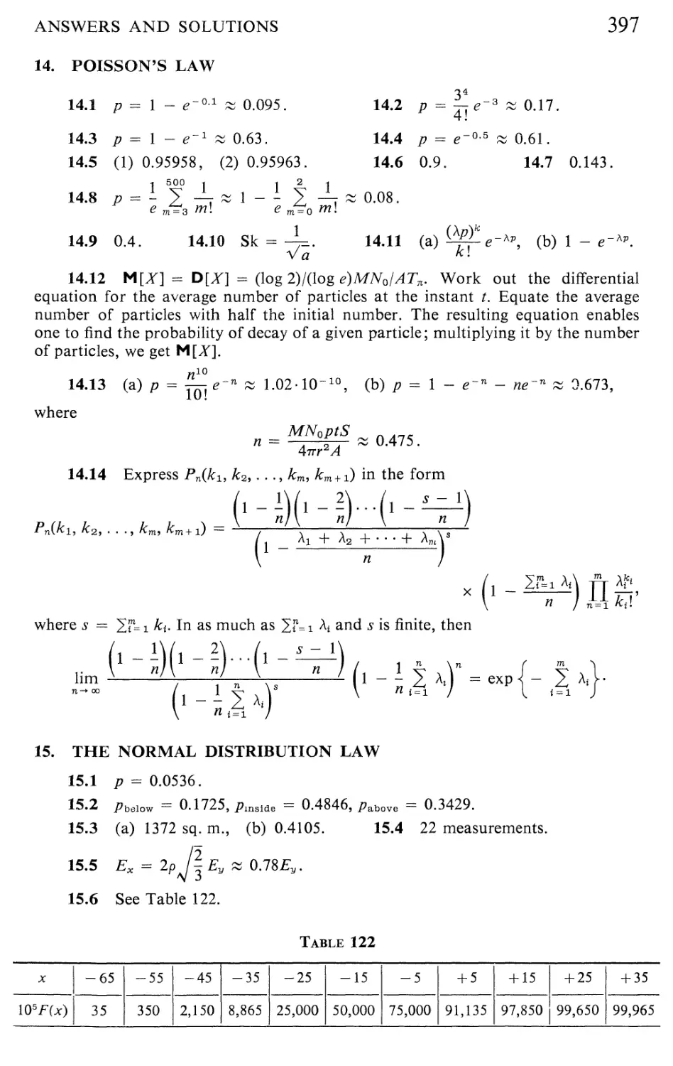
14. Poisson's law 67
15. The normal distribution law 70
16. Characteristic functions 74
17. The computation of the total probability and the probabiUty
density in terms of conditional probability 80
III. SYSTEMS OF RANDOM VARIABLES 84
18. Distribution laws and numerical characteristics of systems of
random variables 84
19. The normal distribution law in the plane and in space.
The multidimensional normal distribution 91
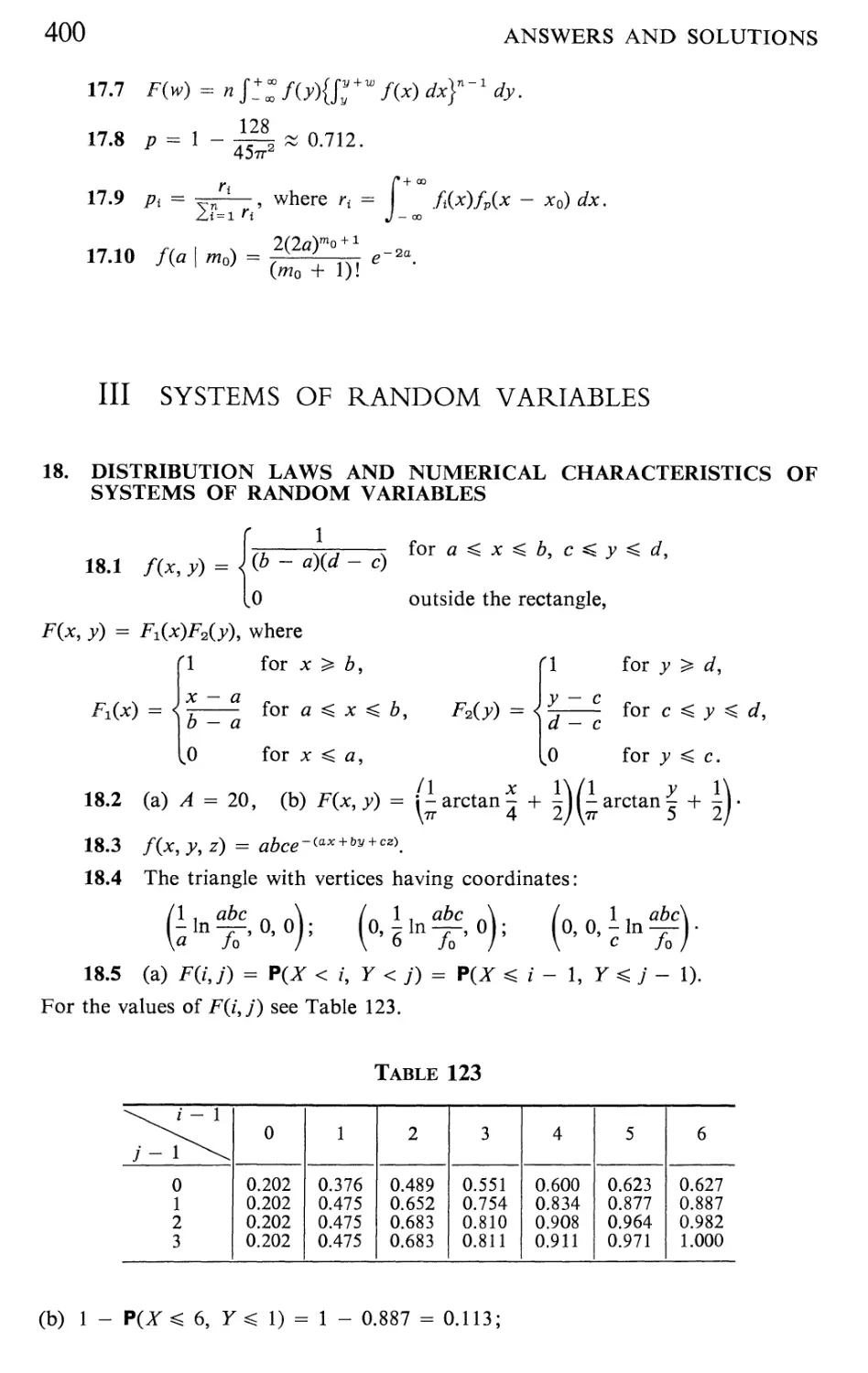
20. Distribution laws of subsystems of continuous random variables
and conditional distribution laws 99
IV. NUMERICAL CHARACTERISTICS AND DISTRIBUTION
LAWS OF FUNCTIONS OF RANDOM VARIABLES 107
21. Numerical characteristics of functions of random variables ... 107
22. The distribution laws of functions of random variables 115
23. The characteristic functions of systems and functions of
random variables 124
24. Convolution of distribution laws 128
25. The linearization of functions of random variables 136
26. The convolution of two-dimensional and three-dimensional
normal distribution laws by use of the notion of
deviation vectors 145
V. ENTROPY AND INFORMATION 157
27. The entropy of random events and variables 157
28. The quantity of information 163
VI. THE LIMIT THEOREMS 171
29. The law of large numbers 171
30. The de Moivre-Laplace and Lyapunov theorems 176

CONTENTS IX
VII. THE CORRELATION THEORY OF RANDOM FUNCTIONS 181
31. General properties of correlation functions and distribution
laws of random functions 181
32. Linear operations with random functions 185
33. Problems on passages 192
34. Spectral decomposition of stationary random functions 198
35. Computation of probability characteristics of random
functions at the output of dynamical systems 205
36. Optimal dynamical systems 216
37. The method of envelopes 226
VIIL MARKOV PROCESSES 231
38. Markov chains 231
39. The Markov processes with a discrete number of states 246
40. Continuous Markov processes 256
IX. METHODS OF DATA PROCESSING 275
41. Determination of the moments of random variables from
experimental data 275
42. Confidence levels and confidence intervals 286
43. Tests of goodness-of-fit 300
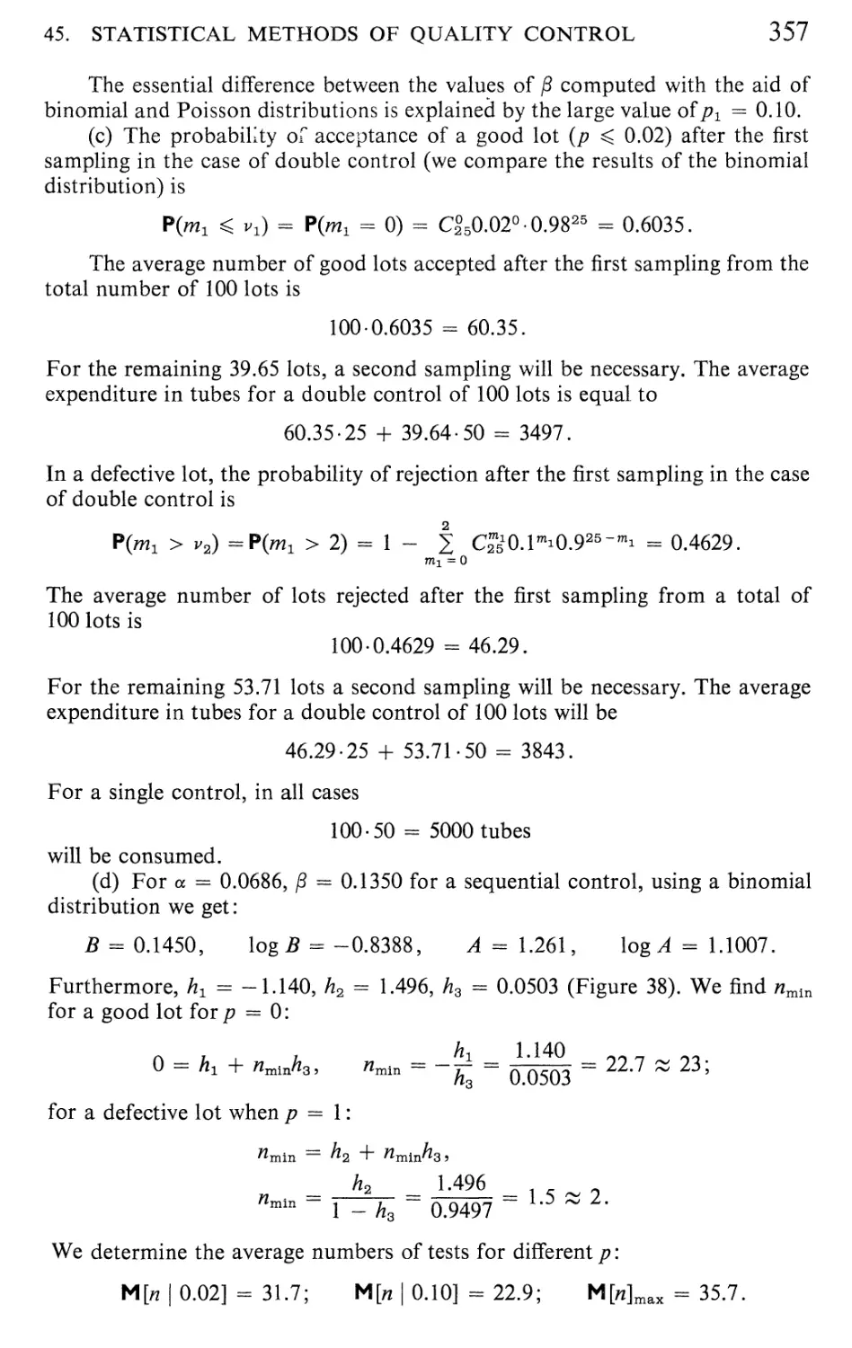
44. Data processing by the method of least squares ..' 325
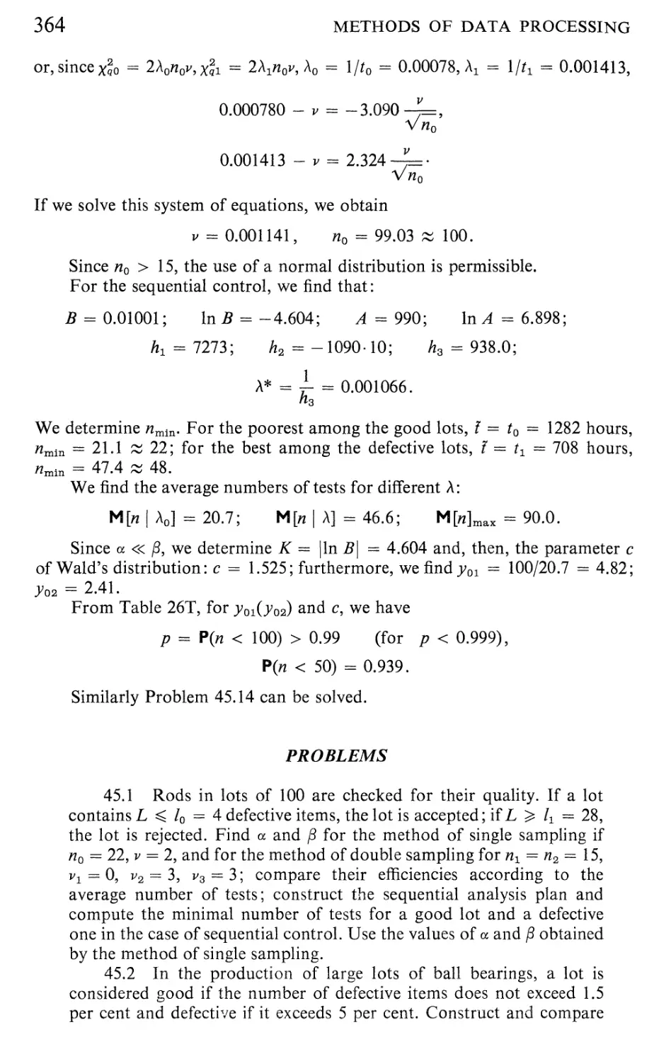
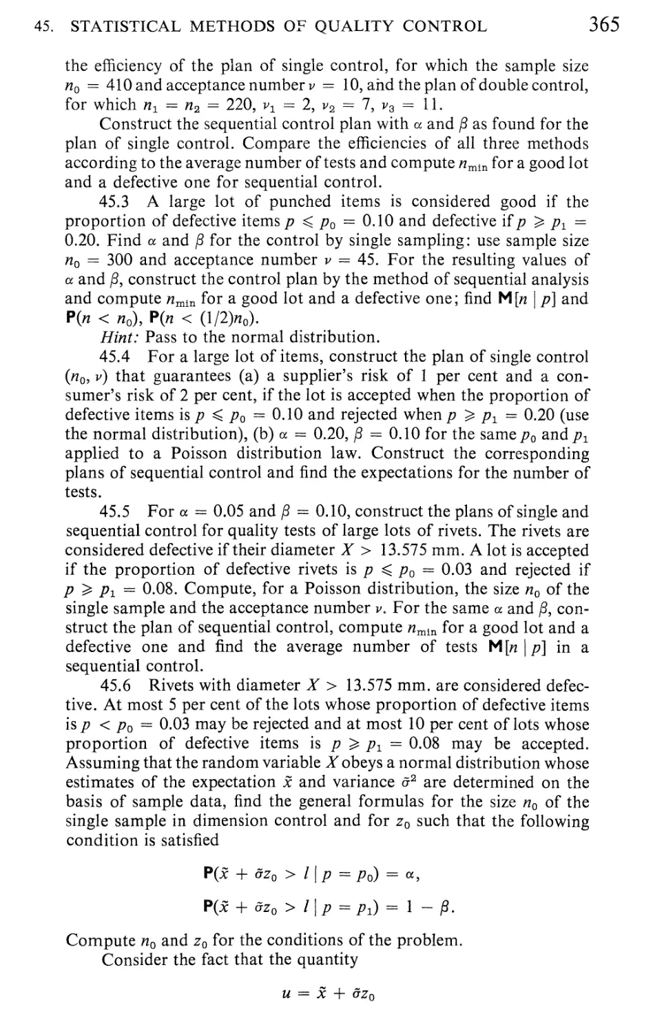
45. Statistical methods of quahty control 346
46. Determination of probabihty characteristics of random
functions from experimental data 368
ANSWERS AND SOLUTIONS 375
SOURCES OF TABLES REFERRED TO IN THE TEXT 471
BIBLIOGRAPHY 475
INDEX 479

I
RANDOM EVENTS
1. RELATIONS AMONG RANDOM EVENTS
Basic Formulas
Random events are usually designated by the letters A, B, C,..., U, V,
where U denotes an event certain to occur and V an impossible event. The
equaUty A = B means that the occurrence of one of the events inevitably brings
about the occurrence of the other. The intersection of two events A and B is
defined as the event C = AB, said to occur if and only if both events A and B
occur. The union of two events A and B is the event C = A ^ B, said to occur
if and only if at least one of the events A and B occurs. The difference of two
events A and B is defined as the event C = ^\^, said to occur if and only if
A occurs and B does not occur. The complementary event is denoted by the
same letter as the initial event, but with an over bar. For instance, A and A
are complementary, A meaning that A does not occur. Two events are said to
be mutually exclusive if AB = V. The events Aj^ (k = 1,2,.. .,n) slvq said to
form a complete set if the experiment results in at least one of these events so
thatUM = i^/c = U.
Solution for Typical Examples
Example 1.1 What kind of events A and B will satisfy the equality
Au B = Al
Solution. The union A\J B means the occurrence of at least one of the
events A and B. Then, for A u B = A, the event A must include the event B.
For example, if A means falling into region Sa and B falhng into region Sb,
then Sb Hes within S^.
The solution to Problems 1.1 to 1.3 and 1.8 is similar.
Example 1.2 Two numbers at random are selected from a table of random
numbers. If the event A means that at least one of these numbers is prime and
the event B that at least one of them is an even number, what is the meaning of
events AB and Akj Bl
Solution. Event AB means that both events A and B occur. The event
A u B means that at least one of the two events occurs; that is, from two selected
1

2 RANDOM EVENTS
numbers at least one number is prime or one is even, or one number is prime
and the other is even.
One can solve Problems 1.4 to 1.7 analogously.
Example 1.3 Prove that AB = A \J B dind C u D = CD.
Proof. If C = A and D = B, the second equality can be written in the
form A u B = AB. Hence it suffices to prove the validity of the first equality.
The event AB means that both events A and B do not occur. The
complementary event AB means that at least one of these events occurs: the union
A\J B. Thus AB = A u B. The proof of this equality can also be carried out
geometrically, an event meaning that a point falls into a certain region.
One can solve Problem 1.9 similarly. The equalities proved in Example 1.3
are used in solving Problems 1.10 to 1.14.
Example 1.4 The scheme of an electric circuit between points M and N
is represented in Figure 1. Let the event A be that the element a is out of order,
and let the events B^{k = 1,2, 3) be that an element b^ is out of order. Write
the expressions for C and C, where the event C means the circuit is broken
between M and N.
Solution. The circuit is broken between M and N if the element a or the
three elements b^{k = 1,2, 3) are out of order. The corresponding events are
A and B^B^B^, Hence C = A\J B^B^B^.
Using the equalities of Example 1.3, we find that
C = y4 u B^B^B^ = AB^B^B^ = A(B^ ^ B^^ B^).
Similarly one can solve Problems 1.16 to 1.18.
PROBLEMS
1.1 What meaning can be assigned to the events A u A and A A ?
1.2 When does the equality AB = A hold?
1.3 A target consists of 10 concentric circles of radius rj^{k = 1,2,
3,..., 10). An event Aj^ means hitting the interior of a circle of radius
rj, (k = 1, 2,. .., 10). What d6 the following events mean:
6 10
B^ [J A„ C= UA,!
k=l fc=5
1.4 Consider the following events: A that at least one of three
devices checked is defective, and B that all devices are good. What is the
meaning of the events (a) A ^ B, (b) ABl
"-Ky
""^ 1
'f^ FIGURE 1
P
Jq.

1. RELATIONS AMONG RANDOM EVENTS
1.5 The events A, B and C mean selecting at least one book
from three different collections of complete works; each collection
consists of at least three volumes. The events A^ and B^ mean that s
volumes are taken from the first collection and k volumes from the
second collection. Find the meaning of the events (a) A u B u C,
(b) ABC, (c) A, u Bs, (d) A2B2, (e) (A.B^ u B,As)C.
1.6 A number is selected at random from a table of random
numbers. Let the event A be that the chosen number is divisible by 5,
and let the event B be that the chosen number ends with a zero. Find the
meaning of the events A\B and AB.
1.7 Let the event A be that at least one out of four items is
defective, and let the event B be that at least two of them are defective.
Find the complementary events A and B. _ _
1.8 Simplify the expression A = {B ^ C){B u C){B u C).
1.9 When do the following equalities hold true: {2i) A ^ B = A,
(b) AB = A,(c) Au B = ABl
1.10 From the following equality find the random event X\
X\J A\J Xu A = B.
1.11 Prove that AB u AB = AB.
1.12 Prove that the following two equalities are equivalent:
u A,= n Aj,, u Aj,= n A,.
k=l k=l k = l k=l
1.13 Can the events A and A u B hQ simultaneous ?
1.14 Prove that A, AB and A u B form a complete set of events.
1.15 Two chess players play one game. Let the event A be that the
first player wins, and let B be that the second player wins. What event
should be added to these events to obtain a complete set ?
1.16 An installation consists of two boilers and one engine. Let the
event A be that the engine is in good condition, let Bj^{k = 1,2) be that
the /cth boiler is in good condition, and let C be that the installation can
operate if the engine and at least one of the boilers are in good
condition. Express the events C and C in terms of A and Bj^.
1.17 A vessel has a steering gear, four boilers and two turbines.
Let the event A be that the steering gear is in good condition, let
Bj^ (k = 1,2, 3, 4) be that the boiler labeled k is in good condition,
let Cy (j = 1, 2) be that the turbine labeled/ is in good condition, and
let D be that the vessel can sail if the engine, at least one of the boilers
and at least one of the turbines are in good condition. Express D and D
in terms of A and Bj,.
1.18 A device is made of two units of the first type and three units
of the second type. Let Aj, {k = 1,2) be that the /cth unit of the first
type is in good condition, let Bj {j = 1, 2, 3) be that the /th unit of the
second type is in good condition, and let C be that the device can operate
if at least one unit of the first type and at least two units of the second type
are in good condition. Express the event C in terms of Aj^ and Bj.

4 RANDOM EVENTS
2. A DIRECT METHOD FOR EVALUATING PROBABILITIES
Basic Formulas
If the outcomes of an experiment form a finite set of n elements, we shall
say that the outcomes are equally probable if the probability of each outcome
is l/«. Thus if an event consists of m outcomes, the probability of the event
is/? = min.
Solution for Typical Examples
Example 2.1 A cube v^hose faces are colored is split into 1000 small cubes
of equal size. The cubes thus obtained are mixed thoroughly. Find the probability
that a cube drawn at random will have two colored faces.
Solution. The total number of small cubes is « = 1000. A cube has 12
edges so that there are eight small cubes with two colored faces on each edge.
Hence m = 12-8 = 96,;? = m/« = 0.096.
Similarly one can solve Problems 2.1 to 2.7.
Example 2.2 Find the probability that the last two digits of the cube of a
random integer will be 1. ^
Solution. Represent N in the form A/' = a + lOZ? -h • • ¦, where a,b,...
are arbitrary numbers ranging from 0 to 9. Then N^ = a^ + 30a^b + • • •. From
this we see that the last two digits of A^^ are affected only by the values of a and b.
Therefore the number of possible values is n = 100. Since the last digit of A^^
is a 1, there is one favorable value a = I. Moreover, the last digit of (A^^ - 1)/10
should be 1; i.e., the product 3b must end with a 1. This occurs only if ^ = 7.
Thus the favorable value (a = I, b = 1) is unique and, therefore, p = 0.01.
Similarly one can solve Problems 2.8 to 2.11.
Example 2.3 From a lot of n items, k are defective. Find the probability
that /items out of a random sample of size m selected for inspection are defective.
Solution. The number of possible ways to choose m items out of n is
Cn- The favorable cases are those in which / defective items among the k
defective items are selected (this can be done in Cl ways), and the remaining
m — 1 items are nondefective, i.e., they are chosen from the total number n — k
(in Cn-ic ways). Thus the number of favorable cases is CiCn-k- The required
probability will htp = (CLC^_-;J)/C;r.
One can solve Problems 2.12 to 2.20 similarly.
Example 2.4 Five pieces are drawn from a complete domino set.
Find the probability that at least one of them will have six dots marked on it.
Solution. Find the probability q of the complementary event. Then
p ^ \ — q. The probability that all five pieces will not have a six (see Example
2.3) is ^ = (C?Cii)/Ci8 and, hence,
/7 = 1 - S = 0.793.
^ By a "random number" here we mean a /:-digit number {k > 1) such that any of
its digits may range from 0 to 9 with equal probability.

2. A DIRECT METHOD FOR EVALUATING PROBABILITIES 5
By a similar passage to the complementary event, one can solve Problems
2.21 and 2.22.
PROBLEMS
lA Lottery tickets for a total ofn dollars are on sale. The cost of
one ticket is r dollars, and m of all tickets carry valuable prizes. Find
the probability that a single ticket will win a valuable prize.
2.2 A domino piece selected at random is not a double. Find the
probability that the second piece also selected at random, will match the
first.
2.3 There are four suits in a deck containing 36 cards. One card
is drawn from the deck and returned to it. The deck is then shuffled
thoroughly and another card is drawn. Find the probability that both
cards drawn belong to the same suit.
2.4 A letter combination lock contains five disks on a common
axis. Each disk is divided into six sectors with diff*erent letters on each
sector. The lock can open only if each of the disks occupies a certain
position with respect to the body of the lock. Find the probability that
the lock will open for an arbitrary combination of the letters.
2.5 The black and white kings are on the first and third rows,
respectively, of a chess board. The queen is placed at random in one of
the free squares of the first or second row. Find the probability that the
position for the black king becomes checkmate if the positions of the
kings are equally probable in any squares of the indicated rows.
2.6 A wallet contains three quarters and seven dimes. One coin is
drawn from the wallet and then a second coin, which happens to be a
quarter. Find the probability that the first coin drawn is a quarter.
2.7 From a lot containing m defective items and n good ones, s
items are chosen at random to be checked for quality. As a result of this
inspection, one finds that the first A: of ^ items are good. Determine
the probability that the next iteni will be good.
2.8 Determine the probability that a randomly selected integer A^
gives as a result of (a) squaring, (b) raising to the fourth power,
(c) multiplying by an arbitrary integer, a number ending with a 1.
2.9 On 10 identical cards are written different numbers from 0 to
9. Determine the probability that (a) a two-digit number formed at
random with the given cards will be divisible by 18, (b) a random three-
digit number will be divisible by 36.
2.10 Find the probability that the serial number of a randomly
chosen bond contains no identical digits if the serial number may be any
five-digit number starting with 00001.
2.11 Ten books are placed at random on one shelf. Find the
probability that three given books will be placed one next to the other.
2.12 The numbers 2, 4, 6, 7, 8, 11, 12 and 13 are written,
respectively, on eight indistinguishable cards. Two cards are selected at random
from the eight. Find the probability that the fraction formed with these
two random numbers is reducible.

RANDOM EVENTS
2.13 Given five segments of lengths 1, 3, 5, 7 and 9 units, find the
probability that three randomly selected segments of the five will be the
sides of a triangle.
2.14 Two of 10 tickets are prizewinners. Find the probability that
among five tickets taken at random (a) one is a prizewinner, (b) two are
prizewinners, (c) at least one is a prizewinner.
2.15 This is a generalization of Problem 2.14. There are n + m
tickets of which n are prizewinners. Someone purchases k tickets at the
same time. Find the probability that s of these tickets are winners.
2.16 In a lottery there are 90 numbers, of which five win. By
agreement one can bet any sum on any one of the 90 numbers or any set of
two, three, four or five numbers. What is the probability of winning in
each of the indicated cases ?
2.17 To decrease the total number of games, 2n teams have been
divided into two subgroups. Find the probability that the two strongest
teams will be (a) in different subgroups, (b) in the same subgroup.
2.18 A number of « persons are seated in an auditorium that can
accommodate n + k people. Find the probability that m ^ n given
seats are occupied.
2.19 Three cards are drawn at random from a deck of 52 cards.
Find the probability that these three cards are a three, a seven and an ace.
2.20 Three cards are drawn at random from a deck of 36 cards.
Find the probability that the sum of points of these cards is 21 if the jack
counts as two points, the queen as three points, the king as four points, the
ace as eleven points and the rest as six, seven, eight, nine and ten points.
2.21 Three tickets are selected at random from among five tickets
worth one dollar each, three tickets worth three dollars each and two
tickets worth five dollars each. Find the probability that (a) at least two
of them have the same price, (b) all three of them cost seven dollars.
2.22 There are 2n children in line near a box office where tickets
priced at a nickel each are sold. What is the probability that nobody will
have to wait for change if, before a ticket is sold to the first customer, the
cashier has 2m nickels and it is equally probable that the payments for
each ticket are made by a nickel or by a dime.
3. GEOMETRIC PROBABILITIES
Basic Formulas
The geometric definition of probability can be used only if the probability
of hitting any part of a certain domain is proportional to the size of this domain
(length, area, volume, and so forth), and is independent of its position and shape.
If the geometric size of the whole domain equals S, the geometric size of a
part of it equals Sb, and a favorable event means hitting Sb, then the probability
of this event is defined to be
Sb
^ = ^'
The domains can have any number of dimensions.

3. GEOMETRIC PROBABILITIES 7
Solution for Typical Examples
Example 3.1 The axes of indistinguishable vertical cylinders of radius r
pass through an interval / of a straight line AB, which lies in a horizontal plane.
A ball of radius R is thrown at an angle q to this line. Find the probability that
this ball will hit one cylinder if any intersection point of the path described by
the center of the ball with the line AB is equally probable. ^
Solution. Let x be the distance from the center of the ball to the nearest
line that passes through the center of a cylinder parallel to the displacement
direction of the center of the ball. The possible values of x are determined by
the conditions (Figure 2)
0 < a: ^ :r / sin ^.
The collision of the ball with the cylinder may occur only if 0 ^ x ^ R + r.
The required probability equals the ratio between the length of the segment
on which lie the favorable values of x and the length of the segment on which
lie all the values of x. Consequently,
' for i< + r :^ - sm^;
P = ^
Isinq "" 2 '
1 forR + r^- sinq.
One can solve problems 3.1 to 3.4 and 3.24 analogously.
Example 3.2 On one track of a magnetic tape 200 m. long some
information is recorded on an interval of length 20 m., and on the second track similar
information is recorded. Estimate the probability that from 60 to 85 m. there is
no interval on the tape without recording if the origins of both recordings are
located with equal probability at any point from 0 to 180 m.
Solution. Let x and y be the coordinates of origin of the recordings,
where x '^ y. Since 0 ^^ ;v: ^ 180, 0 ^ j ^ 180 and x ^ y, the domain of all
the possible values of x and j^ is a right triangle with hypotenuse 180 m. The
area of this triangle is S = 1/2-180^ sq. m. Find the domain of values of x and jj;
FIGURE 2
^ The restriction of equal probability used in formulating several problems with a
point that hits the interior of any part of a domain (linear, two-dimensional, and so forth)
is understood only in connection with the notion of geometric probabiUty.

RANDOM EVENTS
FIGURE 3
favorable to the given event. To obtain a continuous recording, it is necessary
that the inequaUty x — y ^ 20 m. hold true. To obtain a recording interval
longer than or equal to 25 m., we must have x — y ^ 5 m. Moreover, to obtain
a continuous recording on the interval from 60 to 85 m., we must have
45 m. :^ ;; ^ 60 m.,
65 m. < jc < 80 m.
Drawing the boundaries of the indicated domains, we find that the favorable
values of x and y are included in a triangle whose area Sb = 1/2-15^ sq. m.
(Figure 3). The required probability equals the ratio of the area Sb favorable
to the given event and the area of the domain S containing all possible values of
X and y, namely,
= (IIY = JL
^ \180/ 144'
One can solve Problems 3.5 to 3.15 similarly.
Example 3.3 It is equally probable that two signals reach a receiver at
any instant of the time T. The receiver will be jammed if the time difference in
the reception of the two signals is less than r. Find the probability that the
receiver will be jammed.
Solution. Let x and y be the instants when the two signals are received.
The domain of all the possible values of x, 3; is a square of area T^ (Figure 4).
FIGURE 4
^*r

3. GEOMETRIC PROBABILITIES
FIGURE 5
The receiver will be jammed if |x — j| ^ r. The given domain lies between the
straight lines x — y = t and x — y = —r.lts area equals
S, = S-(T- rf,
and, therefore,
One can solve Problems 3.16 to 3.19 analogously.
Example 3.4 Find the probability that the sum of two random positive
numbers, each of which does not exceed one, will not exceed one, and that their
product will be at most 2/9.
Solution. Let x and j be the chosen numbers. Their possible values are
0^:v< 1, O^j^^ 1, defining in the plane a square of area S = I. The
favorable values satisfy the conditions x + _y ^ 1 and xy ^ 2/9. The boundary
X + y = I divides the square in two so that the domain x + ;; ^^ 1 represents
the lower triangle (Figure 5). The second boundary xy = 2/9 is a hyperbola.
The x's of the intersection points of these boundaries are: Xi = 1/3 and
X2 = 2/3. The area of the favorable domain is
1 r
= 3 +
2/3 12
1/3 J y
J:
2/3 dx 1 2
1/3
X
The desired probability is p = Sb/S = 0.487.
One can solve Problems 3.20 to 3.23 in a similar manner.
PROBLEMS
3.1 A break occurs at a random point on a telephone line AB of
length L. Find the probability that the point C is at a distance not less
than / from the point A.
3.2 Parallel lines are drawn in a plane at alternating distances
of 1.5 and 8 cm. Estimate the probability that a circle of radius 2.5 cm.
thrown at random on this plane will not intersect any line.

10 RANDOM EVENTS
3.3 In a circle of radius R chords are drawn parallel to a given
direction. What is the probability that the length of a chord selected at
random will not exceed R if any positions of the intersection points of
the chord with the diameter perpendicular to the given direction are
equally probable ?
3.4 In front of a disk rotating with a constant velocity we place a
segment of length 2h in the plane of the disk so that the line joining the
midpoint of the segment with the center of the disk is perpendicular to
this segment. At an arbitrary instant a particle flies off" the disk. Estimate
the probability that the particle will hit the segment if the distance
between the segment and the center of the disk is /.
3.5 A rectangular grid is made of cylindrical twigs of radius r.
The distances between the axes of the twigs are a and b respectively.
Find the probability that a ball of diameter d, thrown without aiming,
will hit the grid in one trial if the flight trajectory of the ball is
perpendicular to the plane of the grid.
3.6 A rectangle 3 cm. x 5 cm. is inscribed in an ellipse with the
semi-axes a = 100 cm. and b = 10 cm. so that its larger side is parallel
to a. Furthermore, one constructs four circles of diameter 4.3 cm. that
do not intersect the ellipse, the rectangle and each other.
Determine the probability that (a) a random point whose position
is equally probable inside the ellipse will turn out to be inside one of the
circles, (b) the circle of radius 5 cm. constructed with the center at this
point will intersect at least one side of the rectangle.
3.7 Sketch five concentric circles of radius kr, where k = 1,2,
3, 4, 5, respectively. Shade the circle of radius r and two annuli with the
corresponding exterior radii of 3r and 5r. Then select at random a point
in the circle of radius 5r. Find the probability that this point will be in
(a) the circle of radius 2r, (b) the shaded region.
3.8 A boat, which carries freight from one shore of a bay to the
other, crosses the bay in one hour. What is the probability that a ship
moving along the bay will be noticed if the ship can be seen from the
boat at least 20 minutes before the ship intersects the direction of the
boat and at most 20 minutes after the ship intersects the direction of
the boat? All times and places for intersection are equally likely.
3.9 Two points are chosen at random on a segment of length /.
Find the probabiUty that the distance between the points is less than kl,
ifO < k < L
3.10 Two points L and M are placed at random on a segment
AB of length /. Find the probabihty that the point L is closer to M than
to .4.
3.11 On a segment of length /, two points are placed at random so
that the segment is divided into three parts. Find the probability that
these three parts of the segment are sides of a triangle.
3.12 Three points A, B, C are placed at random on a circle of
radius R. What is the probability that the triangle ABC is acute-angled?
3.13 Three line segments, each of a length not exceeding /, are
chosen at random. What is the probabiUty that they can be used to form
the sides of a triangle ?

3. GEOMETRIC PROBABILITIES 11
3.14 Two points M and A^ are placed on a segment AB of length /.
Find the probabiUty that the length of each of the three segments thus
obtained does not exceed a given value a (I ^ a ^ 1/3).
3.15 A bus of line A arrives at a station every four minutes and a
bus of line B every six minutes. The length of an interval between the
arrival of a bus of line A and a bus of line B may be any number of
minutes from zero to four, all equally likely.
Find the probability that (a) the first bus that arrives belongs to
line A,{b) 3. bus of any line arrives within two minutes.
3.16 Two ships must arrive at the same moorings. The times of
arrival for both ships are independent and equally probable during a
given period of 24 hours. Estimate the probability that one of the ships
will have to wait for the moorings to be free if the mooring time for the
first ship is one hour and for the second ship two hours.
3.17 Two persons have the same probability of arriving at a
certain place at any instant of the interval T. Find the probability that
the time that a person has to wait for the other is at most t.
3.18 Two ships are sailing in a fog, one along a bay of width L and
the other across the same bay. Their velocities are v^ and Vz. The second
ship emits sounds that can be heard at a distance d < L. Find the
probability that the sounds will be heard on the first ship if the
trajectories of the two ships may intersect with equal probabilities at
any point.
3.19 A bar of length / = 200 mm. is broken at random into pieces.
Find the probability that at least one piece between two break-points
is at most 10 mm. if the number of break-points is (a) two, (b) three,
and a break can occur with equal probability at any point of the bar.
3.20 Two arbitrary points are selected on the surface of a sphere
of radius R. What is the probability that an arc of a great circle passing
through these points will make an angle less than a, where a < tt?
3.21 A satellite moves on an orbit between 60 degrees northern
latitude and 60 degrees southern latitude. Assuming that the satelHte
can splash down with equal probability at any point on the surface of the
earth between the previously mentioned parallels, find the probability
that the satellite will fall above 30 degrees northern latitude.
3.22 A plane is shaded by parallel lines at a distance L between
adjacent lines. Find the probability that a needle of length /, where
I < L, thrown at random will intersect some line (BufiFon's problem).
3.23 Estimate the probability that the roots of (a) the quadratic
equation x^ + lax + b = 0, (b) the cubic equation x^ + 3ax -\- 2b = 0
are real, if it is known that the coefficients are equally likely in the
rectangle \a\ ^ n, \b\ ^ m. Find the probability that under the given
conditions the roots of the quadratic equation will be positive.
3.24 A point A and the center 5 of a circle of radius R move
independently in a plane. The velocities of these points are constant and
equal u and v. At a given instant, the distance AB equals r (r > R), and
the angle made by the line AB with the vector v equals ^. Assuming that
all directions for the point A are equally probable, estimate the
probability that the point A will be inside the circle.

12 RANDOM EVENTS
4. CONDITIONAL PROBABILITY. THE MULTIPLICATION
THEOREM FOR PROBABILITIES
Basic Formulas
The conditional probability ?{A \ B) of the event A is the probability of
A under the assumption that the event B has occurred. (It is assumed that the
probability of B is positive.) The events A and B are independent if P{A \ B) =
P{A). The probability for the product of two events is defined by the formula
P{AB) = P(A)PiB I A) = P(B)P(A \ B),
which, generalized for a product ofn events, is
P(n/.) = P(A,)P(A, I A,)P(A, I A,A,)- • -Pj^^^lg a).
The events A^, A2,. .., ^4^ are said to be independent if for any m, where
m = 2,3,. . .,n, and any kj (j = 1,2,. . .,n), I ^ ki < k2 < - ¦ - < k^ ^ n.
iR'-)
n p(^.,).
Solution for Typical Examples
Example 4.1 The break in an electric circuit occurs when at least one out
of three elements connected in series is out of order. Compute the probability
that the break in the circuit will not occur if the elements may be out of order
with the respective probabilities 0.3, 0.4 and 0.6. How does the probability
change if the first element is never out of order ?
Solution. The required probability equals the probability that all three
elements are working. Let A^{k = 1,2, 3) denote the event that the kth element
functions. Then;? = P(^i^2^3)- Since the events may be assumed independent,
p ^ P(^i)P(^2)P(^3) = 0.7-0.6.0.4 = 0.168.
If the first element is not out of order, then
p ^ P(^2^3) = 0.24.
Similarly one can solve Problems 4.1 to 4.10.
Example 4.2 Compute the probability that a randomly selected item is of
first grade if it is known that 4 per cent of the entire production is defective,
and 75 per cent of the nondefective items satisfy the first grade requirements.
It is given that P(^) - 1 - 0.04 = 0.96, P(^ | A) = 0.75.
The required probability;? = P(AB) - @.96)@.75) - 0.72.
Similarly one can solve Problems 4.11 to 4.19.
Example 4.3 A lot of 100 items undergoes a selective inspection. The
entire lot is rejected if there is at least one defective item in five items checked.
What is the probability that the given lot will be rejected if it contains 5 per cent
defective items ?

4. THE MULTIPLICATION THEOREM FOR PROBABILITIES 13
Solution. Find the probability q of the complementary event A consisting
of the situation in which the lot will be accepted. The given event is an
intersection of five events A = AiA2A^A^A^, where Aj^(k = 1, 2, 3, 4, 5) means that
the kth item checked is good.
The probability of the event Ai is P{Ai) = 95/100 since there are only
100 items, of which 95 are good.
After the occurrence of the event Ai, there remain 99 items, of which 94
are good and, therefore, P(^2 I ^i) = 94/99. Analogously, P(^3 | A^Az) =
93/98, P(A^ I A^A^As) = 92/97 and P{A^ \ A^A^A^A^) = 91/96. According to
the general formula, we find that
^^94939291^
^ 100'99'98"97'96
The required probability/> = 1 — ^ = 0.23.
One can solve Problems 4.20 to 4.35 similarly.
PROBLEMS
4.1 Two marksmen whose probabilities of hitting a target are 0.7
and 0.8, respectively, fire one shot each. Find the probability that at
least one of them will hit the target.
4.2 The probability that the /:th unit of a computer is out of order
during a time T equals pj^ (k = 1,2,..., n). Find the probability that
during the given interval of time at least one of n units of this computer
will be Out of order if all the units run independently.
4.3 The probability of the occurrence of an event in each
performance of an experiment is 0.2. The experiments are carried out
successively until the given event occurs. Find the probability that it will be
necessary to perform a fourth experiment.
4.4 The probability that an item made on the first machine is of
first grade is 0.7. The probability that an item made on the second
machine is first grade is 0.8. The first machine makes two items and the
second machine three items. Find the probability that all items made
will be of first grade.
4.5 A break in an electric circuit may occur only if one element K
or two independent elements Ki and K2 are out of order with respective
probabilities 0.3, 0.2 and 0.2. Find the probability of a break in the
circuit.
4.6 A device stops as a result of damage to one tube of a total
of A^. To locate this tube one successively replaces each tube with a new
one. Find the probability that it will be necessary to check n tubes if the
probability is p that a tube will be out of order.
4.7 How many numbers should be selected from a table of random
numbers so that the probability of finding at least one even number
among them is 0.9?
4.8 The probability that as a result of four independent trials the
event A will occur at least once is 0.5. Find the probability that the event

14 RANDOM EVENTS
will occur in one trial if this probability is constant through all the other
trials.
4.9 An equilateral triangle is inscribed in a circle of radius R. What
is the probability that four points taken at random in the given circle are
inside this triangle ?
4.10 Find the probability that a randomly written fraction will be
irreducible (Chebyshev's problem).^
4.11 If two mutually exclusive events A and B are such that
P(AO^0 and P(B)=^0, are these events independent?
4.12 The probability that the voltage of an electric circuit will
exceed the rated value is p^. For an increase in the voltage, the
probability that an electric device will stop is;72- Fiiid the probability that the
device will stop as a result of an increase in the voltage.
4.13 A motorcyclist in a race must pass through 12 obstacles
placed along a course AB; he will stop at each of them with probability
0.1. Knowing the probability 0.7 with which the motorcyclist passes
from B to the final point C without stops, find the probability that no
stops will occur on the segment AC.
4.14 Three persons play a game under the following conditions:
At the beginning, the second and third play in turns against the first.
In this case, the first player does not win (but might not lose either) and
the probabilities that the second and third win are both 0.3. If the first
does not lose, he then makes one move against each of the other two
players and wins from each of them with the probabiHty 0.4. After this,
the game ends. Find the probability that the first player wins from at
least one of the other two.
4.15 A marksman hits a target with the probability 2/3. If he
scores a hit on the first shot, he is allowed to fire another shot at another
target. The probability of failing to hit both targets in three trials is 0.5.
Find the probability of failing to hit the second target.
4.16 Some items are made by two technological procedures. In
the first procedure, an item passes through three technical operations,
and the probabilities of a defect occurring in these operations are 0.1,
0.2 and 0.3. In the second procedure, there are two operations, and the
probability of a defect occurring in each of them is 0.3. Determine
which technology ensures a greater probability of first grade production
if in the first case, for a good item, the probability of first grade
production is 0.9, and in the second case 0.8.
4.17 The probabilities that an item will be defective as a result of
a mechanical and a thermal process are pi and p2, respectively. The
probabilities of eliminating defects are p^ and 774, respectively.
Find (a) how many items should be selected after the mechanical
process in order to be able to claim that at least one of them can undergo
the thermal process with a chance of eliminating the defect, (b) the
probability that at least one of three items will have a nonremovable
defect after passing through the mechanical and thermal processes.
^ Consider that the numerator and denominator are randomly selected numbers from
the sequence 1,2,...,/:, and set k-^cc.

4. iHE MULTIPLICATION THEOREM FOR PROBABILITIES 15
4.18 Show that if the conditional probability P(A \ B) exceeds the
unconditional probability P(^), then the conditional probability
P{B I A) exceeds the unconditional probability P{B).
4.19 A target consists of two concentric circles of radius kr and nr,
where k < n. If it is equally probable that one hits any part of the circle
of radius nr, estimate the probability of hitting the circle of radius kr
in two trials.
4.20 With six cards, each containing one letter, one forms the
word latent. The cards are then shuffled and at random cards are drawn
one at a time. What is the probability that the arrangement of letters
will form the word talent']
4.21 A man has forgotten the last digit of a telephone number and,
therefore, he dials it at random. Find the probability that he must dial
at most three times. How does the probability change if one knows that
the last digit is an odd number ?
4.22 Some m lottery tickets out of a total of n are the winners.
What is the probability of a winner in k purchased tickets ?
4.23 Three lottery tickets out of a total of 40,000 are the big
prizewinners. Find (a) the probability of getting at least one big
prizewinner (ticket) per 1000 tickets, (b) how many tickets should be
purchased so that the probability of one big winner is at least 0.5.
4.24 Six regular drawings of state bonds plus one supplementary
drawing after the fifth regular one take place annually. From a total of
100,000 serial numbers, the winners are 170 in each regular drawing
and 270 in each supplementary one. Find the probability that a bond
wins after ten years in (a) any drawing, (b) a supplementary drawing,
(c) a regular drawing.
4.25 Consider four defective items: one item has the paint
damaged, the second has a dent, the third is notched and the fourth
has all three defects mentioned. Consider also the event A that the first
item selected at random has the paint damaged, the event B that the
second item has a dent and the event C that the third item is notched.
Are the given events independent in pairs or as a whole set ?
4.26 Let Ai, Az,..., ^4^ be a set of events independent in pairs.
Is it true that the conditional probability that an event occurs, computed
under the assumption that other events of the same set have occurred,
is the unconditional probability of this event?
4.27 A square is divided by horizontal lines into n equal strips.
Then a point whose positions are equally probable in the strip is taken
in each strip. In the same way one draws n — I vertical lines. Find the
probability that each vertical strip will contain only one point.
4.28 A dinner party of 2n persons has the same number of males
and females. Find the probability that two persons of the same sex will
not be seated next to each other.
4.29 A party consisting of five males and 10 females is divided at
random into five groups of three persons each. Find the probability
that each group will have one male member.
4.30 An urn contains n -\- m identical balls, of which n are white
and m black, where m ^ n. A person draws balls n times, two balls at a

16 RANDOM EVENTS
time, without returning them to the urn. Find the probability of drawing
a pair of balls of different colors each time.
4.31 An urn contains n balls numbered from 1 to n. The balls are
drawn one at a time without being replaced in the urn. What is the
probability that in the first k draws the numbers on the balls will coincide
with the numbers of the draws ?
4.32 An urn contains two kinds of balls, white ones and black
ones. The balls are drawn one at a time until a black ball appears, and
each time when a white ball is drawn it is returned to the urn together
with two additional balls. Find the probability that in the first 50 trials
no black balls will be drawn.
4.33 There are « + m men in line for tickets that are priced at five
dollars each; n of these men have five-dollar bills and m, where
m ^ n + \, have ten-dollar bills. Each person buys only one ticket.
The cashier has no money before the box office opens. What is the
probability that no one in the line will have to wait for change?
4.34 The problem is the same as in 4.33, but now the ticket costs
one dollar and n of the customers have one-dollar bills whereas m have
five-dollar bills, where 2m ^ « + 1.
4.35 Of two candidates, No. 1 receives n votes whereas No. 2
receives m (n > m) votes. Estimate the probability that at all times
during the vote count No. 1 will lead No. 2.
5. THE ADDITION THEOREM FOR PROBABILITIES
Basic Formulas
The probability of the union of two events is given by
P(A UB)= P(A) + P(^) - P{AB),
which can be extended to a union of any number of events:
(n \ n n-1 n
U aA= 1 P(A,) - 2 2 PiA^A,)
k = l J fc = l /c = l; = /c + l
n-2n-ln /^\
+ 2 2 2 P(^.^y^i)---- + (-i)''-^P n A .
fc=lj=k+l i=j+l \k=l /
For mutually exclusive events, the probability of a union of events is the
sum of the probabilities of these events: that is,
P(u a)= 2 P(A).
\k=l J fc=l
Solution for Typical Examples
Example 5.1 Find the probability that a lot of 100 items, of which five
are defective, will be accepted in a test of a randomly selected sample containing
half the lot if, to be accepted, the number of defective items in a lot of 50 cannot
exceed one.

5. THE ADDITION THEOREM FOR PROBABILITIES
17
Solution. Let A be the event denoting that there is no defective item
among those tested and B that there is only one defective item. The required
probabihty is p = P(^) + P(^). The events A and B are mutually exclusive.
Thus p = P(A) -f P{By
There are Cioo ways of selecting 50 items from a total of 100. From 95
nondefective items one can select 50 items in Cis ways. Therefore, P(^) =
CEg/Cfgo. Analogously P{B) = C^Cli/Cfgo. Then
P =
+
47-37
99-97
= 0.181.
Problems 5.1 to 5.12 are solved similarly.
Example 5.2 The scheme of the electric circuit between two points M
and A^ is given in Figure 6. Malfunctions during an interval of time T of different
elements of the circuit represent independent events with the following
probabilities (Table 1).
Table 1
Element
Probability
K,
0.6
K^
0.5
Li
0.4
L2
0.7
Ls
0.9
Find the probability of a break in the circuit during the indicated interval
of time.
Solution. Denote by A^ (j = 1, 2) the event meaning that an element
Kj is out of order, by A that at least one element Kj is out of order and by B
that all three elements L^ (i = I, 2, 3) are out of order.
Then, the required probability is
Since
p = PiAuB)= PiA) + P(B) - P(A)P(B).
P(A) = P{A,) + P(A,) - P{A,)P{A^) = 0.8,
P(^) = P(L,)P{L,)P{Ls) = 0.252,
we get;? ::^ 0.85.
One can solve Problems 5.13 to 5! 16 analogously.
Example 5.3 The occurrence of the event A is equally probable at any
instant of the interval T. The probability that A occurs during this interval is p.
It is known that during an interval t < T, the given event does not occur.
FIGURE 6
^-^
Or
¦oS-*

18 RANDOM EVENTS
Find the probability P that the event A will occur during the remaining interval
of time.
Solution. The probability p that the event A occurs during the interval
ris the probability — p that the given event occurs during time t plus the product
of the probability 11 — —p\ that A will not occur during t by the conditional
probability that it will occur during the remaining time if it did not occur
before. Thus, the following equality holds true:
P ^'fP + y '- fPy
From this we find
Example 5.4 An urn contains n white balls, m black balls and / red balls,
which are drawn at random one at a time (a) without replacement, (b) with
replacement of each ball to the urn after each draw. Find the probability that
in both cases a white ball will be drawn before a black one.
Solution. Let Pi be the probability for a white ball to be drawn before a
black one, and Pu be the probability for a black ball to be drawn before a
white ball.
The probability Pi is the sum of probabilities of drawing a white ball
immediately after a red ball, two red balls, and so forth. Thus, in the case without
replacement we have
p.= ." , ,+ '
n + m + I n + m + ln + m + l— I
+ I LiJ ^ +,
n + m + ln + m + l— In + m + l—2
and in the case with replacement,
_ « In Pn n
n + m + I (n -{- m + ly (n -\- m -\- ly n -\- m
To obtain the probabilities Pn? replace n hy m and m by « in the preceding
formulas. From this it follows in both cases that Pj '.Pu = n'.m. Furthermore,
since Pi + Pu = 1, the required probability in the case without replacement is
also Pi = nl{n + m).
One can solve Problems 5.23 to 5.27 similarly.
Example 5.5 A person wrote n letters, sealed them in envelopes and wrote
the different addresses randomly on each of them. Find the probability that
at least one of the envelopes has the correct address.

5. THE ADDITION THEOREM FOR PROBABILITIES 19
Solution. Let the event Aj^ mean that the A:th envelope has the correct
address, where k = 1,2,. . .,n. The desired probabihty is p = P(U/5=i ^k)-
The events Aj^ are simultaneous; for any k, j, i,. .. the following equalities
obtain:
P(^.) = ! = <"-')'
n n
P{A,A,) = P{A,)PiA, I A,) = ^^^-J^^
PiA^A^Ad
(n ~ 3)!
and finally.
or
p(fl a\ = i-
Using the formula for the probability of a sum of n events we obtain
,(«-!)! ^,(«-2)! («-3)! ,/_n-il
;, = i-l + i-..-+(-ir-l.
For large /2, /? ;^ 1 — e"^.
Similarly, one can solve Problems 5.32 to 5.38.
PROBLEMS
5.1 Any one of four mutually exclusive events may occur with the
corresponding probabilities 0.012,0.010,0.006 and 0.002. Find the
probability that the outcome of an experiment is at least one of these events.
5.2 A marksman fires one shot at a target consisting of a central
circle and two concentric annuli. The probabilities of hitting the circle
and the annuli are 0.20, 0.15 and 0.10, respectively. Find the probability
of not hitting the target.
5.3 A ball is thrown at a square divided into r? identical squares.
The probability that the ball will hit a small square of the horizontal
strip i and vertical strip / \spi^ (S,0=^1 Pa = !)• Find the probability that
the ball will hit a horizontal strip.
5.4 Two identical coins of radius r are placed inside a circle of
radius R at which a point is thrown at random. Find the probability
that this point hits one of the coins if the coins do not overlap.
5.5 What is the probability of drawing from a deck of 52 cards
a face card (jack, queen or king) of any suit or a queen of spades?
5.6 A box contains ten 20-cent stamps, five 15-cent stamps and
two 10-cent stamps. One draws six stamps at random. What is the
probability that their sum does not exceed one dollar A00 cents)?
5.7 Given the probabilities of the events A and AB, find the
probability of the event AB.

20 RANDOM EVENTS
5.8 Prove that from the condition
9C I A) = P(B I A)
it follows that the events A and B are independent.
5.9 The event B includes the event A, Prove that P(^) ^ P(^).
5.10 Two urns contain balls differing only in color. The first urn
has five white, 11 black and eight red balls, the second has 10 white,
eight black and six red balls. One ball at a time is drawn at random
from both urns. What is the probability that both balls will be of the
same color?
5.11 Two parallel strips 10 mm. wide are drawn in the plane at a
distance of 155 mm. Along a perpendicular to these strips, at a
distance of 120 mm. lie the centers of circles of radius 10 mm. Find the
probability that at least one circle will cross one of the strips if the centers
of the circles are situated along the line independent of the position of
the strips.
5.12 The seeds of n plants are sown in a line along the road at
equal distances from each other. The probability that a pedestrian
crossing the road at any point will damage one plant is p (p < l/n).
Find the probability that the mth pedestrian who crosses the road at a
nonpredetermined point will damage a plant if the pedestrians cross the
road successively and independently.
5.13 Find the probability that a positive integer randomly selected
will be nondivisible by (a) two and three (b) two or three.
5.14 The probability of purchasing a ticket in which the sums of
the first and last three digits are equal is 0.05525. What is the probability
of receiving such a ticket among two tickets selected at random if both
tickets (a) have consecutive numbers, (b) are independent of each other.
5.15 Prove that if P(^) = a and P(^) = b, then
P(A\B)^'-±^-
5.16 Given that P(X ^ 10) - 0.9, P(| 7| ^ 1) - 0.95, prove
that regardless of the independence of X and Y if Z = X -{- Y, then
the following inequalities hold:
P(Z ^ 11) ^ 0.85, P(Z ^ 9) ^ 0.95.
5.17 A game between A and B is conducted under the following
rules: as a result of the first move, always made by ^, he can win with
the probability 0.3; if ^ does not win in the first move, B plays next and
can win with the probability 0.5; if in this move B does not win, A makes
the next move, in which he can win with the probability 0.4. Find the
probabilities of winning for A and B.
5.18 Given the probability/» that a certain sportsman improves
his previous score in one trial, find the probability that the sportsman
will improve his score in a competition in which two trials are allowed.

5. THE ADDITION THEOREM FOR PROBABILITIES 21
5.19 Player A plays two games each in turn with players B and C.
The probabilities that the first game is won by B and C are 0.1 and 0.2,
respectively; the probability that the second game is won by J? is 0.3,
and by C, 0.4.
Find the probability that (a) B wins first, (b) C wins first.
5.20 From an urn containing n balls numbered from I to n two
balls are drawn successively; the first ball is returned to the urn if its
number is 1. Find the probabihty that the ball numbered 2 is drawn on
the second trial.
5.21 Player A plays in turn with players B and C with the
probability of winning in each game 0.25; he ends the game after the first loss
or after two games played with each of the other players. Find the
probabilities that B and C win.
5.22 The probability that a device breaks after it has been used k
times is G(k). Find the probability that the device is out of order after n
consecutive uses if during the previous m operations it was not out of
order.
5.23 Two persons alternately flip a coin. The one who gets heads
first is the winner. Find the probabilities of winning for each player.
5.24 Three persons successively toss a coin. The one who gets
heads first is the winner. Find the probabilities of winning for each
player.
5.25 The probability of gaining a point without losing service in a
game between two evenly matched volleyball teams is 0.5. Find the
probability that the serving team will gain a point.
5.26 An urn contains n white and m black balls. Two players
successively draw one ball at a time and each time return the ball to the urn.
The game continues until one of them draws a white ball. Find the
probability that the white ball will be first drawn by the player who starts the
game.
5.27 Two marksmen shoot in turn until one of them hits the
target. The probability of hitting the target is 0.2 for the first marksman
and 0.3 for the second one. Find the probability that the first marksman
fires more shots than the second.
5.28 Prove the validity of the equality
5.29 Simplify the general formula for the probability of a union
of events applicable to the case when the probabilities for products of
equal numbers of events coincide.
5.30 Prove that
P( n A,]= 2 P{A,) - 1' i P{A, u A,)
\k=l I k=l k=lj=k+l
n-2 n-1 n
+ 11 1 P(^. u ^, u ^0 - ¦ • •
k=l j=k+l i=j+l
+ (-l)'-^p(P^ a).

22 RANDOM EVENTS
5.31 Prove that for any events Aj^(k = 0, I,.. .,n) the following
equality holds true:
\ k=l I k=l
+  i P{AoUA,uA,)-.--+i-irp(\J aX
k=lj=k+l \k=0 /
5.32 An urn contains n balls numbered from 1 to n. The balls are
drawn from the urn one at a time without replacement. Find the
probability that in some draw the number on the ball coincides with the
number of the trial.
5.33 An auditorium has n numbered seats; n tickets are distributed
among n persons. What is the probability that m persons will be seated
at seats that correspond to their ticket numbers if all the seats are
occupied at random.
5.34 A train consists ofn cars; k (k ^ n) passengers get on it and
select their cars at random. Find the probability that there will be at least
one passenger in each car.
5.35 Two persons play until there is a victory, which occurs when
the first wins m games or the second n games. The probability that a
game is won is p for the first player and q = \ — p for the second. Find
the probability that the whole competition is won by the first player.
5.36 Two persons have agreed that a prize will go to the one who
wins a given number of games. The game is interrupted when m games
remain to be won by the first player and n by the second. How should the
stakes be divided if the probability of winning a game is 0.5 for each
player?
5.37 This is the problem of four liars. One person {a) out of four
a, b, c and d receives information that he transmits in the form of a
"yes" or "no" signal to the second person (b). The second person
transmits to the third (c), the third to the fourth {d) and the fourth
communicates the received information in the same manner as all the
others. Given the fact that only one person in three tells the truth, find
the probability that the first liar tells the truth if the fourth told the
truth.
5.38 Some parallel lines separated by the distance L are drawn
in a horizontal plane. A convex contour of perimeter s is randomly
thrown at this plane. Find the probability that it will intersect one of the
parallels if the diameter of the smallest circle circumscribed about the
contour is less than L.
6. THE TOTAL PROBABILITY FORMULA
Basic Formulas
The probability P(A) that an event A will occur simultaneously with one
of the events Hi, H2,..., Hr, forming a complete set of mutually exclusive

6. THE TOTAL PROBABILITY FORMULA 23
events (hypotheses) is given by the total probabiHty formula
where
2 PiH,)=l.
k=l
Solution for Typical Examples
Example 6.1 Among n persons, m ^ n prizes are distributed by random
drav^ing in turn from a box containing n tickets. Are the chances of v^inning
equal for all participants ? When is it best to draw a ticket ?
Solution. Denote by Aj, the event that consists of drawing a winning
ticket in k draws from the box. According to the results of the preceding
experiments, one can make k + I hypotheses. Let the hypothesis Hj^s mean
that among k drawn tickets, s are prizewinners. The probabilities of these
hypotheses are
P(H,s) = ^"S"" (^ = 0,1,...,;^),
where
P(//,,) = 0, if^>m.
Since there are n — k tickets left, of which m — s are winners, for m ^ s
By the total probability formula, we find
fc ^S /^k-S yyj __ r,
where CJ^ = 0 for 5 > m.
This equality can also be written in the form
^ ^^ ~ a ^ —c^.—
We have
k ] ^
2/^s r^k~s .,n-k-l _L "V /^^
s = o -^s = o du' du^
1 d^ 1 d^u""-^
kldu^^"" "" ^~k\ du^ -^n-lU
that is, the following equality holds true:
k
2/^s /^k-s /^k
s=0

24 RANDOM EVENTS
The required probability P(Aj^) = m/n for any k. Therefore, all participants
have equal chances and the sequence in which the tickets are drawn is not
important.
Analogously, one can solve Problems 6.1 to 6.17.
Example 6.2 A marked ball can be in the first or second of two urns with
probabilities j!7 and 1 — p. The probability of drawing the marked ball from the
urn in which it is located is P(P t^ 1). What is the best way to use n draws of
balls from any urn so that the probability of drawing the marked ball is largest
if the ball is returned to its urn after each draw ?
Solution. Denote by A the event consisting of drawing the marked ball.
The hypotheses are Hi that the ball is in the first urn, H2 that the ball is in the
second urn. By assumption P(i/i) = p, ^{H^ = \ - p. If m balls are drawn
from the first urn and n — m balls from the second urn, the conditional
probabilities of drawing the marked ball are
P(A \Hi) = I - A - Py, P{A I 7/2) = 1 - A - Pf-"^.
According to the total probability formula, the required probability is
P(^) = p[\ _ A _ P)m] + A _ p)[\ _ A _ p)n-my
One should find m so that the probability P(^) is largest. Differentiating P(^)
with respect to m fto find an approximate value of m, we assume that m is a
continuous variable), we obtain
^^ = -p{\ - PT In A - P) + A - p){l - Pf-'' In {\ - P).
Setting dP(A)/dm = 0, we get the equality A - P)^^-^ = A - p)lp. Thus,
n
m = :r +
Ini^
2 ' 2 In A - P)
The preceding formula is used in solving Problems 6.18 and 6.19.
PROBLEMS
6.1 There are two batches of 10 and 12 items each and one
defective item in each batch. An item taken at random from the first batch is
transferred to the second, after which one item is taken at random from
the second batch. Find the probabihty of drawing a defective item from
the second batch.
6.2 Two domino pieces are chosen at random from a complete
set. Find the probability that the second piece will match the first.
6.3 Two urns contain, respectively, m^ and ^2 white balls and n^
and «2 black balls. One ball is drawn at random from each urn and
then from the two drawn balls one is taken at random. What is the
probability that this ball will be white ?
6.4 There are n urns, each containing m white and k black balls.
One ball is drawn from the first urn and transferred to the second urn.

6. THE TOTAL PROBABILITY FORMULA 25
Then one ball is taken at random from the second urn and transferred
to the third, and so on. Find the probability of drawing a white ball
from the last urn.
6.5 There are five guns that, when properly aimed and fired, have
respective probabilities of hitting the target as follows: 0.5, 0.6, 0.7, 0.8
and 0.9. One of the guns is chosen at random, aimed and fired. What
is the probability that the target is hit?
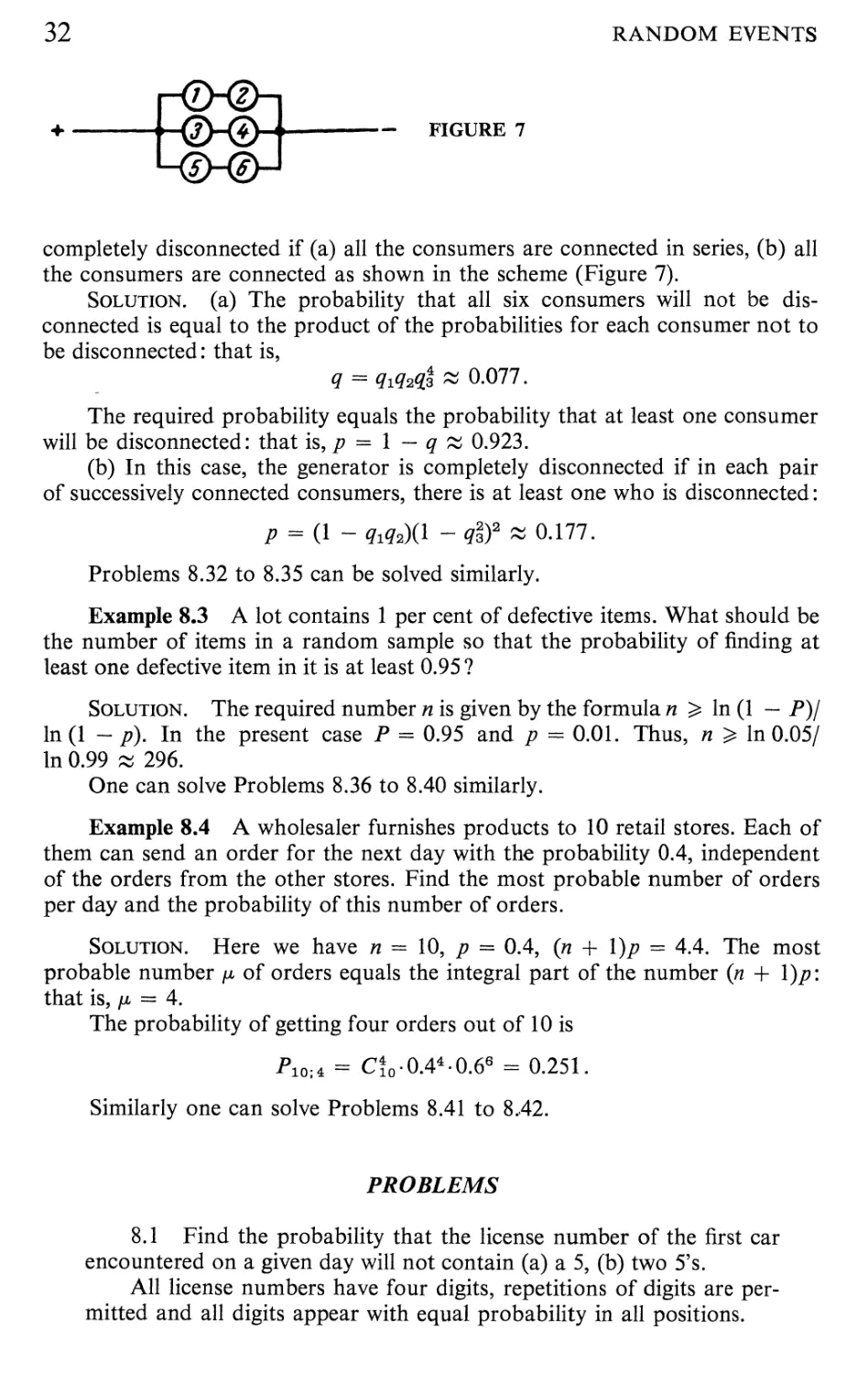
6.6 For quality control on a production line one item is chosen
for inspection from each of three batches. What is the probability that
faulty production will be detected if, in one of the batches, 2/3 of the
items are faulty and in the other two they are all good?
6.7 A vacuum tube may come from any one of three batches with
probabilities pi, p^ and p^, where Pi = Ps = 0.25 and /?2 = 0.5. The
probabilities that a vacuum tube will operate properly for a given
number of hours are equal to 0.1, 0.2 and 0.4, respectively, for these
batches. Find the probability that a randomly chosen vacuum tube will
operate for the given number of hours.
6.8 Player A plays two opponents alternately. The probability
that he wins from one at the first trial is 0.5 and the probability that
he wins from the other at the first trial is 0.6. These probabilities
increase by 0.1 each time the opponents repeat the play against A.
Assume that A wins the first two games. Find the probability that A will
lose the third game if his opponent in the first game is not known and if
ties are excluded.
6.9 A particular material used in a production process may come
from one of six mutually exclusive categories with probabilities 0.09,
0.16, 0.25, 0.25, 0.16 and 0.09. The probabilities that an item of
production will be acceptable if it is made from materials in these categories
are, respectively, 0.2, 0.3, 0.4, 0.4, 0.3 and 0.2. Find the probability of
producing an acceptable item.
6.10 An insulating plate 100 mm. long covers two strips passing
perpendicular to its length. Their boundaries are located, respectively,
at the distances of 20,40 mm. and 65, 90 mm. from the edge of the plate.
A hole of 10 mm. diameter is made, so that its center is located equiprob-
ably on the plate. Find the probability of an electric contact with any
of the strips if a conductor is applied from above to an arbitrary point
located at the same distance from the base of the plate as the center of
the hole.
6.11 The probability that k calls are received at a telephone
station during an interval of time t is equal to Pt(k). Assuming that the
numbers of calls during two adjacent intervals are independent, find the
probability P2t(s) that s calls will be received during an interval 2t.
6.12 Find the probability that 100 light bulbs selected at random
from a lot of 1000 will be nondefective if any number of defective
bulbs from 0 to 5 per 1000 is equally probable.
6.13 A white ball is dropped into a box containing n balls. What
is the probability of drawing the white ball from this box if all the
hypotheses about the initial color composition of the balls are equally
probable ?

26 RANDOM EVENTS
6.14 In a box are 15 tennis balls, of which nine are new. For the
first game three balls are selected at random and, after play, they are
returned to the box. For the second game three balls are also selected
at random. Find the probability that all the balls taken for the second
game will be new.
6.15 There are three quarters and four nickels in the right pocket
of a coat, and six quarters and three nickels in the left pocket. Five
coins taken at random from the right pocket are transferred to the left
pocket. Find the probability of drawing a quarter at random from the
left pocket after this transfer has been made.
6.16 An examination is conducted as follows: Thirty different
questions are entered in pairs on 15 cards. A student draws one card at
random. If he correctly answers both questions on the drawn card, he
passes. If he correctly answers only one question on the drawn card,
he draws another card and the examiner specifies which of the two
questions on the second card is to be answered. If the student correctly
answers the specified question, he passes. In all other circumstances he
fails.
If the student knows the answers to 25 of the questions, what is the
probability that he will pass the examination ?
6.17 Under what conditions does the following equality hold:
P(^) = P(A \B)+ P(A\BI
6.18 One of two urns, each containing 10 balls, has a marked ball.
A player has the right to draw, successively, 20 balls from either of the
urns, each time returning the ball drawn to the urn. How should one
play the game if the probability that the marked ball is in the first urn
is 2/3 ? Find this probability.
6.19 Ten helicopters are assigned to search for a lost airplane;
each of the helicopters can be used in one out of two possible regions
where the airplane might be with the probabilities 0.8 and 0.2. How
should one distribute the helicopters so that the probability of finding
the airplane is the largest if each helicopter can find the lost plane within
its region of search with the probability 0.2, and each helicopter searches
independently ? Determine the probability of finding the plane under
optimal search conditions.
7. COMPUTATION OF THE PROBABILITIES OF
HYPOTHESES AFTER A TRIAL (BAYES' FORMULA)
Basic Formulas
The probability P(Hj^ \ A) of the hypothesis H}^ after the event A occurred
is given by the formula
HH, i A) - ^^ ,
where
P(^)= i P{H,)P(A\H,),
; = i

7. BAYES' FORMULA 27
and the hypotheses Hj (j = I,.. .,n) form a complete set of mutually exclusive
events.
Solution for Typical Examples
Example 7.1 A telegraphic communications system transmits the signals
dot and dash. Assume that the statistical properties of the obstacles are such
that an average of 2/5 of the dots and 1/3 of the dashes are changed. Suppose
that the ratio between the transmitted dots and the transmitted dashes is 5:3.
What is the probability that a received signal will be the same as the
transmitted signal if (a) the received signal is a dot, (b) the received signal is a dash.
Solution. Let A be the event that a dot is received, and B that a dash
is received.
One can make two hypotheses: Hi that the transmitted signal was a dot;
and H2 that the transmitted signal was a dash. By assumption, P(Hi): P(H2) =
5:3. Moreover, P(Hi) + PiH^) = 1. Therefore P(Hi) = 5/8, PiH^) = 3/8. One
knows that
P(A\H,)=l, P(A\H2) = l^
P(B\H,) = l, P(B\H2) = l-
The probabilities of A and B are determined from the total probability
formula:
o,,, 5 3 3 1 1 „,^, 5 2 3 2 1
P(^) = 8-5 + 81 = 2' ^(^) = 8-5 + 8-3 = 2'
The required probabilities are:
(a) P(H, I A) =
(b) P(H2 I B) =
5 3
P(Hi)P{A I ^1) _ 8^ _ 3.
P(^) ~ 1 ~ 4'
2
3 2
P(H2)P(B I H2) _ 8j ^ 1
P(B) 1 2'
2
Similarly one can solve Problems 7.1 to 7.16.
Example 7.2 There are two lots of items; it is known that all the items
of one lot satisfy the technical standards and 1/4 of the items of the other lot
are defective. Suppose that an item from a lot selected at random turns out to
be good. Find the probability that a second item of the same lot will be defective
if the first item is returned to the lot after it has been checked.
Solution. Consider the hypotheses: H^ that the lot with defective items
was selected/ and H2 that the lot with nondefective items was selected. Let A
denote the event that the first item is nondefective. By the assumption of the

28 RANDOM EVENTS
problem P(H^) = ?{H^) = 1/2, P(A \ Hj) = 3/4, P{A \ H^) = I. Thus, using
the formula for the total probability, we find that the probability of the event A
will be P(^) = l/2[C/4) + 1] = 7/8. After the first trial, the probability that
the lot will contain defective items is
P{H, I A) =
1 3
P(H,)P(A I H,) ^14^3
P(^) 7 7*
The probability that the lot will contain only good items is given by
P(H, \A)==^-
Let B be the event that the item selected in the first trial turns out to be
defective. The probability of this event can also be found from the formula for
the total probability. If Pi and;72 are the probabilities of the hypotheses //i and
H2 after a trial, then according to the preceding computations pi = 3/7,
p^ = 4/7. Furthermore, P(^ | H^) = 1/4, P(B \ H^) = 0. Therefore the required
probability is P(^) = C/7)-A/4) = 3/28.
One can solve Problems 7.17 and 7.18 similarly.
PROBLEMS
lA Consider 10 urns, identical in appearance, of which nine
contain two black and two white balls each and one contains five white and
one black ball. An urn is picked at random and a ball drawn at random
from it is white. What is the probability that the ball is drawn from the
urn containing five white balls ?
7.2 Assume that k-^ urns contain m white and n black balls each
and that k2 urns contain m white and n black balls each. A ball drawn
from a randomly selected urn turns out to be white. What is the
probability that the given ball will be drawn from an urn of the first type ?
7.3 Assume that 96 per cent of total production satisfies the
standard requirements. A simplified inspection scheme accepts a
standard production with the probability 0.98 and a nonstandard one with
the probability 0.05. Find the probability that an item undergoing this
simplified inspection will satisfy the standard requirements.
7.4 From a lot containing five items one item is selected, which
turns out to be defective. Any number of defective items is equally
probable. What hypothesis about the number of defective items is most
probable ?
7.5 Find the probability that among 1000 light bulbs none are
defective if all the bulbs of a randomly chosen sample of 100 bulbs turn
out to be good. Assume that any number of defective fight bulbs from 0
to 5 in a lot of 1000 bulbs is equally probable.
7.6 Consider that D plays against an unknown adversary under
the following conditions: the game cannot end in a tie; the first move

7. BAYES' FORMULA 29
is made by the adversary; in case he loses, the next move is made by D
whose gain means winning the game; if D loses, the game is repeated
under the same conditions. Between two equally probable adversaries,
B and C, B has the probability 0.4 of winning in the first move and 0.3
in the second, C has the probability 0.8 of winning in the first move and
0.6 in the second. D has the probability 0.3 of winning in the first move
regardless of the adversary and, respectively, 0.5, 0.7 when playing
against B and C in the second move. The game is won by D.
What is the probability that (a) the adversary is B, (b) the adversary
is C.
7.7 Consider 18 marksmen, of whom five hit a target with the
probability 0.8, seven with the probability 0.7, four with the probability
0.6 and two with the probability 0.5. A randomly selected marksman
fires a shot without hitting the target. To what group is it most probable
that he belongs ?
7.8 The probabilities that three persons hit a target with a dart
are equal to 4/5, 3/4 and 2/3. In a simultaneous throw by all three
marksmen, there are exactly two hits. Find the probability that the third
marksman will fail.
7.9 Three hunters shoot simultaneously at a wild boar, which is
killed by one bullet. Find the probability that the boar is killed by the
first, second or the third hunter if the probabilities of their hitting the
boar are, respectively, 0.2, 0.4 and 0.6.
7.10 A dart thrown at random can hit with equal probability any
point of a region S that consists of four parts representing 50 per
cent, 30 per cent, 12 per cent and 8 per cent of the entire region. Which
part of region S is most likely to be hit ?
7.11 In an urn, there are n balls whose colors are white or black
with equal probabilities. One draws k balls from the urn, successively,
with replacement. What is the probability that the urn contains only
white balls if no black balls are drawn ?
7.12 The firstborn of a set of twins is a boy, what is the
probability that the other is also a boy if among twins the probabilities of two
boys or two girls are a and b, respectively, and among twins of diff'erent
sexes the probabilities of being born first are equal for both sexes ?
7.13 Considering that the probability of the birth of twins of the
same sex is twice that of twins of diff'erent sexes, that the probabilities
of twins of diff'erent sexes are equal in any succession and that the
probabilities of a boy and a girl are, respectively, 0.51 and 0.49, find the
probability of a second boy if the firstborn is a boy.
7.14 Two marksmen fire successively at a target. Their
probabilities of hitting the target on the first shots are 0.4 and 0.5 and the
probabilities of hitting the target in the next shots increase by 0.05 for
each of them. What is the probability that the first shot was fired by the
first marksman if the target is hit by the fifth shot?
7.15 Consider three independent trials, in which the event A
occurs with the probability 0.2. The probability of the occurrence of the
event B depends on the number of occurrences of ^. If the event A
occurs once, this probability is 0.1; if ^ occurs twice, it is 0.3; if A

30 RANDOM EVENTS
occurs three times it is 0.7; if the event A does not occur, the event B is
impossible. Find the most probable number of occurrences of A if it is
known that B has occurred.
7.16 There are n students in a technical school. Of these, n^, where
k = 1, 2, 3, are in their second year. Two students are randomly
selected; one of them has been studying for more years than the other.
What is the probability that this student has been studying for three
years ?
7.17 The third item of one of three lots of items is of second
grade, the remaining items are of first grade. An item selected from one
of the lots turns out to be of first grade. Find the probability that it was
taken from the lot containing second grade items. Find the same
probability under the assumption that a second item selected from the
same lot turns out to be of first grade if the first item is returned to the
lot after inspection.
7.18 Consider a lot of eight items of one sample. From the data
obtained by checking one-half of the lot, three items turn out to be
technically good and one is defective. What is the probability that in checking
three successive items one will turn out to be good and two defective if
any number of defective items is equally probable in the given lot?
8. EVALUATION OF PROBABILITIES OF OCCURRENCE OF
AN EVENT IN REPEATED INDEPENDENT TRIALS
Basic Formulas
The probability Pn;m that an event occurs m times in n independent trials,
in which the probability of occurrence of the event is /?, is given by the binomial
distribution formula
where q = \ — p.
The probability for realization of the event at least m times in n trials
can be computed from the formula
n m-1
k=m k=0
The probability of occurrence of the event at least once in n trials will be
K:i = \-q\
The number of trials that must be carried out in order to claim that a
given event occurs at least once, with a probability at least P, is given by the
formula
In A - P)
n ^
ln(l -p)
where p is the probability of occurrence of the event in each of the trials.
The most probable value /x of the number m of occurrences of the event A
equals the integral part of the number {n + 1)/?, and if (« -h \)p is an integer,

8. REPEATED INDEPENDENT TRIALS 31
the largest value of the probability is attained for two numbers jjli =
(n + l)p — I and /X2 = (« + l)p.
If the trials are independent, but the probabilities for realization of the
event on different trials are different, the probability P^im that the event occurs
m times in n trials equals the coefficient of u"^ in the expansion of the generating
function
k=1 m=0
where qj^ = 1 — p^, pj^ being the probability that the event occurs in the kth
trial.
The coefficients Pn-m can be determined by differentiating the function
G{u):
p = J_ r^"^(^))
which gives, for example,
Pn:o = qiq2' • -qn
Solution for Typical Examples
Example 8.1 What is more probable in playing against an equal adversary
(if the game cannot end in a tie) to win (a) three games out of four or five
out of eight, (b) at least three games out of four or at least five out of eigl^ ?
Solution. Since the adversaries are equal, the probabilities for them to
win or lose a game are equal: i.e., p = q = i-
(a) The probability of winning three games out of four is
P -C^i-i.
The probability of winning five games out of eight is Pq.^ = CqA/2^) =
7/32. Since 1/4 > 7/32, it is more probable to win three games out of four.
(b) The probability of winning at least three games out of four is
^4; 3 — ^4:3 + ^4:4 — 7 + T^ " i~?
1 _1_ ^ ^
4 "^ 16 ~ 16'
and the probability of winning at least five games out of eight is
7 , /8-7 , 8 , ,\ 1 _ 93
32 + 1^^ + 8 + Ij ^ - 25g-
^8; 5 — ^8:5 + ^8; 6 + -* 8;7 + ^8; 8 — 'j^
Since 93/256 > 5/16, it is more probable to win at least five games out of eight.
Similarly one can solve Problems 8.1 to 8.31.
Example 8.2 There are six consumers of electric current. The probability
that under certain conditions a breakdown will occur that will disconnect one
of the consumers is 0.6 for the first consumer, 0.2 for the second, and 0.3 for
each of the remaining four. Find the probability that the generator will be

32 RANDOM EVENTS
mHlH
— FIGURE 7
completely disconnected if (a) all the consumers are connected in series, (b) all
the consumers are connected as shown in the scheme (Figure 7).
Solution, (a) The probability that all six consumers will not be
disconnected is equal to the product of the probabilities for each consumer not to
be disconnected: that is,
^ = ^1^2^1^0.077.
The required probability equals the probability that at least one consumer
will be disconnected: that is,;? = 1 — ^ ;^ 0.923.
(b) In this case, the generator is completely disconnected if in each pair
of successively connected consumers, there is at least one who is disconnected:
/^ = A - ^i^2)(l -^§)^^ 0.177.
Problems 8.32 to 8.35 can be solved similarly.
Example 8.3 A lot contains 1 per cent of defective items. What should be
the number of items in a random sample so that the probability of finding at
least one defective item in it is at least 0.95 ?
Solution. The required number n is given by the formula « ^ In A — P)/
ln(l - p). In the present case P = 0.95 and p = 0.01. Thus, n ^ In 0.05/
In 0.99 ^ 296.
One can solve Problems 8.36 to 8.40 similarly.
Example 8.4 A wholesaler furnishes products to 10 retail stores. Each of
them can send an order for the next day with the probability 0.4, independent
of the orders from the other stores. Find the most probable number of orders
per day and the probability of this number of orders.
Solution. Here we have n = 10, p = 0.4, (n -f- 1);? = 4.4. The most
probable number /x of orders equals the integral part of the number (n + l)p:
that is, /x = 4.
The probability of getting four orders out of 10 is
^0:4 = CioO.4^-0.6^ = 0.251.
Similarly one can solve Problems 8.41 to 8.42.
PROBLEMS
8.1 Find the probability that the license number of the first car
encountered on a given day will not contain (a) a 5, (b) two 5's.
All license numbers have four digits, repetitions of digits are
permitted and all digits appear with equal probability in all positions.

8. REPEATED INDEPENDENT TRIALS 33
8.2 There are 10 children in a family. If the probabilities of a boy
or a girl are both 0.5, find the probability that this family has (a) five
boys, (b) at least three but at most eight boys.
8.3 From a table of random numbers one copies at random 200
two-digit numbers (from 00 to 99). Find the probability that among
them, the number 33 appears (a) three times, (b) four times.
8.4 Consider that a library has only books in mathematics and
engineering. The probabilities that any reader will select a book in
mathematics and engineering are, respectively, 0.7 and 0.3. Find the
probability that five successive readers will take books only in
engineering or only in mathematics if each of them takes only one book.
8.5 Two Hght bulbs are connected in series in a circuit. Find the
probability that an increase in the voltage above its rated value will
break the circuit if, under these assumptions, the probabiHty that a bulb
burns out is 0.4 for each of the two bulbs.
8.6 The event B will occur only if the event A occurs at least three
times. Find the probability for realization of the event B in (a) five
independent trials, (b) seven independent trials, if the probability of
occurrence of the event A in one trial is equal to 0.3.
8.7 An electric system containing two stages of type A, one stage
of type B and four stages of type C is connected as shown in Figure 8.
Find the probability of a break in the circuit such that it cannot be
eliminated with the aid of the key K if the elements of type A are out of
order with the probability 0.3, the elements of type B with the
probability 0.4 and the elements of type C with the probability 0.2.
8.8 The probability that a unit must undergo repairs after m
accidents is given by the formula G{m) = 1 — A — l/o))"^, where o) is the
average number of accidents before the unit is submitted for repairs.
Prove that the probability that after n cycles the unit will need repairs is
given by the formula W^ = 1 — A — pjo^Y, where p is the probability
that an accident will occur during one cycle.
8.9 Consider four independent trials in which the event A occurs
with the probability 0.3. The event B will occur with the probability 1 if
the event A occurs at least twice, it cannot occur if the event A does not
occur, and it occurs with a probability 0.6 if the event A occurs
once. Find the probability of the occurrence of the event B.
8.10 Consider 200 independent shots fired at a target under
identical conditions and leading to 116 hits. Which value, 1/2 or 2/3, for
the probabiHty of hitting in one shot is more probable if, before the
trial, both hypotheses are equally probable ?
FIGURE 8

34 RANDOM EVENTS
8.11 Evaluate the dependence of at least one occurrence of the
event ^, in 10 independent trials, on the probability p for realization of
the event A in each trial for the following values of j^: 0.01, 0.05, 0.1,
0.2, 0.3, 0.4, 0.5, 0.6.
8.12 The probability that an event occurs at least once in four
independent trials is equal to 0.59. What is the probabiHty of occurrence
of the event A in one trial if the probabiHties are equal in all trials ?
8.13 The probability that an event occurs in each of 18
independent trials is 0.2. Find the probability that this event will occur at
least three times ?
8.14 The probability of winning with one purchased lottery
ticket is 0.02. Evaluate the probabilities of winning a prize with n tickets
for «= 1, 10, 20, 30, 40, 50, 60, 70, 80, 90, 100 if the tickets belong to
different series for each case.
8.15 Given that a lottery ticket wins a prize and that the
probabiHties that this prize is a bicycle or a washing machine are,
respectively, 0.03 and 0.02, find the probability of winning at least one of these
items with 10 winning tickets selected from different series.
8.16 A game consists of throwing rings on a peg. A player gets
six rings and throws them until the first success. Find the probability
that at least one ring remains unused if the probability of a successful
throw is 0.1.
8.17 Find the probability of scoring at least 28 points in three
shots fired from a pistol at a target, with the maximal score of 10 points
per shot, if the probability of scoring 30 points is 0.008. Assume that in
one shot the probability of scoring eight points is 0.15, and less than
eight points, 0.4.
8.18 Two basketball players each make two attempts at throwing
a ball into the basket. The probabilities of making a basket at each throw
are, respectively, 0.6 and 0.7. Find the probability that (a) both will have
the same numbers of baskets, (b) the first basketball player will have
more baskets than the second.
8.19 The probability that a tube will remain in good condition
after 1000 hours of operation is 0.2. What is the probability that at
least one out of three tubes will remain in good condition after 1000
hours of operation ?
8.20 Three technicians produce items of excellent and good
qualities on their machines. The first and second technicians make
excellent items with the probability 0.9 and the third technician with the
probability 0.8. One of the technicians has manufactured eight items, of
which two are good. What is the probability that among the next eight
items made by this technician there will be two good and six excellent
items ?
8.21 For victory in a volleyball competition, a team must win
three games out of five; the teams are not equally matched. Find the
probability that the first team will win each game if for equal chances
this team must give odds of (a) two games, (b) one game.
8.22 A competition between two chess players is conducted under
the following conditions: draws do not count; the winner is the one who

8. REPEATED INDEPENDENT TRIALS 35
first scores four points under the assumption that the adversary has in
this case at most two points; if both players have three points each,
the one who scores five points first wins.
For each of the players, find the probability of winning the
competition if the probabilities of losing each game are in the ratio 3:2.
8.23 A person uses two matchboxes for smoking. He reaches at
random for one box or the other. After some time, he finds out that one
box is empty. What is the probability that there will be k matches left in
the second box if, initially, each box had n matches (Banach's problem).
8.24 The probability of scoring 10 points is 0.7, and nine points,
0.3. Find the probability of scoring at least 29 points in three shots.
8.25 During each experiment one of two batteries with powers of
120 watts and 200 watts is connected in the circuit for one hour. The
probabilities of a favorable outcome of this experiment are 0.06 and 0.08,
respectively. One considers that the result of a series of experiments has
been attained if one gets at least one favorable outcome in the
experiment with the battery of 200 watts or at least two favorable outcomes
with the battery of 120 watts. The total energy consumed in all
experiments cannot exceed 1200 watts. Which battery is more efficient?
8.26 A device stops if there are at least five defective tubes of
type I and at least two defective tubes of type II. Find the probability
that the device will stop if five tubes are defective and if the probabilities
of a defective tube among the tubes of type I and II are 0.7 and 0.3,
respectively.
8.27 The probability of a dangerous overload of a device is 0.4
in each experiment. Find the probability that this device will stop in
three independent experiments if the probabilities of a stop in one, two
and three experiments are 0.2, 0.5 and 0.8.
8.28 The probability that any of n identical units takes part in an
experiment isp (p < l/n). If a given unit participates in the experiments
exactly k times, the result of these experiments is considered attained.
Find the probability of attaining the desired result in m experiments.
8.29 Under the assumptions of the preceding problem, find the
probability of attaining the desired result in {2k — 1) experiments if
the experiments are discontinued when the result has been attained.
8.30 The probability that a device will stop in a trial is 0.2. How
many devices should be tried so that the probabihty of at least three
stops is 0.9?
8.31 A point A must be connected with 10 telephone subscribers
at a point B. Each subscriber keeps the line busy 12 minutes per hour.
The calls from any two subscribers are independent. What is the minimal
number of channels necessary so that all the subscribers will be served
at any instant with the probability 0.99?
8.32 Four radio signals are emitted successively. The probabilities
of reception for each of them are independent of the reception of the
other signals and equal, respectively, 0.1, 0.2, 0.3 and 0.4. Find the
probability that k signals will be received, where A: = 0, 1, 2, 3, 4.
8.33 Using the assumptions of the preceding problem, find the
probability of establishing a two-part radio communication system if

36 RANDOM EVENTS
the probability of this event is equal to 0.2 for the reception of one
signal, 0.6 for two signals and 1 for three and four signals.
8.34 The probabilities that three tubes burn out are respectively,
0.1, 0.2 and 0.3. The probabilities that a device will stop if one, two or
three tubes burn out are 0.25, 0.6 and 0.9, respectively. Find the
probability that the device will stop.
8.35 A hunter fires a shot at an elk from a distance of 100 m. and
hits it with the probability 0.5. If he does not hit it on the first shot,
he fires a second shot from a distance of 150 m. If he does not hit the elk
in this case, he fires the third shot from a distance of 200 m. If the
probability of a hit is inversely proportional to the square of the
distance, find the probability of hitting the elk.
8.36 How many numbers should be selected from a table of
random numbers to ensure the maximal probability of appearance
among them of three numbers ending with a 7 ?
8.37 The probability of scoring 10 hits in one shot is p = 0.02.
How many independent shots should be fired so that the probabihty of
scoring 10 hits at least once is at least 0.9 ?
8.38 During one cycle an automatic machine makes 10 items.
How many cycles are necessary so that the probability of making at
least one defective item is at least 0.8 if the probability that a part is
defective is 0.01 ?
8.39 Circles of radius 1 cm. have their centers located 60 cm. apart
on a line. Several lines of this kind are placed parallel to each other in
the same plane; a relative shift of the lines with any amount from 0 to
60 cm. is equally probable. A circle of radius 7 cm. moves in the same
plane and perpendicularly to these lines. What should be the number
of fines so that the probability of intersection of the moving circle with
one of the other circles is at least 0.9 ?
8.40 From a box containing 20 white and two black balls, n balls
are drawn, with replacement one at a time. Find the minimal number
of draws so that the probability of getting a black ball at least once
exceeds 1/2.
8.41 For a certain basketball player the probability of throwing
the ball into the basket in one throw is 0.4. He makes 10 throws. Find
the most probable number of successful throws and the corresponding
probability.
8.42 Find the most probable number of negative and positive
errors and the corresponding probabilities in four measurements if, in
each of them, the probability of a positive error equals 2/3, and of a
negative one, 1/3.
9. THE MULTINOMIAL DISTRIBUTION. RECURSION
FORMULAS. GENERATING FUNCTIONS
Basic Formulas
The probability that in n independent trials, in which the events Ai, A2,.. .,
Am occur with the corresponding probabilities p^, p2, •. •, Pm^ the events A^^,

9. THE MULTINOMIAL DISTRIBUTION 37
where k = 1, 2,..., m, will occur exactly « times B!?=i ^k = ^)j is given by the
multinomial distribution formula:
^1 1 722 I • • • AZ^ 1
The probability P^.^^^„2,....n;„ is the coefficient of wjiwg^- • -u^ in the
following generating function:
G(Wi, W2, . . ., Wj = (;7iWi + ;72W2 + • • • + i^mWrn)"".
The generating function foxn^N independent trials is the product of the
generating functions for n and A^ trials, respectively. Using this property, one
can frequently simplify the calculation of the required probabilities. For the
same purpose one applies a proper substitution of the arguments in the
generating function. If, for instance, one wishes to find the probability that in n trials
the event A^ will appear / times more than the event A2, then in the generating
function one should set W2 = 1/w, 1, where j = 3, 4,. .., m. The
required probability is the coefficient of yJ- in the expansion in a power series
for the function
G{u)=(p,u+P-^+2^p}j\
If Pj^ = l/m, where k = 1,2,.. .,m, and one wishes to find the probability
that the sum of the numbers of the occurring events is r, one looks for the
coefficient of w'' in the expansion in powers of u of the function
G{U) = —^ U\l + W + . . • + U^-'T = —n 1 -) '
In the expansion of G{u), it is convenient to use for A — w)""" the following
expansion:
A - u)-- = 1 + ci-^u + ciiw + cr^u^ + • • •.
Factorials of large numbers can be obtained from logarithm tables (see 2T
in the table Hst) or approximated by Stirling's formula:
n! = V2.nnV-''(l + jl^ + 28|^ +
The probability of occurrence of a given event can sometimes be obtained using
relations (recursion formulas) of the form
Pk = ClkPk-l + bf,pj^^2,
where a^ and Z?^ are given constants. The required probability is determined by
passage from n to n -\- I, after an evaluation, based on initial data, of the
probabilities for several values of k.
Solution for Typical Examples
Example 9.1 The probabilities that the diameter of any item is less than,
greater than or equal to some accepted value are respectively 0.05, 0.10 and

38 RANDOM EVENTS
0.85. From the total lot, one selects 100 random samples. Find the probability
that among them there will be five items with a smaller diameter and five with a
larger diameter than the acceptable diameter.
Solution. Let the event A i mean that an item of the first type, an item
A2 of the second type and Aq of the third type are randomly selected. By
assumption, />i = 0.05, P2 = 0.10, P2 = 0.85. The total number of trials, n, is 100. We
seek the probability p that the events Ai and A2 will occur five times each.
Then rii = 772 = 5, n^ = 90. Therefore the required probability
P = Aoo:5.5,90 = ^y^QJ 0.05^.0.15-0.8590.
If we use logarithms, we find
logp = log 100! - log 90! - 2 log 5! + 5 log 5 + 90 log 0.85 - 15.
Using the logarithm table for factorials and the table for decimal logarithms,
we obtain
log/? = 3.7824, or ;? ;^ 0.006.
Similarly one can solve Problems 9.1 to 9.7 and 9.25.
Example 9.2 In each trial the probability of occurrence of an event equals
p. What is the probabihty that the number of occurrences of the event will be
even in n trials ?
Solution. Let us denote by pj^ the probability that in k trials the event
will occur an even number of times.
Before the /:th trial, one can make two hypotheses: in the (k — l)st trial,
the event occurred an even or odd number of times. The probabilities of these
hypotheses slvq pj^^i and 1 — p^_i, respectively. Then
Pk = Pk-i(^ -/?) + (!- Pk-i)p,
that is,
Pk = P + Pk-i(^ - 2p).
Representing the last expression in the form
yPk ~ 2) " *^^ ~ '2p)yPk-i - 2) (k=l,2,.. ., n)
and, respectively, multiplying the left and right sides of n such equalities, we
obtain
n (..->) = ,!-2.). n(..-.--i)'
Simplifying both sides of the last equality by Y\ \Pk — ^)^ ^^ find
k = l \ ^1
Since /7o = 1, the required probability will be
Pn = \\\^{\ -2pn.
Problems 9.8 to 9.13 and 9.26 can be solved similarly.

9. THE MULTINOMIAL DISTRIBUTION 39
Example 9.3 Find the probability of purchasing a ticket with a number
whose sums of the first three and last three digits are equal if it has six digits
and may be any number from 000000 to 999999.
Solution. Let us first consider the first three digits of the number. Since
they are arbitrary, one can consider that one performs three trials {n = 3), in
which any one digit occurs with the probability/> = 1/10.
In the given case, the number of events, m, is 10, the probability isp == 1/10,
where k = 0, 1,.. ., 9, and the generating function has the form
Gi(Wo, Wi, . . ., Wg) = Yq3 ( 2 "^) '
where the subscript k of w^ indicates the number k occurring in the trial.
Let us set w^ = u^. Then the coefficient of w^ in the expansion of the
function
gives the probability that the sum of the first three digits of the number on the
ticket is a.
Similarly, the coefficient of w""" in the expansion of
gives the probability that the sum of the last three digits of the number is a.
But in this case, the coefficient of w° in the expansion
1 n _ ^io\6
G(u) = GMGM = Yq6^ [l -u)
is equal to the required probability that the sum of the first three digits and the
sum of the last three digits are equal.
We have
A _ wl0N _ I _ ^1^10 _^ ^2^20 ^
A - u)-^ = 1 + Ciw + C?w2 +....
Thus the required probability is
P = W ^^'^ ~ ^^^^' + ^'^''^ ^ 0.05525.
Similarly one can solve Problems 9.14 to 9.24.
PROBLEMS
9.1 Suppose that an urn contains three balls: one black, one red
and one white. One draws balls from it five times, one ball at a time,
with replacement. Find the probability that the red and white balls will
be drawn at least twice each.

40 RANDOM EVENTS
9.2 An employee produces a good item with probability 0.90, an
item with a defect that can be eliminated with the probability 0.09 and
an item with a permanent defect with the probability 0.01. He makes
three items. Find the probability that among them there is at least one
good item and at least one with a defect that can be eliminated.
9.3 Each of nine balls can be placed with equal probability in one
of three initially empty boxes. Find the probability that (a) there will be
three balls in each box, (b) there will be four balls in the first box, three
in the second box and two in the third box.
9.4 Ten shots are fired at a target consisting of an inner circle and
two concentric annuli. The probabilities of hitting these regions in one
shot are 0.15, 0.22 and 0.13, respectively. Find the probability that there
will be six hits in the circle, three in the first annulus and one in the
second annulus.
9.5 A device consists of four units, each made of vacuum tubes.
If one tube is out of order, the probabilities that it belongs to a given
unit are pi = 0.6111, Po. "= p^ = 0.664, p^ = 0.2561, respectively, and
these do not depend on how many tubes were previously out of order.
Find the probability that the device will stop when four tubes are out of
order if this event may occur when at least one tube of the first unit or
at least one tube in each of the second and third units is out of order.
9.6 Twelve persons get on a train that has six cars; each passenger
may select with equal probability each of the cars. Find the probability
that (a) there will be two passengers in each car, (b) there will be one car
without passengers, one with one passenger, two with two passengers
each and the remaining two with three and four passengers, respectively.
9.7 An urn contains / white, m black and n red balls. From it are
drawn, with replacement, one at a time, li + m^ + n^ balls. Find the
probability that (a) first, /i white balls, then mi black balls, and finally,
«i red balls are drawn, (b) /i white, rrii black, and n^ red balls are drawn
so that balls of identical color appear successively, but the succession of
colors may be arbitrary, (c) /i white, rrii black and n^ red balls are drawn
in any succession.
9.8 Find the probability that in n tosses, a coin will show heads
an odd number of times.
9.9 Two equally matched adversaries play chess until one of them
leads by two games. What is the probability that 2n decisive games (that
are not draws) will be needed ?
9.10 Two persons play until one of them wins all the money from
the other. Find the probability that exactly n games will be necessary if
all the stakes are equal, each player has at the beginning three stakes,
and the probability of winning a game is 1/2 for each of the two players,
9.11 Two persons play until one of them is ruined. The first player
has an initial capital of n dollars and the second, m dollars. The
probabilities of winning are, respectively,/> and q (p -\- q = l).ln each game,
the gain for one player (loss for the other) is one dollar. Find the
probabilities of a complete ruin for each of them.
9.12 In a chess competition there are n + I equally good players.
Each man plays each of the others until he loses. The competition con-

9. THE MULTINOMIAL DISTRIBUTION 41
tinues until one of the players wins n games. What is the probability
that m decisive games will be played (draws are not counted) ?
9.13 A competition between two equal chess players takes place
under the following conditions: the draws are not taken into account;
the winner is the one who scores six points if his adversary scores no
more than four points; if one wins six games, and the other five, then
the competition continues until the difference in points becomes two.
Find the probability that the number of decisive games is (a) at
most 10, (b) exactly n.
9.14 The probability that an event occurs in each of n experiments
is equal to p. Prove that the generating function for the probabilities of
at least n — m occurrences of this event is
\ — U
9.15 The probability that an event occurs in the kih experiment
is equal iop^{k = 1, 2,..., «). Prove that the generating functions for
the probabilities of, respectively, at most m occurrences and at least
n — m occurrences of this event, in n independent trials are
n n
n (9fc + PkU) n {Pk + ^ku)
G^{u) = ^-=^ 7, a"'^ G^{u) = ''-^
1 — w 1 — w
9.16 Each of two marksmen fires n shots at his target. Find the
probability that they will score the same number of hits if the
probability of hitting in each shot is 0.5.
9.17 Each of two identical devices, left and right, has two tubes.
After 100 hours of operation, one tube can burn out in only one of them
with the probability 1/4 and both tubes can burn out with the probability
1/16. Find the probability that in n pairs of such devices the number of
burnt-out tubes in the left devices will exceed at least by m (m ^ In)
the number of burnt-out tubes in the right devices. Find this probability
in the case when n = m = 3.
9.18 The competition for the title of world champion in 100
square-board checkers consists of 20 games. Find the probability that
it will end with the score 12:8 if the probability of winning each game is
0.2 for each of the two players.
9.19 To win the competition for the title of world champion in
chess, the challenger must score at least 12.5 points out of a possible 24.
In the case of a tie A2:12) the title is kept by the defending champion.
The participants are two equal players whose probabilities of winning a
game are half as great as the probabilities of a tie. Find (a) the
probability that the defending champion will keep his title, and the
probability that the challenger will become the world champion, (b) the
probability that 20 games will be played in this competition.
9.20 Find the probability that in n throws of a pair of dice, the
sum of points marked on the upper faces will be (a) equal to a given
number m, (b) not greater than m.
Find these probabilities for « = 10 and m = 20.

42 RANDOM EVENTS
9.21 Find the probability of getting a ticket with a number the sum
of whose digits is 21 if all numbers of the ticket from 0 to 999999 are
equally probable.
9.22 Any of the n quantities X^, Xg,..., X^ can take any integral
positive value from 1 to m with equal probability. Find the probability
that the sum Xi + Z2 + • • • + ifn will be (a) equal to a given number
N {nm '^ N ^ n), (b) not less than a given number N.
9.23 Two marksmen fire three shots each at their targets. One can
score any number of points from seven to 10 with equal probability,
whereas for the other, the probability of scoring seven and 10 points is
1/8, and of scoring eight and nine points is 3/8. Find the probability
that (a) the first marksman will score 25 points, (b) the second marksman
will score 25 points, (c) both marksmen will score the same number of
points.
9.24 Two distinguishable coins are tossed simultaneously and
repeatedly. Find the probability that at the «th toss (and not before) each
will have shown heads as many times as the other.
9.25 Find the probability that a runoff will be necessary in the
elections of/persons if « people vote. The probability of being eliminated
is the same for each of the k candidates and equal to p, and to be elected
a candidate must get the majority of the votes. A runoff takes place only
in the case when candidates / and / + 1 get an equal number of votes.
9.26 Two equal volleyball teams play one game. The game
continues until one of the teams leads by two points; the minimal score
necessary is 15. Find the probabilities (a) P^ and Q^ that the game will
be won, respectively, by the first team (which serves the ball first) and the
second team with the score \5'.k (k = 0, 1,.. .,13), (b) Pi and Qi that
the game will be won by each of the teams if the losing team has at most
13 points, (c) Fjc and 2fc that the game will be won with a score of
A6 + k):(l4 + k), where A: = 0, 1,..., (d) Pn and 2ii that the game
will be won if each team loses at least 14 points, (e) P and Q that the
game will be won, respectively, by the first and second teams.

II
RANDOM VARIABLES
10. THE PROBABILITY DISTRIBUTION SERIES, THE
DISTRIBUTION POLYGON AND THE DISTRIBUTION
FUNCTION OF A DISCRETE RANDOM VARIABLE
Basic Formulas
A random variable is said to be discrete if its possible values can be
enumerated.
A discrete random variable X can be specified by: A) a distribution series,
B) a distribution function (integral distribution law).
By a distribution series we mean the set of all possible values Xj of X, and
the corresponding probabilities pi = P(X = Xi). A distribution series can be
represented by a table (see Table 2) or a formula.
The probabilities Pi satisfy the condition
n
2 A = 1,
i = l
in which the value of n may be finite or infinite.
The graphic representation of a distribution series is called a distribution
polygon. To construct it, one represents the values of the random variable (xi)
on the X-axis, and the probabilities/^^ on the j-axis; next, one joins the points Ai
with the coordinates (x^, Pi) by a broken curve (Figure 9).
The distribution function (integral distribution law) of a random variable
X is defined as the function i^(x), equal to the probability P(X < x) that the
random variable is less than the (arbitrarily chosen) value x. The function F{x)
is given by the formula
F{x) = 2 Pi.
Xi<X
in which the summation is extended over all values of / such that Xi < x.
Table 2
Xi
Pi
Xi
Pi
X2
P2
Xn
Pn
43

44
RANDOM VARIABLES
Pt^
I
'.^
IV
¦
A
i v^
V' ''•"'
y^
' I
1 (
\a.
'A
1 to*
FIGURE 9
*^ *^
Solution for Typical Examples
Example 10.1 From a lot of 100 items, of which 10 are defective, a random
sample of size 5 is selected for quality control. Construct the distribution series
of the random number X of defective items contained in the sample.
Solution. Since the number of defective items in the sample can be any
positive integer from 0 to 5 inclusive, the possible values Xi of the random
variable X are
The probability P(Z = /:) that the sample will contain exactly A: (A: = 0, 1,
2, 3, 4, 5) defective items is
?{X = k) =
Ck /^5~k
10^90
The computations with the preceding formula give, with an accuracy of
0.001, the following results:
p^ = P(Z = 0) = 0.583, /72 = P(Z = 1) = 0.340,
p^ = P(Z = 2) = 0.070,
p^ = P(X = 3) = 0.007, i?5 = P(X = 4) = 0,
Pe = P(Z = 5) = 0.
Using for verification the equality 2^=1/^^ == 1, we can convince ourselves that
the computations and the round-ofif are correct (see Table 3).
Table 3
Xi
Pi
0
0.583
1
0.340
2
0.070
3
0.007
4
0
5
0
Similarly one can solve Problems 10.13 and 10.14.
Example 10.2 Items are tested under overload conditions. The probability
that each item passes the test is 4/5 and independence prevails. The tests are
concluded when an item fails to meet the requirements of the test. Derive the formula
for the distribution series of the number of trials.

10. DISCRETE RANDOM VARIABLES
45
Solution. The trials end with the kth item (k = 1, 2, 3,...) if the first
k — 1 items pass the test and the kth item fails.
If X is the random number of trials, then
P(Z = ^) = (l-3) .3 = 3C) , (^=1,2,3,...).
The formula obtained for the distribution series is equivalent to Table 4.
Table 4
Xi
Pi
1
1
5
2
4
52
3
42
5=^
k
4^-1
5^
The peculiarity of the current problem is that theoretically the number of
trials can be infinite, but the probability of such an event is zero:
lim P(X = k) = lim ^
0.
Problems 10.2, 10.4, 10.5, 10.7, 10.10 and 10.12 are solved in a similar
manner.
Example 10.3 A car has four traffic lights on its route. Each of them
allov^s it to move ahead or stop with the probability 0.5.
Sketch the distribution polygon of the probabihties of the numbers of
Hghts passed by the car before the first stop has occurred.
Solution. Let X denote the random number of lights passed by the car
before the first stop occurs; it can assume the following values:
The probabilities Pi = P(X = Xi) that the number of traffic lights X passed
by the car will equal some given value can be computed with the formula
P(^ = Xi) =
p{\ -py-' for /= 1,2,3,4,
A - py for i = 5,
in which p is the probabihty with which the traffic lights can stop the car
(P = 0.5).
As a result of these computations, we obtain that pi = 0.5, p2 = 0.25,
P3 = 0.125, ;?4 = 0.0625, p^ = 0.0625. With these results we construct the
probabihty distribution polygon (Figure 10).
Following this example, we can solve Problems 10.3, 10.8 and 10.9.
Example 10.4 A space rocket has a device consisting of four units A^, A2,
Aq, ^4, each of which fails to operate when at least one elementary particle hits it.
The failure of the entire device occurs either if ^1 fails or if A2, A^ and ^4 fail
simultaneously.

46
RANDOM VARIABLES
FIGURE 10
^ JT;
Construct the distribution function F(x) of the random number of elementary
particles X, for which the entire device will fail if the probability that a particle
reaching the device will hit A^ is pi = 0.4, and the probabilities for hitting A2,
A3 and ^4, are, respectively, P2 = Ps = P4: = 0-2.
Solution. Let Ai, A2, A3, A^ denote the events that ^1, A2, A3, A^ fail.
The required distribution function F{x) equals the probability that the device
will continue its operation after n < x hits; i.e.,
Using the formula (see Section 5)
A^ u ^2^3-^4 = ^1(^2 u ^3 u A^ = A1A2 u A^As u v4i^4
= (^1 u A2) + (^1 u A3) + (^1 u A^)
and applying the formula for the addition of probabilities, we obtain
F(x) = 1 - P[(A, u A2) u (A^ u ^3) u (^1 u A^)]
= 1 - P(A, u ^2) - P(v4i u ^3) - P(^i u A,)
+ P[(^, u ^2X^1 u ^3)] + PPi ^ ^2X^1 u ^0]
+ P[(^, u A3){A, u ^4)] - PPi u ^2X^1 ^' ^3X^1 ^ ^4)],
where all the probabilities are defined under the assumption that n particles hit
the device. Since/>i + P2 + Ps + P4. = ^, and for each hit of a particle one and
only one stage necessarily fails to operate, we have
P(^i u A2) = {P3 + P^T; P(^i ^ ^3) = (P2 +- P^T;
P(A^uA^) = (p2 +P3T;
P[iA, u A2)(A, u ^3)] = Pi;
P[iA,uA2KA,^A,)] =pV,
P[{A^^A3){A^^A^)]=pl',
P[{A^ u ^2X^1 + A3){A, u A,)\ = 0.
Thus, taking into account that/?2 = /'s ^ ^'4 == 0-2, we obtain
F{x) - 1 + 3;7§ - 3B^72)^ = 1 - 3;7§B- _ i) ^ 1 _ 3 -
IQM
where [x] denotes the largest integer less than x, for example, [5.9] = 5, [5] = 4.

10. DISCRETE RANDOM VARIABLES
47
Frxji
FIGURE 11
Therefore, the graph of the probabihty distribution function for several
initial values of x has the form shown in Figure 11.
Problems 10.6 and 10.11 are solved similarly.
PROBLEMS
10.1 Construct the distribution series and the distribution function
for a random number of successful events in one experiment if the
experiment consists of throwing a ball into a basket and the probability of
a success in one trial is p = 0.3.
10.2 An experiment consists of three independent tossings of a
coin, in each of which heads shows up with the probability p = 0.5.
For a random number of heads, construct (a) its distribution series,
(b) distribution polygon, (c) distribution function.
10.3 Five devices are subjected to successive rehability tests. Each
device is tested only if the preceding one turns out to be reliable.
Construct the distribution series of a random number of tests if the
probability of passing these tests is 0.9 for each device.
10.4 Some independent experiments are discontinued when the first
favorable outcome has occurred. For a random number of experiments
find (a) the distribution series, (b) the distribution polygon, (c) the most
probable number of experiments, if the probability of a favorable
outcome in each trial is 0.5.
10.5 Two basketball players shoot the ball alternately until one
of them scores. Construct the distribution series for a random number
of shots thrown by each of them if the probability of a success is 0.4 for
the first player and 0.6 for the second.
10.6 A target consists of a circle numbered 1 and two annuli
numbered 2 and 3. By hitting the circle numbered 1, one scores 10
points; the annulus numbered 2, 5 points; and the annulus numbered 3,

48 RANDOM VARIABLES
1 point. The corresponding probabilities of hitting the circle numbered 1
and annuli numbered 2 and 3, are 0.5, 0.3 and 0.2. Construct the
distribution series for a random sum of scores as a result of three hits.
10.7 An experiment is performed with a series of identical devices
that are turned on successively for a period of five seconds each. The
lifetime of one device is 16 seconds. The experiment is discontinued
when at least one device stops. Find the distribution series for a random
number of devices if the probability of stopping is 1/2 for each device.
10.8 There are n patterns for the same item. The probability of
producing a nondefective item from each of them is p. (a) Find the
distribution series of the number of patterns left after the first non-
defective item has been produced, (b) Construct the distribution series
for a random number of patterns used.
10.9 A lot of n items is tested for reliability; the probability that
each item passes the test is p. Construct the distribution series for a
random number of items that pass the test.
10.10 A device consisting of units a, bi and bz fails to operate if
the event C = A u B1B2, where A denotes the failure of the unit a, and
Bi and B2 denote failure of the units bj_ and Z?2, respectively. The failures
occur when the device is hit by at least one cosmic particle. Construct the
distribution series of a number of random particles hitting the device if
the probabilities that a particle hits one of the units are: P(^) = 0.5,
P(B{) = PiB^) = 0.25.
10.11 An experiment can be a success with probability p or 3,
failure with probability A — p). The probability of a favorable outcome
in m successful trials is P(m) = 1 — A — l/w)"". Construct the
distribution series of the number of trials necessary for a favorable result.
10.12 The number of trials X is a random integer between 0 and
00. The probability P(X = k) = {n^e~"^)lk\. Each trial can be a success
with the probability p and a failure with the probability A — p).
Construct the distribution series of the number of successful trials.
10.13 The probabiHty of obtaining heads in each of five tosses of a
coin is 0.5. Find the distribution series for the ratio of the number X of
heads to the number Y of tails.
10.14 Construct the distribution series for the sum of digits of
three-digit random numbers.
11. THE DISTRIBUTION FUNCTION AND THE PROBABILITY
DENSITY FUNCTION OF A CONTINUOUS RANDOM
VARIABLE
Basic Formulas
A random variable is said to be continuous if it can assume any numerical
values on a given interval, and for which, for any x on this interval, there
exists the limit
^. . ,. P(x < X < X + Ax)
f{x) = hm -^ J- '-.
A^-*0 i\X
called probability density.

11. CONTINUOUS RANDOM VARIABLES 49
A continuous random variable can be defined either by a distribution
function F{x) (the integral distribution law) or by a probability density function
f(x) (differential distribution law).
The distribution function F(x) = P(X < x), where x is an arbitrary real
number, gives the probability that a random variable X will be less than x.
The distribution function F(x) has the following basic properties:
A) P(a^ X<b) = F(b) - F(a);
B) F{xi) ^ F{x2), if Xi < Xa;
C) lim F{x) = 1;
D) lim F(x) = 0.
X-* - 00
The probability density function (differential distribution law) f(x) has the
following fundamental properties:
A) /(x)>0;
B) /W = ^^;
C) r'°f(x)dx=l;
J — 00
D) Pia^X<b)= ff(x)
J a
dx.
The quantity Xp defined by the equality F(Xp) = p is called a quantile; the
quantile Xq.s is called the median. If the density has a maximum, the value of x
for which/(x) = max is called the mode.
The notion of probability density/(x) can also be introduced for a discrete
random variable by setting
n
/W = 2 Pk^(x - xj,
k = l
in which X/^ denote the possible values of the random variable, pj^ are their
corresponding probabilities
Pj, = P(Z = Xfc),
S(x) is the 8-function, that is, a "generalized" function with the properties
foo, X = 0,
/»oo 1*00
S(x) dx = I, (p{x)8{y — x) dx — ^{y),
J — 00 J — 00
where (p{x) is any function continuous at the point x = y. The function S(x)
can be represented analytically by
1 r°°
S(x) = — e^"^ dcxi,
where the integral is understood in the sense of its principal value.^
^ See for example, Gel'fand, I. M., and Shilov, G. E.: Generalized Functions. Vol. 1,
Properties and Operations. Translated by E. Saletan. New York, Academic Press, Inc.,
1964.

50 RANDOM VARIABLES
Solution for Typical Examples
Example 11.1 The projection X of the radius-vector of a random point on
a circumference of radius a onto the diameter has the distribution function (the
arcsine law)
a
11 X
^W = > o + ~ arcsin - for
0
{x ^ a\
-a < X < a;
{x ^ -a.
Determine (a) the probability that X will be on the interval ( — a/2, a/2),
(b) the quantile Xo.75, (c) the probability density/(x) of the random variable X,
(d) the mode and median of the distribution.
Solution, (a) The probability that X assumes values on the interval
(~a/2, a/2) is equal to
'H<^<i)-4")-^H)-
P{-^<X<'^\ -F(S1 - F(-S1 =^ arcsin i = I
(b) By assumption;? = 0.75; solving the equation
J + -arcsin^^^ = 0.75,
I TV a
we obtain
_ flV2
(c) The probability density/(x) of the random variable Zis:
A) for all values of x belonging to the interval (—a, a),
^, , dF(x) d n \ . x\ 1
f{x) = , = T" U + - arcsm - = —, ;
'^ ^ dx dx\2 7T a) Wo" - x^
B) zero for all the remaining values of x.
(d) We call the value of the argument for which the probability density
achieves its maximum the distribution mode. The arcsine law has no mode
since the function
TTVa^ — x^
has no maxima.
We call the quantity Xq 5 the distribution median defined by the equality
^^(^0.5) = 1/2.
Solving the equation
1 1 • Xq r. 1
:= + - arcsm-^ = ^,
we find that Xo.5 = 0.
Problems 11.1 to 11.8 are solved similarly.

11. CONTINUOUS RANDOM VARIABLES
51
Example 11.2 The probability density of a random variable is
f{x) = ax^e-^^ (A: > 0, 0 < X < 00).
Find (a) the coefficient a, (b) the distribution function of the random
variable X, (c) the probability that the random variable belongs to the interval
@, Ilk).
Solution, (a) The coefficient a is given by the equaUty
This implies that
j:
ax^e
' dx = 1.
/»00
x^e'^^ dx
Integrating by parts twice, we obtain
/•oo
Jo
x^e
dx = T^-
Consequently, a = k^/2 and the probability density has the form
fix) = ¦jx^e-^''.
(b) The distribution function F(x) of the random variable X is determined
by the formula
^« - r
k^x^ + 2kx + 2 _,
;o 2 ^^ ^ ™ ^ 2 ^ •
(c) The probability P@ < X < 1//:) that the random variable Z will assume
values on the given interval is computed according to the formula
''h "" <l) = in) = '-Te-'¦'''¦
Similarly one can solve Problems 11.9, 11.10 and 11.12.
Example 11.3 An electronic device has three parallel lines. The probability
that each line fails to operate during the warranty period of the device is 0.1.
Using the S-function, express the probability density for a random number of
lines that fail to operate during the warranty period if the failure of one line
is independent of whether the other lines operate.
Solution. Let us denote by X the random numbers of lines that fail. The
random variable X is discrete, and its distribution series (Table 5) is
Tables
Xk
Pk
0
0.729
1
0.243
2
0.027
3
0.001

52 RANDOM VARIABLES
Using the notion of probability density for a discrete variable, we obtain
f{x) = 0.729S(x) + 0.243S(x - 1) + 0.027S(x - 2) + 0.001 S(x - 3).
Similarly we can solve Problem 11.15.
PROBLEMS
11.1 The distribution function of a uniformly distributed random
variable X has the form
rO for X < 0,
F{x) = \x for 0 ^ x ^ 1,
[l for X > 1.
Find the probabiUty density of the random variable X.
11.2 Given the distribution function of a random variable
F{x) = , exp < ——\dt (normal distribution law),
V 277 J-00 I 2 J
find the probability density of the random variable X.
11.3 Cramer A946) gives the distribution function of the yearly
incomes of persons who must pay income tax:
for X ^ Xo, , .,
(a > 0).
for X < Xq
Find the yearly income that can be exceeded by a randomly selected
taxpayer with the probability 0.5.
11.4 The distribution function of the random period during which
a radio device operates without failures has the form
F@= 1 -exp|-^| (?^0).
Find (a) the probability that the device will operate without failures
during a time period T, (b) the probability density/(O-
11.5 The random variable representing the eccentricity of an item
is characterized by the Rayleigh distribution
v2^
F{x)= 1 - exp^-;^^ (x^O).
x^
2^'
Find (a) the mode of the distribution, (b) the median of the
distribution, (c) the probability density/(x).
11.6 The Weibull distribution function
F{x) = 1 -exp|-^| (x^O)
characterizes in a series of cases the lifetime of the elements of an
electronic instrument.

11. CONTINUOUS RANDOM VARIABLES 53
Find (a) the probability density/(x), (b) the quantile of order;? of
this distribution, (c) the mode of the distribution.
11.7 The random nonoperating period of a radio device has the
probability density
where M = log e = 0.4343... (this is the logarithmic normal
distribution law).
Find (a) the mode of the distribution for Xq = 1 and a = VSM,
(b) the distribution function.
11.8 Given the distribution function of a random variable X\
F(x) = a + b arctan(x/2) (-oo<x<+oo) (the Cauchy probability
law), determine (a) constants a and b, (b) the probability density,
(c) P(a < Z < P).
11.9 How large should a be so that/(x) = ae'""^ is the probability
density of a random variable X varying between infinite bounds ?
11.10 For which value of a is the function
fix) = YTl? ^""^ ^ ^ ^ ^"^^
equal to the probability density of a random variable X ?
Find (a) the distribution function of the random variable X, (b) the
probability that the random variable will fall in the interval (—1,1).
11.11 The scale of a stop watch has divisions of 0.2 seconds each.
What is the probability that the error in the time estimate is larger than
0.05 seconds if the estimate is made with an accuracy of one division with
a round-off to the nearest integer.
11.12 The azimuthal limb has divisions of 1° each. What is the
probability that there will occur an error of ±10' in the computation of
the azimuth if the angle estimates are rounded off to the nearest degree ?
11.13 It is known that the probability of failure for an electronic
tube during Ax days is Mx with a precision of higher order of magnitude
than Ax, and is independent of the number x of days during which the
tube operates prior to the interval Ax. What is the probability of failure
for a tube during / days ?
11.14 A streetcar line has a length L. The probability that a
passenger will get on the streetcar in the vicinity of a point x is
proportional to x(L — x)^, and the probability that a passenger who entered
at point X will get off at point y is proportional to {y — xf-, h ^ 0.
Find the probability that (a) the passenger will get on the streetcar
before point z, (b) the passenger who got on the streetcar at point x will
get off after point z.
11.15 Some devices are subjected to successive accelerated
reliability tests that are terminated when the first failure occurs. Using the
concept of probability density of a discrete random variable, find the
probability density of a random number of devices tested if the
probability of failure for each device is 0.5.

54 RANDOM VARIABLES
12. NUMERICAL CHARACTERISTICS OF DISCRETE RANDOM
VARIABLES
Basic Formulas
The most frequently used characteristics of discrete random variables are
the moments of these variables.
The moments ryij^ and the central moments /x;, of the /cth order of discrete
random variables are defined by the formulas :
i = l
ix^ = M[{x-xn= i (.x,-x)%,
in which M[Z'^] is the expectation of X^, Xi are the possible values of a random
variable X, pi the probabilities of these values and x is the expectation of X.
Therefore, the first moment is determined by the formula
n
X = M[X] = 2 XiPi,
1 = 1
the second central moment or the variance is given by
Dm = M[(Z - xf] = i fe - xfp,
i = l
or by
D[X] = M[Z2] - (M[Z]J.
The mean-square deviation a is given by the relation
a = +VD[T].
If the probabilities of different values of Z depend on the disjoint or mutually
exclusive events A^, then the conditional expectation of X with the condition
that Aj^ occurs is
\f A}c{k ~ 1, 2,..., m) form a complete set of events: that is, 2/c = i P(^fc) = 1?
then the total expectation of X and the conditional expectation are rf^lated by
the formula
m
Mm = M{M[Z| ^]} = Z M[X\A,]P(A,).
fc = l
In all the preceding formulas the number of terms in the sums can be
infinite; in this case, for the existence of the expectation the sum must converge
absolutely.
Solution for Typical Examples
Example 12.1 From a lot containing 100 items of which 10 are defective,
a sample of five items is selected at random for quality control. Find the
expectation for the number of defective items contained in the random sample.

12. CHARACTERISTICS OF DISCRETE VARIABLES 55
Solution. The random number of defective items contained in the sample
has the following possible values:
Xi = U, X2 ^^ I5 -^^3 = 2, X4 = J, X5 = 4, Xq = J.
The probability pi = P(X = Xi) that X will assume a given value Xi is (see
Example 10.1)
Pi = ^'%^'°" (/= 1,2,3,4,5,6).
The required expectation is
^ — A 0* " 1) 7^5 "^ 7^ A y^ioC'go ^•
1 = 1 ^100 <-100 /^o
Since 2y=o CioClo^' is the coefficient of u^ in the product A + w)^°(l + w)^°,
we see J,^=ojC{oCgo^' is the coefficient of u^ in the expression
^^{A + m)io(l + w)i°(l + uy%=^ = I0u{l + uy^
Consequently, we have
2 jCioClo^ = lOCtg, or X = —^ = 0.5.
/To ^100
Similarly, one can solve Problems 12.1 and 12.2.
Example 12.2 A discrete random variable X is given by the distribution
series pj, = P{X =k),k=l,2,3,.... Express the expectation of X in terms
of the generating function G(u) (see Section 9).
Solution. By the definition of the expectation of a random variable:
Mm = I kp,.
fc = l
On the other hand, the value of the derivative of the generating function
computed at w = 1 is
dG(u)
\u = l k^i |ii=l fc^i
GXl) =
= 2 f^PkU"" H = 2 ^p^'
du
Consequently,
Mm = G'(i).
One can solve Problems 12.3 to 12.6 and 12.24 to 12.26 similarly.
Example 12.3 An experiment can be a success with the probability p and
a failure with the probability \ — p.
The conditional probabihty P{m) for achieving the desired result after m
successful trials is
P{m) = 1 - /l - ir {0 1).
Find the expectation of the number of independent trials necessary for
achieving the desired result.

56 RANDOM VARIABLES
Solution. Let Pn(A) denote the probability of achieving the desired result
in n trials. If P^.m is the probability of exactly m successes out of a total of n
trials, then, according to the formula for the total probability, we have
Pn(A) = i Pn,mP(m).
m = 0
Since the trials are independent, and the probability of a successful outcome
in each of them is p,
Pn,m = C-;7-(l -py-'^.
Substituting into the formula for Pn(A) the values of P„,^ and P(m), we
obtain
PniA) = 2 cirrci - pr-'"{i - (i - If] = 1 - (i - £)"•
To attain the desired result, exactly n trials are necessary if it will be attained
at the nth trial. The probability of the latter circumstance is Pn(A) — Pn-i(A).
Consequently, M [X], the expectation of the random number of trials necessary
to attain the desired result, is:
Mm = 2 n[P.iA) - P„_,(^)] = I n{(l - ff" - (l - £)}
To compute the last sum we make use of the equality
V " 1 - -^ V n - ^ r 1 1 _ 1
i'/'' - cfxi'o'' ~ dx\\-x\- {\- xf'
valid for |x| < L Here, setting x = 1 — ploi, we obtain
p \ o)
M[X]
<" fi /. P\\ P
['-(¦-£)]
Similarly Problems 12.10 to 12.15, 12.21 and 12.31 can be solved.
Example 12.4 A device has n fuses. In the case of overload, one of the fuses
burns out and is replaced by a new one. What is the expectation M[A^] of the
number of overloads N after which all the initial fuses of the device are replaced
by new ones if one assumes that it is equally hkely for all fuses (old or new) to
burn out?
Solution. Let us denote by M [TV | k] the expectation of the number of
overloads after which all the initial fuses will be replaced if k fuses have not yet
been replaced.
To compute M[A/^ | /:] we use the formula for the total expectation. If k
fuses (k ^ 1) remain nonreplaced, then, in order that one of them burns out, a
subsequent overload is necessary. The average number of overloads necessary
for a remaining fuse to burn out will depend on the result of the subsequent
overload.

12. CHARACTERISTICS OF DISCRETE VARIABLES 57
In the subsequent overload there can occur two events:
Ai that one of the initial fuses burns out with the probability P(^i) = k/n;
A2 that one of the replaced fuses burns out with the probability P(^2) =
1 - k/n.
If at the subsequent overload A^ occurs, then the expectation of the number
of overloads necessary for the replacement of all k fuses that have not been
replaced before this overload is 1 + M[A^ | /: — 1]. If at the subsequent
overload A2 occurs, then the expectation equals 1 + M[A^ | ^]. Using the formula
for the total expectation, we find
M[N\k] =^{1 + M[A^|;c - 1]} + A -^j{l + tA[N\k]}
= 1 + - M[N \k - l] + ^^^—-^ M[N I k]
or after simple transformations,
M[A/'|/c] - lA[N\k - 1] =^•
If A: = 1, that is, only one fuse has not been replaced, the probability of its
replacement equals l/«. Therefore, according to Example 12.3, we shall have
M[A^| 1] = n.
Thus, we have a chain of equalities
M[N\n\ - M[N\n - 1] = -,
M[N I n - 1] - M[A^ I « - 2] = -^,
M[Ar|3] - IA[N\1] = y
IA[N\2] - M[N\ 1] =^,
M[N\ 1] = n,
whose sum gives
' n n — \ n — 2 3 2
or
M[N] = M[7V I n] = «(l + 1 + i + . • • + ^ + ij-
Problems 12.16, 12.20, 12.22 and 12.23 can be solved in a similar manner.
Example 12.5 As a result of experiments \yith two devices A and B, one
finds the probability of observing a noise whose level is evaluated in a three-
point system (see Table 6).

58
RANDOM VARIABLES
Table 6
Noise level
The probability of
observing a noise
of a given level
Device A
Device B
1
0.20
0.06
2
0.06
0.04
3
0.04
0.10
Using the data from Table 6, select the better device, i.e., the device v^ith
lower noise level.
Solution. Let X denote the random noise level. The average noise level
for the device A is
M^[Z] = 0.20-1 + 0.06-2 + 0.04-3 - 0.44 db.
For the device B\
Mb[Z] = 0.06-1 + 0.04-2 + 0.10-3 = 0.44 db.
Thus, compared according to the average number of points, both devices are
equivalent.
As an additional criterion for comparison, we use the mean-square deviation
of the noise level.
^A - VD^[1^] = VM^[Z2] - {xj,f = VO.80 - 0.442 ^ 0.78 db.,
Gs = VdJx] = VlA^lX^] - (x^y = V1.I2 - 0.442 ^ 0.96 db.
Hence A gives a more stable indication with respect to the means and,
consequently, it is better than B.
PROBLEMS
12.1 Find the expectation of the number of devices failing in
reliability tests if in each test only one device is tested and the proba-
bihty of its failure is p.
12.2 Assuming that the mass of a body can take, with equal
probability, any integral number of grams on the interval 1 to 10,
determine for which of the three sets of weights (a) 1, 2, 2, 5, 10; (b) 1, 2, 3, 4,
10; (c) 1, 1, 2, 5, 10, the average number of necessary weights will be
minimum, if one can place weights only on one scale and the selection of
weights is made to minimize the number used in the process of weighing.
12.3 A certain device consisting of five elements is tested. The
probability that an element numbered i fails to operate is
p, = 0.2 + 0.1(z - 1).
Find the expectation and the variance of the number of elements
that stop if the failures of the elements are independent.
12.4 Three devices are tested independently. The probabilities of
failure for each device are pi, p2 and p^, respectively. Prove that the
expectation of the number of devices faiHng to operate ispi -\- P2 -^ Ps-

12. CHARACTERISTICS OF DISCRETE VARIABLES 59
12.5 Determine the expectation of the number of devices failing
to operate during a test period if the probability of failure for all
devices is p and the number of devices that are tested is n.
12.6 A lottery distributes mi prizes worth ki, rriz; k2,. . ., m^,',
and ky^. The total number of tickets is A^. What should be the cost of
a ticket so that the expectation of a prize per ticket is equal to half its
cost.
12.7 The first player tosses three fair coins and the second, two
fair coins. The winner, who gets all five coins, is the one who scores more
heads. In the case of a tie the game is repeated until there is a decisive
result. What is the expectation of winning for each of the players?
12.8 Three persons A, B and C play a game as follows: two
participate in each game; the loser cedes his place to the third person; the
first game is played by A and B. The probability of winning each game is
1/2 for each player. They continue to play until one of them wins two
games in succession and gets m dollars. What is the expectation of a gain
for each of the players (a) after the first game under the assumption that
A won it, (b) at the beginning of the game ?
12.9 Three persons A, B and C play a game as follows: two players
participate in each game; the winner cedes his place to the third person;
first A plays with B. The probability of winning each game is 1/2 for each
player. They continue to play until one of them wins two consecutive
times and gets a sum of money equal to the number of all games played.
What is the expectation of winning for A and C at the beginning of the
game ?
12.10 An automatic line in a state of normal adjustment can
produce a defective item with probability;?. The readjustment of the line is
made immediately after the first defective item has been produced. Find
the average number of items produced between two readjustments of
the line.
12.11 The probability that a call signal emitted by one radio
station is received by another is 0.2 at each emission. The call signals are
emitted every five seconds until an answer signal is received. The total
passage time for the call and answer signals is 16 seconds. Find the
average number of call signals emitted before a two-way connection has
been established.
12.12 Find the expectation and the variance of the number of
items produced between two readjustments in a production line in
normal adjustment if in the state of normal adjustment, the probability of a
defective item is/?, and the readjustment is made after the ki\\ defective
item has been produced.
12.13 The conditional probability that a device stops, computed
under the assumption that m elements fail to operate, has the form:
(a) for the device A
P(m) = 1 - e-'^'^ (a > 0; m = 0, 1, 2,...);
(b) for the device B
@ for m = 0,
^(^) 1l_g-a(m-l) foj. m= 1,2,3,....

60 RANDOM VARIABLES
8
A
^^-
FIGURE 12
Find the expectation of the number of nonoperating elements that lead
to stops of the devices A and B.
12.14 A blocking scheme consisting of the relay A connected in
series with two relays B and C, which are connected in parallel, must
ensure the closing of the circuit between the terminals I and II (Figure 12).
As a result of damage, the relay A can stop with the probability 0.18,
and the relays B and C with equal probabilities 0.22. Find the average
number of times that the scheme is turned on until the first failure
occurs.
12.15 A certain device contains the elements A^ B and C, which
can be affected by cosmic radiation and stop operating if at least one
particle hits them. The stoppage of the device occurs in the case of failure
of the element A or a, simultaneous failure of the elements B and C. Find
the expectation of the number of particles that caused the stoppage of
the device if the conditional probabilities that a particle reaching the
device hits the elements A, 5 and C are 0.1, 0.2 and 0.2, respectively.
12.16 A certain device has n elements of type A and m elements of
type B. If one element of type A ceases to operate, it is not replaced and
the device continues to operate until there remains at least one non-
defective element of type A. The elements of type B are replaced
repeatedly if they fail so that the number of nondefective elements of type
B remains constant in the scheme. The failures of each of the non-
defective elements of the device are equally probable. Determine the
average number of element failures leading to a total stoppage of the
device, i.e., to nonoperation of all the n elements of type A.
12.17 Prove that the variance of the number of occurrences of an
event in the case of a single experiment does not exceed 1/4.
12.18 Find the conditions under which the third central moment
of the binomial distribution is zero.
12.19 The distribution function of a random variable X is given by
the equality
m<x
Prove that if lim^-^oo «P = «, then lim^^oo ^[X] = a,
12.20 Ten balls are drawn in succession from an urn containing a
very large number of white and black balls mixed in equal proportion.
The balls drawn before the first black ball occurs are returned to the urn;
the first black ball that appears, together with all those that follow, is
placed in another urn, which is initially empty. Find the expectation
of the number of black and white balls in the second urn.
Solve the same problem under the assertion that the number n of

12. CHARACTERISTICS OF DISCRETE VARIABLES 61
balls drawn is random and obeys Poisson's law with parameter a = 10;
that is,
12.21 A game consists of tossing a fair coin until heads shows up.
If heads appears at the kth tossing, player A gets k dollars from player B.
How many dollars should A pay to B before the game starts so that the
expectation of loss for each player is zero (i.e., the game is "fair")?
12.22 A motor transport column can arrive at a service station at
any instant of time. If n repairmen are scheduled on duty by method A,
the average number of cars serviced equals np. If they are scheduled by
method B, the number n[\ — A — pY] will be serviced if the column
arrives during the first two quarters of 24 hours, np if the column arrives
during the third quarter of 24 hours, and 0.5 np if the column arrives
during the last quarter of 24 hours.
For what values ofp should one prefer the scheduling by method B ?
12.23 A repairman services n one-type machines, which are in a
row at a distance a apart from one another. After finishing the repair on
one machine, he moves on to the machine that needs service before all
the others. Assuming that malfunctions of all machines are equally
probable, compute the average distance this repairman moves.
12.24 A random variable X may assume positive integral values
with probabilities decreasing in a geometric progression. Select the first
term and the ratio of the progression so that the expectation of Zis 10,
and under this assumption compute the probability Pio that X ^ 10.
12.25 A random variable X can assume any integral positive value
n with a probability proportional to 1/3"". Find the expectation of X.
12.26 An experiment is organized so that a random variable X
assumes the value l/«'with the probability l/n, where n is any positive
integer. Find M[X].
12.27 A game consists of repeated independent trials in which the
event A can occur with the probabihtyj:?. If ^ occurs inn > 0
consecutive trials, and does not occur at the (n + l)st trial, the first player gets
y"" dollars from the second player. If « = 0, the first player pays one
dollar to the second. Determine the quantity ;; under the assumption that
the game will be "fair," i.e., the expectation of a gain for both players
is 0. Consider the case when/? = 1/13.
12.28 Balls are drawn from a box containing m white and n black
balls until a white /ball appears. Find the expectation of the number of
balls drawn and its variance, if each ball is returned to the box after
each draw.
12.29 Consider two boxes with white and black balls: the first
contains M white balls out of a total of N, and the second contains Mi
white balls out of a total of Ni balls. An experiment consists of a
simultaneous random drawing of one ball from each box and transfer to
the other box, after which the balls are mixed. Determine the
expectation of the number of white balls in the first box after a given number
of k trials. Consider the case when k-^co.

62 RANDOM VARIABLES
12.30 Communication with a floating research station is
maintained by n radio stations. The station that enters in a two-way
connection is the one that first receives the call signals from the floating station,
and the occurrence of this event is equally probable for each of the radio
stations {p = Ijn). The floating research station will communicate m
times. Determine the probability that radio station No. 1 will be
involved k times. Find the expectation and the variance of the number of
times radio station No. 1 communicates.
12.31 The independent trials of a device are repeated until a stop
occurs. The probability /? of a stop is the same for each trial. Find the
expectation and the variance of the number of trials before stop.
12.32 Two persons toss a coin in turn until both get the same num.-
ber of heads. The probability that after 2n tossings both will have an
equal number of heads is
_ {In - 2)!
Pn - 2^n-ij^i(ji\^ 1)!'
Determine the expectation of the number of tosses.
13. NUMERICAL CHARACTERISTICS OF CONTINUOUS
RANDOM VARIABLES
Basic Formulas
The expectation x =^ M[Z] and the variance 0[X] of a random variable X
with the probability density/(:v) can be computed by the formulas
/• + CO
X = tA[X] = xfix) dx,
J — 00
/»+ 00
D[X] = {x~m{x)dx.
J — CO
In the first case it is assumed that the integral converges absolutely.
The expectation and the variance of continuous random variables have the
same properties as the analogous quantities for discrete random variables. The
mean-square or standard deviation a is defined by the formula
For a symmetric distribution law one may define as a dispersion
characteristic of a random variable the mean deviation £, determined by the condition
P(|X-x|<£) = i.
The moment of kth order m^ and the central moment of /:th order /^^
can be computed according to the formulas
m
/•+ 00
x^f{x)dx,
J -= 00
/»+ CO
M/c ^ \ (x ~ xff(x)dx.
J - CO

13. CHARACTERISTICS OF CONTINUOUS VARIABLES 63
Solution for Typical Examples
Example 13.1 The probability density for the random rolling amplitudes
of a ship has the form (Rayleigh's law)
/W = ^ exp |-^| (x > 0).
Determine (a) the expectation M[Z], (b) the variance D[X], and the mean-
square deviation a, (c) the central moments of third and fourth order ^3 and /x^.
Solution. The computation of the moments reduces to the evaluation of
integrals of the form
/•oo
/^ = f^e'^^ dt (n > 0 is an integer)
which for even n are
I,J, 1\ Bk - 1)!! /-
where
{2k - 1)!! = {2k - l){2k - 3){2k - 5)-¦-T-S-S-l,
and for odd n
J2jc.i=\nk+ l) = y-
(a) The expectation of a random rolling amplitude is
x = fA[X] = j^ xf{x)dx = -^ j^ x^QxpJ^-^jdx.
Performing the substitution x/{aV2) = t, we obtain
M[X] = 2V2a r t^e-'' dt = 2\^2aJ^ = 2V2^a = aj"^-
Thus,
X = M[Z] = aJl-
(b) Since
al = D[X] = M[X'] - {xf = 4aV, -\a^ - ^'B - ^)-
then
a, = a^2 - J
(c) /X3 = M[(Z - xf\ = mg - 3x^2 + 2(x)^
where m^ = W2a^J^ = 3aV^.
Consequently,
/X3 = a^{7r - 3)^^,
/X4 = M[{X — xY] = m^ — Axm^ + 6x^m2 — 3ic*,

64 RANDOM VARIABLES
where m^ = ^a^J^ = 8fl^. Hence
Similarly one can solve Problems 13.1 to 13.13, 13.22 and 13.23.
Example 13.2 Find the mean deviation of a random variable w^hose
probability density (the Laplace density) has the form
/(x) = ie-i-l.
Solution. Since the probability density is symmetric with respect to
zero, it follows that x = 0. The mean deviation E is computed according to
the formula
1 ^E \ CE
- = P{\X - x\ < E) = ;r^-'^'Jx = e-'^dx = I - e-^.
^ J-E ^ Jo
From this it follows that ^ = In 2 = 0.6931.
In a similar way Problems 13.1 and 13.4 can be solved.
PROBLEMS
13.1 The probability density of a random variable X has the form
|a: — fl| ^ /,
1^0 for \x — a\ > I.
Determine (a) M[J^] and (b) D[Z]; (c) find the relation between
the mean-square and mean deviations of X.
13.2 The distribution function of a random variable X has the
form
rO for X ^ -1,
F{x) = <a + b arcsin x for — 1 ^ a: ^ 1,
[l for 1 ^ X.
Find the constants a and b. Compute M[X] and 0[X].
13.3 Determine the expectation and the variance of a random
variable X if the probability density is
Qxpi-p^-^y for X ^ 0,
f(x) = ^EVn
[o for X < 0.
13.4 The probability density of a random variable X has the
form (the arcsine law)
/W = /-o o (-a ^ X ^ a).
TrVa^ — x'
.2
Determine the variance and the mean deviation.

13. CHARACTERISTICS OF CONTINUOUS VARIABLES 65
13.5 The probability density of the random rolling amplitudes
of a ship is given by the formula (Rayleigh's law)
in which a^ is the variance of the angle of heel.
Are the amplitudes smaller and greater than the average
encountered with the same frequency ?
13.6 The velocities of the molecules of a gas have the probability
density (Maxwell's law)
f(v) = Av^e-""^"^' (V^O).
Find the expectation and the variance of the velocity of the
molecules and also the magnitude of A for given h.
13.7 The probability density of a random variable X is given
in the form
@ for X <0,
Kx) = \ X-
\rn\
e ^ for X ^ 0.
Find M[jr] and D[Z].
13.8 Find the expectation and the variance of a random variable
whose probability density has the form
x^
1 § for X ^ Xq, (xq > 0).
for X ^ Xq
Find tA[X] and D[X].
13.9 Find the expectation and the variance of a random variable
whose probabiUty density has the form (the Laplace density)
/(x) = ie-i.i.
13.10 A random variable X has the probability density (the beta-
density)
|^x«exp|-^| for x^O (a >-1; ^8 > 0),
[o for X < 0.
Determine the parameter A, the expectation and the variance of
the random variable X.
13.11 A random variable X has the probability density (beta-
density)
^^^^ ~ to for x < 0 and x> \.
Find the parameter A, the expectation and the variance of the
random variable X.

66 RANDOM VARIABLES
13.12 A random variable X has the probability density
f(x) = ^A + x2)-(^ + i)/^
where n > 1 is a positive integer. Determine the constant A, the
expectation and the variance of the random variable X.
13.13 The probability density of a nonnegative random variable X
has the form
/(x)^^x--2exp|-^'j
in which n > \.
Find A, the expectation and the variance of X.
13.14 Prove that if the conditions
lim \xF(x)\ = 0 and lim {x\\ - F(%)]} = 0
Of-* - 00 :Jf->oo
are satisfied, then for the expectation of a random variable the following
equality holds true:
M[Z] = r [1 - F(x)\dx - f F(x)dx,
Jo J - c»
13.15 The probability of finding a sunken ship during a search
time t is given by the formula
pit) = 1 - e-^' (y > 0).
Determine the average time of search necessary to find the ship.
13.16 Find the expectation m(t) of a, mass of radioactive substance
after time t if initially the mass of the substance was Wq, and the
probability of nuclear disintegration of any atom per unit time is a
constant p.
13.17 Find the half-life of a radioactive substance if the
probability of nuclear disintegration of any atom per unit time is a constant/?.
(The half-life period T^ is defined as the instant when the mass of the
radioactive substance is one-half its initial value.)
13.18 The processing of the results obtained in a census has
shown that the differential distribution law of the ages of persons
involved in research can be represented by the formula
f(t) = kit - 22.5)(97.5 - 0^ {t is time in years, 22.5 ^ t < 97.5).
Determine how many times the number of scientific workers under
the average age exceeds those above the average.
13.19 Determine for Student's distribution given by the
probability density
the moments m^ for k < n.

14. POISSON^S LAW 67
13.20 A random variable X obeys the beta-density; i.e., it has the
probability density
-^ ^ WW^ "^"'^ ~ ^^"' @ < X < 1; ;; > 0; ^ > 0).
Find the moment of /:th order.
13.21 Find the expectation and the variance of a random variable
having the probability density 2/77- cos^ x on the interval {—rrjl, ttJI),
13.22 Express the central moment /^^ in terms of the moments.
13.23 Express the moment ruj^ in terms of the central moments
and the expectation x.
14. POISSON'S LAW
Basic Formulas
The distribution series of a random variable X has the form
in which a — M[X], is called the Poisson distribution law.
Poisson's law can approximately replace the binomial distribution in the
case when the probability p of occurrence of an event A in each trial is small
and the number n of trials is large. In such a case, the approximate equality
Pn,m-^ C-/7-(l --pT'^^-^e-^
in which a = np, holds true.
Solution for Typical Examples
Example 14.1 A radio device consists of 1000 electronic elements. The
probability of nonoperation for one element during one year of operation
is 0.001 and is independent of the condition of the other elements. What
is the probability that at least two elements will fail to operate during a
year?
Solution. Assuming that the random number X of nonoperating elements
obeys Poisson's law
P(Z=m) = P„ = |5e-

68
RANDOM VARIABLES
where a = np = 1000-0.001 = 1, we obtain the following:
A) the probability that exactly two elements fail to operate is
B) the probability that at least two elements fail to operate is
P(Z ^ 2) = 2 P,
= 1
= 1 - Po - i^i
0.264.
1 - ^-^A + a)
Similarly one can solve Problems 14.1 to 14.7.
Example 14.2 An explosion of a balloon during a reliability test generates
100 fragments that are uniformly distributed in a cone bounded by angles of
30° and 60° (Figure 13). Find the expectation and the variance of the number of
fragments reaching 1 sq. m. of the surface of the sphere located inside the cone
if the radius of the sphere is 50 m. and its center coincides with the point of
explosion.
Solution. Let a sphere of radius 50 m. intersect the cone formed by
fragments and let us determine the expectation of the number of fragments
passing through a unit area of the spherical zone formed by the intersection of
the cone with the sphere. Let S denote the area of this zone:
5" = 50^ P r sin Odddcp = 50007r(^cosg - cos^)
= 250077(V3 - 1) ;^ 5725 sq. m.
Since the total number of fragments is TV = 100, the expectation for a
fragments passing through a unit area of the surface of the spherical zone
will be
N
a = -pz =
100
5725
= 0.01745 splinters.
The probability that a given fragment will reach a given area Sq = 1 sq. m.
is small (it equals Sq/S = 1.75-10 ~^), therefore, one may consider that the
FIGURE 13

14. POISSON'S LAW 69
random number of fragments reaching 1 sq. m. of the surface of the sphere is
distributed according to Poisson's law and, consequently, the following equality
is valid:
D[X] = M[Z] = fl = 0.01745.
In a similar way one can solve Problems 14.10 and 14.12.
PROBLEMS
14.1 The expectation for the number of failures of a radio device
during 10,000 hours of operation is 10. Find the probability that the
device fails to operate during 100 hours.
14.2 The probability that any telephone subscriber calls the
switchboard during one hour is 0.01. The telephone station services
300 subscribers. What is the probability that four subscribers will call the
switchboard during one hour?
14.3 A device contains 2000 equally reliable elements with the
probabiHty of failure for each of them equal top == 0.0005. What is the
probabiHty that the device will fail to operate if failure occurs when at
least one element fails to operate ?
14.4 A switchboard receives an average of 60 calls during one
hour. What is the probability that during 30 seconds in which the
operator is away there will be no calls ?
14.5 The probability that an item will fail to pass a test is 0.001.
Find the probability that from a total of 5000 items more than one item
will fail. Compare the results obtained using Poisson's distribution with
those obtained with the binomial distribution. In the latter, make use of
logarithm tables with seven significant digits.
14.6 During a certain period of time the average number of
connections to wrong calls per telephone subscriber is eight. What is the
probability that for a preassigned subscriber the number of wrong
connections will be greater than four ?
14.7 Find the probability that among 200 items tested, more than
three will turn out to be defective if the average percentage of defective
items is 1 per cent.
14.8 The proofs of a 500-page book contain 500 misprints. Find
the probability that there are at least three misprints per page.
14.9 In the observations made by Rutherford and Geiger, a
radioactive substance emitted an average of 3.87 a-particles during 7.5
seconds. Find the probability that the substance will emit at least one
a-particle per second.
14.10 Determine the asymmetry coefficient of a random variable
distributed according to Poisson's law. (The asymmetry coefficient is the
quotient Sj^ = /xg/a^.)
14.11 During its ffight period, the instrument compartment of a
space ship is reached by r elementary particles with the probability
P{r,X) = ^e-\

70 RANDOM VARIABLES
The conditional probability for each particle to hit a preassigned unit
equals p. Find the probability that this unit will be hit by (a) exactly k
particles, (b) at least one particle,
14.12 Find the variance for the number of atoms (of a
radioactive substance) that decay in a unit time if the mass of the substance is
M, the half-life is Tp, the atomic weight is A and the number of atoms
in a gram-atomic weight is A^o-^
14.13 Determine the probability that a screen of area S = 0.12
sq. cm. located at a distance r — 5 cm. perpendicular to the flow of
cx-particles emitted by a radioactive substance is hit during one second
by (a) exactly 10 a-particles, (b) not less than two a-particles, if the
half-life of the substance is T^ — 4.4-10^ years, the mass of the substance
is m - 0.1 g., and the atomic weight is ^ - 238.^
14.14 Prove that the multinomial distribution
in which
Pi -^ P2 ^ ' " -^ Pm + Pm + 1 == U
and
ki + k2 +"'-^ km + km^i -= n,
can be approximated by the multidimensional Poisson law
" k,ik,i'-kj'
in which A^ — npi, if all the probabilities pi except for pm + i are small
and n is large.
15. THE NORMAL DISTRIBUTION LAW
Bask Formulas
The probability density of a normally distributed random variable has the
form
or
: (X - Xf
in which a is the mean-square deviation, E = pVl a is the mean deviation
(sometimes also called "probable deviation"), and p = 0.476936....
2 Ignore scattering and absorption of particles. Avogadro^s number, A^o = 6.02 x 10^^,
is the number of atoms in a quantity of the substance whose mass in grams equals its atomic
weight. The half-life Tp is the time during which a mass of the substance decays to half the
original mass.

15. THE NORMAL DISTRIBUTION LAW
71
The probability that a normally distributed random variable X assumes
values on the interval (xi, x^) can be computed by using one of the following
formulas:
in which
A) P(x.<r<x.) = A[a>(^^)-o(iL^^);
is the Laplace function (probability integral);
B) P(xi <X<x^) = \
*r-^')-*('^i]'
in which
*«^i^j:
^ r o-p'^i^
dt
is the normalized Laplace function.
The values of the functions 0(x) and 4)(x) are given in 8T and IIT in the
table list on pages 471, 472.
Solution for Typical Examples
Example 15.1 The measurement of the distance to a certain object is
accompanied by systematic and random errors. The systematic error equals
50 m. in the direction of decreasing distance. The random errors obey the
normal distribution law with the mean-square deviation a- == 100 m. Find
A) the probability of measuring the distance with an error not exceeding 150 m,
in absolute value, B) the probability that the measured distance does not exceed
the actual one.
Solution. Let X denote the total error made in measuring the distance.
Its systematic component is x = — 50 m. Consequently, the probability density
of the total errors has the form
/w =
1
100V'2i
;exp
{x + 50)-
20,000
A) According to the general formula, we have
?{\X\ < 150) = P(-150 < X< 150)
^150 + 50\
\ 100 ; \ 100 /
= i[cDB)-<D(-l)].
The probabiHty integral is an odd function and, hence,
o(-i) = -a)(i).

72 RANDOM VARIABLES
From this we get
P(\X\ < 150) = ^[0B)+ 0A)].
From 8T in the table list, we find
0B) = 0.9545, 0A) = 0.6827;
and, finally,
P(|A^| < 150) = 0.8186.
B) The probability that the measured distance will not exceed the actual
one is
P(-oo < X <0) = ^ [0@.5) + 0(oo)].
Since 0(oo) = lim^^^oo 0(x) = 1, and from 8T in the table list, page 471, we
find 0@.5) = 0.3829, it follows that
P(-oo< Z< 0) = 0.6914.
Similarly one can solve Problems 15.1 to 15.4 and 15.10 to 15.14.
Example 15.2 Determine the mean error of an instrument with no
systematic errors, and whose random errors are distributed according to the
normal law and fall with the probability 0.8 within the bounds ± 20 m.
Solution. From the assumption of the problem, it follows that
P(\X\ ^ 20) = 0.8.
Since the probability density of the random errors is normal, and x = 0
(the systematic error is absent), we have
P,m..0,^1 [*(!)-*(-!)] ^*(f).
The unknown value of the mean error is determined as the solution of the
transcendental equation
*(f)=-
Using IIT in the table hst on page 472, we find
20
from which it follows that
E = 1-90'
20
In a similar way one can solve Problems 15.8 and 15.18.
PROBLEMS
15.1 A measuring instrument gives a systematic error of 5 m. and
a mean error of 50 m. What is the probability that the error of a
measurement will not exceed 5 m. in absolute value ?

15. THE NORMAL DISTRIBUTION LAW 73
15.2 The systematic error in maintaining the altitude of an
airplane is +20 m. and the random error is characterized by a mean
deviation of 50 m. For a flight, the plane is assigned a corridor 100 m.
high. What are the probabilities that the plane will fly below, inside and
above the corridor if the plane is given an altitude corresponding to the
midpoint of the corridor ?
15.3 The mean error in distance measurements with a radar device
is 25 m. Determine (a) the variance of the errors of the measurements,
(b) the probability of obtaining errors not exceeding 20 m. in absolute
value.
15.4 A measuring instrument has a mean error of 40 m. and no
systematic errors. How many measurements should be performed so
that in at least one of them, the error will not exceed 7.5 m. in absolute
value with a probability greater than 0.9 ?
15.5 Given two random variables Zand 7with equal variance,
one being distributed normafly and the other uniformly, find the
correlation between their mean deviations.
15.6 A normally distributed random variable X has the
expectation X = --15 m. and the mean deviation 10 m. Compute the table for
the distribution function for values of the argument increasing by 10 m.
and plot the graph.
15.7 An altimeter gives random and systematic errors. The
systematic error is 4-20 m. and the random errors obey the normal
distribution law. What should be the mean error of the instrument so
that the error in altitude measurement is less than 100 m. with the
probability 0.9?
15.8 Find the relation between the arithmetic mean deviation
E, = M[\X-x\]
of a normally distributed random variable and its mean-square
deviation.
15.9 For a normally distributed random variable X with
M[Z] = 0 find (a) ?{X ^ ka\ (b) P(| Jr| ^ ka) (for /c = 1, 2, 3).
15.10 The gunpowder charge of a shotgun is weighed on scales
with a mean error of 100 mg. The nominal mass of the gunpowder
charge is 2.3 g. Determine the probability of damaging the gun if the
maximum admitted mass of the gunpowder charge is 2.5 g.
15.11 Two independent measurements are made with an
instrument having a mean error of 20 m. and a systematic error of +10 m.
What is the probability that both errors will occur with different signs
exceeding 10 m. in absolute value?
15.12 Two parallel lines are drawn in the plane at the distance L.
On this plane, a circle of radius R is dropped. The dispersion center is
located at distance b outward from one of the parallels. The mean
deviation of the center of the circle in the direction perpendicular to
this parallel is E.
Determine for one throw (a) the probability that the circle will
cover at least one of the parallels, (b) the probability that it will cover both
parallels, if L = 10 m., i? = 8 m., b = 5 m. and E = 10 m.

74 RANDOM VARIABLES
15.13 A product is considered to be of high quality if the deviation
of its dimensions from the standards does not exceed 3.45 mm. in
absolute value. The random deviations of its dimensions obey the
normal distribution with a mean-square deviation of 3 mm.; systematic
errors are absent. Determine the average number of products of high
quality from a total of four items produced.
15.14 What should be the width of the tolerance field in order to
obtain, with a probability at most 0.0027, an item whose size lies outside
the tolerance field if the random deviations of the size from the
midpoint of the tolerance field obey the normal distribution with parameters
X = 0 and a = Sfil
15.15 What should be the distance between two fishing boats
sailing on parallel routes so that the probabihty of sighting a school of fish
moving between the boats in the same direction is 0.5, if the width of
the strip of search for each boat is a normally distributed random
variable with parameters x = 3.7 km. and E == 0.74 km., and for
different boats these quantities are independent?
15.16 In many measurements it has been established that 75 per
cent of the errors (a) do not exceed + 1.25 mm., (b) do not exceed 1.25
mm, in absolute value. Replacing the frequencies of occurrences of the
errors by their probabilities, determine in both cases the mean deviation
of the distribution law of the errors. Assume the distribution is normal
with zero expectation.
15.17 The random deviation X of the size of an item from the
standard obeys the normal law with the expectation x and the mean-
square deviation a. Nondefective items are considered to be those for
which a < X < b. The items subjected to alteration are those for
which X > b.
Find (a) the distribution function for the random deviations of the
sizes of the items subject to alteration, (b) the distribution function for
the random deviations of the sizes of nondefective items.
15.18 A normally distributed random variable A^ has a zero
expectation. Determine the mean deviation E, for which the probability
?{a < X < b) wdll be largest @ < a < b).
16. CHARACTERISTIC FUNCTIONS
Basic Formulas
The expectation of the function e'""^ (where w is a real variable, and
/ = V— 1) is called the characteristic function E(u) of a random variable X:
E(u) = M[e^^^].
For a continuous random variable we have
E{u) = f e'''J{x)dx,
J — 00
where/(x) is the probability density of the random variable X.

16, CHARACTERISTIC FUNCTIONS 75
For a discrete random variable (and only for a discrete one)
k = l
in which Xj, are the particular values of the random variable and;?^ = P(X = Xj^)
are the probabilities that correspond to them.
If the moment mj^ exists, then
^r^j,. 1 d^E(u)
The probability density f{x) is determined uniquely by the characteristic
function:
<+ 00
e ~ ^^^E{u) du,
f^^^-rS
For discrete random variables the last formula gives the probability
density in the form of a sum of S-functions. There is a one-to-one
correspondence between distribution functions and characteristic functions.
Solution for Typical Examples
Example 16.1 A lot of n items contains m defective items. A sample of r
items is drawn from the lot for quality control (m < r < n — m). Find the
characteristic function of the number of defective items contained in the sample.
Solution. The random variable X representing the number of defective
items in the sample may assume all the integral values on the interval @, m).
Let us denote
Pj, — P(X =^ k), where /c = 0, 1, 2,.,., w.
Determining pj^ as the ratio between the number of equally probable (unique)
mutually exclusive results of the experiment and the total number of results, we
find
Pk — ^r •
Consequently, the characteristic function
E(u) = 2 ^r""" e'*".
Similarly one can solve Problems 16.1 to 16.5.
Example 16.2 Find the characteristic function of a random variable X
with the probability density
Solution. Since the characteristic function is
'+ 00
J - 00

76
this leads to
RANDOM VARIABLES
eiiu + l)x ^^
that is,
1 C^"^
E(u) = ^ e^^^-i^ifi^x
•^ J — CO
2\l - iu 1 + iul 1 + w^'
1 + u^
Problems 16.6 to 16.12 can be solved in a similar way.
Example 16.3 A random variable X has the characteristic function
1 + w^
Find the probability density of this random variable.
Solution. The probability density f(x) is related to the characteristic
function E(u) by
f(x) = J- r°° e-'''''E(u)du.
Substituting the value of E{u)^ wq obtain
du.
We shall consider u as the real part of the complex variable w = u + iv.
For X < 0 the integral over the real axis is the integral over a closed
contour consisting of the real axis and the semicircle "of infinite radius" located
in the upper half-plane (Figure 14); that is,
1 f+°° e-^"^ ^ 1 X e-^^^ ,
277 J _ «, 1 + w^ 277 J 1 4- w^
By the theorem of residues
FIGURE 14
^ a

16. CHARACTERISTIC FUNCTIONS 77
or, taking into account that x < 0, we have
Similarly, for x > 0
1 r-^°° e-^"^ , 1 r+°° e^^i^ ^ 1 X e^^^ ^
277 J _ 00 1 + W 277- J _ «, 1 + Wf 27r J 1 + W^
where the integration is extended over the same contour (Figure 14).
According to the theorem of residues
ixw\
= 7Te~^,
w = i
or,
1
pixw
1 + W^
using the fact that x > 0, we have
Therefore,
for any
f(x) =
value of X
/w =
1
2^~
1
Ul^
|a;|^
Similarly one can solve Problems 16.15 and 16.16.
Example 16.4 Find the moments of a random variable X whose
characteristic function is E{u) = 1/A + w^).
Solution. The moments exist up to any order since all the derivatives of
E{u) are continuous at origin. Consequently,
We shall determine the derivatives
d^'Eiu)
as the coefficients of u^jkl in the expansion of the function 1/A + w^) in a
Maclaurin series; that is, we shall use the equahty
1 V d^E{u)
= 2
1 + U" .t^n du""
fc = 0
. = 0^!
On the other hand, the function 1/A + u^) for \u\ < 1 is the sum of the
geometric progression
^ _ 1 _
^2
CO 00 2
= 2 ('¦")""= 2 ''"*B'«)!.-^
l+u' 1 -{iuf ^,^ ' ^, ^- ¦^•Bm)!

78 RANDOM VARIABLES
Thus, the Maclaurin series of the function 1/A + u^) contains only even
powers of u. It follows from this that
d'^Eiu)
i^kl for A: even,
0 for k odd.
and the moments
(k\ for /: even,
1,0 for /codd.
In a similar way one can solve Problems 16.3, 16.7, 16.8, 16.10 and 16.14.
PROBLEMS
16.1 Find the characteristic function of the number of occurrences
of an event in one trial if its probability of occurrence in one trial is p,
16.2 Find the characteristic function of the number of occurrences
of an event A inn independent trials if the probability of occurrence of
A varies from one trial to another and equals Pk (k == 1, 2,..., n) for
the A:th trial.
16.3 Determine the characteristic function of a discrete random
variable X with a binomial distribution and also the corresponding
M[X] and D[Z].
16.4 Find the characteristic function of a discrete random
variable X obeying Pascal's distribution law
p(^ = '«) = (rT^ («>o),
and the corresponding M[Z] and D[X].
16.5 A discrete random variable X obeys Poisson's law
ml
Find (a) the characteristic function E{u), and (b) using E{u), find
M[Z] and D[X].
16.6 Find the characteristic function of a normally distributed
random variable with expectation x and variance a^.
16.7 Find the characteristic function and the moments of a
random variable with the probabiUty density
_ {e-"" for X ^ 0,
^^^^ lo for X < 0.
16.8 Find the characteristic function and all the moments of a
random variable uniformly distributed over the interval (a, b).
16.9 A random variable X has the probability density
f{x) = 2/z2A:e-^'^' {x ^ 0).
Find its characteristic function.

16. CHARACTERISTIC FUNCTIONS 79
16.10 A random variable Zhas the probability density
L^A -\n-ax
for X > 0,
/(x) = ^r(A) ' (a,A>0).
[o for X < 0
Find its characteristic function and moments.
16.11 Find the characteristic function of a random variable X
whose probability density (the arcsine law) is
fix) = I {\x\ ^ a).
ttV or — X^
16.12 Find the characteristic function of a random variable X
obeying Cauchy's distribution law:
n^ . a 1
IT {x — xy + d^
16.13 Using the expression
E{u) = exp < iux y-
for the characteristic function of the normal distribution law, determine
the characteristic function of the random variable (a) Y = aX 4- b,
(b) X = X - x.
16.14 Using the expression
E(u) = exp|-^
for the characteristic function of a centralized random variable X that
obeys a normal distribution law, determine all its central moments.
16.15 The characteristic function of a random variable X is given
in the form
E(u) = e-^'"> {a > 0).
Determine the probability density of X.
16.16 Given the characteristic functions
determine the corresponding probability densities.
16.17 Given the characteristic function
E(u) = ^
le-'"" - 1
show that it corresponds to a discrete random variable. Find the
distribution series of this variable.

80 RANDOM VARIABLES
17. THE COMPUTATION OF THE TOTAL PROBABILITY
AND THE PROBABILITY DENSITY IN TERMS OF
CONDITIONAL PROBABILITY
Basic Formulas
The total probability of an event A is given by the formula
P(^)= r'" f{x)?{A\x)dx,
J — CO
in which/(x) is the probabiHty density of the random variable X, on the values
of which depends the probability of occurrence of A; P(A \ x) is the probability
of occurrence of the event A, computed under the assumption that the random
variable x assumes the value x.
The conditional probability density/(x \ A) of 3, random variable X, i.e.,
the probability density under the assumption that A occurred, is determined
by the formula (the generalized Bayes formula):
fix\A)- ^(-)''(^l-)
r"" fix)P(A \x)dx
J — CO
in which/(x) is the probability density, prior to the experiment, of the random
variable X.
Solution for Typical Examples
Example 17.1 The probability of an event depends on the random
variable X and can be expressed by the following formula:
Find the total probabiHty of the event ^ if Z is a normally distributed
random variable with expectation x and variance a^.
Solution. The total probability of the event A is
P(^)= r^Ax)P(A\x)dx.
J — CO
Substituting here the given probability density
^, . 1 r (x - xf\
we obtain

17. COMPUTATION: PROBABILITY, PROBABILITY DENSITY 81
The exponent of e in the last integral can be reduced to the form
(x — xf 1 _ (pc — X + ku'^y ,
2G^ "-^ 2a2
Consequently,
X exp |-^^x - ^j-| J^ exp | ^, 1 ^x.
Since
then
Similarly one can solve Problems 17.1 to 17.10.
Example 17.2 The deviation of the size of an item from the midpoint of
the tolerance field of width Id equals the sum of two random variables X and Y
with probability densities
and
^^'''^^^.'^^{-k
^^^^ = Z7!^'^p{-fi
Determine the (conditional) probability density of the random variable X
for the nondefective items if the distribution q>{y) does not depend on the value
assumed by X.
Solution. Let A denote the event that an item produced turns out to be
nondefective. The conditional probability 9{A \ x) of getting a nondefective
item, under the assumption that the random variable X takes the value x, is
Let fix; I A) be the conditional probability density of X for nondefective
items so that
J - CO

82 RANDOM VARIABLES
Substituting the values of/(x) and P(A \ x), we obtain
or
fix I A) =
1 1
fix I A) =
W.l + oil
PROBLEMS
17.1 Suppose that a straight line is drawn in the plane and on it
are marked points separated by the distance /. Determine the probability
that at least one point will coincide with the center of a circle of diameter
b and moving in the same plane so that its center describes a straight
line intersecting the given line at an angle 6, equally probable over the
interval (^i, ^a)- The angles 9^ and d^ satisfy the conditions sin 0^ < b/I
and sin 62 > b/l.)
17.2 On each of two parallel lines, points are taken independently
at a constant interval / = 100 m. Determine the probability that at
least one point will lie in an infinite strip of width D = 25 m., located
in the same plane as the two parallels so that the lines that bound it are
perpendicular to these parallels.
17.3 Find the probability of hitting a target in one trial if the
distance to the target at the instant of the shot is a random variable
uniformly distributed over the interval 100 to 200 m. and the conditional
probability of hitting the target is 3000/Z)^, where D is expressed in
meters.
17.4 On a shore of a bay of width L = 30 km. there is an
observation station whose distance of observation is a normally distributed
random variable with the expectation x = 20 km. and mean deviation
E = \ km. A ship can pass with equal probability through the bay,
while moving along the shore at any distance from the station. Find
the probabiHty that the observation station will discover the ship.
17.5 On the right pan of a balance a load is placed whose mass
obeys the normal distribution law with parameters x = 20 kg. and
E = 1 kg. On the left pan another load is placed whose mass is equally
probable within the bounds 0 to 50 kg. Determine the probability that
the right pan will outweigh the left one. Compare the result with that
obtained under the assumption that the load on the right pan is not
random, but is exactly 20 kg.
17.6 Consider a number n of independent measurements of a
normal random variable X whose expectation coincides with the origin
of the reference system and with mean deviation R. Find the probabiHty

17. COMPUTATION: PROBABILITY, PROBABILITY DENSITY 83
that the result of at least one measurement will deviate from the random
variable Z by at most ± r if Z is uniformly distributed over the interval
(-U).
17.7 Given a sequence of random variables X^, X2, • -, Xi with
the same probability density/(x), we call the random variable
in which X^ax is the maximum and J^min the minimum of the obtained
values Xj (j = 1,2,..., n), the range.
Find the distribution function of the range
F(w) = P{Wn < w).
17.8 What is the probability that two points selected randomly
in a circle will lie on one side of a chord parallel to a given direction
and whose distance from the center is a uniformly distributed random
variable ?
17.9 The coordinates Xi of the random points Ai, A2, ..., An
have the probability densities
fl(x) (i = 1,2,...,«),
One of these n points coincides with a point Aq whose deviation of
coordinates from a given number has the probability density f(x).
Determine the probability that the point A will coincide with Aq.
17.10 A random variable X obeys Poisson's law
whose parameter is unknown, but prior to the experiment the parameter
has the probability density
f{a) ^ ae^°' {a > 0).
After the experiment, a random variable X assumes the value mo-
Find the probability density a after the experiment.

Ill
SYSTEMS OF RANDOM
VARIABLES
18. DISTRIBUTION LAWS AND NUMERICAL
CHARACTERISTICS OF SYSTEMS OF RANDOM
VARIABLES
Basic Formulas
The distribution function (integral distribution law) F{x^, Xa,. .., x^) of a
system of n random variables {X^, Zg,..., ZJ is defined by the formula
r(Xl, X2, . . ., Xy^) = ryXi < Xi, X2 < X2, . . ., X^ < Xn) .
For a system of continuous random variables, there can exist a probability
density (differential distribution law) defined by the formula
d^F{x„X2,...,Xrd
J{X„X2,...,XJ - ^^^^^^...^^^
A system of discrete random variables is characterized by the set of
probabilities P(Xi = /i, X2 = 12, •. •, Xn = 4), which can be reduced to a table with
n rows (according to the number of random variables).
The distribution ^linction for continuous random variables can be
expressed in the form of a multiple integral
F(xi,X2, ...,xj = ¦•• f(x^,X2,...,Xr,)dx^dx2---dXn,
J ~ 00 J — CC J — CO
and for discrete random variables in the form of the multiple sum
F{xi, X2, . . ., x^) = Z i ' ' ¦ z. ¦ (^1 — ^i5 ^2 — ^2? ¦ • • 5 Xn = in),
in which the summation is extended over all the possible values of each of the
random variables for which ?1 < Xi, I2 ^ X2, . . . , In < Xfi-
For n = 2, a. system of continuous random variables can be interpreted
as a random point in the plane and for « = 3 as a random point in space.
The probability that a random point lands in a region S is obtained by
integrating the probability density over this region.
84

18. DISTRIBUTION LAWS
85
The basic numerical characteristics of a system of n random variables are:
the expectations,
I* CO /»00 /»CX3
M[Zi] = • • • Xif(xi, Xa,..., xj dxi dx2- "dxn,
J — CO J — OO J — CO
the variances,
/»(» [*(X) /»00
D[A^i] = ku = (J^i = \ • • • (Xi - Xiffixi, Xa,. . ., xj (^Xi (ix2- • -dXn
J — CO J — CO J — CO
and the covariances,
M[iX^ - x)(X, - X,)] = k,¦
l*co l*co l*co
" \ (Xi - Xi)(Xj - X,)/(Xi, X2, . . ., X J <5fXi (iX2 • • • dXn.
J — coj — coj — CO
The moments for discrete random variables can be computed similarly; i.e.,
the integration is replaced by summation over all possible values of the random
variables.
The second central moments form the covariance matrix
ii^«ii =
I ^nl ^n2 ^n3 ' ' ' ^n
in v^hich kij = kji. Sometimes it is very convenient to use the formula
k,, ^ M[X,Xj] - M[X,]-tA[X,].
The random variables X^, X2,..., X^ are said to be uncorrelated if the
nondiagonal elements of the covariance matrix are zero.
The nondimensional correlation characteristic between the random
variables Xi and Xj is the correlation coefficent
kii
k<2.i
ksi
ki2
^22
^32
kis
^23
^33
kin
k^n
k^n
ra =
VD[X,]D[X,]
The correlation coefficients form the normalized covariance matrix
1 ^12 ''is
1 ''21 1 ''23 • • ¦ f'zn 1
W^iiW ~ II ''31 ''32 1 ¦ • • f3n ll
in which r^- = rj^.
^nl ^n2 ^n3
1

86 SYSTEMS OF RANDOM VARIABLES
The continuous random variables X-^, X2, • .., X^ forming a system are
called independent if
and are called dependent if
where/i(jCi) is the probability density of the random variable X^ (see Section 20).
The discrete random variables X^, X2,. .., Xn^LTQ said to be independent if
PiX, = h, X, = Z2, ..., ^. = Q = P(X, = h)P(X^ = y- • P(X, = in).
Solution for Typical Examples
Example 18.1 As a result of a test, an item can be classified as first grade
with the probability pi, second grade with the probability p2 or defective with
the probability ps = I — p^ — p2. A number of n items are tested. Determine
the probability density for different numbers of items of first and second grade,
their expectations, variances and covariances.
Solution. Let X denote the number of items of first grade and Y, of
second grade. Since the tests are independent, the probability that k items will
be classified as first grade, s items as second grade and the remaining n — k — s
items as defective (taking into account all the possible combinations of the
three terms k, s and n — k — s of which the sum is composed) is
Pi + P2 + Ps = ^.
The values of this probability for A: = 0, 1,.. ., «, ^ = 0, 1,. .., « and
k + s ^ n form the required set of probabilities for different numbers of items
of first and second grade. The expectation of the number of first grade items is
Mm = x=2ik., .. j._,„P^.Pipr"-
= ;?i ^ {Pi + P2+ PsT = np^ipi + P2 + P^Y"^ = np^.
The variance of the number of first grade items is
= /?i ^ {nPiiPi + /?2 + ;^3)''~'} - x"
= np^ + n{n - \)pl - n^pf = npi{l - pi).

18. DISTRIBUTION LAWS 87
Similarly, we find that
tA[Y] = np„ D[Y] = np,(l - p,).
The covariance between the number of first grade and second grade items
is
n n-k I
= ;?i — {np^{p^ + ;72 + /^af "^} - n^PiPi
= n{n - l)piP2 - n^PiP2 = -npiPz-
Example 18.2 For the probability density of a system of random variables
(X Y):
f{x,y) = 0.5 sin(x + ;;) {o ^ x ^^, 0 ^ y ^ ^j,
determine (a) the distribution function of the system, (b) the expectations of
X and Y, (c) the covariance matrix.
Solution. We first find the distribution function (for 0 ^ x ^ ttJI and
0 < J ^ 7r/2):
F{x, y) = ?{X < X, Y < y)= \ \ 0.5 sin {x + y) dx dy
Jo Jo
= 0.5[sin :j^ + sin ;; — sin (x + y)].
The expectation of the random variable X is
/•;t/2 f'nl2
M[Z] = 0.5 X sin (x + y)dxdy
Jo Jo
= 0.5 x\ -cos |x + ^) + cos X dx = j = 0.785.
The variance of X is
/•ji/2 /•jr/2 2
D[X] = 0.5 x^ sin (x + y) dx dy - ^
Jo Jo lo
= 0.5 x^ -cos (x + ^J 4- cos XUfa: - ^
= ^ + ^-2 = 0.188.
From the symmetry of the probability density about X and Y, it follows
that
M[7] = M[X], D[Y] = D[X].

88
SYSTEMS OF RANDOM VARIABLES
Hlxlf
FIGURE 15
The covariance is
xy sin (x + y) dx dy —
[*nl2 fnl
= 0.5
Jo Jo
= 0.5 X sin lx-\--\ — smx — - cos Ix + ^^ iK/x - y^
77
2
1 - ^ = -0.046.
16
Therefore, the covariance matrix has the form
II 0.188 -0.046
11-0.046 0.1881
In a similar way Problems 18.18 and 18.19 can be solved.
Example 18.3 A needle of length / is dropped on a smooth table ruled
with equidistant parallel lines at distance L apart. Determine the probability
that the needle will cross one of the lines if / < L (Bufifon's problem).
Solution. Introduce a system of random variables (X, O), where X is
the distance from the midpoint of the needle to the nearest line and O is the
acute angle made by the needle with this line (Figure 15). Obviously, X can
assume all values from 0 to L/2, and ^ from 0 to tt/I with equal probability.
Therefore,/(x, (p) = IjL-ljiT = 4/77L for 0 ^ x ^ L/2, 0 ^ ^^ tt/I.
The needle will cross one of the lines for a given 93 if 0 ^ x ^ (/ sin (p)/2.
From this, it follows that
Cnl2 cl
Jo Jo
Similarly one can solve Problems 18.20 and 18.21
I sin cp/2 2/
dx = —r-
ttL
PROBLEMS
18.1 The coordinates X, 7 of a randomly selected point are
uniformly distributed over a rectangle bounded by the abscissas x = a,
X = b and the ordinates y = c, y = d (b > a, d > c). Find the
probability density and the distribution function of the random
variables {X, Y).

18. DISTRIBUTION LAWS
89
18.2 A system of random variables {X, V) has the probability
density
•^^^' ^^ ^ 77-2A6 + x2)B5 +/)*
Determine (a) the magnitude of A, (b) the distribution function
F{x,y).
18.3 Determine the probability density of a system of three
positive random variables (Z, 7, Z) if their distribution function is
F(x, y, z) = (I - e-'^^Xl - e-^^)(l - e-'') (x ^ 0, y ^ 0, z ^ 0).
18.4 Under the assumptions of the preceding problem, find the
locus of points with the same probabihty density
f(x,y,z) =fo, /o ^ abc.
18.5 From a sample ofn = 6 items, 2^ turn out to be nondefective
and of these F G ^ 3) are of excellent quality. The system (X, Y) is
given by the following two-dimensional probability distribution table
(matrix) (Table 7):
(a) Form the distribution function; (b) find the probability of
obtaining at least two items of excellent quality; (c) find M[2'], M[7] and
the CO variance matrix.
Table 7
P{X=i, Y==J)
0
1
2
3
0
0.202
0
0
0
1
0.174
0.099
0
0
2
0.113
0.064
0.031
0
3
0.062
0.040
0.025
0.001
4
0.049
0.031
0.018
0.002
5
0.023
0.020
0.013
0.004
6
0.004
0.006
0.008
0.011
18.6 A system of independent random variables X^, X2,.. ., X^
is given by the probability densities/i(xi),/2(x2)j • ¦ •,fn(Xn)- Determine
the distribution function of this system.
18.7 The probability density of a system of two random variables
Xi and X2 that can be measured only simultaneously is/(xi, X2). The
values u and v are observed. Find the probability that u will be the
value of the random variable Xi and v that of X2.
18.8 Assume that the probability density for a system of three
random variables that can be measured only simultaneously is
/(xi, X2, X3). The values of u, v, w are observed, but it is not known how
these values and the random variables correspond. Determine the
probability that u is the realization of Xi and w that of Z3.
18.9 Find the probability that a randomly selected point is located
in the shaded region shown in Figure 16 if the distribution function
F(x, y) is known.

90
SYSTEMS OF RANDOM VARIABLES
>^J!'
FIGURE 16
18.10 What is the probability that a point with coordinates
(X, 7) hits a region specified by the inequalities A ^ x < 2,1 ^ y ^ 2)
if the distribution function (a > 0)
F(x,y) =
10
-;c2
-2y2
+ a
-x^ -2y2
for X ^ 0, y ^ 0,
for X < 0 or j; < 0?
18.11 The coordinates of a random point (X, Y) are uniformly
distributed over a rectangle bounded by the abscissas 0 and a and
ordinates 0 and b. Find the probability that a random point hits a
circle of radius Rif a > b and the center of the circle coincides with the
origin of the coordinates.
18.12 The probability density of a system of random variables is
f(x, y) = c(R - Vx^ + y^) for x^ + j^ < R\
Find (a) the constant c, (b) the probability of hitting a circle of
radius a < Rif the centers of both circles coincide with the origin.
18.13 The random variables X and Fare related by the equality
mX -\- nY = c, in which m, n and c are constants (m ^ 0, n ^ 0).
Find (a) the correlation coefficient r^y, (b) the quotient of the
mean-square deviations or^/ay.
18.14 Prove that the absolute value of the correlation coefficient
does not exceed one.
18.15 Show that
k,y, = M[(X - x)(Y - y)(Z - z)]
= M[XYZ] - xky^ - yk^^ ~ zk^y - xyz.
18.16 Suppose that the covariance matrix of a system of random
variables (Xi, X2, X^) is
16 -14 121
ll^o-ll -
14
12
49 -21
-21 36
Form the normalized covariance matrix ||rjy|!.
18.17 Some items are classified by their shape as round or oval
and by their weight as light or heavy. The probabilities that a randomly
selected item will be round and light, oval and light, round and heavy
or oval and heavy are a, /S, y and S=\—a-^ — o, respectively.
Find the expectations and variances for the number X of round items

19. THE NORMAL DISTRIBUTION LAW 91
and Y of light items, and also the covariance k^y between the number of
round items and light items if a = 0.40, /3 = 0.05. y = 0.10.
18.18 Determine the expectations and the covariance matrix of a
system of random variables (X, Y) if the probability density is
f(x,y) =
7t(x^ + y^ + ly
18.19 Find the probability density, the expectation and the co-
variance matrix of a system of random variables (X, Y) defined on the
intervals @ < x ^ tt/I) and @ ^ y ^ tt/I) if the distribution function
of the system is
F(x, y) = sin x siny.
18.20 Solve BufTon's problem; i.e., find the probability that the
needle will cross at least one of the lines, in the case I > L (see Example
18.3).
18.21 A needle of length /is dropped on a plane partitioned into
rectangles with sides a and b. Determine the probability that the needle
will cross at least one side of a rectangle if a < I, b < l.
19. THE NORMAL DISTRIBUTION LAW IN THE PLANE AND
IN SPACE. THE MULTIDIMENSIONAL NORMAL
DISTRIBUTION
Basic Formulas
The probability density of a system of two normal random variables (X, Y)
is (for a normal distribution of the coordinates of a point in the plane)
f(x, y) =
iTTG^d-yX — r
x^y ^'
^ t 2A - r^) L al a^Gy gI J
where x, y are the expectations of X and 7; g^, g^ are the mean-square
deviations and r is the correlation coefficient of X with Y.
The locus of points with equal probability density is an ellipse (dispersion
ellipse) defined by the equation
(^ - ^y 2r(x - x){y -y) {y - yf __
G^ G^Gy Gy
If r = 0, then the symmetry axes of the dispersion ellipse are parallel to
the coordinate axes Ox and Oy, the random variables Xand Fare uncorrelated
and independent and the probability density is
ZTTG^Gy I 2 I G^ (^y ]
p^ .^^ / .2r(^ - ^y , (y - yy
.E.E^'^n-'i^'-w^^ Es

92
SYSTEMS OF RANDOM VARIABLES
where E^ ¦= a^pVl, Ey = OypVl are the mean deviations of X and Y,
respectively, and p = 0.4769....
The eUipse defined by the equahty
(x - xY , (y - yf
+
T72
= 1,
is called the unit ellipse.
The probability density of a system of n normal random variables (for a
multidimensional normal distribution) is
1 r 1 ^ ^
B7r)'*'VA
where
A =
^21 ^22
^2n
is the determinant formed by the elements of the covariance matrix; klj ^^ are
the elements of the inverse matrix,
k^-i) — 1 A —1a.
and Aij is the cofactor of the element kij.
In the case of three independent normal random variables X, Y, Z, we
have k^y = ky^ = k^z = 0 and
f(x, y, z)
1
exp
{lirfi'^G^ayCj^
1 \(x — xY {y — yY (z - z)
r(x_-_
L ol
+
+
\(x-xf , {y - yY ^ (z - z)'
El
4-
where E^^, Ey, E^ are the mean deviations of X, Y, Z, respectively.
This is a particular case where the symmetry axes of the ellipsoid are
parallel to the coordinate axes Ox, Oy and Oz.
Solution for Typical Examples
Example 19.1 Given the covariance matrix of a system of four normal
random variables (X^, X2, X^, X^),
kiA = \
15
3
1
0
3
16
6
-2
1
6
4
1
0
-2
1
3

19. THE NORMAL DISTRIBUTION LAW
93
determine the probability density/(xi, Xs, Xg, x^) if Xi = 10, X2 = 0, x^ = — 10,
X4 = 1.
Solution. We first compute the cofactors of the determinant A = \kij\:
A,,=
^13 ~
^22 —
^24 ~
^34 = "~
16
6
-2
3
1
0
15
1
0
15
1
0
15
3
0
6
4
1
16
6
-2
1
4
1
3
6
-2
3
16
-2
-2
1
3
-2
1
3
0
1
3
1
4
1
1
6
1
28;
16;
= 162;
205;
^12 —
^14 — ~
-405;
Aaa —
3
1
0
3
1
0
15
1
0
15
3
0
15
3
6
4
1
16
6
-2
3
6
-2
3
16
-2
3
16
6
-2
1
3
6
4
1
01
1
3!
0
-2
3
1
6
4
13;
= -14;
- -291;
= 633;
= 404.
Next, we find the value of the determinant:
15 3 1 0
3 16 6 -2
16 4 1
0-213
A =
15.4ii + 3^12 + ^13 = 397.
In deriving the formula for the probability density, we take into account
the fact that for i ^ j, the exponent contains equal terms
The probability density is
1
j{Xi, X2, X3, X4)
1
4.V397^^n94 ^^^^^^ " ''^' " ^^^^^ " ^^^^^
+ 32(xi - 10)(X3 -f 10) - 28(xi - 10)
X (X4 - 1) + 162x1 - 582x2(x3 + 10)
+ 410x2(x4 - 1) + 633(X3 + 10)^
- 810(X3 + 10)(X4 - 1) + 404(X4 - 1)']

94
SYSTEMS OF RANDOM VARIABLES
Example 19.2 A random point in space is given by three rectangular
coordinates forming a system of normal random variables with the probability
density
/(x, J, z) = ^, exp |-| [2x^ + Ay^ - 2y(z + 5) + (z + 5)^]]
(a) Find the covariance matrix, (b) determine the locus of points v^hen the
probability is 0.01.
Solution, (a) Since
f(x,y,z) =Mx)f2(y,z),
where
/i(x) = ci exp \ -
k{y.^) = caexpi-^ \y
2y(z + 5) , (z + 5)^
•- —-T-]
then
^xy f^xz ^ •
This implies that
D[X] = al = 2; D[7] = a;
1
= ^2 _
1 - r^
D[Z] = af =-
C7,a,(l - r^) 4'
CT3,G^ 2'
ll^iyll =
12
p
p
0
4
3
4
3
0 1
4
3
16
3 1
For verification, we can compute the normaHzation factor
1 _ V3 _ V3
B7rK/VA ~ 773/2.2V2-V32 " 1677-3''"
(b) The required locus of points with constant probability density is the
surface of the ellipsoid
2x2 + 4j2 - 2y{z + 5) + (z + 5J = -8 In ^^;^.
Example 19.3 Find the probability that a point {X, 7, Z) lands in a
region representing a hollow parallelepiped whose outer surface is given by the
planes
x = fli, X = ^1, J = Ci, J = (^1, z = mi, z == «i,

19. THE NORMAL DISTRIBUTION LAW 95
and whose inner surface is given by the planes
X = a2, X = b2, y = C2, y = d^, z = m^, 2 = n^
{bi > Ui, di > q, rii > mi, i = 1, 2).
The dispersion of points {X, Y, Z) obeys a normal distribution with the
principal axes parallel to the coordinate axes, the dispersion center at the
point X, y, z and mean deviations E:,, Ey, E;^.
Solution. Since the principal dispersion axes are parallel to the coordinate
axes, the event that one of the coordinates, for instance x, will assume values
on the interval {a, b) is independent of the values assumed by the other
coordinates. Therefore,
P(a ^ X ^ b, c^y^d, m^z^n)
= P(a ^ X ^ b)P(c ^ y ^ d)P(m < z < «),
in which
'(—'»4 K^V *(¥")]¦
The probabilities of the other inequalities can be determined similarly.
The required probability of reaching the interior of the hollow parallelepiped
will be determined as the difference between the probabilities of reaching the
parallelepipeds bounded by the outer and inner surfaces; i.e.,
-=5W^)-*(^)]KV)-*(^)]
PROBLEMS
19.1 It is known that X and Y are independent normal random
variables with expectations x and y and mean deviations E^ and Ey,
respectively. Express the distribution function of the system (X, Y) in
terms of the normalized Laplace functions.
19.2 Given the expectations of two normal random variables
M[Z] = 26, M[F] = —12, and their covariance matrix.
WkiA =
196 -91
-91 169
determine the probability density of the system {X, Y).
19.3 Given the probability density for the coordinates of a
random point in the plane,
fix,y) = cexp{-[4(^ - 5)^ + 2(x - 5)(y - 3) + 5(j - 3)^]},

96
SYSTEMS OF RANDOM VARIABLES
find (a) constant c, (b) the covariance matrix, (c) the area ^Sei of the unit
elhpse.
19.4 Determine at the point Xi = 2, x^ = 1 the probabiUty
density of a system of two normal random variables for which
Xo = 0 and
11^0-11
1 0
0 2
19.5 Given the.covariance matrix of a system of three normal
random variables (Z, 7, Z),
11^0-11
5
2
-2
and expectations x = y = z = ^, find the probability density /(x, j, z)
and its maximum value.
19.6 A system of n normal random variables has the covariance
matrix
1
1
2
2
2 3
2 3
2 3
1
2
3
n — 2 n — 1 n — 2
n — 2 n — \ n — \
n — 2 n — \ n
(a) Compute the inverse of this matrix; (b) find the probability
/(Xi, X2,. . ., X71) 11 Xi = X2 = • ¦ -x^ = 0.
19.7 The coordinates {X^, Y-^) and {X2, Y^ of two random points
in the plane obey the normal distribution law with the expectations of
all coordinates zero and the variances of all coordinates equal to 10.
The covariances between coordinates with the same symbol are equal :
M[JlfiX2] = M[yir2] = 2; the remaining pairs of coordinates are
uncorrected. Find the probability density/(xi, y^, X2, 3^2)-
19.8 The coordinates {X, Y) of a random point A in the plane
obey the normal law
fix, y)
1
27Tab
exp
1 it ^ yl\
2U' W
Determine the probability that A will turn out to be inside an ellipse
with principal semi-axes ka and kb and coinciding with the coordinate
axes Ox and Oy.

19. THE NORMAL DISTRIBUTION LAW 97
19.9 The coordinates (X, Y, Z) of a random point A in space
obey the normal distribution law
^(^' y- '^ = .->-E,E.E, ^''P {-""Km + £i + n)
Find the probability that A is inside an ellipsoid with the principal
semi-axes kEi, kE2 and kE^ coinciding with the coordinate axes Ox,
Oy and Oz.
19.10 The determination of the coordinates of a point in the
plane is accompanied by a systematic error d in one of its rectangular
coordinates and a random error obeying a circular normal distribution
with mean deviation E. Find the probability that the deviation of the
point from its measured position will not exceed a quantity 7?.
19.11 A system of random variables {X, Y) obeys a normal
distribution with numerical characteristics M[Z] = M[7] = 0,
E^ = Ey = 10, kxy = 0. Determine the probability that (a) X < Y,
(b) Z > 0, Y < 0.
19.12 Compute the probability that a random point A with
coordinates X, Y and obeying a normal distribution law will lie in a
rectangle whose sides are parallel to the principal dispersion axes if the
coordinates of its vertices are (a, b), (a, d), (c, b), {c, d) for a = —5,
h = 10^ c = 5, d = 20, and X = 0, J^ = 10, E^ = 20, Ey = 10.
19.13 A random point is distributed in accordance with a normal
circular law with mean deviation E = 10 m. Compare the probability
of hitting a figure whose area is 314 sq. m. if its shape is (a) a circle,
(b) a square, (c) a rectangle whose sides are in the ratio 10:1. The
dispersion center coincides with the geometric center of this figure.
19.14 Find the probability that a randomly selected point lies
inside the shaded region (Figure 17) bounded by three concentric
circles and the rays issuing from their common center if the radius of
the exterior circle is R, and the dispersion of the point in the plane obeys
a circular normal distribution law with mean deviation E. The
dispersion center coincides with the center of the circles.
19.15 Find the probability of hitting a figure bounded by the
arcs determined by the radii Ri and 7?2 and the rays issuing from the
FIGURE 17

98 SYSTEMS OF RANDOM VARIABLES
common center O if the dispersion of a random point in the plane
obeys a circular normal distribution with mean deviation E, and the
angle made by the rays is a. The dispersion center coincides with M
19.16 The probability of hitting a rectangle with sides 2d and 2k
and parallel to the principal dispersion axes satisfies the following
approximate formula:
Traj
which is recommended when d/E^ and k/E^ do not exceed 1.5. Equating
the zero and second moments on the left- and right-hand sides of this
equality, find the values of ^, a, j8.
19.17 Using the approximate formula from the preceding
problem, find the probability of hitting a rectangle with sides 2d and 2k
parallel to the principal dispersion axes if the coordinates of the
dispersion center are uniformly distributed over the given rectangle and
Ex, E^ are known. Compare the result obtained with the probability
of a direct hit in the same region when the center of dispersion coincides
with the center of the region.
19.18 A target consists of four concentric circles of radii 10, 20,
30 and 40 cm., respectively (Figure 18). By hitting the bull's-eye one
scores 5 points, and for each of the three annuli—4, 3, and 2 points.
The score is satisfactory if one scores at least 7 points in three shots,
and excellent if one scores more than 12 points. What is the probability
of a satisfactory score in the case of circular normal dispersion with
mean deviation 20 cm. ? What is the probability of an excellent score?
The dispersion center coincides with the center of the target.
19.19 What is the probability of hitting a right triangle ABC with
legs BC = a and AC = b parallel to the principal dispersion axes
(AC II Oy), (BC II Ox) if the dispersion center coincides with point A
and
FIGURE 18

20. CONDITIONAL DISTRIBUTION LAWS
99
19.20 Find the probability that a point with coordinates X, Y, Z
will hit a region representing a sphere of radius R, from which a central
cube with edge a has been removed (the diagonal of the cube is shorter
than the diameter of the sphere). The dispersion center coincides with
the common center of the sphere and the cube. The distribution is
normal spherical with mean deviation E.
19.21 Find the probability that a point A{X, 7, Z) will lie inside
a right cylinder whose base has radius R, and whose height is h if the
dispersion in the xj-plane parallel to the base obeys a normal circular
distribution with mean deviation E, and the dispersion along the
generator is independent of X, Y and obeys (a) a normal distribution
with mean deviation B (the dispersion center is located on the axis of
the cylinder and divides it in the ratio m: n), (b) a uniform distribution
over the interval ( — H,H) for H > h.
19.22 Find the probability that a random point A{X, Y, Z) will
lie in a right circular cone whose vertex coincides with the dispersion
center, whose height is h and whose base has radius R; the dispersion
in the x;^-plane, which is parallel to the base, obeys a normal circular
law with mean deviation E, and the dispersion along the height is
independent of X, Y and obeys a normal distribution with mean
deviation a.
19.23 A normal distribution law in the plane is given by the
expectations of random variables Xi — X2 — 10 and the covariance
matrix
36 -181
\\U\ =
18
25
Find the locus of points with probability density 10"^.
19.24 A normal distribution law in space is given by the
expectations x^ = 2, X2 = 0, Xg = — 2 and the covariance matrix
4 0 -11
11^0-11 =
0
-1
4
0
Find the locus of points whose probability density is 10"^.
19.25 For the multidimensional normal distribution given
Problem 19.6, find the locus of points with probability density 10
Find the value of n, for which this problem has no solutions.
in
-5
20. DISTRIBUTION LAWS OF SUBSYSTEMS OF
CONTINUOUS RANDOM VARIABLES AND
CONDITIONAL DISTRIBUTION LAWS
Basic Formulas
If F(x, y) is the distribution function of a system of two random variables,
then the distribution function of the random variable X is
F:,(x) = F(x, 00)
'U:
f(x,y)dydx.

100 SYSTEMS OF RANDOM VARIABLES
Similarly, the distribution function of Y is
Fy{y) = F(co, j) = fix, y) dx dy.
J — CO J — CO
The probability densities of the random variables contained in the system
are
/»00
fx{x) = f(x,y)dy,
J — CO
fy(y) = f{x,y)dx.
J — CO
If F(xi, X2,..., Xn) is the distribution function of a system of n random
variables, then the distribution function of some of these variables (subsystems
of random variables), for example, Xi, X2,.. ., Z^ is
^l,2,...,7c(^l5 ^2? • • -5 Xjc) = F{Xi, X2, . . ., Xj^, 00, . . ., 00),
and the corresponding probability density is
/•oo /•oo
Jl,2,...,k\Xi) X2, . . ., X}^) =1 " ' I J\-^li -^2? • • -5 ^7i) "^fc + 1 ' ¦ ' "-^n-
J — CO J — CO
The probability density of one of two random variables, computed under
the assumption that the other random variable assumes a certain value (the
conditional probability density), is
¦f^"" I y^ My) J^y I ^^ ax)
The probability density of the subsystem of the random variables (A^i, X2,
..., Xj^, computed under the assumption that the remaining random variables
X^ + i, Xj^ + 2,'' •¦> ^n assume certain values, is
JyXi, X2, . . ., X/c I X]^ + i, Xj^ + 2, • • •, Xn) =
Jk + 1 n\Xk + U ¦ • -J ^n)
The probability density of a system can be expressed in terms of the
conditional densities by the formula
/(Xi, X2, X35 • ¦ -3 ^n) = /l(^l)/2(^2 I ¦^1O3(^3 I -^13 •^2)- • 'Jn\Xn \ ^1j -^25 • • • j ^n) •
Solution for Typical Examples
Example 20.1 The position of a random point A{X, Y) is equally probable
at any point of an ellipse with the principal semi-axes a and b coinciding with
the coordinate axes Ox and Oy, respectively.
(a) Determine the probability density of each of the two rectangular
coordinates and their mutual conditional probability densities, (b) analyze the
dependence and the correlation of the random variable forming the system.

20. CONDITIONAL DISTRIBUTION LAWS
Solution, (a) Since
101
r 1
Ax, y) =
x^ . y^
Tab
for -o + Z2 < 1.
0 for
x^ , y^
+ T-2 > 1.
for a given x on the interval ( — a, a), the probabiHty density/(x, y) differs from
zero only if —bVl — x^ja^ ^ y ^ bVl — x^/a^; this implies that
J-b^l-(;c2/a2) TTi
TTfl
For |x| > a,fx(x) = 0. From this we obtain
fiy \x) = {
Similarly,
fix I y) =
f 1 / ^
/ -2 for \x\ < a, \y\ ^bjl--^,
I x'-
0 for |x| > a or \y\ > bj I ;
= for |j;| < b, \x\ ^ a JI - ^
7'
2a II
and
fyiy) =f(x\y) = 0 for I j;| > Z? or |x| > a JI - ^^'
(b) The covariance betw^een X and Y is
/»oo /•oo
^;cy = xyf(x,y)dxdy,
J — CO J — 00
where the function integrated is different from zero inside the ellipse
+
1.
Making the change of variables
X = ar cos cp, y = br sin cp,
we obtain
^xy = ^fbr cos cp sin cp —- abr dr dcp = 0.
Jo Jo Trab

102
SYSTEMS OF RANDOM VARIABLES
Thus, the random variables X and Y are uncorrelated {k^y = 0) but
dependent, since
Ux)fy{y)¥^f{x,y).
Example 20.2 The coordinates of a random point in the plane obey the
normal distribution law
Ax,y) =
1
27raiCT2^1 — ^'^
X exp < —
{x - xf lr{x - x){y - y) , (;; - y)
2A
\ \{x - xf _
- r^) L -I
0"l<^2
+
c^i
Determine (a) the probability density of the coordinates X and 7, (b) the
conditional densities f{y \ x) and f{x \ y), (c) the conditional expectations,
(d) the conditional variances.
Solution, (a) For the probability density of the coordinate X, we find
/•oo
fxipc) = f(x,y)dy.
J — CO
Making the change of variables
X — X
<^i
= w,
y - y
^2
= V
and considering the fact that
1
(v - my
J _ ^2 L J 1 - r^
we obtain
/.(.) = exp {-^}-^-^l=J_
(v — ruy] J
;:vi^^^n-2
or
^1
V27r
Similarly we find that
fy{y) =
1
. exp
2a?
a,V2^ ^l 2ai
(b) Dividing/(x, y) by/^(x), we obtain
f(y I ^) =
0^2
1
V2^ VIT^
2A - /-^i

20. CONDITIONAL DISTRIBUTION LAWS
and similarly
1
103
Rx I y) =
aiV27r Vl - r
exp<
2A - r2)G?
(c) From the expressions for conditional probability densities, it follows
that the conditional expectation of the random variable Y for a fixed value
X = x\^
Similarly
M[X\y] = x + r^(y-y).
0^2
These equations expressing the linear dependence of the conditional
expectation of one of the random variables on a fixed value of the other variable
are called the regression equations.
(d) From the expressions for conditional distribution densities, it follows
that the conditional variances are
D[Y\x] = al,, = al(l -r'),
D[X\y] = ai
x\y
crlil - r^).
Example 20.3 Determine the probability density of the length of a radius-
vector if the coordinates of its end A obey the normal circular distribution law
f(x,y) =
1
lira^
exp
x^ + y^
2^
Solution. We pass now from the rectangular coordinates of A to the
polar coordinates (r, cp). The probability that the radius-vector assumes values
on the interval (r, r + dr) is approximately /.(r) dr, and can be interpreted as
the probability for a random point A to lie in an infinitely narrow annulus
shown in Figure 19.
Consequently,
frir)dr =
IS
f{x,y)dxdy.
r2<^2 +y2^(y + drJ
FIGURE 19
^-jr

104 SYSTEMS OF RANDOM VARIABLES
Integrating with respect to the variables r, 9? and considering the expression
for/(x, y), we obtain
(Rayleigh's distribution).
PROBLEMS
20.1 A system of random variables (X, Y,Z) is uniformly
distributed inside a rectangular parallelepiped determined by the
planes x = ai, x = a2, y = b^, y = bz, z = Ci, z = Cg. Find the
probability densities of the system (X, Y, Z), of the subsystem ( Y, Z) and of
the random variable Z. Verify the dependence of the random variables
forming the system.
20.2 The position of a random point (X, Y) is equally probable
anywhere on a circle of radius R and w^hose center is at the origin.
Determine the probability density and the distribution function of each
of the rectangular coordinates. Are random variables X and Y
dependent ?
20.3 Under the assumption made in the preceding problem, find
the probability density/(j^ \ x) for \x\ < R, \x\ = R and |x| > i?.
20.4 Under the assumptions of Problem 20.2, compute the
covariance matrix of the system of variables X and Y. Are these
variables correlated ?
20.5 A system of random variables X, Y obeys a uniform
distribution law over a square with side a. The diagonals of the square
coincide with the coordinate axes.
(a) Find the probability density of the system {X, Y), (b) determine
the probability density for each of the rectangular coordinates, (c) find
the conditional probability densities, (d) compute the covariance
matrix of the system of random variables (X, Y), (e) verify their
dependence and correlation.
20.6 The random variables (X, Y, Z) are uniformly distributed
inside a sphere of radius R. Determine for points lying inside this sphere,
the probability density of the coordinate Z and the conditional
probability density /(x, y \ z).
20.7 Given the differential distribution law for a system of non-
negative random variables
/(x, y) = kxye-'^' ^^'> (x ^ 0, y ^ 0),
determine k, fx(x), fy(y), f(x \ y), f{y \ x), and the first and second
moments of the distribution.
20.8 Given/^(;;), M[A' | >'] and D[A' | >^] for a system of random
variables {X, Y\ find M[X] and D[X].

20. CONDITIONAL DISTRIBUTION LAWS 105
20.9 A system of two random variables {X, Y) obeys the normal
distribution law
/(x, y)^k exp {--^^ {{X - 5f + 0.8(x - 5)
X (;; + 2) + 0.25(j + If]
Determine (a) the conditional expectations and variances, (b) the
probability density of each of the random variables forming the system,
(c) the conditional probability densities/(j | x) and/(x | y).
20.10 The probability density of a system of two random variables
{X, Y) is given in the form
/(X, ;;) = j^^-ax^+hxy-cy^ (fl > 0, C > 0).
Find the distribution law A(x) and fy{y). Under what conditions
are X and Y independent random variables ?
20.11 Given the probability density of a system of two random
variables,
find the constant k, the covariance between X and F, and the conditional
distributions/(x | y) and/(j^ | x).
20.12 The position of a reference point in the plane is distributed
according to a normal law with x = 125 m., j = — 30 m., a^ = 40 m.,
Gy = 30 m. and r^y = 0.6. The coordinate A" defines the deviation of the
reference point with respect to the "distance," i.e., with respect to a
direction parallel to the observation line. The coordinate Y defines the
deviation of the reference point with respect to a lateral "direction"
perpendicular to the observation line. The deviations are estimated from
the origin of coordinates.
Determine (a) the probability density of the deviations of the
reference point with respect to the distance, (b) the probability density of
the deviations of the reference point with respect to the lateral direction,
(c) the conditional probability density of the deviations of the reference
point with respect to distance in absence of lateral deviations, (d) the
conditional probability density of the deviations of the reference point
with respect to lateral direction for a deviation with respect to the distance
equal to + 25 m.
20.13 Under the assumptions of the preceding problem, find the
regression equations of 7 on X and X on Y.
20.14 Determine the probability density of the length of the
radius-vector for a random point and its expectation if the coordinates
{X, Y, Z) of this point obey the normal distribution law
J f±
20.15 The coordinates of a random point A in the x_y-plane obey
the normal distribution law
fix, y, z) = .^ .3,^ 3 exp ] -:r-2 (x^ -}- y^ + z^)
^(^'>^) = 2i^"p{~5@^F')

106 SYSTEMS OF RANDOM VARIABLES
Find the probability densities /.(r) and /<p(9) for the polar
coordinates of this point.
20.16 Under the assumptions of the preceding problem, find the
conditional probability densities/(r | 95) and/((p | r).
20.17 A random point in space obeys the normal distribution law
Find (a) the probability density of the spherical coordinates of this
point (R, &, O) if X = r cos 6 cos (p, y = r cos ^ sin 9, z = r sin 6,
(b) the probability densities of the subsystems (R, 0) and @, O),
(c) the conditional probability densities/(r | 6, 95) and/(931 r, 6).
20.18 For the system of random variables Xi, Yi, X2, Y^
of Problem 19.7, find the probability densities of the subsystems
fx^,xS^i, ^2) and fx^,y,(xi, y^y
20.19 Under the assumptions of the preceding problem, determine
the probability density /(xa, y2 \ ^1, yi), the conditional expectations
and the conditional variances
M[X2 I Xu yil M[r2 I Xu yil OIX^ \ x^ y^l DIY^ \ x^, y,]
for Xi = 0, yi = 10.

IV
NUMERICAL CHARACTERISTICS
AND DISTRIBUTION LAWS OF
FUNCTIONS OF RANDOM
VARIABLES
21. NUMERICAL CHARACTERISTICS OF FUNCTIONS OF
RANDOM VARIABLES
Basic Formulas
The expectation and variance of a random variable Y that is a given
function, Y = <piX), of a random variable X whose probability density f(x) is
known, is given by the formulas
j=M[F]= r <pix)f(x)dx,
J — CO
D[n= r l<pix)mx)dx-y\
J — CO
In a similar way, one may find the moments and central moments of any
order:
J — CO
l^klY] = r Ivix) - mix)dx, k=l,2,....
J - ao
The foregoing formulas extend to any number of random arguments; if
Y=<piXuX2,...,Xrd,thQn
00 00
^k[Y]= J • • • J [(p(Xi, X2,..., XrdffiXl, X2,..., Xn) dx^'" dXn,
- 00 (n) - 00
OO CO
H'k[Y]== J '" J [9(Xi,X2,...,Xn)-yfAXi,X2,...,Xn)dXi-"dXn,
- 00 (n) - 00
107

108 FUNCTIONS OF RANDOM VARIABLES
where /(xi, Xs, • • •? -^n) is the probabiUty density of the system of random
variables (X^, X2,. . ., X^).
For discrete random variables, the integrals in the preceding formulas are
replaced by sums, and the densities by probabilities of the corresponding sets
of values of X^, X2,..., X^.
If the function ^{X^, Z2,.. ., A^J is linear; that is,
Y= 2^a,X, + b,
then
M[7] = i a,M[X,] + b,
D[F] = i a^D[X,] +11. a,a,k„,
3=1 i=lj=l
where kij is the covariance between the random variables X^ and Xj.
Knowledge of the distribution law of the random arguments for the
determination of the moments of the function is unnecessary in some cases.
Let Z = XY, then M[Z] = M[Z]M[y] + k^y. Furthermore, if X and Y are
uncorrected, i.e., the covariance k^y vanishes, then
D[Z] = D[X]D[Y] + x^D[Y] + y^D[X],
M[Z] = M[Z]M[7].
The last formula can be generalized for any number of independent random
variables:
M[n x^ = n^M[z,].
If the moments of the linear function
7 = i a.Xj + b
3 = 1
of independent random variables exist, they can be determined by the formula
mdY] = ^ ^ e'« n^ ^./fl^OUo, fc = 1, 2,...,
where E^^it) = j^^fj(x)e^^^ dx is the characteristic function of the random
variable Xj.
The asymmetry coefficient and the excess of the random variable Y in this
case are given by the formulas
Sk[Y] = -^l^
WV)]
3/2
.=0' ^""^^^" mt)f
where ^(/) = In ] ^^^* U E^^ia^t) \,
Solution for Typical Examples
Example 21.1 A random variable X obeys a binomial distribution law.
Find the expectation and variance of the random variable Y = e""^.

21. NUMERICAL CHARACTERISTICS 109
Solution. The random variable X can assume values 0, 1, 2, ..., «. The
probabihty that it will assume the value m is determined by the formula
¦*¦ n,m — ^ny H
Therefore,
m= 0 m = 0
m = 0 m = 0
= (q + pe^^'Y - (q + pe^'f.
Example 21.2 The screen of a navigational radar station represents a
circle of radius a. As a result of noise, a spot may appear with its center at any
point of the circle. Find the expectation and variance of the distance between the
center of the spot and the center of the circle.
Solution. The random distance R from the center of the circle to the spot
can be expressed in terms of rectangular coordinates X and Y as
R = VWTY^.
The probability density of the system of random variables (X, Y) is known
and is given by the formula
1
2 tor :
[0 for x^ + y^ > a^.
J^ for x'-ry''^a\
Therefore,
x2+y2^a^
°[^^ = ;;^ W ^-^^r)d.dy--r^ = ^^\y^\ydr-\a^ =
18
In a manner similar to that used in Examples 21.1 and 21.2, one can solve
Problems 21.1 to 21.14, 21.20 to 21.24, 21.26, 21.27, 21.29 and 21.30.
Example 21.3 A sample of n items is drawn without replacement from a
lot of A^ items, of which T = Np are defective. Find the expectation and variance
of the number of defective items in the sample.
Solution. Let X denote the random number of defective items in the
sample.
The random variable X can be represented as Z = 2?= i ^j^ where the
random variable X, equals 1 if the jth item selected turns out to be defective,
and zero otherwise. The probability is p that the value is 1 and, consequently,

110 FUNCTIONS OF RANDOM VARIABLES
Xj = M[Z;] = 0-(l — p) + 1 •/?=;? (as in Example 6.1, one can show that the
probability of obtaining a defective item does not depend ony).
Then
L; = i J ; = i
If sampling is done without replacement, the random variables Xj are
dependent and, hence,
D[Z] = D[i Z,l = I D[Z,]+ i I fcy,
where
D[ZJ = A - x,)^p + @ - xO^(l - ;7) = A - pfp + ;72A - 77) = /7^,
k,j = M[(A^, - x,)(Jr, - X,)] = ^[X,Xj] - {M[X,]r
= P(X, = 1)P(Z, = l\X, = l)-p'^=p^^R^-p^ = --^P^
N - \ ^ N - \
Finally,
D[Z] = «m(i-^).
Similarly one can solve Problems 21.15 to 21.17, 21.25 and 21.28.
Example 21.4 Find the expectation for the square of the distance between
two points selected at random on the boundary of a rectangle.
Solution. By selecting two random points on the boundary of a
rectangle, the following unique mutually exclusive events (hypotheses) may occur
(see Figure 20): H^ that the points lie on the same side a, H2 that the points lie
on the same side b, H^ that the points lie on adjacent sides, if4 that the points
lie on opposite sides a, Hr^ that the points lie on opposite sides b.
For the probabilities of these hypotheses, we have
'<"'^=Hi)=$•
where 2p is the perimeter of the rectangle.

2i. NUMERICAL CHARACTERISTICS
111
FIGURE 20
Determine the conditional expectation (i.e., the expectation with the
assumption that the hypothesis Hi occurs) for the square of the distance between two
points:
M[Z2 I H,] = fjj{x,y)(x-yrdxdy = ^2 [ [ (^ " yf dx dy = j,
6"
M
M
[Z^ I 7/2] = p £ £ (x - yy dxdy =
[Z^ I 7^3] = ^ [ £ (x' + y') dxdy = \ {a" + h^),
M[Z2 I //J = tA[b' + (JT - Yf] = b^ -h M[(Z - Yf] = b^ + j,
M[Z2 I H,] = M[«2 + (X- Yf] = a^ + M[(Z - Yf] = a' + ~
We find that the total expectation of the random variable Z^ is:
M[Z2] = 2 P(^y)M[Z2 I Hj] = ^{a^ + 4a^b + 6a^b^ + 4ab^ + b^)
j = i
6p^
(a + by
6/72 6
Problems 21.18 and 21.19 can be solved similarly.
PROBLEMS
21A Find the expectation of the length of a chord joining a given
point on a circle of radius a with an arbitrary point on the circle.
21.2 Find the expectation of the length of a chord drawn in a circle
of radius a, perpendicular to a chosen diameter and crossing it at an
arbitrary point.
21.3 Some steel balls are sorted according to their size so that
the group with rated size 10 mm. contains balls that pass through a
circular slot of 10.1 mm. and do not pass through a slot of diameter
9.9 mm. The balls are made of steel with specific weight 7.8 g./cc. Find
the expectation and variance of the weight of a ball belonging to a given
group if the distribution of the radius in the tolerance range is uniform.
21.4 A fixed point O is located at altitude h above the endpoint
A of Si horizontal segment AK of length /. A point B is randomly
selected on AK. Find the expectation of the angle between segments
OA and OB.

112 FUNCTIONS OF RANDOM VARIABLES
21.5 The legs of a compass, each 10 cm. long, make a random
angle (p, whose values are uniformly distributed over the interval
[0,180°]. Find the expectation of the distance between the ends of the legs.
21.6 A random variable Jif obeys a normal distribution law. Find
the expectation of the random variable Y if
^ fx^ - 2xX\
F==exp|-^^|.
21.7 The vertex C of the right angle of an isosceles right triangle
is connected by a segment with an arbitrary point M on the base; the
length of the base is 2m. Find the expectation of the length of segment CM.
21.8 A point is selected at random on a circumference of radius a.
Find the expectation of the area of a square whose side equals the
abscissa of this point.
21.9 An urn contains white and black balls. The probability of
drawing a white ball isp and drawing a black one, q. A number n of balls
are drawn one by one with replacement. What is the expectation of the
number of instances in which a white ball follows a black one ?
21.10 A system of random variables X, Y obeys the normal
distribution law
Find the expectation of the random variable
R = VY^ -f Y^.
21.11 Two points A^ and Fare randomly selected in a
semicircle of radius a. These points and one end of the bounding diameter
form a triangle. What is the expectation of the area of this triangle ?
21.12 Three points A, B and C are placed at random on a
circumference of unit radius. Find the expectation of the area of the triangle ^5C.
21.13 The number of cosmic particles reaching a given area in
time t obeys Poisson's law
The energy of a particle is a random variable characterized by a mean
value w. Find the average energy gained by the area per unit time.
21.14 An electronic system contains n elements. The probability
of failure (damage) of the kth element isp^ (k = 1,2,..., n). Find the
expectation of the number of damaged elements.
21.15 A system consisting of n identical units stops operating if
at least one unit fails, an event that occurs with equal probability for
all the units. The probability that the system will stop during a
given cycle is /?. A new cycle starts after the preceding one has been
completed or, if the preceding cycle has not been completed, after the
damaged unit has been repaired. Find the expectation of the number of
units subject to repairs at least once during m cycles.
21.16 There are n units operating independently of each other,
and carrying out a series of consecutive cycles. The probability of failure

21. NUMERICAL CHARACTERISTICS 113
for any unit during one cycle is p. A new cycle starts after the preceding
one is completed (separately for each unit), or after repairs if the
preceding cycle is not completed. Find the probability of the number of
units subject to repairs at least once if each unit operates for m cycles.
21.17 In an electronic device the number of elements failing to
operate during some time interval obeys Poisson's law with parameter a.
The duration /^ of repairs depends on the number m of damaged
elements and is given by t^ = T(\ — e'^"^). Find the expectation of the
duration of repairs and the loss caused by delay if the loss is
proportional to the square of the duration of repairs: Sm = kt^-
21.18 A system has n units operating independently. If at least
one unit fails, the system will stop. The probability of occurrence of this
event is p and the failures of all units are equally probable. A new cycle
starts after the completion of the preceding one or after the damaged
unit has been repaired if the preceding cycle has not been completed.
The system must run 2m cycles and, moreover, after the first m
cycles (m < n/2), all the units subject to repairs at least once are
discarded and a number m of cycles are repeated with the remaining units
under the previous conditions. Find the expectation of the number of
units repaired at least once after two series of m cycles each.
21.19 A marksman fires two series of m shots each at n targets.
The shots are fired successively at each target and the detailed results of
each series of shots are not recorded. The bullet can strike, with
probability p, only the target aimed at by the marksman. A target is
considered hit if at least one bullet reaches it. The second series is fired after
the targets hit in the first series are noted. The rules are the same as in
the first series, except that shots are not fired at those targets hit in the
first series. Find the expectation of the number of targets hit during the
whole experiment for w = m = 8 and n ^ 2m.
21.20 Two points are selected at random on adjacent sides of a
rectangle with sides a and b. Find the expectation of the distance
between these two points.
21.21 Find the expectation of the distance between two randomly
selected points on opposite sides of a rectangle with sides a, b.
21.22 Obtain the formulas for the expectation and variance of the
number of occurrences of an event in n independent trials if the
probability for its realization varies from one trial to another and equals
jr7fe (A: = 1, 2,. .., «) at the kt\i trial.
21.23 Ten weights are placed on a scale. The precision of
manufacture of each weight is characterized by a mean error of 0.1 g. The
precision in the process of weighing is characterized by a mean error of
0.02 g. Find the mean error in the determination of the mass of a body.
21.24 Two points are taken at random on a segment of length /.
Find the expectation and variance of the distance between them.
21.25 The probability density of a system of random variables
{X, Y) is specified by the formula

114 FUNCTIONS OF RANDOM VARIABLES
Find the expectation and variance of the random variable
Z = aX -^ bY.
21.26 A random variable X obeys the normal distribution law
,2
^^"^ = iv^'^p{-''^ll.
Evaluate the expectation and variance of the random variable
Y= \X\.
21.27 A random variable X obeys Poisson's law. Find the
expectation and variance of the random variable Y = cos bX.
21.28 The distance from a lighthouse is given as the arithmetic
mean of three measurements. The relation between errors depends on
the rate of measurements and is characterized by the following values
of the correlation coefficients:
(a) for a rate of 3 sec, ria = ^33 = 0.9, ^13 = 0.7;
(b) for a rate of 5 sec, ria = ras = 0.7, ^13 = 0.4;
(c) for a rate of 12 sec, ru = 0,j ^ i.
Determine the value of the variance for the arithmetic mean in
measurements with different rates if the errors of each measurement
are characterized by a variance of 30 sq. m.
21.29 A random variable X obeys a distribution law with a
probability density
/(;C) = |5V!'"P{-5J} ^^^ ^^^'
[0 for X ^0.
The probability density of a random variable Y is given by the formula
[0 for J ^ 0.
Determine the expectation and variance of the. random variable
Z = X — 7 if the random variables X and Y are independent.
21.30 Given a random point in the plane with coordinates {X, Y),
and jc = 10, j; = -10, cr^ = 100, o-j, = 20, kxy = 0, find the expectation
and variance of the distance Z from the origin to the projection of this
point on OZ, which makes with OX an angle a = 30°.
21.31 Determine the correlation coefficient for the random
variables X and 7 if Z is a centralized random variable, and Y = X^,
where « is a positive integer.
21.32 Find the expectation and variance of a random variable
Z = X(Y — y)if the probability density of the system (X, Y) is given
by the formula
/(^'y) = .. /:r- exp i -012-A2 [(y - yy +
a3AV2^^\ 2a^A^'
A^]}.

22. DISTRIBUTION LAWS
115
21.33 A wheel is spun and then slows down because of friction.
When the wheel stops, a fixed radius a makes a random angle 99 with
the horizontal diameter; 9 is distributed uniformly over the interval
0 to 360°. Find the expectation and variance of the distance from the end
of radius a to the horizontal diameter.
21.34 As a result of a central force, a mass point describes an
elliptic trajectory. The major semi-axis a and the eccentricity of the ellipse e
are known. Assuming that it is equally probable to sight the moving
point at any instant, find the expectation and variance of the distance at
the instant of observation if the observer is located at the center of
attraction, at one of the foci of the elHpse, and the distance R to the
point is given by the formula R = a{\ — e^)/{l — cos w), where u is the
angle made by the radius-vector R with the major axis a. (In the case
of a motion in a central field, the sector velocity R^ du/dt = const.)
22. THE DISTRIBUTION LAWS OF FUNCTIONS OF RANDOM
VARIABLES
Basic Formulas
The probability density fy{y) of a random variable Y, where Y = (p{X)
is a monotonic function (i.e., the inverse function X = ip{Y) is single-valued),
is defined by the formula
/.(j)=/J-A(j)]|f(j)|.
If the inverse X = 0( 7) is not single-valued, i.e
correspond several values of X—il^iiy), ^2.{y), ^siy), • •
the probability density of Y is given by the formula
fy(y)= l/.[Uy)]my)\-
For a function of several random arguments, it is proper to start from the
formula for the distribution function Fy(y), For example, Y = (p(Xi, X2), and
let fx{xu X2) be the probability density of the system of random variables
(A^i, X2). If Dy is a region in the plane X1OX2 for which Y < y, then the
distribution function is
to one value of Y there
5 My) (Figure 21)—then
Fy{y) = J J Mxu X2) dx^ dx2,
y^
FIGURE 21
/
4-^i^^ !
^/<^^ ^^ryj B

116
FUNCTIONS OF RANDOM VARIABLES
and the probability density of the random variable Y is fy{y) = dFy(y)/dy.
In the general case, if the Jacobian determinant for the transformation of the
random variables (Xi, Z2,..., X^) to the random variables (Yi, Fg, ..., 7^) is
D =
d{Xl, X2, . . . , XyJ
^(yuy2,---,yn)
dy^
dx2
dy^
^Xn
dy^
dxi
^>2
dx2
^^2
dXn
^y2
dxi
^yn
dxz
^yn
dXr,
dyn
and if this is a one-to-one transformation, then
fy(yu J^2, . . ., yn) = \J^\fx(Xi, X2, • • ., xj,
in which Xi,..., x^ are expressed in terms of ji,..., j^-
Solution for Typical Examples
Example 22.1 A straight line is drawn at random through a point @, /)
(Figure 22). Find the probability density of the random variable rj = / cos cp.
Solution. The angle 95 is a random variable, uniformly distributed over
the interval @, n) (Figure 22).
Since here the inverse ^(t^) is single-valued (when angle 95 varies from 0 to tt,
the function decreases monotonically), to determine the probability density
for Tj, we apply the formula
Mv)=f.mv)]mv)\,
where
ilj(r]) = arccos jj
mv)\ =
V> - (?)'
a
for 0 ^ 99 ^ TT
10 otherwise.
^^
FIGURE 22

22. DISTRIBUTION LAWS
Finally, we have
117
1
tV/2
for
^ /,
[0 for It^I > /.
Similarly one can solve Problems 22.2, 22.5 to 22.7, 22.9 to 22.13 and 22.19.
Example 22.2 A random variable Y is given by the formula
Y =
+ VZ for X-^O,
H-V^^TF for Z< 0.
Find the probability density of F if X is a normal random variable with
parameters x = 0, 0[X] = 1.
Solution. In this example, the inverse is two-valued (Figure 23); since to
one value of Y there correspond two values of X,
and
= -Y
= 72
by the general formula, we have
fy{y) = fl-y'')
r 4j
1—^—ft-s
Jj2
dy
m \ —-
+ ay^)
t\ for
dy
0 .<
[o for ;; < 0.
Problems 22.3, 22.4 and 22.8 can be solved in a similar manner.
Example 22.3 The position of a random point with coordinates (Z, Y) is
equally probable inside a square with side 1 and whose center coincides with the
origin. Determine the probability density of the random variable Z = XY.
Solution. We shall consider separately two cases: (a) 0 < z < 1/4,
and (b) —1/4 < z < 0. For these cases, we shall construct in the plane two
hyperbolas with equations z = xy.
FIGURE 23

118
FUNCTIONS OF RANDOM VARIABLES
In Figure 24A and B, a region is shaded inside which the condition Z < z
is satisfied.
The distribution function of the random variable Z is defined for
0 < z < 1/4 as
Flz) = P(Z < z) = 1 - P(Z > z) = 1 - ISj,.^
/•1/2 /•1/2 1
= 1-2 dy\ dx = 7^ -^ 2z - 2z\n4z,
J2z Jzly ^
where S^'^ is the area of the region D^;
for -1/4 < z < 0,
/•1/2 nzly 1
F,(z) = 2Sd,=2\ dy \ dx = - + 2z - 2z In (-4z).
J-2z J-112 ^
Differentiating these expressions with respect to z, we obtain the probability
density:
for 0 < z < 1/4,
for -1/4 < z < 0,
M^) = ^,F^(^) = -^^^(-'^^)'
FIGURE 24A
^-r
FIGURE 24B

22. DISTRIBUTION LAWS
119
Finally, the probability density for the random variable Z = XY can be
written as follows:
1
4'
1
/.(^) =
-21n4|z|
0
for
for
\z\ <
\z\ ^
Problems 22.16 to 22.19 and 22.21 are solved similarly.
Example 22.4 A system of random variables (Z, Y) is normally
distributed with the probability density
^, , 1 ( x" +y^
^(^'^) = 2^^^^pr"^^
Find the probability density of the system {R, O) if
X = Rcosd),
Y = RsinO.
Solution. To determine the probability density of the system (R, O),
apply the formula
where d(x, y)/d(r, 9) is the Jacobian determinant of the transformation from the
given system to the system (R, O):
^(x, y)
Therefore,
dx
By
dr
dx
dcp
8y
d(p
= r.
/C'-' 9') = ^Z7^ exp
r
frl
cos^ cp + r^ sirr y
2g^
, exp i -
2a^
The random variables R and 0 are independent so that
f(r,cp)=fr(r)fM,
where/Xr) = (r/u^)e~^^'^''^ is Rayleigh's law, and/p(q5) is the uniform
distribution law.
Similarly one can solve Problems 22.22, 22.23 and 22.25 to 22.27.
PROBLEMS
22.1 The distribution function of a random variable X is F^ix).
Find the distribution function of the random variable Y = aX + b.
22.2 Given the probability density f{x) of a random variable X
@ < X < 00), find the probability density of the random variable
r = In X

120 FUNCTIONS OF RANDOM VARIABLES
22.3 Find the probability density of the random variable Z = aX^
if Z is a normal random variable, x = 0, D[X] = o^ and a > 0.
22.4 Evaluate the probability density of the random variable
Y = \X\ if X is a normal random variable for which x = 0, and the
mean deviation E is given.
22.5 A random variable X is uniformly distributed over the
interval @, 1) and related to Y by the equation tan tt 7/2 == e^. Find
the probability density of the random variable Y.
22.6 Find the probability density of the volume of a cube, whose
edge X is a random variable uniformly distributed in the interval @, a).
22.7 A straight line is drawn at random through the point @, /).
Find the probability density of the x-intercept of this line with the
Ox-axis.
22.8 A random variable X is uniformly distributed over the
interval (~T/2; T/2). Find the probability density of the random
variable Y = asin B7r/T)X.
22.9 A random variable X obeys Cauchy's distribution law,
Find the probability density of the random variable Y if
(a) r = 1 - X^ (b) Y = aX^ (c) Y = arctan X.
22.10 Determine the probability density of the random variable
Y = X"", where n is a positive integer, if the probability density for X is
22.11 A random variable X is distributed over the interval @, go)
with the probability density/;t(x) = e~^. Evaluate the probability
density of the random variable Y if (a) Y^ = X and the signs of Y are
equally probable, (b) Y = -\- Vz.
22.12 A random variable X obeys Pearson's distribution law:
r y + 1-5) ^^ _ ^2). foj, 1^1 ^ 1
Mx) = ^ Vtt r(^ + 1)' ' '
[o for |x| > 1.
Find the probability density of the random variable Y = arcsin X.
22.13 A random variable X is uniformly distributed in the
interval @, 1). Evaluate the probability density of the random variable
7 if:
<"' '"\h^j'r"""'{-'-i}'"i
12AA The random variables X and Y are connected by the
functional dependence Y = F^{X). The random variable A" is uniformly
distributed over the interval (a, b) and F^ix) is its distribution function.
Find the probability density of random variable Y.

22. DISTRIBUTION LAWS 121
22.15 A random variable X is uniformly distributed over the
interval @, 1). Assume that there is a function/^(r) ^ 0 satisfying the
condition J^oo/iCO dt = I. The random variables X and Y are related
by the equation X = \_^ft{t)dt. Prove that/^(O is the probability
density of random variable Y.
22.16 A system of random variables (X, Y) obeys the normal
distribution law
f(^, y) = 7^ exp I -- (^ + ^)
What distribution law does the random variable Z = X — Y obey ?
22.17 Find the probability density of the random variable
Z = XYif:
(a) the probability density/(x, j) of the system of random variables
{X, Y) is given,
(b) X and Y are independent random variables with probability
densities
/.(x) =-=exp|-—I (-00 < X < oo),
for ;; ^ 0,
(c) X and F are independent normal random variables with
X = y = 0 and variances ct^ and ay, respectively.
(d) X and Y are independent random variables with probability
densities
1
ttVI -
p
jexpj
P
¦ x^
:-%}
for
for
for
for
\x\ ^ 1
|-^| ^ -"^ 5
|x| > 1,
0 ^ y ^ CO
y ^0.
fx(x)
My)
22.18 Find the probability density of the random variable
Z = XjYif:
(a) the probability density f(x, y) of the system of random
variables {X, Y) is given,
(b) X and Y are independent random variables obeying Rayleigh's
distribution law
Ux)-{a-^^^'\ 2d-
for :x: ^ 0,
y .^^ 1 3^^
for J ^ 0,

122 FUNCTIONS OF RANDOM VARIABLES
(c) X and Y are independent random variables with probability
densities
1 r nx^^
fxix) = -7=exp|—j-y (-00 < X < co),
n/2>'"~'exp|-^
My) = <-\2J ^g)—^ ''' ^^''
for y < 0,
(d) the system of random variables (X, Y) obeys the normal
distribution law
22.19 Find the probability density for the modulus of the radius-
vector R = VX^ + 72 if:
(a) the probability density /(x, y) for the system of random
variables (X, Y) is given,
(b) the random variables X and Y are independent and obey the
same normal distribution law with zero expectation and mean
deviation E,
(c) the probability density for the system of random variables
(X, Y) is given by the formula
.. X f-^ foi* x^ +y^ <: ^\
[0 for x^ -\- y^ > R\
(d) X and Y are independent normal random variables with the
probability density
1 f (x- hY + y^^
f(x,y) = :^—acxpi--
Zttg [^
Icj^
(e) the random variables X and Y are independent and obey a
normal distribution law with x = y = 0, and variances cl and g^,
respectively.
22.20 A system of random variables (X, Y) has the probability
density
fix, y) ^
-^{-wh,[m'H^^r-'^^m^]}

22. DISTRIBUTION LAWS 123
Find the linear transformation leading from random variables X, Y
to the independent random variables U, V. Evaluate the mean-square
deviations of the new random variables.
22.21 Both roots of the quadratic equation x^ + ax + ^ = 0
can take all values from — 1 to +1 with equal probabilities. Evaluate
the probability density for the coefficients a and ^.
22.22 The rectangular coordinates (X, Y) of a random point are
dependent random variables, and x, y, a^, Oy, r^y are given. Find the
probability density of the polar coordinates (T, 99) of this point if
K.ZL^ = rcosO, ^-^ = TsinO.
What distribution laws do T and O obey if r^y = 01
22.23 Let S = So + Vot -{- (At^/2), where Sq, Vq and A are
normal random variables whose expectations and covariance matrix
are known. Evaluate the probability density/(^ | t).
22.24 Find the probability density of the nonnegative square root
of the arithmetic mean for squares of normal centralized random
variables, Y = Vl/«2?=i ^l if the variance D[X^] = a^ (J = I, 2,
22.25 The rectangular coordinates of a random point (Xi, X2,
..., Xn) have the probability density
fix,, X2, . . . , Xrd = ^2^y,2^n ^XP j-^^ _2 ^^
Find the probability density for w-dimensional spherical coordinates
of this point R, Oi, O2, ¦ • •, ^n if:
X, = R sin Oi,
X2 = R sin O2 cos Oi,
Xs = R sin O3 cos Oi cos O2,
Z^_i - R sin (D„_i cos Oi cos O2 • • • cos 0^_2,
Xn = jR COS Oi COS O2 • • -cosO^.i.
22.26 Two systems of random variables (Xi, X2,. .., X^) and
(^1? Y2, •.., Yn) are related by linear equations,
n
^jc= 1 akjYj (^ = 1,2,...,«),
3 = 1
where |fl,y| / 0. Evaluate the probability density/^(jvi, ja? •--j J^n) if
the probability density/^ (xi, X2,..., xj is given.
22.27 Find the distribution law of the system of random variables
(i?, 0), where R = Vx^ + F^ + Z^ is the radius-vector of a random
point in space, and 0 = arcsin Y/R is the latitude, if the probability
density of the rectangular coordinates (X, Y, Z) is/(x, y, z).

124
FUNCTIONS OF RANDOM VARIABLES
23. THE CHARACTERISTIC FUNCTIONS OF SYSTEMS AND
FUNCTIONS OF RANDOM VARIABLES
Basic Formulas
We define the characteristic function of a system of random variables
{Xi, X2,. .., X^) as the expectation of the function exp {/ 2/5 = 1 ^k^k}, where
U}^ (k = \,2,.. .,n) are real quantities, and / = V —I:
(wi, W2,..., Wn) = MI exp U 2^ Uk^k
For continuous random variables,
^Xi,X2,--.,Xn\^l^ ^2j • • -3 ^n)
/•CO poo /•oo f ^ 1
¦ ' • exp ^ / 2 ^kXjc m^i, X2,..., Xn) dxi dx2'- • dx^,
J — CO J — CO J — CO \^ k= 1 J
The characteristic function of a system of independent random variables
equals the product of the characteristic functions of the random variables
contained in the system:
•^1 fX2 J ¦ ¦ • tXji
(u^,U2,...,Un) = n E^XUj).
; = i
For a multidimensional normal distribution with expectations Xi, X2,. . .,
Xn and covariance matrix
WkrA =
/C2
we have
f n -inn >
E(Ui, U2, . . ., Wn) = exp ^ / 2 ^rXr - ^ ^ ^ KsUru\'
I r=l ^ r=ls=l j
If the appropriate moments of a system of random variables exist,
= expi
aw? aw'2'
.2 • • • sw^'^
If the random variable Y = ^(Z), then
 =U2 =-" = 'Un =0-
E,{u) = M[e'"^] = r e*'"'^'=Y(x) dx.
J — 00
The characteristic function of a system of random variables, Gi, F2,...,
FJ, of which each is a function of other random variables
^1 = 9^l{^U X2, . . ., Xm),
^2 = 92(^1? ^2j • • •? ^m)j
^n — 9n(^lj ^2j • • -j ^m)?

23. THE CHARACTERISTIC FUNCTIONS OF SYSTEMS 125
equals
^2/i.....y„(Wl5 " -^^n)
/•CO pco /' 71 >j
= ¦ • • exp ^ / 2 Uj,(pj,(Xi, ...,Xm) yfiXi, .,.,Xm)dXi-" dXm.
J - oo J-00 l^A;=l J
The characteristic function of a subsystem of random variables can be
obtained from the characteristic functions of the system by replacing the
variables Uj,, corresponding to random variables not in the subsystem, by zeros.
Solution for Typical Examples
Example 23.1 A particle starts from the origin and moves in a certain
direction for a distance l^. Then it changes its direction many times, making a
random walk: for a distance /g, then for a distance /g, and so forth. The trajectory
of the wandering particle consists thus of segments of lengths /i, 4, •.., 4, the
direction of each being determined by the angle a^ made with the Ox-axis.
These angles are uniformly distributed in the interval @, Itt), and they are
independent. Find the characteristic function of the coordinate X of the end-
point of the trajectory and the corresponding probability density.
Solution. The coordinate X is determined as the sum of the projections
of segments 4 o^ the Ox-axis:
n
-^=24 cos ocfc.
fc = l
Since aj^ are independent,
n
/(«!, «2, . . ., aj = n /(«fc),
fc = l
and
^, . Itt- for 0 ^ aj, ^ Itt,
[O for a^c < Oj ttfc > 277".
Therefore,
E
c(u) = • • • exp J /W 2 ^fc ^^S "fc r/(^i' ...,an)da^"- da^
J-00 J~CX5 \ k. = l )
= Yl exp {/w4 cos aj-y^ = ri'^oD^),
k=iJo ^'^ k = i
where Jq is the Bessel function of the first kind of zero order.
From this,
/(x)-i- r e-- n Jo(lkU)du,
f(x) = Y~ ^^^ ^^ n •^oDw) du.
^'^ J-00 /i; = 1
fe = l
or

126 FUNCTIONS OF RANDOM VARIABLES
Example 23.2 Given the covariance matrix \\krs\\ of a system of six normal
random variables Xi, X2, ..., Xq with zero expectations, evaluate the
expectation of the product X3X2X4^ by applying the method of characteristic functions.
Solution. The expectation M[X3l^2^4] is determined by the distribution
of the subsystem {X2, X^, X^). The characteristic function corresponding to
this subsystem has the form
Exr„x^,xM2^ , W4) = exp ^ -:r 2 2 ^rsUrUs
\^ ^ r=2 s = 2
The required expectation can be obtained by differentiating the
characteristic function four times:
MIXIX^X^] =
^^^;c2.;c3.;c4(, W3, W4)
du% duo 8ua
\U2 = W3 =M4 = 0 •
The first method. If we expand the characteristic function in a power
series according to its exponent, then we find that in calculating the desired
mixed partial derivative for Wg = Wg = W4 = 0, only one term of the expansion
is different from zero:
rs^r^s)
M[xua,] =
dus duz 5w4
= U3 =7/4 =0-
The mixed derivative of the square of the polynomial for W2 = Wg = W4 = 0
will have terms different from zero if before differentiation they were
proportional to U3U2U4: : that is,
M r V2 V V 1 — BA:g3A:24MgM2^4 + 4/C23/C34l/gM2^4)
f*l[XsX2X,] - 4 SmI 8u^ 8u,
= /Cgg/C24 + ^^2^'^^^ •
The second method. For convenience, we introduce the notation
Then
dE _
awg
d'^E
8ul ~
d^E
dul du2
d^E
dul du2 du^
For Wi =
which implies
d
Tr =
r 1 6 6
{-2 2 2 X'
[^ ^ r=l s=l
Erl-E^^ = Erl-
dU3
-EtIt2
E'^l'^2'^^
U2 = ¦ •
that
+ ZllfTQk23 +
2xiTgT2/Cg4 -
2, KrgUs
rsUj-Ug r
EK33 ,
^'^2^33 5
- £'TgA:24
+
• = Wg = 0, we have
E= 1,
tA[XlX2X,] =
Tr =
= ^33^24
-^Tg,
— IEt^tJc
^^^34^23
= 0,
"f" 2/C23/C34.
23
Et2T
4^33
+ ii/C24/Cg3.
Similarly one can solve Problems 23.11 to 23.14.

23. THE CHARACTERISTIC FUNCTIONS OF SYSTEMS
127
PROBLEMS
23.1 Prove that the characteristic function of the sum of
independent random variables is the product of the characteristic functions
of its terms.
23.2 Given E.
Xi,
n(wi> ^2,..., Wn)j the characteristic function
of the system (Xi, X2,..., Xn), find the characteristic function of the
sum Z = Zi + ^2 + • • • -h X„.
23.3 Find the characteristic function of the linear function
Y = 2fc = i ^k^k + c of the random variables X^, X2,..., Xn whose
characteristic functions are given.
23.4 Find the characteristic function for the square of the
deviation of a normal random variable from its expectation,
Y = {X — xy, and the moments of Y.
23.5 Find the characteristic function of the random variable
Y = aF{X) -h b, where Jif is a random variable and F{x) is its
distribution function.
23.6 Find the characteristic function of the random variable
7 = In F{X), where Z is a random variable and F{x) its distribution
function. Evaluate the moments of Y,
23.7 Find the characteristic function of the projection of a segment
a on the Oy-diXi^ if the angle made by this segment with the Oj^-axis is
uniformly distributed in the interval @, l-n). Evaluate the probability
density of the projection.
23.8 Find the characteristic function of a system of two random
variables obeying the normal distribution law
fix,y)==
1
2ircriCT2-\/l - r^
X exp < —
\ 2{\-r^)[
{x - xf 2r(x - x)(y - y) , (y - yj
o\
CTiCTa
+
'^i
-]}¦
23.9 Find the characteristic function of a system of n random
variables (Xi, X^,.. ., Xj), obeying a normal distribution law, if the
expectations of the random variables forming the system are all equal
to a and their covariance matrix is
\\K.\ =
^
atr^
0
0
0
a.fp'
a^
aa^
0
0
0
aa^
a^
0
0
0
0
aa^
0
0
0 ¦
0 •
0 •
0 ¦
0 ¦
• 0
• 0
• 0
• a^
aa^
0
0
0
aff^
^
23.10 Find the characteristic function of
m=l

128 FUNCTIONS OF RANDOM VARIABLES
in which (X^, Za,..., X^) is a system of normal random variables and
Xm = m,
km,i = n - \m - l\.
23.11 Using the method of characteristic functions, find
M[(J^f — (j^XXl — c72)]ifXi, Z2 are normal random variables for which
Xi = X2 = U,
M[Xn = M[Xi] = a^ and M[^^X^] = •fcis-
23.12 Applying the method of characteristic functions, evaluate
(a) M[X!XIXI], (b) M[(Zf - a^)(Xi - a^XZi - a^)l if Xu X„ X^
are normal random variables for which Xi — X2 — Xq — 0, M[Xl] =
M[Z|] = M[J^3] = a^, and ki2, kiQ, /csa are the covariances between
the corresponding random variables.
23.13 Applying the method of characteristic functions, evaluate
M[ZiJr2^3] if ^1, ^2, ^3 are normal centralized random variables.
23.14 Using the method of characteristic functions, express
M [1^1 J^s 1^3X4] in terms of the elements of the covariance matrix k^i
of the system of random variables (Xi, X2, Xq, X4), whose expectations
are zero.
23.15 Prove that the central moment of even order of a system
of n normal random variables is given by the formula
ri! r2! • • • r^ 1
2^^!
7\ 2^ ^mi h' ' 'k;
rrisls^
where r^ -h r2 + - - • + r^ = 2s, and the summation is extended over all
possible permutations of 2^ indices mi, ^2,..., rrin and h, I2, • - -, L, of
which ri indices equal 1, r2 indices equal 2,..., r^ indices equal n.
23.16 Given a system of dependent normal random variables
(Xi, X2,..., Xn), prove that the random variable Y = 2?=i a^Xj + b
also obeys a normal distribution law.
23.17 The output of a factory consists of identical units, each of
which in the rth quarter of the year (r = 1, 2, 3, 4) is with probability
Pr of first quality and with probability qr = I — Pr of second quality.
An item of first quality costs Si dollars and an item of second quality,
S2 dollars. Evaluate the characteristic function of the system of random
variables (X, Y), where X is the cost of items produced during the first
three quarters of the year, and Y the cost during the last three quarters
of the year. Evaluate the covariance of X and Y. The number of items
produced in the rth quarter is Nr.
24. CONVOLUTION OF DISTRIBUTION LAWS
Basic Formulas
The operation of finding the distribution law of a sum of mutually
independent random variables in terms of the distribution laws of its summands is

24. CONVOLUTION OF DISTRIBUTION LAWS
129
called convolution (composition) of distribution laws. If X and Y are
independent discrete random variables, the distribution series of the random variable
Z = X -{- y is given by the formula
P(Z = z,) = l P(X = x,)PG =z,- X,) = !?(¥ = y,)P(X = z, - y,),
i k
where the summation is extended over all possible values of the random
variables.
If X and Y are continuous random variables, the probability density for
the random variable Z = X ¦\- F is
fz{z) = fx(x)fy(z - x)dx = fy(y)fx(z - y)dy,
J — CO J — CO
and the distribution function F^{z) is determined by the formula
F.iz)
= jj /.(.
)fy(y)dxdy.
The probability density fy(y) of a sum of independent random variables
Xi, X2,. .., Xr, (Y = Xi + X2 + • ¦ ¦ + Xn) can be found either by using the
characteristic functions in accordance with the formula
where
^.,@ = f
e'''%^(x)dx,
or by successive applications of the convolution formula for two random
variables.
Solution for Typical Examples
Example 24.1 Find the probability density of the sum of two independent
random variables Z = X + Y, where X is uniformly distributed over the
interval @, 1), and 7 has Simpson's distribution (Figure 25):
fy for 0 < ;; ^ 1,
fy{y) = \2-y for l^y^2,
[0 otherwise.
FIGURE 25

130
FUNCTIONS OF RANDOM VARIABLES
Solution. Since the functions fx{x) and fy{y) are different from zero
only for particular values of their arguments, it is more convenient first to find
the distribution function of the random variable Z. We have
F,(z) = P(Z < z) = ^^Ux)fy{y) dx dy,
where D^ is the region inside which x + y < z, and none of the functions
fx{x) 2indfy{y) vanishes (Figure 26).
The shape of the integration domain depends on which of the three intervals
@, 1), A, 2) or B, 3) contains z. Computing the integrals for these cases, we
obtain
rO for z < 0,
6
for 0 < z ^ 1,
FJ,z) = {
nz rz-y
fy{y)dy\ L(x)dx
Jo Jo
f*z-l /•! f»z-l rz-x /•! rz-x
dx \ ydy + \ dx \ {2 — y)dy -{- \ dx \ y dy
Jo Jo Jo Jl Jz-1 Jo
B - zf (z - If
= z- 1 +
for 1 ^ z ^ 2,
6 6
1 - f B- y)dy f dx= I -1C - zf for 2 ^ z ^ 3,
Jz-l Jz-y O
1^1 for z > 3.
By differentiation with respect to z, we find the probability density:
rz^
for 0 ^ z < 1,
fz(z) = <
-z^ + 3z - ^ for 1 ^ z ^ 2,
(z2 - 6z 4- 9) for 2 ^ z < 3,
for z < 0 or z > 3.
FIGURE 26
^-r

24. CONVOLUTION OF DISTRIBUTION LAWS
131
1) Normal distribution
2) Simpson's law
3) The convolution of Simpson's law
and the uniform distribution
The functions/^(x),/^(j;) SLXidf^iz) are represented in Figure 27.
Problems 24.1, 24.2, 24.4 and 24.8 can be solved similarly.
Example 24.2 A point C is chosen at random on a segment ^41^42 of length
2L. The possible deviation of the midpoint of segment F1F2 = 2B from the
midpoint of A^A^ has a normal distribution with mean deviation E. Find the
probability that the distance from C to the midpoint of segment F1F2 does not
exceed a given quantity (d + B).
Solution. Let X denote the random deviation of the point C from the
midpoint of A^A2, and let Y be the deviation of the midpoint of F^F^ from
the midpoint of A1A2 (Figure 28). Then the deviation of the point C from the
midpoint of segment F^Fz is Z = Y — X. Since the function fy(y) does not
vanish on the real axis.
The distance from C to the midpoint of F1F2 w^ill not exceed the quantity
d + B if \z\ < d -\- B. Therefore, the probability of this event is given by the
formula
P = P(|z| <d-h B) = j'"^^^ flz) dz
=ij:::j*m"-"*(V)]-
r r (*a + d + B)lE r{L-d-B)IE T p c(L + d + B)IE
= ^\ mdt- ^dtl =^ mdt
^J-^ lJ{L-d-B)IE J(L + d + B)IE J ^J-^ JiL-d-B)IE
1
= ^|(L + 5 + ^:
^/L + B + d
+
3V7
[exp|-
,iL + B + df} - exp
¦ (L
d-Bf}]}.

132
FUNCTIONS OF RANDOM VARIABLES
21
A.
¦^
-t/'X-
FIGURE 28
In a similar manner Problems 24.3, 24.5 to 24.7, 24.13 to 24.15 can be
solved.
Example 24.3 Two groups of identical items, of n^ and «2 items each,
are mixed together. The number of defective items in each group {X and 7,
respectively) has the binomial distribution:
p(z = m) = c;r,/?^^^i-^,
p(Y = m) = c;r,/?v^-^.
Find the distribution series of the random variable Z = X -\- Y.
Solution. For the probability P(Z = z) to be different from zero, Z
must be integral-valued and lie on the interval @, n^ + Wa)- Applying the general
formula and taking into account that 0 ^ x < z, we obtain
P(z = z)= 2 cs,/7^^"^-"C^,-"/?^-V2-^^"
x = 0
z
x = 0
(z = 0, 1,2,. ..,«! + «2).
(The equality 2x = o Cn^Cl'"" = C^^+^a ^^^ be proved, for example, by
induction. First, one proves it for «i = 1 and for any «2-)
This problem can also be solved by using characteristic functions. For the
random variables X and 7, we have
Ey(t) = M[^^^^] = (pe'' + qf^.
Since X and Y are by hypothesis independent, we have
E,(t) = EM)E,(t) = (pe^^ + qf^^-^.
From this, it follows that the random variable Z also has a binomial
distribution.
Similarly one can solve Problems 24.12 and 24.16 to 24.21.

24. CONVOLUTION OF DISTRIBUTION LAWS 133
Example 24.4 Let Xi, Za,..., X^ be independent random variables, each
of which obeys Poisson's law
^ m!
with the same parameter a.
Find the distribution series of the random variable Y = 2?= i ^y ^^^
prove that the centralized and normalized random variable {Y — y)\^y f^^
« -> 00 has a normal distribution.
Solution. We find the characteristic function of the random variable X^:
(fl^'O'' ^ ^-a^ae** ^ ga(e»-l)^
Since the random variables X^ are independent, the characteristic function
of Y is given by the formula
3 = 1
Consequently, the random variable Y has Poisson's distribution law with
parameter na. Use the notation Z = {Y — y)/cry. The random variable Z is
obtained as a result of normalizing and centralizing the random variable Y.
It is known that for Poisson's laWj the expectation and variance are numerically
equal quantities, both equal to the parameter of this law. Thus,
^ Y - na
Vm
Evaluate the characteristic function of Z:
= e~''°'e~^^^''°' Qxp <na Qxp -7=
Consequently,
^2
lim E^(t) = exp^ --
The limit of E^{t) is the characteristic function of the random variable
with a normal distribution, with expectation zero and variance one.
One can solve Problems 24.6, 24.10, 24.19 and 24.20 similarly.

134 FUNCTIONS OF RANDOM VARIABLES
PROBLEMS
24.1 Find the probability density of the sum of two independent
variables, each of which is uniformly distributed over the interval {a, b).
24.2 Find the convolution of two uniform distributions with
parameters a and b (b > a), if the dispersion centers for both
distributions coincide and the parameter of a uniform distribution law is defined
as being half the length of the interval of the possible values of a random
variable.
24.3 The random variable X obeys a normal distribution law
with parameters x and cj^, Y obeys a uniform distribution law with
parameter {b — a)/2 and y = (a + b)/2. Find the probability density
of the random variable Z = X — Yif X and Y are independent.
24.4 Find the probability density of the sum of three independent
random variables, each of which is uniformly distributed over the
interval (a, b).
24.5 Find the convolution of a normal law (with expectation x
and mean deviation E) and a uniform distribution law, given in the
interval (x — I, x + I). Find the relative error caused by replacing the
resulting law by a normal law with the same variance and expectation.
(Perform the computations for x = 0, I = E, I = IE, I = 3E and
I = 4Esit point z = 0.)
24.6 Find the probability density of the random variable
Z = X + Fif the random variables Zand Fare independent and obey
Cauchy's law:
I h 1 ^
/^W = Z 1 , ^2/^ lN2' fy(y) = -
77 1 + h\x - df •'^'•^' IT 1 + k\y - by
24.7 Find the probability density of the sum of two random
variables X and F, obeying the hyperbolic secant law:
77 sech X '^ TT sech y
24.8 Let X and Y be independent random variables with
probability densities given by the formulas
fj^x) = ^ exp I -^1 @ ^ X < oo),
/,(;;) = iexp I-0 @ ^ j < oo).
Find the probability density of the random variable Z = Z + Y.
24.9 Find the probability density of the distance between the
points Ai(Xi, Ti) and AziXz, Fg) if the systems (Xi, Fi) and (Zg, Fa)
are independent and uniformly distributed. The unit dispersion ellipses
of the points Ai and Az have major semi-axes (ci, bi) and (gs, ^2)- The
angle made by ai and az is a. The centers of the unit ellipses coincide.

24. CONVOLUTION OF DISTRIBUTION LAWS 135
24.10 Let Xj (j = 1, 2,..., n) be normally distributed
independent random variables with Xj = 0 and 0[Xj] = 1. Prove that for the
random variable Y = 2?=i ^?> the probabihty density is determined
by the formula
(n/2)-l f ^>
24.11 An instrument gives a systematic error a and a random
error obeying a normal distribution law with mean deviation E. Prove
that for E ^ d, the probability p(a) of an error within a given tolerance
range ±dis approximately given by the formula
^^^^^^^^^^^{-1:)'
where
^., = jE' + ^p^d^
24.12 Two persons fire independent shots, each at his target,
until the first hit is scored. Find the expectation and variance for the
total number of failures and the distribution function for the number
of failures if the probability of hitting a target at each shot is pi for the
first marksman and p2 for the second.
24.13 What should be the reserve shear strength of a sample so
that the probabihty that it will support a load is at least 98 per cent?
The errors in the determination of the given load and of the maximal
load obey a normal distribution with mean deviations: Eq^ = 10%^i,
^Q2 ^ 5%^25 where ^i and ^2 are the expectations for the given and
maximal loads and qi = 20 kg.
24.14 A navigational transmitter is installed on each shore of a
sound of width L. The transmitters serve the ships passing through the
sound. The maximal ranges of each of the transmitters are independent
random variables with expectation x and mean deviation E. Assuming
that any distance between the course of a ship and the shores is equally
probable, and that 2x < L, find (a) the probability that a ship will be
served by two transmitters, (b) the probability that a ship will be served
by at least one transmitter.
24.15 Observer A moves from infinity toward observer B. The
maximal distances for sighting each other are independent random
variables with expectations x^ and Xb, respectively, and mean deviations
Ea, Eb. Find the probability that A wiU sight B first.
24.16 Find the convolution of m exponential distributions with the
same parameter A.
24.17 Let X and Y be independent random variables, assuming
integral nonnegative values i and J with probabilities P(Z = i) =
A — a)a' and P(Y = j) = A — b)b\ where a and b are positive
integers less than one. Find the distribution function of the random
variable Z = X -\- Y,

136 FUNCTIONS OF RANDOM VARIABLES
24.18 Let X and 7be independent random variables; X assumes
three possible values 0, 1, 3 with probabihties 1/2, 3/8, 1/8, and Y
assumes two possible values 0 and 1 with probabihties 1/3, 2/3. Find
the distribution series of the random variable Z = X + Y.
24.19 Let X, Y be independent random variables, each of which
obeys Poisson's distribution:
P(Z= m) = —,e-\
ml
ml
Find the distribution series of the random variable Z = X -{- Y.
24.20 Let Xj (j = 1, 2,. .., «) be independent random variables,
each of which takes only two values: 1 with probabihty/>, and zero with
probability q = I — p. Find the distribution series of the random
variable Y= 2?=i Z,-.
24.21 Let X and Y be independent discrete random variables
assuming positive integral values k from 1 to oo with probability A/2)^.
Find the distribution function of the random variable Z = X + Y.
25. THE LINEARIZATION OF FUNCTIONS OF RANDOM
VARIABLES
Basic Formulas
Any continuous differentiable function, whose derivative is finite at a
given point and for sufficiently small variations about the point, can be replaced
approximately by a linear function, by using a Taylor series and retaining only
the Hnear terms. If the probability is small that the arguments of the function
will assume values outside the region where the function can be considered
linear, this function can be expanded in the vicinity of the point corresponding
to the expectations of its arguments. The approximate values of the expectation
and variance in this case are given by:
(a) for the function of one random argument Y = (p{X),
y^cpix), D[Y] X W(x)fD[X];
(b) for a function of many arguments Y = (p(Xi, X2,.. ., X^),
0In^S(||)V...2i(||)(|K
where kij denotes the covariance for the random variables Xi and X,, and
df/dXi are the derivatives computed for values of the arguments equal to the
expectations.

25. LINEARIZATION OF FUNCTIONS OF RANDOM VARIABLES 137
If the random arguments are mutually uncorrelated, then
For more accuracy in the results of linearization, in the expansion of the
function one must retain, beside the first two terms, some higher-order terms
as v/ell. If one retains the first three terms of the series, then the expectation
and variance are determined by the formulas:
(a) for a function of one argument Y = (p{X),
y^cp(x) + ^<p\x)D[X],
D[Y] ^ [cp\x)fDm + I [9"(x)f{f^dX] - D'[X]} + cpXxyXx)f.,[X];
(b) for a function of several random arguments Y = (p{Xi, Xg,..., X^) the
expectation is given by the formula
in the general case and by the formula
1 n Cxi -
y ^ (p(x^, -^2,. .., ^n) + 2 2 aj ^^^'^
in the case when the random arguments are mutually uncorrelated. If the
random arguments are mutually independent, then the variance is given by the
formula
Solution for Typical Examples
Example 25,1 The expectation of the number of defective devices is given
by the formula
^=^h(i-i&)T
where F is the probability that the trial of one device is considered successful,
Q is the average number of successful trials until the first failure occurs, A^ is the
number of devices tested and m is the number of trials (successes and failures)
for each device.

138
FUNCTIONS OF RANDOM VARIABLES
Using the linearization method, find the dependence of the expectation
and variance of the random variable T on m if N, P and O are independent
random variables, whose expectations and variances are:
M[N] = 5, M[P] = 0.8, M[Q] = 4,
D[A^] == 1, D[P] = 0.1, D[P] = 0.2.
Solution. Applying the general formulas of the linearization method, we
obtain
M[r] X «[l - (l - 0'j = 5A - 0.96-),
where
dT _ dT\
8n 8n
= 1
N = n,P=p,n = cd
(i - 4.Y
CO \ cjnl
dp
dT
25m0.96^
== - 0.05^0.96"^ "S
D[r] ^ 0.00835m20.962<"^-i^ - 0.08m(l - 0.96"^H.96'"-i + A - 0.96'"J.
The approximate values of the expectations and variance of T for different
values of m are given in Table 8.
Tables
m
0[T]
M[r]
2
0.025
0.390
10
0.327
1.675
30
0.684
3.530
100
0.854
4.915
Similarly one can solve Problems 25.1 to 25.11, 25.14, 25.17 and 25.19 to
25.22.
Example 25.2 The maximal altitude of a satellite is given by the formula

25. LINEARIZATION OF FUNCTIONS OF RANDOM VARIABLES 139
where
'^==5(^+^)' ^=^l-4A(l-A)cos^0,
yo is the altitude of the active part of the trajectory, g the acceleration of gravity
on the surface of the earth and R the radius of the earth.
The function Y can be linearized in the domain of practically possible
values of the random arguments. The initial velocity V and the launching
angle 0 are normal random variables with probability density
fiv, d) = \===
Find the approximate value of the variance for the maximal altitude of the
satellite.
Solution. Since the given function is linearizable in the domain of the
practically possible values of the random arguments,
where k^Q = ror^cre,
BY ^ X(R + yo)[2(l - A)BA - 1) cos^ 6 + 1A + /)]
dv vl{l - Xf
dY ^ X{R + yo) sin 26
dd ~ I
and A and / are computed for K = z;, 0 = d.
One can solve Problems 25.13 and 25.23 in a similar way.
Example 25.3 Let X and Y be independent random variables with
probability density
Ux) = J. (O^x^ 1),
ttVI — X^
f,(y) = 1_= @^>;^ 1).
77Vl - y^
Using the linearization method, find the expectation and variance of the
random variable Z = arctan X\ Y. Correct the results obtained by using the
first three terms of the Taylor series.
Solution. Using the general formulas of linearization, we have
M[Z] s arctan|, D[Z] s (f )'d[Z] + ^^\Y\,

140
where
X =
Y] =
dz
dx
dz
dy
y =
D[:
dZ
dx
X
FUNCTIONS OF RANDOM VARIABLES
2 C^ X dx 2
'^ Jo V\ - x^ ^
^, 2 fi x^dx _2 1 4
' TT Jo Vl - X^ 2 77-
y '^
x = x, y =y ^ 'T y T-
X TT
2 _|. J^2 - 4
Thus, the Hnearization method gives
M[Z] ;^ arctan - = 7^
D[Z]^2^
16 27r2 16
Considering the next term of Taylor's series, we obtain
M[Z1 « arcan? + l{(g)Dm + @)D[rlj
where
a2Z_ 2xy _ 7r2
dx^ (x2 + ;;2J
:^_ ^^y - !!f
d^Z ^ x^ - f
ax ax^ ~ 4\ 8/ 32'
dZd^ _ /_^\^ _ _^
a;; a^^ - \ 4/ 8 ~ 32'

25. LINEARIZATION OF FUNCTIONS OF RANDOM VARIABLES 141
2 r^ x^dx ^_ r^2 x^dx ^_,
= - . - 3x . + 2x^
^ Jo Vl - X^ Jo 77 Vl - X^
__4-_3 16_16__5^
Stt tt tt"^ tt"^ Stt
/X4[jr] = />t4[y] = ^4 — 4wim3 + 6wiW2 — Bmf
8 77*377 "^7r2'2 77^ ~ 377^ + 8 77^'
Therefore, taking into account the quadratic terms of the Taylor series, we
obtain
M[Z] ^ \,
^2
Similarly one can solve Problems I'SAl, 25.15, 25.16 and 25.18.
FROBLEMS
25.1 The amount of heat Q in calories produced in a conductor
with resistance i? by a current / in time T is given by the formula
Q = 0.24PRT.
The errors in the measurements of /, R and T are independent
random variables with expectations / = 10 amps, r = 30 D, / = 10 min.
and mean deviations Ei = O.l amp., Er = 0.2 Q, E^ = 0.5 sec. Find
the approximate value of the mean deviation of the random variable Q.
25.2 The fundamental frequency of a string is given by the formula
INI
^^-/^L'
where P is the tension, M the mass of the string and L the length of the
string.
Given the expectations p, in, I and mean-square deviations a^,
o^, a I, find the variance of the fundamental frequency caused by the
variances of the tension, mass and length of the string if the
corresponding correlation coefficients are r^i, rpm^ Vmi-
25.3 The resistance of a section of an electric circuit is given by
the formula
z = Jr^ + (ql - ^)\
where 7^ denotes the ohmic resistance, L the inductance of the conductor,
C its capacity and O the frequency of the current.

142 FUNCTIONS OF RANDOM VARIABLES
Evaluate the mean error in the magnitude of the resistance as a
result of errors in independent measurements of R, L, C and Q, if one
knows P, 1, c, w and the mean deviations Er, El, Ec, E^.
25A If the elements of a circuit are connected in parallel, the
intensity of the current in the circuit is given by the formula
I =-
n
where E is the electromotive force across the system, W is its internal
resistance, n is the number of elements and R is the resistance of an
external section of the circuit.
Using the linearization method, find the expectation and variance
of the intensify of the current if the random variables E, R and W are
independent and e, r, w, ct^, a^, a^ are given.
25.5 Applying the linearization method, find the mean deviations
Ex and Ey, which characterize the variance of coordinates of a mass
point moving in a vacuum, if
X = FT cos 0, Y = Krsin 0 - ^,
where Fis the initial velocity of the point {v = 800 m./sec, Ey = O.l
per cent of v), T is the time of the flight (t = 40 sec, Et = OA sec),
0 is the launching angle F = 45°, Eq = 4') and g is the acceleration of
gravity.
The random variables V, T and d are independent and normal.
25.6 Find the approximate value of the mean value of the error
in estimating the projection Vi of the velocity of a ship on a given
direction. Errors are due to measuring the velocity V and the angle q of
the course. Here Vi = — Kcos q, Ey = 1 m./sec, Eq = 1°, and the most
probable values of V and q are 10 m./sec. and 60°, respectively (K and q
are independent normal random variables).
25.7 Is the linearization method applicable under the
assumptions made in the preceding problem if the error in the computation
formulas must not exceed 0.2 m./sec. ?
25.8 Find the approximate value of the mean-square deviations
for rectangular coordinates of a random point
X = Hcot ecos j3,
Y = H cot e sin/S,
Z = H,
if the random variables H, e and /3 are independent and theirexpectations
and mean-square deviations are equal, respectively, to: ^ = 6200 m.,
e = 45°, jS = 30°, gh = 25 m., g^ = a, = 0.001 radians.

25. LINEARIZATION OF FUNCTIONS OF RANDOM VARIABLES 143
25.9 The passage from spherical to Cartesian coordinates is
given by the formulas:
X = Rsin ©cosO,
7= i^sin ©sinO,
Z == i^cos ©.
The errors in the determination of ©, R and O are independent with
mean-square deviations aj^ = 10 m., a© = a,^ = 0.001 radians. Find
approximate values for mean-square deviations of the rectangular
coordinates if 9 = ^ = 45°, r = 10,000 m.
25.10 The approximate expression for the velocity of a rocket
at the end of the operation of its engine is given by Tsiolkovskiy's
formula
q
where U is the effective velocity of gas flow, q the weight of the rocket
without fuel and Q the weight of the fuel.
The variance of the weight of the fuel is characterized by the
deviation E^. Find the approximate value of the mean deviation of the
velocity caused by the variance of the weight of the fuel if the
expectation M[n] = cD.
25.11 The altitude of a mountain peak H expressed in terms of the
distance D on the slope and the inclination angle e is
i7 = Z) sin e.
Find the approximate value of the mean error in estimating the
altitude if E^ = 80 m., E^ = 0.001°, and the most probable values are
d = 12,300 m. and e = 31°.2, respectively. (The random variables D
and s are independent and normal.)
25.12 Let Z = sin XY, where X and Y are independent random
variables. Find the approximate value of o-^ if x = y = 0,
a^ = Gy = 0.001.
25.13 The altitude of a mountain peak is given by the formula
H = D sin 8. The probability density of the errors in estimating the
distance D on the slope and the inclination angle e is given by
fid, e) ^
2wd<7^V0.91
(d - d)(e - e-)l
^-{-i^[(^T-(^'r--^^
O'd^e
where ua = 40 m., a, = 0.001 radians, d = 10,000 m. and i = 30°.
Find the approximate value for the mean deviation of the errors made
in estimating the altitude.
25.14 The distance D^ (Figure 29) is determined by a radar station
whose errors have the mean deviation Ep = 20 m. Distance Dz can be

144
FUNCTIONS OF RANDOM VARIABLES
c
D,
90°/^
K,
V
k d H
FIGURE 29
determined either with a range finder, which gives errors with mean
deviation E^y = 40 m., or by the formula
D^ = Vnf + d\
Find which method of determination of distance K2C is more
accurate if the errors in estimating the distance between A^i and K2
have mean deviation E^ = 50 m.
25.15 Retaining the first three terms of the expansion of the
function Y = (p(X) in a Taylor series, find the expectation and variance
of the random variable Y if X obeys a normal distribution law.
25.16 The area of a triangle is given by the formula
„ ab .
S = y smy.
Retaining all the terms of the Taylor series of the function
^ = 9^(y) up to y^ inclusive, find the expectation of the area of the
triangle and the variance of its area caused by the dispersion of the
angle if the random variable y is normally distributed, and y and
D[y] are given.
25.17 In the triangle ABC (Figure 30) the side a and the opposite
ailgle a are random variables, which can be considered uncorrelated and
FIGURE 30

26. USE OF DEVIATION VECTORS 145
normal. Find an approximate value for the exectation X of the angle
and its mean deviation if the base h is known and the expectations and
mean deviations of the random variables a and a are known.
25.18 A random variable X obeys the normal distribution law
1 / (^ + Sf
^^^"^==1^^^^--
200
Find an approximate value for the expectation and variance of the
random variable 7 = \\X. Retain two and then three terms of the
Taylor series.
25.19 The radius of a sphere can be considered a normal random
variable with expectation r and variance o-? (r » o^. Find the
expectation and variance of the volume of'the sphere by using the exact
formulas. Compare the results obtained with those of the Hnearization
method.
25.20 To determine the volume of a cone one measures (a) the
diameter of the base and the height, (b) the diameter of the base and
the length of the generator. In which of these two cases is the error in the
determination of volume smaller if the expectation for the height is
^ = 8 dm., for the diameter of the base ^ = 12 dm., for the length of the
generator / = 10 dm. and ct;, = o-^ = cr^ = 0.1 dm.?
25.21 In a weighing process one uses a bar whose average
diameter is 2 mm. What is the mean error if the mean deviation of the
diameter of the roll is 0.04 mm. and the density of the metal of which
the roll is made is 11.2 g./cc. ? Fifty bars are used in the process of
weighing.
25.22 The acceleration g of gravity is computed by the formula
g = Att^L/T^, where L is the length of a physical pendulum, and T, its
period. Find the mean error in g if a measurement of the length of the
pendulum with mean error El = 5 mm. yields L = 5 m. and the measured
period of oscillation is 4.5 sec. The period of oscillation of the
pendulum is estimated for the duration of « = 10 complete
displacements, measured with a mean error Et = O.l sec, and the mean error in
determining the instant when the pendulum passes through a position
of equilibrium is Et = 0.5 per cent T.
25.23 Using the linearization method, find an approximate value
forthe variance of the random variable Z = VkX^ + Y^ifX= sin V,
Y = cos V, the random variable V is uniformly distributed over the
interval @, rr/l) and A: is a known constant.
26. THE CONVOLUTION OF TWO-DIMENSIONAL AND
THREE-DIMENSIONAL NORMAL DISTRIBUTION LAV^^S
BY USE OF THE NOTION OF DEVIATION VECTORS
Basic Formulas
Any two-dimensional (three-dimensional) normal distribution law can be
considered as the convolution of two (three) degenerate normal distribution

146 FUNCTIONS OF RANDOM VARIABLES
laws, describing the. distribution of independent oblique coordinates of a
random point in the plane (space) if the coordinate axes are chosen as conjugate
directions of the unit distribution ellipse (ellipsoid).^
A degenerate normal distribution law is uniquely characterized by a vector
passing through the distribution center of this law, in the direction of one of the
conjugate diameters of the unit ellipse, and equal in magnitude to this diameter.
A vector defined in this way is called a deviation vector.
The convolution of normal distributions in the plane (space) is equivalent
to the convolution of deviation vectors. The convolution of normal distributions
lying in one plane and given by deviation vectors ai (/ = 1, 2,..., A:) is formed
according to the following rules:
A) the coordinates Jc, y of the center of the compound distribution are
given by the formulas,
^ = Z ^i, j^ = 2 j^i,
i = l i=l
where JCj, y^ are the coordinates of the origin of the deviation vector a^;
B) the elements k^^ of the covariance matrix of the compound distribution
are given by the formulas,
^11 - 27 ,fi "^^^ ~ V' ~ V itl '^'' " V'
^ - 1 V - ^
where aix and aiy are the projections of the deviation vector sli on the axis of an
arbitrarily selected unique rectangular system of coordinates;
C) the principal directions (f, rj) of the compound distribution, their
corresponding variances (af, a^) and the angle a made by the axis 0$ with Ox
are determined by the formulas,
orf = kii cos^ a + ki2 sin 2a + k22 sin^ a
= ^[A + C+ V(A - Cy + 452]
4p-
^[A -\- C + (A - C) sec 2a],
a^ = kii sin^ a + ki2 sin 2a + k22 cos^ a
= ±[A + C- V(A - Cf + AB^]
J
Ap
^[A + C - (A - C) sec 2a],
^ If one chooses as conjugate directions the principal diameters of the ellipse (ellipsoid),
the degenerate distribution laws characterize the distributions of independent rectangular
coordinates of a random point.

26. USE OF DEVIATION VECTORS
147
FIGURE 31
where a is any of the roots of the equation
tan 2a =
IB
A - C
The principal semi-axes of the unit ellipse are
a = a^pVl, b = a^pVl.
If a and b are the principal semi-axes of the unit ellipse, if m and n are
two conjugate semi-axes of the same ellipse, if a and p are the angles made by
n and m with the semi-axis a, and if j8 + a is the angle between the conjugate
semi-axes, then in accordance with Apollonius' theorem (Figure 31):
where
m^ -\- n^ = a^ + b^,
mn sin (a + P) = ab,
b^
tan a tan j8 = -5 ?
aW
Z>2 + {a" - Z?2) sin^ «
The convolution of deviation vectors in space is formed following the
same rules. It is convenient to perform the necessary computations by using
Table 9.
Table 9
No.
n/n
1
2
k
1
at
aix
«ly
flis
ai:c
^1
afy
A2
a?.
As
flis^iy
Bi
aixOiz
B2
diyaix
Bs
Ki = Qix
+ A3 + 2
x(Bi + B2 + B3)

148 FUNCTIONS OF RANDOM VARIABLES
The elements of the covariance matrix \\kij\\ of the compound distribution
law are determined by the formulas:
^1 T 2 2 r 2 3
_, /C22 - ^^ - 2^' ^33 - ^- - 2^'
The last two columns of Table 9 serve for checking the accuracy of
computations ; the following equality must be satisfied:
2 Kf = A^-h A2 + As + 2(^1 4- ^2 + ^3).
i = l
The variances ^, rj, ^ with respect to the principal directions of the
compound distribution ellipsoid (af, ct^, af) are given by the formulas
"^ = 2^' "^ = 2^' ^^ = 2?'
where «, Z?, c are the principal semi-axes of the unit ellipsoid of the compound
distribution, and are related to the roots (wi, U2, W3) of the equation u^ ~\- pu -\-
^ = 0 as follows:
a^ = Wi + :r»
A2 ^ I
b^ = U2 + y
1 2 1
I = Ai + A2 + A^,
m = A^A2 + ^2^3 + ^3^1 - Bl - Bl- Bh
n = A^Bf + A2BI + ^3^3 - >4i^2^3 - 2B^B2Bs.
The roots of the cubic equation can be found either from special tables or
the formulas:
Wi = 2^y =x;7Cos|5 W2 = '^J ~^P^^^
9
^ / 1 9 + 277
1/3 = 2^ -^j^cos-
3^^^. 3
where
-9q
cos 93 = —J ¦ - ¦
2V-3i?^

26. USE OF DEVIATION VECTORS 149
The direction cosines of axes i, t], I in the coordinate system Oxyz are
the solutions of a system of three equations (/ = 1, 2, 3):
(^1 - Ai)ail + ^3^12 + ^2«i3 = 01
^a + «z^2 + az^3 = ij
where
Ai = a^, A2 = Z?^, A3 = c^,
and ttiy denotes the cosine of the angle made by the zth coordinate axis of the
system O^iqt, with the 7th axis of the system Oxyz.
Solution for Typical Examples
Example 26.1 The position of a point A is defined from a point of
observation O by distance OA = Z), and the angular deviation from a reference line
OB,
The mean error in estimating the distance is 100/: per cent of the distance;
the mean error in estimating the angular deviation is e radians. The error made
in representing the point ^4 on a chart obeys a normal tircular distribution with
mean deviation r; the error in the position of the point O also obeys a normal
circular distribution law with mean deviation R. Find the compound
distribution characterizing the error in position resulting from the representation of
point A on the chart. How will the probability that point A lies in a rectangle
of size 100 X 100 sq. m. change if D decreases from 20 to 10 km. (r = 20 m.,
i^ = 40 m., £ = 0.003, k = 0.005)?
Solution. Independent deviation vectors kD, r and R act along the
direction of OA, and perpendicular to it there act the independent deviation
vectors eD, r and R,'^ The distribution of the errors made in the position of A
on the chart is defined by a unit ellipse with semi-axes
VF^D^TT^T^ and ^e^D'^ + r^ + R\
and, consequently,
50 \./ 50 \
Wk^D^ + r^ + R^f V
We^D^ + r^ + RV
For distance OA = 20,000 m.,
-' = *(Tfc)*(^) = »•-•
If the distance becomes 10,000 m..
^ Since the angle e is small, the deviation along the arc eD can be replaced by a
deviation of magnitude eD along the tangent and one can consider this deviation perpendicular
to the radius D.

150
FUNCTIONS OF RANDOM VARIABLES
Example 26.2 The position of a point K in the plane is defined by
measuring the distance from it to two points M and A^. The coordinates of the point
obey a normal distribution law given by principal semi-axes a = 60 m. and
h = 40 m., and angle a^ = 47°52' between the semi-axis a and the direction of
NK.
How will the distribution of coordinates of point K change if the mean
error for distance MK decreases to one-half?
Solution. The deviation errors of the coordinates of K arising from
errors in the measurements of MK and NK are the conjugate semi-axes m and
« of a unit ellipse, directed along the normals to MK and NK, respectively
(see Figure 31). Therefore, a = 90°-ai = 42°8'.
a^b'
tan/3 =
2304 sq. m.,
= 0.4913, ^ = 26° 10',
b^ + (a^ ~ b^) sin^ a
b''
a^ tan a
n = 48.0 m.,
. + ^ = 68° 18',
ab
n sin (a -f /S)
= 53.8 m.,
The principal semi-axes of the unit ellipse of the new distribution can be
determined if one considers the fact that the conjugate semi-axes of this ellipse
are the segments n/2 = 24.0 m. and m = 53.8 m., the angle between them being,
as before, equal to a + /S = 68° 18'. Using Apollonius' theorem here, we obtain
af + b
^^f
+ m^
that is,
al + bf = 3470 sq. m.
ai = 58.3 m.,
aibi = -msm(cc -{- 13);
a^bi = 483.9 sq. rn.,
b^ = 8.3 m.
Example 26.3 Find the covariance matrix of a three-dimensional
distribution, representing the convolution of four degenerate normal distributions with
the following deviation vectors (Table 10):
Table 10
i
1
2
3
4
Qi
20
30
50
25
cos {at, x)
0.5
\'q7a
-0.8
0
cos {Ui, y)
-0.5 V3
Va3
0
1
COS (ff;, Z)
0
V03
-0.6
0
Find the principal semi-axes of the unit compound ellipsoid and the
direction cosines of the angles between the major semi-axes and the axes of
coordinates.

26. USE OF DEVIATION VECTORS
151
Solution. A) The computation of the elements of the covariance matrix
is given in Table 11.
Table 11
i
1
2
3
4
di
20
30
50
25
aix
10
18.97
-40
0
Cliy
-17.32
16.43
0
25
aiz
0
16.43
-30
0
«f.
100
360
1600
0
^1
= 2060
^2
300
270
0
625
^2
= 1195
a?^
0
270
900
0
As
= 1170
fliy«i3
0
270
0
0
B,
= 270
dizUix
0
311.7
1200
0
^2
= 1512
^ix^iy
-173.2
311.7
0
0
^3
= 138.5
'^i
-7.32
51.83
-70
25
4
54
2686
4900
625
8265
Sum: 2060 + 1195 + 1170 + 2B70 + 1512 + 138.5) = 8265
Check:
^1
''^i = 2p = ^^^2^'
^5>R —
2p-
593.5,
^22 = 2~^ = 2627,
^31 — "^ ~ 3323,
^33 — y^ — 2572,
A:i2 =
J?3
2p^
= 304.4.
B) The computation of the principal semi-axes of the unit compound
ellipsoid proceeds as follows.
According to the preceding formulas, v^e find
/ = 4425; m = 3892-10^ n = -887M0^
p = -2635-10^; q = -767-10^
cos 9 = 0.4658; cp = 62° 14' 20";
cos I = 0.9352;
cos^-^ --0.1608;
cos^^ =-0.7744;
Wi = 1752; W2 =-301.3; W3 = -1451;
a^ = 3227; b^ = 1174; c^ = 24;
a = 56.8; b = 34.3; c = 4.9.
C) The computation of the cosines of the angles made by the principal
semi-axes a with the axes of coordinates proceeds as follows.
We form the system of equations
-1167aii + 138ai2 + 1512ai3 = 0,
138aii - 2032^12 + 270^13 = 0,
«fi +
ai2 +
= 1.

152
FUNCTIONS OF RANDOM VARIABLES
From the first two equations we find
^12 = 0.1684aii, a^g = 0.7563aii;
and from the third equation,
a^i = ±0.7905.
Thus,
cos {a, x) = cxii = ±0.7905; cos (a,y) = ai2 = ±0.1331;
cos(C, z) = ai3 = ±0.5978.
Similarly one can solve Problem 26.9.
PROBLEMS
26.1 Find the convolution of two deviation vectors Ci and Cg if
the angle between them is y = 30°, Ci = 30 m., Cg = 40 m. and the
distribution centers coincide.
26.2 Solve the preceding problem for y = 0° and y = 90°
26.3 Find the compound distribution that is the convolution of
deviation vectors a^, lying in the same plane if their magnitudes are a^,
and the angles a^ between ^i and the positive direction of the axis of
abscissas are given in Table 12.
Table 12
i
1
2
3
4
ai, m.
0.9
0.5
0.7
0.8
«i
30°3r
59°36'
92°12'
127°ir
/
5
6
7
8
ai, m.
0.4
0.5
0.2
0.3
CCi
158°48'
189° 3'
273°18'
316°54'
26.4 Find the unit ellipse of the compound variance law of the
points in a plane obtained from the composition of the following
deviation vectors lying in this plane (Table 13).
Table 13
i
1
2
3
4
Qi, m.
10
30
30
40
tti, deg.
297
117
117
297
/
5
6
7
8
«i, m.
40
60
70
80
"i, deg.
117
27
297
207
26.5 Find the convolution of the deviation vector A (A = 18 m.),
making an angle ^ = 75° with the direction of Ox, and a normal

26. USE OF DEVIATION VECTORS 153
distribution given by a unit ellipse, one of the semi-axes of which
coincides with Ox and has length a = 30 m. and the other of which has
length Z? = 20 m.
26.6 Find the convolution of two normal distributions in the
plane if (a) the principal semi-axes of the unit ellipses are a^ = b^ =
50 m., a2 = bz = 25 m., (b) the principal semi-axes of the unit ellipses
arefli = 50m.,Z?i = 25 m., «2 = 50m.,Z?2 = 25 m. if the angle between
«i and ^2 is 30°.
26.7 The coordinates of a random point in the plane obey a
normal distribution law given by a unit ellipse with principal semi-axes
a = 24m.,b = 1 m. Find the probability of hitting a diamond with side
2/ = 60 m. and acute angle y = 34°.3. The center of the diamond
coincides with the center of the distribution and the adjacent sides of the
diamond are parallel to two conjugate semi-axes.
26.8 Find two deviation vectors equivalent to a normal
distribution in the plane, characterized by a unit ellipse with principal semi-
axes 80 m. and 60 m. if one of the deviation vectors makes an angle of
30° with the major semi-axis.
26.9 The coordinates of a ship are determined by a radar station,
which estimates the distance from a reference point on the shore and
the direction of the sighting. The errors in measurement are given by a
unit ellipse with principal semi-axes E^ = 80 m. in the direction of the
axis Ox, and E^ = 30 m. in the direction of Oz. The unit ellipse of the
errors made in estimating the coordinates of the reference point and
caused by inaccurate knowledge of its position has major semi-axes
E^ = 100 m., E2 = 40 m. and Ei makes an angle of 20° with the axis
Ox.
Find (a) the probability density for the compound errors made in
determining the position of the ship in the system of coordinates xOz,
(b) the principal semi-axes and the orientation with respect to the axis
Ox of the unit ellipse of the compound errors in the coordinates of the
ship.
26.10 The errors in determining the position of a ship at sea are
due to three deviation errors, whose magnitudes and directions with
respect to the meridian are given in Table 14.
Table 14
Af, m.
e?
Ai = 400
01 = 65
A2 = 800
02 = 35
A3 = 200
Os == 335
Find the unit ellipse of the errors in determining the position of the
ship.
26.11 Find the distribution law for the coordinates of a point C
by sighting it from two points A and B if the base B, the angles /3i and

154 FUNCTIONS OF RANDOM VARIABLES
^2 and the mean angular errors in sighting from both points £'^^ =
E^^ = E^ are given. The positions of A and B are known with certainty
(Figure 32).
26.12 Under the assumptions made in the preceding problem,
compute the major semi-axes of the unit ellipse and its orientation with
respect to direction v4^ for ^ = 15 km., ^i = 60°, /?2 = 75°, E^^ =
E^^ = 0.0005.
26.13 Under the assumptions made in Problems 26.11 and 26.12,
find the compound distribution law for the errors of coordinates of
point C with respect to A if beside the errors in sighting E^^ and ^^^^
there is given as well the distribution law for the errors in the position
of point B with respect to A with the major semi-axes along the base
El = 30 m. and perpendicular to the base £ = 15 m.
26.14 To determine the actual course of a ship and its velocity,
one makes two estimates of the position of the ship (at the points A^
and A2) with respect to some reference points located on the shore and
during an interval of time r = 20 sec. The distribution of the errors in
the position of the ship is circular with the radius of the unit circle
r == 30 m. Find the mean error in estimating the magnitude of the
velocity and the course of the ship if the distance A1A2 is measured as
Z) = 1000 m.
26.15 The coordinates of a ship at time ^ = 0 are known with an
error obeying a normal circular distribution with the radius of the unit
circle of 100 m. The mean error in the magnitude of the velocity is
2 m./sec, representing 10 per cent of its velocity, and the mean error in
estimating its course is 0.08 radians. Calculate the unit ellipse of the
errors made in the position of the ship at time t = I min.
26.16 The position of a meteorological balloon at the instant of
observation is known with an error obeying a normal spherical
distribution law with the radius of the unit sphere equal to 50 m.; the velocity
of the balloon is known with mean error 2 m./sec. The errors in finding
the velocity vector in a plane perpendicular to its course are given by a
normal distribution law with radius of the unit circle equal to 3 m./sec.
Find the unit ellipsoid of the errors in the position of the balloon
20 seconds after the coordinates and the velocity vector have been
determined.
FIGURE 32

26. USE OF DEVIATION VECTORS
155
26.17 Find the probability density for the sum of two random
normal vectors in the space Oxyz, and a random vector in the plane
Oxz, for which the first moments are
Xl -
X2 -
X3 =
= 20,
= 10,
= 15,
Ji=-10,
J2 = 25,
zi = -15,
fa = -40,
Z3 = -20,
respectively, and the covariance matrices for the projections of the
vectors on axes of coordinates are
mi =
12 2
-2 8
0 1
mn
0
1
14
=
,
3
0
-1
\\m\
0
0
0
=
-1
0
5
10
2
1
2
8
-1
1
-1
17
The random vectors are mutually independent.
26.18 Find the convolution of the deviation vector x, parallel to
the axis Ox, x = 25, E^ = 40 of a normal distribution in the plane xOy
with the unit ellipse
(x + 5)^ (y + 10)^ ^
400 "^ 900
and the normal distribution in space with the unit ellipsoid
(X
100
10)^ _!_ iy_
loy
225
+ 64=^'
if X, y, z are the rectangular coordinates of a point in space.
26.19 Construct the covariance matrix of a system of three
random variables (the coordinates of a point in space) that corresponds
to the resultant of the following deviation vectors (Table 15):
Table 15
i
1
2
3
fli
40
60
80
cos (Hi, X)
0.6
1V5
-0.5
cos (aj, y)
-0.8
^^5
0.5
cos (ai, z)
0
-1V5
O.5V2
26.20 Under the conditions of the preceding problem, determine
the major semi-axes of a unit joint distribution ellipsoid and the

156
FUNCTIONS OF RANDOM VARIABLES
FIGURE 33
direction cosines of the angles between the greatest of the major semi-
axes a and the coordinate axes.
26.21 The position of a point J^2 relative to a point K^ is
determined on the basis of measured distances Di and D2 from a point A
and of the angle in the horizontal plane l^KiBK^ = a (see Figure 33).
Find the covariance matrix of the errors in the determination of the
position of the point K^ relative to the point K^ if we know that the mean
errors made in the determination of the distance are equal to Ei^ and
those made in the determination of the angle are equal to E^. The
measuring errors are mutually independent and they obey normal
distribution laws. Assume that the altitude H of the point A over the
horizontal plane K^BK^^^ is known exactly.
26.22 Solve Problem 26.21 with the hypothesis that we know
(exactly), not the altitude H, but the angle e = /__AK^B.

V
ENTROPY AND INFORMATION
27. THE ENTROPY OF RANDOM EVENTS AND VARIABLES
Basic Formulas
Let Ai, A2,..., AnhQ 3, complete set of mutually exclusive events.
Then the entropy of this set of events is defined as ^
and represents the average quantity of information received by knowing which
of the events A^, A2,.. -, A^ occurred in a certain trial. Thus, the entropy is a
measure of uncertainty arising after performing trials involving a complete set
of mutually exclusive events Ai, A2,..., A^.
A similar formula defines the entropy H[X] of a discrete variable X,
assuming values Xi, X2,..., Xn with probabilitiesPi,P2, - - '^Pn-
The same formulas hold for n = co.
The measure of uncertainty of a random variable X assuming a continuous
series of values and having a given probabihty density f(x) is the differential
entropy H[X], defined by the formula
H[X] = -r f{x)\ogaf{x)dx,
J — CO
where/(x) \ogaf(x) = 0 for those values of x for which/(x) = 0.
The conditional entropy of a random variable X with respect to a random
variable Y is defined by
mx\yi] = -l P(X=x,\ Y = y,)log,P(X=x,\ Y = y,)
i= 1
for discrete Zand 7, and for continuous Zand 7by the conditional differential
entropy
mX \y] = ~r fix I y) logaAx I y) dx.
J — CO
' P(Aj) is the probability of event Aj-, P(At) loga P(At) = 0 if P(^,) = 0.
157

158 ENTROPY AND INFORMATION
We call the expectation of the conditional entropy the conditional mean entropy
Hy[X]. For discrete random variables
Hy[X] = M[H[X\y]]
n m
= - 2 l^{y = y;)^{X = Xi I y = y,) log, P(Z = Xi I 7 = y,),
1=1 ;¦ = 1
and for continuous random variables
Hy[X] = M[//[Z \y]] = -\ fy{y)f{x | y) log,/(x | y) dx dy.
J — CO J — CO
Similar formulas hold for systems of random variables. For example,
/»00 /»00
H[X„X„...,Xr,]=-\ •¦• fiXuX„...,Xrd
J — CO J — CO
X loga/(xi, X2,.. ., xj dx^- - ¦ dxn
represents the entropy of a system of n random variables,
/'oo r*co i*co
H,[X, Y] = -\ Mz)f(x, y I z) log^/(x, >' | z) Jx (iy (iz
J — CO J — CO J — CO
the conditional mean entropy of the subsystem (Z, Y) with respect to Z and
/»oo /^oo /»oo
Hx,y[^] = -\ A^, y)Az I X, j) log^/(z I X, y) dx dy dz
J — CO J — 00 J — CO
the conditional mean entropy of the random variable Z with respect to random
variables X and Y. We also have the inequalities
H[X, Y] = H[X] + HAY] ^ H[X] + H[Y]
and
H[X,,X,,...,X^] ^ i //[Z,j,
/c=l
in which equahty corresponds to the case of independent random variables.
For a = 2, the unit of measure for entropy represents the entropy of a
complete set of two mutually exclusive equally possible events. For a ^ 2 the
value of the entropy computed for a = 2 must be multiphed by log^ 2. The
unit of measure for entropy is called binary for a = 2, decimal for a = 10, and
so on.
Solution for Typical Examples
Example 27.1 A number of shots are fired at two targets: two shots at
the first target and three at the second one. The probabilities of hitting a target
in one shot are equal to 1/2 and 1/3, respectively. Which of the two targets
yields a more certain outcome?
Solution. The outcome is determined by the number of hits scored,
v/hich obeys the binomial distribution law P(X = m) = C^/?"'(l — pY'^'K

27. THE ENTROPY OF RANDOM EVENTS AND VARIABLES
159
We form the distribution series of the first target for n = 2 and /? = 1/2
(Table 16), and of the second target for n = 3, p = IjS (Table 17).
Table 16
m
P(X = m)
0
1/4
1
1/2
2
1/4
Table 17
m
P{X = m)
0
1/27
1
2/9
2
4/9
3
SI 21
The entropy of the number of hits is a measure of the uncertainty of the
outcome. For the first target, we have
//i = -^ log - - - log ^ - ^ log ^ = 0.452 decimal units,
and for the second one
1 1 1 2,2 4.4 8.8 noi ^ • 1 v
H2 = -Yi^ogYi ~ 9 ^^^9 - 9^089 - 27^^227 "" decimal units.
The outcome in the case of the first target has a greater certainty.
Similarly one can solve Problems 27.1 to 27.11.
Example 27.2 Among all distribution laws of a continuous random
variable X with the same known variation D, find the distribution with the
maximal differential entropy.
Solution. According to a theorem in calculus of variations, to find a
function y = y{x) that reahzes an extremum of the integral
J a
y) dx
under constraints
f
J a
^s(x, y) dx = Cs (^ = 1, 2,.. ., m),
it is necessary to solve the Euler equation
dy
= 0,

160 ENTROPY AND INFORMATION
where 01 = 0 + ^f=i Xs^s, ^^^ constants A^ are found from the given
constraints. In our example, we are looking for the maximum of the integral
under the constraints
and
¦/:
j:
f\nfdx
— 00
f*CO
fdx=l
J — CO
{x ~ xffdx = D.
From this, it follows that
^i(^,/) = -/ln/+ Ai/+ X^(x - xff.
Consequently, the equation for/(x) has the form
-In/- 1 + Ai + X^ix - xY = 0,
and, therefore,
fix) = ce-^2(^-^>%
where
c = ^-^1 + ^.
From the constraints, we find that
1 , 1
C = —. ? An = 7^"=: •
VIttD 2D
The solution obtained corresponds to maximal entropy.
Therefore, for a given variation D, the maximal entropy has the normal
distribution law
^^"^ = vO''p{"i^"~^^^
Problems 27.12 to 27.15 can be solved in a similar manner.
Example 27.3 Prove that the maximal entropy of a discrete random
variable is loga n (n being the number of possible values of the random variable)
and is attained for pi = p2 = • ¦ • = Pn = l/«-
Solution. We shall make use of the inequality Inx ^ 1 — 1/x (x > 0)
(equality occurs only for x = 1). Applying this inequality, we obtain
-H + loga n = ^ Pj, loga (npj,) ^ tt-; 2 i?/c 1 - rz"
_ Tk=iPi.- 1
In a
It follows that
0.
H = -2 Pk ^OgaPic ^ loga «.
k=l
To the case npj^ = 1, there corresponds maximal entropy: loga «•
One can solve Problem 27.16 similarly.

27. THE ENTROPY OF RANDOM EVENTS AND VARIABLES 161
PROBLEMS
11.\ Two urns contain 15 balls each. The first urn contains five
red, seven white and three black balls; the second urn contains four red,
four white and seven black balls. One ball is drawn from each urn. Find
the urn for which the outcome of the experiment is more certain.
27.2 The probability of occurrence of an event is /?, and of
nonoccurrence, q = I — p. For which value of/? does the result of the trial
have the maximal uncertainty ?
27.3 For which of the following two experiments does the outcome
have the greatest uncertainty: (a) a random point is taken inside an
equilateral triangle and "success" means the point lands inside the
inscribed circle; (b) a random point is taken inside a circle and
"success" means the point lands inside a given equilateral triangle
inscribed in the circle.
27.4 By joining the midpoints of adjacent sides of a regular
^-polygon, one constructs another regular ^-polygon inscribed in the
first. A point taken inside the first polygon may turn out to be inside
or outside the inscribed polygon.
Find (a) the entropy of the experiment, (b) the value of « for which
the entropy is maximal.
27.5 The probability for reahzation of an event A at one trial is p.
The trials are repeated until A occurs for the first time. Find the
entropy of the number of trials and clarify the character of variation of
the entropy with the change o^p.
27.6 Determine the entropy of a random variable obeying
a binomial distribution law (a) in the general case, (b) for n = 2,
p = q = 0.5.
27.7 Determine the entropy of a continuous random variable
obeying (a) a uniform probability distribution over the interval (c, d),
(b) a normal distribution law with variance a^, (c) an exponential
distribution of the form
f( \ _ Jce-''' for X ^ 0 (c > 0),
27.8 Find the entropy of a random variable X with a distribution
function
rO for X ^0,
F{x) = Ix"" for 0 < X ^ 1,
[l for X > 1.
27.9 Estimate the conditional differential entropy i/[Z | 3;] and
the conditional mean differential entropy Hy[X] of a random variable
X with respect to Y, and also H[Y\ x] and H^IY] of the random
variable 7 with respect to X, for the system of normal random variables
{X, Y).
27.10 Find the entropy of a system of n random variables obeying
a normal distribution law.

' 62 ENTROPY AND INFORMATION
27.11 Given the entropies H[X] and H[Y] of two random
variables X and Y, and the conditional mean entropy Hy[X] of the
random variable X with respect to 7, find the conditional mean
entropy H^IY] of F with respect to X.
27.12 Among all distribution laws of a continuous random
variable X whose probability density vanishes outside the interval
a < X < b, determine the distribution law with maximal differential
entropy.
27.13 Among all distribution laws of a continuous random
variable X whose probability density vanishes for x < 0, for a known
expectation M[Z] find the distribution law with maximal differential
entropy.
27.14 Find the probability density for which the differential
entropy of a random variable is maximal if its second moment is mg.
27.15 Among all the distribution laws for continuous systems of
random variables with a known covariance matrix, find the distribution
law for which the entropy of the system is maximal.
27.16 A message is encoded by using two groups of symbols.
The first group has k symbols with probabilities of occurrence pn,
Pi2i-'-,Pik (Si = iPii = ^), the second group has n symbols with
probabilities of occurrence p2u P22, ¦ • • 5 P2n B?= 1 P2j =!—«). For
a fixed value of a, find the probabilities pu and p2j, corresponding to
the maximal entropy.
27.17 Experiment A consists of selecting an integer from 1 to 1050
at random, experiment B of communicating the values of the
remainders upon dividing the selected number by 5 and 7. Find the entropy
of experiment A and the conditional mean entropy of A with respect
to experiment B.
27.18 Between two systems of random variables (Zi, X2,..., X^)
and (Fi, Y2,..., Y^), there exists a one-to-one correspondence
7, = cpj,(X„ X2,..., X,), X, = UYi. ^2,. .., Yn\ where ^ = 1, 2,
...,«. Find the entropy H[Yi, Y2,.. ., Y^] if the probability density
fxi^u X2,..., Xn) is known.
27.19 Two systems of random variables (Zi, X2,. .., Xn) and
(Yi, Y2,. .., Yn) are related by linear expressions
n
Yjc = 1 a^j^j (k=l,2,.. .,n).
Evaluate the difference of the entropies,
H[Yi, F2,.. ., Yn] — H[Xi, X2,. . ., Xn],
(a) in the general case, (b) for « = 3 and the transformation matrix
aj,A -
3
1
0
2
4
-3
-1
-2
5

28. THE QUANTITY OF INFORMATION 163
28. THE QUANTITY OF INFORMATION
Basic Formulas
The quantity of information obtained in the observation of a complete
set of mutually exclusive events is measured by its entropy H\ the quantity of
information that can be obtained by observing the value of a discrete random
variable X h measured by its entropy H[X\.
The quantity of information about a random variable Zthat can be obtained
by observing another random variable Y is measured by the difference between
the entropy of X and its conditional mean entropy with respect to Y:
Iy{X] =
discrete random variables,
Iy{X]
= M[log<,
= M[log„
P(Z= X
?{X--
H{X]
= x)
?{X = x,Y =
?{X=x)?{Y =
- HAX\.
^)]
m
If, after receiving a message about the discrete random variable 7, the value
of the random variable X is completely defined, then Hy{X] = 0 and
4m = H[X].
If X and Y are independent, then Hy[X] = H[X] and Iy[X] = 0.
For continuous random variables,
From the symmetry of the formulas defining the quantity of information
with respect to X and F, it follows that
Iy[X] = IAY].
Solution for Typical Examples
Example 28.1 Using the method of Shannon-Fano,^ encode an alphabet
that consists of four symbols A, B, C and D if the probabilities of occurrence
^ In the case of encoding by the method of Shannon-Fano, a collection of symbols
(alphabet), originally ordered according to the decreasing probabilities of occurrence of
the symbols, is divided into two groups so that the sums of the probabilities of the symbols
appearing in each group are approximately equal. Each of the groups is then subdivided
into two subgroups by using the same principle. The process continues until only one symbol
remains in each group. Each symbol is denoted by a binary number whose digits (zeros
and ones) show to which group a given symbol belongs in a particular division.

164
ENTROPY AND INFORMATION
of each symbol in a message are:
P(^) = 0.28, P(^) = 0.14, P(C) = 0.48, P(D) = 0.10.
Find the efficiency of the code, i.e., the quantity of information per symbol.
Solution. We order the symbols of the alphabet according to the
decreasing probabilities of C, A, B, D and then divide them successively into
groups.
In the first division, the first group contains C and the second A, B and D,
since P(C) = 0.48 and P(A + B + D) = 0.52. We assign the coded symbol 1
to the first group, and to the second, 0. Similarly, from the second group v^e
obtain the subgroups A and B + D with probabihties 0.28 and 0.24, and with
the codes 01 and 00. Finally, the group 5 + D is divided into B and D with
probabilities 0.14 and 0.10, and codes 001 and 000.
It is convenient to represent the coding process by Table 18.
Table 18
Symbols of
the Alphabet
C
A
B
D
Probability
of the
Symbols
0.48
0.28
0.14
0.10
Subgroups
and their
Codes
hoi;
Codes of the
Symbols of
the Alphabet
1
01
001
000
A complete set of mutually exclusive events corresponds to the occurrence
of one symbol of the alphabet, and the total quantity of information in this
particular example is the entropy of the alphabet. Therefore the quantity of
information per coded symbol (efficiency of the code) equals the ratio of the
entropy of the alphabet to the expected length of the coded versions of symbols:
-0.48 log2 0.48 - 0.28 logg 0.28 - 0.14 logs 0.14 - 0.10 loga 0.10
1-0.48 + 2-0.28 + 3-0.14 + 3-0.10
Similarly one can solve Problems 28.9 and 28.11 to 28.13.
1.751
1.760
= 0.995.
Example 28.2 The probabihties for a signal to be received or not received
are a and a = 1 — a, respectively. As a result of noise, a signal entering the
receiver can be recorded at its output with probability jS and not recorded
with probability jS = 1 — ^. In the absence of the signal at the input, it can be
recorded at the output (because of noise) with probabihty y and not recorded
with probability y = 1 — y. What quantity of information about the presence
of the signal at the input do we obtain by observing it at the output.
Solution. Let X denote the random number of input signals, and Y the
random number of output signals.

28. THE QUANTITY OF INFORMATION 165
Then,
P(X = 1) = «, P(X= 0) - d,
P(F = 1 I ^ == 1) = ^, P(r = 0 I Z = 1) = ^,
P(r = 1 I X = 0) - y, PG = 0 I Z = 0) = y,
PG = 1) = «^ + ay, PG = 0) - a^ + ay.
This impHes that
Iy[X] = «/3 loga ^ . + «yloga
ap -\- ay ap + ay
+ «i^ loga ^ __ + ay loga ¦ ^
ap + ay ap + ay
One can also use the formula
Iy[X] = I,[Y] = H[Y]-HAY],
where the unconditional entropy is
H[Y] =^ -{a^ -\- ay) log^ {a^ + ay) - (a^ + ay) log^ (ajS + ay),
and the conditional mean entropy is
H,{Y] = -a{P loga ^ + ^ loga P) - «(y loga 7 + 7 loga f) •
Example 28.3 There are 12 coins of equal value; however, one coin is
counterfeit, differing from the others by its weight. How many weighings,
using a balance but no weights, are necessary in order to identify the counterfeit
coin and to determine whether it is lighter or heavier than the rest.
Solution. Any of the 12 coins may turn out to be the counterfeit one
and thus may be lighter or heavier than a genuine coin. Consequently, there are
24 possible outcomes that, for equal probabilities of these outcomes, give as
the entropy for the whole experiment used to identify the counterfeit coin the
value log2 24 = 3 4- logs 3 = 3 + 0.477/0.301 = 4.58.
Each weighing process has three outcomes, which under the assumption of
equal probabilities give an entropy equal to loga 3 = 1.58.
Therefore, the minimal number of weighings cannot be smaller than
log2 24/log2 3 = 4.58/1.58 = 2.90; i.e., it is at least three. In fact, it will be
shown that for an optimal planning of the experiment, exactly three weighings
will be necessary.
In order that the number of weighings is the minimum, each weighing
must furnish the maximal quantity of information and, for this purpose, the
outcome of a weighing must have maximal entropy.
Suppose that in the first weighing there are / coins on each of the two pans.
As mentioned previously, in this case three outcomes are possible:
A) the pans remain in equilibrium;
B) the right pan outweighs the left;
C) the left pan outweighs the right.

166
ENTROPY AND INFORMATION
For the first outcome, the counterfeit coin is among the 12
aside and, consequently, the probability of this outcome is
2i coins put
Pi =
12 - 2i
12
For the second and third outcomes, the counterfeit coin is on one of the
pans. Thus, the probabilities of these outcomes are
P2 - P^ =
12
In order that a weighing give the maximal information, the probability
distribution of the outcomes must have maximal entropy, which means that
all probabilities must be equal. From this, it follows that
12 — 2i i . .
-12-= 12' ' = 4'
i.e., in the first weighing process, four coins should be placed on each pan.
Next, we consider separately the following two cases: (a) in the first
weighing, the pans remain in equihbrium, (b) one of the pans outweighs the
other.
In case (a) we have eight genuine coins, and four suspect coins that are not
used in the first weighing. For the second weighing, we can place i suspect
coins on the right pan (/ ^ 4) and j ^ i suspect and i — j genuine coins on the
left pan. In this case i + j ^ 4, since the number of suspect coins is 4. All
possible values for / and j and the corresponding probabilities of the outcomes
in the second weighing in case (a) are included in Table 19.
Table 19
Experiment
number
1
2
3
4
5
6
7
8
/
1
1
2
2
2
3
3
4
J
1
0
2
1
0
1
0
0
Pi
0.5
0.75
0
0.25
0.5
0
0.25
0
P2
0.25
0.125
0.5
0.375
0.25
0.5
0.375
0.5
Ps
0.25
0.125
0.5
0.375
0.25
0.5
0.375
0.5
Hij
0.452
0.320
0.301
0.470
0.452
0.301
0.470
0.301
In this table, the entropy of the experiment is also given. It is
H,, = -F^ log P, - P2 log P2 - Ps log Ps.
The maximal entropy is given by experiments 4 and 7. Thus, there are two
equivalent versions of the second weighing: it is necessary either to place two
suspect coins on one pan and, on the other, one suspect and one genuine coin

28. THE QUANTITY OF INFORMATION 167
(experiment 4); or to place three suspect coins on one pan and three genuine
coins on the other (experiment 7).
In both versions, the third weighing solves the problem; that is, it identifies
the counterfeit coin and determines whether it is lighter or heavier than the
rest.
In case (b), in which one of the pans outweighs the other in the first weighing,
the coins are divided into the following three groups: four suspect coins, which
are placed on the right pan; four suspect coins on the left pan D "right" and
4 "left"); and four genuine coins, which are not used in the first weighing.
If, in the second weighing, one places i^ "right" and Zg "left" coins on the
right pan, 7i "right," 72 "left" and ii + z'a —7*1 — J2 genuine coins on the left
pan and then compares the entropy of all the possible versions, there will be 13
equivalent versions with maximal (equal) entropy. Any of these versions, for
example, h = 3, iz = 2, 71 = 1, 7*2 = 0 or /i = 1, i^ = 2, j\ = 0, 72 = 2, gives
maximal information and permits us to identify the counterfeit coin, in the
third weighing and to find out whether it is fighter or heavier than the rest.
Problems 28.2 and 28.5 can be solved in a similar manner.
PROBLEMS
28.1 A rectangle is divided into 32 squares by four vertical and
eight horizontal fines. A point can be inside any one of these squares with
equal probability.
Find the quantity of information in the messages that (a) the point is
in square 27, (b) the point lies in the third vertical and the first horizontal
line, (c) the point lies in the sixth horizontal fine.
28.2 There are A^ coins of equal value, of which one is counterfeit,
that is, lighter than the rest.
How many weighings, on a balance without weights, are necessary
to identify the counterfeit coin? What is the maximal TV for which five
weighings are sufficient ?
28.3 The symbols of the Morse Code can appear in a message with
probabilities 0.51 for a dot, 0.31 for a dash, 0.12 for a space between
letters and 0.06 for a space between words. Find the average quantity
of information in a message of 500 symbols if there is no relation
between successive symbols.
28.4 A composite system can be in one of N equally probable
states Aj. The state of the system can be determined by performing some
control experiments, the result of each showing the group of states in
which the system can be.
In one of the experiments a signal is observed in the states Ai, A2,
. .., Aj^, and not observed in states Aj^ + i, Aj^ + 2, ¦ - -, ^n- In another
experiment, the signal is observed if the system is in one of the states
Ai,A2,. ..,Ai(l^k)oT Aj, + ^, ^fc + 2,. . •, ^k + r (r ^ N - k) and not
observed in the rest. What is the quantity of information in the first and
second experiments?
28.5 A defective television set can be in one out of five different
states, to which there are corresponding different types of failures. To

168
ENTROPY AND INFORMATION
identify the type of failure, one performs several tests out of a total of
seven possible tests, which for different states of the television set make
a control light bulb turn on or off. In the following table, these states are
denoted by ones and zeros.
Test No.
1
2
3
4
5
6
7
1
0
0
0
1
1
1
1
2
0
0
1
0
0
1
1
State No
3
0
0
4
0
1
0
0
0
0
1
5
1
1
0
0
1
0
0
Find a sequence consisting of the minimal number of tests that
permit determination of the type of failure.
28.6 Some messages use the symbols of the alphabet Ai, A2, A3, A^
with probabilities ?{A^) = 0.45, PiA^) = 0.10, P(^3) = 0.15, P(A^) =
0.30.
To transmit a message through a communication channel, one can
use two codes, 1 and 2. In the first code, the symbols a, b, c and d and
in the second code, the symbols a, d, b and c correspond to the symbols
of the alphabet.
Determine the efficiency of the codes, i.e., the average quantity of
information transmitted per time unit, if the transmission times of the
symbols of the code through the communication channel for
conventional time units are
ta =
tb — ^5 ^c — 5, td — 5.
28.7 Under the assumptions made in the preceding problem,
along with codes 1 and 2, consider other possible codes and find the
most efficient one.
28.8 For the transmission of some messages, one uses a code of
three symbols whose probabilities of occurrence are 0.8, 0.1 and 0.1.
There is no correlation among the symbols of the code. Determine the
redundancy of the code; that is, the difference between 1 and the ratio
of the entropy of the given code to the maximal entropy of a code
containing the same number of symbols.
28.9 A message consists of a sequence of two letters A and B,
whose probabilities of occurrence do not depend on the preceding letter
and are P(A) = 0.8, P(B) = 0.2.
Perform the coding by using the method of Shannon-Fano for
(a) separate letters, (b) blocks consisting of two-letter combinations,
(c) blocks of three-letter combinations.
Compare the codes according to their efficiency.

28. THE QUANTITY OF INFORMATION
169
28.10 Compare the codes of the preceding problem according to
their redundancy by calculating the mean probabilities of occurrence
of the symbol a, by the formula
Pfe) =
where Z^y is the number of symbols Uj in the /th coded combination,
and Ri is the number of all symbols in the /th combination.
28.11 A message consists of a sequence of letters A, B and C,
whose probabilities of occurrence do not depend on the preceding
combination of letters and are P(^) = 0.7, P(^) = 0.2 and P(C) = 0.1.
(a) Perform the coding by the method of Shannon-Fano for
separate letters and two-letter combinations; (b) compare the efficiencies
of the codes; (c) compare the redundancies of the codes.
28.12 The probabilities of occurrence of separate letters of the
Russian alphabet are given in Table 20, where the symbol " —"
denotes the space between words.
Perform the coding of the alphabet by the method of Shannon-
Fano, if the probability of occurrence of a letter is independent of the
occurrences of the preceding letters.
Table 20
Letter
Probability
Letter
Probability
Letter
Probability
Letter
Probability
—
0.175
P
0.040
H
0.018
X
0.009
0
0.090
B
0.038
BI
0.016
»c
0.007
e, e
0.072
ji
0.035
3
0.016
lO
0.006
a
0.062
K
0.028
B, "B
0.014
m
0.006
H
0.062
M
0.026
6
0.014
^
0.004
T
0.053
fl
0.025
r
0.013
m
0.003
H
0.053
n
0.023
H
0.012
3
0.003
c
0.043
y
0.021
H
0.010
4)
0.002
28.13 An alphabet consists of n symbols A^ (j = 1,2,...,«)
whose occurrences in a message are independent and have probability
P(^,) = 2-^i,
where kj are positive integers, and
Show that if one codes this alphabet by the method of Shannon-
Fano, each coded symbol contains a maximal quantity of information
equal to one binary unit (one bit).

170 ENTROPY AND INFORMATION
28.14 Two signals, Ai and A2, are transmitted through a
communication channel with the probabilities P(^i) = P(^2) = 0.5. At
the output of the channel the signals are transformed into symbols
fli and ^2 and, as a result of noise to which Ai and A2 are subjected
equally, errors appear in transmission so that an average of one signal
out of 100 is distorted {a^ becomes ^2 or ^2 becomes Ui).
Estimate the average quantity of information per symbol. Compare
it with the quantity of information in the absence of noise.
28.15 Signals A^, A2,..., An are transmitted with equal
probabilities through a communication channel. In the absence of noise,
the symbol Uj corresponds to the signal Aj (j = 1, 2,..., m). In the
presence of noise, each symbol is correctly received with probability
p and is distorted to another symbol with probability q = I ~ p.
Evaluate the average quantity of information per symbol in the cases
of absence and of presence of noise.
28.16 Signals Ai, A2,..., Am are transmitted through a
communication channel with equal probabilities. In the absence of noise, the
symbol a^ corresponds to the signal Aj(j= 1,2,..., m). Because of the
presence of noise, signal Aj can be received correctly with probability
Pjj- or as symbol a^ with probability Pu (i,j = 1,2,..., m, 21"= 1 Pa = 1 )•
Estimate the average quantity of information per symbol that is
transmitted through the channel whose noise is characterized by the matrix
\\PiA-

VI
THE LIMIT THEOREMS
29. THE LAW OF LARGE TSnUMBERS
Basic Formulas
If a random variable X has a finite variance, then for any e > 0, Cheby-
shev's inequahty holds:
?{\X~X\ ^ e) ^^^^
If Xi, X2,. . ., X^.. . is a sequence of random variables, pairwise
independent, whose variances are bounded by the same constant D[X;c] ^ C,k =1,2,
. . ., then for any constant e > 0,
\- y Xj, — y X;, < el = 1
(Chebyshev's theorem).
If the random variables Xi, X2,. . ., X^. .. all have the same distribution
and have finite expectations x, then for any constant e > 0,
lim P( - y Xj, - x\ < s] = I
(Khinchin's theorem).
For a sequence of dependent random variables Xi, X2,. . ., X^,.. .,
satisfying the condition
hm -^ D
for any constant e > 0, we have
lim P
2 ^^
0,
in 1 '^
< e
(Markov's theorem).
In order that the law of large numbers be applicable to any sequence of
dependent random variables X^, Z2,. .., X^, = . ., i.e., for any constant e > 0,
for the relation
1 1 n 1 ^ 1
\n 2 '^^ ~ ~ 2 -^M
lim P
n-> CO
< e
171

172 THE LIMIT THEOREMS
to be fulfilled it is necessary and sufficient that the following equality hold true:
¦ + {^2(^.-4
lim M ^";.= \ '-T-. = 0.
n-*oo
Solution for Typical Examples
Example 29.1 Prove that if (p(x) is a monotonic increasing positive
function and M[99(Z)] = m exists, then
Solution. Taking into account the properties of 9?(x), we obtain a chain
of inequalities
P(X >t)= \ fix) dx^-^( cp(x)f(x) dx
Jx>t 9V) Jx>t
since m = M[99(Z)] = |^^ <pW/W dx. This implies that P(X > t) ^ i^hit),
which we wish to prove.
Similarly one can solve Problems 29.2 to 29.5.
Example 29.2 Given a sequence of independent random variables
Zi, Za,..., Z^,... with the same distribution function
Fix) = X + - arctan -»
2 77 a
determined whether Khinchin's theorem can be applied to this sequence.
Solution. For the applicability of Khinchin's theorem, it is necessary
that the expectation of the random variable X exist; i.e., J^J x dF{x)jdx dx
converge absolutely. However,
p °° I I dF{x) r _2a r xdx _ la C^ x dx
J_oo dx 7T Jo x^ + a^ A->oo TT Jq x^ + a^
= - lim In 11 + -o I = 00,
i.e., the integral does not converge, the expectation does not exist and Khinchin's
theorem is not applicable.
Example 29.3 Can the integral / = j^ (sin x)/x dx (a > 0), after the
change of variables y = ajx, be calculated by a Monte-Carlo method according
to the formula
a
Jn = - / — sm -
where y^ are random numbers on the interval [0, 1 ] ?

29. THE LAW OF LARGE NUMBERS 173
Solution. Performing the previously mentioned change of variables, we
obtain
J = \ - sm - av.
The quantity /„ can be considered an approximate value of / only if the
limit equality hm^^oo P(|A — /| < «) = 1 holds true.
The random numbers y^ have equal distributions and, thus, the functions
(l/jfc) sin (a/jfc) also have equal distributions. To apply Khinchin's theorem,
one should make sure that the expectation M[(l/7) sin (fl/7)] exists, where Y
is a random variable uniformly distributed over the interval [0, 1]; i.e., one
should prove that j^ (l/j) sin {a\y^ converges absolutely.
However, if we denote by s the minimal integer satisfying the inequality
s ^ a/tt, then
fMl . fll , f°° |sinx| , ^ V r'"'''^ Isinxl ^
-sm-U(y= -dx^ > ^-dx
Jo \y y\ Ja X i^sJkn X
^ P sin J ^
Since
the integral diverges too,
\- sm -\ dy.
Jo \y y\
The latter means that M[(l/7) sin (alY)] does not exist and, consequently,
the Monte-Carlo method is not applicable in this particular case.
Example 29.4 Can the quantity
" fc=i
be taken as an approximate value of the variation of errors given by a device
if Xi, X2,..., Xn,... are independent measurements of a constant quantity a
and if they all have the same distribution functions ?
Solution. Let us denote the true value of the variance by o-^. The quantity
Si can be considered as an approximate value for o-^ if
lim P{\Sl- a^\ <e} = 1.
n-»oo
Since X^, X2,.. ., Xn, . .. are independent random variables with equal
distributions, the variables 7^ = (Z^ — aY are independent and have equal
distributions.
We have
M[7;c] = M[(Xfc - af] = M[Xl] - 2aM[Xj,] + a^ = a^ + x^ ~ lax + a^
= G2 + (x-d)\

174
THE LIMIT THEOREMS
where x = M[Z/J. To satisfy the equahty M[7;,] = ct^, it is necessary that
X = a, which means absence of systematic errors in measurements.
Thus, if the measuring device does not give systematic errors, the conditions
for appHcabihty of the law of large numbers are satisfied and, consequently,
hm P
n-> CO
< e
1.
PROBLEMS
29.1 Use Chebyshev's inequality to estimate the probability that
a normal random variable will deviate from its expectation by more
than (a) four mean deviations, (b) three mean-square deviations.
29.2 Prove that for any random variable X and any e > 0, the
following inequality holds:
P{eX> t^ + In/) < e-'\
where/ = M[g^^].
29.3 Prove that if M [e^^] exists,
P(X ^ e) ^ e-^^M[e^^] (a> 0).
29A A random variable X obeys the exponential distribution law
fix)
ml
(x ^ 0).
Prove that the following inequality holds true:
P@ < X < 2(m + 1)) >
m
m + 1
29.5 The probability of occurrence of an event A in one
experiment is 1/2. Can one assert that with probability greater than 0.97 the
number of occurrences of >4 in 1000 independent trials will be within the
limits of 400 to 600?
29.6 Is the law of large numbers vaHd for the arithmetic mean
of n pairwise independent random variables Xj^ specified by the
distribution series in Table 21 ?
Table 21
Xi
Pi
V2
1
4
0
1
2
-V2
1
4
29.7 Let Zfc be a random variable that can assume with equal
probability one of two values, k^ or —k\ For which value of s does the

THE LAW OF LARGE NUMBERS
175
law of large numbers apply to the arithmetic mean of the sequence of
independent random variables Zi, Z2,..., X^,... ?
29.8 Prove that the law of large numbers is applicable to the
arithmetic mean of a sequence of independent random variables Xj^ specified
by the distribution series included in Table 22.
Table 22
Xi
Pi
Vlnk
1
2
-VlnA:
1
2
29.9 Are the sufficient conditions satisfied for the appHcability of
the law of large numbers to a sequence of mutually independent random
variables Xj^ with distributions specified by the formulas:
(a) P(X, = ±2^) = \;
(b) P(X, = ±2^) =
(c) P(Xj, = ±k) =
P(Z, = 0) = 1 - 2-
1
P(X, == 0) = 1
_4.
Vk'
iVk
29.10 The random variables X^, X2,..., Xn,... have equal
expectations and finite variations. Is the law of large numbers apphcable
to this sequence if all the covariances kij = M[(Xi — x) x (Xj — x)
are negative?
29.11 Prove that the law of large numbers is apphcable to a
sequence of random variables in which each random variable can
depend only on random variables with adjacent numbers, and all the
random variables contained in the sequence have finite variances and
expectations.
29.12 A sequence of independent and equally distributed random
variables X^, X2,..., X^,... is specified by the distribution series
P{Xi = k) = TaTTj: (k = 1, 2, 3, . . .),
whereas) = 22"= 1 1/^^ = 1.20256 is the value of the Riemann function
for argument 3. Is the law of large numbers apphcable to this sequence?
29.13 Given a sequence of random variables X^, X2,..., Xn,...,
for which D[Xn] =^ c and r^y -> 0 for |/ — yj -> 00 (r^y is the correlation
coefficient between Xi and Xj), prove that the law of large numbers
can be apphed to this sequence (Bernstein's theorem).
29.14 A sequence of independent and equally distributed random
variables X^, X^,..., X^,... is specified by the distribution series
?{X, = {-\f-^k) =-j^^ (A: =1,2,...);
determine whether the law of large numbers applies to this sequence.

176 THE LIMIT THEOREMS
30. THE DE MOIVRE-LAPLACE AND LYAPUNOV THEOREMS
Basic Formulas
According to the de Moivre-Laplace theorem, for a series of n independent
trials in each of which an event A occurs with the same probabiUty/7@ < p < I),
there obtains the relation:
lim ?(a ^ '^-J^P < ^"j = 1 p g-a-/2) ^^ = \ [0(b) - 0{a)],
n-^co \ Vnpq I yliT Ja ^
where m is the number of occurrences of event A\nn trials and
"'^"'''wS'""""••
is the Laplace function (probability integral) whose values are included in 8T
in the table Hst on page 471.
According to Lyapunov's theorem, for a sequence of mutually independent
random variables Zi, Za,..., Z^c? ¦ • • satisfying for some 8 > Q the condition
the following equality holds:
lim P(a < -i 2 (^-^ -x,)<b)=^ f £-«='« dt = i [<!>(*) - a>(a)],
where jc^ = M[Zfc] is the expectation of Z^, o-g = D[Zfc] is the variance of Z^,
To prove that Lyapunov's theorem is apphcable to equally distributed
random variables, it is sufficient to show that the variances of the terms are
finite and different from zero.
Solution for Typical Examples
Example 30.1 The probability that an item will fail during reliabihty
tests is p = 0.05. What is the probability that during tests with 100 items, the
number failing will be (a) at least five, (b) less than five, (c) between five and ten.
Solution. By the de Moivre-Laplace theorem,
if n is sufficiently large. By assumption, n = 100, p = 0.05, q = I — p = 0.95.
(a) The probability that at least five items fail is
"("¦ > 5) = PE * ™ < .00, . 1 [1.A^=) - *(^)]
-i[<tD3.6)-<Ii@)l-0.5.

30. THE DE MOIVRE-LAPLACE AND LYAPUNOV THEOREMS 177
(b) The probability that less than five items fail is
P(.<5) = P,0.™<5L(o(lg)-*(lg)]
= ^ [<D@) + <1)B.29)] = ^-0.9780 = 0.489.
(c) The probability that five to ten items fail is
= ^ [(DB.29) - 0@)] = ^-0.9780 = 0.489.
Problems 30.1 to 30.4 can be solved similarly.
Example 30.2 How many independent trials should be performed so
that at least five occurrences of an event A v^ill be observed with probability 0.8,
if the probability of ^4 in one trial is P{A) = 6.05.
Solution. From the de Moivre-Laplace theorem, we see that
p > 5>| ^ 1 r^/A2 - 0.05n\ _ ^/5 - 0.05w\1
(m / ) - 2 [ \V0.0475«/ \V0.0475«/J
2 L ' \V0.0475n/J
For « = 1, we have 0D.36V«) ^ 1; therefore, substituting P(m ^ 5) = 0.8,
we obtain
i [l - ^'-j^^] . 0.8
2 L \\/0.0475«/J
or
E - 0.05n\
= — U.o.
\vO.
)
0475«
From 8T in the table list on page 471, we find the argument x = —0.8416
corresponding to the value of the function 0(x) = —0.6. Solving the equation
5-0.05« ^^..,
, = -0.8416,
V0.0475«
we find the unique root n = 144. Thus, in order that A occur at least five times
with probability 0.8, 144 trials are necessary.
Following this example, one can solve Problems 30.5 to 30.7.
Example 30.3 How many trials should be performed to calculate the
integral
rnl2
J = COS X dx
by a Monte-Carlo method so that with probability 0.9 the relative error in
calculating the value of the integral is less than 5 ?

178 THE LIMIT THEOREMS
Solution. The integral (I/tt)/ = B/77) \^'^ cos X dx can be looked upon
as the expectation of the function cos x of the random variable X, uniformly
distributed over the interval @,77-/2). Then the approximate value of the integral
is
n
/n = ^ 2 COSZ;,,
where Xj^ are random numbers on the interval @,7r/2).
Let us form the random variable
J- n ^^ / >
Vd[A]
which according to Lyapunov's theorem has the distribution function
m
Vl-n
because the variables cos X^ are independent and equally distributed, with a
finite variance different from zero, and / = M[/„]. We have
^2 „2
77 __r ^ri ^
D[/J = T-D[cosZ] =
4n Sn
Applying Lyapunov's theorem, for 6 = — a = e we get
/ Sn
\Jn-J\ < 4 ^ 0(e) = 0.9;
consequently, it follows that e = 1.645.
In order that the relative error (/„ — /)// be less than 0.05, since / = 1,
it is necessary to perform n trials so that
J-,.
^^•0.05 > 1.645,
thus, we obtain n > 252.
Similarly one can solve Problems 30.10 to 30.12.
PROBLEMS
30.1 The probability of occurrence of an event in one trial is 0.3.
What is the probability that the relative frequency of this event in 100
trials will he within the range 0.2 to 0.4?
30.2 There are 100 machines of equal power operating
independently so that each is turned on during 0.8 of the entire operating time.
What is the probability that at an arbitrary instant of time, 70 to 86
machines will be turned on ?
30.3 The probability that a condenser fails during a time Tis 0.2.
Find the probability that among 100 condensers during time T (a) at

30. THE DE MOIVRE-LAPLACE AND LYAPUNOV THEOREMS 179
least 20 condensers, (b) fewer than 28 condensers, (c) 14 to 26 condensers
will fail.
30.4 Using the de Moivre-Laplace theorem, show that for a
sufficiently large number of trials.
'(" —^'-)-*(;^)^*($i)
where m/n is the frequency of occurrence of the event whose probability
of occurrence is p.
30.5 The probabihty of an event is evaluated by a Monte-Carlo
method. Find the number of independent trials that insure with
probability at least 0.99 that the value of the required probability will
be determined with an error not exceeding 0.01. Apply Chebyshev's
and Laplace's theorems.
30.6 The probability that an item selected at random is defective
in each test is 0.1. A lot is rejected if it contains at least 10 defective
items. How many items should be tested so that with probability 0.6
a lot containing 10 per cent defective items will be rejected?
30.7 How many trials are necessary so that with probability 0.9
the frequency of a given event will differ from the probability of
occurrence of this event by at most 0.1 if the probability of the event is 0.4?
30.8 The probability of occurrence of a certain event in one trial
is 0.6. What is the probability that this event will appear in most of 60
trials?
30.9 The probability of event ^ is 1/3 and 45,000 independent
trials are performed. What is the mean deviation E of the number of
occurrences of event A from the expectation of this number ?
30.10 The calculation of the integral J = J^ x^ dx is made by
a Monte-Carlo method based on 1000 independent trials. Evaluate the
probabihty that the absolute error in the estimate of / will not exceed
0.01.
30.11 How many trials should be performed to calculate the
integral
J — \ sin X Jx
by a Monte-Carlo method so that with probability P ^ 0.99 the
absolute error of the computed value will not exceed 0.1 per cent of/?
30.12 The probability P(C) = P(^ + B\ where ?{B \ A) is
known, is estimated by a Monte-Carlo method in two ways: A) the
approximate value of P(C) is found as the frequency of occurrence of
the event C in a series of n independent trials, B) the frequency mjn of
occurrence of the event ^ in a series of n independent trials is found and
the approximate value of P(C) is evaluated by the formula
P(C) ^ P^CC) = ^ + (l-^)pE|Z).
(a) Prove that both ways lead to the same result, (b) find the
necessary number of trials in each case so that the error in the estim.ate

180 THE LIMIT THEOREMS
of P(C) does not exceed 0.01 with probability 0.95, ifP(B \ A) = 0.3
and the value of P(^) is of order 0.4.
30.13 There are 100 urns containing five red and 95 black balls
each. The experiment is such that after a ball is drawn it is returned
to the same urn and the outcome of the trial is not communicated to
the observer. How many trials should be performed so that (a) the
probability is 0.8 that at least one red ball is drawn from each urn,
(b) the probability is 0.8 that at least one red ball is drawn from at least
50 urns?
30.14 Compute the characteristic function Ey^(u) of the random
variable
Yn =
V2?=iDra
and find its limit for « -^ oo if the random variables X^, Zg,.. ., Z^,. ..
are independent and have equal probability densities or distribution
series of the form:
(a) fix,) = i 2h
[O for \Xi\ > h;
(b) P(X, = m) = ^e-^i
{0 for Xi < 0,
1(a)
30.15 Find the limit for «-> oo of the characteristic function
Ey^iu) of the random variable
Yn =
V2?=iD[zj
if the random variables X^, Zg,..., Z„,... are independent, have equal
distribution laws, expectations and variances, and the moments of
higher order are bounded.

VII
THE CORRELATION THEORY
OF RANDOM FUNCTIONS
31. GENERAL PROPERTIES OF CORRELATION FUNCTIONS
AND DISTRIBUTION LAWS OF RANDOM FUNCTIONS
Basic Formulas
A random function of a real variable t is a function X{t) that for each t
is a random variable. If the variable t can assume any values on some (finite
or infinite) interval, then the random function is called a stochastic process;
if the variable / can assume only discrete values, X(t) is called a random
sequence.
The (nonrandom) function x{t), which for each t is the expectation
M[Z@] of the random variable X{t), is called the expectation of the random
function X{t).
The correlation (autocorrelation) function Kx(t^, t^ of the random function
X{t) is defined by the formula,
K.{h. h) = M{[X*(?i) - x%h)][X{h) - x{h)]] = Knt2, h),
where * denotes the complex conjugate.^
For stationary random functions we have
Kxih, h) = ^xih — h), x(t) = const.
The variance of the ordinate of a random function is related to K^iti, t<^ by
the formula D[l'(/)] = o-J^^) = Kx{ti, t^. The normahzed correlation function
is defined by the formula
f^^xVU ''2) —
^X(ti)^X(t2)
The total character of a random function is given by the collection of
distribution laws
f{Xi I ti), f{Xi, X2 I ti, ^2)9/(^l> ^2? ^3 I hi ^2? ^3M • • -J
where /(xi,..., x^ | ?i,.. ., O is the density of the joint distribution of the
values of the random function at times (/i, /a, t^,..., /J. The expectation x(t)
^ When not otherwise specified, X{t) is real.
181

182 THE CORRELATION THEORY OF RANDOM FUNCTIONS
and correlation function K^iti, tz) are expressed in terms of the functions
/(xi I ^i) and/(xi, X2 | ti, f2) by the formulas (for continuous random functions)^
/•oo
x(t) = xf(x I t) dx,
J — CO
l*co /»oo
K^ih, ^2) = XiX2f(xi, X2 I ?i, ^2) dxi dx2 - x(ti)x(t2).
J — CO J — 00
For a normal stochastic process, the joint distribution at n times is
completely defined by the functions x(t) and K^Oi, ^2) hy the formulas for the
distribution of a system of normal random variables with expectations
x(ti), x(t2), xito),.. .,x(tn),
and whose elements of the covariance matrix are kji = K^itj, ti), I, j = 1,
2,.. ., «.
The mutual correlation function Rxy{ti, ^2) of two random functions X{t)
and Y{t) is specified by the formula
For stationary processes,
RxyVli ^2) = RxyV2 ~ ^l) •
The notion of correlation function extends to random functions of several
variables. If, for example, the random function X(f, 7^) is a function of two
nonrandom variables, then
KXL. U\ Vu V2) = M{[Z*(^i, 77O - x*(fi, 7;i)][Z(^2, ^2) - x(i2, ^2)]}.
Solution for Typical Examples
The problems of this section are of two types. Those of the first type ask
for the correlation function of a random function and for the general properties
of the correlation function. In solving these problems one should start directly
from the definition of the correlation function. The problems. of the second
type ask for the probability that the ordinates of a random function assume
certain values. To solve these problems, it is necessary to use the corresponding
normal distribution law specified by its expectation and correlation function.
Example 31.1 Find the correlation function K^iti, t^ if
k
X{t) = 2 M; cos cojt + Bj sin ojA],
3 = 1
where cjj are known numbers, the real random variables Aj and Bj are mutually
uncorrected and have zero expectations and variances defined by the equalities
D[^,] = D[5,] = a? (J =1,2,...,^).
X{t) is considered real.

31. GENERAL PROPERTIES OF CORRELATION FUNCTIONS 183
Solution. Since x(t) = J^^=i (dj cos co^t + bj sin ojjt) = 0, by the
definition of the correlation function
Kx{ti, ^2) = M ^ 2 2 M; cos cjjti + Bj sin (JOjti][Ai cos ^^^2 + ^z sin Wi^a]
l^y = 1 z = 1
If we open the parentheses and apply the expectation theorem, we notice
that all the terms containing factors of the form M[^^v4J, M{BjBi] for 7 ^ I
and M[AjBi] for any 7 and / are zero, and M[^?] = ^[B^] = ct?. Therefore
^;c(^i, ^2) = Z^i erf COS a}j(t2 - t^).
Similarly one can solve Problems 31.3 to 31.6 and 31.10.
Example 31.2 Let X{t) be a normal stationary random function with
zero expectation. Prove that if
z@ = 5 [
^ ^ X(t)X(t + r)
\X(t)X{t+r)\
then
z@ = - arccos [ — kx(r)],
where /:;c('^) is the normahzed correlation function of ^@-
Solution. Using the fact that X(t) is normal, we see that the distribution
law of second order can be represented as
f(x X \t t^ r^~ ^ exn / ^f + ^i - 2k,(r)x,x^\
The required expectation can be represented in ihe form
Z(t) = o h + I .^ ^1 /(-^l^ X2 I ^, / + t) fifXi ^X2.
J-00 J-00 ^ L |^*l-^2|J
Since A/2)[1 + (xiXzHxiXzl)] is identically equal to zero if the signs of
ordinates Xi and X2 are different, and equal to one otherwise, we see that
dxo
1*0 1*0 i*co r*oQ
z(t) = f(xi, ^2 I r, r + t) dxi dx2 + \ f{xi, Xzl t,t + t) dx^
J - ao J - CO Jo Jo
f*co l*ao
= 2 /(xi, X2\ t, t ^ t) dxi dx2,
Jo Jo
which by integration leads to the result mentioned in the Example. (For
integration it is convenient to introduce new variables r, cp, setting Xi = r cos 9,
X2 = r sin 95.)
PROBLEMS
31.1 Prove that
(a) \Kxiti, ^2I ^ ^xih)(^x(t.2)'->
(b) \K,(h,t2)\ < ^[^'(^i) + ^'<*2)]-

184 THE CORRELATION THEORY OF RANDOM FUNCTIONS
31.2 Prove that \R^y{h, ^2)! ^ <^x(ti)^ya2)'
31.3 Prove that the correlation function does not change if any
nonrandom function is added to a random function.
31.4 Find the variance of a random function X@ whose ordinates
vary stepwise by quantities A^ at random times. The number of steps
during a time interval r obeys a Poisson distribution with a constant Ar,
and the magnitudes of the steps A; are mutually independent, with
equal variances a^ and zero expectations, and Z@) is a nonrandom
variable.
31.5 Find the correlation function of a random function X{t)
assuming two values, +1 and — 1; the number of changes of sign of the
function obeys a Poisson distribution with a constant temporal density
A, and x(t) can be assumed zero.
31.6 A random function X(t) consists of segments of horizontal
Hnes of unit length whose ordinates can assume either sign with equal
probability, and their absolute values obey the distribution law
f(\x\) = p ' ' .g"'-^' (gamma-distribution).
Evaluate K^ir).
31.7 The correlation function of the heel angle of of a ship 0@
has the form
Kgir) = ae-'^^'^cospT.
Find the probability that at time tz = ti + t the heel angle ©(^a)
will be greater than 15°, if @(t) is a normal random function, ^ = 0,
0(O = 5°, T = 2 sec, a = 30 deg.^ « = 0.02 sec."^ and jS = 0.75
sec.~^.
31.8 It is possible to use a sonic depth finder on a rolling ship
whose heel angle &(t) satisfies |0(O| =^ ^o- The time for the first
measurement is selected so that this condition is satisfied. Find the
probability that the second measurement can be performed after tq sec.
if 0@ is a normal function, ^ = 0, the variance D[@(t)] = a% and the
normalized correlation function A:(t) = KQ(r)\a^ are known.
31.9 The correlation function of the heel angle 0@ of a ship
\%Kq{t) = ae-«^i^"[cosi8T + (a/)8) sini3|T|], wherea = 36deg.2,a = 0.25
sec."^ and j8 = 1.57 sec.~^. At time t the heel angle is 2°, 0(/) ^ 0.
Find the probability that at time (if + 2) second the heel angle will have
an absolute value less than 10° if 0@ is a normal random function and
m = 0.
31.10 Find the expectation and variance of the random function
7@ = a(t)X{t) + Z?@, where fl@ and Z?@ are numerical (nonrandom)
functions and K^iti, t<^ and x{t) are known.
31.11 Find the distribution law of first order for the values of
the random function
X{t) = ^(OcosM+ 0@],

32. LINEAR OPERATIONS WITH RANDOM FUNCTIONS 185
if the distribution laws of first order for the random functions A(t)
and 0(r) have the form
f^(a\t) = -,e~^^''^<^'^ (a^O), f,(d\t) = ^ @ ^ 0 ^ Itt),
a Lit
where ci> is a constant, and at the same time. J@ and 0@ are mutually
independent.
31.12 Random points are distributed over the real axis so that
the probability F^ of occurrence of n points on a prescribed interval r
is given by Poisson's law P„ = (Xry/nl e~^^, where A is a positive
constant. Find the distribution law of first order for a random function
X(m) defining the distance between the mth and the (m + n + l)st
random points.
31.13 Find the distribution law for the values of a random
function of two variables U(x, y), if
U{x, y) = ^(x + io,y + vo) - ^(x, y),
and the correlation function K^(i, -q) defined by
U^.r{) = l^{Ux,y)-l{x,y)]
X [lix ^- ^,y + yj) - l{x -^ ^,y + 7))^^,
is given in the form
KziL-n) = fle-^i'^'-'^^i^icosiSif cosi8277,
where S(^, rj) is a normal random function, a = 100, ai = 0.2, ag = 0.1,
Pi = 0.5, jSa = 1.0, fo = 1 and t^q = 2.
32. LINEAR OPERATIONS WITH RANDOM FUNCTIONS
Basic Formulas
An operator is a mapping of functions into functions.^ The operator Lq
is called Hnear and homogeneous if it fulfills the conditions
luoA(p{t) = ALo(p(t), Lo[9i@ + 9^2@] = Wi@ + Lo952@.
where A is any constant, and (p(t), (pi(t) and (paCO are any functions.
A linear nonhomogeneous operator L is any operator related to a Hnear
homogeneous operator Lq by the expression
Lcp{t) = Locp(t) + F@,
where F(t) is some fixed function.
^ For a more rigorous definition of the notion of "operator," see Taylor, A. E.:
Introduction to Functional Analysis. New York, John Wiley & Sons, Inc., 1958; and
Heider, L. J., and Simpson, J. E.: Theoretical Analysis. Philadelphia, W. B. Saunders
Company, 1967.

186 THE CORRELATION THEORY OF RANDOM FUNCTIONS
If Y(t) = LoX(t) and the operator Lq is linear and homogeneous, then
y(t) = Lox@, Ky(t„ t^) = Ut,Ut,K^iti, h),
where L* is the operator L in which all coefficients have been replaced by their
complex conjugates; the indices ti and tz in the notation of the operator Lq
show that in the first case the operator acts on variable t^, and in the second,
on the variable ^2- (The possibility of applying the operator to the given random
function should be verified in each concrete case.)
If L is a nonhomogeneous operator corresponding to the homogeneous
operator Lq and to the function F{t), and if Z@ = L^CO? then
z@ = Lx@ = Um + F{t), Klh, t^) = Ltt,Ut,K,(h, t^);
i.e., the correlation function does not depend on F(t), the function engendering
the nonhomogeneity of the operator L.
A random function is differentiable (once) if its correlation function has a
second mixed partial derivative for equal values of the variables, which, in the
case of stationary functions, is equivalent to the existence of a second derivative
of K(r) for T = 0.
It is considerably more difficult to find the expectation and correlation
function for the result of the application of a nonlinear operator to a random
function whose probability properties are known. An exceptional case is
represented by a normal stochastic process for some types of nonhnear operators.
For example, if X(t) is a normal random function (we consider X(t) real)
and 7@ = X\t\ then
m = M[X^@] = D[X{t)] + x\t),
Ky(h, t,) = M[X\h)X\t,)] - {D[X(t,)] + x\h)}{D[X(t,)] + x\t,)}
= 2Kx(ti, t2),
since the expectation of the product of four normal variables ^"(^1), X(ti),
X(t2) and X(t2) can be obtained by a differentiation of the characteristic
function of a system of random variables (see Section 23, page 124).
In the same way one can obtain the expectation and correlation function
of an essentially nonlinear expression
Y{t) = sgnX(t),
if X{t) is normal (see Example 32.2).
Solution for Typical Examples
The problems in this section can be solved by using the general formula
for the correlation function of the result obtained by applying a linear operator
to a random function; however, in some problems it is more convenient to
start directly from the definition of the correlation function. The second way
cannot be avoided if, in addition to Hnear operators, a given expression also
contains nonhnear operators. The following are considered examples of apph-
cations of both methods.

32. LINEAR OPERATIONS WITH RANDOM FUNCTIONS 187
Example 32.1 Find the standard deviation of the angle T of rotation of a
direction gyroscope after 10 minutes of rotation as a result of the random
moment M{t), appearing on the axis of the inner suspension ring, if the law
of variation of T(r) can be represented by the equation T(^) = M(t)IH, where
the kinetic moment H = 21.10^ g. cm.^/sec.^, and
^m« = «^^-^'^'(cosiST-^sini3|r|),
n == 1.36-10^g.-cm.2/sec.2, ^ = 0.7 sec. "S a = 0.1 sec.-^
Solution. Since by integration we have W(t) = IjH ^^ M^t^) dt^ (the
initial conditions by the nature of the problem are zero), i.e., T(/) and M(t)
are linearly related, for the correlation function K^{ti, t^ we obtain
K^ih, h) = -^2 £' £' K^it" - n dt" dt\
ice
DmO] = ol,,, = ^, j^' £ Kr^ir - n dt" dt' = ^, J^' (t - t)KM dr
and for the variance
Since
P-0C\Z\(
the last integral can be calculated by integration by parts, leading to
r,/, = 45 .
~ 77 V + iS^)'
Example 32.2 Find the variance of the angle Y@ of rotation of a direction
gyroscope after T = 10 minutes of rotation if T is defined by the equation
^ = ;^sgn0(O,
where 0 is a normal stationary random function with a correlation function
Keij) = ae-^^'^UosPr + ^sin^IrA,
where 6 = 0 and b, H are constants.
Solution. Here, besides the hnear operations of integration and
differentiation, the given expression contains the nonlinear operation signum. Thus,
using the temporary notation 0@ = ^{t), we set Y{t) = sgn X{t), Using the
definition of Ky(T) as the second central mixed moment of the random variables
Yi = sgn X(t) and Fa = sgn X(t + r), we obtain
/»00 /•CO /»0 f*00
Ky(T) = 2 /(xi, Xa) dxi dx2 - 2 \ /(xi, Xa) dx^ dx2,
Jo Jo J- 00 Jo
where the distribution law/(xi, Xa) is normal.

188 THE CORRELATION THEORY OF RANDOM FUNCTIONS
Substituting the value of this distribution law and changing from rectangular
coordinates Xi, X2 to polar coordinates, one easily calculates both integrals
and obtains
2
^3/@ = ~ arcsin k^ir),
where the normahzed correlation function k^ir) is given by the formula
k.{r) = ke(r) = e^'^l^COS ^Sr _ ^sini8|T|).
The required variance
= ^ f (^ - r) arcsin [e-'^'^'^cos jSr - ^sinjSlrAl dr.
The problem can be solved by another method, too. If we use the formula
sgn X = I/tt-j J^^ e^^^ duju and set it in the initial differential equation, then
after we integrate with respect to time and estimate the expectation of ^\t),
we obtain
where E(ui, Uz) is the characteristic function for the system of normal variables
X(h) and X(t2).
If we substitute in the last integral the expression for E{ui, u^ and integrate
it three times, we find for D[T@] the same expression as just obtained.
Example 32.3 Find the expectation and correlation function of the random
function
Y{t) = a{t)X{t) + b{t)^-^,
where a{t) and h{t) are given (numerical) functions, X{t) is a diflferentiable
random function and x{t), Kx(ti, t^ are known.
Solution. The function 7@ is the result of appHcation of the Hnear
operator [a{t) + b{t)djdt] to the random function X\t). Therefore, the
required result can be obtained by applying the general formulas. However, the
solution can be found more easily by direct computation o^ y{t) and Ky(ti, t<^.
We have
dx(t)
m = M^a(t)X(t) + KO^] = mm -f b{t) ^^ ,
X \a{t2)[X(t2) - x{tz)] + bit^)
dti dti
dXitz) dx{h)
dto dto
]]]
+ b*{h)a{h) ^ KXh, h) + b*{h)b{h) g^^ K,{h, h).

32. LINEAR OPERATIONS WITH RANDOM FUNCTIONS 189
PROBLEMS
32.1 Find the correlation function of the derivative of a random
function X{t) if
K^(t) = ae-^^%\ + a\T\).
32.2 Find the correlation function and variance of the random
function
dXjt)
7@ =
dt
if A:^(t) = flre-«i^i[cosiST + (a/jS)siniS|T|].
32.3 Let X{t) be a stationary random function with a known
correlation function. Find the mutual correlation function of ^@ and
dX{t)ldt.
31A How many derivatives does a random function X{t), with
a correlation function Kxij) = a^e""^^^, have?
32.5 How many times can one differentiate a random function
X{t)ifK^{T) = G2^-«'^i[l + «|t| + (l/3)a2T2]?
32.6 Up to what order do the derivatives of a random function
X{t) exist if the correlation function has the form
K^{r) = ale-^M\ + a\T\ - la^r'^ + la^lr^lj?
32.7 A random function X{t^ has a correlation function
KJ^r) = a2^-i^l(l + a|r|).
Find the mutual correlation function of
^^(t + ^o) and X(t).
32.8 The correlation function of a random function X{t) has the
form
K,(r) = aS^-l^'(l + a\r\),
find the variances for the functions
Y{t) = X{t + r) and Z{t) = Jt(t + r).
32.9 Given the correlation function Kx(r) of the stationary
random function X(t),
find the correlation function of
dX{t)
7@ = a -
dt
32.10 Find the probability P that the derivative K of a normal
stationary function X{t) will have a value greater than b = Vs m./sec.
if
K^{t) = ae-^^'^lcos Pt + ^sini3|r|V
where a = 4 sq. m., a = 1 sec."^, jS = 2 sec." ^.

190 THE CORRELATION THEORY OF RANDOM FUNCTIONS
32.11 Given the expectations, correlation functions and mutual
correlation function between two random functions X(t) and Y{t),
find the expectations and the correlation function of the random
function
z(o = ^@ + y{t).
32.12 Express in terms of the distribution laws of a system of n
random functions Xj{t) (j = 1,2,...,«) the expectation and the
correlation function of
z@ = i x,@-
32.13 The correlation function K^(t) of a stationary random
function X(t) is known. Find the correlation function of Y(t) if
no - m . ^ . ^'-
32.14 A random function X(t) has the correlation function
find the correlation function of
d^X(t)
Z{t) = X(t) +
dt'
32.15 Given the correlation function K^ir) of a random function
X(t), find the variance of
7@= f' X(Odi.
Jo
32.16 A stationary random function Y(t) is related to another
function X{t) by
no = ^.
Find the correlation function of X(t) if X(t) = 0 for ? = 0
and Ky^r) is known.
32.17 Find the correlation function of X(t) and 7@ = Jo X@
d^ if Kx{ti, to) is known.
32.18 Find the variance of 7@ for t = 20 sec. if
7@ = jy(h)dt„
K^t) = ae~^^'^{l + a|T|), a = 10 cm.^/sec.^, a = 0.5 sec.'^
32.19 Find the correlation function and the expectation of
7@ = aoX(t) + a, ^1^ + b, f e-^'iX(tO dt, + c
if x@ and Kx{ti, t^) are known and the constants a^, ai and b^ are real.

32. LINEAR OPERATIONS WITH RANDOM FUNCTIONS 191
32.20 Find the mutual correlation function of Ry^it^, t^ if
dX{t)
Y{t) = aX{t) + b ¦
dt
dX(t) ^d^X(t)
where a, b, c and d are real constants.
32.21 The speed of an airplane is estimated with the aid of a
gyroscopic integrator that gives an error
AF@ = g f sin^C^O^^i.
Jo
Here 6{t) is the error in the stabilization of the axis of the integrator,
the correlation function is
Ke(r) = 4.10-«e-°°«'^i rad.2 = «e-«i^i
and g is the acceleration of gravity. Find the mean-square error in the
estimate of the velocity after 10 hours of flight (r is given in seconds).
32.22 A random function 0 is real, normal and stationary and
0 = 0. Find the correlation function
X(t) = a@{t) + b@ + ce\t),
where a, b and c are real constants.
32.23 The perturbation moment acting on the rotor of a
gyroscope installed on a ship is expressed in terms of the heel angle 0@
and the angle of trim difference Y(t) by the relation
M{t) = aQ%t) + bY\t) + c0(O'F(O.
Find the correlation function M{t) if Ke{T) and K^{t) are known,
Rq^{t) = 0, and 0@ and T@ are normal.
32.24 Given that K^ir) = e~"^'^, find the correlation function
Ky(r) if
Y(t) = Xit) + ^-
32.25 Given
K,(r) = ae-'^'^(l 4- «|t| +\^^rA,
find the mutual correlation function between X{t) and d^X(t)ldt^.
32.26 Given the correlation function Kx(t), find i^^(/i, ^2) if
7@ = a@^@ + ^@ d^X(t)ldt^, where a(t) and b(t) are numerical
(nonrandom) functions.
32.27 Let
Y(t) = j'^XiOdi.
Is there a function X(i) different from zero for which 7@ is a stationary
random function ?

192 THE CORRELATION THEORY OF RANDOM FUNCTIONS
32.28 Is the function Z{t) = ^@ + Y stationary in the broad
sense if X{t) is a stationary random function and Y is (a) a random
variable uncorrelated with X(t\ (b) Y = X{to)l
32.29 Find the variance of the error Y(t) of a nonperturbed
gyro-inertial system after one hour of its operation if Y{t) is defined by
the equation
^^ + v'Yit) = X(t),
where v = 1.24-10"^ sec.~^ is the frequency of Shuler and X(t) is the
accelerometer error, which can be considered a stationary normal
function of time
a^ = 0.01 m./sec.^, a = 0.1 sec."^.
32.30 The angular deviations a and j8 of a free gyroscope used as
a vertical indicator on a rolling ship are defined approximately by the
system of equations
/i^-/fd = -^iSgn[T@],
hd-\- H$ = ^2Sgn[0(O],
where the moments of inertia /i, /a, the kinetic moment of the rotor
H and the coefficients of dry friction ki and kz are constants, and the
heel angle Q(t) and the angle of trim difference Y(t) can be assumed to
be two stationary normal functions of time with known correlation
functions.
Find D[a(t)] and D[jS@] if t is large.
Hint. Introduce a new function y{t) = (llVq)a(t) + A/V^MO,
q = HII2, p = Hill and replace sgn [¥{t)] and sgn [0(/)] by integrals
as shown in Example 32.2.
32.31 Find the variance of the function Z{t) defined by the
equation Z{t) + a'il + Y{t)\Z{t) = X(t), Z@) = 0, where X{t) and
Y(t) are independent stationary normal functions with zero expectations
and whose correlation functions are known.
33. PROBLEMS ON PASSAGES
Basic Formulas
A passage (time) at a given level a for a random function X{t) is a time t
when some graph of this function crosses the horizontal fine X = a (from
below).
The probability that a passage (time) hes in an infinitely small time interval
dt around point t is p(a \ t)dt\ the temporal probability density p(a \ t) is
expressed in terms of the differential distribution law/(x, v\t)oft]iQ ordinate
of random function X{t) and its derivative V{t) = ^{t) computed at time t by:
/•oo

33. PROBLEMS ON PASSAGES 193
The temporal probability density for the intercept of the random function
(going down) at the level a is
p^(a\ 0 = - /(«. ^ I t)vdv.
J — 00
For normal functions,
For normal stationary functions,
1 f (a — x)'
ti=t2=t
p(a I 0 = Pi(a I 0 = P(.ci) = 2^ exp I
lal i a
The average number of passages Ha of a stationary random function per
unit time is p(a).
The average number of passages of a stationary function during a time
interval TisNa = Tp(a),
The average duration f^ of a passage of a stationary function is
i/a
/W ^-^
where f(x) is the probability density for the ordinates of this random function
For a stationary normal process
Similar formulas hold for nonstationary processes:
_ .r .CO f rf(x\t)dxdt
Na= \ \ vf(a,v\t)dvdt, f„ = -4^-#
Jo Jo
The problem of finding the average number of maxima of a random
function (the passage of the first derivative through zero from above) and some
other problems can be reduced to problems on passages. For a small average
number of passages during a time interval T, the probability Q for
nonoccurrence of any run during this interval can be estimated approximately by
the formula Q = e~^<^; i.e., the number of passages in the given interval can
be considered as obeying approximately a Poisson law.
The formulas for the average number of passages and the average time
between successive passages can be generaUzed for random functions of several
variables.

194 THE CORRELATION THEORY OF RANDOM FUNCTIONS
Solution for Typical Examples
Example 33.1 Evaluate the average number of times during T = 10
minutes in which the heel angle 0@ of a ship vanishes if ^ =^ 0,
Ke(r) = fl^-o-ii^i^cosO.Tr + ^sin0.7|T|j,
where r is expressed in seconds and @(t) is a normal random function.
Solution. The average number of passages through zero is
Since
we have
Ztt cjy Ztt
k(r) = -(O.72 + O.P)e-°-^i'i(cos0.7T - isin0.7|T|V
;,@) = i- VO.SO = 0.1124sec.-i,
Ztt
and the number of passages during 10 minutes, Nq = 600-0.1124 = 67.5.
The required number is 2No = 135.
Example 33.2 The heel angle Q{t) and the angle of trim difference Y(t)
are uncorrelated normal random functions whose correlation functions are
given by the formulas
Ke(r) = 25e-°o'^'^i(cos0.7T + 0.1 sin0.7|T|)deg.2,
K^ir) = 12.5e-o-o2i^i(cos Vlr + 10-V2 sin Vl \t\) deg.^,
where r is expressed in seconds, and the expectations 6 and i/i are equal to zero.
Find the average time that the mast of the ship is outside the cone whose
axis is vertical and whose generating angle is 2°, if the deviation of the mast
from the vertical v can be defined by the approximate formula v = V©^ -f T^.
Solution. This case differs from the preceding one because the function
v(t) is not normal. Therefore, one should apply the general formula
J a
f{v)dv
vf{a, v)
Jo
dv
where v(t) = dv(t)ldt.
To find the probability density f(v), it is necessary to integrate the
probability density of the system of normal random variables @{t), T@ over the
domain v ^ Vd^ + i/j^ ^ v + dv, which can be performed easily if we pass
from rectangular coordinates 6, 0 to polar coordinates v = VO^ + ip^,
(p = arctan (i/jjO).

33. PROBLEMS ON PASSAGES 195
After integration we obtain
12.5V2 ^ ^
where /o(z) are the Bessel functions of first kind of an imaginary variable.
To obtain f{v, v), it is necessary to integrate the probabihty density of the
system of mutually independent random variables 0@, ^(t), ^(t), T(r) over
the domain of variance of its arguments where the following conditions hold:
This integration can be performed easily if one passes from 6, 6, 0, i[s to the
variables v, v = v, cp, 9. Using the Jacobian of the transformation, we obtain
(i? cos (p — v(p sin 99)^ (i; sin 99 + 1/9 cos 95)^1 It,
H 2 ~ ^ 2 — r "^ "9^-
By assumptions, ^l = cr^ = 12.5 deg.^/sec.^ and, consequently, the double
integral is simplified and can be computed:
^^''' '^ = ^UVT. ^^'^ 1-25 - 0.03.^|/o@.01.^).
Then
I
vf{2, V) dv = f e-°-^Ho(OM).
0 62.5V27r
If we substitute the result obtained and the probability density f(v) in the
formula for f^, we get
(•a
%/o@.01v2) j^
Since in the theory of Bessel functions it is proved that
1
[" e-'''loicvy dv = ^r e-'^Io(cx) dx
2Vb^ - c^
the integral in the numerator can be represented as
r e-^'^^^'loiOmvydv = -^ - r e-°°3^Vo@.01v>^v.
J2 V2 Jo
In the last integral, the value of the argument of the Bessel function for the
upper limit is very small Therefore, using the expansion of the Bessel function
in a series
/o(z)=l + g)\BlF©'+---+(F!r(C+"-'

196 THE CORRELATION THEORY OF RANDOM FUNCTIONS
we obtain
that is,
6.0 sec.
^ 5g-o-i2(i_^ 0.0004 +•••)
Example 33.3 Find the average number of maxima of a normal random
function X(t) per unit time if
Kx(t) = fle""'''(cos j8t + ^sinj3|T|j, . x = const.
Solution. The random function X(t) has a maximum if its derivative
x{t) has a passage through zero from above; that is,
PROBLEMS
33.1 Find the average duration of the passage of a normal random
function X(t) through the level a = 2 cm. if jc = — 8 cm. and
Kx(r) = 100e~°-^'^'(l + 0.1 |t|) sq. cm., where t is expressed in
seconds.
33.2 The average number of passages of a normal stationary
function through the level a = x in one second is 0.01. Find the
variance of the rate of change of this function if the variance of the
function itself is 64 cm.^.
33.3 The correlation function of the heel angle 0 of a ship is
given by the formula
Ke(r) = be-^^'^Uos^T + |sini3|T|j.
If the process of rolling is normal, estimate the average number of
times, in 20 minutes, during which the heel angle is outside the bounds
±25°, ife==0,b= 100 deg.2, a = 0.1 sec."^ and jS = 0.7 sec.-^
33.4 The output errors of a dynamical system are normal, with
zero expectation and correlation function
K(t) = ae-«i^i(l + a|T|),
where a = 5 square angular minutes and a = 1.5 sec."^. Estimate the
average number of times in which the system will be turned off if
this occurs automatically in the case of an error whose absolute value
exceeds 3'.
33.5 The correlation function of a normal stochastic process is

33. PROBLEMS ON PASSAGES 197
Evaluate the time t at which the average number of passages
through the level a = x per unit time is less than a prescribed
number Pq (po > alln).
33.6 To remove the damage caused by a random exterior
perturbation characterized by a normal random function X(t), it is
necessary to use power W(t) proportional to ^\t):
W(t) = A:X2@.
Estimate the average number of times per unit time in which the
power of the motor will be insufficient to remove the damage, if its
maximum possible value is Wq, x = 0,
Kj,(t) = ae-"^'^(cos Pt + ^siniS|T|V
and k, Wq, a, a and jS are known constants.
33.7 On an airplane, there is a device (an accelerometer) that
measures the accelerations normal to the axis of the fuselage and in
the plane of the wing. The automatic pilot is programed for a
horizontal rectihnear flight with constant velocity. Because of errors in
direction, the angle T(^), made by the velocity vector with the fixed vertical
plane, is random. Estimate the average number of times per unit time in
which the sensitive element of the accelerometer will go off scale if
this event occurs when the instantaneous radius of curvature of the
trajectory of the airplane in the horizontal plane becomes equal to the
minimal admitted radius of circulation Rq, The velocity of the plane v
can be assumed constant and
Kri,{t2 - h) = ae-^^'ico^^T + ^sin^|T|j,
where r = t2 — h^
33.8 The altitude H{t) of an airplane directed by an automatic
pilot is a random function whose expectation h is the given altitude of
flight, and whose correlation function is
Kn{T) = ae-^^^'^Uos^T + ^sini8|.
Assuming that H{t) is normal, find the minimal altitude h that
can be established in the system of devices for pilotless flight so that
during time T the probability of failure caused by collision with the
surface of the earth is less than S = 0.01 per cent, if a = 400 sq. m.,
a = 0.01 sec.-\ j8 = 0.1 sec.-i and T = 5 hours.
33.9 A radio control line insures the transmission of a signal
without distortion if the perturbation X(t) at the input of the receiver
during transmission does not exceed in absolute value some level a.
Find the probability Q for transmission without distortion if
X = 0, K^{t) = Z?^-«"^"(l + a\T\),
and the time of transmission is T,

198 THE CORRELATION THEORY OF RANDOM FUNCTIONS
33.10 Find the distribution law for the ordinates of a normal
random X(t) at its points of maxima if
33.11 Given a normal stochastic process X{t), find the
distribution law for the ordinates of its minima if
K^(r) = a^e-^^'^il + cc\t\ + lo^^rA.
3 3; 12 Estimate the average number of inflexion points of a normal
random function X(t) in time Tif
33.13 Estimate the average number of maxima n per unit area
of a normal random function of two variables 2(x, y) if its two-
dimensional correlation function is a function of two variables
K,iS, r,) = M{[£*(x, y) - l*]Ux +^,y + ^)- I]},
and its two-dimensional spectral density
^'^ J - 00 J - 00
is known.
33.14 Under the assumptions made in the preceding problem,
estimate the average number of points n per unit area, in which both
first partial derivatives dt,{x, y)ldx and d^(x, y)ldy change their sign
from" + "to"-."
34. SPECTRAL DECOMPOSITION OF STATIONARY RANDOM
FUNCTIONS
Basic Formulas
Any stationary function X{t) can be written as
X(t) ~ x^ r e^^^JOH,
«/ — 00
where, in the case in which
(* CO
\K:,{r)\ dr < 00,
/:
the increments J€>(aj) satisfy the relations
M[dO(aj)] = 0, M\M%w) d^{oj,)] = SXcj)S(w - CO,) dco doj,.
Here S^ico) is the spectral density of the random function X(t) and 8(x) denotes
the S-function (see Section 11, page 48).

34. SPECTRAL DECOMPOSITION OF STATIONARY FUNCTIONS 199
The correlation function and spectral density are related by mutually
inverse Fourier transforms
which are the consequence of spectral decomposition of X(t). For r = 0, the
first of the foregoing formulas leads to
I* 00
The spectral density cannot have negative ordinates; for real functions,
The random functions with finite variance have spectral densities vanishing at
infinity faster than l/oi.
The spectral density of the derivative X(t) is related to 5^(a») by the
formula
The necessary anxi sufficient condition that a random, function be (once)
dififerentiable is
j:
a>^5^(a>) do) < oo,
which holds only if Sx((jo) approaches zero for increasing w faster than l/oj^.
If the random functions are stationary and stationarily correlated, then
between the mutual correlation function Rxyi^) and the mutual spectral density
S^y(a)) the following relations hold:
J — CO
From the definitions of Rxyi^) and S^yic^), it follows that
The spectral density of the product of two normal (real) stationary random
functions X{t) and Y(t),
Z(t) = X(t)Yit),
is expressed in terms of S^ico), Sy(a}) and Sxy{oj) by the formula
/«00
J - CO
/• 00
+ Sxy{(^ - ^i)SyxM doj^ + x^Syioj) + y^S^(w).
J - CO

200 THE CORRELATION THEORY OF RANDOM FUNCTIONS
In the particular case when Y{t) = X{t), Sy{cD) = Sxy{(j^) = Sx{(j^), we
have Z@ = X\t) and
/•CO
J — CO
The same result can be obtained by using a formula vaHd for any two normal
(stationary) functions:
R,y(r) = K,(T)Ky(r) + R,y{T)Ry,(r) + X^Ky{r) + y'K,{r),
and then applying the Fourier transform to Rxyi^).
Solution for Typical Examples
To solve Problems 34.1 to 34.10, it is necessary to apply the Fourier
transform directly. In determining the correlation function for the case in which
the spectral density is the ratio of polynomials in w, the usual way to obtain
the result is by calculations. To find the spectral density when one knows the
correlation function, and it involves the modulus of its argument, the infinite
domain of integration must be partitioned into two, (—oo, 0) and @,oo). In
the rest of the problems it is necessary to find the correlation function or spectral
density by using their definitions, and in some problems also by using the
properties of normal variables.
Example 34.1 Find the correlation function if
Solution. Using the Fourier transform, we get
For T > 0, J^^ e''^'' dojKoj^ + Af) is the integral of a function
[e'(^^ + ^f)] of ^ complex variable o) over a contour formed by the real
axis and a closed semicircle of infinite radius in the upper half-plane. Thus
the integral's value is calculated by multiplying the residue of the function at
the unique pole co = iXj (we consider Re Ay > 0) located inside the contour by
Itti, i.e., tt/A; e~^i\ and so
; = 1 ^j
Similarly for r < 0, by closing the real axis through the lower half-plane,
we obtain K(r) = n Jj=i a^lXj^ e^^; that is for any sign of r.
; = 1 ^-

34. SPECTRAL DECOMPOSITION OF STATIONARY FUNCTIONS 201
Example 34.2 Find the spectral density if
Solution. Using the notation
J(a, w) = :^ r e-*"Ve-«l^' dr,
we see that
Since
J(a, ^) = ^ { [° e^"-^"^^ dr + r e(-^-i")^ dr\ =
after differentiation with respect to a and simple transformations, we find that
0_2- 5
5(co)
377@.2 _^ ^2K
Example 34.3 Find the spectral density
Z@ = X@^@
if X(t) is normal random function and
K^{r) = «e-«^'^'|cosi8T + ^siniS|T|V
X = 0.
Solution. Since
z@ = -J|z^@,
/•oo
J — ao
^ 2aa(a^ + j8') 0.2(^2 ^ 2Qa2 + 4j32)
TT [@.2 + 4^2 + 4^2J _ 16^2^2](^2 _^ 4^2)'
PROBLEMS
34.1 Given the spectral density,
fa, for -Z? ^ w ^ ft,
^^"^ = 10, for b<H,
find the correlation function K{t).

202 THE CORRELATION THEORY OF RANDOM FUNCTIONS
34.2 Given the spectral density
r 0, for |a;| < a>o,
S(oj) = < C^, for ojq < \aj\ < 2a)Q,
[ 0, for Icoq < |<^| .
find the correlation function K(t).
34.3 Find the spectral density S(a)) if
K(r) = fle-«>^'(l + c.|t|).
34.4 Find the spectral density S{oj) if
(g\1 - \r\) for \r\ ^l,
^(^^='0 for M>1.
34.5 Find the spectral density S(a)) if
K(r) = (T^^-^'^'cosiSr.
34.6 Find the spectral density S(oj) if
K(t) = G2g-«"^>/cosj8r 4- ^sinjSIrl L
34.7 Find the spectral density S{a)) if
34.8 Find the spectral density S(a)) if
K(r) - ae-^'^'^cosiSr - ^siniS|T|V
34.9 According to the form of the spectral density of a random
function X(t), determine how many derivatives this function has if
K^(r) = a^e-^^'^(l + a\T\ + Icc^rA.
34.10 Find the spectral density S(a) if
K{t) = 2 ay^-«i'^i, Re ay > 0.
34.11 Find the values of the quotient a//5 for which the spectral
density
has a maximum at a> = 0.
34.12 Find the variance of the derivative of a random function
X(t) if

34. SPECTRAL DECOMPOSITION OF STATIONARY FUNCTIONS 203
34.13 Find the mutual spectral densities S^xi^j^) and S^xi^) if
Kx{t) = ae-^'^\
34.14 The control signal A(f) sent to the control units of an
automatic system is defined by the formula
A@ = k^U(t) + k^Uit).
Find S^{oj) if
Ku(r) = fle-«'^'(l + a\T\).
34.15 A dynamical system (predictor) is used to obtain the value
of the input random function X{t) at time t + tq, where tq is the lead
time of prediction. Find the mutual spectral density between X{t) and
7@ = X{t + To), if i^^(T) is known.
36.16 A random function X(t) is fed to the input of a dynamical
system. Furthermore, X{t) is the sum of a useful signal U(t) and noise
V(t):
Z@ = U(t) + V{t),
The problem of the dynamical system is the calculation of the
function
Y(t) = £ Uit + To).
Find the mutual spectral density ^'^.^^(a;) if Sy{a)), Su(o)) and Suv((^)
are known.
34.17 Find the spectral density S^^ai) if
Z{t) = mYit)
and if X(t) and Y(t) are independent random functions with known
correlation functions:
Kx{r) = flie--i'^'(coSi8iT + gsinftlrlj,
Ky(r) = a2^-^2i^i/coSi82T -f ™sin/32|T|j.
34.18 Find the spectral density Sz((^) if
Z{t) = Xit)Y(t),
where X{t) and Y{t) are independent random functions, Kx(j) =
ai^~^i'^', Ky(r) = a2^~^2i^i and x and j? are known.
34.19 The "Cardano error" A@, which occurs by using a
Cardano suspension in some of the stabihty devices on ships, is related
to the heel angle @(t) and trim difference angle T(f) by the formula
A@ = QitWit).

204 THE CORRELATION THEORY OF RANDOM FUNCTIONS
Assuming that 0(/) and Y(t) are independent random functions,
find the correlation function, the variance and the spectral density
of the error A@, if <5 = lA = 0 and
Ke(r) = ai^-«il^i(cos iSiT + gsini8i|T|V
K^(r) = a2^-«2i^i/coSi82^ + ^sini^aklV
34.20 Find the spectral density Sy(a)) if
where X(t) is a stationary normal random function and
K^{t) = flje-«"^'^cosj8T + ^sini8|T|V
34.21 Find the spectral density Sy(a)) if
7@ = X\t),
where X(t) is a normal random function, x is known and
34.22 Find the spectral density Sy(oj) if
Yit) = X(t)^,
where X(t) is a normal random function,
and X is known.
34.23 The correction A@ for the roll of a ship to the azimuth
angle of direction of a navigational radar station is defined by the
formula
A@ = -0@ + T(O0(O cos^ q -^ [@\t) - T2@] sin 2q.
Find S^((x)) if q can be considered constant, and the yaw angle
0(r), trim difference angle T(/) and heel angle 0@ are uncorrected
normal random functions with known correlation functions:
^^(r) = flie-«^ii^i(cosi8iT + |isin^i|T|V
K^(ir) = fl2e-^2i^i/cos^2T + |-sin/52|T|V
Keir) = fl3^--3l^l|c0Si83T + gsin^3|r|), ^=6 = ^ = 0.
34.24 A normal random function X(t) has a correlation function
Kx(t) = C7^ e""'^' and expectation x. Find the maximum of the spectral
density Sy(aj) if
7@ = X\t).

35. CHARACTERISTICS AT THE OUTPUT OF SYSTEMS
205
FIGURE 34
Si,
-2
34.25 Two identical disks, whose rotation axes coincide, rotate
with different (incommensurable) angular velocities fii and Qa
(Figure 34). In these disks there are holes bounded by two radii making
a central angle y and by the circumferences of radius r — A/2)A and
r + A/2)A. The centers of these holes are selected on the circumference
of radius y according to a uniform distribution law.
On one side of the disks is a point source of light L, and on the
other side a photocell F in front of which is placed a diaphragm D\
the aperture of the diaphragm has the shape of a sector with angle T
bounded by the circumferences of radius r — A/2)A and r + A/2)A.
The intensity of the photocurrent / is proportional to the sum of the
areas of all the holes within the aperture of the diaphragm. Find the
spectral density for the intensity of the current Sj{oj) if there are n holes
in each disk and if it is equally probable that any hole in the first disk,
independent of the positions of the other holes, is located opposite a hole
in the second disk at any angular distance from the optical axis of the
system, Hght source and the photoelement.^ (Neglect the case when the
size of the aperture is decreased by the diaphragm.)
35. COMPUTATION OF PROBABILITY CHARACTERISTICS OF
RANDOM FUNCTIONS AT THE OUTPUT OF DYNAMICAL
SYSTEMS
Basic Formulas
For any linear differential equation,
the general solution can be represented as
Yit) = 2 QyXO + Y,(t),
J = l
* Such a device was proposed by V. S. Gyterson.

206
THE CORRELATION THEORY OF RANDOM FUNCTIONS
where j'XO is a system of independent particular integrals of the homogeneous
equation, Q are constants determined by the initial conditions and they are,
generally speaking, random quantities, Yj{t) is a particular integral of the non-
homogeneous equation and it satisfies zero initial conditions and is given by the
equality
Yiit) = ! p(t,h)X(t^)dh,
Jo
where/7(^, ^i) is the Green's function of the system (impulse function) expressed
in terms of the particular integrals yj{t) by the formula
P(t, h) =
yiih) ¦¦¦ ynih)
y'liti) ¦¦¦ y'niti)
yiit) ¦¦¦ ynit)
yiik) ¦ ¦ ¦ yniti)
y'lih) ¦¦¦ y'n(ti)
In the case in which the coefficients of the equation are constants, the
Green's function depends only on the difference of the arguments
p(t,h) =p(h - t).
If the system is stable, aj{t) = const., and if X(t) is stationary, then for a
sufficiently large t (compared with the time of the transient process), the
function Y{t) can also be considered stationary. In this case,
1
¦X,
Sy(aj) =
Sx((^)
\(iajy + aJ^icSf-^ +•••+ a^l
and Kyij) can be found by Fourier inversion of Sy{o)).
If X{t) is related to the stationary random function Z{t) by the formula
we have
Sy{0}) =
dr ' ^' dt"^-^
\bo{iajr + b.iioj)
\(ia)Y + uiiiwy-^ +...+ a„
m-l 4_ . . . I A 12
the last formula remaining vahd even when Z(t) does not have an mth derivative;
however, the expression for Sy(a)) decreases faster than llw when w increases.
If the elapsed time t from the start of operation of the system is not large,
if the function X(t) is nonstationary or if the coefficients of the equation depend
on time, then to find the probability characteristics of the solution it is necessary

35. CHARACTERISTICS AT THE OUTPUT OF SYSTEMS 207
to apply the general formulas for linear operators, which (if, for simpUcity, the
constants Q and X(t) are uncorrelated) lead to:
J = 1 Jo
j=ii=i Jo Jo
where \\kji\\ is the correlation matrix of the system of random variables Q.
For equations with constant coefficients, we replace p{ti, tz) by p{t2 — t^)
in the last formulas.
If X(t) is a stationary function, then
YiiO = f Pit, h)x dh + [ X^, 0 d^{a>),
Jo J - 00
where y{co, t) is a particular integral of the equation with zero intial conditions
and where X{t) is replaced by e^^K
In this case,
/•oo
Kyjih, U) = J*(w, h)y{cxy, t2)S^{w) doj.
J — 00
A similar formula holds if X(t) is nonstationary, but can be obtained by
multiplying a stationary function by a known (nonrandom) function of time,
for example:
X@ = b(t)X,{t),
where Xi(t) is stationary. In this case, y(w, t) must be looked upon as a particular
integral of the equation in which the right-hand side has been replaced by
b(t)e^^^; i.e., as before, the stationary function has been replaced by e'^^K
Consider a system of diff'erential equations with constant coefficients
associated with a stable dynamical system
dY,(t)
dt
+ J a,iY,(t) = Z,@, j=l,2,...,n.
where aji are constants, Xj{t) are stationary random functions and time t is
sufficiently large. Its solutions are stationary random functions, whose spectral
densities and mutual spectral densities can be expressed in terms of the spectral
densities and mutual spectral densities of the right-hand sides of the equations
as follows:
Z?=l Zm=l ^Ij^mj^xiXmi^)
Syj{<^)
|AH|^

208
THE CORRELATION THEORY OF RANDOM FUNCTIONS
Here A(w) is the determinant formed from the coefficients appearing on
the left-hand sides of the equations:
AH
ail + ^'^ ^12 • • • ^m
^21 ^22 + i<^ ' ' ' din
dm
«n2
+ ZO)
where Aij(a)) is the cofactor of the element located at the intersection of the zth
row and the yth column, and S^jx^i^) = Sx^icxj).
The distribution law for the solution of a linear equation (system of linear
equations), whose right-hand side contains normal random functions and
variables, is also normal. If the equation is linear but the distribution law of the
random functions on the right-hand side is not normal, the distribution law
for the solution also will not be normal. The expectation y and the central
moments /xy of this distribution law for any t are determined by the formulas
y = j^p{t,ti)x(ti)dti,
/^2 = P(t, ti)p(t, t2)Kx(ti, t^ dti dtz,
Jo Jo
i^3 = P(t, ti)p(t, t2)pit, ts)Kx(ti, t2, to) dti dtz dtQ,
Jo Jo Jo
where X(t) is the random function appearing on the right-hand side of the
equation and
Solution for Typical Examples
Example 35.1 The error e(^) in measuring the acceleration of an airplane
with the aid of an accelerometer is defined by the equation
e(t) + 2hB(t) + n^e{t) = gn^y(t),
where y(t) is a random function characterizing the random perturbation acting
on the sensitive element of the accelerometer, and Sy((x)) = c^ ^ const.
Find the variance of the velocity of the airplane by integrating the
accelerometer readings during time Jif no supplementary errors occur during integration
and the time for the transient process is much less than T.

35. CHARACTERISTICS AT THE OUTPUT OF SYSTEMS 209
Solution. By assumption, the error e@ can be considered a stationary
random function of time and, thus,
|(„2 _ ^2) _^ 2f/za>|2 (co2 - W2J _^ 4/^2^2
The error in velocity ^v = J^ e(?i) fi^^i will not be stationary and its variance
will be defined by the formula D[8i;@] = J^ \l ^e(^2 — ^i) dh ^^2- Passing to
the new variables t = ^2 — ^i? I = ^2 + ^1 and computing the integral with
respect to |, we obtain
D[Si;@] = 2 f"^ (T - T)K,ir) dr ^ IT f" KM dr
Jo Jo
= 27775,@) = iTTg^c^T.
In a similar way one can solve all the problems in which the required
random function is a stationary solution of a linear equation with constant
coefficients or the result of application of a linear operator to a stationary
solution.
Example 35.2 For time t, find the variance of a particular integral Yj(t) of
the equation [dY{t)ldt] 4- aY{t) = tX(t), with zero initial conditions, if
_2
7T (x)^ -i- a^
Solution. In this particular case, 7@ is not stationary because on the
right-hand side of the equation there is a nonstationary function of time.
We have
rt
Y,it) = j'^e-^'-VZ(t,)dt„
where
Z@ = tX(t).
Since
J — 00
then
and
D[Yj{t)] = Ky^t, t) = f f Uh, t,)e-^^'-h-h^ dt, dt,,
Jo Jo
which after integration leads to
D[y,@] = 2a3|2
B t{2a + <x)^ 2a + a
[2aia + a) 2a\a + ccf ^ 4a\a + af
tja-a)- I ,^^„,t , 4a3 - Ba + «)(fl - af

210
THE CORRELATION THEORY OF RANDOM FUNCTIONS
Example 35.3 Find the spectral density and the mutual spectral density
of the stationary solutions of the system of equations,
if
dt^
Sx^{<") =
dt
of
dZjt)
dt
+ 9Z@ = X,{t)
7r(co2 + 1)
'^^2("') = _/'..2 ^
77(^2 + 4)
-'i^l^2
H =
(a.2 - 2f + iw
Solution. If we replace the differential operator by ico on the left-hand
sides, the determinant of the resulting system of algebraic equations becomes
AH =
= [D - co^) + 2iaj](iw + 9).
-o)^ + 2ioj + 4 1
0 io) + 9
The cofactors of the elements of the determinant are:
All = /CO + 9, Ai2 = 0,
A21 = -I, A22 = D - oj^) + 2iaj.
Consequently, applying the general formula we get:
Sy@j) =
\Aii\^S,,(c.) + \A2i\^S,,H + AfiA2iS,,.,{co) + A$iAiiS,^,,(aj)
|A(c.)|^
1
Sy^iu)) =
(w^ + 81)[(a;2 _ 4J ^ 4^2]
fc7f(co^ + 81) 2c7i _ 2a[co^ - 9(a;" - 2)"]
77(C02 + 1) "^ 77@.2 _^ 4) (^2 _ 2L -I- 0J
AfiAi2S^,(oj) + ^i*i^22^;ci;c2H + ^21^12^;c2^i(^) + ^21^22^;c2H
1
|A(o;)|2
fl(/w - 9)
+
2c7i
^^C^) = T7
[(a;2 - 4) + 2/a)](a;2 ^ gj) ]^(^2 _ 2J + f^ ^(^2 ^ 4)
^..H 2ai
/a; + 9|2 77-(a>2 + 4)(aj^ + 81)
35.1 The input signal of a first-order dynamical system, described
by the equation
dY{t)
dt
+ a7@ = X(t), a > 0,

35. CHARACTERISTICS AT THE OUTPUT OF SYSTEMS 211
is a random function X(t) whose spectral density in the frequency band
|aj| < wq, where ojq » a can be considered constant:
Find the correlation function of Y{t) for t » 1/a.
35.2 A dynamical system is described by the equation
where x = const, is known and Kx{t) = cr|e"~"'^', aija^ > 0.
Find the expectation and variance for the stationary solution of
this equation.
35.3 The deviation U{t) of a heel-meter located in the plane of
the midship frame is defined by the equation
^^P + 2h ^^ + n'Uit) = n^F(t) (n > h > 0),
where F(t) = l/gKc@ — cS(t)]. The heel angle 0@ and the velocity
of the lateral shift of the center of gravity of the ship 7)c@? as a result of
orbital motion, can be considered uncorrelated random functions
K^X^) = fli^-«ii^'(cosiSiT + gsin/^Jrlj,
Keir) = fl2^-«2i^i|cosiS2T + 22sin^2|T|V
and all the constants contained in the formulas are known. Evaluate
35.4 An astatic gyroscope with proportional correction is located
on a ship in the plane of the midship frame. Find the variance for the
deviation a of its axis from the direction given by the physical pendulum
if the angle a is determined by the equation
d(t) + ea(t) = eU(t) (e > 0).
Assume the time elapsed since the start of the gyroscope is sufficiently
great so that a(t) can be considered stationary; determine the spectral
density Su((jo) by use of the result of Problem 35.3, where
fli = 1.24 sq. m./sec.^; a^ = 0.1 sec."^; ^i = 1.20 sec."^;
^2 = 3.8-10-2 rad.2; ^^ _ 0.04 sec.-^; ^2 = 0.42 sec."i;
h = 0.6 sec.~^; n = 6.28 sec.~^; c = 10 m.;
e = 0.01 sec.-\
35.5 Find the spectral density and correlation function of the
stationary solution of the equation
^P. + 2h ^^ -f k^Yit) = X(t) (k^ h>0)
if X(t) has the properties of white noise," that is, S^i^^) = c^ ~ const.

212 THE CORRELATION THEORY OF RANDOM FUNCTIONS
35.6 The angular deviation &(t) of the coil of a galvanometer
from the equilibrium position in the case of open circuit is defined by the
equation
I^ + r^ + DQit) = M(t), 4W ^ r^
where / is the moment of inertia of the coil, r is the friction coefficient,
D is the rigidity coefficient of the thread on which the coil is suspended
and M(t) is the perturbing moment caused by the impact of molecules
from the surrounding medium.
Find the spectral density and the correlation function of the angle
@(t) if the spectral density M(t) can be assumed constant and, according
to results of statistical mechanics, af Z) = kT, where k is Boltzmann's
constant and T is the absolute temperature of the medium.
35.7 Two random stationary functions Y(t) and X(t) are related
by the equation
^^7@ d^Yjt) cJYjt) ,d'X(t)
Find the spectral density Sy(a)) for the stationary solution of the
equation if Sx(oj) = [4/77(^2 _^ i>^y
35.8 Does the equation
7@ -27@ + 3 7@ = ^@,
containing on its right-hand side the stationary function X{t), admit
a stationary solution ?
35.9 Find the variance of the ordinate of the center of gravity
of a ship f c@ oil a wavy sea if
UO + 2hUt) + ojUcit) = colX{t),
where the ordinate of the wave front X(t) has the correlation function
K,(r) = fle-«i^i(cos iSr + ^sini8|T|);
h and cdq are constants defined by the parameters of the ship, a is a
parameter characterizing the irregularity of waves, ^ is the dominant
frequency of waves and c^o ^ ^ > 0.
35.10 The error given by an accelerometer measuring the
horizontal acceleration of an airplane is defined by the equation
e@ + 2he{t) + n^e{t) = grt^y{t),
where h = 0.6 sec."^, n = 6.28 sec."^, g = 9.81 m./sec.^ and the heel
angle y@ is a stationary normal random function with a known
correlation function:
Ky(T) = 3.10-*e-°-^'^i(cos5T + 0.12 sin 5|t|).
Find the variance of e@ for the stationary operating mode of the
accelerometer.

35. CHARACTERISTICS AT THE OUTPUT OF SYSTEMS 213
35.11 Prove if the input signal of a linear stable dynamical system
described by equations with constant coefficients is a random function
X{t) with properties of " white noise " (S^ico) = c^), then for a
sufficiently long elapsed time after the start of operations, the correlation
function of the output signal Y(t) is defined by the equality
Ky(r) = 2nc' j\(t)p(t-r)dt.
where p(t) is the Green's function of the system.
35.12 Find the variance of the heel angle &(t) of a ship defined
by the equation
0@ + 2/i0(O + k^&{t) = k^F{t) {k> h> 0),
if the wave slope angle F(t) has a zero expectation,
Kf(T) = ae-
'^'^(cospT + ^sin^IrA,
and the rolHng process can be considered stationary.
35.13 A stationary random function Y(t) is related to the
stationary function ^^@^ whose spectral density is known, by the
equation
7@ + 2hY(t) + k^Y(t) = k^X(t),
where k ^ h > 0.
Find the mutual spectral density Syx{(^) and the mutual correlation
function Ryxi^).
35.14 Given
7@ + 8 7@ + 77@ = ^@,
find the correlation function 7@ for times exceeding the time of the
transient process.
35.15 The input signal of a dynamical system with Green's
function p(t) represents a stationary random function X(t) with zero
expectation. Find the variance of the deviation of the output signal
7@ from some stationary function Z{t) if Kx{t) and R^zi'^) are known,
z = 0 and the transient process of the system can be considered finished.
35.16 Using the spectral decomposition of a stationary random
function X{t), find for time / » Ija the variance for the integral of the
equation
Y(t) + a 7@ = tX(t)
with zero initial conditions, if
Sx(<^) = -^
a
7T o)"^ + a"^

214 THE CORRELATION THEORY OF RANDOM FUNCTIONS
35.17 As a consequence of the random unbalance of the gyro-
motor placed on a platform with a random vertical acceleration W{t),
the direction gyroscope precesses with angular velocity
<*@ = f [i + ^ ^(O].
Find the expectation and variance of the azimuthal departure
a(t) at time t if M[L] = 0, D[L] = af, Ky,(T) and w are known, P, H
and g are known constants and L and W{t) are uncorrelated.
35.18 Find the correlation function of the particular solution
Yi{t) of the equation
Y{t) + 2hY(t) + k^Y{t) = e-^'X{t)
with zero initial conditions, if
'^>) = f:;^ (/:>A>0).
35.19 Two random functions Y{t) and X{t) are related by the
equation
7@ - tY{t) = X{t),
Find Ky{h, t^ if K^{t) = ae'^^'^ and if for t = 0, 7@ = 0.
35.20 Find the expectation and the correlation function of the
particular solution of the equation
7@ - a^tY(t) = bX{t)
with zero initial conditions, if x(t) = t,
35.21 Find the expectation and the correlation function of the
solution of the differential equation,
7@ + \ 7@ = X{t),
if for ^ = ?o # Oj Y{t) = ^0, where y^ is a nonrandom variable and
x{t) = lit;
35.22 Write the general expression for the expectation and
correlation function of the solution 7@ of a differential equation of
«th order whose Green's function isp{ti, t<^, if on the right-hand side of
the equation the random function X{t) appears, x{t) and Kx{ti, t^) are
known and the initial values of 7@ and the first {n — I) derivatives are
random variables uncorrelated with the ordinates of the random
function X{t) with known expectations Cj and with correlation matrix
l|/c,,||(/,;= l,2,...,/2).
35.23 Given the system
7,@ + 3 7i@ - 7^@ = ^@, ?2@ + 27i@ = 0,

35. CHARACTERISTICS AT THE OUTPUT OF SYSTEMS 215
find the variance of Yzit) for t = 0.5 sec. if for t = 0, Yi(t) and
Yzit) are random variables, uncorrelated to X(t); O[Yi@)] = 1,
D[YM] = 2, M{[7,@) - y.miYM - yM]} = -1,
35.24 Find the variance for the solutions of the system of
equations
?i@ + 3 7i(r)- Y,{t)=^txm
Ut) + 2Y,{t) == 0 y
for time t if the initial conditions are zero and
35.25 Find the variance for the solutions of the system of
equations
Ut) + 3Y,(t)- Y^{t) = tXm
Ut) + 2Y,(t) = 0 y
for t = 0.5 sec. if Sx{(*>) = [2/7r(a>2 _^ j^^j ^^^ ^^^ initial conditions
are zero.
35.26 The input signal to an automatic friction clutch serving as a
diflFerential rectifier is a random function X{t). Find the variance for
the rectified function Z(t) and the variance of the rectified velocity of its
variance 7@ if the operation of the friction clutch is described by the
system of equations
bY{t) + 7@ = a:S:{t)'\
bZ{t) + Z@ = X{t) J '
where a and b are constant scale coefficients, and KJj) = o-^e""'^'
and the transient process is finished.
35.27 For ^ = 1, find the distribution law for the solution of the
equation
7@ + 3 7@ + 27@ = X{t)
if for t = 0, 7@ = 7o, 7@ = 7o, and 7o, 7o and X{t) are normal
and mutually uncorrelated and
M[7o] = M[7o] = :^ = 0, D[7o] = 1.5, D[Y,] = 0.2,
KXT) = 2e-^^K
35.28 The deviation U{t) from the vertical position of a plane
physical pendulum whose plane of oscillation coincides with the
diametral plane of a ship is defined by the equations
Vit) + 2hU{t) + Y{t)U{t) = X{t),
x(t) = -j{Ut) + utMt) - P.mt) + t2(o + ntmt)]
+ P.mt) + 0@0@ + 26@0@]},
Ut) - /),T@1
7@ = «4i

216 THE CORRELATION THEORY OF RANDOM FUNCTIONS
where all coefficients are constant, and the yaw angle 0{t), the angle
of trim difference T@, the heel angle @(t) and the velocities of the
coordinates of the center of gravity of the ship idO, vdt), tc{t) are
normal stationary uncorrected random functions.
Express the spectral densities S^io^), Sy(coi) and Sxy(cjui), necessary
for finding the probability characteristics of U(t) on a simulating
system, in terms of spectral densities S(p{co), S^{oj), ^^(aj), *S^^(a>),
S^,{w) and S;Xc^).
35.29 For time t » Ijk, find the asymmetry Sj^ and excess Ex
of a particular solution of the equation
7@ - kYit) = X\t),
with zero initial conditions, if X(t) is a normal stationary function,
jc == 0, K:,(t) = ae-^^'K
35.30 Find the mutual correlation function Ry2{r) of the stationary
solutions of the equations:
dim + 2h,^ + kfY{t) = kU(t),
^^ + 2h,^ + klZ{t) = klX{t),
where the random function X{t) has the properties of "white noise,"
{Sx{cS) ^ c% ki > hi > 0, kz > hz > 0.
36. OPTIMAL DYNAMICAL SYSTEMS
Basic Formulas
By an optimal dynamical system^ we mean a system that for an input
function X(t) = U(t) + V(t), where U{t) is the useful signal and V(t) is the
noise, has an output function Y(t) whose expectation is equal to the expectation
of some function Z{t), and
D[8{t)] = D[Y{t) - Z(t)] - min.
The function Z(t) is related to the useful signal U{t) by
Z(t) = Nt/@ = f n{t, h)U{h) dh,
Jo
where N is a known operator and n{t, ti) is its Green's function.
^ There are other possible definitions of the notion of an optimal dynamical system.
For example, by optimal system, one can understand a system for which the probability
that the difference Y(t) — Z(t) in absolute value does not exceed a prescribed quantity is
maximal. The term "dynamical system" is understood in the technical sense of the word,
i.e., it means any system whose state (characterized by a function obtained at its output)
changes because of the influence of external perturbations (random functions at the "input"
of the system).

36. OPTIMAL DYNAMICAL SYSTEMS 217
To find an optimal system is to determine, according to the probability
properties of the random functions U(t) and V(t) and the form of the operator
N, the form of the operator L or its corresponding Green's function l(t, ti)
so that the function X{t) can be transformed into the function Y{t):
Y(t) = LZ@ = [ l(t, h)X{h)dh.
The problem of determination of an optimal dynamical system can be
solved if the following hold:
(a) the random functions U{t) and V{t) are stationary and stationarily
connected, and N and L are hnear operators independent of time;
(b) the spectral density Sx{<j^) = Su(ct))'+ Sy{(xi) + S^vi^) + Siy(a)) is a
rational function of its argument. It can be expressed as
where the polynomials P,n(^) and 2n(<^) have roots located only in the upper
half-plane of the complex variable; i.e., they can be represented as
J = 1 1 = 1
where the complex numbers /xy and vi have positive imaginary parts, rrij and rii
are the multiplicities of the corresponding roots, 2y = i ^j = ^^ 2/=i ^i = n;
(c) in the determination of the ordinates of the function Y{t), one can use
the values of the ordinates of the function X(t) for an infinitely long time previous
to the current time t. In this case, the transmission function L(/aj) of the optimal
dynamical system related to the Green's function by
L(ico) =
J - oc
e'''''L(iaj)da),
e-''''l(r)dT,
is defined in the following way (we assume that il = v = 0):
If the system operates without delay (that is, Z{t) is the result of application
of some operator to the present or future values of the ordinates of the function
C/@), then
^'•-)=?t&!'<°"'
where
r=i fc = i v"^ ^v;

218 THE CORRELATION THEORY OF RANDOM FUNCTIONS
and A^ (r = 1, 2,..., a) is the pole of multiplicity Ir (of the expression
[Qn(^)IPm(<^)]Sx2((^)) located in the upper half-plane.
If the optimal dynamical system must operate with delay (that is, the function
Z{t) is the result of appHcation of some operator to the ordinates of the function
U{t) at an instant preceding the present time t by tq seconds), then
where
I'r
,4^1 ,4^1 (CO - K,f
and K^ (r = 1, 2,..., a') is the pole of multiplicity I'r (of the expression
[Qt{^)lPmi!^)]Sxz{.^)), located in the lower half-plane.
The variance D[e@] for the optimal dynamical system is
D[e{t)] = D[Z@] - D[7@].
If the dynamical system makes use of the ordinates of the random function
during a finite interval of time {t — T, t) preceding the present time t ("system
with finite memory") and the useful signal is the sum of the polynomial Rjc{t)
of a preassigned degree k (the coefficients of the polynomial being arbitrary
constants) and a stationary random function U(t), that is, the input function
X(t) is
x(t) = i^,(o + uit) + no,
then under the same assumptions about the form of the spectral density S^ioj),
the Green's function /(r) of the optimal dynamical system is defined by the
formulas
l(t) = 2 A^^" + 2 ^^re^-' + r Wt%N(ia.)Su(c^)e''''doj
3 = 0 r=l J-oo \rrn\^)\
n~m n-m
+ 2 M'~^\t) + 2 AS^'"'X^ - T) @ ^t ^T).
1=1 1=1
Here a^ are the roots of the equation |P^(za)|^ = 0, N(ico) is the
transmission function of the operator TV and the constants on the right side of the
equality are determined by substituting the expression for /(r) in the equation
/
^^ l(T)K,(t -T)dr- RUt) = I y'
j=0
@ ^ t ^ T),
satisfied by the Green's function /(r) of the optimal dynamical system and,
then, equating the coefficients of equal powers in t as well as those of equal
exponential functions. To the 2n + k + I equations thus obtained, should
be added the k + I equations formed by equating the moments of the function

36. OPTIMAL DYNAMICAL SYSTEMS 219
/(t) and the Green's function «(t) associated with the operator N; i.e., the
equations
r'/(^y^r = /x, (y = 0,1,2,...,^),
Jo-
/•oo
fJLj = n(r)T^' dr.
J — 00
where
The system of equations thus obtained completely defines all the constants
contained in the expression for /(r). The transmission function L(iw) can be
found from /(r) by a Fourier transform
L(iw) = r e-'^H{T) dr,
J — 00
and the variance of error e(t) for the optimal system in the present case is
DKO] = D[Z@] - RyM + 1 ^iH-
j = Q
In a similar way one can solve the problem of finding the Green's function
of an optimal dynamical system if the nonrandom part of the useful signal
contains a Hnear combination (with constant but unknown parameters) of
trigonometric or exponential functions of time. The only difference is that in
the expression for /(r) a similar linear combination will appear, whose
coefficients can be determined by substitution in the initial integral equation.
In some problems one prefers not to form optimal dynamical systems
because of difficulties connected with their practical reahzation and, instead,
one forms systems that are not optimal in the strict meaning of the word but
that give the minimal variance D[e(^)] among systems whose reahzation in the
particular case presents no special difficulties. For example, to find the value of
the function U(t) at time t + t one can take as Y(t)
Y(t) = a^U{t) + a.^lJ{t)
and determine a^ and ag so that for y{t) = z(t),
D[Y{t) - Z(t)] = min.
For such a statement of the problem, the determination of the form of
operator L (the values of the constants appearing in the expression for this
operator) reduces to the determination of the extremum of a function of several
variables.
Solution for Typical Examples
Example 36.1 A dynamical system is designed to give the best
approximation of the random function Z(t) = NU{t + tq). Find the mutual spectral
density S^J^cj) if X{t) = U{t) + V{t), and the transmission function N{ico) of
operator N, the prediction time tq, the spectral densities Su{oi), S^a)) and the
mutual spectral density Suv{<^) are known.

220 THE CORRELATION THEORY OF RANDOM FUNCTIONS
Solution. Setting U + V (instead of X(t)) in the expression
R..(r) = M{[Z*@ - ^*][Z(^ + r) - z]},
replacing U{t) and V(t) by their spectral decompositions and taking into
account that Z{t) = J^^ n{T)U{t — t) dr, after simple transformations we
obtain
Similarly one can solve Problems 36.1 and 36.2.
Example 36.2 The random function X(t) = U{t) + V{t) is fed into the
input of a dynamical system, where the spectral density of the useful signal
Su(ooi) = cc^l(co^ 4- ^^), Suv{^) = 0 and the spectral density of noise can be
considered constant: Sy(a)) = c^. Find the transmission function L(/aj) of the
optimal dynamical system if the job of the system is to produce the function
Z@ = U(t + t), where (a) r ^ 0, (b) r < 0.
Solution. In this case,
e,(a,) = a. - /jS, y = ^ Va^ + c^p\
(a) For T ^ 0, the expression {Qi{oj)IP^{iJo)\SxJi<^) has one pole in the
upper half-plane: w = z/3; consequently,
,,. , 1 a; - /j3 1 r .^, o) + ip ,v.r «^ 1
L(iw) = -^ f- \(aj - i^) ——f e'""' o . 02
^ ^ c^ w - zy oj - ij8 [^ ^^ CO + zy w^ + i8^Jco = i^
a2 e-^^
^' (^ + y)(y + ^•^)
(b) For T < 0, [2i(ttj)/P*(<^)]5';c2(^) has one pole m the lower half-plane:
o) — —iy\ consequently,
1 o) - i(8 1 r o) + /j8
/y o) + iy
1 _ \.i.. . ^ - ^'^
+
c^ a>2 + yH /(jS + y)
Example 36.3 The distance D{t) to an airplane, measured with the aid
of a radar device with error V{t), is the input to a dynamical system that
estimates the present value of the velocity by taking into account only its values
during time {t — T, t). Determine the optimal Green's function /(r) if
K^{t) = cr^^""'^i; the correct value of the distance can be quite accurately
approximated by a polynomial of third degree in t, o^ = 30 m., a = 0.5 sec.~^,
P = 2.0 sec.-^ and T = 20 sec.

36. OPTIMAL DYNAMICAL SYSTEMS 221
Solution. Since to the correlation function K^{r) there corresponds the
spectral density Sy{oj) = [acj^/77(aj^ + a^)], and the useful part of the random
signal U{t) = 0, then, in the notations assumed in this example, we have
k = 3, n — m = 1, S^ioj) = S^(o)), the numerator of Sy((n) contains no oj and,
consequently, it has no roots.
Green's function of the optimal system will be
To determine the constants after substituting /(r) in the equation
C\{T)K,{t- T)dr = i A/,
Jo- 3=0
we equate the coefficients of equal exponential functions:
-aA, + Z)o - - A + ^ A - 4 ^3 = 0,
-aB^ + Do + -(l + aT)D^ + \{2-\-2aT + a^T^)D2
oc a
+ \F + 6aT+ 3a^T^ + a^T^)Ds = 0.
Adding to these equations the equalities obtained by equating the moments
of/(T)and«(T) = S^^\t):
A, + B, + TDo + ^ T^D, + ^ T'D^ + J T'D^ = 0,
B, + ^TDo + l^ ^'^1 + \ ^'^2 + \ T'Ds = -1,
B, + ^TDo + ^ T^D, + J T^D^ + ^ T'D^ = 0,
B, + ^TDo-\-^ T^D, + ^ T^D^ + ^ T^Z^a = 0,
we obtain a complete system of linear equations, which determine the required
constants. Solving this system, we find:
Do = 5.948-10-S D^ = 9.618-10-2, A^ = 6.138.
Z)i = -7.803-10-S Ds = -0.2896-10-2, B^ = -2.582.
PROBLEMS
36A At the output of a dynamical system,
x{t) = u{t) + no
emerges, where U{t) is a useful signal and V{t) is the noise. Find
S^{ct)) if Sy{(jct), Sy(aj) and 5^u(^) are known.
36.2 At the output of a dynamical system designed to receive a
function Z(t) = U{t), a function X(t) = U(t) + F@ emerges, where

222 THE CORRELATION THEORY OF RANDOM FUNCTIONS
V(t) denotes the noise added in the reception of the ordinates of
function U(t). Find the mutual spectral density S^zi^j) if Su(co), Suv((^)
and Sy(oj) are known.
36.3 Find the transmission function L(/a)) of an optimal
dynamical system designed to receive the derivative of the random function
X(t) during r seconds before the last observation of the ordinate of
X{t) if
(a>2 + a^y
Find the variance of the error in the estimate of the velocity.
36.4 Find the transmission function L(ia)) of an optimal differ-
entiable system if the system serves to determine the derivative of a
random function U(t) at time t — t (t > 0) and, if at the output the
signal is a random function X(t) that is the sum of a useful signal U(t)
and noise V{t) not related to U(t). Assume that
(a;2 + a2J' -vy-^J (^2 + ^2J
36.5 Find the transmission function of an optimal filter designed
to receive the present value of a useful signal if its input signal consists
of the sum of the useful signal U(t) and the noise signal V(t); U(t)
and V(t) are mutually uncorrelated and
^u(<^) = _2 . .2' ^v((^) =
b
2
^2 _j_ ^2 ^vy^J ^2 ^ ^2
36.6 Express the variance of the error of an optimal dynamical
system in terms of the spectral densities S^iu)), S^io)) and S^vi^j^),
{U{t) denotes a useful signal and V{t), the noise) if the transmission
function of the optimal system is L(ioj) and N is the operator that,
applied to the function U(t), minimizes the error in the system.
36.7 At the output of a dynamical system, designed to receive the
derivative U(t), X{t) + U{t) + K@ emerges, where the noise F@ and
the signal U(t) are uncorrelated,
^-H = (^2 _ 2^2J ^ 4^4> ^vH = c^ = const.
Find the optimal transmission function of the system and the
variance of the error in the estimate of the derivative U(t).
36.8 Find the optimal transmission function of a dynamical
system designed to receive the values of the ordinate of U{t + r) if the
input signal is represented by a random function U{t),
Su((^) = 2 , 2' oc > 0, T ^ 0.
CO -j- a
36.9 The spectral density of the input signal is S^ico') == l/(aj^ + 1)^
and T ^ 0 is the prediction time. Find the optimal transmission
function of the dynamical system.

36. OPTIMAL DYNAMICAL SYSTEMS 223
36.10 The spectral density of the input signal is
Sx(<^)
+ 2K*
Find the optimal transmission function of a dynamical system
designed to produce X{t + t) and the variance of the error in the
estimate of X(t 4- r) for r ^ 0.
36.11 The input to a dynamical system consists of the sum of
two uncorrected functions, useful signal U(t) and noise V(t).
Determine the optimal transmission function for the evaluation of the
signal at time ^ + t if t ^ 0,
^2 A2
Su(^) = 2.2' ^t;(^) =
^2 ^ ^2^ -.V-y ^2 _p p2
36.12 The input to a delay filter consists of the sum of two un-
correlated functions, signal U(t) and noise V(t), whose correlation
functions are known:
Find the optimal transmission function of the dynamical system
and the error in filtering if the delay is tq (tq ^ 0).
36.13 The spectral density of the input signal is Sx{<j^) =
a^l{(jo^ + 4a*) and the prediction time is r (r ^ 0). Find the optimal
transmission function of the dynamical system designed for the
determination of X{t + r).
36.14 On a rolling ship it is necessary to determine a time / so
that To seconds later the hnear function of the heel angle 0@ and its
derivative ni@(t) + n2^{t) (where «i and «2 are known constants)
will assume a prescribed value c. Find the optimal transmission function
of the predictor and the variance af of the error if ^ = 0,
Ke{r) = a^e-^'^I^COSiSr + ^sini8|T|j.
36.15 The coordinate of a ship moving on a rectilinear course with
a constant velocity is estimated with an error V{t) characterized by the
correlation function
where o-y = 25 m. and a = 0.25 sec."^.
Find the maximal accuracy attained in estimating the velocity of
variation of the coordinate for the observation times T = 20, 40 and
240 seconds.
36.16 Under the assumptions of the preceding problem, find the
maximal accuracy attained in the estimate of the velocity of variation
of the ship coordinate if
and all the other conditions are the same.

224 THE CORRELATION THEORY OF RANDOM FUNCTIONS
36.17 To estimate the present values of the angular roUing velocity
0@ of a ship, one uses a dynamical system; the input to this system is
the present value of the heel angle &{t), distorted by an error of
measurement V(t). Find the variance of the error e{t) in the estimate
of the angular velocity if this system can be considered optimal with
^ = 0, i; = 0, K,(r) = a^e-'^vN, R^^(r) ^ 0, Ke{r) = ai^"«'^'[coS jSr +
(a/8)sin/3|T|], gq = 0.1 rad., a = 0.1 sec.'S jS = 0.75 sec.-\ o-^ =
2.10-2 -ad. and a^ = 0.5 sec.-\
36.18 A dynamical system has been designed to determine the
values of a random function X(t) at time t -{- tq according to the
values of the ordinates of this function during the interval (t — T, t).
Find the optimal transmission function of the system and the variance
of the error in the determination of X{t + tq) if the measurements
of the ordinates of function X{t) are performed practically without
errors:
^@ = Ci + C2t + U(t),
where Ci and Cg are unknown constants and U(t) is a random function
whose correlation function is
Ku(r) = C7g^-«'^'A + alrl),
CT„ = 1, a = 0.1sec."^, To = 10 sec, r=40sec.
36.19 A dynamical system obtains the derivative of a random
function X(t) at time t + tq. Find the optimal transmission function
of the system if
X(t) = Ci + C^t + t/@, K.ir) = ale- «'^'A + a\r\),
where c^ and Ca are unknown constants and the system has a "finite
memory" (that is, uses only the values of X(t) during the interval
(t - r, r)), o-^ = 1, a = 0.1 sec.-\ To = 10 sec. and T = 40 sec.
36.20 Find the Green's function /(t) of an optimal dynamical
system with "finite memory" T designed for the differentiation of the
function X{t) = i?i@ + ^(Oj ^nd find the error in the determination
of X{t), where R^ is a polynomial of first degree and
36.21 For automatic control of airplanes one can use an inertial
control system consisting of devices of two types: in the first case,
during the operation of the system the following signal is determined:
Wi@ = <^i + <^2^ + <^3 sin Q.t + c^ cos D^,
where Ci, Cg, Cg, c^ are some (unknown) constants, and O. = 1.25-10" ^
sec. ~ ^; in the second case, the signal has the form
^2@ = ^3 sin Qt + C4 cos Qt.
Find the optimal transmission functions of the dynamical systems
used for the determination of the signal in both cases if the systems have

36. OPTIMAL DYNAMICAL SYSTEMS 225
a "finite memory" T, T = 20 sec. and the useful input signal is
distorted by an error V(t),
K.ir) = a^e-'^i^i/cosiST + ^siniS|T|V V = 0,
a = 0.5sQC.-\ i3 = 3sec.-S (j2 = 4-10-^
36.22 The predicting value of the random function X(t + tq)
is Y{t) = aX(t). Find the value of the constant a that minimizes the
variance of the error e(t) = aX(t) — X(t + tq), and the minimal value
of the variance if x = 0,
36.23 The predicting value of the random function X(t + r) is
the linear combination Z(t) = aX(t) + bX(t). Find the values of
constants a and b that minimize the variance of the error
e(t) = aX(t) + bX(t) - X(t + t),
and the minimal variance of this error if x = 0,
i^.W = cTl^-«'^'(cosi8T + ^sin^lrl),
36.24 The predicting value of the random function U(t + tq) is
Y(t) = a[U(t) + V(t)], where V{t) is the error in the estimate of the
present value of the useful signal U(t), Find the value of the constant
a that minimizes the variance of
8(t) = Y(t) - U(t + To) and D[e(t)U^,
if
M
Suv(^) = Oj Su((^) = f 2 r ^' ^M =
irioP- + a^y ^'^^' 77(a;2 _^ ^2y
M = i; = 0.
36.25 A signal must be sent to predict the zero value of the
derivative 0@ by tq seconds. Actually the signal is sent at the instant
in v^hich the following linear combination becomes zero:
7@ = a&(t) + Z?0(O + c.
Find the optimal values of constants a, b and c and the magnitude
of the variance of S(t + tq) if S = 0,
Ke{r) = a^e-^'^'^COS^r + ^sinjSlrl),
O-0 = 5°, i8 = 0.7 sec.-\ a = 0.042 sec.-^ and tq = 0.2 sec.
36.26 Under the assumptions made in the preceding problem,
find the optimal values of the constants a, b and c for which
D[0(/ - To) - 7@] = min.

226 THE CORRELATION THEORY OF RANDOM FUNCTIONS
37. THE METHOD OF ENVELOPES
Basic Formulas
Any normal stationary function X{t) can be represented for x = 0 as
X{t) = ^@ cos 0@,
where the random functions A{t) and 0@ are mutually uncorrelated.
The functions X{t) and Y(t) = A(t) sin 0@ have a mutual correlation
function that can be expressed in terms of Sxioj) by the relation
^xyi'^) = 2 Sx(oj) sin (x)r do) = cTlr(T),
where Rxyi'r) vanishes for r = 0. Consequently, for equal times the functions
X(t) and y@ are uncorrelated and, being normal, they also are independent.
The distribution laws for the ordinates of the functions A{t) and 0@
are uniquely defined by the correlation function Kx(t) = (jlk{r) according to
the following formulas:
the one-dimensional distribution densities,
f(a) = -^ exp ] - £2
fifP) = o~' 0 ^ 95 ^ Itt;
Z/TT
the two-dimensional distribution densities.
rt \ «i«2 f «i + af\ J /aiflaVl - q^\
fin, 92) = £, [y^. + A _12K,2 (i + arcsin .)] ,
where a^, 91 and az, 92 are the values for the amplitude and the phase of the
envelope at times t and t + r, q^ = I — k\T) — r^r), k = k(t) = Vl — q^
cos (992 — 9^1 — y)j 7 = y('^) = arctan Kt)//c(t)] and /o(z) is the Bessel function
of the first kind, of zero order and of an imaginary argument.
The preceding formulas lead to the conditional distribution laws,
fr^ I ^ ^ ^2 ^^„ / «L\ T /^i^2Vl - q^\ ^^^ J ^i(l - q^)\
f(a. I -1) = ^. exp |- ^ /o ( ,.^. ) exp |- -^^2^)'
^(^^ I ^^^ == £ [vh? + A - V- E + ^^^^^^ '^)]
and the formula for the correlation function.

37. THE METHOD OF ENVELOPES 227
where K{k^) and E{k^) denote the total elliptic integrals of first and second
kinds:
Jo wl — k^ sm^cp
E{k^) = r ^ Vl - ^2 sin2 cp dcp.
The four-dimensional and two-dimensional distribution laws for the amplitude
of the envelope, its phase and the corresponding velocities have the form:
f(a, a, cp, cp) =
/(«, S^) =
g^VItt Vcoi - oif
X exp < —
f{a,d)=f{a)m.
(wi - 2^19 + 9^I'
c7^\/27r Vc^i - cof I 2(T|(a;i - oif)
/(^) = "^' " "^
where
2 f°°
o'a; Jo
2 f °°
col = -^ jS;c(^)^^ ^^ •
0":^ Jo
The probability that 9 is greater than zero is defined by
P(*.0) = i(..2i).
Similarly,
For a narrow-band spectrum of the random variable X{t) the quantity
A^ = a>| — Oil is small compared to wf, and some of the foregoing formulas
can be simphfied by expanding the corresponding expressions in powers of the
small quotient A/^i. In particular, for a narrow-band spectrum the variances

228 THE CORRELATION THEORY OF RANDOM FUNCTIONS
D[^'@] and D[(b(t)] become small and, since M[^@] = 0, M[€)@] = c^i, by
differentiating the random function X{t) = A{t) cos 0@ one may consider in
some cases that A{t) vanishes, and replace i>@ by oji.
In the case of a narrow-band spectrum, the probability density of the time r
during which the random function is above (below) the zero level ("the
distribution law of the half-period") has the following approximate expression
whose accuracy increases with the decrease of the quotient A/cui.
Solution for Typical Examples
Example 37.1 Find the average number of passages per unit time for the
random function
0@ = ^@ - ^1^
where 0@ is the phase of the normal random function X(t) if
K.{r) = C7^e-«'^l(l + a\T\),
oji = -^ Sx{co)o) dcj, a = 0.1 sec.~^.
^x Jo
Solution. We determine the spectral density
Consequently,
_ 4a^ p ojdoj _ 2cc
'^'~ TT Jo (co2 + a^r ~ T'
Applying the general formula for the number of passages per unit time, we
obtain
P- [A0j)e = o\0de.
Since 0@ = ^@ — ^i^» © has a uniform distribution law in the interval
@, In), and the distribution law f(d, 6) can be obtained easily if we replace
^ by ^ + oji in the distribution law/(9, 9); that is,
.,v2 _ ,.,2
^2 — ^1
47r[d^ + (col - ^1)]'^^
where
2 r°°
^x Jo
Setting fF, 6) in the formula for p, we get
p = -r- Vcol - col = T-2 = 0.0061 sec.^.

37. THE METHOD OF ENVELOPES 229
PROBLEMS
37.1 The correlation function is defined by the formula
Considering X{t) normal {x = 0), find the correlation function for
the amplitude of the envelope of this function.
37.2 What is the probability that the phase of the envelope of a
normal random function X{t) will decrease if
a = 0.01; 0.10; 0.50 sec.-^?
37.3 For a stationary normal random function X(t), find the
probability that the phase will increase (decrease) if
^.(T) = c7|^-"'^'(cosi8T + ^sini8|T|).
37.4 Find the probability P that the velocity of variation of the
phase of the envelope will be greater than
2 f°°
^x Jo
K^{r) = ale-^^Aco^^T + ^sinjSIrl), X = 0.
if
37.5 For a normal random function X{t), find the distribution law
for the velocity of variation of the phase if
K:,{t) = ale-^^%\ + a\r\), JC = 0.
37.6 Find the distribution law for the phase of a normal random
function X{t) — x, for which
31.7 Find the distribution law for the velocity of phase variation
of a normal random function X{t) with spectral density
^"^"^^ " (a>2 _a2 _ p2y + 4^2^2' ^ = 0-
37.8 Find the distribution law for the envelope and the velocity
of variation of the envelope of a normal random function X(t) if
37.9 Under the assumptions made in the preceding problem,
find the conditional distribution law of the envelope at time r + r if at
time t
^@ = <^x, '^ = 2 sec, a = 0.1 sec.~^.

230 THE CORRELATION THEORY OF RANDOM FUNCTIONS
37.10 Find an approximate expression for the distribution law
of the time during which a random function is below the zero level if
K,{r) = cT^e-ooii^'^cosO.Tr + lsin0.7|T|V X =
0.
37.11 Assuming that the formulas for the envelope of a random
function with a narrow-band spectrum are applicable, find the
distribution law for the intervals between successive moments during which
the deck of a ship passes through equilibrium if the heel angle 0(^) is a
normal random function, whose correlation function
Ks(t) = c7ie-oi"^i(cos0.7T + ^sin0.7|T|V ^ = 0,
and there is no pitching.
37.12 Find the average number of passages beyond the level
2gx per unit time for a random function A(t) if A(t) is the envelope of
the normal random function X(t) and
37.13 Find the average number of passages beyond the level la^
for the amplitude of the envelope of a normal stochastic process X(t)
if
K:,(t) = o-2e-«l^lA + a|T| + ^ a^rA, X =
0.
37.14 Find the conditional distribution law for the phase of a
normal function X(t) at time r + t if at time t, the phase is zero and
K^(r) = ale-^^'^UosPr + ^sin^|T|j, x = 0.
Neglecting the variance of the amplitude of the envelope, determine
the variance of X{t) at time (t + tt/coi), where
Wi = — f S^(oj)a)da), a = 0.01 SCC.'S jS = 0.70 SCC.'^
(^x Jo
37.15 Find the mutual correlation function for two normal
stationary random functions X(t) and Y(t) if
X{t) = Ait) cos 0@, 7@ = A(t) sin 0@,
K:c(r) = (T|e-o-°i'^Ycos0.7T + ;^sin0.7|T|V x = 0.

vm
MARKOV PROCESSES
38. MARKOV CHAINS
Basic Formulas
Let iS be a finite sample space consisting of outcomes Qi, Q2,..., Qm-
A sequence of trials of the underlying experiment is called a finite Markov
chain if Pij{k), the conditional probability at the A:th trial of Qj under the
assumption that Qi occurred at the {k — l)st trial, is independent of the outcomes
at the {k - 2)nd, (k — 3)rd,... trials. The events gi, Q2, ", Qm are called
states of the Markov chain and the A:th trial can be considered as the change of
state at time r^.
In each column of matrix ^ = ||/7iX^)||j there is at least one element
different from zero, and the transition probabilities Pij{k) (ij = 1, 2,..., m)
for any k satisfy the relation
m
2 Pij{k) = I (i = 1,2, ...,m).
A Markov chain is called irreducible if any state can be reached from any
other state and periodic if the return to any state can be made through a number
of steps, which are a multiple of some /c > 1.
A Markov chain is called homogeneous if the transition probabilities
Pij{k) are independent of k; that is, Pij(k) = Pij (i,j= 1,2,..., m).
The column p{n) = {pi(n); p2(/i); ...; Pmi^)}, which is formed of the
unconditional probabilities that at the «th trial the system will pass respectively
to states Qi, Q2, - - -, Qm, is defined by the formula
X«) = (^1^2---^n)>@),
and for a homogeneous chain by
p{n) = i^TpiO),
where the accent means transposed matrix; that is, if ^ = \\pij\\, then
For any n, but relatively small m, to calculate ^"^ we can use the Lagrange-
Sylvester formula, which in the case of simple eigenvalues A^, A2,..., A^ (roots
of the equation | A^ — ^| =0, where S' is the unit matrix) has the form
^n^ y (^ - A,^). ¦ .(^ - A,_,^)(^ - A,,,^)- • -(^ - A,^) ^,^
231

232 MARKOV PROCESSES
In the general case, for finding ^"^ it is convenient to reduce 0^ to normal
form ^ = HJH~ ^, where / is a diagonal or a quasidiagonal matrix, depending
only on the eigenvalues of matrix ^. For simple eigenvalues, /= ll^ifcA^cll*
where 8^^ = ^ for i ^ k and h^^ = 1. The elements of matrices H and H~^
are the solutions of algebraic equations of the form ^H = HJ, H~ ^-^ = JH~ ^,
HH-^ = ^. Then ^^ = HJ''H-\ where for simple eigenvalues /^ = WS^j^X^l
The elements p\f of matrix ^"^ are also determined by the Perron formula
where r is the number of distinct eigenvalues, v^ is their multiphcity
Bs=1 ^s = ^) and ^ji(A) is the cofactor of the element X8ji — Pj^ in the
determinant |A^ - ^|. The matrix ^°° = ||;7jf^|| of the limiting transition probabilities
and the column ;7(oo) = (.^°°);?@) of the limiting unconditional probabilities
can be obtained from the corresponding expression by passage to the limit for
« -> 00. The limits exist only if |As| < 1 for s = 2,3,. . .,r (for the transition
probabiHty matrices [A^l ^ 1 always obtains and one eigenvalue Ai equals
unity). For this,
= M
dX'
where vi is the multiphcity of the eigenvalue Ai = 1.
For 7^1 = 1, all m rows of matrix ^°° are equal and the elements of the
column j:7(oo) coincide with the corresponding elements of any row; that is,
pA^) = P\T' = P'r (hj = 1, 2,..., m).
In this case, the probabilities /?$°°^ can also be determined from the solution of
the algebraic system
m m
I PijPl-' = P'r G = 1, 2,..., m), where 2 p^' = 1.
If the finite Markov chain is irreducible and nonperiodic, then to find the
probabilities/?$°°^ one can use the last equations. If the number of states m = co,
the Markov chain is irreducible and nonperiodic and the system of linear
equations 2i^i ^tPu = "; G = 1? 2,...) has a nontrivial solution for which
2i°=i Wi\ < ^^ and probabilities p^^Kp^^ > 0, y = 1, 2, ...) are the solutions
of the system 2r=i A;A^°°' = pT' U =12,...), where ir=iP'r = L
If one can separate a group of states of the system so that a transition
from any state of this group to any of the remaining states is impossible, the
group can be considered an independent Markov chain. A group may consist
of one state 2^ so thatp^j^ = I; Qj^is called an absorbing state.
In the general case, from the states Qi, Q2, ¦ -, Qm one can select mutually
disjoint groups Ci, C2,..., Q called essential states; the rest form a group T

38. MARKOV CHAINS
233
of inessential states. For a proper numbering of states, the matrix 0^ is reduced
to the form
li^i 0 ••0 ••• Oi
|o i?2 ••¦ 0 •••01
0 0
V
Rn •'• 0
W
where R^, R2, .. ., Rn are the matrices of transition probabiUties of the groups
Ci, C2,. . ., Cfi, W is Si square matrix associated with the inessential states of
group T, and f/ is a nonzero (if there are inessential states) not necessarily
square matrix.
If all the eigenvalues of matrices Ri, R2,. .., Rh, except those equal to
unity, are less than unity in absolute value, then
RT 0
0 RS
0 0
Rn
U^
0
where t/00 is some rectangular matrix.
Let h = I in the matrix ^; i.e., there is one group C of absorbing states.
If the Markov chain formed from the states of this group is nonperiodic, the
probabilities p<^j of transition from an inessential state Qj to the group C of
essential states is determined from the equation
P^j = IPjvP^v + IPjr,
where in the first term the summation is extended over inessential states and
in the second over the essential states.
Let Kj (j = 1, 2,..., h) be the number of eigenvalues (considering their
multiplicity) of the matrix Rj that are not exactly equal to unity, but equal in
modulus to unity. The minimal common multiplicity of these eigenvalues is
the period k of the Markov chain. If the chain is irreducible, all states of the
periodic chain can be divided into groups Go, Gi,.. ., G^.i so that a transition
from a state contained in G^ always leads in one step to a state in G^ +1 (G^ = Go).
In the Markov chain with matrix ^'', each group G^ can be considered an
independent chain. The following limits for r = 0, 1,.. ., /c — 1 exist:
lim ;7§r^''^
'PkK' if Qj is from Gv, and Q/, is from G^ + r,
0 otherwise;
the probabilities pj^^j^ are determined as in the case k = 0.
In the general case, there also exists a matrix (^'^)°° and matrices

234
MARKOV PROCESSES
^, = ^'•(^'^)°° (r - 0, 1,..., /c - 1). The matrix # = ||a;|| of mean limiting
transition probabilities is defined by the formula
1
4-^-1-... + ^^-^)(^^y
The column p of mean limiting unconditional probabilities is given by ^ =
^'p@). If h = I in the matrix ^, then the mean limiting unconditional
probabilities pj (j = 1,2,..., m) are uniquely defined by the equalities: ^'p = p,
Solution for Typical Examples
Example 38.1 Some numbers are selected at random from a table of
random numbers containing integers 1 to m inclusive. The system is in state Qj
if the largest of the selected numbers is j (j = 1, 2, ..., m). Find the
probabilities p\l^ (z, /: = 1, 2,..., m) that after selecting n random numbers from this
table, the largest number will be k if before it was i.
Solution. Any integer 1 to m appears equally probable in the table of
random numbers and, thus, any transition from state Qi (the largest selected
number is 1) to any state Qj is equally probable. Then/7iy = 1/m (j = 1, 2,...,
m). The transition from Q2 tOf Qi is impossible and, consequently, P21 = 0.
The system can remain in state Q2 in two cases: if the selected number is 1 or 2
and, consequently,P22 = 21 m,p2j = 1/m (j = 3, 4,.. ., m). In the general case,
we find
Pij = 0 for i > j; p^j = - for i < j
m
m
(i,j = 1,2, ...,m).
The matrix of transition probabilities can be written as
0 0 0
0 0 0
The characteristic equation
m m
0 1
m
0 0
m
2 J_
m m
m
1
m
1
m
1
m
m — \
m
0
1 1
m
1
m\
1
ml
1
ml
1
|A#-^l.n(A-^)=0

38. MARKOV CHAINS
235
has roots A;^ = kjin (k = 1, 2,..., m). To find the probabUities/^S^^ representing
the elements of the matrix ^""^ let us apply Perron's formula. The cofactors
Aj,i{X) of the elements of the determinant \X^ — ^\ are the following:
for i > k A^iX) = 0; Aj,j,{X)
\X^ - ^1^
k '¦
X--
m
for ,¦ < * ^.,(A). - n (a - i) ^ n^ (a - -)
Substituting these expressions in Perron's formula, we obtain
@
p'^ = \
0"
I l^X _ l^ - ^\ for
for z > k,
for i = k,
i < k.
In a similar way one can solve Problems 38.3 to 38.10.
Example 38.2 A vending machine that sells tokens in a subway station
can be operated with nickels and dimes. If a nickel is inserted, the machine
releases one token if the container, which can hold m nickels, is not full; otherwise
the machine releases no token. If a dime is inserted, the machine releases one
token and a nickel change if there is at least one nickel in the container; if not,
the machine turns off. One knows that a nickel and a dime are inserted with
probabilities p and q = p — 1. Find the probabilities p^il^ (i, k = 0, 1,.. .,m)
that after n demands for tokens, the machine will contain k nickels if initially
it held i nickels.
Solution. Let the state Qj mean that the container has J nickels (j = 0,
1,...., m). For l^j^m— 1, a, transition from Qj to Qj + i is possible with
probability/? and to Qj-i with probability q. When the states Qo or Q^,
representing absorbing states, are reached, the machine turns off. Therefore,
Poo = 1, Pmm = 1, Pjj + 1 = P, Pjj-i =q G = 1, 2,..., m - 1).
The matrix of transition probabilities has the form
10 0 0-
1^ 0 ;? 0 •
\o q 0 p •
0 0 0 0
0 0 0 0
0 0 0
0 0 0
0 0 0
q 0 p\
0 0 1
=
1 0
u w
0 0

236
where W^ is a square matrix of order m
order m — 1;
W =
0 p 0 ¦
q 0 p ¦
0 q 0 ¦
0 0 0-
0 0 0.
• 0 0
¦ 0 0
¦ 0 0
• 0 p
. q 0
u = \
q
0
0
0
1 0
MARKOV PROCESSES
1, and U and V are two columns of
V =
0
p
where the matrix W is associated with the inessential states Qi, 22j • •
The required probabiHties are the elements of the matrix
Qm-l-
and, consequently,
1
Un
0
0
w
0
0
vJ
1 1
Poo
(n) _
1,/m"^= hp'oV-0 (r= 1,2
m),
Prnj
0 G = 0, 1, ...,m- 1).
To find the elements of matrix W^, form the characteristic equation
^m-i = |^<^ — ^1 = 0. For determinants of this type there obtains the
following recursion relation:
Afc = AAfc_i - pq^u-2
withAo = l,Ai = A. Then,
{k = 2,3,..., m - 1),
3(m)'A-
0.
The last term of the equation is {—Vf'^~'^^^\pqY'^ ^^/^ for odd m and
(- iy"^-2>/2(^/2)(j:7^y^-2)/2 for even rrL_
Making the substitution A = \^pq [/x + A//^)], we can write the equation
A;„ _ 1 = 0 in the form
1
l^'
2m
2~'
From this it follows that /x^ = exp {i{k7TJm)} (/: = 1, 2,..., m — 1). Therefore
the eigenvalues will be A^ = l\/pq cos (knlm) {k = 1,2,.. ., m — I).
The matrix W can be reduced to the form W = HJH~^, where / =
\\2Vpq cos {kTTJm) Sy^H, and H = \hj^\ is to be determined.
The matrix equation WH = HJ is equivalent to the following equations:
Q* = 2, 3, • • •, w — 2; /: = 1, 2,..., m — 1).

38. MARKOV CHAINS 237
Up to a factor, the solutions of this system are the elements
h,, = (|y'%in^ {kj= l,2,...,m- 1).
Thus, H = Wiqlpy^ sin (A:7V/m)||.
The inverse matrix //"^ can be written in the form
H~' - 1*5.-1 -
\q/ m
From HH-^ - ^, we find Q = 2/w (^ = 1, 2,. . ., m - 1). Using the equahty
W = HJ^'H-KwQ obtain
' (n + /c-z)/2 (n-fc + o/2 V cos^-sln ^ sin
-1)
; = i
f (n + /c-z)/2 (n-fc + 0/2 V ^Qs^-sln ^ sin^^—
m /ri m m m
(i, k = 1, 2, . . ., m — 1).
To determine the elements p%^ (j = 1,2,. . ., m — 1) of the column 11^,
we shall use Perron's formula. The characteristic polynomial of the matrix ^
will be IA(^ - ^1 - (A - IfUk^i (A - A;,). For the cofactors of Aoj{X) of
the elements of the determinant \X^ — ^|, we get the following expressions:
m-j-l r / \
^o/A) = q\X - 1) n ^ - 2Vm cos -—-. U=h2,...,m-2),
A..-i(A) = r-'(A - 1).
Then,
^'° UJi^l A - A,) ^ ,4i (A. - 1)^ WiZi* (A, - A,)'
where the asterisk means that the factor with k = v must be eliminated from
the product.
The probabilities p^Jil (j = 1,2,..., m — 1) can be calculated similarly.
To evaluate them, we can also use the equalities
m-l
P%= 1 - 2 P%' (j= \,2,...,m- 1).
Problems 38.11 to 38.14 may be solved similarly.
Example 38.3 A substance is irradiated by a stream of radioactive
elements during equal time intervals Ar. The probability that during irradiation
the substance will absorb r radioactive particles is determined by the formula
Pr = a'Irl e'"". Each radioactive particle contained in the substance may decay
during two successive irradiations with probability q. Find the limiting
probabilities for the number of particles in the substance.
Solution. Let state Qi mean that after an irradiation the substance will
contain / (/ = 0, 1,. . .) radioactive particles. During the interval Ar the
transition from Qi to 2/c will occur if / - v particles (v = 0, \,..., i) decay and

238 MARKOV PROCESSES
k — V (k ^ v) are absorbed by the substance. The transition probabilities are
p^^ = 2 cjp^q'-" (u_ X, e-" (/, -fc = 0,1,...),
v = 0
{k - v)\
where p = I — q, and summation is extended up to / if i < k, and up to k
if k < i.
The substance can contain any number of particles; i.e., all the states
of the system are attainable. Therefore the Markov chain is irreducible. Since
probabilities jjii are different from zero, the chain is nonperiodic.
Let us consider the system of equations
2 UiPij = Uj (j= 0, 1,.. .).
i = 0
We set
G(z) = I w,z^
; = 0
and multiply both sides of the system by z^", sum overy from 0 to oo, and then
apply the formula n — I times. Hence,
G(z) = exp {a(z - l)}G[l + (z - 1);?]
= exp {a(z - 1)A +p +p^ +... + p''-^)}G[l + (z - 1);?^].
From this, we find that
G(z) = exp{^(z - 1)}gA) = exp{-^}G(l) f^Jf-'
Comparing the two expressions for G(z), we obtain
«, = exp|-^}G(l)^ a = 0,1,...).
Since Jf^o Wj\ = G(^) and the arbitrary constant G(l) can be taken different
from zero and infinity, the algebraic system has a nontrivial solution and the
series 2y°=o Wj\ is convergent. Consequently, pl""^ can be determined from the
system tr=oPijPi"'^ = pT^ (j = 0, 1,.. .)• The system for pl""^ is similar to the
preceding system solved for Wy and, therefore.
©'
pr = ^^p{-f^G{l)^ G = 0,1,...).
Since 2f=o/''°°'= 1, G(l) = 1 and, thus, the required probabilities are
;7r = ^exp^-^^ a=0,l,...).
a
One can solve Problems 38.16 to 38.22 in a similar way.

38. MARKOV CHAINS
239
Example 38.4 The number X of defective items in each independent
sample of size N selected from an infinitely large lot obeys a binomial
distribution law; that is, ?{X = k) = pj, = C^^p^q^-^ {k = 0, I,.. ., N), q = I - p.
If a sample contains r defective items, then according to the acceptance criteria,
one considers the lot as changing its preceding state Q^ to 2v+r-i- The lot is
rejected ifv + r— l^m and accepted if v + r — 1 = 0. Find the probability
that the lot will be accepted if its initial state is Qj (j = 1, 2,..., m — 1).
Solution. There are m + 1 states Qi (z = 0, 1,..., m - 1) possible.
If the state Qq is reached, the lot is accepted; if Q^ is reached, it is rejected.
Since these two are absorbing states, Pqq = 1, Pmm = 1- If / t^ 0 and / / m,
Pi,i+j-i = Pj(j= 0,1,..., m - i), Pim = I - 1T=oPj (/ = 1, 2,..., m - 1).
The matrix of transition probabilities is
10 0 0
0
0
0
Po
0
0
0
0
0
Pi
Po
0
0
0
0
P2
Pi
Po
0
0
0
P3 '
P2 •
Pi '
0 •
0 .
0 •
•• Pm-2
Pm-3
•• Pm-4:
" Pi
•• Po
0
Pm-1
Pm-2
Pm-3
P2
Pi
0
Pl,m
P2,m
P3,m
Pm-2,m
Pm-l,m
1
The required probabilities /75i.y (j = 1,2,..., m — I) are the probabilities
of transition from inessential states gi, Q2, - -, 2m-i to the essential state Qq
and can be determined from the algebraic system
m-l
P^j = 1 PjvP^v + Pjo U = 1, 2,..., m - 1),
v = l
which can be written in the form
m-l
(pi - ^)p^i + 2 PkP^k = -Po,
fc=2
PoP^,r-l + {Pl - ^)P^r + 2 Pk-r + lP^k
k = r + l
0 (r = 2, 3,..., m - 1).
The determinant A^_i of this system can be found by the recursion formula
Am-r = {Pl - l)A;„-r-l - 2 {-iyPjP'o~^l^m-r-3
3 = 2
(r = 1,2, ...,m - 1),
where Aq = 1. The required probabilities are determined by the equations
p,, = (-1)^0%^ G=1,2,...,^- 1).
Problems 38.23 to 38.25 can be solved in a similar way.

240
MARKOV PROCESSES
Example 38.5 A truck transports goods among 2m points located on a
circular route. These goods are carried only from one point to the next with
probability p, or to the preceding point with probability q = \ — p. Find the
probabilitiespfi^ (j, k = 1,2,..., 2m) that after n transports the truck will pass
from the 7th point to the kth point. Evaluate these probabilities for « -> 00
and compute the mean Hmiting probabilities of transition.
Solution. Let state Qj (j = 1, 2,..., 2m) mean that the truck is at the
kth point. The transition probabilities are
Pjj + 1 = P (j=l,2,...,2m- I),
Pjj-i = ^ (j = 2,3,...,2m - I),
P2m,l — P •> Pi,2m — ^•
The matrix of transition probabilities is
\0 p 0 0 • •• 0 0^
q 0 p 0
0 q 0 p
0 0 0
0 0 0
0 0 0 0 ••• 0 ;? 0
10 0 0 0 •¦• q 0 p\
\p 0 0 0 •• 0 q o\
Let us introduce the matrix H = \\hj},\\ == ||e^^-^^^''-^^|| of order 2m, in which
e = e^^/^ By direct multiplication, we find that ^i/ = H\\(pE^-^ + ^e-^'^-^^S.^H
and, consequently, the eigenvalues of ^ will be Xj^ = pe^"^ -}-qE~^^~^^
(k = 1,2, ...,2w).
The eigenvalues with maximal absolute value are A^ = 1 and Xrn + i = — 1;
they have multiplicity one and, thus, the chain is periodic with period k = 2.
The inverse matrix
H-' = m^'^ =
_i_
2m
-(;-l)(fc-l)||
From the equality ^^ = HrH-\ where /^ = ||A;,S,;,||, we find
2m
^5l'=i2 b-<''-" + 9--<"-"]V
,(v-l)(;-fc)
2m
v = l
which can be written as
„(n)
Pjk
1 ^
)(;¦ - k)
2m
(j,k = 1,2,. . ., 2m).
All terms in the sum except the first are smaller than unity in modulus so that
for n-^ CO,

38. MARKOV CHAINS
241
This implies that
hm ;?$|^^ =
,Bn + l) _
for
for
for
for
j + k -
j + k -
j + k -
j + k -
- even,
- odd,
- odd.
- even.
Hm p%-
The last equalities can be written without using the expression for p%^ as an
irreducible chain, and the transition in one step from the group Co of states
with odd numbers always leads to the group Ci of states with even numbers
and conversely.
The mean limiting transition probabilities are
A-, = i lim (Mr'+;'$f"")= ^
(j, k = 1,2,..., 2m).
Using this solution, one can solve Problems 38.26 and 38.27.
Example 38.6 In discussing the fundamental statements of kinetic theory
of matter, Ehrenfest proposed the following model: m molecules distributed
in two containers are randomly removed one by one from one container to the
other. Find the mean limiting unconditional probabilities for the number of
molecules in the first container.
Solution. Let the state Qi mean that there are / molecules in the first
container (/ = 0, 1,. . ., m). Then Pij-i = ilm, Pi^ + i = 1 — ilm (z = 0, 1,
. . ., m). The matrix of transition probabilities can be written as follows:
^ =
0
1
m
0
0
1
0
2
m
0
0
1 -
0
0
1
m
1
0
0
2
m
0
•¦ 0
•• 0
•• 0
•• 0
0
0
0
1
m
0 0
0
0
1 0
From any state Qi, a return to Qx is possible only in a number of steps
that is a multiple of two. Therefore, in the present case, the Markov chain is
periodic with period k ^ 1. The chain is irreducible because each state can be
reached from any other state.
The column p of mean limiting unconditional probabilities can be
determined from the condition 0^'p = p; that is.
1 .
P
m
1 = PO, ^
- 1\^ , ^+ 1 .
(k = 1, 2,..., m — 1).
Pk,
1 .
Pm = -Pm-1
m

242
MARKOV PROCESSES
From this it follows that p^ = PqC^. Using the equality ^k=oPic = 1, we find
that Ijpo = 2i?=o Cm = 2""; consequently, the required probabilities are
n — -— r^
{k = 0,l,...,m).
Similarly one can solve Problems 38.28 and 38.29.
PROBLEMS
38.1 Show that for a homogeneous Markov chain the transition
probabilities p\f are correlated by the equality
v = l
(i,j = 1,2, ...,m).
38.2 Given the column of initial probabilities p{0) = {a, j8, y}
and the matrices of transition probabiHties for times ti, tz, ?3,
«!
ag
^2
0^2
«!
ag
«3
«2
ai
L ^2 =
0^2
«!
OJg
OCg

«!
«!
0^3
^2
L ^3 = \
OSg
aa
ai
«i
ag
0^2
«2|
aA
0^3 1
determine the column of unconditional probabilities pC).
38.3 According to the rules of a competition, a contestant quits
a match if he loses two points in one game or if there are two ties.
A contestant without ties can win at each game with probability a,
can tie with probability j8 and can lose with probability 1 — a — jS.
In case of one tie, the probability of winning at each game is y. Find the
probability of losing various numbers of points in n games for the
contestant whose outcomes in the previous games are known.
38.4 If the current in an electric circuit increases, the blocking
system of a certain device fails with probability a and the entire device
ceases to operate with probability j8. If the blocking system fails, then at
the next increase of current the device ceases to operate with
probability y. Find the probabilities that no failure will occur in the circuit,
that only the blocking system will fail and that the device will cease to
operate after n increases in current, if the initial state of the device is
known.
38.5 There are several teams in a certain competition. During
each round only three members of a team can compete with another
team. According to the rules of the competition no ties can occur and
the one who loses once is eUminated from this competition. Let a, j8 and
y be the probabilities that, in the next round in turn, among one, two, and
three members remaining respectively, from a team, none loses; let Pi
and yi be the probabilities that in the next round, in turn, among two
and three remaining team members, respectively, one loses and let
y2 be the probability that two among three members of this team lose.
Determine the probabiHties p\]^'^ (/, /: = 0, 1, 2, 3) that after n rounds,
k members of this team compete if before these rounds / members
of the same team competed.

38. MARKOV CHAINS
243
38.6 An automatic system can operate if from A^ identical units,
m — I fail; each unit can fail only during an operation cycle. The
probabilities pij^ of transition of the system during one cycle from state
Qi to state Qj^ are known, where the index of a state represents the
number of units that failed so that for k < i, pij, = 0 {i, k = 0, I,
..., m),Pmm = 1- Prove that the transition probabilities/7^^fc^ for n cycles,
during which the defective units are not replaced with probabilities
Pk = Pkk (^ = 0, 1,..., m), are determined by the formulas:
p'kj^ =Pk (k = 0,\,...,m),
for / > k, p\]!,^ = 0 (i, k = 0,1,.. .,m) and for k > i
PvJ)ki(Pv)
Pik - 2.
'i (Pv - Pi)(Pv - Pi + l)' ¦¦{Pv
where
Pv-l){Pv - Pv + l)
'¦'(Pv - Pk-l)(Pv - Pk)
n,iw =
Pi,i+1
pi + 1 - ^
0
Pi,i+2
Pi + l,i + 2
Pi + 2 - A
Pi,i + 3
Pi + l,i + 3
A+ 2,1 +3
Pi,k-1
Pi + l,k-l
Pi + 2,k-l
Pik
Pi + l,k
Pi + 2,k
0 0 0 ••• P}c-2,k-l Pk-2,k\
0 0 0 ••• ;7fc_i - A ;7fc_i,fc|
38.7 Prove that if under the assumptions made in the preceding
problempj^j^ = p {k = 0, I,..., m — 1), then
;?a = 1, Pil^ = P"" {k = 0,l,..,,m- 1);
for i > k, p\l^ = 0 (/, /c = 0, 1,..., m), and for k > i
{m — k + i
„(n) _
Pik —
{m - 1)!
— {^i[A"/)«(A)]
A = p
Pxm —
{m- 1)
W< [a^ ^'^H
+
A = p
DmiJ})
A -pT-
where Dj^i{X) is determined by the formula of the preceding problem
for/7fc = p{k = 0,\,...,m - \).
38.8 From an Urn containing N white and black balls, m balls are
drawn simultaneously. The black balls are used to replace the white balls
that are drawn. Initially the urn contains m white balls and after
several drawings it contains / white balls. Determine the probabilities p^il^
{i, k = 0,1,.. .,m) that after n additional drawings there will be k
white balls in the urn. Evaluate these probabilities for N = 6, m = 3.
38.9 For a given series of shots, each marksman from one group
scores any number of points ranging from N + I to N + m with equal
probabilities. Determine the probabiHty that among the next n
marksmen of this group at least one will score N + k points, if the
maximal number of points scored by the previous marksmen is A^ + /
(k ^ i = 1, 2,. .., m).

244 MARKOV PROCESSES
38.10 Along a straight line AB in a horizontal plane, there are
placed identical, vertical cyclinders of radius r whose centers are a
distance / apart. Perpendicular to this line spheres of radius R are
thrown, and the path of a moving sphere crosses AB with equal proba-
bihty at any point of the interval L on which there stand m cylinders.
The distance between the centers of the cylinders is / > 2(r + R); each
time a sphere hits a cylinder the number of cylinders decreases by one.
Determine the probabilities p^u^^ (/, /: = 0, 1,. .., m) that after n
throws k cylinders will remain if before this there were / cyhnders.
38.11 In a domain D, partitioned into m equal parts, points are
placed successively so that their positions are equally probable
throughout the domain. Determine the probabilities pif {i, k = 1, 2,..., m)
that after placing a new series of n points, the number of parts of D
containing at least one point will increase from i to k.
38.12 At times t^, t^, ts, ... a ship can change its direction by
selecting one out of m possible courses, Qi, Q2,. .., Qm- The
probability/?iy that at time tr the ship changes from Qi to Qj ispij- = a^_i+y + i,
and a^ + fc = cc„ ^ 0 (/: = 1, 2,.. .,m), 2fc=i ^k = 1- Determine the
probability/?5J^ that for tn < t < t^ + i, the direction of the ship will be
2fc if the initial direction was Qj (j, /: = 1, 2,..., m). Find this
probability for n = CO.
38.13 Consider the following model of the diffusion process with
central force. A particle can lie only on the segment AB at points with
coordinates x^ = x^ + /:A (/: = 0, 1,..., m), where x^ = Xb. It shifts
stepwise from Xj to the next point toward A with probabihty y/m, and
to the next point toward B with probability 1 — Jim. Determine the
probabiHtiespll^ (i, k = 0, I,.. .,m) that after n steps the particle will
be at point x^ if initially it was at Xi.
38.14 The assumptions here are the same as in Example 38.2, but
the machine does not turn off. When there are no nickels in the container
and a dime is inserted, or there are m nickels and a nickel is inserted, the
machine returns the last coin inserted without releasing a token. Find the
probabilities pl^^ (/, /: = 0, 1,..., m) that after n demands for tokens,
there will be k nickels in the container if initially there were / nickels.
38.15 Two marksmen A and B fire shots in turn so that after
each hit A fires, and after each failure B fires. The right for the first
shot is determined on the same basis, by reference to the outcome of a
prehminary shot fired by a randomly chosen marksman. Determine the
probability of failure at the nth trial independent of the previous hits
if the probabilities of failure at each trial for these two marksmen are
a and jS, respectively.
38.16 Given the matrix ^ = \\pij\\ of transition probabilities,
that is irreducible, nonperiodic and twice-stochastic, i.e., the sum of
elements of each column and of each row is unity, find the limiting
probabilities;7$-^^ G = 1, 2,..., m).
38.17 There are m white and m black balls, that are mixed
thoroughly and then equally distributed in two urns. From each urn
one ball is randomly drawn and placed in the other. Find the
probabiHties Pij^ (/, it = 0, 1,..., m) that after an infinite number of such

38. MARKOV CHAINS
245
interchanges, the first urn will contain k white balls if initially it
contained i white balls.
38.18 A segment AB is divided into m equal intervals. A particle
can He only on the midpoint of some interval and shifts stepwise by
an amount equal to the length of one interval toward point B with
probability p and toward point A with probability q = I — p. AX the
endpoints of AB, reflecting screens are placed so that upon reaching A
or B, the particle is reflected toward its initial position. Find the limiting
unconditional probabilities p\^^ {k = 1, 2,. .., m) that the particle is in
each of the m intervals.
38.19 Given the following transition probabilities for a Markov
chain with an infinite number of states,
Pii =
/+ 1
Pi,i + i =
1
i+ 1
(/= 1,2,...),
determine the limiting probabilities /7$°°^ (j = 1, 2,...).
38.20 The transition probabilities for a Markov chain with an
infinite number of states is defined by pn = q, Pi,i + i = p = I — q
{i = 1,2,...). Find the limiting probabilities /?;°°^ (j = 1,2,...).
38.21 A Markov chain with an infinite number of states has the
following transition probabiUties:
Pii
Pl2
Pii
1
Pi,i + 1 —
i - 1
(/ = 2,3,...).
Find the Hmiting probabilities p\)^^ (i, k = 1,2,...).
38.22 A particle makes a random walk on the positive portion of
the X-axis. The particle can shift by one step A to the right with
probability a, to the left with probability jS or it can remain fixed; it can
reach only points with coordinates Xj(j = 1,2,...). From the point with
coordinate x^ = A, the particle can move to the right with probability a
or remain fixed with probability 1 — a. Find the limiting transition
probabilitiesp^^^ {k = 1,2,...).
38.23 The matrix of transition probabilities is given in the form
R 0
u w
where R is the matrix associated with the irreducible nonperiodic
group C of essential states Qi, Q2,..., Qs, and the square matrix W
is associated with the inessential states Qs + i, Qs + 2, - • -, Qm- Determine
the limiting probabilities/)^;- (j = s + \, s -\~ 2, .,., m) that the system
will pass into a state belonging to group C.
38.24 The matrix of transition probabilities is given in the form
\R 0 0
p i^i 0
1 u t/i w\\
where R is the matrix corresponding to the nonperiodic group C of

246
MARKOV PROCESSES
essential states Qi, ^2,. - •, Qs^ and the square matrix W corresponds
to the inessential states Qr + i, Qr + 2, • -, Qm- Find the probabilities
P^j 0 == '' + 1, r + 2, . . ., m) that the system will pass into a state
belonging to the group C if all the elements of W are equal to a and the
sum of elements of any row of matrix U is jS.
38.25 Two players A and B continue a game until the complete
financial ruin of one. Their probabilities of winning at each play are,
respectively, p and q (p + q = I). At each play the win of one player
(loss for the other) is one dollar, and the total capital of the players is m
dollars. Determine the probabilities of financial ruin for each if A has J
dollars (j = 1, 2,..., m — 1) before the game begins.
38.26 Given the transition probabilities;7;^y + i == 10'= 1, 2, ...,
f^ — l)j Pmi = Ij determine the transition probabilities p^Ji^ and the
mean limiting transition probabilities pj^ {j\ k = 1,2,..., m).
38.27 The matrix of transition probabilities is
a
0
0
0
p
0
0
1
y
1
0
0
sil
0
1
0
where a 7^ 1. Determine the transition probabilities p^-j^ and the mean
limiting transition probabilities p^jc G, A: = 1, 2, 3, 4).
38.28 Given the elements of the matrix of transition probabilities,
Pj,j + i = P
Pjj-i = q = I
(j= 1,2,..., 2m- 1),
0'= 2,3, ..., 2m),
without evaluating the eigenvalues of the matrix ^, find the limiting
transition probabilities and the mean limiting unconditional
probabilities.
38.29 A particle is displaced on a segment AB by random impacts,
and can be at the points with coordinates Xy = x^ -f yA (y = 0, 1,..., m).
Reflecting screens are placed at the endpoints A and B. Each impact
can shift the particle to the right with probability p and to the left with
probability ^ = 1 — ;?. If the particle is next to a screen, any impact
shifts it to the screen in question. Find the mean Hmiting unconditional
probabilities that the particle is at each division point of the segment
AB.
39. THE MARKOV PROCESSES WITH A DISCRETE NUMBER
OF STATES
Basic Formulas
The behavior of a system with possible states Qo, Qi, Q2, • • •, Qm can be
described by a random function X{t) assuming the value k, if at time t the
system is in state Qj^. If the passage from one state to another is possible at any

39. MARKOV PROCESSES—DISCRETE NUMBER OF STATES 247
time t, and the probabilities PiJj, r) of transition from state Qi at time t to
state 2fc at time r {r ^ t) are independent of the behavior of the system before
the time t, then X{t) is a Markov stochastic process v^ith a discrete number of
states. (The number of states can be finite or infinite.)
The transition probabilities Pi^it, r) satisfy the relation
m
Pi^iU t) = Z PiAt. s)Pj^{s, t), r ^ 5 ^ t.
; = 0
The process is homogeneous if
Pijcit,T) =Pi^{r - t).
In this case, for the Markov process
m
Piuir -0=2 PiAs - t)P,j,(T - S), t ^S ^ T.
y = o
A Markov process is called regular if:
(a) for each state Qj^ there exists a limit
c,(t) = lim -r- [1 - PUt, t + AOJ;
(b) for each pair of states Qi and Q^ there exists a temporal transition
probability density Piuit), continuous in t, defined by
where the limit exists uniformly with respect to t, and for fixed k uniformly
with respect to i.
For regular Markov processes the probabilities Pi^At, r) are determined
by two systems of differential equations:
^-i^}^^ = -c^{t)P,^{t, t) + 2 PijiU r)c,{T)p,^{T) (the first system),
^^'f/ ""^ = c,{t)P,j,(t, r) - cit) 2 PokiU r)Pij{t) (the second system)
(i,j\ k = 0,1,2,, ..,m),
with initial conditions
PiJc(t,t) = S^j,,
where
^1, for i = k,
{0, for i # k.
^ik =
For a homogeneous Markov process, Ci{t) and Pij{t) are independent of
time, Pihit, r) = Pijcir — t) and the systems of differential equations become
dPijcit)
dt
= -CjcPik{t) + 2 ^jPjkPijit) (the first system).
j^k
dPUt)
(i,j, k = 0,1,2, ...,m)
, - -CiPiuit) + Q 2 PijPjk(t) (the second system)
"*^ j^k

248 MARKOV PROCESSES
with initial conditions
The probabiHties Pjdt) that the system is in state Qj^ at time t is given by the
system of equations /
dP,{t)
dt
- -cMPjcit) + 2 c,{t)pjj,(t)P,{t) 0", k = 0,l,2,...,m),
with corresponding initial conditions for Pj{t). If the initial state 2i is given,
the initial conditions are
A@ = Sffc for ? = 0.
For homogeneous Markov processes, the last system becomes
^^ = -c^Puit) + 2 ^^P^^^oit) 0\ ^ = 0, 1, 2,..., m),
and the initial conditions are
A@ = ^k for t = 0.
If for a homogeneous Markov process there exists a time interval t > 0
such that Pijc{t) > 0 for all / and k, then the process is called transitive and for
it the limit
lim Pifc@ = lim Pj,{t) = p^
exists independent of the index of the initial state. The limiting probabilities ^7^
in this case are determined from the system of algebraic equations
CkPk = 1 CjPjkPj 0*, /c = 0, 1, 2,..., m).
ii^k
The equations for probabilities PiJ^t, r) and Pi{t) can be obtained either by
applying the foregoing general formulas or finding the variations of probabilities
for different states of the system during a small time interval A^ and passing to
the limit as Ar -^ 0.
An example of a Markov process is the simple flow of events with the
following properties:
stationarity, that is, for any A^ > 0 and integer /: ^ 0, the probability
that k events will occur during the interval {t, t + A/) is the same for all f ^ 0;
absence of aftereffect, that is, the probability of occurrence of k events
during the interval {t, t + Ar) is independent of the number of occurrences
before the time t\
or dinar ity, that is,
lim ^ = 0,
Ai->o Ar
where i^2(^0 is the probability that at least two events occur during interval Af.
Solution for Typical Examples
Example 39.1 A system can be in one of the states Qq, Q, Q2, - -, and
it passes, during time Ar, into a state whose index is higher by one with proba-

39. MARKOV PROCESSES—DISCRETE NUMBER OF STATES 249
bility AAr H- o(At). Find the probabilities Fijc{t) of transition from state Q^ to
state 2fc (^ ^ 0 during time t.
Solution. The process is Markovian by assumption. Moreover, it is
regular, since
Ci = lim -:- [AA/ + o(At)] = X = const.,
Ai->0 lAt
.. 1 .. AAr + o{At) ^
Pi,i + i(t) = - hm = 1,
and otherwise/>j;c ^ 0-
Consequently, the equations for homogeneous Markov processes are
applicable;
with initial conditions Pijc@) = Sj^. Multiplying both sides of the obtained
equations by u^ and summing over k from / to oo, we get
—^—Z = X(u - l)G{t,u),
where G{t, u) = 2t = iPiJc(t)uK
The solution of the last equation has the form
In G{t, u) = X{u - l)t + In G@, u).
Since by definition,
G@,w) = I PiMu^ = u\
k = i
we have
Comparing the last expression with the definition of G{t, u), we obtain
PiAt)- ^k-i)l^ •
The initial system of differential equations for ^^@ can also be obtained
in another way: the probability Pij^(t + A^ is the sum of the probability
Afc@[l — ^^^ — ^(^0] that the passage from state 2i to state Qj^ {k > i)
occurred during time T and the probability A,fc-i@[^^^ + <^(^0] that this
passage occurs in the interval {t, t + Ar); that is,
Pi^t + AO = A.@[1 - AA^ - ^(AO] + Pi,k-l{t)[X^t + o{^t)].
Transposing Afc@ to the left side of the equality, dividing both sides by A/ and
passing to the hmit as A? -> 0, we obtain the required equation. In this manner
the equation for k = i Q^n be deduced.
Problem 39.6 may a be solved in a similar way.

250 MARKOV PROCESSES
Example 39.2 A queuing system consists of a large (practically infinite)
number of identical devices, each device servicing only one call at a time and
spending on it a random time that obeys an exponential distribution law with
probability density fie'^K The incoming calls for service form a simple queue
with parameter A. Evaluate (a) the probability Pn@ that at time / exactly n
devices will be busy {n ^ m) if initially all devices were free; (b) the limiting
probabilities Pn = limt^a^ PniOI (p) the expected number of devices busy at
time t.
Solution. Since the queue of calls is simple and the servicing time obeys
an exponential distribution, during the time interval {t, t + Ar) the system
will change its state more than once with a probability whose order of
magnitude is higher than A?.
Therefore, considering only the first-order terms during time interval A^,
we obtain:
Pn,n + i{t, t + At) = AA?A - «/xAO + o(A0 = AA/ + o(A0,
Pn,n-i{t, r + AO = A - XAt)njjiAt + o(A0 = rifiAt + o(At),
Pn,n(t, t + At) = (I - AA0A - «/xAO + o(At)
= 1 - (A + «/x)A^ + o(At).
The system is regular because
.. 1 - Pn,n(t, t +At) .
Cn = lim ^^^"x^ = \ + Hfi = const.,
_ 1 1- Pn,n^l(t, t + At) _ A
^^'^^^ " ^ i™ A^ ~ IT^'
_ 1 li^ Pn,n-l(t, t + At) _ niL
Pn,n-1 — "T Aini
Cn At-^0 At X -{- nfJi
(a) We substitute the calculated values for c^, Pn,n + i and Pn,n-i in the
system of differential equations for Pn{t):
^IM ^ _(A + n^)Pn{t) + XPn-,{t) + (« + lVPn-M@,
fornix and
If one assumes that at time ^ = 0 all devices are free, the initial conditions are
The resulting system can be solved with the aid of the generating function
00
71=0

39. MARKOV PROCESSES—DISCRETE NUMBER OF STATES 251
Multiplying both sides of differential equations by uJ" and summing, after simple
transformations we find
= {I - U)< —AG{t, U) + fJi
dt ' '{ "^ ^ du
The initial condition is G@,u) = 1.
The resulting linear nonhomogeneous partial differential equation is
replaced by an equivalent homogeneous one/
with initial condition K = G — 1 for r = 0.
To solve the last equation it is necessary first to solve the system of ordinary
differential equations
dt _ du _ dG
T ~ ~/x(l - u) ~ ~AA - u)G'
whose independent integrals are
t In A — w) = Ci,
- w — In G = C2.
Using the initial conditions ^ = 0, u = Uq, G = Go, we obtain the Cauchy
integrals of the system
Mo = 1 - A - u)e-^\
Go = Gexp|-A - w)(l - e-"')
The right-hand sides are the principal solutions of the homogeneous partial
differential equation. Using these solutions, we form the solution of Cauchy's
problem for the homogeneous partial differential equation
K = G exp |- A - w)(l - e-^')\ - 1.
The solution of the Cauchy problem for the initial equation is the function G
for which V = 0; hence,
A
G = expj--(l - w)(l - e-^O
The probabilities Pn(t) are related to the generating function G(t, u) by the
equality
1 dG{t,u)\
Pn(t) =
nl du
u = o
^ Weinberger, H. F.: First Course in Partial Differential Equations. Waltham, Mass.,
Blaisdell Publishing Company, 1965; and Petrovskii, I. G.: Partial Differential Equations.
Philadelphia, W. B. Saunders Company, 1967.

252 MARKOV PROCESSES
which leads to
that is, a Poisson law with parameter
(b) The limiting probabilities p^^ are obtained from the initial ones by
passage to the limit:
;.„ = limP„@ = ^Q)%xp{-^
that is, Pn obey a Poisson distribution law with parameter a = Xjij,. (The same
result can be obtained if we solve the system of algebraic equations obtained
from the differential system for /*n@ ^^er replacing Pn(t) by Pn and [dPn(t)ldt]
by zero.)
(c) The expected number of busy devices is
M(t) = f nP,(t).
n = 0
For M(t), write the differential equation:
dM(t) _ V dPr,(t)
2<
dt ^rs dt
n = 0
= 2 «{-(^ + «M)^n@ + AP„_i@ + (n + lVP„ + i@} = A - ,.M@.
n = 0
Since initially all devices are free,
M@ = -A - e-^O-
/^
Problems 39.17 to 39.19 may be solved in a similar way.
Example 39.3 A queuing system consists of m devices, each of which, at
any given time, can service only one call. It services for a random time, obeying
an exponential distribution law with parameter /x. The incoming calls form a
simple queue with parameter A. A call is serviced immediately after it is received
if there is at least one free device at that time; otherwise, the call is rejected and
does not return to the system. Determine the limiting probability for a rejected
call.
Solution. Let Q^ denote a state of the system in which i devices are
busy, then, A/c@ > ^ for a finite time interval. Consequently, we can apply
Markov's theorem, stating that there exist limiting probabilities such that
Pn = limPn@,
i->00
and determined by the formula
(^nVn ~ ^n-lPn-l,nPn-l + ^n + lPn + l,nPn + l -

39. MARKOV PROCESSES—DISCRETE NUMBER OF STATES 253
As in the preceding example, we have
Cn =- A + n}l, Pn,n + 1 = X , ^ ^
YlKl
P^,n-x = ^^ ^ @ ^ n ^ m - I),
Cm = W/X, Pm,m + 1 = 0,
and the other probabiUties pjj^ = 0. Substituting these values fovpjj^ in the
equations for^^, we get
(A + rifijpn = Xpn-i + (n + l)H'Pn + i @ ^ « < m - 1; ;7_i = 0),
mfipm = ^Pm-i-
If we set Zn = ^Pn-i — ^i^Pn, the system becomes
Zi = 0, Zr, - Zn + i = 0 {0 < n < m), z^ = 0,
hence, it follows that z^ = 0 for all n and this means that
'" = ii ©"
The system is certainly in one of states Q^ (« = 0, 1, 2,.. ., m), therefore,
m
^ Pn = ^;
n = 0
from this, the probability po that all devices are free is
1
A 1 /A\^
Po =
y - (-1
The probability that the service is refused is
1 /A\
Pm = ^ 'I'^/Wn (E^rlang's formula).
Following this solution, Problems 39.8, 39.10, 39.11 and 39.14 may be
solved.
PROBLEMS
39J The particles emitted by a radioactive substance in the
disintegration process form a simple flow with parameter A. Each
particle can independently reach a counter with probability p.
Determine the probability that during time t n particles will be recorded by
the counter.
39.2 Two communication channels feed two independent simple
flows of telegrams to a given point. Find the probability that n telegrams

254 MARKOV PROCESSES
will arrive during time t if the parameters of the component flows are
Ai and A2.
39.3 The electronic emission of the cathode of an electronic tube
represents a simple flow of electrons with parameter A. The flight
times for diff'erent electrons are independent random variables with the
same distribution function F{x). Determine the probability that at time
/ after the start of emission there will be exactly n electrons between the
electrodes of the tube, and determine the limiting probability of the
same event.
39.4 For a simple flow of events, determine the correlation
coefficient between the number of occurrences in the intervals @, t)
and @, t + r).
39.5 For a random time T^ of occurrence of the «th event in a
simple flow with parameter A, determine the distribution function ivCO?
the probability density/^(O and the moments m^.
39.6 Find the transition probabilities of a system from state Qi
to state 2fc in time Mn a homogeneous Markov process if, in a single
change of state, the system can pass only from state Q^ to state Qn + ij
and the probability that the system will change its state during time
interval (/, t + Ar) is [AAr + o(A0].
39.7 The customers of a repair shop form a simple queue with
parameter A. Each customer is serviced by one repairman during a
random time, obeying an exponential distribution law with parameter /x.
If there are no free repairmen, the customer leaves without service.
How many repairmen should there be so that the probability that a
customer will be refused immediate service is at most 0.015, if ju, = A.
39.8 One repairman services m automatic machines, which need
no care during normal operation. The failures of each machine form an
independent simple flow with parameter A. To remove the defects, a
repairman spends a random time distributed according to an exponential
law with parameter /x. Find the limiting probabilities that k machines
do not run (are being repaired or are waiting for repairs), and the
expected number of machines waiting for repairs.
39.9 Solve Problem 39.8 under the assumption that the number
of repairmen is r (r < m).
39.10 A computer uses either units of type A or units of type B.
The failures of these units form a simple flow with parameters A^ = 0.1
units/hour and A5 = 0.01 units/hour. The total cost of all units of type
A is a, and that of all units of type B is b {b > a). A defective unit
causes a random delay, obeying an exponential distribution law with an
average time of two hours. The cost per hour of delay is c. Find the
expectation for the saving achieved by using more reliable elements
during 1000 hours of use.
39.11 The incoming calls for service in a system consisting of n
homogeneous devices form a simple queue with parameter A. The service
starts immediately if there is at least one free device, and each call
requires a single free device whose servicing time is a random variable
obeying an exponential distribution with parameter /x (^n > A). If a
call finds no free device, it waits in line.

39. MARKOV PROCESSES—DISCRETE NUMBER OF STATES 255
Determine the limiting values for (a) the probabihties p^^ that there
are exactly k calls in the system (being serviced and waiting in line);
(b) the probability/?* that all devices are busy; (c) the distribution
function F{t) and the expected time t spent by a device waiting in line;
(d) the expected number Wi of calls waiting in hne, the expected number
1712 of calls in the servicing system and the expected number of working
devices m^ that need no service.
39.12 The machines arriving at a repair shop that gives guaranteed
service form a simple queue with parameter A = 10 units/hour. The
servicing time for one unit is a random variable obeying an exponential
distribution law with parameter /x = 5 units/hour. Determine the
average time elapsed from the moment a machine arrives until it is
repaired if there are four repairmen, each servicing only one machine
at a time.
39.13 How many positions should an experimental station have
so that an average of one per cent of items wait more than 2/3 of a
shift to start, if the duration of the experiments is a random variable
obeying an exponential distribution law with a mean shift of 0.2, and
the incoming devices used in these experiments form a simple queue
with an average number of 10 units per shift?
39.14 A servicing system consists of n devices, each servicing only
one call at a time. The servicing time is an exponentially distributed
random variable with parameter /x. The incoming calls for service form
a simple queue with parameter A (/x« > A). A call is serviced
immediately if at least one device is free. If all devices are busy and the
number of calls in the waiting line is less than m, the calls line up in
the waiting line; if there are m calls in the waiting hne, a new call is
refused service.
Find the limiting values for (a) the probabilities p^^ that there will be
exactly k calls in the servicing system; (b) the probability that a call
will be denied service; (c) the probabilities that all servicing devices
will be busy; (d) the distribution function F{t) for the time spent in the
waiting line; (e) the expected number of calls m^ in the waiting line, the
expected number of calls m^ in the servicing system, and the expected
number of devices mg freed from service.
39.15 A barbershop has three barbers. Each barber spends an
average of 10 minutes with each customer. The customers form a simple
queue with an average of 12 customers per hour. The customers stand
in line if when they arrive there are fewer than three persons in the
waiting line; otherwise, they leave.
Determine the probability p^ for no customers, the probability p
that a customer will leave without having his hair cut, the probability
p^ that all barbers will be busy working, the average number of
customers rrii in the waiting line, and the average number of customers
^2 in the barbershop in general.
39.16 An electric circuit supplies electric energy to m identical
machines, which need service independently. The probability that during
the interval (/, / 4- A/) a machine stops using electric energy is /xAr +
o(Ar), and the probability that it will need energy during the same

256 MARKOV PROCESSIS
interval is [AA^ + o(A^)]. Determine the limiting probability that there
will be n machines connected in the circuit.
39.17 A shower of cosmic particles is caused by one particle
reaching the atmosphere at some given moment. Determine the
probability that at time t after the first particle reaches the atmosphere
there will be n particles, if each particle during the time interval
{t, t + Ar) can produce with probability [A^A + o(Ar)] a new particle
with practically the same reproduction probability.
39.18 A shower of cosmic particles is produced by one particle
reaching the atmosphere at some given moment. Estimate the
probability that at time t after the first particle reaches the atmosphere there
will be n particles, if each particle during the time interval {t, t 4- Ar)
can produce a new particle with probability [AAr -h o(A/)] or disappear
with probability [/xA^ + o{^t)].
39.19 In a homogeneous process of pure birth (birth without
death), a number of n particles at time t can change into n + 1 particles
during the interval {t, t + AO with probability A^(OA? + 0(AO, where
_ 1 + an
or they can fail to increase in number. Determine the probability that
at time t there will be exactly n particles.
40. CONTINUOUS MARKOV PROCESSES
Basic Formulas
A continuous stochastic process U(t) is called a Markov process if the
distribution function F(Un | Wi,..., Wn-i) of the ordinate of U{t) at time t^,
computed under the assumption that the values of the ordinates Wi, U2,.. .,Ur,-.i
at times t^, t2,. •., t^-i are known (^1 < tz < • • • < t^-i < O? depends only
on the value of the last ordinate; i.e.,
F(Un I Wi, . . ., Ur,-i) = F(Un \ ^n - l) •
The conditional probability density/(w^ I z^n-i) is a function/(f, x; r, y)
of four variables, where for the sake of brevity one uses the notations:
U(t) = X, U(t) = Y, t ^ r.
The function/(/, x; r, y) satisfies the Kolmogorov equations^
^ + a(t, -^) ^ + 2 ^(^' -^) ^ = 0 (th^ fi^st equation),
a^ "^ a^' ^^^^' -^^-^^ ~ 2 ^ f^*^""' '^'--^^ ^ ^ ^^^^ second equation).
^ The second Kolmogorov equation is sometimes called the Fokker-Planck equation
or Fokker-Planck-Kolmogorov equation since before it was rigorously proved by
Kolmogorov it had appeared in the works of these physicists.

40. CONTINUOUS xMARKOV PROCESSES 257
where
a{t, x) = lim-^ M{[7 - X]\ X = x},
x-^t T — t
b(t, x) = lim —^ M{[Y - Xf\X= x},
T^t r — t
The function/(r, x; r,y) has the general properties of the probabiUty density:
/•oo
/(/,x;t,j) >0, fit,x;r,y)dy=l
J — 00
and satisfies the initial condition
f(t, x; T,;;) = 8{y - x) for r = r.
If the range for the ordinates of the random function is bounded, that is,
cc ^ U{t) ^ ^,
then in addition to the previously mentioned conditions, the function
Gir,y)^air,y)f-^^[b(r,y)f]
should also be constrained by the following boundary conditions:
G(t, a) - G(t, ^) = 0 for any r.
(G(t, y) may be regarded as a "probability flow.")
A set of n random functions Ui{t),..., Un{t) forms a Markov process if
the probabihty density (distribution function)/for the ordinates 7i, Y2,. . ., Y^
of these functions at time t, calculated under the assumption that at time t
the ordinates of the random functions assumed the values X-^, X2,. . ., X^, is
independent of the values of the ordinates of ^1@, ^2@^ • • -^ ^n@ fo^" times
previous to t. In this case, the function/satisfies the system of multidimensional
Kolmogorov equations
y = i
1 ^ d^f
+ 2 2 ^^^(^' -^1' -^2,. . •, ^n) g g = 0 (first equation).
^/
^+2^.[«Xr,^l,...,J^n)/]
1 V- d^
~ 1 X aTajT ^^^¦^^''' ^^i' • • •' yn)f] = O (second equation),
where the coefficients aj and bji are determined by the equations
aj(t, Xi,.. ., Xn) = lim M[(y,. - X,) \ X^^ = x^,. . ., Xn = xj,
b,it, xy,..., x„) = lim -^ M[(F, - Z,)G, - X^\Xy = Xu...,X^ = x„],
T-^f r — t

258 MARKOV PROCESSES
and the initial conditions
r = t,f(t,x^,...,Xn; r,y^,. . .,y^) = 8(y^ - Xi)S(j2 - ^2)' ¦ -Kyn ~ ^n).
Given the differential equation for the components of a Markov process
^1@, ^2@? • • -5 ^nCOs to determine the coefficients a^ and b^i {a and b in the
linear case) one must compute the ratio of the increments of the ordinates of
Uj{t) during a small time interval to (r — t), find the conditional expectations
of these increments and of their products and pass to the limit as r -^ r.
To any multidimensional Kolmogorov equation, there corresponds a
system of differential equations for the components of the process
^^ m = l
I = 1,2,...,«,
where ^^@ are mutually independent random functions with independent
ordinates ("white noise") whose correlation functions are KJj) = S(t), and
the function i/ji and gi^ are uniquely determined by the system
2 SljSm = biml gij = gjil
i = i >» (l,m = 1,2, ...,n).
1/^1 = ai J
To solve the Kolmogorov equations one can use the general methods of
the theory of parabolic differential equations (see, for example Koshlyakov,
Ghner and Smirnov, 1964). When ai and bi^ are linear functions of the ordinates
Ui(f), the solution can be obtained by passing from the probability density
f{t, Xi,. . ., Xnl ", Ji,. .., Jn) to the characteristic function
£(zi, ...,Zn)=\ • • • exp {/(zo'i + • • • + Zr^yn)}
J — CO J — 00
X f{t, Xi, ...,Xn;r,y^,..., y^) dy:^'" dy^,
obeying a partial differential equation of first order, which can be solved by
general methods.^
If the coefficients ai, bi^ are independent of t, then the problem of finding
the stationary solutions of the Kolmogorov equations makes sense. To find the
stationary solution of the second Kolmogorov equation, set df/dr = 0 and
look for the solution of the resulting equation as a function of yi, yz, • - ',yn
only. In the particular case of a one-dimensional Markov process, the solution
is obtained by quadratures.
Any stationary normal process with a rational spectral density can be
considered as a component of a multidimensional Markovian process.
The probability W(T) that the ordinate of a one-dimensional Markov
process during a time T = r — t after a time t will, with known probability
density /o(x) for the ordinates of the random function, remain within the
limits of the interval (a, /3) is
W(T)= r w(r,y)dy,
Jcc
t + T,

40. CONTINUOUS MARKOV PROCESSES 259
where the probabihty density w(t, y) is the solution of the second Kolmogorov
equation with conditions:
H'^,y) =foiy) to T = t,
w(r, a) = w(t, P) = 0 to r ^ t.
When the initial value of the ordinate is known,/oC;;) = h{y — x). The
probability density f{T) of the sojourn time of a random function in the interval
(a, P) is defined by the equality
/'^-f^"-
T= T - t.
The average sojourn time T of the random function in the interval (a, jS) is
related to w{t, y) hy T = j^ W{T) dT. For a 7^ oo, jS = 00, the last formulas
give the probability W{T) of sojourn time above a given level, the probability
density/(r) of the passage time and the average passage time T.
The average number of passages beyond the level a per unit time for a
one-dimensional Markov process is infinity. However, the average number /2(to)
of passages per unit time for passages with duration greater than tq > 0 is
finite, and for a stationary process it is defined by the formula
/•oo
«K) =/(«) v(ro,y)dy,
J a
where f(a) is the probability density for the ordinate (corresponding to
argument cc) of the process and v(t, y) is the solution of the second Kolmogorov
equation for a stochastic process with conditions:
T < t, v(r, y) = 0; T ^ t, v(r, a) = S(t - t),
which is equivalent to the solution of the equation for the Laplace-Carson
transform v(p, y). For a stationary process
— h^ — (bv) — av\ = pv, V = p for y = cc, v = 0 for j^ = 00.
The transform of /2(to) is
p-"^ ' dy
The probability W(T) that the ordinate Ui(t) of a component of a
multidimensional Markov process will remain within the interval (a, p) if initially
the distribution law for the components Ui(t), 1/2@, • • •» ^n@ is known, is
defined by the equation
/•oo (*^ (*P
W(T) = \ • • . w(t, 7i, .. ., yrd dy^"- dy^-i dy^,
J — CO J - CO J a
T = T - t.
where w(t,yi,...,yn) is the probability density that the components of the
process reach a volume element dyi • • • dy^ at time r under the assumption that
during the interval (t, r) the ordinate Ui{t) has never left the limits of the

260 MARKOV PROCESSES
interval (a, j8). The function w(t, ji,. .., jO is the solution of the second
Kolmogorov equation with the conditions
w(^, 3^1,. . •, yn) = /o(ji, •¦¦>yn) for T - ^;
H^, «, J2, •. ¦, 3^n) = w'(t, ^, ;^2, •. ¦, a) = 0 for r ^ r.
The probabihty density f{T) of the sojourn time of Ui{t) in the interval
(a, /3) is defined by the formula
J — CO J — 00 J a ^^
In the last formula, a can be —oo, or /3 can be +oo, which correspond to
probabilities of sojourn time neither above nor below a given level.
Solution for Typical Examples
Example 40.1 Write the Kolmogorov equations for a multidimensional
Markov process whose components Ui{t), £/2@j • ¦ •? Unit) satisfy the system
of differential equations
^^ = Ut, C/i,..., Urd + c,Ut), 7 = 1, 2,..., «,
where i/jj are known continuous functions, q are known constants and f/O are
independent random functions with the property of **white noise"; that is,
m = 0, K,,(r) = 8{r).
Solution. To write the Kolmogorov equations, it suffices to determine
the coefficients Uj and bji of these equations,
Denoting by Xj the ordinate of the random function Uj{t) at time t and
by Yj its ordinate at time r, and integrating the initial equations, we obtain
Yj - Xj = £ ^,[^1, U,(h),.. ., Unih)] dh + c, £ ^X^i) dh-
Considering the difference r — t small, we can carry ifjj- outside the first integral
with a precision up to second order terms and set ti = T, U^ — Zi, U^ = X^^
..., Un = Xn, which leads to
y, - X,. = UU X,,.,., Xrdir -t) + c, j^' Sih) dh;
that is,
-^^^^^ = 0,(^, Zi, . . ., Xrd + ^ f i(h) dt,.
T — I '^ — ^ Jt
Assuming that the random variables X^,..., X^ are equal to ;ci,..., x^, finding
the expectation of the last equality and passing to the limit as t -> ^, we obtain
aj(t, Xi, . . ., Xn) = iffj{t, Xi, . . ., Xn)'

40. CONTINUOUS MARKOV PROCESSES 261
Multiplying the expression for (Yj - Xj) by that for (F, — Xi) and finding the
expectation of the product obtained, we get
M[G, - X,)(Y,~ X,)|x„...,xJ
= i/jj(t, Xi, . . ., X J^iO, Xi,..., xJ(t - tf + CjCi 8{t2 - t^) dt^ dt2
= iP^t, Xi, . . .,Xr,)ifji{t, Xi, . . ., xJ(t - tf + CjCi{t - 0,
which after division by (r — /) and passage to the limit gives
Example 40.2 Given the first Kolmogorov equation for the conditional
probability density/(/', Xi, Xa; r, y\, ^'2) of a normal Markov process,
^ + X2 ^ - (/c^Xi + 2/2X2) p^ + o ^ V^
c)/ (^Xi 5x2 2 5x2
determine the system of differential equations satisfied by the components
t/i@ and U2(t).
Solution, According to the notations, for the coefficients of the
Kolmogorov equations we have
fli = X2, ^2 = -k^Xi - 2/2X2, ^11 = ^12 = 0, Z?22 = CT^.
The required system of equations has the form:
where |^@ is the "white noise" with zero expectation and unit variance. By
the general formula given in the introductory section, p. 258, we have
gh + gh = 0, gllgl2 + gl2g22 = 0,
gl2 + g22 = ff^ ^l = Cli.
Consequently,
gll = gl2 = 0, g22 = ^, ^1 = X2, ^2 = -k^Xi - 2/2X2,
and the required system has the form
dU,(t)
dt
dU2{t)
dt
U2(t),
-[kW,{t) + 2hU2{t)] + am-
Eliminating 0^2@ from the last equation, we obtain for Ui{t) a second-order
equation

262 MARKOV PROCESSES
Example 40.3 A normal stationary process U{t) has the spectral density
where
Qn(x) = x"" + aix"""^ H h a^, n > m,
and ay and Pj are known constants. Considering U{t) as a component of a
multidimensional Markov process, determine the coefficients of the Kolmogorov
equations of this process.
Solution. A stationary normal random function with rational spectral
density is the solution of a Hnear differential equation, containing "white noise"
on the right side. In the present case the equation has the form
We turn from the «th order equation containing the derivatives of ^{t) on its
right side to a system of equations of first order without derivatives of ^{t) on
the right side. Let U{t) = Ui(t), and introduce new variables defined by the
equalities:
U2 = Ui, Us = U2, ..., Un-m = ^n-m-l5
^n-m + 1 ^^ ^n-m ^n-mbj ^n-m + 2 ^^ ^n-m + 1 ^n-m + lb?
where Ci are arbitrary constants for the time being. The foregoing equations
form a system of n — I equations of first order. To get the last («th) equation,
in the initial «th-order differential equation it is necessary to express all
derivatives of U in terms of Uj and their first derivatives. Performing these
transformations, we obtain
+ (Q-m + l + ^l^n-m)b + (^n-m + 2 + <^lQ-m+l
+ ^2Cn-m)i^'^''^^ + • ¦ • + (Cn-i + ttiC^-a + (^2Cn-3 + ' ' '
Determining the coefficients Cj so that the derivatives of i{t) disappear in the
equation, we find the recursion relations
i-i
<^i = ^i + m-n- 2 «z-y^y, I = n - m, . . ., n - 1,
which for the last equation of the system gives
dU_
dt
JTT 71 - 1

40. CONTINUOUS MARKOV PROCESSES 263
Since the components of an /i-dimensional process satisfy a system of first-
order equations on the right sides of which there is the "white noise," the process
is an ?2-dimensional Markov process. The coefficients of the Kolmogorov
equations are determined as in Example 40.1.
Example 40.4 The conditional probability density/(r, Xi, Xzl r, y^, jg) of
a two-dimensional stochastic process Ui(t), U2(t) satisfies the equation
where a and ^ are constants.
Determine the system of differential equations satisfied by U^it) and C/2@-
Solution. The given equation represents the second Kolmogorov
equation and, consequently, the process is a two-dimensional Markov process.
The coefficients of the equation are
«i = -^y2, ^2 = -a.yi, ^11 = ^v 1 + y\
2
*22 = «V1 + jf, Z?i2 = 0.
The required system of equations has the form
"* m = l
where ii{t) and ^2@ ^^^ uncorrelated random functions of the "white noise"
type with unit variance. According to the general theory, to determine gim one
should solve the algebraic system of equations
gli + g?2 = iSVr+TI, gii + gl2 = o^VTTfi,
gllgl2 + gl2g22 = 0.
Hence, it follows that
gi2 = 0, g,, = ^JvfTTi g22 = v«vrT7f,
'Ai = -Py2, 02 = -aji-
Consequently, the required system has the form
da
-^^aU, = VaVl + mUt)^
Example 40.5 Determine the asymmetry Sk and the excess Ex of the
ordinate of a random function Z{t) defined by the equality
^?i^ ^^ l,2y(f\ _ Y2(
dt
4- k^Z{t) = l%t),

264 MARKOV PROCESSES
if ^@ is a normal random function, 1 = 0, K^{r) = o-^e"^'^' and the transient
phase of the process is assumed to have ended (compare with Problem 35.29).
Solution. Since the spectral density
is a rational function of frequency, ^{t) satisfies the equation
where ^(t) is "white noise" with zero expectation and unit variance. Therefore,
considering a two-dimensional stochastic process with components Ui(t) = Z(t),
^2@ = ^(Oj fo^ the conditional probability density f(t,Xi,X2', r, y^, y2) of
this process we obtain the second Kolmogorov equation in the following form:
For the stationary mode/(z', Xi, Xg; r, y^, y2) = f(yi, 3^2) and the Kolmogorov
equation becomes
^ [{yl - k'yi)f] - oc -^ {yj) - .a^ g ^ 0.
dy,'^'' '^^'^ dy^^'"'^ dy:
According to the assumption of this problem, it is necessary to determine the
moments rrii of the ordinate of 7i@ ^P to the fourth, inclusive. The required
moments relate to the two-dimensional probability density/(yi, y^) by
where
f*CO 1*00 /»00
^z = yifiyu y2) dy^ dy^ = xiy2) dy2
J — OQ J — CO J — CO
f*CD
xiy2) = yif(yuy2)dy^.
J — CO
Multiplying both sides of the Kolmogorov equation by y[, integrating the result
with respect to yi with infinite hmits, and taking into account that
f^y{-^^[(y'2-k^yi)f(yi,y2)]dy,
l*co
= y\{yl - k-'y,)f{y,, y,)\1^-l\ y\- \yl - k^y^)f{y„ y,) dy,
J — CO
= ^%C^2) - iy2Xi-i(y2)',
we obtain a recursion relation between xiiyi) ^^^ X/-i(>'2)'
aa'
dyl dy2
+ ^^-iriy^xi) - kHxi = -lylxi-i'

40. CONTINUOUS MARKOV PROCESSES 265
Multiplying both sides of the last equality successively by 1, yl, yi and yl,
integrating by parts and eliminating all zero terms that appear outside the
integral, we get a series of equations:
1 r°°
^ p J y2Xi-i(y2)dy2,
nil
1
/+ 1
^^' k\kH ^- 4a)[(/+ l)/c2 + la]
2aG\6k^ + IkH + 4a)
X \l
/« CO
ylxi-i{y2)dy2 +
J — oo
/-f 1
^ (/ + !)(/ + 2)
^"¦^ ^2(^2/ ^ 5^)(^2/ + y^2 ^ 4a)[y^2(/ + 2) + 2a]
X |/J ylxi-i{y2)dy2
2c7^a[A3/c^ + 7/c^/ + Aa){kH + 6a) + \5k'^{kH + /c^ + 2a)(/ + 2)]m,.^2
60a^
"^ (/ + !)(/ + 2)
/+ 1
m,
Setting / = 1 in these equalities, we can express the four moments in terms of
Xo(>'2)- Because of the normality of function FaCr) = ^(t),
Xo(j^2) = J f{yi, J2) dy^ = f(y2) = —j= ^^P j-^r
Consequently, all the integrals appearing in the preceding equalities can be
computed and the result coincides with that of Problem 35.29, which is solved
in a more complicated manner.
Example 40.6 Determine the conditional probability density/(^, Xi,..., x^;
'^5 J^i5 • • -5 J^n) of 9. multidimensional Markov process if in the second Kolmo-
gorov equation
the coefficients Z^y^ are constants, the coefficients a. are linear functions of v,-:
n
ai = cci -\- 2 (^ij-yj, hj = 1,2,..., 77,
and the range of 3^^ is (-00, 00).
Solution. By assumption, the solution must satisfy the initial condition
f=U S(y, - Xi) for T = t
1 = 1

266 MARKOV PROCESSES
and the condition that/vanishes as | j^^l ->oo, and J^^ • • • j^^fdy^ • ¦ • dy^ = 1
for any r.
We now turn from the probabihty density / of the system of random
variables 7i, Fg,..., Y^ to the characteristic function
f*ao /•oo f ^ ^
E(zu Z2,..., zj = . •. exp ^ / 2 ^lyi ff^y^'' ¦ ^yn-
J - oo J - CO [^ l-l J
For this purpose, we multiply both sides of the second Kolmogorov equation
by exp {i 2?=! ^zJ^z} and integrate with respect to y^, y^-, - • -.yn between infinite
limits.
Since
/»oo /*co ( ^ ^
= -n • • • exp ^ / 2 ^^y^l^i^ifdyi "-dyn
J - CD J - CO [^ j = 1 J
J7 ^ dE
= -iZiaiE - Zi 2_ ^13^'
j = i ^Zj
/•oo /»oo ^2f ( ^ 1
the equation for E has the form
dE
m = l ^^l \ m = l ^ m.Z = l /
Letting E = exp {— K}, we get for V the equation
aF ^ aF . ^ 1 V L
'^^ ;,z = i ^"^l 3 = 1 ^ j,l = i
which according to the initial conditions for / must be solved under the
conditions
n
r = t, F = Z 2 ZjXj.
3 = 1
From the general theory, it is known that the distribution law for the
process considered is normal. Therefore, we seek the solution for V in the form
of a second-degree polynomial of Zy, that is,
-in n
"^3,1=1 3 = 1
where kji and yj are real functions of r. To determine these functions, we
substitute the last expression in the differential equation for F and equate the
coefficients of equal powers of Zj in the left and right sides. We find
^ - 2 -3-iyi = -3;
UJ= 1,2, ••-,«).
dkji ^ 7. _ A

40. CONTINUOUS MARKOV PROCESSES 267
The system of equations for pj is independent of kji and should be solved with
the initial conditions: r = t, yj = Xj. The system of equations for kji is
independent of yj and should be solved with the initial conditions: r = t, kji = 0.
From the general theory of linear differential equations, it follows that y^ and
kji are linear combinations of exponential functions of form e^^'^~^\ where A are
the roots of the corresponding characteristic equation (in case of multiple
roots, the coefficients in the exponent can be polynomials of r). The general
formulas can be obtained by matrix operations.
Example 40.7 Find the conditional probability density f{t, x; r, y) for a
process defined by the equation
df d^
rr-Ty[\^'-Tyy\-i:W^ = ''^ 0<;;<oo
if a and j8 are constants.
Solution. We apply the Fourier method; i.e., first we seek two functions
0(t) and x{y) whose product satisfies the given equation independent of the
form of the initial conditions. Substituting them in the equation, we get
1 # ^ 1 r_^ r / „2\
ipdr ~ X \dy
Since the left side of the equality is independent of y and the right side is
independent of T, both sides must be equal to a constant, which we denote by A,
obtaining
(^-i)']-T$:
T ^? + I [(^--f>]+*' = »•
The first equation has the obvious solution
The second equation has a solution vanishing at infinity only for discrete
values of A = 2/7/3, « = 0, 1,. ... In this case, the equation for x(y) has the
solution
1J '
xW = ;[if.exp{-^}L„(^),
where L-r,(x) = e"" d'^ldx^ {e'^'^'') are the orthogonal Laguerre polynomials, and
o-^ = aP'jip^. Since the functions 0(t) and xiy) depend on the integer n, the
solution/of the initial differential equation can be found as a linear combination
of the products of these functions; that is,
fit. X; r, j) = 2 c^ exp {- 2n^{r _ r)} ^ ^ exp | - ^j^n(^j'
where the coefficients c^ should be such that for r = t, the function/(^, x; r,y)
becomes 8C; — x), that is,
°^ 1 r 2^/2\
1^ <^r. ^ 5 exp |-^,|L„^Z.j = s(^ _ ^y

268 MARKOV PROCESSES
To determine the constants c^, it is sufficient to multiply the last equation by
and to integrate with respect to y between the limits @, oo). Using the
orthogonality of the Laguerre polynomials and the properties of the 5-function, we
find that
^n-^j^2exp| 2u^r\2a^r
that is,
xy ( x^ + y''
f(t,x; r,y) = — exp^ -
(T
2a2
°° 1 / 2 \ / 2 \
)}•
Example 40.8 Find the probability W{t) that the ordinate of the process
U{t) defined by equation dUjdt + all = i{t), where S^{(x)) = c^ = const.,
^ = 0 at time r never exceeds the level j = 0, if for t = 0, U{t) = —^i p > 0.
Solution. The probability density w(t, y) that at time r the ordinate
of the stochastic process, which never exceeds the zero level, will lie on the
interval (y^ y + dy) is defined by the second Kolmogorov equation
which in the present case should be solved for 3^ ^ 0 with the conditions:
^('^5 y) == Ky + ^) for T = 0; \v(t, 0) = O for any r. The required probability
is
W(t)= r w(T,y)dy.
J — 00
To simplify the coefficients of the equation, let us introduce nondimensioiial
variables
Va
-7-1 = ar, yj^ = —y^
after which the equation becomes
1 d^w d , . dw
2 dyl dy^ ^^ ^ dr^
>K^i, Ji) = — Kyi + /Si) for Ti = 0,
vv'(ti, 0) - 0 for Ti > 0, where ^^ = Va/c /3.
Solving this equation by the Fourier method and setting w{r^, v^)
ip(ri)x(yi), we obtain for «/'(ti) and x(yi) ^he equations
1 # _ d^'x , ^^^ f^ , ^^x2 j_ iw - n

40. CONTINUOUS MARKOV PROCESSES 269
The first equation has the obvious solution 0(ti) = exp { — A^r^} and the second
one has finite solutions at infinity only if A^ = « (« = 0, 1, 2,...), when
x(yi) = Qxp{-yl}Hn{yi),
where
HniyO = (-1)" exp {yf} |^ (exp {-yf})
is the Hermite polynomial. Consequently, the solution must be sought in the
form
00
w = exp {->;?} 2 a^Qxp{-nr^}H^(y^).
71 = 0
Since for yi = 0, w must vanish for any r^, the series can contain only
polynomials H^{yi) with odd indices (i/2fc + i@) = 0, H2h{0) ^ 0 for any integer
k > 0). Therefore, the solution should be of the form
00
w = exp{->^f} 2 ^2^ + 1 exp {-B/: + l)Ti}^2fc + i(;^i).
fc = 0
To find the coefficients a2jc + i, it is necessary to fulfill the initial condition;
that is,
CO ^~
exp {-J?} 2 ^2k+iH2jc+iiyi) = —r ^(yi + i^i)^ yi ^ o.
k = 0 ^
This condition is equivalent, for the range ( —oo, +oo) of j^i, to the condition
00 \/~ \/~
exp{->^f} 2 (^2ic-^iH2K^i{yi) = —^ ^(yi + W - -r %i - ^i)-
/c = 0 ^ ^
Multiplying both sides of the last equality by Hzt + iiyi), integrating with respect
to yi from — oo to +oo and considering that
j:
e-^'^HnixWmix) dx == T'nW/'TT ^
{^nn = 1, S^n = 0 for i^ / m), wc obtain
"'''' ~ ~2-''-\2k+\)W-rr^'^"''''^'^-
Thus,
00
-exp{-jf} 2 exp{-B^+ 1)ti}
^2/c + l(^l)^2/c + l(j^l)-
W
k = 0
Returning to variables y and t, we find
^{-^.y) = ^ y Qxp{-Bk + l)Ta}expi--^y

270 MARKOV PROCESSES
Substituting the resulting series in the formula for W(t) and considering that
we obtain that
PROBLEMS
40.1 Find the coefficients of the Kolmogorov equations for an
^-dimensional Markov process if its components Ui(t), U2{t),..., Un(t)
are determined by the system of equations
7 = 1,2,...,«,
where 0j- and (py are known continuous functions of their variables and
|y@ are independent random functions with the properties of "white
noise":
f", = 0, K,lr) = h{r).
40.2 Given the system of differential equations
-^ = i/jjit, C/i,..., Un,Z), j = 1,2,.. .,«,
where i/jj are known functions of their arguments and Z(t) is a normal
stationary stochastic process with spectral density,
add to the multidimensional process Ui{t),..., UJj:) the necessary
number of components so that the process obtained is Markovian.
Write the Kolmogorov equations for it.
40.3 Suppose U{t), a stationary normal process, is given with
spectral density
[(C02 + a2 + ^2J _ 4^2^2]'
where c, a and /S are constants.
Show that ^@ can be considered as a component of a
multidimensional Markov process. Determine the number of dimensions of
this process and the coefficients of the Kolmogorov equations.

40. CONTINUOUS MARKOV PROCESSES 271
40.4 Determine the coefficients of the Kolmogorov equations of a
multidimensional Markov process defined by the system of equations
^ = <p,(/, C/a,...,f/„) + Z,@,
where
z,@ = 0, M[Z,{t)Z,{t + t)] = Mmr),
j, I = 1,2,...,«,
and cpj- and i/jji are known continuous functions of their arguments.
40.5 The random functions Uj{t) satisfy the system of differential
equations
-^ = (pj{t, t/i, . . ., Ur,Z), j = 1, 2, . . ., r,
where cpj are known continuous functions of their arguments and Z{t)
is a stationary normal random function with rational density
where the polynomials
Qnix) = X^ + aiX^-1 +..•+ C^n
have roots only in the upper half-plane.
Show that Ui{t),..., Ur(t) can be considered as components of a
multidimensional Markov process, determine the number of dimensions
and the coefficients of the Kolmogorov equations of this process.
40.6 Show that if the Kolmogorov equations
where ay, aj^, bjm(j, ^ = 1, 2,..., «) are constants, hold for a
multidimensional Markov process, then the stochastic process satisfies the
system of differential equations:
"* m=l
where
40.7 Derive the system of diff'erential equations for the
components of a two-dimensional Markov process Ui{t), U^it) if the
conditional probability density/(/, Xi, Xs; r, y^, y<^ satisfies the equation
df 1
dr fjL
= 0.

272 MARKOV PROCESSES
40.8 Determine the distribution law for the ordinate of a random
function U{t) for the stationary mode if
where a is a constant, (p{U) is a given function that ensures the existence
of a stationary mode and
Solve the problem for the particular case when ^{U) = ^'^U^.
40.9 Determine the stationary distribution law for the ordinate
of a random function U{t) if
^ = 9,(f/) + ^(f/)^@,
where (p{U) and ^{U) are known functions and ^@ represents "white
noise" with zero expectation and unit variance.
40.10 A diode detector consists of a nonhnear element with
volt-ampere characteristic F{V) connected in series with a parallel RC
circuit. A random input signal l(t) is fed to the detector. Determine the
stationary distribution law of the voltage U{t) in the RC circuit if the
equation of the detector has the form
dU 1 T^r 1 r-/^ ^TX
where R and C are constants and t{t) is a normal stationary function
for which
C@-0, 7^^(.) = cx2exp|-^|.
Solve the problem for the particular case in which
(kv, V ^ 0,
^(^) =10, . < 0.
40.11 Determine the distribution law for the ordinate of a
random function U{t) for time t > 0 if
Mx) = ^, exp \ -^, \, U{t) = X for t = 0 {x> 0).
X
7^ ^^^^ i Id-
40.12 An input signal representing a normal stochastic process
l{t) with a small correlation time is received by an exponential detector
whose voltage U{t) is defined by the equation
dt ^ RC^ ~ C^

40. CONTINUOUS MARKOV PROCESSES 273
where R, C, a, Zq are the constants of the detector, t = 0 and
Using the approximate representation
earn ^ M[e^^<^)] + i(t)
and considering that
is a S-correlated process,
K,(r) ^ afS(r),
where
a? = r Ur) dr,
J — oo
determine the stationary distribution law for the ordinate of U(t).
40.13 A stochastic process U(t) satisfies the equation
where cp{U) is a given function, t,(t) represents "white noise" with zero
expectation and unit variance, and for a given form of the function (p{U)
a stationary mode is possible. Determine the probability density f(y)
of the stationary mode.
40.14 A random function U(t) satisfies the equation
^ = a(t) + mu + ymit)
with initial conditions r = t, U(t) = x.
Find the distribution law for the ordinates of this random function
for time r ^ Mf a(t), P(t) and y(t) are known functions of time and
i(t) is "white noise" with zero expectation and unit variance.
40.15 The deviation of the elevator of an airplane is
communicated to the automatic pilot to eliminate the effect of wind pulsations
characterized by a random function £@- The signal is approximately
described by the differential equation
To^ + A = ioe{t),
where Tq and /q are constants.
Determine the conditional probability density/(?, x; r, y) of the
ordinate of the random function A(/) if the expectation i{t) = 0 and
one may approximately consider that Ks{t) = G^S(r), and A = x
for T = t.
40.16 The incoming random perturbation at the input of a system
of second order is described by l{t):
^+ 2/?^+ /^2^= at), k> h>0.

274 MARKOV PROCESSES
Determine the conditional distribution law of the ordinate of the
stochastic process U(t) at time t '^ t if 3,1 time t, U{t) = x, U(t) = 0,
l(t) = 0, Ki^(t) = c^S(t); c, h, k are known constants.
40.17 The equation defining the operation of an element of a
system of automatic control has the form
-^ = -asgn t/+ c|@,
where a and c are constants and
1@ = 0, K,{t) = 8(r).
Write the Kolmogorov equation for the determination of the conditional
probability density/(^, x; r, y),
40.18 A moving charged particle is under the influence of three
forces directed parallel to the velocity vector U(t): the forces created by
the electric field of intensity f@, the accelerating force created by the
field whose intensity can be taken inversely proportional to the velocity
of the particle and the friction forces proportional to the velocity. The
motion equation has the form
f = -^c/ + ^ + «^@.
Find the probability density f(t, x; r, y) for the magnitude of the
velocity U(t) if a, /3 and y are constants and i(t) = 0, K^{t) = S(t);
the mass of the particle is m.
40.19 A radio receiver can detect a random input noise U(t)
only if the absolute value of the signal is greater than the sensitivity
level of the receiver Uq. Determine the probability ]V{T) that during time
T no false signal will be received if U(t) is a normal stochastic process
with zero expectation and with correlation function
where Wq, « and o- are constants and U(t) = 0 for / = 0.
40.20 A radio receiver can detect a random input noise U{t) if the
signal (not its absolute value) is greater than the sensitivity level Uq of the
receiver. Determine the probability W{T) that during time T no false
signal will be received if U(t) is a normal stochastic process with zero
expectation and with correlation function
where Uq, a and a are constants and U{t) = 0 for t = 0.

IX
METHODS OF
DATA PROCESSING
41. DETERMINATION OF THE MOMENTS OF RANDOM
VARIABLES FROM EXPERIMENTAL DATA
Basic Formulas
The approximate values of the moments of random variables obtained
by processing the experimental data are called estimates (fitting values) of these
variables and are denoted by the same symbols as the estimated numerical
characteristics of random variables, but with a tilde above (for example,
i^[X] = X, D[X], kxy, &x, and so forth). The set of values (xi, Xa,..., xj for
a random variable X, obtained in n experiments, is called a sample of size n.
It is assumed that the experiments are performed independently under the same
conditions. If the sample size n tends to infinity, the estimate should converge
in probability to the parameter being estimated. The estimate is called unbiased
if, for any sample size, its expectation coincides with the required parameter.
The unbiased estimate for the expectation is the arithmetic mean,
^ = ^ 2 ^^- = ^ + ^ 2 (^^- - ^)'
'^3 = 1 '^ j = l
where C is an arbitrary number introduced for convenience in computations
("false zero").
If the expected value is unknown, the unbiased estimate of the variance
will be
&[^] = ;r^ i (^i - ^)' = :r^ ^, i^i - Cf - ^ (x - Cf
If the random variable considered is normally distributed, then the
unbiased estimate of the standard deviation is given by the formula
where
275

276
METHODS OF DATA PROCESSING
Table 23
n
3
4
5
6
7
kn
1.1284
1.0853
1.0640
1.0506
1.0423
n
10
12
15
20
25
kn
1.0280
1.0230
1.0181
1.0134
1.0104
n
30
35
40
45
50
Kn
1.0087
1.0072
1.0064
1.0056
1.0051
The values of the coefficient k^ are included in Table 23.
If the expectation is known, the unbiased estimate of the variance is
^7 = 1
If ^1^ >^i5 • • • J -^nj yn are the values of the random variables X and 7,
obtained as a result of n independent experiments that are performed under
identical conditions, the unbiased estimate of the covariance of these random
variables is
1 ^
^^y = ;r:rT 2 (^^- ~ ^)(^> ~ •?)'
for unknown expectations X and Y;
1 '^
^ y = l
for known expectations.
The estimate of the correlation coefficient can be found from the formula
k
For a large sample size the elements of the statistical series are combined
in groups (classes) by representing the experimental data in the form of an
ordered array (Table 24).
Table 24
Class No.
Limits of the class Xj-i — Xj
The mean value xf of the class
Size rrij of the class
Frequency pf = rrijln of the class
1
Xq X\
xf
mi
Pt
2
Xi — X2
xt
ma
P2
k
X}c-i — X]c
Xjc
mi.
Pk
^ If the variable considered is norrnal, then the unbiased estimate for the standard
deviation is determined from the formula

41. MOMENTS OF RANDOM VARIABLES
277
In this case, the estimates for the expectation, variance and moments of
higher order are approximately determined by the formulas:
k
X ^ 2 xfpf,
b[X] ^ i {xf - xfpf,
N{X] X iixf - xYpf,
mAX] X i {xfYpf,
or more precisely (taking into account the Sheppard corrections) by:
m,[X] ^ 2 xfpf.
m,[X] X i ixrfpf - f i xfpf,
3 = 1 H- y = i
k h^ k 7/^4
mdx] ^ 2 (xfYpf - ^ 2 (xfypf +
3 = 1
2ii
240
P-2[X] X i (xf - xfpf ^'
y=i
12'
A3[^] ^ ^{xf - xfpf,
j = l
fidX] ^ .2 (xf - xfpf - ^ J^ (xf - xfpf + ^,
where h is the class interval length.
Solution for Typical Examples
Example 41.1 To determine the precision of a measuring instrument whose
systematic error is practically zero, one performs five independent measurements
whose results are given in Table 25.
Determine the unbiased estimate for the variance of errors if the value of
the quantity being measured is (a) known to be 2800 m., (b) unknown.
Table 25
Experiment No.
Xj, m.
1
2781
2
2836
3
2807
4
2763
5
2858

278
METHODS OF DATA PROCESSING
Solution. The value of the quantity being measured is x. Therefore in
(a) the unbiased estimate of the variance is determined by the formula
1 ^ 6439
D[X] = - 2 (^J ~ ^)' = ^ = 1287.8 sq. m.
If the value of the measured quantity is unknown, its estimate is
1 "
m.
Thus, in (b), the unbiased estimate is
Dm
= —^ y (xj - xf = ^ = 1508.5 sq. m.
/2 - 1 /ri 4 ^
In a similar way one can solve Problems 41.1 to 41.14 and 41.13 to 41.16.
Example 41.2 To determine the estimates of the standard deviation of
the errors given by a measuring instrument whose systematic errors are practically
zero, one performs five independent experiments whose results are included in
Table 26.
Table 26
Experiment No.
Xj, m.
1
92
2
101
3
103
4
98
5
96
To process the data obtained in measurements, the following formulas for
the unbiased estimates are used:
' '* -^ ; = 1
Find di and 02 and determine the variance of these estimates, if the errors obey
a normal distribution law.
Solution. Filling in Table 27 and summing by columns, we obtain:
Ai = Zx, = 490,
jc = ^ = 98 m.
^2 = 2 1-^; - ic| == 16, ai = k^
-^ = 1.064 J~ = 4.51m.,
n - \ V 4
A, = l{x,-xf = 14, 02 =
ln{n - 1)
An = 4.48 m.

41. MOMENTS OF RANDOM VARIABLES
Table 27
279
Xj
92
101
103
98
96
ky
-
6
3
5
0
2
x\
fe - xJ
36
9
25
0
4
The obtained estimates di and 02 are random variables whose expectation
is M[cti] = M[or2] = 0-. To find the variance d^, we have
= klM{b[X]} -a^ = klc-' - (T^ = {kl - \)^.
For the variance of the random variable 02, we have
D[a,] = M[(a,J] - {M[a,]}^
where MKaa)^] = ^2M[BfLi \x^ - x\fl
Let Zj = :)Cj — A/n) 2"=i •''^y- Since Zj is a linear function of normal random
variables, it also obeys a normal distribution law with parameters
D[Zi] = D
Xi
M[z,] =
1 ^
M
Xi
= D
(=
1 ^
"y = i J
= 0,
'n - 1 1 V
n 1
« - 1 2
Therefore,
(ij^'i)"
= ^2{nD[z,] + «(« - l)M[|Zi||z,|]},
71 n-1 n
2 zf + 2 2 2 kil k-l
,1 = 1 i = l;=i4-l
where {j ^ i)
27ra?V
1 r* CO I* a
'1 - r^ J-00 J-
|Zi| IZ2I exp
Zi + zj — 2rziZr
dzi dz2

280
METHODS OF DATA PROCESSING
Passing to polar coordinates, we find
1 r^" r°°
X exp
^ 2a|
Here,
M[z,z,] 1
[Vl — r^ -\- r arcsin r].
r =
2 =  M
a^ G?
("^"-")
i^^(l - r sin 2q>)
2al{\ - r^)
dRdcp
n - 1
X I Xi
n - 1
Finally we get
D[d^] = MKd^y] - a2 = ^ g + Vn(n - 2) - « + arcsin ^^4r-[)'
The ratio between the variances for the random variables d-^ and 0^2 for different
n are shown in Table 28.
Table 28
n
D[a2]
D[a,]
5
1.053
10
1.096
20
1.150
50
1.170
The solution for this example implies that the estimate of o- given by the
formula
has a smaller variance than the result obtained from the formula
n
d'2 = fC 2^ \Xj X\\
J = l
that is, the estimate d^ is more efficient.
Similarly one can solve Problems 41.7, 41.12 and 41.20.
Example 41.3 From the current production of an automatic boring
machine, a sample of 200 cylinders is selected. The measured deviations of the
diameters of these cyhnders from the rated value are given in Table 29.
Determine the estimates for the expectation, variance, asymmetry and the
excess of these deviations.

41. MOMENTS OF RANDOM VARIABLES
281
Solution. To simplify the in^eiT-cdlary calculations, we introduce the
random variable
_ xf - C
where as "false zero" we take C = 2.5 microns and the class width is /? = 5
microns.
Table 29
Class No.
Limits (in from
microns) to
The mean value
X* (in microns)
Size
Frequency
1
-20
-15
-17.5
7
0.035
2
-15
-10
-12.5
11
0.055
3
-10
-5
-7.5
15
0.075
4
-5
0
-2.5
24
0.120
5
0
+ 5
+ 2.5
49
0.245
6
+ 5
+ 10
+ 7.5
41
0.205
7
+ 10
+ 15
+ 12.5
26
0.130
8
+ 15
+ 20
+ 17.5
17
0.085
9
+ 20
+ 25
+ 22.5
7
0.035
10
+ 25
+ 30
+ 27.5
3
0.015
Let us determine the estimates of the first four moments of the random
variable by considering the Sheppard corrections. The calculations are
summarized in Table 30.
Table 30
Class
No.
1
1
2
3
4
5
6
7
8
9
10
1
Pf
2
0.035
0.055
0.075
0.120
0.245
0.205
0.130
0.085
0.035
0.015
xf
3
-17.5
-12.5
-7.5
-2.5
+ 2.5
+ 7.5
+ 12.5
+ 17.5
+ 22.5
+ 27.5
xf -C
4
-4
-3
-2
-1
0
1
2
3
4
5
¦72
5
16
9
4
1
0
1
4
9
16
25
r3
6
-64
-27
-8
-1
0
1
8
27
64
125
1
256
81
16
1
0
1
16
81
256
625
pfzi
8
-0.140
-0.165
-0.150
-0.120
0
0.205
0.260
0.255
0.140
0.075
A
pfzf
9
0.560
0.495
0.300
0.120
0
0.205
0.520
0.765
0.560
0.375
B
pfzf
10
-2.240
-1.485
-0.600
-0.120
0
0.205
1.040
2.295
2.240
1.875
D
PjZj
11
8.960
4.455
1.200
0.120
0
0.205
2.080
6.885
8.960
9.375
E
A
B
0.36;
3.90;
D
E
3.21;
42.24.

282 METHODS OF DATA PROCESSING
Taking into account the Sheppard corrections, we obtain:
X ^ hA + C = 4.30 [JL,
D[X] ^ h^ln - A^ - ^ = 92.25 tx^
fi^[X] ;^ h\D - 3AB + 2A^) = -113.75 [JL^
li,[X] ^ h'^E - aI4D -fj+ b{6A' -^ - 3A^ + ^] = 24,215.62 ^xS
Sk[;^] ^ _ --^^ _ -0.128,
Ex[A^]
/z,[Z] 24,215.62
at 8510.06
For the same variables, but without considering the Sheppard corrections, we
have (see Examples 43.2 and 43.4):
X ^ 4.30 [JL, /xJZ] ^ 25,375.00 [i\
Sk[X] ^ -0.125, Ex[l^] ;^ -0.145.
D[A^] ^ 94.26 [JL^,
Problems 41.5, 41.8, 41.18 and 41.19 can be solved in a similar manner.
PROBLEMS
41.1 In 12 independent measurements of a base of length
232.38 m., which were performed with the same instrument, the
following results were obtained: 232.50, 232.48, 232.15, 232.53, 232.45,
232.30, 232.48, 232.05, 232.45, 232.60, 232.47 and 232.30 m. Assuming
that the errors obey a normal distribution and do not contain systematic
errors, determine the unbiased estimate for the standard deviations.
41.2 The following are the results of eight independent
measurements performed with an instrument with no systematic error: 369,
378, 315, 420, 385, 401, 372 and 383 m. Determine the unbiased estimate
for the variance of the errors in measurements if (a) the length of the base
that is being measured is known: x = 375 m., (b) the length of the
measured base is unknown.
41.3 In processing the data obtained in 15 tests performed with
a model airplane, the following values for its maximal velocity were
obtained: 422.2, 418.7, 425.6, 420.3, 425.8, 423.1, 431.5, 428.2, 438.3,
434.0, 411.3, 417.2, 413.5, 441.3 and 423.0 m./sec. Determine the
unbiased estimates for the expectation and standard deviation of the
maximal velocity assumed to obey a normal distribution law.
41.4 In processing the data of six tests performed with a motor-
boat, the following values for its maximal velocity were obtained:
27, 38, 30, 37, 35 and 31 m./sec. Determine the unbiased estimates for

41. MOMENTS OF RANDOM VARIABLES
283
the expectation and standard deviation of the maximal velocity,
assuming that the maximal velocity of the boat obeys a normal
distribution law.
41.5 The sensitivity of a television set to video signals is
characterized by data in Table 31.
Table 31
xf, [iw
200
225
250
275
300
325
Wy !
10
1
26
8
23
9
xf, [i-v
350
375
400
425
450
500
nif
20
10
29
5
26
24
xf, [lY
550
1 600
625
650
700
800
mj
3
19
3
1
6
4
Find the estimates for the expectation and standard deviation of
the sensitivity of the set.
4L6 A number n of independent experiments are performed to
determine the frequency of an event A. Determine the value of P(^)
that maximizes the variance of the frequency.
41.7 A number n of independent measurements of the same
unknown constant quantity are performed. The errors obey a normal
distribution law with zero expectation.
To determine the estimates of the variance by using the experimental
data, the following formulas are applied:
a!
(Xi - xf
si
y = i
= 2
n - 1
Find the variance of the random variables af and a^.
41.8 The experimental values of a random variable X are divided
into groups. The average value xf for theyth group and the number of
elements nij in theyth group are in Table 32.
Table 32
xf
44
45
46
rrij
1
18
120
xf
47
48
49
rrij
48
33
5
xf
50
52
58
rrij
1
1
2
Find the estimates for the asymmetry coefficient and the excess.
41.9 A sample, Xi, Xa,.. ., x^, selected from a population is
processed by differences in order to determine the estimates for the

284 METHODS OF DATA PROCESSING
variance. The formula used for processing the results of the experiment
is
n-l
How large should k be so that or| is an unbiased estimate of aj if
the random variable X is normal?
41.10 Let Xi, X2,..., Xn be the outcomes of independent
measurements of an unknov^n constant. The errors in measurements obey the
same normal distribution law. The standard deviation is determined
by the formula
n
& = k 2 Ui — ^|j
j = i
where
1 ^
Determine the value of k for which d is an unbiased estimate of a,
41.11 Independent measurements of a known constant x are
Xi, Xs,..., Xn. The errors obey the same normal distribution law. For
processing the results of these observations in order to obtain the
estimates for the standard deviation of errors the following formula is
used:
n _
G = k 2 l^y — a:| .
How large should k be so that the estimates are unbiased for
(a) the standard deviation of the errors, (b) the variance of the errors ?
41.12 Independent measurements Xi,X2, ...,%„ with different
accuracies of the same unknown constant are made. The estimate of the
quantity being measured is determined from the formula
Zjj = 1 ^j
How large should Aj be so that the variance of x is minimal if the
standard deviation of the errors of theyth measurement is a p.
41.13 A system of two random variables with a normal
distribution in the plane is subjected to n independent experiments, in which
the values (x^, y^ {k = 1, 2,...,«) of these variables are determined.
The principal dispersion axes are parallel to the coordinate axes.
Determine the unbiased estimates for the expectation and the standard
deviations of these variables.
41.14 Solve Problem 41.13 for the results of the independent
trials given in Table 33.
41.15 Under the conditions of Problem 41.13 find the estimates
for the parameters of the unit dispersion ellipse if before the experiments
the direction of the principal axes is unknown.
41.16 Solve Problem 41.15 for the results of 16 independent
trials given in Table 34.

41. MOMENTS OF RANDOM VARIABLES
285
Table 33
Experiment
No.
k
1
2
3
4
5
6
7
8
Xfc, m.
55
43
63
57
44
26
59
72
>'fc, m.
77
46 1
34
61
84
54
53
21
Experiment
No.
k
9
10
11
12
13
14
15
16
Xte, m.
41
36
56
72
48
16
49
36
yk, m.
31
60
48
78
62
49
31
64
Table 34

Experiment
No
1
2
3
4
Deviations,
m.
Xi
+ 2
+ 3
+ 2
-2
yt
+ 59
+ 88
+ 32
-24

Experiment
No.
5
6
7
8
Deviations,
m.
Xi
+ 2
0
+ 2
+ 3
yi
+ 72
+ 34
-12
+ 50

Experiment
No.
9
10
11
12
Deviations,
m.
Xi
+ 1
-2
-1
+ 2
yi
+ 7
+ 57
+ 42
+ 23

Experiment
No.
13
14
15
16
Deviations,
m.
Xi
+ 4
0
+ 1
+ 1
yi
+ 103
+ 65
+ 16
+ 28
41.17 A sample x^, X2,. • ., x^ selected from a normal population
is processed to determine the estimates for the standard deviation by
the formula
d = k
2^i(x,-x)^
where
1 ^
" ; = 1
How large should k be so that d is an unbiased estimate of the
standard deviation a.
41.18 From a table of random numbers, 150 two-digit numbers
@0 is taken for 100) are selected. These numbers are divided into
intervals of 10 (Table 35).
Table 35
1-10
16
11-20
15
21-30
19
31-40
13
41-50
14
51-60
19
61-70
14
71-80
11
81-90
13
91-100
16
Construct the histogram and the graph of the frequency count.
Find the estimates for the expectation and variance.

286 METHODS OF DATA PROCESSING
41.19 With the aid of a table of random one-digit numbers 250
sums of five numbers each are formed. The numbers are distributed
into classes as indicated in Table 36 (if the number coincides with the
limit of a class, 1/2 is added to the two adjacent classes). Construct the
histogram and find the estimates for the expectation and variance.
Table 36
0-3
0
24-27
45
3-6
0.5
27-30
30:5
6-9
1.5
30-33
27.0
9-12
10.0
33-36
7.5
12-15
17.5
36-39
1
15-18
28.5
39-42
1
18-21
39
42-45
0
21-24
41
41.20 To determine the value of an unknown constant, n
independent measurements are performed. The systematic errors in
measurements are zero and the random errors are normally distributed. The
following two formulas are used to find the estimated variances:
ol
~ 2(n - 1) 2 (^^- + 1 ^^•)'-
Are orf and dl unbiased estimates of the variance ? Which of these
two formulas gives a more accurate value for the variance ?
42. CONFIDENCE LEVELS AND CONFIDENCE INTERVALS
Bask Formulas
A confidence interval is an interval that with a given confidence level a
covers a parameter 0 to be estimated.
The width of a symmetrical confidence interval 2e is determined by the
condition
P{|0 -@\^e} = a,
where 0 is the estimate of parameter 0, and the probability P{|0 - 0| ^ e}
is determined by the distribution law for 0.
If jCi, ^2,. . ., x^ is a sample from a normal population, then the confidence
level is determined by the formulas:
(a) for the expectation in the case when a is known,
for unknown cr,
P{\x- x\ ^.} = o(^);
J -ta

42. CONFIDENCE LEVELS AND CONFIDENCE INTERVALS 287
where
.o-^®(-^)'
V^K^r:rT)r(^)
is Student's distribution law and
sVn eVn
t. =
;r^|/^^~^-
f
The values of t^ are given in Table 16T,^ whose entries are the number of
degrees of freedom k = n — I and the confidence level a.
(b) For the standard deviation,
a = P{ a - a^e} = Piy—- <X< i -\ = ,_ Mx) dx,
LI + ^ t — ^J JVfc/(l + g)
2(fc-2)/2p
©
The values of the integral j^^'^^'^ Pjcix) ^x are given in Table 20T.
The confidence interval for a (yior, yz^), where the probabilities of its
lying entirely to the right and entirely to the left of the true value are both
A — a)/2, is determined by the formula
n — l^ _ I — a
In order to find yi and ya for a given confidence level a and k = n — \ degrees
of freedom, one may use Table 19T or 18T.
For an exponential distribution law, the confidence interval for expectation
(vix, V2X) is given by the expression
P{| ^ n
From this v^ = Injxl, v^ = 2/2/xf-^.
The values for Xd and xi-6 are determined from Table 18T for the
probabilities S and 1 - S, respectively, and for k = In degrees of freedom.
p^
p^
% - 4 - K'- ^ I - ''-
[x=^!=4-V-»-
References for the table numbers followed by T are found on pages 471-473.

288 METHODS OF DATA PROCESSING
For a sufficiently large sample size (« > 15) the limits of the confidence
interval for x are calculated approximately by the formulas,
^ 2.; = 1 ^j 4 2,; = ! ^j
(V4« - 1 + e^f (V4« - 1 - Bof
where cq is the solution of the equation a = ^(sq).
If, from the same population, there are selected N samples each of size n,
if the event whose probability of reaUzation obeys a Poisson distribution occurs
rrij times (j = 1, 2,..., TV) in the 7th sample and the expected value of the
parameter is given by the formula a = B?= 1 f^j)IN, then for a > 0 the limits
of the confidence interval are determined from the relation
P{2Na > xf} = P{2Na < xf-,} = ^ = §,
that is, the upper and lower limits are equal to
0 2
Xl-6 Xd_
IN ' in'
respectively, where xl-6 and xl for a given S are chosen from Table 18T, xl-6
being taken for /: = 2 2f= 1 ^j degrees of freedom and xa for A: = 2 Bf= 1 my + 1)
degrees of freedom.
For a = 0, the lower limit becomes zero and the-upper limit is xhl'^^^
where xld is found from Table 18T for A: = 2 and level ?{2Na > xh) = 2S.
For a sufficiently large k (practically greater than 30), the limits of the
confidence interval are determined approximately by the formulas:
(lower limit) "-"'^'-V ^ ">'.
(uppeMiMi.) (v^4Zf...^-l + <
where eo is the solution of the equation a = 0(eo).
Ifin «independent trials a certain event occurs exactly w times @ < m < n),
the limits pi, p2 of the confidence interval, if the probability of occurrence of
this event is p, are determined from the equations
3 = m ^
2 G/^2(i -P2r-''
1 - a
y = o
These equations can be solved approximately with the aid of the incomplete
)8-function. In Table 30T the values of pi and /?2 are given for different m and
n and two values of the level a, 0.95 and 0.99.
For n sufficiently large, one can write approximately
Pi = P - ^> P2 = P + e,

42. CONFIDENCE LEVELS AND CONFIDENCE INTERVALS 289
where p = mjn, and e is the solution of the equation
A better approximation is given by the formulas
pj n +
Unp ± !)(« - np + I)
"^ + 2 ± 2 ± ^W ^ —n + i
and
2 arcsm Vpz] ^
^ • ^/ r = 2 arcsm . / . x —7='
2 arcsm vpij ^ n iVn
one of which underestimates the interval, while the other overestimates it by a
quantity of the same order of magnitude; £0 is the solution of a = 0(eo).
If m = 0, then/?i = 0 and/72 = 1 — ^^ — «•
If m = n, then/72 = 1 and/7i = '^1 — a.
The confidence interval for the correlation coefficient whose estimate is
obtained from a normal sample of size n can be expressed approximately in
terms of auxiliary random variable Z = A/2) In [A + r)/(l — r)], whose limits
{zjj, Zb) of the confidence interval are determined by the formulas
Zh = z — eoCTg, Zb = Z + SqG^,
where o-g = 1/V« — 3, eo is the solution of the equation a = 0(£o), z = Ai + A2,
Ai = A/2) In [A + r)/(l — r)] (the value of this quantity is determined from
Table 3 IT) and A2 = rj2{n - 1).
By the values z^ and z^, found from Table 3 IT, or the formula r = tanh z,
one can find the limits of the confidence interval for r. In the case of large n
(n > 50) and small r (r < 0.5), the limits rjj, Yb of the confidence interval for
r are given approximately by
where cq is the solution of the quation a = 0(eo),
1 - r^
Solution for Typical Examples
Example 42.1 The average distance measured from a reference point in
four independent trials is 2250 m. The mean error of the measuring instrument
is £" = 40 m. Given the confidence level, 95 per cent, find the confidence interval
for the quantity measured.

290 METHODS OF DATA PROCESSING
Solution. The probability of covering the true value x of the measured
quantity by the interval {x — s, x -\- e) with random endpoints for a known E
is determined by the formula
where E^ = Ej^/n is the standard deviation of the random variable
:^ = (l/«J?=i^r
Solving the equation ^{eVnjE) = 0.95 by means of Table IIT, we find
that
^ = 291
E '
2.91^ 2.91.40 ,^^
s = —— E = —r— = 58.2 m.
Vn 2
From this, the limits of the confidence interval will be:
the upper limit, 2250 m. + 58.2 m. = 2308.2 m.;
the lower limit, 2250 m. - 58.2 m. = 2191.8 m.
Similarly one can solve Problems 42.1, 42.6 and 42.13.
Example 42.2 The standard deviation of an altimeter is cr = 15 m. How
many altimeters should there be on an airplane so that with confidence level
0.99, the mean error in altitude x is not greater than —30 m., if the errors
given by the altimeters are normally distributed, and there are no systematic
errors ?
Solution. The assumptions of the problem can be written as
P{-30 < X - X <od} = 0.99.
The random variable
— -_- — iV _-
is a linear function of normally distributed random variables and, hence, it
also obeys a normal distribution with parameters
M[Z] = M
-r, 2 ^^¦
L« j=\
= 0,
D[Z] = "—
n
Then
-\[- 0A°)] - 0..

42. CONFIDENCE LEVELS AND CONFIDENCE INTERVALS 291
Solving the equation
<l>(^) = 0.98,
we find from Table 8T that C0V^)/(t = 2.33,
"=(^y - ..36.
Thus, the number of altimeters on the airplane should be at least two.
Problems 42.7 and 42.11 can be solved similarly.
Example 42.3 In control tests performed with 16 light bulbs, estimates
for their expected lifetime and the standard deviation were found: x == 3000
hours and a = 20 hours. If the lifetime of each bulb is a normal random variable,
determine (a) the confidence interval for the expectation and the standard
deviation if the confidence level is 0.9, (b) the probability with which one can
assert that the absolute value of the error x will be at most 10 hours and the
error will be less than two hours.
Solution, (a) To determine the limits of the confidence interval for the
expectation, we make use of the equation
a = Sn{t) dt.
J -ta
In Table 16T for k = n — I and a = 0.9, we find that t^ = eVnja = 1.753,
hence, it follows that e = \J53dlVn = 8.765 hours.
Therefore, the upper and lower limits of the confidence interval for x are
3000 + 8.765 = 3008.765 hours and 3000 - 8.765 = 2991.235 hours,
respectively.
To determine the limits of the confidence interval for cr, we make use of
Table 19T. The entries to this table are k = n — I and the confidence level is a.
For k = \5 and a = 0.9, we have
n =0.775, 72= 1.437.
Consequently, for a confidence level 0.9, the values of o- compatible with
the experimental data lie within the limits 0.715d = 15.50 hours to 1.437G =
28.74 hours.
(b) The probability for the inequality —10 hours < x — x < 10 hours is
determined by Student's distribution.
= P{|X - x\ < e} = Sn^
J -tec
@ dt.
From Table 16T for t^ = eVnId = 10Vl6/20 = 2 and /: = « - 1 = 15,
we find that a = 0.93.
The chi-square distribution permits us to determine the probability for
the existence of inequality — 2 hours < d — a < 2 hours;
« = P{|a- o\ < e}= \ FMdx.

292
METHODS OF DATA PROCESSING
For q = ejc = 2/20 = 0.1 and k = n — I = 15 degrees of freedom, we
find from Table 20T that a = 0.41.
Following this solution one can solve Problems 42.2 to 42.5 and 42.8 to
42.10.
Example 42.4 A random variable T obeys an exponential distribution
law with a probability density/(O = Iji exp { — tji}.
The estimate for the parameter t is determined by the formula
1 ^
'^''3 = 1
Express, in terms of f, the limits of the confidence interval for t so that
?{vj > i} = P{vJ < i} = A - a)/2, if the confidence level a = 0.9 and n
equals 3, 5, 10, 20, 30, 40.
Solution. By the assumptions made in this example,
1 - (
P{yJ > i} = P{vJ < t} =
8.
Rewriting the inequalities in this expression leads to
_ flnt In
?\-Y > —
t vi
Xl
-^t'<!-'-^ = «-
The random variable U = lnt\t has a chi-square distribution w^ith In
degrees of freedom and, for « > 15, the random variable Z = V2[/ has an
approximately normal distribution with z = \/ln — 1 and o-g = 1. Therefore,
in the first case (for « < 15) we have
In
^2
In
After determining xi and xi-^ from Table 18T (for In degrees of freedom
and probabihties S and 1 — S), we calculate v^ and vg (see Table 37).
Table 37
n
xf
Xi-d
v\
V2
3
12.60
L63
0.48
3.68
5
18.30
3.94
0.55
2.54
10
31.40
10.90
0.64
1.83
In the second case (« > 15) according to the formulas at the beginning
of this solution, we have (see Table 38)
4n
(V4n - 1 + eo)'
^2
4n

42. CONFIDENCE LEVELS AND CONFIDENCE INTERVALS
Table 38
293
n
eo
vi
V2
20
L65
0.72
1.53
30
1.65
0.76
1.40
40
1.65
0.79
1.33
The quantity eq is determined from Table 8T for the level a = 0.9.
In Figure 35, there is given the graph representing v^ and vg as functions
of n for the confidence level a = 0.9.
Example 42.5 Three types of devices (A, B and C) are subjected to 50
independent trials during a certain time interval; the numbers of failures are
recorded as in Table 39. Find the Hmits of the confidence intervals for the
Table 39
Number
of
failures
0
1
2
3
4
Number of observations
in which such number of
failures occurred
for
type A
38
12
0
0
0
for
type B
4
16
20
6
4
for
type C
50
0
0
0
0
expected number of failures of each type during a selected time interval if the
confidence level a = 0.9, and the number of failures for each type obeys a
Poisson distribution law during this interval.
FIGURE 35
J
Z
1
0
w
Zff
so
4ff

294 METHODS OF DATA PROCESSING
Solution. To determine the limits of the confidence interval for the devices
of type A, we make use of a chi-square distribution. From Table 18T, for k = 24
degrees of freedom and probability A + a)/2 = 0.95, we find xi-d = 13.8;
for k = 26 and probability 8 = (I - a)/2 = 0.05, we find xf = 38.9.
The upper hmit ^2 and the lower limit a^ of the confidence interval for a
devices of type A are equal to
11^38^^0389 a ='^ = ^
IN 100 ' ^ 27V 100
To determine the limits of the confidence interval for the expected number of
devices of type B that failed, one also should use the chi-square distribution
for /: = 180 and A: = 182 degrees of freedom. Table 18T contains the data
only for k = 30. Therefore, considering that for a number of degrees of freedom
greater than 30, a chi-square distribution practically coincides with a normal
one, we have
= 1.50,
= 2.12.
(V4 2f=
(V4 2f=
4N
iTHj -
1 - ^o)^ .
1 + ^o)^ .
_ (V4-
90
90
- 1 -
200
-1 +
1.64J
1.64J
AN 200
For devices of type C, 2f=i^; = ^ ^^d? therefore, the lower limit of the
confidence interval is certainly zero. From Table 18T, for /: = 2 and probability
1 — a = 0.1, we determine xld = 4.6 and calculate the value for the upper
limit: ^2 = xhl'^^ - 4.6/100 = 0.046.
Example 42.6 Ten items out of thirty tested are defective. Determine the
limits of the confidence interval for the probability of a defect if the confidence
level is 0.95 and the number of defective items obeys a binomial distribution.
Compare the results of the exact and approximate solutions.
Solution. The exact solution can be obtained directly from Table 30T.
For X = 10, « — X = 20 and a confidence level equal to 95 per cent, we have
p^ - 0.173, ;?2 = 0.528.
For large np(\ — p), the equations from which we determine the hmits
of the confidence interval foxp can be written approximately by using the normal
distribution:
n 1 /•n + (l/2) ( (y _ 7 ^2^
2 Qpfd - P.r-'' ^ —^ exp ] -^^3-f^ [ dz
x^m G^VItt Jm-ai2) L ^^1 J
a
2
m4-(l/2) f (Z - Z2J\ r 1 - «
2 C^nPl{\ - P.r- ~ —^ I exp { - L£^ I dz =
From this,
Pij « + ^0 L 2 2

42. CONFIDENCE LEVELS AND CONFIDENCE INTERVALS 295
where p = min = 1/3 and the quantity sq can be determined from Table 8T
for level a = 0.95,
An approximation of the same kind gives the formula
^M ^ arcsin /«^^(i/2) ^ ^
arcsm
arcsm Vp^j V « 2V«
which, when applied, leads to
P2 ^ 0.526, pi ^ 0.166.
By a rougher approximation /?i and pz can be found if one considers that
the frequency p is approximately normally distributed about p with variance
p{l - P)lVn.
In this case,
P2\
. , P ± ^^
Pi)
where s is the solution of the equation a = 0[eV/7/V/i(l — p)].
Using Table 8T for a = 0.95, we get
'^"^ =1.96, .= 1.96/^ = 0.169,
Vp(l - P) ' ' ¦ ^^9-30
hence, it follows that p^ ^ 0.333 - 0.169 = 0.164, p2 ^ 0.333 + 0.169 = 0.502.
Example 42.7 To study the mechanical properties of steel, 30 independent
experiments are performed; based on their outcomes, estimates are determined
for the correlation coefficients fia = 0.88 and fig = 0.40 characterizing the
relation of the endurance level to the resistance and fluidity levels, respectively.
Determine the limits of the confidence interval for ri2 and rig if the confidence
level is 0.95.
Solution. For a large sample size n and small values of the correlation
coefficient r, its estimate r has a distribution approximately normal with
expectation M[r] = r and standard deviation o-^ = A — r)l(Vn — 1). Taking
r ;^ r, we have:
ri2 ^ 0.88, ri3 ^ 0.40,
^ 1 - 0.88
VO.29
1 - 0.40 ^ ...
a. 3 ;:^ —y=^ = 0.111.
VO.29

296
METHODS OF DATA PROCESSING
From Table 8T, for the confidence level a = 0.95, we find eo = 1.96
(eo being the solution of the equation a = 0(eo)) and the confidence interval:
@.84, 0.92) for r^a,
@.18, 0.62) for ri3.
The confidence interval obtained can be corrected if we transform r so
that Gf is independent of r. This leads to a new random variable
Z = 77 In -. ^»
2 \ — r
whose distribution is approximately normal even for small n.
In this case
1 I + r
M[Z]=ilnf^tZ + ;^
2 I — r 2{n
and
1)
1
2 I - r 2(n- I)
Vn
Using Table 3IT, we determine the confidence interval for the random
variable Z:
0.88 A.014, 1.768) for r^^,
0.40 @.053, 0.808) for r^^-
Using Table 3IT, we find the confidence interval:
@.77, 0.94) for f^s,
@.05, 0.67) for rig.
PROBLEMS
42.1 A constant quantity is measured 25 times with an instrument
whose systematic error is zero and random errors are normally
distributed with standard deviation E = 10 m. Determine the limits of the
confidence interval for the values of the quantity being measured if the
confidence level is 0.99 and x = 100 m.
42.2 The results of measurements not containing systematic errors
are written in the form of a statistical series (Table 40). The errors obey a
normal distribution. Determine the estimate of the quantity being
measured and the limits of the confidence interval for a confidence
level 0.95.
Table 40
J
1
2
3
xf, m.
114
115
116
mj
2
5
8
J
4
5
xf, m.
Ill
118
mj
4
3

42. CONFIDENCE LEVELS AND CONFIDENCE INTERVALS
297
42.3 From the results of 40 measurements of a base of constant
length, estimates of the length and the standard deviation are found:
X = 10,400 m. and u^ = 85 m. The errors obey a normal distribution
law. Find the probabilities that the confidence intervals with random
limits @.999JC, l.OOlJc) and @.95or, 1.055) will cover the parameters x
and dx, respectively.
42.4 The results of 11 measurements of a constant quantity are
included in Table 41. The errors are normally distributed and the
systematic errors are absent.
Table 41
Measurement
No.
1
2
3
4
Xj, m.
9.9
12.5
10.3
9.2
Measurement
No.
5
6
7
8
Xj, m.
6.0
10.9
10.3
11.8
Measurement
No.
9
10
11
Xj, m.
11.6
9.8
14.0
Determine (a) the estimates of the length being measured and the
standard deviation, (b) the probability that the absolute value of the
error in finding the exact value is less than 2 per cent of x, (c) the
probabihty that the absolute value of the error in the standard deviation
is less than 1 per cent of d.
42.5 As a result of 100 experiments, it has been established that
the average time necessary for the production of one item is cD = 0.5 sec,
and that a^ = 1.7 sec. Assuming that the time to produce an item is a
normal random variable, find the limits of the true values of d> and cjco
for confidence levels 85 per cent and 90 per cent, respectively.
42.6 The estimate for the velocity of an airplane obtained from
the results of five trials is i; = 870.3 m./sec. Find the 95 per
cent-confidence interval if it is known that the dispersion of the velocity obeys a
normal distribution with standard deviation Ey = 2.1 m./sec.
42.7 The depth of a sea is measured with an instrument whose
systematic error is zero and the random errors are normally distributed
with standard deviation iE" = 20 m. How many independent
measurements should be performed to find the depth with an error of at most
15 m. if the confidence level is 90 per cent?
42.8 Find for confidence level 0.9 the confidence limits for the
distance to a reference point x and the standard deviation £" if in 10
independent measurements, the results given in Table 42 were obtained,
and the errors obey a normal distribution.
Table 42
Experiment
No.
Xj, m.
1
25,025
2
24,970
3
24,780
4
25,315
5
24,907
6
24,646
7
24,717
8
25,354
9
24,911
10
25,374

298 METHODS OF DATA PROCESSING
42.9 Assume that five independent measurements with equal
accuracy are performed to determine the charge of an electron. The
experiments give the following results (in absolute electrostatic units):
4.781-10-1°, 4.792.10-1°,
4.795-10-1°, 4.779-10-1°.
4.769-10-1°,
Find the estimate for the magnitude of the charge and the
confidence limits of a confidence level of 99 per cent.
42.10 From the results of 15 independent equally accurate
measurements, there were derived the following values for the estimate
of the expected magnitude and the standard deviation of the maximal
velocity of an airplane: v = 424.7 m./sec. and d^ = 8.7 m,/sec.
Determine (a) the confidence limits for the expectation and the
standard deviation if the confidence level is 0.9, (b) the probabilities
with which one may assert that the absolute value of the error in v
and o-y does not exceed 2 m./sec.
42.11 The arithmetic mean of the results of independent
measurements performed with n range finders is taken as an estimate of the
distance to a navigational marker. The measurements contain no
systematic errors and the random errors are normally distributed with
standard deviation E = 10 m. How many range finders should there
be so that the absolute value of the error in determining the distance
will be at most 15 m. with probability 0.9?
42.12 It is known that a measuring instrument has no systematic
errors and the random errors of each measurement obey the same
normal distribution law. How many measurements should be performed
to find the estimates for the standard deviation so that with confidence
level of 70 per cent the absolute value of the error is at most 20 per cent
of or?
42.13 The systematic errors of an instrument are practically zero
and the random errors are normally distributed with standard deviation
£¦ = 20 m. It is necessary that the diff"erence between the estimate of the
measured quantity and its true value is at most 10 m. What is the
probability with which this condition will be satisfied if the number of
observations is 3, 5, 10, 25 (construct the graph)?
42.14 The estimate for a measured quantity is given by the
formula
1 n
'I
The results of individual measurements obey the same normal
distribution law. Find the limits of the confidence interval for level 0.9 with
the following conditions: (a) cr = 20m.,n = 3, 5, 10, 25; (b) d = 20 m.,
n = 3,5, 10, 25.
42.15 Ten identical devices are tested. The instants when each of
them failed are recorded. The results of the observations are in Table 43.
Determine the estimate for the expected time t for nonstop

42. CONFIDENCE LEVELS AND CONFIDENCE INTERVALS 299
Table 43
Device No.
ti, hours
1
200
2
350
3
600
4
450
5
400
6
400
7
500
8
350
9
450
10
550
operation of a device and the confidence interval for t if the confidence
level is 0.9 and the random variable T obeys an exponential distribution.
42.16 A randomly selected sample of eight devices is subjected to
reliability tests. The numbers of hours during which the devices
operate without failures are 100, 170, 400, 250, 520, 680, 1500 and
1200. Determine the 80 per cent confidence interval for the average
duration of operation if the reliable operation time obeys an exponential
distribution law.
42.17 The probability density for the time between successive
failures of a radio-electronic device is given by the formula
where / is the operating time between two successive failures, t is the
expected value of the random variable T, which is the expected time
during which the device operates in good condition (called in reliability
theory "the expected lifetime").
For the determination of the estimates of the parameter / 25 failures
were observed and the total duration of the reliable time from the start
of the tests to the last failure turned out to be 2y = i ^y = 1600 hours.
Find the limits of the confidence interval for the parameter /
according to the results of these experiments if the confidence level is a = 0.8.
42.18 To determine the toxic dose, a certain poison is administered
to 30 rats, eight of which die. Determine the limits of the confidence
interval for the probability that the given dose will be fatal if the
confidence level is 0.95 and if the number of fatal outcomes in this
experiment obeys a binomial distribution law.
42.19 In 100 independent trials, a certain event A is observed 40
times. Determine the limits of the confidence interval for the probability
of occurrence of this event if the confidence levels are 0.95 and 0.99 and
the number of occurrences of A has a binomial distribution.
42.20 Ten devices are tested and no failures are observed.
Determine the limits of the confidence interval in the cases in which
the confidence levels are 0.8, 0.9 and 0.99 if the failures have a binomial
distribution.
42.21 A marksman A scores five hits in 10 shots and B scores 50
hits in 100 shots; both marksmen fire shots at the same target. Determine
the limits of the confidence interval for the probabilities that each
marksman scores a hit in one shot if the confidence level is 0.99 and the
hits obey a binomial distribution.
42.22 Six identical devices are tested. During 15 hours of tests
12 failures are recorded. Find the limits of the confidence interval for

300
METHODS OF DATA PROCESSING
the expected number of failures during 15 hours operation of such a
device if the confidence level is 0.9 and the tested devices obey a Poisson
distribution.
42.23 The number of particles recorded by a counter in the
Rutherford-Chadwick-Ellis experiment during every one of 2608
intervals of 7.5 sec. each is given in Table 44. Assuming that the number of
particles obeys a Poisson distribution, determine the hmits of the
confidence interval for the parameter of this distribution, corresponding to
an interval of 7.5 sec. and to the confidence level 0.9999.
Table 44
No. of particles
reaching the
counter
No. of
observations in which
this number
occurred
No. of particles
reaching the
counter
No. of
observations in which
this number
occurred
57
203
383
525
532
408
6
7
8
9
10
273
139
45
27
16
42.24 In analyzing the amount of dodder in seeds of clover, it has
been estabhshed that a sample of 100 g. contains no dodder seeds.
Find the 99 per cent-confidence interval for the average amount of
dodder in a sample that weighs 100 g. if the amount of dodder obeys a
Poisson distribution.
42.25 From the results of 190 experiments performed with items
made of Type A steel, estimates were found for the correlation
coefficients ri2 = 0.55, ^13 = 0.30, ^14 = 0.37, characterizing the
dependence of the coercive force on the grain and carbon and sulphur
compositions, respectively. Determine the limits of the confidence intervals
for the correlation coefficients if the confidence levels are 0.99 and 0.95
and if the random variables have a normal distribution.
42.26 In a certain experiment, 25 pairs of values were obtained for
a system of random variables {X, Y) with a normal distribution. With
these experimental data, the parameters of this system were estimated:
X = 10.5,7 ^ 74, CT^ = 2.0,dy = lO.O,r^y = 0.62. Find the limits of the
confidence intervals for the parameters of the system (X, Y) if the
confidence level is 0.9.
43. TESTS OF GOODNESS-OF-FIT
Basic Notions
The tests of goodness-of-fit permit estimation of the probability that a
certain sample does not contradict the assumption made regarding the form of
the distribution law of a considered random variable. For this purpose, one

43. TESTS OF GOODNESS-OF-FIT 301
selects some quantity k representing the discrepancy measure of the statistical
and theoretical distribution laws, and determines for it a value k^ such that
P(k > K^) = a, where a is a sufficiently small quantity (significance level)
whose value is determined by the nature of the problem. If the experimental
value of the discrepancy measure k^ is greater than /c^, the deviation from the
theoretical distribution law is considered significant and the assumption
regarding the form of the distribution is disproved (the probability of disproving
a correct assumption with regard to the form of the distribution in this case is
equal to a). If k^ < k^, then the experimental data agree with the hypothesis
made about the form of the distribution law.
The test of the hypothesis about the character of the distribution by means
of goodness-of-fit procedures can be performed in another order: according
to the value Kq, one determines the probabihty a^ = P(k < k^). If a^ < a, the
deviations are significant; if ccq ^ a, the deviations are insignificant. The values
ccq, very close to 1 (very good fit), correspond to an event with very small
probability of occurrence and indicate that the sample is defective (for example,
elements with large deviations from the average are eliminated from the initial
sample without further reason).
In different tests of goodness-of-fit, diff'erent quantities are taken as measures
of discrepancy between the statistical and theoretical distributions.
In the chi-square tests (the Pearson tests), the discrepancy measure is the
quantity x^, whose experimental value Xq is given by the formula
where / is the number of classes into which all experimental values of X are
divided, n is the sample size, mi is the number in the /th class and pi is the
probability, computed from the theoretical distribution law, that the random
variable X is in the zth class interval.
For «->oo, the distribution of Xq, regardless of the distribution of the
random variable X, tends to a chi-square distribution with k = I — r — \
degrees of freedom, where r is the number of parameters, computed according
to the given sample, of the theoretical distribution law.
The values of the probabilities P(x^ ^ xl) ^s functions of xl and k are given
in Table 17T.
To apply the chi-square test in the general case it is necessary that the
sample size n and class numbers rrii be sufficiently large (practically, it is
considered sufficient that n ^ 50-60, nii ^ 5-8).
The Kolmogorov test of goodness-of-fit is apphcable only if the parameters
of the theoretical distribution law are not determined by the data of the sample.
The biggest value D of the absolute value of the difference between the
statistical and theoretical distribution functions is selected as the discrepancy
measure of the statistical and theoretical distribution laws. The experimental
value Dq of D is determined by the formula
Dq = max \F(x) - F(x)\,
where F and F are the statistical and the theoretical distribution functions,
respectively.

302 METHODS OF DATA PROCESSING
As n->oo, the distribution law for A = VnD, regardless of the form of
the distribution of the random variable X, tends to the Kolmogorov
distribution. The values of the probabilities a^ = P{D > Dg) = P(X) = 1 — K(X) are
included in Table 25T.
The Kolmogorov test is also a statistical test of the hypothesis that two
samples of size rii and «2 arise from a single population. In this case, a^ = P(A),
where P(A) is given in Table 25T, but
^ = y;rSr--^^i^^(-)-^^(^)i-
rii + «;
where Fi(x) and Fzix) are the statistical distribution functions for the first and
second samples.
The form of the theoretical distribution is chosen either on the basis of
data about the random variables selected or by qualitative analysis of the form
of the distribution histogram. If the form of the distribution cannot be estabhshed
from general considerations, then it is approximated by a distribution whose
first few moments are the same as the estimates obtained from the sample.
For approximating expressions, one can use Pearson's curves (Gnedenko and
Khinchin, 1962), which consider the four first moments or the infinite Edge-
worth series (Gnedenko and Khinchin, 1962). Here, for a small deviation of
the statistical distribution from the normal, one can retain only the first terms,
forming a Charlier-y4 series,
Sk Fx
F(z) = 0.5 + 0.5(D(z) - ^ cp,{z) + ^ cp,(z),
where (p2iz), (psiz) are the second and third derivatives of the normal probability
density ^(z); z = (x — M[x])ld, Sk = As/org is the estimate for asymmetry,
Ex = {fi^ld^ — 3 is the estimate for excess and 5^, /I3 and ji^ are the estimates
for the second, third and fourth central moments, respectively.
The values of 0(z), ^2{^)^ ^aC^) are given in Tables 8T and lOT.
The chi-square test also permits us to test hypotheses about the
independence of two random variables X and Y. In this case, xl is determined by the
formula
where h^j is the number of cases in which the values X = Xi, Y = y, are observed
simultaneously,
hio being the number of cases in which the value X ^ x^'is observed, /zq; is the
total number of cases in which the value Y = yj is observed and / and m are
the numbers of values assumed by the variables X and Y.
The number k of degrees of freedom necessary for the calculation of the
probability P(x^ ^ xl) is given by the formula
k = {l- l)(m - 1).

43. TESTS OF GOODNESS-OF-FIT
303
Solution for Typical Examples
Example 43.1 A radioactive substance is observed during 2608 equal time
intervals (each, 7.5 sec). For each interval the number of particles reaching a
counter is recorded. The numbers Wj of time intervals during which exactly /
particles reached the counter are given in Table 45:
Table 45
/
0
1
2
3
4
5
rui
57
203
383
525
532
408
/
6
7
8
9
10 or more
Total
rrii
273
139
45
27
16
n = 2mi = 2608
Test, using the chi-square test, the hypothesis that the data agree with the
Poisson distribution law
P{ha) = -77-•
The significance level should be taken as 5 per cent.
Solution. Using the data, we compute the estimate a of the parameter a
of the Poisson distribution by the formula
a =
2°
inii
where n = 2r=o ^t = 2608, a = 3.870.
For the function P(i, a) = pi, we compute, using Table 6T, the theoretical
probabilities pi that / particles with Poisson distribution reach the counter.
As a result of interpolation between a = 3 and a = 4, we obtain the values Pi
and npi, which are given in Table 46.
We compute the values of Xq by performing the calculations in Table 46:
X?
= ykHiJZj^P^l^ 13,05,
Since the number of degrees of freedom is k = I — r — 1, where the total
number of intervals is / = 11 and the number of parameters determined from
the data is r = 1 (the parameter a), we have
yt = 11 - 1 - 1 = 9.
From Table 17T, we find for ^ = 9 and x? = 13.05 the probability P(x^ ^ x?)
that the quantity x^ will exceed Xq- We obtain
«, = P(x' ^ Xf) = 0.166.

304
METHODS OF DATA PROCESSING
Table 46
I
0
1
2
3
4
5
6
7
8
9
10
/?i
0.021
0.081
0.156
0.201
0.195
0.151
0.097
0.054
0.026
0.011
0.007
1.000
npi
54.8
211.2
406.8
524.2
508.6
393.8
253.0
140.8
67.8
28.7
18.3
rrii - npi
2.2
-8.2
-23.8
0.8
23.4
14.2
20.0
-1.8
-22.8
-1.7
-2.3
(mi - npiY
4.84
67.24
566.44
0.64
547.56
201.64
400.00
3.24
519.84
2.89
5.29
(mi - npiY
npi
0.088
0.318
1.392
0.001
1.007
0.512
1.581
0.023
7.667
0.101
0.289
xl = 13.049
Since a^ > a = 0.05, the deviations from the Poisson distribution are
insignificant.
Similarly one can solve Problems 43.1 to 43.4.
Example 43.2 A sample of 200 items is selected from the current output
of a precision automatic lathe. The dimension of each item is measured with a
precision of 1 micron. The deviations Xi (from the nominal dimension) divided
into classes and the numbers nii in the classes and their frequencies /?* are given
in Table 47.
Table 47
Class
No.
i
1
2
3
4
5
Limits of
the interval
Xi to X: + 1
-20 to -15
-15 to -10
-10 to -5
-5 to 0
Oto 5
m,
7
11
15
24
49
pr
0.035
0.055
0.075
0.120
0.245
Class
No.
i
6
1
8
9
10
Limits of
the interval
Xi to Xi + 1
5 to 10
10 to 15
15 to 20
20 to 25
25 to 30
mi
41
26
17
7
3
Pf
0.205
0.130
0.085
0.035
0.015
Estimate with the aid of the chi-square test the hypothesis that the sample
distribution obeys a normal distribution law for a significance level a = 5 per
cent.
Solution. We determine the values xf of the midpoints of the intervals
and find the estimates for the expectation and variance by the formulas:
10
jc = 2 xfpf = 4.30 [JL, or2 = ^2 - x^ = 94.26 tx^
i = l
^2=2 xf^Pf = 112.15 ix\
i = l
9.71 fx.

43. TESTS OF GOODNESS-OF-FIT
The computations are summarized in Table 48.
305
Table 48
/
1
2
3
4
5
6
7
8
9
10
11
xf
-17.5
-12.5
-7.5
-2.5
2.5
7.5
12.5
17.5
22.5
27.5
Zi
— 00
-1.99
-1.47
-0.96
-0.44
0.07
0.59
1.10
1.62
2.13
CX)
\ Hzd
-0.5000
-0.4761
-0.4292
-0.3315
-0.1700
0.0279
0.2224
0.3643
0.4474
0.4834
0.5000
Pi
0.0239
0.0469
0.0977
0.1615
0.1979
0.1945
0.1419
0.0831
0.0526
—
npi
4.78
9.38
19.54
32.30
39.58
38.90
28.38
16.62
10.52
200
{nii - npiY
npi
1.04
0.28
1.05
2.13
2.24
0.11
0.20
0.01
0.03
Xi = 7.09
The theoretical probabilities pi that the deviations lie on the intervals
(Xi, Xj + i) are computed by the formula
where z^ is the left limit of the /th interval measured with respect to jc in or units:
Here the smallest Zi = Zq = 2.06 is replaced by —oo, and the largest z^ = 3.09
by +00.
The value of the Laplace function 0(z) is found from Table 8T. The interval
i = 10, because of its small number, is attached to the interval z = 9. The results
of the computations are given in Table 48.
We find that
' {m, - np,r
Xl
1
= 7.09.
The number of degrees of freedom is
A: = /-r-l=9-2-l
6,
since, because of the small numbers in the last two classes, the 9th and 10th
classes are united.
From Table 17T, for the values x? and k we find a^ = P(x^ ^ x?) = 0.313.
The hypothesis on the normality of the deviations from the nominal dimension
does not contradict the observations.
Problems 43.6, 43.7, 43.9, 43.11, 43.13 to 43.21, 43.24 and 43.25 can be
solved in a similar manner.
Example 43.3 The results Xi of several measurements (rounded-off to
0.5 mm.) of 1000 items are given in Table 49.

306
METHODS OF DATA PROCESSING
Table 49
/
1
2
3
4
5
Xi
98.0
98.5
99.0
99.5
100.0
/rii j
21
47
87
158
181
/
6
7
8
9
10
^t
100.5
101.0
101.5
102.0
102.5
rui
201
142
97
41
25
{rrii is the number of measurements giving the result x^.)
By using the Kolmogorov test of goodness-of-fit, verify that the
observations agree with the assumption that the variable X obeys a normal distribution
law with expectation x = 100.25 mm. and standard deviation a = I mm., if
the influence of round-off errors may be neglected.
Solution. The theoretical distribution function F{x) is defined by the
formula
F(x) = l + i<D(x-x).
The statistical distribution function F^(x) can be calculated by the formula
1
F%x,) =
1000
k
1
i = l
^ rrii + O.Sm-^
The computations are performed in Table 50.
Table 50
/
1
2
3
4
5
6
7
8
9
10
Xi- X
-2.25
-1.75
-1.25
-0.75
-0.25
0.25
0.75
1.25
1.75
2.25
I Ofe - X)
-0.4877
-0.4599
-0.3944
-0.2734
-0.0987
0.0987
0.2734
0.3944
0.4599
0.4877
F{xd
0.0123
0.0401
0.1056
0.2266
0.4013
0.5987
0.7734
0.8954
0.9599
0.9877
F*(Xi)
0.0105
0.0445
0.1115
0.2340
0.4035
0.5945
0.7660
0.8855
0.9545
0.9875
\F*(xd - F(xd\
0.0018
0.0044
0.0059
0.0074
0.0022
0.0042
0.0074
0.0089
0.0054
0.0002
For each value Xi, forming the differences jF*(Xi) - F{Xi) and selecting
from them the largest in absolute value, according to Table 50 we find
Dq = 0.0089.
Computing
X = VnD^ = VlOOO-0.0089 = 0.281,

43. TESTS OF GOODNESS-OF-FIT 307
we find the value of P(A) from Table 25T:
a^ = P(X) = 1000.
The value of P(A) is large. Consequently, the deviations are insignificant and
it can be assumed that the hypothesis that the data obey a normal distribution
with parameters x = 100.25, o- = 1 is valid; however, a large value of a leads
to doubts about the high quality of the sample.
Following this solution, one can solve Problems 43.5, 43.8, 43.10, 43.12,
43.22 and 43.23.
Example 43.4 According to the data of Example 43.2, select the
distribution law by using a Charlier-^ series, and test by means of the chi-square test
whether the goodness-of-fit of the data with the resulting distribution law will
be improved by use of the normal distribution.
From Example 43.2, we take the estimates of the expectation x and standard
deviation a:
x = 4.30[JL, or = 9.71 ^.
Moreover, using the data of Tables 47 and 48, we estimate the third central
moment /Xg and the fourth central moment /I4 of the random variable X.
10
i = l
10
xfpf = -113.86 [JL^
xfpf = 25,375 [i-^
1 = 1
The computations are performed in Table 51.
Table 51
i
1
2
3
4
5
6
7
8
9
10
xf
-17.5
-12.5
-7.5
-2.5
2.5
7.5
12.5
17.5
22.5
27.5
Xi — X
-21.8
-16.8
-11.8
-6.8
-1.8
3.2
8.2
13.2
18.2
23.2
{Xi - XY
-10,360
-4,742
-1,643
-314
-6
33
551
2,300
6,029
12,487
te - xY
225,853
79,659
19,388
2,138
10
105
4,125
30,360
109,720
289,702
Total
{Xi - xYpT
-362.6
-260.8
-123.2
-37.7
-1.5
6.8
71.6
195.5
211.0
187.3
-113.86
{Xi - xYpf
7,904.9
4,381.2
1,454.1
256.6
2.4
21.5
587.7
2,580.6
3,840.2
4,345.5
25,375
Furthermore, we compute the estimates for the asymmetry Sk and excess
Ex by the formulas
Sk = ^ = -0.1247,
Ex = ^ - 3 = -0.1455.
or*

308
METHODS OF DATA PROCESSING
Using the first three terms of the distribution function for the Charlier-y4 series,
Fiz) = 0.5 + 0.5<D(z) - ^ cp,iz) + ll <psiz).
where
we find
z =
F(z) - 0.5 + 0.5cD(z) + OmOScp^iz) - 0.006193B:).
We now compute the values F(Zi), and use tables 8T, lOT for the
determination of the values of 0(z), (p2(z), 953B); here Zi are the coordinates with
respect to x in a units of the limits of the intervals. The values of z^ and the
subsequent computations of F(Zi) are given in Table 52.
Table 52
/
1
2
3
4
5
6
7
8
9
10
Zi to Zi + i
-00 to -1.99
-1.99 to -1.47
-1.47 to -0.96
-0.96 to -0.44
-0.44 to 0.07
0.07 to 0.59
0.59 to 1.10
1.10 to 1.62
1.62 to 2.13
2.13 to 00
0.5O(zi) to 0.5^(Zi + i)
-0.5 to -0.4761
-0.4761 to -0.4292
-0.4292 to -0.3315
-0.3315 to -0.1700
-0.1700 to 0.0279
0.0279 to 0.2224
0.2224 to 0.3643
0.3643 to 0.4474
0.4474 to 0.4834
0.4834 to 0.5000
<P2fe) to 932fe + l)
Oto 0.1630
0.1630 to 0.1572
0.1572 to -0.0197
-0.0197 to -0.2920
-0.2920 to -0.3960
-0.3960 to -0.2185
-0.2185 to 0.0458
0.0458 to 0.1745
0.1745 to 0.1460
0.1460 to 0
/
1
2
3
4
5
6
7
8
9
10
953(^0 to (psC^i + i)
Oto 0.1062
0.1062 to -0.1670
-0.1670 to -0.5021
-0.5021 to -0.4472
-0.4472 to 0.0834
0.0834 to 0.5245
0.5245 to 0.4290
0.4290 to 0.0654
0.0654 to -0.1351
-0.1351 to 0
F(zOtoF(Zi + 0
0 to 0.0267
0.0267 to 0.0751
0.0751 to 0.1712
0.1712 to 0.3266
0.3266 to 0.5192
0.5192 to 0.7147
0.7147 to 0.8627
0.8627 to 0.9506
0.9506 to 0.9872
0.9872 to 1.0000
Pi
0.0267
0.0484
0.0961
0.1554
0.1926
0.1955
0.1480
0.0879
0.0366
0.0128
npi
5.34
9.68
19.22
28.08
38.52
39.10
29.60
17.58
7.32
2.56
nii - npi
-1.66
-1.32
4.22
4.08
10.48
-1.90
3.60
0.58
-0.12
{nii - np,)'^
npi
0.516
0.180
0.926
0.593
2.852
0.092
0.438
0.019
0.001
Xl = 5.615
The theoretical probabilities Pi based on the distribution law defined by
the Charlier-yl series are computed by the formula
Pi = i^(Zi4-i) - F{z,).
Using these values and noting that n = 2i^£ 1 rrii = 200, we compute (see
Table 52)
Xl=i^^^^^^^ = 5.615.

43. TESTS OF GOODNESS-OF-FIT
309
The number of degrees of freedom is k = I — r — 1 =4 since the number
of classes is / = 9 (the last two intervals, because of their small number, are
united into a single interval; the number of parameters determined on the
basis of the data is r = 4(x, a, Sk, Ex). From Table 17T, for k = 4 and
X? = 5.615, we find that a^ = P(x^ ^ xD = 0.208.
The hypothesis on the goodness-of-fit of the experimental data with the
distribution law F{z) specified by a Charlier-^ series is not disproved. However,
there are no reasons to assert that the goodness-of-fit is better than what is
provided by the normal distribution law mentioned in the assumption of the
problem.
In a similar way one can solve Problems 43.26 and 43.27.
Example 43.5 There are two groups of 60 identical items produced by
two machines. The data obtained from several measurements of some specific
dimension x of the items are given in Table 53.
Table 53
Item
No.
1
2
3
4
5
6
7
8
9
10
11
12
13
14
15
16
17
18
19
20
Dimension x
Group
I
72.58
72.35
72.33
72.54
72.24
72.42
72.58
72.47
72.54
72.24
72.38
72.70
72.47
72.49
72.28
72.47
71.95
72.18
72.66
72.35
Group
II
72.50
72.35
72.69
72.60
72.54
72.42
72.68
72.54
72.55
72.33
72.56
72.36
72.36
72.15
72.48
72.46
72.36
72.38
72.40
72.38
Item
No.
21
22
23
24
25
26
27
28
29
30
31
32
33
34
35
36
37
38
39
40
Dimension x
Group
I
72.50
72.69
72.54
72.48
72.36
72.50
72.43
72.46
72.56
72.48
72.43
72.56
72.34
72.38
72.56
72.32
72.41
72.14
72.29
72.31
Group
II
72.35
72.16
72.51
72.50
72.50
72.48
72.53
72.25
72.48
72.36
72.53
72.23
72.55
72.51
72.25
72.11
72.44
72.51
72.55
72.24
Item
No.
41
42
43
44
45
46
47
48
49
50
51
52
53
54
55
56
57
58
59
60
Dimension x
Group
I
72.30
72.28
72.51
72.37
72.14
72.42
72.36
72.28
72.20
72.48
72.66
72.64
72.73
72.43
72.28
72.64
72.72
72.35
72.60
72.46
Group
II
72.31
72.46
72.36
72.39
72.30
72.30
72.38
72.55
72.36
72.24
72.23
72.16
72.17
72.37
72.38
72.46
72.12
72.28
72.23
72.38
Test, by means of the Kolmogorov test, the hypothesis that both samples
belong to a single population; i.e., that both machines give the same distribution
of the dimension x at a significance level a = 8 per cent.
Solution. We divide the items into groups according to the increasing
dimension x and compute the statistical distribution functions Fi(x) and Fzix)
for each group (see Table 54).

310
METHODS OF DATA PROCESSING
Table 54
71.95
72.11
72.12
72.14
72.53
72.54
72.55
72.56
72.58
72.60
72.69
72.70
72.72
72.73
Number
X
Group
I
1
1
1
3
43
46
46
49
51
52
57
58
59
60
of values
^ Xi
Group
II
0
1
2
2
50
52
56
57
57
58
60
60
60
60
FAxd
0.0167
0.0167
0.0167
0.0500
0.7167
0.7667
0.7667
0.8167
0.8500
0.8667
0.9500
0.9667
0.9833
1.0000
F2ixd
0
0.0167
0.0333
0.0333
0.8333
0.8667
0.9333
0.9500
0.9500
0.9667
0.0000
1.0000
1.0000
1.0000
FdXi) - hixi)
0.0167
0.0000
0.0167
0.0167
0.1167
0.1000
0.1667
0.1333
0.1000
0.1000
0.0500
0.0333
0.0167
0.0000
We find the largest absolute value I>ni,n2 of the difference F^{x) — F^ix)'.
Dn„n, = 1.667 (see Table 54).
Determining
where in our case rii = n^ =^ 6, we obtain A = 0.9130. Using Table 25T, for A,
we have P(A) = 0.375 = a,.
The value of a^ is large; consequently, the deviations are insignificant and
the hypothesis that both samples belong to the same main population is not
contradicted.
Example 43.6 Six-hundred items are measured and for each item the
dimensions X and Y are checked. The results are given in Table 55, where hij
denotes the number of items with dimensions X = x^, Y = y^.
Table 55
Xi ^"^^^--..^^^
Underestimated: / = 1
Within tolerance limits \ i — 2
Overestimated: i = 3
ho.

Underestimated:
J= 1
6
52
6
54
Within
tolerance
limits:
48
402
38
488

Overestimated:
J = 3
8
36
4
48
hio
62
490
48
600

43. TESTS OF GOODNESS-OF-FIT
311
For X\ i = 1 if the dimension is underestimated, / = 2 if the dimension is
within the tolerance hmits, z == 3 if the dimension is overestimated; for Y:
j = 1, 2, 3 if the dimension is underestimated, within the tolerance limits, or
overestimated, respectively.
Test by using the chi-square test whether the deviations of dimensions
X and Y from admissible dimensions are independent at a significance level
a = 5 per cent.
Solution. We find the estimates rriij of the expected number of
observations in which X = Xf, Y = yj by starting from the hypothesis on the
independence of X and Y:
The values m^^ are given in Table 56.
Table 56
1
2
3
1
6.61
52.26
5.12
2
50.43
308.57
39.06
3
4.96
39.20
3.86
We compute x? by the formula
X?
= 22
i=l;=1
ma
The computations are performed in Table 57, in which the values of
{hi^ - mijflm^j are given.
Table 57
I ^v
1
2
3
2
i
1
0.0563
0.0013
0.1513
0.2089
2
0.1171
0.0295
0.0316
0.1782
3
1.8632
0.2612
0.0077
2.1321
2
i
2.0366
0.2920
0.1906
l = xl = 2.5192
We get Xq = 2.519. Then, we determine the number of degrees of freedom
k = {l - \){m - 1),
where / is the number of groups according to the dimension X, m is the number
of groups according to 7, / = 3, m = 3, /: = 4. Using Table 17T for /: = 4
and xl = 2.519, we find a, = P(x^ ^ x?) = 0-672.

312
METHODS OF DATA PROCESSING
The value of ccq is large; consequently, the hypothesis on the independence
of the deviations of the dimensions of an item according to the test of X and Y
against the admissible dimensions is not disproved.
Problem 43.28 can be solved similarly.
PROBLEMS
43.1 In Table 58 are hsted the numbers m^ of plots of equal area
@.25 km.^) of the southern part of London. During the Second World
War each of the plots was hit by i buzz bombs. Test with the aid of the
chi-square test that the experimental data agree with the Poisson
distribution law
P(U a) =
a'-e'
if the significance level is 6 per cent.
Table 58
i
mi
0
229
1
211
2
93
3
35
4
7
5 or more
1
Total
n = 2 ^i = 576
43.2 For a thin layer of gold solution, there is recorded the
number of particles of gold reaching the field of view of a microscope
during equal time intervals. The results of these observations are given
in Table 59.
Table 59
No. of particles, /
nii
0
112
1
168
2
130
3
68
4
32
5
5
6
1
7
1
Total
lmi = 517
Test with the chi-square test the goodness-of-fit of the Poisson
distribution: use the 5 per cent significance level.
43.3 Ten shots are fired from a rifle at each of 100 targets and the
hits and the misses are recorded. The results appear in Table 60.
Test, by using the chi-square test, that the probabilities of hitting
the targets are the same for all shots; in other words, test that the
outcomes obey a binomial distribution law: use the 10 per cent
significance level.

43. TESTS OF GOODNESS-OF-FIT
Table 60
313
No. of
hits
0
1
2
3
nii
0
2
4
10
No. of
hits
4
5
6
7
nii
22
26
18
12
No. of
hits
8
1 9
10
rrii
4
2
0
43.4 Seven coins are tossed simultaneously 1536 times and each
time the number X of heads is recorded. Table 61 hsts the number nii
of cases in which the number of heads is Xi.
Table 61
Xi
rrii
0
12
1
78
2
270
3
456
4
386
5
252
6
69
7
13
Using the chi-square test, test the hypothesis that the experimental
data obey a binomial distribution law. Assume that the probabihty of
occurrence of a head is 0.5 for each coin. The significance level should
be 5 per cent.
43.5 Each of 100 machines produces a lot of 40 first-grade and
second-grade items during one shift. Samples of 10 items from each lot
are selected and for each sample the number of second grade items is
recorded. The results of the tests are given in Table 62.
Table 62
/
rrii
0
1
1
10
2
27
3
36
4
25
5
1
6 or more
0
The rrii denote the numbers of samples with / second-grade items.
The number of second-grade items produced during a long operation
period of the plant is 30 per cent {p = 0.30) of all production.
Test, by using the Kolmogorov test, that the experimental results
obey the hypergeometric and binomial distribution laws if one uses the
5 per cent significance level.
For the quantity / distributed according to a hypergeometric law,
there obtains the formula
Pi,n
Ci r^n-i

314
METHODS OF DATA PROCESSING
where A^ is the number of items in the lot, L is the number of second-
grade items in the lot and n is the sample size.
For a binomial distribution,
43.6 Table 63 contains the deviations from a given dimension
of the diameters of several cyhnders produced by a machine.
Table 63
The limits of the interval in microns
No. TUi in the class
Frequency pf
Oto5
15
0.06
5 to 10
75
0.30
10 to 15
100
0.40
15 to 20
50
0.20
20 to 25
20
0.04
Test, with the chi-square test, the hypothesis that the observations
obey a normal distribution law if the 5 per cent significance level is used.
43.7 Suppose that 250 numbers are generated by summing the digits
of five-digit numbers selected from a table of random numbers. The
resulting sums are divided into 15 intervals as shown in Table 64.
Table 64
Interval
Oto 3
3 to 6
6 to 9
9 to 12
12 to 15
rrii
0
0.5
1.5
10.0
17.5
Interval
15 to 18
18 to 21
21 to 24
24 to 27
27 to 30
mi
28.5
39.0
41.0
45.0
30.5
Interval
30 to 33
33 to 36
36 to 39
39 to 42
42 to 45
mi
27.0
7.5
1.0
1.0
0
Sums representing multiples of three are equally divided between
two adjacent intervals. Using the chi-square test, test whether the given
statistical distribution obeys a normal distribution whose parameters
are the expectation and variance determined from the data if the
significance level is 5 per cent.
43.8 Solve the preceding problem by using the Kolmogorov test.
Assume (because of the narrowness of the interval in Table 64) that it is
possible to take all elements in each interval to be the value at the
midpoint of the interval. To establish the hypothetical normal distribution
law, consider that any value 0 to 9 for the individual digits of a random
five-digit number has probability j? = 0.1.
43.9 The digits 0, 1, 2,..., 9 among the first 800 decimals of the
number 77 occur 74, 92, 83, 79, 80, 73, 77, 75, 76 and 91 times,
respectively. Using the chi-square test, test the hypothesis that these data obey

43. TESTS OF GOODNESS-OF-FIT
315
a uniform distribution law if the 10 per cent significance level is used.
43.10 Solve the preceding problem by using the Kolmogorov
test, and by assuming that the probabihty that any digit appears at any
decimal place is 0.10.
43.11 From a table of random numbers, 150 two-digit numbers
@0 is also considered a two-digit number) are selected. The results
appear in Table 65.
Table 65
Interval
0 to 9
10 to 19
20 to 29
30 to 39
40 to 49
No. rui in
the class
16
15
19
13
14
Frequency
P? 1
0.107
0.100
0.127
0.087
0.093
Interval
50 to 59
60 to 69
70 to 79
80 to 89
90 to 99
No. mi in
the class
19
14
11
13
16
Frequency
Pf
0.127
0.093
0.073
0.087
0.107
Using the chi-square test, verify the hypothesis that the observations
obey a uniform distribution law for a 5 per cent significance level.
43.12 Solve the preceding problem by applying the Kolmogorov
test. Assume (because of the narrowness of an interval in Table 65)
that all the elements in one interval may be taken equal to the midpoint
of the interval.
43.13 The readings on the scale of a measuring instrument are
estimated approximately in fractions of one division. Theoretically, any
value of the last digit is equally probable, but in some cases certain digits
are favored over others. In Table 66, 200 readings of the last digit
between adjacent divisions of the scale are hsted. Using the chi-square
test, estabUsh whether there is a systematic error in readings, i.e., whether
the observations obey a uniform distribution law if the probability of
appear.ance of any digit is Pi = 0.10 and the significance level is 5 per
cent.
Table 66
Digit, /
Wi
0
35
1
16
2
15
3
17
4
17
5
19
6
11
7
16
8
30
9
24
43.14 The observed daily mean temperature of the air during 320
days is given in Table 67.
Establish, with the aid of the chi-square test, which of the two
distributions, normal or Simpson (triangular), agrees with the data
better, if the significance level is 3 per cent.

316
METHODS OF DATA PROCESSING
Table 67
xu °C
-40 to -30
-30 to -20
-20 to -10
-10 to 0
Oto 10
rrii
5
11
25 i
42
88
Xi, X
10 to 20
20 to 30
30 to 40
40 to 50
50 to 60
rrii
81
36
20
8
4
43.15 In Table 68 there are listed the observed time periods
necessary to find and remove the failure of a certain electronic device; these
periods are expressed in hours with a precision of one minute.
Table 68
Interval
No.,
I
1
2
3
4
5
6
7
Limits of the
interval
yi to j'i+i
1/60 to 3/60
3/60 to 6/60
6/60 to 10/60
10/60 to 18/60
18/60 to 35/60
35/60 to 1.0
1.0 to 1.8
No. in
the class
mi
2
5
7
11
15
21
15
Interval
No.,
i
8
9
10
11
12
13
Limits of the
interval
yi to yi + i
1.8 to 3.2
3.2 to 5.6
5.6 to 10
10 to 18
18 to 30
more than 30
No. in
the class
mi
10
7
4
2
1
0
Using the chi-square test, test that the data obey a logarithmically
normal distribution in which x = logy obeys a normal distribution
if the significance level is 5 per cent.
43.16 The data of the Vorontsov-Vel'yaminov catalog, the
distribution of distances to planetary nebulae, are exhibited in Table 69,
where Xi is the distance (in kiloparsecs) and rrii the number of cases
(number in the class).
Table 69
Xi
0 to 0.5
0.5 to 1.0
1.0 to 1.5
1 5 to 2 0
2.0 to 2.5
2.5 to 3.0
mi
9
11
8
12
13
16
Xi
3.0 to 3.5
3.5 to 4.0
4.0 to 4.5
4.5 to 5.0
5.0 to 5.5
5.5 to 6.0
mi
12
7
10
8
5
0
Xi
6.0 to 6.5
6.5 to 7.0
7.0 to 7.5
7.5 to 8.0
8.0 to 8.5
8.5 to 9.0
mi
3
2
1
0
0
0
Xi
9.0 to 9.5
1 9.5 to 10.0
10.0 to 10.5
mi
2
0
0
n = 2 mi = 119
1 = 1
Using the chi-square test, test the hypothesis that the data agree
with the distribution law whose distribution function F(\x\) has the form

43. TESTS OF GOODNESS-OF-FIT 317
where x and g are the expectation and the standard deviation of the
random variable X obeying a normal distribution law and are related to
the expectation M[l J^|] and the second moment ma of the absolute \X\
by the formulas:
'=/
mo
1 +
Wl + v^'
Here, v is the root of the equation
2[y(v) + 0.5vO(v)] _ M[|jr|]
Vi +
v;
ma
where <p{y) and <b{v) are determined from tables 9T and 8T. The
significance level is 5 per cent.
43.17 In Table 70 the results of several measurements of a quantity
X are given.
Table 70
Limits of
the interval
Xi
75 to 77
77 to 79
79 to 81
81 to 83
83 to 85
rrii
2
4
12
24
25
Limits of
the interval
Xi
85 to 87
87 to 89
89 to 91
91 to 93
93 to 95
mi
32
24
23
22
20
Limits of
the interval
Xi
95 to 97
97 to 99
99 to 101
13
n = 2 mi =
i = l
mi
8
3
1
= 200
Using the chi-square test, test that the data agree with the normal
distribution law, and with the convolution of the normal and uniform
distributions whose parameters are to be determined from the results of
measurements.
Remember that for the random variable Z = Y + Z, where Y
and Z are independent and Y obeys a normal distribution law with
zero expectation and variance u^ and Z obeys a uniform distribution
law in the interval (a, j8), the probability density 0(x) is given by the
expression
To determine the estimates of the parameters a, a, j3, appearing
in the formula for i/f(x), it is necessary to derive, from the data, the
estimates for the expectation x and the second and fourth central

318
METHODS OF DATA PROCESSING
moments fi2 and /X4, after which the estimates of a, a, ^ are given by the
equations:
12
5 2 5
2^2 - g/^4,
= X.
43.18 For 602 samples, the distance r (in microns) of the center of
gravity of an item to the axis of its exterior cyhndrical surface is
measured with the aid of a control instrument. The results of the
measurements appear in Table 71.
Table 71
Intervals
of values
n
Oto 16
16 to 32
32 to 48
48 to 64
64 to 80
rrii
40
129
140
126
91
Intervals
of values
rt
80 to 96
96 to 112
112 to 128
128 to 144
144 to 160
mi
45
19
8
3
1
Using the chi-square test, verify that the data obey a Rayleigh
distribution
1
f(r) =
re
-r2/2a2
the estimate of the parameter a should be determined in terms of the
estimate r for the expectation by the formula
MM = a
Use the 5 per cent significance level.
43.19 Table 72 gives the results of 228 measurements of the
sensitivity A^ of a television set (in microvolts).
Table 72
Xic
200
250
300
350
400
nik
1
2
11
20
28
X}c
450
1 500
550
600
ruh
33
34
31
25
\ Xj,
650
1 700
i 750
800
mjc
19
13
8
3

43. TESTS OF GOODNESS-OF-FIT
319
Using the chi-square test, determine the better fit between the
normal and the Maxwell distribution whose probability density is
defined by the formula
^, , /2 (x - xof
2a^
X ^ Xq.
Assume the expectation M [X] of X and a are related by the formula
M[X] = JCo + 1.596«. For simphcity, select as Xq the smallest observed
value of X.
43.20 A lot of 200 light bulbs is tested for lifetime T (in hours)
and gives results as in Table 73.
Table 73
Class
No.
i
1
2
3
4
5
6
Limits of
the class
ti to ti + i
Oto 300
300 to 600
600 to 900
900 to 1200
1200 to 1500
1500 to 1800
A^. in
the class
nii
53
41
30
22
16
12
Class
No.
i
7
8
9
10
11
12
Limits of
the class
ti to ^i + i
1800 to 2100
2100 to 2400
2400 to 2700
2700 to 3000
3000 to 3300
more than 3300
No. in
the class
mi
9
1
5
3
2
0
Using the chi-square test, test that the data obey an exponential
distribution law whose probability density is expressed by the formula
The significance level should be taken equal to 5 per cent.
Consider the fact that the parameter A of the exponential
distribution law is related to the expectation of the random variable T by
the formula
1
A =
M[T]
43.21 A lot of 1000 electronic tubes is tested for lifetime. Table 74
gives the Hfetime intervals (ti; ti + i) before breakdowns occur and the
corresponding sizes nii of the classes; ti are expressed in hours.
Using the chi-square test, verify the hypothesis that the
experimental data agree with the Weibull distribution law. The distribution
function F(t) for this law is given by the formula
where
F@ = l-exp{-(Y)"
r(x) is the F-function.

320
METHODS OF DATA PROCESSING
Table 74
No. of the
interval i
Limits of the
interval
ti to ^ + 1
No. in the class
nii
No. of the
interval i
Limits of the
interval
titO ti + i
No. in the class
mi
1
Oto
100
78
6
500 to
600
107
2
100 to
200
149
7
600 to
700
77
3
200 to
300
174
8
700 to
800
50
4
300 to
400
165
9
800 to
900
32
5
400 to
500
139
10
900 to
1000
27
11
more than
1000
2
The parameters i (the expected value of T) and m should be
computed from the data. Take into account that m is related to the standard
deviation a by the formula
where
Vm =
- 1;
Vm = cr/t is the coefficient of variation.
In Table 32T, there are given the values of b^ and v^ as functions
of m. Knowing Vm, we can find n and b^ from this table. The following
is a section of this table (Table 75).
Table 75
m
1.7
1.8
bm
0.892
0.889
Vm
0.605
0.575
43.22 The position of a point M in the plane is defined by
rectangular coordinates X and Y. An experiment consists of measuring
the angle 9 made by the radius-vector of a point M with the }^-axis
(Figure 36). The results of 1000 measurements of 9? rounded-off to the
nearest multiple of 15 degrees and the numbers m^ of appearances of a
given value cpi are shown in Table 76.

43. TESTS OF GOODNESS-OF-FIT
321
FIGURE 36
Table 76
^-x
(Pi, degrees
-82.5
-67.5
-52.5
-37.5
rrii
155
118
73
59
(Pi, degrees
-22.5
-7.5
7.5
22.5
rrii
49
48
48
53
9?!, degrees
37.5
52.5
67.5
82.5
mi
67
66
111
153
If Xand Fare independent normal variables with zero expectations
and variances equal to o-^ and (l/4)a^, respectively, then z = tan 9?
must obey the Cauchy distribution (the arctan law),
f(z) =
7t(z^ + 4)
Assuming that there are no errors in the measurements of 9? and that
the round-off errors may be discounted, test, by using the Kolmogorov
test, the validity of the preceding assumptions made about X and Y if
the significance level is 5 per cent.
43.23 To check the precision of a special pendulum clock at
random times, one records the angles made by the axis of the pendulum
and the vertical. The amplitude of oscillation is constant and equal to
a = 15°.
The results of 1000 such measurements, rounded-off to the nearest
multiple of 3°, appear in Table 77.
Table 77
ai measured
in degrees
-13.5
-10.5
-7.5
-4.5
-1.5
mi—no. of
occurrences
of ai
188
88
64
86
62
at measured
in degrees
1.5
4.5
7.5
10.5
13.5
mi—no. of
occurrences
of a-i
74
76
81
100
181

322
METHODS OF DATA PROCESSING
Assuming that the round-off errors may be discounted, test, using
the Kolmogorov test, the hypothesis that the data agree with the arcsine
distribution law if the significance level is 5 per cent.
43.24 To check the stability of a certain machine, the following
test is conducted every hour: a sample of 20 items selected at random
is measured and, using the results of the measurements, one computes in
the zth sample the unbiased estimate of the variance of. The values of
orf for 47 such samples are given in Table 78.
Table 78
/
1
2
3
4
5
6
7
8
9
10
11
12
5?
0.1225
0.1444
0.1296
0.1024
0.1369
0.0961
0.1296
0.1156
0.1764
0.0900
0.1225
0.1156
i
13
14
15
1 16
17
18
19
20
21
22
23
24
5f
0.1444
0.1600
0.1521
0.1444
0.1024
0.0961
0.1156
0.1024
0.1521
0.1024
0.1600
0.1296
/
25
26
27
28
29
1 30
1 31
32
33
34
35
36
of
0.1681
0.1369
0.1681
0.0676
0.1024
0.1369
0.0576
0.1024
0.0841
0.1521
0.0676
0.1225
/
37
38
39
40
41
42
43
44
45
46
47
o?
0.1089
0.1089
0.0784
0.1369
0.0729
0.1089
0.0784
0.5121
0.1600
0.1681
0.1089
Using the chi-square test, test at a 5 per cent significance level the
hypothesis of proportionality of the variances; that is, test the
assumption that there is no disorder, which means that the dispersion varies
with the measured dimension of an item. Take into account the fact that
if this hypothesis is valid, the quantity
<]i =
{rii - l)of
obeys approximately a chi-square distribution law with (rii — I)
degrees of freedom, where d^ is the unbiased estimate for the variance
a^ of the entire main population and can be computed by the formula
.2 lT=i^Kni- 1)
a = — 9
N — m
where Ui = n = 20 is the number of items in each sample, m = 47 is
the number of samples and N = 25"= i ^i = 940 is the total number of
items in all samples.
43.25 There are m = 40 samples of « = 20 items each, and for
the zth group there is given as an estimate for the expectation x^, a
randomly selected value x^ from the zth sample x^ (for example, the
first in each sample), and for the variance, the unbiased estimate of the
variance df for the dimension x of an item. The values of x^, x^, of for
the 40 samples appear in Table 79.

43. TESTS OF GOODNESS-OF-FIT
Table 79
323
i
1
2
3
4
5
6
7
8
9
iO
11
12
13
14
15
16
17
18
19
20
X-ii
148
182
195
81
149
143
133
132
111
156
103
61
149
209
124
52
147
145
128
98
Xi
132
152
145
134
124
144
142
143
109
121
93
118
116
123
106
181
102
124
125
119
of
24
38
40
32
37 1
31 1
31
34
42 1
30 1
35 '
45
38
40
39
46
32
31
34
32
i
21
22
23
24
25
26
27
28
29
30
31
32
33
i 34
1 35
1 36
i 37
38
¦39
40
Xii
114
112
49
116
138
120
120
104
121
99
123
109
100
115
108
125
170
132
114
155
Xi
111
108
97
106
124
149
129
120
105
110
105
123
116
123
109
138
126
132
131
115
5f
39
32
52
36
36
37
41
26
26
32
37
24
32
29
27
35
33
33
28
37
Using the Kolmogorov test, verify for the 10 per cent significance
level the hypothesis that the normal distribution obtains for the
dimension x.
Note that in this case (for n ^ A)
Vi
T^Vn - 2
Vn - I - r
where
Xij Xj
obey a Student's distribution law with k = n — 2 = 18 degrees of
freedom, where Xu- is a randomly selected value from the ith sample (in our
case Xii).
43.26 The results of 300 measurements of some quantity x are
included in Table 80.
Table 80
Limits of
the interval
Xi
50 to 60
60 to 70
70 to 80
80 to 90
90 to 100
rrii
1
2
9
23
33
Limits of
the interval
Xi
100 to 110
110 to 120
120 to 130
130 to 140
mi
56
61
49
25
Limits of
the interval
Xi
140 to 150
150 to 160
160 to 170
170 to 180
mi
19
16
4
2

324
METHODS OF DATA PROCESSING
Using the chi-square test, test that the data agree with the normal
distribution whose parameter estimates should be computed from the
experimental data. Smooth the data with the aid of a distribution
specified by a Charlier-y4 series, and, using the chi-square test, verify
that the data agree with the obtained distribution.
43.27 The measurements of light velocity c in the Michelson-
Pease-Pearson experiment gave the results shown in Table 81. For
brevity, the first three digits of Cj (in km./sec.) are omitted B99 000).
Table 81
Limits of
the interval
Ci
735 to 740
740 to 745
745 to 750
750 to 755
rrii
3
7
4
8
Limits of
the interval
Ci
755 to 760
760 to 765
765 to 770
770 to 775
mi
17
23
29
45
Limits of
the interval
Ci
775 to 780
780 to 785
785 to 790
790 to 795
mi
40
17
16
10
Limits of
the interval
Ci
795 to 800
800 to 805
805 to 810
810 to 815
mi
5
2
3
4
The following estimates for the expected value c and the standard
deviation a were obtained from the data:
c = 299733.85 km./sec, a = 14.7 km./sec.
The chi-square test of the hypothesis that the data agree with a
normal distribution law with parameters c and of gives the value
Xq = Xqh = 18.52; the number of degrees of freedom in this case is
kn = 9 and P(x^ ^ Xqh) = 0.018; small intervals are united. The
hypothesis should be rejected.
Smooth the observations with the distribution law specified by a
Charlier-y4 series and test, with the chi-square test, that the
experimental data obey the resulting distribution law.
43.28 Two lots, each containing 100 items, are measured.
The number of items hu- with normal, underestimated and
overestimated dimensions are exhibited in Table 82.
Table 82
Lot no.
i
1
2
hoj
Dimension j
Results of measurements j
1 {underestimated
dimension)
25
52
77
2 {normal
dimension)
50
41
91
3 {overestimated
dimension)
25
7
32
hio
100
100
200

44. DATA PROCESSING BY METHOD OF LEAST SQUARES 325
Using the chi-square test, determine whether the number of a lot
and the character of the dimensions of the items are independent at a
5 per cent significance level.
44. DATA PROCESSING BY THE METHOD OF LEAST SQUARES
Basic Formulas
The method of least squares is applied for finding estimates of parameters
appearing in a functional dependence between variables whose values are
experimentally determined.
If the experiment gives n + I pairs of values (Xi, yi), where Xi are the values
of the argument and yi are the values of the function, then the parameters of
the approximating function F(x) are selected to minimize the sum
S= I[yi- F{xdf.
1 = 0
If the approximating function is a polynomial, that is,
H^) = QmM = ao + a^x + h amX"^ (m < n),
then the estimates of its coefiicients dj^ are determined from a system of m + 1
normal equations
m
2 Sj^+jUj- = Sj,ao + 5fc+iai + • • • + ^fc + m«m = Vj, (k = 0, 1, 2,..., m),
3 = 0
where
sjc= I xf (/: = 0, l,2,...,2m),
i = 0
Vk= 1 yiXi (k = 0, 1,2, ...,m).
1 = 0
If the values Xi are given without errors and the values yi are independent
and equally accurate, the estimate for the variance a^ ofyi is given by the formula
where S^i^^ is the value of S, computed under the assumption that the
coefficients of the polynomial F{x) = Qm(x) are replaced by their estimates that
are determined from the system of normal equations.
If ji are normally distributed, then the method given is best for finding the
approximating function F{x).
The estimates d^^ of the variances of the coefiicients dj^ and the covariances
^aj,,aj are given by the formulas
where Mj^^- = iS^^jl^, A = \d^j\ is the determinant of the system of normal
equations of the {m + l)st order,
dici = ^k+j 0\ k = 0,1,2,...,m),
^jcj is the cofactor of dj^j in the determinant A.

326 METHODS OF DATA PROCESSING
In solving the system of normal equations by the elimination method, the
quantities M^j may also be obtained without replacing the Vj^. by their numerical
values. The linear combination of the t\ used to represent d^^ will have as the
coefficient of v^ the desired number M^j.
In the particular case of a linear dependence m = I, we have:
y = ao
S2V0 - SiV.^
Uq — 2~'
0-2 _ ^^'2 ^mln
K. , - - —
+ aiX,
ai = -
^l-
Si
-SiVo + SqVi
2 '
^0 *->min
~ S2S0 - sin - I
*^miii ^
"'"' S2S0 ~ sfn - I
In the case in which the measurements are not equally accurate, that is,
>'j have different variances o-f, all the previous formulas remain valid if S, Sj^
and Vj^ are replaced by
n
^' = 2 Piiyi - ciq - aiXi ~ . . . - amXT),
i = 0
s'k= Ipfxf (k = 0,1,2,...,2m),
t = 0
n
4=2 pfyi^ (/: = 0,1,2,..., m),
i = 0
where the "weights" pf of yi are
A 2'
/4^ is a coefficient of proportionality.
If the " weights "^i are known, the estimates of the variances of individual
measurements y.i are computed by the formula
{n - m)pf
If ji is obtained by averaging rii equally accurate results, then the "weight"
of the measurement yi is proportional to Ui. One may take pf = rii. All the
formulas remain unchanged except the one for &f; in this case,
&f ^ ^^
(n — m){ni — 1)
The confidence intervals for the coefficients aj, for any given confidence
level have the form
where y is determined from Table 16T for Student's distribution for the values
of a and k = n ~ m degrees of freedom.

44. DATA PROCESSING BY METHOD OF LEAST SQUARES 327
In the case of equally accurate measurements, the confidence interval for
the standard deviation a and the confidence level a are determined from the
inequahties
yior < a < y^d,
where y^ and 72 are found from Table 19T for a chi-square distribution with
entry value a and k degrees of freedom. For the same purpose, one can use
Table 18T; in this case.
n — m In — m
where xl and xi are determined from the equations
P(x= < xf) = ^-^' P(x^ > xi) = --^
for k = n — m degrees of freedom.
The confidence limits form a strip containing the graph of the unknown
correct dependence j = F(x) with a given confidence level a; they are determined
by the inequalities
where &y(Xi) is the estimate for the variance of y defined by the dependence
y = Qm{x) (it depends on the random variables represented by the estimates
of a J,),
In the general case, the computation of dy{x) is difficult because it requires
the knowledge of all the covariances ka^,ar For a linear dependence (m = 1),
^y{x) = O^ao + O^ai^^ + 2ka,,a,X,
The value of y is determined from Table 16T for Student's distribution for
the entry a and k = n ~ m degrees of freedom.
In the case of equidistant values Xi of the argument, the computation of the
approximating polynomial can be simplified by using the representation
m
Qm{x) =¦ Z hPkA^d^
k = 0
where Pjc^nix'd are the orthogonal Chebyshev polynomials:
p /y^ _ V r-ivrc^- -^X^^ - i)---(^^ ~J+ i)
,^/ X -^min / -^rnax '^min
h
, Xmin are the maximal and minimal values of x^,
^max5 -^min
^k i=Q i=0
The estimates for the variances of the coefficients bi^ are determined by the
formula
S! 1

328
METHODS OF DATA PROCESSING
The values of the Chebyshev polynomials multiplied by Pj^^ni^) for
k = 1 to 5, « = 5 to 20, x' = 0, I,. . .,n are given in Table SOT.
If the coefficients bj^ are computed from Table 30T, then for the
computation of the polynomials Pfc^nC-^') in the formula for Qm(x) it is also necessary to
consider the coefficient Pk,ni^) and to choose the ordinates of these polynomials
from the same tables or to multiply the value of the polynomial, obtained
according to the preceding formula, by Pfc,n@)-
In some cases, the approximating function is not a polynomial, but can be
reduced to a polynomial by a change of variables. Examples of such change
are given in Table 83.
Table 83
Ex.
No.
1
2
3
4
5
6
7
8
Initial function
y = Ae^''
y = Bx^
, CL-L
y = ^o + -.
X X^
y = ao + aix^
+ fl2^^^ + ¦ • •
y = flo^"'" + flix"
The form to which it is
reduced
z = ao + Uix
Z = flo + CliU
y = ao + aiU
y = ao + aiU
z — ao -{- aix + a2X^
y = ao + aiU
+ azu^ +•'•
y = ao + aiU
+ a2U^
z = ao + aiU
Change of variables
z = In y; ao = \n A; ai = k
z = logy; u = log x
1
u = -
X
1
z = log>^;
1 A log ^
flo = \ogA - -j-^;
a log e
1
u = -
X
u = x^
z = yx"^; u = jjc"""^"
If ;^ is a function of several arguments z^, then to obtain the linear
approximating function
y = aQZo + aiZi H h a^Zm
corresponding to the values ji and z^^ in (n H- 1) experiments, it is necessary
to find the solutions a^ of the system of normal equations
Sko^o + ^fci^i + • • • + Sj^m^m = A (/: = 0, 1, 2,. . ., m),
where
n
Sicj = 1 z^iZji {kj = 0, 1, 2,..., m);
h= 1 yi^ki (k = 0, 1,2, ...,w).
i = 0

44. DATA PROCESSING BY METHOD OF LEAST SQUARES 329
If the values Zj^i are known without error and the measurements of yi are
equally accurate, the estimates of the variances of a^ are determined by the
formula
where d^ = Sj^iJin — m) and N^^j^ is the ratio of the cofactor of a diagonal
element of the determinant (of the system of normal equations) to the value of
the determinant itself. In solving the system without using the determinant,
Nj^^j^ will be the solutions of this system if we replace all ^8^ by 1 and the other ^8^
by zeros.
The role of z^ can be played by any functions fj,{x) of some argument x.
For example, if the function y, defined in the interval @, Itt), is approximated
by the trigonometric polynomial
m
y = K + 2 (^fc cos kx + jLt/c sin kx),
then for equidistant values Xi the estimates for the coefficients A^ and /x^ are
determined by the Bessel formulas:
in 1^ n
1 ^
Afc = —r-f 2 y^ ^^^ ^^* ^^ ^ 1, 2,..., m).
For a complex functional dependence and a sufficiently small range of
variation of the arguments Zj^, the computations are simplified if the function
is expanded in a power series of deviations of arguments from their approximate
values (for example, from their mean).
If there are errors in Xi and yi too, and these variables obey a normal
distribution, then, in the case of linear dependence
y = ao + a^x,
the estimate di is the root of the quadratic equation
[sf - in + l)s,]f^ - [d - in + ly,] ^,
and the estimate do is given by the formula
« + 1
where a^, o^ are, respectively, the variances of the Xi and the y^,
Sjc= I ^?, rk= 1 yf (k = 1, 2), 1^1=2 Xiyi.
i=0 i=0 :=0
Of the two roots of the quadratic equation, we select the one that better
fits the conditions of the problem.

330
METHODS OF DATA PROCESSING
Solutions for Typical Examples
Example 44.1 In studying the influence of temperature t on the motion a>
of a chronometer, the following results were obtained (Table 84).
Table 84
tu°C
Wi
5.0
2.60
9.6
2.01
16.0
1.34
19.6
1.08
24.4
0.94
29.8
1.06
34.4
1.25
If
ao + ai(t - 15) -f azit - 15)^
holds, where di are the computed values of w, determine the estimates for the
coefficients a^ and the estimates for the standard deviations, <j of an individual
measurement and d^^ of the coefficients aj^. Establish the confidence intervals
for Ujc and for the standard deviation g, characterizing the precision of an
individual measurement for a confidence level a = 0.90,
Solution. We determine the normal equations for the coefficients a^
and Mj^^j^. To decrease the sizes of the coefficients of the normal equations, we
introduce the variable
t - 15
15
and seek the approximating function
y = do + aiX + azX^.
We then determine the coefficients of the normal equations Sj^ and Vj^, as
in the computations in Table 85.
Table 85
i
0
1
2
3
4
5
6
.V?
.^0 = 7
Xi
-0.667
-0.360
0.067
0.307
0.627
0.987
1.293
^1 = 2.254
xf
0.4449
0.1296
0.0045
0.0942
0.3931
0.9742
1.6718
^2 = 3.7123
X?
-0.2967
-0.0467
0.0003
0.0289
0.2465
0.9615
2.1617
^3 = 3.0555
xt
0.1979
0.0168
0.0000
0.0089
0.1546
0.9490
2.7949
54 = 4.1221
OJi
2.60
2.01
1.34
1.08
0.94
1.06
1.25
t'o=-10.28
OJiXi
-1.7342
-0.7236
0.0898
0.3316
0.5894
1.0462
1.6162
t;i = 1.2154
oJiXf
1.1567
0.2605
0.0060
0.1017
0.3695
1.0327
2.0898
i;2 = 5.0169
We obtain:
^0 = 7; ^1 = 2.254; ^2 =
vo = 10.28; v^
3.712; ^3 = 3.056;
= 1.215; V2 = 5.017.
s^ = 4.122;

44. DATA PROCESSING BY METHOD OF LEAST SQUARES 331
The system of normal equations becomes
7flo + 2.254^1 + 3.712^2 = Vq,
2.254a; + 3.712^1 + 3.056^2 = v^,
3Jl2ao + 3.056^1 + 4.122^2 = v^.
Solving this system by elimination and without substituting the numerical
values for Vj,, we obtain:
do = 0.2869?;o + 0.0986z;i - 0.3314^2,
d[ = 0.0986z;o + 0.7248i;i - 0.6260i;2,
^2 = -0.3314i;o - 0.6260i;i + 1.0051i;2.
Substituting the values of Vj^, we find:
fli = 1.404; ^1 =-1.246; ^2 = 0.8741.
Mj^^j^ are the coefficients of Vj^ in each equation for dl; that is,
Mo,o = 0.2869; Mi,i = 0.7248; M2,2 = 1.0051.
We compute the value kSmm necessary for finding the estimates of the
variance of an individual yi and the variances of the coefficients dj^; the
computations are in Table 86.
Table 86
i
0
1
2
3
4
5
6
flo + a{Xi
2.2352
L8527
L3207
L0217
0.6230
0.1745
-0.2067
a^xf
0.3889
0.1133
0.0039
0.0823
0.3436
0.8515
1.4613
oii
2.624
1.966
1.325
1.104
0.967
1.026
1.255
£i
-0.024
0.044
0.015
-0.024
-0.027
0.034
-0.005
^min —
ef
0.000576
0.001936
0.000225
0.000576
0.000729
0.001156
0.000025
0.005223
We obtain 8,^^^ = 0.005223. Furthermore, we find
= 0.001306; a = 0.03614;
al, = 0.001312;
a^ = 0.0009464;
6-2
^a'o = ^0,0^' - 0.0003746;
or^,^ =. 0.01936; a^', = 0.03076;
Returning to the argument t, we obtain
(I) = do + di{t — 15) + d2{t — 15)^,
a,,^ =0.03623.

332
where
^0 = flo = 1.404;
METHODS OF DATA PROCESSING
«i
5i = ^ = -0.08306;
a^
02
15'
2 = 0.003885,
and the corresponding estimates for the standard deviations d^,^:
a,. = 0.01936;
-a'l
¦^0.0
&a, = ^ = 0.001291;
-'a2
^ = 0.0001610.
15^
We find the confidence intervals for the coefficients a^ for a confidence
level a = 0.90. Using Table 16T, for the values of a and k = n — m = A
degrees of freedom, we find
y = 2.132.
The confidence intervals for a^:
become
1.363 < ao < 1.446,
0.08031 < fli < 0.08581,
0.003542 < fl2 < 0.004228.
We find the confidence interval for the standard deviation a, characterizing
the precision of an individual measurement:
yior < a < y^d,
where yi and y^ are determined from Table 19T for A: = 4, a = 0.90. We have
yi = 0.649; ya = 2.37, hence,
0.02345 < a < 0.08565.
Similarly one can solve Problems 44.1 to 44.3, 44.5, 44.9, 44.10 and 44.13.
Example 44.2 The results of several equally accurate measurements of a
quantity y, known to be a function of x, are given in Table 87.
Table 87
X
0.0
0.3
0.6
0.9
1.2
y
1.300
1.245
1.095
0.855
0.514
X
1.5
1.8
2.1
2.4
2.7
y
0.037
-0.600
-1.295
-1.767
-1.914

44. DATA PROCESSING BY METHOD OF LEAST SQUARES
333
Select a fifth-degree polynomial that approximates the dependence of y
on X in the interval [0, 2.7]. Use (the orthogonal) Chebyshev polynomials.
Estimate the precision of each individual measurement as characterized by the
standard deviation o, and find the estimates of the standard deviations of the
coefficients bj, for the Chebyshev polynomials Pk,n{^)'
Solution. We make the change of variable z = x/0.3 in order to make
the increase of the argument unity. We compute the quantities Sj^, c^, bj,
(A: = 0, 1,.. ., 5) according to the formulas given in the introduction to this
section. The tabulated values of the Chebyshev polynomials are taken from SOT.
The computations are listed in Table 88.
Table 88
z
0
1
2
3
4
5
6
7
8
9
PoAz)
So = 10
PiAz)
9
1
5
3
1
-1
-3
-5
-7
-9
5*1 = 330
^2.9^
6
2
-1
-3
-4
-4
-3
-1
2
6
S^ = 132
P3.9(Z)
42
-14
-35
-31
-12
12
31
35
14
-42
^3 = 8580
P^Az)
18
-22
-17
3
18
18
3
-17
-22
18
^4 = 2860
P5.9W
6
-14
1
11
6
-6
-11
-1
14
-6
5-5 = 780
The computations, performed on a (keyboard) desk calculator with
accumulation of the results, give:
5'i = 330,
S^ = 2860,
Ci = 66.802,
C4 = 14.515,
^2 = 132,
^5 = 780,
C2 = -7.497,
C5 = -1.627.
Z?2 = -0.05680,
h = -0.00209.
So = 10,
Ss = 8580,
Co = -0.530,
cs = -14.659,
For the estimates of the coefficients bj^ we get:
bo = -0.530, 5i = 0.20243,
gg = -0.00486, b^ = 0.00508,
Recall that if one uses the tabulated values of the Chebyshev polynomials,
the formula for the required fifth-degree polynomial has the form
y = boPoAz) + SiPi.sCz) + b^P^^siz) + hPsAz) + hP^z) + hPsA^)-
However, if one uses the analytic formulas for the calculation of the Chebyshev
polynomials, then the coefficients bj, should be replaced by bl =bj^Pj^^n@), where
Pk,niO) is the tabulated value of ^^^^(z) for z = 0.
We compute the estimate a^:
n — m
= 2 (y^ - y*y

334
METHODS OF DATA PROCESSING
where we use the tabulated values of the Chebyshev polynomials from Table
88 for finding the values pi. The computation of ^Smm is indicated in Table 89.
Table 89
Xi
0.0
0.3
0.6
0.9
1.2
1.5
1.8
2.1
2.4
2.7
Zi
0
1
2
3
4
5
6
7
8
9
7i
1.300
1.245
1.095
0.855
0.514
0.037
-0.600
-1.295
-1.767
-1.914
Pi
1.310
1.236
1.098
0.868
0.514
0.017
-0.602
-1.263
-1.793
-1.908
Si
-0.010
0.009
-0.003
-0.013
0.000
0.020
0.002
-0.032
0.026
-0.006
»Jmin ^^
s?
0.000100
0.000081
0.000009
0.000169
0.000000
0.000400
0.000004
0.001024
0.000676
0.000036
0.002499
We obtain:
S^^ = 0.002499,
Next, according to the formula
m
= 0.02503.
we find
a. = 0.007917;
a,3 = 0.0002702;
d,^ = 0.001378;
a^^ = 0.0004680;
a,^ =0.002179;
a,, = 0.0008947.
Problems 44.4, 44.6 and 44.12 can be solved by following this solution.
Example 44.3 The readings of an aneroid barometer A and a mercury
barometer B for diff'erent temperatures t are given in Table 90.
Table 90
/
0
1
2
3
4
r, °C
10.0
6.2
6.3
5.3
4.8
A, mm.
749.0
746.1
756.6
758.9
751.7
B, mm.
744.4
741.3
752.7
754.7
747.9
z
5
6
7
8
9
r, °C
3.8
17.1
22.2
20.8
21.0
A, mm.
757.5
752.4
752.5
752.2
759.5
B, mm.
754.0
747.8
748.6
747.7
755.6
If the dependence of ^ on / and A has the form
B = A + ao + a:^t + a^ilSO - A),

44. DATA PROCESSING BY METHOD OF LEAST SQUARES
335
find estimates of the coefficients a^, construct the confidence intervals for the
coefficients ccj^ and for the standard deviation a of the errors in measuring B
for a confidence level a = 0.90.
Solution. Let us use the notations Zq = 1, Zi = t, Zg = 760 - A,
y = B — A. Then, the required formula becomes
y = a^Zo + aiZi + a2^2.
The initial data for these notations are represented in Table 91.
Table 91
i
0
1
2
3
4
5
6
7
8
9
Zo
Zl
10.0
6.2
6.3
5.3
4.8
3.8
17.1
22.2
20.8
21.0
Z2
11.0
13.9
3.4
1.1
8.3
2.5
7.6
7.5
7.8
0.5
y
-4.6
-4.8
-3.9
-4.2
-3.8
-3.5
-4.6
-3.9
-4.5
-3.9
«o + ai-S"!
-3.725
-3.686
-3.687
-3.676
-3.671
-3.661
-3.799
-3.852
-3.838
-3.840
CC2Z2
-0.739
-0.934
-0.228
-0.074
-0.558
-0.168
-0.511
-0.504
-0.524
-0.034
y
-4.46
-4.62
-3.92
-3.75
-4.23
-3.83
-4.31
-4.36
-4.36
-3.87
kd
0.14
0.18
0.02
0.45
0.43
0.33
0.29
0.46
0.14
0.03
*^mln -
ef
0.0196
0.0324
0.0004
0.2025
0.1849
0.1089
0.0841
0.2116
0.0196
0.0009
= 0.8649
We determine the values Sj,j- = 2?=o Zj^tZji and ^j, = 2'i = Qyi^ki {Kj = 0, 1, 2):
^00 = 10; ^01 = "^lo = 117.5; ^02 = '^20 = 63.6; ^n = 1902.6;
^12 = ^21 = 741.97; ^22 = 577.22; ^80 == -41.7;
^1 =494.87; ^2 = -276.75.
We write the system of normal equations, but for the time being we do
not replace ^^ by their numerical values:
lOao + 117.5% + 63.6(^2 = i^o,
117.5ao + 1902.59ai + 741.97^2 = ^1,
63.6«o + 741.97o:i + 511.lla^ = ^^.
Solving this system by elimination, we find:
a^ = -0.6076ft + 0.02289ft - 0.03754ft,
cxi = -0.02289ft + 0.001916ft + 0.0000591ft,
a2 = -0.03754ft + 0.0000591ft + 0.005792ft.
Setting the numerical values of ft in these expressions, we find a^\ the
coefficients of ft in the expression for a^ are the values of N^y.
ao = —3.621;
A^o.o = 0.6076;
ai = -0.01041;
ATi^i = 0.001916;
a2 = -0.06719;
iV2.2 = 0.005792.

336
METHODS OF DATA PROCESSING
Furthermore, we find: S^^^ = 0.8649 (see Table 91);
or2 = 0.12356;
G^ao =0.07508;
< = 0.0002368;
d^. = 0.0007156;
cr = 0.3515;
a,„ = 0.272;
a,^ = 0.0154;
or,„ = 0.0268.
We construct the confidence intervals for the coefficients aj^ and for the
standard deviation o-, which determines the accuracy of an individual
measurement, by using Student's distribution for aj^ (see Table 16T) and the chi-square
distribution for a (see Table 19T).
The number of degrees of freedom is k = n — m = l and the confidence
level is a = 0.90.
We find: y = 1.897, y^ == 0.705, y^ = 1.797.
The confidence intervals for a^,
become
«fc - y^aj, < OCjc < ^k + y^a„,
-4.141 < ao < -3.101,
-0.0396 < cci < 0.0188,
-0.1180 < aa < 0.0164,
and for the standard deviation a
yid < cr < y^a
0.2478 < a < 0.6316.
or
Example 44.4 Table 92 contains the values Xi, yx and the "weights" px
that determine the accuracy in measuring y^ for a given value Xj.
Table 92
i
0
1
2
3
4
Xi
1.5
1.1
0.7
0.3
-0.1
yx
6.20
3.45
2.00
1.80
2.40
/^f
0.5
1.0
1.0
1.0 j
1.0
/
5
6
7
8
^i
-0.5
-1.0
-1.5
-2.0
yi
4.55
8.85
15.70
24.40
P^i
1.0
1.0
0.5
0.25
If j^ is a second-degree polynomial in x,
3; = flo + a^x + a<2X^,
find the estimates for the variances of individual measurements of y^ and the
variances of the coefficients a^ {k = ^,\,T). Construct the confidence limits
for the unknown true relation y = F(x) at a confidence level a = 0.90.

44. DATA PROCESSING BY METHOD OF LEAST SQUARES
337
Solution. We compute the quantities si and v'j^ for the system of normal
equations but consider the "weight" of each measurement. The computations
are given in Table 93.
Table 93
i
0
1
2
3
4
5
6
7
8
Pf
0.50
1.00
1.00
1.00
1.00
1.00
1.00
0.50
0.25
Xi
1.5
1.1
0.7
0.3
-0.1
-0.5
-1.0
-1.5
-2.0
Xi
2.25
1.21
0.49
0.09
0.01
0.25
1.00
2.25
4.00
xf
3.375
1.331
0.343
0.027
-0.001
-0.125
-1.000
-3.375
-8.000
xf
5.0625
1.4641
0.2401
0.0081
0.0001
0.0625
l.OOOO
5.0625
16.0000
yi
6.20
3.45
2.00
1.80
2.40
4.55
8.85
15.70
24.40
yiXi
9.300
3.795
1.400
0.540
-0.240
-2.275
-8.850
-23.550
-48,800
yix?
13.950
4.174
0.980
0.162
0.024
1.138
8.850
35.325
97.600
We obtain:
^0 = 7.250;
^3 = -1.425;
v'o = 40.100;
^1 = 0;
4 = 11.837;
v[ = -24.955;
We write the system of normal equations:
S2 = 6.300;
v'2 = 64.366.
7.250«o + 0 + 6.300^2 = 40.100^
0 -f 6.300ai - 1.425a2 = -24.9551-
6.300flo - 1.425^1 + 11.837^2 = 64.366]
We find the numerical values of the determinant A of the system and the
cofactors S^y of the elements dj^j = s^ + j of this determinant:
A = 275.87; Sqo = 72.54; S^ = 46.12; 822 = 45.68;
Soi = Sio = -8.98; §02 = S20 = -39.69; 81
We compute the estimates of the coefficients a^ :
~ 8fcofo + 8/cll^l + 8fc2i^2
a,-= ^ '
and get
10.33.
do = 2.096; d^ = -3.068; fla = 3.955.
We find 5niin by performing the computations given in Table 94:
^min = 2 Piiyi - «0 - «1^1 - ^2^n = 0.2208.
i = 0

338
METHODS OF DATA PROCESSING
Table 94
i
0
1
2
3
4
5
6
7
8
yi
6.20
3.45
2.00
1.80
2.40
4.55
8.85
15.70
24.40
So + o^iXi
-2.5044
-1.2775
-0.0507
1.1762
2.4030
3.6298
5.1634
6.6970
8.2305
azXt
8.8945
4.7833
1.9370
0.3558
0.0395
0.9883
3.9531
8.8945
15.8124
yi
6.390
3.506
1.886
1.532
2.442
4.618
9.116
15.592
24.043
fii
-0.190
-0.056
0.114
0.268
-0.042
-0.068
-0.266
0.108
0.357
'S^min
a?
0.0361
0.0031
0.0130
0.0718
0.0018
0.0046
0.0708
0.0117
0.1274
= 0.2208
We compute the estimates of the variances of individual measurements orf
by the formula
~2 _ *^miii 1
and obtain :
n — mpf'
org = 0^2 3^0.0368— = 0.0736;
orf = ai = a§ = or| = ai = ai = 0.0368;
di = 0.1472.
The estimates of the variances of the coefficients a^ and their covariances
are given by the formulas
^flfc
n — m IS.
^a^,aj
We have:
^2 _
0.009336;
C7-, = 0.005936;
-I-
Kao,a, = -0.001156;
^ao.a, =-0.005108;
m A '
al^ = 0.005879;
K,^,a, = 0.001329.
We calculate the estimate of the variance dy(x) of y by the formula
or by
al{x) = 10-5(933.6 - 231.2X - 428.0x2 ^ 265.8x^ + 587.9jc^).
The values ol(Xi) for all Xi are calculated in Table 95.
We construct the confidence limits for the unknown true relation y = F(x):
Pi - y^yi^i) < y < Pi-^ y^yi^i),
where y is determined from Table 16T for a = 0.90 and k = n — m = 6 degrees
of freedom:
y = 1.943.
The confidence limits for ;; are computed as in Table 95.
Similarly one can solve Problems 44.7, 44.8 and 44.11.

44. DATA PROCESSING BY METHOD OF LEAST SQUARES
Table 95
339
i
0
1
2
3
4
5
6
7
8
Xi
1.5
1.1
0.7
0.3
-0.1
-0.5
-1.0
-1.5
-2.0
933.0-
231.2xi
586.8
679.3
771.8
864.2
956.7
1049.2
1164.8
1280.4
1396.0
-428.0;c?
-963.0
-517.9
-209.7
-38.5
-4.3
-107.0
-428.0
-963.0
-1712.0
265.8jcf
897.1
353.8
91.2
7.8
0.3
33.2
265.8
897.1
2126.4
587.9xf
2976.2
860.7
141.2
4.8
0.1
36.7
587.9
2976.2
9406.4
aliXi)
0.03497
0.01375
0.00794
0.00838
0.00953
0.01012
0.01590
0.04197
0.11217
dy{Xi)
0.187
0.117
0.088
0.092
0.098
0.101
0.126
0.205
0.335
%
6.390
3.506
1.886
1.532
2.442
4.618
9.116
15.592
24.043
yi-
ycy{xi)
6.023
3.279
1.715
1.353
2.252
4.422
8.871
15.194
23.392
y^ +
6.753
3.733
2.057
1.711
2.632
4.814
9.361
15.990
24.694
Example 44.5 The values of the electric resistance of molybdenum
depend on temperature T°K as shown in Table 96.
Table 96
T, °K
2289
2132
1988
1830
P,
micro-ohm/cm.
61.97
57.32
52.70
47.92
T,°K
1489
1286
1178
P,
micro-ohm/cm.
37.72
32.09
28.94
If p is linearly dependent on T:
p = ao + QiT,
determine the coefficients ao and a^ by the method of least squares. The errors in
measurements of p and T are specified by the standard deviations o-^ = 0.8
and cTy = 15°, respectively. Find the maximal deviation of the calculated value
of p from the experimental one.
Solution. We calculate the quantities Sj^, r^ (/: = 1, 2), Vi as shown in
Table 97.
Table 97
/
0
1
2
3
4
5
6
Ti
2,289
2,132
1,988
1,830
1,489
1,286
1,178
51 = 12,192
T?-10-^
52,395
45,454
39,521
33,489
22,171
16,538
13,877
52 = 22,344-10^
Pi
61.97
57.32
52.70
47.92
37.72
32.09
28.94
ri = 318.66
Pf
3,840.3
3,285.6
2,777.3
2,296.3
1,422.8
1,029.8
837.5
r2= 15,490
TiprlO-'
14,185
12,221
10,477
8,769
5,617
4,127
3,409
ui = 58,805-10
Pi
61.82
57.15
52.86
48.15
38.00
31.95
28.73
ei
0.15
0.17
-0.16
-0.23
-0.28
0.14
0.21

340
METHODS OF DATA PROCESSING
We obtain:
5i = 12,192; S2 = 22,344-103;
ri = 318.66; r^ = 15,490;
v^ = 58,805-10.
We write the quadratic equation for the coefficient di:
bf
af +
(« + 1)^2] -i - [r! - (« + ly^]
CTy
^1^1 — (« + l)i;i
which, after the substitution of the numerical values, becomes
af + 0.065708^1 - 0.0028444 = 0.
Solving this equation, we find two values for di:
ail = 0.029786; d^^ = -0.095494.
Obviously, the negative root di2 is extraneous since the data contained in
Table 97 show that when T increases p increases. Consequently,
fli = 0.029786.
We determine the coefficient do by the formula
fi - d^s^
Qq =
n + 1
= -6.356.
We calculate the values of do in Table 97:
Pi — Pi^
^0
where p are the computed values of the quantity
P = -6.3558 + 0.029786T.
From the data of Table 97 we find that |emax| = 0.28.
One can solve Problem 44.15 similarly.
PROBLEMS
AAA The results of several equally accurate measurements of the
depth h of penetration of a body into a barrier for different values of its
specific energy E (that is, the energy per unit area) are given in Table 98.
Table 98
i
0
1
2
3
4
Ei
41
50
81
104
120
hi
4
8
10
14
16
/
5
6
'7
8
Ei
139
154
180
208
hi
20
19
23
26
1 /
^ 9
10
11
1 12
Ei
241
250
269
301
hi
30
31
36
37

44. DATA PROCESSING BY METHOD OF LEAST SQUARES
341
Select a linear combination of the form
h = ao + a^E,
Determine the estimates al^ of the variances of the coefficients a^ and
the estimate ct^ of the variance determining the accuracy of an individual
measurement.
44.2 Solve the preceding problem by shifting the origin of E to
the arithmetic mean of E and the origin of /z to a point close to the
expectation of h and thereby simplify the computations.
44.3 The height // of a body in free fall at time t is determined by
the formula
h = Uq + Uit -{- fl2^^>
where a^ is the height at ^ = 0, a^ is the initial velocity of the body and
«2 is half the acceleration of gravity g.
Determine the estimates of the coefficients Uq, Qi, ^2 and estimate the
accuracy of determination of the acceleration of gravity by the indicated
method, by using a series of equally accurate measurements whose
results appear in Table 99.
Table 99
t, sec.
1
30
2
30
3
30
h, cm.
n.86
15.67
20.60
/, sec.
4 ¦
30
5
30
6
30
h, cm.
26.69
33.71
41.93
t, sec.
7
30
8
1 30
9
30
h, cm.
51.13
61.49
72.90
/, sec.
10
30
11
30
12
30
/z, cm.
85.44
99.08
113.77
/, sec.
13
30
\ 14
30
h, cm.
129.54
146.48
44.4 Solve the preceding problem by using (the orthgonal) Cheby-
shev polynomials.
44.5 Several equally accurate measurements of a quantity y at
equally spaced values of the argument x give the results appearing in
Table 100.
Table 100
X
y
-3
-0.71
-2
-0.01
-1
0.51
0
0.82
1
0.88
2
0.81
3
0.49
If y is quite accurately approximated by the second-degree
polynomial
y = Uq + QiX + ^2x2,

342
METHODS OF DATA PROCESSING
determine the estimates of the coefficients a^, the variance of an
individual measurement ct^ and the variances fif^^ of the coefficients d^.
44.6 The amount of wear of a cutter is determined by its thickness
(in miUimeters) as a function of operating time t (in hours). The results
are given in Table 101.
Table 101
t
0
1
2
3
4
5
y
30.0
29.1
28.4
28.1 ,
28.0 1
27.7
t
6
7
8
9
10
11
y
11.5 1
27.2
27.0
26.8
26.5
26.3
t
12
13
14
15
16
y
26.1
25.7
25.3
24.8
24.0
Using (the orthogonal) Chebyshev polynomials, express y both
as a first- and then as a third-degree polynomial of t. Considering that
the results are vaUd, in both cases estimate the magnitude of the
variance of an individual measurement and construct the confidence
intervals for the standard deviation a for a confidence level a = 0.90.
44.7 The value of the compression of a steel bar x^ under a load
ji and the values of the variances af, which determine the accuracy in
measurements of y^, are given in Table 102.
Table 102
i
Xu M-
yu Kg.
o?
0
5
51.33
82.3
1
10
78.00
25.0
2
20
144.3
49.3
3
40
263.6
51.3
4
60
375.2
46.7
Find the linear dependence,
y = Qq + aiX,
associated with Hooke's law. Construct the confidence intervals for the
coefficients a^ (/: = 0, 1) and also the confidence limits for the unknown
correct value of the load for x ranging from 5 to 60 pi if the confidence
level is a = 0.90.
The "weights" of the measurements corresponding to each value
Xi of the compression are taken inversely proportional to af.
44.8 Table 103 contains the average values ofyi corresponding to
the values Xi of the argument and also the number rii of measurements
of >' for X = Xi.

44. DATA PROCESSING BY METHOD OF LEAST SQUARES
Table 103
343
i
0
1
2
Xi
1
2
3
yi
0.10
0.19
0.24
m
21
8
13 1
/
3
4
5
Xi
4
5
6
yi
0.32
0.39
0.48
rii
11
11
10
Construct the approximating second-degree polynomial and
determine the estimates of the standard deviations da^ of the
coefficients flfc.
44.9 The net cost (in dollars) of one copy of a book as a function
of the number (in thousands of copies) in a given printing is
characterized by the data accumulated by the publisher over several years
(Table 104).
Table 104
X
1
2
3
5
y
10.15
5.52
4.08
2.85
X
10
20
30
50
y
2.11
1.62
1.41
1.30
1 ^
100
200
y
1.21
1.15
Select the coefficients for a hyperbolic dependence of the form
7 = ao + -
and construct the confidence intervals for the coefficients (/: = 0, 1)
and also for the quantity y for different values of Xi if the confidence
level is a = 0.90.
44.10 A condenser is initially charged to a voltage U after which
it is discharged through a resistance. The voltage C/is rounded-off to the
nearest multiple of 5 volts at different times. The results of several
measurements appear in Table 105.
Table 105
/
0
1
2
3
tu sec.
0
1
2
3
Ui,y.
100 1
75
55
40 i
/
4
5
6
7
ti, sec.
4
5
6
7
C/i,v.
30
20
15 1
10
/
8
9
1 10
ti, sec.
8
9
10
Ui,v.
10
5
5
It is known that the dependence ofUont has the form
U = Uoe-^K

344
METHODS OF DATA PROCESSING
Select the coefficients Uq and a and construct the confidence intervals
for Uq and a for a confidence level a — 0.90.
44.11 The following data obtained from an aerodynamical test
of a model airplane (see Table 106) express the dependence of the angle
of inchnation S^ (of the elevator ensuring a rectihnear horizontal flight)
on the velocity v of the air stream:
Ob = ciq +
Rotable 106
/
0
1
2
3
4
Vi, m./sec.
80
90
100
110
120
Sfli
-3° 44'
-2° 58'
-2° 16'
-1°39'
-i°2r
rii
8
12
11
9
14
/
i 5
6
7
8
Vi, m./sec.
140
160
180
200
^Bi
-0°38'
-0°07'
0°10'
0°35'
rii
6
9
12
10
Find the estimates of the coefficients Qq and fli and their standard
deviations. The w^ denote the number of measurements for a given value
of the velocity v^.
44.12 The results of several measurements of the dimension x of
a lot of items are divided into intervals and the frequencies pf in Table
107 are computed for them.
Table 107
The limits of
the interval
of Xi
50 to 60
60 to 70
70 to 80
80 to 90
90 to 100
Pf
0.00333
0.00667 1
0.03000 1
0.07667
0.11000
The limits of
the interval
ofxi
100 to 110
110 to 120
120 to 130
130 to 140
Pt
0.18667
0.20333
0.16333
0.08333
The limits of
the interval
ofXi
140 to 150
j 150 to 160
i 160 to 170
j 170 to 180
pT
0.06333
0.05333
0.01333
0.00667
If the values of/>f refer to the midpoints of the intervals Xi, select,
by the method of least squares, the parameters for the relation
(x - xf
Po exp < -
2a^
that approximates the experimental distribution. Apply (the orthogonal)
Chebyshev polynomials. Test whether the resulting dependence obeys
a normal distribution law for x; that is, whether the following equation
holds :
_ 10

44. DATA PROCESSING BY METHOD OF LEAST SQUARES
345
44.13 Table 108 contains the measured values of some quantity
7 as a function of time t (for a 20 hour period).
Table 108
t
0.00
0.05
0.10
0.15
0.20
0.25
0.30
y
-25
-26
-4
7
6
13
-30
/
0.35
0.40
0.45
0.50
0.55
0.60
0.65
y
26
32
40
32
21
11
-5
t
0.70
0.75
0.80
0.85
0.90
0.95
y
-16
3
-21
-22
-29
-32
If
j^ = « sin {cot — (p), where oj = 360
degrees
24 hours'
determine the estimates of the parameters a and 99. Find the maximal
deviation of the measured quantity y from the approximating function y.
Hint. First choose the approximate value cp' and represent y in the
form
y = asm 6 + b cos 6,
where
6 = wt — cp',
b = —a{(p — (p').
44.14 Table 109 contains the experimental data for the values of
a function y = f(x) with period Itt.
Table 109
Xi,
degrees
15
30
45
60
75
90
yi
1.31
1.84
2.33
2.21
2.24
2.39
Xi,
degrees
105
120
135
150
165
180
yi
2.12
2.38
2.98
3.44
3.51
3.33
Xi,
degrees
195
210
225
240
255
270
^t
2.89
2.01
0.92
-0.24
-1.23
-1.98
Xi,
degrees
285
300
315
330
345
360
yi
-2.30
-2.22
-1.57
-1.03
-0.01
-0.82
Find the representation of this function by the polynomial
y = ao + d:i_ cos x + b^ sin x + d^ cos 2x + ^2 sin 2x
and the maximal deviation of the measured quantity y from the
approximating function y.

346
METHODS OF DATA PROCESSING
44.15 Table 110 contains the levels x and y of the water in a river
at points A and B, respectively {B is 50 km. downstream from A).
These levels are measured at noon during the first 15 days of April.
Table 110
i
Xi, m.
yu m.
0
12.1
10.5
1
11.2
9.3
2
9.8
8.3
3
10.4
9.6
4
9.2
^.6
5
8.5
7.1
6
8.8
6.9
7
7.4
5.8
8
6.6
5.2
9
7.0
5.0
10
6.4
5.1
11
6.0
4.6
12
6.5
5.0
13
5.8
4.4
14
5.4
3.9
If the relation
y = Uq -\- a^x.
holds, determine the estimates of the coefficients a^ and d^ and the
maximal deviation y-^ from the calculated values y^ if it is known that the errors
in measurements of x and y are characterized by standard deviations
(Ty = or,, = 0.5 m.
45. STATISTICAL METHODS FOR QUALITY CONTROL
Basic Notions
Quality control methods permit us to regulate product quality by testing.
A lot of items is sampled according to a scheme guaranteed to reject a good lot
with probabihty a ("supplier's risk") and to accept a defective lot with
probability p ("consumer's risk").
A lot is considered good if the parameter that characterizes its quality
does not exceed a certain limiting value and defective if this parameter has a
value not smaller than another hmiting value. This quahty parameter can be
the number / of defective items in the lot (with the hmits /q and /i > /q), the
average value of f or A (with the limits ^o and f ^ > ^o or ^o and A^ > Aq), or
(for the homogeneity control of the production) the variance of the parameter
in the lot (with the limits ctq and ct? > ctq). In the case in which the quality of a
lot improves with the increase of the parameter, the corresponding inequalities
are reversed.
There are different methods of control: single samphng, double sampling
and sequential analysis. The determination of the size of the sample and the
criteria of acceptance or rejection of a lot according to given values of a and ^
constitutes planning.
In the case of single sampling, one determines the sample size nQ and the
acceptance number v; if the value of the controlled parameter is ^v in the
sample, then the lot is accepted, if it is > v, then the lot is rejected.
If one controls the number (proportion) of defective items in a sample of

45. STATISTICAL METHODS OF QUALITY CONTROL 347
size «05 the total number of defective items in the lot being L and the size of the
lot being N, then
« = P(M > V I L = /o) = 1 - 2 V"o"'° '
m = 0 ^ N
^=P(M^v\L = h)= 2
Cm j^UQ-m
h^N-h
m=0 ^ N
where the values C^ can be taken from Table IT or computed with the aid of
Table 2T.
For «o ^ 0.1 A^, it is possible to pass approximately to a binomial distribution
law
« = 1 - i C-,KA - PoTo-^ = 1 - P(po, no, v),
m= 0
^ = 2 ctoPiii -PiT--'" = P{Pu «o,v),
m=0
where p^ = Iq/N, p-^ = IJN, and the values of P{p, n, d) can be taken from
Table 4T or computed with the aid of Tables 2T and 3T.
Moreover, if/>o < 0.1./?i < 0.1, then letting a^ = rioPo, ^i = n^pi (passing
to the Poisson distribution law), we obtain
m = v + l
ml
where
ml
Xqo = 2aQ, Xqi = 2fli, 2, TiT]
are given in Table 7T, and the probabihties P(x^ > Xq) can be obtained from
Table 17T for k = 2(v -}¦ 1) degrees of freedom.
If 50 ^ Hq ^ OAN, rioPo ^ 4, then one may use the more convenient
formulas:
2 2 WrioPoil-Po)'
2 2 WnoP^{l~p^)J
where 0(z) is the Laplace function (see Table 8T).
If one controls the average value x = (l/«o) 2r=i ^t of the parameter in a
sample, and the value of the parameter Xi of one item obeys a normal
distribution with known variance o-^, then

348 METHODS OF DATA PROCESSING
For ^0 > ^i5 the lot is accepted if x ^ v; it is rejected if x < v, and in the
formulas for a and /3 the minus sign is replaced by plus sign.
If the controlled parameter has the probabihty density
then
where Xqo = ^HqXqv, xli = 2«oAiv, and the probability P(x^ ^ xf) is determined
by Table 17T for k = Iuq degrees of freedom. If «o > 15, then approximately
P(,.,,9 = ._..(^)
2Vno
If one controls the product homogeneity and the quality parameter is
normal, then
a = 1 - P(or ^ qQCTo), ^ = P(or ^ q^G^),
where qo = v/ctq, q^ = vjo-^, d^ = (l/«o) 2?=i i^i ~ ^T if the expectation x of
the parameter is known or
^^ = ^2(--i;2 4
if X is unknown, and the probabilities P{d ^ qa) are calculated from Table 22T
for k = Hq degrees of freedom if x is known and for A: = «o — 1 if-^ is unknown.
In the case of a double sampling, one determines the sizes n^ of the first
and «2 of the second samples and the acceptance numbers vi, vg, vg (usually
^1 < [^i/(«i + ^2I^3 < ^2)' If in the first sample the controlled parameter is
^j^i, then the lot is accepted; if the controlled parameter is >V2, then the lot
is rejected; in the other cases the second sample is taken. If the value of the
controlled parameter found for the sample of size (rii + Wa) is ^^^3, then the
lot is accepted and otherwise, it is rejected.
If one controls by the number of defective items in a sample, then
„ = 1 - 2 '° ""'"
+
mi = vi + 1
CmiJ^ni—rrii / V3—mi x-^m2 •^712 ~m2
Iq^N-Iq |i _ V ^h-mi^N-lo-ni
+ mi ]
'-^ \ ^2=0 ^N-
vi x-rmi^-tni—mi
Cmi y-tni — mi
Zi ^N-h
Cmi^m-mi V3-mi ynfm2 /^n2
Zi - ni +mi
mi=0 ^iV mi=vi+lL ^ tJ m2=0 '-'2V-_
As in the case of single samphng, in the presence of certain relations between
the numbers «i, /tg, A^, /q, h an approximate passage is possible from a hyper-
geometric distribution to a binomial, normal or Poisson distribution law.

where
45. STATISTICAL METHODS OF QUALITY CONTROL 349
If one controls by the average value x of the parameter in a sample, then
for a normal distribution of the parameter of one item with given variance o-^
in the particular case when «i = «2 = «? ^i = ^3 = ^, ^2 = ^^ we have
a=^\ -p,- 0.5(/?2 - Pl), ^ = /?3 + 0.5(/7, - pi),
p^ = 0.5 + 0.5(d(^^^^°), p^ = 0.5 + 0.5o(^^-^°),
\cT/Vn/ \cj/V2nJ
p^ = 0.5 + 0.5(d(^^-^), /?4 = 0.5 + 0.50(^^=^V
\ (x/Vn I \u/V2n/
For f 0 > ii, the inequality signs appearing in the conditions of acceptance and
rejection are reversed and, in the formulas forpi, p2, Ps, p^, the plus sign
appearing in front of the second term is replaced by a minus sign.
If one controls by x and the probability density of the parameter X for one
item is exponential: f{x) = Xe~^^, «i = «2 = «? v^ = vg = v, V2 = 00, then
a = 1 - /7i - 0.5(;72 - Pi), ^ = P3 + 0.5(/74 - P3),
where
/>! = 1 - Pix' > X?o), P2=l- P(X^ > Xlo),
P^ = i~ P(x' ^ x?0, /'4 = 1 - P(x' > x?i),
Xqo = IyiXqv, Xqi = 2«Aiv, and the probabilities P(x^ ^ xl) ^^e computed
according to Table 17T for k = 2n degrees of freedom (fovpi and j^g) and k = 4n
(for P2 and;?^).
If one controls the homogeneity of the production when the controlled
parameter is normally distributed, rii = n2 = n, v^ = v^ = v, V2 = 00, then
a= I - p^- 0.5{p2 - Pi), P = P2 + 0.5(;?4 - pi),
where p^, p2, p^. p^ are determined from Table 22T for q and k, and q = qo
for pi and/72, q = qi for p^ and;74; for a known x, k = n for pi and/?3, k = 2n
for P2 and p^; for an unknown x, k = n — I for pi and ps, k = 2{n — 1) for
P2 and 774.
In the sequential Wald analysis for a variable sample size n and a random
value of the controlled parameter in the sample, the likelihood coefficient y
is computed and the control lasts until 7 leaves the hmits of the interval {B, A),
where B = C/A — a), A = (I — ^)/ai if y^B, then the lot is accepted, if
y ^ A, the lot is rejected and for B < y < A the tests continue.
If one controls by means of m defective items in a sample, then
Cm /^n-m
y = y{n, m) =
Cm /^n-m
For n^OAN, a formula vahd for a binomial distribution is useful:
Po\i Po)
where
/o /i
Po - ^' Pi = Y

350
METHODS OF DATA PROCESSING
In this case, the lot is accepted if m ^ /zi + w/zg, the lot is rejected if m^/zs + nh^
and the tests continue if h-^ + nh^, < m < hz + nhs, where
log 5 j^ __ log A
h,=
logf^ + logi^^
Po 1 -i^i
h,.=
log^ + logf
Po A
Po
Pi
log
1 - Po
1
Pi
log^ + log-^
Po
'Po ^ I - Pi
In Figure 37 the strip II gives the range of values for n and m for which
the tests are continued, I being the acceptance range, and III being the rejection
range.
If « ^ OAN.p^ < 0.1, then
y(n, m)
where Qq = npQ, a^ = npi. For the most part, the conditions for sequential
control and the graphical method remain unchanged, but in the present case
h.
log 5
hn =
log A
'<
log
?1
Po
h,=
0A343(p, - Po)
log
Pi
Po
If the binomial distribution law is acceptable, the expectation of the sample
size is determined by the formulas
^[n\po] =
M
A — eg) log ^ + eg log A
p,\ogP-l - {I - p,)log]^'
Po ^ ~ Pi
r„ I „ 1 _ ^l0g^ + (l -p)logA
\fl Pll — ^ --"¦
Pilog
Po
A -;^i)iog
1 -Pi
arrtcjn hj
FIGURE 37

45. STATISTICAL METHODS OF QUALITY CONTROL 351
The expectation of the sample size becomes maximal when the number of
defective items in the lot is / = Nh^:
Mr 1 log 5 log ^ , /o /i
l0g^l0g:j ^
Po 1 -/?i
If one controls by the average value x of the parameter in the sample and
the parameter of one item is a normal random variable with known variance o-^,
then
y = y(n, x) = exp | -^ 2 K^^ " ^i)^ ~ (^^ " ^o)^]
The lot is accepted if nx^hi + h^n, the lot is rejected if nx^h2 + hsn and the
tests are continued if h^ + nh^ < nx < hz + nh^, where
h, = 2.303 , ""' , log B; h^ = 2.303 —^ log ^; h = ^^4-^'
f 1 - f0 f 1 - fo 2
The method of control in the present case can also be graphically represented
as in Figure 37 if nx is used in place of m on the j^-axis. For fo > f i? we shall
have /zi > 0, /zg < 0 and the inequalities in the acceptance and rejection
conditions change their signs.
The expected number of tests is determined by the formulas:
^. , . . _ /za + A - «)(/?! - h^
^0 ~ "'^
bl ~ ^3
MM = -hihi.
¦ ¦ L"Jmax 2
If the parameter of an individual item has the probability density/(x) = Ae"^-^,
then
The lot is accepted if nx^hi + nh^, it is rejected if nx^hz + nh^, and the tests
are continued if hi + w/zg > nx > hz + nhs, where
!l =
_2.303i^;
Ai - Aq
/zo = 2.3C
;,^ = _2.303i5g4_;
Ai — Aq
1 ^1
13. ^.
Ai — Aq
The graphical representation of the method of control differs from that
represented in Figure 37 only because in the present case I represents the rejection

352 METHODS OF DATA PROCESSING
region and III represents the acceptance region. The expected number of tests
is computed by the formulas
, A - a) log ig + a log A
^[n I AoJ = r 7 r-'
log ^ _ 0.4343 ^' ~ ^'
M[n I AJ =
Aq Aq
)glog^ + (l -i3)log^
logi^-0.4343-^^ ~ ^°
Aq Ai
hih^
't3
If the production is checked for homogeneity (normal distribution law), then
, ., erg r n/d^ &'\
y = y(.,.) = -exp|--(-,--,)
The lot is accepted (for a known x) if nd^ ^ hi + nh^, it is rejected if
nd^ ^ /z2 + nh^ and the tests are continued if h^ + nh^ < nd^ < hz + nh^,
where
2
4.606 log 5 , 4.606 log ^ , 2.303 log ^
^1 = -^^ — ' ^2 = j J » Hq = J 1
ag af G§ af org cf
The graphical representation is analogous to Figure 37 with the values of nd^
on the >^-axis.
If X is unknown, then whenever n appears in the formulas it should be
replaced by (n — 1).
The expected numbers of tests are
M[« (JoJ = 2 1; ' "^L« o^iJ = 2 Z
0 - ^^3 (^1 - ^3
MWmax
/2l/Z2
//"r/z^ /0/fl/ number of defects of the items belonging to the sample is checked
and the number of defects of one item obeys a Poisson law with parameter a,
then all the preceding formulas are applicable for the Poisson distribution if we
replace:
m by nx, p^ and/>i by a^ and a^, Gq and ai by nao and na^, Xqo by Ina^
and Xqi by 2nai, where n is the size of the sample.
For n > 50, na ^ 4, it is possible to pass to a normal distribution
- ^m^-a i^ 1 /na - V - 0.5\

45. STATISTICAL METHODS OF QUALITY CONTROL
353
To determine the probability that the number of tests is n < Wg in a sequential
analysis when a « {3 or ^ « a, one may apply Wald's distribution
Piy < y.) = w^iy.) = J^ J\-'^ exp {-5 (j' + ^ - 2)} dy,
where y is the ratio of the number of tests (n) to the expectation of n for some
value of the control parameter of the lot (/, ^, A), j;^ = y\n = ng and the parameter
c of Wald's distribution is determined by the following formulas:
(a) for a binomial distribution of the proportion of the defective product,
1
K
plog^-{l -p)log.
Po
Pi
(b) for a normal distribution of the product parameter,
r -)
c = K
I
(c) for an exponential distribution of the product parameter,
Aol
c= K
2.3031og^-^
where
K =
(^y
2.303|log B\ if the selected value of the parameter is </z3, a « ^;
2.303 log A if the selected value of the parameter is >hQ, ^ « a.
A special case of control by the number of defective products arises in
rehabihty tests of duration t, where the time of reUable operation is assumed to
obey an exponential distribution law. In this case, the probabihty p that an
item fails during time t is given by the formula;? = 1 — e~^*. All the formulas
of control for the proportion of defective products in the case of a binomial
distribution remain valid if one replaces ;7o by 1 — e~'^^\ /^i by 1 — e~^i*. If
Xt < 0.1, then it is possible to pass to a Poisson distribution if, in the
corresponding formulas, one replaces a^ by nXot, a^ by nX^t, xlo by InX^t, xli by
InXj.
The sequential analysis differs in the present case because for a fixed
number Kq of tested items, the testing time t is random. The lot is accepted if
? ^ ^1 + mfg, rejected if ? ^ ?2 + ^t^ and the tests are continued if t-^ + mt^ >
t > t2 + mts, where
log^ . ^ _ nam log^ .
t^ = -2.303
«o(Ai - Ao)'
2.303
/o = -2.303
«o(Ai - Ao)'
log
Ai
«o(Ai - Ao)

354 METHODS OF DATA PROCESSING
and m is the number of failures during time t. To plot the graph, one represents
m on the x-axis and t on the _y-axis.
The expectation of the testing time T for Xt<0.l is determined by the
formulas:
M[T\ Ao] = ^ M[n\po], M[r| A,] = ^-^rA[n \Pi],
where tn is a number chosen to simplify the computations and po = Aq^hj
Pi = K^H'
To determine the probability that the testing time T < ^g if a « j8 or ^ « a,
one apphes Wald's distribution in which one should set y = ^/M[r| A] and
find the parameter c by the formula valid for a binomial distribution for the
preceding chosen value of tw
Solution for Typical Examples
Example 45.1 A lot of A^ = 40 items is considered as first grade if it
contains at most /q = 8 defective items. If the number of defective items exceeds
/i = 20, then the lot is returned for repairs.
(a) Compute a and jS by a single sampHng of size «o = 10 if the acceptance
number is v = 3;
(b) find a and p for a double sampHng for which «i = «2 = 5, v^ = 0,
V2 = 2, vg = 3;
(c) compare the efficiency of planning by the methods of single and double
samphngs according to the average number of items tested in 100 identical lots;
(d) construct the sequential sampling plan for a and ^8 obtained in (a),
determine «min for the lots^with L = 0 and L ==, N.
Solution, (a) We compute a and p by the formulas
3 ^m/^lO-m 1 3
rv - 1 V !n8_hi32__ o _ _L V r"" r^o-'^
a — 1 — ^ ^10 ' P — ^10 Z, ^20^20
m=0 ^40 *^40 771 = 0
Using Table IT for C^, we find
a = 0.089, /S = 0.136.
(b) We compute a and p by the formulas
^40m = 0 mi=l L ^40 \ ^2=0 ^35 /
/^O /^5 2 r/^mi>r>f5_^ 3-mi •^m2 ^5-m2 -i
and obtain
'40 m2=0 ^35
a = 0.105, ^ = 0.134.

45. STATISTICAL METHODS OF QUALITY CONTROL 355
(c) The probability that a first-grade lot in the case of double sampling
will be accepted after the first sampling of five items is
P(m^ ^ vO = P(mi = 0) = ^If^ = 0.306.
The expectation of the number of lots accepted after the first sampling
from a total number of 100 lots is
100 0.306 = 30.6 lots;
for the remaining 69.4 lots a second sampling is necessary. The average number
of items used in double samphng is
30.6-5 + 69.4-10 = 847.
In the method of single sampling, the number of items used is
100-10 = 1000.
In comparing the efficiency of the control methods, we have neglected
the differences between the values of a and ^ obtained by single and double
sampling.
(d) For a = 0.089 and ^ = 0.136 the plan of sequential analysis is the
following:
B = :p-^ = 0.149, log B = -0.826,
1 — a
A = ^—^ = 9.71, log .4 = 0.987.
a
To determine Wmm when all the items of the lot are nondefective, we compute
the successive values of log y(«; 0) by the formulas
log y(l; 0) = log {N - h)\ + log {N - I0 + 1)!
-\og(N-lo)l -\og(N-h + 1)!,
log y(« + 1; 0) = log y(n; 0) - log (A^ - /q - «)! + log (N - h - n)\
We have:
log y(l; 0) = 0.7959; log yB; 0) = 0.5833;
logyC; 0) = 0.3614; logyD; 0) = 0.1295;
logyE;0) = -0.1136; logyF;0) = -0.3688;
logyG; 0) = -0.6377; logy(8; 0) = -0.9217.^
Since the inequality log y(n; 0) < log B is satisfied only if « ^ 8, it follows
thatw^in = 8.
For a lot consisting of defective items, « = m. Wefindlog y(l; 1) = 0.3979.
For successive values of n, we make use of the formula
log y(n + I; m + I) = log y(n; m) + log (/i - m) - log (/q - m).
We obtain logyB; 2) = 0.8316; logyC; 3) = 1.3087 > log ^ = 0.987;
consequently, in this case «min = 3.
Similarly one can solve Problem 45.1.

356 METHODS OF DATA PROCESSING
Example 45.2 A large lot of tubes (N > 10,000) is checked. If the
proportion of defective tubes is p ^ po = 0.02, the lot is considered good; if
P ^ Pi = 0.10, the lot is considered defective. Using the binomial and Poisson
distribution laws (confirm their applicability):
(a) compute a and /S for a single sampling (single control) if « = 47, v = 2;
(b) compute a and /3 for a double sampling (double control) taking
rii = n2 = 25, v^ = 0, vg = 2, vg = 2;
(c) compare the efficiency of the single and double controls by the number
of items tested per 100 lots;
(d) construct the plan of sequential control, plot the graph and determine
«min for the lot with p == 0, p = 1, compute the expectation for the number of
tests in the case of sequential control.
Solution, (a) In the case of binomial distribution,
2 2
a=l- 2 Cr70.02'.98*^-"^, ^= t Cf70.10"^0.90^^-^.
m = 0 m= 0
Using Table 4T for the binomial distribution function and interpolating
between n = 40 and n = 50, we get a = 0.0686, /5 = 0.1350.
In the case of a Poisson distribution law, computing ocq = HqPq = 0.94,
fli = noPi = 4.7, we obtain
V 0.94"^^-°-^* ^ , V 4.7^^-*-'^
a = > j J ^ = 1 — >
Using Table 7T, which contains the total probabilities for a Poisson distribution,
we find (interpolating with respect to a)
a = 0.0698, ^ = 0.159.
(b) For a binomial distribution law, using Table IT and 4T, we find
a = 1 - I C?5'0.02^i0.9825-^i
mi =0
+ i [cS'5'0.02'^i0.9825-^i(l - f'cjg0.02'^20.9825-'^2)l = 0.0704,
mi=lL \ m2 = 0 /J
i8 = Cg5O.PO.925 + i feo.Pi0.925-^i( £'cS'|0.p20.925-^2')l =0.1450.
mi=l L \m2=0 /J
In the case of a Poisson distribution law, using Tables 6T and 7T and
computing aoi = ^-5, «02 = 0-5, clu = 2.5, ^21 = 2.5, we obtain
V 0.5"^ie-°-5
cc = / i
mi = 1
2^5mig-0.25
2 ro.5mig-o.5 / ^ 0.5^2g-o-5\
"^ m^l L ^l'- \m2=3-mi ^^' /
CO /-\ rn
= 0.0715,
mi!
mi = 1
0.1935.
-mi *" '

45. STATISTICAL METHODS OF QUALITY CONTROL 357
The essential difference between the values of ^ computed with the aid of
binomial and Poisson distributions is explained by the large value ofpi = 0.10.
(c) The probability of acceptance of a good lot (p ^ 0.02) after the first
sampling in the case of double control (we compare the results of the binomial
distribution) is
P(mi ^ vi) - P(mi - 0) - Cg50.02°-0.982^ = 0.6035.
The average number of good lots accepted after the first sampling from the
total number of 100 lots is
100-0.6035 = 60.35.
For the remaining 39.65 lots, a second sampling will be necessary. The average
expenditure in tubes for a double control of 100 lots is equal to
60.35-25 + 39.64-50 = 3497.
In a defective lot, the probability of rejection after the first sampling in the case
of double control is
P(m^ > V2) =P(mi > 2) = 1 - i C2^0A^i0.9^^-''i = 0.4629.
mi = 0
The average number of lots rejected after the first samphng from a total of
100 lots is
100-0.4629 = 46.29.
For the remaining 53.71 lots a second sampling will be necessary. The average
expenditure in tubes for a double control of 100 lots will be
46.29-25 + 53.71-50 = 3843.
For a single control, in all cases
100-50 = 5000 tubes
will be consumed.
(d) For a = 0.0686, ^ = 0.1350 for a sequential control, using a binomial
distribution we get:
5 = 0.1450, log5 =-0.8388, .4 = 1.261, log .4 = 1.1007.
Furthermore, h^ = -1.140, h^ = 1.496, /zg = 0.0503 (Figure 38). We find n^,^
for a good lot for /? = 0:
0 = /Zi + flniin/is, «min = "^ = 0'0503 ^ '
for a defective lot whenp = I:
h2 ^ 1.496
""'" ' I - hs 0.9497 ^-^ ~ ^•
We determine the average numbers of tests for different p:
M[« I 0.02] = 31.7; M[« | 0.10] = 22.9; M[«]„^^ = 35.7.

358 METHODS OF DATA PROCESSING
10
0
'A5
'15
111
is:
^2 orcton aow
II
FIGURE 38
/
Problems 45.2 to 45.5, 45.7, 45.8 and 45.10 can be solved by following this
solution.
Example 45.3 A large lot of resistors, for which the time of reliable
operation obeys an exponential distribution, is subjected to reliability tests.
If the failure parameter A :^ Aq = 2-10"^ hours~^, the lot is considered good;
if A ^ Ai = 1-10"^ hours "^, the lot is considered defective. Assuming that
A^o < 0.1, where ^o is a fixed testing time for each item in a sample of size tIq,
determine for a = 0.005, ^ = 0.08, the value of Hq. Use the method of single
samphng for different to, find v with the condition that ^o = 1000 hours and also
construct the plan of sequential control in the case n = Hq for to = 1000 hours.
Compute ^min for a good lot and a defective one and M[r| A], P(^ < 1000),
P(t < 500).
Solution. The size Hq of the sample and the acceptance number v are
determined by noting that A^q < 0.1, which permits use of the Poisson
distribution and furthermore, permits passing from a Poisson distribution to a chi-
square distribution. We compute the quotient Aq/Ai = 0.2. Next, from Table
18T we find the values Xqo for the entry quantities P(x^ ^ Xqq) = 1 - a = 0.995
and k; Xqi for P(x^ > x?i) = ^ = 0.08 and k.
By the method of sampling, we establish that
for ^ = 15
for k =
Interpolating with respect to Xqo/Xqi = 0.2, we find: k = 15.63, Xqo = 4.87,
xli = 23.99. We computer = (A:/2) - 1 = 6.815; we take v = 6, In^Xoto = 4.87,
hence, it follows that «o^o = 4.87/2-0.000002 = 1.218-10"^ The condition
A^o < 0.1 leads to
^0 < 0.1/0.00001 = 10,000 hours (since A^ = 0.00001).
Taking different values ^o < 10,000, we obtain the corresponding values of Hq
given in Table 111.
xlo
xlo
= 4.48,
= 5.10,
xli = 23.22,
x'i = 24.48,
xli
xli
= 0.1930;
= 0.2041.

45. STATISTICAL METHODS OF QUALITY CONTROL
Table 111
to in hours
no
100
12,180
500
2436
1000
1218
2500
487
5000
244
359
We compute B, A, t^, /s for the method of sequential analysis: B = 0.08041,
InB = -2.5211, A = 184, In ^ = 5.2161. Taking «o = 1218, we have
^1 = 258.7 hours;
?2 = —535.3 hours,
ts = 165.2 hours (Figure 39).
The minimal testing time in the case when m = 0 for a good lot is /mm = 258.7
hours; for a defective lot /mm = -535.3 + 165.2m > 0; m = 3.24 ^ 4; for
f^ = 4,/min = 125.5 hours. If for / < 125.5 hours m ^ 4, then the lot is rejected.
To compute the average testing time for n = Nq = 1218, we take
t^ = to = 1000 hours. Then
Po = KtH = 0.002;
p^ = X^tn = 0.010;
Furthermore, we find
M[« |;7o] = 505,
A*/h = -^
0.00497.
M[n\p,] = 572, MMmax= 1001;
FIGURE 39
^
J/7^
£^
200
150
WO
50
'WO
-200
-300
'fyOO
-500
-500
\
/
/• /
A /
/
/\arctar\ t->
./ 2y^
/ ^
A

360
then we compute
M[r| Ao] = 415 hours,
METHODS OF DATA PROCESSING
M[r| AJ = 470 hours,
821 hours.
We find the probability that the testing time for a fixed number of items
rt = «o = 1218is less than 1000 hours and 500 hours. Therefore, for tn = 1000
hours, we compute the value of the parameter c of Wald's distribution and the
value of
_ ^0 _ tn
y M[«|;7o] M[r|A]
with the condition that p^ = Aq^o = 0.002; pi = X^to = 0.01. Taking p = Po
since a « /S, we obtain c = 2.37, y = 1000/415 = 2.406. We find that (see
Table 26T)
P(r < 1000) = P{n < 1218) = W,{y) = 0.9599.
For y = 0.5, we have
;; = 1.203, P(T < 500) = 0.725.
One can solve Problem 45.9 similarly.
Example 45.4 The quality of the disks produced on a flat-grinding
machine is determined by the number of spots on a disk. If the average number
of spots per 10 disks is at most one, then the disks are considered to be of good
quality; if the average number is greater than five, then the disks are defective. A
sample of 40 disks is selected from a large lot (A^ > 1000). Assuming that the
number of spots on a disk obeys a Poisson distribution law:
(a) determine a and ^ for v = 9;
(b) for these a and /3 construct the plan of sequential control, compute
«min for a good lot and a defective one and find the values of M [« | a] ;
(c) test a concrete sample, whose data appear in Table 112, by the methods
of single and sequential control.
Table 112
n
1
2
3
4
5
6
7
8
Xn
0
n
9
10
11
12
13
14
15
16
Xfi
1
1
1
1
2
2
2
2
n
17
18
19
20
21
22
23
24
Xn
2
2
3
3
3
3
3
4
n
25
26
27
28
29
i 30
31
32
Xn
4
4
4
4
4
4
4
4
n
33
34
35
36
37
38
39
40
Xn
4
4
5
5
6
6
7
7
Solution, (a) Using the Poisson distribution, we have «o = 0.1, ai = 0.5,
nuQ = 4, nai = 20. Using Table 7T for the total probabihties of x^ occurrences

45. STATISTICAL METHODS OF QUALITY CONTROL
361
of spots on disks in the sample, we find
= 2
= 0.00813, ^ = 1
20^ne-
0.00500.
(b) For a = 0.0081, ^ = 0.0050, the characteristics of the sequential
control (Figure 40) are:
0.005041; log 5 = -2.298; A = 122.8; log ^ = 2.089,
B
h,=
log 5
-3.29;
log
«o
A, = j£tl . 2.99;
We compute n^
^^^0.4343fe-.o)^^^^^3^
log^^
for Xr, = 0, «inin = 13.2 ^ 14
for Xn = n, «inin = 18.7 = 19.
The average number of tests in the case of sequential control is
M[« I ao] = 21.8; M[« | a,] = 11.8; M[«U, = 39.5.
(c) In a sample with Hq = 40, it turns out that x^ = 7 < v = 9;
consequently, the lot is accepted. Applying the method of sequential control (see
Figure 40), for « = 30 we obtain that the point with coordinates (n, m) lies
below the lower hne; that is, the lot should be accepted. Indeed,
for « = 29, ^n = 4/zi + mh^ = 3.90; x^ > hi + mhs',
for « = 30, Xn = 4/zi + mhs = 4.15; Xn < hi + mhs.
Similarly one can solve Problem 45.11.
Example 45.5 The quality of punchings made by a horizontal forging
machine is determined by the dispersion of their heights X, known to obey a
^r,i
FIGURE 40

362 METHODS OF DATA PROCESSING
normal distribution law with expectation x = 32 mm. (nominal dimension).
If the standard deviation cr < o-q = 0.18 mm., the lot is considered good; if
o- ^ ai = 0.30 mm., the lot is defective. Find a and j8 for the method of single
sampling if yIq = 39 and v = 0.22 mm. Use the resulting values for a and p to
construct a control plan by the method of sequential analysis. Compute «min
for a good lot and a defective one and find M[« | or].
Solution. We compute a and jS by the formulas
a = 1 - P(or < qoao), ^ = P(a ^ qi^^i),
fork = «o = 39,^0 = ^1^0 = 1.221,^1 = v/a^ = 0.733. Interpolating according
to Table 22T for the chi-square distribution, we find
a = 0.0303; p = 0.0064.
We find the values of B, A, hi, hz, h^ for the method of sequential analysis:
J5 = 0.006601; lnJ5 =-5.021; ^4 = 30.10; ln.4 = 3.405;
/zi =-0.528; /Z2 = 0.345; /z3 = 0.0518.
We find /2inin- For the poorest among the good lots, o'^ = al = 0.0324;
«mln^O = /^l + "min/^s; «mm = 27.2 ^ 28.
For the best among the defective lots, a^ = erf = 0.0900; «min<^i = /z2 +
nmiJi3\ «min = 9.3 ;^ 10.
We compute the average numbers of tests M[/2 | a] for different a:
M[« I ao] = 25.9; M[n \ cj^] = 8.8; MM^,, = 34.0.
In a similar manner, one can solve Problem 45.12.
Example 45.6 The maximal pressure X in a powder chamber of a rocket
is normally distributed with standard deviation a = 10 kg./cm.^. The rocket is
considered good if Z =^ f o = 100kg./cm.^;if X ^ f i = 105 kg./cm.^, the rocket
is returned to the plant for adjustment. Given the values a = 0.10 and ^ = 0.01,
construct the plans for single control {tiq, v) and sequential control, compute
the probabiHties P(« < rio) and P(rt < (l/2)«o) that for the sequential control
the average number of tests will be less than n^ and {l/2)nQ, respectively.
Solution. To compute the sample size Hq and the acceptance number v
for a single control, we use the formulas
^("LZM = 1 - 2a, <1>(^) = 1 -
2i3.
Substituting the values for a and j8 and using Table 8T for the Laplace function,
we find
^ - 1^^ Vno = 1.2816, ^^ Vn, = 2.3264;
10 ^'^° ^•""^"' 10
hence, it follows that «o = 52, v = 101.8 kg./cm.^.
For the sequential control, we find that 5 = 0.0111, In 5 = -4.500,
A = 9.9, InA = 2.293, h^ = -90, /zg = 45.86, h^ = 102.5.

45. STATISTICAL METHODS OF QUALITY CONTROL 363
We determine /Zmm- For the poorest among the good lots, when
x = ^0 = 100,
Wxnin-100 = -90 + «^i,. 102.5; n^,^ = 36;
for the best among the defective lots when x = fi = 105,
«xnin-105 = 45.86 + n^^-l02.5; n^^ = 18.3 ^ 19.
The average number of observations M [« | f ] is equal to
M[n I ^o] = 30.6; M[« | f J = 17.8; M[«U, = 41.3.
To determine the probability P(n < 52) since a « jS for x = |^i = 105,
we compute:
K=\nA = 2.293; c = 1.146;
From Table 26T for Wald's distribution law we find that
P(n < 52) = 0.982, P(« < 26) = 0.891.
By following this solution one can solve Problem 45.13.
Example 45.7 The average time of operation of identical electron tubes
represents t ^ t^ = 1282 hours for a good lot and t <, t^ =^ 708 hours for a
defective one. It is known that the time T of rehable operation obeys an
exponential distribution law with the probability density
where the parameter A is the intensity of failures, that is, the inverse of the mean
time of operation of a tube in hours.
Determine for a = 0.001 and /3 = 0.01, the size «o of the single sample
and the acceptance number v, construct the sequential control plan and find
«min, M[« I A], P(« < «o), P(n < (l/2)«o).
Solution. Assuming that Hq > 15 (since a and p are small), we replace
the chi-square distribution, which the quantity IXrio/X obeys, by a normal
distribution; i.e., we set
P(x='>xl) = 0.5-0.50(^^1^),
since the number of degrees of freedom is A: = 2n. We obtain the equations
0.5 _ 0.50(^) = ¦ - ..
hence, it follows, from Table 8T, that
xkzj!? = _ 3.090, A^ = 2.324
2Vn IVn

364 METHODS OF DATA PROCESSING
or, since x'o - 2Xonov,Xai = 2X^n^v,X^ = l/to = 0.00078, A^ = l/t^ = 0.001413,
0.000780 - V = -3.090-^,
0.001413 - V = 2.324-^-
If we solve this system of equations, we obtain
V = 0.001141, Ho = 99.03 ;::; 100.
Since «o > ^5, the use of a normal distribution is permissible.
For the sequential control, we find that:
5 = 0.01001; In J5 =-4.604; .4 = 990; ln^ = 6.898;
/zi = 7273; /zs =-1090-10; /zg = 938.0;
A* = 1 = 0.001066.
We determine w^in- For the poorest among the good lots, t = tQ = 1282 hours,
'^min = 21.1 ;^ 22; for the best among the defective lots, t = t^ = 708 hours,
«^in = 47.4 ^ 48.
We find the average numbers of tests for different A:
M[n I Ao] = 20.7; M[« | A] = 46.6; M[/z]^ax = 90.0.
Since a, « /S, we determine K = |ln 5| = 4.604 and, then, the parameter c
of Wald's distribution: c = 1.525; furthermore, wefindj^oi = 100/20.7 = 4.82;
3^02 = 2.41.
From Table 26T, for j^oi(j^o2) and c, we have
p =: P(n < 100) > 0.99 (for p < 0.999),
P(n < 50) = 0.939.
Similarly Problem 45.14 can be solved.
PROBLEMS
45.1 Rods in lots of 100 are checked for their quahty. If a lot
contains L ^ Iq = 4 defective items, the lot is accepted; if L ^ /i = 28,
the lot is rejected. Find a and ^ for the method of single sampling if
«o = 22, V = 2, and for the method of double samphng for «i = /I2 = 15,
^1 == 0, 1^2 = 3, 1^3 = 3; compare their efficiencies according to the
average number of tests; construct the sequential analysis plan and
compute the minimal number of tests for a good lot and a defective
one in the case of sequential control. Use the values of a and 13 obtained
by the method of single sampling.
45.2 In the production of large lots of ball bearings, a lot is
considered good if the number of defective items does not exceed 1.5
per cent and defective if it exceeds 5 per cent. Construct and compare

45. STATISTICAL METHODS OF QUALITY CONTROL 365
the efficiency of the plan of single control, for which the sample size
yIq = 410 and acceptance number;^ = 10, and the plan of double control,
for which n^ = n^ = 220, ;^i = 2, 1^2 == 7, ;^3 = 11.
Construct the sequential control plan with a and /3 as found for the
plan of single control. Compare the efficiencies of all three methods
according to the average number of tests and compute n^iri for a good lot
and a defective one for sequential control.
45.3 A large lot of punched items is considered good if the
proportion of defective items/? ^ Po = 0-10 and defective if p ^ p^ =
0.20. Find a and ^ for the control by single samphng: use sample size
tiq = 300 and acceptance number v = 45. For the resulting values of
a and 13, construct the control plan by the method of sequential analysis
and compute rij^m for a good lot and a defective one; find tA[n \ p] and
P(n < no), P(n < (l/2)«o).
Hint: Pass to the normal distribution.
45.4 For a large lot of items, construct the plan of single control
(no, v) that guarantees (a) a suppHer's risk of 1 per cent and a
consumer's risk of 2 per cent, if the lot is accepted when the proportion of
defective items is p ^ Po = 0.10 and rejected when j9 ^ p^ = 0.20 (use
the normal distribution), (b) a = 0.20, ^ = 0.10 for the same/7o and/7i
applied to a Poisson distribution law. Construct the corresponding
plans of sequential control and find the expectations for the number of
tests.
45.5 For a = 0.05 and /3 = 0.10, construct the plans of single and
sequential control for quality tests of large lots of rivets. The rivets are
considered defective if their diameter X > 13.575 mm. A lot is accepted
if the proportion of defective rivets is> p ^ p^ = 0.03 and rejected if
p -^ p^ = 0.08. Compute, for a Poisson distribution, the size n^ of the
single sample and the acceptance number v. For the same a and ^,
construct the plan of sequential control, compute w^nm for a good lot and a
defective one and find the average number of tests M [77 | />] in a
sequential control.
45.6 Rivets with diameter X > 13.575 mm. are considered
defective. At most 5 per cent of the lots whose proportion of defective items
is p < Pq = 0.03 may be rejected and at most 10 per cent of lots whose
proportion of defective items is p '^ pi = 0.08 may be accepted.
Assuming that the random variable A^ obeys a normal distribution whose
estimates of the expectation x and variance ct^ are determined on the
basis of sample data, find the general formulas for the size n^ of the
single sample in dimension control and for Zq such that the following
condition is satisfied
?{x -\r oZq > l\p = Pq) = a,
P(x + orzo > /1;? = ;7i) = 1 - /3.
Compute /7o and Zq for the conditions of the problem.
Consider the fact that the quantity
W = X + OZq

366 METHODS OF DATA PROCESSING
is approximately normally distributed with parameters
tA[u] = X + cjzo, ^M = ct2(^ + ||),
where k = n — 1. Compare the result with that of Problem 45.5.
45.7 Using the binomial and Poisson distributions, construct the
plan of double control for n^ = n2 = 30, v^ = 3, ^2 = 5, vg = 8, if a
lot is considered good when the proportion of defective items is
p < Po = O.IO and defective when j9 '> Pi = 0.20. For the values a and
jS found for the binomial distribution, construct the plans of single and
sequential control, compare all three methods according to the average
number of tests. For the sequential control, find «niin for a good lot
and a defective lot and compute the expectation of the number of tests
lA[n\pl
45.8 Construct the control plans by the methods of single and
sequential sampHng for large lots of radio tubes if a lot with proportion
of defective items/? ^ Po — 0.02 is considered good and with/? ^ p^ ~
0.07 is considered defective. The producer's risk is a = 0.0001 and the
consumer's risk is /? = 0.01. For the plan of sequential control,
determine «inin for a good lot and a defective one, find the average number of
tests M[« \p'\ and the probabilities P{n ^ M[« | Pq\), P(n ^ 2M[n \ po]).
45.9 The time of operation T (in hours) of a transformer obeys
an exponential distribution with an intensity of failures A. Assuming
that A^o < 0.1, construct the plans of control by single samphng and
sequential analysis for a = 0.10, ^ = 0.10. For the single control, find
the acceptance number v and the size Hq of the sample if the testing period
of each transformer is to = 500, 1000, 2000, 5000 hours. (Replace the
Poisson distribution by a chi-square distribution.) For the sequential
control, take a fixed sample size Hq corresponding to to = 1000 hours
and find the average testing time of each transformer M[r | A]. Assume
that a lot of transformers is good if the intensity of failures
A ^ Ao = 10"^ hours"^ and defective if A ^ Ai = 2.10"^ hours"^.
45.10 A large lot of electrical resistors is subjected to control for
a = 0.005, p = 0.08; the lot is considered good if the proportion of
defective resistors is p ^ po = 0.02 and defective if p ^ pi = 0.10.
Applying a chi-square distribution instead of a Poisson one, find the
size Ho and the acceptance number v for the method of single sampling;
construct the plan of sequential control for a good lot and a defective
lot; compute the expectation of the number of tested items and the
probabilities P(« < rio), P(n < (l/2)«o)-
45.11 Before planting, lots of seed potatoes are checked for rotting
centers. A lot of seed potatoes is considered good for planting if in each
group of 10 potatoes there is at most one spot and bad if there are five
spots or more.
Assuming that the number of spots obeys a Poisson distribution,
compute cc and /3 for the method of double sampHng if n^ = 40,
«2 = 20, vi = 4, V2 = 12, vg = 14. For the resulting values of a and /3,
construct the plans of single and sequential control. Compare the

45. STATISTICAL METHODS OF QUALITY CONTROL 367
efficiencies of all three methods according to the mean expenditures
of seed potatoes necessary to test 100 lots.
45.12 The quality characteristic in a lot of electrical resistors, whose
random values obey a normal distribution law with a known mean of
200ohms, is the standard deviations, and the lot is accepted if (T ^ gq =
10 ohms and defective if o- ^ cti = 20 ohms. Construct the control
plans by the method of single sampling with Hq = 16, v = 12.92 and
double sampling with rii = riz = 13, v^ = 1^3 = 12, v^ = ^- For the
resulting values of a and p (in the case of single control), construct the
plan of sequential control. Compare the efficiencies of all three methods
of control according to the average number of tests. Compute Wmm for
the poorest among the good lots and the best among the defective
lots.
45.13 Several lots of nylon are tested for strength. The strength
characteristic X, measured in g./denier (specific strength of the fiber),
obeys a normal distribution with standard deviation o- = 0.8 g./denier.
A lot is considered good if X ^ Xq = 5.4 g./denier and bad if Z ^ Xi =
4.9 g./denier. Construct the plan of strength control by single samphng
with «o = 1(^0 and v = 5.1. For the resulting values of a and ^,
construct the plan of control by the method of sequential analysis,
compute the mean expenditure in fibers and the probabilities P(n < tiq),
P(n < (l/2)^o).
45.14 It is known that if the intensity of failures is A ^ Aq = 0.01,
then a lot of gyroscopes is considered rehable; if A ^ A^ = 0.02, the lot
is unreliable and should be rejected. Assuming that the time T of reliable
operation obeys an exponential distribution and taking a = ^ =^ 0.001,
construct the plans for single (uq, v) and sequential controls according
to the level of the parameter A. Find the average number of tested
gyroscopes M[« I A] for the case of sequential control,
45.15 A large lot of condensers is being tested. The lot is
considered good ifthe proportion of unrehable condensers is/? ^ Po = 0.01;
for;? ^ /?i = 0.06 the lot is rejected. Construct the plan of single control
(tiq, v) for the proportion of unrehable items so that a = 0.05, j8 = 0.05.
To establish the reliability, each tested condenser belonging to the
considered sample is subjected to a multiple sequential control for
a = 0.0001, /S' = 0.0001 and a condenser is considered rehable if the
intensity of failures A :^ Aq = 0.0000012 and unrehable for A ^ Ai =
0.0000020 hours "^ (n is the number of tests used to establish the
rehability of a condenser for given a and p'). One assumes that the time
of rehable operation of a condenser obeys an exponential distribution.
45.16. Construct the plans of single and sequential controls of
complex electronic devices whose reliability is evaluated according to the
average time T of unfailing (rehable) operation. lfT^To = 100 hours,
a device is considered reliable and if T ^ Ti = 50 hours, unreliable.
It is necessary that a = ^ = 0.10. Consider that for a fixed testing time
t-r a device is accepted if ^^/m = T ^ v and rejected if T < v, where m
is the number of failures for time t, and v is the acceptance number in the
case of single control («o = 1; in case of failure the device is repaired
and the test is continued). In this case, /^/T obeys approximately a

368 METHODS OF DATA PROCESSING
Poisson distribution. In the case of sequential control, the quantity t
depends on the progress of the test.
(a) Determine the testing time t^ and the acceptance number v for
a single control.
(b) For the plan of sequential control, reduce the condition for
continuation of the tests In ^ < In y{t, m) <\n A to the form t^ +
mts > t > tz + mt^. For ti, tz, ^3, obtain, preliminary general
formulas.
(c) In the case of sequential control, determine the minimal testing
time /min for the poorest of the good lots and the best of the rejected ones.
46. DETERMINATION OF PROBABILITY CHARACTERISTICS
OF RANDOM FUNCTIONS FROM EXPERIMENTAL DATA
Basic Formulas
The methods of determination of the expectation, the correlation function
and the distribution laws of the ordinates of a random function by processing
a series of sample functions does not differ from the methods of determination
of the corresponding probability characteristics of a system of random variables.
In processing the sample functions of stationary random functions, instead of
averaging the sample functions, one may sometimes average with respect to
time; i.e., find the probability characteristics with respect to one or several
sufficiently long realizations (the condition under which this is possible is
called ergodicity). In this case, the estimates (approximate values) of the
expectation and correlation function are determined by the formulas
4r^«
dt.
K,{t) = jj— I [x(t) - x][x(t + t) - ^] dt,
J- — '^ Jo
where Tis the total time of recording of the sample function. Sometimes instead
of the last formula one uses the practically equivalent formula,
1 r^~'
A:^(t) = ;= X{t)x{t + T)dt - X\
J- — T JO
In the case when the expectation x is known exactly,
K,{t) - -X- [^ ' {x{t) - x\{x{t + r) - x] dt
J- — T Jo
^TjX- {^'\{t)x{t+r)dt-x\

46. DETERMINATION OF PROBABILITY CHARACTERISTICS 369
If X and K^(t) are determined from the ordinates of a sample function
of a random function at discrete time instants tj = (j — 1)A, the corresponding
formulas become
1 m
^ = - 2 ^(^^¦)'
1 m-l
^-(^) = ¦;;rz-j 2 t^^^^) - ^1[^(^^- + '^) - ^1
m * ;• = 1
or
1 "i-i
where r = /A, T = mA.
For normal random functions, the variances x and K^ir) may be expressed
in terms of ^^^(t). In practical computations; the unknown correlation function
Kx{r) in the formulas for D[x] and D[Kx(t)] is replaced by the quantity K^ir).
When one determines the value of the correlation function by processing
several sample functions of different durations, one should take as the
approximate value of the ordinates of X;,(t) the sum of ordinates obtained by processing
individual realizations whose weights are inversely proportional to the variances
of these ordinates.
Solution for Typical Examples
Example 46.1 The ordinates of a stationary random function are
determined by photographing the scale of the measuring instrument during equal
time intervals A. Determine the maximal admitted value of A for which the
increase in the variance of K^iO) compared with the variance obtained by
processing the continuous graph of realization of a random function will be at
most 8 per cent if the approximate value of K^ir) = «e""'''' and the total
recording time T is »l/a. It is known that x = 0 and the function X(t) can
be considered normal.
Solution. Since x = 0, by use of the continuous recording, the value of
^;^@) is determined by the formula
K,{0) = ^j\\t)dt.
For finding the variance of ^i(O), we have
D[^,@)] = M[ff@)] - {M[K,{OW = f-2 [ [ KXt2 - h) dt, dt^
Xf2a^j (T- T)e-^"dT.
If after integration we eliminate the quantities containing the small (by
assumption) factor e""^, we get
D[^i@)] = 3l^Bar-1).

370 METHODS OF DATA PROCESSING
If the ordinates of the random function are discrete, the value of K^iO) is
1 ^
Determining the variance of KziO), we find that
0 ^ ffi
rn , = 1 - -
j = l 1 = 1
where for the calculation of the expectation one uses a property of moments of
systems of normal random variables.
Using the value of Kx{t), we obtain
D[^.(o)] = ^22 ^-"'"""' = S 2 C'" - '¦)^"^"" - ^
ri''' j = i 1 = 1 rn ^^Q rn
__ 2a^A T(l - g-^"^^) - 2Ag-^^^
~ T^ A - e-2aA>J
The limiting value of A is found from the equation
^^Sm = 1 + 0.018;
D[Km]
that is, from the equation
—BaT - m - e-^^^r— = ^ + ^-^^^^
For aA « 1, we obtain approximately
-5k + V25k^ + 12A - Uk) 2aT~ I 8
x^==
K =
2A ~ Uk) ' laT- 3 100
PROBLEMS
46.1 Prove that the condition
lim Kx{t) = 0
T-+ 00
is necessary in order that the function X{t) be ergodic.
46.2 Verify whether the expression
T
» = j,|JJ^^"MO^^
may be taken as an estimate of the spectral density if X(t) is a normal
stationary random function (x = 0) and JJ° \K(t)\ dr < 00.

46. DETERMINATION OF PROBABILITY CHARACTERISTICS 371
46.3 To determine the estimate of the correlation function of a
stationary normal stochastic process X{t) (x = 0) a correlator is used
that operates according to the formula
1 r""
KJ,t) = x{t)x{t + T)dt.
^ ~ T Jo
Derive the formula for D[K^(t)].
46.4 Determine the expectations and the variances of the
estimates of correlation functions defined by one of the formulas
^i(^) = T^T T" ^^^^^^^ + r)dt- (x)^
where x = l/(T — r) J^ "^ x{t) dt, if X{t) is a normal random function.
46.5 The correlation function of the stationary stochastic process
X(t) has the form
Find the variance for the estimate of the expectation defined by the
formula
1 F
x = ~ x{t)dt.
46.6 The spectral density SJ^cS) is found by a Fourier inversion
of the approximate value of the correlation function. Determine
D[*S;^(w)] as a function of oj if
1 r
K^{r)==-^^ X{i)x{t'{- T)dt,
X = 0,
the process is normal and, to solve the problem, one may use
K,(t) = ae--\'\\ + a|T|)
instead of Kx{r) in the final formula.
46.7 The correlation function KJj) determined from an
experiment is used for finding the variance of the stationary solution of the
differential equation
Y{t) + 27@ = X{t).
Determine how dy will change if, instead of the expression
K^{r) = a2e-o-2ii^i(cos 0.75t + 0.28 sin 0.75|t|)
representing a sufficiently exact approximation of K^ir), one uses
where oci and jS^ are chosen such that the position of the first zero and
the ordinate of the first minimum of the expression of Kx(r) coincide
with the corresponding quantities for K^ir).

372 METHODS OF DATA PROCESSING
46.8 An approximate value of Kx{t) isused to find D[ F(?)], where
m = ^.
Determine how Gy will change if instead of the expression
K^(r) = a^e-O-ioi^'/cosO.Tr + Lin0.7|r|V
which approximates quite accurately the expression K^(t), one uses
^iW = cT|e-«'^'cos^T,
where a and ^ are chosen such that the position of the first zeros and
the value of the first minimum of the functions K^ir) and Kx{r) coincide.
46.9 The correlation function for the heel angle of a ship can be
represented approximately in the form
Ke(r) = fle-^'^i(cos^T + ^sin^|T|V
where a = 36 deg.^, a = 0.05 sec."^ and /5 = 0.75 sec.~^.
Determine D[Kq(t)] for r = 0 and r = 3 sec. if &(t) is a normal
random function and Kq(t) is obtained by processing the recorded
rolling of the ship during time T = 20 minutes.
46.10 The ordinate of the estimate of the correlation function
for T = 0 is 100 cm.^, and for r = r^ = 4.19 sec. Its modulus attains a
maximum, corresponding to a negative value of 41.5 cm.^. According
to these data, select the analytic expression for K{t) :
(a) in the form K{t) = ^^^-^'^'(cos ^r + (a/jS) sin P\t\),
(b) in the form K(t) = a^^-^'^' cos ^r.
Determine the difference in the values of the first zeros of the
functions K(t) in these two cases.
46.11 Determine D[£^(t)] for r = 0, 2.09, 4.18 and 16.72 sec. if
Kier) = jr^ f" 9(t)d{t + r) dt,
J- — '^ JQ
Keir) = a^-^i^'cos^T,
where a = 25 deg.^, a = 0.12 sec.'S ^ - 0.75 sec."^ and 0@ is a
normal random function, ^ = 0. To determine Kq{t), one uses a 10 m.
recording of 0@, where 1 cm. of the graph along the time axis
corresponds to 1 sec.
46.12 The graph of a sample function of the random function
X{t) is recorded on a paper tape by using a conducting compound
passing at constant speed between two contacts, one shifted with respect
to the other by r seconds along the time axis. The contacts are connected
to a relay system so that the relay turns on a stop watch when the
ordinates of the sample function at the points where the contacts are
located have the same sign and turns it off otherwise. Show that if

46. DETERMINATION OF PROBABILITY CHARACTERISTICS 373
X = 0 and X(t) is a normal stationary random function, the estimate of
its normalized correlation function can be determined by the formula
^(T) = C0S7r(l -fj.
where t^ is the total reading of the stop watch and / is the total time the
tape moves.
46.13 Under the assumptions of the preceding problem, determine
D[^E)] if for the determination of ^E) one uses the graph of the
sample function corresponding to the recording time T = 10 minutes,
k{T) = ^-^'^1, a = 0.2 sec.-^
46.14 As a result of processing three sample functions of a single
stationary random function X(t) for durations Ti, Tg and T^, three
graphs of estimates of the correlation function were obtained. Assuming
that the process is normal, derive the formula for finding the ordinates
of the estimate of the correlation function K^ir). Use all the experimental
data with the condition that the variance of the error is minimal if for
each sample function the estimate of the correlation function is given
by the formula
Kj(t) = ^ jj x{t)x(t + T)dt, 7=1,2,3 (x = 0).
46.15 Determine variance of the estimate for the correlation
function of a normal stochastic process with zero expectation if to find
Kx(r) one takes the ordinates of the sample function of the random
function during equal time intervals A, the duration of recording is
T = mis. and in the final formula KJj) may be replaced by ^^^(t).
46.16 The ordinates of a random function are determined by
photographing the scale of an instrument during equal time intervals
A = 1 sec. Determine the ratio of D[^@)] to the variance obtained by
processing the continuous graph of the sample function if
K{t) = fle-°-5i^i,
(r is expressed in seconds), the process is normal and the observation
time r = 5 minutes.
46.17 An approximate determination of the ordinates of a sample
function of a stationary random function X{t) with zero expectation and
a known correlation function K^{r) is given by the formula
X{t) = 2, (^; COS -^ + Bj sm -j^n.
where A,, Bj are mutually independent random variables with unit
variances and zero expectations and T is a known number. Determine
the constants «;• so that
/:

374 METHODS OF DATA PROCESSING
where Kx(r) is the correlation function corresponding to the preceding
approximate expression for X(t). Determine the magnitude of e for
optimal values of the constants.
46.18 To decrease the influence of the random vibration of the
frame of a mirror-galvanometer used to measure a weak current, the
readings are recorded during T = 10 sec. and the value 7 of the average
recorded ordinate is considered to be the required intensity of the
current. Find the mean error of the result if the vibration of the frame is
described by the correlation function of the intensity of current J(,t):
K{t) = ae~«'^',
where
a = lO-^^A^, a = 10-1 sec.-^

ANSWERS AND SOLUTIONS
I RANDOM EVENTS
1. RELATIONS AMONG RANDOM EVENTS
1.1 By definition A u A = A, A A = A. 1.2 The event A is 3, particular
case of B, 1.3 B = Aq, C = A^.
1.4 (a) A certain event U, (b) an impossible event V.
1.5 (a) At least one book is taken, (b) at least one volume from each of
the three complete works is taken, (c) one book from the first work or three books
from the second, or one from the first and three from the second, (d) two volumes
from the first and second works are taken, (e) at least one volume from the third
work and one volume from the first work and three from the second, or one from
the second and three from the first.
1.6 The selected number ends with 5.
1.7 A means that all items are good, B means that one or none of them is
defective.
1.8 Using the properties of events (B ^ B = B, BB = B, B^J B = U,
BU = B,BB = V,BUV= B), we get A = BC.
1.9 (a) A means reaching the interior of the region ^S*^, A means hitting the
exterior of Sa- Then A'U B = U\ that is^ ^ = V, B = U, (b) AB means reaching
the region Sab common to Sa and Sb\ A means falling outside Sa. Then AB = V;
that is, ^ = U, B = V. (c) AB means reaching the common region SabI A^ B
means hitting Saub', Sab = Saub only if Sa = Sb', that is, A = B.
1.10 X= B. 1.11 Use the equalities A = AB ^ AB, B = AB u AB.
1.12 The equivalence is shown by passing to the complementary events. The
equalities are proved by passage from nto n + 1.
1.13 No, since A\J B = AB. 1.14 Use the equality Au B = AB.
1.15 C means a tie. 1.16 C = A(Bi u B2), C = Au B1B2.
1.17 D = A{Bi \J Bz^ Bs^ B^XCi u C2), D = A kj Bt^B^B^B^ u CiQ.
1.18 C = (^1 u A2){B:,B2 u B1B3 u ^2^3).
2. A DIRECT METHOD FOR EVALUATING PROBABILITIES
2.1 p = rm/n. 2.2 4/9. 2.3 p = 0.25 since the first card may belong
to any suit. 2.4 1/6^ ?ii 0.00013. 2.5 23/240.
2.6 The succession of draws under such conditions is immaterial and therefore
P = 2/9.
375

376 ANSWERS AND SOLUTIONS
2.7 One may consider that for control the items are taken from the total
lot; p = (n — k)l{n + m — k).
2.8 One may consider one-digit numbers, (a) 0.2, (b) 0.4, (c) 0.04.
2.9 (a) N = a + 106. This condition is satisfied only if a is even and a + b
is divisible by 9, p = 1/18, (b) N = a + lOb + 100c. This number should be
divisible by 4 and by 9; that is, a + b + c is divisible by 9, a + lb is divisible by
4(m = 12), p = 11/360.
10-9.8-7-6^ 8-71-3! _ 1 Cl _ 5_^
2-l« 10^ _ 1 - ^•^^^- 2.11 j^j - j^ 2.1Z ^2 - 14*
2.13 0.3. 2.14 (a) |, (b) ^, (c) ^. 2.15 p = ^^^-
2.16 Pj, = -^ (k = 1, 2, 3, 4, 5), 771 = 0.0556, pa = 0.0025, p^ = 0.85-10-^
/74 = 0.2•10-^ ;75 = 0.2-10-^.
2.18 ;» = ^";''""- 2.19 /) = ^%"^^ = 0.0029.
2.20 n= CIg = 7140. The favorable combinations: (a) G,1,7); (b) (9,9,3),
(9, 6, 6); (c) B, 8, 11), B, 9, 10), C, 7, 11), C, 8, 10), D, 6, 11), D, 7, 10), D, 8, 9),
F, 7, 8) and, therefore, m = 4 + 2.4-C| + 4^-8 = 564;;? = 0.079.
^ ^^ rr.\ „ 1 C5C3C2 ^ „- ,.. C5C3 + C5C2 7
2.21 (a) i? = 1 -^— = 0.75, (b) p = pig = ;r^-
2.22 It is necessary to get « — m nickels from 2« buyers. The number of
possible cases is C2n ^\ P ^^ 1 "~ (^/^2n J")* where A^ is the number of cases when
it is impossible to sell 2n tickets, A^ = 2?=^r Ni, Ni = CJn~-'"Bm + d is the number of
cases in which the first nickel came from the Bm + 2)nd buyer, N2 = Cgn~-^Bm + 3)
is the number of cases in which the first nickel came not later than from the
Bm + l)st buyer, and the second nickel from the Bm + 4)th buyer and so on;
1 n~m
P = I - ^ri-m 2 ^2i-l.
3. GEOMETRIC PROBABILITIES
3.1 p = 1 - J-- 3.2 p = -^^ 0.316. 3.3 p = I - ~ ^ 0.134.
3.4 Construction: AB is a segment of length 2h, C is the center of the disk.
AD and BE are tangents to the disk, located on one side of the line AC. The
triangles ADC and BEC coincide by rotation with angle cp = /_DCE; therefore,
l_ACB = (p,h = li2in (cpl2); p = (I/tt) arctan (h/l).
3.5
1 /1 2r + J\/, 2r + d\
3.6 (a) 0.0185, (b) p = ^^^q^qI^"" = 0.076.
3.7 (a) 0.16, (b) 0.6.
3.8 X is the distance from the shore to the boat and y (with the corresponding
sign) from the boat to the course of the ship. Possible values: x ^ 1 -y; for >^ < 0,

ANSWERS AND SOLUTIONS 377
X + y ^ l-v,foTy< 0 \y\ ^ x (z; is the speed of the boat, 1 = 1 hour). The
favorable values: |>^| ^ (l/3>; p = 5/9.
3.9 kB - k).
3.10 X = AL, y = AM. Possible values: 0 < x + j ^ /. The favorable
values: | j — x| ^ x, p = 0.75.
3.11 Two segments x, y. Possible values: 0 ^ x + y ^ I. Favorable values:
X ^ 1/2, y^ ll2,x-hy> 1/2; p = 1/4.
3.12 Two arcs x, y. Possible values: 0 =^ (x + j^) ^ 2TrR. Favorable values:
X ^ ttR, y ^ ttR, X + y ^ ttR; p = 1/4.
3.13 Segments x, y, z. Possible values: 0 ^ (x, y, z) ^ /. Favorable values:
x + y^z, x-\-z^y, y + z^ x; p = 1/2.
3.14 AM = X, MN = y. Possible values-: 0 ^ x + y ^ I. Favorable values:
X ^ fl, y ^ a, X + y > I - a. For 1/3 ^ a ^ 1/2, p = [I - Ca/l)Y; for 1/2 ^
a < l,p = 1 -3[1 - (a/nr.
3.15 X is an arbitrary instant, 0 < x ^ 12 minutes. The instants of arrival
of a bus belonging to line ^: x = 0, 4, 8; the instants of arrival of a bus of line B:
y, y + 6, where 0 =^ j < 4. (a) Favorable values: for 0 < >^ =^ 2, we have
y<x<4, 6 + y^x^ 12; for >^ > 2, we have :)^<x<8or>^ + 6<x< 12;
p = 2/3. (b) Favorable values: 2^x<4, 6^x^8, 10^x^12, 4 + ^^
X ^ 6 + >»; for 7 < 2 we have 0 < x ^ 3; and for y > 2, y — 2 ^ x ^ y; p = 2/3.
3.16 X, y are the times of arrival of the ships. Possible values: 0 =^ x ^ 24,
0 ^ j^ ^ 24. Favorable values: y-x^\,x-y^2;p = 0.121.
3.17 p = 1
- (' - -;)"
3.18 X is the distance from the shore to the first ship, and y the distance to
the second ship. Possible values: 0 =^ (x, y) ^ L. The favorable region |x — j^| =^
dVl + {V2IV1Y is obtained by passage to the relative motion (the first ship remains
fixed and the second ship moves with speed v = V2 — Vi); for L ^ dVl + (^2/2^1)^,
/? = 1 - [1 - (d/L)Vl + (v2/v^yr; for L ^ dVTT~Mhf, P = 1.
3.19 (a) /? = 1 - A9/20J = 0.0975, (b) x, y, z are the coordinates of the
inflection points. Possible values: 0 =^ (x, y, z) ^ 200. Favorable values:
|x - :>^| ^ 10, |x - z| ^ 10, b - z| ^ 10; ;? = 1 - A80/200)^ = 0.271.
- - _ 27tR\\ - cos a) . 2 a
^¦^^ " = M^- = ''''T
3.21 p = ^R^ \ cos (p dcp dijj V : J^2R^ \ cos cp dcp di/j y= 0.21.
3.22 X is the distance from the midpoint of the needle to the nearest line and
99 is the angle made by the line with the needle. Possible values: 0 ^ x =^ L/2,
0 =^ 99 ^ 77". Favorable values: x ^ A/2) sin 93, p = 21/Lit.
3.23 Possible values: \a\ ^ n, \b\ ^ m. (a) Favorable values: b ^ a^.
For m ^ /z^,
2 2nm Jo 2 6m
For m ^ n^,
2nm Jo 3n

378
ANSWERS AND SOLUTIONS
The roots will be positive if a ^ 0, b ^ 0. For m > n^, p = n^l\2m; for m ^ n^.
p = 1/4 - Vm/6n. (b) The roots of the equation will be real if b^
region for favorable values of the coefficients: a ^ 0, b^ ^ —a^.
+ a^ ^0. The
For n^ ^
For rr^ >
1 p ^,
2nm Jo
3/2 da =
5m
P =
1
Inm
rm 1 / 2/3\
3.24 Let A and 5 be the positions of the moving point and the center of the
circle, u and v their velocity vectors and r the distance AB. From the point B we
construct a circle of radius R. We consider that ^ > 0 if the vector v lies to the left
of the Hne AB, -tt ^ p ^ tt. From the point A we construct tangents to the circle
of radius R. The point A reaches the interior of the circle if the relative velocity
vector falls into the resulting sector whose angle is 2e, e = arcsin (R/r). From A we
construct the vector —v. Let O be the endpoint of this vector. From O we draw a
circle whose radius coincides in magnitude with the velocity of the point A. The
point A will lie in the circle only if the vector u — v lies in the sector. Let u > v.
Then the required probability will be (Figure 41) /? = a/l-TT. To determine a, we set
8 = ^OCA, X = AOCD, y = LODC, y = LADO. Then a = 2e + S - y.
Using the equahties
sin (/S — e) sin S _ sin (/8 + e)
u V u
we obtain
smy
V
i^'^
+ arcsin
- sin (j8 + e) - arcsin - sin (^ - e)
The present formula is valid for any /S. For v > u, the problem may be solved
similarly, but in this case one should consider several cases: A) |j8| ^ e + (tt/I),
p = 0. B) Gt/2) + £ ^ 1^1 ^ e: (a) foru^v sin (|/8| - e), we shall have /? = 0,
(b) for V sin (|/8| — e) ^ u ^ v sin (|j8| + e), we have
1
p — - arccos
[%in(liS| -.)],
FIGURE 41

ANSWERS AND SOLUTIONS 379
(c) for M > 2; sin A^1 + e), we shall have
p = - < arccos - sin (|/S| — e) — arccos - sin (|^| + e) V-
C) |/S| ^ e: (a) for M ^ z; sin (e - |/S|), we shall have;? = 1, (b) for
[;sin(e - |j8|) ^ u ^ vsm(e + |^|),
we shall have
p = 1 - - arccos ^ sin (s - |^|) ,
(c) for « > i; sin (e + |i8|), we shall have
p = I ^arccos - sin (e — |^|) + arccos - sin (e + \^\)\
4. CONDITIONAL PROBABILITY. THE MULTIPLICATION THEOREM
FOR PROBABILITIES
4.1 p = 1 - 0.3-0.2 = 0.94. 4.2 p = 1 - fj A - pj,).
4.3 7? == A - 0.2K ^ 0.512. 4.4 0.251.
4.5 p = 1 - (I - 0.3)A - 0.22) ^ 0.328. 4.6 ;7A - /?)^-^
4.7 1 - 0.5" ^ 0.9; n > 4. 4.8 1 - A - pY = 0.5, p ^ 0.159.
4.10 p = (l - l)(l - l)(l - l)(l - l)(l - ^,) ... = -6 . 0.608.^
4.11 From the incompatibility of the events it follows that P(A | ^) = 0 and
P(^ I ^) = 0; that is, the events are dependent.
4.12 p^p2. 4.13 p = 0.7-0.912 ^ 0.197.
4.14 p = 0.7^A - 0.62) ^ 0.314. 4.15 0.75.
4.16 /?i - 0.9-0.8-0.7-0.9 x 0.45, p2 - 0.7^-0.8 ^ 0.39.
4.17 (a) 0,1 = (piPsT; that is, « = - l/(log;?i log;?3),
(b)p = l -{1 - p^psm - p2P,r.
4.18 It follows from the equality P(A)P(B \ A) = P(B)P{A \ B),
"'-#[¦-01 -.-iiiii.. '
6 3 4 3 2 360
9 8 7 4 3 2
4.21 (a) /> = 1 - —^-^ = 0.3, (b) ;. = 1 - 2.£.f = 0.6.
4.22 p^,_in-my.in-ky._
n\ {n — m — k)\
39,997139,000!
40,000138,997!
4.23 (a);. = 1 - ;;-;;;,; T.-^o;; ^ i - (|^)' = 0.073,
^ For solution see Yaglom, A. M., and Yaglom, I. M.: Challenging Mathematical
Problems with Elementary Solutions. San Francisco, Holden-Day, Inc., 1964. Problem 92,
p. 29 and solution to Problem 92, pp. 202-209.

380 ANSWERS AND SOLUTIONS
D0,000 - A^)C9,999 - A^)C9,998 - N) ^ /D0,000 - A^\^
^^ ^ 40,000-39,999-39,998 ^ \ 40,000 / '
A^ ^ 8,252.
A00,000 - 170) A00,000 - 2-170)
100,000 ' A00,000 - 170) ^ ¦"
A00,000 - 60-170 - 10-230)
^ A00,000 - 59-170 - 10-230)
A00,000 - 60-170 - 10-230) ^ ,^^
= ^ roo:ooo ^ ^-^^^^
A00,000 - 5-170 - 230) A00,000 - 11-170 - 2-230)
(D) Psuv == 1 "
4.24 (a) /? = 1
A00,000 - 5-170) A00,000 - 11-170 - 230)
A00,000 - 59-170 - 10-230) _
^ A00,000-59-170-9-230) ^
0.0246,
(C) ;? = 1 - A - ;73up)(l - Pre,), Pre, = 1 " /_ / = 0.1029.
A /'sup
4.25 P(^) = P(B) = P(C) = i-
P(^ I ^) = P(B I ^) = P(C I A) = P(A I C) = PE I C) = P(C I ^) = ^,
that is, the events are pairwise independent;
P(A I BC) = PiB I AC) = P(C I ^B) = 1,
that is, the events are not independent in the set.
4.26 No (see for example, Problem 4.25). 4.27 p = «!/«".
dofi n 9 " ^ (n - 1) (n- 1) 1 . 2(«!J
2« {In - 1) B« - 2) B« - 3) 2 B«)!
M ^f. C'sCio C4C8 CsCe C2C4 . 3 5! 10! n rvoi
4 -ift „ _ ^nCni Cn - 1 Cy^ _ i ^ ^ ^ 1 ' Cm-(Ti-l) _ 2^/21 m! ^
C'n + m C„ + m-2 ^"^-71 +2 ('^ + '^)'
^' ^ n\n - \)"'{n- {k - 1)] n\
13 5 99 100! ^^„
"^'^^ ^ - 2'4* • "Too = 2^°°E0!)^ ^ ^•^^•
4.33 Let fli, Ga,. . ., fln be the buyers who have five-dollar bills and b^, ^2, ¦ • •,
bm those with ten-dollar bills, and suppose that their numbers coincide with their
order in the hne. The event A^ means that one will have to wait for change only
because of buyer bjc {k ~ \,2, . . .,m)',
_ J!L n {n — \) {n — m + \) _ n — m + \
^ ~ 1=1 ~ (n + 1) n {n - m + 2) " n + 1 '
4.34 It may be solved as one solves Problem 4.33;
«^ . X 2 A n/T N « - 2m + 1
^^^^^ = « - 2/c + 3' ^ = n P(^^) = -TTTT—
4.35 The first ballot drawn should be cast for the first candidate. The
probability of this is n\{n + rri). Then the ballots must follow in succession so that the

5.6 p — 1 — -p;^- (Cio + C10C5 + C10C2 + C10C5
ANSWERS AND SOLUTIONS 381
number of drawn votes cast for the first candidate is always not smaller than for the
second one. The probability of this event is {n — m)ln (see Problem 4.33);
n (n — m) n — m
P ~ 7 ^ —
{n -\- m) n n + m
5. THE ADDITION THEOREM FOR PROBABILITIES
5.1 0.03. 5.2 0.55. 5.3 pk = J^^^pkj. 5.4 2(r/R)^. 5.5 11/26.
+ ctoCich + cJoCi) ^ 0.4.
5.7 P(AB) = P(A) - P(AB).
5.8 P(B) = P(AB) + P(AB) = [PiA) + P{A)]P{B \ A) = P(B \ A).
5.9 P(B) = P(A) + P{BA) ^ P(A). 5.10 0.323. 5.11 0.5.
5.12 npq'^-^ 5.13 (a) 1/3, (b) 5/6.
5.14 A means that the first ticket has equal sums, B the second ticket.
(a) PiA u 5) - 2P(A) = 0.1105; (b) P(A u B) = 2P(A) - P\A) = 0.1075.
5.15 From P(^ u B) ^ 1, it follows that P{B) ~ P(AB) ^ P(A) or
P(A\B)^ 1 - p(^- 1 ¦•
5.16 From Z = Xu Y, it follows that Z ^ X + \Y\, Z > X ~ \Y\,
P(Z ^ 11) ^ P{X < 10 and | y| ^ 1) = P{X ^ 10) + P(| y| ^ 1) - P(X ^ 10
or I 7| ^ 1) ^ 0.9 + 0.95 - 1 = 0.85, P(Z > 9) ^ 0.05, P(Z ^ 9) ^ 0.95.
5.17 0.44 and 0.35. 5.18 p{2 - p).
5.19 Pe = 0.1 4- 0.9-0.8-0.3 = 0.316; pc = 0.9@.2 + 0.8-0.7-0.4) - 0.3816.
5.20 p = - 7 -J-. + 1 = -^7 7T--
n {n - \) \ nj n n\n - 1)
5.21 Pb ^ 0.8, Pc ^ 0.2.
5.22 G{m + n) = G{m) + [1 - G{m)]G{n \ m);
G(n -h m) - G(m)
G{n\ m) =
1 - G{m)
Another solution: Pi + P2 = 1, P2 = (l/2)/7i; that is, pi = 2/3, P2 = 1/3.
^^^ ^ . 1 1 1 ¦ 4 2 1
5.24 Pl+ P2-^ P3= I, P2 = 2^^'^3 = 2^2, l-e., Pi = 7j^ P2 = 7j^ P3 == J-
1 2
5.25 p -{- q = l^ q = -p; p =. -.
ffi n -{- 171
5.26 /7i + Pa = 1, Pi —77—; = P2\ P "= Pi ^ ^ , ^,^-
5.27 /?i is the probability of hitting for the first marksman; pz is the probability
ofhitting for the second marksman;/?! +/?2 = l^02p2 = 0.8-0.3/?i;/? = /7i = 0.455.
5.28 Use the condition of Problem 1.12.
5.29 If we calculate the number of identical terms, we get
P(y^^.)= aP{A{) - Cf,PiA,A2) + C'nP(A,A2As) - " - + (-l)"-^p(n ^,).

382 ANSWERS AND SOLUTIONS
5.30 Using the equality Y]k = i Aj^ = 215 = 1 ^fc from Problem 1.12 and the
general formula for the probability of a sum of events, we obtain
i& ^^) =
'fc=l k=l j=k+l
n-2 n-1
+ 21 _
/c = i j = k + l i = j + l
k + l i = j + l \k = l /J
However, according to Problem 1.12 we have nfc = i ^/c = 2fc = i ^/c and, hence, for
any s, P(nfc = i ^k) = 1 - PBfc = i ^k)- Also considering the equality
1 - a + c„2-...+ (-ir = 0,
we get the formula indicated in the assumption of the problem.
5.31 Use the equality
'(^0 fi 4 == p(n ^4 - Kn ^')
\ fc=l / \fc=l / \fc=0 /
k
and the formula from the condition of Problem 5.30.
5-32 P = 2 4^-
k = l "-•
5.33 The probability that m persons out of n will occupy their seats is
Cn(n — m)/n\ ~ I/ml. The probabihty that the remaining n — m persons will not
sit in their seats is
r^^ (-l)fc ^ _]_ ^^ (-l)fe
5.34 The event Aj means that no passenger will enter the yth car,
P(^,) = (l ^ Ij', 9{A,Ad =(\- -^\ P{A,A,A:) = (l - ^j'
and so on. Using the formula from the answer to Problem 5.29, we obtain
P = 1 - Cl[i - i)^ + ^1 - 1^ -...+ (-l)n-.CS-(l -^)
5.35 The first player wins in the following n cases: A) in m games he loses no
game, B) in m games he loses one but wins the {m + l)st game, C) in w + 1 games
he loses two, but wins the (jn + 2)nd game, ...,(«) in w + « — 2 games he loses
n — \ and, then, he wins the {m + n — l)st game.
p = p^{\ + ciq + c^^i^2 + •.. + a;i-2^"-0.
5.36 The stack is divided in the ratio pijpo, of probabilities of winning for the
first and second players,
P^ ~ yi \^ + 2^""^2^^^ + ^'^*"*~'~ O^"-! ^m + n - 2 I ¦
5.37 The event A means that the first told the truth, B means that the fourth
told the truth;
P- P(^l^)- PE)
Let pu be the probability that (in view of double distortions) the ^th liar transmitted
the correct information; pi = 1/3, ;?2 = 5/9, p^ = 13/27, p^ = 41/81, W{A) = pu
P(B\A)=ps,P(B)=p,;p= 13/41,

ANSWERS AND SOLUTIONS 383
5.38 We replace the convex contour by a polygon with n sides. The event
A means that line Atj will be crossed by the zth andyth sides; A = 2?=! 2d = i + i ^u,
/ = 2t"=i l7=i + iPij, where p^ = P{Aij); p' = A/2) H = ipt, pt = If^iPki - Pkk
being the probability that the parallel lines are crossed by the kih side of length 4.
From the solution of Buffon's problem 3.22, it follows that p* = IULtt;
p' = (I/Ltt) 2fc = i Ik' Since this probabihty is independent of the number and size
of the sides, we have p = sILtt.
6. THE TOTAL PROBABILITY FORMULA
11 1 1 2 13 ^^ 3 4 12 7
^•^ ^ = T2-n + T2-n = 132- ^-^ ^ = 4'9 + 4'9 = T8'
6.3 Hi means that among the balls drawn there are no white balls, H2 means
that one ball is white and H^ that both are white;
2 \n
mi , mz
P =
2 \ni -\- mi 172 + Jnz]
6.4 Hji means that a white ball is drawn from the y'th urn;
m
P{Hii) =
P(Hi2) =
m + k
k
m -{• k
P(H22) =
Consider
{m -{- k) (m + k + 1) (m + k) (,m + k + I) ~ m + k
k
m + k'
m + k m + k
Then P(Hj+ 1^1) = m/{m + k). Therefore/? = mjim + k).
6.5 0.7. 6.6 2/9. 6.7 0.225. 6.8 0.75. 6.9 0.332.
6.10 The event A means getting a contact. The hypothesis H^^ means that a
contact is possible on the kih band (A: = 1, 2). Let x be the position of the center
of the hole and y the point of application of the contact.
P{Hi) = PA5 < X ^ 45) = 0.3, P{H2) = PF0 ^ x ^ 95) = 0.35.
The contact is possible on the first band if for 25 ^ x ^ 35|x — >'| ^5, for
15 ^ X ^ 25, 20 ^ y ^ X + 5, for 35 ^ x ^ 45x - 5 ^ ;^ =^ 45. Thus
P{A I ^1) = 1/15. Similarly, P{A \ H2) = 1/14,;? = 0.045.
6.11 The event A means that s calls come during the time interval 2t. The
hypothesis H^: (k = 0, 1,. .., s) means that during the first interval k calls came,
P{Hjc) = Ptik). The probability that s — k calls come during the second interval
will be
PdA I H^) = F,is - k), F2t(s) = i Pi{k)Pt(s - k).
k = 0
6.12 The hypothesis H^ means that there are k defective bulbs, P{Hk) = 1/6
(k = 0, 1,. .., 5). The event A means that all 100 bulbs are good,
/^lOO
P(A \ H^) = ^^i^^ X 0.9" (A: = 0, 1,...,5);
^1000
P^ii P(.A\H^)x 0.78.
" fc=0

384 ANSWERS AND SOLUTIONS
6.13 The hypothesis H^ means that there are k white balls in the urn
(/: = 0, 1, ...,«); the event A means that a white ball will be drawn from the urn,
« + 1 ' ' ""^ n+ V ^ 2(« + 1)
6.14 The hypothesis ^^ (/: = 0, 1, 2, 3) means that k new balls are taken for
the first game. The event A means that three new balls are taken for the second game,
9{H,)=^^^, P(^|^^)^^; ^ = 0.089.
6.15 p = --^^ (9Cl + 8CiC| + ICh) = 0.58.
24 _ 190
'28 ~ 203'
6.17 P(^) = P(AB) + P(AB) = P(B)P(A \ B) + P{B)P{A \ B).
The equality is valid only in several particular cases: (a) A = V, (b) B = U
(c) B = A, (d) B = A, (e) B = V, where U denotes a certain event and V an
impossible one.
6.18 By the formula from Example 6.2, it follows that m '^^ 13, p 'X 0.67.
6.19 In the first region there are eight helicopters, p ^ 0.74.
7. COMPUTATION OF THE PROBABILITIES OF HYPOTHESES
AFTER A TRIAL (BAYES' FORMULA)
6 16 ::. ^ ?4 /25 ^ 5_ 25\
^ 30'29 \309 30'29/
0.1-5/6 5
^'^ ^^0.9.1/2 + 0.1.5/6 = 32- ^'^ ^ = ^''
J _^ kzmzimi + ^i)'
kimi{m2 + «2).
7.3 The hypothesis Hi means that the item is a standard one and H2 that it is
nonstandard. The event A means that the item is found to be good;
P(^i) = 0.96, P(^2) = 0.04, P(^ I/fi) = 0.98, P{A \ H^) =^ 0.05,
P(A) = 0.9428; p = P(Hi \ A) = 0.998.
7.4 The hypotheses Hj^ (k = 0, I,..., 5) means that there are k defective
items. The event A means that one defective item is drawn;
P(i/.) = i, P(A I H,) = |, PiH, I A) = P(^'-)pP(^^|i/.).
The most probable hypothesis is H^; that is, there are five defective items.
7.5 P(^o I A) = ^-i^ = 0.214 (see Problem 6.12).
D. U. /o
7.6 The event A denotes the win of player D; the hypothesis H,c {k = 1,2)
means that the opponent was player B or C;
P(^fc) = h P(A I Hi) = 0.6 X 0.3 + A - 0.18) x 0.7 x 0.5;
P(A I H2) = 0.2 X 0.3 + A - 0.06H.4 x 0.7; P(i/i | A) = 0.59;
P(H2 I A) = 0.41.
7.7 The second group.
7.8 The event A means that two marksmen score a hit, //^ means that the kth
marksman fails;
p = P(Hs \A) = -^-

ANSWERS AND SOLUTIONS 385
7.9 The event A means that the boar is killed by the second bullet;
P(^) = i P(//,).
The hypothesis Hjc means that the /:th marksman hit (k = 1, 2, 3);
P(H^) = 0.048, P(H2) = 0.128, P(Hs) = 0.288,
P(^i I A) = 0.103, P(H2 I A) = 0.277, P(H3 \ A) = 0.620.
7.10 The fourth part. 7.11 p = «VA + 2^ + • • • + n"").
7.12 The events are: Mi that the first twin is a boy, M2 that the second is
also a boy. The hypotheses are: Hi that both are boys, H2 that there are a boy and a
girl;
P(Mi) = a + Ul -(a + b)]; p = P^M^ \ Mi) = ^"^
7.13 y4fe means that the kth child born is a boy and Bjc that it is a girl (k = 1,2);
P(^i^2) + PiBiB^) + 2P(^i52) = 1, P(^i^2 + ^1^2) = 4P(AiB2). Therefore,
PiAiA^) + P(BiB2) = y P(AiB2) = l^ P(AiA2) = 0.51 - p
^ = P(^2 I Ai) = ^.
7.14 5/11. 7.15 One occurrence.
7.16 Hypothesis Hi means that the first student is a junior and H2 means that
he is a sophomore. A denotes the event that the second student has been studying
for more time than the first, B means that the second student is in the third year.
P(^) = („ } ^y[nx(n^ + «3) + «2«3], P{AB) = j^;
P=P(B\A)= 1 + 1
Hi «2
1 + 1 + 1
«1 «2 «3
7.17 1/4 and 2/11.
7.18 The hypotheses J^^ (/: = 0, 1,.. ., 8) mean that eight out of k items are
nondefective. A denotes the event that three out of four selected items are non-
defective :
P(Hj,) = ^, P(i/,M) = 0 G = 0,1,2,8),
CfcCa-te /;, _ o ^ c /c '7\ or A\ _ i.
P(Hj,\ A) = ^^^^^(k = 3,4,5,6,1), P(A) =
p^ P{H,\A)'\-^ P{H,\A)\ = j-^'
8. EVALUATION OF PROBABILITIES OF OCCURRENCE OF AN EVENT
IN REPEATED INDEPENDENT TRIALS
8.1 (a) 0.9^ = 0.656, (b) 0.9^ + 4-0.1-0.9^ = 0.948.
8.2 (a) CI, ^, = g, (b) 1 - ^0 A + Clo + Cfo + Cio + 1) = ^-

386
ANSWERS AND SOLUTIONS
8.3 (a) p = Cioo-0.01^.0.99^9'^ ^ 1.35^-^ = 0.18, (b) p ^ 0.09.
8.4 0.17. 8.5 0.64. 8.6 (a) 0.163, (b) 0.353.
8.7 p = 1 - @.8* + 4-0.83-0.2 + 5-0.82.0.22 + 2-0.8.0.23H.72.0.6 = 0.718.
8.8 Wn = |^C-/?vfl - (l - M"] == 1 - (l - £V.
8.9 p = I - @.7* + 4-0.7^.0.3.0.4) = 0.595.
8.10 Hypothesis Hi means the probabihty of hitting in one shot is 1/2,
H2 means that this probabihty is 2/3. The event A means that 116 hits occurred.
P(Hi I A) ^ 2P(H2 I A); that is, the first hypothesis is more probable.
8.11 See Table 113.
Table 113
p
¦^10; 1
0.01
0.0956
0.05
0.4013
0.1
0.6513
0.2
0.8926
0.3
0.9718
0.4
0.9940
0.5
0.9990
0.6
0.9999
8.12 0.2. 8.13 0.73.
8.14 i?n:i - 1 - ^-°02n („ > 10). See Table 114.
Table 114
n
J^n.l
1
0.02
10
0.18
20
0.33
30
0.45
40
0.55
50
0.63
60
0.70
70
0.75
80
0.80
90
0.84
100
0.86
8.15 p = I - 0.95^0 = 0.4. 8.16 p = I - 0.9^ = 0.41.
8.17 ;? - ;??o + 3pUp9 + Ps) + 3pioP9 = 0.0935.
8.18 {Si) p = 2 ^s/cPs-fc = 0.311, (b) 0.243. 8.19 0.488.
fc = 0
8.20 A denotes the event that two good items are produced. The hypothesis
Hjc means that the kth worker produces the items (k = 1,2,3);
p= 2 P(^/c I A) X P(A I Hj,) ^ 0.22.
8.21 (a) /? = 4= = 0.794, (b) 3/?* - 4p^ + I- = 0, p = 0.614.
V2 2
8.22 Pi= p^ -{- Clp^q + Cip^q^ + C^p^q^p^ + 2p^g) = 0.123; Pu = 0.277.
8.23 p
1
8.24 0.784.
8.25 The 200 w. ones (i?6.i = 0.394; Rio,2 = 0.117).
8.26 0.64. 8.27 0.2816.
8.28 Pm = «C-lp V" for m ^ k; Pm = 0 for m < k.
2/c-l 2fc-l
8.29 ;; = 1 Pn, = np" 2 CH^zlq'--".
m=k m=k

ANSWERS AND SOLUTIONS 387
8.30 We require:
0.i^0.8^[l-f| + ^?^^]; n^25,
8.31 We require: 0.99-5^° = 4^° + Cio4^ + • • • + CM'°~"; « - 5.
8.32 P4.0 = 0.3024, P^^^ = 0.4404, P^.g = 0.2144, P4 3 = 0.0404,
P4,4 = 0.0024.
8.33 0.26. 8.34 0.159. 8.35 95/144. 8.36 n = 29.
8.37 n > 10. 8.38 n ^ 16. 8.39 8. 8.40 8.
8.41 iJL = 4; p = 0.251. 8.42 /x+ = 3, /x_ = 1; /? = 32/81.
9. THE MULTINOMIAL DISTRIBUTION. RECURSION FORMULAS.
GENERATING FUNCTIONS
9.1 ;? = Ps: 2,2,1 + 2^5:3.2.0 = 50/243.
9.2 p = Pa: 1.1,1 + Pa: 2.1 0 + i'a: 1,2,0 = 0.245.
9.3 (a) p = ^3.1 = 0.085, (h) p = 6 ^^^ x 1 = 0.385.
10'
9.4 p = -^ 0.15^0.223-0.13 = 0.13-10-^
6! 3!
9.5 p = I - 2@.0664^ + i 0.2561^ + 4-0.0664-0.2561^
+ 6-0.06642.0.25612 + 4-0.2561-0.0664^) = 0.983.
9.6 (a) ;, = ^, = 0.00344, (b) ;. = ^-^^Jj^.i, = 0.138.
9.7 (^) P^ = g ^ ^ ^ ^)H.m,.n,, (h)p = 6p,,
_ (/i + mi + ni)l Ihnfm''^
9.8 p = Pa, Pk = Pk-1'2 + A - Pk-i) 2 = ^-^^ P = ^•^•
9.9 Let Pk be the probability of a tie when 2k resulting games have been played;
/7. + 1 = ill2)pk(k = 0,h...),po= hPn-i = (Il2r-^;p = (\l2)p,.i = II2\
9.10 The number n should be odd. Let;?^ be the probabihty that after 2^ + 1
games the play is not terminated; po = \,
P^ = D) (^ = 1' 2,. . ., ^-j; p = 4 An-3)/2 = 4 ^4J
9.11 Let Pk be the probabihty of ruin of the first player when he has k dollars.
According to the formula of total probabihty p^ = ppk + i + QPk-i- Moreover,
p + q = \, Po = I, Pn + m = 0. Consequently, g(pk - Pk-i) = p(Pk + i - Pk-
A) p = q. Then Pk = I — kc, c = l/(n + m); that is, pi = m/(n + m), pn =
nl(n + m). B) p ^ q. Then/j^ — Pk-i = {pIqTiPi - 1). Summing these equahties
from \ \o n and from 1 to « + m, we obtain
1
(f)" . _,. '-©"'
1 - ;7n = A - pi) , 1 - Pn + m = A " Pi)
1 - ^
P
^ 1 _ ?

388 ANSWERS AND SOLUTIONS
Thus,
¦-fer _,, ¦-(!)•
'-(f) '-(f)
9.12 P = Pm\Pm = Oform ^ n\Pn = l/2"-^;P^ - l/2"for/2 < m < 2n - 1.
In the general case Pm is determined from the recurrent formula
-* m ^^ ^ -^m - 1  W2 -*^^rn - 2 + • • • + _ ^ i"^^ _ ^ 4. ^ ,
which is obtained by the formula of total probability. In this case, the hypothesis
Hjc means that the first opponent of the winner wins k games;
Pm-j. = P(hJ^^ "^ (k= \,2,...,n- 1).
9.13 Pk is the probabiUty that exactly k games are necessary. For k = 1, 2, 3,
4, 5, Pj, = 0, Pe = Ip^ = l/2^ P, = IClp^q = 3/2^ Pa = IC^p^q^ = 21/2^
Pg = 7/2^ Pio = 63/2^; (a) R = IhliPjc = 193/256, (b) if n is odd, then P„ = 0.
For even n, Pn = (l/2)/>^n-i)/2, where Pfc is the probability that after 2k games the
opponents have equal numbers of points ;/?5 = Cio(l/2^° = 63/2^,/7fc + i = A/2);?^;
that is,
— ^^ //. _ c ^ \ p _ 63
Pk — 2k + 3 V/C — 3j O, . . .;, i^n — 2(n/2) + 3'
9.14 Expand A — u)~^ into a series and find the coefficient of w"".
9.15 The same as in Problem 9.14.
9.16 The required probabiHty is the constant term in the expansion of
generating function
G(u) . ^ (. + 2 + i)"
A + u)-\ „ _ 1 rn
4"m" ' 4"
9.17 The required probabihty is the sum of the coefficients of u raised to
powers not less than m in the expansion of the function
A + m)^^.
/I 1 3 1 1 \''
^(")=(T6"' + 4"+8 + 4^ + T6li^)
-j 4n
P = J2^ Z. Cin
Duy
A2n ^ ^4n-
^ fc = 2n + m
For n = m = 2^, p = 0.073.
9.18 The required probabihty is twice the sum of the coefficients of u'^ in the
expansion of the function
1 / 1 \2o 1 ^ ^"^"^ 20'
^ 52° \ u I 52° m = o n = o rn\ n\ B0 - m - n)\
20' -I- 316-27C
^ " ^ I^ fc?o D + ^)!yc!A6 - 2k)\ " ^¦^^'^•
9.19 (a) The required probability Pch&mp is the sum of the coefficients of non-
negative powers of u in the expansion of the function
A + uy\
l\ 1 1\2^
424^2
1 1
/'champ = T^ ^ ^8 = ^ ^24 (^ ^ + ^48) = 0.5577, Paspirant = 0.4423.
4 fc = 24 ^•'^-

ANSWERS AND SOLUTIONS 389
(b) the probability of the complementary event is the sum of the coefficients of u
whose powers range from — 4 to 3 in the expansion of the function
G{u) = 420 ^^20 ; /^ = 1 - 420 ^2^ ^40 = 0.22.
9.20 (a) The required probability Pm is found with the aid of the generating
function
Using the equality 1/A - u^ = 1 + Cl'^u + Q+i^^ + • • • we obtain
P — __ (C^-^ — /^l/^n-l 1 ^2/^n-l _ . . \
and the series is cut off if w — 6A: < «; (b) Rm = JJk = nPk- Using the equality
1 + Cr' + • • • + C^ii = Q, we obtain
"^ ^^ ~r7i \^m ^n^m-6 ' ^n^m-12 ' * *)•
For n = 10, m = 20,
P20 = ^0 (^'9 - C}oC?s) = 0.0014, i?2o = ^0 (^28 - C^Cii) = 0.0029.
9.21 The desired probability is the coefficient of h^^ in the expansion of the
function
1 1 /I - u^^V
= 1^6 A - Ci«^° + c|«2° )(i + ciu + au^ +•••);
P = 1^6 (Cle - CiCfe + CiCi) = 0.04.
9.22 (a) Pn is the coefficient of u'' in the expansion of the function
Pn — —;; {Cn-1 — CyiCn _^-1 + CnC^-2m-1 ~" * * •K
m
and the series is cut off when N - ms < n;
(b) p = \ + Pm - J, Pic = I + Pn ^i (« - GCJ^f-m + C^CR-^m )
k = n ^
(compare with Problem 9.20).
J.2I /I _ „4\3 1
9.23 (a) G,{u) = ^ \T^) ' /^ = ^ (^i - 3) = 0.1875;
(b) G^iv) ^ ^ A + ^)^ /. = 1 CI = 0.2461;
(c) G(u) = Gi(u) X G
\u) - 323 ¦
A + «2K(i + ^)i
2
/?= 3§3(Ca + 3Cf2) = 0.1585.

390
ANSWERS AND SOLUTIONS
9.24 Hypothesis i/^ means that the numbers of heads for the two coins first
become equal after k tosses of both coins {k = 1, 2, ..., n); the event A means that
after n throws the numbers of heads become equal (previous equality is not excluded).
P(^) = 2 P(H,)P{A I H,),
fc = 1
P = P(Hrd,
P(^) = P{A I i/o).
Consequently, C^n = 2fc = i 4''Qn-2fcP(^fc). Using successful values for n, one can
find;? = P(Hn). Let R(u) = 2k = i u^P{H^\ Q(u) = lT=oU^Pu where/7n-; = P{A \ H,).
Adding together the terms containing uJ", we obtain:
CO n 00
Q{u)R(u) = 2 «" 2 Pn-H^iH^) = 2 u"Pn{A) = Q{u) - 1;
n=l fc=l n=l
00
R{u) = 1 - VT~^ = 2 "'
Bk ~ 2)!
Bn - 2)!
jc = i 2^'^-^k\(k - 1)V "^ 22"-i(/7 - 1)! «!
9.25 Let /x be the number of votes cast for a certain candidate. The probabihty
of this is P^ = C^p'^q^''^. The probabihty that at most /x votes are cast for this
candidate is a^ = 28 = 0^^8. The probability that among k candidates / - 1 receive
at least /x votes, k — I — \ persons get no more than /x votes and two receive /x
votes each is
p =
2A - 1I (k -
kl
^Pl
t pi<-'-'i\ +p. -^.y
2A- \)\(k- l~ l)!,t^o
9.26 The probability of winning one point for the serving team is 2/3.
+ •¦
/l\2fc-2 /9\17-fc /l\2fc /9\15-fc
or
Pk = (I)'' ^ D''-^a5 + A'^-^Cl-^Ch + A<'-^Cl.^Ch +¦¦¦
fi. = A) (f)"iijD" + A'^-^ach + 4'^-^acL + ¦¦¦
+ 4criCi\-i + ch)
ik = 0,l,...,13).
The numbers P^ and Q^ are given in Table 115.
Table 115
k
Pic
Qic
k
Pi..
Qic
0
0.00228
0.00114
7
0.04118
0.03524
1
0.00571
0.00342
8
' 0.04604
0.04064
2
0.01047
0.00695
9
0.04986
0.04525
3
0.01623
0.01159
10
0.05254
0.04890
4
0.02260
0.01709
11
0.05407
0.05148
5
0.02915
0.02312
12
0.05450
0.05299
6
0.03546
0.02929
13
0.05392
0.05345

ANSWERS AND SOLUTIONS
391
(b) Pj = 1 Pu = 0.47401, Qj = 2 G/c = 0.42056.
fc=0 fc=0
(c) let ccfc be the probability of scoring 14 + k points out of 28 + 2k for the
first team (serving), which wins the last ball, jS^ being the analogous probability for
the second team;
^0 = QlS, «0 = C}^
(r©
'\ c!.csji\'a\'\
that is.
«fc + i + /Sfc + i = X (afc + Pk),
Jk
^cco + Po , (-ir
Pk - 3fc + i " + 9te + i (^0 - ^o),
^ 0.10543 _ (-iyo.00148
Pf<^ ~ ik + l o/c + 1 »
+
C^aCii (i)^^ A)^ + (i)^^ = 0.05198,
afc + 1 — /5/c + i = —q(«/c — /^fc);
fe-ft) = ^^(«o-i8o);
_ «0 + ^0 (-1)%^ n.
^ 0.10543 (-1)^0.00148.
(d) Pii = 2 P. = 0.05257, Qii = 2 ?*. = 0.05286;
fc=0 fc=0
(e) p = Pi + Pn = 0.52658, Q = Qi + Qu = 0.47342.
II RANDOM VARIABLES
10. THE PROBABILITY DISTRIBUTION SERIES, THE DISTRIBUTION
POLYGON AND THE DISTRIBUTION FUNCTION OF A
DISCRETE RANDOM VARIABLE
10.1 See Table 116.
Table 116
Xi
Pi
0
0.7
1
0.3
10.2 See Table 117.
CO for X < 0,
F(x) = i 0.7 for 0 < X ^ 1,
[l for X > 1.
Table 117
Xi
Pi
0
0.125
1
0.375
2
0.375
3
0.125

39:
ANSWERS AND SOLUTIONS
Fix) = {
10.3 See Table 118.
^0
0.125
0.500
0.875
J
for
for
for
for
for
0
1
2
Table 118
<
<
<
X
X
X
X
X
^
:^
:^
^
>
0,
1,
2,
3,
3.
Xi
Pi
1
0.1
2
0.09
3
0.081
4
0.0729
5
0.6561
10.5 Xi is the random number of throws for the basketball player who starts
the throws and X2 is the same for the second player;
P(Xi = m) = 0.6^"-^ •0.4'"
P(X2 = m) = 0.6^ + ^-0.4^
10.6 See Table 119.
for all m ^ 1.
Table 119
Xi
Pi
-3
0.008
3
0.036
8
0.060
9
0.054
14
0.180
15
0.027
19
0.150
20
0.135
25
0.225
30
0.125
10.8 (a) P(X = m) =
(b) P{X = m) =
10.7 P(X = m) = q^~^p = 1/2"""^ for all m ^ 4, since the minimal random
number of inclusions is four and occurs if the first device included ceases to operate.
[g''~^ for m = 0,
^qn-m-i fQj, 0 < m ^ n - \\
[pq^~^ for 1 ^ m ^ n — \,
[^q"-~^ for m = n.
10.9 P{X = m) = C^/?"^^"-'" for all 0 ^ m ^ «.
10.10 P(X == m) = \ - 2-0.25'" for all m ^ 1.
10.11 P(X = k) = (\ - pIojY-^pIcj for all A: ^ 1.
10.12 P{X == m) = (npT/ml e'^^ for all m > 0.
10.13 See Table 120.
Table 120
Zi
Pi
0
1
32
1
4
5
32
2
3
10
32
3
2
10
32
4
5
32
00
I
32

ANSWERS AND SOLUTIONS
10.14 See Table 121.
393
Table 121
Xi
lO'p,
Xi
10>,
0
1
14
75
1
3
15
73
2
6
16
69
3
10
17
63
4
15
18
55
5
21
19
45
6
28
20
36
7
36
21
28
8
45
22
21
9
55
23
15
10
63
24
10
11
69
25
6
12
73
26
3
13
75
27
1
11. THE DISTRIBUTION FUNCTION AND THE PROBABILITY DENSITY
FUNCTION OF A CONTINUOUS RANDOM VARIABLE
ILl F(x)
11.2 fix)
1 if X belongs to @, 1),
0 if X does not belong to @, 1).
1
VItt
,-x2/2
11.3 l^i'^xo.
11.4 (a) p ^ i, (b) fix) = ^e-'i^.
11.5 (a) a, (b) ctJ^^ ^ 1.18a, (c) f(x) = ^,e-^''^^'
Xq
(c)
(m - 1 y'"
11.7 (a) 10, (b) F(x) = -^ P\-'''^dt, where t^ = ^°g^-'°g^°.
V2-n- Jo CT
11.8 (a)« = l Z> = 1; (b) i^(x) = ^^(^^;
(c) P(a < X < P) = - arctan ^^-—^ •
11.9 a = 4=- 11-10 (a) /^(x) = i + -arctan X, (b) P(|X| < 1) = l,
Vtt ^ ^
11.11 /? = ~ 11.12 p--^^'
11.13 Introduce the random variable X denoting the time interval during
which a tube ceases to operate. Write the differential equation for F{x) = P(X < x),
the distribution function of the random variable X. The solution of this equation
for X = / has the form F(l) = 1 - e~^K
^2
11.4 (a) £4 FL2 - SLz + Bz^), (b) 1
CO -|
11.5 fix) = 2 y,8{x- xd.
- {^r-

394 ANSWERS AND SOLUTIONS
12. NUMERICAL CHARACTERISTICS OF DISCRETE RANDOM
VARIABLES
12.1 X - p.
12.2 Xa = 1.8, Xb = L7, Xb = 2.0; the minimal number of weighings will be
in the case of system (b).
12.3 M[X] = 2, D[X] = LI.
12.4 To prove this it is necessary to compute M[A^] = dG(u)/du\u = u where
G(u) = (qi + Piu)(q2 + p^u^q^ + P^u).
12.5 We form the generating function G(w) = (^ + ;?«)''; M[Z] = G'{\) = np.
2 "
12.6 - 2 ^i^i-
12.7 For the first, 7/11; for the second, —7/11 coins; that is, the game is lost
by the second player.
12.8 Consider a, b and c as the expected wins of players A, B and C under the
assumption that A wins from B. For these quantities there obtain a = im/2) + (Z?/2),
c = a/2, b = c/2, forming a system of equations for the unknowns a, b and c.
Solving the system, we obtain a = Dll)m, b = (l/7)m, c = Bp)m. In the second case,
we obtain for the players A, B and C, E/14)/77, E/14)/77, B/7)m, respectively.
12.9 M[A] = I + (^ + I) + (J + J)
+ ...
~ ^^2 2^ ^4i 2^^" ~ 2 ~ 49 ~ 98'
^l^) 2^ "^ 2^ "^ 2« 4„4o S'" 4/, 1\2 49"
(>-r
12.10 M[Z] = /7 2 A:(l - ;7)^-i = -•
C» -1-1
12.11 M[X] = /? 2 ^A - /^^"^ = 4 + ^—^ = 3 + i =
12.12 M[Z] = /c//?; D[X] = {k{\ - p)/p]. The series
s= 2
aw!
is summed with the aid of the formula
~ dq^rrio^'' A -^)'^^^'
where q = \ — p.
12.13 (a) M[/w] = CO, where c^ - 1/A - e-% (b) M[m] = w -f 1. For
summation of the series, we use the formulas
i.'"'-=-sl«-=-s(r^)-
12.14 M[X] = \l[p^ + ;72/73(l - i^i)] = 4.55, where p^ = 0.18, p^ =^ p^ =
0.22.
12.15 M[X] = 4B/3). 12.16 MM = n + m 2lJ = i A/A:).
12.17 Find the maximum of the variance as a function of the probability
of occurrence of an event.

ANSWERS AND SOLUTIONS 395
12.18 /X3 = np{\ — p){\ — 2p) vanishes at/? = 0, /? == 0.5, and;? = 1.
12.19 Treat the variance as a function of probability of occurrence of an
event.
12.20 In both cases the expected number of black balls in the second urn is 5,
and of white balls is 4 + 1/2^° in the first case and 4 + e~ ^ in the second case.
12.21 Two dollars. 12.22 For p < 3/4.
12.23 M[Z] = [{n" - l)/3«]«. For finding the probabilities 7?^ = P{X = ka)
that the random length of transition equals ka, use the formula of total probabilities
and take as hypothesis Ai the fact that the worker is at the zth machine.
12.24 ^ = 0.9; Pio = 1 - ^'° ^ 0.651. 12.25 M[X] = -^jl.
12.26 M[A^] = 2^=1 (l/«^) = 77-2/6. 12.27 y = 1/2;?; y = 6.5 dollars.
12.28 M[X] = nim; D[X] = n(m + /i)/m^
12.29 X.= ^^'N+M^^^-^^U-^^1-Y;
N + Ni N + Ni \ N NiJ
limfc^oo Xjc = [{M + Mi)/(N + Ni)]N. Write the equation of finite diff"erences for
the expected number of white balls JGc contained in the first urn after k experiments:
M+ M^ (I 1 \
12.31 X = qlp\ D[X] = q^/p^ + q/p, where ^ = 1 - ;?.
12.32 M[Z] = i 2np. = f ^Jl"' ^>' = f ^^"^'-
n = l n = l ^ l\^ ~ A;U n = 0
^ (xV (,2n)\
7-0 22"(«!J
since
A - xy
13. NUMERICAL CHARACTERISTICS OF CONTINUOUS RANDOM
VARIABLES
13.1 t^[X] = a, D[X] = j, E=a-^-
13.2 M[X] = 0, Dm = i-
13.3 Mm = -^, D[X] = :g (i _ 1).
13.4 Dm = ^, £•= -^•
2 V2
13.5 P(. <.)=!- .-- P(a > a) = .-- ;|^ = ^ = 1.19.
13.6 ^ = ^,Mfn = ^-^. D[K] = i(f-^).
13.7 M[Z] = DtZ] = w + 1.
13.8 Mm = 1^0, Q[X] = \xl.

396 ANSWERS AND SOLUTIONS
13.9 M[Z] = 0, D[X] = 2.
13.10 A = ^..ir(^ ^ 1). Mm = (« + 1)^, D[X] = ^2(« + 1).
13.11 A = r^^), Mm = ,^, Dm - ^'
r(a)rF)' ' ¦¦ a + 6' ' ¦" (a + 6)^(a + A + 1)
r(l±i)
13.12 A = ^_ ^, (, M[X] = 0, Dm = -^ (« > 2).
To calculate the integral J^ A + x'^)'^'"'^^^'^ dx, use the change of variables
X = "^yl(l — y) leading to the B-function and express the latter in terms of the
F-function.
. --(i)
13.13 A = '. Mm = , S'. . Dm = « - 1
13.14 Use the relation
dF{x) d[\ - F{xI
/W =
dx dx
13.15 M[r] = 1/y. Notice that/?@ is the distribution function of the random
time of search (T) necessary to sight the ship.
13.16 m{t) = moe~^\ Consider the fact that the probability of decay of any
fixed atom during the time interval (t, t + Ar) is pl^t and work out the differential
equation for m{t).
13.17 Tn = (l/;?)(log 2)/(log e). Use the solution of Problem 13.16.
13.18 [P(r < f )]/[P(r > f)] = 0.79; that is, the number of scientific workers
who are older than the average age (among the scientific workers) is larger than
that younger than the average age. The average age among the scientific workers is
T = 41.25 years.
...o Bv - l)Bv - 3)-.-5.3.1 ,^ ^^ ,
For the calculation of integrals of the form
foo / ^2\-(n+l)
Jo ^y "- ^) ''''
make the change of variables x = '\^n[y/(l — y)] that leads to the B-function and
express the latter in terms of the F-function.
^^•^^ '^^ - IWVTyTT)-
13.21 Mm = 0, D[X] = ^ + 5*
13.22 fifc= 1 (-If-Kxf-^mj, where rrij = M[X%
; = o
13.23 mfc - i a(Jc)^->„ where fij = M[(X - xVl
j = 0

ANSWERS AND SOLUTIONS
14. POISSON'S LAW
14.1 p = 1 - ^-°-^ ^ 0.095.
397
14.2 p = -.
0.17.
0.61.
14.7 0.143.
1 5O0
'^ ^ ~ ~e mis ml
14.9 0.4.
14.10 Sk =
0.08.
14.11 (a)
(Ml
k\
(b) 1 - ^-^^
14.3 p ^ \ - e~^ ^ 0.63. 14.4 p = ^-^-^
14.5 A) 0.95958, B) 0.95963. 14.6 0.9.
500 -j -j
e rrt^Q ml
J_
Va'
14.12 M[X] = D[X] = (\og2)l(\oge)MNo/ATn. Work out the differential
equation for the average number of particles at the instant t. Equate the average
number of particles with half the initial number. The resulting equation enables
one to find the probability of decay of a given particle; multiplying it by the number
of particles, we get M[A'].
^-n _ „^-n ^ 0.673
14.13 (a) ;? = —^-" ;^ 1.02-10-1°, (\^) p = i
where
„ = ^l^A^, 0.475.
14.14 Express Pn(ki, /c2, • . ., km, km + i) in the form
Fniki, k2, . . ., km, km+l) —
I ^/l ^/ I n )
{'--
+ A2 + • • • + A,
f
('-^)nS'
where s = 2r=i ki. In as much as 21"= 1 \ and s is finite, then
hm
= exp
Za.
15. THE NORMAL DISTRIBUTION LAW
15.1 p = 0.0536.
15.2 ;7beiow = 0.1725, p.^siae = 0.4846, p^^ove = 0.3429.
15.3 (a) 1372 sq. m., (b) 0.4105. 15.4 22 measurements.
15.5 E^ = '^Pjl ^y ^ OJSEy.
15.6 See Table 122.
Table 122
X
\O^F(x)
-65
35
-55
350
-45
2,150
-35
8,865
-25
25,000
-15
50,000
-5
75,000
+ 5
91,135
+ 15
97,850
+ 25
99,650
+ 35
99,965

398 ANSWERS AND SOLUTIONS
15.7 E ^ 39 m. The resulting transcendental equation may be more simply
solved by a graphical method.
15.9 (a) 0.1587, 0.0228, 0.00135; (b) 0.3173, 0.0455, 0.0027.
15.10 p ^ 0.089. 15.11 p = 0.25. 15.12 (a) 0.5196, (b) 0.1281.
15.13 M[X] = 3 items. 15.14 Not less than 30 [i.
15.15 -8.6 km. 15.16 (a) 1.25 mm., (b) 0.73 mm.
15.17 (a) Fa(x) = ^ "" ,, _, for all x > Z>,
(b) Feix) = -j- =( ) zf for a <x < b.
/l2-
15.18 E = p
In (b/a)
16. CHARACTERISTIC FUNCTIONS
16.1 E(u) = q + pe^"", where q = I — p.
16.2 E(u) = n fe + pjce'^^l where;7fc + qjc = I.
i = l
16.3 E(u) = (q + pe'^'Y', M[X] = np, D[X\ = npq.
16.4 E{u) = 1 ^ ^A _ ^iuy Mm = a, D[X] = ad + a).
16.5 E(u) = exp{fl(e^" - 1)}, M[Z] = D[X] = a,
16.6 E(u) = exp I iux — j •
16.7 E(u) = ^ . , Wfc = A:!
piub piua h^ ^ ^ O^"^^
16.8 E{u) = -T-7T ;-, m^ = j-j—-—rrrr \-
iu(b — a) {k + \){b — a)
16.9 E{u) = I + vV^ e-'^^U - 0(y)], where v = u/2h and
_2
Vn
Integrate by parts and then use the formulas:
(i>(v) = -4= r e-^^ dz.
Jo
r°° V 77 r°° 1/77
^-^^ sin2/7x^x = -y-e-^^O(p), e-P^'cosgx<i;c = -g-'^'^^p /-•
16.10 £(w) = ^ - ^j \ m;, =
-^ A(A + 1)---(A + k ~ 1)
2 See Jahnke, E., and Emde, R.: Tables of Functions with Formulae and Curves.
4th rev. ed. New York, Dover Publications, Inc., 1945.

ANSWERS AND SOLUTIONS 399
1 C""
16.11 E{u) = - 6'"''^''°^'^ dcp = Io{au). Pass to polar coordinates and use
TT" Jo
one of the integral representations of the Bessel function.^
16.12 E{u) = exp [ixu — a \ u]. By a. change of variables it is reduced to the
form
^ /• + CO ^ixu
E{u) = e'^^l 72-7-72^^-
The integral in this formula is computed with the aid of the theory of residues,
for which it is necessary to consider the integral
, dz
7T J z^ + a'
over a closed contour. For positive u the integration is performed over the semicircle
(closed by a diameter) in the upper half-plane and for negative n over a similar
semicircle in the lower half-plane.
16.13 Ey(u) = exp < iu(Jb + ax) — — a^u^ K Ex(u) = exp < —
16.14 /X2fc = c^^lk - 1)!!, /X2fc + i = 0.
16.15 fix) = —T-^ 5r (the Cauchy law).
7T{a^ -f x^)
lici^ rr \ f^'"" for X > 0, .. . [0 for X > 0,
16.16 fi{x) = <r^ r r, f2.W = ^ ^ r n
^ ^ 1^0 for a: < 0, \e'' for x < 0.
Solve this with the aid of the theory of residues; consider separate the cases of
positive and negative values of x.
16 Al P{X = k) = 2-^, where k = 1,2,3,. . .. Expand the characteristic
function in a series of powers of A/2)^'" and use the analytic representation of the
5-function given in the introduction to Section 11, p. 49.
17. THE COMPUTATION OF THE TOTAL PROBABILITY AND THE
PROBABILITY DENSITY IN TERMS OF CONDITIONAL
PROBABILITY
l'7-l P = ifa "" a\ A^ tan ^ - In tan yj •
h_
KO^ - 6'i) X^' '"^^ 2 ^^^ ^"^^ 2 ^
17.2 Denoting the diameter of the circle by D and the interval between the
points by /, we obtain
, = m^ = 0.4375.
17.3 p = 0.15.
+
'--H>-*(^)]
2LpV'n
b
^'\ .../ 2(L-^y
expi -r TTsr - exp-^-p
^2 —^ r ^
17.5 In both cases we get the same result, Pi = P2 = 0.4.
0.67.
--•-^j::{'-h*(t)-*m
dz.

400
ANSWERS AND SOLUTIONS
17.7 FM = nS: : fiy){p^ ^ ^ f{x) dxf -'dy.
17.8 p = 1 128
4577^
0.712.
17.9 Pi = ^
lf=iri'
where n =
.fi{x)fp(x - xo) dx.
.^iA rr 1 X 2Bfl)^o + i
17.10 /(. I ^,) . A_i__ ,-
III SYSTEMS OF RANDOM VARIABLES
18. DISTRIBUTION LAWS AND NUMERICAL CHARACTERISTICS OF
SYSTEMS OF RANDOM VARIABLES
1
18.1 Kx,y)
for a ^ X ^ b, c ^ y ^ d,
I (b - a)(d - c)
to outside the rectangle,
F{x, y) = Fi(x)F2{y), where
Fiix) = <
1 for x ^ b,
X — a
for a ^ X ^ b.
b - a
0 for X ^ a.
F2(y)
(\ for y -^ d,
y - c
for c ^ y ^ d.
d — c
10 for j^ ^ c.
18.2 (a) ^ = 20, (b) F(x,;;) = 0arctan| + iV^arctan^ + i)
18.3 f(x, y, z) = abce ' ^^'^ + ^^ + '^\
18.4 The triangle with vertices having coordinates:
e>"f-»-»)^ (»-i'°f-°)^ ("¦"•j'°f)-
18.5 (a) F{iJ) = P(X < i,Y< j) =^ P{X < i - h Y ^ j - 1).
For the values of F{i,j) see Table 123.
Table 123
\. i - 1
^^"^-^^.^
j- 1^\
0
1
2
3
0
0.202
0.202
0.202
0.202
1
0.376
0.475
0.475
0.475
2
0.489
0.652
0.683
0.683
3
0.551
0.754
0.810
0.811
4
0.600
0.834
0.908
0.911
5
0.623
0.877
0.964
0.971
6
0.627
0.887
0.982
1.000
(b) 1 - P{X ^ 6, y ^ 1) = 1 - 0.887 = 0.113;

ANSWERS AND SOLUTIONS
(c) Mm = 1.947; M[Y] = 0.504; \\kij\\ =
401
2.610 0.561
0.561 0.548
.6 F(xuX2,...,Xn)== tl F,(xd= n r fii^ddii.
i = l i = l J -00
f(u, v)
18
18.7 P
f(u, v) + f(v, u)
18.8 P = f(u, V, w): [/(«, V, w) + f{u, w, v) + f(v, u, w)
+ f(v, w, u) + f{w, u, v) + f(w, V, u)].
18.9 P = F(au bs) - F(a^, b,) + Ffe, bO - F(a2, b^) + iF(«3, b^)
- F(a3, bz) + F(a^, bz) - F(a4., b^) + F{a^, b^) - F(as, bi).
18.10 P = fl-3 - fl-6 _ fl-9 + ^-12.
18.11
4ab
P = JAab
(tt - 2^ + sin ip)
for 0 ^ R ^ b,
for b ^ R ^ a.
¦^ (tt - 2a - 2p + sin 2a + sin 2/3) for a ^ i^ ^ Va^ + b^,
u
where a = arc cos (a/R), P = arc cos (b/R).
for R ^ Va^ + b^,
18.12 (a) c = ^3, (h)p- ^,
18.13 (a) r^y =
3_ ... 3fl2
+1 for n/m < 0
(¦-i-
(b)^ =
-Jy
¦ 1 for «/m > 0, ' Oy
18.14 Consider the expectations of the squares of the expressions
ay(X - x) + Gx{Y - y) and ay{X - x) - a^iY - y).
18.15 Make use of the reaction k^y = tA[XY] — xy.
II 1 -0.5 0.5
18.16 ||n,-|| = -0.5 1 -0.5
II 0.5 -0.5 1
18.17 (a) M[X] = a + y = 0.5,
(b) M[Y] = cc + p = 0.45,
D[X] = (a + y)(^ + 6) = 0.25;
D[Y] = (a + ^Xy + 8) = 0.2475;
k^y = M[XY] - M[X]fA[Y] = «-(« + yXa + ^) = 0.175.
1
18.18 M[X] = M[7] = 0; \\k,j\\ =
18.19 f{x,y) = cos x cos;;; M[X] = M[y] = - - 1;
11^0-11 =
77-3 0
0 77-3

402
ANSWERS AND SOLUTIONS
18.20 p
S['
1 L^ L
1 —75" + -7 arc cos
r I
f]'
18.21 p = -^[2(a + b) - I],
irab
Hint. Use the formula ?{A u B) = P(A) + P(b) - P{AB), where the event A
means that the needle crosses the side a and B that it crosses side b.
19. THE NORMAL DISTRIBUTION LAW IN THE PLANE AND IN SPACE.
THE MULTIDIMENSIONAL NORMAL DISTRIBUTION
19.2 f(x,y)
1
X exp
\(x - ler (X - 26Ky + 12) (y + 12)^]
L 196 182 169 J
19.3 (a) c= 1.39, (b) ||A:,,|| =
1
19.4 /B,2) =
19.5 nx,y,z) =
1
196 182
II 0.132 -0.026
II -0.026 0.105
= 0.00560.
(c) Sei = 0.162.
277 V 23077
1
X exp ^ -^ 09x^ + 36y^ + 26z^ - 44xy H- 36xz - 3Syz) }^;
/m
1
277^23077
0.00595.
19.6
(a) WkrjH =
2
-1
0
0
0
0
-1
2
-1
0
0
0
0
-1
2
-1
0
0
0
0
-1
2
-1
0
0
0
0
-1
2
0
0
0
0
0
1
exp
ib)f(,X„...,Xn) =
HI'
B77)
n/2
, where atq = 0.
19.7
\\k.A =
10 0 2 0
0 10 0 2
2 0 10 0
0 2 0 10
f(xu yu X2, y2) =
384^ exp I -— (xf + yf + xl -h yl) -{- -^ (x^Xz + yiyz)

ANSWERS AND SOLUTIONS 403
fc2/2 10 0 pf1^\ ^ ^//.\ _ ?f!E ^-P^k2
19.8 P(/c) = 1 - e-^^^i^. 19.9 P(k) = O(^) -^e
Vtt
19.10 P(i?) = e-^^<^^/^^M iJtP^\e-^dt,
where /o(jc) is the Bessel function of an imaginary argument.
19.11 (a) P{X < F) = i, (b) P(X < 0, F > 0) = i.
19.13 (a) Pcirc = \ - e-''
= 0.2035, (b) Psq = [*(-2^)]' = 0.2030,
@ Pa. = *D^^)<l>(^)= 0.1411.
19.14 P = 0.5A - exp|-p^|^lj-
19.15 P = ^(exp{-p4!}-exp
19.16 A = 4.//:, a = E^Jl + ^^ ^ = ^^Yl + ||^-
19.17 P = <l.(^L>g) < ^(£j^(i), since a > E. ^ > £.
19.18 Psat = 1 - «3 - 3?2A - e) - 39[(;^2 + Pa)" + 2/JP4] - pl = 0.379,
Pexoel = Pl + ^pUPs + Pd + iPiPs = 0.007,
where pz = 0.196, ps = 0.198, Pi = 0.148, ps = 0.055, ? = 0.403.
19.19 P = |[<l)(/t)F.
19.21 (a) P = 0.5A - exp{-.4:})[^(^,^) . *(^;^)].
(b)P = A(i_exp{-p^|;}).
19.22 P = 0.5f*(^) - , '^ ^/V/.-^- + P-.ni.
19.23 25(xi - 10J + 26(xi - 10)te - 10) + 36(^2 - 10)= = 7484.6.
19.24 16(xi - 2J + 5xt + 16(x3 + 2)= + 8(xi - 2)(x3 + 2) = 805.1.
19.25 |^(..-.._0= = i-3|^[5-^IogB.)].
The problem has no solution for n > \2.

404
ANSWERS AND SOLUTIONS
20. DISTRIBUTION LAWS OF SUBSYSTEMS OF CONTINUOUS RANDOM
VARIABLES AND CONDITIONAL DISTRIBUTION LAWS
20.1
1
for ai ^ X ^ a2, bi ^ y ^ bz.
f(x, y,z) = I (fl2 - fli)(/?2 - bOic2 - ci) ci ^ z ^ C2,
[o outside the parallelepiped;
f 1
.,..,, r X. —\ for bi ^ y ^ bz, Ci ^ z ^ c^,
f{y, z) -= i {b2 - bi){c2 - Ci)
[o outside the triangle;
il for ci ^ z ^ C2,
C2 — Ci outside the interval. The random variables
0 X, Y, Z are independent.
20.2 For \x\ ^ R, \y\ ^ R,
^,. IVr^ - x^ ^, . IVr^ - y^
fxM = ^2—» fy(y) =
ttR^
ttR^
^ / X 1 r ¦ X X L x^^ 1
i^.W=-|^arcsm-+-^l--,J +-,
X and Y are independent, since f(x, y) ^ fx(x)fy(y).
20.3
Ay \x) = {
S(z) being the S-function.
20.4
1
iVr^ - x^
I
2
Lo
for \x\ < R,
[8iy + R) + S(j; - R)] for |x| = R,
for \x\ > R,
WkiM =
i?2
R^
; X and Y are uncorrected.
1
inside the square,
20.5 (a) f(x,y) = U'
[0 outside the square. Inside the square;
(b)/.(x) = ^%^l,/.(.) = ^^%2bL
(c) /(>' I X)
1
(d) D[X] = D[Y]
aVl - 2\x
¦, fix I y) =
aVl - 2\y\'
12'
(e) the random variables X and Y are dependent but uncorrelated.

ANSWERS AND SOLUTIONS
405
20.6 flz) = \}{B? - z2)/4i?3] foj. 1^1 < R^ f(x,y\ z) = 1/Ki?= - z^)] for
\z\ < R.
20.7 k = 4, Mx) = Ixe-'^' (x >_0),fy{y) = 2ye-'^' (y > 0),f(x \ y) = /,(x),
f(y I ^) =/.(;'), Mm = M[F] = V7r/2, D[jsr] = D[y] = i - ^4, k.y = o.
20.8 M[;sr] = J"^ M[J!r | ;.]/,(j^) dy,
l*co l*co
D[X] = D[X\ y]fy(y) dy + \ {x - M[X \ y]}Yy<.y) dy.
J - 00 J — 00
20.9 Since M[X] = 5, M[7] = -2, o-^ = a, Gy = 2a, r = -0.8, it follows
that: (a) t^[X\y] = 5 - O.S/2(y + 2) = 4.2 - 0.4;;, M[7| x] = -2 - 0.8 x
2(x — 5) = 6 — 1.6;c, cr;e|y = 0.6cr, Uy^^ = l.2a,
(b) AW = —7^ exp \ -^ ^_2 K A(>^) = ^ ./— exp -^
aVliT
(c) /(x I J) =
/G1 ^) =
1
1
1.2(tV2^
exp
exp^ -
2g^ y^-^'^ 2a V2^
{x + 0.4y - 4.2)^
0.72C72
(j + 1.6JC - 6J
80-2
2.88C72
20.10 AW = V^exp{-(. - g)x j, /.(;.) = V^^K"!' ~ SL"
For the independence of X and F it is necessary that
ttA
exp
h^ Ix^ 4xy y^W _
Vac/TT.
This condition is satisfied for Z? = 0. In this case A
20.11 k
V73
20.12 (a) Mx) =
1
40V2;^
exp
1
^^^^^^^^ = 30Vl^''^^"
(c) fix I 0)
1
(d) f(y I 25) =
32V277-
1
exp
exp
(x - 125)'
3200
(y + 30J
1800
(x - 149J
2048
(>^ + 75y
24 V2^" I 1152
20.13 t^[X\y] = O.Sj + 149, tA[Y \ x] = 0A5x - 86.25.
2^2 f r'^^ 4a
20.14 /(r) = -^ exp ^ -;^ I, r = M(i?) = -^.
aW2'n
2a'
V271
20.15 /.« = ^exp{-5(i, + J,)}/o[L^(J,
where /o(x) is the Bessel function of zero order of an imaginary argument;
/^((p) =
, /cos2 w sin2 (p\

406 ANSWERS AND SOLUTIONS
20.16 /(. I ?>) = r{-^ + -^j exp |-- {-^ + -^j|,
20.17 (a) /(., &, ^) = j^~^^^ exp |-^ ( ^^
+ 6^- -^ ^^)
^,Q . sin ^ /cos^ cos^ (P cos^i^sin^o? sin^7^\~^'^
^('^'^>^4;^i a- + 6^ +-^j '
(c)/(H^,9) = ^7|^( 5^ + P + ^
'^ ""Pi-2 [ ^^ + T- + ^
/(<p I'-, '^) =
-4^^(i -1)]
20.18 f:,c-,.x2{xi, xz) = —-;= exp j -^ Ea:? - Ix^x^ + 5x1)
20.19 /fe, j2 I 0, 10) = 9|;exp /-^ [xi + (j^ - 2)^] ^,
M[Z2 I 0, 10] = 0, M[y2|0, 10] = 2,
DCJTalO, 10] = D[r2|0, 10] = 9.6.
IV NUMERICAL CHARACTERISTICS AND
DISTRIBUTION LAWS OF FUNCTIONS OF
RANDOM VARIABLES
21. NUMERICAL CHARACTERISTICS OF FUNCTIONS OF RANDOM
VARIABLES
21.1 AalTT. l\.l TT{al2). 21.3 M[G] = 4.1 g., D[G] = 0.32 g^.
21.4 MH = arctan / - A }„ ^i + i!j.

ANSWERS AND SOLUTIONS
21.5 40/77-cm. 21.6 M[y] = 1.
21.9 (n - 2)pq^ (for n > 3).
21.11 1 1^2/1877. 21.12 3/77.
407
21.7 1.15 m. 21.8 a''/2.
21.10 M[R] =
2p
...4,-(,-£)¦].
21.13 AdJ.
21.16 n[\ - A - pTl
21.14 2 p^.
k = l
21.17 t = r[l - exp{-fl(l - e-^)}],
s = kT^[\ - 2exp{-fl(l - e-«)} + exp{-fl(l - e-^'^W.
21.18 n
(¦-:)> J.*"-4-('-^n™'
where Pn(k) is the probability that after the first series of cycles exactly k units will
be damaged at least once;
21.19 (a) mp+ 2 {(m - 2k)p + k[l - A - pr]}I^{k) + P^{5)
fc = 0
X [3 - A - py - 2A - py] + 2P-F)
X [1 - A -;7)^] +P?G)[1 -A -/?)«],
where P^(A:) = Cnp\l - i?)""'^ for « = m = 8,
(b) 2«ij[7 for n > 2m.
21.20 -Tyln + ^-In ^ h - V a^ + Ir.
6b a 6a b 3
21.21 — In T + —r-2— Va^ + ^ + ^ -2*
a b 3a^ 3 a^
21.22 i;?„ iMl-;?fc). 21.23 0.316 g. 21.24 //3; /^/IS.
fc=l k=l
21.25 M[Z] = 5fl; D[Z] = 100^^ _^ 225/?^ - ISOab.
21.26 M[y] = -^, D[7] = ^;(i-i).
21.27 M[ y] = exp {-x(l - cos Z>)} cos (x sin Z?),
D[y] = ^ [1 + exp {-jc(l - cos 2b)} cos (x sin 2Z?)] - 7^.
/72
+ T-^, D-77).
21.28 (a) 26.7 sq. m., (b) 22.0 sq. m., (c) 10 sq. m.
21.29 M[Z] = 2aJl - | V^^, D[Z] = .^C - ^) . ^^^
21.30 M[Z] = 5(V3 - 1), D[Z] = 7600.
21.31 r^y = n\llVBn - 2)!!, if « is even; r^^y = 0 if « is odd.
21.32 M[Z] = 0, D[Z] = 2A2cj2. 21.33 —, a^/i _ 4\
77 \Z 77 /
B\ 2 2/ 2\
1 + yl, D[i?] = ^^ (^ ~ t) (^^^^^ ^ ^^ ^^^ eccentricity).

408
ANSWERS AND SOLUTIONS
22. THE DISTRIBUTION LAWS OF FUNCTIONS OF RANDOM
VARIABLES
22.1
Fy(y) = i
22.2 fy(y) = Ue'')e''.
22.3
'J^^-^) for a > 0,
F,
1 - F,
1 r zA
: exp
for z > 0,
/,(z) = <^ aVl-rraz \ ^aa^J
[ 0 for z < 0.
22.4
22.5
f,(y) = I eV^
-^exp^ -p^
(i)'
for y > 0,
for y < 0.
/.(>')
^ for - ^ V :^ - arctan e,
simry 1 tt
0 for J < - or :v > - arctan e.
2 77"
22.6
1
for 0 < V ^ a^.
0 for z; < 0 or y > fl^.
22.7 Ux) = -
1 /
ttI^ + x'
( — 00 :^ a: ^ oo).
22.8
1
22.9 (a) /,(;;) =
(b) if fl > 0, then
if a < 0, then
fy(y) = < ^^a^ - y^
t 0 for \y\ ^ a
1
for \y\ < a (the arcsine law)
37r[l + A - yf^lil - yf^^
fc ^ J . ^""^ /- for y^O,
[ 0 for 7 < 0;
V«
for J ^ 0,
(c)
0 for y > 0;
77
TT
/«(:>') = {
for bl^^,
0 for \y\ >|-

ANSWERS AND SOLUTIONS
22.10 For an odd n.
409
fyiy) = -
ay^-
for even n,
Uy) = M^TW) '^^ ' " ''
[0 for .V ^ 0.
22.11 (a) /,(j) = \y\e-y' (-^ < y ^ ^),
lye-'^'^ for j ^ 0,
for ^^ < 0.
22.12
(b) /.(j)
-{:
fy{y) =
y "^ ^-^^ cos^fc^-^ j; for Ul < %,
0
for \y\ >
;.13 (a)/.(.) = ^exp{-^}, (b)/.(,) = -^exp{-B^}.
22.
22.14
^, . ri for O^j;^ 1,
JvKy) |q for ;; < 0 or :f > 1.
22.16 /^(z) = —;7|=^ exp i -^|, where a| = 0-2 + a^.
22.17 (a) /.(z) = J; i/(., £) ^. - j;^ i/(.. I) ^x,
/^(z) = - exp {- |z|}, (c) /^(z) = ^-— exp \ --^ K-
(b)
(d)
22.18 (a) fJiz) = J" y/(z3', >-) *' - J°^ >'/(^J'. y) dy,
(b) /.(^) = A 1\y
r(l±i)
(c) /.(z) =
(d) Mz)
r(|)vj ^
A + z2)-(n + i)/2 (Student's distribution law),
.2^2 _ o^^„ ^ J. rr2\> for r - 0
ttCctJz^ - 2rzo-^aj, + ct^)'
/aW
{-fe)l
(Cauchy's distribution law).

410 ANSWERS AND SOLUTIONS
22.19 (a) fr{r) = r f J. [/(x, VP^^^) + f{x, - VT^^^)] dx
j-r V/-2 - X^
(b)
(C)
r f(r cos 95, r sin 99) C^9;
(d) /,(r) = ^exp.^ 2a^
where Iq{z) is the Bessel function of zero order of imaginary argument;
22.20 U = {X - x)co^a + {Y - y) sin a;
V = (JT - jc) sin a + (r - j^) cos a; tan 2a = 2 -^^^^^^;
0-2 = c^l cos^ a + org sin^ a + m^^o-y sin 2a;
ctv = f^? sin^ a + (Ty cos^ a - m^o-y sin 2a(crJ + a? = or§ + cj?) .
22.21
[ 0 for |a| > 2;
[0 for |i8| > 1.
For rxy = 0, O is uniformly distributed in the interval @, Itt) and the random
variable T obeys a Rayleigh distribution law.
22.23 f{s I 0 is the probability density of a normal distribution with parameters
M[5| t] = So + vot + a-\
4
D[5 I /] = D[5o] + t^D[Vo] + -J D[a] + ItK,,, + t^ks.a + t^Ka.
22.24 My) = -f4— j;-i exp ^ ''^'
t?)"-'

ANSWERS AND SOLUTIONS 411
The characteristic function of the random variable Xf if a^ = 1, Xj = 0 is Exj(t) =
A — 2t)~^'^. Then, the characteristic function of the random variable U = 2F=i ^?
will be Euit) = A - It)-""^ and the probability density
2- J- pM2n/2
M-'
If the random variables Xj have the same variance a^ and Xj = 0, then the random
variable
Y= +
\J n
Consequently, fy{y) = fu[^iy)MXy)\, where i/jiy) = y^n/a^.
^^ ^JZ rr X r"-"COS"-"yiCOS" -^ya- • -cos 93n-2 -r2/2cT2
22.25 /(r, 91, 92,..., 9n-i) = B77)"^^g^ ^ ^ ' '^'^ .
22.26 /y(>;i, j^2,. . ., y^ = fJ 1 aijyj,..., 2 anjyj)\^\, A = |fl,,-|.
\i = 1 J = 1 /
/•27r
22.27 /(r, d") = r^ cos t^- f(r cos i^- cos 9?, r cos ^ sin 99, r sin ^9-) ^^99.
23. THE CHARACTERISTIC FUNCTIONS OF SYSTEMS AND FUNCTIONS
OF RANDOM VARIABLES
23.1 Make use of the fact that for independent random variables
n
/(a:i, ^2, . . ., ATn) = n Afe)-
fc = l
23.2 Elu) = E^^^x^ ^J^u, u,.,.,u). 23.3 Ey{u) = e'^' fl E^^^a^u).
23.4 Ey{u) = A - liual)-^'^; rrir = M[y^] = l-S-S- • -(Ir - l)af.
piuia + b) x?iwb
23.5 Ey{u) = ^ : — '
^^ lua
23.6 Ey{u) = A + /m)-^ mr = M[yn = (-lyr!
23.7 Ey{u) = Jo(fl«), where /oW = A/277-) Jq'' e*^ °°^«» J9 is the Bessel function
of first kind of zero order;
/•co J
fy{y) — Jo(au) cos w;f du
TrVa^ - y^
23.8 Ex,y{ui, Ma) = exp -^ i(xUi + j^Wa) - 2 (^1^1 + 2ctio-2''«i«2 + ciwi)
23.9 Exj^,x2,... ,Xn(.^l9 ^2i - • ', J^n)
ai ^ Um- -^ ^ Ul - ao-2 2 «m«m + iy.
m=l ^ m=l m=l j
23.10 £^y(M) = exp -liu-
2 6
23.11 M[(Xf - d^XXi - a^)] = 2/cf2.

412
ANSWERS AND SOLUTIONS
23.12 (a) M[X?XSXi] = 8^12^13^23 + la^ikh + kh + kh) + o\
(b) M[(Xi - a^)(Xl - a^XXi - .a^)] = 8^12^13^:23.
23.13 MlX^XzXs] = 0.
23.14 M[X^X2XsX^] = A:i2A:34 + +
23.15 For the proof, make use of the expansion of the characteristic function
-7, 2 2 ^rnlUmUif
^ m = l 1 = 1 J
in an infinite power series of Mi, M2,..., Un.
23.16 For the proof, use the property
n
£ (W) = £:(Mi, . . ., Mn)|ui= ¦¦=u„ = u,
where E(ui,.. .,Un) is the characteristic function of a system of normal random
variables.
23.17 E(uu M2) = (pie'^'i^i + q^e^^'i^^Yiip^e'^''^-^''^^^^ + ^2^«"i+)^2)^2
X (;73e*("l+«2)Si + ^3gK«i+7i2)S2)N3(;74e*^2Sl + ^4^*^252)^4;
kxy = ~2SiS2(N2P2q2 + Nspaqs).
24. CONVOLUTION OF DISTRIBUTION LAWS
24.1
( 0 for z ^ 2a,
z - la
az) = {
ib - ay
lb - z
for la ^ z ^ a •{¦ b,
2 for a + b ^ z ^Ib,
ib - a)
yo for z ^ lb
24.2
0
X + y + a + b — z
Aab
W) = <Yb
a + b — X — y + z
Aab
for z>x-\-y + a-\-b,
for x + y + b — a<:Z^x + y-\ra + b,
for x + y + a — b<,z^x-{-y + b — a,
for x + y — a-b^z^x-\-y + a-b,
for z^x-{-y — a — b.
24<
where

ANSWERS AND SOLUTIONS
24.4
(z - 3ay
lib - of
0
413
lib
(z-
Cb
- of
3a)=
-_zl
- 3[z
2F -
-{b
af
+
2a)f
for z ^ 3a,
for 2>a < z ^ la + b,
for la + b ^ z ^ a + lb,
for a + lb < z ^ 3b,
for z ^ 3b.
24.5 The convolution of the normal distribution law with the uniform
probability law has the probability density
Equating the expectation and variance for /^(z) and for the probability density
fz{z) of the normal distribution law we obtain,
where
If X = 0, then the relative error of such a substitution at the point z = 0 is
A% = '^"^^^TJ"^^^ 100% (Table 124).
Table 124
/
A%
E
-0.30
IE
-3.02
3E
-9.70
AE
-17.10
24.6
/a(^) =
TT 1 + /2(Z - CY
where c = a; + Z?, / = M/(/z + k). (For solution make use of the characteristic
functions of the random variables X and Y.)
1 z
^¦' f^^^^ = ^w-.
24.8
fz{z) =
e-^1%1 - e-^'^) for z ^ 0,
0
for z < 0.
24.9 /.(.) = :^exp{-^^i4^K„
K ^(^^
- A:iiJ + 4A:f2

414
ANSWERS AND SOLUTIONS
where Iq{z) is the Bessel function of zero order;
kii k-
A =
11 a;i2
^21 ^22
k
^22
^12
1
1
[al + al + {bl - al) sin^ a];
[bl + bl + {al- ^Dsin^a];
T-2 («2 - bl) sin 2a = /:2i.
24.12 Mm = 1 + 1-2; D[X] = 1 A - A -f 1 A - iV
Pi P2 Pi \Pl I Pi \i?2 /
^-W = -;r^ {A - ^^)^2[i - A - /7ir]
Pi — Pi
-A -;^2)/?i[i -0 -PiT]}.
24.13 The required reserve resistance is 0.37-^i = 7.4 kg.
^;^ - L + ^\1 , . 1
"•»«^=i /: [' - *(^)] [' * i'^T^)] *
E
pVlT
2L
(b) P = 0.75 -
^h{-K'-i^)"}—{-'#}]}
2L
24.15 P(jr^ > ^b) = 5
WeJ + Ei/i
24.16 /.(z) =
24.17 F^iz)-
a — b
24.18 See Table 125.
Zm-l^m
(m - 1I
1
[fl(l - Z?)(l - «") - Z>A - fl)(l - Z>^)].
Table 125
Zi
PiZ = zd
0
1
6
1
11
24
2
1
4
3
1
24
4
1
12
24.19 P(Z= w) = ^^^-2^
24.20 The random variable Y has a binomial distribution.
24.21 F^(n) = P(Z < «) = 1 - («/2rt - 1) (« = 1, 2,. ..).

ANSWERS AND SOLUTIONS
415
25. THE LINEARIZATION OF FUNCTIONS OF RANDOM VARIABLES
25.1 Eq X 9100 cal.
25.:
-¦""'»ife[(fr^&)"^Gr-
pm
IcFpOiTpi 2(Jm^irmi'\
Pl
ml
25.3 E^
J?^Ei+(^/ - ±)^[^^^? + !!-. + (/+i-)^^^]
y^^+i'^'-iF
25.4 D[/] ;;:; p
r^2
ll 4-
ctI
dl
k'if 4+f
where / =
- . ^
25.5 E ^ 66.66 m.; £'3, ;:s 38.60 m. 25.6 £*„, ;:i; 0.52m./sec.
25.7 For the assumed conditions the function Vi = —Vcosq cannot be
linearized.
25.8 a^ X 23.1 m.; cry x 14.3 m., a^ x 25 m.
25.9 G:x = <^y ^ 8.66 m.; (T3 ^ 7.05 m.
25.10 E^ X [Ul(q -f ciJ)]Eco. 25.11 ^"^ = 43 m.
25.12 a^ ^ 10-^ 25.13 ^^ ?i5 12.98 m.
25.14 The standard deviation of errors in determination of distance by the
formula using the data of the radar station is ;^ 22.85 m.
25.15 y ^ cpix) + ^cp\x)DlX], D[F] ^ [cpXx)rO[X] + ^ [cp'WrO^X],
25.16 M[S]
0[S]
25.17 E^ =
#('-f)
sin 7,
4
[c7? cos^ y + ^ A + cos^ r) + ^ ^y cos=2 yl
& / -r| sin^ a
+ £? COS^ a
-; X = arc sm
mI-sm a I.
Va^ — b^ sin^ a
25.18 (a) By retaining the first two terms of the expansion in the Taylor
series of the function 7 = l/X, we obtain y ^ -0.2, D[y] ps 0.16; (b) By
retaining the first three terms of the expansion in the Taylor series of the function
Y = l/X, we obtain y ^ -1.00, D[Y] x 1.44.
24.19 (a) By the exact formulas
v = ^Ccj?^r').
D[V]^
1677-2
[3a? + 12rV + 3rV];
3 ^"^^ ' ' "' '"' ¦¦ 3
(b) according to the formulas of the linearization method
_ 47rP^
25.20 (a) Measuring the height of the cone, we get D[V] '^^ Att^, (b) by
measuring the length of the generator, we get 0[V] x 3.5777^.
25.21 19.9 mg.
D[V] ^ leir^f^G?.

416 ANSWERS AND SOLUTIONS
25.23 D[Z]
A - ^)=27r
25.22 E, = ^^ Jz^2(Ef + 2E?) + ^= 4.67 cm./sec.^.
96A + k)
26. THE CONVOLUTION OF TWO-DIMENSIONAL AND THREE-
DIMENSIONAL NORMAL DISTRIBUTION LAWS BY USE
OF THE NOTION OF DEVIATION VECTORS
26.1 A normal distribution law with principal semi-axes of the unit ellipse
a = 48.4 m., b = 12.4 m., making Ci the angles a = 19° 40' and 109° 40' with the
deviation vectors.
26.2 Fory = 0, a degenerate normal law (deviation vector) Vcf + ci = 50 m.
For y = 90°, a normal distribution law with principal semi-axes of the unit ellipse
fl = Ci = 30 m., Z) = C2 = 40 m., coinciding with the directions of the deviation
vectors.
26.3 The principal semi-axes a = 1.2 m., b = 1.1 m. make angles of 33° and
123° with the x-axis.
26.4 The principal semi-axes a = b = 100 m.; that is, the total dispersion is
circular.
26.5 fl = 30.8 m., Z> = 26.0 m., a = 18°15'.
26.6 (a) a = b = 25 Vs m., (b) a = 68.9 m., b = 38.8 m., a = 15°.
26.7 From the system of equations for the conjugate semi-diameters m and n,
m^ + n^ = a^ + b^, mn = aZ>/(siny), we find m = 20 m., n = 15 m. and
'=iiY{!^-'¦'''¦
26.8 lm| = 73.2 m., |n| = 68.1 m., e = 74° 21'.
26.9 (a) f(x, y) = 1.17.10"^ exp{-7.06. 10-2@.295jc2 - 0.670x7 + I31y^)},
(b) a = 126.5 m., b = 53.8 m., a = 12° 10'.
26.10 a = 880 m., b = 257 m., a = 39° 12'.
26.11 The distribution law is defined by two error vectors (Figure 42):
BE, sin P2 ^ _ rr - ^^^sinfe
^^ - ^^^ - sin^(^.+^.)' ^^ - ^^- - ^^WTVhi
FIGURE 42

ANSWERS AND SOLUTIONS
417
«! = TT - /S2, a2 = i^i as a consequence of which
2/)^ sm* (Pi + /32)
sin'^ ^1 sin 2j8i — sin^ ^2 sin 2/82
sin^jSi cos 2j8i + sin^ ^2 cos 2^2'
26.12 a = 18.0 km., b = 7.39 km., a = 85° 36'.
26.13 To the error vectors ai and a2 one should add another error vector, as:
tan 2a
«3
V^f sin^ ^2 + £i cos2 ^2
sin ()8i + ^2)
for as = j8o, which gives at the point C a unit ellipse of errors with principal semi-axes
a = 41.2 m., b = 19.7 m., making with the direction of the base the angles 74° 20'
and 164° 20'.
26.14 Ey = 2.1 m./sec, Eq = 0.042 rad.
26.15 a = 156 m., Z? = 139 m.; the principal semi-axes directed along the
course of the ship.
26.16 a = 64.0 m., b = c = 78.1 m.; the semi-axis a is directed along the
course of the ship.
1 f {x - A5Y {y - \5Y {z±15f^
26.17 f{x,y,z) =
;exp
120B77K/2 —^ 1^ 50
26.18 The equation of the unit ellipsoid is
(x - 30)'
32
72
2100
+
1125 "*¦ 64
1.
26.19
WkiA
7421 -2568 -7597 1
-2568 8406 2322
-7597 2322 9672 1
-1.47-10'^, q = -8.9-10^ 9 = 65° 45', Mi = 4106, u^ = -622,
26.20 p
M3 = -3484, a = 89.3, b = 57.0, c
+ 0.3528, cos(fl, z) = +0.7025
19.3, cos(fl,x) = ±0.6179, cos(a,y) =
FIGURE 43

418
ANSWERS AND SOLUTIONS
FIGURE 44
26.21 If we take as the x-axis (Figure 43) the direction BK2 and as the :v-axis
the direction perpendicular to it, then by the linearization method we find three
error vectors:
DiEd Dq^Ed
fli =
Vdi - m
ai = a;
012 =
From this we find:
«3
= Vz)i - H'^Ea,
VZ)| - ^2
0B
0:
0:3
90°.
_ El ID\ cos^ a Dj \
^'^ 2/d2 \d\ - h'^^ Bl- W^y
E% D\ sin a cos a
Dl - m
sin^a
+
El
E?
{Dl
- H^)\
26.22 The error vectors a2 and as remain the same in magnitude and direction
as in the preceding problem. The magnitude of the error vector ai caused by the
error in the distance D^ and its direction ai = l^K^^K^B" is determined from the
formulas (Figure 44):
<2i = K2K2 = E2.X cos e, sin «! = - sin a,
where
y
2Z)i sin e tan e cos a Df sin^ e tan^ e
Vz)i - i)f sin^ e Dl - Dl sin^ e
V ENTROPY AND INFORMATION
27. THE ENTROPY OF RANDOM EVENTS AND VARIABLES
27.1 Since
H.-H2 = Aiog4 - AiogS - llogS - logl5[^ " ^ " b]
= -0.733 < 0,
the outcome of the experiment for the first urn is more certain.

ANSWERS AND SOLUTIONS 419
27.2 p = 1/2.
"¦'-¦ = -i53>-57!-('-J7!)-('-57-5)
= 0.297 decimal unit,
3V3, 3V3 /, 3V3\. I, 3V3\
= 0.295 decimal unit;
that is, the uncertainties are practically the same.
27.4 (a,)H=— cos^ - loga cos^ sin^ - loga sin^ -, (b) « = 4.
n n n n
27.5 Since P(X = k) = p{\ - pf-^, then
^r^. ^ P logg p + {I - p) logg A - p)
P
When p decreases from 1 to 0, the entropy increases monotonically from 0 to 00.
27.6 (a) H[X] = -n[p log, p + {\ - p) loga A - p)
m = l
(b) mx] = 1.5 loga 2.
27.7 (a) loga {d- c), (b) loga KV2^], (c) loga (e/c).
27.8 iy[Z] = loga @.5 V^).
27.9 H[X I y] = Hy[X] = loga feV27rKl - r^)),
mY\x] = H^[Y] = loga {(JyVlireil - r^)),
where CT;^ and o-y are the standard deviations and r is the correlation coefficient between
Zandy.
1
27.10 H[XuX2,...,Xn] = j^^"'j^
VB^;n^
+ loga VB77-r|A:|l ^Xi • • • Ja:^
= loga VBrrer\k\,
where |A:| is the determinant of the covariance matrix.
27.11 H^[Y] = H[Y] - H[X] + Hy[X].
27.12 The uniform distribution law:
^, X I -J for a ^ X ^ b,
fix) = ^b - a
{0 for X < a, X > b.
27.13 The exponential distribution law:
i ®^P \ ~ hATsri \ for X ^ 0,
lO for X <Q.

420 ANSWERS AND SOLUTIONS
HAS The normal law:
/(Xi, X2, . . ., Xn) = . ^ ^ , . exp j -:rr71 2 ^"(^i ~ M[-^f])C^y - ^[Yil)
V{2TrY\k\ I 2|/c| /75
27.16 pu = ^' /?2y = ^-^- 27.17 loga 1050 and loga 30.
27.18 H[Y^, Fa, . . ., FJ - i^EJ^i, Z^, . .., Xn\
where I{c)cp^ldxj) is the Jacobian of the transformation from (Yi, F2,..., Fn) to
(Xi, JiTaj • ¦ •, Xn)'
27.19 (a) The logarithm of the absolute value of the determinant \aicj\,
(b) 1.85 decimal unit.
28. THE QUANTITY OF INFORMATION
28.1 (a) 5 binary units, (b) 5 binary units, (c) 3 binary units.
28.2 For a number of coins satisfying the inequality 3''"^ < A/^ ^ 3'',
k weighings are necessary. For k = 5, one may find a counterfeit coin if the total
number of coins does not exceed 243.
28.3 / = 500(-0.51 loga 0.51 - 0.31 loga 0.31 - 0.12 loga 0.12
- 0.06 loga 0.06) = 815 binary units.
28.4 The first experiment gives the amount of information
h = Ho- H^ = loga N- j^[k loga k + (N- k) loga (A^ - k)]
and the second experiment
l2 = H^- H2^ j;^lk loga k + (N - k) loga (N - k)]
- — [/ loga I + (k - I) loga (k - I) + r loga r
+ (N - k - r) loga (N - k - r)].
28.5 The minimal number of tests is three in the sequences No. 6, No. 5
and No. 3, for example. Hint: Determine the amount of information given by
each test and select as the first test one of those that maximizes the amount of
information. Similarly, select the numbers of successive tests until the entropy of the
system vanishes. To compute the amount of information, use the answer to the
preceding problem.
/ 2i P(^i) log2 P(Ad
28.6
!re P(i
For code No. 1,
T 1j Pia,)t,
where P(fly) = P(Ai) if the code aj corresponds to the symbol Ai of the alphab"
/ 1 782
= 0.304 binary units/time units.
T 5.85
For code No. 2,
/ _ 1.782
T ~ 6.30
= 0.283 binary units/time units.

ANSWERS AND SOLUTIONS
421
28.7 For a more efficient code, the symbols of the code with the same serial
numbers arranged in the order of their increasing durations should correspond to
the symbols of the alphabet arranged in the order of decreasing probabilities; that is,
the symbols d, c, h and a of the code should correspond to the symbols A^, ^4, ^3
and ^2- The efficiency of such a code is
/ 1 782
0.391 binary units/time units.
28.8 / = 1
-* min
H
Hm
4.55
^ J ^ 0.8 log2 0.8 + 0.1 loga 0.1 + 0.1 log2 0.1 ^ Q 42
log2 3
28.9 (a) See Table 126.
Table 126
Letter
Probabilities
Coded notations
A
0.8
1
B
0.2
0
(b) See Table 127.
Table 127
Letter combinations
Probabilities
Coded notations
AA
0.64
1
AB
0.16
01
BA
0.16
001
BB
0.04
000
(c) See Table 128.
Table 128
Letter combinations
Probabilities
Coded notations
AAA
0.512
1
AAB
0.128
Oil
ABA
0.128
010
BAA
0.128
001
ABB
0.032
00011
BAB
0.032
00010
BBA
0.032
00001
BBB
0.008
00000
(a)
The efficiencies of the codes are respectively:
0.722
0.722,
(b) l^ = 0.926, (c) l^ = 0.992.
28.10 (a) P(l) = 0.8, P@) = 0.2, 4=1- 0.722 = 0.278,
(b) P(l) = ?47 = 0.615, P@) = 0.385, /^ = 1 - 0.962 = 0.038,
(c) P(l) =
1.152
2.184
= 0.528, P@) = 0.472, /^ = 1 - 0.9977 = 0.0023.

422
ANSWERS AND SOLUTIONS
28.11 (a) See Tables 129 and 130.
Table 129
Letters
Probabilities
Coded notations
A
0.7
1
B
0.2
01
C
0.1
00
Table 130
Two-letter combinations
Probabilities
Coded notations
AA
0.49
1
AB
0.14
Oil
BA
0.14
010
AC
0.07
0011
CA
0.07
0010
BB
0.04
0001
BC
0.02
00001
CB
0.02
000001
CC
0.01
000000
(b) The efficiencies of the codes are 0.890 and 0.993, respectively,
dancies of the codes are 0.109 and 0.0007, respectively.
28.12 See Table 131.
(c) The redun-
Table 131
Letters
o
e, e
a
H
T
H
C
Coded
notations
111
110
1011
1010
1001
1000
0111
0110
Letters
P
B
n
K
M
A
n
y
Coded
notations
01011
01010
01001
01000
00111
00101
001101
001100
Letters
51
bl
3
b, -b
6
r
H
H
Coded
notations
001001
001000
000111
000110
000101
0001OO
000011
0000101
Letters
X
3K
K)
m
^
m
3
4)
Coded
notations
0000100
0000011
0000010
00000011
00000010
00000001
000000001
000000000
28.13 Use the fact that the coded notation of the letter Aj will consist of kj
symbols.
28.14 In the absence of noise, the amount of information is the entropy of the
input communication system:
/ = - P(^i) logs P(^i) - P(^2) loga P(^2) = 1 binary unit.
In the presence of noise / = 0.919 binary unit; it decreases by an amount equal to
the magnitude of the average conditional entropy, namely
- P(ai)[P(^i I fli) log2 P(^i I «i) + P(^2 I «i) log2 PM2 I fli)]
- P(fl2)[P(-^l I a^) 10g2 P(^l I «2) + P(^2 I «2) logs P(^2 I fl2)],
where
P(^,)P(a, I A,)
P{A, I fl.)
P(«.)

ANSWERS AND SOLUTIONS 423
28.15 If the noise is absent, I = Hi = log2 m; when the noise is present
I = Hi - Hz = log2 m -^ p logs/? + g log2 q/(m - 1).
28.16 / = log2 m + 22 P(adP(A, \ a^) logs P(A, \ ad.
where
m y Zj Pij
VI THE LIMIT THEOREMS
29. THE LAW OF LARGE NUMBERS
29.1 (a) P(\X - x\> 4E) ^ 0.1375, (b) P(\X - x\ > 3a) ^ 1/9.
29.2 It is proved in the same manner as one proves Chebyshev's inequality.
For the proof make use of the obvious inequality
r f(x)dx ^ f ]:e'^-'^f(x)dx,
where Q is the set of all x satisfying the condition
r^ + In/
X >
e
29.3 Using arguments analogous to those in the proof of the Chebyshev
inequality, one obtains a chain of inequalities
1 i»eax
P(X ^ e) ^ — fi?F(e"^) ^ e-"^M[g'=^^].
29.4 Use the Chebyshev inequahty and note that x = m + 1, and M[X^] =
(m + l)(m + 2), hence,
P@ < Z < 2(m + D) = P\\X -x\ <m+l)>l- ^;^^-
29.5 Denoting by Xn the random number of occurrences of the event A in
n experiments, we have Pi\Xn - 500| < 100) > 1 - B50/100^) = 0.975.
Consequently, all questions may be answered "yes."
29.6 The random variables Xjc are mutually independent and have equal
expectations x^ = 0 and variances D[Xfc] = 1, which prove that the conditions of
the Chebyshev theorem are satisfied.
29.7 For s < 1/2, since in this case
lim d[1 2 ^.1 =lim;J i ^" = 0.
,8 lim d[- T Xj] = lim ^ln(«!) = lim -^^ In {«"+<i/2>^-"V2^}
= lim iSJ! = 0.
29

424 ANSWERS AND SOLUTIONS
which proves the applicability of the law of large numbers.
29.9 (a) Not satisfied, since
4D^ - 1)
lim D|- > X}c\ = lim ^ ^—- = oo,
n-foo
(b) satisfied, since
L« fc^i J
lim oi- y XjX = lim - = 0,
lim D^- y ^fc^ > lim
n-^oo l^« fc = 1 J n-^00
(c) not satisfied, since
fl ^ vl. i:^ n{n+\) _ 1
2«=
29.10 Applicable since the inequality
D[Zfc] for all /c = 1,2,
lim d{- y Zfcl = 0,
where c is the upper bound of D[Zfc] for all /: = 1, 2,.. ., «, holds for /:iy < 0. The
relation
follows from the inequality.
29.11 To prove this, it suffices to estimate
D
where
al = D[Xjc], and r^.fc + i =
O'fcO'fc+l
Replacing all a^ by their maximal value b, we obtain
hence, it follows immediately that
lim d\- y Xj] =0.
29.12 Applicable, since all the assumptions of Khinchin's theorem are satisfied.
29.13 Consider
D[Zn] = D[i I d = 1 I 2 i r,a,a, I < ;^ 2 2 k.l,
where aj is the standard deviation of the random variable Xt. Since r^ -> 0 for
1^' — j\-^^, then for any e > 0, one may indicate an A'' such that the inequality
\rij\ < s holds for all \i — j\ > N. This means that in the matrix ||r(j||, containing
n^ elements, at most Nn elements exceed e (these elements are replaced by unity)
and the rest are less than e. From the preceding facts, we infer the inequality
Inn
2 2'-"
i=i j=i
< -o- + -o (« - ^^«)e = e -f- - A - e).
therefore, lim„^oo D^n] = 0; this proves the theorem.
29.14 The law of large numbers cannot be applied since the series
_6 " (-ly-^
^ fc = l '^
defining M[Xi] is not absolutely convergent.

ANSWERS AND SOLUTIONS 425
30. THE DE MOIVRE-LAPLACE AND LYAPUNOV THEOREMS
30.1 P^O.2 ^ ^ < 0.4] = 0.97. 30.2 PG0 ^ w < 86) = 0.927.
30.3 (a) P(m > 20) = 0.5, (b) P(m < 28) = 0.9772,
(c) PA4 ^ 772 < 26) = 0.8664.
30.4 In the limiting equality of the de Moivre-Laplace theorem, set
0 = —a = e / —
V W
and then make use of the integral representations of the functions 0(x) and 0(x).
30.5 Because the probability of the event is unknown, the variance of the
number of occurrences of the event should be taken as maximal; that is, pq = 0.25.
In this case: (a) n x 250,000, (b) n = 16,600.
30.6 In the problems in which the upper limit of the permitted number of
occurrences is equal to the number of experiments performed, b turns out to be so
large that 0(Z?) ;^ 1. In this case, n x 108.
30.7 nx65. 30.8 ;? = 0.943. 30.9 67.5.
30.10 / = Jo x^ dx may be considered as the moment of second order of a
random variable, uniformly distributed over the interval [0, 1]; then its statistical
analog determined by a Monte-Carlo method will be Jn = (l/«) 2/^ = 1 ^k, where
Xfc are random numbers on the interval [0, 1]. With the aid of Lyapunov's theorem,
we find that P(|/iooo - /| < 0.01) = 0.71.
30.11 n X 1.55 • 10^ Set/n = (W2«) 2fc =
1 sin Xk, where Xj^ are random numbers
from the interval @, 77/2).
30.12 (a) Since the difference
P(C) - Pn(C) = [^ - P(^)l X [1 - P(B I A)],
from the point of view of the law of large numbers both methods lead to correct
results, (b) in the first case, 9750 experiments will be necessary and in the second
case, 4500 experiments.
30.13 (a) 3100, (b) 1500.
30.14 In all three cases the limiting characteristic function equals e~'^^'^.
30.15 lim Ey,(u) = e-^""'^.
n->oo
VII THE CORRELATION THEORY OF RANDOM
FUNCTIONS
31. GENERAL PROPERTIES OF CORRELATION FUNCTIONS AND
DISTRIBUTION LAWS OF RANDOM FUNCTIONS
31.1 Denoting by /(xi, X2 \ ti, ^2) the distribution law of second order for the
random function X(t), by the definition of ^^C^i, ^2) we have
Kx(h, ^2) = (xi - Xi)(x2 - X2)f(xi, X2 i h, tz) dxi dx2.

426 ANSWERS AND SOLUTIONS
Applying the Schwarz inequality, we get
J - 00 J - 00
/•oo /•oo
J — CO J — CO
which is equivalent to the first inequality. To prove the second inequality, it suffices
to consider the evident relation M{[X(ti) - x(ti)] - [X^tz) - ^(^2)]!^} > 0.
31.2 The proof is similar to the preceding one.
31.3 It follows from the definition of the correlation function.
31.4 Since X{t) = 2?=i ^j + c, where c is a nonrandom constant and n is the
number of steps during time t, we have 0[X{t)] = M[«or^] = Xta'^.
31.5 The correlation function Kxir) is the probability that an even number of
sign changes will occur during time t minus the probability of an odd number of
sign changes; that is,
31.6 Since Y^[X{t)Xit + rji\ ^ 0 only if {t, ? + r) is contained in an interval
between consecutive integers and, since the probability of this event is 0 if |t| > 0
and A - |t|) if \t\ < 1, we have for \t\ < 1,
K:cir) = A - |t|)M[X^] = A - |ri) X JJ x^ Y^^^) e'" dx
= (A + 2)(A - 1)A - |t|).
Consequently,
f(A + 2)(A + 1)A - |t|), |t|<1,
^^^^> 10, M>i.
31.7 Letting 0i = 0(ri), 02 = 0(^i + r), for the conditional distribution
law we get
m IQ. = 5°) = f-^f^,
where/(^i, ^2) is the normal distribution law of a system of random variables with
correlation matrix
iCe(O) Ke{T)\
Keir) Ke{0)\
Substituting the data from the assumption of the problem, we get
=1
RO^ I 6>i = 5°) J6>2 = ^ [1 - 0B.68)] = 0.0037.
15 ^
31.8 Denoting the heel angles at instants t and ^ + r by 0i and 02, respectively,
and their distribution law by f(du ^2), for the conditional distribution law of the
heel angle at the instant of second measurement, we get
P /(^l,^2)^^l
/(^2| -^0^ 01 ^ ^0)- -^"'^
/•0O r^o
/(^i, ^2) dO^ dd.
The required probability is
P
i^ /: -{-5}Ki^H%) ^ i-^^)] *

ANSWERS AND SOLUTIONS
427
31.9 Denoting Xi = 0@, X^ = 0@, -^s = 0(^ + tq), the correlation matrix
of the system Xi, X^^ X2, becomes
II Km 0 ir,(To) 1
\kn\ = 0 ~ke@) -Kiro) I
II Ke(ro) -Ke(To) Ke@)
which after numerical substitution becomes
II 36 0 36e-o-s
\\kji\\ = 0 36@.25^ + 1.572) 0 I
II 36^-0-5 0 36 I
Determining the conditional distribution law according to the distribution law
f{Xi, X2, X3)
/(xg I ;ci = 2, Xa > 0) =
f
f(xi, X2, X3) dx2
J 00 /"oo
-00 Jo
f(xu Xz, X3) dx2 dx3
xi =2
we obtain for the required probability,
J 10
f(x3 I xi = 2, X2 > 0) dx3 = 0.958.
-10
31.10 KO = a{t)x{t) + Z>(r); Ky{h, tz) = fl*(riM^2)iC:c(ri, /2).
fa(a)fe(d) da dd; f(x) = —^ exp
31.11 f(x)dx
!i
x<acos9 ^x + dx
aVln
x^\
31.12 The probability that the interval T will lie between r and t + dr
is the probability that there will be n points in the interval @, t) and one point in
the interval (t, t + dr). Since by assumption these events are independent, we have
P(t ^ T < T + dr) =
(At)-
e-^'Xdr;
that is.
/(t) =
31.13 /(m) =
1
15.8V27r
exp
\ 498 J
32. LINEAR OPERATIONS WITH RANDOM FUNCTIONS
32.1 Since Kx(r) has no discontinuity at r = 0,
K^ir) = - ^2 ^-"W = aa^e-^^Kl - cc\t\),
32.2 Kyir) = a(a^ + P^)e-^^'^(cos ^r - ^ sin/SJTlj,
0[Y(t)] = Ky(P) = a(a^ + P^).
32.3 Using the definition of a mutual correlation function, we get
dX{t + t)\
Rxxir) = M^ [X*@ - X*]
dr
= 4- M{[^*@ - x*][X(t + r)- x]} = ^ K,{t).
ar uT

428 ANSWERS AND SOLUTIONS
32.4 Since any derivative of Kx{r) is continuous at zero, X(t) may be
differentiated any number of times.
32.5 Twice, since (.d^ldT^)Kx(r)\, = o and (d^ldr^)Kx(r)\, = o exist, {d^ldT^)Kx{T)
has a discontinuity at zero.
32.6 Only the first derivative exists since (d^/dT^)Kx{T) exists for r = 0 and
{d^ldT^)Kx{r) has a discontinuity at this point.
32.7 RUr) = o^''ol{T - to)e-"\^-'o\.
32.8 D[F@] = a|, D[Z{t)] = a^<yl.
32.9 Ky(T) = ld'aloL''e-^''-'\\ - la^r'').
32.10 The distribution f(v) is normal with variance o-? = a(a^ + ^^) and
V = 0,P = 0.3085.
32.11 z@ = x(r) + KO;
32.12. X@ = 2 ^^<^)' ^^(^1. ^2) = 2 i^;c,(^l, ^2) + 2 2 ^^i^i(^l' ^2)-
J = 1 J = 1 Z = 1 J = 1
32.13 Kyir) = Kx(r) + ^ iC.(r) + ^, iT^Cr).
32.14 K,{t) = o-|e-«l^l|l + a\r\ + | a^r^
+ ^' (cc^r^ - a\T\ - 1) + J (a^T^ - 5a|T| + 3)
32.15 Since Kyih, tz) = | ^ K^iti - t[) dt'z dti, if we let t^ = h = t, pass
Jo Jo
to new variables of integration, and perform the integration, we obtain
D[y@] = Ky{t, t) = l f {t - t)Kx{t) dr.
32.16 Solving the problem as we did 32.15, after transformation of the double
integral we get
Kxitu t2) = I ' (^2 - r)Ky{r) dr + \ ' {h - T)Ky{r) dr
Jo Jo
(tz- h - T)Ky{r)dT.
32.17 Rxyih, h) = f' Kx(tu 6 di. 32.18 D[yB0)] = 1360 cm.^.
32.19 KO = aox(t) + fli ^^ + bi [' e-'^hxih) dh + c,
J^yKh, 12) — cioJ^xKti, 12) + flo^i -Q- 1 ^
+ aobM ' e-'^'iKM, ^2) ^^i + j ' e-'^''^Kx{h, ti) dtd
Jo Jo

ANSWERS AND SOLUTIONS 429
32.20 Ryzih, tz) = ac ^^ + ad -^
32.21 Since the variance D[^@] is small, sin 6^6,
D[^V{t)] = 2g^ £ {t - T)Ke(T) dr = ^ a^t - ^ d - ^"^o] ,
which after substitution of numerical values leads to cjav = 18.6 m./sec.
32.22 Using the definition of the correlation function as the expectation of the
product of the deviations of the ordinates of a random function, and the formulas
for the moments of normal random variables, we obtain
K^(t) = a^Ke'^'Kr) + b^Keir) + 2c^K^{t) - labK^ir).
32.23 K,It) = la^Kiir) + Ib^K^ir) - c^KeiryK^ir),
32.24 Kyir) = e-«'^'[l + 2a2(l - Io't^)'].
32.25 R^y{T) = - i «a2^-«l^'(l + a\r\ - a^r^).
32.26 Ky(h, h) = a*(h)a(t2)K.(T) + b^hW^) ^^^^
+ [a*(hMt2) + b*(h)ait2)] ^5^^'
32.27 It does not exist. 32.28 (a) Stationary, (b) nonstationary.
32.29 o-g = 6.5-10«o-2[0.1/ - 0.2 + 0.1 cosB.48-10"^0 - 8.0sinB.48-10"^r)].
For t = 1 hour, ay ^ 1.5 km.
32.30 D[a(t)] X ait; D[^(t)] ^ bit;
2 r°° r 1
fli = — (cos At + 2) - ki arcsin k^^r)
'^P Jo I P
., . _, ^§ arcsin A:4M
J o cos At . , , n I
+ ki arcsm keir)
] dr;
2 C°° ^ 1
bi = — I (cos At + 2) - ^2 arcsin kei^r)
. , 2 cos At . 7 , m
+ ki arcsm k,i,{r)
k^ij) and Keir) are the normalized correlation functions T@ and 0(^); A = ^pq.
32.31 D[Z@] = J^* J^' exp /^^(r, + r^) + j [39(ti) + 39(t2) - ^{t2 - roj
9(t) = 2JJ(t-ti)^,(t0c/ti.
X Kx{t2 - Ti) dTi dT2,
where
33. PROBLEMS ON PASSAGES
33.1 fa = 107r[l - 0AI^1/2 ^ 15 45 sec.
33.2 D[K@] = 0.25 cm.^/sec.^.
33.3 The number of passages (going up) beyond the level a = 25° equals the
number of passages going down beyond the level a = —25°; consequently, the
required number of passages
27-1 Va^+^^exp{-|!} = 11.9.

430
ANSWERS AND SOLUTIONS
33. ^."[l-.(J^)
9.91 sec.
33.5 Starting with t = (V47T^pl - a^)-"-.
33.6 The problem reduces to the determination of the number of passages
of the random function ^(t) beyond the level Vwo/k (going up) and — Vwo/k
(going down).
Answer: - Va^ + j8^ exp < — ¦;—- \ •
33.7 Since the radius of curvature is [y/T(/)], the sensitive element reaches a
stop when T(r) leaves the Hmits of the strip ± i;/i?o, which leads to
^ Va2 + ^2exp|-
33.8 For h ^ 54.5 m.
laioF' + ^2)^2
oT
sec.
33.9 G = exp ^ =— exp j -^
33.10 Denoting by/(x, Xi, x^ the probability density of the system of normal
variables A"@, ^@ and ^@> we get the required probability density,
/(^) =
f(x, 0, Xa) fi?^2
J - 00 J - CO
Considering that the correlation matrix has the form
\\kn\\ =
we find after integration that
^.@)
0
1 Km
0 KM
-KM 0
0 X^v(o)
33.12 The required number equals the number of passages (from both sides)
beyond the zero level; consequently,
33.13 n = p
877-2 V A
T iDlXit)]
-^ V D[X@]
I r r [of
^VIo.
+
V^ssAa /
.(:
X exp < Y^ A33Z3 + -^44^ + 2^34Z3Z4
V/I55A2
(/igsZs + -^452-4)^
)]
Z3Z4
where
1}
fifes JZ4,
Ai = /:ii/c22 - kf
kss ^34 ^35
^34 "^44 ^45
^35 a:45 kss
An a / = 3, 4, 5)

ANSWERS AND SOLUTIONS 431
are the cofactors of the determinant As and kji are included in the answer to Problem
33.14.
33.14 n is the probability density p of sign changes for Cx and ^y in the vicinity
of the point with coordinates x, y. These are related as follows:
pd.dy= p(fe) > 0; m-^-^^ < 0; %>:) > 0; feZ±^ < o)
\ dx dx dy dy ]
The probability p dx dy can be computed if one considers that K{t,, rj) uniquely
defines the distribution law of dt^jdx, d^/dy, 8%/dx^, d%/dy^. Performing the
computations we obtain:
n = p
L_|'l + 4^(^ + arctan-^)l =
iiAa L VAa V VaJI
477 VAi
where
Ai = ^11^22 ~ ^12 > A2 = A^33^44 "~ ^34 >
/•oo/'oo 1*00 1*00
fcii = Si:(aJi, aJ)coi doji dojz; k22 = Si^{a)i, oj2)ctJ dcoi dajz',
J — 00 J - 00 J — ao J - 00
/•oo raO'\ 1*00 /•oo
^34= Si:(a)i, (x}2)(J0ia)l d(x)i d(xJ; kss = Si^icoi, cxJ)ci)i dcoi daJ;
J - ao J - ao J - 00 J - ao
/•oo /•oo /•oo f*ao
^4:4: = Si:(oJi, oJ)co2 dci)i dojz; ki2 = Si^(a)i, co2)oJiaj2 doji daJ;
J — 00 J — 00 J — 00 J - 00
f* ao /•oo l*ao /•oo
^35 = S!:(a)i, aJ)coiC02 dojj^ doj2; k4,5 = Si^((i)i, aJ)o)iOJ2 doji dco2;
J — 00 J — 00 J — 00 J - 00
/•oo /•oo
k55 = \ Si:(oji,(xJ)ojicjijldojid<j02-
J — 00 J — 00
34. SPECTRAL DECOMPOSITION OF STATIONARY RANDOM
FUNCTIONS
^^ ^ T^^ \ ^ sin br z,^ /% T^x \ /^ ox/^ ^x sin cDnT
34.1 K{t) = la 34.2 K{t) = 20^B cos wqt - 1) ^•
T T
34.3 Denoting
•^^'"''^^ 277 J_«,^ "^^ 7r(aj2 + ^2)'
we have
S{o)) = J - a— =
da 77 (^2 + a2J
^ (W2 + a2 + ^2J _ 4^2^2 ^ ^ (^2 _ ^2 _ ^2J _^ 4^2^
77 (W2 + a2 _ ^2J _^ 4^2^2

432 ANSWERS AND SOLUTIONS
^ -^ 77 (a>2 + a2 + ^2J _ 4^2^2 ^ (^2 _ ^^2 _ ^2J + 4^2^2
34.7 Solving this problem as we did 34.3, we get
34.8 S(o))
7r[(a;2 + ^^ + ^2J _ 4^2^2]
34.9 Two derivatives, since Sx(c^) decreases as l/oi^ when co increases.
34.10 5(co) = i y -^^f^.
77 ."r"^ (x)^ + a/
34 11 ^^(^) _ ^^^""^
JW 77[(aj2 - a^ - ^2J + 4c2^2]2
X {4iS2(«2 ^ ^2) _ (^2 + ^2 _j_ ^2J} _
Consequently, for o) = 0 there will always be an extremum. If, for w = 0, the
expression between brackets is negative, the sign of the derivative at this point
changes from plus to minus; there will be one maximum at this point, and no other
maxima. Thus, the condition for no maxima except at the origin is a^ > 3^^. For
a^ = 3^2 S(co) = — , ^ .^,;
that is, S(ci)) also can have only one maximum at the origin. Therefore, if a^ > 3^8^,
then there exists one maximum at the origin, if a^ < 3^^, there will be one minimum
at the origin and two maxima at the points
CO = ±W2, W2 = <^a^ + P^ "^iV^ - Va^ + p^.
34.12 Since
c r \ ^^^^
then
34.13 Since
D[Jf@] = J°°^^:c(a))^a> = ^.
S^icj) = ^J^y- exp ^ -;^ j^» and R^xir) = ^ I «, ^^^ {/ajT}5^(a>) do).
then
Sxx(o}) = icoSx(oj) = ^^^- ®^P ] ~^ f = Sxx{(^).
34.14 Since
^A(r) = ae-^^'Wii\ + « | r) + ^2^:2A _ ^c \ r)],
the Fourier transform leads to
77(^2 + ^2J
S^io>) = ^j-^^--^,{kl + kW),
34.15 Rxy{r) = K,{t + to) = ^ e'^'^'-'o^S.ioj) doj\ S^yicS) = e'^'oS,(co).
34.16 S^yioj) = (icofe'^HSuico) + ^vuML

ANSWERS AND SOLUTIONS 433
34.17 Since
X (cos^iT - ^sin^i|T||(cos^2T - ^sin^airij,
then the Fourier inversion leads to
^ ( \ — /« cos y' + (ctj - jSQ sin y' a cos y' + (cu + P') sin y'
^'^"^^ ~ ""X (CO - ^r + cc^ (a> + ^Y + a^
eg cos y + (gj - jgQ sin y'' _ a cos y'' + (qj + ^") sin y''
"^ (a> - ^y + a2 (^ + ^/.J + ^2
where
a = «! + as, ^' = ^1 + ^2, ^" = ^1 - ^2, y' = yi + y2, y" = yi - y2,
tanyi = 3-5 tanya = n"' « = 1 33
Pi P2 47r COS^ yi COS^ ya
34.18 Since K^(r) = K^(r)Ky(T) + x^Ky(r) + ;?2^;c(t), then
34.19 Since ^a(t) = K^(t)K6(t), the Fourier transform leads to
c z'. .^ ^1^2
477 COS yi cos ya
« cosy' — (co — ^0 siny' a cosy' — (w + /S') siny'
^ \ (w - ^0^ + «^ (w + iSO^ + a-
a cos y" — (oj — j8") sin y" a cos y" — (co + j8'0 sin y'
"^ (oj - ^0^ + cc^ (w + jS")^ + a^
where
a = ai + aa, ^' = ^1 + ^a, iS"''= ^1 - ^a, y' = yi + y2, y" = yi - y2,
«! ^ ^2
tanyi = -5-? tanya = p--
Pi P2
34.20 Applying the general formula
/•go
'5'y(ctj) = 21 (o) — 6UiJ5':^;(aj — coi)a;i5:,;(coi) fifa>i
and the results of Problem 34.17, we get
2fl^«^^ r__l__ 4(«^ + jg") ^ _ a
'^^'^'*'^ ~ TrcosV W + 4a2 + (aJ + 4^2 _ 4^2J + I6a2^2|' tany - ^.
34.21 5,M = ^(-^^, + ^4^).
34.22 53,(a>) = oj^L^aVliT exp |-^j + «^ exp -j^j) *
34.23 Sa{co) = Scpio)) + cos* ^ 5^(a) - (x)i)Se(o)i) dw^
+ isin-2^[J_'^
where 5<p(aj) = 5i(aj), Se(oj) = SaCcu), S^(aj) = SsCoj);
_ 2B,«j «f + jgf
^.^^; - -^ (c^2 + ^2 + ^2) _ 4^2^2' y - 1, 2, 3
and all the integrals may be computed in a finite form. Because the final result is
cumbersome in the present case, it is preferable to use numerical integration methods.

434
ANSWERS AND SOLUTIONS
34.24 Since Ky(r) = 2KKr) + ^x^K^(r), then
4crt a
has one maximum for cu = 0.
77 60^ + 4a^
+ 4X2
7r(aj2 + a2)
34.25
where
5;(aj) = —
cos —
a 1 /^ a\ . o)
- + — 1 sm - h
oja \ a/ a\
---mu^"^
- i)r
Itt
Ait
T =
477^
2(^1 + Q2)
[,,fcJLr],
Q1Q2 y
and y'o is the intensity of photocurrent created when one hole coincides with the
aperture of the diaphragm.
35. COMPUTATION OF PROBABILITY CHARACTERISTICS OF RANDOM
FUNCTIONS AT THE OUTPUT OF DYNAMICAL SYSTEMS
35.1 Y{t) is a stationary function; consequently,
which after a Fourier inversion yields
Ky(T) = ^%-«i^i.
a
35.2 Since F(/) is stationary, finding the expectation of both sides of the
equation we obtain that y = (bilai)x. The spectral density is
b^pc^ + bf _ ala bW + bl
^^^"^^ ~ aW + flf "^^ ~ 77 (flga;2 + fl2)(^2 _^ ^2)'
which after integration between infinite limits gives
D[r@] =
2,.,2C
35.3
where
Su{(j^) =
n^ a;2[5^^(a>) + c^o>^Se{o>)-]
g^ (o.^
la^a^ial + ^f)
„2J _^ 4/^2^2
2a20g2(«2 + ^2)
77-[(a>2 - ^f - a?J + 4afaj2] "^^^^ jt[{oj^ - ^I - «!)" - 4aiaj2]
35.4 Since by the assumption of the problem a{t) can be considered stationary
c2
Sai<^) =
OJ^ + £¦
*S'u(aj),
where Sy{o)) is obtained as in Problem 35.3. Integrating 5a(a>) between infinite
limits with the aid of residues, we get al = 2.13-10"^ rad.^, a^ = 1.46-10"'^ rad.
35.5
Sy{0j)
iG^aja^ + /3^)
where a = h, p = Vk^ — h^^ g^ = 7TC^/2hk^. Applying a Fourier inversion to
Sy(oj), we get
Ky(r) = a^e-"^'^(cospT + ^sin^SlrlV

ANSWERS AND SOLUTIONS 435
Keir) = ai^-«l^l^cos^T + ^sin^|T|j,
^e = -K' « = ^ 7' ^ = T? ^4/i) - r\
where
;cT 1 r ^ 1
_, a = -j, ^ = -
^.^ , 4D90)^ + 25)
J3./ ^y^o;; - ^^^2 + 1J(^2 + 4)(^2 + 9)-
35.8 No, since the roots of the characteristic equation have positive real
parts and, consequently, the system described by the equation is nonstationary.
35.9 Since t,c(t) is stationary, it follows that
0[Ut)]
Oj2 + IhicO + W2|2
X m - ^r + («i + ccymPi + ^r + («i + «)^]
(-jgf + ^^ + «^ + c^f)^ + 4(a^ig! - Ic^fjgf + gf - 2cg^«f + af/3'^)
«i(«? + i8?)
"^ a(a2 + ^2) I'
35.10 Letting coq = n, a = 3'10-^g^, we get D[e(/)] = D[^e(OL where
DKc@] is mentioned in the answer to Problem 35.9. Substituting the numerical
data we get D[e@] = 0.06513; o-g = 0.255.
35.11 The formula is a consequence of the general formula given in the
introduction.
35.12 Letting ojq = k, we obtain D[0(O] = D[^c@], where D[^c@] is given
in the answer to Problem 35.9.
35.13 Sy^(o)) =
/•co
'_\ _ 7,2 I ^icoT
{k^ - 602) - 2hiw
J^yx(.r) = k
(k^ - c^2) _ 2hico
2 I ^icoz. ^'cic^)
/:
35.14 The independent particular integrals of the homogeneous equation are
e~\ e~^\ the weight function isp{t) = (l/6)(g~* - e~'^^),
336
--{'-^}{'-*h (»-¥)]}•
35.15 D[y(r) - Z@] = D[Z@] + f f" ;'*(nMT2)
Jo- Jo-
X K^{t2 - Ti) Jn Jr2 - 2 Re J " p''(r)RUr) dr,

436 ANSWERS AND SOLUTIONS
where the minus sign in the lower Hmits of integration means that the point 0 is
included in the domain of integration.
35.16 D[Y(t)] = , ^1 , \t^ + ;r^^T^(l - 2at)\ .
35.17 a = const., whose value may be taken zero by a proper choice of the
origin;
DWO] = ^ (l + fjt' + ^Jl it - ^)^»W dr.
35.18 Replacing X(t) by its spectral decomposition, we obtain the spectral
decomposition of
where wq = ^k^ — h^. From this it follows that
4ojg
X [[(oj - woJ + (fl - /zJ]g-i«o«2-*i) 4- [(CO + a>oJ + (fl - /zJ]
X gi«2-*l) + [ojg _ (^ _ ^f + /2/J]
X ei«0«l + *2) + [a;2 - (oj + «/ - AfJ]e-i«0(*l + t2)]
+ :z—^-(« + i«)*i-'^i2[(co - Wo + «/ - hOe-^'^oh
ZOJo
+ (-ctj - cjo + a/ - /zzy"o*2]
+ 7i— e-^"'-^''^^2-f^h[(a) - Wo - ai + hOe^'^oh
2a)o
+ (-w - ojo - flz + Az>-*'^o*i]lfifaj,
which, after we substitute the expression for Sx(ou) and integrate with the aid of
residues, gives the final result in the finite form:
<[e^a-a)h - Mia - iVi][g-^^ + °^*2 + Mza - N2]
alia'' + k^ - Iha + a'^Y - 4a^(h - a)^]
¦*" ^^ 2yi3[(^2 - y2 + a^) + li^i^ + /y)
sin /3r.
(cos^tj + —^ sin ^tA, 7=1, 2;
P
y = \h - a\, ^ = wq.
35.19 Ky(h, h) = Y exp |^ (rf + ri + la")
X |[0(/i - a) + 0(a)][(D(/2 + «) + <I>(ri + a)]

ANSWERS AND SOLUTIONS
35.» , = !(-, ^-„p{S^}),
437
oW^/l'
fa^
Kyih, h) = J exp i -y (r? + ri)
r*2 r fl2(^2
+ 4a2)r:
[2 + 2a2)
'1*2 J^o Jio '1*2
X ^ A ('! - ?e) + ^ ('! - 'o) + I: a! - tl)
35.22 K0 = 4 2 A,^y^{t)e,+ C pit, i)x{i) d^,
'^ k.iil Jo
1 "
Kyih, ?2) = Ta 2 AmAikymiti)ykit2)kn
^ k.), !. m = X
+ I ' l" Piti,^)pih,v)KAtv)d^d7j,
Jo Jo
where ;^i@, •.., 7n@ are the independent particular integrals of the corresponding
homogeneous equation,
Ji@) J2@) .-. >^.@)
^ ^ I j1@) J2@) • • • y'niO)
and y4^i are the cofactors of this determinant.
35,23 Since the solution of the system leads to
and
then
D[F2@] =4[| + A -20^-^*+ (it
20\
(I'-fh'-i
3 9,
+ Be-* - e-20^D[r2(O)] + B^-2* - 2e-O^D[Fi@)]
D[ 72@.5)] = 0.624.

438 ANSWERS AND SOLUTIONS
35.24 D[7i@] = I e-*' + U-t^ + 4t- yje""'
35.25 D[Fi@.5)] = 0.01078, D[y2@.5)] = 0.00150.
35.26 Since Y{t) and Z{t) can be assumed stationary,
*>yM = 7 TT' Sz{oi) = 7 T-\'
which after integration leads to
35.27 A normal law with parameters y = 0, or^ = 0.78.
35.28 ^,M = p |a;^6'^,M + J"^ c,fS;,X^,)SUoJ - ^i) ^a>i
+ 3 (o) — ceji)^5^(ct> — cDi)aji5^(aji) <icui
+ 4 (a> — wi)wi5^(oj — cx)i)Sn/(coi) dcx)i
+ pi a)^S^((jS) + (oj - aji)^5'^(a; - coi)Se(o)i) da)i
/•oo
+ 4 (a> - coiycoiScpicj - aJ)Se(coi) dcoA >;
35.29 To find the asymmetry and the excess, one should determine the moments
of Y{t) up to and including the fourth. To find these moments it is necessary to
find the expectations:
H[X\h)X\h)], M[X\h)X^{t^)X%h)] and M[X%h)X\t2)X\t^)X\t,)],
for the determination of which one should take the derivatives of corresponding
orders of the characteristic function of the system of normal random variables.
For example,

ANSWERS AND SOLUTIONS 439
where \\kji\\ is the correlation matrix of the system of random variables X(ti),
X(h), Z(/,), X(h).
M[X%h-)X%t2)] = 2KS(h - h) + Km-,
M[X^(t{)X\t^)X%h)]
= X|@) + 2Z|(?2 - h)KM + 1KI(.H - t2)K,m + 2KS(t3 - h)KM
+ 8K^(t2 - h)K^(t3 - tx)K^ih - h);
i^[X%h)X%QX\t^)X\h)-\
= ^*@) + 2Kl{0)[Kl{t, - U) + mt2 - U) + KSih - h)
+ Klih - f2) + KliU - h) + K^ih - h)]
+ 4K(r2 - fi)A:|D - h) + Kiih - h)KSih - Q
+ SKMlKxits - h)Kx(h - h)Kx(U - h)
+ Kx(ti — t3)Kx{t± — ti)Kx(t^ — ta)
+ Kx{t2 — ti)Kx(t2 — t^Kxit^: — ti)
+ Kxih - h)Kx{h - h)Kxit2 - h)}
+ \6[Kx{h - t2)Kx(h - h)Kx(t2 - h)Kx(t3 - ^4)
+ Kx{t2 — ti)Kx{ti — t^Kx{t2 — t^Kxit^ — t^)
+ Kxih - ts)Kx(h - h)Kx(t2 - h)Kx{t2 - t^)].
Substituting the obtained expressions in the general formulas for moments of
the solution of a differential equation, we get
Sk = FT-^ ^2/:(/: -i- 2«); Ex = 3^ ^^ ^ ^^^3^ ^ ^^^ - ij .
35.30 For r ^ 0, we shall have
. . ^ 27T{kik2Cy _^ ^ ZoJaC^l + /Z2) cos (X}2T - [(X)l - Cof - (hi + /?2)^] sin COaT
"'^^^ 0^2 ^ ' [(C^2 - OJ,r + (hi + h2m(c02 + CUO^ + (hi + h2Y] '
and for r ^ 0,
2'TT(kik2cf
RyM
n % 2aJi(/zi + h<^ cos ctJiT + [(coj - ojf) + (h^ + h<^'^\ sin cuit
"" ^ ' [@J - O^iY + (hi + /l2)'][(a>2 + COi)' + (hi 4- /Z2)'] '
36. OPTIMAL DYNAMICAL SYSTEMS
36.1 Determining Kx(t) as a correlation function of a sum of correlated
random functions and applying to the resulting equality a Fourier inversion, we get
Sx(oy) = 5u(aj) + SJ^ixi) + Suv(oi) + St^(oi),
36.2 ^^,(co) = zaj[5^(aj) + 5,uM]. 36.3 L(/aj) = ioye-'^\ D[e@] = 0.
36.4 L(iixy) =
(gj - idf(oi - i^y
X ^(xj((o^ + ^2J^-^"^
2m
r . .(m - in + zm2e-(" + ^'")^
(^77 — Z«) : f- (o; + m + Z«)
I \m - in — laj
(m + in)
(m + z« — //3\^
\m + m + /«/
X ^-("-^^>^(o; - m + in
}•

440 ^^ ANSWERS AND SOLUTIONS
where
^=V-^^—2 -' ^^^V 2 '
^ a^ + b^ ' "" ~ a^ -b b^ '
36.5 L(M - ^^ (^ -^ ^)(- - ^^>
where
c^ (a + d)(aj — id)'
c = Vfl2 + b\ d=- Va^B^ + b^a^.
c ^
36.6 D[e@] = r \N(ia))\^Su(.oj) doj
- r \L(iaj)\nSu{co) + S^,(w) + Suvi<^) + SUo^)]dco,
Tr \ — ^^^ / m + in oj + m — in
2mc^ \[m + i(n + «i)]^ — ml (o) — mi — ini){cu + m^ — ini)
[m - i(n + «i)]2 - ml
(X) — m — in \
(o) — mi — ini)(ct) + mi — ini))'
where
m = ^Vp^ + y^ +~^, n = '^V^* +/ -~^,
2« 2m^c^ In \m + mj\
where
m + m
/4 =
[m^ - ml - (n + ni)^] + 2f/w(« + «i)*
36.8 L(/w) = e-«^ 36.9 L(/a)) = ^-^[/wt + A + t)].
36.10 L(/w) = J^\^ico\cos^T - (l - g) sinjerl
+ /[Bj8 - a) sin j8t - a cos j8t] I;
-^.—[cos^T+(l-f)sin^r]j.
36.11 ^,-^) = 2g + ^,-..^,
c^(J + a) w - id
where

ANSWERS AND SOLUTIONS 441
36.12 Liico) = ^^J^^ [i<^' + ^^)e-'"'° - 1^ e-OH'^ - ia)i<o - z^)},
where
77 a 7T 7T
36.13 L{iw) — g-^Mcosar + mi pr + i— sinarj.
36.14 L{m) = ^^_ e-^'o{e-'^^o[^ - i(a - y)](cu - )S - /a)
Ap \(x} ly)
+ e«'o[^ + i{a - y)](cu + ^ - ia)};
D[£@] = [«! + nl(a^ + iS2)]a| - 2fl2«i7r|"i ^l^ - Im (-g-^)] '
where
aF = '^ a(oc2 + |32)„|, ^ = 4 e-'-'-'^'oOS + ia - iy), y = ^.
36.15 The required quantity is characterized by the standard deviation of the
error of the optimal dynamical system of 1.67, 0.738, 0.0627 m./sec, respectively.
V 3
6a
rA2 + 6aT + ^27^2)
36.16 D[e@] = 4a2aH v^here
1
4 + 4y + y2 + ± y3
y = aT;
which gives for o-g the values 1.62, 0.829, 0.0846 m./sec.
36.17 DKO] = ciCc^ + ^2) _ -X J^ + lir^ +
rkt (cl ^ 2|C2|
2
2ci
i2
^2 + (cc + a„)'
X [i8^^' - (a + a,)al|,
where
o-^a,
VW'U
a,
Ci = -
(a„ + aOK +i8i)[i8" + (««-«)"]'
_ -a + i^ _ / , .1/
"'^ ~ 2i8(^ + ia + /ai)(i8 + ia + i]8i)(i8 + /a - /aj ~ "" "^ ^^ '
af = a^ - ^2 + ^ + y/ 2 _ ^2 + ^y _ (^2 _^ ^2J _ ;^2^2.
^f = a^-P^ + !j- jL^ -P^+ ^Y - («2 + ^2J _ ^2^2^

442 ANSWERS AND SOLUTIONS
(aj2 + a2J
36.18 L{ia)) =
[a + ioj (a + ioj)^ ioj ixP"
where
- ^"^ ^3'^^'' [SajS - y + 2aAi - A2 - /aj(/3 + Ai)]
_ (^ +^^/c^)^ ^-^"T{^-^[«()S + yD + y] + 2a(Ai + A^T)
+ A2 + zw[(^ + yr)^-«^ + (Ai + AaJ)]},
Ai = ^5^q-^^ - 1^2 = -0.015202 sec.-\
A2=-
4LV2 -a^^y^ ^(/xi -i8)
^ a^r^ + a^r^ + 4ar + 4
= -0.0112 sec. "S
/xi = 1, /X2 = To, jS = A + aTo)^-«^o^ y = ag-^^o;
D[e@] = (Tu 1 + Ai/xi + A2/X2 - ^ BaiS - 2y + aAi - Ag)
a
- J(y + A2)J =0.4525.
36.19 The general formula for L(/a>) is the same as in the preceding problem
except that
/Xi = 0, />t2=l; P = -a^Toe-'^'o; y=-a2e-«^o;
Ai = 4.58-10-^ A2 = -2.54.10-*;
D[e@] = <^u[a^ + A2/X2 - ^ BaiS - 2y + aAi - A2)
- ^(y H- A2) = 0.0110 sec.-2.
36.20 /(r) = S(t), D[e@] = 0.
36.21 For the first system
L(i0j) = [(^2 + a2 _ ^2J _|. 4^2^2]
A3 + /A4 1 '^3 "~ ^'A4
2(Q - a>) ^ 2(Q + a>)
[Ai + Aar _ ^ , ^3 + /A4 ,^r ^3 - /A4 ^-ifirl\
[ io, 0J ^ 2(Q - a>) ^ 2(Q + co) ^ Jj
- [o;2 _ (^2 _^ ^2) _ 2/a6o][2a(Ai + A4) - A2 - A3D - /(Ai + A4)o;]
- e-'^'^W - (oc^ + ^^) + 2/aa;][2a(Ai + X2T + A3 sin D.T + A4 cos Dr)
+ A2 + A3O cos Or - A4Q sin Qr 4- zaj(Ai + A2r
+ A3 sin Qr + A4 cos Qr)],
the constants Ai, A2, A3, and A4 are determined from the system
Ai + IOA2 4- O.I244A2 + 0.9903A4 = 0.000578,
Ai + 13.4034A2 + O.I728A3 + O.962OA4 = 0,
Ai - 0.8752A2 + 0.1657A3 + 0.9837A4 = 0,
Ai + IO.I83IA2 + O.I236A3 + 0.9889A4 = 0.000584,

ANSWERS AND SOLUTIONS 443
which has the solutions: Ai = -0.0018, As = 0.000011, A3 = -0.0106, A4 = 0.0036.
The variance for the optimal system of first type is D[e(r)] = 0.135-10"*. For the
second system, the form of L(ia)) remains the same but Ai = A2 = 0, and A3, A4 are
determined from the system
A3 -f 5.937A4 = 0,
A3 -f 8.OO3A4 = 0.0047,
which leads to A3 = —0.0136, A4 = 0.0023. The variance for this system is
D[e(/)] = 0.266-10-^
36.22 a = e-«^2, D[£@] = A - ^"^'^Sc^S.
36.23 a — e
D
Icos/8t + ^sin^Sri; h = ^ e"""^ sin^Sr;
KO] = «7s[l - e-'^^'U + 2 ^ sin^T cos^T + 2 ^ sin^^rjj .
36.24 a = -^—^ e—0, D[s@] = A\ - -^—^ e-^^^\,
36.25 fl = - ^l±-ff ^-«^o sin^To = -0.09721 sec.'S
h = e-«^o/cosi8ro - gsinjSroj = 0.9736,
c = 0, D[e@] = 0.404 deg.2/sec.2.
36.26 a = e-«^o|cosi3To + | sinjSro) = 0.99,
Z) = - g-«^o sinjSro = 0.20 sec, c = 0.
37. THE METHOD OF ENVELOPES
37.1 Kaij) = ai[2E(l - q^) - ^^KCl - g^) - |] ,
where
Kt) = - f ^ ;|^ do. = l [^— Ei (ar) - e- Ei (-ar)];
7^ Jo <^ + Oi 77
Ei (a:) denotes the integral exponential function.
Ei(A:)= ~-du,
J - 00 M
37.2 Since
5^,@;) = erg -
2a3
we have wi = 2a/7r, 6U2 = «.
P@ ^ 0) = 5 A + ^) = 0-818; PD) ^ 0) = Hi - ^) = 0.
are independent of a.
182

444 ANSWERS AND SOLUTIONS
37.3 P(<i> ^ 0) = 1 [l + ;! V^TW (f + arctan ^)] ;
PD> < 0) = i [l - ^ V^^TT^ (I + arctan^)] •
37.4 P = 0.5 and are independent of a/jS.
37.5 /(<p) =
#-ir-•(•-.4)]-
37.6 The phase is uniformly distributed over the interval [0, In].
j8^ - a^
37.7 /(9)
(.' + w[.-^(i
+ arctan
2ai8
a^ + jg^ /tt
TTjS \2 "^ "'"'''" 2aj8
^2--a2\2-|2
)T
+ 0
+ arctan
zap / J
3/2
37.8 /(«, a) =
.WT.Jr - ^
j_
2a|
a^ +
4-^).
37.9 Since A:(r) = ^-«i^i(l + ajrl), kB) = 0.982,
K2) = 2
= 0.122
r* 2cx^
Jo 7r(aJ + a2)
sin 2cu Joi = - [1.2^-°-2 Ei @.2) - 0.8 Ei (-0.2)]
TT
then
., , . 48.08a
37.10 Since
«p{-^--}'-(««2)-
A^ = ^i - «>? = (a^ + j8^)[l - ^li^ A + arctan ^^2^)'] = 0.0089,
(XJ
the following formula is useful
/(r) ^ -
0.0135 « 1,
4.4577-10-3
\i^ - 0.693^ + 8.9-10-^1
37.11 /(t) =
0.04177
'\{^ - 0.6471 + O.O8I4I
3/2
37.12 The required average number of passages equals the probability of
occurrence of one passage per unit time
p-4
^^ " ^^ e-2 = 0.083a sec.-^
277
37.13 0.0424a sec.-^

37.14
where
ANSWERS AND SOLUTIONS 445
,^ = 1 - /.^W - .^W; r = ^, g H- arctan^y ^ = 4.53 sec;
Kr) = -0.95; r(r) = 2 J^ ,[(^2 + ,. _ ^2). ^ 4,.^.] sin cr ^r;
K = Vl - q^ cos (92 - y); y = 179°;
D[A^(r + t)] ^ M[A^]M[cos^ O] - {M[^]M[cos O]}^;
/•2JC /•271
M[cos O] = f((p2 I 93i) cos 92 <3^952; M[cos2 O] = /(cpz | 91) cos^ 92 d(p2.
37.15 i?;cy(T) = 2ct| Sxici)) sin wr Ja>
^ f-
(a;2 _ ^2 + ^2J + 4^2^2
TT Jo
VIII MARKOV PROCESSES
38. MARKOV CHAINS
38.1 It follows from the equality ^« + ^ = ^«^^.
38.2 pO) = Rp{Qi\ where
i^ = ^i^2^3 = Ikiill; ri = rii = ^22 = ^33 = a? + ai + ai + 6aia2a3;
^•2 = ^12 = ''31 = ''23 = 3(aia2 + oL^a^ + «!«§);
^3 = ''13 = '•21 = '•32 = 3(aiai + afag + a2a§);
/?C) = (ria + rg^ + ray; r^a + ri^ + rgy; r^a + rg^ + riy}.
38.3 States: Qi means that all competitions are won, Q2 means that there is
one tie, Q3 means that" a sportsman is eliminated from the competitions. By the
Perron formula, p^ii = p'-^i = p'-^i = 0, ^3^3^ = 1, /?&> = a", pi^i = y^ pi"^^ = 1 - y^
/'13 — 1 — i?ll — P12,
B i- for y ^ cc,
n^aP'~'^ for y = a.
38.4 States: Qi means that the device is in good repair, Q2 means that the
blocking system is out of order, Q3 means that the device does not operate;
p'^i = p'^i = ^3^2^ = 0, MV = {\ -a- ^r, pi-i = A - yr, p'^i = 1,
pi""^ = 1 - A - yr, p[-^ = 1 - y^^ - p[-i,
(n) L ^ /? [A - « - ^)" - A - yT] for a + i3 ^ y,
y,n) = <^y - a -i«
[na{l - y^-i for a + ^ = y.

446 ANSWERS AND SOLUTIONS
38.5 The state Qj (j = 0, 1, 2, 3) means thaty members of a team participate
in competitions. For / < k,p\]^^ = 0 (z, A: = 0, 1, 2, 3),
p'ol' = 1, p'r^ = cc\ p'^^ = p\ p'^^ = y", /?&^ = \ - a\
p'ii = ^if(cc,P), pi-^ = 1 - pi-^ - pi^^, pipi = yJi^,y),
/aV = y2/(«, y) + PiyMcc, /S, y), p'^-^ = l - ^3^3^ - p'^i - p'^-^,
where
9'feA r) = ^^-^frrf^' <^(-.«.y) = ^3^ - (^.'
(p(a,a,a) = «(« — l)a"~^.
38.6 Make use of Perron's formula for single eigenvalues
m
A, =p, (A: = 0,1 m), \X^ - 3^\ = fl (X - p,).
v = 0
For i > k, AmW = 0,
A - Pic
For k > i,
38.7 Use Perron's formula when the eigenvalue A = /? has multiplicity m,
and the eigenvalue A = 1 is not multiple.
\XS - ^\={X- pr(X - 1); Am,mW
^fci(A) - ^^ „^fc-i + l
A - 1
^..(A) = '^f ~fl (A: = 0, 1, . .., m - 1).
A - ;?
For f > A:, >4fci(A) = 0,
^^i^^) - (A-;?)--i(A- 1)*
For k > U k ^ m,
|A(f - ^|Z),t(A)
(A - 77)'^-
38.8 The state Qj means that there arey white balls in the urn after the drawings.
For y > /, pij = 0; for / ^ j.
Pa — T^^i
The eigenvalues Aq = 1, A^ = Cn-icICn (/: = 1, 2,. .., w) are not multiple. The
transposed matrix ^' is upper triangular; the probabilities p[f^ sltq determined by
the formulas from the hypothesis of Problem 38.6. For N = 6, m = 3,
„(n) „(n) „(n) „(n) „(n) „(n) r\ „(n) 1 „(n)
POI — P02 — P03 — P12 — Pl3 — P23 — U, Poo — 1 , Pli — —>
nin^-lll- l\, „<n)_l_l , 1_ J_,
2" 5" 20"
P31 - iy^ - 5„ + 20nj' /'32 - i\^^n 20"/

ANSWERS AND SOLUTIONS 447
38.9 State Qj means that the maximal number of points is A^ + y; pu = i/m,
Pij = 0 for / > j; Pi J = l/m for / < j (see Example 38.1);
Pr = (^)"; P^' = 0 for / > k; p^ = (I)" - (^J" for / < k.
38.10 The state Qj means that7 cylinders (J = 0, 1,.. ., m) remained on the
segment of length L. The probability that the ball hits a cylinder is j'a, where
a = ; Pjj-:l = jcc, Pij = I - ja, p.i = 0
for / ^ j and i ^ J - 1 (i, j = 0, 1, ..., m). The eigenvalues Xjc = 1 - ka
(/c = 0, 1,.. ., m), p\^'^ = 0 for i < k. For i > k,
i\ \XS' - m
AM) = cc'
kinUiciX- 1 +va)
By Perron's formula for / ^ k, we have
^"^ " A:! ,4 [n'v=. (A - 1 + va)J,=,, ^! ,4 0' - A:)! (i - y)!
v = 0
38.11 State Qj {j = 1,2,.. .,m) means that the selected points are located
in / parts of the region D; pjj = j/m, Pjj + i = 1 — j/m. The eigenvalues A^ = r/m
(r = 1,2, ...,m). From ^H = HJ, it follows that h^c = (ClzyCm'-i) Qii^ = 1);
from H-^^ = JH-^ and H'^H = S it follows that h\;r^^ = i-iy-'CJn~-iC}n--\.
^^ = HJ^'H-K p\j^^ = 0 for / > A: and for / ^ k,
r = 0 \ "^ /
(for another solution see Problem 38.10).
38.12 Set e = e^""'^"^. Then
^- = H\\hj^\l\\H-\
where
m
A;, I «,a(-»«-» (fc= 1,2....,«2).
r = l
1 '" 1
^^"^' ^ ^ 2 ^^^'"''''""'' ^^"'^ = ^ (^'' ^ == 1, 2,..,, m).
38.13 Qi represents the state in which the particle is at point Xi.
Pi,i-i = ^' Pi,i + i = ^ - ^ (z = 0, 1,..., m).
The matrix equation H~^^ = HSfyAjif "^ is equivalent to the equations
A - e)RK^) = m{Xi - miii), a = 0,1,..., m),
where
m
7c = 0
Since Ri{^) is a polynomial, the eigenvalues Xi = 1 — lijm {i = 0,1,. .., m).
From HH-^ = S", it follows that ^^ = 21?= o St^^^ = 2f=o /^iii^Xf). Letting
^ 1 + $ ^' '

448 ANSWERS AND SOLUTIONS
we find the elements htj = h\j~ ^^ of the matrices H = H~^ sltq given by the expression
m m
2 huC' = t ^«""^' = 2-"""(l - D'd + 0""-' 0' = 0, 1 m).
3=0 j=0
The probabilities pl]^^ are the elements of the matrix
38.14 Qi describes a state in which the container of the vending machine
contains/ nickels.
Poo = Q, Pmm = P, Pjj + 1 = P, Pjj-1 = Q (y = 0, 1,..., m).
The eigenvalues are
Ao = 1, Afc = iVpqcos ——r (k = 1,2,..., /w).
^ = H\\8,M\H-\
where
/^io = 1 0' = 0, l,...,m).
'.=(r-;^-(r
sm ^—
W2 + 1
(y = 0, 1,..., m; /: = 1,2, ..., /w).
0* = 1, 2,..:, w; k = 0, l,...,/w).
The constants Q are determined from the condition H~^H = ^\
c ^
2-1
m
P%' = 2 A«^?Mfc" (/. A: = 0, 1,..., w).
38.15 State d means hitting the target and Q2 means a failure;
/'ii = «, P21 = /8, pi@) = i (a + iS), P2@) = 1 - i (a + ^,
{Pi(«); /'2(«)} = (^')"{Pi@); pM).
The eigenvalues are: Ai = 1, A2 = a — ^. By the Lagrange-Sylvester formula for
A2 # 1, we get
^" = 1 _^+^ [^ - (« - j8)# - (« - i8)"(^ - <r)].
/»!(«) = 2A -l + ;8) [2)8 + A - « - i3)(« - ^"^M.
If A2 = 1, then
^'' = ^, Pi(«) = \-

ANSWERS AND SOLUTIONS 449
38.16 From lf=ip'r^ = 1, IT^iPuP^^ = p'j^' U = 1, 2,. . ., m), it follows
that 77$°°^ = 1/mU = 1,2, ...,m).
38.17 Qj describes the state in which the urn contains j white balls;
2jXm - j) {m - jY ]^
Pn = ^ ' Pi.i + 1 = ^ ' ^^'^-^^7^ 0 = 0,l,...,m).
The chain is irreducible and nonperiodic, p\^'^ = pi'^K From the system
p\r' = p'Apjc-ujc + p'lTWic + piViP^^i,ic (/c = 0, 1,. . ., m),
we get
Pk — K^m) Po 9 @0) — 2^ \^m) — ^2m, Pik — Pk — ^m
Po k = 0 '^Sm
(A: = 0, l,...,m).
38.18 Qj describes the state in which the particle is located at the midpoint of
the yth interval of the segment;
Pii = q, Pmm = P^ Pjj + i = P, Pjj-i = Q 0' = 1, 2,..., m).
The chain is irreducible and nonperiodic. The probabilities p\^^ can be determined
from the system
qpi^' + qp'2^' -^ Pi^\
PP'A + PP\^' = p\^\
Ppi^-\ + qpiVi =p\r' {k = 2,3,...,m- 1).
Then
(„\fc-l m
For p = q,p'ic'°^ = 1/m and for^ # q,
1 -^
The probabilities yfc°°^ can also be obtained fromj^Sg^ as «->co (see Problem 38.14).
38.19 The chain is irreducible and nonperiodic. From the system
00
2 UiPij = Uj U = 1,2,...),
it follows that
Since
,2 (Tnyi ^ ^'
there is a nonzero solution. We also have
00 °° 1
2 M = "i 2 7T "" "i(^ - 1) < 00,
3=1 j=lJ-
that is, the chain is ergodic,
p(oo) ^ 1 (CO) _J_ = ^ _ 1 p(«>) = 1 r/ = 1 2 ^
Pj •j/'l 5 @0) ^ A, /?j (^ _ l)yj U-i,^, •••;•

450 ANSWERS AND SOLUTIONS
38.20 The chain is irreducible and nonperiodic. From the system
00
2 UiPij = Uj U = 1,2,.. .),
i = l
it follows that Ui = q 2r=i "i, Uj = Uip^~^. We also have
J = 1 i = 1 ^
consequently, the chain is ergodic;
that is.
i^r = y-yi~\ pi'^' = q.
P'r = qp'-^ G=1,2,...).
38.21 The chain is irreducible and nonperiodic. From the system
it follows that
The series
2 UiPii = Uj U = 1,2,.. .),
«y = 2(/^- 1) (y = 2, 3,...).
is divergent; that is, the chain is nonergodic. This is a null-regular chain for which
p\^^ = 0(i,k= 1,2,...).
38.22 Qj means that the particle is located at the point with coordinate
jAU= 1,2,...);
i7ii = 1 - a, Pjj + :^_ = a, pj + ^j = ^, pj,- = I - a - jB (y = 1, 2, . . .).
The chain is irreducible and nonperiodic. From the system 2^= i ^tPa — ^j» follows
that Mfc = (a/^f-^ui (A: = 1, 2,.. .). For (a/P) < 1, we have
i M = -^ < ^
fc = i 1 _ Z
and, consequently, the chain is ergodir;
„(oo) _ /^\ (c») @0) _ 1 _ ^.
that is,
If a/p ^ 1, the Markov chain is null-regular; 77$^^ = 0 (y, /: = 1, 2,. ..).
38.23 Since W = 0, p^j = 2v = i;?S?^ = 1 (y = 5 + 1, 5 + 2,.. ., m).
38.24 From the system
m
/?*y = a 2 j^*v + ^ (y = r + 1, r -f- 2, . . ., m),
we obtain
P*>=X- a{m - r) (/='•+ 1>'' + 2,..., «/).

ANSWERS AND SOLUTIONS 451
38.25 Qj represents the state in which player A hasy dollars (/ = 0, 1,.. ., m);
;?oo = 1, ;?mm = 1, Pjj + 1 = P, Pjj-1 = ^ 0" = 1, 2,..., m - 1). The probabilities
P^j = P^jo^ of ruin of player A are determined from the system
P^l = P^2P + q, P^,m-l = PP^m-2, P^j = QP^j-1 + PP^j + 1
(j = 2, 3,. .,, m - 2).
Setting p^j = a — b{qlp)\ we find forp^q that
1
ir
1
(f
and forp = q that ^7^:^ = 1 - j/fn (j = 1,2,.... m — 1). The probabiHties of ruin
of B are p^^j{B) = 1 — jo*/^). Another solution of this problem may be obtained
from the expression foTp%^ as «—>oo (see Example 38.2).
38.26 H= \\hjj,\\ = We^^'-^^^'^-^^W, where s = e^""''"^. Then ^H = H\\8j^^Xj,\\,
where A^ = e^~^ {k = 1, 2,..., m). Since |Afc| = 1, the period k = m,
1 m
W v = l
that is, p^Jj^ = 1 if^ -h y — ^ is divisible by m and p^-j^ — 0 otherwise (y, k =
1,2, .. ., m). p^""^'^ = 1 if r + j - k is divisible by m and p^V^""^ = 0 otherwise
(r = 0,l,...,m - 1).
1 "^~^ 1
A^c = - lim 2 i'^r*" = ;^ (y, A: = 1, 2,..., m).
Ifl n-* CO _frn '^
38.27 ^^ =
r = 0
A2 = a, A3 = e, A4 = e^,
where e = ^^t.^/^^ The period /c = 3. For y, A: = 2, 3, 4; p%^ = 1 if n + j - k is
divisible by 3 and p%^ = 0 otherwise. By the Perron formula,
P"^^ 3 1-^3 "^ (a - e)(l - eY 3(a - e^)
^'^ 3 1 - a^ "^ (a - e)(l - Ey 3(a - e^)
^n) ^}, _ o^X^'g + «y + jg) g^-H^g^ + yg + /3) _ g^^-H^g^ + yg^ +/3)
^'* 3 1 - a^ (a - g)(l - gJ 3(a - g^)
= 1 -a--/7^i"a-A1,
A-;c = ^ iim [p^ + i?^+ ^> + y?$-r ^2^],
Ai = 0 0-= 1,2,3,4), p,jc = l (k = 2,3,4; j= 1,2,3,4).
38.28 The chain is irreducible and periodic with period k = 2. The first
group consists of states with odd numbers and the second, those with even numbers.
Then linin-. 00 p%''^ == Pk and lim^ - 00/?$!" ^ ^^ = 0 if 7 + /: is an even number, and
Hmn-vcx) /?$fc"^ = 0, limn-> 00 p%'''^^^ = Pk if J + ^ is an odd number. The mean limiting
absolute probabilities pjc = l/2m (k = 1,2,.. .,2m) are determined from the
equality ^'p = p, pj, = kpj,.

452 ANSWERS AND SOLUTIONS
38.29 Qj describes the state in which the particle is at point atj (/ = 0,1, ..., w);
Poi = 1, Pm.m-i = 1, Pjj + 1 = Pj.j-i = Q (y = 1, 2,.. ., w - 1). The chain is
irreducible and periodic with period/c = l\qp-i = Pq,Pq + qp2 = PuPPm-o. + Pm =
Pm-i,PPm-i = Pm,PPk-i + ^Pk + i = Pk (k = 1,2,..., m - 1). ¥ov p ^ q. We have
1
1-^ . ..... l-'-
'- - 2 UJ ¦
(r ''" -(f)
1-5
^^ = i(-,r777|r™ <^ = i'2 .-1).
For p = q, WQ havePi = Pm = l/2m, pjc = 1/m (k = 1, 2,.. ., m - 1).
39. THE MARKOV PROCESSES WITH A DISCRETE NUMBER OF STATES
39.1 Pn(t) = e-
= .-Ap.(^^.
39.2 P,@ = K^i + ^^^)^J%-(A,-.A,)^
39.3 Pn(
where A@ = A J* [1 - F(;c)] ^x;
39.3 Pn@ = t^^^^-^(«,
where i = J^ [1 — F(x)] dx is the expected flight time of the electron.
Pn^ lim p^) = y^e-
-I-.
39.5
n-l (Ar)fc
1-2 ^^"'* if r^o,
[o if r < 0;
{^¦r^^.e-^' if /^O,
[o if f < 0;
«(« + \)"'{n + k - 1)
/«. = x^
39.6 Solving the first system of equations
for initial conditions Pite(O) = Si/c by induction from Pf,fc + i@ to PikU), we obtain:
(A/y-"^ ^-At if 0 < /c ^ /,

ANSWERS AND SOLUTIONS 453
39.7 For A = /x, the inequality
gives m =
39.8
4.
Pm =
ml
~ rn I
n = 0 '^*-
^ 0.015
The system of equations for the limiting probabiHties pn
Km-
mXpo
- n)X + fi.]pn
H'Pm
= l^Pl
= (m-
= Xpm-2
n + l)Xpn.
L
1
-1 + H^Pn + l>,
J
has the solutions
ml (XY
where po is determined by the condition J,n=oPn = 1- The expected number of
machines in the waiting line is
Lq = m Y^ A - Po).
39.9 The system of equations for the limiting probabiHties pn is:
mXpo = jjupx
[(m - n)X + nii\pn = (m — n + l)A/7n-i + (« + l)/xpn + i for 1 =^ n < r
[(m - n)X + rjjL]pn = (m — n + l)Xpn-i + rfjupn + i for r ^ n ^ m — I
rp-Pm = Xpm-i
and it has the solutions:
Pn
r mA ixy .. ^ ^
-7-7 \"! ~ Lpo if 1 ^ «
\nl{m — n)l \/x/ ^
ml (xy
l^r"^ V! (m — n)l \/x/
^ r.
the expected number of machines in the waiting hne for repairs is
_ ml ^ n - r (XV
^^-P' rl ^,r--\m-ny\) '
39.10 The probability that the computer runs is the limiting probability that
there are no calls for service in the system ;7o = e~^'^, where ju, is the average number
of repairs per hour. The expected efficiency resulting from application of more
reliable elements during 1000 hours of operation is
S = L + 1000c(l - exp|-M)l -\b + XOOOcil - exp|-M)l
= 161c - (b - a).
39.11 (a) The system of equations for the limiting probabilities
A/?o = Wi 1
(A + kiJi)p^ = Xpjc-i + (k + l)fiph: + i (I ^ k < n)>,
(A + nfjL)pj, = A/7fc_i + nfipjc + i (k > n) J

454
has the solutions:
k\ \ul)
Pk ^ {
Po
l-r-r^ (-] Po for k ^ n.
ANSWERS AND SOLUTIONS
for I ^ k < n.
where po is the probability that all devices need no service and can be determined
from the condition 2f = oPk = 1;
f^
^" u4^! W ^ in- \)\{ni^- A)
with the condition that A < ny..
m'
(b) p* ^ 2 p>^ =
Wo
(«- !)!(«/.- A)
(r-
(c) 1 - Fit) = 2 P^^KiT > t),
k-n
where Pfe(r > t) is the probability that the waiting time in the Hne is longer than t if
there are k calls for service in the system:
P,(T> 0 = Y^^~'"'-
Substituting this value, we get
k=n j=0 J
since Pk/Pn — Wfifji)^'^, changing the order of summation we obtain as a result,
1
3 = 0 J • k^n + j \^r/
nfipn
nil — X
and, since/7n//?* = 1 - (A/«/x), then F(t) = 1 - ;?*e-^"^-^>i (for r ^ 0);
-I
^ JF@ = —^
0 «/x
(d)
mi =
^2 = 2 ^^^^ "^ ^^ "^
_A_
39J2 Apply the formulas of Problem 39.11;/ = 2/115 hours.
39.13 Select n so that ;?*e-cn^-^> < 0.01; « = 4 (see Problem 39.11).
39.14 (a) The system of equations for the limiting probabilities
Xpo = //,/?!
(A + kij)pj^ = A;7fc_i -\- {k + l)fipk + i (I < k < n)
(A + rifi)pj, = Xpu-i + nfip}, + i (n ^ k ^ I - 1)\
Xpi^i = nfipi

ANSWERS AND SOLUTIONS
where I = n -h m has the solutions
455
Pic = <
if 1 < k < n,
Po = <
Ifc! W
\-f^J-Y if n<k<l.
In] n" " \fj,/
servic
v' 1 (^Y + 1 (^Y ^ ^"^^
where po is the probability that there are no calls for service in the system:
1
(b) the probabihty of refusal
n - ^0 (^\
(c) the probabihty that all devices are busy is
P^^ = J^ Pk = Pn-
where
(d) F(t) = 1
1 _ Jl
n P° (^Y
¦^p-Ut m-1
p^e
(e)
mi
Pn
U - ±Y I
__ y Qmty r/_A_y _ /_a^\'^
(/ ^ 0).
{m +
1 - ^A^"
n/ji
""^^ n - k (XY
-„ ie 81 32 ^ 52 264 1550 _ , „
^^•15 ^° = 665' ^ = 665' P =m' '"^ = 665' '"^ = ^eF ~ ^'^^^
39.16 The system of equations for the hmiting probabilities
mXpo = fipi ^
[(m - n)X + nfM]pn =- {m - n + \)Xpn-i + (n + l)f^Pn + i >,
mfipm = Xpm-i J
has the solutions
- - «(if-J1r^.)-
jations for the probabiUties
= -nXPniO + (n - l)AF,_i(r)
39.17 The system of equations for the probabilities Pn(t):
dPniO
dt
for initial conditions Pn@) = Sni has the solution Pn@ = ^"^'A - e~^^Y~^.

456
ANSWERS AND SOLUTIONS
39.18 The systems of equations
dPo{t)
dt
dt
= -n{X + fj.)Fn(t) + (n- \)XPn-iit) + (« + l)fiPn + i(t) {n > 1)
for initial conditions Pn@) = Sni is solved with the aid of the generating function
G(t, u) = J,n = Qpn{t)u^\ G(t, u) satisfies the differential equation
dG{t,u) ^. ^, ,.^G(t,u)
with the initial condition G@, u) = u. It has the solution
where
G{t, u)
—
Jf
ll
/_
~
t
+
1 — uXk
Ag(A-M)^ if A 9^ /x.
if A — 1/ •
at '* ^-f"'
thus, it follows that
Po(t) = fJLK, Pn{t) = A - A/C)(l - IIk){XkY-^
39.19 The system of equations
dPo{t)
{n ^ 1).
dt
dPnjt)
dt
= - UOPoiO
= -K(t)Pn(t) + Xn-i(t)Pn-i(t) (u ^ 1)
with the initial condition Pn@) = Sno has the solutions: Po@ = A + at)'^"",
,A + fl)(l + 2a)-..[1 + (n- \)a]
Pn{t) == r(l + flO"^"'-''^^-
«!
40. CONTINUOUS MARKOV PROCESSES
40.1 aj(t,
6j2(?, Xi, X2, . . . , Xn ) = (pj(t, Xi, X2,..., Xn)cpi(t, Xi, X2, . . ., Xn) .
40.2 Qjit, xi,..., Xn) = lAX^, a;i, ..., Xn), y = 1,. .., «;
the remaining bji = 0.
40.3 U(t) = Ui(t) is the component of a two-dimensional Markov process
for which <2i = Xz,
«2 = — (a^ + iS^)^! — 2^X2, bii = c^, 612 = — 2ac^, Z?22 = 4a^c^.
40A Qjit, Xi, . . ., Xn) = (pj{t, Xi, . . ., Xn); ^ji = ijjjAt, Xi, . . ., Xn) .
40.5 The Markov process has r + n dimensions;
fly = 95;(r, Xi,. . ., X,), 7 = 1, 2,. . ., r; a^ + i = Xr + /+ 1, / = 1, 2,.. ., « - 1;
n
flj- + n == ~ Z ^r + n + 1 -j^j\ Or + p,r + q ~ ^r + pC^ + q J /'j^ ~ ^ ~~ ffl, . . ., ft,
j = l
the other Z>yz = 0; here Cr + ic == l^k + m-n - l^~n~mCCjc-jCj + r.

ANSWERS AND SOLUTIONS 457
40.7 u, = -U2 + - ViU; UO; O2 = -9(c/i) + - ^2@,
where |i(r) and ^2{t) are mutually independent random functions with the property
of "white noise."
40.8 /(ji, J2) = c exp I -^ J^ ' 9G^) d7] - ^,
where c is determined from the conditions of normalization. For cp{u) = ^^u^
40.9 /(>^) = ,-^^exp{2J^^g2)^^^,
where c is determined from the condition J^^ f{y) dy = \,
40.10 Setting t/i = ^@, U2 = Ux - U, for t/2 we find an equation that is
independent of Ui. The Kolmogorov equation for U2 will be
8f
dr
and its stationary solution is:
wM-h^^^-'VJ-is
.2 ay^
ttRC dyl
IT , l-nR ["^2
/G2) = c exp I -^ >'i - —^ J^ FG^) fi^77|,
where c is determined from the condition of normalization. The required probability
density f{y) is the convolution of /(J2) and the normal distribution law with zero
expectation. In the particular case
Kyz) = cexpj -"^ - -^^yKl - sgn:i;2)k
where
^ 2V1 + kR
^' cj(l + Vl + kR)'
+ ' [1 + M , " )]
VItt + lirkR + 1 L XaVlTT + lirkR + 1/J
r 77A + kR)u'
X exp -
B77 + 277A:i^ + 1)C7^
40.11 /(r.>') = -3^^exp' «>"
40.12 The Kolmogorov equation for V = exp {-«F} has the form
The stationary solution is:
where
C7? = - e"'^'[£'i(-fl2a2) - 2 In flc7 - 0.57721 • • •]
a
(compare Stratonovich, 1961, p. 243).

458
ANSWERS AND SOLUTIONS
40.13
where
jly) = c exp I -^ J^ cp{rj) dr] I,
40.14 The Kolmogorov equation is:
% + |;{[«(r) + «T)y]/} - i ^ [yV)/3 = 0;
the equation for the characteristic function E(r, z) is:
dE dE y^ f 1 _"!
— - iza{T)E - zpij) -^ + y 2^E = 0, E{t, z) = exp < - 2 ^^^^ "^ ^^^h
= exp I ( P(t^) dr^Ux + ( exp - I '/^(^i) ^'
ag = 1^' exp I - 2 Jj' /3(ti) ^t a y2(T2) dr,
«(t2) ^T2 ^ ,
40.15 The Kohnogorov equation is:
St To ^J
<^^)-5W# = °' /=-7^-Pi-
cryV273
2aJ
^ = xexpi --^j; ^^ = 27^ L' ~ '"H. T^/J '
40.16 Setting C/i@ = U(tX UJ^t) = f/i@, we find that the coefficients of the
Kolmogorov equation are:
fli = X2; a^ == -2hx2 - k^xi; bn = 0; bi2 = 0; h22 = c^l
where
''^¦-^^^^M-'-"^
¦i
i'
CTi =
4hk'
yi = xe ^^''~^Hcosajo{T - t) -\ sin coq (t - 0
L ^0
{(^ ~ S ^~"''') "^ ^ e-^^Hh cos^ ^o5i - coo sin 2ojos^)\;
Tl
r - t; Wo = ^k^ - A'.
a/" a c^ 8^f
40.18 /(,x;.,,) = (|.) 2_^2„,
,-2n0T^~Py^la^
where
and -L^^'X^) are the generahzed Laguerre polynomials.
40.19 W(T) = P w(aZyOdyi;
r(« + 2/x + 1)

ANSWERS AND SOLUTIONS 459
where Da{x) is an even solution of the Weber equation^ (the parabolic cylinder
function):
Qj is a root of the equation Daip) = 0, ti = ar;
a 1 ^ ,^v
40.20 ]V(T) = r w(ar, y^) dy:,;
w(ti, vi)= 2 exp{-AfTi}exp^-^jf j-F(>;i)cy,
where
Va(x) = -L2-/2|2-i/T(i - i«)i)L^>(x)sin7r(i + i «)
+ 2^/^r(^ - ^«)i)S,^>(x)coS7r(i + \ajj;
D^a\x) and DSfXx) are the even and odd solutions of the Weber equation^:
Gj is the root of the equation Fa/jS) = 0; Af = aj - 0.5; ti = ar;
Via ^ Via Va 1_
V za n y La ^ ^ ^ ^z ^cw
Nj = j^^ exp^~^yljVa,(y,) dy.
IX METHODS OF DATA PROCESSING
41. DETERMINATION OF THE MOMENTS OF RANDOM VARIABLES
FROM EXPERIMENTAL DATA
41.1 10.58 m. 41.2 (a) 814.87 sq. m., (b) 921.86 sq. m.
41.3 V = 424.73 m./sec., d^ = 8.84 m./sec.
41.4 y = 33 m./sec, E^ = 3.07 m./sec.
41.5 X = 404.85 sq. m., &^ = 133 sq. m.
41.6 For P(^) = 0.5, Z)n,ax = l/4«.
41.7 D[a!] = ^^^^^ D^m, D[ai] = ^ D[;^].
^ See Tables of Weber Parabolic Cylinder Functions in Fletcher, A., et al.: An Index
of Mathematical Tables. Vol. II. Oxford, England, Blackwell Scientific Publications, Ltd.,
1962.

460
41.8 Sk = 0.85, Ex = 2.70. 41.9 k
41.10 k
ANSWERS AND SOLUTIONS
1
2{n - D*
2n{n - 1)
41.11 (a) ^ = ^ Jy (b) k =
M
1 + -(«-1)
41.12 ^j = A/crf, where A is an arbitrary number.
41.13
1 " 1 '^
the values of kn being given in Table 23.
41.14 Jc = 48.31 m., y = 53.31 m., E^ = 10.75 m., Ey = 12.50 m.
41.15
where
2 n 2 n
^ =;; 2 ^^' y^zl.y'"
jg^ = p V2 Va| cos^ a + kxy sin 2a + org sin^ a;
^77 = p V 2 VctI sin^ a - ^^^y sin 2a + ag cos^ a,
yy
1
Xyic - y)
and angle a is determined from the equation
tan 2a =
Zkx
41.16 jc = 1 m., y = 40 m., E^ = 23 m., £"„ = 1.07 m.
41.17
A: =
10 ^^
First, show that the probability density of the random variable d is determined by
the formula
y(n-i)/2 ( niaV''^
2 /JLV'
la-"
41.18 See Table 132.
Table 132
//
Pi
Fix)
1-10
0.107
0.107
11-20
0.100
0.207
21-30
0.127
0.334
31-40
0.087
0.421
41-50
0.093
0.514
51-60
0.127
0.641
61-70
0.093
0.734
71-80
0.073
0.807
81-90
0.087
0.894
91-100
0.106
1.0
X = 48.50, D[X] = 829.18.

ANSWERS AND SOLUTIONS
41.19 See Table 133.
461
Table 133
h
Pi
0-3
0.000
3-6
0.002
6-9
0.006
9-12
0.040
12-15
0.070
15-18
0.114
18-21
0.156
1 21-24
1 0.164
h
Pi
24^27
0.180
27-30
0.122
30-33
0.108
33-36
0.030
36-39
0.004
39-42 1
0.004 1
42-45
0.000
X = 22.85, D[X] = 40.08.
41.20 off and ai are unbiased estimates of the variance
2a^
(M[ai] = M[a?] = c72); D[a?] - ^ _ ^,
that is, D[af] < D[ai] (see Table 134) for any n > 2.
D[^i]
3«
(n - 1)
2^^
Table 134
n
D[af]
D[5i]
3
0.80
5
0.73
7
0.71
10
0.69
15
0.68
CX)
0.67
42. CONFIDENCE LEVELS AND CONFIDENCE INTERVALS
1
42.1 (92.36 m,, 107.64 m.).
42.2 X = 116^ m., A15.53 m.; 116.57 m.).
42.3 0.55; 0.34. 42.4 (a) x = 10.57 m., d^ = 2.05 m., (b) 0.26, (c) 0.035.
42.5 E.249 sec, 5.751 sec.); A.523 sec, 1.928 sec).
42.6 (867.6 m./sec, 873.0 m./sec). 42.7 Not less than 11 measurements.
42.8 B4,846 m., 25,154 m.), A30.7 m., 294.9 m.).
42.9 D.761-10-1°, 4.805-10-1°), jc ^ 4.783-10-1°.
42.10 (a) D20.75 m./sec, 428.65 m./sec), F.69 m./sec, 12.70 m./sec),
(b) 0.61,0.76.
42.11 Not less than three range finders.
42.12 Not less than 15 measurements.
42.13 0.44, 0.55, 0.71, 0.91. 42.14 See Table 135.
Table 135
n
a = 20 m.
of = 20 m.
3
+ 18.98 m.
±33.72 m.
5
+ 14.71 m.
± 19.05 m.
10
± 10.40 m.
±11.59 m.
25
+ 6.58 m.
± 6.84 m.

462 ANSWERS AND SOLUTIONS
42.15 i = 425 hours, B70.70 hours, 779.82 hours).
42.16 D10.21 hours, 1036.56 hours). 42.17 E0.75 hours, 85.14 hours).
42.18 @.123, 0.459). 42.19 @.303, 0.503), @.276, 0.534).
42.20 @.000, 0.149), @.000, 0.206), @.000, 0.369).
42.21 For marksman A @.128, 0.872), for marksman B @.369, 0.631).
42.22 A.15,3.24). 42.23 C.721,4.020). 42.24 @,4.6).
42.25 For a = 0.99 for a = 0.95
for ri2 @.42, 0.68), for n^, @.45, 0.65),
for ri3 @.13, 0.47), for rig @.17, 0.43),
for ri4 @.21, 0.53), for ri4 @.25, 0.49).
42.26 9.82 < x < 11.18, 1.624 < a^ < 2.632, 70.58 < ^v < 77.42,
8.12 < Gy < 13.16, 0.369 < r^.^, < 0.796.
43. TESTS OF GOODNESS-OF-FIT
43.1 A = 0.928, X? = 2.172, k -= 4, P(x^ ^ x?) = 0.705. The deviation is
insignificant, the hypothesis on agreement of the observations with the Poisson
distribution law is not contradicted.
43.2 A = 1.54, X? = 7.953, k = 6, P(x^ ^ xl) = 0.246. The deviation is
insignificant.
43.3 jc = 5,;? = 0.5, x? = 3.156, A: = 9, P(x^ ^ x") = 0.944. The hypothesis
that at each shot the probability of hitting is the same is not disproved.
43.4 ^2 ^ 10.32, k = 1, P(x^ ^ xl) = 0.176. The deviations are insignificant.
43.5 Z)hyp = 0.1068, Ahyp = 1.068, P(Ahyp) = 0.202, D^n = 0.1401, A^in =
1.401, P(Ai3in) = 0.039. The hypothesis that the observations agree with a hyper-
geometric distribution law is not disproved; the deviation of the statistical
distribution from the binomial is significant and the hypothesis about the binomial
distribution should be rejected.
43.6 X = 11.8 g., a = 4.691 g., ^ = 2, x? = 1.16, P(f > x?) = 0-568. The
hypothesis that the observations obey a normal distribution is not disproved.
43.7 X = 22.85, d = 6.394, /c = 6, x? = 5.939, P(x^ > x") = 0.436. The
hypothesis that the statistical distribution agrees with a normal distribution is not disproved
since the deviations are insignificant.
43.8 M[Z] = 4.5, D[Z] = 8.25, where Z is a random digit;
M[jr] = 22.5, D[Z] = 41.23, o-= 6.423, Z)o = 0.0405,
A = 0.6403, P(A) = 0.807.
The hypothesis that the statistical distribution agrees with a normal distribution is
not disproved.
43.9 X? = 5.012, A: = 9, P(x^ ^ x?) = 0.831. The deviations are insignificant;
the hypothesis that the first 800 decimals of the number tt agree with a uniform
distribution law is not disproved.
43.10 Do = 0.0138, A = 0.3903, P(A) = 0.998. The hypothesis that the first
800 decimals of tt obey a uniform distribution law is not disproved.
43.11 ;y2 ^ 4, A: = 9, P(x^ ^ x?) = 0.91. The hypothesis that the observations
obey a uniform distribution law is not rejected.

ANSWERS AND SOLUTIONS 463
43.12 Do = 0.041, A = 0.5021, P(A) = 0.963. The hypothesis that the
observations agree with a uniform distribution is not rejected since the deviations are
insignificant.
43.13 xf = 24.9, k = 9, P(x^ > x1) = 0.0034. The deviations are significant;
the hypothesis that the experimental data agree with a uniform distribution should
be rejected. The results of the computations contain a systematic error.
43.14 X = 8.75, a = 16.85, xh = 11.86, kn = 5, P(x^ ^ x^h) = 0.0398; an
estimate of S = VSd = 41.28 is obtained for the parameter 8 of the Simpson
distribution law; xlc = 17.06, kc = 5; Pix^ > x?) = 0.00402. The hypothesis that
the observations agree with the Simpson distribution is rejected and the hypothesis
that they agree with a normal distribution may be considered not rejected.
43.15 X = logy, X = -0.1312, d^ = 0.3412, ct^ = 0.5841, n = 9, k = 6,
P(x^ ^ X?) = 0.890. The hypothesis that the experimental data obey a
logarithmically normal distribution law is not disproved (the deviations are insignificant).
43.16 Jc = 2.864, ma = 11.469, M[^] = vG, ^ - i ^^
1 + v^
where v is the root of the equation
rW = 0.4229; TW = ^(-) tg:^^(-) . _^;
Vl + v^ 2Vm2
for V = 1.2, we have T(y) = 0.4200; for v - 1.3, T(v) = 0.4241;
v;^ 1.271, M[Z] = 2.662, ct = 2.094, x? = 5.304, k = 9,
P(X' ^ X?) = 0.894.
The hypothesis that X is the absolute value of a normally distributed variable is not
disproved.
43.17 X = 87.46, d = 2All, a = 80.02, p = 94.90, xh > 500, kn = 7,
P(x^ > Xqh) ^ 0. The probability density T(x) for the convolution of a normal and
uniform distribution has the form
^""^ 2-14.88 L\ 2.471 / \ 2.471 /J ^'^ '^^ '
/:q, = 6, P(x^ > Xqcp) = 0.814. The hypothesis that the experimental data obey a
normal distribution law is disproved. The hypothesis that the experimental data
agree with the convolution of a normal distribution and a uniform one is not
contradicted.
43.18 P = 50.13, a = rj- = 40.0, x? = 2.73, k = ^, P(x^ ^ X?) = 0.95.
'V 77"
The hypothesis that the observations agree with a Rayleigh distribution is not
contradicted.
43.19 X = 508.6, a = 123.7, x?h = 2.95, kn = 1, P(x^ ^ x?h) = 0.888.
The parameter a for a Maxwell distribution is determined from the formula
d = ^^ = 193.4, xIm = 1.383, ^m = 7, P(x^ ^ x?m) = 0.986.
The observations fit a Maxwell distribution better than they fit a normal distribution.
43.20 i = 871.5 hours, a = 0.001148, k = S,x? = 4.495, P(x^ > x?) = 0-808.
The hypothesis that the observations agree with an exponential distribution law
is not disproved (the deviations are insignificant).

464 ANSWERS AND SOLUTIONS
43.21 i = 394.5 hours, a = 228.1 hours, Vm = 0.5782, m = 1.789, bm = 0.8893,
Xl = 13.44, k = 1, P(x^ ^ X?) = 0.0629. The hypothesis on the agreement of the
observations with a Weibull distribution is not disproved.
43.22 The arctan distribution law is
F(z) = \' /(z)^z =^ i + -arctan^» Do = 0.0195, A = 0.6166,
J- 00 2 77 2
P(A) = 0.842.
The hypothesis that the statistical distribution of variable z agrees with a Cauchy
distribution and, consequently, that of the variable Y with a normal one is not
disproved.
43.23 The arcsine distribution function
F(z) = ^ + - arc sin -> Do = 0.0290, A = 0.917, P(A) = 0.370.
The hypothesis that the pendulum performs harmonic oscillations is not disproved.
43.24 d^ = 0.1211, /c = 2, X? = 1.629, P(x^ > x?) = 0.59. The deviations are
insignificant; the hypothesis that the observed values of qi obey a chi-square
distribution with A:' = 19 degrees of freedom and, consequently, the hypothesis on the
homogeneity of the series of variances are not disproved. Hint: The values of qi
should be arranged in their increasing order and divided into intervals so that each
interval contains at least five values qi.
. 1
43.25 FG7i) = =' Z), = 0.126, X = 0.191, P(A) = 0.549.
The hypothesis that the observed values obey a Student's distribution and,
consequently, the hypothesis that the observed values of Xi obey a normal distribution
law are not rejected.
43.26 X = 115.3, a = 21.43, x?h = 10.20, kn = 10, P(x^ ^ x?h) = 0.43,
/I3 = 2046, ^^4 = 6137-102, sl = 0.2079, Ex = -0.0912. The distribution function
for a Charlier-yl series is:
F(z) = 0.5 + O.50(z) - 0.03465(p2(^) - O.OO3893W,
where
z = "" 21.4^"' ^'^^ ^ ^•^^'^' ^c. = 8, P(x^ > xlcn) = 0.411.
The hypotheses on the agreement of the observations with the normal distribution
and a distribution specified by a Charlier-^ series are not disproved and the latter
does not improve the agreement of the observations with the theoretical distribution
law.
43.27 /I3 = -221.12, fi^ = 1560-10^, Sk =-0.06961, E^x = 0.3406. The
distribution function for a Charlier-y4 series is
F(z) = 0.5 + 0.5a)(z) + 0.011609J(^) + O.OUllcpsiz),
where
z = ^ - 299773.85^ ^, ^ ^^^^^ ^ ^ ^^ p^^, ^ ^,^ ^ ^^^^^
The deviations are significant. The hypothesis that the observations agree with a
with a distribution specified by a Charlier-^ series is disproved.
43.28 X? = 20.48, k = 2, P(x^ ^ x?) = 0.001. The deviations are significant.
The hypothesis on the independence of the character of the dimensions on the

ANSWERS AND SOLUTIONS
465
number of the lot is rejected. A systematic underestimate of dimensions is
characteristic for the second lot.
44. DATA PROCESSING BY THE METHOD OF LEAST SQUARES
44.1 h = 0.609 + OAl^lE, Mo,o = 0.3896, Mi,i = 0.00001156, d^ = 1.464,
0.5704, di^
0.0000169.
44.2 h = 0.679 + 0.124E, d^ = 1.450, < = 0.5639, al^ = 0.00001672. The
coincidence with the results of Problem 44.1 is fully satisfactory. The accuracy of the
result in Problem 44.2 is higher than in Problem 44.1 since in solving 44.1 a large
number of computations were performed and among them there occurred
subtraction of approximately equal numbers.
44.3 h = 9.14 + 65.89/ + 489.28/^, dr^ = 0.001245, dg = 1.177 cm./sec.^.
44.4 h = 65.021 + 5.176Pi.i3(a:)-13 + 1.087P2.i3(a:)-13,
where ;^f = 30/ — 1, or«
h = 9.133 -}- 65.895/ + 489.28/^, &g = 1.167 cm./sec.^.
44.5 y = 0.8057 + 0.2004;c - 0.1018^:2, d^ = 0.0002758,
daa = 0.00009192, dai = 0.000009848, da^ = 0.000003283.
44.6 y = 26.97 + 0.3012Pi.i6(/) = 29.38 - 0.3012/,
y = 26.97 -f 0.3012Pi.i6(/) - 0.000916P2.i6@ + 0.01718^3.16@
= 29.82 - 0.7133/ 4- 0.06782/^ - 0.002864/^,
where Pjcie are the tabulated values of the Chebyshev polynomials. For a hnear
dependence of = 0.3048; for a = 0.90, we have 0.2362 < a < 0.4380. For a
dependence of third degree, & = 0.1212; for a = 0.90, we have 0.0924 < a < 0.1800.
44.7 y = 21.07 + 5.954jc, da^ = 2.90, da, = 0.0889, Kao,a, = -0.2041. The
confidence intervals for a^ for a = 0.90 are: 14.3 < Qq < 27.9, 5.75 < ai < 6.16.
d^(x) = 2.900 - 0.4082JC + 0.0889^:^. The confidence limits for y = F(x) for
a = 0.90 are given in Table 136.
Table 136
i
yi - ySy{Xi)
yx + y5y{xi)
0
45.3
57.3
1
11.1
83.3
2
140.0
148.7
3
258.4
268.8
4
366.8
383.6
44.8 y = 0.3548 + 0.06574;c + 0.00130^:^; da, = 0.0147; da, = 0.0106;
8.9734
da^ = 0.00156.
44.9 j? = 1.1188 -+-
< = 0.2316, da, = 0.6157,
for a = 0.95, we have: 1.065 < ao < 1.172,8.831 < a^ < 9.115; ^ao.ai = -0.0854.
The confidence limits for y = F(x) if a = 0.95 are given in Table 137.

466
ANSWERS AND SOLUTIONS
Table 137
Xi
yi - y^yixi)
yi + y^yixi)
1
10.03
10.27
2
5.55
5.66
3
4.06
4.16
5
2.87
2.96
10
1.97
2.06
20
1.52
1.62
30
1.37
1.47
50
1.25
1.35
100
1.16
1.26
200
1.11
1.22
d^(x) = 0.05364 -
0.1708 0.3790
X
+
44.10 U = 100.8e-°-3i27t^ 89.97 < Uo < 112.9, 0.2935 < a < 0.3319.
34205
44.11 8s = 204'.9 - ^^,
44.12 ;, = 0.1822 exp{-(^^^
CTao = 4'.36, &ai = 504.
kmaxi =0.04633,
.25)'
,91
10
= 0.1854.
44.13 99' = 62° is chosen according to the formula y = a' sin (wt - 95'), where
^, ^ bo.Oal + I 3^0^451 + I 3^0.951 ^33^ ^^ 3Q^75 ^.^ (^^ _ 590 59,)^
\y - Jlxnax = 18°.4.
44.14 y = 1.0892 - 1.2496 cos x + 2.0802 sin x
+ 0.9795 cos 2x + 0.4666 sin 2x,
kmaxl = 0.24 for X = 120°.
44.15 J = -3.924 + 1.306;c; |e^ax| = 1.41.
45. STATISTICAL METHODS OF QUALITY CONTROL
45.1 For a single sample a = 0.0323, /3 = 0.0190; for a double sample
a == 0.0067, ^ = 0.0100. The average expenditure of items for 100 lots in the case
of a double sample is 48.36-15 + 51.64-30 = 2275 items. The expenditure for 100
lots in the case of single sampling is 2200 items. The expenditure of items is almost
the same, but in the case of double sampling the probabilities of errors in a and jS
are considerably smaller./I = 30.38,5 = 0.01963, log ^ = 1.4825, log B = -1.7069.
For a good lot if/? = 0,n^,^ = 13; logy A2, 0) = -1.6288, logy A3, 0) = -1.7771.
For a defective lot when;? = l,«min = 2,logy(l, 1) = 0.8451,logy B, 2) = 1.9590.
45.2 For a single sample a = 0.049, /S = 0.009; for a double sample a = 0.046,
^ = 0.008, yl = 19.8, 5 = 0.01053, Ai = -3.758, /?2 = 2.424, /zg = 0.02915;
M[n I Po] = 244.2, M[« | p^] = 113.6, MM^ax = 321.9. For 100 lots in the case
of double sampling, the average expenditure of items is 35.1-220 + 64.9-440 =
36,278 items; in the case of single samphng, the average expenditure is 41,000 items.
In the case of sequential analysis, the average expenditure for 100 good lots is not
greater than 24,420 items.
45.3 The normal distribution is applicable: a = 0.0023, ^ = 0.0307, A =
415.9, B = 0.03077, hi = -4.295, h^ = 7.439, hs = 0.1452. For a good lot if p = 0,
«min = 30; for a defective lot if/? = 1, nmin = 9; M[« | 0.10] = 94.52, M[n \ 0.20] =
128.9, M[«]„,ax = 257.4, c = 2.153, P{n < 300) = 0.9842, P(n < 150) = 0.8488.

ANSWERS AND SOLUTIONS
467
45.4 (a) rio = 285, v = 39 (a normal distribution is applicable); A = 98,
B = 0.0202, //i = -4.814, /zg = 5.565, A3 = 0.1452; M[n \ po] = 102.1, M[« | p^] =
101.0; MM^ax = 219.4; (b) «o = 65, v = 8; ^ = 8, B = 0.2222, h^ - 1.861,
/Z2 = 2.565, hs = 0.1452; r^[n \ po] = 21.6, M[/z |/7i] = 38.6; MM^^x = 38.6.
45.5 Apply the passage from a Poisson distribution to a chi-square
distribution: V = 9, Ho = 180, A = IS, B = 0.1053, Ai = -2.178, /zg = 2.796, /zg =
0.05123; M[« |/^o] = 90.86, M[n \ p^] = 79.82, M[/2kax = 125.2. For a good lot
if;? = 0, we have Wmm = 43, for a defective lot if p = 1, rijnin = 3.
45.6 Zo =
no
where Zp are the quantiles of the normal distribution: F{zp) = 0.5 4- O.50(zp) = p,
^0.97 = 1.881, zo.92 = 1.405; Zo.95 = 1.645, Zo.90 = 1.282, Zo = 1.613, no = 87.
The single sample size in the case of magnitude control for the same a, 13, po, pi is
considerably smaller than in the case of control of the proportion of defectives.
45.7 In the case of a binomial distribution law (with passage to the normal
distribution law) a = 0.1403, ^ = 0.1776, no = 49,v = 6, A = 5.864, B = 0.2065,
h^ = -1.945, fe = 2.182, hs = 0.1452, M[n \ po] = 30.3, M[n \ p^] = 26.4, MM^ax
= 34.2. The average expenditure in the case of double sampHng for 100 lots
represents 64.34 • 30 + 35.66 • 60 = 4070 items. In the case of single sampHng, the
expenditure of items for 100 lots is 4900 items; in the case of sequential analysis, the average
expenditure for 100 good lots is not greater than 3030 items. In the case of a Poisson
distribution, a = 0.1505, P = 0.2176, no = 49, v = 6 (passage to a chi-square
distribution).
45.8 Apply the normal distribution law: no = 286, v = 15, A = 9900,
B = 0.01, hi = 3.529, hz = 7.052, h = 0.04005, M[« | 0.02] = 176.0, M[n \ 0.07] =
231.9, M[«]^ax = 647.1, c = 3.608, P(« < tA[n \ 0.02]) = 0.5993, P{n < 2M[n \ 0.02])
= 0.9476, P(n < no) = 0.8860.
45.9 For no = 925, v = 12. For to =
h = 237.6, t2 = -237.6, h = 74.99; M[r|
M[r]^ax = 750.6.
: 1000 hours, A = -2.197, B = 2.197,
10-^] = 613.2, M[ri 2-10-^] = 482.9,
Table 138
^0, hours
«o
500
1849
1000
925
2000
463
5000
185
45.10 For the method of single sampling, apply the passage from a Poisson
distribution to a chi-square distribution: v = 6, no = 111, A = 184, 5 = -0.08041,
hi = -1.487, /Z2 = 3.077, h^ = 0.0503. For a good lot, if;? = 0, n^m = 30; for a
defective lot, if p = 1, n^in = 4.
M[n I 0.02] = 48.3, M[n \ 0.10] = 54.6, M^^ax = 95.9, c = 5.286;
P(n < Ho) = 0.982, P[n < ;^ «o j
0.001486, /5
0) = 0.
714.
45.11 For a double sample a = 0.001486, /5 = 0.0009152; for a single sample
no = 61, V = 13 (the passage to the normal distribution law); ^ = 671.0, ^ =
0.0009166, hi = -4.446, hz = 4.043, /zg = 0.2485, M[« | ^o] = 29.2, M[« \ ai] =
16.0, M[rt]inax = 70.7. The average expenditure of potatoes per 100 lots in the case

468 ANSWERS AND SOLUTIONS
of double sampling is 62.88-40 + 37.12-60 = 4743 items. The expenditure of
potatoes per 100 lots is 6200 items. In the case of sequential analysis, the average
expenditure per 100 good lots is not greater than 2920 items.
45.12 For a double sample, a — 0.0896, jS = 0.0233; for a single sample,
„o = 15,1^ = 12.45;^ = 10.90, i5 = 0.02560, Ai = -977.7,/?2 = 637.2,/zg = 184.9;
M[/2 I do] = 9.81, M[« i o-i] = 2.78, M[/2]
max — 10. In the case of double sampling,
the average expenditure of resistors per 100 good lots is 85.66-13 -h 14.44-26 =
1488; in the case of single sampling, the expenditure is 1500 items; in the case of
sequential analysis, the average expenditure is not larger than 981 items.
45.13 In the case of single sampling, a = 0.0000884,^8 = 0.00621,^ = 0.00621,
A = 1124-10, h^ = 6.506, /za = -11.94, /zg = 5.15; M[« | ^o] = 26.02; M[« | fj =
47.32, M[«]^ax = 121.4, c = 2.542, P(« ^ 300) > 0.99(< 0.999); P(rt ^ 150) =
0.9182.
45.14 «o = 86, V = 66.7 hours, A = 999, B = 0.001001, hi = 690.8,
h2 = -690.8, h^ = 69.33, A* = 0.01442, M[« | Aq] = 22.48, M[n \ AJ = 35.67,
M[/zUx = 99.31.
45.15 For a single control of proportion of unreliable condensers Hq = 246,
V = 5. For a sequential rehability control of condensers A = 9999, B = 0.0001,
hi = 1152-10^ /Z2 = -1152•10^ hs = 6384-102, A* = 0.000001566.
45.16 tr = 952.6 hours, v = 72.8 hours, In A = 2.197, In^ = -2.197,
111 ATqTi ^^r, ^ 1 In. BTqTi «irk -t 1
h = Tf V = 2^9-^ hours, h = -^ V = -219.7 hours,
ToTi In ^
h = -rj; 4^ = 69.3 hours.
For the poorer of the good lots (f = To = \00)train = 715.7 hours; for the better
of the defective lots (f = Ti = 50)rinin = 569.2 hours.
46. DETERMINATION OF PROBABILITY CHARACTERISTICS OF
RANDOM FUNCTIONS FROM EXPERIMENTAL DATA
46.1 One should prove that if x = (l/T) j^ x{t) dt, then M[jc] = jc,
limT-.Qo 0[x] = 0.
46.2 No, since Hmy^oo ^[Sx(o))] = Sx{(Jt)), but D[*?^(cu)] = Sx(o)) and,
consequently, does not tend to zero as T increases.
2
X K(ti) + Kxiri + T)Kx{ri - r)] dn.
_2_
(T - ry
46.3 D[^,(t)] = T^r^^ JJ" (T-r- n)
46.4 M[^i(r)] = K(t) - ,^ ^ ^,, JJ"' (T-r - rOi^lri) ^n;
M[£2(t)] = ir(T) - ^^ j ^^, JJ~' (r - T - Ti)iC(T + Ti) ^n;
D[^i(r)] = ^f^^2 JJ" (^ - ^ - Ti)[iC2(Ti) + K(Ti + r)A:(Ti - r)] dn
rr-x /T-T /T-T
iC(r3 - fi)K(t2 - h - t) dti dt2 dh\
Jo Jo Jo

ANSWERS AND SOLUTIONS 469
D[^2(r)] = -^J^^^^ JJ" (T - r - n)
X IK\t^) + A:(ti + T)K{r^ - r)
+ K{r)K{T + n) + K(r)K(T^ - t)] rfTi
'^ /T-T TT-T rT-z
- (T - rf Jo Jo Jo ^^^'^ ~ ''^^^^' ~ ''^ ^ '^^^'^ - h + r)
X is:(f3 - ?i - t)] dh dt2 dta
+ (r - ^y {/J" B^ - ^ - Ti)[iC(Ta + r) + X(Ti - t)] c;?tA'
4 f /T-T ^2
,., 2c72 /^ 1 - ^-«n
46.5 D
46.6 D[5M] = ^^, jj (r - 0
r
T
[K(t + rj) + K(t - 7^)] sin (T - rj)a) drj
+
Kit - t) ^t
2 1
dt.
46.7 cjt^ will decrease by 2 per cent. 46.8 Ty will decrease by 3 per cent.
46.9 0[Ke{r) = 11 grad.^ D[^gC)] = 2.8 grad.^
46.10 The value of the first zero of the function K{r) equals (a) 2.20 sec,
(b) 2.30 sec.
46.11 0{Ke{r)] =
2{T - r)
la^ +^ + ^-2-|tcos2)8t + Jsin2^T + ^
D[Kq{0)] = 5.82 grad.S D[^0B.O9)] = 5.35 grad.S
D[^,D.18)] = 4.80 grad.\ D[^eA6.72)] = 2.92 grad.*
and the corresponding standard deviations are 2.41, 2.32, 2.19 and 1.71 grad.^.
46.12 When t increases the quotient, t^jt converges in probability to the
probability P of coincidence of the signs of the ordinates of the random functions X{t)
and X{t + r), related, for a normal process, to the normalized correlation function
kij) hy kir) = cos7r(l — P), which can be proved by integrating the two-dimensional
normal distribution law of the ordinates of the random function between proper
limits.
46.13 Denoting by
z@ = 1
J ^ X{t)X(t + t)
\X{t)X(t + t)|
and by P the probability that the signs of X{t) and X(j + t) coincide, we get z = P\
kx{r) = C0S7r(l — z) ¦x cos7tA — z) + 7r(z — J) sin 7r(l — z).

470 ANSWERS AND SOLUTIONS
Consequently,
D[k{r)] ::^ 7r^D[z]sm^7T{l - F) = 7t^[1 - ^S(t)]D[z];
'7-'2
D[z] = ^ JJ (T - t,)K,(t^) dr^;
tJo Jo Jo Jo Jo Jo J ~ 00 J - 00 J - c» J-oo J - 00 J - oo
rO rO /"oo /•oo>
+ \f{xu -^2, ^3, ^4) dxi dx2 dx3 dx^ - z^
J-ooJ-ooJo Joj
/(xi, JC2, X3, X4) being the distribution law of the system of normal variables X(/i),
X{h + t), Z(/2), X(/2 + t).
46.14 Kx(t) = giKiir) + gzKzir) + gsKsir), where we have the approximate
reaction:
1
5^j
= -j—^—f (y = 1,2,3); C7? = ^ J^^' (r, - t)^Xt) dr
ol al C7§
For Tj exceeding considerably the damping time of Kx(r), it is approximately true
that
where b = j^ tK(t) dr and K(t) is a sample function.
^ m~l-l
46.15 D[^,(t)] = , ^ ¦¦, 2 [^'(^A) + C(iA + /A)^,EA - /A)]
\jn ~ I) s = i
X (m - / - *) + -^^^ [Zf@) + ^|(/A)].
46.16 By 9 per cent.
46.17 «o = y, ^;.(t) t/r; «^ = J ^^W COS -y^ ^T, y > 0;
Aopt = K%{T)dr- Tag -4 2 «'•
Jo ^ i=i
46.18 Since
7 = - I y@ dt.
then
The mean error is Ej = pV2 o-j = 0.58-IQ-M.

SOURCES OF TABLES REFERRED TO
IN THE TEXT*
IT. The binomial coefficients CH'. Beyer, W., pp. 339-340; Middleton, D., 1960;
Kouden, D., 1961, pp. 564-567; Volodin, B. G., et al., 1962, p. 393.
2T. The factorials n\ or logarithms of factorials log n\\ Barlow, P., 1962; Beyer,
W., pp. 449-450; Bronstein, I., and Semendyaev, K. A., 1964; Boev, G., 1956,
pp. 350-353; Kouden, D., 1961, pp. 568-569; Segal, B. I., and Semendyaev,
K. A., 1962, p. 393; Unkovskii, V. A., 1953, p. 311; Volodin, B. G., et al.,
1962, p. 394.
3T. Powers of integers: Beyer, W., pp. 452-453.
4T. The binomial distribution function P(^ < m -\- 1) = P(J ^ m) =
I'^^=o Cip\l - py-^: Beyer, W., pp. 163-173; Kouden, D., 1961, pp.
573-578.
5T. The values of the gamma-function r(x) or logarithms of the gamma-function
logr(;c): Beyer, W., p. 497; Bronstein, I., and Semendyaev, K. A., 1964;
Hald, A., 1952; Middleton, D., 1960; Boev, G., 1956, p. 353; Segal, B. I.,
and Semendyaev, K. A., 1962, pp. 353-391; Shor, Ya., 1962, p. 528.
6T. The probabilities P(m, a) = —^^"^ for a Poisson distribution: Beyer, W.,
pp. 175-187; Gnedenko, B. V.; Saaty, T., 1957; Boev, G., 1956, pp. 357-358;
Dunin-Barkovskii, I. V., and Smirnov, N. V., 1955, pp. 492-494; Segal, B. I.,
and Semendyaev, K. A., 1962.
7T. The total probabilities P(k ^ m) = e'"" 2k=m a^/kl for a Poisson distribution:
Beyer, W., pp. 175-187.
8T. The Laplace function (the probability integral) in case of an argument
expressed in terms of standard deviation 0(z) = l/Vln J^ e~^^'^ dx: Arley,
N., and Buch, K., 1950; Beyer, W., pp. 115-124; Cramer, H., 1946;
Gnedenko, B. v., and Khinchin, A., 1962; Milne, W. E., 1949; Pugachev, V. S.,
1965; Saaty, T., 1957; Bernstein, S., 1946, pp. 410-411.
9T. The probability density of the normal distribution ©(z) = , e~^^'^ for an
VItt
argument expressed in standard deviations: Beyer, W., pp. 115-124;
Gnedenko, B. v., p. 383.
* More complete information on the references is found in the Bibliography, which
follows this section.
471

472 SOURCES OF TABLES REFERRED TO IN THE TEXT
lOT. The derivatives of the probability density of the normal distribution (p(x):
(fzix) = cp'Xx) = (x^ - l)(p{x); 953W = <p'Xx) = -(x^ - 3x)(pix): Beyer, W.,
pp. 115-124.
IIT. The reduced Laplace function for an argument expressed in standard
deviations, 0(z) = 2p/V^ J^ e-^^""^ dx: see 8T.
12T. The probability density of the normal distribution for an argument expressed
in standard deviation, 9B) = p/Vn e~^^^^: see 9T.
13T. The functionX^) = 2/3/V^ Jo e"^'^' dx - 2z(p/V^>-^'^' = (I)(z) - 229G):
see 8T, 9T.
14T. The Student distribution law
r(k/2)Vk7r Jo\ kj
Beyer, W., pp. 225-226; Gnedenko, B. V.; Yaglom, A. M., and Yaglom,
I. M., 1964; Volodin, B. G., et al., 1962, p. 404; Segal, B. I., and Semendyaev,
K. A., 1962.
15T. The probabihties OiCr^, k) = P(|r| < O = 2P(T < r«) - 1 for the Student
distribution law: see 14T.
16T. The values of y associated with the confidence level a = P(\T\ < y) and k
degrees of freedom for the Student distribution: Arley, N., and Buch, K.,
1950; Cramer, H., 1946; Laning, J. H., Jr., and Battin, R. H., 1956; Unkov-
skii, V. A., 1953, pp. 306-307; see also 14T.
17T. The probabilities P(x^ ^ yg) = Y(kl2J^'^ [^ ^^'""'^~^^~'"''^^ for a chi-
square distribution on Xq and k degrees of freedom: Beyer, W., pp. 233-239;
Gnedenko, B. V.; Milne, W. E., 1949; Dunin-Barkovskii, L V., and Smirnov,
N. v., 1955, pp. 505-507.
18T. The values of Xq depending on the probability P(x^ > x?) and k degrees of
freedom for a chi-square distribution: see 17T.
19T. The lower limit yi and the upper hmit 72 of the confidence level a and k
degrees of freedom for a chi-square distribution: Laning, J. H., Jr., and
Battin, R. H., 1956; Smirnov, N. V., and Dunin-Barkovskii, L V., 1959,
p. 405.
20T. The probabilities L{q, k) = P[V^/A + q) < -^ < Vk/(\ - q)] for a chi-
square distribution: see 22T.
2IT. The probability density of a chi-square distribution
fiy^k) = 2(fc-2)/2r(A:/2)'
see 5T, 9T.
22T. The probabilities P{y ^ q^k) for the quantity y obeying a chi-square
distribution: P{y ^ qVk) = 2(^-2)/2r(/^/2) J^ y^~'e-^''^ dy: Beyer, W.,
pp. 233-239; Shor, Ya., 1962.
23T. The Rayleigh distribution law P(X < x) = 1 - ^-^^^2^2. gartlett, M., 1953.
24T. The function K^:) = 1 - ^-^'^': Bartlett, M., 1953.

SOURCES OF TABLES REFERRED TO IN THE TEXT 473
25T. The probabilities
PiDVn ^ A) = P(A) = 1 - K(X), K(X) = f (-l)'<^^-2fc2A2
k= — 00
for the Kolmogorov distribution law: Arley, N., and Buch, K., 1950;
Gnedenko, B. V.; Milne, W. E., 1949; Dunin-Barkovskii, I. V., and Smirnov,
N. v., 1955, pp. 539-540.
26T. The values of j^C/j-quantiles) depending on the parameter c and the Wald
distribution function: p = Wc{,y) = ^9- j^'^'^exp^ -;rljH 2l>-^;^:
Takacs, L., 1962; Basharinov, A., and Fleishman, B., 1962, pp. 338-344.
27T. Tables of random numbers: Beyer, W., pp. 341-345.
28T. The function '^{p) = -p \0g2p: Wald, A., 1947.
29T. The orthogonal Chebyshev polynomials
P (r^ -' y (-)Vr^n ^(-^ - l)---(^ -7+ 1).
PjcnM - .Z ( 1) QC,., ^^^ _ ^^ ^^ - ; + 1)-
Middleton, D., 1960.
30T. Two-sided confidence limits for the estimated parameter in the binomial
distribution law: Beyer, W., 187-189.
31T. The values of z = tan /?" V = ^ In ]^r~' ^wight, H., 1958.
32T. The relations between the parameters bm, Vm and m for the Weibull
distribution law: Koshlyakov, N. S., Gliner, E. B., and Smirnov, M. M., 1964.

BIBLIOGRAPHY
Arley, N., and Buch, K.: Introduction to Probability and Statistics. New York,
John Wiley and Sons, Inc., 1950.
Bachelier, L.: Calcul des Probabilites {Calculus of Probabilities). Paris, 1942.
Barlow, P.: Barlow's Tables of Squares, Cubes, Square Roots, Cube Roots, and
Reciprocals of all Integer Numbers up to 12,500. 4th Ed. New York, Chemical
Publishing Co., Inc., 1962.
Bartlett, M.: Philosophical Magazine, No. 44, 1953.
Basharinov, A., and Fleishman, B.: Metody statisticheskogo posledovateVnogo
analiza i ikh prilosheniya {Methods of statistical sequential analysis and their
applications). Sovetskoe Radio, 1962.
Bernstein, S.: Teoriya Veroyatnostei {Probability Theory). Gostekhizdat, 1946.
Bertrand, I.: Calcul des Probabilites {Calculus of Probabilities). Paris, 1897.
Beyer, W.: Handbook of Tables for Probability and Statistics. Chemical Rubber Co.,
Ohio.
Boev, G.: Teoriya Veroyatnostei {Probability Theory). Gostekhizdat, 1956.
Borel, E.: Elements de la Theorie des Probabilites {Elements of Probability Theory).
Paris, 1924.
Bronstein, I., and Semendyaev, K. A.: Guide Book to Mathematics for Technologists
and Engineers. New York, Pergamon Press, Inc., 1964.
Bunimovich, V.: Fluktuatsionnye protsessy v radio-priemnykh ustroistvakh {Random
processes in radio-reception equipment). Sovetskoe Radio, 1951.
Cramer, H.: Mathematical Methods of Statistics. Princeton, N.J., Princeton
University Press, 1946.
Czuber, E.: Wahrscheinlichkeitsrechnung und ihre Anwendung auf Fehlerausgleichung
Statistik und Lebensversicherung {Probability Theory and its Application to
Error-Smoothing, Statistics and Life Insurance). Leipzig and Berlin, 1910.
Davenport, W. B., Jr., and Root, V. L.: Introduction to Random Signals and Noise.
New York, McGraw-Hill Book Co., Inc., 1958.
Dlin, A.: Matematicheskaya statistika v tekhnike {Mathematical statistics in
technology). Sovetskaya Nauka, 1958.
Dunin-Barkovskii, I. V., and Smirnov, N. V.: Teoriya Veroyatnostei i
Matematicheskaya Statistika v Tekhnike—Obshchaya Chast {Probability Theory and
Mathematical Statistics in Technology—General Part). Gostekhizdat, 1955.
Dwight, H.: Mathematical Tables of Elementary and Some Higher Order
Mathematical Functions. 3rd Rev. Ed. New York, Dover Pubhcations, Inc., 1961.
Feller, W.: Introduction to Probability Theory and its Applications. New York,
John Wiley and Sons, Inc., Vol. 1, 1957, Vol. 2, 1966.
Gantmakher, F. R.: The Theory of Matrices. New York, Chelsea Publishing Co.,
1959.
Glivenko, V.: Kurs Teorii Veroyatnostei {Course in Probability Theory). GONTI,
1939.
Gnedenko, B. V.: Theory of Probability. New York, Chelsea PubHshing Co. Dth Ed.
in prep.).
475

476 BIBLIOGRAPHY
Gnedenko, B. V., and Khinchin, A.: Elementary Introduction to the Theory of
Probability, 5th Ed. New York, Dover Publications, Inc., 1962.
Goldman, S.: Information Theory. Englewood Cliffs, N.J., Prentice-Hall, Inc.,
1953.
Goncharov, V.: Teoriya Veroyatnostei (Probability Theory). Oborongiz, 1939.
Guter, R. S., and Ovchinskii, B. V.: Elementy Chislennogo Analiza i Matemati-
cheskoi Obrabotki ResuVtatov Opita {Elements of Numeral Analysis and the
Mathematical Processing of Experimental Data). Fizmatgiz, 1962.
Gyunter, N. M., and Kuz'min, R. O.: Sbornik Zadach po Vysshei Matematike—
Ch. Ill {Collection of Problems in Higher Mathematics—Part III). Gostekhizdat,
1951.
Hald, A.: Statistical Theory with Engineering Applications. New York, John Wiley
and Sons, Inc., 1952.
Jahnke, E., and Emde, F.: Tables of Functions with Formulae and Curves. New York,
Dover Publications, Inc., 1945.
Kadyrov, M.: Tablitsy Sluchainykh Chisel {Table of P^andom Numbers). Tashkent,
1936.
Khinchin, A.: Raboty po Matematicheskoi Teorii Massovogo Obsluzjevaniya {Work
in the Mathematical Theory of Mass Service [Queues^). Fizmatgiz, 1963.
Koshlyakov, N. S., Gliner, E. B., and Smirnov, M. M.: Differential Equations of
Mathematical Physics. New York, John Wiley and Sons, Inc. (Interscience),
1964.
Kotel'nikov, V.: A nomogram connecting the parameters of Weibull's distribution
with probabihties. Theory of Probability and Its Applications, 9: 670-674, 1964.
Kouden, D.: Statischeskie Me tody Kontrolya Kachestva {Statistical Methods of
Quality Control). Fizmatgiz, 1961.
Krylov, Y. I.: Approximate Calculations of Integrals. New York, The Macmillan
Co., 1962.
Laning, J. H., Jr., and Battin, R. H.: Random Processes in Automatic Control.
New York, McGraw-Hill Book Co., Inc., 1956.
Levin, B.: Teoriya sluchainykh protsessov i ee primenenie v radiotekhnike {Theory of
random processes and its application to radio technology). Sovetskoe Radio, 1957.
Linnik, Y. V.: Method of Least Squares and Principles of the Theory of Observations.
New York, Pergamon Press, Inc., 1961.
Lukomskii, Ya.: Teoriya Korrelyatsii i ee Primenenie k Analizu Proizvodstva
{Correlation Theory and its Application to the Analysis of Production). Gostekhizdat
1961.
Mesyatsev, P. P.: Primenenie Teorii Veroyatnostei i Matematicheskoi Statistiki pri
Konstruirovannii i Proizvodstve Radio-Apparatury {Applications of Probability
Theory and Mathematical Statistics to the Construction and Production of Radios).
Voenizdat, 1958.
Middleton, D.: Introduction to Statistical Communication Theory. New York,
McGraw-Hill Book Co., Inc., 1960.
Milne, W. E.: Numerical Calculus. Princeton, N.J., Princeton University Press, 1949.
Nalimov, V. Y.: Application of Mathematical Statistics to Chemical Analysis.
Reading, Mass., Addison-Wesley PubUshing Co., Inc., 1963.
Pugachev, V. S. * Theory of Random Functions. Reading, Mass., Addison-Wesley
Publishing Co., Inc., 1965.
Romanovskii, V.: Diskretnye Tsepi Markova {Discrete Markov Chains).
Gostekhizdat, 1949.
Romanovr-kii, V.: Matematicheskaya Statistika {Mathematical Statistics). GONTI,
1938.
Rumshiskii, L. Z.: Elements of Probability Theory. New York, Pergamon Press,
Inc., 1965.

BIBLIOGRAPHY 477
Saaty, T.: Resume of useful formulas in queuing theory. Operations Research, No. 2,
1957.
Sarymsakov, T. A.: Osnovy Teorii Protsessov Markova {Basic Theory of Markov
Processes). Gostekhizdat, 1954.
Segal, B. L, and Semendyaev, K. A.: Pyatiznachnye Matematicheskie Tablitsy
{Five-Place Mathematical Tables). Fizmatgiz, 1961.
Shchigolev, B. M.: Mathematical Analysis of Observations. New York, American
Elsevier Publishing Co., Inc., 1965.
Sherstobitov, V. V., and Diner, I.: Sbornik Zadach po StreVbe zenitoi Artilrii
{Collection of Problems in Antiaircraft Artillery Firing). Voenizdat, 1948.
Shor, Ya.: Statisticheskie metody analiza i kontrolya kachestva i nadezhnosti
{Statistical methods of analysis, quality control and safety). Sovetskoe Radio, 1962.
Smirnov, N. V., and Dunin-Barkovskii, I. V.: Kratkii Kurs Matematicheskoi
Statistiki {Short Course in Mathematical Statistics). Fizmatgiz, 1959.
Solodovnikov, V.: Statistical Dynamics of Linear Automatic Control Systems.
Princeton, N. J., D. Van Nostrand Co., Inc., 1956.
Stratonovich, R. L.: Izbrannye voprosy teorii fluktuatsii v radioteknike {Selected
questions in fluctuation theory in radio technology). Sovetskoe Radio, 1961.
Sveshnikov, A. A.: Applied Methods of the Theory of Random Functions. New York,
Pergamon Press, Inc. (in prep.).
Takacs, L.: Stochastic Processes, Problems and Solutions. New York, John Wiley
and Sons, Inc., 1960.
Unkovskii, V. A.: Teoriya Veroyatnostei {Probability Theory). Voenmorizdat, 1953.
Uorsing, A., and Geffner, D.: Metody Obrabotki EksperimentaVnykh Dannykh
{Methods for Processing Experimental Data). IL, 1953.
Venttsel', E. S.: Teoriya veroyatnostei {Probability theory). Izd-vo Nauka, 1964.
Volodin, B. G., et al.: Rukovodstvo Dlya Inzhenerov po Resheniyu Zadach Teorii
Veroyatnostey {Engineer''s Guide for the Solution of Problems in Probability
Theory). Sudpromgiz, 1962.
Wald, A.: Sequential Analysis. New York, John Wiley and Sons, Inc., 1947.
Yaglom, A. M., and Yaglom, I. M.: Challenging Mathematical Problems with
Elementary Solutions. San Francisco, Holden-Day, Inc., 1964.
Yaglom, A. M., and Yaglom, I. M.: Probability and Information. New York, Dover
Publications, Inc., 1962.
Yule, G. U., and Kendall, M. G.: Introductory Theory of Statistics. 14th Rev. Ed.
New York, Hafner Publishing Co., Inc., 1958.

Ind
ex
Absorbing state, 232
Addition, of probabilities, 16-22
Aftereffect, and Markov process, 248
Apollonius' theorem, 147
Arctan law, 321
Arithmetic mean deviation, 73
Asymmetry coefficient, 108
Bayes' formula, 26-30
Bessel formulas, 329
Binomial distribution, 30
Cauchy distribution, 321
Cauchy probability law, 53, 120
Central moment, computation of, 62
definition of, 54
Characteristic ifunction, 74-79
of random variables, 108
subsystems of, 125
systems of, 124-128
Charlier-zl series, 302
Chebyshev's inequality, 171
Chebyshev's polynomials, 327
Chebyshev's theorem, 171
Chi-square test, 301
Complementary events, 1
Composition, of distribution laws, 128-136
Conditional differential entropy, 157
Conditional distribution laws, 99-106
Conditional entropy, 157
Conditional mean entropy, 158
Conditional probability, 12-16
Conditional variance, 103
Confidence intervals, 286-300
Confidence levels, 286-300
Continuous Markov processes, 256-274
Continuous random variables, 48-53
numerical characteristics of, 62-67
Convolution, of distribution laws, 128-136
Correlation coefficient, 85
Correlation theory, of random functions,
181-230
properties of, 181-185
Covariance, of random variables, 85
D, computation of, 62
definition of, 54
S-function, 49
Data processing, methods of, 275-374
Degenerate normal distribution, 145
De Moivre-Laplace theorem, 176-180
Dependent events, 12
Deviation vectors, use of, 145-156
Differential entropy, 157
Differential equations, 205
Discrete random variable, 43-48
numerical characteristics of, 54-62
Distribution ellipse, 146
Distribution function, 43-48
Distribution laws, 84-91
composition of, 128-136
convolution of, 128-136
of functions of random variables, 115-
123
of random functions, 181-185
symmetric, 62
Distribution polygon, 43-48
Double sampling, 348
Dynamical systems, characteristics at
output of, 205-216
479

480
INDEX
Encoding, Shannon-Fano method, 163
Entropy, and information, 157-170
of random events and variables, 157-162
Envelopes, method of, 226-230
Erlang's formula, 253
Essential states, 232
Estimates, of random variables, 275
Excess, of random variable, 108
Expectation, computation of, 62
definition of, 54
Exponential distribution, 319
Limit theorems, 171-180
Linearization, of functions, of random
variables, 136-145
Linear operations, with random functions,
185-192
Linear operator, 185
Logarithmic normal distribution law, 53
Lyapunov theorem, 176-180
Fokker-Planck equation, 256
Generating function, 36-42
Geometric probability, 6-11
Goodness-of-fit, tests of, 300-325
Green's function, 206
Homogeneous Markov chain, 231
Homogeneous Markov process, 297
Homogeneous operator, 185
Hypergeometric distribution, 313
Impulse function, 206
Independent events, 12
Independent trials, repeated, 30-36
Information, and entropy, 157-170
quantity of, 163-170
Integral distribution law, 43
Intersection, of events, 1
Irreducible Markov chain, 231
Jacobian determinant, 116
M, computation of, 62
definition of, 54
Wto, computation of, 62
definition of, 54
/Xfc, computation of, 62
definition of, 54
Markov chains, 231-246
Markov processes, 231-274
with discrete number of states, 246-256
Markov's theorem, 171
Maximal differential entropy, 159
Maxwell distribution, 319
Mean deviation, 62
arithmetic, 73
Mean error, 72
Mean-square deviation, computation of,
62
definition of, 54
Median, 49
Mode, 49
Moment(s), central, computation of, 62
definition of, 54
computation of, 62
definition of, 54
of random variables, 275-286
Multidimensional normal distribution, 91-
99
Multidimensional Poisson law, 70
Multinomial distribution, 36-42, 70
Multiplication of probabilities, 12-16
Mutual correlation function, 182
Mutually exclusive events, 1
Khinchin's theorem, 171
Kolmogorov equations, 256
Kolmogorov test, 301
Nonhomogeneous operator, 185
Normal distribution law, 70-74, 91-99
Normalized covariance matrix, 85
Normalized Laplace function, 71
Lagrange-Sylvester formula, 231
Laplace function, 71
normalized, 71
Large numbers, law of, 171-175
Least squares, data processing by, 325-346
Optimal dynamical systems, 216-225
Ordinarity, of Markov process, 248

INDEX
481
Pascal's distribution law, 78
Passages, problems on, 192-198
Pearson's law, 120
Pearson's tests, 302
Periodic Markov chain, 231
Perron formula, 232
Poisson's law, 67-70
Probability(ies), addition of, 12-16
characteristics of, determination of, 368-
374
conditional, 12-16
evaluation of, direct method for, 4-6
geometric, 6-11
multiplication of, 12-16
total, 22-26
Probability density, computation of, 80-83
Probability density function, 48-53
Probability distribution series, 43-48
Probability integral, 71
Quality control, definition of, 346
statistical methods for, 346-368
Quantile, 49
Rayleigh distribution, 52, 318
Rayleigh's law, 119
Recursion formulas, 36-42
Regular Markov process, 247
Repeated independent trials, 30-36
0, computation of, 62
definition of^ 54
Sequential analysis, 349
Set, of experiments, complete, 1
Shannon-Fano method of encoding, 163
Sheppard corrections, 277
Simpson distribution, 315
Single sampling, 346
Spectral decomposition, of stationary
random functions, 198-205
Spectral density, 198
Standard deviation, 62
State, absorbing, 232
essential, 232
Stationarity, of Markov process, 248
Stationary random function, 181
spectral decomposition of, 198-205
Stochastic process, 181
Student's distribution, 287
Symmetric distribution law, 62
Random event(s), 1-42
relations among, 1-3
Random function(s), correlation theory of,
181-230
definition of, 181
distribution laws of, 181-185
linear operations with, 185-192
stationary, 181
Random sequence, 181
Random variable(s), 43-83
continuous, 48-53
numerical characteristics of, 62-67
discrete, 43-48
numerical characteristics of, 54-62
excess of, 108
functions of, 107-157
distribution laws of, 115-123
linearization of, 136-145
numerical characteristics of, 107-115
moments of, 275-286
systems of, 84-106
characteristics of, 84-91
uncorrelated, 85
Total probability, 22-26
computation of, 80-83
Transition probability, 231
Transitive Markov process, 248
Transmission function, 217
Triangular distribution, 315
Unbiased estimate, of random variables,
275
Uniform distribution, 52
Union, of events, 1
Variance, computation of, 62
definition of, 54
Wald analysis, 349
Weibull distribution function, 52, 319