/
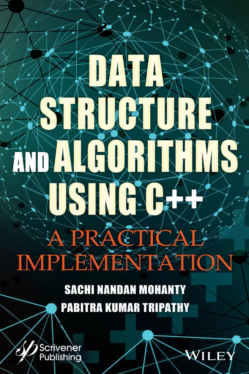


Автор: Mohanty S.N. Tripathy P.K.
Теги: algorithms information technology c++ programming language data structures
ISBN: 978-1-119-75054-3
Год: 2021


Текст
Data Structure and Algorithms
Using C++
Scrivener Publishing
100 Cummings Center, Suite 541J
Beverly, MA 01915-6106
Publishers at Scrivener
Martin Scrivener (martin@scrivenerpublishing.com)
Phillip Carmical (pcarmical@scrivenerpublishing.com)
Data Structure
and Algorithms Using C++
A Practical Implementation
Edited by
Sachi Nandan Mohanty
ICFAI Foundation For Higher Education, Hyderabad, India
and
Pabitra Kumar Tripathy
Kalam Institute of Technology, Berhampur, India
This edition first published 2021 by John Wiley & Sons, Inc., 111 River Street, Hoboken, NJ 07030, USA
and Scrivener Publishing LLC, 100 Cummings Center, Suite 541J, Beverly, MA 01915, USA
© 2021 Scrivener Publishing LLC
For more information about Scrivener publications please visit www.scrivenerpublishing.com.
All rights reserved. No part of this publication may be reproduced, stored in a retrieval system, or
transmitted, in any form or by any means, electronic, mechanical, photocopying, recording, or otherwise, except as permitted by law. Advice on how to obtain permission to reuse material from this title
is available at http://www.wiley.com/go/permissions.
Wiley Global Headquarters
111 River Street, Hoboken, NJ 07030, USA
For details of our global editorial offices, customer services, and more information about Wiley products visit us at www.wiley.com.
Limit of Liability/Disclaimer of Warranty
While the publisher and authors have used their best efforts in preparing this work, they make no rep
resentations or warranties with respect to the accuracy or completeness of the contents of this work and
specifically disclaim all warranties, including without limitation any implied warranties of merchant-
ability or fitness for a particular purpose. No warranty may be created or extended by sales representa
tives, written sales materials, or promotional statements for this work. The fact that an organization,
website, or product is referred to in this work as a citation and/or potential source of further informa
tion does not mean that the publisher and authors endorse the information or services the organiza
tion, website, or product may provide or recommendations it may make. This work is sold with the
understanding that the publisher is not engaged in rendering professional services. The advice and
strategies contained herein may not be suitable for your situation. You should consult with a specialist
where appropriate. Neither the publisher nor authors shall be liable for any loss of profit or any other
commercial damages, including but not limited to special, incidental, consequential, or other damages.
Further, readers should be aware that websites listed in this work may have changed or disappeared
between when this work was written and when it is read.
Library of Congress Cataloging-in-Publication Data
ISBN 978-1-119-75054-3
Cover image: Pixabay.Com
Cover design by Russell Richardson
Set in size of 11pt and Minion Pro by Manila Typesetting Company, Makati, Philippines
Printed in the USA
10 9 8 7 6 5 4 3 2 1
Contents
Preface
xi
1
Introduction to Data Structure
1.1 Definition and Use of Data Structure
1.2 Types of Data Structure
1.3 Algorithm
1.4 Complexity of an Algorithm
1.5 Efficiency of an Algorithm
1.6 Asymptotic Notations
1.7 How to Determine Complexities
1.8 Questions
1
1
2
3
6
7
8
9
13
2
Review of Concepts of ‘C++’
2.1 Array
2.1.1 One-Dimensional Array
2.1.2 Multi-Dimensional Array
2.1.3 String Handling
2.2 Function
2.2.1 User Defined Functions
2.2.2 Construction of a Function
2.2.3 Actual Argument and Formal Argument
2.2.4 Call by Value and Call by Reference
2.2.5 Default Values for Parameters
2.2.6 Storage Class Specifiers
2.3 Pointer
2.3.1 Declaration of a Pointer
2.3.2 Initialization of a Pointer
2.3.3 Arithmetic With Pointer
2.3.4 Passing of a Pointer to Function
2.3.5 Returning of a Pointer by Function
2.3.6 C++ Null Pointer
15
15
16
17
20
26
26
27
31
32
34
35
37
37
37
38
39
40
41
v
vi Contents
2.4
2.5
Structure
2.4.1 The typedef Keyword
Questions
42
46
47
3
Sparse Matrix
3.1 What is Sparse Matrix
3.2 Sparse Matrix Representations
3.3 Algorithm to Represent the Sparse Matrix
3.4 Programs Related to Sparse Matrix
3.5 Why to Use Sparse Matrix Instead of Simple Matrix?
3.6 Drawbacks of Sparse Matrix
3.7 Sparse Matrix and Machine Learning
3.8 Questions
49
49
49
51
52
56
57
57
58
4
Concepts of Class
4.1 Introduction to CLASS
4.2 Access Specifiers in C++
4.3 Declaration of Class
4.4 Some Manipulator Used In C++
4.5 Defining the Member Functions Outside of the Class
4.6 Array of Objects
4.7 Pointer to Object
4.8 Inline Member Function
4.9 Friend Function
4.9.1 Simple Friend Function
4.9.2 Friend With Inline Substitution
4.9.3 Granting Friendship to Another Class
(Friend Class)
4.9.4 More Than One Class Having the Same
Friend Function
4.10 Static Data Member and Member Functions
4.11 Constructor and Destructor
4.11.1 Constructor
4.11.1.1 Empty Constructor
4.11.1.2 Default Constructor
4.11.1.3 Parameterized Constructors
4.11.1.4 Copy Constructor
4.11.2 Destructor
4.12 Dynamic Memory Allocation
4.13 This Pointer
4.14 Class Within Class
4.15 Questions
59
59
60
60
62
64
64
66
67
69
69
70
71
73
75
78
78
79
79
80
81
83
84
86
87
89
Contents vii
5
Stack
5.1 STACK
5.2 Operations Performed With STACK
5.3 ALGORITHMS
5.4 Applications of STACK
5.5 Programming Implementations of STACK
5.6 Questions
91
91
91
93
96
106
126
6
Queue
6.1 Queue
6.2 Types of Queue
6.3 Linear Queue
6.4 Circular Queue
6.5 Double Ended Queue
6.6 Priority Queue
6.7 Programs
6.8 Questions
129
129
129
129
134
138
139
142
165
7
Linked List
7.1 Why Use Linked List?
7.2 Types of Link List
7.3 Single Link List
7.4 Programs Related to Single Linked List
7.4.1 /* Creation of a Linked List */
7.4.2 /* Insert a Node Into a Simple Linked List at
the Beginning */
7.4.3 /* Insert a Node Into a Simple Linked List at
the End of the List */
7.4.4 /* Insert a Node Into a Simple Linked List
When the Node Is Known */
7.4.5 /* Insert a Node Into a Simple Linked List
Information Is Known and Put After Some
Specified Node */
7.4.6 /* Deleting the First Node From a Simple
Linked List */
7.4.7 /* Deleting the Last Node From a Simple
Linked List */
7.4.8 /* Deleting a Node From a Simple Linked
List When Node Number Is Known */
7.4.9 Deleting a Node From a Simple Linked List
When Information of a Node Is Given
167
167
167
168
177
177
178
180
182
184
187
189
191
193
viii Contents
7.4.10 /* SEARCH A NODE INTO A SIMPLE LINKED
LIST WITH INFORMATION IS KNOWN*/
7.4.11 /* Sorting a Linked List in Ascending Order */
7.4.12 /* Reversing a Linked List */
7.4.13 Program for Student Data Using Linked List
7.5 Double Link List
7.6 Programs on Double Linked List
7.6.1 /* Creation of Double Linked List */
7.6.2 /* Inserting First Node in the Doubly
Linked List */
7.6.3 /*Inserting a Node in the Doubly Linked List
When Node Number Is Known*/
7.6.4 /*Inserting a Node in the Doubly Linked List
When Information Is Known*/
7.6.5 /* Delete First Node From a Double Linked List */
7.6.6 /*Delete the Last Node From the Double
Linked List*/
7.7 Header Linked List
7.7.1 /* Inserting a Node Into a Header Linked List */
7.8 Circular Linked List
7.9 Application of Linked List
7.9.1 Addition of Two Polynomial
7.9.2 /* Polynomial With Help of Linked List */
7.9.3 Program for Linked Queue
7.9.4 Program for Linked Stack
7.10 Garbage Collection and Compaction
7.11 Questions
8
TREE
8.1 Tree Terminologies
8.2 Binary Tree
8.3 Representation of Binary Tree
8.3.1 Array Representation of a Tree
8.3.2 Linked List Representation of a Tree
8.4 Operations Performed With the Binary Tree
8.4.1 /*Creation of a Tree*/
8.5 Traversing With Tree
8.5.1 /* Binary Tree Traversal */
8.6 Conversion of a Tree From Inorder and Preorder
197
199
202
203
210
216
216
218
220
223
226
229
231
233
235
239
239
240
241
243
245
247
249
249
251
253
253
254
254
255
256
259
262
Contents ix
8.7
8.8
8.9
8.10
8.11
8.12
8.13
8.14
8.15
8.16
8.17
8.18
8.19
9
Types of Binary Tree
Expression Tree
Binary Search Tree
Height Balanced Tree (AVL Tree)
Threaded Binary Tree
Heap Tree
Huffman Tree
Decision Tree
B-Tree
B + Tree
General Tree
Red–Black Tree
Questions
Graph
9.1 Graph Terminologies
9.2 Representation of Graph
9.3 Traversal of Graph
9.3.1 Breadth First Search (BFS)
9.3.2 Depth First Search
9.4 Spanning Tree
9.4.1 Kruskal Algorithm
9.4.2 Prim’s Algorithm
9.5 Single Source Shortest Path
9.5.1 Bellman–Ford Algorithm
9.5.2 Dijkstra’s Algorithm
9.6 All Pair Shortest Path
9.7 Topological Sorting
9.8 Questions
10 Searching and Sorting
10.1 Linear Search
10.2 Binary Search
10.3 Bubble Sort
10.4 Selection Sort
10.5 Insertion Sort
10.6 Merge Sort
10.7 Quick Sort
10.8 Radix Sort
10.9 Heap Sort
10.10 Questions
265
265
268
272
277
279
282
286
287
292
293
293
294
295
295
301
305
305
311
315
315
318
322
323
327
335
345
347
349
349
351
355
359
361
363
366
369
372
389
x Contents
11 Hashing
11.1 Hash Functions
11.2 Collisions
11.3 Collision Resolution Methods
11.4 Clustering
11.5 Questions
391
391
393
393
394
395
Index
397
Preface
Welcome to the first edition of Data Structures and Algorithms Using C++.
A data structure is the logical or mathematical arrangement of data in
memory. To be effective, data has to be organized in a manner that adds to
the efficiency of an algorithm and also describe the relationships between
these data items and the operations that can be performed on these items.
The choice of appropriate data structures and algorithms forms the fundamental step in the design of an efficient program. Thus, a deep understanding of data structure concepts is essential for students who wish to work
on the design and implementation of system software written in C++, an
object-oriented programming language that has gained popularity in both
academia and industry. Therefore, this book was developed to provide
comprehensive and logical coverage of data structures like stacks, queues,
linked lists, trees and graphs, which makes it an excellent choice for learning data structures. The objective of the book is to introduce the concepts
of data structures and apply these concepts in real-life problem solving.
Most of the examples presented resulted from student interaction in the
classroom. This book utilizes a systematic approach wherein the design of
each of the data structures is followed by algorithms of different operations
that can be performed on them and the analysis of these algorithms in
terms of their running times.
This book was designed to serve as a textbook for undergraduate engineering students across all disciplines and postgraduate level courses in
computer applications. Young researchers working on efficient data storage
and related applications will also find it to be a helpful reference source to
guide them in the newly established techniques of this rapidly growing
research field.
Dr. Sachi Nandan Mohanty and
Prof. Pabitra Kumar Tripathy
December 2020
xi
1
Introduction to Data Structure
1.1 Definition and Use of Data Structure
Data structure is the representation of the logical relationship existing
between individual elements of data. In other words the data structure is a
way of organizing all data items that considers not only the elements stored
but also their relationship to each other.
Data structure specifies
•
•
•
•
Organization of data
Accessing methods
Degree of associativity
Processing alternatives for information
The data structures are the building blocks of a program and hence the
selection of a particular data structure stresses on
• The data structures must be rich enough in structure to
reflect the relationship existing between the data, and
• The structure should be simple so that we can process data
effectively whenever required.
In mathematically Algorithm + Data Structure = Program
Finally we can also define the data structure as the “Logical and mathematical model of a particular organization of data”
Sachi Nandan Mohanty and Pabitra Kumar Tripathy. Data Structure and Algorithms Using C++:
A Practical Implementation, (1–14) © 2021 Scrivener Publishing LLC
1
2 Data Structure and Algorithms Using C++
1.2 Types of Data Structure
Data structure can be broadly classified into two categories as Linear and
Non-Linear
DATA STRUCTURE
LINEAR
ARRAY
QUEUE
NON LINEAR
STACK
TREE
GRAPH
TABLES
SETS
Linear Data Structures
In linear data structures, values are arranged in linear fashion. Arrays,
linked lists, stacks, and queues are the examples of linear data structures in
which values are stored in a sequence.
Non-Linear Data Structure
This type is opposite to linear. The data values in this structure are not
arranged in order. Tree, graph, table, and sets are the examples of nonlinear data structure.
Operations Performed in Data Structure
In data structure we can perform the operations like
•
•
•
•
•
•
Traversing
Insertion
Deletion
Merging
Sorting
Searching
Introduction to Data Structure
3
1.3 Algorithm
The step by step procedure to solve a problem is known as the ALGORITHM.
An algorithm is a well-organized, pre-arranged, and defined computational
module that receives some values or set of values as input and provides a
single or set of values as out put. These well-defined computational steps
are arranged in sequence, which processes the given input into output.
An algorithm is said to be accurate and truthful only when it provides
the exact wanted output.
The efficiency of an algorithm depends on the time and space complexities. The complexity of an algorithm is the function which gives the running time and/or space in terms of the input size.
Steps Required to Develop an Algorithm
• Finding a method for solving a problem. Every step of an
algorithm should be defined in a precise and in a clear manner. Pseudo code is also used to describe an algorithm.
• The next step is to validate the algorithm. This step includes
all the steps in our algorithm and should be done manually
by giving the required input, perform the required steps
including in our algorithm and should get the required
amount of output in a finite amount of time.
• Finally implement the algorithm in terms of programming
language.
Mathematical Notations and Functions
Floor and Ceiling Functions
Floor function returns the greatest integer that does not exceed
the number.
Ceiling function returns the least integer that is not less than
the number.
no
denotes the floor function
no
denotes the ceil function
Ex :
5.23 = 5
5.23
=6
4 Data Structure and Algorithms Using C++
Remainder Function
To find the remainder “mod” function is being used as
A mod B
To find the Integer and Absolute value of a number
INT(5.34) = 5
This statement returns the integer part of
the number
INT(- 6.45) = 6 This statement returns the absolute as well
as the integer portion of the number
Summation Symbol
To add a series of number as a1+ a2 + a3 +…………+ an the
symbol Σ is used
n
Σ ai
i=1
Factorial of a Number
The product of the positive integers from 1 to n is known as
the factorial of n and it is denoted as n!.
0! = 1
Algorithemic Notations
While writing the algorithm the comments are provided with in [ ].
The assignment should use the symbol “: =” instead of “=”
For Input use Read : variable name
For output use write : message/variable name
The control structures can also be allowed to use inside an algorithm but
their way of approaching will be some what different as
Simple If
If condition, then:
Statements
[end of if structure]
Introduction to Data Structure
5
If…else
If condition, then:
Statements
Else :
Statements
[end of if structure]
If…else ladder
If condition1, then:
Statements
Else If condition2, then:
Statements
Else If condition3, then:
Statements
…………………………………………
…………………………………………
…………………………………………
Else If conditionN, then:
Statements
Else:
Statements
[end of if structure]
LOOPING CONSTRUCT
Repeat for var = start_value to end_value by
step_value
Statements
[end of loop]
Repeat while condition:
Statements
[end of loop]
Ex : repeat for I = 1 to 10 by 2
Write: i
[end of loop]
OUTPUT
1 3 5 7 9
6 Data Structure and Algorithms Using C++
1.4 Complexity of an Algorithm
The complexity of programs can be judged by criteria such as whether
it satisfies the original specification task, whether the code is readable.
These factors affect the computing time and storage requirement of the
program.
Space Complexity
The space complexity of a program is the amount of memory it needs to
run to completion. The space needed by a program is the sum of the following components:
• A fixed part that includes space for the code, space for simple variables and fixed size component variables, space for
constants, etc.
• A variable part that consists of the space needed by component variables whose size is dependent on the particular
problem instance being solved, and the stack space used by
recursive procedures.
Time Complexity
The time complexity of a program is the amount of computer time it needs
to run to completion. The time complexity is of two types such as
• Compilation time
• Runtime
The amount of time taken by the compiler to compile an algorithm is
known as compilation time. During compilation time it does not calculate
for the executable statements, it calculates only the declaration statements
and checks for any syntax and semantic errors.
The run time depends on the size of an algorithm. If the number of
instructions in an algorithm is large, then the run time is also large, and if
the number of instructions in an algorithm is small, then the time for executing the program is also small. The runtime is calculated for executable
statements and not for declaration statements.
Introduction to Data Structure
7
Suppose space is fixed for one algorithm then only run time will be considered for obtaining the complexity of algorithm, these are
• Best case
• Worst case
• Average case
Best Case
Generally, most of the algorithms behave sometimes in best case. In this
case, algorithm searches the element for the first time by itself.
For example: In linear search, if it finds the element for the first time by
itself, then it behaves as the best case. Best case takes shortest time to execute, as it causes the algorithms to do the least amount of work.
Worst Case
In worst case, we find the element at the end or when searching of elements
fails. This could involve comparing the key to each list value for a total of
N comparisons.
For example in linear search suppose the element for which algorithm
is searching is the last element of array or it is not available in array then
algorithm behaves as worst case.
Average Case
Analyzing the average case behavior algorithm is a little bit complex than
the best case and worst case. Here, we take the probability with a list of
data. Average case of algorithm should be the average number of steps but
since data can be at any place, so finding exact behavior of algorithm is
difficult. As the volume of data increases, the average case of algorithm
behaves like the worst case of algorithm.
1.5 Efficiency of an Algorithm
Efficiency of an algorithm can be determined by measuring the time, space,
and amount of resources it uses for executing the program. The amount of
time taken by an algorithm can be calculated by finding the number of
steps the algorithm executes, while the space refers to the number of units
it requires for memory storage.
8 Data Structure and Algorithms Using C++
1.6 Asymptotic Notations
The asymptotic notations are the symbols which are used to solve the different algorithms and the notations are
•
•
•
•
Big Oh Notation (O)
Little Oh Notation (o)
Omega Notation (W)
Theta Notation (q)
Big Oh (O) Notation
This Notation gives the upper bound for a function to within a constant
factor. We write f(n) = O(g(n)) if there are +ve constants n0 and C such
that to the right of n0, the value of f(n) always lies on or below Cg(n)
Omega Notation (W)
This notation gives a lower bound for a function to with in a constant factor. We write f(n) = Ωg(n) if there are positive constants n0 and C such that
to the right of n0 the value of f(n) always lies on or above Cg(n)
Theta Notation (q)
This notation bounds the function to within constant factors. We say f(n) =
θg(n) if there exists +ve constants n0, C1 and C2 such that to the right of n0
the value of f(n) always lies between c1g(n) and c2(g(n)) inclusive.
Little Oh Notation (o)
F(n) = o(g(n)) iff f(n) = O(g(n)) and f(n) != Ωg(n).
Introduction
An important question is: How efficient is an algorithm or piece of code?
Efficiency covers lots of resources, including:
CPU (time) usage
Memory usage
Disk usage
Network usage
Introduction to Data Structure
9
All are important but we will mostly talk about CPU time
Be careful to differentiate between:
Performance: how much time/memory/disk/... is actually used
when a program is running. This depends on the machine, compiler, etc.,
as well as the code.
Complexity: how do the resource requirements of a program or algorithm
scale, i.e., what happens as the size of the problem being solved gets larger.
Complexity affects performance but not the other way around. The time
required by a method is proportional to the number of “basic operations”
that it performs. Here are some examples of basic operations:
one
one
one
one
one
arithmetic operation (e.g., +, *).
assignment
test (e.g., x == 0)
read
write (of a primitive type)
Note: As an example,
O(1) refers to constant time.
O(n) indicates linear time;
O(nk) (k fixed) refers to polynomial time;
O(log n) is called logarithmic time;
O(2n) refers to exponential time, etc.
n² + 3n + 4 is O(n²), since n² + 3n + 4 < 2n² for all n > 10. Strictly speaking,
3n + 4 is O(n²), too, but big-O notation is often misused to mean equal to
rather than less than.
1.7 How to Determine Complexities
In general, how can you determine the running time of a piece of code?
The answer is that it depends on what kinds of statements are used.
1. Sequence of statements
statement 1;
statement 2;
...
statement k;
10 Data Structure and Algorithms Using C++
Note: this is code that really is exactly k statements; this is not
an unrolled loop like the N calls to addBefore shown above.)
The total time is found by adding the times for all statements:
total time = time(statement 1) + time
(statement 2) + ... + time(statement k)
If each statement is “simple” (only involves basic operations) then the time for each statement is constant and the
total time is also constant: O(1). In the following examples,
assume the statements are simple unless noted otherwise.
2. if-then-else statements
if (cond) {
sequence of statements 1
}
else {
sequence of statements 2
}
Here, either sequence 1 will execute, or sequence 2 will execute.
Therefore, the worst-case time is the slowest of the two possibilities: max(time(sequence 1), time(sequence 2)). For example, if sequence 1 is O(N) and sequence 2 is O(1) the worst-case
time for the whole if-then-else statement would be O(N).
3. for loops
for (i = 0; i < N; i++) {
sequence of statements
}
The loop executes N times, so the sequence of statements also
executes N times. Since we assume the statements are O(1), the
total time for the for loop is N * O(1), which is O(N) overall.
4. Nested loops
for (i = 0; i < N; i++) {
for (j = 0; j < M; j++) {
sequence of statements
}
}
The outer loop executes N times. Every time the outer loop
executes, the inner loop executes M times. As a result, the
statements in the inner loop execute a total of N * M times.
Thus, the complexity is O(N * M). In a common special case
Introduction to Data Structure
11
where the stopping condition of the inner loop is j < N
instead of j < M (i.e., the inner loop also executes N times),
the total complexity for the two loops is O(N2).
5. Statements with method calls:
When a statement involves a method call, the complexity of
the statement includes the complexity of the method call.
Assume that you know that method f takes constant time,
and that method g takes time proportional to (linear in) the
value of its parameter k. Then the statements below have the
time complexities indicated.
f(k);
g(k);
// O(1)
// O(k)
When a loop is involved, the same rule applies. For example:
for (j = 0; j < N; j++) g(N);
has complexity (N2). The loop executes N times and each
method call g(N) is complexity O(N).
Examples
Q1. What is the worst-case complexity of the each of the following code
fragments?
Two loops in a row:
for (i = 0; i <
sequence of
}
for (j = 0; j <
sequence of
}
N; i++) {
statements
M; j++) {
statements
Answer: Th
e first loop is O(N) and the second loop is O(M). Since you
do not know which is bigger, you say this is O(N+M). This can
also be written as O(max(N,M)). In the case where the second
loop goes to N instead of M the complexity is O(N). You can
see this from either expression above. O(N+M) becomes O(2N)
and when you drop the constant it is O(N). O(max(N,M))
becomes O(max(N,N)) which is O(N).
12 Data Structure and Algorithms Using C++
Q2. How would the complexity change if the second loop went to N
instead of M?
A nested loop followed by a non-nested loop:
for (i = 0; i < N; i++) {
for (j = 0; j < N; j++) {
sequence of statements
}
}
for (k = 0; k < N; k++) {
sequence of statements
}
Answer: Th
e first set of nested loops is O(N2) and the second loop is
O(N). This is O(max(N2,N)) which is O(N2).
Q3. A nested loop in which the number of times the inner loop executes
depends on the value of the outer loop index:
for (i = 0; i < N; i++) {
for (j = i; j < N; j++) {
sequence of statements
}
}
Answer: W
hen i is 0 the inner loop executes N times. When i is 1 the
inner loop executes N-1 times. In the last iteration of the outer
loop when i is N-1 the inner loop executes 1 time. The number
of times the inner loop statements execute is N + N-1 + ... + 2 +
1. This sum is N(N+1)/2 and gives O(N2).
Q4. For each of the following loops with a method call, determine the
overall complexity. As above, assume that method f takes constant time,
and that method g takes time linear in the value of its parameter.
a. for (j = 0; j < N; j++) f(j);
b. for (j = 0; j < N; j++) g(j);
c. for (j = 0; j < N; j++) g(k);
Answer: a. E
ach call to f(j) is O(1). The loop executes N times so it is N x
O(1) or O(N).
b. The first time the loop executes j is 0 and g(0) takes “no operations.” The next time j is 1 and g(1) takes 1 operations. The
last time the loop executes j is N-1 and g(N-1) takes N-1 operations. The total work is the sum of the first N-1 numbers and
is O(N2).
Introduction to Data Structure
c. Each time through the loop g(k) takes k operations and the
loop executes N times. Since you do not know the relative size
of k and N, the overall complexity is O(N x k).
1.8 Questions
1. What is data structure?
2. What are the types of operations that can be performed with
data structure?
3. What is asymptotic notation and why is this used?
4. What is complexity and its type?
5. Find the complexity of 3n2 + 5n.
6. Distinguish between linear and non-linear data structure.
7. Is it necessary is use data structure in every field? Justify
your answer.
13
2
Review of Concepts of ‘C++’
2.1 Array
Whenever we want to store some values then we have to take the help of a
variable, and for this we must have to declare it before its use. If we want
to store the details of a student so for this purpose we have to declare the
variables as
char name [20], add[30] ;
int roll, age, regdno ;
float total, avg ;
etc……
for a individual student.
If we want to store the details of more than one student than we have to
declare a huge amount of variables and which are too much difficult to access
it. I.e/ the programs length will increased too faster. So it will be better to
declare the variables in a group. I.e/ name variable will be used for more than
one student, roll variable will be used for more than one student, etc.
So to declare the variable of same kind in a group is known as the Array
and the concept of array is used for this purpose only.
Definition: The array is a collection of more than one element of same
kind with a single variable name.
Types of Array:
The arrays can be further classified into two broad categories such as:
• One Dimensional (The array having one boundary
specification)
• Multi dimensional (The array having more than one boundary specification)
Sachi Nandan Mohanty and Pabitra Kumar Tripathy. Data Structure and Algorithms Using C++:
A Practical Implementation, (15–48) © 2021 Scrivener Publishing LLC
15
16 Data Structure and Algorithms Using C++
2.1.1 One-Dimensional Array
Declaration:
Syntax :
Data type variable_name[bound] ;
The data type may be one of the data types that we are studied. The
variable name is also same as the normal variable_name but the bound is
the number which will further specify that how much variables you want
to combine into a single unit.
Ex : int roll[15];
In the above example roll is an array 15 variables whose capacity is to
store the roll_number of 15 students.
And the individual variables are
roll[0] , roll[1], roll[2], roll[3] ,……………..,roll[14]
Array Element in Memory
The array elements are stored in a consecutive manner inside the memory.
i.e./ They allocate a sequential memory allocation.
For Ex : int x[7];
Let the x[0] will be at the memory address 568 then the entire array can
be represented in the memory as
x[0]
X[1]
X[2]
X[3]
X[4]
X[5]
X[6]
568
570
572
574
576
578
580
Initialization:
The array is also initialized just like other normal variable except that
we have to pass a group of elements with in a chain bracket separated by
commas.
Ex : int x[5]= { 24,23,5,67,897 } ;
In the above statement x[0] = 24, x[1] = 23, x[2]=5, x[3]=67,x[4]=897
Review of Concepts of ‘C++’
17
Retrieving and Storing Some Value From/Into the Array
Since array is a collection of more than one elements of same kind so while
performing any task with the array we have to do that work repeatedly.
Therefore while retrieving or storing the elements from/into an array we
must have to use the concept of looping.
Ex: Write a Program to Input 10 Elements Into an Array and
Display Them.
#include<iostream.h>
void main()
{
int x[10],i;
;
cout<<“\nEnter 10 elements into the array”;
for(i=0 ; i<10; i++)
cin>>x[i];
cout<<“\n THE ENTERED ARRAY ELEMENTS ARE :”;
for(i=0 ; i<10; i++)
cout<<”
“<<x[i];
}
OUTPUT
Enter 10 elements into the array
12
36
89
54
6
125
35
87
49
6
THE ENTERED ARRAY ELEMENTS ARE :
89 54
6 125 35 87 49
6
12
36
2.1.2 Multi-Dimensional Array
The array having more than one boundary specification is known as multi
dimensional array. The total number of elements to be stored in side a
multi dimensional array is equals to the product of its boundaries.
18 Data Structure and Algorithms Using C++
But we do use the two dimensional array to handle the matrix operations. The two dimensional array having two boundary specifications.
Declaration of Two-Dimensional Array
The declaration of the two dimensional array is just like the one dimensional array except that instead of using a single boundary we have to use
two boundary specification.
SYNTAX
data_type variable_name[boundary1][boundary2];
Ex : int x[3][4];
In the above example x is the two dimensional array which has the capacity
to store (3x4) 12 elements. The individual number of elements are
x[0][0] x[0][1] x[0][2] x[0][3]
x[1][0] x[1][1] x[1][2] x[1][3]
x[2][0] x[2][1] x[2][2] x[2][3]
INITIALIZATION
The array can also be initialized as like one dimensional array.
Ex: int x[3][4] = {{3,5,7,8}, {45,12,34,3}, {56,89,56,23}};
OR
int x[3][4] = {3,5,7,8,45,12,34,3,56,89,56,23};
After the above initialization
x[0][0]=3
x[1][0]=45
x[2][0]=56
x[0][1]=5
x[1][1]=12
x[2][1]=89
x[0][2]=7
x[1][2]=34
x[2][2]=56
x[0][3]=8
x[1][3]=3
x[2][3]=23
Processing of a Two-Dimensional Array
While processing a two-dimensional array we have to use two loops.
Review of Concepts of ‘C++’
19
Example : WAP to input a 3 x 3 matrix and find out the sum of
lower triangular elements.
#include<iostream.h>
void main()
{
int mat[3][3],i,j,sum=0;
/* INPUT THE ARRAY */
for(i=0 ; i<3 ; i++)
for(j=0 ; j<3 ; j++)
{
cout<<“\nEnter a number”;
cin>>mat[i][j];
}
/* LOGIC TO SUM THE LOWER TRIANGULAR ELEMENTS */
for(i=0 ; i<3 ; i++)
for(j=0 ; j<3 ; j++)
{
if(i>=j)
sum=sum+mat[i][j];
}
/* PRINT THE ARRAY */
cout“\nTHE ENTERED MATRIX IS\n”;
for(i=0 ; i<3 ; i++)
{
for(j=0 ; j<3 ; j++)
{
cout<<”
“<<mat[i][j];
}
cout<<“\n”;
}
cout<<“\nSum of the lower triangular matrix is”<<sum;
}
20 Data Structure and Algorithms Using C++
OUTPUT
Enter a number 5
Enter a number 7
Enter a number 9
Enter a number 2
Enter a number 6
Enter a number 8
Enter a number 12
Enter a number 24
Enter a number 7
THE ENTERED MATRIX IS
5
2
12
7
6
24
9
8
7
Sum of the lower triangular matrix is 56
2.1.3 String Handling
The string is a collection of more than one character. So it can also be called
as a character array. The approaching to the string/character array is somewhat different compare to the normal array due to its speciality nature.
The speciality is that the string always terminates with a NULL (‘\0’)
character. So while accessing the string there is no need to use the loop
frequently(We may access it as a array with the help of loop).
When we will access it with the loop (like int, float etc. array) than the
NULL character will not be assigned at the end of it, so while printing it
we are bound to use the loop again. If we want to convert the character
array to a string so we have to assign the NULL character at the end of it,
manually.
Representation of a string and a Character Array
Let char x[10]=”India”;
/* Representation of a string*/
I
n
d
i
a
\0
0
1
2
3
4
5
6
7
8
9
Review of Concepts of ‘C++’
char x[10] = {‘I’,’n’,’d’,’i’,’a’};
21
/* Character Array */
I
n
d
i
a
0
1
2
3
4
5
6
7
8
9
Declaration of a Character Array
The declaration of the string/character array is same as the normal array,
except that instead of using other data type the data type ‘char’ is used.
Syntax : Data_type var_name[size] ;
Ex: char name[20];
Initialization of a String
Let char x[10]=”India”;
/* Representation of a string*/
I
n
d
i
a
\0
0
1
2
3
4
5
char x[10] = {‘I’,’n’,’d’,’i’,’a’};
6
7
8
9
/* Character Array */
Example: Wap to Input a string and display it.
#include<iostream.h>
void main()
{
char x[20];
cout<<"\nEnter a string";
gets(x);
cout<<"\n THE ENTERED STRING IS "<<x;
}
OUTPUT
Enter a string Hello
THE ENTERED STRING IS Hello
OR
22 Data Structure and Algorithms Using C++
This process of Input is not preferable because forcibly we are bound to
input the 10 characters, not less than 10 or above 10 characters.
#include<iostream.h>
void main()
{
char x[20];
int i;
cout<<"\nEnter a string";
for(i=0;i<10;i++)
cin>>x[i];
x[i]='\0'; /* CONVERTING THE CHARACTER ARRAY
TO STRING */
cout<<"\n THE ENTERED STRING IS "<<x;
}
OR
#include<iostream.h>
void main()
{
char x[20];
int i;
cout<<"\nEnter a string";
gets(x);
cout<<"\n THE ENTERED STRING IS ";
for(i=0; x[i]!=’\0’;i++)
cout<<x[i];
}
OUTPUT
Enter a string Hello
THE ENTERED STRING IS Hello
NOTE : If we want to scan a string as individual characters then we
have to use the loop as for(i=0; str[i]!='\0';i++)
This is fixed for all the strings after input it.
Review of Concepts of ‘C++’
23
Example – 2
Write a program to input a string and count how many vowels are in it.
#include<iostream.h>
void main()
{
char x[20];
int i,count=0;
cout<<"\n Enter a string";
gets(x);
cout<<"\n The entered string is"<<x;
for(i=0; x[i]!='\0';i++)
if(toupper(x[i])=='A'
||
toupper(x[i])=='E'
|| toupper(x[i])=='I' || toupper
(x[i])=='O' ||
toupper(x[i))=='U')
count++;
cout<<"\n The string"<<x<< "having"<<count<<"numbers of vowels";
}
OUTPUT
Enter a string Wel Come
The entered string is Wel Come
The string Wel Come having 3 numbers of vowels.
Example :
Write a program to find out the length of a string.
#include<iostream.h>
void main()
{
char x[20];
int i,len=0;
cout<<"\n Enter a string";
gets(x);
for(i=0;x[i]!='\0';i++)
len++;
cout<<"\n THE LENGTH OF"<<x<<"IS"<<len;
}
24 Data Structure and Algorithms Using C++
OUTPUT
Enter a string hello India
THE LENGTH OF hello India IS 11
OR
#include<iostream.h>
void main()
{
char x[20];
int i;
cout<<"\n Enter a string";
gets(x);
for(i=0;x[i]!='\0';i++) ;
cout<<"\n THE LENGTH OF"<<x<<"IS"<<len;
}
OUTPUT
Enter a string hello India
THE LENGTH OF hello India IS 11
String Manipulation
The strings cannot be manipulated with the normal operators, so to have
some manipulation we have to use the help of certain string handling
functions. ’C’-language provides a number of string handling functions
amongst them the most popularly used functions are
a.
b.
c.
d.
e.
f.
g.
Strlen()
Strrev()
Strcat()
Strcmp()
Strcpy()
Strupr()
Strlwr()
These functions prototypes are declared inside the header file string.h
Strlen()
Purpose : Used to find out the length of a string.
Syntax : integer_variable = strlen(string);
Review of Concepts of ‘C++’
25
Strrev()
Purpose : Used to find out the reverse of a string.
Syntax : strrev(string);
Strcat()
Purpose: Used to concatenate(Join) two strings. It will
append the source string at the end of the destination. The
length of the destination will be the length of source + length
of destination
Syntax: strcat(destination,source);
Strcmp()
Purpose: Used to compare two strings.
Process: The string comparison always starts with the first
character in each string and continuous with subsequent
characters until the corresponding characters differ or until
the end of a string is reached.
This function returns an integer value that is
< 0 if s1 < s2
== 0 if s1 == s2
>0 if s1 > s2
ASCII VALUES
A = 65 a = 97
0 = 48
The string comparison is always based upon the ASCII values of the
characters.
Syntax : integer_variable = strcmp(s1,s2);
Strcpy()
Purpose :To copy a string to other.
Syntax : strcpy(destination,source);
Strupr()
Purpose : To convert all the lower case alphabets to its corresponding upper-case.
Syntax : strupr(string);
Strlwr()
Purpose : To convert all the upper case alphabets to its corresponding lower-case.
Syntax : strlwr(string);
26 Data Structure and Algorithms Using C++
2.2 Function
Definition: One or more than one statements combined together to form
a block with a particular name and having a specific task.
The functions in ‘C’ are classified into two types as
a. Library Function or Pre defined function
b. User defined function
The library functions are already comes with the ‘C’ compiler(Language).
Ex : printf(), scanf(), gets(), clrscr(), strlen() etc.
The user defined functions are defined by the programmer when ever
required.
2.2.1 User Defined Functions
We will develop the functions just comparison with the library functions,
i.e/ All the library functions can be categorized into four types as
1. integer variable = strlen(string/string variable)
[The strlen() takes a string ,find its length and returns it to a
integer variable]
2. gets(string variable);
[the gets() takes a variable and stores string inside that which
will be entered by the user]
3. character variable = getch();
[The getch() does not take any value/variable but it stores a
character into the character variable which will be entered
by the user]
4. clrscr();
[This function does not take argument and not return also,
but it does its work that means it clears the screen]
So by studying the above four types of functions we concluded that by
considering the arguments taken by the function and the values returned
by the functions the functions can be categorized into four types as
1.
2.
3.
4.
The function takes argument and also returns value.
The function does not take argument but returns value.
The function takes argument but not return value.
The function does not take argument and also not return values.
Review of Concepts of ‘C++’
Parts of a Function
A function has generally three parts as
1. Declaration (Specifies that how the function will work, it
prepares only the skeleton of the function)
2. Call [It call the function for execution]
3. Definition [It specifies the work of the function i./ it is the
body part of the function]
2.2.2 Construction of a Function
1. Function takes argument and also returns value.
DECLARATION
Return_type function_name(data type, data_type, data_
type, …………….);
Ex: int sum(int,int);
CALL
Variable = function_name(var1,var2,var3,……………..);
Ex: x = sum(a,b);
Where a,b,x are the integer variables
DEFINITION
Return_type function_name(data_type var1, data_type
var2,………..)
{
Body of the function ;
Return(value/variable/expression);
}
Ex:
int sum(int p, int q)
{
int z;
z = p+q;
return(z);
}
2. Function does not take argument but returns value.
DECLARATION
Return_type function_name();
Or
27
28 Data Structure and Algorithms Using C++
Return_type function_name(void);
Ex : int sum();
CALL
Variable = function_name();
Ex : x = sum();
Where x is an integer.
DEFINITION
Return_type function_name()
{
Body of function;
Return(value/variable/expression);
}
Ex:
int sum()
{
int a,b;
cout<<"\nEnter 2 numbers";
cin>>a>>b;
return(a+b);
}
3. Function takes argument but not returns value
DECLARATION
void function_name(data type1,data type2,……………);
Ex : void sum(int,int);
CALL
function_name(var1,var2,var3…………);
Ex : sum(x,y);
Where x and y is an integer.
DEFINITION
Void function_name (data_type1 v1, data_type2 v2,………)
{
Body of function ;
}
Ex:
void sum(int x, int y)
{
cout<<"\nSum = "<<x+y;
}
Review of Concepts of ‘C++’
29
4. Function does not take arguments and not returns value.
DECLARATION
void function_name(void);
Ex : void sum();
CALL
function_name();
Ex : sum();
DEFINITION
Void function_name ()
{
Body of function ;
}
Ex:
void sum()
{
int x,y;
cout<<"\n Enter two numbers";
cin>>x>>y;
cout<<"\nSum = "<<x+y;
}
ARGUMENTS : Based upon which the function works.
RETURN TYPE: The value returned /given by the function to its calling part.
WAP TO FIND OUT THE SUM OF TWO NUMBERS
Category – 1
#include<iostream.h>
void main()
{
int sum(int,int);
int x,y,z;
cout<<"\n Enter two numbers";
cin>>x>>y;
z = sum(x,y);
cout<<"\n Addition of"<<x<<"and"<<y<<"is"<<z;
}
int sum(int p,
int q)
{
int r;
r = p+q;
return(r);
}
30 Data Structure and Algorithms Using C++
OUTPUT
Enter two numbers 5
6
Addition of 5 and 6 is 11
Category – 2
#include<iostream.h>
void main()
{
int sum();
int z;
z = sum();
cout<<"\n Addition is"<<z;
}
int sum()
{
int x,y;
cout<<"\n Enter two numbers";
cin>>x>>y;
return(x+y);
}
OUTPUT
Enter two numbers 5
6
Addition is 11
Category – 3
#include<iostream.h>
void main()
{
void sum(int,int);
int x,y;
cout<<"\n Enter two numbers";
cin>>x>>y;
sum(x,y);
}
void sum(int p,int q)
{
Cout<<“\n Addition
of”<<p<<”and”<<q<<”is”<<p+q;
}
OUTPUT
Enter two numbers 5
6
Addition of 5 and 6 is 11
Review of Concepts of ‘C++’
31
Category – 4
#include<iostream.h>
void main()
{
void sum();
sum();
}
void sum()
{
int x,y;
cout<<"\n Enter two numbers";
cin>>x>>y;
cout<<"Addition of"<<x<<"and"<<y<<"is"<<x+y;
}
OUTPUT
Enter two numbers 5
6
Addition of 5 and 6 is 11
2.2.3 Actual Argument and Formal Argument
Those arguments kept inside the function call is known as actual argument
and those arguments kept inside the function definition is known as the
formal arguments (Because these are used to maintain the formality just to
store the values of the actual arguments).
Ex:
#include<iostream.h>
void main()
{
int sum(int,int);
int x,y,z;
cout<<"\n Enter two numbers";
cin>>x>>y;
z = sum(x,y); /* Here x and y are called as the
actual argument*/
cout<<"\n Addition of"<<x<<"and"<<y<<"is"<<z;
}
int sum(int p, int q) /* Here p and q are called as the formal
argument */
{
int r;
r = p+q;
return(r);
}
32 Data Structure and Algorithms Using C++
OUTPUT
Enter two numbers 5
6
Addition of 5 and 6 is 11
If a function is to use arguments, it must declare variables that accept the
values of the arguments. These variables are called the formal parameters
of the function.
The formal parameters behave like other local variables inside the function and are created upon entry into the function and destroyed upon exit.
While calling a function, there are two ways that arguments can be
passed to a function:
Call Type
Description
Call by value
This method copies the actual value of an argument into
the formal parameter of the function. In this case,
changes made to the parameter inside the function
have no effect on the argument.
Call by pointer
This method copies the address of an argument into the
formal parameter. Inside the function, the address is
used to access the actual argument used in the call.
This means that changes made to the parameter affect
the argument.
Call by reference
This method copies the reference of an argument into the
formal parameter. Inside the function, the reference
is used to access the actual argument used in the call.
This means that changes made to the parameter affect
the argument.
By default, C++ uses call by value to pass arguments. In general, this
means that code within a function cannot alter the arguments used to call
the function and above mentioned example while calling max() function
used the same method.
2.2.4 Call by Value and Call by Reference
When a function is called by its value then that function call is known as
call by value.
When a function is called by its reference/address then that function call
is known as call by reference.
Review of Concepts of ‘C++’
33
Difference Between Call by Value and Call by Reference
In call by value if the value of the variable is changed inside the function
than that will not effect to its original value, because the value of the actual
parameters are copied to the formal arguments so there is no interlink
between them.
But in call by reference if the value of the variable is changed inside
the function then that will be effected to its original value, because in call
by reference the addresses of the actual arguments are copied to the formal arguments that’s why there is a interlink between them. So any change
made with the formal argument then that will effect to the actual value.
Ex:
Call by value
#include<iostream.h>
void main()
{
int x=5,y=6;
void change(int,int);
cout<<“\n X=”<<x<<”and Y=”<<y;
change(x,y);
cout<<“\n X=”<<x<<”and Y=”<<y;
}
void change(int a,int b)
{
a=a+5;
b=b+5;
cout<<“\n X=”<<a<<”and Y=”<<b;
}
OUTPUT
X = 5 and Y=6
X=10 and Y=11
X=5 and Y=6
Call by REFERENCE
#include<iostream.h>
void main()
{
int x=5,y=6;
void change(int *,int *);
34 Data Structure and Algorithms Using C++
cout<<“\n X=”<<x<<”and Y=”<<y;
change(&x,&y);
cout<<“\n X=”<<x<<”and Y=”<<y;
}
void change(int *a,int *b)
{
*a=*a+5;
*b= *b+5;
cout<<“\n X=”<<*a<<”and Y=”<<*b;
}
OUTPUT
X = 5 and Y=6
X=10 and Y=11
X=10 and Y=11
2.2.5 Default Values for Parameters
When you define a function you can specify a default value for each of the
last parameters. This value will be used if the corresponding argument is
left blank when calling to the function.
This is done by using the assignment operator and assigning values for
the arguments in the function definition. If a value for that parameter is
not passed when the function is called, the default given value is used, but
if a value is specified this default value is ignored and the passed value is
used instead. Consider the following example:
#include <iostream>
int sum(int a, int b=20)
{
int result;
result = a + b;
return (result);
}
int main ()
{
// local variable declaration:
int a = 100;
int b = 200;
int result;
Review of Concepts of ‘C++’
35
// calling a function to add the values.
result = sum(a, b);
cout << "Total value is :" << result << endl;
// calling a function again as follows.
result = sum(a);
cout << "Total value is :" << result << endl;
return 0;
}
When the above code is compiled and executed, it produces following
result:
Total value is :300
Total value is :120
2.2.6 Storage Class Specifiers
The storage class specifiers are the keywords which are used to declare the
variables. Without the help of storage class specifier we cannot declare the
variables but till now we declare the variables without using the storage
class specifier. Because by default the c-language includes the variable into
‘auto’ storage class.
‘C++’-language supports four storage class specifiers as auto, static,
extern, register
AUTO
Initial Value
:
Storage Area
:
Life :
Scope :
STATIC
Initial Value
:
Storage Area
:
Life :
Scope
:
Garbage value
Memory
With in the block where it is declared
Local
Zero
Memory
With in the block where it is declared
The value of the variable will persist
between different function calls
EXTERN
Initial Value
: Zero
Storage Area
: Memory
Life :
The variable can access any where of
the program
Scope : Global
36 Data Structure and Algorithms Using C++
REGISTER
Initial Value
:
Storage Area
:
Life :
Scope :
Garbage
CPU Memory
With in the block where it is declared
Local
Difference between STATIC and AUTO
#include<stdio.h>
void main()
{
void change();
change();
change();
change();
}
Void change()
{
auto int x=0;
printf(“\n X= %d”,x);
x++;
}
OUTPUT
X=0
X=0
X=0
#include<stdio.h>
void main()
{
void change();
change();
change();
change();
}
Void change()
{
static int x;
printf("\n X= %d",x);
x++;
}
OUTPUT
X=0
X=1
X=2
Review of Concepts of ‘C++’
37
2.3 Pointer
The pointer is a variable which can store the address of another variable.
Whatever changed with the value of the variable with the help of the
pointer that will directly effect to it.
2.3.1 Declaration of a Pointer
Like other variables the pointer variable should also be declared before its
use
SYNTAX
Data_type *variable_name;
Example: int *p;
2.3.2 Initialization of a Pointer
Initialization means to assign an initial value, since the pointer can store
only the address so during its initialization we have to assign an address of
another variable.
Ex: int *x,p;
X=&p;
/* INITIALIZATION */
NOTE : After declaration of the pointer variable, if we write simply
the variables name than it will represent to address and *variable
will represent to value. But in C++ always we have to use *variable
since it deals with object.
Example :(IN C)
WRITE A PROGRAM TO INPUT A NUMBER AND DISPLAY IT.
#include<iostream.h>
INSIDE MEMORY
void main()
P
X
{
int *p,x;
P=&X
1087
5
p=&x;
printf(“\n Enter a number”);
732
1087 P = 1087, *P=5
scanf(“%d”,&x);
X=5 AND &X = 1087
printf(“\n THE VALUE OF X(THROUGH POINTER) IS %d”,*p);
printf(“\n THE VALUE OF X IS %d”,x);
}
38 Data Structure and Algorithms Using C++
OUTPUT
Enter a number 5
THE VALUE OF X(THROUGH POINTER) IS 5
THE VALUE OF X IS 5
(IN C++)
WRITE A PROGRAM TO INPUT A NUMBER AND DISPLAY IT.
#include<iostream.h>
INSIDE MEMORY
void main()
P
X
{
int *p,x;
P=&X
1087
5
p=&x;
cout<<”\n Enter a number”;
732
1087 P = 1087, *P=5
cin>>*x;
X=5 AND &X = 1087
cout<<”\n THE VALUE OF X(THROUGH POINTER) IS ”<<*p;
cout<<”\n THE VALUE OF X IS”<<*x;
}
OUTPUT
Enter a number 5
THE VALUE OF X(THROUGH POINTER) IS 5
THE VALUE OF X IS 5
2.3.3 Arithmetic With Pointer
In general the arithmetic operations include Addition, Subtraction, Multi
plication, and Division. But in case of pointer we can perform only the addition and subtraction operations. That means when we perform an addition/
subtraction operation with the pointer then it shifts the locations because
pointer means an address. If we add one to the integer pointer then it will
shift two bytes (int occupies two bytes in memory), so for float 4 bytes, char
1 byte, long double 4 bytes and accordingly it will shift the positions.
Ex: Let int *p,x ;
P=&x;
x
p
756
756
1065
Now p = 756
P + 1 = 758
P + 2 = 760
P+5 = 766
p-6
= 754
Review of Concepts of ‘C++’
39
NOTE : Pointer means the address so we can perform any type of operation with *p (value at address)
2.3.4 Passing of a Pointer to Function
As like normal variables we can also pass a pointer to the function as its
argument.
DECLARATION
Return_type function_name(data_type *, data_type *,…………);
CALL
Variable = function_name(ptrvar, ptrvar, ptrvar,………);
DEFINITION
Return_type function_name(data_type *var, data_type *var,…………)
{
body of function ;
return(value/var/exp);
}
Example:
WRITE A PROGRAM TO FINDOUT THE FACTORIAL OF A NUMBER
#include<iostream.h>
void main()
{
long int fact(int *);
int *n;
long int f;
cout<<“\n Enter a number”;
cin>>*n;
f=fact(n);
cout<<“\n Factorial Is”<<f;
}
long int fact(int *p)
{
int i;
long int f=1;
for(i=1;i<=*p;i++)
f*=i;
return(f);
}
40 Data Structure and Algorithms Using C++
When the function f=fact(n) is called then the address which is inside the
pointer variable n that will copied to the pointer variable p(formal argument)
So in this case what ever changes made with ‘p’ that will directly effect to ‘n’
OUTPUT
Enter a number 5
Factorial is 120
2.3.5 Returning of a Pointer by Function
Declaration
Return_type * function_name(data type,data type……………);
CALL
Ptr_Variable = function_name(var1,var2,…………);
DEFINITION
Return_type * function_name(data_type v1,……………………………)
{
body of function
return(pointer_var);
}
EXAMPLE
WRITE A PROGRAM TO FINDOUT THE FACTORIAL OF A NUMBER
#include<iostream.h>
void main()
{
long int * fact(int *);
int n;
long int *f;
cout<<“\n Enter a number”;
cin>>n;
f=fact(&n);
cout<<“\n Factorial Is %ld”<<*f;
}
long int * fact(int *p)
{
int i;
long int f=1;
for(i=1;i<=*p;i++)
f*=i;
return(&f);
}
Review of Concepts of ‘C++’
41
OUTPUT
Enter a number 5
Factorial is 120
2.3.6 C++ Null Pointer
It is always a good practice to assign the pointer NULL to a pointer variable
in case you do not have exact address to be assigned. This is done at the
time of variable declaration. A pointer that is assigned NULL is called a
null pointer.
The NULL pointer is a constant with a value of zero defined in several
standard libraries, including iostream. Consider the following program:
#include <iostream>
using namespace std;
int main ()
{
int *ptr = NULL;
cout << “The value of ptr is “ << ptr ;
return 0;
}
When the above code is compiled and executed, it produces the following result:
The value of ptr is 0
On most of the operating systems, programs are not permitted to access
memory at address 0 because that memory is reserved by the operating
system. However, the memory address 0 has special significance; it signals
that the pointer is not intended to point to an accessible memory location.
But by convention, if a pointer contains the null (zero) value, it is assumed
to point to nothing.
To check for a null pointer you can use an if statement as follows:
if(ptr)
if(!ptr)
// succeeds if p is not null
// succeeds if p is null
Thus, if all unused pointers are given the null value and you avoid the
use of a null pointer, you can avoid the accidental misuse of an uninitialized pointer. Many times uninitialized variables hold some junk values and
it becomes difficult to debug the program.
42 Data Structure and Algorithms Using C++
2.4
Structure
A structure is a collection of data items(fields) or variables of different
data types that is referenced under the same name. It provides convenient
means of keeping related information together.
DECLARATION
struct tag_name
{
Data type member1 ;
Data type member2;
…………………………
…………………………
…………………………
};
The keyword struct tells the compiler that a structure template is being
defined, that may be used to create structure variables. The tag_name identifies the particular structure and its type specifier. The fields that comprise
the structure are called the members or structure elements. All elements in
a structure are logically related to each other.
Let us consider an employee data base, which consists of the fields like
name, age, and salary, so for this the corresponding structure declaration
will be
struct emp
{
char name[25];
int age;
float salary;
};
Here the keyword struct defines a structure to hold the details of the
employee and the tag_name emp is the name of the structure.
Over all struct emp is a user defined data type.
So to use the members of this structure we must have to declare the variable of struct emp type and the structure variable declaration is as same as
the normal variable declaration which takes the form as
struct tag_name variable_name;
Ex : struct emp e;
Here e is a structure variable which has the ability to hold name, age, and
salary and to access these individual members of the structure the way is
Review of Concepts of ‘C++’
43
Structure_variable . member_name;
i.e/ To access name,age,salary the variable will be e.name,e.age,e.salary
Example: WAP TO INPUT THE NAME,AGE AND SALARY OF A
EMPLOYEE AND DISPLAY.
#include<iostream.h>
struct emp //CREATION OF STRUCT EMP DATA TYPE
{
char name[25];
int age;
float salary;
};
void main()
{
struct emp e;
//Declaration of the
structure variable
cout<<"\n Enter the name,age and salary";
gets(e.name);
//Input the name
cin>>e.age>>e.salary;
// Input the age
and salary
cout<<"\n NAME IS "<<e.name;
cout<<"\n AGE IS "<<e.age;
cout<<"\n SALARY IS "<<e.salary;
//Display name
//Display age
//Display salary
}
OUTPUT
Enter the name ,age and salary
H.Narayanan
56
72000
NAME IS H.Narayanan
AGE IS 56
SALARY IS 72000.000000
The above discussed structure is usually used in ‘C’ but the ‘C++’ provides its structure with a little bit modification with the structure of ‘C’ that
is in C++ we may also store the member functions as a member of it.
44 Data Structure and Algorithms Using C++
Ex: WAP TO INPUT A NUMBER AND DISPLAY IT by using
FUNCTION
No doubt that this program is not efficiently used with the structure
because the structure is used when there is a requirement to handle more
than one element of different type. But in the above program only single
variable is to be used but for easy understanding the difference of structure
in ‘c’ and structure in ‘c++’ this one is better.
IN ‘C’
#include<stdio.h>
struct print
{
int x;
} ;
void main()
{
struct print p;
void display(struct print);
printf("\n Enter the number");
scanf("%d",&p.x);
display(p);
}
void display(struct print p)
{
printf("THE ENTERED NUMBER IS %d",p.x);
}
OUTPUT
Enter the number 23
THE ENTERED NUMBER IS 23
IN C++
#include<iostream.h>
struct print
{
int x;
void display( )//Arguments are not required
because both x and display() are in the same scope
{
cout<<"\n Enter the number";
cin>>x;
cout<<"THE ENTERED NUMBER IS "<<x;
Review of Concepts of ‘C++’
45
}
} ;
void main()
{
print p;//In C++ to declare the structure variable struct is not mandatory
p.display();
}
OUTPUT
Enter the number 23
THE ENTERED NUMBER IS 23
Observe that the C++-structure is better than the C-Structure but it
has also some limitation. That means the above program can also be written as
Inside the void main() instead of calling the function as p.display() we
may also replace it as
cout<<”Enter the number”;
cin>>p.x;
cout<<”THE ENTERED NUMBER IS”<<p.x;
Which is not a small mistake it can make frustrate to the programmer that even if the programmer provides a function to does the work
but instead of using that we are using according to our logic. Here the
importance of the designer is Nill and this happens since the structure
allow all of its members to use any where of the program. But if the data
member ‘x’ will not allowed to use inside the main() then we are bound
to use the function which is provided by the programmer.
So Finally the main drawback is that structure does not allow any
restriction to its members.
To overcome this problem C++ implements a new, abundantly used
data type as “class” which is very much similar to the structure but it
allows the security of members i.e/the programmer has a control over its
members.
NOTE: C++ structure also provides data hiding and encapsulation but
other properties like the Inheritance, Polymorphism are not supported by
it. So to overcome this C++ introduces the CLASS.
46 Data Structure and Algorithms Using C++
2.4.1 The typedef Keyword
There is an easier way to define structs or you could “alias” types you create.
For example:
typedef struct
{
char title[50];
char author[50];
char subject[100];
int
book_id;
}Books;
Now you can use Books directly to define variables of Books type without
using struct keyword. Following is the example:
Books Book1, Book2;
You can use typedef keyword for non-structs as well as follows:
typedef long int *pint32;
pint32 x, y, z;
x, y, and z are all pointers to long ints
UNION
The UNION is also a user defined data type just like the structure, which
can store more than one element of different data types. All the operations
are same as the structure. The only difference between the structure and
union is based upon the memory management i.e/ the structure data type
will occupies the sum of total number of bytes occupied by its individual
data members where as in case of union it will occupy the highest number
of byte occupied by its data members.
Example 7.11
Write a program to demonstrate the difference between the structure and
Union.
#include<iostream.h>
struct std
{
char name[20],add[30];
Review of Concepts of ‘C++’
47
int roll,total;
float avg;
};
union std1
{
char name[20],add[30];
int roll,total;
float avg;
};
void main()
{
struct std s;
union std1 s1;
cout<<”\nThe no.of bytes occupied by the structure
is”<<sizeof(struct std));
cout<<”\nThe no.of bytes occupied by the union
is”<<sizeof(union std1));
}
OUTPUT
The no.of bytes occupied by the structure is 58
The no.of bytes occupied by the structure is 30
NOTE: While using UNION we have used the values of the variables
immediately before entering any value to any member. Because the union
shares a single memory area for all the data members.
2.5 Questions
1. What are the advantages of unions over structures?
2. What is a pointer and its types?
3. What is the difference between Library functions and Userdefined functions?
4. What is the difference between call by value and call by
reference.
5. What is the difference between array and pointer?
6. Is it better to use a macro or a function?
7. What is a string?
8. Discuss different types of storage class specifiers.
9. Discuss local and global variables.
10. Is it of benefit to use structure or array? Justify your answer.
3
Sparse Matrix
3.1 What is Sparse Matrix
In computer programming, a matrix can be defined with a two-
dimensional array. Any array with ‘m’ columns and ‘n’ rows represents a
mXn matrix. There may be a situation in which a matrix contains more
number of ZERO values than NON-ZERO values. Such matrix is known
as sparse matrix.
Sparse matrix is a matrix which contains very few non-zero elements.
When a sparse matrix is represented with two-dimensional array, we
waste lot of space to represent that matrix. For example, consider a matrix
of size 100 X 100 containing only 10 non-zero elements.
In this matrix, only 10 spaces are filled with non-zero values and remaining spaces of matrix are filled with zero. That means, totally we allocate 100
X 100 X 2 = 20000 bytes of space to store this integer matrix, and to access
these 10 non-zero elements we have to make scanning for 10,000 times.
3.2 Sparse Matrix Representations
A sparse matrix can be represented by using TWO representations, such as
1. Triplet Representation
2. Linked Representation
Method 1: Triplet Representation
In this representation, we consider only non-zero values along with their
row and column index values. In this representation, the 0th row stores total
rows, total columns, and total non-zero values in the matrix.
Sachi Nandan Mohanty and Pabitra Kumar Tripathy. Data Structure and Algorithms Using C++:
A Practical Implementation, (49–58) © 2021 Scrivener Publishing LLC
49
50 Data Structure and Algorithms Using C++
For example If a Matrix
7
0
0
1
0
2
0
1
9
0
0
0
0
0
0
7
0
0
0
0
0
0
0
0
8
0
0
0
0
0
0
0
3
0
0
0
Sparse Matrix of the Above array is
6
6
8
0
0
7
0
3
1
0
5
2
1
1
1
1
2
9
2
3
7
4
0
8
5
2
3
The elements arr[0][0] and arr[0][1] contain the number of rows and
columns of the sparse matrix respectively. The element arr[0][2] contains
the number of non zero elements in the sparse matrix.
The declaration of the sparse matrix takes the form
Data type sparse[terms + 1][3];
Where the term is the number of non zero elements in the matrix.
Method 2: Using Linked Lists
In linked list, each node has four fields. These four fields are defined as:
•
•
•
•
Row: Index of row, where non-zero element is located
Column: Index of column, where non-zero element is located
Value: Value of the non zero element located at index –
(row,column)
Next node: Address of the next node
Sparse Matrix
0 0 3 0 4
0 0 5 7 0
START
0 2 3
0 4 4
1 2 5
1 3 7
0 0 0 0 0
0 2 6 0 0
3 1 2
3 2 6
NULL
NODE
ROW COLUMN VALUE Address of
next node
STRUCTURE
3.3 Algorithm to Represent the Sparse Matrix
STEP-1 Input the array of mXn elements.
STEP-2 [COUNT THE NUMBER OF NON ZERO ELEMENTS]
REPEAT For I = 1 to m
REPEAT For j = 1 to n
If arr[i][j] !=0 THEN:
Count := count+ 1
[END OF IF]
[END OF LOOP]
[END OF LOOP]
STEP-3
SP[0][0] := m
SP[0][1]:=n
SP[0][2] := COUNT
STEP-4
K:=1
REPEAT For I = 0 to m
REPEAT For j = 0 to n
If arr[i][j] !=0 THEN:
Sp[k][0] := I
Sp[k][1]:=j
Sp[k][2] := arr[i][j]
K:=k+1
[END OF IF]
[END OF LOOP]
[END OF LOOP
STEP-5
REPEAT For I = 1 to k+1
REPEAT For j = 1 to 3
Print sp[i][j]
[END OF LOOP]
[END OF LOOP
STEP-6
EXIT
51
52 Data Structure and Algorithms Using C++
3.4 Programs Related to Sparse Matrix
Program for Array Representation of Sparse Matrix
#include<iostream>
#include<iomanip>
using namespace std;
//driver program
int main()
{
int arr[10][10],i,j,row,col,count=0,k=0,sp[15][3];
//ask user about the numbe o3f ows and columns sparse matx
cout<<”\nENTER HOW MANY ROWS AND COLUMNS”;
//read row and col
cin>>row>>col;
//loop to read the normal matrix
for(i=0;i<row;i++)
for(j=0;j<col;j++)
{
cout<<endl<<”Enter a number”;
cin>>arr[i][j];
}
//loop to print the normal matrix that read from user
cout<<”\nTHE ENTERED ARRAY ELEMENTS ARE\n”;
for(i=0;i<row;i++)
{
for(j=0;j<col;j++)
cout<<setw(4)<<arr[i][j];
cout<<endl;
}
//loop to count the number of non zero elements in the matrix
for(i=0;i<row;i++)
for(j=0;j<col;j++)
if(arr[i][j]!=0)//condition for non zero elements
count++; //increase the count
//set the first row of sparse matrix
sp[0][0]=row;
sp[0][1]=col;
sp[0][2]=count;
k=1;//k points to second row of sparse matrix
//loop to fill theother rows of sparse matrix
for(i=0;i<row;i++)
for(j=0;j<col;j++)
{
if(arr[i][j]!=0)
{
sp[k][0]=i;
Sparse Matrix
sp[k][1]=j;
sp[k][2]=arr[i][j];
k++;
}
}
//print the sparse matrix
cout<<”\nTHE SPRASE MATRIX IS\n”;
for(i=0;i<=count;i++)
{
for(j=0;j<3;j++)
cout<<” “<<sp[i][j];
cout<<endl;
}
}
OUTPUT
53
54 Data Structure and Algorithms Using C++
Transpose of a Sparse Matrix
#include<iostream>
#include<iomanip>
using namespace std;
int main()
{
int arr[10][10],i,j,row,col,count=0,k=0,sp[15]
[3],tran[10][3];
//ask user about the numbe o3f ows and columns sparse matx
cout<<”\nENTER HOW MANY ROWS AND COLUMNS”;
//read row and col
cin>>row>>col;
//loop to read the normal matrix
for(i=0;i<row;i++)
for(j=0;j<col;j++)
{
cout<<endl<<”Enter a number”;
cin>>arr[i][j];
}
//loop to print the normal matrix that read from user
cout<<”\nTHE ENTERED ARRAY ELEMENTS ARE\n”;
for(i=0;i<row;i++)
{
for(j=0;j<col;j++)
cout<<setw(4)<<arr[i][j];
cout<<endl;
}
//loop to count the number of non zero elements in the matrix
for(i=0;i<row;i++)
for(j=0;j<col;j++)
if(arr[i][j]!=0)//condition for non zero elements
count++; //increase the count
//set the first row of sparse matrix
sp[0][0]=row;
sp[0][1]=col;
sp[0][2]=count;
k=1;//k points to second row of sparse matrix
//loop to fill theother rows of sparse matrix
for(i=0;i<row;i++)
for(j=0;j<col;j++)
{
if(arr[i][j]!=0)
Sparse Matrix
{
sp[k][0]=i;
sp[k][1]=j;
sp[k][2]=arr[i][j];
k++;
}
}
//print the sparse matrix
cout<<”\nTHE SPRASE MATRIX IS\n”;
for(i=0;i<=count;i++)
{
for(j=0;j<3;j++)
cout<<” “<<sp[i][j];
cout<<endl;
}
/*TRANSPOSE*/
tran[0][0]=col;
tran[0][1]=row;
tran[0][2]=count;
k=1;
for(i=0;i<col;i++)
for(j=1;j<=count;j++)
{
if(sp[j][1]==i)
{
tran[k][0]=sp[j][1];
tran[k][1]=sp[j][0];
tran[k][2]=sp[j][2];
k++;
}
}
cout<<”\nTRANSPOSE OF THE SPRASE MATRIX
IS\n”;
for(i=0;i<=count;i++)
{
for(j=0;j<3;j++)
cout<<setw(5)<<tran[i][j];
cout<<endl;
}
}
55
56 Data Structure and Algorithms Using C++
OUTPUT
3.5 Why to Use Sparse Matrix Instead of Simple Matrix?
• Storage: There are lesser non-zero elements than zeros and
thus lesser memory can be used to store only those non-zero
elements.
• Computing time: Computing time can be saved by logically
designing a data structure traversing only non-zero elements.
Sparse Matrix
57
3.6 Drawbacks of Sparse Matrix
Memory Drawbacks of a Sparse Matrix
Every element of a program array takes up memory and a sparse matrix
can end up taking unnecessary amounts of memory space. For example,
a 10×10 array can occupy 10 x 10 x 1 byte (assuming 1 byte per element)
= 100 bytes. If a majority of these elements say 70 of 100, are zeroes, then
70 bytes of space is essentially wasted. Sometimes large sparse matrices are
too big to fit into memory.
Computational Drawbacks of a Sparse Matrix
Performing algorithmic computations (like matrix multiplication, for
example) takes up a lot of unnecessary time for each zero computation.
Anything multiplied by zero is zero, but this operation still has to be performed which is seen as a waste of computational time.
A sparse matrix can be compressed and memory reduction can be
achieved by storing only the non-zero elements. However, this will also
require programming additional structures to recover the original matrix
when elements have to be accessed, but overall a compressed sparse matrix
can ultimately increase computational speed.
Sparse matrices are very common in machine learning algorithms. Now
that your question ‘what is sparse matrix’ is answered, let’s understand
some examples and its uses.
3.7 Sparse Matrix and Machine Learning
As mentioned earlier, sparse matrices are a common occurrence in Machine
Learning algorithms.
1. In Data Storage
Activity count arrays often end up being a sparse matrix. For example:
(a) In a movie application like Netflix, the array that stores the check of
which movies are watched and not watched in a catalog.
(b) In e-commerce programs, data that represents the products purchased
and not purchased by a user.
(c) In a music app, the count of songs listened and not listened to by a user.
58 Data Structure and Algorithms Using C++
2. In Data Preparation
Sparse matrices are often seen in encoding schemes, which are used for
data preparation.
Examples:
(a) One-hot encoding, which is used to represent categorical data as sparse
binary vectors.
(b) Count encoding, which is used in the representation of the frequency
of words in a document.
(c) TF-IDF encoding, which is used in representing frequency scores of
words in the vocabulary.
3. Machine Learning Study Areas
Sometimes, machine learning study areas require the development of specialized methods to address sparse matrices as input data. Examples are:
(a)
Natural Language Processing when working with text documents
(b) Recommendation systems for product catalog programs.
(c) In Computer Vision when scanned images have a lot of dark or black
pixels.
Different Methods of Sparse Matrix Representation & Compression
Storing a sparse matrix as is takes up unnecessary space and increases
computational time. There are ways for sparse matrix representation in a
‘compressed’ format, which improves its efficiency.
3.8 Questions
1.
2.
3.
4.
What is a sparse Matrix?
Write some implementation areas of sparse matrix.
How to represent sparse matrix.
Differentiate with suitable example about the representation
of sparse matrix.
5. Is it more beneficial to use sparse matrix than dense matrix?
Explain your answer.
6. What are the limitations of sparse matrix?
7. Specify a few limitations of sparse matrix.
4
Concepts of Class
4.1 Introduction to CLASS
Like structure the class is also a user defined data type or Abstract Data
Type (which derives/combines the properties of different data types into
a single unit), which combines both the data members and member functions into a single unit. The Object oriented properties like Data encapsulation and Data Hiding is fully supported by the class.
Like structure the class has also its declaration and before its use we must
have to declare it. The declaration of the class is very simple except that all
the members of the class can be arranged in different sections (block) to
achieve the data hiding.
The main purpose of C++ programming is to add object orientation to
the C programming language and classes are the central feature of C++
that supports object-oriented programming and are often called userdefined types.
A class is used to specify the form of an object and it combines data
representation and methods for manipulating that data into one neat
package. The data and functions within a class are called members of the
class.
When you define a class, you define a blueprint for a data type. This does
not actually define any data, but it does define what the class name means,
that is, what an object of the class will consist of and what operations can
be performed on such an object.
Sachi Nandan Mohanty and Pabitra Kumar Tripathy. Data Structure and Algorithms Using C++:
A Practical Implementation, (59–90) © 2021 Scrivener Publishing LLC
59
60 Data Structure and Algorithms Using C++
4.2 Access Specifiers in C++
As the name specifies these are the controllers of the members for a class.
To achieve the properties of the OOPs the class provides three different
Access Specifiers such as
• Private
• Public
• Protected
These are also known as Member Access Control.
PRIVATE:
The members which are declared with in the private group they are not
allowed to use outside of the class only the members of the class can share
it which is the data hiding.
PUBLIC:
The members which are declared with in this category are allowed to use
any where of the program.
PROTECTED:
This section is as same as the private category if used in single classes. The
only difference to private is that, these members can be transferred to the
derived classes incase of Inheritance.
4.3 Declaration of Class
class class_name
{
private :
data members;
member functions();
public :
data members;
member functions();
protected:
data members;
member functions();
};
Concepts of Class
61
Member Function
A member function of a class is a function that has its definition or its
prototype within the class definition like any other variable. It operates on
any object of the class of which it is a member, and has access to all the
members of a class for that object.
Example :
class print
{
private:
int x;
public :
void display()
{
cout<<“\n Enter the number”;
cin>>x;
cout<<“THE ENTERED NUMBER IS ”<<x;
}
};
The function display() is kept in the public section because by using this
only one can print the value of x but x is in the private category so any one
want to display a number is bound to use the display(). This is the benefit
of the class.
Difference between the class and structure
Class
Structure
The Keyword class is used
The Keyword struct is used
It provides the inheritance,
polymorphism
It does not provide these concepts
By default the members of class are
private.
By default the members of structure
are public.
Data abstraction is supported
Not supported
Declaration of an OBJECT
The object is an instance of a class. Through the object one can use the
members of the class.
Syntax : class_name object_name;
62 Data Structure and Algorithms Using C++
Accessing the members of a class
The members of a class can be accessed with the help of the objects like the
structure. That means object_name.member_name;
Difference between PRIVATE, PUBLIC, AND PROTECTED in programmatically way.
Example
class differ
{
private :
int x;
public :
int y;
protected:
int z;
};
void main()
{
differ obj;
//Declaration of the object
cout<<”Enter a number for x”;
cin>>obj.x; //Error, because x is private
cout<<”Enter a number for y”;
cin>>obj.y; //No Error, Since Y is public
cout<<”Enter a number for z”;
cin>>obj.z; //Error, because z is protected
}
4.4 Some Manipulator Used In C++
The C++ allows some manipulator functions which are used for to have
some extra formatting during the output. Out of them most commonly
used manipulator functions are
•
•
•
•
•
•
•
endl
setw()
setfill()
dec
oct
hex
setprecision()
Concepts of Class
63
These manipulators are defined inside the <iomanip.h> so before its use
we must have to include<iomanip.h>
endl
This manipulator allows a new line. It does the same work as “\n”.
Ex : cout<<”HELLO”<<endl<<”WEL COME”;
OUTPUT
HELLO
WEL COME
setw()
This manipulator is used to allow some gap in between two numbers.
Ex : int x=5,y=4
cout<<x<<setw(5)<<y;
OUTPUT
5_ _ _ _ 4 (_ indicates the white space)
setfill()
This manipulator is used to allow to fill the gap by a character which is
provided by the setw() manipulator.
Ex :
int x=5,y=4;
cout<<setfill(‘$’);
cout<<x<<setw(5)<<y;
OUTPUT
5$$$$4
Dec,oct,hex
These manipulators are used to display the integer in different base values.
Dec : Display the number in integer format
Oct : Display the number in Octal format
Hex : Display the number in Hexadecimal format
Ex :
void main()
{
int x = 14;
cout<<”DECIMAL ”<<dec<<x;
cout<<endl<<”OCTAL”<<oct<<x;
cout<<endl<<”HEXADECIMAL”<<hex<<x;
}
OUTPUT
DECIMAL 14
OCTAL 16
HEXADECIMAL e
Setprecision()
64 Data Structure and Algorithms Using C++
This manipulator is used to controls the number of digits to be displayed
after the decimal place of a floating point number.
Ex :
float x=5.23456;
cout<<setprecision(2)<<x;
cout<<endl<<setprecision(0)<<x;
cout<<endl<<setprecision(6)<<x;
OUTPUT
5.23
5.23456
5.23456
4.5 Defining the Member Functions Outside
of the Class
We already know that a class consists of different data members and member functions and when we provide the definitions of the member functions inside the class then the class became a complex and it also difficult
to handle the errors.
So it will be better to declare the member functions inside the class
but provide the definitions outside of the class. To achieve this the Scope
Resolution Operator is used.
The process to define the member functions outside of the class is
Return_type class_name :: function_name(data_type var1,data_type
var2……)
{
Body of function ;
Return(value/variable/expression;
}
4.6 Array of Objects
Like other normal variable the objects can also be used as an array and the
declaration is also as same as the normal array.
Declaration
Class_name object[size];
Concepts of Class
Example
Write a program to input the detail of 5 students and display them.
class student
{
char name[20],add[30];
int roll,age;
public :
void input();
void print();
};
void student :: input()
{
cout<<endl<<”Enter the name and address”;
gets(name);
gets(add);
cout<<endl<<”Enter the roll and age”;
cin>>roll>>age;
}
void student :: print()
{
cout<<endl<<”NAME IS ”<<name;
cout<<endl<<”ADDRESS”<<add;
cout<<endl<<”AGE IS ”<<age;
cout<<endl<<”ROLL IS”<<roll;
}
void main()
{
student obj[5];
int i;
for(i=0;i<5;i++)
{
obj[i].input();
}
for(i=0;i<5;i++)
{
obj[i].print();
}
}
65
66 Data Structure and Algorithms Using C++
4.7 Pointer to Object
If the object is a pointer then the members of the class can be accessed by
using the indirection operator as
Object_name -> member_name;
Ex : WAP to check a number as prime or not
#include<iostream.h>
class prime
{
private:
int x;
public :
void input();
void check();
};
void prime :: input()
{
cout<<”Enter the number”;
cin>>x;
}
void prime :: check()
{
int i;
for(i=2 ; i<=x;i++)
{
if(x%i==0)
break;
}
if(i==x || x==1)
cout<<”PRIME”;
else
cout<<”NOT PRIME”;
}
void main()
{
prime *p;
p->input();
p->check();
}
Concepts of Class
67
4.8 Inline Member Function
C++ provides a facility to use the keyword inline for its conventional users.
C++ provides an inline function where the compiler writes the code for the
function directly in the place where it is invoked, rather than generating
the target function for a function and invoking it every time it is needed.
When a normal function calls it always shift the control from its call
to definition part which will take more extra time in executing a series of
instructions for shifting the control, saving registers, returning the value to
the calling function and arranging the values.
To avoid this we may replace the task with macros as
For ex : #define min(a,b) (a<b ? a:b)
This saves the overhead of a function call by simply replacing the
expression
min(a,b) (a<b ? a : b) textually in the program
The major drawbacks of the macro is that they are not really functions
and therefore the usual error checking does not occur during compilation.
So to avoid this C++ introduces a new feature called as Inline function
which is expanded in line when it is invoked. That is when a function calls
then the compiler replaces its call with the function definition. Generally
the inline is used for those functions which having smaller in size. The
inline is not a command. It is a request to compiler and whether the function will be treated as inline or not that depends upon the compiler even if
we mention the inline.
In C++ when we define the member functions of a class inside the body
then by default these will treated as Inline but when we will define the
functions outside of the body of class then we have to define the function
as inline explicitly.
When we define the member function inside a class then by default
the C++ compiler will treat it as inline but when we provide the definition of a function outside of a class then we may also set it as Inline
by the keyword inline.
inline return_type
var………………)
class_name
{
Body of function;
Return(value/variable/expression);
}
::
function_name(data_type
68 Data Structure and Algorithms Using C++
Example
WAP to find out the GCD of two numbers
#include<iostream.h>
class GCD
{
private :
int a,b;
public :
void input();
void find();
};
inline void GCD :: input()
{
cout<<endl<<”Enter two numbers”;
cin>>a>>b;
}
inline void GCD :: find()
{
int r;
if(a<b)
//Makes a as greater than b
{
r=a;
a=b;
b=r;
}
r = a%b;
while(r!=0)
{
a = b;
b = r;
r = a%b;
}
cout<<”GCD”<<b;
}
void main()
{
GCD obj;
obj.input();
obj.find();
}
Syntax :
inline return_type function_name(argument list….)
{
Body of function;
Return(value/variable/expression);
}
Concepts of Class
69
There are some restrictions to use the inline such as
• If a function having a static variable
• If a function having loop, switch or goto statement, conditional statement
• If a function is recursive
• If a function having return statement.
4.9 Friend Function
In normal circumstance we may hide/protect the data members by declaring them in Private. But the friend can access any of the members of the
class, regardless of their access specification. The keyword friend makes a
function as a non member of the class even if its declaration is inside the
class.
The friend function can be declared at any where of the class. Since it is a
non member of the class so we must have to pass an object as its argument
to extract the members of the class.
Syntax
friend return_type function_name(data_type var,………..);
The keyword friend can be studied in four different ways as
•
•
•
•
Simple friend function
Friend with inline substitution
Granting friendship to another class
Two or more class having same friend function.
4.9.1 Simple Friend Function
#include<iostream.h>
class a
{
private:
friend void display(a obj);
int x;
};
void display(a obj)
{
cout<<”Enter a number”;
cin>>obj.x;
70 Data Structure and Algorithms Using C++
cout<<”The value is “<<obj.x;
}
void main()
{
a obj;
display(obj);
}
OUTPUT
Enter a number 23
The value is 23
Question : The friend function is declared inside the class so how it became
the non_member of the class ?
Ans : No doubt the friend function is declared in side the class but it does
not follow the properties of a member of the class that means if we try to
extract the member of a class then it must be accessed with the help of the
object as
Object_name .member_name but the friend function is called as a normal function inside the main()
Second thing is that as a member of a class if we want to provide the
definition outside of the class then we must have to use the scope resolution operator but here we define the friend function as a normal function.
So from the above discussion we came to know that even of the friend
function is declared inside the class but it is not a member of the class.
4.9.2 Friend With Inline Substitution
#include<iostream.h>
class a
{
private:
int x;
public:
friend void display(a obj);
};
inline void display(a obj)
{
cout<<”Enter a numer”;
cin>>obj.x;
cout<<”The value is “<<obj.x;
}
Concepts of Class
71
void main()
{
a obj;
display(obj);
}
4.9.3 Granting Friendship to Another Class (Friend Class)
In this methodology a class can grant its friendship to another class. For
example Let us consider two classes as A and B. Let A grants friendship to
B then B has the ability to access the members of the class A but reverse is
not true.
Syntax
class A
{
friend class B;
private :
data member ;
member function();
public :
data member ;
member function();
protected :
data member ;
member function();
};
class B
{
private :
data member ;
member function();
return_type function_name (A obj);
public :
data member ;
member function();
return_type function_name (A obj);
protected :
data member ;
member function();
return_type function_name (A obj);
};
Example
#include<iostream.h>
#include<iomanip.h>
72 Data Structure and Algorithms Using C++
#include<stdio.h>
class std
{
friend class mark;
private:
char name[20],add[20];
int age,roll,m[5],total;
float avg;
public:
void input();
};
class mark
{
public:
void result(std obj);
};
void std :: input()
{
total=0;
cout<<”Enter the name and address”;
gets(name);
gets(add);
cout<<”Enter the age,roll”;
cin>>age>>roll;
cout<<”Enter the marks in 5 subjects”;
for(int i=0;i<5;i++)
{
cin>>m[i];
total=total+m[i] ;
}
avg= float(total)/5;
}
void mark :: result(std obj)
{
cout<<endl<<”NAME IS “<<obj.name;
cout<<endl<<”ADDRESS “<<obj.add;
cout<<endl<<”AGE IS “<<obj.age;
cout<<endl<<”ROLL IS “<<obj.roll;
for(int i=0;i<5;i++)
cout<<endl<<”MARK “<<i+1<<” IS “<<obj.m[i];
cout<<endl<<”TOTAL IS “<<obj.total;
cout<<endl<<”AVERAGE IS “<<obj.avg;
if(obj.avg>=50)
cout<<endl<<”P A S S”;
else
cout<<endl<<”F A I L”;
}
void main()
{
std obj;
Concepts of Class
73
mark obj1;
obj.input();
obj1.result(obj);
}
4.9.4 More Than One Class Having the Same Friend Function
A friend function can also be used for different classes. For this if N –No
of classes want to keep a friend function as common than we must have to
declare N-1 classes as forward declaration.
class name1 ;
class name2 ;
………………………..
………………………..
……………………….
class nameN-1 ;
class nameN
{
private :
data member;
member function();
public:
data member;
member function();
friend return_type function_name(name1 obj1,name2 obj2…
nameN objn);
protected :
data member;
member function();
};
class name1
{
private :
data member;
member function();
public:
data member;
member function();
friend return_type function_name(name1 obj1,name2 obj2…
nameN objn);
protected :
data member;
member function();
};
74 Data Structure and Algorithms Using C++
………………………………………………………………………………..
………………………………………………………………………………..
………………………………………………………………………………..
class nameN-1
{
private :
data member;
member function();
public:
data member;
member function();
friend return_type function_name(name1 obj1,name2 obj2…
nameN objn);
protected :
data member;
member function();
};
Example
#include<iostream.h>
class A;
class B;
class C
{
private:
int x;
public:
void input();
friend void average(A obj,B obj1,C obj2);
};
class A
{
private:
int y;
public:
void input();
friend void average(A obj,B obj1,C obj2);
};
class B
{
private:
int z;
public:
void input();
friend void average(A obj,B obj1,C obj2);
Concepts of Class
75
};
void C :: input()
{
cout<<”Enter a number”;
cin>>x;
}
void A :: input()
{
cout<<»Enter a number»;
cin>>y;
}
void B :: input()
{
cout<<”Enter a number”;
cin>>z;
}
void average(A obj,B obj1,C obj2)
{
float avg;
avg = float(obj2.x + obj.y + obj1.z)/3;
cout<<”AVERAGE OF “<<obj2.x<<” “<<obj.y<<”
IS “<<avg;
}
void main()
{
A obj;
B obj1;
C obj2;
obj.input();
obj1.input();
obj2.input();
average(obj,obj1,obj2);
}
“<<obj1.z<<”
4.10 Static Data Member and Member Functions
The static is a storage class specifier which is generally used for the declaration of the variable it having a speciality compare to other normal variables
that is it maintain the consistency of the value of the variable even if it is
out of the scope of the function. In C++ we may use the static with the
members of the class. When we declare a data member as static then the
initialized value of the variable is ZERO and it will create a single copy of
the variable for all the objects and that will be shared by all the objects. The
scope of the static variable is local but it works as like a global variable.
76 Data Structure and Algorithms Using C++
The static data members allocated memory during the compilation time
where as the nonstatic data members allocate the memory during compilation time.
Before the main function we must have to define a static data member as
data_type class_name :: variable;
or
data_type class_name :: variable = value;
Difference between normal and static data members
class demo
{
private:
int
x;
};
void main()
{
demo obj,obj1,obj2;
……………………
…………………..
}
In the above case the 3 copies of the data_member ‘x’ will be created for
the three objects obj,obj1,obj2. So if we will change the ‘x’ through obj then
that will not affect the ‘x’ of obj1 and also obj2.
class demo
{
private:
static int
x;
};
int demo :: x;
void main()
{
demo obj,obj1,obj2;
……………………
…………………..
}
In this case instead of creating three copies it will create a single copy
of the data_member ‘x’ for all the objects and that will be shared by the
objects. So if we change the value of the data_member through obj than
that will be effect to obj1 and obj2.
Concepts of Class
77
Example
#include<iostream.h>
class demo
{
private:
static int x;
public:
void change();
void display();
};
void demo :: display()
{
cout<<x;
}
void demo :: change()
{
x++;
}
int demo :: x=5;
void main()
{
demo obj,obj1,obj2;
obj.display();
obj1.display();
obj2.display();
obj.change();
obj.display();
obj1.display();
obj2.display();
}
OUTPUT 555666
The keyword static can also be used with the member function. The
speciality with the function is that it can only use the static data members
and can be called by the class name as
class_name :: function_name();
#include<iostream.h>
class demo
{
static int x;
public :
static void print();
};
void demo :: print()
{
cout<<endl<<++x;
78 Data Structure and Algorithms Using C++
}
int demo :: x=5;
void main()
{
demo obj;
demo :: print();
obj.print();
}
OUTPUT
6
7
4.11 Constructor and Destructor
4.11.1
Constructor
The constructors are the special member functions which are used for the
initialization. It is special because it is working and way of representing
is totally different from the normal functions. We cannot initialize the
data members inside the private section and generally we arrange the data
members inside the private section. So if we want to initialize the member
than we have to do this inside a member function, which is not preferable
because to have an initialized value we have to call a member function. So
it will be better to initialize the data members whenever the class members
will gets activated for use i.e. when the objects are being created. To achieve
the C++ provides the constructors for its conventional programmers.
The constructors are the special member functions which are called
automatically whenever an object is being created.
Certain rules we have to follow which using the constructor such as
•
•
•
•
The name of the constructor is same as the class name.
The constructors do not have any return type not even void.
They cannot be inherited.
The keywords like virtual, const, volatile, static cannot be
used.
The constructors are of four types such as
•
•
•
•
Empty Constructors
Default constructors
Parameterized Constructors
Copy constructors
Concepts of Class
4.11.1.1
79
Empty Constructor
The name itself designates that the constructors whose body part is absent
is called as empty constructors. These constructors are not used.
Syntax :
constructor_name()
{
}
4.11.1.2
Default Constructor
In default constructor we have to initialize the data members by assigning
some value to them and whatever the value may be assigned that will be
fixed for all the objects that means by default the objects members will
store the values which is given inside the default constructors.
Syntax :
constructor_name()
{
data_member = value;
data member = value;
……………………………
…………………………..
data member = value;
}
Example
#include<iostream.h>
class hello
{
private:
int x;
public :
hello();
void display();
};
hello :: hello()
{
x=5;
}
void hello :: display()
{
cout<<endl<<x;
}
80 Data Structure and Algorithms Using C++
void main()
{
hello obj,obj1,obj2;
obj.display();
obj1.display();
obj2.display();
}
//constructors are called
OUTPUT
5
5
5
4.11.1.3
Parameterized Constructors
When we want to initialize the data members according to the values given
by the user then we have to choose the parameterized constructors. In
this type some parameters should have to pass during the creation of the
objects.
Syntax :
constructor name(data type V1, data type V2…………… data type Vn)
{
Member1 = V1;
Member2 = V2;
Member3 = V3;
………………….
………………….
………………….
Membern = Vn;
}
During the creation of object the format would be
class_name obj(v1,v2,…..vn);
Example
#include<iostream.h>
#include<conio.h>
#include<iomanip.h>
class fibo
{
private:
int a,b,c,n;
Concepts of Class
81
public :
fibo(int);
void generate();
};
fibo :: fibo(int x)
{
a=0;
b=1;
c=a+b;
n=x;
}
void fibo :: generate()
{
cout<<”THE FIBONACCI SERIES NUMBERS ARE”;
cout<<endl<<a<<setw(4)<<b;
for(int i=3;i<=n;i++)
{
c=a+b;
cout<<setw(4)<<c;
a=b;
b=c;
}
}
void main()
{
int n;
cout<<”Enter how many digits U want to print”;
cin>>n;
fibo obj(n);
clrscr();
obj.generate();
}
OUTPUT
Enter how many digits U want to print 8
THE FIBONACCI SERIES NUMBERS ARE
0 1 1 2 3 5
8
13
4.11.1.4
Copy Constructor
The copy constructor is a special type of constructor where the data members are initialized by the object. So when there is a need that the initialization should be by the object than use the copy constructor. The format
is same as the parameter constructor except that the argument of the constructor should be always the object.
82 Data Structure and Algorithms Using C++
Since the data members are initialized by the object so before that the
object should have to be initialized so while using the copy constructor we
have to use either the default constructor or parameterized constructor.
Because due to this the data members of the object first will be initialized
and then with the help of the object again the data members are initialized.
Since the data member get the same value two times so this constructor is
so named.
SYNTAX
constructor name(class name &object);
Example
#include<iostream.h>
#include<conio.h>
#include<iomanip.h>
class fibo
{
private:
int a,b,c,n;
public :
fibo(int);
fibo(fibo &obj);
void generate();
};
fibo :: fibo(fibo &obj)
{
a=obj.a;
b=obj.b;
c=obj.c;
n=obj.n;
}
fibo :: fibo(int x)
{
a=0;
b=1;
c=a+b;
n=x;
}
void fibo :: generate()
{
cout<<”THE FIBONACCI SERIES NUMBERS ARE”;
cout<<endl<<a<<setw(4)<<b;
for(int i=3;i<=n;i++)
{
c=a+b;
cout<<setw(4)<<c;
Concepts of Class
83
a=b;
b=c;
}
}
void main()
{
int n;
cout<<”Enter how many digits U want to print”;
cin>>n;
fibo obj(n);
obj.generate();
}
OUTPUT
Enter how many digits U want to print 8
THE FIBONACCI SERIES NUMBERS ARE
0 1 1 2 3 5
8
13
4.11.2
Destructor
A destructor is also a member function of the class which is used for the
destruction of the objects which are created by a constructor. That is this is used
for the de-allocation purpose. The declaration of the destructor is as same as
the constructor except that the destructor is declared with the tiled(~) symbol
and it does not have any return type as well as it does not have any argument.
The destructors are also called automatically. The keyword “virtual” cam
be used with destructor.
Ex :
#include<iostream.h>
#include<conio.h>
class demo
{
public:
demo()
{
cout<<”CONSTRUCTOR IS CALLED”;
}
void input()
{
cout<<endl<<”HELLO”;
}
~demo()
{
cout<<endl<<”DESTRUCTOR IS CALLED”;
getch();
}
84 Data Structure and Algorithms Using C++
};
void main()
{
demo obj;
obj.input();
}
OUTPUT
CONSTRUCTOR IS CALLED
HELLO
DESTRUCTOR IS CALLED
4.12 Dynamic Memory Allocation
Allocation of memory for a variable during run time is known as
DYNAMIC MEMORY ALLOCATION.
Need of Dynamic Memory Allocation
When there is a requirement to handle more than one element of same kind
then the concept of array is being implemented. During the declaration of
an array we must have to mention its size which contradicts the flexibility
nature of an array, because if we specifies the boundary point of an array then
that array will be stipulated for that much amount of data, if the amount of
data exceeds the boundary then the array fails to handle it and on the other
hand if we specify a large volume of boundary for the array then, it does not
matter that it will recover the first drawback but it will lead to memory loss,
because some portion of memory is utilized from a huge block so the remaining unused memory is blocked and that is not used by any other program. But
as a better programmer, he/she should be conscious about the memory, that
means how a task can be completed with a minimum amount of memory.
So to avoid this it will be better to reserve the memory according to the
user choice/requirement and this is only possible during the runtime.
To have a dynamic memory allocation C++ allows a new operator as
“new” and for the deallocation purpose it provides “delete” operator which
does the same work as free() in C-language.
Syntax :
new operator
Data_type *var = new data_type; //for single memory
allocation
Data_type *var = new data_type[n] //for more than one
memory allocation
Concepts of Class
85
delete operator
delete var ; //for single memory cell
delete [ ] var; // for an array
We can also initialize a variable during allocation.
int *x =new int(5);
Example :
Wap to enter n number of elements into an array and display them.
#include<iostream.h>
#include<iomanip.h>
void main()
{
int n;
cout<<”Enter how many elements to be handle”;
cin>>n;
int *p = new int[n];
for(int i=0;i<n;i++)
{
cout<<”Enter a number”;
cin>>*(p+i);
}
cout<<”THE ELEMENTS ARE”;
for(i=0;i<n;i++)
cout<<setw(5)<<*(p+i);
delete []p;
}
Wap to enter N number of elements and display them with the help of
class, constructor and destructor.
#include<iostream.h>
#include<iomanip.h>
class dynamic
{
private:
int *p,n;
public:
dynamic(int);
~dynamic();
void show();
};
dynamic :: dynamic (int a)
{
n=a;
p = new int[n];
if(p==NULL)
cout<<”UNABLE TO ALLOCATE MEMORY”;
else
86 Data Structure and Algorithms Using C++
cout<<”SUCESSFULLY ALLOCATED”;
}
dynamic :: ~dynamic()
{
delete [] p;
}
void dynamic :: show()
{
for(int i=0;i<n;i++)
{
cout<<”Enter a number”;
cin>>*(p+i);
}
cout<<”THE ELEMENTS ARE”;
for(i=0;i<n;i++)
cout<<setw(5)<<*(p+i);
}
void main()
{
int a;
cout<<”Enter how many elements”;
cin>>a;
dynamic obj(a);
obj.show();
}
4.13 This Pointer
This pointer is a special type of pointer which is used to know the address
of the current object that means it always stores the address of current
object. We can also handle the members of a class as
this->member_name;
Example :
#include<iostream.h>
class even
{
private:
int n;
public:
void input();
void check();
};
void even :: input()
{
cout<<”Enter a number”;
Concepts of Class
87
cin>>this->n;
}
void even :: check()
{
cout<<”THE ADDRESS OF OBJECT IS “<<this;
if(this->n %2==0)
cout<<endl<<this->n<<”IS EVEN”;
else
cout<<endl<<this->n<<”IS NOT EVEN”;
}
void main()
{
even obj;
obj.input();
obj.check();
}
OUTPUT
Enter a number 5
THE ADDRESS OF OBJECT IS
5 IS NOT EVEN
0x8fa7fff4
4.14 Class Within Class
Like structure within structure we can also use a class as a member of another
class which is known as the class with in class. It is also called as nested class.
Example
#include<iostream.h>
#include<iomanip.h>
class a
{
public:
void input()
{
cout<<"HELLO";
}
};
class b
{
public :
a obj;
void print()
{
88 Data Structure and Algorithms Using C++
cout<<"INDIA";
}
};
void main()
{
b B;
B.print();
B.obj.input();
}
OR
#include<iostream.h>
class a
{
private:
int x;
public :
void check();
class b
{
private:
int y ;
public:
void print();
};
};
void a :: check()
{
cout<<"Enter the number";
cin>>x;
if(x>=0)
cout<<endl<<"+VE";
else
cout<<endl<<"-VE";
}
void a::b::print()
{
cout<<endl<<"Enter the number";
cin>>y;
if(y%2==0)
cout<<endl<<"EVEN";
else
cout<<endl<<"ODD";
}
void main()
{
Concepts of Class
a obj;
a::b obj1;
obj.check();
obj1.print();
}
4.15 Questions
1.
2.
3.
4.
5.
6.
7.
8.
9.
Define features of object-oriented paradigm.
What are the access specifiers used in class?
Differentiate between inline and macro.
What is the benefit of using friend function?
What are the types of constructors?
What is dynamic memory allocation?
What is the use of this pointer?
What are the types of manipulators in c++?
Discuss features of static data member and static member
functions.
10. Differentiate between structure and class.
89
5
Stack
5.1 STACK
Stack is a linear data structure which follows the principle of LIFO (Last in
First Out). In other words we can say that if the LIFO principle is implemented with the array than that will be called as the STACK.
5.2 Operations Performed With STACK
The most commonly implemented operations with the stack are PUSH,
POP.
Besides these two more operations can also be implemented with the
STACK such as PEEP and UPDATE.
The PUSH operation is known as the INSERT operation and the POP
operation is known as DELETE operation. During the PUSH operation we
have to check the condition for OVERFLOW and during the POP operation we have to check the condition for UNDERFLOW.
OVERFLOW
If one can try to insert an element with a filled stack then that situation will
be called as the OVERFLOW.
In general if one can try to insert an element with a filled data structure
then that will be called as OVERFLOW.
Condition for OVERFLOW
Top = size −1 (for the STACK starts with 0)
Top = size (for the STACK starts with 1)
Sachi Nandan Mohanty and Pabitra Kumar Tripathy. Data Structure and Algorithms Using C++:
A Practical Implementation, (91–128) © 2021 Scrivener Publishing LLC
91
92 Data Structure and Algorithms Using C++
UNDERFLOW
If one can try to delete an element from an empty stack then that situation
will be called as the UNDERFLOW.
In general if one can try to DELETE an element from an empty data
structure then that will be called as OVERFLOW.
Condition for UNDERFLOW
Top = −1 (for the STACK starts with 0)
Top = 0 (for the STACK starts with 1)
EXAMPLES
STACK[5]
0
1
STACK)
2
3
4
top = −1 (CONDITION FOR EMPTY
2
3
4
top = 0
2
3
4
top = 1
53
2
3
4
top = 2
53
2
78
3
4
top = 3
53
2
78
3
99
4
top = 4
PUSH(5)
5
0
1
PUSH(25)
5
25
0
1
PUSH(53)
5
0
25
1
PUSH(78)
5
0
25
1
PUSH(99)
5
0
25
1
Stack 93
PUSH(145)
“OVERFLOW”
(top = size −1 Condition for OVERFLOW)
POP
5
0
25
1
53
2
78
3
4
top = 3
25
1
53
2
3
4
top = 2
25
1
2
3
4
top = 1
1
2
3
4
top = 0
1
2
3
4
top = -1
POP
5
0
POP
5
0
POP
5
0
POP
0
POP
“UNDERFLOW”
(top= −1 Condition for UNDERFLOW)
5.3 ALGORITHMS
ALGORITHM FOR PUSH OPERATION
PUSH(STACK[SIZE], NO, TOP)
[STACK[SIZE] is the Stack]
[NO is the Number to Insert]
[Top is the position of the stack]
STEP-1 : IF (TOP = SIZE - 1) THEN :
WRITE : “OVERFLOW”
RETURN
[END OF IF]
94 Data Structure and Algorithms Using C++
STEP-2 : TOP : = TOP +1
STACK[TOP] := NO
STEP-3 : RETURN
ALGORITHM FOR POP OPERATION
POP(STACK[SIZE], TOP)
[STACK[SIZE] is the Stack]
[Top is the position of the stack]
STEP-1 : IF (TOP = - 1) THEN :
WRITE : “UNDERFLOW”
RETURN
[END OF IF]
STEP-2 : WRITE : STACK[TOP]
TOP := TOP -1
STEP-3 : RETURN
ALGORITHM FOR TRAVERSE OPERATION
TRAVERSE(STACK[SIZE], TOP)
[STACK[SIZE] is the Stack]
[Top is the position of the stack]
STEP-1 : IF (TOP = - 1) THEN :
WRITE : “STACK IS EMPTY”
RETURN
[END OF IF]
Step-2 : SET I : = 0
STEP-3 : REPEAT FOR I = TOP TO 0 BY -1
WRITE : STACK[I]
[END OF LOOP]
STEP-4 : RETURN
ALGORITHM FOR PEEP OPERATION
PEEP(STACK[SIZE], NO, TOP) [STACK[SIZE] is the Stack]
[NO is the Number to Search]
[Top is the position of the stack]
STEP-1 : IF (TOP = - 1) THEN :
WRITE : “STACK IS EMPTY”
RETURN
[END OF IF]
STEP-2 : SET I: =0
Stack 95
STEP-3 : REPEAT FOR I = TOP TO 0 BY -1
IF (NO = STACK[I]) THEN:
WRITE : “NUMBER IS FOUND AT”
WRITE : TOP-I+1
WRITE : “POSITION”
RETURN
[END OF IF]
IF I=0 THEN:
WRITE : “NUMBER IS NOT FOUND”
[END OF IF]
[END OF LOOP]
STEP-4 : RETURN
OR
PEEP(STACK[SIZE], IN, TOP) [STACK[SIZE] is the Stack]
[IN is the Index Number to Search]
[Top is the position of the stack]
STEP-1 : IF (TOP –IN +1 < 0) THEN :
WRITE : “OUT OF BOUND”
RETURN
[END OF IF]
STEP-2 : WRITE : STACK[TOP-IN+1]
STEP-3 : RETURN
ALGORITHM FOR UPDATE OPERATION
UPDATE(STACK[SIZE], NO, TOP)
[STACK[SIZE] is the Stack]
[NO is the Number to Update]
[Top is the position of the stack]
STEP-1 : IF (TOP = - 1) THEN :
WRITE : “STACK IS EMPTY”
RETURN
[END OF IF]
STEP-2 : SET I: =0
STEP-3 : REPEAT FOR I = TOP TO 0 BY -1
IF (NO = STACK[I]) THEN:
STACK[I] = NO
RETURN
[END OF IF]
96 Data Structure and Algorithms Using C++
IF I=0 THEN:
WRITE : “UPDATE SUCCESSFULLY NOT
COMPLETED”
[END OF IF]
[END OF LOOP]
STEP-4 : RETURN
5.4 Applications of STACK
•
•
•
•
Checking of the parenthesis of an expression
Reversing of a string
In Recursion
Evaluation of Expression
CHECKING OF PARENTHESIS OF AN EXPRESSION PROCESS
First scan the expression if an opening parenthesis is found then PUSH it
and if a closing parenthesis is found then POP and this operation will continue up to all the elements of the expression are scanned.
Finally check the status of the TOP i.e/ if top == −1 then the expression
is correct and if not then the expression is not correct.
Second if an closinging parenthesis is found but in the stack no parenthesis then also display that the expression is not correct.
PROGRAM
WAP to check the correctness of the PARENTHESIS of an expression
by using STACK.
#include<stdio.h>
#include<stdlib.h>
#include<iostream>
using namespace std;
//declare the top
static int top = -1;
//declare the stack
char stack[25];
//defination for push()
void push(char no)
{
//condition for overflow
if(top == 24)
cout<<endl<<”STACK OVERFLOW”;
else
Stack 97
{ //insert the open grouping character into stack
top = top+1; //increase the value of top
stack[top] = no; //stare the character to stack
}
}
//defination of ppo()
void pop(char ch)
{
if(top == -1) //condition for underflow
{
cout<<”\n STACK UNDERFLOW”;
cout<<”\n INVALID EXPRESSION”;
exit(0);
}
//pop the character if proper closing charcter is found
if(ch==’)’ && stack[top]==’(‘ || ch==’]’ && stack[top]==’[‘
|| ch==’}’ & stack[top]==’{‘)
--top; //decrease the valeu of top
}
int main()
{
string str;
int i;
cout<<”\n ENTER THE EXPRESSION”;
cin>>str;
for(i=0;str[i]!=’\0’;i++)
{
if(str[i]==’(‘||str[i]==’[‘||str[i]==’{‘)
push(str[i]);
if(str[i]== ‘)’|| str[i]==’]’ || str[i]==’}’)
pop(str[i]);
}
if(top == -1)
cout<<”\n EQUATION IS CORRECT”;
else
cout<<”\n INVALID EXPRESSION”;
}
98 Data Structure and Algorithms Using C++
OUTPUT
• WAP TO REVERSE A STRING BY USING STACK.
#include<iostream>
#include<string.h>
using namespace std;
// A structure to represent a stack
class reverse
{
public:
int top;
int size;
char* stk;
};
reverse* BuildStack(unsigned size)
{
reverse* stack = new reverse();
stack->size = size;
stack->top = -1;
stack->stk = new char[(stack->size *
sizeof(char))];
return stack;
}
// Stack is full when top is equal to the last index
int Filled(reverse* stack)
{ return stack->top == stack->size - 1; }
Stack 99
// Stack is empty when top is equal to -1
int Empty(reverse* stack)
{ return stack->top == -1; }
// Function to add an item to stack.
// It increases top by 1
void push(reverse* stack, char item)
{
if (Filled(stack))
return;
stack->stk[++stack->top] = item;
}
// Function to remove an item from stack.
// It decreases top by 1
char pop(reverse* stack)
{
if (Empty(stack))
return -1;
return stack->stk[stack->top--];
}
// A stack based function to reverse a string
void Reverse(char str[])
{
// Create a stack of capacity
//equal to length of string
int n = strlen(str) ;
reverse* stack = BuildStack(n);
// Push all characters of string to stack
int i;
for (i = 0; i < n; i++)
push(stack, str[i]);
// Pop all characters of string and
// put them back to str
for (i = 0; i < n; i++)
str[i] = pop(stack);
}
// Driver code
int main()
{
char str[50];
cout<<endl<<”Enter a string”;
gets(str);
100 Data Structure and Algorithms Using C++
Reverse(str);
cout << “Reversed string is “ << str;
return 0;
}
Output
In recursive methods the stack is used to store the values in each calling
of the function
• EXPRESSION CONVERSIONS
In general the expressions are represented in the form of INFIX notations that is the operators are used in between the operands. But during
the evaluation process the given expression is converted to POSTFIX or
PREFIX according to the requirements.
INFIX : The operator is used in between the operands.
EX : A+B
POSTFIX : The operator is used after the operands. It is also
known as POLISH notation.
EX : AB+
PREFIX : Th
e operator is used before the operands. It is also
known as REVERSE POLISH notation.
EX: +AB
During conversion we have to concentrate on the precedence of the
operators such as
PRECEDENCE
FIRST
SECOND
THIRD
FOURTH
: ( ), [ ], { }
: ^ , $, arrow mark
: * , / [Left to Right]
: + , - (Left to Right)
Stack 101
CONVERSION OF INFIX TO POSTFIX(reverse polish)
ALGORITHM
STEP 1 : F
irst Insert a opening parenthesis at the beginning and closing
parenthesis at the end of the expression.
STEP 2 : A
rrange the expression in the ARRAY.
STEP 3 : S can every element from the array and if operand than store it
in the POSTFIX and if operator than PUSH it into the STACK
followed by STEP-4 and STEP-5
STEP 4 : If the scanned operator having Less or Equal precedence than the
existing operator than pop out the operators from the stack till a
less precedence operator or opening parenthesis is found.
STEP 5 : I f the scanned operator is a closing parenthesis than pop the operators from the STACK up to the Opening Parenthesis and omit
them and poped operators will store in the POSTFIX.
STEP 6 : R
epeat step-3, step-4, step-5 till all the elements are scanned from
the array.
STEP 7 : Print the POSTFIX as the result.
CONVERSION OF INFIX TO PREFIX(POLISH)
ALGORITHM
STEP 1 : F
irst Insert an opening parenthesis at the beginning and closing
parenthesis at the end of the expression.
STEP 2 : A
rrange the expression in reverse order in the ARRAY by swapping the parenthesis.(i.e/ for open use close and vice_versa)
STEP 3 : S can every element from the array and if operand than store it
in the PREFIX and if operator than PUSH it into the STACK followed by STEP-4 and STEP-5
STEP 4 : If the scanned operator having Less precedence than the existing
operator than pop out the operators from the stack till a less precedence or Equal precedence operator or opening parenthesis is
found.
STEP 5 : I f the scanned operator is a closing parenthesis than pop the operators from the STACK up to the Opening Parenthesis and omit
them and poped operators will store in the PREFIX.
STEP 6 : R
epeat step-3, step-4, step-5 till all the elements are scanned from
the array.
STEP 7 : P
rint the PREFIX in reverse order as the result.
102 Data Structure and Algorithms Using C++
EXAMPLE :
Convert A + B – (C * D – E + F ^ G) + (H + I * J) into POSTFIX by
using STACK.
ARRAY
STACK
POSTFIX
(
(
A
(
A
+
(+
A
B
(+
AB
-
(-
AB +
(
(-(
AB+
C
(-(
AB+C
*
(-(*
AB+C
D
(-(*
AB+CD
-
(-(-
AB+CD*
E
(-(-
AB+CD*E
+
(-(+
AB+CD*E-
F
(-(+
AB+CD*E-F
^
(-(+^
AB+CD*E-F
G
(-(+^
AB+CD*E-FG
)
(-
AB+CD*E-FG^+
+
(+
AB+CD*E-FG^+-
(
(+(
AB+CD*E-FG^+-
H
(+(
AB+CD*E-FG^+-H
+
(+(+
AB+CD*E-FG^+-H
I
(+(+
AB+CD*E-FG^+-HI
*
(+(+*
AB+CD*E-FG^+-HI
Stack 103
ARRAY
STACK
POSTFIX
J
(+(+*
AB+CD*E-FG^+-HIJ
)
(+
AB+CD*E-FG^+-HIJ*+
)
AB+CD*E-FG^+-HIJ*++
Convert A + B – (C * D – E + F ^ G) + (H + I * J) into PREFIX by using
STACK.
ARRAY
STACK
PREFIX
(
(
(
((
J
((
J
*
((*
J
I
((*
JI
+
((+
JI*
H
((+
JI*H
)
(
JI*H+
+
(+
JI*H+
(
(+(
JI*H+
G
(+(
JI*H+G
^
(+(^
JI*H+G
F
(+(^
JI*H+GF
+
(+(+
JI*H+GF^
E
(+(+
JI*H+GF^E
-
(+(+-
JI*H+GF^E
D
(+(+-
JI*H+GF^ED
*
(+(+-*
JI*H+GF^ED
104 Data Structure and Algorithms Using C++
ARRAY
STACK
PREFIX
C
(+(+-*
JI*H+GF^EDC
)
(+
JI*H+GF^EDC*-+
-
(+-
JI*H+GF^EDC*-+
B
(+-
JI*H+GF^EDC*-+B
+
(+-+
JI*H+GF^EDC*-+B
A
(+-+
JI*H+GF^EDC*-+BA
)
JI*H+GF^EDC*-+BA+-+
FINAL RESULT I.E/ PREFIX IS +-+AB+-*CDE^FG+H*IJ
CONVERSION OF POSTFIX TO INFIX
ALGORITHM
STEP-1 : Arrange the given postfix in an array
STEP-2 : S can each element from the array and push it into the
STACK
STEP-3 : I f an operator is found than process it (convert it to infix)
by considering the conjugative two operands and put
then in a pair of parenthesis.
STEP-4 : Finally display the result.
EXAMPLE :
Convert ABC*D-E^F/+ to INFIX
Stack 105
CONVERSION OF PREFIX TO INFIX
ALGORITHM
STEP-1 : A
rrange the given prefix in an array in reverse order.
STEP-2 : S can each element from the array and push it into the
STACK
STEP-3 : I f an operator is found than process it (convert it to infix)
by considering the conjugative two operands and put
then in a pair of parenthesis.
STEP-4 : F
inally display the result in reverse order.
EXAMPLE :
Convert +A/^ - *BCDEF to INFIX
First REVERSE it as FEDCB * - ^ /A +
Finally Reverse it as A + ((((B*C) – D) ^ E) / F)
106 Data Structure and Algorithms Using C++
Evaluation of Expression by using STACK.
Evaluate 12, 5, 2, *, 4, -, 2, ^, 6, /, +
RESULT : 18
5.5 Programming Implementations of STACK
• Wap to perform the PUSH,POP, and TRAVERSE operation with the STACK.
#include<iostream>
#include<stdlib.h>
using namespace std;
static int *s,size,top=-1;
//method to push an integer into stack
void push(int no)
{
if(top == size-1)
cout<<”\n STACK OVERFLOW”;
else
{
top = top+1;
*(s+top) = no;
}
}
//method to pop an element from stack
void pop()
{
if(top == -1)
cout<<”\n STACK UNDERFLOW”;
Stack 107
else
{
cout<<*(s+top)<< “ IS DELETED”;
--top;
}
}
//
method to display the elements of the stack
void traverse()
{
int i;
if(top == -1)
cout<<”\n STACK IS EMPTY”;
else
for(i = top; i>=0;i--)
cout<<*(s+i)<<” “;
}
//driver program
int main()
{
int opt;
cout<<”\n Enter the size of the stack”;
cin>>size; //ask user about the size of stack
s= (int *)malloc(size * sizeof(int)); //dynamically
allocate memory for stack
//
infinite loop to handle the operations of stack
while(1)
{
cout<<”\n Enter the choice”;
cout<<”\n 1.PUSH 2. POP 3. DISPLAY 0. EXIT”;
cin>>opt;
if(opt==1)
{
cout<<”\n Enter the number to insert”;
cin>>opt;
push(opt);
}
else
if(opt==2)
pop();
else
if(opt==3)
traverse();
else
if(opt==0)
exit(0);
else
cout<<”\n INVALID CHOICE”;
}
}
108 Data Structure and Algorithms Using C++
OUTPUT
STACK OPERATIONS USING STL
#include <iostream>
#include <stack>
using namespace std;
int main ()
{
stack <int> myStack;
int n,opt;
Stack 109
while(1)
{
cout<<endl<<”1. PUSH
2. POP 3. SIZE OF STACK 4.
TOP OF STACK 5. QUIT”;
cin>>opt;
if(opt==1)
{
cout<<endl<<”Enter a number to push”;
cin>>n;
myStack.push(n);
}
else
if(opt==2)
{
if(myStack.empty())
cout<<endl<<”Underflow”;
else
{
myStack.pop();
cout<<endl<<”Pop operation
completed successfully”;
}
}
else
if(opt==3)
{
cout<<endl<<myStack.size()<<” elements are in
stack”;
}
else
if(opt==4)
{
if(myStack.empty())
cout<<endl<<”NO ELEMENTS ARE IN
STACK”;
else
cout<<endl<<”The top value is :
“<<myStack.top();
}
else
if(opt==5)
exit(0);
else
cout<<endl<<”Invalid choice”;
}
}
return 0;
110 Data Structure and Algorithms Using C++
OUTPUT
POSTFIX EVALUATION
#include<iostream>
using namespace std;
int stack[1000];//declare a stack of size 1000
static int top = -1;//set the value of top to -1 for empty
stack
//push method to push the characters of expression
void push(int x)
{
stack[++top] = x;
}
//pop method will delete the top element of stack
int pop()
{
return stack[top--];
}
//method to check the validity of expression
int isValid(char str[])
{
int i,cd=0,co=0;
for(i=0;i<str[i]!=’\0’;i++)
{
if(str[i]>=’0’ && str[i]<=’9’)
cd++; //count number of digits
else
co++;//count number of operators
}
Stack 111
if(cd-co==1) //for a valid expression number of
digit - number of operator must be 1
return 1;//return 1 for valid expressison
else
return 0; //return 0 for invalid expression
}
//driver program
int main()
{
char postfix[1000];//declare the postfix as string
to store the expression
int a,b,c,val;
//read the postfix expression
cout<<”Enter the expression :“;
cin>>postfix;
if(!isValid(postfix))
{
cout<<endl<<”Invalid expression”;
exit(0);
}
//loop to scan each character of the expression
for(int i=0;postfix[i]!=’\0’;i++)
{
if(postfix[i]>=’0’ && postfix[i]<=’9’)//
check for digit
{
val = postfix[i] - 48;//convert to
numeric format
push(val);//push it to stack
}
else
{
a = pop(); //pop an element
b = pop(); //again pop another
element for operation
switch(postfix[i]) //switch case is
use to check the type of operator
{
case ‘+’: //condition for +
{
c = a + b; //add two
numbers
break;
}
case ‘-’: //condition for {
c = b - a; //subtract
break;
112 Data Structure and Algorithms Using C++
}
case ‘*’:
{
c = a * b;//multiply
break;
}
case ‘/’:
{
c = b / a;//divide
break;
}
}
push(c);//push the result into stack
}
}
//prin tthe result
cout<<”\nThe Value of expression “<<postfix<<” is
“<<pop();
return 0;
}
OUTPUT
PROGRAM TO CONVERT INFIX TO POSTFIX (ONLY +,-,*,/)
#include<iostream>
#include<string.h>
using namespace std;
char str[100]; //declare a string variable to store the
operators as stack
int top=-1; //initially set -1 to top as empty stack
//push method
void push(char s)
{
top=top+1;
//increase the value of top
str[top]=s;//assign the operator into stack
}
Stack 113
//pop method
char pop()
{
char i;
if(top==-1) //condition for empty stack
{
cout<<endl<<”Stack is empty”;
return 0;
}
else
{
i=str[top]; //store the popped operator
top=top-1;
}
return i;//return the popped operator
}
//method precedence
int preced(char c)
{
if(c==’/’||c==’*’)
return 3; //return 3 for * and /
if(c==’+’||c==’-’)
return 2; //return 2 for + and return 1;//return 1 for other operator if any
}
//method to convert the infix to postfix
void infx2pofx(char in[])
{
int l;
static int i=0,px=0;
char s,t;
char pofx[80];
l=strlen(in);//find the length of infix expression
while(i<l)
{
s=in[i];//extract one by one characer from infix
switch(s) //check for operator precedence
{
case ‘(‘ : push(s);break;
case ‘)’ :
t=pop(); //pop from the stack when close
parenthesis is found
while(t != ‘(‘)
{
pofx[px]=t;
px=px+1;
t=pop();
}
break;
114 Data Structure and Algorithms Using C++
case
case
case
case
‘+’ :
‘-’ :
‘*’ :
‘/’ :
while(preced(str[top])>=preced(s))
{
t=pop();
pofx[px]=t;
px++;
}
push(s);
break;
default : pofx[px++]=s;
break;
}
i=i+1;
}
while(top>-1)
{
t=pop();
pofx[px++]=t;
}
pofx[px++]=’\0’;
puts(pofx);
return;
}
//driver program
int main(void)
{
char ifx[50];
cout<<endl<<”Enter the infix expression”;
//read the infix expression
gets(ifx);
infx2pofx(ifx); //call to the method
return 0;
}
Stack 115
OUTPUT
PROGRAM TO CONVERT POSTFIX TO INFIX (ONLY +,-,*,/)
#include <bits/stdc++.h>
using namespace std;
//method to return true if operand otherwise return false
bool checkOperand(char x)
{
if((x >= ‘a’ && x <= ‘z’) || (x >= ‘A’ && x <= ‘Z’))
return true;
else
return false;
}
//method to convert the postfix to infix
string Infix2Postfix(string post)
{
stack<string> infix;
for (int i=0; post[i]!=’\0’; i++)
{
// Push operands
if (checkOperand(post[i]))
{
string op(1, post[i]);
infix.push(op);
}
// We assume that input is
// a valid postfix and expect
// an operator.
else
{
string op1 = infix.top();
infix.pop();
string op2 = infix.top();
infix.pop();
infix.push(“(“ + op2 + post[i] + op1 + “)”); //
reform the expression
}
}
116 Data Structure and Algorithms Using C++
return infix.top(); //return the expression
}
//main() method
int main()
{
string post;
cout<<endl<<”Enter the postfix
expression”;
getline(cin,post) ;
cout << Infix2Postfix(post);
return 0;
}
OUTPUT
PROGRAM FOR INFIX EVALUATION
#include <bits/stdc++.h>
using namespace std;
//method declarations
int priority(char) ;
int operate(int,char,int);
int solve(string);
//driver program
int main()
{
string infix;//declare a string to store the infix
expression
cout<<endl<<”Enter an Infix expression(Provide a space
between operator and operands)”;
getline(cin,infix);//read the expression
cout<<endl<<infix<<” = “<<solve(infix);//print the result
return 0;
}
//returns the precedence of the operator
int priority(char op){
if(op == ‘+’||op == ‘-’)
return 1;
Stack 117
if(op == ‘*’||op == ‘/’)
return 2;
return 0;
}
//perform the operation according to the operator given
int operate(int x, char ch, int y)
{
if(ch==’+’)
return x + y;
else
if(ch==’-’)
return x - y;
else
if(ch==’*’)
return x * y;
else
if(ch==’/’)
return x / y;
}
//method to return the result of the expression
int solve(string expression)
{
int i,x,y,n,res;
char ch;
//numArr is used to store the numbers
stack <int> numArr;
// opList is sued to store the operators
stack <char> opList;
for(i = 0; i < expression.length(); i++){
//condition for space then no action is needed
if(expression[i] == ‘ ‘)
continue;
//if the scanned character is an opening bracket then
push it into the opList stack
else if(expression[i] == ‘(‘){
opList.push(expression[i]);
}
//if scanned digit is a number then
stack
else if(isdigit(expression[i]))
push it into the
118 Data Structure and Algorithms Using C++
{
n = 0;
//form the number by accumulating the sequence of
digits till operator or space is found
//it is used for the numbers having more than 1
digits
while(i < expression.length() &&
isdigit(expression[i]))
{
n = (n*10) + (expression[i]-’0’); //form the
number
i++;
}
numArr.push(n); //push the number into the stack
}
//scanned charcater is a closing bracket then perform
operation till open bracket
else if(expression[i] == ‘)’)
{
while(!opList.empty() && opList.top() != ‘(‘) //
condition for open bracket and till stack is
empty
{
y = numArr.top(); //extract the top element
into y
numArr.pop(); //pop the stack
x = numArr.top(); //extract the top element
into x
numArr.pop(); //pop the stack
ch = opList.top(); //extract the operator in
top o the stack
opList.pop(); //pop the stack
res = operate(x,ch, y);//perform the
operation
numArr.push(res); //push the result into the
stack
}
//pop the opening bracket
if(!opList.empty())
opList.pop();
}
Stack 119
//if the scanned character is operator
else
{
//perform the operation if the operator in
opList having equal or higher priority to the scanned
character, then perform the operation
while(!opList.empty() && priority(opList.top())
>= priority(expression[i]))
{
y = numArr.top(); //extract the top element
into y
numArr.pop(); //pop the stack
x = numArr.top(); //extract the top element
into x
numArr.pop(); //pop the stack
ch = opList.top(); //extract the operator in
top o the stack
opList.pop(); //pop the stack
res = operate(x,ch, y);//perform the
operation
numArr.push(res); //push the result into the
stack
}
opList.push(expression[i]);
}
}
while(!opList.empty())
{
y = numArr.top(); //extract the top element into y
numArr.pop(); //pop the stack
x = numArr.top(); //extract the top element
into x
numArr.pop(); //pop the stack
ch = opList.top(); //extract the operator in
top o the stack
opList.pop(); //pop the stack
es = operate(x,ch, y);//perform the operation
r
numArr.push(res); //push the result into the
stack
}
120 Data Structure and Algorithms Using C++
// Top of ‘values’ contains result, return it.
return numArr.top();
}
OUTPUT
/* peep operation of the stack using arrays */
# include<stdio.h>
# include<ctype.h>
int top = -1,n;
int *s;
/* Definition of the push function */
void push(int d)
{
if(top ==(n-1))
printf(“\n OVERFLOW”);
else
{
++top;
*(s+top) = d;
}
}
/* Definition of the peep function */
void peep()
{
int i;
int p;
printf(“\nENTER THE INDEX TO PEEP”);
scanf(“%d”,&i);
if((top-i+1) <0)
{
Printf(“\n OUT OF BOUND”);
}
else
{
Printf(“THE PEEPED ELEMENT IS %d”,
*(s+(top-i+1));
}
}
Stack 121
/* Definition of the display function */
void display()
{
int i;
if(top == -1)
{
printf(“\n Stack is empty”);
}
else
{
for(i = top; i >= 0; --i)
printf(“\n %d”, *(s+i) );
}
}
void main()
/* Function main */
{
int no;
clrscr();
printf(“\nEnter the boundary of the stack”);
scanf(“%d”,&n);
stack = (int *)malloc(n * 2);
while(1)
{
printf(“WHICH OPERATION DO YOU WANT TO PERFORM:\n”);
printf(“ \n 1. Push 2. PEEP 0. EXIT”);
scanf(“%d”,&no);
if(no==1)
{
printf(“\n Input the element to push:”);
scanf(“%d”, &no);
push(no);
printf(“\n After inserting “);
display();
}
else
if(no==2)
{
peep();
display();
}
Else
if(no == 0)
exit(0);
else
printf(“\n INVALID OPTION”);
}
122 Data Structure and Algorithms Using C++
/* update operation of the stack using arrays */
# include<stdio.h>
# include<ctype.h>
int top = -1,n;
int flag = 0;
int *stack;
void push(int *, int);
int update(int *);
void display(int *);
/* Definition of the push function */
void push(int *s, int d)
{
if(top ==n-1)
flag = 0;
else
{
flag = 1;
++top;
*(s+top) = d;
}
}
/* Definition of the update function */
int update(int *s)
{
int i;
int u;
printf(“\nEnter the index”);
scanf(“%d”,&i);
if((top-i+1) <0)
{
u = 0;
flag = 0;
}
else
{
flag = 1;
u=*(s+(top-i+1));
printf(“\nENTER THE NUMBER TO UPDATE”);
scanf(“%d”,s+(top-i+1));
}
return (u);
}
/* Definition of the display function */
void display(int *s)
{
Stack 123
int i;
if(top == -1)
{
printf(“\n Stack is empty”);
}
else
{
for(i = top; i >= 0; --i)
printf(“\n %d”, *(s+i) );
}
}
void main()
{
int no,q=0;
char ch;
int top= -1;
printf(“\nEnter the boundary of the stack”);
scanf(“%d”,&n);
stack = (int *)malloc(n * 2);
up:
printf(“WHICH OPERATION DO YOU WANT TO PERFORM:\n”);
printf(“ \n Push->i\n update->p”);
printf(“\nInput the choice : “);
fflush(stdin);
scanf(“%c”,&ch);
printf(“Your choice is: %c”,ch);
if(tolower(ch)==’i’)
{
printf(“\n Input the element to push:”);
scanf(“%d”, &no);
push(stack, no);
if(flag)
{
printf(“\n After inserting “);
display(stack);
if(top == (n-1))
printf(“\n Stack is
full”);
}
else
printf(“\n Stack overflow after
pushing”);
}
else
if(tolower(ch)==’p’)
{
no = update(stack);
if(flag)
124 Data Structure and Algorithms Using C++
{
printf(“\n The No %d is updated”,
no);
printf(“\n Rest data in stack is as
follows:\n”);
display(stack);
}
else
printf(“\n Stack underflow” );
}
opt:
printf(“\nDO YOU WANT TO OPERATE MORE”);
fflush(stdin);
scanf(“%c”,&ch);
if(toupper(ch)==’Y’)
goto up;
else
if(tolower(ch)==’n’)
exit();
else
{
printf(“\nINVALID CHARACTER...Try
Again”);
goto opt;
}
}
• Wap to convert the Infix to Prefix notation
#include<stdio.h>
#include<conio.h>
#include<string.h>
char str[100];
int top=-1;
void push(char s)
{
top=top+1; str[top]=s;
}
char pop()
{
char i;
if(top==-1)
{
printf(“\n The stack is Empty”);
getch();
return 0;
}
Stack 125
else
{
i=str[top];
top=top-1;
}
return i;
}
int preced(char c)
{
if(c==’$’||c==’^’)
return 4;
if(c==’/’||c==’*’)
return 3;
if(c==’+’||c==’-’)
return 2;
return 1;
}
void infx2prefx(char in[])
{
int l;
static int i=0,px=0;
char s,t;
char pofx[80];
l=strlen(in);
while(i<l)
{
s=in[i];
switch(s)
{
case ‘)’ : push(s);break;
case ‘(‘ : t=pop();
while(t != ‘)’)
{
pofx[px]=t;
px=px+1;
t=pop();
}
break;
case ‘+’ :
case ‘-’ :
case ‘*’ :
case ‘/’ :
case ‘^’ :
126 Data Structure and Algorithms Using C++
while(preced(str[top])>preced(s))
{
t=pop();
pofx[px]=t;
px++;
}
push(s);
break;
default : pofx[px++]=s;
break;
}
i=i+1;
}
while(top>-1)
{
t=pop();
pofx[px++]=t;
}
pofx[px++]=’\0’;
strrev(pofx);
puts(pofx);
return;
}
int main(void)
{
char ifx[50];
printf(“\n Enter the infix expression ::”);
gets(ifx);
strrev(ifx);
//scanf(“%s”,ifx);
infx2prefx(ifx);
return 0;
}
5.6 Questions
1.
2.
3.
4.
In which principle does STACK work?
Write some implementations of stack.
What is polish and reverse polish notation?
Write a recursive program to check the validity of an expression in terms of parenthesis ().{},[].
Stack 127
5. Write a recursive program to reverse a string using stack.
6. Explain structurally how stack is used in recursion with a
suitable example.
7. Convert (a+b*c) –(d/e^g) into equivalent prefix and postfix
expression.
8. What are overflow and underflow conditions in STACK?
9. Evaluate: 5,3,2,*,+,4,- using stack.
10. Write a recursive method to find the factorial of a number.
6
Queue
6.1 Queue
Queue is a linear data structure which follows the principle of FIFO. In
other words we can say that if the FIFO principle is implemented with the
array than that will be called as the QUEUE.
The most commonly implemented operations with the stack are
INSERT, DELETE.
Besides these two more operations can also be implemented with the
QUEUE such as PEEP and UPDATE.
During the INSERT operation we have to check the condition for
OVERFLOW and during the DELETE operation we have to check the condition for UNDERFLOW.
The end at which the insertion operation is performed that will be called
as the REAR end and the end at which the delete operation is performed is
known as FRONT end.
6.2 Types of Queue
•
•
•
•
Linear Queue
Circular Queue
D - Queue (Double ended queue)
Priority Queue.
6.3 Linear Queue
OVERFLOW
If one can try to insert an element with an filled QUEUE than that situation
will be called as the OVERFLOW.
Sachi Nandan Mohanty and Pabitra Kumar Tripathy. Data Structure and Algorithms Using C++:
A Practical Implementation, (129–166) © 2021 Scrivener Publishing LLC
129
130 Data Structure and Algorithms Using C++
Condition for OVERFLOW
Rear = size -1 (for the QUEUE starts with 0)
Rear = size (for the QUEUE starts with 1)
UNDERFLOW
If one can try to delete an element from an empty QUEUE than that situation will be called as the UNDERFLOW.
Condition for UNDERFLOW
Front = -1 (for the QUEUE starts with 0)
front = 0 (for the QUEUE starts with 1)
CONDITION FOR EMPTY QUEUE
Front = -1 and Rear = -1 [for the QUEUE starts with 0]
Front = 0 and Rear = 0 [for the QUEUE starts with 1]
EXAMPLES
QUEUE[5]
0
1
2
3
4
front = -1 , rear = -1
2
3
4
front = 0, rear = 0
2
3
4
front = 0, rear = 1
53
2
3
4
front = 0, rear = 2
53
2
78
3
4
front = 0, rear = 3
INSERT(5)
5
0
1
INSERT(25)
5
0
25
1
INSERT(53)
5
0
25
1
INSERT(78)
5
0
25
1
Queue
131
INSERT(99)
5
0
25
1
53
2
78
3
99
4
INSERT(145)
“OVERFLOW”
front = 0, rear = 4
(rear = size -1 Condition for OVERFLOW)
DELETE
0
25
1
53
2
78
3
99
4
front = 1, rear = 4
53
2
78
3
99
4
front = 2, rear = 4
1
2
78
3
99
4
front = 3, rear = 4
1
2
3
99
4
front = 4, rear = 4
1
2
3
4
DELETE
0
1
DELETE
0
DELETE
0
DELETE
0
DELETE
“UNDERFLOW”
front = -1, rear = -1
( front = -1 Condition for UNDERFLOW
ALGORITHM FOR INSERT OPERATION
INSERT(QUEUE[SIZE], FRONT, REAR, NO)
STEP 1 : IF (REAR = SIZE – 1) THEN :
WRITE : “OVERFLOW”
RETURN
[END OF IF]
132 Data Structure and Algorithms Using C++
STEP 2 : IF (REAR = -1) THEN :
FRONT := 0
REAR :=0
ELSE :
REAR :=REAR+1
[END OF IF]
STEP 3: QUEUE[REAR] :=NO
STEP 4: RETURN
ALGORITHM FOR DELETE OPERATION
DELET(QUEUE[SIZE], FRONT, REAR)
STEP 1 : IF (FRONT = -1) THEN :
WRITE : “UNDERFLOW”
RETURN
[END OF IF]
STEP 2 : WRITE: QUEUE[FRONT]
STEP 3 : IF (FRONT ==REAR ) THEN :
FRONT := -1
REAR :=-1
ELSE :
FRONT := FRONT +1
[END OF IF]
STEP 4: RETURN
ALGORITHM FOR TRAVERSE OPERATION
TRAVERSE(QUEUE[SIZE], FRONT, REAR)
STEP 1 : IF (FRONT = -1) THEN :
WRITE : “ QUEUE IS EMPTY ”
RETURN
[END OF IF]
STEP 2 : SET I:=0
STEP 3 : REPEAT FOR I = FRONT TO REAR
WRITE : QUEUE[I]
[END OF LOOP]
STEP 4: RETURN
Queue
133
ALGORITHM FOR PEEP OPERATION
PEEP(QUEUE[SIZE], NO, FRONT, REAR)
[QUEUE[SIZE] is the Stack]
[NO is the Number to Search]
[Front & Rear are the positions
of the stack]
STEP-1 : IF (REAR = - 1) THEN :
WRITE : “STACK IS EMPTY”
RETURN
[END OF IF]
STEP-2 : SET I: =0
STEP-3 : REPEAT FOR I = FRONT TO REAR
IF (NO = QUEUE[I]) THEN:
WRITE : “NUMBER IS FOUND AT”
WRITE : I+1
WRITE : “POSITION”
RETURN
[END OF IF]
IF I= REAR THEN:
WRITE : “NUMBER IS NOT FOUND”
[END OF IF]
[END OF LOOP]
STEP-4 : RETURN
ALGORITHM FOR UPDATE OPERATION
UPDATE(QUEUE[SIZE], NO, FRONT, REAR)
[QUEUE[SIZE] is the QUEUE]
[NO is the Number to Update]
[FRONT & REAR is the position
of the stack]
STEP-1 : IF (REAR = - 1) THEN :
WRITE : “STACK IS EMPTY”
RETURN
[END OF IF]
STEP-2 : SET I: =0
STEP-3 : REPEAT FOR I = FRONT TO REAR
IF (NO = QUEUE[I]) THEN:
QUEUE[I] = NO
134 Data Structure and Algorithms Using C++
RETURN
[END OF IF]
IF I=REAR THEN:
WRITE : “UPDATE SUCCESSFULLY NOT
COMPLETED”
[END OF IF]
[END OF LOOP]
STEP-4 : RETURN
6.4 Circular Queue
In circular queue the rear and front end of the queue are inter connected,
i.e/ after reaching to the rear end if the front end is not at zero than rear
will again set to zero , and same also implemented with the front end also.
OVERFLOW
If one can try to insert an element with an filled QUEUE than that situation
will be called as the OVERFLOW.
Condition for OVERFLOW
rear = size -1 and front = 0 OR FRONT = REAR +1(for the QUEUE
starts with 0)
Rear = size and front = 1 OR FRONT = REAR +1(for the QUEUE starts
with 1)
UNDERFLOW
If one can try to delete an element from an empty QUEUE than that situation will be called as the UNDERFLOW.
Condition for UNDERFLOW
Front = -1 (for the QUEUE starts with 0)
front = 0 (for the QUEUE starts with 1)
CONDITION FOR EMPTY QUEUE
Front = -1 and Rear = -1 [for the QUEUE starts with 0]
Front = 0 and Rear = 0 [for the QUEUE starts with 1]
Queue
135
EXAMPLES
C_QUEUE[5]
0
1
2
3
4
front = -1 , rear = -1
2
3
4
front = 0, rear = 0
2
3
4
front = 0, rear = 1
53
2
3
4
front = 0, rear = 2
53
2
78
3
4
front = 0, rear = 3
53
2
78
3
99
4
front = 0, rear = 4
INSERT(5)
5
0
1
INSERT(25)
5
0
25
1
INSERT(53)
5
0
25
1
INSERT(78)
5
0
25
1
INSERT(99)
5
0
25
1
INSERT(145)
“OVERFLOW”
(rear = size -1 Condition for OVERFLOW)
DELETE
0
25
1
53
2
78
3
99
4
front = 1, rear = 4
53
2
78
3
99
4
front = 2, rear = 4
DELETE
0
1
136 Data Structure and Algorithms Using C++
DELETE
0
1
2
78
3
99
4
front = 3, rear = 4
2
78
3
99
4
front = 3, rear = 0
2
78
3
99
4
front = 3, rear = 1
5
2
78
3
99
4
front = 3, rear = 2
INSERT(87)
87
0
1
INSERT(65)
87
0
65
1
INSERT(5)
87
0
65
1
INSERT(89)
“OVER FLOW”
DELETE
87
0
65
1
5
2
3
99
4
front = 4, rear = 2
5
2
3
4
front = 0, rear = 2
5
2
3
4
front = 1, rear = 2
5
2
3
4
front = 2, rear = 2
DELETE
87
0
65
1
DELETE
0
65
1
DELETE
0
1
Queue
137
DELETE
0
1
2
DELETE
“UNDERFLOW”
3
4
front = -1, rear = -1
( front = -1 Condition for UNDERFLOW
ALGORITHM FOR INSERT OPERATION
INSERT(C_QUEUE[SIZE], FRONT, REAR, NO)
STEP 1 : IF (REAR = SIZE -1 AND FRONT = 0 OR FRONT = REAR +1)
THEN :
WRITE : “OVERFLOW”
RETURN
[END OF IF]
STEP 2 : IF (REAR = SIZE - 1) THEN :
REAR :=0
ELSE :
IF(REAR = -1) THEN:
FRONT :=0
REAR := 0
ELSE
REAR :=REAR+1
[END OF IF]
STEP 3: C_QUEUE[REAR] :=NO
STEP 4: RETURN
ALGORITHM FOR DELETE OPERATION
DELET(C_QUEUE[SIZE], FRONT, REAR)
STEP 1 : IF (FRONT = -1) THEN :
WRITE : “UNDERFLOW”
RETURN
[END OF IF]
STEP 2 : WRITE: C_QUEUE[FRONT]
STEP 3 :IF (FRONT ==REAR ) THEN :
FRONT := -1
REAR :=-1
ELSE :
138 Data Structure and Algorithms Using C++
IF(FRONT = SIZE-1) THEN:
FRONT = 0
ELSE:
FRONT := FRONT +1
[END OF IF]
STEP 4: RETURN
ALGORITHM FOR TRAVERSE OPERATION
TRAVERSE(C_QUEUE[SIZE], FRONT, REAR)
STEP 1 : IF (FRONT = -1) THEN :
WRITE : “ QUEUE IS EMPTY ”
RETURN
[END OF IF]
STEP 2 : SET I:=0
STEP 3 : IF (FRONT > REAR ) THEN:
REPEAT FOR I = FRONT TO SIZE-1
WRITE : C_QUEUE[I]
[END OF LOOP]
REPEAT FOR I = 0 TO REAR
WRITE : C_QUEUE[I]
[END OF LOOP]
ELSE:
REPEAT FOR I = FRONT TO REAR
WRITE : C_QUEUE[I]
[END OF LOOP]
STEP 4: RETURN
6.5 Double Ended Queue
The Double ended queue is also called as D-QUEUE or DE-QUEUE or
DEQUE which allows to perform the insertion and deletion operation at
both the ends. Depending upon the operations this can be categorized into
two types as
• Input Restricted DEQUE
• Output Restricted DEQUE
Queue
139
INPUT RESTRICTED DEQUE
In this type of queue the insertion operation is restricted i.e/ it allows
the insertion operation at one end but the deletion operation is at both the
ends. One can perform the insertion operation at the rear end only but the
insertion and deletion operation can be performed at front end.
OUTPUT RESTRICTED DEQUE
In this type of queue the Deletion operation is restricted i.e/ it allows
the deletion operation at one end but the insertion operation is at both the
ends. One can perform the deletion operation at the front end only but the
insertion and deletion operation can be performed at rear end.
6.6 Priority Queue
Priority queues are a kind of queue in which the elements are dequeued
in priority order.
• They are a mutable data abstraction: enqueues and dequeues
are destructive.
• Each element has a priority, an element of a totally ordered
set (usually a number)
• More important things come out first, even if they were
added later
• Our convention: smaller number = higher priority
• There is no (fast) operation to find out whether an arbitrary
element is in the queue
• Useful for event-based simulators (with priority = simulated
time), real-time games, searching, routing, compression via
Huffman coding
Depending on the heaps the priority queue are also of two types such as
Min Priority Queue
Max Priority Queue
The Set of operations for Max Priority Queue are
• Insert(A,N) : Inserts an element N into A
• Maximum(A,X) : Finds the X from A where X is the
Maximum
140 Data Structure and Algorithms Using C++
• Extract_Max(A) : Remove and returns the element of S with
largest Key
• Increase_Key(A,x,k) : Increases the value of element x’s to
the new value k which is assumed to be at least as large as x’s
current key value.
The Set of operations for Min Priority Queue are
•
•
•
•
Insert
Minimum
Extract_Min
Decrease_Key
The most important application of Max Priority Queue is to schedule
jobs on a shared computer. The Max Priority queue keeps track of the jobs
to be performed and their relative priorities. When a job is finished or
interrupted the highest priority job is selected from those pending using
Extract-Max, A new job can be added to the queue at any time by using
Insert.
EXTRACT_MAX operation returns the largest element. So to find the
largest element from an unordered list takes θ(n) times. An alternative is
to use an ordered linear list . The elements are in non decreasing order if a
sequential representation is used.
The Extract-Max operation takes θ(1) and the Insert time is O(n).
When Max heap is used both Extract-max and insert can be performed in
O(logn) time.
ALGORITHM MAXIMUM(A,X)
1. return A[1]
ALGORITHM EXTRACT-MAX(A)
1.
2.
3.
4.
5.
6.
7.
If heapsize[A]<1
then Write : “Heap Underflow”
Max ←A[1]
A[1] ←A[heapsize[A]]
heapsize[A] ←heapsize[A]-1
Max_Heap(A,1)
retrun Max
Queue
ALGORITHM INCREASE-KEY(A,i,key))
1.
2.
3.
4.
5.
6.
if key <A[i]
then write “key is smaller than the current key”
A[i] ← key
while i > 1 and A[PARENT(i)]< A[i]
do exchange A[i] ↔A[PARENT(i)]
i ← Parent(i)
ALGORITHM INSERT(A,key)
1. heapsize[A] ← heapsize[A] + 1
2. A[heapsize[A]] ← -∞
3. INCREASE-KEY(A, heapsize[A],key)
The running time of INSERT on an n-element heap is O(lgn)
A heap can support any priority-queue operation on a set of size
n in O(lgn) time.
OPERATIONS FOR MIN PRIORITY QUEUE
ALGORITHM MINIMUM(A,X)
2. return A[1]
ALGORITHM EXTRACT-MIN(A)
8.
9.
10.
11.
12.
13.
14.
If heapsize[A]<1
then Write : “Heap Underflow”
Max ←A[1]
A[1] ←A[heapsize[A]]
heapsize[A] ←heapsize[A]-1
Max_Heap(A,1)
retrun Min
ALGORITHM DECREASE-KEY(A,i,key))
7.
8.
9.
10.
if key >A[i]
then write “key is greater than the current key”
A[i] ← key
while i > 1 and A[PARENT(i)]> A[i]
141
142 Data Structure and Algorithms Using C++
11. do exchange A[i] ↔A[PARENT(i)]
12. i ← Parent(i)
ALGORITHM INSERT(A,key)
4. heapsize[A] ← heapsize[A] + 1
5. A[heapsize[A]] ← -∞
6. DECREASE-KEY(A, heapsize[A],key)
6.7 Programs
1. /* INSERTION AND DELETION IN A QUEUE ARRAY
IMPLEMENTATION */
# include<iostream>
#include<stdlib.h>
using namespace std;
int *q,size,front=-1,rear=-1;
void insert(int n)
{
if(rear ==size-1)
cout<<”\n QUEUE OVERFLOW”;
else
{
rear ++;
*(q+rear) = n ;
if(front == -1)
front = 0;
}
}
/* Function to delete an element from queue */
void Delete()
{
if (front == -1)
{
cout<<”\n Underflow”;
return ;
}
cout<<”\n Element deleted : “<<*(q+front);
if(front == rear)
{
front = -1;
rear = -1;
}
else
Queue
front = front + 1;
}
void display()
{
int i;
if (front == -1)
cout<<”\n EMPTY QUEUE”;
else
{
cout<<”\nTHE QUEUE ELEMENTS ARE”;
for(i = front ; i <= rear; i++)
cout<<”\t”<<*(q+i);
}
}
int main()
{
int opt;
cout<<”\n Enter the size of the QUEUE”;
cin>>size;
q= (int *)malloc(size * sizeof(int));
while(1)
{
cout<<”\n Enter the choice”;
cout<<”\n 1.INSERT 2. DELETE 3. DISPLAY 0. EXIT”;
cin>>opt;
if(opt==1)
{
cout<<”\n Enter the number to insert”;
cin>>opt;
insert(opt);
}
else
if(opt==2)
Delete();
else
if(opt==3)
display();
else
if(opt==0)
exit(0);
else
cout<<”\n INVALID CHOICE”;
}
}
143
144 Data Structure and Algorithms Using C++
Output
Queue
2. CIRCULAR QUEUE OPERTIONS
#include<iostream>
#include<iomanip>
using namespace std;
//body of class
class CircularQueue
{
private : //declare data members
int front,rear,size,*cq;
public:
CircularQueue(int); //constructor
//method declarations
void Enqueue(int);
void Dequeue();
void Print();
bool isEmpty();
bool isFull();
void Clear();
int getFront();
int getRear();
};
//body of constructor
CircularQueue :: CircularQueue(int n)
{
size= n;
front=-1; //initialize front
rear=-1; //initialize rear
cq = new int[size]; //allocate memory for
circular queue
}
//method will return the value of rear
int CircularQueue :: getRear()
{
return rear;
}
//method will return the value of front
int CircularQueue :: getFront()
{
return front;
}
//method will clear the elements of queue
void CircularQueue :: Clear()
{
front=-1; //set front to -1
rear=-1; //set rear to -1
}
145
146 Data Structure and Algorithms Using C++
/method will return true if circular queue is
/
full
bool CircularQueue :: isFull()
{
//condition for circular queue is full
if(front==0 && rear == size-1 || front ==
rear+1)
return true;
else
return false;
}
//method will return true if the circular
queue is empty
bool CircularQueue :: isEmpty()
{
if(front==-1) //condition for empty
return true;
else
return false;
}
//method will print the elements of circular
queue
void CircularQueue :: Print()
{
int i;
if (isEmpty()) //check for empty queue
printf(“\n CIRCULAR QUEUE IS EMPTY”);
else
if (front > rear) //print the elements when
front > rear
{
for(i = front; i <= size-1; i++)
cout<<cq[i]<<setw(5);
for(i = 0; i <= rear; i++)
cout<<cq[i]<<setw(5);
}
else //print the elements from front to rear
for(i = front; i <= rear; i++)
cout<<cq[i]<<setw(5);
}
//method will insert an element into circular queue
void CircularQueue :: Enqueue(int n)
{
if (isFull()) //condition for overflow
{
printf(“\n Overflow”);
return;
Queue
147
}
if (rear == -1) /* Insert first element */
{
front = 0;
rear = 0;
}
else
if (rear == size-1) //if rear is
at last then assign it to first
rear = 0;
else
rear++; //increment the
value of rear
//assign the number into circular queue
cq[rear]= n ;
}
//method to delete the elements from queue
void CircularQueue :: Dequeue()
{
int ch;
if (isEmpty()) //condition for underflow
{
printf(“\nUnderflow”);
return ;
}
//print the element which is to be delete
cout<<endl<<cq[front]<<” deleted from circular
queue”;
if(front ==rear) //condition for queue having
single element
{
Clear();
}
else
if ( front == size-1)
front = 0;
else
front++;
}
//driver program
int main()
{
int opt,n;
char ch;
cout<<endl<<”Enter the size of circular queue”;
148 Data Structure and Algorithms Using C++
cin>>n; //ask user about the size of circular queue
CircularQueue obj(n); //declare an object
//infinite loop to control the program
while(1)
{
cout<<endl<<”******* M E N U ********”;
cout<<endl<<”e. ENQUEUE\nd. Dequeue\nm. isEmpty\nu.
isFull\nc.Clear\nf. Get Front\nr. Get Rear\np. Print\
nq. Quit”;
cout<<endl<<”Enter Choice
: “;
cin>>ch;
//condition for enqueue()
if(ch==’e’ || ch==’E’)
{
cout<<endl<<”Enter the number to insert”;
cin>>opt;
obj.Enqueue(opt);
}
else //condition for dequeue()
if(ch==’d’ || ch==’D’)
{
obj.Dequeue();
}
else //condition for call to isEmpty()
if(ch==’m’ || ch==’M’)
{
if(obj.isEmpty())
cout<<endl<<”Circular Queue is EMPTY”;
else
cout<<endl<<”Circular
Queue is not empty” ;
}
else //condition to call isFull()
if(ch==’u’ || ch==’U’)
{
if(obj.isFull())
cout<<endl<<”Circular Queue is FULL”;
else
cout<<endl<<”Circular
Queue is not Full” ;
}
else //condition to call clear()
if(ch==’c’ || ch==’C’)
obj.Clear();
else
Queue
}
}
149
f(ch==’f’ || ch==’F’) //condition to call
i
getFront()
cout<<endl<<”Front = “<<obj.getFront();
else
if(ch==’r’ || ch==’R’) //condition to call
getRear()
cout<<endl<<”Rear = “<<obj.getRear();
else //condition to call Print()
if(ch==’p’ || ch==’P’)
obj.Print();
else //condition to terminate the program
if(ch==’q’ || ch==’Q’)
exit(0);
else
cout<<endl<<”Invalid Choice”;
150 Data Structure and Algorithms Using C++
OUTPUT
Queue
151
152 Data Structure and Algorithms Using C++
Queue
153
154 Data Structure and Algorithms Using C++
3.
CIRCULAR QUEUE PROGRAM FOR INSERT,DELETE,SERCH
AND TRAVERSE OPERATIONS
#include<iostream>
using namespace std;
//structure of class cqueue
class cqueue
{
private:
int front,rear,cnt,queue[10];
public:
cqueue(); //constructor
void enqueue(); //prototype of enqueue()
void dequeue(); //prototype of dequeue()
int count(); //count the number of
elements in queue
void traverse(); //traverse the queue elements
bool search(int); //search an element in
circular queue
};
Queue
155
cqueue :: cqueue()
{
front=-1; //assign -1 to front and rear for empty
queue
rear=-1;
cnt=0;//set 0 to count
}
//method to insert an element into the queue
void cqueue :: enqueue()
{
//condition for overflow
if(front == 0 && rear==9 || front == rear+1)
{
cout<<endl<<”OVERFLOW”;
}
else
{
if(rear==-1) //condition for queue does not
having any element
{
front=0; //set the front and rear to
0
rear=0;
}
else
if(rear==9 && front!=0) //condition
for rear is at last but queue having
empty space
{
rear=0;
}
else
{ //increase the rear for
insertion
rear++;
}
//insert an element into the
queue
cout<<endl<<”Enter an element to insert into
queue”;
cin>>queue[rear];
}
}
//method to delete an element from queue
void cqueue :: dequeue()
{
if(front==-1) //condition for underflow
{
156 Data Structure and Algorithms Using C++
cout<<endl<<”UNDERFLOW”;
}
else
{ //print the element to delete
cout<<endl<<queue[front]<<” deleted from queue”;
//set the front
if(front==rear) //queue having single
element
{
front=-1;
rear=-1;
}
else
if(front==9) //condition for front is
at last
front=0;
else
front=front+1; //increase the front
}
}
//method to traverse the queue
void cqueue :: traverse()
{
int i;
if(front==-1) //condition for empty queue
{
cout<<endl<<”EMPTY QUEUE”;
}
else
if(front >rear) //condition for front
is greater to rear
{
for(i=front;i<=9;i++) //print
the elements from front to last
cout<<queue[i]<<” “;
for(i=0;i<=rear;i++) //print the
elements from 0 to rear
cout<<queue[i]<<” “;
}
else
for(i=front;i<=rear;i++) //print the
elements from front to rear
cout<<queue[i]<<” “;
}
//method to count the number of elements in queue
int cqueue :: count()
{
int i;
cnt=0;
Queue
157
if(rear==-1) //condition for queue does
not having element
return cnt;//return cnt as 0
else
if(front >rear) //condition having
front greater to rear
{
for(i=front;i<=9;i++) //count number
of elements from front to last
cnt++;
for(i=0;i<=rear;i++) //count the
elements from 0 to rear
cnt++;
}
else
for(i=front;i<=rear;i++) //count the
elements from front to rear
cnt++;
return cnt; //return count
}
//method to search an element in queue
bool cqueue :: search(int n)
{
int i;
if(rear==-1) //if queue does not having
any element then return false
return false;
if(front >rear) //condition having
front greater to rear
{
for(i=front;i<=9;i++)//search number
of elements from front to last
if(n==queue[i])
return true;
for(i=0;i<=rear;i++)//search the
elements from 0 to rear
if(n==queue[i])
return true;
}
else
for(i=front;i<=rear;i++)//search the
elements from front to rear
if(n==queue[i])
return true;
return false;
}
//driver program
158 Data Structure and Algorithms Using C++
int main()
{
int opt,n;
cqueue obj;
cout<<endl<<”***********************\n”;
cout<<endl<<”CIRCULAR QUEUE OPERATIONS”;
cout<<endl<<”*****************\n”;
//loop to operate the operations with queue
till user wants
while(1)
{
//display the menu
cout<<endl<<”1. INSERT 2. DELETE 3. COUNT 4.
SEARCH 5. TRAVERSE 0.EXIT”;
cout<<endl<<”Enter your choice”;
cin>>opt; //read the choice
if(opt==1) //condition for insert operation
obj.enqueue();
else
if(opt==2) //condition for delete operation
obj.dequeue();
else
if(opt==3) //condition for count operation
cout<<endl<<”Circular queue having “<<obj.
count()<<” number of elements”;
else
if(opt==4) //condition for search operation
{
cout<<endl<<”Enter an element to
search”;
cin>>n;
if(obj.search(n))
cout<<endl<<n<<” is inside the queue”;
else
cout<<endl<<n<<” is not inside the
queue”;
}
else
if(opt==5) //condition for traverse
operation
obj.traverse();
else
if(opt==0) //condition for terminate the
loop
break;
else //invalid option
cout<<endl<<”Invalid choice”;
}
}
Queue
OUTPUT
159
160 Data Structure and Algorithms Using C++
Queue
161
162 Data Structure and Algorithms Using C++
4. PROGRAM FOR DE-QUEUE INSERTION AND DELETION
#include<iostream>
using namespace std;
#define SIZE 50
class dequeue {
int a[50],f,r;
public:
dequeue();
void insert_at_beg(int);
void insert_at_end(int);
void delete_fr_front();
void delete_fr_rear();
void show();
};
dequeue::dequeue() {
f=-1;
r=-1;
}
void dequeue::insert_at_end(int i) {
if(r>=SIZE-1) {
cout<<”\n insertion is not possible, overflow!!!!”;
} else {
if(f==-1) {
f++;
r++;
} else {
r=r+1;
}
a[r]=i;
cout<<”\nInserted item is”<<a[r];
}
}
void dequeue::insert_at_beg(int i) {
Queue
163
if(f==-1) {
f=0;
a[++r]=i;
cout<<”\n inserted element is:”<<i;
} else if(f!=0) {
a[--f]=i;
cout<<”\n inserted element is:”<<i;
} else {
cout<<”\n insertion is not possible, overflow!!!”;
}
}
void dequeue::delete_fr_front() {
if(f==-1) {
cout<<”deletion is not possible::dequeue is empty”;
return;
}
else {
cout<<”the deleted element is:”<<a[f];
if(f==r) {
f=r=-1;
return;
} else
f=f+1;
}
}
void dequeue::delete_fr_rear() {
if(f==-1) {
cout<<”deletion is not possible::dequeue is empty”;
return;
}
else {
cout<<”the deleted element is:”<<a[r];
if(f==r) {
f=r=-1;
} else
r=r-1;
}
}
void dequeue::show() {
if(f==-1) {
cout<<”Dequeue is empty”;
} else {
for(int i=f;i<=r;i++) {
cout<<a[i]<<” “;
}
}
}
164 Data Structure and Algorithms Using C++
int main() {
int c,i;
dequeue d;
do //perform switch opeartion
{
cout<<”\n 1.insert at beginning”;
cout<<”\n 2.insert at end”;
cout<<”\n 3.show”;
cout<<”\n 4.deletion from front”;
cout<<”\n 5.deletion from rear”;
cout<<”\n 6.exit”;
cout<<”\n enter your choice:”;
cin>>c;
switch(c) {
case 1:
cout<<”enter the element to be inserted”;
cin>>i;
d.insert_at_beg(i);
break;
case 2:
cout<<”enter the element to be inserted”;
cin>>i;
d.insert_at_end(i);
break;
case 3:
d.show();
break;
case 4:
d.delete_fr_front();
break;
case 5:
d.delete_fr_rear();
break;
case 6:
exit(1);
break;
default:
cout<<”invalid choice”;
break;
}
} while(c!=7);
}
Queue
6.8 Questions
1.
2.
3.
4.
5.
6.
What is queue data structure?
What is the benefit of circular queue over linear queue?
What is double-ended queue?
What are the operations performed with priority queue?
Write a few applications of priority queue.
Mention the overflow and underflow condition of circular
queue.
7. Write a program to show the implementation of double
ended queue.
165
7
Linked List
The linked list is the way of representing the data structure that may be linear or nonlinear. The elements in the linked list will be allocated randomly
inside the memory with a relation in between them. The elements in the
linked list is known as the NODES.
The link list quite better than the array due to the proper usage of memory.
7.1 Why Use Linked List?
The array always requires the memory that are in sequential order but the
linked list requires a single memory allocation which is sufficient enough
to store the data. In case of array the memory may not be allotted even if
the memory space is greater than the required space because that may not
be in sequential order.
7.2 Types of Link List
The link list are of Four types such as
•
•
•
•
Single Link List
Double Link List
Circular Link List
Header Link List
Sachi Nandan Mohanty and Pabitra Kumar Tripathy. Data Structure and Algorithms Using C++:
A Practical Implementation, (167–248) © 2021 Scrivener Publishing LLC
167
168 Data Structure and Algorithms Using C++
7.3 Single Link List
STRUCTURE OF THE NODE OF A LINKED LIST
The node of a link list having the capacity to store the data as well as the
address of its next node and the data may varies depending on the users
requirement so it will be better to choose the data type of the node as
STRUCTURE which will have the ability to store different types of elements. The general format of the node is
Struct tagname
{
Data type member1;
Data type member2;
…………………….
……………………
…………………..
Data type membern;
Struct tagname *var;
};
Example:
struct link
{
int info;
struct link *next;
};
This structure is also called as self referential structure.
CONCEPT OF CREATION OF A LINKED LIST
int *p,q=5;
p=&q;
*p = *p + 5
After this the value of q is being changed to 10.
The main observation here is that if a pointer variable points to
another variable then what ever the changes made with the pointer that
will directly affect to the variable whose address is stored inside the
pointer and concept is used to design/create the linked list.
Linked List
169
LOGIC FOR CREATION
struct link
{
int info;
struct link *next;
};
struct link start, *node;
start
200
100
300
200
400
Node
777
300
500
400
NULL
500
LOGIC
NODE = &START
Node->next = (struct link * )malloc(sizeof(struct link))
Node = node->next
Node->next = NULL
Input node->info
ALGORITHM FOR CREATION OF SINGLE LINK LIST
struct link
{
int info;
struct link *next;
};
CREATE(START,NODE) [START IS THE STRUCTURE TYPE
OF VARIABLE]
[NODE IS THE STRUCTURE TYPE
OF POINTER]
170 Data Structure and Algorithms Using C++
STEP-1 : NEXT[START]: = NULL
STEP-2 : NODE := ADDRESS OF START
STEP-3 : ALLOCATE A MEMORY TO NEXT[NODE]
NODE :=NEXT[NODE]
INPUT : INFO[NODE]
NEXT[NODE] : = NULL
STEP-4 : REPEAT STEP-3 TO CREATE MORE NODES
STEP-5 : RETURN
ALGORITHM FOR TRAVERSING OF SINGLE LINK LIST
struct link
{
int info;
struct link *next;
};
TRAVERSE(START,NODE) [START IS THE STRUCTURE TYPE
OF VARIABLE]
[NODE IS THE STRUCTURE TYPE
OF POINTER]
STEP-1 : NODE := NEXT[START]
STEP-2 : REPEAT WHILE (NEXT[NODE] #NULL )
WRITE : INFO[NODE]
Node:=NODE[NEXT]
END OF LOOP
STEP-3 : RETURN
INSERTION
The insertion process with link list can be discussed in four different ways
such as
•
•
•
•
Insertion at Beginning
Insertion at End
Insertion when node number is known
Insertion when information is known
Linked List
171
first
start
200
458
100
300
200
400
Node
300
new
777
500
200
458
400
NULL
500
LOGIC
First = &start
Node = start.next
Allocate a memory to NEW
Input NEW->info
First->next = NEW
NEW->next = node.
ALGORITHM FOR INSERTION AT BEGINNING
struct link
{
int info;
struct link *next;
};
INSBEG(START,FIRST,NODE) [START IS THE STRUCTURE TYPE
OF VARIABLE]
[NODE and FIRST IS THE STRUCTURE
TYPE OF POINTER VARIABLE]
STEP-1 : FIRST := ADDRESS OF START
NODE := NEXT[START]
STEP-2 : ALLOCATE A MEMORY TO NEW
INPUT : INFO[NEW]
NEXT[FIRST] := NEW
[NEXT]NEW := NODE
STEP-3 : RETURN
172 Data Structure and Algorithms Using C++
ALGORITHM FOR INSERTION AT LAST
struct link
{
int info;
struct link *next;
};
INSLAST(START,FIRST,NODE) [START IS THE STRUCTURE
TYPE OF VARIABLE]
[NODE and FIRST IS THE STRUCTURE
TYPE OF POINTER VARIABLE]
STEP-1 : FIRST := ADDRESS OF START
NODE := NEXT[START]
STEP-2 : REPEAT WHILE(NODE != NULL)
NODE := NEXT[NODE]
FIRST := NEXT[FIRST]
[END OF LOOP]
STEP-3 : ALLOCATE A MEMORY TO NEW
INPUT : INFO[NEW]
NEXT[FIRST]:= NEW
[NEXT]NEW := NODE
STEP-4 : RETURN
ALGORITHM FOR INSERTION OF NODE WHEN NODE
NUMBER IS KNOWN
struct link
{
int info;
struct link *next;
};
INSNODE(START,FIRST,NODE,NO) [START IS THE STRUCTURE
TYPE OF VARIABLE]
[NODE and FIRST IS THE STRUCTURE
TYPE OF POINTER VARIABLE]
[NO IS THE NODE NUMBER]
STEP-1 : FIRST := ADDRESS OF START
NODE := NEXT[START]
COUNT :=1
Linked List
173
STEP-2 : REPEAT WHILE(NODE != NULL)
IF(COUNT = NO) THEN:
ALLOCATE A MEMORY TO NEW
INPUT : INFO[NEW]
NEXT[FIRST]:= NEW
[NEXT]NEW := NODE
RETURN
ELSE :
NODE := NEXT[NODE]
FIRST := NEXT[FIRST]
COUNT:=COUNT+1
[END OF IF]
[END OF LOOP]
STEP-5 : RETURN
ALGORITHM FOR INSERTION OF NODE WHEN
INFORMATION IS KNOWN
struct link
{
int info;
struct link *next;
};
INSNODE(START,FIRST,NODE,NO) [START IS THE STRUCTURE
TYPE OF VARIABLE]
[NODE and FIRST IS THE STRUCTURE
TYPE OF POINTER VARIABLE]
[NO IS THE INFORMATION TO INSERT]
STEP-1 : FIRST := ADDRESS OF START
NODE := NEXT[START]
STEP-2 : REPEAT WHILE(NODE != NULL)
IF(INFO[NODE] >= NO) THEN:
ALLOCATE A MEMORY TO NEW
INPUT : INFO[NEW]
NEXT[FIRST]:= NEW
[NEXT]NEW := NODE
RETURN
174 Data Structure and Algorithms Using C++
ELSE :
NODE := NEXT[NODE]
FIRST := NEXT[FIRST]
[END OF IF]
[END OF LOOP]
STEP-5 : RETURN
ALGORITHM FOR DELETION FROM BEGINNING
struct link
{
int info;
struct link *next;
};
DELBEG(START,FIRST,NODE) [START IS THE STRUCTURE TYPE
OF VARIABLE]
[NODE and FIRST IS THE STRUCTURE
TYPE OF POINTER VARIABLE]
STEP-1 : FIRST := ADDRESS OF START
NODE := NEXT[START]
STEP-2 : WRITE : INFO[NODE]
NEXT[FIRST] := NEXT[NODE]
FREE(NODE):
STEP-3 : RETURN
ALGORITHM FOR DELETION THE LAST NODE
struct link
{
int info;
struct link *next;
};
DELLAST(START,FIRST,NODE)
[START IS THE STRUCTURE
TYPE OF VARIABLE]
[NODE and FIRST IS THE STRUCTURE
TYPE OF POINTER VARIABLE]
STEP-1 : FIRST := ADDRESS OF START
NODE := NEXT[START]
Linked List
175
COUNT :=1
STEP-2 : REPEAT WHILE(NODE != NULL)
NODE := NEXT[NODE]
COUNT:=COUNT+1
[END OF LOOP]
STEP-3 : NODE := NEXT[START]
STEP-4 : REPEAT WHILE(COUNT !=1)
NODE := NEXT[NODE]
FIRST := NEXT[FIRST]
COUNT := COUNT-1
[END OF LOOP]
STEP-3 : WRITE : INFO[NODE]
NEXT[FIRST] := NEXT[NODE]
FREE(NODE)
STEP-4 : RETURN
ALGORITHM FOR DELETION OF NODE WHEN NODE
NUMBER IS KNOWN
struct link
{
int info;
struct link *next;
};
DELNODE(START,FIRST,NODE,NO) [START IS THE STRUCTURE
TYPE OF VARIABLE]
[NODE and FIRST IS THE STRUCTURE
TYPE OF POINTER VARIABLE]
[NO IS THE NODE NUMBER]
STEP-1 : FIRST := ADDRESS OF START
NODE := NEXT[START]
COUNT :=1
STEP-2 : REPEAT WHILE(NODE != NULL)
IF(COUNT = NO) THEN:
WRITE : INFO[NODE]
NEXT[FIRST]:=NEXT[NODE]
FREE(NODE)
RETURN
176 Data Structure and Algorithms Using C++
ELSE :
NODE := NEXT[NODE]
FIRST := NEXT[FIRST]
COUNT:=COUNT+1
[END OF IF]
[END OF LOOP]
STEP-5 : RETURN
ALGORITHM FOR DELETION OF NODE WHEN
INFORMATION IS KNOWN
struct link
{
int info;
struct link *next;
};
DELINFO(START,FIRST,NODE,NO) [START IS THE STRUCTURE
TYPE OF VARIABLE]
[NODE and FIRST IS THE STRUCTURE
TYPE OF POINTER VARIABLE]
[NO IS THE INFORMATION TO INSERT]
STEP-1 : FIRST := ADDRESS OF START
NODE := NEXT[START]
STEP-2 : REPEAT WHILE(NODE != NULL)
IF(INFO[NODE] = NO) THEN:
WRITE : INFO[NODE]
NEXT[FIRST]:=NEXT[NODE]
FREE(NODE)
RETURN
ELSE :
NODE := NEXT[NODE]
FIRST := NEXT[FIRST]
[END OF IF]
[END OF LOOP]
STEP-5 : RETURN
Linked List
177
7.4 Programs Related to Single Linked List
7.4.1 /* Creation of a Linked List */
#include<iostream>
#include<iomanip>
#include<stdlib.h>
using namespace std;
struct link
{
int info;
struct link *next;
};
struct link start;
/* Function main */
void create(struct link *);
void display (struct link *);
int main()
{
struct link *node;
create(node);
display(node);
}
void create(struct link *node) /*LOGIC TO CREATE A LINK
LIST*/
{
char ch=’y’;
start.next = NULL;
node = &start;
/* Point to the start of the list */
while(ch ==’y’ || ch==’Y’)
{
node->next = (struct link* ) malloc(sizeof(struct link));
node = node->next;
cout<<”\n ENTER A NUMBER : “;
cin>>node->info;
node->next = NULL;
cout<<”\n DO YOU WANT TO CRTEATE MORE NODES: “;
cin>>ch;
}
}
178 Data Structure and Algorithms Using C++
void display(struct link *node)
{ /*DISPLAY THE LINKED
LIST*/
node = start.next;
cout<<”\n After Inserting a node list is as
follows:\n”;
while (node)
{
cout<<setw(5)<<node->info;
node = node->next;
}
}
Output
7.4.2 /* Insert a Node Into a Simple Linked List at
the Beginning */
#include<iostream>
#include<iomanip>
#include<stdlib.h>
using namespace std;
struct list
{
int info;
struct list *next;
};
Linked List
179
struct list start, *first, *New;
/* Function main */
void create(struct list *);
void display (struct list *);
void insert(struct list *);
int main()
{
struct list *node;
create(node);
insert(node);
display(node);
}
void create(struct list *node) /*LOGIC TO CREATE A LINK LIST*/
{
char ch=’y’;
start.next = NULL;
node = &start;
/* Point to the start of the list */
while(ch ==’y’ || ch==’Y’)
{
node->next = (struct list* ) malloc(sizeof(struct
list));
node = node->next;
cout<<”\n ENTER A NUMBER : “;
cin>>node->info;
node->next = NULL;
cout<<”\n DO YOU WANT TO CRTEATE MORE NODES: “;
cin>>ch;
}
}
void display(struct list *node)
{ /*DISPLAY THE LINKED LIST*/
node = start.next;
cout<<”\n After Inserting a node list is as
follows:\n”;
while (node)
{
cout<<setw(5)<<node->info;
node = node->next;
}
}
void insert(struct list *node)
{
FIRST NODE*/
node = start.next;
/*INSERT AN ELEMENT AT THE
180 Data Structure and Algorithms Using C++
first = &start;
New = (struct list* ) malloc(sizeof(struct list));
New->next = node ;
first->next = New;
cout<<”\n Input the fisrt node value: “;
cin>>New->info;
}
Output
7.4.3 /* Insert a Node Into a Simple Linked List at the End
of the List */
#include<iostream>
#include<iomanip>
#include<stdlib.h>
using namespace std;
struct list
{
int info;
struct list *next;
};
struct list start, *first, *New,*last;
/* Function main */
void create(struct list *);
void display (struct list *);
void insert(struct list *);
int main()
{
struct list *node;
create(node);
Linked List
181
insert(node);
display(node);
}
void create(struct list *node) /*LOGIC TO CREATE A LINK
LIST*/
{
char ch=’y’;
start.next = NULL;
node = &start;
/* Point to the start of the list */
while(ch ==’y’ || ch==’Y’)
{
node->next = (struct list* )
malloc(sizeof(struct list));
node = node->next;
cout<<”\n ENTER A NUMBER : “;
cin>>node->info;
node->next = NULL;
cout<<”\n DO YOU WANT TO CRTEATE MORE NODES: “;
cin>>ch;
}
}
void display(struct list *node)
{ /*DISPLAY THE LINKED LIST*/
node = start.next;
cout<<”\n After Inserting a node list is as follows:\n”;
while (node)
{
cout<<setw(5)<<node->info;
node = node->next;
}
}
void insert(struct list *node)
{
/* LOGIC OF INSERTION(LAST NODE) */
node = start.next;
last = &start;
while(node)
{
node = node->next;
last= last->next;
}
if(node == NULL)
{
New = (struct list* ) malloc(sizeof(struct list));
New->next = node ;
last->next = New;
182 Data Structure and Algorithms Using C++
cout<<”\n ENTER THE VALUE OF LAST NODE: “;
cin>>New->info;
}
}
Output
7.4.4 /* Insert a Node Into a Simple Linked List When the
Node Is Known */
#include<iostream>
#include<iomanip>
#include<stdlib.h>
using namespace std;
struct link
{
int info;
struct link *next;
};
struct link start, *first, *New,*previous;
/* Function main */
void create(struct link *);
void display (struct link *);
void insert(struct link *);
int main()
{
struct link *node;
create(node);
Linked List
183
insert(node);
display(node);
}
void create(struct link *node) /*LOGIC TO CREATE A LINK
LIST*/
{
char ch=’y’;
start.next = NULL;
node = &start;
/* Point to the start of the list */
while(ch ==’y’ || ch==’Y’)
{
node->next = (struct link* )
malloc(sizeof(struct link));
node = node->next;
cout<<”\n ENTER A NUMBER : “;
cin>>node->info;
node->next = NULL;
cout<<”\n DO YOU WANT TO CRTEATE MORE NODES: “;
cin>>ch;
}
}
void display(struct link *node)
{ /*DISPLAY THE LINKED LIST*/
node = start.next;
cout<<”\n After Inserting a node list is as
follows:\n”;
while (node)
{
cout<<setw(5)<<node->info;
node = node->next;
}
}
void insert(struct link *node)
{
/* Inserting a node */
int non = 0;
int pos;
node = start.next;
previous = &start;
cout<<”\n ENTER THE POSITION TO INSERT:”;
cin>>pos;
while(node)
{
if((non+1) == pos)
{
184 Data Structure and Algorithms Using C++
New = (struct link* ) malloc(sizeof(struct
link));
New->next = node ;
previous->next = New;
cout<<endl<<”\n Input the node value: “;
cin>>New->info;
break ;
}
else
{
node = node->next;
previous= previous->next;
}
non++;
}
}
OUTPUT
7.4.5 /* Insert a Node Into a Simple Linked List Information Is
Known and Put After Some Specified Node */
#include<iostream>
#include<iomanip>
#include<stdlib.h>
using namespace std;
struct link
{
Linked List
185
int info;
struct link *next;
};
struct link start, *first, *New,*before;
/* Function main */
void create(struct link *);
void display (struct link *);
void insert(struct link *);
int main()
{
struct link *node;
create(node);
insert(node);
display(node);
}
void create(struct link *node) /*LOGIC TO CREATE A LINK
LIST*/
{
char ch=’y’;
start.next = NULL;
node = &start;
/* Point to the start of the list */
while(ch ==’y’ || ch==’Y’)
{
node->next = (struct link* )
malloc(sizeof(struct link));
node = node->next;
cout<<”\n ENTER A NUMBER : “;
cin>>node->info;
node->next = NULL;
cout<<”\n DO YOU WANT TO CRTEATE MORE NODES: “;
cin>>ch;
}
}
void display(struct link *node)
{ /*DISPLAY THE LINKED LIST*/
node = start.next;
cout<<”\n After Inserting a node list is as
follows:\n”;
while (node)
{
cout<<setw(5)<<node->info;
node = node->next;
}
}
186 Data Structure and Algorithms Using C++
void insert(struct link *node)
{
int no= 0;
int ins;
node = start.next;
before = &start;
cout<<”\n Input value node the node you want to
insert:”;
fflush(stdin);
cin>>ins;
while(node)
{
if(node->info <= ins)
{
New = (struct link* ) malloc(sizeof(struct
link));
New->next = node;
before->next = New;
New->info = ins;
break ;
}
else
{
node = node->next;
before= before->next;
}
no++;
}
}
Linked List
187
Output
7.4.6 /* Deleting the First Node From a Simple Linked List */
#include<iostream>
#include<iomanip>
#include<stdlib.h>
using namespace std;
struct link
{
int info;
struct link *next;
};
struct link start, *previous,*node;
/* Function main */
void create(struct link *);
void display (struct link *);
void delet(struct link *);
int main()
{
create(node);
printf(“\n THE CREATED LINKED LIST IS :\n”);
display(node);
delet(node);
188 Data Structure and Algorithms Using C++
printf(“\n AFTER DELETING THE FIRST NODE THE LINKED LIST IS “);
display(node);
}
void create(struct link *node) /*LOGIC TO CREATE A LINK LIST*/
{
char ch=’y’;
start.next = NULL;
node = &start;
/* Point to the start of the list */
while(ch ==’y’ || ch==’Y’)
{
node->next = (struct link* ) malloc(sizeof(struct
link));
node = node->next;
cout<<”\n ENTER A NUMBER : “;
cin>>node->info;
node->next = NULL;
cout<<”\n DO YOU WANT TO CRTEATE MORE NODES: “;
cin>>ch;
}
}
void display(struct link *node)
{ /*DISPLAY THE LINKED LIST*/
node = start.next;
while (node)
{
cout<<setw(5)<<node->info;
node = node->next;
}
}
void delet(struct link *node)
{
node = start.next;
previous = &start;
if (node == NULL)
cout<<”\n Under flow”;
else
{
previous->next = node->next;
free(node);
}
}
Linked List
189
Output
7.4.7 /* Deleting the Last Node From a Simple Linked List */
#include<iostream>
#include<iomanip>
#include<stdlib.h>
using namespace std;
struct link
{
int info;
struct link *next;
};
struct link start, *previous,*node;
/* Function main */
void create(struct link *);
void display (struct link *);
void delet(struct link *);
int main()
{
create(node);
printf(“\n THE CREATED LINKED LIST IS :\n”);
display(node);
delet(node);
printf(“\n AFTER DELETING THE LAST NODE THE LINKED LIST IS “);
display(node);
}
void create(struct link *node) /*LOGIC TO CREATE A LINK LIST*/
{
190 Data Structure and Algorithms Using C++
char ch=’y’;
start.next = NULL;
node = &start;
/* Point to the start of the list */
while(ch ==’y’ || ch==’Y’)
{
node->next = (struct link* ) malloc(sizeof(struct link));
node = node->next;
cout<<”\n ENTER A NUMBER : “;
cin>>node->info;
node->next = NULL;
cout<<”\n DO YOU WANT TO CRTEATE MORE NODES: “;
cin>>ch;
}
}
void display(struct link *node)
{ /*DISPLAY THE LINKED LIST*/
node = start.next;
while (node)
{
cout<<setw(5)<<node->info;
node = node->next;
}
}
void delet(struct link *node)
{
int n = 0;
node = start.next;
previous = &start;
if (node == NULL)
cout<<”\n Underflow”;
else
while(node)
{
node = node->next;
previous = previous->next;
n++;
}
node = start.next;
previous = &start;
while(n != 1)
{
node = node->next;
previous = previous->next;
n --;
Linked List
}
previous->next = node->next;
free(node);
}
Output
7.4.8 /* Deleting a Node From a Simple Linked List When
Node Number Is Known */
#include<iostream>
#include<iomanip>
#include<stdlib.h>
using namespace std;
struct link
{
int info;
struct link *next;
};
struct link start, *previous,*node;
/* Function main */
void create(struct link *);
void display (struct link *);
void delet(struct link *);
int main()
{
191
192 Data Structure and Algorithms Using C++
create(node);
printf(“\n THE CREATED LINKED LIST IS :\n”);
display(node);
delet(node);
printf(“\n AFTER DELETION THE INKED LIST IS “);
display(node);
}
void create(struct link *node) /*LOGIC TO CREATE A LINK
LIST*/
{
char ch=’y’;
start.next = NULL;
node = &start;
/* Point to the start of the list */
while(ch ==’y’ || ch==’Y’)
{
node->next = (struct link* ) malloc(sizeof(struct
link));
node = node->next;
cout<<”\n ENTER A NUMBER : “;
cin>>node->info;
node->next = NULL;
cout<<”\n DO YOU WANT TO CRTEATE MORE NODES: “;
cin>>ch;
}
}
void display(struct link *node)
{ /*DISPLAY THE LINKED LIST*/
node = start.next;
while (node)
{
cout<<setw(5)<<node->info;
node = node->next;
}
}
void delet(struct link *node)
{
int n = 1;
int pos;
node = start.next;
previous = &start;
printf(“\n Input node number you want to delete:”);
scanf(“ %d”, &pos);
Linked List
while(node)
{
if(n == pos)
{
previous->next = node->next;
free(node);
break ;
}
else
{
node = node->next;
previous = previous->next;
}
n++;
}
}
OUTPUT
7.4.9 Deleting a Node From a Simple Linked List When
Information of a Node Is Given
#include<iostream>
#include<iomanip>
#include<stdlib.h>
using namespace std;
struct link
193
194 Data Structure and Algorithms Using C++
{
int info;
struct link *next;
};
struct link start, *previous,*node;
/* Function main */
void create(struct link *);
void display (struct link *);
void delet(struct link *);
int main()
{
create(node);
printf(“\n THE CREATED LINKED LIST IS :\n”);
display(node);
delet(node);
printf(“\n AFTER DELETION THE INKED LIST IS “);
display(node);
}
void create(struct link *node) /*LOGIC TO CREATE A LINK LIST*/
{
char ch=’y’;
start.next = NULL;
node = &start;
/* Point to the start of the list */
while(ch ==’y’ || ch==’Y’)
{
node->next = (struct link* ) malloc(sizeof(struct
link));
node = node->next;
cout<<”\n ENTER A NUMBER : “;
cin>>node->info;
node->next = NULL;
cout<<”\n DO YOU WANT TO CRTEATE MORE NODES: “;
cin>>ch;
}
}
void display(struct link *node)
{ /*DISPLAY THE LINKED LIST*/
node = start.next;
while (node)
{
cout<<setw(5)<<node->info;
node = node->next;
}
Linked List
195
}
void delet(struct link *node)
{
int non= 1;
int dnode;
node = start.next;
previous = &start;
printf(“\n Input information of a node you want to
delete: “);
scanf(“%d”, &dnode);
while(node)
{
if(node->info == dnode)
{
printf(“\n Position of the information in the list is : %d”,
non);
previous->next = node->next;
free(node);
break ;
}
else
{
node = node->next;
previous = previous->next;
}
non++;
}
}
196 Data Structure and Algorithms Using C++
OUTPUT
ALGORITHM FOR SEARCHING
struct link
{
int info;
struct link *next;
};
SEARCH(START,NODE,NO) [START IS THE STRUCTURE TYPE
OF VARIABLE]
[NODE IS THE STRUCTURE TYPE OF
POINTER VARIABLE]
[NO IS THE INFORMATION TO SEARCH]
STEP-1 : NODE := NEXT[START]
STEP-2 : SET COUNT :=1
SET OPT := 0
STEP-3 : REPEAT WHILE(NODE != NULL)
IF(COUNT = NO) THEN:
WRITE : INFO[NODE]
Linked List
197
WRITE : “IS FOUND AT ”
WRITE : COUNT
WRITE : “POSITION”
OPT:=1
RETURN
ELSE :
NODE := NEXT[NODE]
FIRST := NEXT[FIRST]
COUNT:=COUNT+1
[END OF IF]
[END OF LOOP]
STEP-4 : IF (OPT != 1)
WRITE : “THE NUMBER IS NOT FOUND”
[END OF IF]
STEP-5 : RETURN
7.4.10
/* SEARCH A NODE INTO A SIMPLE LINKED LIST
WITH INFORMATION IS KNOWN */
#include<iostream>
#include<iomanip>
#include<stdlib.h>
using namespace std;
struct link
{
int info;
struct link *next;
};
struct link start, *new1,*node;
/* Function main */
void create(struct link *);
void display (struct link *);
void search(struct link *);
int main()
{
create(node);
printf(“\n THE CREATED LINKED LIST IS :\n”);
display(node);
search (node);
}
198 Data Structure and Algorithms Using C++
void create(struct link *node) /*LOGIC TO CREATE A LINK LIST*/
{
char ch=’y’;
start.next = NULL;
node = &start;
/* Point to the start of the list */
while(ch ==’y’ || ch==’Y’)
{
node->next = (struct link* )
malloc(sizeof(struct link));
node = node->next;
cout<<”\n ENTER A NUMBER : “;
cin>>node->info;
node->next = NULL;
cout<<”\n DO YOU WANT TO CRTEATE MORE NODES: “;
cin>>ch;
}
}
void display(struct link *node)
{ /*DISPLAY THE LINKED LIST*/
node = start.next;
while (node)
{
cout<<setw(5)<<node->info;
node = node->next;
}
}
void search(struct link *node)
{
int val;
int flag = 0,n=0;
node = &start ;
cout<<”\n ENTER THE NUMBER TO SEARCH”;
cin>>val;
if (node == NULL)
{
cout<<”\n List is empty”;
}
while(node)
{
if( val == node->info )
{
cout<<”\n THE NUMBER “<<val<<” IS AT “<<n<<” POSITION
IN THE LIST”;
node = node->next;
flag = 1;
Linked List
break;
}
else
{
node = node->next;
}
n++;
}
if(!flag)
{
cout<<”\n THE NUMBER %d IS NOT FOUND IN THE
LIST”<<val;
}
}
OUTPUT
7.4.11
/* Sorting a Linked List in Ascending Order */
#include<iostream>
#include<iomanip>
#include<stdlib.h>
using namespace std;
struct link
{
int info;
struct link *next;
};
199
200 Data Structure and Algorithms Using C++
struct link start, *New,*node,*temp;
/* Function main */
void create(struct link *);
void display (struct link *);
void sort(struct link *);
int main()
{
create(node);
cout<<”\n THE CREATED LINKED LIST IS :\n”;
display(node);
sort(node);
cout<<”\n AFTER SORT THE LINKED LIST IS :\n”;
display(node);
}
void create(struct link *node) /*LOGIC TO CREATE A LINK LIST*/
{
char ch=’y’;
start.next = NULL;
node = &start;
/* Point to the start of the list */
while(ch ==’y’ || ch==’Y’)
{
node->next = (struct link* ) malloc(sizeof(struct
link));
node = node->next;
cout<<”\n ENTER A NUMBER : “;
cin>>node->info;
node->next = NULL;
cout<<”\n DO YOU WANT TO CRTEATE MORE NODES: “;
cin>>ch;
}
}
void display(struct link *node)
{ /*DISPLAY THE LINKED LIST*/
node = start.next;
while (node)
{
Linked List
cout<<setw(5)<<node->info;
node = node->next;
}
}
void sort(struct link *node)
{
for(New = start.next; New->next != NULL; New =
New->next)
{
for(temp = New->next; temp != NULL; temp =
temp->next)
{
if(New->info > temp->info)
{
int t = New->info;
New->info = temp->info;
temp->info = t;
}
}
}
}
OUTPUT
201
202 Data Structure and Algorithms Using C++
7.4.12
/* Reversing a Linked List */
#include <stdio.h>
#include <alloc.h>
struct link
{
int info;
struct link *next;
};
int i, no;
struct link *start, *node, *previous, *current, *counter;
void display(struct link *);
void create(struct link *);
struct link * reverse(struct link *);
void main()
{
struct link *node;
struct link *p;
node = (struct link *) malloc(sizeof(struct link));
create(node);
printf(“\n Original List is as follows:\n”);
display(node);
p = ( struct link *)malloc(sizeof(struct link));
p = reverse(node);
printf(“\n After reverse operation list is as
follows:\n”);
display(p);
}
struct link * reverse(struct link *start)
{
current = start;
previous = NULL ;
while( current != NULL )
{
counter = (struct link *)malloc(sizeof(struct link));
counter = current->next ;
current->next = previous ;
previous = current ;
current = counter;
}
start = previous;
return(start);
}
void display(struct link *node)
{
while (node != NULL)
{
Linked List
203
printf(“ %d”, node->info);
node = node->next;
}
}
void create(struct link *node)
{
int i;
int no;
printf(“\n Input the number of nodes you want to
create:”);
scanf(“%d”, &no);
for (i = 0; i < no ; i++)
{
printf(“\nEnter the number”);
scanf(“%d”, &node->info);
node->next = (struct link* ) malloc(sizeof(struct
link));
if( i == no - 1)
node->next = NULL;
else
node = node->next;
}
node->next = NULL;
}
7.4.13
Program for Student Data Using Linked List
# include<iostream>
#include<fstream>
#include<stdlib.h>
#include<iomanip>
using namespace std;
struct student
{
string fname,lname;
int yob,mob,dob;
char sex;
float mark;
struct student *next;
};
struct student start,*last,*New;
//method declarations
void insert(struct student *);
void create(struct student *);
void display(struct student *);
void average(struct student *);
void maximum(struct student *);
void search(struct student *);
204 Data Structure and Algorithms Using C++
//driver program
int main()
{
/* FUNCTION MAIN */
struct student *node;
create(node); //create the link list
int opt;
//infinite loop
while(1)
{//display the menu
cout<<endl<<”1. Add Friend \n2. Display
friends\n 8. Print Average age of friends\n 9. Print Male
Friends\N0. Exit\n”;
cout<<endl<<”Enter choice”;
cin>>opt; //read the choice
//call to the corresponding methods according
to the users input
if(opt==1)
insert(node);
else
if(opt==2)
display(node);
else
if(opt==8)
average(node);
else
if(opt==9)
printmale(node);
else
if(opt==0)
exit(0);
else
cout<<endl<<”Invalid choice”;
}
}
//create method read the data from file and stores it into
link list
void create(struct student *node)
{
int n;
char ch;
string name;
start.next = NULL; /* Empty list */
node = &start;
/* Point to the start of the list */
while(1)
{
//allocate memory for a node of list
Linked List
205
node->next = (struct student* ) malloc(sizeof
(struct student));
node = node->next; //shift the node to next node
cout<<endl<<”Enter the first name”;
cin>>name;
node->fname=name;
cout<<endl<<”Enter the last name”;
cin>>name;
node->lname=name;
cout<<endl<<”Enter the year of birth”;
cin>>n;
node->yob=n;
cout<<endl<<”Enter the month of birth”;
cin>>n;
node->mob=n;
cout<<endl<<”Enter the day of birth”;
cin>>n;
node->dob=n;
cout<<endl<<”Enter the sex[m/f]”;
cin>>ch;
node->sex=ch;
node->next = NULL;//assign NULL to end
cout<<endl<<”Do you want to create more nodes[y/n]”;
cin>>ch;
if(ch==’n’|| ch==’N’)
break;
}
}
//insert a new node
void insert(struct student *node)
{
string name;
int n;
char ch;
node = start.next;
last = &start;
while(node)//loop will continue till end
{
node = node->next;
last= last->next;
}
if(node == NULL)
{
//allocate new memory for new node
New = (struct student* ) malloc(sizeof(struct
student));
//logic for insertion
206 Data Structure and Algorithms Using C++
New->next = node ;
last->next = New;
//ask data to user
cout<<endl<<”Enter the first name”;
cin>>name;
New->fname=name;
cout<<endl<<”Enter the last name”;
cin>>name;
New->lname=name;
cout<<endl<<”Enter the year of birth”;
cin>>n;
New->yob=n;
cout<<endl<<”Enter the month of birth”;
cin>>n;
New->mob=n;
cout<<endl<<”Enter the day of birth”;
cin>>n;
New->dob=n;
cout<<endl<<”Enter the sex[m/f]”;
cin>>ch;
New->sex=ch;
}
}
//method to diaply the data
void display(struct student *node)
{
node = start.next;//points to first node oflist
while (node)//loop will continue till end of list
{//print the data
cout<<endl<<node->fname<<”\t”<<node->lname<<”\t”<<node>yob<<”\t”<<node->mob<<”\t”<<node->dob<<”\t”<<node->sex;
node = node->next;//shift the pointer to next node
}
}
void printmale(struct stiudent *node)
{
node = start.next;//points to first node oflist
while (node)//loop will continue till end of list
{
if(node->sex==’m’||node->sex==’M’)
//print the data
cout<<endl<<node->fname<<”\t”<<node->lname<<”\t”<<node>yob<<”\t”<<node->mob<<”\t”<<node->dob<<”\t”<<node->sex;
node = node->next;//shift the pointer to next node
}
}
void average(struct stiudent *node)
{
Linked List
207
float avg;
int sum=0,c=0;
node = start.next;//points to first node oflist
while (node)//loop will continue till end of list
{
c++;
sum=sum+ node->age;
node = node->next;//shift the pointer to next node
}
avg=(float)sum/c;
}
void youngest(struct stiudent *node)
{
int minyear,minmon,minday,c=0;
string name1,name2;
node = start.next;//points to first node oflist
minyear=node->yob;
minmon=node->mob;
minday=node->dob;
while (node)//loop will continue till end of list
{
if(minyear>node->yob)
{
name1=node->fname;
name2=node->lname;
}
if(minyear == node->yob && minmom > node->mob)
{
name1=node->fname;
name2=node->lname;
}
if(minyear == node->yob && minmom == node->mob &&
minday >node->dob)
{
name1=node->fname;
name2=node->lname;
}
node = node->next;//shift the pointer to next node
}
cout<<endl<<”Youngest Friend is “<<name1<<”\t”<<name2;
}
void oldest(struct stiudent *node)
{
int minyear,minmon,minday,c=0;
208 Data Structure and Algorithms Using C++
string name1,name2;
node = start.next;//points to first node oflist
minyear=node->yob;
minmon=node->mob;
minday=node->dob;
while (node)//loop will continue till end of list
{
if(minyear < node->yob)
{
name1=node->fname;
name2=node->lname;
}
if(minyear == node->yob && minmom < node->mob)
{
name1=node->fname;
name2=node->lname;
}
if(minyear == node->yob && minmom == node->mob &&
minday < node->dob)
{
name1=node->fname;
name2=node->lname;
}
node = node->next;//shift the pointer to next node
}
cout<<endl<<”Oldest Friend is “<<name1<<”\t”<<name2;
}
Linked List
OUTPUT
209
210 Data Structure and Algorithms Using C++
7.5 Double Link List
The double link list is designed in such a way that each node of the list can
able to store two address parts one is its next and other is its previous node.
The general format of the node of a double link list is
Struct tagname
{
Data type member1;
Linked List
211
Data type member2;
…………………………
…………………………
…………………………
Data type membern;
Struct link *var1,*var2;
};
Ex:
Struct Dlink
{
int info;
struct Dlink *next,*prev ;
};
Graphically
START
NULL
200
100
100
59
300
200
200
75
400
300
300
75
500
400
400
LOGIC FOR CREATION
Struct link
{
int info;
struct link *next,*prev;
};
Struct link start,*node;
Node=&start;
Allocate a memory to node->next
Node->next ->prev = node
Node = node->next
Node->next = NULL
NULL
212 Data Structure and Algorithms Using C++
ALGORITHM FOR CREATION OF A DOUBLE LINK LIST
CREATE(START,NODE)
STEP-1 : NEXT[START]:=NULL
PREV[START] :=NULL
STEP-2 : ALLOCATE A MEMORY TO NEXT[NODE]
PREV[NEXT][NODE] := NODE
NODE := NEXT[NODE]
NEXT[NODE] := NULL
STEP-3 INPUT : INFO[NODE]
STEP-4 : REPEAT STEP-2 AND STEP-3 TO CREATE MORE NODES
STEP-5 : RETURN
ALGORITHM FOR TRAVERSE OF A DOUBLE LINK LIST
TRAVERSE(START,NODE)
STEP-1 : NODE : = NEXT[START]
STEP-2 : WRITE : “FORWARD TRAVERSE”
STEP-3 : REPEAT WHILE (NEXT[NODE] != NULL)
WRITE : INFO[NODE]
NODE := NEXT[NODE]
[END OF LOOP]
STEP-4 : WRITE : “REVERSE TRAVERSE”
STEP-5 : REPEAT WHILE (PREV[NODE]!=NULL)
WRITE : INFO[NODE]
NODE : = PREV[NODE]
[END OF LOOP]
STEP-6 : RETURN
ALGORITHM FOR INSERTION OF A NODE AT BEGIN
INSBEG(START,NODE)
STEP-1 : NODE : = NEXT[START]
STEP-2 : ALLOCATE A MEMORY TO NEW
STEP-3 : PREV[NEW] := PREV[NODE]
NEXT[NEW] := NODE
NEXT[PREV[NODE]] := NEW
PREV[NODE] :=NEW
STEP-4 : INPUT : INFO[NEW]
STEP-5 : RETURN
Linked List
213
ALGORITHM FOR INSERTION OF A NODE AT END
INSLAST(START,NODE)
STEP-1 : NODE : = NEXT[START]
STEP-2 : REPEAT WHILE (NEXT[NODE]!=NULL)
NODE : = NEXT[NODE]
[END OF LOOP]
STEP-3 : ALLOCATE A MEMORY TO NEW
STEP-4 : PREV[NEW] := PREV[NODE]
NEXT[NEW] := NODE
NEXT[PREV[NODE]] := NEW
PREV[NODE] :=NEW
STEP-4 : INPUT : INFO[NEW]
STEP-5 : RETURN
ALGORITHM FOR INSERTION OF A NODE WHEN NODE
NUMBER IS KNOWN
INSNODE(START,NODE,NO)
STEP-1 : NODE : = NEXT[START]
STEP-2 : COUNT :=1
STEP-3 : REPEAT WHILE (NEXT[NODE]!=NULL)
IF(COUNT = NO ) THEN:
ALLOCATE A MEMORY TO NEW
PREV[NEW] := PREV[NODE]
NEXT[NEW] := NODE
NEXT[PREV[NODE]] := NEW
PREV[NODE] :=NEW
ELSE:
NODE : = NEXT[NODE]
COUNT := COUNT+1
[END OF IF]
[END OF LOOP]
STEP-4 : INPUT : INFO[NEW]
STEP-5 : RETURN
214 Data Structure and Algorithms Using C++
ALGORITHM FOR INSERTION OF A NODE WHEN
INFORMATION IS KNOWN
INSINFO(START,NODE,VAL)
STEP-1 : NODE : = NEXT[START]
STEP-2 : REPEAT WHILE (NEXT[NODE]!=NULL)
IF(INFOR[NODE] <=VAL) THEN:
ALLOCATE A MEMORY TO NEW
PREV[NEW] := PREV[NODE]
NEXT[NEW] := NODE
NEXT[PREV[NODE]] := NEW
PREV[NODE] :=NEW
ELSE:
NODE : = NEXT[NODE]
[END OF IF]
[END OF LOOP]
STEP-3 : INFO[NEW] :=VAL
STEP-4 : RETURN
DELETION
ALGORITHM FOR DELETION OF A NODE AT BEGIN
DELBEG(START,NODE)
STEP-1 : NODE : = NEXT[START]
STEP-2 : WRITE : INFO[NODE]
STEP-3 : NEXT[PREV[NODE]] := NEXT[NODE]
PREV[NEXT[NODE]] := PREV[NODE]
STEP-4 : FREE(NODE)
STEP-5 : RETURN
ALGORITHM FOR DELETION OF A NODE AT END
DELLAST(START,NODE)
STEP-1 : NODE : = NEXT[START]
STEP-2 : COUNT : = 1
STEP-3 : REPEAT WHILE (NEXT[NODE]!=NULL)
NODE : = NEXT[NODE]
COUNT : = COUNT+1
[END OF LOOP]
Linked List
215
STEP-4 : NODE : NEXT[START]
STEP-5 : REPEAT WHILE (COUNT != 1)
NODE : = NEXT[NODE]
COUNT : = COUNT-1
[END OF LOOP]
STEP-6 : WRITE : INFO[NODE]
STEP-7 : NEXT[PREV[NODE]] := NEXT[NODE]
PREV[NEXT[NODE]] := PREV[NODE]
STEP-8 : FREE(NODE) STEP-9 : RETURN
OR
DELLAST(START,NODE)
STEP-1 : NODE : = NEXT[START]
STEP-2 : REPEAT WHILE (NEXT[NODE]!=NULL)
NODE : = NEXT[NODE]
COUNT : = COUNT+1
[END OF LOOP]
STEP-3 : NODE : PREV[NODE]
STEP-4 : WRITE : INFO[NODE]
STEP-5 : NEXT[PREV[NODE]] := NEXT[NODE]
PREV[NEXT[NODE]] := PREV[NODE]
STEP-6 : FREE(NODE)
STEP-7 : RETURN
ALGORITHM FOR DELETION OF A NODE WHEN NODE
NUMBER IS KNOWN
INSNODE(START,NODE,NO)
STEP-1 : NODE : = NEXT[START]
STEP-2 : COUNT :=1
STEP-3 : REPEAT WHILE (NEXT[NODE]!=NULL)
IF(COUNT = NO ) THEN:
WRITE : INFO[NODE]
NEXT[PREV[NODE]] := NEXT[NODE]
PREV[NEXT[NODE]] := PREV[NODE]
FREE(NODE)
216 Data Structure and Algorithms Using C++
ELSE:
NODE : = NEXT[NODE]
COUNT := COUNT+1
[END OF IF]
[END OF LOOP]
STEP-4 : RETURN
ALGORITHM FOR INSERTION OF A NODE WHEN
INFORMATION IS KNOWN
INSINFO(START,NODE,VAL)
STEP-1 : NODE : = NEXT[START]
STEP-2 : REPEAT WHILE (NEXT[NODE]!=NULL)
IF(INFOR[NODE] =VAL) THEN:
WRITE : INFO[NODE]
NEXT[PREV[NODE]] := NEXT[NODE]
PREV[NEXT[NODE]] := PREV[NODE]
FREE(NODE)
ELSE:
NODE : = NEXT[NODE]
[END OF IF]
[END OF LOOP]
STEP-3 : RETURN
7.6 Programs on Double Linked List
7.6.1 /* Creation of Double Linked List */
#include <iostream>
#include<iomanip>
# include <stdlib.h>
using namespace std;
struct link
{
int info;
struct link *next;
struct link *previous;
};
struct link start;
void create (struct link *);
void display (struct link *);
Linked List
217
void create(struct link *node)
{
char ch=’y’;
start.next = NULL; /* Empty list */
start.previous = NULL;
node = &start;
/* Point to the start of the list */
while( ch == ‘y’ || ch==’Y’)
{
node->next = (struct link *)
malloc(sizeof(struct link));
node->next->previous = node;
node = node->next;
cout<<”\n ENTER THE NUMBER”;
fflush(stdin);
cin>>node->info;
node->next = NULL;
fflush(stdin);
cout<<”\nDO YOU WANT TO CREATE MORE NODES[Y/N] “;
fflush(stdin);
cin>>ch;
}
}
void display (struct link *node)
{
node = start.next;
cout<<endl<<”Link list elements printing in Forward
Direction\n”;
while(node->next)
{
cout<<setw(5)<<node->info;
node = node->next;
}
cout<<setw(5)<<node->info;
cout<<endl<<”Link list elements printing in Backward
Direction\n”;
do {
cout<<setw(5)<<node->info;
node = node->previous;
} while (node->previous);
}
int main()
{
struct link *node;
create(node);
cout<<”\n AFTER CREATING THE LINKED LIST IS \n”;
display(node);
}
218 Data Structure and Algorithms Using C++
Output
7.6.2 /* Inserting First Node in the Doubly Linked List */
# include <iostream>
#include<iomanip>
# include <stdlib.h>
using namespace std;
struct link
{
int info;
struct link *next;
struct link *previous;
};
struct link start,*New;
void create (struct link *);
void display (struct link *);
void insert(struct link *);
void create(struct link *node)
{
char ch=’y’;
start.next = NULL; /* Empty list */
start.previous = NULL;
node = &start;
/* Point to the start of the list */
while( ch == ‘y’ || ch==’Y’)
Linked List
219
{
node->next = (struct link *)
malloc(sizeof(struct link));
node->next->previous = node;
node = node->next;
cout<<”\n ENTER THE NUMBER”;
fflush(stdin);
cin>>node->info;
node->next = NULL;
fflush(stdin);
cout<<”\nDO YOU WANT TO CREATE MORE NODES[Y/N] “;
fflush(stdin);
cin>>ch;
}
}
void display (struct link *node)
{
node = start.next;
cout<<endl<<”Link list elements printing in Forward
Direction\n”;
while(node->next)
{
cout<<setw(5)<<node->info;
node = node->next;
}
cout<<setw(5)<<node->info;
cout<<endl<<”Link list elements printing in Backward
Direction\n”;
do {
cout<<setw(5)<<node->info;
node = node->previous;
} while (node->previous);
}
void insert(struct link *node)
{
node = start.next;
New = (struct link *) malloc(sizeof(struct link ));
fflush(stdin);
cout<<”\n Input the first node value: “;
cin>>New->info;
New->next = node;
New->previous = node->previous;
node->previous->next = New;
node->previous = New;
}
220 Data Structure and Algorithms Using C++
int main()
{
struct link *node;
create(node);
cout<<”\n AFTER CREATING THE LINKED LIST IS \n”;
display(node);
insert(node);
cout<<”\n List after insertion of first node \n”;
display (node);
}
OUTPUT
7.6.3 /*Inserting a Node in the Doubly Linked List When Node
Number Is Known*/
# include <iostream>
#include<iomanip>
# include <stdlib.h>
using namespace std;
struct link
Linked List
221
{
int info;
struct link *next;
struct link *previous;
};
struct link start,*New;
void create (struct link *);
void display (struct link *);
void insert(struct link *);
void create(struct link *node)
{
char ch=’y’;
start.next = NULL; /* Empty list */
start.previous = NULL;
node = &start;
/* Point to the start of the list */
while( ch == ‘y’ || ch==’Y’)
{
node->next = (struct link *)
malloc(sizeof(struct link));
node->next->previous = node;
node = node->next;
cout<<”\n ENTER THE NUMBER”;
fflush(stdin);
cin>>node->info;
node->next = NULL;
fflush(stdin);
cout<<”\nDO YOU WANT TO CREATE MORE NODES[Y/N] “;
fflush(stdin);
cin>>ch;
}
}
void display (struct link *node)
{
node = start.next;
cout<<endl<<”Link list elements printing in Forward
Direction\n”;
while(node->next)
{
cout<<setw(5)<<node->info;
node = node->next;
}
cout<<setw(5)<<node->info;
cout<<endl<<”Link list elements printing in Backward
Direction\n”;
do {
cout<<setw(5)<<node->info;
222 Data Structure and Algorithms Using C++
node = node->previous;
} while (node->previous);
}
void insert(struct link *node)
{
int n,i;
cout<<”\nENTER THE NODE NUMBER TO INSERT”;
cin>>n;
i=1;
node = start.next;
New = (struct link *)malloc(sizeof(struct link ));
fflush(stdin);
cout<<”\n ENTER THE VALUE TO INSERT “;
cin>>New->info;
while(node)
{
if(i==n)
{
New->next = node;
New->previous = node->previous;
node->previous->next = New;
node->previous = New;
break;
}
else
{
node=node->next;
i++;
}
}
}
int main()
{
struct link *node;
create(node);
cout<<”\n AFTER CREATING THE LINKED LIST IS \n”;
display(node);
insert(node);
cout<<”\n List after insertion of first node \n”;
display (node);
}
Linked List
OUTPUT
7.6.4 /*Inserting a Node in the Doubly Linked List When
Information Is Known*/
# include <iostream>
#include<iomanip>
# include <stdlib.h>
using namespace std;
struct link
{
int info;
struct link *next;
struct link *previous;
};
struct link start,*New;
void create (struct link *);
void display (struct link *);
void insert(struct link *);
223
224 Data Structure and Algorithms Using C++
void create(struct link *node)
{
char ch=’y’;
start.next = NULL; /* Empty list */
start.previous = NULL;
node = &start;
/* Point to the start of the list */
while( ch == ‘y’ || ch==’Y’)
{
node->next = (struct link *)
malloc(sizeof(struct link));
node->next->previous = node;
node = node->next;
cout<<”\n ENTER THE NUMBER”;
fflush(stdin);
cin>>node->info;
node->next = NULL;
fflush(stdin);
cout<<”\nDO YOU WANT TO CREATE MORE NODES[Y/N] “;
fflush(stdin);
cin>>ch;
}
}
void display (struct link *node)
{
node = start.next;
cout<<endl<<”Link list elements printing in Forward
Direction\n”;
while(node->next)
{
cout<<setw(5)<<node->info;
node = node->next;
}
cout<<setw(5)<<node->info;
cout<<endl<<”Link list elements printing in Backward
Direction\n”;
do {
cout<<setw(5)<<node->info;
node = node->previous;
} while (node->previous);
}
Linked List
void insert(struct link *node)
{
int n;
cout<<”\nENTER THE INFORMATION VALUE TO INSERT”;
cin>>n;
node = start.next;
while(node)
{
if(node->info >= n)
{
New=(struct link *)malloc(sizeof(struct link));
New->info = n;
New->next = node;
New->previous = node->previous;
node->previous->next = New;
node->previous = New;
break;
}
else
{
node=node->next;
}
}
}
int main()
{
struct link *node;
create(node);
cout<<”\n AFTER CREATING THE LINKED LIST IS \n”;
display(node);
insert(node);
cout<<”\n List after insertion of first node \n”;
display (node);
}
225
226 Data Structure and Algorithms Using C++
OUTPUT
7.6.5 /* Delete First Node From a Double Linked List */
# include <iostream>
#include<iomanip>
# include <stdlib.h>
using namespace std;
struct link
{
int info;
struct link *next;
struct link *previous;
};
struct link start,*New;
void create (struct link *);
void display (struct link *);
void Delete(struct link *);
Linked List
227
void create(struct link *node)
{
char ch=’y’;
start.next = NULL; /* Empty list */
start.previous = NULL;
node = &start;
/* Point to the start of the list */
while( ch == ‘y’ || ch==’Y’)
{
node->next = (struct link *) malloc(sizeof(struct
link));
node->next->previous = node;
node = node->next;
cout<<”\n ENTER THE NUMBER”;
fflush(stdin);
cin>>node->info;
node->next = NULL;
fflush(stdin);
cout<<”\nDO YOU WANT TO CREATE MORE NODES[Y/N] “;
fflush(stdin);
cin>>ch;
}
}
void display (struct link *node)
{
node = start.next;
cout<<endl<<”Link list elements printing in Forward
Direction\n”;
while(node->next)
{
cout<<setw(5)<<node->info;
node = node->next;
}
cout<<setw(5)<<node->info;
cout<<endl<<”Link list elements printing in Backward
Direction\n”;
do {
cout<<setw(5)<<node->info;
node = node->previous;
} while (node->previous);
}
void Delete(struct link *node)
{
node = start.next;
if( node == NULL)
{
printf(“\n Underflow”);
228 Data Structure and Algorithms Using C++
}
else
{
node->previous->next = node->next ;
node->next->previous = node->previous ;
free(node);
}
}
int main()
{
struct link *node;
create(node);
cout<<”\n AFTER CREATING THE LINKED LIST IS \n”;
display(node);
Delete(node);
cout<<”\n List Deletion of first node \n”;
display (node);
}
OUTPUT
Linked List
229
7.6.6 /*Delete the Last Node From the Double Linked List*/
# include <iostream>
#include<iomanip>
# include <stdlib.h>
using namespace std;
struct link
{
int info;
struct link *next;
struct link *previous;
};
struct link start,*New;
void create (struct link *);
void display (struct link *);
void Delete(struct link *);
void create(struct link *node)
{
char ch=’y’;
start.next = NULL; /* Empty list */
start.previous = NULL;
node = &start;
/* Point to the start of the list */
while( ch == ‘y’ || ch==’Y’)
{
node->next = (struct link *) malloc(sizeof(struct
link));
node->next->previous = node;
node = node->next;
cout<<”\n ENTER THE NUMBER”;
fflush(stdin);
cin>>node->info;
node->next = NULL;
fflush(stdin);
cout<<”\nDO YOU WANT TO CREATE MORE NODES[Y/N] “;
fflush(stdin);
cin>>ch;
230 Data Structure and Algorithms Using C++
}
}
void display (struct link *node)
{
node = start.next;
cout<<endl<<”Link list elements \n”;
while(node->next)
{
cout<<setw(5)<<node->info;
node = node->next;
}
cout<<setw(5)<<node->info;
}
void Delete(struct link *node)
{
int n=0;
node = start.next;
if( node == NULL)
{
cout<<”\n Underflow”;
}
else
while(node->next)
{
node = node->next;
n++;
}
node = start.next;
while(n != 1)
{
node = node->next;
n--;
}
node=node->next;
node->previous->next = NULL;
free(node);
}
Linked List
231
int main()
{
struct link *node;
int n;
create(node);
cout<<”\n AFTER CREATING THE LINKED LIST IS \n”;
display(node);
Delete(node);
cout<<”\n List Deletion of Last node \n”;
display (node);
}
OUTPUT
7.7 Header Linked List
The header link list is a special type of linked list in which a special node
will be usd as header node. The purpose of this node is to store the total
number of elements present in the linked list. On necessity we can easily
access the elements of the linked list.
Types of Header Linked List
Basically two types of header linked list are used as
Grounded Header Linked List and Circular Header Linked list.
232 Data Structure and Algorithms Using C++
1. Grounded Header Linked List
In this type of linked list the last node will have the NULL
pointer.. In the header linked list thestart pointer always
points to the header node. start -> next = NULL indicates
that the grounded header linked list is empty. Like single
linked list and double linked list we can also perform all type
of operations with this type of header linked list.
START
Header
Node
NULL
2. Circular Header Linked List
In this type of linked list the last node will point or connected to header node. Because in circular linked list
the last node will connect to the first node of linked list.
So formally we can say that the list does not indicate first or
last nodes. In this case, external pointers provide a frame of
reference because last node of a circular linked list doesnot
contain the NULL pointer. Like single linked list and double
linked list we can also perform all type of operations with
this type of header linked list.
Linked List
233
START
Header
Node
Connected to
header node
7.7.1 /* Inserting a Node Into a Header Linked List */
# include <stdio.h>
# include <alloc.h>
struct link
{
int info;
struct link *next;
};
int i;
int number;
struct link *start, *new;
void insert(struct link *);
void create(struct link *);
void display(struct link *);
void create(struct link *node)
{
char ch=’y’;
start->next = NULL;
node = start;
list */
/* Empty list */
/* Point to the header node of the
234 Data Structure and Algorithms Using C++
node->next = (struct link* ) malloc(sizeof(struct
link)); /* Create header node */
i = 0;
while(ch == ‘y’ || ch==’Y’)
{
node->next = (struct link* )
malloc(sizeof(struct link));
node = node->next;
printf(“\nENTER THE NUMBER”);
scanf(“%d”, &node->info);
node->next = NULL;
fflush(stdin);
printf(“\nDO YOU WANT TO CREATE MORE NODES[Y/N]”);
scanf(“%c”,&ch);
i++;
}
printf(“\n NUMBER OF NODES = %d”, i);
node = start;
node->info = i; /*ASSIGN TOTAL NUMBER OF NODES INTO
THE HEADER LIST*/
}
void insert(struct link *node)
{
int n = 1;
int no,count;
node=start;
count = node->info;
node = node->next;
printf(“\nENTER THE NODE NUMBER TO INSERT”);
fflush(stdin);
scanf(“%d”, &no);
while(count)
{
if(n == no)
{
new = (struct link* )
malloc(sizeof(struct link));
new->next = node->next ;
node->next = new;
printf(“\nENTER THE VALUE”);
fflush(stdin);
scanf(“%d”, &new->info);
node = node->next;
}
else
{
Linked List
235
node = node->next;
count--;
}
n++;
}
node = start;
node->info = node->info+1;
}
void display(struct link *node)
{
int count;
node=start;
count = node->info;
node = node->next;
printf(“\n THE LINKED LIST IS \n”);
while (count)
{
printf(“ %d”, node->info);
node = node->next;
count --;
}
}
void main()
{
struct link *node;
clrscr();
create(node);
display(node);
insert (node);
display(node);
}
7.8 Circular Linked List
As the name specifies this type of linked lists forms a circle. That means the
last node of the list will be connected to the beginning of the linked list.
This can be of
Single Circular linked list
Double circular linked list
Example
236 Data Structure and Algorithms Using C++
START
Connected to
strat node
Advantages of Circular Linked Lists:
1) Any node can be a starting point. We can traverse the whole
list by starting from any point. We just need to stop when the
first visited node is visited again.
2) Useful for implementation of queue. Unlike this implementation, we do not need to maintain two pointers for front and
rear if we use circular linked list. We can maintain a pointer
to the last inserted node and front can always be obtained as
next of last.
3) Circular lists are useful in applications to repeatedly go
around the list. For example, when multiple applications
are running on a PC, it is common for the operating system
to put the running applications on a list and then to cycle
through them, giving each of them a slice of time to execute, and then making them wait while the CPU is given to
another application. It is convenient for the operating system to use a circular list so that when it reaches the end of
the list it can cycle around to the front of the list.
4) Circular Doubly Linked Lists are used for implementation of
advanced data structures like Fibonacci Heap.
Linked List
237
• CREATING CIRCULAR HEADER LINKED LIST */
# include <stdio.h>
# include <stdlib.h>
#include<conio.h>
struct link
{
int info;
struct link *next;
};
int i; /* Represents number of nodes in the list */
int number=0;
struct link start,*node, *new1;
void create()
{
char ch;
node = &start;
/* Point to the header node in
the list */
i = 0;
do
{
node->next = (struct link* ) malloc(sizeof(
struct link));
node = node->next;
printf(“\n Input the node: %d:”, (i+1));
scanf(“%d”, &node->info);
fflush(stdin);
printf(“\n DO YOU WANT TO CREATE MORE[Y/N] “);
ch = getchar();
i++;
}while(ch==’y’ || ch==’Y’);
node->next = &start;
start.info = i; /* Assign total number of nodes to
the header node */
}
void insertion()
{
struct link *first;
first=&start;
node=start.next;
int opt;
int count = node->info;
int node_number = 1;
int insert_node;
node = node->next;
printf(“\n Input node number you want to insert: “);
printf(“\n Value should be less are equal to the”);
printf(“\n number of nodes in the list: “);
238 Data Structure and Algorithms Using C++
scanf(“%d”, &insert_node);
while(count--)
{
if(node_number == insert_node)
{
new1 = (struct link* )
malloc(sizeof(struct link));
first->next=new1;
new1->next = node;
printf(“\n Input the node value: “);
scanf(“%d”, &new1->info);
opt=1;
break;
}
else
{
node = node->next;
first=first->next;
}
node_number ++;
}
if (opt==1)
{
node = &start; /* Points to header node */
node->info = node->info+1;
}
}
/* Display the list */
void display()
{
node=&start;
int count = node->info;
do
{
printf(“ \n%5d “, node->info);
node = node->next;
}while(count--);
}
int main()
{
create();
printf(“\n Before inserting a node list is as
follows:\n”);
display();
insertion();
printf(“\n After inserting a node list is as
follows:\n”);
display();
}
Linked List
7.9 Application of Linked List
1. Representation of different data structures link stacks and
queues,sparse matrix,tree,graph, etc…
2. Implementation of graphs: Adjacency list representation of
graphs is most popular which is uses linked list to store adjacent vertices.
3. Dynamic memory allocation: We use linked list of free blocks.
4. Maintaining directory of names
5. Performing arithmetic operations on long integers
6. Manipulation of polynomials by storing constants in the
node of linked list
7.9.1 Addition of Two Polynomial
Struct poly
{
int coef,exp;
struct poly *next;
};
SUM(P1,P2,P3)
STEP-1 : REPEAT WHILE (P1 != NULL AND P2 != NULL)
IF (DEGREE[P1] > DEGREE(P2)) THEN :
ADD(P3, DEGREE[P1], COEF[P1])
P1 := NEXT[P1]
ELSE :
IF(DEGREE[P1] < DEGREE(P2)) THEN :
ADD(P3, DEGREE[P2], COEF[P2])
P2 := NEXT[P2]
ELSE :
ADD(P3, DEGREE(P1),(COEF(P1) + COEF(P2))
P1 := NEXT[P1]
P2 := NEXT[P2]
[END OF IF]
[END OF LOOP]
STEP-2 : IF (P1 = NULL)
REPEAT WHILE (P2 != NULL)
ADD(P3,DEGREE(P2),COEF(P2))
P2 := NEXT(P2)
[END OF LOOP]
[END OF IF]
239
240 Data Structure and Algorithms Using C++
STEP-3 : IF (P2 = NULL)
REPEAT WHILE (P1 != NULL)
ADD(P3,DEGREE(P1),COEF(P1))
P1 := NEXT(P1)
[END OF LOOP]
[END OF IF]
STEP – 4: RETURN
ADD(P3,COEF,EXP)
STEP-1 : ALLOCATE A MEMORY TO P3->NEXT
STEP-2 : P3 : = NEXT[P3]
STEP-3 : COEF[P3] := COEF
EXP[P3] := EXP
STEP-4 : NEXT[P3] := NULL
STEP-5 : RETURN
7.9.2 /* Polynomial With Help of Linked List */
# include <stdio.h>
# include <alloc.h>
struct link
{
int coef;
int expo;
struct link *next;
};
int i;
int number;
struct link start, *previous, *new;
void create(struct link *node)
{
char ch=’y’;
start.next = NULL; /* Empty list */
node = &start;
/* Point to the start of the list */
i = 0;
while(ch == ‘y’ || ch==’Y’)
{
node->next = (struct link* )
malloc(sizeof(struct link));
node = node->next;
printf(“\nENTER THE COEFFICIENT VALUE:”);
fflush(stdin);
scanf(“%d”, &node->coef);
printf(“\nENTER THE EXPONENT VALUE:”);
Linked List
fflush(stdin);
scanf(“%d”, &node->expo);
node->next = NULL;
fflush(stdin);
printf(“\nDO YOU WANT TO CREATE MORE
NODES[Y/N]”);
scanf(“%c”,&ch);
i++;
}
printf(“\nNUMBER OF NODES = %d\n”, i);
}
void display(struct link *node)
{
node = &start;
node = node->next;
printf(“ %d”, node->coef); // PRINTING THE FIRST
ELEMENT
printf(“X^%d”, node->expo);
node=node->next;
while (node)
{
printf(“+ %d”, node->coef);
printf(“X^%d”, node->expo);
node = node->next;
}
}
void main()
{
struct link *node;
create(node);
display(node);
}
7.9.3 Program for Linked Queue
#include<stdio.h>
#include<iostream>
using namespace std;
struct Q
{
int info;
struct Q *next;
};
struct Q *front,*rear,*New;
241
242 Data Structure and Algorithms Using C++
void insert()
{
New = (struct Q *)malloc(sizeof(struct Q));
printf(“\n Enter a number”);
scanf(“%d”,&New->info);
New ->next = NULL;
if(front == NULL)
{
front = New;
rear = New;
}
else
{
rear->next = New;
rear = rear ->next;
}
}
void delet()
{
if(front == NULL)
{
printf(“\n QUEUE IS EMPTY”);
return;
}
New = front;
if(New != NULL)
{
printf(“%d IS DELETED”,New->info);
front = front-> next;
free(New);
}
}
void display()
{
New = front;
if(New == NULL)
{
printf(“\n QUEUE IS EMPTY”);
return;
}
printf(“\n THE QUEUE IS “);
while(New != NULL)
{
printf(“%5d”,New->info);
New = New->next;
}
}
Linked List
int main()
{
int opt;
while(1)
{
cout<<”\n 1. INSERT 2. DELETE 0. EXIT”;
cin>>opt;
if(opt==1)
{
insert();
cout<<”\n AFTER INSERTION THE QUEUE IS :”;
display();
}
else
if(opt==2)
{
delet();
printf(“\n AFTER DELETE THE QUEUE IS: “);
display();
}
else
if(opt==0)
exit(0);
}
}
7.9.4 Program for Linked Stack
#include<stdio.h>
#include<dos.h>
struct stack
{
int info;
struct stack *next;
};
struct stack *start=NULL,*node, *first,*New;
void push()
{
New = (struct stack *)malloc(sizeof(struct stack));
printf(“\n Enter a number”);
scanf(“%d”,&New->info);
if(start == NULL)
{
start = New;
New->next = NULL;
}
243
244 Data Structure and Algorithms Using C++
else
{
New->next = start;
start = New;
}
}
void pop()
{
first = start;
if(start == NULL)
printf(“\n STACK IS EMPTY”);
else
{
start = start->next;
printf(“\n %d IS POPPED”,first->info);
free(first);
}
}
void traverse()
{
if(start == NULL)
printf(“\n EMPTY STACK”);
else
{
first = start;
while(first)
{
printf(“
%d”,first->info);
first = first->next;
}
}
}
int main()
{
int opt;
while(1)
{
printf(“\n 1. PUSH 2. POP 0.EXIT”);
scanf(“%d”,&opt);
if(opt==1)
{
push();
Linked List
245
printf(“\n AFTER PUSH THE STACK IS “);
traverse();
}
else
if(opt==2)
{
pop();
printf(“\n AFTER DELETE THE STACK IS “);
traverse();
}
else
if(opt==0)
exit(0);
}
}
7.10 Garbage Collection and Compaction
After use of any memory it must be reusable, and its the work of the operating system to find out those memory which are allocated but not used anywhere so the operating system will perform a task as a result these unused
memory spaces will added into the free memory space.
The technique which does this collection is called garbage collection.
The garbage collection may take place when there is only some minimum amount of space or no space at all left in the free storage list, or when
the CPU is idle and has time to do the collection. The garbage collectionis
invisible to the programmer.
Memory management system uses the concept called compaction,
which collects all free space blocks and places them at one location in a single free block. So the request for memory allocation will be from this free
block. Memory management system uses some technique for tis. Different
methods for assigning the requested memory from free block such as
• FIRST FIT METHOD
• BEST FIT METHOD
• WORST FIT METHOD
In first fit method of memory allocation, the first entry which has free
block equal to or more than required one is taken.
246 Data Structure and Algorithms Using C++
For example
0
100
FREE
0
190
A
100
B
250
FREE
190
250
A
370
FREE
450
C
370
450
FREE
30
Now to allocate a memory of 30 Byte for B the system will choose the
memory area of 0–100.
In best fit method of memory allocation, the entry which is smallest
among all the entries which are equal or bigger than the required one is
choosen.
For example
0
100
FREE
190
A
250
FREE
Free
A
B
0
100
190
370
FREE
FREE
250
370
450
C
450
220
Now to allocate a memory of 30 Byte for B the system will choose the
memory area of 190–250.
In worst fit method of memory allocation, the system always allocates a
portion of the largest free block in memory.
Linked List
247
For example
0
FREE
0
FREE
100
A
100
A
190
250
370
450
FREE FREE C
190 250
370
450
B
280
Now to allocate a memory of 30 Byte for B the system will choose the
memory area of 250-370.
7.11 Questions
1.
2.
3.
4.
5.
6.
7.
What is the benefit of linked list over array?
What are the types of linked list?
What is garbage collection?
What is compaction?
What are the types of memory allocation?
What is header linked list?
Write a program to implement employee data base using
double-linked list.
8. Write a program to implement a phone directory system
using header linked list.
9. What is the use of linked list?
10. Write a program to add, subtract, and multiply two polynomials using linked list.
8
TREE
A tree is a nonlinear data structure in which the elements are arranged in
the parent and child relationship manner. We can also say that in the tree
data structure the elements can also be stored in a sorted order, and is used
to represent the hierarchical relationship.
A TREE is a dynamic data structure that represents the hierarchical
relationships between individual data items.
In a tree, nodes are organized in a hierarchical way in such a way that
¾¾ There is a specially designated node called the root, at the
beginning of the structure except when the tree is empty
¾¾ Lines connecting the nodes are called branches and every
node except the root is joined to just one node at the next
higher level(parent)
¾¾ Nodes that have no children are called as leaf nodes or
terminal nodes.
8.1 Tree Terminologies
Level 0
A
C
B
E
K
F
G
L
Level 1
D
H
I
M
J
N
Level 2
Level 3
Sachi Nandan Mohanty and Pabitra Kumar Tripathy. Data Structure and Algorithms Using C++:
A Practical Implementation, (249–294) © 2021 Scrivener Publishing LLC
249
250 Data Structure and Algorithms Using C++
NODE: Each element of a tree is called as node. It is the basic structure in
a tree. It specifies the information and links(branches) to other data items.
In the above diagram 14 nodes are there.
ROOT: It is specially designated node in a tree. It is the first node in the hierar-
chial arrangement of data items. In the diagram A is the root node.
PARENT: Parent of a node is the immediate predecessor of an node. Here Bis the
parent of E and F.
CHILD:
Each immediate successor of a node is known as child. In the above diagram B,
C, D are children of A.
SIBLINGS:
The child nodes of a given parent node are called siblings. In the figure H, I, J
are siblings.
DEGREE OF A NODE:
The number of sub-trees of a node in a given tree is called degree of that node.
In the figure
The degree of node A is 3
The degree of node B is 2
The degree of node G is 1
The degree of node F is 0
DEGREE OF TREE:
The maximum degree of nodes in a given tree is called the degree of the tree. In
the figure the maximum degree of nodes A and D is 3. So the degree of Tree is 3.
TERMINAL NODE:
A node with degree zero is called terminal node or a leaf. In the figure K, F, L,
H, M, N, J are terminal nodes.
NON-TERMINAL NODE:
Any node (except the root node) whose degree is not zero is called as non-terminal node. In the above tree B, E, C, G, D, I are non-terminal nodes.
LEVEL:
The entire tree structured is leveled in such a way that the root is always at the
level 0, then its immediate children are at level 1, and their immediate children are
at level 2 and so on up to the leaf node. The above tree has four levels.
EDGE:
Edge is the connecting line of 2 nodes. CG is an edge of the above tree.
PATH:
Path is the sequence of consecutive edges from the source node to
the destination node. In the above tree the path between A and M is
(A,D),(D,I),(I,M)
TREE
251
DEPTH:
The depth of node n is the length of the unique path from the root to n. The
depth of E is 2 and B is 1.
HEIGHT:
The height of node n is the length of the longest path from n to leaf. The height
of B is 2 and F is 0.
BINARY TREE
A binary tree is a special form of a tree in which every node of the tree
can have at most two children.
OR
In a binary tree the degree of each node is less than or equal to 2.
EXAMPLE
A
C
B
F
D
E
G
H
8.2 Binary Tree
The BINARY TREE are of THREE types such as
•
•
•
•
Complete Binary Tree
Almost Complete Binary Tree
Strictly Binary Tree
Extended Binary Tree
COMPLETE BINARY TREE
A binary tree with n nodes and of depth d is a strictly binary tree all of
whose terminal nodes are at level d. In a complete Binary Tree the out
degree of every node is either 2 or Nil.
252 Data Structure and Algorithms Using C++
EXAMPLE:
A
C
B
C
D
C
C
ALMOST COMPLETE BINARY TREE
An almost complete binary TREE IS A BINARY TREE in which the following conditions must hold:
1. All the leaves are at the bottom level or the bottom 2 levels
2. All the leaves are in the leftmost possible positions and all
levels are completely filled with nodes.
STRICTLY BINARY TREE
If every non-terminal node in a binary tree consists of non empty left subtree
and right subtree , then such a tree is called as the STRICTLY binary tree.
EXAMPLE
A
B
D
F
C
E
G
EXTENDED BINARY TREE
A binary tree is called as extended binary tree or 2-TREE if every node of
tree has zero or two children.
TREE
253
In this case the nodes with 2-children are called as Internal nodes and
the nodes with 0 children are called as External nodes.
EXAMPLE
EXAMPLE
It is not a 2-TREE but Binary Tree It is the extended form of the
previous binary tree and it is
2-TREE
8.3 Representation of Binary Tree
A binary tree can be represented by using
• Array
• Linked List
8.3.1 Array Representation of a Tree
An array can be used to represent the BINARY tree. The total number of
elements in the array depends on the total number of nodes in the TREE.
The ROOT node is always kept as the FIRST element of the array i.e/ in
the 0-Index the root node will be store. Then, in the successive memory
locations the left child and right child are stored.
Ex.
A
B
D
A
B
C
E
F
G
D
C
E
254 Data Structure and Algorithms Using C++
ARRAY REPRESENTATION
A
B
C
D
E
F
G
A
B
C
D
_
_
E
8.3.2 Linked List Representation of a Tree
*
*
*
NULL
D
B
A
*
*
*
*
NULL
NULL
*
E
*
*
NULL NULL
F
C
*
*
*
NULL
NULL
G
*
NULL
While representing the Binary tree we will have to use the Concept of
Double Linked List.
8.4 Operations Performed With the Binary Tree
The most commonly implemented operations with the Binary Tree are
¾¾ Creation
¾¾ Insertion
¾¾ Deletion
¾¾ Searching
¾¾ Some other operations are
¾¾ Copying
¾¾ Merging
¾¾ Updating
TREE
255
ALGORITHM FOR CREATION OF BINARY TREE
CREATE (NODE, INFO) [NODE is the Structure type Variable having both left and right pointer. INFO is the
information]
STEP-1 : IF (NODE = NULL) THEN:
ALLOCATE A MEMORY TO NODE
INFO[NODE] := INFO
LEFT[NODE] := NULL
RIGHT[NODE] := NULL
RETURN
[END OF IF]
STEP-2 : IF INFO[NODE] >= INFO THEN:
CREATE(LEFT[NODE],INFO)
ELSE:
CREATE(RIGHT[NODE],INFO)
[END OF IF]
STEP3 : RETURN(NODE)
8.4.1 /*Creation of a Tree*/
#include<stdio.h>
# include<alloc.h>
struct node
{
int info;
struct node *left;
struct node *right;
};
struct node *create(int , struct node *);
void display(struct node *, int );
void main()
{
int info ;
char ch=’y’;
struct node *tree ;
tree = NULL;
while(ch == ‘y’ || ch==’Y’)
{
printf(“\n Input information of the node: “);
scanf(“%d”, &info);
tree = create(info, tree);
printf(“\n Tree is “);
256 Data Structure and Algorithms Using C++
display(tree, 1);
printf(“\nDO YOU WANT TO CREATE MORE
CHILDS[Y/N]”);
scanf(“%c”,&ch);
}
}
struct node * create(int info, struct node *n)
{
if (n == NULL)
{
n = (struct node *) malloc( sizeof(struct node ));
n->info = info;
n->left = NULL;
n->right= NULL;
return (n);
}
if (n->info >= info )
n->left = create(info, n->left);
else
n->right = create(info, n->right); return(n);
}
void display(struct node *tree, int no)
{
int i;
if (tree)
{
display(tree->right, no+1);
printf(“\n “);
for (i = 0; i < no; i++)
printf(“
“);
printf(“%d”, tree->info);
printf(“\n”);
display(tree->left, no+1);
}
}
8.5 Traversing With Tree
The tree traversing is the way to visit all the nodes of the tree on a specific
order. The Tree traversal can be accomplished in three different ways such as
¾¾ INORDER traversal
¾¾ POST ORDER traversal
¾¾ PRE ORDER traversal.
¾¾ Level Order Traversal
TREE
Tree traversal can be performed in two different ways such as
¾¾ BY USING RECURSION
¾¾ WITHOUT USING RECURSION
RECURSIVELY
Inorder traversal
¾¾ Traverse the Left Subtree in INORDER(Left)
¾¾ Visit the Root node
¾¾ Traverse the Right Subtree in INORDER(Right)
Preorder traversal
¾¾ Visit the Root Node
¾¾ Traverse the Right Subtree in PREORDER(Left)
¾¾ Traverse the Right Subtree in PREORDER(Right)
Postorder traversal
¾¾ Traverse the Right Subtree in POSTORDER(Left)
¾¾ Traverse the Right Subtree in POSTORDER(Right)
¾¾ Visit the Root Node
WITHOUT USING RECURSION
Nonrecursive Inorder Traversal Algorithm
STEP-1 NODE = root;
STEP -2 Repeat while(node or stack is nonempty)
if(node != NULL) then
stack=node->info
node=node->link
else
pop stack into node;
visit the node
node = node->right
[end of if]
OR
257
258 Data Structure and Algorithms Using C++
STEP1: Repeat Step 2,3 while STACK is not empty or Ptr is not Equal
to NULL
STEP2: If Ptr is not Equal to NULL
PUSH ptr on STACK
Ptr = ptr -> left_child
STEP3: If ptr is equal to NULL
POP an address from STACK
Traverse the node at that address
Ptr = ptr->right_child
Nonrecursive Preorder Traversal Algorithm
Step - 1 node = root; //start the traversal at the root node
Step-2 while(node or stack is nonempty)
if(node)
visit node
stack=node->info
node = node->left
else
pop stack into node
node = node->right
[end of if]
OR
STEP1: Push the Address of Root node on the STACK
STEP2: POP an address from the STACK
STEP3: IF the popped address is NOT NULL
TRAVERSE THE NODE
PUSH RIGHT CHILD OF NODE ON STACK
PUSH LEFT CHILD OF NODE ON STACK
[END OF IF]
STEP4: Repeat Steps 2,3 until the STACK is not Empty
Nonrecursive Postorder Traversal Algorithm
STEP1: First PUSH NULL to STACK
Step2: Repeat Step 3,4,5 while ptr != NULL
STEP3: Move on the leftmost path rooted at ptr, and all the nodes which
come on this path are to be pushed on STACK and the value of flag is
TREE
259
made1 for these nodes. Besides putting these nodeson the STACK we
also check whether the node has right child or not, if the node has right
child then that right child is also pushed on STACK and the value of flag
is made -1 for these types of nodes.
STEP4: Save the value of top_prev , and then pop an address from the
STACK and assign that address to ptr.
STEP5: Repeat following steps while flag[top_prev]= 1
Traverse the node whose address is ptr.
POP another node from the STACK.
LEVEL ORDER TRAVERSAL
In this type of traversal the elements will be visited according to level wise
but it is not so far used.
EXAMPLES
A
B
C
E
D
H
INORDER
:DBHEAFCIG
PREORDER
:ABDEHCFGI
POST ORDER : D H E B F I G C A
LEVEL ORDER : A B C D E F G H I
8.5.1 /* Binary Tree Traversal */
# include<stdio.h>
struct link
{
int info;
struct link *left;
struct link *right;
};
G
F
I
260 Data Structure and Algorithms Using C++
struct link *binary(int *list, int lower, int upper)
{
struct node *node;
int mid = (lower + upper)/2;
node = (struct link *) malloc(sizeof(struct link));
node->info = list [mid];
if ( lower>= upper)
{
node->left = NULL;
node->right = NULL;
return (node);
}
if (lower <= mid - 1)
node->left=binary(list, lower, mid - 1);
else
node->left = NULL;
if (mid + 1 <= upper)
node->right = binary(list, mid + 1, upper);
else
node->right = NULL;
return(node);
}
void output(struct link *t, int level)
{
int i;
if (t)
{
output(t->right, level+1);
printf(“\n”);
for (i = 0; i < level; i++)
printf(«
«);
printf(« %d», t->info);
output(t->left, level+1);
}
}
void preorder (struct link *node)
{
if (node)
{
printf(“ %d”, node->info);
preorder(node->left);
preorder(node->right);
}
}
void inorder (struct link *node)
{
if (node)
TREE
{
inorder(node->left);
printf(“ %d”, node->info);
inorder(node->right);
}
}
void postorder (struct link *node)
{
if (node)
{
postorder(node->left);
postorder(node->right);
printf(“ %d”, node->info);
}
}
void main()
{
int list[100];
int number = 0;
int info;
char ch=’y’;
struct link *t ;
t = NULL;
while(ch == ‘y’ || ch==’Y’)
{
printf(“\n Enter the value of the node”);
scanf(“%d”, &info);
list[number++] = info;
printf(“\nDO YOU WANT TO CREATE MORE
NODES[Y/N]”);
scanf(“%c”,&ch);
}
number --;
printf(“\n Number of elements in the list is %d”,
number);
t = binary(list, 0, number);
output(t,1);
printf(“\n Pre-order traversal\n”);
preorder (t);
printf(“\n In-order traversal\n”);
inorder (t);
printf(«\n Post-order traversal\n»);
postorder (t);
}
261
262 Data Structure and Algorithms Using C++
8.6 Conversion of a Tree From Inorder and Preorder
INORDER
:DBHEAFCIG
PREORDER : A B D E H C F G I
Choose the ROOT from the preorder and from inorder find the nodes in
left and right and this process will continue up to all the elements are chosen from the preorder/inorder.
STEP1: From preorder A is the root and from inorder we will find that in
the left of A (D,B,H,E) and in the right (F,C,I,G)
A
(D,B,H,E)
(F,C,I,G)
STEP2: Again from Preorder ‘B’ will be chosen as PARENT and from
Inorder in the left of B (D) and in the right (H,E).
A
(F,C,I,G)
B
(H,E)
D
STEP3: From Preorder ‘E’ will chosen as the PARENT and from inorder
on its left ‘H’ is present.
A
(F,C,I,G)
B
E
D
H
TREE
263
STEP4: From Preorder we will choose ‘C’ as the PARENT and from inorder we observe that in the left of ‘C’ (F) will placed and in the right (I,G)
A
B
C
(I,G)
F
E
D
G
STEP5: From the PREORDR we observe that ‘G’ is the parent and from the
INORDER I will be used as the Left child of ‘G’.
A
B
C
E
D
F
H
G
I
CONVERSION OF A TREE FROM INORDER AND POSTORDER
INORDER
:DBHEAFCIG
POST ORDER : D H E B F I G C A
Choose the ROOT from the postorder (from the right) and from inorder
find the nodes in left and right and this process will continue up to all the
elements are chosen from the postorder/inorder.
STEP1 : From the right of POSTORDER ‘A’ will be chosen as the ROOT
and from INORDER we observe that in the left of A (D,B,H,E,A) and in
the right (F,C,I,G) will be there.
A
(D,B,H,E,A)
(F,C,I,G)
264 Data Structure and Algorithms Using C++
STEP2: From the POSTFIX ‘C’ will be chosen as the PARENT and from
INORDER we observe that in the right of ‘C’ (I,G) and to the left (F) will
be used.
A
(D,B,H,E)
C
(I,G)
F
STEP3: From the right of POSTORDER ‘G’ will be chosen as the PARENT
and from inorder to the left of ‘G’ (I) will be used.
A
(D,B,H,E)
C
F
G
I
STEP4: From the right to postorder ‘B’ will be chosen as the PARENT and
from the INORDER to we observe that to the right of ‘B’ (H,E,A) and to
the left (D) will be used.
A
B
C
(H,E)
D
F
G
I
TREE
265
STEP5: From the right to postorder we will choose ‘E’ as PARENT and
from the Inorder to the left of ‘E’ (H) will be used.
A
B
D
C
E
G
F
H
I
8.7 Types of Binary Tree
There are different types of BINARY trees are found but some of them
which are frequently used are
¾¾ Expression Tree
¾¾ Binary Search Tree
¾¾ Height Balanced Tree (AVL Tree)
¾¾ Threaded Binary Tree
¾¾ Heap Tree
¾¾ Huffman Tree
¾¾ Decision Tree
¾¾ Red Black Tree
8.8 Expression Tree
An expression tree is a Binary Tree which stores/represents the mathematical (arithmetic) expressions.
The leaves of an expression tree are operands, such as constants or variable names and all the internal nodes are the operators. An expression
tree will be always a binary tree because an arithmetic expression contains
either binary operators or unary operators.
266 Data Structure and Algorithms Using C++
Formally we can define an expression Tree as a special kind of binary
tree in which:
• Each leaf is an operand. Examples: a, b, c, 6, 100
• The root and internal nodes are operators. Examples: +, -,
*, /, ^
• Subtrees are subexpressions with the root being an operator.
Construction of Expression Tree:
Now For constructing expression tree we use a stack. We loop through
input expression and do following for every character.
1) If character is operand push that into stack.
2) If character is operator pop two values from stack make
them its child and push current node again.
At the end only element of stack will be root of expression tree.
EXAMPLE
Represent an Expression Tree
A + (B*C) – (D^E) / F + G * H
While constructing the TREE choose an operator in such a way that the
terms in parenthesis will be in a side (for better construction) and choose
a operator having higher precedence.
STEP1:
/
A + (B*C) – (D^E)
F+G*H
STEP2:
/
–
A + (B*C)
*
(D^E)
F+G
H
TREE
267
Step3:
/
–
*
+
A
D
*
B
+
^
E
F
H
G
C
Depending on the expression used we have different types of expressions:
• Prefix expression
• Infix expression
• Postfix expression
Example
Construct an expression tree for 5 7 - 3 /
Scan the symbols from left and since 5 and 7 are operands so push them
into stack.
5
7
Next read ‘-‘, since – is an operator so pop the stack and make these as
chile of the operator.
−
5
7
268 Data Structure and Algorithms Using C++
Next, ‘3’ will read then push it into stack.
–
5
3
7
Last read the character ‘/’ since it is an operator so pop the symbols from
stack and add them into ‘/’ as its child.
/
–
5
3
7
8.9 Binary Search Tree
A binary Search Tree is a Binary Tree that is either empty or in which each
node possesses a key that satisfy the properties like
• The element in the left subtree are smaller than the key in
the root
• The element in the right subtree are greater than or equal to
the root
• The left and right subtrees are also the Binary Search Tree.
OPERATIONS PERFORMED WITH A BST
The most commonly used operations with BST are
Insertion
Deletion
Searching
TREE
269
EXAMPLE
58
47
35
78
55
65
49
98
86
52
80
SEARCHING
To search any node in a Binary tree, initially the data item that is to be
searched is compared with the data of the root node. If the data is equal to
the data of the root node then the search is successful.
If the data is found to be greater than the data of the root node then the
searching process proceeds in the right sub-tree, otherwise searching process proceeds in the left sub-tree.
Repeat the same process till the element is found and while searching if
Leaf node is found than print that the number is not found.
INSERTION
To insert any node into a binary search tree, initially data item that is to be
inserted is compared with the data of the root node.
If the data item is foundto be greater than or equal to the data item of root
node then the new node is inserted in the right sub tree of the root node,
other wise the new node is inserted in the left sub tree of the root node.
Now the root node of the right or left sub tree is taken and its data is
compared with the data that is to be inserted and the same procedure is
repeated. This is done till the left or right sub tree where the new node to be
inserted is found to be empty. Finally the new node is made the appropriate
child of this current node.
270 Data Structure and Algorithms Using C++
DELETION
While deletion if the deleted node has only one sub tree, in this case simply
link the parent of the deleted node to its sub tree.
When the deleted node has both left and right sub tree then the process
is too complicated and there we have to follow the following four cases
such as
CASE1: No node in the tree contains the specified data item.
CASE2: The node containing the data item has no children
CASE3: The node containing the data item has exactly one child
CASE4: The node containing the data item has two children.
CASE1
In first case we have to check the condition whether tree is empty or not.
Condition is
IF (ROOT = NULL)
WRITE : “TREE IS EMPTY”
[END OF IF]
CASE2
In this case where the node to be deleted is a leaf node i.e/ its left and right
node is not there then just delete it by assigning NULL to its parent node.
Condition is
IF ([left]item = NULL AND [RIGHT]ITEM = NULL)
Ex: If we want to delete 52 than add NULL to 49.
CASE3
In this case where the node having either left sub tree or right sub tree.
Condition is
IF ([left]item != NULL AND [RIGHT]ITEM = NULL)
IF ([left]item = NULL AND [RIGHT]ITEM != NULL)
Ex: If we want to delete 49 , which has only one child , so we can delete it
simply by giving address of right child to its parent left pointer. Here 55 is
the parent of 49 and 52 is the right child of 49. So after delete of 49 52 will
be added to left of 55.
TREE
271
58
78
47
35
65
55
98
86
52
80
CASE4
In this case the node to be deleted has two children. Now we have to consider the condition when the node has both left and right child. This can
be checked as
If(left[item] !=NULL AND right[item]!=NULL)
For example Let we want to delete 78, which has left and right children,
for this we have to first delete the item which is inorder successor of 78.
Here 80 is the inorder successor of 78. We delete the 80 by simply giving
NULL value to its parents left pointer.
58
80
47
55
35
52
98
65
86
272 Data Structure and Algorithms Using C++
8.10 Height Balanced Tree (AVL Tree)
A height balanced tree is a binary tree in which the difference in heights
between the left and the right subtree is not more than one for every
node.
The height of a tree is the number of nodes in the longest path from the
root to any leaf.
The property of this tree is described by two Russian Mathematicians
G.M. Adel’son – vel’skii and E.M. Landis. There fore this tree is so called
for their honour.
A Binary Search Tree in which the difference of heights of the right and
left sub trees of any node is less than or equal to one is known as AVL
tree.
While insertion of any node to the tree we have to find out the Balancing
Factor which is the difference between the left height–right height.
the Balancing Factor is 1 than the tree is Left heavy
If the Balancing Factor is
-1 than the tree is Right Heavy
If the Balancing Factor is
0 than the tree is Balanced
INSERTION WITH AN AVL TREE
We can insert a new node into an AVL tree by first using the usual binary
tree insertion technique, comparing the key of the new node with that
in the root and inserting the new node into the left or right subtrees
accurately.
But AVL tree has a property that the height of left and right subtree will
be with maximum difference 1. Suppose after inserting new node, this difference becomes more than 1, i.e/ the value of the balance factor has some
value other than -1,0,1. So now our work is to restore the property of AVL
tree again.
To convert an unbalanced tree to AVL tree some rotations are needed
such as
•
•
•
•
LR rotation
RL Rotation
LL rotation
RR notation
273
TREE
For simplification just observe the follwing rotations carefully.
TRICK1
BF = 0
BF = 2
15
10
BF = 1
10
BF =0
BF = 0
AFTER ROTATION
8
15
BF = 0
8
TRICK2
58
BF = –2
BF = 0
68
BF = –1
68
AFTER ROTATION
BF = 0
BF = 0
78 BF = 0
58
78
TRICK3
68
BF = 2
60
BF = –1
55
AFTER ROTATION
BF = 0
BF = 0
BF = 0
BF = 0
68
55
60
TRICK4
TRICK4
60
BF = –2
70
65
BF = 0
65 BF = 0
BF = 1
AFTER ROTATION
BF = 0
BF = 0
60
70
274 Data Structure and Algorithms Using C++
TRICK5:
60
80
80
50
70
AFTER ROTATION
60
90
90
70
50
95
95
TRICK6:
TRICK 6:
60
50
40
50
40
70
55
AFTER ROTATION
30
60
55
70
30
CONSTRUCT AN AVL TREE BY CONSIDERING THE NUMBERS
12, 25, 32, 65, 74, 26, 13, 08, 45
STEP1:
BF=0
12
STEP2 :
12
BF=–1
25
BF=0
TREE
275
STEP3:
BF=–2
12
25
BF=0
25
AFTER ROTATION
BF=–1
32
12
BF=0
32
BF=0
BF=0
STEP4:
25
STEP4:
BF=0
BF=–1
BF=−1
32
12
BF=0
65
STEP5:
STEP5:
BF=–2
25
BF=0
12
BF=–2
25
BF=0
32
12
BF=–1
65
AFTER ROTATION
BF=–1
BF=0
65
BF=0
74
32
BF=0
74
276 Data Structure and Algorithms Using C++
STEP6 :
STEP6 :
25 BF=–2
26
AFTER ROTATION
BF=0
12
65
BF=1
65
25
BF=1
BF=0
32
74
12
32
74
BF=0
26
STEP7:
STEP7:
BF=1
BF=2
BF=0
26
BF=0
25
BF=1
12
BF=0
13
BF=0
AFTER ROTATION
65
65
13
BF=0
BF=0
32
26
74
BF=0
12
BF=0
25
32
74
BF=0
BF=0
STEP8:
26
13
12
08
65
25
32
74
45
DELETION: The deletion from an AVL tree is the same as the Binary
Search Tree.
TREE
277
8.11 Threaded Binary Tree
When a binary tree is represented using pointers then the pointers to
empty subtrees are set to NULL. That is the left pointer of a node whose
left child is an empty subtree is normally set to NULL simillarily the right
pointer of a node whose right child is an empty subtree is also set to NULL.
Thus a large number of pointers are set to NULL. It will be useful to use
these pointers fields to keep some other information for operations in
binary tree. The most common operation in Binary tree is traversing. We
can use these pointer fields to contain the address pointer which points to
the nodes higher in the tree. Such pointer which keeps the address of the
nodes higher in the tree is called as Thread. A binary tree which implements these pointers is called Threaded Binary Tree.
In the context of Data structure the threaded binary tree are of three
types such as
• Left threaded Binary tree
• Right threaded binary tree
• Complete threaded binary tree
ADVANTAGE
Thread mechanism is used to avoid recursive function call and also it
saves stacks and memory.
LEFT-THREADED BINARY TREE
278 Data Structure and Algorithms Using C++
Here all the left pointers are attached with its inorder predecessor.
RIGHT-THREADED BINARY TREE
Here all the right pointers are attached with its inorder predecessor.
COMPLETE-THREADED BINARY TREE
TREE
279
8.12 Heap Tree
A heap is a complete binary tree and is implemented in an array as sequential representation rather than the linked representation. A heap can be
constructed in two different ways such as MAX – HEAP or MIN – HEAP.
A heap is called as Max – Heap or Descending Heap is every node of
a heap has a value greater than or equal to the value of every child of that
node. In max heap the value of the root will be the biggest number.
A heap is called as min heap or ascending heap if every node of heap has
a value less than or equal to the value of every child of that node.
CREATION OF HEAP TREE
When we want to create an heap it must be filled up in a sequential order
i.e/ either from left or from right side. After fill up one level then the next
level insrtion will start.
Ex:
Create a MAX-HEAP by considering the numbers
14, 52, 2, 65, 84, 44, 35
STEP1:
14
STEP2:
52
14
INTERCHANGE
14
52
STEP3:
STEP3:
52
14
2
280 Data Structure and Algorithms Using C++
STEP4:
STEP4:
52
52
14
2
2
65
INTERCHANGE
65
14
65
INTERCHANGE
2
52
14
STEP5:
STEP5:
65
65
2
52
84
14
14
14
2
52
52
INTERCHANGE
84
65
2
84
INTERCHANGE
TREE
281
STEP6:
STEP 6:
84
84
65
65
2
44
INTERCHANGE
14
52
44
14
52
2
STEP7:
STEP 7:
84
44
65
14
52
2
35
Like the MAX-HEAP we can also create a MIN-HEAP by following the
same procedure but the main aim should that the root node must be the
smallest element.
INSERTION WITH HEAP
When we want to insert an element into an heap it must have to satisfy the
property of HEAP if not then make some interchange with that tree.
DELETION FROM THE HEAP
The delete operation can be as
• Find the index number of the number to be deleted
• Take the last node of the tree at the place of deleted node
• Keep the node at the appropriate place.
282 Data Structure and Algorithms Using C++
To keep the node at right place the steps would be
• Compare it with its parent, if the parent is less than the
node then interchange with its parent. Compare it again
with it’s new parent until the parent is greater than the
inserted item.
• If the parent is greater than the node then compare it with
left and right child, if it is smaller then replace it with
greater value child. Compare it again until it is greater
than or equal to both the left and right child.
8.13 Huffman Tree
Generally the HUFFMAN TREE concept is implemented based upon the
concepts of extended binary tree. In extended binary tree we known that
every node has zero or two children. The nodes which have two children
that is called as internal nodes and the node which have no children that is
called as external node.
In every extended binary tree the number of external nodes is more
than the number of internal nodes.
Mathematically
External node = internal node + 1
i.e/ E = I+1
TREE
283
The external nodes are represented by the square brackets and the internal nodes are represented by the Circles.
The path length for any node is the number of minimum nodes traversed from root to that node.
In the above figure the total length for internal and external nodes are :Path(I) = 0 + 1 + 2 + 1 + 2 + 3 = 9
Path(E) = 2 + 3 + 3 + 2 + 4 + 4 + 3 = 21
We can also get the total path length of external node as
PATH(E) = PATH(I) + 2N Where N is the number of internal nodes.
Suppose each node having some weights then the weighted path length
will be
P = W1P1 + W2P2 + …………… + WNPN
W is the weight and P is the path length of an external node.
FOR EXAMPLE
Let we will create different trees with 5, 8, 10, 6
Programming in Data Structure
TYPE2
TYPE-1
10
5
5
8
6
10
6
8
TYPE4 :
TYPE3
10
6
8
10
8
5
5
6
284 Data Structure and Algorithms Using C++
FOR TYPE1 :
P = 5*2 + 8*2 + 10*2 + 6*2= 10 + 16 + 20 + 12 = 58
FOR TYPE2 :
P = 10*1 + 5*2 + 8*3 + 6*3 = 10 + 10 + 24 + 18 = 62
FOR TYPE3 :
P = 6*1 + 10*2 + 8*3 + 5*3 = 6+20+24+15 = 65
FOR TYPE4 :
P = 8*2 + 10*1 + 5*3 + 6*3 = 16+10+15+18 = 59
From the above we observe that different trees have different path
lengths even if same type of trees. So problem arises to find the minimum
weighted path length. This type of extended binary tree can be obtained by
the Huffmann algorithm.
HUFFMAN ALGORITHM
STEP1 : Lets Consider there are N numbers of weights as W1,W2,…..,WN
STEP2 : Take two minimum weights and create a sub tree. Suppose W1
and W2 are first two minimum weights then sub tree will be of the form
STEP3 : Now the remaining weights will be W1 + W2 , W3,….WN
STEP4 : Create all subtrees at the last weight
Example
Create a Huffman Tree by considering the numbers as
15, 18, 25, 7, 8, 11, 5
STEP1: Taking Two nodes with minimum weights as 5 and 7
12
5
7
TREE
Now the elements in the list are : 15, 18, 25, 12, 8, 11
STEP2: Taking two nodes with minimum weights as 8 and 11
19
11
8
Now the remaining nodes are 15, 18, 25, 12, 19
STEP3: Taking two nodes with minimum weights as 12 and 15
27
15
12
7
5
Now the remaining elements are 18, 25, 27, 19
STEP4: Taking two nodes with minimum weights as 18 and 19
37
19
18
8
11
Now the remaining elements are 37, 25, 27
285
286 Data Structure and Algorithms Using C++
STEP5: Taking two nodes with minimum weights as 25 and 27
52
27
25
12
5
15
7
Now the remaining elements are 37 and 52
STEP6: Taking the two remaining elements as 37 and 52 the tree will be
89
52
37
18
19
08
27
25
15
12
11
05
07
8.14 Decision Tree
A decision tree is a binary tree where a node represents some decision
and edges emanating from a node represent the outcome of the decision.
External nodes represent the ultimate decisions.
TREE
condition
DECISION 1
DECISION 2
EXAMPLE
Find the Greatest among 3 numbers
A>B
B>C
A>C
A
C
B
C
8.15 B-Tree
B-TREE is a balanced multi way tree.
• It is also known as balanced sort tree.
• It is not a binary tree.
• All the leaves of the tree must be at same level and height of
the tree must be kept minimum.
B-Tree of order N can be defined as
• All the non-leaf nodes (except the root node) have at least
(n/2) children and at most (n) children.
• All leaf nodes will be at same level
• All leaf nodes can contain maximum (n-1) keys.
• All non leaf nodes can contain (m-1) keys where m is the
number of children for that node.
• All the values that appear on the left most child of a node are
smaller than the first value of that node. All the values that
appear on the right most child of a node are greater than the
last value of that node.
287
288 Data Structure and Algorithms Using C++
INSERTION IN B-TREE
While insertion process we have to use the traversing. Through traversal it
will find that key to be inserted is already existing or not. Suppose key does
not exist in tree then through traversal it will reach the leaf node. Now we
have to focus on two cases such as
• Node is not FULL
• Node is already FULL
In the first case we can simply add the key at that node. But in the second case we will need to split the node into two nodes and median key will
go to the parent of that node. If parent is also full then same thing will be
repeated until it will get non full parent node. Suppose root is full then it
will split into two nodes and median key will be the root.
EXAMPLE
Create an B-TREE of order 5
12, 15, 33, 66, 55, 24, 22, 11, 85, 102, 105, 210, 153, 653, 38, 308, 350, 450
STEP1: Insert 12
12
STEP2: Insert 15
12 15
STEP3: Insert 33
12 15 33
STEP4: Insert 66
12 15 33 66
STEP5: Insert 55
33
12 15
55 66
TREE
STEP6: Insert 24
33
12
15
24
55
66
STEP7: Insert 22
33
12
15
22
24
55
66
STEP8: Insert 11
15
11
12
33
22
24
55
66
STEP9: Insert 85
15
11
12
22
33
24
55
66 85
STEP10: Insert 102
15
11
12
22
33
24
55 66 85 102
289
290 Data Structure and Algorithms Using C++
STEP11: Insert 105
15
11
12
22
33 85
24
55
66
102
105
STEP12: Insert 210
15
11
22
12
33 85
24
55
66
102 105 210
STEP13: Insert 153
15
11
12
22
33
85
24
55
102 105 153 210
66
STEP14: Insert 653
15
11 12
22
33
55
24
85
153
66
102
105
210 653
STEP15: Insert 38
15
11 12
22
24
33
85
153
38 55 66
102 105
210 653
TREE
291
STEP16: Insert 308
15
11 12
22
33
85
153
38 55 66
24
210 308 653
102 105
STEP17: Insert 350
15
11 12
22
33
85
153
38 55 66
24
102 105
210 308 350 653
STEP18: Insert 450
85
15
11 12
22 24
33
38 55 66
153
102 105
350
210 308
450 653
DELETION FROM THE B-TREE
Deletion from a B-Tree is similar to the insertion. Initially we need to find
the node from which the value is to be deleted. After the deletion of the
value we need to check, whether the tree still maintains the property of
B-TREE or not.
Like insertion here also two situations will occur as
• Node is leaf node
• Node is non leaf node
292 Data Structure and Algorithms Using C++
For example: Delete 55
85
153 350
15 33
11 12
22 24
102 105
38 55 66
210 308
450 653
Delete 33
85
15 38
11 12
153 350
66
22 2 4
102 105
210 308
450 653
8.16 B + Tree
In B-TREE we can access records randomly but sequential traversal is not
provided by it. B+ TREE is a special tree which provides the random access
as well as sequential traversal.
In B+ tree all the non leaf nodes are interconnected i.e/ a leaf node will
point to next leaf node.
85
15 38
11 12
22 44
153 350
66
102 105
210 308
450 653
TREE
293
8.17 General Tree
A general tree is such a tree where there is no rules or restrictions such as
A
B
D
C
E
F
G
H
I
J
L
K
To convert a general tree to Binary tree just create a link in between like
A
C
B
D
K
F
E
G
H
I
J
L
FOREST
Forest is the collection of number of trees which are not linked with each
other. A forest can be obtained by removing the root from a rooted tree.
8.18 Red–Black Tree
A red-black tree is a binary search tree with one extra attribute for each
node: the colour, which is either red or black. We also need to keep track
of the parent of each node, so that a red-black tree’s node structure
would be:
294 Data Structure and Algorithms Using C++
struct TREE {
enum { red, black } colour;
void *item;
struct t_red_black_node *left,
*right,
*parent;
}
For the purpose of this discussion, the NULL nodes which terminate the
tree are considered to be the leaves and are coloured black.
Definition of a red-black tree
A red-black tree is a binary search tree which has the following red-black
properties:
1. Every node is either red or black.
2. Every leaf (NULL) is black.
3. If a node is red, then both its children are black.
4. Every simple path from a node to a descendant leaf contains the
same number of black nodes.
A red-black tree with n internal nodes has height at most 2log(n+1).
8.19 Questions
1. What is TREE data structure and how can it be used in a
computer system?
2. What are the different types of tree traversals?
3. Provide nonrecursive algorithms for TREE traversal.
4. What is an expression and how can it be formed? Explain
with a suitable example.
5. What is Height balanced tree? Construct by using 12,45,
65,7,87,98,6,54,22,23.
6. How to find the Lowest Common Ancestor of two nodes in
a Binary Tree?
7. What is the difference between B Tree and B+ Tree?
8. What is a Heap Tree? What is its use?
9. What is a 2-3 TREE?
10. What is RED-BLACK tree.
9
Graph
GRAPH is a non linear data structure in which the elements are arranged
randomly in side the memory and are interconnected with each other
like TREE. The GRAPH having a wide range of application in general life
implementation like road map, electrical circuit designs etc…
A graph G is an ordered pair of sets (V,E) where V is the set of vertices
and E is the edges which connect the vertices.
A graph can be of two types such as
• Directed Graph
• Undirected Graph
DIRECTED GRAPH
A graph in which every edge is directed is called undirected graph.
UNDIRECTED GRAPH
A graph in which every edge is undirected is called undirected graph.
If in a graph some edges are directed and some are undirected then that
graph will be called as mixed graph.
9.1 Graph Terminologies
DIRECTED GRAPH
A graph in which every edge is directed is called undirected graph.
UNDIRECTED GRAPH
A graph in which every edge is undirected is called undirected graph.
Sachi Nandan Mohanty and Pabitra Kumar Tripathy. Data Structure and Algorithms Using C++:
A Practical Implementation, (295–348) © 2021 Scrivener Publishing LLC
295
296 Data Structure and Algorithms Using C++
WEIGHTED GRAPH
A graph is said to be weighted if its edges have been assigned some non
negative value as weight.
ADJACENT NODES
A node N0 is adjacent to another node or is a neighbor of another node N1
if there is an edge from node N0 to N1.
In undirected graph if (N0, N1) is an edge than N0 is adjacent to N1 and
N1 is adjacent to N0.
In Digraph < N0, N1> is an edge then N0 is adjacent to N1 and N1 is
adjacent from N0.
INCIDENCE
In an undirected graph the edge (VO, V1) is incident on nodes VO and V1.
In a digraph the edge <VO, V1> is incident from node VO and is incident
to node V1
PATH
A path from a node U0 to node Un is a sequence of nodes U1, U2, U3,…….., Un
such that U0 is adjacent to U1 , U1 is adjacent to U2, ………., Un-1 is adjacent
to Un,.
In other words we can say that (U0, U1), (U1, U2),( U2, U3) …….. are
the edges.
LENGTH OF PATH
It is the total number of edges included in the path.
CLOSED PATH
A path is said to be closed if first and last nodes of the path are same.
SIMPLE PATH
Simple path is a path in which all the nodes are distinct with an exception
that the first and last nodes of the path can be same.
Graph
297
CYCLE
Cycle is a simple path in which first and last nodes are the same or we can
say that a closed simple path is a cycle.
In a digraph a path is called a cycle if it has one or more nodes and the
start node is connected to the last node.
In an undirected graph a path is called a cycle if it has at least three
nodes and the start node is connected to the last node. In undirected graph
if (u,v) is an edge then u-v-u should not be considered as a path since (u,v)
and (v,u) are the same edges. So for a path to be a cycle in an undirected
graph there should be at least three nodes.
CYCLIC GRAPH
A graph that has cycles is called as cyclic graph
ACYCLIC GRAPH
A graph that has no cycle is known as acyclic graph.
DAG
A directed acyclic graph is named as dag after its acronym. Graph-5 is a
dag.
DEGREE
In an undirected graph the number of edges connected to a node is called
the degree of that node, or we can say that degree of a node is the number
of edges incident on it. In graph-2 degree of the node A is 1, degree of node
B is 0. In graph-3 the degree of the node A is 3 and the degree of the node
B is 2.
In digraph there are two degrees for every node known as indegree and
outdegree.
INDEGREE
The indegree of a node is the number of edges coming to that node or in
other words edges incident to it. In graph-8 the indegree of nodes A, B, D,
and G are 0, 2, 6, and 1, respectively.
298 Data Structure and Algorithms Using C++
OUTDEGREE
The outdegree of node is the number of edges going outside from that
node, or in other words the edges incident from it. In graph-8 outdegrees
of nodes A, B, D, F, and G are 3, 1, 6, 3, and 2, respectively.
SOURCE
A node which has no incoming edges, but has outgoing edges, is called a
source. The indegree of source is zero. In graph-8 nodes A and F are sources.
SINK
A node, which has no outgoing edges but has incoming edges, is called as
sink. The outdegree of a sink is zero. In graph-8 node D is a sink.
PENDANT NODE
A node is said to be pendant if its indegree is equal to 1 and outdegree is
equal to 0.
REACHABLE
If there is a path from a node to any other node then it will be called as
reachable from that node.
ISOLATED NODE
If a node has no edges connected with any other node then its degree will be
0 and it will be called isolated node. In graph-2 node B is an isolated node.
SUCCESSOR AND PREDECESSOR
In graph is a node u is adjacent to node v, then u is the predecessor of v and
v is the successor of u.
CONNECTED GRAPH
An undirected graph is connected if there is a path from any node of graph
to any other node, or any node is reachable from any other node. Graph-2
is not a connected graph.
Graph
299
STRONGLY CONNECTED
A digraph is strongly connected if there is a directed path from any node
of graph to any other node. We can also say that a digraph is strongly connected if for any pair of node u and v, there is a path from u and v and also
a path from v to u. Graph-7 is strongly connected.
WEAKLY CONNECTED
A digraph is weakly connected or unilaterally connected if for any pair of node
u and v, there is a path from u to v or a path from v to u. If from the digraph
we remove the directions and the resulting undirected graph is connected then
that digraph is weakly connected. Graph-6 is weakly connected graph.
MAXIMUM EDGES IN GRAPH
In an undirected graph there can be n(n − 1)/2 maximum edges and in a
digraph there can be n(n − 1) maximum edges, where n is the total number
of nodes in the graph.
COMPLETE GRAPH
A graph is complete if any node in the graph is adjacent to all the nodes
of the graph or we can say that there is an edge between any pair of nodes
in the graph. An undirected complete graph will contain n(n − 1)/2 edges.
MULTIPLE EDGE
If between a pair of nodes there is more than one edge then they are known
as multiple edges or parallel edges. In graph-3 there are multiple edges
between nodes A and C.
LOOP
An edge will be called loop or self edge if it starts and ends on the same
node. Graph-4 has a loop at node B.
MULTIGRAPH
A graph which has loop or multiple edges can be described as multigraph.
Graph-3 and Graph-4 are multigraphs.
300 Data Structure and Algorithms Using C++
REGULAR GRAPH
A graph is regular if every node is adjacent to the same number of nodes,
Graph-1 is regular since every node is adjacent to other three nodes.
PLANAR GRAPH
A graph is called planar if it can be drawn in a plane without any two edges
intersecting. Graph-1 is not a planar graph, while graphs Graph-2, graph3, and graph-4 are planar graphs.
ARTICULATION POINT
If on removing a node from the graph the graph becomes disconnected
then that node is called as the articulation point.
BRIDGE
If on removing an edge from the graph the graph becomes disconnected
then that edge is called the bridge.
TREE
An undirected connected graph will be called tree if there is no cycle in it.
BICONNECTED GRAPH
A graph with no articulation points is called as a biconnected graph.
A
B
A
B
A
D
C
D
C
C
B
GRAPH-1
A
GRAPH-2
B
GRAPH-3
A
B
D
C
E
D
C
GRAPH-4
GRAPH-5
Graph
A
301
A
B
C
B
C
GRAPH-6
GRAPH-7
A
B
E
D
C
G
F
GRAPH-8
A
4
C
9
8
5
B
GRAPH-9
A
B
D
C
F
G
E
GRAPH-10
9.2 Representation of Graph
The major components of the graph are node and edges. Like tree the graph
can also be represented in two different ways such as
• ARRAY REPRESENTATION
• LINKED REPRESENTATION
302 Data Structure and Algorithms Using C++
But Ovarall there are four major approaches to represent the graph as
•
•
•
•
Adjacency Matrix
Adjacency Lists
Adjacency Multilists
Incedince Matrix
ADJACENCY MATRIX
The nodes that are adjacent to one another are represented as matrix. Thus
adjacency matrix is the matrix, which keeps the information of adjacent or
nearby nodes. In other words we can say that this matrix keeps the information whether the node is adjacent to any other node or not.
The adjacency matrix is a sequence matrix with one row and one column for each vertex. The values in the matrix are either 0 or 1. The adjancy
matrix of the graph G is a two dimensional array of size n * n(Where n is
the number of vertices in the graph) with the property that A[I][J] = 1, if the
edge (VI, VJ) is in the set of edges and A[I][J] = 0 if there is no such edge.
EXAMPLE:
V2
V1
V3
V4
V5
V6
ADJACENCY MATRIX IS
V1
V2
V3
V4
V5
V6
V1
0
0
0
0
0
0
V2
1
0
0
0
0
0
V3
0
0
0
0
0
0
Graph
V1
V2
V3
V4
V5
V6
V4
1
1
0
0
0
0
V5
0
0
1
1
0
1
V6
0
0
0
0
1
0
303
If the above is Undirected then the matrix will be
V1
V2
V3
V5
V4
V6
V1
V2
V3
V4
V5
V6
V1
0
1
0
1
0
0
V2
1
0
0
1
0
0
V3
0
0
0
0
1
0
V4
1
1
0
0
1
0
V5
0
0
1
1
0
1
V6
0
0
0
0
1
0
ADJACENCY LIST
The use of adjacency matrix to represent a graph is inadequate because of
the static implementation. The solution to this problem is by using a linked
list structure, which represents graph using adjacency list. If the graph is
not dense, that is if the graph is sparse, a better solution lies in an adjacency
list representation.
For each vertex we keep a list of all adjacent vertices. In adjacent list
representation of graph, we will maintain two lists. First list will keep the
track of all nodes in the graph and in the second list we will maintain a
304 Data Structure and Algorithms Using C++
list of adjacent adjacent nodes for every node. Each list has a header node
which will be the corresponding node in the first list. The header nodes
are sequential providing easy random access to the adjacency list for any
particular vertex.
EXAMPLE :
V1
V2
V3
V4
V5
V6
V4
V1
N
V3
V2
V1
V3
NULL
V4
V2
V5 N
V3
V6 N
V5
V6
V5 N
NULL
INCEDENCE MATRIX
Consider the Graph as
V1
E1
V2
E4
V6
E2
E3
E5
V5
E6
V3
E7
V4
E8
Graph
305
In this type of representation the major part is the edges of the graphs it
clearly signifies that to which vertices the edges are connected. The vertex
from where the edge start that represented as 1 and the end at which it ends
that is represented by −1
V1
V2
V3
V4
V5
V6
E1
1
-1
0
0
0
0
E2
-1
0
0
0
0
1
E3
0
-1
0
1
0
0
E4
0
1
0
0
-1
0
E5
0
0
1
0
0
-1
E6
0
0
1
0
-1
0
E7
0
0
1
-1
0
0
E8
0
0
0
-1
1
0
9.3 Traversal of Graph
The Graph Traversal is of two types such as
• Breadth First Search (BFS)
• Depth First Search (DFS)
9.3.1 Breadth First Search (BFS)
BFS starts at a given vertex, which is at level ‘0’. In the first stage we visit all
vertices at level 1. In the second stage we visit all vertices at second level.
These new vertices, which are adjacent to level 1 vertices and so on.
The BFS terminates when every vertex has been visited.
BFS used to solve
1. Testing whether graph is connected or not.
2. Computing a spanning forest of Graph.
3. Computing a cycle in graph or reporting that no such cycle
exists.
306 Data Structure and Algorithms Using C++
4. Computing for every vertex in graph, a path with the minimum number of edges between start vertex and current vertex or reporting that no such path exists.
Analysis: Total Running time of BFS = O(V + E)
ALGORITHM BFS(G,S)
1.
2.
3.
4.
5.
6.
7.
8.
9.
10.
11.
12.
13.
14.
15.
16.
17.
for each vertex u ∈V[G]- {S}
do color[u] ←white
d[u] ← ∞ i.e/ distance from S
P[u] ← NIL i.e/ Parent in the BFS tree
color[S] ← gray
d[S] ← 0
Q ← {S}
while Q ≠ ϕ do
u ← head[Q]
for each v ∈ Adj[u] do
if color[v] = white then
color[v] ← gray
d[v] ← d[u] + 1
p[v] ← u
ENQUEUE(Q,v)
DEQUEUE(Q)
color[u] ← black
Example :
R
S
T
U
V
W
X
Y
BFS(G,S)
for each vertex u ∈V[G]- {S}
do color[u] ←white
so color[S] = white
color[S] = gray
d[S] = 0
Q = {S}
Graph
R
V
S
∞
W
∞
T
∞
X
∞
U
∞
∞
Y
∞
∞
STEP-2 While Q ≠ ϕ
Since Q is not empty so S = Head[Q]
for each v ∈ Adj[u]
i.e/ for each v ∈ Adj[S]
find Adj[S] = [R,W]
if color[v] = white i.e/ color[R] = WHITE and color[W] = white
so color[R] = gray and color[W] = gray
d[v] = d[u] + 1 i.e/ d[R] = d[S] + 1 = 0 + 1 = 1
d[W] = d[S] + 1 = 0 + 1 = 1
ENQUE(Q,v)
i.e/ ENQUE(Q,R) and ENQUE(Q,W)
DEQUEUE(Q) and color[S] = BLACK
So DEQUEUE(S) and color[S] = black.
R(g)
S
T
U
1
0
∞
∞
Q[W,R]
∞
W
1
(g)
X
Y
∞
∞
STEP-3
R(g)
S
T(g)
U
1
0
2
∞
Q[R,T,X]
V
W
X(g)
Y
∞
1
2
R
S
T(g)
∞
STEP-4
0
1
V(g)
2
W
2
X(g)
1
U
2
∞
Q[T,X,V]
Y
∞
307
308 Data Structure and Algorithms Using C++
STEP-5
STEP-5
R
S
T
U(g)
1
0
2
3
Q[X,V,U]
V
W
2
X(g)
Y
1
∞
2
STEP-6
STEP-6
R
S
T
U(g)
1
0
2
3
W
X
V(g)
2
1
2
Q[V,U,Y]
Y(g)
3
STEP-7
R
S
T
U(g)
1
0
2
3
V
W
2
Q[U,Y]
X
1
Y(g)
2
3
STEP-8
R
S
T
U
1
0
2
3
V
W
2
1
X
2
Q[Y]
Y(g)
3
Graph
STEP- 9
R
S
T
1
0
2
3
Q
V
2
W
X
1
Y
3
2
Final result of BFS is S,W,R,T,X,V,U,Y
Final result of BFS is S,W,R,T,X,V,U,Y
Simplest Way for BFS
1
2
3
4
5
6
7
8
9
BREADTH FIRST SEARCH
The BFS uses QUEUE for the traversal of Graph.
PROCEDURE
1. Insert Starting Node into the QUEUE
2. Delete front element from the queue and insert all its unvisited neighbors into the queue at the end and traverse them.
Also make the value of visited array true for these nodes.
3. Repeat Step-2 until the queue is empty
309
310 Data Structure and Algorithms Using C++
STEP-1
Insert starting node 1 into the QUEUE
Traverse nodes = 1
Visited[1] = T
Front = 0 Rear = 0 queue = 1
Traversal = 1
STEP-2
Delete the element from the queue and insert all the unvisited neighbors
into the queue i.e/
Traverse node = 2,4,5
Visited[2] = T Visited[4] = T visited [5] = T
Front = 0 Rear = 2 queue = 2,4,5
Traversal = 1,2,4,5
STEP–3
Delete front element node 2 from queue, traverse its unvisited neighbors 3 and insert it into the queue
Traverse node = 3
Visited [3] = T
Front = 1 Rear = 3 queue = 4,5,3
Traversal = 1,2,4,5,3
STEP-4
Delete 4 and insert 7
Traverse nodes = 7
Visited[7] = T
Front = 2 Rear = 4 queue = 5,3,7
Traversal = 1,2,4,5,3,7
STEP-5
Delete 5 and insert 6,8
Traverse nodes – 6,8
Visited[6]= T visited[8] = T
Front = 3 Rear = 6 queue = 3,7,6,8
Traversal = 1,2,4,5,3,7,6,8
STEP-6
Delete 3 and since it has no unvisited neighbors so insert operation will
not perform
Front = 4 Rear = 6 queue = 7,6, 8
Traversal = 1,2,4,5,3,7,6,8
STEP-7
Delete 7 and since it has no unvisited neighbors so insert operation will
not perform
Front = 5 Rear = 6 queue = 6, 8
Traversal = 1,2,4,5,3,7,6,8
Graph
311
STEP-8
Delete 6 and since it has no unvisited neighbors so insert operation will
not perform
Front = 6 Rear = 6 queue = 8
Traversal = 1,2,4,5,3,7,6,8
STEP-9
Delete 8 and insert 9
Front = 0 Rear = 0 queue = 9
Traversal = 1,2,4,5,3,7,6,8,9
STEP-10
Delete 9 and since it has no unvisited neighbors so insert operation will
not perform
Front = -1 Rear = -1 queue = EMPTY
Traversal = 1,2,4,5,3,7,6,8,9
9.3.2 Depth First Search
Depth First Search is another way of traversing of graph. It uses STACK
data structure for traversing.
ALGORITHM DFS(G)
1.
2.
3.
4.
5.
6.
7.
for each vertex u ∈V[G]
do color[u] ← white
π (u) ← NIL
time ← 0
for each vertex u ∈ V[G]
do if color[u] ← white
DFS-VISIT(u)
ALGORITHM DFS-VISIT(u)
1.
2.
3.
4.
5.
6.
7.
8.
9.
color[u] ←gray
time ← time + 1
d[u] ← time
for each v ∈Adj[u]
if color[v] ← white
then π (v) ← u
DFS-VISIT(v)
color(u) ← black
finish[u] ← time ← time+1
312 Data Structure and Algorithms Using C++
EXAMPLE
R
S
T
U
V
W
X
Y
STEP-1 u=R
Color[R] = gray, time = 0+1 = 1 d[R] = 1
v ∈Adj[u] ⇒ v = (S,V)
if color(S) = white and Since color(S) = white
π (V) = u ⇒π (S) = R
COLOR
PARENT (π)
R
S
T
U
V
W
X
Y
Nil
Nil
Nil
Nil
Nil
Nil
Nil
Nil
R
W
Y
R
S
T
X
R
S
T
U
V
W
X
Y
1
2
4
7
14
3
5
6
16
13
11
8
15
12
10
9
TIME
R
S
T
U
V
W
X
Y
White
White
White
White
White
White
White
White
Gray
Gray
Gray
Gray
Gray
Gray
Gray
Gray
Black
Black
Black
Black
Black
Black
Black
Black
8
6
4
1
7
5
3
2
Graph
Simplest Way for DFS
1
2
3
4
5
6
7
8
9
DEPTH FIRST SEARCH
DEPTH FIRST SEARCH
The DFS uses STACK for the traversal of Graph.
PROCEDURE
1. PUSH starting node into the STACK
2. Pop an element from the STACK, if it has not traversed then
traverse it, if it has already been traversed then just ignore
it. After traversing make the value of visited array true for
this node.
3. Now PUSH all the unvisited adjacent nodes of the popped
element on STACK. PUSH the element even if it is already
on the stack.
4. Repeat Step-3 and step-4 until stack is empty.
STEP-1
PUSH 1 into STACK
Top = 0 stack =1
STEP–2
Pop 1 and traverse it and add all the unvisited adjacent node as 5,4,2
Traverse Node = 1
Visited[1] = T
Top = 2 stack = 5,4,2
Traversal = 1
313
314 Data Structure and Algorithms Using C++
STEP-3
Pop 2 and traverse it and insert 5,3 into STACK
Traverse node = 2
Visited[2] = T
Top = 3 stack = 5,4,5,3
Traversal = 1,2
STEP-4
Pop 3 , traverse it and insert 6 into the STACK
Traverse node = 3
Visited [3] = T
Top = 3 stack = 5,4,5,6
Traversal = 1,2,3
STEP-5
Pop 6 , traverse it and nothing is to PUSH into the STACK
Traverse node = 6
Visited [6] = T
Top = 2 stack = 5,4,5
Traversal = 1,2,3,6
STEP-6
Pop 5 , traverse it and PUSH 8 into the STACK and 6 is also adjacent but
since it is visited so it will not PUSH.
Traverse node = 5
Visited [5] = T
Top = 2 stack = 5,4,8
Traversal = 1,2,3,6,5
STEP-7
Pop 8 , traverse it and PUSH 9 into the STACK.
Traverse node = 8
Visited [8] = T
Top = 2 stack = 5,4,9
Traversal = 1,2,3,6,5,8
STEP-8
Pop 9 , traverse it and nothing is to PUSH into the STACK.
Traverse node = 9
Visited [9] = T
Top = 1 stack = 5,4
Traversal = 1,2,3,6,5,8,9
STEP-9
Pop 4 , traverse it and PUSH 7 into the STACK.
Traverse node = 4
Visited [4] = T
Graph
315
Top = 1 stack = 5,7
Traversal = 1,2,3,6,5,8,9,4
STEP-10
Pop 7 , traverse it and nothing is to PUSH into the STACK.
Traverse node = 7
Visited [7] = T
Top = 0 stack = 5
Traversal = 1,2,3,6,5,8,9,4,7
STEP-11
Pop 5 , traverse it but since Visited[5] = T so just ignore it.
Top = 0 stack =EMPTY
9.4 Spanning Tree
Let a graph G = (V,E) , if T is a sub graph of G and contains all the vertices
but no cycles/circuit, then T may be called as Spanning Tree.
MINIMUM SPANNING TREE
If a weighted graph is considered, than the weight of the spanning tree (T)
of graph G can be calculated by summing all the individual weights, in the
spanning tree T. But we observe that for a graph a number of spanning tree
are available but minimum spanning tree means the spanning tree with
minimum weight.
A tree is a connected Graph with no cycles
1. A graph is a tree if and only if there is one and only one path
joining any two of its vertices.
2. A connected graph is a tree if and only if every one of its
edges is a bridge.
3. A connected graph is a tree if and only if it has N vertices
and N-1 edges.
One practical implementation of MST would be in the design of network.
Another useful application of MST is to finding airline routes.
9.4.1 Kruskal Algorithm
The Kruskal Algorithm is used to build the minimum spanning tree in
forest. Initially each vertex is in its own tree in forest. Then algorithm
316 Data Structure and Algorithms Using C++
considers each edge in turn, order by increasing weight. If an edge (u,v)
connects two different trees then (u,v) is added to the set of edges of MST
, and two trees connected by an edge(u,v) are merged into a single tree.
On the other hand if an edge(u,v) connects two vertices in the same tree,
then edge(u,v) is discarded. It uses a disjoint set data structure to maintain
several disjoint sets of elements.
Each set contains the vertices in a tree of current forest.
ALGORITHM KRUSKAL(G,W)
1.
2.
3.
4.
5.
6.
7.
8.
9.
A = { ϕ}
for each vertex v ∈V[G]
do MAKE-SET(v)
Sort edges E by increasing order of weight W
for each edge(u,v) in E(G)
do if FIND-SET(u) ≠ FIND-SET(v)
then A = A ∪{(u,v)}
UNION(u,v)
return A
Example :
1
B
5
5
9
6
A
C
3
2
G
8
4
F
5
6
D
7
E
First sort the edges according to their weights in ascending order.
EDGES
WEIGHT
(B,C) 1
(G,D) 2
(C,D) 3
(F,G) 4
(A,B) 5
Graph
317
(C,G) 5
(G,E) 5
(A,G) 6
(F,E) 6
(E,D) 7
(A,F) 8
(B,G) 9
Now connect each and every edge from the beginning of the above list and
if a closed path is found then discard that edge.
(B,C)
1
B
C
(G,D)
1
B
C
2
G
D
(C,D)
1
B
C
3
2
G
D
(F,G)
B
1
C
3
G
4
F
2
D
318 Data Structure and Algorithms Using C++
(A,B)
B
1
C
5
3
A
2
G
D
4
F
Since (C,G) forms a closed path so discard it.
(G,E)
1
B
C
3
5
A
2
G
4
F
D
5
E
Since (A,G), (F,E), (E,D), (A,F), (B,G) forms closed paths so discard
them and the above graph is the minimum spanning tree.
The Kruskal Algorithm is a greedy algorithm because at each step it
adds to the forest an edge at least possible.
9.4.2 Prim’s Algorithm
The key to implementing Prim’s algorithm efficiently is to make it easy to
select a new edge to be added to the tree formed by the edges in A in the
pseudo code below, the connected graph G and the root R of the minimum
spanning tree to be grown are inputs to the algorithm. During execution of
the algorithm all vertices that are not in the tree reside in a min priority queue
Q based in a key field. For each vertex V, Key[V] is the minimum weight of
any edge connecting V to a vertex in the tree, by conversion key[V]= ∞ if
there is no such edge. The field π (V) names the parent of V in the tree.
Graph
ALGORITHM PRIM(G,W,R)
for each u ∈ V(G)
do key[u] ←∞
π(u) ← Nil
Key[R] ← 0
Q ← V(G)
While Q ≠ ϕ
do u ← EXTRACT-MIN(Q)
for each v ∈ Q and w(u,v) < key(v)
then π(v) ← u
key[R] ← w(u,v)
1.
2.
3.
4.
5.
6.
7.
8.
9.
10.
Example:
8
B
2
4
8
7
4
14
9
E
10
6
H
B
F
G
1
A
Queue :
D
I
11
A
7
C
C
D
2
E
F
G
H
I
G
∞
H
∞
KEY
Steps
0
1
2
3
4
5
6
7
A
∞
0
B
∞
C
∞
D
∞
E
∞
F
∞
4
I
∞
8
8
7
4
10
2
6
2
7
1
9
319
320 Data Structure and Algorithms Using C++
PARENT (π)
Steps
1
2
3
4
5
6
7
A
Nil
B
Nil
A
C
Nil
D
Nil
E
Nil
F
Nil
G
Nil
H
Nil
A
I
Nil
B
C
C
C
I
F
F
I
G
D
Step-1: u = Extract_min(Q) i.e/ A and Key[A] = 0
V = {B,H} [Adjacent of A]
W(A,B) < Key[B] i.e/ 4 < ∞ so Key[B] = 4 π(B) = A
W(A,H) < Key[H] i.e/ 8 < ∞ so Key[H] = 8 π(H) = A Delete A
Step-2: u = Extract_min(Q) i.e/ B because the Minimum of [4,8] so 4 i.e/ B
V = {C,H} [Adjacent of B]
W(B,C) < Key[C] i.e/ 8 < ∞ so Key[C] = 8 π(C) = B
W(B,H) < Key[H] i.e/ 8 < 8 Since condition is false so no action will
take
Delete : B
Step-3: u = Extract_min(Q) i.e/ Min of (8,8) so C
V = {B,I,F,D} [Adjacent of C] Since B is not in Q so B will not be
considered.
W(C,I) < Key[I] i.e/ 2 < ∞ so Key[I] = 2
π(I) = C
W(C,F) < Key[F] i.e/ 4 < ∞ so Key[F] = 4
π(F) = C
W(C,D) < Key[D] i.e/ 7 < ∞ so Key[D] = 7 π(D) = C Delete C
Step-4: u = Extract_min(Q) i.e/ Min of (7,4,8,2) so I
V = {C,H,G} [Adjacent of I] Since C is not in Q so C will not be considered
W(I,H) < Key[H] i.e/ 7 < 8 so Key[H] = 7
W(I,G) < Key[G] i.e/ 6 < ∞ so Key[G] = 6
π(H) = I
π(G) = I Delete I
Graph
321
Step-5: u = Extract_min(Q) i.e/ Min of (7,4,6,7) so F
V = {E,C,D,G} [Adjacent of F] Since C is not in Q so C will not be considered
W(F,G) < Key[G] i.e/ 2 < 6 so Key[G] = 2
π(G) = F
W(F,E) < Key[E] i.e/ 10 < ∞ so Key[E] = 10 π(E) = F Delete F
W(F,D) < Key[D] i.e/ 14 < 7 (False)
Step-6: u = Extract_min(Q) i.e/ Min of (D,E,G,H)(7,10,2,7) so G
V = {H,I,F} [Adjacent of G] I,F will not be considered (Not In Queue)
π(H) = G Delete G
W(G,H) < Key[H] i.e/ 1 < 7 so Key[H] = 1
Step-7: u = Extract_min(Q) i.e/ Min of (D,E,H)(7,10,1) so H
V = {A,B,I,G} [Adjacent of H]
Since all are not in Queue so all will be discarded
Delete H
Step-8: u = Extract_min(Q) i.e/ Min of (D,E)(7,10) so D
V = {C,F,E} [Adjacent of D] C,F will not be considered (Not In
Queue)
π(E) = D Delete D
W(D,E) < Key[E] i.e/ 9 < 10 so Key[E] = 9
Step-9: u = Extract_min(Q) i.e/ Min of (E)(9) so E
V = {D,F} [Adjacent of H]
Since all are not in Queue so all will be discarded
Delete E
Finally all the vertices are deleted from the Q. Now plot the graph
according to the parent table.
8
4
7
C
B
D
9
2
4
I
A
H
1
E
G
2
F
322 Data Structure and Algorithms Using C++
9.5 Single Source Shortest Path
The shortest path weight from a vertex u ∈V to a vertex v ∈V in the weighted
graph is the minimum cost of all paths from u to v if there exists no such
path from vertex u to vertex v then the weight of the shortest path is ∞
We can also define as
p
Min{w(p) : u
δ(u, v) =
v if there is a path from u to v }
∞
otherwise
NEGATIVE WEIGHTED EDGES
The negative weight cycle is a cycle whose total weight is –ve. No path from
starting vertex S to a vertex on the cycle can be a shortest path.
Since a path can run around the cycle many many times so it may get any
-ve costing other word we can say that a negative cycle invalidates the
notion of distance based on edge weights.
If some path from S to v contains a negative cost sysle , there does not
exist a shortest path otherwise there exist one that is simple.
–2
A
B
–5
–4
C
–3
D
RELAXATION TECHNIQUE
This technique consists of testing whether we can improve the shortest
path found so far, if so update the shortest path. A relaxation step may or
may not decrease the value of the shortest path estimate.
ALGORITHM RELAX(u,v,w)
1. if d[u] + w(u,v) <d[v]
2. then d[v] ←d[u] + w(u,v)
3. π [v] ← u
Graph
323
Example :
5
A
8
1
B
RELAX
5
A
6
1
B
ALGORITHM INITIALIZE_SINGLE_SOURCE(G,S)
1.
2.
3.
4.
for each vertex v ∈ V[G]
do d[v] ← ∞
π (v) ← Nil
d[s] ← 0
9.5.1 Bellman–Ford Algorithm
Bellman ford algorithm solves the single source shortest path problem in
the general case in which edges of a given digraph can have –ve weight as
long as G contains no negative cycles.
It uses d[u] as an upper bound on the distance d[u,v] from u to v.
The algorithm progressively decreases an estimate d[v] on the weight of
the shortest path from the source vertex S the each vertex v in V until it
achieves the actual shortest path.
This algorithm returns TRUE if the given digraph contains no –ve cycle
that are reachable from source vertex S otherwise FALSE.
ALGORITHM BELLMAN-FORD(G,W,S)
1.
2.
3.
4.
5.
6.
7.
INITIALIZE-SINGLE-SOURCE(G,S)
for each vertex i = 1 to V[G] – 1 do
for each edge(u,v) ∈ E(G) do
RELAX(u,v,w)
for each edge(u,v) in E(G)
do if d[u] + w(u,v) < d[v]
then return FALSE
324 Data Structure and Algorithms Using C++
8. Return TRUE
5
–2
U
V
6
–4
8
S
7
–3
7
2
X
Y
9
Distance
Steps
1
2
3
4
5
6
7
S
∞
0
U
∞
V
∞
Y
∞
6
X
∞
7
11
9
4
2
2
-2
No effect
Parent (π)
Steps
1
2
3
4
5
6
7
S
Nil
U
Nil
S
V
Nil
Y
Nil
U
Y
X
U
V
U
No effect
X
Nil
S
Graph
325
STEPS
For i=1
Consider the vertex S
Now Since the Adj(S) = (U,X) now implement Relax with (S,U)
and (S,X)
Relax(s,u,w)
d[s] + w(s,u) < d[u] = 0 + 6 < ∞ so d[u] = 6 and π(u) = S
Relax(s,x,w)
d[s] + w(s,x) < d[x] = 0 + 7 < ∞ so d[x] = 7 and π(x) = S
For i=2
Consider the vertex U (min(u,x))
Now Since the Adj(U) = (V,X,Y) now implement Relax with
(U,V),(U,X) and (U,Y)
Relax(u,v,w)
d[u] + w(u,v) < d[v] = 6 + 5 < ∞ so d[v] = 11 and π(v) = u
Relax(u,x,w)
d[u] + w(u,x) < d[x] = 6 + 8 < 7 (False)
Relax(u,y,w)
d[u] + w(u,y) < d[y] = 6 + -4 < ∞ so d[y] = 2 and π(y) = u
For i=3
Consider the vertex Y (minimum)
Now Since the Adj(Y) = (V,S) now implement Relax with (Y,V)
and (Y,S)
Relax(y,v,w)
d[y] + w(y,v) < d[v] = 2 + 7 < 11 so d[v] = 9 and π(v) = y
Relax(y,s,w)
d[y] + w(y,s) < d[s] = 2 + 2 < 0 (False)
For i=4
Consider the vertex X (minimum)
Now Since the Adj(X) = (V,Y) now implement Relax with (X,V)
and (X,Y)
Relax(x,v,w)
d[x] + w(x,v) < d[v] = 7 + -3 < 9 so d[v] = 4 and π(v) = x
326 Data Structure and Algorithms Using C++
Relax(x,y,w)
d[x] + w(x,y) < d[y] = 7 + 9 < 2 (False)
For i=5
Consider the vertex V (minimum)
Now Since the Adj(V) = (U) now implement Relax with (V,U)
Relax(v,u,w)
d[v] + w(v,u) < d[u] = 4 + -2 < 6 so d[u] = 2 and π(u) = v
For i=6
Consider the vertex U (minimum)
Now Since the Adj(U) = (V,Y,X) now implement Relax with
(U,V),(U,Y),(U,X)
Relax(u,v,w)
d[u] + w(u,v) < d[v] = 2 + 5 < 4 (False)
Relax(u,y,w)
d[u] + w(u,y) < d[y] = 2 + -4 < 2 so d[y] = -2 and π(y) = u
Relax(u,x,w)
d[u] + w(u,x) < d[x] = 2 + 8 < 7 (False)
For i=7
Consider the vertex Y (minimum)
Now Since the Adj(Y) = (V,S) now implement Relax with
(Y,V),(Y,S)
Relax(y,v,w)
d[y] + w(y,v) < d[v] = -2 + 7 < 4 (False)
Relax(y,s,w)
d[y] + w(y,s) < d[s] = -2 + 2 < 0 (False)
So the shortest path graph is
U(2)
V(4)
S(0)
X(7)
Y(–2)
Graph
327
9.5.2 Dijkstra’s Algorithm
Dijkstra’s algorithm solves the single source shortest path problem when all
edges have non –ve weights. It is a greedy algorithm and similar to prim’s
algorithm. Algorithm starts at the source vertex S it grows a tree T that ultimately spans all vertices rechable from S. Vertices are added to T in order of
distance i.e/ first S, then the vertex closest to S, then the next closest and so on.
ALGORITHM DIJKSTRA(G,W,S)
1.
2.
3.
4.
5.
6.
7.
8.
INITIALIZE-SINGLE-SOURCE(G,S)
S ←{ }
Initialize Priority Queue i.e/ Q ←V[G]
While Q ≠ ϕ
do u ← Extract_min(Q)
S ← S ∪{u}
for each vertex v ∈Adj[u]
do RELAX(u,v,w)
Example:
1
V
U
10
2
3
9
4
6
S
5
7
2
X
Y
Distance
Steps
1
2
3
4
S
∞
0
U
∞
10
8
V
∞
Y
∞
X
∞
5
14
13
9
7
328 Data Structure and Algorithms Using C++
Parent (π)
Steps
S
U
V
Y
X
Nil
Nil
Nil
Nil
Nil
1
S
2
X
S
X
3
Y
4
U
X
STEP-1
Consider the vertex S
Now Since the Adj(S) = (X,U) now implement Relax with (S,U)
and (S,X)
Relax(s,u,w)
d[s] + w(s,u) < d[u] = 0 + 10 < ∞ so d[u] = 10 and π(u) = S
Relax(s,x,w)
d[s] + w(s,x) < d[x] = 0 + 5 < ∞ so d[x] = 5 and π(x) = S delete S
STEP-2
Consider the vertex X (minimum)
Now Since the Adj(X) = (U,V,Y) now implement Relax with (X,U)
(X,Y)and (X,V)
Relax(x,u,w)
d[x] + w(x,u) < d[u] = 5 + 3 < 10 so d[u] = 8 and π(u) = X
Relax(x,v,w)
d[x] + w(x,v) < d[v] = 5 + 9 < ∞ so d[v] = 14 and π(v) = X
Relax(x,y,w)
d[x] + w(x,y) < d[y] = 5 + 2 < ∞ so d[y] = 7 and π(y) = X delete X
STEP-3
Consider the vertex Y (minimum)
Now Since the Adj(Y) = (S,V) now implement Relax with (Y,S)
(Y,V)
Relax(y,s,w)
d[y] + w(y,s) < d[s] = 7 + 7 < 0 (False)
Relax(y,v,w)
d[y] + w(y,v) < d[v] = 7 + 6 < 14 so d[v] = 13 and π(v) = Y
delete Y
Graph
329
STEP-4
Consider the vertex U (minimum)
Now Since the Adj(U) = (V,X) now implement Relax with (U,V)
(U,X)
Relax(u,v,w)
d[u] + w(u,v) < d[v] = 8 + 1 < 13 so d[v] = 9 and π(v) = U
Relax(u,x,w)
d[u] + w(u,x) < d[x] = 8 + 2 < 5 (False)
So final shortest path matrix is
U
8
S
1
delete U
V
9
3
0
5
5
7
X
Y
Dsv = Dsx + Dxu + Duv = 5 + 3+ 1 = 9
PROGRAM USING DIJKSTRA ALGORITHM
#include<stdio.h>
#include<conio.h>
#define INFINITY 9999
#define MAX 10
void createGraph(int G[MAX][MAX],int n) ;
void dijkstra(int G[MAX][MAX],int n,int startnode);
int main()
{
int G[MAX][MAX],i,j,n,u;
char ch;
//input the number of vertices
printf(“Enter no. of vertices:”);
scanf(“%d”,&n);
createGraph(G,n);
printf(“\nEnter the starting node:”);
330 Data Structure and Algorithms Using C++
fflush(stdin);
scanf(“%c”,&ch);//read the starting vertex
u= toupper(ch)-65;//convert to its equivalent numeric
value i.e/ a=0,b=1,c=2 and so on....
dijkstra(G,n,u);
return 0;
}
//create the graph by using the concepts of adjacency
matrix.
void createGraph(int G[MAX][MAX],int n)
{
int i,j;
//read the adjacency matrix
printf(“\nEnter the adjacency matrix:\n”);
for(i=0;i<n;i++)
for(j=0;j<n;j++)
scanf(“%d”,&G[i][j]);
}
void dijkstra(int G[MAX][MAX],int n,int startnode)
{
int cost[MAX][MAX],distance[MAX],pred[MAX];
int visited[MAX],count,mindistance,nextnode,i,j;
char ver=’A’;
//pred[] stores the predecessor of each node
//count gives the number of nodes seen so far
//create the cost matrix
for(i=0;i<n;i++)
for(j=0;j<n;j++)
if(G[i][j]==0)
cost[i][j]=INFINITY;
else
cost[i][j]=G[i][j];
//initialize pred[],distance[] and visited[]
for(i=0;i<n;i++)
{
distance[i]=cost[startnode][i];
pred[i]=startnode;
visited[i]=0;
}
distance[startnode]=0;
Graph
331
visited[startnode]=1;
count=1;
while(count<n-1)
{
mindistance=INFINITY;
//nextnode gives the node with minimum
distance
for(i=0;i<n;i++)
if(distance[i]<mindistance&&!visited[i])
{
mindistance=distance[i];
nextnode=i;
}
//check if a better path exists through
nextnode or not
visited[nextnode]=1;
for(i=0;i<n;i++)
if(!visited[i])
if(mindistance+cost[nextnode][i]<distance[i])
{
distance[i]=mindistance+cost[nextnode][i];
pred[i]=nextnode;
}
count++;
}
//print the path and distance of each node from
strating node
for(i=0;i<n;i++)
if(i!=startnode)
{
printf(“\nDistance of node from %c to %c
= %d”,ver, ver+i,distance[i]);
printf(“\nPath=%c”,ver+i);
j=i;
do
{
j=pred[j];
printf(“<-%c”,ver+j);
}while(j!=startnode);
}
}
332 Data Structure and Algorithms Using C++
OUTPUT
BY USING ADJACENCY MATRIX
#include<iostream.h>
#define INFINITY 9999
void dijkstra(int gra[50][50],int n,int startnode,int last);
int main()
{
int gra[50][50],i,j,n,u,v;
cout<<”Enter no. of vertices:”;
cin>>n;
// ask about the number of vertices
cout<<”\nEnter the adjacency matrix:\n”;
Graph
333
// enter the graph
for(i=1;i<=n;i++)
for(j=1;j<=n;j++)
cin>>gra[i][j];
cout<<endl<<”GRAPH IS \n”;
for(i=1;i<=n;i++)
{
for(j=1;j<=n;j++)
cout<<”
“<<gra[i][j];
cout<<endl;
}
cout<<”\nEnter the starting node:”;
cin>>u;
// input the starting vertex
cout<<”\n Enter the last vertex”;
cin>>v;
//enter the last vertex
dijkstra(gra,n,u,v);
return 0;
}
//find the shortest path
void dijkstra(int gra[50][50],int n,int startnode,int last)
{
int cost[50][50],distance[50],pred[50];
int visited[50],count,mindistance,nextnode,i,j;
//pred[] stores the predecessor of each node
//count gives the number of nodes seen so far
//create the cost matrix
for(i=1;i<=n;i++)
for(j=1;j<=n;j++)
if(gra[i][j]==0)
cost[i][j]=INFINITY;
else
cost[i][j]=gra[i][j];
//initialize pred[],distance[] and visited[]
for(i=1;i<=n;i++)
{
distance[i]=cost[startnode][i];
pred[i]=startnode;
visited[i]=0;
}
distance[startnode]=0;
visited[startnode]=1;
count=1;
334 Data Structure and Algorithms Using C++
while(count<n-1)
{
mindistance=INFINITY;
//nextnode gives the node at minimum distance
for(i=1;i<=n;i++)
if(distance[i]<mindistance&&!visited[i])
{
mindistance=distance[i];
nextnode=i;
}
//check if a better path exists through nextnode
visited[nextnode]=1;
for(i=1;i<=n;i++)
if(!visited[i])
if(mindistance+cost[nextnode]
[i]<distance[i])
{
distance[i]=mindistance+cost[nextnode]
[i];
pred[i]=nextnode;
}
count++;
}
//print the path and distance of each node
for(i=1;i<=n;i++)
if(i!=startnode && i==last)
{
cout<<”\nShortest Distance “<<startnode<<” to
“<<i<<” = “<<distance[i];
cout<<”\nShortest Path = “<<i;
j=i;
do
{
j=pred[j];
cout<<”<-”<<j;
}while(j!=startnode);
}
}
Graph
335
OUTPUT
9.6 All Pair Shortest Path
Given a directed, connected weighted graph G(V,E), for each edge ⟨u,v⟩∈E,
a weight w(u,v) is associated with the edge. The all pairs of shortest paths
problem (APSP) is to find a shortest path from u to v for every pair of vertices u and v in V.
The representation of G
The input is an n×n matrix W=( wij ).
0
w(i , j ) = the weight of the directed edge〈i , j〉
∞
ifi = j
ifi ≠ jand 〈i , j〉 ∈E
ifi ≠ jand 〈i , j〉 ∉E
The all-pairs-shortest-path problem is generalization of the singlesource-shortest-path problem, so we can use Floyd’s algorithm, or Dijkstra’s
algorithm (varying the source node over all nodes).
• Floyd’s algorithm is O(N^3)
• Dijkstra’s algorithm with an adjacency matrix is O(N^2), so
varying over N source nodes is O(N^3)
336 Data Structure and Algorithms Using C++
• Dijkstra’s algorithm with adjacency lists is O(E log N), so
varying over N source nodes is O(N E log N)
For large sparse graphs, Dijkstra’s algorithm is preferable.
Floyd–Warshall Algorithm
Floyd–Warshall’s algorithm is based upon the observation that a path linking any two vertices u and v may have zero or more intermediate vertices.
The algorithm begins by disallowing all intermediate vertices. In this case,
the partial solution is simply the initial weights of the graph or infinity if
there is no edge.
The algorithm proceeds by allowing an additional intermediate vertex at
each step. For each introduction of a new intermediate vertex x, the shortest path between any pair of vertices u and v, x,u,v∈V, is the minimum of
the previous best estimate of δ(u,v), or the combination of the paths from
u→x and x→v.
The Floyd–Warshall algorithm compares all possible paths through the
graph between each pair of vertices. It is able to do this with only Θ(|V|3)
comparisons in a graph. This is remarkable considering that there may be
up to Ω(|V|2) edges in the graph, and every combination of edges is tested.
It does so by incrementally improving an estimate on the shortest path
between two vertices, until the estimate is optimal.
δ(u,v)←min(δ(u,v),δ(u,x)+δ(x,v))
Let the directed graph be represented by a weighted matrix W.
FLOYD–WARSHALL (W)
1 n ← rows [W]
2 D(0) ← W
3 for k ← 1 to n
4
do for i ← 1 to n
5
do for j ← 1 to n
6
do d (ijk ) ← MIN d (ijk −1) , d (ikk −1) + d (kjk −1)
7 return D(n)
(
)
The time complexity of the algorithm above is O( n3 ).
Graph
337
Example
7
4
V1
V4
5
7
2
V2
1
V3
3
The path matrix is
7
D0 = 7
∞
4
5
∞
3
∞
∞
∞
∞
1
∞
2
∞
∞
According to the algorithm k = 4, i= 4 and j= 4.
So the total number of repetition will be O(43) = 64
We have to compute D1,D2,D3,D4.
For k =1 & I = 1
J=1 : D1[1][1] = min(D0[1][1], D0[1][1] + D0[1][1]) = (7,7+7) = 7
J=2 : D1[1][2] = min(D0[1][2], D0[1][1] + D0[1][2]) = (5,7+5) = 5
J=3 : D1[1][3] = min(D0[1][3], D0[1][1] + D0[1][3]) = (∞,7+∞) = ∞
J=4 : D1[1][4] = min(D0[1][4], D0[1][1] + D0[1][4]) = (∞,7+∞) = ∞
For k =1 & I = 2
J=1 : D1[2][1] = min(D0[2][1], D0[2][1] + D0[1][1]) = (7,7+7) = 7
J=2 : D1[2][2] = min(D0[2][2], D0[2][1] + D0[1][2]) = (∞,7+5) = 12
J=3 : D1[2][3] = min(D0[2][3], D0[2][1] + D0[1][3]) = (∞,7+∞) = ∞
J=4 : D1[2][4] = min(D0[2][4], D0[2][1] + D0[1][4]) = (2,7+∞) = 2
For k =1 & I = 3
J=1 : D1[3][1] = min(D0[3][1], D0[3][1] + D0[1][1]) = (∞,∞+7) = ∞
J=2 : D1[3][2] = min(D0[3][2], D0[3][1] + D0[1][2]) = (3, ∞+5) = 3
J=3 : D1[3][3] = min(D0[3][3], D0[3][1] + D0[1][3]) = (∞,∞+∞) = ∞
J=4 : D1[3][4] = min(D0[3][4], D0[3][1] + D0[1][4]) = (∞,∞+∞) = ∞
338 Data Structure and Algorithms Using C++
For k =1 & I = 4
J=1 : D1[4][1] = min(D0[4][1], D0[4][1] + D0[1][1]) = (4,4+7) = 4
J=2 : D1[4][2] = min(D0[4][2], D0[4][1] + D0[1][2]) = (∞,4+5) = 9
J=3 : D1[4][3] = min(D0[4][3], D0[4][1] + D0[1][3]) = (1,4+∞) = 1
J=4 : D1[4][4] = min(D0[4][4], D0[4][1] + D0[1][4]) = (∞,4+∞) = ∞
7
7
D1 =
∞
4
5
12
3
9
∞
∞
∞
1
∞
2
∞
∞
For k =2 & I = 1
J=1 : D2[1][1] = min(D1[1][1], D1[1][2] + D1[2][1]) = (7,5+7) = 7
J=2 : D2[1][2] = min(D1[1][2], D1[1][2] + D1[2][2]) = (5,5+12) = 5
J=3 : D2[1][3] = min(D1[1][3], D1[1][2] + D1[2][3]) = (∞,5+∞) = ∞
J=4 : D2[1][4] = min(D1[1][4], D1[1][2] + D1[2][4]) = (∞,5+2) = 7
For k =2 & I = 2
J=1 : D2[2][1] = min(D1[2][1], D1[2][2] + D1[2][1]) = (7,12+7) = 7
J=2 : D2[2][2] = min(D1[2][2], D1[2][2] + D1[2][2]) = (12,12+12) = 12
J=3 : D2[2][3] = min(D1[2][3], D1[2][2] + D1[2][3]) = (∞,12+∞) = ∞
J=4 : D2[2][4] = min(D1[2][4], D1[2][2] + D1[2][4]) = (2,12+2) = 2
For k = 2 & I = 3
J=1 : D2[3][1] = min(D1[3][1], D1[3][2] + D1[2][1]) = (∞,3+7) = 10
J=2 : D2[3][2] = min(D1[3][2], D1[3][2] + D1[2][2]) = (3, 3+12) = 3
J=3 : D2[3][3] = min(D1[3][3], D1[3][2] + D1[2][3]) = (∞,3+∞) = ∞
J=4 : D2[3][4] = min(D1[3][4], D1[3][2] + D1[2][4]) = (∞,3+2) = 5
For k =2 & I = 4
J=1 : D2[4][1] = min(D1[4][1], D1[4][2] + D1[2][1]) = (4,9+7) = 4
J=2 : D2[4][2] = min(D1[4][2], D1[4][2] + D1[2][2]) = (9,9+12) = 9
J=3 : D2[4][3] = min(D1[4][3], D1[4][2] + D1[2][3]) = (1,9+∞) = 1
J=4 : D2[4][4] = min(D1[4][4], D1[4][2] + D1[2][4]) = (∞,9+2) = 11
7
7
D2 =
10
4
5
12
3
9
∞
∞
∞
1
7
2
5
11
Graph
339
For k =3 & I = 1
J=1 : D3[1][1] = min(D2[1][1], D2[1][3] + D2[3][1]) = (7, ∞+10) = 7
J=2 : D3[1][2] = min(D2[1][2], D2[1][3] + D2[3][2]) = (5, ∞+3) = 5
J=3 : D3[1][3] = min(D2[1][3], D2[1][3] + D2[3][3]) = (∞,∞+∞) = ∞
J=4 : D3[1][4] = min(D2[1][4], D2[1][3] + D2[3][4]) = (7, ∞+5) = 7
For k =3 & I = 2
J=1 : D3[2][1] = min(D2[2][1], D2[2][3] + D2[3][1]) = (7, ∞+10) = 7
J=2 : D3[2][2] = min(D2[2][2], D2[2][3] + D2[3][2]) = (12, ∞+3) = 12
J=3 : D3[2][3] = min(D2[2][3], D2[2][3] + D2[3][3]) = (∞,∞+∞) = ∞
J=4 : D3[2][4] = min(D2[2][4], D2[2][3] + D2[3][4]) = (2, ∞+5) = 2
For k = 3 & I = 3
J=1 : D3[3][1] = min(D2[3][1], D2[3][3] + D2[3][1]) = (10, ∞+10) = 10
J=2 : D3[3][2] = min(D2[3][2], D2[3][3] + D2[3][2]) = (3, ∞+3) = 3
J=3 : D3[3][3] = min(D2[3][3], D2[3][3] + D2[3][3]) = (∞,∞+∞) = ∞
J=4 : D3[3][4] = min(D2[3][4], D2[3][3] + D2[3][4]) = (5, ∞+5) = 5
For k =3 & I = 4
J=1 : D3[4][1] = min(D2[4][1], D2[4][3] + D2[3][1]) = (4,1+10) = 4
J=2 : D3[4][2] = min(D2[4][2], D2[4][3] + D2[3][2]) = (9,1+3) = 4
J=3 : D3[4][3] = min(D2[4][3], D2[4][3] + D2[3][3]) = (1,1+∞) = 1
J=4 : D3[4][4] = min(D2[4][4], D2[4][3] + D2[3][4]) = (11,1+5) = 6
7
7
D3 =
10
4
5
12
3
4
∞
∞
∞
1
7
2
5
6
For k =4 & I = 1
J=1 : D4[1][1] = min(D3[1][1], D3[1][4] + D3[4][1]) = (7, 7+4) = 7
J=2 : D4[1][2] = min(D3[1][2], D3[1][4] + D3[4][2]) = (5, 7+4) = 5
J=3 : D4[1][3] = min(D3[1][3], D3[1][4] + D3[4][3]) = (∞,7+1) = 8
J=4 : D4[1][4] = min(D3[1][4], D3[1][4] + D3[4][4]) = (7, 7+6) = 7
For k =4 & I = 2
J=1 : D4[2][1] = min(D3[2][1], D3[2][4] + D3[4][1]) = (7, 2+4) = 6
J=2 : D4[2][2] = min(D3[2][2], D3[2][4] + D3[4][2]) = (12, 2+4) = 6
J=3 : D4[2][3] = min(D3[2][3], D3[2][4] + D3[4][3]) = (∞,2+1) = 3
J=4 : D4[2][4] = min(D3[2][4], D3[2][4] + D3[4][4]) = (2, 2+6) = 2
340 Data Structure and Algorithms Using C++
For k = 4 & I = 3
J=1 : D4[3][1] = min(D3[3][1], D3[3][4] + D3[4][1]) = (10, 5+4) = 9
J=2 : D4[3][2] = min(D3[3][2], D3[3][4] + D3[4][2]) = (3, 5+4) = 3
J=3 : D4[3][3] = min(D3[3][3], D3[3][4] + D3[4][3]) = (∞,5+1) = 6
J=4 : D4[3][4] = min(D3[3][4], D3[3][4] + D3[4][4]) = (5, 5+6) = 5
For k =4 & I = 4
J=1 : D4[4][1] = min(D3[4][1], D3[4][4] + D3[4][1]) = (4,6+4) = 4
J=2 : D4[4][2] = min(D3[4][2], D3[4][4] + D3[4][2]) = (4,6+4) = 4
J=3 : D4[4][3] = min(D3[4][3], D3[4][4] + D3[4][3]) = (1,6+1) = 1
J=4 : D4[4][4] = min(D3[4][4], D3[4][4] + D3[4][4]) = (6,6+6) = 6
7
6
D3 =
9
4
5
6
3
4
8
3
6
1
7
2
5
6
From the above matrix we can plot the graph with All pair shortest path.
Example
The path matrix is
0
D0 = ∞
4
∞
8
0
∞
2
∞ 1
1 ∞
0 ∞
9 0
According to the algorithm k = 4, i= 4 and j= 4.
So the total number of repetition will be O(43) = 64
We have to compute D1,D2,D3,D4.
For k =1 & I = 1
J=1 : D1[1][1] = min(D0[1][1], D0[1][1] + D0[1][1]) = (0,0+0) = 0
J=2 : D1[1][2] = min(D0[1][2], D0[1][1] + D0[1][2]) = (8,0+8) = 8
J=3 : D1[1][3] = min(D0[1][3], D0[1][1] + D0[1][3]) = (∞,0+∞) = ∞
J=4 : D1[1][4] = min(D0[1][4], D0[1][1] + D0[1][4]) = (1,0+∞) = 1
For k =1 & I = 2
J=1 : D1[2][1] = min(D0[2][1], D0[2][1] + D0[1][1]) = (∞,∞+0) = ∞
J=2 : D1[2][2] = min(D0[2][2], D0[2][1] + D0[1][2]) = (0, ∞+8) = 0
Graph
341
J=3 : D1[2][3] = min(D0[2][3], D0[2][1] + D0[1][3]) = (1, ∞+∞) = 1
J=4 : D1[2][4] = min(D0[2][4], D0[2][1] + D0[1][4]) = (∞,∞+1) = ∞
For k =1 & I = 3
J=1 : D1[3][1] = min(D0[3][1], D0[3][1] + D0[1][1]) = (4,4+0) = 4
J=2 : D1[3][2] = min(D0[3][2], D0[3][1] + D0[1][2]) = (∞, 4+8) =12
J=3 : D1[3][3] = min(D0[3][3], D0[3][1] + D0[1][3]) = (0,4+∞) = 0
J=4 : D1[3][4] = min(D0[3][4], D0[3][1] + D0[1][4]) = (∞,4+1) = 5
For k =1 & I = 4
J=1 : D1[4][1] = min(D0[4][1], D0[4][1] + D0[1][1]) = (∞,∞+0) = ∞
J=2 : D1[4][2] = min(D0[4][2], D0[4][1] + D0[1][2]) = (2, ∞+8) = 2
J=3 : D1[4][3] = min(D0[4][3], D0[4][1] + D0[1][3]) = (9, ∞+∞) = 9
J=4 : D1[4][4] = min(D0[4][4], D0[4][1] + D0[1][4]) = (0, ∞+1) = 0
0
D = ∞
4
∞
1
8 ∞
0
1
12 0
2
9
1
∞
5
0
For k =2 & I = 1
J=1 : D2[1][1] = min(D1[1][1], D1[1][2] + D1[2][1]) = (0,8+∞) = 0
J=2 : D2[1][2] = min(D1[1][2], D1[1][2] + D1[2][2]) = (8,8+0) = 8
J=3 : D2[1][3] = min(D1[1][3], D1[1][2] + D1[2][3]) = (∞,8+1) = 9
J=4 : D2[1][4] = min(D1[1][4], D1[1][2] + D1[2][4]) = (1,8+∞) = 1
For k =2 & I = 2
J=1 : D2[2][1] = min(D1[2][1], D1[2][2] + D1[2][1]) = (∞,0+∞) = ∞
J=2 : D2[2][2] = min(D1[2][2], D1[2][2] + D1[2][2]) = (0,0+0) = 0
J=3 : D2[2][3] = min(D1[2][3], D1[2][2] + D1[2][3]) = (1,0+1) = 1
J=4 : D2[2][4] = min(D1[2][4], D1[2][2] + D1[2][4]) = (∞,0+∞) = ∞
For k = 2 & I = 3
J=1 : D2[3][1] = min(D1[3][1], D1[3][2] + D1[2][1]) = (4,12+∞) = 4
J=2 : D2[3][2] = min(D1[3][2], D1[3][2] + D1[2][2]) = (12, 12+0) =12
J=3 : D2[3][3] = min(D1[3][3], D1[3][2] + D1[2][3]) = (0,12+1) = 0
J=4 : D2[3][4] = min(D1[3][4], D1[3][2] + D1[2][4]) = (5,12+∞) = 5
For k =2 & I = 4
J=1 : D2[4][1] = min(D1[4][1], D1[4][2] + D1[2][1]) = (∞,2+∞) = ∞
J=2 : D2[4][2] = min(D1[4][2], D1[4][2] + D1[2][2]) = (2,2+0) =2
342 Data Structure and Algorithms Using C++
J=3 : D2[4][3] = min(D1[4][3], D1[4][2] + D1[2][3]) = (9,2+1) = 3
J=4 : D2[4][4] = min(D1[4][4], D1[4][2] + D1[2][4]) = (0,2+∞) = 0
0
D = ∞
4
∞
2
8
0
12
2
9
1
0
3
1
∞
5
0
For k =3 & I = 1
J=1 : D3[1][1] = min(D2[1][1], D2[1][3] + D2[3][1]) = (0, 9+4) = 0
J=2 : D3[1][2] = min(D2[1][2], D2[1][3] + D2[3][2]) = (8, 9+12) = 8
J=3 : D3[1][3] = min(D2[1][3], D2[1][3] + D2[3][3]) = (9,9+0) = 9
J=4 : D3[1][4] = min(D2[1][4], D2[1][3] + D2[3][4]) = (1,9+5) = 1
For k =3 & I = 2
J=1 : D3[2][1] = min(D2[2][1], D2[2][3] + D2[3][1]) = (∞, 1+4) = 5
J=2 : D3[2][2] = min(D2[2][2], D2[2][3] + D2[3][2]) = (0, 1+12) = 0
J=3 : D3[2][3] = min(D2[2][3], D2[2][3] + D2[3][3]) = (1,1+0) = 1
J=4 : D3[2][4] = min(D2[2][4], D2[2][3] + D2[3][4]) = (∞,1+5) = 6
For k = 3 & I = 3
J=1 : D3[3][1] = min(D2[3][1], D2[3][3] + D2[3][1]) = (4, 0+4) = 4
J=2 : D3[3][2] = min(D2[3][2], D2[3][3] + D2[3][2]) = (12, 0+12) =12
J=3 : D3[3][3] = min(D2[3][3], D2[3][3] + D2[3][3]) = (0,0+0) = 0
J=4 : D3[3][4] = min(D2[3][4], D2[3][3] + D2[3][4]) = (5, 0+5) = 5
For k =3 & I = 4
J=1 : D3[4][1] = min(D2[4][1], D2[4][3] + D2[3][1]) = (∞,3+4) = 7
J=2 : D3[4][2] = min(D2[4][2], D2[4][3] + D2[3][2]) = (2,3+12) = 2
J=3 : D3[4][3] = min(D2[4][3], D2[4][3] + D2[3][3]) = (3,3+0) = 3
J=4 : D3[4][4] = min(D2[4][4], D2[4][3] + D2[3][4]) = (0,3+5) = 0
0
D = 5
4
7
3
8
0
12
2
9
1
0
3
1
6
5
0
For k =4 & I = 1
J=1 : D4[1][1] = min(D3[1][1], D3[1][4] + D3[4][1]) = (0, 1+7) = 0
J=2 : D4[1][2] = min(D3[1][2], D3[1][4] + D3[4][2]) = (8, 1+2) = 3
J=3 : D4[1][3] = min(D3[1][3], D3[1][4] + D3[4][3]) = (9,1+3) = 4
J=4 : D4[1][4] = min(D3[1][4], D3[1][4] + D3[4][4]) = (1, 1+0) = 1
Graph
343
For k =4 & I = 2
J=1 : D4[2][1] = min(D3[2][1], D3[2][4] + D3[4][1]) = (5,6+7) =5
J=2 : D4[2][2] = min(D3[2][2], D3[2][4] + D3[4][2]) = (0, 6+2) = 0
J=3 : D4[2][3] = min(D3[2][3], D3[2][4] + D3[4][3]) = (1,6+3) = 1
J=4 : D4[2][4] = min(D3[2][4], D3[2][4] + D3[4][4]) = (6, 6+0) = 6
For k = 4 & I = 3
J=1 : D4[3][1] = min(D3[3][1], D3[3][4] + D3[4][1]) = (4, 5+7) = 4
J=2 : D4[3][2] = min(D3[3][2], D3[3][4] + D3[4][2]) = (12, 5+2) = 7
J=3 : D4[3][3] = min(D3[3][3], D3[3][4] + D3[4][3]) = (0,5+3) = 0
J=4 : D4[3][4] = min(D3[3][4], D3[3][4] + D3[4][4]) = (5, 5+0) = 5
For k =4 & I = 4
J=1 : D4[4][1] = min(D3[4][1], D3[4][4] + D3[4][1]) = (7,0+7) = 7
J=2 : D4[4][2] = min(D3[4][2], D3[4][4] + D3[4][2]) = (2,0+2) = 2
J=3 : D4[4][3] = min(D3[4][3], D3[4][4] + D3[4][3]) = (3,0+3) = 3
J=4 : D4[4][4] = min(D3[4][4], D3[4][4] + D3[4][4]) = (0,0+0) = 0
The all pair shortest path matrix is
0
D = 5
4
7
4
3
0
7
2
4
1
0
3
1
6
5
0
PROGRAM FOR FLOYD–WARSHALL
#include<stdio.h>
int i, j, k,n,x,y,dist[10][10];
void floydWarshell ()
{
for (k = 0; k < n; k++)
{
printf(“\n For K = %d”,k);
for (i = 0; i < n; i++)
{
for (j = 0; j < n; j++)
{
if (dist[i][k] + dist[k][j] < dist[i][j])
{
printf(“\nFor i=%d, j= %d,dist[%d]
[%d]+dist[%d][%d] < dist[%d][%d], %d + %d < %d (T), dist[%d]
[%d] = %d”,i,j,i,k,k,j,i,j,dist[i][k] ,dist[k][j],dist[i]
[j],i,j,dist[i][k] + dist[k][j]);
344 Data Structure and Algorithms Using C++
dist[i][j] = dist[i][k] + dist[k][j];
}
else
{
printf(“\n For i=%d, j= %d,dist[%d][%d]
+ dist[%d][%d] < dist[%d][%d] i.e/ %d + %d < %d
(False)”,i,j,i,k,k,j,i,j,dist[i][k] ,dist[k][j],dist[i][j]);
}
}
}
printf(“\n\n PATH MATRIX - %d\n”,k+1) ;
for (x = 0; x < n; x++)
{
for (y = 0; y < n; y++)
printf (“%d\t”, dist[x][y]);
printf(“\n”);
}
getch();
}
}
int main()
{
int i,j;
printf(“enter no of vertices :”);
scanf(“%d”,&n);
printf(“\n”);
for(i=0;i<n;i++)
for(j=0;j<n;j++)
{
printf(“dist[%d][%d]:”,i,j);
scanf(“%d”,&dist[i][j]);
}
floydWarshell();
printf (“ \n\n shortest distances between every pair of
vertices \n”);
for (i = 0; i < n; i++)
{
for (j = 0; j < n; j++)
printf (“%d\t”, dist[i][j]);
printf(“\n”);
}
return 0;
}
Graph
345
9.7 Topological Sorting
In any directed graph which has no cycle, topological sort gives the sequential order of all the nodes x,y and x comes before y in sequential order if a
path exists from x to y. So this sequential order will indicate the depedency
of one task on another.a
For topological sorting the steps are
• Take all the nodes which have zero indegree.
• Delete those nodes and edges going from those nodes.
• Do the same process again until all the nodes are deleted.
Ex :
A
F
B
E
C
D
G
The Adjacency List of the above graph is
A -> B,F
B -> E,F
C -> B,D
D -> B,E
E ->
F ->
G-> E,F
STEP-1:
Indegree of the Nodes are
A=0, B=3, C=0, D=1, E=3, F=3, G=0
STEP-2:
1) Taking all the nodes, which have zero indegree
A,C,G
2) Add all zero indegree nodes to queue
QUEUE : A,C,G
front = 1 Rear = 3
346 Data Structure and Algorithms Using C++
3) Delete the node A and edges going from A
QUEUE : C,G
front = 2 Rear = 3 SORT : A
4) Now the indegree of nodes will be
B=2, D=1, E=3, F=2
STEP-3:
1) Delete the node C and edges going from C
QUEUE :G
front = 3 Rear = 3 SORT :A,C
2) Now the indegree of nodes will be
B=1, D=0, E=3, F=2
STEP-4:
1) Add the node D to the Queue
QUEUE : G,D
front = 3, rear = 4
SORT : A,C
2) Delete the node G and edges going from G
QUEUE :D
front = 4 Rear = 4 SORT :A,C,G
3) Now the indegree of nodes will be
B=1, E=2, F=1
STEP-5:
1) Delete the node D and edges going from D
QUEUE :
front = 0 Rear = 0 SORT :A,C,G,D
2) Now the indegree of nodes will be
B=0, E=1, F=1
STEP-6:
1) Add the node B to the Queue
QUEUE : B
front = 1, rear = 1
SORT : A,C,G,D
2) Delete the node B and edges going from B
QUEUE :
front = 0 Rear = 0 SORT :A,C,G,D,B
3) Now the indegree of nodes will be
E=0, F=0
STEP-7:
1) Add the node E,F to the Queue
QUEUE : E,F
front = 1, rear = 2 SORT : A,C,G,D,B
2) Delete the node E and edges going from E
QUEUE :F
front = 2 Rear = 2 SORT :A,C,G,D,B,E
Graph
347
STEP-8:
1) Delete the node F and edges going from F
QUEUE :
front = 0 Rear = 0 SORT :A,C,G,D,B,E,F
Now the topological sorting graph will be A,C ,G,D,B,E,F
9.8 Questions
1. What is graph data structure?
2. Draw the Minimum spanning tree of
a
6
b
0
c
1
d
2
e
0
5
7
4
3
2
8
3
1
j
4
h
5
h
6
g
4
f
1
3
8
9
8
7
7
5
0
k
2
l
1
m
0
n
6
o
3. Write a program to implement PRIM’S algorithm.
4. What are the types of graph traversing?
5. What is the difference between Dijkstra and Bellman–Ford
algorithm?
6. What is topological sorting?
10
Searching and Sorting
Searching is the process of finding out the position of an element in an list.
If the element is found inside the list then the searching process is successful otherwise the searching process is failure.
Searching is of two types such as
Linear Search
Binary Search
10.1 Linear Search
This is the simplest method of searching .In this method the element to be
found is sequentially searched in the list.
This method can be applied to a sorted or an un-sorted list.Searching is
case of sorted list starts from 0th element and continues until the element
is found or an element whose value is greater (Assuming the list is sorted
in ascending order) than the value being searched is reached.
As against this,searching in case of unsorted list starts from 0th element
and continues until the element is found or the end of list is reached.
Algorithm
N → Boundary of the list
Item → Searching number
Data → Linear array
Step-1
I=0
Step-2 Repeat while I<=n
If (item = data[i])
Print “Searching is successful”
Exit
Sachi Nandan Mohanty and Pabitra Kumar Tripathy. Data Structure and Algorithms Using C++:
A Practical Implementation, (349–390) © 2021 Scrivener Publishing LLC
349
350 Data Structure and Algorithms Using C++
Else
Print “Searching is Unsuccessful”
Step-3 exit
Analysis of the Sequential Search
The number of comparisons for a successful search is depends upon the
position where the key value is present. If the searched value is present at
the 1st place then m 1 comparison is required. So in general mth comparisons are required to search the mth element.
Best Case Complexity
If the key value is present at first position on the array then T(n) = O(1)
Worst Case Complexity
If the value is present at the end of the array then T(n) = O(n)
Average Case Complexity
(Best case + Worst Case)/2 = (1+n)/2
T(n) = O(n)
Program on Linear Search
#include<iostream>
using namespace std;
int main()
{
int *a,no,n,i;
//ask user to input the number of elements to store in the
array
cout<<”\nENTER HOW MANY ELEMENTS TO BE STORED IN THE LIST”;
cin>>n; //read the number
a = new int[n]; //dynamically allocate memory for array
//loop to input the elements into the array
for(i=0;i<n;i++)
{
cout<<”\nENTER A NUMBER”;
cin>>a[i];
}
cout<<”\nENTER THE NUMBER TO SEARCH”;
cin>>no; //ask user to input the number to search
//loop to search the number in the list
for(i=0;i<n;i++)
Searching and Sorting
351
{
if(a[i]==no)
{
cout<<”\nTHE NUMBER IS FOUND IN THE LIST”;
break;
}
else
if(i==n-1)
cout<<”\nTHE NUMBER IS NOT FOUND IN THE LIST”;
}
}
OUTPUT
10.2 Binary Search
Binary search method is very fast and efficient. This method requires that
the list of element is to be sorted.
In this method to search an element we compare it with the element
present at the center of the list..I f it matches then the search is successful.
Otherwise,the list is devided into two halfs.One from the 0th position to
center position(1st half) and another from center to last element (2nd half).
352 Data Structure and Algorithms Using C++
As a result all the element in the 1st half are smaller than the center element,
whereas all the elements in the 2nd half are greater than the center element.
The searching will now proceed in either of the two halves depending
upon whether the element is greater or smaller than the center element .If
the element is smaller than the center element then searching will be done
in the 1st half otherwise in the 2nd half. Same process of comparing the
required element with the center element and if not found then deviding
the elements into two halves is repeated for the 1st half or 2nd half.This
procedure is repeated till ther element is found, or the division of half parts
gives one element.
For eg
1 2 3 9 11 13 17 25 57 80
Suppose the array consists of 10 sorted numbers and 57 is the number
that is to be searched.Then the binary search method when applied to this
array work as follows.
57 is compared with the element present at the center of the list i.e/11
since 57 is greater than it, the searching is applied only to the 2nd half of
the array.
Now 57 ios compared with the center element of the 2nd half of the
array i.e/25. Here again 57 is greater than 25,so searching is now proceed
ion the elements present between the 25 and the last element 90.
This process is repeated till 57 is found or no further division of array
is possible.
Algorithm
STEP-1
Step-2
step-3
step-4
low=0,up=n-1
Repeat while low<=up
mid = int(low+up)/2
if(no=arr[mid])
print “Searched element is found”
exit
else
if(no < arr[mid]) then
up = mid-1
else
low = mid+1
print “searched element is not found”
exit
Searching and Sorting
353
Best Case Complexity
If the searched value is found at the middle of the list then the comparison
required
T(n) = O(1)
Worst Case Complexity
Let K, be the smallest integer such that n<=2k and c is one constant time
required for one comparison so,
T(n) = T(n/2) +c
t(2k) = T(2K/2) +c => T(2k) = T(2k-1) + c
By the method of induction we have
T(2k) = T(2k-1) +c
T(2k-1) = T(2k-2) +c
………………….
………………….
…………………..
………….……….
T(2l) = T(2k-l(k-l))+c
T(2k) = T(l) + kc
T(n) <=kc
T(1) as constant
T(n) <= c* log2 n ( n=2k => k = log2n)
T(n) = O(logn)
Program for Binary Search
//input the elements in ascending order
#include<iostream>
using namespace std;
int main()
{
int *a,no,up,i,low=0,f=0;
cout<<”\nENTER HOW MANY ELEMENTS TO BE STORED IN THE LIST”;
cin>>up;
a = new int[up];
//loop to input the elements into the array
for(i=0;i<up;i++)
354 Data Structure and Algorithms Using C++
{
cout<<”\nENTER A NUMBER”;
cin>>a[i];
}
cout<<”\nENTER THE NUMBER TO SEARCH”;
cin>>no;
for(i=(low+up)/2;low<=up;i=(low+up)/2)
{
if(a[i]==no)
{
f=1;
break;
}
else
if(a[i]>no)
up=i-1;
else
low = i+1;
}
if(f==1)
cout<<”\nTHE SEARCHING ELEMENT IS FOUND”;
else
cout<<”\nTHE SEARCHING ELEMENT IS NOT FOUND”;
}
OUTPUT
Searching and Sorting
355
SORTING
Sorting means arranging the data in a particular order. i.e. either ascending
or descending.
There are different methods for sorting. These methods can be divided
into two categories such as
Internal Sorting
External Sorting
INTERNAL SORTING
If all the data that is to be sorted can be accommodated at a time in memory then internal sorting method can be used.
EXTERNAL SORTING
When the data is to be sorted is so large that some of the data is present in
the memory and some is kept in auxiliary memory(Hard disk, floppy disk,
tape etc.) then the external sorting methods are used.
INTERNAL SORTING
There are different types of internal sorting methods are used out of them
some of are discussed. All the methods below are discussed for the ascending order.
10.3 Bubble Sort
Bubble sort is a reasonable sort to use for sorting a fairly small number
of items and is easy to implement.
But for the smaller list this sorting procedure works fine.
In this method to arrange elements in ascending order, begin with the
0th element, and is compared with the 1st element. If it is found to be
greater than the 1st element then they are interchanged. Then the 1st element is compared with the 2nd element. If it is found to be greater then
they are interchanged. In the same way all the elements (Excluding the last)
are compared with their next element and are interchanged if required.
356 Data Structure and Algorithms Using C++
This is the 1st iteration and on completing this iteration the largest element gets placed at the last position. Similarily, in the second iteration the
comparisons are made till the last but one element and this time the second
largest element gets placed at the second last position in the list. As a result,
after all the iterations the list becomes a sorted list.
For ex.
Let an array having five numbers.
8
12
10
78
5
Step-1: In the 1st iteration the 0th element 8 is compared with 1st element 12 and since 8 is less than 12 then there is nothing to do.
Step-2: Now the 1st element 12 is compared with the 2nd element 10
and here the swapping will be performed.
Step-3: This process is repeated until (n − 2)th element is compared
with the (n − 1)th element and during comparison if the 1st element other
wise no intercheange.
Step-4: If there are n number of elements then n-1 iterations are
required.
ALGORITHM
n->Number of elements of the array
Step-1 I=0
Repeat through step 3 while (I<n)
Step-2 j=0
Repeat through step 3 while j<n-I
Step-3 if arr[j]<arr[j+1]
Temp = arr[j]
arr[j+1] = arr[j]
arr[j]=temp
Step-4 exit
Program for Bubble Sort
#include <iostream>
#include<iomanip>
using namespace std;
void sort(int a[], int size)
Searching and Sorting
{
int i, j,temp;
for (i = 0; i < size-1; i++)
// Last i elements are already in place
for (j = 0; j < size-i-1; j++)
if (a[j] > a[j+1])
{
{
temp = a[j];
a[j] = a[j+1];
a[j+1] = temp;
}
}
}
//method to display the array elements
void display(int a[], int size)
{
int i;
for (i = 0; i < size; i++)
cout << a[i] << “ “;
cout << endl;
}
//driver program
int main()
{
int *arr,i,j,temp,no;
cout<<”\nHOW MANY ELEMENTS TO BE INSERTED INTO THE
LIST”;
cin>>no;
arr = new int[no];
for (i = 0; i < no; i++)
{
cout<<”\nENTER A NUMBER”;
cin>>arr[i];
}
sort(arr,no);
cout<<”\n Sorted list is as follows\n”;
display(arr,no);
}
357
358 Data Structure and Algorithms Using C++
Output
By using functions
#include<stdio.h>
#include<math.h>
#define SIZE 20
//function prototypes
void FillArray(int *array,int size);
void PrintArray(int *array,int size);
void BubbleSort(int *array,int size);
void swap(int *x,int *y);
//driver program
int main()
{
int NumList[SIZE],i;
FillArray(&NumList,SIZE);
printf(“\n Before sort array elements are :\n”);
PrintArray(&NumList,SIZE);
BubbleSort(&NumList,SIZE);
printf(“\n After sort array elements are :\n”);
PrintArray(&NumList,SIZE);
}
//code for fillarray()
void FillArray(int *array,int size)
{
int i;
for(i=0;i<SIZE;i++)
*(array+i)= rand() % 100 ; //generate 20 random
numbers and assigned to array
}
//logic for printing the array elements
void PrintArray(int *array,int size)
Searching and Sorting
359
{
int i;
for(i=0;i<SIZE;i++) //loop to print the array
elements
printf(“%5d”,*(array+i));
}
//logic for bubble sort
void BubbleSort(int *array,int size)
{
int i,j;
//logic for bubble sort
for(i=0;i<SIZE-1;i++)
{
for(j=0;j<SIZE-1-i;j++)
{ //condition for descending order sorting
if(*(array+j) <= *(array+(j+1)))
swap((array+j),(array+(j+1))); //
invoke swap()
}
}
}
//logic for swappingof two numbers
void swap(int *x,int *y)
{
int z;
z=*x;
*x=*y;
*y=z;
}
10.4 Selection Sort
This is the simplest method of sorting. The selection sort starts from 1st
element and searches the entire list until it finds the minimum value. The
sort places the minimum value in the first place,select the second element
and searches for the second smallest element. This process will continue
until the complete list is sorted.
360 Data Structure and Algorithms Using C++
ALGORITHM
Step-1 Repeat through step-3 while I < n
Step-2 Repeat through step-3 while k= I+1 to n
Step-3 If arr[i] >arr[k]
Temp = arr[k]
arr[k] = arr[i]
arr[i] = temp
Step-4 exit
Program for selection sort
#include<iostream>
#include<iomanip>
using namespace std;
int main()
{
int n,*arr;
int i,k,temp;
cout<<endl<<”Input the number of elements in the list:”;
cin>>n;
arr = new int[n];
for(i = 0 ; i < n ; i++)
{
cout<<endl<<”Enter a number”;
cin>>arr[i];
}
cout<<”\nLIST BEFORE SORTING :\n”;
for(i=0;i<n;i++)
cout<<setw(5)<<arr[i];
for(i=0; i<n-1 ;i++)
for(k = i+1; k<n;k++)
{
if(arr[i] > arr[k])
{
temp = arr[k];
arr[k] = arr[i];
arr[i]=temp ;
}
}
cout<<”\n LIST AFTER SORTING :\n”;
for(i=0;i<n;i++)
cout<<setw(5)<<arr[i];
}
Searching and Sorting
361
OUTPUT
10.5 Insertion Sort
Insertion sort is implemented by inserting a particular element at the
appropriate position.In this method, the first iteration starts with the comparison of 1st element with the 0th element. In the second iteration 2nd
element is compared with the 0th element and 1st element.
In general, in every iteration an element is compared with all the elements
before it.During comparison if it is found that the element in question can
be inserted at a suitable position then a space is created for it by shifting
the other elements one position to the right and inserting the element at a
suitable position.This procedure is repeated for all the elements in the array.
For Ex.
Consider the array
76
52
66
45
33
Step-1 : I n the first loop the 1st element 52 is compared with the 0th element 76. Since 52<76, 52 is inserted at 0th place. The 0th element
76 is shifted one position to the right.
Step-2 : In the second loop, the 2nd element 66 and the 0th element 52
are compared since 66>52, then no change will be performed.
Then the second element is compared with the 1st element and
same procedue will be continued.
362 Data Structure and Algorithms Using C++
Step-3 : I n the third loop ,the 3rd element is compared with the 0th element 52, since 45 is smaller than 52 then 45 is inserted in the 0th
place in the array and all the elements fom 0th to 2nd are shifted
to right by one position.
Step-4 : In the fourth loop the fourth element 33 is compared with the
0th element 45,since 33<45 then 4th element is inserted into the
0th place and all the elements from 0th to 3rd are shifted by one
position and as a result we will got the sorted array.
Algorithm
Step-1 Repeat through step-4 while (I<no)
Step-2 Repeat while j<I
Step-3 If arr[j]>arr[i]
Temp = arr[j]
Arr[j] = arr[i]
Repeat while k= I to j
Arr[k]=arr[k-1]
Step-4 Arr[k+1]=temp
Program for Insertion Sort
#include<iostream>
#include<iomanip>
using namespace std;
int main()
{
int *arr,i,j,k,temp,no;
cout<<”\nHOW MANY ELEMENTS TO BE INSERTED INTO THE
LIST”;
cin>>no;
arr = new int[no];
for (i = 0; i < no; i++)
{
cout<<”\nENTER A NUMBER”;
cin>>arr[i];
}
for (i = 1; i < no; i++)
for (j = 0; j < i; j++)
if (arr[j] > arr[i])
{
temp = arr[j];
arr[j] = arr[i];
Searching and Sorting
363
for(k=i;k>j;k--)
arr[k] = arr[k-1];
arr[k+1]=temp;
}
cout<<”\n Sorted list is as follows\n”;
for (i=0;i<no;i++)
cout<<setw(5)<<arr[i];
}
OUTPUT
10.6 Merge Sort
Merging means combining two sorted lists into one sorted list. For this the
elements from both the sorted lists are compared .The smaller of both the
elements is then stored in the third array .The sorting is complete when all
the elements from both the lists are placed in the third list.
ALGORITHM
step-1 I=0
J=0
K=0
Step-2 repeat step-3 while I<n and j<m
Step-3 if(lista[i] < listb[j])
List[k] = lista[i]
I = I+1
364 Data Structure and Algorithms Using C++
K=k+1
Else
If(lista[i] > listb[j])
List[k] = listb[j]
j = j+1
K=k+1
Else
List[k] = lista[I]
I=I+1
J=j+1
K=k+1
Step-4
if I<n
Step-5 for l= I to n-1
List[k] = lista[I]
I=I+1
K=k+1
Step-6
else
If j<m
Step-7
for l = j to m-1
List[k] = listb[j]
J=j+1
K=k+1
Step-8 stop
PROGRAM
#include<iostream>
#include<iomanip>
using namespace std;
int main( )
{
int a[5];
int b[5];
int c[10] ;
int i, j, k, temp ;
cout<<endl<<”Enter 5 elements for first array”;
for(i=0;i<5;i++)
{
cout<<”\nENTER A NUMBER”;
cin>>a[i];
}
cout<<endl<<”Enter 5 elements for second
array”;
for(i=0;i<5;i++)
Searching and Sorting
365
{
cout<<”\nENTER A NUMBER”;
cin>>b[i];
}
cout<<”\nFirst array:\n”;
for ( i = 0 ; i <= 4 ; i++ )
cout<<setw(5)<<a[i];
cout<<”\n\nSecond array:\n”;
for ( i = 0 ; i <= 4 ; i++ )
cout<<setw(5)<<b[i];
for ( i = 0 ; i <= 3 ; i++ )
{
for ( j = i + 1 ; j <= 4 ; j++ )
{
if ( a[i] > a[j] )
{
temp = a[i] ;
a[i] = a[j] ;
a[j] = temp ;
}
if ( b[i] > b[j] )
{
temp = b[i] ;
b[i] = b[j] ;
b[j] = temp ;
}
}
}
for (i=j=k=0;i<=9;)
{
if ( a[j] < b[k] )
c[i++] = a[j++] ;
else
if(a[j]>b[k])
c[i++] = b[k++] ;
else
{
c[i++]=a[j++]; ++k; }
j++
if ( j == 5 || k == 5 )
break ;
}
//c[i++]=b[k++],
366 Data Structure and Algorithms Using C++
for ( ; j <= 4 ; )
c[i++] = a[j++] ;
for ( ; k <= 4 ; )
c[i++] = b[k++] ;
cout<<”\n\nArray after sorting:\n”;
for ( i = 0 ; i <= 9 ; i++ )
cout<<setw(5)<<c[i] ;
}
OUTPUT
10.7 Quick Sort
Quick sort uses the concepts of divide and conquer method. It is also
known as partition exchange sort. To Partion the list, we first choose some
key from the list for which about half the keys will come before and half
after. This selected key is called as pivot. We next partition the entries so
that all the keys which are less than the pivot come in one sublist and all
the keys which are greater than the pivot come in another sublist. We will
Searching and Sorting
367
repeat the same process until all elements of the list are at proper position
in the list.
Ex.
20 55 46 37 9 89 82 32
From the above list choose first number as pivot i.e/20 and the list is
partitioned into two sublists
(9) and (55 46 37 89 82 32)
At this point 20 is in its proper position in the array x[1], each element
below that position (9) is less than or equals to 20 and each element above
that position (55 46 37 89 82 32) is greater than or equals to 20.
The problem is broken into two sub problems that are to sort the two
sub arrays. Since the first sub array contains only a single element, so it is
already sorted .To sort the second sub array we choose its first element 55
as the pivot and again get two sub arrays (46 37 32) and (89 82) .
So the entire array can be represented as
9 20 (46 37 32) 55 (89 82)
Repeating the same process we will get the result with the steps
20 55 46 37 9 89 82 32
9 20 (46 37 32) 55 (89 82)
9 20 (37 32) 46 55 (89 82)
9 20 (32) 37 46 55 (89 82)
9 20 32 37 46 55 (82) 89
9 20 32 37 46 55 82 89
The average run time efficiency of the quick sort is O(n(log2 n). In the
worst case when the array is already sorted, the efficiency of quick sort may
drop down to O(n2)
PROGRAM
#include<iostream>
#include<iomanip>
using namespace std;
int split ( int*, int, int) ;
void quicksort ( int *, int, int ) ;
368 Data Structure and Algorithms Using C++
int main()
{
int arr[10] = { 11, 2, 9, 13, 57, 25, 17, 1, 90, 3 }
;
int i;
cout<<»\nTHE GIVEN ARRAY IS\n» ;
for ( i = 0 ; i <= 9 ; i++ )
cout<<setw(5)<<arr[i];
quicksort ( arr, 0, 9 ) ;
cout<<»\nSORTED ARRAY IS\n»;
for ( i = 0 ; i <= 9 ; i++ )
cout<<setw(5)<<arr[i];
}
void quicksort ( int a[ ], int lower, int upper )
{
int i ;
if ( upper > lower )
{
i = split ( a, lower, upper ) ;
quicksort ( a, lower, i - 1 ) ;
quicksort ( a, i + 1, upper ) ;
}
}
int split ( int a[], int lower, int upper )
{
int i, p, q, t ;
p = lower + 1 ;
q = upper ;
i = a[lower] ;
while ( q >= p )
{
while ( a[p] < i )
p++ ;
while ( a[q] > i )
q-- ;
if ( q > p )
{
t = a[p] ;
a[p] = a[q] ;
a[q] = t ;
}
}
t = a[lower] ;
a[lower] = a[q] ;
a[q] = t ;
return q ;
}
Searching and Sorting
369
OUTPUT
10.8 Radix Sort
The radix sort is based upon the positional value of the actual digits of the
number being stored. This method was earlier performed on a mechanical
card sorter. For Ex. The number 245 in decimal notation written with a 2
in the hundredth position, 4 in the ten’s position and 5 in the unit position.
This three digits will be sorted in maximum three passes. In the first pass,
the unit digit will be sorted, in the second pass the tens digit will be sorted
and in the third and final pass the hundreds digit will be sorted.
Radix sort technique is also used when large lists of names are to be
sorted alphabetically.
For Ex.
Sort
42
20
64
51
34
70
31
16
15
12
19
33
6
7
8
9
In the first pass the unit digits are sorted i.e/.
Number
0
1
42
20
3
4
42
20
64
64
51
51
34
70
2
34
70
5
370 Data Structure and Algorithms Using C++
Number
0
31
1
2
3
4
5
6
7
8
9
31
16
16
15
15
12
12
19
19
33
33
In the second pass the unit digits are sorted i.e/
Number
0
1
20
2
3
4
5
6
7
8
9
64
70
20
70
70
51
51
31
31
42
42
12
12
33
33
64
64
34
34
15
15
16
16
19
19
Finally we will get the sorted list as
12
15
16
19
20
31
33
34
42
51
Searching and Sorting
PROGRAM FOR RADIX SORT
#include<iostream>
using namespace std;
//method to find the maximum value in the array
int maximum(int a[], int n)
{
int max = a[0],i;
for (i = 1; i < n; i++)
if (a[i] > max)
max = a[i];
return max;
}
void sort(int a[], int n, int exp)
{
int out[n]; // output array
int i, count[10] = {0};
for (i = 0; i < n; i++)
count[ (a[i]/exp)%10 ]++;
for (i = 1; i < 10; i++)
count[i] += count[i - 1];
//construct the output array
for (i = n - 1; i >= 0; i--)
{
out[count[ (a[i]/exp)%10 ] - 1] = a[i];
count[ (a[i]/exp)%10 ]--;
}
for (i = 0; i < n; i++)
a[i] = out[i];
}
void radix(int a[], int n)
{
// Find the maximum number to know number of digits
int m = maximum(a, n);
for (int exp = 1; m/exp > 0; exp *= 10)
sort(a, n, exp);
}
371
372 Data Structure and Algorithms Using C++
void print(int a[], int n)
{
for (int i = 0; i < n; i++)
cout << a[i] << “ “;
}
int main()
{
int n,*arr,i;
cout<<endl<<”Input the number of elements in the list:”;
cin>>n;
arr = new int[n];
for(i = 0 ; i < n ; i++)
{
cout<<endl<<”Enter a number”;
cin>>arr[i];
}
radix(arr, n);
print(arr, n);
return 0;
}
OUTPUT
10.9 Heap Sort
Heaps are based on the concept of a complete tree. Formally a binary tree
is completely full if it is of height h and has 2h+1 − 1 nodes. A binary tree of
height h is complete if
1. it is empty or
2. Its left subtree is complete of height h − 1 and its right subtree is completely full of height h − 2 or
Searching and Sorting
373
3. its left subtree is completely full of height h − 1 and its right
subtree is complete of height h − 1.
A binary tree has the heap property if
1. it is empty or
2. The key in the root is larger than that in either child and both
subtrees have the heap property.
A heap can be used as priority queue: the highest priority item is at the
root and is trivially extracted .But if the root is deleted , we are left with
two sub-trees and we must efficiently re-create a single tree with the heap
property.The value of the heap structure is that we can both extract the
highest priority item and insert a new one in O(logn) time.
A heap is an ordered balanced binary tree (complete binary tree) in
which the value of the node at the root of any sub-tree is less than or equals
to the value of either of its children.
ALGORITHM
Step-1 Create a heap
Step-2 [do sorting]
Repeat through step-10 for k = n to 2
Step-3 list[1] = list[k]
Step-4 temp = list[1]
I=1
J=2
Step-5 [find the index of largest child of new element]
If j+1<k then
If list[j+1] > list[j]
Then j=j+1
Step-6 Construct the new heap
Repeat through step-10 while j<=k-1 and list[j]>temp
Step-7 Interchange elements
List[I] = list[j]
Step-8 Obtain left child
I=j
J= 2*I
Step-9 [Obtain the index of next largest child]
If j+1<k
If list[j+1] > list[j] then j=j+1
374 Data Structure and Algorithms Using C++
Else
If j>n then j=1
Step-10[Copy elements into its proper place]
List[j] = temp
Step-11 exit
/*PROGRAM FOR HEAP SORT*/
#include<iostream>
#include<iomanip>
using namespace std;
void heap(int *, int );
void create(int *, int);
void display(int *, int);
int main()
{
int arr[100];
int i, size;
cout<<endl<<”Enter number of elements”;
cin>>size;
cout<<”\n Size of the list: “<< size;
for(i = 1 ; i <= size ; ++i)
{
cout<<”\n Enter a number”;
cin>>arr[i];
}
cout<<”\n Entered list is as follows:\n”;
display(arr, size);
create(arr, size);
cout<<”\n Heap tree is \n”;
display(arr, size);
cout<<endl<<endl;
heap(arr,size);
cout<<”\n\n Sorted list is as follows :\n\n”;
display(arr,size);
}
void create(int list[], int n )
{
int k, j, i, temp;
Searching and Sorting
for(k
{
= 2 ; k <= n;
++k)
i = k ;
temp = list[k];
j = i / 2 ;
while((i > 1) && (temp > list[j]))
{
list[i] = list[j];
i = j ;
j = i / 2 ;
if ( j < 1 )
j = 1 ;
}
}
}
list[i] = temp ;
void heap(int arr[], int n)
{
int k, temp, value, j, i, p;
int step = 1;
for(k = n ; k >= 2; --k)
{
temp = arr[1] ;
arr[1] = arr[k];
arr[k] = temp ;
i = 1 ;
value = arr[1];
j = 2 ;
if((j+1) < k)
if(arr[j+1] > arr[j])
j ++;
while((j <= ( k-1)) && (arr[j] > value))
{
arr[i] = arr[j];
i = j ;
j = 2*i ;
if((j+1) < k)
if(arr[j+1] > arr[j])
j++;
else
if( j > n)
j = n ;
375
376 Data Structure and Algorithms Using C++
arr[i] = value;
}
cout<<”\n Step = “<<step;
step++;
for(p = 1; p <= n; p++)
cout<<setw(5)<<arr[p];
}
}
void display(int arr[], int n)
{
int i;
for(i = 1 ; i <= n; ++ i)
{
cout<<setw(5)<<arr[i];
}
}
OUTPUT
Searching and Sorting
377
SORTING
TECHNIQUE
BEST CASE
AVERAGE CASE
WROST CASE
Bubble
O(n)
O(n2)
O(n2)
Insertion
O(n)
O(n2)
O(n2)
Selection
O(n2)
O(n2)
O(n2)
Quick
O(n2)
O(n logn)
O(n2)
Merge
O(n logn)
O(n logn)
O(n logn)
Radix
O(n2)
O(n logn)
O(n logn)
Heap
O(n logn)
O(n logn)
O(n logn)
COMPARISON BETWEEN THE SORTING PROGRAMS
#include<iostream>
#include <ctime>
#include <stdlib.h>
void adjust(int);
void heapify(int);
void swap(long int &,long int &);
int partition(int,int);
void quickSort(int,int);
void merge(int l, int m, int r);
void mergesort(int l, int r) ;
using namespace std;
long int *a;
int n;
void swap(long int* a, long int* b)
{
long int t = *a;
*a = *b;
*b = t;
}
//selection sort
void selection(int n)
{
int i,j;
long int t;
//logic to sort the array of elements
for(i=0;i<n;i++)
{
for(j=i+1;j<n;j++)
378 Data Structure and Algorithms Using C++
{
if(a[i]>a[j])
{ //swap the numbers
t=a[i];
a[i]=a[j];
a[j]=t;
}
}
}
}
//method to generate n random numbers and store it into array
void input(int n)
{
int i;
int timetaken[5][6];
a = new long int[n];//allocate memory for n number of
elements
for(i=0;i<n;i++)
{ //generate the numbers and assign to array
a[i] = rand() % 10000 + 1;
}
}
//heapsort() method
void heapsort(int n)
{
int i,t;
heapify(n); //call to heapify method
for (i=n-1;i>0;i--) {
t = a[0]; //perform swap operation
a[0] = a[i];
a[i] = t;
adjust(i);
}
}
//heapify() method
void heapify(int n) {
int k,i,j,item;
for (k=1;k<n;k++) {
item = a[k];
i = k;
j = (i-1)/2;
while((i>0)&&(item>a[j])) {
a[i] = a[j];
i = j;
j = (i-1)/2;
}
Searching and Sorting
379
a[i] = item;
}
}
//adjust() methjod
void adjust(int n) {
int i,j,item;
j = 0;
item = a[j];
i = 2*j+1;
while(i<=n-1) {
if(i+1 <= n-1)
if(a[i] <a[i+1])
i++;
if(item<a[i]) {
a[j] = a[i];
j = i;
i = 2*j+1;
} else
break;
}
a[j] = item;
}
//quick sort
int partition(int low, int high)
{
long int pivot = a[high];
//assign the pivot element
int i = (low - 1);
for (int j = low; j <= high- 1; j++)
{
if (a[j] <= pivot)
{
i++;
// increment index of smaller element
swap(&a[i], &a[j]);
}
}
swap(&a[i + 1], &a[high]);
return (i + 1);
}
void quicksort( int low, int high)
{
if (low < high)
{
int pi = partition(low, high);
380 Data Structure and Algorithms Using C++
quicksort(low, pi - 1);
quicksort(pi + 1, high);
}
}
//merge sort
void mergesort(int l, int r)
{
if (l < r)
{
int m = l+(r-l)/2;
// Sort first and second halves
mergesort(l, m);
mergesort(m+1, r);
merge(l, m, r);
}
}
void merge(int l, int m, int r)
{
int i, j, k;
int n1 = m - l + 1;
int n2 = r - m;
int L[n1], R[n2];
for (i =
L[i]
for (j =
R[j]
0; i < n1; i++)
= a[l + i];
0; j < n2; j++)
= a[m + 1+ j];
i = 0;
j = 0;
k = l; //index for merge array
while (i < n1 && j < n2)
{
if (L[i] <= R[j])
{
a[k] = L[i];
i++;
}
else
{
a[k] = R[j];
j++;
}
Searching and Sorting
k++;
}
//copy the rest elements of left array
while (i < n1)
{
a[k] = L[i];
i++;
k++;
}
//copy the remaining elements of right array
while (j < n2)
{
a[k] = R[j];
j++;
k++;
}
}
//bubble sort
void bubble (int n)
{
int i, j;
for (i = 0; i < n; ++i)
{
for (j = 0; j < n-i-1; ++j)
{
if (a[j] > a[j+1])
{
a[j] = a[j]+a[j+1];
a[j+1] = a[j]-a[j + 1];
a[j] = a[j]-a[j + 1];
}
}
}
}
//insertion sort
void insertion(int n)
{
int k,t,j;
for(int k=1; k<n; k++)
{
t = a[k];
381
382 Data Structure and Algorithms Using C++
j= k-1;
while(j>=0 && t <= a[j])
{
a[j+1] = a[j];
j = j-1;
}
a[j+1] = t;
}
}
//driver program
int main()
{
int timetaken[5][6],i,j;
clock_t start, finish;
double duration;
//selection sort
//assign 10000 to n
n = 10000;
input(n);
start =clock( ); //time in milliseconds
selection(n);
finish=clock( ); //time in milliseconds
duration = (double) ( (finish-start) ); //time in secs.
timetaken[0][0] = duration;
delete a;
//assign 20000 to n
n = 20000;
input(n);
start =clock( ); //time in milliseconds
selection(n);
finish=clock( ); //time in milliseconds
duration = (double) ( (finish-start) ); //time in secs.
timetaken[1][0] = duration;
delete a;
//assign 30000 to n
n = 30000;
input(n);
start =clock( ); //time in milliseconds
selection(n);
Searching and Sorting
383
finish=clock( ); //time in milliseconds
duration = (double) ( (finish-start) ); //time in secs.
timetaken[2][0] = duration;
delete a;
//assign 40000 to n
n = 40000;
input(n);
start =clock( ); //time in milliseconds
selection(n);
finish=clock( ); //time in milliseconds
duration = (double) ( (finish-start) ); //time in secs.
timetaken[3][0] = duration;
delete a;
//assign 50000 to n
n = 50000;
input(n);
start =clock( ); //time in milliseconds
selection(n);
finish=clock( ); //time in milliseconds
duration = (double) ( (finish-start) ); //time in secs.
timetaken[4][0] = duration;
delete a;
//heap sort
//assign 10000 to n
n = 10000;
input(n);
start =clock( ); //time in milliseconds
heapsort(n);
finish=clock( ); //time in milliseconds
duration = (double) ( (finish-start)); //time in secs.
timetaken[0][1] = duration;
delete a;
//assign 20000 to n
n = 20000;
input(n);
start =clock( ); //time in milliseconds
heapsort(n);
finish=clock( ); //time in milliseconds
duration = (double) ( (finish-start)); //time in secs.
timetaken[1][1] = duration;
delete a;
//assign 30000 to n
n = 30000;
input(n);
start =clock( ); //time in milliseconds
heapsort(n);
finish=clock( ); //time in milliseconds
duration = (double) ( (finish-start)); //time in secs.
384 Data Structure and Algorithms Using C++
timetaken[2][1] = duration;
delete a;
//assign 40000 to n
n = 40000;
input(n);
start =clock( ); //time in milliseconds
heapsort(n);
finish=clock( ); //time in milliseconds
duration = (double) ( (finish-start) );
timetaken[3][1] = duration;
delete a;
//assign 50000 to n
n = 50000;
input(n);
start =clock( ); //time in milliseconds
heapsort(n);
finish=clock( ); //time in milliseconds
duration = (double) ( (finish-start) );
timetaken[4][1] = duration;
delete a;
//quick sort
//assign 10000 to n
n = 10000;
input(n);
start =clock( ); //time in milliseconds
quicksort(0,n-1);
finish=clock( ); //time in milliseconds
duration = (double) ( (finish-start));
timetaken[0][2] = duration;
delete a;
//assign 20000 to n
n = 20000;
input(n);
start =clock( ); //time in milliseconds
quicksort(0,n-1);
finish=clock( ); //time in milliseconds
duration = (double) ( (finish-start) );
timetaken[1][2] = duration;
delete a;
//assign 30000 to n
n = 30000;
input(n);
start =clock( ); //time in milliseconds
quicksort(0,n-1);
finish=clock( ); //time in milliseconds
duration = (double) ( (finish-start) );
timetaken[2][2] = duration;
delete a;
//time in secs.
//time in secs.
//time in secs.
//time in secs.
//time in secs.
Searching and Sorting
385
//assign 40000 to n
n = 40000;
input(n);
start =clock( ); //time in milliseconds
quicksort(0,n-1);
finish=clock( ); //time in milliseconds
duration = (double) ( (finish-start) ); //time in secs.
timetaken[3][2] = duration;
delete a;
//assign 50000 to n
n = 50000;
input(n);
start =clock( ); //time in milliseconds
quicksort(0,n-1);
finish=clock( ); //time in milliseconds
duration = (double) ( (finish-start)); //time in secs.
timetaken[4][2] = duration;
delete a;
//merge sort
//assign 10000 to n
n = 10000;
input(n);
start =clock( ); //time in milliseconds
mergesort(0,n-1);
finish=clock( ); //time in milliseconds
duration = (double) ( (finish-start)); //time in secs.
timetaken[0][3] = duration;
delete a;
//assign 20000 to n
n = 20000;
input(n);
start =clock( ); //time in milliseconds
mergesort(0,n-1);
finish=clock( ); //time in milliseconds
duration = (double) ( (finish-start) ); //time in secs.
timetaken[1][3] = duration;
delete a;
//assign 30000 to n
n = 30000;
input(n);
start =clock( ); //time in milliseconds
mergesort(0,n-1);
finish=clock( ); //time in milliseconds
duration = (double) ( (finish-start) ); //time in secs.
timetaken[2][3] = duration;
delete a;
//assign 40000 to n
n = 40000;
input(n);
386 Data Structure and Algorithms Using C++
start =clock( ); //time in milliseconds
mergesort(0,n-1);
finish=clock( ); //time in milliseconds
duration = (double) ( (finish-start)); //time in secs.
timetaken[3][3] = duration;
delete a;
//assign 50000 to n
n = 50000;
input(n);
start =clock( ); //time in milliseconds
mergesort(0,n-1);
finish=clock( ); //time in milliseconds
duration = (double) ( (finish-start) ); //time in secs.
timetaken[4][3] = duration;
delete a;
//bubble sort
//assign 10000 to n
n = 10000;
input(n);
start =clock( ); //time in milliseconds
bubble(n);
finish=clock( ); //time in milliseconds
duration = (double) ( (finish-start)); //time in secs.
timetaken[0][4] = duration;
delete a;
//assign 20000 to n
n = 20000;
input(n);
start =clock( ); //time in milliseconds
bubble(n);
finish=clock( ); //time in milliseconds
duration = (double) ( (finish-start) ); //time in secs.
timetaken[1][4] = duration;
delete a;
//assign 30000 to n
n = 30000;
input(n);
start =clock( ); //time in milliseconds
bubble(n);
finish=clock( ); //time in milliseconds
duration = (double) ( (finish-start) ); //time in secs.
timetaken[2][4] = duration;
delete a;
//assign 40000 to n
n = 40000;
input(n);
start =clock( ); //time in milliseconds
bubble(n);
Searching and Sorting
387
finish=clock( ); //time in milliseconds
duration = (double) ( (finish-start) ); //time in secs.
timetaken[3][4] = duration;
delete a;
//assign 50000 to n
n = 50000;
input(n);
start =clock( ); //time in milliseconds
selection(n);
finish=clock( ); //time in milliseconds
duration = (double) ( (finish-start) ); //time in secs.
timetaken[4][4] = duration;
delete a;
//insertion sort
//assign 10000 to n
n = 10000;
input(n);
start =clock( ); //time in milliseconds
insertion(n);
finish=clock( ); //time in milliseconds
duration = (double) ( (finish-start) ); //time in secs.
timetaken[0][5] = duration;
delete a;
//assign 20000 to n
n = 20000;
input(n);
start =clock( ); //time in milliseconds
insertion(n);
finish=clock( ); //time in milliseconds
duration = (double) ( (finish-start)); //time in secs.
timetaken[1][5] = duration;
delete a;
//assign 30000 to n
n = 30000;
input(n);
start =clock( ); //time in milliseconds
insertion(n);
finish=clock( ); //time in milliseconds
duration = (double) ( (finish-start)); //time in secs.
timetaken[2][5] = duration;
delete a;
//assign 40000 to n
n = 40000;
input(n);
start =clock( ); //time in milliseconds
insertion(n);
388 Data Structure and Algorithms Using C++
finish=clock( ); //time in milliseconds
duration = (double) ( (finish-start)); //time in secs.
timetaken[3][5] = duration;
delete a;
//assign 50000 to n
n = 50000;
input(n);
start =clock( ); //time in milliseconds
insertion(n);
finish=clock( ); //time in milliseconds
duration = (double) ( (finish-start)); //time in secs.
timetaken[4][5] = duration;
delete a;
//print the details
cout<<endl<<”\tSELECTION HEAP
QUICK
MERGE
BUBBLE
INSERTION\n\n”
;
for(i=0;i<5;i++)
{
cout<<(i+1)*10000<<”\t”;
for(j=0;j<6;j++)
{
cout<<timetaken[i][j]<<”
}
cout<<endl;
}
}
OUTPUT
\t
“;
Searching and Sorting
10.10 Questions
1. With detailed steps, sort 12,34,54,6,78,34,2,33,41,87 using
heap sort.
2. Write the algorithm for Quick sort.
3. Write a program to implement the merge sort.
4. Write a single program to compare selection sort, insertion
sort, and bubble sort by generating 1000 random numbers.
5. Compare all sorting techniques in terms of time taken by
them to sort 10,000 randomly generated numbers.
6. When are binary search and linear search implemented?
Explain with an example.
7. Sort 123,435,678,.8765,324,23,4,56 using radix sort.
389
11
Hashing
A Hash table is simply an array that is addressed via a function. For Ex.
The below hash table is an array with eight elements. Each element is a
pointer to a linked list of numeric data. The hash function for this example
is simply divides the data key by 8. and uses the remainder as an index
into the table. This yields a number from 0 to 7. Since the Range of indices
for hash Table is 0 to 7. To insert a new item in the table, we hash the key
to determine which list the term goes on and then insert the item at the
beginning of the list. Ex to insert 11, we divide 11 by 8 whose remainder
is 3. Thus, 11 goes on the list starting at hash table [3]. To find a number
we hash the number and chain down the correct list to see if it is in the
table. To delete a number we find the number and remove and remove the
node from the linked list.
11.1 Hash Functions
The hash functions are chosen to avoid collision and also with simple operations. When we choose a particular hashing method is noted that hash
function should not be biased towards any particular slot in the hash table
so as to minimize collision. Also a hash function will have the characteristic that each key is likely to hash to anyone of the slots available in the hash
table. Some of the hash functions are
Division Method
This method is considered as a simplest method. In this method integer x is
divided by M and then by using the remainder. This method is also called
as the division method of hashing.
Sachi Nandan Mohanty and Pabitra Kumar Tripathy. Data Structure and Algorithms Using C++:
A Practical Implementation, (391–396) © 2021 Scrivener Publishing LLC
391
392 Data Structure and Algorithms Using C++
The format of hash function will be H(x) = x mod m;
This method works fine for just about any value of M. While choosing
the value of M some care should be taken and it is better to take an large
prime number. A way making M as a large prime number the keys are
spreaded out evenly. The advantage of the division hash function is simplicity and drawback of this method is due to the property that conjuctive
keys are mapped consecutive hash values.
Middle Square Method
The middle square method employs hashing method that avoids the use
of division and the working of this hash method is that a key is multiplied by itself and the address is obtained by choosing an appropriate
number of bits or digits from the middle of the square. The selection
depends upon the table size and also they should fit into one computer
word of memory. The same positions in the square must be used for all
keys.
Ex: 56,789 squaring it the number becomes 3,224,990,521. If three digit
address is needed then choose 990.
Multiplication Method
We can form this hashing method by making slight variation in
middle-square method. In this technique instead of multiplying the value
by itself we have to multiply the number by a constant and then extract the
middle K bits from the result.
Folding Method
In this technique a key is divided into a number of parts and each part
should have equal length. The exception should given to the last part. The
splitted parts are then added together and if we get final carry it should be
ignored.
Ex : Let us consider 456,123,789. Now this key is divided into three sub
parts and adding them we will get 456 + 123 + 789 = 1386.
So by ignoring the final carry of 1 we will have 368 and this method is
called as fold-shifting.
A slight variation can also be implemented by reversing the first and last
subparts. This process is known as foldboundary method.
Hashing 393
11.2 Collisions
It is not guarantee that the hash function will generate the unique hash key
value for all the entries. It also happened that two or more entries having a
same key value. So in that situation these two records have to place at the
same hash table and also in the same position, which does not possible.
This situation leads to the collision. So it is work to find out a space for the
newly allocated element. The problem of avoiding these collisions is the
challenge in designing a good hash function.A good hash function minimizes collisions by spreading the elements uniformly throughout the array.
But Minimization of the collision is very difficult.
11.3 Collision Resolution Methods
Linear Probing
A simple approach to resolving collisions is to store the colliding record
into the next available space. This technique is known as linear probing.
Linear probing resolves hash collision by sequential searching a hash table
beginning at the location returned by the hash function. What happens if
the key hashes to the last index in the array and that space is in use? We
consider the array as circular structure and continue looking for an empty
room at the beginning of the array.
Ex: Consider a hash function as h(x) = x%7
Then arrange the numbers 23,50,30,38 in the hash table
0
1
2
3
4
50
23
30
38
5
6
Quadratic Probing
In this case, when collision occurs at the hash address h, then this method
searches the table at location h+1, h+4, h+9, etc. The hash function is
defined as (h(x) + i2) % hash size.
Ex : The numbers are 23,81,93,113
The function is h(x) = x % 10
0
1 2
81
3 4 5
23 93
6
7 8
113
9
394 Data Structure and Algorithms Using C++
Separate chaining
The hash function is h(x) = x %10
Store the numbers 23,45,56,78,81,38,113
0
1
81
2
3
23
113
4
5
45
6
56
7
8
78
38
9
Entries in the hash table are dynamically allocated and entered on a
linked list associated with each hash table entry.This technique is known as
Chaining. An alternative method, where all entries are stored in the hash
table itself, is known as direct or open addressing and may be found in the
references.
11.4 Clustering
One problem with the linear probing is that its results in a situation called
clustering. A good hash function results in a uniform distribution of
indexes throughout the array, each room equally likely to be filled.
Bucket and Chaining
Another alternative way for handling Collisions is to allow multiple element keys to hash to the same location. One solution is to let each computed hash location contain rooms for multiple elements.rather than just
a single element. Each of these multi-element locations is called buckets.
Using this approach, we can allow collisions to produce duplicate entries
at the same hash location, up to a point. When the becomes full we must
again deal with handling collisions.
Another solution, which avoids this problem, is to use the hash value not as
the actual location of the element., but as the index into an array of pointers.
Each pointer accesses a chain of elements that share the same hash location.
Hashing 395
Selecting a Good Hash Function
One way to minimize collisions is to use data structure that has more space
than is actually needed for the number of elements, inorder to increase the
range of the hash function.
11.5 Questions
1.
2.
3.
4.
Why is hashing necessary?
Discuss the different methods of hashing.
What is collision and how to avoid it?
Discuss different collision resolution methods with suitable
example.
5. How to minimize collision?
6. Given the keys as 3,7,17,33,47,9,26,14,13,23,50,40. Hash
function is H(x) = x%10. Explain the hashing process using
linear probing and Quadratic probing.
7. Given the elements as 66,47,87,90,126,140,145,153,177,285,
393,395,467,566,620,735. Hash function is h(X) = x mod 20.
Rehash function is (key+3) mod 20. Allocate the elements in
20-sized heap.
Index
Absolute Value, 4
Access Specifiers, 60
Actual Argument, 31–33
Acyclic Graph, 297
Adjacency List, 239, 302, 303, 304, 336,
345
Adjacency Matrix, 302, 303, 330, 332,
335
Adjacency Multists, 302
Algorithemic Notations, 4
Algorithm, 1–9, 51, 57, 93–95, 101, 104,
105, 131–133, 137–142, 169–176,
196, 212–216, 255, 257, 258, 284,
306, 311, 315–321, 327, 329,
335–337, 349, 352, 356, 360, 362,
363, 373
All Pair Shortest Path, 335, 340, 343
Arithmatic with pointer, 38
Array, 2, 15–22, 47, 49, 50–54, 57, 64,
84, 85, 91, 101–105, 120, 122, 129,
164, 247, 253, 254, 279, 301, 302,
309, 356–368, 371, 377, 378, 380,
381
Array Element, 16, 17, 52, 54, 357–359
Articulation Point, 300
Asymptotic Notations, 8, 13
Auto, 35, 36
Average Case, 7, 350, 377
B- Tree, 287, 288, 291, 292, 372, 373
B+ Tree, 292, 294
Bellman Ford Algorithm, 323, 347
Best Case, 7, 350, 353, 377
Best–Fit, 245, 246
Biconnected Graph, 300
Big Oh, 8
Binary Search, 249, 251–253, 265, 268,
269, 272, 276, 289, 293, 294
Binary Search Tree, 265, 268, 269, 272,
276, 293, 294
Binary Tree, 251–255, 259, 265, 266,
268, 269, 272, 277–279, 282, 284,
286, 287, 293, 294, 372, 373
Breadth First Search, 305, 309
Bridge, 300, 315
Bubble Sort, 355, 356, 359, 381, 386,
389
Call by reference, 32, 33, 47
Call by Value, 32, 33, 47
Ceiling Function, 3
Child, 249–253, 256, 258, 259, 263,
266, 268–271, 277, 279, 282, 287,
294, 373
Circular Linked List, 232, 235, 236
Circular Queue, 129, 134, 145–148,
154, 158, 165
Class, 35, 45, 47, 59–89, 98, 145, 154,
162
Clustering, 394
Collision Resolution Methods, 393,
395
Collisions, 393, 394, 395
Compaction, 245, 247
Complete Graph, 299
Complexity, 3, 6, 7, 9–12, 350, 353
Connected Graph, 298–300, 315, 318
Construction of a Function, 27
397
398
Index
Constructors, 78–85, 89, 145, 154
Copy Constructor, 78, 81, 82
Creation, 80, 168, 177, 211, 212, 216,
254, 255, 279
Creation of a Tree, 255
Cyclic Graph, 297
DAG, 297
Data Structure, 1, 2, 91, 92, 129, 167,
236, 239, 249, 277, 283, 295, 311,
316
Dec, 62
Decission Tree, 265, 286
Declaration, 6, 16, 18, 21, 27–29, 34,
37, 39–43, 50, 59–64, 69, 73, 75,
83, 84, 116, 145, 203
Declaration of pointer, 37
Decrease_Key, 140
Default Constructor, 78, 79, 82
Degree of a node, 250, 297
Degree of a tree, 250
Deletion, 138, 139, 142, 162–164,
174–176, 192, 194, 214, 215, 228,
231, 254, 268, 270, 276, 281, 291
Depth , 251, 305, 311, 313
Depth First Search, 305, 311, 313
Dequeue, 139, 145, 147, 148, 154, 155,
158, 162, 163, 164, 306, 307
Destructors, 78, 83, 84, 85
Dijkstra’s Algorithm, 327, 335, 336
Double Ended Queue, 129, 138, 165
Double Linked List, 167, 210, 212, 216,
226, 229, 232, 254
Dynamic Memory Allocation, 84, 89,
239
Edge, 250, 286, 295–302, 305, 306,
315–318, 322, 323, 327, 335, 336,
345–347
Efficency, 3, 7, 8, 58, 367
Empty Constructor, 78, 79
endl, 35, 52–55, 62–65, 68, 72
Enqueue, 139, 145, 146, 148, 154, 155,
158, 306, 307
Expression Tree, 265–267
Extern, 35
Extract_MAX, 140
Extract_MIN, 140, 320, 321, 327
Factorial, 4, 39–41, 127
First–Fit, 245
Floor, 3
FOR loop, 10
Formal Argument, 31, 33, 40
Friend Class, 71, 72
Friend function, 69, 70, 73, 89
Front, 129–139, 142–149, 154–157,
162–164, 236, 241, 242, 309–311,
345–347
Garbage Collection, 245, 247
GCD, 68
General Tree, 293
Graph, 2, 239, 295–309, 311, 313, 315,
317–319, 321–333, 335–337,
339–341, 343, 345, 347
Graph Terminologies, 295
Hash Functions, 391
Hashing, 391, 392, 393, 395
Header Linked List, 231–233, 237, 247
Heap Sort, 372, 374, 383, 389
Heap Tree, 265, 279, 294, 374
Heapsize, 140–142
Height, 251, 265, 272, 287, 294, 372,
373
Height Balanced Tree, 265, 272, 294
Hex, 62, 63
Huffman Tree, 265, 282, 284
if….else, 5
if…else ladder, 5
Incedince Matrix, 302
Indegree, 297, 298, 345, 346
Infix, 100, 101, 104, 105, 112, 113, 115,
116, 126, 267
Initialization of pointer, 37
Inline Member Function, 67
Index
399
Inline Substitution, 69, 70
Inorder, 256–265, 271, 278, 395
Insertion, 2, 129, 138, 139, 142, 155,
162, 163, 170–173, 181, 205,
212–214, 216, 220, 225, 237, 238,
243, 254, 268, 269, 272, 281, 288
Insertion Sort, 361, 362, 381, 387, 389
Isolated Node, 298
Objects, 62, 64, 75, 76, 78–80, 83
Oct, 62, 63
Omega, 8
One-Dimensional Array, 16
Outdegree, 297, 298
Overflow, 91–93, 96, 106, 120, 123, 127,
129–131, 134, 135, 137, 142, 146,
155, 162, 163, 165
Key, 7, 140–142, 268, 272, 287, 288,
318–321
Krushkal Algorithm, 315, 318
Paramerized Constructor, 80, 82
Path, 250, 251, 258, 283, 284, 294,
296–299, 306, 317, 318, 322, 323,
337
Pendant Node, 298
Planar Graph, 300
Pointer, 32, 37–41, 46–48, 66, 86, 89,
168–173, 175, 176, 196, 206–208,
232, 236, 255, 270, 271, 277, 278
POP, 91–94, 97, 99, 101, 106, 107,
109–115, 118, 119, 124–126, 239,
244, 245, 257–259, 266–268,
313–315
Postfix, 101–104, 110–113, 115, 116,
127
Postorder, 257, 258, 261, 263–265
Predecessor, 250, 278, 298, 330, 333
Prefix, 100–105, 124, 127, 267
Preorder, 257–263
Prim’s Algorithm, 318, 327, 347
Priority Queue, 129, 139–141, 165, 318,
327, 373
Private, 60–62, 65, 66, 68, 70–74, 77, 79,
81–83, 85–88, 98, 145, 154
Protected, 60, 62, 71–74
Public, 60–62, 66, 68–74, 76–80, 82,
85, 86, 88, 145, 154
PUSH, 91–93, 96, 97, 99, 101, 104–107,
109–112, 114–126, 243–245, 258,
259, 266, 267, 268, 313, 314, 315
Level, 249–252, 256, 259, 260, 279,
287, 305
Linear Queue, 129, 165
Linear search, 7, 349, 350, 389
Linked List, 2, 50, 167–211, 213,
215–229, 231–237, 239–241, 245,
247, 253, 254, 303, 391, 394
Little oh, 8
LL-Rotation, 272
Looping construct, 5
LR-Rotation, 272
Machine Learning, 57, 58
Manipulators, 62–64
MAX-heap, 279, 281
Member Function, 43, 59–61, 64, 67,
71, 73–75, 77, 78, 83
Merge Sort, 363, 380, 385, 389
Merging, 2, 254, 363
MIN-heap, 279
Minimum, 140, 141, 245, 283–287,
306, 315, 318, 320, 322, 325, 326,
328, 329, 331
Minimum Spanning Tree, 315, 318,
347
Multi-Dimensional Array, 17
Multi-Graph, 299
Nested loop, 10
Non-terminal Node, 250, 252
Null Pointer, 41, 232
Queue, 2, 129–165, 236, 239, 241–243,
306, 307, 309–311, 318, 319, 321,
327, 345–347, 373
Quick Sort, 366, 367, 379, 384, 389
400
Index
Radix Sort, 369, 371, 389
Rear, 129–139, 142–149, 154–157,
162–164, 236, 241, 242, 309–311,
345–347
Rechable, 298, 323
Recursion, 96, 127, 257
Red-Black Tree, 265, 293, 294
Register, 35, 36, 67
Regular graph, 300
Remainder Function, 4, 391
Representation of Graph, 239, 301, 303
RL-Rotation, 272
Root, 249–251, 253, 257, 258, 262, 263,
266, 268–270, 272, 279, 281, 283,
287, 288, 293, 318, 373
RR-Rotation, 272
Search, 7, 94, 95, 133, 154, 157, 158,
196–198, 203, 265, 268, 269, 272,
276, 293, 294, 305, 309, 311, 313,
349–354, 359, 389
Searching, 2, 7, 139, 196, 254, 268, 269,
349–355, 359, 363, 365, 367, 369,
371, 373, 375, 379, 381, 383, 385,
387, 389
Selection Sort, 359, 360, 377, 382, 389
setfill(), 62, 63
setprecision(), 62, 63
setw(), 52, 54, 55, 62, 63, 81, 85, 86,
146, 178–183, 185, 188, 190, 192,
194, 198, 201, 217, 219
Siblings, 250
Sigle-Source Shortest Path, 322, 323,
327
Simple if, 4
Single Linked List, 167–170, 177, 232
Sink, 298
Sorting, 2, 199, 345, 347, 349, 351, 353,
355, 357, 359–361, 363, 367, 369,
371, 373, 375, 377, 379, 381, 383,
385, 387, 389
Source, 25, 250, 298, 322, 323, 327,
335, 336
Spanning Tree, 315, 318, 347
Sparse, 49, 50, 53–58, 239, 303, 336
Stack, 2, 6, 91–127, 129, 133, 239,
243–245, 257–259, 266–268, 277,
311, 313–315
Static, 35, 36, 69, 75–78, 89, 96, 106,
110, 113, 125, 303
STL, 108
Storage class specifiers, 35, 47
strcat(), 24, 25
strcmp(), 24, 25
strcpy(), 24, 25
String Handling, 20, 24
strlen(), 24, 26, 99, 113, 125
strlwr(), 24, 25
strrev(), 24, 25, 126
Structure, 42
strupr(), 24, 25
Successor, 250, 271, 298
Summation Symbol, 4
Theta, 8
This Pointer, 84, 89, 239
Threaded Binary Tree, 265, 277, 278
Top, 91–99, 106, 107, 109, 110, 112–116,
118–126, 236, 259, 313–315
Topological Sorting, 345, 347
Transpose, 54, 55
Traversal of Graph, 305, 309, 313
Traversing, 2, 56, 170, 256, 277, 288,
311, 313, 347
Tree, 2, 239, 249–259, 262–279,
281–295, 300, 301, 306, 315, 316,
318, 327, 347, 372–374
Tree Terminologies, 249
typdef, 46
Underflow, 91–94, 97, 106, 109, 124,
127, 129–132, 134, 137, 140–142,
147, 155, 156, 165, 190, 227, 230
Union, 46, 47, 316
Updating, 254
Worst Case, 7, 350, 353, 367, 377
Worst–Fit, 245, 246