Springer
Berlin
Heidelberg
New York
Barcelona
Hong Kong
London
Milan
Paris
Singapore
Tokyo

William Cherry Zhuan Ye
Nevanlinna's Theory
of Value Distribution
The Second Main Theorem
and its Error Terms
Springer

Willia", Chrry
University of North Texas
Department of Mathematics
Iknton, TX 76203
USA
e-mail: wchent.edu
Zhuan Yt
Northern IUinois University
Department of Mathema tical Sciences
DeKalb, IL 60115
USA
e-mail: ymath.niu.edu
elP dAtaapphed (or
Di OwttcM BibliolMk .OP.Einhti..aufnahnw
Owrry. WaUiam:
nJinna'lthtOry of valu diJtribullon : tM wcond main theoftm and nl nor trms I Wilham
Chrry: 7.huan Y. · Ikrlin; Hftcltlrs; }Hw York 8arciona; HOfti Ko London; Milan; Paris;
S....po Tokyo: Sprinpr. ZOO I
(Sprinsr monosnphs in mathnnaticl)
ISBN ). S4H641t..5
Mathematics SubjKt Classification (2000): 30D3S (Primary);' "97 (Setond.ry)
ISSN 1439-7382
ISBN 3-540-66415 Springer-Verlag Berlin Heidelberg New York
nu. work 11 subJ«t to copyriaht. AU nptl a raaved. whdhtr th wIMM or part o(
th matr'" II concrMd. IpecifKaUy th riptl of tranUtion. reprinti r o( iDUllntionl.
recitation. broackaltinl- production on miaoftJm or in any OChr way. and ItoraF in c:Iata banks.
Ouph<ation o( thiJ publication or partlth( is p«nutted only u...ur the provisioRi of tM Gftman
Copyn"'t Law of ptftftr 9. 1965. in itl cunnt wrlion. and Pftmallion (or  mutt alweY' 
obtaaned (rom Sprinpr. Vrlaa. Violatioftla li&bl (or prosecution undtr th Gftnw n Copyri..t Uw.
Sprinpf. Vnlaa Bfttin HdtI'I New York
a mftl\bn ol BmmmannSpral1lu SciMu+BuailWU Med GmbH
http-Jlwww..sprinpr.dr
o Sprinftt. VftbiS sm.n Hftd.'I ZOO I
Printed in Gftmany
11w UK ollftWtal dncriptift nam"- "listfted namft. tra-.narb de. in thit pubhcatlon doct not
imply. n in the ablmC o( a lpecific .tatftMnt. thlt such nam1 an nnnpt from th mt
protK1iw bI..and repJ.tionl and thndor (ree (or snftal UM.
Covu dnian: Erulr K,rclr"". twidtlbnJ
TyJHMninS b, tM authon uina a  macro 
PriDled on acid.(ree pepa SPIN 10724004 41/)142ck.54 )210

Preface
The Fundamental Theorem of Algebra says that a polynomial of degree d in one
complex variable will take on every complex value precisely d times, provided the
values are counted with their proper multiplicities. Toward the end of the nineteenth
century. Picard [Pic 1879) generalized the Fundamental Theorem of Algebra by
proving that a transcendental entire function - a sort of polynomial of infinite degree
- must take on all but at most one complex value infinitely many times. However,
there are a great many infinities, and after Picard's work, mathematicians tried to
distinguish between ..different''' infinite degrees.
In hindsight, one recognizes that the key to progress was viewing the degree
of a complex polynomial P(z) as the rate at which the maximum modulus of
P(z) approaches infinity as Iz(  00. A decade after Picard's theorem, work of
J. Hadamard [Had I 892a), [Had I 892b), [Had 1897) proved there was a strong con-
nection between the growth order of an entire function and the distribution of the
function's zeros. E. Borel [Bor 1897) then proved a connection between the growth
rate of the maximum modulus of an entire function and the asymptotic frequency
with which it must attain all but at most one complex value. Finally, R. Nevanlinna
[Nev(R) 1925) found the right way to measure the ..growth" of a meromorphic func-
tion and developed the theory of value distribution which now bears his name, and
which is the subject of this book.
In the late 1920's, Nevanlinna organized his theory into the monograph [Nev(R)
1929). That theory, including more recent developments, also makes up a substan-
tial part of his his later monograph [Nev(R) 1970). Another classic monograph,
unfortunately now out of print, that discusses the theory in detail is that of W. Hay-
man [Hay 1964). Many of those who grew up in the Russian speaking part of the
world learned the theory from the excellent book by A. A. Gol'dberg and I. V.Os-
trovskiT [OoOs 1970), a book which for some reason has yet to be translated into
English. One of the reasons we have decided to write the present book is that the
above mentioned books, though far from obsolete, are now somewhat out of date,
and with the exception of [Nev(R) 1970), are becoming harder to find. We hasten to
point out though that each of the above books contains many interesting topics and
ideas we do not touch on here, and that we definitely do not see our present work as
a replacement for any of these "classics."

\'1
Preface
R. Nevanlinna's original proof (Nev(R) 1925) of his "Second Main Theorem,"
the focus of our book, makes heavy use of special pn)perties of logarithmic deriva-
tives. Almost immediately after R. Nevanlinna proved the Second Main Theorem..
F. Nevanlinna.. R. Nevanlinna's brother, gave a ...geometric.... proof of the Second
Main Theorem - see [Nev(F) 19251, [Nev(F) 1927), and the ".note" at the end of
(Nev(R) 1929]. This geometric viewpoint was later expanded upon by T. Shimizu
I Shim 1929] and L. Ahlfors [Ahlf 1929).. (Ahlf 1935a1, and tilliater by S.-S. Chern
[Chern 19601. Both the "geometric" and "logarithmic derivative'" approache to the
Second Main Theorem has certain advantages and disadvantages.. so we will treat
hoth approaches in detail.
Despite the geometric investigation and interpretation of the main term in Nevan-
Iinna's theorems, the so-called "error term'" in Nevanlinna"s Second Main Theo-
rem wa... until recently. largely ignored. Motivated by an analogy between Nevan-
linna theory and Diophantine approximation theory, discovered independently by
c. F. Ogood [Osg I 985)and  Vojta (Vojt 1987). S. Lang recognized that the care-
ful study of the error term in Nevanlinna.s Second Main Theorem would be of inter-
est in itself. To promote its study Lang wrote the lecture notes volume (Lang 1990)..
where in the introduction he wrote:
.... . it seemed to me useful to give a leiurely exposition which might lead people
with no background in Nevanlinna theory to some of the basic problems which
now remain about the enur term. The existence of these problems and the possi-
bly rapid evolution of the subject... made me wary of writing a book.. ... ,..
As Lang predicted, a flurry of activity in the investigation of the error term.. much of
it involving the second author of this book, developed after [Lang 1990) appeared.
Now things have calmed down on this front.. and the error term in Nevanlinna's
Second Main Theorem is very well understood and full of interesting geometric
meaning. What remains to be done probably requires fundamentally new ideas, and
so we felt this was a good time to write a book collecting together the existing work
on error terms.
We have included a small sampling of applications for Nevanlinna"s theory be-
cause we feel some exposure for the reader to the myriad of possible applications
is essential to the reader's aesthetic appreciation of the field. However, applications
are not the emphasis of this work and indeed. many of the applications we discuss
are due to Nevanlinna himself and already present in his 1929 monograph (Nev(R)
1929]. We do describe in some detail how knowledge of explicit error terms in
Nevanlinna's theory provides a new look at some old theorems. but we have left it
to others to write up to date accounts of applications to such subjects as differential
equations, complex dynamics and unicity theorems. For a more in depth overview
of applications.. the reader may want to read the book of Jank and Volkmann (JaVo
1985).. and those particularly interested in complex differential equations may want
to look at 1. Laines book [Laine 1993].
Because the connection between Nevanlinna theory and Diophantine approxima-
tion has been the motivation for so much of the current work in Nevanlinna theory
and because of the considerable cross-fertilization between the two fields, we have

Preface
vii
included several sections discussing this connection in some detail, although lack-
ing complete proofs. These sections assume no background at all in number theory
and we hope these sections will whet the appetites of a few die hard analysts enough
that they will seek out more advanced treatments such as [Vojt 19871.
While including the state of the art in errorterms we have retained Lang's philos-
ophy of providing a leisurely introduction to the field to those with no background in
Nevanlinna theory, and this book will be easily accessible to those with only a basic
course in one complex variable. Some readers may feel a bit uncomfortable at times
because we did not hesitate in our use of the language of differential forms. Readers
having difficulty with this language may want to consult a book such as [Spiv 19651.
We have two reasons for using this language of differential forms. First, we believe
it is the language that most clearly and efficiently conveys the ideas behind some of
the geometric arguments, and second learning this language is absolutely essential
to learning the several variable theory, a topic we plan to address in a future volume.
Finally, the reader should be aware that our bibliography is by no means a com-
plete guide to the literature in the vast field of value distribution theory. Rather we
have tried to cite references that give the reader a good sense of the historical origins
of the main ideas around the Second Main Theorem, and we have tried to provide a
guide to the most recent work on the Second Main Theorem's error terms. We made
no attempt to provide a complete history of each idea from its birth to today's state
of the art error terms. Thus our bibliography omits many important works that have
advanced the field over the years.
Denton, Texas, 2000
DeKalb, Illinois 2000
WILLIAM CHERRY
ZHUAN YE
Acknowledgements. The authors would like to begin by thanking their Ph.D.
advisors, Serge Lang and David Drasin. They got us interested in this field they
introduced us to each other's work, they encouraged us to begin this project and
they helped us in other ways too numerous to mention here. Walter Bergweiler,
Mario Bonk, Gunter Frank, Rami Shakarchi, and Paul Vojta provided very helpful
and detailed feedback on early drafts of this work, sometimes simplifying or im-
proving some of our proofs. The authors are grateful to Alexander Eremenko for
numerous references and his extensive knowledge of the history of mathematics.
They would also like to thank Linda Sons and Eric Behr for their concern and sup-
port. Dr. Catriona Byrne was our first contact at Springer- Verlag. We thank her for
being so patient with our questions throughout the process and for her understand-
ing whenever our writing fell behind schedule. When this project began, William
Cherry was at the University of Michigan, and much of this book was written while
he wa. visiting the Mathematical Sciences Rch Institute, the Institute for Ad-
vanced Study.. and the Technische Universitiit Berlin. In addition to the University
of North Texas, he would like to thank each of the places he visited for their ex-
ce

ent working conditions and their friendly faculties. Last but nOileast William
Cherry would like to acknowledge the generous financial support of the U.S. Na-
tional Science Foundation (through grants DMS-9S0S041 and DMS-9304580) and

VIII
Preface
the Alexander von Humboldt Foundation in Germany. Without this support. this
book would have never been written. Zhuan Ye would like to thank Northern Illi-
nois University for providing him with a good working environment. Zhuan Ye is
especially grateful to his wife. Mei Chen. and to his children Allen and Angelin
for their understanding, for their patience. and for allowing him to spend many long
hours and weekends working on this project.

A Word on Notation
We use the standard notation of Z, R, and C to denote the integers. real numbers"
and complex numbers. respectively. We use the notation Z>o to denote those inte-
gers that are > O. We use en, R n, etc. to denote the n -th Cartesian producl of
these spaces.
The closed interval {x E R : a < x < b} is denoted [a, b], and the open interval
is denoted (a, b). Half-open intervals are denoted (a, b] or [a, b).
A function is called Coo if derivatives of all orders exist. If / is a function of
several variables" then Coc means all partial derivatives exist. A function is called
C" if all (partial) derivatives of order < k exist and are continuous.
If ..1; is a set in R n, in en, or in some other space" we denote the closure of }(
by X.
We write complex numbers either as z = x + yi or z = x + y A . As we often
want to keep the letter i free for summation indices. we tend use the A notation.
though the i notation looks better in exponents. If z = x + y A is a complex
number. then we use z = x - y A to denote the complex conjugate. The real part
x is denoted Rc z, and the imaginary part y is denoted 1m z. Note that if X is a
multi-point subset of e, then X will be used to denote the closure of "Y in e as
defined in the Ia.t paragraph, and it does not denote the image of "Y under complex
conjugation.
We often write / = 0 when we want to say that a function / is the zero function.
and similarly the notation /  0 means that / is not the constant function O. Purists
will argue that the proper notation for this is / = 0 and /  0 respectively, but it
sometimes happens that some authors write / (z)  0 to mean / never takes on the
value 0, whereas others use this to mean / does not vanish at the point z. Thus it
is convenient to have the notation /  0 to avoid this confusion.
As do the physicists. we use the symbols « and» to mean umuch less than'"
and Umuch greater than:. Thus. r » 0, means for all r sufficiently large.
We use big and little ....oh.. notation throughout for asymptotic statements. though
in a slightly non-standard way. For example.. if f(t) and g(t) are real-valued func-
tions of a real variable t and if h( t) is a real-valued function which is positive as
t  to, meaning that h(t) is positive for t sufficiently near to (or sufficiently large
if to = (0). then if we write f(t) < g(t) + O(h(t»), and we are interested in what

x
Notation
happens asymptotically as t  to, then we mean that
1im sup f(t) - g(t) < 00.
''o h(t)
When we write j(t) < g(t) + o(h(t)), then we mean
lim sup f(t) - g(t) < o.
''o h(t) -
Usually when we write such asymptotics. it will be clear from the context what
asymptotic value to we are interested in, and we will not state this explicitJy.. Most
often. we will mean as t  00. Ifwe write j(t) = g(t) + O(h(t)), then we mean
that both j(t) < g(t) + O(h(t)) and g(t) < j(t) + O(h(t)), and similarly for
the little uoh u notation. Often h( t) will be taken to be the constant function 1. So
for example. the statement j (t) < g( t) + O( 1), means that j (t) - g( t) is bounded
above for t sufficiently near to (sufficiently large in the typical case when to = oc)..
Occasionally, we may write something like j(t) < g(t) + O(h(t)) to emphasize
that
1 .. j(t) - g(t)
.msup h( )
'-"0 t
is bounded hy a constant that may depend on some external parameter €.
Constants which do not especially interest us will often be called C or some odler
unfancy name. Thus, the symbol C stands for many different constants throughout
the book. and may even change its meaning within a single proof. Constants that
we find interesting or want to refer back to at a later point are given names with sub-
scripts. such as e'm. or 13... All such Ulong-term" constants appear in the Glossary
of Notation so that their definitions can be easily located.
Theorems. lemma.., propositions. and so fonh are numbered by chapter and sec-
tion. Thus. Theorem 2.3.1 would refer to the first theorem in the third section of
Chapter 2.
Especially important equations are also numbered by chapter and section. Equa-
tions that we want to refer back to several times within the context of a single proof.
but never again later. are labeled by (.), (..), elt:. Thus, there are many equation
( . ) · s. and a reference to equation (.) alway refers to the most recently occurring
equation (.).

Contents
Preface . . . . . . . .
v
A Word on Nolatlon
IX
Introduction . . . .
I
1. The Fint Main Theoftlll . . . . 5
 1.1. The Poisson-Jensen Formula 5
 1.2. The Nevanlinna Functions .. 12
Counting Functions. . . . . . . . . . . . . . . . 12
Mean Proximity Functions . . . . . . . . . . . . . . . . . .. 13
Height or Characteristic Functions . . . . . . . . 17
 .3. The First Main Theorem .................. 17
 .4. Ramification and Wronskians . . . . . . . . . . . . . . . . . .. 20
 .5. Nevanlinna Functions for Sums and Products ...... . . .. 23
 .6. Nevanlinna Functions for Some Elementary Functions. . . .. 24
 .7. Growth Order and Maximum Modulus. . . . . . . . . . . . . . . .. 27
 .8. A Number Theoretic Digreion: The Product Formula .. .. .. 28
 .9. Some Differential Operators on the Plane ............... 31
 .I o. Theorems of Stokes, Fubini, and Green-Jensen. . . . . . . . . . . .. 33
 .11. The Geometric Interpretation of the Ahlfors-Shimizu Characteristic . 35
 .12. Why N and t are Used in Nevanlinna Theory Instead of n and A 41
 .13. Relationships Among the Nevanlinna Functions on Average . . . . .. 43
 .14. Jensen's Inequality ........................ 47
2. The Second Main Theoftlll via Neptlve Curvature . . . . . . . 49
2.1. Khinchin Functions and Exceptional Sets ............. 49
2.2. The Nevanlinna Growth Lemma and the Height Transform . 5 I
2.3. Definitions and Notation ... . . . . . . . . . . . . . 56
2.4. The Ramification Theorem . . . . . . . . . . . . . . . 57
2.5. The Second Main Theorem . . . . . . . . . . . . . . 60
2.6. A Simpler Error Term . . . . . . . . . .. . . . . . 71
2.7. The Unintegrated Second Main Theorem. . . . . . . . . . . . . 73

;l(ii
Contents
2.8. A Uniform Second Main Theorem . . . . · 74
2.9. The Sphericallsoperimetric Inequality . . . 78
3. Logarithmk Derivatives . . . . . . . . . . . . . .. 89
3.1. Inequalities of Smirnov and Kolokolnikov . . . . . . . . . . . . . .. 89
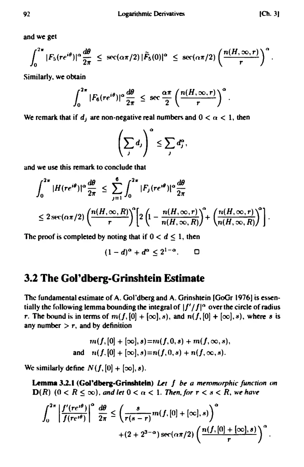
3.2. The Gordberg-Grinshtein Estimate. . . . . . . . . . . . .. 92
3.3. The Borel-Nevanlinna Growth Lemma . . . . . . . . . . . . . . . .. 98
3.4. The Logarithmic Derivative Lemma . . . . . . . . . . . 104
3.S. Functions of Finite Order . . . . . . . . . . . . . . . . . . . . . . . . 106
4. The Second MaIn Theorem via Logarithmic Derivatives . . . . 107
4.1. Definitions and Notation . . . . . . . . . . . . . . . . . . . . . 107
4.2. The Second Main Theorem . . . .... . . . . . . . . . 108
4.3. Functions of Finite Order . . .. .. . . . . . . . . . . . . . 117
s. Some Applications . . . . . . . . . . . . . . . . . . . . . . . . 119
5 .1. Infinite Products . ...... . . . . . . . . . . . . . . . . . 120
5.2. Defect Relations. . . . . . . . . . . . . . . . . . . . . . . . . . . 123
5.3. Picard's Theorem . . . . . . . . . . . . . . . . . . . . . . . . . . . . 128
5.4. Totally Ramified Values. . . . . . . . . . . . . . . . . . . . . . . . . 129
5.5. Meromorphic Solutions to Differential Equations . . . . . . . . . . . 129
5.6. Functions Sharing Values . . . . . . . . . . . . . . . . . . . . . . . . 135
5. 7. Bounding Radii of Discs . . . . . . . . . . . . . . . . . . . . . . . . 136
5.8. Theorems of Landau and Schottky Type . . . . . . . . . . . . . . . . 141
5. 9. Slowly Moving Targets . . . . . . . . . . . . . . . . . . . . . . . . . 144
5.1 O. Fixed Points and Iteration . . . . . . . . . . . . . . . . . . . . . . . . 146
6. A Further Digression Into Number Theory: Theorems 01 Roth and
Khinchln ................................. 15 I
6.1. Roth. Theorem and Vojta.s Dictionary. . . . . . . . . . 151
6.2. The Khinchin Convergence Condition . . . . . . . . . . . . . . . . . 158
7. More on the Error Term . . . . . . . . . . . . . . . . . . . . . . . . . 161
7 .1. Sharpness of the Second Main Theorem and the Logarithmic Deriva-
tive Lemma . . . . . . . . . . . . . . . . . . . . . . . . . . . . 161
7 .2. Better Error Terms for Functions with Controlled Growth . . . . 170
7 .3. Error Terms for Some Classical Special Functions . . . . . 177
Bibliography . . . . . . . . .
Glossary 01 Notation . . . . .
187
193
I Jadex . . . . . . . . . . . . . . . . . . . .
...... ............
197

Introduction
One of the first theorems we learn as mathematics students is the the Fundamen-
tal Theorem of Algebra, which says that a degree d polynomial of one complex
variable will have d complex zeros. provided that the zeros are counted with multi-
plicity. If P(z) is a degree d polynomial. then
max{IP(rei')1 : 0 < 8 < 211'}
grows essentially like r tl as r  00. Therefore, we can rephrase the Fundamental
Theorem of Algebra as follows: a non-constant polynomial in one complex vari-
able takes on every finite value an equal number of times counting multiplicity, and
that number is determined by the order of growth of the maximum modulus of the
polynomial on the circle of radius r centered at the origin as r  00. A good way
to sum up value distribution theory, otherwise known as Nevanlinna theory. is by
saying that the main theorems in value distribution theory are generalizations of the
Fundamental Theorem of Algebra to holomorphic and meromorphic functions. The
purpose of this book is to describe this theory for meromorphic functions on the
complex plane C, or more generally for functions meromorphic in a disc in C.
Before we begin to be precise about how the Fundamental Theorem of Alge.
bra can be extended to meromorphic functions. we make a few quick observations
about the differences between polynomials and transcendental functions. First. we
note that the entire function e= takes on many values infinitely often but never takes
on the value O. Thus, the most naive generalization of the Fundamental Theorem
of Algebra that one might imagine is not true for entire functions. Second, tran-
scendental functions take on values an infinite number of times, so we cannot really
speak of the total number of times that a function takes on a value. Since a function
meromorphic on the entire complex plane can have only finitely many zeros inside
any finite disc. what we can and will speak of instead is the rate at which the number
of zeros inside a disc of radius r grows as the radius tends to infinity.
Given a meromorphic function I and a value a E C U {oo}, Nevanlinna theory
studies the relationship between three associated functions: N(f, a, r).. nl(/, a, r),
and T(f, r). We will wait until  1.2 to give precise definitions of these functions
and content ourselves here with the following informal descriptions. The function
N(/, a, r) is called the "counting function" because it counts, as a logarithmic av.
erage. the number of times I takes on the value a in the disc of radius r. The

2
Introduction
function m(/, a, r) is called the "mean-proximity function:' and it measures the
perccntage of the circle of radius r where the value of the function I is closc to
the value a. The function T(/, r) is called the "characteristic" or "height" func-
tion it essentially mea.ures the area on the Riemann sphere covered by the image
of thc disc of radius r under the mapping I and does not depend on the value a. If
I is an entire function. then the characteristic function measures the growth of the
maximum modulus of the function I. The characteristic function plays the same
role in Nevanlinna Theory that the degree of a polynomial plays in the Fundamental
Theorem of Algebra.
In Chapter I we define thesc "Nevanlinna functions" prccisely. and we prove:
First Main Theorem If I is a non-constant romorphi(' function on C and II
is a point in C U { 00 }, then
T(/,r) - m(/,a,r) - N(/,a,r) = 0(1)
a." r  00.
Since ,n(/,a,r) > 0 and T(/,r) does not depend on ll, the First Main Theo-
rem says that the function I cannot take on the value a too often in the scnse that
the frequency with which I takes on the value a cannot be so high that the func-
tion N(/, a, r) grows faster than T(/, r). This is analogous to the statement that
a polynomial of degree d takes on every value a at most d times. Actually. the
First Main Theorem says even more in that it says the sum m(/, a, r) + N(/, a, r)
must be essentially independent of a. Thus. if I takes on the value a with a small
enough frequency that N(/,a,r) does not grow as fast as T(/,r), then the fUnc-
tion m(/.. a. r) must compensate. meaning that the image of I stays near the value
a for sufficiently large arcs on large circles centered at the origin.
The subject of the later chapters is the deeper:
Serond Main Theorem If I is a non-constant meronuJrphic function on C, and
(II .. . . .  a q a" distinct points in C U {oo }, then
q
(q - 2)T(/,r) - LN(/,aj,r) + N,am(/,r) < o(T(/,r»)
J=J
for a sequence of r  00.
In fact. we will prove stronger and more precise forms of this theorem. The term
lJ'am(/, r) is positive (at least when r > 1) and measures how often the function I
is ramified. Thus. the Second Main 1beorem provides a lower bound on the sum of
any finite collection of counting functions N (I, a j , r) for certain arbitrarily large
radii r. Thus. taken together with the First Main Theorem. which provides an upper
bound for the counting functions. we have our generalization of the Fundamental
Theorem of Algebra.
The key results presented in this book. namely the First and Second Main 1beo-
rems. are essentially due to R. Nevanlinna (Nev(R) 1925) and F. Nevanlinna (Nev(F)

Introduction
3
1927]. The Nevanlinnas gave precise, though not Ubest possible," estimates for the
function implicit in the o{T(/, r» on the right of the inequality in the Second Main
Theorem. This function is known as the .'error term." The fine structure of the error
term was not considered especially interesting until relatively recently. In this book,
we pay careful attention to the error terms, and the error terms we give are better
than those obtained by the Nevanlinna brothers.
In many ways our presentation of this material resembles those of Nevanlinna
(Nev(R) 1970], Hayman [Hay 1964], and Lang [Lang 1990]. Those familiar with
the Russian work by A. A. GoI'dberg and I. V. OstrovskiT [GoOs 1970] or the Ger-
man work by Jank and Volkmann [JaVo 1985) will also recognize their inftuence
on our presentation. The primary manner in which our presentation of the Second
Main Theorem differs from those of Nevanlinna and Hayman is that we are careful
in our treatment of the error terms, and of what is known as the "exceptional set:'
There are several fundamentally different ways of proving the Second Main The-
orem. Each approach has its own advantages and disadvantages, and the Second
Main Theorems that result from each approach are not quite the same.
Chapter 2 contains the first of two fundamentally different proofs we will give for
the Second Main Theorem. This proof is based on "negative curvature," a technique
introduced by F. Nevanlinna into the theory almost from the very beginning [Nev(F)
1925], [Nev(F) 1927]. The error term estimate we give in Chapter 2 is essentially the
work of -M. Wong [Wong 1989], and our presentation is quite similar to Chapter I
of [Lang 1990]. In 2.6 we incorporate the work of Z. Ye (Ye 1991] in order to
simplify the appearance of Wong's error term. Finally. in 2.8, we discuss how the
Second Main Theorem is uniform over families of functions, and we are not aware
of any other similar treatment.
In Chapter 3, we undertake a detailed study of Logarithmic derivatives. The main
result of that chapter is:
GoI'dberg-Grinshtein Inequality If / is a meromorphic function on C then
for any r and p with 1 < r < p < oc.
, { p(2T(/. p) + 13.) }
m(J I Jt 00, r) < max 0, log r(p _ r) + c.. .
Here fJl and " are constants that will be defined in Chapter 3.
In Chapter 4, using ideas from Ye's refinement of Cartan's approach to the Sec-
ond Main Theorem [Cart 19331, as in rYe 19951, we use the precise estimate on
,n(/' / /, r, X) provided by the Gol'dberg-Grinshtein estimates in Chapter 3 to
prove the Second Main Theorem and give a careful analysis of the error term and
exceptional set obtained by this method.
There is a third altogether different approach to proving the Second Main The-
orem, initiated by A. Eremenko and M. Sodin (ErSo 1991]. This relatively new
approach might be said to be a potential theoretic approach. Although this newer
approach to the subject is very interesting and important, we have chosen not to

4
Introduction
discuss this method in this volume because ll as yet, no one has succeeded in proving
a version of the Second Main Theorem that includes the ramification term by this
potential theoretic approach ll nor has a detailed analysis of the error term coming
from this approach been undenaken.
Although the applications of Nevanlinna.s theory are not our focus, we feel that
some detailed discussion of applications is essential in order that those readers new
to the subject can gain an appropriate aesthetic and utilitarian appreciation for what
often appears to be a very technicaJ and obscure subject. There fore 11 we have in-
cluded a lengthy chapter. Chapter S. on applications. We chose our applications
only to illustrate the utility of the theory. and thus we made no effort to choose the
most current or refined application of any given type. Our chosen applications are
for the most part as in [Hay 1964] and [Nev(R) 1970], and many of them are due
to R. Nevanlinna himself. In fact, those readers looking for more refined applica-
tions than those we give in Chapter S might wen stan by reading Nevanlinna's first
monograph [Nev(R) 1929]. Our applications chapter does differ somewhat though
from pa.t treatments in that we have put some emphasis on what can be gained from
precise knowledge of the error terms ll something ignored by most previous authors.
The materiaJ covered in Chapter 7. where we discuss the sharpness of the error
termsll the precise error terms of some classicaJ special functions ll and improvements
to the error term for functions with restricted growth. has. up till now. only been
available in the research literature.
The connection between Nevanlinna theory and Diophantine approximation the-
ory has inspired a lot of recent work in both fields. and we have therefore including
several sections ll referred to as unumber theoretic digressions,u explaining and moti-
vating in some detail this connection. We assume no background in number theory
in these sections and hope that these sections ill encourage even the most pure
analysts to further explore this fascinating connection.
Given our emphasis on the Second Main Theorem and its error terms ll we have
not discud anywhere in this volume the various other techniques for studying
the distribution of values of meromorphic and entire functions. We instead refer
the reader to the recent book [Rub 1996 J for an introduction to some of these other
techniques.

1 The First Main Theorem
As we mentioned in the introduction ll the basis for Nevanlinna's theory are his two
umain" theorems. This chapter discusses the first and ea.ier of the two.
To understand where we are headed. looking at the concrete example of the tran-
scendental entire function e Z is again helpful. We pointed out that e:: takes on all
values other than zero infinitely often. Notice also that by periodicity each of these
non-zero values is also taken on with the same asymptotic frequency. Of course
e:: never attains the value 0; nor does it attain the value 00. On the other hand ll
on every large circle centered at the origin ll the function e:: spends most of its time
close to one of these two omitted values. That iS ll fixing a small €, the percentage of
the circle of radius r where e: is either smaller than £ or larger than 1/£ tends to
100% a. the radius of the circle tends to infinity
Nevanlinna's First Main Theorem will tell us that this behavior is typical. That
is. if a meromorphic function takes on a panicular value less often than uexpected:lI
then it must compensate for this by spending a lot of time "near" that value. As
a consequence, Nevanli nna ll s First Main Theorem gives an upper bound (in terms
of the growth of the function) on how often a meromorphic function can attain
any value. This is analogous to the statement that a polynomial of degree d can
take on any value at most d times. Note this last statement about polynomials is
much easier to prove than the full Fundamental Theorem of Algebra. It is thus no
surprise that Nevanlinna's First Main Theorem is much ea.ier than his Second Main
Theorem ll which says that most values are taken on by a meromorphic function with
the maximum asymptotic frequency allowed by the First Main Theorem.
1.1 The Poisson-Jensen Formula
We begin this chapter with this brief section which recalls the Poisson Formula for
harmonic functions and applies this to the logarithm of the modulus of an analytic
function to derive what is known as the "Poisson-Jensen Formula. u The material
in this first section is usually covered in a first course in complex analysis. and we
could have chosen to regard the material in this section as a prerequisite. On the
other hand ll the Poisson Formula is at the very heart of Nevanli nna ll s theory of value
distributionll and the First Main Theorem of Nevanlinn8 theory is really nothing

6
1be First Main Theorem
(eb. I)
other than the Poisson-Jensen formula dressed up in new notation. Thus. we felt a
detailed treatment of this material here would be of value to the reader.
We begin with some general notation. We will use C to denOie the complex
plane. We will use rand R to denote positive real numbers. which will usually
be radii of discs, we will always have r < R, and we will also allow R = 00,
whenever this makes sense. We will use D(r) and D(R) to denOie open discs of
radius r and R, respectively, each centered at the origin. When R is aJlowed to
be infinite, D( R) will refer to the entire complex plane C. We will consider the
value distribution of meromorphic functions on D( R), and it will be convenient to
consider a meromorphic function as a holomorphic map to what is known as the
Riemann sphere or the projective line C = C U {<x>} = Pl. To be more consistent
with the higher dimensional theory. we prefer to refer to the Riemann sphere as the
pn)jective line Pl.
If R < 00, we will use D(R) to denote the closure of the disc D(R) in the com-
plex plane. If we say a function is harm onic. respectively holomorphic. or respec-
tively meromorphic on the closed disc D(R), then we mean that function should
be harmonic. res pective ly holomorphic. or respectively meromorphic on some open
neighborhood of D(R).
We will now recall the Poisson and Poisson-Jensen Formulas. Let
P(z,() = /(/2 _/Z/2 = Re { ( + Z } .
I( - zl2 ( - Z
The function P(z, () is called the Poisson kernel. Note that for fixed ( and for
Izi < 1(1.
(+z
(-z
is holomorphic, and hence P( z, () being the real part of a holomorphic function is
harmonic in z.
We being by showing how the Poisson kernel transforms under a MObius auto-
morphism of a disc.
Proposition 1.1.1 ut
T(w) = R2(Z - w) .
R2 - zw
Then, T(tJ,) is an automorphi,fm of D(R) that interrhange,f 0 and z. Mo"over.
when IT(u')1 = R, then
dw d(
= P(z, T(w)) 2 ... ( '
21ri UJ II .
whe" P(z, () is the Poi,fson kernel and ( = T(w).

(S 1.1)
Poisson-Jensen Formula
7
Proof. One easily verifies that T(w) is holomorphic on D(R ), and that when
Iwl = R, then IT(w)1 = R. Hence. T is an automorphism of D(R) that inter-
changes 0 and z.
Noting that T is its own inverse in the group of linear fractional transformations,
we have that
= T( / ) = R2(Z - ()
W , R2 _ z( .
We then compute
dw _  ( -1 Z ) d( _ ( -( Z( ) d(
21riw - 21ri z - ( + R2 - z( - z - ( + Kl - z( 27ri( .
Note that when 1(1 2 = R 2 ,
-( + z( = -( + _z( = R 2 -lzl 2 = R.e { ( + z } . 0
z - ( R2 - z( z - ( «( - z) I( - zl2 ( - Z
Our first theorem. called the Poisson Formula. allows us to express a hannonic
function in a disc as an integral around the boundary circle.
Theorem 1.1.2 (Poisson Formula) ut u b e hanno nic in the open disc D(R),
R < 00 and continuous on the closed disc D(R). ut z be a point inside the
disc. Then
u(z) = 1 2 . u(ReiB)p(z.RI"B),
whe" P(z, () denotes the Poisson umel.
P roof Fi rst we will prove the theorem in the case that u is hannonic on the closed
disc D (R). Let ( = T(w) as in Propositio n 1.1. 1. Because T is holomorphic on
D(R), we know u(T(w)) is harmonic on D(R). By the mean value property of
harmonic functions.
u(z) = u(T(O» = 1 2 . u(T(Re iB ))  = f u(T(W» 2w '
ItL'I=R
Leuing ( -= Re iB . using Proposition 1.1.1. and recalling that  = d8,
u(z) _ f u(T(w» du: = f2. u (Re. B ) P(z, ne i9 ) d8 .
21rlW 10 211'
ItI'l=R
In the case that u is not harmonic in a neig hbo rhood of D(R), all we need do is
note that for p < 1, u(pw) is harmonic on D(R), and we can use what we have
already proven to conclude that
f2rr R2 - Izl 2 d8
u(pz) = 10 u (pRe'B) l&i9 _ zl2 b'
The result follows by noting that u(pw) -+ u(w) uniformly on Iwl = R as p -+ 1.
o

8
TIle First Main Theorem
(eb. I)
Corollary 1.1.3 Let P(z.. () denote the Poisson uI"M1 and let R > O. Then
2Jf
L P(z. Re iS ) : = 1.
Proof Apply Theorem 1.1.2 to the constant function u (z) = 1. 0
We can also use the Poisson kernel to create harmonic functions in a disc if we are
just given a continuous function on the boundary circle. This is known a. "solving
the Dirichlet Problem for the disc:' To prove this 9 we need the following estimate.
Proposition 1.1.4 Let P( z, () denote the Poisson umel. Given (0 su,.h that
1(.)1 > 0, Riven E > 0, and Riven d > 0, the" exists a d' such that for all
( M.ith I( - <01 > d and 1(1 = 1(01, and all z with 0 < Iz - (01 < d'.. Wi' ha,'e
iP(z..()1 < E.
Proof We have for z near (0 and I( - <01 > d that
1(1 2 - Izl 2 1<01 2 - Izl 2 1<01 2 - Izl 2
P(z, () = . = < .
I( - zl2 1(( - <0) - (z - (0)1 2 - (d - Iz - (01)2
The term on the right clearly tends to zero as z -+ (0' 0
Theorem 1.1.5 (Solution to the Dirichlet Problem) Let <fJ(Re iB ) be a continu-
ou... fun,.tion of 8 for a fixed R < 00. Then.
1 2Jf dB
der . .
u(z) = <fJ(Re'B)p(z, Re 'B ) -
o 2
i... i' han"oni,'fun,.tion of z in D(R). andfor ea,.h 8 0
lim u( z) = <fJ( Re 'BO ).
::.RI.O
Proo! To check that u is harmonic. we differentiate under the integral sign with
respect to z. which we can do because <fJ is continuous in 8 and so are P and its
z -derivatives since Izl < R. Because P is harmonic in z. so is u.
It remains to check that
lim tl( z) = tfJ( Re '8o ).
:.H'.O
We have by Corollary 1.1.3
:l Jf d8
lu(z) - (Rt)s)1 = 1 (tj)(Re tJI ) - tj)(Re'So» P(z. Rt.'s) 211'
< 1 2 " 1tj)(Re'S) - tj)(Re'SO)1 P(z, Re'S)  ,

(I.I)
PoisM)J1..Jenscn Fonnula
9
since P( z, () is always positive. Let € > O. By the continuity of 4>, there exists a
d > 0 such that 14>( Re iB ) - 4>(Re iBO ) I < € for those 8 with IReIBo - &IB I < d.
Hence
f 1t/)(Rt'I8)_(ReiBO)IP(z.R{.iB) : < 1 2 "eP(z,Rc. B ) : e.
{B'I R'. - R'.o I <6}
On the other hand. from Proposition 1.1.4.. there exists a d' such that if
o < Iz - Re iBo I < d' and IRc,Bo - ReiBI > d,
then IP(z, Re iB ) I < €. Thus.. for these z,
f 1t/)(Re iB ) - (Re'BO)1 P(z, Re iB ) :
{B:I R'. - R'.o 16}
(21f dB
< e J o 1t/)(Re'B) - t/)(Rc'BO) I 211"
The proof is completed by noting that
f2" 1t/)(Re iB ) _ t/)(&iBO)1 d8
10 2
is bounded by the continuity of 4>. 0
If I is analytic and free from zeros.. then log III is harmonic.. and we can there-
fore apply the Poisson Formula to it. However.. since we are interested in the distri-
bution of the zeros of I, we will want to see what happens in the case that I ha.
zeros. This is what is called the "Poisson-Jensen'" Formula.
Before giving the precise statement of the Poisson-Jensen Formula. we introduce
some additional notation. Given a non-constant meromorphic function I and a
point a in the complex plane. we can always write I (z) = (z - a) m g( z), where
,,, is an integer.. and 9 is analytic and non-vanishing in a neighborhood of a. The
integer ,n is called the order of I at the point a and is denoted ord a I. Note
that ordal > 0 if and only if I has a zero at a, and ordal < 0 if and only
if I has a pole at a. We will refer to the non-zero complex number g(a) as the
Initial Laurent coefliclent of I at a, denoted i1c( I, a), because it is the first non-
vanishing coefficient of the Laurent expansion of I expanded about a.
Theo rem 1.1.6 (Poisson-Jensen Formula) Let I  0,00 be meromnrphic nn
D(R). Let a1,... ,a p dennte the zeros of I in the lJn disc D(R), each zero
rrpeated acc.lJrding tn it.' multiplicity. and let b., . . . , b, denote the poles of I in

10
The First Main Theorem
(Ch. 11
D(R). also rrpeated a,.,.orrJing to multiplicity. For any: in D(R) which is not
a :ero or pole of J, we have
(2" R2 - 1:1 2 . dB
log 1/( z)1 = 10 1 Re" _ zl2 log I/(Re." )1 2 11'
- t IOK 1 :;za:) 1 + t log 1 :;z b:)
(2" R2 _ 1:1 2 . dB
= 10 IRe i ' - zl2 IOK 1/(Re")1 2 11'
I R2 (
- L (ord<f) log R(z  (z)
{ED( R)
If :. = 0, thi.f .fimplifies to
1 2" dB
log IJ(O)I = log IJ(Re is ) 1- 2
() 1r
1 2" dB
= log IJ(Re' S )1-
o 21r
- tlOgl  1 + tlOgl  1
- L (ord<f) IOK 1  I.
(ED( R)
Corollary 1.1.7 Let R, J, 01,...,01" and hI, . . . ,h, be as in Theorrm 1.1.6.
Thn, for an)' : which is not a zero or pole of J,
J' (:) (2" 2Re' s dB
/(z) = 10 (Rei' - z)2 log I/(Re")/ 2;
1' ( a 1 ) ' ( b 1 )
+ . + - ' - +
L W-iiz z-a L W-bz z-b
.= I · · i= I · ·
1 2" 2Re'S . dB
= (R" )2 log 1 /(Re")1- 2
o e' -: 1r
+ L (ord<f) ( R2  (z + z  ( ) ·
(ED( H)
Proof of Corollal)' I. 1.7. Note that
J' ( : ) a {)
/(z) = az log /(z) = 2 ()z log I/(z )1.
where the last equality follows from the Cauchy-Riemann equations since
1 -
log IJ(:)I = 2 [log J(:) + log J(:)).
The corollary then follows by differentiating the equation in the theorem and moving
the derivative inside the integral. D

[51.1)
Poiwn-Jensen Formula
II
Corollary 1.1.1 Let 1 _ 0, 00  meromorph;c on D( R). Let 0". . . ,op de-
note tM non-zero zeros of 1 in D(R), rrpeated according to ""'Itiplicity. and
let b". . . , b, denote the non-zero poles of 1 in D( R), rrpeated according to
multiplicity. Then.
1"
loglilc(f.O)1 = 1 logl/(Re")I ::
p R 9 R
- Llog - + Llog - - (ordo/)logR
. , o. . , bi
.= .=
1 211' dB I R I
= 0 log 1/(Re i ')l 21f - L (orf) log "(
(ED( R)
(O
- (ordo/) log R. (1.1.9)
Remark. Equation (1.1.9) in Corollary 1.1.8 as well as the second equation in
Theorem 1.1.6 are referred to simply as Ihe Jensen Formula.
Proof of Corollary /. / .8. Simply apply Theorem 1.1.6 (the Poisson.Jensen for-
mula) to Ihe function I(w)w-ordol. D
Proof of Theorrm /./.6. First of all. note that it suffices to prove the theorem
when 1 has no zeros or poles on the circle of radius R. Indeed. because zeros and
poles on the circle of radius R do not cause the integrals on the right hand sides
of the formulas to diverge, we can consider the function 1 (pw) t which will not
have any zeros on the circle of radius R for all p sufficiently close to. but less than
1. The theorem follows from this case by letting p -+ 1 and Lebesgue dominated
convergence.
Now we assume 1 has no zeros or poles on the circle of radius R. Consider the
function
p ( R1_ii'W )
n R(w - :i)
F(w) = I(w) , ( R2 _ biw ) ·
II R(w - b,)
.= ,
We have chosen F so that it has no zeros or poles in the closure of D(R) and so that
IF("J)I = I/(w)1 when 1 1EJ R . The function log IF(w)1 is therefore harmonic in
an open neighborhood of D( R). The proof of the theorem is completed by applying
the Poisson Formula to log IFI. 0
If we look closely at equation (1.1.9). we can start to see our generalization of
the Fundamental Theorem of Algebra. The left-hand side of equation (1.1.9) is just
a constant. The right-hand side of the equation has two different types of terms.
The first term on the right is an integral over the circle of radius R involving the
absolute value of I. The other term is a sum over the zeros and poles of f. If f is

12
The First Main Theorem
(Ch. 1 J
holomorphic or meromorphic on the whole plane C, then as R -+ 00, the left-hand
side of this equation does not change. so that means although all the terms on the
right-hand side might tend to infinity. if they do. then they always essentially cancel
each other out.
1.2 The Nevanlinna Functions
At the end of the last section. we noted that equation (1.1.9) can be viewed as the
first step toward generalizing the Fundamental Theorem of Algebra to meromorphic
functions. In this section. we explore this in more detail. We begin by defining the
Nevanlinna functions and then state the first fundamental relationship between them..
known as the uFirst Main Theorem'" of Nevanlinna theory. Although the First Main
Theorem is really just a restatement of the Jensen Formula (Corollary 1.1.8). it is
this formulation which makes clear that Jensen's Formula is a weak generalization
of the Fundamental Theorem of Algebra.
As we proceed to define the Nevanlinna functions. I will always be a meromor-
phic function on D(R), where R might be 00, and r < R. Note that most of our
definitions will not mau an)' senSe for certain constant functions I, and thus we
exclude an)' such constant functions from consideration.
Counting Functions
First.. we define the countine functions. The unlntegrated counting function
71(/.. Xi, r) simply COunl\ the number of poles the function I has on the closed
disc D( r). each pole counted according to its multiplicity. Note that because I is
meromorphic on some larger disc.. this number is always finite. If a is a complex
number. we define n(/, a, r) to be
n(f,a,r) = n ( / a .oo,r),
which i imply the number of times I take s on the vaJue (1 on D(r). We choose
to count the a-points of I in the closed disc D(r) instead of in the open disc D(r)
because we can then use n(/, O. r) to denote the multiplicity with which I takes on
the value a at z = O.
We then define the Integrated countlne function N(/, a, r) by
l r dt
l\r (I, (1, r) = 11 (I. a, 0) log r + [11 ( I, a, t) - n (I, a, 0)] - .
o t
So. in panicular.
N(f.O,r) - (ordtf)logr + :<ordf)logl;l,
: E DC r)
:

(S 1.21
1be Nevanl inna Functions
13
where ord I = max{O,ordz/} is just the multiplicity of the zero. Note that the
points % on the circle 1%1 = r where 1(%) = 0 do not contribute to N(/, 0, r) since
in that case log Ir / % 1 = O. Thus we see that the integrated counting function is very
similar to the terms in the right hand side of equation (1.1.9). In fact. with this new
notation, we can rewrite Corollary 1.1.8 as
Corollary 1.2.1 Let I _ 0, 00 be meromorph;c on D( r ). Then.
(2W ,dB
loglilc(/,O)I = 10 logl/(re' 8 )1 2 11' + N(/,oo,r) - N(f,O,r).
The unintegrated counting function n(/, a, r) of course appears to be the more
Unatural" of the two counting functions to consider. and those new to the field often
wonder why N(/, a, r) is used so often instead of n(/, a, r). One reason is that it
is N and not n that naturally appears in Corollary 1.2.1. Another advantage of N
over n is that it is a continuous function of r. We will say a bit more on this in
1.11.
We will also have occasion to discuss truncated counting functions. We let
n(lt)(/, 00, r) denote the number of poles I has in the closed disc of radius r,
but this time we only count each pole with a maximum multiplicity of k. In other
words, if %0 is a pole of I in the disc with multiplicity < k, then it is counted ac-
cording to its multiplicity. If. however, %0 is a pole of I in the disc with multiplicity
greater than k, then we count %0 as if it only had multiplicity k. We similarly de-
fine n(lt) (I, a, r). Note in particular that n(l)(I,a, r) counts the number of times
I takes on a without counting multiplicity at all. As the reader might now expect.
the integrated truncated counting function N(Ir)(/,a, r) is then defined by
(r dt
Nllr)(f,a, r) = n(Ir)(f,a,O) logr + 10 [n11r)(f, a, t) - n(Ir)(f,a,O)]T'
Mean Proximity Functions
We will now explain the significance of the integral term in Corollary 1.2.1. To
begin with, it is useful to introduce the notion of a Weil function. Given a point a
in pi , a Weil function with singularity at a is a continuous map
'\4: pi \ {a} -. R
which has the propeny that in some open neighborhood U of a in pi, there is a
continuous function 0 on U such that
J\4 ( %) = - log 1% - a I + Q ( % ),
where % is a holomorphic local coordinate on U. Thus.. Weil functions are almost
continuous functions. except that they have a cenain specified logarithmic singular-
ity at the point a. Notice that the difference between any two Weil functions with

14
The Firsl Main Theorem
ICh. I J
the same singular point will be a continuous function on pI and will therefore be
bounded since pi is compact. Also notice that for a meromorphic function / (: )
on D(R), the composition of / with a Weil function >'0(/(:)) is large precisely
when / (:) is close to a. Given a Weil function >'0' one defines a meaa proxinalty
lunction
(2Jr dB
m(f, ,r) = 10 '\0 (f(re iS )) 211" .
The mean proximity function measures how close / is. on average. to a on the
circle of radius r. Note that if we take two different Weil functions with the same
singularity a, then the mean proximity functions we get from each Weil function
will differ by a bounded amount 8.\ r -+ R.
One has many choices for Weil functions. but many things do not depend on the
specific choice of Weil function. Two specific types of Weil functions come up often
in Nevanlinna theory. each type having its own advantages. R. Nevanlinna used the
following Weil functions in his first proof of the his main theorems.
+ 1
 (z) = log I I if a, z  00
:-a
>'0 (oc) = 0 if a 1- 00
>'0 (:) = log+ 1:1 if a = 00,
where for a positive real number x, log + x = max { 0, log z }. Hence. we define
1 2Jr 1 I dB
m(f,a,r) = log+ f( 'S) _ 2
o re' - a 11'
(2" dB
m(f, 00, r)= 10 log+lf(rc, S )1 2 11" .
a 1- 00 and
When looking at things from an ..analytic" viewpoint. we will find it convenient
to use Nevanlinna.s choice of Weil function as above. but when we wish to look at
things ..geometrically;. we will prefer a different choice of Weil function. which we
now describe.
Let :1 = rl e i8 . and :2 = r2ei8 be two points in C. If we use stereographic
projection to identify the complex plane with the sphere of radius 1/2 centered at
the origin in R 3 , minus the nonh pole. and if (pj,8 J , (J),j = 1 2 are the cylin-
drical coordinate representations of the images of : j, then we have the following
relations:
r. r 2 - 1
P _ J (- J
J - 1 + r j - 4( 1 + r) .
J J
Now. the square of the standard Euclidean distance in R 3 between the two points
(PJ,8j,) is given by
2 2 2 2
PI + p;j - 2PIP2C08(8 1 - 8 2 ) + (I + (2 - 2(1(2.

( I. 2]
The Nevanlinna Functions
IS
Writing P J and (j in terms of r j and simplifying. one sees that the square of the
distance between the images of ZI and Z2 in a 3 is given by
rl + r - 2rl r2 cos(9 1 - 9 2 ) _ IZ1 - z21 2
(1 + r1)(1 + r) - (I + Izd 2 )(1 + IZ212).
We therefore define the (square of the) chordal distance between two poinl in the
complex plane to be
2 I Z 1 - z11 2
IIzl. z211 = (1 + Izd 2 )(1 + IZ212) '
The term "chordal distance" comes from the fact that we derived this formula by
measuring the length of the chord of the sphere connecting Z 1 and Z2 when thought
of as points on the sphere. We note that it is not obvious by just looking at the
formula for II ZI , z211 that this distance satisfies the triangle inequality. However.
since the chordal distance comes directly from the Euclidean distance in a 3 . it
clearly must satisfy the triangle inequality. We can continuously extend our notion
of chordal distance to pi by saying thai
2 1
IIz,ooll = 1 + Iz12 '
We now define another Weil function associated to a by
G (z) = - log II z, all,
and this is the other Weil function we will choose to work with.
Note that unlike the Weil function used by Nevanlinna. this more "geometric"
.
Weil function J\G is smooth, and even real analytic. away from the point a. In
Ahlfors's collected works [Ahlf 1982. pp. 56). Ahlfors says '4rightly or wrongly"
he was initially .'somewhat disturbed" by the non-smoothnes. of the \.Veil function
J\. used by Nevanlinna. He explains that his experimentation with oo as an al-
ternative was what led him [Ahlf 1929) to discover the geometric interpretation of
Nevanlinna t s characteristic function (to be defined below). This interpretation had
previously been discovered by T. Shimizu [Shim 1929) and will be explained in
detail in  1.11.
Since we have identified the Riemann sphere with the sphere of radius 1/2 in
a:\ we always have J\a (z) > 0 since II z ,all < I. We will take
1 2W dB
"'U. a, r) = 0 - log 11/( rei.), all 21r
to be our definition of the "geometric" mean proximity function to a of I, which
we distinguish from our previous definition by writing a small circle above the m.
Since working with explicit constants is one of our goals in this book. we record
here the explicit constant relating Nevanlinna's definition of mean proximity to this
other mean proximity function.

16
The Fil'Sl Main Theorem
[ Ch. I)
Proposition 1.2.2 For all x > 0,
1 . lo g 2
log+z < 2log(1 + z2) < log+z + To
Also. Riven a E pI and a meromorphic function f _ a on D(R), we have for
all r < R..
o log 2
,n(f,a,r) < n,(f,a,r) < m(f,a,r) + T'
Proof. The inequalities
1 . log 2
log+z < 2 log (1 + z2) < log+z + To
are elementary. and the other inequality follows from this and the definitions. 0
We also record here the following useful observation. which we will use to relate
the various proximity functions. For those already familiar with Nevanlinna theory.
this observation is what is used in what is often known as the 6'product into sum'"
estimate. We will say more about this when we discus.\ the Second Main Theorem.
Proposition 1.2.3 iLt a., . . . , a 9 be q dLttinct points in p'. Then. for all w in
p' ,
9 ( 1 ) .-' ( )
II IIw. 0)11 > 2 mjn II 110" 0)11 m)n IIw, 0)11 0
J= . 'J
Morrover. if '\(1) arr Weil function.f with singularities at the points aj suc.h that
therr exiJt non-negativec.onstants C 1 and C 2 so thatforallu, 1- aj in p',
-C. < - log lIaj, wll - '\a) (w) < C 2 ,
then for all w 1- a J in p', we hove
q
L '\a J (w) < m '\oJ (w) + log n} II lIa;, ajll-l + (q - I) log2 + qC 1 + C:z.
. J J.
J= 'J
Proof The point is that w cannot be close to all the points at the same time. More
precisely, since liz, wll is a metric on p', the triangle inequality implies that there
is at most one index j such that
II w, a j II < _ 2 1 mi n 110;, a) II.
'J
For all other indices i. again by the triangle inequality.
1
II w , a,1I > 2 11a j , ai II.
Thus, the first statement. The second follows easily from the first. 0
Because Proposition 1.2.3 will be used on several occasions, it is convenient to
introduce some notation. Given distinct points aI, . . . , a., we define
· II -I
V(a.,...,a.) = logmax lIa;,ajll + (q-I)log2.
J . .
'J

IS 1.3)
The Firs. Main Theorem
17
Height or Characteristic Functions
Finally. we define the last of our Nevanlinna functions. The Nevanlinna height or
NevanJInna characteristic ruoctlon with respect to a is defined by
IT(j,a,r) = m(J,a,r)+N(J,a,r),]
and the "geometric" height or characteristic ruDdion with respect to a is defined
by
o
T(/ta..r) = m(l,a,r) + l'/(/a,r) + r-tm' (I, a),
where C fm . (I, a) is a constant that does not depend on r and is defined by
log II/(O)t all if 1(0) 1- a
r-tmt (I.. a) - log lilc(1 - at 0)1 + 2 log lIa, ocll if 1(0) = a, a 1- 00 (1.2.4)
- Jog 1i1(/t 0)1 if 1(0) = a = oc.
The geometric characteristic function is often called the Ahlrors-Shimizu charac-
teristic runctlon for reasons that we will explain in  1.11. The constant C("" is
known as the First Main Theorem constant. for reasons which will become appar-
ent below.
The height or characteristic function T (or t), the mean proximity function m
(or m), and the counting function N are the three main Nevanlinna functions.
Nevanlinna theory can be described as the study of how the growth of these three
functions is interrelated. We would like to point out that there is not universal agree-
ment on what the order of the three arguments to each of these functions should be.
and many authors use a subscript for one or more of the arguments.. We have decided
we would like to avoid subscripts for typographical reasons, and we have ordered
the arguments the way we have because one often thinks of having one function 1
at a time. a finite number of values a, and an infinite set of radii r. Our arguments
thus appear in order of increasing cardinality.
1.3 The First Main Theorem
This brings us to the main result of this section. Nevanlinna's First Main Theorem
says that the height function T does not really depend on a. More precisely,
Theorem 1.3.1 (First Main Theorem) LLI a E C, and leI 1 _ at 00 be a
meromorphicfunclion in D(R), R < 00. Then.
IT(J. a, r) - T(J, OCt r) + log 1i1c(J - a,O)11 < log+ lal + log 2,
and t(/t at r) = t(/, 00, r).

18
The Fil'Sl Main Theorem
(Ch. I)
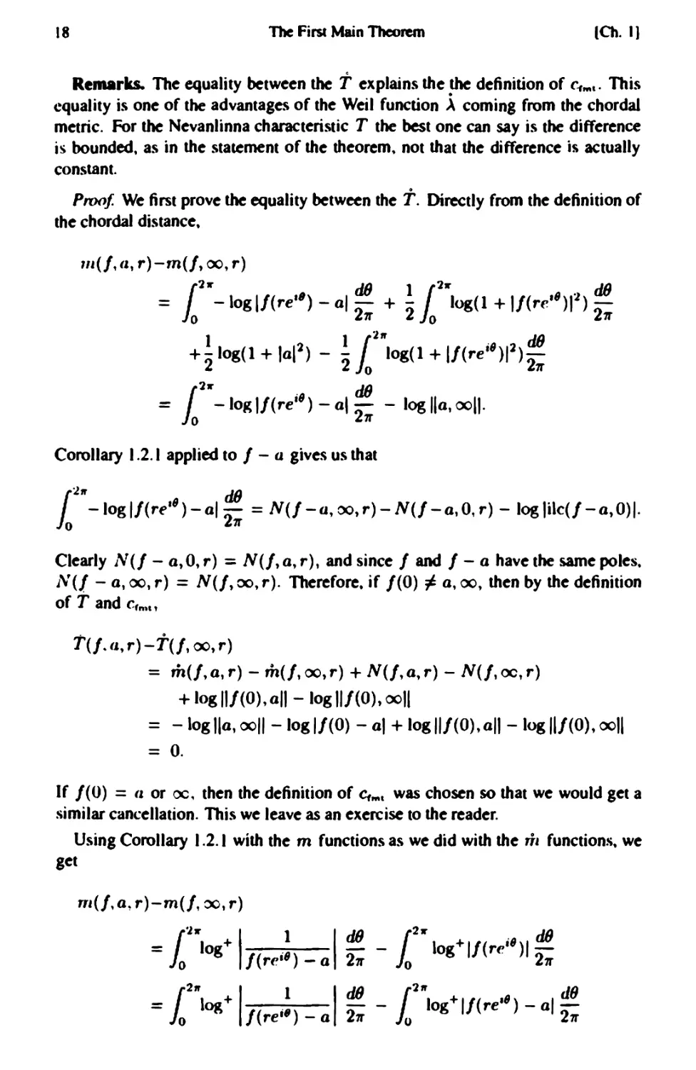
Re....rks. The equality between the t explains the the definition of C-("". This
.
equality is one of the advantages of the Weil function ,\ coming from the chordal
metric. For the Nevanlinna characteristic T the best one can say is the difference
is bounded. as in the statement of the theorem 9 not that the difference is actually
constant.
Proof We first prove the equality between the T. Directly from the definition of
the chordal distance.
"i (I, (1, r) -m(/, 00, r)
{2Jr dB 1 (2Jr dB
- 10 - logl/(re. 8 ) - a 1 21r + 2 10 log(l + 1/(rc"W) 21r
1 1 (2" dB
+ 2 log(l + lal 2 ) - 2 10 log( 1 + 1/(re i ')/2) 21r
(2Jr dB
- 10 - log I/(re i ') - a l 2; - log /la, 0011.
Corollary 1.2.1 applied to I - a gives us that
'2"
L - log I/(re") - al :: = N(f -0,00, r) - N(f -a.O, r) - log lilc(f -a,O)I.
Clearly 1\/(1 - a, 0, r) = N(/, a, r), and since I and I - a have the same poles.
"(I - a, 00, r) = N(/, 00, r). Therefore. if 1(0) 1- a, 00, then by the definition
of T and Cfm',
T(/.. (I, r) -T(/, 00, r)
- m(/, a, r) - m(/, 00, r) + N(/, a, r) - N(/, oc, r)
+ log 111(0), all - log 11/(0),0011
- - log lIa, 0011 - log 1/(0) - al + log 11/(0), all - log 11/(0), 0011
= o.
If 1(0) = (lOr oc" then the definition of Ct"" was chosen so that we would get a
similar cancellation. This we leave as an exercise to the reader.
Using Corollary 1.2.1 with the m functions as we did with the ';i functions. we
get
"'(I, a, r)-m(/,, r)
.lJr I
1
= 10 +
10 g /(re i ') - a
1 2" 1
= I +
o og I(re i ') - a
dB 1 2Jr dB
- - log+l/(re i8 )1-
21r 0 21r
dB 1 2" dB
- - log+l/(re. 8 )-al-
21r 0 21r

[ I. 3]
The Firsl Main Theorem
19
. (2Jr . dB 1 2ft' . dB
+ 10 log+ I!(re") - al 211" - 0 log+ 1!(re")1 211"
= N(j, 00, r) - N(j, a, r) - log lilc(j - a,O)1
1 2Jr dB
+ (log+lj(re i8 ) - aJ -log+lj(re i8 )1] -.
o 2
For the inequality involving the T functions. note that if x and y are positive real
numbers. then
log+ (x + y) < log+ (2 max{ x, y}) < log + x + log+ y + log 2.
Thus.. if w is any complex number.
Ilog+ Iw - al - log+ Iwll < log+ lal + log 2.
This then gives us
IT(f, a,r) - T(f, oc, r) + log lilc(f - a,O)11
S 1 2 " Ilog+I!(re") - al-log+I!(rei')II :: < log+lal + log2. 0
Note that the First Main Theorem is really just Jensen's Formula written with
different notation. and is thus not particularly deep. Given the First Main Theorem.
one often writes just T(j, r) instead of T(j, a, r) since any two of these differ by
a term bounded independent of r. To be definite, we will take
I T(f, r) = T(f, 00, r), I and similarly I r(f, r) = r(f, 00, r).1
We began this chapter by promising that it would contain a generalization of the
Fundamental Theorem of Algebra. Lefs see where we are in that regard. If it were
true that N (j, a, r) were essentially independent of a, then we would indeed have
a generalization of the Fundamental Theorem of Algebra. because this would say
that the rate of growth of the set of points where j is equal to a is independent of a,
or loosely speaking j takes on all values equally often. We have already mentioned
that this cannot be true because. for example. e;: is never O. In fact. if one allows
a = 00, this is not even true for polynomials. since polynomials have no poles.
What the First Main Theorem tells us though is that
m(j,a,r) +N(j,a..r)
does not depend on a, except for a bounded term independent of r. Thus. if we
measure the growth of not only the set of points where j is equal to a, but also

20
The Firs. Main Theorem
(Ch. IJ
where 1 is ..close to" a, then this combination grows in such a way that it is es-
sentially independent of a, and this is our first generalization of the Fundamental
Theorem of Algebra. Of course. this is not a strict generalization in the sense that
it in no way implies the Fundamental Theorem of Algebra. This also explains why
the function '11(1. a, r) is sometimes called the compensation ruDdion because it
"compensates" for the fact that the most naive generalization of the Fundamental
Theorem of Algebra is not true for meromorphic functions. We point out that since
,n (I, a, r) is always positive. the First Main Theorem gives us an upper bound on
the number of times 1 takes on the value a. Thus. it can be regarded as an analog
of the statement that a polynomial of degree d has at mtJ.ft d zeros.
Looking back at our example of {:, we notice that although e= is never O. it is
close to zero (meaning that it is les. than E in absolute value. € a positive number
much less than one) on nearly half of each large circle centered at the origin. On
the other hand. if a is a non-zero finite value. then e: hits a regularly. e= being a
periodic function. but e Z is close to a, meaning thaa e: - a is less than E in abso-
lute value. only on a very tiny arc of each large circle centered at the origin. Notice
that for (;: , the counting function N dominates the sum 111 (I, a, r) + N (I, a, r) for
most values of a, and only for the special values of 0 and 00 is the mean proxim-
ity function m significant. Those readers already familiar with Picard's Theorem.
which states that a non-constant meromorphic function on the complex plane can
omit at most two values in p1, might already suspect that for most a, the counting
function is the dominant term. This is indeed the case. and later when we discuss the
Second Main Theorem. we will turn toward proving deeper resull in thaa direction.
In summary. the First Main Theorem gives us an upper bound on N (I, a, r) and
hence on the number of times 1 takes on the value a, wherea.\ the more elusive
lower bounds on N(/, a, r) will have to wait u,:,til Chapter 2 and Chapter 4 where
we prove the Second Main Theorem.
1.4 Ramification and Wronskians
We now diM:uSS "ramification" and introduce one last piece of notation. Although
we will not prove anything about ramification until Chapters 2 and 4. we would like
to introduce the concept and the notation here.
A point Zo in D(R) is called a ramification point for a non-constant meromor-
phic function I: D( R) -+ P' if 1 is not locally a topological covering map at the
point Zo. If I(Zo) :F 00, then 1 has a series expansion at Zo of the form
I(z) = .4 + B(z - zo)P + (z - zO)p+1g(Z),
where B :F 0 and g( z) is analytic in a neighborhood of zo0 One ea.ily sees that 1
is locally a topological covering map at Zo precisely when p = 1, in which ca. 1
is locally a one sheeted covering by the inverse function theorem. If p > 1, then
locally in a neighbomoodof Zo, the map 1 is a p to 1 cover. except at Zo. If p > 1,

[ 1.4]
Ramification and Wronskians
21
then the integer (p - 1) is called the ramlftcatlon Index of I at Zo. Note that if I
is analytic. then I ramifies precisely at the zeros of I', and if %0 is a ramification
point then its ramification index is given by ordzo/'. If I(zo) = 00, then one must
look at the series expansion of 1/1 at Zo, and in that case. the rami fication index
of I at Zo is given by ord: o (1/ I )'. We emphasize that the ramification index is
always non-negative, even at a pole of I.
Let I be a meromorphic function and write I = I. / 10. where 10 and 11 are
holomorphic without common factors. We regard the fact that any meromorphic
function on D(R), R < x can be written as the quotient of two holomorphic func-
tions without common zeros to be a fundamental fact from complex variables. and
we will make use of this fact throughout without further comment. Those unfamiliar
with this result should see. for example, Chapter XIII of (Lang 1993]* Then. away
from the poles of I (i.e. the zeros of 10). we have that
I , = 10/; - loll
(/0)2 '
and this is zero precisely when 101: - 1/1 = O. At the poles of I, which are not
zeros of 11 since we have assumed 10 and I. to be without common factors.
( ! ) ' _ I/. - 101:
I (I. )2
and again the zeros of (1/ I)' are given precisely by 10/. - 101: = O. Thus. the
Wronskian
w = W(/o, It> = !: = 10/; - I/I
of 10 and 11 is a useful function since its zeros are precisely the ramification points
of I. and ord: o ". is exactly the ramification index of I at Zo. The zeros of Jlt
together with their multiplicities are referred to 8.\ the ralDlftcation divisor of I.
Note that t,,. has no poles.
If P is a polynomial, then the ramification divisor for P is given by the zeros of
P'. counted with multiplicity. and so the degree (= the number of points counted
with multiplicity) of the ramification divisor of P is one less than the degree of
P itself.. In some sense, one of the consequences of the Second Main Theorem in
Nevanlinna theory will be a generalization of this observation to entire functions.
For meromorphic functions. looking only at polynomials is actually misleading.
Instead. we should look at rational functions. Let R = P/Q be a non-constant
rational function. where P and Q are polynomials without common factors. Let p
be the degree of P and let q be the degree of Q. The ramification divisor of R is
determined by the zeros of the Wronskian of P and Q. which is a polynomial of
degree at most (p + q) - 1. Thus. the number of points. counted with multiplicity. in
the ramification divisor cannot be more than a little less than the sum of the number
of zeros and pole of R, again counted with multiplicity. It is a generalization ofthi5

22
The First Main Theorem
I Ch. I)
statement to meromorphic functions that will be part of the content of the Second
Main Theorem.
Of course the ramification divisor of a holomorphic or meromorphic function can
have infinitely many points. and so we do not measure its size by counting the total
number of points. but rather its growth. just as we did with the zeros and a-points
(a in pi ) of the function itself. We thus introduce the unintegrated and integrated
counting functions associated to the ramification divisor. Let I be a meromorphic
function on D(R), and let W be the associated Wronskian. Then for r < R,
define
nram(/, r) = n(W, 0, r) and N,am(/, r) = N(W, 0, r).
The following alternative to Wronskians for computing the ramification term will
also be useful.
Proposition 1.4.1 ut I be meromorph;c' on D( R). Then. for r < R,
n,am(/, r) = n(/', 0, r) + 2n(/, 00, r) - n(/', , r),
and
N,am(/, r) = N(/', 0, r) + 2N(/, 00, r) - N (I', oc, r).
Proof. If Zo is a ramification point of I, and if I is analytic at zo, then Zo is a
zero of I', and moreover the ramification index of I at zo is the order of vanishing
of I' at zoo Clearly, such zo are not poles of I nor I'. On the other hand, if Zo is
both a pole of I and a ramification point with ramification index p - 1, then locally
at Zo, I looks like
( 1 ) p ( 1 ) p-I
I(z) = A + g(z),
z-zo z-zo
where 9 is analytic in a neighborhood of zo, and A is a non-zero constant. Thus.
I'(z) = -Ap ( 1 ) 1'+1 + ( 1 ) " h(z),
z - Zo z - zo
where Ii is analytic in a neighborhood of Zo. Therefore I has a pole of order p at
Zo and I' has a pole of order p + 1 at zoo Hence.
20rd zo l - ord:o/' = 2p - (p + 1) = p - 1,
and this is the ramification index at Zo. 0
Remark. We conclude this section by pointing out that R. Nevanlinna used the
notation N I for ramification, and that Nevanlinna's notation is more widely used
than the notation rram that we use here. We prefer the N ram notation because we
feel it is more descriptive notation. and therefore easier to remember what it stands
for. Moreover. we feel that the use of the N I notation makes it harder for the reader
to distinguish when one means the ramification counting function from when one
means the counting function truncated to order 1.

( I.S)
Sums and Products
23
1.5 Nevanlinna Functions for Sums and Products
As complicated functions are often built by piecing together simpler functions. in
this brief section. we discus.\ how the Nevanlinna functions of sums and products
are related to the Nevanlinna functions of the summands and factors.
Proposition 1.5.1 UI fl, 0 . . , fp be men)morphic func"tions  . We have Ihe
flJllowinR inequalities
m(E fi, oc, r) < L 111(f,,, r) + logp,
m(n fi, oc, r) < L m(f,,, r),
N(E fi, 00, r) < L N(fi, 00, r),
N(n fi, oc, r) < L N(fro. r).
T(E fi, r) < L T(f" r) + logp,
T(n fi, r) < L T(f., r).
Remark. Similar statements are true for m and T since these differ from m and
T by bounded terms.
PnJ(J/. The inequalities involving the mean-proximity functions are obvious once
one notes that for positive real numbers XI, . . . , X p,
p P
log+ LX, < log+(pmaxx,) < log+ Inaxxi + logp < L log+ L, + logp.
=1 ,=1
The inequalities involving the counting functions follow from the observation that
the only way a point Zo can be a pole of a sum or product is if it is a pole of at
least one of the summands or factors. The height inequality then follows simply by
adding the proximity and counting inequalities together. 0
We now verify that the height or characteristic function is unchanged. up to a
hounded term. after po"t-composition by a linear fractional transformation.
Proposition 1.5.2 If f i.f a non-c'onslant meromorphic function. and if
af +6
9 = (Of + d'
for con.'flanl.'f a, b. c, and d with ad - br # 0, Ihen
T(g, r) = T(j, r) + O( 1).

24
The Fil'Sl Main Theorem
(Ch. ) J
Proof If r = 0, then this is trivial by Proposition 1.5.1. If c 1- 0, note that if we
set
Ii = / + d . h = ('ft. h = 1 1 , and /. = (be - ad) fa ,
c 2 r
then g = f4 + aIr, and so by repeated use of Proposition 1.5.1" and the First Main
Theorem (Theorem 1.3.1), we see that
T(g, r) = T(f.. r) + 0(1) = T(f3, r) + 0(1)
= T(f2, r) + O( I)
=T(f"r) +0(1) = T(f,r) +0(1). D
1.6 Nevanlinna Functions for Some Elementary
Functions
We now compute the Nevanlinna functions for some familiar meromorphic func-
tions.
Rational Fuactions
Consider
p + p-l +
f( ) = z a p _' z · · · ao
z c b ' J.._ '
zq + q _ , zq - ... + 110
where the numerator and denominator have no common factors, and r 1- O. If
p > q. then f(z)   as z  00, and so m(f,a,r) = ()(I) a.. r  oc for
all finite a. Also, the equation f (z) = a has p -roots, counting multiplicity, for all
finite li_ making l\1(f, r, a) = p log r + O( I) a.'i r -+ oc. Hence,
T(f, r) = m(f, a, r) + N(f, a, r) + O( I) = p log r + O( I).
The equation f ( z) =  has q solutions, so
1V(f, oc, r) = q logr + 0(1),
and hence by the First Main Theorem (Theorem 1.3.1),
m(f, 00, r) = (p - q) log r + O( I).
Turning things upside-down, we have if q > p, that
T(f, r) = q log r + 0(1).
For a 1- 0, we have
N (I, a, r) = q log r + O( I) and m (f, a, r) = ()( 1 ).

( 1.61
Elemen.ary Functions
2S
Also,
m(/,O, r) = (q - p) log r + O( 1), and N(/, 0, r) = p log r + 0(1).
On the other hand, if p = q, then
T (I, r) = q log r + O( 1 ) .
Also. for a  c,
m(/,a,r) = 0(1), and f t l(/.lI_r) = qlr + 0(1).
Furthermore. if k denotes the order of vanishing of 1 - c at 00, then
'11(/, c, r) = k logr + 0(1) and J\r(/"t., r) = (q - k) logr + 0(1).
In all cases, I T(f, r) = d log r + O( 1) ,I where d is the degree of the rational map.
In 5.1 we will take up a discussion of representing cenain meromorphic func-
tions. specifically those of finite order. as cenain infinite producl. When we do so,
we will derive the converse to what we have discussed here. Namely, if we know
T(/, r) = O(logr), then 1 must be a rational function.
The Exponential Function e:
Now consider the function 1 (z) = e:. In this case.
m(f,oc,r) = f 2 "log+le rt '.1 dB = I t rcos9 dB _ r
J 0 211' - i 211' 11'
Since 1 is entire. N(/ _ r) = 0 and so T(/, r) = r/lI'. For a not equal to zero
or infinity. I( z) = a has solutions which are 211'i periodic. Thus. there are about
2t /211' roots in the disc of radius t, and hence
l rtdt r
N(/,a,r) = - - + O(logr) = - + O(logr).
o 11' t 11'
Hence. m(/,a,r) = O(logr).
In fact. using a more refined analysis, we can see:
Proposition 1.6.1 ILt 1 (z) = e Z . If a  0 is a non-zero ('omplex number. then
T(/,a,r) =  + 0(1), ]\,'(/,a,r) =  + 0(1), andm(/,a,r) = 0(1).
11' 11'
I/a = 0 or oc, then
T(/,a,r) =, .(/,a,r) = 0, andm(/,a,r) = .
11' 11'
Herr. as u.fual. the ()( 1) term.f arr bounded/unction.f a.f r  oc.

26
The First Main Theorem
I Ch. I J
Proof. We have already proven this in the case a = 0, 00. and simply restated it
here for the convenience of the reader. That
r
T(/,a,r) = - + 0(1)
1r
for all other a then follows immediately from the First Main Theorem (Theo-
rem 1.3.1). Also. that m(/..lI, r) = O( 1) for a 1- 0, oc will follow from the
First Main Theorem and the statement, N (I, a, r) = 2r/21r + ()(I).
We will now do the estimate for 1'1(/, I, r). Exactly the same method gives the
ame estimate for r (I. a, r) for any a 1- 0,00, but the notation is a little more
straightforward in the case a = I, so we leave the other cases as an exercise for
the reader. The function e: is equal to 1 at the points :!: 21r k R .. where k is a
non-negative integer. Thus,
N(f,I,r) = logr+2 L log 2:k '
O<Il$r /2"
where the sum runs over posi tive integers k < r / 21r. If we let l r / 21r J denote the
largest integer < r /2k, then we easily see that this can be written
N(f,I,r) = logr + 2 U ;1r J IOK ;1r -log l ;1r J').
We now recall that Stirling's formula tells us that for integers j,
-,
I . J.
1m . ..tEiJ = I.
Jrx jJe- J 1rJ
We can use this to replace the logLr/21rJ! term in our expression for N(/, I, r) to
conclude that \.(/, 1, r) is equal to
JOK r + 2 ( l !... J log .!...- - l -!:... J log l  J + l !- J - ! Jog l  J ) + O( I).
21r 21r 21r 21r 21r 2 21r
Now.
r l r J ( lr /21r J + 1 ) ( 1 ) 1
IOK 21r - lug 21r < lug lr /21r J < log 1 + lr /21r J < lr /21r J + 0(1).
Thus the term
l ;1r J (II ;1r -log l ;1r J)
appearing in our expression for !\;.(/.. I.. r) is bounded. Moreover, the IOKlr/21r J
cancels the logr term out front, up to a bounded term, and the only thing that
remains is the 2lr /21r J term, which is of course equal to r / 1r, up to a bounded
term. 0

(S I. 7 J
Growth Order and Maximum Modulus
27
The Trlconometrk Functions sin z and cos z.
We can use the same analysis based on Stirling's formula that we used to prove
Proposition 1.6.1 to conclude that for all finite a,
N(sin z. a, r) + 0(1) = N(ms z. (1. r) + O( 1) = 2r + O( 1).
1r
Since sill z and cos z can be expressed as linear combinations of f': and e- i :.. we
have
. 2r
T(slIlz,r) + 0(1) = T(c08z.r) + ()(I) < - + 0(1).
1r
It follows that
. 2r
T(slnzr) + 0(1) = T(cosz,r) + ()(I) = - + 0(1),
1r
and
,,,(sin z, a, r) + 0(1) = m(ros z,a, r) + 0(1) = 0(1).
1.7 Growth Order and Maximum Modulus
In this section we define the "growth order" of a meromorphic function 1 in terms
of the growth of the Nevanlinna height (or characteristic) function T(/, r) defined
in  1.2. In the case that 1 is holomorphic. we also compare the growth of T(/, r)
to the growth of the maximum modulus of I. In this section. we only consider non-
constant meromorphic functions 1 defined on all of C. We define the (Crowth)
order p and lower (Crowth) order ,\ of 1 by
I . log T(/, r)
p= 1m sup I
r-+oo og r
and
\ I . · f log T(/, r)
,,= 1m In .
r-+oo log r
If p = 00, then 1 is said to be of Infinite order. and if p < 00, then 1 is said to be
of finite order. When 0 < p < oc one further distinguishes the growth of T(/, r)
8..\ follows. Let
C . T(/,r)
= hmsup .
r-+oo r P
One says that 1 has naaxinaal type if C = +00, one says 1 has mean type if
o < C < oc, and one says 1 has minimal type if C = O. In addition. one says that
1 belongs to the conve... class if f: T(/, t)/t P + 1 dt converges. We remark
that if 1 belongs to the convergence class. then 1 is also of minimal type.
To put things in perspective. we now compute the growth orders of the elementary
functions we discussed in  1.6. In  1.6. we saw that if 1 was a rational function.
then T(/, r) = O(log r). Therefore. rational functions have order O. If 1 = e:',
then we saw that T(/. r) = r/1r + ()(I). Hence. c:' is of order I, mean type. and

28
The First Main Theorem
I Ch. II
the same is true for sin: and cos:. The function e' is an example of a function
with infinite order.
We now consider only the case of holomorphic functions I. Define the maxi-
mum modulus ruDCtlon
Af(/.. r) = Illax 1/(:)1.
1:I=r
We then have the following fundamental relationship between J\l and T.
Proposition 1.7.1 ut I  a holomorphic function in an open neighborhood of
Izl < R < oc. If 0 < r < R, then
R+r
T(/, r) < log+ M(/, r) < R _ r T(/, R)
Proof. The first inequality follows from the fact that since I is holomorphic..
(2W dB
T(/, r) = 10 log+lI(re i6 )1 211' .
Note that the second inequality is trivial if A/(/, r) < 1. If A/(/, r) > 1.. then
choose o so that II ( rc''''O ) I = AI (I, r). From the Pois.n-Jensen Formula, The-
orem 1.1.6. we then have
101(+ \I (I, r) = log AI (I, r) = log I/(rei'f?O)1
(21f R 2 - r 2 if dB
< 10 I&i' - re'4>o 1 2 log I/(Re )1 2 11'
< : + r (2. log+ 1 /(Rt"8)1 2 dB
- r J o 1r
= : + r T(/, R). 0
-r
The significance of this proposition is that for a holomorphic function I, we can
define the growth order and growth type with T(/, r) as we have done here.. or in
the more cla.sical way. by using Jog AI (I, r), and in either case we get the same
resu It.
1.8 A Number Theoretic Digression: The Product
Formula
A lot of current research in Nevanlinna theory is motivated by the deep analogy
between Nevanlinna theory and Diophantine approximation. Although in this book
we will never go very deeply into number theory or this analogy.. we will from time

(  1.8 J
Product Formula
29
to time make brief digressions into number theory to point out certain aspects of this
imponant connection between the two fields. In this section. we make our first such
digression to explain how the Jensen Formula can be considered the Nevanlinna
theory analogue to what is known as the '.product formula" in number theory.
Let F be a field. By an absolute value ()n F, we mean a real-valued function II
on F satisfying the following three conditions:
AV I. lal > 0, and lal = 0 if and only if a = o.
AV 2. labl = lallbl.
AV 3. la + bl < lal + Ibl.
The inequality in condition AV 3 is known as the triangle Inequality. Two absolute
values II. and 112 are called equivalent if there is a positive constant ,\ such that
II. = II. Over the rational number field Q, we have the following absolute values.
We have the standard Archimedean absolute value II, also called "the absolute value
at infinity" and sometimes denoted 1100, which is defined by Ixl<Xi = x if x > 0,
and Ixl oo = -x if x < 0.. Given a prime number p, we can also define a p-adk
absolute value as follows. Given a rational number x, write x = pt a/b, where e is
an integer and a and b are integers relatively prime to p. Then define Ixl p = p-.
It is left to the reader to verify that lip satisfies the three conditions neces. to be
an absolute value. In fact. lip satisfies a strong form of AV 3, namely
AV 3'. III + bl p < max{ lal p , Ibl p }.
An absolute value that satisfies this strong form of the triangle inequality. A V 3',
is called non-Ardllmedean, and an absolute value that does not satisfy AV 3' is
called Archimedean. A theorem of A. Ostrowski [Ostr 1918) states that any abso-
lute value on Q is equivalent to one of the following: a p-adic absolute value for
some prime p, the standard Archimedean absolute value 1100, or the trivial absolute
value 110 defined by Ix 10 = 1 for all x  O. See, for example. (CaFr 1967] for the
proof of Ostrowski's Theorem.
Now notice that if x is a non-zero rational number. and p is a prime that does not
divide the numerator or denominator of x, then l.rl p = 1. Consider the product
II Ixl p,
p
where we include the ca p = ex in the product. This product is well-defined
because only finitely many terms in the product are different from I. Now it is an
easy exercise to check that for any non-zero r this product is in fact equal to one.
Written additively. this so-called product formula reads
() = L log Ixl" -
p
L log Irl p + log Ixl.
p. "'nlt..

JO
The First Main Theorem
( Ch. I)
Although the product formula is trivial to verify on Q, the Artin-Whaples Product
Formula says that over any number field F (a number field is just a finite extension
of Q),. we can choose absolute values II t. in the various equivalence classes v of
absolute values on F so that
o = LIOglxltr -
L
log Ixlt l + LinK Ixl",
( I .8. I )
't
t.
't non - Ar("hirnfdan
t.
If Ar("hin.dAn
We remark that for the non-Archimedean v, we can choose exactly one absolute
value per equivalence class. and each equivalence class is counted precisely once.
However, for the Archimedean equivalence classes. we count each equivalence cla.s
with multiplicity either one or two. This is a technical detail which can be ignored
for now we will return to it in 6.1.
C. F. Osgood (Osg 1981] (Osg 1985] noticed similarities between the structure
of some proofs in Nevanlinna theory and the proofs of some Diophantine approxi-
mation results from number theory. Later,. but independently from Osgood,. P. Vo-
jta (Vojt 1987] explored the connections between Nevanlinna theory and number
theory in much greater depth,. creating a complete dictionary translating between
Nevanlinna theory and Diophantine approximation theory. We will discuss Vojta's
dictionary in greater detail in Chapter 6.
One of Vojta"s observations was that the Anin-Whaples Product Formul equa-
tion (1.8.1), is the analogue of the Jensen Formula. equation (1.1.9). To better
appreciate this. we can define the fo llowing absolute values on the field of me ro-
morphic functions defined on D( r). Let I be a function meromorphic on D( r). If
z is a non-zero point in the interior of D( r), we can define
I r 1 - ord.1
1/1:.r = - .
z
Notice that these absolute values are completely analogous to the p-adic absolute
values on Q. If z = 0, then we define
I/lo.r = r-ordo/.
The analogues to the Archimedean absolute values are given by the uabsolute val-
,.,.
ues
Ifl/l.r = I f (reI') I,
as (J varies between 0 and 271'. Note that technically these are not really absolute
values because they do not satisfy condition AV I and because they can be infinite
at poles of I. However. if I  0,00, then the zeros and poles of I are discrete,.
so the I/IB.r are well-defined and non-zero for all but finitely many 8. We can then
re-write equation (1.1.9) as
2. dO
log lik(f, 0)1 = L log Ifl:.r + 1 log Ifl/l.r 271" '
:€D( r) 0

( 1.9)
Some Differential Operalors on Ihe Plane
31
This looks exactly like the Artin- Whaples Product Formula. except that on the left-
hand side we have a constant instead of zero. and on the right-hand side we have
an infinite number of Archimedean absolute values. so we have to integrate them
instead of adding them up.
1.9 Some Differential Operators on the Plane
As usual. let z = x + y A be the complex variable on the plane. where x and
y are the standard Canesian coordinates on the plane. Let {)/{Jx and {J/{}y be the
usual partial differential operators on the plane. The following differential opercltors
will be useful:
 = ! [ !... - p !... ]
{Jz 2 {)x lJy
and
 = ! [ i. + p i. ] .
{)z 2 {)x lJy
The operator {J / {J z goes back at least to H. Poincare (Poin 1899) but was perhaps
first used systematically as we shall here by W. Wininger (Win 1927J. We will
therefore refer to these operators as Wininger derivatives. Note that in terms of the
Wininger derivatives. the Cauchy-Riemann equations can be written {Jj /{Ji = O.
Associated to the Wininger derivatives. we have the differential operators {J and a.
If j is a CI function, then {J j and fJ J are the I-forms:
{Jj
{)j = -dz
{Jz
and
- {)j
{J j = -dz
{Ji '
and the operators () and [) are extended to forms of all degrees in the natural way.
Most often we will prefer to work with the operators:
I d=a+8
and
,r =  (8 - a). I
Note that d is just the standard exterior derivative. and that both operators are real
in the sense that if '1 is a real-valued form. then so are d" and tJC". The operator
tJC wa first introduced by J. Carlson and P. Griffiths in (CaGr 1972]. and the con-
stant out front was chosen to help minimize the number of constants appearing in
imponant formulas. We also note at this point that if j is a C 2 function. then
A - P {J'lj _ 1 ( {J2j ()2 f )
M f = 271" aDf = 271" azDz dz 1\ dz = 471" Dx'l + {)y2 dx 1\ dy,
and so j is hannonic if and only if dJC' j = O. Here we have used the standard
notation A for the wedge product. We also remark that in polar coordinates (r.8),
the operator tJC has the form:
tf' j = ! ( r {) j dO _ () j  ) .
2 Or 271' 08 271'r
( I. 9.1 )

32
The Firsl Main Theorem
[Ch. I I
In terms of the holomorphic coordinate z, any I-form" can be written as
 =g(z,z)dz +h(z,z)dz,
where 9 and h are functions on the plane. The pull back of a I-form '1 by a
differentiable function f, denoted f* '1, is then given by
r" = (g 0 f) [ : + :: ] dz + (h 0 f) [ : + : ] dE.
Similarly, any 2 -form 0 can be written
o = g(z, i)dz " di,
and pull back by a function f takes the form
* [ of aj lJ! lJ f ]
f 0 = (g 0 f) {jz . {ji - a; · oz dz" dz = (g 0 f)J(f)dz "di,
where J(f) denotes the determinant of the Jacobian matrix of f. Note in panicular
that if " = g( z )dz is a holomorphic I-form and f is a holomorphic function, then
f*" = (g 0 f)f'dz, and that if n = II(z, z)dz "dz is a 2-form and f is again
holomorphic. then
f-O = (II 0 f)lf'1 2 dz " di.
Combining the operator drY with the logarithm function will be imponant in var-
ious contexl. so we state here a proposition containing some useful formulas. Note
that the opercltor M log is an imponant operator 1 called the first Chem operator,
because it i related to the first Chern class associated to a line bundle. However,
we prefer not to discus. this relationship in the one variable setting so as to keep the
one variable discussion as simple as possible.
Proposition 1.9.2 ut u be a C 2 function. Then
u 2 M log u = u - du "d'u,
Mu du "iTu
M log(1 + u) = 1 - ( )2 '
+u I+u
Mu ,,2dJC' log u
- (l+u)2 + (l+u)2 '
du " cf' u udJC' log u
= + .
u(l+u)2 I+u
Proof Equations dd c 1 and dd c 2 follow by direct computation using the fact
that d and rY are derivations, and hence they satisfy the ibniz Rule. Equation
dd c 3 follows by combining dd c 1 and dd c 2, and dd c 4 follows by again using
dd c 1. 0
dd C l
dd C 2
dd C 3
dd C 4

( 1.10)
Theorems of Siokes. Fubini. and Green-Jensen
33
1.10 Theorems of Stokes, Fubini, and Green-Jensen
We began this chapter with the Poisson and Poisson-Jensen formulas. We will look
at these again. but this time in the context of Stokes's Theorem (or Green.s Theo-
rem). We first recall Stokes's Theorem in the form we will need.
Theorem 1.10.1 (Stokes's lbeorem) ut" be a I-form which is C 1 in a neigh-
borhood of the disc of radiu.t t, D(t). t'XCt'pt po.t.tibly at a discrete set of points
Z. Assume that d" i.t absolutely integrablt' on D( t), and that '1 i.t absolutely in-
tegrable on oD(t). Denote by S(Z, €) tht' formal.tum of.tmall (.ircles of radius
E around the points in Z. Then
/ d'i = / '1 -  /'1'
D(I) lID(') S( l'.)
Remark. The formula in Stokes's Theorem consists of three different integral
terms. each of which we will give a name according to the following table:
interior term boundary term si.......r term
/ d" /" lim /"
o
D(I) lID(' ) S( z.)
We also recall here Fubini 9 s Theorem in a global form.
Theorem 1.10.2 (Fublnl) ut 11': .. -+ 1" be a fibering of real manifoldt. mean-
ing a COC map of manifolds which i.t locally i.tomorphic to a pnJduct. ut
q = dinl}" and dim 4 = P + q, so p is the dins;on of a fibt'r. ut '1 be
a p -form on ..\ and let  be a q -form on }". Assume that 11'.  A '1 i.t absolutely
integrable on ..Y. Then.
/1f. A" = /
X liE }'
/ " (1I).
,..-1(11)
Proof. By using a partition of unity. the proof reduces to a local statement which
is nothing more than the more familiar Fubini Theorem over a product space. 0
Before stating the next theorem. we recall that dB can be considered as a I-form
on C \ to}. Namely.
J d I ( Y ) rdy - ydr IC" I 2
au = tan - - = . . = 211'u IOK Z I .
X x'l + y2

34
The First Main Theorem
( Ch. 11
Theoftm 1.10.3 (Green-Jensen Fonnul.) Let u be a function that is C2 in a
neighborhood of D(r) except at a disc"te set of singularitie.t Z, and a.tsume
that u i.t (.ontinuous at O. Assume further that u sati.tfies the following three
conditions:
GJ I. u i.t abj"olutel)' integrable on 8D(r).
GJ 2. du 1\  is abJolutely integrable on D(r).
GJ 3. For eve f)' non-Zero a in Z, Urn f u 2 dD = O.
£-+0 'If'
I:-al=£
GJ 4. Mu is absolutely integrable on D(r).
Then
1 r f 1 r f 1 1 2. dD 1
- dtf"u + - lim tf'u = 2 u(re")- 2 - 2 u (O),
o tot £ -+0 0 1r
D(I) S( Z.t ,I)
M'he" S(Z,E, t) is the portion of S(Z,E) i1Ltide D(t).
Proof. We will evaluate the integral
f du 1\ 
D(r)
twoditTerent ways: by using Stokes's Theorem and by using Fubini's Theorem. We
remark that the integral is convergent by condition GJ 4.
If () is in Z.. let Z' = Z \ {OJ, and otherwise let Z' = Z. To apply Stokes's
Theorem. note that
f d (u :: ) = ! f d (u  ),
D(r) D(r)- (D(£)UO(ZI .t))
where D( Z' . E) denotes the formal sum of open discs of radius E centered around
the points of Z'. Because d(dD) = O.
du 1\  = tI ( u  )
and applying Stokes's Theorem (Theorem 1.10. 1 ). we get
/ d ( U  ) = / tJ  - li!Po [ / u r'; + / u  ] ·
D(r) 8D(r) 8D(t) .(Z',f)

ISl.lll
The Geomctric Inlcrpretation of the Ahlfors-Shimizu Characlcrislic
35
Now,
Urn / u 2 dD = u(O)
1-+0 7r
8D( ! )
since u is a.umed to be continuous at O. The term
. / 118
hOl u _ 2
£-+0 7r
S(Z' .!)
vanishes by assumption GJ 3.
Before applying Fubini, note that for any two C'l functions (} and 8, we have,
for degree reasons,
do: 1\ IE (j = d8 1\ tE ().
So in particular, away from singularities,
du A  = du A tf log Izl 2 = d log Izl:l A tfu.
The disc D(r) is fibered over the interval (0, r) by the map z t-+ Izl, and the
form d log Izl 2 is the pull back of the form 2dt/t on the interval (0, r) under this
mapping. Therefore. when we apply Fubini (Theorem 1.10.2), we get
/ dB (r dt /
du A 2; = 2 10 T tfu.
D(r) lID(t)
Thus,
l r dt / 1 / dO 1
- lEu = - u(re") - - -u(O).
o t 2 27r 2
8D(I) OD( r)
Since for almost all t, the set of singularities Z does not intersect the boundary of
D(t), we can therefore again apply Stokes's Theorem (Theorem 1.10.1) to the left
hand side of the above equality to complete the proof. 0
1.11 The Geometric Interpretation of the
Ahlfors-Shimizu Characteristic
With these preliminaries out of the way. we begin to explore the geometric signifi-
canceofthe Ahlfors-Shimizu characteristic function T(f, r). The Fubinl-Study or
spherical.rea form w on pi is defined in terms of a local coordinalc z by
A dz I\di
w = 27r (1 + IzI2)7l.

6
The First Main Theorem
(Ch. I J
Note that this form is well-defined on all of p' because it remains invariant if we
replace z by l/w. The form w is called the spherical area form because if D is a
subset of pi and if we think of P' as a sphere in R3. then
l)
j, pn}ponional to the area of D thought of as a subset of the sphere in R3. When
we discussed the chordal distance in  1.2, we identified pi with the sphere in R J
of rudius 1/2. which has total area 7r. Here, the form w i normalized so that
( w = 1,
}Pl
so thi is not entirely consistent with what we did in  1.2. Nonetheless, this dis-
crepancy by a factor of 7r in our normalization of the area form turns out to be
convenient in that introducing the factor of 7r here once and for all keeps various
factors of 7r from entering into imponant formulas.
The Euclidean form + on the complex plane C is defined by
I R 1 d8 1
· . = 271" dz A dz = ;dz A dy = 2r dr A 2;'
where (r.y) and (r.8) are the standard Canesian and polar coordinates on the
plane. If D i a subset of the complex plane, then
L.
is. again up to a factor of 1/ 7r. the area of D considered as a subset of the plane.
If I = I. / 10 is a meromorphic function with 10, II holomorphic without com-
mon zeros. then let
(It) 4?
1/'1 2
(1 + I/I2fl
11'W1 1
-
(1/01 2 + 1/112)2'
where 1" = 101: - 1/l is the Wronskian of 10 and I., which is holomorphic.
Note that 1/01 2 + 1/.1 2 is a positive real analytic function, and hence (/)2 is also
real analytic. Funhermore, we have
I j"w = (f)2..1
Since (/)'l mea.ures the ratio of the forms 1-:.' and +, we see that (/)'l measures
how much I locally distons area as it maps from the Euclidean plane to pi , where

rI.11)
The Geometric Inlerpretation of the Ahlfors-Shimizu Characterislic
37
area on P' is spherical area. For this reason. the quantity I' is called the spherical
derivative of the mapping I.
The form I.w is what is known as a "pseudo area form:' Away from the zeros
of I C .. I.w is an actual area form, but because I.' is zero when I is zero. it is
not a true area form, and hence the term ....pseudo:.
The following proposition is an example of what is known as a "curvature com-
. "
putatlon.
Proposition 1.11.1 We ha't'
(i)
I.w = (/ 2 fl+ = dlr'loK(l/oI 1 + 1/112).
Away from the poles of I.
(ii)
dJ' Jog( 1 + 1/1 2 ) = M log(l/ol 2 + 1/.1 1 ).
AM-'a)' from point. z where 1 2 (z) = 0, M-'hh"h a" p"(:i.tely the ramifi('ation points
of I.
(iii)
-MJog/2 = dcflog(l/ol 2 + 1/.1 2 ),
Remark. The equation I. w = -M log II is a manifestation of the fact that pi
with the Fubini-Study metric has constant curvature + 1. Notice that with positive
curvature. one gets a negative sign in equations involving M log, Conversely. with
negative curvature, one does not get a minus sign in M log equations. Thus. in
many ways, it would have been more convenient had the notions of positive and
negative curvature been reversed.
Proof. Because
1 + 1/12 = l/ol:.! + 1/.1 2
1/01 2
and because l log 1/01 = O. we get (ii), Since (/ C )2 = 1""1 1 /(1/01 2 + II. Fl)2,
and M IOK 11'''1 = 0, (iii) follows similarly. To get (i). we apply equation dd c 3
of Proposition 1.9,2 with 1J = 1/1 2 . Away from the poles of I,
MI/12 = 11'1:1+ and dtt' log 1/1 2 = o.
Combining this with dt log 1/01 = 0 and (ii) gives us (i), 0
Proposition 1.11.2 ut 9 be hollJmorphic on an opt'n neighborhood oftht' closed
di.tc of radiu,t r, and as.tume g(O) :F o. Let Z dt'note the zero,f of 9 inside
D(r), and let S(Z. E) denote the formal .tum of ,tmall cirr:le,t of radius E cen.
te"d at each of the point.t in Z. Then, log Igl 2 .tati.tfie.t the GJ condition.t of
Theo"", /./0.3. and 'no"o\'er
I i II. f If' log I 9 1 2 = 11 (g. O. r).
E'o
S(Z.e-)

38
The Firsl Main Theorem
(Ch. I)
Proof. If 9 has no zeros on the circle of radius r, then condition GJ I is clearly
satisfied. Since 9 has at most finitely many zeros on the circle of radius r, the
question of integrability is local. We leave it as an exercise to the reader to verify
that for a  0, the function log Iz - al is integrable on the circle of radius lal.
From this. GJ I easily follows.
Because M log Igl2 = 0 away from singularities. condition GJ 4 is trivially
satisfied.
Let w be a local coordinate around a zero of g, so that w = 0 corresponds to the
lero. Then. we can write
g(w) = wmh(w),
where" is a holomorphic function with h(O)  O.
For GJ 2. note that in terms of z,
dl I ( )1 2 d8 A ( g,(Z) 1 g'(z) 1 ) d d -
og 9 z A - = - + - - z A z.
271' 471' g(z) Z g(z) z
Thus.
dlogI912"  I$ I  ldZ"dzl.
Near z = 0, Ig' /gl is bounded since we assume that g(O)  O. Convening to polar
coordinates.
1 1
f;i-
and
Idz A dil = 2rdrl18,
and so d log Igl4! A d8 is absolutely integrable in a neighborhood of O. The other
possible problems could be the zeros of g. In terms of the local coordinate w,
g'(w) m h'(w)
--+
g(w) - w h(w) ·
Because h(O)  0, the term Ih' /hl is bounded in a neighborhood of w = o. The
term 1/lzl is bounded in a neighborhood of w = 0, and so convening to polar
coordinates tlf = pei." around w = 0, we again see d Jog Igl2 A d8 is absolutely
i ntegrab Ie.
For condition GJ 3,
/ Ing Igl 2 dO = / Ing ItlJl 2 . n dO + f log Ihl2 dO
271' 2 271'
Iu'l=t Iwl=t lu'I=!
= log£2m /  + / log Ihl  .
I u'l =t I u'l =t

IS 1.11)
The GeomClriC Inlcrpretalion of Ihc Ahlfors.Shimizu Characlerisli
39
Since w = 0 is not at z = 0, by Stokes's Theorem.
/  = /
lu'l=t lu'I(
d(dD) = o.
271'
Also. since log Ihl 2 is Coc near w = 0,
/ "J dB
Jim log Ihl _ 2 = o.
t-+O 71'
lu'l=t
Thus. Jog Igl2 satisfies GJ 3.
We now compute
Jim f iT log Ig12.
t-+O
S( Z.t)
To finish the proof of the proposition. it suffices to show
.. / 2
11m iT log Igl = ordu'=o g.
t-+O
Iwl=!
Because
Jog Igl 2 = log Iwl 2m + log Ih1 2 ,
and because Jog Ihl 2 is Coo at w = 0,
lim / (f" log Igl2 = linl f iT Jog Iwl 2m .
!-+o tO
Iwl=! 1I=t
Using the polar coordinate formula for tf', equation (1.9.1), we get
/ 1 2" d
tf' Jog lu'1 2m = m.£ = m. 0
o 211'
I u'l = t
Combining Proposition 1.11.1 and Proposition 1.11.2 gives us a geometric in.
terpretation of the height or characteristic function. which was first discovered by
Ahlfors IAhlf 19291 and Shimizu (Shim 19291. and this is why we have attached
their names to t.
lbeorem 1.11.3 (Ahltors-Shlmizu) LLt I bf' a non-constant fun(.t;on. mero.
morphic in an opf'n neighborhood of D(r), and /f't w be the Fubin;-Stud}'form
on pl. Then.
T I l r dt f . l r dt f C 2
( · a, r) = T(f, 00. r) = 0 t I :.oJ = 0 f (f ) ct.
0(1) 0(1)

....... ...... ......... .."''''...
,''''". · J
We point out here that the geometric significance of this theorem is that the
Ahlfors-Shimizu height function measures. as a logarithmic average. the growth
of the spherical area on pI covered by the map I. Hence the First Main Theorem
says that up to the constant cfmt(/, a). the sum ,n(/, a, r) + N(/, a, r) is equal to
the natural geometric quantity
L r t / rw.
0(1)
Proof of Theo"m /.//.3. By Proposition 1.11.1.
L r t / rw = L r tt / (fC)2+ = L r t / tId'" log(l + 1/12).
0(1) O(t) 0(1)
Write I = I. / lo where I. and 12 are holomorphic without common zeros. For
now. assume that 1(0)  X). Recall that
log(l + 1/12) = IOK(l/o1 1 + 1/112) -log 1/01 2 .
The function log(l/ol 1 + 1/112) is Coc, and since 10(0)  0, the function log 1101 1 ,
and hence the function log(l + 1/12), satisfies the conditions of Theorem 1.10..3 by
Proposition 1.11..2. Applying 'Theorem 1.10.3. we get
j r dt / 1 j 21C dB
II f dtf" log( 1 + 1112) = 2 0 10,;(1 + I/(re'B)12) 271"
0(1 )
1
- 2 log (1 + 1/(0)1 2 )
j r dt /
- - Iim cf 10K( 1 + 1/1 2 ).
o t  o
S(Z.t.l)
Directly from the definitions
1 d9
 L log(1 + I/( re iB )12) 211' = m(f, 00, r),
and
I 1
- 2 10g (1 + 1/(0)1 ) = log 11/(0),0011.
Because log(l/ol2 + 1/.12) is ex., it does not contribute to the limit as E  O. and
so the final term becomes
L r dt /
- t linl cr 10K 1/01 2 = 1'1(/. oc, r)
o EO
S(Z..I)

1!tI.I.l1
Why N and T
41
by Proposition 1.11.2.. Putting these together gives us the theorem when 0 is not a
pole of f. In the case that 0 is a pole. then let 9 = II f. Noting that w is invariant
under z ..... II z, and applying Theorem 1.3..1. we get
T(f, 00. r) = T(f, 0, r) = T(g, oc, r)
= l r t f g.w -
0(1)
l r t f rw. 0
0(1)
Since
f rw
0(1)
is a nondecreasing. nonnegative function of t, an easy consequence of the Ahlfors-
Shimizu interpretation of the height is that T(f, r) is a convex. strictly increa.ing
function of Jog r. Recall that a real valued function X(t) of a real variable t is called
convex (sometimes called "concave up") if for every pair of real numbers x and y
and every t in the interval [0, 1), one ha
X(tx + (1 - t)1/) $ tX(x) + (1 - t)X(1/),
or in other words that every secant line for the graph of cP lies above the graph itself.
That N(f. a, r) is a nondecreasing convex function of log r is immediate from its
definition (since n(f, a, t) is a nonnegative nondecreasing function of t.) However.
the proximity function m(f a, r) need not be nondecreasing nor a convex function
of 10K r. Thus. that T is a convex nondecreasing function of Jog r is not immediate
from the definition
T(f, a, r) = 111(f, a, r) + N(f, a, r) + 0(1)..
We will see in  1.13 that the Nevanlinna characteristic T(f, r) is also a convex
function of log r.
o
1.12 Why Nand T are Used in Nevanlinna Theory
Instead of n and A
We saw in  I. I I that
. (r dt f
T(f, r) = 10 T rw.
0(1)
People first learning Nevanlinna theory often wonder about the logarithmic integra-
tion with respect to dtlt. If one lets
.4(/, r) = f rw,
O(r)

42
The First Main Theorem
(Ch. II
then .-t(/, r) measures the amount of spherical area covered by the imge of D(r)
under I. This seems like it might be a more natural quantity than T(/, r), and
similarly the unintegrated counting function n(/, a, r) seems more natural than the
integnlted form /vP(/, a, r). After all. if I is a degree d polynomial. then the Fun-
damental Theorem of Algebra ys
d = iii" 11(1, a, r) = Urn ..4(/, r)
r ......1')(. r -. .x
for all tl in C. Thus. one might think that comparing n(/. a, r) to .4(/.. r) for an
arbitrary meromorphic function is a more natural generalization of the Fundamental
Theorem of Algebra than the comparison between 1'1(/, a, r) and T(/.. a. r) given
by the First Main Theorem. However. the natural occurrence of \ (I. a, r) in the
Jenen Formula (Corollary 1.2.1) indicates that working with N (I, a. r) may in
fact be more natural than working with n(/, a, r). Once one accepts that integrating
11(/.. a, t) against dtlt is a natural thing to do. doing the same with ,,4(/, r) to get
T(/.. r) is clearly the natural quantity with which to compare N (I, a, r).
As it turns out. comparing n(/, a, r) and A(/, r) is a far more subtle busi-
ness than comparing 1\/(/, a, r) and T(/, r). Because 1n(/, a, r) is positive. The-
,
orem 1.3.1 implies that NJ/, a, r) < T(/, r) - Cfmt (I, a), and we interpreted this
informally as saying that T provides an upper bound on how often I can attain the
value a. An analog of the First Main Theorem would be an inequality of the form
11(/. a, r) < .4(/, r) + O( 1). However. J. Miles (Miles 1971) gave an example of a
meromorphic function such that
I . 11(/,0, r) _
1m sup A(I ) - 00.
r-.oc , r
In fact.. in {0011978). Gordberg constructed an entire function I such that for every
a in C.
. n(/,a,r)
hm !lUP 4(/ = :)0.
rx. . ,r)
Thus. unlike with l\T and T. one cannot bound n in terms of .4 for all sufficiently
large r.
There are weaker statements that one can prove. For example. if we replace
lint sup by linl iuf, then the First Main Theorem implies that if I is a meromorphic
function on C, then
11(/. a, r) < .-t(/, r) + o( 1) for a sequence of r -+ 00.
( 1.12.1 )
Indeed. if inequality (1.12.1) were false. then n(/,a,r) would be greater than
.-t(/..lJ, r) for all r sufficiently large. Integrating this inequality against dtlt would
then contradict the First Main Theorem. Inequality (1.12.1) could be called the
Uunintegrated First Main Theorem:. One disadvantage of inequality (1.12.1) is that
the sequence of r -+ oc for which the inequality holds may depend on the point
a. This problem is addressed by a theorem ofW. Hayman and F. Stewart {HayStew
1954 J (see also I Hay 1964)).

(1.13J
Nevanlinna Functions on Average
43
Theoftllll.l2.% (Hayman-Stewart) Let I bf' a non-constant romorphic.func-
tion on C and set
n(/, r) = up n(/, a, r).
a€P'
Then.
1 < 1 " · f n(/, r) <
1m In e.
- r.....X> .4(/, r) -
Hayman and Stewart asked whether the constant e in Theorem 1.12.2 could be
reduced to 1, and then this would have been an analog of the First Main Theorem
for 11 and A. However, S. Toppila (Topp I 976J constructed a meromorphic function
I such that for all r sufficiently large..
80
n(/, r) > 79 A(/, r).
The constant e in Theorem 1.12.2 is not best possible and has recently been im-
proved by J. Mi les (Mi les 1998).
1.13 Relationships Among the Nevanlinna Functions on
Average
Recall that the First Main Theorem (Theorem 1.3.1), said that for a function I
meromorphic on C,
T(/, a, r) = m(/, a, r) + N(/, a, r)
is essentially independent of the value a, in that for fi xed I, and r  x), changing
a changes T by a bounded term. We also promised we would see later that for
"mos'" values of a, N is the dominant term in the sum, and this was indeed the
case in the specific examples we considered in  1.6. In the next chapter, we will
begin in earnest our journey toward Nevanlinna's Second Main Theorem.. which
makes this statement precise in a very strong way. In the present section we content
ourselves with a weaker statement, first proved by H. Canan (Cart 1929J. Cartan's
theorem allows us to conclude that N is the dominant term for "most" a, and it
follows almost immediately from the Jensen formula.
Theorem 1.13.1 (Cartan) ut I(z) bf' a meromorphicfunction in D(R), and
let 0 < r < R. Then.
T(f, r) = 1 2 '1< N (fte;"', r)  + C,
"'he" C = log+ 1/(0)1 if 1(0)  OC, and C = log lilr(/, 0)1 if 1(0) = 00.
Furthenno",
[21C d
10 rn(f,e i "', r)  < log 2.

44
The Firs. Main Theorem
I Ch . I J
Since the First Main Theorem tells us that N(/,a,r) < T(/.r) +0(1)" one
should think of Theorem 1.13.1 as saying that the proximity function m(/, a, r) is
insignificant for most values a on the unit circle. and that T( I.. r) essentially equals
i.\(/" a. r) for most values (Ion the circle. Note that there is nothing panicularly
special about the unit circle. Indeed.. since T remains invariant up to a bounded term
if 1 is replaced by L 0 I, where L is a Mobius transformation (Proposition 1.5.2).
a similar inequality is true if the unit circle is replaced by any circle or line in the
plane. In fact" Frostman [Fros 1934] has shown that a imilar result holds if the
circle is replaced by any set of positive capacity.
Since t differs from T by a bounded amount, we get similar results for T and
II'.. up to bounded terms.
Because lV is convex function of log r, and we have expressed T as an integral
of \r. we immediately get the following corollary.
Corollary 1.13.2 Th" function T(/. r) is a convexfunct;on of log r.
We begin the proof of Theorem 1.13.1 with a Proposition.
Proposition 1.13.3 For any a E C,
'l1C d8
[ log 10 - rt)"'I- = max{log 101, log r}
10 271'
Prr)(if. The case (I = 0 is obvious. so we assume (I  O. We apply the Jensen
Formula (Corollary 1.2.1)" to the function a - z when I z I = r. If lal > r, we get
21C 
log 101 = 1 log 1 0 - rth'l 271" '
and if 0 < lal < r, we get
'l1C d I I
log lal = [ log Itl - re i .;- I 2 'P + log . 0
10 71' r
PrrHif of Th"orem /./3./. If 1(0)  x. then for all ..; for which 1(0)  e l .,;' .
Corollary 1.2.1 applied to I(z) - (_''; gives us
21C d
log 1/(0) - t""'1 = 1 log I/(re'o) - e''''' ffr + N(f. 00. r) - N(J,e'';, r).
If 1(0) = 00.. then we get instead
21C . d8 .
log lik(f, 0)1 = 1 log I/(re") - (""'1 2 71" + N(f, 00. r) - N(f, .''''. r)

l1.13J
Nevanlinna FunClions on Average
45
for all 'P. In either case, we integrate with respect to 'P. When 1(0)  00, we get
{2ft d {.11t (11C d8 
J o 10'; '/(0) - e i "', 2: = J o J o log 1/(re '8 ) - ei"'l 271" 2;
+N(f,x.r) _1 2 1< N(f,el.;.r).
Interchanging the order of integration in the double integral. and making use of
Proposition 1.13.3, we get
log+ 1/(0)1 = 1 2 1< log+I/(re i8 )1  + N(f. ce. r) - 1 2 1< N(f, e i ",. r) : .
In case that 1(0) = 00, we get log lilc(/, 0)1 on the left hand side instead. and we
have proved the first equality.
For the second inequality. by the First Main Theorem, Theorem 1.3.1. for each
'P, we have
Im(f, e i .;, r) + N(f, e i .." r) - T(f, 00, r) + log lilc(f - ('1"',0)1\ < log 2.
We now integrate with respect to 'P. From the first equality in the statement of the
theorem. we have that
T(f, 00, r) - 1 2 1< N(f, e ' ''', r) ::' = C.
If 1(0) = 00, then i1c(/- e;"', 0) = ilc(/.O) for all 'P. and so
1'l1< 10'; Iilc(f - e'''', 0)1 ::' = log lilc(f, 0)1 = C.
If. on the other hand. 1(0)  00, then for all 'P such that 1(0)  e i "" we have
ilc(1 - c'''', 0) = 1(0) - ci, and so
{"l1C . d (2ft . 
J o 10'; Iilc(f - e'''', 0)1 2 = J o log 1/(0) - e''''1 271" = C,
where the second inequality follows from Proposition 1.13.3. This cancellation
leaves us with the desired inequality. 0
We now give another variation on this theme.
Theorem 1.13.4 111(z) ;smeromorphic in D(R) and 0 < r < R. then
T(f, r) = f N(f, (I, r) w, and
aEP'
f m(f,a.r)w
aEP'
1
= -,
2
whef'P w is the ...pherical arra lonn defined in .tection  /.//.

46
The Firsl Main 1beorem
I Ch. II
Before proceeding to the proof. we state a couple of Propositions.
Proposition 1.13.5 Forany z E C,
jlogiz - olw =  log(l + IzI 2 ).
aEP1
Proof From the definition of wand from Proposition 1.13.3. we have
j 1 00 1 2. d4p 2rdr
log I z - al w = log I z - re' I - 2
o 0 211" (1 + r 2 )
aEP'
1 00 2rdr
= max{log Izl, log r} 2
o (1 + r 2 )
1
= 2 log ( I + Iz1 2 ), 0
Proposition 1.13.6
j c,.... (/.0) w = - ,
aEp1
PrrHJf For almost all a in pI,
1 2 1 2
(.fm' (I, a) = log 1/(0) - al- 2 10g (1 + 1/(0)1) - 2 log (1 + lal ).
Integrating over a in pi and applying Proposition 1.13.S. we find
j c,....(/.o) = -  jlog(l + /0/2) W.
aEPJ aEP1
The integral on the right is a straightforward computation:
1 j . 1 f2 tr f fX, log( 1 + r 2 ) dO 1
-2 log(l + 1012)w = -2 J o J o (l + r2)2 ,2rdr 271" = -2' 0
(J E P J
PrrN}f of Theorrm /./3.4. By replacing 1 by 1/1 if necessary. we may assume
without loss of generality that 1(0) ¥- X>. For all a ¥- 1(0), we have again by
Corollary 1.2.1 that
(2W d9
log 1/(0) - 01 = 10 log I/(re iB ) - 01 2; + 111(/,00, r) - N(/, 0, r).

(1.14J
Jensen.s I nequalily
47
Integrating over 0 E pi and making use of Proposition 1.13.5, we get
1 (2JC 1 dB
2 10 ,;(1 + 1/(0)1 2 ) = 10 2 1 011;(1 + 1/(re./I)1 2 ) 271" + N(f, 00, r)
- / N(f,a,r)w.
a€p1
The term on the left is nothing other than -t.,...,(/. oc) and the first integral on the
right is the definition of ,;,,(/,00, r). Hence
/ N(f,a,r)w = m(f,oo,r) + N(f,oc,r) + cfm.(f, (0) = T(f,r).
aEpl
This together with the First Main Theorem (Theorem 1.3.1), and Proposition 1.13.6
impl ies that
/ m(f,a, r)w = - / Ctm.(f,a)w =. a
aEP' aEPI
In [Ahlf 1935a), Ahlfors extended the averaging technique presented in this sec-
tion. Rather than integrating against just the spherical area form, Ahlfors considered
integrals of the form
/ N(f,a,r)p(a)w,
oEpl
where p is an almost everywhere continuous and positive probability distribution
on pi, meaning in particular that
/ p(a)w = l.
aEPI
Choosing p judiciously and using some of the techniques we will explain in Chap-
ter 2, Ahlfors gave a panicularly clear and easy proof of Nevanlinna's Second Main
Theorem that illuminates the underlying geometry behind the Second Main Theo-
rem.
1.14 Jensen's Inequality
We conclude this chapter with an imponant lemma of a different character. Recall
that a real-valued function  on the interval (0, b) (where we allow 0 = -00 and
b = +(0) is called concave (or "concave down") if for every z and 11 in the interval
(0, b), and for every t in the interval [0, 1], we have
(tz + (1 - t)lI) > t\(.r) + (1 - t)(lI).
Note that this is just the familiar fact from calculus that a function is concave down
if and only if all the secant lines lie below the graph of the function.

48
The First Main Theorem
(Ch. I J
Theorem 1.14.1 (Jensen's InequaUty) Let (X, IJ) be a measu" space such that
IJ(.\") = 1. Let  be a concave function on the interval (a, b) (whe" we allow
a = -00 and b = +oc'. Then. for an.v integrable "al valued function 1 with
a < f(x) < bforalmostall x in .-, we have
l (f(x))dl'(x) <  (If(X)dlJ(X)) .
Remark. The concavity of  implies that  is continuous. and hence measur-
able. so the integral on the left makes sense. As we will only apply Theorem 1.14.1
to specific functions like log and log + which are obviously continuous. we leave
this fact as an exerci se. We wi II typically apply Theorem 1.14.1 in the following
context:
1 2 " logf(8)  < log (1 2 " f(8)  ) ·
ProofofTheo"m /./4./. Let
c = f f(x)dlJ(x).
x
By the concavity of , for any 8 and t such that a < s < c < t < b, we have
(c) - (8) (t) - (c)
> .
(.-8 - t-c
Hence. if we let
(t) - (c)
m = sup ,
c<I<" t -: c
then for a < s < c < t < b,
(c) - (8) > > (t) - «(..)
1n .
(:-8 - - t-c
This implies that
(/(x)) - (r) < m(f(x) - c)
for almost all r because a < I(x) < b. Integrating this Ia.t inequality and making
u of the fact that IJ(.) = 1, we see that
l \ (f(x))dl'(x) - (t.-) < m [If(X)dlJ(X) - c] ·
But.
('= / f(x)dl'(x) and so [(f(X))dlJ(r) <  (/ f(X)dlJ(r)).
as desired. 0

2 The Second Main Theorem via Negative
Curvature
Shortly after R. Nevanli nna" s first proof of the Second Main 'Theorem.. Nevanlinna.s
brother.. F. Nevanlinna.. gave a ..geometric.... proof of the Second Main Theorem. In
this chapter. we give a geometric proof of the Second Main 'Theorem based on "neg-
ative curvature;" which broadly speaking, has the same overall structure as F. Nevan-
Iinna"s proof.. although in terms of details, the proof we present here bears much
greater resemblance to the work of Ahlfors (Ahlf 1941). In Chapter 4, we will give
another proof of the Second Main Theorem that is closer to R. Nevanlinna's original
proof. Of course.. neither the Nevanlinna brothers nor Ahlfors were interested in the
exact structure of the error term. The error term we will present here is essentially
due to P.-M. Wong (Wong 1989).
We have decided to begin with a negative curvature proof because obtaining a
good error term using the geometric method requires le preparation than does the
logarithmic derivative approach used in R. Nevanlinna"s original proof. The ge-
ometric proof also has the virtue that the explicit constanl occurring in the error
terms have natural geometric interpretations. Another advantage of the geometric
method is that one can use it to obtain the best possible error term for what's known
as the "Ramification theorem;" something which has yet to be accomplished using
logarithmic derivatives. Moreover.. in higher dimensions.. the geometric approach
has been successfully applied to a greater variety of situations than has the loga-
rithmic derivative approach. On the downside.. the structure of the error term here
initially appears to be somewhat more complicated than the error term we will ob-
tain in Chapter 4.
2.1 Khinchin Functions and Exceptional Sets
Before proceeding directly to the Second Main Theorem. we introduce some nota-
tion and terminology that will help us in our discussion of U error terms:"
We begin with a definition. A function tjJ will be called a Khlnchin function if !P
is a real-valued. continuous.. nondecreasing.. and > 1 on the interval [e, oc), and 1/J
satisfies the following convergence condition (known as the Khinchln convergence
condition ):
I X> 1
cLr < 00.
(" .c1/'( x)

50
Second Main Theorem via Nelative Curvature
(Ch. 21
In fact. since we will be interested in the value of the above integral. we will give it
a name. Given a Khinchin function 1jJ, define
1  1
ko=ko(w)= , dx<oc.
 x1JJ(x)
We will explain in 6.2 why we have chosen the names uKhinchin function.. and
"Khinchin convergence condition:. We note that in the original work of Nevan-
linna. 1;_.( x) was taken to be (log x) I +! for positive €. One might find it helpful to
keep this example in mind. Note that our choice of c a. the stan of the interval of
definition of 1/1 could be replaced with an arbitrary positive number. but because we
have the prototypical example of .,( x) = (log x) I +1 in mind. and because we want
ti'.( r) > 1, the number e is a convenient choice.
One technical element that exists in all proofs of Nevanlinna.s Second Main The-
orem is the use of what is known as a "growth lemma:' Historically. the growth
lemmas were stated and proved for arbitrary functions 1/J satisfying the Khinchin
convergence condition. but then before using the growth lemma. to prove theo-
rems in value distribution theory. the function 1/J was immediately specialized to be
(log r) 1 +!. S. Lang suggested keeping 1/J arbitrary throughout.. We will also explain
the number theoretic motivation for keeping 1/J arbitrary in 6.2..
Nevanlinna's Second Main Theorem will assel1 that a certain inequality holds for
all radii r outside of a cenain set E known as the exceptional set (of radii). The
Second Main Theorem will have non-trivial content because the "size;. in a sense
we will make more precise in the next paragraph. of the exceptional set will be
bounded in terms of our choice of Khinchin function 1jJ, or more precisely in terms
of ko ( w ). Thus. the larger our function 1/J, the smaller ko ( 1/J) will be. and therefore
the smaller our exceptional set. However. then: will also be a tradeoff. in that the
Khinchin function w will also appear in the various inequalities themselves in such
a way that the larger the function 1jJ, the weaker the inequalities will be.
Included in the statements the Second Main Theorem. the Khinchin function 1/J
will always have a companion function which we will always denote by t/J. As we
mentioned above. the Second Main Theorem will tell us that a certain inequality
i true for all radii outside an exceptional set whose .'size.. is bounded in terms of
ko( tjJ). The function 4> is what specifies what we mean by "size:. More precisely.
our exceptional sets E will be such that the integral
f dr
J E 4>(r)
can be hounded in terms of ko ( fJ''). For example. if we take tfJ( r) = I, then our
exceptional sets will have finite Lebesgue measure. and in fact. Lebesgue measure
bounded in terms of ko( t/,). If we take t/)(r) = r, then our exceptional sets will have
finite Ulogarithmic mea.ure:. meaning that if E is such an exceptional set. then
1 dr
- < 00.
E r

lS2.2)
The Nevanlinna Growth Lemma and the Height Transform
51
In applications of the Second Main Theorem. as in Chapter S, the idea is to choose
tb and t/J so that the exceptional set will be ..small" and yet 1/J will not be too "large."
When one studies meromorphic functions defined (except for poles) on the whole
plane. one often wants to choose t/J so that for every r.,
(OC dr
Jrl <t>(r) = x.
Then, since inequalities coming from the growth lemmas will hold true for all r
outside a set E with
( dr
J E t/J(r) < 00,
we conclude that the exceptional set E cannot contain any intervals of the form
(r. , 00 ), and so there must be a sequence of r outside E which tends toward infin-
ity. In other words, whatever inequality is of interest to us will hold for a sequence
of r tending toward infinity. For example. one often chooses t/J(r) = 1 or t/J(r) = r.
Similarly. when one studies functions meromorphic in a disc of radius R < 00, then
one often chooses. for example. t/J(r) = R - r so that for every r. < R,
(R dr
J,., t/J( r) = 00,
and again we can find a sequence of r tending to R outside any exceptional set E
whose measure with respect to t/J is bounded.
If one chooses a larger function t/J, then the exceptional set E can grow larger.
However. it is also often true that the larger the function t/J, the better the inequality
that will hold. Thus. the advantage of keeping t/J arbitrary is that one can trade a
larger exceptional set for an improvement in an inequality. This trade-off was recog-
nized by the Nevanlinnas almost from the beginning. So. although the appearance
of arbitrary Khinchin functions t/J in the statement of key theorems in value distribu-
tion appears only recently. the presence of arbitrary functions t/J in these statements
goes back almost to the beginning.
Finally. we would like to point out that although continuity is pal1 of our definition
of Khinchin function, it is not really necessary to require the continuity of t/J. With a
little effol1. one easily sees that the same qualitative results can be obtained without
assuming the continuity of t/J.
2.2 The Nevanlinna Growth Lemma and the Height
Transform
The main result of this section is a technical result. known as a Ugrowth lemma."
When one is interested in good explicit error terms. as we shall be. one must care-
fully formulate one.s growth lemma because it affects the qualiry and structure both

2
Second Main Theorem via Negative Curvature
(Ch. 2 ]
of the error terms and of the exceptional set. Although the statement and proofs of
the results in this section can get a little "technical:' the ideas involved are never
deeper than those of freshman calculus. and therefore growth lemma. are often re-
ferred to as "calculus lemmas". A reader who is new to the subject of Nevanlinna
theory might want to skip this section on a first reading. referring back to it as the
various lemmas are used later on,
We now present the Nevanlinna growth lemma. an "elementary.. growth lemma,
which we will use in an iterated fashion (Lemma 2.2.3 below) in what we term the
.'curvature'. approach to the proof of the Second Main Theorem. Because we iterate
the growth lemma in this way, the Sb"Ucture of the error terms we will obtain via the
curvature approach will be somewhat complicated.
Lemma 2.2.1 ut F(r) be a positive nondecreasing fun('tion defined and > e
for ro < r < R < 00. AS,fume further that F has piecewise continuous
derivative. Ut (x) be a positive. n(}nde,'reasing. continuous function defined
for e < x < 00, and let (r) be any positive asurable fun(.tion defined for
ro < r < R, Ut C be a positive constant and let E be the ('Iosed subset of
[ro. R) defined by
{ , (F(r)) }
E = r E [ro. R) : F (r) > CF(r) 4I(r) .
Then. for all p with ro < p < R,
I dr 1 f F(p) dx
4I(r) < C r x{(x)'
En[,.o.p)
Proof. From the definition of E and change of variables,
I dr 1 f p F'(r)dr <  fFIP) dx .
(r) < C ro F(r){(F(r)) - C )Flro) x{(x)
En(,.o.p)
The lemma follows since F(ro) > e. 0
Lemma 2.2.2 (Nevanllana) Ut R, F(r), and </J be a..f in umma 2.2. J. and let
t/, b a Khinchinfunction. Then. there exists a mea,furable set of radii E K'ith
/, dr f iX dx
- < ko(1J'J) = ·
F: Q(r) - f' .l'tp(x)
such that for all ro < r < R and not in E. the inequality
F'(r) < F(r) 1J!(F(r))
</J( r)
is valid.

I 2.21
The Nevanlinna Growth Lemma and the Height Transform
53
Remark. Intuitively. Lemma 2.2.2 simply says that the derivative F' of a non-
decreasing function F cannot be big unless F itself is big most of the time.
prrHJf. Let C = 1, let (x) = 4>(x), and choose E a. in Lemma 2.2.1. Because
tJ', satisfies the Khinchin convergence condition. for all p < R, we have
I F (P) dx j x dz
< = ko(tf')'
 x1/J(x) ,. x1b(r)
The proof is completed by letting p  R. 0
In the Second Main Theorem we will want to bound a second derivative of the
II .
characteristic function T in terms of T itself. Hence. we iterate Lemma 2.2.2 to get
the following complicated looking lemma which simply says the second derivative
of a nondecreasing function F can be bounded in terms of F outside an "excep-
tional set:.
Lemma 2.2.3 ut F (r) be a C2 function defined for ro < r < R < oc. A.f.fume
further that both F(r) and rF'(r) arepositivenondecreasingfun(.tions(Jfr, and
tMt F(ro) > e. Ut b l be any numlHrsu,'h tMt blrF'(r) > e for all r > ro.
(Such a number trivially exists since we Mve assumed rF'(r) is positive and
nondecreasing.) Ut 1jJ be a Khinchinfunction and let 4> be a positive measurable
function defined fi}r ro < r < R < 00. Then, there exists a measurable .fet of
radii E ((.alled the Uexceptionol set") such that
( dr
J E q,(r) < 2ko(t/!).
.fuch tMt for all ro < r < R and not in E, we Mve
w(F(r)) ,
b.rF(r) q,(r) > b1rF (r) > e,
and su(.h that for all ro < r < Rand n(Jt in E, the inequality
. ( 1/J(F(r)) )
!  [ r dF ] < F(r) 1/I(F(r» tp b.rF(r) q,(r)
r dr dr 4>(r) 4>(r)
i. valid.
f'f'(){Jf. Apply Lemma 2.2.2 twice. first to F(r), and then to b l rF'(r). 0
Remark. Lemma 2.2.3 was stated and proved in this generality by R. Nevanlinna.
However. Ncvanlinna and those who followed immediately specialized the function
tjJ to tjJ(x) = (logx)I+£. S. Lang (Lang 1990] suggested keeping the function tt:
arbitrary to better see its connection to Diophantine approximation.
We now describe the main context in which the functions to which we will apply
Lemma 2.2.3 arise. Let u be a function defined on D( R), R < oc satisfying the
following three hypotheses:

54
, Second Main Theorem via Neptive CurvatUR
(Ch. 2)
HT I. u is continuous and > 0 except at a discrete set of points
HT 2. For all 0 < r < R, the integral
1 2,.. dS
u(re l ') -
o 21f
is absolutely convergent and the function
1 2,.. dS
r H u(re i ') -
o 21f
is continuous.
HT 3. There exists ro such that
1 "0 dt f
o T u+ > e.
D(C)
Here + is the Euclidean area form on C, defined in  1.11. Given a function u
satisfying HT 1.3. define the ht.p t transfonn. which we will denote by 1i(u, r),
by
,,. dt f
'H(u,r) = 10 T u+.
D(t)
Lemma 2.2.4 Ifu satisfiesHTI-3.1l(u,r) is a C 2 functionofr and
! [ cnl(u,r) ] = 21 2 ,.. ( ., ) dS
d r d urc 2 .
r r r 0 1f
Proof. Recalling that in polar coordinates + = 2rdrdS /21f, we see that
dF 1 2"' 1 " dS
r dr = 2 0 0 u(te")t dt2;'
Differentiating once more and dividing by r gives us the formula. 0
Combining Lemma 2.2.3 and Lemma 2.2.4. we immediately get the following
fundamental estimate for the height transform.
Lemma 2.1.5 Ut u be a function on D(R), R < 00 .fatisfying HT 1.3. let ro
be .tu("h that 1l( u, ro) > e, and let b. be any nur such that
6, f u+ > e.
D( "0 )

I 2.2]
The Nevanlinna Growth Lemma and the Height Transform
55
Ut tP be a Khinchinfunction. and let 4J be a positive measurable function defined
ftlr ro < r < R. Then, there exists a s1 E of radii with
f dr < 2kohb)
J E 4J(r)
and su(.h that for all r > ro and not in E. the inequality
(2f1 dB
log 10 u(re " ) 211'
{ . }
. 1JJ(H.( u, r
< log 1l( IJ, r) + log 4I(r))) + log
.. (b ,u ( ) 1b (1i ( u, r) ) )
tp l r n. u,r (r)
(r)
is valid.
Remark. We could have subtracted log 2 from the right hand side. but we .ve
chosen to throw this out.
The right hand side of Lemma 2.2.5 is a little messy, and we will use the following
lemma to simplify some results after applying Lemma 2.2.5.
Lemma 2.2.6 Ut tP(r) be a Khinchinfunction. Ut p  1 be a ,-ral number. Set
tP. (r) = min{ tP(max{ e, r l / P }), r l / P }.
Then tP.(r) is also a Khin(.hinfunction with
ko(tP.) < 2p - 1 + pko( t/ J ).
Moreover
t/J.(r) < r 1 / p , tP.(r P ) < f/J(r), and w.(r) < tP(max{e,r 1 / P }),
forall r > e.
Proof Clearly tP. is continuous. nondecrea.ing. and greater than 1. Moreover.
1 00  - f b f 
 rtP. ( r ) rt/J. ( r) + rtP. (r )
{,.t': tP.(")"'I"} {,.t': .(")<"'I")
Clearly.
l oc dr j oe dr
< r rrl/r> + r rtJI(max{e,r'/r>}f
l ex: dr / = . p / < p.
t rl+l PeP
Setting s = r 1 /p. we get
j x.. dr 1 X> pds
,. rt/'(max{e,r 1 / p }) - 1/" stJ"(max{e,s})
1  pdb 1 00 pds
< -+ -
- 'I" S t' sw(s)
p - 1 + pko ( t/, ). 0

56
Second Main Theorem via Negative Curvature
(Ch. 2)
2.3 Definitions and Notation
Throughout the remainder of thi. (.hapter. we maintain the following notational ('on-
\'entions:
R will be a positive real number or oc.
D(R) will be the disc of radius R (or C when R = oc).
I = I. /10 will be a meromorphic function on D(R).. and 10 and II will be
holomorphic without common zeros.
II. = 101: - I. I will be the Wronskian of I.
IV,..m(/, r) = N ("',0, r).
q will be an integer > o.
(I. . . . . . a q will be distinct points in P'.
D(a., . . . , a q ) = - log mn n lIai, aj II + (q - 1) log 2.
J
'J
.
TO will be a positive real number so that T(/, ro) > e.
tI.' will be a Khinchin function.
4>(r) will be a positive measurable function on [ro, R).
f oc dx
ko(Ji.) = .( ) < 00.
 xtp X
IJI will be any positive number such that
d
6. ro dr TU, r) > e.
"0
(/) = log lilc(I"., 0)1 - log(l/o(0)1 2 + II. (0)(2)
b 3 (q) = 12 q 2 + 2q31o 2.
b.. (I. a. , . . . , a q )
o
log+ lilc(1 - a J , 0)1
+(or<lo(1 - a J ))Iog+(l/ro)
log+ (1 /lilc(/, 0) I)
+ (or<lo( 1 / I) )Iog+ (l/ro)
if 1(0) # a J for all j
if for some j,
1(0) = a J # oc
if for some j,
1(0) = aj = 00.
,. = v:; dz A di will be the Euclidean form on c.
A dz" di" b " . S d  P I
c..) = 211' (1 + Iz12)2 will be the Fu 101- tu y .orm on ·

r2.41
The Ramification Theorem
57
 will be a positive constant between 0 and 1.
.\(r) will be a nonincreasing function of r with values between 0 and 1.
/,,\(z) = (11 I1f (Z),Ojll-21 1 - A <I:m) (/'(Z))2,
OA(Z) = (t,lIf(Z),OJII-211-ACI:III) (p(Z))2.
0(/, {a"... ,aq},A) = ( t IIf,OJII-;lII-.\I ) I.w = OA+.
)=,
Remarks. When It(O)  0, then bz(/) = 1011;/ ' (0). We will see later that if
1 1 (0)  0, then we can estimate ro and b, only in terms of It(O).
2.4 The Ramification Theorem
One of the consequences of Nevanlinna's Second Main Theorem is a bound on how
uramified.. a meromorphic function can be. in terms of its growth. This bound is
known as the uRamification Theorem." and obtaining the Ramification Theorem
by using negative curvature is somewhat easier than obtaining the general Second
Main Theorem. Hence. we will begin our discussion of the Second Main Theorem
with the Ramification Theorem. Before stating the Ramification Theorem. we state
a proposition expressing the Ahlfors-Shimizu height or characteristic function as a
height transform, as in 2.2.
Proposition 2.4.1 ut I be a meromorphic function on D(R). Then for all
. CI
o < r < R, we have T(/, r) = 1l((/'f2, r).
Proof. This follows directly from Theorem 1.11.3 and the definitions. 0
Proposition 2.4.2 Ut I be a meromorphic funt'tion on D(R), and let (/) be
dfined a.f in 2.3. Then. for all r < R, we have
N ' I CI _ 1 1 2Jr I I 2 dB
r.m( ,r) - 2T(/, r) - 2 0 log( ) 211' - (/).
If IC(O)  0, then (/) = IUK IC(O), and this simplifies to
r .. 1 (2Jr I 2 d8 a
r.n.(/' r) - 2T(/, r) = 2 Jo log(f) 211' - log f (0).

58
Second Main Theorem via Negll ive Curvature
(Ch. 2)
Proof. Let s = n,am(f,O) and let
u = log(f')2 - slog Iz1 2 .
Note that because we have corrected for the ramification of f at 0, the function u
is Crx. at O. and satisfies the conditions of Theorem 1.10.3 by Proposition 1.11.2.
The formula stated in the proposition is a consequence of the Green-Jensen formula
a." fo 1I0ws.
To compute the interior term in Stokes's Theorem. note that away from singular-
ities. M log Izl 2 = 0, and so by Proposition 1.11.1 and Theorem 1.11.3. we have
1 r t / Mu = 1 r t / M log(/')2
0(1) 0(1)
1 ,. dt /
= 0 t -M log(l/ol2 + 1/11 2 )2 -
0(1)
-2T(f, r).
For the singular term. note that
1 ,. dt lim f er u = 1 ,. dt liln / if" log W 2 .
o t! o 0 t t o z.
S(Z.!.t) S(Z.!.I)
Keeping in mind that we are canceling out the ramification at zero. we now have
from Proposition 1.11.2. and the fact that the zeros of R'" count the ramification.
that the singular term is
Nram(f, r) - slog r.
Putting the singular and interior terms together and applying Green-Jensen (Theo-
rem 1.10.3) we get that
J\ffam(f, r) - s logr - 2f(f, r)
1 " dt / 1 ,. dt h
= - liln cJC u + - M u -
o t! -+0 0 t o( t )
S(Z,t.I)
1 1 2" d8 1
- u(re") - - -u(O).
2 0 271' 2
Now.
1 1 2" dB 1 1 2" d8
- u(re i8 ) - = - log(fC(re"))2 - - sloKr.
2 0 211' 2 0 211'
Canceling the .41 10K r terms on both sides and computing u(O) gives us what we
want. 0
Theorem 2.4.3 (Ramification Theorem) ut f be a non-con.ftant meromorphic
funt.tion on D(R). Ut tjJ, (jJ, ro, ko, b l , and b- l be defined as in 2.J. Then.
there exi.ft.f a measurable .fet E of radii. called "the exceptional set," with
( dr
J E 4J( r ) < 2 ko ( '" )

12.4 )
The Ramification Theorem
59
such that for all r > ro and outside E, the following inequality holds:
Nram(/, r) - 2T(/, r)
1. { tj'(T(/, r)) }
< 2 logT(/, r) + log q,(r)
+ log
t/J (6 1 rT(/, r) t/J(; r» )
4>( r )
- (f).
Proof From Proposition 2.4.2, we have that
1 (2ff d8
N.. m (/, r) - 2t(/, r) = 2 10 log(/')2 211' - b- l (/).
We use the concavity of the logarithm, Theorem 1.14.1, to pull the logarithm out of
the integral
! {2" log(/I)2 dB < ! log {OZ" (/')2 dB .
2 10 211' 2 10 211'
Noting that T(/, r) = 11.((/1)2, r) by Proposition 2.4.1, and applying the growth
lemma. namely Lemma 2.2.5, we get a set E as in the statement of the theorem
such that for r not in E,
1 1 2,.. d8
-log (f' (rei') )2 -
2 0 2
tP ( 61 rt(/, r) fjJ(; r» )
1 1 { w(T(/, r)) }
< 2 log T(/, r) + log (r) + log q,(r)
and hence the theorem follows. 0
The Ramification Theorem gives an upper bound on the growth of the ramifica-
tion divisor of a meromorphic function I. Namely. it says that except for a small
error term. the ramification divisor can grow at most twice as fast a. T(f, r). Com-
pare this to the fact that the ramification divisor of a rational function has degree at
most twice that of the function itself.
Notice that 1 ramifies precisely when I' = O. Recall also that the pseudo area
form f- w is "pseudo'. precisely when II = O. In some sense. the ramification

60
Second Main Theorem via Nepaivc CUrv8Uture
(Ch. 2]
of I is adding negative curvature to the pseudo area fornn I.w, and thus what
is happening in this "curvature" proof of Theorem 2.4.3 is that we are bounding
the growth ()f the ramification divisor of I by bounding t the amount of negative
curvature a pseudo area form on D( R) can have.
The right hand side of the inequality in Theorem 2.4.3 is i called the "error term."
It i called an error term because in many applications it is imsignificant compared to
the terms on the left. and thus the error term can often be mcore or less ignored. This
is one of the reasons that historically people were not very 1 interested in the precise
structure of the error term. We emphasize though that the staructure of the error term
i i mponant for some applications. and we have chosen sorme of our applications in
Chapter S to illustrate this.
The Ramification Theorem. with this error tenn, is due t to Lang (Lang 1988]. It
is interesting that we can get the 1/2 out front here. That thne coefficient 1/2 is best
possible was shown by Z. Ye (Ye 1991].
Notice also that although the exceptional set E in the Raamification Theorem can
and does depend on the panicular function I.. the size of E · is bounded independent
of I. Of course. the inequality only holds for r > ro(/»), and so there is some
dependence on I. However. this is a very explicit dependeence. and in applications
to cenain families of functions. one can often easily estimabte ro uniformly over the
family. See Corollary 2.8.2 where such a unifonn bound is" established.
2.5 The Second Main Theorem
We now state the Second Main Theorem that can be obtainned by the method of this
cha pter.
Theorem 2.5.1 (Second Main Theoftlll) ut a". . . , aJ q be a finite set of dis-
tinct point.t .in pI , and let I be a non-constant merrJmo,rphic function on D(R).
Let '\ 4>, V(fl't..., a q ), ro, ko, b" b. 1 . b:J.. and b.. be: defined as in 2.3. Then,
there exists a measurable .tet E ofradi; .;th
1 dr
- < 2ko(tIJ)
E tjJ(r) -
.uch that for all r > ro and outside E, tht follo';ng in.equality holds:
q
(q - 2)T(/, r) - L N(/, a J , r) + J\',.", (I, r)
J=I
1 { <>2 } { ' 1P((q)t2(/, r)) }
< 2 log b;j(q)T (f.r) + log. q,(r)

I .51
The Second Main Theorem
61
+ log
tj, (6, rb:J {q )j2 (f, r) tjJ{ 6 3 { (f. r)) )
(r)
-(/) + V(a.,... ,a q ) + b..(/,al,." ,at) + 1.
Remark. Recall that b 4 = 0 if 1(0)  a J for all j, and b-l(/) = log I(O) if
1=(0)  o.
When q > 2, Theorem 2.5.1 complemenl the upper bound on the counting
functions provided by the First Main Theorem by saying that the sum of q counting
functions is bounded below by (q - 2) times the characteristic function. again up
to the error term. Thus. for most values a, the characteristic function gives both an
upper and lower bound on the number of times the function 1 takes on the value a,
and the Second Main Theorem gives a precise limit on how much the lower bound
can fail for all a's taken together.
Before proceeding toward the proof. we make some remarks about the error term.
First, notice that in Theorem 2.5.1. we have t2(/, r) on the right hand side. whereas
in Theorem 2.4.3. we only had T(/, r). After combining log f2(/, r) with the
o
1/2 out front. we get log T(/, r) as the dominant term in the error term in Theo-
o
rem 2.5.1. Theorem 2.5.1 was proved by R. Nevanlinna with O(logrT(/,r)) for
an error term. Theorem 2.5.1 with the error term given is due to P.-M. Wong [Wong
1989]. S.-S. Chern. in (Chern 1960J. obtained an error term with dominant term
(1/2 + €) log T(/. r), but Chern's paper contains an error that went unnoticed until
S. Lang (Lang 1988J found it. We will give examples of functions. due to Z. Ye
[Ye I990J (also (Ye 1991 J) in 7.1 that sh one cannot obtain an error term for the
Second Main Theorem with (1/2 + €) log T(/, r) as the dominant term.
The overall structure of the proof of Theorem 2.5.1 using curvature is similar to
the proof of Theorem 2.4.3. Of course. the added complication here is the fact that
we now also have to deal with the points al,. . . , a q via what is called a "curvature
computation." The use of curvature in value distribution theory was initiated by
F. Nevanlinna (cf. (Nev(R) 1970J). although the way curvature appears in this chap-
ter is closer to Ahlfors (Ahlf 1941 J. and wa. often used by Stoll (cf. (Stoll 1981 J).
The result we present here in its precise form is due to P.-M. Wong (Wong 1989J.
although a weaker version of it appears in Stoll (Stoll 1981. Theorem 10.3J as an
uAhlfors estimate."
To describe what we mean by a "curvature computation:' we begin by introducing
some notation. We let .\(r) denote a (for now arbitrary) nonincreasing function of
r.. and we recall the following functions and forms on D(R), which we defined

62
Second Main Theorem via Negative Curvature
[Ch. 21
in 2.3:
"YA(Z) = (}1I1/(z),a ill - 2 (,-AIIZI)I) (/'(z»"l,
o,,(z) = (t,II/(z),aJII-211-AIIZI)I) (/I(z))"l,
O( I, {a 1 , . . · , a q }, \) = ( t II /, a J 11- 2 ( I - A» ) I.  = 0.\ + .
J=t
These functions and forms appear in the various works of Ahlfors. Stoll. and Wong.
The form O( I, {a 1 , . . . , Oq }, A) is known as a Usingular area form," and note that
this is not quite an area form because it can be zero at those points z where I' (z )
vanishes. Moreover. 0(/, {at,. . . , a q }, A) is not CX) at those points z where
I(z) = a J , and this is the reason that it is called a "singular U area form. The
.curvatureU we will compute is the curvature of the singular metric coming from
the singular area form 0(/, {al,.. . ,a q }, A).
In some sense. we would really like to consider A = 0, but in that ca. our
curvature estimates Iow up:. The way to get around this is to choose \ allowing
\ -. 0 as r -. R. The error in Chern.s work (Chern 1960] that was mentioned
above was caused by Chern's attempt to simplify Ahlfors.s work by considering
only constant , rather than functions A(r) of the radius r. In the end. Chern needs
to take a limit as  tends to zero (actually  -. 1 in Chern.s notation), but as
this happens. the size of Chern.s exceptional set might a priori grow and become
unbounded.
We present Wong.s curvature computation in a sequence of lemmas. We be-
gin with a lemma collecting useful derivative formulas involving the expression
II I, an 2 .\.
Lemma 2.5.2 Let I be a meromorphic function. let a be a point in pI, let  be
a real number> 0, and let u = III, an 2 . Then.
(i) M log u.\ = _(/.)2+,
(ii) dtJ 1\ cFu = u(1 - u)(/')2+.
( ;;i) M u.\ = { 2 U - ( 1 - .\) -  ( + 1) u.\ } ( I' ) 2 + ,
,2 - ( 1 -.\) ' ( , + 1 ) .\ ,2.\
( . J_IC" I (1 .\ ) _ J\ U - J\ J\ U - J\ U (1 ' ) 2+
,v)uu og +u - (l+u.\)2 ·
Proof We recall that
2 (I - a)(1 - lJ)
11/, all = (1 + //)(1 + oaf

IS2.S1
The Second Main Theorem
63
For equation (i), note that taking log convens the product into a sum, and the only
term that contributes to dcY is therefore the (I + I I) term in the denominator.
For equation (ii), note that for any Cl function ,  1\ tY differs from lJ 1\ {J
by a factor of R /21r. By direct computation. we see that
811/. a 1l 2 = {-  · 11 j)"l · (1 + aha/.
+ aa (1 +
Since III, all 2 is real valued, we get the tJ derivative just by conjugating the above.
Wedging them together gives us
8111 all 2 ,,(Jill all 2 = (f - a)(f - ii)(l + a/ + I + Cliil f) al ,,(Jf.
" (I + aii)2 (1 + I I)"
The definition of III, all, switching back to d and tY, and noting that
R 81 "hf = 11'1"l+
21r
completes the proof of (ii).
For the proof of (iii), first note that
dtfu). = ( - l)u).-2du I\cEu + u)'-IMu.
We can use equation (ii) to express du I\cru in terms of (/')2 +, and formula ddcl
from Proposition 1.9.2 gives us that
dtJ 1\ cJC u
cUru = uMlogu + .
u
Using (i) for the M log u term and (ii) for the du 1\ cru term gives us another
expression in (/a)2 +. Combining all the (/-)2 + factors results in the expression
on the right hand side of (iii).
For (iv). we can use dd c 3 from Proposition 1.9.2 to express M log(1 + u).) in
terms of Mu). and M log u).. We then use equations (iii) and (i) to conven M IJ).
and dtr log u). into expressions involving (/')2+. So doing. gives us (iv). 0
Next we give the curvature estimate for constant .
LemhUI 2.5.3 UI I b a meromorphi('function. let a be a p(}int in pI, and let
  (, "al numhe r btM'en 0 and I. Then
211/, all- 2 (1-).) (/I) + < 4dl£ log( 1 + III, aIl 2 .\) + 12(/- )2+.

64
Second Main Theorem via Negative Curvalure
ICh. 2 J
PrrN}f. We stan with equation (iv) of Lemma 2.5.2. and then note that since
o < III, a1l 2 '\ < 1, we get
dd'" I()K(l + III, all) > { A211/, all- 2 ( I-) - A(A + 1) - A} (/')2+.
Now. ,\ + 1 < 2, and so
M IOK(l + III, all) > {  II/,all-( I-) - 3A} (/')2+,
which. after rewriting, is what wa. to be shown. 0
Now we check that we can apply the Green-Jensen formula.
Lemma 2.5.4 Let I be a meromorph;c function on D(R), let a be a point in
pI" let ,\ be a real number> 0, and let u = III, a1l 2 . Then. for all r < R,
f" dt /
10 T M log(l + u)
D(t)
1 f'lJr dB 1
= 2 10 log(l + u(rei8)) 2; - 2 log (1 + u(O)).
Proof. In what follows. one needs to make obvious adjustments for the ca.
a = 00. We leave these adjustments as an exercise for the reader.
Note that v = 10K( 1 + u'\) is continuous. and so in panicular it is continuous at
O. integrable on oD(r), and satisfies condition GJ 3.
The singularities of v occur at points Zo where I(zo) = a. Let w be a local
coordinate around such a point Zo such that w = 0 corresponds to zoo Then,
I/(w) - al 2 = Iwl 2m 8(w),
where ,n i a positive integer. and ll(w) is non-zero and Coc in a neighborhood of
w = O. Let w = ..., be polar coordinates in a neighborhood of Zo.
To see that v tisfies GJ 4. note that by equation (iv) of Lemma 2.5.2, the dis-
continuity of M v comes from the term
U-(I-'\)(/')2+.
To check that this is integrable reduces to checking that
1/'(w)1 2 _
I/(w) _ aI2(1-) Idw 1\ dwl

(S2.51
The Second Main Theorem
65
is integrable in a neighborhood of w = O. Up to invenible factors. If'(w)1 2 looks
like I w1 2 ( m -1) and If (w) - al 2 looks like IwI 2 ,n. Thus, the question of integrability
boils down to whether
I w I 2 (m-l) _
Iwl 2m (l- ,\) Idu' " dwl
is integrable. Switching to polar coordinates. this is the same as
p2Um-1)-m(I-)] pdpd = p-I+m dpdl.p.
Since 711'\ > 0, this is indeed integrable.
To check GJ 2, note that
'\u-ldtJ
dv = 1  .
+u
In a neighborhood of at = 0,
IU-l I < A/lwl:l m ( -I) ,
for some constant AI. By direct computation,
du = ,nlu'I 2 (m-1)8(w)(wdw + wdw) + Iwl 2m d/}(tl'),
where 13 is a Coo function. Thus, in a neighborhood of w = 0,
IU-I dul < A/'lwI2'n-1 !
for some constant AI'. If Zo  0, then dB /21f is smooth in a neighborhood of
w = 0, and so
dv " : < AJ"lwI 2m ,\-lldw" dwl = M" p"lm,\-I pdpd,p,
for a constant AI". Thus.
dB
dv 1\ -
21f
is integrable (and even continuous) at zo. If Zo = 0, then
dB 1
- <-
21f - lUll'
and so we only lose one power of p in the above estimate for
dB
dt, 1\ 21f '
which is therefore st ill integrable.

66
Second Main Tbeorem via Negative Curvature
(Ch. 2)
It remains to check that the singular term in Stokes's Theorem makes no contribu-
tion. Using the polar coordinate expression for tIC, equation (1.9.1), this amounts
to verifying that
lim f P O l} log (I + p1rn" fJ. ({J("» d 2 "" = o.
O p 
,,=
where /J I is C'X.J and non-zero in a neighborhood of UJ = O. But, by direct compu-
tation.
o
p-Iop; (1 + p2m). 8 1 (/WI.,,))
Op
p2m).ym).-1 #1 (pe') + p2m).+I0{3I/0p
1 + p2m). IJI (pel)
and this clearly tends to 0 as p  O. 0
We now state the key estimate.
Lemma 2.5.5 ut .\(r) be a nonincreas;ng function of r with 0 < .A < 1. ut
I be a non-con.ttant meromorphic function. Given q distinct point. a I , . . . , a q
in pI, we Mve for all r < R,
il ( ) 2q log 2 12qT(/, r)
OA.r < A2(r) + A(r) ·
Proof. Because 0A, and hence also il (()\ , r), are additive in the a J' it suffices
to verify the inequality when q = 1. Thus. we may assume
QA(Z) = II/(z),all- 2 (I-A(I:I»(/ C (z))2,
for some point a in pl. Let ). = A(r), and let.
o).(z) = n/(z),all- 2 ('-).)(/I(z))2.
Since .\ is nonincreasing and between 0 and 1,
II/(z),all- 2 (I-A(I:I» < II/(z),all-2(1-\(,.» foralllzi < r.
Hence.
. 
1l ( 0 A , r) < 1l ( () )., r).
Then. from Lemma 2.5.3. we get
1l( 0)., r) d('f 1 ,. dt f ill, all- 2( 1-),) (I' )2+
u t
D(I)
< ;2 1 r  f Mlog(1 + II/.aIl 1 ") + I: l r 7 f (f)2.
D(t) D(t)
4 (r dt f ;l)' 12 0
- >.2 )0 T Mlog(1+II/.all )+TT(f,r).
D(t)

(S2.SJ
The Second Main Theorem
67
Now, applying the Green-Jensen formula in the form of Lemma 2.5.4. we get
f" dt /
10 t M log(l + III, aIl 2 '\)
D(t)
1 1 2" dB 1
= - log(1 + II/(re t '), aIl 2 '\) - - - 2 Iog(1 + 1I/(O),aIl 2 '\).
2 0 2
Since 11/( z), all < I, we get
o 2 log 2 12.
'H(o,\, r) < 2 + >:t(/, r). [J
In the above curvature estimate we used the additivity of {}A in the a j. However.
it is "'fA that we will need in our proof of the Second Main Theorem. Thus, we need
a way to go from "'fA to GA. We do this by what is known as a "product into sum"
estimate, which we now state.
Proposition 2.5.6 (Product Into SUDI) Let aI, ..., a q be q distinct points in
pl. TMn. for all w  aj in pI, andfor all  with 0 <  < I, we have
q q
II IIw, a l l1- 2 ( 1-'\) < e 2D (GI....G.) L IIw, Uj 11- 2 ( 1-,\),
J=I j=1
where
D(a",.. ,a q ) = -logmn II lIa., aj II + (q - I) log 2,
J .
tJ
just as in PlrJpo.tition 1.2.3.
Proof Let
( I ) q-I
s= 2 minllllai,ajll,
J ij
and note that by the triangle inequality, i.e. Proposition 1.2.3,
q
II IIw,a J II- 2 (1-'\) < .-2(1-,\) mlIw,aJII-4!('-'\)
. I J
J=
q
< s - 2( I - ,\) L II w, a j 11- 2( I - ,\) .
j=1
Since 8,  < I, we have 8- 2 (1-'\) < s-2, and the proposition follows from the
definition of V(al , . . . , a q ). 0
We have a... an immediate corollary:

68
Second Main Theorem via Negative Curvature
(Ch. 2)
Corollary 1.5.7 log 1'.\ < OA + 2V(al, . . . , a q ).
We now have all the tools we need to give the negative curvature proof of the
Second Main Theorem.
Proof of Thorem 2.5. J. Directly from the definition.
1 1 211 dB
,;, (f, a J' r) = 2 0 lop; II I ( rt " ), a j 11- 2 2;'
Thus. for any constant ,\..
1 1 2,.. " d8
(I - >'),h(f, a j, r) = 2 0 log III (rl,I'). a J 11- 2(1 -.\) 211"
Combining this with the Proposition 2.4.2. we get that
9
L (1 - ,\) m (I, a J ' r) - 2T (I t r) + ftl r . m (I t r)
J=I
9 1 (21l . d8
- L 2 10 log II/(rc " ).a J II- 2 (hA) 2;
J=1 0
1 (1.Jr dB
+ 2 10 1()p;(f(rei'))2 211' - "'1 (f).
So. if we let
''1.\(z) = (ll.II/(Z),llJII- 1 (1-.\») (f(z))2.
we have that
9
L(l - ).)Th(f.. a J .. r ) - 2t(f,r)+N r . m (f.r)
J=1
1 ('l1l "' d8
= 2 10 log 'h(r,,' ) 211' - "'1(f).
Note that r remains constant in the integral on the right. so if we let
1
A{r) = (f)'
(IT t r
and let ,\ = . \ ( r), we get
q
L( 1 - .\(r))';,(/,oJ. r)-2T(/.. r) + 1\',....(/.. r)
J=l
1 ('J'" dB
= 2 10 log 1,\ (rei') 211' - /}.z(f).

lS2.S)
The Second Main Theorem
69
By concavity of the logarithm. Theorem 1.14.1.
(2. d9 (2W d9
J o log'1'A (re i8 ) 211' < lop; J o '1'.\ (re i8 ) 211"
Note that by the definition of ro.. .\ (,.) < 1 for all r > TO' Therefore. by the
product into sum estimate. Lemma 2.5.7.
1 2. d9 1 1. d9.
lop; 0 1.\ (re I8 ) 2; < log 0 0.\ (re i8 ) 211' + 2'l>(ol.' . . , U.,).
for all r > roo
Because 0.\ > (fC)2t we have
1l(o.\.r» lforr > ro and 6. / 0.\+ > 1.
D( ro)
Therefore we can apply the growth lemma. Lemma 2.2.5. to get the existence of a
mea.urable set of radii E such that
1 dr .
- < 21:0(.;:).
E <t>(r)
and such that for all r > ro t
1 2. dB
log 0 n.\ (rf'i8) 211'
tiJ( 6. r F( r) fj,;;» )
< lop; F(r) + log { t/';» } + log (r)
where F(r) = 1l(o;\,r). From the curvature computation. Lemma 2.5.5. we get
that
F( ) 2qlog2 12qT(ft r)
r < 2 + .
- .\ (r) .\(r)
Substituting l/qt(f, r) for At we get
F(r) < (2q:' JOK 2 + 12q'l)T2(f. r) = b:J(q)T2(f. r).
At this point. we have
q
(1 - .A(r)) E ,n(f, (I). r) - 2T(/. r) + N,am (I, r)
);1

10
Second Main Theorem via Negative Curvature
(Ch. 2)
  logb 3 t 2 (f, r) + log { tP(:;;{' r)) }
tjJ (b1rb:tt'l(f, r) tP(b:t:;;{, r)) )
+ log .p(r)
.
-(/) + 1'(al,..' ,a,).
By the definition of T(/, r), we have that if 1(0)  aj, then
T (I, r) - N (I, a j , r) = m (I, a j , r) + log III (0), a j II < ,h( I, a j, r).
If 1(0) = aj for some j, then for that particular j,
T(/, r) - N(/, aj, r) S m(/, a J , r) + C,
where
C = { max{o, log lilc(1 - aj, O)I} if a J  00
max{O, -log lilc(/, O)l} if aj = 00.
Hence. keeping in mind that 0 < A(r) < I,
(I - .\(r)) ( qt(f,r) - t N(f, aj, r) ) < (1 - .\(r)) t m(f,aj' r) + C.
J=I J=I
Thus.
,
(I - 4\(r))qT(/,r) - LN(/,aj,r)
J=1
, ,
< (I - .A ( r)) L '11 (I, a j , r) + C - \ ( r) L N ( I, a j . r)
j= 1 j= 1
, ,
< (I - A(r)) L m(/, aJ' r) + C + L nlax{O, -N(/, aj, r)}
J=I J=I
q
 (1-.\(r))L m (/,aJ,r)+b 4 ,
j=1

IS2.6 J
A Simpler Error Term
11
by our choice of constant h4. Recalling that
1
A(r) = 0 ,
qT(/. r)
leaves us with
q q
qT(f, r) - L .""(/, aj, r) < (1 - .\(r)) L m(/, a J , r) + h4 + 1.
J:I J=I
and completes the proof of the theorem. 0
2.6 A Simpler Error Term
As wa done by Z. Ye lYe 199IJ. we now use a calculus lemma (Lemma 2.2.6) to
show that the error terms in the theorems in this chapter can be simplified at the cost
of enlarging the exceptional set by a I ittle bit.
Theorem 1.6.1 (RanUftcation Theorem) LLt f IH a non-constant memmorphic
function on D(R). LLt fjJ, t/J, ko, hi, and   defined as in 2.3. Then. there
exist.f a measurable set E of radii with
f dr <
J F: 4>(r) - 8ko(tb)
.uch that for all r outside E and so large that
T(/, r) > max{e, hi (I)},
the following inequality holds:
Nr.m(f, r) - 2t(f, r)
1: 1jJ(T(f, r)) 1 ( { r })
< 2 log T(f. r) + log 4>(r) + i 10g tb max e, 4>(r) - b-l(f).
Proof Define ti ' . as in lemma 2.2.6 with p = 4. Apply Theorem 2.4.3 with fjJ.,
which provides an exceptional set such that
/, dr
F. 4>(r) < 8ko( t/!).
We now examine the terms on the right-hand side of the inequality of Theorem 2.4.3
one by one. We leave the term (1/2) log T(f, r) alone. For the next term. we have
1/1.(t) < 1/1.(t 4 ) < 1jJ(t), fort > 1

72
Second Main Theorem via Negative Curvature
(Ch. 21
by construction. and so
I, tj'.(T(f.r)) < 11 tiJ(T(f.r))
2 og (r) - 2 og (r) .
We now come to the term involving
,.., (b T  (f ) 1J"e (T(f, r)) )
t.i . t r  r (r) .
By construction.
fP.(T(f,r)) < Tt/-t(f,r) < T(f,r).
Moreover. we assume that t(f, r) > ht. Thus.
h T (f ) tiJ.(T(f.r)) < T3 (f )
tr ,r (r) - (r) ..r ·
.
If T(f.. r) > r/(r), then the above expression is < T4(f, r). If. on the other
hand. T(f, r) < r/(r), then the above expression is < (max{e, r/(r)})4. By
construction. we have that 1jJ. (t 4 ) < 1/J(t), and so we have
( .. 1/ J e(T(f,r)) ) «-
log 1;". hI rT(f. r) <{>(r) < log )(T(f. r)) + log fiJ(max{ r.. r / (j,(r)}).
The proof is completed by combining these estimates. 0
As was mentioned earlier. we know from the work of Z. Ye [Ye 1991) that the
coefficient 1/2 in front of the term log t(f, r), the dominant term in the error term.
is best possible. and the term log ,;'(T(f, r))/(r) is also necessary. It is not known
if the term
1
2 log 1JJ ( m ax { e, r / 4J ( r ) } )
is extraneous. and it remains an open question whether one can prove
, · 1. 1P(T(f,r))
N,....(f. r) - 2T(f, r) < 2 10g T(f. r) + log <{>(r) + O( 1)
fur all r sufficiently large and outside a set whose measure with respect to  de-
pends only on .;J.
We can use the same trick to simplify the error term for the Second Main Theo-
rem. This time Lemma 2.2.6 is applied with p = 5, and we leave the details as an
exercise for the reader.

[2.11
Uninlegratcd Second Main Theorem
13
Theorem 2.6.2 (Second Main Theorem) LLt at,..., a q In a finite set of dis-
tinct points in pt, and let I In a non-constant memmorphic /unction on D(R).
LLt 1/J, t1J, D(at,..., a q ), ko, b l , , b 3 - and b 4 be defined as in 2.3. Then.
theTP exists a mea.furable set E of radii with
f dr < lOko(1/J)
JE t1J(r) -
.fuch that for all rand out.fide E and so lal'Re that
T(/,r)  max{e,bt(/)b:J(q)},
the following inequality holdf:
q
(q - 2)T(/, r) - L N(/,a), r) + N,.m(/, r)
)=1
< logT(f,r) + log 1/I()r)) +  IOK' (max {e. q,r) })
1 ..
+2Iogb3(q) - b-l(/) + 1'(al,.'. ,a q ) + b 4 (/,a.,... ,a q ) + 1.
In particular. if t1J(r) > r, then for all r as above,
q
(q-2)T(/,r) - LN(/,aj,r)+N,.m(/,r)
j=t
< logt(f,r) + log 1/I(;r)) + 0(1).
2.7 The Unintegrated Second Main Theorem
In  1.12. we briefty discussed the unintegrated First Main Theorem.. which said that
if I is a non-constant meromorphic function on C, then for all a, there exists a
sequence of r -+ oc such that
A(f,r) = / rw.
D(r)
By 4'differentiating U the Second Main Theorem. we get what is known as the "unin-
tegrated Second Main Theorem."
,1(/, a, r) < .4(/, r) + 0(1),
where
Theorem 2.7.1 (Unlntegrated Second Main Theorem) If I is a memmorphi,.
junction on C and at, .... (I, aTP q distinct points in pt, Ihen
q
(q - 2).4(/, r) - L n(/. n), r) + n..n.(/, r) < 0(.4(1, r))
J=:t
for a sequence of r -+ 00.

14
Second Main Theorem via Negative Curvature
(Ch. 2)
In [Ahlf 1935b). in work that won Ahlfors one of the first Fields medals. Ahlfors
developed a theory of "covering surfaces" to interpret Nevanlinna's theorems as ge-
ometric propenies of the covering surface determined by the meromorphic function
I. In panicular. Ahlfors proved the following.
Theorem 2.7.2 LLt 1 be a non-con.ftant memmorphi,' function on C and let
1I1' ..., a q be a finite set of distinct points in Pl. Then.
q
L lI(I)(/,aj, r) > (q - 2)A(/.r) - kL(/. r),
j=1
,,'heTP k is a po.fitive constant, L(/, r) i.f the length of thf' boundar)' of the CI}V.
ering .fur/ace determined by 1 TPstricted to D(r), and ml}I'PO,'er;
I . · f L(/, r) 0
1m In A(I ) = ·
r:)O , r
Ignoring the geometric interpretation of L(/, r), the statement of Theorem 2.7.2
is weaker than Theorem 2.7.1. which was a trivial consequence of the Second Main
Theorem. but the significance of Theorem 2.7.2 is its geometric character and proof.
Ahlfors's method allowed him to generalize his theory to both quasiconformal map-
pings and to replace the "points" a j by simply connected domains D j' We will
not attempt to give a detailed account of Ahlfors.s theory here. We simply remark
that Theorem 2.7.2 can be viewed as the natural generalization of the Riemann-
Hurwitl Theorem to meromorphic functions. The geometric basis for Value Distri-
bution theory developed by Ahlfors in [Ahlf I 935bJ and the explicit connection he
made between the Second Main Theorem and the "Gauss-Bonnet Formula" in [Ablf
1937) were profoundly impol1ant in extending Nevanlinna's theory to qUa.iconfor-
mal mappings and to higher dimensional holomorphic mappings. For a detailed
discus-ion of Ahlfors's theory, we refer the reader to [Ahlf 1935bJ. [Nev(R) 1970],
or [Hay I964J.
In the case of entire functions. some may consider it more natural to compare
the counting functions n (I, a J ' r) to loll. AI (I, r). In [Berg 1997 J t W. Bergweiler
gives a lower bound on the unintegntted counting functions associated to an entire
function in terms of log AI (I, r) that is analogous to the Second Main Theorem.
This is more subtle than Theorem 2.7.1 because one must be able to compare the
counting functions to .4(/, r) and A(/, r) to log Al (I, r) using the same sequence
of r  00.
2.8 A Uniform Second Main Theorem
In Theorem 2.5.1. the constants ro, hl,, and h.. depend on the function I. For
some of our applications. we wish to bound these constants uniformly in I. Recall

12.81
Uniform Second Main Theorem
7S
that if I( 0)  01,..., 0q, then the constant h4 is zero, so for convenience we
now assume that 1(0)  OJ for all j. We wish to bound the remaining constants
uniformly in I. In particular, if we normalize our function so that 1'(0) = 1, then
we would like to find explicit bounds for these constants, independent of I given
this nonnalization. Of course, once we normalize 1'(0) to be 1, then  = 0
directly from the definition. Thus, we are faced with bounding ro and hi.
We begin with an estimate for rOt which follows easily from the First Main The-
orem. lbe inequality in Theorem 2.5.1 is valid for all r (oulide an exceptional
set) greater than ro, where ro is such that t(/, ro) > e. We are thus looking for
a universal constant ro such that if 1'(0) = I, then T(/, ro) > e for all such I.
In fact. we can take ro to be the number e, which is an easy consequence of the
following proposition.
Proposition 1.8.1 UI I In a fMmmorphic junction on D(R) with 1.(0)  O.
Then flYr all r < R, we have
T(/, r) > log r + log 1'(0).
Proof. Because replacing I by 1/1 affects neither 1 1 (0) nor T(/, r), by The-
orem 1.11 .3, we assume that 1(0)  00. In that case, the First Main Theorem and
equation ( 1.2.4), which defines t, give us
T(/,r) = T(/,/(O),r)
= m(/, 1(0), r) + N(/, 1(0), r)
+ log I He (I - 1(0) to) I + 2 log II I (0), 00 II.
Now, ';, IS always positive, and directly from the definition. since I is assumed
un rami fied at 0,
N (I, I (0), r) > log r.
Since I'({D)  0, the other two terms combine together to give log 1'(0). 0
Corou.ry 2.8.2 If 1 1 (0) = 1, then T(/, r) > e /tlr all r > e, or in other
words. ""0 (I) < ef'.
Remarlk. The function I (z) = z shows that the constant e cannot be improved.
The estiimate for hi is more involved than the very elementary estimate we just
gave fur r(O. Recall that hi is a con stant such that
d
b. ro dr t(f, r) > e,
ro
or what is nhe same thing,
/ (J')2ft > ;: .
D( ro)

76
Second Main Theorem via Negative Curvature
ICh. 2 J
In the case weare interested in we will take ro = e, so the estimate for hi amoUnts
to finding a lower bound for
A(f, (''') = / (f' )24».
D(. )
Geometrically this integral measures how much area on the Riemann sphere is cov-
ered by the function j. Thus giving an upper bound on hi amounts to giving a
lower bound on the spherical area covered by j. The constant hi is then also a
natural geometric constant.
We base our bound on hi on the following theorem of Dufresnoy (Duf 1941 J.
Theorem 2.8.3 (Dufresnoy) Suppose j is meromorphic on D(R) and suppo.fe
.4(j.R) < 1. Then. for all 0 < r < R.. we have
1 A(j, r) <  .4(j, R)
r'l 1 - .4(j, r) R2 1 - .4(j, R) .
Moreover.
[j -(O) ) 'l <  .4(j, R)
- R'l 1 - .4(j, R) .
Proof. To prove the theorem we need a spherical isoperimetric inequality. which
we will prove in 2.9. Theorem 2.9.3 will tell us that because .4(j, R) < 1, we
have
A(j, r)[l - .4(j, r)) < (L(j, r))2,
for all r < R. where
f2rr dB
L(f, r) = 10 j'(re") 2,.. '
We apply the Cauchy-Schwarz Inequality to the L"l term.
[L(f,rW < [L 21r 1  ] [L 21r [j'(r("'W  ] .
We recognize the right hand side as
{2tr (f'(re"W d8 _
10 271'
1 d.4(j, r)
2r dr
_ ! tI.4(j, r)
2 d log r ·
and hence we have
dA(j, r)
2A(f, r)[l - A(f, r)] < dlog r ·

12.81
Unifonn Second Main Theorem
71
Thus,
2f R di f R d.4(/,r)
ogr < ,
r r .4(1. r)[1 - .4(/, r)}
and we get
I R2 < I .4(/, R)/[l - .4(/. R)}
og2_og [ 1 } .
r .4(/, r)/ 1 - .4{ , r)
Exponentiating resulL in
I A(/, r) < I .4(r, R)
rI-A(/,r) R 1-.4(/,R).
Now, for r near 0, we see from the definition of .4(/, r) that .4(/, r) is like
[/'(O)}2 r 2. Thus" taking the limit as r -+ 0 in the above inequality results in
[/ .(0) } 2 <  A(/, R) 0
- /(l 1 - A(/, R) ·
CoroUary 1.8.4 Set
b 1 =e(l+e- 2 t')
If 1 is a memm(}rphic function with 1'(0) = I, then
- d '
hi ro dr T(/, r) > e,
ro
for all ro > e .
Remark. Again the function I(z) = z shows the constant b, cannot be im-
proved
Proof. It suffices to assume .4 (I, e) < 1, in which ca. we can apply Theo-
rem 2.8.3 to conclude that
1 = [1'(0)]2 <  A(f,e t ) .
- f/lt' 1 - A(/, et')
Isolating .4{/. ef') gives us that
A ( J, (') > 1 1 2 ·
- + p- 
Taking the reciprocal and multiplying by e gives us our bound. 0

78
Second Main Theorem via Negative Curvature
(Ch. 21
Theorem 2.8.5 (Uniform Second Main 1beorem) LLt a I, ..., a q In a finite
set of di.ftinct points in pi, and let 1 In a nOn-COft..ftant me romorphic function on
D(R). AS.fume further that 1(0)  a J for all j and that 11(0) = 1. LLt 1/J, 4J,
o
!to, b3, and D(al,.. ., aq)..1n defined as in 2.3 (and note that none of the con-
.'.tants dendf on I). LLt b l < 2.74  the constant defined in Corollary 2.8.4.
Then. thelP exists a measurable set E of radii with
f dr
J E cf>(r) < 2ko( "')
.fu,.h that for all r > f and outside E, the following inequa!it.v holds:
q
(q - 2)T(/, r)- L N(/, aj, r) + Nr.m(/, r)
J=I
<  logt2(f,r) +Iog{ tiJ(b 3 :;;{'r)) }
./. ( b b T 2 (1 ) fjJ(b3T2(/, r)) )
'P I r 3 , r 4J( r )
4J( r )
+ log
.
+ D( a I , . . . , a q ) + 1..
Proof Given Corollary 2.8.2 and Corollary 2.8.4. this "theorem" is an immediate
corollary of Theorem 2.5.1. 0
2.9 The Spherical Isoperimetric Inequality
In this section we introduce the spherical isoperimetric inequality which we needed
() prove Theorem 2.8.3. which we used in 2.8 to give the best possible estimate on
b l . Our presentation here is potential theoretic and based on a paper of A. Huber
(Hub 1954J. with some ideas from [Ran 1995]. As such. this section is of a rather
different character from the rest of the book. We work toward our goal of our spe-
cific case of the isoperimetric inequality as quickly as possible and do not attempt
to give a detailed introduction to potential theory or isoperimetric inequalities in
general. To try to keep things as simple as possible for those reader unfamiliar with
potential theory and subhannonic functions. we work only with the specific subhar-
monic functions we have already met in this chapter. Those already familiar with the
theory will recognize the general principles behind what we do here. Those readers

12.91
Sphericallsoperimetric Inequality
79
interested only in Nevanlinna's theory may skip this section without impairing their
understanding of the rest of the book.
We begin with the Ahlfors-Beurling Inequality [AhlBeu 1950).
Theorem 2.9.1 (Abifors-BeurUnllnequaiity) LLt K be a ,.ompact .fub.fet of C
and let .4 = f" 4-, wheTP 4- i.f the Eu,-lidean form defined in  J. 9. Then, for an)'
z in C,
f 1 (w) < VA.
]I\W-Z
Proof The inequality is clear if A = 0, so we may assume .4 positive. By
translating and rotating K, we may assume that z = 0 and that f" u,-I 4-( w) IS
positive. Let
 = {W : Re (  ) > 2 } ·
which is a disc of radius VA. Then. since f K w- I 4-( w) is real,
i  (w) = i Re (  ) (w).
By the definition of , and since
f  = A = f ,
] ]"
we have
i R (  ) (w) < I Rc (  ) (w) + I 2 1 a (w)
I\() K\( K())
= I Re (  ) (w) + I 2 (w).
"()  \( K())
Thus,
f .!.(w) < f R(' ( ! ) 4-(u,)
]" w ] w
= f  1 2 VA COlt (I C05 (J rdrdD _
VA. 0
w O r 1r
- I
This leads immediately to the following version of the planar isoperimetric in-
equality.

80
Second Main Theorem via Negative Curvature
(eb. 2)
Theorem 2.9.2 (Isoperlnletric Inequality) ut F be analytic on D( r). Then.
f 1F12+ < [1 2 " 'F(re;'),  r ·
D(r)
Remark. This form of the isoperimetric inequality is due to Carleman [Carl
1921].
Proof. Let G be analytic on D(r) such that G' = F. Define
and
A d.r f 1F12+ = f G.+.
D(r) D(r)
L d.' f2" IF(re i ')1 28 = t.IG'(rl")1 2(J .
10 21r 10 21r
Then. by a change of variables formula that counts multiplicity.
.4 = f G... = f [ (2rr G'(z) dZ ] "(w)
10 G(z) - w 21r N
D(r) (.(D(r)
- _ 1 2rr f 1 A.. (w) G'(z)dz
[ Fubini J 'If'
G(z) - w 21r N
(;(D(r»)
< 1 2 "
f I G ' ,9 I dB
G ( z) - w · ( t1! ) I ( re ) 211'
G( D( r»
f
G(D(r)
1 (2rr dB
G(z) - IJ1 +(w) 10 IG'(reiO)1 r,;
(Ahlfors- Bcurl ing 1
< f +(w). L
G(D(r))
(Change of Variables]
< f G... L = LJA. 0
D(r)
Remark. One sees the geometric content of the theorem most clearly when one
thinks of F = G' with G a conformal homeomorphism of D(R). Then. Theo-
rem 2.9.2 says that of all curves of a fixed length, none encloses more area than a

(S2.9)
Sphericallsoperimetric Inequality
81
circle. In fact. one can also show that if equality holds. then the boundary curve
must be a circle.
Now we will work towards a spherical isoperimetric inequality. For the remainder
of this section we will let I be a meromorphic function on D(R), and will will have
o < r < R. We also define
(2rr de
L(/, r) = 10 f(re'o) 271'
A(/, r) = / /"w = / (/')2,..
D(r) D(r)
Theorem 1.9.3 (Spherkallsoperimetric InequaBty) Wi,h notation as above.
4(/, r)(1 - A(/, r)} < (L(/, r)}2.
Remark. Note that the spherical isoperimetric inequality only has non-trivial
content when A(/, r) < I. This should not be a surprise because if A(/, r) is more
than one. then I can map D(r) onto the whole sphere.
Before proceeding to prove Theorem 2.9.3. we need to recall the notion of "sub-
harmonic function." A function  is said to be subharmonk if for every point Zo
and for every p such that the disc Iz - zol < p is in the domain of , we have
2rr . dB
,p(Zo) < 1 4>(zo + pe'o) 271' ·
This inequality is known as the sub mean value property. Compare this with the
mean value property of harmonic functions. where equality holds. A Iso note that
if a harmonic function is added to or subtracted from a subharmonic function, the
result is still subharmonic.
As in the previous sections we choose holomorphic functions 10 and I. without
common zeros so that I = I. / 10, and we let W be the Wronskian of 10 and I. .
Proposition 1.9.4 The functions
z  log 11' ' ( z ) I
and
z  log(l/o(z)1 2 + 1/.(z)1 2 )
are subharml1nic on D( R).
Proof. Fix Z() in D(R) and let p < R - Izol. We need to show
log IW(zo)I < 1 271 loglW(zo + IX"')I  and
log( IJo(zoW + IJdzo)12) < 1 271 log(IJo(zo + pt'j')1 2 + IJdZo + pt'j' )1 2 ) .

82
Second Main 1beorem via Nelative Curvature
(Ch. 2)
If Z() is a zero of W, then the inequality is clear. so we may assume log IWI is
continuous at Z(). Thus. we have by continuity in both cases. that
1 2" . dB
log 1""(Zo)1 = lim log IW(Zo + ee")1 _ 2
£-+0 0 1r
log(1 lo(zo) 1 2 +1/. (Z(») 1 2 )
2"
= lint { logO/o(Zo + fe"W + 1ft (zo + u")12) d8 2 .
t-+oJo 1r
and
In both cases. we use Stokes's Theorem (Theorem I. 10.1) to compare the inte-
gral along I Z() - z I = p and I Z() - z I = e. Noting that away from singularities
titr log 11'''1 = 0, we have
{2rr _ dB {2" . dB
10 loglW(Zo + pe")1 2 11' > 10 loglW(Zo +ce")I2;
by Proposition 1.1 1.2. On the other hand,
{2rr dB
10 logO/o( Zo + fe")1 2 + 1ft (Zo + cei9)12) 211'
{2" dB
> 10 logO/o(Zo + pei')1 2 + 1ft (zo + pe")12) 211'
by Proposition 1.1 1.1. 0
We now use Theorem 1.1.5 to create harmoni functions associated with the two
subharmonic functions in Proposition 2.9.4. Hencefonh we fix r so that the Wron-
skian 'I. has no zeros on the circle Izi = r, and let P(z, () be the Poisson kernel.
Dc fi ne
u. (z) = f: rr log 1"'(rei')IP(z, rei') 
U2(Z) = f: rr log(l/o(re i ')1 2 + III (rei')12)P(z rei') : .
Then. by the definition of P and Theorem 1.1.5, ". and U2 are harmonic functions
that agree with log 1""'''1 and log(l/012 + 1/.12) respectively on the boundary circle
Izl = r. Let
.., . ( z) = U I (z ) -log I W ( z ) I
and
"'2 (z) = U2 (z )-log(l/o(z )1 2 +1/. (z) 12).
Then. because -.., 1 and -"'2 are subharmonic functions that are identically zero
on the boundary circle Izl = r, we see from the sub mean value property for sub-
harmonic funct ions that .., 1 and "'2 are non-negative functions. We also define
I U = u. - U2. ,

IS 2.91
Spherical lsoperimetric Inequality
83
It turns OUt it will be useful to have an integral representation for "'2, so we briefly
introduce here the concept of a .'Green's function;. which has a close relationship
with the Poisson kernel. We define the Glftn's function g(z, () for D(r) by
r 2 - (z
g(z, () = log r(z _ () ·
Notice 9 is harmonic in both variables except for the singularity at z = (. Notice
also that 9 is defined in tenns of a Mobius automorphism of D(r). Those readers
familiar with distribution theory will recognize this as a distribution that inverts the
Laplacian. We make a connection here to the Poisson kernel.
Proposition 2.9.5 LLt g(z, () be the Green'sjunction/or D(r) and let P(z, ()
In the Poisson kernel. Then/or 1(1 = r and all z E D(r), we have
-d(g(z,() = P(z,()tflogl(1
Remark. The ( in the subscript of tJC is to remind us that we are differentiating
with respect to ( and keeping z fixed.
Proof. Let
( = T(w) = r 2 .(z -_w) ,
r 2 - zw
as in Proposition 1.1.1. Then. Proposition 1.1.1 tells us that for Iwl = r,
cE log Iwl = P(z, ()tf log 1(1.
But.
I 1 1 1 r 2 (z - ()
og w = og r 2 _ i(
=Iog r 2 (z --()
r 2 - (z
=-g(z,() + logr 0
This allows us to find our integral representation for "'2.
ProposItion 2.9.6 With th notation above.
+2(Z) = 2 / g(z,()/"w«).
<eD(r)

84
Second Main Theorem via Nelative Curvature
[Ch. 2)
Proof By Proposition 1.11. I. we have
/ g(z,()rw«) = / g(z,()M IOK<I 10 «H' + IIa«W).
(ED(r) (ED(r)
Let 0 and tJ be C 2 functions. Then.
d(oC£ 13 - :Jet' (}) = do " cf tJ + oM jj - dfl " tf' (} - /JM o.
Since do " cE/l = d(J " If" 0, we find from Stokes.s Theorem that,
/ oM{J - / (JMo = / ofFfJ - / llcEo.
D(r) D(r) 1.I=r 1:I=r
We will apply this with
o() = g(z,()
and
P() = log(l/o()1 2 + II. ()12),
although we have to remember that 0 is singular at z. In fact, except for this singu-
larity, 0 is harmonic. and hence we can use Proposition 1.11.2 to calculate that the
singular term in Stokes's Theorem will be precisely
- log(l/o(z)fl + 1/,(z)1 2 ).
Because g( z. () = 0 for 1(1 = r, we only have to compute the boundary term
-1271log(l/o(re.")f'! + IIa(re")1 2 )fFg(z,rc")
1 211' dB
= ! log(l/o(re"H' + IIa(re")1 2 )P(z,re iO )-
2 0 2
I
= 2u:z(z)
from Proposition 2.9.5 and the definition of U:z. Putting this together we find
2 / g( z, ()rw«) = U2( z) - log( I/o(z W + II, (z W!) = "':l( z). 0
(ED(r)
We nuw begin putting together the proof of Theorem 2.9.3. We being by applying
the planar iperimetric inequality as follows.
Lemma 2.9.7 If Ii i.f the harmonic function defind earlier in this s("tion. then
! e:luJII < [L(/,rW.
D(r)

12.9)
Spherical I soperi metric lnequalily
85
Proof Let u. be a conjugate harmonic function for u on D(r). Then
F = ea,+ ,a,-
is holomorphic on D(r) with IFI = e U . Thus. the planar isoperimetric inequality
(Theorem 2.9.2) tells us
f [ 2w dB ] 2
e2u < 1 e." (rl"o) 271" .
D(r)
Because .., I and '11 2 vanish on 1:1 = r, the integral on the right is just
2w dB
1 exp[log I W (re" ) I-Iog( I foe re." W + If. (re" W)] 271"
1 2w dB
= /-(r(!UJ) - = L(/, r). 0
o 211'
Beginning of the proof of Theorrm 2.9.3. Let ..4(/, r). 1l, 'III, and '11 2 be defined
as earlier in the section. Then.
.4(/, r) = f rw
D(r)
= f (jD)2
D(r)
= f exp(2[logIWI-log(lfoI 2 + If.12)])
D(r)
= f e 2 "-2"'. +2"'2
D(r)
< f 12U+:l.2
D(r)
since 'III is non-negative.
Let
'1(z) = L; ('xp(u + iu.),
where again u. is a conjugate harmonic function for u On D(r). Clearly '1 always
ha. non-zerO derivative. Therefore. we can find a simply connected Riemann surface

86
Second Main Theorem via Negative Curvature
(eb. 2)
..\ spread over a planer domain D so that ..\' is conformally homeomorphic to
D(r). Then. let T be the isometric mapping from X down onto D. By the change
of variables formula.
f e2u+2'1t2,. = f e 2 '1t 2 IrlI 2 ,. = 1 e2'1t2o,,-loT:F0,..
.'(
[)(r) [)(r)
We now take a break from the proof of Theorem 2.9.3 in order to make some
estimates on the surface 4"(. Our first lemma comes from (PoSz 1945.IV.89J.
Lemma 2.9.8 LLt D be a planar domain and let T : X  D be an alUJlytic
map with non-vanishing derivative from a simply connected Riemann surface ..\'.
Assume
1 :F 0 " < 00.
.'(
LLt Q : ..\'  D(p) be a ('onfonnal homeomorphi.fm of .-\' onto a disc. and
choose p so that
p2 = { :F 0 ".
lx
Then for all p' < p,
f :F 0 " < (p')2.
v - · ( [)( p' ))
Proof. Write
:)0
ToQ-l(Z) = LcnZ n .
n=O
Then.
( 1 p 1 271' 00 00 dB
A d.f J, :F 0 " = L L nJRCncmtm+n-2ei(n-m)' 21r 2tdt.
x 0 0 n = 1 nl = 1
By periodicity. the 8 integrals remove all terms from the sum where m 1: n, and
we are left with
{ l pOC 00
lJ :F 0 " = Ln2lcnl2t2n-22tdt = L n lc n l 2 l n ,
x 0 n=1 n=1
Similarly.
a d.r f :F 0 " = f: nlc n I 2 (p')2n.
(;_1 ([)(p')) n= I

(S2.9)
Sphericallsoperimetric Inequality
87
Thus,
A p2
-;; - (P')2 =
00
(p'fl p2 L nlc ra I 2 (p2n-2 _ (p')2n-2)
n=2 > 0
00 - ·
L nl(.ul4!(p')2n-4!
'.= 1
The lemma follows from the assump(ion that ..4 = p"J.. 0
Corollary 2.9.9 LLt .\'  the Riemann surface for the proof of TheoTPm 2.9.3.
Choo.fe p .fO that
l = ( T..
J..'(
LLt Zo in .\' and let Q be a conformal homeomorphi.fmfmm .\' onto D(p) such
that Q(zo) = o. Note that such a Q exists by the Riemann mapping theoTPm.
Assume A(j, r) < 1. LLt g(z,O) = log p - log IzllH the Green"s function on
D(p). Then.
( [ A j ) I'! ) 0 ] . (L(j, r)]2
J x exp 2 ( · r g((z. ) T  < 1 - A(/. r) ·
Proof. Because the level lines of the function g( z , 0) are concentric circles cen-
tered at the origin in D(p), we conclude from Lemma 2.9.8 that
Ix (>xp[2.4(/.r)g(g(z).O)JT. < / exp[2A(/,r)g(z.O)]
D(p)
1 21f 1 p dB
= 0 0 (>xp(2A(/. r)(log p - log t) 2tdt 211'
_ p2
- 1 - A(j, r).
The corollary then follows from
l = /'1( T. = / D(r)ez.. $ [L(/. rW,
with the last inequality being Lemma 2.9.7. 0
Lemma 2.9.10 ut .Y, Q, T, and u  as above. A.fsume that A(j, r) < 1.
Then
( exp[2+ 2 0,,-1 0 .T)T. < fL(/, r)):l .
J.'( - 1 - A(j, r)

K8
Second Main Theorem via Negative Curvature
[Ch. 2]
Proof By Lemma 2.9.6, we can compute '112 as an integral representation in-
volving the Green.s functions. Pulling this up to ..\", that means
L ('xp[21112 0,,-1 0.1").1".. = / cxp[4 / g(Q(z), Q(w»dJl(w»).1"...
: e .\' u.e .\'
where dp is the Borel measure on ..1; equal to (f 0 ,,-. 0 T). w. For N a positive
constant. let
g. (z, 11') = JIlin { N.. g( Q (z ), Q (w)) }
and let
IN = / exp[2 / 9N(Z, w)dJl(w»).1"...
:e.x u.e .'(
The point is that by cutting off the Green's function. the integral in the exponent
is well behaved and we can nOw approximate the Borel mea.ure I' by a discrete
collection of point masses. Indeed, suppose that the points WI, ..., W m with
weighL q., ..., qm approximate dp, which of course implies that
m
L qj = 1 dJl = .4(/, r).
J= I .\'
For convenience, set PJ = qj/A{f,r).. Then,
IN = / ('xp[2 L QJ9N(Z, w J »).1"..
:e.'(
m
= / II [exp[2A(/, r)gN(z, Wj)JJP) .1"...
:e.\' J=I
Now we apply the Holder inequality to get that the integral on the right is bounded
by
j1 [ :L ('X1>[2A(j, r)gN(z. W J »).1"..] p)
Now that the second integration is gone. we are in the situation of Corollary 2.9.9.
The proof is completed by taking a limit as l\  00. 0
Completion of the proof of Theorem 2.9.3. Lemma 2.9.10 essentially completes
the proof of Theorem 2.9.3. except for the technical detail that we often assumed that
the Wronskian Ii" did not have any zeros On Izi = r. This is not a serious problem
ince these r values are discrete and the integrals in the statement of the theorem
are well-behaved for all values of r. Thus, we can conclude that the theorem holds
for all values of r by, for example. Lebesgue dominated convergence. 0

3 Logarithmic Derivatives
For obvious reasons. a meromorphic function 9 is said to be a logarithmic deriva-
tive if
I'
g-
-7
for some meromorphic function I. Not any meromorphic function can be expressed
as a logarithmic derivative. and thus one might ask what special properties functions
which are logarithmic derivatives posses. For example. if 9 = 1'/1 is a logarithmic
derivative. then aJl the poles of 9 must be simple poles. In terms of what to expect
from a value distribution point of view. we again look at polynomials for a clue. If
P is a polynomial. then P' ha. degree smaller than P, and so P / P stays small a.-;
z goes to infinity. Of course. one cannot expect exactly this behavior in general. For
example. if I = e: 2 , then I' /1 = 2z, and so II' / II  00 a. Izl  00. However.
we see here that the rate at which log II' /11 approaches infinity is very slow by
comparison to T(/, r). The main result of this chapter is what is known as the
Lemma on the Logarithhmic Derivative (Theorem 3.4.1 ). which essentially says that
if I is a meromorphic function. then the integral means of log+ II' /11 over large
circles cannot approach infinity quickly compared with the rate at which T(/, r)
tends to infinity.
The Lemma on the Logarithmic Derivative was first proved by R. Nevanlinna and
was the basis for his first proof of the Second Main Theorem. The presentation we
give in this chapter is closer to that given in [GoOs 1970]. However. we incorporate
various refinements from the work of A. Gordberg and A. Grinshtein [GoGr 1976J.
as in the work of J. Miles (Miles 1992J. In fact. it is often the Gordberg-Grinshtein
result. either in the form of Lemma 3.2.1 or in the form of Theorem 3.2.2. that is
most convenient to apply in applications. particularly if One is after the best error
terms.
3.1 Inequalities of Smirnov and Kolokolnikov
Before stating any results about logarithmic derivatives, we derive some preliminary
estimates. Our flrst lemma is due to v. Smimov (Smir 1928).


Logarithmic Derivalives
[ Ch. 3)
1"e1lUlUl3.1.1 (Smlmov's Inequality) ut R < 00, and let F(z) be alUJlytic;n
the disc D(R). For 0 < 8 < 211', define u(8) by
u(8) = linlinf IF(z)l.
:.......Rr...
I:I<R
If either of the functions Re F( z) or 1m F( z) has "onj"tant sign, then for an)' 0
ut;th 0 < (} < 1, we have
1 2" dO
o u" (8) 211' < sec( 11'0/2) I F(O)l" .
Proof Assume, without loss of generality. that Re F(z) > 0 for Izl < R. The
function F is non-zero in D(R), and we can fix a choice of arg F(z) so that
largF(z)1 < 11'/2 for Izl < R. Thus the function
(z) = IF(z)IQe,o&rKF(:)
is analytic in D(R). and it follows that R(' {(z)} is harmonic. Since
Re F Q ( z) = 1 F( z ) I Q cos( n arg F ( z)) > 1 F ( z ) 1 Q cos( 011' /2) 
we have
1 2. dO 1 2. dO
IF(rr i8 )I U - < scc(()1r/2) ReF Q (re,8)- 2 = sec(nlr/2)Re(O),
o 211' 0 11'
and so
1. dO
1 IF(re,8)IQ- < sc((01r/2) IF(O)I Q , forany r < R.
o 211'
Finally. we conclude the proof of the lemma by passing to the limit as r -+ R and
making use of Fatou's L-emma. 0
We will apply Smimov's inequality in the form of the following inequality due to
A. Kolokolnikov, who also studied logarithmic derivatives [Kol 1974 J.
Lemma 3.1.2 (Kolokolnikov.s Inequality) ut R < 00, and let {Ci} be a finite
sequence of complex numbers;n D(R). For It = % 1, define
L i'
H(z) = .
z - rlt
k
Then, for any a with 0 < a < I, andfor 0 < r < R.
1 1 " IH(rf'.8)I O  < (2 + 2:l-0) sec(01l' /2) ( n(H,;. R) ) <> .

[3.11
Inequalities of Smimov and Kolokolnikov
91
Proof L-et <Pit = arg Cit , p" = 61t COS 'Pit , and qlt = It in <Pit. We can then write
the function H(z) in the form
H(z) = '" eiop.p,. +
 z - Cit
le,1 > r
p,>O
e i .,:, Pit
L z - (',
1("" I >r
p" <0
L -ei"" qlt L -ei"" qlt
+ H + H
z - rlt Z - Cit
k,l>r 1(",1> r
" >0 q, < 0
'" It '" It
+  z - Cit +  z - ("It
1(",I$r k,l$r
6, = 1 6, =-1
= F 1 ( z) + F 2 ( Z) + . . . + F6 (Z ) .
Since for ICIt I > rand Iz I < r, we have that Re {e'..p, j (z - CIt)} < 0, we know
the functions FI" . . , F4 satisfy the assumptions of L-emma 3.1.1. Therefore, for
j = 1,...,4,
.
1 IFJ(re i8 )IO = < sec(01l" /2) IFj(O)IO
< sec(Q1I'j2) ( L IC:I ) ()
le,1 > r
< sec(01l" /2) ( n(H, OC, R) ; n(H, 00, r) ) <> .
When Izl = r, we have
1
L z - (",
1c,1 $ r
- L r 2  c,.z .
Ic,l$r
Therefore. if we define
-- '" r
F 5 (z) =  2 - ,
Ic,lrr -CItZ
6,=1
then because when ICIt I < r and I z I < r we have Re (r 2 - Cit z) > 0, we can apply
L-emma 3.1.1 to
IF(re;8)1 _ IF!)(r(Jio)1 - 
 r:l - ,re.18 ·
Ie. 1 $ r
6,=1

92
Logarithmic Derivatives
ICh. 3)
and we get
1 2 . IF:;(re i8 W  < !K'C(01l" /2) IFI\(OW:' < 8e('(a1l" /2) ( n("'r OO , r) ) "
Similarly. we obtain
{2. !F6(re i8 ) 1 0 dO < see 011" ( n(H, 00, r) ) 0
J 0 211' - 2 r ·
We remark that if d j are non-negative real numbers and 0 < C.t < 1, then
(  d J ) 0 <  dj ,
and we use this remark to conclude that
1 2. dO 6 1 2. dO
IH(re i ')10 - < L IFj(re")IO-
o 211' )=1 0 21r
< 2s(a1r/2) ( n(H,00,R) ) Q [ 2 (1- n(H,oo,r) ) "+ ( 1I(H,00,r) ) 0 ] .
r  n(H, 00, R) n(H, 00, R)
The proof is completed by noting that if 0 < d < 1, then
(1 - d)O + cr < 2 1 -°. 0
3.2 The Gol'dberg-Grinshtein Estimate
The fundamental estimate of A. Gol'dberg and A. Grinshtein [GoOr 1976J is essen-
tially the following lemma bounding the integral of 1/'/ IIQ over the circle of radius
r. The hound is in terms of nl(/, (0] + (00), .41), and n(/, [0] + [00], s), where S is
any number> r, and by definition
111(/,[0] + [:x>],s)=111(/,0,s) + m(/,00,.4f),
and 11(/.(0] + [oo],8)=n(/,0,s) + n(/,oo,8).
We similarly define N (I, [0] + [:x>], s).
Lemma 3.2.1 (Gol'dberg-Grinshteln) ut I be a meronuJrph;c function on
D(R) (0 < R < 00), and let 0 < l} < 1. Then.for r <.41 < R, we have
1 2Jf 1'(rc.8) 1 0 dO ( S ) 0
/(re. 8 ) 211" < r(s _ r) m(f, [0) + [oc), s)
+(2 + 2 3 - 0 ) Sf>{'(a1l" /2) ( n(f, [0) ; (00),8) ) " .

13.2J
The GoI'dbelJ-Grinshtein Estimate
93
Proof. L-et at,... ,a, (resp. b t ,... b q ) denote the zeros (resp. poles) of I in
D(8), repeated according to multiplicity. From the Poisson-Jensen formula (Corol-
lary 1.1.7), we have that for any z in D( 8) which is not a zero or pole of I,
I'(z) {2. 28e. .. d',?
/( z) = Jo (sei.p - z )2 log 1/(8('....) 1 211'
+ t ( 82 j ii . z + z  (J ) - t ( /12  b . z + z  b ) .
)=1 ) ) )=t ) )
Consequently.
I'(z) (2. 28 I I d."
/(z) < Jo 18e'''' - zl2 log 1/(8(""')1 2
L p 0- L q b'
+ ) _ )- +
8 2 - ii . Z 8 2 - b . z
j= t ))= t )
p 1 q 1
L z-a -L z-b .
j=t ) j=t )
For 0 < () < 1 and for positive real numbers d), we know that (E d))n < E dj .
Applying this to the above inequality, we get
I' (z) Q < ( (2. 28 I log 1/(8ei) I I c/,J.p ) n
I(z) - Jo 18e. - zl2 211"
Q (t
, ii- q b ' 1 q 1
+ ) - ) + - .
 8 2 - 0 Z  8 2 - b z  z - a -  z - b .
)=t ) )=t ) j=t ) j=l )
Now. set z = rc i8 and integrate with respect to 8 to get
( 0 2Jf I' (re'8) n dB {2. ( (2Jf 2.41 I . I d\;? ) n dB
Jo /(re' 8 ) 211' < Jo Jo 18e'''' - r('.81 2 log 1/(8(' "')1 211' 211'
Q
+ ( o 2.  fI)  b)
Jo  8 2 - a re. 8 -  8 2 - b re. 8
)=t ) j=l )
dB
211'
a
+ 1 2. P 1 q 1
L re i8 - a. - L r('.8 - b
)=1 ) )=1 )
= It + 12 + 13.
By applying the Holder inequality and Interchanging the order of integrdtion, we
see that
dB
211"
"lJf 2Jf dB
t/a f ( f 28 I I i8 1I d )
It < Jo Jo Is("'" - rf'.81 2 IOK /(81' ) 211' 211'
[2. ( [2. 1 dB ) . d
= 2s Jo Jo Isf'.... - r('.81 2 211' I log 1/(8(""'>11 2: '

94
Logarithmic Derivatives
101. 31
By the Poisson Fonnula (Theorem 1.1.2). taking u = 1. we see that the inner
integral above is equal to
1
1 ." .
8 - r-
Moreover.
1 2" tip 1 2" . d 1 2" 1 d",
o I log IJ(lIe''''') 11 211" = 0 log+ IJ(8f"";) 1 2: + 0 log + J(8f",p) 211"
= m(/ 00,8) + 111(/,0,8) = ,,,(/, [0] + [oc],8).
Thus.
I, < ( 2 211 2 m(f, [0] + [00],8) ) a < ( (8 ) m(f, [0] + [00],8) ) 0 ,
8 -r r8-r
where the last equality follows directly from s + r > 2r.
Now we estimate 1 2 . For each zero OJ (resp. each pole b j ).. let {Ij = R('o)
(resp. '11j = Re b j ). and let 2j = 1m 0) (resp. 'h) = 1m b j ). Write
 ii)  h j (  Ij  '1lj )
 8 2 - ii z -  .,2 - h z =  8 2 - ii z -  S2 - b z
) = 1 )) = I ) ( I" >0 ) '11" < 0 )
(  -Ij  -'11) )
-  8 1 - ii'z -  8 2 - b Z
(1,,$0 ) '11"0 )
_ R (  2j _  '12)_ )
 8 2 - ii z  8 2 - b Z
(:2" >0 ) '12" <(J )
+ R (  -1) _  -rn! )
 8 2 - ii z  8 2 - b Z
(2" o ) '12" o )
= hi (z) - h 1 (z) - R /'3(z) + H h 4 (z).
Note that we have iij and h j in the numerator, which accounts for the minus signs
in the imaginary part. So.
.. 1 2. dO
h  L Ih)(rc,8W 211" '
j= I ()
Because R(, (.,2 - ii) re,8) and RE:' (8 2 - b j re iO ) are positive, we can now apply
Lemma 3.1.1 to get
20 4
8 1 2 < ",2a  1 / ,)(0)1°
Sf'('(01r /2) - 
j=1
 t [ Co Ii) I + ,,o l'Iij I) 0 + Co I{i) I + ,,o l'Iij I) 0] ·

IS3.2)
The GoI'dberg-Grinshlein Eslimaie
95
Note that Itj I and l'1tj I are < s, so the last sum is
$ 8 0 t. [ (/ + o 1) <> + (o 1 + o 1) a] ·
L-et
L 1+ L 1
(." >0 '11rJ <0 < 1
"Yt = .
n(/, [0] + [oc], s) -
So. in other words.
sa t. [(o 1 + o 1) 0 + (o 1 + '/O 1) <> ]
2 Q Q
= 8 0 L [ ( "Ylrn(/, [0) + [00),8)) + ((1 - "Y1r )n(/, [0) + [00),8)) ],
t=1
and hence
2a 2
8 h < (sn(/, [0) + locI, s))O Lhf + (1 - "Y1r )0).
(a/2) t=1
We will now estimate the second factor on the right in the last inequality. Note
that for any l' between 0 and I. and for any () between 0 and I 
2
"Yo + (1 - 1')Q < 2 1 - Q and so L["Yt + (1 - "Yt )Q] < 2 2 - Q .
t=1
Thus.
/ 1 < S.( n /2) 8 -1 a . Sa . (n( /, [0] + [00), 8)Q . 2 2 - Q
= 22-0 !«'(:(mr /2) ('.(/, [0) ; locI. s) ) <>
< 2 2 - 0 !«'(:(O1l' /2) ( n(/, [0) ; locI, 8) ) a ,
where the last inequality is simply s > r.
Finally. we estimate 13 by applying L-emma 3.1.2 on D(8), whereby
/3 < (2 + 2 2 - 0 ) seder1l' /2) ('.(/, [0) ; [00), If) ) 0 .

96
Logarithmic Derivatives
ICh. 3)
The lemma follows by combining the estimates for I. t 1 2 and 13' 0
An imponant feature of Lemma 3.2.1 is that the constants involved are indepen-
dent of the function I. One often wants to bound the integral on the left in the
Lemma in tenns of the characteristic function T. Such a bound is an easy conse-
quence of the lemma and the First Main Theorem. a. in the following theorem. but
because of the use of the First Main Theorem. one must either formulate the bound
under the nonnalizing assumptions 1(0) = 1, or one must allow the constant on the
right hand side to depend on I. Our precise fonnulation of Theorem 3.2.2 differs
a little bit from what is in [GoOr 19761 because Gordberg and Grinshtein chose to
normali7.e I so that 1(0) = 1, whereas we prefer to treat the general case.
Theorem 3.1.2 (Gol'dberg-Grinshteln) UI I be a meromlJrphic fun('Iion in
D(R) (0 < R < oo).andlelO<o<l, Ihen.forro<r<p<R, we have
L 2 Jf I' ( re' 8 ) Q dO ( p ) Q Q
f(re'8) 211' < Cu(a) r(p _ r) (2T(/, p) + fld ,
where
81 = 81 (/, ro) = lordofllog+ r: + I log lilc(/.O)II + log 2
and
Cu(a) = 2° + (8 + 2. 20) (11' .
Remark. It turns out that we will want to apply Theorem 3.2.2 with an n such
that
df 1
c..(n) = -logCM(n)
a
is small. Thus. we let
r u = inf c..(n).
Q
By doing some numerical calculation. we see that
1(".. $; ("..(0.7866) $; 4.5743.1
Proof. Let If = (r + p) /2. Then. Lemma 3.2.1 tells u
f 0 2. 1'(rei8) 0 dO ( 11 ) 0
in f(re iO ) 211' < r(.. _ r) m(/, (01 + [001, ..)
+ (2 + 23-0) sec(01l' /2) ( n(/, [01 ; [001. ..) ) .. . (.)

(3.2J
The Gol tdbelJ-Grinshtein Estimate
97
Note that 8 - r = p - 8 = (p - r)j2, and so
8 = r + p < 2p .
r(.4J - r) r(p - r) - r(p - r)
Now. using the definitions of the Nevanlinna functions together with the First Main
Theorem (Theorem 1.3.1). we see that
,,,(/,0, s) = T(/, 0.8) - N (/,0.8)
1
< T(/,O, 8) + max{O.ordo/}log+-
ro
< T(/,oc,s) + max{O,ordof}log+ r: + IIOKlilc(/,O)11 + log 2.
Similarly. m(/.00.8) < T(/,oo.s) + max{O,-ordo/}log+(ljro), and so we
have
m(/, (0] + (00],8) = m(/. 0,8) + m(/, 00, II) < 2T(/, s) + 13..
Moreover. because p> 8, we know that T(/,8) < T(/,p). Thus. the first tenn on
the right in (.) is less than or equal to
2 Q ( r(p r) ) Q (2T(/, p) + PdQ.
Now we estimate the second term on the right in (.) in terms of T(/, p). We
have
P ( N(/, (0) + (00), p) + lordo/llog+ .!. )
P-8 
l p dt
> p n(/, (0] + (X)], t) - t
P - 8 .
p l p dt
> 11(/, (0] + (00], 8) -
p-s . p
= n(/, (0] + (00],.1).
Hence.
11(/, [0] + (X)], 8) < p ( N (/, (0) + (oc), p) + lordo/llog+ .!. )
P-8 
< 2p (2T(/,p) + tJd.
p-r
where the last inequality follows from the First Main Theorem. Thus, the second
tenn on the right in (.) is
< (8 + 2. 2") sec(mr/2) ( r(p r) ) 0 (2T(f,p) + PdQ. 0
Choosing an n lets us bound m(/' j 1,00. r).

9H
Logarithmic Derivatives
101. 3)
Coronary 3.2.3 (GoI'dberg-Grinshtein) ut 1 be a meromorphic !unt:tion on
D(R) (0 < R < :)0). Then. lor any r and p with ro < r < p < R..
m(f' /1. oc. r) < log+ P(2T/, p) ; Pa) + c..
rp-r
< log+T(f.p) + I(lg+ (p ) + log+ 8 1 + c.. + 21og2,
rp-r
,.:here, a.f in the theorem,
8 1 = fl. (f. ro) = lordolllog+ :0 + 1 log lik(f, 0)11 + log 2.
and c.. is the constant defined in the remark 101/0 wing the theorem.
Remark. In [GoOr 1976]. Gol.dberg and Grinshtein consider only the case when
1 (0) = 1. but in that case they obtain
rn(/' / I, r) < log+T(/, p) + log+ (p ) + 5.8501,
rp-r
where the 5.8501 is a somewhat better constant than what we obtain if we specialize
the inequality in Corollary 3.2.3 to the cCL 1(0) = 1.
PnHif. Using the concavity of log+ (Theorem 1.14.1) to pull the log+ outside
the integrdl, and then using Theorem 3.2.2, we get
, 1 1 2" + 1'(re i8 ) (. dO 1 f 1 2Jf 1'(r(18) Q dO
rn(f /I,oc,r)=- log I( .;8) _ 2 < -log 1 8
a 0 rc. 1r 0 0 (re') 21r
<.!.log+C (0) + log+ p(2T(f,p) + Pa) .
- a II r(p - r)
Using the identity
log+ (..r + y) < log+ x + logf y + log 2,
we get.
log+ P(2T/. p) ; i1.} < log+T(f, p) + log + (p ) + log + 8. + 2 log 2.
rp-r rp-r
The proof is completed by replacing log+CII(n) with c... 0
3.3 The Borel-Nevanlinna Growth Lemma
In this section we will prove another "growth'. or "calculus" lemma which will be
used in contexts similar to that of L-emma 2.2.3. If the reader hCL skipped Chapter 2.
he or she may now want to go back and read Section 2.1 before proceeding with the
rest of this chapter. The growth lemma we state and prove here stems from E. Borel
[Bor 1897]. The idea was then further developed by R. Nevanlinna (Nev(R) 1931].
The form we present here is similar to the formulations in: [Hay 1964]. [Hink 1992].
and (Wang 1997].

13.3 )
The Borel-Nevanlinna Growth Lemma
99
Lemma 3.3.1 ut F(r) and (j>(r) be positive. nondecreasing. continuousfunc.
tions defined for ro < r < 00. and a......ume that F(r) > e for r > ro. ut (x)
be a positive, nondecrecuing, continuous funt...tion defined for e < x < x. ut
C > 1  a constant. and let E  the ('Iosed subset of [ro, 00) defined by
E = {r E (ro,:x»: F (r + (» ) > CF(r)}.
Then, for all R < x,
f
En(ro.RJ
dr <  + 1 f F(R' dx .
(j>(r) - (e) log C r x(x)
Proof To ease notation. set h(r) = (j>(r)/(F(r)).
We may assume the set E is non-empty. otherwise the lemma is trivial. Since E
is not empty. let rl be the smallest r E E with r > ro.
Now assume we have found numbers rl, . . . . r n , 81. . . . , 8n-I' We describe here
how to inductively extend this set.. and we continue this process as long as possible.
If there is no number 8 with F(8) > CF(r n ), then stop here. Otherwise. by the
continuity of F, there exists an 8 with F(8) = C F(r n ). L-et 8n be the smallest
such 8. Then. if there is an r E E with r > 8n, let r n + 1 be the smallest such r.
Otherwise. stop here.
For each pair rj, S j, clearly Sj > rJ' and since rJ E E,
F(rJ + h(r J )) > CF(r)) = F(8j).
Since F is nondecreasing. this implies r j + h( r j) > 8 j. and so 8 J - r j < II( r j ).
Moreover. F(rJ+I) > F(8)) = CF(rj) since rJ+l > 8). Hence.
F(rn+l) > C F(r n ) > C 2 F(rn-I) > . .. > C n F(rl)'
It follows that either we could only find finitely many r n or else the sequence r n
goes to 00 as n goes to :)0.
L-et 1'1 < 00 denote the largest" such that r n < R. If 8n > R or could not be
found, then replace 8n by R. The set En (ro, R) is clearly contained in the union
of intervals
N
U (r n . sn).
n=1
and so
".
f dr (!1 ft dr
4>(r) <  Jr N 4>(r) '
En( ro. RJ

100
Logarithmic Deri vatives
ICh. 3)
Because tP is non decreasing, and since S n - r n < h( r n),
1 ." dr .',. - r n 1
-< < .
r" 4>(r) - 4>(r n ) - (F(rn))
Since  and F are nondecreasing,
f dr N 1 lV 1
4>(r) <  {(F(r,,)) <  {(Cn-IF(r.))
"'n[ro.HI
1 1 I F (R) dll
< + .
- w(F(rl)) logC f'(r.) (u)
The lemma follows since F(rl) > e and (x) > (e). 0
We will apply L-emma 3.3.1 in the following two contexts, depending on whether
we are working with functions defined on the whole plane or only in a disc of finite
radius.
Lemm.3.3.2 (Plane Growth Lemma) ut F(r)  a po.itive, nondecrea.ing,
cont;nuousfunction defined and > e for e < ro < r < 00. ut fIJ  a Khinchin
function, and let 4>( r) IH a positive. nondecreas;ng, continuous function defined
for ro < r < oc. Set p = r + 4>(r)j1J',(F(r)). If 4>(r) < r for all r > ro. then
there exists a clo.ed .et E C (ro, oc) (called the "exceptional set") such that
r dr
J F: 4>( r) < 1 + ko ( tJl) < 00.
and .fuch that for all r > ro and not in E, 'e have
logF(p) < logF(r) + 1
and
p tp(F(r))
log ( ) < log () + log 2.
rp-r - 4>r
If. on the other hand, cP( r)  r, then there exi.t. a ,.Iosed set E C (ro oc) (called
the "exceptional set.. ) such that
r d ( r ) < 1 + 2ko(fIJ) < oc,
J. tP r
and .uch that for all r > ro and not in E, 'e have
log F(p) < log F(r) + 1 
and
log+ r(p  r) < log+ ");)) + log 2.

(3.31
The Borel-Nevanlinna Growth Lemma
101
Proof. Apply L-emma 3.3.1 with { = ti'" C = e, and R -+ 00 to conclude there
exists a set Ea such that
1 dr f F( R) d.r f oc d.r
- < 1 + linl < I + = I + ko(ti')
F:. 4>(r) - R-+ r .r1;..(.r) - (' x1i 1 (X)
and such that
F(p) = F (r + ,)) ) < f'F(r).
for all r > ro and not in E.. Thus, for r not in Ea"
10gF(p) < IF(r) + I.
If 4>(r) < r, then note that
p 1/'(F(r)) 1 < w(F(r)) + 1 21b(F(r))
r(p - r) = q,(r) +;: q,(r) < r) ·
and so the lemma follows with E = Ea.
If 4>( r)  r, then let
E2 = {r > ro : 4>(r) > rti,(r)},
and observe that
1 dr f 'X- 1
- < = ko(t/,).
1:: 1 4>( r) - r r1i1( r)
We now work with the tenn
log p
r(p- r)
and consider various cases. For those r not in E2 such that F(r) > r > ro, we
have
p = 1 ( l+ p-r ) = 1/,(F(r)) ( I+ (r) )
r(p - r) p - r r 4>(r) r1f"(F(r))
< w( F ( r)) ( I + 4>( r) )
- rp(r) rti,(r)
2 tP (F(r))
< <>(r).
If.. on the other hand. F(r) < r, and in addition p < 2r, then
p < 2 = 2 1P (F(r)) .
r(p - r) - p - r 4>( r)

)02
Logarithmic Derivatives
(01. 3)
Therefore. in either of these two cases.
log + P < log+ t/J(F(r)) + log 2.
r(p - r) - 4>(r)
The last case to consider is the case that F(r) < r 9 and p > 2r. Note that
d [ P ] -r2
dp r(p - r) = r 2 (p _ r)2 < 0,
and so
pt-+ P
r(p- r)
is decreasing in p. Since 2r > p by assumption, if we replace p by 2r9 we get
p < 2r =  < 2
r(p - r) - r(2r - r) r 9
where the last inequality follows since r > F(r) > e > 1. Hence in this case.
log+ p < log 2.
r(p - r) -
The proof of the lemma is completed by taking the E to be El U . 0
Lemma 3.3.3 (Disc Growth Lemma) LLt F(r) be a positive, nondecretU;ng,
,'ontinuous function defined and > e for 0 < ro < r < R < 00, LLt t/J be a
Khinch;n function. and let 4>( r) be a positive continuous function defined for
ro < r < R, and ,uch that the function r t-+ (R - r)-14>(r) is nondecreas;ng.
Then, there exists a clo.ed set E C [ro, R) (called the "exl:ept;onal set") .uch
that
r dr
J F: cf>(r) < 1 + ko(v') < 00,
and .uch that if we .et
[ 1 (R - r)-24>(r) ] -1
p=R- R-r + ejl(F(r)) ,
then for all r > ro and not in E9 we have
10gF(p) < 10gF(r) + 1,
and
log+ (p ) < log + t/J( (;)) + log+ R 1 + log!! + log 2.
rp-r r -r r
Moreover. if <t>(r) < R - r, then
log p < log t/J(F(r)) + log R + log 2.
r(p - r) - 4>(r) r

(S3.3J
The Borel-Nevanlima Growth Lemma
103
Proof. Consider the function
1
s = ..1 ( r) =
R-r
whose inverse is given by
1
r = r( s) = R - -.
s
Clearly the functions s and r are increasing, and the function s is a bijection from
the interval [ro, R) to the interval [lj(R - ro), x). Let
1
So = s(ro) = R ·
- ro
Set F(s) = F(r(s)), and observe that F(s) is a continuous. positive. nondecreas-
ing function > e on the interval [so, 00 ). Set
(s) = s24>(r(s)),
which by a."umption is positive. continuous. and nondecreasing on [so, 00). Thus
\!e may apply Lemma 3.3.1 (with  = t/J, C = e, and R -+ oc) to get a closed set
E in [so, 00) such that
( _d8 < 1 + 100(1/1),
Ji 4>(s) -
-
and such that for all s > So and not in E, we have
F ( 8 + 8) ) < eF(s).
t/J( F(..1))
This can be rewritten as
F ( R _ [ 1 + (R - T)-Zq,(T) ] -1 )
R - r tP(F(r))
- F (R - [s + :;:) rl)
_ F ( s + 4>..') )
vJ(F(s))
-
< eF(..,) = eF(r),
and the inequality holds provided r is not in the set E de! r( E). Let p be as in the
statement of the lemma. and note that since
(s)
s(p) = s(r) + _ > s(r).
t/J(F(s))

104
Logarithmic Derivatives
101. 3)
we have r < p < R. After some manipulation. one finds that
1 1I,(F(r)) 1
= + '
p-r 4>(r) R-r
If (,')(r) < R - r. then
1 tlJ(F(r)) + 1 2 w (F(r))
< < .
p-r- (r) - 4>(r)
In general.
log+ 1 < Iog+ .p((;)) + log+ R 1 + log 2.
p-r 4>r -r
The proof of the theorem is completed by noting that for r outside E,
log F(p) < log F(r) + 1,
and that by the change of variables fonnula,
fdr f cL" fds< 1 0
11£ <I>(r) = 1.(1£1 8 2 <1>(8) = 1 i; 4>(8) 1jJ(F(r)) + ko(1/J).
3.4 The Logarithmic Derivative Lemma
Theorem 3.4.1 (Lemma on the Log.rlthmlc DeriVlltive) ut C u be the con-
...tant from CORJllar)' 3.2,3. and let J  a nOR-constant meRJmlJrphic function
Oil D(R). R < 00, Assume that T(J, ro) > ( for some ro, and that in the case
n = oc that ro > e. ut
8. = fJl (J, ro) = lordo/llug+ .!.. + I log liI(:(J, 0)1 1 + log 2,
ro
and let 1i'J  a Khin,'hinfunct;on,
( I, In the ca...e that R = 00. let 4>( r) be a p(}.it;'.tI. nonde,'reasing. continuous
fun,'tion dtlfintld for ro < r < 00. Then. the", exist... a clostld set E of radii
...u,-If that
f dr
fi>( r) < 2ko( 'I') + 1.
E
and su('h that for all r > ro out,..ide of E, we have
fj'(T(J, r))
m(f'//,oc.r) $lugT(f.r) + logt q,(r)
+c u + log+/jl + 31og2 + 1.

13.4J
The Logarithmic Derivative Lemma
10S
Moreover. if 4>(r) < r, then
f dr
- < ko ( tlJ ) + 1,
4>( r ) -
E
and for all r > ro outside of E, we have
, '.(T(J, r))
m(f / /,00, r) < log T(f. r) + lug tJ>(r)
+c.. + log+;31 + 3 log 2 + 1.
(2, In the case that R < 00, let 4>(r)  a positive ('ontinu(}u.function defined
for ro < r < R, .uch that r ...... (R - r)-24>(r) ;s a nondecreasingfun(.t;on.
Then, there exists a closed set E of radii .uch that
f dr 1
(r) < ko("') + t/J(T(f, ro» < ko(t/J) + 1,
E
and .uch that for all ro < r < R and outside of E, we have
t/J(T(J, r» + 1
m(f' / /, oc, r) < logT(f, r) + log+ () + log R
4>r -r
R
+ log - + log+ 13. + c.. + 3 log 2 + 1.
r
Moreover. if 4>(r) S R - r, then
tlJ(T(J, r))
m(f' / /, 00, r)  log T(f, r) + log (r)
R
+ log - + log+ PI + c.. + 31og2 + 1.
r
Remarks. Theorem 3.4.1 is known as the uLemma on the Logarithmic Deriva-
tive,n but it is a significant result and of independent interest.. so we have decided to
call it a ..theorem."
So that the reader can appreciate the fonn in which we have stated the Lemma
on the Logarithmic Derivative, we briefty recall our discussion of exceptional sets
at the beginning of Chapter 2. Namely, the idea is to take tIJ(x) small subject to the
Khinchin convergence condition, for example 1P(x) = (logX)I+t. Similarly, one
often wants to choose 4> so that for every rl 
i n (Ir
rl 4>(r) = 00,

106
Logarithmic Derivatives
I Ch. 3 )
and thus the exceptional set E cannot contain any intervals of the fonn (rl, R), and
so there must be a sequence of r tending toward R for which the key inequality
holds. Thus. the L-emma on the Logarithmic Derivative says that a logarithmic
derivative poorly approximates infinity when Iz 1 is large and outside of a small
exceptional set.
Proof The theorem follows immediately from Corollary 3.2.3 and the Borel-
Nevanlinna growth lemma in the fonn of L-emma 3.3.2 or Lemma 3.3.3 as appro-
priate. 0
3.5 Functions of Finite Order
In the case of meromorphic functions of finite order. the error tenn in the L-emma
on the Logarithmic Derivative can be funher simplified.
Theorem 3.5.1 (Ngoan-OsarovsldJ) If J ;s a non-constant meromorphic func-
tion on C of finite order p, then for all E > 0, and for all r Juffi(.iently large
(depending on E).
m(J'jJ,r) < max{O,(p-l+E)logr} +0(1).
Remark. Note how the order of the function appears as a coefficient in the error
tenn in a natural way. Theorem 3.5.1 says that the mean-proximity function of the
logarithmic derivative of a meromorphic function of order p grows essentially at
most like the characteristic function of a polynomial of degree p - 1. We emphasize
that the inequality in Theorem 3.5.1 is true for all sufficiently large r, and that
there is no need for an exceptional set of radii. Theorem 3.5.1 was first proved by
V. Ngoan and I. V. OstrovskiT in [NgoOst 1965].
PnJ(if. From Corollary 3.2.3. we have for p > r,
m(f' / f. r) < log+ p(2T(f, p) + 0(1)) + O(l).
r(p - r)
Taking p = 2r, the right hand side simplifies to
log+ 4T(f, 2r) + 0(1) + 0(1).
r
For r sufficiently large. 4T(J,2r) + 0(1) < 5T(J.. 2r). Thus. for r sufficiently
large.
111(J' j J, r) < nuiX{O, logS + log T(J, 2r) - log r} + O( 1).
Since J has order p, we have log T(J, 2r) < (p + E) l()r for r sufficiently large.
and hence the theorem follows. 0

4 The Second Main Theorem via Logarithmic
Derivatives
In this chapter we give a logarithmic derivative based proof of the Second Main
Theorem. R. Nevanlinna's original proof of this theorem was along these lines, and
the proof we give here is generally speaking similar to the proof given in Hayman's
book (Hay 1964]. Neither Nevanlinna nor Hayman were interested in the precise
structure of the error tenn. and they did not use the refined logarithmic derivative
estimates of Gol'dberg and Grinshtein. as we shall here. A sharp error tenn in the
Second Main Theorem using this type of method was first obtained by Hinkkanen
[Hink 1992]. The exact method of proof given here makes use of ideas from Ye's
refinement of Canan's method [Can 1933), as in lYe 1995).
4.1 Definitions and Notation
Thn}ughout this chapter. unless explicitl}' stated otherwise. we maintain the follow-
ing notational conventions:
R will be a positive real number or 00.
D(R) will be the disc of radius R (or C if R = 00).
J will be a meromorphic function on D(R).
N,.rn(J, r) = N (J', 0, r) + 2N (J, 00, r) - N (J', oc, r) (see Proposition 1.4.1).
q will be an integer > 2.
01, . . . ,Oq will be distinct points in p I , at least two of which are finite. Without
loss of generality, we will assume that if one of the points oJ is infinity, then it is
a q = oc.
q' > 2 will equal the number of finite a J .
V(al'... ,a q ) = (q' - 1) [ IOg+ Inax laJI + log+ ( .  I )] .
IJq' mln o. - O.
I.<jq' J
ro will be a positive real number so that T(J, ro) > e. Moreover, if R = 00.
then we assume ro > e.
11.' will be a Khinchin function.

10M
Second Main Theorem via Logarithmic Derivatives
1 Ch. 4 )
f OO dx
ko ( "'1) = ( ) < ee.
r XtjJ X
3d! - OJ I rO) = lordo(f - uJ)llog+ r: + I log lik(f - IIJ. 0)11 + log 2.
,
q
J"l(/, al,. . · , a,) = L log lilc(1 - OJ' 0)1 - log 1i1('(/'. 0)1.
J=)
 3 (I, ai, · . . . a q' ro) = log + max {21og + la j 1 + ,fl l (I - a J <I ro) } "
)  J  q'
Rem.rk. The constant V(al" . . , (lq) is a geometric constant that more or less
mea.ures how close the a J are to one another on the Riemann sphere. By this we
mean that 1>( a I , . " . , a q ) gets big in one of two ways. Either one of the points gets
close to 00, or two of the finite points get close to one another. Compare this with
o
the term V(a) , . . . , a q ) defined in  1.2 in connection with Proposition 1.2.3.
4.2 The Second Main Theorem
Theorem 4.2.1 (Second M.in Theorem) ut a), " . . , a q be a finite .tet of d;s.
tin(.t po;nt. in pi such that at lea.t two of them al'r finite. ut 1 be a non-
constantmeromorphic fun("t;on on D(R), and let ro, 132.. f:J:J, and 1>(al".., a q )
 defined a. at the R;nning of the .e(.t;on. Then.
(I, We have ftJr all ro < r < p < R,
q
(q - 2)T(/, r) - L.lV (I, a J , r) + Nr.m(/ r)
j=1
p
< log T (f. p) + log ( ) + V( 0 I . . .. . Oq)
rp-r
+{:J2(/, (ll,. . . .. a q ) + ,8 3 (/, ai, . . . , a q , ro)
+  log q + 5 + (q + 1) log 2
- log T(f. p) + 101/; p) + 0(1).
r(p - r
(2, If R = x. and 4>(r) is a po.itive. nonde("reasing. c(Jntinuou. fun("t;on on
[ro, 00), then there exists a cl(}'ed set ofradi; E .u("h that
r dr 1
J f: 4>(r)  tjJ(T(f. ro)) + 2ko(t/l)  1 + 21.0("") < ee,
and such that for all r  ro and outside of E,
q
(q - 2)T(/,r) - L IV(/,aJ,r) + .'.m(/,r)
J=I

[.21
The Secood Main Theorem
109
+ 1/ J (T(/, r))
 log T(f. r) + log <I>(r) + 'D(01, .. · ,0,)
+ fJ2 (I, a 1 . . . . , a q ) + fJ3 (I, ai, · . · , a q , ro)
4
+ 3 log q + 6 + (q + 2) log 2
- log T(f, r) + log+ "'(:; r)) + O( 1).
If. in addition, 4>( r)  r, then
L <I>) < fi'(T(, ro)) + 1.0(1/1) < 1 + 1.0(1/1) < 00,
and for all r > ro and outside of E,
q
(q - 2)T(/, r) - L ]\l(/, a), r) + Nram(/, r)
)=1
t/J(T(/,r))
< log T(f, r) + log cf>(r) + 'D(OI. . . ..0,)
+82(/, al,. . · , a,) + 83(1, al,.. · .., a" ro)
4
+ 3 log q + 6 + (q + 2) log 2
- logT(f,r) + log t/1(:()) + 0(1).
(3, If R < 00, and 4>(r) i. a po.;tive continuous function defined on [ro, R)
such that r ...... (R - r) - 24>(r) is nondecreasing, then there exists a closed
set of radii E such that
r dr 1
J E cf>(r)  t/1(T(f, ro)) + ko()  1 + ko(t/J) < :)0,
and such that for all ro  r < R and outside E,
,
(q - 2)T(/, r) - L N (I, OJ, r) + NrAm(/, r)
)=1
< I T(I ) I + t/J(T(/..r))
- og , r + og 4>( r )
+ 1 R
+ lOll; R + log - + V( 01 , . . . , Oq)
-r r
+.82(/' ai, .. · · , a q ) + 83(/,01,. ... , a" ro)
4
+ 3 log q + 6 + (q + 2) log 2
_ logT(f,r) + log+ tP(:;r))
1
+Iog+ R _ r + 0(1).

110
Second Main Theorem via Losarithmic Derivatives
[Ch. 4]
If. in addition. c/)( r) < R - r, then for all ro < r < Rand out.fide E,
,
(q - 2)T(f, r) - L N(f, aj, r) + N,.rn(f, r)
)=1
< log T(f, r) + log "'(:; r))
R
+ log - + 'D(al,... ,0,)
r
+ /l (f, a 1, · . · , a,) + j1 3 (f, a I , · · . , a" ro)
4
+3logq + 6 + (q + 2) log 2
_ log T(f, r) + log 1/J(:;r)) + 0(1).
Before we actually give a proof of the Second Main Theorem 9 we make a few
comments and state some corollaries.
If one chooses c/) and 1/1 appropriatelY9 one sees that the error term in inequality
(2) in the theorem is of order 0 (log T (f, r) ), and the error term in inequal ity (3)
is of order
o (logT(f, r) + log+ R  r ) ·
With an error term of order O(log rT(f, r)) in the R = 00 C8Se 9 and of order
o (IOg(rT(f, r)) + log+ R  r ) ,
in the ca. of finite R, the Second Main Theorem is due to R. Nevanlinna. An error
term of the form
log T(f, r) + log+ tiJ(:; r)) + O( 1)
in the case R = oc. or of the form
1/1(T(f, r)) I
log T(f, r) + log+ I/)(r) + Iop;+ R _ r + 0(1)
in the ca. of finite R was first obtained by A. Hinkkanen [Hink 1992]. We will
see in 7.1 that the coefficient 1 in front of the log T(f, r) term in the error term
is best possible. Hinkkanen also gives explicit O( 1) constanl. Since the details of
our proof differ from Hinkkanen 9S proof 9 the explicit O( 1) constants we get are dif-
ferent from those that Hinkkanen gets 9 though not in any imponant way. However 9
notice that in inequality (1) in Theorem 4.2.1 9 we have
log[p/(r(p - r))]

r.21
The Second Main 'Theorem
III
on the right-hand side, whereas Hinkkanen has log+ in his corresponding term. We
will take advantage of this seemingly small improvement when we discuss func-
tions of finite order. Moreover, 8..\ we will show in Theorem 4.2.4, by combining
Theorem 4.2.1 with Theorem 2.6.2, one can avoid the use of log + entirely in the
R = 00 c8...
We would also like to point out that by the First Main Theorem,
, q
(q-2)T(f,r)- LN(f,aJ,r) = L,n(f,a J .r)-2T(f,r)+O(I),
j=l j=l
and thus the left-hand side of the inequalities in Theorem 4.2.1 (which is always the
same) can be replaced with
,
L m(f,a J , r) - 2T(f, r) + h'uun(f, r),
j=1
provided that the ()( I) term on the right is modified according to the constant terms
that appear in the First Main Theorem. Moreover, since the mean-proximity func-
tions are all positive, for any ql < q, we have
" ,
Nr.rn(f,r) < Lm(f,aJ,r) + Nr.rn(f,r) < Lm(f,aj,r) + .r.rn(f,r).
j=l j=1
Thus, we can immediately conclude the following corollaries.
Corollary 4.2.2 (Ramlftralion Theorem) ut f be a non-constant meromor-
phicfunct,'on on D(R), and let ro, t/J and c/)  as in the theorem. Then
( I) If R = 00, then for r > ro, out.vide an exceptional set as in the theorem.
f N ' (f ) I T f I + 1jJ(T(f, r)) )
- 2T ( . r) + .om ,r < og ( ,r) + og 1/>( r) + 0 (1 ·
( 2) If R < oc. then for r > ro, outside an exceptional set as in the theorem,
-2T(f. r)+ l\l, am (f, r)
< logT(f, r) + log+ f/J(TJ) r)) + log+ R 1 + 0(1).
c/)r -r
Corollary 4.2.3 Let a 1 . . . . "a, be arbitrary distinct point.f in pi, without any
restriction on the number. ut f be a non-constant meromorph;c function on
D( R), and let ro, tjJ and c/) be as in the theorem. Then

112
Second Main Theorem via Logarithmic Derivatives
I Ch. 4)
(/) /f R = 00, then for r > ro, outside an exceptional set as in the theorem..
q
(q - 2)T(f, r)- L N(f, aj, r) + N,am(f, r)
j=l
< log T(f, r) + log + "'(:  ) r» + O( 1).
(2) /f R < 00, then/or r > ro, outside an exceptional set as in the theorem.
q
(q - 2)T(f, r)- L N(f,aj, r) + Nrarn(f, r)
J=I
< logT(f, r) + log+ ")(TJ; r» + Iop;+ R 1 + 0(1).
c/)r -r
Remark. If one funher restricts c/), as in Theorem 4.2.1.. then one can change
log + t/(T(f, r)) / c/)(r) to log 1/J(T(f, r))/ c/)(r), as in Theorem 4.2.1.
Note that the difference between Corollary 4.2.3 and the theorem itself is that in
the corollary we allow q < 2 and we do not require that two of the a j be finite.
One could of course work out the precise constants O( 1) in these corollaries.. as
we did in the theorem itself. Indeed.. one simply needs to add points (l J until the
hypotheses of Theorem 4.2.1 are satisfied.. apply the First Main Theorem to conven
to mean-proximity functions, and then adjust the explicit constants given in the
theorem accordingly. However.. this is quite tedious.. and so we have decided to omit
this computation. Recall that we gave explicit O( 1) constants for the Second Main
Theorem. without any conditions on the number of points a J' in Chapter 2.
We remark that here in Corollary 4.2.2 the coefficient in front of the log T(f, r)
term in the elTOr term is 1, whereas it was 1/2 in Theorem 2.6.1 (the Ramification
Theorem proven by way of negative curvature). On the other hand.. the error term in
Theorem 2.6. I had a term of the form log 1/) ( max { e, c/)( r) / r } ), and no such term is
present here. To either prove or find a counterexample to the Ramification Theorem
with elTOr term of the form
 log T(f, r) + log+ ,/J(:;r» + 0(1)
is sti II an open problem.
PrrHJf of Theorem 4.2./. Just as in the Lemma on the Logarithmic Derivative
(Theorem 3.4.1), inequalities (2) and (3) follow from inequality (1) and the Borel-
Nevanlinna Growth Lemma in the form of Lemma 3.3.2 or Lemma 3.3.3 as appro-
priate. Thus we prove (1).
Recall that we a.'tumc that if one of the aj.s is infinite, then it is a q = 00. Recall
also that q' = q - 1 in that case, and otherwise q' = q.

[ 4. 21
The Second Main Theorem
113
Let
8 = min la, - ajl.
, $;<j$q'
As in Proposition 1.2.3. for each %, I (%) can be close to at most one point a J. More
precisely, by the triangle inequality, for each .: which is not a pole of I, there is at
most one index io < q' such that I I (%) - II Jo I < 8/2. For now we wi II regard z a.
a fixed point such that: (i) % is not a pole of I; (ii) I(z)  a J for any j; and (iii)
I' ( z)  O. We let io be an index such that
I I (%) - a jo I < I I (%) - a) I for all j < q',
and so in panicular, by what was just said,
I/(z) - ajl >  for all j < q' and :F jo.
Thus, for all j < q' and not equal to jo,
log+l/(z)1 < 10g+l/(z) - ajl + log+laJI + log 2
2
< 1081/(%) - ajl + log+ - + lug+lajl + log 2.
8
Therefore,
(q' - 1) log + I I ( z ) I
, ,
q q 2
< L logl/(z) - ajl + L log+laJI + (q' - l)(log+ s + log 2)
J=1 J;1
jjo jjo
, ,
q q 2
< L log 1/(%) - aJI + L log+ laJI + (q' - 1) (log + - + log 2)
!f
j=1 J=1
J j
,
q
< L log I I (%) - a J I + 1)( ai, · . . , a q ) + (q - 1) log 2.
j=1
Jjo
Now.
,
q
L IOKI/(%) - a J I
J='
JJO
,
q I' ( )
- L lugl/(z) - aJI-logl/,(z)1 + lug /( ) 
J= , % a Jo
< t,lu g I/(z) - aJI - log 1/,(z)1 + log (t, /(:;()(IJ I) .

114
Second Main Theorem via Logarithmic Derivatives
1 Ch. 41
This last expression does not involve jo, and therefore we no longer need to regard
= as fixed. Note that f' is the derivative of f - a j, and so the last term on the
right above involves logarithmic derivatives. We have thus established a bound for
(q' - l)log+lf(z)1 that involves logarithmic derivatives.
The strategy for the rest of the proof will be to use the techniques of the previous
section to bound this logarithmic derivative term, and to use Jensen's Formula to
identify the other terms with terms in the statement of the theorem..
By integrating log + If(z)1 around the circle and making use of the bound we
established above, we find
1 2" l8
(q' - l)m(f, oc, r) = 0 (q' - l)log+I/(rei')1 ;11'
I
q 1 2" d8 1 2" dB
< L log I/(re") - ajl 211' - log II'(rei')1 211'
J= I 0 0
( I )
2. q f'(re i ') dB
+ 1 log L /(rei') _ a. 211' + l>(a..... , a,)
J=l J
+ (q - 1) log 2.
From Jensen's Formula (Corollary 1.2.1), we have
(2ff dB
10 log I/(rf"') - a J 12; = N(f, aj, r) - N(ft oc, r) + log lilc(f - aj, 0)1.
and
(21f log II' (re")! dJJ _ N (f', 0, r) - N (I', 00, r) + log lilc(f', 0)1.
10 21r
Thus,
(q' - l)m(f, oc, r)
q'
- L Jl1V(f a J , r) + q' N(f, 00, r) + N(f', 0, r) - l\l(f', 00, r)
J=I
( , )
1ff q f'(re") dB
< log , -
- 1 0 L /(rf"') - a. 211'
J=l J
+ ( f log lilc(f - a J , 0)1 ) - log lih(f', 0)1
J=I
+ 1)( al , . . .. , a q ) + (q - 1) log 2

[S4.21
The Second Main Theorem
II S
1 2" ( 9' f'(rc i ') ) d8
- 0 log L J(re") - a 2",
)=1 )
+f32(f,al,...,a,) +1)(al...... a ,) + (q-l)log2.
The left-hand side of this last inequality is nothing other than
9'
(q' - l)T(f, r) - L N(f, aj, r) - \r(f. . r) + N,.m(f, r).
)=1
If a, = 00, then note that this is exactly
,
(q - 2)T(f, r) - L N(f,a), r) + N,.m(f, r),
)=1
which is what appears on the left-hand side of the inequality in the statement of
the theorem. If a,  OC, then since -T(f, r) < -N(f, 00, r), we still have the
expression on the left in the theorem bounded by
( , )
2. 9 f' (rei')
l log {; J(re i ') - aj
d8
21r +{:J2(f, a), · · · , a,) + 1>(al, · · . ,a,)
+ (q - 1) log 2.
To complete the proof of the theorem, we still need to bound the integral term
involving logarithmic derivatives. Let Q be a real number between 0 and 1, so
( , ) ( , ) 0
2. , f'(re i ') d8 1 2. q f'(re i8 ) dB
1 0 log L J(re i ') - a 2; < a 1 0 log L I f(re") - a. 21r .
)=1) )=1)
Since Q < 1, we can bring the Q inside the sum to get the above
1 1 2" ( q' 1 f'(re") 1 ° ) dB
< - log'" - .
- B 0  f (re") - a 21r
)=1 )
Next, apply concavity of the logarithm in the form of Jensen's Inequality (Theo-
rem I .14.1 ) and interchange the integral with the sum to get this
( ' )
1 '2" f'(r'8) a dB
< Q log f; 1 I J(re i ') - aj I 2", ·

116
Second Main Theorem via Losarithmic Derivatives
ICh. 4]
Now we apply the Goldberg-Grinshtein estimate (Theorem 3.2.2) to get that the
above expression is
< ('..(0) + log r(p r) +  log ( t(2T(f - a},p) + ,8d! - a},ro))o ) ,
J='
where c..(t.t) is as in Theorem 3.2.2. We will eventually take Q = 3/4, and then
one can check numerically that c ss (3/4) < 5. We thus concern ourselves with the
term involving the T(f - aJ,p). Now
,
1 q
o log)2T(f - aj,p) + 3d! - a},ro))O
J=I
< .!.. logq' max{(2T(f - aj, p) + fl. (J - a), ro))!)}
o J$q'
- .!..Iogq' + log max{2T(J - u}, p) + 11. (J - a), ro)}.
o Jq'
Using Proposition 1.5.1.. we see
logmax{2T(f - aJ,p) + IJI (f - aj, ro)}
Jq'
< log max{2T(f, p) + 210g+ laj 1+ BI (f - a J , ro)}.
J$q'
Finally.. using log+ (x + y) < log+ x + Ing+ y + log 2, we get
log Inax{2T(f, p) + 210g+ la J I + 8 1 (f - aj, ro)}
Jq'
< logT(f,p) + P3(f,al,.'. ,aq,ro) + 2 log 2.
Combining these various estimates completes the proof of the theorem. 0
If we combine the Second Main Theorem in this Chapter with the Second Main
Theorem in Chapter 29 then we obtain the following Second Main Theorem with the
simplest error term possible:
Deorem 4.2.4 Let a" . . . , a q be a finite .fet of distinct po;nt.f in pi, let f be a
non-constant meromorphic fun("tion on C, let 1jJ be a Khinchinfunction. and let
<II be a fHJS;tive. non-decrea.fing. cont;nuou.ffunction on [ro, oc). Then for all r
.uffi(.;entl.\'large and out.fide an exceptional .et E of radii M,.;th
f dr < 00
J, tJ>(r) ,
we have
q
(q - 2)T(f, r) - L N(f, aj.. r) + .l*-l,..", (f. r)
J=I
< log T(f, r) + log t/J(:; r)) + O( 1).

[4.31
Functions of Finite Order
117
PlOOf. Combine Theorems 4.2.1 and Theorem 2.6.2. Use the inequality in The-
orem 4.2.1 for those r where tI>(r) < r, and use the inequality in Theorem 2.6.2
when tI>(r) > r. 0
That one could combine Theorems 4.2.1 and Theorem 2.6.2 to obtain an inequal-
ity without any log+ .s in the elTOr term. as in Theorem 4.2.4 was first observed by
H. Chen and Z. Ye (ChYe 2000].
4.3 Functions of Finite Order
We will now see how the error term in the Second Main Theorem can be simplified
in the event that the meromorphic function f ha. finite order.
Theorem 4.3.1 Let f  a non-con.ftant meromorphic fun(.t;on on C of finite
order p, let al , . . . , a q  q > 0 distinct {HJint.f in pi , and I"t e > O. Then. for
all r sufficiently large.
q
(q - 2)T(f, r) - L N(f, a J , r) + Nram(f, r) < (p - I + e) logr + 0(1).
j=1
Remark. Note how the order of the function appears as a coefficient in the error
term in a natural way.. and note that we agai n get (p - 1 + E) as in Theorem 3.5.1.
However, unlike in Theorem 3.5.1. the error term in Theorem 4.3.1 actually tends to
- oc in the ca. that f has order smaller than 1, and in particular if f is rational.
We emphasi7. as we did in the logarithmic derivative case, that the inequality in
Theorem 4.3.1 is true for all sufficiently large r, and that there is no need for an
exceptional set. The error term of the precise form (p - 1 + e) log r + O( 1) for
the Second Main Theorem is due to Z. Ye (Ye 1996a].
Proof As in the discussion preceding Corollary 4.2.2. since we make no state-
ment about the value of the implicit constant in the ()( 1) notation. we may. without
loss of generality. assume q > 3. If we then take p = 2r in statement (I) of
Theorem 4.2.1.. we get
q
(q - 2)T(f, r) - L .(f,(JJ" r) + 'rarn(f, r) < log T(f, 2r) - log r + 0(1).
J=I
Note that to get the - log r term, it is imponant that we have written statement (1)
of Theorem 4.2.1 with lug on the right hand side and not with log+ . Now. since f
ha order p, and since e is regarded as fixed. we then have that for all r sufficiently
large (depending on e and f). that log T(f. 2r) < (p + e) 10'; r, and hence the
theorem is proved. 0

5 Some Applications
The emphasis of this book is Nevanlinna's Second Main Theorem, and the precise
structure of its error term: applications of the Second Main Theorem, or of Nevan-
linna theory more generally, are not our focus. However, for the student just learning
Nevanlinna theory, we feel we must provide some son of survey of what Nevanlinna
theory is "good for" so to speak, and this is what we aim to do in the present chapter.
Our goal here is to describe a variety of applications in as little space as possible. not
to present the most cun-ent or refined application of any given type, Indeed, many
of the applications we give here are due to R. Nevanlinna himself, and Nevanlinna's
own 1929 monograph (Nev(R) 1929] is one place the reader can find more refined
versions and more detailed exploration of some of the applications we present here.
We have, however, also made some limited effon to direct the interested reader to
some of the cUlTent literature related to the applications discus. here.
We have chosen the topics in this chapter according to whether we feel they meet
one of two criteria: (I) the problem to which the Second Main Theorem is applied
can be ea.ily described to someone who is not familiar with Nevanlinna theory, or
(2) the application requires knowledge about the structure of the error term in the
Second Main Theorem. Examples of applications meeting the first criterion are
our sharing values and iteration applications. Examples such a. these were chosen
because we feel they have the greatest impact in convincing someone new to Nevan-
linna theory of its utility. Examples, like our radius bound application, that fit the
second criterion were chosen because they illustrate the value of studying the error
terms, which is what distinguishes our book from most others on the subject. In
fact. a few of the applications we discuss do not really fit either of these criterion,
but have been included because they will help us discus.. another application which
does. We do not mention a number of celebrated applications of the Second Main
Theorem, either because the result does not fit either of our criteria or because we
could not treat the application in what we felt to be a rea.onable amount of space.
given the emphasis of our book. We therefore apologize to the expen in Nevanlinna
theory who does not find his or her favorite type of application of the Second Main
Theorem in this chapter.
We remark that many of the applications that we chose because they fit our first
criterion are applications of the Second Main Theorem that do not require any
knowledge about the error term except that it is of order o(T(/. r)), and this is

120
Applications
ICh. 5)
one of the reasons error tenns were ignored for so long. We should also point out
that many of the results in this chapter can be proved without making use of the Sec-
ond Main Theorem at all. and that we occasionally give a brief indication of these
alternate approaches.
s. t Infinite Products
We begin by discussing an application that does not even require the Second Main
Theorem. but which funher emphasizes the connection Nevanlinna theory makes
between entire (meromorphic) functions and polynomials (rational functions). A
consequence of the Fundamental Theorem of Algebra is that any polynomial P( z)
can be written
P(z) = cz P ,iI (1 - : ) t
J=p+1 J
where the Z J are the non-zero zeros of P, repeated with multiplicity. Of course.
given any finite set of zeros. we can also use such a product to make a polynomial
with precisely those zeros.
We will now see how this can be generalized so that meromorphic functions of
finite order can be written as infinite products of functions specifying the zeros and
poles. We define. for any non-negative integer q, the Weientrus pri....ry 'actor
Eq(z) = (1- z)e:+::l/ 2 +...+:'/q,
where fur q = 0 we take Eo(z) = 1 - z.
Theorem 5.1.1 ut f be a meromorphic fun (.tion on C with :eros a J and poles
IJ) repeated ac('ording to multiplicity. SUppo..fl' there exists an integer q .fu('h that
either
(a)
I . . f T(f.. r) - 0
1m III +1 -
r oc r q
or
(b)
lim T(f, r) = O.
roo r q + I
Then, there exi..fts an ;nteRer p and a polynomial of degree at most q su("h that
II Eq(z/aj)
P p ( . ) In J 1< r
f( z) = z e V" linl
r.-x II Eq(z/b j )
Ib J 1< r
convees uniformly on compa(.t sub..fets of the plane. K'here in case (a) the limit
taU.f place o,'er ..fome sequence of r -+ oc, K'hereas in case (b). the limit takes
place over all r -+ 00.

(SS.11
Infinite Products
121
Re....rk. Theorem 5.1.1 does not assen that the products in the numerator and
denominator converge separately. Note also that if 1 is a meromorphic function of
finite order (respectively finite lower order). then 1 automatically satisfies hypoth-
esis (b) (respectively hypthesis (a) ) of the theorem for sufficently large q.
Corollary 5.1.2 /f 1 ;s a romorph;(.funct;on on C then 1 is a rationalfun('.
tion if and on/)' if T(/, r) = O(log r) as r -+ oc. Moreo,'er. if 1 is not rational.
then
I . T(/,r)
1111 I = +X>.
roo ogr
Proof of Corollary 5./.2. We already saw in  1.6 that rational functions satisfy
T(/, r) = O(logr). For the converse. note that if
I . . f T(/,r) - c
1m 10 I - < x.
roo ogr
then because. for any r,
(I ) < I ' . f N(/, a,p) - N(/, a, r)
n ,a,r Imlo
- p-+oc logp - logr
I " . f T(/,p) + 0(1) - N(/,a, r)
< 1m In
- poc logp - log r
1 can only take on each value a at most C times. In particular. 1 has at most a
finite number of zeros and poles. The corollary follows by noting that we may take
q = 0 in the theorem. and hence the theorem tells us that 1 is the quotient of two
polynomials. 0
Proof of Theorem 5././. Because of the factor zP out front. we can always divide
out by zP and asume 1(0)  0,00. We wish to compute
= C < X)
lfI+ I
8zQ+l log/(z).
From the Poisson-Jensen Fonnula (Theorem 1.1.6). as long as z is not a zero or
pole of I, we can write
1 1Jr . re i9 + z dB
log I/(z)1 = log 1(/(re I9 )1 R(\ 9 _ 2
o rei - z 1r
r 2 - jj z r 2 - b z
_  lug J +  J
 r(z - a )  r(z - b )
laJI<r J IbJI<r J
As in Corollary 1.1.7. from Cauchy-Riemann. multiplying by 2. and moving the
derivatives inside the integral, we get
{fI+ I '" (-1 )qq! '" (-1 )9q!
DZ'l+I IOK/(z) =  (z _ (&)'1+1 -  (z _ b.)9+ 1 + Sr(.:) + Ir(z).
luJI<r J IbJI<r J

122
Applications
(Ch. 51
where
and
( - ) q+ I ( b ) q+ I
Sr(z) = q! L r 2 :i aoz - q! L r 2 _ib z '
1:,I<r J IbJI<r)
2. i9
I ( , 1 1 I f i 9 I 2re (18
r (Z) = q + 1). oK (re ) ( 9 ) t1 _ 2 ·
o rei - % q 1r
The idea is to show that Sr and Ir tend to zero unifonnly on compact subsel as
r -+ x, possibly through a panicular sequence in case (a). Once we know that.
we can write
iJI+1 { II }
10 f(z = (-I)q+l q ! lim - .
Ozq.. I g) r....:x; L (z - b)q+J L (z - a )q+J
IbJI<r J la,l<r J
Since the sums converge unifonnly on compact subsets. we can integrate tenn by
term q + 1 times and exponentiate to get the statement of the theorem. Note that
Pq(%) is the polynomial of degree (at most) q such that
a* ()*
{) Ie Pq ( %) = {) It log f ( % ) , k = 0, · · · , q.
% :=0 % .:=0
Thus. we just need to show that Sr and Ir vanish unifonnly on compact sets.
For Sr.. note that for 1%1 < t < r, we have
il)
r'l - il %
)
la)1 1
< . <-.
- r'l - laj Ir r - t
Therefore..
( - ) q+ I
L r2 :J a z
la,l<r )
< n(f,O,r) _ u(f,O..r)
(r - t)q+I - r q + 1 (I - t/r)q+I ·
Note that
l r dt
u(/. O. r) = n(/. 0, r) r t
l r dt
< r n(/.O.t)T
< N(f,er,O) < T(f,er) + ()(I).
Therefore. since
I . . f T(f, r) 0
1m III + 1 =
roo r q
or
lim T(f, r) = 0
rXI r q + 1

(SS.2)
Defect Relations
123
the same is true for n(f, 0, r)/r q + l , and hence the sum converges unifonnly for
1:1 < t. A similar estimates shows the convergence for the sum involving the poles
b J , and hence 5r tends to zero unifonnly on compact sets as r -+ oc, through an
appropirate sequence in case (a).
We now estimate Ir. Again. let I: 1 < t. Then.
11r(z)1 < : = :1: 1 211 Ilog IJ(rf"O)1I :
< 2 (q + I)! [m (f , 0, r) + '" (f. oc, r) + () ( 1 ) ]
- (I - t/r )q+'lr q + I
4(q+I)! T(f,r) +0(1)
< ,
- (I - t/r)q+2 r q + I
and hence I r also tends to zero unifonnly on compact subsel. 0
5.2 Defect Relations
Given a meromorphic function f, and al,. . . , a q distinct points in pi, denote by
q
5(f, {aj} = I' r) = (q - 2)T(f, r) - L (f, aj, r) + N"arn(f, r)
j=1
q
= (q - 2)t(f, r) - L N(f,a J , r) + N"am(f, r) + 0(1).
J=I
The following weak fonnulation of the Second Main Theorem is all that is needed
for many of the applications discussed in this chapter.
Theorem 5.2.1 (Weak Second MaIn Theorem) ut aI, ..., a q  distinct
points in pl. If f ;s a non-constant meromorphic function defined on C, then
S (f { a' }  r )
I . · f ' J J= I ' < 0
1m In .
rX) T(f, r) -
If f ;.f a meromorph;c function defined on D(R), R < 00. such that
r . f T(f, r)
JJ = II:: log(l/(R _ r» > 0,
thl'n
I . . f 5(f, {aJ}=I,r) < 1
1m In -.
rR T(f, r) - p,

124
A pplicatiOR.\
[Ch. S I
PTno/. If f is defined on all of C, then by taking f/)(r) _ I and by taking
-,"(x) = (logx)2 in the Second Main Theorem, in the fonn of either Corollary 4.2.3
or Theorem 2.5.1, we have that
S (f, {a J } : I ' r) < U (log T (f, r) ) ·
for r sufficiently large and outside of a set of finite Lebesgue measure.
If f is defined on D(R), R < 00, then instead choose (j)(r) = R - r and apply
the Second Main Theorem in the fonn of Theorem 2.5.1 to conclude thai
S(f. {a) }J=I' r) < log R  r + O(log T(f. r»
for all r sufficiently close to R and outside an exceptional set that cannot contain
any intervals of the fonn (R - E, R) for E > o. Thus.
I . . f S (f, { a J }  = I ' r) I . log ( I I (R - r)) I
1m 111 < 1m sup = -
rH T(f, r) - r-+R T(f, r) Jl
by the definition of Jl. Note that the lim sup is required on the right because we do
not know where the exceptional set lies. 0
We pause to remark that in the disc case R < 00, the precise bound of lip
cannot be obtained by Theorem 4.2.1 or its corollaries: we must use the negative
curvature version of the theorem, as we have done in the proof. This is because the
error tenn in Theorem 4.2.1 has an extra tenn of the fonn log I/(R - r) which,
when combined with the log I/f/)(r) tenn, makes the bound of lip unobtainable
by this method.
Our first application of the Second Main Theorem will be an application to the
study of what are known as "defects." In all honeslY, this application is more of a
weaker re-fonnulation of the Second Main Theorem than a true application of it.
We introduce this topic first because we derive some of our other applications as a
consequence of the so-called "defect relation" rather than of the full Second Main
Theorem.
We begin by defining defects and introducing notation for them. Although defects
are mot often discused in the context of meromorphic functions defined on all of
C. we will also define them for meronnorphic functions on a disc, D( R), so let
f be a meromorphic function on D(R), R < 00. We will only be able to make
meaningful statements about defects in the event that
HIli T(f, r) = 00..
r-+R
su we hencefonh assume this, and we remark that if R = 00, then this assumption
is nothing more than assuming f to be non-constant. Given a point a in pi, the
Nevanlinna defect d(f.. a) is defined by
 (f .. f { N(f,a,r) }
o ,n) = h'N 1 - T(f, r) ·

( SS.21
Defect Relations
125
We remark that by the First Main Theorem.
. . ,n ( I. a, r)
6(f, a) = lam IIIf T(f ) .
r.--.R .r
We also point out that one gets the same thing if one uses T( I. r) in place of T( I. r)
(or ril(/,a,r) in place of 'n(/,ar).
Recall that we defined the truncated counting function .\r( 1) in  1.2. and that
this function counl how often a meromorphic function takes on a panicular value
without regard for multiplicity. We warn the reader not to confuse what we have
denoted by N( I) with what R. Nevanlinna and subsequent authors have denoted by
.lV l . which they use to denote the counting function associated to the ramification
divisor.. One of the reasons we have broken with tradition and use Prarn to denote
the ramification counting function is so that it will not be confused with the counting
function truncated to order 1.
We define the ramlftcatlon defect
a (1 ) = I . . f { "(/,a, r) - NO )(/, a, r) }
u , a 1m In T(I ) .
r.--.R , r
The quantity
{ N( I ) (I a r) }
6 111 (f, a) = 6(f. a) + 9(f. a) = li:f 1 - T(f.' r)'
is known as the truntated defect (to order 1) since the truncated counting function
is used in its definition. Calling the defect "truncated" is a bit of a misnomer though
in the sense that <5( I) > <5. We also point out that what we have denoted by <5( I) is
often denoted bye. We prefer the <5( I) notation because in higher dimensions one
wants to discuss defects truncated to order j, which is convenient to denote by cS()) .
As a direct consequence of the First Main Theorem. we have
Proposition 5.1.1 For l'Vl'1)' a in pi,
o < <5(/, a). 0 < 9(/, a), and <5( I) (I, a) = <5(/, a) + 9(/, a) < 1.
A value a is cCilied deftcient for 1 if <5(/, a) > O. The value a is said to be
maximally deficient if <5(/, (J) = 1. Note that any omitted value is maximally
deficient.
Theorem 5.1.3 lit 1 M a non-(.onstant ml'romorphic function on C. Thl'n. thl'
.fl't oj"(,IUl'.f a .fuch that <5(/. a) > 0 or 8(/, a) > 0 ;.f (.ountabll'. and morl'O"l'r.
L dO) (I, (,) = L (cS(/, a) + 8(1, a)) < 2.
nEP' aEP'

126
ApplicatiOR.\
(Ch. S I
PrrHJf. Let ai, . . . , a q be a finite number of distinct points in pl. Then.
q
L(tS(f,o)) +9(f,aj))
)=1
q q q
qT(f. r) - L N(f, ajt r) + L "1(f, aj. r) - L N(I )(f. 0), r)
linl inf )=1 j=1 j=l
roc T(f, r)
Observe that
;" (f, at r) - N(I) (f, a, r)
counts the number of times f = a with multiplicity greater than 1. and so
q q
L N(f,a J , r) - L N(I)(f,aJ' r) < N.....(f,r) + u,....(f, O)log+ .
)=1 )=1
Note that the log + (1 /r) tenn is zero for r > 1 t and in any case bounded as r -+ oc.
Thus.
q
q qT(f,r)- LN(f,('J,r)+N.....(f,r)
"'(tS(fta))+9(ft a j)) < liminf )=1
 r T(f, r)
)=1
2 + lim inf
roo
q
(q - 2)T(f, r) - L N(f, a), r) + "',am(f, r)
j=l
T(f, r)
2 I . . f S(f,{aj}j=l,r)
+ 1m In < 2,
r T(f, r)
the last inequality being Theorem 5.2.1.
Thus. for any finite collection of distinct point. the sum of the defects is at most
two. In panicular. for every positive integer kt there are at most finitely many values
o with (I )(f, a) > 1/ k. Since

{(,: (l)(fta) > O} = U {a: tS(l)(f,a) > l/k},
k=l
there are at most countably many a uch that (1 )(f, a) > o. If there are only
finitely many such 0, we are done. If there are countably many such a. then enu-
merate them by a) and note that
00 q
'" tS(I )(f, aj) = lim '" (I )(f, a)) < 2.
 q-+ 
j=l j=_
since each finite sum is < 2 by what was shown above. 0

rS.2J
Defecl Relations
121
Corollary 5.2.4 If / is an entire fun(.tion. then
L 6(1 )(/. a) = L (6(/. a) + 9(/. a)) < 1.
nEC nEC
Proof. If / is entire, then 6(1) (/, oc) = 6(/. 'X:,) = 1. 0
The so-called defect relations are our long sought after generalizations to the
Fundamental Theorem of Algebra. The defects measure how far the Fundamental
Theorem of Algebra is from holding for / at the value () (i.e. 6(/, a) measures to
what extent / does not take on the value a with the expected frequency), and the
defect relation ys in some sense that the analogue of the Fundamental Theorem of
Algebra fails by a finite amount. and provides a quantitative bound for that failure.
The following question was posed by Nevanlinna and is known as the Nevanlinna
Inverse Problem.
Question 5.1.5 (Nevanlinna Inverse Problem) For 1 < i < N < oc, let {6,}
and {9,} be sequences of non-negative real numbers su("h that
o < 6, + 9, < 1
and
L(6; + 9,) < 2.
ut ai. 1 < i < N be distin('t po in tj' in pl. Does there exist a meromorph;c
function / on C such that
6(/,a,) = 6, 9(/,a,) = 9, 1 < i < f.;
and so that 6(/, a) = 9(/, a) = 0 for all a  {ai}.?
Nevanlinna solved this "inverse problem" in some special cases, and the problem
was completely solved by D. Drasin in (Dras 1976J.
We conclude this topic by stating a disc version of the defect relation.
1beorem5.2.6 ut / be a meronuJrphicjunction on D(R),R < 00. If
r . f T(/, r) 0
p, = 1 I!":: IOK ( 1 / (R - r)) > ,
then the .fet of values a in pi ,fuch that 6(/, a) > 0 or 8(/, a) > 0 ;s ('.ountable.
and mo"over.
L /S(I)(j,a) = L (t5(j, a) + 8(j,a» < 2 +.!..
a E P · a E P . I'

128
Applications
r Ch. S I
pfoof The proof is exactly the same as the proof of Theorem 5.2.3. 0
Wc mention without proof that if
f: D(R) -+ pi \ {a), . . . . a q }
i a universal covering map with q > 3, then
1 . · f T(f,r) 1
11!..IJl log( 1/( R - r)) - q - 2
4tnd f clearly has q maximally deficient values. Thus, the bound in Theorem 5.2.6
is sharp. We refer the reader to (Nev(R) 1929] for a funher diussion.
For a more thorough treatment of defects as well as the discussion of some illu-
minating examples we refer the reader to Chapter X of [Nev(R) 1970). Chapter 4
of [Hay 1964] consists of a much broader study of defects than we have presented
here, and includes, among other things. a panial solution to the Nevanlinna Inverse
Problem a. well a. some additional conditions that defects of functions of finite
order must satisfy.
5.3 Picard's Theorem
The defect relation we just derived has as immediate consequcnce:
Theorem 5.3.1 (Picard's Theorem) ut f  a meromorphic fun (.t;on on C. If
f omit.f th"e di.ftinct ,'alues in p i , then f must be constant.
Proof. If f omits three distinct values, then there are three distinct points a with
.s(f. a) = I. This clearly contradicts Theorem 5.2.3. 0
We take a moment to remind the reader of Picard's original proof [Pic 1879]. If f
omit three values. then by post -composition with a fractional linear transformation,
onc may assume the values are 0, 1, and XL Then, in present day language, the
Picard modular function gives a universal covering map from the unit disc to pi \
{O, 1. x>}. Thus any meromorphic function on C that omits O. 1, and x can be
lifted to the universal cover, namely the disc. This lifted map is bounded (since it
maps into the disc) and therefore must be constant by Liouville's Theorem.
In somc sense Picard's proof is simpler than the proof we present based on the
Second Main Theorem. On the other hand, Picard's proof relies on knowing that
the thrice puncturcd sphcrc is uniformized by the disc, and this is in some sense
"deeper" (though cenainly not morc complicated) than the proof of the Second Main
Thcorem, which is really only Stokes's Theorem and a lot of calculus. Therefore.
some people regard the Second Main Thcorem proof of Picard's Theorem as a more
"clementary:' if more complicated, proof of Picard's Theorem. An advantage of the
proof being "elementary" is that this proof generalizes to prove highcr dimensional
analogs of Picard's Theorem in cases that Picard's "uniformization" proof does not.

rS.41
Totally Ramified Values
129
5.4 Totally Ramified Values
We call a point a in pi a totally ramlfted value for a meromorphic function f
if for every z such that f(z) = a, we have ord:(f - a) > 1 if a is finite. or
ord:f < -1 if a = 00. Note that an omitted value trivially satisfies this definition.
but that it will be useful to distinguish between omitted values and non-omitted
totally ramified values.
Theorem 5.4.1 (R. NevanHnna) If f is a nOli-constant meromorphic function
defined on all of C. then m'ice the number of omitted values plus the numr of
non-omitted totall)' ramified values cannot e.t(.eed 4. In particular. a meromor-
phi£" function f has at most four totall)" ramifif'd ,'alues. a holomorphic fun(.t;on
has at mO.ft m'o finite totally ramified valut's. and a unit (i.e. a holomorphicfunc-
tion that i.f never zero) can have no totally ramified '.alue.f (other than 0 and 00
which a" omitted).
Proof. If a is an omitted value. then a is totally ramified and
t5(1)(f.a) = t5(f,a) = 1.
If a is totally ramified. but not omitted. then since every value is taken with at least
multiplicity 2, we have by the First Main Theorem that
(1) . · { N(l)(f,a,r) } .. f { ;" (')(f.a,r) } 1
6 (f. a) = hmlnf 1 - T(f ) > hmm 1- N(f ) > _ 2 '
r'--'OO ,a,r roc ,a.r
Thus. the defect relation, Theorem 5.2.3, implies that the number of omitted values.
plus half the number of totally ramified but not omitted values. can be no more than
two. 0
We remark that cos z is an entire function with 1 and - 1 a" totally ramified
values. and thus an entire function can have two totally rdmi fied values. We leave it
as an exercise for the interested reader to check that the WeierstrdSs V function has
four totally ramified (and not omitted) values. and thus Theorem 5.4.1 is sharp.
5.5 Meromorphic Solutions to Differential Equations
Value distribution theory has proved to be an indispensable tool in the study of entire
or meromorphic solutions to differential equations. Here we give only one modest
example of a theorem which can be proven using Nevanlinna theory.
Theorem 5.5.1 (Malmquist's Theorem) Denote by C(z) thf' field of rational
f"nction.f in 'he ,.c,ric,ble .: K.ith cOlnple,t cOf'fficients. Df'notf' h.\' C(.:)[ .\"] the
one ,'aric,ble polynomial ring ".ith c(Jt'ffi("ients in C(.:). lit P(._\"') and Q(..\"') be
"Iat;,'el,'" prilne f'lel,rents of C(.: )(.-\"']. If the diffe"nt;al equation
f' = P(f)
Q(f)

130
Applications
ICh. 51
ha.( a transcendental meromorphic solution I, then Q has deRlYe zero in .,\ and
P ha.'i dg lYe at most 2 in .\.
Rentarks. A differential equation of the form
I' = Oo(z) + 0, (z)1 + O'l(z )/ 2 ,
is called a Riccati equation. Thus. Malmquist's Theorem says that the only differen-
tial equations of me form I' = P(/)/Q(/) mat admit transcendental meromorphic
solutions are the Riccati equations.
Malmquist's proof [MaIm 1913J of Theorem 5.5.1 Was published in 1913. well
before Nevanlinna invented his theory. K. Yosida gave the first Nevanlinna the-
ory based proof when he generalized Malmquist's Theorem in [Yos 1933]. Since
that time. a whole range of theorems in differential equations can be cla.sified a.
"Malmquist- Yosida" theorems.
We break the proof of Malmquist's Theorem up into pieces. First we prove a
proposition relating me characteristic function of P(/) /Q(/) to the characteristic
funct ion of I.
Proposition 5.5.2 ut P and Q be as in TheolYm 5.5./ t and let I be a tran-
scendental meromorphic function. Set 9 = P(/)/Q(/). Then
T(g, r) = max{ deg P, d Q}T(/, r) + o(T(/, r)).
Proof Write
p
P(.Y) = L aj(z)..yj
)=0
q
and Q(..Y) = L b)(z )..\' j,
j=O
where a) (z) and b) (z) are rational functions of z. Note mat by Corollary 5.1.2.
T(aj,r) = ()(Jogr) = o(T(/,r)), and similarly forme b j .
We first treat the polynomial case. that is the ca. when q = deg Q = 0, in which
ca we may assume Q = 1.
We show T(g,r) = T(P(/),r) < pT(/r) + o(T(/,r)) by induction on p.
When p = 0 mis inequality is trivial. In general. note mat
P(f) = / (t, OJ/j-I) + 00.
Thus. by Proposition 1.5.1. we have
T(P(f). r) < T(f, r) + T (t Ojj1-1 ,r) + T(ao, r) + IOK 2,

I SS.S)
Meromorphic Solutions to Differential EquatiOM
131
and hence me induction step.
To show T(P(/), r) > pT(/, r) + o(T(/, r)), we consider me counting and
mean-proximity functions separately.
The counting function is me easier of the two. There are only finitely many points
where one of the rational functions a J can have zeros or poles. If Zo is not one of
these finitely many points and if / has a pole of order k at zo, then /P has a pole of
order pk at Zo, and hence so does P(/). Thus, if it weren't for the zeros and poles
of the coefficient functions aj, we would have lV(P(/), OC, r) = pN(/, 00, r).
Taking the finitely many zeros and poles of the coefficients into account gives us
N(P(/), oc, r) > pN(/, oc, r) - O(log r).
Because the coefficient functions a J are rational functions, there exists an integer
d such mat for r » 0 and for j = 0, . . . ,p - I,
la J (re '8 )1 d
lop( reiB)1 < r .
Deli ne
Sr = {8 E [0,211'] : 1/(re i8 )1 > rd+I},
and denote by S me complement of Sr in me interval [0,211']. Then, for Z = re ,8
with 8 E Sr and r > 0, we see
P  aj(z)
1P(f(z))I = lop(z)ll/(z)l 1 +  op(z)[/(z)]P-j
> 10p(z)II/(z)l p (1 - ) > la,,(Z)ll/(z)lp,
and thus for mese z and r » 0,
1/( z)1 < 1/ (z )11' < 21  )1 .
On the other hand. for z = re i8 with 8  Sr, we have 1/(z)1 < r d + I. Thus. for all
sufficiently large r,
1 ,m (f. oc, r) = f log+ 1/(re'B)!" dB + j log+ 1/(reiB)lp dIJ
J S,. 211' s 211'
< f log+2 IP (f(re'B»I dIJ + f log+rp(d+l) dB
- J s,. la p ( re '8 ) I 211' J s 211'
2w d9
< 1 log+IP(J(re'B))1 2", + O(logr),

132
Appl ications
ICh. 51
and hence fll(P(f), oc, r) > JlfI1(f, oc, r) - O(log r). Combining this with our
earlier etimate for the counting functions. we have
T(P(f), r) > pT(f, r) + o(T(f, r)).
We now show
T (g, r) < IIlax {p, q } T ( f, r) + o( T (f, r) )
in the general case g = P(f)/Q(f) when d('gQ > 1. By the First Main Theorem
(Theorem 1.3.1), T(g, r) = T( 1/ g, r) + O( 1), and  without loss of generality we
may assume p > q'! and we proceed by induction on q. By the division algorithm.
we can write P/Q = A + B/Q, were _4,B E C(z)[X), with the degree of A (in
_\) equal to p - q, and the degree of B strictly le than the degree of Q. Thus,
from Proposition 1.5.1 
T(g,r) < T(A(f),r) + T(B(f)/Q(f),r) + 0(1).
We have already proven the inequality for polynomials. so
T(_4(f), r) < (p - q)T(f, r) + o(T(f, r)).
Using the First Main Theorem (Theorem 1.3.1) and the induction hypothesis. we
have
T( R(f)/Q(f). r) = T(Q(f)/ B(f), r) + O( 1) < qT(f. r) + o(T(f, r)).
and hence T(g, r) < pT(f, r) + o(T(f, r)) as was to be shown.
It remains to show T(g, r) > IUax{p, q}T(f, r) + O( 1), and here we need to use
the assumption that P and Q are relatively prime. Since P and Q are relatively
prime. we have by the Chinese Remainder Theorem. 1 = CP + DQ, for some
C, D E C(z)[..\]. Dividing through by CQ, we have
1 P D
CQ = Q + C .
Again by the First Main Theorem. we may assume q > p, in which case
r = d(gC > dD.
Because CQ is a polynomial (in .-\). and we have already proved the proposition
for polynomials.
T(C(f)Q(f), r) = (l' + q)T(f, r) + o(T(f, r)).

IS.SJ
Men)morphic Solutions to Differential Equalion
133
On the other hand. by Proposition 1.5.1 and the inequality in the other direction
( 1 ) ( P(/) ) ( 8(/) )
T C(f)Q(f) , r < T Q(f) ' r + T Q(f) · r + log 2
< T (  . r) + rT(f, r) + o(T(f, r)).
Making use of the First Main Theorem one last time.
«(' + q)T(f. r) + o(T(f, r)) = T ( C(f)(f) ' r)
< T (  , r) + ('T(f. r) + o(T(f. r)).
and hence the proposition. 0
We now state a weaker version of Malmquist's Theorem as a lemma.
...emma 5.5.3 ut P(..\) and Q(x) be rrlat;,'/y prime polynomial.'t in C( z )[..\]
and It I M a tranj"cendental meromorphic solution to
J' = P(f)
Q(/) .
Then. d('g P < 2 and <leg Q < 2.
Proof. Let d = nlax{dgP,d('gQ}. Since I' - P(/)/Q(/) by Proposi-
tion 5.5.2 we have
Irr(/, r) = T( P(/)/Q(/), r) + o(T(/, r))
= T ( I' . r) + o( T (I. r ) ) = nl (I' . oc, r) + t\' ( I' , x, r) + o( T (I. r ) ) ·
Now.1V(/',ocr) < 2N(/,oc.r) for r > I. and by Proposition 1.5.1
, ( I' )
m(f ,00, r) < 111 7' x. r + m(f. 00. r).
Clearly. '''(/.:)0. r) + 2"'(/. OCt r) < 2T(/, r), and so we conclude from the Log-
arithmic Derivative Lemma (Theorem 3.4.1 ) that
0(/. r) < 2T(/. r) + o(T(/. r)).
for a sequence of r  :)0. or in other words that d < 2. 0
Lemma 5.5.3 reduces the proof of Theorem 5.5.1 to the case when P and Q
are quadratic. The proof is essentially completed by a the following elementary
proposition about quadratic polynomials.

134
Applicalions
(Ch. s 1
PropositJoo5.5.4 UI
P('t) = a2..'t 2 + al"'t + ao
and
'1 
Q(..¥) = b-.l.¥ + b l ..\: + bo,
,,'h,-re (10, a1, a2' bo, b l .. and b- 1 arr in C(z). UI
P(.Y) = ao.y:l +a1" Y +a2
and
Q(..Y) = bo..y 2 + bl..Y + h- 1 .
Then, P and Q arr rrlalively prime in C( z )[ ..\'] if and only if P and Q arr
rrlalively prime in C(z )[..Y].
Proof Let Co and CI be elements of C(z). Then. (c-1..Y + c-()) is a common factor
of P and Q if and only if (C()..Y + CI) is a common factor of P and Q. 0
Proof of Theorrm 5.5. J. Let I be a transcendental meromorphic solution to the
differential equation
/' = P(f)
Q(/) .
By Lemma 5.5.3.
P(..Y) = 02..y2 + al"\' + ao
and
Q(.,Y) = b- 1 ..y 2 + b 1 .'t + bo,
where 00, 01, a2t bot b l t and  are in C(z). We need to show that
b 1 (z) = b:z(z) = o.
Let 9 = 1/1 Then.
, - - I' _
9 - 1 2 --
ao + all + a2/ 2 _ g2[ao + ally + a2/g2]
12[bo + bll + /2] - bo + b./g 2 + /g2
2 [ '1 ]
_ 9 aog + al 9 + a2
- bog 2 + big + b:z
Thus. 9 is a transcendental meromorphic solution to
, g2 P(g)
9 = - ..
Q(g)
where P(..Y) and Q(..\') are defined as in Proposition 5.5.4. Since ..t 2 P(..\') has
degree 4 > 2, Lemma 5.5.3 implies that ..y2 P(..t) and Q(..\') have a quadratic
factor in common. On the other hand. P and Q are relatively prime by Proposi-
tion 5.5.4. Thus. ..y 2 divides Q(..'t). 0
For a comprehensive introduction to the role of Nevanlinna theory in Ihe study of
meromorphic solutions to differential equations. see (Laine 1993J.

( 5.6J
Funclions Sharing Value 
135
5.6 Functions Sharing Values
Perhaps some of the most striking applications oflNevanlinna theory are results
that state if two functions share values then they must be identical (or differ by a
constant. or differ by a fractional linear transfonnaion. etc.). We content ourself
here with giving just one such example due to Nevar"linna himself.
Theorem 5.6.1 (NevanliODa Five Values Theoftm) ut /1 and /2 M mem-
morphic !un ('.tionj' on C. For a point a in Pl. an" for I = 1. 2, denote by
G/(a) = {z E C : /,(Z) = ll}.
If G I (a)) = G 2 (aj) for five di.ttinct value. al.. , . ,a. then either /1 = /2 or
/1 and /2 arr both constant.
Remark. When GI(a) = G 2 (a), the function /1 and /1. are said to share
the value a (ignoring multiplicity). Note that e: nd c-  share the four values
0, 1. -1. and 00, so the 5 in the statement of tHe theorem cannot be replaced
by 4. We emphasize that the sets G t do not aCCOUl1lt for multiplicity. If one takes
the multiplicities into account. meaning that /1 =' a and /2 = a occur at the
same points and with the same multiplicities. then Ievanlinna [Nev(R) 1929) also
showed that apan from certain explicit exceptions (Ike the example of I': and e-::
mentioned above). three or four shared values are su\1)cient to detennine /.
Proof. Suppose that /1 and /2 are neither both constant. nor identical. If either
/1 or /2 is constant. then our as.umption implies the ,l)ther Omil\ at least four values.
and so is constant also by Picanfs Theorem. Thus. we may assume neither /, is
constant. ,
Let g( z) = (/1 (z) - /2(Z)) -I, and note that 9 is Rot identically 00 since /1 and
/2 are assumed not to be identical. From the First Nlain Theorem (Theorem 1.3.1)
and Proposition 1.5.1. we know that
T(g,r) = T(/I - /2,r) + 0(1) S T(/I,r) + T(/2,r) + 0(1).
J
Let al,... ,a be five values such that G I (a)) = (rl2(a J ) for each j = 1,...,5.
Without Ios.\ of generality. we may assume none of the a) are infinite. Define
 5 ·
.l\(I)(r) = E.1\r(l)(/I,aj,r) = E r-. f (1)(/2,a),r).
)=1 );1
By construction. for r > 1,
f{l)(r) < }\r(l)(g.x,r) < N(g,oo,r) < T(g,r).
On the other hand. for I = 1, 2, and r > 1, we have
5 J
N{I)(r) > Li'(/I,(l),r) - !\'ram(/,r) = 3T(.ft,r) - 5(/" {aj}}=I,r).
j=l

136
Applications
(Ch. SJ
Therefore,
2
3[T(/I, r)+T(/2, r)) < 2.'\:,(1 )(r) + L S(II, {a) };=1' r)
'=1

< 2T(g.r) + LS(II,{aj}=I.r)
t= I

< 2[T(/I' r) + T(/, r)) + L S(II, {a) };:1' r) + 0(1).
,= 1
As the It are non-constant by assumption. this contradicts the weak Second Main
Theorem (Theorem 5.2.1 ). 0
We now describe a variation of this idea. Given a subset S of pi and a mero-
morphic function I on C, define
GI\t(/ S) = {z E C: I(z) = a for some a E S}
and G(,I (I, S) =
{(z, rn) E C x Z>o : I(z) = (J with multiplicity rn for some a E S}.
Here "1M" and "CM" stand for ignoring and counting multiplicity. If a subset S of
pi is such that whenever GII (II. S) = GI\t (/" S) for two non-constant mero-
morphic functions II and 12, then II must be identically equal to 11. then S is
called a unique nnle set ignoring multiplicity. We similarly define the notion of a
unique range set counting multiplicity. A very interesting and active topic of current
research in Nevanlinna theory is to provide necessary and sufficient conditions for
a subset of pI to be a unique range set, and another problem is to find the minimal
cardinality of a unique range set (counting or ignoring multiplicity). As things are
not settled yet, and there is rapid progress in this area, we prefer not to state any
results. but simply reference the recent work of E. Mues and M. Reinders (MuRe
19(5). the work of G. Frank and M. Reinders (FrRe 1998). and the work of P. Li
and C.C. Yang: (LiYa 1996) and (LiYa 1995].
S.7 Bounding Radii of Discs
We aw above in the discusion of Picard's Theorem that a meromorphic function
omitting Ihree values in the Riemann sphere mut be constant. We now turn to a
finite version of this question. That is to say suppose that a function meromorphic
in a disc omits at least three values. then is there a bound on how big the radius of
that disc can be? or course for this question to make sense. one must normalize the
derivative of the meromorphic function at the origin. Thus, we will now examine
the following question:

155.7)
Bounding Radii of Discs
137
Question 5.7.1 ut q  3, and let al.. . ., a q be q distinct points in Pl. ut
1 be a function memmorphic on D( R). omillinR the values a I , , . . . a q , and
normaliz.edsothat 1'(0) = 1. Can ".efindan explicit upper bound on R (inde.
pendent of 1 )?
We remark that any such bound must certainly depend on the omitted values a)
because as the omitted values cluster together (i.e. as the distance between the a)
decreases) one can obviously map larger and larger discs into the sphere omitting
the a).
It turns out that finding an explicit bound on R in Question 5.7.1 is a direct con-
sequence on our uniform Second Main Theorem (Theorem 2.8.5 ). although because
of the generality with which we have stated the fundamental inequality in Theo-
rem 2.8.5. we need to do some routine manipulations to get uch a bound out of the
inequality. We also need to make several arbitrary choices as we pfOl;eed. We have
tried to make these choices in a relatively straightforward. yet efficient, manner; one
can make different such choices to get better bounds.
We begin with a proposition that chooses specific functions for the functions :,
and tP. in Theorem 2.8.5 and then separates terms containing the characteristic func-
tion t from the other terms.
Proposition 5.7.2 ut aI, . . . ,a q be q > 3 di.tin(.t points in Pl. ut bJ(q). bl'
and V(al' . . . ,a q ) M as in Theorrm 2.8.5. Let 1 M a memmorphic function
on D(R) ",,'hich omits the aj. Assume that 1 is normali:.ed so that 1 1 (0) = 1.
Then. for all r such that (loll; r)2 > ef' and outside tl set of Lebesgue measurr at
mo.(t 2,
(q - 2)T(/, r)- 101( T(/, r) - 2 log log T(/. r) - log log 101( r 2 (/. r)
. 1
< log log r + D( (l1 . · . . . a q ) + 2 log b:J (q) + lug lug h3 (q )
+ log log log b:J(q) + log log hi b:J(q) +  log 2 + 1,
Rentark. The right hand side of the above inequality is independent of I, and
the only term on the right that depends on r is the lOll; log r term.
PRlot Start with the inequality in Theorem 2.8.5. and note that the .N(/, ('j. r)
terms are all zero since the (J j are all omitted values. The function f is unramified
at the origin.. and in any case r > 1. ) the 1\',.", (I.. r) term is positive and can be
ignored. Choose
tP(r) = 1 and fo"(.r) = (log.r)1.
Ry freshman calculus. ko('.) = I. and so the Lebesgue measure (ince tP = 1) of
the exceptional set is bounded by 2. By the First Main Theorem. or more precisely
by Proposition 2.8.1. since we have assumed (log r)2 > e. we knoW! that
21o log t 2 (I, r) > 2 log log( (log r)2) > 2.

138
Appl ic Blions
ro. SJ
Similarly, 10gt(/, r), lob3, 2Iulogb:1 and logb.b:J are all > 2, and so we can
repeatedly use the inequality
log( J" + Y) < log r + log y x , y > 2
to simplify the inequality in Theorem 2.8.5. Collecting all the terms involving
T( 1ft r) on the left then gives the desired inequality. 0
To simplify our estimate, we now make the left had side of the inequality in the
previous proposition linear in T.
Proposition 5.7.J The left hand .(ide of the inequality in Pmpo.(ition 5.7.2 can be
rrplaced by (q - 5/2)t(/, r).
Proof. We assume t 2 (/, r) > ef! > 9, and by elementary calculus one easily
sees that for all x > 9,
1 2
2X < x -logx - 2 log log x -lologlogx. 0
Next we again use that T(/, r) > logr to eliminate the T(/, r) terms. and we
will be left with a bound on r. Namely.
Theorem 5.7.4 Ut 01, . . . , 0,  q  3 distinct points in Pl. ut b., b 3 (q) and
D(o... . . . .. 0,)  defined as in Theorrm 2.8.5. ut I  a memmorphic function
in D(R) omillinR the values OJ and normali:.ed .fO that 1'(0) = 1. Then. we
ha,'e that
. [ ? 1
log R < (q - 13/5) - V( o. , · · . , 0,) + 2 log b: 1 + log log b:J
+ lop; log log  + log log b,  + 4 log 2 + I] + log 2.
Proof ince t( I, r) > I() r by Proposition 2.8.1, we can replace the term
(q - 5/2)T(/, r) with (q - 5/2) logr. Then we gather the terms depending on r
and use the fact that
2 1
5logr < 2Iogr-log!ugr. (!ogr)2 > e,
which can be verified by elementary calculus, to conclude that
? 1
(q - 13/5) log r < V( u. . · · · , u,) + 2 log b 3 + log IUK b:J + log log log b:J
+ log 10 g b. b- J + 410g2 + 1.

I S. 71
Bounding Radii of Discs
139
Solving for log r and adding log 2 to account for the possibility that the exceptional
set could be the interval [R - 2, R) gives us the upper bound for R. 0
We would like to point out that one can prove a theorem like Theorem 5.7.4 with-
out actually using the Second Main Theorem. One can construct a negatively curved
singular area form (in a similar manner as in the curvature proof of the Second Main
Theorem) and then apply an Ahlfors-Schwarz type lemma. We also point out that
one cannot prove a theorem like Theorem 5.7.4 by using the Second Main Theorem
as we have if one only knows that the error term in the Second Main Theorem is of
order O(log T(j, r)), because the error term (and the size of the exceptional set for
that matter) could a priori depend on the function j in some complicated way. To
get any kind of radius bound. one must have some sort of uniform estimate on the
error term 8.\ we provided in Theorem 2.8.5. and if one want an explicit bound as
we have given here. then the constants in the error term must be estimated explicitly
as well.
We conclude this topic with a discussion of the sharpness (or lack thereoO of
the bound in Theorem 5.7.4. For special cases. Theorem 5.7.4 is very far from
sharp. We leave it as an exercise to the reader to check that if q = 3 and if
{al,a2,a3} = to, l,oc}, then the bound given to us by Theorem 5.7.4 is on the
order of R < (3O, which. although explicit. is much much larger than the sharp
bound. M. Bonk and W. OIerry (BoCh 1996) showed that the sharp bound in this
case IS
R r(1/4)4 4 4 30
< 2 <. <t:e .
- 41f
On the other hand. thinking of q 8.\ fixed. the only part of the bound in Theo-
rem 5.7.4 that depends on the points a 1, . . . , a q is V(a 1, . . . , a q ). If we set
8 = illllai, ajll,
'J
then we e8.i Iy see that 8.\ 8 -+ 0,
e(al.....a.) = 0 ( (r-l) .
Thus the bound in Theorem 5.7.4 is of the type
q-l
R < 0 ( ) q - 13/5
a. s -+ 0, where the constants implicit in the 0 notation depend on q. Actually.
one easily sees that the same techniques we used to derive Theorem 5.7.4 from
Theorem 5.7.2. can be used to show that given any € > O.
( q-l )
R < O ()q-2-t .

140
Applications
(Ch. S)
where the implicit constants now depend on both q and . In any case" the point we
wish to make here is that in either case, the exponent of 118 tend\ to I as q  x.
To see the significance of this" specialize to the case that
a J = A/c'JtriV'=i/q. j = I,.. ., q!
and .\1 large. Using stereographic projection to compute the minimal chordal dis-
tance between the points (l J' one easily sees that
! = O( AI)
...
as 41  00. where again the implicit constants depend on q. Thus, when the (IJ
are chosen in this manner,
q-I
R<O Alq- 13 / 5
On the other hand, the map f(z) = z satisfies fl«()) = I and maps the disc
of radius AI into C \ {(ll. . . . , a q }, and so we see that Theorem 5.7.4 is in some
nse sharp as both 8  0 and q  x at the same time. This leaves us with the
following question:
Question 5.7.5 Given a fixed q > 3, 'haL i.( the smallest pOJ.(ible exponent
p(q) su(.h that if (ii, ..., a q a" di.ftinct point.) ,,'ith lIu"tlJII > ." for all
i :/: j. and if f is a meTrJmorphi('function on D(R) omilling the value.( u J and
1IlJn"t,li:.ed .(0 that fC(O) = I, then
R < 0 ( ()P(q)) .
,,'he" the con.(tant.( impli(.it in the biN () 1I(ltation ma.\' depend on q. but not on
f or the tl J .
Remark. The discus-'tion above shows that
q-I
I < p(q) < 2 +€'
q-
for any positive €. Note that this does not imply p(q) < (q - 1)/(q - 2)" since the
constants implicit in the big 0 notation could a priori blow up a. € --+ O.

ISS.8)
Theorems of Landau and Schottky Type
141
5.8 Theorems of Landau and Schottky Type
Theorem 5.7.4 gives us a bound on the radius of a map given a normali7.ation of
its derivative at the origin. Obviously. one can turn this around and normalize the
radius. and then get a bound on the derivative at the origin. When such a theorem
is stated this way. it is known as a theorem or Landau type after E. Landau.s
Theorem [Land I904J. Composing with a disc automorphism allow one to bound
the derivative at any point. and it is this result we now state as a corollary of Theo-
rem 5.7.4.
Corollary 5.8.1 (Landau's Theorem) Let 01,. . . 'IOq be q > 3 distinct values
in pl. ut b l . b:J(q) and V(o". . . 'I a q ) be as in ThelJn'm 2.8.5. ut
C = exp { (q - 13/5)-' [i>(a...... (1 9 ) +  logb:J + log logb 3
+ log log log b:J + log log b. b:J + 4 log 2 + 1] + log 2 } .
ut 1 be a menJmorphic function on D( R), R < 00 (JmillinR the 0). Then. f(Jr
all z in D(R).
c
f' (z) < R ( 1 _I  I) ·
Proof. Assume the conclusion of the theorem is false for some %0 in D( R). Since
we may replace 1 by 1/1 and the II) by I/a) without changing the statement of
the corollary. we may a.ume without loss of generality that %0 is not a pole of I.
Let
AI = Rf'(:o) (1-I  r) > c.
Let h be the automorphism of D( R) given by
h ( ) = R 2 (% - %0)
% R 2 - ,
- Zo%
and let
g( z) = f 0 h ( , z ) ,
which is holomorphic in the disc of radius AI. We see that g(O) = 1(%0) and that
Ig'(O)1 =  (1 -I  r) 1/'(:0)1 = (l + 1/(zoI1)

142
Applications
I Ch. S J
by construction. Hence. g-(O) = 1. Theorem 5.7.4 then tells us that
log Al < log C. 0
We remark that this theorem gives an etTective upper bound on 1/'(0)1 in terms
of 1/(0)1 and the minimal distance between the ai' We point out that the version of
Landau' Theorem in (Land 1904] follows ea..ily from the Schwarz Lemma and the
fact that pi minus the omitted points is covered by the unit disc. This observation.
first made by Caratheodory (Cara 1905]. bounds 1/'(0)1 in terms of 1/(0)1 and the
universal covering map. which of course i not the same form of the theorem we
have given here. The bound we have given here is of the form
1/'(0)1 < Const. x (1 + 1/(0)1 2 ).
On the other hand. if the omitted values are 0, 1 and oc, one knows (see Hempel
(Hemp 1979] and Jenkins (Jenk 1981]) that
1/,(0) 1 < 21/(0)1 (I log 1/(0)11 + r(:)4 ) .
and this is clearly a better bound. and in fact best possible. as 1/(0) 1 goes to zero or
infinity. Although. see [BoCh 1996) for a further discus."ion of the quadratic bound.
including the computation of the best possible constant.
Integrating Corollary 5.8.1 results in an etTective version of Schottky.s Theorem
(Scho 1904].
Corollary 5.8.2 ut ai, ..., a q be q > 3 dutin,.t values in pi, and let C be as
in Corollary 5.8./. ut / be a meromorphic function on D( R), R < oc omitting
th II). Then. for all r < R,
o C'J. R2
T(/,r) < T 10g R2 _ r 2 .
Proof Using Theorem 1.11.3 expressing t as an integral of (/_)2 and the bound
on /c given in Corollary 5.8.1. we get
T(/. r) = l r t f (/')21)
OCt)
l r dt 1 2Jr i t C2 dO
< 0 too R2(l- s2fR2)2 2sds 27r
l r [ 1 ] dt
= c 2 U (l - flf R2) - 1 t
C2 R2
= T log 1fl _ r 2 . 0

IS.81
Theorems of Landau and Schottky Type
143
If the function 1 is holomorphic. rather than meromorphic. we can use Propo-
sition 1.7.1 to restate this last corollary in terms of the maximum modulus of the
function. or in other word. give an upper bound on II (:) 1 in terms of 1 % I. Such a
theorem is called a theorem oIhoUky type.
Corollary 5.8.3 (hottky's Theorem) ut al  .." a q be q > 3 distinct \'alues
in pi, and let C be a.f in Corolla", 5.8./. ut 1 be a holomorphic function on
D( R). R < X) omillinR the a j. Then. for all r < R.
4R [ C 2 4R2 ]
log 1/(:)1 < R _ 1:1 Tlog R2 _ 1:12 - lop; 11/(0), cell ·
Proof Let : be in D(R) and let r = 1%1. From Proposition 1.7.1 we have for
any p between rand R,
p+r
log 1/(%)1 < T(/, p).
p-r
By taking p = (R + r)/2, we get
4R
log 11(:)1 < R _ r T(/, (R + r)/2).
Using equation (1.2.4) and Proposition 1.2.2 to relate T and t, we have
4R [ '0 ]
log 1/(:)1 < R _ r T(/. (R + r)/2) -loJP; 11/(0), cell .
Finally. we use the estimate in Corollary 5.8.2 and the fact that
1 4
R 2 _ ( R ; r ) 2 < R2 - r 2
to conc lude
4R [ C 2 4R2 ]
log 1/(:)1 < R _ r T log R2 _ r 2 - log 11/(0),0011 . 0
We again point out that the venion of Schottky's Theorem we have given here
is effective. but we again stress that for typical cases. such a. the complement of
0, 1, 00, the constant we give is very far from best possible.

144
Appl ical ions
ICb. 51
5.9 Slowly Moving Targets
Borrowing the language of number theory (see Chapter 6). the Second Main Theo-
rem gives us information about how well a meromorphic function I approximates a
finite number of points on the Riemann sphere. (If the function has large deficiency
for the value a, then it stays close to the value a often and so "well-approximates U
the value a. The Second Main Theorem says that a non-constant function cannot
well-approximate too many values.) One could also ask. ..how well does I approx-
imate other functions'!.. To be more precise. we say that a meromorphic function
a(:) on D( R) is slowly IDOving with respect to a meromorphic function I (also
defined on D(R) if
. T(a,r)
hm T(f ) = n.
r-. R , r
One also calls a slowly moving function a smaD function. One can then define the
various Nevanlinna function in this context of moving targets; for example.
In(/, a, r) = In(1 - a, o r). and l\r(1 )(/, a, r) = ]\/(1 )(1 - a, O. r).
Nevanlinna showed that the Second Main Theorem for fixed targets implies the
following panial second main theorem for moving targets.
Theorem 5.9.1 ut I, ai, a2 and a3 be meromorphic functions on C. A.\'sume
tlratthe a J a" 'I(},,'ly movinR 'ith "Sctt(} I, and that no two of the aj a"
identically equal. Then. for all r sufficientl)' large and out.tide of a set of finite
ubesgue mea.\'u".
3
T(/,r) - EN(')(/,aJ,r) < o(T(/,r)).
j=1
Actually, Nevanlinna had an extra ()( log r) term on the right because he had this
term in his error term for the Second Main Theorem. Since we do not have this term
in our error terms. we do not get it here either.
Because the main emphasis of this book is the precise structure of the em)r term
in Nevanlinna theory. and because the fine structure of the error term in the case
of moving targets ha.. yet to be seriously studied. we have decided not to include
any discussion of the modem treatment of the Second Main Theorem with moving
targets. We content ourselves here with giving a proof for the theorem of Nevanlinna
tated above. which we will need for our discussion of iteration later in this section.
and we simply direct the readers attention to the work of Osgood. Steinmetz. Ru. and
Stoll: (Osg 1985). (Stei 1986). (RuSt 1991a) (RuSt 1991bl. and (Ru 19971 for more
detailed treatments of moving targets. However. we remark that the three moving
target theorem of Nevanlinna that we shall prove presently includes a "ramification
term U in that we have stated the theorem using the truncated counting functions.
This sort of ramification term seems elusive in the mOre general slowly moving

ISS.91
Slowly Moving Targets
145
target theorems cited above. and finding a proof for a moving target second main
theorem that works with truncated counting functions is an important open problem.
Proof of Theorem 5.9. /. Let
(j - "I )(a:! - (13)
g= .
.. (j - 03) ( (I:l - (II )
If we let
S(r) = T(g,r) - .(1)(g,oo,r) - N(I)(g,O,r) - 1\.(1)(g, l,r),
then we know from the Second Main Theorem for fixed targets that
S(r) < O(logT(g. r))
for all large r outside a set of finite Lebesgue measure. Using Proposition 1.5.1. the
First Main Theorem (Theorem 1.3.1). and the fact that the OJ are slowly moving
with respect to j, we see
T(j,r) = T(j,oc,r) < T(j-03,r)+T(03,r)+O(1)
< T(j - 03,0, r) + o(T(j, r))
< T((03 - UI )/(j - 03).OC, r) + o(T(j, r))
( 03 - UI )
< T 1 + 1_ ":I ,r + o(T(f,r))
= T( (j - 01 )/(j - a:.), r) + o(T(j, r )).
Similarly.
T((02 - 0,)/(02 - 03),r) = o(T(j.r)),
and so T(j, r) < T(g, r) + o(T(j. r)). Therefore.
:.
T(j, r) - L !\( I )(j, OJ, r) < S(r) + o(T(j, r)) < O(log T(g r)) + o(T(j, r))
)=1
for all r sufficiently large and outside a set of finite measure. But. again by Propo-
sition I.S. I.
T(g. r) < T(j. r) + o(T(j, r)),
and so the theorem is proven. 0

146
Application.
(eb. S)
5.10 Fixed Points and Iteration
The study of the dynamics of rational functions is a rich and diverse branch of math-
ematics. One can also study the dynamics of transcendental holomorphic functions
namely if / is holomorphic. then consider
/n(z) = /0. .. o/(z),
where / is composed with itlf n times. What happens a. ,. becomes large? How
i the behavior of /n related to propenies of /? These are some of the sons of
questions one studies in complex dynamics. We will not discuss dynamics in any
detail. but we simply state that one theme that occurs frequently in dynamics is the
study of fixed points. A point Zo is called a fixed point for a holomorphic map /
if /(zo) = zoo Generalizing this idea. we call a point Zo a fixed point or order
u. if /n(zo) = Zo. If Zo is a fixed point of order n and not a fixed point of any
lower order. then Zo is called a fixed point of exact order n. We remark. that if
/n(Zo) = Zo, then Zo is a zero of the function /n(z) - z, and thus that Nevanlinna
theory should be a useful tool in the study of fixed points. or complex dynamics
more generally. really comes as no surprise.
We give here just one example of how Nevanlinna theory can be used in the study
of dynamics of transcendental holomorphic functions. Our discussion here is taken
essentially from Hayman (Hay 1964]. The result we discuss here depends on a
Schottky type theorem. and the only real difference between our treatment and that
of Hayman. is that we use Corollary 5.8.3. which was a direct consequence of the
Second Main Theorem. whereas Hayman uses a Schottky type theorem derived by
other means.
The example we have decided to give in this section is the following theorem of
Baker (Bakr 1960 J.
Theorem 5.10.1 (Baker) /f / i.f a tran..f("endental (i.e. non-pol.\'nomial) enti"
function. then exceptfor at mO.ft one pt}'itive integer n. the function / possesses
infinitely many fixed point.f of exact order n.
We postpone the proof of Theorem 5.10.1 for now so that we may state and prove
some results we shall need for the proof of Theorem 5.10.1; these results are also of
idependent interest.
First we give a theorem of Bohr (Bohr 1923J.
Theorem 5.10.2 ut / be a holomorphic fun(.tion in the unit dis(' .fuch that
/(0) = 0 and .fu(.h that .\f(/, 1/2) > 1. ut
r. = [1 + 48 c: r C2 ] -I.
whe" C is as in Corollary 5.8. J. Then. the" exists some r > ro .fuch that /
takes on every value w on the cirrle Iwl = r at lean once inside the unit dis('
Izi < 1.

IS.IO)
Fixed Points and Iteration
147
Re....rk. Hayman [Hay 1951 J has shown. by different methods. that Theo-
rem 5.10.2 remains true with r, = 1/8.. which is much better than what we have
done here.
PrrJOf. Let r2 > 0 be such that for every r > r2, there exists a point W r with
Iwrl = r, and such that W r is omitted by I. We need to how that r2 > r,. For
j = 1,2, choose points w) so that IWjl = jr2 and such that I(z) # Wj for all
Izi < 1. Then. let
1 ( z) - tl I
g(z) = ,
U'2 - w,
and note that 9 is analytic on the unit disc and omits the values 0 and 1  Note also
that
Ig(O)1 = -WI < 1.
W2 - w,
Then. Schottky.s Theorem (Corollary 5.8.3) tells us that
- ( 16 )
log Ig( Z H < C = 4 C2 log 3" + log 2
1
for 1 z 1 < 2.
Thus.
I/(z)l < Iw,1 + I W 2 - w,llg(z)1 < r2(1 + Je c )
On the other hand. we.ve assumed the maximum modulus on Izl - 1/2 to be at
least one. and thus
1
r2 > - = r,. 0
1 + 3 e C'
Next we will state and prove a lemma which tells us that the chardcteristic func-
tion of the composite of two entire transcendental functions grows faster than the
characteristic function of the oUlide function.
Lemnaa 5.10.3 ut 9 and h be transcendental (i.e. non-pol).nomial)enti" func-
tions, and let I(z) = go h(z). 1Mn.
lim T(g, r) = O.
r.....OO T(/, r)
Proof. Let r be a positive number and let
.. ,,( r z /2) - ',(0)
"r(Z) = M(f, - h(O), r /4) '
Note that hr(O) = 0 and AI(h r ,I/2) = 1. Let r, be as in Theorem 5.10.2 and
apply Theorem 5.10.2 to h r to conclude that there exists some r > r, such that h r

148
A ppl ications
I Ch. S I
assumes all values Iwl = r at lea..\t once in the unit disc. In other word" h assumes
in Izl < r /2. all values on some circle
{w: Iu,. - h(O)1 = R,},
with
RI > rl A/(h - h(O), r/4) > rl (A/(h, r/4) - Ih(O)I).
Choose 8 0 so that
g(h(O) + R t e,8 o ) = R'ax Ig(w)l,
lu' - h(O)I=RI
and choose Zo so that Izol < r/2, and I(Zo) = h(O) + R,e i80 . Then. by the
maximum modulus principle.
I/(Zo)1 = Ig(h(Zo))1 = Ig(h(O) + R,eiOo)1
= max Ig(u')1
lu.-h(OH=HI
> max Ig(w)1 = A/(g, R, -lh(O)I).
lu'IRI-lh(O)l
In other words" A/(/, r/2) > A/(g, R'J), where R 2 = R, -lh(O)I. Thus. by using
Proposition 1.7.1 to relate the Nevanlinna characteristic function to the maximum
modulus. we obtain
III
T (I, r) > '3 101. Af (I, r /2) > '3 log ..f (g  R ) > '3 T (g. R 2) ·
Note that R"l > r, A/(h, r/4) - (rl + 1)lh(O)I. Because h is transcendental. for
any fixed positive integer k and for all r sufficiently large. we have
r, M (I, r /4) > r' + t + (r 1 + I) I h( 0) I,
and so
) 1 '+1
T(/, r > '3T(g, r ).
By Corollary 1.13.2. T(g, r) is a convex function of log r and thus
T(g, r) - T(g, r2)
log r - log r,
is non-decreasing a. r -+ X) and r2 remains fixed. Thus.
T(g"r lct ') > (k+ I)T(g,r) +0(1)
for r sufficiently large. where the O( I) term does not depend on r or k. Thus" for
r sufficiently large (depending on k).
k+1
T(f, r) > 3 T(g, r) + O( 1),

ISS.IOI
Fixed Poinls and Ileralion
149
and hence the theorem is proved. 0
Proof of Theo rtm 5. /0. /. Suppose that I has only a finite number of fixed points
of exact order n, and call them (I , . . . , (q. It suffices to prove that I ha..\ infinitely
many fixed points of exact order k for all k > n. So. let k > n, and let Zo be a
solution to the equation lit (z) = lit - n (z ). Then
In(/lt-n(zo)) = Ik-n(zo),
and so ( = lit - n ( zo) is a fixed point of order 11. Thus. either ( is one of the (j, or
else ( is a fixed point of exact order strictly less than n.
If ( is not among the (j, then note that
IIt-n+m(zo) = IIt-n(zo),
where ,n < n - 1 is the exact order of the fixed point (. Thus. any solution to
IIt(z) = IIt-n(z) is either a solution to IIt-n(z) = (j for some j, or a solution to
IIt-n+m(z) = IIt-n(z) for some 1 < m < n - 1. Thus.
N(I)(/It_ IIt-n, 0, r)
n-I q
<  N(I)(IIt-n+m _ IIt-n,O,r) + N(I)(/It-n,(j,r)
m=l )=1
< 0 (T(l,r)) ,
where the last inequality follows from the First Main Theorem. Clearly.
lit = It 0 lit -I , 1 < l < k - 1,
and I' and lit -I are transcendental. Hence we know that T (I' , r) = o( T (lit, r) )
by Lemma 5.10.3. Thus the functions
01 (z) = z, 02(Z) = IIt-n(z), and 03(Z) = 00
are all slowly moving with respect to lit, and therefore by Theorem 5.9.1. we have
a sequence of radii r, -. 00 such that
3
T(/It,r,) S N(l)(IIt,o),ri) +o(T(/It,r;)).
)=1
However. fit has no poles since it is entire. and we just saw that
N(I)(flt, flt-n, r) = o(T(flt, r)).

ISO
Applications
(Ch. 5)
Thus. T(flc, r;) < N(I)(flt ,aI, r;) + o(T(flt, r;». Now. again by the First Main
Theorem and Lemma 5.10.3. the number of fixed points of order strictly less than
k is o(T(flc, r», and so f ha. infinitely many fixed points of exact order k for all
k > n. []
Remark. In the proof. we used Lemma 5.10.3 simply to compare T(flc, r) with
T(f'..r). We chose to include Lemma 5.10.3 even though its proof. making use
of Theorem 5.10.2, is somewhat complicated because it is a nice application of
Schottky's Theorem (Corollary 5.8.3). However. if Theorem 5.10.1 were our only
goal. it would have sufficed to use the following lemma, which. given the Second
Main Theorem. is much easier to prove.
Lemnaa5.10.4 iLt 9 and It tran.tcendental(i.e. non-polynomial)entirefunc-
tions, and let f (z) = 9 0 h( z). Then, there exist.t an exceptional set E with finite
iLsgue measure such that
. T(h, r)
lam T(/ ) = o.
roo . r
rfE
Proof Because 9 is transcendental, there exists a point bEe such that g( z) = b
has infinitely many solutions. aI, a2, .... To see this. suppose no such b existed.
Then. we conclude from Theorem 5.1.2 that every value b is deficient for g. This
contradicts Theorem 5.2.3. Then. from the First Main Theorem. for each q,
q
T(f, r) + 0(1) > N(f,b, r) > L N(h,a), r).
j=1
For each q we can use the Second Main Theorem to find an exceptional set Eq with
Lebesgue measure < 2- q such that
q
LN(h,a),r) > (q-2)T(h,r)-o(T(h,r»
j=1
for all r > ro outide Eq. Thus.
1 . T(h, r) 1
un <
roo T(f, r) - q - 2
rfE.
The proof is completed by taking E to the union of all the Eq. 0
One can remove the exceptional set from Lemma 5.10.4. See, for instance, [Clun
1970].
We conclude by remarking without proof that W. Bergweiler [Berg 1991) has
improved Baker's Theorem.
Theorem 5.10.5 (BergweUer) If f ;s a transc'endental entire function and n i.t
an integer > 2, then f ha.t infinitely many fixed points of exact order n.
For a general introduction to they dynamics of entire and meromorphic functions.
see [Berg 1993). [ChuYal990). [Oro 1972]. or [HuaYa 1998].

6 A Further Digression into Number Theory:
Theorems of Roth and Khinchin
This chapter is our second digression into number theory. We saw in  1.8 that
Jensen's Fonnula (or the First Main Theorem) can be viewed a. an analogue of
the Anin- Whaples product fonnula in number theory. In the present chapter, we
discus. a celebrated number theory theorem known as Roth's Theorem, and we ex-
plain how this is analogous to a weak fonn of the Second Main Theorem. In fact, it
was the fonnal similarity between Nevanlinna's Second Main Theorem and Roth's
Theorem that led C. F. Osgood (see [Osg 1981] and [Osg 1985) to the discovery
of an analogy between Nevanlinna theory and Diophantine approximations. As we
said previously, such an analogy was later. but independently. explored in greater
depth by P. Vojta. In this chapter we will discuss, without proof, some of the key
points in Vojta's monograph [Vojt 1987), and we include Vojta's so called "dictio-
nary" relating Nevanlinna theory and number theory. This section is intended for
the analytically inclined and is only intended to provide the most basic insight into
the beautiful analogy between Nevanlinna theory and Diophantine approximation
theory. By omitting proofs, we have tried to make this section less demanding on
the reader than [Vojt 1987]. However, a true appreciation for Vojta's analogy cannot
be obtained without also studying the proofs of the number theoretic analogues in
their full generality. Any reader that is seriously interested in the connection be-
tween Nevanlinna theory and Diophantine approximation is highly encouraged to
carefully read Vojta's monograph [Vojt 1987).
We will also discus. in this section some of the ways that the analogy we explore
here has affected the study of Nevanlinna theory, and in panicular, we will discuss
how it led Lang (Lang 1988]t and then others, to the more detailed study of the error
tenn in Nevanlinna's Second Main Theorem, which is the main emphasis of this
book.
6.1 Roth's Theorem and Vojta's Dictionary
We begin by stating Roth's theorem over the rational numbers, as in Roth's original
paper [Roth 1955]. We recall that a real or complex number is called an algebraic
number if it is the zero of a polynomial with rational coefficients.

152
Theorems of RO(h and Khinchin
(Ch. 6)
Theorem 6.1.1 (Roth'. Theorem) Let 0  an algebraic nr and let E  a
real number > O. Then, for all but finitely many pairs of relatively prime integers
nl and n (n > 0), the followinR inequality hold.t:
1 0 -  1 > .
n - n 2 +t'
Roth's theorem is a quantitative statement, but qualitatively what it is saying is
that an algebraic number cannot be too closely approximated by infinitely many
rational numbers. The appearance of the 2 in the exponent in the inequality in
Roth's theorem, and the appearance of the 2 in the Second Main Theorem (as in
((1 - 2)T(/, r), or as in the sum of the defects is less than 2) is what, in pan, led
Osgood to find an analogy between Nevanlinna theory and number theory. We point
out here that the Euler characteristic of the Riemann sphere is also 2, and as one
sees if one studies higher dimensional Nevanlinna theory and higher dimensional
versions of Roth's Theorem, this is no coincidence.
Before eXplaining in more detail how Roth's Theorem connects to Nevanlinna
theory, we first introduce some notation and state a more general version of Roth's
theorem. This more general version of Roth's theorem demands some patience from
the reader unfamiliar with number theory and its notation, but we feel this general
version of Roth't s theorem is essential to understanding the analogy. We will state the
general Roth theorem over an arbitrary number field, but we encourage the reader
who has never n these ideas before to continually think of what happens in the
concrete case of the rational number field Q.
We will let F denote a number field. recalling that a number field is a finite
extension of the rationals Q. We let [F: Q] denote the degree of F over Q, or
in other words the dimension of F as a Q -vector space. Now, recall that in  1.8.
we discu the Artin- Whaples product fonnula (equation (1.8.1», which says.
when written multiplicatively, that we can choose absolute values I 'v in the various
equivalence classes v of absolute values on F such that for every x in F \ {O}, we
have Ix I.,  1 for at most finitely many v, and moreover
II Ix'v = 1.
v
We will now describe the absolute values I I t' in more detail, recall ing that these
absolute values can be divided into Archimedean and non-Archimedean absolute
values.
The Archimedean absolute values arise in the following way. We note that any
number field has only a finite number of embeddings (1: F  C. For each such
embedding (1 , and for x in F, we define the absolute value
Ix I a = 1(1(x)l,
where the absolute value on the right is the standard absolute value on C. We re-
mark that if (1(F) is not contained in the real numbers R, then (1 has a conjugate

(S6. I J
Roth.s Theorem and Vojta'5 Dictionary
153
embedding l1 coming from complex conjugation. and that in this case Ixl a = Ixl
for all x. In such cases. we consider both Iia and II, even though they are really
the same. Alternatively. one can consider conjugate pairs of embeddings to be one
embedding. but counted with multiplicity two.
The non-Archimedean absolute values on F arise in much the same way as they
do on Q, although to get the product fonnula to work out. they have to be nor-
malized appropriately. More precisely. recall that an algebraic number x is called
an algebraic Integer if x is a root of a monic polynomial with coefficients in Z.
Recall that a polynomial with integer coefficients is said to be monic if the leading
coefficient is one. The elements of F which are also algebraic integers fonn a ring
R, called the ring oflntegen in F. Many of the nice propenies we take for granted
about the ring Z need not apply to R. In panicular. one may not be able to uniquely
factor elements of R into primes, nor need R be a principal ideal domain. A key
advance in number theory came about when one realized that rather than look at
the factorization of elements of R, one should look at the factorization of ideals in
R. Let x be an element of R, and let p be a prime ideal in R. Although we may
not be able to uniquely factor the element x into a product of prime or irreducible
elements. the principal ideal in R generated by x does factor uniquely into a prod-
uct of prime ideals. We denote by ordpx the number of times the prime ideal p
appears in this ideal factorization. Every prime ideal p lies above some everyday
prime p in Q, namely the characteristic of the finite field R/ p. Let Qp be the
completion of Q with respect to the p-adic absolute value I I p on Q. Note that
this completion is fonned in the standard way by looking at equivalence classes of
Cauchy sequences. two Cauchy sequences being equivalent if their difference is a
sequence converging to o. Write F = Q(XI,..., x 4 ) so that the Xj generate F.
Then. let F p = Qp(Xt,.. . ,x 4 ). Note that F  FH although this embedding is
not unique. We remark that some elements of F which are not in Q might already
be in Qp, and so [F p : Qp) might be strictly less than [F: Q). For elements x in R,
we now define
Ixl p = p-IFp:Q,.lordpz.
Note here the similarity with the absolute value lip on Q. The factors [F",: Qp)
are necessary for the product fonnula to work out. The absolute value lip and the
order function ord p extend to F in the natural way by writing any x in F as the
quotient of two elements in R.
We remark that the factors (F p : Qp) used in the nonnalization of lip can be
thought of as the 4. mu ltiplicities" with which we count an absolute value in that
equivalence class. In this way. these factors correspond to the "multiplicities"
[R: R] = 1 and [C: RJ = 2 that arise in the Archimedean case depending on
whether for a complex embedding D, we have t7(F) contained in R or not. If we
insist on sticking with absolute values. we cannot include the Archimedean multi-
plicities in the nonnalization. as we have in the non-Archimedean case. because II
does not satisfy the triangle inequality if Iia is an Archimedean absolute value.

154
Theorems of Roth and Khinchin
I Ch. 6)
The product fonnula (equation (1.8.1» can then be written as
1 = ( II I x l a ) · ( II Ixlp ) t
a F.......C P
where if x  0, then for all but finitely many prime ideals p, Ixl., = I.
Let x be an element of F, and define the relative he....t H (F, x), by
H(F,x) = ( n max{l, Ix I,,} ) . ( II max{l, Ix I.,} ) .
a : ,. ....... c P
The height H (F, x) measures the Usize" or "complexity" of a number. To get an
intuitive feel for the height. the reader should right now verify that if F is the
rational number field Q, then
H(Q,x) = max{lml,lnl},
where x = m/n, and m and n are relatively prime integers. Thus. the height of a
number is large if either the numerator or the denominator is large. For the reader
unfamiliar with number theory. it is useful to keep this special case in mind.
The height H(F, x) is called "relative" because it is relative to the number field
F. Note however that if E is a finite extension of F and if x is in F, then
H(E,x) = H(F,x)IF::".).
(6.1.2)
Also note that:
Given a positive number M, only a finite number of elements x in F have
H(F,x) < M.
Given a in pi, let '\Q be any Weil function. For definiteness. one can take
{ IOg+ a  x>, Z  a,oc
Q(z) = 1%  al
lo+lzl a = OCt z  
We are now ready to state the more general version of Roth's theorem.
Theorem 6.1.3 (General Roth Theorem) iLt al,.. . ,a, be (not nce.t.tarily
distinct) elements of F U {oc}, where F i.t a number field. Then. given e > 0,
there are only finitely man)' x in F that do not sati.tj)' the ;nequal;t)'
L m '\a(oJ )(o(.r» < (2 + e) log H(F, x),
}
a
where the sum is taun over all embeddinR.t 0: F y C, and where by convention
we let l7( 00) = X>.

(.I )
Roth's Theorem and Vojta's Dictionary
155
Remarks. The inequality does not make sense for z = aj, and so the a J are
among the finitely many exceptions.
We leave it as an exercise for the reader to prove that Theorem 6.1.3 actually
implies Theorem 6.1.1. Note that in Theorem 6.1.1 we do not require (} to be
rational, but in Theorem 6.1.3 we require the a} to be in F. By way of a hint.
we remark that the one shou Id consider for F the spl itting field for the irreducible
polynomial of which Q is a root. and then take u- 1 (0) for the a} as D runs through
the embeddings u: F '-+ C (i.e. the other roots of the irreducible polynomial). We
also point out that since to prove Theorem 6. 1.1 . one only needs to consider rational
numbers close to 0, and so one need only consider rational numbers z = m/n
where m and n are relatively prime positive integers. and H(Q, x) < Cn for some
constant C.
If we introduce more notation, we will see how this is the analogue of Nevan-
linna's Second Main Theorem. First. we modify our notion of height a little. Given
a non-zero algebraic number z contained in a number field F, we define the abso-
lute loprlthmk height by
1
h(x) = [F:Q1 IogH(F,x).
We note that by equation (6.1.2) this height does not depend on the number field
F, and hence the term absolute; we also thus omit F from the notation. This
height h(z) will be the Diophantine analogue to Nevanlinna'5 characteristic func-
tion T(f, r).
Now. let's see what the analogues to the other Nevanlinna functions should be.
To do this, let's think back to our discussion of the product formula in  1.8. In the
notation of  1.8. for a in C,
1", + 1 d8
m(f,a, r) = f log If I _ 2 .
10 - a , ,r 11'
Now. recall that we thought of the ..absolute values" Ifl',r for (J between 0 and
211' as the analogues of the Archimedean absolute values on a number field. i.e. the
absolute values Iia coming from embeddings u of F into C. By this analogy then,
given a number field F, and two distinct points a and z in F, define
1  + 1 1 
m(F,a, z) = [F: QI L log Ix _ al., = [F: QI L ..\"(4, )(O'(Z»,
a : F.......C a ; F.......C
and similarly,
m(F,oc,x) = [FQI L log+lxl., = [FQI  ..\",,(O'(x»,
t1:F.......C a:" c
where we have used ,\ to denote the Weil function formed with log+. Of course,
one can define such U mean proximity" functions using any Weil function.
Now that we have all this additional notation, we can see the resemblance to the
Second Main Theorem by stating Roth's Theorem as follows.

156
Theorems of Roth and Khinchin
(Ch. 6)
Theorem 6.1.4 iLt F  a number field. and let al,. . . , a 4  q distinct ele-
ment.f of F u {oc }. Then. given t > 0, there are only finitely many x in F that
do not satisfy the inequality
q
L,n(F,aj,x) < (2+t)h(x).
j=1
Note to see that Theorem 6.1.4 is equivalent to Theorem 6.1.3 one must use the
fact that only finitely many elements of F have bounded height. and also Proposi-
tion I .2.3 to go between the sum over j in Theorem 6.1.4 and the maximum over j
in Theorem 6.1.3.
To funher explore the analogy, we introduce even more notation. Recall that in
Nevanlinna theory, we saw that when 1(0)  a,
N(f,a,r) = L (ord:(f - a» log 1:1'
: E D( r)
Now. let p be a prime in F, and let F p be as above. As usual. we define
ord:x = max{O,ordpx}.
We will replace the log(r/lzl) in the definition of N(/, a, r) with [Fp: Qp] logp to
define the number theoretic analogue of the counting function. Namely. given two
distinct elements x and a in a number field F, we define
1
N(F,a,z) = [F:Q) L(ord:(z-a»[Fp:Qp)logp,
"EF
and similarly we define
1 ,,+1 ]
N(F, oc, z) = IF: Q) L)ord p z )[ F p : Qp logp,
pEF
taking N(F, 00,0) = O.
Let's now come back to the Artin-Whaples Product Fonnula. When put into the
present notation, thi!\ says that for non-zero x,
n1 (F, 0, x) + ". ( F, 0, x) = h( x) = m (I, 00, x) + N (I, oc, x).
The reader should right now verify thi asertion in the ca. that F i Q. Moreover,
one easil y sees that
h(x - a) = h(x) + 0(1),
thinking of x as variable and a as fixed. Thus.
h(x) = nl(F,a,x) + N(F,a,x) + 0(1),
where the 0(1) term depends on a, and x is considered the variable. In other
words, we have the analogue of Nevanlinna's First Main Theorem. and so we can
again re..tate Roth's Theorem as

IS6.1)
Roth's Theorem and Vojta's Dictionary
157
Table 6.1: Vojta's Dictionary
Value DistrlbutJoo
non-con.\tant I: C  pi
A radius r
A finite measure set E of radii
An angle 8
I/(rc i ' )1
r
(ord: I) log iZi
Characteristic function:
T(f, r) = L 2 " log+ 1/(re"')1 g;
+N(/, 00, r)
Mean-proximity function:
1n(/, a, r) -
1 2" I + 1 dB
o OK I(re") - a 211'
Counting function:
"'(/, a, r) =
L (ord-;<1 - a)) log 
1:1< 
First Main Theorem:
,..r(/, a, r) + m(/, a, r)
= T(/, r) + O( 1)
Second Main Theorem:
q
(q - 2)T(/, r) - L N(1) (I, oJ' r)
J=I
< 10g(T(/, r)tjJ(T(/, r))) + O( 1)
Weaker Second Main Theorem:
q
(q - 2)T(/, r) - L "'(/, oJ' r)
J=I
< E:T(/.. r)
Jenn' Formula:
1 2" dB
o log 1/(rc")1 2,..
= N(f,O, r) - N(f, 00, r) + 0(1)
DIophantine Appro......tion
infinite {.r} in a number field F
An element z of F
A finite subset of {x}
An embeddint! a: F  C.
Ixl 6
(ord....z)(F....Qp) logp
Logarithmic height:
h(x) =  L log+I.rI..
(F:Q) ": "'-..c
+N(F,oc,r)
Mean-proximity function:
m(F,o,x) =
L log+ xa
: "'-..c "
Counting function:
N(F,o,x) =
 L (ord;(x - a))IF,,:Q.Jlogp
("':Q( ",E F
Height propeny
l\.(F, a, z) + m(F, a, x)
= h(x) + 0(1)
Roth type conjecture:
q
(q - 2)h(x) - L ,..(I)(F,oJ'x)
J=I
< log (h (x) tP ( h (z) )) + 0 ( 1 )
Roth's Theorem:
q
(q-2)h(z)- LN(F,o},z)
J=I
< E:1,(x)
Anin- Whaples Product Fonnula:
L log Ixl =
6ES
= l\'(F, 0, x) - N(F, OO,.E)

158
Theorems of Roth and Khinchin
(Ch.6)
Theorem 6.1.5 iLt F be a number field. Let aI, · . . ,a,  q distinct elements
in F U {  }. Then. given e > 0, there are only finitely many x in F that do not
satisfy the inequality
,
(q - 2)h(x) - L ;(F,aj,x) < eh(x).
)=1
In Vojta's dictionary, a non-constant meromorphic function in Nevanlinna theory
is the analogue of an infinite set of numbers {x} in a number field F. We empha-
size that the meromorphic function in Nevanlinna theory does not correspond to an
individual number. Rather. a theorem in Diophantine approximation which holds
for all but finitely many numbers x corresponds to a theorem in Nevanlinna theory
that holds for all radii r outside a set of finite measure. Thus, in some sense, the
individual numbers x correspond to radii r.
As an illustration of how Roth's Theorem can be applied in ways similar to the
Second Main Theorem, we look at the following analogue of Picard's Theorem. the
proof of which we leave a. an exercise to the reader.
Theorem 6.1.6 ut F be a numr field. let at, a2, and a3  three distinct
elements in F U {oc }. Then. there are on (v finitely many elements x in F such
that 1/ (x - a) (or X itself if a j = (0) ;.f an algebraic integer for all j = 1, 2,3.
Now that we have introduced this analogy and pointed out some similarities be-
tween the Second Main Theorem and Roth. s Theorem. let's make some observations
about the differences.
The most significant difference between Roth.s Theorem and the Second Main
Thcorem is that none of the versions of Roth's Theorem we have stated here contains
a tcoo analogous to the ramification teoo N,am(f, r) in Nevanlinna's Second Main
Thcorem. Proving a version of Roth's Theorem with some son of ramification teoo.
for example truncated counting functions, would have dramatic consequences in
number theory. In fact. one could convincingly argue that finding a proof for a Roth
type theorem that includes a ramification teoo is the most important open problem
in Diophantine approximation theory. For a more detailed discuion of conjectural
number theory analogs to the ramification teoo and their imponance, see Chapter 5
of VOjta's monograph (Vojt 1987].
6.2 The Khinchin Convergence Condition
Another difference between the versions of Roth's Theorem stated here and the
Second Main Theorem is that the error teoo in the above Roth theorems is eh(x).
This is not as strong as the error teoo we have given for the Nevanlinna Second Main
Theorems. Given the error teoos that have been obtained in Nevanlinna theory, one
could ask whether the following stronger refinement of Roth's Theorem is true.

rS6.2)
The Khinchi n Convergence Condition
159
Conjecture 6.1.1 leI F be a number field and let aI, . . . ,a, be distinct ele-
ments of F U {oc }. Let 1/1 be a Khinchin function. Then. for all but finite(v many
z in F,
,
L m(F,aJ,z) - 2h(x) < 10g(h(r)1J"(h(z») + 0(1).
';=1
In fact, that Roth' s Theorem could be improved along the lines of Conjecture 6.2. I
is a conjecture of Lang dating back to the sixties.. see [Lang 1965] and [Lang 1971 I.
Similar conjectures were also made by Bryuno (Bry 19641. and by Richtmyer. De-
vaney. and Metropolis (RDM 1962]. Lang's motivation for Conjecture 6.2.1 was
the following theorem of Khinchin (see (Khin 19641).
Theorem 6.1.1 (Khinchin'. Theorem) Let t/ be a positive increasing function
.fuch that
00 1
L - < 00.
n=1 n1/J(n)
Then. all real numbers Q outside a set of measure 0 (dending only on tP)
are such that for all but finitely man.v pairs (m, n) of relatively prime integers.
n > 0, the inequalit.".
-login - : 1- 210gn < log tb(n)
;s valid, the finitely many exceptional pain dependinR on ,,, and Q.
Note the similarity with Roth's Theorem. To compare Theorem 6.2.2 with Con-
jecture 6.2.1. set
tJ(n) = (log n)1P(log n),
and note that because t/J is a Khinchin function, 1/, satisfies the conditions ofTheo-
rem 6.2.2. In fact, this is why we call our functions 1/J "Khinchin functions:' Thus.
Conjecture 6.2.1 says that algebraic numbers behave like almost all numbers. After
Lang became aware of the analogy between the Second Main Theorem and Roth's
Theorem. he conjectured that the best possible error tenn for the Second Main Theo-
rem would have the same strUcture as his conjectured refinement of Roth's Theorem.
This is what led people to compute the exact fonn of the error tenn, as in this book,
and why Lang introduced the arbitrary Khinchin functions tP into the theory.
Lan_g (see ILang 196001 and [Lang I 966b1) defined a real number it to be of
type 1/ if all but finitely many pairs of relatively prime integers (711" n) with n > 0
satisfy the fOllowing inequality:
- log In - ': 1- 2 log n < log lI(n).
Lang then posed the problem of computing the types of algebraic numbers, as well
as "cla.icar' numbers like P,7r and so forth. Lang also transposed this problem to

160
Theorems of Roth and Khinchin
(Ch. 6)
Nevanlinna theory, namely to compute the precise form of the error tenn in the Sec-
ond Main Theorem for the classical special functions. We will take up a discussion
of this in 7 .3.
Z. Ye rYe 1996b] addressed the question of finding a Nevanlinna theory analog
of Theorem 6.2.2.

7 More on the Error Term
In this final chapter. we funher explore the error tenn in the Second Main Theorem
and the Logarithmic Derivative Lemma. In 7.1. we construct examples showing
that in the general case. the error tenns we have given in the previous chapters
are essentially the best possible. In 7 .2. we explain how by putting rather modest
growth restrictions on the functions under consideration and by enlarging the excep-
tional set. the lower order tenns in the error tenn can be funher improved. Finally.
in  7.3. we compute the precise fonn of the error tenn for some of the more familiar
special functions.
7.1 Sharpness 01 the Second Main Theorem and the
Logarithmic Derivative Lemma
In thi section we will discuss the sharpness of the error tenns in the Second Main
Theorem and in the Lemma on the Logarithmic Derivative. We do this by construct..
ing specific holomorphic and meromorphic functions for which we can explicitly
estimate the growth of these error tenns. We show that the coefficient 1 in front of
the log T( f, r) tenn in the error terms in the Second Main 1beorem and Lemma on
the Logarithmic Derivative cannot be reduced. and we show that some son of tenn
involving a Khinchin function tP is necessary. More precisely.
Theorem 7.1.1 (Sharpness of SMT and LDL) Let ro < R < 00, and let
h(r) be a positive continuous function on [ro, R). Let {(x) be any positive non..
decrrasing function defined on (e, x» such that
1 00 dz
t {(x) = 00.
(7.1.2)
Then. therr exists a ,'Iosed set E in [ro, R) such that in the case that R = 00,
{ dr < 00,
J ,.;
and in the case that R < 00,
f dr
J E (R - r)2 < 00;

162
More on the Error T enn
(Ch. 7)
and such that morrover;
(I) Therr exists a holomorphic function 1 on D(R) .tuch that for all r > ro
and outside E,
,n(/' / 1,00, r) > log T(/, r) + 10g{(T(/. r» + h(r),
and
(2) Given a I , . . . , a q (q > 1) distinct points in pi, the" ex;.tt.t a meromorphic
function 1 such that for all r > ro and out.tide E,
q
(q - 2)T(/, r)- L N(/,a), r) + N,.rn{/, r)
)=1
> log T(/, r) + log {(T(/, r» + h(r).
Before proving the theorem, we make various remarks.
Because {(z) = 1 satisfies equation 7.1.2. we see that for any function h(r), we
can find a meromorphic function whose error tenn in the Logarithmic Derivative
Lemma or Second Main Theorem is > logT(/, r) + h(r). Thus. the coefficient 1
in front of the log T( I, r) in the error tenns for the Second Main Theorem and
Logarithmic Derivative Lemma cannot be reduced.
Compare the role of the function { in Theorem 7.1.1 with the role of Khinchin
functions 1P in the Lemma on the Logarithmic Derivative and the Second Main
Theorem. Equation 7.1.2 says precisely that the functions { in Theorem 7.1.1 do
not satisfy the Khinchin convergence condition. Thus, Theorem 7.1.1 shows that
some son of tenn involving Khinchin functions is necessary in the error terms of
the Second Main Theorem and Logarithmic Devative Lemma.
Notice that the role of the exceptional set E here in Theorem 7.1.1 is son of
dual to the role of the exceptional set in the Second Main Theorem and Logarithmic
Derivative Lemmas.
The results in this section that we use to prove Theorem 7.1.1 are laken from the
work of J. Miles [Miles 1992), Z. Ye [Ye 1991), and A. Hinkkanen [Hink 1992).
The type of construction use here has been used in various contexL in value distri-
bution theory before. see for example [EdFu 1965). Miles [Miles 19921 was the first
to use this construction to demonstrate that the error tenn in the Lemma on the Log-
arithmic Derivative is sharp. For the case R = oc, Miles obtained statement I in
Theorem 7.1.1 in the special ca. that h(r) = -log r, except that he only showed
the inequality for a set of r outside a set E such that
( dr < 00.
i,.; r
His treatment of the case R <  was for the case h(r) - -log(R - r), and
outside a set E such that
f dr
J,.; (R - r) < .

IS7.1 J
Sharpness
163
At around the same time. Ye [Ye 1991] improved Miles.s result in the case
R = 00 to the fonn presented here, and he observed that this same construction also
shows the sharpness of the error tenn in the Second Main Theorem. A. Hinkkanen
[Hink 1992) also constructed, in the same manner as we do here. examples show-
ing sharpness of the Logarithmic Derivative Lemma and the Second Main Theorem.
and Hinkkanen improved on Miles's treatment of the disc case (i.e. R < 00). which
ww; not addressed in lYe 1991).
In [Ye 1991), Ye also showed that the coefficient 1/2 in front of the log T(j, r)
tenn in the error tenn in the Ramification Theorem (i.e. Theorem 2.4.3) is best pos-
sible. We have decided not to include the details of that computation here becuase
it is more involved than the other examples.
We further postpone the proof of Theorem 7.1.1 until after we prove some prelim-
inary results. We will use the given data. namely the functions { and h, to construct
a holomorphic function 9 on D(R) and the exceptional set E. We will then prove
various propenies about this function g, and we will finally see that elementary
modifications of the function 9 will give us the functions j needed in the theorem.
Given a sequence rj,j > jo, we will consider functions defined by infinite prod-
ucts of the following fonn:
00 ( 2J )
g( z) = II 1 + ( rZ ) ·
J=Jo J
(7.1.3)
Notice that the multiplicity of the zeros of 9 grow exponentially with j, and that
therefore the function 9 has rather large growth.
Proposition 7.1.4 Let rJ for j > jo be a nondecrrasing .fequence of rral num-
rs in [ro, R) such that rj  R as j  00. Then the function 9 defined b)'
equation (7.1.3) is holomorphic on D(R).
Proof. Let Izl < t < R. Then. because rJ  R, we have for all j sufficently
large that
2 J
t
1
<-
- 2'
r.
J
We thus have that for all j sufficiently large.
log ( 1 + (  r ' )
< 2 .:.. 1 21 t
rj
and thus for Izl < t < R, the sum
 log ( 1 + ( :. ) "lJ )
J= Jo J

164
More on the Error T enn
ICh. 7]
converges unifonnly. 0
We now turn to the question of how to choose the rJ' We begin by remarking
that we can make the following simplifying assumptions. First. without loss of
generality. we may a.ume that h is increasing and that h(r)  00 as r  R.
This is because replacing h by a bigger function only makes the statement of the
theorem stronger. Second. we can a.sume without loss of generality that { and h
are both Coc. Indeed. it is ea.y to see that one can smooth h in such a way that
h only gets larger. It is only slightly harder to see that { can be smoothed in such
a way that { only increases. but not so much that the divergence of the integral in
equation (7.1.2) is affected.
Proposition 7.1.5 Let {(z) be as;n the statement of Theorrm 7. I. I. and assume
the { is COC. Let 80 > 0, let H (s) M a po.f;t;ve Coo function on [So, x» such
that H(s) ;s strictly incrras;ng. and as.fume that H(8)  X> as s  oc. Then.
the function
j ' dz
U(t) = c x{(x)
;s a CXJ strictly incrras;ngfunct;on talcing (e, (0) onto [0, (0). Morrover. ifwe
then define
"'(8) = u- 1 (1: H(t)dt) ,
then \  ;s a strictly ;ncrras;ng Coo function on [so, oc), and
V'(s) = H(s)V(s){(V(s)).
Proof. Freshman calculus. 0
Proposition 7.1.6 Let ro, R, {, and h be as in the statent of Theorrm 7././.
A,\.,\'ume { and h arr Coo, that h(r) ;s strictly incrras;ng. and that h(r)  00
as r  R. Let
s(r) = { 
R-r
,/R=oc
if R < OCt
and let
r(s) = { 8 1
R--
s
be tht' ;nver.fe function of s(r). Let So = s(ro). and define H(8) on ['.0, X» by
ifR=oc
ifR<oc
H(..,) = ph(r(.))+,.
Let ,(..) be defined a.f in Proposition 7.1.5. Finally. define v(r) by
v(r) = rH(s(r)) \' (s(r) )(' (s(r)) )s' (r).

(1.1 )
Sharpness
165
Then. therr exists ;0 such thatfor each integer; > jo, the equation
2 J + 1 = v(rj)
(7.1.7)
has a unique solution rj in (ro, R), and morrover the rJ arr strictly incrrasing
with rj  R as j  00.
PITH)f. The function H(s) is increasing by assumption. the function s(r) is in-
crea.ing by definition. the function { is increasing by assumption. and the function
"'''(8) is incre4Ling by Proposition 7.1.5. Clearly s'(r) is nondecreasing. and so v
is therefore strictly increasing, Since we have a.umed H(s)  X> as s  OC, we
clearly have v(r)  00 as r  R. The rest easily follows. 0
We now state the key lemma.
Lem.... 7.1.8 ut ro, R, {, and h be as;n the statement ofTheorrm 7././. with
{ and h also assumed Coo, h incrrasing. and h(r)  oc as r  R. ut
""(s) be a.f in Proposition 7./.5. and let s(r), r(s), H(r). and v(r) be as in
Proposition 7./.6. ut rj,j > ;0 be defined as in equation (7.1.7), and let g(z)
M defined by equation (7.1.3) using these r j. Then. 9 ;s a holomorphic function
on D(R) such that
N(g,O,r) < V(s(r)) + 0(1).
Morrover. therr exist,f a closed set E in [ro, R) su(.h that
Ldr<oo ifR=oo
or
i dr
<X>
F: (R - r)2
if R < x>,
.fuch that for all r > ro and not in E, we have
(1)
T(g, r) = N(g,O, r) + O( 1),
and such that for all z with Izl = r, and r > ro and not in E, we have
(2) log ((:: > log T(g, r) + log{(T(g, r)) + h(r) + s(r) - 0(1).
Proof. In as much as possible we try to uniformly treat the cases R < oc and
R = x>. Whenever we say. "for r sufficiently large;' this will be mean for r
sufficiently close to R in the case that R < 00. We also point out we can add
any interval of the fonn [ro, t] for any t < R to the set E without destroying the
finite measure condition required by the theorem. Thus. whenever we say for r
sufficiently large. we add such an interval to E, and provided we only do this a
finite number of times. we will be OK.
Now then. we already know that 9 is holomorphic on D(R) by Proposition 7.1.4.
so the first thing we need to show is:
N(g,O, r) < V(s(r» + 0(1).

166
More on the Error T enn
(eb. 71
Given r sufficiently large. choose j such that r J -1 < r < r J' Then.
J
n(g,O,r) = L 2' = 2 j - 2 JO < v(r) - 2 jo .
'=JO
By the definition of v and Proposition 7.1.5,
v(r) = H(s(r))\'(s(r)){(\'(s(r)))s'(r) = \"(s(r))s'(r).
r
Thus
N(g,O,r) = j r n(9,O,t) dt + 0(1)
ro t
< j r v(t) dt _ 2jo logr + 0(1)
ro t
1 .(r)
< V'(s)d.. + 0(1) < V(s(r)) + 0(1),
. ( ro )
as was to be shown.
We now describe the set E. For each j > jo, let
rj = r(s(rJ) - j-2),
" ( ( ) '-2 )
rJ = r tJ rJ + J ,
and Ej = [rj, rj'l.
In addition to any small r that we want to exclude as per our comment in the first
paragraph of this proof. we will take
00
E  U EJ'
j=jo
If R = x, then clearly
1 dr < O( 1) + L  < :)0.
f: j=jo J
If. on the other hand. R < x>, then
1 dr 1 002
(R _ r)2 = dll < 0(1) + L "':2 < OC.
R .( E) J=jo J
Note that although the Ej need not be disjoint. E has the propeny that for any r
not in E, there exisL a unique integer k such that
r > r;' for j = jo, . . . , k and r < rj for j = k + 1,. . . .

IS1.1)
Sharpness
161
Note that if Izl = r, and r is not in E, then if we choose k as above, we have
It It I 2) I
loglg(z)1 = 2jlog  + Iog C: ) + 1
00 2)
+ L log 1 + ( : )
j=lt+l )
(.)
= N(g, 0, r) + 1: 1 + 1: 2 ,
We will now show that 11:.1 and 11: 2 1 are 0(1) as r  R, from which (1) in
the statement of the lemma follows. In order to do these estimates. we remark that
if R = 00, then for large r,
v(r) > e"(r)+r > (r
and so r) < j + 1 for large j. On the other hand. if R < 00, then for large it
rj<R<i+1.
Therefore. if r  rj', and j is sufficiently large. then
r ( r-r. )
log - = log 1 + )
rj r)
( '-2 ) 1 '-2 '-2
> log 1 + L > - . L >  .
- r) - 2 r) - 2(J + 1)
Thus. for those r, we have
( ) 2J ( 2) )
 > exp 2j2(j + 1) ·
(..)
Similarly. if r < r; and j is sufficiently large. then
( ) ( '-2 ) °-2 1
r r. - r J J -
log - = log 1 - J < log 1 - - < - - < '2' .
r) r) r) r) J (J + 1)
So we have for these r,
2)
(  ) < exp ( - P (j2 1) ) .
(...)
Now. from (..), there exists t such that if j > t, and r  r) and not in E, we
have
1 r j 1 2' < !.
r - 2

168
More on the Error Term
leb. 7)
Thus. for r sufficiently large. again using (..),
k 2'
II:. I < L log CJ ) + 1
, 1 Z
J=
t - 1 2'
< L log C; ) +1
J=I
k 2'
+ L2( ; )
j=t
00 ( 2j )
< 0(1) + 2 L exp - 2 ":l( " 1) < 0(1).
j=l J J +
Similarly. using (...), for r sufficiently large. we have
00 2'
1I:21 < 2J  . (  )
00 ( 2J )
< 2 L exp - '2 ( . + 1)
J=I J J
< 0(1).
Hence. we have proven (1).
We now proceed to prove (2) in the statment of the lemma. Differentiating (.)
and multiplying by z we get
k k 00 2 . / 2'
zg'(z ) -2J J (z r.)
. =  2 J +  +  J
g(z)   1 + (z/r. ) 2' .  1 + (z/r. ) 2'
J=I J=I J J=i+1 J
= n(g,O, r) + E3 + E...
From (..) and (...), we find
i 2 J 00. ( 2J )
1I: 3 1 < 2 L ( / -)2' < 2 L 2 J exp - 2 '2(" 1) + 0(1) < 0(1),
j=1 r rJ j=1 J J +
and
oc 2 j ( r / r J ) 2' x). ( 2) )
1I: 4 1 < L _ ( / .)2' < 2L2'exp - ':l(' 1) +0(1) < 0(1).
 1 1 r r J . J J +
J=A+ J=I
Thu. when Izl = r and r is not in E, we have
f'(z) = n(g,O,r) + 0(1).
f(z) r
Choose j so that rj_1 < r < rJ' and so then.
1 . 1
n(g,O,r) = 2 J - 2 JO = 2 v(rJ) - 2 JO > 2 v(r) - 0(1).

(7.1 )
Sharpness
169
Thus. using the definition of v and H,
I f ' ( rei9 ) n ( 0 )
I > Iog g" r - 0 ( 1 )
og f(rei9) r
> log v(r) - 0(1)
r
> 10gH(s(r)) + 10g(1-"(s(r){(l"(s(r)))) + logs'(r) - 0(1)
> h ( r) + s ( r) + log \ r ( S ( r )) + log {( , · ( s ( r) )) - 0 ( 1 ) .
Now. we have already shown that for r not in E,
T(g, 0, r) < N(g,O, r) + 0(1) < '.(s(r)) + 0(1),
and hence we have shown (2). 0
Now that we have Lemma 7.1 .8, it is very easy to complete the proof of Theo-
rem 7, I. I.
ProofofTheorrm 7././. Let 9 and E be as in Lemma 7.1.8. Let s(r) be as in
Proposition 7.1.6. Note that from (2) in Lemma 7.1.8. we immediatly have for all
r > ro and not in E, that
, (f'(re i ') I dB
m(g /g, 00, r) > J E log I(re i ') 2,..
> log T(g, r) + 10g{(T(g, r)) + h(r) + s(r) - 0(1).
Now note that s(r)  X> as r  R, so by enlarging E if necessary we can
assume the s( r) tenn cancels the -O( 1) tenn and we have proven statement (1)
in Theorem 7.1.1 by taking f = g.
For statement (2) in the theorem, recall that we have assumed q > 1. In the case
that o. = 00, then again take f = g. Otherwise. take
1
f = a. + -.
9
In either case, note that
Nr.m(f, r) = N(g', 0, r).
Also note that
m(f, 0" r) = nl(g, 00, r),
and of course T(f, r) = T(g, r) + 0(1). Because 9 is holomorphic. we also have
",(g, , r) = T(g, r).. and so we have
q
(q - 2)T(f, r)- L N(f,a J , r) + Nr.m(f, r)
j=l
> m(f, a" r) + Nr.,"(f, r) - 2T(f, r) - 0(1)
= N(g',O, r) - T(g, r) - 0(1).

170
More on the Error Term
(01. 7)
An easy computation reveals (again using that 9 is holomorphic)9
N(g',O,r) = N(g,O,r) - N(g'lg, 00, r) + N(g'lg,O,r).
Now. the First Main Theorem (Theorem 1.3.1) tells us
N(g'lg,O,r) - N(g'lg,oo,r) = rn(g'lg,oo,r) - m(g'lg,O,r) + 0(1).
Thus.
N(g',O,r) - T(g,r) = N(g,O,r) + m(g'lg,oo,r) - m(g'lg,O,r) - T(g,r).
Using (1) in Lemma 7.1.8 9 we have
N(g,O,r) - T(g,r) = 0(1)
for r outside E. Thus, for r outide E,
q
(q - 2)T(f, r)-  N(f,a J , r) + N,.m(f, r)
j=1
> N(g',O,r) - T(g,r) - 0(1)
> m(g'lg, 00, r) - m(g'lg, 0 9 r) - 0(1)
1 2. g'(rei6) dB
- log (9) 2 - - 0(1).
o 9 rei 
The proof is completed by applying (2) of Lemma 7.1.8 and enlarging E as neces-
sary so that s(r) absorbs any -0(1) tenn. 0
7.2 Better Error Terms for Functions with Controlled
Growth
The error tenns in the versions of the Logarithmic Derivative Lemma and Second
Main Theorem presented in this book have always had tenns of the fonn
I f/J(T(f, r))
og 4>( r),
where vJ satisfies the Khinchin convergence condition. Such inequalities are valid
for radii outide a set E of finite measure. The measure of the set E is bounded
by the integral in the Khinchin convergence condition 9 and the type of mea.ure
(Lebesgue. logarithmic. etc.) is specified by the function 4>. As we have em-
phasized before 9 taking smaller functions tP and larger functions 4> improves the

(7 .2)
Functions with Controlled Grow(h
171
log tjJ(T(f, r))/t/J(r) tenn in the error tenns at the cost of enlarging the exceptional
set. It is then a natural question whether this kind of trade off can be funher ex-
ploited. That is. can we get even further improvements in the error tenn by enlarging
the exceptional set even f unher?
We recall here the notion of the (upper) density of a set. Let t/J be a positive
function on (ro, R), and let E be a measureable subset of (ro, R). Then. we define
the upper density of the set E with respect to the function t/J to be
/ dt
t/J( t )
I . En(ro.r)
1m sup l r d t ·
r-+R
ro t/J( t)
Thus. the upper density of a set is a real number between 0 and 1 and measures what
percentage of the interval (ro, R) the set E fills up. where percentage is measured
with respect to t/J. If t/J is chosen so that
{R dt
J ro t/J ( t ) = 00,
then any set E with finite measure with respect to t/J, i.e. such that
( dt
J b. 4>(t) < 00,
will clearly have upper density O.
A natural question is u can the error tenn in the Second Main Theorem or the
Logarithmic Derivative Lemma be improved if we ask only that the inequality hold
outside a set of density zero or outside a set of density less than I?" Recall that
for many applications. all that is needed to apply the Second Main Theorem is the
existence of a sequence of r  R such that the inequality holds. If the Second
Main Theorem holds outside an exceptional set with upper density le than one.
then the existence of such r would of course follow.
The examples constructed in the last section show that, in general. no such im-
provement is possible. That is. Theorem 7.1.1 says that for { not satisfying the
Khinchin convergence condition. there exist meromorphic functions f with error
tenns greater than
10gT(f, r) + 10g(T(f, r))
for all r outside a set E of finite measure (at least for certain t/J). and so in particular
the error tenns are large outide a set of density zero.
On the other hand. we also remarked that the functions constructed in the pre-
vious section grow very rapidly. M. Jankowski (Jan 1994) recognized that by

172
More on the Error Term
(at 7]
restricting the growth of the functions under consideration and applying Borel-
Nevanlinna growth Lemma (Lemma 3.3.1) to functions that do not necessarily sat-
isfy the Khinchin convergence condition, the error tenn in the Lemma on the Log-
arithmic Derivative could be improved outside an exceptional set of upper density
less than one. This idea was carried out in complete generality based on the Borel-
Nevanlinna growth lemma (Lemma 3.3.1) by Y. Wang [Wang 1997) and based on
the Nevanlinna growth lemma (Lemma 2.2.1 )by H. Chen and Z. Ye [ChYe 2(00). In
this section, we briefty describe this work for functions meromorphic on the whole
plane. Analogous results are true for functions meromorphic in a disc, but we leave
the precise fonnulations in the disc ca. to the reader.
Wang's key observation was that the Borel-Nevanlinna growth lemma in the fonn
of Lemma 3.3.1 immediately implies the following:
Lemma 7.2.1 ilt F and f/> be a positive. non-decrrasing. continuous functions
on (ro, (0), and leI  be a positive. non-decrrasing. continuousfunction defined
on (, 00 ). Suppose further that
I F (r) dx
lim !lU!> t r x{(x) < T < OC,
r-.oc 1 dx
f: tJ>(z)
and that
1 °c dr
ro tJ>(r) = 00.
Then. the upr density (with rrspect to f/» of the set
E = {r E (ro.oo) : F (r + {()) ) > CF(r) }
i.f < T(log C)-', wherr C is a positive constant.
Note of course that Lemma 7.2.1 has non-trivial content only when log C > T.
Theorem 7.2.2 (Wang) /1t tJ> he a positive. nondecrrasing. continuous function
defined for 0 < ro < r < 00 .fuch that
1 °c dr
ro tJ>(r) = 00.
ilt { be a positive. nondecreasing. continuou.ffunct;on defined on (e, (0). ilt I
he a meromorph;c function on C .fuch that
1r(/.r) dx
. J . z(z)
(} = hmsup [ r-l_
r-+oo cu-
. tJ>( z )
< 00.

(7.2)
Functions with Controlled Growth
173
If 0 > 0, ler 0 < B < 1. If 0 = 0, rhen ler fj = O. Then
1 ' / +{(T(/,r)) 0
(1) m( /, r)  log T(f, r) + log (r) + a.a(1)
ourside an ex('eprional ser of radii of upper den...;' (K'irh rr.fpecr ro dJ) < [-J.
Morro\'er. for an.\'finire ser of disrincr poinrs a) . . . . , (1 41 in pt,
(2)
(q - 2)T(/, r)+ E=t N(/, aj. r) + r-..ra,.,(/, r)
 (T(f. r))
< logT(f,r)+loK (r) +0 0 ..1(1)
ourside an ex('eprional...er of radii of upper den...i,y (wirh rr...pe('r ro f/» < /J.
Remark. Theorem 7.2.2 is only an improvement over the theorems in previous
chapters in the event that
1 00 dz
 z(z) = 00.
Proof The theorem follows immediately from Corollary 3.2.39 statement (1) of
Theorem 4.2.1, and Lemma 7.2.1 in a manner that the reader should by now find
routine. 0
Chen and Ye recognized that an argument similar to Wang's9 but applied to
Lemma 2.2.1 instead of Lemma 3.3.1. would result in the following.
Lemma 7.2.3 /1r F(r) be a C 2 funcrion definedfor ro < r < :x). A......ume fur-
rher rhar borh F(r) and rF'(r) arr posirive nonde('rrasingfuncr;()n... of r and
rhar F(ro) > (. /1r b 1 beanynumbersuchrhar btrF'(r) > forall r > roo
/1r t/) be a po...ir;ve measurrable funcrion defined for ro < r < 00, ilr  be a
fH}...irive nondecrrasing conrinuous funcrion defined on (e, 00.) Suppo...e further
rhar
I F'r' dz
limsup r 1r (X)  T < :xJ.
r-+oc
€ t/)(z)
and rhar
(OC dr
J rn tP(r) = 00.
/1r C be a po...irive consranr. Then. rherr exisrs a ser E of upr den...ir.\' (,,'irh
rr,"pe('r ro f/» < 2T / C ...uch rhar for all r > ro and our...ide E.
1 d [ dF ] 2 (F(r))  (Ch. rF(r) !!!I )
;: dr r dr < C F(r) If>(r) If>(r) .

174
More on the Error Tenn
rCh. 7)
Proof Let
E, = {r; ; [rF'(r)] > CF'(r) (h,;(r)) }.
Then. applying Lemma 2.2.1 to the function b1rF'(r) and using
I F (r) dz
lim sup r r z(z) < T,
r-.oc 1 dz
 (x)
we bound the upper density of EI by r IC. Outside E 1 ,
! d d [r F' ( r )] < C F' ( r) ( h, r r; ( r)) .
r r  r
Now. set
 = {r: F'(r) > CF(r) ()) }
and apply Lemma 2.2.1 to F(r). Then.  has upper density < rlC. Because 
is nondecreasing. we have the desired inequality for all r outide E 1 U , which
has density < 2r1C. 0
Theorem 7.2.4 (Chen-Ye) /1r  be a posirive. nondecrras;ng. ('onrinuousfunc-
rion on 0 < ro < r < oc such rhar
roo dr
Jro (r) = 00.
iLr  be a posirive. nondecreasing, conrinuous/JIncrion defined on (e, oc). /1r f
be a meromorphic funcrion on C such rhar
j T(/,r) dz
I '  x(x)
o = In1 sup l r..l- < 00.
r-+oo (U"
 (x )
If 0 > 0, ler 0 < fj < 1. If (} = 0, rhen ler /3 = o. Then. for an)' fin ire ser of
disrincr poinrs ai, .... a q in pI,
q
(q - 2)T(f,r)+ E N(f,aJ,r) + N,.m(f,r)
j=1
(T(f, r))
< logT(f, r) + log 4>(r) + O(t.(l)
oursidean exceprional.fet of radii of upper density (wirh rescr ro ) < /1.

r7 .2)
Func(ions wim Coo(rolled Growth
175
Proof We break the proof into two cases. If tIJ(r) < r, then choose C large
in Lemma 7.2.1 and use statement (1) of Theorem 4.2.1 and an argument as in
Lemma 3.3.2 to get the desired in equality.
If9 on the other hand 9 tIJ(r) > r, then we proceed as follows. As in Lemma 2.2.6 9
we let
.(z) = min{(max{('.xl/}),xl/}.
Notice that9 using the same computation as in the proof of Lemma 2.2.6 9 we see
I T (I.r , dz
limsup t r z{.(z)
r-+Xo 1 dz
f: tIJ(z)
l 'T(/t r ) dx
9+5
< limsup .. 4(z)
- r-+oo l r dz
t <1>( x)
< 50 < oc.
Moreover.
.(Z5) < (z) and .(z) < :rl/. (.)
Then 9 we replace the use of Lemma 2.2.3 in the proof of Theorem 2.5.1 with
Lemma 7.2.3 using . in place of  and choosing a large constant C. This gives
us a set E of upper density < 100:/C such that for all r > ro and outside E, we
have
,
(q - 2)T(f, r) - I: N(f, aJ, r) + N,.",(f, r)
j=1
<  log {C2t:l(J, r)} + log { {.(:\I, r)) }
{. (blrct:l(J, r) {.(:(:\/I r)) )
+ log 4>(r)
+ 0(1).
Here b l and b:J are as in 2.3. We fix C so large that lOo:/C < /3. Then 9 the first
tenn on the right in the above inequality becomes
log T(f, r) + On.fl( 1).
Becau we can add any finite interval to E without changing its upper density. we
may assume
T(f, r) > max{b 1 Cb:J, Cb:J}.

176
More on the Enol" Term
[Ch. 7)
Hence
I { . (b 3 f2(/, r)) } < I (T(/, r))
og 4>(r) - og 4>(r)
by (.). For the last tenn,
.(b:Jt2) < [t2]1/ < t
by the construction of . and since t(/, r) > b 3 . Moreover.
O 2
b Cb T .2 (1 ) .(b3T (/,r)) <  (I )
1 r 3 , r 4>( r ) - 4>( r).L - ,r.
o 0
For each fixed r, either T(/,r) > r/4>(r) or T(/,r) < r/4>(r), and hence
{. (blrCb:,t2(/,r) {.(b:,:\I,r» )
log </>( r )
< IOg {()r» +log{(max{,r/</>(r)}),
again by (.). We are then done because we have assumed 4>(r) > r, so the second
tcnn on the right is bounded. 0
Remark. Note that the proof of Theorem 7.2.4 shows that the theorem remains
true if 4> is assumed only to be positive and measureable. provided one adds the
tenn
1
2 log  ( max { e , r / 4>( r ) } )
to the error tenn in the inequality.
Corollary 7.2.5 /1t I be meromorphi(' on C such that 10gT(/, r) = O(r),
and let al,. . . , a q be distinct points in pl. Then. outside an exceptional set of
ubesgue upper density < 1,
m(/' / I, r) < 10gT(/, r) + 0(1)
and
q
(q - 2)T(/,r) - L N(/,aj,r) + Nr.m(/,r) < logT(/,r) + 0(1).
j=1

(7 .3]
Error Terms for SpeciaJ Fuoc(ions
177
Proof Apply Theorem 7.2.4 with  = 1 and t/J = 1. 0
We leave it as an exercise for the reader to check that the inequality in Theo-
rem 4.3.1 is recovered by applying Theorem 7.2.2 or Theorem 7.2.4 with  = 1 and
t/J( r) = r, but only outside an exceptional set of logarithmic density < 1.
Given natural growth restrictions on I it is usually easy to see that there exist
functions  satisfying the hypotheses of either Theorem 7.2.2 or Theorem 7.2.4 for
I such that
1 00 dz
 x(x) = 00.
In fact in [Wang 1997). Wang shows that for any meromorphic function I, there
exists some function  satisfying the hypotheses of Theorem 7.2.2 and such that
1 00 dz
 x(x) = oc.
Moreover, one may always find such divergent  so that the 0 in the theorems is O.
7.3 Error Terms for Some Classical Special Functions
Recall that in 6.2 we discussed Khinchin's Theorem (Theorem 6.2.2), which said
that almost all real numbers 0 have the property that for all but finitely many rela-
tively prime pairs of integers (m, n),
1 Tn 1 -
-log 0-;- -2Iogn < log1/1(n),
where 1/1 is analogous to a Khinchin function. Recall that we also mention that
S. Lang defined the type of a number 0 to be the best (or smallest) function f/J that
could be taken so that the above inequality is satisfied for the specific number o.
Lang then posed the problem of finding the "types" of the well-known numbers like
e, 1f' , "y, and so fonh. After the analogy between Nevanlinna theory and Diophantine
approximation was established, Lang [Lang 1990) transposed this problem of find-
ing the type of well-known numbers to finding the type of well-known functions.
Lang's problem of detennining the type of cenain well-known functions was taken
up by L. Sons and Z. Ye in [SoYe 1993]. where they compute the type of Euler.s
gamma function and the various Weierstrass functions from the theory of elliptic
functions. In this chapter we will compute the types of rational functions. the expo-
nential function, some trigonometric functions, and Euler.s gamma function. which
is the easiest of the functions treated by Sons and Ye.
We now make a precise definition of what we mean by the "typen of a function.
which following Sons and Ye ISoYe 1993], we will call the ""Lang type". Let  be a
positive real-valued function on the interval (e, (0). A function f meromorphic on
C is said to be of Lang type less than or equal to  if

]78
More on the Error Term
[ Ch. 7]
LT < . Given any finite set of distinct complex numbers aI, a2, ..., a q ,
q
(q-2)T(/,r) - LN(/,aj,r) + Nram(/,r) < 10g(T(/,r)) +0(1),
j=1
for all r outside a set of finite Lebesgue measure.
In the other direction, a function 1 meromorphic on C is said to be of Lang type
greater than or equal to  if
LT > . There exists some (possibly empty) set of distinct complex numbers aI,
a2, ..., a q such that
q
(q - 2)T(/, r) - L N(/, aj, r) + N ram (I, r) > log (T(/, r)) + 0(1),
j=1
for all r outside a set of finite Lebesgue measure.
If conditions LT < and LT > are satisfied at the same time for the same function 
then we say that the meromorphic function 1 has precise Lang type . This agrees
with what Sons and Ye termed simply "Lang type."
If  can be taken to be a constant function in LT < or LT > , then we say 1 has
Lang type less than or equal to 1, Lang type greater than or equal to 1, or precise
Lang type 1, accordingly.
If (x) == x1/}(x) for any Khinchin function , then the Second Main Theorem
exactly tells us that any non-constant meromorphic function has Lang type < . On
the other hand, if we take q = 0 in condition LT > , we see that for all r > 1,
-2T(/, r) + Nr"m(/, r) > -2T(/, r) = loge- 2T (/,r),
and so all non-constant meromorphic functions have Lang type > e -2x .
What interests us here is the determination of the precise Lang type for various
special functions. We begin with rational functions.
Rational Functions
Proposition 7.3.1 If 1 is a rationalfunction ofdegree d > 0, then 1 has precise
Lang type e- x / d .
Proof. Note that we determined in  1.6 that
T(/,r) = T(/,r) +0(1) = dlogr+O(I).
Thus,
loge-T(/,r)/d == -logr + 0(1),

(7.3]
Error Terms for Special Functions
179
and so to prove the proposition, we must show on the one hand that for every finite
set of distinct points a 1, ..., aq, we have
q
(q - 2)T(f, r) - L N(f, a}, r) + Nram(f, r) < -logr + 0(1),
j=1
while on the other hand for some choice of a I, ..., a q ,
q
(q-2)T(f,r) - LN(f,aj,r) + Nrf&m(f,r) > -logr+O(l).
j=1
Because f is rational, it extends to a function on all of pl. Let c = f(oo), and let
m be the multiplicity with which f takes on the value c at 00. Then, for a :I c and
for all large r,
N(f,a,r) == dlogr + 0(1) == T(f,r) + 0(1).
On the other hand, for the value c,
N(f,c,r) = (d-m)logr+O(l),
for all large r. For all large r, we also have
Nram(f, r) == 2(d - 1) logr - (m - 1) logr.
Let a1 == c and let a2 be any other point in pI (so q = 2). Then,
2
(q-2)T(f,r) - LN(f,aj,r) + Nram(f,r)
jl
- 0 - [(d - m) logr + dlogr] + [2(d -1) logr - (Tn - l)logr] + 0(1)
-logr + 0(1),
establishing that f has Lang type > e- x / d . On the other hand, adding more points
a} does not change the left hand side, except by a bounded term, since the Nand
t terms cancel. Taking away the points al or a2 makes the left hand side smaller.
Thus f also has Lang type < e- x / d . 0
Remark. Since rational functions have order 0, Theorem 4.3.1 implies the
weaker statement that rational functions of degree d > 0 have Lang type less than
or equal to e(€-1)x/d for all positive c.

180
More on the EnorTerm
(Ch. 7 J
Exponential and Trigonometric Functions
Now we turn our attention to a transcendental function. namely e=.
Proposition 7.3.2 The exponential/unction e= has prrc;se Lang ty 1.
Proof Letting a} = 0 and a2 = 00. the left hand side of the key inequality in
the Second Main Theorem is equal to O. so e% is clearly of Lang type > 1. The
reverse inequality is a consequence of Proposition 1.6.1. 0
We leave it a. an exercise for the reader to show that sin z and cos z also have
precise Lang type 1. The reader will need to show that for these functions
Nram(j, r) = T(j, r) + O( 1).
See the discussion of sin z and cos z in S 1.6 following Proposition 1.6.1.
Euler's Gamma Function
Recall that Euler's gamma function f(z) is a meromorphic function with the fol-
lowing propenies:
. r has simple poles at the non-positive integers: 0, -1, -2, ..., and these
are its only poles.
. f(z + 1) = zf(z) for all z which are not poles.
. f(l) = 1.
From this it follows that for all strictly positive iritegers n, f(1') = (n - I)!, and
so r is a meromorphic function extending the factorial function on the positive
integers. We will take for our definition of f the following product development:
1 n °o ( Z ) :
-=e"Y z z 1+- e- n ,
r(z) n=l n
n 1
where, = lim ( -logn +  -: ) .
n-+oo  J
j=l
The constant "Y is is called Euler's consbmt. For those unfamiliar with the proper-
ties of the gamma function. see Section 2.4 of Chapter S of (Ahlf 1966).
As was said before. f has simple poles at the non-positive integers. and it is clear
from the product development of 1 If given above that it has no zeros.
We will now discuss some of the well-known propenies of f', the derivative of
the gamma function.
Proposition 7.3.3 The derivative o/the gamma function f' has at least one zero
on the positive rral-ax;s. and/or each integer k > 1. therr u;sts a negative rral
numMr XIc: with -k < XIt < -k + 1 such that f'(xlt) = O.

(7 .3)
Error Terms for Special Functions
181
Remark. In fact. all the zeros of f' are real. there is precisely one zero between
every two non-positive integers. and there is exactly one positive real zero. This will
follow from what we will do a bit later in this chapter. See Corollary 7.3.8.
Proof We consider f( x) as a function of a real-variable x. Then f is real-valued
and smooth away from the non-positive integers. Since f interpolates the factorial
function. we know f(I) = O! = I = I! = f(2) and so by calculus, f' has a zero
between I and 2. Similarly. f has poles at the non-positive integers, it is never zero.
and therefore must have local extrema between every non-positive integer. 0
We now prove a well-known (see for example fonnula 6.3.20 of (Dav 1965)
estimate giving more precise infonnation on the location of the negative real zeros
of f'.
Proposition 7.3.4 Let Xlc: with -k < Xk < -k + I be a negative rral zero of
f'. Then,
XA: = -k + 10 k :f: 0 ( (10: k):l ) ·
Proof. We find the zeros of f' by finding the 7.eros of
d I  { I I }
-Iogf(z)=-"Y--+ -;- . ,
dz z . 1 z + 1
)=1
where this fonnula comes from logarithmically differentiating the product expan-
sion for Iff. We assume Xlc: is a zero between -k and -k + I and plug in to
get
I ex { I I }
o = -"Y - - + L  - . .
XIc: . 1 XIt + 1
)=1
Now we separate the su m
OC { I I }
 J - XA: + j
I I 00 { I I } 00 { II }
- k - XI: + k + L j - j - k + L j - k - XA: + j .
j=1 )=1
) j1c:
The first sum on the right telescopes to
Ic:-I
L'
j=1 1

182
More on (he Error Tenn
(01. 7]
and this differs from log k by a bounded amount. The second sum is easily seen to
be hounded. Finally. since Xle and k are bounded away from zero. l/xle and Ilk
are bounded. Thus.
1
k -Iogk < 0(1).
:rle +
From this the proposition follows. 0
At this point. we know everything about the zeros and poles of r, and we know
quite a bit about the real zeros of its derivative. This is enough to give a lower bound
on the Lang type of r.
Lemma 7.J.5 Euler.s gamma/unction has Lang type > logx.
Proof Because N (r , 0, r) = 0 for all r, to prove the lemma, it suffices to show
Nram(f,r) - N(f,oc,r) > loglogr - 0(1)
for all sufficiently large r. We know all the poles of f. Thus. if K is the largest
integer < r,
K
.I\'(f, 00, r) = logr + )og  .
1e=1
All the poles of r are simple poles. so none of the poles are ramification points
for f. Thus Nram(r, r) = N(r', 0, r). By Proposition 7.3.3. we know that for every
polc of f, there is a zero of r' to the right of the pole on the real-axis. Thus. for
r > 2, f' has at least as many zeros in D(r) as r ha. poles. Let Xo denote the
lcro of f' on the positive real-axis. and let XIe, k > 1 denote the negative zeros of
r' a in Proposition 7.3.4. Then. if r > 2 and K is as before.
K
r  r
Num(f,r) > log- + Iog-,
Xo L -Xle
a-=1
and so
K
N...n(r,r) - N(r,oc,r) > Llog - i: + 0(1).
1e=1
Note that logk/( -XIe) > 0 since k - 1 < -Zle < k. From Proposition 7.3.4.
'" k K k
L log -Xi: = L k - l/{logk) % O(I/(logk)2)
">0 1e>0
K
1
=  1 - I/(klogk) % 0(1/(k(logk)2))
a->O
= t log (I + klgk % 0 ( k(lOk)2 )) ·
a->O

IS743)
Error Tenns for Special Funclions
183
We now use the Taylor expansion for log in a neighborhood of 1 to conclude
KkK 1 K ( 1 )
L log =;- = L klo k % L 0 k(lu 10)2 > loglogr % o(log log r).
t>o t t>o g t>o g
From this the lemma follows. 0
Remark. From the fact that f is zero-free. Proposition 2.4.2. the First Main
Theorem. and the definition of the proximity functions nl(f, O. r) and m(f  oc r)
we have
.. 1 2" f'(rtl.8) dB
J'.n.(r, r) - N(r, 00, r) = (I log [(re i8 ) 211" + 0(1).
In (SoYe 1993). Sons and Ye use a Stirling's fonnula type estimate for this integral
to prove Lemma 7.3.5 for all r outside a set of finite Lebesgue measure. M. Bonk
suggested the method of proof used here based on the precise locations of the zeros
of f'.
We now directly estimate an upper bound for the Lang type of r. Our approach
here is the same as in (SoYe 1993).
Proposition 7.3.6 T ( f, r) = (1 + o( 1)) r log r.
7r
Proof By the First Main Theorem. Theorem 1.3.1.
T (f , r) = nJ (f , 0, r) + N (f , 0, r) + O( 1),
and since f is zero-free. we need only estimate
f1Jl + 1 d8
m(r. O. r) = 10 log r(rri8) 2;'
We do this using the product development for l/f. Write log 11/rl as
log I r:z) I = log Izi + log Ihr..(z)1 + log Ihr.z(z)1 + log Ih r .3(Z)I.
where for fixed r > 1. the h r . i are the holomorphic functions defined by
"r.. (z) = t'xp ( "'yZ - L  )
n<:lr
n<2r
hr.:z(z) = II (1 + :. )
n=1
h r .3(Z) = II (1 +  ) c-:/ n .
nr

184
More on (he Error Term
[Ch. 71
Note that
log Ih r . 1 (re. 8 )1 = ( -r - L  ) r (OS 8.
n<2r
We see from the definition of "Y that
( -r- L  ) = -(I+o(I))logr,
n<2r
where the o( 1) tenn tends to zero as r -+ oc. Thu.
log+ Ih,..1 (re I8 )1 = (1 + CJ( 1))r log r nlax{O, - cos8},
and so
'l" 3" /2
/IOg+lhr.a(r,(J)I  = (1 +o(l))rlogr / -n)S9  = (I +0(1)) : logr.
o ,,/2
If we show that h,..1 is the dominant tenn and the other tenns can be neglected. then
we will have proved the proposition.
We make two observations about the function h r . 2 . First. IIr.2 is largest on the
positive real-axis. and so
n<2r
log Ih r ,2(re ill )1 < log Ih r . 2 (r)1 < L Ig( 1 + r /11) < O(r)
n=1
hy comparison with the integral
(2r
1. log( 1 + r /;e) dr.
Second. since h r : l has no poles and since N(h r . 2 , 0, r) is non-negative for r > 1,
we have from the Jensen Fonnula (Corollary 1.2.1) that
1 2W 1 d9 l 'lW d9
log+ h ( ,ill) _ 2 < log+lhr.:l(rc.9)1- 2 - \r(f,O,r) < O(r)
o ,..:l rc 7r 0 7r
by our upper bound on log Ih r . 2 1 above.
The function h,..:t is even easier to estimate. Namely.
11c)Klh r . J (z)11 = E log (I + ;, ) - E : .
n 2" n 2r

r7 .3)
Error Terms for Special Functions
18S
Because Iz/nl < 1/2 here, we can use the Taylor expansion for log x around I.
which is an alternating series. to conclude
Iloglh,..3(re i8 )1t < 0 ( L ( : f ) = O(r),
n :l,.
where the last equality follows by comparison with the integral
1 ,")(., cLc
:l .
2,. r
Therefore, we clearly have
m(r, 0, r) < ,n(h r .!, 00, r) + m(I'r.2, OC, r) + ".(h r . 3 , 00, r)
r
= (1 + o(I))-logr + o(r lor).
7r
For the inequality in the other direction.
m(f. O. r) = 1 2 . log + Ire" h r . 1 (rei')hr.2(re")hr.3(rei8)1 
1 2" + ;9 dB 1 2" + 1 d8
> log Ih r . 1 (re )1- 2 - log h ( ")
a 1r 0 r.2 re. 21r
:l" dB
-1 log + hr.3(e") 2'11'
r r
> (1 + o(l))-logr - O(r) - O(r) = (1 + o(I))-logr
7r 7r
by our estimates above. 0
Theorem 7.3.7 Euler'j gammafunct;on has prec;.fe I..tJng type logx.
Proof. We have already shown in Lemma 7.3.5 that r ha. Lang type > log x.
We show here that r has Lang type < logx. Indeed, we have by the Second Main
Theorem, in the fonn of statement (1) of Theorem 4.2.1 (taking p = 2r). that for
r sufficiently large and for any finite collection of distinct points ai, . . . , "fl'
(q - 2)T(f. r) - t N(f. a}. r) + N."m(f. r) < log T(f. 2r) + O( 1).
r
)=1
Then. using Proposition 7.3.6. we have
log T(f. 2r) = loglogr + 0(1). (]
r

186
More on the Enor Term
(Ch. 7J
Corollary 7.3.8 The z.ero.f of r' arr all rral. each occurring with multiplicity
one. Therr;s exactly one po.fit;ve rralz.ero. and for each integer Ie > 1, therr ;.f
e.ta(.tly (Jn :.ero X" with -k < X" < -k + 1.
Proof We have already seen that the zeros specified in the corollary exist. Were
there any other zeros. we would have a tenn in Nram{r. r) that would not be can-
celed by a tenn in l'l(r, OCt r), and thus we would have
.1\.r.n.{r, r) - N{r. OCt r) > Jog r :f: o(log r).
This contrctdicts the theorem. 0
Remark. Corollary 7.3.8 follows from "Laguerre.s Theorem on Separation of
l..cros... This is because l/r is contained in what is known a. the "Polya-Laguerre
cla.:' which consists of entire functions that are real on the real axis. have only
real zeros. and have "genus.. 0 or 1. See [Rub 1996. Chapter IS) and (Lev 1980.
Chapter VIII].
Sons and Ye did not compute the Lang type of the Riemann zeta function in their
paper [So Ye 1993 J. Ye has since made some computations of the Nevanlinna func-
tions for the zeta function lYe 1999]. Nevenheless. detennining the Lang type for
the Riemann zeta function remains an open problem. In Corollary 7.3.8 we used
our precise detennination of the error tenn for r to conclude that r' has no zeros.
other than the ones we know must exist for obvious reasons. Thus. Corollary 7.3.8
is an example of how the precise error tenn for a special function can be used to
dcduce a strong statement about the value distribution of that function (or a closely
related function). Because precise error tenns can sometimes be used to make such
conclusions, it would be very interesting to compute the Lang type of the Riemann
lcta function. Because detennining the zero distribution of the Riemann zeta func-
tion is known to be a hard problem. it is perhaps no surprise that the Lang type has
alo yet to be detennined.

Bibliography
[Ahlf 19291
[Ahlf 1935a)
(Ahlf 1935bl
[Ahlf 1937]
[Ahlf 19411
[Ahlf 19(6)
[Ahlf 19821
[AhiBeu 19S01
[Bakr 19601
(Berg 19911
(Berg 1993)
[Berg 19971
(Bohr 19231
[BaCh 1996)
rBor I H97)
[Bry 19641
L. V. AHLFORS. B;triiR :.ur Thor; dr mnH1lOrphn FwWiOMn..
C.R. r Conge. Math. Scand. (1929).. pp. 84-88.
L. V. AHLFORS. Or ;n Mthod in dr Thori dr mromorpMn
FlUlkiiOMn. Soc. Sei. Fenn. Comment. Phys.-Malh. (193S).. pp. 1-14.
L. V. AHLFORS. 2Mr 1Mori dr OMrlagrunRsjliichn. Acta Math. 6S
(1935). pp. I S7-194.
L. V. AHLFORS. Or d; AnwndlUlg difJTrnt;aIRomtriscMr Mth.
odn ZIIr Ulllnucluulg VOla Orlagl1UIS/liicMn. Acta Soc. Sci. Fenn.
N. S. A.. Tom II (6) (1937). pp. 1-17.
L. V. AHLFORS. 1M tMory of mromorphic cun's. ACla. Soc. Sci.
Fenn. Nova Sere A 3 (1941). pp. 1-31.
L. V. AHLFORS. CompIx Anal.vsis. McGraw-Hili. Inc.. ond edition.
1966.
L. V. AHLFORS. ColI(.td Prltwn. Birkhiuser. 1982.
L. V. AHLFORS and A. BEURLINO.. ConfomuJl invariants andflUlction-
thoTrt;c null-s's. Acta Math. 13 (19SO).. pp. 101-129.
I. N. BAKER, Th x;stnc of fixpoints of ntiTr function.t. Math. Z. 73
( 1960). pp. 2284.
W. BERGWEII..R.. Priodic points of ntiTr functions: proof of a ('onjc-
tUTr ofBaklr, Complex Variables Theory Appl.17 (1991). pp. S7-72.
W. BERGWEILER. It1Dt;on of mromorphic flUlctions. Bull. Amer.
Math. Soc. (N.S.) 29 (1993). pp. ISI-ISH.
W. BEROWEILER.. Some Trnwrlcs on Picard's thoTrm and Nnanlinna
tMory. Bull. Hong Kong Math. Soc. 1 (1997). pp. 219-224.
H. BOHR. OMr ;nn Satl von Edmund Lantklu. Scripta Univ. Hi-
en)S()lymilanarum I (1923).
M. BONK and W. CHERRY. Bound.t on sphrical drivat;vs for nwps
into TrRions with s.vmmtri.t. J. Anal. Math. 69 (1996). pp. 249-274.
E. BOREL.. Sur I.t l/m.t ds ftHictions ntiITr.t. Acta MMh. 20 (1897).
pp. 3S7-396.
A. D. BRYUNO. Th xpansion of aIRbra;c numMn into continud
fractions. . Vytisl. Mal. i MM. Fiz. 4 (1964). pp. 211-221. (Russian.
English translalion in U.S.S .R. Compul. Math. and Malh. Phys. 4 ( 19(4).
pp. I-IS).

IH8
ICara I90S)
I C atl 1921)
ICaGr 1972)
ICan 19291
I(an 19331
ICaFr 1967)
IChYe 2000)
IChem 19601
IChuYal990)
IClun 1970)
IDav I96S)
IDras 19761
I Duf 19411
IEdFu I%SI
IErSo 19911
IFrRe 1998)
I Fros 1934)
IGoI 1978)
Bibliography
C. CARATHODORY. Sur qu/qus giniraJi.tations du thiortm d M.
Pi('am. C.R. Acad. Sci. Paris 141 (I 90S). pp. 1213-12IS.
T. C ARLEMAN. ZMr Thori dr Min;malfliichn. Math. Z. 9 (1921). pp.
154-160.
J. CARLSON and P. GRIFATHS. A dfct rrlat;on for quidimnsional
ho/omorph;c nwppinRs MtM,'n algbraic varitis. Ann. of Math. (2) 9S
( 1972). pp.. SS7-S84.
H. CARTA!'!. Sur la djri\.j par rappon d log r d la fon(.tion d ('n,i.t-
Janc T(r; /). C.R. Acad. Sci. Paris 189 (1929). pp. S21-523.
H. C ARTAN. Sur I.t :inM d.t combinaisons linj(,irrj" d 1) fonct;on!
holomorphs d(HUI;s. Mathematica (Cluj) 7 ( 1933). pp. S-31.
J. W. S. CASSELS and A. FROHLICH. Algbra;c NumMr Thof)'. Aca-
demic Press. 1967.
H. CHEN and Z. YEt Th rror tmu ;n N\'anlinM's inqUQlity. Sci.
China Ser. A 43 (2000). pp. 1060-1066.
S.-S. CHERN. Comp/xanal.vt;c mapping! of Rimann surfacs. I. Amer.
J. Math. 82 (1960). pp. 323-337.
C. T. CHUANG and C. C. YANG. Fix..Points and Fat:tori:,ation of Mro-
morphic FlUlctions. World Scientific. 1990.
J. CLUNIE. Th composition of nt;rr and mn'morphic functions. in
Math1fUJI;cal Es.tG.\'s Ddicatd to A. J. Macintyrr. pp. 7S-92. Ohio Uni-
versily Press. 1970.
P. DAVIS. Gamnw Funct"'on and R/atd Funet;on..t. in M. Abramovitz
and I. Stegun. editors. Handbook of Mathnwtical Functions. pp. 2S3-
294. Dover, I96S.
D. DRASIN. TM Invn Prob/m ofth Nn'OnlinM Thof)\ Acta Math.
138 (1976). pp. 83-1 S I.
J. DUFRESNOY. Sur I.t donw;ns couvns par Is \'a/urs d'un fonc-
tion miromorph alg;bn';'d. Ann. Sci. Ecole Nonn. Sup. (3) 58 (1941).
pp. I 79-2S9.
A. EOREI and W. H. J. FUCHS. Entirr and mromorphi('fu,,(.tion.t ....;th
ClS.\'mptot;call,v prr.'i('rilNd charactrist;c. Canad. J. Math. 17 (I96S). pp.
383-395.
A. EKEMENKO and M. SODIN. Distribution of \'alus of mromorph;c
fun(.tions and mmmorphic curvs from th standpoint of potnti(,1 th..
Of)'. Algebra i Analiz3 (1991). pp.. 131-164. (Russian. English translalion
in St. PetebulJ Math. J. 3 (1992). pp. 109-136).
G. FRANK and M. REINDERS. A un;qu rang st for mmmorphi('
functions with 11 /mnts . Complex Variables Theory Appl. 37 ( 1998).
pp. 185-193.
C. FKOSTMAN. UlNr d; dfk.tn Wn inr mTrHnorph" f.unk.tion.
C.R. 8 Congr. Math. Scand. ( 1934). pp. 392-396.
A. A. GOL.DBERG. (.ountinR fun(.t;ons of sqn('s of a .pt,ints for
ntirr functions. Sibirsk. Mat. Z. 19 (1978). pp. 28-.36. 2J6. (Russian.
English translalion in Siberian Math. J. 19 (1978). pp. 19-28).

Bi bI iography
IGoGr 19761
(GoOs 1970)
(Grn 19721
(Had 1892aJ
IHad 1892b)
1 Had 1897)
1 Hay 19S I )
[Hay 1964)
IHayStcw 1954)
[Hemp 1979)
1 Hink 19921
(HuaYa 1998(
(Hub 1954)
lJaVo 1985)
(Jan 19941
(Jenk 1981)
1 Khin I964J
(Kol 1974)
ILainc 199 (
ILand 19041
IH9
A. A. GOL' DB ERG and A. GRINSHTEIN. Th logarithmic drivati\' of a
mromorph;c function. Mal. Zamelki 19 (1976), pp. S2S-S30. (Rus.,ian.
English translation in Math. Notes 19 (1976), pp. 320-323).
A. A. GOL'DBEKG and I. V. OSTROVSKIT, Distribution of Valus of
Mromorphic Functions. Nauka. 1970, (Russian).
F. GROSS, Factoriation of Mn'morph;(' Fun(.t;ons, U. S. Government
Printing Office, 1972.
J. HADAMARO. Sur Is fon(.t;ons d laform e 9 . C.R. Acad. Sci. Pari
114 (1892).
J. HAOAMARD. Etud Jur lej pn'pri;tis ds fon(.tion.t IIt;"rrJ t II
paniculir d.lUI fon(.tion cOtlSidir; par Rimann. J. Math. Pu Appl.
(4) 9 (1892). pp. 171-2IS.
J. H ADAMARO. Sur I.t fOll(.tion.t; nt;irr.t. Bull. Soc. Math. France 14
( 1896), pp. 186-1 K7.
W. K. HAYMAN. Som applications of th tran!fin;t d;amtr to th
thory of functions. J. Analyse Math. I ( 19S I ). pp. I SS-179.
W. K. HAYMAN, Mn,,"orphic Functions, Clarendon Press. Oxford.
1964.
W. K. HAYMAN and F. M. STEWART, Ral illqualiti.t with appli-
cations to function thof)" Proc. Cambridge Philos. Sac. 50 ( 1954), pp.
2SO-260.
J. A. HEMPEL, Th Poincari mtric on tM tw;c puncturt'd plan and
th thorrm.t of unuJau and Schottky. J. London Math. Soc. (2) 10 ( 1979).
pp.43S4tS.
A. HINKKANEN, A sharp form ofNvanlilUUJ's !(.tmdfundamntal th-
orrm. Invenl. Math. 108 (1992). pp. 549-S74.
X. H. HUA and C.-C. YANG, D.\'1ItJmi(.s of trunscndIItal flUl(.tions,
Asian Mathematics Scries I, Gordon and Breach, 1998.
A. HUBER, ()n th i.toperimtr;c inqUQIiI)' on surfacs of\'ariab/ Gaus-
j;an ('u","turr. Ann. of Malh. (2) 60 (19S4). pp. 237-247.
G. JANK and L. VOLKMANN. Mn'mt'rph f'lUIlctionn und Diffrrntial-
g/ichungn. Birkhiiuser Verlag. 1985.
M. JANKOWSKI. An stimtJt for th 'ORarithm;(' dr;vat;v ofmromor-
phic functions. Analysis 14 ( 1(94), pp. 18S-19S.
J. A. JENKINS. On xplicit bou,uJs in Ltuu/Qu 's thorrm II. Canad. J.
Malh. 33 ( 1981), pp. SS9-562.
A. Y A. KHINCHIN, Continudfract;ons, Chicago Universily . 1964.
A. S. KOLOKOLNIKOV. Th 10Rar;thmic tkri\tiv of a mromorph;c
function, Mat Zametki IS ( 1974). pp. 711-718. (Rus.ian. English lrans-
lation in Math. Note IS ( 1974), pp. 42S-429).
I. LAINF.. Nvanlinna tht'f)' and comp/x diJfrrntial quations. de
Gruyter Studies in Malhematics IS, Walter de Gruyter and Company.
1993.
E. LANDAU, OMr ;M VraIlRm;nrunR d.t Pi(.ardj'(.hn Sats, S.-B.
preuB ADd. Wiss.. Phys.-ma(h. KI. (1904), pp. 1118-1133.

190
(Lana l96S ]
I Lana 1966a)
(Lang 1966b 1
1 Lana 1971)
(Lang 1988)
ILang 1990)
(Lana 19931
Ilcv 1980)
(LiYa 19(5)
ILiYa 1996)
(Maim 19131
1 Mil 1971)
(Miles 19921
IMiles 19(8)
(MuRe 19951
INcv(F) 1925)
(Nev(F) 1927)
(Nev(R) 1925]
(Nev(R) 1929)
1 Nev(R) 19311
(Nev(R) 19701
B i bI iography
S. LANG. Rport on diophantin approximations. Bull. Soc. Math.
France 93 (1965). pp. 177-192.
S. LANG. AS"vmptotic Dioplumtin approximations. Proc. Nat. Acad. Sci.
U.S.A. 55 (1966). pp. 31-34.
S. LANG. Introduction to Dioplumtin approximation.t. Addison- Wesley.
1966.
S. LANG. TranscndntaJ numlwrs and Diophantin approximation.
Bull. Amer. Math. Soc. 77 (1971). pp. 635-677.
S. LANG. T rror t"" in NvanliMQ thorv. Duke Math. J. 56 (1988).
pp. 193-218.
S. LANG. uctU"S on Nn'QllliMQ Thory. in S. Lana and W. Cherry.
Topic.t in Nn'QlliinM Thory. Lecture Notes in Math. 1433. Sprinaer-
Verlag. 1990.
S. LANG. Comp/x Analysis. Springer-Verlaa. third edition. 1993.
B. LEVIN. Distribution (If uros of En';" Fun(.tions. Translations of
Mathematical Monographs 5. American Mathematical Society. 1980.
P. LI and C.-C. Y ANG. Som furtMr "suits on th uniqu rang sts of
meromorphic fulU:t;ons. Kodai Math. J. 18 (1995). pp. 43750.
P. LI and C.-C. YANG. On th uniqu rang st ofmromorphic fun('-
tions. Proc. Amer. Math. Soc. 124 (1996). pp. 177-185.
J. MALMQUIST. Sur Isfonctions Ii un nomb" fini iUs branchs difinjs
par Is iqlUJtions d;ffi"nt;IIs du p"mir ord". Acta Math. 36 (1913).
pp. 297-343.
J. MILES. Bounds on tM Ratio n(r,a)/S(r) for Mromorphic Func-
tions. Trans. Amer. Math. Soc. 162 (1971). pp. 383-393.
J. MILES. A sharp fo,," of th Imma on th logarithmic drivativ. J.
London Math. Soc. (2) 45 (1992). pp. 243-2S4.
J. MILES. On a tho"m of HaymtJ1l and Stwart. Complex Variables
Theory Appl. 37 ( 19(8). pp. 425-455.
E. MUES and M. REINDERS. Mmmtlrphic Functions Sharing On Valw
and Uniqw Rang Sts. Kodai Math. J. 18 (1995). pp. 515-522.
F. NEVANLINNA. OlNrdi rtvrtilung ;nraMl.vtischn Funkt;on
in dr Umgbung iMr isolirtn wsntlich singulii"n StII. ff Congr.
 Math. Scand. (1925).
F. NEVANLINNA. OlNr di Anwndung inr Klass unifo,,";si"n-
dr Transz.ndntn lur Untrsuchung dr rtvrtilung anal)"t;M'Mr
Funklionnl. Acta Math. 50 (1927).
R. NEVANLINNA.lMr TMoridr meromorphn Funlctionn. Acta Math.
46 (1925).
R. N E VA N LI N NA. u thiorime d Picard-So"' tla thjori ds fonctions
mjromorphs. Gauthier- Villars et Cie. 1929.
R. NEVANLINNA. Rmarqus sur Is fonctions monotonJ. Bull. Sci.
Math. 55 ( 1931 ). pp. 140-144.
R. NEVANLINNA. Analytic functions. Sprinaer-Verlaa. 1970. (translated
from the second German edition).

B ibl iOiraphy 191
INloOst 1965) V. NOOAN and I. v. OSTROVSKII. TM logarithmic dri\tat;\. of a men}-
morphic function. Akad. Nauk. Armjan. SSR Dold. 41 (196). pp. 272-
277. (Russian).
(0511981) C. F. OSGOOD. A numr tho"t;c-d;ff"ntial qllQt;onj approach to
RnralilinR Nt'Vanlinna thory.. Indian J. Math 13 (1981). pp. 1-15.
(0s119851 C. F. OSGOOD. Somt;mj ff'ct;v Thu-Sig/-Roth-Schm;dt Nvan-
linna boUNb or /N1Ir. J. Number Theory 21 (1985). pp. 347-389.
100tr 1918] A. OSTROWSKI. iJr ;niR LOsunRn dr l"unlct;oIltJIR/ichung
IPic 1879]
IPoin 1899)
IPoSz 1945)
IRan 19951
(RDM 1962]
(Roth 19551
IRu 19971
IRuSt 1991al
IRuSt 1991bl
IRub 19961
IScho 19041
I Shim 1929]
(Smir 19281
(SoVe 19931
ISpiv 19651
IStei 1986]
4>(.c) . (y) = (Zfl).
Acta Math. 41 (1918). pp. 271-284.
E. PICARD. Sur un propr;;te ds fon(.t;ons nI;j"s. C.R. Acad. Sci.
Paris 81 (1879).
H. POINCARE. Sur Ij propriitis du potnt;1 t sur Is fon(.t;on.t
abiliftMs. Acta Math. 22 (1899). pp. 89-178.
G. P6LYA and G. SZEGO. AufRn und uhrsiitz.e aUj dr AnaI.vs;s.
Dover. 1945.
T. RANSFORD. Potnt;al Thory in th Comp/x Plan,. London Mathe-
matical Society Student Texts 28. Cambridle University Press. 1995.
R. RICHTMYER. M. DEVANEY. and N. METROPOLIS. Cont;nwdfrac-
t;on uptUU;ons of alRbraic fUlnt/Nrs. Numer. Math. 4 (1962). pp. 68-84.
K. F. ROTH. Rat;OIIQI approximations to alRbraic nUmMrs. Mathe-
matika 2 (1955). pp. 1-20.
M. Ru. On a Rnral form of th scOftd main tho"m. Trans. Amer.
Math. Soc. 349 (1997). pp. S093-5IOS.
M. Ru and W. STOJ.I.. Th, scond main tho"m for mo\'inR tat1lts. J.
Geom. Anal. 1 (1991). pp. 99-138.
M. Ru and W. STOI.I.. Th Cartan conjctU" for movinR tat1lts. Proc.
Symp. Pure Math. 52 (1991). pp. 477-508.
L. RUBEL with J. CotJJANDER. Ent;" and Mmmorph;c Functions.
Sprinler- Verlal. 1996.
F. SCHOTTKY. O/Nr dn P;carrhcn Sat:. und d; Bo"'schen Ung/;-
('hungn. S.-B. preuB Akad. Wis.. Phys.-math. KI. (1904). pp. 1244-
I 263.
T. SHIMIZU. On th th(}ry' of mn""(}rph;(' fun(.t;(Jns. Jap. J. Math. 6
(1929). pp. 119-171.
V. I. SMIRNOV. Sur Ij ,wurs lim;tj ds fonct;ons rlgulii"s Ii
I';ntir;ur d'un crr/. Joumallcninlr. Fi7.. Mat. 2 (1928). pp. 22-37.
L. R. SONS and Z. VEt Th /N.tt rmr trms ofclass;('alfunct;ons. Com-
plex Variables Theory Appl. 28 (1995). pp. 5.
M. SPIVAK. Ca/(.ulus (In Manifolds. A modm approach to class;cal
theo"ms of ad\'allced (.a/('ulus. W. A. Benjamin. 1965.
N. STEINMETZ. Eine VraIlRm;nrunR ds lM'itn Nvanli1UlllScMn
HauptJQtlS. J. Reine Angcw. Math. 368 (1986). pp. 134-141.

192
(Stoll 19811
ITopp 19761
IVojt 19871
IWan 19971
IWan 19271
(Wong 19K91
(Ye 19901
(Ye 19911
(Ye 19951
lYe I996aJ
lYe 1996bJ
lYe I999J
IYos 193JJ
Bibliography
W. SToLt, Th Ahlfon- W"YlthoT)t of mromorphic map.f 011 parabolic
manifolds, in I. Laine and S. Rickman, editors, Valu distribution thoT)t,
Lecture Notes in Math. 981. pp. 101-219, Springer-Verlag. 1981.
S. TOPPILA, On t counting function for th a .\'alu.f({ a mromorphic
function, Ann. Acad. Sci. Fenn. Ser. A I Math. 2 (1976). pp. 565-572.
P. VOJTA. Di(}plumtin Approximations and Valu Oi.ftribution Tho,,'.
Lecture Notes in Math. 1139, Springer- Verlag, 1987.
Y. WANG. Sharp forms of NvanJinna 's rror trms, J. Anal. Math. 71
(1997). pp. 87-102.
W. WIRTINGER, 1Mr fOmul/n Thori dr Funlction"a \'011 m,hr kom.
p/xn VriinJrli('hn, Math. Ann. fJ7 (1927), pp. 357-375.
P. M. WONG, On th .fCOftd main thom ofNvanlinM thoT)', Amer.
J. Math. 111 (1989). pp. 549-58:\.
Z. Y E, APl¥ndix. On Nn'anliMQ 's Error Trm, in S. Lang and W. Cherry.
Topics in Nn'anlinM Tory, Lecture Notes in Math. 1433. Sprinaer-
Verlag, 1990.
Z. Y E. On Nn'anlinM's rror tmu, Duke Math. J. 64 (1991 ), pp. 243-
260.
Z. Y E. On N\'anIiMQ 's scond main thftJ"m in projctiv s(JQC', Invent
Math. 122 (1995). pp. 475-507.
Z. YE. A sharp form of NvanIiMQ's scOftd main tho"m of s('\1,ral
comp/x variab/s, Math. Z. 122 (1996), pp. 81-95.
Z. Y E, An aMIORU of Khinchin 's to"m in Diophantin approximation
for NvanliMQ tJ"Ol)', in XVlth Rolf NC'\'anlinM Colloquium (Jnsuu,
1995J, pp. 309-319. Walter de Gruyter and Company, 1996.
Z. Y E, Th N'anliMQ functions of th, Ri,numn uta.function, J. Math.
Anal. Appl. 233 (1999), pp. 425-43$.
K. YOSIDA, A R'nraliUllion of Malmquist's tho"m, Jap. J. Math. 9
( 1933), pp. 253-256.

Glossary of Notation
I:
(a, b)
(a, b)
(a, h)
(a. b)
"
II
110
II x
lip
II 
II, .r
Ill.r
<:
>
X
II . II
z
A
spherical derivative of I. 36
open interval. ix
half-open interval. ix
half-open interval. ix
closed interval. ix
wedae product. 31
absol ute value. 29
trivial absolute value. 29
Archimedean absolute y.tlue. 29
p-adic absolute value. 29
p-adic absolute value. 153
Archimedean '.absolute value" of meromorphic function. 30
" % -adic" absolute value of meromorphic function. 30
much le\ than. ix
much greater than. ix
closure of the set ... ix
chordal distance. 15
complex conjugate of the complex number z. IX
ident ically equal. i x
imaainary unit. ix
.-1
spherical area covered by a meromorphic function. 41. 81
q distinct points in p.. 56. 107
expression u.\eful in proof of the Second Main Theorem. 57
a J
0.\
b.
b.

b 3
b4
li.
d I w
chosen  bl ro;r;: T(/. r) > c. 53. 56
ro
h. chosen uniformly for all I with I: (0) = I.. 77
b 2 (/) = log lilr.('. 0)1 - log(l/o(O)1 2 + II. (0)1 2 ). 56
b 3 (q) = 12 q J + 2q.llug 2. 6
a contant in the error term of the Second Main Theorem. 56
l. (I - oJ' ro) = lordo(1 - a J )lIog+.!. + log lilc(1 - oJ' 0)1 + log 2.
ro
96. 104. 108
/J-J
q'
8'J(/. a... .. ,Oq) = L log lilc(1 - a J . 0)1 - log lilc(/', 0)1. 108
J-I

194
J3
C
C
C
C(:)
C(:)(.\']
("'m'
C u
('..
Cx.
C lc
C n
tl
f)
f)
D(oo)
D(r)
(f'
(f'
WE
dcY log
8
iJ
8/D%
8/8i
d
dB
f.:
e.
/
/0
/.
FJ>
9
r
!
H
h
11.
.
i Ie ( /, 0 )
Glos. of Notation
'i:\(/, 0" . . . t Oq, ro) = log+ max {210«+ IOJ I + fl. (/ - oJ t ro)}. 108
. J q'
an unspcci fied constant. x
complex numbers or plane. ix.6
Riemann sphere (or projective line). 6
field of rational functions in z with complex coefficients. 129
one variable polynomial rina with coefficienl\ in C( % ) . 129
Fit Main Theorem constant. 17
Gordbera-Grinshtein constant. 96
Gordberg-Grinshtein constant, 96
infinitely differentiable. ix
k -differentiable. ix
complex n -space. ix
exterior derivative = 8 + a. 31
constant depending on the distances between the points OJ' 107. 108
c()ntant from Proposition 1.2.3. 16. 56
a disc of infinite radius. or in other word. the complex plane. 6
open disc of radius r in C centered at O. 6. 56. 107
= £! ( a-8 ) 31
4" ·
pol ar coordi nate fonn of tJC. 31
complex Laplacian. 31
first Chern operator. 32
8 -operator, 31
a.operator, 31
Wirtinaer derivative with respect to % . 31
Wirtinaer derivative with respect to %. 31
Nevanlinna defect. 124
I.form dB. 33
exceptional set. 50
exponential function. 5
a meromorphic function on D(R).. 12. 56. 107
analytic "denominator" of /, ;.. / = /. //0. 21. 56
analytic "numerator" of /, ;.. / = /. / /0 . 21. 56
field extension of Qp. 153
Green's function. 83
aamma function. 180
Euler's constant. 180
relative heiaht of an element of a field F, I 
absolute loaarithmic height of an alaebraic number, 155
hciaht transform. 54
A . ix
initial Laurent coefficient of the meromorphic function / at the point o. 9

Glossary of Notation
195
1m
ii. IX
.J
Jacobian. 32
ko
k o (.,) = 1 00 l/(z'(x))dr. So.. 107
L lenth. 81
.\(r) nonincreasina function with values between 0 and 1. 57.61
 lower (growth) order. 27
 positive real number between 0 and 1. 56
 Weil function with sinaularity at a. 13
 Weil function with sinaularity at a (Nevanlinna.s). 14
 Weil function with sinaularity at a (acometric). 15
log + 10«+ z = max{O,log z}. 14
AI
maximum modulus function. 28
mean proximity function (Nevanlinna .s). 2. 14
number theoretic analog of mean proximity. 155
mean proximity function (aetxnetriC). 15
,n
".
".
N r . n .
countina function (intearated). I. 12
number theoretic analog of countina function. 156
countina function (unintegrated). 12
Nevanlinna's oriainal notation for lV,,,m. 22. 125
truncated countina function. 13
truncated countina function (unintearated). 13
countina function associated to ramification divisor. 2. 22. 56. 107
countina function (unintegrated) a.,,\uciated to ramification divisor. 22
N
N
R
N.
N(Ir)
'1 ( Ir )
R..n.
o
ord o /
ord: /
bia "oh", ix
little "oh.'. ix
bia "oh.. with implicit con!\tant dcpcndina on e. x
sinaular area form. 57
Fubini-Study form. 35. 56
order of the function / at the point a. 9
= max{O, orela/}. 13
o
O
n
\.Ai"
p
p
P
pi
.
4>
IP
Poisson kernel. 6
Weief'S(ra.\ ,)-function. 129
prime ideal. 153
projective line (or Riemann phere). 6
Euclidean form. 36. 56
companion to Khinchin function. 50. 56
Khinchin function. 49. 6. 107
Q
q
q'
rat ionaJ numbers, 29
An inteaer - the number of points a J. 56. 107
An inteaer - the number of finite points a J. 107

196 Glossary of Notat ion
Qp field of p-adic numbers. 153
Ii an upper bound on the lengths of all radii under l.onsideration. 6. 56. 107
R rina of inteaers. 153
r the length of a radius. uually < R. 6
R real numbers. ix
ro positive real number such that T(f, ro) > e or T(f, ro) > t:. 56. 7. 107
Rt- real part. ix
p (growth) order. 27
R ra real'l-space. ix
S( z. €)
S (f, {a I . . . . t a q } t r) = (q - 2)T (f.. r) -  = I N (f. a J ' r) + .,.. '''"' (f, r) .
123
formal sum of small circles around Z. 33
embeddina of a field in C. 152
S
n
T
T
e
8
characteristic (or heiaht) function (Nevanlinna.s). 2. 17. 19
characteritic (or heiaht) function (geometric). 17. 19. 39
traditional notation for the truncated defect d( I) . 125
rami fication defect. 125
''"
Wronskian. 21. 56
Z
Z>u
inteaers. ix
integers > O. IX

Index
Baker. I. N.. 146
Bergweiler, W.. 74, 150
Beurlina, A., 79
Bohr, H., 146
Bonk, M., 139, 183
Borel, E., v, 98
Borel-Nevanlinna growth lemma. 98
boundary term (in Stokes's Theorem). 33
Bryuno. A., I 9
calculus lemma, 52, 53
Caratheodory, C.. 142
Carleman, T., 80
Carlson, J., 31
Canan's Theorem equaling height or
characteristic with the averaae of
the counting function, 43
Cartan, H., 3. 43, 107
Cauchy-Riemann equations, 31
chuacteristic function. 2
expressed as average of countina
function. 43. 45
expsed as heiaht transfonn, 57
aeometric (Ahlfors-Shimizu). 17, 39
invariance under linear fractional
tran5fonnation.23
Nevanlinna. 17
Chen, H.. 117, 172, 173
Chern class. 32
Chern operator, S fil'S( Chern operator
Chern, S.-S., vi, 61. 62
Cherry. W., 139
chordal distance, 15
compensation function, S mean prox-
imity function
complex conjuaate. ix
concave, 47
concavity of the logarithm, 48
conjuaate, complex, S complex conju-
gate
coo.\tants, x
converaence c IL"", 27
convex. 4.
convexity of T(f. r) (in log r). 41
convexity of T(f, r) (in log r ), 44
absolute value, 29
p-adic, 153
Archimedean, 29
on a number field, 152
at infinity. 29
equivalence between. 29
for meromorphic functions. 30
non-Archimedean, 29
on a number field, 153
p -adic, 29
trivial, 29
Ahlfors's theory of coverina surfaces. 74
Ahlfors, L., vi, 15, 39, 47, 49, 61, 62. 74.
79
Ahlfors-Beurlinalnequality, 79
Ahlfors-Shimizu characteristic (or
heiaht). S characteristic function
algebraic integer. 153
alaebraic number. 151
Archimedean absolute vaJue. s, absolute
vaJue, Archimedean
Artin- Whaples Product Formula, 30. 152,
154. 156
AV 1-3, 29
A V 3' . 29

198
cos ine
Nevanlinna functions for. 27
order of. 28
counting function. I. 12
associated to ramification divisor. 22.
12
number theoretic analogue of. 156
truncated. I 3. 125
unintegrated. 12
compared to A. 42
upper bound on. 20
curvature. 37. 60
curvature computation. 37. 61
ddCl - 4.32
defect. 124
ramification. 125
truncated. 125
deficient. 125
density
upper. 171
Devaney. M.. 159
differentiaJ equations. 129
Dufrenoy. J.. 76
Eremenko. A.. 3
error term. vi. 3. 60
Euclidean form. 36
Euler's constant. 180
Eulcr's gamma function. j gamma
funct ion
exceptional set. 3. 50
exponential function. S. 20
Lang type of. 180
Nevanlinna functions for. 2S
order of. 27
exterior derivative. ] I
finite order. j' order. finite
Second Main Theorem for functions
of. 117
fil1\t Chern operator. 32
First Main Theorem. 2. 5. 17
equivalent to Jenn' Formula. 19
unintegrated. 42
First Main Theorem constant. 17
fixed point. 146
of order n. 146
Frank. G.. 136
Index
Fubini's Theorem. 33
Fubini.Study form. 35
Fundamental Theorem of Algebra. v. I.
II. 19.42. 120
gamma function. I KO
derivative of. 180
Lang type of. 185
Gaus.\-Bonnet Formula. 74
GJI-4.34
GoJ'dberg. A. A.. v. 3. 42. 89. 92. 96. 98.
107
Gol'dberg.Grinshtein inequality. 3. 92.
96.98
Green's function. 83
Green-Jensen Formula. 33
Greens function
relation to Poisson kernel. 83
Griffiths. P., 31
Grinshtein, A.. 3. 89. 92. 96. 98. 107
growth lemma. 52. 53
growth order. $ order. growth
growth type. $ type. growth
Hadamard.J..v
harmonic, 31
on closed disc. 6
Hayman. W.. v. 3. 42. 107. 146. 147
Hayman-Stewart Theorem. 43
height
absolute logarithmic. 155
number theoretic. 154. 155
height function. 2
expressed as average of counting
fUIk.'tion. 43. 45
geometric (Ahlfors-Shimilu). 17. 39
invariance under linear fractional
transfonnation. 23
Nevanlinna. 17
height transform. 54
Ahlfors-Shimizu characteristic ex-
pres.\ed L\. 57
fundamental estimate for. 54
second derivative expressed as inte-
gral on circle. 54
Hempel. J.. 142
Hinkkanen. A.. 107. 110. 162. 163
holomorphic
on closed disc. 6

HT 1-3. 53
Huber. A.. 78
imaginary pan. ix
infinite order. S order, infinite
example. 28
initial Laurent coefficient. 9
integers. in a number field. 15J
interior term (in Stok's Theorem). 3]
isoperi metric inequal ity
planar, 79
spherical. 81
Jank. G.. vi, 3
Jankowski, M., 171
Jenkins, J., 142
Jensen Formula. II
Jen.n's inequality. 48
Jensen. J.. 9
Khinchin convergence condition. 49. 159
Khinchin function. 49. 159
Khinchin's Theorem. 159. 177
Khinchin, A.. I S9
Kolokolnikov's inequality. 90
Kolokolnikov, A.. 90
Laguerre'5 1beorem. 186
Laine, I.. vi
Landau type theorem. S theorem of
Landau type
Landau. E.. 141
Lang type. 177
greater than or equal. 178
Lang type 1. 178
less than or equal, 177
of exponential function. 180
of gamma function, 185
of rational fun(.1ion. 178
of trigonometric funct ions. 180
precise. 178
Lang. S.. vi. 3. 50. 5J. 60, 61. I  I. I S9.
177
Lemma on the Logarithmic Derivative.
89. 104
sharpne, of, 161
Li,. 136
logarithmic derivative. 89
logarithmic measure. SO
Index
199
lower order. j order. growth. lower
LT < . 177
LT > .178
Malmquist's Theorem. 129
Malmquist. J.. 130
maximal type. 27
maximum modulus function. 28
mean proximity function
difference between Nevanlinna and
geometric. 15
geometric. 15
Nevanlinna. 14
number theoretic analog of. I SS
sometimes caJ led "compensation"
function. 20
mean type. 27
mean-proximity function, 2
meromorphic
on closed disc. 6
MetropOlis. N.. 159
Miles. J.. 42. 43. 89. 162
minimal type. 27
monic polyoomial. I S3
moving targets. 144
Mues. E.. 136
Nevanlinna characteristic function. .t
characteristic function
Nevanlinna defect. .t defect
Nevanlinna functions. 17
for exponential function. 25
for rational functions. 24, 121
for sine and cosine. 27
for sums and products, 23
how they are related on average. 43
Nevanlinna growth lemma. 52. 53
Nevanlinna Inverse Problem. 127
Nevanlinna theory. I. 17
Nevanlinna. F.. vi. 2. 3. 49. 61
Nevanlinna. R.. v. vi. 2-4. 14.49.53.61.
89.98.107.127.129.135.144
Ngoan. V., 106
non-Archimedean. t" absolute value,
non-Archimedean
number field. 30
number theoretic digresion. 4. 29
numbering conventions. x

200
"(Jh" notation, ix
order
finite. 27
growth, 27
lower, 27
infinite, 27
of a zero or pole, 9
Osgood. C. F., vi, 30, 144, 151
OstrovskiT. I. V.. v,3, 106
Ostrowski, A., 29
p-adic absolute value, .t absolute value,
p-adic
Picard's Theorem, 20, 128
number theory analogue of. 158
Picard. E., v, 128
Poincare. H., 31
Poisson Formula, 7
Poisson kernel, 6
hannonic. 6
relation to Green's function, 83
tranM)fmation under MObius automor-
phism. 6
Poi\..on. S., 7
Poisson-Jensen Formula, 9
polar coordinate form of tJC , 31
Polya-Laguerre class. 186
product formula, 29
product into sum. 16, 67
projective line, 6
proximity function. S mean proximity
function
pseud<) area form, 37
pudo volume (area) form, 59
pull back. 32
radiu bound. 138
ralnificatioo, 20
alternative to Wronskian, 22
c()Unting function. s, counting func-
tion Lsociated to ramification di-
vi sor
defect. I 25
divisor. 21
for polynomials and rational func-
tions. 21
index, 21
point, 20
Index
term, S counting function asssoci-
ated to ramification divisor
Ramification Theorem, 58. 71, III
coefficient 1 /2 bet pos-\ible, 60
open question about improving enor
term. 72, 112
rational function
Lang type of, 178
rational functions
Nevanlinna functions for. 24, 121
real pan, ix
Reinders, M., 136
Riccati equation, 130
Richtmyer, R.. 159
Riemann sphere. 6
Riemann zeta function. 186
Riemann-Hurwitz Theorem. 74
ring of integers, 153
Roth's Theorem, 151, 154, 156, 158
conjectural improvement of. 159
Roth. K., 151
Ru. M., 144
Schottky type theorem. s, theorem of
Schottky type
Schottky, F., 142, 143
Second Main Theorem, vi, 2. 60. 72, 77.
108
or moving targets, 144
for functions of finite order, 117
sharpness of, 161
uniform. 77
via curvature, 60, 72
via logarithmic derivatives, 108
sharpness
of the Lemma on the Logarithmic
Derivative, 161
of the Second Mai n Theorem, 161
Shimizu, T., vi, 15, 39
ine
Nevanlinna functions for, 27
order of, 28
ingular term (in Stokes's Theorem). 33
contribution from log Igl:l , 37
singular volume (area) form. 62
slow Iy moving. 144
mall function, 144
Smimov's inequality. 90
Smimov, V.. 89, 90

SocIin. M.. 3
Solution to the Dirichlet Problem. 8
S<Mt\.L.. 177.183.186
"pherical area form. 35
spherical derivative. 37
Steinmetz. N.. 144
stereographic projection. 14
Stewart. F. 42
Stirling's formula. 26
Stokes's Theorem. 33
Stoll W.. 61. 62. 144
ub mean value propeny. 81
subharmonic. 81
theorem of Landau type. 141
theorem of Scholtky type. 14J
Toppila. S.. 43
totally ramified value. I 29
triangle inequality. 29
for chordal distance. 15
trigonometric functions
Lang type of. 180
truncated counting function. sr counting
function. truncated
truncated defect. s, defect. truncated
type
of a function. s Lang type
of a number. I 59. 177
growth. 27
Index
201
uniform estimate for b. . 77
uniform estimate for ro. 75
uniform Second Main Theorem s, Sec-
ond Main Theorem. uniform
unintegnted First Main Theorem. 42
unique range set. 1:\6
upper density. 171
value distribution theory. I
Vojta' dictiooary. 157. 158
Vojta. . vi. vii. 30. 151. I 57  158
Volkmann L.. vi 3
Wang V.. 172. 173. 177
wedge product. 31
Weietra.\s p - function 129
Weierstrass primary factor. 120
Weil function 13. 155
for geometric proximity. 15
for Nevanlinna proximity 14
Wininger derivatives. 31
Wininger. W.. 31
Wong. -M.. 3 49. 61. 62
curvature computation of. 62
Wn)nskian 21
Vang. C.C.. 136
Vet Z.. 3. 60. 61. 71. 72. 107. 117. 162.
163. 172. 17J 177.183.186
Vosida. K..IJO

Springer Monographs in Mathematics
This s«ies publishn advanced monosraphssiving well-written presentations of the Mstate-of-the-art-
in fields of mathematic&! research that have acquired the maturity needed for such a treatmenL They are
sufficiently If-<ontained to be accessible to more than just the intimate specialists of the subj«t, and
sufficimtly comprehensive to rtmain valuable referencn for many years. Bnides the current state of
knowledge in its field, an SMM volume Ihould also describe its rtln'ance to and interaction with
neighbouring fields of mathematic and give pointers to future directions of rearch.
Abhyankar, S.S. Raoludoa of Shtplaritin of Embedded Alpbraic Surfaces 2nd enlarged ed 1998
ArmitaF. D.H.; GardiMr. S.'. a,..ieal PoktdialTheory 2001
Arnold, L Random Dyaamical SystftDsl998
Aubin, T. Some No "I1....... p in IUellWlDiaa Geometry 1998
Bang-'mn. ,.; Gutin. G. Dipapha 2001
&aun. H.- ,. CombbaatOM Fouacladoa of HomolOl)' aad HoJDOtopy 1999
Brown. K.S. B uiJdil,p I It ed.I998. 3rd prin ting2000
CJwrry. W.:. Ye, Z. inDa" Theory of Value DWtribadoa 2001
Ching. W.K.ltentm Methoda for QaNiq aad Muufacturiq SJlIelDl2001
Crabb. M.C.; 'ama, I.M. FibrewiM HomotoP1 Theory 1998
Dineen. S. Compla Aulyail oa la6aite DimallloDaI Spetet 1999
Elstrodt, '.; Grunewald. F.; Mennicke, ,. Group' ActiDa oa H yperbol ic Space 1998
Fade", E.R.; Huueini. S. Y. Geometry and'lbpololY of CoDfiaantioa Specn 200 I
Fedorov, Y.N.. Kozlov. V.V. A Memoir oa IDtepabie Syltau 2001
Flenner, H.; o'CarroU, L Vosel, W. ,oiDi andlDtenectioDi 1999
Grins. R.L'r. 1WeIw SpoNdic Groapsl998
Ivru. V. Mkroloca1 AaaIyUI and PndM Spectral Alymptotica 1998
'ol1enson, ,.:. Lang. S. Sphaicallawnloa oa SY.) 2001
Kozlov. 'l; Mu')'. 'l Diff.eNDt ial !quatIoDl.ilb Operator Cocffidcatl 1999
Landsman. N.P. Mathematiall Topic. between a.tt&'aJ a Quant... MecbwClI998
Lcmmerme)'ft'. F. ,"ocl ty Laws: From Euler to £iIe....eia 2000
Malle, G.; Matzat, B.H.lnWI'MGaloilTheory 1999
Mardesic. S. Stroal Shape and HomolOl)' 2000
Narkiewia. W. The  "tIop meal of Prime NIIIDMr Theory 2000
Prntel, A.; DeluIl, C.N. Politi" polyDomiala 2001
Ranicki. A. Hiab-4imnWoui Kaot Theory 1998
Ribenboi  The Theory of a.--ir.1 Vahaatioa. 1999
. E.G. Geometrical PhyIica in MiAkowIkl Spacetime 200 I
Rud Y.B. On nom Spectra, OriadabUity aact Cobordiam 1998
Serre. ,- Complex Semiaimple w A1pbru 2001 (reprint of fint ed. 1987)
Serre. ,- Local AJaebn 2000
SprinFr, T.A.; VeldIwnp. F.D. 0ct0n1... ,onIu AJa*u. aad Exceptio'" Groupe 2000
Sznitman, A.-S. BrowaiaD Motion. ObItadn aact Random Media 1998
Ost6Ml, A.-S.; Zakai, M. TraDIformaI1oa of Meaaare oa W-Inft' Spece 2000