< *
I
I
ι

North-Holland Mathematical Library
Board of Advisory Editors:
M. Artin, H. Bass, J. Eells, W. Feit, P. J. Freyd, F. W. Gehring, H.
Halberstam, L. V. Hormander, M. Kac, J. H. B. Kemperman, H. A.
Lauwerier, W. A. J. Luxemburg, F. P. Peterson, I. M. Singer, and A. C.
Zaanen
VOLUME 16
|Xp
H1981
q>^?C
north-holland publishing company
amsterdam · new york · oxford

The Theory of
Error-Correcting Codes
F.J. MacWilliams
N.J.A. Sloane
Bell Laboratories
Murray Hill
NJ 07974
U.S.A.
north-holland publishing company
amsterdam · new york · oxford

© North-Holland Publishing Company 1977
All rights reserved. No part of this publication may be reproduced, stored in a retrieval system, or
transmitted, in any form or by any means, electronic, mechanical, photocopying, recording or
otherwise, without the prior permission of the copyright owner.
LCC Number: 76-41296
ISBN: 0 444 85009 0
and 0 444 85010 4
Published by:
North-Holland Publishing Company
Amsterdam ■ New York ■ Oxford
Sole distributors for the U.S.A. and Canada:
Elsevier/North-Holland Inc.
52 Vanderbilt Avenue
New York, NY 10017
Library of Congress Cataloging in Publication Data
MacWilliams, Florence Jessie, 1917-
The theory of error-correcting codes.
1. Error-correcting codes (Information theory)
I. Sloane, Neil James Alexander, 1939- joint author.
II. Title.
QA268.M3 519.4 76-41296
ISBN 0 444 85009 0
and 0 444 85010 4
Second printing 1978
Third printing 1981
PRINTED IN THE NETHERLANDS

Ρ ref асе
Coding theory began in the late 1940's with the work of Golay, Hamming
and Shannon. Although it has its origins in an engineering problem, the
subject has developed by using more and more sophisticated mathematical
techniques. It is our goal to present the theory of error-correcting codes in a
simple, easily understandable manner, and yet also to cover all the important
aspects of the subject. Thus the reader will find both the simpler families of
codes-for example, Hamming, BCH, cyclic and Reed-Muller
codes-discussed in some detail, together with encoding and decoding methods, as well
as more advanced topics such as quadratic residue, Golay, Goppa, alternant,
Kerdock, Preparata, and self-dual codes and association schemes.
Our treatment of bounds on the size of a code is similarly thorough. We
discuss both the simpler results-the sphere-packing, Plotkin, Elias and
Garshamov bounds - as well as the very powerful linear programming method
and the McEliece-Rodemich-Rumsey-Welch bound, the best asymptotic
result known. An appendix gives tables of bounds and of the best codes
presently known of length up to 512.
Having two authors has helped to keep things simple: by the time we both
understand a chapter, it is usually transparent. Therefore this book can be
used both by the beginner and by the expert, as an introductory textbook and
as a reference book, and both by the engineer and the mathematician. Of
course this has not resulted in a thin book, and so we suggest the following
menus:
An elementary first course on coding theory for mathematicians: Ch. 1, Ch.
2 (§6 up to Theorem 22), Ch. 3, Ch. 4 (§§1-5), Ch. 5 (to Problem 5), Ch. 7 (not
§§7, 8), Ch. 8 (§§1-3), Ch. 9 (§§1, 4), Ch. 12 (§8), Ch. 13 (§§1-3), Ch. 14
(§§1-3).
A second course for mathematicians: Ch. 2 (§§1-6, 8), Ch. 4 (§§6, 7 and
part of 8), Ch. 5 (to Problem 6, and §§3, 4, 5, 7), Ch. 6 (§§1-3, 10, omitting the

VI
Preface
proof of Theorem 33), Ch. 8 (§§5, 6), Ch. 9 (§§2, 3, 5), Ch. 10 (§§ 1-5, 11), Ch. 11,
Ch. 13 (§§4, 5, 9), Ch. 16 (§§1-6), Ch. 17 (§7, up to Theorem 35), Ch. 19 (§§1-3).
An elementary first course on coding theory for engineers: Ch. 1, Ch. 3,
Ch. 4 (§§1-5), Ch. 5 (to Problem 5), Ch. 7 (not §7), Ch. 9 (§§1, 4, 6), Ch. 10
(§§1, 2, 5, 6, 7, 10), Ch. 13 (§§1-3, 6, 7), Ch. 14 (§§1, 2, 4).
A second course for engineers: Ch. 2 (§§1-6), Ch. 8 (§§1-3, 5, 6), Ch. 9
(§§2, 3, 5), Ch. 10 (§11), Ch. 12 (§§1-3, 8, 9), Ch. 16 (§§1, 2, 4, 6, 9), Ch. 17 (§7,
up to Theorem 35).
There is then a lot of rich food left for an advanced course: the rest of
Chapters 2, 6, 11 and 14, followed by Chapters 15, 18, 19, 20 and 21 -a feast!
The following are the principal codes discussed:
Alternant, Ch. 12;
BCH, Ch. 3, §§1, 3; Ch. 7, §6; Ch. 8, §5; Ch. 9; Ch. 21, §8;
Chien-Choy generalized BCH, Ch. 12, §7;
Concatenated, Ch. 10, §11; Ch. 18, §§5, 8;
Conference matrix, Ch. 2, §4;
Cyclic, Ch. 7, Ch. 8;
Delsarte-Goethals, Ch. 15, §5;
Difference-set cyclic, Ch. 13, §8;
Double circulant and quasi-cyclic, Ch. 16, §§6-8;
Euclidean and projective geometry, Ch. 13, §8;
Goethals generalized Preparata, Ch. 15, §7;
Golay (binary), Ch. 2, §6; Ch. 16, §2; Ch. 20;
Golay (ternary), Ch. 16, §2; Ch. 20;
Goppa, Ch. 12, §§3-5;
Hadamard, Ch. 2, §3;
Hamming, Ch. 1, §7, Ch. 7, §3 and Problem 8;
Irreducible or minimal cyclic, Ch. 8, §§3, 4;
Justesen, Ch. 10, §11;
Kerdock, Ch. 2, §8; Ch. 15, §5;
Maximal distance separable, Ch. 11;
Nordstrom-Robinson, Ch. 2, §8; Ch. 15, §§5, 6;
Pless symmetry, Ch. 16, §8;
Preparata, Ch. 2, §8; Ch. 15, §6; Ch. 18, §7.3;
Product, Ch. 18, §§2-6;
Quadratic residue, Ch. 16;
Redundant residue, Ch. 10, §9;
Reed-Muller, Ch. 1, §9; Chs. 13-15;
Reed-Solomon, Ch. 10;

Preface
VII
Self-dual, Ch. 19;
Single-error-correcting nonlinear, Ch. 2, §7; Ch. 18, §7.3;
Srivastava, Ch. 12, §6.
Encoding methods are given for:
Linear codes, Ch. 1, §2;
Cyclic codes, Ch. 7, §8;
Reed-Solomon codes, Ch. 10, §7;
Reed-Muller codes, Ch. 13, §§6, 7; Ch. 14, §4.
Decoding methods are given for:
Linear codes, Ch. 1, §§3, 4;
Hamming codes, Ch. 1, §7;
BCH codes, Ch. 3, §3; Ch. 9, §6; Ch. 12, §9;
Reed-Solomon codes, Ch. 10, §10;
Alternant (including BCH, Goppa, Srivastava and Chien-Choy generalized
BCH codes) Ch. 12, §9;
Quadratic residue codes, Ch. 16, §9;
Cyclic codes, Ch. 16, §9,
while other decoding methods are mentioned in the notes to Ch. 16.
When reading the book, keep in mind this piece of advice, which should be
given in every preface: if you get stuck on a section, skip it, but keep reading!
Don't hesitate to skip the proof of a theorem: we often do. Starred sections
are difficult or dull, and can be omitted on the first (or even second) reading.
The book ends with an extensive bibliography. Because coding theory
overlaps with so many other subjects (computers, digital systems, group
theory, number theory, the design of experiments, etc.) relevant papers may
be found almost anywhere in the scientific literature. Unfortunately this
means that the usual indexing and reviewing journals are not always helpful.
We have therefore felt an obligation to give a fairly comprehensive
bibliography. The notes at the ends of the chapters give sources for the
theorems, problems and tables, as well as small bibliographies for some of the
topics covered (or not covered) in the chapter.
Only block codes for correcting random errors are discussed; we say little
about codes for correcting other kinds of errors (bursts or transpositions) or
about variable length codes, convolutional codes or source codes (see the

VIII
Preface
Notes to Ch. 1). Furthermore we have often considered only binary codes,
which makes the theory a lot simpler. Most writers take the opposite point of
view: they think in binary but publish their results over arbitrary fields.
There are a few topics which were included in the original plan for the
book but have been reluctantly omitted for reasons of space:
(i) Gray codes and snake-in-the-box codes - see Adelson et al. [5,6],
Buchner [210], Cavior [253], Chien et al. [290], Cohn [299], Danzer and Klee
[328], Davies [335], Douglas [382,383], Even [413], Flores [432], Gardner
[468], Gilbert [481], Guy [571], Harper [605], Klee [764-767], Mecklenberg et
al. [951], Mills [956], Preparata and Nievergelt [1083], Singleton [1215], Tang
and Liu [1307], Vasil'ev [1367], Wyner [1440] and Yuen [1448, 1449].
(ii) Comma-free codes-see Ball and Cummings [60,61], Baumert and
Cantor [85], Crick et al. [316], Eastman [399], Golomb [523, pp. 118-122],
Golomb et al. [528], Hall [587, pp. 11-12], Jiggs [692], Miyakawa and Moriya
[967], Niho [992] and Redinbo and Walcott [1102]. See also the remarks on
codes for synchronizing in the Notes to Ch. 1.
(iii) Codes with unequal error protection-see Gore and Kilgus [549],
Kilgus and Gore [761] and Mandelbaum [901].
(iv) Coding for channels with feedback-see Berlekamp [124], Horstein
[664] and Schalkwijk et al. [1153-1155].
(v) Codes for the Gaussian channel-see Biglieri et al. [148-151], Blake
[155, 156, 158], Blake and Mullin [162], Chadwick et al. [256,257], Gallager
[464], Ingemarsson [683], Landau [791], Ottoson [1017], Shannon [1191],
Slepian [1221-1223] and Zetterberg [1456].
(vi) The complexity of decoding-see Bajoga and Walbesser [59], Chaitin
[257a-258a], Gelfand et al. [471], Groth [564], Justesen [706], Kolmogorov
[774a], Marguinaud [916], Martin-Lof [917a], Pinsker [1046a], Sarwate [1145]
and Savage [1149-1152a].
(vii) The connections between coding theory and the packing of equal
spheres in η-dimensional Euclidean space-see Leech [803-805], [807], Leech
and Sloane [808-810] and Sloane [1226].
The following books and monographs on coding theory are our
predecessors: Berlekamp [113, 116], Blake and Mullin [162], Cameron and Van Lint
[234], Golomb [522], Lin [834], Van Lint [848], Massey [922a], Peterson
[1036a], Peterson and Weldon [1040], Solomon [1251] and Sloane [1227a];
while the following collections contain some of the papers in the bibliography:
Berlekamp [126], Blake [157], the special issues [377a, 678,679], Hartnett
[620], Mann [909] and Slepian [1224]. See also the bibliography [1022].
We owe a considerable debt to several friends who read the first draft very
carefully, made numerous corrections and improvements, and frequently
saved us from dreadful blunders. In particular we should like to thank I.F.
Blake, P. Delsarte, J.-M. Goethals, R.L. Graham, J.H. van Lint, G. Longo,
C.L. Mallows, J. McKay, V. Pless, H.O. Pollak, L.D. Rudolph, D.W.
Sarwate, many other colleagues at Bell Labs, and especially A.M. Odlyzko for

Preface
ιχ
their help. Not all of their suggestions have been followed, however, and the
authors are fully responsible for the remaining errors. (This conventional
remark is to be taken seriously.) We should also like to thank all the typists at
Bell Labs who have helped with the book at various times, our secretary
Peggy van Ness who has helped in countless ways, and above all Marion
Messersmith who has typed and retyped most of the chapters. Sam Lomonaco
has very kindly helped us check the galley proofs.

J·

Preface to the third printing
We should like to thank many friends who have pointed out errors and
misprints. The corrections have either been made in the text or are listed below.
A Russian edition was published in 1979 by Svyaz (Moscow), and we are
extremely grateful to L. A. Bassalygo, I. T. Grushko and V. A. Zinov'ev for
producing a very careful translation. They supplied us with an extensive list of
corrections. They also point out (in footnotes to the Russian edition) a number of
places we did not cite the earliest source for a theorem. We have corrected the
most glaring omissions, but future historians of coding theory should also
consult the Russian edition.
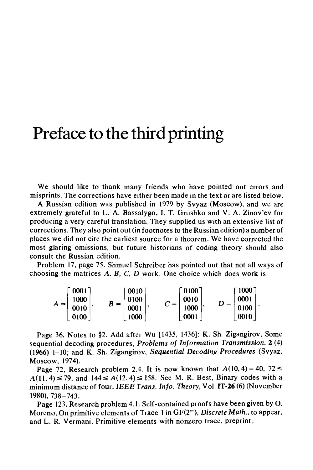
Problem 17, page 75. Shmuel Schreiber has pointed out that not all ways of
choosing the matrices А, В, C, D work. One choice which does work is
"1000"
0001
0100 '
0010.
Page 36, Notes to §2. Add after Wu [1435, 1436]: K. Sh. Zigangirov, Some
sequential decoding procedures, Problems of Information Transmission, 2 (4)
(1966) 1-10; and K. Sh. Zigangirov, Sequential Decoding Procedures (Svyaz,
Moscow, 1974).
Page 72, Research problem 2.4. It is now known that A(10,4) = 40, 72 <
Д(11,4)<79, and 144 < Л(12,4)< 158. See Μ. R. Best, Binary codes with a
minimum distance of four, IEEE Trans. Info. Theory, Vol. IT-26 (6) (November
1980), 738-743.
Page 123, Research problem 4.1. Self-contained proofs have been given by O.
Moreno, On primitive elements of Trace 1 in GF(2m), Discrete Math., to appear,
and L. R. Vermani, Primitive elements with nonzero trace, preprint.
0001 Γ0010Ί 0100
1000 0100 0010
0010 ' 0001 ' 1000
0100 1000 0001

xii
Preface to the third printing
Chapter 6, pp. 156 and 180. Theorem 33 was proved independently by Zinov'ev
and Leont'ev [1472].
Page 166, Research problem 6.1 has been settled in the affirmative by I. I.
Dumer, A remark about codes and tactical configurations, Math. Notes, to
appear; and by C. Roos, Some results on г-constant codes, IEEE Trans. Info.
Theory, to appear.
Page 175. Research problem 6.3 has also been solved by Dumer and Roos [op.
cit.].
Page 178-179. Research problems 6.4 and 6.5 have been solved by Dumer [op.
cit.]. The answer to 6.5 is No.
Page 267, Fig. 9.1. R. E. Kibler (private communication) has pointed out that
the asterisks may be removed from the entries [127, 29,43], [255,45,87] and [255,
37, 91], since there are minimum weight codewords which are low-degree
multiples of the generator polynomial.
Page 280, Research problem 9.4. T. Helleseth (IEEE Trans. Info. Theory, Vol.
IT-25 (1979) 361-362) has shown that no other binary primitive BCH codes are
quasi-perfect.
Page 299, Research problem 10.1. R. E. Kibler (private communication) has
found a large number of such codes.
Page 323. The proof of Theorem 9 is valid only for q = 2m. For odd q the code
need not be cyclic. See G. Falkner, W. Heise, B. Kowol and E. Zehender, On the
existence of cyclic optimal codes, Atti Sem. Mat. Fis. Universita di Modena, to
appear.
Page 394, line 9 from the bottom. As pointed out by Massey in [918, p. 100], the
number of majority gates required in an L-step decoder need never exceed the
dimension of the code.
Page 479. Research problem 15.2 is also solved in I. I. Dumer, Some new
uniformly packed codes, in: Proceedings MFTI, Radiotechnology and
Electronics Series (MFTI, Moscow, 1976) pp. 72-78.
Page 546. The answer to Research problem 17.6 is No, and in fact R. E. Kibler,
Some new constant weight codes, IEEE Trans. Info. Theory, Vol. IT-26 (May
1980) 364-365, shows that 27 < Λ(24, 10, 8) < 68.
Appendix A, Figures 1 and 3. For later versions of the tables of A(n, d) and
A(n, d, w) see R. L. Graham and N. J. A. Sloane, Lower bounds for constant
weight codes, IEEE Trans. Info. Theory, Vol. IT-26 (1980) 37-43; M. R. Best,
Binary codes with a minimum distance of four, loc. cit., Vol. ГГ-26 (1980), 738-743;
and other papers in this journal.
On page 682, line 6, the value of X corresponding to F = 30 should be changed
from .039 to .093.

1
Linear codes
§1. Linear codes
Codes were invented to correct errors on noisy communication channels.
Suppose there is a telegraph wire from Boston to New York down which O's
and l's can be sent. Usually when a 0 is sent it is received as a 0, but
occasionally a 0 will be received as a 1, or a 1 as a 0. Let's say that on the
average 1 out of every 100 symbols will be in error. I.e. for each symbol there
is a probability ρ = 1/100 that the channel will make a mistake. This is called a
binary symmetric channel (Fig. 1.1).
There are a lot of important messages to be sent down this wire, and they
must be sent as quickly and reliably as possible. The messages are already
written as a string of O's and l's-perhaps they are being produced by a
computer.
We are going to encode these messages to give them some protection
against errors on the channel. A block of к message symbols и = u,u2... uk
Fig. 1.1. The binary symmetric channel, with error probability p. In general Osp =si.

2
Linear codes
Ch. 1. §1.
MESSAGE
SOURCE
MESSAGE
ENCODER
CODEWORD
x*x5 xn
CHANNEL
NOISE
Fig. 1.2
(m, = 0 or 1) will be encoded into a codeword χ = xtx2... x„ (*, = 0 or 1) where
η 3: к (Fig. 1.2); these codewords form a code.
The method of encoding we are about to describe produces what is called a
linear code. The first part of the codeword consists of the message itsejf:
Xi = «,, X2= U2 Xk = Mk,
followed by η - к check symbols
JCk + l, . . . , Xn·
The check symbols are chosen so that the codewords satisfy
(1)
where the (n - k) χ η matrix Η is the parity check matrix of the code, given
by
Я = [Л|1„_к], (2)
A is some fixed (n - k)x к matrix of O's and l's, and
is the (n-k)x(n-k) unit matrix. The arithmetic in Equation (1) is to be
performed modulo 2, i.e. 0+1 = 1,1 + 1=0, - 1 = + 1. We shall refer to this as
binary arithmetic.
Example. Code # 1. The parity check matrix
H =
Г0 1 1
1 0 1
.1 1 0
1 0 0]
0 1 0
0 0 lj
(3)
defines a code with к = 3 and η = 6. For this code
A =
Γ0
1
1
1
0
1
1]
1
0

Ch. 1. §1.
Linear codes
3
The message м,м2м3 is encoded into the codeword χ = χιΧ2χ3*4*5*6, which
begins with the message itself:
*, = M,, X2=U2, *з=Мз,
followed by three check symbols хлх5хь chosen so that Hx"=0, i.e. so that
*2 + *λ + *4= 0,
*,+*3 + *5=0, (4)
*, +*2 + *6= 0.
If the message is и = 011, then *i = 0, x2= 1, *з = 1, and the check symbols
are
*4 =-1-1 = 1 + 1=2 = 0,
*5= - 1 = 1, *6= - 1 = 1,
so the codeword is * = 011011.
The Equations (4) are called the parity check equations, or simply parity
checks, of the code.
The first parity check equation says that the 2nd, 3rd and 4th symbols of
every codeword must add to 0 modulo 2; i.e. their sum must have even parity
(hence the name!).
Since each of the 3 message symbols м,м2м3 is 0 or 1, there are altogether
23 = 8 codewords in this code. They are:
000000 011011 110110
001110 100011 111000.
010101 101101
In the general code there are 2k codewords.
As we shall see, code # 1 is capable of correcting a single channel error (in
any one of the six symbols), and using this code reduces the average
probability of error per symbol from ρ = .01 to .00072 (see Problem 24). This
is achieved at the cost of sending 6 symbols only 3 of which are message
symbols.
We take (1) as our general definition:
Definition. Let Η be any binary matrix. The linear code with parity check
matrix Η consists of all vectors χ such that
Hx" = 0.
(where this equation is to be interpreted modulo 2).
It is convenient, but not essential, if Η has the form shown in (2) and (3), in
which case the first к symbols in each codeword are message or information
symbols, and the last η - к are check symbols.

4
Linear codes
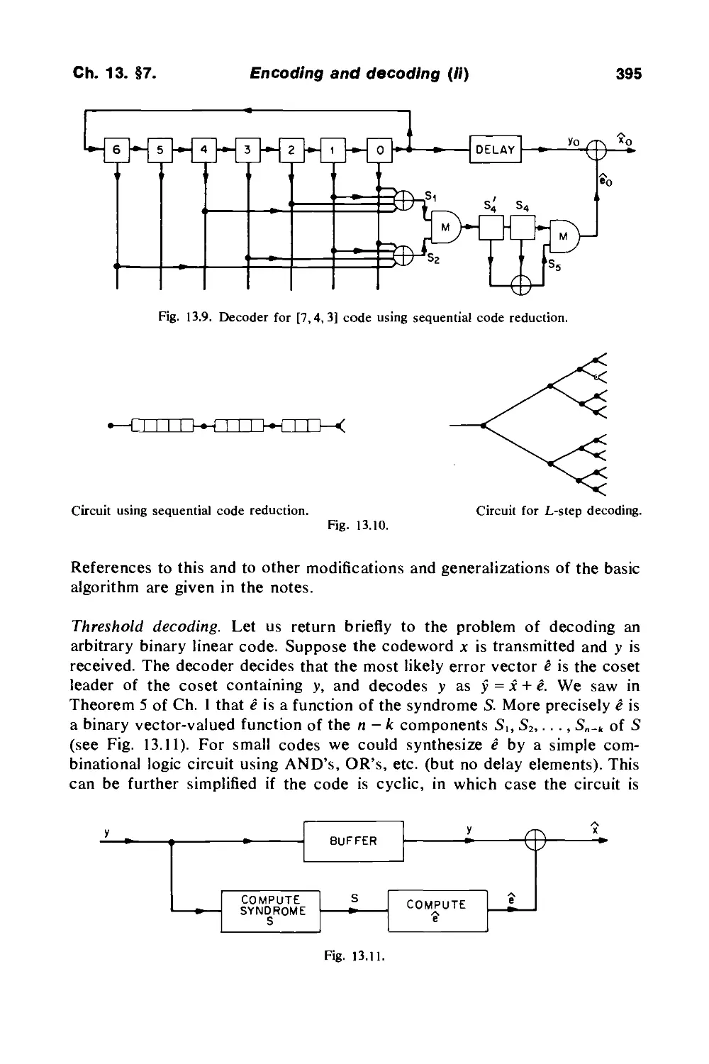
Ch. 1. §1.
Linear codes are the most important for practical applications and are the
simplest to understand. Nonlinear codes will be introduced in Ch. 2.
Example. Code # 2, α repetition code. A code with к = Ι, η = 5, and parity
check matrix
И
I l
I l
I l
I I
(blanks denote zeros).
Each codeword contains just one message symbol u. The parity check
equations are
.V ι + Xz = 0, Χ ι + ΛΊ = 0, A'i + Xt = 0, .V ι + X·. = 0,
i.e. Xi = x? = x* = xt = x*= u. So there are only two codewords, 00000 and
ll 111. The message symbol is simply repeated 5 times: this is called a
repetition code.
Example. Code # 3, an even weight code. A code with к = 3, и = 4 and parity
check matrix Η = (l 111). Each codeword contains 3 message symbols χ,.χ-χ,
and one check symbol .v4 = Xi+ x2 + x*- The 21 = 8 codewords are 0000, 0011,
0101, 1001, 0110, 1010, 1100, 1111, i.e. all vectors with an even number of l's.
1010
1101
Problems. (1) Code #4 has parity check matrix
Η =
List all the codewords. Repeat for
Η =
0111
1101
How are these codes related?
(2) Code # 5 has parity check matrix
Η
0111100
1011010
Ί loiooi.
List all the codewords.
(3) If ρ >j in Fig. 1.1, show that interchanging the names of the received
symbols changes this to a binary symmetric channel with ρ < ί. If ρ = j show
that no communication is possible.

Ch. 1. §2. Properties of a linear code 5
§2. Properties of a linear code
(i) The definition again: χ = xt ■ ■ ■ x„ is a codeword if and only if
tfxu = 0. (1)
(ii) Usually the parity check matrix Η is an (n - k) χ η matrix of the form
H = [A\Ink], (2)
and as we have seen there are 2k codewords satisfying (1). (This is still true
even if Η doesn't have this form, provided Η has η columns and η - к
linearly independent rows.) When Η has the form (2), the codewords look like
this:
X = Xl ' ' Xk Xk + l ' ' Xit ·
message check
symbols symbols
(iii) The generator matrix. If the message is и = м, ■ ■ -uk, what is the
corresponding codeword χ = Χι ■ ■ ■ χ„Ί First x, = uly.. . ,xk = uk, or
'x,\ /иЛ
i J = Ik\ '■■ J, Ik = unit matrix.
\xk/ \uk/
(5)
Then from (1) and (2),
[A | Ι„_,]ί ;' j = 0,
\Xn I \xki
= -aI : ) from (5).
(6)
In the binary case -A = A, but later we shall treat cases where - ΑΦ A.
Putting (5) on top of (6):
>WE
and transposing, we get
where
χ = uG (7)
G = [Ik\-A"l (8)

6
Linear codes
Ch. 1. §2.
If Η is in standard form G is easily obtained from Η - see (2). G is called a
generator matrix of the code, for (7) just says that the codewords are all
possible linear combinations of the rows of G. (We could have used this as
the definition of the code.) (1) and (7) together imply that G and Η are related
by
GH,r = 0 or HG,r = 0. (9)
Example. Code # / (cont.). A generator matrix is
G = [J1|-A,r]
100
010
001
011
101
110
row 1
row 2
row 3.
The 8 codewords are (from (7))
Mi · row 1 + u2 ■ row 2 + Mi · row 3 (и,, u2, Mi = 0 or 1).
We see once again that the codeword corresponding to the message и = 011 is
χ = uG
= row 2 + row 3
= 010101 +001110
= 011011,
the addition being done mod 2 as usual.
(iv) The parameters of a linear code. The codeword χ = л-, ■ · ■ x„ is said to
have length n. This is measuring the length as a tailor would, not a
mathematician, η is also called the block length of the code. If Η has η - к
linearly independent rows, there are 2k codewords, к is called the dimension
of the code. We call the code an [n, k] code.
This code uses η symbols to send к message symbols, so it is said to have
rate or efficiency R = kin.
(v) Other generator and parity check matrices. A code can have several
different generator matrices. E.g.
[1110] ГИ
LoioiJ' Lo
011
101
are both generator matrices for code # 4. In fact any maximal set of linearly
independent codewords taken from a given code can be used as the rows of a
generator matrix for that code.
A parity check on a code <€ is any row vector h such that hx" = 0 for all
codewords i£t Then similarly any maximal set of linearly independent
parity checks can be used as the rows of a parity check matrix Я for <ё. E.g.
[1010] [
Lι ιοί J' L
0111
1101
are both parity check matrices for code # 4.

Ch. 1. §3.
At the receiving end
7
(vi) Codes over other fields. Instead of only using O's and l's, we could have
allowed the symbols to be from any finite field (see Chapters 3 and 4). For
example a ternary code has symbols 0, 1 and 2, and all calculations of parity
checks etc. are done modulo 3 (1+2 = 0, -1 =2, 2 + 2= 1, 2 · 2 = 1, etc.). If
the symbols are from a finite field with q elements, the code is still defined by
(1) and (2), or equivalently by (7) and (8), and an [n, k] code contains qk
codewords.
Example. Code # 6. A [4, 2] ternary code with parity check matrix
The generator matrix is (from (8))
с=[/2|-дч=га rowi
L0121J row 2.
There are 9 codewords и, · row 1 + u2 ■ row 2 (м,, u2 = 0, 1 or 2), as follows:
message codeword message codeword message codeword
и χ и χ и χ
00 0000 10 1022 20 2011
01 0121 11 1110 21 2102
02 0212 12 1201 22 2220
This code has rate R = kin = \.
(vii) Linearity. If χ and у are codewords of a given code, so is χ + у,
because H(x + y)" = Hx" + Ну" = 0. If с is any element of the field, then ex is
also a codeword, because H(cx)" = cHx" = 0. E.g. in a ternary code if χ is a
codeword so is 2x = -x. That is why these are called linear codes. Such a
code is also an additive group, and a vector space over the field.
Problems. (4) Code # 2 (cont.). Give parity check and generator matrices for
the general [n, 1] repetition code.
(5) Code # 3 (cont.). Give parity check and generator matrices for the
general [η, η - 1] even weight code.
(6) If the code <€ has an invertible generator matrix, what is "£?
§3. At the receiving end
(We now return to binary codes.) Suppose the message и = м, · · · uk is
encoded into the codeword χ =x, ···*„, which is then sent through the
channel. Because of channel noise, the received vector у = у, ■ ■ ■ y„ may be

8
Linear codes
Ch. 1. §3.
different from x. Let's define the error vector
e = у -χ = e, · · · en. (10)
Then e, = 0 with probability 1 - ρ (and the i,h symbol is correct), and e, = 1
with probability ρ (and the i,h symbol is wrong). In the example of §1 ρ was
equal to 1/100, but in general ρ can be anywhere in the range 0=£ ρ < 1. So we
describe the action of the channel by saying it distorts the codeword χ by
adding the error vector e to it.
The decoder (Fig. 1.3) must decide from у which message и or (usually
simpler) which codeword χ was transmitted. Of course it's enough if the
decoder finds e, for then χ = у - e. Now the decoder can never be certain
what e was. His strategy therefore will be to choose the most likely error
vector e, given that у was received. Provided the codewords are all equally
likely, this strategy is optimum in the sense that it minimizes the probability
of the decoder making a mistake, and is called maximum likelihood decoding.
To describe how the decoder does this, we need two important definitions.
MESSAGE
SOURCE
\
>
U = Uj' ■ U
HESSAGE
ENCODER
: с
< = χ,- ■ χ
CHANNEL
η
У.
η
ODEWORD
~\
J
*>
у = χ + e
DECODER
/
\'
\
USER
RECEIVED ESTIMATE ft
VECTOR OF MESSAGE
s e = ег еП/
ERROR
VECTOR
Fig. 1.3. The overall communication system.
Definition. The (Hamming) distance between two vectors χ = Χι ■ ■ ■ x„ and
У = У* ' ' ' У« 's the number of places where they differ, and is denoted by
dist(jc, y). E.g.
dist(10111,00101) = 2, dist(0122, 1220) = 3
(the same definition holds for nonbinary vectors).
Definition. The (Hamming) weight of a vector χ = χ ι ■ ■ ■ x„ is the number of
nonzero Xi, and is denoted by wt(jt). E.g.
wt(101110) = 4, wt(01212110) = 6.
Obviously
dist(x,y) = wt(x-y), (11)
for both sides express the number of places where χ and у differ.

Ch. 1. §3.
At the receiving end
9
Problem. (7) Define the intersection of binary vectors χ and у to be the vector
χ * у = (x,yl,...,x„y„),
which has l's only where both χ and у do. E.g. 11001 * 10111 = 10001. Show
that
wt (x + y) = wt (ж) + wt (y) - 2 wt (x * y). (12)
Now back to decoding. Errors occur with probability p. For instance
Prob{e = 00000} = (l-p)5,
Prob{e = 01000} = p(l-p)\
Prob{e = 10010} = p2(l-p)\
In general if υ is some fixed vector of weight a,
PTOb{e = v} = p°(l-p)"-°. (13)
Since ρ < s, we have 1 — ρ > p, and
(l-p)5>p(l-p)4>p2(l-p)3>···.
Therefore a particular error vector of weight 1 is more likely than a particular
error vector of weight 2, and so on. So the decoder's strategy is:
Decode у as the nearest codeword χ (nearest in Hamming distance), i.e.:
Pick that error vector e which has least weight.
This is called nearest neighbor decoding.
A brute force decoding scheme then is simply to compare у with all 2k
codewords and pick the closest. This is fine for small codes. But if к is large
this is impossible! One of the aims of coding theory is to find codes which can
be decoded by a faster method than this.
The minimum distance of a code. The third important parameter of a code %,
besides the length and dimension, is the minimum Hamming distance between
its codewords:
d = min dist (η, υ)
= minwt(H-r) ие%1)е«,м^1). (14)
d is called the minimum distance or simply the distance of the code. Any two
codewords differ in at least d places.
A linear code of length n, dimension k, and minimum distance d will be
called an [n, k, d] code.
To find the minimum distance of a linear code it is not necessary to
compare every pair of codewords. For if и and t; belong to a linear code <€,
и —v = w is also a codeword, and (from (14))
d= min wt(w).
we<«.w*o

10
Linear codes
Ch. 1. §3.
In other words:
Theorem 1. The minimum distance of a linear code is the minimum weight of
any nonzero codeword.
Example. The minimum distances of codes # 1, #2, #3, #6 are 3, 5, 2, 3
respectively.
How many errors can a code correct?
Theorem 2. A code with minimum distance d can correct [i(d - 1)] errors* If d
is even, the code can simultaneously correct \{d - 2) errors and detect d\2
errors.
Proof. Suppose d = 3 (Fig. 1.4). The sphere of radius r and center и consists
of all vectors t; such that dist (η, ν) *£ r. If a sphere of radius 1 is drawn
around each codeword, these spheres do not overlap. Then if codeword и is
transmitted and one error occurs, so that the vector a is received, then a is
inside the sphere around и, and is still closer to и than to any other codeword
v. Thus nearest neighbor decoding will correct this error.
Similarly if d = 2t + l, spheres of radius t around each codeword do not
overlap, and the code can correct t errors.
Now suppose d is even (Fig. 1.5, where d = 4). Spheres of radius \{d -2)
around the codewords are disjoint and so the code can correct \{d - 2) errors.
But if d\2 errors occur the received vector a may be midway between 2
codewords (Fig. 1.5). In this case the decoder can only detect that d\2 (or
more) errors have occurred. Q.E.D.
Thus code # 1, which has minimum distance 3, is a single-error-correcting
code.
(tHp
— d = 3 »
Fig. 1.4. A code with minimum distance 3 (® = codeword).
*[x] denotes the greatest integer less than or equal to x. E.g. [3.5] = 3, [- 1.5] = -2.

Ch. 1. §3.
At the receiving end
11
φ"Φ
-· d=4 ■■
( ® = CODEWORD )
Fig. 1.5. A code with minimum distance 4.
On the other hand, if more than d/2 errors occur, the received vector may
or may not be closer to some other codeword than to the correct one. If it is,
the decoder will be fooled and will output the wrong codeword. This is called
a decoding error. Of course with a good code this should rarely happen.
So far we have assumed that the decoder will always try to find the nearest
codeword. This scheme, called complete decoding, is fine for messages which
can't be retransmitted, such as a photograph from Mars, or an old magnetic
tape. In such a case we want to extract as much as possible from the received
vector.
But often we want to be more cautious, or cannot afford the most
expensive decoding method. In such cases we might use an incomplete
decoding strategy: if it appears that no more than / errors occurred, correct
them, otherwise reject the message or ask for a retransmission.
Error detection is an extreme version of this, when the receiver makes no
attempt to correct errors, but just tests the received vector to see if it is a
codeword. If it is not, he detects that an error has occurred and asks for a
retransmission of the message. This scheme has the advantages that the
algorithm for detecting errors is very simple (see the next section) and the
probability of an undetected error is very low (§5). The disadvantage is that if
the channel is bad, too much time will be spent retransmitting, which is an
inefficient use of the channel and produces unpleasant delays.
Nonbinary codes. Almost everything we have said applies equally well to
codes over other fields. If the field F has q elements, then the message и, the
codeword x, the received vector y, and the error vector
e = у - χ = e,e2 ■ ■ ■ e„
all have components from F.
We assume that e, is 0 with probability 1 - ρ >4, and e, is any of the q - 1
nonzero elements of F with probability pl(q — 1). In other words the channel
is a q-ary symmetric channel, with q inputs, q outputs, a probability 1 - ρ > \lq
that no error occurs, and a probability ρ <(q- \)lq that an error does occur,
each of the q - 1 possible errors being equally likely.

12
Linear codes
Ch. 1. §3.
1-p
SEND RECEIVE
p=ERROR PROBABILITY
Fig. 1.6. The ternary symmetric channel.
Example. If q = 3, the ternary symmetric channel is shown in Fig. 1.6.
Problems. (8) Show that for binary vectors:
(a) wt(jt+.y)& wt (x) - wt (y), (15)
with equality iff x* = 1 whenever yf = 1.
(b) wt (x + z) + wt (y + z) + wt(x + y + z)
&2wt(jt+y + x * y)-wt(z), (16)
with equality iff it never happens that x: and y* are 0 and z-, is 1.
(9) Define the product of vectors χ and у from any field to be the vector
x * у = (дс,у ,x„y„).
For binary vectors this is called the intersection - see Problem 7. Show that
foi ternary vectors,
wt(jt+y) = wt(jt) + wt(y)-/(jt * y), (17)
where, if и = и, · · · и„ is a ternary vector containing α 0's, b l's and с 2's,
then /(h) = b + 2c. Therefore
wt (x) + wt (y) - 2 wt (x * y) « wt (x + y) =£ wt (ж) + wt (y) - wt (x * y). (18)
(10) Show that in a linear binary code, either all the codewords have even
weight, or exactly half have even weight and half have odd weight.

Ch. 1. §3.
At the receiving end
13
(11) Show that in a linear binary code, either all the codewords begin with
0, or exactly half begin with 0 and half with 1. Generalize!
Problems 10 and 11 both follow from:
(12) Suppose G is an abelian group which contains a subset A with three
properties: (i) if α,, a2 ε A, then a, - a2GA, (ii) if b,, Ь2(£ A, then b, - b2EA,
(iii) if a E A, b£A, then a + b£A. Show that either A = G, or A is a
subgroup of G and there is an element b&A such that
G = AU(b+A),
where b + A is the set of all elements b + a, a e A.
(13) Show that Hamming distance obeys the triangle inequality: for any
vectors χ = x, · · ■ x„, у => y, ■ ■ · y„, ζ = z, · · · z„,
dist (x, y) + dist (y, ζ) ^ dist (x, z). (19)
Show that equality holds iff, for all /, either xt = yf or yf = z, (or both).
(14) Hence show that if a code has minimum distance d, the codeword χ is
transmitted, not more than j(d-l) errors occur, and у is received, then
dist (ж, у) < dist (y, z) for all codewords ζΦχ. (A more formal proof of
Theorem 2.)
(15) Show that a code can simultaneously correct «a errors and detect
a + 1,. .. , b errors iff it has minimum distance at least a + b + 1.
(16) Show that if χ and у are binary vectors, the Euclidean distance
between the points χ and у is
(E(*-y.)2)"2 = V(dist(x,y)).
(17) Combining two codes (I). Let G,,G2 be generator matrices for
[n,, k, d,] and [n2, k, d2] codes respectively. Show that the codes with
generator matrices
/G,0 \
\o gJ
and (G,\G2) are [n, + n2, 2k, min {d,, d2\] and [n, + n2, k, d] codes, respectively,
where d^ d, + d2.
(18) Binomial coefficients. The binomial coefficient (Д), pronounced "л
choose m" is defined by
o-
x(x -
1,
0,
-1)·
■■(*-
m\
-m + \)
1
if m is a p
if m =0,
otherwise,
where χ is any real number, and m ! = 1 · 2 · 3 · . .. · {m - l)m,0! = 1. The

14
Linear codes
Ch. 1. §3.
reader should know the following properties:
(a) If χ = η is a nonnegative integer and η ** m ** 0,
(«) = ul
\m/ m \(n -
my:
which is the number of unordered selections of m objects from a set of η
objects.
(b) There are (£) binary vectors of length η and weight m. There are
(q - l)m(m) vectors from a field of q elements which have length η and weight
m. [For each of the m nonzero coordinates can be filled with any field element
except zero.]
(c) The binomial series:
(a + b)" = 2 ( )a"'mbm, if η is a nonnegative integer;
(l + b)'= У (X)bm, for Ы<1 and any real x;
(\ _ hY+l = ^ ( Ρ'· for |b| < 1 and any real x.
[Remember the student who, when asked to expand (a + b)" on an exam
replied: ,...,-, ы+ы, (a + b)\ (a + b)", (a + b)",. . . ?]
(d) Easy identities. (Here η and m are nonnegative integers, χ is any real
number)
\tn/ \n — m/'
(m)=Q form>'n»0,
o+L-,)-(":')·
.tC)-2"·
Σ (£)=Σ CD"2-" i'«»i.
m even \"l / m odd \"l /
ς,(-ιγ(:)=ο if«*i.
Σ (") = i[2- + (l + i)"+(l-i)"],i = V-l. (20)
m divisible by 4 \W1 /
(19) Suppose u and υ are binary vectors with dist (u, v)= d. Show that the
number of vectors w such that dist (и, w)=r and dist(r, w) = s is (f)("lf),

Ch. 1. §4. More about decoding a linear code 15
where i = (d + r- s)/2. If d + r- s is odd this number is 0, while if r + s = d it
•s α
(20) Let h, v, w and χ be four vectors which are pairwise distance d apart;
d is necessarily even. Show that there is exactly one vector which is at a
distance of d/2 from each of u, ν and w. Show that there is at most one vector
at distance d/2 from all of u, υ, w and x.
§4. More about decoding a linear code
Definition of a coset. Let 9? be an [n, k] linear code over a field with q
elements. For any vector a, the set
a + <g = {a+x:xG(€}
is called a coset (or translate) of 9?. Every vector b is in some coset (in b + %
for example), a and b are in the same coset iff (a - b) ε 9?. Each coset
contains qk vectors.
Proposition 3. Two cosets are either disjoint or coincide (partial overlap is
impossible).
Proof. If cosets a + % and b + % overlap, take ν E(a + <в)Г\(Ь + <€). Then
v = a+x = b+y, where χ and yE.%. Therefore b = a + χ - у = a + χ' (χ' e сё),
and so Ь + свСа + (в. Similarly a + % С b + % and so a + % = b + %. Q.E.D.
Therefore the set F" of all vectors can be partitioned into cosets of 9?:
F" = % U (α, + %) U (β2 + «) U · · · U (a, + %) (21)
where t = qn~" - 1.
Suppose the decoder receives the vector у. у must belong to some coset in
(21), say у = a,, + χ (χ ε %). What are the possible error vectors e which could
have occurred? If the codeword x' was transmitted, the error vector is
e = у - χ' = a, + χ - χ' = at + χ" e a,■ + 9?. We deduce that:
the possible error vectors are exactly the vectors in
the coset containing y.
So the decoder's strategy is, given y, to choose a minimum weight vector ё
in the coset containing y, and to decode у as χ = у — e. The minimum weight
vector in a coset is called the coset leader. (If there is more than one vector
with the minimum weight, choose one at random and call it the coset leader.)
We assume that the a,'s in (21) are the coset leaders.

16
Linear codes
Ch. 1. §4.
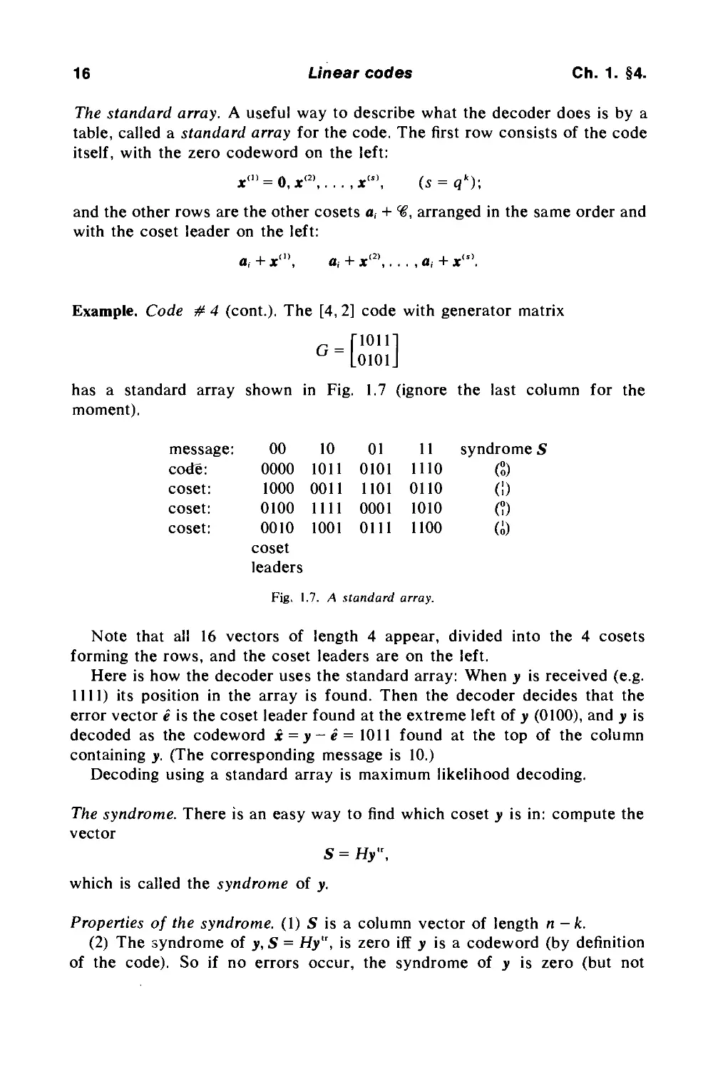
The standard array. A useful way to describe what the decoder does is by a
table, called a standard array for the code. The first row consists of the code
itself, with the zero codeword on the left:
ж"1 = 0, ж'2',. . . , x"\ (s = qk);
and the other rows are the other cosets a, + 9?, arranged in the same order and
with the coset leader on the left:
a, + x°\ a, + x<2\ ...,«,+ x<s\
Example. Code # 4 (cont.). The [4, 2] code with generator matrix
rioin
LoioiJ
has a standard array shown in Fig. 1.7 (ignore the last column for the
moment).
message:
code:
coset:
coset:
coset:
00 10
0000 1011
1000 ООП
0100 1111
0010 1001
coset
leaders
01
0101
1101
0001
0111
Fig. 1.7. A standard
11
1110
0110
1010
1100
array.
syndrome S
(°o)
0
(?)
(A)
Note that all 16 vectors of length 4 appear, divided into the 4 cosets
forming the rows, and the coset leaders are on the left.
Here is how the decoder uses the standard array: When у is received (e.g.
1111) its position in the array is found. Then the decoder decides that the
error vector e is the coset leader found at the extreme left of у (0100), and у is
decoded as the codeword χ = у - e = 1011 found at the top of the column
containing y. (The corresponding message is 10.)
Decoding using a standard array is maximum likelihood decoding.
The syndrome. There is an easy way to find which coset у is in: compute the
vector
S = Ну",
which is called the syndrome of y.
Properties of the syndrome. (1) S is a column vector of length η - к.
(2) The syndrome of y, S = Ну", is zero iff у is a codeword (by definition
of the code). So if no errors occur, the syndrome of у is zero (but not

Ch. 1. §4. More about decoding a linear code 17
conversely). In general, if у = χ + e where xE.%, then
S = Ну" = Hx" + He" = He". (22)
(3) For a binary code, if there are errors at locations a, b, c,. .. , so that
e =0· · 010· · · 1 · · · 1 · · 0,
a be
then from Equation (22),
S = Σ еМ, (Я, = i,h column of H)
i
=* Ha + Hb + Hc + ■ ■ ■
In words:
Theorem 4. For a binary code, the syndrome is equal to the sum of the
columns of Η where the errors occurred. [Thus S is called the "syndrome"
because it gives the symptoms of the errors.]
(4) Two vectors are in the same coset of <€ iff they have the same
syndrome. For и and t; are in the same coset iff (н - ν) ε % iff H(u - υ)" = 0
iff Ни" = Ην". Therefore:
Theorem 5. There is a l-l-correspondence between syndromes and cosets.
For example, the cosets in Fig. 1.7 are labeled with their syndromes.
Thus the syndrome contains all the information that the receiver has about
the errors.
By Property (2), the pure error detection scheme mentioned in the last
section just consists of testing if the syndrome is zero. To do this, we
recompute the parity check symbols using the received information symbols,
and see if they agree with the received parity check symbols. I.e., we
re-encode the received information symbols. This only requires a copy of the
encoding circuit, which is normally a very simple device compared to the
decoder (see Fig. 7.8).
Problems. (21) Construct a standard array for code # 1. Use it to decode the
vectors 110100 and 111111.
(22) Show that if % is a binary linear code and a£ %, then % U (a + %) is
also a linear code.

18
Linear codes
Ch. 1. §5.
§5. Error probability
When decoding using the standard array, the error vector chosen by the
decoder is always one of the coset leaders. The decoding is correct if and only
if the true error vector is indeed a coset leader. If not, the decoder makes a
decoding error and outputs the wrong codeword. (Some of the information
symbols may still be correct, even so.)
Definition. The probability of error, or the word error rate, Pcn, for a particular
decoding scheme is the probability that the decoder output is the wrong
codeword.
If there are Μ codewords x"\. .. ,x'M\ which we assume are used with
equal probability, then
1 M
i'crr = tt Σ Ρ rob {decoder output Φ χω Ι x(0 was sent}. (23)
Μ -τ!
If the decoding is done using a standard array, a decoding error occurs iff e
is not a coset leader, so
Perr = Prob {e Φ coset leader}.
Suppose there are a, coset leaders of weight /. Then (using (13))
P«rr=l-2«<P'(1-P)"" (24)
(Since the standard array does maximum likelihood decoding, any other
decoding scheme will have P„„ з= (24).)
Examples. For code #4 (Fig. 1.7), a0 = 1, a, = 3, so
Pc„=l-(l-p)4-3p(l-p)3
= 0.0103... if Ρ =7^·
For code # 1, a0= 1, a, = 6, a2= 1, so
Pc„= l-(l-p)6-6p(l-p)5-p2(l-p)4
= 0.00136... ifp=j^.
If the code has minimum distance d = It + 1 or 2i + 2, then (by Theorem 2)
it can correct t errors. So every error vector of weight «i is a coset leader.

Ch. 1. §5.
Error probability
19
I.e.
«. = (") forO«i«f. (25)
But for / > t the <*i are extremely difficult to calculate and are known for very
few codes.
If the channel error probability ρ is small, l-p = l and р'(1-р)п~'>
p'+'(l -p)""'"'. In this case the terms in (24) with large / are negligible, and
Ρ«φ1-Σ(?)ρ'(1-Ρ)"-' (26)
or
P„ =5= 1 - Σ ("V'd - pT" ~ α,+ιρ'+,(1-ρΤ-' (27)
ί-α \l /
are useful approximations. In any event the RHS of (26) or (27) is an upper
bound on Pc„.
Perfect codes. Of course, if α{ = 0 for i> t = [(d - l)/2], then (26) is exact.
Such a code is called perfect.
Thus a perfect t-error-correcting code can correct all errors of weight «i,
and none of weight greater than t. Equivalently, the spheres of radius t
around the codewords are disjoint and together contain all vectors of length n.
We shall see much more about perfect codes in Chs. 6, 20.
Quasi-perfect codes. On the other hand, if a, =0 for / > f + 1, then (27) is
exact. Such a code is called quasi-perfect.
Thus a quasi-perfect t-error-correcting code can correct all errors of
weight =£ t, some of weight t + 1, and none of weight > t + 1. The spheres of
radius t + 1 around the codewords may overlap, and together contain all
vectors of length n.
We shall meet quasi-perfect codes again in Chapters 6, 9 and 15.
Sphere-packing or Hamming bound. Suppose 9? is a binary code of length η
containing Μ codewords, which can correct t errors. The spheres of radius t
around the codewords are disjoint. Each of these Μ spheres contain 1 -I- (7) -·-
■■■+(") vectors (see Problem 18(b)). But the total number of vectors in the
space is 2". Therefore we have established:
Theorem 6. (The sphere-packing or Hamming bound.)
A t-error-correcting binary code of length η containing Μ codewords must
satisfy

20
Linear codes
Ch. 1. §5.
Similarly, for a code over a field with q elements,
M(l + (q - 1)(") + ·-·+(<?- 1)'(")) « q". (29)
For large η see Theorem 32-of Ch. 17. Since the proof of these two bounds
did not assume linearity, they also hold for nonlinear codes (see Ch. 2).
By definition, a code is perfect iff equality holds in (28) or (29).
Symbol error rate. Since some of the message symbols may be correct even if
the decoder outputs the wrong codeword, a more useful quantity is the symbol
error rate, defined as follows.
Definition. Suppose the code contains Μ codewords x<0 = х\° ■ ■ ■ x%\ i =
1,..., M, and the first к symbols x\" ■ ■ ■ χ\!} in each codeword are information
symbols. Let χ = χ, ■ ■ ■ x„ be the decoder output. Then the symbol error rate
Psymb is the average probability that an information symbol is in error after
decoding:
ι к М
Psymb=ш ? ?Prob to φ *'" ι *"'was sent} (30)
Problem. (23) Show that if standard array decoding is used, and the messages
are equally likely, then the number of information symbols in error after
decoding does not depend on which codeword was sent. Indeed, if the codeword
χ = jti · · · jt„ is sent and is decoded as χ = xt ■ ■ ■ x„, then
Р.уп,ь = т2РгоЬ{х,*хЛ, (31)
К , = |
= {l/(«)Prob{e}, (32)
where f(e) is the number of incorrect information symbols after decoding, if
the error vector is e, and so
1 2>
* symb ι
κ ,_i
where F{ is the weight of the first к places of the codeword at the head of the i,h
column of the standard array, and Р(с<) is the probability of all binary vectors
in this column.
Example. The standard array of Fig. 1.7. Here f(e) = 0 if e is in the first column
of the standard array (a coset leader), = 1 if e is in columns 2 or 3, and = 2 if e is
in the last column. From (32):
Psymb = i[l · (P4 + 3p3<J + 3pV + PQ') + 2 ■ (p'q + 3p2q2)], q=\-p,
= 0.00530... if ρ = 1/100.

Ch. 1. §5.
Error probability
21
Using this very simple code has lowered the average probability of error per
symbol from 0.01 to 0.0053.
Problems. (24) Show that for code # 1 with standard array decoding
Psymb = (22p V + 36p V + 24рУ + I2p5q + 2p6)/3
= 0.00072... if ρ = 1/100.
As these examples suggest, Psymb is difficult to calculate and is not known for
most codes.
(25) Show that for an [n, k] code,
- Ρ «Ρ -=ξ Ρ
ι * егт л symb *■ err
Incomplete decoding. An incomplete decoding scheme which corrects =£ /
errors can be described in terms of the standard array as follows. Arrange the
cosets in order of increasing weight (i.e. decreasing probability) of the coset
leader (Fig. 1.8).
correct errors (coset
leaders of weight =£ /).
1 detect errors (coset
headers of weight >/).
Fig. 1.8. Incomplete decoding using a standard array.
If the received vector у lies in the top part of the array, as before у is decoded
as the codeword found at the top of its column. If у lies in the bottom half, the
decoder just detects that more than / errors have occurred.
Error detection. When error detection is being used the decoder will make a
mistake and accept a codeword which is not the one transmitted iff the error
vector is a nonzero codeword. If the code contains A, codewords of weight /,
the error probability is
Pe„ = S AP'O-P)""'· (33)
i = l
/
The probability that an error will be detected and the message retransmitted is
Pre.™..= l-(l-p)--P„. (34)
Example. For code #1, A0 = 1, A3 = 4, A4 = 3, and
Ре„ = 4р3(1-Р)3 + Зр4(1-Р)2
= 0.00000391... ifp=-i-.

22
Linear codes
Ch. 1. §6.
This is very much smaller than the error probability of 0.00136 obtained from
standard array decoding of this code. The retransmission probability is
Prelrans = 0.0585 ....
Research Problem 1.1. Find the distribution {a,} of coset leaders for any of the
common families of codes. This is still unsolved even for first-order Reed
Muller codes-see Chapter 14, Berlekamp and Welch [133], Lechner [797-799],
Sarwate [1144] and Sloane and Dick [1233].
§6. Shannon's Theorem on the existence oi good codes
In the last section we saw that the weak code # 4 reduced the average
probability of error per symbol from 0.01 to 0.00530 (at the cost of using 4
symbols to send 2 message symbols), and that code # 1, which also had rate I,
further reduced it to 0.00072 (at the cost of using 6 symbols to send 3 message
symbols).
In general we would like to know, for a given rate R = kin, how small we can
make Psymb with an [n, k] code. The answer is given by a remarkable theorem of
Shannon, which says that Perr (and hence Psymb, by Problem 25) can be made
arbitrarily small, provided R is less than the capacity of the channel.
Definition. The capacity of a binary symmetric channel with error probability ρ
(Fig. 1.1) is (see Fig. 1.9)
C(p)=l + plog2p+(l-p)log2(l-p). (35)
Theorem 7. (Shannon's Theorem; proof omitted.) For any e >0, if R< C(p)
and η is sufficiently large, there is an [n, k] binary code of rate kin =* R with error
probability Perr<e.
CAPACITY
C(p)
0
0 1/2 1
Ρ
Fig. 1.9. Capacity of binary symmetric channel.
и

Ch. 1. §7.
Hamming codes
23
(A similar result holds for nonbinary codes, but with a different definition of
capacity.)
Unfortunately this theorem has so far been proved only by probabilistic
methods and does not tell how to construct these codes.
In practice (as we have seen) it is difficult to find Pcrr and P^mb< so the
minimum distance d is used as a more convenient measure of how good the
code is. For then the code can correct [ϊ(ά - 1)] errors (Theorem 2), and (26) is a
good approximation to Perr, especially if ρ is small.
So one version of the main problem of coding theory is to find codes with
large R (for efficiency) and large d (to correct many errors). Of course these are
conflicting goals. Theorem 6 has already given an upper bound on the size of a
code, and other upper bounds will be given in Ch. 17 (see especially Fig. 17.7).
On the other hand Theorem 12 at the end of the chapter is a weaker version of
Theorem 7 and implies that good linear codes exist. However, at the present
time we do not know how to find such codes.
Of course for practical purposes one also wants a code which can be easily
encoded and decoded.
§7. Hamming codes
The Hamming single-error-correcting codes are an important family of
codes which are easy to encode and decode. In this section we discuss only
binary Hamming codes.
According to Theorem 4, the syndrome of the receiver vector is equal to the
sum of the columns of the parity check matrix Η where the errors occurred.
Therefore to design a single-error-correcting code we should make the columns
of Η nonzero (or else an error in that position would not affect the syndrome
and would be undetectable) and distinct (for if two columns of Я were equal,
errors in those two positions would be indistinguishable).
If Η is to have r rows (and the code to have r parity checks) there are only
2r - 1 columns available, namely the 2r - 1 nonzero binary vectors of length r.
E.g. if r = 3, there are 23 — 1 = 7 columns available:
0 0 0 1111
0 110 0 11 (36)
10 10 10 1,
the binary representations of the numbers 1 to 7. For a Hamming code we use
them all, and get a code of length η = Ύ - 1.
Definition. A binary Hamming code Ж, of length η = 2r - 1 (r & 2) has parity
check matrix Η whose columns consist of all nonzero binary vectors of length
r, each used once. Ж, is an [n = 2r - 1, к = 2r - 1 - r, d = 3] code.

24
Linear codes
Ch. 1. §7.
Example. Code # 5, the [7,4, 3] Hamming Code Жъ, with
Η =
0 0 0 1111
0 110 0 11
10 10 10 1
(37)
Here we have taken the columns in the natural order (36) of increasing binary
numbers. To get Η in the standard form of (2), we take the columns in a different
order:
In general,
"0111100
H'= 10 110 10
1 10 10 0 1
H' = [A\L]
(38)
(39)
where A contains all columns with at least two l's.
Obviously changing the order of the columns doesn't affect the number of
errors a code can correct or its error probability.
Definition. Two codes are called equivalent if they differ only in the order of
the symbols. E.g.
0000 0000
ООП, 0101
1100 1010
1111 1111
are equivalent [4,2,2] codes. So Η and H' give equivalent codes.
Problems. (26) Show that the generator matrices
G =
generate equivalent codes.
(27) Show that
Ί 1
1
1
1 1_
G =
11
11
11
G' =
1 1
1 1
1 1
G' =
111111
II 11
1 1
generate equivalent codes.
(28) Show that the Hamming code Ж, is unique, in the sense that any linear
code with parameters [2r - l,2r - 1 - r, 3] is equivalent to Ж,.

Ch. 1. §7.
Hamming codes
25
There may be very good engineering or aesthetic reasons for preferring one
code to another which is equivalent to it. For example a third parity check
matrix Η for code # 5 is
H" =
1110 10 0
0 1110 10
0 0 1110 1
(40)
-the same columns, but in yet another order. Now the code is cyclic, i.e. a
cyclic end-around shift of a codeword is again a codeword. We shall see later
(Ch. 7) that binary Hamming codes can always be made cyclic.
Problem. (29) Code # 7, the Hamming [15, 11,3] code Ж4. Give the three forms
of H, corresponding to (37), (38) and (40). Using the (38) form, encode the
message и = 11111100000, and decode the vector 111000111000111.
Decoding. Suppose we use Η in the form (37), with the Γ" column H, = binary
representation of i. If there is a single error in the /-th symbol, then from (22) the
syndrome is S = Ну" = He" = Ht = binary representation of /. So decoding is
easy! (It will never be this easy again.)
Since the code can correct any single error, it has minimum distance d s=3 (by
Theorem 2). In fact d is equal to 3, for it's easy to find codewords of weight 3 (e.g.
11100 ··· 0 if Я is (37)). See also Theorem 10 below.
Theorem 8. The Hamming codes are perfect single-error-correcting codes.
Proof. Since the code can correct single errors, the spheres of radius 1 around
the codewords are disjoint. There are η + 1 = Ύ vectors in each sphere, and
there are 2* = 22' ' r spheres, giving a total of 22'"' = 2" vectors. So every
vector of length η is in one of the spheres and the code is perfect. Q.E.D.
Summary of Properties of Hamm
Жг is
equiv
length η =
dimension к =
number of parity checks =
minimum distance d =
ing
T-
T-
r,
3.
Code Ж,
- 1 (for
-1-r,
r =
a perfect single-error-correcting code, and
alence. The parity check matrix
columns are all nonzero r-tuples.
Fig.
.10.
Η is an
2,
is
r x η
3,...),
unique
matrix
up
to
whose

26
Linear codes
Ch. 1. §8.
Problems. (30) Write down a generator matrix G for Жг and use it to show
every nonzero codeword has weights 3. [Hint: if a codeword has weight «2
it must be the sum of «2 rows of G.]
(31) Show that the distribution of coset leaders for a Hamming code is
£*o= 1, a, = n. What is the error probability Perr?
§8. The Dual Code
If и = u, ■ ■ ■ u„, ν = v, ■ ■ ■ vn are vectors (with components from a field F),
their scalar product is
и · t; = u,v, + ■ ■ ■ + unvn (41)
(evaluated in F). For example the binary vectors и = 1101, t; = 1111 have
и ν = 1 + 1+0+ 1= 1.
If и ■ ν = 0, и and t; are called orthogonal.
Problem. (32) For binary vectors и ■ υ = 0 iff wt(u * ν) is even, = 1 iff
wt (h * v) is odd. Also и ■ и = 0 iff wt(н) is even.
As this problem shows, the scalar product in finite fields has rather
different properties from the scalar product of real vectors used in physics.
Definition. If % is an [n, k] linear code over F, its dual or orthogonal code (€±
is the set of vectors which are orthogonal to all codewords of 9?:
9Г = {h I и ■ υ = 0 for all t> e %}. (42)
Thus from §2, %L is exactly the set of all parity checks on 4o. If <€ has
generator matrix G and parity check matrix H, then c6± has generator
matrix = H, and parity check matrix = G. Thus (€± is an [n,n-k] code. c€± is
the orthogonal subspace to %. (We shall discuss the minimum distance of 9?1
in Ch. 5.)
Problems. (33) (a) Show that (9Г)1 = <β. (b) Let <€ + 3) = {u + v. и e <β, υ e 2}.
Show that (« + Э)1 = ГПЭ|.
(34) Show the dual of the [η,Ι,η] binary repetition code (#2) is the
[η, η - 1,2] even weight code ( # 3).
If % С %l, we call <g weakly self dual (w.s.d.), while \f<€ = <€\<€\% called
(strictly) self dual.
Thus <€ is w.s.d. if и ■ ν = 0 for every pair of (not necessarily distinct)
codewords in %. % is self-dual if it is w.s.d. and has dimension к =\n (so η
must be even).

Ch. 1. §9. Construction of new codes from old (II)
27
For example the binary repetition code # 2 is w.s.d. iff η is even. When
η = 2, the repetition code {00,11} is self-dual. So is the ternary code #6.
Problems. (38) Construct binary self-dual codes of lengths 4 and 8.
(36) If η is odd, let 9? be an [n,^(n-l)] w.s.d. binary code. Show
<<Г = 9? U {1 + 9?}, where 1 is the vector of all l's.
(37) Show that the code with parity check matrix Η = [A\ I] over any field
is strictly self-dual iff A is square matrix such that AAU = -I.
(38) If % is a binary w.s.d. code, show that every codeword has even
weight. Furthermore, if each row of the generator matrix of 9? has weight
divisible by 4, then so does every codeword.
(39) If % is a ternary w.s.d. code, show that every codeword has Hamming
weight divisible by 3.
§9. Construction oi new codes from old (II)
(I) Adding an overall parity check. Let % be an [n, k, d] binary code in which
some codewords have odd weight. We form a new code % by adding a 0 at
the end of every codeword of <# with even weight, and a 1 at the end of every
codeword with odd weight. % has the property that every codeword has even
weight, i.e. it satisfies the new parity check equation
X\ + Xi+ ■
+ xn+l =0,
the "overall" parity check.
From (12), the distance between every pair of codewords is now even. If
the minimum distance of 9? was odd, the new minimum distance is d + 1, and
% is an [n + 1, k, d + 1] code. This technique, of adding more check symbols,
is generally called extending a code.
If % has parity check matrix H, % has parity check matrix
Η =
11··
Η
■ 1
0
0
Example. Code # 8. Adding an overall parity check to code # 5 gives the
[8,4,4] extended Hamming code with
Η
~1 1 1 1 1 1 1 1
0 0 0 11110
0 110 0 110
-1 0 1 0 1 0 1 0J
locations 12 3 4 5 6 7 0
(43)

28
Linear codes
Ch. 1. §9.
Since this has d = 4, according to Theorem 2 it can correct any single error
and detect any double error. Indeed, recalling that the syndrome S is the sum
of the columns of Я where the errors occurred, we have the following
decoding scheme. If there are no errors, S = 0. If there is a single error, at
location i, then
"ft
where (xyz) is the binary representation of i (see (43)). Finally if there are two
errors,
S =
and the decoder detects that two (or more) errors have occurred.
Problems. (40) Show that code # 8 is strictly self-dual.
(41) Show that the extended Hamming code is unique (in the same sense as
Problem 28).
For nonbinary codes the same technique may or may not increase the
minimum distance.
(42) If one adds an overall parity check (i.e. make the codewords satisfy
Σ/ x, = 0 mod 3) to the ternary codes with generator matrices
Г110001 Г120001
LooinJ and L00122J'
what happens to the minimum distance?
(II) Puncturing α code by deleting coordinates. The inverse process to
extending a code *€ is called puncturing, and consists of deleting one or more
coordinates from each codeword. E.g. puncturing the [3,2,2] code #9,
code #9
0 0 0
0 1 1
1 0 1
1 1 0
by deleting the last coordinate gives the [2,2,1] code
0 0
0 1
1 0
1 1

Ch. 1. §9. Construction of new codes from old (II) 29
The punctured code is usually denoted by (€*.
In general each time a coordinate is deleted, the length η drops by 1, the
number of codewords is unchanged, and (unless we are very lucky) the
minimum distance d drops by 1.
(Ill) Expurgating by throwing away codewords. The commonest way to
expurgate a code is the following. Suppose <€ is an [n, k, d] binary code
containing codewords of both odd and even weight. Then it follows from
Problem 10 that half the codewords have even weight and half have odd
weight. We expurgate <€ by throwing away the codewords of odd weight to
get an [n, к - 1, d'] code. Often d' > d (for instance if d is odd).
Example. Expurgating the [7,4,3] code #5 gives a [7,3,4] code.
(IV) Augmenting by adding new codewords. The commonest way to augment
a code is by adding the all-ones vector 1, provided it is not already in the
code. This is the same as adding a row of l's to the generator matrix. If 9? is
an [n, k, d] binary code which does not contain 1, the augmented code is
«"" = % U {1 + <<?}.
I.e. Si"" consists of the codewords of % and their complements, and is an
[n, к + 1, d"°] code, where
d'a) = m\n{d, η -d'},
and d' is the largest weight of any codeword of 9?.
Example. Augmenting code # 9 gives the [3,3, 1] code consisting of all
vectors of length 3.
(V) Lengthening by adding message symbols. The usual way to lengthen a
code is to augment it by adding the codeword 1, and then to extend it by
adding an overall parity check. This has the effect of adding one more
message symbol.
(VI) Shortening a code by taking a cross-section. An inverse operation to the
lengthening process just described is to take the codewords which begin x, = 0
and delete the *, coordinate. This is called taking a cross-section of the code,
and will be used in later chapters to shorten nonlinear codes.
Dual of Hamming code. We illustrate these six operations by performing them
on the Hamming code (Fig. 1.11) and its dual (Fig. 1.13).

30
Linear codes
Ch. 1. §9.
EXTEND BY
ADDING OVERALL
PARITY CHECK
EXTENDED HAMMING CODE
[2r,2r-1-r,4]
e.g. [16,11,4]
PUNCTURE
LENGTHEN
CROSS-SECTION
>И = 0
HAMMING CODE Jir
[2r-1,2r-1-r,3]
e.g. [l5,11,3]
EXPURGATE
AUGMENT
(ADD 1)
EVEN WEIGHT SUBCODE OF Xr
[2r-1,2r-2-r,4]
e.g. [l5,10,4]
Fig. 1.11. Variations on a Hamming code.
Definition. The binary simplex code ifr is the dual of the Hamming code Ж,. By
§8 we know ifr is a [2r - 1, r] code with generator matrix Gr which is the
parity check matrix of Ж,. E.g. for У2,
and the codewords are
For Уз,
and the codewords are
= Г0111
'■ L101J
у> =
Г000
G3 =
Oil
101
Г000
000
011
10Г
110
1111
IG2
ООП
0101
1
0
111
]·
^3 =
000
011
101
110
000
011
101
110
0
0
0
0
1
1
1
1
000
011
101
110
111
100
010
001
ifl
Уг
0
0
0
0
1
1
1
1
У:
9,

Ch. 1. §9. Construction of new codes from old (II)
31
We see by induction that if, consists of 0 and 2' - 1 codewords of weight
2'"1. (The reader may recognize this inductive process as one of the standard
ways of building Hadamard matrices - more about this in the next chapter.)
This is called a simplex code, because every pair of codewords is the same
distance apart. So if the codewords were marked at the vertices of a unit cube
in η dimensions, they would form a regular simplex. E.g. when r = 2, У2 =
code # 9 forms a regular tetrahedron (the double lines in Fig. 1.12)
011
000
.jEjk'ioi
110
Fig. 1.12.
Code #9 drawn
as a tetrahedron.
The simplex code if, will also reappear later under the name of a maximal-
length feedback shift register code (see §4 of Ch. 3 and Ch. 14).
CR OSS - SECTION jf
1ST ORDER REED-MULLER CODE
[гг,г+1,гг-л]
е.д.[16, 5, В ]
/lengthen puncture\
SIMPLEX CODE
e.g. [15,4,b]
EXPURGATE
AUGMENT
(ADD 1)
^N^ EXTEND BY
V ADDING OVERALL
\ \PARITY CHECK
PUNCTURED REED-MULLER CODE
[2r-1,r + 1,2r-1-l]
*.g. [15, 5,7]
Fig. 1.13. Variations on the simplex code.
The dual of the extended Hamming code is also an important code, for it is
a first-order Reed-Muller code (see Ch. 13). It is obtained by lengthening У, as
described in (V). For example lengthening Уъ in this way we obtain the code in
Fig. 1.14.
Problem. (43) A signal set is a collection of real vectors χ = (jc, · · · x„). Define
χ · у = ΣΓ-ι x,-yi (evaluated as a real number) and call χ · χ the energy of x. The
'"..., s(n) (where s(i) has a 1 in the Γ" component and 0
unit vectors s
(I)

Linear codes
Ch. 1.§10.
0 0(0 0 0000
OJjO 10 10 1
0011 001 1
0 1 1 0 |θ 1 10
0000 1111
0101 1010
0011 1100
0110 1001
1111 1111
1010 1010
1100 1100
1001 1001
1111 0000
1010 0101
1 100 001 1
100 1 0110
Fig. 1.14. Code # 10, an [8,4,4] 1st order Reed-Muller Code.
elsewhere) form an orthogonal signal set, since s(,) · sw = δ4. Consider the
translated signal set {f(i) = s(i)-a}. Show that the total energy ΣΓ-, f(i) · f(0 is
minimized by choosing
The resulting {f(,)} is called a simplex set (and is the continuous analog of the
binary simplex code described above). The biorthogonal signal set {± s(i)} is
the continuous analog of the first order Reed-Muller code.
§10. Some general properties of a linear code
To conclude this chapter we give several important properties of linear
codes. The first three apply to linear codes over any field.
Theorem 9. If Η is the parity check matrix of a code of length n, then the code
has dimension η — r iff some r columns of Η are linearly independent but no
r + 1 columns are. (Thus r is the rank of H).
This requires no proof.

Ch. 1. §10. Some general properties of a linear code
33
Theorem 10. If Η is the parity check matrix of a code of length n, then the code
has minimum distance d iff every d — 1 columns of Η are linearly independent
and some d columns are linearly dependent.
Proof. There is a codeword χ of weight w iff Hx" = 0 for some vector χ of
weight w iff some w columns of Η are linearly dependent. Q.E.D.
Theorem 10 gives another proof that Hamming codes have distance 3, for
the columns of Η are all distinct and therefore any 2 are independent, and
there are three columns which are dependent.
Problem. (44) Let G be the generator matrix for an [n, k, d] code %. Show that
any к linearly independent columns of G may be taken as information
symbols - in other words, there is another generator matrix for % in which
these к columns form a unit matrix.
Theorem 11. (The Singleton bound.) If % is an [n, k, d] code, then n-k^
d-1.
1" Proof, r = η - к is the rank of Я and is the maximum number of linearly
independent columns.
2nd Proof. A codeword with only one nonzero information symbol has weight
at most η - к + 1. Therefore d^n-k + l. Q.E.D.
Codes with r — d-l are called maximum distance separable (abbreviated
MDS), and are studied in Chapter 11.
Theorems 6 and 11 have provided upper bounds on the size of a code with
given minimum distance. Our final theorem is a lower bound, which says that
good linear codes do in fact exist.
Theorem 12. (The Gilbert-Varshamov bound.) There exists a binary linear
code of length n, with at most r parity checks and minimum distance at least d,
provided
Proof. We shall construct an r χ η matrix Η with the property that no d-1
columns are linearly dependent. By Theorem 10, this will establish the

34
Linear codes
Ch. 1. §11.
theorem. The first column can be any nonzero r-tuple. Now suppose we have
chosen ι columns so that nod-1 are linearly dependent. There are at most
(;>-(Λ)
distinct linear combinations of these ι columns taken d - 2 or fewer at a time.
Provided this number is less than Τ - 1 we can add another column different
from these linear combinations, and keep the property that any d - 1 columns
of the new rx(i + 1) array are linearly independent. We keep doing this as
long as
1+(!)+···+(Λ)<2· QED·
For large η see Theorem 30 and Fig. 17.7 of Ch. 17.
Problem. (45) The Gilbert-Varshamov bound continued. Prove that there
exists a linear code over a field of q elements, having length n, at most r
parity checks, and minimum distance at least d, provided
Σ («-<:■)<,·.
§11. Summary of Chapter 1
An [n, k, d] binary linear code contains 2k codewords χ = χ, ■ \■ x„, Χι = 0 or
1, and any two codewords differ in at least d places. The code is defined
either as those codewords χ such that Hx" = 0, where Я is a parity check
matrix, or as all linear combinations of the rows of a generator matrix G. Such
a code can correct [1(^-1)] errors. Maximum likelihood decoding is done
using a standard array. At rates below the capacity of the channel, the error
probability can be made arbitrarily small by using sufficiently long codes.
A binary Hamming code Ж, is a perfect single-error-correcting code with
parameters [n = 2' - 1, к = 2' - 1 - r, d = 3], г з= 2, and is constructed from a
parity check matrix Η whose columns are all 2' - 1 distinct nonzero binary
r-tuples.
Notes on Chapter 1
§1. The excellent books by Abramson [3], Gallager [464], Golomb [522] and
Wozencraft and Jacobs [1433] show in more detail how codes fit into
communication systems.

Ch. 1.
Notes
35
The following papers deal with the more practical aspects of coding theory
and the use of codes on real channels. Asabe et al. [31], Baumert and
McEliece [88,89], Blythe and Edgcombe [167], Borel [171], Brayer et al.
[191-194], Buchner [209], Burton [214], Burton and Sullivan [217], Chase
[264,265], Chien et al. [282,287], Corr [309], Cowell [311], Dorsch [380],
Elliott [408], Falconer [414], Forney [438], Franaszek [448], Franco and
Saporta [449], Fredricksen [450], Freiman & Robinson [458], Frey and
Kavanaugh [460], Goodman and Farrell [535], Hellman [639], Hsu and Kasami
[671], the special issues [678,679], Jacobs [686], Kasami et al. [735,742],
Klein and Wolf [769], Lerner [818], Murthy [977], Posner [1071], Potton
[1073], Ralphs [1088], Rocher and Pickholtz [1120], Rogers [1121], Schmandt
[1156], Tong [1333-1336], Townsend and Watts [1337], Trondle [1340] and
Wright [1434].
The following are survey articles on coding theory: Assmus and Mattson
[47], Bose [176], Dobrushin [378], Goethals [494], Jacobs [686], Kasami [724],
Kautz [749], Kautz and Levitt [753], Kiyasu [762], MacWilliams [876], Sloane
[1225], Viterbi [1374], Wolf [1429], Wyner [1439] and Zadeh [1450].
We have described the channel as being a communication path, such as a
telegraph line, but codes can be applied equally well in other situations, for
example when data is stored in a computer and later retrieved. Various
applications of codes to computers are described by Brown and Sellers [203],
Chien [278, 281, 284], Davydov [337], Davydov and Tenengol'ts [338], Fischler
[430], Hong and Patel [662], Hsiao et al. [668-670], Kasahara et al. [720],
Lapin [794], Malhotra and Fisher [890], Oldham et al. [1011], Patel and Hong
[1029] and Sloane [1230].
We usua,ly consider only a binary symmetric channel, which has no
memory fron one symbol to the next, and doesn't lose (or add) symbols. Most
real channels are not like this, but have bursts of noise, and lose
synchronization. (For example, one channel has been described as "a very good channel,
with errors predominantly due to a noisy Coke machine near the receiver"
[438].) A lot of work has been done on using codes for synchronizing - see for
example Bose and Caldwell [182], Brown [202], Calabi and Hartnett [226,
227], Eastman and Even [400], Freiman [456], Freiman and Wyner [459],
Gilbert [482], Golomb et al. [526, 527], Hatcher [627], Hellman [640], Kautz
[751], Levenshtein [820-822], Levy [829], Mandelbaum [900], McEliece [943],
Pierce [1045], Rudner [1129], Scholtz et al. [1163-1166], Shimo et al. [1197],
Shiva and Seguin [1203], Stanley and Yoder [1263], Stiffler [1278-1280], Tanaka
and Kasai [1302], Tavares and Fukuda [1312, 1313], Tong [1333], Ullman [1358]
and Varshamov [1362-1365]. See also the papers on comma-free codes
mentioned in the introduction. Burst-correcting codes are discussed in Ch. 10.
§2. Other kinds of codes. Our codes are block codes: a block of message
symbols becomes a codeword. Very powerful rival codes, not considered
here, are convolutional and tree codes, which encode the message symbols

36
Linear codes
Ch. 1.
continuously without breaking them up into blocks. These can be very
efficiently decoded either by sequential decoding or by the Viterbi algorithm.
See Forney [439, 441^444], Forney and Bower [445], Heller and Jacobs [638],
Jelinek [691], Viterbi [1372, 1373] and Wu [1435, 1436].
On the other hand cryptographic codes have little in common with our
codes: their goal is to conceal information, whereas our codes have the
opposite aim. See Feistel et al. [422,423], Gaines [463], Geffe [469,470],
Gilbert et al. [484], Hellman [640a], Kahn [707] and Shannon [1190].
Another class of codes are those for correcting errors in arithmetic
operations (see for example Peterson and Weldon [1040] and Rao [1093]).
§3. Slepian [1224] calls Fig. 1.3 the information theorist's coat-of-arms. For
binomial coefficients see Riordan [1114]. Problem 19 is from Shiva [1199].
§4. Linear codes. The basic papers are by Slepian [1217-1219]. To help with
synchronizing, sometimes a coset of the code is used rather than the code
itself-see Posner [1071, Fig. VII].
§5. Theorem 6 is due to Hamming [592]. For lots more about the error
probability of codes see for example Batman and McEliece [80], Cain and
Simpson [224], Crimmins et al. [317-319], Gallager [464], Jelinek [690],
Leont'ev [817], Posner [1070], Redinbo and Wolf [1103], Slepian [1220],
Sullivan [1292] and Wyner [1437, 1438]. Hobbs [656] gives an approximation
to the distribution of coset leaders of any code.
§6. For a proof of Shannon's Theorem (Shannon [1188, 1189]) see Gallager
[464, §6.2].
Remark. Incomplete decoding (see Fig. 1.8) which corrects all error patterns
of weight «/ = [(d - l)/2] and no others is called bounded distance decoding. It
follows from the Elias or McEliece-Rodemich-Rumsey-Welch bounds
(Theorem 34, 35, or 37 of Ch. 17) that bounded distance decoding does not
achieve channel capacity-for details see Wyner [1437] or Forney [437]. On
the other hand only a slightly more complicated decoding scheme will achieve
capacity (e.g. Abramson [3, p. 167].
§7. Hamming codes were discovered by Golay [506,514a] and Hamming
[592]; see also Problem 8 of Ch. 7.
§8. In the language of vector spaces, a vector и is called isotropic if и · и = 0,
and a weakly self dual code is called totally isotropic. (See for example Lam
[790]).

Ch. 1.
Notes
37
§9. Deza [373], Farber [416], Hall [580], Hall et al. [581], Landau and Slepian
[792], Van Lint [852] and Tanner [1308, 1309] study simplex codes. For more
about Problem 43 see Wozencraft and Jacobs [1433, p. 257].
§10. Although Theorem 11 is nowadays usually called the Singleton bound
(referring to Singleton [1214]), Joshi [700] attributes this result to Komamiya
[775]. It applies also to nonlinear codes (Problem 3 of Ch. 11 and Problem 17
of Ch. 17). For Theorem 12 see Gilbert [479], Varshamov [1362] and Sacks
[1140].

2
Nonlinear codes, Hadamard
matrices, designs and
the Golay code
§1. Nonlinear codes
".. . good codes just might be messy"
J.L, Massey
One basic purpose of codes is to correct errors on noisy communication
channels, and for this purpose linear codes, introduced in Ch. 1, have many
practical advantages. But if we want to obtain the largest possible number of
codewords with a given minimum distance, we must sometimes use nonlinear
codes.
For example, suppose we want a double-error-correcting code of length 11.
The largest linear code has 16 codewords, whereas there is a nonlinear code,
shown in Fig. 2.1, which contains 24 codewords, an increase of 50%. (This is a
Hadamard code, see §3).
Our notation for nonlinear codes is given by the following.
Definition. An (n,M,d) code is a set of Μ vectors of length η (with
components from some field F) such that any two vectors differ in at least d
places, and d is the largest number with this property.
In this chapter all codes are binary. Note that square brackets denote a
linear code, while round parentheses are used for a code which may or may
not be linear. An [n,k,d] binary linear code is an (n,2k,d) code.
We usually assume that there is no coordinate place in which every

Ch. 2. §1. Nonlinear codes 39
0123456789 10
0 0 0
1 1
1 1
1 1
1
1
1
1 1
1 1 1
1 1
1 1
1
1
1
1 1
1 1
1 1 1
1 1
1
1
1
1 1 1
0
1
1
1
1
1
1
1
1
1
1
1
1
0
1
1
1
1
1
1
1
1
1
1
1
1
0 0
1
1
1
1
1
1
1
1
1
1
1
1
1
1
1
1
1
1
1
1
1
1
1
1
0
1
1
1
1
1
1
1
1
1
1
1
1
0
1
1
1
1
1
1
1
1
1
1
1
1
0 0
1
1
1
1 1
1 1
1
1
1 1
1
1
1
1 1
1 1
1
1
1
1
1 1
The first twelve rows form the (11, 12, 6) Hadamard code sil2;
all 24 rows form the (11, 24, 5) Hadamard code 99,2
Fig. 2.1.
codeword is zero (otherwise it would be an (n - 1, M, d) code). Also, since the
distances between codewords are unchanged if a constant vector is added to
all the codewords, we may, if we wish, assume that the code contains the zero
vector.
We say that two (η, Μ, d) binary codes <€ and 3) are equivalent if one can
be obtained from the other by permuting the η symbols and adding a constant
vector, or more formally if there is a permutation π and a vector a such that
3) = {тг(и) + а: и е <€}. If 9? and 2 are linear this reduces to the definition of
equivalence given in §7 of Ch. 1. As an example,

40
Nonlinear codes
Ch. 2. §1.
000 111
Oil 100
ιοί and οίο
110 001
are equivalent codes (take а = 111).
[More generally, the equivalence of nonbinary codes is defined as follows.
Let % and 2 be codes of length η over a field of q elements. Then <€ and 2
are equivalent if there exist η permutations π,,..., 7г„ of the q elements and
a permutation σ of the η coordinate positions such that
if («,,...,«„)£<£ then σ(7Γ,(Μ,),. .. , тг„(и„))е Э.
In words, the field elements in each coordinate place are permuted and then
the coordinate places themselves are permuted. If % and 2 are both linear
only those 7Ti generated by scalar multiples and field automorphisms (§6 of
Ch. 4) can be used.]
Definition. If 9? is an (л, Μ, d) code, let A be the number of codewords of
weight i. The numbers A0, A\,..., A„ are called the weight distribution of 9?.
Of course A0 + A, + ■ ■ ■ + A„ = M. We have already used the weight
distribution in calculating error probabilities in Ch. 1.
If 0 is a codeword, then an observer sitting on 0 would see A- codewords at
distance / from him. For a linear code the view would be the same from any
codeword. (Why?) However, in a nonlinear code this need not be true, as
shown by the code {00,01, 11}. (If it is true, the code is said to be distance
invariant. The Nordstrom-Robinson code (§8) is distance invariant, and other
examples will be given in Ch. 6.) Therefore for a nonlinear code it is useful to
consider the average number of codewords at distance i from a fixed
codeword.
Definition. The distance distribution of <€ consists of the numbers
Βο,Βι,... ,Bn, where
Bi = — · (number of ordered pairs of codewords
u, ν such that dist (w, v) = i).
Note that B0 = 1 and B0 + Bi + ■ ■ ■ + B„ = M. For linear codes the weight and
distance distributions coincide. Also a translated code a + % has the same
distance distribution as <ё.
It is helpful to think of these codes geometrically. A binary vector
(αϊ,..., a„) of length η gives the coordinates of a vertex of a unit cube in η

Ch. 2. §2.
The Plot kin bound
41
111
' 4
ч
000
Д CUBE SHOWING
Д (3,2,3) CODE.
Д 4-DIMENSIONAL CUBE
OR TESSERACT, SHOWING
A (4,B,2)C0DE.
Fig. 2.:
dimensions. Then an (η, Μ, d) code is just a subset of these vertices (Fig. 2.2).
In this geometrical language the coding theory problem is to choose as
many vertices of the cube as possible while keeping them a certain distance
apart.
This is a packing problem, for if the code has minimum distance d, the
Euclidean distance between codewords is з= ^/d. So finding an (η, Μ, d) code
means finding Μ nonoverlapping spheres of radius \\/d with centers at the
vertices of the cube.
Aside: Research Problem 2.1. The analogous problem of placing Μ points on
the surface of a unit sphere in η dimensions is also unsolved. In other words,
where should Μ misanthropes build houses on the surface of a planet, so,as
to maximize the smaljest distance between any two houses? This problem is
also important for communication theory-it is the problem of designing the
best signals for transmitting over a band-limited channel.
§2. The Plotkin bound
Theorem 1. (The Plotkin bound.) For any (n, M, d) code <€ for which η <2d,
we have
M«2
bd-nj·
(1)
Proof. We shall calculate the sum
Σ Σ dist(n, ν)
in two ways. First, since dist (и, v)^ d if и Φ υ, the sum is ^ M{M - \)d. On

42
Nonlinear codes
Ch. 2. §2.
the other hand, let A be the Μ χ я matrix whose rows are the codewords.
Suppose the /,h column of A contains x> O's and Μ - x< l's. Then this column
contributes 2xt{M - jc,) to the sum, so that the sum is equal to
22*(Af-*)■
If Μ is even this expression is maximized if all χ{ = [Μ, and the sum is
nM2
; 2 '
or
•ъпМ2. Thus we have
M{M- \)d
2d
But Μ is even, so this implies
Μ^2^7Γ· ™
M«2
L2d-nJ·
On the other hand if Μ is odd, the sum is «л(М2- 1)/2, and instead of (2) we
get
2d-η 2d-η
This implies
using [2x] «2[x]+ 1. Q.E.D.
Example. The top half of Fig. 2.1 forms an (11, 12, 6) code (sdn in the notation
of §3) for which equality holds in (1).
Problems. (1) Does there exist a (16, 10, 9) code?
(2) Construct a (16,32,8) code. [Hint: from the proof of Theorem 1, each
column must contain half O's and half l's.]
Let A(n, d) denote the largest number Μ of codewords in any (л, М, d)
code. The next theorem shows it is enough to find A(n, d) for even values
of d:
Theorem 2.
A(n,2r- 1)= A{n + l,2r)

Ch. 2. §2.
The Plotkin bound
43
Proof. Let <€ be an (n,M,2r- 1) code. By adding an overall parity check
(Ch. 1, §9), we get an (n + 1, M, 2r) code, thus
A(n,2r- l)=s A(n + l,2r).
Conversely, given an (n + \,M, 2r) code, deleting one coordinate gives an
(η, Μ, d 2* 2r - 1) code, thus
A(n,2r-l)»A(n + l,2r). Q.E.D.
Theorem 3.
A{n,d)^2A{n - l,d).
Proof. Given an (n,M,d) code, divide the codewords into two classes, those
beginning with 0 and those beginning with 1. One class must contain at least
half of the codewords, thus
A(n-\,d)^kA(n,d). Q.E.D.
Corollary 4. (The Plotkin bound.) If d is even and 2d > n, then
Μη,ν^^Ι (3)
A(2d,d)^4d. (4)
If d is odd and 2d + 1 > n, then
A(2d + 1,ί/)^4ί/ +4. (6)
Proof. To prove (4), we have from Theorem 3 and Equation (1)
Д(4г,2г)«2Д(4г- l,2r)=s8r.
If d is odd, then by Theorem 2
Equation (6) follows similarly. Q.E.D.
If Hadamard matrices exist of all possible orders (which has not yet been
proved), then in fact equality holds in Equations (3)-(6). Thus the Plotkin
bound is tight, in the sense that there exist codes which meet this bound. This
is Levenshtein's theorem, which is proved in the next section.

44
Nonlinear codes
Ch. 2. §3.
§3. Hadamard matrices and Hadamard codes
Definition. A Hadamard matrix Η of order η is an η χ η matrix of + l's and
- l's such that
HHT = nl.
(7)
In other words the real inner product of any two distinct rows of Η is zero,
i.e., distinct rows are orthogonal, and the real inner product of any row with
itself is n. Since H1 = (\jn)HT, we also have HTH = nl, thus the columns
have the same properties.
It is easy to see that multiplying any row or column by - 1 changes Η into
another Hadamard matrix. By this means we can change the first row and
column of Η into + l's. Such a Hadamard matrix is called normalized.
Normalized Hadamard matrices of orders 1,2,4,8 are shown in Fig. 2.3
where we have written - instead of - 1, a convention we use throughout the
book.
n = l: H, = (l)
η = 4: H4
H2
(!')
η = 8: Я,
1111111
- 1 — 1 — 1 —
1 - - 1 1 -
- - 1 1 - - 1
111
- 1 - - 1 - 1
1 1 1
- - 1 - 1 1 -/
Fig. 2.3, Sylvester-type Hadamard matrices of order 1, 2, 4 and 8.
Theorem 5. If a Hadamard matrix Η of order η exists, then η is 1,2 or a
multiple of 4.
Proof. Without loss of generality we may suppose Η is normalized. Suppose
η *z 3 and the composition of the first three rows of Η is as follows:
11
11
11
11
11
11
11
1 11
1
1 —■■■-
i j к I

Ch. 2. §3. Hadamard matrices and Hadamard codes
45
Since the rows are orthogonal, we have
/ + j - к - I = 0,
/ - / + к - I = 0,
i - j - к + I = 0,
which imply i = j = к = I, thus η = 4/ is a multiple of 4. Q.E.D.
It is conjectured that Hadamard matrices exist whenever the order is a
multiple of 4, although this has not yet been proved. A large number of
constructions are known,,and the smallest order for which a Hadamard matrix
has not been constructed is (in 1977) 268. We give two constructions which
are important for coding theory.
Construction I. If H„ is a Hadamard matrix of order n, then it is easy to verify
that
"*-(£-£)
is a Hadamard matrix of order In. Starting with H, = (1), this gives ιί:, -Γ14, lis
(as shown in Fig. 2.3),... and so Hadamard matrices of all orders which are
powers of two. These are called Sylvester matrices.
For the second construction we need some facts about quadratic residues.
Quadratic residues
Definition. Let ρ be an odd prime. The nonzero squares modulo p, i.e., the
numbers l2, 22,32,.. . reduced mod p, are called the quadratic residues mod p,
or simply the residues mod p.
To find the residues mod ρ it is enough to consider the squares of the
numbers from 1 to ρ - 1. In fact since (p - a)' = (-a)2 = a~ (mod p), it is
enough to consider the squares
|-\22,...,(^y (modp).
•
These are all distinct, for if i2 = j~ (mod p), with 1 *£ i, / =s ί(ρ - 1) then ρ
divides (i - j)(i +j), which is only possible if i = j.
Therefore there are i(p-l) quadratic residues modp. The з(Р~1)
remaining numbers mod ρ are called nonresidues. Zero is neither a residue nor a
nonresidue.
For example if ρ = 11, the quadratic residues mod 11 are
12=1, 22 = 4, 32 = 9, 42 =16 = 5. and 52 = 25 = 3

46
Nonlinear codes
Ch. 2. §3.
mod 11, i.e. 1, 3, 4, 5, and 9. The remaining numbers 2, 6, 7, 8 and 10 are the
nonresidues. [The reader is reminded that
A = В (modulo C),
pronounced "A is congruent to В mod C", means that
C\A-B
where the vertical slash means "divides," or equivalently
А- В is a multiple of C.
Then A and В are in the same residue class mod C]
We now state some properties of quadratic residues.
(Ql) The product of two quadratic residues or of two nonresidues is a
quadratic residue, and the product of a quadratic residue and a nonresidue is a
nonresidue. The proof is left as an exercise.
(Q2) If ρ is of the form 4/c + 1, — 1 is a quadratic residue mod p. If ρ is of
the form 4/c +3, -1 is a nonresidue mod p.
The proof is postponed until Ch. 4.
(Q3) Let ρ be an odd prime. The function χ, called the Legendre symbol, is
defined on the integers by
χ(Ί) = 0 if i is a multiple of p,
χ('ι) = 1 if the remainder when i is
divided by ρ is a quadratic
residue mod p, and
χ(Ί) = - 1 if the remainder is a nonresidue.
Theorem 6. For any сф 0 (mod p),
"Lx(b)x(b+c) = -l.
Proof. From (Ql) it follows that
x(xy) = x(x)x(y) for 0=£x, у «ρ- 1.
The term b = 0 contributes zero to the sum. Now suppose b Φ 0 and let
ζ = (b + c)/b(mod p). There is a unique integer z, 0 « ζ « ρ - 1, for each b. As
b runs from 1 to ρ - 1, ζ takes on the values 0, 2,..., ρ - 1 but not 1. Then
ΣχΦ)χ^+α)=ΣχΦ)χφζ)
= Σ X(bfx(z)
= Σχω = 0-χ(1) = -1· Q.E.D.
= 0
2*1

Ch. 2. §3. Hadamard matrices and Hadamard codes
47
Remark. Very similar properties hold when ρ is replaced by any odd prime
power pm, the numbers 0, 1,... ,p - 1 are replaced by the elements of the
finite field GF(pm) (see Ch. 3), and the quadratic residues are defined to be the
nonzero squares in this field.
Construction II: The Paley construction. This construction gives a Hadamard
matrix of any order η = ρ + 1 which is a multiple of 4 (or of order η = pm + 1
if we use quadratic residues in GF(pm)).
We first construct the Jacobsthal matrix Q = (q„). This is a p χ ρ matrix
whose rows and columns are labeled 0, 1,..., ρ - 1, and q,y = χ(] - /). See Fig.
2.4 for the case ρ = 7.
0
0
1
2
= 3
4
5
6
0 12 3 4 5 6
Ό 1 1 - 1 - -
-011-1-
- - 0 1 1-1
1 - - 0 1 1 -
- 1 - - 0 1 1
1 - 1 - - 0 1
1 1 - 1 - - 0
Fig. 2.4. A Jacobsthal matrix.
Note that q» = χ(Ί - j) = χ(- 1)χ(] - i) = - q„ since ρ is of the form 4/c - 1 (see
property (Q2)), and so Q is skew-symmetric, i.e., QT = — Q.
Lemma 7. QQT = pi - J, and QJ = JQ = 0, where J is the matrix all of whose
entries are 1.
Proof. Let Ρ = (pl7) = QQT. Then
p-l
Pa = ^t qfk = Ρ - I,
?■/ - Σ Qik
Pa = А, Ятя* = Σ x(k ~ i)x(k - Ϊ), for iV j,
k«0 k-0
§ х(Ь)х(Ь
+ с) where b = к - i, с = i - j,
= - 1 by property (Q3).
Also QJ = JQ = 0 since each row and column of Q contains ί(ρ — 1) +l's and
2(p-l)-l's. Q.E.D.

48
Nonlinear codes
Ch. 2. §3.
Now let
Then
H = (iV-/)· (8)
Н//Т = 1Г Q-l)(lT QT-l) = \ О J+(Q-I)(QT-I))
But from Lemma 7 J + (Q - J)(QT -J) = J+pJ-J-Q-QT + J = (p + 1)1, so
ЯНТ = (ρ + 1)JP+1. Thus Я is a normalized Hadamard matrix of order ρ + 1,
which is said to be of Paley type.
Example. Fig. 2.5 shows the Hadamard matrices of orders 8 and 12 obtained
in this way.
H8
11111111
1 - 1 1 - 1 - -
- - 1 1 - 1 -
1 1-1
1 11-
- 1 11
1-1 1
1 1 1-1
H,
11111111111
-1-111 1 -
- - 1 - 1 1 1 1
1 - - 1 - 1 1 1
_ 1 _ _ 1 _ 1 1 1 _ _
- - 1 - - 1 - 1 1 1 -
1 _ _ 1 _ 1 1 1
1 1 - - 1 - 1 1
1 1 1 - - 1 - 1
1 1 1 1 - - 1 -
-111 1 - - 1
1-1 1 1 1 - -
Fig. 2.5. Hadamard matrices of orders 8 and 12.
Constructions I and II together give Hadamard matrices of all orders
1,2,4,8,12, ...,32.
Let us call two Hadamard matrices equivalent if one can be obtained from the
other by permuting rows and columns and multiplying rows and columns by — 1.
Then it is easy to see that there is only one equivalence class of Hadamard
matrices of orders 1,2 and 4. We shall see in Ch. 20 that there is only one class of
order 8 (so the Hadamard matrices of order 8 shown in Figs. 2.3 and 2.5 are
equivalent) and one class of order 12. Furthermore it is known that there are five
classes of order 16, and 3 of order 20. The number of order 24 is unknown.
Problem. (3) If η = 2m, let «,,...,«„ denote the distinct binary ra-tuples. Show
that the matrix Η = (h„) where h, = (-1)"' "' is a Hadamard matrix of order η
which is equivalent to that obtained from Construction I.

Ch. 2. §3. Hadamard matrices and Hadamard codes
49
Hadamard Codes. Let H„ be a normalized Hadamard matrix of order n. If
+ l's are replaced by O's and - l's by l's, H„ is changed into the binary
Hadamard matrix A„. Since the rows of H„ are orthogonal, any two rows of
A„ agree in kn places and differ in [n places, and so have Hamming distance \n
apart.
A„ gives rise to three Hadamard codes:
(i) an (и - 1, η, jn) code. s£„, consisting of the rows of A„ with the first
column deleted (sdt is shown in Fig. 2.7 and sii2 is the top half of Fig. 2.1 if the
rows are read backwards);
(ii) an (n - 1, In, \n - 1) code. 33„, consisting of s£„ together with the
complements of all its codewords (99,2 is shown in Fig. 2.1); and
(iii) an (л, 2л, jn) code, <€„. consisting of the rows of A„ and their
complements.
sd„ is a simplex code, since the distance between two codewords is jn (see
Ch. 1, §9). In fact these three codes are nonlinear generalizations of the codes
in Fig. 1.13. Furthermore if H„, with η = 2r, is obtained from Construction I,
these are linear codes and are the same as the codes shown in Fig. 1.13.
On the other hand if H„ is obtained from Construction II, the resulting
codes are nonlinear for η > 8. We get linear codes by taking the linear span of
these codes; these are called quadratic residue codes, and will be studied in
Ch. 16. But if H„ is not obtained from Constructions I or II, little appears to
be known about the binary rank of A„.
Problem. (4) Show that if η is a multiple of 8, A„Al = 0(mod 2), and hence the
binary rank of .A„ is «In. [Hint: use the fact that if В and С are лхл
matrices over any field then rank (B) + rank (C) =£ η + rank (ВС) (see Theorem
3.11 of Marcus [914]).]
Levenshtein's theorem. In this section we prove Levenshtein's theorem,
which says that codes exist which meet the Plotkin bound.
First a couple of simple constructions.
(i) The codewords in sd„ which begin with 0 form an (n -2, nil, nil) code
sd'„, if the initial zero is deleted (sd'n is shown in Fig. 2.7).
(ii) Suppose we have an (ηι,Μι,άι) code 'ё, and an (n2, M2, d2) code ^3.
We paste a copies of <€ι side by side, followed by b copies of <€2 (Fig. 2.6).
C-i С ^ C^ C2 C2
1
α
OMIT
Fig. 2.6. Forming a new code by pasting together copies of two codes.

50
Nonlinear codes
Ch. 2. §3.
(9)
Now omit the last M2- Mi rows of ^2 (if M, < M2), or omit the last M, - M2
rows of c€l (if M, > M2). The result is an (л, M, d) code with η = ал, + bn2,
Μ = min {M,, M2}, and d з= ad, + bd2, for any vajues of α and b. We denote
this code by α«, ® b^_.
Theorem 8. (Levenshtein.) Provided enough Hadamard matrices exist,
equality holds in the Plotkin bound (3)-(6). Thus if d is even,
/Un,d) = 2[^y if2d>n^d,
/l(2d,d) = 4d; (10)
and if d is odd.
Mn,d) = l[2dd++l1^ if2d + l>n^d, (11)
A(2d+\,d) = 4d+4. (12)
Proof. (11), (12) follow from (9), (10) using Theorem 2, so we may assume that
d is even.
The Hadamard code ^2ί/ above is a (2d, 4d, d) code, which establishes (10).
To prove (9) we shall construct an (n,M,d) code with Μ =2[d/(2d-n)]
for any η and even d satisfying 2d > η =* d. We need the following simple
result, whose proof is left to the reader. If 2d > η з= d, define к = [d/(2d - n)],
and
a = d(2k + l)-n(k + l), b = kn - d(2k - \). (13)
Then a and b are nonnegative integers and
n=(2k-\)a+{2k + \)b
d = ka+(k + \)b.
If η is even then so are a and b (from (13)). If η is odd and к even, then b is
even. If η and к are odd, then a is even.
Now consider the code <€, where:
if η even, ^ = ^ ^ik © «■ .2^k+4
if η odd, /c even, <€ = a^Ik ©x-^<к+4
if η and /c odd, <€ = | ^;k © kstf2k+2
Then in each case it is clear from remark (ii) above that <€ has length n, minimum
distance d, and contains 2k =2[d/(2d - n)] codewords. The existence of this
code establishes (9). Q.E.D.

Ch. 2. §3. Hadamard matrices and Hadamard codes
51
Note that the proof of (10) requires a Hadamard matrix of order 2d and
that Hadamard matrices of orders 2/c (if к even), 2/c +2 (if к odd), 4k, 4k + 4
are sufficient for the proof of (9).
Example. We illustrate Levenshtein's method by constructing a (27,6,16)
code. Referring to the proof of the theorem, we find к = 3, а = 4, b = 1. This
is the case η and к odd, so the code is obtained by pasting together two
copies of si'i2 and one copy of s£g.
sds and sd'n are obtained from Hs and Hi2 in Fig. 2.4, and are shown in Fig. 2.7.
"0000000"
10 0 10 11
110 0 10 1
1110 0 10
0 1110 0 1
10 1110 0
0 10 1110
0 0 10 111
0000000000
110 10 0 0 111
1110 110 10 0
0 1110 110 10
0 0 1110 110 1
10 0 0 1110 11
Fig. 2.7. The (7,8,4) code sis and the (10,6,6) code si'n.
The resulting (27,6, 16) code is shown in Fig. 2.8.
000 0 000000 0000000000 0000000
110 10 0 0 111
ι ι ι ο ι i ο ι ο ο
0 1110 110 10
0 0 1110 110 1
10 0 0 1110 11
110 10 0 0 111
1110 110 10 0
0 1110 110 10
0 0 1110 110 1
10 0 0 1110 11
10 0 10 1 I
1 10 0 10 1
1110 0 10
0 1110 0 1
10 1110 0
Fig. 2.8. A (27,6, 16) code illustrating Levenshtein's construction.
Problem. (5) Construct (28,8, 16) and (32,8, 18) codes.
Other applications of Hadamard matrices.
(1) Maximal determinants. If Η is a Hadamard matrix of order n, taking
determinants of (7) we get
det (HHT) = det Я · det HT = (det H)2 = n",
so Η has determinant ±n"12. An important theorem of Hadamard [572] states
that if A = (an) is any real η χ η matrix with - 1 « a„ =£ 1, then
|det/\|«n"'2.

52
Nonlinear codes
Ch. 2. §3.
Furthermore equality holds iff a Hadamard matrix of order η exists (and so η
must be a multiple of 4). (See also Bellman [100, p. 127], Hardy et al. [601, p.
34], Ryser [1136, p. 105].) If η is not a multiple of 4, less is known about the
largest possible determinant-see Problem 8.
(2) Weighing designs. By weighing several objects together instead of
weighing them separately it is sometimes possible to determine the individual
weights more accurately. Techniques for doing this are called weighing
designs, and the best ones are based on Hadamard matrices.
These techniques are applicable to a great variety of problems of
measurement, not only of weights, but of lengths, voltages, resistances,
concentrations of chemicals, frequency spectra (Decker [341], Gibbs and
Gebbie [478], Golay [507, 508], Harwit et al. [622], Phillips et al. [1042], Sloane
et al. [1234-1236]), in fact to any experiment where the measure of several
objects is the sum of the individual measurements. For simplicity, however,
we shall just describe the weighing problem.
Suppose four light objects are to be weighed, using a balance with two
pans which makes an error e each time it is used. Assume that e is a random
variable with mean zero and variance σ\ which is independent of the amount
being weighed.
First, suppose the objects are weighed separately. If the unknown weights
are a,b,c,d, the measurements are v,, y2, ул, у*, and the (unknown) errors
made by the balance are 61,62, e^ 64, then the four weighings give four
equations:
α = \Ί+6ι, b = y2 + ei, c = .Vi + ei, d = y* + e4.
The estimates of the unknown weights a,b,... are
a = Vi = a - ε,, b = \z = b - e2, · · ·,
each with variance σ2.
On the other hand, suppose the four weighings are made as follows:
a+b+c+d = yi +6i,
a — b + с — d = V2 + 62,
(14)
a +b — с — d = yi + es
a - b — с + d = y4 + 64.
This means that in the first weighing all four objects are placed in the left
hand pan of the balance, and in the other weighings two objects are in the left
pan and two in the right. Since the coefficient matrix on the left is a Hadamard
matrix, it is easy to solve for a, b, c", d. Thus the estimate for a is
„ _ у, +у2 + Ут + У4
a 4
6. + 6; + 6l + 64

Ch. 2. §3. Hadamard matrices and Hadamard codes
53
The variance of ce, where с is a constant, is c2 times the variance of e, and
the variance of a sum of independent random variables is the sum of the
individual variances. Therefore the variance of ά is 4 · (σ2/16) = σ2/4, an
improvement by a factor of 4. Similarly for the other unknowns.
In general if η objects are to be weighed in η weighings, and a Hadamard
matrix of order η exists, this technique reduces the variance from σ~ to σ'Ιη.
This is known to be the smallest that can be attained with any choice of signs
on the left side of (14). For a proof of this, and for much more information
about weighing designs, see Banerjee [65,66], Geramita et al. [473-477],
Hotelling [665], Mood [972], Payne [1032] and Sloane and Harwit [1236].
Now suppose the balance has only one scale pan, so only coefficients 0 and
1 can be used. In this case the variance of the estimates can also be reduced,
though not by such a large factor. Again we illustrate the technique by an
example. If seven objects a,b,c,...,g are to be weighed, use the following
weighing design:
a +c +e + g = y. + e>
b + c +f + g = yi + e2
a +b +e +f = y3 + e,
d+e+f + g = y.+e4 (15)
a + с + d +f = у, + e.s
b +c +d +e = y6 + e6
a + b + d +g = y-i + e-,
The coefficients are determined in an obvious way from the Hadamard matrix
H» of Fig. 2.3. Then the estimate for a is (cf. Problem 7)
У. - У2 + Уз - У4 + y.s - y6 + y7
a= 4
6, - e2 + e,- 64+ €·, — eb+ 67
= a 4 '
which has variance 7σ2/16, and similarly for the other weights. In general if
there are η objects and a Hadamard matrix of order η + 1 exists, this
technique reduces the variance to 4ησ2Ι(η + l)2, which is in some sense the
best possible-see Mood [972], Raghavarao [1085, Ch. 17], and Sloane and
Harwit [1236].
We can describe these techniques by saying that we have used a Hadamard
code to encode, or transform, the data before measuring it.
Another type of weighing problem, also related to coding theory, will be
discussed in Ch. 6.
(3) The Hadamard Transform. Let Я be a Hadamard matrix of order n. If
X ={x,,... ,x„) is a real vector, its Hadamard transform (or Walsh, or
discrete Fourier transform) is the vector
X=XH.

54
Nonlinear codes
Ch. 2. §3.
Let Fm denote the set of all binary m-tuples, The entries (-1)"'", for
μ, ν Ε Fm, form a Hadamard matrix of order η = 2m (Problem 3), If / is a
mapping defined on Fm, its Hadamard transform / is given by
/(")= Σ (-1)"'"/(»), «eF*.
We shall use / in an important lemma (Lemma 2) in Ch, 5, and in studying
Reed-Muller codes. Hadamard transforms are also widely used in
communications and physics, and have an extensive and widely scattered
literature - see for example Ahmed et al. [12-15], Harmuth [603-604,680],
Kennett [757], Pratt et al. [1079], Shanks [1187] and Wadbrook and Wollons
[1375]. Analysis of the effect of errors on the transform involves detailed
knowledge of the cosets of first order Reed-Muller codes-see Berlekamp
[119].
Problems. (6) Let
be a normalized Hadamard matrix of order n. Show that SST = nl - J,
SJ = JS = -J, S ' = (l/n)(ST-J).
(7) Let Τ ={{J -S) (so that Τ is the coefficient matrix in (15)). Show that
T~' = -(2ln)ST.
(8) Maximum determinant problems. Suppose A = (an) is a real matrix of
order n. Let
fin) = max |det (A)\ subject to a» = 0 or 1,
g(n) = max |det(/\)| subject to a»■ = - 1 or 1,
h(n) = max |det (A)\ subject to at, =-1,0, or 1,
F(n) = max |det(A)| subject to 0«a„« 1,
G(n) = max jdet (A)\ subject to - 1 « an *£ 1.
Show
(a) f{n) = F{n),
(b) gin) = hin) = Gin),
(c) gin) = 2-'fin-I).
Thus all five problems are equivalent! Hadamard [572] proved that /(n)«
2"(n + ly*0'2, with equality iff a Hadamard matrix of order η + 1 exists. The
first few values of / are as follows:
η 12 3 4 5 6 7 8 9 10 11 12 13
fin) 1 1 2 3 5 9 32 56 144 320 1458 3645 9477
See for example Brenner and Cummings [196], Cohn [298], Ehlich [403],
Ehlich and Zeller [404] and Yang [1445].

Ch. 2. §4.
Conference matrices
55
§4. Conference Matrices
These are similar to Hadamard matrices but with a slightly different
defining equation. They also give rise to good nonlinear codes. Our treatment
will be brief.
Definition. A conference matrix С of order η is an η χ η matrix with diagonal
entries 0 and other entries +1 or - 1, which satisfies
CCT = (n-1)I. (16)
(The name arises from the use of such matrices in the design of networks
having the same attenuation between every pair of terminals.) These matrices
are sometimes called C-matrices.
Properties. (1) As with Hadamard matrices we can normalize С by multiplying
rows and columns by - 1, so that С has the form
Mrs)
where S is a square matrix of order η - 1 satisfying
SST = (n-l)I-J, SJ = JS = 0. (18)
For example, normalized conference matrices of orders 2 and 4 are shown
in Fig. 2.9
\l 1 - 0/
Fig. 2.9. Conference matrices of orders 2 and 4.
(2) If С exists then η must be even. If η = 2 (mod 4) then С can be made
symmetric by multiplying rows and columns by -1, while if η =0 (mod 4)
then С can be made skew-symmetric.
(3) Conversely if a symmetric С exists then η = 2 (mod 4) and η - 1 can be
written as
n-] = a2 + b2
where a and b are integers. If a skew-symmetric С exists then η = 2 or η = 0
(mod 4). (For the proof of these properties see Delsarte et al. [366] and
Belevitch [97].)

56
Nonlinear codes
Ch. 2. §4.
Several constructions are known. The most useful for our purpose is the
following
Construction. (Paley.) Let η = ρ'" + 1 = 2 (mod 4), where ρ is an odd prime.
As in §3 we define the pm x pm Jacobsthal matrix Q = (qit) where q,t = χ(] - i).
Now pm = 1 (mod 4), so Q is symmetric by property (Q2). Then
is a symmetric conference matrix of order n.
Examples, (i) η = 6, pm = 5. The quadratic residues mod 5 are 1 and 4, and the
construction gives the first matrix shown in Fig. 2.10.
(ii) η = 10, pm = 32. Let the elements of the field GF(32) defined by or + α +
2 = 0 be 0, 1, 2, а, а + 1, а + 2, 2a, 2a + 1, 2a + 2 (see Ch. 4). The quadratic
residues in this field are 1, 2, α + 2, 2α + 1. Then the construction gives the
second matrix shown in Fig. 2.10.
C6 =
0
1
1
1
1
1
0 12 3 4
Mill
0 1 - - 1
1 0 1 - -
- 1 0 1 -
- - 1 0 1
1 - - 1 0
C,o =
0
0 1 2
1 1 1
0 1 1
1 0 1
1 1 0
- 1 -
|
1 - -
- - 1
- 1 -
α α + 1
I 1
]
1
0 1
1 0
1 1
1
1 -
α +2
1
I
-
1
|
0
1
2α 2α + 1 2α +2
1 1 1
I
1
]
1
0 1 1
1 0 1
1 1 0
о
1
2
«
« + 1
α +2
2α
2α+ 1
2α+2
Fig. 2.10. Symmetric conference matrices of orders 6 and 10.
The above construction gives symmetric conference matrices of orders
6,10,14,18,26,30,38,42,50 Orders 22,34,58,... do not exist from
Property 3. A recent construction of Mathon [1477] gives matrices of order 46,
442

Ch. 2. §4.
Conference matrices
57
Codes from conference matrices. Let C„ be a symmetric conference matrix of
order η (so η = 2 (mod 4)), and let S be as in Equation (17). Then the rows of
i(S +1 + J), U-S +1 + J), plus the zero and all-ones vectors form an
(n - 1,2и,;(и-2))
nonlinear conference matrix code. That the minimum distance is [(n-2)
follows easily from Equation (18).
Example. The conference matrix C,„ in Fig. 2.10 gives the (9,20,4) code 4i>4
shown in Fig. 2.11.
000 000 000
111 001 010
111 100 001
111 010 100
010 111 001
001 111 100
100 111 010
001 010 111
100 001 111
010 100 111
100 110 101
010 011 110
001 101 011
101 100 110
110 010 011
011 001 101
110 101 100
011 110 010
101 011 001
111 111 111
Fig. 2.11. A (9,20.4) conference matrix code 45».
(The zero codeword could be changed to a vector of weight 1 without
decreasing the minimum distance. Therefore there are at least two
inequivalent codes with parameters (9,20,4).)
This important code was first found by Golay [509]. using a different
method. We shall give two other constructions for (9, 20, 4) codes in §7. In §8
the code of Fig. 2.11 will be used to generate infinitely many nonlinear
single-error-correcting codes.

58
Nonlinear codes
Ch. 2. §5.
The first few conference matrix codes are the following:
(5,12,2), (9,20,4), (13,28,6), (17.36,8),
(25,52,12), (29,60,14), (37,76,1*8), (41,84,20).
Research Problem 2.2. Since η is greater than 2d the Plotkin bound does not
apply to these codes. However we will see in Ch. 17 that the (9,20,4) code is
optimal in the sense of having the largest number of codewords for this length
and distance. (Thus Λ(9, 4) = 20.) We conjecture that all of these codes except
the first and third are similarly optimal. (There exists a (5, 16,2) linear code
and a (13,32,6) nonlinear code - see §8.)
§5. /-designs
Definition. Let X be a r-set (i.e. a set with ν elements), whose elements are
called points or sometimes (for historical reasons) varieties. A t-design is a
collection of distinct /c-subsets (called blocks) of X with the property that any
f-subset of X is contained in exactly A blocks. In more picturesque language,
it is a collection of committees chosen out of ν people, each committee
containing к persons, and such that any t persons serve together on exactly A
committees. We call this a t-(v, k, A) design*, f-designs are also sometimes
called tactical configurations.
Example. The seven points and seven lines (one of which is curved) of Fig.
2.12 form the projective plane of order 2. If we take the lines as blocks, this is
a 2-(7, 3, 1) design, since there is a unique line through any two of the seven
points. The seven blocks are
013, 124, 235, 346, 450, 561, 602.
A 2-design is called a balanced incomplete block design, and the
terminology of the subject comes from the original application of such designs in
agricultural or biological experiments. For example suppose ν varieties of
fertilizer are to be compared in their effect on b different crops. Ideally each
crop would be tested with each variety of fertilizer, giving b blocks of land
(one for each crop) each of size v. This is a 2-(v, v, b) design known as a
complete design. However for reasons of economy this is impossible, and we
seek a design where each crop is tested with only к of the varieties of
fertilizer (so each block now has size k), and where any two fertilizers are
used together on the same crop a constant number A of times. Thus the design
is balanced so far as comparisons between pairs of fertilizers are concerned.
*Some authors put the letters in a different order.

Ch. 2. §5. t-designs 59
Fig. 2.12. The projective plane of order 2.
This is a 2-(v, /c, A) design with b blocks, and is incomplete if к < υ.
Some other f-designs also have names of their own.
Definition. A Steiner system is a f-design with A = 1, and a t-{v,k, 1) design is
usually called an S{t, k, v). Thus the example of Fig. 2.12 is an S(2, 3, 7).
Definition. A projective plane of order η is an S(2, η + 1, n2 + η + 1) with η э= 2.
That's why Fig. 2.12 is a projective plane of order 2. (For details see
Appendix B.)
Definition. An affine plane of order η is an S(2, n, n2) with η >2.
Theorem 9. In α f-(u, /c, A) design, let P,,..., P, be any f distinct points, let \t
be the number of blocks containing P,,..., P,, /or 1 =£ i =£ f, and let K0= b be
the total number of blocks. Then A; is independent of the choice of P,,. .., P,
and in /acf
γ. for 0 « i « f,
i)(v -i- !)■ ■ -(u-f + 1)
~" (fc-/)(fc -/- 1)· · (fc-i+ 1)" (19)
This implies that a t-(v, k, A) design is also an i-(v, k, \{) design for 1 « i =s f.
A,=
il

60
Nonlinear codes
Ch. 2. §5.
Proof. The result is true for i = t by definition of a f-design, since any t points
are contained in exactly A blocks. We proceed by induction on i. Suppose we
have already shown that A,*, is independent of the choice of P,,... , P1 + i. For
each block В containing P,,..., Ρ and for each point Q distinct from
P,,..., Pt define x(Q, B) = 1 if Q ε B, = 0 if Q£ B. Then from the induction
hypothesis
Q В
= ΣΣχ( (?.я) = -м*-о, (20)
в о
which proves that A; is independent of the choice of P,,... , P„ and
establishes (19). Q.E.D.
Corollary 10. In α t-(v, /c, A) design the total number of blocks is
ь 40
СГ
and each point belongs to exactly r blocks, where
bk = vr. (22)
Furthermore in a 2-design,
A(r-l)=r(fc-1). (23)
Proof, b = A„ is given by (19). Since r= A,, (22) and (23) follow from (20).
Q.E.D.
If b = v, and hence r = /c, the design is called symmetric.
Corollary 11. A necessary condition for a t-(v, k, A) design to exist is that the
numbers A('r'J)/(t ,') be integers for 0*£ i *£ f.
In some cases, e.g., for Steiner systems S(2, 3, r), S(2, 4, r), S(2, 5, t;) and
S(3, 4, r), this condition is also sufficient, but not always. For example we
shall see in Ch. 19 that an S(2, 7, 43) or projective plane of order 6 does not
exist, even though the above condition is satisfied.
Research Problem 2.3. It has been conjectured that for any given f, к and A, if
the conditions of Corollary 11 are satisfied and ν is sufficiently large, then a
t-(v, k, A) design exists. But so far this has only been proved for t = 2, see

Ch. 2. §5.
t-designs
61
Wilson [1420-1422], and in fact no designs are presently known with i>5,
except trivial ones.
*Definition. In a t-(v, fc, A) design, let P,,..., P* be the points belonging to one
of the blocks. Consider the blocks which contain Ρ,,.,.,Ρ, but do not
contain P/+i,..., Pi7 for 0=sj" =£ i. (For j = 0 we consider the blocks which do
not contain Ρ,,..., P(, and for j = i we consider the blocks which contain
P,,..., Pj). If the number of such blocks is a constant, independent of the
choice of P.,..., Pi, we denote it by Ay. The Ац are called block intersection
numbers.
Theorem 12. The Ай are well defined for i s= f. In fact \it = A, for i =£ f, with
A„ = A, and are given by Theorem 9. Also the \ц satisfy the Pascal property
Aij — Aj + lj + Aj+iJ+i
whenever they are defined. Finally, if the design is a Steiner system so that
λ = 1, then A„ = A,+ ,., + , = · · · = \kk = 1, and the \it are therefore defined for all
0 s= j s= i s= k.
Proof. The Pascal property holds because A„ is equal to the number of blocks
which contain Pb ..., P, but do not contain PJ+2, · · ·, P. + i· These blocks can
be divided into those which contain PJ + i, i.e., Ai + U+1, and those which do not,
i.e., Ai + U. That the Al7 are defined for / «s f is an immediate consequence of
Theorem 9. Indeed, both the total number of blocks, A о — Aoo> and the number
of blocks through P,, A, = AM, are independent of the choice of P„ hence the
number of blocks not containing P, is A,0 = A0 — A,, and is also constant, and
so on. The last sentence of the theorem is obvious. Q.E.D.
Thus for any t-(v,k,\) design we may form the "Pascal triangle" of its
block intersection numbers:
Aoo = A0
Α ίο Α11 == Α ι
A 2o Aii Аг2=Аг
E.g. for the S(2, 3,7) of Fig. 2.12, we obtain the triangle
7
4 3
2 2 1
0 2 0 1
*The remainder of this section can be omitted on the first reading.

62
Nonlinear codes
Ch. 2. §5.
From a given t-(v, k, A) design with block intersection numbers \it we can
obtain several other designs. Let 38 be the set of b blocks of the original
design.
Suppose we omit one of the points, say P, from all the blocks of 58, and
consider the two sets of blocks which remain: the first, 38, say, consists of the
A i.o blocks of к points that did not contain Ρ in the first place, and the second,
582 say, consists of Α,.ι blocks of к - 1 points.
Theorem 13. The blocks S8i form α (t-l)-(v- 1,/c, A,.,-,) design with block
intersection numbers A-/' = Ai+,j. The blocks <382 form α (t - 1) - (v - 1, к - 1, A)
design with block intersection numbers \f = \i+Ki+l. These are called derived
designs.
The proof is left to the reader.
Corollary 14. If a Steiner system S(t, k, v) exists so does an S(t - 1, к - 1, υ - 1).
If ν - к 5ϊ ί, taking the complements of all the blocks in 58 gives the
complementary design, which is a f-( ) design with block
intersection numbers A!/c) = Aj.j-,.
Incidence Matrix. Given a t-(v,k,\) design with ν points P\,...,PU and b
blocks B,,..., Bb, its b χ υ incidence matrix A = (a,,) is defined by
ait =
fi if Р,ев„
[θ if P,jg B,.
For example the incidence matrix of the design of Fig. 2.12 is
/1 1 0 1 0 0 On
0 110 10 0
0 0 110 10
A = | 0 0 0 1 1 0 1 |, (24)
10 0 0 1 10
0 10 0 0 1 1
10 10 0 0b
(which is a matrix the reader should recognize from §3).
Problem. (9) If t > 2, show that
(1) ATA = (r-A2)I + Aj,
(2) det(ATA) = (r-A2r-'(t;A2-A2+r),
(3) if b > 1, then b s* ν (Fisher's inequality).

Ch. 2. §5.
t-designs
63
Codes and Designs. To every block in a Steiner system S(f, k, v) corresponds
a row of the incidence matrix A. If we think of these rows as codewords, the
Steiner system forms a nonlinear code with parameters
(„ = „, Μ = b = (j)/(i), d э. 2(fc - f + 1)).
For two blocks cannot have more than t - 1 points in common (or else there
would be t points contained in two blocks, a contradiction), and therefore the
Hamming distance between two blocks is at least 2(/c - t + 1). Note that every
codeword has weight k: this is a constant weight code.
One can also consider the linear code generated by the blocks, but little
seems to be known in general about such codes. (There are a few results for
t = 2, concerning the codes generated by affine and projective planes, as we
shall see in Ch. 13.)
Conversely, given an (η, Μ, d) code, one can sometimes obtain a design
from the codewords of a fixed weight. For example:
Theorem 15. Let Жт be an [n = 2m - 1, к = 2m - 1 - m, d = 3] Hamming code
(Ch. 1, §7), and let Жт be obtained by adding an overall parity check to Жт.
Then the codewords of weight 3 in Жт form a Steiner system S(2, 3, 2m - 1),
and the codewords of weight 4 in Жт form an S(3,4, 2m).
Definition. A vector ν covers a vector и if the ones in и are a subset of the
ones in v; for example 1001 covers 1001, 1000, 0001, and 0000. Equivalent
statements are
и * ν = и,
wt(M + υ) = wt(r)-wt(M).
Proof of Theorem 15. The first statement follows from the second using
Corollary 14. To prove the second statement, let the coordinates of Жт be
labelled P0,P P», where P„ is the overall parity check. Let и be an
arbitrary vector of weight 3, with l's at coordinates Ph. Pi, P, say, with
h < i < j. We must show that there is a unique codeword of weight 4 in Жт
which covers u. Certainly there cannot be two such codewords in Жт, or their
distance apart would be 2, a contradiction. Case (i), j < n. Since Жт is a
perfect single-error-correcting code, it contains a codeword с at distance at
most 1 from u. Either с = и, in which case the extended codeword с = | с | 1 |
has weight 4, is in Жт, and covers u, or else с has weight 4 and с = | с | 01
works. Case (ii), j = n. The vector u' with l's in coordinates Ph, Pi is covered
by a unique codeword с ε Жт with weight 3, and с = | с | 1 | covers u. Q.E.D.

64
Nonlinear codes
Ch. 2. §6.
Corollary 16. The number of codewords of weight 3 in Жт is
ПГ - \\ 1П>\ = (2"1- l)(2m-'-l)
and the number of weight 4 in Жт is
Пт\ //4\ = 2'"~2(2'" - l)(2m ' - 1)
The codewords of weight 3 in Жт can be identified with the lines of the
projective geometry PG(ra - 1,2), as we shall see in Ch. 13.
Problem. (10) Find the codewords of weight 3 in the Hamming code of length
7, and verify Corollary 16 for this case. Identify those codewords with the
lines of Fig. 2.12.
Exactly the same proof as that of Theorem 15 establishes:
Theorem 17. Let <€ be a perfect e-error-correcting code of length n, with e odd,
and let <€ be obtained by adding an overall parity check to <€. Then the
codewords of weight 2e + 1 in <€ form a Steiner system S(e + 1, 2e + 1, л), and
the codewords of weight 2e + 2 in <€ form an S(e + 2, 2e + 2, η + 1).
Generalizations of this Corollary and much more about codes and designs
will be given in Ch. 6.
Problem. (11) If H„ is a Hadamard matrix of order η 5s 8, let S be defined as in
Problem 6. Show that if — l's are replaced by 0's the rows of S form a
symmetric
2-(.-l.f-..J-l)
design, and conversely.
§6. An introduction to the binary Golay code
The Golay code is probably the most important of all codes, for both
practical and theoretical reasons. In this section we give an elementary
definition of the code, and establish a number of its properties. Further
properties will be given in Chs. 16 and 20.

Ch. 2. §6.
An introduction to the binary Golay code
65
Definition. The extended Golay code
Fig. 2.13.
has the generator matrix shown in
■/
ЭС
1
1
1
1
1
1
1
1
1-
1
1
2.13
012345678 9 10
1
1
1
1
1
1
1
1
1
1
1
Generator matrix for extended
ЭС
1
Go]
0
1
1
1
1
1
1
1
iy
1 2 3
1 1
1 1
1 1
1 1
1
1
1
1 1
1 1 1
1 1
1 1 1
4
1
1
1
1
1
1
1
code ^24.
5 6 7 8 9 10
1 1
1 1 1
1 1 1
1 1 1
1 111
11 111
11 11
111 1
1 1 1
1 1 1
1 1
111111
The columns are
row
0
1
2
3
4
5
6
7
8
9
10
11
L/o/i · ■ · /юг.го ■ ■ ■ r.o- The 11x11 matrix on the right is A,
The 11x11 binary matrix Au on the right of the generator matrix is obtained
from a Hadamard matrix of Paley type (cf. Figs. 2.1 and 2.5). This implies
that the sum of any two rows of Ли has weight 6. Hence the sum of any two
rows of G has weight 8.
Lemma 18. <&4 is self dual: <S24 = «£,.
Proof. If и and ν are (not necessarily distinct) rows of G, then wt(« * t;) = 0
(mod 2). Therefore every row of G is orthogonal to all the rows, and so
%4 С "&„· But G has rank 12, so %4 has dimension 12, and therefore %4 = ^L·
Q.E.D.
Lemma 19. (i) Every codeword of %4 has weight divisible by 4.
(ii) %4 contains the codeword 1.
Proof, (i) Problem 38 of Ch. 1. (ii) Add the rows of G.
Q.E.D.
Lemma 20. %4 is invariant under the permutation of coordinates
Τ = (/.Г.)(/оГ0)(/|Г10)(/2Г,) · · · (ί,οΓ,),
which interchanges the two halves of a codeword. To be quite explicit:

66
Nonlinear codes
Ch. 2. §6.
If ^24 contains the codeword \L\R\ with L = а*.а0а,аг, ■ ■ ■, a,0, R =
b*,b0b,b2,.. ■ ,b,o, it also contains the codeword \ L' \ R'] where
L' = Ь-*.ЬоЬ\оЬч, ■ ■. ,b\, R' = a,aua\aa<),..., a.\.
Proof. Τ sends row 0 of G into
0, 1,0100011101, 1, 1,0000000000
which is easily verified to be the sum of rows 0,2,6,7,8, 10, 11, and therefore
is in the code. Similarly for rows 1 through 10. Τ sends the last row of G into
ll20'2, which is the complement of the last row, and is in the code by Lemma
19. Q.E.D.
Remark. This lemma implies that whenever ^24 contains a codeword | L \ R \
with wt (L)=i, wt (R) = j, then it also contains a codeword | L' \ R' | with
wt(L')=j, wt(K') = i.
The possible weights of codewords in ^24 are, by Lemma 19,
0,4,8,12,16,20,24.
If и has weight 20, then и + 1 has weight 4. We show that there are no
codewords of weight 4, hence none of weight 20.
Lemma 21. ^24 contains no codewords of weight 4.
Proof. For any codeword | L | К | of "δ24, wt (L) = wt (J?) = 0 (mod 2). By
lemma 20 we may suppose that a codeword of weight 4 is of one of the types
(1) wt(L) = 0,wt(K) = 4; (2) wt (L) = 2, wt (R) = 2.
(1) is impossible, since if wt (L) = 0, wt (R) = 0 or 12. (2) is impossible, since if
wt (L) = 2, L is the sum of one or two rows of G, plus possibly the last row. In
each case wt(K) = 6 by the paragraph preceding Lemma 18.
Thus the weights occurring in ^24 are 0, 8, 12, 16,24. Let A-, be the number
of words of weight i. Then A0 = A2i = 1, A» = A,6. To each left side L there
are two possible right sides, R and R. If wt(L) = 0, then wt (R)¥ 4 (by
Lemma 21) and wt (R) / 8 (or else wt (R) = 4, again violating Lemma 21), so
wt(R) = 0 or 12. If wt(L) = 2, then wt(K) = 6 by a similar argument.
Proceeding in this way we arrive at the following possibilities for codewords in

Ch. 2. §6. An introduction to the binary Golay code
67
Number
1
H+(")
(УЖУ)
а =?
β = Ί
(V)+ ('.')
С.') + (!А)
1
wt(L)
0
2
4
6
6
8
10
12
wt(K)
0
6
4
2
6
4
6
0
wt(K)
12
6
8
10
6
8
6
12
total
0
8
8
8
12
12
16
12
weight
12
8
12
16
12
16
16
24
But by Lemma 20, α is equal to the number of vectors of type (2, 6), which
,(„♦(■■)).
Therefore
and so A,2 = 2576. Thus we have shown that the weight distribution of ^24 is:
1: 0 8 12 16 24
Ar. 1 759 2576 759 1
Theorem 22. Any binary vector of weight 5 and length 24 is covered by
exactly one codeword of %4 of weight 8.
Proof. If a vector of weight 5 were covered by two codewords и, ν of weight 8,
then dist (u, v)« 6, a contradiction. Each codeword of weight 8 covers (5) vectors
of weight 5, which are all distinct, and
7»(H254) ***
Corollary 23. The codewords of weight 8 in the extended Golay code %4 form a
Steiner system S(5,8,24). Hence by Corollary 14 we get Steiner systems
S(4,7,23), S(3,6,22), and S(2,5,21).
We shall refer to codewords in ^24 of weights 8 and 12 as octads and
dodecads respectively.
Theorem 24. The block intersection numbers \ц for the Steiner system formed
by the octads are shown in Fig. 2.14.

68 Nonlinear codes Ch. 2. §6.
i |0 759
1 506 253
2 330 176 77
3 210 120 56 21
4 130 80 40 16 5
5 78 52 28 12 4 1
6 46 32 20 8 4 0 1
7 30 16 16 4 4 0 0 1
8 30 0 16 0 4 0 0 0 1
Fig. 2.14. Block intersection numbers λ„ for the octads in the extended Golay code.
i I 0 2576
1 1288 1288
2 616 672 616
3 280 336 336 280
4 120 160 176 160 120
5 48 72 88 88 72 48
6 16 32 40 48 40 32 16
7 0 16 16 24 24 16 16 0
8 0 0 16 0 24 0 16 0 0
Fig. 2.15. Generalized block intersection members λ„ for the dodecads in ^,4.
Corollary 25. The codewords of weight 16 in "Эг4 form а 5-(24, 16,78) design,
and the corresponding Pascal triangle is obtained by reflecting Fig. 2.14 about
the middle and omitting the last three rows.
Proof. This is the complementary design to that formed by the octads.
Q.E.D.
Theorem 26. The dodecads in <Э24 form a 5-(24, 12,48) design. Suppose
Pi P8 form an octad. Temporarily misusing the notation, let A„ be the
number of dodecads containing P,, P, and not containing PJ + ,,..., P„ for
0« j -s i ^ 8. Then the Ац are as shown in Fig. 2.15.
Proof. We first show that Абб= A76= A86= 16. In fact there is an obvious
1-1-correspondence between dodecads containing P,,...,Pb (and which
cannot contain P7 or Ps), and octads containing P7 and P« but not containing
Pi,...,P6. Therefore A«,= 16 from Fig. 2.14. From this it follows that

Ch. 2. §6. An introduction to the binary Golay code
69
3x16 = 48 dodecads contain P,,...,P„ thus A,, = 48. Therefore the dode-
cads form a 5-design. The rest of the table can now be filled in from Theorem
9 and the Pascal property. Q.E.D.
In Chapter 6 we shall give a sufficient condition for codewords of a fixed
weight in any code to form a f-design, which includes these results as a
special case.
Problems. (12) Show that the Golay code also gives rise to the following
designs:
ν к b Ai A2 Аз А4
23 7 253 77 21 5 1
23 8 506 176 56 16 4
22 6 77 21 5 1
22 7 176 56 16 4
22 8 330 120 40 12
(13) Show that the 4096 cosets of ^24 have the following weight distributions:
Number Weight 0 2 4 6 8 10 12 14 16 18 20 22 24
1 1 759 2576 759 1
276 1 77 352 946 1344 946 352 77 1
1771 6 64 360 960 1316 960 360 64 6
Number Weight 13 5 7 9 11 13 15 17 19 21 23
24 1 253 506 1288 1288 506 253 1
2024 1 21 168 640 1218 1218 640 168 21 1
Definition. The (unextended) Golay code of length 23, %-,, is obtained by
deleting the last coordinate from every codeword of %*. We shall see in Ch.
16 that deleting any coordinate from %* gives an equivalent code.
Theorem 27. %i is a [23, 12,7] code, with weight distribution
i 0 7 8 11 12 15 16 23
A, 1 253 506 1288 1288 506 253 1
Proof. This follows immediately from Fig. 2.14. For example the codewords
of weight 7 in %i are the octads in ^24 with last coordinate equal to 1: the
number of these is An = 253. Q.E.D.
Theorem 28. The Golay code 'S» is a perfect triple-error-correcting code.

70
Nonlinear codes
Ch. 2. §7.
Proof. Since the code has minimum distance 7, the cosets of minimum weight
«3 are disjoint (by Theorem 2 of Ch. 1). The number of such cosets is
so this includes all cosets of %i. Therefore %i is perfect. Q.E.D.
§7. The Steiner system S(5,6,12), and nonlinear single-error-correcting codes
Lemma 29. The nonlinear code consisting of the rows of Au (see Fig. 2.13), the
sums of pairs of rows of A„, and the complements of all these, is an
(11,132,3) code.
Proof. There are
2(„ ♦(»))-.32
codewords. A typical codeword has the form a+b or a + b +1, where a, b
are distinct rows of Ли (and b may be zero). To show that the distance between
codewords is at least 3, we must check 4 cases, (i) dist (a + b, a + c) =
wt (b + c) = 6, by the paragraph proceeding Lemma 18. (ii) Similarly dist (a +
b, a + с + 1) = 5. (iii) dist (a + b, с + d) = wt (a + b + с + d) э= 4. For if it were
less than 4, the corresponding codeword of %4 would have weight less than 8, a
contradiction, (iv) Similarly dist (a + b, с + d + 1) э= 3. Q.E.D.
Theorem 30. The codewords of the extended (12, 132,4) code form the blocks
of a Steiner system S(5,6, 12).
Proof. Any vector of weight 5 can be covered by at most one block, or else there
would be two codewords at distance less than 4 apart, which is impossible.
Therefore the 132 blocks cover 132.6= ('52) distinct vectors of weight 5. Thus
every vector of weight 5 is covered by exactly one block. Q.E.D.
From Corollary 14 we obtain Steiner systems S(4,5,11), S(3,4, 10), and
S(2,3,9).
Nonlinear single-error-correcting codes. It will be convenient to rearrange the
coordinates of the (12,132,4) code of Theorem 30 so that it contains the
codeword (or block) 111111000000. Let the coordinates be labelled
x,,...,x,2. We may now include the 12 vectors of Fig. 2.16 in the code

Ch.2.§7.
The Steiner system 5(5,6,12)
71
without decreasing the minimum distance, and obtain a (12, 144,4) code,
which we denote by ^ι2.
X\ Xz Xi -^4 X* Хь Χι X» Хч Х\н Х\\ Х\2
1
0
0
0
1
1
1
0
0
0
1
1
0
1
0
1
0
1
0
1
0
1
0
1
0
0
0
1
1
1
0
0
0
1
1
1
0
0
0
1
1
1
0
0
0
1
1
1
0
0
0
1
I
1
0
0
0
1
1
1
0
0
1
1
1
0
0
0
1
1
1
0
Fig. 2.16. The 12 extra codewords.
Lemma 31. Some codeword с in ^i2 is at distance 4 from 51 other codewords.
Proof. We take с = 111 111 000 000. The block intersection numbers \ц for
S(5,6, 12) are as follows.
132
66 66
30 36 30
12 18 18 12
4 8 10 8 4
13 5 5 3 1
10 3 2 3 0 1
The blocks at distance 4 from с must meet с in exactly 4 places. The number
of such blocks is (ϊ)λ6,4 = 153 = 45. Six of the codewords of Fig. 2.16 are also
at distance 4 from c, for a total of 51. Q.E.D.
(It is clear from this proof that no codeword is at distance 4 from more than
51 codewords.)
We shall construct 4 shorter codes from ^,2:
(i) Taking the codewords in ^,2 for which x,2= 1, we obtain an (11,72,4)
code <€„. A similar argument to that of Lemma 31 shows that there is a
codeword in <€t, at distance 4 from 34 others.
(ii) Taking the codewords in ^,2 for which x,2= 1, Хю = 0, we obtain a
(10,38,4) code ^',ο'· There is a codeword in ^W at distance 4 from 22 others.
(iii) Taking the codewords in ^i2 for which xn = x,t= \, we obtain a
(10,36,4) code ^W which contains 0. There is a codeword at distance 4 from
30 others.
(iv) Taking the codewords in <€l3 for which x,2 = Xw = 1, Xi0 = 0, we obtain a

72
Nonlinear codes
Ch. 2. §7.
(9,20,4) code ^9 containing 0. There is a codeword at distance 4 from 18
others. (Another (9,20,4) code was given in §4.) This code becomes an
(8,20,3) code if one coordinate is deleted.
An alternative construction for an (8,20,3) code is shown in Fig. 2.17. Note
that this code is cyclic, in the sense that a cyclic shift of any codeword is
again a codeword!
Since the number of codewords is not a power of 2, none of these codes
are linear. As mentioned in §4 the (9, 20, 4) code is optimal.
Research Problems (2.4). Are the (10, 38, 4), (11, 72, 4), (12, 144, 4) codes
optimal? At present the best bounds known are Д(10,4)«40, Д(11,4)«80 and
Д(12,4)« 160 (see Ch. 17 and Appendix A).
(2.5) Generalize the (12, 144,4) code by finding other good nonlinear codes
from the rows of a Hadamard matrix taken 1,2,... at a time.
(2.6) Generalize Fig. 2.17 by finding other good nonlinear cyclic (n,M,d)
codes with η greater than 2d.
00000000
1 10 10 0 0 0
0 1 10 10 0 0
0 0 1 10 10 0
0 0 0 1 10 10
0 0 0 0 1 10 1
10 0 0 0 1 10
0 10 0 0 0 1 1
10 10 0 0 0 1
1110 0 10 0
0 1110 0 10
0 0 1110 0 1
10 0 1110 0
0 10 0 1110
0 0 10 0 111
10 0 10 0 1 1
1 10 0 10 0 1
10 10 10 10
0 10 10 10 1
11111111
Fig. 2.17. An (8,20,3) code.
Because the 12 codewords of Fig. 2.16 can be permuted in many ways,
there are several inequivalent versions of the codes %<>,..., %t2.

Ch. 2. §8. An introduction to the Nordstrom-Robinson code 73
§8. An introduction to the Nordstrom-Robinson code
The extended Golay code ^ may be used to construct some interesting
nonlinear double-error-correcting codes.
The construction. It will be convenient to change the order of the columns of
%a so that %4 contains the codeword 1111 1111 00... 0= 18016. Let G be a
generator matrix for the new version of %4.
Now the first 7 columns of G are linearly independent, for otherwise Щ*
would contain a nonzero codeword of weight *£ 7. But %4 = 'SU, so this is
impossible. Thus the first 7 coordinates may be taken as information symbols,
and the 8lh coordinate is the sum of the first 7.
We divide up the codewords according to their values on the first 7
coordinates: there are 27 possibilities, and for each of these there are 2'2/27 =
32 codewords. Thus there are 8 χ 32 = 256 codewords which begin either with
seven 0's (with 8lh coordinate 0), or with six 0's and a 1 (with 8lh coordinate 1).
Definition. The Nordstrom-Robinson code Я1Ь is obtained by deleting the first
8 coordinates from these 256 vectors. (See Fig. 2.18, where Л1Ь is enclosed
within the double lines.)
Theorem 32. The Nordstrom-Robinson code Jf[b is a (16, 256, 6) code.
0000000
10OO000
0100000
—
0000001
...
I—~l
0
1
1
1
32
1
1
32
i
NORDSTROM-
ROBINSON CODE
LIST OF ALL CODEWORDS IN GOLAY CODE
Fig. 2.18. Construction of the Nordstrom-Robinson code.

74
Nonlinear codes
Ch. 2. §8.
Proof. Let a, b be distinct codewords of Л16, obtained by truncating the
codewords a', b' of «24. Since dist (a', b') ^ 8, dist (a, b) ^ 6. Q.E.D.
Observe that jV16 is made up of a linear [16, 5, 8] code 38, say (obtained from
the codewords of %t which are zero in the first 8 coordinates), plus 7 of its
cosets in i§24. In Ch. 15 we shall give several generalizations of the Nord-
strom-Robinson code, namely the Kerdock and Preparata codes, which have
this same kind of structure.
Problem. (14) Show that Л16 is not linear.
Since %* contains l24, the subcode 58 contains Г6. All the other codewords
of 58 must then have weight 8. Therefore the weight distribution of 58 is
/ 0 8 16
A, 1 30 1.
Consider one of the cosets of 58 in Л,6, say Ά = у, + 58. Clearly the only
weights which can occur in 58j are
6=8-2, 10=12-2, 14=16-2
Since 1 e 58, if 3ii contained a vector of weight 14, it would also contain one
of weight 2, which is impossible. Also A6 = Al0. Therefore the weight
distribution of SHi is
/ 6 10
A-, 16 16
(We shall see in Ch. 14 that 58 is a first-order Reed Muller code, and the
vectors in Sdi are bent functions.) Putting all this together we find that the
weight distribution of Л16 is as shown in Fig. 2.19.
/ 0 6 8 10 16
A, 1 112 30 112 1
Fig. 2.19. Weight distribution of Nordstrom-Robinson code jV,6.
Problems. (15) Show that if с is any codeword of Jf,6, the number of
codewords at distance i from с is also given by Fig. 2.19. Thus Л16 is distance
invariant. (Hint: look at the weight distribution of the translated code с + Л16,
and use Fig. 2.18).
Thus we know that the distance distribution of Л16 is equal to its weight
distribution and is given by Fig. 2.19.
By shortening Jil6 we obtain (15, 128, 6), (14, 64, 6) and (13, 32, 6) codes. All
four are optimal (Ch. 17). It is known that the (16,256,6), (15,256,5),

Ch. 2. §8. An Introduction to the Nordstrom-Roblnson code 75
(15,128,6), (14,128,5), (14,64,6), (13,64,5) and (13,32,6) codes are unique,
but the (12,32,5) shortened code is not.
The following problems give alternative constructions of a (12,32,5) code
and of jV,6.
(16) (Van Lint)
Let
Ρ =
Q = P7
= PT = J - I - P. Show that 0 and the rows of the matrices α, β, γ, 8 form a
(12,32,5) code, where
y = (J-I,J-I,J-I,J-I),
s =
/000 111 111 111\
111 000 111 111
111 111 000 111
ч111 111 111 000/
(17) (Semakov and Zinov'ev.) Let А, В, С, D be 4x4 permutation
matrices such that A + B + C + D = J, let К = A + D, L = A + C and Μ =
A + B. Show that the rows of α,,.,.,α, and their complements form a
(16,256,6) code, where
αϊ
A
A
A
A
A
D
В
С
О
Μ
К
L
A
A
A
A
D
A
С
В
Μ
О
L
К
А А
А А
А А '
А А
В С
С В
A D
D А_
К L
L К
О Μ
Μ О
А В С D
В A D С
С Ό А В
φ С В А
О К L Μ
К О Μ L
L Μ О К
Μ L К О
Ρ Ρ Ρ Ρ
Ρ Ρ Ρ Ρ
Ρ Ρ Ρ Ρ
Ρ Ρ Ρ Ρ
А С Ό Β
С А В Ό
Ό В А С
BOCA
Ο L Μ К
L О К Μ
Μ К О L
К Μ L О
Ρ =
0
0
0
0
0
1
0
1
0
0
1
1
0
1
1
0
and the bar denotes complementation.
Research Problem 2.7. Generalize the construction of Problems 16 and 17.

76
Nonlinear codes
Ch. 2. §9
§9. Construction of new codes from old (III)
The direct sum construction. Given an (n,,M,,di) code <£, and an
(л2, M2, d2) code <£2, their direct sum consists of all vectors* | и \ ν |, where
и Ε <£,, ν Ε ^2. This is clearly an (л, + л2, M,M2, d = min {d,, d2}) code.
Although simple, this construction is not very useful. More intelligent is:
The \u | и + ν | construction. Given an (л, Μ,, d,) code <£,, and an (л, M2, d2)
code <€?, with the same lengths, we may form a new code ^ consisting of all
vectors
| и | и + ν |, «£«,, υ ε ^3.
Theorem 33. ^3 is α (2л, M,M2, d = min {2d,, d2}) code.
Proof. Let α = | и \ и + ν |, b = \ u' \ u' + v'\ be distinct codewords of ^з, where
u, u' Ε <€,, ν, ν' Ε <€-,. If ν = ν' then dist (α, b) = 2 dist (и, и') з= 2d,. Now
suppose νϊ ν'. Then
dist (α, b) = wt (и - и') + v/t (и - и' + ν - ν')
=* wt (и - и') + wt (и - ν') - wt (и - и'),
by Problem 8 of Ch. 1
= wt(u-i/)3=d2. Q.E.D.
This construction builds up good codes very quickly:
Examples. Taking <€, = [4, 3,2] even weight code, <ё2 = [4, 1,4] repetition code,
we get ^з = [8,4,4] first order Reed-Muller code. Again with <€, = this [8, 4, 4]
code, ^2 = [8, 1,8] code, we get <€, = [16,5,8] first order Reed-Muller code. In
fact all Reed-Muller codes can be built up in this way, as we shall see in Ch.
13.
Remarks, (a) If <€, and <€2 are of different lengths the construction still works
if we add enough zeros at the end of the shorter code.
(b) If "£, and ^2 are linear, say <€, = [л,, /с,, d,], ^2 = [л2, к2, d2], then ^з is an
[л ι + max {л ι, л2}, к, + k2, d = min {2d,, d2}] linear code.
*lf и = u,. , , u„, ν = и, , .. υ„ then |u|u| denotes the vector u, ... umv, .. . v„ of length m + и.

Ch. 2. §9. Construction of new codes from old (III)
77
An infinite family of nonlinear single-error-correcting codes. Starting with the
(8,20, 3),..., (11, 144, 3) codes given in §7, we can construct an infinite
family:
(8, 128,2), (8,20,3)^(16,?6· 2", 3)
(9,256,2),(9,20,4)^(18,f2-2,2,4)^(17,f§-2,2,3)
(12,2", 2), (12, 144,4) -»(24, Й · 2'8,4) -»(23, jf · 2'8,3)
(16,2'5,2),(16,?6·2",3)^(32,ϋ·226,3)
Continuing in this way we obtain
Theorem 34. For any block length η satisfying 2m *£ n <3.2m"' there exists a
nonlinear (n, A · 2"~m~\ 3) code, where A =u, и or {I.
Remarks. It follows from the sphere-packing bound (Theorem 6 of Ch. 1) that
the largest single-error-correcting linear code of the same length, which is an
[n,n — m — 1,3] shortened Hamming code, has only 2""m"' codewords.
VasiVev nonlinear single-error-correcting codes. The Hamming codes that
were constructed in §7 of Ch. 1 are unique: any binary linear code with the
parameters [n = 2m - 1, к = η - m, d = 3] is equivalent to a Hamming
code. This is so because the parity-check matrix must contain all 2m — 1
nonzero binary m -tuples in some order.
But this is not true if the assumption of linearity is dropped.
Problems. (18) Vasil'ev codes. Let <£ be an (n = 2m - 1, Μ = 2"_m,d = 3)
perfect single-error-correcting binary code, not necessarily linear. Let A be
any mapping from <€ to GF(2), with A(0) = 0, which is strictly nonlinear:
А (и + υ) ^ А (и) + K(v) for some ιι,ιιΕί. Set 7г(м) = 0 or 1 depending on
whether wt(«) is even or odd.
Show that the code
T = {\u\u + v\n(u) + \(v)\: и e F", υ e <€}
is a (2m+1 - 1,22" m, 3) perfect single-error-correcting code which is not
equivalent to any linear code. Show that such codes exist for all m ^ 3.
(19) Let % (/=1,2) be [n, k,] linear codes. Show that (i) if «=
{\u\u\: и e <#,} then ^ = {\a\a + v\: a arbitrary, υ Ε <€t}, (ii) if <€ = {\u\u + v\:
uE^u vE<€2) then c€± = {\a + b\b\; aE^t, Ь £<€£}, (iii) if « =

78
Nonlinear codes
Ch. 2. §9.
{\a + x\b + x\a + b + x\: a,b ε <£,, χ ε <ё2} then ^x = {\u + w\v + w\u + ν + w
u,ν ε<g,\ we Щ).
Notes on Chapter 2
§1. The epigraph is from [876]. Plotkin [1064] was the frrst to seriously study
nonlinear codes. That the largest double-error-correcting linear code of length
11 contains 16 codewords follows from Helgert and Stinaff's useful table
[636]. For connections between codes and sphere-packing see Leech and
Sloane [810].
§2. Theorem 1 and Corollary 4 are due to Plotkin [1064].
§3. References on Hadamard matrices are Baumert [81], Bussemaker and
Seidel [221], Goethals and Seidel [501], Golomb [522], Hadamard [572], Hall
[583, 586-588, 590], Van Lint [853], Paley [1019], Ryser [1136], Sylvester
[1296], Thoene and Golomb [1320], Todd [1328], Turyn [1345-1347], Wallis et
al. [1386] and Whiteman [1413].
For properties of quadratic residues see LeVeque [825, I, Ch. 5], Perron
[1035], Ribenboim [1111], and Uspensky and Heaslet [1359, Ch. 10].
Plotkin [1064] and Bose and Shrikhande [187] construct binary codes from
Hadamard matrices. Semakov et al. [1179-1182] have generalized these
constructions to fields with q elements. Theorem 8 is from Levenshtein [819].
The largest possible [n, k, d] linear code in the region η *£ 2d is given in
Theorem 27 of Ch. 17.
§4. Conference matrices were introduced by Belevitch [95-97]. Other
valuable references are Delsarte et al. [366], Goethals and Seidel [500], Van Lint
[853], Van Lint and Seidel [856], Paley [1019], Turyn [1346], and Wallis et al.
[1386]. The codes C„ were given by Sloane and Seidel [1238]. Conference
matrices have been used to construct Hadamard matrices (Paley [1019],
Raghavarao [1085, §17.4]), in network theory (Belevitch [95-97]), in weighing
designs (Raghavarao [1085, Ch. 17]), and in studying strongly regular graphs
(Seidel [1175-1177]).
§5. References for f-designs are Alltop [21-24], Bose [173, 177], Carmichael
[250], Collens [300], Dembowski [370], Doyen and Rosa [386], Hall [585,587],
Hanani [595-600], Hughes [673], Hughes and Piper [675], DiPaola et al.
[1020], Raghavarao [1085], Rokowska [1122], Ryser [1136], Stanton and
Collens [1266], Vajda [1360, 1361], Wilson [1420-1422] and Witt [1423, 1424].
§6. %i was discovered by Golay in 1949 [506]. For the extensive literature
about this code see Ch. 20.

Ch. 2.
Notes
79
§7. This construction of S(5,6, 12) is due to Leech [803]. This design is
unique-see Problem 19 of Ch. 20. ^-^ were discovered by Golay [509]
and Julin [701]. The constructions given here are from Leech and Sloane [810]
and Sloane and Whitehead [1239].
§8. Л16 was found by Nordstrom and Robinson [1002] (see also [1119, 1253])
and independently discovered by Semakov and Zinov'ev who gave the
alternative construction of Problem 17 in [1180]. The construction from the
Golay code is due to Goethals [493] and Semakov and Zinov'ev [1181]. The
(13,64,5) and (12,32,5) codes were found by Stevens and Bouricius [1277] in
1959, and rediscovered by Nadler [982} and Green [556]. The (15,256,5),
(14, 128,5), (13,64,5) and (12,32,5) codes contain twice as many codewords
as any linear code with the same length and minimum distance, since from
Fontaine and Peterson [434] or Calabi and Myrvaagnes [228] there is no
[12, 5,5] linear code. Problem 16 is due to Van Lint [851]. For the uniqueness
of these codes see Goethals [497] and Snover [1247].
§9. The |m|m + v\ construction was apparently first given by Plotkin [1064],
and rediscovered by Sloane and Whitehead [1239]. See also Liu et al. [858],
where a generalization is used to construct the Nordstrom-Robinson code.
Theorem 34.is from [1239], where other applications of this construction will
be found. Problem 18 is from Vasil'ev [1366].

3
An introduction to BCH codes
and finite fields
§1. Double-error-correcting BCH codes (I)
Hamming codes, we saw in Chapter 1, are single-error-correcting codes.
The codes which in some sense generalize these to correct t errors are called
Bose-Chaudhuri-Hocquenghem codes (or BCH codes for short), and we
introduce them in this chapter. We shall also introduce one of the central
themes in coding theory, namely the theory of finite fields.
We begin by attempting to find a generalization of the Hamming codes
which will correct two errors.
The (binary) Hamming code of length η = 2m - 1 needed m parity checks to
correct one error. A good guess is that 2m parity checks will be needed to
correct two errors. So let's try to construct the parity check matrix H' of the
double-error-correcting code, by adding m more rows to the parity check
matrix Η of the Hamming code.
As an example take m = 4, η = 15. Then Η has as columns all nonzero
4-tuples:
~0 0 0 0 0 0 0 1 1 1 1 1 1 1 Γ
000111100001111
011001100110011'
-10101010101010 1-
which we abbreviate to
Η = [1,2,3,..., 14, 15], (1)
where each entry ι stands for the corresponding binary 4-tuple. We are going
to add 4 more rows to H, say
H'=\ l 2 3 151 (2)
L/(D /(2) /(3) · · · /(15)J' l '

Ch. 3. §1. Double-error-correcting codes (I) 81
where each /(/) is also a 4-tuple of O's and Vs. The ι"1 column of H' is
a column vector of length 8.
How do we choose /(/)? Suppose 2 errors occurred, in positions ι and j.
The syndrome (from Theorem 4 of Ch. 1), is
S = Η, + Hi
= \fU)+f(i))
-£) ^
We must choose /(/) so that the decoder can find ί and j from S, i.e., can
solve the simultaneous equations
1 +j = Z,
/0')+/(/)= 22 (4)
for ι and j, given z, and z2. But all of /, j, f(i),f(j), z,, z2 are 4-tuples.
In order to solve these equations we would like to be able to add, subtract,
multiply and divide 4-tuples. In other words we want to make 4-tuples into a
field. We next describe the construction of this field and then return to the
problem of finding double-error-correcting codes
Definition, A field is a set of elements in which it is possible to add, subtract,
multiply and divide (except that division by 0 is not defined). Addition and
multiplication must satisfy the commutative, associative, and distributive
laws: for any a, /8, γ in the field
α +β = β +α, αβ = /8a,
α+(β + Ύ) = (α+β) + Ύ, α(βγ) = (αβ)γ,
α (β + у) = αβ + ay;
and furthermore elements 0,1, ~«, «~' (f°r all a) must exist such that:
0 + α=α, (-α) + α =0, 0α=0,
Ια = α, and if α ¥■ 0, (al)a = 1.
A finite field contains a finite number of elements, this number being called
the order of the field. Finite fields are called Galois fields after their
discoverer.

82
ВС Η codes and finite fields
Ch. 3. §2.
§2. Construction of the field GF(16)
The 4-tuples of O's and l's can clearly be added by vector addition, and in
our case subtraction is the same as addition. Furthermore at)ala2cii +
ααακα2αι = 0. We must however define a multiplication. To do this we
associate with each 4-tuple a polynomial in a:
4-tuple Polynomial
0000 0
1000 1
0100 а
1100 1 + а
0010 α2
1010 1+α2
0001 α'
1111 1+α+α2 + αλ
Multiplying two of these polynomials will often give a polynomial of degree
greater than 3, i.e., something which is not in our set of objects. E.g.
1101 . 1001 «-» (1+α + αλ)(1 Η α') = 1 + α + α4 + α".
We want to reduce the answer to a polynomial of degree =£ 3. To do this we
agree that α will satisfy a certain fixed equation of degree 4; a suitable
equation is
7r(a) = 1 + α + а* = 0 or а* — \ + а.
Then а" = а + а2, аь = а2 + а\ so
1+α +α" + α"= 1+α + 1+α+α2 + α'=α2 + α\
This is equivalent to dividing by α" + α + 1 and keeping the remainder:
a2 +1
a" + a + 1 \a" +04 +a + 1
У * ι Ι ι 2
ι a + a + a
a " + αλ + a2 + a + 1
a" +a + 1
a' + a2 = remainder
Thus the product 1101 times 1001 is
(1 +a +α')(1 +αλ)= Ι +α +α4 + α6 = (1 + α2)π(α) + a2 + a*
= a2 + a* since 7r(a) = 0
•«•ООП

Ch. 3. §2. Construction of the field GF(16) 83
Another way of describing this process is that we reduce a product of
polynomials modulo π(α):
\ + a + a4 + a" = (\ + α2)π(α) + a2 + a"
= a2 + a* mod π(α).
Similarly a" = 1 + a mod π(α), etc.
Now if this multiplication is to have an inverse, which it must if our system
is to be a field, π(χ) must be irreducible over GF(2).
Definition. A polynomial is irreducible over a field if it is not the product of
two polynomials of lower degree in the field. Loosely speaking an irreducible
polynomial is like a prime number: it has no nontrivial factors. Any
polynomial can be written uniquely (apart from a constant factor) as the
product of irreducible polynomials (just as any number can be written
uniquely as the product of prime numbers). We shall see in a moment that
x" + χ + 1 is irreducible over GF(2).
Theorem 1. // π(χ) is irreducible, then every nonzero polynomial B(a) of
degree *£3 has a unique inverse B(a) ' such that
B(a) .B{a) ' = 1 modTr(a).
Proof. Look at the products A(a)B(a) where A(a) runs through all the
polynomials
I, a, a + l,or\ . . . , a'+ a2 + a + 1 (5)
of degree «3. These products must ail be distinct mod π(α), for if
At(a)B(a) = A2(a)B(a) mod π(α)
then ir(a) | (Λ,(α)- Α2{α))Β{α) and (since π(α) is irreducible) either
π(α)\ Λ,(α)- Λ2(α) or π(α)\Β(α). Because the degrees of
A,(a), A2(a), B{a) are less than the degree of π(α) this can only happen if
A,(a) = Λ2(α). Thus all the products A(a)B(a) are distinct, and so they must
also be equal to (5) in some order. In particular for just one A(a), A(a)B(a) =
1, and A(a)= B(a) '. Q.E.D.
Example, (i) To find the inverse of a, note that 1 = a + a4= a(] + a') so
£*-'= 1 +a\
(ii) To find the inverse of a + or, suppose it is at, + a,a + a2a2 + a^a\ Then
(a + a2)(a,i + a,a + a7a2 + a*a*) = 1. which implies

84
BCH codes and finite fields
Ch. 3. §2.
α2 + αϊ = 1
a0 + a2 = 0
a0+ a, + ay = 0
a, + a2 = 0
whose solution is an = a, = a2 = 1, аз = 0. Therefore the inverse is 1 + a + a2.
Logarithm tables (e.g.. Fig. 3.1) make finding an inverse much easier, as
will be explained below.
Division. To find Λ/β, first find the inverse В ' = 1/B and then use the rule
We must check that 7τ(χ) = χ" + χ + 1 is irreducible. It has degree 4 and so,
if not irreducible, contains a factor of degree 1 or 2. The only polynomials of
degree 1 are χ and χ + 1. Clearly х^тКл:). If χ + 1 | π(χ) then 7г(-1) = О. But
7г(-1)= 1 + 1 + 1= l..x + 1%π(χ). What about a factor of degree 2? We can
rule out jr + x and jr + 1 = (x + If. This only leaves χ2 + χ + 1, which we test by
a division using detached coefficients:
JJ
111)10011
111
111
111
1 = remainder
Therefore χ" + χ + 1 is irreducible.
Thus we have made the 16 4-tuples of 0's and l's into a field. This is called
the Galois field of order 16, abbreviated GF(2") or GF(16). The field elements
can be written in several different ways, as shown in Fig. 3.1.
We note that the nonzero elements of the field form a cyclic group of order
15 with generator a, where a " = 1; and that we have been fortunate enough to
choose an irreducible polynomial π(χ) which has a generator of this group as
a zero (cyclic groups are defined on p. 96).
a (or any other generator of this cyclic group) is called a primitive element
of GF(2"). For example a, a2, a" are primitive but a3, a5 are not. A
polynomial having a primitive element as a zero is called a primitive
polynomial. Not all irreducible polynomials are primitive, e.g. x" + x* + x2 +
χ + 1 is irreducible, so could be used to generate the field, but is not a
primitive polynomial.
Any nonzero element у of GF(2") can be written uniquely as a power of a,
say
y = a* for0*£/*£l4.

Ch. 3. §2.
Construction of the field GF(16)
as a as a as a
4-tuple
0000
1000
0100
0010
0001
1100
0110
ООП
1101
1010
0101
1110
0111
1111
1011
1001
polynomial
0
1
a
a2
1
a
1 +a
a + a2
2 ι 3
a + a
1 + a + a3
1 +a2
a + a3
l+a +a2
a + at2 + a*
l+a +a2 + a}
1 +a2 + a}
1 +a3
power of a
0
1
a
a2
3
a
a4
a
a6
7
a
a"
a"
a'"
a"
a12
a"
a'4
logarithm
— 00
0
1
2
3
4
5
6
7
8
9
10
11
12
13
14
Fig. 3.1. GF(24) generated by a" + a + I = 0.
(Of course a0 = a]s = 1.) Then i is called the logarithm (or sometimes the
index) of γ. It is convenient to say that 0 = a '.
It is helpful to think of the first representation (columns 1 and 2 of Fig. 3.1)
as resembling the representation of a complex number ζ in rectangular
coordinates:
Z = X + ly,
and the second (columns 3 and 4) as the representation in polar coordinates:
ζ = rew.
The rectangular representation is best for addition, while the polar
representation is best for multiplication.
Indeed, to multiply two field elements, take logarithms and add,
remembering that a"= 1. (So that the logarithms are manipulated mod 15.)
Example: To multiply 0111 and 1111:
0111
1111
11
+ 12
23
But a"= 1, so the answer is 0111.1111 = a2' = a2i" = a" = 1010.
To find a reciprocal:
(1010)-' = («")"'

86
BCH codes and finite fields
Ch. 3. §3.
To find a square root:
(01 ΙΟ)"2 = (α5)"2 = (a20)"2 = a ,0 = 1110.
We shall see in Chapter 4 that any finite field can be constructed in exactly
the same way, and has the property that the multiplicative group of nonzero
elements is cyclic, with a primitive element as generator. We shall also see
that the number of elements in a finite field is a prime power, and that there is
essentially only one field with a given number of elements.
In particular, if we take π(χ) to be a primitive irreducible polynomial over
GF(2) of degree m, we get the field GF(2m) of all 2m binary m-tuples.
§3. Double-error-correcting BCH codes (II)
Now that our new field GF(16) makes it possible to do arithmetic with
4-tuples, let's return to the problem of designing the double-error-correcting
BCH code of length 15. How should we choose /(/) in Equation (4) so that
these equations can be solved (in GF(16))?
A bad choice would be /(/) = c/, where с is a constant. For then (4)
becomes
c(i + j) = z2
which are redundant and can't be solved. Another bad choice is /(/) = i2, for
i2 + j'2 = (i + j')2 (mod 2), and (4) becomes
1 +j = 2,
(i + jf = z2
which are also redundant.
A good choice is f(i) = i\ for then (4) becomes
i + j = z, ^ 0
•3 -3 (6)
!3 + J3 = Z2
which we can solve. We have
22 = I" + J'3 = (/ + J)(l'2 + Ц + ft = 2,(2? + ij)
.'. «=7 + 2?. (7)
2i
From (6), (7), / and j are the roots of
£♦«)-'
(2, Φ 0). (8)

Ch. 3. §3. Double-error-correcting codes (II)
87
Note that if there are no errors, z, = z2 = 0; while if there is a single error at
location /, z2 = /3 = z]. Thus we have:
Decoding scheme for double-error-correcting BCH code. Receive y, calculate
the syndrome S= Ну" = I ' I say. Then
(i) If z, = z2 = 0, decide that no errors occurred.
(ii) If ζ, Φ 0, z2 = z], correct a single error at location ί = ζ,.
(iii) If ζ, Φ 0, Zt Φ z], form the quadratic (8). If this has 2 distinct roots ί and
j, correct errors at these locations.
(iv) If (8) has no roots, or if z, = 0, z2 Φ 0, detect that at least 3 errors
occurred.
Let us repeat that /, j, z,, z2 are all elements of GF(16), and that (8) is to be
solved in this field. (Unfortunately the usual formula for solving a quadratic
equation doesn't work in GF(2"). One way of finding the roots is by trying
each element of the field in turn, and another method will be described in §7
of Ch. 9).
The parity check matrix. Now let us rearrange the matrix Η so that the first
row is in the order 1, a, a2, a3... ; i.e., our matrix is
/la a2 a" a4 a5 a" a1 a" a" a"' a" a'2 a" a,4\
\l a3 a" a" a'2 I a3 a" a" a'2 1 a' a6 a" a'2)
(9)
This has the important advantage, as we shall see in Ch. 7. of making the code
cyclic.
Notice that not all powers of a appear in the second row: this is because, «'
is not a primitive element (since (αλ)5= 1).
Expanding this in binary we obtain
^0001001 ] 0 1 0 1 1 Γ
010 011010111100
0 0 10 0 110 10 11110
I oooiooiioioiii. ι (10)
1 100011000110 0 0 1 '
000110001100011
0010 10010100101
y0 1 1 1 1 0 1 1 1 1 0 1 1 1 ly
Example of decoding procedure. First let's suppose two errors occurred, say
in places 6, 8 (i.e. in the columns (a\a"), (a\a4).) Then z, = 1001= a'\
z2 = 0100 = a, and (z2/z,) + z\ = a2 + a " = 1001 = a "\ Thus the equation (8) for
i, J is
x2 + a"x + a'4 = (x + ab)(x + a")
and indeed the roots give the locations' of the errors.

88
BCH codes and finite fields
Ch. 3. §4.
On the other hand, suppose three errors occurred, in places 0, 1, 3 say.
Then 2, = 1101 = a\ z2 = 1100= a\ and Equation (8) is
2 ι 7 ι ^
χ + α χ + a .
By trying each element in turn the decoder finds that this equation has no
zeros in the field, and so decides that at least three errors occurred.
Nothing in our construction depends on the length being 15, and plainly we
can use any field GF(2m) to get a double-error-correcting BCH code of length
2m - 1. The parity check matrix is
where each entry is to be replaced by the corresponding binary m -tuple.
The decoding scheme given above shows that this code does indeed correct
double errors. We return to these codes, and construct i-error-correcting
BCH codes, in Chapters 7 and 9.
Problems. (1) Find the locations of the errors if the syndrome is S =
(10010110)" or (0101 1111)".
(2) If the received vector is 11000 · · · 0, what was transmitted?
§4. Computing in a finite field
Since elements of GF(2") are represented by 4-tuples of 0's and l's, they
are easy to manipulate using digital circuits or in a binary computer. In this
section we give a brief description of some circuits for carrying out
computations in GF(2"). (A similar description could be given for any field
GF(2m).) For further information see Bartee and Schneider [72], Peterson and
Weldon [1040, Ch. 7], and Berlekamp [113, Chs. 1-5]. Good references for
shift registers are Gill [485], Golomb [523], and Kautz [750].
The basic building blocks are:
4> >-
Storage element (or flip-flop). Binary adder* (output is
contains a 0 or a 1. 1 iff an odd number of
inputs are 1). Also
called an EXCLUSIVE-OR
gate.
Binary multiplier (output is
1 iff all inputs are 1). Also
called an AND gate.
♦Strictly speaking this should be called a half-adder, since there is no carry.
>-

Ch. 3. §4.
Computing in a finite field
89
Thus an element of GF(2") generated by а" + а + 1=0 (see Fig. 3.1) is
represented by 4 0's and l's, which can be stored in a row of 4 storage
elements (called a register):
30ШШ contains the element ООП <-»α2 + α3.
To multiply by a. The circuit shown in Fig. 3.2, called a linear feedback shift
register, multiplies the contents of the register by a in GF(2").
Ф-О-ОСН
Fig. 3.2.
For if initially it contains
la,.I la,
a2
a,
<-» a0 + a,a + a2a2 + a?>a?
then one time instant later it contains
□ Π D □<-» a(a0 + a,a + a2a2 + a^aJ)
= α-> + {θο + a,)a + a,a2 + azaJ.
If initially this register contains 1000 <-» 1, then at successive time instants it
contains 1, a, a2,.. . , at'4, a" = 1, a,. . . , since a is primitive. So the output of
the circuit in Fig. 3.3 is periodic with period 15. This is the maximum possible
period with 4 storage elements (since there are just 24- 1 = 15 nonzero states).
Segments of length 15 of the output sequence are codewords in a maximal-
length feedback shift register code, which is a simplex code (see §9 of Ch. 1
and Ch. 14).
■e
•OUTPUT
Fig. 3.3.
To multiply by a fixed element. E.g. to multiply an arbitrary element a0+ ■ ■ ■ +
a^ai by 1 + a2:
(a0+ a,a + a2a2 + α3α3)(1 + a2) = a0+ α,α +(α„+ a2)a2
+ (a, + α3)α3+ α2α" + a^a5
= (a0 + a2) + (a, + a2 + aja +(a0+ a2 + a,)a2 + (a, + aja^;
which is accomplished by the circuit in Fig. 3.4.

90
BCH codes and finite fields
Ch. 3. §4.
°i
Φ
On + a3
-Τ])» J I °ι+°2 + α3
— ^
а0 +аг +а3
-=Ф
О; +Ol
Fig. .1.4.
Similarly to divide by a fixed element, multiply by the inverse.
To multiply two arbitrary field elements. Unfortunately (because this is an
essential step, for example, in decoding BCH and Goppa codes, see Chapters
9 and 12), this is considerably more difficult.
Suppose we want to form the product
с = a. b = (a,, + aia + a2a2 + а,а')(Ь„ + b,a + b2a2 + b,a')
given a and b.
Methods. (1) (Brute force.) If с = c„ + da +с,а" + с-,а' then
cn= anbn + aib) + a2b2 + a?bi
c, = a0bi + ai(b„ + b,) + a2(b2 + b}) + a,(b, + b,),etc,
and a large and complicated circuit is needed to form the c,'s from the a,'s
and bi's.
(2) Mimic long multiplication as done by hand. Thus we write
с = b{la + b,(aa) + b2(a2a) + Ь^а^а),
and use the circuit in Fig. 3.5. At each step, add a'a to с iff b{ = 1, and then
multiply a'a by a.
Laws and Rushforth [796] have recently described a cellular array circuit
which also multiplies in this way, but is iterative in space rather than in time,
and so is faster than the above circuit.
(3) Use log and antilog tables. To multiply two elements of GF(2"), take

Ch. 3. §4.
Computing in a finite field
91
Φ
O^
MULTIPLIES BY α
CONTAINS α,ααι
ага ,α*α
ADD α'α ТО с
I FF b; - 1
*♦ ί t t
гФп Л Д r^l
,
,
■
■
1
1 -
1
■*- FORMS с
Fig. 3.5.
their logarithms to base α (as in §2), where α is a primitive element of the
field, add the logs as integers modulo 15, and take the antilog of the answer.
Figure 3.6 shows this schematically.
LOG
LOG
LOG α
LOG b
ADD
MOD (5
ANTILOG
-»· c = a · b
Fig. 3.6.
Unlike the logarithm of a real number, the logarithm in a finite field is an
extremely irregular function. No good shortcut is known for finding lofea,
α Ε GF(2"). Either one calculates it directly, by computing successive powers
of α until α is reached (which is slow), or, better, a log table is used, as in Fig.
3.1 above, or Figs. 4.1, 4.2. This method is fine for GF(24) but is not
practicable for GF(2m) if m is large, especially as an antilog table of the same
length is needed.
(4) Zech's logarithms (Conway [301]). In this scheme only the polar
representation (i.e. as a power of a primitive element a) of the field elements
is used. Multiplication is now easy, but what about addition? This is carried
out by using Zech's logarithms. The Zech's logarithm of η is defined by the
equation
1 +an =az<n'
(see Fig. 3.7). Then to add a", a":
am + a" = am(\ + a""m) = a"+ *--»>.
Thus the antilog table has been eliminated. For example,
a' + a* = «3(1 + a2) = a'aza' = a ".

92
Notes
Ch. 3.
η
— ос
0
1
2
3
4
5
6
Z(n)
0
— 00
4
8
14
1
10
13
η
7
8
9
10
11
12
13
14
Z(n
9
2
1
5
12
11
6
3
Fig. 3.7. Zech's logarithms in GF(24).
Notes on Chapter 3
§2. The theorem that any polynomial over a field can be written uniquely as
the product of irreducible polynomials may be found in any textbook on
algebra- see for example Albert [19, p. 49] or Van der Waerden [1376, Vol. 1,
P. 60].
§3. The decoding scheme. Note that not all quadratic equations can be solved
in GF(2")-see Berlekamp [113, p. 243]. This decoding scheme is incomplete,
for it doesn't correct those triple errors that the code is capable of
correcting-see Ch. 9. Other references on computations in Galois fields are
Beard [92], Levitt and Kautz [827] and Tanaka et al. [1300]. See also the
Notes to Ch. 4.
Gives Z(n) where
1+«" = «*""

4
Finite fields
§1. Introduction
Finite fields are used in most of the known construction of codes, and for
decoding. They are also important in many branches of mathematics, e.g. in
constructing block designs, finite geometries (see Appendix B), etc. This
chapter gives a description of these fields.
The field GF(2") was defined in Ch. 3 to consist of all polynomials in χ with
binary coefficients and degree at most 3, with calculations performed modulo
the irreducible polynomial π(χ) = χ" + χ + 1. This chapter will show that all
finite fields can be obtained in this way.
The fields GF(p), ρ = prime. The simplest fields are the following. Let ρ be a
prime number. Then the integers modulo ρ form a field of order p, denoted by
GF(p) or Zp. The elements of GF(p) are {0, 1. 2 ρ - 1}, and +, -, x, - are
carried out mod p.
E.g. GF(2) is the binary field {0, 1}. GF(3) is the ternary field {0, 1,2}, with
1+2 = 3 = 0 (mod 3), 2 · 2 = 4 = 1 (mod 3), 1 - 2 = - 1 = 2 (mod 3), etc.
Problems. (1) Check that GF(p) is a field.
(2) Write out the addition and multiplications tables for GF(5) and GF(7).
If a field Ε contains a field F we say that Ε is an extension of F. E.g. the
field of real numbers is an extension of the field of rational numbers.
Construction of GF(pm). The same construction that was used in Ch. 3 to
construct GF(2") from GF(2) will work in general, provided we know a
polynomial π(χ) which (i) has coefficients from G F(p), and (ii) is irreducible over

94
Finite fields
Ch. 4. §1.
GF(p); i.e., is not the product of two polynomials of lower degree with
coefficients from GF(p). (Such a polynomial will be described briefly as being
irreducible over GF(p). Corollary 16 will show that such polynomials always
exist.)
E.g. x2 + χ + 1 = (x + 2)2 is not irreducible over GF(3), but χ2 + χ + 2 and
x2 + 1 are.
If π(χ) has degree m, we proceed as in Ch. 3 and obtain:
Theorem 1. Suppose π(χ) is irreducible over GF(p) and has degree m. Then
the set of all polynomials in χ of degree *£ m - 1 and coefficients from GF(p),
with calculations performed modulo ir{x). forms a field of order pm.
We shall see later (Theorem 6) that there is essentially only one field of
order pm. This is called a Galois field and is denoted by GF(pm).
Any member of GF(pm) can also be written as an га-tuple of elements from
GF(p), just as we saw in Ch. 3.
The members of GF(pm) may also be described as residue classes (cf. §3 of
Ch. 2) of the polynomials in χ with coefficiems from GF(p), reduced·modulo
tt(x). Let a denote the residue class of χ itself, i.e. the element 0100 · · · 0 of
GF(pm). Then from the construction of GF(pm), π(α) = 0. Thus the equation
π(χ) = 0 has a root a in GF(pm). We say that GF(pm) was obtained from
GF(p) by adjoining to GF(p) a zero of π(χ).
Then GF(p'") consists of all polynomials in a of degree *£ra-l, with
coefficients from GF(p). An element of GF(pm) is:
a0ax ■ ■ ■ am , «-» α„+ α,α + · · · + am-lam ',
where iiiGGF(p) and π(α) = 0.
This construction also works for infinite fields. For example, let Q denote
the rational numbers. If we adjoin to Q a zero of the polynomial x2-2 we
obtain the field Q(V2) consisting of all numbers a +bV2, with addition and
multiplication just as one would expect. Finite fields are a good deal simpler
than infinite fields.
Example. Using the irreducible polynomial π(χ) = χ2 + χ +2 over GF(3), we
obtain the representation of GF(32) shown in Fig. 4.1.
Problems. (3) Find binary irreducible polynomials of degrees 2, 3 and 5. List
the elements of GF(8) and carry out some calculations in this field.
(4) Find a polynomial of degree 3 which is irreducible over GF(3).
Outline of chapter. §2 and §3 give the basic theory of finite fields. Any finite
field contains pm elements, for some prime ρ and integer m s= 1, and there is

Ch. 4. §2.
Finite fields: the basic theory
95
00 = 0
10= 1
01 = α
12= 1 + 2α
22 = 2 + 2α
20=2
02= 2α
21 =2+ α
11 = 1+ α
Fig. 4.1. GF(3!) wilh π(α) = α? + α + 2 = 0.
essentially only one such field, which is denoted by GF(pm) (Theorem 6).
Furthermore such a field exists for every ρ and m (Theorem 7). Theorem 4
shows that every finite field contains a primitive element, enabling us to take
logarithms.
Associated with each element of the field is an irreducible polynomial
called its minimal polynomial. §3 studies these polynomials, which are
important for cyclic codes. In §4 we show how to find irreducible polynomials,
using the important formula (8).
§5 contains tables of small fields and primitive polynomials. In §6 it is
shown that the automorphism group of GF(pm) is a cyclic group of order m
(Theorem 12). §7 contains a formula (Theorem 15) for the number of
irreducible polynomials. The last two §'s discuss different kinds of bases for
GF(pm) considered as a vector space over GF(p). In particular §9 gives a
proof of the important (but difficult) normal basis theorem (Theorem 25).
§2. Finite fields: the basic theory
In Galois fields, full of flowers.
Primilive elements dance for hours ...
S.B. Weinslein
The characteristic of a field. Let F be an arbitrary finite field, of order q say.
F contains the unit element 1, and since F is finite the elements 1, 1+1=2,
1 + 1 + 1=3,... cannot all be distinct. Therefore there is a smallest number ρ
such that ρ=1+1+··· + 1(ρ times) = 0. This ρ must be a prime number (for
if rs = 0 then r = 0 or s = 0) and is called the characteristic of the field. The
field GF(2") constructed in Ch. 3 has characteristic 2. If F has characteristic p,
then ρβ = 0 for any element β ε F.
Thus F contains the ρ elements
0.1,1 + 1 = 2, 1 + 1 + 1=3 ]+··· + ]=ρ-1.
The sum and product of such elements have the same form, so these ρ
=
=
=
=
α4
α
α6
α7.

96
Finite tieids
Ch. 4. §2.
elements form a subfield GF(p) of F. If q = p, there are no other elements in
F, and F = GF(p).
Other elements of F. Supposing q> p, we choose a maximal set of elements
of F which are linearly independent over GF(p), say /80 = .l, /8,,..., /Sm_,.
Then F contains all the elements
α0/8ο + α>/8> + · · · + am_,j8m_,, a,GGF(p),
and no others. Thus F is a vector space of dimension m over GF(p), and
contains q = pm elements for some prime ρ and some integer m > 1 (or, F has
order pm). Let F* stand for the set of q - 1 nonzero elements of F
The important special property of finite, as distinct from infinite, fields is:
Theorem 2. F* is a cyclic multiplicative group of order pm - 1. [A finite
multiplicative group is cyclic if it consists of the elements 1, a, a2,..., a''1,
with a' = 1. Then a is called a generator of the group.]
Proof. That F* is a multiplicative group follows from the definition of a field.
Let a E F*. Since F* has size pm - 1, a' has at most pm - 1 distinct values.
Therefore there are integers r and /, with 1 «s r «s pm - 1, such that a'*' = a', or
a' = 1. The smallest such r is called the order of a.
Now choose a so that r is as large as possible. We shall show that the
order / of any element β e F* divides r. For any prime π, suppose r = -n-V,
/ = π"1', where r' and /' are not divisible by тт. Then a"" has order r', /8' has
order π", and a"°/S' has order -n-V (by Problem 7). Hence b *s α οτ else r
would not be maximal. Thus every prime power that is a divisor of / is also a
divisor of r, and so / divides r. Hence every β in F* satisfies the equation
x' - 1 = 0. This means that *' - 1 is divisible by ПееР. (χ - β). Since there are
pm-\ elements in F*, r^pm-\. But r=£pm-l, hence r = pm-l. Thus
rU<=F· (jc — /S) = χ·""-1 - 1, and the nonzero elements of F form the cyclic group
a, a2,..., a""1 2, ар""' = 1. Q.E.D.
Corollary 3. (Fermat's theorem.) Every element β of a field F of order pm
satisfies the identity
/8P~ = β,
or equivalently is a root of the equation
x"m =x.
Thus
*ρ"-* = Π(*-β). (i)

Ch. 4. §2.
Finite fields: the basic theory
97
If F is a field of order pm, an element α of F is called primitive if it has
order pm - 1 (cf. §2 of Ch. 3). Then it follows that any nonzero element of F
is a power of a. A second corollary to Theorem 2 is:
Theorem 4. Any finite field F contains a primitive element.
Proof. Take α to be a generator of the cyclic group F*. Q.E.D.
The following lemma is very useful.
Lemma 5. In any field of characteristic p,
(x + y)" = x" + y".
Proof. From problem 18 of Ch. 1,
where
(UK)-1·
Also if lssfcssp- 1,
P\ ..p(p-D-(p-fc + l)
k) 1 2 fc
= 0 (mod p)
since the numerator contains a factor of ρ but the denominator does not.
Q.E.D.
E.g. in a field of characteristic 2, we have
(x + yf = x2 + y\ (x + y)" = x" + y\ (x + yf = xs + y\
We end this section with an application of Corollary 3. Using it in the field
GF(p) we get the important result that
bp~l = l (modp) (2)
for any integer b which is not a multiple of p. This is the usual version of
Fermat's theorem, which implies for example, that
T= 1 (mod 7), 2'°= 1 (mod 11),

98
Finite fields
Ch. 4. §2.
i.e.,
7 | 26-1 = 63, 11|2,0-1= 1023.
Problems. (5) Derivative of a polynomial over a finite field. If
/(*) = Σ α*', fl,£GF(p"),
define the derivative
Show that (i) (f(x) + g(x))' = f(x)' + g(x)'. (ii) (/Wg (*))' =/(*)'#(*) +
/(jc)g(jc)'.(iii) If (jc-a)* divides/(jc), show that (jc-a)*-1 divides/U)'.(iv) If/(jc)
has no multiple zeros in any extension field, then f(x) and f(x)' are relatively
prime, (v) If ρ = 2, /(л)' contains only even powers and is a perfect square. Also
/W=o.
(6) Suppose that F is a finite extension field of GF(p) which contains all
the zeros of x"m - x. (i) Show that x"m — χ has distinct zeros in F. [Hint: show
that this polynomial and its derivative are relatively prime.] (ii) Prove directly
that these zeros form a field.
(7) Let G be a commutative group, containing elements g and h of orders r
and s respectively, (i) Show that if g" = 1 then r | n. (ii) Show that if r and s are
relatively prime then gh has order rs. (iii) Show that if r = г^г2 then gr< has
order r2.
(8) The Euler φ-function (or totient function) φ(ηι) is the number of
positive integers «s ra that are relatively prime to m, for any positive integer
m.
(i) Show
?i* \ P/
where ρ runs through the primes dividing m.
(ii) Show
φ(ί/) = m,
d\m
where the sum is over all divisors of m, including 1 and m.
(iii) Prove the Fermat-Euler theorem: If a and m are relatively prime, then
a'im)= 1 (mod ra).
(9) Let Am be the number of primitive elements in GF(pm). Show that
Am = φ(ρ™ - 1), where φ is the Euler function defined in Problem 8. Hence
show lim infm-«<, AJp" = 0.

Ch. 4. §3.
Minimal polynomials
99
§3. Minimal polynomials
Fermat's theorem (Corollary 3) implies that every element β of GF(q),
q = pm, satisfies the equation
x"-x=0- (3)
This polynomial has all its coefficients from the prime field GF(p), and is
monic (has leading coefficient 1). But β may satisfy a lower degree equation
than (3).
Definition. The minimal polynomial over GF(p) of β is the lowest degree
monic polynomial M(x) say with coefficients from GF(p) such that
M(/8) = 0.
Example. In GF(2"), where the minimal polynomials have coefficients equal to
0 or 1, we have:
Element Minimal Polynomial
0
1
a
a '
a
a
X
χ + 1
x" + x + 1
x4 + x"+ 1
χ" + χ' + χ2 + χ + 1
x' + χ + 1
We shall see how to find minimal polynomials in §4.
Properties of minimal polynomials. Suppose M(x) is the minimal polynomial
of ^£GF(p").
Property (Ml). M{x) is irreducible.
Proof. If M{x) = MAx)M2(x) with the degrees of M,{x) and M2{x) both >0,
then Μ (β) = Μ,(β)Μ2(β) = 0 and so either Μ,(β) or Μ2(β) = 0, contradicting
the fact that Μ (χ) is the lowest degree polynomial with β as a root.
Q.E.D.
Property (M2). If f(x) is any polynomial (with coefficients in GF(p)) such that
/(/8) = 0, then M(x)\f(x).
Proof. By dividing Mix) into /(*), write
/(*)= M(x)a(x)+r(x),

100
Finite fields
Ch. 4. §3.
where the degree of the remainder r(x) is less than that of M(x). Put χ = β:
0 = 0 + r(/8),
and so r(x) is a polynomial of lower degree than M(x) having β as a root.
This is a contradiction unless r(x) = 0, and then f(x) is divisible by M(x).
Q.E.D.
Property (M3).
M(x)\x"m -x
Proof. From (M2) and Corollary 3. Q.E.D.
Property (M4). deg M{x) *£ m.
Proof. GF(pm) is a vector space of dimension m over GF(p). Therefore any
m + 1 elements, such as 1, β,..., β", are linearly dependent, i.e., there exist
coefficients fli£GF(p), not all zero, such that
1^ = 0.
Thus
Σ ape'
is a polynomial of degree =£ m having β as a root. Therefore deg M(x)^m.
Q.E.D.
Property (M5). The minimal polynomial of a primitive element of GF(pm) has
degree m. Such a polynomial is called a primitive polynomial.
Proof. Let β be a primitive element of GF(pm), with minimal polynomial M(x)
of degree d. As in Theorem 1 we may use M(x) to generate a field F of order
p". But F contains β and hence all of GF(pm), so d ξ» т. By (M4) d = m.
Q.E.D.
Note. If an irreducible polynomial π(χ) is used to construct GF(pm) and
a e.GF(pm) is a root of 7t(jc), then obviously 7t(jc) is the minimal polynomial
of a.
We can now prove the uniqueness of GF(pm).

Ch. 4. §3.
Minimal polynomials
101
Theorem 6. All finite fields of order pm are isomorphic. [Two fields F, G are
said to be isomorphic if there is a one-to-one mapping from F onto G which
preserves addition and multiplication.]
Proof. Let F and G be fields of order pm, and suppose α is a primitive
element of F with minimal polynomial M(x). By (M3), M(x) \ x"m - x.
Therefore from Corollary 3 there is an element β (say) of G which has minimal
polynomial M(x). Now F can be considered to consist of all polynomials.in a
of degree «s m - 1, i.e. F consists of polynomials modulo M(x). Furthermore
G contains (and therefore consists of) all polynomials in β of degree «s m - 1.
Therefore the mapping α** β is an isomorphism F«-» G. Q.E.D.
For example, consider the two versions of GF(23) shown in Fig. 4.2, one
defined by π(χ) = x} + χ + 1, the other by π(χ) = χ' + χ2 + 1.
defined by хъ + χ + 1 defined by χ' + χ2 + 1
000 = 0
100= 1
010=α
001 = a2
110=α3
011 = α4
111 = α'
101 = α"
(α7= 1)
000 = 0
100 = 1
010=7
001 = у2
101 = у'
111 = γ4
110=7'
011 = 7"
(τ7=υ
Fig. 4.2. Two versions of GF(2')
Then a and β = у* both have minimal polynomial хъ + χ + 1, and α<-» уъ is an
isomorphism between the two versions. For example 1 + a2 = ah in the first
version becomes \+(yif = {yit in the second version. We take the first
version as our standard version (see Fig. 4.5).
Finite fields can also be represented as irreducible cyclic codes-see Ch. 8.
Conversely, GF(pm) always exists:
Theorem 7. For any prime ρ and integer m 3= 1, there is a field of order pm,
which is denoted by GF(pm). (By the previous theorem, this field is essentially
unique.)
Proof. For m = 1, GF(p) = Zp was defined in §1. Suppose then that m > 1, and
set Ft = GF(p). The idea of the proof is to construct a sequence of fields until
we reach one, Fr say, which contains all the zeros of x"m - x. Then from
Problem 6 the zeros of x"m —>· χ in Fr form the desired field of order pm. Let

102
Finite fields
Ch. 4. §3.
fi(x) be an irreducible factor of degree з= 2 of x"" - χ over F, (if there is one),
and use the construction of Theorem 1 with ir(x) = f\(x) to obtain a new field
F>. Let /2(л:) be an irreducible factor of degree з= 2 of jc""1 - χ over F2 (if there
is one), and again use the construction of Theorem 1 with n(x) = f2(x) to
obtain a new field F,. After a finite number of steps we arrive at a field Fr
which contains all the zeros x"m - x. This completes the proof of the theorem.
Alternative proof. From Corollary 16 below there exists an irreducible
polynomial of degree m over GF(p). The theorem then follows from the
construction of Theorem 1. Q.E.D.
Problem. (10) Show that the mapping у-*-/" is an isomorphism from GF(pm)
onto itself.
Subfields of GF(pm). We could iterate the construction of Theorem 1 (as we
did in the proof of Theorem 7). First, obtain the field GF(pm) from GF(p) by
adjoining a zero of a polynomial π(χ) of degree m which is irreducible over
GF(p). Now let f(x) be a polynomial of degree η which is irreducible over
GF(pm). Form a new field from GF(pm) by adjoining a zero of f(x). The
argument used in Ch. 3 now shows that this new field has pmn elements.
Hence by Theorem 6 it is GF(pm"). So iterating the construction doesn't give
any new fields.
But going from GF(p) to GF(pm") in two steps does allow us to deduce the
following useful theorem..
Theorem 8. (i) GF(p') contains a subfield (isomorphic to) GF(p') iff s divides
r. (ii) // β eGF(p') then β is in GF(p') iff β"' = β. In any field if β2 = β then β
is 0 or 1.
The proof requires a lemma.
Lemma 9. // n, r, s are integers with η ** 2, r 3= 1, s э= 1, then
η" - 1 | η' - 1 iff s\r.
(Recall that the vertical slash means "divides".)
Proof. Write r = Qs + R, where 0 *£ R < s. Then
л'-l « я*»-! , nR-l
~;—7 = n '—;—г
H—;—Γη - 1 η - I n - 1
Now n°" — 1 is always divisible by ns — 1. The last term is less than 1 and so is
an integer iff R = 0. Q.E.D.

Ch. 4. §3.
Minimal polynomials
103
Problem. (11) (i) Show that in any field
xv - 1 | xr - 1 iff s\r.
(ii) Show that g.c.d. {xr - 1, x* - 1} = x" - 1, where
d = g.c.d. {r. s}.
Proof of Theorem 8. (i) If s | r then from Problem 6 GF(p') contains a subfield
isomorphic to GF(p'). For the converse, let β be a primitive element of
GF(pv). Then
βη--ι= γ βΡ' l= L
So p4 - 1 | p' — 1, and s | r by the lemma.
(ii) The first statement is immediate from Corollary 3, and the second
statement is obvious. Q.E.D.
For example, the subfields of GF(212) are shown in Fig. 4.3.
GF(26) GF(24)
GF(23) GF(22)
Conjugates and cyclotomic cosets.
Property (Мб), β and β1' have the same minimal polynomial. In particular, in
GF(2m), β and β2 have the same minimal polynomial.
Proof by example. Suppose β GGF(2") has minimal polynomial x" + хъ + 1.
Then
(β2)4 + (β2γ + 1 = (/S4 + /S3 + l)2 by Lemma 5
= 0.

104
Finite fields
Ch. 4. §3.
So by (M2) the minimal polynomial of β2 divides x" + xy + 1. But (/82)8 = β, so
we can use the same argument to show that the minimal polynomial of β
divides that of β2. Therefore they are equal. Q.E.D.
Elements of the field with the same minimal polynomial .are called
conjugates. (This is the reason ί and - ί are called conjugate complex numbers -
both have minimal polynomial x2 + 1 over the reals.)
Let's look at what happens in GF(2"). By (M6), the following elements all
have the same minimal polynomial: a, a2, (a2)2 = a", (a4)2 = a8 (and (a8)2 = a
again). Likewise a3, a6, a12, a24= a9 (and αι*= aty again) all have the same
minimal polynomial, and so on. We see that the powers of a fall into disjoint
sets, which we shall call cyclotomic cosets. All a' where j runs through a
cyclotomic coset have the same minimal polynomial.
Definition. The operation of multiplying by ρ divides the integers mod ρ m — 1 into
sets called the cyclotomic cosets modpm - 1.
The cyclotomic coset containing s consists of
{s,ps,p2s,p*s,... ,pm' {s}
where ms is the smallest positive integer such that pm·. s = s (modpm- 1).
E.g. the cyclotomic cosets mod 15 (with ρ = 2) are:
C„ = {0},
C, = {1,2,4,8},
C3 = {3,6, 12,9},
С, = {5, 10},
C7 = {7, 14, 13, 11}.
Our notation is that if s is the smallest number in the coset, the coset is called
C. The subscripts s are called the coset representatives modpm - 1.
Problems (12) Verify the cyclotomic cosets for ρ = 2 shown in Fig. 4.4.
(13) Find the cyclotomic cosets mod 8 and 26 (p = 3).
Definition of Ma\x). Let M"\x) be the minimal polynomial of a'£GF(p").
Of course by (M6)
M""'(jc) = M"'(jc). (4)
From the preceding discussion it follows that if ι is in the cyclotomic coset Cs,
then in GF(pm)
Π (x-α') divides M"\x). (5)

Ch. 4. §3.
Minimal polynomials
105
mod 7 mod 31 mod 63
C„ = {0} C„ = {0} C„ = {0}
C, = {1,2,4} C, = {1,2,4,8, 16} C, = {1, 2, 4, 8, 16, 32}
C, = {3,6,5} C, = {3,6, 12,24, 17} C, = {3,6, 12, 24, 48, 33}
Cs = {5, 10, 20, 9, 18} C, = {5, 10, 20,40, 17, 34}
C7 = {7, 14, 28, 25, 19} C7 = {7, 14, 28, 56,49, 35}
С = {H, 22, 13,26,21} С, = {9, 18,36}
Cs = {15, 30, 29, 27, 23} С,, = {11, 22, 44, 25, 50, 37}
C„= {13, 26,52,41,19, 38}
C,s = {15, 30,60, 57, 51, 39}
C2, = {21,42}
C,, = {23, 46, 29, 58, 53,43}
C;7 = {27, 54, 45}
Cm = {31,62,61,59, 55,47}
mod 127 mod 127 (cont.)
C„ = {0} C2, = {21 42 84 41 82 37 74}
C, = { 1 2 4 8 16 32 64} С\, = {23 46 92 57 114 101 75}
C,= { 3 6 12 24 48 96 65} C27 = {27 54 108 89 51 102 77}
C< = { 5 10 20 40 80 33 66} C29 = {29 58 116 105 83 39 78}
C7 = { 7 14 28 56 112 97 67} C„ = {31 62 124 121 115 103 79}
C, = { 9 18 36 72 17 34 68} C, = {43 86 45 90 53 106 85}
С = {11 22 44 88 49 98 69} C47 = {47 94 61 122 117 107 87}
C„ = {13 26 52 104 81 35 70} Css = {55 110 93 59 118 109 91}
C,s = {15 30 60 120 113 99 71} C,3 = {63 126 125 123 119 111 95}
C, = {19 38 76 25 50 100 73}
Fig, 4.4. Cyclolomic cosels mod 7. 31. 63 and 127.
Problem (14) Show that the coefficients of the LHS of (5), which are the
elementary symmetric functions of the a''s, are in GF(p). [Hint: use Theorem
8(ii).] Conclude that the LHS of (5) is equal to M"'(x).
Property (M7). // ί is in С then
M"'(x)= Π (*-«'> (6)
Furthermore from Equation (1)
χ·""-'- Ι =Π M'*\x), (7)
where s runs through the coset representatives modpm - 1.

106
Finite fields
Ch. 4. §3.
Problems. (15) When ρ = 2 and η = 2m - 1, show that C, Φ C3 and |C,| = |C,| =
ra, provided m з= 3. Hence deg М'"(л:) = deg М(3)(л:) = га. What about C5?
(16) If π(χ) is an irreducible polynomial over GF(q), say that it belongs to
exponent e if all its roots have order e. Show that this implies π(χ) \ xc- 1 but
π(χ) \ x" - 1 for η < e.
(17) Let β eGF(q) have minimal polynomial M(x). Show that deg M(x) =
d iff d is the smallest positive integer such that β4" = β.
(18) If
show that
where d = mlms.
/00= Π (*-«"■)
/(jc)=[M("(jc)]d
Representation of the Field by Matrices. The companion matrix of the
polynomial a(x) = a0 + atx + ■ ■ · + ar-,xrl + x' is defined to be the rx r matrix
M =
0 1 0
0 0 1
0 0 0
- a0 -a, - a2
0
0
1
" Яг-I
Problems. (19) Show that the characteristic polynomial of M, i.e., det(M-
AJ), is equal to a(\). Hence deduce that a(M) = 0.
(20) Let Μ be the companion matrix of a primitive polynomial π(χ) of
degree m over GF(q). Show that M' = I if i = qm-l, Μ'ΦΙ for 1 *£ i <
qm - 1. Deduce that the powers of Μ are the nonzero elements of GF(qm).
For example, take π(χ) = χ3 + χ + 1 over GF(2). The elements of GF(23)
can then be represented as:
M" M7
/101\ /100\
100 010 ,
Voio/ Vooi/
where addition and multiplication in the field correspond to addition and
multiplication of these matrices.
This is a very laborious way of describing the field. It is less trouble to
write the first row of each matrix as a polynomial in a, i.e., M<-> a, M2 <-» a2,
M3 <-» 1 + a etc., and perform multiplication modulo a3 + a + 1. Of course this
gives the same representation of the field that we had in Theorem 1.

Ch. 4. §4.
Irreducible polynomials
107
§4. How to find irreducible polynomials
The first two theorems present the key formulas.
Theorem 10.
xpm - χ = product of all monk polynomials,
irreducible over GF(/>), whose
degree divides m. (8)
Proof, (i) Let π(χ) be an irreducible polynomial over GF(p) of degree d,
where d \ m. The case π(χ) = χ is trivial, so assume π(χ) Φ χ. if we Use π(χ)
to construct a field, then π(χ) is the minimal polynomial of one of the
elements and 7г(х) | x"""l — 1 from (M3). From Lemma 9 and Problem 11,
pJ -\ \pm - 1, and x""-'- 1 | x"""' — 1. Therefore π(χ)\χ·"" -χ.
(ii) Conversely let π(χ) be a divisor of x"'" - x, irreducible and of degree d.
We must show d \ m. Again we can assume π{χ) Φ χ, so that π(χ) \ χ"" ' - 1. As
in part (i) we use π(χ) to construct a field F of order p". Let α ε F be a root
of π(χ) and let β be a primitive element of F, say
β = a„+ata +■ ■ ■ + ad^ct" '. (9)
Now π(α) = 0, so a'" = α and from (9) and Lemma 5 β"" = /8. Thus /S"™"' = 1,
so the order of β, pd - 1, must divide pm - 1. Therefore d | m from Lemma 9.
Q.E.D.
A similar argument shows:
Theorem 11. For any field GF(q), q = prime power,
x"" - χ = product of all monic polynomials,
irreducible over GF(q), whose
degree divides m. (10)
We use Equation (7) and Theorem 10 to find irreducible polynomials and
minimal polynomials. For example when q = 2 we proceed as follows.
m = 1: Theorem 10 says
x~ + χ = x(x + 1).
There are two irreducible polynomials of degree 1, namely χ and χ + 1. The
minimal polynomials of 0 and 1 in GF(2) are respectively χ and χ + 1.
m =2:
x22 + x = л4 + л = л(л + \)(χ- + χ + 1).

108
Finite fields
Ch. 4. §4.
There is one irreducible polynomial of degree 2, x2 + x + \. The minimal
polynomials of the elements of GF(22) are:
element minimal polynomial
0 χ
1 M<°Xx) = x + l
a, a2 M"'(x) = M,2'(x) = χ2 + χ + 1
m = 3:
x2' + χ = xs + χ = x(x + l)(x6 + x5 + x* + хъ + χ2 + χ + 1)
= х(х + \)(х' + х + 1)(хъ + х2+1). (11)
There are two irreducible polynomials of degree 3, namely
хъ + х + \ and xy + x2+\.
In GF(23) defined by a3 + a + 1 = 0 we have:
element minimal polynomial
0 χ
1 M<°\x) = x + l
a, a2, a4 M,l'(x) = M,2)(x) = M,4\x) = x> + χ + 1
α3, α6, α5 Μ(3,(χ) = Μ(6,(χ) = М(5|(х) = M'-"(jc) = хъ + х2 + 1
Observe that (11) does agree with Theorem 10: m = 3 is divisible by 1 and 3,
and x2' + x is the product of the two irreducible polynomials of degree 1 and
the two of degree 3.
x* + x + 1 and xy + x2 + 1 are called reciprocal polynomials. In general the
reciprocal polynomial of
a„x" + a„^,x"~' + · · · + α,χ + a0
is
aox" + a,xnl + ■ · ■ + a„-tx + a„
obtained by reversing the order of the coefficients. Another way of saying this
is that the reciprocal polynomial of f(x) is
The roots of the reciprocal polynomial are the reciprocals of roots of the
original polynomial. The reciprocal of an irreducible polynomial is also
irreducible.
So if a has minimal polynomial M°\x), we know immediately that a'1 has
minimal polynomial M(""(jc) = reciprocal polynomial of Mil\x).
m=4: We know these factors of x2' + x: x, x + l, χ2 + χ + 1 (irreducible of
degree 1 and 2); χ* + χ + 1 and its reciprocal х" + ху+ 1 (irreducible of degree
4). By division we find the remaining irreducible polynomial of degree 4:

Ch. 4. §5.
Tables of small fields
109
x4 + x3 + x2 + x + 1, and so
x^ + x = x(x + l)(x2 + χ + l)(x4 + χ + l)(x4 + x3+l)(x4 + x' + x2 + x + 1).
In GF(24) defined by a4 + a + 1 = 0 we have:
element minimal polynomial
0 χ
1 M'u'(x) = x + 1.
α, α2, α4, a8 M'" = M'2) = M,4) = M'8' = χ4 + χ + 1
a3, a6, a ,2, a9 M<" = M,6) = M"2' = M'9' = x4 + x3 + x3 + x + 1
a\a'° M'5)=M"0) = x2 + x + l
a7, aM, al\an M'7' = M"4' = M"3' = M"" = M'"" = x4 + x' + 1
Theorem 4 implies that the polynomial π(χ) used to generate the field may
always be chosen to be a primitive polynomial. (Simply take π(χ) to be the
minimal polynomial of a primitive element.) As we saw in Fig. 3.1, this has the
advantage that an element of the field can be written either as a polynomial in
a of degree «m-1, oras a power of a, where a is a zero of π(χ).
But it is a lot harder to find which of the irreducible polynomials are
primitive: see §3 of Ch. 8.
Problem. (21) Show that
x2< + x =x(x + l)(xs + x2+ 1)(х5+х'+1)(х5 + х4 + х' + х2+1)
.(х5 + х4 + х' + х + l)(xs + x4 + x2 + x + l)(xs + x' + x2 + x + 1)
and that in GF(2') defined by a" + a2+ 1 =0:
minimal polynomial
χ
Ml0)(x) = x + 1
M"'(x) = xs + x2+l
M"3)(x) = xs + x4 + x' + x2+l
M|S)(x) = xs + x4 + x2 + x + l
M'7'(x) = xs + x' + x2 + x + l
al\a22,a'\a2\a2' M""(x) = Xs + x4 + x' + x + 1
M"5'(x) = M'-'\x) = Xs + x' + 1
§5. Tables of small fields
Figure 4.5 gives the fields.GF(2), GF(22), GF(2'), GF(2S), GF(2"), GF(3), and
GF(33). The first column gives the element у as an m-tuple, while the second
gives the logarithm /, where у = a'. (GF(24) and GF(32) will be found in Figs.
3.1 and 4.1.)
a
«\
s
7
el
,α2,
a\
,a'°
«U
lement
0
1
a4,
«'2,
,«20
28
8 16
a , a
24
9
,«"
a
a
, a

110
Finite fields
Ch. 4. §5.
GF(2) GF(22) GF(23)
element
0
l
log
— 00
0
element
000
100
010
001
110
Oil
111
101
log
— ОС
0
1
2
3
4
5
6
element
00
10
01
11
log
— X
0
1
2
GF(25) with π (α) = α5 + a ■ + 1 = 0
element
00000
10000
01000
00100
00010
00001
10100
01010
00101
10110
01011
10001
11100
OHIO
00111
10111
log
— 00
0
1
2
3
4
5
6
7
8
9
10
11
12
13
14
element
11111
11011
11001
11000
01100
00110
00011
10101
11110
01111
10011
11101
11010
01101
10010
01001
log
15
16
17
18
19
20
21
22
23
24
25
26
27
28
29
30
GF(26) with π(α) = a6 + a + 1 = 0
element
000000
100000
010000
001000
log
— 00
0
1
2
element
110111
101011
100101
100010
log
21
22
23
24
element
010111
111011
101101
100110
log
42
43
44
45
Fig. 4.5. Some Galois fields.

Ch. 4. §5.
Tables of small fields
111
element
000100
000010
000001
110000
011000
001100
000110
000011
110001
101000
010100
001010
000101
110010
011001
111100
011110
001111
GF(26) with π (α) =
log
3
4
5
6
7
8
9
10
11
12
13
14
15
16
17
18
19
20
element
010001
111000
011100
001110
000111
110011
101001
100100
010010
001001
110100
011010
001101
110110
011011
111101
101110
Ь ι
a + a
log
25
26
27
28
29
30
31
32
33
34
35
36
37
38
39
40
41
+ 1=0
element
010011
111001
101100
010110
001011
110101
101010
010101
111010
011101
111110
011111
111111
101111
100111
100011
100001
log
46
47
48
49
50
51
52
53
54
55
56
57
58
59
60
61
62
GF(3)
GF(33)
element
0
1
2
log
— 00
0
1
π(α)
' + 2α + 1=0
element
000
100
010
001
210
021
212
111
221
202
110
Oil
211
201
log
— 00
0
1
2
3
4
5
6
7
8
9
10
11
12
element
200
020
002
120
012
121
222
112
101
220
022
122
102
log
13
14
15
16
17
18
19
20
21
22
23
24
25
Fig. 4.5. (cont.)

112
Finite fields
Ch. 4. §6.
Problem. (22) Of course GF(26) contains GF(23), from Theorem 8. Let ξ be a
primitive element of GF(26). Show that GF(23) = {0, 1, ξ", ξι\ξ27,ξί(; ξ4\ Γ*}·
Show that if ξ6 + ξ + 1 = 0 then to get the first version of GF(23) (shown in Fig.
4.2) we must take the primitive element of GF(23) to be ξ27, ξ45 or ξ54.
Figure 4.6 gives a short list of primitive polynomials, chosen so that the
number of terms in the polynomial is a minimum. For binary polynomials only
the exponents are given. E.g. the fifth line 520 means that x5 + x2 + l is
primitive.
Over GF(2)
exponents of terms
1
2
3
4
5
6
7
8
9
10
11
12
13
14
15
16
17
18
19
20
0
1
1
1
2
1
1
6
4
3
2
7
4
12
1
1
5
3
7
6
3
0
0
0
0
0
0
5
0
0
0
4
3
11
0
3
0
0
5
0
4
3
1
1
2
1
0
0
0
0
0
0
Over GF(3)
x + l
x2 + x + 2
хъ + 2х + 1
χ4 + χ + 2
χ5 +2x + 1
x6 + x +2
Over GF(5)
x + l
x2 + x +2
хъ + 3х +2
x4 + x2 + 2x+2
Over GF(7)
x + l
x2 + x +3
хъ + 3х +2
Fig. 4.6. Some primilive polynomials over GF(p).
§6. The automorphism group of GF(pm)
Associated with the field GF(pm) is the set of mappings, called
automorphisms, of the field onto itself which fix every element of the subfield GF(p),
and preserve addition and multiplication. Such a mapping will be denoted by
σ: β-»β".

Ch. 4. §6. Automorphism group of GF(pm)
113
Definition. An automorphism of GF(pm) over GF(p) is a mapping σ which
fixes the elements of GF(p) and has the properties
(0 (α+βγ = α*+βσ
(ϋ) (αβΤ = α'β".
The set of all automorphisms of GF(pm) forms a group if we define the
product of σ and τ by
a = (a ) .
This group is called the automorphism group or Galois group of GF(pm).
Example. The field GF(4) = {0, I, a, a2}, with a2 = a + 1, a3= 1. The
automorphism group of GF(4) consists of the identity mapping 1 and the mapping
11 2 2
or: 1 —» 1, a -» a , α -» α.
Clearly σ2= 1.
Theorem 12. The automorphism group of GF(pm) is the cyclic group of order
m consisting of the mapping σρ: β -> βρ and its powers.
Proof. Using Lemma 5 it is clear that σρ and its powers are automorphisms of
GF(pm). Let α be a primitive element and σ an automorphism of GF(pm).
From the definition of an automorphism, a and a" have the same minimal
polynomial. By Problem 14, a" is one of a, a", a"\ ..., a'""'. But if
a" = a"', then σ = (σ„)\ Q.E.D.
This theorem shows that in a finite field of characteristic ρ every element
has a unique plh root. We shall occasionally use the fact that every element of
GF(2m) has a unique square root, given by V(/S) = β2""'.
If p^2 exactly half the nonzero field elements have square roots. These
elements are the quadratic residues, mentioned in Ch. 2. If α is a primitive
field element the quadratic residues are a2', the even powers of a. It is now
obvious that they form a group and that property (Ql) of Ch. 2 holds, namely:
residue · residue = residue,
nonresidue · nonresidue = residue,
residue · nonresidue = nonresidue.
We can also prove property (Q2), namely:
Theorem 13. If pm = 4k + 1, then - I is a quadratic residue; if pm = 4k - 1, - 1
is a nonresidue.

114
Finite fields
Ch. 4. §7.
Proof. a'(p",-" = -l. If pm = 4k + l then 'г(рт - 1) = 2k, and - 1 is an even
power of a; while if pm = 4/c - 1 then [(pm - 1) = 2k - 1, and - 1 is an odd
power of a. Q.E.D.
Problems. (23) Prove Dedekind's theorem: if φι,..., φ„ are distinct
automorphisms of a field F, then it is impossible to find elements a,,..., a„, not all 0,
in F, such that αφν< + ■ ■ ■+ αηβν- = 0 for all β ε F.
(24) Regard σρ as a linear transformation and let Τ be the matrix of this
transformation. Show that f(x) = xm- 1 is the least degree polynomial such
that/(T) = 0.
§7. The number of irreducible polynomials
Let l„(m) be the number of monic polynomials of degree m which are
irreducible over GF(q), where q is any prime power. This number can be
expressed in terms of the Mobius function, which is defined by:
ί 1 if η = 1
μ(η) = (- 1)' if η is the product of r distinct primes
ί 0 otherwise
The fundamental properties of the Mobius function are given by
Theorem 14.
(ii) The Mobius inversion formula:
if /(") = Σ R(d) f°r all positive integers n.
then j?(n) = 2>(d)/(n/d).
dTTr
(iii) φ(η) = Υάμ(ηΙά) fornix.
Problem. (25) Prove the above theorem.

Ch. 4. §8.
Bases of GF(pm) over GF(p)
115
Then we have:
Theorem 15.
Proof. From Theorem 11,
d\wn
The result then follows by Mobius inversion. Q.E.D.
E.g. when q = 2, Theorem 15 gives J2(l) = 2, J2(2) = 1, J2(3) = 2, J2(4) = 3, in
agreement with the calculations above.
Corollary 16. Jq(m)3s 1 for all q, m.
Proof. To get a lower bound from Theorem 15, replace μ(ά) by - 1 for d > 1.
Then I<l(m)>(qm - qm~' ·- 1)1 m >0 by a simple calculation. Q.E.D.
Thus there is a polynomial of degree m, irreducible over GF(p), for all ρ
and m, giving the second proof of Theorem 7.
§8. Bases of G¥(pm) over GF(p).
GF(pm) is a vector space of dimension m over GF(p). Any set of m
linearly independent elements can be used as a basis for this vector space.
In constructing GF(pm) from a primitive irreducible polynomial π(χ), we
used the basis 1, a, a2,..., am~\ where a is a zero of π(χ). However there
are other possibilities.
Trace
Definition. The sum
rm(/S) = β + β' + β*2 + ■ ■ ■ + βρ™' = Σ β"

116
Finite fields
Ch. 4. §8.
is called the trace of |SeGF(p"). Since
from Theorem 8 Tm(/S) is one of 0, 1,2 ρ - 1 (i.e., an element of GF(p)).
Thus the trace of an element of GF(2m) is 0 or 1.
Problem. (26) Show that the trace has the following properties.
(i) Tm(/S + y)= Tm(fi) + Tm(y), j3,re GF(pm).
(ii) Гт(/8) takes on each value in GF(p) equally often, i.e., pm> times.
[Hint: from Problem 23, Tm is not identically zero.]
(iii) Tm(/Sp)=Tm(/S)p = Tm(/S).
(iv) rm(l) = m(modp).
(v) Let Tm(x) be the polynomial
Σ*"·
For s ε GF(p), show
TM)~s= Π ix-β),
x"""-x= Π (Tm{x)~s).
!€GF(p)
(vi) If M(z) = ζ' + Μ,-ιΖ'~* + · · · is the minimal polynomial of β e GF(pm),
show that Tm(/S) = - mM,-Jr.
Lemma 17. (The Vandermonde matrix.) The matrix
/ 1 α, α] αϊ ■ ■ ■ a"'' \
I 1 a2 al al ■ ■ ■ a"'' \
\ 1 a„ al al ■ ■ ■ a"„ ' /
(where the a^s are from any finite or infinite field), is called a Vandermonde
matrix. Its determinant is
Π Π (*-«/).
which is nonzero if the at's are distinct.

Ch. 4. §8.
Bases of GF(pm) over GF(p)
117
Proof. It is easy to show that the determinant is equal to
((a2-at) (α2- α,)α2 (α2-α^αΐ ■■■ (α2-α,)α"~'
(α,-αι) (α3-αι)α3 (α3- at)a2 ■·· (α3-αι)α"~2
(α„ - α,) (α„ - α^)α„ (α„ - α^αΐ · · · (α„- α,)αΓ
The result then follows by induction. Q.E.D.
*The complementary basis. In the remainder of this section we restrict
ourselves to fields of characteristic ρ = 2.
Two bases ft, β2,..., ft, and A,, A2,.. ., Am are said to be complementary
if
Гт(ДА,) = 0 fonVj,
Гт(ДА,.)=1.
These are also sometimes called dual bases.
Lemma 18. Let β,, β2,..., β„ be a basis. The matrix
ft ft βΤ ■■■ βΓ"
β2 βΐ β? ■■■ βΓ" \ (12)
ft, βΐ βΐι ■■■ β2:"
is invertible, and det В = 1.
Proof. Expressing the basis 1, a,..., aml in terms of the basis β,, ft,..., ft,,
we have
1
a \ I ft
«2 \=C / ft
for some binary matrix C. Then
1 1 · · · 1
CB
a a2 ■ · · a2
-' (a2)1"'1 ■ ■ ■ (а2·"")"1-'
*Starred sections can be omitted on first reading.

118
Finite fields
Ch. 4. §9.
By Lemma 17 this matrix is invertible, hence В is invertible. Now
/ Tm(0.) Tm(fitfi2) · · · Ттффт)
ΒΒτΙ Τ„(βιβ2) Τ„(β2) · · · Τ„(β2β„)
\Τ„(β,β„) Τ„(β2β„) · · · Τ„(β„)
is a binary matrix, so has determinant 0 or 1. Thus det BBr = (detB)2 = 1,
which implies det В = 1. Q.E.D.
Problem. (27) If β,, β2,..., β„ is a basis then Τ„(β,) = 1 for at least one βι.
Theorem 19. Every basis has a complementary basis.
Proof. Recall that the inverse of a matrix [av] is obtained by replacing ait by
the cofactor of a„, divided by det [a«]. It is readily seen that B"' is of the form
A, A2 ··
A? A22 ··
vA?-' A?
where A,, A2,... , Am are linearly independent over GF(2).
Then the equation BB* = I shows that β,, β2,..., β™ and A,, A2,... , Am
are complementary bases. Q.E.D.
Problem. (28) If T6GF(2") then
У = Σ Tm(yA,)ft.
*§9. Linearized polynomials and normal bases
Let q = p" be a power of the prime p.
Definition. A linearized polynomial over GF(q') is a polynomial of the form
Ш = Σ l,z"\
where ljEGF(qs), lh = \. E.g. ζ + ζ2 + ζ" is a linearized polynomial over
GF(2') for any s.

Ch. 4. §9. Linearized polynomials 119
Let the zeros of L(z) lie in the extension field GF(qm), m^= s.
Lemma 20. The zeros of L(z) form α subspace of G¥(qm), where G¥(qm) is
regarded as a vector space over GF(q).
Proof. If /Si, /82 are zeros of L(z) then so is A,/8, + A2/82, for \iEGF(q), by
Corollary 3 and Lemma 5. Q.E.D.
Problem. (29) If r divides m, show that the zeros of L(z) which lie in GF(q')
form a subspace of GF(qm).
Since L'(z) = /o, if Ό Φ 0 the qh zeros of L(z) are distinct and form an
h-dimensional subspace of GF(qm).
Lemma 21. Conversely, let U be an h-dimensional subspace of GF(qm). Then
L(z)= Π U-β)
set;
is a linearized polynomial over GF(qm), i.e.
L(z) = z4" + L^z4"" + ■ ■ ■ + loz. (13)
Proof. Let /So,... , A·.-, e GF(qm) be a basis for U over GF(q). By Lemma 18
the matrix
" /So /Si βί ■■■ βί '"
/8, /8? /8?2 · · · /8?" '
is invertible. Thus there is a solution /0,... , U-ι in GF(qm) to the equations
β?"+ Σ Ιβ?'= 0, i = 0,:..,h-\.
i-o
Therefore /So,..., /8h-i are the zeros of the polynomial
L(z) = z"h + 2liz'".
i-o
Any linear combination of the β,, i.e. any element of U, is also a zero of L(z).
Hence
L(z)= Π (2-/8). Q.E.D.
Set;

120
Finite fields
Ch. 4. §9.
Example. Let U be the subspace of GF(23) consisting of the points 000, 100,
010, 110. Then (from Fig. 4.5)
Π (ζ-β) = ζ{ζ- \){ζ - a)(z - a3) = z4 + a'z2 + a4z
is a linearized polynomial over GF(2').
Normal bases.
Definition. A normal basis of GF(pm) over GF(p) is a basis of the form у, y",
y'\ ypm '.
For example GF(22) clearly has the normal basis a, a2 over GF(2). We shall
occasionally use a normal basis in future chapters, hence this section is
devoted to proving that there always is such a basis.
A linearized polynomial
Hz) = Σ W
i-0
will be called a p-polynomial if the coefficients l, are restricted to GF(p).
By Lemmas 20 and 21 the zeros of a p-polynomial form a subspace Μ of
GF(pm) over GF(p) for some choice of m. They have the additional property
that if μ belongs to Μ so does μ" (since L(/a)p = 1Ддр)). A subspace with
this property will be called a modulus. If /0^0, L(z) has only simple zeros,
and we suppose this is always the case.
On the other hand, if Μ is a modulus, then by Lemma 21 ΠβεΜ {ζ - β) is a
linearized polynomial L(z). Now Μ consists of a union of sets of the form
{β.βρ.βρ1 }, and so by Problem 14 the coefficients of L(z) are in GF(p).
Thus we have:
Lemma 22. Suppose L(z) is a linearized polynomial over GF(pm). The zeros of
L{z) form a modulus iff L{z) is a p-polynomial.
Example. From the table of GF(2") in Fig. 3.1 it is easy to see that the
elements 0, 1, a. a2, a", a", a\ a'0 of GF(2") form a modulus. The
corresponding p-polynomial is z" + z" + z2 + z.
The ordinary product of two p-polynomials is not a p-polynomial. We
define the symbolic product of two p-polynomials F(z) and G(z) to be
F(z)®G(z) = F(G(z)).
Problems. (30) Show that this multiplication is commutative, i.e. F{G{z)) =
G(F(z)).

Ch. 4. §9.
Linearized polynomials
121
To the p-polynomial
F(z) = Σ \л'·
we associate the ordinary polynomial
/(z) = Σ hz'.
(31) Show that the ordinary polynomial associated with F(z) ® G(z) is
/(z).A'(z).
Lemma 23. // α p-polynomial H{z) is a symbolic product F(z)(g) G(z) of
p-polynomials then H(z) is divisible in the ordinary sense by F(z) and G{z).
Conversely, if H(z) is divisible by G{z), then H(z) = F(z)®G(z) for some
F(z).
Proof. First let/(zj = (l/z)F(z). Then H(z) = f{G{z)) .G(z), so is divisible by
G(z), and similarly by F(z). Conversely, suppose H(z) = A(z). G(z). Then
dividing H(z) symbolically by G(z) we obtain
H(z) = F(z) ® G(z) + R(z) = f(G(z)) ■ G{z) + R(z)
where deg R(z) <deg G(z). But since H(z) = A{z). G{z) we must have
R(z) = 0. Q.E.D.
Example. Consider the p-polynomial of the last example. We have
z* + z4 + z2 + z = (z2 + z)® (z4 + z) = {zA + z + l)(z4 + z)
= (z6 + z, + z4 + z' + l)(z2 + z).
If L(z) cannot be written in the form F(z) <ξζ> G{z) it is said to be
symbolically irreducible. A zero μ of L(z) is called a primitive zero if it is not
a zero of a p-polynomial of lower degree.
Theorem 24. A p-polynomial L(z) for which /,, Φ 0 always has a primitive zero.
Proof. Let
L(z) = F,{zY< ® FAz)·*®· ■ ■ ® FXzY- (14)
be the decomposition of L{z) into symbolically irreducible factors, where the
F(z) are distinct and F,{z) has degree p"\ Then L{z) has degree pm, where
m =1 e,m,· Since /0^0, L(z) has only simple zeros.
If μ is an element of GF(ps) there is a unique p-polynomial of smallest
degree, U(z) say, which has μ as a zero; i.e. U(z) is the polynomial with

122
Finite fields
Ch. 4. §9.
zeros μ, μ", μ"2,... and all linear combinations of these. Furthermore if μ is
a zero of L(z) then L(z) is divisible by U(z). Hence a zero of L(z) is a
primitive zero if it is not a zero of any of the symbolic divisors of L(z). Using
the principle of inclusion and exclusion the number of such zeros is
pm - Σ Ρ""""' + Σ Pm""rm<
>0. (15)
Thus L(z) has a primitive zero. Q.E.D.
Example. The p-polynomial
Xs + x* + x2 + χ = (x2 + x) (g> (x2 + x) (g) (χ2 + x),
and χ2 + χ is symbolically irreducible. Therefore the number of primitive
zeros is 23(1 - ϊ) = 4. Indeed, the primitive zeros are a, a2, a4, a8, where a* +
a + 1 = 0.
Now let
L(2) = 2P",+L-,2P""' + ---+/,2P + /02, l,eGF(p), /o*0,
be any p-polynomial. By Theorem 24, L(z) has a primitive zero μ. L(z) is the
unique p-polynomial of lowest degree having μ as a zero. The zeros of L(z)
are the pm elements
€0μ + €ιΜΡ + €2μρ2 + · ■ · + €„-,μρ""',
where e: ε GF(p), and they form a modulus Μ by Lemma 22. Clearly this
modulus has the normal basis
μ, μ", μ"2,. . . ,μ"""'.
We can now prove the main theorem of this section.
Theorem 25. (The normal basis theorem.) A normal basis exists in any field
GF(pm).
Proof. Choose L(z) = z"m - z. We know that the zeros of L(z) are all the
elements of GF(pm). The preceding remarks show that GF(pm) has a normal
basis over GF(p). Q.E.D.
Problem. (32) For characteristic 2, show that the complementary basis of a
normal basis is also a normal basis.

Ch. 4. §9.
Linearized polynomials
123
Now suppose ρ is 2 and m is odd, so that xm + 1 has no multiple zeros. Let
i = l
be the factorization of xm + 1 into distinct irreducible factors. By Problem 31,
z2~ + ζ = F,(z) ® · · · ® FXz).
From (15), the number of primitive zeros of this polynomial, and hence the
number of elements μ which generate normal bases of GF(2m), is
Ν(2,™) = 2ς-.Π(ι-^γ)
= Π (2m- ~ О
i = 1
which is odd. The number of normal bases is N(2, m)jm, which is also odd.
Thus we have proved:
Theorem 26. // m is odd, GF(2m) has a self-complementary normal basis.
Example. We have
хъ+ 1 =(x + \)(x2 + x + 1),
Ζ2' + Ζ = (Ζ2 + Z) ® (Z22 + Z2 + Z).
Hence the number of elements which generate normal bases for GF(23) over
GF(2) is 22 - 1 = 3, and there is one such normal basis, i.e. a\ a6, a" using the
table of Fig. 4.5. This basis is self-complementary.
We state without proof the following refinement of the normal basis
theorem.
Theorem 27. (Davenport.) Any finite field GF(pm) contains a primitive element
у such that γ, γ",... , γ"""' is a normal basis.
Corollary 28. GF(2m) contains a primitive element of trace 1.
Research Problem. (4.1) Find a simple direct proof of Corollary 28.
Problem. (33) Show that the only symbolically irreducible p-polynomials over
GF(2) of degree < 16 are: ζ, ζ2, ζ2 + ζ. ζ" + ζ2 + ζ, ζ* + ζ2 + ζ and z* + zA + z.

124
Finite fields
Ch. 4. §9.
Notes on Chapter 4
Good references on finite fields are Albert [191, Artin [30], Berlekamp [113,
Ch. 4], Birkhoff and Bartee [153], Conway [301], Jacobson [687, Vol. 3],
Peterson and Weldon [1040, Ch. 6], Van der Waerden [1376, Vol. 1]. and
Zariski and Samuel [1454, Vol. 1]. Further properties will be found in
Berlekamp et al. [131], Carlitz [242-246], Cazacu and Simovici [254],
Davenport [329], Daykin [340], Roth [1126], Zierler [1466, 1467] and Zierler and
Brillhart [1469].
§2. The epigraph is from Weinstein [1395]. We are taking for granted two
theorems. Let f(x) be a polynomial of degree η with coefficients in a field F.
(1) If /(/S) = 0 for |36F then f(x) = (x - /8)g(x) for some g(x) with
coefficients in F. (See for example p. 40 of [19] or p. 31, Vol. I of [1454].) (2) Hence
f(x) has at most η zeros in F. For Problem 8 see Hardy and Wright [602].
§4. Berlekamp [113, p. 112] describes more sophisticated methods for finding
minimal polynomials.
§5. For more extensive tables of small fields, see Alanan and Knuth [17],
Bussey [222, 223] and Conway [301]. Extensive tables of irreducible
polynomials can be found in Alanen and Knuth [17], Green and Taylor [554],
Marsh [917]. Mossige [973], Peterson and Weldon [1040] and Stahnke [1260].
See also Beard and West [93] and Golomb [524a]. Factoring polynomials over
finite fields is discussed in Ch. 9.
§6. For Problem 23 see e.g. [30, p. 25] or [687. Vol. 3, p. 25].
§7. For the Mobius function see Hardy and Wright [602]. Knuth [772, p. 36]
gives the inverse of a Vandermonde matrix. See also Althaus and Leake [27].
§9. The usual proof of the normal basis theorem (see for example Jacobson
[687, Vol. 3, p. 61]) requires much more background. The proof given here is
due to Ore [1015]. For another proof see Berger and Reiner [107]. Linearized
polynomials have been studied by Ore [1015, 1016], Pele [1034], and
Berlekamp [ 113, Ch. 11]. Theorem 27 is from Davenport [330] (see also Carlitz [243]).
Lempel [814] shows that every field GF(2m) has a self-complementary basis. See
also Mann [910].

5
Dual codes and their weight
distribution
§1. Introduction
The main result of the chapter, Theorem 1, is the surprising fact that the
weight enumerator of the dual <€x of a binary linear code 9o is uniquely
determined by the weight enumerator of 9o itself. In fact it is given by a linear
transformation of the weight enumerator of 9o. This theorem is proved in §2.
If the same transformation is applied to the distance distribution of a
nonlinear code, we obtain a set of nonnegative numbers with useful properties
(§5). In order to study nonlinear codes we need to develop some algebraic
machinery, namely Krawtchouk polynomials (end of §2), the group algebra
(§3) and characters (§4). In §6 we return to linear codes and consider several
different types of weight enumerators of nonbinary codes. For each of these
there is a result analogous to Theorem 1, namely that the enumerator of the
dual code ^ is given by a linear transformation of the enumerator of <<?.
Theorem 14 is a very general result of this type. However, the results for the
complete weight enumerator (Theorem 10) and the Hamming weight
enumerator (Theorem 13) are the most useful. The last section (§7) gives further
properties of Krawtchouk polynomials.
§2. Weight distribution of the dual of a binary linear code
Recall (from §8 of Ch. 1) that if 9? is a linear code over a finite field, the
dual code c£± consists of all vectors и having inner product zero with every
codeword of <<?. If <<? is an [n, k] code, <&*- is an [η, η - к] code.
Weight enumerators. As in Ch: 2, A, will denote the number of codewords of

126 Dual codes and their weight distribution Ch. 5. §2.
weight ι in %. We will call the polynomial
Σ As" V
i Ί
the weight enumerator of ^, and denote it by W,(x, y).
Observe that there are two ways of writing Wt(x, y):
η
WMx.y) = 2 A*" У
i О
= Σ *"-"""'у"""'. (ί)
Here л and у are indeterminates, and W„,(jc, y) is a homogeneous
polynomial of degree η in χ and y. It is frequently useful for W,,(-v. у) to be a
homogeneous polynomial. But we can always get rid of χ by setting χ = 1, and
still have a perfectly good weight enumerator
W,(l,y)=Wf(y) = i,Aiy'· (2)
i - Ί
Likewise ΛΊ will denote the number of codewords of weight ί in r€L. The
weight enumerator of <<?J is
WV(*.y) = 2 A'jc" У
= Σ ^""".ν"""" (3)
«PC1
Examples, (i) Consider the even weight code {000,011, 101, 110}, denoted by
<£,. The dual <€i is {000,111} (Problem 34 of Ch. 1), and the weight
enumerators are:
WVy(x,y) = xi + 3xy2.
W^x,y) = x> + y\
(ii) The code {00, 11}, denoted by <#2. is self-dual: <gi = <g2. and
W-tXx, y) = *2 + y2.
(iii) The [7.4,3] Hamming code Ж,. From §9 of Ch. 1.
W*,(x, У) = *7 + 7x4y' + 7*V + y7,
W^(x,y) = x1 + 7x,yA.
MacWilliams theorem for binary linear codes. The main result of this chapter
is that №V(*, y) is given by a linear transformation of Wt(x, y). We give first
the version for binary codes (Theorem 1).
Let F" be the set of all binary vectors of length n. This is a vector space of
dimension η over the binary field F = {0, 1}.

Ch. 5. §2.
Weight distribution
127
Theorem 1. (MacWilliams theorem for binary linear codes.) // <t? is an [n,k]
binary linear code with dual code 4OL then
WAx, y) = ±-. WAx + y. x ~ y). (4)
I To |
where \<€\ = 2k is the number of codewords in "tf. Equivalently,
2 A'kx" У=^1л(а: + уГ-'(х-уУ. (5)
к -О I и I i-0
or
Σ *"—""у"""" = тщ Σ (x + У)" """"(* ~ У)"""'. (6)
Equations (4), (5), and (6) are sometimes called the MacWilliams identities.
The proof depends on an important lemma. Let / be any mapping defined
on F". We must be able to add and subtract the values f(u), but otherwise /
can be arbitrary. The Hadamard transform f of f (see §3 of Ch. 2) is defined
by
/(")= Σ (-1)" 7(ю). «ег. (7)
Lemma 2. // "t? is an [n, k] binary linear code (i.e., a k-dimensional subspace
of F").
Σ /(«ο-τέτΣΑ")· (8>
Proof.
ΣΛ«)=Σ Σ (-υ"■'/(»)
= Σ /<ΐ')Σ<-ι>"'"'·
r-EF" h€ f:
Now if f ε <f?\ и · t> is always zero, and the inner sum is |<f?|. But if u£ 4OL
then by Problem 12 of Ch. 1, и · r takes the values 0 and 1 equally often, and
the inner sum is 0. Therefore
Σ/(ό = Ι«Ι Σ /(»)· Q-e.d.
,E< re/·
Proof of Theorem 1. We apply the lemma with
/(m) = x"~w'""vw'"".
Then we have
/(")= Σ (-')" 'χ—"У"1· (9)

128 Dual codes and their weight distribution Ch. 5. §2.
Let и = (u, · · · u„), υ = (υ, ■ ■ ■ v„). Then
/(")= Σ (-I)"'·'*" ■■*""'" Пдс'-'у"'
= Σ Σ ■■■ Σ Π(-о-'^'-'у''· (ю)
Just as
a0b0c0+ cioboCi + a0blc0 + а0Ьусх + atb0c0 + a,b0Ci + aibiC0 + aib,c,
= (a0 + ai)(bo + bi)(Co + c,),
so (10) is equal to
nii-O-'-Jc'-y"'.
i =1 *· =0
If «i = 0, the inner sum is χ + у. If и, = 1, it is χ - у. Thus
}(u) = (x + y)—""'(х-у)"*"". (11)
Then Equation (8) reads
£ ^-«иу",,.., = 1 ^ (JC + y)--.<-)(jc _ у)«<.о Q.E.D.
Examples. We apply Theorem 1 to the examples at the beginning of this
section.
(i) W*,(x,y) = x3 + 3xy2,
- W«,(x + y, χ - y) = - [(x + y)3 + 3(jc + y)(jc - y)2]
= x3 + y3,
which is indeed W^(x, y). Again,
~ W,t(jc + y, χ - y) = \ \{x + y)3 + (x - y)3]
= x' + 3xy2= W^(x,y),
illustrating that the theorem is symmetric with respect to the roles of 9? and
(ii) W*(jc, У) = х2 + У2- So
\ W^x + y,x - y) = i[(jc + y)2 + (x - y)2]
= JC2 + y2= WH(jC;-y),
which is correct since 9?2 is self-dual.

Ch. 5. §2.
Weight distribution
129
Problems. (1) Verify that
"jjj Wx,(x + y, χ - y) = x7 + 7*У = Wxt(x, y).
(2) Show that Theorem 1 is symmetric with respect to the roles of % and <€±,
i.e.,
W*(x, y) = t^tt W^ix + y,x- y).
[Hint: Put и = χ + у, ν = χ - у in Equation (5) and remember that W is
homogeneous.]
(3) Show that the weight enumerator of the [n = 2m - 1, η - m, 3] Hamming
code Жт is
^-j- [(x + У)" + n(x + уУ"-",2(х - y)<n+',/2].
(4) (a) If % is a code with minimum distance ^3, show that there are iA,
vectors of weight i - 1 at distance 1 from 9?, and (η— ί)Α vectors of weight
ί + 1 at distance 1 from %.
(b) Hence show that for a Hamming code,
Σ W' + Σ Л'У' + Σ (и - олу'*' = (i + у)".
i.e. the weight distribution satisfies the recurrence A0= 1, A, = 0,
(Ϊ + 1)AI+, + A, +(n-i+ 1)Λ-ι = ("J.
(5) The extended Golay code (§6 of Ch. 2) is self-dual. Verify this by
working out the RHS of Equation (4) for this code.
Relationship between the A"s and the Aj's. What is the relationship between
the weight distributions {A',} and {A,} obtained from (5)? If we write
(x + y)-'(jc - y)' = Σ Pk(0x"'kyk (12)
then from (5)
A'k = ffi%A,Pk(l)- (13)
Pk(i) is a Krawtchouk polynomial. The formal definition of these
polynomials follows.

130 Dual codes and their weight distribution Ch. 5. §2.
Krawtchouk polynomials.
Definition. For any positive integer n, the Krawtchouk polynomial Pk(x; n) =
Pk(x) is defined by
^;n)=|(-D'(;)(nfc:;> *=0,ι,2,... (i4)
where χ is an indeterminate, and the binomial coefficients are defined in
Problem 18 of Ch. 1. Thus Pk(x; n) is a polynomial in χ of degree k. If there is
no danger of confusion we omit the n.
From the binomial series (Problem 18 again) Pk(x;n) has the generating
function
11+ζ)--(\-ζ)χ = Σ Pk(x)zk. (15)
If ι, η are integers with 0«i=£n this becomes
(1+2)""'(1-2)' = Σ P*(i)zk. (16)
The first few values are
P„(*)=l,
P,(x) = η -2χ,
P2(x)= (£j-2nx+2x\
РЛх) = (") - (η2 - η +1)jc + 2nx-- ~.
For further properties see §7.
The A'k's given by (13) are interesting even if % is a nonlinear code (cf.
Theorems 6 and 8). But to deal with nonlinear codes we need some new
machinery.
*Moments of the weight distribution. Before proceeding with nonlinear codes
we digress to give some other identities relating the weight distribution {A,} of
an [n, k] code, and the weight distribution {A\} of the dual code.
Our starting point is equation (5) with χ = 1, rewritten as
2а<у'==£т]£аК1+уГ'(1-у)'. (Π)
i-О ^ i-0
Setting ν = 1 gives (since A'0= 1)
as it should.
Differentiating (17) with respect to у and setting у = 1 gives the first

Ch. 5. §2.
Weight distribution
131
moment:
Σψ = \(η-Α\) = \η if Ai = 0.
So if A\ = 0, the mean weight is \n. Continuing in this way we obtain:
for ν = 0, 1,..., n. The LHS of (18) is called a binomial moment of the At's.
Now suppose the dual code has minimum distance d', so that
A[ = ■ ■ ■ = A,-, = 0.
If ν < d', the RHS of (18) no longer depends on the code: thus
This will be used in the next chapter. Equation (19) shows that the v'"
binomial moment, for ν = 0, 1,..., d' - 1, is independent of the code, and is
equal to that of the [n, n, 1] code F".
Problems. (6) Prove the following alternative version of (18):
ir0 V ν I f^\n-v]
for ν = 0, 1,..., n.
(7) If instead of differentiating (17) with respect to у we apply the operator
y(djdy) ν times and set у = 1, we obtain the power moments of the Ai's. For
ν < d' these are particularly simple. Show that
Σί2φ = \η(η + \), if 2 < d', (20)
and
$0ι"ψ = 1τΖ!"(ΐ)' if0^v<d'- (21)
In general, show that for ν = 0, 1,...
Σ ΪΆ, = Σ (- D'AifΣ ''·«(". 02k'(" " J)l, (22)
ί = 0 1=0 1.1=0 \" '/J
where
s(,/)4i(-i)'-'C)^
is a Stirling number of the second kind (and the conventions for binomial

132
Dual codes and their weight distribution Ch. 5. §3.
coefficients given in Ch. 1 apply). The equations (22) are frequently called the
Pless identities.
(8) Show that if there are only r unknown A's, and A\,..., A'., are
known, then all the A's can be determined. [Hint: the coefficients of the LHS
of (22) form a Vandermonde matrix - see Lemma 17 of Ch. 4.]
(9) Moments about the mean, (a) Show that (17) implies
Σ Ai«'" 2I,X = 2k Σ A'> cosh" ^ sinh'x. (23)
(b) Hence show that for r = 0, 1,...
γ Σ (f - '")'*.■ = ^r Σ Я"(и) A',, (24)
where
^l(n) = |^7cosh""ixsinh^| .
(c) Show that F/'(n)^0 and
(d) Hence, for r = 0, 1,...,
Note that the RHS of (25) is the r'h moment about the mean of the weight
distribution of the [η, η, 1] code F".
(e) Show that the equality holds in (25) if r«d'- 1.
Research Problem (5.1). Let <<? be a linear code. As in §5 of Ch. 1 let at be the
number of coset leaders of 9o of weight i, and a', the corresponding number
for <^J-. To what extent do the numbers {α<} determine {a!}?
§3. The group algebra
We are going to describe binary vectors of length η by polynomials in
z,,. .. , z„. For example, 100 0 will be represented by z,, 1010 · · · 0 by zxzy,
and so on. In general υ = υ,υ2 ■ ■ ■ v„ is represented by z"z22 · · · z°„", which we
abbreviate z". Clearly if we know z" we can recover v. Thus 1„s4z" is just a
very fancy weight enumerator for 9?. (We shall use this type of weight
enumerator again in §6 for codes over GF(q).) We make the convention that
z,2 = 1 for all i. This makes the set of all z" into a multiplicative group denoted

Ch. 5. §3.
The group algebra
133
by G. Thus F" and G are isomorphic groups, with addition in F"
V +W = (V,, . . . , Vn) +(W,, . . . ,W„) = (V, + W,,. . . ,Vn + Wn)
corresponding to multiplication in G:
uk· ui un wl wn υΙ + κΊ υπ+κ,π υ+κ·
ζ ζ = z, ■ ■ ■ z„ ■ z, ■ ■ ■ zn = z, ■ ■ ■ z„ = ζ
Definition. The group algebra QG of G over the rational numbers Q consists
of all formal sums
2 α„ζϋ, av EQ, z° Ε G.
.EF'
Addition and multiplication of elements of QG are defined in the natural way
by
2 aX + 2 ЪХ = 2 (a„ + bJzu,
uEF1 uEF1 uEF1
r 2 a„z" = 2 γ^.ζ", reQ
uEF1 uEF1
and
Σ α„ζ"· Σ bjzw= Σ ajbjz.'*".
ueF" wEF" u.wEF"
QG gives us an algebraic notation for subsets of F", or codes:
corresponding to the code Ч> С F" we have the element
c=2 z-
of QG. For example, corresponding to the code {000,011, 101, 110} we have
С = 1 + z2z? + z,Zi + z,z2.
In general it may be helpful to think of the elements of QG as "generalized
codes"; the coefficient av being the number of times υ occurs in the "code."
Problem (10). For η = 3 show that
(z, + z2 + z3)2 = 3 + 2(z,z2 + z2Zy + ztz,).
One of the nice things about the group algebra notation is that it provides a
concise way of stating certain properties of codes. Let
y,= Σ ζ-
wl (u) = i
represent the vectors of weight /. For example,
Уо=1
У, = z,+z2 + - ■ ■ + z„.
Y2 = z,z2 + z,z3 + · · · + z„-,z„.

134 Dual codes and their weight distribution Ch. 5. §4.
The sphere of radius e around υ is then described by
If 9? is a perfect (η, Μ, 2e + 1) code, this fact is expressed by the identity
С-(У0+У, + · ·· + *.)= Σ ζ', (26)
where
.с = Σ ζ:
Example. For the perfect single-error-correcting code {000,111}, C =
1 + Z1Z2Z3, Yo + Y\ = 1 + 2, + z2 + ζ,, and indeed
С ■ (Y0+ Y,)= 1+ Z,+Z2 + Z3 + ZtZ2 + ZiZi + Z2Zi + Z\Z2Z).
Problem. (11) Describe the direct sum construction and the |и|и + г|
construction (§9 of Ch. 2) using the group algebra.
§4. Characters
To each и Ε F" we associate the mapping \u from G to the rational
numbers given by
*.(ζ·) = (-1)"Λ (27)
where и ■ υ is the scalar product of the vectors u, ν over Q. \u is called a
character of G. χα is extended to act on QG by linearity:
*.(Σ 0.2")= Σ α.*.(ζ")= Σ (-D"'"a.· (28)
\>eF" ' >EF" >EF"
Note that
. „. ί 1 if u, ν are orthogonal,
*(2) = l-l if not.
Problems. (12) (i) χΛζ") = χΛζ").
(») χΛζ')χΛζ") = χ.(ζ'*').
(iii) If C\, C2 are arbitrary elements of QG,
хЛС1)хЛС2) = хЛС1-С2).
(iv)x.(zw)x.lz") = x.„lz").
(13) If 9? is a linear code and С = Σ„ε« ζ", then
*л ; lo if»
£<r

Ch. 5. §4.
Nonlinear codes
135
(14) Show that if и ε F" has weight /, then
Σ (-1)" ' =хЛП) = Рк(1)·
wi (i>>=k
(15) More about characters. More precisely, a character χ of an abelian
group G is any homomorphism from G to the multiplicative group of the
complex numbers of absolute value 1. For G as defined at the beginning of
Section 3, the characters take the values ±1. Show that the characters of G
form a group X which is isomorphic to G (and to F"). Then (27) is just one
example of an isomorphism between F" and X.
(16) (An inversion formula) Let
C= Σ W
and suppose the numbers
X»(C)= Σ с„(-1Г"
are known. Show that
C=^r Σ (-1)""*.(C),
and so С is determined by the хЛС).
§5. MacWilliams theorem for nonlinear codes
Weight enumerator of an element of the group algebra. Let
C= Σ ы°
be an arbitrary element of the group algebra QG, with the property that
M= Σ cr*0.
uEF"
We call the (n + l)-tuple {A„ A„}, where
A = Σ c"
the weight distribution of C. This is the natural generalization of the weight
distribution of a code. Of course Σ A = M. As in §2 we also define the weight
enumerator of С to be
Wl(x.y)= Σ с*-"*"■>"*'-
|EF"
= Σ Α,χ-y.

136 Dual codes and their weight distribution Ch. 5. §5.
Definition. The transform of С is the element C" of QG given by
_l_
Μ
C' = il χΛΟζ-, (29)
KEF"
where χ was defined in §4.
Suppose
c= Σ c.zm,
uE F"
so that
t- u в* Xu \^~- )
= ii Σ (-D"'"c„, ueF. (30)
uE F"
(The ci's are proportional to the Hadamard transform of the c„'s-see §3 of
Ch. 2.) Then the weight distribution of C" is {АО,..., A'n}, where
A5= Σ c'° = T7 Σ ХЛС), (31)
wi(u)=i tVl wi(u)=i
and the weight enumerator of C" is
Wc.(jc,y) = 2 Αϊ*""'?'·
As in Theorem 1, Wc. is given by a linear transformation of Wc.
Theorem 3.
Wc{x,y) = jjWc{x + y,x-y), (32)
or equivalently, using (15),
a: = }^£ APk(i), к=0,...,и. (33)
This theorem and Theorem 5 can be thought of as MacWilliams theorems for
nonlinear codes.
Proof. (32) is also equivalent to
Μ
Σ cU-w,<"yw"") = i Σ сЛх + y)"—iu\x - уГ<и>
>EF"

Ch. 5. §5.
Nonlinear codes
137
From (30), the LHS is equal to
jj Σ cu Σ (-1)" 'x" -""У""
= ^ Σ с„(* + у)"-""""(*-уГ"",
ue f"
by (9) and (11) of §2. Q.E.D.
For any (n + l)-tuple {A0,. · -, A„} with
Μ = Σ A*0
we call {Ai,..., An} the MacWilliams transform of the A,'s. By Theorem 3
this can be obtained either from (31) or from (33).
Problems. (17) Show that (C)' = C/c0, provided c0 φ 0.
(18) Show that A,', = 1.
(19) Show that
(20) Let <<? be an [л, k] linear code and suppose the coset ν + <# contains Я(
vectors of weight /. Use (31) to show that the transform E\ is at - /Si, where a;
is the number of codewords of weight i in <€*- which are orthogonal to v, and
/Si is the number which are not. Hence show
Σ Е,х"'У =~Σ{<*>~β>)(χ + У )""'(* ~ У)'·
i»0 ^ i-0
Distance distribution of a nonlinear code. Now let 9o be a linear or nonlinear
(л, М, d) code. 9? is described by the element
С = Σ ζ* (34)
t-ече
of QG.
Problem. (21) Show that if 4> is linear then
C'= Σ z\
Thus Theorem 1 is a special case of Theorem 3.

138 Dual codes and their weight distribution Ch. 5. §5.
Now let 9? be linear or nonlinear. Let D = (1/M)C2. If we expand
w£F"
the weight distribution of D is {B„,..., B„}> where
Bi= Σ d~
wi (κ·|=ί
Lemma 4. {B0, · · ·, B„} is the distance distribution of <<o.
Proof.
Μ Μ „'tie „e«
В*
= ι^Σ Σ^
= Σ^ Σ г
disi (u.i>) = i"
= Σ d„z":
= Σ dw
wt (κ·)= ί
= X7 Σ ΐ·
Therefore
Q.E.D.
disi (u.v) = i
By applying Theorem 3 to the element D = (1/M)C2 of QG we obtain:
Theorem 5. The transform of the distance distribution is
b; = ^ Σ *.u».
in wi(u) = s
= Т?]£в,Р,(0, s = 0,...,n. (35)
Proof. Use Theorem 3 and note that
Σ <*-= 7, (Σ c»)2 = Af- QED·
.EF" '" \EF" '

Ch. 5. §5.
Nonlinear codes
139
Properties of the B,'s.
Theorem 6. B\ s* 0, i = 0,..., n.
Proof.
Βί = Τ7 Σ *-(£>) = τ^ Σ *-(C2)
= ΊΪ72 Σ X-(C)2, by Problem 12,
J" Wt(U)-i
3*0.
This innocent-looking result turns out to be quite useful-see the linear
programming bound (§4 of Ch. 17). Another proof is given in Theorem 12 of
Ch. 21.
Theorem 7. (a) If 0 ε % Bt = 0 φ Α, = 0.
(b) В! = 0ф^(С) = 0 for all и of weight ΐφΛ; = 0.
(c) В;*0фх„(С)*0 for some и of weight i.
Proof, (a) is obvious, (b) and (c) follow from (36) and (31). Q.E.D.
Dual distance and orthogonal arrays.
Definition. The dual distance d' of a code % is defined by B', = 0 for
1 «s i «s d' - 1, B'd Φ 0. If <€ is linear, d' is the minimum distance of 9?x.
Note that with this definition of d', Equations (18) to (25) and Problems (6)
to (9) hold for the distance distributions of nonlinear codes.
Let [Щ be the Μ x η array of all code words of %. If % is linear, any set of
r^d'—l columns of [Щ must be linearly independent, otherwise (€± would
contain a vector of weight r < d'. (This is the dual statement to Theorem 10 of
Ch. 1.) This statement is also true for nonlinear codes. We rephrase it slightly.
Theorem 8. Any set of r « d'— 1 columns of [Щ contains each r-tuple exactly
M\2' times, and d' is the largest number with this property.
Remark. An array with this property is called an orthogonal array of η
constraints, 2 levels, strength d'- 1 and index ΜΙ2Λ'~λ (see §8 of Ch. 11).
(36)
Q.E.D.

140
Dual codes and their weight distribution Ch. 5. §5.
Proof. To prove the first half, from the proof of Theorem 7 we have xu(C) = 0
for all и of weight 1,2,... ,d' - I. x„(C) = 0 for all и of weight 1 implies that
each column of [9?] has M/2 zeros and M/2 ones. Then x„(C) = 0 for all и of
weight 2 implies that each pair of columns contains M/4 occurrences of each
of 00, 10, 01, 11. Clearly one can go on like this up to d' - 1. Conversely, since
Bi Ψ 0, there is а и of weight d' such that *„(С) Φ 0. Q.E.D.
Examples, (i) The (11, 12, 6) Hadamard code sdl2 (§3 of Ch. 2). Since this is a
simplex code and contains 0, the weight and distance distributions are equal:
/: 0 6
A, = B,: 1 11'
The transformed distribution is obtained from
WJ,I1(jc,y) = Jc,,+ my
^ W^Jx + y, jc - y) = -1 «jc + y)" + 1 1(jc + y)5(x - У)6)
and is equal to
= 2в''*""У,
i: 0 3 4 5 6 7 8 11
Bi: 1 1& 36| 29^ 291 36| 18i 1
Note that ΣΒ-= 170f = 2"/l2. Also В;з*0, as required by Theorem 6. This
table shows that d' = 3.
The list of codewords [s4l2] is found in the top half of Fig. 2.1. To illustrate
Theorem 8 we observe that in any two columns of [^,2] the vectors 00, 01, 10,
11 each occur 3 times.
(ii) The (8,16,2) code shown in Fig. 5.1.
00000000
1 10 0 0 0 0 0
10 10 0 0 0 0
10 0 10 0 0 0
10 0 0 10 0 0
10 0 0 0 10 0
10 0 0 0 0 10
10 0 0 0 0 0 1
1111
0 0 11
0 10 1
0 110
1111
1111
1111
1111
0 1110 111
0 111
0 111
0 111
10 11
110 1
1110
Fig. 5.1. An (8,16,2) nonlinear code.
See Problem 22 of Ch. 15. Again the weight and distance distributions

Ch. 5. §6. Generalised MacWilliams theorems 141
coincide:
i: 026 8 , „ „
W(x, y) = x° + 7x6y2 + 7x2y6 + у8.
Л, = В.: 1 7 7 1
The transformed distribution is obtained from -hW(x + y, χ - у). But, after
simplification, this turns out to be equal to W(x, y)\ So that for this code
B\ = B,. Also d' = 2.
This code has another unusual property, namely D' = D. The proof of this
is a good exercise in the use of the group algebra:
Problem. (22) Show that
С = 1 + 2,22 + · · · + Z,Z« + Z2 · · · Zg (—+···+ — ) + Z,Z2 ■ ■ ■ Zt,
\Z2 Zg/
and that
D = rec2
D' = D.
Note that if we only know D, in general С cannot be recovered.
(iii) The (16,256,6) Nordstrom-Robinson code Л16 (§8 of Ch. 2). Once
again Ai = B,-see Fig. 2.19. This code also has the property that B'i^B,,
although it is laborious to show this directly. It will follow from the results of
Ch. 15.
Problem. (23) Let % be a code and С be given by (34). (i) Show D = С iff % is
linear.
(ii) Show C"= С iff <€ is linear and self-dual.
*§6. Generalised MacWilliams theorems for linear codes
In this section we describe several weight enumerators of linear codes over
an arbitrary field F = GF(q) = GF(pm), where ρ is a prime. Let the elements
of GF(q) be denoted by ω0 = 0, ω,,..., ω„-,, in some fixed order.
Complete weight enumerator. The first weight enumerator to be considered
classifies codewords и in F" according to the number of times each field
element o>i appears in u.

142
Dual codes and their weight distribution Ch. 5. §6.
Definition. The composition of и = (u,,. .. ,u„), denoted by comp (и), is
(.So, s,,..., sq-,) where s, = Si(u) is the number of components u, equal to a)f.
Clearly
4-1
Σ Si = П.
Let ^ bea linear [n, k] code over GF(q) and let A(f) be the number of
codewords и ε Ч> with comp (и) = f = (f0,..., fq_,). Then the complete weight
enumerator of <# is
T«(2b z,-,) = X A(f)zo° · · · zi'--,'
For example, let <#4 be the [4, 2, 3] ternary code #6 of Ch. 1. The complete
weight enumerator is
W^(Z0, Zi, 22) = 2o + 2P2? + 3ΖοΖ?Ζ2 + 3202,2^ + 202г
= 2o(2o3 + (2, + Ζ2Ϋ). (38)
Characters of GF(q). In order to state the theorem we need to define the
characters of GF(q). Recall from Ch. 4 that any element β of GF(o) can be
written in the form
β = βο + β,α +β2α2 + · · ·+β„-,α'""',
or equivalently as an ra-tuple
β = (βο, β, β™-,),
where α is a primitive element of GF(q), and 0=£β,=£ρ-1. Let ξ be the
complex number e2""". This is a primitive p,h root of unity, i.e., ξ" = e2"' =
1, while ξ'Φ 1 for 0</<p.
Definition. For each β = (β0,..., β„_,) e GF(q) define ^ to be the comDlex-
valued mapping defined on GF(q) by
x*(y) = e°y°+■■■+·—*— (39)
for γ = (γο,..., 7»,-ι) £ GF(^). ^ is called a character of GF(q).
Problems. (24)Show *>,(?) = χΎ(β), for all β, γ e GF(q).
(24) Show that
Χβ(Ύ + У') = X*{y)X*(y') (40)

Ch. 5. §6. Generalised Mac Williams theorems
143
for all β, у, у' GGF(q). Thus χβ is a homomorphism from the additive group
of GF(q) into the multiplicative group of complex numbers of magnitude 1.
(26) Show that
Χί>+β(γ) = Χβ(γ)χΑγ)
for ail β, β', у EGF(q). Thus the set of all q characters χ№ forms a group
which is isomorphic to the additive group of GF{q).
Example. q = ρ = 3, with GF(3) = {0,1, 2} and ξ = ω = e2""3 =
cos 120° +1 sin 120°. There are three characters:
A-o(O) = 1, χο( 1) = 1, *o(2) = 1 (the trivial character);
*,(0)=1, *,(1) = ω, Χ.(2) = ω2;
Ы0)=1, Α-2(1) = ω2, χΑ2) = ω.
Lemma 9. For any nonzero β EGF(q),
Σ **(?) = 0.
»ECF(4)
Proof. The sum is equal to
Σ ?°y°~"^ 'v- ■ = Π (Σ f"·*')·
reCF(i) j-0 \γ,=0 /
Since βΦ 0 there is a nonzero Д, say /8,^ 0. Then the r!h factor in the above
product is
P^1 p-1 1 £P
Σ^' = Σ^ = ΤΓ7=0. Q.E.D.
Example. In GF(3) with β = 1 the lemma says
2
Σ ων= Ι + ω+ω2=0.
To give the next theorem we must choose any one of the characters χβ
with βφ 0. For concreteness we choose β = 1, i.e., the character #, defined by
XAy)=V\ for γ = (γ0,....γ—.)eGF(fl). (41)
If q is a prime p, this is simply xt(y) = ξΎ,γ e. GF(p), where ξ = e2""".
MacWilliams theorem for complete weight enumerators.
Theorem 10. // <<? is a linear [n,k] code over GF(q) with complete weight

144 Dual codes and their weight distribution Ch. 5. §6.
enumerator °W4, the complete weight enumerator of the dual code <^± is
W^(z0, . . . , Zr, . . . , Zq-,) = Щ\°ИГ.«\У4 λΊ(ω0ω5)2„ . . . , 2 #.(ω,ω5)ζ5, . . . J
(42)
Example. For a code over GF(3) the theorem states that
W^{z0, Z,, Z2) = i^j Ж4(20 + Ζ, + Z2, Z0 + ωζ, + ω2Ζ2, Z0 + ω2Ζ, + ωζ2) (43)
where ω = e2""3. I.e., Ж*' is obtained by applying the linear transformation
l! ω2 ωΊ (44)
\1 ω ω Ι
to °W4, and dividing the result by |<<?|. E.g., for the code <£4 given above,
Wvi(Zo, Z,, Z2) = kzo + Z,+ Z2)[(Z0 + Z> + Z2f + (2z0 - Z, - Z2)3].
Problem. (27) Show that <#4 is self dual. Chedc this by showing
The theorem depends on the following lemma.
Lemma 11. For u,v Ε F" let χΛν) = xAu · v). As in Lemma 2, the Hadamard
transform f of a mapping f defined on F" is given by
/(")= Σ *.(»)/(»)·
«EF"
Then if 9o is any [n, k] code over GF{q),
Σ /(") = ^Σ/(")· (45)
The proof is essentially the same as that of Lemma 2, but requires the use
of Lemma 9.
Proof of Theorem 10. We apply Lemma 11 with
/(и) = ζΓ' · · · ζϊΐ"\
/(«)= Σ χΛυ)ζ„ · · · ζ,"-,' ,
• 6F"
= Π (Σ ΑΤι(ω,ω,)ζ,) ,
r=0 \.ϊ=0 /

Ch. 5. §6. Generalised MacWllllams theorems 145
in the same way that (11) is obtained from (9). Then Equation (45) gives the
theorem. Q.E.D.
Lee weight enumerator. By setting certain variables equal to each other in the
complete weight enumerator we obtain the Lee and Hamming weight
enumerators, which give progressively less and less information about the
code, but become easier to handle.
Definition. Suppose now that q = 25 + 1 is an odd prime power, and let the
elements of GF(q) be labeled ω0 = 0, ω,,..., ωβ, ωβ+ι,..., ω,_,, where ω,,-i =
-ω, for 1 *£ ί *£ δ. E.g., we take
GF(5) = {o)0 = 0, ω,= 1,ω2 = 2,ω3= -2= 3,ω4 = -1 = 4}.
The Lee composition of a vector и e F", denoted by Lee (и), is (/0, /,,..., /e)
where /0 = s0(u), I, = s,(u) + sq-i(u) for 1 =£ ί =£ 8.
E.g., for q = 5, the Lee composition classifies codewords according to the
number of components which are 0, the number which are ± 1, and the
number which are ±2.
The Lee enumerator of code 4> is
SbiZo Z.) = Σ 2οζ\' ■ ■ ■ Ζδ\
For example, the self-dual code sd over GF(5) of length 2 consisting of the
codewords
00, 12, 2- 1, -21, -1-2,
has Lee enumerator zl + 4ζ,Ζι.
MacWilliams theorem for Lee enumerators.
Theorem 12. The Lee enumerator for the dual code 4>x is obtained from the
Lee enumerator of 9? by replacing each z, by
Zo + Σ {*ι(ω'ω») + Λί(— ωίω,)}^,.
s = l
and dividing the result by \4>\.
Proof. Set zq-i = Zi for 1 «Ξ i « δ in Theorem 10. Q.E.D.
For the code sd in the preceding example, we have #,(ω,ω5) = a" where
a = e2""5 = cos 72° + ί sin 72°, and the transformation of the theorem replaces

146 Dual codes and their weight distribution Ch. 5. §6.
/1 2 2 \/z„\
. 1 α+αΛ α2 + α> ζ, ,.,,
ЬУ \l «' + «' α+dVW (46)
Since .s/ is self-dual the theorem asserts correctly that
z0 + 4z,z2 = i[(z0 + 2z, + 2z2)2 + 4{z„ + (a + а4)г, + (a2 + a')z2}{zo + (a2 + a')2,
+ (a+a4)22}].
Problem. (28) Verify this identity.
Hamming weight enumerator. Now let <j be any prime power. As in §3 of Ch.
1 the Hamming weight, or simply the weight, of a vector и = (и,,..., u„) e F"
is the number of nonzero components ut, and is denoted by wt(«). We shall
use the notation of §2 and let A, be the number of codewords of weight /, and
W.U,y) = 2 Ax-'y1
1=0
_ ^ ~n w|(u) w[(u)
be the Hamming weight enumerator of a code "<?.
MacWilliams theorem for Hamming weight enumerators.
Theorem 13.
W«'(*.y> = 4i W.r(JC+(q-l)y,JC-y). (47)
Proof. In Theorem 10 put z() = jc, z, = z2= ■ ■ ■ = z4-i = y, and use Lemma 9.
Q.E.D.
Example. For the code sd of the preceding example, W« = л:2 + 4у2, and the
theorem asserts correctly that
x2 + 4y2 = ^[(x +4y)2 + 4(jc-y)2].
When q = 2, Theorem 13 reduces to Theorem 1.
A weight enumerator which completely specifies the code. By introducing
enough variables it is possible to specify the code completely. An example will
make this clear. Suppose F = GF(5). We describe the vector и = (2,0,4) ε F'
by the polynomial z^ZmZm. In general, the variables z, means that the i'h place

Ch. 5. §6. Generalised MacWilliams theorems 147
in the vector и is the j,h element ω, of F. The vector и = (ω„,, ω„2,..., ω„π) is
described by the polynomial
f(u) = ζλα,ζ2*, · · · ζηα„. (48)
Thus и is uniquely determined by /(и). This requires the use of nq variables
Zn (1 =£ / =£ n, 0*£j =£ q - 1). (This is similar to what we did in §3 for binary
codes).
What we shall call the exact enumerator of a code 4> is then defined as
MacWilliams theorem for exact enumerators.
Theorem 14. &*1 is obtained from %* by replacing each z,r by
4-1
Σ Α-.(ω^.)2,, (49)
and dividing the result by |<<?|.
Proof. Use Lemma 11 with /(и) defined by (48). Q.E.D.
Theorem 14 is a very general version of the MacWilliams theorem and of
course all the earlier theorems follow from it. In the remainder of this section
we give a few more corollaries which give information about the contents of
certain coordinate positions of the codewords.
Joint weight enumerators. The joint weight enumerator of two codes sd and 58
measures the overlap between the zeros in a typical codeword of Μ and a
typical codeword of 99. This generalizes the Hamming weight enumerator just
as a joint probability-density function generalizes a single density function.
For simplicity we only consider the binary case, with F= GF(2).
For и = (м„ ..., un), υ = (t>,, njeF" let
i(u, υ) = number of r such that ur
j(u, v) = number of r such that ur
k(u, v) = number of r such that u,
l{u, v) = number of r such that u.
Of course
i(u, v) + j(u, v) + k(u, ν) + /(«, v)= η
j(u,v) + l(u,v) = v/t(v),
k(u, v) + l(u, v) = wt(M).
0, vr = 0,
0, »r=l,
1, v, = 0,
1, v,= \.

148 Dual codes and their weight dlstriOution Ch. 5. §6
The joint weight enumerator of si and 99 is
$*л{а,Ь,с,а)= Σ Σ α"""V"·V,"■'V(,'■'ί, (50)
The joint weight enumerator of a code si with itself is called the biweight
enumerator of si.
Problems. Establish the following properties of the joint weight enumerator.
(29) ^..а(1,1,1,1)=И|33|,
β<».Αα, b, с, d) = β*Αα, с, b, d).
The single weight enumerators are given by
wax, y) = щ β «Αχ, *, у, у),
W*(*, У) = r^T JVa(x, У, JC, У),
«<„,(jc, y) = β.^Λ{χ, 0, у, 0), provided 0 e 38
W»(x, у) = <&*.я(х, у, 0,0). provided 0 e si
Also
WAx, y)WM(z, t) = $«m (xz, xt, yz, yt).
(30) If si = {0, 1} = repetition code of length n,
β.«Αα, b,c,d) = a" + b" + c" + d".
If si = {0}, 38 arbitrary,
β«.*(α, Ь, с, d) = WAa,b).
If .s/ arbitrary, 99 = F" = all codewords of length n,
iv*(a, b, c, d) = ИМ α + b, с + d)
If si arbitrary, 99 = {all even weight vectors},
β.«.Αα, b, c, d) = | И^(а + ft, с + d) +| И^(а - ft, с - d).
1
(31) ^.3(а,/),с,с/)=7^^.я(а + с,Ь + d, α - с, ft - d).
1
:|98|*
1
\si\\®\'
$.«.*>{a,b,c,d) = T^$«.*{a +b,a- b,c +d,c - d).
(32) β*\^(α, b,c,d) = т-тщ\ β*.» (a+b+c + d,a-b+c-d.
a+b-c-d,a-b-c + d). (51)

Ch. 5. §6. Generalised Mac Williams theorems 149
(33) For the [n = 2m - 1, m, 2m>] simplex code = dual of Hamming code, for
m 5*2,
$*м{а, b, c, d) = a" + na(" ,V2(b("+,)/2 + c'"+,)/2 + d'"+l,n)
+ «(«_zi)(ai,cd)..+.«
(34) For the [n = 2m - 1, 2m - m - 1, 3] Hamming code, for m =s 2,
$*Ла. b, c, d) = ^rjy2 [σ7 + η(^υ (σ4- 2σ22 + 8ffim)(" + ,V4
+ паГ"/2{(а-Ь + с-с/Г+,)/2
+ (α + b - с - d)'"+,)/2 + (α - fr - с + d)'"+,)/2}l,
where σ denotes a symmetric function of a, b, c, d:
σ,■ = a' + b' + c'+d'
ay=a'(b'' + c''+d/) + b'(a/ + c/+d') + · · · , iV J,
σ,-. = a'V + a'c' + ad' + b'c' + b'd' + c'd'
σ,-ш = a'b'c'd'.
(35) For the [n = 2m, m + 1, 2m '] first-order Reed-Muller code, for ш > 2,
Д^(а, b, с, d) = σ„ +2(η - 1)σ„/2.„/2 + 4(π - l)(n -2)σΓ!1ι.
(36) To emphasize that the biweight enumerator gives more information
about a code than does the weight enumerator, show that the codes generated
by {110000, 001100, 000011} and {110000, 011000, 001111} have the same
weight enumerator but different biweight enumerators. Another such pair
consists of the [32, 16,8] second-order Reed-Muller code and the quadratic
residue code with the same parameters (see Ch. 19).
Split weight enumerator. In many codes the vectors are divided naturally into
a left half and a right half. For example, codes formed from the \u \ и + v\
construction (§9 of Ch. 2), Reed-Muller codes and codes obtained from them
(see Chs. 13 and 15). For such codes it is useful to keep track of the weights
of the two halves separately.
The left and right weight of a vector ν = (v,,... ,vm,vm+ v2m) are
respectively wL = wt(t; vm), wR = wt(t;m+ v2m). The split weight
enumerator of a [2m, k] code 4> is
5Mjc, У, К Υ) = Σ χ" w'-iv'yw'iv'Xm-'w*iv,Yw«i·".
Problems. (37) Let 9? and 2 be codes of length η with weight enumerators
W,(x, y), W2(x, y) and split weight enumerators Sf,(x, y, X, Y), if2(x, y, X, Y).

150
Dual codes and their weight distribution Ch. 5. §7.
Show that the direct sum
«фЭ={|и|ю|: ке«,»£Э}
has weight enumerator W,(x,y)W2(x,y) and split weight enumerator
W,(x, y)W2(X, Y). On the other hand the code
<£ || 2 = {\u' | v' | u" | v"\: u = \u'\ u"\ Ε<β,ν = \υ'\ ν"\ Ε Щ,
(where и and ν have each been broken into two equal halves) has the
same weight enumerator but its split weight enumerator is
Sf,(x, y, X, Y)Sf2(x, y, X, Y). Notice that <# || 2 can be obtained from «0ЭЬу
permuting the coordinates of the codewords. As an example take 4> = 3) =
{00,11}, with
W,(x, y) = x2 + y\ <f,(x, y, X, Y) = xX + yY.
Then the split weight enumerators of
«фЭ= {0000,0011, 1100, 1111}
and
«||Э ={0000,0101,1010,1111}
are respectively W,(x, y)W,(X, Y) = (x2 + y2)(X2+ Y2) and <f,(x, y,X, Y)2 =
(xX + yY)\
(38) Prove
&<4x, y, X,Y) = ±Sf*{x+y,x-y,X+Y,X- Y). (52)
(39) Give the split weight enumerator of a first-order Reed-Muller code.
(40) Let 9o be a linear code of length 2m, and suppose the first m symbols
of each codeword are sent over a binary symmetric channel with error
probability p, and the last m symbols over a channel with error probability P.
Let
d, = min {a, w,.(u) + a2wR(u)},
where the minimum is taken over all nonzero и in <&, and a, = log(l - p)lp,
a2 = log (1 - P)IP. Show that <# can correct all error vectors e satisfying
a,w,,(e) + a2wR(e) < « d,.
(If the split weight enumerator of 9? is known, d, can be easily obtained.)
§7. Properties of Krawtchouk polynomials
The results of §3—§5 dealing with weight enumerators of nonlinear codes
can also be generalized to GF(q). To do so requires a slightly more general
version of the Krawtchouk polynomials which we give in this section.

Ch. 5. §7. Properties of Krawtchouk polynomials 151
Definition. For any prime power q and positive integer n, define the
Krawtchouk polynomial
P„(jc; n) = Pk(x) = Σ (- 1)У~'(*)(Пк _ J), к = 0,1, ..·, «,
(53)
where у = q - 1, and the binomial coefficients are defined in Problem 18 of
Ch. 1. These polynomials have the generating function
i\ + yz)-x{\-zY = ΣΡΛχ)ζ\ (54)
If χ is an integer with 0=£ χ « η the upper limit of summation can be replaced
by n.
Theorem 15. (Alternative expressions.)
(о ™-р-мкХ-Ш (55)
(i0 PM = p-W~in~j+i)(nk-f)· (56)
Proof, (i)
(1 + yzr-(l - ζ)' = (1 + γ2)"(ΐ - jf^J
= Σ(-42)'(ΐ + γ2)"-'(*).
ί-ο \] I
The coefficient of zk in this is
(ii) The proof is similar, starting from
(1 + γζ)"-*(1-ζ)* = (1-ζ)"(ΐ+γ^-Υ '. Q.E.D.
Thus Pk(x) is a polynomial of degree к in x, with leading coefficient
(-q)klk\ and constant term
Л0) =(£)/· (57)
Theorem 16. (Orthogonality relations.) For nonnegative integers r,s,
± p)y'Pr(/)P,(i) = «ν(")&.., (58)
w/iere 5r.s =1 if r = s, 8r,s =0 if r^ s is the Kronecker symbol.

152
Dual codes and their weight distribution Ch. 5. §7.
Proof. The LHS is the coefficient of y'z' in
Σ (J)t'(1 + ГУ)" '(1 - У)'(1 + 7Z)-'(1 - z)1
= [(l + yy)(l + yz) + y(\-y)(\-z)r
= q"(l+yyz)". Q.E.D.
Theorem 17. For nonnegative integers i, s,
Ύ'(")ΡΛί)=Ύ'$ΡΜ. (59)
Proof. This follows at once from (53) by rearranging the binomial coefficients.
Corollary 18.
2Pr(i)Pi(s) = e"fi,...
Proof. This is immediate from Theorems 16 and 17. Q.E.D.
Theorem 19. (Recurrence.) The Krawtchouk polynomials satisfy a three-term
recurrence:
(k + 1)P,m(jc) = [(n - k)y + к - qx]Pk(x)~y(n -k + l)Pk-,{x), (60)
for к = 1, 2 with initial values Plt(x) = 1, Ρ,(x) = yn - qx.
Proof. Differentiate (54) with respect to z, multiply by (1 + yz)(\ - z), and
equate coefficients of zk. Q.E.D.
Theorem 20. // the Krawtchouk expansion of a polynomial a(x) of degree t is
a{x)=^akPk(x), (61)
then the coefficients are given by
a„ = q-J, a(i)P,(k).
i-0
Proof. Multiply (61) by Pt(l), set χ = ι, sum on /, and use Corollary 18. Q.E.D.

Ch. 5. §7. Properties of Krawtchouk polynomials 152
Problems. (41) Show
£(".><*>-«'C71)·
(42) Show
P0(x;n) + P,(x;n)+- ■ +Pr(x;n) = PAx- l; η - D-
In the remaining problems q = 2.
(43) Show that Pk(i) = (~ 1)'Рп-к(0, 0« ι « и.
(44) Show P„(fc) = (-l)k, Pk(l) = (l-(2k/n))(i).
(45) Show that
^Р,(к) = Д..,
i-O
Σ/P,(fc) = 2"'(«&.*-ft...),
i = 0
2 i'2P,-(k) = 2"-2{«(« + l)5k.o-2n5k,+25k2}.
1=0
(46) For nonnegative integers ι and к show that
(и - k)P,(k + 1) = (n - 2/)P,(fc) - /cP,(/c - 1).
[Hint: Theorems 17 and 19.]
(47) Because the Krawtchouk polynomials are orthogonal (Theorem 16),
many of the results of Szego's book [1297] apply to them. For example, prove
the Christoffel-Darboux formula (cf. Theorem 3.2.2 of [1297]):
P,+,(x)P,(y)-P,(*)P,+,(y)
y-x
[Hint: Use Theorem 19 to show that
(f + l){P,M(x)P,(y)-P,(*)P,+,(y)}/(")
= f{P,(jc)P,-.(y)-P, .(*)Р.(У>}/(, ",)
-2(jc-y)P,(Jc)P,(y)/(j),
then sum on f.]
Notes on Chapter 5
§2. Theorems 1, 10, and 13 are due to MacWilliams [871,872]. Lemma 2 is
from Van Lint [848, p. 120]. Lemmas 2 and 11 are versions of the Poisson

154
Notes
Ch. 5.
summation formula-see Dym and McKean [396, p. 220]. Theorem 1 has also
been proved by the methods of combinatorial geometry-see Greene [560].
Krawtchouk polynomials were defined by Krawtchouk [782]; see also
Dunkl [393], Dunkl and Ramirez [394], Eagleson [398], Krawtchouk [783],
Vere-Jones [1370], and especially Szego [1297]. They were first explicitly
used in coding theory by Delsarte [350-352]. We shall meet these polynomials
again in Ch. 21 as the eigenvalues of a certain association scheme.
The power moment identities were given by Pless [1051]. See also Stanley
[1261] and Zierler [1464]. Problem 8 is also from Pless [1051]. For more about
Stirling numbers see Riordan [1113, p. 33]. Berlekamp [113, §16.2] gives a
more general family of moments.
Let the burst-length of a vector be the distance between the first 1 and the
last 1. Korzhik [777] considers the distribution of codewords according to
their burst length. Problem 4 was suggested by our colleague John I. Smith.
§§3,4. The group algebra (also called the group ring) and characters can be
found in many books on algebra, e.g. Mann [907, p. 73]. They can be
generalized to codes over GF(q), along with the results of §5.
§5. The nonlinear MacWilliams theorem can be found in MacWilliams et al.
[886] and in Zierler [1468]. McEliece [942] has given a version of this theorem
in which the underlying alphabet need not be a field.
Theorems 6, 7, and 8 are due to Delsarte [350]. Orthogonal arrays were
defined by Bose and Bush [181]; see also Bush [220], Hall [587] and
Raghavarao [1085]. Problem 20 is due to Assmus and Mattson [47].
§6. For the Lee enumerator and codes for the Lee metric see Lee [801],
Berlekamp [115], Golomb et al. [524, 525, 529, 531, 532], Mazur [934] and the
Notes to Ch. 6. Theorem 12 is from MacWilliams et al. [883]. The remaining
weight enumerators in this section were defined in [883] and by Mallows and
Sloane [895]. Katayama [747] has given a version of the MacWilliams theorem
which applies to r-tuples of codewords (generalizing (50) and (51), which are
the case r = 2), and has applied it to the Hamming code and its dual.
§7. Szego [1297] and Erdelyi et al. [410, Ch. 10] are good references for
orthogonal polynomials.

6
Codes, designs and perfect
codes
§1. Introduction
This chapter continues the study of set-theoretic properties of codes begun
in Chapter 5.
We begin in §2 by defining four fundamental parameters d, d\ s, s'
associated with any linear or nonlinear code 9o. d is the minimum distance
between codewords of <<?, and s is the number of different nonzero distances
between codewords. For a linear code d' and s' are the analogous quantities
for the dual code <£'. For a nonlinear code d', still called the dual distance,
was defined in §5 of Ch. 5; and s' is the number of subscripts iV 0 such that
B'^O, where B\ is as usual the transform of the distance distribution, s' is
called the external distance of the code, because any vector is at distance *£ s'
from at least one codeword of <#. (Theorem 21 of §6. However, s' need not be
the smallest integer with this property: see Problem 11.)
A number of interesting codes are such that either s « d' or s' =£ d. When
this happens the minimum distance (or the dual distance) is at least as large as
the number of unknowns in the distance distribution, and the MacWilliams
identities can be solved. From this it follows that such codes have three
remarkable properties, which we establish in §§3, 4, 7:
(a) The number of codewords at distance ι from a codeword υ is
independent of the choice of v. Speaking loosely, the view of the code from any
codeword is the same as the view from any other codeword (Theorem 3 and
Corollary 5 of §3). Such a code is called distance invariant. If the code
contains the codeword 0, then the weight and distance distributions coincide.
(Of course property (a) always holds for linear codes.)
(b) If 0, τ,,. . ., τ, are the weights occurring in the code, then the number of

156 Codes, designs and perfect codes Ch. 6. §2.
codewords of weight τ, is an explicit function of л, M, and the numbers τ,
(Theorems 2 and 4 of §3 and Theorem 7 of §4).
(c) The codewords of each weight form a f-design, where t is at least a" — s
or d - s'. (Actually we prove a slightly stronger result than this. See Theorem
9 of §4, Corollary 14 of §5, and Theorem 24 of §7.)
In §5 we show that if the codewords of each weight in any binary linear
code c-d form f-designs then so do the codewords of each weight in 9?1
(Theorem 13).
§6 studies the weight distribution of the translates of any linear or
nonlinear code.
§8 establishes two properties of perfect codes: the fact that a code is
perfect iff s' = e (Theorem 27), and Lloyd's necessary condition for a code to
be perfect (Theorem 28).
Up to this point in the chapter all the codes considered have been binary.
Then in §9 we discuss how the results may be generalized to codes over
GF(q). We only consider constructing designs from linear codes over GF(q)
(Theorem 29). When restricted to binary codes Theorem 29 gives a result
which is apparently stronger than Corollary 14 (see Corollary 31).
Finally in §10 we prove the Tietavainen-Van Lint theorem (Theorem 33)
that the only nontrivial perfect codes over any field are those with the
parameters η, Μ, and d of the Hamming or Golay codes.
§2. Four fundamental parameters of a code
Let *£ be an (η, Μ, d) binary code, not necessarily linear, which contains 0.
Suppose {Bj is the distance distribution of 9o, i.e., B; is the number of ordered
pairs of codewords at a distance ί apart, divided by M. Thus B0 = 1. (See §1 of
Ch. 2.)
Let 0, τι, τ2 i\ be the subscripts ί for which ΒίΦ 0, where
0 < τ, < · · · < τ„ =s n.
Then d = τ, is the minimum distance between codewords of <<?, and s is the
number of distinct (nonzero) distances between codewords.
Let {B!} be the MacWilliams transform of {B,}, given by (see §5 of Ch. 5)
1 + 2в„у'- = mi "2)B'.(i + y>" '(i-y)'. (i)
or equivalently by Equations (35) or (36) of Ch. 5. Suppose 0, σ,,..., as, are
the subscripts ί for which B!^0, where
0 < σ, < · ■ ■ < σ,· *£ п.
We call s' the external distance of <<?, and d' = σ> is the dual distance. We saw

Ch. 6. §2.
Four fundamental parameters
157
in Theorem 8 of Ch. 5 that d' is the largest number such that each (d'- 1)-
subset of the coordinates of 9? contains all (d' — l)-tuples an equal number of
times.
The weight distribution of % is {A,}, where A, is the number of codewords
of weight f, and {A1,} is the MacWilliams transform of {A,}.
Lemma 1. The number of nonzero A,- is at most s, the number of nonzero A[ is
at most s', and
A=0 for 0<i<d,
A', = 0 for 0<i<d'.
Proof. The statements about A, follow from the definitions of d and s. The
statements about A] follow from Theorem 7 of Ch. 5. Q.E.D.
Suppose now we change the origin, i.e., replace 9? by 9?* = % + v, where υ
is a codeword. The new code %* is still an (л, М, d) code with the distance
distribution {B,} and a possibly different weight distribution {A?} say.
However Lemma 1 is still true for {A?}.
Note: If 9? is linear, then A, = B, = weight distribution of <&, A', = B\ =
weight distribution of <%±, and d' is the minimum distance of %^.
Our first goal in this chapter is to study the interesting properties of codes
for which either j«d' or s'^d. Some examples of such codes arer
(El) The [η, η - 1, 2] even weight code, whose dual is the [n, 1, n] repetition
code. Here d = 2, s =[jn], d' = n, s' = 1.
(E2) The [n = 2m - Г, т, 2m~l] simplex code, whose dual is the [2m - 1,2m -
1 - m, 3] Hamming code. Here d = 2m'\ s = 1, d' = 3, s' = η - 4.
Problem. (1) More generally, for the (η, η + 1, j(n + 1)) Hadamard code si„+i of
§3 of Ch. 2, (where п = Ъ (mod 4)), show that d = \(n + 1), s = 1, d' = 3,
s' = n-4.
(E3) The [n = 2m,m + 1, 2""-1] first-order Reed-Muller code (§9 of Ch. 1),
whose dual is the [2m, 2m - m - 1,4] extended Hamming code. Here d = 2m~\
s = 2, d'=4, s' = jn-2.
Problem. (2) Show that the Hadamard code ^„ also has these parameters.
(E4) The [24, 12, 8] extended Golay code (§6 of Ch. 2), which is self-dual,
has d = d'= 8, s = s' = 4.
(E5) The (16,256,6) Nordstrom-Robinson code Л16 (§8 of Ch. 2), has
d = d' = 6, s = s' = 4 (see the end of §5 of Ch. 5).

158 Codes, designs and perfect codes Ch. 6. §3.
Other examples (which include some quadratic residue codes, Reed-
Muller, Kerdock and Preparata codes) will be found in later chapters.
Problem. (3) Show that for the code {00000,00011, 00101, 11011}, A, = B, for all
i, yet the code is not distance invariant.
§3. An explicit formula for the weight and distance distribution
Theorem 2. If s ^ d', then an explicit formula for the distance distribution {B,}
in terms of η, M, and the t,'s is
/-i ~i ~i i' f-o \« / 1-х ~i ~i
i*i l*i
where N = 2"/M. (N.B. An empty product is equal to 1, by convention.)
Proof. As in §2 of Ch. 5, we differentiate (1) j times, divide by j!, and set
у = 1. This gives s equations
To solve these we set BT, = aT, + bT„ where
The matrix of coefficients for both systems is
T =
1
τ,
1
т2
1
(?) (?) - &
(s-l) (s-l) " (s-l)
The inverse of Τ is obtained as follows. Let
/*(*) = Π
Μ τ,-τ,'
(2)
(3)

Ch. 6. §3. Formula for distance distribution 159
Expand fr,(x) in binomial coefficients, viz.
>-<*>=§4*)·
where
(*) = x(x - 1) ··■(*-j+l)/j!.
Clearly
lfJT-) = fr,(rk) = Slk,
1=0 \J /
and so
Τ ' = [/,,].
Now multiply the column vectors on the right hand side of Equation (3) by
Τ '. We obtain
Now
Thus
bT, = - /.„ = - Π —Ιΐ—. QE.D.
Μ Τ/ ~ τ,-
Theorem 3. // s < d\ A, = B, /or α// ι.
Proof. Α,-Φ 0 implies Β{Φ 0, so the only possible nonzero A/s are A0, AT1
AT.. From Lemma 1, A[ = Ofor 1 *£ ι =£ d'- 1. Thus the AT,'s satisfy (2), and the
proof of Theorem 2 applies. QE.D.
Problem. (4) Given that the only distances occurring in the Nordstrom-
Robinson code Л,6 are 0, 6, 8, 10, 16, and that d' = 6, use Theorem 2 to obtain
the distance distribution.

160 Codes, designs and perfect codes Ch. 6. §4.
Theorem 4. Suppose s'« d. Then A\ = B\ for all i, and
Proof. Exactly as for Theorems 2 and 3. Q.E.D.
Corollary 5. If s'^d, A, = B, for all i.
Proof. {A,}, {BJ are the MacWilliams transforms of {A!}, {B·}. Q.E.D.
Theorem 6. If s ^ d' or s'^ d the code is distance invariant.
Proof. Theorem 3 and Corollary 5 hold for any translate of 9? by a codeword.
Q.E.D.
Remr.rk. Although the conditions s ^ d' or s'«d are sufficient for A, = Bi,
they are not necessary, as shown by the code of Fig. 5.1 or by problem 3 of
this chapter.
§4. Designs from codes when s *£ d'
In this section we show that if s =£ d' then the codewords of each weight
form a f-design (see the definition in §5 of Ch. 2). To begin with we restate
slightly the formula for AT,.
From Theorem 3, if s *£ d', then A„ = B„ = 0 or 1. We now assume that A„
is known (it usually is), so that the unknown A/s are AT ATJ, where
_ = (s if A„ = 0
S is — 1 ifA„=l.
Theorem 7. If s =£ d', then for I *£ / *£ s,

Ch. 6. §4. Designs from codes when s « o" 161
Proof. As for Theorem 2, except that Equation (2) is now written as
Q.E.D.
If A„ = I, then Tj+,-i = л - τ*. Thus the Г' and 3rd terms in (4) can be
combined into
(-Itl-D'^iJL,
V п-ъ ) ,Μ τ, - т(
Let S(x) = Π/=ι (η -*). Then (4) can be written:
1*1
7Yie codewords of weight τ, form a t-design. Let и be a fixed vector of F" of
weight f, where 0 < t < d'. For т* з= f, let AT,(w) be the number of codewords of
9o of weight τ, which cover u.
Theorem 8. The numbers kT,(u) satisfy the d' -1 equations
|(У)м»>=#С:')=^(V)· ·«/«<■—.■
(7)
Proof. Use Theorem 8 of Ch. 5 to count in two ways the vectors of weight t + j
which cover и and are covered by a codeword of <#. Q.E.D.
Since the vector 1 covers everything, we may write (7) as
ί (VW»H^-.)(V)·
If we can choose t so that d' - t = s, we have s linearly independent equations
for the s unknowns \T[(u). Then the λτ, do not depend on the particular choice
of u. Thus the codewords of each weight τ, form a f-design, where t = d' — s.
The parameters of this design are obtained as follows.
Equations (8) are of the same form as (5), and the solution is:
I n~t /„ a\
ληίη-ι(τ1-ί)=-ζ( r JgTr.,(r)-Amgv.,(n-t),
where {
gr,-,(x) = lJ^(Ti-t-x).

162 Codes, designs and perfect codes Ch. 6. §4.
Clearly gTl-,(x - t) = gr,(x), so the solution is
grXr,)\r, = 77 Σ ("_ t) 8rXr) - Α&ΎΙ(η),
or
Thus we have proved:
Theorem 9. If s < d', then the codewords of weight ъ in <g form α (d' - §)-
(η, τ,·, λΤ|) design, with λτ, given by (9), provided that rt>d'—s.
Examples, (cont.) (El) Supposing η to be even, the even weight code contains
the all-ones vector, so s = s-l = jn-l. From the theorem, the codewords
of any weight 2г**\п + 1 form an (jn + l)-design. However, since this code
contains all vectors of weight 2r, this is in fact a 2r-design. Thus the
conclusion of the theorem is not always the strongest possible result.
(E2) From the theorem, the codewords of weight \{n + 1) in the Hadamard
code jin+i form a 2-design, (in agreement both with problem 11 of Ch. 2 and
with example (i) at the end of §5 of Ch. 5).
(E3) Similarly we get 3-designs from the codewords of the first-order
Reed-Muller code (and the Hadamard code ^n).
If the extended Hamming code is considered to be the main code, the
primes are interchanged, and d'— s = 2m~' - (?n - 3) = 3. Thus the codewords
of each weight in the extended Hamming code form a 3-design, agreeing with
Theorem 15 of Ch. 2.
(E4) Similarly the codewords of the extended Golay code form 5-designs
(cf. Corollaries 23, 25 and Theorem 26 of Ch. 2).
(E5) Similarly the codewords of the Nordstrom-Robinson code give 3-
(16,6,4), 3-(16,8,3), and 3-(16,10,24) designs.
Problem. (5) Check this.
Identities satisfied by the weights. Since the codewords of weight τ, form a
(d' - s)-design, then they certainly form a p-design for all ρ <d' - s. Suppose
this is a p - (η, τ„ ApT,))-design.
From (9) for ρ = 1 we obtain
АГ,П(ггт,)=м«)+^(«-;)М.
j-1 η - τ, Ν fix \r - 1 / ъ - r

Ch. 6. §4. Designs from codes when s «s a" 163
Since
and ΑΎ. is given by (6), we obtain the following identity for the weights of the
code:
Also, if A, = 1, *
S(«) = (-1)'Π (и-*) = (-! )'S(0).
We now consider two cases. If A„ = 0, then (10) becomes
Similarly, if A„ = 1, (10) becomes
S(0)( 1+(-OO = ■£· 2 (")s(r). (12)
Problem. (6) Prove (12) directly from the expressions for AT, given by
Theorem 2 and Equation (6). Show that (12) is trivial for s odd.
More generally, since the codewords form a p-design for 2 =£p =£ d' - s, we
have
(« - ρ + ΐ)λ'τ'' = (т. - ρ + da;v.- (13)
Using the expressions for ApTi> and λρτΛ from (9), we obtain
Thus we have proved:
Theorem 10. Suppose s *£ d'. Then the weights of the codewords satisfy the
following numerical conditions (where
S(*) = Π (η-*)):
(i) // A„ = 0, i/ien
-их,:;;,1)*--·
for 2*£p^d'-s.

164
Codes, designs and perfect codes Ch. 6. §5.
(ii) If An= 1, then
S(0)(l+(-l)s) = ^-g (")s(r),
(-D'sw-si^-^j.c:;;;)^).
/or 2«p«d'-s.
Problem. (7) If A„ = 0, d' ^ 3 and s = s = 1 (all nonzero codewords have the same
weight τ) show that the codewords can form at most a 2-design; and if they do
then τ = з(и + 1), Μ = и + 1, and M is divisible by 4.
§5. The dual code also gives designs
In this section we let 9o be any [n, k, d] binary linear code with the property
that for some t <d the codewords of each weight w >0 form a f-design.
Let Τ be a set of t coordinate places. The code obtained by deleting these
places from <# will be denoted by <#r. Thus <#r is an [n - t, k, d - f ] code. Let
{A]} be the weight distribution of <#r.
Lemma 11. AJ is independent of the choice of T.
Proof. Let λ," be the number of codewords of <# of weight ν which contain
exactly ί coordinates of T. By §5 of Ch. 2, λ" does not depend on the choice
of T. Then neither does
AJ= λί,+ ίλ',+ 1 + Q АГ + · · · + (J) λί+'. Q.E.D.
Let <#°*т be the shortened code obtained by taking those codewords of <#
which are zero on Τ and deleting the coordinates of T. Thus <€°®T is an
[n-t,k~t,d] code. Also (<€±)°@T is the dual of %T (cf. Figs. 1.11, 1.13).
Corollary 12. The weight distribution of (9?X)0@T is independent of the choice of
T.
Proof. By Theorem 1 of Ch. 5.
Q.E.D.

Ch. 6. §5. The dual code also gives designs
165
Theorem 13. Let 9? be an [n, k, d] binary linear code with к > i, such that for
each weight w>0 the codewords of weight w form a t-design, where t <d.
Then the codewords of each weight in 9?x also form a t-design.
Remark. If к = 1, in order to have a f-design % must be the repetition code.
Then 9?х consists of all even weight vectors and gives trivial designs-see
example (El) above.
Proof. Since к > 1, 9? contains codewords of some weight ν in the range
0 < υ < n, and by hypothesis these codewords form a f-design.
Pick w such that 9?x contains a codeword b (say) of weight w. If w = η
there is nothing to prove, so we may suppose w < n.
The first step is the show that w < η - t. (a) Suppose w = η - t. If υ - t is
odd, pick a codeword a in <€ of weight v, which is 1 where b is 0.
< w > « t *
b = I 1 1 111 000000
(1=000 111 111111
* »
v- t
Then a ■ b = ν — t = \ (mod 2), which is impossible. On the other hand if υ — t
is even, pick α to be 1 on all but one of the zeros of b.
* w * « 1 *
b=lll 111 000000
fl=000 111 111110
<— —»
υ-t + 1
That this can be done follows from the fact that, in the notation of §5 of Ch.
2, λ,_, > λ,. Now a ■ b = υ - t + 1 = 1 (mod 2), again a contradiction. This
proves w^ η - t.
(b) Suppose w = η — t + i = η — (t - i), where ι > 0. But this is impossible
by (a), since a f-design is automatically a (f — i)-design. This proves that
w < η - t.
We shall now show that if w < η - t, then the set of codewords of weight w
in ^x forms a f-design. Let c,,..., c, be the complements of these
codewords, where s = A'w. Let Τ be any set of f coordinates.
The number of o's which are 1 on Τ is exactly the number of codewords
of weight w in C#x)0@r. Thus by Corollary 12 this number is independent of
the choice of T, and so the c,'s form a f-design. Hence the codewords of
weight w form the complementary design (§5 of Ch. 2). Q.E.D.

166 Codes, designs and perfect codes Ch. 6. §6.
Example. (E2) (cont.) From Theorem 9 the codewords in the simplex code
form a 2-design. From Theorem 13, the codewords of each weight in the
Hamming code also form a 2-design.
Combining Theorems 9 and 13 we have:
Corollary 14. Let ^ be α linear code with parameters d, s, d', s'. Let s be as
above, and
S U'-l ifAi=l.
// either s < d' or s' < d, then the codewords of weight w in <# form a t-design,
where
t = max {d' - s,d - s'},
provided that t < a.
Research Problem (6.1). In all nontrivial examples known to us, d' — s is less
than d and the final proviso of the theorem is unnecessary. Is this always so?
§6. Weight distribution of translates of a code
In this section we study the weight distribution of translates of any
(η, Μ, d) code 9?. If / is any vector of F", let A,(f) be the number of vectors
of weight ι in the translate 9? + /. Of course if % is linear, 9? + / is the coset of
9? containing /. The Mac Williams transform of the {A,(f)} is, from (31) of Ch.
5,
А>(Л = т7 Σ хЛСН-iy',
iVI wt(u)=/
where
represents the code in the group algebra notation of Ch. 5.
When / = 0, A(0) = A, is the weight distribution of % and Л!(0) = A\.
Note that (cf. Problems 18, 19 of Ch. 5)
Ai(/)=1,
Σα;(/) = ^Λ„(/)2",
which is zero if f£ 9?.

Ch. 6. §6. Weight distribution of translates 167
Theorem 15. The A'(f) are orthogonal:
Proof.
м22 m)A)(i)= Σ хлс) 2 ^(ο2(-ΐ)/·,"+··.
/eF" wt(u)=i wt(u)=/ /eF"
Now
,ti-K ' 12" if« + t; = 0.
If ιφ j, then и + υφ 0, which proves the first part of the theorem. If ί = j, by
(36) of Ch. 5,
Μ
1 2 *Ш = 2" ( Σ ХЛС))2 = 2"М2В;. (15)
Q.E.D.
Corollary 16. B\ = 0 iff A\(J) = 0 /or all f £ F".
Proof. Theorem 7 of Ch. 5, and Equation (15). Q.E.D.
As in §3 of Ch. 5 let
wi (v)=i
Lemma 17. If и Ε Fn has weight s,
*<«>-£<-ι>-(ϊ:;)0-μ«>.
w/iere P,00 is α Krawtchouk polynomial.
Proof.
*.(ул= Σ (-ο-".
wt(i.-) = i
There are (ϊ-Ο(ί) vectors υ of weight ί which have i—r l's in the n-s
coordinates where и is 0, and r l's in the s coordinates where и is 1. Each of
these vectors υ contributes (— l)r to the sum. Q.E.D.

168
Codes, designs and perfect codes Ch. 6. §6.
The annihilator polynomial of <<? is defined to be
"^-Ш1-^)· (16)
where 0, σ,, σ2,..., as- are the subscripts ι for which B\ Φ 0. Note that for
0 < i *£ η either α(ί) = 0 or B\ = 0. Hence by Corollary 16 A\(f) Φ 0 for some /
implies a(i) = 0.
The expansion of a(x) in terms of Krawtchouk polynomials,
a(jc) = Ja(P,(jc),
i-O
is called the Krawtchouk expansion of a(x), and the a, are called the
Krawtchouk coefficients. The expansion stops at Ρ,·{χ) since a{x) is of degree
s'. Also α,- Φ 0 and (from Theorem 20 of Ch. 5)
«, = =г2>(*)Р*(0.
^ k-0
Lemma 18.
с jj«,y,= 2 2".
i=0 MEF"
Proof. To prove that these two elements of the group algebra are equal it is
enough (by Problem 16 of Ch. 5) to show that *„(LHS) = *„(RHS) for all
ν ε F". Now
*.(RHS)= Σ (-0"'"=2"βα.,
ue.F"
xALHS) = X.(C)X. ($"*),
by Problem 12 of Ch. 5. First, if υ has weight w > 0, by Lemma 17
Χ„(Σα,Ύ/) = Σα,Ρ,(νν) = α(νν).
\| = 0 / 1=0
If w is one of the a;'s, a(w) = 0 by definition, but if not, x„(C) = 0 by
Theorem 7 of Ch. 5. Thus in either case
*.(LHS) = χ» (C Σ «^.) = 0, v*0. (17)
Second, if υ = 0, *0(LHS) = ^C)a(O) = Μ · 2"/M = 2". Q.E.D.
Property (17) is the reason a(x) is called the annihilator polynomial of <#.

Ch. 6. §6. Weight distribution of translates 169
Lemma 19. //
Σβχ
has the property that
Xu (c J) βίΥ) = 0 for all и ε F", и у* О,
ί/ien ί/ie annihilator polynomial a(x) of <# divides
Problem. (9) Prove Lemma 19.
Theorem 20. For each f Ε F" the numbers A,(f) are uniquely determined by
A0(f),..., A,-,{f).
Proof, (i) We first show that A,(f) is given in terms of A0(/),.. ■, A,-,(f) by
a,.A..(/)=l-2'a(Al(/). (18)
i-O
(Recall as- Φ 0.) To prove this we calculate
CYt=2z'■ Σ г-= 2 2 г"+-
= 2 2 2'' where / = ν + w,
"еч* /ef- with
wt(/+o) = i
= 2 A,(/)z',
since A,(/) is the number of codewords t> at distance i from /. Then
2 2 <*iMf)z' = C'OlalYl = 2 *'- (by Lemma 18)
/ef- i=0 i=0 /eF"
so that
which proves (18).
(ii) If we expand
Σ«Λ(/)=1, (19)
jca(jc)=2 A-PiU),

170
Codes, designs and perfect codes Ch. 6. §6.
then the proof of Lemma 18 shows
С Σ ft У. = 0,
hence
Σ β.Α(/) = 0
i-0
giving As+l(f). To obtain A,+2(/) we expand x2a(x), and so on. Q.E.D.
Remark. The recurrence formula for Krawtchouk polynomials (Theorem 19
of Ch. 5) is helpful in obtaining the expansion of xa(x) from that of a(x).
Example (1) For the Hamming code Ж of length n, since the code is perfect
there are just two types of cosets, namely the code itself, and η cosets with
coset leader of weight 1. If / ε Ж, A,(f) = Д. If /g Ж, A + nA(f) = (?), so
A(/) = (l/n)((7)-A). For η =7, see Fig. 6.1
number
1
7
0 12 3 4 5 6 7
1 7 7 1
13 4 4 3 1
Fig. 6.1. Weight distribution of cosets of Hamming code of length 7.
We illustrate Theorem 20 by verifying the second line of this figure.
For this code s'=l, σ, = 4, so a(x) = 8(1 -&) = 8- 2x = P,(x) + P0(x).
Hence a0= a, = 1, and Λ,(/) = 1 - AJJ). Since /g Ж, A0(f) = 0, A,(f) = 1.
The recurrence (Theorem 19 of Ch. 5) gives
xPk(x) = - Hk + 1)P**.(jc) + 1Р*(х) - (4 - hk)Pk-,(x),
i.e.,
JcP0(Jc) = -jP1(jc) + iPo(Jc),
jcP,(jc) = - P2(x) + 1P,(jc) -IPoOO,
^P2(^) = - |Рз(дс) + iP2(jc) - 3P,(jc).
Next, χα(χ) = χΡι(χ) + χΡο(χ) = -Ρι(χ) + ^Ρι(χ). Therefore 3Λ,(/)- Λ2(/) =
0, so Л2(/) = 3. Again,
x2a(x) = - xP2(x) + 3xPt(x)
= !Рз(*) - ЧРЛх) + f Ρ ,(jc) - VPo(jc),
|Л3(/) - ¥Α2σ) + ?^,(/) - ¥Λ0(/) = 0,
which gives A3(/) = 4, verifying the second line of Fig. 6.1.

Ch. 6. §6. Weight distribution of translates 171
Example (2) The Nordstrom-Robinson code Jflf, (§8 of Ch. 2) has distance
distribution B0 = Blf,= 1, Bft=Bio=112, B„=30, and the transformed
distribution is the same, B\ = B,. Thus the annihilator polynomial is
«<" = 2'H)H)('^)('-75)
= ^P4(x) + \P£x) + таР2(*) + Ρ,(χ) + PoOO,
xa(x) = - mP4x) + £Pi(x) + tP,(jc),
Continuing in this way we find the weight distributions of the translates of Л,ь
shown in Fig. 6.2.
Fig. 6.2. Weight distribution of translates of J°f„
Number\Weight 0 2 4 6 8 10 ·
1 1 112 30 112 ·
120 1 14 63 100 63 ·
7 20 48 120 48 ·
Number\ Weight 13 5 7 9
16 1 42 85 85 · · ·
112 5 33 90 90 ·· ·
Example (3) Cosets of double-error-correcting BCH codes. Let <<? be a
double-error-correcting BCH code with parameters [2m - 1, 2m - 1 - 2m, 5] for
odd m z* 3. It will be shown in §4 of Ch. 15 that <&*- has just 3 nonzero
weights, namely 2m"'±2<m"'"2 and 2m'\ Therefore the annihilator polynomial
(16) of <£ is
For the present purpose we need only to find a3. The coefficient of xi in a(x)
is
/^2m -2 Лт-1\Лт-1
and the coefficient of хъ in
™-(v)-(v)*+<"-*>©-e)

172 Codes, designs and perfect codes Ch. 6. §6.
is -|S. Therefore
= 3 22m _ 3
Thus in a coset of 4> with minimum weight 3, from (18)
2m~' - 1
Therefore all cosets with minimum weight 3 have the same weight
distribution. Equation (18) also shows that all cosets must have minimum weight
0, 1, 2 or 3. Since the code is double-error-correcting, there is one coset of
weight 0, η of weight 1, and (") of weight 2. The rest have weight 3. Thus <# is
a quasi-perfect code (see §5 of Ch. 1).
For even values of m the double-error-correcting BCH code of length
2m - 1 is still quasi-perfect, as we shall see in §8 of Ch. 9, although the dual
code now contains more than 3 nonzero weights. The following theorem
explains why s' is called the external distance of the code.
Theorem 21. For any vector f Ε F" there is a codeword at distance *£ s' from
f.
Proof. From (18), not all of the numbers A,(/) for ι *£ s' can be zero.
Q.E.D.
Example. For the Hamming code s' = 1, and indeed since the code is perfect
there is a codeword at distance *£ 1 from every vector.
Remark. We may define the covering radius of <# to be
t = max mindist (u,f).
/eF" ue*
Thus t is the true external distance of the code, i.e., t is the maximum of the
smallest weight in any translate of <#. Theorem 21 says that t *£ s'. But t may
be less than s', as we see in Problem 11.
Two other metric properties of a code are its diameter,
8 = max dist (κ, ν),
and radius,
ρ = min max dist (κ, ν).

Ch. 6. §6. Weight distribution of translates
173
ρ can be obtained if we know the weight distributions of the translates of <#,
for ρ is the minimum of the largest weight in any translate.
Problems. (10) Show that
ϊδ « ρ « 8. (20)
(11) (i) Show that f = 2ml - 1 for the [n = 2m - 1, к = m, d = 2m '] simplex
code. [Hint: use the Plotkin bound.] (ii) Show s' = η - 4, and thus t < s'. (iii)
Show ρ = 8 = 2m_1. (iv) Hence show there are infinitely many codes for which
equality holds on the RHS of (20), and similarly for the LHS.
Research Problem (6.2). Find bounds on t for any code, and a good method for
calculating it.
Theorem 22. Let % be an [n,k,d] binary linear code, z°. For
t *£ [|(d — 1)] let D, = CY„ representing the vectors which are at distance t from
some codeword of 9o, i.e., the union of the cosets with coset leaders of weight t.
Let f„ be the number of vectors of weight s in D,. Then
Σ /-*""'У' = J-τ Σ a;p,(j)(jc + у)-Чх - у)'. (21)
Proof. Write D, = X„eF» d„z". Then by Problems 16 and 14 of Ch. 5,
rf. = ^2 (-1)" ■"*.«:)p,(wt(H))
by Problem 13 of Ch. 5. Therefore the LHS of (21) is
2 d^"-w.<-yw.<„=_L_ 2 Σ (-D""P((wt(M))x"-""<'V<'". (22)
On the other hand the RHS is
~L Σ P(wt(M))(* + yy-"iu\x - уГ("'
which is equal to (22) by Equations (9) and (11) of Ch. 5. Q.E.D.
Problem. (12) Suppose a code has minimum distance d = 2e + 1, and consider
the incomplete decoding algorithm (§5 of Ch. 1) which corrects all error
patterns of weight *£f and no more, for some fixed f=se. Show that the

174 Codes, designs and perfect codes Ch. 6. §7.
probability of correct decoding is
SO''"-""·
and that the probability of the decoder making an incorrect decision is
Σ Σ /«ρό-рг'.
i'=0 s=i+l
§7. Designs from nonlinear codes when s' <d
If the code is nonlinear, the case s' < d is noi covered by Corollary 14. The
following weaker result applies to this case.
Theorem 23. Let Ή be an (n, M, d) code. If d - s' *£ s' < d, the codewords of
weight d in <<? form a
(d-j')-(H,d,1~g°d-·) (23)
design.
Proof. Let / be a vector of weight d - s'. If d - s' < s', in the translate <g + f
we have
A0(/) = · · · = A,-,.-,(/) = А,-,.+,(Я = · · · = As._,(/) = О,
Ad-.</)=l,
and As(f) is the number of codewords of weight d which cover /. By (18),
As-(f) = ^^,
which is independent of the choice of /. If s' = d - s' (i.e., s' = Ы), then
AJJ) = · · · = A.-AS) = 0, a..A.if) = I-
In this case As(f)- 1 is the number of codewords of weight d which cover /,
and
a,·
which is also independent of /. In either case then, the number of codewords
of weight d which cover / is the same for all / of weight d-s', so these
codewords form a
(d-s')-(n, d,(l-ad_,.)/a,.) design. Q.E.D.

Ch. 6. §8.
Perfect codes
175
Theorem 24. // d - s' *£ s' < d, the codewords of any fixed weight w in 9? form a
(d - s')-design.
Proof. Let / have weight d - s'. The theorem is true for codewords of weight
d by Theorem 23. The number of codewords of weight d + 1 which cover / is
Λ,·+ι(/). Since А,и(/) is independent of the choice of / by Theorem 20, the
theorem is true for w = d + 1.
We may write Ast2(/) = T, + T2, where T, is the number of codewords of
weight d + 2 which cover /, and T2 is the number of codewords of weight d
which cover exactly d - s'- 1 ones of /. T2 is determined by Theorem 23, and
is independent of the choice of /. Therefore T, is also independent of the
choice of /, and so the theorem is true for w = d + 2. Clearly we may continue
in this way. Q.E.D.
Theorem 24 is weaker than Corollary 14. For the codewords of weight 8 in
the extended Golay code form a 5-design (by Corollary 14 or even by
Theorem 9), but Theorem 24 only says they form a 4-design.
Research Problem (6.3). Strengthen Theorem 24 for nonlinear codes.
§8. Perfect codes
In this section we shall prove that an (n, M, d = 2e + 1) code is perfect if
and only if s' = e. We conclude the section with an important necessary
condition (Lloyd's theorem) for a code to be perfect.
Theorem 25. For any code, s'^\(d- 1).
Proof. Assume that 9? contains the codeword 0. First suppose d is odd and let ν
be a vector of weight ?(d- 1). If s' <{(d- 1) then by Theorem 21 there is a
codeword с at distance <з(^ ~ 1) from v. But then wt (c) <d, a contradiction.
Similarly if d is even. Q.E.D.
Lemma 26. // s' = {{d-l) (d is odd) then a(x) = P0(x) + P,(x) +
•■■ + Pj,d-.XJc).
Proof. Let / be a vector of weight ί <i(d - 1). In <# + / we have
Ao(/) = · · · = Λ-,(/) = 0, A,(/)=l,
Α1+ι(/)=··· = A,</) = 0.

176 Codes, designs and perfect codes Ch. 6. §9.
Then by (18), a, = 1 for ι = 0, 1 s'- 1. If/ has weight s' = ΐ(ά - 1), then
Л„(/) = · · · = A,-,(/) = 0, A„.(fl=l,
so again as. = 1 from (18). Q.E.D.
Theorem 27. Ал (η, Μ, 2e + 1) code <# is perfect iff s' = e.
Proof. Suppose s'= e. Then by Theorem 21 every vector is at distance *£ e
from some codeword, which says that the spheres of radius e about the
codewords fill F", and % is perfect. Conversely, suppose <<? is perfect, so that
(26) of Ch. 5 holds.
We apply Lemma 19 with β(χ) = P0(x) + · · · + P,(x) and deduce that the
annihilator polynomial a(x) of 4> must divide P0(*)+ · · · + P,(x). Hence
e = deg{P0(x) + · · · + P.(x)}» deg a(x) = s'.
But j'^cby Theorem 25. Q.E.D.
Thus the annihilator polynomial of a perfect code is
a(x)=P0(x)+-+Pt(x)-
This is called Lloyd's polynomial and is denoted by L,,(x). By Problem 42 of
Ch. 5, Lt(x) = Pt(x - 1; η - 1). It follows that:
Theorem 28. (Lloyd.) // there exists a binary (n, M, 2e + 1) perfect code then
Lt(x) has e integer zeros σ, σ€ satisfying
0 < σ, < · ■ · < σ. < п.
Example. For the [7,4,3] Hamming code, Lt(x) = S-2x.
§9. Codes over GF(<j)
Most of this chapter can be generalized to codes over GF(q). To begin
with, the parameters d, s, d', s' are defined as in §2 with weight and distance
replaced respectively by Hamming weight and Hamming distance.
Equation (1) now reads
1 + Σ B,y> = Mq- Σ B4L\ + yyy-'d - y)\
where γ = q — 1, and Theorem 2 becomes

Ch. 6. §9.
Codes over GF(q)
177
Theorem 2.* If s *z d\ then
for 1 *£ ί *£ s, where N = q"IM.
Theorem 4 is changed similarly, while Lemma 1 and Theorems 3, 5, 6 are
unchanged.
Since there is no longer a unique vector of weight n, we cannot introduce s,
and there is no analog of Theorem 7.
t-Designs from nonbiliary codes. If 9? is a linear code of length η over GF(q),
we shall try to get a f-design from the codewords of weight w, w > 0, in the
following way. The set of w coordinates where a codeword is nonzero is
called the support of the codeword. Of course (since the code is linear) the
q - 1 scalar multiples of this codeword have the same support. Then this
support (counted once, not q — 1 times) will form a block of the f-design.
The f-design may still contain repeated blocks. However this will not be so
for binary codes, nor for codes over GF(q) if w is equal to the minimum
weight d of the code. For suppose с and c' are codewords of weight d with
the same support which are not scalar multiples of each other. Then there is a
scalar multiple of c, tc say, such that 0 < dist (fc, c') < d, a contradiction.
For example, consider code #6 of Ch. 1. The codewords 0121 and 0212
both have support 0111. Thus the 8 codewords of weight 3 give the four
blocks
0111, 1011, 1101, 1110,
forming a trivial 3-(4, 3, 1) design.
A sufficient condition for this construction to produce a f-design is given
by:
Theorem 29. (Assmus and Mattson.) Let 4> be an [n, fc, d] linear code over
GF(q). Suppose we can find an integer f, with 0 < f < d, such that there are at
most d-t аГя in the range 1 *£ σ, *£ η - t. (Here the σ,'χ are the weights
occurring in 9?L, as in §2.) Then the supports of the codewords of weight d in
4> form a t-design.
Proof. Let Τ be any set of f coordinate places, and (as in §5) let 4>τ be formed
by deleting those coordinates from <<?. Thus ^T is an [n - f, fc, d - t] code. The
dual code is (<втУ = (<<Г)"("'. By hypothesis (<tiT)L has « d - t nonzero weights
and its dual has minimum distance d-t. So we may apply Theorem 2* to
obtain the weight distribution of (^T)\ and hence by Theorem 13 of Ch. 5,

178 Codes, designs and perfect codes Ch. 6. §9.
the weight distribution of <#T. In particular the number of codewords of
weight d -t in <#τ, α say, is independent of the choice of T.
Each of these α codewords comes from a codeword in <<? with weight d,
whose support contains T. Now (as we showed above) all codewords with
weight d with the same support are scalar multiples of each other. Therefore
the number of blocks which contain Τ is a/(q — 1), and is independent of the
choice of T. Q.E.D.
Example. The self-dual code #6 of Ch. 1 contains codewords of weight 0 and
3 only. Thus η = 4, d = σ, = 3. Therefore we may take t = 2, and deduce from
Theorem 29 that the supports of the codewords of weight 3 form a 2-design.
In fact, as we saw earlier, they form a 3-design, so the conclusion of the
theorem is not aiways the strongest possible result.
Corollary 30. Assume the same hypotheses as Theorem 29, and q > 2. Then
for each weight ъ in the range d *£ τ* *£ v0, the supports of the codewords of
weight ъ in <<? form a t-design, where v0 is the largest integer satisfying
[v0+ q -2] ,
Proof. The definition of v0 implies that if two codewords of weight τ, =ε ν„ have
the same support, then they must be scalar multiples of each other. The proof
then proceeds as in Theorem 29. Q.E.D.
For example, the [12,6,6] ternary Golay code ^,2 (see Ch. 20) is a self-dual
code with weights 0. 6, 9, 12. Then v„= 11, so the supports of the codewords
of weights 6 and 9 form 5-designs.
In the binary case we can never have repeated blocks, therefore:
Corollary 31. Let 4> be an [л, к, d] binary linear code. If the hypothesis of
Theorem 29 is satisfied then the codewords of any weight τ, form a t-design.
Example. For the [24, 12, 8] extended Golay code we may take t = 5, for there
are d - t = 3 a,'s in the range [1, 19], namely 8, 12. 16. Thus the codewords of
each weight form a 5-design, as we have seen before.
We have not been able to generalize Theorem 13, and state this as:
Research Problem (6.4). Generalize Theorem 13 to GF(q).

Ch. 6. §10. There are no more perfect codes 179
Problem. (13) Show that Corollary 31 implies Corollary 14.
Research Problem (6.5). Is Corollary 31 truly stronger than Corollary 14?
Weight distribution of translates, and perfect codes. All the results of §§6, 8
hold for codes over GF(q). The proofs for the binary case used the group
algebra introduced in Ch. 5. The proofs for codes over GF(q) are the same,
but require a more elaborate notation for the group algebra, which we do not
propose to give.
For example, Lloyd's theorem becomes:
Theorem 32. (Lloyd.) // there exists an (n, M, 2e + 1) perfect code over GF(q),
then the Lloyd polynomial
Le(x)= Po(x;n)+- ■ - + P.(x;n)
= P,(jc-1; n-1)
has e integer zeros σ,,.,.,σ. satisfying
0<σ, < ■ ■ ■ <σ, <η.
Now Pk(x; n) is given by Equation (53) of Ch. 5.
Problem. (14) Let 9?.be an [n, k, 2e + 1] linear code over GF(q). Show that 4g is
perfect iff the codewords of weight 2e + 1 form an (e + 1) - (л, 2e + l,(q- 1)')
design. If 9? is perfect, show that the number of codewords of weight 2e + 1 in
% is
(<?-ir'(.:,)
*§10. There are no more perfect codes
Three types of perfect codes were discovered in the late 1940's:
(i) The linear single-error-correcting Hamming codes. We have seen the
binary version in §7 of Ch. 1. In Ch. 7 we shall construct the Hamming codes
over GF(q). These have the parameters
η = , k = n-m,d = 3\.

180 Codes, designs and perfect codes Ch. 6. §10.
(ii) The binary [23, 12,7] Golay code У» (§6 of Ch. 2, and Ch. 20).
(iii) The ternary [11,6,5] Golay code «,, (Ch. 20).
As we shall see in Ch. 20, the parameters of the two Golay codes determine
them uniquely: any code with these parameters must be equivalent to one of
the Golay codes. But for single-error-correcting perfect codes the situation is
different. In 1962 Vasil'ev constructed a family of nonlinear binary single-
error-correcting codes with the same parameters as Hamming codes (see §9 of
Ch. 2). Later Schonheim and Lindstrom gave nonlinear codes with the same
parameters as Hamming codes over GF(q) for all q. This question is still not
completely settled:
Research Problem (6.6). Find all perfect nonlinear single-error-correcting
codes over GF(q).
Finally there are the trivial perfect codes: a code containing just one
codeword, or the whole space, or a binary repetition code of odd length.
Subsequently many people attempted to discover other perfect codes, or
when this failed, to prove no others existed. Van Lint made considerable
progress on this problem, which was finally Finn-ished by Tietavainen in 1973.
The final result is:
Theorem 33. (Tietavainen and Van Lint.) A nontrivial perfect code over any
field GF(q) must have the same parameters η, Μ and d as one of the
Hamming or Golay codes.
We break this up into five parts, Theorems 37-41. The essence of the proof
is to show that the only cases in which Lloyd's polynomial has distinct integer
zeros in the range [1, η - 1] are those given above.
Throughout §10 let <<? be an (n, M, 2e + 1) perfect code over GF(q), where
q = p\ ρ = prime, and let σ, <σ2< ■ ■ ■ <σ. be the integer zeros of Lt(x)
(Theorem 32).
First some lemmas.
Lemma 34. (The sphere packing condition.) The number of codewords Μ is a
power of q, and
2(4-1)'(ΐ)=4' (25)
for some integer I.

Ch. 6. §10. There are no more perfect codes 181
Proof. Since the code is perfect (cf. Theorem 6 of Ch. 1),
Therefore Μ = ρ' and
Thus q - 1 = p' - 1 divides p"r ' - 1. By Lemma 9 of Ch. 4, r divides j and Μ
is a power of q. Q.E.D.
Lemma 35. L«(0)= q'; and if <<? is nontrivial, Le(l) and Lt(2) are nonzero.
Proof. From (24), using ("') = (-1)' (see Problem 18 of Ch. 1),
Μ0)=Σ(.-ΐΓ'(β!,)
= q' (from Lemma 34).
Also from (24),
L.(D = (Q-D'(n e l)
which is nonzero since e *£ η - 1; and
L.(2) = (g е1Г ("_f){q(n-e-l)-n + l], (26)
which is zero only if q = 1 + e/(n - e - 1). But q 3= 2, so this implies η *£ 2e + 1,
and <£ is trivial. Q.E.D.
Lemma 36.
e(n-e)(q-l) e(e + 1)
ΟΙ + ■ ■ ■ + σ« — 1 ζ ,
Q 2
σ,σ2 ■ ■ ■ σ« = e! q'~'.
Proof. From Theorem 15 of Ch. 5, Le(x) is a polynomial in χ of degree e. The
coefficient of x' is (- q)"/e!. and the coefficient of л:'-1 is
_t^Y(eJep1+q^1 ]

182 Codes, designs and perfect codes Ch. 6. §10.
Theorem 37. A perfect single-error-correcting code over GF(q) has the same
parameters η, Μ and d as the Hamming code.
Proof. The sphere packing condition (Lemma 34) is
l+(q-l)n = q\
and Lloyd's theorem (Theorem 32) says that
L,(x)= P0(x) + P,(x) = l+{(q- \)n-qx}
has an integer root χ = σ,. Thus
1 +(q~ \)n-qal = Q.
Hence σ, = q'~' and η = (q' - \)l(q - 1). The size of this code is q" ' from the
sphere packing bound. Q.E.D.
Furthermore this perfect code has the same weight and distance
distribution as the Hamming code. This follows from the GF(q) version of
Theorem 4, since d = 3 and s' = e = 1.
Theorem 38. There is no nontrivial binary perfect double-error-correcting
code.
Proof. The sphere packing condition says
or
(2n + l)2=2i+3-7. (27)
Lloyd's polynomial is 2L2(x) = y2 - 2(n + l)y + 2i+l, where у = 2x. Therefore by
Lemma 35 this polynomial must have distinct roots y, = 2σι and y2=2a2
which are even integers greater than 4. Since y,y2 = 2i+l, y, = 2" and y2 = 2b for
3 =s a < b. Then y, + y2 = 2" + 2" = 2(n + 1), so (27) becomes
fya ι *}b 1 \2 _ ^i + 3 η *ya+b + 2 -J
Reducing both sides modulo 16 gives 1 =-7, a contradiction. Q.E.D.
Theorem 39. The only possible parameters for a nontrivial perfect double-
error-correcting code over a field GF(q), q = p\ are the parameters of the
ternary Golay code.

Ch. 6. §10. There are no more perfect codes
183
Proof. The sphere packing condition is now
l+(q-\)n+(q-\)2(£)=q\ (28)
which implies
2(q-l)n = q-3 + y/(q2-6q + \ + Sq').
From Lemma 36,
σ,σ2 = 2q'~2
__2(n-2)(q-\)
σ, + σ2 = 1- 3.
Q
Eliminating η gives
ί?(σ, + σ2)= l + V(ij2-6ij + l+8ij'). (29)
Since σ,, σ2>2 by Lemma 35, we have σ, = ρ\ σ2=2ρΜ for λ, μ s= 1 and
λ + μ = r(/ - 2). Substituting in (29), squaring and dividing through by q we
obtain
- 2(pA + 2p") + q(p" +2p")2=q-6 + Sq'~'. (30)
All the terms except - 6 contain a factor of p. Therefore ρ is 2 or 3. If ρ is 2,
then q-6 must be divisible by 4 and so q = 2, which is impossible by
Theorem 38.
Now suppose ρ = 3. If q = 3, (30) becomes
-2(3A +2· 3") + 3(3A +2· 3")2=-3 + 8-3'"'.
If / «3 this has no solutions. For / &4 after dividing by 3 we have
32A + 4 ■ 3A+" + 4 · 32" - 2 ■ 3A"' - 4 · 3" ' = - 1 + 8 ■ 3'"2.
Therefore μ = 1, and so λ = 2. This implies / = 5 and (from (28)) η = 11, which
are the parameters of the ternary Golay code.
Finally suppose q = 3' with r > 1. Equation (30) modulo 9 is
7(3A+2-3") = 3-q' ' (mod 9)
which shows / > 1, so
7(3Α+2·3")=3 (mod 9),
i.e., (multiplying by 4),
3A+2-3" = 3 (mod 9).
Therefore λ = 1 and μ > 1. 1+μ = τ(/-2) implies 3I+" = q' 2. Then (30)
becomes
- 2(3 + 2 · 3") + 3'(3 + 2 ■ 3")2 = 3' - 6 + 8 ■ 3'+"+l,
- 4 · 3" + 8 · 3' = 4 ■ 3'+"+l - 4 · 32μ+'.

184 Codes, designs and perfect codes Ch. 6. §10.
But now the RHS is divisible by a higher power of 3 than the LHS.
Q.E.D.
Remark. A computer search has shown that the only solutions to Equation
(25) in the range η *£ 1000, e *£ Ю00, q *£ 100 are the trivial solutions, the
parameters of the Hamming and Golay codes, and one more solution:
η = 90, к = 78, e = 2 when q = 2.
But Theorem 38 shows there is no code with the latter parameters.
Research Problem (6.7). How close can one get: is there a [90, 77, 5] binary
code?
Theorem 40. There is no nontrivial perfect e-error-correcting code over GF(q),
q=p\ if q>2 and e>2.
Proof, (i) We first show 2σ, *£ σ,. If s is an integer, s = p"t, where (p, t) = 1, we
define ap(s) = t. Clearly ap(s,s2) = ap(s,)ap(s2), and ap(s) «s s. From Lemma 36,
σ,σ2 ■ ■ ■ σ, = e\ q'~', so
αρ(σι)αρ(σ2) ■ ■ ■ αρ(σ€)= ар(е!)*£ е!.
So either two of the ap(at)'s are equal, say αρ(σ,) = αΡ(σ,), or else the numbers
α„(σ,),..., ap(at) are equal to 1,..., e in some order and ρ > e s= 3. In the
first case at = p"t, σ, = pBt, and if ι < j, 2σ, «ϊ σ(. In the second case for some /
and j, αρ(σ,)= 1, α„(σ()=2, σ, = ρ", σ, = 2ρΒ, and (interchanging i and j if
necessary) 2σ, *£ σ,. Therefore 2σ, *£ 2σ, *£ σ, *£ σ,.
(ii) Next we show
^8/σ, + σΛ2
σ,σ' 9\—2—/ ' ^ *
Writing л = σ«/σ, this becomes
л «1(1+ л)2 for χ ξ* 2
which is immediate,
(iii)
(-l)'MO)
σ'σ2' " ' coeff.ofx'inL,(x)
= Q-'eli(q-lY4("i) (32)
/-0 \e J/
>q-'(q- l)'n(n-l)- ■ ■ (n - e + I),

Ch. 6. §10. There are no more perfect codes 185
taking only the term j = 0 in the sum,
><r(4-i)'«'(i-^^). (33)
(iv) We shall now use a weighted version of the arithmetic-mean geometric-
mean inequality, which states that for real numbers x, =* 0, and weights а, > 0
satisfying
we have
Thus
Π *."■ < Σ «Λ- (34)
ι = Ι ι = Ι
e
Π σ. = (σ,σ.) ■ (σ2 ■ ■ ■ σ,_,)
by (ii) and (34),
^8 /σ, + ■ ■ ■ + ог.у
using (34) again.
Thus we have an improved version of the arithmetic-mean geometric-mean
inequality which applies to the a,'s. From Lemma 36, the last expression is
= |{(я-)(«-1) + £+1}· (35)
<|4-'(4-l)'«' (36)
after a bit of algebra using q > 2. Combining (33) and (36) gives
1 e(e-l) S
In 9'
я<1е(«-1). (37)
(ν) Since
Π (σ, - 1) = 4 MD = (r"'("''.)-(""t> (38)
i -1 <? <?
must be an integer, we have
р"|(и-1)(и-2) ■■■(«-*).
Suppose a is the largest power of ρ dividing any of η - 1,..., η - e. What

186 Codes, designs and perfect codes Ch. 6. §10.
can we say about the power of ρ dividing the product (и - 1) ■ ... ■ (n - e)?
This is at most
and we must have A^p". Therefore
er
э —
2"
Thus p'"12' = q"'2' divides η - ί for some /, and so
η > q"l2\ (39)
(vi) From (37), (39)
У"2> si ql'm < η <\e(e - \)
which implies that e*£ll, <j*£8, and η <495. By the computer search
mentioned above, there are no perfect codes in this range. Q.E.D.
Theorem 41. The only possible parameters for a nontrivial binary perfect
e-error-correcting code with e > 2 are those of the Golay code.
Proof. From (26),
Π(σ,-2)=*!Μ2)/2'
= (n - 2)(n - 3) · ■ ■ (л - e){n -2e- l)/2'. (40)
Since (σ,-1)(σ,-2) is even, (38) and (40) imply 23'|(n - l)(n - 2)2 · · ■ (n-
e)2(n-2e- 1), and hence η >l 2"2. The rest of the proof follows that of
Theorem 40, using (32) and (35) to get an upper bound on η analogous to (37).
Q.E.D.
A code with the same parameters as the [23, 12,7] binary Golay code has
the same weight and distance distributions as this code. This follows from
Theorem 4, since d = 7 and s' = e = 3. Similarly for the ternary Golay code.
Notes on Chapter 6
Paige [1018] and Bose [174] were probably the first to obtain designs from
codes, while Assmus and Mattson [37,41,47] were the first to give results
similar to Theorems 9 and 23. Our treatment follows Delsarte [350-352].
Semakov and Zinov'ev [1180, 1181] study the connection between constant
weight codes and f-designs.

Ch. 6.
Notes
187
§3. Theorems 2 and 4 appear to be new.
§5. This section is based on Shaughnessy [1195].
§6. Most of this section follows Delsarte [351], although some of the proofs
are different. An alternative proof of Theorem 21 can be found in Assmus and
Mattson [41].
In Euclidean space of dimension n. Equation (20) can be improved to
-see Jung [702]. Problem 11 shows that no such improvement is possible in
Hamming space. Theorem 22 is from MacWilliams [872].
§8. Theorems 25, 27 are from MacWilliams [871,872]. Problem 13 is due to
Assmus and Mattson [37] (see also [47]).
Theorem 28 is due to Lloyd [859]. For Theorem 32 and other
generalizations see Assmus and Mattson [41], Bassalygo [76a, 77], Biggs [144], Delsarte
[380], Lenstra [815] and Roos [1123].
A code is said to be uniformly packed if s' = e + 1 [505].
§9. Theorem 29 and Corollary 30 are due to Assmus and Mattson [41,47].
Delsarte [351] has given a different generalization of Theorems 9 and 24 to
codes over GF(q).
§10. Van Lint [855] is an excellent survey article on perfect codes, and
includes references to the early work (which we have omitted). Tietavainen's
work on perfect codes will be found in [1321-1324], and Van Lint's in
[845-850,854,855]. For some recent Russian work see [1471, 1472].
Schonheim [1159] (see also [1160]) and Lindstrom [842] show that for any
q 3* 3 and m > 2 there is a genuinely nonlinear perfect single-error-correcting
code of length η = (qm+> - l)l(q - 1) over GF(q).
The proof of Theorem 33 given here follows Van Lint [848] and [854] and
Tietav'ainen [1323], with contributions by H.W. Lenstra and D.H. Smith
(unpublished) in the proof of Theorem 41. The computer search used in
proving Theorems 40 and 41 was made by Van Lint [845]; Lenstra and A.M.
Odlyzko (unpublished) have shown that it can be avoided by tightening the
inequalities. For the arithmetic-mean geometric-mean inequality see for
example Beckenbach and Bellman [94, p. 13].
Generalizations of perfect codes. For perfect codes in the Lee metric, or
over mixed alphabets, or in graphs, see Astola [54], Bassalygo [77], Baumert et
al. [84], Biggs [144-147], Cameron et al. [236], Golomb et al.
[524, 525, 529, 531, 532], Hammond [593, 594], Heden [628-630], Herzog and
Schonheim [643], Johnson [698], Lindstrom [843], Post [1072], Racsmany
[1084], Schonheim [1159, 1160, 1162] and Thas [1319].

7
Cyclic codes
§1. Introduction
Cyclic codes are the most studied of all codes, since they are easy to
encode, and include the important family of BCH codes. Furthermore they
are building blocks for many other codes, such as the Kerdock, Preparata,
and Justesen codes (see later chapters).
In this chapter we begin by defining a cyclic code to be an ideal in the ring
of polynomials modulo x" — 1 (§2). A cyclic code of length η over GF(q)
consists of all multiples of a generator polynomial g(x), which is the monic
polynomial of least degree in the code, and is a divisor of x" — 1 (§3). The
polynomial h(x) = (x" — l)lg(x) is called the check polynomial of the code
(§4).
In §5 we study the factors of x" — 1. We always assume that η and q are
relatively prime. Then the zeros of x" - 1 lie in the field GF(qm), where m is
the least positive integer such that η divides qm - 1.
At the end of §3 it is shown that Hamming and double-error-correcting
BCH codes are cyclic. Then in §6 we give the general definition of f-error-
correcting BCH codes over GF(q). In §7 we look more generally at how a
matrix over GF(qm) defines a code over GF(q). The last section describes
techniques for encoding cyclic codes.
Further properties of cyclic codes are dealt with in the next chapter.
§2. Definition of a cyclic code
A code ^ is cyclic if it is linear and if any cyclic shift of a codeword is also
a codeword, i.e., whenever (c0,c ,c„-i) is in 9? then so is

Ch. 7. §2.
Definition of a cyclic code
189
(c„-i, c0,..., c„_2). For example, the Hamming code (40) of Ch. 1 is cyclic. So
is the code «3 = {000, 110, 101,011}.
To get an algebraic description, we associate with the vector с =
(c0, с c„_i) in F" (where F is any finite field GF(q)) the polynomial
c(x) = c0 + c,x + ■ ■ ■ + cn-,x"~'. E.g. %y corresponds to the polynomials 0,
1 + x, 1 +x\ x+x2.
We shall use the following notation. If F is a field, F[x] denotes the set of
polynomials in χ with coefficients from F.
In fact, F[x] is a ring.
Definition. A ring R (loosely speaking) is a set where addition, subtraction,
and multiplication are possible. Formally, R is an additive abelian group,
together with a multiplication satisfying ab = ba, a(b + c) = ab + ac, (ab)c =
a(bc), and which contains an identity element 1 such that 1 ■ a = a. [Thus our
ring is sometimes called a commutative ring with identity.]
The ring R„ = F[x]l(xn - 1). For our purposes another ring is more important
than F[x]. This is the ring Rn = F[x]l(xn - 1), consisting of the residue classes
of F[x] modulo x" — 1. Each polynomial of degree «и - 1 belongs to a different
residue class, and we take this polynomial as representing its residue class.
Thus we can say that c(x) belongs to Rn. Rn is a vector space of dimension η
over F.
Multiplying by χ corresponds to a cyclic shift. If we multiply c(x) by χ in R„ we
get
xc(x) = CoX + CiX2 + ■ ■ ■ + cn-2x" ' + <:„_,*"
= С„-, + СоДС + - ■ ■ + Cn-2X"'\
since x" = 1 in Rn. But this is the polynomial associated with the vector
(c„_„ c0 c„_2). Thus multiplying by χ in R„ corresponds to a cyclic shift!
Ideals.
Definition. An ideal % of R„ is a linear subspace of R„ such that:
(i) if c(x) e % then so is r(x)c(x) for all r(x) e R„. Clearly (i) can be
replaced by:
(ii) if c(x) ε % then so is xc(x).
Our initial definition can now be simply written as:
Definition. A cyclic code of length η is an ideal of Rn.

190
Cyclic codes
Ch. 7. §3.
Example. (€} = {0, 1 + x, 1 + x2, χ + χ2} is an ideal in K3. For 9?3 is closed under
addition (hence linear), and any multiple of c(x) ε ^з is again in 9?3 (e.g.,
x2(l + x2) = x2 + x* = x2 + x, since χ = χ4 in R3).
77ie group algebra FG. A second description of R„ is often helpful. Let
G = {1, x, jc\ ..., jc" '}, x" = 1, be a cyclic group of order n. The group algebra
FG of G over F, (cf. §3 of Ch. 5), consists of all formal sums
c(x) = 2 с'*'' c· e F-
i-0
Addition in FG is by coordinates, and multiplication is modulo x" - 1. Clearly
FG coincides with R„.
Problems. (1) What is the ideal describing the cyclic code {0000, 0101, 1010,
1111}?
(2) Describe the smallest cyclic code containing the vector 0011010.
(3) Show that R„ is not a field (Hint: χ - 1 has no multiplicative inverse).
(4) Show that a polynomial f(x) has a multiplicative inverse in R„. if and
only if f(x) is relatively prime to x" - 1 in F[x].
(5) Show that in an [n, k] cyclic code any к consecutive symbols may be
taken as information symbols.
§3. Generator polynomial-
A particularly simple kind of ideal is a principal ideal, which consists of all
multiples of a fixed polynomial g(x) by elements of R„. It will be denoted by
g(x) is called a generator polynomial of the ideal.
In fact every ideal in Rn is a principal ideal; every cyclic code has a
generator polynomial. The next theorem proves this and other basic
properties of cyclic codes.
Theorem 1. Let % be a nonzero ideal in R„, i.e., a cyclic code of length n.
(a) There is a unique monic polynomial g(x) of minimal degree in <€.
(b) <€ = (g(x)), i.e., g(x) is a generator polynomial of %.
(c) g(x) is a factor of x" - 1.
(d) Any c(x) ε % can be written uniquely as c(x) = f(x)g(x) in F[x], where
f(x) ε F[x] has degree <n - r,r = deg g(x). The dimension of % is η - r. Thus
the message f(x) becomes the codeword f(x)g(x).
(e) If g(x) = go + gix + · · · + gX, then <€ is generated (as a subspace of F")

Ch. 7. §3.
Generator polynomial
191
by the rows of the generator matrix
G =
go g\ gi
go gi
0
go
g, о
gr-l gr
'g(x)
xg(x)
xn'r"g(x).
(1)
using an obvious notation.
Proof, (a) Suppose f(x), g(x) ε % both are monic and have the minimal degree r.
But then f(x) - g(x) e % has lower degree, a contradiction unless f(x) = g(x). (b)
Suppose c(x) ε %. Write c(x) = q(x)g(x) + r(x) in R„, where deg r(x) < r. But
r(x) = c(x) - q(x)g(x) e % since the code is linear, so r(x) = 0. Therefore
c(x) e (g(x)). (c) Write x" - 1 = /i(*)#00 + r(x) in FU1, where deg r(x) < r. In
1?„ this says r(x) = - h(x)g(x)G % a contradiction unless r(x) = 0. (d), (e):
From (b), any (c)x e Si, deg c(x) < n, is equal to q(x)g(x) in 1?„. Thus
c(x) = q(x)g(x) + e(x)(x" - 1) in F[x],
= (q(x) + e(x)h(x))g(x) in F[x],
= f(x)g(x) in F[x],
(2)
where deg/(jc)« η - r- 1. Thus the code consists of multiples of g(x) by
polynomials of degree *£n - r- 1, evaluated in F[x] (not in Rn). There are
η - r linearly independent multiples of g(x), namely
g(x),xg(x),... ,x"~r~'g(x). The corresponding vectors are the rows of G.
Thus the code has dimension η - r. Q.E.D.
We next give some examples of cyclic codes.
Binary Hamming codes. Recall from §7 of Ch. 1 that the parity check matrix
of a binary Hamming code of length η = 2m - 1 has as columns all 2m - 1
distinct nonzero m -tuples. Now if α is a primitive element of GF(2m) (§2 of
Ch. 3, §2 of Ch. 4) then 1, a, a2,..., α2""2 are distinct and can be represented
by distinct nonzero binary m -tuples.
So the binary Hamming code Жт with parameters
[n =2m-l,/c =n-m,d = 3]

192
Cyclic codes
Ch. 7. §3.
has a parity check matrix which can be taken to be
Я =(1,а,а2,...,а2"-2),
(3)
(4)
where each entry is to be replaced by the corresponding column vector of m
O's and l's.
E.g. for %>,
Η =(1, α, α2, α3, α4, α5, α6)
/0010111\
= 0101110
\1001011/'
where a e GF(23) satisfies α3 + a + 1 = 0.
A vector с = (Со, с,..., c„_i) belongs to Жт
iff Hcr = 0
iff 2 c,a' = 0
i-0
iff c(a) = 0
where c(x) = c„ + c,x + · · · + о,-,*""1. From property (M2) of Ch. 4, с ё Ж„ iff
the minimal polynomial M0)(x) divides c(x). Thus Жт consists of all multiples
of М("(л), or in other words:
Theorem 2. The Hamming code Жт as defined above is a cyclic code with
generator polynomial g(x) = M"\x).
From Theorem 1 a generator matrix for Жт is
E.g. for X>,
G =
xM0)(x)
x2M"\x)
jc-—-'M"»(jc)
G =
110 1
110 1
110 1
110 1
(5)
(6)
Problem. (6) Verify that the rows of (4) are orthogonal to those of (6).
Double-error-correcting BCH codes. In Equation (11) of Ch. 3 a double-error-
correcting code % of length η = 2m - 1 was defined to have the parity check

Ch. 7. §3.
Generator polynomial
193
matrix
" = (l α3 α6 · · ·α'<-4 (7)
where again each entry is to be replaced by the corresponding binary m-tuple.
Now
ce«iffHcr=0
iff2c,a'=0 and 2 c,a3'= 0
i-0 i-0
iffc(a) = 0 and c(a3) = 0
iff M(,,(x) | c{x) and M(3,(x) | c(x), by (M2),
where M°\x) is the minimal polynomial of a\
iff l.c.m. {M("(x), M(3,(x)} | c(x).
But M("(x) and M(3l(x) are irreducible (by (Ml)) and distinct (by Problem 15
of Ch. 4), so finally we have
с e % iff M("(x)M(3,(x) | c(x).
Thus we have proved:
Theorem 3. The double-error-correcting BCH code % has parameters
[n =2m -l,k = n-2m,d^5l m^3,
and is a cyclic code with generator polynomial
g(x) = M("(x)M(3,(x).
Proof. degg(x) = 2m follows from Problem 15 of Chapter 4. The minimum
distance was established in Ch. 3 (another proof is given by Theorem 8
below). Q.E.D.
Problem. (7) Show that the double-error-correcting BCH code of length 15
given in §3 of Ch. 3 has generator polynomial g(x) =
(χ4 + χ + l)(x" + χ3 + χ2 + χ + 1) (use §4 of Ch. 4). Give a generator matrix.
Remark. So far nothing has been said about the minimum distance d of a
cyclic code. This is because in general it is very difficult to find d. The BCH
bound (Theorem 8 below) will give a lower bound to d if the zeros of g(x) are
known. In Ch. 8 we will see that in some cases the Mattson-Solomon
polynomial enables one to find d.
Problems. (8) Nonbinary Hamming codes, (a) The Hamming code 1Km(q) over
GF(ij) has an m x (qm - l)/(q - 1) parity check matrix whose columns are

194
Cyclic codes
Ch. 7. §4.
all nonzero га-tuples from GF(q) with first nonzero entry equal to 1. Code #6
of Ch. 1 shows 3if2(3). Prove that 3€„(q) is a perfect [n = (qm - \)l(q - 1),
к = η - m, d = 3] code.
(b) If m and q - 1 are relatively prime prove that 3€m(q) is equivalent to the
cyclic code with zeros a, a", a"\... where a GGF(qm) is a primitive n'h root
of unity.
(9) Shortened cyclic codes. Engineering constraints sometimes call for a
code of a length for which there is no good cyclic code. In this case a
shortened cyclic code %* can be used, obtained by taking those codewords of
a cyclic code ^ which begin with ί consecutive zeros, and deleting these
zeros. The resulting code is of course not cyclic. However, show that there is
a polynomial f(x) such that %* is an ideal in the ring of polynomials mod f(x),
and conversely, any ideal in such a ring is a shortened cyclic code.
§4. The check polynomial
Let % be a cyclic code with generator polynomial g(x). From Theorem 1,
g(x) divides x" - 1. Then
h(x) = (x"-\)lg(x)
= 2 **"'(say), (Λ**0),
is called the check polynomial of %. The reason for this name is as follows. If
c(x) = 2cix,=f(x)g(x)
is any codeword of %, then
c(x)h(x) = 2 CiX' ■ 2 hjx'
i=0 J -0
= f(x)g(x)h(x)
= 0 in R„.
The coefficient of x' in this product is
2c,/i;-,=0, j = 0,1,..., и-1, (8)
where the subscripts are taken modulo n. Thus the Equations (8) are parity
check equations satisfied by the code. Let

Ch. 7. §4.
The check polynomial
195
Я-
hk ■ · · h2 h, h0
hk ■ · ■ h2 h, h0
h2 h, h0
(9)
h(x)
xh(x)
lx"
'h(x)
using an obvious notation. Then (8) says that if с e <€ then HcT = 0. Since
к = deg h(x) = η - deg g(x) = dimension %,
and the rows of Η are obviously linearly independent, the condition HcT = 0
is also sufficient for с to be in the code. Thus Я is a parity check matrix for
Example. For the Hamming code
(x + l)(x3 + x2 + 1) = χ4 + χ2 + χ + 1. Thus
Я =
10 111
10 111
10 111
h(x) = (x1+\)l(xi + x + l) =
ПО)
This is the same as (4).
Problem. (10) For the code of Problem 7, give h(x), H, and verify that this
matrix defines the same code as Equation (10) of Ch. 3.
Note that Equation (8) says that the codeword с must satisfy the parity
check equations
c„-k-\hk + cn-khk-t + · · · + cn-,h0 = 0,
c„-k-2hk + c„-k-thk-, + · · · + cn-2h0 = 0,
c0hk + c,hk-t + · · · + ckho = 0.
I.e., с satisfies the linear recurrence
c,hk + с1+1/ц-, + · · · + c,+kho = 0
(ID
(12)
for 0«/ssn-fc-l. Thus if c„_,,..., c„-k are taken as message symbols,
Equations (12) successively define the check symbols <:„_*_,,..., c0 (since
hk*0).

196
Cyclic codes
Ch. 7. §5.
The dual code. Let ^ be a cyclic code with generator polynomial g(*) and
check polynomial h(x) = (x" - \)lg(x).
Theorem 4. The dual code <€L is cyclic and has generator polynomial
g1(x) = xd*B,,")h(x-')
Proof. From Equation (9). Q.E.D.
By this theorem the code with generator polynomial h(x) is equivalent to
<€x. In fact it consists of the codewords of %L written backwards.
Problem. (11) Show that the [7,4,3] code with g(x) = хъ + χ + I and the
[7, 3, 4] code with g(x) = x" + xy + x2 + 1 are duals.
§5. Factors of x" - 1
Since the generator polynomial of a cyclic code of length η over GF(q)
must be a factor of x" - 1, in this section we study these factors, and
introduce the splitting field of x" - 1.
We assume always that η and q are relatively prime. (Thus η is odd in the
binary case.) By Problem 8 of Ch. 4 there is a smallest integer m such that η
divides qm - 1. This m is called the multiplicative order of q modulo n. By
Problem 11 of Ch. 4, x" - 1 divides x"m~' - 1 but does not divide x"'~' - 1 for
0<s <m.
Thus the zeros of x" - 1, which are called n'h roots of unity, lie in the
extension field GF(qm) and in no smaller field.
The derivative of x" - 1 is nx"~\ which is relatively prime to x" - 1, since η
and q are relatively prime. Therefore x" - 1 has η distinct zeros.
Factoring x" - 1 over GF(qm). Thus there are η distinct elements
βο,βι α,., in GF(qm) (the n'h roots of unity) such that
n-l
хя-1 = Ц(х-а,).
GF(qm) is therefore called the splitting field of x" - 1.
Problems. (12) Show that the zeros of x" - 1 form a cyclic subgroup of
GF(qm)*. I.e., there is an element a in GF(qm), called a primitive n'h root of
unity, such that

Ch. 7. §5.
Factors of χ" -Λ
197
χ--1 = Υ[(χ-α'). (13)
Throughout this chapter a will denote a primitive n'h root of unity.
(13) Show that the zeros of x" - 1 form the multiplicative group of a field iff
η = qm -1.
Factoring x" - 1 orer GF(q). Cyclotomic cosets mod pm - 1 were defined in
§3 of Ch. 4. More generally the cyclotomic coset mod η over GF(q) which
contains s is
Cs = {s, sq, sq2,... ,sqm·-'},
where sqm- = s mod n. (It is convenient but not essential to choose s to be the
smallest integer in Cs.) Then the integers mod η are partitioned into
cyclotomic cosets:
{0, 1,...,« -1}=UC„
s
where s runs through a set of coset representatives mod n. Note that m = m, is
the number of elements in C,.
E.g. for η = 9, q = 2,
C„ = {0},
C, ={1,2,4,8,7,5},
C3 = {3, 6}.
Thus m =6, and x9- 1 splits into linear factors over GF(26).
Then as in Ch. 4 (see especially Problem (14)) the minimal polynomial of
a' is
M"\x)= Π (x-a').
ief,
This is a monic polynomial with coefficients from GF(q), and is the lowest
degree such polynomial having a' asa root.
Also
x" - 1 = Π Mis)(x) (14)
s
where s runs through a set of coset representatives mod n. This is the
factorization of x" - 1 into irreducible polynomials over GF(q).
E.g. η = 9, q = 2:
x9+ 1 = Mm(x)M0\x)M°\x),
where
M<0\x) = x + \,
М0)(х) = хь + ху+1,
M0)(x) = x2 + x + l.

198
Cyclic codes
Ch. 7. §5.
Figure 7.1 gives the factors of x" + 1 over GF(2) for η «£63 and η = 127. Of
course x2m + 1 = (xm + \f (Lemma 5 of Ch. 4), so only odd values of η are
given. Also for η = 3, 5, 11, 13, 19, 29, 37, 53, 59, 61 the factorization is
x" + 1 = (x + 1 )(*""' + · · · + χ + 1), since for these primes there are only two
cyclotomic cosets, C0 and d. The factors are given in octal, with the lowest
degree terms on the left. Thus the first line of the table means that
l+x7 = (l +x)(l +x2 + x')(l +х+хъ).
Problems. (14) Show that if s is relatively prime to n, then C, contains m
elements.
(15) Let
/(*) = Π (*-«')·
where К is a subset of {0, 1,... ,n - 1}. Show that f(x) has coefficients in
GF(<7) iff к е К Ф qk (mod n)EK.
η
1
9
15
17
21
23
25
27
31
33
35
39
41
43
45
47
49
51
55
57
63
127
Factors (in octal, lowest degree on left)
6.54.64.
6.7.444.
6.7.46.62.76.
6.471.727.
6.7.54.64.534.724.
6.5343.6165.
6.76.4102041.
6.7.444.4004004.
6.45.51.57.67.73.75.
6.7.4522.6106.7776.
6.54.64.76.57134.72364.
6.7.57074.74364.77774.
6.5747175.6647133.
6.47771.52225.64213.
6.7.46.62.76.444.40044.44004.
6.43073357.75667061.
6.54.64.40001004.40200004.
6.7.433.471.637.661.727.763.
6.76.7776.5551347.7164555.
6.7.5604164.7565674.7777774.
6.7.54.64.414.444.534.554.604.634.664.714.724.
6.406.422.436.442.472.516.526.562.576.602.626.646.652.
712.736.742.756.772.
Fig. 7.1. Factors of 1 + x" over GF(2).

Ch. 7. §5.
Factors of χ"-Λ
199
(16) Show that if
h(x) = Y\(x-a.)
is a divisor of x" - 1 over GF(q), then
x"°*hvnh(x-') = constant · Π (* ~ «Γ1)·
ι
(17) Show that properties (M1)-(M6) given in Ch. 4 hold for this more
general definition of minimal polynomials.
The Zeros of a code. Let ^bea cyclic code with generator polynomial g(x).
Since g(x) is a divisor of x" - 1 over GF(q) we have
«00= Π (*"«'). (15)
where (by Problem 15) ι ε Κ φ q/ (mod η) ε /С. К is a union of cyclotomic
cosets. The n'h roots of unity {a1: i e K} are called the zeros of the code.
(Naturally the other n'h roots of unity are called the nonzeros -these are the
zeros of h(x) = (x" - \)lg(x).)
Clearly if c(x) ε R„ then c(x) belongs to % iff c(a') = 0 for all ί ε Κ. Thus
a cyclic code is defined in terms of the zeros of c(x). By Problem 16, the
zeros of the dual code are the inverses of the nonzeros of the original code.
I.e. if % has zeros a' where / runs through Cu,, C„2,..., then (€± has nonzeros
a' where j runs through C-Ul, C_U2,....
Up to now we have taken the generator polynomial of a code to be
g(x) = the lowest degree monic polynomial in the code. But other generators
are possible.
Lemma 5. If p(x) ε R„ does not introduce any new zeros, i.e.. if p(a') Φ 0 for
all ig K, then g(x) and p(x)g(x) generate the same code. (E.g. g(x)2 generates
the same code as g(x).)
Proof. Clearly (g(x)) D (p(x)g(x)). By hypothesis p(x) and h(x) are relatively
prime, so by Corollary 15 of Ch. 12 there exist polynomials a(x), b(x) such
that
1 =a(x)p(x) + b(x)h(x) in F[x].
.·. g(x) = a(x)p(x)g(x) + b(x)g(x)h(x) in F[x].
= a(x)p{x)g(x) inK„.
·'· (g(x))Q<PCx)g(x)). Q.E.D.

200 Cyclic codes Ch. 7. §5.
Problem. (18) If <€ = (/(*)> let К = {/, 0 < ί « и - 1: /(«') = 0}. Show that <€ =
(g(x)) where
g(x) = l.c.m. {M(i,(x): / e X}.
Lemma 6. Lei f £ GF(qm) be any zero of x" - 1. Then
"f fO iff*
1
Proof. If f = 1, the sum is equal to n. Suppose ξφ 1. Then
|ί' = (1-η/(1-ί) = 0. Q.E.D.
Lemma 7. Ли inversion formula. The vector с = (c0, c,,..., c„_,) may be
recovered from c(x) = c0+ c,x + · · · + <:„_,*""' by
c. = ^ Σ <:(«')«-*· (16)
Proof.
2 c(a')«-* = Σ Σ ^«/<k-"
j-0 fc-0
n-1 n-1
= Σ с* Σ a"*"" = nc· ЬУ Lemma 6. Q.E.D.
k-0 /-0
Problems. (19) Let A be the following Vandermonde matrix over GF(2m) (cf.
Lemma 17 of Ch. 4):
П 1 1
α0 αϊ · · · α--ι'
A=\ al a? · · · al-t
n — 1 n —1 n — 1 J
i«o a, ··· a„-J
where the ai are the n'h roots of unity. Show that det(A) = 1 and
A=\

Ch. 7. §6.
t-Error-correctlng BCH codes
201
(20) Let c(x) = Co + c,x + · · · + c„-,x" ' e Rn and
(c0 α
C"~'.C°....
Ci C2
Show that A'MA = diag [c(a0), c(a ,),.··, c(a„_,)]. (See also Problem 7 of
Ch. 16.) Hence give another proof that dim <€ = η - deg g(x).
(21) Show that 1 is in a cyclic code iff g(l) Φ 0. Show that a binary cyclic
code contains a codeword of odd weight iff it contains 1.
§6. t-Error-correcting BCH codes
Theorem 8. (The BCH bound.) Let % be a cyclic code with generator
polynomial g(x) such that for some integers b 3*0, 8 3* 1,
g(ab) = g(ab+1)=--- = g(ab+-2) = 0.
I.e. the code has a string of 8 - 1 consecutive powers of a as zeros. Then the
minimum distance of the code is at least 8.
Proof. If с = (c0, c,,..., c„-,) is in % then
c(ab) = c(ab+l) = ·■■ = c(ab+*-2) = 0,
so that H'cT = 0 where
H' =
(Note that H' need not be the full parity check matrix of *£.) The idea of the
proof is to show that any 8 - 1 or fewer columns of H' are linearly
independent over GF(qm). Suppose с has weight и>«8-1, i.e., c,^0 iff iG
{a„ a2,..., aw}. Then H'cT = 0 implies
V'" ■■■a"-b
«,«>+" . . . а°».<ь+11
' ' · ' 0.
Ί
1
α" a2b ■
α"+1 ажь+,) ■■
α"+-2
, . а(п-1ХЬ+1>
■ · a("-ixb+i"2>
a,(b + w-l)
Hence the determinant of the matrix on the left is zero. But this determinant

202
Cyclic codes
Ch. 7. §6.
is equal to α(α,+ +α«"' times
/1 ..·, \
\αν-'> ... „■»<« '>/
which is a Vandermonde determinant and is nonzero by Lemma 17 of Ch. 4, a
contradiction. Q.E.D.
Examples. The binary Hamming code Жт has generator polynomial Mil\x)
(see §3). Now Mw(a) = M,l)(a2) = 0 (by (M6) of Ch. 4), so the code has a pair
of consecutive zeros, a and a2. Hence by Theorem 8 the minimum distance is
The binary double-error-correcting BCH code has g(x) = Mw(x)Mm(x).
Now M'"(a) = M'"(a2) = Mn)(a4) = 0 and М0)(аъ) = О. Therefore there are 4
consecutive zeros: а,а2,аъ,а"\ and thus d > 5, in agreement with Ch. 3.
The minimum distance of <€ may in fact be greater than δ, for more than
δ-l columns of H' may be linearly independent when the entries are
replaced by m -tuples from GF(q).
Corollary 9. A cyclic code of length η with zeros a", a"*r, ab*2\ ..., α"+(δ"2",
where r and η are relatively prime, has minimum distance at least 8.
Proof. Let β = a'. Since r and η are relatively prime, β is also a primitive n'h
root of unity. Therefore ab = β' for some f, and the codes has zeros
β',β'+\...,β'+ε-2. The result follows from the proof of Theorem 8 with β
replaced by a.
BCH codes.
Definition. A cyclic code of length η over GF(q) is a BCH code of designed
distance δ if, for some integer b > 0,
g(x) = l.c.m. {M<b,(x), M(b+,,(x),..., Mib+s-2\x)}. (17)
I.e. g(x) is the lowest degree manic polynomial over GF(q) having
a", ab+\ ..., ab+B~2 as zeros. Therefore
с is in the code iff c(a") = c(ab + >) =■■ ■ = c(a"+s-2) = 0. (18)
Thus the code has a string of 8 - 1 consecutive powers of a as zeros. From
Theorem 8 we deduce that the minimum distance is greater than or equal to
the designed distance 8.
Equation (18) also shows that a parity check matrix for the code is

Ch. 7. §6.
t-Error-correctlng BCH codes
203
1 „Ь 2Ь (n-l)b
la a · · · a
1 ab+l a2(b+" · · · a("-ll(b+l1
\ 1 ab+S~2 · · · a<n-l)(b+S-2)
where each entry is replaced by the corresponding column of m elements
from GF(q).
After this replacement the rows of the resulting matrix over GF(q) are the
parity checks satisfied by the code. There are m(S - 1) of these, but they need
not all be linearly independent. Thus the dimension of the code is at least
η - m(8 - 1). For a second proof, from (M4) of Ch. 4 deg Ma\x) *£ m, hence
deg g(x) = η - dimension of code *£ra(5 - 1). Thus we have proved:
Theorem 10. A BCH code over GF(q) of length η and designed distance δ has
minimum distance d ^ 8, and dimension 3sn—m(S — \). (m was defined in
§5.)
The dimension will be greater than this if some of the rows of the GF(q)
version of Η are linearly dependent, or (equivalently) if the degree of the
RHS of (17) is less than m(8 - 1). Examples of this are given below.
A generator matrix and an alternative form for the parity check matrix are
given by Equations (1) and (9) respectively.
Remarks. (1) If b = 1 these are sometimes called narrow sense BCH codes. If
η = qm - 1 they are called primitive, for then α is a primitive element of the
field GF(qm) (and not merely a primitive ntb root of unity).
If some a' is a zero of the code then so are all a', for / in the cyclotomic
coset C/. Since the cyclotomic cosets are smallest if η — qm - 1, this is the
most important case.
(2) If b is fixed, BCH codes are nested. I.e., the code of designed distance
δ, contains the code of designed distance δ2 iff δ,«*δ2.
(3) In general the dual of a BCH code is not a BCH code.
Binary BCH codes. When q = 2, by property (M6) of Ch. 4,
Mm(x) = M0,(x),
and so the degree of g(x) can be reduced. For example if b = 1 we may
always assume that the designed distance δ is odd. For the codes with
designed distance 2f and 2f + 1 coincide-both have
g(x) = l.c.m. {M"\x), Ma)(x),..., Mi2-"(x)} (20)
Thus deg g(x)*smt, and the dimension of the code is ^n - mt. The parity
(19)

204
Cyclic codes
Ch. 7. §6.
check matrix is
Я =
1 a
1 a3
a
6
a
(21)
1 a2
where each entry is replaced by the corresponding binary m-tuple. Of course
the second column of Η need only contain a, a'1, a**,... where 1, i\, i2, ■ ■ ■ are
in different cyclotomic cosets.
Examples. We begin by listing in Figs. 7.2, 7.3 all the (narrow-sense, primitive)
binary BCH codes of length 15 and 31. Fortunately the minimal polynomials
of the elements of GF(16) and GF(32) were given in §4 of Ch. 4.
designed
distance
8
1
3
5
7
9, 11,13
or 15
generator
polynomial
8(x)
1
M(,,(x)
M(,,(x)M(3,(x)
M(,,(x)M(3,(x)M(5,(x)
Λf<llM(3,M(5,M(7,
= (*"+ !)/(*+ 1)
exponents of
roots of
g(x)
_
1,2,4,8
1-4,6,8,9, 12
1-6,8-10, 12
1-14
dimension
= η ■
-degg(x)
15
11
7
5
1
actual
distance
d
1
3
5
7
15
Fig. 7.2 BCH codes of length 15.
designed
distance
8
1
3
5
7
9 or 11
13 or 15
17, 19, ...,31
generator
polynomial
8(x)
1
M("
Mil,Mm
M<"M(3,M(5)
Λf<,lM(3,M(5,M(7,
Mil)MwM0)Ma)Mo,)
M(,,M(3,M(5,M(7)M(",M(,5,
dimension
= η
-degg(x)
31
26
21
16
11
6
1
actual
distance
d
1
3
5
7
11
15
31
Fig. 7.3. BCH codes of length 31.

Ch. 7. §6.
t-Error-correcting BCH codes
205
Note that the codes of designed distance 9 and 11 coincide. This is because
the latter code has generator polynomial
g(x) = l.c.m. {M(l,(x), M(3,(x), Mm(x), Ma,(x), Mi9\x)}.
But 9e C5, so the minimal polynomials of a9 and a5 are the same: M,4'(x) =
M'5,(x). Therefore
g(x) = M°)(x)M,i)(x)M")(x)Ma)(x)
which is also the generator polynomial of the code of designed distance 9.
This example shows that a BCH code of designed distance δ may coincide
with a BCH code of designed distance 8\ where δ'> 8. The largest such 8' is
called the Bose distance of the code. From the BCH bound the true minimum
distance is at least equal to 8\ but may be greater, as the next examples show.
Finally Fig. 7.4 gives the binary (nonprimitive) BCH codes of length
η = 23. The cyclotomic cosets are
C„ = {0},
C, ={1,2,4,8, 16,9,18, 13,3,6, 12},
C5 = {5, 10,20, 17, 11,22,21,19, 15,7,14}.
Since |Cn| = 11, the multiplicative order of 23 mod 2 is 11 (see §5). Thus x"+ 1
splits into linear factors over GF(2"), and α is a primitive 23rd root of unity in
GF(2").
Over GF(2),x23 + 1 factors into
x"+l =(jc + 1)M,"(jc)M")(jc),
see Fig. 7.1, where
M'V)= x"+x" + X7 + Xb + x' + JC + 1,
M"\x) = χ" + jc1" + x* + xs + хл + x2 + 1.
The BCH code with designed distance δ = 5 (and b = 1) has generator
polynomial
g(x) = l.c.m.{MU)(x),Mm(x)}.
But M(l)(x) = Mm(x). Therefore g(x) = Mw(x), and the parity check matrix is
Η=(1,α, α\ ...,α22),
where each entry is replaced by a binary column of length 11. The dimension
of the code is 23 - deg g(x) = 12.
Figure 7.4 shows that the Bose distance of this code is also 5. However, as
we shall see in Ch. 20, this BCH code is equivalent to the Golay code ^i, and
has minimum distance 7. Thus here also the minimum distance is greater than
the designed distance, illustrating the fact that the BCH bound is not tight.

206
Cyclic codes
Ch. 7. §6.
designed generator actual
distance polynomial dimension distance
δ g(x) = n-degg(x) d
1 1 23 1
3 or 5 M(" 12 7
7,9, ...,23 M("M№ 1 23
Fig. 7.4. BCH codes of length 23.
We return to BCH codes in Ch. 9.
Problems. (22) Using a table of cyclotomic cosets for η = 63, find the
dimensions of the BCH codes for δ = 3, 5, 7,9, 11. Do the same for η = 51.
(23) Use the BCH bound to show that the [2m - 1, m] simplex code with
h(x) = M"\x) has d = 2m'\
(24) (Hard) Hartmann and Tzeng's generalization of the BCH bound.
Suppose that, for some integers c, and c2 relatively prime to n, a cyclic code
has zeros ab+,'c'4'^ for all i, = 0, 1,..., δ - 2 and i2 = 0, 1 , s. Show that the
minimum distance is at least δ + s. (Thus if c, = 1 the code has s + 1 strings of
δ - 1 consecutive zeros. The BCH bound is the special case s = 0.)
Reversible codes.
Definition. A code *€ is reversible if (c0, c,,..., cn_2, <:„_,) ε % implies
(с,,-,, c„-2, · · ·, с,, c0) ε %. For example {000, 110, 101, 011} is a reversible code.
So is the [15,6,6] binary BCH code of length 15 with g(x) =
М'-|,(л)М(0)(л)М",(л).
Problems. (25) Show that the BCH code with b = -t and designed distance
δ = 2f + 2 is reversible.
(26) Show that a cyclic code is reversible iff the reciprocal of every zero of
g(x) is also a zero of g(x).
(27) Show that if -1 is a power of q mod η then every cyclic code over
GF(q) of length η is reversible.
(28) Melas's double-error-correcting codes. Show, using Problem 24, that if
m is odd the [n = 2m - 1, к = η - 2m] reversible binary code with g(x) =
M'-"(x)M(l,(x) has d^5.
(29) Zetterberg's double-error-correcting codes. Let η = 22' + 1 (i > 1) and
let a £GF(2*) be a primitive n'h root of unity. Again using Problem 24, show
that the code with g(x) = M'"(jc) is a reversible code with d > 5.

Ch. 7. §7. Using a matrix to define a code 207
(30) (Korzhik) Show that if h(x) is divisible by xT - 1, then the minimum
distance is at most njT.
*§7. Using a matrix over GF(qm) to define a code over GF(fl)
This section studies more carefully how a matrix over the big field GF(qm)
can be used to define a code over the little field GF(q).
First suppose the code is to be defined by a parity check matrix Я over
GF(qm). More precisely, let Я=(Я„), where Яч е GF(iT) for 1 *£ ί *£ r,
1 ss j < n, be an r χ η matrix of rank r over GF(qm). Then let %H be the code
over GF(q) consisting of all vectors а = (а,,..., α„), α, ε GF(q), such that
Ηατ =0.
Another way of getting 4oH is as follows. Pick a basis α,,...,α„ for
GF(qm) over GF(ij), and write
Hu = 2Hu,a,,He,eGF(4).
i = l
Define Я to be the rm χ η matrix obtained from Η by replacing each entry Щ
by the corresponding column vector (Нц,,..., Hiim)T from GF(q). Thus
H=\
Then
α e <€„ iff 2 Η,/flj =0 for ί = 1,..., r
i-i
iff 2 Н,ца, = 0 for ί = 1,..., r; / = 1,..., m
iff Йат =0.
Thus either Я or Я can be used to define %H. The rank of Я over GF(q) is at
most rm, so %H is an [n, к ^ η - rm] code, assuming rm *£ n.
Of course we could also consider the code <€% over GF(qm) consisting of
all vectors b =(b,,..., bn), b, e GF(qm), such that HbT = 0. Then %t, is an
[n, n-r] code over GF(qm). Since GF(q) С GF(qm), every codeword in 9?„ is
in %t,. In fact 'Wh consists of exactly those codewords of <€£ which have
components from GF(q). We will denote this by writing
<eH = <€H\GF(q), (22)
and call 9?„ a subfield subcode of ^н.

208
Cyclic codes
Ch. 7. §7.
In general, if %* is any [n, k", d*] code over GF(qm), the subfield subcode
'W'lGF(q) consists of the codewords of 9?" which have components from GF(q).
Then «"iGFiq) is an [л, /с, d] code with η - m(n -k")^k^k* and d > d*.
For example, let <ii# be the [7,6,2] BCH code over GF(23) with generator
polynomial χ + a, where aEGF(23) satisfies ay + a + 1 = 0. Let 9? be the
subfield subcode «*|GF(2). The codeword a(x) = (x + a)(x + a2)(x + a4) =
хъ + х + 1 is in %* and hence in <€,. Thus % contains the [7, 4, 3] code Жъ. In
fact % = Жъ, since Si has minimum distance at least 2.
The trace mapping Tm from GF(qm) to GF(q) can be used to express the
dual of %* | GF{q) in terms of the dual of 9?*. This mapping is defined by
TM) = χ + χ" + χ"1 + ■ ■ ■ + x«m ', xeGF(iT),
-see §8 of Ch. 4. Let Tn,^*) be the code over GF(q) consisting of all distinct
vectors
Tm(b) = (Tm(b,) Tm(b„)), forbe^*. (23)
Then Tm{<€") is an [л, к, d] code over GF(q) with k**=k < mk* and d < d*.
Theorem 11. (Delsarte.) The dual of a subfield subcode is the trace of the dual
of the original code, or
W\GF(q)r = Tm№)% (24)
Proof, (i) Γ„((<£Ύ) С (<€* I GF(q))\ To prove this, if α ε LHS we must show
that ac=0 for all с ε 9Г | GF(q). In fact a = (Т„(Ьх),..., Tm(bn)) for
Ьё(Г)1. Therefore
a ■ с = J TUbdCi = Tm(J b,c.) = Tm(0) = 0.
(ii) («"|GF(i}))xC Tm((«T), or equivalents
(T^OYce'lOFta) (25)
To prove (25), if α ε LHS we must show that α ε 9?*. By definition a ■ с = 0
for all c = (Tm(b,), ...,T„(b„)) where ί>ε(Ό\ If /)e(«T so is Ab for all
A eGF(qm). Therefore
2 aTm(Ab,) = T„(a 2 яА) = 0 for all Α ε GF(qm),
SO
η
2 αΑ =0 and α ε <g#. Q.E.D.
For example the dual of the above [7,6,2] code has generator polynomial
(x7+ l)l(x + α") = χ" + aV + aV + a**1 + aV + a2x + a. The trace of this is
x6 + x5 + x* + x2, and in this way we obtain the [7, 3, 4] code Ж\.

Ch. 7. §8.
Encoding cyclic codes
209
Problems. (31) Let С be any invertible rxr matrix over GF(qm) and set
H, = CH. Show that 9?„, = ^н; i.e. CH and Я define the same code.
(32) As a converse to the preceding, let <€ be any [n, k] code over GF(q).
Show that if rm^n-k there is an rx η matrix Я over GF(qm) such that
19 = ЮН·
(33) (a) Let %* be a cyclic code over GF(qT) with zeros a' for ί ε /C, where
a EGF(q'). Show that 'W | GF(q) is a cyclic code with zeros
a', a'4, ai4\ . . . , a'4"" for ι ε Κ.
(b) As an illustration of (a), take <€* to be the [7, 5] cyclic code over GF(23)
with generator polynomial (x + a)(x + a2), where α is a primitive element of
GF(23). Show that %*\ GF(2) = Жъ.
§8. Encoding cyclic codes
In this section two encoding circuits are described which can be used for
any cyclic code. We illustrate the technique by two examples.
Examples. (El) The [15, 11, 3] Hamming code Ж4, a cyclic code with generator
polynomial g(x) = χ" + χ + 1.
(E2) The [15,7,5] double-error-correcting BCH code with
g(x) = (x4 + x + l)(x4 + xy + χ2 + χ + 1)
= x8 + x7 + xb + x4+ 1.
Suppose the message и = u„, u,,..., ul0 is to be encoded by code (El), and
the corresponding codeword is
С — Co* · · · ι C3, C4, . . . , Сi4
check message
symbols symbols
See Fig. 7.5.
MESSAGE
SOURCE
u Vuo ·· '"ίο
ENCODER
C = C0" " "C3 C4 " " "c(4
CHANNEL
\ I \ I \ /
MESSAGE CHECKS MESSAGE
Fig. 7.5.
Encoder #1. The first encoder requires degg(x) delay elements, с is in the
code iff the polynomial c(x) is divisible by g(x) = x" + x + 1. So we must
choose c0,..., c3 to make this happen. One way to do this is to divide
c'(x) = cl4xl4 + ctixli+ ■ ■ - + c4x4

210
Cyclic codes
Ch. 7. §8.
by x" + χ + 1, giving a remainder r(x) = r3Jc3+ · · · + r<>. Then set c, = r, (i =
0,... , 3), for c(x) = c'(x) + r(x) is divisible by x" + χ + 1.
To implement this, a circuit is needed which divides by χ" + χ + 1. A simple
example will show how to construct such a circuit. Suppose we divide
χ" + χ" + χ-+ x4 by x" + x+\,
using detached coefficients. (I.e. we write 10011 instead of x* + x + \, etc.)
110110 = quotient
10011)1100110000 = dividend
10011
10101
10011
01100
00000
11000
10011
10110
10011
01010
00000
1010 = remainder
The quotient is x" + x" + x2 + χ and the remainder r(x) is x* + x.
The key point to observe is that each time there is a 1 in the quotient, the
dividend is changed 3 and 4 places back.
Therefore the circuit shown in Fig. 7.6 performs the same ca'culation.
0000H0011
DIVIDEN
UOH/---4
D ^
Φ
QUOTIENT
Fig. 7.6. A circuit to divide by χ* + χ + I.
The remainder (0101 = χ + χ*) is what is left in the register when the dividend
has been completely fed in.
So our first attempt at encoding is: Feed in the dividend (message symbols
followed by zeros)
0 0 0 0 c„, с c,4.
The remainder when all 15 have been fed in is
A circuit to do this is shown in Fig. 7.7.

Ch. 7. §8.
Encoding cyclic codes
211
0000 C4- · · CM-
Д
SOURCE
Ί7Τ
B,C
A
"" Τ "—τ" * "-
Α,Β
- CqC| C2C3
/ΤΛ^
TLT
-ψ
CHANNEL
Fig. 7.7. Preliminary version of encoder # I.
The switches have three positions: at A for 11 clock cycles, during which
time the message is fed into the channel and into the register: at В for 4
cycles, while 4 zeros enter the register; and at С for 4 cycles, while the
remainder enters the channel.
The disadvantage of this scheme is obvious: the channel is idle while the
switches are at B.
To overcome this difficulty, we feed the message into the right-hand end of
the shift register. This has the effect of premultiplying the symbols by x" as
they come in. So instead of the divisor circuit of Fig. 7.6 we use that of Fig.
7.8.
-Ф-
<>
QUOTIENT
C4· · · Cl4
Fig. 7.8. Division circuit, with premultiplication by x'.
The remainder is now available in the register as soon as c4 has been fed in.
The final encoder is shown in Fig. 7.9. The switches are at Л for 11 cycles,
and В for 4 cycles.
a
A A
Fig. 7.9. Final version of encoder Φ I.

212
Cyclic codes
Ch. 7. §8.
It is clear that a similar encoder will work for any cyclic code, and requires
degg(x) delay elements in the shift register. Figure 7.10 shows the encoder
for Example (E2).
s
0
и
R
С
Ε
Δ
-
I ·> « »Ь » II
с
Η
Ν
Ν
Fig. 7.10. Encoder Φ 1 for a BCH code.
Encoder #2. The second encoder requires deg h(x) delay elements. We saw
above that the check symbols are defined by Equations (11).
For Example (E2),
h(x) = (x"+\)lg(x)
= (x + l)(x2 + x + 1)(х4 + хъ+ 1)
= х7 + л:6+л:4+ 1.
So the codeword satisfies
c7+c8+c10+ c14 = 0,
Сь+ Ст + C9+ C,j = 0,
If C|4, ...,cg are the message symbols, this defines the check symbols
c7, c6,..., c0. Figure 7.11 shows the encoder to do this. The switch is
MESSAGE A
SOURCE
-*
1
с'Л
Се
"V
г
G9
C(o
Си
Ciz
Си
cE
Сэ-
• С
14
Cl4
Fig. 7.11. Encoder #2 for a BCH code.

Ch. 7. §8.
Encoding cyclic codes
213
at A for 7 cycles, at В for 8 cycles. The circuit is shown immediately after the
last message symbol, c8, has been fed in, and the first check symbol
Cy = Cs + Сю + Си
is being calculated.
Clearly Encoder #2 will wjrk for any cyclic code, and requires deg h(x) =
n-degg(jc) delay elements. Often one chooses that encoder having the
smaller number of delay elements.
Problems. (34) Design Encoder #2 for Example El.
(35) (a) Show that Encoder # 1 corresponds to the following generator
matrix
G,
α oo
α ίο
Я or-1
air-!
Як-ю Як-
Як-
1
О
О
1
(26)
in the sense that if the message и = u0ut ■ · · ик_, = c„-kc„-k-i · ■ · c„_, is input
to Encoder #1, the codeword c = uG, is obtained. Here ai0 + a,,x + · · · +
α^-,χ''1 is the remainder when xr+l is divided by g(x), for ί = 0,..., к - 1.
Thus (26) is obtained from (1) by diagonalizing the last к columns. If we write
(26) as G, = [Ai|J], the corresponding parity check matrix is Я, = [/|ΑΠ·
(b) Similarly show that Encoder #2 corresponds to the following parity
check matrix
Dr-lk-l Dr-lk-2 ' ' ' "г-10
Dr_2k-1 Dr-2k-2 ' ' ' Dr-20
H2
1
0
1.
_0
[I\B2
1
(say),
(27)
and to the generator matrix G2 = [ВЛЛ> where bik-lxk ' + blk-2xk 2 + ■ ■ ■ + bti
is
the remainder when xk+l is divided by h(x), for ί = 0,.
obtained from (9) by diagonalizing the first r columns.
r- 1. Thus (27) is
Calculating the syndrome. Techniques for decoding cyclic codes will be
described in §6 of Ch. 9 (BCH codes), §9 of Ch. 12 (alternant codes), §7 of Ch.
13 (RM codes), and §6 of Ch. 16 (cyclic codes in general, and especially
quadratic-residue codes). The first decoding step is always to calculate the
syndrome which essentially means re-encoding the received vector (see §4 of
Ch. 1). If the code is being used for error detection (not error correction) this
is all the receiver has to do.
Problem. (36) (a) Suppose the received vector у = y0yi · · · yn-i is input to
Encoder # 1. Let s0Si ■ ■ ■ sr-, be the contents of the shift register when all η

214
Cyclic codes
Ch. 7. §8.
digits of у have been fed in. Show that S = (s„s, · · · s, ,)r satisfies S = H,yT
and hence is the syndrome of y. [Hint: write y(jc) = (y„+ · · · + yk txk~') +
(ykxk + - ■ ·+>>„_,x" ') = yh(x) + y,(x), and y,(x) = q(x)g(x) +f(x), then s(x) =
Sw' = f(x) + yh(x), etc.]
(b) Show that after one additional clock cycle the shift register contains the
syndrome corresponding to xy(x), a cyclic shift of y.
(c) If Encoder #2 is used to calculate the syndrome the circuit (e.g. Fig.
7.11) must be modified slightly. Show that Fig. 7.12 will indeed form the
syndrome S = H2yT. The switches are in position A for к = 7 clock cycles,
during which time the (possibly distorted) information symbols are fed into
the shift register. Then the switches are in position В for r = 8 cycles, and the
output gives S.
·· SYNDROME
Fig. 7.12. Encoder #2 modified to calculate syndrome.
Notes on Chapter 7
§2. Prange [1074-1077] seems to have been the first to study cyclic codes. See
also Abramson [2].
§3. Much more about binary and nonbinary Hamming and related codes can
be found in Abramson [1], Azumi and Kasami [55], Bose and Burton [180],
Cocke [296], Farrell and Al-Bandar [419], Golay [512], Hsiao [667], Van Lint
[848,855], Lytle [867], Marcovitz [913], Peterson and Weldon [1040], Sankar
and Krishnamurthy [1143] and Stirzaker and Yuen [1281].
Two combinatorial problems which are related to perfect codes and
especially to nonbinary Hamming codes are the coin-weighing and the
football pool problems-for details see Bellman [101], Golay [510], Kamps and
Van Lint [712,713], Katona [748], Van Lint [855], Stanton [1265], Stanton et
al. [1267] and Zaremba [1452, 1453]. See also the covering problem mentioned
in §3 of Appendix A.
For shortened cyclic codes see Peterson and Weldon [1040, §8.10] and
Tokura and Kasami [1332]. Kasami [728] has shown that these codes meet the
Gilbert-Varshamov bound.

Ch. 7.
Notes
215
§5. The real factors of x" - 1 are called cyclotomic polynomials-see Berle-
kamp [113], Kurshan [788], Lehmer [811]. See also [1200]. Problem 20 holds
for circulant matrices over any field. See Muir [974, pp. 444-445]. Lemma 7 is
a special case of the inversion formula for characters of an Abelian group (cf.
Mann [907, p. 75]).
§6. Binary BCH codes were discovered simultaneously by Bose and Ray-
Chaudhuri [184, 185] and Hocquenghem [658]. The nonbinary codes are due to
Gorenstein and Zierler [552]. Levinson [826] gives a brief description of BCH
codes. See also Lum [863]. Problem 24 is from Hartmann and Tzeng [615];
see also Hartmann [608,610]. The references for reversible codes are
Hartmann and Tzeng [615], Hong and Bossen [661], Massey [919], Melas [953],
Tzeng and Hartmann [1350] and Zetterberg [1455]. Problem 30 is from
Korzhik [778].
BCH codes are not always the best cyclic codes. For example Chen [266]
found [63,45, 8], [63, 24, 16] and [63, 28, 15] cyclic codes which are better than
BCH codes (see Fig. 9.1). See also Berlekamp and Justesen [127] and
Appendix A.
§7. Theorem 11 is from Delsarte [359].
§8. The encoding techniques follow Peterson and Weldon [1040], who give an
excellent treatment of digital circuitry.

8
Cyclic codes (cont.):
Idempotents and Mattson-
Solomon polynomials
§1. Introduction
This chapter continues the study of cyclic codes begun in Chapter 7. In §2
of that chapter we saw that a cyclic code consists of all multiples of its
generator polynomial g(x).
Another useful polynomial in a cyclic code is its idempotent E(x), defined
by the property E(xf = E(x) (§2). (It is sometimes easier to find the idem-
potent than the generator polynomial.) The smallest cyclic codes are the
minimal ideals (§3). These are important for several reasons: (i) any cyclic
code is a direct sum of minimal ideals (Theorem 7); (ii) a minimal ideal is
isomorphic to a field (Theorem 9); (iii) minimal ideals include the important
family of simplex codes.
The automorphism group of a code (i.e. the set of all permutations of
coordinates which fix the code) is discussed in §5. This group is important for
understanding the structure of a code and also for decoding.
A useful device for getting the weight distribution of a code is its Mattson-
Solomon (MS) polynomial (§6). The last section uses the MS polynomial to
calculate the weight distribution of some cyclic codes.
Throughout this chapter <# is a cyclic code of length η over F=GF(q),
where η and q are relatively prime. As in §5 of Ch. 7, m is the multiplicative
order of q modulo n, and α ε GF(qm) is a primitive n'h root of unity. Also R„
is the ring GF(ij)[*]/(*" - 1) consisting of all polynomials of degree < η — 1
with coefficients from G¥{q).

Ch. 8. §2.
Idempotents
217
§2. Idempotents
In Sections 2-4 we restrict ourselves to binary codes of length n, where η
is odd.
Definition. A polynomial E(x) of R„ is an idempotent if
E(x) = E(x)2 = E(x2).
For example χ + χ2 + χ" is an idempotent in R7 since (x + x2 + x4)2 =
χ + x2 + x". So are 1 and хъ + хь + xf. In general
η \
E(x)= 2 с**'
is an idempotent iff e, = e2, (subscripts mod л). Thus the exponents of the
nonzero terms are a union of cyclotomic cosets.
Plainly if E(x) is an idempotent so is 1 + E(x).
Theorem 1. (i) A cyclic code or ideal 9? = (g(x)) contains a unique idempotent
E(x) such that <€ = (E(x)). Also E(x) = p(x)g(x) for some polynomial p(x),
and
£(<*') = 0 iff g(a') = 0.
(ii) c(x)E % if and only if c(x)E(x) = c(x).
{% may contaia several idempotents, but only one of them generates %.)
Proof. Let x" + 1 = g(x)h(x), where g(x), h(x) are relatively prime. An easy
consequence of the Euclidean algorithm (Corollary 15 of Ch. 12) is that there
exist polynomials p(x),q(x) such that
p(x)g(x) + q(x)h(x)=\, mF[x]. (1)
Set E(x) = p(x)g(x). Then from (1)
p(x)g(x)[p(x)g(x)+ q(x)h(x)] = p{x)g{x),
i.e.,
E(jc)2 + 0=E(jc) in R„,
so E(x) is an idempotent. An nlh root of unity is a zero of either g or h but
not both. From (1), ρ and h are relatively prime. So if there is an nlh root of
unity which is a zero of p, it must also be a zero of g. Since p{x) doesn't
introduce any new zeros, by Lemma 5 of Ch. 7 E(x) and g(x) generate the
same code. To prove (ii), if c(x) = c(x)E(x) then clearly c(x) ε 9?. Conversely,
if с(х)е<в then c(x)=b(x)E(x), and c(jc)£(jc) = b(x)E(xf = b(x)E(x) =

218
Cyclic codes (cont.)
Ch. 8. §2.
c(x). Finally to show that E(x) is the unique idempotent which generates 9?,
suppose F(x) is another such. Then from (ii), F(x)E(x) = E(x) = F(x).
Q.E.D.
For example, the [7,4,3] Hamming code Жъ has g(x) = x* + χ + I, h(x) =
(x + l)(x3 + x2+ l) = x4 + x2 + x+ 1, and
xg(x)+h(x) = 1.
Thus the idempotent of this code is E(x) = xg(x) = x" + x2 + x.
Problem. (1) Convince yourself that E(x) does generate this code.
Lemma 2. E(x) is an idempotent iff
E(a') = 0 or 1 for ι = 0, 1,. . ., η - 1.
Proof. Suppose E(x) is an idempotent. Then E(a!)2 - E(a'), so is equal to 0 or
1 by Theorem 8 of Ch. 4. For the converse, suppose
E(x) = J'β*'.
Since Ε(α>) is 0 or 1, E(a2i) = Ε(α>)2 = Ε(α>). By the inversion formula of
Lemma 7 of Ch. 7,
€,- = § Ε(α>)α-« = ΣΣ α~\
where s runs through a subset of the cyclotomic cosets. Thus e,- = c2„ and
E(x) is an idempotent. Q.E.D.
Corollary 3. Dimension of %
= number of a1 for which g(a') Φ 0,
= number of a' for which E(a') = 1.
Problem. (2) Show that
g(x) = (E(x),x- + l),
where (a, b) denotes the greatest common divisor of a and b.
If a(x) = a0 + a,x + ■ ■ ■ + a„-,x"~l we define
a*(x) = a0+ a„-,x + · · · + a,x"~l
(so that the constant term is unchanged while the other coefficients are
reversed). Plainly a(a~l) = a*(a).

Ch. 8. §3.
Minimal Ideals etc.
219
Lemma 4. If E(x) is an idempotent so is E*(x).
Proof. If
Ε(χ)=Σ Σ *'
< iec,
then
E*(x)= Σ Σ *'· Q.E.D.
Theorem 5. Let % be a code with idempotent E(x). Then ^x has idempotent
(1+ £(*))*·
Proof. Let α,,.,.,α, be the nlh roots of unity; suppose that a,,..., a, are the
zeros of <β\ i.e., £(<*,) = () for 1 < ί < f, £(<*,)= 1 for t + 1 < ί < п. Then
1 + E(x) has zeros a, + 1,..., a„, and (1 + E(x))* has zeros α,Λ,..., α„"'. These
are the zeros of 9Г by Theorem 4 of Ch. 7. Q.E.D.
Problems. (3) Show that 1 + E(x) is the idempotent of the code with the
generator polynomial h(x).
(4) Find the generator polynomial and idempotent for each cyclic code of
length 15, and identify the duals.
§3. Minimal ideals, irreducible codes, and primitive idempotents
A minimal ideal is one which does not contain any smaller nonzero ideal.
The corresponding cyclic code is called a minimal or irreducible code, and the
idempotent of the ideal is called a primitive idempotent. We shall see that
every idempotent is a sum of primitive idempotents, and that any vector in R„
can be written uniquely as a sum of vectors from minimal ideals.
The nonzeros of a minimal ideal must be {α1: ί ε С,} for some cyclotomic
coset С We denote this minimal ideal by M„ and the corresponding primitive
idempotent by ft, and often write M, = <0S). Thus
*,(«') = {' ,f/eC· (2)
10 otherwise.
In particular, 0o(x) has the single nonzero χ = 1 and is given by
θα(χ) = {χη + \)Κχ+\)=Σχ\
We give an explicit construction for θ<(χ), using the inversion formula of
Lemma 7 of Ch. 7.

220
Cyclic codes (cont.)
Ch. 8. §3.
Theorem 6.
η — I
β,(*) = Σ «■*'
where
e, = Σ «" for/э=0.
jec,
Proof. From Lemma 7 of Ch. 7,
€, = 2 Θ.Λ<*')<*~* = Σ «""· Q-ED·
j-o iec,
For example, if η = 7 the coefficients of θ,, Θ, are
β,: €f = α-' + α-2' + α-4',
β,: €, = α-3, + α-6/+α-5ί.
Since 7 = 21- 1, α is in this case a primitive element of GF(23).
Problems. (5) Use the table of GF(23) in Fig. 4.5 to show that 0„ =
1 + χ + ■ ■ ■ + χ", 0, = 1 + χ + χ2 + x\ 03 = 1 + xy + xs + x".
(6) If instead GF(2') is defined by «'+ a2 + 1 = 0 show that 0, and 0, are
interchanged.
Thus using a different polynomial to define the field has the effect of
relabelling the 0,'s.
Theorem 7. The primitive idempotents satisfy:
(ϊ)Σ,β,= 1.
(ii)0,0,=O i/iVj.
(iii) R„ is the direct sum of the minimal ideals generated by the 0,. Thus any
vector α(χ)£Ξ R„ can be written uniquely in the form
a(x)= Σ a.(x),
where a,(x) is in the ideal generated by 0,.
(iv) // E(x) is any idempotent, then for some α, ε GF(2), E(x) can be
written as
Conversely, any such expression is an idempotent.

Ch. 8. §3.
Minimal Ideals etc.
221
Proof, (i)
Σ* = ΣΣ(Σ«-"ν
n-.l n-\
= t *'Σ «~ч
i-0 1-0
= 1 by Lemma 6 of Ch. 7.
(ii) Let M:„ Μ-, be the minimal ideals with idempotents 0„ 0Λ Μ, Π ЛЦ is a
proper sub-ideal of M„ hence 0. 0,0,- e Λί,- П Λί;, thus 0,0,- = 0.
(iii) From (i),
a(x)· l = a(Jc)2e, = 2a,(jc),
where a, (jc) is in the ideal generated by 0S.
(iv) The nonzeros of E(x) are a union of sets of nonzeros of minimal
idempotents. The result follows from Lemma 2 and (2). The converse then
follows from (ii). Q.E.D.
The polynomial 0*(x) is also a primitive idempotent, and so there is a
unique smallest 5' such that
*.*(*) = β.<χ).
Thus s'e C-s. The nonzeros of 0s*(x) are {a': 1 e C_s}.
If η = 2m - 1, 0,00 generates the [2m - 1, m,2m"1] simplex code Sfm = 3€i,
and has weight 2m-1. The nonzero codewords are the 2m - 1 cyclic shifts of
0,00- If η = 2m - 1 and s is prime to η,α' is also a primitive element and so
0s(jc) generates a code equivalent to ifm. Stated another way, if h(x) is any
primitive polynomial, the code with check polynomial h(x) is equivalent to
*s m·
Problems. (7) Using the table of GF(24) given in Fig. 3.1 of §3.2, show that the
primitive idempotents for η = 15 are:
θο
β,
07
03
05
= 0o*
= 07*
= 0f
= 03*
= 05*
= xl4 + xl3+ ■ ■ -+x2 + x + 1,
= x'2 + x9 + Xй + xb + x4 + x* + x2 + x,
= X '" + X '3 + X l2 + X " + X9 + X7 + X" + X\
= (xl4 + xl3 + xl2 + x,,) + (x9 + xg + x'' + x'') + (x4 + x3 + x2 + x),
= (x,4 + xl3) + (x,, + x,0) + (xg + x1) + (x5 + x4) + (x2 + x).
(8) Similarly show that the primitive idempotents for η = 31 are (only the

222
Cyclic codes (cont.)
Ch. 8. §3.
exponents are given):
0„=0,? = (O, 1,2,...,30),
0, = Of, = (0, 5, 7,9, 10, 11, 13, 14, 18, 19, 20, 21, 22, 25, 26,28),
0, = 07* = (0, 3,6, 7, 12, 14, 15, 17, 19, 23, 24, 25, 27, 28, 29, 30),
0s = flf, = (0, 1, 2,4, 5, 8,9, 10, 15, 16, 18, 20, 23, 27, 29, 30),
07 = Of = (0, 1, 2, 3, 4,6, 7, 8, 12, 14, 16, 17, 19, 24, 25, 28),
0,,= 0<* = (Ο, 1,2,4,8, 11, 13, 15, 16,21,22,23,26,27,29,30),
e„ = 0ΐ = (0,3,5,6,9, ίο, 11,12,13,17,18,20,21,22,24,26).
The primitive idempotents for η = 63 are shown in Fig. 8.1. Here the
idempotents are written in octal with lowest degree terms on the left, e.g.,
β, = 321026251 170156307277
β, = 012231301223130122313
β, = 044160277124317353233
ΘΊ = 044044044044044044044
09 =723516472351647235164
β,, = 010305172162267315277
0,,= 3 75263355116136243020
0„ = 3231 1203231 1203231 120
02, = 333333333333333333333
021 =331327363052375016044
θ27 = 456271345627134562713
0„ = 375343166036225150213
Fig. 8.1. Primitive idempotents for length η = 63. (Here α is a root of 1 + χ + χ2 + χ' + χ* = 0.)
(9) Find the primitive idempotents in R„ for η = 5, 7, 9, 11.
(10) If sd, has idempotent E, and sd2 has idempotent £2, then (a) s4t П ^2
has idempotent E,E2,
(b) .si, и s&2 (the smallest ideal containing both s4t and ^2) has idempotent
El + E2 + ElE2-
(11) If the idempotent of % is
ft + Θ, + ■ ■ ■ + 0k,
the nonzeros of the code are a" for ν ε G U · · · U Ck. If the idempotent is
1 + ft + 0; + · · · + 0k,
the nonzeros of % are a" for v£ G U · · · U Ck.

Ch. 8. §3.
Minimal ideals etc.
223
(12) Show that the Hamming code Жт has idempotent 1 +0,00, and the
[2m - 1, 2m - 1 - 2m, 5] double-error-correcting BCH code has idempotent 1 +
β,ΟΟ + β,οο.
(13) Study the [9,6,2] irreducible code with idempotent θ,(χ) = x? +x".
Find all the codewords and show that the weight distribution is A„ = 1, A2 = 9,
A4 = A„=27.
(14) Call two codes 9?,, <вг of length η disjoint if <в,П<в2 = 0. Let 9?,, <€2 be
cyclic codes with idempotents E,,E2 and generator polynomials gi,g2. (i)
Show that 9?,, %2 are disjoint iff, when £,, E2 are written as sums of primitive
idempotents 0* (cf. Theorem 7), no Θ, occurs in both, (ii) Show 9?,, 9?? are
disjoint if and only if x" + 1 | g,g2. (iii) Show that d\st(c6„ce2) =
min{dist (u, ν): ι/ε1?,, ν ε %2, not both zero} = min.dist. of the code with
generator polynomial g.c.d. {gi,g2} and idempotent E, + E2 + EtE2.
(15) (Lempel) Let
V>(x)= Σ x',
ief,
Show that in GF(2)[x] - i.e. not mod x" + 1 -
ν,(χΧΐ + ν.(χ))=ν'ΛχΧΐ + χ"'\
where r)(s0\x) is the sum of the odd powers of χ occurring in η,(χ).
(16) Show that there are (p(n)jm minimal ideals equivalent to ifm (and the
same number of cyclic codes equivalent to Жт), where φ(η) is the Euler
function of Problem 8, Ch. 4.
(17) (Hard) Let h(x) be a polynomial which divides x" + 1. Let E(x) be the
idempotent of the ideal with generator polynomial g(x) = (x" + l)lh(x). Show
that
EW = (,. + 1)(^+e),
where h'(x) is the derivative of h(x), and 8 =0 if the degree of h(x) is even,
and 1 if the degree of h(x) is odd. Hence show that
E(jc) = **·*"-'K(*)r'Q,
where r(x) = x^^hiHx). [Hint: Show deg£(x)<n - 1· Then show £(<*,) =
1 if h(ai) = 0 and Ε(α,) = 0 if h(ai) Φ 0.]
Degenerate cyclic codes. A cyclic code which consists of several repetitions of
a code of smaller block length is said to be degenerate. For ^instance <0O> =
{0,1} is degenerate since it consists of several repetitions of the code {0, 1}.

224
Cyclic codes (cont.)
Ch. 8. §3.
Problem. (18) For η = 15, verify that 03 and 0, are idempotents of degenerate
ideals. Find the dimensions of these ideals.
Lemma 8. <g(*)> is degenerate if and only if the check polynomial h(x) divides
xr + 1 for some r<n.
Proof. If (g(x)) is degenerate, every codeword, including g(x), is of the form
s(x)(l + xr + x2r + ■ ■ ■ + x"~r) for some r. Thus r divides η (Problem 11 of Ch.
4) and
g(x) = s(jc)(jc" + \)l(xr + 1), h(x) = (xr + 1)/s(jc).
Conversely, let r<n be the smallest integer such that h(x) divides xr + \.
Then r divides η (for if not, h(x) divides x'' + 1 where r' = (r,n)). Thus
. . x" + 1 д:" + 1хЧ1 . W1
8(χ) = ΊφΟ=χ' + ι h(x)=s(x)(l + x+-+x >·
Every codeword is of the form
a(x)s(x)(l + xr + x2r + ■ ■ ■ + x"'r),
where by Theorem 1 of Ch. 7, deg a(x)s(x)< r. Q.E.D.
Problem. (19) Show that for η = 15, if s = 1, 5 or 7, <0S) consists of 0 and all
cyclic shifts of Θ,. On the other hand <03) consists of the vectors |u|u|u| where
и is in the [5,4, 2] even weight code. Algebraically <03) consists of all elements
a(x)(x + x2 + хъ + x4)(\ + л:5 + л:,0), where deg a(x)*£3.
Remark. We now have a method of telling whether an irreducible polynomial
h(x) of degree m is primitive. (See §2 of Ch. 3, §4 of Ch. 4.) We form the
idempotent E(x) = (x" + 1) · (xh'(x)lh(x) + 8) where η = 2m - 1 (Problem 17).
If this idempotent has 2m - 1 distinct cyclic permutations the polynomial is
primitive; if not, the code generated by E(x) is degenerate.
Problems. (20) Do this for the polynomial h(x) = x" + x3 + x2 + x + 1.
(21) Show that:
(a) If (s, n) = 1 then \C,\ = m, deg Mis\x) = m, and the ideal generated by Θ,
has dimension m and is nondegenerate.
(b) If (s,n)>\ the ideal is degenerate, and its dimension divides m and
may equal m.
(c) If s is relatively prime to η = 2m - 1, the ideal consists of the codewords
0, x% for ./ = 0, l,...,2m-2.
(22) Let ^bea linear code with no coordinate always zero, in which there

Ch. 8. §3.
Minimal Ideals etc.
225
is only one nonzero weight. Show that there is a minimal ideal Μλ such that
is equivalent to the code {|м|м| · · · \u\: и EMt}.
A minimal ideal is isomorphic to a field.
Theorem 9. The minimal ideal Ms = (θ„) of dimension ms is isomorphic to the
field GF(2m·)·
Proof. This will follow if we show that if at(x), a2(x) are in M, and
at(x)a2(x) -0, then either at(x) or a2(x) is zero.
Suppose a,(x) Φ 0. Let
Я = {b(x) e Ms: b(x)ai(x) = 0}.
Л is an ideal. Since Ji„ is minimal and Л CM,, either Л = Ms or Л = 0. By
Theorem 1 θ,α^χ) = a,(x), so ЯФМ,. Therefore a2(x) = 0. Q.E.D.
For example, the ideal <0O) is a highly redundant picture of the ground field
GF(2).
Lemma 10. An isomorphism φ between M„ and GF(2m·) is given by:
ifa(x)EMs, α(χ)φ=α(β),
where β ε GF(2m') is a primitive n'b root of unity which is a nonzero of Ms. (Of
course different choices for β give different mappings.)
For example, consider the [7,3,4] code with idempotent 6t(x) =
1 + χ + x2 + x*. Using Fig. 4.5 we may take β = a, a2 or a", giving the
mappings from the code to GF(23) shown in Fig. 8.2.
Codeword a(x) Elements of GF(23)
0 1 2
0 0 0
1 1 1
0 1 1
0 0 1
1 0 0
0 1 0
1 0 1
1 1 0
3
0
0
1
1
1
0
0
1
4
0
1
0
1
1
1
0
0
5
0
0
1
0
1
1
1
0
6
0
0
0
1
0
1
1
1
a(a)
0
1
a
a2
a3
a4
a5
a6
a(a2)
0
1
a2
a4
a6
a
a3
a5
a(«4)
0
1
a4
a
a5
a2
a6
a3
Fig. 8.2. Three mappings from if, to GF(23).

226
Cyclic codes (cont.)
Ch. 8. §3.
Proof. Suppose for simplicity that β = a'. Let ξ be a primitive element of
GF(2m·), and consider the mapping ψ from GF(2m·) to M, defined by
({')* = Σ Tm.({^-')Jc'. (3)
i=o
We shall show that φ is the inverse mapping to φ. Let the RHS of (3) be
denoted by α(,)(χ)· We first show that aw(x)GMs.
α<η(α")="'ΣΤηι%(ξία-")α11'
i-o
i-0 j-0
if* iffc = s2' for some/,
lO otherwise.
Thus a(O(ak) = 0 unless keC,; hence aa\x) EJis. Then it is immediate that
α(!)(χ)' = α(!\β)=ξ!.
From Theorem 9, φ must be the inverse of ψ and both maps are 1-1 and
onto. Also φ clearly preserves addition and multiplication, hence is an
isomorphism. Q.E.D.
The idempotent of M, maps onto the unit of GF(2m·)· If Ci,c2EJi, and
ct(x)c2(x)= 6s(x) then c, and c2 are inverses in M,. (Of course clfc2 have no
inverses in Rn.) Note also that (χα(χ))ψ = βα(β).
Idempotents of cyclic codes over GF(q). Let ?bea cyclic code of length η
over GF(q), where η and q are relatively prime. An element E(x) of R„, the
ring GF(q)[x]l(x" - 1), is an idempotent if E(x)= E(x)2.
Problems. (23) Show that there is a unique polynomial in % which is both an
idempotent and a generator.
(24) If <€ has idempotent E(x), show that <€"- has idempotent (l-E(x))*.
(25) Show that there is a set of primitive idempotents θ0,θ,,...,θ, such
that
θ?=θ„ θ,9, = 0 ifiVj, 2«,= 1.
i-0
Also 1?„ is the direct sum of the minimal ideals generated by the 0;.
(26) Show that the minimal ideal of dimension m, generated by Θ, is
isomorphic to the field GF(qm·).

Ch. 8. §4. Weight distribution of minimal codes
227
§4. Weight distribution of minimal codes
Let 9? be an [n,k] nondegenerate minimal cyclic code, with nonzeros
β, β2,..., β2""'. Then ns = 2k - 1, and к is the smallest integer for which such
an equation is possible. (Thus к = т.) We suppose s > \.
Let ξ be a primitive element of GF(2"), with β = ξ'. Let λ(χ)Ε % be the
codeword such that λ(χ)" = ξ. Then (xk(x))" = fs+1; in fact, the η cyclic shifts
of λ(χ) correspond to ξ,ξί+\ξ2'+\... ,ξί"-,)ί+>. Thus the codewords of %
which correspond to 1, ξ, ξ2,..., ξ''1 are a complete set of cycle
representatives for 9?, and determine the weight distribution of %.
A way to find the cycle representatives. Consider the [2k - 1, k] simplex code
Ук with nonzeros ξ, ξ2,..., ξ2"''. Codewords of ifk are written as polynomials
in y, where y2""1 = 1. The idempotent of Sfk is
2»-2
E(y)= Σ esy\ е, = Тк(Г')·
ί = 0
The coefficients of E(y) may be arranged in an s χ η array
e\ es+\ ' ' ' £(n_ijs+i
e,-\ e2,-\ ■ ■ ■ ens-t
Let
Ci(x) - Σ βι+ί·χί> for 0 «= j «= s - 1.
;-o
Theorem 11. с,(л:)е'^, and c^x)" = ξ~'. Thus the C)(x) are a set of cycle
representatives for %.
Proof.
cM = Σ rk(rsV = Σ ΤΛβ~')χ',
ί-0 ί-0
which is the idempotent of 9?. Then
^(χ)=Στ^ξ4β-')χ>
ί-0
and hence с^х)" = ξ4. Q.E.D.
Clearly any cyclic shift of the idempotent will also give a set of cycle

22β
Cyclic codes (coot.)
Ch. 8. §4.
representatives. A cyclic shift of the idempotent of Sfk is easily found as the
output of the associated shift register (see Figs. 14.2, 14.3).
For example, the [15,4,8] code £f, has idempotent 000 100 110 101 111
from Equation (1) of Ch. 14, or Problem 7 of Ch. 8. Arranged as in (4) with
s = 3, η = 5 this becomes
0 1111
0 0 10 1,
0 0 0 11
giving a set of cycle representatives for the [5,4, 2] code.
Problem. (27) Show that the weight distribution of the [21,6] code is
i: 0 8 12
A,: 1 21 42
A special case. Suppose the cycle representatives are θ(χ), Α,(χ),..., As ,(jc),
where θ(χ)" = 1, \,(χ)" = ξ'. Clearly \2(x) = λ,(χ)2 = А,(л2), so A2(jc) has the
same weight as \,(x). A particularly simple case is where all the λ,-(χ) have the
same weight as λ,(χ). For example, if η = 51 = (28- l)/5, \(x)" = ξ, \(χ2)" =
ξ\ \(х4Г = f, A(x8)' = f8= f,+\ Thus \(xs) is a cyclic shift of the codeword
corresponding to f\ Hence the code has only two nonzero weights, namely
wt(0(x)) and wt(A(x)).
In general, if s is any prime for which 2 is a primitive root [i.e., there are
only two cyclotomic cosets mod s, C0 and d], the code Mt has at most two
weights, τ, and τ2 say. Mt contains η codewords of weight τ, which are the
cyclic shifts of β,, and n(s - 1) of weight τ2.
The weight distribution when there are two nonzero weights. Suppose M, has
only two nonzero weights τ,,τ2, where the idempotent Θ, has weight τ,. The
dual code has minimum distance 3 by the BCH bound. From Theorem 1 of
Ch. 5,
1 + иут' + n(s - l)y'' = 2m-{(l + y)" + AJO + УГ3(1 - У)3 + · · ·}·
Differentiating twice and setting у = 1 we obtain
t, + (s-1)t2 = 2"-',
t,(t, - 1) + (s - 1)t2(t2 - 1) = (r - 1)2"-2.
Solving for т2 we find

Ch. 8. §5. The automorphism group of a code
229
Thus m must be even, and
2m/2_,^+2_ l) if s divides 2m/2+ 1
2ml2-'^—f-^-+ l) if s divides 2m/2- 1.
Figure 8.3 gives some examples of two weight codes.
η
21
51
85
93
315
341
819
1365
13797
m
6
8
8
10
12
10
12
12
18
s
3
5
3
11
13
3
5
3
19
T|
8
32
48
32
128
160
384
704
26.28
Fig. 8.3.
T2
12
24
40
48
160
176
416
672
27.28
Remark· Even if 2 is not a primitive root of s there are many other cases
where the code has only 2 nonzero weights - see Problem 5 of Ch. 15.
§5. The automorphism group of a code
Let % be a binary code of length n. Any permutation of the η coordinate
places changes 9? into an equivalent code having many of the same properties
as ^ (same minimum weight, weight distribution, etc.).
Definition. The permutations of coordinate places which send 9? into itself-
codewords go into (possibly different) codewords-form the automorphism
group of %, denoted by Aut(9?).
Problem. (28) Show that AutC#) is indeed a group.
A typical permutation -π of the symbols {1, 2,..., n} sends each ί into π(ί)
(or, in a more convenient notation, into in). The vector с = (с,,..., c„) goes
into ctt = (c„(i),... , c„,„,).* If ρ is another permutation, the product πρ means
*An equally good, although different, definition is ctt = (c„-'(1) c,,1,,,,).

230
Cyclic codes (cont.)
Ch. 8. §5.
"first apply π, then p". Thus c(np) = (cn)p. E.g. If π = (123), ρ = (14),
(Ci, C2, Сз, С4)7Г = (C2, C3, Сь С4),
(с,, c2, c3, c4)7rp = (c2, c3, c4, c,).
Thus Aut (9?) is a subgroup of the symmetric group if„ consisting of all η!
permutations of η symbols.
Examples. (1) The automorphism groups of the repetition and even weight
codes are both equal to if„.
(2) The group of the code
12 3 4
/0 0 0 0\
0 0 11
110 0
\l 1 1 l/
consists of these 8 permutations:
(1), (12), (34), (12)(34), (13)(24), (14)(23), (1324), (1423).
Problems. (29) If 9? is linear, Aut % = Aut <g\
(30) If % is linear and <€, is obtained from <€, (a) by adding a parity check,
or (b) by adding the vector 1, then Aut 'W, D Aut <€. In case (b), if Ή has odd
length and only even weights, then Aut <€l = Aut <€.
(31) Show that <£, С ^2.does not imply that Aut <€, D Aut %i.
(32) Let 9? be the [12, 6, 3] code with generator matrix specified by Fig. 8.4.
Thus row 1 has ones in coordinates {1236}, row 2 in {345},.... Show that
AutC#) contains only the identity permutation.
It is in general difficult to determine the complete automorphism group of a
linear code, and even more difficult if the code is not linear. We shall see in
Ch. 16 how the automorphism group may be used for decoding.
Let % be an [л, к] linear code with generator matrix Μ; Μ contains к
linearly independent rows.
Fig. 8.4. A [12,6,3] code with trivial automorphism group.

Ch. 8. §5. The automorphism group of a code
231
Lemma 12. The permutation of coordinate places represented by the η x η
matrix A is in Aut % if and only if
KM = MA
for some invertible к х к matrix К.
Proof. MA is a generator matrix for % if and only if the corresponding
permutation is in Aut(9?). MA can be obtained from Μ by the linear
transformation K. Q.E.D.
Example. The [7, 3, 4] simplex code ify has
0 12 3 4 5 6
/1 1 1 0 I 0 0\
Μ = [0 1 1 10 10)
\0 0 1 1 10 1/
The permutation σ2 = (0)(124)(365) sends codewords into codewords. In fact
0 12 3 4 5 6
/1 1 1 0 1 0 0\ /10 0\
Μσ2 =101001 llUlOll) Μ.
\0 1 1 1 0 I 0/ \0 1 0/
Definition. The set of all invertible к х к matrices over a field F is called the
general linear group and is denoted by GL(/c, F). If F is a finite field GF(q) we
write this as GL(/c, q).
Theorem 13. The general linear group GL(fc, q) has order
(qk - №к - qKqk - q2) · ■ ■ (qk - qk-1).
Proof. Let К be a matrix in GL(/c, q). The first column of К can be any
nonzero vector over GF(q), hence can be chosen in qk - 1 ways. The second
column must not be a multiple of the first, hence can be chosen in qk - q
ways. And so on. Q.E.D.
By Lemma 12, if the columns of the generator matrix are distinct the automorphism
group οϊ\ binary linear code of dimension к is isomorphic to a subgroup of GL(Ar, 2).
Problems. (33) (Hard.) (a) Suppose no coordinate of % is always zero. Then

232
Cyclic codes (cont.)
Ch. 8. §5.
for any Κ Ε GL(/c, 2), KM is another generator matrix for the same code %.
Show that К corresponds to an element π of Aut(9?) (i.e., the л х л matrix A
corresponding to π satisfies KM = MA) iff К preserves the weight of every
codeword, (b) Hence show that the automorphism group of the simplex code
ifm is isomorphic to GL(m, 2).
(34) Other groups associated with a code. Suppose % is an [n,k] code
over GF(q), and let
% = {A Ε GL(n, q): uA = и for all и Ε <€},
% = {AE GL(n, q): uAE% for all и Е %}.
Show that
N = <r'lW-i)-nV-i)·
i-l (=1
Next we give a useful property of weight distributions.
Theorem 14. Suppose % is a code of length N in which all weights are even and
with the property that no matter which coordinate is deleted, the resulting
punctured code (cf. §9 of Ch. 1) has the same weight distribution. If {A} is the
weight distribution of %, and {a:} is that of any of the punctured codes, then
..N-2/ ,
Furthermore the punctured codes have odd minimum distance.
Proof. Consider the array if whose rows are the A2I codewords of weight 2\ in
4o. This array contains 2jA2i Vs. By hypothesis the number of l's in each
column of if is the same, and is equal to a2j-i· Thus
α2ί-, = ^. (5)
The second formula follows because A2I = a2i + a2j-i. Q.E.D.
A group G of permutations of the symbols {1,.. ., n) is transitive if for any
symbols /, j there is a permutation π Ε G such that Ίπ = j. More generally G is
t-fold transitive if, given t distinct symbols ιΊ, /2,..., i>, and t distinct symbols
Ji. U, ■ ■ ■ , it, there is a π Ε G such that ί,π = j„ .. . , ΐ,π = j,.

Ch. 8. §5. The automorphism group of a code 233
Corollary 15. Suppose 9? is fixed by α transitive permutation group. Then (i)
deleting any coordinate place gives an equivalent code %*, and (ii) if all
weights in 9? are even then %* has odd minimum weight.
We shall see later that many extended cyclic codes do have transitive
automorphism groups. But beware! Theorem 14 does not apply to all cyclic
codes, as Problem (35) shows.
Problems. (35) Let % be the degenerate [9, 3, 3] cyclic code generated by
х6 + л:3+ 1. Show that the extended code does not satisfy the hypothesis of
Theorem 14.
(36) Show that if <€ has length N and is fixed by a transitive permutation
group then Ν | iA, where A, is the number of codewords of weight /.
(37) Let % be a code of length N in which all weights are even, which is
invariant under a transitive permutation group, and has weight enumerator
W(x, y). Let c€l with weight enumerator W,(x, y) be obtained from % by
puncturing any one coordinate, and let <€2 with weight enumerator W2(x, y) be
the even weight subcode of 4o\. Show that
^'У) = ^^У) and W^y) = -k(j-x+Jj)W(x<y)-
(38) (Camion.) Suppose Aut(9?) is f-fold transitive, where % is an [n,k,d]
cyclic code over GF(q). Show that k»(n- t + l)/(d - t + 1).
The automorphism group of a cyclic code. By definition the automorphism
group of a cyclic code contains all the cyclic permutations, i.e., the cyclic
permutation (0, 1, 2,..., η - 1) and all its powers.
Because η is odd, the map σ2:χ->χ2 is a permutation of R„ (for σ2
permutes the basis 1, x, x2,..., x" '). Now α(χ)σ2 = a(x2) = a(x)2 is in the
same code as a(x). Therefore the automorphism group of a cyclic code
contains σ2 as well as all the cyclic permutations. σ2 is a permutation of order
ra, where m = |d|.
Problems. (39) Find an automorphism group of the code of Fig. 5.1.
(40) Show that σ2 and Τ = (0, 1,..., η - 1) together generate a group of
order mn consisting of the permutations {σ2Τ\ for 0^i<m and 0^j<n}.
Example. The effect of σ2 on the codewords of the simplex code if у is shown
in Fig. 8.5.

234
Cyclic codes (cont.)
Ch. 8. §5.
1 χ x2
1 1 1
0 1 1
0 0 1
0 1 0
1 0 0
1 1 0
1 0 1
X*
0
1
1
0
1
1
0
x4
1
0
1
1
1
0
0
xs
0
1
0
1
1
0
1
x"
0
0
1
1
0
1
1
E(x)
a(*) =
a(x)2
a(x)4
b(x)-
b(xf
b(x)4
Fig. 8.5.
Equivalence of cyclic codes. We now consider Rn to be the group algebra of a
cyclic group G of order η (rather than as a polynomial ring). The mappings
σ» :χ' -*x'*, where μ is an integer prime to n, form a group <S of automorphisms
of G. [An automorphism of a group G is a mapping σ from G onto itself which
preserves multiplication: a(ab) = a(a)a(b).] Thus "S permutes the coordinate
places of R„, and sends cyclic codes into cyclic codes.
For example, if η = 7, μ = 3, σ3 is the permutation (1 )(jc, jc\ x2, xb, x4, xs) of
G (or of the coordinate places). Thus σ3 interchanges the idempotents
Θ, = 1 + χ + x2 + x" and β, = ] + xi + xe + x\ and so also interchanges the cyclic
codes generated by these idempotents.
■3 is a multiplicative abelian group, isomorphic to the multiplicative group
of integers less than and prime to n, and has order φ(η) (see Problem 8 of Ch.
4).
The mapping /-» ίμ, where μ is prime to n, permutes the cyclotomic cosets.
For example if η = 31 the mapping i" —> 3ί has the following effect:
Co-* С 0, (-* i ~~*^3~"*C.S~"*^I5~"*(-7~"*^ll~"* Cl,
(cf. Fig. 4.4).
On the other hand if μ is a power of 2, the mapping σ„: ι -» ίμ fixes the
cyclotomic cosets. Similarly the mapping σ„ fixes every cyclic code. Hence to
find the permutations which actually change cyclic codes we must factor out
the subgroup {σ(: ί Ε С,} from 'S. The quotient group consists of one σ„ from
each cyclotomic coset containing numbers prime to n, and has order φ(η)/«ι.
For example, when η = 63 the cyclotomic cosets containing numbers prime
to η are
C, = { 5 10 20 40 17 34},
С = {11 22 44 25 50 37},
C3I = {31 62 61 59 55 47},
C„ = {23 46 29 58 53 43},
C„={13 26 52 41 19 38},
C, = { 1 2 4 8 16 32}.
E(x)2
a(xT
b(xT

Ch. 8. §5. The automorphism group of a code
235
The boldface numbers are the powers of 5 mod 63; therefore in this case the
quotient group is a cyclic group of order 6.
The effect of σ5 on the primitive idempotents (or on the cyclotomic cosets)
0, -» θ5 -* <?,, -» 031 -» 023 -* $13 -» θ)
Θ2Ι -» θ2ι
вз-» β,5 -» 03
β7^β7
β, -» 027 -» β9
We observe that σ5 has sorted the primitive idempotents into classes. Those
in the first class are the nondegenerate cyclic codes of length 63. Those in the
second are repetitions of a cyclic code of length 3, those in the third of length
21, in the fourth, 9, and in the fifth, 7. A moment's reflection shows that this
must always happen: any nondegenerate idempotent of block length η may be
obtained by applying a suitable σ» to β,.
Thus all nondegenerate minimal ideals of the same block length are
equivalent.
Of course using σ5 we can see that many other codes are equivalent. E.g.
the codes of length 63 with idempotents
#1 + #5, #5 + 011, #11 + #31, #3, + #23, #23 + #,3, #,3 + #1
are equivalent.
Problem. (41) (i) For η = 7 show that ί->3ί maps
С 1 ~"* Сз ~"* Cl.
(ii) For η = 15, ι-=*7ί maps
Ci—»C7—*Ci, Сз —* Сз, Cs —* C5.
(Hi) For η = 127, ί —> 3ί maps
Ci -» C3 —> C9 —> Cn~* Co —* С»-* С47—»
-* C-T-* C21 —* СбЗ —* C31 —* C55 -» С 19—»
-* С23 —* Си —* С5 —* С 15 —* C43 —* С|.
The automorphism group of BCH codes. Let <€ be a code of length η = 2m - 1.
We label the coordinate places by nonzero elements of GF(2m), i.e.,
I, a, a2,..., a2™"2. We add an overall parity check place labeled by <*>,
corresponding to the zero of GF(2m):
coordinate: 0 12 ■ ■ ■ n - \ <x>
corresponding
element of
GF(2m): 1 a a2 ■ ■ ■ a""1 0

236
Cyclic codes (cont.)
Ch. 8. §5.
Definition. The affine group. Let Pu.„ permute the elements of GF(2m) by:
Pu.„: a'-+ua' + v, 0->v
where u,v Ε GF(2m), и * 0. Ρ„\0 is a cyclic shift of к places, fixing 0, i.e. fixing
the coordinate °°.
E.g. for length η = 7, with GF(23) as in Fig. 4.5, the permutation Pa.a sends
1 ^ f\ 4 6 3 2^1 5 S
l-»U-»a-»a -» α -» α -» α -»1, α -» α .
Thus 1 α «2 «3 α" α5 α6 0
codeword: c0 Ci c2 c3 c4 c5 c6 c»,
permuted codeword: с», с» с0 с2 с6 с5 с, с,
The set of all Pu.„ forms a group called the affine group on GF(2m). This
group has order 2m(2",-l) and is doubly transitive. (We shall use a k-
dimensional generalization of this group in Ch. 13).
Problem. (42) Show that this group is doubly transitive: if ί, Φ i2, j\ Φ J2, the
equations ua', + v=ai\ ua4 + ν = α'2, or Μα'ι + ϋ=α/|, Ma'2+t;=0 have a
solution for μ, ν Ε GF(2m).
Theorem 16. Let <€ be a primitive BCH code of length η = 2m - 1 and designed
distance δ, and /ef Ί" be the extended code. Then the automorphism group of %
contains the affine group on GF(2m).
Proof. Let Pu.„ be any permutation in the affine group. Let с =
(Co, Ci,..., c„-i, c») be a codeword of weight w in $, with l's in coordinates
corresponding to the elements XX,...,XW in GF(2m). Thus X, = a"· if cat = 1,
X„ = 0 if c„ = 1.
Let Sk = 2r.,X', fc = 0, 1, 2,..., where 0°=1. Then S0=I,1,1 = w = 0
since cei Also Sk = c(ak) = 0 for к = 1, 2,... , 8 - 1 since 9? is a BCH code.
Let X',= uX; + ν be the locations of the l's in the permuted codeword.
Then
ί ί
- Σ (?)»'»'-Σ ж-^О·"·"*
= 0 for 0=е/с=£5-1.
Therefore the permuted codeword is also in 't. Q.E.D.

Ch. 8. §5. The automorphism group of a code 237
Corollary 17. Let % be cyclic and % the extended code. If AutC^) is transitive,
then % has an odd minimum distance d, and also contains codewords of
(even) weight d + 1. In particular this applies if % is a primitive binary BCH
code.
Proof. From Theorem 14, if a, is the number of codewords in 9? of weight i,
(N-2j)a2/_, = 2ja2), Q.E.D.
Problem. (43) Modify the proof of Theorem 16 to obtain the following
generalization due to Kasami, Lin and Peterson. For a positive integer ί let
J(i) denote the set of positive integers whose binary expansion is "covered"
by that of /. Thus if ί = Σ 8,2'', where δ, = 0 or 1, then
J(i) = {]■ i = Σ e,2', e, = 0orl, e, =e δ,}.
Let % be a cyclic code of length 2m-l for which 1 is a nonzero, and let <€ be
the extended code. Then % is invariant under the affine group iff whenever a'
is a zero of %, so is a' for all j ε J(i).
Theorem 18. If % is a binary code which is invariant under a t-fold transitive
group G, then the codewords of each fixed weight i in % form a f-(n, ι, λ)
design, where λ = Α,(',)Ι(").
Proof. Let S/(Pi,..., P,) be the set of codewords of Weight i which contain
l's in coordinates P,,... , P,. Since G is f-fold transitive, |S,(P,,..., P,)| is
independent of the particular choice of P, P,. Therefore the codewords
of weight ι form a t-(n, i, λ) design. From Theorem 9 of Ch. 2, A, = λ(?)/(|).
Q.E.D.
Corollary 19. The codewords of each weight in an extended primitive binary
BCH code form a 2-design. (But compare Theorem 15 of Ch. 2.)
Problems. (44) Show that the minimum distance of the double-error-correcting
BCH code of length 2m - 1 is exactly 5 if m ξ» 4.
(45) Let a + <€ be a coset of <€ and тт е Aut C#). Show that π(α + <€) is also
a coset of 4o.
(46) (Camion.) Corresponding to the r'h matrix (ati) in GL(m, q) define the
column vector xr = (a,,, a,2, ■ ■ ■, amm)T of length ra2, for r=l,...,n =
|GL(m,q)|. Show that the code over GF(q) with m2 x. η generator matrix

238
Cyclic codes (cont.)
Ch. 8. §5.
G = (x,,x2,... ,xn) has parameters
n = U(qm-ql), k=m2, d = n(qm - q - \)(qm - qml)l(qm - q)(qm - \).
i = 0
The automorphism group of a nonbinary code.
Definition. A monomial matrix is a matrix with exactly one nonzero entry in
each row and column. Thus a monomial matrix over GF(2) is a permutation
matrix, and a monomial matrix over an arbitrary field is a permutation matrix
times an invertible diagonal matrix.
Let ? bea code of length η over GF(q). We first suppose that q = ρ = a
prime.
Definition. The automorphism group Aut C#) of a linear code % consists of all
η x η monomial matrices A over GF(p) such that cAE.% for all cE.%.
For example the [3, 1,3] code % ={000, 111,222} over GF(3) has
automorphism group of order 2.3! = 12. For the code is fixed by any permutation of
the coordinates, and by multiplying each codeword by 2, i.e. by the monomial
matrix
/200\
020
\002/'
Thus AutC#) consists of the monomials
Ίοο\
010
,001/
'200\
020
,002/
/100\
001
MHO/
/200\
002
\020/
/001 \
010
Vioo/
/002\
020
\200/
/010\
100
\001/
/020\
200
\002/
/010\
001
Vioo/
/020\
002
\200/
/001
100
\010.
/002'
200
\020,
Problem. (47) Show the automorphism group of code #6 of Ch. 1 has order
48.
If q is a prime power, the automorphism group of % also contains any field
automorphisms of GF(q) which preserve %. An example will be given in Ch.
16.

Ch. 8. §6. The Mattson-Solomon polynomial
239
§6. The Mattson-Solomon polynomial
In Ch. 7 the vector а = (а0, а,,..., α„_,) was represented by the polynomial
a(x) = a0 + a,x + ■ ■ ■ + an-,x"~\ We now introduce another polynomial
associated with a, the Mattson-Solomon polynomial A(z). Let F = GF(q),
& = GF(qm), and «£?bea primitive nth root of unity.
Definition. The Mattson-Solomon (MS) polynomial associated with a vector
a = (a0, a,,. .., a„-,), α, ε 9, is the following polynomial in &[z]:
A(z) = Σ Α,ζ-',
1-1
(6)
where
Α, = α(α')=Σα<**, j = 0, ± 1, ±2,.... (7)
(N.B. A(z) is not to be taken mod z" - 1.) Alternative forms for A(z) are
A(z) = 2 Α-,ζ1
n-l n-1
= ΣαιΣ(«"''ζ)'· (8)
For example the MS polynomials of the codewords 1 + χ + χ2 + χ" and
x(\ + x + x2 + x*) in the [7,3,4] simplex code £^3 are z3 + z5 + z6 and aV +
a2z5 + az6 respectively, where a EGF(23) (using Fig. 4.5).
Remarks. (1) The coefficients Д are given by
A„
A,
A2
Λπ-1
1
1
1
1
1
a
2
a
a
1 ·
a2 ■
4
a
#
• 1
• a""1
2(n-l)
• a
• a'-"2
a„
«1
a2
a„
For this reason A(z) is sometimes called a discrete Fourier transform of a;
however, we shall always refer to it as the Mattson-Solomon polynomial.
(2) If the at e F, then (As)" = ASq for all j (subscripts mod и).
(3) A narrow-sense BCH code of designed distance δ can now be defined
as all vectors a for which A, = A2 = ■ ■ ■ = A«-i = 0.
(4) We apologize for using Д both for the number of codewords of weight

240
Cyclic codes (cont.)
Ch. 8. §6.
i and for the coefficients of the MS polynomial. We hope the meaning will be
clear from the context.
Theorem 20. (Inversion formula.) The vector a is recovered from A(z) by
а> = -А(а% ί = 0,1 η - 1,
η
α=£(Α(1),Α(α),..., Α(α-')), (9)
α(χ) = ^ΣΜα,)χ'.
и ft5
Proof. Use (16) of Ch. 7 and (6). Q.E.D.
Notation. If /(y) is any polynomial, the remainder when f(y) is divided by
y" - 1 will be denoted by [/(y)]„. The componentwise product of two
polynomials
/(у)=Е/^ and «(у)=Е^у'
i-0 i=0
is defined to be
n-\
f(y) * g(y)= 2/*y'·
Lemma 21. // a is a binary vector then A(z) is an idempotent in the ring of
polynomials over GF(2m) taken modulo z" - 1, i.e.
[A(z)% = A(z).
Proof. A(a') = 0 or 1 from Theorem 20. The result then follows from Lemma
2. Q.E.D.
Theorem 22. (Other properties.)
(i) If c(x) = a(x) + b(x), then
C(z) = A(z) + B(z).
(ii)
c(x) = [a(x)b(x)]„
iff
C(z) = A(z) * B(z).

Ch. 8. §6. The Mattson-Solomon polynomial 241
(iii) Similarly
c(x)= a(x) * b(x)
iff
C(z) = ^[A(z)B(z)]„.
(iv) The MS polynomial of a cyclic shift of a, (a„ a2,..., a„-„ a0), is A(az).
(v) The MS polynomials of 0 and 1 are 0 and η respectively.
(vi) An overall parity check on a is given by
2 a, = Л(0) = Д„. (10)
Proof of (ii). If c(x) = [a(x)b(x)]n, then С, = с(а')= а(а')Ь(а') = A,Bh
therefore C(z) = A(z) * B(z). Conversely, suppose C, = Д-В, for all j. Then we
must show
Σ ckx^ΓΣ a*' ■ Σ b*']. (11)
From (16) of Ch. 7, the RHS of (11) is
(л-l I n-1 ·. /n-1 | n-1 \
Σ ζ: Σ β(α')α-ν)(Σ ± 2 *>(«>-"*')
i-o " j-α / \/=o П 7_o /
reduced modulo л" - 1. The coefficient of xk in this product is
§ (Ι; Σ«(«')«-") (^ Σ ^(«^«-'""-"ή
= i Σ «(«') Σ b(aJ)«-<"+k,J Σ «'"-"·
П j=0 J-O f-0
By Lemma 6 of Ch. 7 the inner sum is zero unless } - J, so this expression
becomes
= -Σ «(«'>(«')«~'k
1 j-o
= i§ABfa-*
» J=0
» J=0
which by Theorem 20 is equal to ck, the coefficient of xk on the LHS of (11).
The proof of the rest of the theorem is straightforward and is omitted.
Q.E.D.

242
Cyclic codes (cont.)
Ch. 8. §6.
We now examine more carefully the mapping between a(x) and its Matt-
son-Solomon polynomial A(z). (See Fig. 8.6.)
Let T(x) be the set of all polynomials in χ with coefficients in GF(qm), of
degree <n. T(x) can be made into a ring (see §2 of Ch. 7) in two ways.
Addition is as usual in both rings. In T(x)Q the multiplication of two
polynomials is performed modulo jc" — 1, i.e. a(x) ■ b(x) = [a(x)b(x)]n. In
T(x)* the product of a(x) and b(x) is the componentwise product a(x) *
b(x), as defined above.
Then the mapping which sends a(x) into its Mattson-Solomon polynomial
A(z) is, from Theorem 22, a ring isomorphism from T(x)Q onto T(z)*, and
also from T(x)* onto T(z)Q. The inverse mapping is given by Equation (9).
[A ring homomorphism is a mapping φ from a ring A into a ring В which
preserves addition and multiplication, i.e. φ(α, + α2) = φ(αι)+ φ(α2) and
φ(αια2) = φ(αι)φ(α2). If φ is 1-to-l and onto it is called a ring isomorphism.]
In the binary case we can say a bit more. Set qm = 2m, and let S(x) be the
subset of T(x) consisting of polynomials with coefficients restricted to GF(2).
Define S(x)0 and S(x)* as before. Any binary polynomial a(x)E. S(jc)* is an
idempotent, i.e. satisfies a(x) * a(x) = a(x). From Lemma 21, a(x) is mapped
into an idempotent A(z) in T(z)0. Note that the idempotents of T(z)0 form a
ring E(z)Q say, for in characteristic 2 the sum of two idempotents is again an
idempotent. In fact E(z)Q is the image of S(x)* under the MS mapping. For
the inverse image of an idempotent of T(z)0 is in S(x)* by Theorem 20 and
Lemma 2. Thus S(x)* * E(z)Q is a ring isomorphism.
Let E(z)* be the ring consisting of the polynomials in E(z)Q but with
componentwise multiplication. (Note that the elements of E(z)* are not
idempotents under componentwise multiplication.) Then SQ—^-» £ * is also
a ring isomorphism - see Fig. 8.6.
T(x) = polynomials in x, coefficients from GF(qm), degree <n.
T(x)* = (T(x), +, *) —^ T(2)0 = (T(2), +, ·)
T(x)o = (T(jc), +, ■)—^-*· T(z)* = (T(2), +, *)
If 4 = 2, and S(x) = subset of T(x) with coefficients from GF(2):
S(x) * ™ > £(2)0 = idempotents С Γ(ζ)0
S(x)o—^£(2)*CT(2)*.
Fig. 8.6. The Mattson-Solomon mapping.

Ch. 8. §6. The Mattson-Solomon polynomial 243
Binary linear codes are the linear subspaces of S(x)Q (or S(x)*), hence of
£(z)* (or £(2)0). Binary cyclic codes are the ideals in S(x)Q, and become
ideals in £(z)*. An ideal in S(x)Q consists of all multiples of a fixed
polynomial, as we saw in Theorem 1. Ideals in £(z)* also have a simple
structure, as follows.
Lemma 23. An ideal in E(z)* consists of the set of all polynomials A(z) =
Σ A-iZ' such that A:, = ■ ■ ■ = A„ = 0 for some fixed subscripts i„ ..., /,.
Proof. Let % be the image of this ideal in S(x)Q. Since <€ is also an ideal, it has
a certain set of zeros a'·,..., a'1 in GF(2m)-i.e. the zeros of the generator
polynomial of % - such that
a(x) e 9? iff a(a'·) =■ ■ ■ = α(α'') = 0
iff A;, = ■ ■ ■ = A, = 0. Q.E.D.
For example a narrow-sense BCH code of designed distance 8 is the ideal of
£(z)* with A, = A2 = ■ ■ ■ = A4-i = 0.
In Ch. 12 it will be shown that Goppa codes can be described in terms of
multiples of a fixed polynomial in £(2)0. But ideals in E(z)o are not
particularly interesting - see Problem 50.
Problems. (48) For η =3 show that E(z)Q consists of 0, 1, z + z2, 1 + z + z2,
az + a2Z2, a2z + az2, 1 + az + a2Z2, 1 + a2Z + az2.
(49) Let si be a "cyclic code" in £(2)0, i.e. a subspace of £(2)0 such that
A(z) <Esdd> [zA(z)]n e sd. Show that si = {0} or si = {0, 1 + ζ + ζ2 + ■ ■ ■ + ζ"'1}.
(50) Let si be an ideal in £(2)0. Show that the corresponding code in
S(x)* consists of all vectors which are zero in certain specified coordinates.
Thus these codes are not interesting. [Hint: work in S(x)*.]
Locator polynomial. Suppose the vector a = (a0, au ..., a„_,), a,E.F, has
nonzero components
a,,, ah aiw
and no others, where w = wt(a). We associate with a the following elements
of &:
Λι = at ', . . . , Aw = οι *,
called the locators of a, and the following elements of F,
У, = a.,,..., У» = α.„,

244
Cyclic codes (cont.)
Ch. 8. §6.
giving the values of the nonzero components. Thus a is completely specified
by the list (X,, У,),..., (X„ У».). Of course if α is a binary vector the У.-'s are
1.
Note that
a(a') = Α, = Σ ΥιΧ!.
Definition. The locator polynomial of the vector a is
a(z)=f[(\-X;Z)
i = \
= 2 cr,z\ σ0= 1.
(The roots of σ(ζ) are the reciprocals of the locators.) Thus the coefficients σ,
are the elementary symmetric functions of the X:
σ, = -(.ΧΊ + · · · + Χ».),
0*2 = Χ\Λ2 ~^~ X\Xl ~\- ' ' Λ- \W-\XW ,
ο·» — (— 1)"'Χι · · · Xw
Generalized Newton identities. The A's and the σ,-'s are related by a set of
simultaneous linear equations.
Theorem 24. For all j, the A:'s satisfy the recurrence
A,+K. + σ,Αι+ „_,+ ··· +σ„Αι = 0. (12)
In particular, taking j = 1, 2,. .., w,
' Aw A*
-Ακ-t-i A*
(13)
к Л2»1-1 Л2»-2
Proof. In the equation
Π (1 - Χ*) = 1 + σ,ζ + · · · + w"
put 2 = 1/X, and multiply by Y;X!+W:
Υ;Χ{+~ + σ, Υ;Χ\*"~λ + ■■■ + σ„Υ,Χ! = 0.
Summing on ί = 1,..., w gives (12). Q.E.D.

Ch. 8. §6. The Mattson-Solomon polynomial 245
Problems. (51) Let α be a vector of weight w. Show that
IAV Av-\ ' ' ' /\\
Av+\ Av ' ' ' Ai
\A2v-\ A-iv-2 ' ' ' Λ
is nonsingular if ν = w, but is singular if ν > w.
(52) The usual form of Newton's identities. Let XX,...,X„ be indeter-
minates, and
σ(ζ) = Π(1-Χ,ζ)=Σσ,ζ;,
i-l i-0
where σ, is an elementary symmetric function of the Χ,-, σ0 = 1, and σ, = 0 for
i > w. Define the power sums
P, = 2 К for all i.
(a) If Ρ (ζ) = ΣΓ- Ρ,ζ', show that
σ(ζ)Ρ(ζ) + ζσ'(ζ) = 0.
(b) By equating coefficients show that
Ρ, + σ, = 0
Ρ2 + σ,Ρ, + 2σ2 = 0
P. + σ,Ρ»-, + · · · + σ»_,Ρ, + ννσ». = 0
and, for ι > w,
Р, + ахР,-х + ·· · + σΛ>;-„ = 0. (15)
Observe that (15) agrees with (12) in the case that all У, are 1 (e.g. if α is a
binary vector).
(53) Suppose the Xt belong to a field of characteristic p. For s fixed, show
that P, = 0 for 1 *£ / «£ s if σ, = 0 for all / in the range 1 *£ / «£ s which are not
divisible by p.
(54) In the binary case show that Equations (14), (15) imply
(16)
\A-2w-2 Л2„-з ' - - - - - Aw-\/ \CTW I \A2».-l/
(55) (Chien.) Use Equation (12) to give another proof of the BCH bound.
Ί
A2
A,
0
A,
A3
0 0
1 0
Аг Αι
0 ·
0 ·
1 ·
•0 Ч
■0 )
• 0
/σ,
\ σ2
L

246
Cyclic codes (cont.)
Ch. 8. §6.
(56) (Chien and Choy.) In the binary case (q = 2) show that the MS
polynomial of a(x) can be obtained from the locator polynomial σ(ζ) of a(x)
by the formula
A(z) = *" + »f*)+(z. + l)w,
where σκ(ζ) = zV(l/z)and w = a(\)= wt(a). Hence σκ(ζ)Α(ζ) = 0 mod z" + I.
Application to decoding BCH codes. Equations (12)-(16) are important for
decoding a BCH code of designed distance 8, as we shall see in the next
chapter. In this application a is the error vector and the decoder can easily
find A,,..., A*-,. Then Equations (12)—(16) are used to determine σ(ζ). To
obtain the Y-,'%, define the evaluator polynomial
ω(ζ) = a(z) + f,zX,Yi fl(l-Xfi). (17)
1*1
Once ω(ζ) is known, У, is given by
Υ, = ω(Χη/γ\{\-Χ,Χ7>)
I i*i
= -Χ,ω(ΧΓι)Ισ'(Χ7ι). (18)
Theorem 25.
where
<o(z) = (l + S(z))a(z), (19)
S(z)=f/Aizl. (20)
Note that since deg ω(ζ) *£ deg σ(ζ) - w, only A,,...,A„ are needed to
determine ω(ζ) from (19).
Proof.
ω(ζ)= . fjXiYL
Α ι -
σ(ζ) ,tt 1 - ζΧ,
= 1 + 2 Я Σ (**-)'
f-l J=l
= 1 + S(z). Q.E.D.
T/ie weight of a vector.
Theorem 26. 77ie weight of a is η - r, w/iere r is the number of nth roots of
unity which are zeros of the Mattson-Solomon polynomial A(z).

Ch. 8. §6. The Mattson-Solomon polynomial 247
Proof. From (9).
Corollary 27. If α has MS polynomial A(z), then wt(a)3=n - deg A(z).
We use Theorem 26 to give another proof of the BCH bound.
Theorem 28. (The BCH bound.) Let % be a cyclic code with generator
polynomial g(x) = П,ек(* - α'), where К contains a string of d - 1
consecutive integers b, b + 1,..., b + d - 2, for some b. Then the minimum weight
of any nonzero codeword a E.% is at least d.
Proof. Since a(x) is a multiple of g(x), by hypothesis a(a') = 0, for b^j'^
b + d - 2. Therefore
A(z) = α(α)ζ"~ι + · · · + α(α"-ι)ζ"-"+ι + α(α''+',-,)z"~''~',+ , + · · · + a(a").
Let
A(z) = 2Ь-'Л(2) - (a(a)z"-2 + · · · + a(a"-'))(2" - 1)
= a{ab*d-')z"-d + ■■■+ a(a")zbl + a(a)z"-2 + ■ ■ ■ + a(a"-1).
Clearly the number of nlh roots of unity which are zeros of A(z) is the same as the
number which are zeros of A(z). This number is ^ deg A(z) ^ η - d. Thus the
weight of a is at least d by Theorem 26. Q.E.D.
Mattson-Solomon polynomials of minimal ideals. In the remainder of this
section we restrict ourselves to binary codes.
The MS polynomials of θ„ θ*, χ'θ? are respectively
Σ ζ-', Σ ζ', Σ «""*'.
(EC, /EC, j'ec,
We see that it is easier to work with Θ* than with Θ,. Provided we are careful,
the notation can be simplified by using the trace function. Let
Tl(z) = z + z2 + z* + z2'+--- + z2'-',
where exponents greater than η are immediately reduced modulo n. For
example, if η = 15, Γ4(ζ3) = ζ3 + ζ6 + ζ12 + ζ9, and not z3 + z6+ zl2 + z2\ Failure
to observe this convention leads to errors.
Problem. (57) For η =31, show that Γ5(ζ3) = ω2 when ζ = ω, ω being a
primitive cube root of unity.
Thus the MS polynomials of θ*, χ'θ* and χ'θ, are respectively Tm,(z'),
Tm>-V) and Tm,(a+V").

248
Cyciic codes (cont.)
Ch. 8. §6.
We can also handle minimal ideals which are not just cyclic shifts of the
idempotent. Let Ms = (θΐ) be any minimal ideal. The elements a(a~s) where
a(x)G Jis form a subfield 5F, of GF(2m) which is isomorphic to GF(2m"). as in
Theorem 9. Therefore the MS polynomial of a(x) is
A(z)= Σ α(α')2' = Τ„,(α(α-5)2')
jec,
= Tm,(0Z'),
where β = a(a") is an element of &s. Exponents of β in the latter expression
are reduced modulo 2m· - 1, and the exponents of ζ are reduced modulo n.
Mattson-Solomon polynomials of codewords. Any element a{x)E. R„ can be
written, by Theorem 7 (iii), as
α(χ) = ΣαΛχ)θ?Μ- (2D
Its MS polynomial is
А(г) = 2^(РЛ β.Ε.9„ (22)
where s runs through a complete set of coset representatives modulo n. as(x)
may be zero, in which case β, is also zero.
Note (21) may be written as
αΟΟ=Σ*'·0*ΟΟ, (23)
its
where S is a set of coset representatives with repetitions allowed. The MS
polynomial of a(x) is then
Α(ζ)=Σ Σ i"4-zy. (24)
ies jeC,
Let ^bea cyclic code whose nonzeros are in C-u C-u,. A codeword
a(x) in % can be written as
a(jc)=2««.(jc)e*(jc),
i-l
and has MS polynomial
Α(ζ) = Σ T4(ftz"'),
i = l
where n, = |C_„,| and /8, e 9nr A codeword in Si1- has the form
b(x)= Σ ЬЛхШ*),
with MS polynomial
Β (ζ) =Σ TycMuZ-").

Ch. 8. §6. The Mattson-Sofomon polynomial 249
Example. Codes of length 15 (cf. Problem 7). The [15,4,8] simplex code
(θ?) = (θι) consists of the vectors with MS polynomials
Α(ζ)=Τ4(βζ), /SeGF(24).
In general the [n = 2m - 1, m,2m~l] simplex code ifm is given by
A{z) = Tm(/S2), j3EGF(2"). (25)
The [15, 2, 10] simplex code (05> = (ΘΪ) consists of 0, 05, χθ,, χ2θ>. The MS
polynomials are
T2(/8z-), β e {0, 1, a\ a10} = GF(22).
I.e.
0, z' + z'°, aV + a'V°, awz5 + a'zw.
The [15,4,6] code (θ,) = (Θ*) consists of the MS polynomials
T4(/8z3), /3eGF(24).
The [15, 11,3] Hamming code consists of all vectors of the form
α0θ0(χ) + α,χ'·θ,(χ) + ίι(χ)θ,(χ) + αα''0,(χ),
where α0,α(, a5eGF(2); /,,/5e{0, 1 14}; deg/3(jc)«3. The MS
polynomials are
!ί-|
A similar expression holds for any Hamming code.
Problem. (58) Show that the [23, 12, 7] Golay code consists of the vectors with
MS polynomial
α + Τ„(βζ'), aeGF(2),/SeGF(2").
Another formula for the weight of a vector. Theorem 31 gives a formula which
will sometimes enable us to find the weight distribution of a code explicitly.
The proof depends on an identity (Theorem 29) satisfied by the MS
polynomial.
Let A'{z) denote the derivative of A(z). We note that in characteristic 2,
zA'(z) consists of those terms yz' in A(z) for which j is odd.
Theorem 29. The MS polynomial A{z) of any vector α ε R„ satisfies
Л(г)(Л(г)+1)
ZA(Z)- pr^-j .

250
Cyclic codes (cont.)
Ch. 8. §6.
Proof. By (24) it suffices to prove the theorem for A(z) = X/ec, (βζ)', where
β" = 1. Let [r]s denote the remainder when r is divided by s. Then
«1,-1
A{z) = Σ {βζ)ι°2\
i-0
A{zY = "5' (02)2['2'Ч
i-0
Note that the exponents in A(zf may be greater than n. If [s2']„ is an even
number, then
[52']„ = 2[52'-']„
and in A(zf + A(z) the term with exponent [s2']„ in A(z) cancels the term
with exponent 2ls2'"']„ in A(zf. If the exponent [s2']„ is odd, then
[s2']n = 2[s2'-l]n - n.
Combining the term with exponent 2[s2']„ - η in A(z) and the term with
exponent 2[s2']„ in A(zf we obtain
(/8z)[s2'4l + z") (recall that β" = 1).
Thus we obtain (z" + 1) multiplied by the terms with odd exponents in A(z),
i.e. zA'(z)(z" + 1). Q.E.D.
Problem. (59) Check the theorem for η = 9, С, = {1,2,4,8,7,5}.
Corollary 30. If ζ is a zero of A'(z) or z"+' + z, then Α(ζ) is 0 or 1.
Define
/,(2) = (A(2),z- + l),
/2(2) = (A(2),2A'(Z)),
where (a(z), b(z)) denotes the monic greatest common divisor of a(z) and
b{z). Since A(z), A(z)+ 1 are relatively prime, Theorem 29 implies
A{z) = /8/.(z)/2(z), for some β e GF(2m), βΦ 0.
We have therefore proved:
Theorem 31. The weight of the vector with MS polynomial A(z) is
η - deg /,(z) = η - deg A(z) + deg /2(z).
Problem. (60) Let the binary expansion of the weight w of vector

Ch. 8. §7.
Some weight distributions
251
a = (a0a{ ■ ■ ■ a„_,) be
w = Γ,(α) + 2Γ2(α) + 4Γ4(α) + ■ ■ ■
where Л(<0 = 0 or 1. Show:
(i) Γ2(α) = (?) mod 2 [Hint: Lucas' Theorem 28 of Ch. 13];
(ii) Q = Ii</aia/;
(iii) Hence if w is even,
(n-l)/2
Γ2(α)= Σ Α'Αη-,
i = l
§7. Some weight distributions
Theorem 3l is useful when it is easy to find the degree of /2(z).
Examples. (1) The simplex code of length η = 2m - 1. From (25) any codeword
has MS polynomial
A{z) = Σ (βζ)2'.
i-0
Hence zA'(z) = βζ and /2(z) = gcd(A(z), zA'(z)) = z. The degree of f2(z) is 1,
and the weight of the codeword is
(2) The degenerate simplex code {Θ*) of length η = 2m - 1, where m = 2м з= 4
is even, and s = 2" + 1.
The cyclotomic coset Cs is
s = 2" + l, 2"+l + 2, ...,2m-' + 2"-'
of length u. (Check for η = 15, s = 5, and η = 63, s = 9.) The ideal with
idempotent 0? has dimension u, and its nonzero codewords are χ'θΐ, 0^j',s£
2" - 2. The MS polynomial of a typical codeword is
Α(β, ζ)=Σ (βζ)',
/ее,
of degree 2"-1 + 2""'. Thus ζΑ'(β, ζ) = β'ζ\ and /2(z) = ζ' has degree 2" + 1, so
the weight of each codeword is
22"-'+2""'.
(3) The code with idempotent θ* + Θ?, with n, m, s as in Example 2. This
code has dimension Зм, and a typical codeword is
αχ'θΤ + Ьх'вТ,

252
Cyclic codes (cont.)
Ch. 8. §7.
where a, beGF(2) and 0 « ί « 22" - 2, 0«j «2"-2. If α = 1, b=0 this
codeword has weight 22" '. If α = 0, b = l the weight is 22" ' + 2" '. If
a = b = 1 we have a cyclic permutation of a codeword of the form
χ'θΤ + ΘΤ.
The MS polynomial is
Α(β,ζ)= Σ (0гУ+ Σ 2'-
jec, jec,
A'(/S,2) = /S + 2r, where r = 2".
We shall find /2(z). Now A'(/8, ζ) = 0 for β = ζ', or
г = г2" = (z'Y = /8'.
Then
А(/8,/8')=Гт(/3'+|)+ Σ β".
jec.
Now β"' is in GF(2") by Theorem 8 of Ch. 4. Thus
Τ„(β",) = 2Γ.(β'*ι) = 0,
2 /8" =/8"' + ,82'+2+· · - + /S"'2,
jec,
= Τ.(β"').
This is either 0 or I, depending on β. If Α(β, /8') = 0, the degree of /2(z) is
r+ I and the codeword has weight 22"-'+ 2""'. If Α(β, β")= 1, the degree of
/2(2) is 1, and the codeword has weight 22" '-2" '. Thus we have:
Theorem 32. For m = 2м ^ 4, and s = 2" + 1, ί/ie code vvif/i idempotent Θ* + θΐ
has three nonzero weights, namely τ, = 22""' - 2"\ τ2 = 22"-', τ, = 22"' + 2""'.
Theorem 33. The weight distribution of this code is:
Weight Number of Codewords
0
*y2u-l 'ju-l
*\1u-\
*\2u-\ 1 'Ju — l
1
2""'(22"- 1)
22u-I
•^Зы-1 Л2ы ι *Ju-\
Proof. Since the code contains 9Ct, its dual is contained in Жт. Thus d' ^ 3 and
we may apply Theorem 2 of Ch. 6. Q.E.D.
Problems. (61) Show that the dual code has minimum distance 3.
(62) Let 9? be the code with idempotent θ0+ θΐ + θΐ, formed by adding the

Ch. 8. §7.
Some weight distributions
253
codeword 1. Show that % has dimension Ъи + 1, and c€± has minimum
distance 4. Let % be the code obtained from 9? by adding an overall parity
check. Show that the weight distribution of % is:
Weight Number of Codewords
0 I
T( = 22u-._2"-i ДТ1 = 23"-22"
т2 = 22"-' A„ = 2(22"-l)
τ,= 22"-' + 2"-' Α„ = 23"-22"
22" 1.
Some Examples. The [16,7, 6] code obtained by extending the cyclic code with
idempotent θ„+ ΘΤ + θϊ:
ι: 0 6 8 10 16
Ar. 1 48 30 48 1
The [64, 10,28] code obtained by extending the cyclic code with idempotent
0o+0* + 0*:
/: 0 28 32 36 64
A,: 1 448 126 448 1
Example. (4) The code of length η = 2m - 1, where m = 2м + 1 is odd, which has
idempotent 0ί + 0f, / = 2" + 1. Now / and η are relatively prime and
C, = {2" + l,2"+' + 2, ...,.22" + 2", 2"*' + 1,..., 22" + 2" '}
of length m. (Check for η = 31, / = 5, and η = 127, / = 9.) The code has
dimension 2m, and consists of the codewords
ax'ef + Ьх'в?.
If either a or b is zero, the codeword has weight 22". Every codeword with
a = b = 1 is a cyclic permutation of a codeword of the form
χ'θΤ + θΤ-
The MS polynomial, of degree 22" + 2", is
Α(β, ζ) = 2 (βζ)1 + Σ г', β eGF(2m).
/ее, jEf,
Let r = 2", then Α'(β, ζ) = β + ζ" + ζ2' = (β2' + ζ + ζ2)'. Then τ(β,ζ) =
β2" + ζ + ζ2 may have 0, 1 or 2 zeros in common with A(z), and the degree of
/2(2) is correspondingly 1, r+1, or 2r+ 1.

254
Cyclic codes (cont.)
Ch. 8. §7.
Thus the only possible weights are
2m - 1 - (22u + 2" - 1) = 22" - 2",
2m - 1 - (22u + 2" - 1 - 2") = 22",
2m — 1 — (22u + 2" - 1 - 2"*') = 22" + 2".
This argument does not prove that both extremal weights occur. However,
since <€± has minimum distance ^3, we may use Theorem 2 of Ch. 6 to
calculate the number of codewords of each weight:
Theorem 34. The [n =2m - 1,2m, 22u - 2"] cyclic code, where m=2u + \, with
idempotent Θ* + 0*, / = 2" + 1, has the following weight distribution.
Weight Number of Codewords
0
τ, = 22" - 2"
τ2 = 22"
τ, = 22" + 2"
1
Лт, = n(22"'+2"-').
Ar,_= n(22" + 1),
^=n(2-"-'-2""').
Some examples of Theorem 34 are shown in Fig. 8.7.
Problem. (63) Prove the following for η = 31, m = 5.
(1) If Γ(α) = 0 then α = λ+λ2 = (λ + 1) + (λ + l)2 for some λ in GF(25).
Thus t(/S, ζ), α = /S2r, has two zeros in GF(2S).
(2) In this case exactly one of these is a zero of Α(β,ζ).
(3) If Τ(β)= Ι, τ(β,ζ) is irreducible over GF(2S).
Corollary 35. (€± has minimum distance 5. Thus the codewords of each weight
form a 2-design with parameters
TAT1 _ Π _ ->2и-2с)2и
Α.,
λ.
λ„
= Ατ
= Α*
= Ar
'(2"
'(2"
'(2"
' -l)(2m-
τ2(τ2-1)
' - l)(2m -
т,(г,-1)
'-l)(2m-
■2)
■2)
■2)
22"~2(22" - 2" - 1),
= 22"-'(22" + l),
= 22"-2(22"+2"-l).
Problem. (64) Form the [2m, 2m + 1] code <€ by adding a parity check to the

Ch. 8.
Notes
255
code with idempotent θ0 + θ* + θ*. Show that the vectors of each weight form
a 3-design and find the parameters.
[31,10,12] /: 0 12 16 20
A,: 1 10.31 17.31 6.31
[127,14,56] /: 0 56 64 72
A,: 1 36.127 65.127 28.127
[511,18,240] i: 0 240 256 272
A,: 1 136.511 257.511 120.511
Fig. 8.7. Examples of Theorem 34.
Notes on Chapter 8
§2. Some of §§2,3 follow immediately from ring theory. (See Burrow [212],
Curtis and Reiner [321]). The group G = {1, x,..., x"~'} (of §2 of Ch. 7) has
order η which is relatively prime to q, so any representation of G over G¥(q)
is completely reducible (Maschke's theorem). Therefore the group algebra FG
(and so R„) is semisimple. By Wedderburn's first theorem, R„ is a direct sum
of minimal ideals, and each minimal ideal contains a unique idempotent
generator. For properties of idempotents see Cohen et al. [297], Goppa [540]
and MacWilliams [874, 882].
§3. Theorem 6 is not recommended for machine computation of the primitive
idempotents. Prange's algorithm ([1077], see also MacWilliams [874]) is
superior. Problems 14, 15, 17, 22 are due to Goodman [534], Lempel [813],
Goppa [540] and Weiss [1397].
§4. The following papers study the weight distribution of cyclic and related
codes: Baumert [83], Baumert and McEliece [86], Berlekamp [113, 114, 118]
Buchner [208], Delsarte and Goethals [362] for other two-weight codes,
Goethals [488], Hartmann et al. [613], Kasami [727,729], Kerdock et al. [759],
MacWilliams [874], McEliece [940,941,945], McEliece and Rumsey [949],
Oganesyan et al. [1003-1006], Robillard [1117], Seguin [1174], Solomon [1249],
Stein et al. [1275] and Willett [1418].
§5. Problem 33, Theorem 14, Theorem 16, Problem 43, and Problems 38, 46
are due to MacWilliams [870,871], Prange [1074-1077], Peterson [1038],
Kasami et al. [738] (see also Delsarte [344]), and Camion [239] respectively.
Lin [832] proved Theorem 18 in the case t = 2.
§6. MS polynomials were introduced by Mattson and Splomon [928]; see also

256
Cyclic codes (cont.)
Ch. 8.
Chien and Choy [286], Kerdock et al. [759]; and Dym and McKean [396, Ch.
4] for the discrete Fourier transform. For Newton's identities and other
properties of symmetric functions see David and Barton [331, Ch. 17], David,
Kendall and Barton [332], Foulkes [447], Kendall and Stuart [756, Ch. 3],
Turnbull [1342, §32] and Van der Waerden [1376, vol. 1, p. 81]. Problem 55 is
from Chien [283] (see also Delsarte [346]), Problem 56 from Chien and Choy
[286], and Theorem 25 is due to Forney [435].
Problem 60 is from Solomon and McEliece [1256]. Other properties of the
Г-,{а) will be found there and in McEliece [939,940]. These properties are
useful in finding weight distributions.
§7. For odd m the weight distributions of all codes of length 2m - 1 with
idempotents of the form θ* + Θ*, s = 2' + 1, have been given in [759]. Berle-
kamp [118] and Kasami [729] have given very general results on the weight
distribution of subcodes of second-order Reed-Muller codes, i.e. of codes
with idempotents Σ, Θ* where j runs through a set of numbers of the form
2' + 1 (see Ch. 15).

9
BCH codes
§1. Introduction
BCH codes are of great practical importance for error correction,
particularly if the expected number of errors is small compared with the length.
These codes were first introduced in Ch. 3, where double-error-correcting
BCH codes were constructed as a generalization of Hamming codes. But
BCH codes are best considered as cyclic codes, and so it was not until §6 of
Ch. 7 that the general definition of a ί-error-correcting BCH code was giv^n.
Naturally most of the theory of cyclic codes given in Chs. 7 and 8 applies to
BCH codes.
For example, BCH codes are easily encoded by either of the methods of §8
of Ch. 7. Decoding will be dealt with in §6 below.
We recall from Ch. 7 that a BCH code over GF(q) of length η and designed
distance S is the largest possible cyclic code having zeros
a'.tt'*1 α'4'"2,
where a e GF(qm) is a primitive nlh root of unity, b is a nonnegative integer,
and m is the multiplicative order of q modulo η (see §5 of Ch. 7).
Important special cases are b = 1 (called narrow-sense BCH codes), or
η = qm - 1 (called primitive BCH codes). A BCH code is assumed to be
narrow-sense and primitive unless stated otherwise. BCH codes with η =
q — 1 (i.e. m = 1, a EGF(q)) are another important subclass. These are known
as Reed-Solomon codes, and the next chapter is devoted to their special
properties.
The following bounds on the dimension к and minimum distance d of any
BCH code were obtained in §6 of Ch. 7.

258
BCH codes
Ch. 9. §1.
Theorem 1. (a) The BCH code over GF(q) of length η and designed distance 8
has dimension fc s» η - m(8- 1) and minimum distance d ^ S.
(b) The binary BCH code of length η and designed distance 8 = It + 1 has
dimension k^n - mt and minimum distance d ** 8.
Naturally one wishes to know how close these bounds are to the true
values of к and d, and we shall study this question in §§2 and 3 of this
chapter. The answer is roughly that they are quite close. However the precise
determination of d is still unsolved in general.
§4 contains a table of binary BCH codes of length ^ 255. In this range (and
in fact for lengths up to several thousand) BCH codes are among the best
codes we know (compare Appendix A). But as shown in §5 their performance
deteriorates if the rate R = kin is held fixed and the length approaches
infinity.
There is a large literature on decoding BCH codes, and very efficient
algorithms exist. §6 contains an introduction to the decoding, giving a simple
description of the main steps.
The final step is to find the zeros of the error locator polynomial. If this
should be a quadratic equation (over a field of characteristic 2) the zeros can
be easily found, as we see in §7. The results of §7 are also used in §8 to show
that binary double-error-correcting BCH codes are quasi-perfect.
In §9 a deep result from number theory is used to show that if % is a BCH
code of. designed distance not exceeding about nl, then all the weights of
9?х are close to |n.
The weight distributions of many codes can be observed to have the
approximate shape of a normal probability density function. §10 gives a
partial explanation of this phenomenon.
In the final section of the chapter we describe an interesting family of
non-BCH triple-error-correcting codes.
Notation. 9? will usually denote an [n,k,d] (narrow-sense, primitive) BCH
code over GF(q) of designed distance 8. As usual a eGF(qm) is a primitive
n'h root of unity, where m is the multiplicative order of q mod η (see §5 of
Ch. 7).
Let a = (a0,..., α„^,) be a vector over GF(q) of weight w, with
a(x)= Σ a>x'-
i-0
If a,,,..., aiw are the non-zero components of a, we define the locators of a to
be X, = a1', r= I,..., w, the locator polynomial to be
σ(ζ)=Πθ-*Λ)=Σ<ν, (D

Ch. 9. §2.
True minimum distance
259
and let Yr = air, r = 1,..., w. Also the power sums are defined by
Λ = α(α')=2 YXr, / = 0,1,..·. (2)
(See §6 of Ch. 8.) In particular, if a belongs to %, then
A = 0, for 1«Ξ/«δ- 1.
§2. The true minimum distance of a BCH code
The first three theorems say that under certain conditions the true
minimum distance of a BCH code is equal to the designed distance. The last
theorem gives an upper bound on the true minimum distance for any BCH
code. The first two results are easy:
Theorem 2. (Farr.) The binary BCH code of length η = 2m - 1 and designed
distance δ = It + 1 has minimum distance 2f + 1 if (a)
S( iD>2"· (3)
or if (b)
m > log2(f + 1)! + 1 ~ t logzit/e) as f -> °o.
Proof, (a) By Corollary 17 of Ch. 8 the minimum distance d is odd. Suppose
d 2s 2f + 3. The dimension of the code is » η - mt, so from the sphere-packing
bound
2—'ίέ ί")^2"·
But this contradicts (3). That (b) implies (a) is a routine calculation which we
omit. Q.E.D.
Example. Let m = 5, t = 1, 2, 3. Then it is readily checked that
Thus as shown in Fig. 9.1, the codes of length 31 with δ = 3, 5, 7 actually have
d = 3, 5,7.
Theorem 3. (Peterson.) If η = ab then the (not necessarily primitive) binary

260
BCH codes
Ch. 9. §2.
BCH code 9? of length η and designed distance a has minimum distance
exactly a.
Proof. Let α be a primitive nth root of unity, so that a"V 1 for ί <α. Since
x" - 1 = (xb - 1)(1 + x" + x2b + ■ ■ ■ + xia',)b), the elements a, a2,..., aal are
not zeros of xb - 1 and are zeros of 1 + xb + ■ ■ · + x(a~,)b. Therefore the latter
is a codeword of weight a in 9?. Q.E.D.
Example. The code of length 255 and designed distance 51 has minimum
distance exactly 51.
The following Lemma characterizes locator polynomials of vectors of 0's
and l's (over any finite field).
Lemma 4. Let
σ{ζ) = J <W'
i-0
be any polynomial over GF(qm). Then σ(ζ) is the locator polynomial of a
codeword a of 0's and Vs in a BCH code over GF(q) of designed distance δ iff
conditions (i) and (ii) hold.
(i) The zeros of σ{ζ) are distinct n"1 roots of unity.
(ii) σ, is zero for all i in the range Kiii-1 which are not divisible byp, where
q is a power of the prime p.
Proof. If σ(ζ) is the locator polynomial of such a vector a, then A, = 0 for
1 =£ / =£ 8 - 1. The result then follows by Problem (53) of Ch. 8. On the other
hand suppose (i), (ii) hold, and let Xi,.. ., Xw be the reciprocals of the zeros
of σ(ζ). Then the vector a with l's in these locations satisfies A, = 0 for
1 s£ / ϊ£ δ - 1 (again by Problem (53)) and so belongs to the BCH code.
Q.E.D.
We use this lemma to prove
Theorem 5. A BCH code of length η = qm - 1 and designed distance 8 = qh — 1
over GF(q) has true minimum distance 8.
Proof. We shall find a codeword of weight 8. Let U be an /i-dimensional

Ch. 9. §2.
True minimum distance
261
subspace of GF(qm). By Lemma 21 of Ch. 4
W= Π (г-β)
βευ
= гч1,+1н-12ч1-' + --- + 1о2 (4)
is a linearized polynomial over GF(qm). Consider the vector α which has as
locators all nonzero β in U, and has l's in these locations. The locator
polynomial of α is therefore
σ(ζ) = \\{\-βζ)
β*0
= Лог')
where ffj = 0 if i is not equal to qh — q', for j = 0, 1 Л. By Lemma 4 α is a
vector of weight qh - 1 in the BCH code of designed distance qh - I.
Q.E.D.
Example. Let q = 2, m = 3, h = 2-i.e. consider the BCH code of length 7 and
designed distance 3. This is the [7,4,3] Hamming code. The proof of the
theorem shows that the code contains the incidence vectors of all lines in the
projective plane over GF(2) (see Fig. 2.12 and Equation (24) of Ch. 2), and
hence the true minimum distance is 3.
Theorem 6. The true minimum distance d of a primitive BCH code 9? of designed
distance δ over GF(q) is at most qS - 1.
Proof. Define d0 by q" ' *£ 8 < d0 = q" - 1. Since BCH codes are nested, <€
contains the code of designed distance d0, which by the previous theorem has
true minimum distance d0. Therefore
d^do^qS-l. Q.E.D.
Although a number of results similar to Theorems 2, 3, 5 are known (see
notes at the end of the chapter), the following problem remains unsolved:
Research Problem (9.1). Find necessary and sufficient conditions on η and the
designed distance S for the minimum distance d to equal δ.
The exact determination of d, in the case d > S, will be even harder.

262
BCH codes
Ch. 9. §3.
§3. The number of information symbols in BCH codes
Suppose <<? is a BCH code over GF(q) of length η = qm - 1 and designed
distance δ. In Theorem 1 we saw that the number of information symbols,
which we denote by I(n, δ), is at least η - m(8 - 1). But the precise number
depends on the degree of the generator polynomial g(x), for
Ι(η,δ) = n-degg(x).
The degree of g(x). By definition g(x) is the lowest degree polynomial having
a, a2 a"~' as zeros, where α is a primitive element of GF(qm). If a' is a
zero of g(x) so are all the conjugates of a', namely a", a*2 The number
of different conjugates of a' is the smallest integer m, such that iqm> = i
(mod qm - 1). In the notation of §3 of Ch. 4, m, is the size of the cyclotomic
coset containing i.
There is an easy way to find m,. Write i to the base q as
i = im^,qm '+ · · +i,q + i0,
where 0 s£ iv s£ q - 1. Then
qi = L~2q""' + ■ ■ ■ + i,q2 + i0q + i»-, (mod qm - 1).
I.e. the effect of multiplying by q is a cyclic shift of the m-tuple (ΰ-ι Ί.
ίο)·
For example, suppose q = 2, m = 4, qm - 1 = 15. Then i = 1 gives the
4-tuple (0001), which has period 4 under cyclic shifts: (0001), (0010), (0100),
(1000), (0001),...; hence m, = 4. Equivalently the cyclotomic coset C, =
{1,2,4,8} has size 4. On the other hand ί = 5 = (0101) has period 2: (0101),
(1010), (0101),...; hence m5 = 2. Thus C5 = {5, 10}.
If i is sufficiently small compared to n, then mf = m. More precisely, we
have
Theorem 7. For q = 2 and η = 2m - 1, the cyclotomic cosets C,, C3, C5 C,
are distinct and each contain m elements, provided
i < 2""'2' + 1 (5)
(where {x^ denotes the smallest integer^x). Thus m, = m if i satisfies (5).
Proof, (i) We first prove that these cosets are distinct. Consider the coset С
The binary expansion of ί written as an m-tuple is
00·· 0ХХ ■ ■ XI, Af = 0or.l. (6)

Ch. 9. §3.
Information symbols
263
Could there be a cyclic shift of (6) which also begins with [m/2] zeros and
ends with a 1? Obviously not. Therefore there cannot be an odd /<2'm/2' + 1
with C, = Cj.
(ii) The number of elements in C, is the number of distinct cyclic shifts of
the binary expansion of i written as an m-tuple. It is easy to see that all m
cyclic shifts are distinct if ί <2""/2' + 1. Q.E.D.
Example, η = 63, m = 6. The first few cyclotomic cosets are:
binary 6-tuple
c,=
Сг
c5
C7:
c9
= {1,2,4,8,16,32},
= {3,6,12,24,48,33},
= {5,10,20,40,17,34},
= {7,14,28,56,49,35},
= {9,18,36}.
000001
000011
000101
000111
001001
Indeed, G,..., C7 are distinct and have size 6, as predicted by the theorem.
This theorem has an immediate corollary.
Corollary 8. Let ^ be α binary BCH code of length η = 2m - 1 and designed
distance δ = 2f + 1, where
It- \<2Ш2Л+\.
Then dim <€ = 2m - 1 - mt.
This corollary applies when the designed distance 8 is small. For arbitrary
δ we have
Theorem 9. The degree of g(x) is the number of integers i in the range
l^f^ qm - 1 such that some cyclic shift of the q-ary expansion of i {written
as an m-tuple) is «8-1.
Proof. The condition simply states that a' is a root of g(x) iff a' has conjugate
a*' with 1 siiq'^S- 1. Q.E.D.
For example, consider the binary BCH code of length 15 and designed
distance 5 = 5. g(*) has roots a, a2, a4, a8, and a3, a6, a'2, a9. The exponents i
are
0001, 0010, 0100, 1000,
ООП, 0110, 1100, 1001,

264
BCH codes
Ch. 9. §3.
and degg(*) = 8, verifying the theorem. The number of information symbols
1(15,5)= 15-8 = 7.
But if 8 = 7, g(x) has the additional zeros a\ a'0, with i = (0101), (1010),
and deg g(x) = 10, 1(15, 7) = 15 - 10 = 5.
Problems. (1) How many information symbols are there in the binary BCH
codes of length 63 and with 8 = 5, 7, 11, 21, and 27?
(2) Repeat for the BCH codes over GF(3) of length 80 and 8 = 4, 7, and 11.
Designed distance 8 = qk. In the rest of this section we shall find an upper
bound to I(n, 8) in the special case where η = qm - 1 and 8 = qk. Note that
8 Я" -r
— = —--p—- ~ q , as λ -»oo
η qm - 1 ч '
where r = m - λ.
In the m-tuple i0, ιΊ,..., im-i a maximal string of consecutive zeros is called
a run. We distinguish between straight runs and circular runs. For example
0100100 contains two straight runs of length 2 and one of length 1, and one
circular run of length 3 and one of length 2.
Theorem 9 now implies:
Lemma 10. The degree of g(x) is the number of integers i in the range
ls£is£qm-l such that the q-ary expansion of i (written as an m-tuple)
contains a circular run of length at least r.
Proof, ί = im-,qm~' + · · · + i,q + i0 is =e qA - 1 iff iA = iA+, = · · . = ;m_, = o, i.e. iff
(im-i · · · iii'o) starts with a run of length at least m- λ = r. Q.E.D.
From now on let r be fixed. Let s(m) denote the number of m-tuples of
elements from {0, 1,..., q — 1} which contain a straight run of length at least
r; and let c(m) be the number of m-tuples which contain a circular run of
length at least r but no such straight run. Then from Lemma 10,
deg g(x) = s{m) + c(m)- 1 (7)
(the last term because ί = 0 is excluded), and
I(<T-l,qA)=<r-s(m)-c(m). (8)
Thus the problem is reduced to the purely combinatorial one of determining
s(m) and c(m). For our present purpose we can drop c(m):
I(qm - \,q*)^qm - s(m)
(9)

Ch. 9. §3.
Information symbols
265
(but see Problem 3 at the end of this section). It is easy to find a recurrence
for s(m):
Lemma 11.
s(k) = 0 for Os£fc<r, s(r)=I, (10)
s(m)=qs(m - l) + (q- l){qm'r'- s(m-r- 1)}, m > r. (II)
Proof. (10) is immediate. To prove (11), observe that an га-tuple counted in
s(m) either contains a run of length r in the last m - 1 places (giving the first
term), or else must have the form
0 · · · OL-r-iim-,-2 · · · ίο
where im-,-, Φ 0 and there is no run of length r in the last m - r- 1 places.
Q.E.D.
If we let φ{ητ) = qm - s(m) then
Hqm-l,qx)^<p(m) (12)
and, from Lemma 11,
<p(k)=qk for 0^k<r, <p(r)=q'-\, (13)
(p{m) = q(p(m - 1)- (q - \)<p(m - r- 1), m > r. (14)
The most general solution to the recurrence (14) is
<p(m) = 2 aip."'. (15)
i-0
where a0, · · ·, ar are determined by the initial conditions (13) and p0,..., p,
are the real or complex roots of
p'^ = qpr-{q-\). (16)
Now all the roots of (16) satisfy |#| < q. This is clearly true for real roots. For
a complex root ρ = be'", ΘΦ0, it is even true that b < 1. For suppose b ^ 1.
From (16), using the triangle inequality,
b'^ + q-\>qb'. (17)
On the other hand (16) also implies
p' = (q-l)(p' -' + ···+ 1),
ί»'*(ί-1)(ί»'- + ··· + 1),
b'***qb'-{q-\),
which contradicts (17).

266
BCH codes
Ch. 9. §4.
We have therefore proved:
Theorem 12. (Mann.) The number of information symbols in the narrow-sense
BCH code over GF(q) of length qm - 1 and designed distance qx is
I(<T-l,qA)*£J>>pr
;-o
where r = m - λ, and a0 ar, p0 pr depend on r (but not on m), and
satisfy |ρ;| < q.
We shall use this result in §5.
Problem. (3) (Mann.) Show that I(qm-l,qA) can be found exactly, as
follows:
(i) If m^lr then
r—1
c(m) = {q - \f 2J (г- к - l){qm rk'2 - s(m -r-k- 2)}.
(ii) Hence (12) may be replaced by the equality
I{qm - 1, qx) = ?(m) - (q - Ι)2 Σ (г ~ к - \)9(m - г- к - 2),
k-0
for m * 2r.
(iii) The roots of (16) are p0= 1, p, real with qrl(r+ 1)< p, < q, and |p;| < 1
for 2«iir.
(iv)In(15),
. Pi(p'~ О
Qi рГ'-(Ч-1)г-
(v) Finally, after some manipulation,
Kq"-!.«*)= Σ P."
= nearest integer to 1 + pT, for large m.
§4. A table of BCH codes
Even though the performance of BCH codes deteriorates for large η if the
rate is held fixed (as we shall see in §5), for modest lengths, up to a few
thousand, they are among the best codes known. Figure 9.1 gives a table of
primitive binary BCH codes of length ^ 255. For each code we give the length

η к
7 4
15 11
7
5
31 26
21
16
11
6
63 57
51
45
39
36
30
24
18
16
10
7
27 120
113
106
99
92
85
78
71
64
57
50
43
36
d
3
3
5
7
3
5
7
11
15
3
5
7
9
11
13
15
21
23
27
31
3
5
7
9
11
13
15
19
21
23
27
31#
31
η к
127 29
22
15
8
255 247
239
231
223
215
207
199
191
187
179
171
163
155
147
139
131
123
115
107
99
91
87
79
71
63
55
47
45
37
29
21
13
9
d
43*
47
55
63
3
5
7
9
11
13
15
17
19
21*
23
25*
27
29*
31
37*
39*
43*
45*
47
51
53*
55
59*
61*
63
85
87*
91*
95
111
119
127
#d=S+2
*lower bound on
Fig. 9.1. A table of BCH codes.
267

268
BCH codes
Ch. 9. §4.
η, dimension к, and minimum distance d. If d is marked with an asterisk, it is
only a lower bound on the true minimum distance.
For only one code in this Fig., the [127,43,31] code of designed distance
8 = 29, is it known that d > δ. However (see Notes), there are infinitely many
such codes for larger values of m. It is easy to find examples of .nonprimitive
BCH codes with d > δ, as we saw in Ch. 7.
Interesting nonprimitive BCH codes. Sometimes nonprimitive BCH codes
(when shortened) contain more information symbols for the same number of
check symbols than do primitive BCH codes.
For example, let η = 33. The first two cyclotomic cosets are
C, = {1, 2,4, 8, 16, - 1, - 2, - 4, - 8, - 16},
C3 = {3, 6, 12, 24, 15, - 3, - 6, - 12, - 24, - 15}.
In general, if η = 2m + 1, then \C,\ = 2m, so x" + 1 has zeros in GF(22m). If β is
a zero of a minimal polynomial, so is β''. Hence any cyclic code of length
2m + 1 is reversible (§6 of Ch. 7).
Let 4> be the (wide-sense, nonprimitive!) BCH code with generator
polynomial M<0\x)M"\x) ■ ■ ■ M,u\x). Then g(x) has zeros a' for i = 0,
± 1,..., ± (u + 1), and so by the BCH bound has minimum distance ^ 2м + 4.
For и = 1, <<? is a [2m + 1, 2m - 2m, 6] code, which has one more information
symbol and the same number of check symbols as the [2m, 2m - 1 - 2m, 6]
extended primitive BCH code. (See §7.3 of Ch. 18.)
Problem. (4) Let Τ be the permutation (0, 1,... , η - 1), η odd, and let
K = (0, η - l)(l,n-2),..., ((и-3)/2,(и + l)/2), ((« - l)/2) be the reversing
permutation. Of course Τ generates a cyclic group G, = {T': 0*£i < n}. (i)
Show that Τ and R generate a group G2 = {T\ RT': 0 *£i < n) of order 2n.
This is called the dihedral group, and is the group of rotations and reflections
of a regular polygon with η sides. Show that
T" = R2 = (TRf = I. (18)
(ii) Let G be a group containing elements Τ and R such that (18) holds, and
TV / for 1 *£ i < n, R* I, TR* I. Show that the subgroup of G generated by
Τ and R is isomorphic to the dihedral group of order 2n. (iii) A reversible
cyclic code 9? of length η is invariant under the group G3 generated by
σ2:ί-»2ι (mod η), Τ and R. Show that (a) if m, the multiplicative order of
2 mod n, is even and η \ 2m,2+ 1, then R = σΤ'2Τ~\ and G3 has order mn and is
the group given in Problem 40 of Ch. 8; but (b) otherwise G3 = {σΊΤ', a^RT1:
0*£i < m, 0s£j' < n) has order 2mn.

Ch. 9. §5.
Long BCH codes are bad
269
§5. Long BCH codes are bad
The Gilbert-Varshamov bound (Theorem 12 of Ch. 1, Theorem 30 of Ch.
17) states that if R is fixed, O^R ^ 1, then there exist binary [n,k,d] codes
with k/n > R and d/n > H2'(1 - R), where Ηϊ'(χ) is the inverse of the entropy
function (see §11 of Ch. 10). However except in the case R = 0 or R = 1, no
family of codes yet constructed meets this bound.
Definition. A family of codes over GF(q), for q fixed, is said to be good if
it contains an infinite sequence of codes <<?,, ^ where ^ is an [л,, fc, d(]
code, such that both the rate Rt = kjn, and djni approach a nonzero limit as
Unfortunately, as we shall now see, primitive BCH codes do not have this
property-asymptotically they are bad\
Theorem 13. There does not exist an infinite sequence of primitive BCH codes
over GF(q) with both d/n and k/n bounded away from zero.
Proof. Suppose <£,, 9?2, · ·. is a sequence of such codes, where "& is an
[n, = qm< - l,ki,di] code, and kjn, з*в,>0, djn, s*B2>0. Let <£', be the BCH
code of length n, and designed distance δ, = [(d, + 1)1 q]. By Theorem 6, the
true minimum distance of <<?■ is *£ d;, hence 4d\ Э 4ί,.
Choose λ, so that qA+' > Ь, з» q\ and let <£'/ be the BCH code of length n,
and designed distance q\ Clearly ^"Э <#';D %, so
/(<?"'-l,4')?fc. (19)
Now
£U>A>4__JLa,5i_JL>o.
n, qn, q п( qn, q qnt
Let r, = m, - λ,. Since
η cannot increase indefinitely, say r, ^ A,. From Theorem 12,
/(<Γ.-1,<7Α0«Σ^,(Ρί"Γ·
1=0
Since r, is an integer between 0 and A,, there are only finitely many different
aj-"'s. Let A2 = max |a{"|. Similarly let A3 = max |p{"| < q. Then
/(<T'-l,qA0=s(A,+ l)A2A?',

270
BCH codes
Ch. 9. §6.
therefore
But from (19),
a contradiction.
/(<T'-l,qA0
qm- - 1
■* 0 as i -»oo.
*^Ч—°-
Q.E.D.
Even though long BCH codes are bad, what about other cyclic codes? The
answer to this important question remains unknown.
Research Problem (9.2). Are cyclic codes over GF(q) good, for q fixed?
§6. Decoding BCH codes
A good deal of work has been done on decoding BCH codes, and efficient
algorithms now exist. This section contains a simple description of the main
steps. Much more information will be found in the extensive list of references
given at the end of the chapter.
To begin with let <# be an [л, к, d] binary BCH code, of odd designed
distance δ. Suppose the codeword с = c0c, ■ · ■ c„~, is transmitted and the
distorted vector у = с + e is received, where e = e0e, ■ ■ ■ e„~, is the error
vector (Fig. 9.2). The decoding can be divided into 3 stages. (I) Calculation of
the syndrome. (II) Finding the error locator polynomial σ(ζ). (Ill) Finding the
roots of σ(ζ). We shall describe each stage in turn.
Stage. (I) Calculation of syndrome. The parity check matrix can be taken to be
a
a"
„3(rf-D
„(β-2Χη-η/
CODEWORD
ι v
С = C0 · · · Cn-1
CHANNEL
Г
"Φ"
RECEIVED VECTOR
/—τ ^
y=c + e = y0·· · yn_,
e = e0···епИ
\ /
ERROR VECTOR
Fig. 9.2.

Ch. 9. §6. Decoding BCH codes 271
As usual let c(x) = Σ dx\ e(x) = Σ е:х\ y(x) = Σ у:х'. The syndrome of у is (§4
of Ch. 1)
(20)
where A( = y(a'). (Note that A2r = y{a2') = y(a'f=A2r.) The decoder can
easily calculate the At from y(x), as follows. Divide y(x) by the minimal
polynomial Min(x) of a', say
y(x) = Q(x)M<0(x) + K(x), deg K(x) < deg M"\x).
Then A, = y(a') is equal to R(x) evaluated at χ = a'. The circuitry for this was
given in §4 of Ch. 3 and §8 of Ch. 7.
For example, consider the [15,7,5] BCH code of Ch. 3, with 5 = 5.
Suppose y(x) = y0 + y,x + · · · + Ум*14 is received. To calculate A,, divide y(x)
by M°\x) = x4 + x+ \ (see §4 of Ch. 4) and set χ = a in the remainder, giving
A, = R(a) = u0+ u,a + u2a2+ иъаг. This is carried out by the top half of Fig.
9.3. To calculate A3, divide y(x) by M°\x) = x* + хъ + χ2 + χ + 1 and obtain the
remainder R(x) = R0+ R,x + · · · + K3*3· Then
.9
А3 = Я(а3)= Ra+ R,a3+ R2a"+ R3a
= R0+ Л,а3+Л2(а2+а3)+ R3(a + a3)
= R0+ Riot + R2a2 + (K, + R2 + R,)a3
= v0+ v,a + v2a2+ ьъаг.
This calculation is carried out by the bottom half of Fig. 9.3.
Thus by the end of Stage (I), the decoder has found A,, A3,..., Ae~2. Also
A2= A2,, A4= A\,..., A6-, = A(2e-D/2 are easily found if needed.
Stage. (II) Finding the error locator polynomial σ{ζ). Suppose e has weight w
and contains nonzero components e,„..., eiw. Then i,,...,iw are the
coordinates of у which are in error. As at the end of §1 define the locators
Xr = a'\ r = 1,..., w and the error locator polynomial
σ(ζ) = Υ[(1-Χ:Ζ)=Σσ!ζ\ (21)

272
BCH codes
CHANNEL |У.У°У1---У14
Ch. 9.
то
§6
DIVIDE BY
χ4 + χ + 1
u3
u0
A1
DIVIDE BY
χ"» + χ3 +χ2+χ+ι
=^4Hv»
Fig. 9.3. Stage 1 of decoder: Finding the syndrome.
Now we have
A, = y(a') = c(a')+e(a')
= e(a'), for l«l«i-l,
since c(a') = 0 follows from the definition of a BCH code of designed
distance 8, thus
A, = Σ *■'·
1=1
In Stage (I) the decoder has found the power sums A,, A2,.. ., Ae_,. Stage
(II), which is much harder than the other stages, is to determine σ(ζ) from A,,
A2 As-,. The σ/s and A,'s are related by Newton's identities (in two
forms, Equation (12) and Problems 52, 54 of Ch. 8). However, as we saw in

Ch. 9. §6.
Decoding BCH codes
273
§3 of Ch. 1, the syndrome, i.e. the A('s, do not determine e or σ(ζ) uniquely.
The decoder must find the vector e of lowest weight w, or the lowest degree
σ(ζ), that will satisfy Newton's identities. (It is this uncertainty in w which
makes Stage (II) so difficult.)
Several techniques are known for finding σ(ζ).
To begin with a simple example, consider the double-error-correcting BCH
code of §3 of Ch. 3. The decoding algorithm given there can be restated as
follows.
Stages. (I) Compute the syndrome
- О
(И)
(i) If A, = A3 = 0, set σ(ζ) = 0.
(ii) If A, * 0, A3 = A], set σ(ζ) = 1 + Α,ζ.
(iii) If A,y*0, A,* A], set
σ(ζ)= 1 + Α.2+ (^+A?)
(22)
(iv) If A, = 0, A3 Φ 0, detect that at least three errors occurred.
Once σ(ζ) is found (in cases (i), (ii), (iii)) the decoder proceeds to Stage
(III) to find the reciprocals of the roots of σ(ζ), the X('s, which say which
locations are in error.
For a general f-error-correcting BCH code, there are two approaches to
finding σ(ζ), based on the two versions of Newton's identities.
Method. (1) Using Newton's identities in the form of Equations (14), (16) of
Chapter 8. We begin with this method because of its simplicity, even though it
is not practical unless t is small. From Problem 54 of Ch. 8, if w errors
occurred, the at's and A,'s are related by
(23)
For example, for a double-error-correcting code this equation is (if w = 2)
[a2 aJUJ = La,}
This solution is
л At, . A3 2
σ,= Α,, σ2 = —+ A2 = —+ A,,
A\ Ai
1 0
A2 A,
A4 Аз
^2κ·-4 A2w-5
J^2w-2 ^2κ·-3
0 0 0·
10 0·
A2 A, 1 ·
• · 0 ~
• · 0
• 0
AK,_3
Ak.-_i
~σ,
σ2
СГз
σ.
Α, Π
Аз
А5
Аг».-з
A2w~\

274
BCH codes
Ch. 9. §6.
and so the error locator polynomial is
σ(ζ) = 1 + σ,ζ + σ2ζ2
in agreement with (22).
In general, Equations (23) can be solved iteratively using the following
theorem.
Theorem 14. (Peterson.) Let
The ρ χ ρ matrix
a, = Σ χι-
M„ =
1 0 0 0 0·
A2 A, 10 0·
A4 A3 A2 A, 1 ·
A2„-4 A2v-*
\jyiv-2 A2v-y
• 0
• 0
• 0
• A._,
• Αν-λ
is nonsingular if w = ρ or w = ρ — 1, and is singular if w < ρ - 1.
Proof, (i) Suppose w < v- 1. Then
M„
= 0
from (23). and so M„ is singular,
(ii) Suppose w = v. Then
det M„ = Π (Xi + X,)-
For if we put X, = X„ det M„ = 0 by (i). Therefore det Mv = const. П^ДХ, +
Χι), and the constant is easily found to be 1.
(iii) Finally, if w = ρ - 1, M„ is nonsingular from (ii). Q.E.D.
Using this theorem we have the following iterative algorithm for finding
σ(ζ), for a BCH code of designed distance δ = 2ί + Ι, assuming w errors
occur where W *£ t.

Ch. 9. §6.
Decoding BCH codes
275
Assume t errors occurred, and try to solve Equations (23) with w replaced
by t. By Theorem 14, if t or t — 1 errors have occurred, a solution exists and
we go to Stage (III). But if fewer than t- 1 errors occurred, the equations
have no solution. In this case assume f - 2 errors occurred, and again try to
solve (23) with w now replaced by f — 2. Repeat until a solution is found.
The difficulty with this method is that it requires repeated evaluation of a
large determinant over GF(2m). For this reason if t is large (e.g. bigger than 3
or 4) the next method is to be preferred.
Method. (2) Using the generalized Newton's identities - the Berlekamp
algorithm. Assuming that w errors occurred, the ffj's and A,'s are related by
Equations (12), (13) of Ch. 8. Equation (12) can be interpreted as saying that
the A,'s are the output from a linear feedback shift register of w stages, with
initial contents A,, A2,. .., A».-see Fig. 9.4. The register is shown at the
Aw + 1
Fig. 9.4. The A,'s are produced by a shift register.
instant when it contains A,, A2,..., A„. and
Aw-t-l CT\AW CFi/\w-\ · · · ■
1A2 CFWA\
is being formed.
The decoder's problem is: given the sequence A,, A2,..., Ae-,, find that
linear feedback shift register of shortest length w which produces A,,...,
Aa-i as output when initially loaded with A,,..., A».
There is an efficient algorithm for finding such a shift register (and hence
the error locator polynomial σ(ζ)) which is due to Berlekamp. In Chapter 12
we shall describe a version of this algorithm which applies to a wide class of
codes, including Goppa codes and other generalization of BCH codes.
Whichever method is used, at the end of Stage (II) the decoder knows the
error locator polynomial σ(ζ).
Stage. (Ill) Finding the roots of σ(ζ). Since σ(ζ) = ΠΓ-ι (1 - Χ,ζ), the
reciprocals of the zeros of σ(ζ) are X, = a'·,. .., Xw = a'-, and errors have occurred
at coordinates ιΊ,..., ί»..
If σ(ζ) has degree 1 or 2, the zeros can be found directly (see §7). But in

276
BCH codes
Ch. 9. §6.
CHANNEL
Уо
'
>Ί
•·*13>
14
1
FORM
Αϊ
FORM
Аз
Αι
Аз
FORM
σ(ζ)
σ·\
σζ
DELAY
EVALUATE
σ(α' )
- ρ /τν e .
У Ч-
I
/ч
,е
Q
NOT
USER
STA'GEI STAGE Л STAGE Ж
Fig. 9..S. The complete decoder.
general the simplest technique is just to test each power of a in turn to see if
it is a zero of σ(ζ). This part of the decoding is often called the Chien search.
There is an error in coordinate i iff σ(α ') = 0.
Figure 9.5 shows all three stages of the decoder. To illustrate the circuitry
for Stage (III) we again consider the [15, 7, 5] code. See Fig. 9.6. The first digit
of у to reach point Ρ is yM, and yM is in error iff σ(α",4)=σ(α) =
Ι +σ,α + σ2α7 = 0. The next digit to arrive is y,,, which is in error iff
σ(α n) = σ(α2) = I + σ,α~ + σ2α4 = 0, and so on.
The circuit shown in Fig. 9.6 does exactly what is required. Initially the
three registers are loaded with Ι, σ, and σ2 (obtained from Stage II). The
LOAD INITIALLY
WITH CTl
MULTIPLIES BY a
LOAD INITIALLY
WITH σ2
MULTIPLIES BY a1
NOT
Fig. 9.6. Stage 111.

Ch. 9. §7. Quadratic equations over GF(2m) 277
second register is wired to multiply by a, the third register by a2. After one
clock cycle the registers contain 1, σ,α, σ2α2, and the output from the OR gate
at the bottom is 0 iff 1 + σ,α + σ2α2 = σ(α) = 0. Otherwise the output is 1. The
NOT gate complements this output, and so a 1 arrives at Q iff yt4 is in error.
Then the adder at Ρ corrects any error in yu.
One clock cycle later, a 1 reaches Q iff y,3 is in error, and so on.
Thus Stage III finds the zeros of σ(ζ), and corrects the corresponding
errors in y.
Decoding nonbiliary BCH codes. Stage I is much the same as in the binary
case-the decoder finds A, Ae-,. In Stage II, Equation (13) of Ch. 8 must
be used instead of Newton's identities (16). After rinding σ(ζ). Equation (19)
of Ch. 8 may be used to find the error evaluator polynomial ω(ζ).
Alternatively, Berlekamp's algorithm gives an efficient way of finding σ(ζ) and
ω(ζ) simultaneously. In Stage (III), when a zero of σ(ζ) is found, indicating
the presence of an error. Equation (18) of Ch. 8 is used to find the value of the
error.
Correcting more than t errors. The decoding algorithms we have described
only correct t or fewer errors in a BCH code of designed distance 2f + I.
Complete decoding algorithms (in the sense of §3 of Ch. 1) are known for all
double- and some triple-error-correcting codes (see Notes), but the following
problem remains unsolved.
Research Problem (9.3). Find a complete decoding algorithm for all BCH
codes.
Problem. (5) What is the expression for σ(ζ) analogous to Equation (22), if
three errors occur in a triple-error-correcting BCH code?
§7. Quadratic equations over GF(2m)
The last step in decoding a BCH code is to find the roots of the error
locator polynomial σ(ζ). Over GF(2m) quadratic equations can be solved
almost as easily as linear equations, as we see in this section. The results
obtained here will also be used in §5 of Ch. 12 when studying double-error-
correcting Goppa codes.
In §9 of Ch. 4 it was shown that GF(2m) has a basis of the form у, y2.
y" y1" ', called a normal basis. A typical element β of GF(2"') can be
written
β = b0y + biy2 + b2y" + - ■ · + />,„,?-"' ', (24)

278
BCH codes
Ch. 9. §7.
b, = 0 or I, and the trace of β is (since Tm{y2) = Tm(y) = I)
rm(0)=fco+ ί>ι + · ■• + bm.,. (25)
Theorem 15. The quadratic equation χ2 + χ + β = 0, β Ε. GF(2'"), has two roots
in GF(2m) if Tm(/8) = 0, and has no roots in GF(2m) if Tm(/S)= I. Thus
χ2+χ + β = (χ + η)(χ + ξ), for η, £eGF(2m),
if Tm(/8) = 0, but χ- + χ + β is irreducible over GF(2m) if Tm(/8) = I.
Proof. Express χ in terms of the normal basis as
x = xay + x,y2 + ■ ■ ■ + xm-,y2'" ',
x2 = xmly + xuy2+- ■ ■ +xm^y2m '·
If χ is a solution to χ2 + χ + β =0 then (equating coefficients of y2'),
Xil "Ь Xm -1 ~ Ь(), Xl + Xo — £>1, . . . , Xm~ 1 + Xn:-2 ~ t>m -1 ·
Adding these equations gives
0= 2'^=Τ„(/3), by (25).
Thus Tm(/8) = 0 is a necessary condition for x2 + χ + β = 0 to have a solution.
It is also sufficient, for if Tm(/3) = 0, then there are two solutions given by
x0 = 8, x, = δ + b,, x2= 8 + b, + b2,. .. ,Χη,-ι - 8 + b, + ■ ■ ■ + bm-,, where 5 = 0
or I. Q.E.D.
Examples. In GF(2), T,(l)= 1 and x2 + χ + I is irreducible. In GF(4), T2(a) =
a + a2= 1, and χ2 + χ + a is irreducible.
Theorem 16. Let β be a fixed element of GF(2m) with trace 1. Any irreducible
quadratic over GF(2m) can be transformed into ξ{χ2 + χ + β), for some ξΕ.
GF(2m), by an appropriate change of variable.
Proof. Suppose ax2 + bx + с is irreducible, with αφ 0, сф 0. Furthermore ЬФ 0
or this is a perfect square. Replacing χ by bx/a changes this to
b2 ( 2 ac\ ,. , , ,. , ac
— [χ2 + χ + -ρ) = ξ(χ- + χ + ά), d = y2.
Now Tm{d)=\ by Theorem 15. Therefore Tm(/8 + d)= Τ„(β)+ Tm(d) = 0.
Again by Theorem 15 there exists an e in GF(2m) such that e2 + e + (β + d) =
0. Replacing χ by χ + e changes the quadratic to ξ(χ2 + χ + β). Q.E.D.

Ch. 9. §8. Double-error-correcting BCH codes 279
Problem. (6) Let β be a fixed element of GF(2m) with trace 0. Show that any
reducible quadratic over GF(2m) with distinct roots can be transformed into
ξ{χ2 + χ + β), for some f eGF(2m), by an appropriate change of variable.
§8. Double-error-correcting BCH codes are quasi-perfect
Theorem 17. (Gorenstein, Peterson, and Zierler.) Let ^ be a double-error-
correcting binary BCH code of length η = 2m - 1. Then <<? is quasi-perfect (see
§5 of Ch. 1), i.e. any coset of 9? contains a vector of weight «3.
Proof. If m is odd this result was established in §6 of Ch. 6.
Suppose m is even. C^1 now has five weights-see Fig. 15.4-so the
argument used in Ch. 6 fails.) Let the parity check matrix of <<? be
/la a2 ··· a""1 \
" ll a3 a* · · · a,(" 'V'
If и is any vector of length n, with locators X, X, f = wt(M), the
syndrome of и is
HuT=(AA A, = £X, A, = 2^·
By Theorem 5 of Ch. 1 there is a one-one correspondence between cosets and
syndromes. So we must show that for any syndrome A,, A3 there is a
corresponding vector и of weight «3. In other words, given any Α,, Α,ε
GF(2m), we must find X,, X2, X, in GF(2m) such that
Λ. ι τ Λ. 2 ' -Л з ~ Αι,
X- + XI + Xi = A,. (26)
Put y, = X, + A,, / = 1, 2, 3. Then X,, X2, X, exist satisfying (26) iff у,, у2, у,
exist satisfying
У| + Уз + Уз = О
у" + уз + у' = s,
where s = Αί+ Α,. Substituting у, = у, + у2 into the second equation gives
>'|У2(У| + У2)= S-
We will find a solution with y2 Φ 0. Setting у = у,/у2 gives
y?+y + A = 0. (27)
By Theorem 15 we must find a y2 such that TMlyl) = 0. If s = 0, (27) has the

280
BCH codes
Ch. 9. §9.
solutions у = 0 and 1. Suppose s = aili+v, where ν = 0, 1, or 2. If ν = 0, take
y2 = a" and Tm(s/y23) = Tm(l) = 0 as required. There are л/3 elements with
«/ = 0. Since л/3 < л/2, there is a 0eGF(2m) with Tm(0) = O which is not a
cube, say β = a3i+l (the case β = α3'4"2 is similar). Then β2 = α3'4"2 also has trace
0. Now if for example s = a3k+l, the choice y2 = ak~' gives Tm(.s/y2) = Tm(0) =
0 as required. Q.E.D.
Problem. (7) (Gorenstein, Peterson and Zierler.) (i) Let 9?, be a BCH code
over GF(q) of Bose distance d, = 2f, + 1 (see §6 of Ch. 7). Suppose the BCH
code % of designed distance 2f, + 2 has Bose distance d2. Show that <#2 has a
coset of weight 3= d,.
(ii) Hence show that a primitive triple-error-correcting binary BCH code of
length at least 15 has a coset of weight 3=5, and so is not quasi-perfect.
Research Problem (9.4). Show that no other BCH codes are quasi-perfect.
§9. The Carlitz-Uchiyama bound
Theorem 18. Suppose Ή is a binary BCH code of length л = 2m - 1 with
designed distance 8 = 2f + 1, where
It- 1<2W!'+1. (28)
Then the weight w of any nonzero codeword in (^± ties in the range
2m"-'-(f- l)2m/2*£ w«2m"' + (i- l)2m/2. (29)
Note that w must be even.
Proof. The idea of the proof is this. The number of 0's in a codeword
a = (a0,..., α„_ι)ε Ч>±, minus the number of l's, is equal to Σ (- 1)°'. Using
the Mattson-Solomon polynomial this is written as an exponential sum (30)
involving the trace function. Then a deep theorem of Carlitz and Uchiyama is
invoked to show this sum is small. Therefore the number of 0's is
approximately equal to the number of l's, and the weight of a is roughly |л.
The zeros of 9? are in the cyclotomic cosets G, C3,..., C2<-i. From (28)
and Corollary 8 these cosets are all distinct and have size m. By §5 of Ch. 7,
the nonzcros of ^ are C-,, C-3,..., C_2r+1. By §6 of Ch. 8 the MS polynomial
of α e «i is
A(z)= Σ Тт(Д2'), /S;eGF(2m),
ι odd
= Tjg'fr2'J=rm/(2),

Ch. 9. §9.
The Carlitz-Uchiyama bound
281
where f{z) has degree 2f - 1 and /(0) = 0. Now
л-l
Σ (~ 1)°' = number of 0's in а - number of l's in а
= η - 2 wt (a)
= Σ (- 1)л""''' ЬУ Theorem 20 of Ch. 8,
-Σί-ΐ)7"-*""'".
i-0
We quote without proof the following:
(30)
Theorem 19. (Carlitz and Uchiyama.) If f(z) is α polynomial over GF(2m) of
degree r such that f(z) Φ g(zf + g(z) + b for all polynomials g(z) over GF(2m)
and constants b EGF(2m), then
Σ (-D
_ 1 \Tm(/(Sii
;(r-l)2"
Certainly our f(z) satisfies the hypothesis since it has odd degree.
Therefore
{-If-"**» + Σ (-If-'
;(2f-2)2m/2,
|l + n-2wt(a)|«(2i-2)2m/2.
which implies (29).
Q.E.D.
Corollary 20. Let 4> be any binary BCH code of length η = 2m - 1 and designed
distance 8 = It + 1. Then the minimum distance of C€L is at least
■(i — 1)2"
(31)
Proof. If It - К 2""m + 1 the result follows from Theorem 18. But if It - 1
2lm/2'+ 1, the expression (31) is negative.
Q.E.D.
Examples. When t = 1, <^± is a simplex code with all nonzero weights equal to
2m_l, and in fact (29) states w = 2m"'. When t = 2, (29) gives 2m"' - 2m/2 =£ w =£
2m"'+2m/2, which is consistent with Figs. 15.3 and 15.4.
As a final example let 9? be the BCH code of length 127 and designed
distance 11. From Fig. 4.4 of Ch. 4, <€*- has 15 consecutive zeros a"\ ..., a126,
1, and so by the BCH bound (Theorem 8 of Ch. 7), d э= 16. However Theorem
18 gives d3= 19, and since d must be even, d 3= 20.
In fact the data suggest that a slightly stronger result should hold.

282
BCH codes
Ch. 9. §10.
Research Problem (9.5). Can the conclusion of Theorem 18 be strengthened to
2m~' - (f - l)2lm/21 =e w *£ 2m~' + (f - i)2lm/21?
A simpler bound on the minimum distance of the dual of a BCH code is
given by the following
Theorem 21. (Sikel'nikov.) Let % be a binary BCH code of length 2m - 1 and
designed distance It + 1. Then 9ο1 has minimum distance
d' 3= 2m~,~[lo*ii2'~'H
Proof. The MS polynomial of a E c€i has the form
Α(ζ) = ΣΣΑ*''. AeGF(2m),
i ,-ec-,
where ι runs through the distinct coset representatives among C, Ci,...,
C2,-|. The binary га-tuple corresponding to any such ι has the form
(0 0, /r_ /,,/„), /,- = 0 or I,
where r ^ 1 + [log2(2f - 1)]. This contains a run of at least m — \ —
[log2 (2i - 1)] zeros. The binary m-tuple corresponding to j ε G is some cyclic
shift of the m-tuple corresponding to i, hence
By Theorem 26 of Ch. 8, since 0 is a zero of A(z),
wt (a) 3= 2m - I - (deg A(z) - 1)
3=2m '-[log2(2i-I)]· Q.E.D.
*§10. Some weight distributions are asymptotically normal
Let 9? be an [л, к, d] binary code, with weight distribution (A,„ A A„),
where A, is the number of codewords of weight i. Then
a = (a0,a a„), where a, = A,/2\ (32)
is a vector with a0 = 2 k, a, = · · · = ad ι = 0, af 3=0, and Σ α, = 1.
Example. Let Ή be the [31,21,5] double-error-correcting BCH code. From
Fig. 15.3, <&*- has weight distribution
/: 0 12 16 20
A\: 1 310 527 186

Ch. 9. §10.
Weight distributions
283
By Theorem 1 of Ch. 5, the weight enumerator of <# is
ψ, l(x + У)" + 310(x + y)'\x - У)'2 + 527(jc + y)"(x ~уУ+ l86(x + у)"(* - у)20].
Therefore the weight distribution of <# is
i:
0 5 6
8
10
11
12
Ti 6 26 85 255 610 1342 2760 4600
13 14 15 16 17
6300 8100 9741 9741 8100 ···
The numbers a0,..., ait are plotted in Fig. 9.7. The reader will immediately be
struck by how smooth and regular this figure is. The same phenomenon can
be observed in many codes. A rule-of-thumb which works for many codes is
that at is well approximated by the binomial distribution, i.e. by
а^Ъ-,=^ ("j for j 3= d.
(33)
.156
.125
.094
.063
.031
^1
0 10 20 30
Fig. 9.7. The numbers a, = AJ27' for the [31,21,51 BCH code.

284
BCH codes
Ch. 9. §10.
Note that equality holds in (33) if <<? is the [n, n, 1] code F". Also it is not
difficult to show that (33) holds for an [n, k] code chosen at random (see
Problem 8).
In this section we give, in Theorem 23, some justification for (33) in the
case that the dual code ^ has large minimum distance. Some knowledge of
probability theory is assumed.
So far we haven't said what we mean by the symbol » in (33). To get a
precise statement we shall define a cumulative distribution function A(z)
associated with the code.
Let a = (a0,..., a„) be any real vector with a, 3=0 and Σ a-, = 1. The mean
and variance of a are defined by
η
μ = μ(α)= Х/а,-,
σ2=σ2(α) = Σ(μ-/)4
J-О
The r,h central moment is
Μ«) = Σ(^>, r = 0,l,....
Thus μ0(α)= Ι, μ,(β) = 0, μ2(α)= I.
Of course the binomial vector b = (b0,..., b„), where b, = 2"("), plays a
special role. For this vector
"(m-j^G")-1"·
"■<»>-£f(;)«'
Lemma 22. Let 9? be a code and a be as in Equation (32). If <€± has minimum
distance d', then
μ,(α) = μ,(ί>) for r = 0, 1,. ..,d'- 1.
Proof. Follows from Problem 9e of Ch. 5. Q.E.D.
Definition. The cumulative distribution function (c.d.f.) A(z) associated with a
is given by
η
A(z) = Σ ah
for any real number z.

Ch. 9. §10.
Weight distributions
285
The classical central limit theorem then states that the cumulative
distribution function B(z) of b approaches the normal or Gaussian c.d.f. defined
by
as η -»°°. This is a special case of the main theorem of this section:
Theorem 23 (Sidel'nikov.) Let <<? be an [n, k, d] binary code, and let d' 3=3 be
the minimum distance of the dual code (ti±. Then
\Α{ζ)-Φ{ζ)\-
20
;V(dT
Proof. (Some details are omitted.) Let a be any codeword of <<?. By (20) of Ch.
5, σ2(α)= л/4. Define the characteristic function of a(t) of a by
~ο£Ό r! (. σ J
= Σ β/ ei,("-il"'.
(35)
(36)
Equation (35) is the Taylor series of a(t), and we shall need a bound on the
tail of this series. One first shows (e.g. by induction on r) that for r = 1,2>...
and t >0,
e-.-f
(йГ
(r-1)!
Using (36) this implies that, for r even and any f,
r!'
a(f+0-a(f)--^a'(f)-
Γ
(r-1)!
a"""(f)
МД«)7Г'
and so, putting f = 0,
α(0-Σμ.(-)^
s!
■μ-Λα)—.
(37)
Now set r = 2[(d'-l)/2], the largest even integer less than d'. Then from
Lemma 22, (37) can be replaced by
«(Ο-Σμ-Ι·)? ^^{b)^. (38)
As starting point for the proof we use a classical formula from probability

286
BCH codes
Ch. 9. §10.
theory (see for example Feller [427, Equation (3.I3) p. 5I2 and Equation (5.3)
p. 516]):
7Г J^t | I
df +
24
T7rV(27T)'
(39)
for all T>0. Using (38) the integral in (39) is
«ϊΓή|Σ<-<»>!ϊί-·-Λ
w J-t |f | I s-o л !
2 fT lfl'~'
di
(40)
The first of these two integrals is equal to
cos tn 5-e~
1Γ1
nlr\t
_ _2_ j e * en{i(i/v("ii2+
π )n ( |
di
logcosd/Vi"))}
di.
Let τ = tn К We estimate 5т2 + log cos τ by expanding log(I - (I - cos τ)) in
powers of I - gos т. This gives
-+log cos τ
«£
cos τ — I + у
Σ Γ («-cos τ)'
*ii + 7 = -£-· *"Н<1.
using
Thus the integrand is
2 -> 4
τ τ τ
1 21 ^^us T - 1 2! 4!'
ι,-'2'2 It1
: 5 (Ρ7'4'24" — Π ^ 7l4/24n -l2/2
τ ~~ 24n
using e'-l«xe" for л з= О,
«Ц-е"5'2'24 provided Τ < и-1.
24η
Therefore the first integral in (40) is
127ГП Jo
168
25 πη'
di

Ch. 9. §10.
Weight distributions
287
The second integral in (40) is
4μ,(*)7"
irr ■ r\
By Problem 9, this is
тгг ■ r! \e/
Collecting these results gives, for all Τ <л5,
l^)-^)|^25^+^iW)W + TW(2,r)·
The choice of
now leads to the desired result. Q.E.D.
From the Carlitz-Uchiyama bound (Theorem 18), and Theorem 21, this
theorem applies to BCH codes of small designed distance. Other applications
will be given in the Notes and in the quadratic residue code chapter.
Corollary 24. A version of the classical central limit theorem. The cumulative
distribution function B(z) of the binomial distribution b satisfies
\Β(ζ)-Φ(ζ)\^^-γ
Proof. Let <# be the [n, n, 1] code F". Then d' = n. Q.E.D.
Of course the constant^O, in Theorem 23 is very poor, for d' must exceed
400 before Theorem 23 says anything. On the other hand Fig. 9.7 suggests that
Φ(ζ) is a good approximation to A(z) even for short codes.
Research Problem (9.6). Strengthen Theorem 23.
Problems. (8) (See also Problem 31 of Ch. 17.) Consider an [n, k] binary code
<# with generator matrix G = [I \ A], where A is а к x (n - k) matrix of 0's and
l's (cf. Equation (8) of Ch. 1). Suppose each entry of A is chosen at random,
to be 0 or 1 with probability {, and then choose one of the codewords и of 9o

288
BCH codes
Ch. 9. §11.
at random. Show that
Prob{wt(M) = 0}=2~\
Prob{wt(M) = J} = 2'" {(")-(":*)}, j>0.
Thus we can say that (33) holds for an [n, k] code chosen at random.
(9) Show that μ,(ί>) given by Equation (34) satisfies
μ,(*)«ί^ν rV6 for r even 3=2.
[Hint. Define independent random variables X,,..., X„, where each X, is + 1
or — 1 with probability 5. Xt is approximated by a normal random variable Yt
with mean 0 and variance 1. If r is even, EX[= 1 =ε£Ύ,'. Then
^->ЙХ')'4ЕЙУ')'·]
§11. Non-BCH triple-error-correcting codes
In this final section we describe some triple-error-correcting non-BCH*
binary codes. These are similar to BCH codes, and have the same parameters,
but require a different and interesting technique to find d. They will be used in
§7 of Ch. 15 to construct nonlinear Goethals codes.
The block length will be n=2m-l, where m = 2t + \, i3=2. a is a
primitive element of GF(2m) and M"\x) is the minimal polynomial of a\
Triple-error-correcting binary BCH codes normally have g(x) =
M"\x)M,i\x)M")(x). But the new codes have g(x) = M"\x)M'rXx)M"\x),
where r = 1 + 2"', s = 1 + 2'. By Problem 14 of Ch. 7, №\x) and M("\x) have
degree m. The first examples of the new codes are:
m =5. A [31, 16, 7] code with g(x) = M0\x)M0\x)M^\x)-this is a triple-
error-correcting BCH code.
m = 7. A [127, 106, 7] code with g(x)= M°\x)M('\x)M("\x).
First we consider the [η, η -2m] code 38 with g(x) = M'"(jc)M',"(jc).
38 is a double-error-correcting code. To show this we use linearized
polynomials.
Let a(x) = χ'· + х'г + ■ ■ ■ + χ'" be any binary vector of length η and weight
w, with locators X = {a'\ ..., a'w}. Note that
a(a>)= Σ β' = Αί (41)
Sex
*But see Research Problem 9.7.

Ch. 9. §11. Non-BCH triple-error-correcting codes 289
The elements of X may be represented as binary m-tuples. Let V„ be the
subspace of GF(2m) generated by these m-tuples.
Let the rank of a, denoted by r„, be the dimension of this subspace.
Naturally ra ^ w with equality iff the elements of X are linearly independent
over GF(2).
Each vector of V„ represents an element β of GF(2m). We set L(z) =
Πβ6ν_(ζ-/8). Since Xc V.,
L(/8) = 0 for β eX. (42)
It follows from §9 of Ch. 4 that L(z) is a linearized polynomial, i.e.
L(2)=2'^2', /,eGF(2m). (43)
i-0
Lemma 25. If a(x) is a codeword of 38 with rank ra «4, then a(a'+2') = 0 for all
13=0.
Proof. For this a(x) we have
L(z) = loz + Lz2 + l2z" + Uz* + Uz'\
where /0 * 0. From (42), L(/S) = 0 for all β e X and so
ο=Σ βΐΛβ)2'~2 = Σ'Γ2 Σβ,+2'+'~2
= Σ'Γ2α(α'+2'*'2) by (41).
i=0
Rearranging:
«(«'+2'"2) = Σ(^)2,2«(«ι+2'*'"3)
Now by definition of 58,
α(αι+2' ')=α(αι+2') = 0,
α(αι+2,*') = α(αι+2,)2'*' = 0,
α(αι+2'") = α(αι+2' У2 = 0,
hence α(αι+2' 2) = 0. Furthermore,
Σ /Щ/8)2'2' = 0 for 1 *£/*£*-2,
so we can successively show that
α(αι+2' ') = α(αι+2' 4)= · · · = α(α2) = 0. Q.E.D.

290
BCH codes
Ch. 9. §11.
Corollary 26. // a(x) is a codeword of 38 with rank «4, then wt(a(x))3=7.
Proof. From the Lemma, a(a2) = a(a*) = a(a*) = 0. Then by the BCH bound,
wt(a(x))3=7. Q.E.D.
Theorem 27. 38 has minimum distance at least 5.
Proof. For ae 38, \\Ί(α)=ε4φ r„ «4 φ wt(a)3=7 (by Corollary 26), which is
a contradiction. Q.E.D.
Problems. (10) Show that for a(x)G 38, wt(a(A;)) = 5^ r„ =5, i.e.
а(х) = л:'' + · · · + x'\
where a'1,..., a'" are linearly independent over GF(2).
(11) Let a(x) be an even weight vector of the Hamming code generated by
M°\x). Suppose X = {β„ β2 β2«}, Χ = {β. + β2«, β2 + β2 β*-, + β2«},
and let a(x) be the vector defined by X. Show that a(x) is also in the Hamming
code.
Finally we establish the minimum distance of our triple-error-correcting
code.
Theorem 28. Let <<? be the [и, и-Зги] code with generator polynomial
M(l)(x)M(r)(x)M("\x). Then <# has minimum distance 7.
Proof. Let sd be the Hamming code generated by M"\x). Then <# = sd П 58,
and <<? has minimum distance 3= 5.
Suppose a(x)E<ti has weight 5. By Problem 10, α(α)^0. So α(χ)£.2#, a
contradiction.
Nowsuppose wt (a(*)) = 6, and X = {β,,..., /8*}· Since a(x)E sd, Σ*„, β, =
0. Let Χ = {β, + β<), β2 + β«,. ..,β, + β*}, and let <5(x)be the vector defined by
X. We show that a(x)E. <6, a contradiction since wt (α(*)) = 5. By Problem 11,
a(x)Esi. Also
ά(α'*2') = (β, + β,,Χβ, + β,)2' + · · · + (β, + β*)(β, + β*)2'
= (β, + β*)(β2' + β;) + · · · + (β, + β*)(β2' + β;)
= β,ι*2'+· · + β;:2' usingx^ = o,
= α(αι+2') = 0.
Similarly ά(α142' ') = α(α'*2' ') = 0. Q.E.D.

Ch. 9.
Notes
291
Research Problem (9.7). Does <<? have the same weight distribution as the
triple-error-correcting BCH code? If so, are the codes equivalent? (We
conjecture they are not.)
Notes on Chapter 9
§1. The original references to Bose, Ray-Chaudhuri and Hocquenghem were
given in Ch. 7. The weight distributions of various BCH codes will be found
in Berlekamp [113, Table 16.1], Goldman et al. [518], Kasami [727] and
Myrvaagnes [981]. Chien and Frazer [289] apply BCH codes to document
retrieval; see also Bose et al. [179].
§§2 and 4. The true minimum distance of BCH codes. A number of results are
known besides the ones we give here. For example Kasami and Lin [734]
have shown that d = δ if η = 2m - 1 and δ = 2m_s~' - 2m-'—' - 1 for 1 *£ i: «
m - s -2 and 0< s < m -2i.
Also Peterson [1039] shows that if the BCH code of length 2m -si and
designed distance δ has d = δ, then the code with designed distance δ' =
(δ + l)2m~* - 1, where h 3= δ, has minimum distance δ'.
In order to determine the true minimum distance of the codes in Fig. 9.1 we
used the following sources: Berlekamp [113, Table 16; 116], Chen [266],
Kasami, Lin and Peterson [737], Peterson [1038, 1039], and Theorems 2, 3 and
5. Other results on the exact determination of d will be found in Chen and Lin
[274], Hartmann et al. [612], Knee and Goldman [770], Lin and Weldon [839],
and Wolf [1428]. Theorem 2 is due to Farr [417] and Theorems 3 and 4 to
Peterson [1038, 1039]·. See also [932].
We would appreciate hearing from anyone who can remove any of the
asterisks from Fig. 9.1. The entry marked with # was found by Kasami and
Tokura [744], who give an infinite family of primitive BCH codes with d > δ.
Cerveira [255] and Lum and Chien [864] give nonprimitive BCH codes with
d>5.
Stenbit [1276] gives generator polynomials for all the codes in Fig. 9.1.
§3. This section follows Mann [906]. (There is an unfortunate misprint in the
abstract of [906]. In line 3, for ι = 1,..., ν read ι = 1,..., ν — I.) Berlekamp
[112; 113, Ch. 12] gives a general solution to the problem of finding Ι(η,δ).
See also Peterson [1036].
§4. For Problem 4 see Coxeter and Moser [314, p. 6].
§5. Theorem 13 was discovered by Lin and Weldon [838] and Camion [237].
Berlekamp [122] has proved:

292
BCH codes
Ch. 9.
Theorem 29. For any sequence of primitive binary BCH codes of rate R,
d~2n—^ , as length η ->°°,
log2 η
where d may be interpreted as the designed distance, Bose distance, or true
minimum distance.
Unfortunately the proof is too long to give here.
Kasami [728] has given the following generalization of Theorem 13. Any
family of cyclic codes is bad if it has the property that the extended codes are
invariant under the affine group. By Theorem 16 of Ch. 8 this includes BCH
codes. On the other hand McEliece [938] has shown that there exist (possibly
nonlinear) codes which are invariant under large groups and meet the Gilbert-
Varshamov bound. See also Theorem 31 of Ch. 17.
§6. Decoding. The main source is Berlekamp [113]. Excellent descriptions are
also given by Peterson and Weldon [1040], and by Gallager [464]. Chien [282]
contains a good survey.
Special decoding algorithms for certain BCH codes have been given by
Banerji [67], Bartee and Schneider [71], Blokh [164], Cowles and Davida
[312], Davida [333], Kasami [725], Matveeva [929,930], and Polkinghorn
[1065].
Theorem 14 is from Peterson [1036]. For the Berlekamp algorithm see the
original reference [113, Ch. 7], Massey [922, 922a], Gallager [464], Peterson
and Weldon [1040, Ch. 9], and also Ch. 12. Refinements will be found in
Burton [216], Ong [1014], Sullivan [1293], and Tzeng et al. [1352]. Bajoga and
Walbesser [59] study the complexity of this algorithm.
For the Chien search see Chien [279]. Gore [543,547] and Mandelbaum
[896, 899] describe techniques for speeding up or avoiding the Chien search.
The Chien search can be avoided if the zeros of σ(ζ) can be found directly, so
the following references on factoring polynomials over finite fields are
relevant: Berlekamp [111, 113, 117, 121], Berlekamp et al. [131], Chien et al. [288],
Golomb [523], McEliece [937] and Mills and Zierler [961]. Other references on
decoding BCH codes are: Berlekamp [110], Chien and Tzeng [293], Davida
[334], Forney [435], Laws [795], Massey [920], Michelson [954], Nesenbergs
[985], Szwaja [1298], Tanaka et al. [1301, 1304], Ullman [1357], and Wolf
[1426].
Correcting more than t errors. The complete decoding of
double-error-correcting BCH codes is given by Berlekamp [113, §16.481] and Hartmann [607].
Complete decoding of some (perhaps all) triple-error-correcting BCH codes is
given by Van der Horst and Berger [663]. Their algorithm applies to all
triple-error-correcting BCH codes if the following problem is settled.

Ch. 9.
Notes
293
Research Problem (9.8). Show that the maximum weight of a coset leader of
any coset of a triple-error-correcting BCH code is 5. (This is known to be true
except possibly for m 3= 12 and m = 2 (mod 4).)
Berger and Van der Horst [106] use their decoding algorithm to apply
triple-error-correcting codes to source coding.
Hartmann [609], Hartmann and Tzeng [619], Reddy [1096], and Tzeng and
Hartmann [1351] give decoding algorithms for correcting a little beyond the
BCH bound in certain cases.
§8. The results of this section are from Gorenstein, Peterson, and Zierler
[550]. See also Berlekamp [113, §16.481] and [663]. Leont'ev [816] has
partially solved Research Problem 9.4 by showing that a binary BCH code of
length η = 2m - 1 and designed distance δ = 2f + 1 is not quasi-perfect if
2<f <n*l\ogn and m^7.
§9. Theorem 19 is from Carlitz and Uchiyama [249], and depends on a deep
theorem of Weil [1394]. See also Williams [1419]. Anderson [28] was the first
to use Theorem 19 in coding theory; however, our result is slightly stronger
than his.
Research Problem (9.9). Can any other bound from number theory, for
example those of Lang and Weil [793] or Deligne [342], be used to obtain
bounds on the minimum distance of codes?
Theorem 21 is from Sidel'nikov [1208].
§10. Theorem 23 is also due to Sidel'nikov [1208] (except that he has 9 where
we have 20). It has been generalized by Delsarte [360]. The proof is modeled
on Feller's proof of the Berry-Esseen central limit theorem given in [427, Ch.
16, §5]. Sidel'nikov has also proved that for many BCH codes
Д=^г(")(1+€), where |e|< Or'"0,
but the proof is too complicated to give here.
Combining Theorems 21, 23 and 29 we deduce that the weight distributions
of primitive binary BCH codes of fixed rate are asymptotically normal.

10
Reed-Solomon and Justesen
codes
§1. Introduction
The first part of the chapter deals with Reed-Solomon codes, which are
BCH codes over GF(q) with the special property that the length η is q — \.
Besides serving as illuminating examples of BCH codes, they are of
considerable practical and theoretical importance, as we shall see. They are
convenient for building up other codes, either alone (for example by mapping
into binary codes, §5) or in combination with other codes, as in concatenated
codes (§11).
Justesen codes (§11) are a family of concatenated codes which can be
obtained in this way. Justesen codes are distinguished by being the first family
of codes we have seen with the property that, as the length increases, both the
rate and distance/length remain positive. Thus, unlike BCH codes (see §5 of
Ch. 9), asymptotically Justesen codes are good.
§2. Reed-Solomon codes
Definition. A Reed-Solomon (or RS) code over GF(q) is a BCH code of
length N = q—ί. Of course q is never 2. Thus the length is the number of
nonzero elements in the ground field. We shall use Ν, Κ and D to denote the
length, dimension, and minimum distance (using capital letters to distinguish
them from the parameters of the binary codes which will be constructed
later). Figure 10.6 gives a summary of the properties of these codes.

Ch. 10. §2.
Reed-Solomon codes
295
Since x"~' - 1 = neeGF«i)· (x ~/8), the minimal polynomial of a' is simply
Μ0)(x) = χ - a'. Therefore an RS code of length q - 1 and designed distance 8
has generator polynomial
g(x) = {x- ah)(x - ah+') ·-·(*- ah+s~2). (1)
Usually, but not always, b = 1.
Examples. (1) As usual take GF(4) = {0, 1, α, β = α2} with α2 + a + 1 =0. An
RS code over GF(4) with N = 3, designed distance 2 and b = 2 has g(x) =
χ - β. The 42 codewords are shown in Fig. 10.1.
000 1α0 /80a /Sal
01a a/80 10/8 111
Oa/8 /810 l/8a aaa
0/81 aOl a 1/8 /8/8/8.
Fig. 10.1. A [3, 2. 2| RS code over GF(4).
(2) The RS code over GF(5) with N = 4 and designed distance 3. We take
α = 2 as the primitive element of GF(5), so that
g(x) = (x-a)(x- a2) = (x- 2){x - 4) = x2 + Ax + 3.
Some of the 25 codewords are 3410, 2140, 1320, 0341, 1111
The dimension of an RS code is К = N -degg(x) = N - 8 + 1. The
minimum distance D is, by the BCH bound (Theorem 8 of Ch. 7), at least
8 = N - К + 1. However, by Theorem 11 of Ch. 1 it can't be greater than this.
Therefore
D=N -K+ 1,
and RS codes are maximum distance separable (see §10 of Ch. 1, and the next
chapter). It follows that the Hamming weight distribution of any RS code is
given by Theorem 6 of Ch. 11.
RS codes are important for several reasons:
(i) They are the natural codes to use when a code is required of length less
than the size of the field. For, being MDS, they have the highest possible
minimum distance.
(ii) They are convenient for building other codes, as we shall see. For
example they can be mapped into binary codes with surprisingly high
minimum distance (§5). They are also used in constructing concatenated and
Justesen codes (§11).
(iii) They are useful for correcting bursts of errors (§6).
Encoding and decoding are discussed in §7 and §10.
Problem. (1) Show that the dual of an RS code is an RS code.

296 Reed-Solomon and Justesen codes Ch. 10. §4.
§3. Extended RS codes
Adding an overall parity check to a code does not always increase the
minimum distance, as Problem 42 of Ch. 1 showed. However:
Theorem 1. Let <€ be the [N = qm - 1, K, D] RS code with generator
polynomial
g(x) = (x-a)(x-a2)---(x-aD"). (2)
Then extending each codeword с of 9? by adding an overall
parity check
N-l
Cn ^ C,
1=0
produces an [N + 1, K, D + 1] code.
Proof. Suppose с has weight D. The minimum weight is increased to D + 1
provided
N-l
c(l)=-cN = 2 c^O.
But c(x)= a(x)g(x) for some a(x), so c(l) = a(l)g(l). Certainly g(l)^0.
Furthermore α(1) Φ 0, or else c(x) is a multiple of (л — l)g(x) and has weight
3=D+ 1 by the BCH bound. Q.E.D.
Example. The preceding example gives the [4, 2, 3] code shown in Fig. 10.2. In
fact a further extension is always possible-see §5 of Ch. II.
0000 ΙαΟ/S /80a 1 /8a 10
Ola/8 a/801 10/8a 1111
Oa/81 /810a l/8a0 aaaa
0/8 la a01/8 a 1/80 /8/8/8/8.
Fig. 10.2. A [4,2,31 extended RS code.
§4. Idempotents of RS codes
In this section we assume q = 2m. Minimal RS codes have dimension I
(hence D = N) and are easy to describe. The check polynomial is h(x) =
x+a\ for some / = 0,1 N -I, and g(x) = (x™ + 1)/ h(x). There are q - 1

Ch. 10. §4.
idempotents of RS codes
297
nonzero codewords, all of weight N, and they consist of all scalar multiples of
one codeword.
Suppose
E(x) = Σ β*'
ι -0
is the corresponding primitive idempotent, with /S0= I. Since the code is
cyclic,
β,χΕ(χ) = β,βΝ-, + β,χ+ Σ βιβιχ'*'
ι = Ι
is also in the code, and must be equal to E(x) (or else E(x)- β,χΕ(χ) would
have weight less than N). Therefore β2 = β2- Repeating this argument shows
that
E(x)= I + βχ + (βχ)2 + (βχ)' + ■ ■ -+(βχ)Ν~ι (3)
for some β.
For example, when N = 7, the primitive idempotents are shown in Ftg. I0.3
(taking β = Ι, α,..., a"), together with the corresponding check polynomials.
E(x) h(x)
θη=Ι + χ +x2 +x- +x" +x" +x" x + l
θ,= 1 + αχ +α2χ2+α'χ' + αΛχΛ+α"χ" + α''χ'' χ + a"
θ2= I + a2x + a*x2 + a"x3 + αχ4 +α'χ4αΥ χ + a'
θ, = I + a'x + a"x2+a2x3+a'x't+ax- + a"x" χ + a"
Bt= ] + a4x.+ ax2 + a"xJ + a2x" + «V + a'x" χ + a'
Θ, = I +a'x + a3x2 + ax' + a"x4 + a"x" + a2x" χ + a2
β„= I + a"x + a-χ2 + a"x' + a3x" + a2xf + ax" x + a
Fig. I0.3. Idempotents of minimal [7. 1.7] RS codes over GF(8).
Then the idempotent of the [2m - I, .K, 2m - *П RS code (with b = 1) is
Σ*,, ft. (This is somewhat easier to find than the generator polynomial
Equation (I), although both require a table of GF(2m).)
Problem. (2) Show that the idempotent of the [7,2,6] RS code (with b = 1) is
E(x)= a'x + ax2 + α V + α V + α V + αχ".
Show that the codewords consist of cyclic permutations of the 9 codewords
0,, ft, a'E(x), 0=£i«6.

298 Reed-Solomon and Justesen codes Ch. 10. §5.
§5. Mapping GF(2") codes into binary codes
We know from Ch. 4 that elements of GF(q), where q = p'", can be
represented by m-tuples of elements from GF(p). Therefore an [N, K, D] RS
code over GF(q) becomes an [n = mN, к = mK, d э= D] code over GF(p). If
q = 2m the binary codes obtained in this way (and others derived from them)
often have high minimum distance, as we now see.
Let ξ fm be a basis for GF(2m) over GF(2). Then if β = Σ™, b& is any
element of GF(2m), b,EGF(2), we map β into b,,b2, ■ ■ ■ ,bm. This mapping
sends linear codes into linear codes (but cyclic codes need not go into cyclic
codes).
Examples. (1) Using the basis 1, α for GF(4) over GF(2), 0 maps into 00, I into
10, α into 01, a2 into 11. Then the [3,2,2] RS code over GF(4) of Fig. 10.1
becomes the [6,4, 2] binary code of Fig. 10.4.
000000 100100 110001 110110
001001 011100 100011 101010
000111 111000 101101 010101
001110 010010 011011 111111.
Fig. 10.4. A [6, 4, 2| binary code obtained from Fig. 10.1.
(2) Let с = (Со, с cN_,) belong to an [JV, .K, D] RS code over GF(2'").
Replace each d by the corresponding binary m-tuple, and add an overall
parity check on each m-tuple. The resulting binary code has parameters
η =(m + l)(2m-l), k = mK, d^2D = 2(2m - K), (4)
for any К = 1,..., 2m - 2. The same construction applied to the extended RS
code gives
[(m + l)2m,mK,d»2(2m-K+\)] (5)
binary codes, for К = 1 2m - 1.
E.g. From the [15,10,6] and [16,10,7] codes over GF(24) we obtain
[75,40,12] and [80,40,14] binary codes. Even though slightly better codes
exist-we shall construct an [80,40,16] quadratic residue code in Ch. 16-
nevertheless this construction is impressively simple. (See also §8.1 of Ch.
18.)
(3) Using the basis 1, α, α" for GF^1) over GF(2), the mapping is
0-^000, a2-*10l, a^Oll,
1-^100, a'-* 110, a"-*001.
a-^010, a4-^ 111,

Ch. 10. §5.
Mapping GF(2m) codes
299
Consider the [7,5,3] RS code over GF(23) with generator polynomial
g,(x) = (*+ «')(* +a")
= a4 + αχ + x2.
It is surprising that this is mapped onto the [21, 15, 3] binary BCH code with
generator polynomial
g2(y)=M"'(y) = 1 + У + У2+у4+у6.
For g,(x) itself is mapped onto the vector
III, 0I0, I00, 000, 000, 000, 000
which is g2(y). Also ag,(x) is mapped onto yg2(y), a'g,(x) onto y2g2(y), xg,(x)
onto y3g2(y), and so on.
This is the only known, nontrivial, example of a cyclic code mapping in this
way onto a cyclic code!
Problem. (3) Let φ be a linear mapping from GF(2m) onto GF(2)m, ащ! ф be
the induced mapping from vectors of length 2m - I over GF(2m) onto binary
vectors of length m(2m - I). Suppose <#, is a cyclic code over GF(2m) with
generator polynomial g,(x), and 9o2 is a binary cyclic code with generator
polynomial g2(y). Show that φ maps <<?, onto 4>2 iff y'g^y) is the image under φ
of some scalar multiple of g,(x), for all 0^ i « m - I.
Research Problem (Ι0.Ι). Find some more examples of cyclic codes mapping
onto cyclic codes.
The effect of changing the basis. A change of basis may change the weight
distribution and even the minimum weight. For example, consider the [7,2,6]
MDS code with idempotent Θ, + 0„ and check polynomial (x + a)(x + a6).
(This is not an RS code.) The codewords (over GF(23)) are cyclic
permutations of the 9 vectors in Fig. I0.5.
Using the basis Ι, α, α2 we obtain the binary weights in column 8. Using the
basis a3, a*, a* we have the mapping
0-^000, α2-» Ι0Ι, a'-»00l,
l-»lll, а'-ИОО, α"-*0Ι0,
a-»0ll, a4-*H0,
giving the binary weights in column 9. Notice the minimum weight obtained
from the first mapping is 8, but from the second only 6.

300
Reed-Solomon and Justesen codes Ch. 10. §5.
I
I
I
0
0
0
0
0
0
0
X
а
аь
α5
аь
I
а
а2
1
а
а4
Codeword
χ2
а2
5
а
а3
а4
ч
а
а
1
а
а2
х3
а3
а4
а
1
а
а2
1
а
а4
а
л4
а4
а3
6
а
1
а
а2
а3
4
а
а
*5
ч
а
а2
а3
а4
ч
а
аь
1
а
а2
х"
а
а
ч
а
а
I
а
а2
а3
а4
Basis # I
Weight
12
12
14
10
10
8
8
10
12
Basis #2
Weight
12
12
6
12
12
10
12
10
10
Fig. 10.5. A cyclic code and the weights of two binary codes obtained from it.
Problem. (4) Show that the weight distribution of the first binary code is:
A0= 1, As= 14, Aio= At2 = 21, A,4 = 7. For the second: A0= 1, A6= 7, A,0 =
21, Al2 = 35.
Research Problem (10.2). Given a code % over GF(2m), which basis for GF(2m)
over GF(2) maps 9? into the binary code <#* with the greatest minimum
distance? How much effect does this have on the minimum distance of 9o*?
Does it help to use nonlinear mappings?
RS codes contain BCH codes. The codes in Example 2 are so good that it is
worth examining their performance for large m. This deteriorates because of
Theorem 2. The [N = 2m - 1, K, D] RS code with zeros a, a2,..., aD''
contains the primitive binary BCH code of length N and designed distance D.
Similarly the extended RS code contains the extended BCH code.
Proof. If с belongs to the BCH code, с is a binary vector with c(a)= ■ ■ ■ =
c(aD"') = 0, and so also belongs to the RS code. Q.E.D.
Therefore the minimum distance of the RS code is at most the minimum
distance of the BCH code. From this we can show that, just as long BCH
codes are bad (§5 of Ch. 9), so are these long binary codes obtained from RS
codes.
Theorem 3. The binary codes obtained from RS codes and having parameters
given in (4) and (5) are asymptotically bad. That is, they do not contain an
infinite family of codes with both rate and distance/length bounded away from
zero.

Ch. 10. §7. Encoding Reed-Solomon codes
301
Proof. Let <ti be an [N = 2m - \, K, D = N - К + I] RS code. From Theorem
2, <# contains the binary BCH code ^i of length N and designed distance D.
Define d2 by
ΐ '<D«d2 = 2'- 1,
so that 9oi contains the BCH code ^ of designed distance d2. By Theorem 5
of Ch. 9, d2 is the true minimum distance of 9o2.
Now let <#3 be the [(m + \)N, mK, d3] binary code obtained from <<?, as in
(4). (The proof for (5) is similar.) Then
d3« 2d2 < 4D.
Therefore if the rate = тКЦт + \)N « KIN of <#3 is held fixed, the ratio
distance _ d3 4D 4(N - К + I)
length (m + l)N (m + l)N (m + \)N
approaches zero as m-»<». Q.E.D.
However, by using only a slightly more complicated construction, it is
possible to get asymptotically good binary codes from RS codes-see §11.
§6. Burst error correction
On many channels the errors are not random but tend to occur in clusters,
or bursts.
Definition. A burst of length b is a vector whose only nonzeros are among b
successive components, the first and last of which are nonzero.
Binary codes obtained from RS codes are particularly suited to correcting
several bursts. For a binary burst of length b can affect at most r adjacent
symbols from GF(2m), where r is given by
(r-2)m +2==b*£(r-l)m + l.
So if D is much greater than r, many bursts can be corrected.
§7. Encoding Reed-Solomon codes
Since RS codes are cyclic, they can be encoded by either of the methods
described in §8 of Ch. 7. However, the following simple encoding method
(which is in fact the original method of Reed and Solomon) has certain
practical advantages.

302
Reed-Solomon and Justesen codes Ch. 10. §7.
Let u = (uluu uK ι), M/EGF(<7), be the message symbols to be
encoded, and let K ,
u(z)= Σ и'г'·
Then the codeword corresponding to и is taken to be the vector с whose
Mattson-Solomon polynomial is Nu(z), where N = q - I. Thus
с = (м(1), и{а), ...,u(aN ')). (6)
[Or (u(Q),u(\),u(a) u(aN ')) for the extended code with an overall
parity check added.] We show that с is in the Reed-Solomon code by
verifying that N_,
has a, a~,. .., a" 'as zeros. In fact the MS polynomial of c, Nu(z), is equal to
N I
2 A ;Z\ where A , = c{a '),
by Equation (8) of Ch. 8. Therefore, equating coefficients, and using N = - I
in GF(c/), we have
r(l)=-и„,с(а ')=-!< c(a K") = -uK , (7)
and c(a') = 0 for I =sj « JV - К = D- 1. Thus с is in the RS code, and this is
an encoding method for this code. Notice however that this encoder is not
systematic.
Definition. Suppose <€ is an (η, Μ = qk, d) linear or nonlinear code over
GF(q), with an encoder which maps a message м, uk , onto the codeword
Co c„_|. The encoder is called systematic if there are coordinates
ίο in ι such that м„ = r„„ . .. , uk , = r4 ,, i.e. if the message is to be found
unchanged in the codeword.
For example, the encoder
message codeword
00 000
01 010
10 101
11 III
is systematic (with /„ = 0, i, = I), while the same code with the encoder
message
00
01
Ю
II
codeword
000
III
101
010

Ch. 10. §8. Generalized Reed-Solomon codes 303
is not. An unsystematic code scrambles the message. Even after the error
vector and codeword have been recovered, in an unsystematic code a further
computation is necessary to recover the message. In the present example
Equation (7) tells how to recover the message from the codeword.
Problem. (5) Show that any linear code has a systematic encoder. What about
the nonlinear codes {000,110,011,111} and {000,100,010,001}?
For example, consider the [4,2,3] RS code over GF(5) described in
Example 2 of §2. Encoder #1 of §8 of Ch. 7 would map the message (u0, и,)
onto the codeword (2м0 + 2м,, м0 + Зи,, и0, и,). On the other hand the encoder
just described maps (м0, и,) onto the codeword
с = (м0+ и,, m0+2mi, m0 + 4M|, m0+3mi).
Problem. (6) Verify the last two statements.
An RS code of length N = q - 1 over G¥(q) is a cyclic code with
generator polynomial g(x) = (x - аь)(х - ab+l) ■ ■ ■ (x - ab+a'2),
where α is a primitive element of GF(q). The dimension is K =
N - 8 + 1 and the minimum distance is δ. (Often b = 1.) This is a
BCH code, and is MDS (Ch. 11). It may be extended to [q +
\,K,q- K + 2] and (if q = 2m) [2m+2, 3,2m] and [2m + 2,2m - 1,4]
codes (§5 of Ch. 11). The idempotent is given in §4. RS codes are
important in concatenated codes (§11) and burst correction (§6).
Fig. 10.6. Properties of Reed-Solomon codes.
*§8. Generalized Reed-Solomon codes
A slightly more general class of codes than RS codes are obtained if
Equation (6) is replaced by
с = (υ,Μ(Ι), v2u(a),..., υΝΜ(αΝ-')), (8)
where the ty are nonzero elements of GF(q). Equation (6) is the case when all
Vi = 1. This suggests a further generalization.
Definition. Let α = (α αΝ) where the a, are distinct elements of GF(qm),
and let ν = (v,,... ,vN) where the vt are nonzero (but not necessarily distinct)
elements of GF(qm). Then the generalized RS code, denoted by GRSK(a, v),
consists of all vectors
(v,F(al),v2F(at),. . . ,vNF(aN))
(9)

304
Reed-Solomon and Justesen codes Ch. 10. §8.
where F(z) ranges over all polynomials of degree <К with coefficients from GF(qm).
This is an [N, K] code over GF(qm). Since F has at most K- 1 zeros, the
minimum distance is at least N — К + 1, and hence is equal to N - К + 1. The
code is MDS.
Theorem 4. The dual of GRSK(ct, v) is GRSN-K(a, v') for some v'.
Proof. First suppose К = N - 1, and let 3) be the dual code to GRSN_i(a, v).
Then 3) has dimension 1 and consists of all scalar multiples of some fixed
vector v' = (v't,..., v'N). We must show that all ν', Φ 0. ν' satisfies
vtv', + - ■ ■ + vNv'N=0,
a,v,v', + ■ ■ ■ + aNvNv'N= 0,
t?-2v,v\ + - ■ - + aZ~2vNvb = 0,
or
1
1
a*
v,v\
VNV*
(10)
If any v'i = 0 then (10) gives a set of simultaneous equations for the other w',
whose coefficient matrix is Vandermonde. Hence from Lemma 17 of Ch. 4 all
ν,ν\ = 0 and so all v': = 0, which is impossible.
Then GRSK(a, v) is dual to GRSN-K<a, V), for all K<N -\, since
2 (ai»,)(ai»i) - Σ «ι'*'»ι»ί = 0
for s ίΞ *: - 1, t =e N - К - 1, from (10).
Q.E.D.
It follows from Theorem 4 that GRSK(a, v) has parity check matrix equal
to a generator matrix for GRSN_K(a, v'), which is
«r"x"'t!
UN
«nDn
«Г*"'
N-JC-l
<*N
»i
(ID
We shall meet these codes again in §2 of Ch. 12.

Ch. 10. §9.
Redundant residue codes
305
Problem. (7) (a) If /8, = cot,■. + d (i = I JV), for сФ 0, d£GF((j'"), show that
GRSK(a, u) = GRSK(/S, υ).
(b) When are GRSK(a, v) and GRSK(a, w) equivalent?
(c) Show that GRSK(a, v) = GRSK(a, w) iff ν = \w, A^0eGF(q"').
§9. Redundant residue codes
Equation (6) also suggests another way of looking at RS codes. Observe
that u(a') is the remainder when the message u(x), of degree less than K, is
divided by M("(jc) = χ - α'. So we can restate Equation (6) by saying that u(x)
is encoded into
(r0, r, rN_i), (I2)
where r, is the residue of u(x) modulo M"'(x).
u(x) can be recovered from its residues with the aid of:
Theorem 5. (Chinese remainder theorem for polynomials.) Let
m0(x) mK^,(x) be polynomials over GF(q) which are pairwise relatively
prime, and set M{x) = m„(x)ml(x) ■ ■ ■ mKi(x)- If roU) rK~i(x) are any
polynomials over GF(q), there exists exactly one polynomial u(x) with
deg M(jc)<deg M(x) such that
u(x) = r,(x) (mod mt(x)), (I3)
for all / = 0 К - I. In fact, let a:(x) be such that
~^ a,{x) = I (mod m,(x)), i = 0 К-I.
(Such an α,(χ) exists by Corollary 15 of Ch. 12.) Then the solution to (13) is
u(x) = Σ ^Ц~ г,(х)ъ(х) reduced mod Af(jc). (14)
fr0 mi(x)
Problem (8). State the corresponding theorem for integers.
Theorem 5 shows that r() rK-\ in (12) are enough to reconstruct u(x), in
the absence of noise. Thus rK(x) rN ,(x) are redundant residues which are
included in the codeword for protection against errors. Any code of this type
is called a redundant residue code. We have shown that RS codes are
redundant residue codes, and in Ch. 12 we shall see that some Goppa codes
are also of this type. Other examples are mentioned in the Notes.

306 Reed-Solomon and Justesen codes Ch. 10. §11.
§10. Decoding RS codes
Since RS codes are special cases of BCH codes, they can be decoded by
the methods of §6 of Ch. 9. The original majority logic decoding method of
Reed and Solomon is also worth mentioning because of its considerable
theoretical interest, even though it is impractical.
Suppose the codeword (6) has been transmitted, an error vector e =
(e0 «n-i) occurs, and у = (y0 Ум-ι) is received. Thus the decoder
knows
y0= e„-l- un+ u, + u2+ ■ ■ ■ + Mk-i,
v, = e, + un+ au, + ct2u:+ ■ ■ ■ + ак~'ик ,, (15)
yN-, = e,._, + M„+aN 'm,Wn "k2+·· ·+α,κ"'Ν ■"«».,.
If there are no errors, e = 0, and any К of these equations can be solved to
determine the message и = (u0 uK_,), since the coefficient matrix is Van-
dermonde (Lemma 17 of Ch. 4). Thus there are (£) determinations, or votes,
for the correct u.
If there are errors, some sets of К equations will give the wrong u. But no
incorrect и can receive too many votes.
Theorem 6. If w errors occur, an incorrect и will receive at most ("*£'') votes.
The correct и will receive at least Ckw) votes.
Proof. Since the equations in (15) are independent, any К of them have
exactly one solution u. To obtain more than one vote, и must be the solution
of more than К equations. An incorrect и can be the solution of at most
w + К - 1 equations, consisting of w erroneous equations and К - 1 correct
ones. (For if the и is the solution of К correct equations then и is correct.)
Thus an incorrect и can be the solution to at most ("*£'') sets of К equations.
Clearly there are С к") sets of correct equations giving the correct u. Q.E.D.
Thus the message и will be obtained correctly if Ckw)>C+k~'), i-e. if
N-w>w + K-l,or D = N - К + \>2w. So error vectors of weight less
than half the minimum distance (and possibly others) can be corrected. Of
course if (к) is large this method is impractical.
§11. Justesen codes and concatenated codes
In §5 of Ch. 9 we saw that long BCH codes are bad, and in §5 of this
chapter that long binary codes obtained from RS codes are also bad.

Ch. 10. §11. Justesen and concatenated codes
307
However, by a very simple construction it is possible to obtain an infinite
family of good binary codes (called Justesen codes) from RS codes, as we
now show.
The starting point is an RS code Si over GF(2m) with parameters [N = 2m -
l,K, D = N -K+ 1]. Let α be a primitive element of GF(2m). Let a =
(a0 αΝ-ι), α, ε GF(2m), be a typical codeword of Si. Let b be the vector
b = (α0, a0\ a,, aa,\ a2, a2a2\. · · ; <1n-i, αΝ 'αΝ~ι).
Finally, replacing each component of b by the corresponding binary ra-tuple,
we obtain a binary vector с of length 2mN.
Definition. For any N and K, with 0< Κ < Ν, the Justesen code βΝ.κ consists
of all such vectors с which are obtained from the [Ν, Κ] Reed-Solomon code
St.
Clearly βΝ.κ is a binary linear code of length η = 2mN and dimension
к = mK. The rate of this code is kin = KI2N <ί. A larger class of Justesen
codes which includes codes of rate зМ will be described below.
Justesen codes are an example of concatenated codes, which we now
describe.
Concatenated codes. Consider the arrangement shown in Fig. 10.7. Suppose
the inner encoder and decoder use a code (called the inner code) which is an
[n, k, d] binary, code. The combination of inner encoder, channel, and inner
decoder can be thought of as forming a new channel (called a superchannel)
which transmits binary fe-tuples. If these fe-tuples are considered as elements
of GF(2k), we can attempt to correct errors on the superchannel by taking the
outer code to be an [Ν, Κ, D] code over GF(2k). Frequently a Reed-Solomon
code is used as the outer code. This combination of codes (or any similar
scheme) is called a concatenated code. The overall code (the supercede) is a
binary code of length nN, dimension kK, and rate (kin) ■ (K/N).
The encoding is done as follows. The kK binary information symbols are
divided into К fe-tuples, which are thought of as elements of GF(2k). These
are then encoded by the outer encoder into the codeword Each
a; is now encoded by the inner encoder into a binary η-tuple b,. Then
bob, ■ ■ ■ bN_, is the codeword of the supercode and is transmitted over the
channel.
INNER
DECODER
OUTER
DECODER
OUTER
ENCODER
INNER
ENCODER
CHANNEL
\ /
SUPERCHANNEL
Fig. 10.7. A concatenated code.

308
Reed-Solomon and Justesen codes Ch. 10. §11.
Problem. (9) (a) Show that the minimum distance of the concatenated code is
at least dD.
(b) For example, use an [8,4,4] binary inner code and a [12, 6, 7] outer RS
code over GF(24) to obtain a [96, 24, 28] binary concatenated code. Obtain a
[104, 24, 32] code in the same way.
Justesen codes may be thought of as concatenated codes where the inner
encoder uses N distinct codes. Let % be the [2m, m] binary code consisting
of the binary representations of the vectors (и, а'и), и ε GF(2m). Then the ilh
symbol α; of the outer code is encoded by %.
Minimum distance of Justesen codes. The key point is that every binary
vector (u, v) of length 2m with иф 0, νφ 0 belongs to exactly one of the codes
%. Therefore a typical codeword с of β contains at least D distinct binary
(2m)- tuples.
Since there aren't many (2m)-tuples of low weight, the total weight of с
must be large. Thus if / is as large as possible subject to
then if D is large so is /, and
wt(c)5*2<2D
is also large.
Estimates of binomial coefficients. Before proving the first theorem we need
some estimates of binomial coefficients. These involve the entropy function
H2(x), defined by
H2(x) = -x log2x-(l-x)log2(l -x)
where 0=£x*£ 1 (Fig. 10.8). Fano [415] gives a useful table of H2(x). H2(x) is
1
H2(x) 1/2
о —
0 1/2 I
χ
Fig. 10.8. The entropy function H7(x).

Ch. 10. §11. Justesen and concatenated codes
309
Hp(y)
1/2 -
Fig, 10,9, The inverse funclion H2 '(y).
used in information theory as a measure of "uncertainty", but to us it is just a
convenient function to have because of its role in Lemmas 7 and 8.
We shall also need the inverse function H2'(y) (see Fig. 10.9) defined by
jc = Hi-(y)iffy = H2(x)
for 0 «*=£!.
Lemma 7. (An estimate for a binomial coefficient.) Suppose An is an integer,
where 0 < A < 1. Then
1
V8nA(l-A)
,,,Η,ίΛ, / П \
■ \\n)
1
V2u7iA(l- A)
2"H,(M
(16)
Proof. The proof uses Stirling's formula for n!
_ Л-Ч/2 _-π*Ι/Ι2ιι-ι/360ι
ттп е
<V2WT"2e-^"'2".
V2™M*"2e-',t'"2"""360',,<n!
Therefore, with μ = 1 - A,
\\n) (An)!(
(μη)!
^ -
1
_ - Ι/Ι2πλ -Ι/Ι2πμ.
^/2πη\μ\λ"μ'"'
1
(17)
\/2πη\μ
The LHS of (16) now follows after a bit of algebra. The proof of the RHS is
similar and is left to the reader (Problem 10).

310
Reed-Solomon and Justesen codes Ch. 10. §11.
Remark. For most purposes simpler versions of Stirling's formula,
\1Ъпп"^2 e " < η! < V2~W""2 е-*"'2", (18)
or
η! ~ \/2чтп"*ш е~" asn-»oo
are adequate.
Lemma 8. (Estimate for a sum of binomial coefficients.) Suppose An is an
integer, where {< A < 1. Then
ΛηΗ2(λ) η /и\
~Σ ( )«2-Η',Α). (19)
*-χ» vfc/
V8«A(1-A)
Proof. We first prove the RH inequality. For any positive number r we have
Thus
Choose r = log2(A/(l - A)). Then this sum is
й=2"н>(Л|(1-А +А)" = 2"Η'(λ|.
The LH inequality follows from
k?Lur W
and the previous lemma. Q.E.D.
Corollary 9. For 0<μ<1
ν8ημ(1
Analysis of Justesen codes.
=^Σ(ΐ)^-Η^· (20)
— μ,) k-o \K/
Lemma 10. If we are given Μ distinct nonzero L-tuples, where
M = y(26l--l), 0<γ<1, 0<δ<1,

Ch. 10. §11. Justesen and concatenated codes 311
then the sum of the weights of these L-tuples is at least
Ly(2sl--!)(№-'(«)-o(l».
[Recall that f(L)= o{g{L)) means /(L)/g(L)->0 as L-><»,]
Proof. The number of these L-tuples having weight *£AL is at most
by Corollary 9, for any 0< λ <ί.
So the total weight is at least
KL(M - 2'-">,A)) = ALM(I - 2' Η=(λ,/Μ).
Choose A = H2"'(5 - l/log L) = H2'(8) - o(l), with A <I Then the total weight
is at least
L7(2eL - 1)(1 - ο(1))(Η2-'(δ) - o(l)),
= L7(5eL-l)(H2-'(5)-o(l)). Q-E.D.
Theorem 11. (Justesen.) Let R be fixed, 0< R <{, For each m choose
K = \R-2N\ = \R2(2m-\)\. (21)
Then the Justesen code βΝ.κ is a binary code of length η = 2mN with rate
R = — > J?
2N "
and the minimum distance dm satisfying
— 3= (1 - 2K)(H,-'(0,5) - o(l))
η
«0.110(1 -2R),
The lower bound on djn is linear in R and is plotted in Fig. 10.10.
Proof. Let с be any nonzero codeword. As we saw earlier, с contains at least
N — К + I distinct nonzero binary (2m)-tuples, From (21),
Ι Ιζ
R + 2N>Rm = 2N^R<
N
-K + l = Jv(l-^-!-WjV(l-2K),

312 Reed-Solomon and Justesen codes Ch. 10. §11.
0.51
° 4r\
0.3
d/n
0.2
0.1
0
0 0.2 0.4 0.6 OB 1.0
R
Fig, 10,10, The Justesen codes compared with the Gilbert-Varshamov bound.
We can now apply Lemma 10 with L = 2m, 8 = 2, у = 1 _ 21?, and deduce that
wt (c)» 2m(l - 2R)(2m - l)(H2-'(0.5) - o(l)),
2^т»(1-2К)(Н2-'(0.5)-о(1))· Q.E.D.
Theorem 11 only gives codes of rate less than 2. A larger class of codes can be
obtained by puncturing βΝ,κ in the following way. Each component of the
vector
b = (α0, α0\ α,, aa,\ a2, a2a2;. . . , aN~'aN-t)
is expressed as a binary m-tuple as before, and then the last s binary digits
are punctured from the alternate components
a0 aa, a2a2 · · · αΝ~'αΝ-,.
The set of all such punctured vectors forms the Justesen code β%,κ- This is a
binary linear code with parameters
η = (2m- s)N, k = mK.

Ch. 10. §11. Justesen and concatenated codes
313
We shall choose s later. This is a concatenated code for which the inner codes
have rate
m
2m — s'
the outer RS code has rate RRS = KIN, and the overall rate of β%.κ is the
product
D _ _ R _ mK
Km — rmKRS —
(2m~s)N'
As before the vector (a0, · · ·. αΝ-1) has
(K — 1\
1 τι— Υ
However, after puncturing each nonzero pair may occur as many as 2s times.
The lowest weight would occur when each nonzero (2m - s)-tuples appears
exactly 2" times. The number of distinct nonzero {2m - s)-tuples is then at
least
ν(,-^')>«2-·-Ι,(,-^).
2
Given R we choose
so that
К = \RNi2™-S)\ (22)
K- 1 <R(2m-s)
JV m
Therefore the number of distinct nonzero (2m - s)-tuples is
^{2—-\){\-R(lmm~S)\
From Lemma 10 with L = 2m - s, 8 = (m - s)/L, у = 1 - R(2m - s)lm we
deduce that the weight of the codeword is at least
2'(2m -5)(ΐ-Κ{2η^~5)\2"-' - 1)(Я '(δ)- o(l)),
where the initial 2' is because each (2m - s)-tuple occurs 2s times (in the
worst case). So for this code
distance 2m-T(. R(2m - s)
length
>^('-™^)M^H'>)

314
Reed-Solomon and Justesen codes Ch. 10. §11.
Choose an r such that j*£r< 1, and set
= [7(2r-l)], (23)
so that
Then as m -»°°,
з= r.
< 1,
2--1 *''
and the lower bound on distance/length approaches
rm —
s
m
'Jm
m
2m-
2r-
r
-T
■ s
1
ИК-
'(1 - r) as m -»oo.
Finally we shall choose r to maximize this expression. Setting the derivative
with respect to r equal to 0 we find that r should be chosen as the solution r„
(say) of
2
R = r+log2[l-H2-(l-r)] (24)
provided r„3=j. If r„<2, which happens when К < 0.30, take r = 3. Thus we
have proved
Theorem 12. (Justesen.) Let R be fixed, 0< R < 1. 77ie punctured code β*.κ,
with r equal to the maximum of 5 and the solution of (24), and s and К given
by (23) and (22), has a lower bound to distance!length equal to
('->;
(1 — r) as m -»oo.
For comparison, the asymptotic form of the Gilbert-Varshamov bound
(Theorem 12 of Ch. 1, Theorem 30 of Ch. 17) is that codes exist for which
distance/length has a lower bound which approaches H2 (1 - R) as length -»<».
(See Fig. 10.10.) Consider a point (r, H2~'(l - r)) on this curve. The straight line
joining the projections of this point on the axes, i.e. (r, 0) and (0, H2'(l — r)),
has equation у = (1 - /?/r)H2~'(l - r). The Justesen bound of Theorem 12 is
the maximum of (1 -/?/r)H2~'(l - r) for 5«£r«£l, and so is the envelope of
these lines. This bound is also shown in Fig. 10.10.
The bounds of Theorems 11 and 12 meet when R = 0.30.
Finally, the following simple argument shows that concatenated codes exist
which lie οϊι or above the envelope of these lines for all 0*£r=s 1. Consider

Ch. 10.
Notes
315
codes obtained by concatenating an inner [n, k, d] binary code and an
[N, K, D] outer code over GF(2'1). To avoid trivial cases we insist that both η
and N approach infinity. The overall rate is R = kK/nN.
Theorem 13. (Zyablov.) There exist concatenated codes with η-><*>, N -*«>, in
which the outer code is maximal distance separable, and which satisfy
distance
length
^^{(•-fK'1-')}·
Proof. Since the outer code is MDS, D = N - К + 1, so
JV Ν Ν'
Take the inner code to meet the Garshamov bound, so din 2> H2~'(l - r), where
r= kin. Then for the overall code
distance dD
^.(l-%'(l-D
nN \ r ]
length
as n->°°, JV->°°. Q.E.D.
This bound is indicated by the broken line in Fig. 10.10. For R > 0.30
Justesen codes meet the bound.
Research Problem (10.3). Give an explicit construction for concatenated codes
which meet the bound when R <0.30.
Remark. Blokh and Zyablov have shown [165] that the class of all
concatenated codes (with n-»oo and /V-»°°) contains codes meeting the
Garshamov bound. As usual this proof is not constructive.
Problem. (10) Prove the RHS inequality of (16).
Notes on Chapter 10
§2. The first time RS codes appear as codes is in Reed and Solomon [1106].
However, they had already been explicitly constructed by Bush [220] in 1952,
using the language of orthogonal arrays. RS codes are extensively discussed
by Forney [436]. Gore [547] has shown that in many situations the binary
versions of RS codes have a lower error probability than binary BCH codes
with the same parameters.

316
Reed-Solomon and Justesen codes
Ch. 10.
Solomon [1254] uses codewords of maximum weight in an RS code to
encode messages over alphabets which "are not quite the right size, field-
wise", i.e. are not of prime power order, such as the English alphabet.
Solomon [1250] and Reed et al. [1105,1107] describe synchronizable codes
constructed from RS codes. See also Ebert and Tong [402] and Wolverton
[1432].
§3. For extending RS codes see Bush [220], Gross [563], Tanaka and Nishida
[1303] and Wolf [1427].
§5. Example 3 was found by Solomon [1252]; see also MacWilliams [879].
§6. Burst error correcting codes. Peterson and Weldon [1040] have an
excellent treatment. Some of the most important papers are: Bahl and Chien
[57], Bridewell and Wolf [197], Burton [215], Burton et al. [218], Chien et al.
[280,285,292], Elliott [407], Forney [440], Fujiwara et al. [462], Hagelbarger
[573], Iwadare [684,685], Kasami [723], Kasami and Matora [743], Mandel-
baum [897], Pehlert [1033], Posner [1069], Shiva and Sheng [1204], Tanaka
and Nishida [1305], Tauglikh [1310], Tavares and Shiva [1314], Tong [1334-
1336] and Wainberg and Wolf [1382, 1384].
§7. Other encoding methods for RS codes are described by Stone [1282].
§8. Delsarte [359] has studied generalized RS codes.
§9. For the Chinese remainder theorem see Niven and Zuckerman [995, p. 33]
or Uspensky and Heaslet [1359, pp. 189-191]. Bossen [188], Bossen and Yau
[189], Mandelbaum [896, 898, 899], and Stone [1282] have described other
redundant residue codes, which are also MDS codes over GF(qm). However,
Reed-Solomon codes seem to be the most important codes in this class.
§10. Burton [215], Gore [543, 547], Mandelbaum [896, 898, 899] and Yau and
Liu [1446] have studied the decoding of RS codes.
§11. Justesen's original paper is [704]; see also [705]. Sugiyama et al. [1285,
1287] and Weldon [1405] (see also [1406]) have given small improvements on
Justesen's construction at very low rates. Concatenated codes were
introduced by Forney [436]. See also Blokh and Zyablov [165, 166], Savage
[1151], Zyablov [1475, 1476] and §§5 and 8.2 of Ch. 18. Problem 9b is due to
Sugiyama and Kasahara [1286].
Lemma 7 is a special case of the Chernoff bound-see Ash [32J, or Jelinek
[690, p. 117]. Park [1021] gives an inductive proof of the RHS of (16). Massey
[923] has given an alternative version of Lemma 10. Theorem 13 is due to
Zyablov [1475] (see also [165, 166 and 1476]).

11
MDS codes
§1. Introduction
We come now to one of the most fascinating chapters in all of coding
theory: MDS codes. In Theorem 11 of Ch. 1 it was shown that for a linear
code over any field, d^ η - к + \. Codes with d = η - к + 1 are called
maximum distance separable, or MDS for short. The name comes from the
fact that such a code has the maximum possible distance between codewords,
and that the codewords may be separated into message symbols and check
ymbols (i.e. the code has a systematic encoder, using the terminology of §7
of Ch. 10). In fact any к symbols may be taken as message symbols, as
Corollary 3 shows. MDS codes are also called optimal, but we prefer the less
ambiguous term.
In this chapter various properties of MDS codes will be derived. We shall
also see that the problem of finding the longest possible MDS code with a
given dimension is equivalent to a surprising list of combinatorial problems,
none of which is completely solved-see Research Problem 11.1a to 11.If. In
Fig. 11.2 and Research Problem 11.4 we state what is conjectured to be the
solution to some of these problems.
In §2 of the preceding chapter it was shown that there is an [n = q —
1, k, d = η - к + 1] Reed-Solomon (or RS) code over GF(q), for all к = 1,...,
η, and that these codes are MDS codes. Furthermore in §3 an overall parity
check was added producing [n + 1, k, η - к +2] extended RS codes, also
MDS. It is natural to ask if more parity checks can be added, while preserving
the property of being MDS. The answer seems to be (§§5, 7 below) that one or
two further parity checks can be added, but probably no more. More
generally, we state the first version of our problem.

318
MDS codes
Ch. 11. §2.
Research Problem (11.1a). Given к and q, find the largest value of η for which
an [n,k,n — k+l] MDS code exists over GF(q). Let m(k,q) denote this
largest value of n.
It will turn out that in all the known cases, when an [n, k, d] MDS code
exists, then an [n, k, d] RS or extended RS code with the same parameters
also exists. Thus as far as is known at present, RS and extended RS codes are
the most important class of MDS codes. For this reason we don't give a
separate discussion of decoding MDS codes but refer to §10 of Ch. 10.
Problem. (1) Show that [η, \,η], [η, η-1,2] and [n, n, 1] MDS codes exist
over any field. These are called trivial MDS codes. For a nontrivial code,
2*£fc*sn-2.
§2. Generator and parity check matrices
Let 9? be an [n, к, d] code over GF(q) with parity check matrix Η and
generator matrix G.
Theorem 1. 9? is MDS iff every η - к columns of Η are linearly independent.
Proof. 9? contains a codeword of weight w iff w columns of Η are linearly
dependent (Theorem 10 of Ch. 1). Therefore 9? has d = η - k+ 1 iff no η - к
or fewer columns of Η are linearly dependent. Q.E.D.
Theorem 2. // <# is MDS so is the dual code 9Г.
Proof. Я is a generator matrix for 9о^. From Theorem 1, any η - к columns of
Η are linearly independent, so only the zero codeword is zero on as many as
η - к coordinates. Therefore <€χ has minimum distance at least k+ 1, i.e. it
has parameters [η, η - к, к + 1]. Q.E.D.
Example.
/10 1 П
\0 1 α β)
is the generator matrix for a [4,2,3] MDS code 9? over GF(4) =

Ch. 11. §3. Weight distribution of an MDS code 319
{Ο, Ι, α, β = a2}. The dual code 4>± has generator matrix
/1 a 1 0\
\1 β 0 l)
and is also a [4, 2, 3] MDS code.
Corollary 3. Let 4Ό be an [n, k, d] code over GF(q). The following statements
are equivalent:
(i) <£ is MDS;
(ii) every к columns of a generator matrix G are linearly independent {i.e.
any к symbols of the codewords may be taken as message symbols);
(iii) every n-k columns of a parity check matrix Η are linearly
independent.
Proof. From Theorems 1 and 2. Q.E.D.
The open problem can now be restated as
Research Problem (11.1b). Given к and q, find the largest η for which there is a
к x η matrix over GF(q) having every к columns linearly independent.
Equivalently, in vector space terminology:
Research Problem (11.1c). Given a /c-dimensional vector space over GF(q),
what is the largest number of vectors with the property that any к of them
form a basis for the space?
Problems. (2) Show that the only binary MDS codes are the trivial ones.
(3) The Singleton bound for nonlinear codes. If 4> is an (η, Μ, d) code over
GF(q), show that d =£ η - logq Μ + 1.
§3. The weight distribution of an MDS code
Surprisingly, the Hamming weight distribution of an MDS code is
completely determined.
Theorem 4. Let <<? be an [n, k, d] code over GF(q). Then 9? is MDS iff <€ has a
minimum weight codeword in any d coordinates.

320
MDS codes
Ch. 11. §3.
Proof. (Only if.) Given any η - к + 1 coordinates, take one of them together
with the complementary к — 1 coordinates as message symbols (which can be
done by Corollary 3). Setting the single coordinate equal to 1 and the к - 1 to
0 gives a codeword of weight η - к + 1. The proof of the converse is left to
the reader. Q.E.D.
Corollary 5. The number of codewords in <<? of weight η - к + 1 is
«-"(π-ϊ+ΐ)·
An MDS code has к distinct nonzero weights, n-k + l n, and the
dual code has minimum distance d' = к + 1. Therefore by Theorem 29 of Ch.
6, the codewords of weight d form a f-design, which however by Theorem 4 is
just a trivial design. Theorem 4 of Ch. 6 also determines the weight
distribution, but in this case it is easier to begin from the Mac Williams identities in
the form of Problem (6) of Ch. 5, namely
Since A, = 0 for 1 « ι « η - к and A] = 0 for 1 « ί « к, this becomes
...KVb-GV'-"· '=0·' *-·
Setting j = к - 1 and к-2 gives
(ί: IK-+*-->=(*-2) fc1-1*·
A"~k+2 = (k - 2) [(q2 - ·) - (" - k + 2)(« -
•Jilt is not hard to guess (and to verify) that the general solution is
Λ--··4-Γ)Ι<-'>'(%'>'-'-'>·
Hence we have
Theorem 6. The number of codewords of weight w in an [n, k, d = η - к + 1]

Ch. 11. §4. Matrices 321
MDS code over GF(t/) is
-*.-(;) §(-■)■ (7) й-»--.)
We note that
An-k+2=(k^^(q-l)(q-n+k-l).
This number must be nonnegative, hence
Corollary 7. Lei ^ be an [n, k, η - к + I] MDS code. // к 3* 2, q з= η - fc + I. If
k^n-2, q^ k+\.
Proof. The second statement follows from examining the weight distribution
of <€\ ^Q.E.D.
Problems. (4) Prove the converse part of Theorem 4.
(5) A real code consists of all linear combinations with real coefficients of
the rows of a generator matrix G = (qa), where the щ are real numbers.
Justify the statement that most real codes are MDS.
Research Problem (11.2). What can be said about the complete weight
enumerator (see §6 of Ch. 5) of an MDS code, or even of an RS code?
§4. Matrices with every square submatrix nonsingular
Theorem,8. An [n, k, d] code <£ with generator matrix G = [I \ A], where A is a
kx(n - k) matrix, is MDS iff every square submatrix (formed from any i rows
and any i columns, for any i = I, 2 min {k, η - к}) of A is nonsingular.
Proof. (Ф) Suppose <€ is MDS. By Corollary 3, every к columns of G are
linearly independent. The idea of the proof is very simple and we shall just
illustrate it by proving that the top right 3x3 submatrix A' of A is nonsingular.
Take the matrix В consisting of the last к - 3 columns of / and the first 3

322 MDS codes Ch. 11. §4.
columns of A:
0
1
1
1
A'
Then det В = det Α' Φ 0. The general case is handled in the same way. (Φ)
The converse is immediate. Q.E.D.
Examples. (1) The [4,2,3] code over GF(4) shown in Fig. 10.2 has
4f;]·
and indeed every square submatrix of A (of size 1 and 2) is nonsingular.
(2) The [5, 2,4] extended RS code over GF(5) has
*-[!ίί]·
From Theorem 8 the next version of our problem is:
Research Problem (11.Id). Given к and q, find the largest r such that there
exists а к x г matrix having entries from GF(q) with the property that every
square submatrix is nonsingular.
Problem. (6) (Singleton.) Show that any rectangular submatrix A of the arrays
in Fig. 11.1 has the property that any к x к submatrix of A is nonsingular over
GF(q).
1111
12 3 4
q=5 13 4
1 4
Fig. 11.1.
111111
13 6 4 2 5
q=7 16 4 2 5
14 2 5
1 2 5
1 5
Research Problem (11.3). Generalize Fig. 11.1. for larger q.

Ch. 11. §5.
MDS codes from RS codes
323
Problem. (7) (a) Show that any square submatrix of a Vandermonde matrix
with real, positive entries is nonsingular. Show that this is not true for
Vandermonde matrices over finite fields.
(b) Given x,,...,x„,y,,...,yn the matrix С = (с,,) where с, = 1/(л:, + у,) is
called a Cauchy matrix. Show that
Π (Χι - *)(У· - У<)
det (C) = ^^ .
Π (* + Λ)
Hence, provided the xt are distinct, the yt are distinct, and x, + y,^ 0 for all i, j,
it follows that any square submatrix of a Cauchy matrix is nonsingular over
any field.
§5. MDS codes from RS codes
Let a,,..., aq-, be the nonzero elements of GF(q). The [q, k, d = q - к + 1]
extended RS code of §3 of Ch. 10 has parity check matrix
H,=
One more parity check can always be added, producing a [q + 1, k, q - к + 2]
MDS code, by using the parity check matrix
1
a,
«?
a?-"-' ·
• · 1
• · aq-i
• · α«-ι
• · nq~k~
aq-\
1
0
0
0
H2 =
1 · · · 1 10
a, ■ ■ ■ aq-i 0 0
a? · · · a*_, 0 0
a?" ··· <:f 0 1
(1)
To show this, we must verify that any q - к + 1 columns of H2 are linearly
independent, i.e. form a nonsingular matrix. In fact, any q — к + 1 of the first
q - 1 columns form a Vandermonde matrix (Lemma 17 of Ch. 4) and are
nonsingular. Similarly, given any q - к + 1 columns which include one or both
of the last two columns, we expand about these columns and again obtain a
Vandermonde matrix.
In fact, there exist cyclic codes with the same parameters.
Theorem 9. For any k, 1 *£ к *£ q + 1, there exists a [q + 1, k, q - к + 2] cyclic
MDS code over GF(q).

324
MDS codes
Ch. 11. §5.
Proof. We only prove the case q = 2"1, the case of odd q being similar. To
exclude the trivial cases we assume 2*sk*sq- 1. Consider the polynomial
л:2"""' + 1 over GF(2m). The cyclotomic cosets, under multiplication by 2m and
reduction modulo 2m + 1, are
{0}
{l,2m} = {l,-l}
{2,2m-l} = {2,-2}
{2m-',2m-' + 1} = {2—', -2m '}.
For example, if 2m + 1 = 33 we have the cyclotomic cosets
{0}
{1,32} {9,24}
{2,31} {10,23}
{3,30} {11,22}
{4,29} {12,21}
{5,28} {13,20}
{6,27} {14,19}
{7,26} {15,18}
{8,25} {16,17}
Thus л:2""*'+1 has, besides x + l, only quadratic factors over GF(2m), and
these are of the form
x2 + (a' + a')x + 1 ={x + a')(x + a'),
where α is a primitive (2m + l)-st root of unity. Now a E GF(22m); in fact if ξ
is a primitive element of GF(22m) we may take a = ξ2"~'.
Problem. (8) With this value of a show a'+ a' is in GF(2m).
Now consider the [2m + 1, 2m + 1 - 2f - 1] cyclic code with generator
polynomial
r
(x+ l)Y\(x2 + (a· +a')x + 1).
This has 2f + 1 consecutive zeros
a',a-',. ...a"', l,a,...,a-\a';
thus by the BCH bound the minimum distance is at least 2f + 2. Since
η = 2m + 1, к = 2m + 1 - It - 1, η - к + 1 = It + 2, and the code is MDS. This
constructs the desired codes for all even values of k.

Ch. 11. §5.
MDS codes from RS codes
325
Similarly the code with generator polynomial
Π (х2 + (а' + а-')х+\)
i-2m~'-t+\
has the 2f consecutive zeros
2m-i_f + | 2"·-' ?»-*+1 г^-' + г
a ,. . . ,a ,a , .. . , a
and is a [2m + 1, 2m + 1 - 2f, It + 1] MDS code. This gives the desired codes for
all odd k. Q.E.D.
Example. Codes of length η = 9 over GF(23). Let ξ be a primitive element of
GF(26), β = ξ9 a primitive element of GF(23), and a = ξ1 a primitive 9,h root of
unity. Then from Fig. 4.5, /83 = /82+ 1, and
ι — I >-7 , £56 _ /)5 2. -2 _ £|4 . £49 _ fl)
α + α = ξ +ξ =β , α + α - ξ +ξ - β ,
„, 3 ι -3 _ £21 , £42 _ ι 4 , -4 _ £28 , £35 _ fl6
α + α = ξ + ξ =1, α + α —ξ + ξ — β .
Therefore
χ9+ 1 = (χ+ 1)(χ2 + χ+ 1)(χ2 + β'χ + 1)(χ2+β5χ+ \)(χ2 + β"χ+ 1).
The code over GF(8) with check polynomial x2 + x + l is degenerate (for
x2 + χ + 1 divides x3+ 1, see Lemma 8 of Chapter 8). It is a [9,2, 6] code with
idempotent χ + x2 + x* + x5 + x7 + xg, or 011011011 using an obvious notation.
The other three codes of dimension 2 are [9, 2, 8] codes. Their idempotents
are readily found to be:
Idempotent Check polynomial
0 /S3 β" Ι β5 β5 1 β" /S3 χ2 + β'χ+\
0 β5 β' 1 /S6 β" 1 /S3 /S5 χ2 + /85χ+1
0 β" β5 1 /S3 /S3 1 /S5 /S6 χ2 + /86χ+1
The codes with these idempotents are minimal codes (§3 of Ch. 8) and consist
of the 9 cyclic shifts of the idempotent and their scalar multiples. The code
with generator polynomial χ2 + β''χ + 1 and zeros a4, a"4 is а [9,7,3] code.
The polynomial (x + l)(x2 + β5χ + 1) has zeros a'1, 1, a and generates a
[9, 6,4] code; the polynomial (x2 + χ + l)(x2 + /S6* + 1) has zeros a3, a4, a5, a6
and generates a [9,5,5] code, and so on.
Problem. (9) Find the idempotents and weight distributions of these codes.
The case к = 3 and q even. There are just two known cases when another
parity check can be added: when q = 2m and fc = 3orfc = q-l.

326
MDS codes
Ch. 11. §6.
Theorem 10. There exist [2m + 2, 3, 2m] and [2m + 2, 2m - 1,4] triply-extended
RS (and MDS) codes.
Proof. Use the matrix
I · · · 1 10 0
a, ■■■ aq., 0 1 0
a? · · · a*_, 0 0 1
(2)
as either generator or parity check matrix. Any 3 columns are linearly
independent, since the a? are all distinct. Q.E.D.
n-arcs
There is also a connection between MDS codes and finite geometries. From
Corollary 3 we see that the problem of finding an [n, k, η - к + 1] MDS code 4>
can be looked at as the geometric problem of finding a set S of η points in the
projective geometry PG(/c — \,q) (see Appendix B) such that every к points
of S are linearly independent, i.e. such that no к points of S lie on a
hyperplane. The coordinates of the points are the columns of a generator
matrix of <#.
For example, the columns of (2) comprise 2m + 2 points in the projective
plane PG(2,2m) such that no three points lie on a line.
Definition. An η-arc is a set of η points in the geometry PG(/c - 1, q) such that
no к points lie in a hyperplane PG(/c - 2, q), where η з= к з= 3. E.g. (2) shows a
(2m+2)-arc in PG(2,2m).
Thus another version of our problem is:
Research Problem (1 l.le). Given к and q, find the largest value of η for which
there exists an η-arc in PG(fc - 1, q).
There is an extensive geometrical literature on this problem, but we restrict
ourselves to just one theorem.
Theorem 11. If ^ is a nontrivial [njc 3= 3, л - к + 1] MDS code overGF(q),q odd,
then η *£q + /c-2. Equivalently, for any η-arc in PG(/c - l,q), q odd, η *£
q + k-2.

Ch. 11. §7.
The known results
327
Proof. Let G = (g,j) be а к χ η generator matrix of % let r,,..., rk denote the
rows of G, and let С be the 0-chain in PG(/c - I, q) consisting of the points
whose coordinates are the columns of G. A generic point of PG(/c - I, q) wili
be denoted by (x,,..., xk). It is clear that the hyperplane x, = 0 meets С in
those points for which g„ = 0. Therefore the weight of the first row, r,, of G
equals η - number of points in which the hyperplane x, = 0 meets C. Similarly
the weight of the codeword Σί=, км of 9o equals η - number of points in which
the hyperplane Σ?,, λ,χ, = 0 meets С.
We know from Corollary 7 that η *£ q + к - I. Suppose now η = q + к - I,
which implies A„_k+2 = 0. Then С meets the hyperplanes of PG(/c - \,q) in
k—\, к-Ъ, k — 4,...,l, or 0 points (but not к-2 since there are no
codewords of weight η - к + 2).
Pick a hyperplane which contains к - 3 points of C, say P,,..., Pk_3. Let Σ
be a subspace PG(k -3,q) lying in this hyperplane and containing
Pi,..., Рк-з. Any hyperplane through Σ must meet С in 2 or 0 more points.
Let r be the number which meet С in 2 more points. The union of all these
hyperplanes is PG(/c - l,q), so certainly contains all the points of C.
Therefore
2r + k-3 = q + k-l,
or 2r= q+2, which is a contradiction since q is odd. Q.E.D.
§7. The known results
For к = 3 and q odd, Theorem II says n*£q + I, and so the codes of
Theorem 9 have the largest possible n. Thus one case of Research Problem
11.la is solved: m(3, q) = q + I if q is odd.
On the other hand for к = 3 and q even, η *£ q + 2 by Corollary 7, and the
codes of Theorem I0 show that m(3, q) = q + 2 if q is even.
The results for general к are best shown graphically. Figure 11.2 gives the
values of к and r for which an [n = к + r, k] MDS code over GF(q) is known
to exist (thus r is the number of parity checks).
By Corollary 2 the figure is symmetric in к and r. Apart from the codes of
Theorem I0, no code is known which lies above the broken line η = к + г =
q + I (r 3= 2, к з= 2). Codes above the heavy line are forbidden by Corollary 7.
There is good evidence that the broken line is the true upper bound, and we
state this as:
Research Problem (11.4). Prove (or disprove) that all MDS codes, with the
exception of those given in Theorem I0, lie beneath the line n = k + r=q + l
in Fig. 11.2.

328
MDS codes
Ch. 11. §8.
q + 1
q
q-1
q-2-
3 -
2-
1-
0
ч£
-η—«»-
\
^4
-O <>-
-O <»-
-4
ΟΙ 2 3
\
\
\
\
\
-H>—> * f j
q-2 q-1 q q + 1
Fig. 11.2. The best [n = к + r, k] MDS codes known. · means a code exists for all q; x means a
code exists iff q = 2™.
This is known to be true for codes with fc « 5, or q « 11, or q > (4/c - 9)2,
and in some other cases.
Stated in terms of the function m(k, q) the conjecture is that
m
(M) = j^lfor 2<k<q,
except for
1 for q < к,
m(3, q) = m(q- \,q)=q + 2 if q = V
(3)
(4)
Orthogonal arrays
Definition. An Μ χ η matrix A with entries from a set of q elements is called
an orthogonal array of size Μ, η constraints, q levels, strength к, and index λ
if any set of к columns of A contains all qk possible row vectors exactly λ
times. Such an array is denoted by (M,n,q,k). Clearly Μ = \qk. The case
q = 2 was considered in Theorem 8 of Ch. 5.
Examples. The code sin of Fig. 2.1 is a (12, 11,2, 2) (see Theorem 8 of Ch. 5).
Fig. 11.3 shows a (4,3,2,2), and the codewords in Fig. 10.1 form a (16,3,4,2)

Ch. 11.
Notes
329
with entries from GF(4).
Ί Ι Γ
- I -
I - -
- - I
Fig. 11.3. A (4, 3, 2,2) orthogonal array.
Theorem 12. The rows of a (qk, n, q, k) linear orthogonal array A of index
unity and symbols from GF(q) are the codewords of an [n, k] MDS code over
GF(q), and conversely.
Proof. Any qk x к submatrix of A contains each /c-tuple exactly once о the
corresponding к coordinates can be taken as message symbols <=> the code is
MDS, by Corollary 3. Q.E.D.
Problem. (10) Show that if H4A is a normalized Hadamard matrix of order 4λ
(§3 of Ch. 2), then the last 4λ - I columns of H4A form a (4λ, 4λ ->J, 2, 2)
orthogonal array of index λ. Fig. 11.3 is the case λ = 1.
Thus the final version of our problem is:
Research Problem (II.If). Find the greatest possible η in a (q\ n,q, k)
orthogonal array of index unity.
Notes on Chapter 11
§1. Singleton [1214] seems to have been the first to explicitly study MDS
codes. However in 1952 Bush [220] had already discovered Reed-Solomon
codes and the extensions given in Theorems 9 and 10, using the language of
orthogonal arrays (§8).
Some other redundant residue codes besides RS codes are also MDS-see
§9 of Ch. 10.
Assmus and Mattson [41] have shown that MDS codes whose length η is a
prime number π are very common, by showing that every cyclic code of
length 7Γ over GF(p') is MDS for all /, for all except a finite number of primes
P-
Without giving any details we just mention that an MDS code with к = 2 is
also equivalent to a set of η — к mutually orthogonal Latin squares of order q
(Denes and Keedwell [371, p. 351], Posner [1068], Singleton [1214]). Therefore

330
MDS codes
Ch. 11.
the more general problem of finding MDS codes over alphabets of size s (i.e.
not necessarily over a field) includes the very difficult problem of finding all
projective planes! (See Appendix B.)
§3. The weight distribution of MDS codes was found independently by
Assmus, Gleason, Mattson and Turyn [50], Forney and Kohlenberg [436], and
Kasami, Lin and Peterson [736]. Our derivation follows Goethals [491]. See
also [933].
Corollary 7 is due to Bush. It is also given in [1214] and by Borodin [172].
Our proof follows Robillard [1118].
§4. For Problem 7 see Knuth [772, p. 36] and Polya-Szego [1067, vol. 2, p. 45].
§5. See the Notes to §3 of Ch. 10.
§6. Segre [1170-1173] and later Thas [1316, 1317], Casse [252], Hirschfeld
[655] and many others have studied η-arcs and related problems in finite
geometries. Two recent surveys are Barlotti [69,70]. See also Dowling [385],
Gulati et al. [565-569].
Using methods of algebraic geometry Segre [1170; 1173, p. 312] and Casse
[252] have improved Theorem 11 as follows:
Theorem 13. Assume q з= к + 1.
(i) // к = 3, 4 or 5 then (3) and (4) hold.
(ii) If k^6 then m(k,q)*£q + k-4.
Thas [1316] has shown:
Theorem 14. For q odd and q > (4k - 9)2, m(k, q) = q + 1.
Maneri, Silverman, and Jurick ([904, 905, 703]) have shown
Theorem 15. (3) and (4) hold forq^l I.
Other conditions under which (3) and (4) hold are given by Thas [1318].
It also follows from the geometrical theory that if q is odd then in many
(conjecturally all) cases there is an unique [n = q + 1, k, q - к + 2] MDS code.
But if q is even this is known to be false.
In a projective plane of order h, a set С of h + 1 points no 3 of which are
collinear is called an oval. Segre [1171; 1173, p. 270] has shown that in a
Desarguesian plane of odd order (i.e. h = q, an odd prime power) these points
form a conic. For example, if we take the columns of the generator matrix ((2)

Ch. 11.
Notes
331
without the penultimate column) of the [q + I,3,q-I] MDS code as the
points, we see that they satisfy the equation xj = x,x3.
If however q = 2m, all lines which meet the oval С in a single point are
concurrent; the point in which they meet is called the nucleus or knot of С
The points of С together with the nucleus give 2m + 2 points no 3 of which are
collinear, and give a [2m + 2, 3, 2m] MDS code with the same parameters as the
code given in Theorem I0.

12
Alternant, Goppa and other
generalized BCH codes
§1. Introduction
Alternant codes are a large and powerful family of codes obtained by an
apparently small modification of the parity check matrix of a BCH code.
Recall from Ch. 7 that a BCH code of length η and designed distance 8 over
GF(q) has parity check matrix Η = (Я,,) where Н-,, = аи (1 *£ ί *£ δ - 1, 0*s j *£
η - 1) and a EGF(qm) is a primitive n-th root of unity. By changing H;j to
а]'1у„ where* a = (at,,. .. ,a„) is a vector with distinct components from
GF(qm), and у = (у,,..., y„) is a vector with nonzero components from
GF(qm) we get the alternant code s£{a, y). The properties of this code are
summarized in Fig. 12.2.
The extra freedom in the definition is enough to ensure that some long
alternant codes meet the Gilbert-Varshamov bound (Theorem 3), in contrast
to the situation for BCH codes (Theorem 13 of Ch. 9).
In fact, it turns out that alternant codes form a very large class indeed, and
a great deal remains to be discovered about them. For example, which
alternant codes meet the Gilbert-Varshamov bound? How does one find the
true dimension and minimum distance?
Of course BCH codes are a special case of alternant codes. In sections 3 to
7 various other subclasses of alternant codes are defined, namely Goppa
(§3—§5 - see Fig. 12.3 for a summary), Srivastava (§6, especially Fig. 12.4) and
Chien-Choy generalized BCH (§7 and Fig. 12.5) codes. The rather
complicated relationship between these codes is indicated in Fig. 12.1 (which is
not drawn to scale).
The encoding and decoding of alternant codes is similar to that of BCH
*We apologize for using α in two different ways.

Ch. 12. §2.
Alternant codes
333
GOPPA CODES
GENERALIZED
SRlVASTAvA
CODES
NARROW - SENSE,
PRIMITIVE
BCH CODES
CHIEN-CHOY
GBCH CODES
BCH COOES
Fig. I2.I. Relationship between various subclasses of alternant codes.
codes, and is discussed in §9. The key step in decoding is the use of the
Euclidean algorithm to go from the syndrome vector to the error locator and
error evaluator polynomials. Of course this method applies equally well to
BCH codes, and so we are able to fill in the gap in decoding BCH codes that
was left in §6 of Ch. 9.
The Euclidean algorithm, for finding the greatest common divisor of two
integers or polynomials, is described in §8. As a consequence of the algorithm
we also are finally able to prove the result (Corollary 15), used several times
in earlier chapters, which says that if / and g are relatively prime polynomials
(or integers), then there exist polynomials (or integers) U and V such that
Uf+Vg= I.
Alternant codes
Alternant codes are closely related to the generalized Reed-Solomon codes
GRSk,,(a, i') of §8 of Ch. 10. For convenience we repeat the definition. Let
a = (a„...,a„) where the a, are distinct elements of GF(q'"), and let v =
(«ι,... , vn) where the v{ are nonzero (but not necessarily distinct) elements of
GF(qm). Then GRSJa, v) consists of all vectors
(»,F(a1),u2F(aJ),...,u„F(a,,))
(I)

334
Generalized BCH Codes
Ch. 12. §2
where F(z) is any polynomial of degree <k0 with coefficients from GF(qm).
GRSiJa, v) is an [n, k0, r + 1] MDS code over GF(qm), where r= η - k0, and has
parity check matrix
Η =
У, У2
а,У, а2у2
а2,у, а1у2
аГу, ■■■
"1 1
а, а2 ■ ■
α? αϊ
а',-' «Г ··
■ ■ Уп
■ ■ а„у„
■ ■ а1у„
ап~'у„
1 "
а„
αϊ
«r'j
"У.
0
»
У2
0 "
У".
(2)
= XY (say),
where у =(у„... ,у„), with у, eGF(qm) and у,^0, is such that GRSJa, υ)χ =
GRSn-иЛа, у).
Definition. The alternant code si(a, y) consists of all codewords of GRSk„(a, v)
which have components from GF(q), i.e. si(a, y) is the restriction of
GRSiJa, v) to GF(q). Thus M(a, y) consists of all vectors a over GF(q) such
that HaT = 0, where Η is given by (2).
A parity check matrix Η with elements from GF(q) can be obtained by
replacing each element of Η by the corresponding column vector of length m
from GF(q), just as was done for BCH codes. Since sd(a, y) is a subfield
subcode of GRSk„(a, v) it follows from §7 of Ch. 7 that si(a, y) is an [n, k, d]
code over GF(q) with
mri к ^п — r,
r+l.
(The properties of $i(a, y) are collected in Fig. 12.2.) It is possible to obtain
this estimate on d directly from the parity check matrix.
Theorem 1. s£(a, y) has minimum distance d 3= r+ 1.
Proof. Suppose α is a nonzero codeword of s£(a, y) with weight ^ r. Then
HaT =XYaT = 0. Set bT = YaT, then wt(b) = wt(a) since Υ is diagonal and
invertible. Thus XbT =0, which is impossible since X is Vandermonde, by
Lemma 17 of Ch. 4. Q.E.D.

Ch. 12. §2.
Alternant codes
335
s£(a, y) is defined by the parity check matrix (2) (or (3)), where
£*,,...,£*„ are distinct elements of GF(qm) and y,,...,y„ are
nonzero elements of GF(qm). $ί(α, у) is a linear code over GF(q)
with
length n, dimension /с э= η - mr,
minimum distance d 3= r + 1.
sd{a, y) is the restriction of GRSiJa, v) to GF(q), where k0 = η - r.
The dual si(a, уУ = T^GRSn-^a, y)) (Theorem 2). There exist
long alternant codes which meet the Gilbert-Varshamov bound
(Theorem 3). Important subclasses of alternant codes are BCH,
Goppa (§§3-5), Srivastava (§6), and Chien-Choy generalized BCH
(§7) codes. For decoding see §9.
Fig. 12.2. Properties of alternant code sl(a, y),
Let С = (c,j), Сц EGF(qm) be any invertible matrix. Then an equally good
parity check matrix for sd{a, y) is (from Problem 31 of Ch. 7).
H' = CXY,
=
=
say, where
C|| C|2 ' ' ' C\r
Ci\ C22 ■ ■ ■ Сгг
Cr 1 C-2 ' ' ' Crr
"1 1
a, a2
«г' «г1 ··
yigi(«i) y2g,(ai) ■ ■ ■ yngi(ot„)~
yigiia,) y2g2(a2) ■ ■ ■ yngi(an)
Jigria,) y2gr(a2) ■ ■ ■ y„gr(a„)_
• 1
• a„
■ a'-
Уп
g;(x) = Сц + Ci2X + СцХ2+ ■ · · + CirXr '(I = 1, . . . , Г)
(3)
(4)
is a polynomial of degree < r over GF(qm).
Note from (2) or (3) that it is natural to label the coordinates of the
codewords by a,,... ,a„. This is useful for encoding and decoding.
Examples. First put a = (1, a, a2,. . ., α6), у = (1, 1,. . . , 1) where a is а
primitive element of GF(23). Then if r = 2 the alternant code M(a, y) has
parity check matrix (2) equal to
L1 a a a a a a J

336
Generalized BCH codes
Ch. 12. §2
Replacing each entry by the corresponding binary vector of length 3 we
obtain
Я
1111111
0000000
0000000
1001011
0101110
0010111
Thus sd(a, y) is a [7,3,4] code. On the other hand, if y =
(I, a, a2, a3, a4, a5, a6) then
\_laaaaaaj
The second row of this matrix is redundant, for if
Σ hoi = 0
i = 1
where h, e GF(2m) and a, = 0 or 1 then
Thus we can take
Я =
1001011
0101110
0010111
and sd(a, y) is now a [7,4, 3] Hamming code. (In this case the effect of у has
been to decrease the minimum distance and increase the number of
information symbols.)
Other examples of alternant codes are BCH codes. For the parity check
matrix of a general BCH code is (Equation (19) of Ch. 7)
Я =
Ί ab
1 ab+'
_1 «i+!
"1 1
1 a
1 a2
1 n*-2
1 OL
a2b
a*b+
-2
1
a* ...
a4 ···
• · · a'"-
l)b
) . . . a<"-'Xb + i>
(n-l)(b + S-2)
1
a —
a2'—'
(5-2ХЛ-1)
Ί
a"
a2"
Л
U
0
'a'"
-
-1)Ь
which is an alternant code.

Ch. 12. §2.
Alternant codes
337
The dual of an alternant code.
Theorem 2. The dual of the alternant code sd{a, y) is the code
Tm(GRS._„(a, y)) = Tm(GRS„(a, »)x). (5)
Recall from §7 of Ch. 7 that if <£* is any code over GF(qm), the trace code
Tm(<<?#) is the code over GF(q) consisting of all distinct vectors
(Tm(c,),...,Tm(c)) where (c„ .. ., c„) e <<Г.
Proof. From Theorem 11 of Ch. 7 and Theorem 4 of Ch. 10. Q.E.D.
An illustration of this theorem will be found following Theorem 11 of Ch.
7.
Long alternant codes are good.
Theorem 3. (a) Given n, h and δ, let m be any number dividing η — h. Then
there exists an alternant code M(a,y) over GF(q) with parameters [n,k^
h, d s* 8] provided
2(я-1г(")<(ят-1Г")1т. (6)
(b) Hence there exist long alternant codes which meet the Gilbert-
Varshamov bound.
Proof, (i) Let a be any vector over GF(q). The number of codes GRSiJa, v)
which contain a, for fixed k0 and a, and varying v, is at most (qm - 1)4 To
show this, observe from (1) that GRSiJa, v) contains a iff
-=F(Ui), /=1 n,
Vi
for some polynomial F(z) of degree <k0. Since F(z) is determined by its
values at ^ k0 points, we can choose at most k0 ty's before F(z) is
determined. There are qm - 1 choices for each of these w,'s.
(ii) Consider the family 9 of alternant codes M(a, y) which are restrictions
of some GRSiJa, v) to GF(q), where k0= η-(n - h)lm. Then M(a, y)E&
has dimension к э= η - m(n - k0) = h. From (i) the number of M(a, у) Е 9
which contain a is at most (qm - i)"-<--*>"". Therefore the number of
M(a, у)Е!Р with minimum distance <δ is at most
(q"-l)"","-*)/"S(q-ir('1). (7)
»■=! \W/

338
Generalized BCH codes
Ch. 12. §3.
(iii) The total number of codes s£{a, y) in SP is equal to the number of
choices for v, which is (qm - I)"· So if this number.exceeds (7), there exists an
sd{a, y) with dimension 3=/i and minimum distance э=5. This proves (a).
Asymptotically, when η is large and hln fixed, (6) is the same as the
Gilbert-Varshamov bound (Theorem 12 of Ch. I, Theorem 30 of Ch. I7).
Q.E.D.
Of course Theorem 3 doesn't say which alternant codes are the best, only
that good ones exist. Since the class of alternant codes is so large, it is useful
to have names for some subclasses. In the following sections we shall
describe the subclasses known as Goppa, Srivastava and Chien-Choy
generalized BCH codes. These are obtained by placing restrictions on a or y,
or both.
Problem. (I) Consider the binary alternant code with η = 6, α< = α'+ί for
ι = 0,. .., 5 where α is a primitive element of GF(23), all y{ = 1, g,(x) = 1 + χ
and g2(x) = x. Show that this is a [6,2,4] code.
§3. Goppa codes
This is the most interesting subclass of alternant codes. Just as cyclic codes
are specified in terms of a generator polynomial (Theorem I of Ch. 7), so
Goppa codes are described in terms of a Goppa polynomial G{z). In contrast
to cyclic codes, where it is difficult to estimate the minimum distance d from
the generator polynomial, Goppa codes have the property that d э=
degG(z)+ I. We first give the definition in terms of Goppa polynomials and
then show that these are alternant codes.
The definition of a Goppa code of length η with symbols from GF(q) calls
for two things: a polynomial G{z) called the Goppa polynomial, having
coefficients from GF(qm), for some fixed m, and a subset L = {a„..., a„) of
GF(qm) such that G(a,)^0 for all afE.L. Usually L is taken to be all the
elements of GF(qm) which are not zeros of G(z).
With any vector a = (a„...,a„) over GF(q) we associate the rational
function
ΐτ, ζ — a.
Definition. The Goppa code f(L, G) (or Γ) consists of all vectors a such that
RAz) = 0 mod G(z), (9)
or equivalently such that Ra(z) = 0 in the polynomial ring GF(qm)[z]lG(z).
If G(z) is irreducible then Γ is called an irreducible Goppa code.

Ch. 12. §3
Goppa codes
339
Figure 12.3 shows the basic properties of these codes. Examples will be
given after Theorem 6.
f(L, G) is a linear code over GF(q), defined by Equation (9).
length η = \L\
dimension к з= η - mr, г = deg G(z)
minimum distance d э= r + 1.
T(L,G) = alternant code sd{a, y) where yi = G(aiy\ r{L,G)x =
Tm(GRS,(a, y)). In the binary case if G(z) has no multiple zeros
then d^2r+l. There exist long Goppa codes which meet the
Gilbert-Varshamov bound. Extended binary
double-error-correcting Goppa codes are cyclic (§5).
Fig, 12.3. Properties of the Goppa code r(L,G).
The parity check matrix of Г. It is obvious that Г is a linear code. The parity
check matrix can be found from (9). For in the ring of polynomials mod G(z),
ζ - a, has an inverse (since it does not divide G(z)). The inverse is
for indeed
(z-«,)- = -G(*>-G("W-.
ζ ott
_ {z _ g<)(G(z)-G(a,)) С(в|)-, . , mod G(z)
ζ cxt
Therefore a is in T(L, G) iff
1 = 1 Ζ — Otj
as a polynomial (not mod G(z)). If G(z) = ILogtz', with gf e GF(qm) and gr^ 0,
then
G(2)~G(a,) = g,(2'- + z'-2at + ■■■ + αΓ) + β,-(ζ'-2 + · · · + «Г2) + · · ·
ζ — a,
+ g2(z + a,) + g,.
Equating the coefficients of z'~\ z'~2,..., 1 to zero in (10) we see that a is in
r(L,G) iff Ha" = 0, where
Я
e,G(a.)"' · · · grG(an)-'
(g,_, + a^Gia,)-' ■ ■ ■ (gr-i + a#r)G{anrl
ig, + a,g2 + - ■ ■ + arr'gr)G{a,y' ■■■ (g, + a„g2+ ■ ■ ■ + arn''gr)G(any\

340
Generalized BCH codes
Ch. 12. §3.
gr 0
gr-, gr
gr-2 gr
0
0
gr
1
a,
a2,
_a\-
1
a2
a\ ■
■ ■ 1
• · a„
■■ al
■ ■ a'~_
~G(a,)-' 0
G(a2y'
0
G(any
_gi gi gs · · · gr a, a
= CXY (say), (11)
is a parity check matrix for T(L, G). Since С is invertible, by Problem 31 of
Ch. 7 another parity check matrix is
H' = XY
[G(a,r'
a,G(a,y'
G(a„)-'
a„G(a„)~
ar'Gia,)-' ■ ■ ■ α'η-Ό(αη)-[
(12)
and this is usually the simplest to use.
A parity check matrix with elements from GF(q) is then obtained by
replacing each entry of Η (or H') by the corresponding column vector of
length m from GF(q).
Comparing (11) with (3) we see that r{L,G) is an alternant code M(a, y)
with a = (a„ . .. , α„) and у = (G(a,)'\ ..., G(an)~l). Therefore T(L, G) has
dimension k^n - rm and minimum distance d э= r + 1.
In fact it is easy to find the generalized Reed-Solomon code which produces
Г{Ь, G).
Theorem 4. r(L,G) is the restriction to GF(q) of GRS„-,(a, υ), where ν
(ν,,.. .,vn) and
G(a.) . ,
v,, = ^^—, i=l,...,n.
Π («< - <*·)
Proof, (i) Take и e GRS„-,(a, ν) | GF(q). Then
Π («--«/)
where F(z) is a polynomial of degree < η - r. Thus
у и, 1
ll(z-af)
(г-а;)
i-i j*t (a, at)

Ch. 12. §3
Goppa codes
341
Let
N(z) = Σ F(ai)G(ai) Π (ζ ~ «,)/(«, - a,).
Then N(di)= F(ai)G(ai) for ι = 1 η. Also deg Ν(ζ)ί£ л - 1 and
deg F(z)G(z) ^ л - 1. Since the polynomial N(z) - F(z)G(z) is determined by
its values at η points, N(z) = F(z)G(z). Therefore
f и, F(z)G(z)
i-iZ-Oli π
[[(z-ati)
( = 1
and hence и ε f(L, G). Thus
T(L, G) D GRS„-,(a, ν) | GF(q)
(ii) The converse is similar and is left to the reader. Q.E.D.
From Theorem 2 we obtain:
Theorem 5. The dual of a Goppa code is given by
Г(Ь, GY= Tm(GRS,(a,y)) (13)
where y, = G(ai)~\
Problem. (2) Prove directly that GRS,(a, y), where y, = G{a,)~\ and
GRS„_,(a, y'), where
y, = G{cu)
Π («j "«ι)'
are dual codes.
Binary Goppa codes. Just as for BCH codes one can say a bit more in the
binary case (cf. §6 of Ch. 7). Suppose Γ = F(L, G) is a binary Goppa code
(with q = 2). Let a = (a, ■ ■ ■ a„) be a codeword of weight w in Γ, with
a, = · · · = л. = 1, and define
/.(*) = ΙΪ (*-«'.)· (14)
Then
Λ(*) = Σ Π (*-«'.)-
*■<*>-;?;t^=£(ϋfrom(8) (15)
The ai's are distinct, from the definition of Γ, so f'a(z) and /u(z) have no
common factors, and (15) is in lowest terms. Since С(а,)^0, fa(z) and G(z)

342
Generalized BCH codes
Ch. 12. §3.
are relatively prime, and so from (15)
J?a(z) = 0modG(2) iff G{z)\f'„{z).
We are working mod 2, so f'a(z) contains only even powers and is a perfect
square. Let G(z) be the lowest degree perfect square which is divisible by
G(z). Then
G(z) I /i(z) iff G(z)|/i(z).
We conclude that
a e Г iff Ra(z) = 0 mod G(z)
iff G(z) | /i(z). (16)
In particular, if аФО, deg/o(2)3=deg G(z). Hence
min. distance of Г 3=degG(z)+1. (17)
An important special case is:
Theorem 6. Suppose G(z) has no multiple zeros, so that G(z) = G{z)2. Then
min. distance of Г ;» 2 deg G(z) + 1. (18)
If G{z) has no multiple zeros then Г is called a separable Goppa code.
Examples of binary Goppa codes. (1) Take G(z) = z2 + ζ + I, L = GF(23) =
{0,1, a,... ,a"} where a is primitive, q = 2, and qm = 8. Certainly G(/S) Φ 0
for β e GF(23), for the zeros of ζ2 + ζ + 1 belong to GF(22), GF(24), GF(26),.. .
but not to GF(23)- see Theorem 8 of Ch. 4. We obtain an irreducible Goppa
code Γ of length η = \L\ = 8, dimension к з= 8 - 2.3 = 2, and minimum distance
ds=5. From (12) a parity check matrix is
Η =
1 1
G(0) G(l)
0 1
1
G(a)
α
1
G(a")
G(0) G(l) G(a) G(a6)
From Fig. 4.5 we find
_ Π 1 a2 a4 a2 a a a4~\
H ~10 I a3 a6 a5 a5 a" a'\
0 1 α α2 α3 α4 a5 a6
"110 0 0 0 0 0"
0 0 0 10 111
0 0 1110 0 1
0 1111111
0 0 10 110 1
0 0 0 1 1 1 10

Ch. 12. §3
Goppa codes
343
The codewords are
0 1 2 3 4 5 ί
ι α α α α α α
00000 000
0 0 111111
110 0 10 11
1111 0 1 0 0
so this is an [8,2,5] Goppa code. By adding an overall parity check and
reordering the columns the following [9,2,6] code is obtained:
I a4 a6 oo a2 a5 0 a a3
0 0 0 00 0 000
0 1 10 1 10 11
10 1 10 1 10 1
II 0 11 0 110
(19)
This code is cyclic! An explanation for this phenomenon will be given in §5.
This example can also be used as an illustration of Theorem 4. Here
n-r = 8-2 = 6, and v,= G(ai) = a2' + a' + 1, since n^Actj - a,) = 1 for all /.
Thus Theorem 4 states that the [8, 2, 5] Goppa code is the restriction to GF(2)
of the code over GF(23) with generator matrix
Ί 1 а5 a3 a5 a" a" af
0 1 a6 a5 a a3 a4 a2
0 11 1 a4 1 a2 a
0 1 a a2 1 a4 1 1
0 1 a2 a4 a3 a a5 a"
0 1 a3 a6 a6 a5 a3 a\
It is readily checked that
row 1 + row 2 + row 6=1 1 1 10100,
row 1 + row 5 + row 6=1 100101 1,
row 2 +row 5 =00111111.
(2) Take G(z) = ζ3 + ζ + 1 and L = GF(25). Again G(/S) Φ 0 for β e L (using
Theorem 8 of Ch. 4). Then r{L,G) is a [32, 17,7] irreducible Goppa code,
with parity check matrix given by Equation (12) (here α is a primitive element
of GF(25)):
Η =
1
1
1
1
G(0) G(l) G(a)
_0 1_ a
G(0) G(l) G(a)
02 l2 a2
G(0) G(l) G(a) G(a30)_
G(«30)
a30
G(0
a60

344
Generalized BCH codes
Ch. 12. §3.
"l I a4
0 1 a5
0 I a6
Ί I 0 1
0 0 0 0
0 0 0 1
0 0 0 1
0 0 10
0 111
0 0 0 0
0 0 10
0 0 0 0
0 0 0 1
0 10 0
0 0 11
0 0 0 1
0 0 11
0 0 0 0
*8
y'°
12
1
0
1
1
1
1
1
0
0
1
0
0
1
1
0
a14
a'7
a20
2fT
• a
• · · a25
... a"_
f
1
1
0
1
1
0
0
1
1
0
1
1
1
1
where we have used the table of GF(25) given in Fig. 4.5. The weight
distribution of T(L, G) was found (by computer) to be:
/: 0 7 8 9 10 11 12 13 14 15
A,: 1 128 400 800 1903 4072 6876 10360 14420 17448
16 17 18 19 20 21 22 23 24 25 26
18381 17336 14330 10360 6860 4136 2068 760 250 136 47
(3) Of course the coefficients of G(z) need not be restricted to 0's and l's.
For example we could take G(z) = ζ2 + ζ + α3, where α is a primitive element
of GF(24). From Theorem 15 of Ch. 9 G{z) is irreducible over GF(24), since
Тл(а3) = a3 + a" + a'2 + a9 = 1. Therefore we can take L = GF(24), and obtain a
[16,8,5] irreducible Goppa code.
Problem. (3) Find a parity check matrix for this code.
(4) Irreducible Goppa codes. Consider G(z) = z3 + z+\, which is
irreducible over GF(2). The zeros of G{z) lie in GF(23) and hence by Theorem 8
of Ch. 4 are in GF(26), GF(2"),.... Provided m is not a multiple of 3 we can
take L = GF(2m), and obtain an
[n =2m,k 3=2m-3m, d з= 7] (for3^m)
(20)
irreducible Goppa code. When m = 5, the bounds for к and d are exact, as we
saw in example (2).

Ch. 12. §3
Goppa codes
345
Alternatively, taking G(z) to be an irreducible cubic over GF(2m) we get a
code with parameters (20) for any m.
More generally, taking G(z) to be an irreducible polynomial of degree r
over GF(2m) we obtain an
[n=2m,k^2m-rm,d^2r+\] (21)
irreducible Goppa code for any r and m. The comparable primitive BCH code
has parameters
[n=2m-l,k^2m-l-rm,d^2r+\], (22)
which (if equality holds for к and d in (21) and (22)) has one fewer
information symbol.
Problem. (4) Let G(z) have degree r, distinct zeros, coefficients in GF(25), and
satisfy G(0)*0, G(1)*0. Let GF(2') be the smallest field which contains all
the zeros of G(z). Show that we can choose L = GF(2m) for any m such that
s \m and ((, m) = 1, and obtain a Goppa code with parameters (21).
(5) BCH codes. Narrow-sense, primitive BCH codes are a special case of
Goppa codes: choose G{z) = z" and L = {1, a,..., a""1} when η = qm - 1 and
α is a primitive element of GF(qm). Then from Eq. (12),
Я =
1
1
_1
а '
-1
а
а~2'
а~2
which becomes the parity check matrix of a BCH code (Equation (19) of Ch.
7) when a"1 is replaced by β.
To obtain a f-error-correcting binary BCH code we take G(z) = z2' and
L = GF(2m)*.
In examples (1) and (2) it turned out that к and d coincided with the
bounds given in Fig. 12.3. But this is not always so, as the example of BCH
codes shows.
Research Problem (12.1). Find the true dimension and minimum distance of a
Goppa code.
Problem. (5) Another form for the parity check matrix. Suppose G(z) has no
multiple zeros, say G{z) = {z - z,) ■ ■ ■ (z - z,), where zu ■ ■ ■, z, are distinct
elements of GF(2S). Show that aGT(L,G) iff HaT = 0, where Я = (Я„),
Η» = 1/(2, - a,), for 1 =e i =£ r, 1 *£ j *£ n.
Remark. Note that in this problem Я is a Cauchy matrix (see Problem 7 of

346
Generalized BCH codes
Ch. 12. §4.
Ch. II). If Я is the parity check matrix of a ί-error-correcting code then
every 2f columns of Η must be linearly independent, from Theorem I0 of Ch.
I. Now in classical matrix theory there are two complex matrices with the
property that every square submatrix is nonsingular. These are the Vander-
monde and Cauchy matrices- see Lemma I7 of Ch. 4 and Problem 7 of Ch.
II. The Vandermonde matrix is the basis for the definition of a BCH code (§6
of Ch. 7), and we have just seen that the Cauchy matrix is the basis for
separable Goppa codes.
Problem. (6) A Goppa code with G(z) = (ζ - βΥ for some β is called
cumulative. Show that there is a weight-preserving one-to-one mapping between
r(GF(2m)-{/8},(z-/8)r) and the BCH code r(GF(2m)*, zr).
Example (I) suggests the following problem.
Problem. (7) (Cordaro and Wagner.) Let <<?„ be that [n, 2, d] binary code with
the highest d and which corrects the most errors of weight [|(d- I)]+ I. Set
r=[%(n + I)]. Show that d = 2r if η =0 or I mod 3, and d = 2r~ 1 if η = 2
mod 3; and that a generator matrix for %„ can be taken to consist of r
columns equal to (','), r columns equal to (i), and the remaining columns equal
to (!).
§4. Further properties of Goppa codes
Adding an overall parity check. Let f(L, G) be a Goppa code over GF(q) of
length η = qm, with L = GF(qm) = {0,1, a,..., a"2} and G(z) = a polynomial
of degree r with no zeros in GF(qm). From (12), a = (α(0), α(1),..., a(a"~2))
is in Г(Ь, G) iff
Σ 4^ = ° fori = 0.1,....r-l. (23)
r(L,G) may be extended by adding an overall parity check a(°°) given by
α(«) = - Σ aW)
or
Σ α(β) = 0. (24)
peGF(4™)U(oo)
With the convention that I/°° = 0, the range of summation in (23) can be

Ch. 12. §4 Further properties of Goppa codes 347
changed to GF(qm)U {°°}. Finally, combining (23) and (24), we obtain the
result that ά = (α(0), α(1),..., α(α"~2), α(°°)) is in the extended Goppa code iff
Σ ^W = 0 f°r«=0,l,....r. (25)
The extended code will be denoted by t(L, G).
Problem. (8)(a) Let тг be the permutation of GF(qm) U {°°} defined by
ay + b
7Г Ϊ-» —~ 7, (26)
1 cy + d v '
where a, b, c, deGF(qm) satisfy ad-bc^O, and у е GF(qm) U{<»}. First
check that this is a permutation of GF(qm) U {<»}. Then show that π sends the
extended Goppa code f(L, G) into the equivalent code t(L. G,), where
(b) Suppose G(z) is such that
for some eeGF(qm)*. Show that тг fixes T(L, G).
Goppa codes and Mattson-Solomon polynomials. In the special case in which
L consists of all n'h roots of unity, a nice description of Goppa codes can be
given in terms of Mattson-Solomon polynomials (see Cor. 8). Only the binary
case will be considered.
Recall from §6 of Ch. 8 that if a(x) = Σ?ΐ£ a(x\ a,, = 0 or I, is any
polynomial, its Mattson-Solomon polynomial A(z) is given by
A(z) = 2 Α.,ζ', (27)
(-0
where A, = a(a') and α ε GF(2m) is a primitive n'h root of unity. The inverse
operation is
α(χ)=ΣΑ(α')χ>. (28)
If L = {I, a, a2,..., α""1}, there is a relation between
of Equation (8) and A(z). This is given by the following theorem. We use the
notation that if /(y) is any polynomial, [f(y)]„ denotes the remainder when
/(y) is divided by y" - I.

348
Generalized BCH codes
Ch. 12. §4.
Theorem 7.
A(z)=[z(z" + l)RAz)]n, (29)
*.<*> = Σ τ*5?· (30)
Proof. Write RAz) = F(z)l(z" + 1), where
F(z) = Σ aif[ (* + «')·
Then
2(2" + l)Ra(z) = zF(z) = 2 α^Π (2 + «')·
Also
i-0 ;=0
Then (29) will follow if we show that
ΓζΠ(* + «')1 =£«-V,
L i*· Jn i=o
i.e.
Ji*l J=0
To see that this holds, just multiply both sides by ζ + α'. Finally (30) follows
from (28). Q.E.D.
Corollary 8. Let f(L, G) be α binary Goppa code with L = {1, a,. .. , a"''},
where a EGF(2m) is a primitive n'h root of unity. Then
T(L, G) = {a(x): [ζ""'A(z)]„ = 0 mod G(z)}. (31)
Proof. As in the proof of the theorem, write Ra(z) = F(z)l(z" + 1). Since z" + 1
and G{z) are relatively prime, a(x)E T(L,G) iff F(z) = 0 modG(z). From
(29), A(z) = [zF(z)]n and so [ζ"~Ά(ζ)]„ = F(z). Q.E.D.
Note that if wt (α,(χ)) is even, A0 = 0 and [z"~'A(z)]„ = A(z)/z. Thus in this
case zG(z) divides A(z).
Example. Consider the binary Goppa code f(L, G) where G = z3 + z+\,L =

Ch. 12. §4 Further properties of Goppa codes 349
{1, a,. .., a14} and α is a primitive element of GF(24). The parity check matrix
(12) is
1 1
1
1
1
1
1 1
1 1
1 1
1 1
1
1
1
1
1
1
1
1
1
1
1
1
1 1
1 1
1
1
1
1
[ 1
1
1
1
1 1
1
1
1
1
1
1
1
1
1
1
1
1
1
1
1
1
1
1
1
1
1
1
1
1
1
1
1
1
1
1
1
1
1
1
1
1
1
1
1
1
1
1
1
1
1
1
1
1
Then r(L,G) is a [15,3,7] code with generator matrix
u, 111 11 1 1
u2 1 111 11 1
u3 11111111111111
This is a poor code, but a good illustration of the Corollary. The Mattson-
Solomon polynomials corresponding to the codewords и,, и3 and u2 are
respectively
\ + z + z2 + z" + zs,
Ζ + Ζ2 + Ζ3+· · - + 214,
1 + w2z + wz2 + wz3 + w2z* + wz5 + w2z6 + w2zn
+ wz* + wz9 + w2z10 +wzli+ wz12 + wV3 + wz",
where w stands for a5. Applying the Corollary to the first of these we find
[2,4Λ(2)]15= 1 + Ζ + Ζ3+Ζ7+ΖΙΛ
which is indeed a multiple of z3 + z+ 1. The reader is invited to verify the
Corollary for the other two polynomials.
Corollary 9. Let <# be α binary Goppa code T(L, G) with L = {1, a,..., a"'1},
where a eGF(2m) is a primitive n* root of unity. If <ti is cyclic then 4> is a
BCH code and G(z) = zr for some r.

350
Generalized BCH codes
Ch. 12. §5.
Proof; Suppose G(z) Φ yz' for any у e GF(2m) and integer /. Then G(z) has a
zero /8^0 in some field GF(2'). Let a(x) be a nonzero codeword in <<? with
even weight. From Corollary 8, [z"~'A(z)]„ = A(z)lz is a multiple of G(z),
hence Α{β) = 0. Since <# is cyclic, by Theorem 22 (iv) of Ch. 8, A(a'/8) = 0 for
/ = 0 η — I. Thus A{z) has at least η distinct zeros, so deg A(z) 3= n,
which is impossible. Q.E.D.
Long Goppa codes are good. It was shown in §2 that long alternant codes
meet the Gilbert-Varshamov bound. In fact this is true for a much smaller
class of codes, as shown by the following problem.
Problem. (9)(a) Show that there exists a Goppa code T(L, G) over GF(q) with
G(z) = an irreducible polynomial over G¥(qm) of degree r and L = GF(qm),
having parameters [n = qm, k^n — rm, d], provided
%[^}^-^(q:)<\^-ir-X)q-% (32)
[Hint: From Theorem 15 of Ch. 4, show that there are Л,-(г)з=
(I/r)(q™ -(r- \)q""12) irreducible polynomials of degree r over GF(qm).]
(b) Hence show that there exist long irreducible Goppa codes which meet
the Gilbert-Varshamov bound.
But this doesn't say which G(z) is best.
Research Problem (12.2). Which Goppa polynomial G(z) gives the highest
minimum distance (or the lowest redundancy)?
*§5. Extended double-error-correcting Goppa codes are cyclic
In this section certain extended binary double-error-correcting Goppa
codes are shown to be cyclic (generalizing Ex. 1 of §3). To do this we find a
group of permutations which preserve the code, and then show that one of
these permutations consists of a single cycle.
The codes to be considered have Goppa polynomial G(z) which is a
quadratic with distinct roots, and L consists of all elements of GF(2m) that are
not zeros of G(z). Thus T(L, G) is a double-error-correcting code. There are
two cases, depending on whether or not G(z) is irreducible. From Theorem 16
and Problem 6 of Ch. 9, G(z) can be taken to be ζ2 + ζ + β, where β is an
element of GF(2m) with trace 1 if G{z) is irreducible over GF(2m), or with
trace 0 if G(z) is reducible over GF(2m). Let f(L, G) be the extended code

Ch. 12. §5. Extended double-error-correcting Goppa codes 351
obtained by adding an overall parity check to r(L,G), with coordinates
labeled by LU{»}. Thus f(L, G) has length 2m + I if G{z) is irreducible, or
length 2m - I if G(z) is reducible.
The irreducible case is considered first.
Theorem 10. Let r(L,G) be the [2m + I, 2m -2m, 6] extended double-error-
correcting Goppa code just defined, where G(z) is irreducible over GF(2m).
Then f(L,G) is fixed by the group Gr consisting of the 2m(2m + I)
permutations
Gr = {C', C'B(t)), CD, C'DB(t)); for ι = 0 m-\ and all 4eGF(2")}
(33)
where
В(7)):у^т±А±л,
γ + τη
ε:γ^γ2 + β. (34)
D: у-* у + I,
act on all у in GF(2m) U{°°}. (More about Gr in the next theorem.)
Proof, (i) First we show that the permutations Β(η), С and D preserve
t{L,G). (Note from Problem 8a that Β(η) is a permutation, for Τ„(η2 + η) =
0, Tm(/8)= I hence η2 +η +/8* 0.) From Problem 8b, B(r))and D preserve/".
To show that С preserves Г, let a = (a(0), a(\),..., α(°°)) be a codeword of Г
and let Ca = (α'(0), α'(Ι), · · · , α'(°°)), where a'(y) = a(y2 + β). Then from (25)
Ca e f iff
■yeCiF(2"')U{°°}
Σ 7α W = 0 for/ = 0,1,2. (35)
Set α = y2 + β, or γ = V(a + /S) (recall from §6 of Ch. 4 that every element of
GF(2m) has a unique square root). Then (35) becomes
у (α + βΥ'2α(α)
Squaring this we obtain
(a +j3)'fl(q)
«6GF(2m)UM
у
•^ α2+ α +/S
which from the definition of Γ, Equation (25), is indeed zero for / = 0, 1, 2.
Therefore С preserves Г. (ii) Secondly we show that the group generated by

352 Generalized BCH codes Ch. 12. §5.
С, Ό and all Β (η) is given by (33). Any permutation of the form*
ay + b
cy + d'
a, b, c, deGF(2m), ad-bc^Q, (36)
can be represented by the invertible matrix (°S). For example Β(η) and D are
represented by
ГГ) - (J!)·
Of course (°S) and e(°S), for any e in GF(2m)*, represent the same permutation.
If permutations π,, π2 are represented by the matrices M,, M2, then π,π2
(which means first apply π,, then π2) is represented by the matrix-product
M2M,. For example DB(i\) is represented by
(7 %+')Q-(?■;,)·
Note that
B(t,)2 = D2 = /, (38)
Ст:у^у + Ттф) = у + 1 (39)
so C" = D and C2m = /.
Let Η be the group generated by D and all Β(η). From (38) and
B(e)B(r,)=DB^fp) if„*«,
Β(η)ΰ = ΰΒ(1+η).
it follows that
H = {/,B(tj),ADB(tj); for all ηεΟΡ(2"·)},
and has order 2(2m + 1). It remains to show that the group generated by Η and
С is given by (33). This follows from
В(т))С = CB(V2 + β),
DC = CD. Q.E.D.
Problem. (10) Show that CB(tj)C~' = Β((η +/S)2""').
We shall now prove that f(L, G) is equivalent to a cyclic code.
'The group of all such permutations is called PGL2(2"") (cf. §5 of Ch. 16).

Ch. 12. §5. Extended double-error-correcting Goppa codes 353
Theorem 11. (Berlekamp and Moreno.) Let f(L, G) be an extended irreducible
double-error-correcting Goppa code as in Theorem 10. The group Gr given by
(33), which fixes t(L,G), contains a permutation DB(r)0) which is a single
cycle consisting of all the elements of GF(2m) U{°°}. Thus the coordinate
places can be rearranged so that t(L, G) is cyclic.
Proof. The elements of GF(2m) U{°°} will be represented by nonzero vectors
(0 with r,s£GF(2"), where Q represents the element r/s if s^O, (5)
represents oo. Also {',) and eQ represent the same element, for e £ GF(2™)*.
The permutation ΩΒ(η) given by (37) sends
or equivalently, using the vector notation,
/iWt) β \(l\ = h\^h β \(7'\ = (Ύ'2 + β\^( ν' + βν+β \
\0) \1 1 + т,Д<У \l) \l 1+nAli \ 1 ) \ν2+ν + 1+β)
We shall find an η0 such that DB(r)0) consists of a single cycle, i.e. such that
the least integer η for which
ClfJ(oH(o)' forsome/cEGF(2~),
is 2m + 1. The eigenvalues of (7 ,+„) are λ and 1 +λ, where
λ(1+λ) = η2+η+/8.
The eigenvectors are given by
(?,?„)(λ ΓΗ-"(Αΐη)-
CfXTl-fT1)·
Let us write (i) in terms of the eigenvectors as
Therefore
(?,fJGH-"-(Ar)-f+r')·
Now let η be the smallest integer such that
(7,fJ(i)-'Q

354
Generalized BCH codes
Ch. 12. §5.
for some it£GF(2"). Then
(λ+1)"(λ + η)+λ"(λ + η + 1)=Λ, (40)
(λ + 1)" + λ"=0. (41)
Substituting (41) into (40) we obtain
* = λ". (42)
Let £€GF(22m), fjEGF(2m). Then
so by Theorem 8 of Ch. 4,
ξ2"+ξ=α (say)eGF(2m).
Now suppose ξ is a primitive (2m+l)s' root of unity. Then ξ2" = ξ~\ so
ξ-' + ξ + α =0, or
ξ2 + αξ + 1 = 0.
We choose η0 by setting λ = ξ/α, thus
η„2+ηο+/8 = λ(1 + λ) = (£2+α£)/α2= 1/α2. (43)
Now λ = ξ/α is a zero of χ2 + χ + l/α2, so Tm(l/a2) = 1 by Theorem 15 of Ch.
9. Hence Tm(/8 + 1/α2) = 0, and from (43) and Theorem 15 of Ch. 9, η0 is in
GF(2m).
From (42), we must have λ" = (ξ/α)" eGF(2m), i.e.
(J) =(f2—y=l. (44)
But 2m - 1 and 2m + 1 are relatively prime, so ξ2"'' is also a primitive (2m + l)5'
root of unity. Therefore η = 2m + 1 is the smallest number for which (44) is
possible, and so ΟΒ(η0) consists of a single cycle. (Note that Equation (41)
holds with n = 2m + 1.) Q.E.D.
From §4 of Ch. 9, any cyclic code of length 2m + 1 is reversible (as the code
(19) is). So once we know from Theorem 11 that t(L, G) is cyclic, it follows
that the automorphism group of t(L, G) contains the reversing permutation R
and the permutation σ2 (which sends ί to 2i if the coordinates are labeled
properly)-see §4 of Ch. 9. By Problem 4 of Ch. 9, the automorphism group
of t(L, G) has order at least 2m(2m + 1). In fact R and σ2 are contained in Gr,
Problem 11, so Gr is exactly the group generated by the cyclic permutation
DB(T)0) and σ2.
Of course the automorphism group of /"(L, G) may be larger than Gr, as
shown by the examples below.

Ch. 12. §5. Extended double-error-correcting Goppa codes 355
Problem. (11) (i) Show that the permutation
' Ύ2 + β + \
is in Gr, fixes the point (!), and sends (DB(t)0))' (!) to (DB(t)0))2' (!). So this is
[Hint: Write (!) = (λ + η)(λΓ) + (λ + η + 1)(λ+Γ').]
(ii) Show that R = a?(DB(rio))~' = DB(r)0)D is the reversing permutation.
Examples. To illustrate Theorems 10 and 11, consider f(L, G) = the [9,2,6]
code (19) of example 1 in §3. Some of the- permutations fixing this code are
C:y^>y2+l, which is (oo)(01)(αα6α4α3α2α5),
D: γ-► γ + 1, which is (οο)(01)(αα3)(α2α6)(α4α5),
and
DB(t)0) = DB(a2): ?->" Ύ+}, which is (1α4α6οοα2α50αα3).
γ + a
As shown in (19), arranging the coordinate places in the order 1, a4, a6, oo, a2,
a5, 0, a, a3 does make the code cyclic. For this code σ2 (Equation (45)) is
•y-> My2, which is (1)(α4α6α2α3αα5)(οο0).
From Theorem 11 the code is fixed by the 54 permutations of Gr- In this
case the code is in fact fixed by many additional permutations.
Problem. (12) Show that the automorphism group of the [9,2,6] code (19) has
order 1296.
Applying Theorem 11 to example 3 of §3 we obtain a [17,8,6] cyclic code,
which is in fact a quadratic residue code (see Ch. 16) whose automorphism
group has order 2448.
As a third example, take G(z) = ζ2 + ζ + 1 and L = GF(25). Then f(L,G) is a
[33,22,6] cyclic code with generator polynomial 1 + x2 + x5 + x* +x9 + x".
The case when G(z) is reducible. Similar results hold if G(z) is reducible over
GF(2m), say G(z) = ζ2 + ζ + β = {ζ + k)(z + λ + 1), where β, AeGF(2m) and
Tm(/8) = 0. Now we take L = GF(2m)-{A, λ + 1}. The 2m - 1 coordinates of
t(L, G) are labeled by L U{°°}. For η^ λ, η^ λ + 1 we again define Β(η), С
and D by (34). These are indeed permutations of LU{°°}, for Β(η) and D
interchange λ and λ + 1, and С fixes λ and λ + 1. Then we have:
Theorem 12. // G(z) is reducible then the [2m - l,2m -2m -2,6] extended

356 Generalized BCH codes Ch. 12. §5.
Goppa code f{L,G) is fixed by the group G'r consisting of the 2m(2m - Μ
permutations
{C, С'В(т)), CD, C'DB(V); for i = 0,..., m - 1
and all η eGF(2m)- {λ, λ + 1}} (46)
acting on L U{°°}. This group contains a permutation ΩΒ(η0) which is a single
cycle consisting of ull the elements of L U {<»}. Hence f(L, G) is equivalent to a
cyclic code.
Proof. The first statement is proved as in Theorem 10. Note that now Cm = /.
To prove the second statement we will show that GF(2m) contains an element
λ = λ0 (say) that does not satisfy the equation
λ" + (λ + 1)"=0 (47)
for any d<2m- 1. Then choose r)ȣGF(2m) so that
τ)ο + τ)ο+/8 =λ0(λ0+ 1).
This can be done since Tm(/8) = Tm(\l+ λ0) = 0. Then η = 2m - 1 is the
smallest number for which Equations (41) and (42) hold, which completes the
proof.
It remains to show that there is a λ in GF(2m) such that (47) does not hold
for any d <2m — 1. The minimum d for which (47) holds must be a divisor of
2m-l. For
λ2""' = (λ + 1)2"-' (since AGGF(2"))
and so from (47), λδ = (λ + 1)δ where 8 = gcd (d, 2m - 1). But d is minimal so
8 = d and d | 2m - 1. Let Fd be the number of zeros of λ" + (λ + 1)" in GF(2m),
where d|2m-l. Now λ" + (λ + 1)" divides λ2"-1 + (λ + I)2""1, and the latter
equation has 2m-2 zeros in GF(2m) (namely all of GF(2m) except 0 and 1).
Thus all the zeros of λ" +(λ + 1)" are in GF(2m), i.e. Fd = d~ 1.
The number of zeros of λ2™_ι + (λ + l)2™"1 which are not zeros of (47) for
some d<2m - 1 is
Σ М^г1)' (48)
where μ is the Mobius function defined in Ch. 4. For if ξ is such a zero it will
be counted in the term d = 2m - 1 and no other term, and so is counted once.
On the other hand, if ξ is a zero of Ad + (λ + l)d for d <2m - 1, it is also a zero
of λ° + (λ + 1)° whenever d \ D, i.e. the number of times it is counted in the
sum is ,2m _ y. ,2„ _ j.
Σ /Μ n )= Σ /Μ w ., ) where D=dd',
d|D|2"-, \ υ I d4,2"-.„d \ ad I
= 0 by Theorem 14 of Ch. 4.

Ch. 12. §6.
Generalized Srlvastava codes
357
Finally (48) is equal to
dl2"-l \ « / d|2"-l \ « / d|2™-1 \ " /
= φ(2""-1)-0 (by Theorem 14 of Ch. 4)
>0, as required. Q.E.D.
Problem. (13) Show that this code is also reversible and the reversing
permutation may be taken to be Β(η0)·
Hence in this case f(L,G) is fixed by the group of order 2ra(2m-l)
generated by the cyclic permutation DB(t)0), σ2 (Equation (45)), and the
reversing permutation Β(η0)· (See Problem 4 of Ch. 9.)
Research Problem (12.3). What other extended Goppa codes are cyclic?
*§6. Generalized Srivastava codes
Another interesting class of alternant codes are the generalized Srivastava
codes. (See Fig. 12.4.)
The code is defined by the parity check matrix (51), where a,
a„, w, ws are η + s distinct elements of GF(qm), and z, z„
are nonzero elements of GF(qm). It is an [n, к 2* η - mst, d 3= st + 1]
code over GF(q), and is an alternant code. The original Srivastava
codes are the case t = 1, ζ, = αϊ for some μ.
Fig. 12.4. Properties of generalized Srivastava code.
Definition. In the parity check matrix (3) for the alternant code sd(a, y),
suppose r= st and let a,,..., a„, w, w< be η + s distinct elements of
GF(qm), z,,...,z„ be nonzero elements of GF(qm). Also set
ii (* -",)'
(note that this is a polynomial in x), and
y,-=- . /=! n, (50)
Π («■· - w>)'
J-l ■

358
Generalized BCH codes
Ch. 12. §6.
so that
У£(|-1).+к(а.) =
(α,- w,)k'
The resulting code is called a generalized Srivastava code. Thus the parity
check matrix for a generalized Srivastava code is
Я
Я,
Я2
Я,
(51)
where
Я,
2, Z2
α ι — Wt a2— w,
2, 22
(α, - Wi)2 (α2- w,)2
2i 22
(a,- w,)' (a2- w,)'
2„ "I
a„ - w,
2„
(a„ - w,)2
2„
(a„ - w,)'_
(52)
for / = 1,..., s.
The original Srivastava codes are the special case t = 1, 2f = αί* for some μ,
and have parity check matrix
Я
a,
a„
at - w,
a„ - w,
αϊ
a, - ws
(53)
Since there are s w.'s, there can be at most qm - s af's, so the length of a
generalized Srivastava code is at most qm - s.
If a ,α, are chosen to be all the elements of GF(qm) except the w,'s,
then η = qm - s and the codes are called primitive (by analogy with BCH
codes).
Since it is an alternant code, a generalized Srivastava code has к з* п - mst
and d»st + l.
Example. Consider the generalized binary Srivastava code with m = 6, η = 8,
r = 2, s = 1, t = 2, a,,..., ag = the elements of GF(23) lying in GF(26), i.e.
{«„ . . . , a.} = {0, 1, α9, α'\ α27, a36, a45, a54},
where a is a primitive element of GF(26). Also
wt = a, 2j = 1 for ι = 1,..., 8.

Ch. 12. §6.
Generalized Srivastava codes
359
Therefore
Я
1
1
1
1
Ο — α Ι —α α9—α α'*—α
1111
(О-α)2 (1-α)2 (а9-а)2 (а18-а)2 (а54- а)
(54)
The second row is the square of the first and is redundant. Expanding the first
row in powers of α we find from Fig. 4.5
Я
The codewords are
10 0 0 0 0 0 1
0 10 0 1111
0 1 10 10 0 0
0 10 1110 0
0 1 10 0 10 0
110 110 11
00000000
11110 0 0 1
0 10 11110
10 10 1111
(55)
This is an [8,2,5] code which is in fact equivalent to the Goppa code of
example 1 of §3.
Problems. (14) Show that a Srivastava code (with ί = 1) is a Goppa code;
hence d s* 2s + 1 for binary Srivastava codes.
(15) Show that the binary Srivastava code (53) with m = 4, s = 2, η = 14,
w, =0, w2= 1, (a al4} = GF(24)-{0, 1} and μ = 0 is а [14,6,5] code, and
that the dual code has minimum distance 4.
(16) Show that the binary Srivastava code with m = 4, s = 2, η = 13,
w, = £*"', w2=a~\ {a,,···, al3} = GF(24)-{0, a~\ а~г) and μ = 1 is a [13, 5, 5]
code, and that the dual code has minimum distance d' = 5.
(17) If m = 1, show that a generalized Srivastava code is MDS (Ch. 10).
These are sometimes called Gabidulin codes.
(18) Let % be a binary primitive generalized Srivastava code with zt = 1 for
all i, and n=2m-s. (i) If s = 1, show that % is unique and is a primitive
narrow-sense BCH code, (ii) If s = 2, again show that <€ is unique and that the
extended code % is fixed by a transitive permutation group.
(19) Prove the following properties of the binary non-primitive generalized
Srivastava code with parameters:
m = Ш|Ш2, with m, > 1, m2> 1,
s = m2,

360
Generalized BCH codes
Ch. 12. §7.
w, = α2 ',ί=1,..., m2, where α is a primitive element of GF(2m),
£*,,...,£*„ distinct elements of GF(2m')C GF(2m),
n=e2m',
Zi,..., z„ nonzero elements of GP^"1·)·
(i) The rows of H2,..., Hs in (51) are redundant. Hence Η can be taken
to be the RHS of (52) with w, replaced by a.
(ii) (54) is a code of this type.
(iii) k^n - mt and d 3= m2t + 1.
(iv) If all z: = 1 then k^n- mt/2.
(v) If all Zi = 1 and m2= 2, then the extended code is fixed by a transitive
permutation group.
*§7. Chien-Choy generalized BCH codes
These are another special class of alternant codes, and are defined in terms
of two polynomials P(z) and G(z). (See Fig. 12.5) Let η be relatively prime to
q, and let GF(qm) be the smallest extension field of GF(q) which contains all
n'h roots of unity.
GBCH(P, G) consists of all a(x) such that (56) holds, and is an
[n, /сз= η - rm, d э= r+ 1] code over GF(q), where P(z) and G(z)
are polynomials over GF(qm), degP^n-1, r = degG^n-l,
which are relatively prime to z" — 1. A parity check matrix is given
by (57). These are a special class of alternant codes.
Fig. 12.5. Properties of Chien-Choy generalized BCH code GBCH(P, G).
Definition. The Chien-Choy generalized BCH code of length η over GF(q)
with associated polynomials P(z) and G(z)- abbreviated GBCH(P, G)-is
defined as follows. Let Ρ (ζ) and G(z) be polynomials with coefficients from
GF(qm) with deg P(z) *£ η - 1 and r = deg G(z) «£ η - 1, which are relatively
prime to z"-l. Then GBCH(P, G) consists of all a(x) with coefficients in
GF(q) and degree ^n - 1 for which the MS polynomial A(z) satisfies
[A(2)P(z)].=0 modG(z). (56)
For example, in the binary case GBCH(z"~', G) is the Goppa code T(L, G)
where L consists of the n'h roots of unity, by Corollary 8.
The parity check matrix for GBCH(P, G) is found as follows.
a(x)EGBCH(P,G)
iff 3U(z) such that [A(z)P(z)]„= U(z)G(z) and deg U(z)^n-\-r
iff (from Theorem 22, Ch. 8) 3 u(x) with coefficients from GF(qm) such

Ch. 12. §7. Chlen-Choy generalized BCH codes
361
that a(x) * p(x) = u(x) * g(x) and U, = · · · = U, = 0, where u(x), p(x)
and g(x) are obtained from U(z), P(z) and G(z) by the inverse
mapping Equation (9) of Ch. 8.
iff 3 «o,..., "„-, e GF(qm) such that ap, = и& (ι = 0,..., η - 1) and Ut =
■■■= Ur = 0. (Note that p,·* 0, g,* 0 by hypothesis.)
iff J 32-V( = L/j) = 0 for j= l,...,r.
In other words α = (α0,. · ·, α,-,) e GBCH(P, G) iff HaT = 0, where
Polgo P,alg, p2a2lg2 ■ ■ ■ p„-ta"~4gn->
Η
Polgo P.a2/gi Pioi'lgi
■ Pn-\Ol
*-"lgn-t
Polgo PiaVgi p2a27g2
"11 1 · · · 1
la a2 ■■ ■ a""1
1 a'~l ■■■ a"-|X"-
• Pn-)Ct
Ρ J go
Υβ„-
Pia/gi
PiaVgi
p„-,a" 7g„
(57)
Thus Я is a parity check matrix for the code. This shows that GBCH(P, G) is
an alternant code with a,,...,a„ chosen to be the n'h roots of unity and
yt = Pi_,a,-1/g,-i. Therefore GBCH(P, G) has parameters [n,k^n-rm, ds*
r + 1] where r = deg G(z).
If P(z) = z8+"-2, G(2) = 28- then GBCH(P, G) is a BCH code, for it is
easily seen that the parity check matrix is then
1 ab
1 ab+>
(П-1ХЫ-8-2)
which is the parity check matrix of a BCH code (Equation 19 of Ch. 7).
If Ρ(ζ) = ζ*+"'-2 + ζδ+"*-2, G(z) = zs-' then GBCH(P, G) contains the
intersection of the corresponding BCH codes, and in fact may equal this
intersection.
For example, let η = 15 and consider P(z) = z, G(z) = z2. The parity check
matrix is
[11111111111 1 1 1 1 ]
Ll a a2 a3 a4 a5 a6 a7 a8 a9 a10 a" a12 a'3 al4J
and defines the [15, 10, 4] BCH code with idempotent 03 + Θ5 + ΘΊ (see Problem
7, Ch. 8 for the idempotents of block length 15). If P(z) = z', G{z)=z2 the

362
Generalized BCH codes
Ch. 12. §8.
parity check matrix is
1 α4 α8 α12 α α5 α9 α13 α2 α6 α10 α14 α3 α7 α'Ί
1 a5 a10 1 ,a5 a10 1 a5 a,0l a5 a10 1 a5 a'T
This determines the [15,9] BCH code with idempotent 0o + 03 + 07.
GBCH(z + z\ z2) has parity check matrix.
1 а а2 а" а* а10 а7 а" а8 а13 а5 а3 а14 а9 а12]
1 а2а4 аыа* 1 а13 а13 а а7 1 а14 а" а7 а"!
When this is written in binary it is seen that one row can be discarded; hence
it defines a code of dimension 8 which is in fact the cyclic code with
idempotent 07 + 0з, i.e. with zeros 1, а, а2, а4, а8, а5, а'0.
Since this example is a cyclic code which is not a BCH code it follows
from Corollary 9 that the class of alternant codes includes other codes besides
Goppa codes.
Further properties and examples are given in the following problems, and
in [286].
Problems. (20) Show that a(x)£GBCH(P,G) iff deg [A(z)P(z)/G(z)]„ «
η — 1 — r.
(21) Show that GBCH(P, G) = GBCH(P*, zr), where P(z)* =
[zrP(z)IG(z)]„ and r = degG(z). Thus these codes could have been defined
just in terms of P*, without introducing G. However, the definition in terms
of two polynomials simplifies the analysis.
§8. The Euclidean algorithm
A crucial step in decoding alternant codes uses the Euclidean algorithm.
This is a simple and straightforward algorithm for finding the greatest
common divisor (g.c.d.) of two integers or polynomials, or for finding the
continued fraction expansion of a real number.
We shall describe the algorithm as it applies to polynomials, since that is
the case of greatest interest to us. Only trivial changes are needed to get the
algorithm for integers. In this section the coefficients of the polynomials can
belong to any field. If f(z) and g(z) are polynomials, by a g.c.d. of f(z) and
g(z) we mean a polynomial of highest degree which divides both f(z) and
g(z). Any constant multiple of such a polynomial is also a g.c.d. of f(z) and
8(z).
Theorem 13. (Euclidean Algorithm for polynomials.) Given polynomials r-i(z)
and r0(z), with deg r0 ^ deg r_(, we make repeated divisions to obtain the series of

Ch. 12. §8.
The Euclidean algorithm
363
equations
r-t(z) = qt(z)r0(z) + r,(z), deg r, < deg r„,
ro(z) = q2(2)r,(2) + r2(z), deg r2 < deg r„
r,-2(z) = чД2)гу-,(2) + r,(z), deg r; < deg η-„
ri-i(z) = q,+l(z)ry(z).
T/ien ί/ie /asf nonzero remainder r,(z) in the division process is a g.c.d. of
r_i(z) and r0(z).
Proof. Clearly ή(ζ) divides η-ι(ζ), hence divides η -2(z),..., hence divides
both r„(z) and r-,(z). Conversely, if h(z) divides r-,(z) and r0(z), then /1(2)
divides r,(z),..., η(ζ). Therefore η(ζ) is a g.c.d. of r_i(z) and r„(z). Q.E.D.
Example. We find the g.c.d. of r-,(z) = z4 + z3 + z2 + 1 and r0(2) = 23+l over
the field GF(2):
ΖΛ + 23 + Ζ2 + 1 = (2 + 1)(23 + 1) + (Ζ2 + 2),
z'+\ = (z + l)(z2 + z) + (z + \),
z2+ z = z(z + 1).
Hence r2(z) = 2 + 1 is the g.c.d. of r~,(z) and r0(z).
As a by-product of the Euclidean algorithm we obtain the following useful
result.
Theorem 14. Let r-,(z) and r„(z) be polynomials with deg r0«deg r_,, and with
g.c.d. h(z). Then there exist polynomials U(z) and V(z) such that
U{z)r-<{z)+V(z)r0(z) = h{z), (58)
where deg U and deg V are less than deg r_,.
Proof. Let the polynomials U,{z) and ν;(ζ) be defined by
[/_,(*) = 0, C/0(2)=l,
V_,(z)=l, V„(z) = 0, (59)
and
U,(z)= q,(z)Ui-,{z)+ U.-fc),
Vi(z)=qi{z)V,-<{z)+Vi.2(z). (60)

364
Generalized BCH codes
Ch. 12. §8.
Then
\u,(z) и..щ = ш l(z) Ц-2(2)]Гч,(2) η
lV,(z) V.-Ш YV^(z) V^(z)\[. 1 Oj
-[ii][ri]-h"i]
Also
[>,-2(z)] Γ<ϊ,(ζ) 11Гг,-,(2)]
U-.(z)J L 1 OJL r,(z) J
ГМ2)1Г<1м(г) 11Γ<*(ζ) ПГг-,(2)1
Lr,-2(2)J L 1 OJL 1 OJL r,(z) J
Гг_,(2)] = Гч,(2) 1] fq,-, 1]Γ4ί ПГг.-.иЛ
Lr„(z)J L ι oj L ι oJLi oJL пи)\
= \U,(z) Ц-,(2)]Гг-,(2)1 (62)
[ V,(Z) V,-,(2)JL n(z) J
The determinant of the RHS of (61) is (- 1)'. Hence from (61) and (62)
Гг-|(г)1 _ lvfVH(z) -U.-tzmr-dz)-]
[ηζ)Γ{~1)[-ν,(ζ) Щг) }[r0(z)\- (63)
In particular
r,(z) = (- l)'[ - Vj(2)r-,(2) + С/Д2)Г„(2)], (64)
which is (58). Also
i
deg Ц = 2 deg <?ь
deg rf-, = deg r_, - £ deg qk,
k-l
deg Ц = deg r-, - deg r,-, < deg r-,,
and similarly for V,. Q.E.D.
Corollary 15. // r-,(z) and r0(z) are relatively prime then there exist
polynomials U(z) and V(z) such that
U{z)r-,{z)+ V(z)r0(z)=\.
Of course similar results hold for integers.

Ch. 12. §9. Decoding alternant codes 365
Example. Continuing the previous example, we find
C/_, = 0, Uo=\, [/, = 2+1, U2=z\
V-t=l, Vo = 0, V,= l, V2=z+\
and Equation (58) states that
ζ + 1 = (2 + l)(z4 + z3 + z2 + 1) + z2(z3 + 1).
Problem. (22) Show that Щг) and Vi{z) are relatively prime.
§9. Decoding alternant codes
In this section we describe an efficient decoding algorithm for alternant
codes which makes use of the Euclidean algorithm of the previous section.
The decoding is in 3 stages, as for BCH codes: Stage I, find the syndrome.
Stage II, find the error locator and error evaluator polynomials using the
Euclidean algorithm. Stage III, find the locations and values of the errors, and
correct them. Since this decoding method applies equally well to BCH codes,
it completes the gap left in the decoding of BCH codes in §6 of ch. 9.
Let si be an alternant code si(a, y) over GF(q) with parity check matrix
Η = XY given by Equation (2), and having minimum distance d^r+l,
where r is even. Suppose t =£ r/2 errors have occurred, in locations
X, = ait,. . ., X, = αϊ,,
with error values
Y, = ait,..., Y, = cii„
as in §6 of Ch. 9.
Stage I of the decoding is to find the syndrome. This is given by
~yt o"
У2
Уз
о " y„_
~0"
0
Y,
"l
a,
2
a,
_«<"'
- _
S„
s,
&-■
1
£*2
2
a2
(say),
1
a„
2
a„
a'n

366
Generalized BCH codes
Ch. 12. §9.
where
= Σ XiV.y,., (65)
for μ = 0, . . . , Г— 1.
Sfage // uses the syndrome to obtain the error locator polynomial
σ(ζ) = Π (1-Χ,ζ)
i-l
= 2^', σ0=ι, (66)
and the error evaluator polynomial
ω(ζ)= 2 У.у,. Π (1-Χμζ). (67)
*=l μ-1
(Note that this is a slightly different definition from that in Equation (17) of
Ch. 8). These polynomials are related by
^= S(z) mod zr (68)
σ(ζ)
where
S(z) = 2 S„z».
μ-0
(The proof of (68) is the same as that of Theorem 25 of Ch. 8.)
Thus the goal of Stage II is, given S(z), to find σ(ζ) and ω(ζ) such that (68)
holds and such that the degree of σ(ζ) is as small as possible. There certainly
is a solution to (68), since it is assumed that < r/2 errors occurred. Equation
(68) is called the key equation of the decoding process.
The key equation can be solved by the Euclidean algorithm of the previous
section. In fact, Equation (63) implies
r,(z) = (- iyu,(z)r^z) (mod r_,(z)). (69)
Thus we can use the following algorithm for Stage II.
Algorithm. Set
r-,(z) = Z', r„(2)=S(2),
and proceed with the Euclidean algorithm until reaching an rk(z) such that
degrk-,(2)ss^r and deg rk(z)^ir- 1. (70)

Ch. 12. §9. Decoding alternant codes 367
Then the error locator and evaluator polynomials are given by
a(z)=8Uk(z) (71)
ω(ζ) = (-1)"8η(ζ) (72)
where 8 is a constant chosen to make σ(0) = 1, and satisfy
ω(ζ) = a(z)S(z) mod zr, (73)
dega(z)*£*r, (74)
deg«»(z)<ir-l. (75)
Proof. (73) follows from (69). Also deg ω = deg rk «sir- 1 and dega =
deg Uk = deg r-, - deg rk-, *£ ir from (70). Q.E.D.
That these are the correct values of σ(ζ) and ω(ζ) follows from
Theorem 16. The polynomials σ(ζ) and ω{ζ) given by (71), (72) are the unique
solution to (73) with σ(0) = 1, deg σ *£ £r, deg ω «^r ^ 1, and deg σ as small as
possible.
Proof. (1) We first show that if there are two solutions to (73), say σ,ω and
σ',ω', with deg σ *£ ir, deg ω « У - 1, deg σ'«kr, deg ω'«{г - 1, then
σ = μσ' and ω = μω'
for some polynomial μ. In fact,
ω = aS mod ζ', ω' = σ'5 mod ζ',
ωσ' = ω'σ mod z'.
But the degree of each side of this congruence is less than r. Therefore
ωσ' = ω'σ, and
ω σ . .
— = -7= μ (say),
ω <τ
(2) If the solution σ,ω given by (71), (72) is not that for which dega is
smallest, then from 1,
σ = μσ' and ω = μω'
for some μ, where σ',ω' is also a solution. Then from (63) and (72),
a>(z) = (-l)ko>k(z)
= - SV„(z)z'+ a(z)S(z),
μ(ζ)ω'(ζ) = - δVk(z)z' + μ(ζ)σ'(ζ)Ξ(ζ). (76)

368
Generalized BCH codes
Ch. 12. §9.
Also from (73), for some ψ(ζ),
ω'(ζ) = ff'U)S(z) + φ(ζ)ζ\ (77)
(76) and (77) imply μ(ζ) \ Vk(z). But μ(ζ) also divides σ{ζ)= SUk(z). Since
{Λ(ζ) and Vk(z) are relatively prime (Problem 22), μ{ζ) is a constant. Q.E.D.
Stage III is as for BCH codes: the error locators X-, are found as the
reciprocals of the roots of σ(ζ), and then the error values are given by
n = ω(Χ?) (7g)
yu π (i-вд:1)
Notes on Chapter 12
§2. Alternant codes were defined and studied by Helgert in a series of papers
[631-635]. Many important results are given by Delsarte [359]. The name
alternant code is based on the fact that a matrix or determinant of the form
7o(*o) /i(JCo) · · · fn-t(Xo)
_/o(x,-i) /ι(Χ,-ι) · · · fn-,(.X,-,)_
is called an alternant-see for example Muir [974, pp. 341, 346].
Other generalizations of Goppa codes have been given by Mandelbaum
[903] and Tzeng and Zimmerman [1356].
§3. Goppa introduced his codes in [536] and [537]. See also the short survey
article [125] by Berlekamp. §§3,4 are partly based on these three papers.
Further properties are given by Goppa [538-539] and Sugiyama et al. [1291];
these papers describe a number of other good codes that can be constructed
using Goppa codes as building blocks. For the reference to Gabidulin codes see
Goppa [537].
§5. Theorem 11 is due to Berlekamp and Moreno [130], and Theorem 12 to
Tzeng and Zimmerman [1355]. Other classes of extended Goppa codes which
are cyclic have been given in [1355] and in Tzeng and Yu [1353]. However,
Research Problem 12.3 remains unsolved. For PGL2 (q) and related groups
see for example Huppert [676, p. 177].
§6. The first published reference to Srivastava codes is Berlekamp
[113, §15.1]. These codes and generalized Srivastava codes have been studied
by Helgert [631-635] and this section is based on his work. The actual

Ch. 12.
Notes
369
dimension and minimum distance of a number of Srivastava codes are given
in [631] and [632]. Sugiyama et al. [1289] have found some good codes by
modifying Srivastava codes.
§7. Generalized BCH codes are described by Chien and Choy in [286], and
many further properties of these codes are given in that paper.
§8. For the Euclidean algorithm see for example Niven and Zuckerman [995],
Stark [1272], and Uspensky and Heaslet [1359].
§9. The idea of expressing the key step in the decoding as finding the shortest
recurrence that will produce a given sequence is due to Berlekamp [113, Ch. 7]
and Massey [992]. Helgert [635] gave the key equation (67) for decoding
alternant codes. See also Retter [1109, 1110] for Goppa codes. The use of the
Euclidean algorithm for solving the key equation seems to be due to
Sugiyama et al. [1288] (see also [1290]), and our treatment follows that paper. Mills
[960] has also noticed the connection between decoding and the continued
fraction algorithm. A different decoding algorithm, also based on the
Euclidean algorithm, has been given by Mandelbaum [903] (see also [902]).
Yet another algorithm has been proposed by Patterson [1030]. See also Sain
[1141].
Which decoding algorithm is best! Aho, Hopcroft and Ullman [16, §8.9]
describe an algorithm which computes the GCD of two polynomials of degree
η in 0(n log2n) steps. By using this algorithm instead of the Euclidean
algorithm, Sarwate [1145] shows that a ί-error-correcting Goppa code of
length n, for fixed tin, can be decoded in 0(n log2n) arithmetic operations. (A
similar result for RS codes has been obtained by Justesen [706].)
Similarly, using Theorem 29 of Ch. 9, a primitive binary BCH code of
length η and rate R can be decoded up to its designed distance in 0(n log л)
arithmetic operations. These results are better than those obtained with the
Euclidean algorithm, but unfortunately only for excessively large values of n.
For practical purposes the original version of the Berlekamp algorithm
(Berlekamp [113,Ch. 7]) is probably the fastest, although this depends on the
machinery available for the decoding. Nevertheless, decoding using the
Euclidean algorithm is by far the simplest to understand, and is certainly at
least comparable in speed with the other methods (for η < 106) and so it is the
method we prefer.

13
Reed-Muller codes
§1. Introduction
Reed-Muller (or RM) codes are one of the oldest and best understood
families of codes. However, except for first-order RM codes and codes of
modest block lengths, their minimum distance is lower than that of BCH
codes. But the great merit of RM codes is that they are relatively easy to
decode, using majority-logic circuits (see §§6 and 7).
In fact RM codes are the simplest examples of the class of geometrical
codes, which also includes Euclidean geometry and projective geometry
codes, all of which can be decoded by majority logic. A brief account of these
geometrical codes is given in §8, but regretfully space does not permit a more
detailed treatment. In compensation we give a fairly complete bibliography.
§§2, 3 and 4 give the basic properties of RM codes, and Figs. 13.3 and 13.4
give a summary of the properties. Sections 9, 10 and 11 consider the
automorphism groups and Mattson-Solomon polynomials of these codes.
The next chapter will discuss Iм order RM codes and their applications,
while Chapter 15 studies 2nd order RM codes, and also the general problem of
finding weight enumerators of RM codes.
§2. Boolean functions
Reed-Muller codes can be defined very simply in terms of Boolean
functions. We are going to define codes of length η = 2m, and to do so we shall
need m variables vt,... , vm which take the values 0 or 1. Alternatively, let
ν = (w,,..., vm) range over Vm, the set of all binary га-tuples. [In earlier
chapters this set has been called Fm, but in Chs. 13 and 14 it will be more

Ch. 13. §2.
Boolean functions
371
convenient to call it Vm.] Any function f{v) = f(v,,.. ., vm) which takes on the
values 0 and I is called a Boolean function (abbreviated B.f.). Such a function
can be specified by a truth table, which gives the value of / at all of its 2m
arguments. For example when m = 3 one such Boolean function is specified
by the truth table:
t)j = 0 00 0l I I I
»: = 0 0l I 0 0 I I
υ, = 0 I 0 I 0 I 0 I
/ = 0 0 0 I I 0 0 0
The last row of the table gives the values taken by /, and is a binary vector of
length η = 2m which is denoted by /. A code will consist of all vectors /,
where the function / belongs to a certain class.
The columns of the truth table are for the moment assumed to have the
natural ordering illustrated above.
The last row of the truth table can be filled in arbitrarily, so there are 22™
Boolean functions of m variables.
The usual logical operations may be applied to Boolean functions:
/ EXCLUSIVE ORg=/ + g,
/ AND g = /g,
(I)
/ OR g=/+g+/tf,
NOT / = /=! + /.
The right-hand side of these equations defines the operations in terms of
binary functions.
A Boolean function can be written down immediately from its truth table:
in the preceding example,
/ = υ,υ2ϋ, OR й(й21Ь,
since the right-hand side is equal to I exactly when / is. This is called the
disjunctive normal form for / (see Problem I).
Using the rules (I) this simplifies to (check!)
/ = «.·,+ 1>|1>2+ V,V3+ V2V1.
Notice that w? = v{. It is clear that in this way any Boolean function can be
expressed as a sum of the 2m functions
Ι, «ι, ib,..., wm, w,i)2, w,i)3,..., um-,«,„...., w,ib ···«„, (2)
with coefficients which are 0 or I. Since there are 22" Boolean functions
altogether, all these sums must be distinct.
In other words the 2m vectors corresponding to the functions (2) are
linearly independent.

372
Reed-Muller codes
Ch. 13. §3.
Problem. (1) (Decomposition of Boolean functions.) If f(v,,... ,vm) is a
B.f., show the following.
(a) /(«,,..., vm) = vj(v,,..., wm-,, 1) OR tW(Ui,..., vm~,, 0), and
(b) /(«,,..., t;m) = umg(u,,..., t;m-,) + h(vu ..., vm-,) where g, h are B.f.'s.
(c) Disjunctive normal form:
It
/(«,,...,«„)= Σ ■· · Σ /οι. · · · - '-»)ννϊ' ■ ■ ■vv-'
i,=0 i„=0
where
w'r = wr, w? = tJr.
Theorem 1. Лпу Boolean function f can be expanded in powers of vt as
f(v„...,vm)= 2 g(a)v°' · ■ ■ νϊ, (3)
where the coefficients are given by
β(α)= Σ/C*<. ···.*»), (4)
ЬСй
and b С a means that the Vs in b are a subset of the Vs in a.
Proof. For m = 1, the disjunctive normal form for / is
/(»,) = /(0)(l + »,) + /(l)»l
= /(0)l + (/(0) + /(l))»„
which proves (3) and (4). Similarly for m = 2 we have
/(»„ t;2) = /(0, 0)(1 + »,)(1 + »,) + /(0, 1)(1 + vt)vt + f(l, 0)»,(1 + vt)
+ /(1,1)ю|ю1 = /(0,0)1+(/(0,0) + /(1,0)}»|
+ {/(0,0) + /(0, l)K + {/(0,0) + /(0, 1) + /(1,0) + /(1, 1 )}»,»„
which again proves (3) and (4). Clearly we can continue in this way. Q.E.D.
Problem. (2) (The randomization lemma.) Let f(v,,..., vm-t) be an arbitrary
Boolean function. Show that vm +f(vt,..., vm~t) takes the values 0 and 1
equally often.
§3. Reed-Muller codes
As in §2, ν = (vi,..., vm) denotes a vector which ranges over Vm, and / is
the vector of length 2m obtained from a Boolean function f(v,,..., vm).

Ch. 13. §3.
Reed-Ми Her codes
373
Definition. The r'h order binary Reed-Muller (or RM) code 9t(r,m) of length
n = 2m, for O^r^ra, is the set of all vectors /, where f(v,,..., vm) is a
Boolean function which is a polynomial of degree at most r.
For example, the first order RM code of length 8 consists of the 16
codewords
a0l + a,v, + a2v2+ ЯзЯз, α = 0 or 1,
which are shown in Fig. 13.1.
0 00000000
t>3 0 0 0 0 1111
v2 0 0 110 0 11
v, 0 10 10 10 1
v2 +1>3 0 0 11110 0
v, + v, 0 10 110 10
t>, + t>2 0 110 0 110
v, + v2+vi 0 110 10 0 1
1 11111111
1 +1>3 11110 0 0 0
l + v2 11001100
l + i>, 10 10 10 10
1 + v2 + t>3 110 0 0 0 11
1 + t>, + t>3 10100101
l + v, + v2 10011001
l + v, + v2+vi 10 0 10 110
Fig. 13.1. The 1" order Reed-Muller code of length 8.
This code is also shown in Fig. 1.14, and indeed we shall see that 91(1, m) is
always the dual of an extended Hamming code. 9t(\, m) is also the code ^
obtained from a Sylvester-type Hadamard matrix in §3 of Ch. 2.
All the codewords of 9t(\, m) except 0 and 1 have weight 2m~'. Indeed any
B.f. of degree exactly 1 corresponds to a vector of weight 2ml, by Problem 2.
In general the r,h order RM code consists of all linear combinations of the
vectors corresponding to the products
1, v,,..., vm, ViV2, ϋιϋ3,..., vm-,vm,... (up to degree r),
which therefore form a basis for the code. There are
A:= 1 +
(D+(T)--0

374
Reed-MuHer codes
Ch. 13. §3.
such basis vectors vectors, and as we saw in §2 they are linearly independent.
So к is the dimension of the code.
For example when m = 4 the 16 possible basis vectors for Reed-Muller
codes of length 16 are shown in Fig. 13.2 (check!).
1 1111111111111111
t>4 0000000011111111
t>, 0000111100001111
V2 0011001100110011
v, 0101010101010101
t>3t>4 0000000000001 1 1 1
v2vt 00000000001 1001 1
ν,νΛ 0000000001010101
υ2υι 0000001 10000001 1
г,г3 00000 10100000101
v,v2 0001000100010001
viviv* 0000000000000011
v,v3vt 0000000000000101
vtv2v4 0000000000010001
vtv2v-> 0000000100000001
t>,t>2t>3t>4 000000000000000 1
Fig. 13.2. Basis vectors for RM codes of length 16.
The basis vectors for the r'" order RM code of length 16, 3$(r, 4), are:
Order r
0
1
2
3
4
Rows of Fig. 13.2
1
1-5
1-11
1-15
all
Reed-Muller codes of length 2m+l may be very simply obtained from RM
codes of length 2m using the \u | и + v\ construction of §9 of Ch. 2.
Theorem 2.
9l(r+ 1, m + \) = {\u | и + v\: и &Щг+ 1, m), ν Ε Su(r, m)}.
For example 58(1,4) was constructed in this way in §9 of Ch. 2.
There is an equivalent statement in terms of generator matrices. Let
G(r, m) be a generator matrix for S?(r, m). Then the theorem says
G{r+l,m + l)=[ 0 G j.

Ch. 13. §3.
Reed-Muller codes
375
(Indeed, a codeword generated by this matrix has the form \u | и + v\ where
uE3l(r+l,m), vE3l(r,m).)
Proof. By definition a typical codeword / in @t(r+ \,m + \) comes from a
polynomial /(w(,..., wm+() of degree at most r+1. We can write (as in
Problem 1)
/(«,,..., twO = g(v„ ..., vm) + vm+,h(v,,..., vm),
where deg (g)=s r + 1 and deg (h)*£r. Let g and h be the vectors (of length 2m)
corresponding to g(vt,.. ., vm) and h(v,,..., vm). Of course g ε @t(r +\,m)
and heS?(r, m). But now consider g(u,,...,vm) and wm+1h(Wi,..., «„,) as
polynomials in w,,..., wm+(. The corresponding vectors (now of length 2m+l)
are |g | g| and |01 A| (see Problem 7). Therefore / = \g | g\ + |01 A|. Q.E.D.
Notice the resemblance between the recurrence for RM codes in Theorem
2 and the recurrence for binomial coefficients
r+l) = Ul) + (r)· (5>
(See Problem 4.)
The minimum distance of Reed-Muller codes is easily obtained from
Theorem 2.
Theorem 3. 9t(r, m) has minimum distance 2m'r.
Proof. By induction on m, using Theorem 33 of Ch. 2. Q.E.D.
Figure 13.3 shows the dimensions of the first few [n, k, d] RM codes
(check!)
Notice that @t(m, m) contains all vectors of length 2m; 9l(m - 1, m)
consists of all even weight vectors, and i%(0, m) consists of the vectors 0, 1
(Problem 5).
Theorem 4. SH(m - r- 1, m) is the dual code to 9t{r,m), for Oss r «wi - 1.
Proof. Take a ^9t(m -r- 1, m), b e Щг, m). Then a(v,,..., vm) is a
polynomial of degree =Sm — r— I, b{v{,..., vm) has degree «r, and their product
ab has degree =sm — l. Therefore ab ε 9l(m - 1, m) and has even weight.
Therefore the dot product a ■ b = 0 (modulo 2). So 9l(m - r-\,m)C

376
Reed-Muller codes
Ch. 13. §3.
distance d
1
2
4
8
16
32
64
128
■>r *
512
length η
m
4
2
4
3
1
8
3
8
7
4
1
16
4
16
15
11
5
1
32
5
64
6
128
7
dimension к
32
31
26
16
6
1
64
63
57
42
22
7
1
128
127
120
99
64
29
8
1
256
8
256
255
247
219
163
93
37
9
1
512
9
512
511
502
466
382
256
130
46
10
1
Fig. 13.3. Reed-Muller codes.
S$(r, m)\ But
dim 9t{m - r- l,m) + dim 9t(r,m)
which implies 3$(ra - r- 1, ra) = 3$(r, m)\
These properties are collected in Fig. 13.4.
Q.E.D.
For any m and any r,0^r^m, there is a binary r"1 order RM code
3?(r, ra) with the following properties:
length η = 2m,
dimension fc=l + (. ) + ··· + ( j,
minimum distance d = 2m~r.
9t(r,m) consists of (the vectors corresponding to) all polynomials
in the binary variables v,,...,vm of degree ^r. The dual of
9l(r,m) is 9l(m - r- \,m) (Theorem 4). $t{r,m) is an extended
cyclic code (Theorem 11), and can be easily encoded and decoded (by
majority logic, §§6,7). Decoding is especially easy for first-order RM
codes (Ch. 14). Aut (Si (r, m)) = GA (m) (Theorem 24). Good practical
codes, also the basis for constructing many other codes (Ch. 15).
Fig. 13.4. Summary of Reed-Muller codes.

Ch. 13. §4. RΜ codes and geometries 377
Punctured Reed-Muller codes.
Definition. For 0 «£ r «£ m - 1, the punctured RM code Щг, т)* is obtained by
puncturing (or deleting) the coordinate corresponding to w, = · · · = wm = 0
from all the codewords of 9l(r,m).
(In fact we shall see in the next section that an equivalent code is obtained
no matter which coordinate is punctured.)
Clearly 3$(r, m)* has length 2m - 1, minimum distance 2m~' - 1, and
dimension 1 + (T) + ■ ■ · + (7).
Problems. (3) Show that 3$(r, m) is a subcode of g$(r + 1, m). In fact show that
S$(r + 1, m) = {a + b: a E.9i{r, m),b is zero or a polynomial in υ,,..., vm of degree
exactly r + 1}.
(4) If Theorem 2 is used as a recursive definition of RM codes, use
Equation (5) to calculate their dimension. Obtain Fig. 13.3 from Pascal's
triangle for binomial coefficients.
(5) Show that 38(0, m) and 38(0, m)* are repetition codes, Щт-\,т)
contains all vectors of even weight, and @t(m,m) and S?(m - l,m)* contain
all vectors, of the appropriate lengths.
(6) Let \S | T\ = {\s 111: s e S, t Ε Τ]. Show that
Щг+\,т + 1) = U \S\S\
where S runs through those cosets of &t(r,m) which are contained in
S?(r+ l,m).
(7) Let /(υ,,..., vm) be a B.f. of m variables, and let / be the
corresponding binary vector of length 2m. Show that the vectors of length 2m+l
corresponding to g(v,,..., vm+l) = f(v,,... ,vm) and to h(v„...,vm+,) =
vm+1f(vt, ...,vm) are |/|/| and |0 |/| respectively.
§4. RM codes and geometries
Many properties of RM codes are best stated in the language of finite
geometries. The Euclidean geometry EG(m, 2) of dimension m over GF(2)
contains 2m points, whose coordinates are all the binary vectors ν =
(vt,..., vm) of length m. If the zero point is deleted, the projective geometry
PG(m - 1,2) is obtained. (See Appendix В for further details.)
Any subset S of the points of EG(m, 2) has associated with it a binary
incidence vector x(S) of length 2m, containing a 1 in those components s E.S,
and zeros elsewhere.

378
Reed-МиНег codes
Ch. 13. §4.
This gives us another way of thinking about codewords of $H(r, m), namely
as (incidence vectors of) subsets of EG(ra, 2).
For example, the Euclidean geometry EG(3,2) consists of 8 points
P0, P,,..., P7 whose coordinates we may takd to be the following column
vectors:
P0 P, P2 P3 Рд Р5 Ре P7
юз 1 1 1 ί О О О О
ϋ2 110 0 110 0
ю, 10 10 10 10
The subset S = {Р2, Ρ г, Ρ л, Р5} has incidence vector
^■(S) = 00111100.
This is a codeword of 34(1,3)-see Fig. 13.1.
For any value of m let us write the complements of the vectors vm,..., v,,
as follows:
vm 1 1 •••0000
ϋ , 1 1 · · · 0 0 0 0
»2 1 1 · · · 1 1 0 0
tJ, 1 0 · · · 1 0 1 0.
We take the columns of this array to be the coordinates of the points in
EG(ra, 2). In this way there is a 1-to-l correspondence between the points of
EG(ra, 2) and the components (or coordinate positions) of binary vectors of
length 2m. Any vector χ of length 2m describes a subset of EG(ra, 2),
consisting of those points Ρ for which xP = 1. Clearly χ is the incidence
vector of this subset. The number of points in the subset is equal to the
weight of x.
For example the vectors vt themselves are the characteristic vectors of
hyperplanes which pass through the origin, the ιμ>, describe subspaces of
dimension m — 2, and so on. (Of course there are other hyperplanes through
the origin besides the rf. For example no v, contains the point 11·· · 1.
Similarly the ViV, are not the only subspaces of dimension m - 2, and so on.)
One of the advantages of this geometrical language is that it enables us to
say exactly what the codewords of minimum weight are in the r'h order
Reed-Mulier code of length 2m: they are the (m - r)-flats in EG(m, 2). This is
proved in Theorems 5 and 7. In Theorem 9 we use this fact to determine the
number of codewords of minimum weight. Then in §5 we show that the
codewords of minimum weight generate S?(r, m). Along the way we prove
that the punctured code Si(r, m)* is cyclic. The proofs given in §§4, 5 should
be omitted on a first reading.
Let Η be any hyperplane in EG(m, 2). By definition the incidence vector

Ch. 13. §4.
RM codes and geometries
379
h = χ(Η) consists of all points ν which satisfy a linear equation in v,,..., vm.
In other words, the Boolean function h is a linear function of w,,..., vm, and
so is a codeword of weight 2m'{ in 9t(r, m).
We remark that if /Ei%(r, m) is the incidence vector of a set S, then
Λ/ε i%(r + 1, m) and is the incidence vector of S D Я. We are now ready for
the first main theorem.
Theorem 5. Let f be α minimum weight codeword of 9l(r, m), say f = x(S).
Then S is an (m - r)-dimensional flat in EG(m, 2) (which need not pass
through the origin).
E.g. the 14 codewords of weight 4 in the [8,4, 4] extended Hamming code
are the 14 planes of Euclidean 3-space EG(3, 2).
Proof. Let Я be any hyperplane EG(m -1,2) in EG(m, 2) and let Я' be the
parallel hyperplane, so that EG(m, 2) = Я U H'.
By the above remark SDH and SDH' are in Щг + 1, m), and so contain
0 or s» 2m—x points. Since \S\ = 2m" = \S П H\ + \S П H'|, |S П H| = 0, 2"-r-'
or 2m_r. The following Lemma then completes the proof of the theorem.
Lemma 6. (Rothschild and Van Lint.) Let S be a subset of EG(m, 2) such that
\S\ = 2m~r, and \S П H\ = 0, 2m'r'K or 2m'r for all hyperplanes Η in EG(m, 2).
Then S is an (m - r)-dimensional flat in EG(m, 2).
Proof. By induction on m. The result is trivial for m = 2.
Case (i)· Suppose for some H, \SDH\ = 2m'r. Then SCH, i.e. Sc
EG(m - 1, 2). Let X be any hyperplane in H. There exists another hyperplane
H" of EG(m, 2) such that X = Я П Я", and S П X = S П Я", i.e. |S П X | = 0,
2—,_,,_,,_, Qr 2,m.(,_,,._„ By the induction hypothesis S is an ((m - l)-(r- 1))-
flat in EG(m -1,2) and hence in EG(m, 2).
Case (ii). If for some Я, |SDH| = 0, then replacing Я by its parallel
hyperplane reduces this to case (i).
Case (Hi). It remains to consider the case when |S П Я| = 2m~r~' for all Я
Consider
Σ is η яр = Σ (Σ*η«οΥ
HCEGim. 2) HCEG(m. 2) \«£S /
= Σ Σ Σ Хн(а)хн(Ь)
aeS beS HCEGim. 2)
= |S|(2m-l) + |S|(|S|-l)(2m-|-l)

380
Reed-Muller codes
Ch. 13. §4.
since there are 2m - 1 hyperplanes in EG(m, 2) through a point and 2m'{ - 1
through a line. The LHS is 22m"2r"l(2m - 1). Substituting \S\ = 2— on the RHS
leads to a contradiction. Q.E.D.
The converse of Theorem 5 is:
Theorem 7. The incidence vector of any (m - r)-flat in EG(m, 2) is in 9i(r, m).
Proof. Any (m - r)-flat in EG(m, 2) consists of all points ν which satisfy r
linear equations over GF(2), say
m
2 а,уЦ = bh i=l,...,r,
or equivalent у
m
2 aaVj + b, + l = l, i = 1,..., r.
J-I
This can be replaced by the single equation
Π(Σ^νι + ^ + ΐ)=1,
'-I \J-I /
i.e., by a polynomial equation of degree «s r in v,,. .., vm. Therefore the flat is
in &(r,m). Q.E.D.
Combining Theorems 5 and 7 we obtain
Theorem 8. The codewords of minimum weight in $H(r,m) are exactly the
incidence vectors of the (m - r)-dimensional flats in EG(m, 2).
Minimum weight codewords in $H(r,m)* are obtained from minimum
weight codewords in @t(r, m) which have a 1 in coordinate 0 (by deleting that
1). Such a codeword is the incidence vector of a subspace PG(m - r - 1,2) in
PG(m -1,2). (We remind the reader that in a projective geometry there is no
distinction between flats and subspaces-see Appendix B.)
Theorem 9. The number of codewords of minimum weight in:
(а) Щг,т)* is
Ar~-t = Π 2 " !
11 ^m-r-i _ ι ·

Ch. 13. §5. Minimum weight vectors 381
(b) 9t{r, m) is
m — r— f — — — ■"
Ar-=T Π
1 1 -ym-r-i _ 1 ·
i-0 *■ '
Proof. Theorems 3 and 5 of Appendix B.
*§5. The minimum weight vectors generate the code
Theorem 10. The incidence vectors of the projective subspaces Ρϋ(μ - 1,2) of
PG(m - 1, 2) generate 9t(r, m)*, where μ = m - r.
Proof. (The beginner should skip this.) Let α be a primitive element of
GF(2m). Then the points of PG(m-l,2) can be taken to be
{1, a, a2, a3,..., a2""2}. Let / = 2" - 2.
A subset Τ = {ad°,..., ad") of these points will be represented in the usual
way by the polynomial
WT(x) = Xd° + - ■ ■ +Xd".
If Τ = {a"»,..., a"'} is a Ρϋ(μ -1,2) then the points of Τ are all nonzero
linear combinations over GF(2) of μ linearly independent points a0,.. ■, αμ-ι
(say) of GF(2m). In other words the points of Τ are
2 a««; = a"', / = 0,1,...,/,
where (α,ο, α.ι, · · ·, α,μ-ι) runs through all nonzero binary μ-tuples. Also
xwT(x) represents the Ρΰ(μ-1,2) spanned by aa0,..., ααμ_ι. Thus every
cyclic shift of the incidence vector of a Ρϋ(μ - 1, 2) is the incidence vector of
another Ρϋ(μ - 1,2).
Let % be the code generated by all wT(x), where Τ is any Ρϋ(μ - 1,2).
Clearly <€ is a cyclic code and is contained in @t(r, m)*; the theorem asserts
that in fact % = Щг, т)*. We establish this by showing that
л-ш«.,+(т)+...+(7>
The dimension of % is the number of as which are not zeros of %\ i.e. the
number of a' such that ννΓ(α5)#0 for some T. Now
wr(as)=i«sd'=ifi'^«,y
i-0 i-0 \j'=0 /
= 2 (b0a0+- ■ ■ + /?μ-,αμ-,)5

382
Reed-Mulier codes
Ch. 13. §5.
where the summation extends over all nonzero binary μ-tuples b =
(b„,..., b„-i). Call this last expression Fs(a0,..., αμ-,). Then
Fs(a0, . . . , αμ-ι) = 2 (b0a0+y)\
where γ = b,a, + · · · + />μ_ιαμ_ι,
= b Σ (τ' + («ο+γ)')
= Σ (.· JaoFs-,(ai, . . . , £*„-.,)
_ ν s! ίο /»-.
- Ζι ; ι . . . ,· , «о ■ · · αμ-ι·
ς;,=5 Jo! Jw-i!
'■<»' (6)
This is a homogeneous polynomial of degree s in a0,..., αμ-,.
Then dim 9? is the number of s such that Fs(a0,..., αμ-ι) is not identically
zero, when the at are linearly independent.
In fact we will just count those Fs(a0, ■ ■ ■, αμ-ι) which contain a coefficient
which is nonzero modulo 2. We note that such an F
(i) cannot be identically zero, and
(ii) cannot have a0,..., αμ_, linearly dependent (Problem 8). From Lucas'
theorem, a multinomial coefficient
s!
Jo! · · · L-A
is nonzero modulo 2 iff
0Ό). + 0Ί), + · · · + (j;_,), =s(s), for all ι, Ο «Ξ ι «Ξ m - 1,
where (x)t denotes the i,h bit in the binary expansion of x.
Therefore (6) contains a nonzero coefficient whenever the binary expansion
of s contains 3=μ l's. For example if s = 2'°+ 2'1 + · · · + 2'»-', (6) contains a
nonzero coefficient corresponding to j0 = 2'°,... ,)μ_, = 2'»-'.
The number of such s in the range [l,2m - 1] is
CK:.)--C)—O—O *-·
Problem. (8) Show that if a0,..., αμ_, are linearly dependent, then
F,(a0,. .., αμ_ι) is identically zero modulo 2.

Ch. 13. §5.
Minimum weight vectors
383
Important Remark. For nonnegative integers s let w2(s) denote the number of
l's in the binary expansion of s. Then the proof of this theorem has shown
that a' is a nonzero of 9t(r,m)* iff 1 s£ s s£2m - 1 and w2(s)ss д. Or in other
words,
Theorem 11. The punctured RM code 0t(r,m)* is a cyclic code, which has as
zeros a' for all s satisfying
l«w2(s)«=m-r-l and 1 *£ s s= 2m - 2.
The generator and check polynomials, for the punctured RM code 9t(r, m)*
are, for O^r^m - \,
g(x)= Π М«\х) (7)
|«K-2(i)«m—r— 1
l«i5«i2m-2
/i(jc) = (jc+1) Π M°\x) (8)
m — Γ<κ·2(ί)«»η— I
l«<2m-2
where s runs through representatives of the cyclotomic cosets, and Mis\x) is
the minimal polynomial of a'. (Remember that an empty product is 1.)
An alternative form is obtained by using a'1 instead of a as the primitive
element. This has the effect of replacing s by 2m - I- s and w2(s) by
m - w2(s). Then
g(x) = Π M<S,W (9)
l«i5«i2m-2
A(jc) = (jc+1) Π Mis)(x). (10)
l«5«2m-2
If the generator polynomial of 9l(r,m)* is given by Equation 7, then by
Theorem 4 of Ch. 7, the dual code has generator polynomial (10).
The idempotent of 9t{r,m)* is
βο+ Σ β.
(«лег"*-2
or equivalently (again replacing a by a'),
θ0+ Σ β.
l«l«2™-2
where s runs through the representatives of the cyclotomic cosets, and 0S is
defined in Ch. 8.
The dual to i%(r, m)*, by Theorem 5 of Ch. 8, has the idempotent
(ΐ + βο+ Σ <0*= Σ β*
l«s«2m-2 l«i «2m-2

384
Reed-Muller codes
Ch. 13. §5.
For example, the idempotents of iR(l, m)* and ί%(2, m)* may be taken to be
and
θο+θΤ
βο+βί+ Σ О*
i-l(m+l)/21
respectively, where /, = 1 + 2'. Then general forms for codewords in various
RM codes of length 2m are as follows. Here the first part of the codeword is
the overall parity check, and the second part is in the cyclic code ί%*.
&(0,m):
9t(\,m):
\a | αθ0\
\a \ав0+а,х1,вТ\
9t(2, m): \α\αθ0+αιχ'<θΤ+ Σ α^2,β*|
Я(т-2,ш): |/(1) |/(jc)(1 + 0,)l
Я(т-1,т): |/(1)|/U)|
where α,, «ι e GF(2), /,, s, e {0,1,2,..., 2m - 2}, and f(x) is arbitrary.
Nesting habits. Figure 13.5 shows the nesting habits of BCH and punctured
RM codes. Here 3S(d) denotes the BCH code of designed distance d, and the
binary numbers in parentheses are the exponents of the zeros of the codes
(one from each cyclotomic coset). The codes get smaller as we move down
the page.
Л(т-1)* = в(1> {0}
I
А(т-2)* = в(3) {l}
β(5)
β(9){ΐ,11,101,11ΐ}
β(11) {-1 .-1-1.1 01.111.100l}
β (13) ίΐ ,11,1 01,111,1001,1011}
<8(ΐ5)ίΐ, 11,1 01,111,1001,101 1,1101}
β(17){ΐ 1111}
β(7)·
/
R(m-3)*{l,11,1 01,1001, ...}
R(m-4)*{wT< з}
Fig. 13.5. Nesting habits of BCH and punctured RM codes.

Ch. 13. §6.
Encoding and decoding (I)
385
We see that
Щг, m)*C BCH code of designed distance 2m" - 1,
i%(r, m) С extended BCH code of designed distance 2m'r - 1.
Theorem 12. The incidence vectors of the (m - r)-flats in EG(m, 2) generate
®.{r,m).
Proof. We recall that i%(r, m) is 0t(r, m)* with an overall parity check added.
By Theorem 10, the incidence vectors of the (m - r)-flats with a 1 in
coordinate 0 generate i%(r, m). So certainly all the (m - r)-flats generate
Щг,т). Q.E.D.
We mention without proof the following generalization of this result.
Theorem 13. (MacWilliams and Mann.) The rank over GF(p) of the incidence
matrix of the hyperplanes of an m-dimension Euclidean or projective geometry
over GF(ps) is
rr.y + .
where e = + 1 for the projective and 0 for the Euclidean geometry.
Research Problem (13.1). Is there a codeword a(x) E. 9l(r, m)* which is the
incidence vector of a PG(m - r- 1, 2) and generates i%(r, m)*?
§6. Encoding and decoding (I)
There are two obvious ways to encode an RM code. The first uses the
generator matrix in the form illustrated in Fig. 13.2 (this is a nonsystematic
encoder). The second, which is systematic, makes use of the fact (proved in
Theorem 11) that RM codes are extended cyclic codes. In this § we give a
decoding algorithm which applies specifically to the first encoder, and then in
§7 we give a more general decoding algorithm which applies to any encoder.
We illustrate the first decoder by studying the [16, 11,4] second-order RM
code of length 16, ί%(2,4). As generator matrix G we take the first 11 rows of
Fig. 13.2. Thus the message symbols
a = αοαΛα3α2α,α^α2Αα,Λα2}αοαι2

386 Reed-Muller codes Ch. 13. §6.
are encoded into the codeword
χ = aG = a0\ + αΛνΛ+ ■ ■ ■ + atv, + ■ ■ ■ + a12v,v2 (11)
= XoX, · · · л:,, (say).
This is a single-error-correcting code, and we shall show how to correct one
error by majority logic decoding. (Unlike the majority logic decoder for RS
codes given in Ch. 10, this is a practical scheme.) The first step is to recover
the 6 symbols an,..., 034. Observe from Fig. 13.2 that if there are no errors,
Я|2= Xo+ X) +JC2+JC3
= ХЛ+ Х5+ ХЬ+ X7
= Xg + X? + Χιο~Ι~ Χιι
= X,2 + Xt3 + Xl*+XlS, (12)
Я|3 = Χθ+ X) + X*+ *5
= X2+ X3 + Хб + Xy
= Xg + X9 + Xl2+ X13
= X,o + Xu + Хы + Χα, (13)
Я34 — Xo + X4 + X» + X{i
- X, + X5 + X9 + JC,3
^^ X2 T~ ^6 '^10' X\4
~ x-> + x7 + xu + r,3.
Equation (12) gives 4 votes for the value of a,2, Equation (13) gives 4 votes
for a,3, and so on. So if one error occurs, the majority vote is still correct, and
thus each au is obtained correctly.
To find the symbols a„ ..., α„, subtract
a34t>3t>4+ · · · + al2v,v2
from x, giving say χ' = χΌχ', ■ ■ ■ x't5. Again from Fig. 13.2 we observe that
a, = x'0+ x\
= Х2+х'г
a2 = x'0 + x'2
Now it is easier: there are 8 votes for each a,, and so if there is one error the

Ch. 13. §6.
Encoding and decoding (I)
387
majority vote certainly gives each af correctly. It remains to determine a„. We
have
x" = χ' - αΛνΛ- ■ ■ ■ - α,ν,
= a0l + error,
and a0 = 0 or 1 according to the number of l's in x".
This scheme is called the Reed decoding algorithm, and will clearly work
for any RM code.
How do we find which components of the codeword χ are to be used in the
parity checks (12), (13),... ? To answer this we shall give a geometric
description of the algorithm for decoding 9i(r, m). We first find ασ, where
σ = σ, ■ ■ ■ σ, say. The corresponding row of the generator matrix, υσ, ■ ■ ■ νστ,
is the incidence vector of an (m - r)-dimensional subspace S of EG(m, 2). For
example, the double line in Fig. 13.6 shows the plane S corresponding to al2-
Let Τ be the "complementary" subspace to S with incidence vector
»τ, · · · »т„-г. where {ти..., тт_г} is the complement of {σ,,.,.,σ,} in
{1,2,..., m}. Clearly Τ meets S in a single point, the origin.
Let [/(,..., \Ji— be all the translates of Τ in EG(m, 2), including Τ itself.
(These are shaded in Fig. 13.6.) Each U, meets S in exactly one point.
Theorem 14. If there are no errors, ασ is given by
ασ = 2 Xp, ' = l,...,2m~r
psu:
0110 1110
0001 10O1
Fig. 13.6. EG(4,2) showing the subspace S (double lines) and U,,...,U4 (shaded).

388 Reed-Muller codes Ch. 13. §7.
These equations are a generalization of Equations (12), (13), and give 2m'r
votes for ασ.
Proof. Because of the form of the generator matrix, the codeword χ is
χ = 2 αρ"ρ.' ' ' «V.
P = Pl ■ ■ ■ Pi
where the sum is over all subsets {p ps} of {1 m} of size at most r.
(This generalizes Equation (11)). Therefore
Σ x„ = Σ «ρ Σ ("»,- - - ν*.)ρ
реи, ρ ps υ,
Ρ
where N(Ui,p) is the number of points in the intersection of Ut and the
subspace W with incidence vector vp, ■ ■ ■ v„,.
We use the fact that the intersection of two subspaces is a subspace, and
all subspaces (except points) contain an even number of points. Now Τ and
W intersect in the subspace
vT, ■ ■ ■ vr„_rvpl ■ ■ ■ »„..
If s < r, this subspace has dimension at least 1, and N(U„ p) is even. On the
other hand, if s = r but VW S, then one of the pt must equal one of the Th say
Pi = T|. Then Τ and W intersect in
»r, · · · vr„_rv„ ■ · ■ v„,
which again has dimension at least 1, and N(Ui7 p) is even. Finally, if W = S,
ЛГЩ,р)=1. Q.E.D.
This theorem implies that, if no more than [2(2m-r-l)] errors occur,
majority logic decoding will recover each of the symbols ασ correctly, where
σ is any string of r symbols. The rest of the a's can be recovered in the same
way, as shown in the previous example. Thus the Reed decoding algorithm can
correct Ш - 1)] = Й(2т_г - 1)] errors.
§7. Encoding and decoding (II)
The Reed decoding algorithm does not apply if the code is encoded
systematically as an extended cyclic code, as in §8 of Ch. 7. Fortunately
another majority logic decoding algorithm is available, and its description will
lead us to a more general class of codes, the finite geometry codes.
If 9? is any [n, k] code over GF(q), the rows of the Η matrix are parity

Ch. 13. §7.
Encoding and decoding (II)
389
checks, i.e. define equations
Σ h,x, = 0
which every codeword χ must satisfy. Of course any linear combination of
the rows of Η is also a parity check: so in all there are q"'k parity checks.
The art of majority logic decoding is to choose the best subset of these
equations.
Definition. A set of parity check equations is called orthogonal on the i'h
coordinate if xt appears in each equation, but no other x, appears more than
once in the set.
Example. Consider the [7,3,4] simplex code, with parity check matrix
"noiooo"
0110100
0011010 '
_0001101_
Seven of the 16 parity checks are shown in Fig. 13.7.
"0123456"
1 10 10 0 0
0 110 10 0
0 0 110 10
0 0 0 1 10 1
10 0 0 110
0 10 0 0 1 1
_ 1 0 1 0 0 0 1
Fig. 13.7. Parity checks on the [7,3,4] code.
Rows 1, 5, 7 of Fig. 13.7 are the parity checks
x0+ x, + x3 = 0,
X0+ Хл+ X5 = 0,
л:0+ х2+ xb = 0,
which are orthogonal on coordinate 0. Of course these correspond to the lines
through the point 0 in Fig. 2.12. Similarly the lines through 1 give three parity
checks orthogonal on coordinate 1, and so on.
Suppose now that an error vector e occurs and у = χ + e is received. If
there are J parity checks orthogonal on coordinate 0, we define S,,..., Sj to
be the result of applying these parity checks to y. In the above example we

390
Reed-MuПег codes
Ch. 13. §7.
have
Si = Уо+У| + Уз = е0+ е, + еъ,
St. = Уо + Уд + у5 = e0 + e4 + e„
S3 = y0 + y2 + y6 = e0 + e2 + eb.
Theorem 15. If not more than [{J] errors occur, then the true value of e0 is the
value taken by themajority of the Si's, with the rule that ties are broken in favor of
0.
Proof. Suppose at most У errors occur, (i) If e0 = 0, then at most [У]
equations are affected by the errors. Therefore at least (У1 of the Si's are
equal to 0. (ii) If e0 = 1, then less than [{J] equations are affected by the other
errors. Hence the majority of Si's are equal to 1. Q.E.D.
Corollary 16. If there are J parity checks orthogonal on every coordinate, the
code can correct [{J] errors.
Remarks, (i) If the code is cyclic, once a set of J parity checks orthogonal on
one coordinate has been found, J parity checks orthogonal on the other
coordinates are obtained by cyclically shifting the first set.
(ii) The proof of Theorem 15 shows that some error vectors of weight
greater than [Ц] will cause incorrect decoding. However, one of the nice
features of majority logic decoding (besides the inexpensive circuitry) is that
often many error vectors of weight greater than [{J] are also corrected.
(Hi) Breaking ties. In case of a tie, the rule is to favor 0 if it is one of the
alternatives, but otherwise to break ties in any way. Equivalently, use the
majority of {0, S,, S2,...}.
This method of decoding is called one-step majority logic decoding.
However, usually there are not enough orthogonal parity checks to correct up
to one-half of the minimum distance, as the following theorem shows.
Theorem 17. For a code over GF(q), the number of errors which can be
corrected by one-step majority logic decoding is at most
n- 1
2(d'-l)'
where d' is the minimum distance of the dual code.
Proof. The parity checks orthogonal on the first coordinate have the form
2^if-l
1 xxx 0000
1 0 0 0 χ χ χ χ

Ch. 13. §7.
Encoding and decoding (II)
391
since each corresponds to a codeword in the dual code. Therefore J ^
(n - l)/(d'-1). By Remark (ii) above, some error pattern of weight [Цп-
l)/(d'- 1)]+ 1 will cause the decoder to make a mistake. Q.E.D.
Examples. (1) For the [23, 12, 7] Golay code, d' = 8, and so at most [22/2.7] = 1
error can be corrected by one-step decoding.
(2) Likewise most RS codes cannot be decoded by one-step decoding, since
d' = n-d + 2.
However, there are codes for which one-step majority logic decoding is
useful, such as the [7,3,4] code of Fig.' 13.7 and more generally the
difference-set cyclic codes described below.
L-step decoding. Some codes, for example RM codes, can be decoded using
several stages of majority logic.
Definition. A set of parity checks S,, S2,... is called orthogonal on
coordinates a, b,. .. ,c if the sum xa + xb + ■ ■ ■ + xc appears in each S„ but no other
Χι appears more than once in the set.
Example. 2-step decoding of the [7,4,3] code. The 7 nonzero parity checks are
0 12 3 4 5 6
1110 10 0
0 1110 10
0 0 1110 1
10 0 1110
0 10 0 111
10 10 0 11
.1 10 10 0 1.
There are two parity checks orthogonal on coordinates 0 and 1, namely
S, = e0+ e, + e2 + e„,
S2 = e0 + e, + e3 + eb,
two which are orthogonal on coordinates 0 and 2,
Si = e0+ e, + e2 + e4,
S3 = e0 + e2 + e5 + eb,
and so on. Suppose there is one error. Then the majority rule gives the correct
value of e0+e, (from the first pair of equations), and of e0+ e2 (from the

392
Reed-Muiler codes
Ch. 13. §7.
■second pair). Now the equations
54 = e0+ e,
55 = e0 + e2
are orthogonal on e0 and again the majority rule gives e0- This is a two-step
majority logic decoding algorithm to find e0. A circuit for doing this is shown
in Fig. 13.8.
~^Ί Μ j—»■ = MAJORITY GATE
Fig. 13.8. Two-step majority decoding of the [7,4,3] code.
Since the code is cyclic, it is enough to design a decoder which corrects the
first coordinate. The others are then corrected automatically.
A decoder which has L levels of majority logic is called an L-step decoder.
The basic idea, as illustrated in the preceding example, is that the number of
coordinates in the check sums which are being estimated decreases from level
to level, until at the final step we have estimates for the individual
coordinates.
Lemma 18. // there are J checks at each stage of the decoding, then [U] errors
can be corrected.
Proof. As for Theorem 15.
Q.E.D.
Even with L-step decoding it may not be possible to correct up to half the
minimum distance.
Theorem 19. For a code over GF(q), the number of errors which can be

Ch. 13. §7.
Encoding and decoding (II)
393
corrected by L-step majority decoding is at most
n__]_
d' Τ
where d' is the minimum distance of the dual code.
Proof. Suppose there are a set of J parity checks orthogonal on / coordinates.
We shall show that J ^2nld'- 1, which by Remark (ii) above proves the
theorem. Let the Γ" parity check involve a, coordinates besides the /. Since
these checks correspond to codewords in the dual code, we have
1 + 0,3x1', α, + α,.» d'OV i)- (14)
Set S = 1U, a,. Then S *s η - /, and from (14),
Jl + S^Jd', (J-l)S»Qd'.
Eliminating / gives η - S^(Jd'- S)U, and eliminating S then gives
V-l)d'*s2n-2d'. Q.E.D.
Example. For the [23, 12, 7] Golay code, L-step decoding cannot correct more
than 2 errors.
In contrast to this, we have:
Theorem 20. For the rth.order RM code 9i(r, m),(.r+ l)-step majority decoding
can correct rj(d - 1)] = [L2(2m'r - 1)] errors.
Proof. The dual code is 9t(m- r- l,m) and by Theorem 8 the low weight
codewords in the dual code are the incidence vectors of the (r + l)-dimensional
flats in EG(m, 2).
Let V be any r-flat. We will find a set of parity checks orthogonal on the
coordinates yP, Ρ e V. In fact, let U be any (r+ l)-flat containing V. Now
each of the 2m -2' points not in V determines a U, and each U is determined
by 2r+l-2r such points. Therefore there are (2m -2r)/(2r+l -2r) = 2m" - 1
different C/'s. Any two such C/'s meet only in V. Thus we have an estimate
for the sum
This estimate will be correct provided no more than [{(2m'r - 1)] errors occur.
We repeat this for all r-flats V.
Next, let W be any (r- l)-flat, and let V be any r-flat containing W. There

394
Reed-Muiier codes
Ch. 13. §7.
are 2m'r+' - 1 such V's and from the first stage we know the values of the
corresponding sums. Therefore we can obtain an estimate for the value of the
sum
PEW
Proceeding in this way, after r + 1 steps we finally arrive at an estimate for yP,
for any point P, which will be correct provided no more than [|(d - 1)] =
[|(2"-r - 1)] errors occur. Q.E.D.
Improvements of the decoding algorithm. A more practical scheme than the
preceding is to use the cyclic code 9t{r, m)*, since then one need only
construct a circuit to decode the first coordinate. The dual code i%(r, m)*x
now contains the incidence vectors of all (r + l)-flats in EG(m, 2) which do not
pass through the origin.
This is illustrated by the [7,4,3] code, for which we gave a two-step
decoding algorithm in Fig. 13.8. This code is in fact ί%(1,3)*.
The following technique, known as sequential code reduction, considerably
reduces the number of majority gates, but at the cost of increasing the delay
in decoding.
We shall illustrate the technique by applying it to the decoder of Fig. 13.8.
The idea is very simple. In Fig. 13.8, let
J4j ^4» *-M, · · ·
denote the output from the first majority gate at successive times. Then
S4= e0+ e,,
Si = e, + e2,
Note that
S4+S'4=S5\
So if we are willing to wait one clock cycle, S5 can be obtained without using
the second majority gate. The resulting circuit is shown in Fig. 13.9.
In general this technique (when it is applicable) will reduce the number of
majority gates, adders, etc., from an exponential function of the number of
steps to a linear function, at the cost of a linear delay (as in Fig. 13.10).
The name "sequential code reduction" comes from the fact that at each
successive stage of the decoder we have estimates for additional parity
checks, and so the codeword appears to belong to a smaller code. In the
example, after the first stage we know all the sums et + eh which are in fact
parity cnecKs on the [7, 1, /] repetition code.
Unfortunately, sequential code reduction doesn't apply to all codes (and
even when it does apply, it may be a difficult task to find the best decoder).

Ch. 13. §7. Encoding and decoding (li) 395
2 *- 1
=3&
=^
Jsz
DELAY
Si S,
Уо
Φ
А э4
' ,
-Φ-
Fig. 13.9. Decoder for [7,4,3] code using sequential code reduction.
*o
eo
Circuit using sequential code reduction.
Fig. 13.10.
Circuit for L-step decoding.
References to this and to other modifications and generalizations of the basic
algorithm are given in the notes.
Threshold decoding. Let us return briefly to the problem of decoding an
arbitrary binary linear code. Suppose the codeword χ is transmitted and у is
received. The decoder decides that the most likely error vector ё is the coset
leader of the coset containing y, and decodes у as у = χ + ё. We saw in
Theorem 5 of Ch. 1 that с is a function of the syndrome S. More precisely ё is
a binary vector-valued function of the η - к components S,, S2,. . ., Sn-k of S
(see Fig. 13.11). For small codes we could synthesize с by a simple
combinational logic circuit using AND's, OR's, etc. (but no delay elements). This
can be further simplified if the code is cyclic, in which case the circuit is
У
COMPUTE
s
s
У
COMPUTE
2
η
/Ν
е
"^
J
χ
Fig. 13.11.

396
Reed-Muiier codes
Ch. 13. §7.
called a Meggitt decoder. Figure 13.8 is a simple example of a Meggitt
decoder. See also Problem 36 of Ch. 7.
But larger codes (e.g. BCH codes, Fig. 9.5) require more complicated
components to synthesize ё. For example in this chapter we have used
majority gates to decode RM codes. A more general notion is that of a
weighted majority gate, or threshold gate, which is a function 6(vu .. . , vm) of
«„..., vm, with real weights au...,am, defined by
m | m
1 if 2 «>λΣ α»
'" (15)
0 if 2 Wi «λΣ α"
θ{ν„.. . ,vm) =
i-l *■ i-l
where these sums are real.
In contrast to majority logic decoding any code can be decoded by a
one-step threshold gate decoding algorithm- It is easy to show that this can
always be done: what is hard is to find an efficient way of doing it.
Theorem 21. (Rudolph.) Any binary linear code can be decoded by one-step
threshold gate decoding.
Proof. Write ё = (f,,.. . ,/„), where each component / = /(S) = /(Si,.. . , S„-k)
is a function of the syndrome. Let F;(S) = 1 - 2//(S) be the corresponding real
±l-valued function. By Equation (11) of Ch. 14, F,(S) can be written
fi(S)==ir Σ F,(ii)(-1)"-S,
where the F,(u) are the Hadamard coefficients of F,(S) given by Equation (8)
of Ch. 14. Then
№) = \(\-ψζ Σ_/,(«)(-1)" s).
If θ is any threshold gate function of the 2"" inputs Σ^ί иД-, и е V"'k, with
weights au, it is immediate from the definition of θ that
e(^ii,-S:iie V"k) = ^(l-sgn J ta.(-l)"-s),
where sgn(x) = 1 if χ 3=0, = - 1 if χ <0. Therefore
/i(S) = i(2nSl:i(£V-k) (16)
if we take a„ = F,(m)/2"~\ Since we can do this for each /, the theorem
follows. Q.E.D.

Ch. 13. §8.
Other geometrical codes
397
Unfortunately Equation (16) represents ё as a threshold function of all the
2"'k parity checks, so this is not a practical algorithm. However in a number
of cases it has been possible to find a different one-step threshold gate
realization of ё which involves many fewer parity checks (see Notes).
Research Problem (13.2). Find the most efficient one-step threshold gate
realization of a given Boolean function.
§8. Other geometrical codes
(I) Difference-set cyclic codes. Let Π be the projective plane PG(2, ps) of
order ps (see Appendix on Finite Geometries). Π contains η = p2s + ps + 1
points, which can be represented as triples
(β„β2,β3), fteGF(p').
Note that (λ/8,, λ/82, λ/83), AeGF(p')*, is the same point as (/S,,/S2,/S3). Each
triple can be regarded as an element of GF(p3s), i.e. can be written as a power
of a, where α is a primitive element of GF(p3s). Some scalar multiple of each
triple is equal to a" for 0*£ / < n. We label the η points of the plane by these
powers of a.
Let a'1,. . ., a\ / = ps + 1, be a line of П. The incidence vector of this line
has l's in exactly the coordinates /,,... , /,. By the proof of Theorem 10, any
cyclic shift of this vector is the incidence vector of another line. Since there
are η shifts and η lines, every line of Π is obtained in this way.
Let 3> be the code generated over GF(p) by these η incidence vectors, and
let <€ = ®\ Clearly 3> is a cyclic code of length n. From Theorem 13, 3> has
dimension ("?')* + 1.
9? can be decoded by one-step majority logic, as follows. The incidence
vectors of the / = ps + 1 lines through a point of Π form a set of orthogonal
checks on that coordinate. (They are orthogonal because two lines through a
point have no other intersection.) By Corollary 16, one-step majority logic
decoding will correct Kps + 1) errors, and the code has minimum distance at
least ps + 2.
Examples. (1) The simplest example is when ρ -■= 2, s = 1. Then <€ is the
[7,3,4] binary simplex code again, as shown in Fig. 13.7.
(2) If ρ = s = 2, 3> is generated by the lines of the projective plane of order
4, and % is a [21, 11,6] binary code.
These codes are closely related to difference sets.
Definition. A planar difference set modulo η = /(/ - 1) + 1 is a set of / numbers

398 Reed-Muiier codes Ch. 13. §9.
d,,. .. , dt with the property that the /(/ - 1) differences di - d-, (iV j), when
reduced modulo n, are exactly the numbers 1, 2,. . ., η — 1 in some order.
Examples. (1) For / = 3, the numbers dt = 0, d2=l, d3 = 3 form a planar
difference set modulo 7. Indeed, the differences modulo 7 are 1-0=1,
3-0 = 3, 3-1=2, 0-1=6, 0-3 = 4, 1-3 = 5.
(2) {0, 1,3,9} is a difference set modulo 13, and {0, 2, 7,8, 11} is a difference
set modulo 21.
The only known planar difference sets are those obtained from a projective
plane Π of order p' in the following way: let a'\ . . ., a'· be the points of a line
of Π. Then {ι,,. . ., /J is a planar difference set. For suppose two differences
are equal, say
ir - i, = ιΊ - L, where ΊΤΦ /,.
Then the cyclic shift of this line which sends the point a'r into the point a'·
gives a new line which meets the first in two points, a contradiction. Thus we
have proved
Theorem 22. (Singer.) // a'1,. .., a1·, I = p' + 1, are the points of a line in a
projective plane PG(2, p'), then {i,,. . ., /,} is a planar difference set modulo
p2' +p' + 1.
Research Problem (13.3). Are there any other planar difference sets?
(II) Euclidean and projective geometry codes. Instead of taking 3) to be
generated by the incidence vectors of the lines of a projective plane, we may
use the incidence vectors of the r-dimensional flats of a Euclidean geometry
EG(m, p') or a projective geometry PG(m, p'). Then % = 3)x is a Euclidean
or projective geometry code. There is no simple formula for the dimension of
these codes. Decoding can be done by r-step majority logic decoding as for
RM codes. Further details and generalizations can be found in the references
given in the notes. All of these codes can be regarded as extensions of RM
codes.
§9. Automorphism groups of the RM codes
Let A = (α„) be an invertible mx m binary matrix, and let b be a binary
m-tuple. The transformation
T: replace ( ! ) by aI ; \ + b (17)
is a permutation of the set of 2m m-tuples which sends 0 into b.

Ch. 13. §9. Automorphism groups of the RM codes
399
We may also think of Τ as permuting Boolean functions:
T: replace f(v,,... ,vm) by f( £ α,,-w,- + b,,. . . , £ amjv,-,+ bm\. (18)
The set of all such transformations Τ forms a group, with composition as
the group operation. The order of this group is found as follows. The first
column of A may be chosen in 2m - 1 ways, the second in 2m - 2, the third in
2m -4,. . . . Furthermore there are 2m choices for b. So this group, which is
called the general affine group and is denoted by GA(ra), has order
|GA(m)| = 2m(2m - l)(2m - 2)(2m - 22) ■ ■ ■ (2m - 2"-1). (19)
A useful approximation to its order is
|GA(m)| = 0.29 2m2+m for m large.
(We encountered another form of this group in §5 of Ch. 8.)
It is clear from (18) that if / is a polynomial of degree r, so is Tf. Therefore
the group GA(ra) permutes the codewords of the r,h order RM code 9t{r, m),
and
GA(m)C Aut&(r, m). (20)
The subgroup of GA(ra) consisting of all transformations
/v,\ /v,\
T: replace ! by ΛI ! (21)
(i.e., for which b = 0) is the general linear group GL(ra, 2) (see §5 of Ch. 8),
and has order
|GL(m, 2)| = (2m - l)(2m - 2)(2m - 22) ■ · · (2m - 2"-1)
= 0.29 2m2 for m large. (22)
Since (21) fixes the zero m-tuple, the group GL(m,2) permutes the
codewords of the punctured RM code i%(r, m)*\
GL(m,2)C Aut3i(r, m)*. (23)
Note that GL(m, 2) is doubly transitive and GA(ra) is triply transitive
(Problem 9).
Theorem 23. For l^r«m-l,
(a) Aut&(r, m)*C Aut&(r+ \,m)*
(b) Aut&(r, m)C Aut3i(r+ \,m).
Proof of (b). Let χ,,. . . ,xB be the minimum weight vectors of 0t(r, m). For
7Γ e Aut3i(r, m), let πχ-, = χ,-. Now ж, is an (m - r)-flat. If Υ is any {m-r- 1)-

400
Reed-Muller codes
Ch. 13. §9.
flat, then for some i, j, Υ = x{ * x,. Therefore
πΥ = π(χί * Xj)
= ττχ, * ttXj = Xj- * xr,
which is the intersection of two (m - r)-flats; and contains 2m'r'i points since
π is a permutation. Thus πΥ is an (m - r- l)-flat. So π permutes the
generators of 9t(r + I, m), and therefore preserves the whole code. Part (a) is
proved in the same way. Q.E.D.
It is immediate from Problem 5 that
Aut 9t(r, m)* = У2*·-, for r = 0 and m - I,
Aut9t(r, m)= У2- for r = 0, m - I and m.
In the remaining cases we show that equality holds in (20) and (23).
Theorem 24. For I *£ r « m - 2,
(a) Aut&(r, ra)* = GL(m, 2),
(b) Aut&(r, m) = GA(m).
Proof, (i) We have
puncture 0
add I „ coordinate „
simplex code Жут > Si (I, m)* * 91(1, m).
By Problem 30 of Ch. 8, Aut Mt = Aut9i(l, m)*. From (23), and the remark
following Theorem 13 of Ch. 8, since Ж$, has dimension m,
Aut Жут= Aut Щ\,т)* = GL(m, 2),
Finally, by Problem 29 of Ch. 8, Aut Жт = GL(m, 2).
(ii) Let G, = Aut 91(1, m)*, G2 = Aut Щ\, т). Clearly G, is the subgroup of
G2 which fixes the 0 coordinate. Since GA(ra) is transitive, so is G2- Each
coset of G, in G2 sends 0 to a different point, so \G2\■= 2m|Gi|. Therefore from
(19) and (22) G2 = GA(m). Again by Problem 29 of Ch. 8, Aut 9t(m -2,m) =
Aut 91(1, m) = GA(m).
(iii) From Theorem 23 and (i), (ii),
GA(m) = Aut 91(1, m)C Aut 91(2, m) С ■ ■ ■ С Aut 9l(m -2, m) = GA(m)
GL(m,2) = Aut 9t(l, m)* Q Aut 9t(2, m)* Q ■ ■ ■ С Aut 9t(m - 2, m)*
= GL(m,2).
Q.E.D.
Problem. (9) Show that GL(m,2), GA(ra) are in fact groups of the stated
orders, and are respectively doubly and triply transitive.

Ch. 13. §10. Mattson-Solomon polynomials of RΜ codes 401
*§10. Mattson-Solomon polynomials of RM codes
In this section we shall show that the Boolean function defining a
codeword of an RM code is really the same as the Mattson-Solomon polynomial
(Ch. 8) of the codeword.
Let α be a primitive element of GF(2m). Then 1, a,..., am~' is a basis for
GF(2m). Let λ0,..., Am_, be the complementary basis (Ch. 4). We shall now
consider RM codes to be defined by truth tables in which the columns are
taken in the order 0, 1, a, a2,..., α2™-2. For example, when m = 3, the truth
table is shown in Fig. 13.12.
0 1 a a2 a3 a4 a5 a6
t>3 0 0 0 10 111
v2 0 0 10 1110
v, 0 10 0 10 11
Fig. 13.12.
Lemma 25. The MS polynomial of the codeword r, in 91 (1, m) is Tm(kjZ), where
Tm is the trace function defined in §8 of Ch. 4.
Proof. Let Μ be the matrix consisting of the rows vm,... ,v, of the truth table,
with the first, or zero, column, deleted. Μ is an m χ 2m - 1 matrix (Мы), and
a' =m'%Mliiam~k-\ 0 *S / =£ 2m - 2.
lc-0
We must show that
Тт(кр') = МтЧ-и.
In fact,
Гт(А,а') = 2 -*t.Tm(A1o"-*-') = -*„-,-,.„
fc-0
by the property of a complementary basis. Q.E.D.
Corollary 26. // a is any binary vector of length 2m, corresponding to the
Boolean function a(v,,..., vm), then the MS polynomial of a is
A(z) = a(Tm(k0z),..., Tm(Am_,z)). (24)
Notes, (i) A(0) = Σ2Ιο2 A(a') = a(0,..., 0) is an overall parity check on a.
(ii) When evaluating the RHS of (24), high powers of ζ are reduced by

402
Reed-Muller codes
Ch. 13. §11.
z2" ' = 1. However, ^nce A(z) has been obtained, in order to use the
properties of MS polynomials given in Ch. 8, A(z) must be considered as a
polynomial in 9[z], ^=GF(2m).
Conversely, if a is the vector with MS polynomial A(z), the B.f.
corresponding to a is
A(v,+ v2a + ■ ■ • + «„,a™"1).
Example. Suppose m = 3 and the codeword is Θ*, so that the MS polynomial is
A{z) = ζ + z2 + z4. Then the corresponding B.f. is
A(v, + v2a + Via2) = v, + v2T3(a) + ьгТг(а)
= ν, + (ν2+ υ3)(α + a2+ a4) = v,,
in agreement with Fig. 13.12.
Problem. (10) Repeat for the codeword Θ*.
*§11. The action of the general affine group on Mattson-Solomon polynomials
Definition. An affine polynomial is a linearized polynomial plus a constant (see
§9 of Ch. 4), i.e. has the form
F(z) = yo + Σ Ύ*2', where γ, e GF(2m).
i-0
Problem. (11) Show that those zeros of an affine polynomial which lie in
GF(2m) form an r-flat in EG(m,2).
The main result of this section is the following:
Theorem 27. A transformation of the general affine group GA(m) acts on the
MS polynomial A{z) of a vector of length 2m by replacing ζ by F(z), where
F(z) is an affine polynomial with exactly one zero in GF(2m). Conversely, any
such transformation of MS polynomials arises from a transformation of
GA(m).
Proof. Consider any transformation belonging to GA(ra), say
vT-+AvT + b,
where
t; = (w„ ..., wm) = (Τ„(λ0ζ),..., Tm(Am-,2)).

Ch. 13.
Notes
403
The variable ζ in the MS polynomial is related to t; by
ζ = ν, + v2a + · · · + vmam~' = a ■ vT,
where a = (1, a,..., am~'). Thus ζ is transformed as follows:
z-+aAvT + a b. (25)
Now . ,
/Tm(A0)2 \ /|ο(λθ2)2'
aAl \ = aA I
\Tmam-,z)J yzix^zf
= (αΑλτ)ζ + (αΑ(λ2)τ)ζ2+ ■ ■ ■ +(аЛ(А2"-,)г)г2™"',
where A2* = (λ^,..., λ^_,) and the Τ denotes transpose.
Let aA = β = (/S0,..., /Sm-,) be a new basis for GF(2m). Then
ζ -» α b + (β \τ)ζ + (β (λ2)Γ)ζ2 + · · · + φ · (λ2" ')Γ)22"-', (26)
which is an affine polynomial.
Problem. (12) Show that the polynomial (26) has exactly one zero in GF(2m).
Conversely, any transformation
z-»F(z) = ii0 + /(z), H„eGF(2"), (27)
when f(z) is a linearized polynomial and F(z) has exactly one zero in GF(2m),
is in GA(in). We decompose (27) into
z-*z + u0,
which is clearly in GA(m), followed by
z^f{z) = "%yiz*. (28)
i-o
Problem. (13) Show that (28) is in GL(m, 2), i.e. has the form
z-*2,(0-(A2W
(«0
for some basis /80, ■ ■ ■, /Sm-i of GF(2m).
Notes to Chapter 13.
§1. Reed-Muller codes are named after Reed [1104] and Muller [975]
(although Peterson and Weldon [1040, p. 141] attribute their discovery to an
earlier, unpublished paper of Mitani [963]).

404
Reed-Muller codes
Ch. 13.
Nonbinary RM codes have been defined by several authors-see Delsarte
et al. [365], Kasami, Lin and Peterson [739-741], Massey et al. [924] and
Weldon [1401]. See also [99, 1396].
§2. Truth tables are widely used in switching theory (see for example
McCluskey [935, Ch. 3] and in elementary logic, where they are usually
written with FALSE instead of 0 and TRUE instead of 1 (see for example
Kemeny et al. [755, Ch. 1])· In either form they are of great importance in
discrete mathematics. For the disjunctive normal form see Harrison [606, p.
59] or McCluskey [935, p. 78].
§3. Problem 6 is due to S.M. Reddy.
§4. Lemma 6 is from Rothschild and Van Lint [1128].
§5. The proof of Theorem 10 is taken from Delsarte [343].
Lucas' theorem for multinomial coefficients was used in the proof of
Theorem 10. This is a straightforward generalization of the usual Lucas
theorem for binomial coefficients, which in the binary case is as follows.
Theorem 28. (Lucas [862].) Let the binary expansions of n, к and I = η - к be
и = 5>2*. к = ^кЛ\ /=Σ'.2',
ι ί i
where nt, /c„ h are 0 or 1. Then
(") = { ' (mod 2) iff fcf « n, for alii
\k) l0(mod 2) iff k> > nt for some i.
Equivalently,
/n\ = Г1 (mod 2) iff /c, + /,«;«, for all i
\k)~ [θ (mod 2) iff fc + /, > n, for some /'.
For a proof see for example Berlekamp [113, p. 113]. Singmaster [1216] gives
generalizations.
That RM codes are extended cyclic codes (Theorem 11) was
simultaneously discovered by Kasami, Lin and Peterson [739, 740] and Kolesnik
and Mironchikov (see [774] and the references given there). See also Camion
[237].
Theorem 13 is from MacWilliams and Mann [884]. The ranks of the
incidence matrices of subspaces of other dimensions have been determined
by Goethals and Delsarte [499], Hamada [591], and Smith [1243-1246].
§6. The Reed decoding algorithm was given by Reed [1104], and was the first
nontrivial majority logic decoding algorithm. For more about this algorithm

Ch. 13.
Notes
405
see Gore [544] and Green and San Souci [555]. Massey [918] (see also [921])
and Kolesnik and Mironchikov (described in Dobrushin [378]) extensively
studied majority logic and threshold decoding. Rudolph [1130, 1131]
introduced one-step weighted majority decoding, and this work was extended
by Chow [294], Due [387], Gore [544, 545], Ng [990] and Rudolph and Robbins
[1134].
Techniques for speeding up the decoding of Reed-Muller codes were given
by Weldon [1403]. See also Peterson and Weldon [1040, Ch. 10]. Decoding
Reed-Muller and other codes using a general purpose computer has been
investigated by Paschburg et al. [1025, 1026].
Due [388] has given conditions on a code which must be satisfied if L-step
decoding can correct [Ца - 1)] errors. See also Kugurakov [786].
The Reed decoding algorithm will correct many error patterns of weight
greater than [l(d-l)]. Krichevskii [784] has investigated just how many.
Theorems 17 and 19 are given by Lin [835-837].
Other papers on majority-logic decoding are Berman and Yudanina [137],
Chen [271], Delsarte [348], Due and Skattebol [390], Dyn'kin and Tene-
gol'ts [397], Kasami and Lin [732, 733], Kladov [763], Kolesnik [773], Lon-
gobardi et al. [860], Redinbo [1101], Shiva and Tavares [1205], Smith [1245]
and Warren [1390].
§7. Decoding by sequential code reduction was introduced by Rudolph and
Hartmann [1132]. Some applications are given in [1112]. Meggitt decoders
were described in [952]. Theorem 21 is due to Rudolph [1131]. Rudolph and
Robbins [1134] show that the same result holds using only positive weights at
in (15). Longobardi et al. [860] and Robbins [1115] have found efficient
threshold decoding circuits for certain codes.
§8. Difference-set cyclic codes were introduced by Weldon [1400]. Their
dimension was found by Graham and Mac Williams [553]. For Theorem 22 see
Singer [1213].
For more about difference sets see Baumert [82], Hall [589], Mann [908]
and Raghavarao [1085, Ch. 10].
Euclidean and projective geometry codes were studied by Prange [1074,
1075], but the first published discussion was given by Rudolph [1130]. There is
now an extensive literature on these codes and their generalizations - see for
example Chen [267-270], Chen et al. [273, 274, 276], Cooper and Gore [307],
Delsarte [343], Goethals [491, 494], Goethals and Delsarte [499], Gore and
Cooper [548], Hartmann et al. [611], Kasami et al. [732, 740, 741], Lin et al.
[833, 835-837, 840], Rao [1092], Smith [1246] and Weldon [1402].
§9. The class of codes which are invariant under the general affine group has
been studied by Kasami, Lin and Peterson [738] and Delsarte [344].
§11. Problem 11 is from Berlekamp [113, Ch. 11].

14
First-order Reed-Muller
codes
§1. Introduction
In this chapter we continue the study of Reed-Muller codes begun in the
previous chapter, concentrating on the first-order codes 91(1, m). Under the
name of pseudo-noise or PN sequences, the codewords of 91(1, m), or more
precisely, of the simplex code Sfm, are widely used in range-finding,
synchronizing, modulation, and scrambling, and in §2 we describe their
properties. In §3 the difficult (and essentially unsolved) problem of classifying
the cosets of 9t(\,m) is investigated. Then §4 describes the encoding and
decoding of 9t(l,m). This family of codes is one of the few for which
maximum likelihood decoding is practical, using the Green Machine decoder.
(One of these codes was used to transmit pictures from Mars.) The final
section deals with cosets of greatest minimum weight. These correspond to
Boolean functions which are least like linear functions, the so-called bent
functions.
§2. Pseudo-noise sequences
The codewords (except for 0 and 1) of the cyclic [2m - 1, m,2m~'] simplex
code Ут or the [2m, m + l,2m~'] extended cyclic first-order Reed-Muller code
9t(\, m) resemble random sequences of O's and l's (Fig. 14.1). In fact we shall
see that if с is any nonzero codeword of ifm, then с has many of the properties
that we would expect from a sequence obtained by tossing a fair coin 2m - 1
times. For example, the number of O's and the number of l's in с are as nearly
equal as they can be. Also, define a run to be maximal string of consecutive
identical symbols. Then one half of the runs in с have length 1, one quarter

Ch. 14. §2.
Pseudo-noise sequences
407
0 0 0 0 0 0 0
1 1 1 0 1 0 0
0 I 1 I 0 I 0
0 0 I I I 0 I
1 0 0 I I I 0
0 I 0 0 I I I
1 0 I 0 0 I I
I I 0 I 0 0 I
Fig. 14.1. Codewords of the [7,3,4] cyclic simplex code.
have length 2, one eighth have length 3, and so on. In each case the number of
runs of 0 is equal to the number of runs of I. Perhaps the most important
property of с is that its auto-correlation function is given by
р(0)=1,р(т)=-
I
2m-l
for I « τ «£ 2"
(see Fig. 14.4).
This randomness makes these codewords very useful in a number of
applications, such as range-finding, synchronizing, modulation, scrambling,
etc.
Of course the codewords are not really random, and one way this shows up
is that the properties we have mentioned hold for every nonzero codeword in
a simplex code, whereas in a coin-tossing experiment there would be some
variation from sequence to sequence. (For this reason these codewords are
unsuitable for serious encryption.)
These codewords can be generated by shift registers, and we now describe
how this is done and give their properties.
Let
h(x) = xm + /im-i*"1 ' + · · · + h,x + I
be a primitive irreducible polynomial of degree m over GF(2) (see Ch. 4). As
in §3 of Ch. 8, h(x) is the check polynomial of the [2m - \,m, 2m~'] simplex
code ifm. We construct a linear feedback shift register whose feedback
connections are defined by h(x), as in Fig. 14.2.
OUTPUT
Fig. 14.2. Feedback shift register defined by h(x).

408
First-order Reed-Muller codes
Ch. 14. §2.
<T\
I
I
OUTPUT SEQUENCE
STATES
0
1
0
0
1
1
0
1
0
t
1
1
0
0
0
0
1
0
0
1
1
0
1
0
1
1
1
0
0
0
0
1
0
0
1
1
0
1
0
1
1
1
1
0
0
0
1
0
0
1
1
0
1
0
1
1
•1111010110010001
\ /
PERIOD = 15
0 0 0 1
(REPEATS)
Fig. 14.3. Shift register corresponding to h(x) = x' + x + \, showing successive states.
For example, if h(x) = хл + х + 1, the shift register is shown in Fig. 14.3.
Suppose the initial contents (or state) of the shift register are
am-„..., a„ a0 as in Fig. 14.2. The output is taken from the right-hand end of
the register, and is the infinite binary sequence a = a0a,a2.. ■■
Definition. For any nonzero initial state, the output a is called a pseudo-noise
(or PN) sequence. (These sequences are also called pseudo-random
sequences, га-sequences, or 'maximal length feedback shift register
sequences.) An example is shown in Fig. 14.3, which gives the successive
states of the shift register if the initial state is 0001. The output sequence is
the 4th column, i.e.,
a = a„a,·
= 100 010 Oil 010 111,100
(1)
having period 15.
Properties of a PN sequence.
Property Ι. Λ PN sequence a satisfies the recurrence
a, = a,-i/im-, + · · · + a,-m+,/i, + a,-m,
for I = m,m + 1,. . ..

Ch. 14. §2.
Pseudo-noise sequences
409
Property II. For some initial state a„... am-, the sequence a is periodic with
period η = 2m - 1, i.e. an+i = a, for all i 3=0, and η is the smallest number with
this property.
Proof. Observe that for any a, Property (I) implies
Call this m x m matrix U. Then
Now U is the companion matrix of h(x) (see §3 of Ch. 4), and by problem 20
of Ch. 4, η = 2m - 1 is the smallest number such that U" = I. Therefore there
is a vector b =(a0...am-t) such that U"bT = bT, and U'bT*bT for l*£i*£
η - 1. If the initial state is taken to be b, then a has period 2m - 1. Q.E.D.
Property III. With this initial state, the shift register goes through all possible
2m - 1 nonzero states before repeating.
Proof. Obvious because the period is 2m - 1. Q.E.D.
Note that the zero state doesn't occur, unless a is identically zero. Also 2m - 1
is the maximum possible period for an m-stage linear shift register.
Property IV. For any nonzero initial state, the output sequence has period
2m - 1, and in fact is obtained by dropping some of the initial digits from a.
Proof. This follows from (III).
Q.E.D.

410
First-order Reed-Ми Her codes Ch. 14. §2.
Now let us examine the properties of any segment
с = a,. . . α,+„-ι
of length η = 2m - I from a.
Property V. с belongs to the simplex code Sfm with check polynomial h(x).
Proof, с is clearly in the code with parity check polynomial h(x), since с
satisfies Equation (12) of Ch. 7. Since h(x) is a primitive polynomial, this is a
simplex code (by §3 of Ch. 8).
Property VI. (The shift-and-add property.) The sum of any segment с with a
cyclic shift of itself is another cyclic shift of c.
Proof. Immediate from V. Q.E.D.
Problems. (1) (The window property.) Show that if a window of width m is
slid along a PN sequence then each of the 2m - 1 nonzero binary m-tuples is
seen exactly once in a period.
(2) Consider an га-stage shift register defined by h{x) (as in Fig. 14.2),
where h(x) is not necessarily a primitive polynomial. If the initial state is
a0= I, a, = ■ ■ ■ = am-, = 0, show that the period of a is p, where ρ is the
smallest positive integer for which h(x) divides x" — 1.
(3) If h{x) is irreducible, but not necessarily primitive, then ρ divides
2m-l.
(4) If a = a0a, ...is a PN sequence, then so is b = a0afiv... if j is
relatively prime to 2m — I.
(5) Some shift of a, i.e. b = a,a,+,ai+2 ■ ■ ■ = b0bib2.. ■ (say) has the property
that Ь{ = b2i for all /. (b just consists of repetitions of the idempotent of the
simplex code-see §4 of Ch. 8.)
Pseudo-randomness properties.
Property VII. In any segment с there are 2m~' l's and 2m~' - 1 0's.
Proof. From (V). Q.E.D.
Property VIII. In c, one half of the runs have length 1, one quarter have length
2, one eighth have length 3, and so on, as long as these fractions give integral
numbers of runs. In each case the number of runs of 0's is equal to the number
of runs of l's.

Ch. 14. §2.
Pseudo-noise sequences
411
Problem. (6) Prove this.
Autocorrelation function. We come now to the most important property, the
autocorrelation function. The autocorrelation function ρ(τ) of an infinite real
or complex sequence s0SiS2- · of period η is defined by
pw4Xs/s'»i forT = 0,±l,±2,... (2)
" I'-O
where the bar denotes complex conjugation. This is a periodic function:
ρ(τ) = p(j + n). The autocorrelation function of a binary sequence a0a, ... of
period η is then defined to be the autocorrelation function of the real
sequence (- 1)"°, (- l)"1,... obtained by replacing l's by - l's and O's by + l's.
Thus
ρ(τ) = ;Σ(-1)^· (3)
Alternatively, let A be the number of places where a0... a„_, and the cyclic
shift ατατ+ι ... aT+„-\ agree, and D the number of places where they disagree
(so A + D = n). Then
/ * A~D ι as
P(t)= n ■ (4)
For example, the PN sequence' (1) has autocorrelation function p(0) = 1,
ρ(τ) = - τι for 1 ^ τ ^ 14, as shown in Fig. 14.4.
Property IX. The autocorrelation function of a PN sequence of period η =
2m - 1 is given by
p(0) = 1
ρ(τ) = -- for 1=£т=£2т-2. (5)
r η
I
\
/
\
OH)
t
V.i
I
1
15
1
1
30
*
15
Fig. 14.4. Autocorrelation function of a PN sequence.

412
First-order Reed-Muller codes Ch. 14. §3.
Proof. From (4)
, η-2d ,,.
Ρ(τ) = —-— (6)
where d = dist (aa... a„_,, aT... ατ+„-ι) = wt (ασ... ασ^„,) for some σ, by (VI).
The result then follows from (V) and (VII). Q.E.D.
Problems. (7) Show that (5) is the best possible autocorrelation function of
any binary sequence of period и = 2m — 1, in the sense of minimizing max p(i).
0<i<n
(8) (A test to distinguish a PN sequence from a coin-tossing sequence.)
Let c0,..., cN_i be N consecutive binary digits from a PN sequence of
period 2m - 1, where JV <2m - 1, and form the matrix
Co
c,
_C„-
c, ■
c2 ·
Сь '
Cn ~ь
Сы-ь + \
Cn-i _
where m<b <Ш- Show that the rank of Μ over GF(2) is less than b. [Hint:
there are only m linearly independent sequences in ifm.\ On the other hand,
show that if Co,..., cN-, is a segment of a coin-tossing sequence, where each
d is 0 or 1 with probability |, then the probability that rank (M)< b is at most
22b-N-, Thjs js very small jf b ^iN
Thus the question "Is rank (M) = b?" is a test on a small number of digits
from a PN sequence which shows a departure from true randomness. E.g. if
m=ll, 2m - 1 = 2047, b = 15, the test will fail if applied to any JV = 50
consecutive digits of a PN sequence, whereas the probability that a coin-tossing
sequence fails is at most 2 2I.
§3. Cosets of the first-order Reed-Muller code
The problem of enumerating the cosets of a first-order Reed-Muller code
arises in various practical situations. The general problem is unsolved (see
Research Problem 1.1 of Chapter 1), although the cosets have been
completely enumerated for η «32. However, there are a few interesting
things we can say. For example, finding the weight distribution of the coset
containing ν amounts to finding the Hadamard transform of v. Also
enumerating the cosets of ί%(1, m) is equivalent to classifying Boolean
functions modulo linear functions. The properties of the cosets described here
will also be useful in decoding (see §4). We end this section with a table of
cosets of'34(1,4). Those cosets of greatest minimum weight are especially
interesting and will be studied in the final section of the chapter.

Ch. 14. §3. Cosets of the first-order Reed-Muller code
413
Notation. As in §2 of the preceding chapter, υ = (v,,..., vm) denotes a vector
which ranges over V", and if f(vt,... vm) is any Boolean function, / is the
corresponding binary vector of length 2m.
The first-order Reed-Muller code ί%(1, m) consists of all vectors
m
и 1 + Σ ".■»■■> и, = 0 or 1, (7)
corresponding to linear Boolean functions. Define the orthogonal code 0m to
be the [2m, m, 2m '] code consisting of the vectors
m
2 w.u = и ■ υ, м,е{0, 1}.
Thus
9Hl,m) = 0mU(l + Cm).
Suppose that in the codewords of ί%(1, m) we replace l's by - l's and O's
by l's. The resulting set of 2m+l real vectors are the coordinates of the vectors
of a regular figure in 2m-dimensional Euclidean space, called a cross-poly tope
(i.e. a generalized octahedron). For example, when m = 2, we obtain the
4-dimensional cross-polytope (also called a 16-cell) shown in Fig. 14.5.
Fig. 14.5. 4-dimensional cross-polytope, with vertices corresponding to codewords
of 38(1,2).

414
First-order Reed-Muller codes Ch. 14. §3.
This set of real vectors is also called a biorthogonal signal set-see
Problem 43 of Ch. 1.
If the same transformation is applied to the codewords of €m, we obtain a
set of 2m mutually orthogonal real vectors.
For any vector u = (u■,..., um) in Vm, f(u) will denote the value of / at u,
or equally the component of / in the place corresponding to u.
It will be convenient to have a name for the real vector obtained from a
binary vector / by replacing l's by - l's and O's by + l's-call it F. Thus the
component of F in the place corresponding to и is
F(m) = (-1)/(u)
Hadamard transforms and cosets of 0t{\,m). Recall from Ch. 2 that the
Hadamard transform of a real vector F is given by
Л") = 2 (-1)"-"F(»), uG Vm,
uev™
= Σ (-1)""+"") (8)
F is a real vector of length 2m. Alternatively
F = FH,
where Η is the 2m x 2m symmetric Hadamard matrix given by
H = (HU.„), Hu.„=(-1)" ■", u,vGVm. (9)
Consequently
F = ^FH, (10)
or
F(») = ^r Σ ("О" °F(u). (11)
Observe from (8) that F(u) is equal to the number of O's minus the number of
l's in the binary vector
m
Thus
F(M) = 2m-2dist{/, Jjt^J, (12)
or
dist {/, Σ w] = H2m - Ли )}· (13)

Ch. 14. §3. Cosets of the first-order Reed-Muller code 415
Also
dist {/, 1 + 2 и,*,} = k{2m + F(u)} (14)
Now the weight distribution of that coset (of a code 9?) which contains / gives
the distances of / from the codewords of %. Therefore we have proved:
Theorem 1. The weight distribution of that coset of 9t(\, m) which contains f is
}p.m±F(u)} forMeVm
The weight distribution of the coset containing f is thus determined by the
Hadamard transform of F.
Problem. (9) If the coset of 0m containing / has weight distribution A'Xf),
0^ ί ^2m, show that the coset of ί%(1, m) containing / has weight distribution
A, (/) = A',(f) + Ai~_. (/), 0 * / * 2m
Equations 13 and 14 say that the closest codeword of Sfr(\,m) to / is that
Σ Uid for which \F(u)\ is largest.
Example. For m = 2, we have
r2 = 0 0 1 1
v, =0 1 0 1
Suppose / =0001 = v,v2-
Then F = 1 1 1 - (where - stands for - 1).
The Hadamard transform coefficients of F are, from (8),
F(00) = F(00) + F(01) + F(10) + F(l 1)
= 1+1+1-1=2,
F(01) = F(00) - F(01) + F(10) - F(l 1) = 2,
F(10) = 2,
F(ll) = -2.
Indeed,
F = ^{2x(llll) + 2x(l-l-) + 2x(ll—)
-2x(l—l)}= Ill-
verifying (11).
The code Si(1,2) consists of the vectors {0000,0101,0011,0110,1111,1010,
1100,1001}. The weight distribution of the coset containing / = 0001 is,

416 First-order Reed-Muller codes Ch. 14. §3.
according to Theorem 1,
Λ,(/) = 4, Aif) = 4,
which is indeed the case.
The Hadamard transform coefficients of a (+ 1,-1)- vector F satisfy the
following orthogonality relation.
Lemma 2.
Proof.
V bi ч bi _, ч i22m if » = 0
LHS= Σ Σ (-l)"-"F(w> Σ (-\Г+Ь) 'F(x)
= Σ (-1)" *F(w)F(x) 2 (-1)" <~+*>.
K-.jteVm BEVm
The inner sum is equal to 2m5K..x. Therefore
LHS = 2m Σ ("О" ~F(w)2
«■ev™
= 2m Σ (-1)"". since F(w) = ±l,
«■ev™
= 22m5„.„. Q.E.D.
Corollary 3. (Parseval's equation.)
Σ F(M)2=22m (15)
uev™
Note that Corollary 3 and Equation (12) imply that the weight distribution
A't(f), 0^i^2m, of the coset/+Cm satisfies
Σ (2m - 2ifA\(f) = 22m
Boolean functions and cosets of 91(1, w). The codewords of 9t(\, ra) are the
linear functions (7) of v,,... , t;m. Let us say that two Boolean functions
f(v,,..., vm) and g(u,,..., t;m) are equivalent if the difference
f(v,,... , vm)-g(v,,... , vm)
is in 91(1, m). If this is so, / and g are in the same coset of 91(1, m).
Equivalence classes of Boolean functions under this definition of equivalence
are in 1-1- correspondence with the cosets of 91(1, m).

Ch. 14. §3. Cosets of the first-order Reed-Muller code
417
Theorem 4. Suppose the Boolean functions f and g are related by
g(v) = f(Av + B), (16)
for some invertible m x m binary matrix A and some binary m-tuple B. We say
that g is obtained from f by an affine transformation. Then the cosets of
ί%(1, m) containing f and g have the same weight distribution.
Proof. From Theorem 1 it is enough to show that the sets [±G{u): и ε V"'}
and {±F(u): и е V'"} are equal. In fact,
G{u)= Σ (~iyG(v)
= Σ (- 1)""F(A» + B).
i,evm
Set ν = A~'w + A''B, then
G{u)= Σ (-l)"-A""(-D"-A"'BF(w)
= ± Σ (-l)"'""F(w), where W = uA'
= ±F(m')· Q.E.D.
Therefore, in order to lump together cosets with the same weight
distribution, we can introduce a stronger definition of equivalence. Namely we
define / and g to be equivalent if
m λ
g(υ) = f(Av + B) + a0l + Σalϋi (17)
i-l
for some binary invertible matrix A, vector В and constants a,. Now all
Boolean functions in the same equivalence class belongs to cosets with the
same weight distribution.
However, the cosets containing / and g may have the same weight
distribution even if / and g are not related as in Equation (17). The first time
this happens is when η = 32, when for example the cosets containing
f=VtV2+ ViV4
and
g = υ,υ2υ3+ ν,νΛν5+ ν2ντ+ ν2ν4+ v^v^
both have the weight distribution
A'l2(f) = AUf) = 16, A'M) = 32.
We conclude this section with a table giving the weight distribution of the
cosets of ί%(1,4) (Fig. 14.6). The table gives, for each weight distribution, the

Number
1
16
120
560
840
35
448
28
Typical
Boolean
function
1234
123
1234+12
123 + 14
12
1234+12 + 34
12 + 34
Weight Distribution
0 12 3 4 5 6 7 8 9 10 11 12 13 14 15 16 Remarks
1 30
1 15 15
1 7 16 7 1
1 3 12 12 3 1
2 8 12 8 2
4 24 4
6 10 10 6
16 16
1 The code itself
Bent functions
Fig. 14.6. Cosets of first-order Reed-Muller code of length 16.

Ch. 14. §4. Encoding and decoding ЩЛ, m)
419
simplest corresponding Boolean function / and the number of cosets having
this weight distribution. For example, the last line of the table means that there
are 28 cosets with weight distribution
A6(/) = A,„(/)=16,
where/ = v,u2 + ν->νΛ or is obtained from this by a substitution of the form shown
in Equation (17). These 28 /'s are called bent functions, for reasons which will be
given in the final section (see also Problem 16).
§4. Encoding and decoding 01(1, m)
General techniques for encoding and decoding Reed-Muller codes were
described in Ch. 13. However there are special techniques for first-order
Reed-Muller codes which are described in this section.
9t(\,m) is a [2m, m + l,2m~'] code, and so has low rate and can correct
many errors. It is therefore particularly suited to very noisy channels. For
example 9t(\,5) was succesfully used in the Mariner 9 spacecraft to transmit
pictures from Mars, one of which is shown in Fig. 14.7. (Each dot in the
picture was assigned one of 64 levels of greyness and encoded into a 32-bit
codeword.)
Encoding is especially simple. We describe the method by giving the
encoder for Si(1,3), an [8,4,4] code.
A message и0и^гиу is to be encoded into the codeword
(XoXt . . .Л:7) = (М0М|М2Ыз)
11111111
0 0 0 0 1111
0 0 110 0 11
0 10 10 10 1
(18)
This is accomplished by the circuit shown in Fig. 14.8. The clock circuit in
Fig. 14.8 goes through the successive states ί,ί2ί3 = 000,001,010,011,100,
111,000,001,... (i.e., counts from 0 to 7). The circuit forms
m0+ f,M, + t2u2+ f3M3
which, from Equation (18), is the codeword XoXi...x7. Nothing could be
simpler.
Decoding. As we saw in §3 of Ch. 1, maximum likelihood decoding requires
comparing the received vector / with every codeword (7) of 91(1, m). I.e., we
must find the distance from / to every codeword of 91(1, m), and then decode
/ as the closest codeword. From Equations (13) and (14) above, this amounts
to finding the largest component |F(")I> where F is the Hadamard transform
of F given by Equation (8). Suppose the largest component is \F(ut,... , um)\.

420
Fifiti-Qrdm ft&ed-Mufler codes Cft. 14, §4.
Fig. i'4.7: Pari of ibt Grand Ganyer? en Mars..This pihotegraph: was transmitted by
ibe'Marmgr:9 spacecraft «ri 19 January ;!<Ш'using :she fifs^ordcr jR^ecMM oiler code
■^(li:S).-.piti<>ti>gfapn::cowtes¥ sif N'ASAiJPL.
"0
Φ-
MESSAGE
«1
Φ-
y«
©—-
®-
Φ
eppEWQRD
. CLOCK
Fig, :;!48*'.Encoder iter £№{■!, 3):

Ch. 14. §4. Encoding and decoding ЩЛ, m)
421
If F(u,,..., um) з= О we decode / as
i = I
(from (13)), whereas if F(w,,..., um) <0 we decode / as
1 + 2 u^.
i= ι
Direct calculation of F = FH2™ by multiplying F and H2™ would require
about 2m x 2m = 22m additions and subtractions. Fortunately there is a faster
way to obtain F, which is a discrete version of the so-called Fast Fourier
Transform. This is possible because H2™ can be written as a product of
m 2" x 2" matrices, each of which has only two non-zero elements per
column. Thus only m2m additions and subtractions are needed to evaluate
F = FH2~.
In order to explain this decomposition of H2™ we must introduce
Kronecker products.
Kronecker product of matrices.
Definition. If A = (a,;) is an m x m matrix and В = (by) is an η χ η matrix over
any field, the Kronecker product of A and В is the mn x mn matrix obtaining
from A by replacing every entry au by a„B. This product is written A (χ) Β.
Symbolically we have
A ® В = (a„B).
For example if
-a - МП-
h®H2 =
H2®I2 =
110 0
1-00
0 0 11
0 0 1-
10 10
0 10 1
10-0
0 10-
(19)
(20)
This shows that in general A ® ВФ В ® A.
Problem. (10) Prove the following properties of the Kronecker product,
(i) Associative law:
A®(B®C) = (A®B)®C

422 First-order Re&d-Muller codes Ch. 14. §4.
(ii) Distributive law:
(A + B)®C = A®C + B®C.
(iu)
(A®B)(C®D) = (AC)®(BD). (21)
Hadamard matrices. Let us define the Hadamard matrix H2™ of order 2m
inductively by
ή:')·
H2™ = H2® Η2-·, for m 3= 2.
H2"· is the Sylvester-type Hadamard matrix of Ch. 2 (see Fig. 2.3; it is also the
matrix given by Equation (9) above provided и and ν take on values in Vm in
the right order.
Theorem 5. (The fast Hadamard transform theorem.)
H2- = M$M$> ■ ■ ■ M&\ (22)
where
M$ = j2„-,®н2® J2-■, 1 =e ί =s m,
and L· is an η χ η unit matrix.
Proof. By induction on m. For m = 1 the result is obvious. Assume the result
is true for m. Then for 1 ss iί s= m
M<2'-U. = J2—-. ®H2® J2i-"
= ΐ2®Ιί-'®Η2®/2-
= h ® №*,
and
ΛΓ2™Λ'> = Я2 ® I2~.
Therefore
M<W+. · · · jiiJKi» = (J2 ® JV^2W) · · · (J2 ® AijS'KH, ® J2™)
= H2®(M^···^') by (21),
= Н2®Н2~ by the induction hypothesis,
= H2—. Q.E.D.
Example. For m = 2,
Afi" = J2® H2, ЛД2) =H2® J2,

Ch. 14. §4.
Encoding and decoding ЩЛ, m)
423
(see (19) and (20)), and indeed
Μ11)Μ?' =
1 1 0 0\/l 0 1 0
1 - 0 0 1/0 1 0 1
0 0 1 1 II 1 0 - 0
\0 0 1 -/ \0 1 0 -
= H4.
For m = 3,
Λβ2)=Ι2®Η2®Ι2,
Λίέ3) = H2 ® I4.
Decoding circuit: the Green machine. We now give a decoding circuit for
i%(l,m) which is based on Theorem 5. This circuit is called the Green
machine after its discoverer R.R. Green. We illustrate the method by
describing the decoder for ί%(1,3).
Suppose / = fofi · · · /7 is the received vector, and let
F = F0F1-- F7
= ((-D'°,(-i)'',...,(-i)'').
We wish to find
Now
F = FHg
= (FoF, · · · F,)\UnMPM?\ from (22).
Mi" =
1 1
1 -
1 1
1 -
1 1
1 -
1 1
1 -
So
FMl" = (F0+ F„ F0-F„ F2+ F,,..., Fb+F,, F6-
F7).
The circuit shown in Fig. 14.9 calculates the components of FJVfi" two at a
time. The switches are arranged so that after F0- ■ ■ F3 have been read in, the
two-stage registers on the right contain (F0 - F,, F0 + F,) and (F2 - F3, F2 + F3)
respectively. These four quantities are used in the second stage (see Fig.
14.10). Then F4- ■ ■ Fj are read in, and (F, - F5, Ft+ F5) and (F„- F7, F6+ F7)
are formed in the same pair of two-stage registers.
The second stage calculates
(F„ + F, Fo-F^-.^F,- F7)Ml2\
(23)

424
First-order Reed-Muiier codes
Ch. 14. §4.
INPUT
F7F6··· F, F0
Fig. 14.9. First stage of Green machine.
Ii
'"O-M
F0+F, *>*»»
» *» F2-Fj F2 +F,
Fig. 14.10. Second stage of Green machine.
where
Μΐ
I I
I I
I
I
I I
I I
I
1
So the product (23) is
(F0+F, + F2+F,, F0-F, + F2- F,,..., F,- F5- F6 + F7).
This product is formed by the circuit shown in Fig. 14.10. The third stage
calculates
(F0+F, + F2+ F3,..., F4-F5-Fb+F7)M?\
(24)

Ch. 14. §4. Encoding and decoding ЩЛ, m) 425
Ш
I 1
1 1
1 1
1 1
I
I
So the product (24) is
= (F„ + F, + · · · + F7, F„- F, + F2- F, + F,- F,+ F6- F7,..., F„- F, - F2
+ F3-F,+ F5+Fe-F7)
= (£„£,£·■■£)
which are desired Hadamard transform components. These are formed by the
circuit shown in Fig. 14.11.
Figures 14.9-14.11 together comprise the Green machine. The final stage is
to find that / for which \F,\ is largest. Then / is decoded either as the /,h
codeword of 91(1,3) if F,3=0, or as the complement of the /,h codeword if
F<0.
Note that the Green machine has the useful property that the circuit for
decoding 9t(\,m + \) is obtained from that for 91(1, m) by adding an extra
register to the ra,h stage and then adding one more stage.
'
F0-F,
-F2 + F3
F4-F5
"F6 + F7
'
F0 "F,
-F2+Fj
-F4+F5
+ F6-F7
Fo+Fl
-F2-F3
F4+F5
-F6-F7
1
F0-F1
+F2-F3
F4-F5
+F6 -F7
Fo+Fl
+ F2+F3
F4+F5
+ F6+F7
1
1
"^""x
1
^^
1
F0-F,
+ F2-Fj
+ F4 - F5
+ F6 -F7
F0+F,
+ F2+F3
+ F4+F5
+ F6+F7
"^
^5 F4
Fig. 14.11. Third stage of Green machine.

426
First-order Reed-Muiier codes
Ch. 14. §5.
Problem. (11) Show that M$M$ = M&M&. (This implies that the order of the
stages in the decoder may be changed without altering the final output.)
§5. Bent Functions
Cosets of a first-order Reed-Muller code with the largest minimum weight
are especially interesting. When m is even the corresponding Boolean
functions are called bent functions, because they are in some sense furthest away
from linear functions. In this section we study their properties and give
several constructions. Bent functions will be used in the next chapter in the
construction of the nonlinear Kerdock codes.
Definition. A Boolean function /(«,,..., wm) is called bent if the Hadamard
transform coefficients F(u) given by Equation (8) are all ±2m/2.
Examples. (1) f(vt, v2) = v,v2 is a bent function, since the F(u) are all ±2 (see
the example preceding Lemma 2).
(2) f(v,, v2, υ3, νΛ) = v,v2 + V3V4 is bent, as shown by the last row of Fig. 14.6.
Since F(u) is an integer (from Equation (8)) if /(«,,..., vm) is bent then m
must be even. From now on we assume m is even and з= 2.
Theorem 6. A bent function f(v,,..., vm) is further away from any linear
function
a0l + 2 ciiV-,
i = l
than any other Boolean function. More precisely, f(v,,. .., vm) is bent iff the
corresponding vector f has distance 2m"'±2m/2_1 from every codeword of
Щ\,т). If f is not bent, f has distance less than 2m-'-2m/2"' from some
codeword of 91(1, m).
Proof. If / is not bent, then the F(u) are not all ± 2m/2. From Corollary 3, since
there are 2m summands in Equation (15), some \F(u)\ must be bigger than 2m/2.
Therefore from Equation (13) or (14), the distance between / and some
codeword of 91(1, m) is less than 2m-' - 2m/2_l. Q.E.D.
Theorem 7. /(«,,..., vm) is bent iff the 2m χ 2m matrix Η whose (u, vf entry is
(l/2m/2)F(« + v) is a Hadamard matrix.
Proof. From Lemma 2.
Q.E.D.

Ch. 14. §5.
Bent functions
427
Note that if /(«,,..., t;m) is bent, then we may write
: = (-l)/<u\ (25)
f(») / nfw
which defines a Boolean function f(u,,..., um). The Hadamard transform
coefficients of / (obtained by setting / = / in Equation (8)) are 2W2(- 1)/<U) =
±2m/2. Therefore / is also a bent function!
Thus there is a natural pairing /<-»/ of bent functions.
Problem. (12) Show that / is bent iff the matrix whose (u,vfh entry is
(- l)'<"+">, for u, ν e Vm, is a Hadamard matrix.
Theorem 8. If f(v„ ..., vm) is bent and m>2, then deg/^|m.
Proof. Suppose / is bent and m > 2. The proof uses the expansion of / given
by Theorem 1 of Ch. 13, and requires a lemma.
Let F(u) = (- 1)/<U), let F(u) be the Hadamard transform of F(u) given by
Equation (8), and let /(и) be as in Equation (25).
Lemma 9. If % is any [m, k] code,
Σ /(и) = 2m-"-' - 2^m- + 2^-" Σ /(и), (26)
where the sums are evaluated as real sums.
Proof. This is just a restatement of Lemma 2 of Ch. 5. We start from
and set F(u) = 1 - 2/(и) and F(m) = 2m/2(l - 2/(м)). Q.E.D.
To complete the proof of the theorem, we apply the lemma with
%± = {b<E Vm:bCa},
<€ = {b<EVm:bCa},
where a is some vector of Vm and a is its complement. Then |^x| = 21"""
and (26) becomes
Σ fib) = 2mi°)-' -2>m-' +2w,""^m Σ fib). (27)

428 First-order Reed-Muiler codes Ch. 14. §5.
Now Theorem 1 of Ch. 13 states that
/(«„..., vm) = Σ g(a)v? · · · v^r,
where
8(a) = Σ/(*>) (mod 2).
Thus g(a) is given by Equation (27). But if v/t(a)>'2m and m>2, the RHS
of (27) is even, and g(a) is zero. Therefore / has degree at most \m. Q.E.D.
Problem. (13) Show that / is bent iff for all v*0, vG Vm, the directional
derivative of / in the direction v, defined by
/„(*) = /(* + ») + /(*). *εν™,
takes the values 0 and 1 equally often.
We shall now construct some families of bent functions.
Theorem 10.
h(ul um,vu v„) = f(u,, um) + g(v,,..., v„)
is a bent function (of m + η arguments) iff f is a bent function (of и , um)
and g is a bent function (of ν v„).
Proof. We shall write w Ε Vm+" as w = (u, v) where и Е. Vm and ν Ε V". From
Equation (8),
H(w)= Σ (-1Γ"+*"\ where t = (r,s),
re vm*n
= Σ Σ (-ι)--'"-'<"*«"
re vm s-e v"
= F(u)G(v). (28)
If / and g are bent, then from Equation (28) H(w) = ± 224m+n) and so h is bent.
Conversely, suppose h is bent but / is not, so that |F(A)| > lSm for some λ Ε Vm.
Then with w = (λ, ν),
±2¥'"+">=H(w)=F(k)G(v)
for all ν Ε V. Therefore |G(t>)| < 2=" for all ν ε V", which is impossible by
Corollary 3. Q.E.D.

Ch. 14. §5. Bent functions 429
Theorem 10 enables us to generalize examples (1) and (2):
Corollary 11.
v,v2 + V3V4+ ■ ■ ■ + vm-,vm (29)
is bent, for any even m ^ 2.
It is easy to see that if f(v) is bent then so is any function f(Av + B)
obtained from / by an affine transformation.
Problems. (14) Show that if m is even then v,v2+ v,Vi + ■ ■ - + vm-,vm is bent.
(15) Use Dickson's theorem (Theorem 4 of the next chapter) to show that
any quadratic bent function is an affine transformation of (29).
(16) (a) The bent function v,v2 + υ3υ4 can be represented by the graph
1 2
4 3
Show that the 28 quadratic bent functions of ν,, v2, ν3, νΛ are:
Ы
(3 types), (12 types), (12 types), and (1 type).
(b) Let /= W1W2 + tbtf-i. Show that the vectors of weight 6 in /+ 91 (1,4) form
a 2-(16,6,2) design. (This design is called a biplane-see for example
Cameron [231]).
(17) Show that v,v2 and v,v2 + υ3υ4 are essentially the only bent functions of 2
and 4 arguments.
A Boolean function f(v) = /(«,,..., vm) is called decomposable if there is a
binary matrix A such that
/(Aw) = /,(«,,..., v,)+f2(v,+„..., vm)
for some /. Otherwise / is indecomposable.
Problem. (18) Show that if /(«,,..., vm) is a bent function of degree [m ^3,
then / is indecomposable.

430 First-order Reed-Muller codes Ch. 14. §5.
Theorem 12. For any function g(v,,..., vm), the function
/(«,,..., мт, w„ . .., wm) = 2 4;Vi + g(v„ ...,vm) (30)
Proof. From Equations (8) and (13), f{u,,..., um, v„ ..., vm) is bent iff the
number of vectors (и, ν) = (и,,..., ит, w,,..., vm) which are zeros of
h =/(Mi, um, v„..., vm) + Σ λ^ + Έ M.-Wi (31)
i-l i=l
is 22m"' ±2m_l, for all λ = (λ,,..., λ„), μ = (μ,,..., μ„). Substituting (30) into
(31) we obtain
m m
h = g(v„ ...,ν„) + Σ(νί + λ,-) μ,- + 2 μ.-«.··
i- I 1 = 1
(i) For any υ^λ, the first sum is not identically zero, and Λ is a linear
function of Mi,..., мт. Thus there are 2m_l choices of н,,..., um for which h
is zero. The total number of zeros of h of this type is 2ml(2m - 1).
(ii) Now suppose ν = λ. Then
h = g(v„..., υ„) + ΣμΜ'
i-l
which is either 0 or 1, independent of u,,..., um. If it is 1, the total number of
zeros of h is 22m"'-2m"1. But if it is 0, there are 2m additional zeros (и
arbitrary, ν = λ), for a total of 22m"' + 2m"'. Q.E.D.
Problems. (19) Let
/,(м,,..., мт, υ,,..., vm) = Σ "·■«.■-
i-l
Show that /,, /| + н,н2Нз, /, + м.МгМзМд,.. ·, and /, + к, · · · um are ш - 1
inequivalent bent functions, of degrees 2, 3,..., m.
(20) Show that
f(u„ ..., um, w„ ..., wm) = <р,(н„ ..., мт)и + g(w,,..., v„)
is bent, where g(u) is arbitrary and φ(κ) = (<p,(u),..., φ„(κ)) is a 1-1-mapping
of Vm onto itself.
Thus we have constructed a number of bent functions, and many others
will be found in the references given in the Notes. But the following problem
is unsolved:
Research Problem (14.1). Classify all bent functions of m variables.

Ch. 14.
Notes
431
Notes on Chapter 14
§2. There is an extensive body of literature on pseudo-noise sequences. See
for example Ball et al. [62], Balza et al. [63], Briggs and Godfrey [198],
Brusilovskii [207], Carter [251], Chang [262], Chang and Ho [263], Cumming
[320], Davies [336], Duvall and Kibler [395], Fillmore and Marx [429],
Fredricsson [455], Godfrey [487], Gold [515-516], Goldstein and Zierler [521],
Harvey [621], Hurd [677], Kotov [780], Mayo [931], Parsley and Sarwate
[1024], Roberts and Davis [1116], Scholefield [1167], Sidel'nikov [1207], Tretter
[1339], Tsao [1341], Weathers et al. [1392], Weng [1407], Willett [1416], [1417]
and especially Golomb [522,523], Kautz [750], Selmer [1178] and Zierler
[1461, 1465].
For applications of PN sequences to range-finding see Evans and Hagfors
[412], Golomb [522, Ch. 6], Gorenstein and Weiss [551], Pettengill [1041]; to
synchronizing see Burrowes [213], Golomb [522, Ch. 8], Kilgus [760], and
Stiffler [1280]; to modulation see Golomb [522, Ch. 5]; and to scrambling see
Feistel et al. [423], Henriksson [641], Nakamura and Iwadare [984] and Savage
[1148]. The unsuitability of PN sequences for encryption is mentioned for
example by Geffe [469, 470].
Sequences of period 2m (rather than 2m — 1) can be obtained from nonlinear
shift registers, and are called de Bruijn sequences. See de Bruijn [206],
Fredricksen et al. [451-454] and Knuth [772, p. 379].
If s0,..., s„-, is a sequence of length n, its periodic autocorrelation
function is defined by (2). Its aperiodic autocorrelation function is given by
φ(τ)= J" s,si+n 0«τ«η-1. ,(32)
1=0
The problem of finding binary sequences with small aperiodic autocorrelation
function is much harder-see for example Barker [68], Barton and Mallows
[73], Caprio [241], Golay [511,513,514], Golomb and Scholtz [530], Kruskal
[785], Lindner [841], MacWilliams [875], Moharir et al. [968-970], Schneider
and Orr [1157], Simmons [1212], Turyn [1343, 1344], Turyn and Storer [1348]
and Tseng and Liu [1349]. Problems 7 and 8 are from Golomb [522, p. 48] and
Gilbert [480].
§3. For geometric properties of cross-polytopes see Coxeter [313]. Lechner
[797-799] has shown that the number of equivalence classes of Boolean
functions (with equivalence defined by Equation (17)) is as follows:
m 12 3 4 5
number 1 2 3 8 48.
Research Problem (14.2). Find these numbers when m 3=6. How fast do they
grow with m?

432
First-order Reed-Muller codes
Ch. 14.
The cosets of 58(1,5) have been classified by Berlekamp and Welch [133].
Figure 14.6 is based on Sloane and Dick [1233]. See also Hobbs [656], Holmes
[660], Kurshan and Sloane [789], and Sarwate [1144]. Berlekamp [119] applied
Theorem 1 to study the effect of errors in the transformed vector F on the
reconstructed vector F. This problem arises when Hadamard transforms are
used to transmit pictures. For an application of these cosets in spectroscopy
see Tai et al. [1298a].
The cosets of a certain [n2,2n — \,n] code arise in studying the Berle-
kamp-Gale switching game (Brown and Spencer [204], Gordon and Witsen-
hausen [542]).
§4. A good reference for the encoding and decoding of 91(1, m) and its use in
the Mariner 69 spacecraft is Posner [1071]. Detailed descriptions of the
encoder and decider are given by Duffy [392] and Green [557,558]. For the
theory of fast Hadamard and Fourier transforms see Bergland [108], Brigham
[199], Cairns [225], Gentleman [472], Green [557,558], Nicholson [991], Rush-
forth [1135], Shanks [1187] and Welch [1398]. For the Kronecker product of
matrices see Bellman [100] or Marcus [914].
Clark and Davis [295] describe how the Green machine can be modified to
apply to other codes.
A coset of 38(1,5) rather than 38(1,5) itself was actually used on the
Mariner spacecraft, to facilitate synchronizing the received codewords. (See
Posner [1071], or Baumert and Rumsey [90,91].)
§5. The name "bent function" and most of the results of §5 are due to
Rothaus [1127]. Dillon [376] (see also [377]) gives an excellent survey, and
constructs several other families of bent functions. He shows that bent
functions are equivalent to elementary Hadamard difference sets. See also
McFarland [950].

15
Second-order Reed-Muller,
Kerdock and Preparata codes
§1. Introduction
The key idea in this chapter is that the second-order RM code S?(2, m) is a
union of cosets of the first-order RM code 34(1, m), and that these cosets are
in 1-1 correspondence with symplectic forms (Theorem 1). A symplectic form
is a Boolean function of 2m variables u,,..., um, v,,... vm given by Σ^ мДу^у
where В = (Bit) is a symmetric binary matrix with zero diagonal. The rank of
the matrix is called the rank of the symplectic form, or of the coset, and
uniquely determines the weight distribution of the coset (Theorem 5). In §2
we count symplectic forms by rank, and hence find the weight distribution of
91(1, m) (Theorem 8). The problem of finding the weight distribution of a
general RM code is unsolved, although in §3 we do give, without proof, two
general results. First, Kasami and Tokura's formula for the number of
codewords of weight <2mr+l in 9t(r, m) (Theorem 11). Second, McEliece's
theorem that the weight of any codeword in 9t(r, m) is divisible by 2"ml|/r|
(Corollary 13).
In §4 we obtain the weight distribution of certain interesting small
subcodes of 91(2, m)*, including the dual of the double-error-correcting BCH
code (Figs. 15.3 and 15.4).
In §5 we build up maximal sets of symplectic forms with the property that
the rank of the sum of any two forms in the set is 3=2d. The corresponding
subcodes of 91(2, m) have several interesting properties. These subcodes are
linear if m is odd; but for even m they are the nonlinear generalized Kerdock
codes 2Щт,а). When d = hm, 2Щт,\т) is the Kerdock code Ж(т). The
first Kerdock code, 5if(4), is equivalent to the (16, 256, 6) Nordstrom-
Robinson code Л,ь given in Ch. 2. Shortly after the discovery of Jf,b,
Preparata succeeded in generalizing Jf,b to get an infinite family of codes

434
Second-order Reed-Muller codes Ch. 15. §2.
&(m) with parameters (2m, 22™"2m, 6), for all even m3=4. (See Fig. 15.12
below.) Then in 1972 Kerdock discovered the codes Ж{т). These have
parameters (2m, 22m, 2m"'- 2<m"2>/2), and are a kind of dual to 9>(m) in the sense
that the weight (or distance) distribution of Ж(т) is the Mac Williams
transform (§5 of Ch. 5) of the weight distribution of 9>{m). (See Fig. 15.6.) The
codes 9>(m) and Ж(т) appear to contain at least twice as many codewords as
the best linear code with the same length and minimum distance.
The codes 9)Щт, d) were discovered by Delsarte and Goethals. In the last
paragraph we describe the codes #(m), found by Goethals, which are a kind
of dual to 2><S(m, Km - 2)).
The construction of the codes Ж(т), &(m), 2^(ηι, d),... will require a good
deal of the algebraic machinery developed in earlier chapters-for example
the group algebra and annihilator polynomial from Ch. 5 and idempotents and
Mattson-Solomon polynomials from Ch. 8.
§2. Weight distribution of the second-order Reed-Muller code
Codewords of the second-order Reed-Muller code S?(2, m) of length
η = 2m are given by the Boolean functions of degree ^2 in ν = v„ ..., vm (see
§3 of Ch. 13). Thus a typical codeword is given by the Boolean function
S(v)= 2 QuW+ Σ U + «·
We may write this as
S(v)= vQvT + LvT + e,
= Q(») + L(») + e, (1)
where
Q(») = vQvT,
L{v) = LvT,
and Q = (qlf) is an upper triangular binary matrix, L = (/b ..., /m) is a binary
vector, and e is 0 or 1. Here Q(v) = Q(v,,..., vm) is called a quadratic form
and L(v) = L(v,,..., vm) is a linear form. (A form is a homogeneous
polynomial.)
If Q(v) is fixed and the linear function L(v) + e varies over the first-order
Reed-Muller code Щ1,т), then S(v) runs through a coset of Щ1,т) in
i%(2, m). This coset is characterized by Q. Alternatively we can characterize it
by the symmetric matrix В = Q + QT; В has all diagonal elements zero.
Associated with the matrix В is another form 58(м, ν), defined by
Щи, ν) = uBvT.
(3)

Ch. 15. §2.
Weight distribution
435
Alternatively
Щи, v) = u(Q + QT)vT
= uQvT + vQuT
= Q(u + v)+Q(u)+Q(v) (4)
= S(u + v)+S(u)+S(v) + e by(l). (5)
Щи, v) is bilinear, i.e. satisfies (from (3))
Щи + v, w) = Щи, w) + 3S(v, w),
Щи, v + w) = Щи, ν) + Щи, w). (6)
From Equation (4), Щи, ν) is also alternating, i.e. satisfies
Щи, и) = 0 (7)
and
Щи, ν) = Щь, и). (8)
A binary form which is alternating and bilinear is called symplectic. Similarly
a binary symmetric matrix with zero diagonal is called a symplectic matrix.
Thus В is a symplectic matrix.
For example the matrix
is symplectic, and the corresponding symplectic form is
Щи„ U2, V„ V2) = (Mi, M2)(.q)( ') = "1^2 + U2V,.
As a concrete example, consider the first- and second-order RM codes of
length 16. Щ\, 4) is a [16, 5,8] extended simplex code, and is generated by the
first five rows of Fig. 13.2. 58(2,4) is a [16, 11,4] extended Hamming code, and
is generated by the first 11 rows of that figure. Щ2,4) consists of 2""5 = 64
cosets of 38(1,4). One coset is 38(1,4) itself, and the quadratic and symplectic
forms corresponding to this coset are zero.
Another coset consists of the 16 vectors v,v2 + ν^νΛ + 38(1,4), four of which
are shown in Fig. 15.1.
The Boolean functions S(v) (Equation (1)) corresponding to these four
000100010001111 0=ΐ),ΐ)2+ΐ)3«4
1110111011100001 = v,v2+ViV4+ 1
010001000100101 1 = v,v2+ U3U4+ v,
1011101110110100= v,v2+viv*+v,+ 1
Fig. 15.1. Four vectors of the coset vtv2+ v,vA+ Я(1,4).

436
Second-order Reed-Muller codes Ch. 15. §2.
vectors are
V,V2+ u3t>4,
v,v2 + Viv4+ 1,
υ,ν2 + ν-,νΛ+ υ,,
v,v2+ ν3νΛ+ ν, + 1.
(Incidentally these are bent functions - see §5 of Ch. 14.) They all have the
same quadratic part (Equation (2)),
Q(v) = v,v2+ ν3νΛ
[i>ii>2t>3t>4
"oioo"
0000
0001
0000
v,
v2
V)
_"*_
Thus
Q =
0100
0000
0001
0000
and B = Q + QT
"0100
1000
0001
0010
(9)
are the upper triangular and symplectic matrices corresponding to this coset.
The symplectic form corresponding to this coset (Equation (3)) is
SB(m, v)= uBvT
= U, V2+ U2V, + «3^4+ «4^3-
Problem. (1) Show that if a function Й9(м, ν) satisfies Equations (6) and (7)
then 38(м, v) = Q(u + v)+ Q(u) + Q(v) for some quadratic form Q(u).
Thus we have shown:
Theorem 1. There is a \-l-correspondence between symplectic forms and
cosets of@t(\,m) in @t(2, m). The zero form corresponds to @t(\.,m) itself.
We shall use the symbol 38 to refer to both to the coset and to the
corresponding symplectic form.
Clearly the number of distinct symplectic forms or matrices is 2Ы . But we
also need the number of each rank.
Theorem 2. Let N(m, r) be the number of symplectic m χ m matrices of rank r
over GF(2). Then
N(m,2h + 1) = 0,

Ch. 15. §2. Weight distribution 437
ft Λ2; _ *\ 2ft-I
N(m,2/i) = Il^rrf· Π (2m--l)
_(2"-ΐ)(2-ι-ΐ)···(2-2*<·|-1) ,„„_,,
(22л - 1)(22Л-2- 1) - - -(22-1)
Proof. Note that JV(1, 0) = 1, JV(1, 1) = 0 and JV(2, 0) = 1, JV(2, 1) = 0, JV(2, 2) =
1.
We shall derive a recursion formula for N(m, r). Let Л be a fixed mx m
symplectic matrix of rank r, and set
of size (m + 1) χ (m + 1).
Lemma 3. Of the 2m different matrices B, 2m - 2r have rank r + 2, and 2' have
rank r.
Proof of Lemma. If у is independent of the rows of A, which can happen in
2m -2r ways, then (?) has rank r + 1 and В has rank r + 2. On the other hand,
if у is dependent on the rows of A, say у = xA, then (?) has rank r. To show
that (усГ) is dependent on the columns of (?), we observe that
(?>'-(£)-&0-(О· адо-
From Lemma 3, the recurrence for N(m, r) is
N(m + 1, r) = 2rJV(m, r) + (2m - T'2)N(m, r - 2).
The initial value JV(1, 1) = 0 implies N(l,2h + 1) = 0 for all h. It is
straightforward to verify, using the initial value N(m,0)= 1, that the solution of the
recurrence is
,(2",-l)(2"--l)(2'-2-l)(2'-3-l) 2
Wlm,4j (24-l)(22-l) '
and in general is the formula stated in the theorem. Q.E.D.
We next show that the weight distribution of the coset SB depends only on
the rank of the matrix B. For this we need a fundamental theorem due to
Dickson, which we state as follows:

438
Second-order Reed-Muller codes Ch. 15. §2.
Theorem 4. (Dickson's theorem.) (1) If В is a symplectic m x m matrix of rank
2h, then there exists an invertible binary matrix R such that RBRT has zeros
everywhere except on the two diagonals immediately above and below the main
diagonal, and there has 1010 ... 100 ... 0 with h ones.
Examples of RBRT are, when h = 2,
'ото \ /oiooo\
1000 1 / 10000 \
0001 I 00010
0010/ I 00100 J
\ooooo/
(2) Any Boolean function of degree ^2,
vQvT + L(v)+e,
where Q is an upper triangular matrix and L, e are arbitrary, becomes
ft
Т"(У)=ЕУ2<-.У2< + Ь,(у) + €
under the transformation of variables у = vR~\ where R is given by Part (1)
and В = Q+ QT. Moreover y„ ..., y2h are linearly independent.
(3) If L,(y) is linearly dependent on y,,..., y2h, we may by an affine
transformation of variables write T(y) as
h
2 Хц-,Хц + «ι, €, = 0or 1, (10)
i-l
where х,,...,х2и are linearly independent, and each x, is a linear form in
Уь ·· .,У2/., Ι-
Proof. (1) The statement is clearly true for m = 1,2. Suppose it is true for
ms£f and h^[tl2]. Then a (f+l)x(f+l) symplectic matrix В may be
written as
В
-(;n
where A is of the same type. For example, a 3 x 3 symplectic matrix can be
written as
or

Ch. 15. §2. Weight distribution 439
If rank A <2[f/2], we may, by elementary row and column operations, reduce
В to
where
(i- 0
is of size «s t x t'. By induction this may be brought into the form described.
Thus we may suppose that A has rank 2[f/2]. If 2[f/2] = f, then В has rank f,
and
B =
0 0 a,\
0 0 a2
0 1 a,-
1 0 a,
a,-, a, 0
In this case
R =
/10 0 0
0 10 0
\a2 а, ал аъ
If 2[//2] = i-1 then
0 0 0a,
0 0 0 a2
0 1 θα,.
1 0 θα,.
0 0 0 e
α,_2 α,-i е 0
where rank В = t - 1 if e = 0 and ί + 1 if e = 1. In either case use
1 0 0 · · · 0 0 0 0\
D , 0 1 0 · · · 0 0 00
\a2 а, ал ■ ■ ■ α,_2 a,-, 0 1
(Check this for m =4,5.)

440 Second-order Reed-Muller codes Ch. 15. §2.
(2) The transformation χ = uR~\ у = vR~' changes the bilinear form uBvT
into
ft
xRBRTy = 2 {Xii-ty* + ХъУ*->).
The corresponding quadratic form is
ft
Σ У2.--1У2.-·
i = l
(3) Let
ft
T(y)=ΣУ*-^Уr,+L^y) + e,
i = i
where L(y) is linearly dependent on the y„ say
2ft
Ь(у) = 2'.-У-
i = l
For example, if /i = 1, /2 = 0, so that
Г(у) = У1У2+У1 + · · · ,
the substitution y, = x,, y2 = x, + x? changes this to
ft 2ft
Г(У) = Χ,Χΐ + Σ У2.-1У2, + Σ ''У-
i-2 / = 3
If /, =/2 = 1 then T(y) - У1У2 + yi + y2+ · · · is changed by the substitution
yi = x, + 1, y2 = *2 + 1 into
ft 2ft
Т(у) = х,Х2+% У2/-1У2/ + Σ 1>У> + !·
i=2 i=3
Clearly we can continue in this way. Q.E.D.
Remarks. (1) Since 9t(\,m) contains the Boolean function 1, the coset 58 will
contain both
/1 /1
Σ Χι,-1X2, and 2 ^2.-i-^2i + 1-
i = 1 i = 1
(2) The Mattson-Solomon polynomial corresponding to the canonical form
/1
/. Xii-\Xr,
; = i
is, by Corollary 26 of Ch. 13,
2 Гт(а,2)Гт(/8,2), (11)
i = l
where «i,..., ал, 0Ь ... , 0„ are linearly independent elements of GF(2m).

Ch. 15. §2.
Weight distribution
441
Problem. (2) In part (3) of the theorem, show that the constant ei is given by
ft
«ι = Σ bi-1/2; + €·
i-i
Hence show that the number of L(y) for which e, = 1 is 22"''- 2h'\
We now use the canonical expression for a quadratic form given by
Theorem 4 to obtain the weight distribution of the corresponding coset, as
shown in the following theorem. This result will be used many times in this
chapter.
Theorem 5. If the matrix В has rank 2h, the weight distribution of the
corresponding coset 93 of 9i(l, m) in S?(2, m) is as follows:
Weight Number of Vectors
-^m— 1 'Jm—h — l **2ft
Лт-1 Лт+1 ^2Л+1
We shall need two lemmas for the proof.
Lemma 6. The number of values of (xiy.... х2н) for which
h
2j -K21-1-K2;
is zero is 22h~l + 2h~\
Proof. If h = 1 this number is 3 (they are 00, 10, 01) so the lemma is true. We
proceed by induction on h.
/1+1 ft
/. -*2;-i-*2; = 2j *2;-ι-*2; + -*2/ι+ι-*2/ι+2
i-l i=l
= F, + F2 (say).
There are 3(22h"'+ 2""') cases with F, = F2 = 0, and 22',-,-2',-, cases with
F, = F2 = 1. The total number is
4.22'— + 2-2""' = 22",+,)-' + 2",+,)-'. Q.E.D.
Therefore the number of vectors (x,,..., %2hy -^2Λ+1» · · · » Xm ) for which
/1
Χ -*2;-ι-*2;
i-l
is zero is
*}m-2/1 /^2/1-1 . ^/i-l\ *4m-l . *ym-h-l

442
Second-order Reed-Muller codes Ch. 15. §2.
Lemma 7. Let
m
i =2/1+1
where the a, are not all zero. The number of values of xt,..., xm for which
ft
/. X2l-iX21 + Llh+1
i = l
/s zero is 2ml.
Proof. Use the randomization lemma of Problem 2 of Ch. 13. Q.E.D.
Proof of Theorem 5. Let В have rank 2to. By Dickson's theorem, the quadratic
part of any Boolean function in the coset SB can be transformed to
/I
Q(X) = Σ *2.1*2,·
i-1
Let the linear part be L(x). Suppose L(x) has the form
2ft
L(x) = 2 ал.
i=l
which can happen in 22h ways. Using Part 3 of Dickson's theorem Q(x)+ L(x)
becomes either
h h
Σ У2,-1У2( ОГ 2 y2i-iy2i + 1·
i-1 i-1
By the remark following Lemma 6 these have weights 2ml-2m""1 and
2m-' + 2""1"' respectively. On the other hand if L(x) is not dependent on
x,,... ,x2h, which happens in 2m+'' - 22h + 1 ways, by Lemma 7 the codeword has
weight 2m"'. Q.E.D.
Remark. Theorem 5 shows that the larger h is, the greater is the minimum
weight in the coset. h = 0 corresponds to 9l(\,m) itself. The largest possible
minimum weight occurs when 2h = m (and so m must be even). The Boolean
function corresponding to such a coset is a quadratic bent function (see §5 of
Ch. 14, especially Problem 15).
We illustrate Theorem 5 by finding the weight distribution of the
coset vtv2 + ν3νΛ + S?( 1,4). The matrix В is given in Equation (9) and has rank
4. Thus h = 2, and the coset has weight distribution A6 = A,0= 16 (in
agreement with the last row of Fig. 14.6).
An immediate consequence of Theorem 5 is:

Ch. 15. §2.
Weight distribution
443
Theorem 8. (Weight distribution of second-order Reed-Muller code.) Let A, be
the number of codewords of weight i in ί%(2, m). Then A, = 0 unless i = 2m"' or
i = 2m-'±2"-'-h for some h, 0*sft*:[im]. Also A0= A2- = 1 and
,-«»♦„ (2"-1)(2"-'-1)···(2"-2'1+ι-1)
A2„-i2 2 · (22* _ ιχ2«*-2 - 1)... (22 - 1)
/or 1 *£ /ι « [im]. (12)
There is no simple formula for A*--1, bwi o/ course
A2„-, = 2l+m+<?>- 2 A,.
(pi2m-l
Proof. From Theorems 2 and 5 Q.E.D.
Example. The weight distribution of the [32, 16,8] Reed-Muller code Щ2,5) is
/ A,
0
8
12
or
or
or
16
32
24
20
1
620
13888
36518
Remarks. (1) Putting h = 1 in (12) gives A2--* = i(2m - l)(2m"'- 1) for the
number of codewords of minimum weight, in agreement with Theorem 9(b) of
Ch. 13.
(2) Equation (12) is rather complicated, but can be simplified by writing it in
terms of Gaussian binomial coefficients.
Definition. For a real number Ьф\, and all nonnegative integers k, the b-ary
Gaussian binomial coefficients [i] are defined by
й-·
Где] _(fc'-l)
UJ Фк-
)(bx-' - 1) · · · (b'-k+> - 1)
1)(ί>*-'-1)···(ί>-1)
к =1,2 (13)
(Here χ is a real number, usually an integer.) For example
b2 + b + l.
There are many similarities between Gaussian binomial coefficients and
Ш-
(b3-l)(b2-l) ,,2
(b2- l)(b - 1)

444
Second-order Reed-Muiler codes Ch. 15. §2.
ordinary binomial coefficients, as the following problem shows (cf. Problem
18 of Ch. 1).
Problem. (3) Properties of Gaussian binomial coefficients.
И-[.-J·
(c) Define [n] by
[0]=1,
[n] = (bn - l)(b-'- I) ■ ■ -(b-\), for η = 1,2,....
Then
(d) LJ = [*][«-*]"
(y + l)(y + b)(y + b2)---(y + b-*) = Σ [I] b'-kK"-k-"/2yk.
(0 y" = Σ( - 1У'"[1](у + »)(y + b) ■ ■ ■ (y + />"-').
(g) ί(-\γ-^^'χν2\^^ = 8,.
In terms of Gaussian binomial coefficients with b=4, Equation (12)
becomes
А^±^^Г^т[^][кт~1)} (14)
Another useful property of these coefficients is:
Theorem 9. The number of distinct (although not necessarily inequivalent)
[n,k] codes over GF(q) is the q-ary Gaussian binomial coefficient [I] (with
b = q).
Proof. The number of ways of choosing к linearly independent vectors is
(q" - l)(q" - q) ■ · · (q" - qki).
Each such set is the basis for an [n, k] code 4>. But the number of bases in 9o

Ch. 15. §3.
Weight distribution
445
is
(qk - l)(qk - q) ■ ■ ■ (qk - q"1).
Therefore the number of distinct 9o's is
(q"-l)(q"-q)· ··(<?"-<?*-')
[»]. Q.E.D.
(qk - \)(qk - q) ■ ■ ■ (qk - qk~{)
This is easy to remember: the number of [n, k] codes is [!].
Problems. (4) (Sarwate.) Let W(x, y) be the weight enumerator of 91(2, m),
and let w(z; m) = W(l, 2). Show that
w(z; m) = w(z2; r· - 1) + z2™ ' w(l; m - 1)
+ 2m-'(2m-2)z2'"~2w(z2;m-2)
[Hint: the three terms correspond to the codewords in @t(\,m- 1) of weights
0, 2m-1 and 2m_2 respectively.]
(5) Use the methods of this section to prove the following theorem. Let
ns = 22ri - 1, s>\, / > 1, and s is a divisor of Τ + 1. Let <# be an [n, 2rl]
minimal cyclic code. Show that 9? consists of 0, η codewords of weight
(22""' +e(s-l)2rf-')/s, and n(s - 1) codewords of weight (22"'1 — e2"-')/s,
where e = (- 1)'. [Hint: Let β e GF(22ri) be a nonzero of <<?. If (a0 · · · α,-ι) ε
<<?, then α; = Τ2*(γβ') for some y£GF(2M) (Theorem 9 of Ch. 8). First take
s = 2r + 1, and β = £2Γ+Ι where £ is a primitive element of GF(22ri). Show that
Q(t)=T2rl(7f'+')
is a quadratic form in ξ, and that the rank of the corresponding symplectic
form is either 2r/-2r if у = η2Γ+ι for some η£θΡ(22,<), or 2r/ otherwise.
Secondly, if s is a proper divisor of 2r + 1, divide the group generated by ξ'
into cosets of the subgroup generated by f2+'.]
§3. Weight distribution of arbitrary Reed-Muller codes
The first-order RM code ί%(1, m) has weight distribution
A0=A2~ = 1, A2~-. = 2m + l-2; (15)
and the weight distribution of the second-order is given in Theorem 8. Now
$H(m — r— 1, m) is dual to $H(r, m), so from Theorem 1 of Ch. 5 the weight
distributions of @t(m -2, m) (the extended Hamming code) and @t(m —3, m)
are also known. But so far there is no formula for any other general class of
Reed-Muller codes.

446
Second-order Reed-Muller codes Ch. 15. §3.
Research Problem (15.1). Find the weight distribution of i%(3, m),....
Nevertheless there are some general results about the weight enumerator
of i%(r, m), which we now state without proof.
Theorem 8 shows that in ί%(2, m) with minimum distance d = 2m"2, the only
weights occurring in the range d to 2d are of the form
w = 2d - 2' for some /.
This property holds for all RM codes, and in fact Kasami and Tokura have
found the number of codewords of weight w in i%(r, m) for all w < 2d = 2m_r+l
(actually for all w < 2{d - see below). To do this they found a canonical form
for all the relevant Boolean functions, as follows:
Theorem 10. Let f(v,,.... vm) be a Boolean function of degree at most r, where
r3=2, such that
wt(/)<2m-'+l.
Then f can be transformed by an affine transformation into either
(i) / = vt ■ ■ ■ υΓ_μ(υΓ_μ+ι ■ ■ ■ vr + vr+l ■ ■ ■ υΓ+μ),
where μ satisfies 3 ^ μ ^ r and μ ^ m - r, or
(U) /= W| · · · νΓ-2(νΓ-,νΓ + Vr+lVr+2+ ■ ■ ■ + υΓ+2μ-3υ,+2μ-2),
where μ satisfies 2^2μ ^m — r + 2.
From this result and Theorem 8 Kasami and Tokura [745] proved:
Theorem 11. (Weight distribution of 9t(r, m) in the range d to 2d.) Let A„ be
the number of codewords of weight w in @t(r, m), where гэ=2, and suppose
d = 2m-'^w<2d.
Define a = min (m - r, r) and β = h(m — r + 2). Then
(i) Д„ = 0 unless w = νν(μ) = 2m_r+l-2","Γ+Ι"μ for some μ in the range
1 ^ μ ^ max (α, β). The case μ = 1 corresponds to w = d and is taken care of
by Theorem 9(b) of Ch. 13.
(ii) If μ =2 or max (a, 2) < μ ^ β then
Γ+2μ-3
2Γ+μ2+μ_2 Π (2m_i - 1)
А„ш = —Ъ 1=-ίτι . (16)
Π(2'-2-'-1)Π(4'+'-1)
(iii) // max (β, 2) < μ «£ a then

Ch. 15. §3.
Weight distribution
447
2'+μ2+μ~' Π (2m"'- 1)
^»·(μ) = r-μ-Ι μ^Π . (1')
Π (2'-"-'- 1) Π (2μ '-D2
(iv) // 3«£μ *£min(a,/8) ί/ien Λκ.(μ) is eqwa/ ίο ί/ie sum of (16) and (17).
Theorem 11 has been extended to weights «s 2jd by Kasami, Tokura and
Azumi [746], but the algebra becomes very complicated and it would seem
that a different approach is needed to go further.
The weight enumerators of all Reed-Muller codes of lengths *£ 256 are now
known-see Kasami et al. [746], Sarwate [1144], Sugino et al. [1284], and Van
Tilborg [1325]. The smallest Reed-Muller codes for which the weight
distributions are not presently known (in 1977) are Si(3,9), S?(4,9) and 3$(5,9).
The second general result is McEliece's theorem that the weight of every
codeword in S?(r, m) is divisible by 2[<m"')/rl. This follows from:
Theorem 12. (McEliece [939, 941].) // <<? is a binary cyclic code then the weight
of every codeword in <<? is divisible by 2'1, where I is the smallest number such
that I nonzeros of the code (with repetitions allowed) have product 1.
The proof of this theorem is difficult and is omitted.
Corollary 13. All weights in 9i(r,m) are multiples of
->[(m-l)/i·] _ ->[m/rl-l '
Proof. From Equation (10) of Ch. 13, a' for 1 is s=2m -2 is a nonzero of the
punctured cyclic code S?(r, m)* iff the binary expansion of s has from 1 to r
ones in it. Now the product
a''a$1 ■ ■ ■ a'1 = 1
iff
s, + s2 + · ■ - + s, =2m- 1. (18)
Looking at Equation (18) in binary, we see that each term on the left has at
most r ones, whereas the RHS contains m ones. From this it follows that the
smallest / for which (18) has a solution is \m/r]. The result then follows from
Theorem 12. Q.E.D.
Example. The weights in 91(2,5) are divisible by 22, as we saw in the example
following Theorem 8.

448 Second-order Reed-Muller codes Ch. 15. §4.
*§4. Subcodes of dimension 2m of 91(2, m)* and 91(2, m)
We begin by proving a simple theorem which makes it easy to find the
weight distribution of many small subcodes of 91(2, m)* and @t(2,m), by
finding the rank of the corresponding symplectic forms.
Theorem 14. Let В be a symplectic matrix of rank 2h. Then the set of binary
m-tuples ν such that uBvT = 0 for all и ε Vm is a space of dimension m - 2h.
Proof. Let R be the matrix described in Theorem 4 and set u'= uR'=
(u\,... «:), v' = vR~' = (v\ vi,). Then uBvT = u'RBRTv'.
Now RBRT is of the form
<— 2й
01 · ·
10 · ·
00 · ·
00 · ·
0
• 00
• 00
• 01
• 10
0
0
Thus
u'RBRTv' = u',V2 + u'2v\ + uWa + «4^3 + · · ·
+ U'2h^Vu + U'2hV2h-{.
This is identically zero for all и' iff
e'=(0· ■■0»i» + , ■■■»:).
Such v' form a space of dimension m -2Л. Q.E.D.
Now let S(v) (Equation (1)) be the Boolean function describing a
codeword с of Si(2, m). The components of с are obtained from S(v) by letting
(v, ■ ■ ■ vm) run through all binary ш-tuples. We can also consider these
components to be the values of Ξ(ξ), for £eGF(2m). Define Q(£) for
£eGF(2m) by
0(f) = lOT,
where ξ is the m-tuple corresponding to f EGF(2m). The values of the
corresponding symplectic form are, by Equation (4),
m&v) = Q(t + v) + Q(t) + Q(v)
(19)

Ch. 15. §4.
Subcodes
449
We shall find that 38(f, η) can usually be written as
St(&7,)=Tm(€LB(T,)),
where LB(x) is a linearized polynomial. Then from Theorem 14
rank В = m - dimensional (kernel LB), (20)
where kernel LB is the subspace of η in GF(2m) for which Lb(t)) = 0.
Small subcodes of 91(2, m)*. In this section we shall find the weight
distribution of the [2m-l,2ra] cyclic code with idempotent θ* + θ*, where /,· =
1+2', for all /. This is a subcode of 91(2, m)*. In particular the code with
idempotent 0ΐ + 0? is the dual of the doubje-error-correcting BCH code.
Our method for finding the weight distribution is as follows. First the
Mattson-Solomon polynomial of a typical codeword is obtained, and from
this the Boolean function S(f) describing the codeword. This is a quadratic
since the code is a subcode of $H(2,m)*. Then we find the corresponding
symplectic form 58(£, η), the rank of this form from Equation (20), and use
Theorem 5 to find the possible weights in the code. Finally the methods of
Chapter 6 are used to obtain the weight distribution.
From Equation (8) of Ch. 13 the nonzeros of 9t(2, m)* can be taken to be
as with w2(s)> m — 3; i.e. those powers of a with exponents belonging to the
cyclotomic cosets
Co, C-, and C-,„ for all /, = 1 + 2',
The idempotent of Щ2, m)* is
[m/2]
βο+βτ+ Σ ft?.
ι-I
Case (I), m odd, m = 2f + 1. This case is easy because of the following result,
whose proof we leave to the reader.
Problem (6) (a) Show that if m is odd, and 1 «/ «f, then 2m - 1 and 2' + 1 are
relatively prime, (b) Show that 2' + 1 and 2m_l + 1 are the only odd numbers in
the cyclotomic coset Ct„ and that this coset has m elements.
We shall find the weight distribution of the [2m-l,2m] subcode % of
9i(2, m)* with idempotent θ* + β*. A nonzero codeword of % has one of the
forms χ'θ*{, χ'θ*-, or х'вЧ + хкв*, for some integers j and k. The first two
codewords have weight 2m_1, and give us no trouble.
The third type of codeword is a cyclic shift of the codeword a =

450
Second-order Reed-Muller codes Ch. 15. §4.
χ'~"θ1 + β,*. The MS polynomial of a is
A(z)= Σ (Τ*)'+ Σ ζ
IeC, i e C,,
= Tm(-)/2)+Tm(2l+2'),
see §6 of Ch. 8. Let S(f) be the Boolean function describing a. Then from
Theorem 20 of Ch. 8,
S(i)=Tm(^)+Tm(i,+2i), foralUeGF(2m)*. (21)
The constant term e (see Equation (1)) is e = S(0) = 0. Let a' be the vector
obtained from a by adding an overall parity check (which is zero).
We use Equation (21) to find the symplectic form corresponding to that
coset of <%(1, m) in S?(2, m) which contains a'. This is, from (5) and (21),
Я(£ η) = TM(y(f + η)) + Tm((f + η)ι+2')
+ TM(yf)+ Tm(£l+2')+ Tm(yr,)+ Τ„(η,+2').
Since
(? + η) - S +?η+ίη+η ,
38(ξ, η) becomes
ТЖ'-п + ξν2')= ΤΛξ(-η2"~' + η2')), since ΤΜ)= ΤΜ2).
Next we use Equation (20) to find the rank of 58. 58(f, η) is zero for all
values of ξ
iff τΓ'+η2' =0
iff (η2"2' + η)2' = 0
.„ 2"-2<
lit η — η
iff η e GF(2m-2i) Π GF(2m) = GF(2'),
where s = (m - 2/, m) = (i, m) (by Theorem 8 of Ch. 4). Thus the space of η
for which 58(f, η) = 0 for all ξ has dimension s. From Equation (20), the rank
of В is m - s. We conclude from Theorem 5 that the codewords of the form
χ'θ? + хквТ, have weights 2m_l and 2m""' ±2<m+-2)/2.
Finally the dual code lit is a subcode of the Hamming code, so has d'^3.
We can therefore use Theorem 2 of Ch. 6 to find the weight distribution of %,
which is given in Fig. 15.2. Figure 15.2 extends the result of Th. 34 of Ch. 8.
i Aj
0 1
sym—l ^(m+5-2)/2 CJm 1 \CJm~5-' _1_ Л(т—5—2)/2\
2m-1 (2m - l)(2m - 2—* + 1)
im-l , ^(m+5-2)/2 />yn _ . w~m-5-l _ л(т_,_2)^ч
Fig. 15.2. Weight distribution of the code with idempotent 0t + 9,*, where I, = 1 + 2', s = (i, m), m
odd.

Ch. 15. §4.
Subcodes
451
Note that <#3, with idempotent θ* + Θ*, is a [2m - 1, 2m, 2m_l - 2<m-|)/2] code
which is the dual of the double-error-correcting BCH code. In this case ι = 1,
j = 1 and the weight distribution is shown in Fig. 15.3. (This was used in §8 of
Ch. 9 to show that the double-error-correcting BCH code is quasi-perfect.)
ι
0 1
2m_l (2m - 1)(2—' + 1)
Fig. 15.3. Weight distribution of dual of double-error-correcting BCH code of length 2m-l, m
odd.
Examples. For η = 31, <#, and <& are [31, 10, 12] codes; for η = 127, <#,, <#2 and
% are [127, 14,56] codes; and for η =511, <g„ <& and <&, are [511,18,240]
codes. The weight distribution of these codes are the same as those given in
Fig. 8.7. For η =511, <#3 is a [511,18,224] code with the weight distribution
Weight Number of Words
0
224
256
288
1
36.511
449.511
28.511
Case (II). m even. This case is more difficult because /, = 1 + 2' is frequently
not prime to 2m - 1.
We begin by doing a special case, the [2m - 1, 2m, 2m_l - 2W2] code <#3 with
idempotent 0* + Θ*, which is the dual of the double-error-correcting BCH
code.
Now 3 divides 2m - 1 since m is even, so the general form of a codeword of
% is а0х',вТ + Ь(х)в*. This has MS polynomial
Σ (β.*)'+Σ №2)'·
/ее, jec3
(§6 of Ch. 8). The corresponding Boolean function has values
S(f) = rM(0,f + (/82f )3) for f e GF(2m)*,
from Theorem 20 of Ch. 8. The symplectic form is
= Γm(f(/8Iη2 + /82+2'"-y'"-,)).
So we must find the dimension of the space of zeros of the expression
βίν2 + /S^-V"-' = (Ύ2ν + Ύν2""Ύ, (22)

452
Second-order Reed-Muller codes Ch. 15. §4.
here y2 = β2""ι+\ γΛ = /83. Now η is a zero of (22) iff η is zero or
w
V2""2" = y. (23)
How many different y's are there in GF(2m)* which satisfy this equation? If ω
is a primitive element of GF(22)C GF(2m), then
η - (ωη) - (ω η)
for all 4EGF(2"). Conversely, if
2™-J-l _ 2mJ-l
η - η<
then T)/T),eGF(2m-2)nGF(2m) = GF(22). Therefore there are h(2m - 1) -y's in
GF(2m)* which satisfy (23).
If γ has the form η2""2'' for some η ε GF(2m)*, then Equation (22) has four
zeros in GF(2m), and the rank of В is m - 2. Therefore the weight of the
corresponding codeword is 2""' or 2m~' ±2m/2. If у is not of this form, (22) has
only the zero η = 0, and the codeword has" weight 2""' ±2<m_2)/2.
The minimum distance of the dual code is 5, and again the weight
distribution of 9o3 may be obtained from Theorem 2 of Ch. 6, and is shown in
Fig. 15.4.
ί A,
0 1
*\m-\ _ <jm}2 l*\(m-2)12-\/*\(m-2)12 , 1 \/Лт _ 1\
*\m-\ _*\ml2-\ lj(m+2)J2-i/'ymJ2 . \\(/ym _ \\
2m~' (2—2-ь l)(2m — 1)
2m~l , 2m'2-| i2<m+2)/2-l/2'"/2 \\Om — \\
2"-l , 2m/2 12<m-2)/2-l/2<m-2)/2 _ 1\f2m — 1 ">
Fig. 15.4. Weight distribution of the dual of the double-error-correcting BCH code for even m.
Now we do the general case, the code % with idempotent θ* + β*,
/, = 1 + 2', where 1 < ι < km. (The case ι = km was treated in Ch. 8.)
The codewords of % are of one of the forms χ'θΐ, α(χ)θ*, or χ'θ* + α(χ)θ*.
The first of these always has weight 2m '; while for the others we obtain a
symplectic form
^^^(fos^' + ^v™"')).
Hence we need to find the number of η such that
0 = β-η2' + β2"-ν2"- = (y2'v + γη2™-*)2', (24)
or equivalently the number of nonzero η such that
V = У ■ (25)
The number of solutions to (25) is given by Problem 7 below. From this, if
(m,i) = (m,2i)=s, (24) has 2s solutions in GF(2m) for any choice of y.

Ch. 15. §5. The Kerdock code and generalizations
453
Therefore % contains just 3 weights, 2""' and 2m '±2(m+s 2I/2,
and the weight distribution is the same as if m were odd and is shown in Fig. 15.2.
On the other hand, if (m, 2i) = 2{m, i) = 2s, Equation (24) has either 1 or 22s
solutions depending on the choice of y, and therefore 4>, contains 5 weights,
namely 2m~', 2""'±2im+2s'2v2, and 2—' ± 2m/2_l. By Problem 8 <it has
minimum distance at least 5, and again we can use Theorem 2 of Ch. 6 to obtain
the weight distribution, which is shown in Fig. 15.5.
/ A,
0 1
2m"' (2m - 1){(2S - l)2m_2s+1}
2"-i _,_ 2(m+2s~2)/2 2<m~2s~2>'2om _ ι \/2<m~2s)/2 zl. ι )l(2s + Π
2m~' _|_2m/2-i 2im+2s~2>/2f2m \\Oml2 + 1 \l(2s 4- 1Ϊ
Fig. 15.5. Weight distribution of code with idempotent β^ + β,*, where /, = 1+2', l<i<im,
(m, 2i) = 2(m,i) = 2s.
Problems. (7) Let m be even and g arbitrary. Show that the number of
integers χ in the range 0*£x =s2m -2 which satisfy
(2m~2i - \)x = (2' - l)g mod 2m - 1
is
(0 Г
(ii) 2s
(πι) Ο
- 1
- 1
if (m, 2i) = (m, i) = s,
if (m, 2i) = 2(m, i) = 2s
if (m, 2i) = 2(m, i) = 2s
and (2s + l)|g,
and (2s + l)/g.
(8) Use the Hartmann-Tzeng generalized BCH bound, Problem 24 of Ch.
7, to show that the minimum distance of ^ is at least 5.
(9) Show that 2m - 1 and ΐ + 1 are relatively prime iff (m, i) = (m, 2i). If
(m, 2i) = 2(ra, i) then 2' + 1 and 2m — 1 have a nontrivial common factor.
(10) Show that dual of the [2m,2m - 1 -2m, 6] extended d.e.c. BCH code
has parameters
[2m,2m + l,2m-'-2[m/2)].
*§5. The Kerdock code and generalizations
In this rather long section we are going to study a special kind of subcode
of the second-order RM code Si(2, m). Let if be the set of symplectic forms
<38(f, η) associated with the codewords of this subcode (see Equations (4) and
(19)). Then if has the property that the rank of every nonzero form in if is at
least 2d, and the rank of the sum of any two distinct forms in if is also at
least 2d. Here d is some fixed number in the range 1 =£ d *£ [m/2]. In Ch. 21 we

454 Second-order Reed-Muller codes Ch. 15. §5.
shall see that the maximum size of such a set if is
2<2,+lxr-d+D if m = 2i + l, (26)
2(2,+1xr-d+2> if m = 2i + 2. (27)
Hence the maximum size of the corresponding subcode of ί%(2, m) is 2'+т\У\.
In Ch. 21 we shall also find the number of symplectic forms of each rank in a
maximal size set, and hence the distance distribution of the corresponding
code.
For odd m these maximum codes turn out to be linear, but for even m they
are nonlinear codes which include the Nordstrom-Robinson and Kerdock
codes as a special case. The material in this section is due to Delsarte and
Goethals.
Case (I), m odd, m = It + 1. The general codeword of 3?(2, m)* is
r
Ьв0 + αοχ^θ? + Σ арс''в*, /, = 1 + 2'.
/-ι
This has the MS polynomial
Σ (Тог)' + J Σ (Τ/*)',
»ec, /-ι sec^
so the corresponding Boolean function and symplectic form are
5(ξ) = Στ2,+^ξ'+2')
(-0
and
/-ι
= T2r+1(fLB(T,)), (28)
where
LB(v)=t(ym2' + (ymf'+'")· (29)
/-I
By setting either the first d - 1 or the last d - 1 γ,'β equal to zero in (28) we
get a symplectic form of rank 3= 2d.
Clearly the sum of two such symplectic forms also has yt = 0 for the same
values of i. (This is why the corresponding code is linear.)
Theorem 15. // y, = y2 = · · · = yd-\ = 0 then the symplectic form (28) has rank
2= 2d.

Ch. 15. §5. The Kerdock code and generalizations 455
Proof. If γ, = ■ ■ ■ = yd., = 0 then
(
r / \ ^"* / 2> / \22, + ,~\
LB(r))= ^(У'7) +(ym> )
J-d
= L'B(V)2\
where degree L'B(r))*£ 22<l_dl+'. Thus the dimension of the space of η for which
L„(t)) = 0 is at most 2(f - d) + 1, and so rank В Ξ* 2f + 1 - 2(f - d) - 1 = 2d.
Q.E.D.
Theorem 16. // γ,-^ = γ,-^ = · · · -у, = 0 then again the symplectic form (28)
has rank ^2d.
Proof. The exponents of η which occur in Lb(t)) are now
2, 2\ ..., 2'-d+l, 2,+d, 2,+d+',...,22'. Set /8 = η2'". Then the exponents of
/8 in Lb(t)) are 1,2,..., 2' d, 2'-d+2,..., 22(,-d)+2. The highest power of β is at
most 2(f - d) + 2, so the dimension of the space of β for which Lв(η) = 0 is at
most 2(f - d) + 2. Since m is odd, this dimension must be odd (Equation (20)),
and is at most 2(f - d) + 1. Hence the rank of В is at least 2f + 1 - 2(f - d) -
1 = 2d. Q.E.D.
By setting γ, = 0 we are removing the idempotent Θ* from the code. So as a
corollary to Theorems 15 and 16 we have:
Corollary 17. Let m =2t + \ be odd, and let d be any number in the range
1 *£ d *£ t. Then there exist two
[2m, m(t- d + 2)+ 1, 2m,-2m'"'],
subcodes of S?(2, m). These are obtained by extending the cyclic subcodes of
9t(2,m)* having idempotents
θο+θΐ + Σθ*> (3°)
j-d
and
β0+βτ + '~Σ вц. (3i)
These codes have weights 2m_l and 2m~'±2m"~' for all h in the range
d^h^t.
Proof. We have seen that the nonzero symplectic forms associated with the
codewords have rank s*2d. The result then follows from Theorem 5. Q.E.D.

456
Second-order Reed-Muller codes Ch. 15. §5.
Remarks. From Equation (26) these codes have the maximum possible size.
The weight distribution can be obtained from the results given in §8 of Ch. 21.
Case (II). m even, m = 2f + 2. Again we are looking for maximal sets of
symplectic forms such that every form has rank ^ 2d and the sum of every
two distinct forms also has rank ^ 2d. But now for even m the resulting codes
turn out to be nonlinear. We begin with the case d = {m, in which case we get
the Kerdock codes. Before giving the definition, we summarize in Fig. 15.6
the properties of this family of codes. (For m = 4, see Fig. 2.19.)
For even m ^ 4, Ж(т) is a nonlinear code with
length η = 2m,
contains 22m codewords,
minimum distance 2™~'-2(m~2)/2.
The first few codes are (16, 256,6), (64, 2'2,28), (256, 2'6, 120) codes,
and the first of these is equivalent to the Nordstrom-Robinson code
Я\ь. The general form for a codeword of Ж(т) is Equation (34). Ж(т)
is systematic. The weight and distance distributions coincide and are
given in Fig. 15.7. Also 9t(\, т)СЖ(т)С 91(2, m). The codewords
of each weight in Ж(т) form a 3-design.
Fig. 15.6. Summary of properties of Kerdock code X(m).
A,
2—
'Jm —
*}m~
*\m
0
_ 2<m~2)/2
ι 2<m~2>/2
1
2И(2""'-
*ym+\ _ 2
2m(2m~'-
1
1)
1)
Fig. 15.7. Weight (or distance) distribution of Kerdock code Ж(т).
Definition of Kerdock code Ж(т). Ж(т) consists of 9t(\,m) together with
2m"'-l cosets of 9t(\,m) in 91(2, m). The cosets are chosen to be of
maximum rank, m, and the sum of any two cosets is also of rank m.
Alternatively, the Boolean functions associated with these cosets are
quadratic bent functions (§5 of Ch. 14), with the property that the sum of any two of
them is again a bent function. Since there are a total of 2m"' cosets (or
associated symplectic forms), by Equation (27) Ж(т) is as large as it can be.
We shall write the codewords of 9i(\,m) in the form | ы J м + t»/, where
nei(l,fB-l) and vG9l(0, m - \) (see Theorem 2 of Ch. 13). With this

Ch. 15. §5. The Kerdock code and generalizations
457
notation ί%(1, m) consists of the codewords
| α | αθ0 + α,χ''θΤ \Ь\Ьв0+ α,χ'<θΐ\, (32)
where а, а„ b, b,eGF(2) and 0« ι «2m~'- 2.
The Kerdock codeЖ(т), form = It + 2 5* 4, consists of Щ\, т) together with
μ = 22'"'- ι cosets of 3#(I, m) in Ά(2, m) having coset representatives
w, = |0|jc'5J «f |0|дс'(в?Ч-2 β?)|, (33)
for j = 1,..., μ where as usual /, = I + 2'. Let w0 = 0.
Thus the general codeword of l(m) is
| α | αθ0 + α,χ''θΤ + ex> Σ β* ΙΜ be° + Я'*''^ + €χ'(θΐ + Σ β*)
where e = 0 or 1 and 1 =£ j ^ μ.
(34)
Problems. (11) Let <<o be any code which consists of a linear code Ж together
with / cosets of Ж with coset representatives w,-:
Thus | (€\ = (/ + 1)| Ж|. 3? and <# are represented by the elements
Н.= Уг' and <£ = Я + Σ ζ "Ή
of the group algebra (see §5 of Ch. 5). Show that the distance distribution of 9o
is equal to the weight distribution of
(12) Show that the linear code generated by Ж(т) is S?(2, m).
The MS polynomials for the left and right halves of w-, are
Uz)=t, Σ (7*)',
i-ι «и,
and
Κ(*)=Σ Σ (τ*)' + Σ (тг)',
ι-ι sec, «ее,
respectively, where γ EGF(22,+')* depends on j.

458
Second-order Reed-Muller codes Ch. 15. §5.
Let the elements of GF(22l + l) be (£> = 0, ξ £,), in some fixed order.
Then
w, = \Шо)\ЩЛ. · · ·, UL)\R(€o)\Rlii), · · ·, RlDl
where
L(f,)=2T2l+l(yf,r',
i-l
ж&) = Σ ъ,+,(?£р' + T2l+I(yfj,
for 0=ε«;*£μ. If we write the elements of GF(22,+2) as pairs (ξ, e), where
£EGF(22I+I) and e = 0 or 1, then we can use these pairs to index the
components of w, (or other vectors of ί%(2, m)), where e = 0 on the LHS of
wh and e = 1 on the RHS of wh
For example, if t = 1 (so that w, has length 16), we write the elements of
GF(24) as pairs (ξ, e), where ξ £GF(23) and e = 0 or 1, as shown in Fig. 15.8.
Here у is a primitive element of GF(24) with y4+y + I=0, and α is a
primitive element of GF(23) with аъ + a + 1 = 0.
y' 4-tuple ξ, e
0
1
У
у2
у3
ν4
у5
у6
у7
у8
у9
У'°
у"
у'2
у'5
у'4
0000
1000
0100
0010
0001
1100
0110
ООП
1101
1010
0101
1110
0111
1111
1011
1001
Fig. 15.8. The field GF(2") in the (£,
0,0
1,0
α,Ο
α2,0
ο,ι
a\0
α4,0
α2, 1
α\1
α6,0
α, 1
α5,0
α4, 1
α5, 1
α6, 1
ι,ι
e) notation, £eGF(23).
For concreteness Fig. 15.9 shows w7 and some codewords of ί%(1,4), first
(Fig. 15.9a) as codewords of an extended cyclic code with the overall parity
check in the component labeled °°, and second (Fig. 15.9b) indexed by the
pairs (ξ, e), ξ e GF(23), e = 0 or 1. Figure 15.8 is used to convert from Fig.
15.9a to 15.9b. Note that in Fig. 15.9 w-, = χΛθΐ + θί + 0? and hence is in
Я(2,4)·

Ch. 15. §5. The Kerdock code and generalizations 459
(a) as codewords of an extended cyclic code.
ОС
0
0
0
I
in2/ ул у5 уь у1 у* у9 yi0 y" y'2 y" yli
11100111010 1 1 1 0
00010011010 1 1 1 1
11110001001 1 0 1 0
11101100100 100 0
name
w-, = χ4θ? + θΐ + θ?
α = θΐ
b = у'в?
С = θο+θΐ
(Неге θ* is an idempotent of block length 15-see Problem 7 of Ch. 8.)
(b) indexed by (£ e), £eGF(23), e = 0 or 1.
ОС
0
0
0
1
1,0
α,Ο
α\0
α\0
α\0
α\0
α\0
1110 10 0
0 0 0 0 0 0 0
1110 0 10
1111111
0, Ι
ο ο
υ
α, Ι
α2, Ι
«Μ
«Μ
α\\
αΛ,
0 111111
1111111
0 0 0 110 1
0 0 0 0 0 0 0
name
α = |0|0|1|βο|
Ь = \0\х2в?\1\во+х2в?\
с = |1|β„|0|0|
(Here θ* is an idempotent of block length 7-see Problem 5 of Ch. 8.)
Fig. 15.9. w-, and some codewords of Я(1,4).
Next we want a Boolean function fy(v) = fy(v,,..., v2^2) which represents
%■, i.e. such that
fy = Wj (equality of vectors of length 22,+2).
We set ξ equal to the element of GF(22,+1) represented by the binary vector
«ι,..., υ2,-Η and set e = w2,+2. Then /„ is given by
fy{vu...,v2,^) = fM,e)
t
= 2Т2,^ЫУ^ + еТ2, + 1Ы)-
Then indeed
fy = *V

460
Second-order Reed-Muller codes Ch. 15. §5.
The crucial result is the following.
Theorem 18. fy(v) is a bent function, and for уф 8, fy(v) + f6(v) is also a bent
function.
Proof. The proof is by showing that the symplectic forms corresponding to
fy(v) and to fy(v) + /e(v) have rank 2i+ 2. The symplectic form corresponding
to /v(f, e) is, from Equation (5),
i-l
+ T2, + l(y(el7) +€2ξ))
= Τ2,^(γ2£η)+ Τ2ι+ι(γξ)Τ2ι+ι(γ-η)
+ Τ2„.Αγ(βι7, + €ιξ)). (35)
To find the rank of 58„ we must find the dimension of the space of (η, e2) such
that S8V((£ «Ο, (η, €2)) = 0 for all (£ e,). By choosing (£ e,) = (0, 1) we deduce
that T2t^,(yv) = 0, hence 58„ = Τ2ι+\((γξ)(γτι + e2)). So we must have y-η + e2 =
■ '■ T2t+\{yi\ + e2) = 0,
·'. T2,.,(e2) = 0,
.'. €2 = 0 (because 2f + 1 is odd).
·'. ®v = Τ2„ΧΎ2ξν)
and so η must be 0.
Therefore (η, e2) = (0,0) is the only pair for which ЙЦ(£ €,),(η, e2)) = 0 for
all (ξ, €,). Hence the rank of 3By is 2f+ 2.
It remains to show that 58„ + $Re has rank 2f + 2 if уфЬ. The proof is
similar to the preceding and is left to the reader. Q.E.D.
Weight distribution of Ж(ш). From Theorem 5 a coset of ί%(1, m) of rank m
contains 2m vectors of weight 2m_[ — 2'"'2~' and 2m vectors of weight 2m_' +
2m/2 '. The first-order RM code itself contains 2m - 2 codewords of weight
2m~' and the words 0 and 1. Hence the weight distribution of f(m) is as given
in Fig. 15.7. From Problem 11 and Theorem 18 the distance distribution is also
given by Fig. 15.7. In particular, Ж(4) is equivalent to Jflb, since ΜΊ6 is unique
(§8 of Ch. 2).
In §6 we shall describe another nonlinear code, the Preparata code $P(m),
which has the surprising property that its weight (or distance) distribution {Bj
is the Mac Williams transform of the weight distribution of Ж(т). Thus from
Equation (13) of Ch. 5,
22mB, = РД0) + 2m(2m~' - \){Pl(2""> - 2<m-2)/2) + Р^(2т"' + 2<т-2)/2)}
+ (2""'-2)P,(2m ') + P,(2m), (36)

Ch. 15. §5. The Kerdock code and generalizations
461
where P,(*) is a Krawtchouk polynomial (§2 of Ch. 5). It is readily checked
that the minimum distance in 04jn) is d' = 6. It then follows from Theorem 9
of Ch. 6 that the codewords of each weight in Ж(т) form 3-designs (since
s =3).
Case II. m even, m=2t + 2 (continued). We now study the general case,
where d is any number in the range 1 *£ d ^\m. The nonlinear codes we are
about to describe were discovered by Delsarte and Goethals, and are denoted
by 2>^(га, d). Here is the definition.
If d = km let <в = Щ\, It + 1), while if 1 « d < Ы let <€ be the
[22,+1, (2f + l)(f - d + 2) + 1,22' - 22-"]
code defined by Equation (31) of Corollary 17. Let w0 = 0, w,,... ,w„ be the
vectors defined by Equation (33), and let v0 = 0 ■ ■ · 01 · · · 1.
Definition. For l«d«im =f+ 1 the code 2^(т, d) consists of all vectors
\c(x)\c(x)\ + Wi + €Vo, (37)
for C(X)E % 0s£j «μ, € = 0 ОГ 1.
Theorem 19. 2Щт, d), where m = It + 2 ^ 4, is α code of length 22'"2
containing 2(2'+"<'-''+2>+2'-1 codewords and having minimum distance 22'"' -22,+,-d.
If d = 1, а>Щт, 1) = Si(2, m), while for 2^d^L2m, 2)Щт, d) is a nonlinear
subcode of S?(2, m).
Proof. There are 2(2'+"°-d+2)+2'+3 codewords of the form (37). That these are all
distinct and in fact have distance at least 22'^' -22,^'"d apart will follow from
Theorem 20 below. Q.E.D.
Note that 2>^(га, d) contains the Kerdock code Ж(т) as a subcode. This is
so because |c(x)|c00| + ev0 includes all codewords of 3?(l,2f + 2). Also
3}^(т, \т) is equal to Ж(т). Thus these codes are a generalization of the
Kerdock codes. From Problem 12 the linear code generated by 9)Щт, d) is
9L(2,m).
The first few codes *3>Щт,4) are shown in Fig. 15.10, where к = log2
(number of codewords) and δ = minimum distance.
2^(т, d) is contained in @t(2,m) and is a union of cosets of 0t(\,m).
Consider the coset of 3?(l,m) which contains the codeword (37). The
symplectic form corresponding to this coset is

462 Second-order Reed-Muller codes Ch. 15. §5.
m
4
6
8
d
1
2
1
2
3
1
2
3
4
2Щт,
η
16
16
64
64
64
256
256
256
256
A:
11
8
22
17
12
37
30
23
16
d)
8
4
6
16
24
28
64
96
112
120
name
S«(2,4)
Ж(4) = Jflb
S?(2,6)
Щ6)
S$(2,8)
^"(8)
Fig. 15.10. The parameters (n, 2', 6 = minimum distance) of the first Э>^{т, d) codes.
33γ((£ e,), (η, e2)) = Τ2„,(ξ~Σ (W + ("Wf""')
+ Τ2ι+,(γ2ξν)+ Γ2(+,(γ£)Γ2,+ ,(γη)
+ Γ2(+,(-)/(€,η + €2£)). (38)
The first term comes from |c(jc)|c(jc)| via Equations (28), (29), and the rest
from Wy via Equation (35). γ corresponds to Wy. The number of distinct
symplectic forms of this type is (22,+ ')'"d+2. From the following theorem and
Equation (27) this number is as large as it can be.
The crucial property of these codes is given by:
Theorem 20. The rank of any symplectic form (38) is at least 2d, and the rank
of the sum of any two such forms is also at least 2d.
Proof. We write (38) as
<ЗМ(£е,),(т,,е2))=Г2,+,(Шт,))
+ T2(+,(£Lv(t))) + T2r+,(?(e^ + €2ξ)),
where
i-l
Ly(v)=y2r,+yT2,M7v)- (39)
It suffices to show that the sum Sd„ + ί$δ, уФ 8, of two such forms has rank
>2d. Since « is a linear code T2„,(£L(t,))+ T2i+1(£L'(t))) = Γ2ι+,(^"(η)),
where L" is given by (39) for suitable -y.-'s. Therefore

Ch. 15. §5. The Kerdock code and generalizations
463
Я,((£ е.), (η, 62» + «.((£ е.), (η, e2))
= T2,+l(fL'(T,)) + T2l+l(fL,(T,)) + T2M1(fL.(T,)) + Γ2,.,((γ + δ)(6,η + e,f)).
(40)
It is convenient to define
Я'(£ η) = Я,((£ 0), (η, 0)) + S8.((£ 0), (η, 0)),
which is a symplectic form with f, η GGF(22,H). Then
»'(f.T»)=r2l+l(fLB(T,)). (4I)
where
LB(v)= Σ (yrf' + iymf" ')
i=l
+ (γ2 + δ2)η + γΤ2, + ι(γτ») + δ7\,.,(δη).
Let the rank of ®'(£η) be 2ft. We shall show that 2ft >2d-2.
Expand
2Γ + Ι
^β(η)= Σ *'V-
Then
А, = У+2' + в'+2, for <-d + 2«i«f + d-l. (42)
Let us assume that the underlying Boolean function is in the canonical form
given by Theorem 4. Its MS polynomial is given by Equation (II). It is readily
seen that the values of the corresponding symplectic form are T2,+1(£Lb(t))),
where
Lb(t,)= 2 (а,Г2|+,(Ат,) +ДГ21 + 1(а,т,)) (43)
and « ,α,, β,,... ,βκ are linearly independent elements of GF(22'*').
Comparing (42) and (43) we see that, for f-d + 2*£i«£f + d- I,
i'l
= Σ «2"+ ft,+2,+ («.· +A)'*1")·
If we write
/l
s-, - у +δ +2,(ati + β, +(α, + βί) ),
J-I
then clearly
sf = 0 for f-if+2s£/s£f + d-l. (44)

464
Second-order Reed-Muller codes Ch. 15. §5.
Let U be the set {y, 8, au /8,, a, + /8,,..., ah, βΗ, ah + /8„}, so that we can write
s,= Σ "'**· (45)
Let V(U) be the smallest subspace of GF(22'"') which contains all of U.
Clearly dim V(U) =ε2/ι +2. Let σ(ζ) be the linearized polynomial
corresponding to U (see §9 of Ch. 4), given by
σ(ζ) = Π U + A)= Σ σ^2'.
Aev(U) i-o
Note that σο^0 (for otherwise σ(ζ) is a perfect square). Then
0=2 «or»
= σ2'Σ «'+2' + σΓ Σ α'^' + ···
«ει/ «eLf
2' ^ Ι η 2<*2hi2
+ 0^2 Ζ tt
2Λ + 2
= σ2\ + Σ of^; by (45). (46)
Now we assume that 2h +2 «2d-2 and arrive at a contradiction. This will
prove that 2h + 2 > 2d - 2 or 2h 3= 2d - 2, as claimed.
Setting / = t - d + 1 in (46) and using (44) we deduce that s,_d^, = 0. Then
setting ί = t - d,... implies s, = 0 for all 0«£ ί « t + d- 1. But s0= y2 + SVO,
a contradiction.
Therefore the restricted form 99' has rank at least 2d - 2. If the rank of 99'
is 2d or more, so is the rank of 99„ + 99δ and we are done. Suppose then that
the rank of 99' is exactly 2h =2d-2. We need a lemma.
Lemma 21. Let 99((f, e,), (η, e2)) be the symplectic form
99((£e,), (т»,е2))= Тг.^^Цг])) + β(β2ξ + e,r,)),
where L(tj) is a linearized polynomial over GF(22,+I) and β eGF(22,+1). Let
99'(£η)=99((£0),(τ,,0))
= r2l + 1(fL(T,)).
Then if the equation L(j)) = β has no solutions in GF(22'^'),
rank 99 = rank 99'+ 2.
Proof of Lemma. To find the rank of 99 we need to know the number of (η, e2)
such that 99((£ «,), (η, e2)) = 0 for all (ξ, e,)· Setting (ξ, e,) = (0, 1) we see that
Γ2,+,(/8η) = 0. Thus 99 = Τ2,^{ξ^(-η) + β€2)). So we must have L(T))+/8e2 = 0.

Ch. 15. §5. The Kerdock code and generalizations
465
If L(tj) = β has no solution, the only zeros have e2 = 0. In fact the zeros are
{(η,Ο):Ι,(η)=Γ2,.,(0η) = Ο}.
Now from (20),
rank 99' = 2f + 1 - dim (kernel £(η)),
and hence
rank 99 3= 2i + 2 - dim (kernel L(tj)).
Thus rank 99 > rank 99', i.e. rank 99 = rank 99'+ 2 (since it cannot be more
than this). This completes the proof of the lemma. Q.E.D.
For the proof of the theorem, 99 and 58' are given by (40) and (41), and
β = у + δ. To complete the proof we must show that if rank 99' = 2d - 2 then
the equation Lb(t)) = у + δ has no solution in GF(22, + I).
Suppose then that у + δ = Lb(t)) for some T/EGF(22,tl). From Equation
(43) у + 8 is linearly dependent on a,,..., ah, /8,,..., /8h, i.e.,
/I
у + δ = Σ («/«у + bfit), for α„ bt e GF(2),
J-l
/I
= Σ (fli(«i + brt) + Mft + art)).
J-l
Let U' be the set
[/' = {-y + δ, α, + b.-y,/8, + α,% α,+ j8, +(a,+ b,)-y,. . . ,
oth + bhy, /8„ + ahy, α„+β„+ (ah + bh)y),
and V(U') the smallest subspace of GF(22,+1) containing all of U'. Clearly
dim V( [/')« 2Λ = 2d - 2. Now defining
it is straightforward to verify that si=s,·. Then by the same argument as
before, s,-= 0 for i*£f + d-l. But again s0^0, a contradiction. Hence our
assumption that у + δ = LB(r)) is false, thus completing the proof of the
theorem. Q.E.D.
From Theorem 5 it follows that 2Щт, d) has distances 0,2ml, 2m and
2—1±2—*-i for d«ft «f + 1. In §8 of Ch. 21 we will show how to find the
distance distribution of this code. The distance distributions in the special
cases d = t + 1 and d = t are given in Figs. 15.7 and 15.13.
Problem. (13) Show that 3)Щт, d+1) is a union of disjoint translates of
a><S(m, d).

466 Second-order Reed-Muller codes Ch. 15. §6.
*§6. The Preparata code
We now describe another nonlinear code, the Preparata code &(m), which
has the property that its weight (or distance) distribution {B,} is the Mac-
Williams transform of the weight distribution of the Kerdock code Ж(т), and
is given by Equation (36). Of course the Preparata code is not the dual of the
Kerdock code in the usual sense, since both codes are nonlinear.
$P(m) can be constructed in a similar way to the Kerdock code, as the
union of a linear code Π and 2m~' - 1 cosets of Π in 91 (m - 2, m). Recall that
Ш(т -2,m) is the extended Hamming code and is the dual code to ί%(1, m).
From Theorem 2 of Ch. 13, $H(m -2,m) consists of the codewords
|u |μ + v\: и even weight, υ ε $H(m — Ъ,т — 1);
i.e. consists of the codewords
|/i(l)|/i(jc)|/i(l) + *(l)|/i(jc) + *(jc)(l + e,)|
where h{x) and k(x) are arbitrary.
Definition. For m even, m = 2f + 2 э= 4, the Preparata code £?(ra) consists of a
linear code Π (which is contained in 9i(m — 2, m)), together with μ = 2""' - 1
cosets of Π in $H(m —2,m) having coset representatives wh j = 1,..., μ. Π
consists of the codewords
|g(l)|g(x)(l + βι)|/(1) + β(1)|β(*)(1 + в,) + /(дс)(1 + β, + β,) I, (47)
where f(x) and g(x) are arbitrary, and
^ = |1|дс'|0|дс'в,|, /=1,...,μ. (48)
Thus II has dimension 2™"' - 1 - (m - 1) + 2m"' - 1 - 2(m - 1) = 2m - 3m + 1. Я
is a [16,5,8] code if m = 4, and a f2m, 2m -3m + 1,6] code if m?6.
5P(m) consists of the following 2k codewords, where к = 2m - 2m:
\g(l) + a\g(xKl + e,)+ax'\f(l) + g(l)\g(x)(l + e,)
+ /(χ)(1 + θ] + θ3) + αχ'θ,\, (49)
where a = 0 or 1 and 1 «/«μ. (See Fig. 15.12.)
The first Preparata code coincides with the first Kerdock code (and hence
is equivalent to the Nordstrom-Robinson code ^Vi6):
Lemma 22. i?(4) = Ж(4), i.e. the Preparata and Kerdock codes of length 16 are
the same.
Proof. The primitive idempotents for length 7 are θ0, θ,, вг with 0* = 03, θ* =
0ι, 0ο + θ, + & = 1. Thus Π consists of the codewords

Ch. 15. §6.
The Preparata code
467
Ιβ(ΐ)Ιβ(*)(βο+βϊ)|/(ΐ) + β(ΐ)|β(χ)(0ο+β3) + /(*)βο|
= \g{l)\g{l)e0+ αιΧ'θ?\ί(\) + 8(\)\Η\)Θ0 + g(l)e0
+ α,χ'·θ?\.
Therefore Π = Si (1,4).
From Equations (33) and (48) the coset representatives for Ж(4) and @>(4)
are respectively
\νί(3£) = \0\χίθί\0\χ'(θΐ + θ?)\,
п>)(&) = \1\х'\0\х'в,\.
Their sum is
|1|х'(0о + е?)|о|х''е?|,
which is in 38(1,4). Hence νν((9ίΓ) and w^) define the same coset of <%(1,4).
Therefore 0>(4) = Щ4). Q.E.D.
Problem. (14) Show that the linear code generated by <Ρ(ηι) is a [2"', 2m - 2m +
1,4] subcode of S?(m -2,m) consisting of all codewords of the form
\F(l)\F(x)\e + F(l) + G(l)\ee0+ F(x) + G(x)(l + θ, + θ,)\.
Lemma 23. Я1 consists of the codewords
\с\св0 + CJC'iflo* + С,ДС'''в,*|й|Йво+ ίΊ^'β* + СзДс''в?|,
where c, c,, c3, d, d, are 0 or 1 and /,, i3, j, G {0,..., 2m"' -2}.
Proof. We may write Π = sl,+ sl2, where si ι and sl2 consist of the vectors
|0|0|/(1)|/(χ)(1 + β, + β,)|,
\g(l)\g(xXl + e,)\g(l)\g(xK\ + e,)\
respectively. Then sit and sli consist of the vectors
|c|/i,(jc)|d|de0+ d.jc^ef + с,дс^в?|,
\e, |(e, + ег)в0+ h(x)+ cx'-ef | e2|/i(jc)|
respectively. Therefore in Пх = sit Π ^ (see Problem 33 of Ch. 1) we must
have с = e,, Ai,(jc) = (e, + e2)d0 + h(x) + с,х''вТ, etc. These equations imply that
П1 is as stated. Q.E.D.
Note that 9(1,т)СП' cS?(2, m) (see Fig. 15.11).

468
Second-order Reed-Muller codes Ch. 15. §6.
Fig. 15.II.
We come now to the main theorem of this section.
Theorem 24. The weight (or distance) distribution {B,} of 0>(m) is the
MacWilliams transform of the weight distribution of Ж(т), and has the
generating function
22m2 B,z, = (l + zr+2m(2m-1- I)
• {(I + 2)I--**-»"(i- zf--*-""
+ (1+2Γ"-2'"""2(1-2)2"^2'"""2}
+ (2""'-2)(1-22Γ ' + (Ι-2)2". (50)
Alternatively B, is given by Equation (36).
Proof. The distance distribution of 0>{m) is (from Problem II) the weight
distribution of the element
Ό = Η + ^Σ ζ"Η+^-2 Σ ζ"·*"·Η
£· j= I ^ l*si<)*s:>m ' -1
of the group algebra, where
Я = Σ г\
The MacWilliams transform of this weight distribution is the set of numbers
where the sum is over all vectors и of length 2m and weight / (from Theorem
5 of Ch. 5).
We show that Ai = 0 unless / is one of the numbers 0, 2m ' ±2(m 2|/2, 2m~' or
2m; i.e. one of the weights of Ж(т); and that in fact the set of numbers Ai is
the weight distribution of Ж(т).

Ch. 15. §6.
The Preparata code
469
We consider separately the contribution to A\ from м£5?(1,га), иЕ.
Пх-Щ\,т) and м£Л\
Case (I). uE®(l,m).
Lemma 25. // иЕЩ\,т), x„(D) = \&(m)\.
Proof. ^(m)CSi(l, m)\ thus (-1)" '"= 1 for all ν E9>(m). Q.E.D.
Corollary 26. 77ie codewords of ί%(1, ra) contribute 1 ίο Ai, Ι ίο Az™ and
2m"'-2 ίο Ai-ι.
Case (II). «гЛ1.
Lemma 27. If u£ П\ xu(D) = 0.
Proof. We have χ„(Η) = 0, hence xu(z"-H) = (-1)" **(H) = 0, and
Xu(z~—H) = (- 1)" '-".'хЛН) = 0. Q.E.D.
Case (III), и ε Πχ - ί%(1, «ι). This case is more complicated. We must
calculate
X„(D) = χΛΗ)(ΐ + фгг 2 Σ ' (- 1)" ■ "■
Σ (_1Γ„^Λ
l«si<j-s2m '-I /
1
Τ
Suppose μ · w, is even for α values of ί and odd for β values of i. Then
clearly
2m-'- l = a+/S,
2(-i)" -· = <*-β.
Also и ■ (w; + W/) is even for (") + (%) pairs w„ w, and odd for a/8 pairs. Thus
,..,5.-,, <-'>"--'=G)+(?H
= H(«-/S)2-(« + /S)},
and
\^\ = ^Λα-β + λΫ· (51)

470 Second-order Reed-Muller codes Ch. 15. §6.
We now find the possible values of β.
Lemma 28. Let 9t(\, m)+ s be a coset of 9t{\,m) in Л\ Then for any и in the
coset, (-I)"·''" = (- I)"-".
Proof, и = s + r, rE9l(l,m), and (- l)"· r = I. Q.E.D.
The dimension of П1 is Зга - I, and the dimension of ί%(1, ra) is ra + 1, so
there are 22m 2 cosets. We take the coset representatives to be
s = | 0 Icjc'-ef + с3х''0,*| 0 |с,лЛ0,*|,
where c,, c,EGF(2), 0« /,, /, =£2'""' - I.
Consider the scalar product of s and w, = 111 jcj 10|дс'в, |. Now x'0, · χ''θί is
always even (since the dual of the code generated by 0i is generated by
I + 0* = ΣΓ*ι 0*, and this contains the code generated by θί). The scalar
product is I if x' has a nonzero coefficient in cx'O* + c3jc'303*, and is
otherwise zero, hence β = wt (C|X''0* + c,jc''0*). Figure 15.3 shows that this
vector has weight 0, 2'" \ or 2'"": ±2"" ;>/;.
If β =2"' \ then a = 2'" 2- I and from (51) Xu(D)l\9>(m)\ = 0.
If js = 2"'-3±2<,"-2,/-, then α = 2m° +2'"'"-I and Xa(D)l\9(m)\ = l/2m~2.
If c1jc,'i0f+ Сздс''10з* has weight 2m '± 2<m2|/2, the coset representative s has
weight 2m ' ±2(m2|/2 since x'303* has weight 2m"2. Thus the coset of Щ\, га) in
П± is a maximum rank coset in 58(2, ra); and contains 2m vectors of weight
2m"' + 2(m"2|/2 and 2m vectors of weight 2m_l - 2(m-2l/2. This coset contributes
2m/2m"2 = 4 to Λ! for / = 2—' ±2<m-2,/2. Now from Fig. 15.3 the total number of
s of weights 2m_l + 2<m"2"2 and 2m_l - 2(m'2|/2 is 2m-2(2m_l - I). This completes
Case III.
The contributions to A', from the three cases are as follows:
Case: 1^ II III
A'0 I 0 0
A'2-. 2m+'-2 0 0
A'2~ I 0 0
A;- r;,.-« 0 0 2m(2m_l- 1)
Adding the three cases we obtain the weight distribution of the Kerdock code
as shown in Fig. 15.7. This proves that the distance distribution of i?(ra) is the
transform of the weight distribution of Ж(т). It remains to show that the
weight and distance distributions of 0>{m) coincide.
It is readily checked from (50) that 0>(m) has minimum distance 6. Since
Ж(т) has s=3 it follows from Theorem 3 of Ch. 6 that i?(ra) is distance
invariant. Q.E.D.

Ch. 15. §6.
The Preparata code
471
Corollary 29. i?(ra) has minimum distance 6.
Remark. 0>(m) has the same length and minimum distance as the [2m,2m-
2m - 1,6] extended BCH code, but contains twice as many codewords. We
shall see in Chapter 17 that 5P(m) has the greatest possible number of
codewords for this minimum distance.
The properties of 5P(m) are summarized in Fig. 15.12.
For even тз>4, i?(ra) is a nonlinear code with
length η = 2m,
contains 2" 2m codewords,
minimum distance 6.
The general form for a codeword is Equation (49). $P(m) is
systematic and quasi-perfect, contains twice as many codewords as
an extended double-error-correcting BCH code of the same length,
and has the greatest possible number of codewords for this
minimum distance. The weight and distance distributions coincide
and are given by Equations (36) or (50). 0>(4)= Щ4) = (16, 256,6)
Nordstrom-Robinson code. Also @t(m — 3, m)C 5P(m)C
$H(m -2,m). The codewords of each weight in 5P(m) form a
3-design (Theorem 33).
Fig. 15.12. Properties of Preparata code 0>(m).
The shortened Preparata code 0>(m)*. Let 0>{m)* be the code obtained from
5P(m) by deleting one coordinate place (any one). In this section we show:
(1) The weight and distance distributions of 0>(m)* do not depend on
which coordinate is deleted (Theorem 32).
(2) The codewords of each weight in i?(ra)* form a 2-design (Theorem 33).
(3) The whole space F2™"' is the union of disjoint translates of &(m)* by
vectors of weights 1, 2, and 3; i.e. 0>(m)* is quasi-perfect (Theorem 34).
Let 4> be any code containing 0, of even block length n, and such that all
codewords have even weight. Let 9o* be the code obtained from 9o by deleting
a fixed coordinate place, which for convenience we suppose to be the last. Let
{A,} and {aj be the distance distributions of 9? and <<?*. As usual the
transformed distributions are denoted by primes.
Theorem 30.
A\ = a\ + a'n^,.
Proof. Let σ, = {и e F": wt (u) = i), ή = {и Е. F"~': wt (u) = i}. The transforms
of the distance distributions of <#* and 9? are, by Theorem 5 of Ch. 5,

472
Second-order Reed-Muller codes Ch. 15. §6.
№: = Σ Σ (-ΐΓ<ΰ+ί\
\^\2a',= Σ Σ (-ir<u+"\
= Σ Σ (-Di<u+i)
+ Σ Σ (-ΐ)^'<ύ+ύ,+""+\
where we have written w = \ w\ w„ |, и = \ й\ u„ | etc., with
n-\ n-\
«n = Σ"» r"= Σ "■■
i = I i - I
since <<? is an even weight code. Therefore
\%\2А\ = \<в\2а] + 2 Σ (-1)'**"·"*"
ιίΈί,-ι u, tie-**
But the last term is \c€\2a'„-i. Q.E.D.
Corollary 31. A\ = A'„-,; in particular A'0 = A'n = 1.
Remark. Theorem 30 and Corollary 31 are trivial for linear codes, since {A'}
and {α'ϋ are the weight distributions of ^ and (<β*γ.
Problem. (15) For linear codes show that (<β*Υ is obtained from ^ by
deleting the fixed coordinate place and discarding all resulting odd weight
vectors.
We now apply Theorem 30 to 0>(m); viz.
Д'2™-1 + 2(™ 21/2 = Д'2™-1,.2Ст-2>/2 = а2™-1 + 2С™-2>/2 + Д2~ - 1 _ 2(m -2>/2?
A'2-- = 2ai"-..
Thus the transform of the distance distribution of 0>(m)* contains s' = 3
nonzero terms besides a'0= I. Since i?(ra)* has minimum distance d at least 5,
we can find a'r-wf-w, al··-' from Theorem 2 of Ch. 6. Since s'< d, by
Theorem 6 of Ch. 6 this is also the transform of the weight distribution. The
result is given in the following theorem.
Theorem 32. Let 3f(m)* be the punctured Preparata code of length и —I,
where η = 2m, m even 3=4.
(1) The transform of the distance (and weight) distribution of i?(m)* is:
a'o = I. а'ыг = η - I,
α('η-νή,/2 = i(n - 2)(и + Vn), α,'η+ν,τ,/2 = i(n - 2)(и - Vn).

Ch. 15. §6.
The Preparata code
473
(2) The distance (and weight) distribution of @>(m)* is given by the
generating function
Σ aizi = (l + z)n->
\9{m)\&
+ i(n + Vriiin - 2)(1 + 2)'"2'<-v"'-'(i _ 2)c/'K-v-,
+ ϊ(η - Vn)(n - 2)(1 + 2)<"2'"-v">-'(i - :)'"«"tV")
+ (n-l)(l+2)"'2"'(l-2)"/2.
where | 9>(m)\ = \ 9>(m)*\ = 2""2m^2.
(3) The distance (and weight) distribution of $>(m)* does not depend on
which coordinate of $>(m) is deleted.
(4) The minimum distance of $P(m)* is 5.
Theorem 33. The codewords of any fixed weight in 04m)* form a 2-design. In
particular the
a5 = a(2'"-l)(2m-2)(2m-4) (52)
codewords of weight 5 in <Р(т)* form a
2 - (2m - 1,5, ,L(2m - 4)) design. (53)
The codewords of any fixed weight in 0>(m) form a 3-design. In particular the
A<)=iso2m(2m-l)(2m-2)(2m -4) (54)
codewords of weight 6 in 04m) form a
3 - (2m, 6, \(2m - 4)) design. (55)
Proof. For 0>(m)*, d = 5 and s' = 3, so the first statement follows from
Theorem 24 of Ch. 6. Similarly for the third statement. To find the value of λ
in (53), observe that the annihilator polynomial of $P(m)* is
a(x) = 2m I 1 — yn-\ _ 2d/2xm-2) 111 — yn\ 2"/2|<m-2))(1 — y^\ I
= Po(x) + Pi(jc) + -r (Рг(х)+ P,(jc)), (56)
where r = j(2m - 1). From Theorem 23 of Ch. 6,
l-(l/r)=l
(1/r) 3K '
a5 is the number of blocks in this design and from Equation (21) of Ch. 2 is
given by Equation (52). A* then follows from Theorem 14 of Ch. 8. Q.E.D.

474 Second-order Reed-Muller codes Ch. 15. §6.
Problem. (I6) Show that there are
a· = ш(2т - I)(2m - 2)(2m - 4)(2m - 6)
codewords of weight 6 in 04m)*.
The last two theorems in this section show that, first, the whole space, and
second, the Hamming code, is a union of disjoint translates of 5P(m)*.
Theorem 34. The whole space F"'\ η = 2m, is the union of disjoint translates
of 0>(m)* by all vectors of weights 0, 1, 2, and 2m"' - 1 vectors g,,..., g2~-■_,
of weight 3.
Proof. Let {аЛ/)} be the weight distribution of the translate f + 0>(m)*. We
shall use Equation (19) of Ch. 6, where (from Equation (56) above) a0= a,= I,
a2= a*= llr. Therefore wt (/) = 1 implies a0(f) = 0, a,(/) = I, and a2(J) =
a,(/) = 0. Also wt (J) = 2 implies a0(J) = a,(/) = 0, a2(/) = I and a,(/) = r - I =
s(2m - 4).
The
I+(2m-I)+(r2_1)
translates of 04m)* by vectors of weights 0, 1 and 2 are clearly disjoint. The
number of remaining vectors in F"~' is |^(m)*|(2m ' - 1). These must lie in
translates with a0(J) = a,(J) = a2(/) = 0, a,(/) = r.
Let Τ be the set of vectors of weight 3 in F"'\ Write Τ = T2U T3, where
T2={/e T:dist(/, u) = 2 for some ме^(ш)*},
Г, = {/eT:dist(/, м)эЗ for all uG&im)*}.
We shall show that the remaining translates of 0>im)* are g + 0>im)* for
those g Ε Γ, which have a 1 in any fixed coordinate.
Problems. (17) If g e T3, show that the translate g + 0im)* is disjoint from all
translates / + ®>im)*, where wt (/) = 0, 1 or 2.
(18) If g,,g2Er3 have a nonempty intersection, show that the translates
g, + 2Pim)* andg2+^(m)* are disjoint.
By Theorem 33 there are 5(2'" -4) codewords of weights 5 in i?(m)* which
have I's in any two fixed coordinates. Each of these codewords contains 3
vectors of T2 with I's in these two coordinates. The total number of weight 3
vectors in F"~' with I's in these two coordinates is 2"' - 3. Hence the number
in Г, is (2m-3)-(2'"-4)= I.

Ch. 15. §6.
The Preparata code
475
Thus the vectors of T3 form a 2- (2m - 1,3,1) design; hence also a
l-(2m - 1, 3, λ) design with λ = 2m_l - 1 from Theorem 9 of Ch. 2. Therefore
there are 2""' - 1 vectors g,,..., g2™->-i in T3 with a 1 in a fixed coordinate.
The translates of i?(ra)* by these vectors are disjoint and exactly cover the
remaining vectors in F"'\ Q.E.D.
Corollary 35. 0>(m)* is quasi-perfect.
Theorem 36. The union of 9>(m)* and the translates gi + 3>{m)*, i =
1, 2m~' - 1, forms a linear [2m - 1, 2m - 1 - m, 3] Hamming code.
Proof. (I) We first show that for j = 0, 1 2m~' - 2
|jci 11 |jcj | (57)
and
|*'6>,f0|0|, (58)
define the same coset of 0>(m)*. In fact, their sum is \x'(\ + 03)| 11*' |, which is
indeed in i?(ra)*-set g(x) = х'въ, f(x) = x' and a = 1 in Equation (49).
(II) We next show that the coset of &(m)* defined by (58) has minimum
weight 3; thus the vectors (57) are in fact the same as the vectors gi,...,g„. of
Theorem 34. A typical vector of such a coset is
\g(x)(\ + 6>,)+ ax'+ jc'6»3|/(l)|g(jc)(l + 0,) + /(jc)(1 + 6), + 6>,)+ ax%\. (59)
If a = 0, then the RHS is in the Hamming code, so has weight at least 3 unless
it is 0. If it is 0, then f(x) = g(x) = 0 and the LHS has weight 2m'2. If a = 1, the
LHS and the RHS are both nonzero. Including the parity check in the middle,
the weight is 3=3.
(III) Therefore the translates of i?(m)* by the vectors (57) (or 58)) form a
code with 22m~'~m vectors and minimum weight 3. It remains to show that this
code is linear; by Problem 28 of Chapter 1 it is therefore equivalent to a
Hamming code. We must show that the sum of two vectors of the form (59),
\(g,(x) + g2(x))(l + θ,)+ a,x'< + a2x'* + (χΊ + х'')въ\
l/.(l) + /2(l)|(g,(*) + g2(*))(l + e,) + (/,(*) +
+ /2(x))(l + θ, + θ,) + (αιΧ'' + α,χ^θ, Ι, (60)
is again of the form (59). Only the case a, = a2= 1 gives any trouble. Since the
codewords of weight 3 in a Hamming code form a 2-design (Theorem 15 of
Ch. 2), there is a gi(x) and a j3 such that
х'' + хь + х'*= g*(x)(l + e,), (61)
and, multiplying by Θ,,
(х''ч-х'')0, = *''»,. (62)

476
Second-order Reed-Muller codes Ch. 15. §7.
Note that the χ'θι are coset representatives for cosets of the double-error-
correcting BCH code in the Hamming code (of length 2m"' - 1). Hence we can
write
g,(x)(\ + Θ,) = χ'<θι + β(χ)(1 + θ, + β3),
for suitable J4 and β(χ). Also
(i + e,)(i + e, + e,)= ι + β, + e3.
(63)
(64)
From Equations (61)-(64), we see that (60) is of the form of Equation (59)
withg(jc) = ff,(Jc) + g2(Jc) + 0(jc)(l + 0, + «,), a = \, j = j3, χ'β, = (*'■ + χ^ + χ,·)θ,
(this can be done since 03 is the idempotent of a simplex code), and
f(x) = /,(jc) + /2(jc) + β(χ)(1 + θ, + θ,). Q.E.D.
Problems. (19) Preparata defined 0>(m) to consist of all codewords
\m{\)+ q(\)\m(x)+ q(x)\i\m(x) + (m(\) + ί)θ0+ s(x)+ q(x)6,\
where m(x) is in the Hamming code generated by M°\x), s(x) is in the
distance 6 BCH code generated by Mm(x)M°\x)Mm(x),. q(x)£
{0,1,х,...,х2т~'~г}, and ι = 0 or 1. Show that this defines the same code as
Equations (47) and (48).
(20) (a) Show that the first T"-2m bits of 0>(m)* can be taken to be
information symbols; hence the code is systematic.
(b) Show that the remaining symbols of i?(4)* are quadratic functions of
the information symbols.
(21) In the notation of Problem 16 of Ch. 14, show that the Nordstrom-
Robinson code consists of the [16,5,8] Reed-Muller code and the seven
cosets corresponding to the bent functions
-R
\Л N
с/
(22) Show that the nonlinear code of Fig. 5.1 consists of the vectors
(χ,,... ,xg) where the x, satisfy five quadratic equations.
7. Goethals' generalization of the Preparata codes
We saw in §5 that the codes 3}<g(m. d) generalize the Kerdock codes, for
2^(111, mjl) = jK{m){ior m even). The Preparata codes, as we have just seen, are
a kind of dual to the Kerdock code, in the sense that the weight distribution of
$>{m) is the MacWilliams transform of that of Ж(т). In this section we
construct a nonlinear triple-error-correcting code $(m) which is the same
kind of dual of ®Щт, i(m - 2)).

Notes
477
The construction is due to Goethals [495] and [496], and we refer the reader
to his papers for a proof of the following facts.
For ra =2i + 23=6, $(m) is a nonlinear code of length 2m, containing 2k
codewords where к = 2m -Зга + 1, and with minimum distance 8. The first
few codes have parameters
(64,247,8), (256,22", 8), (1024,2"5,8),....
$(m) contains 4 times as many codewords as the extended triple-error-
correcting BCH code of the same length.
As usual, $(m) consists of a linear code π together with 2m~' - 1 cosets of
7Γ. 7Γ consists of the codewords
\g(l)\g(x)(l + e,)|/(l) + g(l)|g(jc)(l + *,) + /(* )(1 + β, + вг + θ.)\, (65)
where г =1 + 2''' and s = 1 + 2'. Hence π has dimension 2m-4ra + 2. The
cosets representatives w, are given by Equation (48).
The weight and distance distribution of ${m) coincide, and are equal to the
Mac Williams transform of the weight distribution of l3)cS{m,\(m-2)). The
latter distribution is given in Fig. 15.13 (although this won't be proved until
Ch. 21).
/ A,
0 or 22,+2 1
22t+,±2'+l 22'(22,+,-l)(22,+2-l)/3
2*+ι±2· 22,+2(22,+,-l)(22'+,+4)/3
22,+ l 2(22,+2- l)(24,+ l-22' + 1)
Fig. 15.13. Weight (or distance) distribution of 3><9(m,i(m-2)).
Research Problems (15.2). Let &"(m) be obtained from 0>(m) by changing 03 to
β, in the linear subcode. Does £^'(га) have the same properties as ^(ra)?
(15.3) Find a code whose distance distribution is the transform of that of
2>Щт, d), for any d.
(15.4) Show that i?(ra) and ЭС(т) contain at least twice as many codewords
as any linear code of the same length and minimum distance. What about
2)<S(m,d) and #(m)?
Notes on Chapter 15
§2. Theorem 2 is due to Albert [18], see also MacWilliams [878]. For Theorem
4 see Dickson [374, p. 197]. Theorem 8 is from Sloane and Berlekamp [1232];
see also McEliece [936]. Properties of the codewords of minimum weight in
S?(2, ra) have been studied by Berman and Yudanina [138].

478
Second-order Reed-Muller codes
Ch. 15.
For Gaussian binomial coefficients see Berman and Fryer [134], Goldman
and Rota [519] or Polya and Alexanderson [1066]. For Problem 4 see Sarwate
[1144J; Problem 5 is due to Delsarte and Goethals [362] and Wolfmann [1431].
§3. Theorem 10 is from Kasami and Tokura [745], and extends the results of
Berlekamp and Sloane [132].
Theorem 12 extends an earlier result of Solomon and McEliece [1256]; the
proof is given in [939] and [941]. This result has been extended to Abelian
group codes-see Delsarte [347] and Delsarte and McEliece [369]. Van Lint
[848] has given a direct proof of Corollary 13.
§4. The weight distributions given in §4 are due to Kasami [727, 729].
§5. For odd values of m the linear codes described in this section were
analyzed by Berlekamp [118] and Delsarte and Goethals [364]. The weight
distributions of other subcodes of S?(2, m) can be found in [118,729]. See also
Dowling [384].
Research Problem. (15.5) Щ4)=0>{4) is unique. Are either l(m) or 9>(m)
unique for m > 4?
We mention (without giving any more explanation) the following result:
Theorem 38. (Berlekamp [120], Goethals [493], Snover [1247].) The
automorphism groups of the Nordstrom-Robinson codes Ж(4)* and Ж(4) are
respectively the alternating group sdi, and sd7 extended by the elementary abelian
group of order 16. The latter is a triply transitive group of order 16.15.14.12.
The Kerdock codes were discovered in 1972-see Kerdock [758]. The
description given here follows N. Patterson (unpublished) and Delsarte and
Goethals [364]. The generalizations to the codes 3)Щт, d) were also given in
[364]. Another way of looking at the Kerdock codes has been given by
Cameron and Seidel 1235]. For a possible generalization to GF(3) see
Patterson [1031].
§6. The Preparata codes were introduced in [1081]; (see also [1080, 1082]). In
this paper Preparata also shows that these codes are systematic, and gives
algebraic encoding and decoding methods for them. Mykkeltveit [978] has
shown that the Kerdock codes are systematic. The weight distribution of
0>(m) was first obtained by Semakov and Zinov'ev [1181]. In Ch. 18 we shall
use the Preparata codes to construct a number of- other good nonlinear
double-error-correcting codes.

Ch. 15.
Notes
479
The Preparata codes are the chief example of a class of codes called nearly
perfect codes (the definition will be given in Ch. 17). A more general class of
codes are uniformly packed codes. See Bassalygo et al. [78, 79], Goethals and
Snover [504], Goethals and Van Tilborg [505], Lundstrom et al. [844a, 844b],
Semakov et al. [1183] and Van Tilborg [1326, 1327]. The proof of Theorem 36
follows Zaitsev et al. [1451].
§7. The material in this section is due to Goethals [495] and [496]. Research
problems 15.2 and 15.3 have been solved by Goethals [498].

16
Quadratic-residue codes
§1. Introduction
The quadratic-residue (QR) codes Ά, Ά, Л, Л are cyclic codes of prime
block length ρ over a field GF(/), where / is another prime which is a
quadratic residue modulo p. (Only the cases / = 2 and 3 have been studied to
any extent.) 2. and Л are equivalent codes with parameters [pA(p + \),d>
Vp], while Ά and Jf are equivalent codes with parameters [pAip - 1), d>
Vp]. Also 2. D 2. and ЛЭ Jf. These codes are defined in §2 and a summary of
their properties is given in Fig. 16.1.
Examples of quadratic-residue codes are the binary [7,4,3] Hamming
code, and the binary [23, 12,7] and ternary [11,6,5] perfect Golay codes Ч&з
and "Si, (see §10 of Ch. 6 and Ch. 20). Other examples are given in Fig. 16.2.
Thus QR codes have rate close to {, and tend to have high minimum
distance (at least if ρ is not too large, but see Research Problem 16.1). Several
techniques for decoding QR and other cyclic codes are described in §9. The
most powerful method is permutation decoding, which makes use of the fact
that these codes have large automorphism groups.
Other properties of QR codes discussed in this chapter are idempotents
(§3), dual codes and extended codes of length ρ + 1 (§4), and automorphism
groups (§5). Extended QR codes are fixed by the group PSL2(p) if / = 2, or by
a slight generalization of this group if / >2 (Theorem 12), and in many cases
this is the full group (Theorem 13).
Further properties of binary QR codes are described in §6, including
methods for finding the true minimum distance. It is also shown in §6 that
some QR codes have a generator matrix of the form [/|A], where A is a
circulant or bordered circulant matrix. Such codes are called double circulant
codes. Double circulant codes over GF(2) and GF(3) for a particular choice of

Ch. 16. §2. Definition of quadratic-residue codes
481
A are studied in §§7,8. These have properties similar to QR codes, although
less is known about them. The codes over GF(3) are the Pless symmetry
codes.
In this chapter, proofs are usually given only for the case ρ = 4k - 1; the
case ρ = 4/c + 1 being similar and left to the reader.
§2. Definition of quadratic-residue codes
We are going to define quadratic-residue (QR) codes of prime length ρ over
GF(/), where / is another prime which is a quadratic residue mod p. In the
important case of binary quadratic residue codes (/ = 2), this means that ρ has
to be a prime of the form 8m ± 1 (by Theorem 23 of the Notes).
Let Q denote the set of quadratic residues modulo ρ and N the set of
nonresidues. (See §3 of Ch. 2 and §6 of Ch. 4). If ρ is a primitive element of
the field GF(p), then ρ' ε Q iff e is even, while ρ' ε Ν iff e is odd. Thus Q is
a cyclic group generated by p2. Since / ε Q, the set Q is closed under
multiplication by /. Thus Q is a disjoint union of cyclotomic cosets mod p.
Hence
<7(*)= Π (*-«') and «(*)= Π (*-«") (1)
гЕО «EN
have coefficients from GF(/), where α is a primitive p'h root of unity in some
field containing GF(/). Also
x" - \ = (x - l)q(x)n(x). (2)
Let R be the ring GF(/)[x]/(xp - 1).
Definition. The quadratic-residue codes St, St, Л, Л are cyclic codes (or ideals)
of R with generator polynomials
q(x), (x-l)q(x), n(x), (лс - 1)п(лс) (3)
respectively. Sometimes St and Л are called augmented QR codes, and St and
Л expurgated QR codes.
Clearly 2.Э 2. and Л D Л. In the binary case §. is the even weight subcode
of Ά, and Л is the even weight subcode of Л.
The permutation of coordinates in R inducedby *->*" for a fixed
nonresidue η interchanges St and Л, and also St and Л, so that these codes are
equivalent. St and Л have dimension \{p + 1), and St and Л have dimension
l(p-l). (See Fig. 16.1.)
Example. If / = 2 and ρ = 7, then St has generator polynomial (x + a)(x +
a2)(x + a") = x} + χ + 1, where α ε GF(23), and is the [7,4, 3] Hamming code.

482
Quadratic-residue codes
Ch. 16. §2.
Ά is the [7,3,4] subcode with generator polynomial (χ + \)(χλ + χ + 1). Ж is the
equivalent [7,4,3] Hamming code with generator polynomial (x + a\x +
а5)(л: + α6) = x^ + χ2 + 1. (Note that a different choice of a would interchange
2 and Л.)
The Golay codes. It has already been mentioned in §6 of Ch. 2 and §10 of Ch.
6 that there are two perfect Golay codes, namely a [23, 12, 7] binary code %ъ
and an [11,6,5] ternary code %,. One definition of %ъ was given in Ch. 2. We
now give a second definition and also define "Э,,, as QR codes.
Definition. The Golay code %, is the QR code 2 (or Л) for / = 2 and ρ = 23.
The Go/ay code <SU is the code 2 (or jV) for / = 3 and ρ = 11. These have
parameters [23, 12,7] and [11,6,5] respectively. (It will be shown in §7 that
the two definitions of ^ are equivalent. This will also follow from Corollary
16 of Ch. 20.)
Over GF(2) (see Fig. 7.1)
x" + 1 = (x + l)(x" + Xю + x6 + x< + x" + x2 + 1)(jc" + χ9 + χ7 + χ6 + χ5 + χ + 1),
so the generator polynomial of %} can be taken to be either
xn + x,0+xb + xs + x'' + x2+ 1 or x" + x9 + x'' + x* + xi + x + 1. (4)
Over GF(3),
χ " - 1 = (x - 1)(*5 + x'-x' + x2- 1)(*5 - .x3 + x2 - χ - 1),
so the generator polynomial of "S,, can be taken to be either
ι
x5+ x"-x^ + x2- 1 or х*-хъ + х2-х - 1. (5)
Other examples are shown in Fig. 16.2. (Upper and lower bounds on d are
given in some cases.)
They are defined by (3) and are codes over GF(/) with
length ρ = prime,
dimension ^p + I) for &,Л; {(ρ - 1) for Ά,Л,
minimum distance d 3= Vp,
where / is a prime which is a quadratic residue mod p. If ρ = 4/c — 1.
d2 - d + 1 >p (Theorem 1). Idempotents are given by Theorems 2
and 4. For generator matrices see Equations (22), (23), (28), (31), (39),
(44), (45). If p=4/c-l, &L = 2, ^ = Л; if p=4/c + l, SL·1 = If,
Л1 = 2.. The extended codes 2, Л are defined by adding the overall
parity check (27). If ρ = 4/c - 1, U and Я" are self-dual; if ρ = 4/c + 1,
(йу = Л. Aut(i) contains PSL2(p) (Theorems 10 and 12). Figure
16.2 gives examples and Fig. 16.3 properties of the binary codes.
Fig. 16.1. Properties of quadratic-residue codes 9. 2, N. §.

Ch. 16. §2. Definition of quadratic-residue codes
483
η
8
18
24
32
42
48
72
η
12
14
24
38
A:
4
9
12
16
21
24
36
A:
6
7
12
19
d
4
6
8
8
10
12
12
d
6
6
9
?
(a) Over GF(2)
η
74
80
90
98
104
114
128
A:
37
40
45
49
52
57
64
d
14
16
18
16
20
12-16
20
(b) Over GF(3)
η
48
60
62
72
A:
24
30
31
36
d
15
18
?
?
η
138
152
168
192
194
200
η
74
84
98
A:
69
76
84
96
97
100
A:
37
42
49
d
14-22
20
16-24
16-28
16-28
16-32
d
?
?
?
Fig. 16.2. A table of extended quadratic-residue codes ΐ.
The square root bound on the minimum distance.
Theorem 1. // d is the minimum distance of Ά or Л, then d23= p. Furthermore,
if ρ = 4k - I, then this can be strengthened to
d'-d+l^p. (6)
Proof. Let a(x) be a codeword of minimum nonzero weight d in &. If η is a
nonresidue, a(x) = a(x") is a codeword of minimum weight in Jf. Then
а(х)й(х) must be in 2. Г\Л, i.e. is a multiple of
Π (χ - «') Π (* - «") = ί1 (χ - «О = Σ *'·
rSQ η eN j-l j-О
Thus a(x)a(x) has weight p. Since a(x) has weight d, the maximum number of
nonzero coefficients in a(x)a(x) is d2, so that d2s=p.
If ρ = 4k - 1, we may take η = - 1 by property (Q2) of Ch. 2. Now in the
product a(x)a(x') there are d terms equal to 1, so the maximum weight of
the product is d2 - d + 1. Q.E.D.
Example. The [7,4, d] quadratic residue code over GF(/) has d3=3 (and if
1 = 2, d = 3).

484
Quadratic-residue codes
Ch. 16. §3.
As the codes in Fig. 16.2 show, d is often greater than the bound given by
Theorem 1.
Research Problems (16.1). Fill in the gaps in Fig. 16.2, extend these tables, and
compute similar tables for other primes /.
(16.2) How does the minimum distance of QR codes behave as ρ -»<»?
§3. Idempotents of quadratic-residue codes
The case / = 2 is considered first.
Theorem 2. If 1 = 2 and p=4k—l, then a can be chosen so that the
idempotents of Ά, Ά, Л, Л are
Eq(x) = Σ x'> F«(x) = 1 + Σ χ">
(7)
£„(*)= Σ *"- F„(jc)=1 + 2 xr,
respectively.
Proof. Since 2 is a quadratic residue mod ρ (Theorem 23), {E4{x)f = E4(x),
etc., so these polynomials are idempotent. Thus £„(<*') = 0 or 1 by Lemma 2
of Ch. 8. For any quadratic residue s,
Eq(as)= Σ «"= Σ <*'=Ец(а),
ГЕО г'ЕО
independent of s. Similarly
£,(«')= Σ α"=Σ «r = £„(«'),
ГЕО ГЕО
for any nonresidue t. Since E„{a) + £4(a"') = 1, either
Е,(а') = 0 forallseQ and Ε„(α')=1 for all ί e JV (8)
0Г £,(«')=! forallsEQ and £„(«') = 0 for all ί e JV,
depending on the choice of a. Let us choose a so that (8) holds, then E„{x) is
the idempotent of St. Also
E„(a')= Σ «"'= Σ "r = 0 foriEJV,
ηΕΞΝ rEO
and £„(α!)= 1 for s ε Q. Thus £„(jc) is the idempotent of Л.

Ch. 16. §3. Idempotents of quadratic-residue codes 485
Finally, F4(as) = 0 for s Ε Q and F4(l) = 0, so F„(x) is the idempotent of Ά.
Similarly for St. Q.E.D.
Note. If / = 2 and ρ = 4/c + 1, the idempotents of St, St, Л, Л may be taken to
be
ι + Σ^Σ^-' + Σ *". Σ *' (9)
геО нем яе\ геО
respectively.
Example. If / = 2 and ρ =23, then Q = {1,2,3,4,6,8,9, 12,13, 16, 18} and the
idempotents of St and Л are
2 *r and 2 * r (10)
ГЕО ГЕО
respectively. Both generate a code equivalent to the Golay code %i.
Idempotents if />2. In describing the idempotents for />2, the following
number-theoretic result will be useful. Recall from property (Q3) of Ch. 2 that
the Legendre symbol χ(ί) is defined by
0 if ι is a multiple of p,
\(i) = 1 if ί is a quadratic residue mod p,
- 1 if ι is a nonresidue mod p.
Also x(i)xU) = x(ij). Define the Gaussian sum
9=Ь('К (ID
Σ
Since Θ' = 0, θ e GF(/).
Theorem 3. If ρ = 4k - 1, then Θ2 = - p. (This result holds if a is a primitive p"
root of unity over any field.)
Proof.
P-I p-l
ΣΣ
02 = ΣΣ*(ο*ον*'
The ρ - 1 terms in the sum with i + j = ρ all have coefficient - 1, for one of ι
and j is a residue and the other is a nonresidue mod ρ (since - 1 is a
nonresidue). Hence
β2 = -(ρ-1) + Σ Σ x(i)xU)<*'*'·

486
Quadratic-residue codes
Ch. 16. §3.
The terms with i = j contribute
p-l p-l p-l
i-l i-l i-l
Thus „_,
β2=-ρ + Σ«"<«*),
where
Ф(к) = Σ *(«'(*-0)-
ι = |
i*fc,2i*li
It remains to show that ф(к) = 0. Let Mk = {f: t = i(k - i) for some ι with
1 «ε ι «ρ - 1, iV fc, 2iV fc}. Then |Mk| = |(P - 3). We show that Mk contains
?(p - 3) residues and ?(p - 3) nonresidues mod p, so that indeed ф(к) = 0. If
t = i(k - /) then i2 - ki + t = 0, and fc2 - 4f = ((i2 - f )/02· Since ι'2 Φ t, k2-4tG
Q. Thus -4t = r-k2 for some rGQ, гФ к2; or {-4Mk}= {г- к2: rGQ,
гф к2}. By Perron's Theorem (Theorem 24 of the Notes), this set contains
equal numbers of residues and nonresidues. Q.E.D.
Note. If ρ = 4k + 1, then Θ2 = + p.
Example. When ρ = 7, for any /,
Λ ι 2 3,4 5 6
0 = α + α —α + α — α — α ,
β2 = -6+Σ «'= -7.
i-I
Theorem 4. If l>2 and ρ = 4k ± 1 ί/ie idempotents of Ά, Ά, Л, Л are
Е.<И(|+МИ).1>'ЧСЧ)1*· <|2>
™-К-Д-&Ч)*'-&Ч).£*-· "3|
«*>-IKH№HG4).s.*-· "<»
*»-К-?)-К,Ч)£Н(,Ч)£*- о,
respecf/re/y.
Proof. It is easy to check that for rE.Q,
Ец(а1 = ΡΛ<*') = 0, Εη(αΊ = Fn(ar) = 1,

Ch. 16. §3. Idempotents of quadratic-residue codes 487
while if η ε Ν,
EM") = ΡΛ<*Ί = 1, £.(«") = Fn(an) = 0.
Also Еч(1) = E„(l) = 1, F4(l) = F„(l) = 0. This proves that E4(x), F*(x), E„(x),
F„(x) are the desired idempotents, from Lemma 2 of Ch. 8. Q.E.D.
Example. If / = 3 and ρ = 11, then Q = {1, 3,4, 5, 9}. Also «eGF(35) is a
primitive IP" root of unity. Rather than calculating θ from (11) we shall use
Theorem 3: Θ2 = - 11 = 1 (mod 3), so θ = ± 1. We choose a so that θ = 1. Then
from (12) and (14) the idempotents of <& and Л are
-Σχ' and ~Σχ r (16)
respectively. Both generate a code equivalent to the Golay code 'Sh- Note that
if / = 3 and ρ = 4k - 1 the idempotents will always be of this form, since Θ2 is
a quadratic residue modulo 3, and so Θ2 = 1.
It may be helpful to indicate how these idempotents were discovered. A
plausible guess is that they have the form
a + b 2 xr + с 2 *"· (17)
To square such an expression we use:
Lemma 5. Suppose ρ = 4k - 1. Then in R,
VeO / гЕО nEN
(Σ *")2 = ϊ(ρ + ι)Σ*' + 4(ρ-3)Σ *\
\η€Ν / reQ nEN
Σ *' Σ *" = Κρ - υ + Κρ - 3) Σ χ.
Proof. From Perron's Theorem 24. Q.E.D.
It follows that (17) is an idempotent iff
a2 + (p - \)bc = a,
2ab+\{p -3)b2 + \(p + l)c- + i(P -Ъ)Ьс = b,
2ac+Kp + l)b2 + {(p -3)c2 + |(P -У)Ьс = с.
The solution of these equations gives the idempotents of Theorem 4.

488
Quadratic-residue codes
Ch. 16. §4.
§4. Extended quadratic-residue codes
We first find the duals of the QR codes.
Theorem 6.
In both cases.
ΆΧ = Ά, ЛХ = Л if ρ = 4A: - 1,
2,Х = Л, Л1-= 2. ifp=4fc+l.
Ά is generated by §, and 1,
Л is generated by Л and 1.
(18)
(19)
(20)
(21)
Proof. Suppose p = 4k-l. The zeros of 2. are a' for rE.Q. Hence by
Theorem 4 of Ch. 7, the zeros of 21 are 1 and a" for η Ε N. But - η ε Q, so
2i = Ά. From Theorems 2 and 4,
Ρ ι-Ο
which implies (20). Similarly for the other cases.
Q.E.D.
Next we find generator matrices for these codes. Let
F4(x) = §/,*'
be the idempotent of &, given by Theorem 2 or 4. Then a generator matrix for
& is the ρ x ρ circulant matrix
G =
/ο /ι · · · /p-i
/p-l /θ ' ' ' /p-2
_/■ /2 · · · /o
= (gi,-). 0 «£ 1, j «ε ρ - 1, with g„ = /M,
and with subscripts taken mod p. A generator matrix for & is
6
[rrN
.1 1 · · · 1.
and similarly for jV and Л. Of course (22) has rank l(p - 1).
(22)
(23)
Examples. If / = 2, ρ = 7, a generator matrix for the [7, 4, 3] Hamming code Ά

Ch. 16.
Extended quadratic-residue codes
489
is
0 12 3 4 5 6
1 111
11 11
111 1
111 1
1 111
1 111
1 111
1111111
(24)
If / = 3, ρ = 11, a generator matrix for the [11, 6, 5] Golay code "Sn is
0123456789 10
1 1
1 1
1 1
1 1
1 1
1 1 1
1 1
1
1
1
1 1 1
1
1
1
1
1
1
1
1
1
1
1
1
1
1
1
1
1
1 1
1
1 1
1 1
1 1
1
1
1
1
1
1
1
1 1
1 1
1 1 1
1 1
1
1
1
1 1
1 1
1 1
1 1 1
(25)
Extended QR codes. QR codes may be extended by adding an overall parity
check in such a way that
(26)
(ΆΥ = i, (ЛУ = Л, if ρ = 4k - 1,
{&Y = Sf, \ip = 4k + \,
where denotes the extended code. If а = (α0,... , αρ-,) is a codeword of 2L
(or Я), and ρ = 4k - 1, the extended code is formed by appending
ν *
a- = _ У Σ α»
(27)
where l + y2p=0. Since (yp)2 = -ρ = Θ2, it follows that у = ев1р, where
e = ± 1 (either choice of sign will do). Note that у is chosen so that the
codeword (1, 1,..., 1, -yp) of 21 (or Jf) is orthogonal to itself. If / = 2 or 3, у
may be taken to be 1. 21 and Л are [ρ + 1,ϊ(ρ + 1)] codes.

490
Quadratic-residue codes
Ch. 16. §4.
Theorem 7. // ρ = 4k - I, the extended QR codes 2. and Js are self-dual.
Proof. A generator matrix for St is obtained by adding a column to (23), and is
given by
G
I I · · · I
0
0
0
- yp_
Since Ά С (ΆΥ, every row of G is orthogonal to itself and to every other row.
Thus every row of G is orthogonal to all the rows of G, and so 2. С (<&У. But
G has rank {(p + 1), so Ά = (i)\
Thus the extended Golay codes %, = %ι and ^12= 'Su are self-dual.
Note. If ρ = 4k + 1, the extended codes may be defined so that (Uy = Si.
Theorem 8. (i) If 1 = 2 and ρ = 4/c - 1, the weight of every codeword in 2. is
divisible by 4, and the weight of every codeword in Ά is congruent to 0 or
3 mod 4. (ii) If I = 3 (and without restriction on p) the weight of every
codeword in Ά is divisible by 3, and the weight of every codeword in Ά is
congruent to 0 or 2 mod 3.
Proof, (i) If 2 is a quadratic residue mod p, then by Theorem 23 ρ = Sm ± 1. So
we may assume ρ = 8ra - 1. The number of residues or nonresidues is 4m - 1,
and so the weight of each row of G is a multiple of 4. The result then follows
from Problem 38 of Ch. I. (ii) If a e Ά then al+a]+· · - + ai = 0mod3, by
Theorem 7. But a, = ± 1, a2, = 1, and the result follows. Q.E.D.
Note. If / = 2 and ρ = 4k + I, all we can say is that the weights of 2. are even.
Application. Theorems 1, 8 establish that %i and "S,, have minimum distances
7 and 5 respectively. Thus %t only contains codewords of weights 0, 8, 12, 16
and 24 (as we saw in Ch. 2), and ^,2 only contains weights 0, 6, 9 and 12 (see
Ch. 19).
Problem. (1) Show that the weight distribution of a binary quadratic residue
code is asymptotically normal. [Hint: Theorem 23 of Ch. 9].

Ch. 16. §5. The automorphism group of QR codes
491
§5. The automorphism group of QR codes
In this section it is shown that the extended QR code 2. is fixed by the large
permutation group PSL2(p).
Definition of PSL2(p). Let ρ be a prime of ι he form &m ± I. The set of all
permutations of {0, 1, 2,..., ρ - I,00} of the form
У^*Ц, (29)
cy + d '
where a, b, c, d ε GF(p) are such that ad — be = I, forms a group called the
projective special linear group PSL2(p) (sometimes also called the linear
fractional group).
The properties of PSL2(p) that we need are given in:
Theorem 9. (a) PSL2(p) is generated by the three permutations
S: y^y+l
V: y^py (30)
T:y^--
where ρ is a primitive element of GF(p).
(b) In fact PSL2(p) consists of the 2p{p2~ I) permutations
V'S': y^p2iy + j
V'S'TS": у ->· к - (p2'y + j) '
where 0 =ε ι < j(p - I), 0 *£ j, к < р.
(c) If ρ = 8m - I, the generators S, V, Τ satisfy S" = V'""" = T2 = (VT)2 =
(STf= 1, and V'SV= S"\
(d) PSL2(p) is doubly transitive.
Proof, (a), (b) A typical element of PSL2(p)
ay + b ,
y-> — ;, ad-bc=l
cy + d
can be written either as
y^>a2y + ab if с = 0 (for then d = l/a),
or
у----г-Цт ifc^O (for then Ь = ^-Я
с cy + cd \ с с/

492
Quadratic-residue codes
Ch. 16. §5.
and these are respectively V'S"" (where а = p% and v^'^S"1' (where
с = ρ'), (с) and (d) are left as straight-forward exercises for the reader.
Q.E.D.
The binary case of the main theorem is:
Theorem 10. (Gleason and Prange.) If 1 = 2 and p=Sm±l, the extended
quadratic-residue code 2 is fixed by PSL2(p).
Proof. S is a cyclic shift, and V fixes the idempotent, so 2 and hence 2 are
fixed by S and V. From Theorem 9(a) it remains to show that 2 is also fixed
by T. Only the case ρ = 8m - I is treated. We shall show that each row of the
generator matrix (28) of 2, i.e.
I I
G
• · · I
0
0
0
I .
is transformed by Γ into another codeword of 2. (i) The first row of G, R0
say, is
|ι+ Σ *"|ο|.
нем
Then
Γ(Κο) = | Σ Jc"|l| = R„+ie3.
(ii) Suppose sE.Q; the (s + I),h row of G is
Rs = \xs + Σ x""|0|.
nEN
We shall show that T(RS) = RUs + R0 + 1 e 2. It is just a matter of keeping
track of where the I's go. T(RS) has I's in coordinate places — I/s and
- I/(n + s) for η Ε Ν, which comprise °° (if η = -s), 2m - I residues and
2m nonresidues (by Perron's Theorem 24). Also
R.„. = \x-,"+ Σ *"-"!|0|
nEN
has I's in places - lis and η — lis (η ε Ν), which comprise 2m residues and
2m nonresidues. Therefore the sum T(RS) + R~th has a I in place °° and a 0 in

Ch. 16. §5. The automorphism group of QR codes 493
place — 1/s (a nonresidue). If - l/(n + s) ε Ν, then - l/(n + s) = n' - (1/s) for
some η'ε /V, and the l's in the sum cancel. Thus the nonresidue coordinate
places in the sum always contain 0. On the other hand, if - l/(n + s) ε Q, then
- l/(n + s)^ n'- 1/s for all η'ε /V, and so the sum contains 1 in coordinate
places which are residues. I.e.,
T(RS) + R-Us = | 2 *'|1| = Ko+ 1.
Similarly if f ε JV,
Γ(Κ,) = K-1/( + Ко. Q.E.D.
From Theorem 18 of Ch. 8, the codewords of each weight in St form a
2-design. In some cases much stronger statements can be made-see the end
of §8 below.
Corollary 11. An equivalent code St is obtained no matter which coordinate
place of St is deleted.
Proof. From Corollary 15 of Ch. 8, since PSL2(p) is transitive. Q.E.D.
The automorphism group of nonbinary QR codes. If / >2 then (as defined in
§5 of Ch. 8) Aut(3) consists of all monomial matrices which preserve St.
Since U is linear it is fixed by the / - 1 scalar matrices
Ιβ ο\
β
\° ' β)
for β ε GF(/)*. It is convenient to ignore these and to work instead with
Aut(i)t = Aut(i)/scalar matrices. Clearly | Aut (St)\ = (/ - l)|Aut(a)t|.
Theorem 12. (Gleason and Prange.) // />2, Aut(i)t contains the group
isomorphic to PSL2(p) which is generated by S, V and T', where Τ is the
following monomial generalization of T: the element moved from coordinate
place i is multiplied by χ(ϊ) for 1 *£ i =£ ρ - 1; the element moved from place 0
is multiplied by e; and the element moved from °° by ±e; where e was defined
in the previous section, and the + sign is taken if ρ = 4k + 1, the — sign if
p = 4k-l.
Proof. Similar to that of Theorem 10.

494
Quadratic-residue codes
Ch. 16. §6.
Theorems 10 and 12 only state that Aut(3)t contains PSL2(p). There are
three* known cases in which Aut (3)t is larger than this. For / = 2 and ρ = 7,
£ is the [8,4,4] Hamming code and |Aut(i)| = 1344, by Theorem 24 of Ch.
13. For / = 2, ρ = 23 and / = 3, ρ = 11 Si is an extended Golay code and
Aut(3)t is a Mathieu group (see Chapter 20).
But for all other values of / and p, Aut (3)t is probably equal to PSL2(p).
This is known to be true in many cases, for example:
Theorem 13. (Assmus and Mattson.) // j(p _ 1) is prime and 5 <p «4079 then
apart from the three exceptions just mentioned, Aut(3)t is (isomorphic to)
PSL2(p).
The proof is omitted.
Problems. (2) Show that £ and £ have the same minimum distance, while that
of Ά is 1 less.
(3) Show that (29) belongs to PSL2(p) iff ad-be is a quadratic residue
mod p.
(4) Show that the generator V in (30) is redundant: S and Γ alone generate
PSL2(p).
(5) If ρ = $m - 1, show that the relations given in Theorem 9(c) define an
abstract group of order {p(p2- 1), which is therefore isomorphic to PSL2(p).
Research Problem (16.3). Show that the conclusion of Theorem 13 holds for all
p>23.
§6. Binary quadratic residue codes
Figure 16.3 gives a summary of the properties of binary QR codes.
Examples of binary quadratic residue codes Ά.
(i) The [7, 4, 3] Hamming code (see p. 481).
(ii) The [17,9,5] code with generator polynomial x" + x* + x4 +x3 + 1 and
idempotent xl* + x" + x" + x" + x" + x4 + x2 + x + 1.
(iii) The [23, 12, 7] Golay code %> (see p. 482).
(iv) The [31, 16,7] code with generator polynomial x" + x12 + x7 + x* + x2 +
χ + 1. The quadratic residues mod 31 are C, U C5 U C7.
(v) The [47,24,11] code with generator polynomial x" + x'9 + x>s + xl4 +
x" + x'2 + x"3 + x9 + x7 + x* + x* + x3 + x2 + χ + 1.
*Four if the [6, 3. 4] code over GF(4) is counted-see p. 520 below.

Ch. 16. §6. Binary quadratic residue codes 495
&, &, Л, Л have length ρ = 8m ± 1 (Theorem 23) and generator
polynomials
q(x) = Π (x + «'). (x + !)«(*), n(x) = Π (x + «"), (* + !)«(*)
rEO IE»
(32)
respectively, where α is a primitive p,h root of unity over GF(2). St,
Л have dimension |(p + 1); St, Л consist of the even weight
codewords of St, Л and have dimension |(p - 1). St and Л are
equivalent codes. For the minimum distance see Theorem 1.
Examples are given in Fig. 16.2.
For ρ = 8m - 1 the idempotents of St, St, Л, Л may be taken to
be
Σ*', 1+Σ*". Σ x", 1 + Σ*'· (33)
rEQ aEN >EK rEO
For ρ = 8m + 1 the idempotents may be taken to be
1 + Σ χΓ> Σ x"> ! + Σ x"' Σ x'· (34)
rEQ пел? лелг reO
If ρ = 8ш - 1, adding an overall parity check to &, Л gives self-
dual codes Ά, Л with parameters [p + 1,|(P + 1)]. All weights in Ά,
Л are divisible by 4. If ρ = 8m + 1, (&У = Л In both cases Ά, Л
are invariant under PSL2(p). & is a quasi-cyclic code with
generator matrix (31), (44), and sometimes (39) or (48).
Fig. 16.3. Properties of binary QR codes.
The first two codes with ρ = 8m - 1 are both perfect codes. If % is any
binary self-dual code with all weights divisible by 4, we will see in Ch. 19 that
d ^4[n/24] + 4. This (upper) bound is considerably larger than the square root
(lower) bound of Theorem 1, and is attained by the QR codes 2. of lengths 8,
24, 32, 48, 80, 104 (and possibly others). This phenomenon has led to a
considerable amount of work on determining the actual minimum distance of
QR codes, some of which we now describe.
Other forms for the generator matrix of &. The generator matrix G for St
given in Eq. (31) is a (p + l)x(p + 1) matrix which only has rank |(p + 1).
Sometimes it is easy to find a generator matrix for & in the form [/1 A], where
/ is a unit matrix and A is either a circulant matrix or a bordered circulant.
Canonical form 1 - two circulants.
Lemma 14. For any prime ρ > 3, PSL2(p) contains a permutation π,
consisting of two cycles of length \(p + 1).

496
Quadratic-residue codes
Ch. 16. §6.
Proof. As in §5 of Ch. 12 we represent the coordinates {0, 1,... , ρ - !,<»} on
which PSL2(p) acts by nonzero vectors (*), where x, y£GF(p). Thus (J)
represents the coordinate xly. We also represent an element /-»
(ai + b)l(ci + d) of PSL2(p) by the matrix (°S). We must find 7r,ePSL2(p)
such that for all nonzero Q,
τ^ (*) = //*) for some fceGF(p)* iff |(p + l)|r. (35)
Then 7T| does indeed consist of two cycles of length |(p + 1).
Let a EGF(p2) be a primitive (p2- l)'h root of unity. Then η = a2"'2 is a
primitive i(P + l),h root of unity. Set λ = 1/(1 + η). Then it is immediate that
λ' = (Ι-λ)' iff |(p + l)|r.
Now define a - λ2- λ. Then - a is a quadratic residue mod p. For - a =
α2ρ2/(1 + η)2 = b2 where b = ap '/(1 + η), and b e GF(p) since
P2-P l-P
Now we take π, = (l i)EPSL2(p). The eigenvectors of π, are given by
"(Л)Ч-,)· -(Л)="-)(-л)·
so
- = <.-°лК' ^егеВ = (л^.-л)'
πΙ = Β(ο (ΐ-λ)-Κ'·
Therefore (35) holds iff λΓ = (1 - A)r = k, which from the definition of λ is true
ИП(р + 1)|г. Q.E.D.
For example, if ρ = 7, π, is /->(/ +l)/3/, which consists of the cycles
(oo560)(1324).
In general, let πι consist of the cycles
(/,/2· · · /J,,,.,,)(r,r2· · · n(p + ll) (36)
We take any codeword cE.2. and arrange the coordinates in the order
Ί · · · 'ίΐρ^ι,Γ, · · · ri,P+i) given by (36). Then the codewords c, 7r,c,
7г2с v'i"l)'2c form an array
[L|K], (37)
where L and Л are 2(p + 1) χί(Ρ + I) circulant matrices. For example, if
с = (c0Ci · · c6c„„) = (01101001) is the extended idempotent of the [8,4, 4] code

Ch. 16. §6. Binary quadratic residue codes 497
& then [L\R] is
c:
ttic:
tt\c\
tt]c\
oo 5 6 0 13 2 4
I 10 11
1 110 1
1 1110
10 111
(38)
Of course (37) always generates a subcode of Ά. But if we can find a
codeword с such that either L or R has rank j(P + 1). we can invert it (see
Problem 7) and obtain a generator matrix for 2. in the first canonical form
G, = [J|A],
(39)
where A is a |(p + 1) χ |(p + 1) circulant matrix. For example, (38) is already in
this form.
A code with generator matrix of the form (39) is called a double circulant
code. We also apply the same name to codes with generator matrices (45),
(46), etc., differing from (39) only in the presence of borders around various
parts of the matrix. It will be shown in §7 that such codes are examples of
quasi-cyclic codes. Further properties of these codes are given there.
Example. The [24, 12,8] Golay code %4· If ρ = 23 the permutation π,: i
(i + l)/5/ consists of the cycles
(21,7, 16, 12, 19,22,0,oo, 14, 15, 18,2)(20,17,4,6, 1,5,3, 11,9, 13,8, 10).
(40)
For c(x) we take the sum of the idempotent
Ε(χ)=Σχ'
of G23 and three cyclic shifts of E(x) (with an overall parity check added):
00 0 1 2 3 4 5 6 7 8 9 10 11 12 13 14 15 16 17 18 19 20 21 22
E(x)= 11111111 11 1 1
xE(x)= 1 1111111 11 1 1
x2E(x)= 1 1111111 11 1 1
x3E(x)= 1 11111 11 11 1 1
c(x)= 11111 1 11
Arranging the coordinates of с(х) in the order (40) we obtain the generator
matrix for %4 shown in Fig. 16.4.

498
Quadratic-residue codes
Ch. 16. §6.
G,=
21 7 16 12 19 22 0 oo 14 15 18 2 20 17 4 6 1 5 3 11 9 13 8 10
1
1
1
1
1
1
1
1
1
1
1
1
1
1
1
1
1
1
1
1
1
1
1
1
1
1
1111
1 1111
11 111
11 11
1 1 1
1 1
1 1 1
1 1
1 1
1 1 1
111 1
1111 1
1
1
1
1 1
1 1
1 1
1
1
1 1
1
1
1
1
1 1
1 1
1 1
1
1
1 1
1
(41)
Fig. 16.4. A double circulant generator matrix for the Golay code i§24.
Research Problem (16.4). Is it always possible to find с such that either L or R
in (37) is invertible? Find a general method for getting the canonical form (39)
for an extended QR code.
Canonical form 2: Two bordered circulants. The second canonical form arises
because PSL2(p) contains the permutation 7г2: i-*ri, where r = p2 is a
generator of the cyclic group of quadratic residues mod p. The cycle structure
of 7T2 is
(oo)(n,nr,nr2,...,nr(p-JV2)(l,r, r\
2)(0),
(42)
where η is any nonresidue. (For ρ = 8m — 1 we may take η to be - 1). Let ό2
be obtained from G by arranging the rows and columns of G in the order
shown in (42).
Example. The generator matrix for the [8,4,4] code ((24) with an overall
parity check) becomes
oo 6 5 3 12 4 0
G2 =
1
1 1 1
1 1
1 1
1 1
1
1
1
1 1 1
1 1 1
1 1
1 1
1 1
1 1
1 1
1 1
1
1
1
1
1
(43)

Ch. 16. §6. Binary quadratic residue codes
In general we write G2 as
499
oo П ПГ
1 r
0
G2 =
η
nr
1
r
1
0
0
0
0
0
1 1
A
С
1 1
1 1
в
D
о о
1
€+ 1
€+ 1
1
(44)
where
_fl ifp = 8m-l,
10 ifp=8m + l.
Problem. (6) (a) Show that А, В, С, D are circulant matrices.
(b) If p=8m-l, show that С = CT = В + J and D= AT = A+C + J,
where J is a matrix all of whose entries are 1. Also the rows of А, В and D
have weight 2m and the rows of С have weight 2m - 1.
(c) If ρ = 8m + 1, show that A = Ατ, Β = CT, D = DT, the rows of В, С and
D have weight 2m, and the rows of A have weight 2m - 1.
Now if ρ = 8m - 1 С may be invertible (А, В and D are certainly not since
they have even weight), and if ρ = 8m + 1, A may be. If so we readily arrive
at the following canonical form for the generator matrix:
G3 =
/
а а · · ·
Τ
а
b
с
с
с
(45)
where / is а {п х jn unit matrix, Γ is a (jn - 1) x (In - 1) circulant matrix (here
η = ρ + 1), and α, b, с are 0 or 1. This is called a (bordered) double circulant
code.
Examples. (1) For ρ = 7, С in (43) is already an identity matrix and we obtain
G3 =
1
1 1 1
1 1
1 1
1 1
0Ί
1
1
1_
(46)

500
Quadratic-residue codes
Ch. 16. §6.
(2) The Golay code ^24 again. The first two rows of the generator matrix G,
Equation (3I), are:
00 0 I 2 3 4 5 6 7 8 9 I0 II I2 I3 I4 I5 I6 I7 I8 I9 20 2I 22
I II II II l III!
II II II III I I I · · ·(*)
Using (42), we arrange the rows and columns in the following order:
I4 5 I0 20 I7 II 22 2I 19 15 7
I III I
I 2 4 8 16 9 18 13 3 6 12
I III II
The first rows of С and D are obtained from (*) and are shown above. To
find the inverse of С (see Problem 7) we write the first row of С as
a(x) = x3 +x5 +xb +x''+ x9 and find the inverse of a(x) modj:"+I. This is
l + x + x2 + x5 + xs + x9 + x10. To find CO we compute
(I + χ + x2 + x5 + xs + x" + x,0)(l + x> + x4 + x" + x" + x10) mod x" + I
= I + x2 + xb + x1 + x" + Xю
= I + Σ x", Ν = nonresidues mod 11.
Thus ^24 has a generator matrix
(47)
G3 =
where T= C'XD is the circulant with first row given by (47):
0123456789 10
I 0 I 0 0 0 I I I 0 I
(48)
(49)
This is equivalent to the definition of ^24 given in Fig. 2.13 (see Problem 9).
Thus we have shown that some binary QR codes are equivalent to (possibly
bordered) double circulant codes. (The same procedure can be applied to
non-binary codes.)
Research Problem (16.5). Sometimes it is not possible to invert С or Λ (e.g. for
ρ = 127-see Karlin [715]). In this case is it still possible to find a generator
matrix of the form (45)?
Problems. (7)-Circulant matrices, (i) Show that the algebra of η x η circulant
matrices over a field F is isomorphic to the algebra of polynomials in the ring

Ch. 16. §6. Binary quadratic residue codes
501
F[x]l(x" - 1), if the circulant matrix
a0
a„-
a,
a, ·
a0 ·
a2 ■
• αη-ι
• an-2
• a0
is mapped onto the polynomial
a(x) = a0+a,x + · · ·+ an-,x"~>. (51)
(ii) The sum and product of two circulants is a circulant. In particular
AB = С where c(x) = a(x)b(x) mod x" - 1.
(iii) A is invertible iff a(x) is relatively prime to x" - 1. The inverse, if it
exists, is В where a(x)b(x) = 1 mod x" - 1.
(iv) AT is a circulant corresponding to the polynomial a0 + a„_,x + · · · +
a,x"~'.
(v) Let Г be the circulant with a, = 1, a, = 0 for \Ф 1. Show that A =
Σΐ~ί α,Τ'.
(vi) Let β be a primitive n,h root of unity in some field containing F. Show
that α(1), α(/8),..., α(β"~') are the eigenvalues of A (see Problem 20 of Ch. 7).
(8) Let si (resp. 38) be a binary [2m, m] code with generator matrix [I\A]
(resp. [/|B]) where A and В are circulants with first rows
m — 1 m — 1
i-0 1-0
(i) Show that si and 38 are equivalent (a) if В = AT, or (b) if a, = bm^,-t for all
ι (i.e. if b(x) is the reciprocal of a(x)), or (c) if a(x)b(x) = 1 mod xm - 1, or (d) if
b(x) = a(x)2 and m is odd, or (e) if b(x) = a(x") where и and m relatively
prime.
(ii) Show that slx is equivalent to si.
(iii) Show that sl^ = si iff ЛЛ7" = /.
(9) Show that the generator matrix (48), (49) for Ήμ is equivalent to the one
given in Fig. 2.13.
(10) Let % have generator matrix (45) with a = с = 1, b = 0. Show that c€x=c€
iff TTT = I+J.
A method for finding low weight codewords in 2. (Karlin and & MacWilliams
[718]). The generator matrix (45) makes it simpler to find the minimum distance
of & or &. Many of the results shown in Fig. 16.2 were found in this way.
In some cases it is possible to find low weight codewords directly, as we now
show.
The permutation V: y^>p2y, where ρ is a primitive element of GF(p), is in
Aut (Й). The order of this permutation is Kp - 1); if this is a composite number,
say Kp _ 1) = sf> then ^ contains codewords which are fixed by the permutation
U:y-*p2sy. Let ЭД be the subcode consisting of such codewords. We

S02 Quadratic-residue codes Ch. 16. §6.
describe how to find Ш for ρ = 8m - 1. Let e = 2s, ρ - 1 = ef, where s and / are
odd. Divide the integers mod ρ into e classes
Г,- = {р«*':/ = 0, 1 /-1}, / = 0 e-l.
For example, if ρ = 71, ρ - 1 = 70 = 14.5, e = 14, ρ = 7:
Го = {1, 7U, 728, 742, 756} = {1, 54, 5, 57, 25}
Г, = {7, 7'5, 729, 74\ 757} = {7, 23, 35, 44, 33}
Define the polynomials
Χ,= ΣΧ' for ί = 0 e-l. (52)
Problem 11. (i) Show that X, is fixed by U, and that any polynomial which is
fixed by U is a linear combination of 1, X0 Xe-t.
(ii) Show that Eq(x) = X0 + X2 + ■ ■ ■ + Xe_2.
(iii) Show that X,E4(x) = η, + Σ'^'0 *Λ for some η„ en in GF(2), for i =
0 e-l.
(iv) Thus °11, the subcode of 2. fixed by U, consists of linear combinations of
Eq(x) and X:Eq(x) for ί = 0 e-l.
The coefficients τ^ and eti are shown in Fig. 16.5.
Eq(x)
X0Eq(x)
Xe~2Eq(x)
XsEq(x)
Xe-2+sEq(x)
1
0
О ··· О
1
1
Ao A2 * * * A€_2
1 1 · · · 1
A
B+J
As A2+s ' ' ' A«-2+$
00 ··· 0
в
A + I +J
Fig. 16.5.

Ch. 16. §6. Binary quadratic residue codes
(These are not the same as the matrices A and В in (44).) Then
503
G =
0
о ··· о
1
1
1 · · · 1
A
B + J
0 · ·· 0
В
A + I+J
(53)
is a generator matrix for 4. We state the following results without proof. G is a
(2s + 1) x (2s + 1) matrix with rank s + 1. A, B are circulant matrices, and the
first rows are given by the following easy formula:
Let
f 1 if m is a quadratic residue mod p,
10 if m is a nonresidue or 0.
[m] =
Then
α; = [ρ2"-1], b, = [-p2"-
a0 = ^(s + l)mod2, b0 = 0.
1], /= 1,... ,s- 1,
Thus °U may be regarded as a [2s + 1, s + 1] code. The connection with St is that
if η + Xh+· · · + XiM is a minimum weight codeword in 4L, then & contains
codewords of weight η + sf. Thus the minimum weight of ЭД provides an upper
bound to the minimum weight of Ά. In fact in all cases for which we know the
minimum weight of Ά, this weight is found in 4L.
Example, ρ = 71, e = 14, / = 5, ρ = 7.
To find the first rows of A and В we calculate, using Vinogradov [1371, pp.
220-225],
49s- 1
49'°-
49"-
4920-
49"_
4930-
= 44e JV
= 36eQ
= 3iejv
1= 19EQ
i= nejv
= 29EQ
-495- 1
-49'°-
-49"-
-4920-
-4925-
-4950-
= 25eQ
= 33ejv
= 39EQ
= 50eQ
= 52eJV
= 40 e Q,
and the first rows of A, B are therefore
0
0
1
0
2
1
3
0
4
1
5
0
6
1
»
0
0
1
1
2
0
3
1
4
1
5
0
6
1

504
Quadratic-residue codes
Ch. 16. §6.
Notice that all that is needed to write down the matrix G is a table of powers of
p. Further the same matrix G will appear for many different primes p.
The matrix A is frequently invertible, in which case one finds a generator
matrix for °U in the form
(54)
0
о ··· о
I
11··
• 1
I
11··
1
0 0 · · · 0
R+J
1 I · · · 1
where R is гл orthogonal circulant matrix.
Example. (Cont.) The inverse of the polynomial x2 + x* + x6
x + x2 + x3 + x"+ x5. Thus G becomes
0 1111111 0000000
mod x7 + 1 is
I 1 I I 1 I I
1 1
1 1
1 1
1 1
0 1
1 0
1 1 0
0 1
0
I 1 1
The sum of the first, second and last rows of this matrix is 1 + X0 + -^n, so Й is a
[71, 36] code which contains codewords of weight 1 + 2.5 = 11.
The procedure for ρ = 8m + 1 is similar.
Some negative results obtained in this way are shown in Fig. 16.6.
ρ bound
ρ = 8m-l
ρ = Sm + 1
631
111
751
991
233
241
257
761
1361
83
67
99
91
25
41
33
75
135
Fig. 16.6. Upper bounds on the minimum distance of Ά.

Ch. 16. §7. Double circuiant and quasi-cyclic codes 505
Research Problem (16.6). If Ά contains nontrivial subcodes °U, is a codeword of
minimum weight always contained in one of these subcodes?
Another method of using the group to find weights in 2.. A powerful method for
finding the weight enumerator of QR and other codes has been used by
Mykkeltveit, Lam and McEliece [979]. It is based on the following.
Lemma 15. Let ^ be α code and Η any subgroup of Aut(9?). If A, is the total
number of codewords in % of weight i, and A(H) the number which are fixed by
some element of H, then
A, = Ai(H) mod \ Η \.
Proof. The codewords of weight ί can be divided into two classes, those fixed
by some element of H, and the rest. If a E 9? is not fixed by any element of H,
then the \H\ codewords ga for g e Η must all be distinct. Thus A, = Л,(Я) +
a multiple of \H\.
For a prime q dividing | Aut(9?)|, let Sq be a maximal subgroup of Aut(9?)
whose order is a power of q (S„ is a Sylow subgroup of Aut(9?); these groups
are especially simple if AutC#) = PSL2(p).) By letting Η run through the
groups Sq the lemma determines A, mod q° and hence determines
Ai mod | AutC#)|, from the Chinese Remainder Theorem (Problem 8 of Ch. 10).
If |AutC#)| is large this often enough to determine A exactly. See [979] for
examples.
Problem. (12) For some values of ρ in Fig. 16.2, & has d' > s, in the notation of Ch.
6. Find these values and investigate the designs formed by the codewords.
§7. Double circuiant and quasi-cyclic codes
A double circuiant code was defined in the previous section to be a code
with generator matrix of the form
I
a a ■ ■ ■ a
A
b
с
с
с

506
Quadratic-residue codes
Ch. 16. §7.
where Λ is a circulant matrix with first row α(χ) = α0+ α>* + a2x2+ · · ·, and a,
b, с are 0 or 1. We use the same name for various codes obtained from (55), for
example that obtained by deleting the first row and the first and last columns.
The latter transformation changes (55) to
[J I A] (56)
where / and A are к х к matrices: (56) generates a [2k, k] double circulant code
which we denote in this section by 3)a. Some properties of 3)a are given in
Problem 8.
Problem. (13) Show that 2„ is particularly simple to encode: the message и(χ)
becomes the codeword \u(x)\u(x)a(x)\.
Quasi-cyclic codes. A code is called quasi-cyclic if there is some integer s such
that every cyclic shift of a codeword by s places is again a codeword. Of course
a cyclic code is a quasi-cyclic code with s = I.
By taking the columns of (56) in the order 1, к + 1, 2, к + 2,. .. we see that a
double circulant code 3>a is equivalent to a quasi-cyclic code with s = 2. For
example (46) gives
Ί 1 0 0 0 f
0 1110 0.
0 0 0 111
which is indeed quasi-cyclic with s = 2. Also Lemma 14 and Equation (44)
show that any binary QR code Ά with one coordinate deleted, or any extended
code 3., is equivalent to a quasi-cyclic code with s = 2.
Since many of the codes in this Chapter have the form (56), we know that
there are good codes of this type. In fact some long double circulant (or
quasi-cyclic) codes 3)a meet the Gilbert-Varshamov bound. The following
theorem is a slightly weaker result.
Theorem 16. If к is a prime such that 2 is a primitive element of GF(fc), and if
then there is a [2k, k] double circulant binary code ЯЬа with minimum distance at
least 2r.
Proof. Choose a (x) to have odd weight less than k. The number of such codes
3>a is 2k~'- 1. From the assumption about k, the complete factorization of

Ch. 16. §7. Double circulant and quasi-cyclic codes
507
xk + 1 over GF(2) is (x + 1) Σ?»ό *'· Hence a(x) has an inverse in the ring
GF(2)[x]l(xk + 1].
Let | /(jc) | r(x) | be a typical codeword of 3>a; by Problem 13, фс) = /(χ)α(*)·
Hence wt (/(*)) and wt(r(jc)) have the same parity. Note also that 3>a contains
the codeword 1 (the sum of the rows of (56)).
If l(x) has odd weight less than k, then |/(jc) | r(jc)| for a given r(x) is in
exactly one code 3>a, namely the one for which a(x) = 1(х)~*г(х).
If l(x) has even weight then again | /(jc) | г(х) | is in exactly one 3>„, namely
that for which
a(x) = (l + l(x))'\l + r(x)).
Therefore each | /(jc) | r(jc) | with weight less than к is in exactly one code 3>„.
The remainder of the proof is as usual-cf. Theorem 31 of Ch. 17. Q.E.D.
Unfortunately it is at present only a conjecture that there are infinitely many
primes к such that 2 is a primitive element of GF(fe). If this were proved, then
we could simply take к to be arbitrarily large in Theorem 16 and deduce that
some very large codes 3>a meet the Gilbert-Varshamov bound. But even without
this result Kasami has used Theorem 16 to show that some codes 3>„ meet the
Gilbert-Varshamov bound-see [730] for the proof.
The double circulant codes 38. We now define a certain family of binary double
circulant codes of length 8m, where q = Am - 1 is a prime of the form 8k + 3
(but now 8m - 1 need not be a prime).
Definition. Let 3d be the [8m = 2q +2, q + 1] code with generator matrix
loo /ο Μ ' ' ' *q-l f*« 'Ό 'Ί ' ' ''q-l
1
1
1
0
I
0 0 ·
• 0
0
0
0
1
A
11···
1
where Λ is a circulant matrix which in the first row has a 1 in position r, iff ί = 0
or i is a quadratic residue mod q, i.e.
a(x)= l + Σ χΓ·

508 Quadratic-residue codes Ch. 16. §7.
For example, if q = 3,
loo /q Η 12 f*« 7*0 ^1 ''г
1
1
1
0
1 0 0
0 1 0
0 0 1
0 0 0
0
0
0
1
1 1 0
0 1 1
1 0 1
1 1 1
which of course is equivalent to the extended Hamming code (46). For q = 11
we obtain the [24, 12,8] Golay code, as we saw in Problem 8.
Problem. (14) Show that 38 is self-dual and has all weights divisible by 4.
If q = 19 38 is a [40,20, 8] code, and if q = 43 58 is a [88,44, 16] code, both of
which have the greatest possible minimum distance for self-dual codes with
weights divisible by 4, as will be shown in Ch. 19. The weight distributions of
these codes will also be given there.
58 can also be considered as an extended cyclic code over GF(4). Let
ω ε GF(4) be a primitive cube root of unity, with ω2 + ω + 1 = 0, and change /(, r,
into Vi = Ι,ω + Γ,ω2; i.e.
0 0«-»0
1 0<-»ω
0 1<W
1 1«-»1
Problem. (15) Show that this mapping sends 98 into an extended cyclic code 3>
over GF(4). The idempotent of ® is
ω2 2 Χ' + ω 2 Χ",
rsQ нем
where Q and N are the quadratic residues and nonresidues mod q. Show that ЯЬ
is obtained by extending the cyclic code with generator polynomial Π,ε<?(* +
α'), where α is a primitive qlh root of unity in GF(4'). (Thus we may say that ЯЬ
is an extended quadratic-residue code over GF(4).)
Example. Consider a code in which the first row of the generator matrix is
1 1000000000001 101 1 100010.

Ch. 16. §7. Double circuiant and quasi-cyclic codes 509
(This is the Golay code.) This maps into the GF(4) vector
ω 1 ω2 0 ω2 ω2 ω2 0 0 0 ω2 0
By adding the vector 1 and multiplying by ω we obtain the (extended)
idempotent
1 (\ 2 2 2 2 2
I U ω ω ω ω ω ω ω ω ω ω.
Problems. (16) Show that Aut(58) contains (i) PSL2(q) applied simultaneously
to both sides of (57), and (ii) the permutation
(L rJ(/„ r„)(/, rq_,)(/2 rq_2) · · · (/„„, r,) (59)
which interchanges the two sides.
(17) Show that 2, the code over GF(4), is fixed by PSL2(<j) and by the
generalized permutation (νπ)(ν0)(νιυ<,-ι)(υ2υ<,-2) ■ ■ ■ with ω and ω2
interchanged.
Research Problem (16.7) Is there a square root bound for the minimum
distance of 58, analogous to Theorem 1?
We conclude this section with a table (Fig. 16.7) showing some examples of
good double circuiant codes. The first row of A, a(x) = a0+ a,x + · · · is given
in octal as 1а0а^а21аъалаь1 ■ ■ ■ E.g. 426 stands for 1+ x4 + xb+ x7.
η
6
8'
10
12
14
16
18
20
22
24'
24'
26
28
к
3
4
5
6
7
8
9
10
11
12
12
13
14
d
3
4
4
4
4
5
6
6
7
8
8
7
8
Definition
(56)
(38)
(56)
(56)
(56)
(56)
(56)
(56)
(56)
(41)
(48)
(56)
(57)
a(x)
3
7
7
6
77
426
362
75
355
675
5072 or 6704
653
26064
η
28
30
31
32
39
40'
40
42
56'
64'
88'
108
к
14
15
16
16
20
20
20
21
28
32
44
54
d
8
8
8
8
8
8
9
10
12
12
16
20
Definition
(56)
(56)
(57)*
(56)
(57)*
(57)
(56)
(56)
(57)
(57)
(57)
(57)
a(x)
727
2167
23642
557
236503
636503
5723
14573
§
'Self-dual, weight divisible by 4.
*With first column deleted.
§a(*) = 62473705602153. Fig. 16.7. Good double circuiant codes.

510
Quadratic-residue codes
Ch. 16. §8.
§8. Quadratic-residue and symmetry codes over GF(3)
Examples of extended QR codes over GF(3) are given in Fig. 16.2. These
codes have length 12ra or [2m + 2, by Problem 25 below, and have all weights
divisible by 3 (Theorem 8). The first is the Golay code %2 (see p. 482). The
minimum distances of the [24,12,9], [48,24, 15], and [60,30,18] codes were
found with the aid of a computer. As will be shown in Ch. 19, these are the
largest possible minimum distances for self-dual codes over GF(3).
Pless symmetry codes. These are double circulant codes over GF(3) (see Fig.
16.8).
Definition. Let ρ be a prime = - 1 (mod 6), and let S be the following
(p + 1) x (p + 1) matrix (with rows and columns labeled oo, 0, 1,..., p-1):
oo 0 1 · · · p- 1
0
€
e
e
1 1
С
1
where e = 1 if ρ = 4/c + 1, € = - 1 if ρ = 4/c - 1, and С is a circulant matrix in
which the first row has a 0 in column 0, a 1 in columns which are quadratic
residues mod p, and a - 1 for the nonresidues. Then the Pless symmetry code
S2p+2 is the [2p + 2, ρ + 1] code over GF(3) with generator matrix [J | S], where
I is a (p + 1) x (p + 1) unit matrix.
Example. For ρ = 5, S,2 has generator matrix
oo 0 1 2 3 4
1
1
1
1
1
1
0
11111
0 1 - - 1
1 0 1 - -
-10 1-
- - 1 0 1
1 - - 1 0

Ch. 16. §8. Quadratic-residue and symmetry codes 511
Problems. (18) Show that S,2 is equivalent to the Golay code %2.
(19) (i) Show that SST = -1 (over GF(3)).
(ii) If ρ = 4k + 1, S = ST = - S'; if ρ = 4k - 1, S = - ST = S'\
Theorem 17. S2p+2 is a self-dual code with all weights divisible by 3.
Proof. By Problem 19. Q.E.D.
Examples. The first five symmetry codes have parameters
[12,6,6], [24, 12,9], [36, 18, 12], [48,24, 15], [60, 30, 18] (62)
S24, S48 and S60 have the same Hamming weight enumerator as the extended
QR codes with the same parameters (see Ch. 19), but are not equivalent to
these codes (Problem 20). Note that these 5 codes have d = in +3, which is
the largest it can be (see Ch. 19). Unfortunately the next code is an [84,42]
code for which it is known that d «21.
Theorem 18. The automorphism group of S2p+2 contains the following
monomial transformations: if a codeword |L|/?| is in S2p+2 so are
-\L\R\, \R\-eL\, \S(L)\S(R)\,
\V(L)\V(R)\ and \T'(L)\T'(R)\,
where S, V, Τ are as in Theorem 9. Hence Aut(S2p+2) contains a subgroup
isomorphic to PSL2(p).
For ρ = - 1 (mod 6), S2p+2 is a [2p + 2, ρ + 1] double circulant,
self-dual code over GF(3) with generator matrix [I\S], S given by
(60). Aut(S2p+2) contains PSL2(p), and if |L|£| is a codeword, so is
|/?|-eL|. (62) gives examples.
Fig. 16.8. Properties of Pless symmetry codes.
Problems. (20) Use Theorems 12 and 13 to show that Ά and S2p+2 are not
equivalent for 2p + 2 = 24, 48 and 60 [Hint: PSL2(p) <Z PSL2(2p + 1).]
(21) Show that any extended QR or symmetry code of length η = Vim over
GF(3) contains at least In codewords of weight n. In fact there is an
equivalent code which contains the rows of a Hadamard matrix of order η
and their negatives.
Research Problem (16.8). How does d grow with ρ in S2p+2?

512
Quad ratio-residue codes
Ch. 16. §9.
5-designs. When the results of Ch. 6, especially Theorem 9 and Corollary 30,
are applied to the codes in Fig. 16.2 and (62), a number of 5-designs are
obtained. The parameters are determined by the weight enumerators of these
codes (derived in Ch. 19) and are shown in Fig. 16.9. For example the second
line of the figure means that the codewords of weights 8, 12, 16 and 24 in the
[24, 12,8] extended binary Golay code form 5-designs, and the first of these is
a 5-(24,8, 1) design (in agreement with Theorems 24-26 of Ch. 2). See also (67)
below.
[n,k,d]
[12,6,6]
[24,12,8]
[24,12,9]
[48,24,12]
[48,24,15]
[60,30,18]
[24,12,9]
[36, 18, 12]
[48,24,15]
[60,30,18]
field
GF(3)
GF(2)
GF(3)
GF(2)
GF(3)
GF(3)
(ii)
GF(3)
GF(3)
GF(3)
GF(3)
(i) From QR codes
design from
min. wt. words
5-(12,6, 1)
5-(24,8, 1)
5-(24,9,6)
5-(48, 12,8)
5-(48, 12,364)
5-(60, 18, 1530)
these weights also
give 5-designs
9
12,16,24
12,15
16,20,24, ...,36,48
18,21,24,27
21,24,27,30,33
From symmetry codes
5-(24,9,6)
5-(36, 12,45)
5-(48, 12,364)
5-(60, 18, 1530)
12,15
15,18,21
18,21,24,27
21,24,27,30,33
Fig. 16.9. 5-Designs from codes.
§9. Decoding of cyclic codes and others
Encoding of cyclic codes was described in §8 of Ch. 7, and specific
techniques for decoding BCH codes were given in §6 of Ch. 9, alternant codes
in §9 of Ch. 12, and Reed-Muller codes in §§6,7 of Ch. 13. In this section
several decoding methods are described which may be applicable to cyclic or
double circulant codes.
Let % be an [n, k, d] binary code. Suppose the codeword с = c0Ci ■ ■ ■ c„-i is
transmitted, an error vector e = e0e> ■ ■ ■ e„-l occurs with weight t where
d 3= 2f + 1, and the vector у = с + е = y0y> · · · Ул-ι is received. For simplicity
we assume that <€ has generator matrix G = [A\I] and parity check matrix
Η = [I\AT]. Thus Co · · · cr~\ are the r = η - к check symbols in the codeword
and cr · · · C-, are the к information symbols. For example we might be using
Encoder # 1 of §8 of Ch. 7.
The following theorem is the basis for these decoding methods.

Ch. 16. §9. Decoding of cyclic codes and others 513
Theorem 19. Suppose an error vector e = e0e{ ■ ■ ■ e„-i of weight t occurs, where
It + 1 ss d. Let у be the received vector, with syndrome S = HyT. If wt(S) «£ t,
then the information symbols yr · · · y„-, are correct, and S = (e0- ■ · er-i)Tgives
the errors. If wt(S) > t, then at least one information symbol y,(r «£ ί «£ η - 1)
is incorrect.
Proof, (i) Suppose the information symbols are correct, i.e. et = 0 for r«i«£
η-I. Then S = [I\AT]eT = (e0- ■ ■ er.,)r and wt(S)«f. (ii) Let ew =
e0 ■ ■ ■ er-u ew= er ■ ■ ■ e„_,, and suppose еалФ О. Consider the codeword c' =
e<2)G = e<2)[A|il = |e<2,A|e(2)|. Since cVO, wt(c')3=2f+l by hypothesis.
Therefore wt(e<2>) + wt(e<2)A) >2i + 1. Now S = HeT = e^ + ATe
(2)> SO
wt(S)&wt(Arei))-wt(e(,;))>2i + 1 - wt (<><„)- wt(e(2,)3= t + 1. (Q.E.D.
Decoding method I: permutation decoding. This method applies to codes with
a fairly large automorphism group, for example cyclic codes or, even better,
quadratic-residue codes.
Suppose we wish to correct all error vectors e of weight =s f, for some fixed
f «£[s(d- 1)]. In order to carry out the decoding, we must find a set Ρ =
{πι= 1, 7Γ2, · · ·, π*} of permutations which preserve <€ and which have the
property that for any error vector e of weight *£ f, some π, ε Ρ moves all the
l's in e out of the information places.
Example. Let <€ be the [7,4, 3] Hamming code, with t = 1. Then a suitable set
of permutations is Ρ = {1, S3, S6}, where S is the cyclic permutation, as shown
by Fig. 16.10. E.g. if e = 0001000, S" moves the 1 out of the information
places: S"e = 0010000.
Information
Places
1 ' с = С0С1С2 C3C4C5C6
о · с = C4C5C6 C0C1C2C3
О * С = С1С2С3 СдСзСбСо
Fig. 16.10. The three permutations for permutation decoding of [7,4,3] code.
The decoding method is as follows. When у is received, each 7r,y and its
syndrome S"1 = H(n,y)T in turn is computed, until an ί is found for which
wt(S(,))*£f. Then from Theorem 19, the errors are all in the first r places of
7r,y, and are given by e0 ■ ■ ■ er-, = S")T. Therefore we decode у as
с = тгГЧтпу + е0 ■ ■ ■ er„,0 · · · 0). (63)
If wt(S"))>i for all /, we conclude that more than t errors have occurred.
Very little work has been done on finding minimal sets P.

514
Quadratic-residue codes
Ch. 16. §9.
Error trapping (Rudolph and Mitchell [1133]). An example of permutation
decoding in which only the cyclic permutation S is used. Thus Ρ =
{1, S, S2,..., S"~'}. This method will correct all error vectors e which contain
a circular run of at least к zeros, i.e. contain a string of at least к consecutive
zeros if e is written in a circle.
Problem. (22) Show that all errors of weight *£ f will be corrected, where
f = [(#i - l)/fc].
So this method is only useful for correcting error vectors with a big gap
between the l's-i.e. for correcting a small number of random errors, or a
burst of errors. For example if applied to the [23, 12, 7] Golay code, f = [Щ =
1, so some errors of weights 2 and 3 will not be corrected.
However, the method is very easy to implement. All we do is keep shifting
у until the syndrome of some shift S'y has weight «£ f, and then decode using
(63). Note from Problem 36(b) of Ch. 7 that if the division circuit of Encoder
# 1 is used to calculate the syndrome of y, it is easy to get the syndromes
corresponding to cyclic shifts of y. These are simply the contents of the shift
register at successive clock cycles.
Examples. (1) The [31,21,5] double-error-correcting BCH code. Here [I?] = 1,
so error trapping will not correct some double 'errors. However, suppose we
are willing to use the permutation σ2 which sends y0y> · · · Узо to z0zt ■ ■ ■ z,0
where z2, = y, (subscript mod 31). σ2 preserves the code, as shown in §5 of Ch.
8. Also σ\= 1. It is not difficult to show that the set of 155 permutations
Ρ = {S\ri, 0 «£ ί *£ 30,0 *£ / *£ 4} will move any error pattern of weight 2 out of
the information places, and hence can be used for permutation decoding.
(2) The [23,12,7] Golay code. Again error trapping can only correct 1
error. However the set of 92 permutations Ρ = {S'aL 0*£ ι «22,
j = 0, 1,2 or 10} will move any error pattern of weight «3 out of the information
places (see MacWilliams [873]), and can be used for permutation decoding.
Neither of these sets of permutations is minimal.
Research Problem (16.9). Find a minimal set Ρ of permutations for decoding
(a) the Golay codes %, and <&„, (b) the [31,21,5] BCH code, (c) the
[48, 24, 12] code Ά, etc.
Decoding method II: covering polynomials (Kasami [725]). This is a
modification of error trapping which permits more errors to be corrected.

Ch. 16. §9. Decoding of cyclic codes and others
515
Suppose we wish to correct all error patterns of weight ^ f, where now t is
any integer such that 2f + 1 *£ d.
To do this we choose a set of polynomials
QoiJc) = 0,Q,(jc),..., Q.(jc),
called covering polynomials, with the following property. For any error vector
e(x) of weight «£ f, there is a (?,(*) such that some cyclic shift of e(x) agrees
with Q,(x) in the information symbols. For example, if e(x) contains a circular
run of к consecutive zeros, there is some cyclic shift of e(x) which agrees
with Q0(x) = 0 in the information symbols.
Example. For the [23,12,7] Golay code %,, with t = 3, we may choose
Qo(jc) = 0, Q,(x) = x,b, Q2(x) = *'7. For it is easy to check that for any error
vector e(x) of weight ^3, drawn as a wheel on the left of Fig. 16.11, we can
turn the wheel so that it agrees with one of the three wheels on the right in the
information places 11-22. E.g. if e(x) = xs + х" + л:22, the cyclic shift x"e(x)
has just one nonzero symbol in the information places, in x'6, and agrees with
19 H-4-i ,14
^ORMATVo
ΊιβίϊΤ1,5*.
13
ERROR VECTOR
eU)
CHECKS
00(x)
checks
c^U)
checks
q2U)
Fig. I6.ll. Covering polynomials for Golay code.
Let qt = HQ) be the syndrome of Q, / = 0 a. The proof of the
following theorem is parallel to that of Theorem 19.
Theorem 20. Let S = HyT. The information symbols (i.e. the last к symbols) of
y(x) + Qi(x) are correct iff wt (ST + qf) «£ t ~ wt (Qt(x)). If this is the case then
the errors in y(x) + Qj(x), which are in the first r symbols, are given by
e0 ■ ■ ■ er-\ = ST + qh and the errors in y(x) itself are given by Q, + ST + q,.
In view of this theorem we have the following decoding algorithm. Keep
shifting y(x) until some shift, .v'y(jc) say, has syndrome S'" such that
wt(S," + 4j)«f-wt(Q(jc))

516
Quadratic-residue codes
Ch. 16. §9.
for some / = 0, 1,..., α. Then decode y(x) as
c(x) = x""(xiy(x) + Q] + ST + qi).
(64)
Problem. (23) Show that Q0(x) = 0, Q,(x) = x22 and Q2(x) = x" are covering
polynomials for the [31, 16,7] BCH code with t = 3.
Very similar decoding methods have been proposed by Karlin [716], Tzeng
and Zimmerman [1354], and Berlekamp [123]. For example instead of shifting
the received vector and adding the syndromes of the covering polynomials,
one can add all vectors of weight *£ f/2 to the information places or the check
places until a syndrome is found with weight *£ t.
As an illustration we give Berlekamp's decoding method for the [24, 12, 8]
Golay code 'Зи, using the generator matrix (48), which we write as
G =
1 1 · · · 1
A
0 "
1
1
= [/и|в]
= (Ml, . . . , Ml2, />13, . . · , Ьи),
giving names to the columns. Thus ш is a vector with a 1 in coordinate /.
Since %4 is self-dual, GGT = 0, hence I + BBT = 0 or В ' = BT.
Also let
B =
bj2
giving names to the rows.
Suppose the codeword с = (с,..., с2д) is transmitted, the error vector
e = (e)5..., е2л) occurs, and у = с + е is received. The syndrome is
Also
S = HyT = HeT
12 24
= Σ ем + Σ ъы.
ί-Ι ί=13
BTS = BTHeT = [BT\I]eT
12 24
= Σ eat + Σ βιΜι-ΐ2.
(65)
(66)
Suppose that wt (e) « 3. Then at least one of the following conditions must

Ch. 16. §9. Decoding of cyclic codes and others
517
hold:
12
Case I: wt(en,.. ., eu) = 0, wt(S) *£ 3,Σ β«,- = S.
24
Case II: wt(e„ ..., e12) = 0, wt(BrS)«3, Σ «■■«.■-.2 = BTS.
ί — 1 3
Case III: wt(ei3,..., е2Л) = 1, so for some j, 13 «j *£ 24,
12
wt (S + />,) «2 and Σ e.-Hi = S + bj.
Case IV: wt(e,,..., e,2) = 1, so for some j, 1 *£ j *£ 12,
24
wt(BrS + by)«2 and Σ е.-м,-,2 = BrS + b,.
Thus the decoding can be done by computing the weights of the 26 vectors
S, S + b, (l«£j«£l2), BrS, BrS + b, (l«£j«12).
Example. Sr = 11100 · · · 0, wt(S) = 3, so case I applies. ST = Ui+ u2+ u3, so
e = 11100 · · · 0.
Decoding method III: using t-designs (Assmus et al. [33,42,43], Goethals
[492,493]). Threshold decoding (see §§6,7 of Ch. 13) is often possible if the
dual code contains a f-design. The idea is as follows. Suppose the codewords
of some weight w in the dual code form a t-design, for some t. Let hu ... ,ha
be the blocks of this design (= codewords of weight w in ^L) which have a 1
in the first coordinate. Form the a parity checks у · /ι„ where у is the
received vector, and let ν be the number of times у ■ hi = I.
The decoding algorithm we seek is of the following form:
(i) If ρ = 0, no error has occurred;
(ii) If ν < 0i or if ν belongs to some set of exceptional values Ψ\, then the
first coordinate is correct;
(iii) If ν э= 02 or if ν ε Ψ2, then the first coordinate is incorrect;
(iv) For all other values of v, decide that an uncorrectable error has
occurred.
Repeat for all coordinates of the received vector.
We illustrate by giving a threshold decoding algorithm for the Golay code
^24 (from [493]). Since ^24 is self-dual, any codeword can be used as parity
check. Let us see how to decode one coordinate, say the first. Take as parity
checks the 253 codewords of weight 8 containing the first coordinate (from
Fig. 2.14). If there is exactly one error, the number ν of parity checks which
fail is either 253 or 77, depending on whether or not the first coordinate is in
error. If two errors occur, ν is either 176 or 2-56= 112 in the two cases.
Finally if there are 3 errors, ν is either 120 + 21 = 141 or 3 · 40 + 5 = 125 in the two

518
Quadratic-residue codes
Ch. 16. §9.
cases. To summarize:
ν if first coordinate
number of errors in error not in error
1 253 77
2 176 112
3 141 125
Therefore there is a simple threshold test: if more than 133 out of the 253
parity checks fail, the first coordinate is in error, if less than 133 fail this
coordinate is correct.
This test can then be applied successively to all the coordinates (using the
fact that AutC&J is transitive, Theorems 9 and 10).
A more complicated algorithm for the [48,24, 12] QR code is given in [43].
It appears to be difficult to find a general threshold decoding algorithm of
this type, or even to decide how many errors such an algorithm can correct.
Rahman and Blake [1086] have given a lower bound on this number in terms of
the parameters of the f-design.
Research Problem (16.10). If the codewords of each weight in <£*~ form a
f-design, how many errors can be corrected by threshold decoding?
Of course if we allow arbitrary weights to be given to the parity checks we
know from Theorem 21 of Ch. 13 that in theory [j(d - 1)] errors can be
corrected for any code (but we don't know how to do it).
Notes on Chapter 16
Further properties of quadratic residues (cf. §3 of Ch. 2) General references
are LeVeque [825, Vol. I] and Ribenboim [1111]. We begin by proving the
fundamental theorem that 2 is a quadratic residue mod ρ if ρ = 8m ± 1, and a
nonresidue if ρ = 8m ±3. First some lemmas
Lemma 21. (Euler's criterion.) For any integer α, χ(α) = αίρ "/2 mod ρ if ρ is
odd.
Proof. The result is obvious if α is a multiple of p, so assume a^O mod p. Let
ρ be a primitive element of GF(p); then p""i)l2 = - 1 mod p. Now a = p' mod ρ
for some i and so a(p""/2 = (- 1)' mod p. From §6 of Ch. 4, α is a quadratic
residue iff i is even. Q.E.D.
Lemma 22. (Gauss' criterion.) Let ρ be an odd prime and let μ be the number

Ch. 16.
Notes
519
of elements of the set a, 2a,..., \(p - \)a whose numerically least residue
mod ρ is negative. Then χ(α) = (- 1)".
Example, ρ = 7, a = 2. The set 2,4,6 becomes 2,-3,-1, and μ = 2.
Proof. Let Γι, r2,..., -r[, -r'2,... be the values of the numerically least
residues of a,2a,... ,k(p - 1)α· Clearly r-,Φ r„ r\ ^ r\ if iV j, and r^ rj; for if
ffiia = r,modp and m2a = - r■ mod ρ then r-, = r\ implies (mi + m2)a =
0 mod p, or mi + m2 is divisible by p. This is impossible since mi + m2^ ρ — 1.
Hence the j(p - 1) numbers r, r' are distinct integers between 1 and г(р - 1),
so are the numbers 1, 2,..., \{p - 1) in some order. Thus
α·2α···ϊ(ρ- 1)α = (- D^^-^'.modp
or
a"-1"2 = (- l)"mod p.
The result now follows from Lemma 21. Q.E.D.
Theorem 23. 2 is a quadratic residue mod ρ if ρ = Ьт ± 1, and a nonresidue if
ρ =Sm ±3.
Proof. Set a = 2 in Lemma 22. μ is the number of integers 2m(l^m *£
j(p-l)) such that 2m>\p, or m >p/4. Thus μ = j(P ~ 0~ [P/4]. The four
cases are
Ρ μ
8m-3 4m-2-(2m-\) = 2m-l
8m - 1 4m - 1 - (2m - 1) = 2m
Sm + 1 4m - 2m = 2m
$m +3 4m + l-2m=2m + l
Q.E.D.
Theorem 24. (Perron.) (i) Suppose p = 4k-\. Let ru..., r2k be the 2k
quadratic residues mod ρ together with 0, and /ef a be a number relatively
prime to p. Then among the 2k numbers r, + a there are к residues (possibly
including 0) and к nonresidues.
(ii) Suppose ρ = 4k - 1. Let nb . .., n2ki be the 2k - 1 nonresidues, and let
a be prime to p. Then among the 2k - 1 numbers n, + a there are к residues
(possibly including 0) and к - 1 nonresidues.
(iii) Suppose ρ = 4k + 1. Among the 2k + 1 numbers r, + a are, if a is itself a

520
Quadratic-residue codes
Ch. 16.
residue, k + l residues (including 0) and к nonresidues; and, if a is a
nonresidue, к residues (not including 0) and к + 1 nonresidues.
(iv) Suppose ρ = 4k + 1. Among the 2k numbers n, + a are, if a is itself a
residue, к residues (not including 0) and к nonresidues; and, if a is a
nonresidue, к + 1 residues (including 0) and к - 1 nonresidues.
For the proof see Perron [1035].
Problems. (24) Gauss' quadratic reciprocity law. Set
£] _ \ 1 when α is a quadratic residue mod ρ
ρ) Ι- 1 when α is a nonresidue mod p.
If p, q are distinct odd primes, show that
(e)(s). «_„!.-...!.-..
(25) Show that 3 is a quadratic residue mod ρ iff ρ = ± 1 (mod 12).
§2. Quadratic-residue codes have been extensively studied by Assmus and
Mattson in a long series of reports and papers [34], [37-39,41-47,49-53,927]
and a great deal of this chapter is based on their work. An alternative method
of defining and generalizing QR codes has recently been given by Ward
[1387]. His approach definitely merits further study.
It is possible to use (3) to define QR codes over any field GF(q), where q is
not necessarily prime, in which case most of the properties given in this
chapter still hold. QR codes over GF(4) were mentioned briefly in Problem 15.
Since the cases q = 2 and 3 are the most important we have restricted
ourselves to q = I = prime. But there are some interesting QR codes over
GF(4)-see Assmus and Mattson [42,44]. One example is the [6,3,4] code
over GF(4) given in Example E9 of Ch. 19, §1. The group of this code is three
times the alternating group on 6 letters. With this additional exception,
Theorem 13 still holds even if / is allowed to be a prime power. See also Stein
and Bhargava [1274]. Another example is a [30, 15, 12] code over GF(4)-see
[41]. The weight distribution of the latter is found in Ch. 19, and hence from
Corollary 30 of Ch. 6 gives 5-designs with parameters
5-(30, 12,220), 5-(30, 14, 5390) and 5-(30, 16, 123000), (67)
which could be added to Fig. 16.9. For more about GF(4) codes see [1478].
The sources for Fig. 16.2 are Assmus and Mattson (references as above),
Berlekamp [113, p. 360], Karlin [715,717], Karlin and MacWilliams [718],
Mykkeltveit et al. [979], and Rosenstark [1124]. See also Pless [1052],
Solomon [1248].
Van Tilborg [1325] has obtained the following strengthening of Theorem 1.

Ch. 16.
Notes
521
Theorem 25. If Ά is a binary QR code of length ρ = $m - 1, and d2 - d + 1 = p,
then (i) ρ = 64i2 + 40i + 7 з= 2551 and d = Si + 3, for some i, and (ii) there exists
a projective plane of order d - 1. If d2 - d + l> p, then d2 - d - 11 3= p.
This shows that the [47, 24] QR code has d ^ 11. Now d ^ 15 is impossible
by the sphere-packing bound (Ch. 1), hence d = 11 or 12 by Theorem 8. But d
must be odd by Corollary 15 of Ch. 8, so we conclude that d = 11.
Assmus, Mattson and Sachar [49] have generalized Theorem 1 as follows.
Theorem 26. Suppose <<? is an [η,ΐ(η + 1), d] cyclic code over GF(q) such that
<tiD<ti±. If the supports of the minimum' weight codewords form a 2-design
then d2 - d + 1 ξ» η.
§3. For Theorem 3 see Ribenboim [1111]. Theorem 4 is due to N. Patterson,
unpublished.
§5. For properties of PSL2(p) see for example Conway [306], Coxeter and
Moser [314] or Huppert [676]. Theorems 10, 12, 13 are given by Assmus and
Mattson [41,47,927]. See also Shaughnessy [1193, 1194]. We mention without
giving any further details the following theorem of Assmus and Mattson
[47,53], and Shaughnessy [1193]:
Theorem 27. Suppose Aut(i2)t properly contains PSL2(p). Then
(i) Aut(i2)t is isomorphic to a nonsolvable transitive permutation group on
ρ letters.
(ii) If ρ = 2m + 1 & 23, and m is a prime, then Aut(^)t is simple and is
isomorphic to a 5-fold transitive group.
The proof of Theorem 13 is based on Theorem 27 and a computer search
made by Parker and Nikolai [1023] for groups with certain properties.
Research Problem (16.11). Extend Parker and Nikolai's search to larger values
of p.
Some further results about permutation groups which are applicable to QR
codes are given in Neumann [988,989].
It is worth mentioning that Kantor [714] has shown that PSL2(p) is the full
automorphism group of (p + 1) x (p + 1) Hadamard matrices of Paley type for
all ρ > 11. (See also Assmus and Mattson [39], Hall [588,590].) Problem 2 is
from [47].
§§6,7. Leech [803] seems to have been the first to obtain the generator matrix

522
Quadratic-residue codes
Ch. 16.
(48) for ^24. Karlin [715] studied the decomposition of QR codes into double
circulants. For properties and tables of double circulant and quasi-cyclic
codes see Bhargava et al. [142], Chen et al. [275], Hoffner and Reddy [659],
Karlin [715], Kasami [730], Peterson and Weldon [1040, §8.14], Stein and
Bhargava [1273], Tavares et al. [1311], and Townsend and Weldon [1338].
Another proof of Lemma 14 follows from Huppert [676, Theorem 8.4(d), p. 192].
The techniques for finding low weight codewords are based on Karlin
[715], Karlin and MacWilliams [718], Mykkeltveit, Lam and McEliece [979].
Assmus and Mattson [44] describe another method using cyclotomy.
That 2 is a primitive element of infinitely many fields GF(fc), к = prime, is
known as Artin's conjecture; see Shanks [1186, p. 81].
For the double circulant codes 33 see Karlin [715,717]. The entries in Fig.
16.7 are taken from [275,715,717,1273,1311]. The weight distributions of
some of these codes are given in [1273] and [1311]. These references also give
some good multiple circulant codes, with generator matrices of the form
[J|A|B|···] where A, B,... are circulants. But even less is known about
codes of this type. See also Bhargava and Stein [141]. For circulant and other
matrices over finite fields see Bellman [100], Berlekamp [109], Carlitz [247-
248], Daykin [339], MacWilliams [878,881] and Muir [974].
§8. For QR codes over GF(3) see the papers of Assmus and Mattson. The
Pless symmetry codes have been extensively studied by Pless [1055-
1057, 1060]; see also Blake [160, 161]. Figure 16.9 is from Assmus and Mattson
[41]. Theorems 17, 18 and Problem (20) are due to Pless [1055].
§9. Permutation decoding was introduced by Prange [1078], but our treatment
follows MacWilliams [873]. General properties of cyclic codes which can be
permutation decoded have been studied by Shiva et al. [1201, 1202], and Yip
et al. [1447].
Berlekamp (unpublished) has found a set of 40 permutations which can be
used to decode the Golay code %,.
Kasami [725] sketches circuits for implementing Decoding Method II, and
gives covering polynomials for several other codes.
Research Problem (16.12). Give a systematic method of finding covering
polynomials.
Berlekamp [123] also considers which error patterns of weight 4 can be
corrected. Further papers on decoding cyclic and other codes are: Ahamed
[8-11], Chase [264], Chien and Lum [291], Ehrich and Yau [405], Hartmann
and Rudolph [614], Kautz [749], Mitchell [964], Miyakawa and Kaneko [966],
Nili [994], Omura [1012,1013], Pierce [1046], Solomon [1255], Tanaka and
Kaneku [1299], Weldon [1404], Zierler [1462, 1463] and Zlotnikov and Kaiser
[1473].

17
Bounds on the size of a code
§1. Introduction
Probably the most basic problem in coding theory is to find the largest
code of a given length and minimum distance. Let
A(n, d) = maximum number of codewords in any
binary code (linear or nonlinear) of length η
and minimum distance d between codewords.
In this chapter upper and lower bounds are given for A(n, d), both for small и
(see Figs. 1, 2 of Appendix A) and large η (see Fig. 17.7 below). For large η
the best upper bound is the McEliece-Rodemich-Rumsey-Welch bound
(Theorems 35 and 36), which is obtained via the important linear programming
approach (see §4). This is a substantial improvement on the Elias bound, the
old record-holder (Theorem 34). The best lower bound for large η is the
Gilbert-Varshamov bound (Theorem 30), but there is still a considerable gap
between the upper and lower bounds (see Research Problem 17.9).
One way of tackling A(n, d) is by studying sets of codewords having
constant weight. To this end we define
A(n, d, w) = maximum number of binary vectors of
length n, Hamming distance at least d apart,
and constant weight w.
Fig. 3 of Appendix A gives a table of small values of /\(n, d, w). The best
upper bounds on A(n, d, w) are the Johnson bounds (§2), which are used in §3
to obtain bounds on A(n, d). The linear programming approach, which applies
to both large and small values of n, and to both A(n, d) and A(n, d, w), is
described in §4.

524
Bounds on the size of a code
Ch. 17. §2.
Another important function is
B(n, d) = greatest number of codewords in any
linear binary code of length η and minimum distance d.
Of course B(n, d)^A(n, d). An upper bound which applies specifically to
B(n, d) is the Griesmer bound, described in §5. An interesting technique for
constructing linear codes which sometimes meet the Griesmer bound is
presented in §6. The construction uses anticodes, which are codes which have
an upper bound on the distance between codewords (and may contain
repeated codewords). An excellent table of B(n, d) covering the range η *£ 127
has been given by Helgert and Stinaff [636], so is not given here. For large η
the best bounds known for B(n, d) are the same as those for A(n, d).
Instead of asking for the largest code of given length and minimum
distance, one could look for the code of shortest length having Μ codewords
and minimum distance d. Call this shortest length N(M, d).
Problem. (1) Show that the solution to either problem gives the solution to the
other. More precisely, show that if the values of A(n, d) are known then so
are the values of N(M, d) and vice versa. State a similar result for linear
codes.
Most of this chapter can be read independently of the others. The
following papers dealing with bounds are not mentioned elsewhere in the chapter,
but are included for completeness: Bambah et al. [64], Bartow [74,75],
Bassalygo [76], Berger [105], Chakravarti [259], Freiman [457], Hatcher [626],
Joshi [700], Levenshtein [823,824], Levy [830], MacDonald [868], McEliece
and Rumsey [948], Myravaagnes [980], Peterson [1037], Sacks [1140], Sidel-
nikov [1209, 1210], Strait [1283] and Welch et al. [1399].
§2. Bounds on A(n, d, w)
We begin by studying A(n, d, w), the maximum number of binary vectors
of length n, distance at least d apart, and constant weight w. This is an
important function in its own right, and gives rise to bounds on A(n, d) via
Theorems 13 and 33. In this section we give Johnson's bounds (Theorems 2-5)
on A(n, d, w), and then a few theorems giving the exact value in some special
cases. A table of small values of A(n, d, w) is given in Fig. 3 of Appendix A.
(Another bound on A(n, d, w), using linear programming, is described in §4.)

Ch. 17. §2.
Bounds on A(n, d, w)
525
Theorem 1.
(a) A(n,28~l,w) = A(n,28,w).
(b) A(n,28, w) = A(n,28, n- w).
(c) A(n, 28, w)=l ifw<5.
(d) A(n, 28, 8) = [g].
Proof (a) follows because the distance between vectors of equal weight is
even. To get (b) take complements, (c) is obvious, (d) follows because the
codewords must have disjoint sets of l's. Q.E.D.
The next result generalizes (d):
Theorem 2. (Johnson [693]; see also [694-697].)
^•"•■Hi^Ted (1)
provided the denominator is positive.
Proof. Let <<? be an (η, Μ, 28) constant weight code which attains the bound
A(n, 28, w); thus Μ = A(n,28, w). Let X = (x„) be an Mxn array of the
codewords of 9o; each row has weight w. Evaluate in two ways the sum of the
inner products of the rows:
Σ Σ Σ *'-*'-
ί= Ι 1= Ι >·= Ι
Since the distance between any two rows is at least 25, their inner product is
at most w - 8. Hence the sum is =s(w - 8)M(M - 1).
On the other hand, the sum is also equal to
η Μ Μ
/i /j /j X\vX'iv
■I i-I )- I
If k„ is the number of l's in the »/h column of X, this column contributes
k„(k„ - 1) to the sum. Hence
Σ Mfc.-l)«(w-fi)Af(Af-l). (2)
But
Σ к. = wM
к- I
(the total number of l's in X), and Σ%, /d is minimized if all k„ = wMjn, in

526
Bounds on the size of a code
Ch. 17. §2.
which case
Therefore from (2)
¥^-~ wM*z(w~8)M(M- 1).
η
Solving for Μ gives (1). Q.E.D.
Since the /c„'s must be integers this can be strengthened slightly.
Theorem 3. Suppose Д(л, 25, w) = M, and define к and t by
wM = nk + f, 0«(<n.
(77ш is fhe rofa/ number of Vs in all codewords.) Then
nk(k-l) + 2kt^(w~8)M(M~\). (3)
Proof. The minimum of Σ",\ kl, subject to
η
and the /c„'s being integers, is attained when kt = ■ ■ ■ = k, = k + I, k,+t = ■ ■ ■ ~
k„ = k. This minimum is
t(k + l)2 + (n~t)k\
so from (2)
t(k + \)2+(n~t)k2~(nk +t)^(w~8)M(M~ 1). Q.E.D.
Examples. From Theorem 2
and the code {111100000,100011100,010010011} shows that Λ(9,6,4) = 3.
Again from Theorem 2,
A^6<V [ϊΗϊϊμ] = 3·
But if Λ(8,6,4) = 3, then applying Theorem 3 we find
3.4= 1.8 + 4,

Ch. 17. §2.
Bounds on A(n, d, w)
527
so к = 1, f = 4 and Equation (3) is violated. Hence Л(8,6,4) «2. The code
{111 10000, 10001110} shows that Д(8,6,4) = 2.
The following recurrence is useful in case Theorem 2 doesn't apply (and in
some cases when it does).
Theorem 4.
A(n,28, w)*sl—A(n-l,2S. w-l)l. (4)
Proof. Consider the codewords which have a 1 in the i'h coordinate. If this
coordinate is deleted, a code is obtained with length η - 1, distance ^ 25, and
constant weight w—l. Therefore the number of such codewords is *£ A(n -
1,25, w- 1). The total number of l's in the original code thus satisfies
wA(n, 28, w) =£ nA(n - 1, 25, w ~ 1). Q.E.D.
Corollary 5.
«"■««Kifcr t^] ■· ■]]■
Proof. Iterate Theorem 4 and then use Theorem 1(d). Q.E.D.
In practice Theorem 4 is applied repeatedly until a known value of
A(n, d, w) is reached.
Example.
Л(20,8,7)«ГуЛ(19,8,6)1 from (4),
«[у[уЛ(18,8,5)]] from (4).
Now Theorem 2 applies:
a(i8' 8'5^ МЫ=[τ]=ι°·
But Λ(18, 8, 5) = 10 is impossible from Theorem 3, since 50 = 18 - 2+ 14 but
18 · 2 + 2 · 2 · 14 > (5 - 4) · 10 · 9. Hence Л(18, 8. 5) =£ 9, and so
Л<20,8,7)«[|[^]] = [^] = 80.
In fact equality holds in both of these (see Fig. 3 of Appendix A).

528
Bounds on the size of a code
Ch. 17. §2.
Problem. (2) Show
A(n,2S,w)*[j^;A(n-l,28,w)]. (6)
[Hint: use Theorem 1(b).]
Sometimes (6) gives better results than (4).
Research Problem (17.1). Given n, 28, w, in which order should (4), (6) and (1)
be applied to get the smallest bound on A(n,28, w)?
Problems. (3) Some easy values. Show
Д(10,6,3) = 3, Д(10,6,4) = 5, Д(10,6,5) = 6,
Д(11,6,4) = 6, Д(11,6,5)= 11,
Д(12,6,4) = 9.
(4) Assuming a 4rx4r Hadamard matrix exists, show that
A(4r-2,2r,2r~l) = 2r, (7)
Л(4г-1,2г,2г-1) = 4г-1, (8)
Л(4г,2г, 2r) = 8r-2. (9)
[Hint: use the codes sin, <£„, si'n of page 49 of Ch. 2.]
(5) Show
A(n + 1,28, w)^ A(n, 28, w) + A(n, 28, w ~ 1).
(6) Show that
Α("'2δ'νν)^ w(w-l)-5 (10)
with equality iff a Steiner system S(w - 8 + 1, w, n) exists (cf. §5 of Ch. 2).
Thus known facts about Steiner systems (see Chen [277], Collens [300],
Dembowski [370], Denniston [372], Doyen and Rosa [386], Hanani [595-600],
Di Paola et al. [1020], Witt [1423, 1424]) imply corresponding results about
A(n, d, w). For example, the Steiner systems S(3, q + 1, q2+ 1) exist for any
prime power q [370, Ch. 6], and so
A(q2+ l,2q -2,q + 1) = q(q2 + 1), q = prime power. (11)
Similarly, from unitals [370, p. 104],
A(q3 + 1, 2q, q + 1) = q2(q2 ~ q + 1), q = prime power. (12)

Ch. 17. §2.
Bounds on A(n, d, w)
529
Problem 6 also shows that the determination of A(n, 25, w) is in general a
very difficult problem. For example Λ(111,20, 11) *£ 111 from (10), with
equality iff there exists a projective plane of order 10. The following results
are quoted without proof.
Theorem 6. (Schonheim [1158]; see also Fort and Hedlund [446], Schonheim
[1161], Spencer [1259] and Swift [1294].)
Λ(η,4,3) =
Bfr1]] /orn^5(mod6),
[f Рт~Ч] ~' for n s 5(mod 6)-
Theorem 7. (Kalbfleisch and Stanton [708], Brouwer [201a].)
«(«-!)(«-2) ...
A(n,4,4) = ·
4-3-2
n(n~ l)(n-3)
4-3-2
if η = 2 or 4(mod 6),
if η = I or 3(mod 6).
я(я2-3я-6) i/ns0(mod6)
4-3-2
Research Problem (17.2). Find A(n,4,4) in the remaining cases of Theorem 7.
Theorem 8. (Hanani [595-598].)
n(n~ 1) .
A(n, 6, 4) =
Λ(η,8,5) =
4-3
n(n~ 1)
5-4
iff η = 1 or 4(mod 12),
iff η = 1 or 5(mod 20).
The proofs of Theorems 6-8 give explicit constructions for codes attaining
these bounds.
Theorem 9. (Erdos and Hanani [411], Wilson [1420-1422].)
(a) For each fixed k»2, there is an na(k) such that for all η > n0(k),
A(n, 2k - 2, k) = "λ? Ζ \l iff n = \ or /c(mod k(k ~ 1)).
K(K 1)

530
Bounds on the size of a code
Ch. 17. §2.
Also
lim ^r—ri Mn, 2k - 2, fc) = 1.
(b) // ρ is α prime power then
»т^я+1у<;-';Л(н.2р-2,р + 1)=1.
„^ n(n - l)(n - Z)
(See also the papers of Alltop [21-24] and Rokowska [1122].)
But even when none of the above theorems apply, there is still a good
method for getting lower bounds on A(n, 25, w): we find a code of length η
and minimum distance 25, and use the set of all codewords of weight w. E.g.
using the 2576 codewords of weight 12 in the [24, 12, 8] Golay code ^ shows
A(24, 8, 12)3=2576. (Actually equality holds.)
More generally, one can use the vectors of weight w in any coset of a code
of length η and distance 25. E.g. using the cosets of %4 given in Problem 13 of
Ch. 2 shows А(24,8,6)з=77, A(24, 8, 10) ^ 960, etc.
Constant weight codes have a number of practical applications-see Cover
[310], Freiman [456], Gilbert [483], Hsiao [666], Kautz and Elspas [752],
Maracle and Wolverton [911], Nakamura et al. [983], Neumann [986,987],
Schwartz [1169] and Tang and Liu [1307]. But little is known in general about:
Research Problem (17.3). Find good methods of encoding and decoding
constant weight codes (cf. Cover [310]).
Problem. (7) Equations (4) and (1) imply A(12,6,5)« [12A(ll,6,4)/5] = 14.
Show that A(12,6,5)= 12.
[Hint, (i) By trial and error find an array showing that A(12,6, 5)3= 12.
(ii) In any array realizing A(12,6,5), the number of l's in a column is
=£A(11,6,4) = 6.
(iii) The number of pairs of l's in any two columns is «£ A(10, 6, 3) = 3.
(iv) Suppose columns 2, 3 contain 3 I l's. Without loss of generality the first
3 rows are
011111000000
011000111000
011000000111
Let b, c, d, e be the number of rows beginning 110, 101, 100, 000 respectively.
Then b +c +d + e^9, b«3, c«3, b + c+d^6 hence e 3= 3. But e =s
A(9,6, 5) = 3, hence e = 3 and there are < 12 rows.
(v) Suppose no pair of columns contain 3 11 's. Then the column sums are ^ 5

Ch. 17. §3.
Bounds on A(n, d)
531
and again there are «£ 12 rows. For if column 1 has weight 3= 6, look at the rows
with 1 in column 1, and show that some column has inner product ^3 with
column 1.]
Problem. (8) (Hard.) Show that Λ(13,6,5)= 18.
Some other papers dealing with A(n, d, w) are Niven [996] and Stanton et
al. [1270].
§3. Bounds on A(n, d)
The bounds on A(n, d, w) obtained in §2 can now be used to bound A(n, d).
First we quote some results established in §§2, 3 of Ch. 2. Theorem 11 gives
A(n, d) exactly if η *£ 2d.
Theorem 10.
(a) A(n,28) = A(n-l,2S-l)
(b) A(n,d)^2A(n-l,d)
Theorem 11. (Plotkin and Levenshtein.) Provided suitable Hadamard matrices
exist:
(a)
A(n, 2δ) = 2 Γ 2f 1 if 48>n» 28,
A(48, 28) = S8.
(b)
A(n,2g + l) = 2i,g25^2 1 if48+3>n^28 + \,
|_4o + 3 — η J
Λ(4δ+3,2δ + 1) = 8δ+8.
The following result, proved in Theorem 6 of Ch. 1, is useful if d is smali.
Theorem 12. (The sphere-packing or Hamming bound.)
A(n, 28 + 1) (l +(") + ·· + (g)) < 2". (13)
This theorem can be strengthened by introducing the function A(n, d, w).

532 Bounds on the size of a code Ch. 17. §3.
Theorem 13. (Johnson.)
Ι /„Ν /„Ν (^ΐ)-(2δ*+')Α<"·2β+2·2δ + Ι>1
д(„,2г + 1)|1+(;)+... + (;)> + ■; l s > j<r.
(14)
Proof, (i) Let <<? be an (n,M,d) code with Μ = A(n, d), d = 25 + 1, which
contains the 0 vector. Let S be the set of vectors at distance i from <<?, i.e.
S, = {u e F": dist(M, ν) ^ ι for all t; e <<?, and
dist(«, v) = i for some υ ε 9?}.
Thus So = <£· Then
So US, U· · -USd-, = F\
for if there were a vector at distance 3= d from <# we could add it to 9? and get
a larger code. The sphere-packing bound (Theorem 12) follows because
So, · · ·, Ss are disjoint. To obtain (14) we estimate S5+i.
(ii) Pick an arbitrary codeword Ρ and move it to the origin. The codewords
of weight d = 25 + 1 form a constant weight code with distance ^ 25 +2, i.e.
the number of codewords of weight d is ^A(n, 28 +2,25 + 1).
(iii) Let W6+, be the set of vectors in F" of weight 5 + 1. Any vector in Ws+,
belongs to either S5 or S5+i. Corresponding to each codeword Q of weight d
there are (ί) vectors of weight 5 + 1 at distance 5 from Q. These vectors are in
Ws+i Π Ss, and are all distinct- Therefore
\ws+, η s5+,| = \ws+,\- \ws+, η s5|
(iv) A vector R in Ws+, Π S5+i is at distance 5 + 1 from at most [n/(5 + 1)]
codewords. For move the origin to R and consider how many codewords can
be at distance 5 + 1 from R and have mutual distance d (really d + 1 = 25 +2).
Such codewords must have disjoint sets of l's, so their number is *£[n/(5 +
1)]·
(v) Now let Ρ vary over all the codewords, and count the points in
SoU· · US5+1; (14) follows. Q.E.D.
Example.
2'2
A(\2,5)*£
1 + (',2) + ('22) + {('э2)-10Д(12,6,5)}/4
But Л(12,6,5) = 12 from Problem 7. Tnerefore A(12,5) =e 39. For comparison

Ch. 17. §3.
Bounds on A(n, d)
533
the sphere-packing bound only gives Λ(12,5)^51. We shall see in the next
section that in fact A(12,5) = 32.
Corollary 14.
Α(η,2δ + 1)
"(>-<Y
■■ss2".
(15)
Proof. From Corollary 5,
A(n,28+ 2,28 + 1)'
.»(»-!)■
(28 + 1)25
(n- 5 + 1) Γη -51
• · (5+2) [δ + iy
Substituting this in (14) gives (15).
Q.E.D.
If equality holds in (13) the code is called perfect (see Ch. 6). A code for
which equality holds in (15) is called nearly perfect (Goethals & Snover [504]).
Problems. (9) (a) Show that a perfect code is nearly perfect.
(b) Show that a nearly perfect code is quasi-perfect.
(10) Show that the [2r - 2,2r - r-2,3] shortened Hamming code, and the
punctured Preparata code 0>{m)* (p. 471 of Ch. 15) are nearly perfect. Hence
A(2r - 2,3) = 22'-'-1 and A(2m -1,5) = 22"-2m for even m > 4. This shows that
the Preparata code has the greatest possible number of codewords for this
length and distance.
It has recently been shown by K. Lindstrom [844] that there are no other
nearly perfect binary codes. The proof is very similar to that of Theorem 33
of Ch. 6.
Problems. (11) For even η show that A(n, 3)<2"/(n + 2) [Hint: Combine
Theorems 6 and 13. For η = 4(mod6) one can say a bit more.]
(12) (Johnson.) Prove the following refinement of (14):
Λ<,28 + „{, + (ί)+.- + (β")
+ -
A(n, 25 + 2, 5 + 1) A(n, 25 + 2,5 + 2)
s2",
(16)

534
Bounds on the size of a code
Ch. 17. §3.
where
C.+I = (fi + ,) " f V l) Mn, 28 + 2,28 + 1),
Cst2 = (δ +2) ~ {28-l) Mn' 2δ +2>2δ + ·>
-(2\+1)(П-™-1)Мп,28+2,28 + 1)
-(^δ8+2)Α(η,28+2,28+2)
~(2/+ι3)Α(η'2δ + 2'2δ + 3)·
[Hint: Any vector at distance δ +2 from a codeword belongs to one of SSi,
■be, ibg+i or ibg+2-J
(13) Generalize (16).
(14) Show that if η «2d then A(n, d) is either 1 or an even number,
provided suitable Hadamard matrices exist. [Hint: Theorem 11.] Use Fig. 1 of
Appendix A to show that if A(n, d) is odd and greater than 1 then A(n,d)^
37.
Research Problem (17.4). Is it true that if A(n, d) > 1 then A(n, d) is even, for
all η and d? (Elspas [409].)
Just as the bound for A(n, 28 + 1) given in (14) depends on A(n, 28 +2,28 +
1), so it is possible to give bounds for A(n, d, w) which depend on a function
denoted by T(wi, n,, w2, n2, d). These bounds are rather complicated and we
do not give them here (see [697]). But the function Τ is of independent
interest.
Definition. T(wt, η,, νν2, n2, d) is the maximum number of binary vectors of
length n, + n2, having Hamming distance at least d apart, where each vector
has exactly ηί l's in the first n, coordinates and exactly w2 l's in the last n2
coordinates.
Example. T(l,3, 2,4, 6) = 2, as illustrated by the vectors
10 0 110 0
0 10 0 0 11
(the l's must be disjoint!).

Ch. 17. §4.
Linear programming bounds
535
Problem. (15) Prove:
(a) T(wi, и ι, w2, n2, 25) = T(n, - w,, n,, w2, n2, 25).
(b) If 2w, + 2w2 = 25 then
Т(и.„И1,^Иг.2в) = тт{[^].[^]}.
T(wi, η ι, w2, Πι, 28) *£ —- T(w, - 1, η ι - 1, vv2, n2,25) .
T(w,, и ι, w2, n2, 25) s£ !— T(w,, n,- 1, w2, n2, 25) .
In, - w, J
(c)
(d)
(e) T(w,,n,, w2, n2, 28):
1 1- 8 — w, — us
n, n2
provided the denominator is positive.
(f) T(0, η,, νν2,η2, 2δ) = Λ(η2, 25, w2).
(g) Γ(ηί, η ι, w2, n2, 25)« A(n2, 25 - 2vv,, w2).
(h) (A generalization of Theorem 3). Suppose Γ(νν,, и,, w2, n2,25) = M, and
for (' = 1, 2 write Mw,- = q,n, + r„ 0« r, < n,. Then
M2(w, + w2)^r,(q,+ l)2 + (n,-r,)qf
+ r2(q2 + l)2 + (n2 - r2)q? + 8M(M - 1).
(i)
T(l,9,4,9,8) = 3, 7(1,9,4,9,10) = 2,
T(l, 9, 5, 13, 10) = 3, T(l, 9,6, 14, 10) = 7,
T(l,8,7, 15, 10) «11, Г(1,9,7, 15, 10) «12.
Tables of T(w,, n,, w2, n2, d) are given by Best et al. [140].
§4. Linear programming bounds
It is sometimes possible to use linear programming to obtain excellent
bounds on the size of a code with a given distance distribution. This section
begins with a brief general treatment of linear programming. Then the
applications are given, first to arbitrary binary codes, and then to constant
weight codes. Asymptotic results, valid when η is large, are postponed to §7.
Linear programming (see for example Simonnard [1211] or Ficken [428]).
This is a technique for maximizing (or minimizing) a linear form, called the
objective function, subject to certain linear constraints. A typical problem is
the following:

536
Bounds on the size of a code
Ch. 17. §4.
Problem. (I) The primal linear programming problem. Choose the real
variables x,,... ,xs so as to maximize the objective function
Σ сЛ (17)
ί-Ι
subject to the inequalities
Xi^O, j=l s, (18)
2 OiiXi > - b„ i=l,...,n. (19)
Associated with this is the dual problem, which has as many variables as
the primal problem has constraints, and as many constraints as there are
variables in the primal problem.
Problem. (II) The dual linear programming problem. Choose the real variables
id,..., u„ so as to
η
minimize 2 и&> (20)
subject to the inequalities
m,s*0, i = l,...,n, (21)
2 u,a„ =e - c„ j = l,...,s. (22)
i- I
It is convenient to restate these in matrix notation.
(I)' Maximize cxT subject to χ >0, AxT**-bT,
(II)' Minimize ubT subject to и >0, uA^-c.
A vector χ is called a feasible solution to (I) or (I)' if it satisfies the
inequalities, and an optimal solution if it also maximizes cxT.. Similarly for
(II). The next three theorems give the basic facts that we shall need.
Theorem 15. If χ and и are feasible solutions to (I) and (II) respectively then
cxT *£ ubT.
Proof.
s
2 aux, 3= - b, and и, > О
together imply
s
m, 2 aaxi ** ~ Uibi or uAxT =s - ubT.
1=1

Ch. 17. §4.
Linear programming bounds
537
Similarly
η
2 и,а„ а£ - с, and х-, ^ 0
imply uAxT 5= - cxT. Then cxT 5= - мАхт =s ubT. Q.E.D.
Theorem 16. (The duality theorem.) Let χ and и be feasible solutions to (I) and
(II) respectively. Then χ and и are both optimal iff cxT = ubT.
Proof. (Ф) Suppose cxT = ubT but χ is not optimal. Then there is a feasible
solution у to (I) such that cyT > cxT = ubT, contradicting the previous
theorem. The second half of the proof is omitted (see [1211]). Q.E.D.
Theorem 17. (The theorem of complementary slackness.) Let χ and и be
feasible solutions to (I) and (II) respectively. Then χ and и are both optimal iff
for every j = 1,..., s, either
η
χ, = 0 or У u,a>i = ~ сь
and for every i = 1,..., n, either
s
m, = 0 or У a»xi = ~~ h-
In words, if a primal constraint is not met with equality, the corresponding
dual variable must be zero, and vice versa.
The proof may be left to the reader.
Applications to codes (Delsarte [350-352]). Let <# be an (η, Μ, d) binary code
in which the distances between codewords are τ0 = 0 < τ, < τ2 < ■ ■ ■ < τ,. Let
{Β,} be the distance distribution of "#, i.e. B, is the average number of
codewords at distance / from a fixed codeword (§1 of Ch, 2), Thus B0= 1,
BTj ξ»0 0=1,..., s) and B, = 0 otherwise. Also Μ = 1 +Σ,-,, BTj. The
transformed distribution {B'k} is given by (Theorem 5 of Ch, 5)
= Ь%В'Рк(т,)' & = 0"·"η' С23)
where Pk(x) is a Krawtchouk polynomial (§2 of Ch, 5), Also B'0= 1 and
1nk,0B'k = 2nIM. We now make good use of Theorem 6 of Ch, 5 (or Theorem

538
Bounds on the size of a code
Ch. 17. §4.
12 of Ch. 21), which states that
B'k^0 for k=0,...,n. (24)
Thus if 9o is any code with distances {τ,}, j = 0,.. . , s, between codewords,
then BTl,. ., , BT, is a feasible solution to the following linear programming
problem.
Problem. (Ill) Choose BTt,.. , , BT, so as to
s
maximize 2 &·
subject to
BTf>0, j = l,...,s, (25)
|ячВД^-(к"), k=i,...,«. (26)
Therefore we have the following theorem.
Theorem 18. (The first version of the linear programming bound for codes,) If
Βΐ,,,.,,Β*, is an optimal solution to (III), then l+Σ,',,Β*. is an upper
bound on the size of 4>.
Note that (III) certainly has a feasible solution: BT, = 0 for all /.
It is often possible to invent'other constraints that the BT,'s must satisfy,
besides (25) and (26), We illustrate by an example,
Example. The Nadler code is optimal. Let us find the largest possible double-
error-correcting code of length 12, Adding an overall parity check to such a
code gives a code <<? of length 13, minimum distance 6, in which the only
nonzero distances are 6, 8, 10 and 12; suppose <<? has Μ codewords. Let А*(м)
be the number of codewords in <# at distance i from the codeword «£^ The
distance distribution of <<? is
Β, = ^ΣΜα), 1=0...., 13.
Then B0= 1, and the B^'s are zero except (possibly) for B6, B8, B,0 and B,2.

Ch. 17. §4.
Linear programming bounds
539
The inequalities (26) become
Be- 3B8- 7B,o- 11B,2^-13,
-6B6- 2B8+18B,0 + 54B,2^-(123V
-6B6+ 14B8- 14B.O- 154B,2>- (13V (27)
15B6- 5В8-25В,„ + 275В,2&-(143У
15B6-25B8 + 63B,o-297B,2>-(13\
- 20B6 + 20B8- 36B,o+ 132B,2» - (13Y
(There are only 6 distinct inequalities-see Problem 43 of Ch. 5.)
Another inequality may Jbe found, Clearly А,2(и)*£ 1 (for taking и = 0 we
see that the number of ν ε 9? of weight 12 is at most 1), Also
А,о(м)«Д(13,6, 10)
= Д(13,6,3) by Theorem 1,
= 4 from Fig, 3 of Appendix A,
(It is easy to prove this directly,) Finally, if A,2(u)= 1 then A,o(u) = 0. So
certainly
A,0(u)+4A,2(u)*s4 forallwe^,
Summing on и ε <<? gives the new inequality
B,„ + 4B,2«4. (28)
Actually (28) and the first two constraints of (27) turn out to be enough, and
so we consider the problem:
subject to
and
Maximize B6 + B» + B,0 + В,2
ВеЭ-0. B8>0, Β,ο^Ο, Bn^O
B6-3B8- 7B.0- llfl,2s»-13,
- 6B6 - 2B8 + 18B,o+ 54BI23=-78, (29)
- B,o- 4B,2^-4.
The dual problem is:
Minimize 13м, +78и2 + 4м3

540
Bounds on the size of a code
Ch. 17. §4.
subject to
Μ,Ξ»0, Μ2Ξ»0, Μ3Ξ»0
and
и, - 6м2 *£ - 1,
-Зм,- 2и2 *£- 1, (30)
— 7м, + 18м2 — и3«£-1,
-Пи, +54м2-4м3 *£- 1.
Feasible solutions to these two problems are
B6 = 24, B»=3, Bl0 = 4, B,2 = 0, (31)
«, = «2 = 3, M3 = f. (32)
In fact since the corresponding objective functions are equal:
24 + 3 + 4 + 0= 13· Η78·Η4· J*= 31,
it follows from Theorem 16 that (31) and (32) are optimal solutions, (These
solutions are easily obtained by hand using the simplex method-see [428] or
[1211].)
The following argument shows that (31) is the unique optimal solution. Let
*6, x», *,o, x,2 be any optimal solution to the primal problem, The u, of (32) are
all positive and satisfy the first three constraints of (30) with equality but not
the fourth, Hence from Theorem 17, the x, must satisfy the primal constraints
(29) with equality, and х,2 = 0, These equations have the unique solution
л:6=24, jc8=3, jcio = 4.
Thus (31) is the unique optimal solution,
The other constraints in (27) are also satisfied by (31), hence from Theorem
18, 9o has at most 32 codewords, So we have proved that any double-error-
correcting code of length 12 has at most 32 codewords, This bound is attained
by the Nadler code of Ch, 2, §8,
Note that this method has told us the distance distribution of 9?, Also, since
the first two of the constraints (27) are met with equality, in the transformed
distribution B\ = B'2 = 0, and d' = 3, But there are only 3 nonzero distances in
9?, Hence by Theorem 6 of Ch, 6, 9? is distance invariant, and А(м) = В, for
all u£^, (These remarks apply only to the extended code "#, not to the
original code of length 12.)
If the bound obtained by the linear programming method is an odd number,
say |^| *£ b, b odd, then the bound can sometimes be reduced by the following
argument (see Best et al, [140]), For suppose |9?| = b, then from (36) of Ch, 5,

Ch. 17. §4. Linear programming bounds 541
ьв'к = 2 вы})
=4 Σ (Σ(-ι)"")2·
The inner sum contains an odd number of ± l's, hence is nonzero. Therefore
ЬВ£з= (1/b)Q, i.e, we can replace (26) by the stronger condition
±впркы*- (ι-I)(fc"). (33)
The following example shows how this is used.
Example. A(8,3) = 20. Let ^ be a largest single-error-correcting code of
length 8, and let <<? be the extended code of length 9 and distance 4 with
distance distribution B0 = 1, B4, B6, B8. The conditions (26) are:
B4-3B6- 7Β8ξ*- 9,
-4B4 + 20Β8ξ*- 36, (34)
-4В4 + 8В6-28В8з=- 84,
6Β4-6Β6+ 14В82=- 126,
and we can also impose the conditions
B8«l,
B6 + 4B8«12, (35)
which are proved in the same way as (28), By linear programming we find that
the largest value of B^ + Be + B^ subject to (34) and (35) is 2(H, so |«|«21.
Suppose |<#| = 21. Then (33) applies, and the RHS's of (34) can be multiplied
by 20/21. Linear programming now gives B^ + B6 + B»^ 19.619, , ., so |<<?| «20.
Since an (8, 20, 3) code was given in Ch, 2, it follows that A(8, 3) = 20, Many
other bounds in Fig, 1 of Appendix A were obtained in this way,
We now return to the general case and consider the dual problem to (III),
This will enable us to obtain analytical bounds, The dual to (III) is:
Problem. (IV) Choose /S,,,,,, /S„ so as to
minimize 2 ft u) (36)
subject to
/8k2*0, k = l,...,n, (37)
ΣβΛ(τι)*-1, j = l,...,s. (38)
fc-l
The advantage of using the dual formulation is that any feasible solution to

542
Bounds on the size of a code
Ch. 17. §4.
(IV) is, by Theorem 15, an upper bound to the size of the code, whereas only
the optimal solution to (III) gives an upper bound, The easiest way to specify
a feasible solution to (IV) is in terms of a polynomial we shall call β(χ).
Lemma 19. Let
β(χ) = ι + Σ β-Pkix).
Then βι,...,β„ is a feasible solution to (IV) iff /8k 3*0 for к = 1,, , , , η, and
β(τ,)*0 for j=l,...,s.
Proof.
β(τ,) = 1 + Σ βΛ(τ,). Q.E.D.
From the preceding remark we have immediately:
Theorem 20. (The second version of the linear programming bound for codes,)
(Delsarte [350],) Suppose a polynomial β(χ) of degree at most η can be found
with the following properties. If the Krawtchouk expansion (p. 168 of Ch. 6) of
β(χ) is
β(χ) = Σ βΑW, (39)
k = 0
then β(χ) should satisfy
/So=l, (40)
0»>O/orfc = l,...,n, (41)
β(τ,)*0 for }= l,...,s. (42)
Then if 9o is any code of length η and distances {τ,}, j = 1,, , , , s, between
codewords,
|«|*0(O)=l+2ft(j!)- (43)
Corollary 21. If
β(χ) = Σ β'Ρ'Μ
k-0
satisfies (i) /S0= 1, /Sk >0 for к = 1,, , , , η, and (ii) /S(j)=s0 for j = d, d +
1,, , ,, n, then
A(n, d) =£ /8(0). (44)

Ch. 17. §4. Linear programming bounds 543
From Theorem 17, any code which meets (43) with equality must satisfy
certain conditions:
Theorem 22. Let BTI,. . ., BT, and β,,. .., β„ be feasible solutions to (III) and
(IV) respectively. They are optimal solutions iff
(i) /3kB£ = 0 forl^k^n,
and
(··) /3(τ,)Βτ,=0 for] = \,...,s.
Examples. (1) We begin with a very simple example, and show that the dual of
a Hamming code is optimal. That is, we use Corollary 21 to show that a code
4> of length 2m - 1 and minimum distance 2m"' can have at most 2m
codewords. (Of course this also folJows from Theorem 11a.) We choose
β(χ) = 2(2m-' - x)
= PoiJc) + P,(jc),
thus /80=/3,= 1, /8k =0 for k> 1. Since
/8(j)*£0 for j =2"-', 2m"'+ 1,. . ,,2m- 1,
the hypotheses of Corollary 21 are satisfied, and so from (44)
l^|«/S(0) = 2m.
Thus the dual of a Hamming code is optimal,
Furthermore, from Theorem 22(ii), B, = 0 in % for / > 2m"'; thus <# has just
one non-zero distance, 2m"'.
(2) The Hadamard code 9?4m of Ch. 2 with parameters (4m, 8m, 2m) is
optimal: A(4m, 2m) = Sm. (Another special case of Theorem 11a.) To show
this, use Corollary 21 with
β(χ)= — (2m-x)(4m-x)
= P0(x) + Pl(x) + Ym-P2(.x).
(3) Let us find a bound on the size of a code with minimum distance d,
using a β(χ) which is linear, say /S(x) = 1 + β,Ρ,(χ) = 1 + β,(η -2л:), where
β,>0. We want β(ά), β(ά + 1),. . ,,/8(η)=ε0 and /8(0) = 1+/S,n as small as
possible. The best choice is to set /8(d) = 0, i.e. /8,= M(2d - n). Then (44)
gives |^| *£ /8(0) = 2dl(2d - n). This is a weaker version of the Plotkin bound,
Theorem 11.
Problem. (16) (Delsarte.) Obtain the sphere packing bound from Corollary 21.

544
Bounds on the size of a code
Ch. 17. §4.
[Hint: Let d = 2e + 1. Take
where L,(x) is the Lloyd polynomial of Ch. 6, Theorem 32. Use Corollary 18 of Ch. 5
to show
)=0 for 2e + 1 *£ i =£ n, /8(0) = 2"/J (").]
/SO'
Example. (4) The Singleton bound (Delsarte). One way of satisfying the
hypotheses of Corollary 21 is to make /8(j) = 0 for j = d,. . ,, n. Thus we take
«"=2"^ЙИ)·
The coefficients /8k are given by (Theorem 20 of Ch. 5)
&=4г2/8(0Р<(*0
_1_ ^ / n-i
£C-";!,W(<-.)
-G=i)/(-".)-»·
by Problem 41 of Ch. 5. Note β„ = 0 for η - d + 2 =£ к =£ η. Therefore:
if <# is any (л, М, d) binary code,
Μ =£/8(0) = 2"-""'. (45)
This is a generalization of the Singleton bound (Ch, 1, Theorem 11) to
nonlinear codes.
Problems. (17) Show that if <# is an (n,M,d) code over GF(q), M=Sq""d+l.
(18) (Delsarte.) Let 9? be an (л, М, d) binary code with the property that if
и ε <<? then the complementary vector й is also in 9o, (Example: any linear
code containing 1.) Prove that
лж ^ 8d(n - d) ....
M^n-(n-2dr (46)
provided the denominator is positive. Equation (46) is known as the Grey-
Rankin bound, after Grey [561] and Rankin [1090, 1091]. [Hint: Form an
(л, Ш, d) code c€' by taking one codeword of <£ from each complementary
pair. The distances in c€' are in the range [d, η - d]. Use Corollary 18 of Ch. 5
β(χ) = a(d - x)(n - d - x) where α is a suitable constant.]

Ch. 17. §4. Linear programming bounds 545
Note that the (n - 1, In, {{n -2)) conference matrix codes of Ch. 2, §4
satisfy (46) with equality, yet are not closed under complementation. See
Research Problem 2.2.
(19) Show that every feasible solution to Problem (III) satisfies BT, «£(£).
(20) (McEliece [944].) Another version of Corollary 21: if
£ fc-0
satisfies (i) 5(0) = 1, 8Ц) ^ 0 for j = 1,..., n, and (ii) 8k =£ 0 for к = d, d +
1,..., n, then
A(n, ά)*ζδ0 = Σ (") «(Л- (47)
[Hint: Set /Sk = S(k) and use Corollary 18 of Ch. 5.]
(21) ([944].) If η is even, choose S(x) to be a quadratic with 5(0) =1,
5(n/2 + 1) = 0, and hence rederive Problem 11.
(22) ([944].) If n^l(mod4), choose 8(x) = {(x - a)2-{-{Pn{x)}l(a2- 1),
where a=(n + l)/2, and show A(n, 3) *£2"/(n +3). In particular, show
A(2m-3,3) = 22"-m-3.
Research Problem (17.5). Give a combinatorial proof that A(2m-3,3) =
^2m-m -3
77ie linear programming bound for constant weight codes. (Delsarte [352].)
There is also a linear programming bound for constant weight codes. Let ЯЬ be
a binary code of length n, distance 25, and constant weight w. Then |®|*£
A(n, 25, w). Let {B2J, ί=0, Ι,.,.,νν, be the distance distribution of 2. It
follows from the theory of association schemes (see Theorem 12 of Ch. 21)
that the transformed quantities B'2k are nonnegative, where now
B*k=W\toB2iQk(i)' fc=0'-'VV' <48>
and the coefficients Qk(0 are given by
q.o->=^b4")/(:)(v). m
and
sw=g(- υ·"(7-7X7 Τ" V'"*) (50)
is an Eberlein polynomial (see §6 of Ch. 21).
So we can get bounds on A(n, 28, w) by linear programming: maximize
Bo + B2 + ■ ■ ■ + B2». subject to B2, 3= 0 and B2), > 0 for all ί and k. As before it
is often possible to impose additional constraints.

546
Bounds on the size of a code
Ch. 17. §5.
Example. A(24, 10,8) =£69. When η = 24, 2δ = 10 and w = 8 the variables B,0,
B,2, flu, Bi6 must satisfy an additional constraint, namely Bi6« A(16, 10,8) =
4 (from Appendix A). (For B,6 is bounded by the number of vectors of weight
8 which are disjoint from a fixed vector of weight 8 and have mutual distance
at least 10 apart). By linear programming the maximum of Bi0 + B,2 + Bu+ B,6
subject to these constraints is 68, and is attained when
B,o=56, B,2 = 0, Bu=8, B,6 = 4.
Thus Λ (24, 10,8) «69.
Research Problem (17.6). Is there a code with this distance distribution? The
answer is no. (R. E. Kibler, written communication.)
The entries in Fig. 3 of Appendix A which are marked with an L were
obtained in this way. It is also possible to give a linear programming bound
for T(w,,n ι, w2, n2, d) - see Best et al. [ 140].
§5. The Griesmer bound
For an [n, k, d] linear code the Singleton bound (45) says η з= d + к - 1. The
Griesmer bound, Equation (52), increases the RHS of this inequality. The
bound is best stated in terms of
N(k, d) = length of the shortest binary
linear code of dimension к and
minimum distance d.
Theorem 23.
N(k,d)»d + N(k-l,^. (51)
Proof. Let 9? be an [N(k, d), k, d] code, with generator matrix G. Without loss
of generality,
< N(k, d)-d > < d *
0 0 0 0-000
G,
1 1 1 · ·· 1 1
G, has rank к - 1, or else we could make the first row of G, zero and 9? would
have minimum distance less than d. Let G, generate an [N(k, d) — d,k - 1, d,]

Ch. 17. §6. Constructing linear codes; anticodes 547
code. Suppose \u | v\ ε Ч> where wt(«) = d\. Since \u \ v\ ε "<o, we have
d, + wt(t;)3=d,
d,+d-wt(t;)>d,
and, adding, 2di & d or d, з= [d/2]. Therefore
N(k-l,\dl2])^N(k,d)-d. Q.E.D.
Theorem 24. (The Griesmer bound [562]; see also Solomon and Stiffler [1257].)
Proof. Iterating Theorem 23 we find:
JV(/c,d)^d + Jv(/c-l,i|l)
—ill- (-411)
Examples. (1) Let us find /V(5,7), i.e. the shortest triple-error-correcting code
of dimension 5. From Theorem 24,
л/(5,7)>7 + т+т+г«71+ш
= 7 + 4 + 2 + 1 + 1 = 15.
In fact there is a [15,5,7] BCH code, so JV(5,7)= 15.
(2) If d = 2"-', then from Theorem 24
N(k, 2"-') > 2"-' + 2k^2 + · · · + 2 + 1 = 2" - 1.
In fact the [2k — 1,/c, 2k '] simplex code (see Ch. 1) shows that this bound is
realized.
§6. Constructing linear codes; anticodes
Let Sk be the generator matrix of a [2k — 1, k, 2k"'] simplex code; thus the
columns of Sk consist of all distinct nonzero binary /c-tuples arranged in some
(52)
Q.E.D.

548
Bounds on the size of a code
Ch. 17. §6.
order. As the preceding example showed, this code meets the Griesmer
bound, as does the code whose generator matrix consists of several copies of
Sk placed side-by-side.
An excellent way of constructing good linear codes is to take Sk, or several
copies of Sk, and delete certain columns. (See Figs. 17.1a, 17.1b.) The columns
to be deleted themselves form the generator matrix of what is called an
anticode (after Farrell et al. [418], [420], [421]; see also [889], [1098]). This is a
code which has upper bound on the distance between its codewords. Even a
distance of zero between codewords is allowed, and thus an anticode may
contain repeated codewords.
Definition. If G is any к х m binary matrix, then all 2k linear combinations of
its rows form the codewords of an anticode of length m. The maximum
distance 8 of the anticode is the maximum weight of any of its codewords. If
rank G = r, each codeword occurs 2k_r times.
Example. (1)
generates the anticode
G =
0
1
_1
1
0
1
f
1
0_
0 0 0
0 1 1
1 0 1
1 1 0
1 1 0
1 0 1
0 1 1
0 0 0
of length m = 3, with 23 codewords and maximum distance 5=2. Each
codeword occurs twice. Similarly one finds an anticode of length 3, with 2k
codewords and maximum distance 2, for any к ** 2.
GENERATOR MATRIX FOR
SIMPLEX CODE. CODEWORDS
HAVE CONSTANT WEIGHT
2*-\
GENERATOR MATRIX
FOR ANTICODE.
CODEWORDS HAVE
MAXIMUM WEIGHT 6.
2"-1 - m
GENERATOR MATRIX
FOR NEW CODE,OF
LENGTH 2k-1-m,
DIMENSION <k,
Μ IN. WT. 2
k-1 .
Fig. 17.la. Using an anticode to construct new codes.

Ch. 17. §6. Constructing linear codes; antlcodes
549
Sk
s(2k-1
Sk
s COPIES OF Sk.
CONSTANT WEIGHT s2><
к
m
=
GENERATOR MATRIX
-1 OF ANT | CODE.
MAX. WEIGHT δ.
к
s(2k-1)-m
NEW CODE.
MINIMUM WEIGHT
Fig. 17.1b. If the anticode has repeated columns.
Using an anticode to construct new codes. First suppose the к х т generator
matrix of the anticode has distinct columns. Then (see Fig. 17.1a) the columns
of this matrix can be deleted from Sk, leaving a generator matrix for the new
code. Clearly the new code has length 2k - 1 - m, dimension *£fc, and
minimum distance 2k_l — 8.
Example. (2) Deleting the columns of the anticode in Example 1 from Sk we
obtain a [2k - 4, k, 2""' - 2] code, provided к ξ» 3.
Let the new code <<? have dimension r, and suppose r =sfc - 1. A generator
matrix for 4> then contains 2k - 1 - m distinct nonzero columns, no к of which
are linearly independent. Thus 2k - 1 - m *£2k_l - 1, so ra&2k_l. Hence if
m <2k_l the dimension of <<? is k.
More generally, suppose s is the maximum number of times any column
occurs in the generator matrix of the anticode. Then the new code is formed
by deleting the columns of this matrix from s copies of Sk placed side-by-side
(Fig. 17.1b), and has length s(2k-\)-m, dimension *£fc, and minimum
distance s2k_l- δ.
Further examples will be specified using the language of projective
geometry (see Appendix B). The points of the projective geometry PG(fe - 1,2)
consist of all 2k - 1 nonzero binary Лс-tuples, and so are exactly the columns of
Sk. A subset of these columns is thus just a subset of the points of the
geometry.
Examples. (3) Delete a line (= 3 points) from S3:
Ό ο ο ι ι ι ι] Γο ι ιΊ Γο ο ι ι"
0110011 - 101 = 0101
1010101 110 1001
s3
Anticode
(aline)
New code
with η = 4,
k = 3,d = 2.
(4) For к = 5, form the anticode whose columns consist of the 15 points of
a projective subspace of dimension 3 and a single point not on this subspace,
as shown in Fig. 17.2.

550
Bounds on the size of a code
0 1 2 3 4 5 6 7 8 9 10 11 12 13 14
Ch. 17.
1 111
1 1 11
1 111
1 111
1
1
1
1
1
1
1
1
1
1
1
1
1
1
1
1
1
Fig. 17.2. Generator matrix for an anticode with m = 16, k = 5, δ =9.
Deleting these columns from S5 gives a [15,5,7] code meeting the Griesmer
bound.
(5) In S6 choose a projective subspace B5 of dimension 4 (a 4-flat)
containing 31 points, and a 3-flat B4 (15 points). These meet in a plane C3 (7
points). Choose a plane B3 which does not meet C3. (B3 intersects B5 in a line
C2 and Вл in a point C,.) Choose a line B2 which does not meet B4 or B3 (and
meets B5 in a point C\). Finally choose a point B, which does not lie on any
previous B,. The generator matrix of the anticode has as columns the
31 +15+ 7 + 3+1= 57 points of B5, B„, B3, B2 and B,. The columns of C3, C2,
G and С! appear twice in this matrix. The maximum weight is 16 + 8 + 4 + 2 +
1 = 31, and к = 6. We delete this anticode from two copies of S6, as follows:
DeleteB,, C,,Bi Delete B„, B3- d, B2
Note that the points of C3, C2, G and C[ get deleted fwice, once from each
copy of S6. The resulting code has length η = 2 ■ 63 - 57 = 69, fe = 6, d =
2 ■ 32- 31 = 33, and meets the Griesmer bound.
Problems. (23) Use a line and a 3-flat in PG(5,2) to get an anticode with
m = 18, к = 6, 8 = 10, and hence find a [45, 6, 22] code.
(24) Construct a [53, 6,26] code.
A General Construction (Solomon and Stiffler [1257], Belov et al. [102]; see
also Alltop [25].) The following technique for forming anticodes from sub-
spaces generalizes the preceding examples and gives a large class of codes
which meet the Griesmer bound.
Given d and к, define
=M4
and d = s2"
Σ2"'"1,
(53)
where к > и. >
>u„**l.
Suppose we can find ρ projective subspaces Bu. . ,BP of Sk, where B, has

Ch. 17. §6. Constructing linear codes; anticodes 551
2"' - 1 points, with the property that
every s + I Bf's have an empty intersection. (54)
This means that any point of Sk belongs to at most s B,'s. The anticode
consists of the columns of Bu . . . and Bp; no column occurs more than s
times. The new code is obtained by deleting the anticode from s copies of Sk.
It has length
n=s(2k-l)-2(2"'-l),
i= 1
dimension k, minimum distance given by (53), and meets the Griesmer bound.
These codes are denoted by BV in Fig. 2 of Appendix A.
Theorem 25. (Belov et al. [102].) The construction is possible О
min(£+ I. p)
Σ u, * sk.
Proof. (Ф) Let fi(x) be a binary irreducible polynomial of degree к - u{, for
ι = 1,. . ., p, and let Л, consist of all multiples of /,(*) having degree less than
k. Then А{ is a vector space of dimension и,-, spanned by f<(x),
xfi(x), ■ ■ ■, jc"'~'/.U). Bi can be identified with the nonzero elements of this
space in the obvious way. Suppose
mm (i + l.p)
Σ и, « sk.
We must show that if I is any (s + l)-subset of {1,2,..., p} (if s + 1 *£p) or if
I ={1,. . .,p} (if s+ l>p) then П,е,В, =0. In fact,
Π Β, = 0 Ο Π Α,■ = 0
ίε/ ίεί
Odeglcm/i(A:)3= fc
о2(к-и<)>к
«2u,^ sk
min(_s^ I. p)
(since «ι > u2 > ■ ■ ), as required.
(Ф) Suppose the construction is possible, i.e. (54) holds. If s + 1 > ρ there
is nothing to prove. Assume s + 1 *£ p. From (54), for any (s + l)-set I we

552 Bounds on the size of a code Ch. 17. §6.
have nie,B, =0. But by Problem 27,
Qa>[exp2(|)ii.-sk)
Hence Σ,ε, «i =e s/c. QE.D.
Corollary 26. Given d and k, there is an [n, k, d] code meeting the Griesmer
bound if
min(i + l.p)
Σ «f « sk,
i-l
where s, uu ■ ■ ■, up are defined by (53).
Note that the [5,4,2] even weight code meets the Griesmer bound. In this
case s = 1, d = 2 = 8-4-2, м, = 3, u2 = 2, ρ = 2, and 2:f=,ui>sk. So the
conditions given in the Corollary are not necessary for a code to meet the
Griesmer bound. Baumert and McEliece [87] have shown that, given k, the
Griesmer bound is attained for all sufficiently large d.
Research Problem (17.7). Find necessary and sufficient conditions on к and d
for the Griesmer bound (52) to be tight.
The above construction can be used to find the largest linear codes in the
region η «£ 2d.
Theorem 27. [Venturini [1369]; rediscovered by Patel [1027]. See Patel [1028]
for the generalization to GF(q).] Given η and d, let
d = Xi2>-Σ au2', for / = 0,1,... (55)
i-O
where x, is a positive integer and α„ =0 or 1, and let
ti = X> ~ Σ α-ν- (56)
There is a unique value of j, say j = k, for which fk_, s* 2d - η and tk < 2d - n.
Then the largest linear code of length η and minimum distance d contains
B(n, d) = 2k codewords.
The proof is omitted. To construct such an [n, k, d] code we proceed as
follows. Set f = 2d - n. Then
k-2
tk-, = JCjc-i — 2 а"*-' ^ f> (57)

Ch. 17. §6.
Constructing linear codes; anticodes
553
η = 2d - t
= (f*-i - f) + xk-A2k - I) - 2 a;.k-,(2i+l - 1),
(58)
from (55). Form the anticode consisting of projective subspaces Bi+1 (with
2i+1 — 1 points) for every ι for which aLk-,= 1. Delete this anticode from xk-\
copies of Sk, which is possible by (57). Finally, add fk_, - f arbitrary columns.
The resulting code has length η (from (58)), dimension k, and minimum
distance (at least)
*k-,2k-'-2 a,.k-,2' = d, from (55).
Problem. (25) Show Д(100, 50) = 200, B(100, 50) = 32. Thus Bin, d) can be
much smaller than A(n, d).
Theorem 28. If d «2k ', and 9? is an [n, k, d] code which attains the Griesmer
bound, then 9o has no repeated columns.
Proof. Suppose 9? has a repeated column. Then the generator matrix of <# may be
taken to be
Ί i ■ ■
G =
0 0
о о
Let <t?' be the [n -2, к - 1, d'] code generated by G,. Then from (52)
and so 9? does not meet the Griesmer bound. Q.E.D.
Definition. An optimal anticode is one with the largest length m for given
values of к and maximum distance δ.
Suppose an anticode is deleted from the appropriate number of copies of a
simplex code. If the resulting code meets the Griesmer bound, the anticode is
certainly optimal. Thus the above construction gives many optimal anticodes

554
Bounds on the size of a code
Ch. 17. §6.
formed from subspaces. E.g. the anticodes of Examples 3, 4, 5 are optimal.
Farrell and Farrag [420, 421] give tables of optimal anticodes.
Theorem 29. Let si be an optimal anticode of length m, with 2k codewords and
maximum distance 8, such that no column appears in si more than s times.
Suppose further that the code obtained by deleting si from s copies of Sk meets
the Griesmer bound- Then the new anticode si' obtained by taking every
codeword of si twice is also optimal.
Proof. By hypothesis
s(2'-l)-m=|J^-*]. (59)
From (59) and
it follows that
s(2-'-l)-m=£p^],
hence sSk+, — si' meets the Griesmer bound. Q.E.D.
This theorem often enables us to get an optimal anticode with parameters
m, к + 1, 8 from one with parameters m, k, 8.
Not all optimal anticodes have a simple geometrical description. For
example, the [f + 1, f, 2] even weight code 9o meets the Griesmer bound. Thus
S, - 9? is an optimal anticode with length 2' - f - 2, 2' codewords and
maximum distance 2'"' — 2. From Theorem 29 we get optimal anticodes with 2k
codewords for all к ** t, and hence new codes meeting the Griesmer bound, as
follows.
(fc=4)
(fc=5)
Example. (6)
, = т m=. Я = 7П 15'4> 8]-[ 12,4, 6]
' ' l[ 31,5, 16]-»[ 28,5,14]
,_4 w_lft Я_Л[ 31,5,16]->[ 21,5,10] (fc = 5)
f-4, ш-10, δ-6|[63)6)32]^[53 626] (fc=6)
, = S m=7< Я=МД 63,6,32]-»[ 38,6,18] (fc=6)
' ' l[127,7,64]-»[102,7,50] (k = 7).
The first two anticodes consists of the 3 points of a line. However the

Ch. 17. §6. Constructing linear codes; anticodes 555
others are not of the geometrical type constructed above. E.g. the second
example consists of 10 points and 10 lines in PG(3,2) with 3 points on each
line and 3 lines through each point, as shown in Fig. 17.3. Figure 17.3 is called
the Desargues configuration, since it arises in proving Desargues' theorem-
see Hubert and Cohn-Vossen [654, Fig. 135, p. 123].
Research Problem (17.8). Is there a natural description of the geometrical
configurations corresponding to the other optimal anticodes?
Problem. (26) ([420].) Since an anticode can contain repeated codewords,
anticodes may be "stacked" to get new ones.
(a) Construct anticodes si and 38 with parameters m = 10, к = 5, 8 = 6, and
m = 16, к = 5, 8 = 9, respectively.
(b) Show that the stacks
0 si si . 0 38 38
1 si si 1 58 58
(where 0 and 1 denote columns of 0's and l's) form anticodes with m =21,
к = 6, 8 = 12; and m = 33, к = 6, 8 = 18.
(c) Hence obtain [42,6,20] and [30,6, 14] codes.
As a final example, Fig. 17.4 lists some of the optimal linear codes with
к = 6 (thus giving values of N(6, d)).
0101
Fig. 17.3. The Desargues configuration.

556 Bounds on the size of a code Ch. 17. §7.
Code
[63,6, 32]
[60,6, 30]
[56, 6, 28]
[53,6, 26]
[48, 6, 24]
[45,6,22]
[42, 6, 20]
[38,6,18]
[32, 6, 16]
[30,6,14]
[26,6,12]
[23,6,10]
[18,6, 8]
[15,6, 6]
[11,6, 4]
[ 7, 6, 2]
anticode
—
a line
a plane
plane + line, or Fig. 17.3
3-flat
3-flat + line
see Problem 26
see Example 6
4-flat
see Problem 26
see Baumert and McEliece [87]
see Baumert and McEliece [87]
see Baumert and McEliece [87]
(A BCH code)
(A shortened Hamming code)
(Even weight code)
Fig. 17.4. Optimal codes with к = 6.
Helgert and Stinaff [636] give a much more extensive table.
Problems. (27) ([102]) For ι = 1..... f let % be an [n, k,] binary linear code.
Show that
dim Π <#,5=max |0,2 k,-(t- l)n\.
[Hint: induction on f.]
(28) Show that if <<? is an optimal anticode with δ even and m < 2k - 1, then
an extra column can be added to the generator matrix to give an m + 1, k, 8 + 1
optimal anticode.
(29) ([889].) Let <€ have generator matrix [Ik | A] where A is а к x (n - k)
matrix whose rows have weight < 1 and columns have even weight > 0. This implies
Ък > In. Show thaf<o is an [n,k] code with maximum weights.
§7. Asymptotic bounds
This section treats asymptotic bounds, applicable when η is large. In this
case it turns out that the simplest results are obtained if the rate of the largest
code,
R =-log2 A(n,d)
η

Ch. 17. §7.
Asymptotic bounds
557
is plotted as a function of din. Figure 17.7 shows the best bounds presently
known. All codes lie on or below the McEliece-Rodemich-Rumsey-Welch
upper bound (Theorems 35, 37), while the best codes lie on or above the
Gilbert-Varshamov lower bound. The latter was given in Ch. 1, Theorem 12,
and asymptotically takes the following form.
Theorem 30. (The Gilbert-Varshamov lower bound.) Suppose 0*£δ <l Then
there exists an infinite sequence of [n, k, d] binary linear codes with djn 5* 8
and rate R = k)n satisfying
R^l-Η,Ά for all n.
Notation. f(n)*zg(n) as «-»«= means /(n)^g(n)(l +e(n)), where |е(л)|-*0 as
η -*». Also H2(x) = -x]og2x-(\-x)\og2(\-x). (See §11 of Ch. 10).
Proof. From Theorem 12 of Ch. 1 and Corollary 9 of Ch. 10. Q.E.D.
There are alternant codes (Theorem 3 of Ch. 12), Goppa codes (Problem 9
of Ch. 12), double circulant or quasi-cyclic codes (§7 of Ch. 16) and self-dual
codes (§6 of Ch. 19) which meet the Gilbert-Varshamov bound. (See also
Research Problem 9.2.) Often the following very simple argument is enough
to show that a family of codes contains codes which meet the Gilbert-
Varshamov bound.
Theorem 31. Suppose there is an infinite family of binary codes Φ,, Φ2,
where Φ, is a set of [n„ k,] codes such that (i) fc//n, > R and (ii) each nonzero
vector of length n, belongs to the same number of codes in Φ,. Then there are
codes in this family which asymptotically meet the Gilbert-Varshamov bound,
or more precisely, are such that
R^l-H2(-) for all n.
Proof. Let No be the total number of codes in Φ,, and N, the number which
contain a particular nonzero vector v. By hypothesis A/, is independent of the
choice of v, hence
(2"·-])N, = (2"·-1)Ν„
The number of vectors ν of weight less than d is

558
Bounds on the size of a code
Ch. 17. §7.
hence the number of codes in Φ, with minimum distance less than d is at most
Provided this is less than N0, ie. provided
|'("')<(2"'-1)/(2к'-1),
Φ, contains a code of minimum distance s* d. The result now follows from
Corollary 9 of Ch. 10. Q.E.D.
Problems. (30) Show that there are linear codes of any given rate R which
meet the Gilbert-Varshamov bound. [Hint: take Φ, to be the set of linear
codes of length ι and dimension /c, = [Ril.]
(31) (Kosholev [779], Kozlov [781], Pierce [1044]; see also Gallager [464,
465].) Let G be а к х п binary matrix whose entries are chosen at random,
and let 9?(G) be the code with generator matrix G. Show that if kin is fixed
and n-*°°, ^(G) meets the Gilbert-Varshamov bound with probability
approaching 1.
If d/n s* 1/2 then it follows from the Plotkin bound that (1/n) log2 A(n, d)-*0
as η -*°°, so in what follows we assume d/n < 1/2.
We shall give a series of upper bounds, of increasing strength (and
difficulty). The first is the sphere-packing bound, Theorem 12, which
asymptotically becomes:
Theorem 32. (The sphere-packing or Hamming upper bound.) For any
(л, М, d) code,
R^\-H2(£\ asn-*™.
The next is the Elias bound, which depends on the following simple result
(A(n, d, w) was defined in §1):
Theorem 33.
0
Proof. Let 9? be an (л, М, 28) code with the largest possible number of

Ch. 17. §7. Asymptotic bounds 559
codewords, i.e. Μ = A(n, 28). For u, ν ε F" define
. . Π if и e <# and dist(w, v) = w,
^»'") = lo otherwise.
We evaluate in two ways the following sum.
«ef- .εΡ news, \W/ \W/
= Σ Σ χ(«.ι')
ueF" ueF"
*£ Σ ^(η.2δ, νν) = 2"Λ(η,2δ. νν).
«EF"
Q.E.D.
Theorem 34. (The Elias upper bound [1192].) For any (n, M,d) code,
^■-"'(HVO-t))· ""-*"■ (60)
Proof. From Theorem 2, Λ(η,2δ, νν)^δη/(νν2 — wn + δη). Set
Γη η // 4(8-1)\·
Then Λ(η,2δ, wo) «δ, and from Theorem 33, Λ(η - 1,25 - 1) = A(n, 2δ)=ε
2"δ/(;0). Now (60) follows from Ch. 10, Lemma 7. Q.E.D.
Finally we come to the strongest upper bound presently known. This is in
two parts; we begin with the simpler.
♦Theorem 35. (The McEliece-Rodemich-Rumsey-Welch upper bound I [947].)
For any (η, Μ, d) code,
Proof. This will follow from the second linear programming bound (Corollary
21), with the proper choice of β(χ). Set
a(x) - j^ {P,+ i(x)P,(a) - P,(jc)Pl+,(a)}2, (62)
w
here a and t will be chosen presently. From the Christoffel-Darboux

560
Bounds on the size of a code
Ch. 17. §7.
formula (Ch. 5, Problem 47),
P„,(x)P.(a) - P, (*)*♦,(«> = 2~^f (J) Σ ^ψ^,
thus
«w = 7TT (?) {p<-wp<(fl) - p.(*)p.*.(a)} Ё/'(*Д'(а)·
Since a(x) is a polynomial in χ of deg2f + 1, it may be expanded as
<*(x) = 5'α„Ρ„(*).
We will then choose
β(χ) = a(x)la0.
In order to apply Corollary 21 it must be shown that
(63)
(')
(ii)
(iii)
a(i) «0 for ι = d,..., n,
a, ^0 for ι = 1,. . . , n,
a0>0 (so that/S0 = 1).
From (62), α(ι)*£θ if x> a, so (i) holds if a < d. Since the Krawtchouk
polynomials form an orthogonal family (Ch. 5, Theorem 16) it follows from
Theorem 3.3.1 of Szego [1297] that
(a) P,(x) has t distinct real zeros in the open interval (0, n); and
(b) if xV < < x!° are the zeros of P,(x), and we set 4" = 0, jciVi = n, then
P,+i(jc) has exactly one zero in each open interval (x\'\ x\+,), i = 0,..., t (see
Fig. 17.5). To make (ii) and (iii) hold, we choose a in the range x\'*[) < a <x['\
Fig. 17.5. The zeros of Krawtchouk polynomials are interlaced.

Ch. 17. §7.
Asymptotic bounds
561
Then for 0 « ι « t
Ρ,(α)Ρ,(α)>0, Ρ,+ ,(α)Ρ,(α)<0. (64)
Now from Corollary 4 of Ch. 21, it follows that, for к +1 < n,
Pk(x)P,(x) = '2cklmPm(x), (65)
m
where the coefficients ck/m are nonnegative integers. From (63)-(65) ths
coefficients a, are nonnegative, proving (ii).
From Ch. 5, Theorem 20,
which simplifies to (using (63))
"« = "JTli") P'Ma)P,(a)>0,
and proves (iii). So provided
a<d and х'Гп< a <x\'\
Corollary 21 applies, giving
a(0)
Ayit, d) =£ ,8(0) = ■
i{G:i)w(r)^4'
-ΪΤϊ(Γ)ρ'+ι(β)Ρ'(β)
(?){«-f-(f + i)Q}2.
(66)
-2a(r + l)Q
wriere
Next we need a result about the asymptotic behaviour of x[n asn-»» and
the ratio t/η is held (approximately) fixed.
Lemma 36. If t = [An], where 0< λ < 1, then
^iA"'=e|-VA(l-A), asn-*oo. (67)

562 Bounds on the size of a code' Ch. 17. §7.
Proof of Lemma. Suppose (67) is false. Then there is a fixed e with 0<e <
Va(1 -A) and an infinite sequence of n's such that χ\λ"]^ n(r + 2e), where
r = |-VA(l- λ). For each η in the sequence set t = f(n) = [An]. Then
P,(x) = (- 2)'(jc - χ·,") · · · f* - xi")/f!,
Set ι = i(n) = [n(r + «)], so that |i - 4"|s= |/ - x\n\ s» en, and
, p.(' +1) ^ ι , ^/ι\
Similarly
Hence
*,%?-i^o(i).
. P,(i + 1) . P,(i) „/IN
log'-p^r~log'P^i) = °UJ'
P,(i) P,(/-l)\ \n)r (° '
Now from Problem 46 of Ch. 5,
(n - /)P,(/ + 1) = (n - 2f)P,(0 - /P,(/ - 1),
(и~|)_р^'р^РПГ( 2°p^Hj+'-°· (70)
If we set ρ = P,(i)/P,(/ - 1) then from (69), (70)
(n - /)p2- (n - 2t)p + ι + p20(l) = 0.
From (68), p=£e"'(l + 0(l/n)), so
(n-iV-(n-2f)P + i + O(l) = 0. (71)
Since ρ is real, we must have
(n - 2f )2 - 4/(n - i) + O(n) ^ 0,
i.e.,
(l-2A)2-4(r + €)(l-r-€) + o(^0.

Ch. 17. §7.
Asymptotic bounds
563
But (l-2A)2 = 4r(l-r), so
e2-e(l-2r) + o(^Wo.
But this is false for large n, since
e<VA(l-A) = (l-2r)/2.
This completes the proof of the Lemma.
It is possible to show by contour integration that (l/n)^"'-]-Va(I-A)
as η -»», but to prove Theorem 35 a crude lower bound is sufficient. Suppose
t<nl2. Since P,(0) = O>0 and P,(l) = 1 -(2f/n)(") >0, it follows from
Theorem 3.41.2 of Szego that P,(x)>0 for 0<x < 1. Hence
х',"з*1. (72)
We can now choose a and t in the proof of the theorem. From Fig. 17.5
there is a value of a in the range x\'*n < a < x\'\ say a = a0, for which
Q = Р,-н(а0)/Р|(ао) = — 1. Set α = a0. From the lemma if we choose t = [An]
where A is such that
1
, Va(i-a)<-,
ζ η
i.e. if
l-Vf('-f)-4
then i|"«ii for и large. Using these values we get, from (66),
A("'d)"2(, + l),r'
so
Л = - log2 A(n, d) *s H2 (-), using (72) and Ch. 10, Lemma 7,
η \n/
^(WfO-f)) from(73)· qed·
The same kind of argument can be applied to the linear programming
bound for A(n, d, w) (see p. 545). Combining this with Theorem 33 gives:
Theorem 37. (The McEliece-Rodemich-Rumsey-Welch upper bound II [947].)
For any (л, М, d) code,
-<e
as η -><*>, (74)

564
Bounds on the size of a code
Ch. 17. §7.
where
B(5) = minB(M, 8),
0<м*£ 1 —25
and
B(u, 8)=l + h(u2) - h(u2 + 28u + 28),
h(x) = H2(\-W(l-x)).
The proof is omitted.
Notice that B(l -25, 8) = H2({- V(5(l - δ))), so
«©-■(bV(f(-a))·
and Theorem 37 is never weaker than Theorem 35. In fact it turns out that for
din э=0.273, B(dln) is actually equal to
«•G-V(f(-f)))
and in this range Theorems 35 and 37 coincide. For din < 0.273, Theorem 37 is
slightly stronger, as shown by the table in Fig. 17.6. The best upper and lower
bounds are plotted in Fig. 17.7.
Gilbert- Sphere-
Varshamov packing Elias McEliece-Rodemich-
lower upper upper Rumsey-Welch
bound, bound, bound, upper bounds
d
η Theorem 30 Theorem 32 Theorem 34 Theorem 35 Theorem 37
0.531
0.278
0.119
0.029
0
0.714
0.531
0.390
0.278
0.189
0.702
0.492
0.312
0.150
0
0.722
0.469
0.250
0.081
0
0.693
0.461
0.250
0.081
0
Fig. 17.6. Bounds on the rate R of the best binary code as a function of din, for η large.
Research Problem (17.9). What is the true upper bound on (1/n) log2 A(n, d) as a
function of d/n, as и-»»?

Ch. 17. §7.
Asymptotic bounds
565
Fig. 17.7. Asymptotic bounds on the best binary codes.
(At present it is not even known if the limit
lim — log2 A(n, d)
„-»> η
exists, when djn is fixed and between 0 and L)
It is possible to obtain an asymptotic bound for Corollary 21 which applies
just outside the region where the Plotkin bound is tight.
Theorem 38. (McEliece [944].) For any positive j satisfying j = o(\/d), we
have
A(2d + j, d) *s 2d(j + 2), asd-+™. (75)
Proof. This time we choose a(x) to be a cubic, with roots at d, I and /+ 1,
where

566
Bounds on the size of a code
Ch. 17. §7.
Then
a(x) = (d - x)(l - x)(l + 1-х)
= a0 + aiP,(x) + a2P2(x) + a3P3(x),
where
d\i + 2) d2
a° 20+ I)2' "' 2(y+1)2'
d 3
α2~ΓΓϊ' α3 = 4·
We take /S(x) =α(χ)/α0. Since the a, are positive, and /8(/)*£θ for / =
d,...,2d + j, Corollary 21 applies, and so
/l(2d + j, d)<a(0)la0~2d(j + 2) asd-^oo. Q.E.D.
For j = 1 (75) gives A(2d + 1, d) «s 6d, weaker than Theorem 11(b). But for
j = 2, 3,... (75) is the best asymptotic result known.
Notes on Chapter 17
§1. B(n,d) is related to the critical problem of combinatorial geometry-see
Crapo and Rota [315], Dowling [385], Kelly and Rota [754] and White [1411].
§3. The purported proof that Λ(9, 3)«39, Л(10, 3)«78 and Л(11,3)«154
given by Wax [1391] (based on density arguments of Blichfeldt [163] and
Rankin [1089]) is incorrect-see Best et al. [140].
§4. McEliece et al. (unpublished) and Best and Brouwer [139] have
independently used the linear programming method to show that
A(2m -4, 3) = 22'

18
Methods for combining codes
§1. Introduction
This chapter describes methods for combining codes to get new ones. One
of the simplest ways to combine two codes is to form their direct product (see
Fig. 18.1), and the first part of this chapter studies product codes and their
generalizations. We use the informal term "product code" whenever the
codewords are rectangles. After defining the direct product (in §2) we give a
necessary and sufficient condition for a cyclic code to be direct product of
cyclic codes (§3). Since this is not always possible, §§4,5 and 6 give some
other ways of factoring cyclic codes.
The construction in §4 takes the direct product of codes over a larger field
and then obtains a binary code by the trace mapping. We saw in §11 of Ch. 10
that concatenated codes can be very good. Of course a concatenated code is
also a kind of product code. §5 studies concatenated codes in the special case
when the inner code is an irreducible cyclic code-this is called the *
construction. Finally §6 gives yet another method of factoring, due to Kasami,
which applies to any cyclic code. This works by expressing the Mattson-
Solomon (MS) polynomials of the codewords in terms of the MS polynomials
of shorter codes.
The second part of the chapter gives a number of other powerful and
ingenious ways to combine codes; a summary of these techniques will be
found at the beginn'ng of that Part (on page 581).

588 Methods for combining codes Ch. 18. §2.
PART I: Product codes and generalizations
§2. Direct product codes
Let sd and 58 be respectively [n,,fc,,d,] and [n2, k2, d2] linear codes over
GF(q). Suppose for simplicity that the information symbols are the first k,
symbols of sd and the first k2 symbols of 58.
Definition. The direct product si® 3ft is an [n,n2, k,k2, d,d2] code whose
codewords consist of all η, χ n2 arrays constructed as follows (see Fig. 18.1).
INFORMATION
SYMBOLS
CHECKS ON
COLUMNS
CHECKS ON
ROWS
CHECKS ON
CHECKS
Fig. 18.1. Codewords of the direct product code si ® 58.
The top left corner contains the k,k2 information symbols. The first k2
columns are chosen so as to belong to si, and then the rows are completed so
as to belong to 58. This is also called the Kronecker product of si and 58, and
is the simplest kind of product code. The columns are codewords of si, and
the rows are codewords of 3d.
Example. (1) The direct product of the [3,2,2] binary code with itself is the
[9,4,4] code consisting of the 16 arrays shown in Fig. 18.2.
Problems. (1) Verify that si ® 3d is a linear code over GF(q) with parameters
[n,n2, k,k2, d,d2].
(2) The codewords could be also formed by first completing the top k,
rows, then all the columns. Show that this gives the same code.
More generally, let si and Sb be arbitrary [n,,/c,,d,] and [n2,k2,d2] linear
codes, without assuming that the initial symbols are the information symbols.

Ch. 18. §2.
Direct product codes
569
[3,2, 2]® [3,2, 2] = [9,4, 4] code
0 0 0
0 0 0
0 0 0
0 1 1
0 0 0
0 1 1
1 0 1
0 0 0
1 0 1
1 1 0
0 0 0
1 1 0
0
0
0
0
0
0
1
0
1
1
0
1
0 0
1
1
1
1
0
0
1
1
1
1
0
1
1
1
1
0
1
1
0
0
1
1
0
1
1
0
1
1
1
1
0
1
1
0
0
0
0
1
0
1
0
0
0
1
0
1
0
1
1
1
1
0
1
1
0
0
1
1
0 0 0
1 1 0
1 1 0
0 1 1
1 1 0
1 0 1
1 0 ι
1 1 0
0 1 !
1 1 0
1 1 С
0 0 0
Fi'g. 18.2.
Then the direct product si ® 3d is defined to be the [n,n2, /c,/c2, d,d2] code
whose codewords consist of all η, χ r>2 arrays in which the columns belong to
si and the rows to SB.
Unfortunately direct product codes usually have poor minimum distance
(but are easy to decode). Sometimes the rectangular form of the codewords
makes them useful in certain applications - see Notes.
Problem. (3) Let G, and G2 be generator matrices for si and 53 respectively.
Show that the Kronecker product G, ® G? (defined in §4 of Ch. 14) is a
generator matrix for si ® 58.
Suppose Л? and 58 are cyclic corles, as in Example 1. Then the direct
product si ® SB is invariant under cyclic permutation of all the rows
simultaneously, or all the columns simultaneously. We shall represent a typical
codeword
~ floo Qui ■ ■ ■ Яо.лз-1
«ίο an · · ' α<.η2-ι
vl)
_ ίϊη,-1.0 ■ ■ ■ Яп,-|.пг- |_
of si ® 3d by the polynomial
fix, y) = Σ Σ w'y'- (2)
If we assume x"< = 1 and y"2= 1, then xf(x,y) and yf(x,y) represent cyclic
shifts of the rows and of the columns, and also belong to si ® 38. In other

570 Methods for combining codes Ch. 18. §2.
words, sd ® 38 is an ideal in the group algebra 'S of the abelian group
generated by χ and у with x"' = y"2 = 1.
Suppose Mi and n2 are relatively prime. Then by the Chinese remainder
theorem (§9 of Ch. 10) for each pair i,, i2 withO*£ /, < n,, 0«£ i2 < n2 there is a
unique integer J(/,, /2) in the range 0*zl(i,,i2)<n,n2 such that
I(i,,i2) = i, (mod л,),
I(ii, /2) = /2 (mod n2). (3)
This implies that we can rewrite f(x, y) in terms of the single variable ζ = xy,
by replacing each term x''y'2 by z'"1''2'. (In this case <£ is the group algebra of
the cyclic group of order n, n2 generated by z.)
For example if n, = 3, n2 = 5 the values of !(/,, /2) are:
N(2 0 12 3 4
l| \
0 0 6 12 3 9
1 10 1 7 13 4 I(i'„i2)
2 5 11 2 8 14
The codeword f(x, y) becomes
f(x, y)= aoo +a0,zb + a02z'2 + a„3z3 + awz9
+ α,0ζ'°+α,,ζ + αΙ2ζΊ + α13213 + auz4 (4)
+ амг" + α3,ζ" + α22ζ2 + α2,ζ" + α24ζ'4.
Theorem 1. If si and 38 are cyclic codes and (л,, n2) - I then Ή = sd ®@t is
also cyclic.
Proof. As shown above, a codeword f(x, y) ε <# can be written as g(z) where
ζ = xy. Also if /(*, y) e % yf(x, y) e «, hence xy/(x, y) = zg(z) e «. Therefore
9? is an ideal in the group algebra of the cyclic group generated by z. Q.E.D.
Example. (2) Let su and 38 be the [3,2,2] and [5, 4, 2] even weight codes.
Since (3,5)= 1, <# = si ® 58 is a cyclic [15,8,4] code. Some typical
codewords of 9? are
"01010'
10 0 10
110 0 0
V =
*
"0 0 0 0 0"
0 1111
_0 1 1 1 1_
w =
»
"1 10 0 0"
0 110 0
10 10 0
The first four columns are arbitrary codewords of si and the last column is
their sum. Equation (4) gives the cyclic representation of <<?. For example, the
idempotent of <# is (cf. Problem 7 of Ch. 8)
01 + 07= Ζ + Ζ2 + Ζ4 + Ζ1 + 2* + Ζ" + Ζ13 + Ζ14,

Ch. 18. §3. Factoring cyclic codes 571
and the generator polynomial is 1 + ζ + z2 + z5 + z6 + z7. These are the
codewords ν and w respectively.
Problems. (4) Suppose (n,,n2)= 1 and E,(x), E2(y) are the idempotents of si
and 38. Show that the idempotent of su ® 38 is obtained from E,(x)E2(y) by
replacing xy by z.
(5) Suppose (n,, n2) = 1. If j8i,..., /3k, and γι,..., уьг are respectively the
nonzeros of si and 58, show that the k,k2 nonzeros of si ® 58 are /8^, for
ls£/s£fc,, 1 *£J=Sfc2.
(6) Take si and 98 to be respectively [3, 2, 2] and [7, 3,4] codes. Find the
parameters, weight distribution, idempotent, and generator polynomial of
si® 98.
(7) Other choices for ζ besides z = xy may make si ® 98 into a cyclic code.
When do different choices give a different cyclic code? [Hint: for the code of
Problem 6 show that ζ = xy and ζ = xy3 give different results.]
Sometimes knowing that a code is a direct product enables one to find its
weight distribution.
(8) (Hard.) Let si and 98 be [2m> -l,m„ 2m''] and [2m>- 1, m2, 2m^'] simplex
codes, where (m„ m2)= I and mi> m2. Show that ^ (x) SS has ra2 distinct
nonzero weights, namely w, = (2mz-2m2_i)2m,~' for ι = 1,..., m2. Show that the
number of codewords of weight Wj is
F(m2, /)(2m' - l)(2m> - 2) · · · (2m> - 2т'";),
where F(r, k), r^k, is given by the recurrence
F(r,0)= l,F(r, r)= 1,
F(r + 1, k) = F(r, к - 1) + 2kF(r, /c).
* §3. Not all cyclic codes are direct products of cyclic codes
For example, suppose 9? is a nondegenerate irreducible [n, k] binary cyclic
code with η = n,n2, (n,, n2) = 1 and n, > 1, n2> 1. We shall show that only in
certain cases is it possible to write 4> = si ® $& where si and ^ are cyclic
codes of lengths n, and n2.
Let a, a2, a",.. ., a2* ' be the nonzeros of 9o, a a primitive n'h root of unity in
GF(2k). Since (n,, n2)= 1, by §8 of Ch. 12 there exist integers a, b such that
an, + bn2 = 1. Define β = α""2 and γ = α""1, and let /с,, fc2 be the least integers for
which β e GF(2k'), у е GF(2k')·
Theorem 2. 77iere exisf cyc/ic codes ^ and @t, of lengths n, and n2. such that
% = si ®& iff (k„ k2) = 1. (Then the dimensions of si and 3& are k, and k2.)

572 Methods for combining codes Ch. 18. §3.
Proof. Making the substitution ζ = xy puts any codeword g(z) ε <<? into an
ηί χ n2 array described by f(x, y). Note that
Za", = Xa"<ya"< = y"l = уЬ"2у«"| = у,
and similarly zb":i= x. Then zan<g(z) = yf(x, y) Ε % and similarly xf(x, у) е 9?.
Therefore the columns of the arrays obtained in this way form a cyclic code
si (say), and the rows form a cyclic code 58.
Now β"' = y"2= 1, and α = β-γ. So the nonzeros of <<? are
ft* (ft?)2, •••.(ft?)2*"·
Lemma 3. The nonzeros of si and 58 are β, β2,..., β2 ' and у, у2,..., у2 2
respectively.
Proof. Let yj e GF(2k) be an n2'h root of unity not in the set {y, y2,..., -y2'1"1},
and let β, eGF(2") be any n,,h root of unity. Thus β,γι is a zero of <£. Let
/(jc, y) = r„(y) + xr,(y) + · · · + x"'-'r„,-,(y)
be a nonzero codeword of % where r,(y) is the /,h row. Then
n,-l
/(ft. 7/) = Σ β'ΜΎι) = 0
holds for all n, choices of /8(, giving n, linear homogeneous equations for the
η ι quantities ri(yt), 0 « ί « η ι — 1. Since the coefficient matrix is Vandermonde
(Lemma 17 of Ch. 4), hence nonsingular, r,(yi) = 0 for all /. Therefore yt is a
zero of the row code 58. The nonzeros of 58 must therefore be as stated.
Similarly for si. Q.E.D.
Clearly k, and k2 divide k, and in fact if s is the g.c.d. of kt and k2 then
k=^ = \.c.m.{kl,k2}.
The theorem now follows easily. If (k,, k2) = 1 then к = /c,/c2 and Ч> = si ®&&.
On the other hand if <ti = si®& then fc = k,k2, so s = 1. Q.E.D.
Examples. (3) Let 9? be the [15,4,8] cyclic code with idempotent z + z2 + z3 +
z4+ z" + z*+ z9+ z'2. Let и, = 3, n2 = 5. The nonzeros of <# are a, a2, a4, a8
with a"= 1. Then a = 2, b = -l, /S = a'°, -y = a6, /S4 = β, γ6 = у, and /с, = 2,
/c2 = 4. Since 2 and 4 are not relatively prime, Ή^ si ®3S. Indeed, si and 3d
are respectively [3,2,2] and [5,4,2] codes, and si® Si is a [15,8,4] code.
(4) Let <<? be the [21,6,8] code of Problem 6, with nonzeros
a,a2,a\a\a'6,a" where a2' = 1. Then и, = 3, n2 = 7, -2.3 + 7= 1, /8 = a7,
•y = a", /c, = 2, /c2 = 3, and indeed <<? = ^ ® 58.

Ch. 18. §4.
Factoring cyclic codes
573
§4. Another way >f factoring irreducible cyclic codes
With the same notation as in §3, if (k,k2) = s > 1 then <<?^^®S8.
However, <<? can be factored in a different way:
Theorem 4. It is always possible to find irreducible cyclic codes й and 58 over
GF(2S) such that
sd = T,(s4),
& = T,(£), (5)
and
<£=rsU®$). (6)
As in Ch. 10, if ЯЬ is an [n, k, d] code over GF(2S), the trace of 3), Ts(3)), is the
[n, /c'«£ sk, d'*£ d] binary code consisting of all distinct codewords
(T,(u,),..., Ts(un)) where (м,,..., u„)G 2.
Proof. To find stl and <3§ we proceed as follows. The nonzeros of <<? are
a, a2,..., a2* ', corresponding to the cyclotomic coset G =
{1, 2, 22,..., 2k"'} mod n. Over GF(2S) G splits into the s cyclotomic cosets
C,= l^',...^'*'-",
21"1 — £■ , ± , . . . , Ζ
The idempotents over GF(2*) associated with these cosets are defined by
&(*■'*-J1' ,ei?2''
<-4i ό;
otherwise,
for / = 0,..., s - 1. Then by Theorem 6 of Ch. 8,
ΘΑζ) = Σ e„z<, (7)
where
€ι,= Σ«~"· (8)
The idempotent of 4> itself is
β(ζ) = Σ Φ1, (9)
where
e, = Σ «'"· (1°)
fee,

574 Methods for combining codes Ch. 18. §4.
Then from the above definitions
θ(ζ) = Σ θ2<(ζ)
= Σ τΛ*<)ζ' for all / = 0,..., s - 1. . (Π)
( = 0
Thus <<? = Ts(%2<), Os£i«£s- 1. Now <f, is an [n,n2, k/s] code over GF(2') with
nonzeros a, a2',..., a2"". We apply the technique of the previous section to
<f,. As before, β = аЬп\ у = a°"\ where β e GF(q"'ls), у e GF(q"^) and q = T.
Then a codeword of <t, can be written as an n,xn2 array, in which each
column belongs to an [n„ kjs] cyclic code Л, with nonzeros /8, β2',.. ■, β2' ',
and each row to an [n2, /сг/s] cyclic code &t, with nonzeros γ, γ2',..., γ2'2-'.
Since fci/s and k2ls are relatively prime, "ti = sut ® &,, and
<#= Ts(^,®^,). Q.E.D.
Example. (3) (cont.) Let <# be the [15, 4, 8] code discussed above, with s =2.
Set ω = α5; ω is a primitive element of GF(22). Then 0i(z), вг(2) are as shown
in Fig. 18.3
0
0
0
0
1
ω
2
ω
1
2
2
ω
ω
1
3
ω
2-
ω
1
4
ω
2
ω
1
5
0
0
0
6
2
ω
ω
1
7
1
1
0
8
2
ω
ω
1
9
2
ω
ω
1
10
0
0
0
11
1
1
0
12
ω
2
ω
1
13
1
1
0
14
1
1
0
Fig. 18.3.
Arrange the idempotent β, in a 3 χ 5 array
1
0
0
0
У
2
ω
ω
1
у2
ω
1
2
ω
у3
ω
1
2
ω
у4
2
ω
1
Thus θι(χ, у) = (1 + ω2χ + ωχ2)(ω2γ + о»у2 + ωγ3+ ω2γ4), which is the product
of the idempotents of ^, and $,. These are [3, 1,3] and [5,2,4] codes over

Ch. 18. §5. Concatenated codes: the * construction 575
GF(22). Similarly 02 gives the array
1 2 3 4
1 У У У У
0
0
0
ω
2
ω
1
2
ω
1
ω
2
ω
1
ω
ω
2
ω
1
and θ2(χ, у) = (Ι + ωχ + ω2χ2)(ωγ + ω2γ2 + ω2γ3 + ωγ4). Clearly <# =
Γ2(^,®58,) = Γ2(^2®$2).
Problems. (9) Show that T2(^,®^2) and Τ2(ά2®&ι) are both equal to the
other [15,4,8] code.
(10) Use the above method to factor the nondegenerate irreducible codes
of length 63 = 7.9. (The necessary idempotents are given in Fig. 8.1.)
§5. Concatenated codes: the * construction
Any concatenated code (Ch. 10) is a kind of product code. If the inner code
is irreducible and n,,n2 are relatively prime then we shall see that the
concatenated code is cyclic. We call this the * construction.
Two codes are needed, (i) An [n,,/c,, d,] irreducible cyclic binary code M
with (say) nonzeros /8, β2, β4,..., /S2''-', where β Ε GF(2k|) is a primitive и,*
root of unity; and (ii) an [n2, k2, d2] cyclic code 58 over GF(2fel)· Recall from §3
of Ch. 8 that sd is isomorphic to GF(2fe')· There is an isomorphism φ from si
to GF(2"') given by
а(ху = α(β),
with inverse map ψ which sends δ ε GF(2fel) into the binary η,-tuple
(δ)* = (Tk,(S), Τ,χδβ-'), Τ,χδβ-2),..., η,(δβ<"'-η)) e si. (12)
The * construction. The new code, which is denoted by si * 58, is formed by
taking each codeword (δ0,..., δ„2-,) of 38 and replacing every δ, by the binary
column vector obtained by transposing (δ.)*. Thus si * 58 is an [ntn2, /c,/c2]
binary code with minimum distance ^d,d2, whose codewords are n,xn2
arrays. In other words, s4 * U is formed by concatenating the inner code si
with the outer code 58.
Example. (5) Let s4 be the [3, 2, 2] code which is isomorphic to GF(22) Under

576
Methods for combining codes Ch. 18. §5.
the mapping
GF(22)
1
ω
0 0 0
0 1 1
1 0 1
1 1 0
(13)
Let 33 be the [5, 2,4] code over GF(22) with idempotent
ω2γ + wy2 + ω)>3 + o)2y4.
Then 3l consists of the codewords
0 0 0 0 0
0 ω ω ω ω
ω 0 ω ω ω
ω ω 0 ω ω
ω ω ω U ω
ω ω ω ω
0
and their multiples by ω and ω2. Then ,я# * 38 is found as follows:
ω ω ω ω
1 0 1 ω2 ω'
ο ι ι ι Γ
0 10 0 1
0 0 110
"0001 1 "
10 111
10 10 0
and is our old friend the [15,4,8] code.
Recall that the idempotent E(x) of su maps onto the element 1 ε GF(2k'). If
sd is a simplex code then a typical codeword x'E(x) is mapped onto β'. But in
general we also need to know (ξ)*, where ξ is a primitive element of GF(2k').
Problem. (11) Show that the idempotent of
maps onto the idempotent of
Theorem 5. If (л,, n2) = 1 then su * SB can be made into a cyclic code by the
transformation used in Theorem 1 (i.e. by setting ζ = xy).
Proof. Let (1) be a typical codeword of su * 38, obtained from (So,..., δ„2-ι) ε
58. As in Theorem 1 it will follow that su * $) is a cyclic code if the cyclic

Ch„ 18. §5. Concatenated codes; the * construction 577
shifts
"ίϊη,-Ι.Ο · · · Ял,-1.п2-|
floo · ' ' Яо.л2-|
βη,-2.0 - - - αη,-2.η2-|_
are in si * й§. In fact these are obtained from the codewords
(δ„2-,, δ„,..., δ„2-2) and (,8δ„,..., /S5„2-,) (by Lemma 10 of Ch. 8). Q.E.D.
Example. We choose I to be a cyclic MDS code, for example the [9,4, 6]
code over GF(23) with zeros a"2, a"', I, a, a2, where α is a primitive element
of GF(26). This has weight distribution (se.e Ch. 11)
i 0 6 7 8 9
A, 1 588 504 1827 1176
Take si to be the [7, 3,4] simplex code. Then si * 38 is a cyclic [63, 12, 24]
code with weight distribution
1 0 24 28 32 36
Ax 1 588 504 1827 1176
Theorem 6. Assume (n,, n2) = 1. The k,k2 nonzeros of si * 58 are
2 = /82V, for j = 0, 1,..., k, - 1, i = 1,..., k2,
where β, β2,..., β2 ' and у,,..., ук7 are the nonzeros of si and &
respectively.
Proof. A typical codeword of si * £& is
r0(y) + xrl(y) + ---+xn'-,rn,-,(y).
Now
r„(y) + fi2'r,(y) + ■■■ + (/S2i)"'"V„,-,(y) = δ2' + 8fy + ···+ С-.У"2"',
where (δ„, δ,,..., δ„2-,) e Ш. Also (δ2,',..., δ22-ι) is a codeword of the [n2, k2]
cyclic code £§' with nonzeros y2',..., γ22. Thus β2'γΐ is a nonzero of si * 38.
Q.E.D.
Example. (5) (cont.) Let α be a primitive element of GF(24) and set ω = α5.
Then the nonzeros of si, & and si * & are β = α5, β2 = α10; γ, = α3, γ2 = α12;
„_ J 5 3_8 5I2_2I0 6_ ΙΟ 9 4 248
ana α · α — α , α · α = α , α · α — α, α · α = α . α, α , α , a are
indeed the nonzeros of the [15,4,8] code.
Problem. (12) Show that any irreducible [n,n2, k] binary code 9? with (nt, n2) =
a„.„
a0,n
a„,-,.n
and

578 Methods for combining codes Ch. 18. §6.
1, Πι> 1, n2> 1, can be factored as <€ = sd * 38. [Hint: Take 38 to be the
[n2, klk,] irreducible code over GF(2k') with nonzeros у2'"', i = 0, 1,...,kjk,- 1.]
*§6. A general decomposition for cyclic codes
This section gives a method of Kasami [731] which expresses the Mattson-
Solomon polynomials of any cyclic code of composite length in terms of MS
polynomials of shorter codes. (The methods of §§3-5 do not always apply to
reducible codes.)
Let <<? be an [n = n,n2, k, d] binary cyclic code, where (n,,n2)= 1, n, > 1,
n2> 1. (The same procedure works over any finite field.)
Notation. As before, an, + bn2= 1, a" = 1, β = аь"3, у = aan\ Also /(/,/) is
defined by (3).
Case (I). <<? is irreducible, with say nonzeros a', i ε G, where C, is the
cyclotomic coset {1, 2, 22, 23,..., 2k"'}mod n,n2. Write
C, = {/(μι, Vi),..., /(μ*, у,,)}·
Then μι,..., μk consists of several repetitions of the cyclotomic coset
C; = {l,2,22,...,2'-'}modn,.
The set {v. 1(1, v) e C,} consists of {1, 2\ 22r,..., 2k-r} mod n2.
For example, if 9? is a [63, 6, 32] code then η = 63, η, = 7, n2 = 9, /с = 6, and
С, = {1,2,4, 8, 16,32}
= {1(1, 1), 1(2, 2), 1(4, 4), 1(1, 8), 1(2, 7), 1(4, 5)},
CI = {1,2,4}, r=3,
{«/:1(1,«0еС,} = {1,8}.
Let sd be the [л,, г] irreducible binary cyclic code with nonzeros
β, β2,..., β2"\ and 58 the [n2, fc - r+ 1] irreducible cyclic code over GF(2r)
with nonzeros y, y2',..., y2"".
The MS polynomial of a codeword of sd is
F(Y)=T,^Y-'),
where ξ is an arbitrary element of GF(2r). The MS polynomial of a codeword
of 58 is
Φ(Ζ) = cZ~' + (cZ'Y + ■■■+ (cZ-y,
where с is an arbitrary element of GF(2k).

Ch. 18. §6. A general decomposition for cyclic codes 579
Theorem 7. (Kasami.) The MS polynomial of any codeword of 4> is obtained
from F(Y) by replacing ξ by Φ(Ζ) and setting X = YZ and Y"< = Z"2= 1.
Proof. Let F(Y, Z) be the polynomial obtained in this way. Then
F(Y,Z)= Τ,(Φ(Ζ)Υ-')
= Тк(сХ'н,-")=Тк(сХ-')
after some algebra. But this is the MS polynomial of a codeword of <#.
Q.E.D.
For the preceding example,
F(Y,Z) = T^cY-'Z-' + c'Y-'Z")
= Тз(сХ-'(,-" + с8Х-'(,-8))
= T6(cX'), с е GF(26).
Case (II). In general, let <<? be any [n, k] cyclic code, with nonzeros a',
j Ε {С,: ι = 1,..., s}. Suppose |C,| = k:. For each / = 1,..., s, let
C' = {μ: Ι(μ, и) ε С, for some ρ},
let b: be the smallest number in C\, r, = |C|| and
K, = {p: J(b„ v)ec4}.
(It may happen that C' = C's while Κ{Φ Kh or vice-versa.) Let sd be the binary
cyclic code of length n, with nonzeros β1, j ε {d, i = 1,..., s}, and let 38,,be
the irreducible cyclic code over GF(2'') of length n2 with nonzeros •y", μ ε Κ,.
The MS polynomial of a codeword of sd is
F(y) = 2Tf,(f,y-b'),
i = l
for 6 ε GF(2r')· Note that, if d = C'-„ this cyclotomic coset appears twice in
the sum, once with £ and once with ξ,. The MS polynomial of a codeword of
S8, is
Φ,{Ζ) = cZ-" + (οΖ-")2''+ · · · + (<-Ζ-")2"'"\
where μ ε K„ с, ε GF(2"0.
Theorem 8. (Kasami.) The MS polynomial of any codeword of 4> is obtained
from F(Y) by replacing ξ-, by Φ,(Ζ), and setting X = YZ, Y"< = Z"2 = 1.
For example let 9? be the [63, 18] code with nonzeros a', j ε С, U C5 U C,s.

580 Methods for combining codes Ch. 18. §6.
Then η = 63, η, = 7, n2 = 9,
С, = {1(1, 1), 1(2, 2), 1(4, 4), 1(1, 8), 1(2, 7), 1(4, 5)},
C5 = {/(5, 5), 1(3, 1), 1(6, 2), 1(5, 4), J(3, 8), 1(6, 7)},
C15 = {/(1,6), 1(2, 3), 1(4,6), 1(1, 3), 1(2, 6), 1(4, 3)},
С;=Сз={1,2,4}, b, = b3 = l,r,= r3=3,
β = {5, 3, 6}, b2 = 3, r2 = 3,
K, = K2 = {l,S},K3={6,3},
β = α*,Ύ = α28.
.si has nonzeros β', j = 0,..., 6 and is the [7, 6, 2] even weight code. 58, = 582
has nonzeros γ, γ8, check polynomial (x + y)(x + у*) = χ2 + a54x + 1, and 383
has nonzeros y3, y6 and check polynomial (x + y*)(x + y6) = x2 + χ + 1.
The MS polynomials of sd, 3d,, 3S2, 98з are respectively
F(Y)=T3(€,Y-,)+ ТМ2у-ъ) + Тг(йгУ-'),
<Pl(Z)=clZ-, + clZ~\
Φ2(Ζ) = c2Z-' + clZ\
φ3(Ζ) = Съг-г + c\z~\
After replacing ξι by ΦΧΖ) we obtain
T6(c,X-1) + T6(c2X-5) + T6(c3X-0),
which is the MS polynomial of a codeword of 9?.

Ch. 18. §7. Methods which increase the length 581
PART II: Other methods of combining codes
We have already seen a few ways of putting codes together to get new
ones:
(i) The direct sum of two codes (Problem 17 of Ch. 1, §9 of Ch. 2);
(ii) The technique of pasting two codes side by side (Problem 17 of Ch. 1,
Fig. 2.6);
(iii) The \u\u + v\ construction (§9 of Ch. 2);
(iv) Concatenating two codes (§11 of Ch. 10);
and of course the various product constructions described in Part I of this
chapter. It is very easy to invent other constructions, and indeed the literature
contains a large number (see the papers mentioned in the Notes). What makes
the constructions given below special is that they have all been used to find
exceptionally good codes. They are record holders. We usually speak of one
code as being better than another if it contains more codewords (and has the
same length and minimum distance), or alternatively if it has a greater length
(and the same redundancy and minimum distance). This neglects all problems
of encoding and decoding, but we justify this by arguing that once good
codes, by this definition, have been found, decoding algorithms will follow.
Append1* A contains a table giving the best codes presently known by length
up to 512; many of these were found by the methods described here.
We begin (in §7) by describing techniques for increasing the length of a
code in an efficient way. The tail constructions X and X4 are given in §7.1
and §7.2. Section 7.3 is a digression, giving a brief summary of what is known
about the largest single- and double-error-correcting codes; even these
comparatively simple problems are unsolved. §7.4 describes the \a + x\b + x\a +
b + χ | construction, important because it is one of the simplest ways to get
the Golay code. Then a construction of Piret for doubling the length of an
irreducible code is given in §7.5.
§8 gives some constructions related to concatenated codes. In particular,
§8.2 presents a powerful technique of Zinov'ev for generalizing concatenated
codes.
Finally, section 9 gives some clever methods for shortening a code.
§7. Methods which increase the length
§7.1. Construction X: adding tails to the codewords. This combines three
codes to produce a fourth. Suppose <<?, and <#2 are (n,,Mi,Ji) and (n,,M2 =
ЬМ,, аг) codes, with the property that <£2 is the union of b disjoint translates

582
of <£,:
Methods for combining codes
Ch. 18.
<e2 = (x, + <e,) υ (χ2 + <<?.) и · · · и (jc„ + <#,),
for suitable vectors x,, x2,..., xb.
(14)
Example. (6) Let <g, be the (4,2,4) repetition code {0000, 1111}, and <<?, the
(4,8,2) even weight code {0000, 1111, ООП, 1100, 0101, 1010, 1001, 0110}.
Then b = 4 and
«2=«,U (0011 + <<?,) U (0101 + <<?,) U (1001 + <£,).
Let 9?з= {yi,..., Уь} be any (n3, b, <i3) code. In the example we could take
<£3 to be the (3,4,2) code {000, 011, 101, 110}. Then the new code <£ is defined
to be
|*, + <<?,|у,|и|х2 + <<?,|у2|и· · · и |jcb + ^,|yb |
(15)
In other words 4> consists of the vectors | jc; -t- и |yj for и Ε <£,, i = 1,..., b.
Simply stated, <#2 is divided into cosets of <#, and a different tail (y,) is
attached to each coset-see Fig. 18.4.
COSETS
OF C1
TAILS
Χι + <t
x2 + С,
Xh+«1
>
Fig. 18.4. Construction X: adding tails to 4*.
Theorem 9. The new code 4> has parameters
(η ι + n3> M2, min {d„ d2 + d3}).
Proof. Let X = |χ | у | and A" = |x'\ у'| be distinct codewords of <#. If χ and x'
belong to the same coset of <<?, in <#2, dist(A", X')=sdist(x, x')^d,. Η χ and χ'
belong to different cosets, then dist (x, x') & d2 and dist (у, у') & d3. Q.E.D.

Ch. 18. §7. Methods which increase the length
583
Example. (6) (cont.) Attaching the tails ^ we find that <t? is the (7,8,4) linear
code {0000000, 1111000, 0011011, 1100011, 0101101, 1010101, 1001110,
0110110}.
As this example shows, if 9oi, 9o2 and 9o3 are linear then we can arrange the
x, and y, so that 9o is linear.
Construction X can be applied whenever nested codes are found. For
example, the primitive BCH code of designed distance d2 is a union of cosets
of the BCH code of designed distance d, > d2 (§6 of Ch. 7). So the
construction applies to any pair of primitive BCH codes. E.g. if d,^d2 + 2 and
b = 2\ then 9?з can be taken to be the (k + l,2k, 2) code. In this case we are
combining [n„ k,, d, &d2 + 2] and [n,,k + k,,d2] codes to obtain an [nt + k +
1, к + fci, d2 + 2] code. (This generalizes the Andryanov-Saskovets
construction [113, p. 333].) Some examples are
To | B2 К
[31,6,15] [31,11,11] [37,11,13]
[63,36,11] [63,39,9] [67,39,11]
Codes formed by applying construction X to BCH codes are indicated by XB
in Fig. 2 of Appendix A.
Other nested codes to which the construction may be applied are cyclic
codes (indicated by XC); Preparata codes, §6 of Ch. 15 (XP); and the
Delsarte-Goethals codes, Fig. 15.10 (ЕЮ). E.g. in view of Theorem 36 of Ch.
15, we can use c€i = ^(m)*, 9о2 = a Hamming code, and obtain an infinite
family of nonlinear
(2m + m - 1,22 m_l,5), m =4,6,8,... (16)
codes. If m = 4 this is a (19,2", 5) code.
Problems. (13) (a) Apply Construction X to the Ш(т, d) codes (§5 of Ch. 15)
to obtain (74,2'7,28) and (74,2'2,32) codes.
(b) Apply Construction X with <#, = 34(1,6), <t?2 = 3if(6) to obtain a
(70,2'2,30) code.
(14) (a) Construction X3. Let the (и,, M3 = cM2= bcM,,d3) code <t?3 be a
union of с disjoint translated of the («■, M2 = bM„ d2) code <#2, say
«3= U (и/ + «2);
ι-Ι
where <#2 is the union of b disjoint translates of the (n„M,,d,) code "t?,, say
<#2 = ύ (vi + <#,).
/-I
Each codeword of <t?3 can be written uniquely as и, + vs + с, с ε <#,. Also let

584 Methods for combining codes Ch. 18. §7.
^4= {yi, · · ·, Уь} and <#5 = {z„... ,zc} be (n4, b, A) and (n5, c, δ) codes. Show
that the code consisting of all vectors | ut + v, + с | yf | zt | has parameters
(л, + n4+ n5, M3, d = min {d,, d2 + A, d3 + δ}).
(b) For example, take <£, = [255, 179, 21], <£2 = [255, 187, 19], <£3 = [255, 191,
17] BCH codes, and <£„= [9, 8, 2], <£5 = [8, 4, 4] codes to obtain a [272, 191, 21]
code.
(c) The following double tail construction has been successfully used by
Kasahara et al. [721]. Let α be a primitive element of GF(2m), and define three
BCH codes:
Code Zeros Parameters
38, 1,α,α2,...,α2' [2m - 1, k, 2i + 2]
SB2 a-2, «"',·.·, «2i [2m- l,/c-m,2i + 4]
$3 l,a,a2,...,a2i+2 [2m - 1, к - m', 2/ + 4]
where m' is the degree of the minimal polynomial of a2t+l. Now 58, is the
union of 2m cosets of 582. So we can append a tail r(x) of length ra to
u(x) Ε 58, such that vectors in the same coset have the same tail, but vectors
in different cosets have different tails. Again 38, is the union of 2m cosets of
583, and we add a tail s(x) of length m' in a similar way. Then the new code 4>
consists of the vectors
|ii(jc)|r(jc)|s(jc)|s(l)|.
Show that <<? has parameters
[2m + m+m',k,2i + 5]. (17)
(d) Use this construction to obtain [22,6,9] (m =4) and [76,50,9] (m =6)
codes.
For other examples and generalizations see [721]. Codes obtained in this
way are denoted by XQ in Fig. 2 of Appendix A.
§7.2. Construction X4: combining four codes. Suppose we are given four
codes: an (n,,M,,d,) code <#,, an (n,,M2= bM,,d2) code Ш2, an (n3, M3, d3&
d,) code 9?з, and an (n3, M4 = ЬМг, d4) code 9?4, with the properties that (i) <#2
is a union of b disjoint cosets of <#,:
«2 = (X, + <#,) U (*2 + <#,) U · · · U (Xb + <#,),
and (ii) <#4 is a union of b disjoint cosets of 9?з:
<£4 = (у, + <£з) U (у2 + <£з) U · · · U (уь + <£з);
for suitable vectors x,,... ,хь and у,,..., yb. Then the new code 9o consists of

Ch. 18. §7. Methods which Increase the length 585
all the vectors
\x, + u\yt + v\, i= \,...,b, и е<£„ ν е^з. (18)
Simply stated, the vectors of the i,h coset of <#, in <#2 are appended to the
vectors of the fh coset of <#3 in <#4 in all possible ways-see Fig. 18.5.
»1 + Й1
У1+«з
*b+ C1
*1
yb + <s3
Fig. 18.5. Construction X4, combining four codes.
Theorem 10. The new code <<? has parameters
(iti + пг, M2M3, d э» min {di, d2 + d4}).
(19)
The proof is immediate. If ^-^д are linear then 9o can be made linear.
Example. (7) Take 9?i = the (15,256,5) Nordstrom-Robinson code (Lemma 22
of Ch. 15), <#2= the (15., 1280,3) code consisting of <#, together with any four
of the eight cosets of <£, in the [15,11,3] Hamming code, <#3=the (5,2,5)
code {00000, 11111}, and <g4 = the (5, 10,2) code {00000, 11111, 11000, 00111,
10100, 01011, 10010, 01101, 10001, OHIO}. Then <€ is a (20,2560,5) code.
Further examples are given in §7.3 and in Fig. 2 of Appendix A (indicated
by X4).
Sugiyama et al. [1291] have successfully applied Constructions X and X4
and modifications of them to Goppa codes. A large number of good codes
found in this way are denoted by GP in Fig. 2 of Appendix A.
Problem. (15) Apply Construction X4 to extend e-error-correcting BCH codes
of length n, = 2m-l. Let m^ae-β, where 0«£/8<έ>, and take <£,, <£2, ^э
equal to [n„ n, - em,2e + 1], [n„n,-(e - l)m,2e- 1] and [2",2° — ea— \,2e +
2] BCH codes. Take <#„ equal to <#3 plus 2m - 1 other cosets of <#3 in the
[2", 2" - 1,2] even weight code. Show that <£ is a [2m +2" - 1,2m + 2" - em -
β-2,2e + 1] code. In the most favorable case, when m is divisible by e and

586 Methods for combining codes Ch. 18. §7.
β = 0, the number of information symbols in <#, has been increased by
2m/* - 1 « n"' at the cost of adding one check symbol.
§7.3. Single- and Double-Error-Correcting Codes
Single-error-correcting codes. The best binary linear single-error-correcting
codes are known. They are Hamming and shortened Hamming codes, with
parameters [η, η - га, 3], where 2m~' «n^2"-l.
Problem. (16) Prove this statement!
For at least half the values of η there exist nonlinear codes with more
codewords - see Theorem 34 of Ch. 2 and Fig. 2 of Appendix A.
Research Problems (18.1). Determine A(n, 3) for лг9. (For η ^8 see Fig. 1 of
Appendix A.)
Double-error-correcting (d.e.c.) codes.
Much less is known.
(18.2) What is the longest binary linear double-error-correcting code of
redundancy r, for r = 4,5,. . . ? If this length is denoted by nL(r), the following
values are known (from Helgert and Stinaff [636]):
r: 4 5 6 7 8 9 10
nL(r): 5 6 8 11 17 23-29 32-42 ··· (20)
Now let us study the best linear or nonlinear dec. codes. We have already
seen the following codes.
(i) Primitive d.e.c. BCH codes with parameters [2m - l,2m - 1-2ra,5].
However, these are always inferior to:
(ii) Nonprimitive d.e.c. BCH codes with parameters [2m, 2m -2ra,5],
obtained by shortening the code of length 2m + 1 and zeros a', ie C0U C,.
(iii) The Preparata codes 0*(га)* with parameters (2m - l,22",~2m, 5) for even
ra 3=4.
(iv) The extended Preparata codes (16).
(v) The (11,24,5) Hadamard code of §3 of Ch. 2, and the (20,2560,5) code
of Example 7 above.
The following dec. codes are also known:
(vi) [2m +2l(m+,)/21- l,2m + 2[(m+l)/21-2ra -2,5] shortened BCH codes, given
in Problem 28 below.
(vii) A [74,61,5] shortened alternant code (Helgert [633]) and a [278,261,5]
shortened generalized BCH code (Chien and Choy [286]).
(viii) Wagner's [23, 14,5] quasiperfect code ([1378]).

Ch. 18. §7. Methods which increase the length 587
Research Problem (18.3). Give a simple construction of the latter code.
Let n*(r) be the length of the longest binary (linear or nonlinear) dec.
code of redundancy r. Of course n*(r)^ nL(r). From (ii) and (iii) we have
η*(4α + 2)^22α+ι and n*(4a + 3) ^22a+2- 1. (21)
Problem. (17) Show n*(4a + 3) = 22a+2- 1 [Hint. Corollary 14 of Ch. 17.]
Construction X4 can be used to get further lower bounds on n*(r). Take
<#, = 0>(m)*, <<?2 = Hamming code Жт, <<?3 = the longest distance 6 code of
redundancy m, of length n*(m — 1)+ 1, and <<o4 = an even weight code of the
same length. The new code 4> has length 2m + n*(m - 1), redundancy 2m, and
so
n*(2m)^n*(m- l) + 2m, for even m^4. (22)
Thus the Preparata code $P(m)* has been extended by the addition of
V(i + 1) information symbols at the cost of adding one check symbol.
Problems. (18) Show that, for even m 3=4, n*(2m + l)^ n*(m) + 2m.
(19) Show л*(12)Э:70, п*(16)э271, n*(20)^1047 and n*(21) ξ* 1056.
The best lower bounds on n*(r) known to us are shown in Fig. 2 of
Appendix A (and Table II of [1237]). The only exact values known are
n*(6) = 8, n*(7) = 15, and n*(4a + 3) from Problem 17. Also n*(8) = 19 or 20.
Research Problem (18.4). Determine n*(r).
Even less is known about triple-error-correcting codes!
§7.4. The \a + x\b + x\a + b + x\ Construction. Let <<?i and <#2 be (η, Μ,, d,)
and (л, M2, d2) binary codes. The new code <<? consists of all vectors
\a+x\b+x\a + b+x\, a, b e <ti„x e <#2. (23)
Clearly 9? is a code of length 3n containing MfM2 codewords, and is linear if
9oi and 9o2 are. No simple formula is known for the minimum distance of "<o,

588 Methods for combining codes Ch. 18. §7.
although a lower bound is given by:
Theorem 11. For any binary vectors a, b, x,
wt\a + x\b + x\a + b+x\ = 2wt (a.OR.b) - wt (x) + 4s,
5s2wt(a.OR.b)-wt(x), (24)
where s is the number of times a is 0, b is 0 and χ is 1.
Problem. (20) Prove Theorem 11.
Theorem 12. (Turyn.) Let 58, be the [7,4,3] Hamming code with nonzeros
a', i Ε С,, and let 582 be formed by reversing the codewords of 58,. Let Ч>, and
<#2 be [8, 4, 4] codes obtained by adding overall parity checks to 58, and S82
Then the code <ti given by (23) is the [24, 12,8] Golay code %t.
Proof. Only the minimum distance needs to be checked. That this is the Golay
code then follows from Theorem 14 of Ch. 20. Let u = \a + x\b + x\a + b + x\
be a nonzero codeword of <#. Each of a, b, χ has weight 0, 4 or 8. (i) If at most
one of a, b, χ has weight 4, wt (и) Э: 8. (ii) If two of a, b, χ have weight 4, then
wt (и) г 8. (For if wt (a) = 4, wt (x) = 4 then wt (a + x) S 2, etc.) (iii) Suppose
wt(a) = wt(b) = wt(x) = 4. If a* b, wt(a.OR.b) ξ»6 and Theorem 11 implies
wt(M)2:8. Hence in all cases wt(M)&8. Q.E.D.
Problem. (21) Generalizing Theorem 12, let <#, and <#2 be [2m, m + 1, 2m"']
first-order Reed-Muller codes one of which is the reverse of the other (except
for the overall parity check). Show that 4> has parameters
[3-2m,3m + 3,2m], т^Ъ.
[Hint: see [1237].] When m = 4 this is a [48, 15, 16] code.
Research Problem (18.5). Find other applications of (23). Are there other
constructions like (23) which give good codes?
§7.5. Piret's construction. This is a technique for doubling the length of an
irreducible code. Let 4> be an [n, k, d] irreducible cyclic binary code, with
idempotent θι(χ) (see Ch. 8). Here к is the smallest integer such that η divides
2" — 1. Put N = (2"-\)ln, let ξ be a primitive element of GF(2"), and let
a = ξΝ. Thus a" = 1, and the nonzeros of 9? may be taken to be
a, a2, a2\ ..., a2" '. Also 9? consists of the codewords ί(χ)θι(χ) (mod x" - 1),
where deg i(x) <k.

Ch. 18. §8. Constructions related to concatenated codes 589
We recall from Ch. 8 that <# is isomorphic to GF(2"), with
Element of <# <-» Element of GF(2k)
θ,(χ) <-» 1
χθι(χ) <-» α
•у(х)0|(*) <-» £ (this defines y(x))
Then any nonzero codeword of <<? can be written as
γ(χ)'θ,(χ) ~ ξ',
0«j'«2'-2. Let wJ = wt(-y(Jc)'e,(Jc)). Then wi+N = w,. (For γ(χ)'+Νβι(*) <-»
£/+N = a£' <-> Χ7»(χ)'βι(Λ).) We now choose the integer α so as to maximize
d' = min (Wj + Wj+α). (24a)
The new code 3> consists of 0 and the vectors
и,=|7(*)'в.(*)17(*)'"ад1. (25)
0«j «2' -2. Then § is a [In, k, d'] code where d' is given by (24a).
Often it is possible to enlarge 3) by adding one or both of the generators
11 100 · · · 0 and 00 · · · 011 · · · 1, and adding one or two overall parity
checks.
For example, let <# be the [9,6,2] code with idempotent fl,(Jc) = л:3 + л:6.
Here N = 7, ξ is a primitive element of GF(26) (see Fig. 4.5), α = ξ7, y(x) =
л:3 + л:4 + л:6 + л:8, and (vv0, w„ ..., w6) = (2,6,6,4,6,4,4). The best choice for а
is 1, and 3> is an [18,6,6] code which can be enlarged to a [20,8,6] code.
Codes obtained in this way are indicated by the symbol PT in Fig. 2 of
Appendix A.
Problems. (22) Let « be a [17,8,6] code, with N = 15. Obtain [34,8, 14] and
[35, 9, 14] codes.
(23) Let «bea [21,6,8] code, with N = 3. Obtain a [44,8, 18] code.
Research Problem (18.6). Let <# be a cyclic code of length n. How should a(x)
be chosen so that the minimum distance of the code {| u(x) | a(x)u(x)(mod x" -
1)|:и(х)е^} is as large as possible?
§8. Constructions related to concatenated codes
§8.1. A method for improving concatenated codes. Let 9o" be an [n',k',d' =
n'-fc' + l] MDS code over GF(2k) (see Ch. 11), with codewords written as
column vectors. If each symbol in a codeword is replaced by the
corresponding binary /c-tuple (as in Example 2, §5 of Ch. 10), an n'xk binary

590 Methods for combining codes Ch. 18. §8.
OVERALL PARITY
CHECK COLUMN
Fig. 18.6. A typical codeword of <#.
array is obtained. Adding an overall parity check to each row gives an
[n'(k + 1), kk',2d'] binary code 9?-see Fig. 18.6. (This is a simple form of
concatenated code.) The minimum distance of <<? is at least 2d' because there
are at least d' nonzero rows, each having weight ^2.
Kasahara et al. [722] have pointed out that it is often possible to increase
the dimension of 9o by 1. The new code ЯЬ consists of the codewords of <<o
together with the codewords formed by complementing the last column of
Fig. 18.6.
Theorem 13. The new code 3> has parameters
[n'(k + l),kk'+l,2d'],
provided n'^2d'.
(26)
Problem. (24) Prove this.
For example, let <#' be a [17, 11,7] Reed-Solomon code over GF(24). Then
3) is an [85,45,14] code. For further examples and a generalization see [722].
Codes obtained in this way are denoted by KS in Fig. 2 of Appendix A.
Problem. (25) Construct [156,76,24] and [168,76,28] codes.
*§8.2. Zinov'ev's generalized concatenated codes. This is a generalization of
concatenated codes, and produces a number of good codes (denoted by ZV in
Fig. 2 of Appendix A). The construction calls for the following codes. (1) A
collection of r codes s&lt..., s&„ where Д is an (n, Nh St) code over GF(q,)
and q, is a power of 2. (2) An (m, q,q2... q„ d,) binary code 58(0) which is the
union of q, disjoint codes 3δ,-,ο(0 « i, =s qi - 1), where S8},0 is an (m, q2.
code. Each 38,," must be the union of q2 disjoint codes 3δί,2Λ(0« i2 =
where
has parameters (m, q3... qr, d3), and so on. Finally, .each
• qn d2)
■qi-D,
8(r-2)
l,l2...l,-2

Ch. 18. §8. Constructions related to concatenated codes 591
must be the union of q,disjoint codes 38i^" ir ,(0 « /r_,«(jH-l), each with
parameters (m, qr, dr). Thus
®т = Ъ' w,\ зи? = Ъ'я%„....
!l-0 i2-0
and d, <d2< ■ ■ ■ <dr. A typical codeword of 3Sm will be denoted by
bf,i2...,r(0*£ i, *£ q, - 1,... ,0*£ i, *£ qr - 1), with subscripts chosen so that
b,,i2.,.lr belongs to 38Ϊ," and to S8!£, etc., and is the i'r,h codeword of Я'ГГ,0.^,·
The construction. Form an η χ r array
~/7(l) /7(2) · · · /7(Г,_
ill ill «ι
_fli° α™ · · · α<"_
where the first column is in si„ the second is in si2, · · · · Replace each row
аУ\ а"\ . .., а\г) by the binary vector
"(1) (2) (r)
αι . (Jj a;
(To do this, label the elements of each field GF(qf) by the numbers
0, 1,. . ., q,ι - 1 in some arbitrary but fixed way.) The resulting η x m binary
arrays (considered as binary vectors of length nm) form the new code Si,
called a generalized concatenated code.
Theorem 14. (Zinov'ev [1470].) Si is an
(nm, N,N2 ■■ . N„ d 3 min {8,d„ . .., 8Л})
binary code. (Of course Si is not necessarily linear).
Example. Take S8(0) = (4, 16, 1) binary code. S8(0) is the union of the (4,8,2)
even weight code 3C and the (4, 8, 2) odd weight code 3B\n. Both 380" and 38,"
are the union of 4 translates of the (4, 2, 4) code {0000, 1111}. Thus r = 3,
q, = 2, q2 = 4, q3 = 2. We also take
si, = (8, 2, 8) code over GF(2),
^ = (8, 44,4) code over GF(4) (generated by (43) of Ch. 1),
si, = (8, 27, 2) code over GF(2).
Then Si is a (32, 2'6, 8) code.
Proof of Theorem. Only the minimum distance is not obvious. Suppose (a,(l))
and (c}°) are two arrays (27), which first differ in the v'h column. Then they
differ in at least δ„ places in the vlh column. By definition b„i2 ;^,„ and

592 Methods for combining codeu Ch. 18. §9.
bi,i2...,,_,0... (α^ β) both belong to SSl.'J.1!.^,, and so differ in at least dy places.
Therefore the corresponding binary codewords of 2E differ in at least 8Jty
places. Q.E.D.
Problems. (26) Use г = 2, q, = 8, q2 = 2, S8(0) = [8, 4, 4], $i" = [8, 1, 8] binary
codes, si, = [7, 2, 6] code over GF(8), M2 = [7,4, 3] code over GF(2) to obtain
a [56, 10, 24] binary code S.
(27) Use г = 4, ®(0) = [16, 11, 4], 38,(l) = (16, 2", 6), «g° = [16,5,8], «g? =
[16,1,16], ^, = [6,1,6] over GF(8), su2 = [6, 3, 4] over GF(8), j<,= [6,4,3]
over GF(16), s&, = [6, 5, 2] over GF(2) to obtain a (96, 2", 24) binary code 2t.
§9. Methods for shortening a code
§9.1. Constructions Y1-Y4. Let <# be an [n, k, d] binary code with parity check
matrix H. If i information symbols are set to zero an [n - i, к - i, d] code is
obtained. We can do better if we know the minimum distance d' of the dual
code 9?x. For then we can assume that the first row of Η has weight d'. If we
delete the columns of Η where the first row is 1, the remaining matrix H, has
a row of zeros and is the parity check matrix of a code <#, of length η - d',
dimension (n - d')-(n - к - 1) = к - d' + 1, and minimum distance at least d (by
Theorem 10 of Ch. 1). In fact <#, consists of exactly those codewords of 9?
which have zeros under the l's of the first row of Η (with these zeros
deleted). In short.
[n, k, d] code, d' = dist. of dual
Φίπ-d', /c-d'+l,55d]code. (28)
An example was given in §8 of Ch. 1, where this method was used to
construct the Nordstrom-Robinson code from the Golay Code. Further
examples are given in Hashim [623], Helgert and Stinaff [636, 637] and Sloane
et al. [1237]. Codes obtained in this way are indicated by ΥI in Fig. 2 of
Appendix A.
Problems. (28) Take « to be a [2m+l, 2m+l -2m -3, 6] extended BCH code.
From Problem 10 of Ch. 15, the dual code 9ox has minimum distance
d' = 2m-2l(m+l)/21. Hence obtain a d.e.c. code of length 2m +2l(m+l)/2)- 1 and
redundancy 2m + 1.
(b) The dual of the [48, 15, 16] code of Problem 21 has minimum distance 4.
Obtain a [44, 12, 16] code.
(29) Construction Y2. Suppose the first row of Я is 11 ... 100... 0, of
weight d', and let S consist of the codewords of 4> beginning with d' zeros.
Thus 9?, is S with the first d' coordinates deleted. Let Τ be the union of S and
all of d'- 1 cosets of S in <€ with coset leaders HO""2, 1010"-3,.. ., 10d'_210"_d'.

Ch. 18. §9. Methods for shortening a code 593
Show that if the first d' coordinates of Τ are deleted the result is an
(n-d',dT-d + \^d-2) (29)
nonlinear code. For example, use the fact that the dual of the [31, 10, 12] BCH
code has minimum distance d' = 5 to obtain a (26, 320, 10) code.
Construction Y3. Similarly use all cosets with coset representatives of weight
2 to obtain an
(n-d',(l + (2'))2-d + l,^d-4) (30)
nonlinear code. For applications see [1237].
Problem. (30) Construction Y4. Let d" be the minimum weight of the vector и
OR v, for μ, ν e <#x, иф v. Show that deleting these columns gives an
[n-d',k-d" + 2,&d]
code. Applications are given in [637].
§9.2. A construction of Helgert and Stinaff. Suppose 9? is an [n, k, d] code
with к x η generator matrix G. The first row of G can be assumed to be
и = ld0"-d, thus
G =
П1 ·· · 1 00-01
L G~, I Gl j
Then G2 is the generator matrix of an [n - d, к - 1, d2] code %, where
d2 s= id/21. For let ν be any nonzero codeword of 9?2 of weight w,
corresponding to a codeword t of 9?.
к = 11 ■ · ■ 1 11 - - - 1 00-0 00 0
t = 11 · · 1 00 ·· 0 11 - - - 1 00 · · 0
и + r = 00 ■ ■· 0 11 - - - 1 11 - - - 1 000
Then k + wzzd and d - λ + w Э: d, hence 2w^-d and w 2: \dj2\. In short
(Helgert and Stinaff [636])
[n,fc,d]^[n-d,fc-l,|"|j]. (31)
For example,
[24, 12,8] Golay^[16, 11,4] Hamming,
[51,8,24] cyclic (Ref. [266]) φ [27,7, 12].
Codes obtained in this way are denoted by ΗS in Fig. 2 of Appendix A.

594
Methods for combining codes'
Ch. 18.
Notes on Chapter 18
§1. General references on product codes and generalizations are Berlekamp
and Justesen [127], Burton and Weldon [219], Elias [406], Forney [436],
Goethals [490], Gore [546], Kasami [726, 731], Lee and Cheng [802] and Weng
[1407]. See also Hartmann et al. [616-618]. Applications of product codes are
given by Bahl and Chien [58], Chien and Ng [292], Goethals [489], Kuroda
[787], Tang and Chien [1306], Weng and Sollman [1408] and Wolf and Elspas
[1430].
For decoding product codes see: Abramson [4], Due [389], Due and
Skattebol [391], Kasami and Lin [733], Lin and Weldon [839], Reddy
[1097, 1099], Reddy and Robinson [1100], Wainberg [1381] and Weldon [1404].
Some applications use codewords which are rectangles (rather than
vectors), and here product codes and their generalizations are very useful. The
theory of two- and higher-dimensional codes is described by Calabro and
Wolf [229], Gordon [541], Ikai and Kojima [681], MacWilliams and Sloane
[885], Nomura et al. [998-1001], Reed and Stewart [1106a] and Spann [1258].
For applications see Calingaert [230], Imai [682], Knowlton [771], Nakamura
and iwadare [984], Patel and Hong [1029], Schroeder [1168], Sloane et al.
[1230], [1234-1236] and especially [885].
Goldberg [517] and Rao and Reddy [1094] have found several good codes
by taking the union of a product code and certain of its cosets· This is a
promising technique which needs further study.
Research Problem (18.7). Generalize the constructions of [517] and [1094].
§2. For the theory of ideals in the group algebra "S see Ikai and Kojima [681]
and Nomura et al. [998-1001].
§7. The following papers give other techniques for constructing codes: Alltop
[25], Assmus and Mattson [40], Bambah et al. [64], Bell [98],'Blake [159],
Bobrow et al. [168-170], Bredeson [195], Campopiano [240], Dagnino [326],
Denes and Keedwell [371, Ch. 10], Goppa [538], Hakimi et al. [575-577],
Hashim and Constantinides [624], Hsaio et al. [668-670], Lecointe [800],
Levitt and Wolf [828], Marchukov [912], Massey et al. [924], Olderogge
[1010], Salzer [1142], Sauer [1147], Shiva [1198], Shrikhande [1206], Wallis
[1385] and Wolf [1425, 1428].
Another class of codes, abelian group codes, show promise, but so far have
not led to any really good codes- See Berman [135, 136], Camion [238],
Delsarte [345], and MacWilliams [877,880].
A number of interesting computer searches have been made for good
codes. See for example Chen [266], Fontaine and Peterson [433,434], Hashim
and Constantinides [625], Tokura et al. [1331], and Wagner [1377-1380].

Ch. 18.
Notes
595
Constructions X and X4 are described by Sloane et al. [1237], which also
gives encoding and decoding methods. See also Zaitsev et al. [1451] and
Miyakawa et al. [965]. Theorem 12 is from [53]. Curtis [322] gives a different
and very interesting proof of this theorem. Problem 13(b) is due to Ohno et al.
[1009], Problems 14(a), (b) and 28(b) to Tezuka and Nakanishi [1315], and
Problems 14(c), (d) to Kasahara et al. [721].
§7.5. For Piret's construction see [1047], and also [1048-1050].

19
Self-dual codes and invariant
theory
§1. Introduction
A linear code <# is self-dual if <# = <<Г (§8 of Ch. 1). We have seen that
many good codes are self-dual, among them the extended Golay codes and
certain quadratic residue codes. The most important property of self-dual
codes is given by Gleason's theorem (Theorem 3c), which imposes strong
constraints on the weight enumerator. This theorem is proved by a powerful
nineteenth-century technique known as invariant theory (§§2,3). The same
technique proves numerous similar theorems, dealing with other kinds of
weight enumerators (§4). One corollary of Gleason's theorem is an upper
bound on the minimum distance of a self-dual code (Theorems 13, 17).
However (Corollary 16, Theorem 17) this upper bound can only be attained
for small values of n. Nevertheless self-dual codes exist which meet the
Gilbert-Varshamov bound (Theorems 21, 24).
Most of the results in this chapter apply equally well to a larger class of
codes, namely linear or nonlinear codes with the property that the transform
of the distance distribution is equal to the distance distribution (e.g. the
Nordstrom-Robinson code). Such codes are called formally self-dual. The
formally self-dual codes encountered in this chapter have the same distance
distribution as weight distribution, and so we work throughout with the weight
distribution.
We remind the reader that a self-dual code has even length η and
dimension ΐη.
The most interesting self-dual or formally self-dual codes have the
property that all distances are multiples of some constant t > 1. There are just
four nontrivial cases when this can happen.

Ch. 19. §1.
Introduction
597
Theorem 1. (Gleason, Pierce and Turyn [53].) Suppose <<? is a formally
self-dual code over GF(q) in which the distance between codewords is always
a multiple of t>\. Then either <<? is a trivial [n, jn, 2] code with Hamming
weight enumerator
((q-l)x2 + y2)"'2, (1)
for any q, or else one of the following holds:
(i) q=2,t = 2,
(ii) q=2, f = 4,
(iii) q = 3, t = 3,
(iv) q = 4, f = 2.
The proof is omitted. Codes of type (ii) are sometimes called even self-dual
codes·
The following are some examples of self-dual codes-
Codes of type (i). (El) The binary code {00, 11} is the simplest self-dual code,
and has weight enumerator (we.)
Wi(x,y) = x2+y2. (2)
More generally the code over GF(q) with generator matrix [ab], a, b^O, is
formally self-dual and has w.e. x2 + (q-l)y2. The direct sum of л/2 such
codes is formally self-dual and has w.e. given by Equation (1).
(E2) The (16,256,6) Nordstrom-Robinson code jV16 (§8 of Ch. 2, Ch. 15).
(E3) The [18,9,6] extended QR code (§6 of Ch. 16).
(E4) The (8, 16,2) formally self-dual code of Fig. 5.1.
Codes of type (ii). (E5) The [8,4,4] Hamming code with w.e.
W2(x,y) = x*+\4x4y4+y*. (3)
(E6) The [24, 12, 8] Golay code <SU with w.e.
W3(x, y) = x24 + 759* V + 2576* l2y '2
+ 759*У6+у24. (4)
More generally any extended QR code of length η = 8m is of type (ii)
(Theorems 7, 8 of Ch. 16).
Recall from Ch. 5 that a code over GF(3) has two weight enumerators, the
complete w.e. W{x, y, ζ) = Σ Amx'y'zk, where Am is the number of codewords
containing i 0's, ) l's, and к 2's; and the Hamming w.e. W(x, y) = W(x, у, у).
Codes of type (iii). (E7) The [4, 2, 3] ternary code #6 of Ch. 1, with Hamming
w.e.
W*(x, y) = x4 + Sxy\
(5)

598 Self-dual codes and invariant theory Ch. 19. §2.
(E8) The [12,6,6] ternary Golay code <SI2 (defined by (25) of Ch. 16), with
w.e.'s
W,(jc, y,z) = x,2+y,2+z'2 + 22(x6y6 + jcV + yV)
+ 220(x6y V + x!yV + x3yV),
W6(x, у) = лl2 + 264*V + 440х'у9 + 24у|2. (6)
More generally, any extended ternary QR or symmetry code is of type (iii)
(by Equation (26) and Theorems 7, 8 and 17 of Ch. 16).
Codes of type (iv). (E9) The [6,3,4] formally self-dual QR code over GF(4)
(see p. 520 of Ch. 16). This is obtained by adding an overall parity check to the
cyclic code with generator polynomial (x - β)(χ - β4), where β ε GF(16) is a
fifth root of unity. A generator matrix is
"l ω2 1 0 0 or"
0 1 ω2 1 0 ω2 ,
_0 0 1 ω2 1 ω2_
where ω e GF(4), ω2 + ω + 1 = 0.
Problems. (1) Let <€ be a cyclic [2n-l,n] code. Find a necessary and
sufficient condition on the zeros of <<? for the extended code <<?* to be
self-dual. [Hint: study the cases η = 8, 16.]
(2) Let q be even. Show that there exists an RS code <<? over GF(q) such
that <<?* is self-dual. Show this is impossible if q is odd.
Remark. It follows from Theorem 3c below that the [32,16,8] QR and
second-order RM codes have the same weight distribution. However, they are
not equivalent because: (i) They have different groups. The group of the QR
code is at least PSL2(31), of order l· 31(312- 1)= 14880, by Theorem 13 of
Ch. 16. However, since 29 and 31 are twin primes, a theorem of Neumann
[988,989] implies that the group is no bigger than this. On the other hand, the
group of the RM code is the general affine group GA(5), of order
32-31-30-28-24-16=319979520, from Theorem 24 of Ch. 13. (ii) The
cosets have different weight distributions (Berlekamp and Welch [133]). (iii)
They have different biweight enumerators (cf. Problem 36 of Ch. 5).
Two inequivalent [14,3,5] codes with the same weight distribution are
given by Fontaine and Peterson ([434]).
§2. An introduction to invariant theory
This section is an elementary introduction to invariant theory, showing
how it is used to study weight enumerators.

Ch. 19. §2. An Introduction to Invariant theory
599
Suppose 9? is a binary self-dual code with all weights divisible by 4, or an
even self-dual code for short, and let W(x, y) be its weight enumerator. Since
<# is self-dual, Theorem 1 of Ch. 5 implies
W(x,y) = ~-2Wix + y,x-y)
' Ό^
V2' V2
(for W{x, y) is homogeneous of degree n). Since all weights are divisible by 4,
W{x, y) only contains powers of y4. Therefore
W(x, y) = W(x, iy), (8)
where i = \/(-l). The problem we wish to solve is to find all polynomials
W(x, y) satisfying (7) and (8).
Invariants. Equation (7) says that W(x, y) is unchanged, or invariant, under
the linear transformation
χ + у
replace χ by
replace у by
V2'
T,:
*-y
V2'
or, in matrix notation,
Т.: герысе (J) by ^ (J _!)(;).
Similarly Equation (8) says that W(x, y) is also invariant under the
transformation
replace χ by χ
7Y.
replace у by iy
or
replace (*) by (J ?) (*).
Of course W(x, y) must therefore be invariant under any combination Tf,
TiT2, Г1Г2Г1,... of these transformations. It is not difficult to show (as we
shall see in §3) that the matrices
^(1 -!) and (d/)
when multiplied together in all possible ways produce a group <βί containing
192 matrices.

600
Self-dual codes and Invariant theory Ch. 19. §2.
So our problem now says: find the polynomials W(x, y) which are invariant
under all 192 matrices in the group (§l.
How many invariants'} The first thing we want to know is how many
invariants there are. This isn't too precise, because of course if / and g are
invariants, so is any constant multiple cf and also / + g, f - g and the product
fg. Also it is enough to study the homogeneous invariants (in which all terms
have the same degree).
So the right question to ask is: how many linearly independent,
homogeneous invariants are there of each degree dl Let's call this number ad.
A convenient way to handle the numbers a0,a,,a2,... is by combining
them into a power series or generating function
Φ(λ) = α0+ α,λ + α2λ2 +
Conversely, if we know Φ(λ), the numbers ad can be recovered from the
power series expansion of Φ(λ).
At this point we invoke a beautiful theorem of T. Molien, published in 1897
([971]; Bourbaki [190, p. 110], Burnside [211, p. 301], Miller et al. [955, p.
259]).
Theorem 2. For any finite group <£ of complex m x m matrices, Φ(λ) is given
by
Ф(А)^1НеТаЬй) (9)
where \Щ is the number of matrices in <ё, det stands for determinant, and I is a
unit matrix. In words, Φ(λ) is the average, taken over all matrices A in the
group, of the reciprocal of the polynomial det (J - X.A).
We call Φ (λ) the Molien series of "S. The proof of this theorem is given in
§3.
For our group "S,, from the matrices corresponding to J, ΤΊ, T2,... we get
ф(л) = ^{(Т^ + Г1Р + (1-л)1(1-1-л) + ···}· (10)
There are shortcuts, but it is quite feasible to work out the 192 terms directly
(many are the same) and add them. The result is a surprise: everything
collapses to give
Ф(А)=(1-А-)(1-А»)· (11)
Interpreting Φ(λ). The very simple form of (11) is trying to tell us something.

Ch. 19. §2. An Introduction to Invariant theory
601
Expanding in powers of λ, we have
Φ(λ) = α0+ α,λ + α2λ2 + · · ·
= (1 + λ8 + λ'6 + λ24+ ···)(! + λ24 +λ48+· · ·)· (12)
We can deduce one fact immediately: ad is zero unless d is a multiple of 8.
I.e., the degree of a homogeneous invariant must be a multiple of 8. (This
already proves that the block length of an even self-dual code is multiple of
8.) But we can say more. The RHS of (12) is exactly what we would find if
there were two "basic" invariants, of degrees 8 and 24, such that all invariants
are formed from sums and products of them.
This is because two invariants, Θ, of degree 8, and φ, of degree 24, would
give rise to the following invariants.
degree
0
8
16
24
32
40
48
d
invariants
1
θ
θ2
θ\ψ
θ\θφ
θ\ θ2φ
θ6, θ'φ, φ2
number ad
1
1
1
2
2
2
3
(13)
Provided all the products θ'φ' are linearly independent-which is the same
thing as saying that θ and φ are algebraically independent-the numbers ad in
(13) are exactly the coefficients in
1·+λ8 + λ|6 + 2λ24 + 2λ32 + 2λ40 + 3λ48+···
= (1 + λ8 + λι6+λ24+· · ·)(1 + λ24 + λ4β+· · ·)
1
24ч,
(1-λ")(1-λ24)
(14)
which agrees with (11). So if we can find two algebraically independent
invariants of degrees 8 and 24, we will have solved our problem. The answer
will be that any invariant of this group is a polynomial in θ and φ. Now
W2(x, y) and W3(jc, y), the weight enumerators of the Hamming and Golay
codes, have degrees 8 and 24 and are invariant under the group. So we can
take θ = W2(x, y) and φ = Wi(x, y). (It's not difficult to verify that they are
algebraically independent.) Actually, it is easier to work with
Ψ - W'Ax, y) =^(*'y)>-^(*y) = *W-yy (15)
rather than W3(*, y) itself. So we have proved the following theorem,
discovered by Gleason in 1970.

602
Self-dual codes and invariant theory Ch. 19. §2.
Theorem 3a. Any invariant of the group <§, is a polynomial in W2(x, y)
(Equation (3)) and W'}(x,y) (Equation (15)).
This also gives us the solution to our original problem:
Theorem 3b. Any polynomial which satisfies Equations (7) and (8) is a
polynomial in W2(x, y) and W%(x, y).
Finally, we have characterized the weight enumerator of an even self-dual
code.
Theorem 3c. (Gleason [486].) The weight enumerator of any even self-dual
code is a polynomial in W2(x, y) and W',(x, y).
Alternative proofs of this theorem are given by Berlekamp et al. [129],
Broue and Enguehard [201], and Feit [424] (see also Assmus and Mattson
[47]). But the proof given here seems to be the most informative, and the
easiest to understand and to generalize.
Notice how the exponents 8 and 24 in the denominator of (11) led us to
guess the degrees of the basic invariants.
This behavior is typical, and is what makes the technique exciting to use.
One starts with a group of matrices 'S, computes the complicated-looking sum
shown in Equation (9), and simplifies the result. Everything miraculously
collapses, leaving a final expression resembling Equation (11) (although not
always quite so simple-the precise form of the final expression is given in
§3). This expression then tells the degrees of the basic invariants to look for.
Problem. (3) (Gleason [486; 129, 883].) Use the above technique to show that
the weight enumerator of any binary self-dual code is a polynomial in
W,(x,y) = x2+y2 and
Wi{Xt y) = W,lx,yy-W*x,y) = χγ(χ2_ y 2)2 (16)
[Hint: By problem 38 of Ch. 1, all weights are divisible by 2. The group is
generated by T, and
(i -°)·
has order 16 and Molien series 1/(1 — A 2)(1 — A*).]
Finding the basic invariants. In general, finding the basic invariants
simpler problem than finding Φ(λ). Either one can use the weight enumer

Ch. 19. §2. An Introduction to Invariant theory 603
of codes having the appropriate properties, as in the above example, or basic
invariants can be found by averaging, using the following simple result
(Droved in §3).
Theorem 4. If f(x) = f(x,,..., xm) is any polynomial in m variables, and <£ is a
finite group of m x m matrices, then
is an invariant, where A ° f(x) denotes the polynomial obtained by applying
the transformation A to the variables in f.
Of course f(x) may be zero. An example of the use of this theorem is
given below.
An application of Theorem 3. To show the power of Theorem 3c, we use it to
find the w.e. of the [48, 24] QR code. From Theorems 7, 8, 25 of Ch. 16, this is
an even self-dual code with minimum distance 12. Therefore the weight
enumerator of the code, which is a homogeneous polynomial of degree 48, has
the form
W(x,y) = x4°+A,2x36y,2+·· ·. (17)
The coefficients of x41y, х**у2,..., хЪ1у" are zero. Here Al2 is the unknown
number of codewords of weight 12. It is remarkable that, once we know
Equation (17), the weight enumerator is completely determined by Theorem
3c. For Theorem 3c says that W(x, y) must be a polynomial in W2(x, y) and
Wj{x, y). Since W(x, y) is homogeneous of degree 48, W2 is homogeneous of
degree 8, and W5 is homogeneous of degree 24, this polynomial must be a
linear combination of Wt, WlWh and W?.
Thus Theorem 3c says that
W(x, y) = aoWt+a,WiW'3+a2W'32 (18)
for some real numbers a0, a,, a2. Expanding Equation (18) we have
W(x, y) = a^48 + 84*"V + 2946л"У + ■ ■ ■)
+ а,(х4У + 38Х40? "+■■■)
+ а2(х4У ), (19)
and equating coefficients in Equations (17), (19) we get
α0=1, α, = -84, a2 = 246.
Therefore W(x, y) is uniquely determined. When the values of a0, at, a2 are

604 Self-dual codes and Invariant theory Ch. 19. §2.
substituted in (18) it is found that
W(x, y) = x48 + 17296x36y,2 + 535095x32y,6
+ 3995376x28y20 + 7681680x24y24 + 3995376x20y28
+ 535095л V2+ 17296л ,2у36+у48. (20)
Since the minimum distance is as large as it can be, this is called an extremal
weight enumerator - see §5. Direct calculation of this weight enumerator
would require finding the weight of each of the 224= 1.7 χ 107 codewords, a
respectable job even for a computer.
Of course there is also a fair amount of algebra involved in the invariant
theory method, although in the preceding example it can be done by hand.
The reader may find it helpful if we give a second example, in which the
algebra can be shown in full.
A very simple example. The weight enumerator of a self-dual code over GF(q)
by Theorem 13 of Ch. 5 satisfies the equation
Problem: find all polynomials which satisfy Equation (21).
The solution proceeds as before. Equation (21) says that W(x, y) must be
invariant under the transformation
Гз: replace (*) by A (*),
/here
(I <:|).
V<7 U
Now A2 = J, so W(x, y) must be invariant under the group ■& consisting of the
two matrices I and A.
To find how many invariants there are, we compute the Molien series Φ(λ)
from Equation (9). We find
det(J-AJ) = (l-A)2,
det(J-AA) = det| \q \q |=1-λ2
V<7 V<7
^^((tVi^)
ι
(1-λ)(1-λ2)' С23)

Ch. 19. §2. An Introduction to Invariant theory
605
which is even simpler than Equation (11). Equation (23) suggests that there
might be two basic invariants, of degrees 1 and 2 (the exponents in the
denominator). If algebraically independent invariants of degrees 1 and 2 can
be found, say g and h, then Equation (23) implies that any invariant of % is a
polynomial in g and h.
This time we shall use the method of averaging to find the basic invariants.
Let us average χ over the group-i.e., apply Theorem 4 with f(x, y) = x. The
matrix I leaves x unchanged, of course, and the matrix A transforms χ into
(1/V<7)(* + (Я ~~ 1)У)· Therefore the average,
f(x,y) = \[x+^{x+(q-l)y}]
_(V<?+l){* + (Vq-l)y}
is an invariant. Of course any scalar multiple of f(x, y) is also an invariant, so we
may divide by (V<7 + l)/2\/<7 a"d take
g = * + (V<7-l)y (24)
to be the basic invariant of degree 1. To get an invariant of degree 2 we
average x2 over the group, obtaining
12[х' + ±{х + (Я-1)уГ\
This can be cleaned up by subtracting ((q + l)/2q)g2 (which of course is an
invariant), and dividing by a suitable constant. The result is
h = y(x-y),
the desired basic invariant of degree 2.
Finally g and h must be shown to be algebraically independent: it must be
shown that no sum of the form
Σ Ctjg'h', c,i complex and not all zero, (25)
is identially zero when expanded in powers of χ and y. This can be seen by
looking at the leading terms. (The leading term of a polynomial is the first one
to be written down when using the natural ordering illustrated in Equations
(15), (20), (24).) Thus the leading term of g is x, the leading term of h is xy,
and the leading term of g'h' is x'*'y'. Since distinct summands in Equation (25)
have distinct leading terms, (25) can only add to zero if all the o, are zero.
Therefore g and h re algebraically independent. So we have proved:
Theorem 5. Any invariant of the group %, or equivalently any polynomial
satisfying (21), or equivalently. the weight enumerator of any self-dual code
over GF(q), is a polynomial in g = χ + (γ/<7 - l)y and h = y(x - y).

606 Self-dual codes and Invariant theory Ch. 19. §2.
At this point the reader should cry Stop!, and point out that a self-dual
code must have even length and so every term in the weight enumerator must
have even degree. But in Theorem 5 g has degree 1.
Thus we haven't made use of everything we know about the code. W(x, y)
must also be invariant under the transformation
replace (*) by В (*),
where
В
-U >-'
This rules out terms of odd degree. So W(x, y) is invariant under the group ■&
generated by A and B, which consists of
J, A, -I, -A.
The reader can easily work out that the new Molien series is
Φ*(λ) = |{Φ^(λ)+Φ^(-λ)}
-ife
ι , il
1-λ)(1-λ2) (1 + A)(1-A2)J
1
(i-λ2)2·
(26)
There are now two basic invariants, both of degree 2 (matching the exponents
in the denominator of (26)), say g2 and h, or the equivalent and slightly
simpler pair g* = x2 + (q - \)y2 and h = y(x - y). Hence:
Theorem 6. The weight enumerator of any self-dual code over GF(q) is a
polynomial in g* and h.
The general plan of attack. As these examples have illustrated, there are two
stages in using invariant theory to solve a problem.
Stage I. Convert the assumptions about the problem (e.g. the code) into
algebraic constraints on polynomials (e.g. weight enumerators).
Stage II. Use the invariant theory to find all possible polynomials satisfying
these constraints.

Ch. 19. §3. The basic theorems of Invariant theory
607
§3. The basic theorems of invariant theory
Groups of matrices. Given a collection A, A,ofmXm invertible matrices
we can form a group Ή from them by multiplying them together in all possible
ways. Thus Ή contains the matrices J, A,, A2,... , A|A2,..., Α2Α~,'Άί'Аз, ■ ■..
We say that "S is generated by A,,...,Ar. Of course "S may be infinite, in
which case the theory of invariants described here doesn't directly apply. (But
see Dieudonne and Carrell [375], Rallis [1087] and Weyl [1410].)
Example. Let us show that the group <§, generated by the matrices
-£('.-!) - Hi!)
that was encountered in §2 does indeed have order 192. The key is to discover
(by randomly multiplying matrices together) that (§i contains
''-(J -?)■ *-<*"■-£'©·
So "Si contains the matrices
α(θ ±l)' a(±l О/' «е0,',-1,-'},
which form a subgroup Ж, of order 16. From this it is easy to see that, "S,
consists of the union of 12 cosets of Ж,:
«, = 0 акЖ„ (27)
where a,,... ,a6 are respectively
\0 lMo ij'Vni -1/'V2\/ -i)'V2\l -ir\/2\i 1/'
a7= ηα„... ,a,2= ηα6, and η = (1 + i)ly/2. Thus "S, consists of the 192
matrices
for O^wsl and α, β е{1, ι,- 1,-/}.
As a check, one verifies that every matrix in (28) can be written as a
product of M's and J's; that the product of two matrices in (28) is again in
(28); and that the inverse of every matrix in (28) is in (28). Therefore (28) is a
group, and is the group generated by Μ and J. Thus св\ is indeed equal to (28).

608 Self-dual codes and Invariant theory Ch. 19. §3.
We have gone into this example in some detail to emphasize that it is
important to begin by understanding the group thoroughly. (For an alternative
way of studying "Э, see [201; pp. 160-161].
Invariants. To quote Hermann Weyl [1409], "the theory of invariants came
into existence about the middle of the nineteenth century somewhat like
Minerva: a grown-up virgin, mailed in the shining armor of algebra, she
sprang forth from Cayley's Jovian head." Invariant theory become one of the
main branches of nineteenth century mathematics, but dropped out of fashion
after Hubert's work: see Fisher [431] and Reid [1108]. Recently, however,
there has been a resurgence of interest, with applications in algebraic
geometry (Dieudonne and Carrell [375], Mumford [976]), physics (see for
example Agrawala and Belinfante [7] and the references given there),
combinatorics (Doubilet et al. [381], Rota [1125]), and coding theory
([883, 894, 895]).
There are several different kinds of invariants, but here an invariant is
defined as follows.
Let "S be a group of g m x m complex matrices Ai,...,As, where the
(/, /c),h entry of Aa is a*\ In other words <ё is a group of linear transformations
on the variables x,,... ,xm, consisting of the transformations
m
Tfa): replace x, by *}-> = Σ αϊ'**, / = 1 m (29)
k-l
for а = 1, 2, ...,g. It is worthwhile giving a careful description of how a
polynomial f(x) = f(x„ ... ,xm) is transformed by a matrix Aa in <ё. The
transformed polynomial is
Aa ■/(x) =/ОсГ *Г)
where each x'"' is replaced by ΣΓ_, α,ΐ'χι,. Another way of describing this is to
think of x = (jci, ... ,Xm)T as a column vector. Then f(x) is transformed into
A. ° /(x) = f(Ajc), (30)
where Aax is the usual product of a matrix and a vector. One can check that
В ° (A ° f(x)) = (AB) > f(x) = f(ABx). (31)
For example,
Hi -ΐ)
transforms x] + x2 into (χι + 2x2)2-x2.
Definition. An invariant of "S is a polynomial f(x) which is unchanged by
every linear transformation in Щ. In other words, f(x) is an invariant of <ё if

Ch. 19. §3. The baste theorems of invariant theory
609
Д„ о f{x) = f(Ajc) = /(x)
for all α = 1, . .., g.
Example. Let
«"{Wi-?)}·
a group of order g = 2. Then л2, xy and y2 are homogeneous invariants of
degree 2.
Even if fix) isn't an invariant, its average over the group is, as was
mentioned in §2.
Theorem 4. Let fix) be any polynomial. Then
Fix) = ^А„· fix) (32)
g =-l
is an invariant of 4$.
Proof. Any Αβ Ε "S transforms the right-hand side of (32) into
;ί(^)·/(χ). by (31). (33)
g =-l
As Aa runs through % so does ΑαΑβ, if A^ is fixed. Therefore (33) is equal to
;i^« /(*),
g y-\
which is fix). Therefore fix) is an invariant. Q.E.D.
More generally, any symmetric function of the g polynomials Λ ι °
fix),. .., As ° fix) is an invariant of <S.
Clearly if fix) and hix) are invariants of % so are fix) + hix), /(jt)h(jt), and
cfix) (c complex). This is equivalent to saying that the set of invariants of %
which we denote by $^), forms a ring (see p. 189).
One of the main problems of invariant theory is to describe β^). Since the
transformations in "S don't change the degree of a polynomial, it is enough to
describe the homogeneous invariants (for any invariant is a sum of
homogeneous invariants).
Basic invariants. Our goal is to find a "basis" for the invariants of % that is, a
set of basic invariants such that any invariant can be expressed in terms of
this set. There are two different types of bases one might look for.

610 Self-dual codes and invariant theory Ch. 19. §3.
Definition. Polynomials />(*), ■ ■ ■, fr(x) are called algebraically dependent if
there is a polynomial ρ in r variables with complex coefficients, not all zero,
such that p(f,(x),...,fr(x)) = 0. Otherwise /,(*),... ,/,(*) are called
algebraically independent. A fundamental result from algebra is:
Theorem 7. (Jacobson [687], vol. 3, p. 154.) Any m + 1 polynomials in m
variables are algebraically dependent.
The first type of basis we might look for is a set of m algebraically
independent invariants /,(jc), ... ,fm(x). Such a set is indeed a "basis," for by
Theorem 7 any invariant is algebraically dependent on f,,... ,fm and so is a
root of a polynomial equation in / ,fm. The following theorem guarantees
the existence of such a basis.
Theorem 8. (Burnside [211, p. 357].) There always exist m algebraically
independent invariants of Ή.
Proof. Consider the polynomial
ΓΙα-Α, ·χ,)
in the variables t, x,,... ,x„. Since one of the Aa is the identity matrix, t = χ ι
is a zero of this polynomial. When the polynomial is expanded in powers of t,
the coefficients are invariants by the remark immediately following the proof
of Theorem 4. Therefore x, is an algebraic function of invariants. Similarly
each of X2, ■ ■ ■, xm is an algebraic function of invariants. Now if the number of
algebraically independent invariants were m' (<m), the m independent
variables Xi,...,x„ would be algebraic functions of the m' invariants, a
contradiction. Therefore the number of algebraically independent invariants is
at least m. By Theorem 7 this number cannot be greater than m. Q.E.D.
Example. For the preceding group "&,, we may take /, = (x + y)2 and /2 =
(x - y)2 as the algebraically independent invariants. Then any invariant is a
root of a polynomial equation in /, and /2. For example,
x2 = i(V/. + V/2)2,
*y=i(/.-/2),
and so on.
However, by far the most convenient description of the invariants is a set
/1,... ,/ι of invariants with the property that any invariant is a polynomial in
/1,..., ft. Then /1,..., /ι is called a polynomial basis (or an integrity basis) for

Ch. 19. §3. The basic theorems of invariant theory
611
the invariants of "S. Of course if / > m then by Theorem 7 there will be
polynomial equations, called syzygies, relating /■,... ,f.
For example, ft=x2, fi = xy, /з = у2 form a polynomial basis for the
invariants of ■&. The syzygy relating them is
The existence of a polynomial basis, and a method of finding it, is given by
the next theorem.
Theorem 9. (Noether [997]; see also Weyl [1410, p. 275].) The ring of
invariants of a finite group Ή of complex m x m matrices has a polynomial
basis consisting of not more than ("£*) invariants, of degree not exceeding g,
where g is the order of "S. Furthermore this basis may be obtained by taking the
average over Ή of all monomials
Λ| Λ2 Xm
of total degree Σ bt not exceeding g.
Proof. Let the group <S consist of the transformations (29). Suppose
/(JC|, . . . , Xm) — £j C*X\ ' ' ' ХпГ9
e
c. complex, is any invariant of "S. (The sum extends over all e = е, · · · em for
which there is a nonzero term x'' ■ · ■ xm- in f(xt,..., xm).) Since f(x,,..., xm)
is an invariant, it is unchanged when we average it over the group, so
/(*„ ...,xm) = - {f (jci",..., jcU») + · · · + f(x\"\ ..., xL"1)}
= - Σ с {(*{")*■ · · · (xir- + ■■■ + (χ?ν ■ ■ ■ (*гу-}
8 «
= -XcJ. (say).
8 «
Every invariant is therefore a linear combination of the (infinitely many)
special invariants
J. = t, (χ?Ϋ ■ ■ ■ W)'™-
a = I
Now ], is (apart from a constant factor) the coefficient of uV ■ ■ ■ «™" in
P. = i(u,xr+--- + umx'°y, (34)
where e = et + - - - + em. In other words the Pe are the power sums of the g

612 Self-dual codes and invariant theory Ch. 19. §3.
quantities
и ,χί" + · · · + u„xZ\ . .., и ,χίβ) + · · · + umxZ\
Any power sum P«, e = 1,2,. .., can be written as a polynomial with rational
coefficients in the first g power sums P,, P2,. .., Pg (Problem 3). Therefore
any J. for
m
e = Σ e, > g
(which is a coefficient of Pe) can be written as a polynomial in the special
invariants
J. with e,+ ■ ■ ■ + em =Sg
(which are the coefficients of Pb . .., Pg). Thus any invariant can be written
as a polynomial in the J. with ΣΓ-ι e, *£ g. The number of such J. is the number
of e,, e2,...,em with е,з=0 and e, + · · · + em «g, which is (m^8). Finally
degj. «g, and J. is obtained by averaging χϊ · · · Jc^r over the group.
Q.E.D.
Molien's theorem. Since we know from Theorem 9 that a polynomial basis
always exists, we can go ahead with confidence and try to find it, using the
methods described in §2. To discover when a basis has been found, we use
Molien's theorem (Theorem 2 above). This states that if ad is the number of
linearly independent homogeneous invariants of "S with degree d, and
Φ«(λ) = Σ οΑ",
then
The proof depends on the following theorem.
(35)
Theorem 10. (Miller et al. [955, p. 258], Serre [1185, p. 29].) The number of
linearly independent invariants of Ή of degree 1 is
a, =- Σ trace (Aa).
g «-I
Proof. Let
S = ^ t Aa

Ch. 19. §3. The basic theorems of invariant theory 613
Changing the variables on which "S acts from x,,..., xm to y,,..., ym, where
(Уь · · ·, У-) = (-«ι, · - ·, Xm)T", changes S to S' = TST'. We may choose Τ so
that S' is diagonal (see Burnside [211, p. 252]). Now S2 = S, (S')2= S', hence
the diagonal entries of S" are 0 or 1. So with a change of variables we may
assume
S =
1
.0
0"
with say r l's on the diagonal. Thus S ° yt = y, if l«i«r, S ° у, = О if
r+ 1 «/ ^m.
Any linear invariant of "S is certainly fixed by S, so a, *£ r. On the other
hand, by Theorem 4,
1
S ° y, = - Zi Aa ° y,
g » - I
is an invariant of "S for any /, and so at ** r.
Q.E.D.
Before proving Theorem 2 let us introduce some more notation. Equation
(29) describes how Aa transforms the variables xi,...,x„. The d,h induced
matrix, denoted by ALd|, describes how Aa transforms the products of the xt
taken d at a time, namely x",, xt,..., x1~'x2,... (Littlewood [857, p. 122]). E^g.
- (2)
transforms χ2, χ,Χι and xl into
a2x2 + 2abx,x2+ b2xl,
acx] + (ad + bc)xix2 + bdxl,
c2x2 + 2cdx,x2 + d2xl
respectively. Thus the 2nd induced matrix is
AL2,=
a2 lab b2
ac ad + be bd
c2 led d2
Proof of Theorem 2. To prove Equation (35), note that ad is equal to the
number of linearly independent invariants of degree 1 of <SWI = {A1.1: a =

614 Self-dual codes and invariant theory Ch. 19. §3.
1,..., g . By Theorem 10,
ad = - Σ trace A^
Therefore to prove Theorem 2 it is enough to show that the trace of ALd| is
equal to the coefficient of Ad in
1
1
det(I-AA«) (1-λω,) ·· -(1-λω™)'
(36)
where ω,,... ,ω„ are the eigenvalues of A«. By a suitable change of variables
we can make
A =
AL"> =
ω]
0
0
d-l
ω, ω 2
and trace Aid| = sum of the products of ω,,.,.,ω. taken d at a time. But this
is exactly the coefficient of λ" in the expansion of (36). Q.E.D.
It is worth remarking that the Molien series does not determine the group.
For example there are two groups of 2 x 2 matrices with order 8 having
Φ(λ) =
1
(1-λ2)(1-λ4)
(namely the dihedral group 2>4 and the abelian group ЗГ2хЗГ4). In fact there
exist abstract groups si and 58 whose matrix representations can be paired in
such a way that every representation of si has the same Molien series as the
corresponding representation of 38 (Dade [3241).
A standard form for the basic invariants. The following notation is very
useful in describing the ring $(Щ of invariants of a group "S. The complex
numbers are denoted by C, and if p(x), q(x),... are polynomials C[p(x),
q(x),. ..] denotes the set of all polynomials in p(x), q(x) with complex
coefficients. For example Theorem 3a just says that $i?£\) = €[θ, φ].
Also © will denote the usual direct sum operation. For example a
statement like β(<£) = R ® S means that every invariant of "S can be written
uniquely in the form r+s where r ε R, s ε S. (Theorem 12 below illustrates
this.)
Using this notation we can now specify the most convenient form of
polynomial basis for $(Щ.

Ch. 19. §3. The basic theorems of invariant theory
615
Definition. A good polynomial basis for β(^) consists of homogeneous
invariants /■,...,/((/ з= m) where /,,... ,/m are algebraically independent and
Л^) = С[/„...,/т] if/ = m, (37a)
or, if l> m,
β(%) = C[/,,..., /m] ©/m+,C[/,,..., /m] © · · ·©/<€[/,,..., /„]. (37b)
In words, this says that any invariant of Ή can be written as a polynomial
in / ,/m (if / = ra), or as such a polynomial plus /m+i times another such
polynomial plus · · · (if / > m). Speaking loosely, this says that, to describe an
arbitrary invariant, /■,...,/», are "free" invariants and can be used as often
as needed, while /m+,,...,/( are "transient" invariants and can each be used
at most once.
For a good polynomial basis f„ ..., /( we can say exactly what the syzygies
are. If / = m there are no syzygies. If / > m there are (/ - m)2 syzygies
expressing the products //; (i 3= m, / з= m) in terms of f,,...,/(.
It is important to note that the Molien series can be written down by
inspection from the degrees of a good polynomial basis. Let d, =
deg/„.. .,di =deg/(. Then
Φ«(λ) = γι-ίΐ-χΐ,γ iil = m> (38a)
or
^(Λ) = πΓ,α-'λ'ο· if,>w' (38b)
(This is easily verified by expanding (38a) and (38b) in powers of λ and
comparing with (37b).)
Some examples will make this clear.
(1) For the group % of §2, /, = W2(x, y) and /2 = W%x,y) form a good
polynomial basis, with degrees d, = 8, d2 = 24. Indeed, from Theorem 3a and
Equation (11),
f((S,) = C[W2(x,y), Wi(x,y)]
and
Φ*'(λ) = (1-λ8)(1-λ24)'
(2) For the group % defined above, /, = x2, f2 = y2, h = *У is a good
polynomial basis, with d, = d2 = ds = 2. The invariants can be described as
#(%<) = C[x2,y2]®xyC[x2,y2]. (39)

616 Self-dual codes and invariant theory Ch. 19. §3.
In words, any invariant can be written uniquely as a polynomial in x2 and y2
plus xy times another such polynomial. E.g.
(x + y)4 = (x2)2 + 6x2y2 + (y2)2 + xy(4x2 + 4y2).
The Molien series is
ф-(л) = Н(Т^ + (йЫ
1 + A2
~0-λ2)2
in agreement with (38b) and (39). The single syzygy is x2 ■ y2 = (xy)2. Note that
/ι = x2, /2 = *y, /3 = y2 is not a good polynomial basis, for the invariant y4 is
not in the set C[x2,xy]@y2C[x2,xy].
Fortunately the following result holds.
Theorem 11. (Hochster and Eagon [657, Proposition 13]; independnetly
proved by Dade [325].) A good polynomial basis exists for the invariants of
any finite group of complex m x m matrices.
(The proof is too complicated to give here.)
So we know that for any group the Molien series can be put into the
standard form of Equations (38a), (38b) (with denominator consisting of a
product of m factors (1 - Adi) and numerator consisting of sum of powers of λ
with positive coefficients); and that a good polynomial basis Equations (37a),
(37b) can be found whose degrees match the powers of λ occurring in the
Molien series.
On the other hand the converse is not true. It is not always true that when
the Molien series has been put into the form (38a), (38b) (by cancelling
common factors and multiplying top and bottom by new factors), then a good
polynomial basis for $(Щ can be found whose degrees match the powers of λ
in Φ(λ). This is shown by the following example, due to Stanley [1262].
Let % be the group of order 8 generated by the matrices
-1 0 0\ /1 0 0\
0-1 0 and 010.
0 0 - 1 / \0 0 ί /
The Molien series is
φ*(λ) = (Γ=7¥
l + A2
(1-λ2)2(1-λ4)'
A good polynomial basis exists corresponding to Equation
(40)
(41)
(41), namely

Ch. 19. §4. Generalizations of Gleason's theorem 617
/(««) = C[x2, y2, z4] 0 xyC[x2, y2, z4],
but there is no good polynomial basis corresponding to (40).
Research Problem (19.1). Which forms of Φ(λ) correspond to a good
polynomial basis and which do not?
One important special case has been solved. Shephard and Todd [11%]
have characterized those groups for which (37a) and (38a) hold, i.e., for which
a good polynomial basis exists consisting only of algebraically independent
invariants. These are the groups known as unitary groups generated by
reflections. A complete list of the 37 irreducible groups of this type is given in
[1196].
Problem. (4) Let
Р.=ЁуГ, «=0, 1,2
where yi,..., y„ are indeterminates. Show that P€ is a polynomial in
P,,...,P„ with rational coefficients. [Hint: Problem 52 of Ch. 8; see also
[756]].
*§4. Generalizations of Gleason's theorem
All of the generalized weight enumerators of self-dual codes can be
characterized by invariant theory. We work out one further example in detail,
illustrating the general plan of attack described in §2 in a situation where it is
more difficult to find a good polynomial basis. Several other generalizations
are given as problems.
The complete weight enumerator of a ternary self-dual code. Let <<? be an
[n, \n, d] ternary self-dual code which contains some codeword of weight n.
By suitably multiplying columns by - 1 we can assume that <<? contains the
codeword 1 = 111 · · · 1.
The goal of this section is to characterize the complete weight enumerator
of 4> by proving:
Theorem 12. If W(x, y, z) is the complete weight enumerator of a ternary
self-dual code which contains 1, then
W(x, y, z) e C[a,2, βΐ, δ3β] © 06?i.C[aI2, βΐ, δ*]

618 Self-dual codes and Invariant theory Ch. 19. §4.
(i.e., W(x, y, z) can be written uniquely as a polynomial in α,2, βϊ, 8^ plus ββ-γ™
times another such polynomial), where
a12=a(a3 + 8p3),
β6= a2- Xlb,
•y,8= a6-20a3p3-8p6,
5з6 = р3(а3-р3)3,
and
a = χ3 + y3 + z3,
ρ = 3xyz,
b = x3y3 +xV + yV.
Note that
y\% = «i2 - 645зб.
(The subscript of a polynomial gives its degree.)
Proof. The proof follows the two stages described in §2.
Stage I. Let a typical codeword «£^ contain a O's, b l's, and с 2's. Then
since <% is self-dual and contains 1
и ■ H = 0(mod. 3)фЗ|0 + с)
(the Hamming weight is divisible by 3),
в · 1 = 0 (mod. 3) Φ 3 | (b - c) φ 3 | b and 3 | c,
1-1 = 0 (mod. 3) φ 3 | (a + b + с) ф 3 | a.
Therefore W(x, y, z) is invariant under the transformations
/ω 0 0\ /10 0\ /1 0 0\
0 10, J3= 0 ω 01, 0 1 0), ω = β2'"/3.
\0 0 1/ \0 0 1/ \0 0 ω/
Also — в contains α O's, с l's, b 2's, and l+в contains с O's, a l's, b 2's.
Therefore W(x, y, z) is invariant under
/1 0 0\ /0 1 0\
0 0 1,001,
\0 10/ \1 0 0/
i.e., under any permutation of its arguments.
Finally, from Equation (43) of Ch. 5, W(x, y, z) is invariant under
1 I' ' l\
M3 = V3 Ι1 ω2 ω2 ·
\1 ω ω /

Ch. 19. §4. Generalizations of Gleason's theorem
619
These 6 matrices generate a group %, of order 2592, consisting of 1944
matrices of the type
s"l ω" J Mil шс I, s = e™l\
and 648 matrices of the type
5"(4·)ρ·
where 0 *£ ν *£ 11, 0 *£ α, b, с, d *£ 2, e = 1 or 3, and Ρ is any 3x3 permutation
matrix.
Thus Stage I is completed: the assumptions about the code imply that
W(x, y, z) is invariant under the group %.
Stage II. consists of showing that the ring of invariants of % is equal to
C[a,2, βϊ, 5зб] © β6Ύι»0[α,2, βΐ, δ*,]. First, since we have a list of the matrices in
%, it is a straightforward hand calculation to obtain the Molien series, Eq. (9). As
usual everything collapses and the final expression is
Φ»,(λ) =
(ΐ-λ'ΤΟ-λ36)'
This suggests the degrees of a good polynomial basis that we should look for.
Next, % is generated by Λ, M3, and all permutation matrices P. Obviously
the invariants must be symmetric functions of x, y, ζ having degree a multiple
of 3. So we take the algebraically independent symmetric functions a, p, b,
and find functions of them which are invariant under J3 and M3. For example,
/86 is invariant under Л, but is sent into - β6 by M3. We denote this by writing
J, M,
ββ * * /8β, /8β * * - /8β.
Therefore βϊ is an invariant. Again
a < > -д (a + 2p) > -д (a + 2ωρ) * * Γ/j (α + 2ω2ρ),
soi another invariant is
al2 = a(a + 2p)(a + 2ωρ)(α + 2ω2ρ) = a(a3 + 8p3).
Again
J, Щ
У\%* * ·)Ί8, y\s* * - ·)Ί8,

620 Self-dual codes and invariant theory Ch. 19. §4.
so /86·)Ί8 is an invariant. Finally
M, 1 73 1 M, ,$ 2
P< » V3(a_p) *гд(а-о>Р)* *Ζ/3^α~ω ρ)
gives the invariant
β* = p\a - p)\a - ωρ)\α - ω2ργ = ρ3(α3 - ρ3)3.
The syzygy γ28 = α,2 - 645^ is easily verified, and one can show that α,2, β\, 8^
are algebraically independent. Thus f, = au, /2 = βϊ, /з = 836, /4= ββγιβ is a
good polynomial basis for β(%), and the theorem is proved. Q.E.D.
Remark. Without the assumption that the code contains the all-ones vector
the theorem (due to R. J. McEliece) becomes much more complicated ([883,
§4.7], Mallows et al. [892]). See also Problem 5:
Applications of Theorem 12. For the ternary Golay code (Equation (6))
Ίν = ϊ(5α,2 + βϊ). For the [24, 12, 9] symmetry code of Ch. 16,
W = т£а?2 + ϊα,2β! + 452/Se + й/Зб-у ιβ-
Th e complete weight enumerator of the symmetry codes of lengths 36, 48 and
60 have also been obtained with the help of Theorem 12 (see Mallows et al.
[892]).
Other generalizations. The following problems contain further theorems of the
same type. Some results not given here are the Lee enumerator of a self-dual
code over GF(7) (MacWilliams et al. [883, §5.3.2], Mallows and Sloane [894]);
other split w.e.'s -see Mallows and Sloane [895]; and the biweight enumerator
and joint w.e. (§6 of Ch. 5) of binary self-dual codes [883, §4.9, §5.4.1].
Rather less is known about the complete and Lee w.e.'s of a self-dual code
over GF(q)-see [883, §§5.3.1, 5.3.2] and Theorem 6 above.
The Hamming w.e.'s of the codes of types (i) and (ii) of Theorem 1 are
described in Theorem 3c and Problem 3. The other two types are as follows.
Problems. (5) (Gleason [486], Berlekamp et al. [129], Feit [425, 883].) The
Hamming w.e. of a self-dual code over GF(3) is a polynomial in WA(x, y)
(Equation (5)) and
W'6(x, y) = UW<(x, y)3- W6(x, y)}= y3(x3- y3)3. (42)
[Hint: The group is generated by
τ? С-i) - П· —-·
has order 48 and Molien series 1/(1 - λ4)(1 - λ12).]

Ch. 19. §4. Generalizations of Gleason's theorem
621
(6) ([883].) (a) The Hamming w.e. of a self-dual code over GF(4) with all
weights divisible by 2 is a polynomial in / = jc2+3y2 and g = y2(jc2— y2)2.
[Hint: The group has order 12.] The Hamming w.e. of the [6,3,4] code of
example (E9) is f - 9g. The [30, 15, 12] code mentioned on p. 76 of Ch. 16 has
Hamming w.e. /,5-45/,2g+585/9g2-2205/6g3+ 1485fg4-3249g5.
(b) A [2m, m] code over GF(4) with even weights is formally self-dual. If it
is self-dual, then it has binary basis.
(7) Lee enumerator for GF(5). Let 9? be a self-dual code over GF(5), with
Lee enumerator
и^Ч
where /0(м) is the number of 0's in u, l,(u) is the number of ± l's, and l2(u) is
the number of ±2's (see p. 145 of Ch. 5). Then J£(x, y, z) is a polynomial in A,
В and C, where
A = x2 + YZ,
В = 8x4YZ - 2x2Υ2Ζ2 + Y3Z3-x(Y' + Z'),
С = 320x6Y2Z2 - 160x4y3Z3 + 20x2Y4Z4 + 6Y5Z5
- 4x( Υ5 + Z5)(32*4 -20x2YZ + 5 Y2Z2)
+ y,0+Z10, (43)
and Υ = 2у, Ζ = 2z. [Hint: the group has order 120. See [883, §5.3.2] and Klein
[768, pp. 236-243].] The following examples illustrate this result.
Generators for code Lee weight enumerator
{12}
{100133,010313,001331}
{1122000000,0000100122,0000010213,
1414141414,2420430100}
A
A3-IB
A5 - \A2B + 25eC
(8) (Feit [424], Mallows and Sloane [895].) Suppose η is odd and let <# be an
[n, {(n- 1)] binary code which is contained in its dual and has all weights
divisible by 4. Examples are the little [7,3,4] Hamming and [23, 11,8] Golay
codes, with w.e.'s
φ7=χ7 + 7*ν, (44)
y23 = x" + 506*,5y8+ 1288*"y12 + 253*7y '6. (45)
Then η must be of the form 8ra ± 1. If η = $m - 1, the w.e. of ^ is an element
of
<pM W2{x, y), W'3(x, y)] 0 y2,C[ W2{x, y), W%x, y)], (46)
while if η = 8m + 1, the w.e. is an element of
xC[W2(x, y), W'i(x, y)] © ψ„€[\ν2(χ, у), W'3(x, у)], (47)

622 Self-dual codes and invariant theory Ch. 19. §4.
where
ψ„= χ'7 + Пх"у* + 187*V + 51*У2 (48)
is the w.e. of the [17,8,4] code Iff found by Pless [1058]. Hence show that
the w.e.'s of the [31, 15,8] and [47,23, 12] QR codes are respectively
-\4<pyW'i(x,y)+y2iW2(x,y),
Я- 253φ7νν2(χ, y)2W'3(x, y) + y2i(7W2(x, y)3- 4l'W'3(x, y))}.
For the corresponding theorems for binary self-dual codes with weights
divisible by 2, and for ternary self-dual codes, see Mallows et al. [892], [895].
(9) Split weight enumerators. Suppose 9? is a [2m, m] even self-dual code
which contains the codewords 0mlm and lm0m, and has the property that the
number of codewords with (vvL, wR) = (/, k) is equal to the number with
(wL, wr) = (k, j). (Here wL and wR denote the left and right weights - see p. 149
of Ch. 5.) Such a code is "balanced" about its midpoint, and the division into
two halves is a natural one. Then the split w.e. Уч(х, y,X, Y) of <£ (р. 149 of
Ch. 5) is a polynomial in η8, θ,6 and 724, where
η8 = xAXA + x4 Y4 + y4X4 + y4 Y4 + 12*2y 2X2 Y2, (49)
e,6 = (x2X2-y2Y2)2(x2Y2- y2X2)2, (50)
y24=x2y2X2Y\x4- y4)\X4- Y4)2. (51)
(10) Examples of split w.e.'s. Use a detached-coefficient notation for if, and
instead of the terms
a(xaybXcY" + xay"XdYc + xbyaXcYd + xbyaXdYc)
write a row of a table:
cjo χ у Χ Υ #
a a b с d 4
giving respectively the coefficient, the exponents, and the number of terms of
this type. The sum of the products of the first and last columns is the total
number of codewords. Use the preceding problem to obtain the split w.e.'s
shown in Fig. 19.1 (taking the generator matrices for these codes in the
canonical form of Equation (57) of Ch. 16).
(11) Suppose Π is a projective plane of order n, where η = 2 (mod 4) (see p.
59 of Ch. 2). Let A = (a0) be the (л2 + η + 1) x (η2 + η + 1) adjacency matrix of
Π, where а>, = 1 if the i'h line passes through the j,h point, and a„ = 0
otherwise. Let Ή be the binary code generated by the rows of A, and let Ш*
be obtained by adding an overall parity check to "#. (i) Show that if η = 2, Ч> is
the [7,4, 3] Hamming code, (ii) Show in general that
<#* is an [n2+ η + 2, Цп2 + п +2), η + 2]
even self-dual code, (iii) Hence show that there is no projective plane of order

Ch. 19. §4. Generalizations of Gleason's theorem 623
Code
[8,4,4]
Hamming
[24,12,8]
Golay
code %4
[48,24,12]
QR
code
У
V»
θ ,6
?24
do
1
12
I
-2
4
I
-2
4
1
132
495
1584
1
276
3864
13524
9016
125580
256335
950544
1835400
3480176
χ у Χ Υ
4 0 4 0
2 2 2 2
8 0 4 4
6 2 6 2
4 4 4 4
10 2 10 2
10 2 6 6
6 6 6 6
12 0 12 0
10 2 6 6
8 4 8 4
6 6 6 6
24 0 24 0
22 2 14 10
20 4 16 8
20 4 12 12
18 6 18 6
18 6 14 10
16 8 16 8
16 8 12 12
14 10 14 10
12 12 12 12
#
4
1
4
4
1
4
4
1
4
4
4
1
4
8
8
4
4
8
4
4
4
1
Fig. 19.1. Split w.e."s of even self-dual codes.
6 [Hint: from Theorem 3c, since 8/Ϊ 44]. Note that the results of problem 6
apply to the w.e. of <#. The w.e. of the hypothetical plane of order 10 is
discussed by Assmus et al. [43, 48], MacWilliams et al. [888] and Mallows and
Sloane [895].
Research Problem (19.2). Let 4> be a binary code with weights divisible by 4,
having parameters [n, \n] if η is even or [л,|(л - 1)] if η is odd, with 9? с 9?х.
Characterize the biweight enumerator of Ή.

624
Self-dual codes and invariant theory Ch. 19. §5.
§5. The nonexistence of certain very good codes
In this section Theorem 3c is used to obtain an upper bound (Theorem 13)
on the minimum distance of an even self-dual code. It is then shown
(Corollary 16) that this upper bound can only be attained for small values of
n. The method generalizes the calculation of the w.e. of the [48,24, 12] QR
code given in §2. Similar results hold for the other types of self-dual codes
given in Theorem 1.
Let <<? be an [n,\n, d] even self-dual code, having w.e. W(x, y) =
x" + Adx"~dyd + ■ ■ ·. From Theorem 3c, W(x, y) is a polynomial in W2(x, y)
and \νί(χ, у), and can be written as
W(x, y) = 2 arW2(x, y)'-3'W;(*, УУ, (52)
where η = 8/ = 24μ + 8ν, ν = О, 1 or 2.
Suppose the μ + 1 = [л/24] + 1 coefficients α, in (52) are chosen so that
W(x, y) = x" + Λ4*μ+4Χ""4μ-νμ+4+ · · ·
= W(x, y)* (say). (53)
I.e., the at are chosen so that W(x,y) has as many leading coefficients as
possible equal to zero. It will be shown below that this determines the at
uniquely. The resulting W(x, y)* given by (53) is the weight enumerator of
that even self-dual code with the greatest minimum weight we could hope to
attain, and is called an extremal weight enumerator.
If a code exists with weight enumerator W(x, y)*, it has minimum distance
d* = 4μ +4, unless it should happen that AAli+4 in (53) is accidentally zero, in
which case d* =* 4μ + 8. But this doesn't happen.
Theorem 13. (Mallows and Sloane [893].) Α*μ+4, the number of codewords of
minimum nonzero weight in the extremal weight enumerator, is given by:
GX^MV)' <·/—4μ,
\n(n-\){n-2)(n-A)^^~, ,/„=24μ+8, (55)
|Μ^-2)μ(Κ4μ++24)Γ <'/"=24μ + 16, (56)
and is never zero. Therefore the minimum distance of an even
self-dual code of length η is at most 4[n/24] + 4.

Ch. 19. §5. The nonexistence of certain very good codes 625
Proof. Here we give an elementary proof for the case η = 24μ; the other
cases are similar. A second proof which applies to all cases simultaneously
will be given below.
By Theorem 9 of Ch. 6 the codewords of weight 4μ + 4 form a 5-design. It
is easiest to calculate the parameter λ£\.4 of the consequent 4-design. From
Equation (9) of Ch. 6 this is given by
λ4μ+44 (4μ Ζ)\ μ1 +2'2"2,Д r_4 ;4μ + 4_Γ.
where
S(*) = 4ff (4μ+4/-*).
The following identities are easily verified.
S(r-4)-S(r)_ S(r)
16μ-4 4μ + 4-Γ'
2^E(24r^44)S(r)= S(2^). (Equation (14) of Ch. 6).
Hence
Α£+44-(4μ - 2)! = _4^5μ-2). + 2·4ρ5μ-1)1
μ! (4μ-1)μ!
4) _(6μ-1)(5μ-2)!
Λ4"+4 μ!(4μ-1)! '
and so
χ (') _ 4μ (4)
~ 24μ - 4 μ+4
Ч5;:,2)·
Thus the number of codewords of weight 4μ + 4 is given by (54).
Q.E.D.
The known codes which attain the bound in Theorem 13 are shown in Fig.
19.2. For the double circulant codes on this list see Fig. 16.7.
The extremal weight enumerators for η «£200 and η = 256 (and in particular
the w.e.'s of all codes in Fig. 19.2 are given in [893]. These were obtained
from Theorem 15.)

626
Self-dual codes and invariant theory Ch. 19. §5.
[n,k,d]
[8,4,4]
[16,8,4]
[24,12,8]
[32,16,8]
[40,20,8]
[48,24,12]
[56,28,12]
[64,32,12]
[80,40,16]
[88,44,16]
[104,52,20]
Code
Hamming code.
Direct sum of two Hamming codes.
Golay code.
2nd order RM or QR code.
Double circulant code (Fig. 16.7)
QR code.
Double circulant code.
Double circulant code.
QR code.
Double circulant code.
QR code.
Fig. 19.2. Even self-dual codes with <i = 4[n/24] + 4
Feit [426] has found a [96,48, 16] even self-dual code using the \α + χ \ b +
χ | a + b + x\ construction of Ch. 18. All even self-dual codes of length «24
are given by Pless [1058], Pless and Sloane [1062, 1063]. The first gap in Fig.
19.2 is at η = 72.
Research Problem (19.3). ([1227].) Is there a [72, 36, 16] even self-dual code?
Problem. (12) Suppose <£ is a binary self-dual code (of type (i)), with length
η = 8m and minimum distance 2m +2. Show that the number of codewords
of weight 2m + 2 is
8m(8m- l)(8m -2) /3m - 2\
(2m + 2)(2m + l)2m \ m - 1 /'
But if η is very large then the extremal w.e. contains a negative coefficient,
and the bound of Theorem 13 cannot be attained. This can be proved by the
method used to prove Theorem 13, as shown in the following problem.
Problem. (13) Suppose <# is an even self-dual code of length η = 24μ whose
w.e. is the extremal w.e. W*(x, y). The codewords of each weight form a
5-design. (a) Show that the parameter λί^+β of the 4-design formed by the
codewords of weight 4μ + 8 is
_ (4μ - 1)(6μ - 1) /5μ - 2\ /5μ - 1\ _ /5μ - 3\
μ \μ-1/ \μ + 1/ \μ-1/
+^(r,2)fv4)/r;4)·

Ch. 19. §5. The nonexistence of certain very good codes 627
(b) Hence show that Λ4μ+8<0 for sufficiently large μ.
An alternative, more powerful proof makes use of:
Theorem 14. Biirmann-Lagrange (Whittaker and Watson [1414, p. 133],
Goldstein [520], Good [533], Sack [1137-1139]). Let f(x) and Φ(χ) be analytic
functions near χ = 0, with Φ(0) Φ 0. Provided that the equation
χ = еф(х)
defines χ uniquely in some neighborhood of the origin, then f(x) can be
expanded in powers of e as follows:
f(x) = /(0) + g y{~^ [Γ(α)Φ(α)'].-ο, (57)
valid for sufficiently small e. (The prime denotes differentiation.)
To apply this theorem to the extremal weight enumerator, we first replace χ
by 1 and y4 by χ in (52). Then W2(x, y) becomes f(x) = 1 + 14* + x2 and
W'3(x, y) becomes g(x) = x(l- x)4. For simplicity suppose that η is a multiple
of 24, soc = 0 and j = 3μ; the other two cases are handled similarly. Equating
(52) and (53) gives
iv*=i#)!,"!№)r = i+ Σ A**r- (58)
Divide by /(χ)3μ:
/W"3'=i«'0'-/(^r!M Σ ^4V, (59)
1--0 \l\X) I r-μ+Ι
where
ТГ-л = ,, , .,—г~^з~х for χ small.
f(x) (1 + 14л: + χ )
Let us expand /(*)"3μ by Theorem 14 in powers of e = g(x)lf(xf, with
., . χ (1 + 14Λ- + Χ2)3
ф(1)а7- (i-xr ■
Я* г- = Σ «*'. («J)
1--0
where α0 = 1 and
1 d'-' Vd „ , ,„_ , ,ч_3и (1
αν =
-3μ dr~' Γ(14 + 2*)(1 + 14* + *2)3Γ~3μ"1 ,ftn
- r\ dx'-'l (Ι-хГ J,-o ( '

628 Self-dual codes and Invariant theory Ch. 19. §5.
for r = 1, 2, Comparing (59) and (60) we see that
a, = ar for r = 0, 1,..., μ, (62)
and
2 atf(xY»-3rg(xy = - 2 Afcc'. (63)
So far we have proved:
Theorem 15. ([893].) The extremal weight enumerator of an even self-dual code
of length η = 24μ is given by (58), where the coefficients ar are given explicitly
by Equations (61), (62). Also, equating coefficients of x**' and x**2 in (63)
gives
Α4*μ+4=-αμ+ι (64)
and
Α?μ+8= - αμ+2 + (4μ +46)αμ+,. (65)
Now αμ+ι<0 and A£+4>0 follow immediately from (61), giving another
proof of the upper bound in Theorem 13. But the next coefficient becomes
negative:
Corollary 16. (Mallows et al. [891].) Α?μ+8<0 for all η = 24μ sufficiently large.
Proof. After some messy algebra, (61) implies that |αμ+2/αμ+,| is bounded for
large μ, and so Α?μ+8<0 follows from (65). The details are omitted.
Q.E.D.
The proof shows that Α?μ+8 first goes negative when η is about 3720.
Indeed, when η = 3720 a computer was used to show that
W*(x, y) = x™°+ Д*24*3096у624 + A6*28x30SV28+ · · ·
where A6*24 = 1.163 ... · ΙΟ'70, Λ6*28 = - 5.848 ... · 10'70, and At > 0 for 632 =£ ί«
3088.
The same argument can be used to show that Corollary 16 holds also in the
cases η = 24μ + 8 and η = 24μ + 16. An alternative method of showing that
|αμ+2/αμ+ι| is bounded is given in [891]. This uses the saddle-point method to
expand the expression inside the square brackets in (61).
So far we have just considered codes of type (ii) of Theorem 1.
Corresponding results hold for the other types, with a similar proof.

Ch. 19. §6.
Good self-dual codes exist
629
Theorem 17. The minimum distance of a self-dual code over GF(q) with all
weights divisible by t is at most d*, where:
q t d*
2 2 2 [|] + 2 (66)
2 4 4[£] + 4 (67)
3 3 з[уу + 3 (68)
4 2 2 [|] + 2 (69)
But for all sufficiently large η there is no code meeting these bounds.
Note that the McEliece et al. bound (Theorem 37 of Ch. 17) for binary
codes of rate h is din *s 0.178, and the Elias bound (Theorem 34 of Ch. 17) for
codes of rate ΐ is d/n^ 0.281 (over GF(3)) and d/n « 0.331 (over GF(4)), as
n-*<*>. Thus (67), (68) are stronger bounds, while (66), (69) violate the latter
bounds.
The bound (66) is met by self-dual codes of lengths 2, 4, 6, 8, 12, 14, 22, 24
but no other values of η (see [893, 1058, 1062, 1063], and Ward [1389] for the
proof). Formally self-dual codes meeting (66) exist in additon for η = 10, 16,
18, 28 and possibly other values ([893, 1389]).
The bound (68) is met for η = 4, 8, 12 (the Golay code), 24, 36, 48, and 60
(QR and symmetry codes), 16 and 40 (using a code with generator matrix
[J | H] where Я is a Hadamard matrix-H.N. Ward, private communication),
and possibly other values (see [892]). Much less is known about codes
meeting (69), but see [1478].
Research Problem (19.4). What is the largest η for which codes exist meeting
the bounds of Theorem 17?
The following stronger result is also proved in [891]. For any constant b
there is an n0(b) such that all self-dual codes of length greater than n0(b) have
minimum distance less than d* - b, where d* is given by Theorem 17.
§6. Good self-dual codes exist
This section counts self-dual codes in various ways and shows that some of
them meet the Gilbert-Varshamov bound. For simplicity only the binary case

630
Self-dual codes and invariant theory Ch. 19. §6.
is considered-for the general case see Mallows et al. [892], Pless [1053],
[1054], Pless and Pierce [1061], and also Zhe-Xian [1457].
If «С <<Г then <€ is called weakly self-dual (w.s.d.)
Theorem 18. (MacWilliams et al. [887].) Let η = It and suppose <# is an [n, k]
w.s.d. (binary) code, with k**\. Then the number of [n, t] self-dual codes
containing 4> is
Π(2' + 1). (70)
Proof. Let σ„.„, к =£ m < t, be the number of [n, m] w.s.d. codes which contain
"#. We establish a recursion formula for σ„.„. An [n, m] w.s.d. code 2
containing <<? can be extended to an [л, m + 1] w.s.d. code containing <# by
adjoining any vector of 2s- not already in 2. Write 2>х as the union of 2""m/2m
cosets of 2,
2±=2)U(h, + 2))U ■ ■ ■ U (A, + 2),
where / = 2" 2m-l. There are / different extensions of 2, namely 2 Ό
(hi+ 2) for /=1,2,...,/. In each of these extensions there are 2m+lk-l
[n, m] subcodes 2' which contain "#, since that is the number of nonzero
vectors in 2 U (A, + 2) which are orthogonal to <£. Thus for /c =£ m < t,
/Jn—2m |
CFn.m+1 &n.m ' *jm+ l-fc ι * ( ' U
Starting from σ„„ = 1 gives (70). Q.E.D.
Corollary 19. The total number of binary self-dual codes of length η is
Π (2' + 1). (72)
Proof. Take <# = {0,1} in Theorem 18. Q.E.D.
Corollary 20. Let ν be a binary vector of even weight other than 0 or 1. The
number of self-dual codes containing ν is
Π (21 + О- (73)
Theorem 21. ([887].) There exist long binary self-dual codes which meet the
Gilbert-Varshamov bound.

Ch. 19. §6.
Good self-dual codes exist
631
Proof. This follows from Corollaries 19, 20 in the usual way-see Theorem 31
of Ch. 17. Q.E.D.
A corresponding argument shows that the same result holds for self-dual
codes over GF(q) ([1061]). The hardest case is that of even self-dual codes,
and the reader is referred to [887] for the proof of the next result.
Theorem 22. Let η be α multiple of 8, and suppose <<? is an [n, k] w.s.d. binary
code with all weights divisible by 4. The number of [л,|л] even self-dual codes
containing 4> is
2 2 Π (2' + l). (74)
Corollary 23. The total number of even self-dual codes of length η is
2 U (2' + 1). (75)
The number which contain a given vector ν other than 0 or 1, with wt(r) = 0
(mod 4), is
2 Π (2' + 1)· (76)
Theorem 24 (Thompson [1320a]; see also [887].) There exist long even self-dual
codes which meet the Gilbert-Varshamov bound.
For the next six problems, let Ф„.к = the class of w.s.d. binary [л, к] codes,
Ф'п.к = the subclass of Ф„к of codes containing 1, for 0=£k =ε л/2 (see [1063]).
Problems. (14) Let η be even and 4> ε Φή„. Show that the number of codes in
Ф'„.к(к 3= s) which contain 9? is
fc-з- I >yn-2s-2i |
11 ">/ + · _ 1 ·
(15) Show that the total number of codes in Ф'„.к is
Y\ —=j—— if η even, 0 if л odd.

632 Self-dual codes and Invariant theory Ch. 19. §6.
(16) Let <# e Φ„.» - Φ'η.,. Show that the number of codes in Ф„.к - Ф!,.к (fc з= s)
which contain 9o, is
Г'Ц 2'-l (n even)'
k-s *\n-2s-2}+ I ι
Π—2T3i— (n odd)'
(17) The total number of codes in Ф„.к - Ф'„л is
2" Π 2' - l (n even)'
Π^ν—Γ- (« odd)·
/-ι Ζ — 1
(18) Let η be even and 9? ε Φ„,5 - Φή... The number of codes in Ф„.к (fc > s)
which contain <# is
(2"-k-s-l) Π (2"-2l2/ - 1)/Π (2' - 1).
I-1 I J-I
(19) If η is even, the total number of codes in Ф„.к is
(2"-к-1)П(2"-2'-1)/П(2'-1).
(20) Show that the sum of the weight enumerators of all self-dual codes of
length η is (for η even)
(л/2)-2 г /И\ 1
0 (2' + l) 2'"/2,-'(^" + y") + 2 (")*""'>'■
The same sum for even self-dual codes is (if η is divisible by 8)
(Л/21-Э I- , . -]
Π (2/+l)l2("/2)-2(x" + y") + 2r)^"",yi ·
(21) ([1053, 1054].) Let <£ be an [n, fc] w.s.d. code over GF(3) which is
maximal in the sense of not being contained in any longer w.s.d. code of the
same length, (a) Show that
Ил if η = 0 (mod. 4),
fc = j !(n - 1) if η is odd,
U(n - 2) if η = 2 (mod. 4).

Ch. 19.
Notes
633
(b) The number of such maximal codes is
(n-2)/2
2 Π (3'+ 0 if n=0 (mod. 4),
f-1
(n-D/2
Π (3' + 1) if η is odd,
л/2
Π(3' + 1) if η = 2 (mod. 4).
(c) Thus a self-dual code exists iff η is a multiple of 4.
(22) ([1054].) More generally, show that an [n, \n] self-dual code exists over
GF(q) iff one of the following holds: (i) q and η are both even, (ii) q = 1 (mod.
4) and η is even, and (iii) q = 3 (mod. 4) and η is a multiple of 4.
(23) ([1054].) Show that if the conditions of the previous problem are
satisfied then the number of [n,\n] self-dual codes over GF(q) is
1„-1
ьП(<?' + 1),
where b = 1 if q is even, b = 2 if q is odd.
Research Problem (19.5). How many inequivalent self-dual codes of length η
are there? (See [1058, 1059, 1062, 1063, 892] for small values of n.)
Notes on Chapter 19
There are many parallels between self-dual codes and certain types of
lattice sphere packings. There are analogous theorems about lattices to most
of the theorems of this chapter. See Berlekamp et al. [129], Broue [200],
Broue and Enguehard [201], Conway [302-306], Gunning [570], Leech [804,
805, 807-809], Leech and Sloane [810], Mallows et al. [891], Milnor and
Husemoller [962], Niemeier [992] and Serre [1184].
The ALTRAN system (Brown [205], Hall [579]) for rational function
manipulation makes it very easy to work with weight enumerators on a
computer.
This chapter is based in part on the survey [1231]; see also [1228]. Another
reference dealing with self-dual codes is [141]. For more about self-dual and
formally self-dual codes over GF(4) see [1478].

20
The Golay codes
§1. Introduction
In this chapter we complete the study of the Golay codes by showing that
their automorphism groups are the Mathieu groups, and that these codes are
unique. There are four of these important codes: [23,12,7] and [24,12,8]
binary codes, and [11,6,5] and [12,6,6] ternary codes, denoted by %3, %*,
c§ll, св1г respectively.
Properties of the binary Golay codes. We begin with %л (rather than %3) since
this has the larger automorphism group and is therefore more fundamental.
The [24, 12, 8] code ^2л may be defined by any of the generator matrices given
in Fig. 2.13, Equations (41), (48) of Ch. 16, or Equation (6) below; or by the
\a+ x\b + x\a + b + x\ construction (Theorem 12 of Ch. 18); or by adding an
overall parity check to %3. %* is self-dual (Lemma 18 of Ch. 2, Theorem 7 of
Ch. 16), has all weights divisible by 4 (Lemma 19 of Ch. 2, Theorem 8 of Ch.
16), and has weight distribution:
1: 0 8 12 16 24
Ar. 1 759 2576 759 1 (1)
The codewords of weight 8 in %л form the blocks of a Steiner system
S(5,8, 24) (Corollary 23 of Ch. 2; see also Corollary 25 and Theorem 26 of Ch.
2). These codewords are called octads, and the same name is also used for the
set of eight coordinates where the codeword is nonzero. Let С = {x,x2 · · · Xs}
be an octad and denote the number of octads which contain x, ■ ■ ■ x, but not
Xi+, ■ ■ ■ Xi by Аи (0 =£ / =£ 1 =£ 8). These numbers are independent of the choice
of О (Theorem 10 of Ch. 2), and are tabulated in Fig. 2.14. We will show
below (Theorem 9) that the Steiner system S(5, 8, 24) is unique. Since there is

Ch. 20. §1.
Introduction
635
a generator matrix for "Эй all of whose rows have weight 8, it follows that the
octads of S(5,8,24) generate "Эй. This is used in §6 to show that "Эм is itself
unique (Theorem 14). The codewords of weight 12 in "Эй are called dodecads.
The automorphism group of "Эй contains PSL2(23) (Theorem 10 of Ch. 16),
but is in fact equal to the much larger Mathieu group M24 (Theorem 1). This is
a 5-fold transitive group, of order 24 · 23 · 22 · 21 · 20 · 48 = 244823040 and is
generated by PSL2(23) and an additional permutation W given in Equation
(8).
The [23, 12,7] perfect code %3 may be obtained by deleting any coordinate
of "^24 (it doesn't matter which, by Corollary 11 of Ch. 16), or as a quadratic
residue code with idempotent equal to either of the polynomials in Equation
(10) of Ch. 16, and generator polynomial given in Equation (4) of Ch. 16. The
weight distribution is:
/: 0 7 8 11 12 15 16 23
A: 1 253 506 1288 1288 506 253 1 (2)
The codewords of weight 7 in %3 form the blocks of a Steiner system
S(4,7,23), and these codewords generate %3. Both %3 and S(4,7,23) are
unique (Corollary 16 and Problem 14).
The full automorphism group of %3 is the Malhieu group M23 (Corollary 8).
This is 4-fold transitive group of order 23 · 22 · 21 · 20 · 48 = 10200960.
Decoding methods for these codes are given in §9 of Ch. 16.
Properties of the ternary Golay codes. The [12,6,6] code %2 may be defined
by any of the generator matrices given in Equations (25) or (61) of Ch. 16, or
Equation (13) below; or by adding an overall parity check to "S,,. <g,2 is
self-dual (Theorem 7 of Ch. 16), so has all weights divisible by 3. The
minimum distance is 6 (from Theorem 1 of Ch. 16), hence the Hamming and
complete weight enumerators are as given in Equation (6) of Ch. 19. The
supports (the nonzero coordinates) of codewords of weight 6 form the 132
blocks of the Steiner system S(5,6, 12) (see Fig. 16.9). Both <S,2 and S(5, 6,12)
are unique (Theorem 20 and Problem 18).
The automorphism group AutCS,2)t (p. 493 of Ch. 16) contains a group
isomorphic to PSL2(11) (Theorem 12 of Ch. 16), but is in fact isomorphic to
the much larger Mathieu group M,2 (Theorem 18). This is a 5-fold transitive
group of order 12 · 11 · 10 · 9 · 8 = 95040.
The [11,6,5] perfect code "S,, may be obtained by deleting any coordinate
of ^|2 (again it doesn't matter which), or as a quadratic residue code with
idempotent and generator polynomials given by Equations (16), (5) of Ch. 16.
The Hamming and complete weight enumerators of <£,, are given by Mallows
et al. [892]. The supports of the codewords of weight 5 form the blocks of the
Steiner system S(4,5, 11). ^,, and S(4,5, 11) are unique (Corollary 21 and
Problem 18).

636
The Golay codes
Ch. 20. §2.
2. The Mathieu group Mu
In this section the Mathieu group М2д is defined and shown to preserve ^24·
Notation. The coordinates of %3 will be labeled {0, 1,..., 22}, and the
coordinates of %* by Ω = {0, 1,... ,22, oo}, the last coordinate containing the
overall parity check. Also
Q = {1,2,3,4,6,8,9, 12, 13, 16,18},
N = {5,7, 10, 11, 14, 15, 17, 19, 20,21,22} (3)
denote the quadratic residues and nonresidues mod 23.
For concreteness we take %3 to be the cyclic code with idempotent
θ(χ) = Σ x' (4)
iEN
and generator polynomial
(1 + χ + χ20)θ(χ) = 1 + χ2 + χ4 + χ5 + χ6+χ'°+χ". (5)
%t is then obtained by adding an overall parity check to %3, and has
generator matrix
(6)
Π
11 · · 1
f
1
1
where Π is the 23x23 circulant whose first row corresponds to θ(χ). The
(/+ l),h row of (6) is |jc''e(jc)|l|, 0«i«22.
From Theorem 10 of Ch. 16, %t is preserved by the group PSL2(23), which
has order k · 23 · (232 - 1) = 6072, and is generated by the following
permutations of Ω (Equation (30) of Ch. 16):
i+1,
•2/,
_\
i"
(7)
In other words,
S = (oo)(0 12 3··· 22),
V = (oo)(0)(l 2 4 8 16 9 18 13 3 6 12)
(5 10 20 17 11 22 21 19 15 7 14),
Τ = (oo 0)(1 22)(2 11)(3 15)(4 17)(5 9)(6 19)
(7 13)(8 20)(10 16)(12 21)(14 18).

Ch. 20. §3.
M2* Is five-fold transitive
637
Definition. The Mathieu group Мм is the group generated by S, V, Τ and W,
where
Wsends
or equivalently
oo to 0, 0 to oo,
ί to - φ)2 if / e Q,
/ to (2i)2 if / e N, (8)
W = (<*> 0)(3 15)(1 17 6 14 2 22 4 19 18 11)
(5 8 7 12 10 9 20 13 21 16).
Theorem 1. MM preserves <ём.
Proof. We have only to check that W fixes <ём- It is easily verified that
VV( | θ(χ) 111) = | θ(χ) 111 + 1 e ^«.
W(\x6(x)111) = \χ2θ(χ) + χί1θ(χ) + χ20θ(χ)\ 11 e <&4,
Wilx^eix) 111) = | θ(χ) + χθ(χ) + χ2οθ(χ) + χ22θ(χ) ΙОI е <&4.
We now make use of the identity
VW = WV2 = (oo 0)(18 21)(1 22 16 20 6 10 13 15 12 17)
(2 19 3 14 8 5 9 11 4 7). (9)
Since У(\х<в(х)\\\) = \χ2Ιθ(χ)\\\, we have
\¥(\χ2Ιθ(χ)\ 1|) = (ν\νχ\χ'θ(χ)\ 11) = (WT^2)(|x'e(jc)|l|),
and so W transforms every row of (6) into a codeword of "Sm. Q.E:D.
§3. Мы is five-fold transitive
Theorem 2. MM is five-fold transitive.
Proof. Mm contains the permutation U = W'2:
[/ = (oo)(0)(3)(15)(l 18 4 2 6)(5 21 20 10 7)(8 16 13 9 12)(11 19 22 14 17).
(10)
MM is generated by S, T, U, V, since W = TU2. By multiplying the generators
we find permutations of the following cycle types: 1 · 23, l2 · 112, l3 · 7\ l4 · 54,
1" · 2", 2'2 and 46. (For example, S, V, US2, U, (St/)3, Τ and (S"TU2)\)
The permutations of cycle types 1 · 23 and 212 show that Мм is transitive.
By conjugating (using Problem 1), we see that the stabilizer of any point (the
subgroup leaving that point fixed) contains a permutation of type 1 · 23, so is

638
The Golay codes
Ch. 20. §4.
transitive on the remaining 23 points. Therefore M24 is doubly transitive.
Again by conjugating, the stabilizer of two points contains the types l2· ll2
and l3 · 7\ so is transitive on the remaining 22 points. Therefore M24 is triply
transitive. Similarly the stabilizer of three points contains the types l3 · 73 and
l4· 5", so is transitive on the remaining 21 points. Therefore M24 is quadruply
transitive. The subgroup fixing a set of 4 points as a whole contains the types
1" · 5" and 46, so is transitive on the remaining 20 points. Therefore M24 is
transitive on 5-element subsets of Ω. The subgroup fixing any 5-element
subset as a whole contains the types 14·54 and l8 · 2", which induce
permutations of types 5 and l3 · 2 inside the 5-set (again conjugating using
Problem 1). Since the latter two permutations generate the full symmetric
group on 5 symbols (Problem 2), M24 is quintuply transitive. Q.E.D.
Problems. (1) Let π, σ be permutations, with π written as a product of
disjoint cycles. Show that the conjugate of ν by σ, σ'πσ, is obtained from π
by applying σ to the symbols in π. E.g. if π = (12)(345), σ = (1524), then
σ-'ττσ=(54)(312).
(2) Show that any permutation of {1,2,..., л} is generated by.the
permutations (12 · · · n) and (12).
(3) Show T~'VT = V-' and U~'VU= V\
(4) Show Τ = W\ so M24 is generated by S, V and W.
(5) Show that U sends x-»x3/9 if x=0,°° or xGQ, and x->9x3 if χ e N.
(6) Show that M24 is transitive on octads. [Hint: use Theorem 2.]
§4. The order of Mu is 24 · 23 · 22 · 21 · 20 · 48
First we need a lemma. Let Γ be a group of permutations of a set S, and let
Τ be a subset of S. уЕГ sends Τ into y(T) = {γ(ί): t e T}. The set of all
y(T) is called the orbit of Τ under Γ, and is denoted by Tr. Let Γτ be the
subgroup of Г fixing Τ setwise (i.e. if t ε Τ and у ε Γτ, γ(ί) ε Τ).
Lemma 3.
\Γ\ = \ΓΤ\·\ΤΓ\.
The most important case is when Τ consists of a single point.
Proof. For y, 8 ε Γ we have y(T) = δ(Τ) iff -yS-1 ε Γτ. Thus | Tr| is equal to
the number of cosets of Гт in Г, which is |Г|/|ГТ|. Q.E.D.

Ch. 20. §4.
The order of MX4
639
Theorem 4.
| M24| = 24 · 23 · 22 · 21 · 20 · 48 = 244823040.
Proof. Suppose {a, b, c, d, e, f, g,h) is an octad. Let Г be the subgroup of M24
fixing this octad setwise, and let Η be the subgroup of Γ which fixes in
addition a ninth point i. Since M24 is transitive on octads (Problem 6),
|M24| = 759|Γ| by Lemma 3. The calculation of \Γ\ is in four steps, (i) We
show Я is a subgroup of Г of index 16, so \Г\ = 16|H|. (ii) By looking at the
action of Η on the remaining. 15 points, we show Η is isomorphic to a
subgroup of GL(4,2), so \H\ =£ |GL(4,2)| = 20160. (iii) By looking at the
action of Η inside the octad, we find Η contains a subgroup isomorphic to the
alternating group s4%, of order ^81 = 20160. (iv) Therefore Я =GL(4, 2) = sis,
\H\ = 20160, \Г\= 16-20160, and |M24| = 759· 16-20160 = 244823040.
Step (i). A permutation π of AutC&t) which fixes 5 points setwise must fix
the octad 0 containing them (or else wt(C? + π(ϋ)) <8). M24 contains a
permutation of type 1 · 3 · 5 · 15, e.g. US". The octad containing the 5-cycle in
this permutation is fixed by it and so must be the union of the 3- and the
5-cycles. Then by conjugating US", using Problem 1, we may assume Γ
contains the permutation λ = (abcde)(fgh)(i)(jkl · · · x). M24 also contains a
permutation of type l2 · 2 · 4 · 82, e.g. US5. The octad containing one of the
fixed points and the 4-cycle must be the union of the 4-, 2-, and 1-cycles.
Therefore Γ contains a permutation which fixes the octad {a,..., h) setwise
and permutes the remaining 16 points {/, j, k,...,x}in two cycles of length 8.
Thus Γ is transitive on {/,..., x}, and so H, the subgroup fixing i, has index, 16
in Γ by Lemma 3.
Step (ii). Let 9? be the code of length 15 obtained from those codewords of
%л which are zero on the coordinates {a, b,..., i}. Since 'вы is self-dual we
know exactly the dependencies in %* among these 9 coordinates - there is
just one, corresponding to the octad {a,b,..., h}. Therefore 9? has size
212/28= 2". Furthermore 9? only contains codewords of weights 8 and 12, and
12 is impossible or else %* would contain a word of weight 20. Therefore 9? is
a [15,4,8] code containing 15 codewords of weight 8. It follows (Problem 7)
that 9? is equivalent to the simplex code with generator matrix
(111111110000000\
111100001111000 \
110011001100110 I ( '
101010101010101/
and has automorphism group GL(4,2).
Each nontrivial permutation in Η induces a nontrivial permutation of 9o.

640
The Golay codes
Ch. 20. §4.
(For if h,h'GH induce the same permutation on <<?, then h~xh' has 16 fixed
points, and (Problem 8) only the identity permutation in M24 can fix 16 points.)
Thus Η is isomorphic to a subgroup of GL(4,2).
Step (///). Let H2 be the group of permutations on the octad {a,..., h)
induced by H. The 5th power of the permutation λ defined in Step (i) gives
(fgh)GH2, and by conjugating (fgh) we can get all 3-cycles. Therefore H2
contains the alternating group s4t (which is generated by 3-cycles, by Problem
9). Q.E.D.
This theorem has a number of important corollaries.
Corollary 5. M24 is the full automorphism group of %*.
Proof. Let Μ = AutC&4). We know Μ D M24. The proof of Theorem 4 goes
through unchanged if M24 is replaced throughout by M. Hence | Μ | = 244823040
andM=MM. Q.E.D.
Corollary 6. The subgroup of M24 fixing an octad setwise has order 8.8!
Corollary 7. GL(4, 2) = si» (Corollaries 6 and 7 follow directly from the proof of
Theorem 4.)
Definition. The Mathieu group M23 consists of the permutations in M24 fixing a
point in Ω. Thus M23 is a 4-fold transitive group of order 23 · 22 · 21 · 20 · 48.
Corollary 8. M23 is the full automorphism group of ^23.
Problems. (7) Let <# be any [15,4,8] code containing 15 codewords of weight 8.
Show that 9? is equivalent to the simplex code with generator matrix (11).
Hence show that the automorphism group of 9? is GL(4,2). [Hint: Theorem 24
of Ch. 13.]
(8) Show that a permutation π in M24 which fixes 16 points (individually),
where the other 8 form an octad, must fix all 24 points. [Hint: Suppose π fixes
8,...,°° where f={0, ...,7} is an octad. An octad s with |sPli| = 4 is
transformed by η into s or t + s. By considering all such s, show π is the
identity.]
(9) Show that the alternating group si„ is generated by all 3-cycles (ij'/c).
(10) Show that the pointwise stabilizer of an octad is an elementary abelian
group of order 16, and is transitive on the remaining 16 points; and that the

Ch. 20. §5. The Stelner system S(5,8,24) is unique 641
pointwise stabilizer of any five points has order 48. [Hint: in the first part use
the permutation (l/S5)4, and in the second use λ5].
(11) Show that M24 is transitive on dodecads.
§5. The Steiner system 5(5, 8, 24) is unique
The goal of this section is to prove:
Theorem 9. There is a unique Steiner system S(5, 8, 24). More precisely, if there
are two Steiner systems S(5, 8, 24), si and 38 say, then there is a permutation
of the 24 points which sends the octads of si onto the octads of 38. {In this
section an octad means a block of an S(5, 8, 24).)
The proof makes good use of the table of A,('s given in Fig. 2.14. In
particular, the last row of this table implies that two octads meet in either 0, 2
or 4 points. We begin with some lemmas.
Lemma 10. (Todd's lemma.) In an S(5, 8, 24) if В and С are octads meeting in
4 points then В + С is also an octad.
Proof. Let В = {abcdefgh}, С = {abcdijkl} and suppose В + С is not an octad.
Then the octad D containing {efghi} must contain just one more point of C,
say D= {efghijmn}. Similarly the octad containing {efghk} is Ε = {efghklop}.
But now it is impossible to find an octad containing {efgik} and meeting
B, C, D, £ in 0, 2 or 4 points. This is a contradiction, since there must be an
octad containing any five points. Q.E.D.
Lemma 11. If the 280 octads meeting a given octad ΰ in four points are known,
then all 759 octads are determined.
Proof. From Fig. 2.14 we must find 30 octads disjoint from 0 and 448 meeting
б in two points, i.e. 16 octads meeting 0 in any two specified points a and b.
Let ΰ = {xyzab ■ ■ ·}. There are four octads, besides 0, through {xyza}, say
A,,A2, A3, Ал, and four through {xyzb}, say B,, B2, B3, Вл. The sums Л + В/
are octads by Lemma 10, are readily seen to be distinct, and are the 16 octads
through a and b. The 6 sums At + Д are octads which are disjoint from 6.
Clearly these are distinct and A, + A( Φ Β, + B(. Since there are 5 choices for a
these give the 30 octads disjoint from ΰ. Q.E.D.

642
The Golay codes
Ch. 20. §5.
Definition of sextet. Any four points abed define a partition of the 24 points
into 6 sets of 4, called tetrads, with the property that the union of any two
tetrads is an octad. This set of 6 tetrads is called a sextet (= six tetrads). (To
see this, pick a fifth point e. There is a unique octad containing {abede}, say
{abedefgh}. Then {efgh} is the second tetrad. A ninth point / determines the
octad {abcdijkl} and the tetrad {ijkl}. By Todd's lemma {efghijkl} is an octad,
and so on.)
Lemma 12. An octad intersects the 6 tetrads of a sextet either 3 · l5, 4г · 0" or
2* · 02. {The first of these means that the octad intersects one tetrad in three
points and the other five in one point.)
Proof. Two octads meet in 0, 2 or 4 points.
Q.E.D.
Lemma 13. The intersection matrix for the tetrads of two sextets is one of the
following:
400000~
040000
004000
000400
000040
000004
У
"220000
220000
002200
002200
000022
000022
У
"20001Г
020011
002011
000211
111100
111100
У
310000
130000
001111
001111
001111
JKHlll
Proof. From Lemma 12 and the definition of a sextet.
Q.E.D.
Proof of Theorem 9. In a Steiner system S(5,8,24) let С be a fixed octad. The
idea of the proof is to determine uniquely all the octads meeting б in 4 points;
the theorem then follows from Lemma 11. To find these octads we shall
construct 7 sextets S,,..., S7,
Let Χι · · · x6 be six points of б and x7 a point not in 6. Suppose S, is the
sextet defined by {χ,λ^χ,} and let its tetrads be the columns of the 4x6
array:
S,=
Χι X;
Z* Zs Z12
X2 Xe Ζ, 25 29 2,з
-*э }Ί Z-i Zt Zio 2i4
\_ХЛ у2 23 Ζ-, 2,, 2,5.
Thus 0 consists of the two left-hand columns.
The octad containing {x^*.^,*.,} must intersect S, 3 · l5, by Lemma 12, and
so, after relabeling the Zi, can be taken to be {*2*з*4*5Х724282,2}. The tetrad

Ch. 20. §5. The Stelner system S(5,8,24) Is unique 643
{х2хъх^х5} determines a sextet which by Lemma 13 can be taken to be
S2 =
2 1
1 2
1 2
1 2
3 3
4 4
5 5
6 6
3 3
4 4
5 5
6 6
This diagram means that the tetrads of S2 are {х2хъх*Х!}, {-"с^бУ^г}, {χ7ζ*ζ»ζι2},
{ζχΖίΖ,Ζη}, {ζιΖβΖ,οΖ,*} and {2з272,,2,5}. In this notation
S,=
1 2
1 2
1 2
1 2
3 4
3 4
3 4
3 4
5 6'
5 6
5 6
5 6
Remark. We have now identified the 30 octads disjoint from 0. They are (i)
the sums of any two rows of
ΧΊ Ζλ
2, 25
22 26
23 27
2e 2i2
29 2i3
2ю 2i4
2ц 2i5
(ii) the sums of any two columns of this array, and (iii) the sums of (i) and (ii).
These are illustrated by
(0
X
X
X
X
X
X
X
X
' (ii)
X
X
X
X
X
X
X
X
' (iii)
X
X
X
X
X
X
X
X
The octad containing {χ,*3X4*5*7} intersects both S, and S2 3 · l5, and so can
be taken to be {χχΧ^χ*χ,χΊζ,ζιαΖχ5}. The tetrad {χ,χ^ΧαΧ,} defines a sextet which,
using Lemma 13 and considering the intersections with the 30 octads
mentioned in the above Remark, can be taken to be
s3 =
"1 1
2 2
1 2
1 2
3 4
4 3
6 5
5 6
6 5"
5 6
3 4
4 3
At this stage we observe that the sextets S,, S2 and S3 are preserved by the
following permutations of {yty2Z,z2 ■ ■ · zl5}:
π = (24282,2)(Ζ52,ο2|5)(Ζ|2223)(292|427)(262,|2,3),
σ = (Z4Z8)(272ii)(2,22)(Z,32,4)(25210)(2629),
φ = (У1У2).

644
The Golay codes
Ch. 20. §5.
The octad containing {xlx2X}X5x7} cannot contain any of 2,2223242821225210 or
2i5 because of the intersections with the previous octads, and so must be
either
X X
X
X
X
X
X
X
or
X X
X
X
X
X
X
X
Since these are equivalent under σ the octad can be taken
{χιΧ2*3*5*727292ΐ4}. The tetrad {*,*2*3*5} then determines the sextet
to be
S4 =
1 1
1 2
1 2
2 2
3 4
5 6
6 5
4 3
5 6"
3 4
4 3
6 5
In the same way we obtain
S5 =
5 6
4 3
6 5
3 4
Now the octad containing {x 1*2*5*6*7} cuts S, Τ · О2 and so, using я-, may be
assumed to intersect the first four columns of Si 2". So we can take this octad
to be {*i*2*5*6*72i2425}. This gives the sextet
S6 =
I l
1 l
2 2
2 2
3 3
3 3
5 5
5 5
4 4
4 4
6 6
6 6
Similarly, using φ, we can take the octad containing {*,*3*5*7Z2} to be
{* ι *3*5*7yi222426}, giving the sextet
s7 =
l l
2 2
l l
_2 2
3 3
4 4
3 3
4 4
5 5 "
6 6
5 5
6 6
It remains to show that the 280 octads meeting б in 4 points are determined
by S„...,S7.
If two sextets meet evenly (i.e. if their tetrads intersect in the third matrix
of Lemma 13), then we can add suitable octads in them to get a new octad and
sextet. For example, from S6 and S7,

Ch. 20. §5. The Stelner system S(5, 8, 24) Is unique
645
X X X X X X X X
X X X X X X X X
X X X X X X X X
octad
+
'2 2
1 1
1 1
2 2
octad
new octad
3 3
4 4
4 4
3 3
5 5
6 6
6 6
5 5
= new sextet.
It is easily checked that in this way we obtain all ϊ(5) = 35 sextets defined by
four points of 6. But these sextets give all the octads meeting С in 4 points.
Q.E.D.
Witt's original proof of Theorem 9 was to successively show the
uniqueness of S(2,5,2l), S(3,6,22), S(4.7,23) and finally S(5,8,24). The
starting point is:
Problems. (12) Show that the affine planes S(2, m, m2) are unique for m =
2,3,4,5 (see §5 of Ch. 2 and Appendix B, Theorem 11). [Hint: Pick a family
of m nonintersecting blocks in S(2, m, m2) and call them "horizontal lines,"
and another family of nonintersecting blocks called "vertical lines." The point
at the intersection of vertical line χ and horizontal line у is given the
coordinates (x, y). Each of the m2-m remaining blocks consists of points
(1, αι)(2, a2) · · · (m, am). Form the (m2- m)x m matrix A(m) whose rows are
the vectors (αια2 ■ ■ ■ am). Show that A(m) is essentially unique for m = 2-5.]
(13) Show that the projective planes S(2, m + 1, m2 + m + 1) are unique for
m = 2-5. [Hint: Since the affine planes are unique they are the planes
constructed from finite fields (given in §2 of Appendix B). There is a unique
way to extend such a plane to a projective plane.]
(14) Show that the Steiner systems S(3,6,22) and S(4, 7,23) are unique.
[Hint: Let Ρ be a fixed point of an S(3, 6,22). The idea is to show that the
blocks containing Ρ belong to an S(2,5,21), unique from Problem 13, and the
other blocks form ovals (p. 330 of Ch. 11) in S(2,5,21). See Witt [1424] or
Luneburg [866].]
(15) (a) Show that a Hadamard matrix Ht of order 8 is unique up to
equivalence (cf. p. 48 of Ch. 2). [Hint: Use the fact that S(2, 3,7) is unique.]
(b) Show that Hi2 is unique.
(16) Show that the Steiner system S(3,4,8) is unique, and hence so is the
[8, 4, 4] extended Hamming code.

646
The Golay codes
Ch. 20. §6.
§6. The Golay codes %з and (§ы are unique
Theorem 14. Let <# be any binary code of length 24 and minimum distance 8.
Then (ι) |«|«212. (ii) If \<g\ =212, <£ is equivalent to %*.
Proof, (i) This follows from linear programming (§4 of Ch. 17, see also Ch. 17,
Problem 16) or from the sphere-packing bound (Theorem 6 of Ch. 1). (ii)
Suppose |9о| = 212. Then the linear programming bound shows that the
distance distribution of 9o is
B0=B24=1, B8=B.6 = 759, B12 = 2576; (12)
i.e. is the same as that of "S^. The transform of (12), Equation (23) of Ch. 17,
coincides with (12). Hence it follows from Theorem 3 of Ch. 6 that the weight
and distance distributions of <<? coincide, assuming <# contains 0.
Let a, b be two codewords of <<?. From the formula (Equation (16) of Ch. 1)
dist (a, b) = wt (a) + wt (b) - 2wt (a * b)
it follows that wt(a * b) is even (since all the other terms are divisible by 4).
Hence every codeword of 9? is orthogonal to itself and to every other
codeword. The following simple lemma now implies that 4> is linear.
Lemma 15.
Let А, В be subsets of F" which are mutually orthogonal, i.e.
2 а,Ы = 0 for all (a, · · · a„) e A, (b, · · · b„) e В
f = l
Suppose further that \A\ = 2" and \B \ э=2""к-' + 1. Then A is a linear code.
Proof. Let A and В be the linear spans of A and B. Clearly A, B are mutually
orthogonal, hence
dim A +dim В *£.n.
But by hypothesis dim A » к and dim Вгл-к, Thus dim A = к and A = A.
Q.E.D.
Theorem 22 of Ch. 2 proves that the codewords of weight 8 in 9? are the
octads of a Steiner system S(5, 8, 24). By Theorem 9 this system is unique,
and as mentioned above generates a code equivalent to %л. Hence ^ is
equivalent to %л. Q.E.D.
Corollary 16. Any (23, 212,7) binary code is equivalent to %3.

Ch. 20. §7. The groups of the ternary Golay codes
Proof. Add an overall parity check and use Theorem 14.
647
Q.E.D.
§7. The automorphism groups of the ternary Golay codes
In this section we show that the automorphism group AutCS|2)t is
isomorphic to the Mathieu group M,2. Recall from Ch. 16 that if 9? is a ternary code,
AutC<o) consists of all monomial matrices A (permutations with ± signs
attached) which preserve <<?, and
Aut(«)t = Aut («)/{ + !},
which is the quotient group obtained by identifying A and - A. Thus
|Aut(<<?)| = 2| Aut(<£)t|.
Notation. The coordinates of ^12 are labeled by Ω = {0, 1,... ,9, X, °°}, and
Q = {1, 3, 4, 5,9}, N = {2, 6, 7, 8, A"). As the generator matrix for <S12 we take
T =
Π
(13)
11 · ·· 1 1.
where Π is the 11x11 circulant whose first row corresponds to
i.e. is the vector (—1 111-1), writing- for-1. (Check that this matrix does
generate %i-see p. 487.)
From Theorem 12 of Ch. 16, ^,2 is preserved by the group, isomorphic to
PSL2(11), which is generated by S, V and T', where S and V are the
permutations
S: ί-»ί+1,
V: ί-*3ί, (14)
and Τ' is the monomial transformation which sends the element in position 1 to
position -1/i after multiplying it by 1 if ί = °° or iEQ, or by - 1 if ί = 0 or ί e N.
In addition, ^12 is also preserved by the permutation
A = (°o)(0)(l)(2X)(34)(59)(67)(8). (15)
For it is readily checked that if νν,(ί = 0, 1,..., 10) is the (i + l),h row of (13),
then
A(Wi) = ννδ<1),

648
The Golay codes
Ch. 20. §8.
where
8 =(oo)(0)(3)(A-)(19)(26)(45)(78). (16)
The monomial group generated by S, V, T" and Δ will be denoted by M',2;
we have shown that
Aut(«l2)tDM[2.
Definition. The Mathieu group M,2 is the permutation group on Ω obtained by
ignoring the signs in M',2. Thus M,2 is generated by S, V, Τ and 4, where Τ
sends ί to - 1/i. Clearly M,2 is isomorphic to M[2.
By imitating the proof of Theorems 2 and 4 we obtain Theorems 17 and 18.
Theorem 17. M,2 is 5-fold transitive, and has order 12 · 11 · 10 · 9 · 8 = 95040.
Theorem 18. M[2 is the full automorphism group AutCS,2)t.
Corollary 19. Aut(iS,i)t is isomorphic to the Mathieu group M„ consisting of
the permutations in M,2 fixing a point of Ω. M„ is a 4-fold transitive group of
order 11 · 10 · 9 · 8.
Problem. (17) Show that the subgroup of M24 fixing a dodecad setwise is
isomorphic to M,2.
§8. The Golay codes <£„ and %2 are unique
Theorem 20. Any (12, 36,6) ternary code is equivalent to ^,2.
Sketch of Proof. (1) By linear programming we find that the largest code of
length 12 and distance 6 contains 36 codewords, and has the same distance
distribution as ^Ι2.
(2) As before (though with somewhat more trouble) it can be shown that
the code is orthogonal to itself and hence must be linear.
(3) The total number of ternary self-dual codes of length 12 is N0 =
Τ ■ 5 · 7 · 41 · 61 (Problem 21 of Ch. 19). There are two inequivalent [12,6, 3]
codes, namely <#,, the direct sum of 3 copies of the [4, 2, 3] code #6 of Ch. 1,

Ch. 20.
Notes
649
and 9o2, a code with generator matrix
"1 1 1
1 1 1
1 1 1
1 1 1
1 - 1 - 1 -
- 1 1 - 1 -
(17)
Then | Aut (<£,)| = 23-3!(4!)3and I Aut(<£2)| = 2(3!)44! From Lemma 3, there are
N, = 212· 12!/23 · 3!(4!)3 = 2* · 3 · 52 · 7 · 11 codes equivalent to <<?,, and N2 =
212· 12!/2(3!)4·4! = 2|4·52·7· 11 codes equivalent to <<?2. Finally, there are
N3 = 2'2· 12!/2|M12| = 27 · 33 · 5 · 11 codes equivalent to %2. Since N0 =
N, + N2 + N3, all self-dual codes of length 12 are accounted for, and ^,2 is
unique. Q.E.D.
Corollary 21. Any (11,36, 5) ternary code is equivalent to "Э,,.
Problem. (18) Show that the Steiner systems S(3,4, 10), S(4,5, 11) and
S(5,6, 12) are unique. [Hint: Witt [1424], Luneburg [866].]
Notes on Chapter 20
The Golay codes were discovered by Golay [506]. Our sources for this
chapter are as follows. For all of Sections 2, 3, 4 and 7, Conway [306].
Theorem 9 is due to Witt [1424], but the proof given here is from Curtis [322].
Another proof is given by Jonsson [699]. Lemma 10 is from Todd [1330]. The
latter paper gives a list of all 759 octads. Problems 12, 13, 14, 16 are from Witt
(op. cit.), but see also Luneburg [865,866]. Theorem 14 was first proved by
Snover [1247], but the proof given here is that of Delsarte and Goethals [363]
and Pless [1054]. Theorem 20 is also from [363] and [1054]. For more about
the enumeration of self-dual codes over GF(3) see Mallows et al. [892]. The
counting method could also be used to prove that %* is unique, although there
are many more codes to be considered - see Pless and Sloane [1063].
The Mathieu groups were discovered by Mathieu in 1861 ([925,926]) and
have since accumulated a rich literature - see for example Assmus and
Mattson [35,36], Berlekamp [120], Biggs [143], Conway [306], Curtis
[322,323], Garbe and Mennicke [466], Greenberg [559], Hall [584,590], James
[689], Jonsson [699], Leech [806], Luneberg [865,866], Paige [1018], Rasala
[1095], Stanton [1264], Todd [1329, 1330], Ward [1388], Whitelaw [1412], and
Witt [1423, 1424]. These groups are simple, i.e., have no normal subgroups (for
a proof see for example Biggs [143]), and do not belong to any of the known

650
The Golay codes
Ch. 20.
infinite families of simple groups. Many properties of MM can be obtained
from ^24, for example the maximal subgroups of MM can be simply described
in this way (Conway [306], Curtis [323].) Wielandt [1415] is a good general
reference on permutation groups.
Finally, three very interesting topics not described in this chapter are:
(i) Curtis' Miracle Octad Generator, or MOG, [322], which miraculously
finds the octad containing 5 given points in the S(5,8, 24),
(ii) Conway's diagram (Fig. 1 of [306], p. 41 of [322]) showing the action of
Mm on all binary vectors of length 24, and
(iii) the Leech lattice (see Leech [804], Conway [302-306], Leech and
Sloane [810]), which is a very dense sphere-packing in 24 dimensional space
constructed from ^м- The automorphism group of this lattice is very large
indeed-see Conway [302,303].

21
Association schemes
§1. Introduction
This chapter gives the basic theory of association schemes. An association
scheme is a set with relations defined on it satisfying certain properties (see
§2). A number of problems in coding and combinatorics, such as finding the
largest code or the largest constant weight code with a given minimum
distance can be naturally stated in terms of finding the largest subset of an
association scheme. In many cases this leads to a linear programming bound
for such problems (using Theorem 12).
Association schemes were first introduced by statisticians in connection
with the design of experiments (Bose and Mesner [183], Bose and Shimamoto
[186], James [688], Ogasawara [1007], Ogawa [1008], Yamamoto et al. [1444],
Raghavarao [1085]), and have since proved very useful in the study of
permutation groups (see Notes) and graphs (Biggs [144-147] and Damerell
[327]). The applications to coding theory given in this chapter are due to
Delsarte [352-358,361 and 364].
The chapter is arranged as follows. §2 defines association schemes and
gives the basic theory. §§3-6 discuss the three most important examples for
coding theory, the Hamming, Johnson and symplectic form schemes. We will
see that a code is a subset of a Hamming scheme, and a constant weight code
is a subset of a Johnson scheme. Section 7 studies the properties of subsets of
an arbitrary association scheme. Finally §§8,9 deal with subsets of symplectic
forms and with f-designs.
§2. Association schemes
This section gives the basic theory.

652
Association schemes
Ch. 21. §2.
Definition. An association scheme with η classes (or relations) consists of a
finite set X of ν points together with η + 1 relations R0, R,,..., Rn defined on
X which satisfy:
(i) Each Ri is symmetric: (x, y) Ε Rt Φ (у, χ) Ε J?,.
(ii) For every x, у Ε X, (x, y) Ε Rt for exactly one i.
(iii) R0 = {(*, jc): χ ε A"} is the identity relation.
(iv) If (л:, у) Ε Kk, the number of ζ Ε X such that (χ, ζ) Ε Κ( and (у, ζ) Ε Kf
is a constant c,,k depending on i,j, к but not on the particular choice of χ and
У-
Two points χ and у are called i'h associates if (*, y)£R. In words, the
definition states that if χ and у are i'h associates so are у and x; every pair of
points are ith associates for exactly one i; each point is its own zeroth
associate while distinct points are never zeroth associates; and finally if χ and
у are kth associates then the number of points ζ which are both /,h associates
of χ and /,h associates of у is a constant cijk.
It is sometimes helpful to visualize an association scheme as a complete
graph with labeled edges. The graph has ν vertices, one for each point of X,
and the edge joining vertices χ and у is labeled ί if χ and у are i'h associates.
Each edge has a unique label, and the number of triangles with a fixed base
labeled к having the other edges labeled ί and j is a constant cijk, depending on
i,j,k but not on the choice of the base. In particular, each vertex is incident
with exactly cli0= v, (say) edges labeled ί; υ-, is the valency of the relation /?,.
There are also loops labeled 0 at each vertex x, corresponding to R0.
Examples of association schemes are given in the following sections. The
most important for coding theory are the Hamming, Johnson, and symplectic
form schemes.
The da, satisfy several identities:
Theorem 1-
C-jk — Cjiit, C0jk — Ojk,
VkCiik = ViCkji,
η
π π
У, CijmCmkl — £j CihiCjbh.
(1)
(2)
Proof. The last identity follows from counting the quadrilaterals
i i ί
k, either as ί
к or as ί
Q.E.D.

Ch. 21. §2.
Association schemes
653
We describe the relations by their adjacency matrices. Д, the adjacency
matrix of /?, (for ί = 0,..., η), is the ν x ν matrix with rows and columns
labeled by the points of X. defined by
(U,hy l0 otherwise.
The definition of an association scheme is equivalent to saying that the Д
are υ x υ (0, l)-matrices which satisfy
(i) Д is symmetric,
(ii) ^B = J (the all-ones matrix), (3)
i-0
(iii) D0=/. (4)
(iv) ДД = g ciikDk = ДД, i, j = 0,..., n. (5)
Indeed the (x, y)'h entry of the left side of Equation (5) is the number of paths
χ ° ° ° у in the graph. Also the rows and columns of Д contain t;,
l's:
dj = m = rjr. (6)
7>ie Bose-Mesner Algebra. Let us consider the vector space Μ consisting of
all matrices ΣΓ-οαΛ, α, real. From (i), these matrices are symmetric. From
(ii). До,..., Д, are linearly independent, and the dimension of sd is η + 1.
From (iv), sd is closed under multiplication, and multiplication is
commutative. Multiplication is associative (matrix multiplication is always
associative; alternatively, associativity follows from (2)). This associative
commutative algebra sd is called the Bose-Mesner algebra of the association
scheme.
Since the matrices in si are symmetric and commute with each other, they
can be simultaneously diagonalized (Marcus and Mine [915]). I.e. there is a
matrix S such that to each AGi there is a diagonal matrix ΛΑ with
S'AS=AA. (7)
Therefore sd is semisimple and has a unique basis of primitive idempotents
Jo, ■ ■ ■ ,Jn- These are real η χ η matrices satisfying (see Burrow [212], Ogawa
[1008], Wedderburn [1393])
Л = J,, ί = 0 η, (8)
Л/к=0, iVfc, (9)
Σ·ί = ϊ· (ίο)

654
Association schemes
Ch. 21. §2.
From Equations (3), (6), (lh)J is a primitive idempotent, so we shall always
choose
J„ = -J.
υ
Now we have two bases for si, so let's express one in terms of the other, say
η
A = Σ/>"('')·/.. k=0,...,n (11)
for some uniquely defined real numbers pk(/)· Equations (8), (9), (11) imply
DJi=Pk(l)Ji. (12)
Therefore the Pt(i), i = 0,..., n, are the eigenvalues of IX. Also the columns
of the J, span the eigenspaces of all the matrices IX. Let rank J, = μ( (say) be
the dimension of the i'h eigenspace, i.e. the multiplicity of the eigenvalue pk(i)·
Conversely, to express the Λ in terms of the A, let Ρ be the real
(n + \)x(n + 1) matrix
P =
>o(0) p,(0)
Po(l) p,(l)
and let
Q = »p-' =
_P„(n) Pi(n) .
4o(0) q,(0)
4o(l) 4,(1)
Pn(0)
Pn(D
Pn{n)_
Qn(0)'
Qn(D
(say).
q0(n) q,(n) ■ ■ ■ qn(n)
l_ —'
We call Ρ and Q the eigenmatrices of the scheme. Then
Л=-2ф(0Д, к=0,...,и.
(13)
(14)
(15)
Theorem 2.
Ρο(0 = <?α(0 = 1. pk(0) = t;k, дк(0) = дк.
Proof. Only the last equation is not immediate. Since Л is an idempotent the
diagonal entries of S~'JkS (see Equation (7)) are 0 and 1. Therefore
trace S 'JkS = trace Л = rank Л = au.
Since trace β = vSoi, (15) implies дк = <jk(0).
Q.E.D.

Ch. 21. §2.
Association schemes
655
Problem. (1) Show that |pb(i) | =s vk.
Theorem 3. The eigenvalues pk(i) and qk(i) satisfy the orthogonality
conditions :
Σ M'Pk(')Pi(0 = VVtSu,
π
Also
μΜΐ) = v,q,(i), ί, j = 0 n.
In matrix terminology these are
PTA„P = υΔ„
QTA„Q = юД.,
where 4„ = diag{t;0, t;,,..., t;„}. 4μ = diag^0, μ,,... ,μ„}.
(16)
(Π)
(18)
(19)
(20)
Proof. The eigenvalues of ДД are ρ*(ί)Ρι(<) with multiplicities μί. From (5),
π
vvk8ki = trace ДД = 2 μ·.-Ρ»(')Ρι(0,
i = 0
which proves (16) and (19). From (19),
which gives (17), (18) and (20).
Q.E.D.
Corollary 4.
p,(s)Pi(s) = 2 ciJkpk(s), s = 0 n.
Proof. Equate eigenvalues in (5).
Q.E.D.
An isomorphic algebra of (n + 1) x(n + 1) matrices. We briefly mention that
there is an algebra of (n + 1) x(n + 1) matrices which is isomorphic to si, and
is often easier to work with. Let
Ooo Cio
C'oi Cm
CinO
Cin I
t-ίθπ t'iln t-inn
i = 0 n.

656
Association schemes
Ch. 21. §3.
Then Equation (2) implies
i-'ii-'i — £j GjfcA^fc.
(21)
Thus the L, multiply in the same manner as the Dt. Since cik0 — 8lk, it follows
that L0,...,L„ are linearly independent. Therefore the algebra 38 consisting
of all matrices ΣΓ_0 aiLi (a{ real) is an associative commutative algebra, which
is isomorphic to sd under the mapping Dt -» L,.
From Corollary 4
PLkp-'=diag{pk(0),...,pk(n)},
(22)
which implies that the pk(i) (i=0,... , n) are the eigenvalues of Lk.
(Alternatively since sd and 58 are isomorphic, Dk and Lk have the same
eigenvalues.) Since Lt, is much smaller than Dk it is sometimes easier to find
the pk(i) in this way.
Now it is time for some examples.
§3. The Hamming association scheme
The Hamming or hypercubic association scheme is the most important
example for coding theory. In this scheme X = F", the set of binary vectors
of length n, and two vectors x, у ε F" are i,h associates if they have Hamming
distance i apart. Clearly conditions (i), (ii) and (iii) of the definition of an
association scheme are satisfied. Problem 19 of Ch. 1 shows that (iv) holds
with
' < к \/ n-k\
i-j+k i+j-k
Ciik —
0
ifi + j — k is even,
if i + j - к is odd.
Also υ =\X\-2" and v{ = (7). The matrices in the Bose-Mesner algebra sd are
2" x 2" matrices, with rows and columns labeled by vectors χ ε F". In
particular the (x, y),h entry of Dk is 1 if and only if dist (x, у) = к.
For example, let η = 3 and label the rows and columns of the matrices by
000,001,010, 100,011, 101, 110, 111. The graph which has edges labeled 1 is of
course the cube (Fig. 21.1).
011
ttt
001
000
010
/^
101
tto
100
Fig. 21.1.

Ch. 21. §3. The Hamming association scheme 657
D,=
D3 =
The diagonals of the faces of the cube are labeled 2, and the four main
diagonals are labeled 3. The adjacency matrices are D0= /,
Ό ο ο ο ο ο ο Γ
0 0 0 0 0 0 10
0 0 0 0 0 10 0
0 0 0 0 10 0 0
0 0 0 10 0 0 0
0 0 10 0 0 0 0
0 10 0 0 0 0 0
J OOOOOOOj
Note that
Di = 3J + 2D2,
D,D2 = 2D,+3D3, (23)
Ciio= Vi = 3, Cm = 0, c,i2 = 2, Сиз = 0, C220 = t>2 = 3, Сззо= ^з = 1, and so on.
Theorem 5. In α Hamming scheme the primitive idempotent Jk(k = 0,..., n) is
the matrix with (x, у)а entry
0 1 1 10 0 0 0
10 0 0 1 10 0
10 0 0 10 10
10 0 0 0 1 10
0 1 10 0 0 0 1
0 10 10 0 0 1
0 0 1 10 0 0 1
0 0 0 0 1 1 10
D2 =
0 0 0 0 1 1 10
0 0 1 10 0 0 1
0 10 10 0 0 1
0 1 10 0 0 0 1
10 0 0 0 1 10
10 0 0 10 10
10 0 0 1 10 0
0 1 1 10 0 0 0
1 £ (-1)«"»>-.
^ wt(z)=fc
The eigenvalues are given by
Рк(0 = Чк(0 = P*(i;n),
(24)
(25)
where Pk(x; n) is the Krawtchouk polynomial defined in Equation (14) of Ch.
5.
Proof. Let Ak denote the matrix with (x, y)th entry (24). We show
1 "
•^ i = 0
(26)
so Ak e si. We then show (8)—(10) hold, so the Ak are the primitive idem-
potents. Then (26) implies qk(i) = Pk(i; n), and from (18) (and Theorem 17 of
Ch. 5)
*»-<4")/(7)
= P,(*; «)(£)/(") = P*(i;«).
To prove (26), Problem 14 of Ch. 5 implies
(A-)*., = ψ P*(wt(jc + у); и),

658
Association schemes
Ch. 21. §3.
hence
A. =-^Σ Pk(i; n)D,.
The (x, y),h entry of AkA, is
φ-η Σ Σ (-l)<'+")" Σ (-1)<и+у,Л
ueF« ««<■»-»
Wl (*·)=(
which simplifies to
£&. Σ (-i)"+y,u>
the (jc, y)th entry of 5kiAk, and proves (8), (9). (10) follows easily. Q.E.D.
Equation (16) now becomes the familiar orthogonality relation for
Krawtchouk polynomials (Theorem 16 of Ch. 5).
For example, when η = 3, J0 = U,
J|=i
3 111
1 3-1-1
1-1 3-1
1-1-1 3
111-3
11-31
1-311
3 -1 -1 -1
-1 -1 -1
1 1 -3
1 -3 1
-3 1 1
3 -1 -1
-1 3 -1
-1 -1 3
1 1 1
-3
-1
-1
-1
3
J2 = i -
3
-1
— 1
— 1
-1
3
-1
3
-1
-1
-1
-1
3
-1
-1
-1
3
3
-1
-1
-1 -1 -
-1 -1 -
-1 -1
3 3-
3 3-
-1 -1
-1 -1 -
-1 -1 -
1 -1
1 3
3 -1
1 -1
1 -1
3 -1
1 3
1 -1
3~
-1
-1
-1
-1
-1
-1
3
Then
J, = *
I = Jo + J, + Jl + h,
D, = 3J0 + J, - h - 3J3,
D2 = 3J0 -J,-J2 + 3J3,
D-i —Jo — J1 + J 2 — J3,

Ch. 21. §4.
Metric schemes
659
and
P=Q =
-l
0 0
о о
2 0
0 3
1 0
L2 =
3 3
1 -1
-1 -1 1
-3 3-1
0 0 10
0 2 0 3
3 0 2 0
0 10 0
L0=I,
u =
0 0 0 1
0 0 10
0 10 0
10 0 0
Problems. (2) Verify that the eigenvalues of L, are the (i + l)st column of P.
(3) Find Ρ when η = 4.
§4. Metric schemes
The Hamming scheme and others given below are examples of metric
schemes, which are defined by graphs.
Let Γ be a connected graph with ν vertices, containing no loops or multiple
edges, and let X be the set of vertices. The distance p(x, y) between x, у Ε Χ
is the number of edges on the shortest path joining them. The maximum
distance η (say) between any two vertices is called the diameter of Γ.
Definition. The graph Γ is called metrically regular (or perfectly- or distance-
regular) if, for any x,yGX with p(x, y) = k, the number of ζ ε A" such that
p(x, z) = i and p(y, z) = j is a constant Сщ, independent of the choice of χ and
У·
Clearly we obtain an association scheme with η classes from a metrically
regular graph of diameter η by calling x,y E.X ilh associates if p(x, y) = i.
Association schemes which can be obtained in this way are called metric
schemes. To recover the graph from the scheme, define χ and у to be
adjacent iff (x, y) Ε R,.
For example the Hamming scheme is metric, and the graph is the skeleton
of a unit cube in η-dimensions (see Fig. 21.1).
Metrically regular graphs of diameter two are called strongly regular
graphs.
Problems. (4) Show that any association scheme with two classes is metric
(and is obtained from a strongly regular graph).
But not all association schemes are metric.

660
Association schemes
Ch. 21. §4.
(5) Show that a scheme is metric iff (i) cui+l Φ 0 and (ii) СщФ 0 Φ i - 1 *£./' «£
i + 1. [Hint: (only if) Let Γ be the graph defined by R,, and show p(x, y) = i iff
(*, у) е R,.]
Thus if an association scheme is metric then for к = 1,2,...
D,Dk = Ci.k.k+,Dk+, + c,kkDk + c,.k.k~iDk ι, (27)
and hence Dk is a polynomial in D, of degree fe. ^ is the algebra of
polynomials in D,, and all the eigenvalues are determined when the
eigenvalues of D, (or L,) have been found. In the above example 2L2 = L]-3I
(from (23)), so if α is any eigenvalue of L,, (a2 - 3)/2 is an eigenvalue of L2. In
general, from (27)
pi(i)pk(i) = c,kk+.pk + i(i) + c,kkpk+i(i) + Cikk-iPk-,(i). (28)
for i = 0,..., n.
Problem. (6) Prove that if Dk is a polynomial in D, of degree к then the
scheme is metric.
The most interesting property of a metric scheme is that the eigenvalues
pk(i) are obtained from a family of orthogonal polynomials.
Definition. An association scheme is called a P-polynomial scheme if there
exist nonnegative real numbers zo = 0, z„...,z„ and real polynomials
Φο(ζ), Φι(ζ),..., Фк(2), where deg Фк(г) = к, such that
Pk(i) = Фк(г;), i,k=0,...,n. (29)
Theorem 3 implies that the Фк(г) are a family of orthogonal polynomials:
2 μ;ΦΛζ;)Φ,(ζ,) = vvk8kl. (30)
i-o
A Q-polynomial scheme is defined similarly.
For example, a Hamming scheme is both a P- and Q-polynomial scheme
(with z, = i, Фк(2) = Рк(г;и)).
Theorem 6. (Delsarte.) An association scheme is metric iff it is a P-polynomial
scheme.
Proof. If the scheme is metric, then pk(i) is a polynomial in p,(i) of degree k.
Set z, = ii, -pi(i)· Then there exist polynomials Фк(г) such that pk(i) = Фк(г,)

Ch. 21. §5.
Symplectic forms
661
and deg <f>k(z) = k. Also z0=0 and 2 3=0 by Problem 1. The Ά are distinct
because z( = z, implies Pk(i) = PkO). к = 0,. .., n, which is impossible since Ρ
is invertible. Hence the scheme is P-polynomial.
Conversely, suppose the scheme-is P-polynomial, and write Φ,(ζ) =
b-(l/a)z (a >0). Then p,(i) = Φι(ζ,) and p,(0) = v, imply b = r, and z =
a(t;i — Pi(i))- Since the Φι,(ζ) are orthogonal they satisfy a 3-term recurrence
(Szego [1297, p. 42]) say
α„+|Φ„+ι(ζ) = (/Sk - г)Фк(г)- укФк-,(г)
where ak+, > 0. (The coefficients must satisfy various conditions that do not
concern us here.) Evaluating this recurrence at z, gives
-ζ,Φι.(ζ,) = α„+ιΦ„+ι(ζ,) -/8кФк(г,) + >Φι-ι(ζ,),
P\(i)Pk(i) ~ Cik*-nPk+i(i) + clkkpk(i) + c,kk-,pk-,(i),
for suitably defined cilk. Problem 5 now implies the scheme is metric. Q.E.D.
Research Problem (21.1). Give a similar characterization for Q-polynomial
schemes.
*§5. Symplectic forms
In this section we construct the association scheme of symplectic forms,
essential for studying subcodes of the second-order Reed-Muller code (see
Ch. 15).
The set X consists of all binary symplectic forms in m variables, or
equivalently all m x m symmetric binary matrices with zero diagonal (§2 of
Ch. 15). Thus |*| = t; = 2m(m-')/2. We define (x,y)GR: iff the rank of the
matrix χ + у is 2i, for i = 0, 1,..., η = [ra/2]. The number of symplectic forms
of rank 2i, vh is given by Theorem 2 of Ch. 15. Let D, be the adjacency matrix
of R,.
We shall prove that this is an association scheme by showing that (3)-(5)
hold, and at the same time construct the Bose-Mesner algebra sd. The
treatment is parallel to that of the Hamming scheme, but uses Gaussian
binomial coefficients with b = 4 (see Problem 3 of Ch. 15).
For matrices χ = (х„), у = (у,,) ε X, define the inner product
Σ Σ хцуц
<х,у> = (-1Г"-' (31)
Problem. (7) Show that
2 {x,y)~=v80

662
Association schemes
Ch. 21. §5.
Theorem 7. If χ has rank 2i then
ς ^y>=i(-i)k'b<v,Ln:il[v1c'
ranky-2k ( = 0 L" "JL J J
where b =4 and с = 2m (ra odd) or с = 2m~' (ra even).
(32)
Sketch of Proof. We first show that
rank (y)=2k
depends only on the rank of x. If R is an invertible m x m matrix, the map
y->RyRT is a permutation of the set of symplectic matrices which preserves
rank. Hence
Σ <*.?>= Σ (x,RyRT)-
rank (y ) = 2k rank (y)=2k
Also (x, RyRT) = (RxRT, y). By Theorem 4 of Ch. 15 there is an R such that
RxRT =
G
G
0
0
0
G
0
0
= JV; (say),
(33)
where
-Pi]
and there are i = rank (x) G's down the diagonal. Then
Σ <*.У>= Σ <^.y>=Pkm,(i) (say),
гаЛк(у)=2к гапк(у)=2к
depending only on i, к and m.
The next step is to prove a recurrence for p\T\i):
pfT\i) = 1, Р'ГЩ = | (2m - l)(2m-' - 1),
p\TM) = pTΜ - 1) - 22—2i—ρίΓ-"ο'(/ - 1).
(34) follows from Theorem 2 of Ch. 15, and then by induction on i
p\m\i) = \ (22m~2i-' - 3.2m~' + 1).
(34)
(35)
(36)
Let χ = /V;, and define M; to be the matrix obtained from N: by changing the
first G to
Γ°Ί·
Lo oj·

Ch. 21. §5.
Symplectlc forms
663
Then
Pr(i-1)-рГ(0= Σ «Л4,у>-<М,у»
rank (y)=2fc
= Σ <А«, у>(1 - (- 1)»«)
rank (y)=2k
where yI2 is the appropriate entry in y,
= 2 Σ <Μ„ y>.
rank (y)=2fc
and у 12= I
Now (M,, y) = (A, D) where A, D are of size (m - 2) x (m - 2), and
'-[£3- 4*: :::*::]· *-°-'· <37)
If
4?£] - ^-1?У·
where F = D + ZTGZ is an (m - 2) x (m - 2) symplectic matrix of rank 2k - 2.
Thus
рГ(1-1)-рГ(0 = 2 Σ <A,F+ZrGZ>.
rank(F)=2k-2,
all Ζ
Now ZTGZ is either 0 or of rank 2. By Problem 8 the number of Ζ such that
ZrGZ = 0 is 3.2m2-2, and the number of Z such that ZTGZ is a particular
matrix of rank 2 is 6. Thus
pkm'(i-l)-pkm,(0 = (3.2m"'-4) Σ <Α>ρ)
rank(F)=2k-2
+ 12 Σ (A,F) Σ <^>£>
rank(F) = 2k-2 rank(E)=2
= (3.2m-' - 4)pkm72)(i - 1) + 12ρί72)(ΐ - l)pim-2)(i - 1). (38)
Combining (36) and (38) gives the recurrence (35). Finally (32) is the solution
to (34) and (35); we omit the details. Q.E.D.
The RHS of (32) will be denoted by pk(i), for it will turn out that these are
the eigenvalues of the scheme.
Define matrices Л, к = 0,..., η, by
(Λ),., = - Σ <*+У.*>. (39)
V rankz-2k
An argument similar to that used in the proof of Theorem 5 shows that the Λ

664
Association schemes
Ch. 21. §5.
satisfy (8)—(10) and hence are primitive idempotent
ν ;-ο
where pk(i) is given by (32).
Lemma 8.
v,pk(i) = vkpi(k).
Proof. Consider in two ways the sum
Σ Σ <*,y>. Q-e.d.
rankx = 2i rank y = 2k
Theorem 9. (The orthogonality relation.)
π
Σ Vipk(i)pi(i) = vvkSkl.
Proof. Consider in two ways the sum
Σ Σ' Σ <*,y><*,2>,
»ex rank у -2k rank ζ-21
and use Problem 7. Q.E.D.
From Lemma 8 and Theorem 9,
Σ Ρ*(0Ρί(0= vSk„
i-0
hence the matrix Ρ with (i, fe)'h entry pk(i) satisfies P2= υΐ, Ρ' = υΡ.
Therefore (40) implies
α=2>»(ί)Λ· (41)
i-0
Let si be the commutative algebra generated by the Λ. From (10) this has
dimension η + 1, and from (40), (41) the Dk are also a basis. Therefore (3)-(5)
hold, and this is an association scheme. From (40), (41) the eigenvalues
Pk(0 = 4k(0 of (11), (15) are indeed given by (32), as claimed.
Problems. (8) Show that (i) the number of Z, given by Equation (37), such that
ZrGZ=0 is 3.2m2-2; and (ii) if rank (B) = 2, there are 6 Ζ such that
ZTGZ = B.
matrices, and that
(40)

Ch. 21. §6. The Johnson scheme 665
(9) Show that pk(i) is a polynomial of degree к in the variable b~', and
hence from Theorem 6 that this is a metric association scheme.
§6. The Johnson scheme
Our third example is the Johnson or triangular association scheme. Here X
is the set of all binary vectors of length / and weight n, so υ = \X\ = (!,). Two
vectors x, у e X are called i,h associates if dist(jc, y) = 2i, for i = 0, 1,..., n.
Problem. (10) Show that this is an association scheme with η classes, and find
the c„k. Show that
v, = OCT").
Theorem 10. The eigenvalues are given by
pk(i) = Ek(i), qk(i) = ^ E,(fc),
where
l-2i+\ (l\
and Ek(x) is an Eberlein polynomial defined by
*«-S<-4%:i)('V-7")· k^° "
For the proof see Yamamoto et al. [1444] and Delsarte [352]
Theorem 11. (Properties of Eberlein polynomials.)
(i) Ek(x) is a polynomial of degree 2k in x.
(ii) Ek(x) is a polynomial of degree к in the variable ζ = x(l + 1 - x). Hence
this is a P-polynomial scheme.
(ϋ·)
*<*>Ф-'>Ш:;)('*"Л
(iv) A recurrence:
Eo00 = l, E,(x) = n(l - n) -x(l + 1-х),
(k + l)2Ek+l(x) = {E,(x) - k(l - 2k)}Ek(x) -(n-k + 1)(/ - η - к + 1)Ек-,(х).
For the proof see Delsarte [352,361].
(42)
(43)
(44)

666
Association schemes
Ch. 21. §7.
Problem. (11) Let A, be the ('„) x (!) matrix with rows labeled by the binary
vectors χ of weight η and columns by the binary vectors ξ of weight i, with
(Aiki=lO if
Also let С, = АДГ. Show that
Hence CO,.... C„ is a basis for ^.
1 if ξ С л:
not."
§7. Subsets of association schemes
A code is a subset of a Hamming scheme. In this section we consider a
nonempty subset У of an arbitrary association scheme X with relations
°0, J?l, . . . , Λη·
Suppose | У | = Μ >0. The inner distribution of У is the (n + l)-tuple of
rational numbers (B0, Bi, · · ·, #-.), where
В,=^|К,ПУ2|
is the average number of ζ ε У which are ith associates of a point у ε У In
the Hamming scheme (B0, · · ·, Β-.) is the distance distribution (§1 of Ch. 2) of
the code У
Of course Bo= 1,
Β,&Ο, i = 1 n, (45)
and
Bo+B, + · · +Bn = M. (46)
Delsarte has observed that certain linear combinations of the B,- are also
nonnegative:
Theorem 12. (Delsarte.)
Bi = j^2*(»')Bi>0 (47)
/or к = 0,..., η, w/iere ί/ie qk(i) are ί/ie eigenvalues defined in §2.
Proof. Let μ be a vector indicating which elements of X belong to У:
м, = 1 ifjcey, м,=0 if xg У

Subsets of symplectlc forms 667
βί = Λ^"(?ο^(0£>')"Γ'
= ^5·ιιΛιιτ, from (15). (48)
Since Λ is idempotent, its eigenvalues are 0 or 1, and hence Λ is nonnegative
definite. Therefore B'k ξ* 0. Q.E.D.
For example, applying Theorem 12 to codes we have another proof of
Theorem 6 of Ch. 5. Applying it to the Johnson scheme we obtain the results
about constant weight codes used on page 545 of Ch. 17. In general, Equation
(46) makes it possible to apply linear programming to many problems which
involve finding the largest subset of an association scheme subject to
constraints on the B, and B'k. Such a problem can be stated as: Maximize
B0+ B, + ■ ■ ■ + Bn (= M), subject to (45), (47) and any additional constraints.
For examples see pages 538 and 546 of Ch. 17.
*§8. Subsets of symplectic forms
Let X be the set of symplectic forms in m variables (see §5), and Υ a
subset of X which has the property that if y, y'E Υ then the form у + у' has
rank at least 2d. Such a set Υ is called an (m, d)-set. In this section we derive
an upper bound on the size of an (m, d)-set.
Let Bo, Β,,.,.,Βη, η = [mil], be the inner distribution of Y. Then
β, = · · =Bd-, = 0.
Theorem 13. (Delsarte and Goethals.) For any (m,d)-set Y, | У | *£ c"~d+l,
where с was defined in Theorem 1.
Proof. It was shown in §5 that for the association scheme of symplectic forms
*<o-s<-u^;:i][";-']c.
Using parts (b), (c), (g) of Problem 3 of Ch. 15, this implies
Ch. 21. §8.
Then

668
Association schemes
Ch. 21. §8.
Then
"Г[;:Я*-'£*"Г№»
Now Β, = · · · = Bd_,=0 and
so this becomes
[/-.КГ [;:?]*-[,.".]<■-*"
Also, from Theorem 2,
в; = 2 <*.(»')* = Σ a = IП
i-0 i-0
Therefore
"S[^i]*-[c/-l](C""-+,-|y|)·
By Theorem 12 Bi^O, hence | У | =£ c"'"d+'.
This theorem shows that the sets of symplectic forms described in Ch. 15
are indeed maximal sets.
Theorem 14. If an (m,d)-set Υ is such that \Y\ = c"~d+', then the inner
distribution of Υ is given by
B-- = Σ (- О'-'Ь'^^^^с""^"'- 1) (52)
for i = 0, 1,..., η - d.
Proof. If Υ attains the bound every term on the LHS of (51) is zero, i.e.
во = |у| = с"""+', в; = о, k = i,...,n-d + i.
Now for j = 0,..., η
"o Lи -Ji ί^ο Ά In - j J
(50)
(51)
Q.E.D.

Ch. 21. §8. Subsets of symplectic forms 669
For j s£ л -d all terms on the left except the first vanish, and using (49) this
becomes
[?>--1[V>·'- -"·
But B0 = - · · =Bd-i =0, so
1и']в—Ш'"*'м-,>-
The stated result now follows from Problem 3g of Ch. 15. Q.E.D.
This theorem gives the distance distributions of the codes constructed from
maximal (m, d)-sets in Ch. 15.
Problem. (12) (Kasami, [727].) Use Theorem 14 to show that if m &5 is odd
then the dual of the triple-error-correcting BCH code has parameters
[2m-l,3m,2m-'-2(m+,)/2]
and weight distribution
i A,
0 1
i«-i + vi»ti)i2 ι, 2<,"~5w2/'2|m~3)/2 + 1 V2m — 1 V2m_l — Π
2m_i -η 2<m-D'2 ι, 2<m_3)/2/'2(m~')/2 + lV2m — ΠΓ5 2m~' + 4)
2--ι (2m-l)(9-22m~"+3· 2m~3+1).
Remark. For even m this method doesn't work. However in this case the
weight distribution has been found by Berlekamp ([113, Table 16.5], [114] and
[118]). The dual of the extended triple-error-correcting BCH code has
parameters
[N = 2m, 3m + 1, 2m" - 2(",+2)/2], for even m » 6,
and weight distribution
i A
0,2m 1
2m-,±2<m+2)/2 JV(JV-l)(JV-4)/960
,m-,+?mi2 7N2(N-l)/48
z - 2JV(JV-l)(3JV+8)/15
2™"' ± 2<m"2W2 (JV _ 1)(29/V2 _ 4/V + 64)/32.

670
Association schemes
Ch. 21. §9.
Problem. (13) Apply construction У1 of §9.1 of Ch. 18 with <# equal to a
[2m+',2m+l -Зга -4,8] extended triple-error-correcting BCH code, and obtain
codes with distance 7, redundancy Зга +2, and length 2m + 2(m+2)/2~ ι if ra is
even, or length 2m + 2(m+3)/2- l if m is odd, for all ra ξ»3.
t-Designs and orthogonal arrays
A subset У of A" is called a t-design if BI
for this definition comes from:
= ΒΊ = 0. The justification
Theorem 15. A subset Υ in the Johnson scheme is α t-design iff the vectors of
Υ form an ordinary t-(l,n,\) design for some λ.
Proof. Note from (48) that in any association scheme У is a f-design iff
uJkuT = 0 forfc = l t (53)
where и is the indicator vector of У as defined in the proof of Theorem 12.
Suppose that the vectors of У form a f-(/, η, λ) design. For 1 s£ i s£ t let A,
and G be as in Problem 11. Then AjuT is a column vector in which the ξα
entry is the number of vectors in У which contain the vector ξ of weight i.
Since the vectors of У also form an i-(/, η, λ,) design, with λ, = | Y|(7)/(!).
ЛГмг=А,
/!\
1
\ι/
Since G = Л|ЛГ,
о-Шс[.
11У
(54)
As the G are a basis for si, (54) holds for all the matrices in si, and in
particular:
л-'-Щл
(ή)
But
1
w
Jo = rxJ and Λ/0 = 0 (fe > О);
(я)

Ch. 21.
Notes
671
hence
Лиг =0 for l«fc=£f,
uJkuT =0 for l=£fc=£f,
and У is a f-design in the association scheme by (53).
Conversely, if У is a f-design in the association scheme, uJkuT = 0, hence
Лиг =0 since Л is nonnegative definite. Reversing the above proof shows
that У is an ordinary f-design. Q.E.D.
For example, let У consist of the 14 codewords of weight 4 in the [8,4,4]
Hamming code. The inner distribution and its transform are
B„=l, B2=12, B4=l,
B\ — D2 ~ B3 — 0, Вд — 56,
and indeed these codewords form a 3-(8, 4, 1) design.
Theorem 16. У is α t-design in the Hamming scheme iff the vectors of Υ form
an orthogonal array of size \Y\, η constraints, 2 levels, strength t and index
| У |/2'.
Proof. See Theorem 8 of Ch. 5 and §8 of Ch. 11. Q.E.D.
Notes on Chapter 21
§1. Association schemes were introduced by Bose and Shimamoto [186] and
the algebra sd by James [688] and Bose and Mesner [183]. For further
properties see Yang [103, 104], Blackwelder [154], Bose [178], Yamamoto et
al. [1422-1444], Wan [1458] and Wan and Yang [1459].
The group case. An important class of association schemes arise from
permutation groups. Let i§ be a transitive permutation group on a set X
containing ν points. X is called a homogeneous space of "Э. Let % be the
subgroup of permutations fixing χ ε X, and let S0 = {x}, S,,..., S„ be the
orbits in X under %. Then <§ is said to be of rank η + 1.
Define the action of <S on X x X by g(x, y) = (g(x), g(y)), g e % x, у е X.
Then A" x A" is partitioned into the orbits R„ = {(χ, χ): χ e A"}, R,,,,., Rn
under % and there is a 1-1-correspondence between the /?,- and the S„
(X, R0, ■ ■ ■, Rn) is a homogeneous configuration in Higman's terminology. The
Ri are relations on X which however need not be symmetric. If they are
symmetric the configuration is called coherent, and forms an association
scheme with η classes. The algebra sd can be defined even if the R-, are not

672
Association schemes
Ch. 21.
symmetric, si is the set of all complex ν x ν matrices which commute with all
the permutation matrices representing the elements of % and is called the
centralizer ring of <ё. Then si is commutative iff the R, are symmetric, in
which case si coincides with the Bose-Mesner algebra defined in §2. Higman
[652] has proved
Theorem 17. si is commutative if η *£ 5
For much more about this subject see for example Cameron [232], Hes-
tenes [644], Hestenes and Higman [645], Higman [646-653], Koornwinder
[776] and Wielandt [1415].
For example, the Hamming, Johnson and symplectic schemes are coherent
configurations corresponding to the following groups (i) the group of the
η-cube, of order 2"n!, (ii) the symmetric group ift, and (iii) the group of all
m x m invertible matrices (cf. Theorem 4 of Ch. 15).
A combinatorial problem closely related to association schemes is that of
finding the largest number of lines in η-dimensional Euclidean space having a
given number of angles between them-see Cameron et al. [233], Delsarte et
al. [367], Hale and Shult [578], Lemmens and Seidel [812] and Van Lint and
Seidel [856].
§4. For metrically regular graphs see Biggs [144-147], Damerell [327], Doob
[379], Higman [649] and Smith [1240-1242]. Strongly regular graphs are
described by Berlekamp et al. [128], Bose [175], Bussemaker and Seidel [221],
Chakravarti et al. [260,261], Delsarte [349], Goethals and Seidel [502,503],
Higman [646], Hubaut [672] and Seidel [1175-1177].
§§5,8 are based on Delsarte [364], which also gives the theory of symplectic
forms over GF(q) (in which case В is a skew-symmetric matrix). The association
scheme of bilinear forms over GF(q) is described by Delsarte in [355].
§6. The Eberlein polynomials are defined in [401]. They are closely related to the
dual Hahn polynomials - see Hahn [574] and Karlin and McGregor [719]. The
association scheme of subspaces of a vector space is closely related to the
Johnson scheme-see Delsarte [357,361].
A preliminary version of this chapter appeared in [1229].

Appendix A
Tables of the best
codes known
§1. Introduction
This Appendix contains three tables of the best codes known (to us).
Figure 1 is a table of upper and lower bounds on A(n, d), the number of
codewords in the largest possible (linear or nonlinear) binary code of length η
and minimum distance d, for η « 23 and d « 9. Figure 2 is a more extensive
table of the best codes known, covering the range η «512, d «29. Thus Fig. 2
gives lower bounds on A(n, d). Figure 3 is a table of A(n, d, w), the number of
codewords in the largest possible binary code of length n, distance d, and
constant weight w, for η « 24 and d « 10.
The purpose of these tables is to serve as a reference list of very good
codes, as bench-marks for judging new codes, and as illustrations of the
constructions given throughout the book. We would greatly appreciate
hearing of improvements (send them to N. J. A. Sloane, Math. Research Center,
Bell Labs, Murray Hill, New Jersey, 07974). Many of the lower bounds in Fig.
3 are extremely weak (or nonexistent).
General comments.
(1) It is enough to give tables for odd values of d only (or even values of d
only) in view of Theorem 10a and Theorem la of Ch. 17.
(2) A code given without reference is often obtained by adding zeros to a
shorter code. (Thus A(n + 1), d) 3= A(n, d) and A(n + 1, d, w) 3= A(n, d, w).)
(3) Some other tables worth mentioning are: Berlekamp's table [113] of
selected linear codes of length < 100 and their weight distributions; Chen's
table [266] of all cyclic codes of length «65; Delsarte et al.'s table [368] of
upper bounds on A(n, d, w); Helgert and Stinaff's table [636] of upper and

674
Tables of the best codes known Appendix A. §1.
η
5
6
7
8
9
10
11
12
13
14
15
16
17
18
19
20
21
22
2,
d = 3
4
8d
16
20*
38b-40
72b-80
144b-160
256
512
1024
2048"
2560b-3276
5120b-6552
9728b-13104
19456b-26208
d=5
2
2
2
4
6
12
24
32е
64
128
256'
256-340
512-680
1024-1288
2048"-2372
2560"-4096
4096-6942
8192-13774
16384--24106
d = 7
2
2
2
2
4
4
8
16
32
36h-37'
64-74
128-144
256-279
512
1024
2048
40%*
d=9
2
2
2
2
2
4
4
6
10
20
40
40-55
48'-90
64-150
128k-280
Fig. 1. Values of A(n, d).
Key to Fig. 1.
a See p. 541 of Ch. 17. g See §7.3 of Ch. 18.
b Constructed in §9 of Ch. 2. h A conference matrix code (§4 of Ch. 2).
d A Hamming code, §7 of Ch. 1. i From Best et al. [140].
e See p. 538 of Ch. 17. j The Golay code «« (§6 of Ch. 2).
f The Nordstrom-Robinson code (§8 of Ch. 2). к Constructed by W. O. Alltop [26].
1 From a Hadamard code <вм (§3 of Ch. 2).
lower bounds on linear codes of length *£ 127; Johnson's tables [695], [696] of
upper bounds on A(n, d) and A(n, d, w); and McEliece et al.'s table [946] of
upper bounds on A(n,d). Also Peterson and Weldon [1040] contains a
number of useful tables.
Research Problem (Al). An extended version of Berlekamp's table would be
useful, giving weight distributions of a number of the best linear and distance-
invariant nonlinear codes of length up to 512.

Appendix A. §1. Tables of the best codes known
675
FIGURE 2
THE BEST CODES KNOWN OF LENGTH UP TO 512
AND MINIMUM DISTANCE UP TO 29.
FOR EACH LENGTH N AND MINIMUM DISTANCE D,
THE TABLE GIVES THE SMALLEST REDUNDANCY
R = LENGTH - LOG (NUMBER OF CODEWORDS)
OF ANY KNOWN 3INARY CODE.
REMARKS. LAST REVISED AUGUST 12, 1976. THE CODES NEE J
NOT BE LINEAR. AN EARLIER VERSION OF THIS TABLE
APPEARED IN [ 1225].
DISTANCE D = 3
(SEE SECT. 9 OF CH 2 AND
SECT. 7.3 OF Ch 18)
N
DISTANCE D = 5
(SEE SECT. 7.3 OF CH 18)
N R TYPE REF
TYPE REF
4- 7
8
9
10- 11
12- 15
16- 17
18- 19
2 0- 2 3
24- 31
3 2- 3 5
36- 39
40- 47
48- 63
64- 71
72- 79
80- 95
96-127
128-143
144- 159
160- 191
192-255
256-287
288-319
320-383
384-511
512
3
3.678
3.752
3.830
4
4.678
4.752
4.830
5
5.678
5.752
5.830
6
6.678
6.752
6.830
7
7.678
7.752
7.830
8
8.678
8.752
8.830
9
9.678
HG
SW
SW
SW
HG
SW
SW
SW
HG
SW
3W
SW
HG
SW |
SW
SW |
HG
SW
SW |
SW |
HG |
SW |
SW |
3W |
riG |
SW [
[ 592]
509]
■ 509]
■ 701]
" 592]
1239 ]
L 1239]
; 1239]
t 592]
1239]
. 1239 ]
1239]
592]
1239]
1239 ]
1239 ]
592]
1239]
1239 ]
1239]
592]
1239]
1239 ]
1239]
592]
1239]
7-
9-
12-
16-
21-
24-
3 3-
64-
7 1-
7 5-
129-
256-
272-
279-
- d
- 11
- 15
19
20
- 23
- 32
63
70
74
128
255
271
278
512
6
LI
6.415 HD
7
Й
?л
XP
8.678 X4
9
10
1 1
12
13
14
15
16
17
18
LI
В
PR
X4
A.L
в ι
PR |
X4 |
Ci3 |
В [
[308]
819]
L 1002]
L 12 37 ]
L 1237]
l 1378]
L 518]
1081 ]
1237 ]
633]
1237]
1081 ]
1237]
286]
1237]

676
Tables of the best codes known Appendix A. §1.
DISTANCE D = 7
N

ΙΟΙ 2-
17-
25-
28-
31-
36-
6 5-
68-
73-
88-
129-
256-
258-
266-
312-
■ 11
■ 15
16
■ 23
24
27
■ 30
35
63
64
67
72
87
128
255
2 57
265
311
512
R
9
10
10.
11
12
13
14
15
16
17
18
19
20
21
22
2 3-
25
26
27
DISTANCE
TYPE
LI
RM
830 CM
30
DC
DC
LI
IM
XC |
LI
ZV |
GP
IM |
24
liP [
SV
3P |
D = 9
REF
[308]
1239]
; 506]
[715]
[715]
1094]
495]
1237]
625]
1470]
536]
495]
1291 ]
631]
536]
N
13-
17-
22-
2 4-
27-
31-
3 7-
42-
46-
48-
50-
53-
7 5-
77-
92-
129-
136-
143-
168-
257-
266-
275-
312-
14
15
16
19
20
21
23
26
30
35
36
41
45
47
49
52
73
74
76
91
128
135
142
167
256
265
274
311
512
R
12
13
13.
13.
14.
15.
16
17
18
18.
19.
20
21
22
22.
23
24
25
26
27
28
29
30
31
32
33
34
35
36
415
678
678
415
415
415
193
ΓΥΡΕ
LI
HD
HD
HD
LI |
LI
FT ι
Y2
QR
QR
LI
Y2
SV
В
XQ
AL
3
XB |
XQ
AL
В
ЗР
GP
SV
в
REF
.308]
819]
[819]
819]
26]
625]
1047]
. 1237]
.113]
625]
' 1237 ]
631]
741]
721]
; 633]
1237]
1225]
[721]
633]
1237]
[ 1291 ]
1291 ]
' 631]
' 1237 ]
DISTANCE D = 11
N
16-
21-
2 5-
27-
33-
3 6-
48-
51-
64-
69-
7 3-
7 8-
9 0-
97-
129-
136-
143-
150-
192-
257-
265-
273-
281-
312-
- 17
18
19
20
23
24
26
■ 31
32
35
47
50
63
67
68
71
72
77
89
96
128
135
142
149
191
256
264
272
280
311
512
R
15
16
16.
17
17.
18.
19
20
21
22
23
2 4-
27
28
29
30
31
32
33
34
35
36
37
38
39
40
41
42
43
44
45
TYPE
LI
415 HD
В
415 HD
300 CM
HS
В
Yl
QR
26
В
XB
IV
GP
CY
GB
GP
XB
XQ
GP
Yl
GP
XB
XQ
GP
SV
GP
REF
Ϊ308]
[819]
L 518]
[819]
[ 1238]
[636]
[ 1237]
[ 1225]
[ 1470]
[ 1291 ]
[ 1083A]
[286}
[536]
[ 1225]
[721]
[ 1291 ]
[637]
[536]
[ 1225]
[721]
[ 1291 ]
[631]
[536]

Appendix A. §1. Tables of the best codes known
677
DISTANCE D = 13
N
19-
2 1-
2 5-
30-
32-
3 5-
39-
ЦЦ,
46-
57-
61»-
71-
7'J-
7 8-
8 0-
92-
100-
129-
136-
143-
150-
157-
192-
257-
265-
273-
281-
289-
328-
• 20
■ 22
23
21»
• 27
28
29
31
3i»
37
38
43
45
55
56
63
70
73
74
77
79
90
91
99
128
135
142
1 49
156
191
2 56
264
272
280
288
327
512
R
18
19-
го.
21
21.
22.
23
24
25
26
27
28
29-
31
32
33
34
35
36
37
38
39
ι»0
41
42
43
44
i»5
l»6
47
i»8
49
50
51
52
53
54
TYPE
LI
20
1»15 HD
BV
193 HD
09 3 CM
RM
SP
PT
X3
CY
30
Y2
В
XB
XQ
QR
KS
CY
GB
В
XB
XQ
3P
3P
Yl
в
XB
XQ
3P
SP
Yl
в
REF
[308]
[819]
[ 102]
[ 819]
[ 1238]
[ 62 5A]
[ 10i»7]
[ 1225]
[ 113]
[ 1237]
L 1225]
[721]
[715]
[722]
[ 1083A]
[ 286]
[ 1237]
[ 1225]
[ 721]
[ 1291 ]
[ 1291 ]
[ 637]
[ 1237]
[ 1225]
[ 721 ]
L 1291 ]
L 1^91 ]
L 637]
[ 1237 ]
22
21»
29-
3 6-
4 0-
42-
4 5-
48-
51-
56-
64-
73-
75-
8 0-
82-
88-
91-
9 3-
96-
100-
102-
105-
129-
136-
143-
150-
157-
164-
192-
257-
265-
273-
281-
289-
297-
328-
DISTANCE D
4
- 23
- 25
26
27
28
- 31
32
33
34
35
- 39
- 41
- 44
- 47
- 50
■ 55
- 63
■ 72
■ 74
■ 79
81
■ 87
90
- 92
- 95
99
101
104
128
135
142
149
156
163
191
256
264
272
280
288
296
327
512
R
21
2 2-
23.
24
24.
25
26
26.
27.
28
29
30
31
32
33
34
35
36
37-
39
4 0-
42
4 3-
46
46.
47
47.
48
49
50
51
52
53
54
55
56
57
58
59
60
61
62
63
- 23
415
678
830
752
38
41
45
678
678
= 15
TYPE
LI
HD
BV
HD
RM
HD
CM
Ζ
ЗР
xc
LI
AX
CY
CY
CY
CY
QK
QR
CY
KS
QR
KS
3B
3P
X3
XQ
3P
SP
3P
Yl
3P
ХБ
XQ
3P
GP
3P
Yl
SP
REF
[ 308
[ 819
[ 102
[819
[ 819
[ 123
[ 122
[ 129
[ 123
[ 859J
[ 123
[ 113
L 113
[ 744
[ 108
[715
[715
[ 1081
[722
[715
[722
[ 286
[ 536'
[ 1225
[721
[ 1291
[ 1291
[ 1291
[ 637]
[ 536
; 1225
; 721]
; 1291
1291
: 1291
' 637]
536-

678
Tables of the best codes known Appendix A. §1.
DISTANCE D
N
2 5- 26
27- 28
29
30
31
32
33- 35
36
37
38
39
40- 41
42
4 3- 4 4
45- 46
47- 49
50
51- 53
54- 55
56
57- 62
63- 66
67- 71
72- 89
90- 93
9 4-101
102
103-105
106-107
108-125
126
127-128
129-135
136-142
143-149
150-156
157-163
164-170
171-191
192-256
257-264
265-272
273-280
281-288
289-296
297-304
305-331
332-512
R
24
2 5-
26.
27.
28
28.
28.
29.
30.
31.
32.
33
34
35
36
37
38
39
39.
40
41
42
43
44
4 5-
49
50
51
5 2-
54
55
56
57
58
59
60
61
62
63
64
65
66
67
68
69
70
71
72
26
415
415
415
830
752
678
608
54 1
142
48
53
= 17
TYPE
LI
HD
BV
HD
HD
CM
HD
CM
HD
3P
3P
XQ
LI
LI
Y3
Yl
CY
XC
Yl
QR
QR
DC
В
в ι
XB |
XQ
3P
3P |
GP |
GP ι
Yl |
в i
XB |
XQ |
GP L
3P |
GP |
GP |
Yl
в ι
REF
[ 308]
[ 819]
[ 102]
819]
819]
1238]
819]
1238]
819]
[26]
' 1291 ]
; 721]
; 717]
[715]
' 1237]
; 1237]
L 266]
1237 ]
1237 ]
[715]
[715]
715]
1237]
1225]
721]
1291 ]
1291 ]
1291 ]
1291 ]
637]
1237]
1225]
721]
1291 ]
1291 ]
1291 ]
1291 ]
637]
1237]
DISTANCE D
N
2 8- 29
30- 32
33
34
35
36
37- 39
40
41
42
4 3- 44
45
46- 48
49- 51
52
53- 55
56- 59
60- 61
6 2- 63
64- 72
73- 76
77- 83
84-103
104
105-107
108-109
110-127
12 8-129
130-131
132-135
136-139
140-141
14 2-143
144-147
148-151
152-191
192-255
256-260
261-263
264-271
272-273
274-280
281-288
289-296
297-304
30 5-312
313-339
340-512
R
27
28-
30.
31
31.
32.
32.
33.
34.
35.
36
37
38
39
40
41
42
43
44
45
46-
50
51
52
53
5 4-
56
57-
59
60
61
6 2-
64
65
66
67
68
69
70-
73
74
75
76
77
78
79
80
81
30
415
678
415
678
608
541
541
49
55
58
63
72
= 19
TYPE
LI
HD
CY
HD
HD
HD
CM
HD
AX
HS
LI
Y2
DG
В
CY
CY
Yl
QR
DC
В
GP
GP
XC
NL
NL
GP
Yl
В
XB
GP
GP
GP
GP
GP
GP
3P
Yl
GP
REF
[ 308
[ 819
[ 266
[ 819
i 819
[ 819
[ 123
[ 819
[26]
[636
[717
[ 123'
[ 364
[ 266
[ 108.
[ 123"
[715
[ 715
[ 1291
[ 1291
[ 1 231
[ 1291
[ 1291
[ 1291
[ 637
[ 1225
[ 1291
[ 1291
[ 1291
[ 1291
[ 1291
[ 1291
[ 1291
[637]
[ 536'

Appendix A. §1. Tables of the best codes known 679
DISTANCE D = 21 DISTANCE D = 23
N
31- 32
33- 35
36
37
38
39
40
41- 43
44
45
46- 47
48- 50
51- 53
54- 57
58- 61
62- 63
64- 67
6 8- 6 9
70
71- 72
73- 77
78
79- 86
87- 90
91- 95
96
97-101
102-105
106-127
128-135
136-138
139-142
143-146
147-148
149-150
151-154
155-158
159-191
192-255
256-264
265-268
269-270
27 1-272
273-279
280-281
282-288
289-296
297-304
305-312
313-320
321-339
340-512
R
30
31-
33.
34.
35
35.
36.
36.
37.
38.
39
40-
43
43.
44
45
46-
50
51
52
53
54
55
56-
60
61
61.
62
63
64
65-
68
69
7 0-
72
73
74
75
76
77
78
79-
81
82
83
84
85
86
87
88
89
90
33
415
415
678
193
541
541
415
42
415
49
59
678
67
71
80
ΓΥΡΕ
LI
HD
BV
HD
HD
HD
HD
3P
ZV
Y2
DG
В
GP
GP
XC
В
ZV
ZV |
Yl
в
XB |
GP ι
XQ ,
NL |
NL |
xg
Yl
в
XB |
XQ j
X3
GP |
GP |
GP |
3P |
GP |
GP |
GP |
Yl |
в 1
REF
[ 308]
[819]
[ 102]
[819]
819]
; 819]
' 819]
26]
1470]
1237 ]
. 364]
. 1291 ]
' 1291 ]
. 1237 ]
. 618]
1470]
1470]
637]
1225]
1291 ]
721]
1291 ]
1291 ]
721]
637]
1225]
. 721]
ZH. 18
1291 ]
1291 ]
1291 ]
1291 ]
1291 ]
1291 ]
1291 ]
637]
1237]
N
34- 35
36- 38
39
40
41
42
43
44
45- 47
48
49- 50
51- 52
53- 55
56- 63
64
65- 66
67- 72
73- 74
75
76- 87
88- 91
92- 95
96- 98
99-101
102-104
105-111
112-1 13
114-127
128-135
136-142
143-145
146-149
150-153
154-155
156-161
162-167
168-173
174-207
208-255
256-264
265-272
273-276
277-279
280-287
288-289
290-296
297-304
305-312
313-320
321-328
329-347
348-512
R
33
3 4-
36.
37.
38
39
39.
40
40.
41.
42
4 3-
45
46
47
48
4 9-
55
56
57
58-
62
63-
65.
66
67
68-
70
71
72
73-
76
77
7 8-
80
81
82
83
84
85
86
87
88-
91
92
93
94
95
96
97
98
99
36
415
415
415
415
356
44
54
61
65
678
69
75
79
90
TYPE
LI
HD
BV
HD
CY
HD
CM
CY
ZV
DG
XB
ZV
LI
ZV
ZV
ZV
ZV
В
XB
XQ
GP
3P
KS ,
KS |
KS ,
Yl
в
XB |
XQ
GP |
GP I
GP |
GP
GP |
3P |
GP |
GP |
Yl |
GP j
REF
[ 308]
[819]
[ 102]
[ 819]
266]
819]
1238]
; 266]
[ 1470]
; 364]
[ 1225]
[ 1470]
[715]
; 1470]
1470]
1470]
1470]
1225]
. 721 ]
1291 ]
1291 ]
722]
722]
722]
. 637]
1225]
721]
1291 ]
1291 ]
1291 ]
1291 ]
1291 ]
1291 ]
1291 ]
1291 ]
637]
536]

680 Tables of the best codes known Appendix A. §1.
DISTANCE D
N
37-
39-
49-
56-
62-
64-
68-
72-
7 4-
76-
79-
8 3-
87-
9 2-
95-
100-
103-
110-
126-
128-
136-
143-
150-
153-
157-
162-
16 8-
174-
180-
186-
192-
208-
256-
265-
273-
281-
■ 38
- 42
43
44
45
46
47
48
■ 51
52
53
54
55
61
63
66
67
71
73
75
78
81
82
86
91
93
94
99
101
102
109
125
127
135
142
149
152
156
161
167
173
179
185
191
207
255
264
272
280
284
R
36
37-
40.
41.
42
42.
43.
44
44.
45.
46.
47.
48
49
5 0-
52
53
54
5 5-
57
58-
61
62
63
6 4-
69
70
71
72
73
74
75
76-
78
79
80
81-
84
85
86
87
88
89
90
91
92
93
94
95
96
40
415
415
678
415
300
245
193
193
51
56
60
68
77
83
= 25
TYPE
LI
HD
BV
HD
HD
HD
HD
CM
HD
LI
DG
LI
DG
X
PT
в
LI
GP
KS
Y1
В
XB
XQ
GP
GP
KS
KS
KS
KS
KS
KS
Y1
в
XB
XQ
GP
GP
REF
[308]
1819]
[102]
[819]
[819]
[819]
[819]
[ 1238]
[819]
[25]
[758]
[715]
CH. 18
[26]
[ 1047]
[637]
CH. 10
[ 1291 ]
[722]
[637]
[ 1225]
[721]
[ 1291 ]
[ 1291]
[722]
[722]
[722]
[722j
[722]
[722]
[637]
[ 1225]
[721]
[ 1291]
[ 1291 ]
285-287
288-295
296-297
298-304
305-312
313-320
321-328
329-336
337-347
348-512
97-
100
101
102
103
104
105
106
107
108
99
GP
GP
GP
GP
3P
GP
GP
Y1
в
1291 ]
; 1291 ]
1291 ]
1291 ]
1291 ]
1291 ]
1291 ]
637]
1237 ]
DISTANCE D - 27
N
40-
42-
53-
58-
64-
68-
7 4-
7 8-
80-
82-
8 5-
89-
94-
96-
98-
100-
104-
112-
12 8-
13
ΟΙ 32-
136-
140-
142-
14 4-
148-
152-
157-
159-
41
45
46
47
48
49
50
51
52
55
56
57
63
67
73
77
79
81
84
88
93
95
97
99
103
1 11
127
129
131
135
139
141
143
147
151
156
158
167
R
39
4 0-
43.
44.
45
46
46.
47.
47.
48.
49.
50.
51
52-
56
5 7-
61
6 2-
64
65
66-
71
7 2-
74
75
76
77
78-
80
81
82
8 3-
85
86
87
88
8 9-
91
TYPE
43
415
415
678
193
830
193
193
093
55
60
63
70
73
79
84
90
LI
HD
CY
HD
HD
HD
HD
HD
DG
DG
NL
CY
В
LI
ZV
Y4
Y1
В
GP
GP
XC
NL
NL
GP
GP
KS
REF
[308]
[819]
[266]
[819]
[819]
[819]
[819]
[819]
[758]
CH. 18
[ 1291 ]
[ 1083A]
[637]
CH. 10
[ 1470]
[637]
[637]
[ 1291]
[ 1291 ]
[ 1237]
[ 1291 ]
[ 1291 ]
[ 1291 ]
[ 1291 ]
[722]

Appendix A. §1. Tables of the best codes known
168-
174-
180-
186-
192-
198-
200-
208-
256-
265-
273-
281-
289-
293-
296-
304-
306-
313-
321-
329-
337-
345-
353-
173
179
185
191
197
199
207
255
264
272
280
288
292
295
303
305
312
320
328
336
34 4
352
512
1- 98
92
93
94
95
96
97-
99
100
101
102
103
104
105
106-108
109
110
1 1 1
112
113
1 14
115
116
117
KS
KS
KS
KS
KS
Y1
в
XB
XQ
GP
GP
GP
UP
GP
GP
GP
3P
GP
GP
GP
GP
722]
722]
722]
722]
722]
637]
1225]
721]
1291 ]
1291 ]
1291 ]
1291 ]
1291 ]
1291 ]
1291 ]
1291 ]
1291 ]
1291 ]
1291 ]
536]
N
4 3-
4 5-
57-
6 5-
70-
75-
DIST
44
48
49
50
51
52
53
54
55
56
59
60
61
62
63
64
69
74
77
ANCE D =
-- 29
R TYPE
42
43- 46
46.415
47.415
48.415
49
49.678
50.415
51. 193
51.678
52.093
53.046
54
55
55.913
56.913
57
58- 62
62.752
LI
HD
BV
HD
HD
HD
HD
HD
CM
RM
HD
X
zv
REF
[308]
[819]
[ 102]
[819]
[819]
[819]
[819]
[819]
[ 1238]
[819]
CH.18
[ 1470 ]
78
79
80- 81
82- 83
84- 36
87
88- 89
90
91- 95
96- 99
100-101
102-104
105
106-111
112
113-125
126-127
128-135
136-138
139-142
143-146
147-148
149-150
151-154
155-158
159-163
164-167
168-179
180-185
186-191
192-197
198-202
203-207
208-255
256-264
265-272
273-280
281-288
289-296
297-300
301-303
304-311
312-313
314-320
321-328
329-336
337-344
345-352
353-360
361-512
63.
64
65
6 6-
68
69
70
71
72
7 3-
77
78
79
80
81
82
8 3-
85
86-
89
90
91-
93
94
95
96
97
98
99
100
101
10 2-
107
108
109
110
11 1
112
113
114
115-
118
119
120
121
122
123
124
125
126
752
67
76
84
88
92
106
117
NL
GP
GP
ZV
ZV
LI
ZV
ZV
В
XB
GP
XQ
NL
NL
GP
3P
KS
KS
KS
KS
KS
Y1
В
XB
XQ
GP
GP
GP
GP
GP
GP
GP
GP
GP
GP
GP
GP
В
[ 1291 ]
[ 1291 ]
[ 1291 ]
[ 1470]
[1470]
CH. 10
[ 1470]
[ 1470]
[744]
[ 1225]
[ 1291 ]
[721]
[ 1291 ]
[ 1291 ]
[ 1291 ]
[ 1291 ]
[722]
[722]
[722]
[722]
[722]
[637]
L 1225]
[721]
[ 1291 ]
[ 1291 ]
[ 1291 ]
[ 1291 ]
[ 1291 ]
[ 1291 ]
[ 1291 ]
[ 1291 ]
[ 1291 ]
[ 1291 ]
[ 1291 ]
[ 1291 ]
[ 1237]

682 Tables of the best codes known Appendix A.
THE NUMBER OF CODEWORDS IN FIG. 2
IF THE REDUNDANCY R - I + X WHERE I IS AN INTEGER AND
X IS BETWEEN 0 AND 1, THE NUMBER OF CODEWORDS IS
F.2** (N-I-5)
WHERE F IS GIVEN BY
X:
F:
X:
F:
0
32
.415
24
.046
31
.476
23
.039
30
.541
22
. 142
29
.608
21
. 193
28
.678
20
.245
27
.752
19
300
26
.830
18
.356
25
.913
17
TYPES OF CODES IN FIG.
AL = ALTERNANT CODE (LINEAR) (CH. 12, [63 3])
AX - THE JA+X|B+X;A+B+X! CONSTRUCTION (LINEAR) (SECT. 7.4
OF CH. 18, [1237 ])
В = BCH OR SHORTENED BCH CODE (LINEAR) (CH. 3,7,9 )
BV - BELOV ET AL.'S LINEAR CODES WHICH MEET THE 3RIESMER
BOUND (SECT. 6 OF Cn. 17, [102])
CM - CONFERENCE MATRIX CODE (NONLINEAR) (SECT. 4 OF CH. 2,
[1238])
CY = CYCLIC OR SHORTENED CYCLIC LINEAR CODE.
DC - DOUBLE CIRCUIANT CODE (LINEAR) (SECT. 7 OF CH. 16,
[715])
DG - DELSARTE-GOETHALS GENERALIZED KERDOCK CODE. (NONLINEAR)
(SECT. 5 OF CH. 15, [364])
GB = GENERALIZED BCH CODE (LINEAR) (SECT. 7 OF CH. 12,
[286])
GO = GOLAY CODE (LINEAR) (SECT. 6 OF CH. 2, [506])
GP = GOPPA OR MODIFIED GOPPA CODE (LINEAR) (SECT. 3 OF СИ.
12, [536], [ 1291])
HD - HADAMARD MATRIX CODE (NONLINEAR) (SECT. 3 OF CH. 2,
[819])
HG - HAMMING CODE (LINEAR) (SECT. 7 OF CH. 1, [592])
HS = HELGEKT AND STINAFF'S CONSTRUCTION A (SECT. 9.2 OF CH.
18, [636])
IM - GOETHALS NONLINEAR CODE I(M) (SECT. 7 OF Ch. 15,
[195])
KS = KASAHARA ET AL. S MODIFIED CONCATENATED CODES (LINEAR
OR NONLINEAR) (SECT. 8.1 OF CH. 18, [722])
LI = LINEAR CODE.
NL = NONLINEAR CODE.
PR = PREPARATA CODE (NONLINEAR) (SECT. 6 OF CH. 15, [1081])
PT - PIRET'S CONSTRUCTION (LINEAR) (SECT. 7.5 OF Ch. 18,
[1047])
QR = QUADRATIC RESIDUE CODE (LINEAR) (CH. 16)

Appendix A. §2. Tables of the best codes known
683
RM
SV
sw
X
XB
xc
XP
XO.
X3
ХЧ
Y1
Y2
Y3
γα
ζ
zv
SHORTENED REED-MULLER CODE (LINEAR)
9 OF JH.
,7 OF Cri.
REED-MULLER OR
(CH. 13)
SRIVASTAVA CODE (LINKAR) (SECT. 6 OF CH. 12)
NONLINEAR SINGLE-ERROR-CORRECTING CODE (SECT.
2, [ 1^39])
CONSTRUCTION X (LINEAR Ok NONLINEAR) (SECT. 7.
18, [ 1237])
APPLY CONSTRUCTION X TO A BCH СОГЕ (LINEAR) (SEC1. 7.1
OF CH. 18, [ 1237])
APPLY CONSTRUCTION X TO A CYCLIC CODE (LINEAR) (3ECT.
7. 1 OF CH. 18, [ 1237])
APPLY CONSTRUCTION X TO A PREPARATA CODE (NONLINEAR)
(SECT. 7.1 OF CH. 18, [1237])
KASAHARA ET AL.'S EXTENDED BCH CODES (LINEAR) (PROBLEM
14 OF CH. 16, [ 721 ])
CONSTRUCTION X3 (LINEAR OR NONLINEAR) (PROBLEM 1Ц OF
CH. 18)
CONSTRUCTION X«
CH. 18, [ 1237])
CONSTRUCTION Y1
CONSTRUCTION Y2
CONSTRUCTION Y3
CONSTRUCTION Y«
(LINEAR OR NONLINEAR) (SECT. 7.2
OF
(LINEAR) (SECT. 9.1 OF CH. 18.)
18)
18)
(NONLINEAR) (PROBLEM 29 OF CH.
(NONLINEAR) (PROBLEM 29 OF Cri.
(LINEAR) (PROBLEM 30 OF CH. 18, [637])
THE jUjU+Vj CONSTRUCTION (LINEAR OR NONLINEAR) (SECT.
9 OF CH. 2, [ 1239 ])
ZIMOVIEV'S CONSTRUCTION (LINEAR OR NONLINEAR) (SECT.
8.2 OF CH. 18, [ 1470])
§2. Figure 1, a small table of A(n, d)
Figure 1 gives upper and lower bounds on A(n, d). The Plotkin-
Levenshtein theorem (Theorem 11 of Ch. 17) gives all codes in this figure on and
above the line η = 2d + 1. Below the line η = 2d + 1 unless indicated otherwise
the upper bounds are obtained by linear programming (§4 of Ch. 17) or Theorem
10b of Ch. 17. The lower bounds are continued in Fig. 2.
Research Problem (A2). Of course all the undecided entries in these figures are
research problems. One particularly interesting code which might exist is a
(20,4096, 5) code, corresponding to A(20,5) 1 4096. The weight distribution of
the (21,4096,6) extended code would be, from linear programming (§4 of Ch.
17): B„=l, Вб=314, BR=595, B,o=1596, Bl2=1015, Bl4=490, Bl6=84,
B30= 1.

С
ω
υ
с
— — w-i О
v~\ r~- —
— — -Ч- m Ό
-" Д
tNO*
— m so
— — m oo oo
—' —■ m r~-
oo
SO SO ι
m so rA
г
•<fr 00 Ο «Ι —
— — m m >/-)
с
•<fr r- oo ts m г- о
— — — ts
fSfsmm^i-^i-w-iw-iso
^>/->sor--ooos©—< fs
so
SO
04 7
ι ts
m oo
Д ™
5 22
Γ ι
os —
Л
SO
SO
684
00
ι ts
m oo
— m
SO чО
fS ι
■n '
Д so
О о
Ν 7
д ^
9 22
00
О
I
m
—
fS
m
r-
fS
I
1 «">
ГЛ fS
— r-
Ю 1
I Ю
7
I О
i/i so
34
v~\ о
m so
rt чо
13 I
Д ю
"» 7
13 ι
О
О
О f*>
О
О
о
О
О
Ι «~>
— r-
I so
1С! f>
Γ ι
о
4
SO
r-
7
ι ts
OS OS
r- ι
о
SO
r-
I
о
SO

γι Csl
fS i/~>
OS OS
r- ι
4
SO
r-
7
Д f~·
5
_o
ζ
■α
о
8й
So
■J!
If
IS
2 Щ
о й
£
•α
<4-ι
о
ее

1188-
-1428
00
I
о
SO
О· OS
1
о
о
SO
P- OS
1
00
1
d1188-
-1428
Д ^
О чО
00 ^
^ 1
00
OS
00
OS
00
SO
r-
c^· oo
1
c^· oo
1
о
SO
00
1
о
SO
00
1
c-· oo
1
SO
r-
1
1 OS
00 00
ι ts
— r-
SO I
00

Γι/Ι
OS
OS
о
OS
P- SO
OS
1
о
C-. OS
τ
о
^ SO
1
о
1
о
OS
P- SO
OS
1
e— —
1
Д *>
fS ι
si^
— OS
00 |
00
о
SO
о
о
7
-22610
1
1
о
I
SO
Τ
00

ΓΙ
^Ss
Γ1 ι
ι r-
о —
О
o
fS
7
-49742

rise
1
OS
1
I
-8
1 OS
r- oo
OS rfr
SO
00
00
-
7
-104006
о
О
7
SO

γι
c-. oo
1
c^· oo
00
fS
1
1
1 Os
ST
00
-
7
-208012
SO
SO
τ
OS
OS
r-
c^. vo
τ
^ SO

γι
so
-PI
SO.
^ 00
τ
00
о
r-
oo сЗ
00
OS
00
00
fS
685

i oo
so*
ε
so
u
с
с
— — — l/~)
—· — — Tfr Ι/-Ϊ
—
— — — n- n- cs
— rl-
— — —с τι- m oo о
- N h-
00
— ■* d>
SO
— — — m so fS so
— fS
— — — m w-i —<
—a
— — fS m
— fS
·— 00
«~> 00
•4- vo
Ν (Ο Ν Ο
CS fS ·* <--
SO —< Π 00 00 rs
- - - N t
л л л л
fsmw-ivoosm't^i
— ~* »m
u
NNNmmmtft'ii
«hooovO-'Nm,tifi
О
fS
00
rr
fS
90-
-156
oo
^ 1
ι SO
О ^
■s"4 7
fS
_M
£
00
rr
о
fS
V~\
-
SO
00
SO
1 so
— —
ι ·*
— fS
1 f>
>λ oo
fS fM
1 f*1
1
1 SO
ts m
—■ —■
"" '
00
SO
о
fS
w-i
-

ΓΙ f>
4 я
27
1
1 oo
m "4"
ts 1
j
OS w-i
Я 8
so m
4 >>
it о
2 r"»
I
00 Г-
SO 1
fS
fS
л
SO
-
00
1 О
00 fS
fS 1
1 Os
m r~-
r*> 1
1 OS
fS 00
·* ι
f4· 2;
Г~- 00
ril <*
Г> 1
j
00 О
1
1 oo
fS fS
Г- fS
1 f>
fS 00
r- 1
tf
w-i
SO
-
OS
A%
OS _,
^ 1
72-
1363
so ,
J
4δ
5 ·*
? 7
1 Ъ
fS SO
SO —
13 1
si
Tl- __
1
О w-i
£4
1 so
fS Γ-
m fN
СЧ 1
1 °
J. о
-00 7
о
m
SO
-
о
fS
686

1068-
-2364
1286-
-2702
1 J
00 ®
_- fS
Ό Ι
1 J
00 -Ч-
so so
о m
— fS
Ό ι
"668-
-1708
1 00
SO 00
^fr 1
ι ο
r< ι
1 vo
№
t~
-
Μ
1450-
-4416
ι J
в in
Ό 1
1 -J
00 "~>
■a 1
00 r-
О fS
Ό 1
1 °
■A s
r— _
^ 1
■4· so
OS ■*
<N 1
1 vo
л
t~
-
1
J
1
j
1
OS
c^· oo
1
SO
1
OS ,
OS i/->
О
я
t~
-
J
SO
C^· OS
>n
τ
00
1
J
00
τ
00
1
C^· IT)
1 vo
00 (g
so p!
m -.
1 О
fS oo
«n у
sS 2
Γ ι
и
00
-
__.__.Tfr
— — — — ГЛ vf)
— — — — № vo SO
_ _ — -rnrrofj
— —■ — — mmt^>/->
— —с — fS rr, rfr
— —< fS fS
— fS
о
Tfr rfr Г- О SO
Ν Ν («1 Μ rf « iO
fSfSfSfsr^mmm·^·
oooso — N m ^t ii *
t~
t~
— m
fS 1
I «П
f. 1
Γ ι
ι 1.
J3
t~
rr
-
-
t~
00
s:
00
1)
и
с
я
687

о r3
m 1
si *>
rr 1
ι ο
ос Si
?· ι
j46-
-63
ι i.
&Ί
σ\
rr
-
-
00
1 r~
m ι
1 r~~
00 OS
ι ^
00 2
00 ,
1 СЧ
00 fS
00 —
1
00 £
C~ 1
ri !n
.!Γ Ι
00
fS
rr
-
-
os
130-
-142
SO fS
— Csl
1
SO fS
OS
m —<
о
00
о
vO
>n
-
-
о
280-
-331
si os
f> 1
^i Ж
о
о
SO
>n
.c
>n
-
-
fS
616-
-728
fS OS
SO fS
5T
<N 7
О
so
>n
-
-
1 t~~
00 —
00 rfr
r+- —
oo J-
~ 1
J
SO —
1
О 00
SO
о
in
>n
<N
1 О
Г- 00
t~~ 1
at
>n
-
-
SO
>n
-is
1
Д «*
© m
SO SO
OS —
1
О so
SO —
1
OS
>n
1 ^fr
>n ts
fS 1
ι fM
Г- OS
Г~ 1
и
SO
-
-
688

00
"" о
— — — — fsmmvo
— — — ts ts m
- - Ν Ν
— fS
00
2-2
at
00
t « » N "j1
Γ* ^
J2
fS m m «-> so oo о
с
fSfSfSmmm-^-Ttio
fSfSfSfSfSmmmmm·^·
0-Nmtil*>»0l0
1 —
ι σ\
00 ■*
f> 1
00$
J. *>
fN ι
at '
t^
Tf-
-
-
-
fS
1
j
<^· oo
1
1
at 1
at '
1 OS
w-i —'
t~
rr
-
-
-
I
j
7
j
c^· —
7
-So
fS 00
at |
m О
at |
"16-
-23
00
rr
-
-
-
j
1
I
j
1
j
OS
P- —
7
^4
at '
J. ^
fS ι
at '
OS
rr
-
-
-
689

690
Tables of the best codes known Appendix A. §3.
Key to Fig. 3
a Theorems 6,7 of Ch. 17.
b Shen Lin [83 Ц.
с Η. R. Phinney [10431.
d A. E. Brouwer [201a].
e From Problem 6 of Ch. 17 and the Steiner systems S(5,6,12), S(3,5,17), S(3,6,26),
S(5,6,24), S(5,7,28) (Chen [2771, Denniston [3721, Doyen and Rosa [386]).
f From the nonexistence of Steiner systems S(4, 5,15), S(4,6,18) ([386]).
g A cyclic code.
h From the /-design 3-(16,6, 4) (from the Nordstrom-Robinson code),
i From translates of the Nordstrom-Robinson code (see Fig. 6.2 and [201al).
j From the [24,12,81 Golay code.
к See Problem 1.
L Linear programming bound (§4 of Ch. 17).
m From a conference matrix,
π A quasi-cyclic code,
q Problems 7 and 8 of Ch. 17.
r W. G. Valiant, personal communication.
s D. Stinson, personal communication,
t See [140].
§3. Figure 2, an extended table of the best codes known
Let Μ be the size of the largest known (linear or nonlinear) binary code of
length N«512 and minimum distance D«29. Figure 2 tabulates the
redundancy
R = N- log2M
of this code.
Since the code may be nonlinear, R need not be an integer. A small table
below Figure 2 makes it easy to find Μ given R. If R = I + X, where I is an
integer and 0=£ X < 1, the number of codewords is
M = F- 2"-'-5.
where F is given in the table. For example, consider the entry
N = 8, R = 3.678, Type = SW, Ref. [509]
near the beginning of the figure. Here I = 3, X = 0.678, F = 20 and the number of
codewords is
Μ = 20 · 2° = 20.
This is an (8,20,3) code, of type SW (see the list of types below the figure),
found by Golay [509] - see §7 of Chapter 2.
To save space, several entries have been compressed into one. For
example, under Distance D= 11, the entry
48-50 24-26

Appendix A. §4. Tables of the best codes known
691
is a contraction of
48 24
49 25
50 26.
Shortened codes have been given the same name as the parent code. For
example CY denotes a cyclic code or a shortened cyclic code.
§4. Figure 3, a table of A(n, d, w)
This table is important because it leads to bounds on A(n, d) (§3 of Ch. 17),
and in its own right for providing constant weight codes (§2 of Ch. 17) and as
the solution to a packing problem. The packing problem is sometimes stated
as follows. Find D(t,k,n), the maximum number of fc-sets from an η-set S
such that every f-set from S is contained in at most one fc-set (see for
example Gardner [467], Kalbfleisch et al. [708-711], Mills [957-959], Stanton
[1265], Stanton et al. [1267-1271] and Swift [1295]. See also the football pool
problem mentioned in Ch. 7. Since D(t, k, n) = A(n, 2k - It + 2, k), Fig. 3 is also
a table of D(t, k, n).
Unless indicated otherwise the upper bounds in Fig. 3 are from the
Johnson bounds Theorems 1-4 and Problem 2 of Ch. 17, or from Problem 4
of Ch. 17. Unmarked lower bounds are also from Theorem 4 and Problem 2
of Ch. 17, or can be found by easy constructions. The small letters are
explained in the key on p. 690. Letters on the left refer to lower bounds, on the
right to upper bounds. There may be several ways to construct one of these
codes, but only the simplest is mentioned. A slightly later version of this table
will appear in Best et al. [140].
Problem. (1)
Use the last row of Fig. 5 of Ch. 14 to show that A(\6,8,6)= 16 and
A(15,8,6) = 10.
Research Problem (A3). A 2-(17, 6, 15) design certainly exists (Hanani [600]).
But is there a 2-(17,6, 15) where the blocks form a code proving that
A(17,6,6)= 136?
Research Problem (A4). Some more constant weight codes which might exist,
together with their distance distributions (found by linear programming)
A(2\, 4,5) 1 1197 (B0 = 1, Вл = 80, B6 = 320, Bs = 540, B,„ = 256),
A(16,6,8)1 150 (Bo = 1,Вб=64,В8 = 20,В,0 = 64,В,6= 1).
Research Problem (A5). Is it true that if n>i<w2«in then A(n, d, wi)*£
A(n, d, w2)?

Appendix В
Finite geometries
§1. Introduction
Finite geometries are large combinational objects just as codes are, and
therefore it is not surprising that they have turned up in many chapters of this
book (see especially Ch. 13). In this Appendix we sketch the basic theory of
these geometries, beginning in §2 with the definitions of projective and affine
geometries. The most important examples (for us) are the projective geometry
PG(m, q) and the affine or Euclidean geometry EG(ra, q) of dimension m
constructed from a finite field GF(q). For dimension m ^ 3 there are no other
geometries (Theorem 1).
In §3 we study some of the properties of PG(m, q) and EG(ra, q),
especially their collineation groups (Theorem 7 and Corollary 9) and the
number of subspaces of each dimension (Theorems 4-6).
In dimension 2 things are more complicated. A projective plane is
equivalent to a Steiner system S(2, η + 1, η2 + η + 1), for some η » 2, and an
affine plane to an S(2, n, n2) for some n&2 (Theorem 10). But now other
kinds of planes exist besides PG(2, q) and EG(2, q)-see §4.
§2. Finite geometries, PG(m, q) and EG(m, q)
Definition. A finite projective geometry consists of a finite set Ω of points
p,q,... together with a collection of subsets L, M,... of Ω called lines, which
satisfies axioms (i)-(iv). (If ρ ε L we say that ρ lies on L or L passes through
P.)
(i) There is a unique line (denoted by (pq)) passing through any two
distinct points ρ and q.

Appendix В. §2.
Finite geometries
693
(ii) Every line contains at least 3 points.
(iii) If distinct lines L, Μ have a common point p, and if q, r are points of L
not equal to p, and s, t are points of Μ not equal to p, then the lines (qt) and
(rs) also have a common point (see Fig. 1).
Fig. 1. Axiom (iii).
(iv) For any point ρ there are at least two lines not containing p, and for
any line L there are at least two points not on L.
A subspace of the projective geometry is a subset S of Ω such that
(v) If p, q are distinct points of S then S contains all points of the line (pq).
Examples of subspaces are the points and lines of Ω and Ω itself. A
hyperplane Я is a maximal proper subspace, so that Ω is the only subspace
which properly contains H.
Definition. An affine or Euclidean geometry is obtained by deleting the points
of a fixed hyperplane Η (called the hyperplane at infinity) from the subspaces
of a projective geometry. The resulting sets are called the subspaces of the
affine geometry.
A set Τ of points in a projective or affine geometry is called independent if,
for every χ ε Τ, χ does not belong to the smallest subspace which contains
T-{x}. For example, any three points not on a line are independent. The
dimension of a subspace S is r- 1, where r is the size of the largest set of
independent points in S. In particular, if S = Ω this defines the dimension of
the projective geometry.
The projective geometry PG(ra, q). The most important examples of
projective and affine geometries are those obtained from finite fields.
Let GF(q) be a finite field (see Chs. 3,4) and suppose m 5=2. The points of
Ω are taken to be the nonzero (m + l)-tuples
(a0,at am), a;eGF(q),

694
Finite geometries
Appendix B. §2.
with the rule that
(a0,...,am) and (\a0,..., \am)
are the same point, where λ is any nonzero element of GF(q). These are
called homogeneous coordinates for the points. There are qm + l - 1 nonzero
(m + l)-tuples, and each point appears q - 1 times, so the number of points in
Ω к (qm+'- \)l(q - I).
The line through two distinct points (a0,..., am) and (b0,..., bm) consists
of the points
(λα0 + μ&ο, · · · ,λα-η + bμm), (1)
where λ, μ EGF(q) are not both zero. A line contains q + 1 points since there
are q2- 1 choices for λ, μ and each point appears q - 1 times in (1).
Axioms (i), (ii) are clearly satisfied.
Problem. (1) Check that (iii) and (iv) hold.
The projective geometry defined in this way is denoted by PG(m, q).
Problem. (2) Show that PG(m,q) has dimension m.
Examples. (1) If m=q=2, the projective plane PG(2,2) contains 7 points
labeled (001), (010), (100), (011), (101), (110), (111), and 7 lines, as shown in
Fig. 2 (cf. Fig. 2.12).
(001)
(011) (110) [111] (101)
Fig. 2. The projective plane PG(2, 2).

Appendix В. §2.
Finite geometries
695
(2) If m =2, q = 3 we obtain the projective plane PG(2,3), containing
32 + 3+ 1 = 13 points
(001) (010) (Oil) (012)
(100) (101) (102) (110)
(111) (112) (120) (121)
(122),
and 13 lines, nine of which are shown in Fig. 3.
Fig. 3. The 13 points and nine of the 13 lines of the projective plane PG(2, 3).
It is convenient to extend the definition of PG(m, q) to include the values
m = - 1, 0 and 1, even though these degenerate geometries do not satisfy
axiom (iv). Thus PG( - 1, q) is the empty set, PG(0, q) is a point, and PG(l, q)
is a line.
A hyperplane or subspace of dimension m - 1 in PG(m, q) consists of
those points (a0,... ,am) which satisfy a homogeneous linear equation
λ0α0+kidi+ ■ ■ · + kmam =0, A,eGF(q).
Such a hyperplane is in fact a PG(m - l,q), and will be denoted by
[λο,..., λ„]. Note that [λ0,..., Am] and [μλ0,..., μλ„], μ Φ 0, represent the
same hyperplane. The lines (i.e. hyperplanes) in Figs. 2, 3 have been labeled in
this way. Clearly a point (a0,-...,am) is on the hyperplane [λ0, ...,λ„] iff
ΣΓ-ο λ,α, = 0.

696
Finite geometries Appendix B. §2.
Problems. (3) Show that the points of PG(m, q) can be uniquely labeled by
making the left-most nonzero coordinate equal to 1 (as in Example 2).
(4) Show that PG(ra, q) is constructed from a vector space V of dimension
m + 1 over GF(q) by taking the 1-dimensional subspaces of V to be the points
of PG(ra, q) and the 2-dimensional subspaces to be the lines.
(5) Find the four missing lines in Fig. 3.
(6) Construct PG(3,2).
The affine or Euclidean projective geometry EG(m, q). This is obtained from
PG(m, q) by deleting the points of a hyperplane Η (it doesn't matter which one,
by Corollary 8). For example, deleting the line [100] from Fig. 2 gives the EG(2,2)
In general if we choose Η to be the hyperplane [1 0 · · · 0] consisting of all
points with a„ = 0, we are left with the points whose coordinates can be taken
to be (I, a,,..., am). In this way the qm points of EG(ra, q) can be labeled by
the ra-tuples (a,,..., am), ak e GF(q).
Again we make the convention that EG(- \,q) is empty, EG(0, q) is the
point 0, and EG(I, q) is a line.
Problem. (7) Show that the dimension (as defined above) of EG(m, q) is equal
to m. Show that EG(ra, q) is also a vector space of dimension m over GF(q).
Remark. The nonzero elements of GF(qm+l) represent the points of PG(m, q),
but there are q - 1 elements sitting on each point. For example, take GF(4) =
{0,1, ω, ω2}. The elements 100, ω00, ω200 of GF(43) all represent the point
(100) of PG(2,4). The line through (100) and (010) contains the five points
100 (or ω00 or ω200),
010 (or 0ω0 or 0ω20),
1 10 (or ωωΟ or ω2ω20),
1ω0 (or ωω20 or ω210),
1ω20 (or ω 10 or ω2ω0).
The points of the affine geometry are all elements of GF(qm).
Desarguesian geometries. If the dimension exceeds 2 all projective and affine
geometries come from finite fields. But in dimension 2 things can be more
complicated.

Appendix В. §3.
Finite geometries
697
Theorem 1. If m & 3 then a finite projective geometry of dimension m is a
PG(m, q) for some q, and an affine geometry of dimension m is an EG(m,q)
for some q.
PG(m,q) is called a Desarguesian geometry since Desargues' theorem holds
there.
The proof of Theorem 1 is in three steps, (i) A projective geometry of
dimension m >2 is one in which Desargues' theorem holds; (ii) the points of a
Desarguesian geometry can be given coordinates from a possibly noncom-
mutative field S; (iii) if S is finite it is commutative, hence S = GF(q) for
some q. For the details see Artin [29, Ch. 2], Baer [56, Ch. 7], Dembowski
[370,Ch. 1], Herstein [642,p. 70], Veblen and Young [1368, Vol. l,Ch. 2].
§3. Properties of PG(m, q) and EG(m, q)
Subspaces of PG(m,q)
Problem. (8) Show that if S is a subspace of PG(ra, q) then S is a PG(r, q) for
some r, 0 *£ r «£ m, and that S may be defined as the set of points satisfying
m - r independent homogeneous linear equations.
This implies that the intersection of two distinct PG(m - \,q)'s in a
PG(m, q) is a PG(m - 2, q) (since the points satisfy two linear equations). The
intersection of a PG(m -\,q) and a PG(m -2,q) is either the PG(m -2,q)
or a PG(m - 3, q), and so on. The intersection of a PG(m - \,q) and a line is
either the line or a point.
In general, the intersection of a PG(r, q) (defined bym-r equations) and a
PG(s, q) (m — s equations) has dimension r,r- 1,..., or r - m + s, supposing
s**r. If r—m+s<0, the subspaces may be disjoint.
Principle of duality. Since points and hyperplanes in a PG(m,q) are both
represented by (m + l)-tuples, there is a natural 1 - 1-correspondence between
them, with the point ρ corresponding to the dual hyperplane [p]. Similarly
there is a 1 - 1-correspondence between lines and subspaces PG(m-2,q),
with the line (pq) corresponding to the dual subspace [p]C\[q]. This
correspondence has the property that if ρ is on the line (qr) then the dual
hyperplane [p] contains the dual subspace [<j]n[r].
Similarly there is a 1 - 1-correspondence (the technical term is a
correlation) between subspaces of dimension r and subspaces of dimension
m - r- 1, which preserves incidence. For example if two PG(r,q)'s meet in a
point then the dual PG(m — r— \,q)"s span a hyperplane.
This correspondence justifies the principle of duality, which says that any

698
Finite geometries Appendix B. §3.
statement about PG(m, q) remains true if we interchange "point" and
"hyperplane," "PG(r, q)" and "PG(m - r- 1, q)" "intersect" and "span,"
and "contained in" and "contained by."
An important application of this principle is:
Theorem 2. If s ^ r, the number of subspaces PG(s, q) in PG(m, q) which
contain a given PG(r, q) is equal to the number of PG(m - s - 1, q) contained
in a given PG(m — r — ],q).
Problem. (9) Prove directly the special case of Theorem 2 which says that the
number of lines through a point is equal to the number of points on a
hyperplane.
The number of subspaces
Theorem 3. The number of PG(r, q) contained in a PG(m, q) is
(<?■"+' - Щдт+< -q)·· (qm+l - qr) _ \m + 11
(<T' - 1)(<T' - Q) ■ ■ ■ (Qr+> ~ q') Lr+lJ' (Δ>
where
is a Gaussian binomial coefficient defined in Problem 3 of Ch. 15.
Proof. The numerator of (2) is the number of ways of picking r+ 1
independent points in PG(m, q), to define a PG(r, q). However, many of these
sets of points determine the same PG(r, q), so we must divide by the
denominator of (2), which is the number of ways of picking r + 1 independent
points in a PG(r, q). Q.E.D.
A similar argument proves:
Theorem 4. In PG(m, q) let R = PG(r, q) С S = PG(s, q). The number of
subspaces Τ of dimension t with R С Г С S is
[;:;]■
Problem. (10) Use Theorem 3 to show that the number of PG(r, q) contained
in PG(m, q) is equal to the number of PG(m - r - 1, q) contained in PG(m, q).

Appendix В. §3.
Finite geometries
699
Subspaces and flats of EG(m, q). A subspace S of EG(ra, q) is called a flat.
Problem. (11) Show that if a flat contains the origin then it is a linear subspace
of EG(ra, q) regarded as a vector space; and that a flat not containing the
origin is a coset of a linear subspace.
Thus a flat of dimension r in EG(ra, q) is a coset of an EG(r, q), and will be
referred to as an EG(r, q) or an r-flat. A subspace PG(r, q) of PG(m,q) is
also called an r-flat.
Theorem 5. The number of EG(r, q) in an EG(ra, q) is
Proof. Let EG(m, q) be obtained from PG(m, q) by deleting the hyperplane H.
A PG(r,q) either meets Я in a PG(r - l,q) or is contained in H. Thus the
desired number is the difference between the number of PG(r, q) in PG(m, q)
and the number of PG(r, q) in H. By Theorem 3 this is
by Problems 3(b), 3(e) of Ch. 15. Q.E.D.
Theorem 6. In EG(m, q) let R = EG(r, q) С S = EG(s, q), where r ^ 1. The
number of flats Τ of dimension t with R С Τ С S is
Proof. Follows from Theorem 4. Q.E.D.
Note that in a projective geometry two hyperplanes always meet in a
subspace of dimension m - 2, whereas in an affine geometry two hyperplanes
may meet in a subspace of dimension m-2or not at all. Disjoint hyperplanes
are called parallel.
Problem. (12) Show that EG(m, q) can be decomposed into q mutually parallel
hyperplanes.
The collineation group of PG(m, q).

700
Finite geometries
Appendix B. §3.
Definition. A collineation of a projective or affine geometry is a permutation
of its points which maps lines onto lines. It follows that every subspace is
mapped onto a subspace of the same dimension.
For example, the permutation ((Oil), (010), (001)) ((110), (111), (100)) is a
collineation of PG(2, 2)-see Fig. 2.
The set of all collineations of PG(m,q) forms its collineation group.
Suppose q = ps where ρ is a prime.
Recall from Theorem 12 of Ch. 4 that the automorphism group of the field
GF(p") is a cyclic group of order s generated by
σρ:β^β", /SeGF(ps).
Clearly σρ is a collineation of PG(m,p!).
Let С be an invertible (m + \)x(m + \) matrix over GF(ps). Then the
permutation of the points of PG(m,p!) given by
(a0,..., am)~*(a0,... ,am)C
is also a collineation. Clearly С and AC, λ^0, are the same collineation.
Together σρ and the matrices С generate a group consisting of the
permutations
(ti,„...,ara)-»(ai;,,....tiS,,)C, 0*i<s. (3)
There are s nrU(<Jm + ' - q') such permutations, but only
ТГТ Π (*·""-«') <4>
distinct collineations. This group of collineations is denoted by PrL„,+i(q),
q = p".
Theorem 7. (The fundamental theorem of projective geometry.) PrLm+i(q) is
the full collineation group of T>G(m,q).
For the proof see for example Artin [29, p. 88], Baer [56, Ch. 3] or
Carmichael [250, p. 360].
Since PrLm+i(q) is doubly transitive we have:
Corollary 8. There is essentially only one way of obtaining EG(m,q) from
PG(m,q).
Corollary 9. The full collineation group of EG(m,q) is the subgroup of
PrLm+i(q) which fixes the hyperplane at infinity (setwise), and has order

Appendix В. §4. Finite geometries
701
m-l
(See for example Carmichael [250, p. 374]).
Problem. (13) Given EG(m, q) show that there is essentially only one way to
add a hyperplane and obtain PG(m,q).
§4. Projective and affine planes
A projective geometry of dimension 2 is a projective plane. Unlike the
situation in higher dimensions, a projective plane need not be a PG(2,q) for
any q.
In §5 of Ch. 2 we defined a projective plane to be a Steiner system
S(2, η + 1, n2 + η + 1) for some η =* 2, or in other words (Definition 2): a
collection of n2 + η + 1 points and n2 + η + 1 lines, with η + 1 points on each
line and a unique line containing any two points.
However, the best definition of a projective plane is this. Definition 3. A
projective plane is a collection of points and lines satisfying (i) there is a
unique line containing any two points, (ii) any two distinct lines meet at a
unique point, and (iii) there exist four points no three of which lie on a line.
Theorem 10. The three definitions of a projective plane are equivalent.
Sketch of Proof. Definition 1 (§2) φ Definition 3. It is only necessary to show
that any two lines meet. This follows because otherwise the two lines would
contain four independent points and the dimension would not be 2.
Definition 3 φ Definition 2. Take two points p, q and a line L not
containing them. Then the number of lines through ρ (or through q) is equal to the
number of points on L. Call this number n+ 1. Then the total number of
points (or lines) is n(n + 1) + 1 = n2+ η + 1.
Definition 2 φ Definition 1. To prove (iii) we show that any two lines meet.
This follows from evaluating in two ways the sum of χ(ρ, L, M) over all
points ρ and distinct lines L, M, where χ(ρ, L, M) =1 if ρ = L(~\M, = 0
otherwise. The dimension is 2, for if p, q, r, s are independent points then the
lines (pq) and (rs) do not meet. Q.E.D.
A Steiner system S(2, η + 1, n2+ η + 1) is called a projective plane of order
n. Thus Figs. 2,3 show projective planes of orders 2 and 3. In general a
PG(2, q) is a projective plane of order q. From Theorem 7 of Ch. 4, this gives
Desarguesian projective planes of all prime power orders.

702
Finite geometries Appendix B. §4.
However, not all projective planes are Desarguesian. In fact non-Desar-
guesian planes are known of all orders η =p">8 where ρ is a prime and
e > 1. For η *£ 8 we have
Theorem 11. The projective planes of orders η =2,3,4, 5, 7, 8 are unique (and
are the Desarguesian planes PG(2, n)).
For the proof see Problem 13 of Ch. 20, and the references on p. 144 of
Dembowski [370].
We know from Problem 11 of Ch. 19 that there is no projective plane of
order 6. This is a special case of
Theorem 12. (Bruck and Ryser.) If η = 1 or 2 (mod 4) and if η is not the sum
of two squares then there is no projective plane of order n.
For the proof see Hall [587, p. 175] or Hughes and Piper [674, p. 87].
Thus planes are known of orders 2, 3, 4, 5,7,8,9,11,13, 16,17,19,..., orders
6, 14, 21,... do not exist by Theorem 12, and orders 10, 12, 15, 18, 20,. .. are
undecided. For the connection between codes and orders η = 2 (mod 4) see
Problem 11 of Ch. 19.
Affine or euclidean planes. An affine geometry of order 2 is an affine plane,
and is obtained by deleting the points of a fixed line from a projective plane.
A second definition was given in §5 of Ch. 2: an affine plane is an S(2, n, n2),
η »2. A third definition is this. An affine plane is a collection of points and
lines satisfying (i) there is a unique line containing any two points, (ii) given
any line L and any point p(E L there is a unique line through ρ which does not
meet L, and (iii) there exist three points not on a line. Again the three
definitions agree, and we call an S(2, n, n2) an affine plane of order n. Then the
results given above about the possible orders of projective planes apply also
to affine planes.
Notes on Appendix В
Projective geometries are discussed by Artin [29], Baer [56], Biggs [143],
Birkhoff [152, Ch. 8], Carmichael [250], Dembowski [370], Hall [583, Ch. 12],
MacNeish [869], Segre [1173], and Veblen and Young [1368]. References on
projective planes are Albert and Sandler [20], Hall [582, Ch. 20 and 587, Ch.
12], Segre [1173] and especially Dembowski [370] and Hughes and Piper [674].
For the numbers of subspaces see for example Carmichael [250] or Goldman
and Rota [519]. See also the series of papers by Dai, Feng, Wan and Yang
[103, 104, 1441, 1457-1460, 1474].

Bibliography
At the end of each entry is a number in square brackets giving the chapter
(or appendix) which refers to this entry. Although we give references to the
English journals whenever possible, note that Problems of Information
Transmission, Soviet Mathematics Doklady, Electronics and Communications
in Japan, and others are translations of journals originally published in
another language.
A
[1] N. M. Abramson, A class of systematic codes for поп-independent errors, IEEE Trans.
Info. Theory, 5 (1959) 150-157 [7].
[2] N. Abramson, Error 'correcting codes from linear sequential networks, in: C. Cherry,
ed., Fourth London Symposium on Info. Theory, (Butterworths, London, 1961) [7].
[3] N. Abramson, Information Theory and Coding, (McGraw-Hill, New York, 1963) []].
[4] N. Abramson, Encoding and decoding cyclic code groups, Problems of Information
Transmission, 6 (2) (1970) 148-154 [18].
[5] L. E. Adelson, R. Alter and Т. В. Curtz, Long snakes and a characterization of maximal
snakes on the d-cube, Proc. 4th S-E Conf. Combinatorics, Graph Theory, & Computing,
(Utilitas Math., Winnipeg, 1973) pp. 111-124 [Intro.].
[6] L. E. Adelson, R. Alter and Т. В. Curtz, Computation of d-dimensional snakes, Proc. 4th
S-E Conf. Combinatorics, Graph Theory, & Computing (Utilitas Math., Winnipeg, 1973)
pp. 135-139 [Intro.].
[7] V. K. Agrawala and J. G. Belinfante, An algorithm for computing SU(n) invariants, BIT
11 (1971) 1-15 [19].
[8] S. V. Ahamed, The design and embodiment of magnetic domain encoders and single-error
correcting decoders for cyclic block codes, Bell Syst. Tech. J., 51 (1972) 461-485 [16].
[9] S. V. Ahamed, Applications of multidimensional polynomial algebra to bubble circuits,
Bell Syst. Tech. J., 51 (1972) 1559-1580 [16].
[10] S. V. Ahamed, Extension of multidimensional polynomial algebra to domain circuits with
multiple propagation velocities, Bell Syst. Tech. J-, 51 (1972) 1919-1922 [16].
[11] S. V. Ahamed, Serial coding for cyclic block codes, Bell Syst. Tech. J., 59 (1980) 269-276 [16].
[12] N. Ahmed, R. M. Bates, and K. R. Rao, Multidimensional B1FORE Transform,
Electronics Letters, 6 (1970) 237-238 [2].

704
Bibliography
[13] N. Ahmed and К. R. Rao, Discrete Fourier and Hadamard transforms. Electronics Letters,
6(1970) 221-224 [2].
[14] N. Ahmed and K. R. Rao, Complex B1FORE transform. Electronics Letters, 6 (1970)
256-258 and 387 [2].
[15] N. Ahmed and K. R. Rao, Additional properties of complex B1FORE transform, IEEE
Trans. Audio Electroacoustics, 19 (1971) 252-253 [2].
[16] A. V. Aho, J. E. Hopcroft and J. D. Ullman, The Design and Analysis of Computer
Algorithms (Addison-Wesley, Reading, MA., 1974) [12].
[17] J. D. Alanen and D. E. Knuth, Tables of finite fields, Sankh\a, Series A, 26 (1964) 305-328
[4].
[18] A. A. Albert, Symmetric and alternating matrices in an arbitrary field, Trans. Amer. Math.
Soc. 43 (1938) 386-436 [15].
[19] A. A. Albert, Fundamental Concepts of Higher Algebra, (University of Chicago Press,
Chicago, 1956) [3,4].
[20] A. A. Albert and R. Sandler, An Introduction to Finite Projective Planes (Holt, New
York, 1968) [B].
[21] W. O. Alltop, An infinite class of 4-designs, J. Comb. Theory, 6 (1969) 320-322 [2, 17].
[22] W. O. Alltop, Some 3-designs and a 4-design, J. Comb. Theory 11 A (1971) 190-195 [2, 17].
[23] W. O. Alltop, 5-designs in affine space. Pacific J. Math.. 39 (1971) 547-551 [2, 17].
[24] W. O. Alltop, An infinite class of 5-designs, J. Comb. Theory. 12 A (1972) 390-395 [2, 17].
[25] W. O. Alltop, Binary codes with improved minimum weights, IEEE Trans. Info. Theory,
11 (1976) 241-243 [17, 18, A].
[26] W. O. Alltop, private communication [A].
[27] H. L. Althaus and R. J. Leake, Inverse of a finite-field Vandermonde matrix, IEEE Trans
Info. Theory, 15 (1969) 173 [4].
[28] D. R. Anderson, A new class of cyclic codes, SIAM J. Appl. Math., 16 (1968) 181-197 [9].
[29] E. Artin, Geometric Algebra (Wiley, New York, 1957) [B].
[30] E. Artin, Galois Theory (Notre Dame, IN, 2nd edition, 1959) [4].
[31] T. Asabe, H. Nakanishi and Y. Tezuka, On cyclic multilevel codes. Electron. Commun.
Japan, 55-A (2) (1972) 8-15 [1].
[32] R. Ash, Information Theory (Wiley, New York, 1965) [10].
[33] E. F. Assmus, Jr., J.-M. Goethals, and H. F. Mattson, Jr., Generalized f-designs and
majority logic decoding of linear codes. Info, and Control, .32 (1976) 43-60 [16].
[34] E. F. Assmus, Jr.. and H. F. Mattson, Jr., Error-correcting codes: An axiomatic approach,
Info, and Control, 6 (1963) 315-330 [16].
[35] E. F. Assmus, Jr., and H. F. Mattson, Jr., Disjoint Steiner systems associated with the
Mathieu groups. Bull. Am. Math. Soc. 72 (1966) 843-845 [20].
[36] E. F. Assmus, Jr., and H. F. Mattson, Jr., Perfect codes and the Mathieu groups, Archiv
der Math., 17 (1966) 121-135 [20].
[37] E. F. Assmus, Jr., and H. F. Mattson, Jr., On tactical configurations and error-correcting
codes, J. Comb. Theory, 1 (1967) 243-257 [6, 16].
[38] E. F. Assmus, Jr., and H. F. Mattson, Jr., Research to Develop the Algebraic Theory of
Codes, Report AFCRL-68-0478, Air Force Cambridge Res. Labs., Bedford, Mass.,
September, 1968 [16].
[39] E. F. Assmus, Jr., and H. F. Mattson, Jr., On the automorphism groups of Paley-
Hadamard matrices, in: R. C. Bose and T. A. Dowling, eds. Combinatorial Mathematics
and Its Applications, (Univ. North Carolina Press, Chapel Hill, NC 1969) [16].
[401 E. F. Assmus Jr., and H. F. Mattson, Jr., Some Op.p) codes, in: Information Processing
68, (North-Holland, Amsterdam, 1969) pp. 205-209 [18].
[41] E. F. Assmus, Jr., and H. F. Mattson, Jr., New 5-designs, J. Comb. Theory, 6 (1969)
122-151 [6, 11, 16].
[42] E. F. Assmus, Jr., and H. F. Mattson, Jr., Algebraic Theory of Codes 11, Report
AFCRL-69-0461. Air Force Cambridge Res. Labs., Bedford, Mass., 15 October, 1969 [16].
[43] E. F. Assmus, Jr., and H. F. Mattson, Jr., Algebraic Theory of Codes 11, Report
AFCRL-71-0013, Air Force Cambridge Res. Labs., Bedford, Mass., 15 October, 1970
[16, 19].
[44] E. F. Assmus, Jr., and H. F. Mattson, Jr., On weights in quadratic-residue codes. Discrete
Math., 3 (1972) 1-20 116].

Bibliography
705
[45] Ε. F. Assmus, Jr., and H. F. Mattson, Jr., Contractions of self-orthogonal codes, Discrete
Math., 3 (1972) 21-32 [16].
[46] E. F. Assmus, Jr., and H. F. Mattson, Jr., Error-Correcting Codes, Report AFCRL-72-
0504, Air Force Cambridge Res. Labs., Bedford. Mass., August 31. 1972 [16].
[47] E. F. Assmus, Jr., and H. F. Mattson. Jr.. Coding and combinatorics, SIAM Review, 16
(1974) 349-388 [5,6,16, 19].
[48] E. F. Assmus. Jr., H. F. Mattson, Jr.. and M. Garcia, Self-orthogonal Steiner systems and
projective planes. Math. Z., 138 (1974) 89-96 [19].
[49] E. F. Assmus, Jr., H. F. Mattson, Jr.. and Η. Ε. Sachar. A new form of the square-root
bound. SIAM J. Appl. Math., 30 (1976) 352-354 [16].
[50] E. F. Assmus, Jr., H. F. Mattson, Jr.. and R. J. Turyn. Cyclic Codes, Air Force Cambridge
Research Labs.. Report AFCRL-65-.332, Bedford Mass.. April 28, 1965 [11, 16].
[51] E. F. Assmus, Jr.. H. F. Mattson, Jr.. and R. J. Turyn, Cyclic Codes, Report AFCRL-66-
348, Air Force Cambridge Res. Labs.. Bedford. Mass.. April 28, 1966 [16].
[52] E. F. Assmus. Jr., H. F. Mattson, Jr., and R. J. Turyn. Low Weights in Quadratic Residue
Codes, Inst, of Stat. Mimeo Series 484.3, Dept. of Stat., Univ. of N. Carolina. Chapel Hill,
N. C. 1966 [16].
[53] E. F. Assmus, Jr.. H. F. Mattson, Jr., and R. J. Turyn. Research to Develop the Algebraic
Theory of Codes, Report AFCRL-67-0365, Air Force Cambridge Res. Labs.. Bedford,
Mass., June 1967 [16. 19].
[54] J. Astola, On the nonexistence of certain perfect Lee-error-correcting codes. Ann. Univ.
Turku., Ser. A, (1975) 167 [6].
[55] S. Azumi and T. Kasami. On the optimal modified Hamming codes. Trans. Inst. Elect, and
Commun. Engineers, (Japan) 58 (6) (1958) 325-330 [7].
В
[56] R. Baer, Linear Algebra and Projective Geometry, (Academic Press, New York, 1952) [B].
[57] L. R. Bahl, and R. T. Chien, On Gilbert burst-error-correcting codes, IEEE Trans. Info.
Theory 15 (1969) 431-433 [10].
[58] L. R. Bahl and R. T. Chien, Single - and multiple - burst-correcting properties of a class of
cyclic product codes. IEEE Trans. Info. Theory, 17, (1971) 594-600 [18].
[59] B. G. Bajoga and W. J. Walbesser, Decoder complexity for BCH codes. Proc. IEE 120
(1973) 429-432 [Intro., 9].
[60] A. H. Ball and L. J. Cnmmings, The comma-free codes with words of length two. bull
Austral. Math. Soc, 14 (1976) 249-258 [Intro.].
[61] A. H. Ball and L. J. Cummings, Extremal digraphs and comma-free codes. Ars Combinat., 1
(1976) 239-251 [Intro.].
[62] J. R. Ball. A. H. Spittle and H. T. Liu, High-speed m-sequence generation: a further note,
Electronics Letters, 11 (1975) 107-108 [14].
[63] С Balza, A. Fromageot, and M. Maniere, Four-level pseudo-random sequences.
Electronics Letters, 3 (1967) 313-315 [14].
[64] R. P. Bambah, D. D. Joshi and 1. S. Luthar, Some lower bounds on the number of code
points in a minimum distance binary code. Information and Control, 4 (1961) 313-323
[17. 18].
[65] K. S. Banerjee, An introduction to the weighing problem, Chemica Scripta 6 (1974)
158-162 [2].
[66] K. S. Banerjee, Weighing Designs for Chemistry, Medicine. Economics, Operations
Research, Statistics (Marcel Dekker, New York. 1975) [2].
[67] R. B. Banerji, A decoding procedure for double-error correcting Bose-Ray-Chaudhuri
codes, Proc. IEEE, 49 (1961) 1585 [9].
[68] R. H. Barker, Group synchronizing of binary digital sequences, in: Communication
Theory (Butterworth, London, 1953) pp. 273-287 [14].
[69] A. Barlotti. Some topics in finite geometrical structures. Institute of Statistics Mimeo
Series No. 439, Univ. of N. Carolina. Chapel Hill. N. Carolina, August 1965 [11].
[70] A. Barlotti, Some classical and modern topics in finite geometrical structures, in: J. N.
Srivastava et al., eds.. A Survey of Combinatorial Theory, (North-Holland, Amsterdam,
1973) [11].

706
Bibliography
[71] Т. С. Bartee and D. I. Schneider, An electronic decoder for Bose-Chaudhuri-
Hocquenghem codes. IEEE Trans. Info. Theory, 8 (1962) 17-24 [9].
[72] Т. С Bartee and D. I. Schneider. Computation with finite fields, Info. Control 6 (1963)
79-98 [3].
[73] D. E. Barton and С L. Mallows, Some aspects of the random sequence, Annals Math-
Stat. 36 (1965) 236-260 [14].
[74] J. E. Bartow, A reduced upper bound on the error correction ability of codes, IEEE
Trans. Info. Theory, 9 (1963) 46 [17].
[75] J. E. Bartow, An upper bound on the error correction ability of codes, IEEE Trans. Info.
Theory, 9 (1963) 290 [17].
[76] L. A. Bassalygo, New upper bounds for error correcting codes, Problems of Information
Transmission, 1 (4) (1965) 32-35 [17].
[76a] L. A. Bassalygo, A generalization of Lloyd's Theorem to the case of any alphabet,
Problems of Control and Information Theory, 2 (2) (1973) 25-28 [6].
[77] L. A. Bassalygo, A necessary condition for the existence of perfect codes in the Lee
metric, Math. Notes, 15 (1974) 178-181 [6].
[78] L. A. Bassalygo, G. V. Zaitsev and V. A. Zinov'ev, Uniformly packed codes, Problems of
Info. Transmission, 10 (1) (1974) 6-9 [15].
[79] L. A. Bassalygo and V. A. Zinov'ev, Remarks on uniformly packed codes, Problemy
Peredachi Informatsii, 13 (No. 3, 1977) 22-25 [15].
[80] S. A. Butman and R. J. McEliece, The ultimate limits of binary coding for a wideband
Gaussian channel, JPL Progress Report 42-22 (1975) 78-79 [1].
[81] L. D. Baumert. Cyclic Hadamard matrices. JPL Space Programs Summary, 37-43-IV
(1967) 311-314 and 338 [2].
[82] L. D. Baumert, Cyclic Difference Sets, Lecture Notes in Math. No. 182 (Springer, Berlin,
New York, 1971) [13].
[83] L. D. Baumert and J. Mykkeltveit, Weight Distributions of Some Irreducible Cyclic Codes,
JPL Technical Report, 32-1526 (1973) 128-131 [8].
[84] L. D. Baumert et al., A combinatorial packing problem, in: G. Birkhoff and M. Hall, Jr.,
eds., Computers in Algebra and Number Theory, Am. Math. Soc. Providence, R. 1. (1971)
pp. 97-108 [6].
[85] L. D. Baumert and D. Cantor, Evolution and coding: inverting the genetic code, JPL
Space Programs Summary, 37-65-111 (Oct. 31, 1970) 41-44 [Intro.].
[86] L. D. Baumert and R. J. McEliece, Weights of irreducible cyclic codes, Inf. Control, 20
(1972) 158-175 [8].
[87] L. D. Baumert and R. J. McEliece, A note on the Griesmer bound, IEEE Trans. Info.
Theory, 19 (1973) 134-135 [17].
[88] L. D. Baumert and R. J. McEliece, A Golay-Viterbi Concatenated Coding Scheme for
MJS'77, JPL Technical Report, 32-1526 (1973) 76-83 [1].
[89] L. D. Baumert and R. J. McEliece, Golay-Viterbi Decoding: Results of The MVM'73
X-Band Telemetry Experiment, JPL Progress Report. 42-25 (1974) 108-110 [1].
[90] L. D. Baumert and H. C. Rumsey, Jr., The index of comma freedom for the Mariner Mars
1969 high data rate telemetry code, JPL Space Programs Summary, 37-46-IV (1967)
221-226 and 249-250 [14].
[91] L. D. Baumert and H. C. Rumsey, Jr., The maximum indices of comma freedom for the
high-data-rate telemetry codes, JPL Space Programs Summary 37-51-111 (June 1968),
215-217 [14].
[92] J. T. B. Beard, Jr., Computing in GF(q), Math. Сотр., 28(1974) 1159-1168 [3].
[93] J. T. B. Beard, Jr., and K. 1. West, Some primitive polynomials of the third kind, Math.
Сотр., 28(1974) 1166-1167 [4].
[94] Ε. F. Beckenbach and R. Bellman, Inequalities (Springer, Berlin, 1961) [6].
[95] V. Belevitch, Theory of 2n-terminal networks with applications to conference telephony.
Electronics Comm., 27 (1950) 231-244 [2].
[96] V. Belevitch, Synthesis of four-wire conference networks and related problems, in: Proc.
Symposium Modern Network Synthesis, Polytech. Inst. Brooklyn, (April 1956), pp. 175-
195 [2].
[97] V. Belevitch, Conference networks and Hadamard matrices, Ann. Soc. Scientifique
Bruxelles, 82 (1) (1968) 13-32 [2].

Bibliography
707
[98] D. A. Bell, Class of binary codes, Proc. IEE, 111 (1975) 47 [18].
[99] D. A. Bell and R. Laxton, Some BCH codes are optimum, Electronics Letters, 11 (1975)
296-297 ЦЗ].
[100] R. Bellman, Introduction to Matrix Analysis (McGraw-Hill, New York, 1960) [2, 14, 16].
[101] R. Bellman. On various versions of the defective coin problem, Info, and Control, 4 (1961)
118-131 [7].
[102] B. I. Belov, V. N. Logachev, and V. P. Sandimirov, Construction of a class of linear
binary codes achieving the Varshamov-Griesmer bound, Problems of Info. Transmission,
10(3) (1974) 211-217 [17, A].
[103] B.-F. Yang, Studies in finite geometries and the construction of incomplete block designs
VII, Acta Math. Sinica, 15 (1965) 812-825 [21, B].
[104] B.-F. Yang, Studies in finite geometries and the construction of incomplete block designs
VIII, Acta Math. Sinica, 15 (1965) 826-841 [21, B].
[105] E. R. Berger, Some additional upper bounds for fixed-weight codes of specified minimum
distance, IEEE Trans. Info. Theory, 13 (1967) 307-308 [17].
[106] T. Berger and J. A. van der Horst, see Ref. 663.
[107] T. R. Berger and I. Reiner, A proof of the normal basis theorem, Amer. Math. Monthly, 82
(1975) 915-918 [4].
[108] G. D. Bergland, A guided tour of the fast Fourier transform, IEEE Spectrum, 6 (July,
1969), 41-52 [14].
[109] E. R. Berlekamp, Distribution of cyclic matrices in a finite field, Duke Math. J. 33 (1965)
45-48 [16].
[110] E. R. Berlekamp, On decoding binary Bose-Chaudhuri-Hocquenghem codes, IEEE
Trans. Info. Theory, 11 (1965) 577-579 [9].
[Ill] E. R. Berlekamp, Factoring polynomials over finite fields, Bell Syst. Tech. J., 46 (1967)
1853-1859 [9].
[112] E. R. Berlekamp, The enumeration of information symbols in BCH codes, Bell Syst. Tech.
J., 46 (1967) 1861-1880 [9].
[113] E. R. Berlekamp, Algebraic coding theory (McGraw-Hill, New York, 1968) [many
references].
[114] E. R. Berlekamp, Weight enumeration theorems, Proc. Sixth Allerton Conf. Circuit and
Systems Theory, (Univ. of Illinois Press, Urbana, 1L, 1968) pp. 161-170 [8,21].
[115] E. R. Berlekamp, Negacyclic codes for the Lee metric, in: R. C. Bose and T. A. Dowling,,
eds., Combinatorial Mathematics, (Univ. of N. Carolina Press, 1969) pp. 298-316 [5].
[116] E. R. Berlekamp, A Survey of Algebraic Coding Theory, (International Centre for
Mechanical Sciences, Udine, Italy, 1970) [1,9].
[117] E. R. Berlekamp, Factoring polynomials over large finite fields, Math. Сотр., 24 (1970)
713-735 [9].
[118] Ε. R. Berlekamp, The weight enumerators for certain subcodes of the second order
Reed-Muller codes, Info, and Control, 17 (1970) 485-500 [8, 15,21].
[119] E. R. Berlekamp, Some mathematical properties of a scheme for reducing the bandwidth
of motion pictures by Hadamard smearing, Bell Syst. Tech. J., 49 (1970) 969-986 [2,14].
[120] E. R. Berlekamp, Coding theory and the Mathieu groups, Info. Control, 18 (1971)
[2,15,20].
[121] E. R. Berlekamp, Factoring polynomials, in: Proc. 3rd S-E Conf. Combinatorics, Graph
Theory and Computing, (Utilitas Math., Winnipeg, 1972) pp. 1-7 [9].
[122] E. R. Berlekamp, Long primitive binary BCH codes have distance d ~ 2л In K~'/log η ...,
IEEE Trans. Info. Theory, 18 (1972) 415-426 [9].
[123] E. R. Berlekamp, Decoding the Golay code, JPL Technical Report 32-1526, Vol. IX, pp.
81-85, Jet Propulsion Laboratory, Pasadena, Calif., 1972 [16].
[124] E. R. Berlekamp, Block coding for the binary symmetric channel with noiseless, delayless
feedback, pp. 61-85 in: H. B. Mann ed., Error Correcting Codes, (Wiley, New York, 1973)
pp. 61-85 [Intro.].
[125] E. R. Berlekamp, Goppa codes, IEEE Trans. Info. Theory 19 (1973) 590-592 [12].
[126] E. R. Berlekamp, editor, Key Papers in the Development of Coding Theory (IEEE Press,
New York, 1974) [Intro.].
[127] E. R. Berlekamp and J. Justesen, Some long cyclic linear binary codes are not so bad,
IEEE Trans. Info. Theory, 20 (1974) 351-356 [7,18].

708
Bibliography
[128] Ε. R. Berlekamp, J. H. van Lint, and J. J. Seidel, A strongly regular graph derived from
the perfect ternary Golay code, in: J. N. Srivastava et al., eds., A Survey of
Combinatorial Theory (North-Holland, Amsterdam, 1973) Ch. 3 [21].
[129] E. R. Berlekamp, F. J. Mac Williams, and N.J. A. Sloane, Gleason's theorem on self-dual
codes, IEEE Trans. Info. Theory, 18 (1972) 409-414 [19].
[130] E. R. Berlekamp and O. Moreno, Extended double-error-correcting binary Goppa codes
are cyclic, IEEE Trans. Info. Theory, 19 (1973) 817-818 [12].
[131] E. R. Berlekamp, H. Rumsey, and G. Solomon, On the solutions of algebraic equations
over finite fields. Inform. Control, 10 (1967) 553-564 [4,9].
[132] E. R. Berlekamp and N. J. A. Sloane, Restrictions on weight distribution of Reed-Muller
codes, Info. Control, 14 (1969) 442-456 [15].
[133] E. R. Berlekamp and L. R. Welch, Weight distributions of the cosets of the (32,6)
Reed-Muller code, IEEE Trans. Info. Theory, 18 (1972) 203-207 [1, 14, 19].
[134] G. Berman and K. D. Fryer, Introduction to Combinatorics (Academic Press, New York,
1972) [15].
[135] S. D. Berman, On the theory of group codes, Cybernetics 3 (1) (1967) 25-31 [18].
[136] S. D. Berman, Semisimple cyclic and abelian codes 11, Cybernetics 3 (3) (1967) 17-23 [18].
[137] S. D. Berman and A. B. Yudanina, Codes with generalized majority decoding and
convolutional codes, Problems Info. Trans., 6 (1) (1970) 1-12 [13].
[138] S. D. Berman and A. B. Yudanina, Irreducible configurations of minimum-weight elements
in second order Reed-Muller codes, in: B. N. Petrov and F. Csaki, eds., 2nd Internal. Symp.
Info. Theory, (Tsahkadsor, 1971) (Akademiai Kiado, Budapest, 1973) pp. 151-168
[15].
[139] M. R. Best and A. E. Brouwer, The triply shortened binary Hamming code is optimal,
Discrete Math., 17 (1977) 235-245.
[140] M. R. Best, A. E. Brouwer, F. J. MacWilliams, A. M. Odlyzko and N. J. A. Sloane,
Bounds for binary codes of length less than 25, IEEE Trans. Info. Theory, 24 (1978) 81 -S3
[17, A].
[141] V. K. Bhargava and J. M. Stein, (v, k. A) configurations and self-dual codes, Info. Control,
28 (1975) 352-355 [16, 19].
[142] V. K. Bhargava, S. E. Tavares, and S. G. S. Shiva, Difference sets of the Hadamard type
and quasi-cyclic codes, Info, and Control, 26 (1974) 341-350 [16].
[143] N. Biggs, Finite Groups of Automorphisms, London Math. Soc. Lecture Note Series, No.
6, (Cambridge Univ. Press, London 1971) [20, B].
[144] N. L. Biggs, Perfect codes in graphs, J. Comb. Theory. 15B (1973) 289-296 [6,21].
[145] N. L. Biggs, Algebraic Graph Theory (Cambridge Univ. Press, London, 1974)
[6,21].
[146] N. L. Biggs, Perfect Codes and Distance-transitive Graphs, in: Combinatorics, T. P.
McDonough and V. C. Mavron eds., London Math. Soc, Lecture Notes No. 13
(Cambridge Univ. Press, London 1974) pp. 1-8 [6,21].
[147] N. Biggs, Designs, factors and codes in graphs, Quart. J. Math. Oxford (2) 26 (1975)
113-119 [6,21].
[148] E. Biglieri and M. Elia, On the existence of group codes for the Gaussian channel, IEEE
Trans, on Info. Theory, 18 (1972) 399-402 [Intro.].
[149] E. Biglieri and M. Elia, Cyclic-group codes for the Gaussian channel, IEEE Trans. Info.
Theory. 22 (1976) 624-629 [Intro.].
[150] E. Biglieri and M. Elia, Optimum permutation modulation codes, and their asymptotic
performance, IEEE. Trans. Info. Theory, 22 (1976) 750-753 [Intro.].
[151] E. Biglieri and M. Elia, Some results on symmetric-group codes for the Gaussian channel,
preprint [Intro.].
[152] G. Birkhoff, Lattice Theory, 2nd Edition, Colloq. Publications vol. 25, (Amer. Math Soc,
Providence, Rl, 1961) [B].
[153] G. Birkoff and Т. С Bartee, Modern Applied Algebra, (McGraw-Hill, New York, 1970) [4].
[154] W. C. Blackwelder, On constructing balanced incomplete block designs from association
matrices with special reference to association schemes of two and three classes, J.
Combinat. Theory, 7 (1969) 15-36 [21].
[155] 1. F. Blake, The Leech lattice as a code for the Gaussian Channel, Info. Control, 19 (1971)
66-74 [Intro.].
[156] 1. F. Blake, Distance properties of group codes for the Gaussian channel, SIAM J. Appl.
Math. 23 (1972) 312-324 [Intro].

Bibliography
709
[157] 1. F. Blake, editor, Algebraic Coding Theory: History and Development (Dowden,
Stroudsburg, PA., 1973) [Intro.].
[158] 1. F. Blake, Configuration matrices of group codes, IEEE Trans. Info. Theory, 20 (1974)
95-100 [Intro.].
[159] 1. F. Blake, Permutation codes for discrete channels, IEEE Trans. Info. Theory, 20 (1974)
138-140 [18].
[160] 1. F. Blake, Properties of generalized Pless codes, in: Proc. 12th Allerton Conference on
Circuit and System Theory, Univ. Illinois, Urbana, 111. (1974) pp. 787-789 [16].
[161] 1. F. Blake, On a generalization of the Pless symmetry codes, Info, and Control, 27 (1975)
369-373 [16].
[162] I. F. Blake and R. С Mullin, The Mathematical Theory of Coding, (Academic Press, New
York 1975) [Intro.].
[163] H. F. Blichfeldt, The minimum value of quadratic forms, and the closest packing of
spheres, Math. Ann., 101 (1929) 605-608 [17].
[164] E. L. Blokh, On a decoding method for 3-error-correcting Bose-Chaudhuri codes, Izv.
Akad. Sci. USSR (Tekh. Kibern.), No. 3, Sect. IV, (1964) 30-37 (in Russian) [9].
[165] E. L. Blokh and V. V. Zyablov, Existence of linear concatenated binary codes with optimal
error-correcting properties, Problems of Info. Trans., 9 (4) (1973) 271-276 [10].
[166] E. L. Blokh and V. V. Zyablov, Coding of generalized concatenated codes, Problems of
Info. Trans., 10 (3) (1974) 218-222 [10].
[167] J. H. Blythe and K. Edgcombe, Net coding gain of error-correcting codes, Proc. IEE, 122
(1975) 609-614 [1].
[168] L. S. Borrow, Decoding augmented cutset codes, IEEE Trans. Info. Theory. 17 (1971)
218-220 [18].
[169] L. S. Bobrow and В. М. Franaszczuk, On cyclic codes generated by graphs, Info. Control
22 (1973) 296-301 [18].
[170] L. S. Bobrow and S. L. Hakimi, Graph theoretic 0-ary codes, IEEE Trans. Info. Theory
17 (1971) 215-218 [18].
[171] D. Borel, Application of the theory of cyclic codes to data transmission (in French), Onde
Elec, 48 (1968) 55-59 [1].
[172] L. F. Borodin, Some problems in the theory of group codes, Radio Engineering and
Electronic Physics, 7 (8) (1962) 1199-1207 [11].
[173] R. C. Bose, On the construction of balanced incomplete block designs, Ann. Eugenics, 9
(1939) 353-399 [2].
[174] R. C. Bose, On some connections between the design of experiments and information
theory, Bull. Intern. Stat. Inst., 38 (1961) 257-271 [6].
[175] R. C. Bose, Strongly regular graphs, partial geometries and partially balanced designs,
Рас. J. Math., 13 (1963) 389-419 [21].
[176] R..C. Bose, Error correcting, error detecting and error locating codes, in: Essays in
Probability and Statistics, Univ. of North Carolina Press, Chapel Hill, N.C., (1970) pp.
147-178 [1].
[177] R. C. Bose, Graphs and designs, in: Finite Geometric Structures and their Applications
(Edizioni Cremonese, Rome, 1973) pp. 1-104 [2].
[178] R. C. Bose, Characterization problems of combinatorial graph theory, in: J. N. Srivastava
et al., eds., A Survey of Combinatorial Theory (North-Holland, Amsterdam, 1973) [21].
[179] R. C. Bose, С. Т. Abraham and S. P. Ghosh, File organization of records with multiple-
valued attributes for multi-attribute queries, in: R. C. Bose and T. A. Dowling, eds.,
Combinatorial Mathematics, and its Applications, (U. of N. Carolina Press, 1969) pp.
277-297 [9].
[180] R. С Bose and R. С Burton, A characterization of flat spaces in a finite geometry, and the
uniqueness of the Hamming and MacDonald codes, J. Combinatorial Theory, 1 (1966)
96-104 [7].
[181] R. С Bose and K. A. Bush, Orthogonal arrays of strength two and three, Ann. Math.
Stat., 23 (1952) 508-524 [5].
[182] R. C. Bose and J. G. Caldwell, Synchronizable error-correcting codes, Info. Control, 10
(1967) 616-630 [1].
[183] R. C. Bose and D. M. Mesner, On linear associative algebras corresponding to association
schemes of partially balanced designs, Ann. Math. Stat., 30 (1959) 21-38 [21].
[184] R. C. Bose and D. K. Ray-Chaudhuri, On a class of error correcting binary group codes,
Info, and Control, 3 (1960) 68-79 [7].

710
Bibliography
[185] R. С. Bose and D. K. Ray- Chaudhuri, Further results on error correcting binary group
codes, Info, and Control, 3 (I960) 279-290 [7].
[186] R. C. Bose and T. Shimamoto, Classification and analysis of partially balanced incomplete
block designs with two associate classes, J. Amer. Stat. Assoc, 47 (1952) 151-184 [21].
[187] R. C. Bose and S. S. Shrikhande, A note on a result in the theory of code construction,
Info, and Control, 2 (1959) 183-194 [2].
[188] D. С Bossen, Ь-adjacent error correction, IBM J. Res. Devel., 14 (1970) 402-408 [10].
[189] D. С Bossen and S. S. Yau, Redundant residue polynomial codes. Info, and Control, 13
(1968) 597-618 [10].
[190] N. Bourbaki, Groups et Algebres de Lie, (Hermann, Paris, 1968) Ch. 4, 5 and 6, [19].
[191] K. Brayer, Error control techniques using binary symbol burst codes, IEEE Trans.
Commun., 16 (1968) 199-214 [1].
[192] K. Brayer, Improvement of digital HF communication through coding, IEEE Trans.
Commun., 16 (1968) 771-786 [1].
[193] K. Brayer, Error correction code performance on HF, troposcatter, and satellite channels,
IEEE Trans. Commun., 19 (1971) 781-789 [1].
[194] K. Brayer and O. Cardinale, Evaluation of error correction block encoding for high-speed
HF data, IEEE Trans. Commun., 15 (1967) 371-382 [1].
[195] J. G. Bredeson and S. L. Hakimi, Decoding of graph theoretic codes, IEEE Trans. Info.
Theory, 13 (1967) 348-349 [18].
[196] J. Brenner and L. Cummings, The Hadamard maximum determinant problem, Amer.
Math. Mnthly, 79 (1972) 626-630 [2].
[197] J. D. Bridewell and J. K. Wolf, Burst distance and multiple burst correction, Bell Syst.
Tech. J., 49 (1970) 889-909 [10].
[198] P. A. N. Briggs and K. R. Godfrey, Autocorrelation function of a 4-level m-sequence,
Electronics Letters, 4 (1963) 232-233 [14].
[199] E. O. Brigham, The Fast Fourier Transform (Prentice-Hall, Englewood Cliffs, 1974) [14].
[200] M. Broue, Codes correcteurs d'erreurs auto-orthogonaux sur le corps a deux elements et
formes quadratiques entieres definies positives a discriminant +1, in: Comptes Rendus des
Journees Mathematiques de la Societe Math, de France (Univ. Sci. Tech. Languedoc,
Montpellier 1974) pp. 71-108 [19]. See also Discrete Math., 17 (1977) 247-269.
[201] M. Broue and M. Enguehard, Polynomes des poids de certains codes et fonctions theta de
certains reseaux, Ann. Scient. Ec. Norm. Sup., 5 (1972) 157-181 [19].
[201a] A. E. Brouwer, personal communication [17, A].
[202] D. A. H. Brown, Some error-correcting codes for certain transposition and transcription
errors in decimal integers, Computer Journal, 17 (1974) 9-12 [1].
[203] D. T. Brown and F. F. Sellers, Jr., Error correction for IBM 800-bit-per-inch magnetic
tape. IBM J. Res. Dev., 14 (1970) 384-389 [1].
[204] T. A. Brown and J. H. Spencer, Minimization of ±1 matrices under line shifts, Colloq.
Math., 23 (1971) 165-171 [14].
[205] W. S. Brown, ALTRAN User's Manual, 4th ed. (Bell Laboratories, N.J., 1977) [19].
[206] N. G. de Bruijn, A combinatorial problem, Nederl. Akad. Wetensch. Proc. Ser. A. 49
(1946) 758-764 (=Indag. Math. 8 (1946) 461-467) [14].
[207] K. A. Brusilovskii, Hardware simulation of pseudorandom binary sequences, Automation
and Remote Control 36 (5) (1975) 836-845 [14].
[208] M. M. Buchner, Jr., Computing the spectrum of a binary group code, Bell Syst. Tech. J., 45
(1966) 441-449 [8].
[209] M. M. Buchner, Jr., Coding for numerical data transmission, Bell Syst. Tech. J., 46 (1967)
1025-1041 [1].
[210] M. M. Buchner, Jr., The equivalence of certain Harper codes. Bell Syst. Tech. J., 48 (1969)
3113-3130 [Intro.].
[211] W. Burnside, Theory of Groups of Finite Order, 2nd ed. (Dover, New York, 1955) [19].
[212] M. Burrow, Representation Theory of Finite Groups (Academic Press, New York, 1965)
[8,21].
[213] N. E. Burrowes, The timing of remote events using periodic telemetry samples, Proc.
I.R.E.E. Australia, 27 (1966) 244-253 [14].
[214] H. O. Burton, A survey of error correcting techniques for data on telephone facilities, in:
Proc. Intern. Commun. Conf, San Francisco, Calif., 1970, pp. 16-25 to 16-32 [1].

Bibliography
711
[215] Η. Ο. Burton, Some asymptotically optimal burst-correcting codes and their relation to
single-error-correcting Reed-Solomon codes, IEEE Trans. Info. Theory, 17 (1971) 92-95
[10].
[216] H. O. Burton, Inversionless decoding of binary BCH codes, IEEE Trans. Info. Theory, 17
(1971) 464-466 [9].
[217] H. O. Burton and D. D. Sullivan, Errors and error control, Proc. IEEE 60 (1970)
1293-1301 [1].
[218] H. O. Burton, D. D. Sullivan, and S. Y. Tong, Generalized burst-trapping codes, IEEE
Trans. Info. Theory, 17 (1971) 736-742 [10].
[219] H. O. Burton and E. J. Weldon, Jr., Cyclic product codes, IEEE Trans. Info. Theory, 11
(1965) 433-439 [18].
[220] K. A. Bush, Orthogonal arrays of index unity, Ann. Math. Stat., 23 (1952) 426-434
[5, 10,11].
[221] F. C. Bussemaker and J. J. Seidel, Symmetric Hadamard matrices of order 36, Ann. New
York Acad. Sci., 175 (Article 1) (1970) 66-79 [2,21].
[222] W. H. Bussey, Galois field tables for P" s 169, Bull. Amer. Math. Soc, 12 (1905) 22-38 [4].
1223] W. H. Bussey, Tables of Galois fields of order less than 1,000, Bull. Amer. Math. Soc, 16
(1910) 188-206 [4].
С
[224] J. B. Cain and R. Simpson, Average digit error probability in decoding linear block codes,
Proc. IEEE 56 (1968) 1731-1732 [1].
[225] T. W. Cairns, On the fast Fourier transform on finite abelian groups, IEEE Trans.
Computers, 20 (1971) 569-571 [14].
[226] L. Calabi and W. E. Hartnett, A family of codes for the correction of substitution and
synchronization errors, IEEE Trans. Info. Theory, 15 (1969) 102-106 [1].
[227] L. Calabi and W. E. Hartnett, Some general results of coding theory with applications to
the study of codes for the correction of synchronization errors, Info. Control, 15 (1969)
235-249 [1].
[228] L. Calabi and E. Myrvaagnes, On the minimal weight of binary group codes, IEEE Trans.
Info. Theory, 10 (1964) 385-387 [2, A].
[229] D. Calabro and J. K. Wolf, On the synthesis of two-dimensional arrays with desirable
correlation properties, Info, and Control, 11 (1968) 537-560 [18].
[230] P. Calingaert, Two-dimensional parity checking, J. ACM, 8 (1961) 186-200 [18].
[231] P. J. Cameron, Biplanes, Math. Zeit., 131 (1973) 85-101 [14].
[232] P. J. Cameron, Suborbits in transitive permutation groups, in: M. Hall, Jr., and J. H. Van
Lint, eds., Combinatorics, (Reidel, Dordrecht, 1975) pp. 419-450 [21].
[233] P. J. Cameron, J.-M. Goethals, J. J. Seidel, and E. E. Shult, Line graphs, root systems and
elliptic geometry. J. Algebra, 43 (1976) 305-327 [21].
[234] P. J. Cameron and J. H. Van Lint, Graph Theory, Coding Theory and Block Designs,
London Math. Soc. Lecture Note Series, No. 19 (Cambridge Univ. Press, London, 1975)
[Intro.].
[235] P. J. Cameron and J. J. Seidel, Quadratic forms over GF(2), Koninkl. Nederl. Akad.
Wetensch., Proc, Ser. A, 76 (1973) 1-8 [15].
[236] P. J. Cameron, J. A. Thas and S. E. Payne, Polarities of generalized hexagons and perfect
codes, Geometriae Dedicata, 5 (1976) 525-528 [6].
[237] P. Camion, A proof of some properties of Reed-Muller codes by means of the normal
basis theorem, in: R. C. Bose and T. A. Dowling, eds., Combinatorial Mathematics and
its Applicants, (Univ. North Carolina Press, Chapel Hill, N.C. 1969) Ch. 22 [9, 13].
[238] P. Camion, Abelian codes, Math. Res. Center, Univ. of Wisconsin, Rept. 1059 (1970) [18].
[239] P. Camion, Linear codes with given automorphism groups, Discrete Math., 3 (1972) 33-45
[8].
[240] C. N. Campopiano, Construction of relatively maximal, systematic codes of specified
minimum distance from linear recurring sequences of maximal period, IEEE Trans. Info.
Theory, 6 (1960) 523-528 [18].
[241] J. R. Caprio, Strictly complex impulse-equivalent codes and subsets with very uniform
amplitude distributions, IEEE Trans. Info. Theory, 15 (1969) 695-706 [14].

712
Bibliography
[242] L. Carlitz, Some problems involving primitive roots in a finite field, Proc. Nat. Ac. Sci, 38
(1952) 314-318 [4].
[243] L. Carlitz, Primitive roots in a finite field, Trans. Amer. Math. Soc, 73 (1952) 373-382 [4].
1244] L. Carlitz, Distribution of primitive roots in a finite field, Quart. J. Math. Oxford, (2) 4
(1953) 4-10 [4].
[245] L. Carlitz, The distribution of irreducible polynomials in several indeterminates, ///. J.
Math., 7 (1963) 371-375 [4].
[246] L. Carlitz, The distribution of irreducible polynomials in several indeterminates II, Canad.
J. Math., 17 (1965) 261-266 [4].
[247] L. Carlitz and J. H. Hodges, Distribution of matrices in a finite field, Pacific J. Math. 6
(1956) 225-230 [16].
[248] L. Carlitz and J. H. Hodges, Distribution of bordered symmetric, skew and hermitian
matrices in a finite field, J. Reine Angew. Math. 195 (1956) 192-201 [16].
[249] L. Carlitz and S. Uchiyama, Bounds for exponential sums, Duke Math. J.,24 (1957) 37-41 [9].
[250] R. Carmichael, Introduction to the Theory of Groups of Finite Order (Dover, New York,
1956) [2,B].
[251] D. E. Carter, On the generation of pseudo-noise codes, IEEE Trans. Aerospace and
Electronic Systems, 10 (1974) 898-899 [14].
[252] L. R. A. Casse, A solution to Beniamino Segre's "Problem I,," for q even, Atti Accad.
Naz. Lincei, Rend. CI. Sc. Fis. Mat. Natur., 46 (1969) 13-20 [11].
[253] S. R. Cavior, An upper bound associated with errors in Gray code, IEEE Trans. Info.
Theory, 21 (1975) 596-599 [Intro.].
[254] C. Cazacu and D. Simovici, A new approach to some problems concerning polynomials
over finite fields, Info, and Control, 22 (1973) 503-511 [4].
[255] A. G. Cerveira, On a class of wide-sense binary BCH codes whose minimum distances
exceed the BCH bound, IEEE Trans. Info. Theory, 14 (1968) 784-785 [9].
[256] H. D. Chadwick and L. Kurz, Rank permutation group codes based on Kendall's
correlation statistic, IEEE Trans. Info. Theory, 15 (1969) 306-315 [Intro.].
[257] H. D. Chadwick and I. S. Reed, The equivalence of rank permutation codes to a new class
of binary codes, IEEE Trans. Info. Theory, 16 (1970) 640-641 [Intro.].
[257a] G. J. Chaitin, On the length of programs for computing finite binary sequences: statistical
considerations, J. ACM, 16 (1969) 145-159 [Intro.].
[258] G. J. Chaitin, On the difficulty of computations, IEEE Trans. Info. Theory, 16 (1970) 5-9
[Intro.].
[258a] G. J. Chaitin, Information-theoretic computational complexity, IEEE Trans. Info. Theory,
20 (1974) 10-15 [Intro.].
[259] I. M. Chakravarti, Bounds on error correcting codes (non-random), in: R. C. Bose, ed.,
Essays in Probability and Statistics. (Univ. of North Carolina, 1970) Ch. 9 [17].
[260] I. M. Chakravarti, Some properties and applications of Hermitian varieties in a finite
projective space PG(N, q2) in the construction of strongly regular graphs (Two-class
association schemes) and block designs, J. Combin. Theory, 11B (1971) 268-283 [21].
[261] I. M. Chakravarti and S. Ikeda, Construction of association schemes and designs from
finite groups, J. Combin. Theory, 13A (1972) 207-219 [21].
[262] J. A. Chang, Generation of 5-level maximal-length sequences, Electronics Letters, 2 (1966)
258 [14].
[263] R. W. Chang and E. Y. Ho, On fast start-up data communication systems using
pseudorandom training sequences, Bell Syst. Tech. J., 51 (1972) 2013-2027 [14].
[264] D. Chase, A class of algorithms for decoding block codes with channel measurement
information, IEEE Trans. Info. Theory, 18 (1970) 170-182 [1, 16].
[265] D. Chase, A combined coding and modulation approach for communication over
dispersive channels, IEEE Trans. Commun., 21 (1973) 159-174 [1].
[266] C.-L. Chen, Computer results on the minimum distance of some binary cyclic codes,
IEEE Trans. Info. Theory, 16 (1970) 359-360, and Appendix D of Peterson and Weldon,
Ref. [1040]; [7,9, 18, A].
[267] C.-L. Chen, On decoding Euclidean geometry codes, Proc. 4th Hawaii Int. Conf. Systems
Sciences, (1971) pp. 111-113 [13].
[268] C.-L. Chen, On majority-logic decoding of finite geometry codes, IEEE Trans. Info.
Theory, 17 (1971) 332-336 [13].

Bibliography
713
[269] C.-L. Chen, Note on majority-logic decoding of finite geometry codes, IEEE Trans. Info.
Theory, 18 (1972) 539-541 [13].
[270] C.-L. Chen, On shortened finite geometry codes, Info, and Control, 20 (1972) 216-221 [13].
[271] C.-L. Chen, Some efficient majority-logic decodable codes, NTC'73 Conference Record,
1973 [13].
[273] C.-L. Chen and R. T. Chien, Recent developments in majority-logic decoding, Proc. 26th
Annual National Electronics Conf., (1970) pp. 458—461 [13].
[274] C.-L. Chen and S. Lin, Further results on polynomial codes, Info, and Control, 15 (1969)
38-60 [9, 13].
[275] C.-L. Chen, W. W. Peterson, and E. J. Weldon, Jr., Some results on quasi-cyclic codes,
Info, and Control, 15 (1969) 407-423 [16].
[276] C.-L. Chen and W. T. Warren, A note on one-step majority-logic decodable codes, IEEE
Trans. Info. Theory, 19 (1973) 135-137 [13].
[277] Y. Chen, The Steiner system S(3,6,26), J. of Geometry, 2 (1) (1972) 7-28 [17, A].
[278] R. T. Chien, Orthogonal matrices, error-correcting codes and load-sharing matrix switches,
IEEE Trans. Computers. 8 (1959) 400 [1].
[279] R. T. Chien, Cyclic decoding procedure for the Bose-Chaudhuri-Hocquenghem codes,
IEEE Trans. Info. Theory, 10 (1964) 357-363 [9].
[280] R. T. Chien, Burst-correcting codes with high-speed decoding, IEEE Trans. Info. Theory,
15 (1969) 109-113 [10].
[281] R. T. Chien, Coding for error control in a computer-manufacturers environment: A
foreword, IBM J. Res. Devel., 14 (1970) 342 [1].
[282] R. T. Chien, Block-coding techniques for reliable data transmission, IEEE Trans. Comm.,
19 (1971) 743-751 [1,9].
[283] R. T. Chien, A new proof of the BCH bound, IEEE Trans: Info. Theory, 18 (1972) 541 [8].
[284] R. T. Chien, Memory error control: beyond parity, Spectrum, 10 (7) (1973) 18-23 [1]·
[285] R. T. Chien, L. R. Bahl and D. T. Tang, Correction of two erasure bursts, IEEE Trans.
Info. Theory, 15 (1969) 186-187 [10].
[286] R. T. Chien and D. M. Choy, Algebraic generalization of BCH-Goppa-Helgert codes,
IEEE Trans. Info. Theory, 21 (1975) 70-79 [8, 12, 18, A].
[287] R. T. Chien, V. E. Clayton, P. E. Boudreau and R. R. Locke, Error correction in a
radio-based data communications system, IEEE Trans. Commun., 23 (1975) 458-462
[1].
[288] R. T. Chien, B. D. Cunningham, and I. B. Oldham, Hybrid methods for finding roots of a
polynomial-with application to BCH decoding, IEEE Trans. Info. Theory, 15 (1969)
329-335 [9].
[289] R. T. Chien and W. D. Frazer, An application of coding theory to document retrieval,
IEEE Trans. Info. Theory, 12 (1966) 92-96 [9].
[290] R. T. Chien, C. V. Freiman and D. T. Tang, Error correction and circuits on the n-culje,
Proc. 2nd Allerton Conf. Circuit Syst. Theory, Sept. 1964, Univ. of 111., Monticello, 111., pp.
899-912 [Intro.].
[291] R. T. Chien and V. Lum, On Golay's perfect codes and step-by-step decoding, IEEE
Trans. Info. Theory, 12 (1966) 403-404 [16].
[292] R. T. Chien and S. W. Ng, Dual product codes for correction of multiple low-density burst
errors, IEEE Trans. Info. Theory, 19 (1973) 672-677 [10, 18].
[293] R. T. Chien and К. К. Tzeng. Iterative decoding of BCH codes, Coordinated Science Lab,
Univ. of Illinois, Urbana, 111., Tech. Report, Feb. 1968 [9].
[294] D. K. Chow, On threshold decoding of cyclic codes, Info, and Control, 13, (1968) 471-483
[13].
[295] G. C. Clark, Jr., and R. C. Davis, A decoding algorithm for group codes and convolution
codes based on the fast Fourier-Hadamard transform, unpublished paper presented at
IEEE 1969 Intl. Symp. on Info. Theory, Ellenville, NY [14].
[296] J. Cocke, Lossless symbol coding with nonprimes, IEEE Trans. Info. Theory, 5 (1959)
33-34 [7].
[297] G. Cohen, P. Godlewski, and S. Perrine, Sur les idempotents des codes, С R. Acad. Sci.
Paris, Sir. A-B, 284 (1977) A509-A512.
[298] J. H. E. Cohn, On the value of determinants, Proc. Amer. Math. Soc, 14 (1963) 581-588
[2].
[299] M. Cohn, Affine m-ary Gray codes, Info, and Control, 6 (1963) 70-78 [Intro.].

714
Bibliography
[300] R. J. Collens, A listing of balanced incomplete block designs, in; Proc. 4th S-E Conf.
Combinatorics, Graph Theory and Computing, (Utilitas Math., Winnipeg, 1973) pp. 187-
231 [2, 17].
[301] J. H. Conway, A tabulation of some information concerning finite fields, in: R. F.
Churchhouse and J.-C. Herz eds., Computers in Mathematical Research, (North-Holland,
Amsterdam, 1968) pp. 37-50 [3,4].
[302] J. H. Conway, A perfect group of order 8,315,553,613,086,720,000 and the sporadic simple
groups, Proc. Nat. Acad. Sci., 61 (1968) 398-400 [19,20].
[303] J. H. Conway, A group of order 8,315,553,613,086,720,000, Bull. London Math. Soc, 1
(1969) 79-88 [19,20].
[304] J. H. Conway, A characterization of Leech's lattice, Invent. Math., 7 (1969) 137-142
[19,20].
[305] J. H. Conway, Groups, lattices, and quadratic forms, in: Computers in Algebra and
Number Theory, SIAM-AMS Proc. IV, (Am. Math. Soc, Providence, R.I. 1971) pp.
135-139 [19,20].
[306] J. H. Conway, Three lectures on exceptional groups, in: Finite Simple Groups, ed. Μ. Β.
Powell and G. Higman (Academic Press, New York, 1971) pp. 215-247 [16, 19,20].
[307] A. B. Cooper and W. С Gore, A recent result concerning the dual of polynomial codes,
IEEE Trans, on Info. Theory, 16 (1970) 638-640 [13].
[308] J. T. Cordaro and T. J. Wagner, Optimum (N,2) codes for small values of channel error
probability, IEEE Trans. Info. Theory, 13 (1967) 349-350 [A].
[309] F. P. Corr, Statistical evaluation of error detection cyclic codes for data transmission,
IEEE Trans. Commun. Systems, 12 (1964) 211-216 [1].
[310] T. M. Cover, Enumerative source encoding, IEEE Trans. Info. Theory, 19 (1973) 73-77
[17].
[311] W. R. Cowell, The use of group codes in error detection and message retransmission,
IEEE Trans. Info. Theory, 7 (1961) 168-171 [1].
[312] J. W. Cowles and G. I. Davida, Decoding of triple-error-correcting BCH codes,
Electronics Letters, 8 (1972) 584 [9].
[313] H. S. M. Coxeter, Regular Polytopes, 2nd Edition, (MacMillan, New York, 1963) [14].
[314] H. S. M. Coxeter and W. O. J. Moser, Generators and Relations for Discrete Groups, 2nd
Edition, (Springer, Berlin, 1965) [9, 16].
[315] H. H. Crapo and G.-C. Rota, On the Foundations of Combinatorial Theory: Combinatorial
Geometries, (MIT Press, Cambridge, Mass., 1970) (Preliminary version) [17].
[316] H. C. Crick, J. S. Griffiths and L. E. Orgel, Codes without commas, Proc. Nat. Acad. Sci.,
43 (1957) 416-421 [Intro.].
[317] T. R. Crimmins, Minimization of mean-square error for data transmitted via group codes,
IEEE Trans. Info. Theory, 15 (1969) 72-78 [1].
[318] T. R. Crimmins and Η. Μ. Horwitz, Mean-square-error optimum coset leaders for group
codes, IEEE Trans. Info. Theory, 16 (1970) 429-432 [1].
[319] T. R. Crimmins, H. M. Horwitz, C. J. Palermo and R. V. Palermo, Minimization of
mean-square error for data transmission via group codes, IEEE Trans. Info. Theory, 13
(1967) 72-78 [1].
[320] I. G. Cumming, Autocorrelation function and spectrum of a filtered, pseudo-random
binary sequence, Proc. IEE, 114 (1967) 1360-1362 [14].
[321] C. W. Curtis and I. Reiner, Representation Theory of Finite Groups and Associative
Algebras, (Wiley, New York, 1962) [8].
[322] R. T. Curtis, A new combinatorial approach to Λί24, Math. Proc. Camb. Phil. Soc, 79
(1976) 25-41 [18,20].
[323] R. T. Curtis, The maximal subgroups of Mu, Math Proc. Cambridge Phil. Soc, 81 (1977)
185-192.
D
[324] E. C. Dade, Answer to a question of R. Brauer, J. Algebra, 1 (1964) 1-4 [19].
[325] E. C. Dade, private communication [19].
[326] G. Dagnino, On a new class of binary group codes, Calcolo, 5 (1968) 277-294 [18].
[327] R. M. Damerell, On Moore graphs, Proc. Comb. Phil. Soc, 74 (1973) 227-236 [21].

Bibliography
715
[328] L. Danzer and V. Klee, Length of snakes in boxes, J. Combin. Theory, 2 (1967) 258-265
[Intro.].
[329] H. Davenport, On primitive roots in finite fields, Quart. J. Math. Oxford, (l) 8 (1937)
308-312 [4].
[330] H. Davenport, Bases for finite fields, J. London Math. Soc, 43 (1968) 21-39 [4]. See also
Addendum, 44 (1969) p. 378.
[331] F. N. David and D. E. Barton, Combinatorial Chance, (Hafner, New York, 1962) [8].
[332] F. N. David, M. G. Kendall and D. E. Barton, Symmetric Function and Allied Tables,
(Cambridge Univ. Press, London, 1966) [8].
[333] G. I. Davida, Decoding of BCH codes, Electronics Letters, 7 (1971) 664 [9].
[334] G. I. Davida, A new error-locating polynomial for decoding of BCH codes, IEEE Trans.
Info. Theory, 21 (1975) 235-236 [9].
[335] D. W. Davies, Longest "separated" paths and loops in an N-cube, IEEE Trans.
Computers, 14 (1965) 261 [Intro.].
[336] W. D. T. Davies, Using the binary maximum length sequence for the identification of
system dynamics, Proc. IEE, 114 (1967) 1582-1584 [14].
[337] A. A. Davydov, Higher data-storage reliability with the aid of programmable error-
correcting codes, Automation and Remote Control, 34 (1) (1973) 137-143 [1].
[338] A. A. Davydov and G. M. Tenegol'ts. Codes correcting errors in the exchange of
information between computers, Eng. Cyber., 9 (1971) 700-706 [1].
[339] D. E. Daykin, Distribution of bordered persymmetric matrices in a finite field, J. Reine
Angew. Math., 203 (1960) 47-54 [16].
[340] D. E. Daykin, Generation of irreducible polynomials over a finite field, Amer. Math.
Mnthly, 72 (1965) 646-648 [4].
[341] J. A. Decker, Jr., Hadamard-transform spectrometry: A new analytical technique.
Analytical Chemistry, 44 (1972) 127A-134A [2].
[342] P. Deligne, La conjecture de Weil I, Institut des Hautes Etudes Scientifiques, Publ. Math.
No. 43, pp. 273-307 [9].
[343] P. Delsarte, A geometrical approach to a class of cyclic codes, J. Combin. Theory, 6 (1969)
340-358 [13].
[344] P. Delsarte, On cyclic codes that are invariant under the general linear group, IEEE
Trans. Info. Theory, 16 (1970) 760-769 [8, 13].
[345] P. Delsarte, Automorphisms of abelian codes, Philips Res. Rept., 25 (1970) 389-402
[18].
[346] P. Delsarte, BCH bounds for a class of cyclic codes, SIAM Jnl. Applied Math., 19 (Ϊ970)
420-429 [8].
[347] P. Delsarte, Weights of p-ary Abelian codes, Philips Res. Repts., 26 (1971) 145-153 [15].
[348] P. Delsarte, Majority-logic decodable codes derived from finite inversive planes, Info, and
Control, 18 (1971) 319-325 [13].
[349] P. Delsarte, Weights of linear codes and strongly regular normed spaces, Discrete Math., 3
(1972) 47-64 [21].
[350] P. Delsarte, Bounds for unrestricted codes, by linear programming, Philips Res. Reports,
27 (1972) 272-289 [5,6, 17].
[351] P. Delsarte, Four fundamental parameters of a code and their combinatorial significance,
Info, and Control, 23 (1973) 407-438 [5,6, 17].
[352] P. Delsarte, An algebraic approach to the association schemes of coding theory, Philips
Research Reports Supplements, No. 10 (1973) [5,6, 17,21].
[353] P. Delsarte, Association schemes in certain lattices, Report R 241, MBLE Res. Lab.,
Brussels, 1974 [21].
[354] P. Delsarte, Association schemes and f-designs in regular semi-lattices, J. Combin. Theory,
20 A (1976) 230-243 [21].
[355] P. Delsarte, Bilinear forms over a finite field, with applications to coding theory, J. Combin.
Theory, 25A (1978) 226-241 [21].
[356] P. Delsarte, The association schemes of coding theory, in; M. Hall, Jr. and J. H. van Lint,
Combinatorics, (Reidel, Dordrecht, 1975) pp. 143-161 [21].
[357] P. Delsarte, Hahn polynomials, discrete harmonics and t-designs, SIAM J. Appl. Math., 34
(1978) 157-166.
[358] P. Delsarte, Regular schemes over an abelian group, Report R302, MBLE Res. Lab.,
Brussels, 1975 [21].

716
Bibliography
[359] P. Delsarte, On subfield subcodes of Reed-Solomon codes, IEEE Trans. Info. Theory, 21
(1975) 575-576 [7, 10, 12].
[360] P. Delsarte, Distance distribution of functions over Hamming spaces, Philips Res.
Reports, 30(1975) 1-8 [9].
[361] P. Delsarte, Properties and applications of the recurrence F(i + 1, к + 1, η + 1) =
q""F(i, k + \,n)-q"F(i, k, n), SIAM J. Appl. Math., 31 (1976) 262-270 [21].
[362] P. Delsarte and J.-M. Goethals, Irreducible binary cyclic codes of even dimension, in:
Combinatorial Mathematics and its Applications, Proc. Second Chapel Hill Conference,
May 1970 (Univ. of N. Carolina, Chapel Hill, N.C., 1970) pp. 100-113 [8, 15].
[363] P. Delsarte and J.-M. Goethals, Unrestricted codes with the Golay parameters are unique,
Discrete Math., 12 (1975) 211-224 [20].
[364] P. Delsarte and J.-M. Goethals, Alternating bilinear forms over GF(q), J. Combin. Theory,
19A (1975) 26-50 [15, 21, A].
[365] P. Delsarte, J.-M. Goethals and F. J. MacWilliams, On generalized Reed-Muller codes and
their relatives, Info, and Control, 16 (1974) 403-442 [13].
[366] P. Delsarte, J.-M. Goethals, and J. J. Seidel, Orthogonal matrices with zero diagonal II.,
Canad. J. Math., 23 (1971) 816-832 [2].
[367] P. Delsarte, J.-M. Goethals, and J. J. Seidel, Bounds for systems of lines and Jacobi
polynomials, Philips Research Reports, 30 (1975) 91*-105* [21].
[368] P. Delsarte, W. Haemers and С Weug, Unpublished tables, 1974 [A].
[369] P. Delsarte and R. J. McEliece, Zeroes of functions in finite abelian group algebras,
Amer. J. Math.. 98 (1976) 197-224 [15).
[370] P. Dembowski, Finite Geometries (Springer, Berlin, 1968) [2, 17, B].
[371] J. Denes and A. D. Keedwell, Latin Squares and their Applications, (Academic Press,
New York, 1974) [11,18].
[372] R. H. F. Denniston, Some new 5-designs, Bull. London Math. Soc, 8 (1976) 263-267 [17, A].
[373] M. Deza, Une proprieie extremale des plans projectifs finis dans une classe de code
equidistants, Discrete Math., 6 (1973) 343-352 [1].
[374] L. E. Dickson, Linear groups with an exposition of the Galois field theory (Dover, New
York, 1958) [15].
[375] J. Dieudonne and J. B. Carrell, Invariant Theory, Old and New, (Academic Press, New
York, 1971) [19].
[376] J. F. Dillon, Elementary Hadamard difference sets, Ph.D. Thesis, Univ. of Maryland, 1974
[H].
[377] J. F. Dillon, Elementary Hadamard difference sets, in: Proc. 6th S-E Conf.
Combinatorics, Graph Theory and Computing, (Utilitas Math., Winnepeg, 1975) pp. 237-249
[14].
[377a] Discrete Mathematics, Special triple issue on coding theory, 3 (Numbers 1,2,3, 1972)
[Intro.].
[378] R. L. Dobrushin, Survey of Soviet research in information theory, IEEE Trans. Info.
Theory, 18 (1972) 703-724 [1,13].
[379] M. Doob, On graph products and association schemes, Utilitas Math., 1 (1972) 291-302
[21].
[380] B. G. Dorsch, A decoding algorithm for binary block codes and /-ary output channels,
IEEE Trans. Info. Theory, 20 (1974) 391-394 [1].
[381] P. Doubilet, G.-C. Rota, and J. Stein, On the foundations of combinatorial theory: IX
Combinatorial methods in invariant theory, Studies in Appl. Math., 53 (1974) 185-216
[19].
[382] R. J. Douglas. Some results on the maximum length of circuits of spread к in the d-cube, J.
Combin. Theory, 6 (1969) 323-339 [Intro.].
[383] R. J. Douglas, Upper bounds on the length of circuits of even spread in the d-cube, J.
Combin. Theory, 7 (1969) 206-214 [Intro.].
[384] T. A. Dowling, A class of tri-weight cyclic codes, Instit. Statistic Mimeo series No. 600.3,
(Univ. North Carolina, Chapel Hill, N.C., Jan. 1969) [15].
[385] T. A. Dowling, Codes, packings and the critical problem, Atti Del Convegno Di Geometria
Combinatoria e Sue Applicazioni, Universita Degli Studi di Perugia, Istituto di Matematica
(1971) 209-224 [11, 17].
[386] J. Doyen and A. Rosa, A bibliography and survey of Steiner systems, Bollettino Unione
Matematica Italiana, 7 (1973) 392-419 [2,17, A].

Bibliography
717
[387] N. Q. Due, Pseudostep orthogonalization: a new threshold decoding algorithm, IEEE
Trans. Info. Theory, 17 (1971) 766-768 [13].
[388] N. Q. Due, On a necessary condition for L-step orthogonalization of linear codes and its
applications, Info, and Control. 22 (1973) 123-131 [13].
[389] N. Q. Due, On the Lin-Weldon majority-logic decoding algorithm for product codes,
IEEE Trans. Info. Theory, 19 (1973) 581-583 [18].
[390] N. Q. Due and L. V. Skattebol, Algorithms for majority-logic check equations of
maximal-length codes, Electron. Letters, 5 (1969) 577-579 [13].
[391] N. Q. Due and L. V. Skattebol, Further results on majority-logic decoding of product
codes, IEEE Trans. Info. Theory, 18 (1972) 308-310 [18].
[392] J. O. Duffy, Detailed design of a Reed-Muller (32,6) block encoder, JPL Space Programs
Summary, Vol. 37-47-111, (1967) 263-267 [14].
[393] C. F. Dunkl, A Krawtchouk polynomial addition theorem and wreath products of
symmetric groups, Indiana Univ. Math. J., 25 (1976) 335-358 [5].
[394] С F. Dunkl and D. E. Ramirez, Krawchouk polynomials and the symmetrization of
hypergroups, SIAM J. Math. Anal., 5 (1974) 351-366 [5].
[395] P. F. Duvall and R. E. Kibler, On the parity cf the frequency of cycle lengths of shift
register sequences, J. Cornbin. Theory, 18A (1975) 357-361 [14].
1396) H. Dym and H. P. McKean. Fourier Series and Integrals. (Academic Press. New York,
1972) [5,8].
[397] V. 1. Dyn'kin and G. M. Tenengol'ts, A class of cyclic codes with a majority decoding
scheme, Problems Info. Trans., 5 (No. 1, 1969) 1-11 [13].
Ε
[398] G. K. Eagleson, A characterization theorem for positive definite sequences on the
Krawtchouk polynomials, Australian J. Stat., 11 (1969) 29-38 [5].
[399] W. L. Eastman, On the construction of comma-free codes, IEEE Trans. Info. Theory, 11
(1965) 263-267 [Intro.].
[400] W. L. Eastman and S. Even, On synchronizable and PSK-synchronizable block codes,
IEEE Trans. Info. Theory, 10 (1964) 351-356 [1].
[401] P. J. Eberlein, A two parameter test matrix, Math. Сотр., 18 (1964) 296-298 [21].
[402] P. M. Ebert and S. Y. Tong, Convolutional Reed-Solomon codes. Bell Syst. Tech. J., 48
(1969) 729-742 [10].
[403] H. Ehlich, Determinantenabschatzung fur binare Matrizen mit η = 3 mod 4, Math. Zeit., 84
(1964) 438-447 [2].
[404] H. Ehlich and K. Zeller, Binare Matrizen. Zeit. Angew. Math. Mech., 42 (1962) 20-21 [2].
[405] R. W. Ehrich and S. S. Yau, A class of high-speed decoders for linear cyclic binary codes,
IEEE Trans. Info. Theory, 15 (1969) 113-117 [16].
[406] P. Elias, Error-free coding, IEEE Trans. Info. Theory. 4 (1954) 29-37 118].
[407] E. O. Elliott, Estimates of error rates for codes on burst-noise channels. Bell Sxst. Tech.
J., 42 (1963) 1977-1997 [10].
[408] E. O. Elliott, On the use and performance of error-voiding and error-marking codes, Bell
Syst. Tech. J., 45 (1966) 1273-1283 [1].
[409] B. Elspas, A conjecture on binary nongroup codes, IEEE Trans. Info. Theory, 11 (1965)
599-600 [17].
[410] A. Erdelyi et al., Higher Transcendental Functions, Vols. 1-3, (McGraw-Hill, New York,
1953) [5].
[411] P. Erdos and H. Hanani, On a limit theorem in combinatorical analysis, Publ. Math.
Debrecen, 10 (1963) 10-13 [17].
[412] J. V. Evans and T. Hagfors, eds., Radar Astronomy, (McGraw-Hill, New York, 1968) [14].
[413] S. Even, Snake-in-the box codes, IEEE Trans. Computers, 12 (1963) 18 [Intro.].
F
[414] D. D. Falconer, A hybrid coding scheme for discrete memoryless channels, Bell Syst.
Tech. J. 48 (1969)691-728 [1].
[415] R. M. Fano, Transmission of Information, (MIT Press, Cambridge, MA, 1961) Appendix В
110].

718
Bibliography
[416] S. Farber, On signal selection for the incoherent channel. Abstract 4.5, International
Symposuim on Info. Theory, Program and Abstracts of Papers, (IEEE New York, 1969)
ΠΙ-
[417] Ε. Η. Farr, unpublished [9].
[418] P. G. Farrell, Linear binary anticodes. Electronics Letters, 6 (1970) 419-421 [17].
[419] P. G. Farrell and Z. ΑΙ-Bandar, Multilevel single-error-correcting codes. Electronics
Letters. 10 (1974) 347-348 [7].
[420] P. G. Farrell and Α. Α. Μ. Farrag, Further properties of linear binary anticodes.
Electronics Letters, 10 (1974) 340-341 [17].
[421] P. G. Farrell and Α. Α. Μ. Farrag, New error-control codes derived from anti-codes, in
preparation [17].
[422] H. Feistel, Cryptography and computer privacy. Scientific American, 228 (No. 5, 1973)
15-23 [1].
[423] H. Feistel, W. A. Notz and J. L. Smith, Some cryptographic techniques for machine-to-
machine data communications, Proc. IEEE, 63 (1975) 1545-1554 [1, 14].
[424] W. Feit, Some remarks on weight functions of spaces over GF(2), unpublished (1972)
[19].
[425] W. Feit, On weight functions of self orthogonal spaces over GF(3), unpublished (1972)
[19].
[426] W. Feit, A self-dual even (96,48,16) code, IEEE Trans. Info. Theory, 20 (1974) 136-138
[19].
[427] W. Feller, An Introduction to Probability Theory and its Applications, Vol. 2 (Wiley, New
York, 1966) [9].
[428] F. A. Ficken, The Simplex Method of Linear Programming, (Holt, Rinehart and Winston,
New York, 1961) [17].
[429] J. P. Fillmore and M. L. Marx, Linear recursive sequences, SIAM Review, 10 (1968)
342-353 [14].
[430] M. A. Fischler, Minimax combinational coding, IEEE Trans. Info. Theory, 14 (1968)
139-150 [1].
[431] C. S. Fisher, The death of a mathematical theory: A study in the sociology of knowledge.
Arch. Hist. Exact Scl, 3 (1967) 136-159 [19].
[432] 1. Flores, Reflected number systems, IEEE Trans. Computers, 5 (1956) 79-82 [Intro.].
[433] A. B. Fontaine and W. W. Peterson, On coding for the binary symmetric channel. Trans.
AIEE, 77 Part 1 (1958) 638-646 [18].
[434] A. B. Fontaine and W. W. Peterson, Group code equivalence and optimum codes, IEEE
Trans. Info. Theory, 5 (Special Supplement) (1959) 60-70 [2, 18, 19].
[435] G. D. Forney, Jr., On decoding BCH codes, IEEE Trans. Info. Theory, 11 (1965) 549-557
[8.9].
[436] G. D. Forney, Jr., Concatenated Codes. (M.l.T. Press, Cambridge, MA., 1966) [10,11,18].
[437] G. D. Forney, Jr., Generalized minimum distance decoding, IEEE Trans. Info. Theory, 12
(1966) 125-131 [1].
[438] G. D. Forney, Jr., Coding and its application in space communications, IEEE Spectrum, 7
(June 1970) 47-58 [1].
[439] G. D. Forney, Jr., Convolutional codes 1: algebraic structure, IEEE Trans. Info. Theory,
16 (1970) 720-738 and 17 (1971) 360 [1].
[440] G. D. Forney, Jr., Burst-correcting codes for the classic bursty channel, IEEE Trans.
Commun., 19 (1971) 772-781 [10].
[441] G. D. Forney, Jr., Maximum likelihood estimation of digital sequences in the presence of
intersymbol interference, IEEE Trans. Info. Theory, 18 (1972) 363-378 [1].
[442] G. D. Forney, Jr., The Viterbi algorithm, Proc. IEEE, 61 (1973) 268-278 [1].
[443] G. D. Forney, Jr., Convolution codes, 11: maximum likelihood decoding. Info, and Control,
25 (1974) 222-226 [1].
[444] G. D. Forney, Jr., Convolutional codes 111: sequential decoding. Info, and Control. 25
(1974) 267-297 [1].
[445] G. D. Forney, Jr., and Ε. Κ. Bower, A high-speed sequential decoder: prototype design
and test, IEEE Trans, on Commun.. 19 (1971) 821-835 [1].
[446] M. K. Fort, Jr., and G. A. Hedlund, Minimal coverings of pairs by triples. Pacific J. Math.,
8 (1958) 709-719 [17].

Bibliography
719
[447] Η. Ο. Foulkes, Theorems of Kakeya and Polya on power-sums. Math- Zeit., 65 (1956)
345-352 [8].
[448] P. A. Franaszek, Sequence-state coding for digital transmission. Bell Syst- Tech. J-, 47
(1968) 143-157 [1].
[449] A. G, Franco and L. J. Saporta, Performance of random error correcting codes on the
switched telephone network, IEEE Trans. Commun., 15 (1967) 861-864 [1].
[450] H. Fredricksen, Error Correction for Deep Space Network Teletype Circuits, Report
32-1275, Jet Propulsion Lab., Pasadena, CA., June 1968 [1].
[451] H. Fredricksen, The lexicographically least de Bruijn cycle, J. Combin- Theory, 9 (1970)
1-5 [14].
[452] H. Fredricksen, Generation of the Ford sequence of length 2", η large, J. Combin. Theory,
12A (1972) 153-154 [14].
[453] H. Fredricksen, A class of nonlinear de Bruijn cycles, J. Combin. Theory, 19A (1975)
192-199 [14].
[454] H. Fredricksen and I. Kessler, Lexicographic compositions and de Bruijn sequences, in:
Proc. 6th S-E Conf. Combinatorics, Graph Theory and Computing, (Utilitas Math..
Winnipeg, 1975) pp. 315-339 [14].
[455] S. Fredricsson, Pseudo-randomness properties of binary shift register sequences, IEEE
Trans. Info. Theory, 21 (1975) 115-120 [14].
[456] C. V. Freiman, Optimal error detection codes for completely asymmetric binary channels.
Info, and Control, 5 (1962) 64-71 [1, 17].
[457] C. V. Freiman, Upper bounds for fixed-weight codes of specified minimum distance, IEEE
Trans. Info. Theory, 10 (1964) 246-248 [17].
[458] C. V. Freiman, and J. P. Robinson, A comparison of block and recurrent codes for the
correction of Independent errors, IEEE Trans. Info. Theory, 11 (1965) 445-449 [1].
[459] C. V. Freiman and A. D. Wyner, Optimum block codes for noiseless input restricted
channels. Info, and Control, 7 (1964) 398-415 [1].
[460] A. H. Frey and R. E. Kavanaugh, Every data bit counts in transmission cleanup.
Electronics, (Jan. 22 1968) 77-83 [1].
[461] G. Frobenius, Uber die Charaktere der mehrfach transitiven Gruppen, Sitzungbertchte Ak.
Benin, (1904) 558-571 [20].
[462] C. Fujiwara, M. Kasahara, Y. Tezuka and Y. Kasahara, On codes for burst-error
correction. Electron. Commun. Japan, 53-A (7) (1970) 1-7 [10].
G
[463] H. F. Gaines, Cryptanalysis, (Dover, New York, 1956) [1].
[464] R. G. Gallagher, Information theory and reliable communication (Wiley, New York, 1968)
[Intro., 1,9,17].
[465] R. G. Gallager, The random coding bound is tight for the average code, IEEE Trans. Info.
Theory, 19 (1973) 244-246 [17].
[466] D. Garbe and J. L. Mennicke, Some remarks on the Mathieu groups, Canad. Math. Bull., 7
(1964) 201-212 [20].
[467] B. Gardner, Results on coverings of pairs with special reference to coverings by
quintuples, in: Proc. Manitoba Conf. Num. Math., (Dept. of Computer Sci., Univ. of
Manitoba, Winnipeg, 1971) pp. 169-178 [A].
[468] M. Gardner, The curious properties of the Gray code..., Scientific American, 227
(August) (1972) 106-109 [Intro.].
[469] P. R. Geffe, An open letter to communication engineers, Proc. IEEE, 55 (1967) 2173
[1,14].
[470] P. R. Geffe, How to protect data with ciphers that are really hard to break. Electronics, 46
(Jan. 4) (1973) 99-101 [1,14].
[471] S. I. Gelfand, R. L. Dobrushin and M. S. Pinsker, On the complexity of coding, in: Β. Ν,
Petrov and F. Csaki, eds., 2nd Internal. Symp. Info. Theory, Akad. Kiado, Budapest, 1973
pp. 177-184 [Intro.].
[472] W. M. Gentleman, Matrix multiplication and fast Fourier transforms. Bell Syst. Tech- J.,
47 (1968) 1099-1103 [14].

720
Bibliography
[473] Α. V. Geramita, J. Μ. Geramitaand J. S. Wallis, Orthogonal designs. Linear and Multilinear
Algebra, 3 (1976) 281-306 [2].
[474] A. V. Geramita, N. J. Pullman and J. S. Wallis, Families of weighing matrices. Bull. Aust.
Math. Soc, 10 (1974) 119-122 [2].
[474a] A. V. Geramita and J. H. Verner, Orthogonal designs with zero diagonal, Canad. J.
Math.. 28 (1976) 215-224 [2].
[475] A. V. Geramitaand J. S. Wallis, Orthogonal designs 11, Aequat. Math.. 13(1975)299-313 [2].
[476] A. V. Geramita and J. S. Wallis, Orthogonal designs III; weighing matrices, Utilitas
Mathematics. 6 (1974) 209-236 [2].
[476a] A. V. Geramita and J. S. Wallis, A survey of orthogonal designs, in: Proc. 4th Manitoba
Conf. Num. Math.. (1974) pp. 121-168 [2].
[477] A. V. Geramita and J. S. Wallis, Orthogonal designs IV; existence questions, J. Combin.
Theory, 19A (l')7f) 66-83 [2].
1478] J. E. Gibbs and H. A. Gebbie. Application of Walsh functions to transform spectroscopy.
Nature, 224 (1969) 1012-101.1 [2].
[479] E. N. Gilbert, A comparison of signalling alphabets. Bell Syst. Tech. Jni, 31 (1952)
504-522 [,].
[480] E. N. Gilbert. Unpublished notes, 1953 [14].
[481] E. N. Gilbert, Gray codes and paths on the π-cube. Bell Syst. Tech. J., 37 (1958) 815-826
[Intro.].
[482] E. N. Gilbert, Synchronization of binary messages, IEEE Trans. Info. Theory, 6 (1960)
470-477 [1].
[483] E. N. Gilbert, Cyclically permutable error-correcting codes, IEEE Trans. Info. Theory, 9
(1963) 175-182 [17].
[484] E. N. Gilbert, F. J. MacWilliams and N. J. A. Sloane, Codes which detect deception. Bell
Syst. Tech. J., 53 (1974) 405-424 [1].
[485] A. Gill, Linear Sequential circuits: Anahsis, Synthesis, and Applications (McGraw-Hill,
New York, 1966) [3].
[486] A. M. Gleason, Weight polynomials of self-dual codes and the MacWilliams identities, in:
Actes Congres Internl. de Mathematique, 3 1970 (Gauthier-Villars, Paris, 1971) 211-215
[19].
[487] K. R. Godfrey, Three-level m-sequences. Electronics Letters, 2 (1966) 241-243 [14].
[488] J.-M. Goethals, Analysis of weight distribution in binary cyclic codes, IEEE Trans. Info.
Theory, 12 (1966) 401-402 [8].
[489] J.-M. Goethals, Cyclic error-locating codes. Info, and Control, 10 (1967) 378-385 [18].
[490] J.-M. Goethals, Factorization of cyclic codes, IEEE Trans. Info. Theory, 13 (1967) 242-246
[18].
[491] J.-M. Goethals, A polynomial approach to linear codes. Philips Res. Reports, 24 (1969)
145-159 [11,13].
[492] J.-M. Goethals, On f-designs and threshold decoding. Institute of Statistics Mimeo Series,
No. 600.29, (Univ. of North Carolina, Chapel Hill, N.C., June, 1970) [16J.
[493] J.-M. Goethals, On the Golay perfect binary code, J. Combin. Theon, 11 (1971) 178-186
[2, 15, 16].
[494] J.-M. Goethals, Some combinatorial aspects of coding theory, Ch. 17 in: J. N. Srivastava
et al., eds., A Survey of Combinatorial Theory, (North-Holland, Amsterdam, 1973) [1, 13].
[495] J.-M. Goethals, Two Dual Families of Nonlinear Binary Code.s, Electronics Letters, 10
(1974) 471-472 [15, A].
[496] J.-M. Goethals, Nonlinear Codes Defined by Quadratic Forms Over GF(2), Information
and Control, 31 (1976) 43-74 [15, A].
[497] J.-M. Goethals, The extended Nadler code is unique, IEEE Trans. Info. Theory, 23 (1977)
132-135 [21.
[498] J.-M. Goethals, personal communication [15].
[499] J.-M. Goethals and P. Delsarte, On a class of majority-logic decodable cyclic codes, IEEE
Trans. Info. Theory, 14 (1968) 182-188 [13].
[500] J.-M. Goethals and J. J. Seidel, Orthogonal matrices with zero diagonal, Canad. J. Math.,
19 (1967) 1001-1010 [2].
[501] J.-M. Goethals and J. J. Seidel, A skew Hadamard matrix of order 36, J. Aust. Math. Soc,
11 (1970) 343-344(21.

Bibliography
721
[502] J.-Μ. Goethals and J. J- Seidel, Strongly regular graphs derived from combinatorial
designs, Canod. J. Math.. 22 (1970) 597-614 [21].
[503] J.-M. Goethals and J. J. Seidel, The regular two-graph on 276 vertices. Discrete Math-, 12
(1975) 143-158 [21].
[504] J.-M. Goethals and S. L. Snover, Nearly perfect binary codes. Discrete Math-, 3 (1972)
65-88 [15, 17].
[505] J.-M. Goethals and H. С A. van Tilborg, Uniformly packed codes. Philips Research
Reports. 30 (1975) 9-36 [15].
[506] M. J. E. Golay, Notes on digital coding, Proc. IEEE, 37 (1949) 657 [1,2,20, A].
[507] M. J. E. Golay, Multi-slit spectrometry, J. Optical Soc. America, 39 (1949) 437-444 [2].
[508] M. J. E. Golay, Static multislit spectrometry, and its application to the panoramic display
of infrared spectra, J. Optical Soc. America, 41 (1951) 468-472 [2].
[509] M. J. E. Golay, Binary coding, IEEE Trans. Info- Theory. 4 (1954) 23-28 [2, A].
[510] M. J. E. Golay, Notes on the penny-weighing problem, lossless symbol coding with
nonprimes, etc., IEEE Trans. Info. Theory, 4 (1958) 103-109 [7].
[511] M. J. E. Golay, Complementary series, IEEE Trans- Info. Theory. 7 (1961) 82-87 [14].
[512] M. J. E. Golay, Note on lossless coding with nonprimes, IEEE Trans. Info. Theory, 14
(1968) 605 [7].
[513] M. J. E. Golay, A class of finite binary sequences with alternate autocorrelation values
equal to zero, IEEE Trans- Info. Theory. 18 (1972) 449-450 [14].
[514] M. J. E. Golay, Hybrid low autocorrelation sequences, IEEE Trans. Info. Theory, 21
(1975) 460-462 [14].
[514a] M. J. E. Golay, Anent codes, priorities, patents, etc., Proc. IEEE. 64 (1976) 572 [1].
[515] R. Gold, Characteristic linear sequences and their coset functions, J. SI AM Appl. Math-,
14 (1966) 980-985 [14].
[516] R. Gold, Maximal recursive sequences with 3-valued recursive cross-correlation
functions, IEEE Trans. Info. Theory, 14 (1968) 154-156 [14].
[517] M. Goldberg, Augmentation techniques for a class of product codes, IEEE Trans. Info.
Theory, 19 (1973) 666-672 [18].
[518] H. D. Goldman, M. Kliman, and H. Smola, The weight structure of some Bose-Chaudhuri
codes, IEEE Trans- Info. Theory. 14 (1968) 167-169 [9, A].
[519] J. Goldman and G.-C. Rota, The number of subspaces of a vector space, in: W. T. Tutte,
ed.. Recent Progress in Combinatorics, (Academic Press, New York, 1969) pp. 75-83
[15, B].
[520] A. J. Goldstein, A residue operator in formal power series, preprint [19]. l
[521] R. M. Goldstein and N. Zierler, On trinomial recurrences, IEEE Trans. Info. Theory, 14
(1968) 150-151 [14].
[522] S. W. Golomb, ed.. Digital Communications with Space Applications. (Prentice-Hall,
Englewood Cliffs, NJ, 1964) [1,2, 14].
[523] S. W. Golomb, Shift Register Sequences. (Holden-Day. San Francisco, 1967) [Intro.,
3,9,14].
[524] S. W. Golomb, A general formulation of error metrics, IEEE Trans. Info. Theor\, 15
(1969) 425-426 [5,6].
[524a] S. W. Golomb, Irreducible polynomials, synchronization codes, and the cyclotomic
algebra, in: R. C. Bose and T. A. Dowling, eds.. Combinatorial Mathematics and Its
Applications. (Univ. North Carolina Press, Chapel Hill, NC, 1969) pp. 358-370 [4].
[525] S. W. Golomb, Sphere packing, coding metrics, and chess puzzles, in: Proc Second
Chapel Hill Conf. on Combin. Math- Applic, (Univ. of North Carolina, Chapel Hill, NC,
1970) pp. 176-189 [5,6].
[526] S. W. Golomb et al.. Synchronization, IEEE Trans. Commun-, 11 (1963) 481-491 [1].
[527] S. W. Golomb and B. Gordon, Codes with bounded synchronization delay. Info, and
Control, 8 (1965) 355-372 [1].
[528] S. W. Golomb, B. Gordon and L. R. Welch, Comma-free codes, Canad. J. Math., 10 (1958)
202-209 [Intro.].
[529] S. W. Golomb and E. C. Posner, Rook domains, Latin squares, affine planes, and
error-distribution codes, IEEE Trans. Info. Theory, 10 (1964) 196-208 [5,6].
[530] S. W. Golomb and R- A. Scholtz, Generalized Barker sequences, IEEE Trans. Info.
Theory, 11 (1965) 533-537 [14].

722
Bibliography
[531] S. W. Golomb and L. R. Welch. Algebraic coding and the Lee metric, in: Η. B- Mann, ed..
Error Correcting Codes, (Wiley, New York, 1968) pp. 175-194 [5,6].
[532] S. W. Golomb and L. R. Welch, Perfect codes in the Lee metric and the packing of
polyominoes, SI AM J. Appl. Math., 18 (1970) 302-317 [5,6].
[533] 1. J. Good, Generalizations to several variables of Lagranges's expansion, with
applications to stochastic processes, Proc Camb. Phil. Soc, 56 (1960) 367-380 [19].
[534] R. M. F. Goodman, Binary codes with disjoint codebooks and mutual Hamming distance.
Electronic Letters, 10 (1974) 390-391 [8].
[535] R. M. F. Goodman and P- G. Farrell, Data transmission with variable-redundancy error
control over a high-frequency channel, Proc IEE, 122 (1975) 113-118 [1].
[536] V. D. Goppa, A new class of linear error-correcting codes. Problems of Info.
Transmission, 6 (3) (1970) 207-212 [12, A].
[537] V. D. Goppa, Rational representation of codes and (L,g)- codes. Problems of Info.
Transmission, 7 (3) (1971) 223-229 [12].
[538] V. D. Goppa, Codes constructed on the basis of (L,g)- codes. Problems of Info.
Transmission, 8 (2) (1972) 165-166 [12, 18).
[538a] V. D. Goppa, Binary symmetric channel capacity is attained with irreducible codes.
Problems of Info. Transmission, 10 (1) (1974) 89-90 [12].
[539] V. D. Goppa, Correction of arbitrary error patterns by irreducible codes. Problems of
Info. Transmission, 10 (3) (1974) 277-278 [12].
[540] V. D. Goppa, On generating idempotents of cyclic codes, preprint [8].
[541] B. Gordon, On the existence of perfect maps, IEEE Trans. Info. Theory, 12 (1966)
486-487(18].
[542] Y. Gordon and H. S. Witsenhausen, On extensions of the Gale-Berlekamp switching
problem and constants of ln-spaces, Israel J. Mathematics, 11 (1972) 216-229 [14].
[543] W. C. Gore, Generalized threshold decoding and the Reed-Solomon codes, IEEE Trans.
Info. Theory, 15 (1969) 78-81 [9, 10].
[544] W. C. Gore, The equivalence of L-step orthogonalization and a Reed decoding procedure,
IEEE Trans. Info. Theory, 15 (1969) 184-186 [13].
[545] W. C. Gore, Generalized threshold decoding of linear codes, IEEE Trans. Info. Theory, 15
(1969) 590-592 [13].
[546] W. С Gore, Further results on product codes, IEEE Trans. Info. Theory, 16 (1970)
446-451 [18].
[547] W. C. Gore, Transmitting binary symbols with Reed-Solomon codes, Proc. 7th Annual
Princeton Conf. Information Sciences and Systems, (Dept. of Electrical Engineering,
Princeton University, Princeton, NJ, 1973) pp. 495-499 [9, 10].
[548] W. C. Gore and A. B. Cooper, Comments on polynomial codes, IEEE Trans. Info. Theory,
16 (1971) 635-638 [13].
[549] W. C. Gore, and С. С. Kilgus, Cyclic codes with unequal error protection, IEEE Trans.
Info. Theory, 17 (1971) 214-215 [Intro.].
[550] D. С Gorenstein, W. W. Peterson, and N. Zierler, Two-error correcting Bose-Chaudhuri
codes are quasi-perfect. Info, and Control, 3 (1960) 291-294 [9].
[551] D. С Gorenstein and E. Weiss, An acquirable code. Info, and Control, 7 (1964) 315-319
[14].
[552] D. C. Gorenstein and N. Zierler, A class of error-correcting codes in p™ symbols, J. Soc.
Indus. Applied Math., 9 (1961) 207-214 [7].
[553] R. L. Graham and F. J- MacWilliams, On the number of information symbols in
difference-set cyclic codes. Bell Syst. Tech. J., 45 (1966) 1057-1070 [13].
[554] D. H. Green and I. S. Taylor, Irreducible polynomials over composite Galois fields and
their applications in coding techniques, Proc. IEE, 121 (1974) 935-939 [4].
[555] J. H. Green, Jr.. and R. L. San Souci, An error-correcting encoder and decoder of high
efficiency, Proc: IEEE, 46 (1958) 1741-1744 [13].
[556] M. W. Green, Two heuristic techniques for block-code construction, IEEE Trans. Info.
Theory, 12 (1966) 273 [2].
[557] R. R. Green, A serial orthogonal decoder, JPL Space Programs Summary, Vol. 37-39-1V
(1966) 247-253 [14].
[558] R. R. Green, Analysis of a serial orthogonal decoder, JPL Space Programs Summary, Vol.
37-53-111 (1968) 185-187 [14].

Bibliography
723
[559] P. Greenberg, Mathieu Groups, (Courant Institute of Math. Sci., NY, 1973) [20].
[560] C. Greene, Weight enumeration and the geometry of linear codes, Studies in Applied
Math., 55 (1976) 119-128 [5].
[561] L. D. Grey, Some bounds for error-correcting codes, IEEE Trans. Info. Theory, 8 (1962)
200-202 and 355 [17].
[562] J. H. Griesmer, A bound for error-correcting codes, IBM J. Res. Develop., 4 (1960) 532-542
[17].
[563] A. J. Gross, Some augmentations of Bose-Chaudhuri error correcting codes, in: J. N.
Srivastava et al., eds., A Survey of Combinatorial Theory, (North-Holland, Amsterdam,
1973) Ch. 18 [10].
[564] E. J. Groth, Generation of binary sequences with controllable complexity, IEEE Trans.
Info. Theory, 17 (1971) 288-296 [Intro.].
[565] B. R. Gulati, On maximal (k, f)-sets, Annals Inst. Statistical Math., 23 (1971) 279-292 and
527-529 [11].
[566] B. R. Gulati, More about maximal (N, K)-sets, Info, and Control, 20 (1972) 188-191 [11].
[567] B. R. Gulati, B. M. Johnson and U. Koehn, On maximal г-linearly independent sets, J.
Comb. Theory, ISA (1973) 45-53 [11].
[568] B. R. Gulati and E. G. Kounias, On bounds useful in the theory of symmetrical fractional
designs, J. Roy. Statist. Soc, Ser. B, 32 (1970) 123-133 [11].
[569] B. R. Gulati and E. G. Kounias, Maximal sets of points in finite projective space, no
г-linearly dependent, J. Comb. Theory, ISA (1973) 54-65 [11].
[570] R. C. Gunning, Lectures on Modular Forms, (Princeton Univ. Press, Princeton, NJ, 1962)
[19].
[571] R. K. Guy, Twenty odd questions in combinatorics, in: R. С Bose and T. A. Dowling,
eds., Combinatorial Mathematics and its Applications, (Univ. N. Carolina Press, 1970)
[Intro.].
Η
[572] J. Hadamard, Resolution d'une question relative aux determinants, Bull. Sci. Math., (2) 17
(1893) 240-248 [2].
[573] D. Hagelbarger, Recurrent codes; easily mechanized burst-correcting binary codes, Bell
Syst. Tech. J., 38 (1959) 969-984 [10].
[574] W. Hahn, Uber Orthogonalpolynome, die q-Differenzengleichungen geniigen, Math.
Nachr., 2 (1949) 4-34 [21].
[575] S. L. Hakimi and J. G. Bredeson, Graph theoretic error-correcting codes, IEEE Trans.
Info. Theory, 14 (1968) 584-591 [18].
[576] S. L. Hakimi and J. G. Bredeson, Ternary graph theoretic error-correcting codes, IEEE
Trans. Info. Theory, 15 (1969) 435-437 [18].
[577] S. L. Hakimi and H. Frank, Cut-set matrices and linear codes, IEEE Trans. Info. Theory,
11 (1965) 457-458 [18].
[578] M. P. Hale, Jr. and Ε. Ε. Shult, Equiangular lines, the graph extension theorem, and
transfer in triply transitive groups, Math. Zeit., 135 (1974) 111-123 [21].
[579] A. D. Hall, Jr., The ALTRAN system for rational function manipulation-A survey,
Comm. Assoc. Comput. Mach., 14 (1971) 517-521 [19].
[580] J. I. Hall, Bounds for equidistant codes and partial projective planes, Discrete Math., 17(1977)
85-94 [1].
[581] J. I. Hall, A. J. E. M. Janssen, A. W. J. Kolen and J. H. van Lint, Equidistant codes with
distance 12, Discrete Math., 17 (1977) 71-83 [1].
[582] M. Hall, Jr., The Theory of Groups (Macmillan, New York, 1959) [B].
[583] M. Hall, Jr., Hadamard matrices of order 16, Research Summary, No. 36-10 (Jet
Propulsion Lab., Pasadena, CA, Sept. 1, 1961) Vol. 1, pp. 21-26 [2].
[584] M. Hall, Jr., Note on the Mathieu group M13, Arch. Math., 13 (1962) 334-340 [20].
[585] M. Hall Jr., Block designs, in: E. F. Bechenbach, ed., Applied Combinatorial
Mathematics, (Wiley, New York, 1964) pp. 369-405 [2].
[586] M. Hall, Jr., Hadamard matrices of order 20, Technical report 32-761, (Jet Propulsion
Lab., Pasadena, CA, Nov. 1, 1965) [2].
[587] M. Hall, Jr., Combinatorial Theory (Blaisdell, Waltham, MA, 1967) [Intro., 2,5, A, B].

724
Bibliography
[588] Μ. Hall, Jr., Automorphisms of Hadamard matrices, SIAM J. Appl. Math., 17 (1969)
1094-1101 [2,16].
[589] M. Hall, Jr., Difference sets, in: M. Hall, Jr., and J. H. van Lint, eds., Combinatorics,
(Reidel, Dordrecht, Holland 1975) pp. 321-346 [13].
[590] M. Hall, Jr., Semi-automorphisms of Hadamard matrices, Math. Proc. Camb. Phil. Soc,
77 (1975) 459-473 [2, 16,20].
[591] N. Hamada, On the p-rank of the incidence matrix of a balanced or partially balanced
incomplete block design and its applications to error correcting codes, Hiroshima Math. J.,
3 (1973) 153-226 [13].
[592] R. W. Hamming, Error detecting and error correcting codes Bell Syst. Tech. J., 29 (1950)
147-160 [1,A].
[593] P. Hammond, Perfect codes in the graphs (\, J. Comb. Theory, 19B (1975) 239-255 [6].
[594] P. Hammond, Nearly perfect codes in distance-regular graphs, Discrete Math., 14 (1976)
41-56 [6].
[595] H. Hanani, On quadruple systems, Canad. J. Math., 12 (1960) 145-157 [2, 17].
[596] M. Hanani, The existence and construction of balanced incomplete block designs, Annals
Math. Stat., 32 (1961) 361-386 [2, 17].
[597] H. Hanani, On some tactical configurations, Canad. J. Math., 15 (1963) 702-722 [2, 17].
[598] H. Hanani, A balanced incomplete block design, Annals Math. Stat., 36 (1965) 711
[2,17].
[599] H. Hanani, On balanced incomplete block designs with blocks having five elements, J.
Comb. Theory, 12A (1972) 184-201 [2, 17].
[600] H. Hanani, Balanced incomplete block designs and related designs, Discrete Math., 11
(1975) 255-369 [2, 17, A].
[601] G. H. Hardy, J. E. Littlewodd and G. Polya, Inequalities, (Cambridge Univ. Press,
Cambridge, 1959) [2].
[602] G. H. Hardy and Ε. Μ. Wright, An Introduction to the Theory of Numbers, (Oxford
University Press, Oxford, 3rd edition, 1954) [4].
[603] H. F. Harmuth, Applications of Walsh functions in communications, IEEE Spectrum, 6
(Novembe . 1969) 81-91 [2].
[604] H. F. Hjrmuth, Transmission of Information by Orthogonal Functions, (Springer, New
York, 1970) [2].
[605] L. H. Harper, Combinatorial coding theory, in: R. С Bose and T. A. Dowling, eds.,
Combinatorial Mathematics and its Applications, (Univ. of North Carolina Press, Chapel
НШ, NC, 1970) pp. 252-260 [Intro.].
[606] M. A. Harrison, Introduction to Switching and Automata Theory, (McGraw-Hill, New
York, 1965) [13].
[607] С R. P. Hartmann, A note on the decoding of double-error-correcting binary BCH codes
of nrimitive length, IEEE Trans. Info. Theory, 17 (1971) 765-766 [9].
[608] C. R. P. Hartmann, A note on the minimum distance structure of cyclic codes, IEEE
Trans. Info. Theory, 18 (1972) 439-440 [7].
[609] С R. P. Hartmann, Decoding beyond the BCH bound, IEEE Trans. Info. Theory, 18
(1972) 441-444 [9].
[610] C. R. P. Hartmann, Theorems on the minimum distance structure of binary cyclic codes,
in: B. N. Petrov and F. Csaki, eds., 2nd Internal. Sympos. on Info. Theory, (Akad. Kiado,
Budapest, 1973) pp. 185-190 [7].
[611] C. R. P. Hartmann, J. B. Ducey and L. D. Rudolph, On the structure of generalized
finite-geometry codes, IEEE Trans. Info. Theory, 20 (1974) 240-252 [13].
[612] C. R. P. Hartmann, L. Kerschberg and M. A. Diamond, Some results on single error
correcting binary BCH codes, Tech. Rep. 6-74, Syracuse Univ., 1974 [9].
[613] C. R. P. Hartmann, J. R. Riek, Jr. and R. J. Longobardi, Weight distributions of some
classes of binary cyclic codes, IEEE Trans. Info. Theory, 21 (1975) 345-350 [8].
[614] C. R. P. Hartmann and L. D. Rudolph, An optimum symbol-by-symbol decoding rule for
linear codes, IEEE Trans. Info. Theory 22 (1976) 514-517 [16].
[615] С R. P. Hartmann and К. К. Tzeng, Generalizations of the BCH bound, Info, and
Control, 20 (1972) 489-498 [7].
[616] C. R. P. Hartmann and K. K. Tzeng, A bound for cyclic codes of composite length, IEEE
Trans. Info. Theory, 18 (1972) 307-308 [18].

Bibliography
725
[617] С. R. P. Hartmann, K. K. Tzeng and R. T. Chien, Some results on the minimum distance
structure of cyclic codes, IEEE Trans. Info. Theory, 18 (1972) 402-409 [18].
[618] C. R. P. Hartmann and К. К. Tzeng, On some classes of cyclic codes of composite length,
IEEE Trans. Info. Theory, 19 (1973) 820-822 [18, A].
[619] С R. P. Hartmann and K. K. Tzeng, Decoding beyond the BCH bound using multiple sets
of syndrome sequences, IEEE Trans. Info. Theory, 20 (1974) 292-295 [91.
[620] W. E. Hartnett, ed., Foundations of Coding Theory, (Reidel, Holland, 1974) [Intro.].
[621] J. T. Harvey, High-speed m-sequence generation, Electronics Letters, 10 (1974) 480-481
[H].
[622] M. Harwit, P. G. Phillips, T. Fine and N. J. A. Sloane, Doubly multiplexed dispersive
spectrometers, Applied Optics, 9 (1970) 1149-1154 [2].
[623] A. A. Hashim, New families of error-correcting codes generated by modification of other
linear binary block codes, Proc. IEE, 121 (1974) 1480-1485 [18].
[624] A. A. Hashim and A. G. Constantinides, Class of linear binary codes, Proc. IEE 121
(1974) 555-558 [18].
[625] A. A. Hashim and A. G. Constantinides, Some new results on binary linear block codes,
Electronics Letters, 10 (1974) 31-33 [18, A].
[625a] A. A. Hashim and V. S. Pozdniakov, Computerized search for linear binary codes,
Electronics Letters, 12 (1976) 350-351 [A].
[626] T. R. Hatcher, On minimal distance, shortest length and greatest number of elements for
binary group codes, Report TM-6-3826, Parke Math. Labs., Inc., Carlisle, Mass., Sept.
1964 [17].
[627] T. R. Hatcher, On a family of error-correcting and synchronizable codes, IEEE Trans.
Info. Theory, 15 (1969) 620-624 [1].
[628] O. Heden, Perfect codes in antipodal distance-transitive graphs, Math. Scand., 35 (1974)
29-37 [6].
[629] O. Heden, A generalized Lloyd theorem and mixed perfect codes, Math. Scand., 37 (1975)
13-26 [61.
[630] O. Heden, A new construction of group and nongroup perfect codes, Info. Control, 34
(1977)314-323.
[631] H. J. Helgert, Srivastava codes, IEEE Trans. Info. Theory, 18 (1972) 292-297 [12, A].
[632] H. J. Helgert, Noncyclic generalizations of BCH and Srivastava codes, Info, and Control,
21 (1972) 280-290 [12].
[633] H. J. Helgert, Alternant codes, Info, and Control, 26 (1974) 369-380 [12, 18, A].
[634] H. J. Helgert, Binary primitive alternant codes, Info, and Control, 27 (1975) 101-108 [12].
[635] H. J. Helgert, Alternant Codes, Talk given at Information Theory Workshop, Lenox,
Mass., June 1975 [12].
[636] H. J. Helgert and R. D. Stinaff, Minimum-distance bounds for binary linear codes, IEEE
Trans. Info. Theory, 19 (1973) 344-356 [2, 17, 18, A].
[637] H. J. Helgert and R. D. Stinaff, Shortened BCH codes, IEEE Trans. Info. Theory, 19
(1973) 818-820 [18, A].
[638] J. A. Heller and I. M. Jacobs, Viterbi decoding for satellite and space communications,
IEEE Trans. Commun. Theory, 14 (1971) 835-848 [1].
[639] M. E. Hellman, On using natural redundancy for error detection, IEEE Trans, on
Computers, 22 (1974) 1690-1693 [1].
[640] M. E. Hellman, Error detection in the presence of synchronization loss, IEEE Trans.
Commun., 23 (1975) 538-539 [1].
[640a] M. E. Hellman and W. Diffie, New directions in cryptography, IEEE Trans. Info. Theory,
22 (1976), 644-654 [1].
[641] U. Henriksson, On a scrambling property of feedback shift registers, IEEE Trans.
Commun., 20 (1972) 998-1001 [14].
[642] I. N. Herstein, Noncommutative rings, Carus Monog. 15, (Math. Assoc. America and
Wiley, N.Y., 1968) [B].
[643] M. Herzog and J. Schonheim, Linear and nonlinear single-error-correcting perfect mixed
codes, Info. Control, 18 (1971) 364-368 [6].
[644] M. D. Hestenes, On the use of graphs in group theory, in: F. Harary, ed., New Directions
in the Theory of Graphs, (Academic Press, New York, 1973) pp. 97-128 [21].
[645] M. D. Hestenes and D. G. H'igman, Rank 3 groups and strongly regular graphs, in:

726
Bibliography
SIAM-AMS Proc. Vol. IV, Computers in Algebra and Number Theory, (Amer. Math.
Soc, Providence, 1971) pp. 141-159 [21].
[646] D. G. Higman, Finite permutation groups of rank 3, Math. Zeit., 86 (1964) 145-156 [21].
[647] D. G. Higman, Intersection matrices for finite permutation groups, J. Algebra 4 (1967)
22-42 [21].
[648] D. G. Higman, Characterization of families of rank 3 permutation groups by the sub-
degrees, I and II, Archiv. Math. 21 (1970) 151-156 and 353-361 [21].
[649] D. G. Higman, Combinatorial Considerations about Permutation Groups, Lecture notes.
Math. Inst., Oxford, (1972) [2Ц.
[650] D. G. Higman, Coherent configurations and generalized polygons, pp. 1-5 of
Combinatorial Mathematics, Lecture Notes in Math. 403, Springer-Verlag N.Y. 1974 [21].
[651] D. G. Higman, Invariant relations, coherent configurations, and generalized polygons, in:
M. Hall, Jr., and J. H. van Lint, eds.. Combinatorics, (Reidel, Dordrecht, 1975) pp. 347-363
[21].
[652] D. G. Higman, Coherent configurations, part I: ordinary representation theory, Geometriae
Dedicate, 4 (1975) 1-32 [21].
[653] D. G. Higman, Coherent configurations, part II: weights, Geometriae Dedicata, 5 (1976)
413^*24 [21].
[654] D. Hubert and S. Cohn-Vossen, Geometry and the Imagination, (Chelsea, N.Y. 1952)
117].
[655] J. W. P. Hirschfeld, Rational curves on quadrics over finite fields of characteristic two,
Rendiconti di Matematica, 3 (1971) 772-795 [11].
[656] C. F. Hobbs, Approximating the performance of a binary group code, IEEE Trans. Info.
Theory, 11 (1965) 142-144 [1, 14].
[657] M. Hochster and J. A. Eagon, Cohen-Macaulay rings, invariant theory, and the generic
perfection of determinantal loci, Amer. J. Math., 93 (1971) 1020-1058 [19].
[658] A. Hocquenghem, Codes correcteurs d'erreurs, Chiffres (Paris), 2 (1959) 147-156 [7].
[659] С W. Hoffner and S. M. Reddy, Circulant bases for cyclic codes, IEEE Trans. Info.
Theory, 16(1970) 511-512 [16].
[660] J. K. Holmes, A note on some efficient estimates of the noise variance for first order
Reed-Muller codes, IEEE Trans. Info. Theory, 17 (1971) 628-630 [14].
[661] S. J. Hong and D. C. Bossen, On some properties of self-reciprocal polynomials, IEEE
Trans. Info. Theory, 21 (1975) 462-464 [7].
[662] S. J. Hong and A. M. Patel, A general class of maximal codes for computer applications,
IEEE Trans. Comput.,11 (1972) 1322-1331 [1].
[663] J. A. van der Horst and T. Berger, Complete decoding of triple-error-correcting binary
BCH codes, IEEE Trans. Info. Theory, 11 (1976) 138-147 [9].
[664] M. Horstein, Sequential transmission using noiseless feedback, IEEE Trans. Info. Theory,
9 (1963) 136-143 [Intro.].
[665] H. Hotelling, Some improvements in weighing and other experimental techniques. Annals
Math. Stat., 15 (1944) 297-306 [2].
[666] M. Y. Hsiao, On calling station codes, IEEE Trans. Info. Theory, 15 (1969) 736-737 [17].
[667] M. Y. Hsiao, A class of optimal minimum odd-weight-column SEC-DED codes, IBM J.
Res. Dev., 14 (1970) 395-401 [7].
[668] Μ. Υ. Hsiao, Incomplete block design codes for ultra high speed computer applications,
Discrete Math., 3 (1972) 89-108 [1,18].
[669] M. Y. Hsiao and D. C. Bossen, Orthogonal Latin square configuration for LSI memory
yield and reliability enhancement, IEEE Trans, on Computers, 24 (1975) 512-516 [1, 18].
[670] M. Y. Hsiao, D. С Bossen and R. T. Chien, Orthogonal Latin square codes, IBM J. Res.
Devel., 14 (1970) 390-394 [1,18].
[671] H. T. Hsu and T. Kasami, Error-correcting codes for a compound channel, IEEE Trans.
Info. Theory, 14 (1968) 135-139 [1].
[672] X. L. Hubaut, Strongly regular graphs, Discrete Math., 13 (1975) 357-381 [21].
[673] D. R. Hughes, f-designs and groups, Amer. J. Math., 87 (1965) 761-778 [2].
[674] D. R. Hughes and F. С Piper, Projective Planes, (Springer, New York, 1973) [B].
[675] D. R. Hughes and F. С Piper, Block designs, in preparation [2].
[676] B. Huppert, Endliche Gruppen I, (Springer, New York, 1967) [12, 16].
[677] W. J. Hurd, Efficient generation of statistically good pseudonoise by linearly
interconnected shift registers, Report 32-1526, vol. XI, Jet Propulsion Labs, Pasadena, 1973 [14].

Bibliography
727
I
[678] IBM Journal of Research and Development, Special issue on Coding for Error Control, 14
(July 1970) [Intro., 1].
[679] IEEE Trans. Commun. Technology, Special Issue on Error Correcting Codes, 19 (October
1971, Part II) [Intro., 1].
[680] IEEE Transactions on Electromagnetic Compatibility, Special Issue on Applications of
Walsh functions, 13 (August 1971) [2].
[681] T. Ikai and Y. Kojima, Two-dimensional cyclic codes, Electron. Commun. Japan, 57-A
(No. 4, 1974) 27-35 [18].
[682] H. Imai, Two-Dimensional Fire Codes, IEEE Trans. Info. Theory, 19 (1973) 796-806 [18].
[683] I. Ingemarsson, Commutative group codes for the Gaussian channel, IEEE Trans. Info.
Theory, 19 (1973) 215-219 [Intro.].
[684] Y. Iwadare, A unified treatment of burst-correcting codes, Electron. Commun. Japan, 52-A
(No. 8, 1969) 12-19 [10].
[685] Y. Iwadare, A class of high-speed decodable "burst-correcting codes, IEEE Trans. Info.
Theory, 18 (1972) 817-821 [10].
J
[686] I. M. Jacobs, Practical applications of coding, IEEE Trans. Info. Theory, 20 (1974)
305-310 [1].
[687] N. Jacobson, Lectures in Abstract Algebra, (Van Nostrand, Princeton, New Jersey; Vol.
1, 1951; Vol. 2, 1953; Vol. 3, 1964) [4, 19].
[688] A. T. James, The relationship algebra of an experimental design, Ann. Math. Stat., 28
(1957) 993-1002 [21].
[689] G. D. James, The modular characters of the Mathieu groups, J. Algebra, 27 (1973) 57-111
[20].
[690] F. Jelinek, Probabilistic Information Theory, (McGraw-Hill New York, 1968) [1,10].
[691] F. Jelinek, Fast sequential decoding algorithm using a stack, IBM J. Res. DeveL, 13 (1969)
675-685 [1].
[692] B. H. Jiggs, Recent results in comma-free codes, Canad. J. Math., 15 (1963) 178-187
[Intro.].
[693] S. M. Johnson, A new upper bound for error-correcting codes, IEEE Trans. Info. Theory,
8 (1962) 203-207 [17].
[694] S. M. Johnson, Improved asymptotic bounds for error-correcting codes, IEEE Trans.
Info. Theory, 9 (1963) 198-205 [17].
[695] S. M. Johnson, Unpublished tables, 1970 [17, A].
[696] S. M. Johnson, On upper bounds for unrestricted binary error-correcting codes, IEEE
Trans. Info. Theory, 17 (1971) 466-478 [17, A].
[697] S. M. Johnson, Upper bounds for constant weight error correcting codes, Discrete Math.,
3 (1972) 109-124 [17].
[698] S. M. Johnson, A new lower bound for coverings by rook domains, Utilitas Math., 1 (1972)
121-140 [6].
[699] W. Jonsson, On the Mathieu groups М2г, M2J, M2A and the uniqueness of the associated
Steiner systems, Math. Z., 125 (1972) 193-214 [20].
[700] D. D. Joshi, A note on upper bounds for minimum distance bounds. Info. Control, 1 (1958)
289-295 [1, 17].
[701] D. Julin, Two improved block codes, IEEE Trans. Info. Theory, 11 (1965) 459 [2, A].
[702] H. W. E. Jung, Uber die kleinste Kugel, die eine raumliche Figur einschliesst, J. reine
angew. Math., 123 (1901) 241-257 [6].
[7031 R. R. Jurick, An algorithm for determining the largest maximally independent set of
vectors from an r-dimensional vector space over a Galois field of η elements, Tech. Rep.
ASD-TR-68-40, Air Force Systems Command, Wright-Patterson Air Force Base, Ohio,
September 1968 [11].
[704] J. Justesen, A class of constructive asymptotically good algebraic codes, IEEE Trans.
Info. Theory, 18 (1972) 652-656 [10].

728
Bibliography
[705] J. Justesen, New convolutional code construction and a class of asymptotically good time
varying codes, IEEE Trans. Info. Theory, 19 (1973) 220-225 [10].
[706] J. Justesen, On the complexity of decoding Reed-Solomon codes, IEEE Trans. Info.
Theory, 22 (1976) 237-238 [Intro., 12].
К
[707] D. Kahn, The Codebreakers, (Macmillan, New York, 1967) [1].
[708] J. G. Kalbfleisch and R. G. Stanton, Maximal and minimal coverings of (k - D-tuples by
fc-tuples. Pacific J. Math., 26 (1968) 131-140 [17, A].
[709] J. G. Kalbfleisch and R. G. Stanton, A combinatorial problem in matching, J. London
Math. Soc, 44 (1969) 60-64 [A].
[710] J. G. Kalbfleisch, R. G. Stanton and J. D. Horton, On covering sets and error-correcting
codes, J. Combinat. Theory, 11A (1971) 233-250 [A].
[711] J. G. Kalbfleisch and P. H. Weiland, Some new results for the covering problem, in: W. T.
Tutte, ed.. Recent Progress in Combinatorics, (Academic Press, New York, 1969) pp.
37-45 1A].
[712] H. J. L. Kamps and J. H. van Lint, The football pool problem for 5 matches, J. Comb.
Theory, 3 (1967) 315-325 [7].
[713] H. J. L. Kamps and J. H. van Lint, A covering problem, Colloquia Math. Soc. Janos Bolyai,
Vol. 4: Combinatorial Theory and its Applications. (Balatonfured, Hungary, 1969) pp.
679-685 [7].
[714] W. M. Kantor, Automorphism groups of Hadamard matrices, J. Comb. Theory, 6 (1969)
279-281 [16].
[715] M. Karlin, New binary coding results by circulants, IEEE Trans. Info. Theory, 15 (1969)
81-92 [16, A].
[716] M. Karlin, Decoding of circulant codes, IEEE Trans. Info. Theory, 16 (1970) 797-802
[16].
[717] M. Karlin, personal communication [16, A].
[718] M. Karlin and F. J. MacWilliams, On finding low weight vectors in quadratic residue codes
for ρ = 8m - 1, SIAM J. Appl. Math.. 25 (1973) 95-104 [16].
[719] S. Karlin and J. L. McGregor, The Hahn polynomials, formulas and an application, Scripta
Math., 26(1961) 33-46 [21].
[720] M. Kasahara, H. Nakonishi, Y. Tezuka and Y. Kasahara, Error correction of data using
computers, Electron. Commun. Japan, 50 (1967) 637-642 [1].
[721] M. Kasahara, Y. Sugiyama, S. Hirasawa and T. Namekawa, A new class of binary codes
constructed on the basis of BCH codes, IEEE Trans. Info Theory, 21 (1975) 582-585
[18, A].
[722] M. Kasahara, Y. Sugiyama, S. Hirasawa and T. Namekawa, New Classes of Binary Codes
constructed on the basis of concatenated codes and product codes. IEEE Trans. Info.
Theory, 22 (1976), 462-468 [18, Aj.
[723] T. Kasami, Optimum shortened cyclic codes for burst-error correction, IEEE Trans. Info.
Theory, 9 (1963) 105-109 [10].
[724] T. Kasami, Error-correcting and detecting codes, Electron. Commun. Japan, 46 (9) (1963)
90-102 [1].
[725] T. Kasami, A decoding procedure for multiple-error-correcting cyclic codes, IEEE Trans.
Info. Theory, Μ (1964) 134-138 [9, 16].
[726] Т. Kasami, Some lower bounds on the minimum weight of cyclic codes of composite
length, IEEE Trans. Info. Theory, 14 (1968) 814-818 [18].
[727] T. Kasami, Weight distributions of Bose-Chaudhuri-Hocquenghem Codes, in: R. С Bose
and T. A. Dowling, eds.. Combinatorial Math, and its Applications, (Univ. of North
Carolina Press, Chapel Hill, NC, 1969) Ch. 20 [8,9, 15,21].
[728] T. Kasami, An upper bound on kin for affine invariant codes with fixed djn, IEEE Trans.
Info. Theory, 15 (1969) 174-176 [7,9].
[729] T. Kasami, The weight enumerators for several classes of subcodes of the 2nd order
binary Reed-Muller codes, Info, and Control, 18 (1971) 369-394 [8, 15].
[730] T. Kasami, A Gilbert-Varshamov bound for quasi-cyclic codes of rate 1/2, IEEE Trans.
Info. Theory, 20 (1974) 679 [16].

Bibliography
729
[731] Т. Kasami, Construction and decomposition of cyclic codes of composite length, IEEE
Trans. Info. Theory, 20 (1974) 680-683 [18].
[732] T. Kasami and S. Lin, On majority-logic decoding for duals of primitive polynomial codes,
IEEE Trans. Info. Theory, 17 (1971) 322-331 [13].
[733] T. Kasami and S. Lin, The construction of a class of majority-logic decodable codes,
IEEE Trans. Info. Theory, 17 (1971) 600-610 [13, 18].
[734] T. Kasami and S. Lin, Some results on the minimum weight of BCH codes, IEEE Trans.
Info. Theory, 18 (1972) 824-825 [9].
[735] T. Kasami and S. Lin, Coding for a multiple-access channel, IEEE Trans. Info. Theory, 22
(1976) 129-137 [1].
[736] T. Kasami, S. Lin and W. W. Peterson, Some results on weight distributions of BCH
codes, IEEE Trans. Info. Theory, 12 (1966) 274 [11].
[737] T. Kasami, S. Lin and W. W. Peterson, Linear codes which are invariant under the affine
group and some results on minimum weights in BCH codes, Electron. Commun. Japan, 50
(No. 9, 1967), 100-106 [9].
[738] T. Kasami, S. Lin and W. W. Peterson, Some results on cyclic codes which are invariant
under the affine group and their applications. Info, and Control, 11 (1968) 475-496
[8, 13].
[739] T. Kasami, S. Lin and W. W. Peterson, Generalized Reed-Muller codes, Electron.
Commun. Japan, 51-C(3) (1968) 96-104 [13].
[740] T. Kasami, S. Lin and W. W. Peterson, New generalizations of the Reed-Muller codes,
Part I: Primitive codes, IEEE Trans. Info. Theory, 14 (1968) 189-199 [13].
[741] T. Kasami, S. Lin and W. W. Peterson, Polynomial codes, IEEE Trans. Info. Theory, 14
(1968) 807-814 and 16 (1970) 635 [13, A].
[742] T. Kasami, S. Lin and S. Yamamura, Further results on coding for a multiple-access
channel. Trans, of Colloquium on Info. Theory, (Keszthely, August 25-29, 1975) [1].
[743] T. Kasami and S. Matora, Some efficient shortened cyclic codes for burst-error correction,
IEEE Trans. Info. Theory, 10 (1964) 252 [10].
[744] T. Kasami and N. Tokura, Some remarks on BCH bounds and minimum weights of binary
primitive BCH codes, IEEE Trans. Info. Theory, 15 (1969) 408-413 [9, A].
[745] T. Kasami and N. Tokura, On the weight structure of Reed-Muller codes, IEEE Trans.
Info. Theory, 16 (1970) 752-759 [15].
[746] T. Kasami, N. Tokura and S. Azumi, On the Weight Enumeration of Weights Less than 2.5dof
Reed-Muller codes, (Faculty of Engineering Science, Osaka University, Osaka, Japan, June
1974) [15].
[747] T. Katayama, Enumeration of linear dependence structures in the π-cube. Electron.
Commun. Japan, 55-D(2) (1972) pp. 121-129 [5].
[748] G. O. H. Katona, Combinatorial search problems, in: J. N. Srivastava et al., eds., A
Survey of Combinatorial Theory, (North-Holland, Amsterdam, 1973) pp. 285-308 [7].
[749] W. H. Kautz, Codes and coding circuitry for automatic error correction within digital
systems, in: R. H. Wilcox and W. C. Mann, eds., Redundancy Techniques for Computing
Systems, (Spartan Books, Washington, 1962) pp. 152-195 [16].
[750] W. H. Kautz, ed.. Linear sequential switching circuits: Selected papers, (Holden-Day, San
Francisco, 1965) [3, 14].
[751] W. H. Kautz, Fibonacci codes for synchronization control, IEEE Trans. Info. Theory, 11
(1965) 284-292 [1].
[752] W. H. Kautz and B. Elspas, Single-error-correcting codes for constant-weight data words,
IEEE Trans. Info. Theory, 11 (1965) 132-141 [17].
[753] W. H. Kautz and K. N. Levitt, A Survey or progress in coding theory in the Soviet
Union, IEEE Trans. Info. Theory, 15 (1969) 197-244 [1].
[754] D. Kelly and G.-C. Rota, Some problems in combinatorial geometry, Ch. 24 in: J. N.
Srivastava et al., eds., A Survey of Combinatorial Theory, (North-Holland, 1973)
[17].
[755] J. G. Kemeny, H. Mirkil, J. L. Snell and G. L. Thompson, Finite Mathematical Structures,
(Prentice-Hall, Englewood Cliffs, N.J., 1959) [13].
[756] M. G. Kendall and A. Stuart, The Advanced Theory of Statistics, Vol. 1, (Hafner, New
York, 1969) [8, 19].
[757] B. L. N. Kennett, A note on the finite Walsh transform, IEEE Trans. Info. Theory, 16
(1970) 489-491 [2].

730
Bibliography
[758] Α. Μ. Kerdock, A class of low-rate nonlinear codes, Info, and Control, 20 (1972) 182-187
[15, A].
[759] A. M. Kerdock, F. J. MacWi'lliams and A. M. Odlyzko, A new theorem about the
Mattson-Solomon polynomial and some applications, IEEE Trans. Info. Theory, 20
(1974) 85-89 [8].
[760] С. С Kilgus, Pseudonoise code acquisition using majority logic decoding, IEEE Trans.
Commun., 21 (1973) 772-774 [14].
[761] С. С. Kilgus and W. С Gore A class of cyclic unequal-error-protection codes, IEEE
Trans. Info. Theory, 18 (1972) 687-690 [Intro.].
[762] Z. Kiyasu, Information Theory, Electron. Commun. Japan, 50(10) (1967) 109-117 [1].
[763] G. K. Kladov, Majority decoding of linear codes, Problems of Info. Trans., 8(3) (1972)
194-198 [13].
[764] V. Klee, Long paths and circuits on polytopes, in: B. Griinbaum et al., eds.. Complex
Polytopes, (Wiley New York, 1967) Ch. 17 [Intro.].
[765] V. Klee, A method for constructing circuit codes, J. Assoc. Comput. Math., 14 (1967)
520-528 [Intro.].
[766] V. Klee, What is the maximum length of a d-dimensional snake? Amer. Math. Monthly, 77
(1970) 63-65 [Intro.].
[767] V. Klee, The use of circuit codes in analog-to-digital conversion, in: B. Harris, ed..
Graph Theory and its Applications, (Academic Press, New York, 1970) pp. 121-131
[Intro.].
[768] F. Klein, Lectures on the Icosahedron and the Solution of Equations of the Fifth Degree,
2nd rev. ed., 1913. New York: Dover, 1956, 1st German ed., 1884 [19].
[769] T. J. Klein and J. K. Wolf, On the use of channel introduced redundancy for error
correction, IEEE Trans, on Commun. Tech., 19 (1971) 396-402 [1].
[770] D. Knee and H. D. Goldman, Quasi-self-reciprocal polynomials and potentially large
minimum distance BCH Codes, IEEE Trans. Info. Theory, 15 (1969) 118-121 [9].
[771] K. Knowlton, private communication [18].
[772] D. E. Knuth, The Art of Computer Programming, Vol. 1, Fundamental Algorithms,
(Addison-Wesley, Reading, MA, 1969) [4, 11, 14].
[773] V. D. Kolesnik, Probabilistic decoding of majority codes. Problems of Info. Trans., 7(3)
(1971) 193-200 [13].
[774] V. D. Kolesnik and Ε. Τ. Mironchikov, Cyclic Reed-Muller codes and their decoding,
Problems of Info. Trans., 4 (1968) 15-19 [13].
[774a] A. N. Kolmogorov, Three approaches to the quantitative definition of information,
Problems of Info. Trans., 1(1) (1965) 1-7 [Intro.].
[775] Y. Komamiya, Application of logical mathematics to information theory, Proc. 3rd Japan.
Natl. Cong. Applied Math., (1953) 437 [1].
[776] Т. Н. Koornwinder, Homogeneous spaces, spherical functions and association schemes,
unpublished notes, 1974 [21].
[777] V. I. Korzhik, The correlation between the properties of a binary group code and those of
its null space, Problems of Info. Trans., 2(1) (1966) 70-74 [5].
[778] V. I. Korzhik, An estimate of dm,„ for cyclic codes, Problems of Info. Trans., 2(2) (1966)
78 [7].
[779] V. N. Koshelev, On some properties of random group codes of great length, Problems of
Info. Trans., 1(4) (1965) 35-38 [17].
[780] Y. I. Kotov, Correlation function of composite sequences constructed from two M-
sequences, Radio Eng. Elect. Phys., 19 (1974) 128-130 [14].
[781] M. V. Kozlov, The correcting capacities of linear codes, Soviet Physics-Doklady, 14 (1969)
413-415 [17].
[782] M. Krawtchouk, Sur une generalisation des polynomes d'Hermite, Comptes Rendus, 189
(1929) 620-622 [5].
[783] M. Krawtchouk, Sur la distribution des racines des polynomes orthogonaux, Comptes
Rendus, 196 (1933) 739-741 [5].
[784] R. E. Krichevskii, On the number of errors which can be corrected by the Reed-Muller
code, Soviet Physics-Doklady, 15(3) (1970) 220-222 [13].
[785] J. B. Kruskal, Golay's complementary series, IEEE Trans. Info. Theory, 7 (1961) 273-276
[14].

Bibliography
731
[786] V. S. Kugurakov, Redundancy of linear codes with orthogonal and λ-connected checks.
Problems of Info. Trans., 8(1) (1972) 25-32 [13].
[787] H. Kuroda, Note on error-control systems using product codes, Electron. Commun.
Japan, 57-A(2) (1974) 22-28 [18].
[788] R. P. Kurshan, What is a cyclotomic polynomial? preprint [7,8].
[789] R. P. Kurshan and N. J. A. Sloane, Coset analysis of Reed-Muller codes via translates of
finite vector spaces, Info, and Control, 20 (1972) 410-414 [14].
L
[790] T. Y. Lam, The Algebraic Theory of Quadratic Forms, (Benjamin, Reading, MA, 1973) [1].
[791] H. J. Landau, How does a porcupine separate its quills?, IEEE Trans. Info. Theory, 17
(1971) 157-161 [Intro.].
[792] H. J. Landau and D. Slepian, On the optimality of the regular simplex code, Bell Syst.
Tech. J., 45 (1966) 1247-1272 [1].
[793] S. Lang and A. Weil, Number of points of varieties in finite fields, Amer. J. Math., 76
(1954) 819-827 [9].
[794] V. S. Lapin, The problem of grouped errors on magnetic tape. Problems of Info. Trans.,
4(1) (1968) 28-34 [1].
[795] B. A. Laws, Jr., A parallel BCH decoder, (Technical Report, Bozeman Electronics
Research Lab, Montana State Univ., June 1970) [9].
[796] B. A. Laws, Jr. and С. К. Rushforth, A cellular-array multiplier for GF(2"), IEEE Trans.
Computers, C-20 (1971) 1573-1578 [3].
[797] R. J. Lechner, Affine Equivalence of Switching Functions, Ph.D. Thesis, Applied
Mathematics, Harvard University, January 1963 = Report BL-33, "Theory of Switching",
Computation Laboratory of Harvard University, December 1963 [1, 14].
[798] R. J. Lechner, A correspondence between equivalence classes of switching functions and
group codes, IEEE Trans. Computers, 16 (1967) 621-624 [1, 14].
[799] R. J. Lechner, Harmonic analysis of switching functions, in: A. Mukhopadhyay, ed..
Recent Developments in Switching Theory, (Academic Press, New York, 1971) pp. 121-228
[1,14].
[800] P. Lecointe, Generalisation de la notion de reseau geometriques et application a la
construction de codes correcteurs, Comptes Rendus, (A) 265 (1967) 196-199 [18].
[801] С Υ. Lee, Some properties of non-binary error-correcting codes, IEEE Trans. Info).
Theory, 4 (1958) 77-82 [5].
[802] Y. L. Lee and M. C. Cheng, Cyclic mappings of product codes, IEEE Trans. Info. Theory,
21 (1975) 233-235 [18].
[803] J. Leech, Some sphere packings in higher space, Canad. J. Math., 16 (1964) 657-682
[Intro., 2, 16].
[804] J. Leech, Notes on sphere packings, Canad. J. Math., 19 (1967) 251-267 [Intro., 19,20].
[805] J. Leech, Five-dimensional nonlattice sphere packings, Canad. Math. Bull.. 10 (1967)
387-393 [Intro., 19].
[806] J. Leech, A presentation of the Mathieu group M12, Canad. Math. Bull.. 12 (1969) 41-43
[20].
[807] J. Leech, Six and seven dimensional nonlattice sphere packings, Canad. Math. Bull., 12
(1969) 151-155 [Intro., 19].
[808] J. Leech and N. J. A. Sloane, New sphere packings in dimensions 9-15, Bull. Amer. Math.
Soc, 76 (1970) 1006-1010 [Intro., 19].
[809] J. Leech and N. J. A. Sloane, New sphere packings in more than thirty-two dimensions, in:
Proc. Second Chapel Hill Conference on Comb. Math, and Applic. (Chapel Hill, NC,
1970) pp. 345-355 [Intro., 19].
[810] J. Leech and N. J. A. Sloane, Sphere packings and error-correcting-codes, Canad. J.
Math., 23 (1971) 718-745 [Intro., 2, 19,20].
[811] E. Lehmer, On the magnitude of the coefficients of the cyclotomic polynomials. Bull. Am.
Math. Soc, 42 (1936) 389-392 [7].
[812] P. W. H. Lemmens and J. J. Seidel, Equiangular lines, J. Algebra, 24 (1973) 494-513 [21].
[813] A. Lempel, Analysis and synthesis of polynomials and sequences over GF(2), IEEE
Trans. Info. Theory, 17 (1971) 297-303 [8].

732
Bibliography
[814] A. Lempel, Matrix factorization over GF(2) and trace-orthogonal bases of GF(2"), SIAM
J. Comput., 4 (1975) 175-186 [4].
[815] H. W. Lenstra, Jr., Two theorems on perfect codes, Discrete Math., 3 (1972) 125-132 [6].
[816] V. K. Leont'ev, A conjecture about Bose-Chaudhuri codes, Problems of Infor. Trans.,
4(1) (1968) 83-85 [9].
[817] V. K. Leont'ev, Error-detecting encoding, Problems of Info. Trans., 8(2) (1972) 86-92 [1].
[818] T. Lerner, Analysis of digital communications system using binary error correcting codes,
IEEE Trans. Commun., 15 (1967) 17-22 [1].
[819] V. I. Levenshtein, The application of Hadamard matrices to a problem in coding,
Problemy Kibernetiki, 5 (1961) 123-136. English translation in Problems of Cybernetics, 5
(1964) 166-184 [2, A].
[820] V. I. Levenshtein, Binary codes capable of correcting spurious insertions and deletions of
ones. Problems of Info. Trans., 1(1) (1965) 8-17 [1].
[821] V. 1. Levenshtein, Binary codes capable of correcting deletions, insertions, and reversals,
Soviet Physics-Doklady. 10(8) (1966) 707-710 [1].
[822] V. I. Levenshtein, A method of constructing quasilinear codes providing synchronization in
the presence of errors. Problems of Info. Trans., 7(3) (1971) 215-222 [1].
[823] V. I. Levenshtein, Upper-bound estimates for fixed-weight codes, Problems of Info.
Trans., 7(4) (1971) 281-287 [17].
[824] V. I. Levenshtein, Minimum redundancy of binary error-correcting codes, Problems of
Info. Trans., 10(2) (1974) 110-123; and Info, and Control, 28 (1975) 268-291 [17].
[825] W. J. LeVeque, Topics in Number Theory, 2 vols., (Addison-Wesley, Reading, MA., 1956)
[2, 16].
[826] N. Levinson, Coding theory: a counterexample to G. H. Hardy's conception of applied
mathematics, Amer. Math. Monthly, 77 (1970) 249-258 [7].
[827] K. N. Levitt and W. H. Kautz, Cellular arrays for the parallel implementation of
binary error-correcting codes, IEEE Trans. Info. Theory, 15 (1969) 597-607 [3].
[828] K. N. Levitt and J. K. Wolf, A class of nonlinear error-correcting codes based upon
interleaved two-level sequences, IEEE Trans. Info. Theory, 13 (1967) 335-336 [18].
[829] J. E. Levy, Self synchronizing codes derived from binary cyclic codes, IEEE Trans. Info.
Theory, 12 (1966) 286-291 [1].
[830] J. E. Levy, A weight-distribution bound for linear codes, IEEE Trans. Info. Theory, 14
(1968) 487-490 [17].
[831] Shen Lin, personal communication [A].
[832] S. Lin, Some codes which are invariant under a transitive permutation group, and their
connection with balanced incomplete block designs, in: R. C. Bose and T. A. Dowling,
eds., Combinatorial Mathematics and its Applications, (Univ. of North Carolina Press,
Chapel Hill, NC, 1969) pp. 388-401 [8].
[833] S. Lin. On a class of cyclic codes, in: Η. Β. Mann, ed., Error correcting codes, (Wiley,
New York, 1969) pp. 131-148 [13].
[834] S. Lin, An Introduction to Error-Correcting Codes, (Prentice-Hall, Englewood Cliffs, N.J.
1970) [Intro.].
[835] S. Lin, Shortened finite geometry codes. IEEE Trans. Info. Theory, 18 (1972) 692-696
[13].
[836] S. Lin, On the number of information symbols in polynomial codes, IEEE Trans. Info.
Theory, 18 (1972) 785-794 [13].
[837] S. Lin, Multifold euclidean geometry codes, IEEE Trans. Info. Theory, 19 (1973) 537-548
[13].
[838] S. Lin and E. J. Weldon, Jr., Long BCH codes are bad, Info, and Control, 11 (1967)
445-451 (9].
[839] S. Lin and E. J. Weldon, Jr., Further results on cyclic product codes, IEEE Trans. Info.
Theory, 16 (1970) 452-495 [9, 18].
[840] S. Lin and K.-P. Yiu, An improvement to multifold euclidean geometry codes, Info, and
Control, 28 (1975) 221-265 [13].
[841] J. Lindner, Binary sequences up to length 40 with best possible autocorrelation function,
Electronics Letters, 11 (1975) 507 [14].
[842] B. Lindstrom, On group and nongroup perfect codes in q symbols, Math. Scand., 25
(1969) 149-158 [6].

Bibliography
733
iS43] В. Linstrom, Group partition and mixed perfect codes, Canad. Math. Bull., 18 (1975)
57-60 [6].
[844] K. Lindstrom, The nonexistence of unknown nearly perfect binary codes, Ann. Univ.
Turku., Ser. A, No. 169, (1975), 3-28 [17].
[844a] K. Lindstrom, All nearly perfect codes are known, Info. andControl, 35 (1977) 40-47 [15].
[844b] K. Lindstrom and M. Aaltonen, The nonexistence of nearly perfect nonbinary codes for
1 «« =s 10, Ann. Univ. Turku, Ser. A\, No. 172 (1976), 19 pages [15].
[845] J. H. van Lint, 1967-1969 Report of the Discrete Mathematics Group, Report 69-WSK-04
of the Technological University, Eindhoven, Netherlands (1969) [6].
[846] J. H. van Lint, On the nonexistence of perfect 2- and 3-Hamming-error-correcting codes
over GF(q), Info, and Control, 16 (1970) 396-401 [6].
[847] J. H. van Lint, On the Nonexistence of Perfect 5-, 6-, and 7-Hamming-Error-Correcting
Codes over GF(q), Report 70-WSK-06 of the Technological University, Eindhoven,
Netherlands, 1970 [6].
[848] J. H. van Lint, Coding Theory, (Springer, New York, 1971) [many references].
[849] J. H. van Lint, On the nonexistence of certain perfect codes, in: A. O. L. Atkin and B. J.
Birch, eds., Computers in Number Theory, (Academic Press, New York, 1971) pp. 227-282
[6].
[850] J. H. van Lint, Nonexistence theorems for perfect error-correcting-codes, in: Computers
in Algebra and Number Theory, Vol. IV, (SIAM-AMS Proceedings, 1971) [6].
[851] J. H. van Lint, A new description of the Nadler code, IEEE Trans. Info. Theory. 18 (1972)
825-826 [2].
[852] J. H. van Lint, A theorem on equidistant codes, Discrete Math., 6 (1973) 353-358 [1].
[853] J. H. van Lint, Combinatorial Theory Seminar Eindhoven University of Technology,
Lecture Notes in Mathematics 382, (Springer, Berlin, 1974) [2].
[854] J. H. van Lint, Recent results on perfect codes and related topics, in: M. Hall, Jr. and J. H.
van Lint, eds., Combinatorics, (Reidel, Dordrecht, Holland, 1975) [6].
[855] J. H. van Lint, A survey of perfect codes. Rocky Mountain J. of Mathematics, 5 (1975)
199-224 [6, 7].
[856] J. H. van Lint and J. J. Seidel, Equilateral point sets in elliptic geometry, Kon. Ned. Akad.
Wetensch. Proc. A 69 (=Indag. Math. 28) (1966) 335-348 [2,21].
[857] D. E. Littlewood, A University Algebra, 2nd ed, (Dover, New York, 1970) [19].
[858] C. L. Liu, B. G. Ong and G. R. Ruth, A construction scheme for linear and nonlinear
codes, Discrete Math., 4 (1973) 171-184 [2].
[859] S. P. Lloyd, Binary block coding, Bell Syst. Tech. J., 36 (1957) 517-535 [6].
[859a] S. J. Lomonaco, Jr., private communication [A].
[860] R. J. Longobardi, L. D. Rudolph and C. R. P. Hartmann, On a basic problem in majority
decoding, Abstracts of papers presented at IEEE International Symposium on Information
Theory, October 1974, IEEE Press, N.Y., 1974 p. 15 [13].
[862] Μ. Ε. Lucas, Sur les congruences des nombres Euleriennes, et des coefficients differentials
des functions trigonometriques, suivant un-module premier. Bull. Soc. Math. France, 6 (1878)
49-54 [13].
[863] V. Lum, Comments on "The weight structure of some Bose-Chaudhuri codes", IEEE
Trans. Info. Theory, 15 (1969) 618-619 [7].
[864] V. Lum and R. T. Chien, On the minimum distance of Bose-Chaudhuri-Hocquenghem
codes, SI AM J. Appl. Math., 16 (1968) 1325-1337 [9].
[865] H. Luneburg, Uber die Gruppen von Mathieu, J. Algebra, 10 (1968) 194-210 [20].
[866] H. Luneburg, Transitive Erweiterungen endlicher Permutationsgruppen, Lecture Notes in
Math. 84, Springer-Verlag, N.Y. 1969 [20].
[867] F. E. Lytle, Hamming type codes applied to learning machine determinations of molecular
formulas. Analytical Chemistry, 44 (1972) 1867-1869 [7].

734 Bibliography
Μ
[868] J. Ε. MacDonald, Design methods for maximum minimum-distance error-correcting codes,
IBM J. Res. Devei, 4 (I960) 43-57 [17].
[869] H. F. MacNeish, Four finite geometries, Amer. Math Monthly, 49 (1942) 15-23 [B].
[870] F. J. MacWilliams, Error correcting codes for multiple level transmission, Bell Syst. Tech.
J., 40 (1961) 281-308 [8].
[871] F. J. MacWilliams, Combinatorial problems of elementary group theory, Ph.D. Thesis,
Department of Math., Harvard University., May 1962 [5,6,8].
[872] F. J. MacWilliams, A theorem on the distribution of weights in a systematic code, Bell
Syst. Tech. J., 42 (1963) 79-94 [5,6].
[873] F. J. MacWilliams, Permutation decoding of systematic codes, Bell Syst. Tech. J., 43
(1964) 485-505 [16].
[874] F. J. MacWilliams, The structure and properties of binary cyclic alphabets, Bell Syst.
Tech. J., 44 (1965) 303-332 [8].
[875] F. J. MacWilliams, An example of two cyclically orthogonal sequences with maximum
period, IEEE Trans. Info. Theory, 13 (1967) 338-339 [4].
[876] F. J. MacWilliams, Error-correcting codes-An Historical Survey, in: Η. Β. Mann, ed.,
Error-Correcting Codes, (Wiley New York, 1969) pp. 3-13 [1,2].
[877] F. J. MacWilliams, Codes and ideals in group algebras, in: R. C. Bose and T. A. Dowling,
eds., Combinatorial Mathematics and its Applications, (Univ. North Carolina Press,
Chapel Hill, 1969) Ch. 18 [18].
[878] F. J. MacWilliams, Orthogonal matrices over finite fields, Amer. Math. Monthly, 76 (1969)
152-164 [15, 16].
[879] F. J. MacWilliams, On binary cyclic codes which are also cyclic codes over GF(2'), SIAM
J. Applied Math., 19 (1970) 75-95 [10].
[880] F. J. MacWilliams, Binary codes which are ideals in the group algebra of an Abelian
group, Bell Syst. Tech. J., 49 (1970) 987-1011 [18].
[881] F. J. MacWilliams, Orthogonal circulant matrices over finite fields, and how to find them,
J. Comb. Theory, 10 (1971) 1-17 [16].
[882] F. J. MacWilliams, Cyclotomic numbers, coding theory, and orthogonal polynomials,
Discrete Math., 3 (1972) 133-151 [8].
[883] F. J. MacWilliams, C. L. Mallows and N. J. A. Sloane, Generalization of Gleason's
theorem on weight enumerators of self-dual codes, IEEE Trans. Info. Theory, 18 (1972)
794-805 [5, 19].
[884] F. J. MacWilliams and Η. Β. Mann, On the p-rank of the design matrix of a difference set,
Info, and Control, 12 (1968) 474-488 [13].
[885] F. J. MacWilliams and N. J. A. Sloane, Pseudo-random sequences and arrays, Proc. IEEE 64
(1976) 1715-1729 [18].
[886] F. J. MacWilliams, N. J. A. Sloane and J.-M. Goethals, The MacWilliams identities for
nonlinear codes, Bell Syst. Tech. J., 51 (1972) 803-819 [5].
[887] F. J. MacWilliams, N. J. A. Sloane and J. G. Thompson, Good self-dual codes exist,
Discrete Math., 3 (1972) 153-162 [19].
[888] F. J. MacWilliams, N. J. A. Sloane and J. G. Thompson, On the existence of a projective
plane of order 10, J. Comb. Theory. 14A (1973) 66-78 [19].
[889] G. K. Maki and J. H. Tracey, Maximum-distance linear codes, IEEE Trans. Info. Theory,
17 (1971) 632 [17].
[890] V. K. Malhotra and R. D. Fisher, A double error-correction scheme for peripheral
systems, IEEE Trans. Info. Theory, 25 (1976) 105-114 [1].
[891] C. L. Mallows, A. M. Odlyzko and N. J. A. Sloane, Upper bounds for modular forms,
lattices, and codes, J. Algebra, 36 (1975) 68-76 [19].
[892] С L. Mallows, V. Pless and N. J. A. Sloane, Self-dual codes over GF(3), SIAM J. Applied
Math., 31 (1976) 649-666 [19,20].
[893] C. L. Mallows and N. J. A. Sloane, An upper bound for self-dual codes, Info, and Control,
22 (1973) 188-200 [19].
[894] С L. Mallows and N. J. A. Sloane, On the invariants of a linear group of order 336, Proc.
Camb. Phil. Soc, 74 (1973) 435-440 [19].
[895] C. L. Mallows and N. J. A. Sloane, Weight enumerators of self-orthogonal codes, Discrete
Math., 9 (1974) 391-400 [5, 19].

Bibliography
735
[896] D. Mandelbaum, A method of coding for multiple errors, IEEE Trans. Info. Theory, 14
(1968) 518-521 [9, 10].
[897] D. Mandelbaum, Note on Tong's burst-trapping technique, IEEE Trans. Info. Theory, 17
(1971) 358-360 [10].
[898] D. Mandelbaum, On decoding of Reed-Solomon codes, IEEE Trans. Info. Theory, 17
(1971) 707-712 [10].
[899] D. Mandelbaum, Some results in decoding of certain maximal-distance and BCH codes,
Info, and Control, 20 (1972) 232-243 [9, 10].
[900] D. M. Mandelbaum, Synchronization of codes by means of Kautz's Fibonacci encoding,
IEEE Trans. Info. Theory, 18 (1972) 281-285 [1].
[901] D. M. Mandelbaum, Unequal error-protection derived from difference sets, IEEE Trans.
Info. Theory, 18 (1972) 686-687 [Intro].
[902] D. M. Mandelbaum, On the derivation of Goppa codes, IEEE Trans. Info. Theory, 21
(1975) 110-111 [12].
[903] D. M. Mandelbaum, A method for decoding of generalized Goppa codes. IEEE Trans. Info.
Theory, 23 (1977) 137-140 [12].
[904] C. Maneri and R. Silverman, A vector-space packing problem. J. Algebra. 4 (1966) 321-330
[11].
[905] C. Maneri and R. Silverman, A combinatorial problem with applications to geometry, J.
Comb. Theory, ΠΑ (1971) 118-121 [11].
[906] Η. Β. Mann, On the number of information symbols in Bose-Chaudhuri codes, Info, and
Control, S (1962) 153-162 [9].
[907] Η. Β. Mann, Addition Theorems, (Wiley, New York, 1965) [5,7].
[908] H. B. Mann, Recent advances in difference sets, Amer. Math. Monthly, 74 (1967) 229-235
[13].
[909] Η. Β. Mann, ed., Error Correcting Codes, (Wiley, New York, 1969) [Intro].
[910] H. B. Mann, On canonical bases for subgroups of an Abelian group, in: R. C. Bose and T.
H. Dowling, eds., Combinatorial Mathematics and its Applications. (Univ. of North
Carolina Press, Chapel Hill, NC, 1969) pp. 38-54 [4].
[911] D. E. Maracle and C. T. Wolverton, Generating cyclically permutable codes, IEEE Trans.
Info. Theory, 20 (1974) 554-555 [17].
[912] A. S. Marchukov, Summation of the products of codes. Problems of Info. Trans., 4(2)
(1968) 8-15 [18].
[913] A. B. Marcovitz, Sequential generation and decoding of the P-nary Hamming code, IEEE
Trans. Info. Theory, 7 (1961) 53-54 [7].
[914] M. Marcus, Basic Theorems in Matrix Theory, National Bureau of Standards Applied
Math. Ser. No. 57, U.S. Department of Commerce, Washington, D.C., 1960 [2, 14].
[915] M. Marcus and H. Mine, A Survey of Matrix Theory and Matrix Inequalitities, (Allyn and
Bacon, Boston) 1964 [21].
[916] M. A. Marguinaud, Application des algorithms rapides au decodage de codes polynomiaux,
Journee d'Etudes Sur les Codes Correcteurs d'Erreurs, Paris, 10th March, 1971 [Intro].
[917] R. W. Marsh, Table of Irreducible Polynomials over GF(2) Through Degree 19, Office of
Technical Services, Dept. of Commerce, Washington D.C., October 24, 1957 [4].
[917a] P. Martin-Lof, The definition of random sequences, Info, and Control, 9 (1966) 602-619
[Intro].
[918] J. L. Massey, Threshold decoding, (MIT Press, Cambridge, MA, 1963) [13].
[919] J. L. Massey, Reversible codes. Info, and Control, 7 (1964) 369-380 [7].
[920] J. L. Massey, Step-by-step decoding of the Bose-Chaudhuri-Hocquenghem codes, IEEE
Trans. Info. Theory, " (1965) 580-585 [9].
[921] J. L. Massey, Advances in threshold decoding, in: A. V. Balakrishnan, ed., Advances in
Communication Systems, vol. 2, (Academic Press. NY.. 1968) pp. 91-115 [13].
[922] J. L. Massey, Shift-register synthesis and BCH decoding, IEEE Trans. Info. Theory, 15
(1969) 122-127 [9,12].
[922a] J. L. Massey, Notes on Coding Theory. (Waltham Research Center, General Telephone
and Electronics, Inc., Waltham, Mass., 1969) [Intro., 9].
[923] J. L. Massey, On the fractional weight of distinct binary π-tuples, IEEE Trans. Info.
Theory, 20 (1974) 131 [10].
[924] J. L. Massey, D. J. Costello and J. Justesen, Polynomial weights ;ind code constructions,
IEEE Trans. Info. Theory, 19 (1973) 101-110 [13, 18].

736
Bibliography
[925] Ε. Mathieu, Memoire sur l'etude des fonctions de plusiers quantites, J. Math. p. et a., 6
(1861) 241-323 [20].
[926] E. Mathieu, Sur la fonction cinq fois transitive de 24 quantites, J. Math. p. et a., 18 (1873)
25-46 [20].
[927] H. F. Mattson, Jr. and E. F. Assmus, Jr., Research program to extend the theory of weight
distribution and related problems for cyclic error-correcting codes. Report AFCRL-64-605,
Air Force Cambridge Res. Labs., Bedford, Mass., July 1964 [16].
[928] H. F. Mattson, Jr. and G. Solomon, A new treatment of Bose-Chaudhuri codes. J. Soc.
Indust. Appl. Math., 9 (1961) 654-669 [8].
[929] M. V. Matveeva, On the 3-error-correcting Bose-Chaudhuri codes over the field GF(3),
Problems of Info. Trans., 4(1) (1968) 20-27 [9].
[930] M. V. Matveeva, On a solution of a cubic equation in a field of characteristic 3, Problems
of Info. Trans.. 4(4) (1968) 76-78 [9].
[931] Ε. A. Mayo, F.fficient computer decoding of pseudorandom radar signal codes, IEEE
Trans. Info. Theory, 18 (1972) 680-681 [14].
[932] L. E. Mazur, A class of polynomial codes, Problems of Info. Trans., 8(4) (1972) 351-533
[9].
[933] L. E. Mazur, Minimum code distance of a particular subcode class of Reed-Solomon
codes, Problems of< Info. Trans., 9(2) (1973) 169-171 [9, 11].
[934] L. E. Mazur, Codes correcting errors of large weight in the Lee metric, Problems of Info.
Trans., 9(4) (1973) 277-281 [5].
[935] E. J. McCluskey, Introduction to the Theory of Switching Circuits, (McGraw-Hill, New
York. 1965) [13].
[936] R. J. McEliece, Quadratic forms over finite fields and second-order Reed-Muller codes,
JPL Space Programs Summary, 37-58-111 (1969) 28-33 [15].
[937] R. J. McEliece, Factorization of polynomials over finite fields, Math. Сотр., 23 (1969)
861-867 [9].
[938] R. J. McEliece, On the symmetry of good nonlinear codes, IEEE Trans. Info- Theory, 16
(1970) 609-611 [9].
[939] R. J. McEliece, On periodic sequences from GF(q), J. Comb. Theory, 10A (1971) 80-91
[15].
[940] R. J. McEliece, Weights modulo 8 in binary cyclic codes, JPL Technical Report 32-1526,
XI, (Jet Propulsion Lab.. Pasadena, Calif. Oct. 1972) pp. 86-88 [8].
[941] R. J. McEliece, Weight congruences for p-ary cyclic codes, Discrete Math., 3 (1972)
177-192 [8, 15].
[942] R. J. McEliece, A nonlinear, nonfield version of the MacWilliams identities, unpublished
notes, 1972 [5].
[943] R. J. McEliece. Comment on "A class of codes for asymmetric channels and a problem
from the additive theory of numbers", IEEE Trans. Info. Theory, 19 (1973) 137 [1].
[944] R. J. McEliece. An application of linear programming to a problem in coding theory,
unpublished notes, 1973 [17].
[945] R. J. McEliece, Irreducible cyclic codes and Gauss sums, in: M. Hall, Jr. and J. H. van
Lint, eds., Combinatorics. (Reidel, Dordrecht, 1975) pp. 185-202 [8].
[946] R. J. McEliece, E. R. Rodemich, H. С Rumsey, Jr. and L. R. Welch, unpublished tables,
1972, [A].
[947] R. J. McEliece, E. R. Rodemich. H. С Rumsey, Jr. and L. R. Welch, New upper bounds
on the rate of a code via the Delsarte-MacWilliams inequalities, IEEE Trans. Info. Theory,23
(1977) 157-166 [17].
[948] R. J. McEliece and H. С Rumsey, Jr., Sphere-Packing in the Hamming Metric, Bull.
Amer. Math. Soc, 75 (1969) 32-34 [17].
[949] R. J. McEliece and H. С Rumsey, Jr., Euler products, cyclotomy, and coding, J. Number
Theory, 4 (1972) 302-311 [8].
[950] R. L. McFarland, A family of difference sets in non-cyclic groups, J. Comb. Theory, ISA
(1973) 1-10 [14].
[951] P. Mecklenburg, W. K. Pehlert. Jr. and D. D. Sullivan, Correction of errors in multilevel
Gray-coded data, IEEE Trans. Info. Theory. 19 (1973) 336-340 [Intro.].
[952] J. E. Meggitt. Error correcting codes for correcting bursts of errors, IBM J. Res. Devel., 4
(1960) 329-334 [13].

Bibliography
737
[953] С. Μ. Melas, A cyclic code for double error correction, IBM J. Res. Devel., 4 (1960)
364-366 [7].
[954] A. M. Michelson, Computer implementation of decoders for several BCH codes, in: Proc.
of Symp. on Computer Processing in Communications, (Polytech. Inst. Brooklyn, New
York, 1969) pp. 401^*13 [9].
[955] G. A. Miller, H. F. Blichfeldt and L. E. Dickson, Theory and Applications of Finite
Groups, (Dover, New York, 1961) [19].
[956] W. H. Mills, Some complete cycles on the π-cube, Proc. Am. Math. Soc, 14 (1963)
640-643 [Intro.].
[957] W. H. Mills, On the covering of pairs by quadruples, J. Comb. Theory, 13A (1972) 55-78
and ISA (1973) 138-166 [A].
[958] W. H. Mills, Covering problems, in: Proc. 4'" S-E Conf. Combinatorics, Graph Theory
and Computing, (Utilitas Math., Winnipeg 1973) pp. 23-52 [A].
[959] W. H. Mills, On the covering of triples by quadruples, in: Proc. 5"" S-E Conf. on
Combinatorics, Graph Theory and Computing, (Utilitas Math. Publ., Winnipeg, 1974) pp.
563-581 [A].
[960] W. H. Mills, Continued fractions and linear recurrences, Math. Сотр., 29 (1975) 173-180
[12].
[961] W. H. Mills and N. Zierler, On a conjecture of Golomb, Pacific J. Math., 28 (1969) 635-640
[9].
[962] J. Milnor and D. Husemoller, Symmetric Bilinear Forms, (Springer, Berlin, 1973) [19].
[963] N. Mitani, On the transmission of numbers in a sequential computer, delivered at the
National Convention of the Inst, of Elect. Engineers of Japan, (November, 1951) [13].
[964] M. E. Mitchell, Simple decoders and correlators for cyclic error-correcting codes, IEEE
Trans. Info. Theory, 8 (1962) 284-292 [16].
[965] H. Miyakawa, H. Imai and I. Nakajima, Modified Preparata codes-optimum systematic
nonlinear double-error-correcting codes, Electron. Commun. in Japan, 53A,(10) (1970)
25-32 [18].
[966] H. Miyakawa and T. Kaneko, Decoding algorithms for error-correcting codes by use of
analog weights, Electron. Commun. Japan, 58A(1) (1975) 18-27 [16].
[967] H. Miyakawa and T. Moriya, Methods of construction of comma-free codes with fixed
block sync patterns, Electron. Commun. Japan, 52A(5) (1969) 10-18 [Intro.].
[968] P. S. Moharir, Ternary Barker codes, Electronics Letters, 10 (1974) 460-461 [14].
[969] P. S. Moharir and A. Selvarajan, Optical Barker codes, Electronics Letters, 10 (1974) ,
154-155 [14].
[970] P. S. Moharir and A. Selvarajan, Systematic search for optical Barker codes with
minimum length, Electronics Letters, 10 (1974) 245-246 [14].
[971] T. Molien, Uber die Invarianten der linear Substitutions-gruppe, Sitzungsber. Konig.
Preuss. Akad. Wiss., (1897) 1152-1156 [19].
[972] A. M. Mood, On Hotelling's weighing problem, Ann. Math. Stat., 17 (1946) 432-446 [2].
[973] S. Mossige, Table of irreducible polynomials over GF(2) of degrees 10 through 20, Math.
Сотр., 26 (1972) 1007-1009 [4].
[974] Т. Muir, A Treatise on the Theory of Determinants, (revised by W. H. Metzler, Dover,
New York, 1960) [7, 12, 16].
[975] D. E. Muller, Application of Boolean algebra to switching circuit design and to error
detection, IEEE Trans. Computers, 3 (1954) 6-12 [13].
[976] D. Mumford, Geometric Invariant Theory, (Springer, N.Y. 1965) [19].
[977] B. R. N. Murthy, An efficient parity checking scheme for random and burst errors, IEEE
Trans. Commun., 24 (1976) 249-254 [1].
[978] J. Mykkeltveit, A note on Kerdock codes, Technical Report 32-1526, Vol IX., June 15,
1972, pp. 82-83, Jet Propulsion Lab, Pasadena, Calif. [15].
[979] J. Mykkeltveit, C. Lam and R. J. McEliece, On the weight enumerators of quadratic
residue codes, JPL Technical Report 32-1526, Vol. XII, pp. 161-166, Jet Propulsion
Laboratory, Pasadena, Calif., 1974 [16].
[980] E. Myravaagnes, On maximum-weight codes, IEEE Trans. Info. Theory, 9 (1963) 289-290
[17].
[981] E. Myrvaagnes, The weight distribution of two cyclic codes of length 73, IEEE Trans.
Info. Theory, 11 (1965) 316 [9].

738
Bibliography
Ν
[982] Μ. Nadler, A 32-point η = 12, d = 5 code, IEEE Trans. Info. Theory, 8 (1962) 58 [2].
[983] G. Nakamura. N. Ikeno and K. Naemura, Optimally of constant-weight codes, Electron.
Commun. Japan, 55-A(7) (1972) 32-37 [17].
[984] K. Nakamura and Y. Iwadare, Data scramblers for multilevel pulse sequences, NEC
Research and Development, (26) (July 1972) pp. 53-63 [14, 18].
[985] M. Nesenbergs, Comparison of the 3-out-of-7 ARQ with Bose-Chaudhuri-Hocquenghem
coding systems. IEEE Trans. Comm., 11 (1963) 202-212 [9].
[986] P. G. Neumann, A note on cyclic permutation error-correcting codes. Info, and Control, 5
(1962) 72-86 [17].
[987] P. G. Neumann, On a class of cyclically permutable error-correcting codes, IEEE Trans.
Info. Theory. 10 (1964) 75-78 [17].
[988] P. M. Neumann. Transitive permutation groups of prime degree, in: Proc. Second.
Internat. Conf. on Theory of Groups. (Springer-Verlag. NY. 1975) pp. 520-535 [16, 19].
[989] P. M. Neumann. Transitive permutation groups of prime degree (IV), Proc. London Math.
Soc. 32 (1976) 52-62 [16, 19].
[990] S. W. Ng, On Rudolph's majority-logic decoding algorithm, IEEE Trans. Info. Theory, 16
(1970) 651-652 [13].
[991] P. J. Nicholson. Algebraic theory of finite Fourier transforms. J. Computer and Syst. Sci.
5 (1971) 524-547 [14].
[992] H.-V. Niemeier. Definite Quadratische Formen der Dimension 24 und Diskriminante 1,
J. Number Theory. S (1973) 142-178 [19].
[993] Y. Niho, On maximal comma-free codes. IEEE Trans. Info. Theory, 19 (1973) 580-581
[Intro.].
[994] H. Nili, Matrixschaltungen zur Codierung und Decodierung von Gruppen-Codes. Arch'w
fur Elekt. Ubertragung, 18 (1964) 555-564 [16].
[995] 1. Niven and H. S. Zuckerman. An Introduction to the Theory of Numbers, 2nd ed.,
(Wiley. New York, 1966) [10, 12].
[996] S. Niven, On the number of fc-tuples in maximal systems m(k. I. л,), in: R. K. Guy et al.,
eds., Combinatorial Structures and their Applications. (Gordon and Breach. New York,
1970) pp. 303-306 [17].
[997] E. Noether, Der Endlichkeitssatz der lnvarianten endlicher Gruppen, Math. Ann., 77
(1916) 89-92 [19].
[998] T. Nomura and A. Fukuda. Linear recurring planes and two-dimensional cyclic codes,
Electron. Commun. Japan, 54A(3) (1971) 23-30 [18].
[999] T. Nomura. H. Miyakawa, H. lmai and A. Fukuda, A method of construction and some
properties of planes having maximum area matrix, Electron. Commun. Japan. 54A(5)
(1971) 18-25 [18].
[1000] T. Nomura, H. Miyakawa. H. lmai and A. Fukuda. Some properties of the γβ-plane and its
extension to three-dimensional space. Electron. Commun. Japan. 54A(8) (1971) 27-34 [18].
[1001] T. Nomura, H. Miyakawa, H. lmai and A. Fukuda, A theory of two-dimensional linear
recurring arrays. IEEE Trans. Info. Theory. 18 (1972) 775-785 [18].
[1002] A. W. Nordstrom and J. P. Robinson, An optimum nonlinear code, Info, and Control, 11
(1967) 613-616 [2. A].
О
[1003] S. Sh. Oganesyan. V. 1. Tairyan and V. G. Yagdzyan. Decomposition of cyclic codes into
equal-weight classes, Problems of Control and Info. Theory, 3(2) (1974) 13-21 [8].
[1004] S. Sh. Oganesyan and V. G. Yagdzhyan, Weight spectra of certain classes of cyclic
correcting codes. Problems of Info. Trans.. 6(3) (1970) 213-218 [8].
[1005] S. Sh. Oganesyan and V. G. Yagdzhyan, Class of optimum cyclic codes with base p,
Problems of Info. Tran.. 8(2) (1972) 167-169 [8].
[1006] S. Sh. Oganesyan. V. G. Yagdzhyan and V. 1. Tairyan. On a class of optimal cyclic codes.
in: B. N. Petrov and F. Csaki, eds., 2nd International Symposium on Information Theory,
(Akademiai Kiado, Budapest, 1973) pp. 219-224 [8].

Bibliography
739
[1007] Μ. Ogasawara, A necessary condition for the existence of regular and symmetrical PBIB
designs of T„· type, Inst, of Stat. Mimeo. Ser. No. 418 (Univ. of North Carolina. Chapel
Hill, NC, Feb. 1965) [21].
[1008] J. Ogawa. The theory of the association algebra and the relationship algebra of a
partially balanced incomplete block design, Institute of Stat. Mimeo- Ser. No. 224 (Univ.
of North Carolina. Chapel Hill, NC. April 1959) [21].
[1009] K. Ohno, H. Nakanishi and Y. Tezuka, A method for combining several codes and its
application to data transmission, Technical Report of the Institute of Electronics and
Communication Engineers of Japan, AL 73-56, Nov. 27, 1973 [18, A].
[1010] G. B. Olderogge, On some special correcting codes of matrix type. Radiotechniques, 18(7)
(1963) 14-19 (See Denes and Keedwell [371. p. 356]) [18].
[1011] I. B. Oldham, R. T. Chien and D. T. Tang, Error detection and correction in a
photo-digital storage system. IBM J. Res. Devel., 12 (1968) 422-430 [1].
[1012] J. K. Omura, A probabilistic decoding algorithm for binary group codes (Abstract), IEEE
Trans. Info. Theory, 16 (1970) p. 123 [16].
[1013] J. K. Omura, Iterative decoding of linear codes by a modulo-2 linear program, Discrete
Math., 3 (1972) 193-208 [16].
[1014] A. Ong, A note on the nonbinary BCH code, IEEE Trans. Info. Theory, 15 (1969) 735-736
[9].
[1015] O. Ore, On a special class of polynomials, Trans. Amer. Math. Soc. 35 (1933) 559-584 36
(1934) 275 [4].
[1016] O. Ore, Contributions to the theory of finite fields, Trans. Amer. Math. Soc, 36 (1934)
243-274 [4].
[1017] R. Ottoson, Group codes for phase- and amplitude-modulated signals on a Gaussian
channel, IEEE Trans. Info. Theory. 17 (1971) 315-321 [Intro.].
Ρ
[1018] L. F. Paige, A note on the Mathieu groups. Canad. J. Math., 9 (1956) 15-18 [6,20].
[1019] R. E. A. C. Paley, On orthogonal matrices. J. Math, and Phys., 12 (1933) 311-320 [2].
[1020] J. W. di Paola, J. S. Wallis and W. D. Wallis, A list of (v, b, r, k. A) designs for r £ 30, in:
Proc. 4'h S-E Conf. Combinatorics, Graph Theory and Computing, (Utilitas Math.,
Winnipeg 1973) pp. 249-258 [2, 17].
[1021] J. H. Park, Jr., Inductive proof of an important inequality, IEEE Trans. Info. Theory. 15
(1969) 618 [10].
[1022] Parke Mathematical Laboratories Staff, Annotated Bibliography on Error Correcting
Codes, Report AFCRL-62-101, Parke Math. Labs., Carlisle, Mass., Dec. 1961 [Intro.].
[1023] E. T. Parker and P. J. Nikolai, A search for analogues of the Mathieu groups, Math.
Сотр., 12 (1968) 38-43 [16].
[1024] Μ. Β. PursleyandD. V.Sarwate, Bounds on aperiodic crosscorrelation for binary sequences.
Electronics Letters, 12 (1976) 304-305 [14].
[1025] R. H. Paschburg, Software implementation of error-correcting codes, Coordinated Science
Lab. Report R-659. University of Illinois. Urbana, 111.. 1974 [13].
[1026] R. H. Paschburg, C. L. Chen and D. V. Sarwate, Comparison of various software coding
systems, Abstracts of papers presented at IEEE Internet. Symposium on Info. Theory,
October 1974, IEEE Press, N.Y. 1974 p. 80 [13].
[1027] A. M. Patel, Maximal group codes with specified minimum distance, IBM J. Res. Devel.,
14 (1970) 434-443 [17].
[1028] A. M. Patel, Maximal q-nary linear codes with large minimum distance, IEEE Trans. Info.
Theory, 21 (1975) 106-110 [17].
[1029] A. M. Patel and S. J. Hong, Optimal rectangular code for high density magnetic tapes,
IBM J. Res. Devel., 18 (1974) 579-588 [1, 18].
[1030] N. J. Patterson, The algebraic decoding of Goppa codes, IEEE Trans. Info. Theory, 21
(1975) 203-207 [12].
[1031] N. J. Patterson, A 4-dimensional Kerdock set over GF(3), J. Comb. Theory, 20A (1976)
365-366 [15].
[1032] S. E. Payne, On maximizing det (ATA). Discrete Math., 10 (1974) 145-158 [2].

740
Bibliography
[1033] W. К. Pehlert, Jr., Design and evaluation of a generalized burst-trapping error control
system, IEEE Trans, on Comm. Theory, 19 (1971) 863-868 [10].
[1034] R. L. Pele, Some remarks on the vector subspaces of a finite field, Acta Math. Acad. Sci.
Hungar., 20 (1969) 237-240 [4].
[1035] O. Perron, Bemerkungen iiber die Verteilung der quadratischen Reste, Math. Zeit., 56
(1952) 122-130 [2, 16].
[1036] W. W. Peterson, Encoding and error-correction procedures for the Bose-Chaudhuri
codes, IEEE Trans, info. Theory, 6 (1960) 459-470 [9].
[1036a] W. W. Peterson, Error-Correcting Codes, (MIT Press, Cambridge, MA, 1961) [Intro.].
[1037] W. W. Peterson, Bounds for error-correcting codes, IEEE Trans, info. Theory, 8 (1962) 60
[17].
[1038] W. W. Peterson, On the weight structure and symmetry of BCH codes, J. Inst. Elec.
Commun. Engrs. Japan, 50 (1967) 1183-1190 (in Japanese). For English version see
Scientific Report AFCRL-65-515, Air Force Cambridge Research Labs., Bedford, Mass.,
July 1965 [8, 9].
[1039] W. W. Peterson, Some new results on finite fields with applications to BCH codes, in: R.
C. Bose and T. A. Dowling, eds., Combinatorial Mathematics and its Applications, (Univ.
North Carolina Press, Chapel Hill, NC, 1969) Ch. 19 [9].
[1040] W. W. Peterson and E. J. Weldon, Jr., Error-Correcting Codes, 2nd ed., (MIT Press, 1972)
[many references].
[1041] G. H. Pettengill, Radar astronomy, in: M. I. Skolnik, ed., Radar Handbook, (McGraw-Hill,
New York, 1970) [14].
[1042] P. G. Phillips, M. Harwit and N. J, A. Sloane, A new multiplexing spectrometer with large
throughput, in: Proc. Aspen Internat. Conf. Fourier Spectroscopy, (Air Force Systems
Command, 1970) pp. 441-444 [2].
[1043] H. R. Phinney, personal communication [A].
[1044] J. N. Pierce, Limit distribution of the minimum distance of random linear codes, IEEE
Trans. Info. Theory, 13 (1967) 595-599 [17].
[1045] J. R. Pierce, Synchronizing digital networks, Bell Syst. Tech. J., 48 (1969) 615-636
[1].
[1046] W. H. Pierce, Linear-real codes and coders, Bell Syst. Tech. J., 47 (1968) 1065-1097 [16].
[1046a] M. S. Pinsker, On the complexity of decoding, Problems of Info. Trans., 1(1) (1965)
84-86 [Intro.].
[1047] P. Piret, Good block codes derived from cyclic codes, Electronics Letters, 10 (1974)
391-392 [18, A].
[1048] P. Piret, On a class of alternating cyclic convolutional codes, IEEE Trans. Info. Theory,
21 (1975) 64-69 [18].
[1049] P. Piret, Structure and constructions of cyclic convolutional codes, IEEE Trans. Info.
Theory, 22 (1976) 147-155 [18].
[1050] P. Piret, Some optimal AMC codes, IEEE Trans. Info. Theory, 22 (1976) 247-248 [18].
[1051] V. Pless, Power moment identities on weight distributions in error correcting codes, Info.
and Control, 6 (1963) 147-152 [5].
[1052] V. Pless, Weight Distribution of the Quadratic Residue (71; 35) Code, Air Force
Cambridge Research Lab. Report 64-697 (1964) [16].
[1053] V. Pless, The number of isotropic subspaces in a finite geometry, Rend. CI. Scienze fisiche,
matematiche e natural/, Accad. Naz. Lincei, 39 (1965) 418-421 [19].
[1054] V. Pless, On the uniqueness of the Golay codes, J. Comb. Theory, 5 (1968) 215-228
[19,20].
[1055] V. Pless, On a new family of symmetry codes and related new five-designs, Bull. Am.
Math. Soc, 75 (1969) 1339-1342 [16].
[1056] V. Pless, The weight of the symmetry code for ρ = 29 and the 5-designs contained therein,
Annals N.Y. Acad. Sci., 175 (Article 1) (1970) 310-313 [16].
[1057] V. Pless, Symmetry codes over GF(3) and new five-designs, J. Comb. Theory, 12 (1972)
119-142 [16].
[1058] V. Pless, A classification of self-orthogonal codes over GF(2), Discrete Math., 3 (1972)
209-246 [19].
[1059] V. Pless, Formulas and enumeration theorems in coding: origins and uses, Proc. 4th
Manitoba Conf. Numerical Math., 1974 pp. 29-51 [19].

Bibliography
741
[1060] V. Pless, Symmetry codes and their invariant subcodes, J. Comb. Theory, 18 (1975)
116-125 [16].
[1061] V. Pless and J. N. Pierce, Self-dual codes over GF(q) satisfy a modified Varshamov
bound, Info, and Control, 23 (1973) 35-40 [19].
[1062] V. Pless and N. J. A. Sloane, Binary self-dual codes of length 24, Bull. Amer. Math. Soc,
80(1974) 1173-1178 [19].
[1063] V. Pless and N. J. A. Sloane, On the classification and enumeration of self-dual codes, J.
Combin. Theory, 18A (1975) 313-335 [19,20].
[1064] M. Plotkin, Binary codes with specified minimum distances, IEEE Trans. Info. Theory, 6
(1960) 445-450. (This paper had already appeared as a research report in 1951.) [2].
[1065] F. Polkinghorn, Jr., Decoding of double and triple error-correcting Bose-Chaudhuri codes,
IEEE Trans. Info. Theory, 12 (1966) 480-481 [9].
[1066] G. Polya and G. L. Alexanderson, Gaussian binomial coefficients, Elemente der Ma-
thematik, 26 (1971) 102-109 [15].
[1067] G. Polya and G. Szego, Aufgaben und Lehrsatze aus der Analysis, 2 vols., 2nd ed.,
(Springer, Berlin, 1964) [11].
[1068] E. С Posner, Nonbinary codes and projective planes, JPL Calif. Inst. Tech., Space
Programs Summary, 37-16-IV (Pasadena, California, August 1962) pp. 42-45 [11].
[1069] E. C. Posner, Simultaneous error-correction and burst-error detection using binary linear
cyclic codes, SIAM J. Appl. Math., 13 (1965) 1087-1095 [10].
[1070] E. C. Posner, Properties of error-correcting codes at low signal-to-noise ratios, SIAM J.
Appl. Math., 15 (1967) 775-798 [1].
[1071] E. С Posner, Combinatorial structures in planetary reconnaissance, in: Η. Β. Mann, ed.,
Error Correcting Codes, (Wiley, New York, 1969) pp. 15-46 [1, 14].
[1072] K. A. Post, Nonexistence theorems on perfect Lee codes over large alphabets. Info, and
Control, 29 (1975) 369-380 [6].
[1073] A. Potton, Implementing an error locating code, Electronics Letters, 5(6) (1969) 121-122

[ΠΙ 1074] Ε. Prange, The following technical notes issued by Air Force Cambridge Research Labs,
Bedford, Mass: Cyclic Error-Correcting Codes in Two Symbols, TN-57-I03, (September,
1957) [7].
[1075] Some cyclic error-correcting codes with simple decoding algorithms, TN-58-156, (April
1958) [7].
[1076] The use of coset equivalence in the analysis and decoding of group codes, TN-59-I64,
(1959) [7].
[1077] An algorism for factoring x" - 1 over a finite field, TN-59-175, (October 1959) [7, 8].
[1078] E. Prange, The use of information sets in decoding cyclic codes, IEEE Trans. Info.
Theory, 8(5) (1962) pp. S5-S9 [16].
[1079] W. K. Pratt, J. Kane, and H. C. Andrews, Hadamard transform image coding, Proc.
IEEE, 57 (1969) 57-68 [2].
[1080] F. P. Preparata, Weight and distance structure of Nordstrom-Robinson quadratic code,
Info, and Control, 12 (1968) 466-473: 13 (1968) 172 [15].
[1081] F. P. Preparata, A class of optimum nonlinear double-error correcting codes. Info, and
Control, 13 (1968) 378-400 [15, A].
[1082] F. P. Preparata, A new look at the Golay (23, 12) code, IEEE Trans. Info. Theory, 16
(1970) 510-511 [15].
[1083] F. P. Preparata and J. Nievergelt, Difference-preserving codes, IEEE Trans. Info. Theory,
20 (1974) 643-649 [Intro.].
[1083a] G. Promhouse and S. E. Tavares, private communication [A].
R
[1084] A. O. H. Racsmany, Perfect single-Lee-error-correcting code, Studia Scient. Math. Hung.,
9 (1974) 73-75 [6].
[1085] D. Raghavarao, Constructions and Combinatorial Problems in Design of Experiments,
(Wiley, New York, 1971) [2,5, 11, 13,21].
[1086] M. Rahman and I. F. Blake, Majority logic decoding using combinatorial designs, IEEE
Trans. Info. Theory, 21 (1975) 585-587 [16].

742
Bibliography
[1087] S. J. Rallis, New and old results in invariant theory with applications to arithmetic groups,
in: W. M. Boothby and G. L. Weiss, eds.. Symmetric Spaces, (Dekker, New York, 1972)
pp. 443-458 [19].
[1088] J. D. Ralphs, Limitations of error-detection coding at high error rates, Pror. IEE, 118
(1971) 409-416 [lj.
[1089] R. A. Rankin, On the closest packing of spheres in η dimensions, Annals of Math., 48
(1947) 1062-1081 [17].
[1090] R. A. Rankin. The closest packing of spherical caps in n-dimensions, Proc. Glasgow
Math. Assoc, 2 (1955) 139-144 [17].
[1091] R. A. Rankin, On the minimal points of positive definite quadratic forms, Mathematika, 3
(1956) 15-24 [17].
[1092] C. R. Rao, Cyclical generation of linear subspaces in finite geometries, in: R. C. Bose and
T. A. Dowling, eds., Combinatorial Mathematics and Its Applications, (Chapel Hill, NC,
1969) [13].
[1093] T. R. N. Rao, Error Coding for Arithmetic Processors, (Academic Press, New York, 1974)
[1].
[1094] V. V. R.io and S. M. Reddy, A (48, 31, 8) linear code, IEEE Trans. Info. Theory, 19 (1973)
709-711 [18, A].
[1095] R. Rasala, Split codes and the Mathieu groups, J. Algebra, 42 (1976) 422-471 [20].
[1096] S. M. Reddy, A note on decoding of block codes, IEEE Trans. Info. Theory, 15 (1969)
627-628 [9].
[1097] S. M. Reddy, On decoding iterated codes, IEEE Trans. Info. Theory, 1* (1970) 624-627
[18].
[1098] S. M. Reddy, On block codes with specified maximum distance, IEEE Trans. Info.
Theory, 18 (1972) 823-824 [17].
[1099] S. M. Reddy, Further results on decoders for q-ary output channels, IEEE Trans. Info.
Theory, 20 (1974) 552-554 [18].
[1100] S. M. Reddy and J. P. Robinson, Random error and burst correction by iterated codes,
IEEE Trans. Info. Theory, 18 (1972) 182-185 [18].
[1101] G. R. Redinbo, Generalized bandpass filters for decoding block codes, IEEE Trans. Info.
Theory, 21 (1975) 417-422 [13].
[1102] G. R. Redinbo and J. R. Wolcott, Systematic construction of cyclically permutable code
words, IEEE Trans. Commun., 23 (1975) 786-789 [Intro].
[1103] G. R. Redinbo and G. A. Wolf, On minimum mean-square error linear block codes when
the data have q-adic weighting, Info, and Control, 26 (1974) 154-177 [1].
[1104] 1. S. Reed, A class of multiple-error-correcting codes and the decoding scheme, IEEE
Trans. Info. Theory, 4 (1954) 38-49 [13].
[1105] 1. S. Reed, k'* order near-orthogonal codes, IEEE Trans. Info. Theory, 17 (1971) 116-117
[10].
[1106] 1. S. Reed and G. Solomon, Polynomial codes over certain finite fields, J. SIAM, 8 (1960)
300-304 [10].
[1106a] 1. S. Reed and R. M. Stewart, Note on the existence of perfect maps, IEEE Trans. Info.
Theory, 8 (1962) 10-12 [18].
[1107] I. S. Reed and С. Т. Wolverton, The systematic selection of cyclically equivalent codes,
IEEE Trans. Info. Theory, 18 (1972) 304-307 [10].
[1108] С Reid, Hilbert, (Springer, New York, 1970) [19].
[1109] С. Т. Retter, Decoding Goppa codes with a BCH decoder, IEEE Trans. Info. Theory, 21
(1975) 112 [12].
[1110] C. T. Retter, Correcting burst and random errors with Goppa codes, IEEE Trans. Info.
Theory, 22 (1976) 84 [12].
[1111] P. Ribenboim, Algebraic Numbers, (Wiley, New York, 1972) [2, 16].
[1112] J. R. Riek, Jr., С R. P. Hartmann and L. D. Rudolph, Majority decoding of some classes
of binary cyclic codes, IEEE Trans. Info. Theory, 20 (1974) 637-643 [13].
[1113] J. Riordan, An Introduction to Combinatorial Analysis, (Wiley, New York, 1958) [5].
[1114] J. Riordan, Combinatorial Identities, (Wiley, New York, 1968) [1].
[1115] W. E. Robbins, Weighted-majority-logic decoding using nonorthogonal parity checks-an
application, in: Proc. 12'" Allerton Conference on Circuit and System Theory, (Dept. of
Elect. Engin., Univ. Illinois, Urbana, 1L, 1974) pp. 567-573 [13].

Bibliography
743
[1116] P. D. Roberts and R. H. Davis, Statistical properties of smoothed maximal-length linear
binary sequences, Proc. IEE, 113 (1966) 190-1% [14].
[1117] P. Robillard, Some results on the weight distribution of linear codes, IEEE Trans. Info.
Theory, 15 (1969) 706-709 [8].
[1118] P. Robillard, Optimal codes, IEEE Trans. Info. Theory, 15 (1969) 734-735 [11].
[1119] J. P. Robinson, Analysis of Nordstrom's optimum quadratic code, Proc. Hawaii Intern.
Conf. System Sciences, (1968) pp. 157-161 [2].
[1120] Ε. Υ. Rocher and R. L. Pickholtz, An analysis of the effectiveness of hybrid transmission
schemes, IBM J. Res. Devei, 14 (1970) 426-433 [1].
[1121] W. F. Rogers, A practical class of polynomial codes, IBM J. Res. Devel., 10 (1966) 158-161
[1].
[1122] B. Rokowska, Some new constructions of 4-tup|e systems, Colloq. Math., 17 (1967)
111-121 [2, 17].
[1123] J. E. Roos, An algebraic study of group and nongroup error-correcting codes. Info, and
Control, 8 (1965) 195-214 [6].
[1124] J. Rosenstark, On a sequence of subcodes of the quadratic residue code for ρ = 8m + 1,
SIAM J. Appl. Math., 28 (1975) 252-264 [16].
[1125] G.-C. Rota, Combinatorial theory and invariant theory, Lecture notes, Bowdoin College,
Maine, Summer 1971 [19].
[1126] Η. Η. Roth, Linear binary shift register circuits utilizing a minimum number of mod-2
adders, IEEE Trans. Info. Theory, 11 (1965) 215-220 [4].
[1127] O. S. Rothaus, On "bent" functions, J. Comb. Theory, 20A (1976) 300-305 [14].
[1128] B. L. Rothschild and J. H. van Lint, Characterizing finite subspaces, J. Comb. Theory, 16A
(1974) 97-110 [13].
[1129] B. Rudner, Construction of minimum-redundancy codes with an optimum synchronizing
property, IEEE Trans. Info. Theory, 17 (1971) 478-487 [1].
[1130] L..D. Rudolph, A class of majority-logic decodable codes, IEEE Trans. Info. Theory, 13
(1967) 305-307 [13].
[1131] L. D. Rudolph, Threshold decoding of cyclic codes, IEEE Trans. Info. Theory, 15 (1969)
414-418 [13].
[1132] L. D. Rudolph and С R. P. Hartmann, Decoding by sequential code reduction, IEEE
Trans. Info. Theory, 19 (1973) 549-555 [13].
[1133] L. D. Rudolph and M. E. Mitchell, Implementation of decoders for cyclic codes, IEEE
Trans. Info. Theory, 10 (1964) 259-260 [16].
[1134] L. D. Rudolph and W. E. Robbins, One-step weighted-majority decoding, IEEE Trans.
Info. Theory, 18 (1972) 446-448 [13].
[1135] С. К. Rushforth, Fast Fourier-Hadamard decoding of orthogonal codes, Info, and
Control, 15 (1969) 33-37 [14].
[1136] H. J. Ryser, Combinatorial Mathematics, Carus Monograph 14, Math. Assoc. America,
1963 [2].
S
[1137] R. A. Sack, Interpretation of Lagrange's expansion and its generalization to several
variables as integration formulas, J. SIAM, 13 (1965) 47-59 [19].
[1138] R. A. Sack, Generalization of Lagrange's expansion for functions of several implicitly
defined variables, J. SIAM, 13 (1965) 913-926 [19].
[1139] R. A. Sack, Factorization of Lagrange's expansion by means of exponential generating
functions, J. SIAM, 14 (1966) 1-15 [19].
[1140] G. E. Sacks, Multiple error correction by means of parity checks, IEEE Trans. Info.
Theory, 4 (1958) 145-147 [1, 17].
[1141] Μ. Κ. Sain, Minimal torsion spaces and the practical input/output problem, Info, and
Control, 29 (1975) 103-124 [12].
[1142] C. Saltzer, Topological codes, in: Η. Β. Mann, ed.. Error-Correcting Codes, (Wiley, New
York, 1968) pp. 111-129 [18].
[1143] P. V. Sankar and E. V. Krishnamurthy, Error correction in nonbinary words, Proc. IEEE,
61 (1973) 507-508 [7].

744
Bibliography
[1144] D. V. Sarwate, Weight Enumeration of Reed-Muller Codes and Cosets, Ph.D. Thesis,
Dept. of Elec. Engin., Princeton, N.J, August 1973 [1, 14, 15].
[1145] D. V. Sarwate, On the complexity of decoding Goppa codes, IEEE Trans. Info. Theory, 23
(1977) 515-516 [Intro., 12].
[1147] N. Sauer, On the existence of regular л-graphs with given girth, J. Comb. Theory, 9 (1970)
144-147 [18].
[1148] J. E. Savage, Some simple self-synchronizing digital data .scramblers, Bell Syst. Tech. J.,
46 (1967) 449-487 [14].
[1149] J. E. Savage, The complexity of decoders: 1-Classes of decoding rules, IEEE Trans.
Info. Theory, 15 (1969) 689-695 [Intro.].
[1150] J. E. Savage, Three measures of decoder complexity, IBM J. Res. Devel., 14 (1970)
417-425 [Intro.].
[1151] J. E. Savage, A note on the performance of concatenated codes, IEEE Trans. Info.
Theory, 16 (\9',b) .512-513 [ID].
[1151a] J. E. Savage, Coding efficiency and decoder complexity, JPL Space Programs Summary,
37-62-H (1970) 73-75 [Intro.].
[1151b] J. E. S;r ai>e. The asymptotic complexity of the Green decoding procedure, JPL Space
Programs Summary, 37-64-11 (1970) 29-32 [Intro.].
[1152] J. E. Savnge, The complexity of decoders: 11-Computational work and decoding time,
IEEE Trans. Info. Theory, 17 (1971) 77-85 [Intro.].
[1152a] J. A. Savage, Computational work and time on finite machines. J. ACM, 19 (1972)
660-674 [Intro.].
[1153] J. P. M. Schalkwijk. A class of simple and optimal strategies for block coding on the
binary symmetric channel with noiseless feedback. IEEE Trans. Info. Theory. 17 (1971)
283-287 [Intro.].
[1154] J. P. M. Schalkwijk and T. Kailath, A coding scheme for additive noise channels with
feedback. IEEE Trans. Info. Theory. 12 (1966) 172-189 [Intro.].
[1155] J. P. M. Schalkwijk and K. A. Post. On the error probability for a class of binary
recursive feedback strategies. IEEE Trans. Info. Theory, 19 (1973) 498-511 and 20 (1974)
284 [Intro.].
[1156] F. D. Schmandt. Coding need: A system's concept, in: J. N. Srivastava et al.. eds.. A
Survey of Combinatorial Theory, (North-Holland, Amsterdam, 1973) Ch. 32 [1].
[1157] K. S. Schneider and R. S. Orr. Aperiodic correlation constraints on large binarv sequence
sets. IEEE Trans. Info. Theory, 21 (1975) 79-84 [14].
[1158] J. Schonheim,On maximalsystemsof A-tuples,Sf/<J.Sa. Ми*/|.Ныляиг., К 1966)363-368[17].
[1159] J. Schonheim, On linear and nonlinear single-error-correcting q-nary perfect codes. Info.
and Control. 12 (1968) 23-26 [6].
[1160] J. Schonheim. Semilinear codes and some combinatorial applications of them. Info, and
Control. 15 (1969) 61-66 [6].
[1161] J. Schonheim. On the number of mutually disjoint triples in Steiner systems and related
maximal packing and minimal covering systems, in: W. T. Tutte, ed.. Recent Progress in
Combinatorics. (Academic Press. New York, 1969) pp. 311-318 [17].
[1162] J. Schonheim. A new perfect single error-correcting group code. Mixed code, in: R. Guy et
al.. eds.. Combinatorial Structures and their Applications, (Gordon and Breach. New
York. 1970) p. 385 [6].
[1163] R. A. Scholtz. Codes with synchronization capability, IEEE Trans. Info. Theory. 12 (1966)
135-142 [1].
[1164] R. A. Scholtz. Maximal and variable word-length comma-free codes, IEEE Trans. Info.
Theory. 15 (1969) 300-306 [1].
[1165] R. A. Scholtz and R. M. Storwick, Block codes for statistical synchronization. IEEE
Trans. Info. Theory. 16 (1970) 432-438 [1].
[1166] R. A. Scholtz and L. R. Welch. Mechanization of codes with bounded synchronization
delays. IEEE Trans. Info. Theory, 16 (1970) 438-446 [1].
[1167] P. H. R. Scholefield. Shift registers generating maximum-length sequences. Electronic
Technology, 37 (1960) 389-394 [14].
[1168] M. R. Schroeder, Sound diffusion by maximum-length sequences. J. Acoustical Soc.
Amer.. 57 (1975) 149-150 [18].
[1169] J. W. Schwartz. A note on asynchronous multiplexing, IEEE Trans. Info. Theory. 12
(1966) 396-397 [17].

Bibliography
745
[1170] В. Segre. Curve razionali normali e fc-archi negli spazi finiti. Ann. Mat. Рига Appl.. 39
(1955) 357-379 [11].
[1171] B. Segre. Ovals in a finite projective plane. Canad. J. Math.. 7 (1955) 414-^16 [11].
[1172] B. Segre. Le geometrie di Galois. Annali di Mat.. 48 (1959) 1-97 [11].
[1173] B. Segre. Lectures on Modern Geometry. (Edizioni Cremonese. Rome. 1961) [11. B].
[1174] G. Seguin. On the weight distribution of cyclic codes. IEEE Trans. Info. Theory. 16 (1970)
358 [8].
[1175] J. J. Seidel. Strongly regular graphs, in: W. T. Tutte. ed.. Recent Progress in
Combinatorics. (Academic Press. New York. 1969) pp. 185-198 [2.21].
[1176] J. J. Seidel. A Survey of two-graphs, in: Colloq. Internal. Teorie Combinatorie. Atti dei
Convegno Lincei 17. Tomo 1. Roma 1976. pp. 481-511 [2.21].
[1177] J. J. Seidel. Graphs and two-graphs, in: Proc. 5'" S-E Conf. Combinatorics. Graph Theory
and Computing, (Utilitas Math. Winnipeg. 1974) pp. 125-143 [2,21].
[1178] E. S. Selmer. Linear recurrence relations over finite fields. (Dept. of Math.. Univ. of
Bergen. Norway. 1966) [14].
[1179] N. V. Semakov and V. A. Zinov'ev. Equidistant maximal q-ary codes and resolvable
balanced incomplete block designs, Problems of Info. Trans.. 4(2) (1968) 1-7 [2].
[1180] N. V. Semakov and V. A. Zinov'ev. Complete and quasi-complete balanced codes.
Problems of Info. Trans.. 5(2) (1969) 11-13 [2.6].
[1181] N. V. Semakov and V. A. Zinov'ev, Balanced codes and tactical configurations, Problems
of Info. Trans., 5(3) (1969) 22-28 [2.6. 15].
[1182] N. V. Semakov. V. A. Zinov'ev and G. V. Zaitsev. A class of maximum equidistant codes.
Problems of Info. Trans.. 5(2) (1969) 65-68 [2].
[1183] N. V. Semakov, V. A. Zinov'ev and G. V. Zaitsev. Uniformly packed codes. Problems of
Info. Trans.. 7(1) (1971) 30-39 [15].
[1184] J. P. Serre. Cours d'arithmetique. (Presses Univ. de France. Paris, 1970. English translation
published by Springer. Berlin. 1973) [19].
[1185] J. P. Serre. Representations Lineaires des Groupes Finis. 2nd ed.. (Hermann. Paris. 1971)
[19].
[1186] D. Shanks. Solved and Unsolved Problems in Number Theory. Vol. I. (Spartan Books.
Washington, 1962) [16].
[1187] J. L. Shanks. Computation of the fast Walsh-Fourier transform. IEEE Trans. Computers.
18 (1969) 457-459 [2, 14].
[1188] С Ε. Shannon. A mathematical theory of communication. Bell Syst. Tech. J.. 27 (1948),
pp. 379-423 and 623-656. Reprinted in: С Ε. Shannon and W. Weaver, eds.. A
Mathematical Theory of Communication. (Univ. of Illinois Press. Urbana. Illinois. 1963)
[1].
[1189] С Ε. Shannon, Communication in the presence of noise. Proc. IEEE. 37 (1949) 10-21 [1].
[1190] С Ε. Shar.non. Communication theory of secrecy systems, Bell Syst. Tech. J.. 28 (1949)
656-715 [1].
[1191] C. E. Shannon. Probability of error for optimal codes in a Gaussian channel. Bell Syst.
Tech. J.. 38 (1959) 611-656 [Intro.].
[1192] С Ε. Shannon. R. G. Gallager and E. R. Berlekamp. Lower bounds to error probability for
coding on discrete memoryless channels. Info, and Control. 10 (1967) 65-103 and 522-552
[17].
[1193] E. P. Shaughnessy, Codes with simple automorphism groups. Archiv der Math.. 22 (1971)
459-466 [16].
[1194] E. P. Shaughnessy. Automorphism groups of the (/ + 1. (/ + l)/2) extended QR codes for /
and (/-l)/2 prime. 5 < / < 4079. Abstract 722-A5. Notices Am. Math. Soc. 22 (1975)
A-348 [16].
[1195] E. P. Shaughnessy. Disjoint Steiner triple systems. Preprint [6].
[1196] G. С Shephard and J. A. Todd, Finite unitary reflection groups. Canad. J. Math., 6 (1954)
274-304 [19].
[1197] J. Shimo, H. Nakanishi and Y. Tezuka. Word synchronization for data transmission using
cyclic codes, Electron. Commun. Japan. 55-A(l) (1972) 17-24 [1].
[1198] S. G. S. Shiva, Certain group codes, Proc. IEEE, 55 (1967) 2162-2163 [18].
[1199] S. G. S. Shiva, Some results on binary codes with equidistant words. IEEE Trans. Info.
Theory, 15 (1969) 328-329 [1].

746
Bibliography
[1200] S. G. S. Shiva and P. E. Allard. A few useful details about a known technique for
factoring 1 + X2"-', IEEE Trans. Info. Theory, 16 (1970) 234-235 [7].
[1201] S. G. S. Shiva and К. С. Fung. Permutation decoding of certain triple-error-correcting
binary codes. IEEE Trans. Info. Theory. 18 (1972) 444-446 [16].
[1202] S. G. S. Shiva. K. C. Fung and H. S. Y. Tan. On permutation decoding of binary cyclic
double-error-correcting codes of certain lengths, IEEE Trans. Info. Theory. 16 (1970)
641-643 [16].
[1203] G. S. S. Shiva and G. Seguin. Synchronizable error-correcting binary codes. IEEE Trans.
Info. Theory. 16 (1970) 241-242 [1].
[1204] S. G. S. Shiva and C. L. Sheng. Multiple solid burst-error-correcting binary codes. IEEE
Trans. Info. Theory. 15 (1969) 188-189 [10].
[1205] S. G. S. Shiva and S. E. Tavares. On binary majority-logic decodable codes. IEEE Trans.
Info. Theory. 20 (1974) 131-133 [13].
[1206] S. S. Shrikhande. A note on minimum distance binary codes. Calcutta Statistical Assoc.
Bull.. (1962) 94-97 [18].
[1207] V. M. Sidel'nikov. Some fc-valued pseudo-random sequences and nearly equidistant codes.
Problems of Info. Trans.. 5(1) (1969) 12-16 [14].
[1208] V. M. Sidel'nikov. Weight spectrum of binary Bose-Chaudhuri-Hocquenghem codes.
Problems of Info. Trans.. 7(1) (1971) 11-17 [9].
[1209] V. M. Sidel'nikov. On the densest packing of balls on the surface of an n-dimensional
Euclidean sphere and the number of binary code vectors with a given code distance.
Soviet Math. Doklady. 14 (1973) 1851-1855 [17].
[1210] V. M. Sidel'nikov. Upper bounds for the number of points of a binary code with a
specified code distance. Problems of Info. Trans.. 10(2) (1974) 124-131: and Info. Control.
28 (1975) 292-303 [17].
[1211] M. Simonnard. Linear Programming. (Prentice-Hall. Englewood Cliffs. N.J.. 1966) [17].
[1212] G. J. Simmons. A constructive analysis of the aperiodic binary correlation function. IEEE
Trans, on Info. Theory. 15 (1969) 340-345 [14].
[1213] J. Singer. A theorem in finite projective geometry, and some applications to number
theory. Trans. Amer. Math. Soc. 43 (1938) 377-385 [13].
[1214] R. С Singleton. Maximum distance q-nary codes. IEEE Trans. Info. Theory. 10 (1964)
116-118 [1.11].
[1215] R. С Singleton. Generalized snake-in-the-box codes. IEEE Trans. Computers. 15 (1966)
596-602 [Intro.].
[1216] D. Singmaster. Notes on binomial congruences: I - A generalization of Lucas' congruence.
J. London Math. Soc. 8 (1974) 545-548 [13].
[1217] D. Slepian. A class of binary signaling alphabets. Bell Syst. Tech. J.. 35 (1956) 203-234
[1].
[1218] D. Slepian. A note on two binary signaling alphabets. IEEE Trans. Info. Theory. 2 (1956)
84-86 [1].
[1219] D. Slepian. Some further theory of group codes. Bell Syst. Tech. J.. 39 (1960) 1219-1252

[ΠΙ 1220] D. Slepian. Bounds on communication. Bell Syst. Tech. J.. 42 (1963) 681-707 [1].
[1221] D. Slepian. Permutation modulation. Proc. IEEE. 53 (1965) 228-236 [Intro.].
[1222] D. Slepian. Group codes for the Gaussian channel. Bell Syst. Tech. J.. 47 (1968) 575-602
[Intro.].
[1223] D. Slepian. On neighbor distances and symmetry in group codes. IEEE Trans. Info.
Theory. 17 (1971) 630-632 [Intro.].
[1224] D. Slepian. ed.. Key Papers in The Development of Information Theory. (IEEE Press.
New York. 1974) [Intro.. 1].
[1225] N. J. A. Sloane. A survey of constructive coding theory, and a table of binary codes of
highest known rate. Discrete Math.. 3 (1972) 265-294 [1. A].
[1226] N. J. A. Sloane. Sphere packings constructed from BCH and Justesen codes. Ma-
thematika. 19 (1972) 183-190 [Intro.].
[1227] N. J. A. Sloane. Is there a (72.36) d = 16 self-dual code? IEEE Trans. Info. Theory. 19.
(1973) p. 251 [19].
[1227a] N. J. A. Sloane. A short course on error-correcting codes (Lectures given at International
Centre for Mechanical Sciences. Udine. 1973). Springer-Verlag. N.Y. 1975 [Intro.].

Bibliography
747
[1228] N. J. A. Sloane. Weight enumerators of codes, in: M. Hall. Jr. and J. H. van Lint. eds..
Combinatorics. (Reidel Publishing Co.. Dordrecht. Holland. 1975) pp. 115-142 [19].
[1229] N. J. A. Sloane. An introduction to association schemes and coding theory, in: R. A.
Askey. ed.. Theory and Application of Special Functions. (Academic Press. New York.
1975) pp. 225-260 [21].
[1230] N. J. A. Sloane. A simple description of an error-correcting code for high density magnetic
tape. Bell Syst. Tech. J.. 55 (1976) 157-165 [1. 18].
[1231] N. J. A. Sloane. Error-correcting codes and invariant theory: new applications of a
nineteenth-century technique. Amer. Math. Monthly. 84 (1977) 82-107 [19].
[1232] N. J. A. Sloane and E. R. Berlekamp. Weight enumerator for second-order Reed-Muller
codes. IEEE Trans. Info. Theory. 16 (1970) 745-751 [15].
[1233] N. J. A. Sloane and R. J. Dick. On the enumeration of cosets of first order Reed-Muller
codes. IEEE Intern. Conf. on Commun.. 7 (Montreal 1971) 36-2 to 36-6 [1. 14].
[1234] N. J. A. Sloane. T. Fine and P. G. Phillips. New methods for grating spectrometers.
Optical Spectra. 4 (1970) 50-53 [2. 18].
[1235] N. J. A. Sloane. T. Fine. P. G. Phillips and M. Harwit. Codes for multislit spectrometry.
Applied Optics. 8 (1969) 2103-2106 [2. 18].
[1236] N. J. A. Sloane and M. Harwit. Masks for Hadamard transform optics, and weighing
designs. Applied Optics. 15 (1976) 107-114 [2. 14. 18].
[1237] N. J. A. Sloane. S. M. Reddy and С L. Chen. New binary codes. IEEE Trans. Info.
Theory. 18 (1972) 503-510 [18. A].
[1238] N. J. A. Sloane and J. J. Seidel. A new family of nonlinear codes obtained from
conference matrices. Annals N.Y. Acad. Sci.. 175 (Article 1. 1970) 363-365 [2. A].
[1239] N. J. A. Sloane and D. S. Whitehead. A new family of single-error-correcting codes. IEEE
Trans. Info. Theory. 16 (1970) 717-719 [2. A].
[1240] D. H. Smith. Bounding the diameter of a distance-transitive graph. J. Comb. Theory. 16B
(1974) 139-144 [21].
[1241] D. H. Smith. Distance-transitive graphs, in Combinatorics, edited by T. P. McDonough
and V. C. Mavron. London Math. Soc. Lecture Notes No. 13. Cambridge Univ. Press.
Cambridge. 1974. pp. 145-153 [21].
[1242] D. H. Smith. Distance-transitive graphs of valency four. J. London Math. Soc. 8(2) (1974)
377-384 [21].
[1243] K. J. С Smith. On the rank of incidence matrices in finite geometries. Univ. of North
Carolina. Institute of Statistics Mimeo Series No. 555. Chapel Hill N.C.. 1967 [13].
[1244] K. J. С Smith. Majority decodable codes derived from finite geometries. Univ. North
Carolina. Institute of Statistics Mimeo Series No. 561. Chapel Hill. N.C.. 1967 [13].
[1245] K. J. С Smith. An application of incomplete block designs to the construction of
error-correcting codes. Univ. of North Carolina. Institute of Statistics Mimeo Series No.
587. Chapel Hill. N.C.. 1968 [13].
[1246] K. J. C. Smith. On the p-rank of the incidence matrix of points and hyperplanes in a finite
projective geometry. J. Comb. Theory. 7 (1969) 122-129 [13].
[1247] S. L. Snover. The Uniqueness of the Nordstrom-Robinson and the Golay Binary Codes.
Ph.D. Thesis. Dept. of Mathematics. Michigan State Univ.. 1973 [2. 15.20].
[1248] G. Solomon. A note on a new class of codes. Info. Control. 4 (1961) 364-370 [16].
[1249] G. Solomon. A weight formula for group codes. IEEE Trans. Info. Theory. 8 (1962) S1-S4
[8].
[1250] G. Solomon. Self-synchronizing Reed-Solomon codes. IEEE Trans. Info. Theory. 14
(1968) 608-609 [10].
[1251] G. Solomon. Algebraic coding theory, in: A. V. Balakrishnan. ed.. Communication Theory.
(McGraw-Hill. New York. 1968) Ch. 6 [Intro.].
[1252] G. Solomon. The (7.5) R-S code over GF(2') is a (21. 15) BCH code. IEEE Trans. Info.
Theory. 15 (1969) 619-620 [10].
[1253] G. Solomon. Coding with character, in: R. С Bose and Т. Н. Dowling. eds.. Combinatorial
Mathematics and its Applications. (Univ. of North Carolina Press. Chapel Hill. NC. 1970)
pp. 405-415 [2].
[1254] G. Solomon. A note on alphabet codes and fields of computation. Info, and Control. 25
(1974) 395-398 [10].
[1255] G. Solomon. Unified theory of block and convolutional codes. Preprint [16].

748
Bibliography
[1256] G. Solomon and R. J. McEliece. Weights of cyclic codes. J. Comb. Theory. 1 (1966)
459-475 [8.15].
[1257] G. Solomon and J. J. Stiffler. Algebraically punctured cyclic codes. Info, and Control. 8
(1965) 170-179 [17].
[1258] R. Spann. A two-dimensional correlation property of pseudorandom maximal-length
sequences. Proc. IEEE. 53 (1965) 2137 [18].
[1259] J. Spencer. Maximal consistent families of triples. J. Comb. Theory. 5 (1968) 1-8 [17].
[1260] W. Stahnke. Primitive binary polynomials. Math. Сотр.. 27 (1973) 977-980 [4].
[1261] R. Stanley. Moments of weight distributions. JPL Space Programs Summary. 37-40-IV
(Pasadena. California. 1966) pp. 214-216 [5].
[1262] R. P. Stanley. Private communication [19].
[1263] R. P. Stanley and M. F. Yoder. A study of Varshamov codes for asymmetric channels.
Report 32-1526. Vol. 14. pp. 117-123. Jet Propulsion Labs.. Pasadena. Calif.. 1973 [1].
[1264] R. G. Stanton. The Mathieu groups. Canad. J. Math.. 3 (1951) 164-174 [20].
[1265] R. G. Stanton. Covering theorems in groups (or: how to win at football pools), in: W. T.
Tutte. ed.. Recent Progress in Combinatorics. (Academic Press. New York. 1969) pp.
21-36 [7. A].
[1266] R. G. Stanton and R. J. Collens. A computer system for research on the family
classification of BIBDs. in: Colloq. Interna:. Teorie Combinatorie. Atti del Convegni Lincei
17. Tomo 1. Roma 1976. pp. 133-169 [2. 17].
[1267] R. G. Stanton. J. D. Horton and J. G. Kalbfleisch. Covering theorems for vectors with
special reference to the case of four or five components. J. London Math. Soc. 2 (1969)
493-499 [7. A].
[1268] R. G. Stanton and J. G. Kalbfleisch. Covering problems for dichotomized matchings.
Aequationes mathematicae. 1 (1968) 94-103 [A].
[1269] R. G. Stanton and J. G. Kalbfleisch. Intersection inequalities for the covering problem.
SIAM J. Appl. Math.. 17(1969) 1311-1316 [A].
[1270] R. G. Stanton and J. G. Kalbfleisch. Coverings of pairs by fc-sets. Annals N.Y. Acad. Sci..
175 (1970) 366-369 [17. A].
[1271] R. G. Stanton. J. G. Kalbfleisch and R. С Mullin. Covering and packing designs, in: R. С
Bose et al.. eds.. Proc. Second Chapel Hill Conference on Comb. Math, and Applic.
(Chapel Hill. NC. 1970) pp. 428-450 [A].
[1272] H. M. Stark. An Introduttion to Number Theory. (Markham. Chicago. 1970) [12].
[1273] J. M. Stein and V. K. Bhargava. Equivalent rate 1/2 quasi-cyclic codes. IEEE Trans. Info-
Theory. 21 (1975) 588-589 [16].
[1274] J. M. Stein and V. K. Bhargava. Two quaternary quadratic residue codes. Proc. IEEE. 63
(1975) 202 [16].
[1275] J. M. Stein. V. K. Bhargava and S. E. Tavares. Weight distribution of some "best"
(3m. 2m) binary quasi-cyclic codes. IEEE Trans. Info. Theory. 21 (1975) 708-711 [8].
[1276] J. P. Stenbit. Table of generators for Bose-Chaudhuri codes. IEEE Trans. Info. Theory.
10 (1964) 390-391 [9].
[1277] R. F. Stevens and W. G. Bouricius. The heuristic generation of large error-correcting
codes. IBM-R&s. Memo.. (Yorktown Heights. New York. August 1. 1959) [2].
[1278] J. J. Stiffler. Comma-free error-correcting codes. IEEE Trans. Info. Theory. 11 (1965)
107-112 [1].
[1279] J. J. Stiffler. Rapid acquistion sequences. IEEE Trans. Info. Theory. 14 (1968) 221-225 [1].
[1280] J. J. Stiffler. Theory of Synchronous Communication. (Prentice-Hall. Englewood Cliffs.
N.J.. 1971) [1.14].
[1281] L. R. Stirzaker and C. K. Yuen. A note on error-correction in nonbinary words. Proc.
IEEE. 62 (1974) 1399-1400 [7].
[1282] J. J. Stone. Multiple-burst error-correction with the Chinese remainder theorem. J. SIAM.
11 (1963) 74-81 [10].
[1283] P. T. Strait. A lower bound for error-detecting and error-correcting codes. IEEE Trans.
Info. Theory. 7 (1961) 114-118 [17].
[1284] M. Sugino. Y. lenaga. M. Tokura and T. Kasami. Weight distribution of (128.64)
Reed-Muller code. IEEE Trans. Info. Theory. 17 (1971) 627-628 [15].
[1285] Y. Sugiyama and M. Kasahara. A class of asymptotically good algebraic codes using
second-order concatenation. Electron. Commun. in Japan. 57-A (2) (1974) 47-53 [10].
[1286] Y. Sugiyama and M. Kasahara. Personal communication [10].

Bibliography
749
[1287] Υ. Sugiyama. Μ. Kasahara. S. Hirasawa and T. Namekawa. A modification of the
constructive asymptotically good codes of Justesen for low rates. Info, and Control. 25
(1974) 341-350 [10].
[1288] Y. Sugiyama. M. Kasahara. S. Hirawawa and T. Namekawa. A method for solving key
equation for decoding Goppa codes. Info, and Control. 27 (1975) 87-99 [12].
[1289] Y. Sugiyama. M. Kasahara. S. Hirasawa and T. Namekawa. Some efficient binary codes
constructed using Srivastava codes. IEEE Trans. Info. Theory. 21 (1975) 581-582 [12. A].
[1290] Y. Sugiyama. M. Kasahara. S. Hirasawa and T. Namekawa. An erasures-and-errors
decoding algorithm for Goppa codes. IEEE Trans. Info. Theory. 22 (1976) 238-241 [12].
[1291] Y. Sugiyama. M. Kasahara. S. Hirawawa and T. Namekawa. Further results on Goppa
codes and their applications to constructing efficient binary codes. IEEE Trans. Info. Theory.
22 (1976) 518-526 [12. 18. A].
[1292] D. D. Sullivan. A fundamental inequality between the probabilities of binary subgroups
and cosets. IEEE Trans. Info. Theory. 13 (1967) 91-95 [1].
[1293] D. D. Sullivan. A branching control circuit for Berlekamp's BCH decoding algorithm.
IEEE Trans. Info. Theory. 18 (1972) 690-692 [9].
[1294] J. D. Swift. Quasi-Steiner systems. Accad. Nazionale dei Lincei. Rend. CI. Sci. fis. mat. e
nat.. (8) 44 (1968) 41-44 [17].
[1295] J. D. Swift. On (k. /(-coverings and disjoint systems, pp. 223-228 of Proc. Symp. Pure
Math.. 19 Combinatorics. (Amer. Math. Soc. Providence 1971) [A].
[1296] J. J. Sylvester. Thoughts on inverse orthogonal matrices, simultaneous sign successions.
and tesselated pavements in two or more colors, with applications to Newton's rule.
ornamental tile-work, and the theory of numbers. Phil. Mag.. 34 (1867) 461-475 [2].
[1297] G. Szego. Orthogonal Polynomials. Colloquium Publications. Vol. 23. New York: Amer.
Math. Soc. revised edition 1959. pp. 35-37 [5. 17.21].
[1298] Z. Szwaja. On step-by-step decoding of the BCH binary codes. IEEE Trans. Info.
Theory. 13 (1%7) 350-351 [9].
Τ
[1298a] M. H. Tai. M. Harwit and N. J. A. Sloane. Errors in Hadamard spectroscopy or imaging
caused by imperfect masks. Applied Optics. 14 (1975) 2678-2686 [14].
[1299] H. Tanaka and S. Kaneku. A fuzzy decoding procedure for error-correcting codes.
Electron. Commun. Japan. 57-A (7) (1974) 26-31 [16].
[1300] H. Tanaka. M. Kasahara. Y. Tezuka and Y. Kasahara. Computation over Galois fields'
using shift registers. Info, and Control. 13 (1968) 75-84 [3].
[1301] H. Tanaka. M. Kasahara. Y. Tezuka and Y. Kasahara. An error-correction procedure for
the binary Bose-Chaudhuri-Hocquenghem codes. Electron. Commun. Japan. 51-C (1968)
102-109 [9].
[1302] H. Tanaka and T. Kasai. Synchronization and substitution error-correcting codes for the
Levenshtein metric. IEEE Trans. Info. Theory. 22 (1976) 156-162 [1].
[1303] H. Tanaka and F. Nishida. A construction of a polynomial code. Electron. Commun.
Japan. 53-A (8) (1970) 24-31 [10].
[1304] H. Tanaka and F. Nishida. A decoding procedure for polynomial codes. Systems.
Computers. Controls. 1(3) (1970) 58-59 [9].
[1305] H. Tanaka and F. Nishida. Burst-trapping codes constructed by connecting
error-correcting block codes. Electron. Commun. Japan. 55-A (6) (1972) 17-23 [10].
[1306] D. T. Tang and R. T. Chien. Cyclic product codes and their implementation. Info, and
Control. 9 (1966) 196-209 [18].
[1307] D. T. Tang and C. N. Liu. Distance-2 cyclic chaining of constant-weight codes. IEEE
Trans. Computers. 22 (1973) 176-180 [Intro.. 17].
[1308] R. M. Tanner. Contributions to the simplex code conjecture. Report 6151-8. Center for
Systems Research. Stanford Univ.. Dec. 1970 [1].
[1309] R. M. Tanner. Some content maximizing properties of the regular simplex. Рас. J. Math..
52 (1974) 611-616 [1].
[1310] G. L. Tauglikh. A polynomial weighted code correcting multiple group errors. Problems of
Info. Trans.. 8(2) (1972) 93-97 [10].
[1311] S. E. Tavares. V. K. Bhargava and S. G. S. Shiva. Some rate-p/(p + 1) quasi-cyclic codes.
IEEE Trans. Info. Theory. 20 (1974) 133-135 [16].

750
Bibliography
[1312] S. Ε. Tavares and M. Fukada. Matrix approach to synchronization recovery for binary
cyclic code. IEEE Trans. Info. Theory. 15 (1969) 93-101 [1].
[1313] S. E. Tavares and M. Fukada. Further results on the synchronization of binary cyclic
codes. IEEE Trans. Info. Theory. 16 (1970) 238-241 [1].
[1314] S. E. Tavares and S. G. S. Shiva. Detecting and correcting multiple bursts for binary cyclic
codes. IEEE Trans. Info. Theory. 16 (1970) 643-644 [10].
[1315] Y. Tezuka and H. Nakanishi. Personal communication [18].
[1316] J. A. Thas. Normal rational curves and fc-arcs in Galois spaces. Rendiconti di Matematica.
1 (1968) 331-334 [11].
[1317] J. A. Thas. Normal rational curves and (q + 2)-arcs in a Galois space S„-2, (q = 2"). Atti
Accad. Naz. Lincei. Rend. CI. Sc. Fis. Mat. Natur.. (8) 47 (1969) 115-118 [I I J.
[1318] J. A. Thas. Connection between the Grassmannian Gk_, „ and the set of the fc-arcs of the
Galois space S„„. Rendiconti di Matematica. 2 (1969) 121-134 [11].
[1319] J. A. Thas. Two infinite classes of perfect codes in metrically regular graphs. J. Combin.
Theory. 23B (1977) 236-238 [6].
[1320] R. Thoene and S. W. Golomb. Search for cyclic Hadamard matrices. JPL Space Programs
Summary. 37-40-IV (1966) 207-208 [2].
[1320a] J. G. Thompson. Weighted averages associated to some codes. Scripta Math.. 29 (1973)
449-452 [19].
[1321] A. Tietavainen. On the nonexistence of perfect 4-Hamming-error-correcting codes.
Ann. Ac. Sci. Fennicae. Ser. A. 1. No. 485. 1970 [6].
[1322] A. Tietavainen. On the nonexistence of perfect codes over finite fields. SIAM J. Appl.
Math.. 24 (1973) 88-96 [6].
[1323] A. Tietavainen. A short proof for the nonexistence of unknown perfect codes over
GF(q). q>2. Annates Acad. Scient. Fennicae. Ser. A. (I. Mathematica). No. 580.
(Helsinki. 1974) pp. 1-6 [6].
[1324] A. Tietavainen and A. Perko. There are no unknown perfect binary codes. Ann. Univ.
Turku. Ser. A. I 148 (1971) 3-10 [6].
[1325] H. С A. van Tilborg. On weight in codes. Report 71-WSK-03. Department of
Mathematics. Technological University of Eindhoven. Netherlands. December 1971 [15. 16].
[1326] H. C. A. van Tilborg. Binary uniformly packed codes. Thesis. Tech. Univ. Eindhoven. 1976
[15].
[1327] H. C. A. van Tilborg. All binary, (n. e. r)-uniformly packed codes are known. Preprint [15].
[1328] J. A. Todd. A combinatorial problem. J. Math, and Phys.. 12 (1933) 321-333 [2].
[1329] J. A. Todd. On representations of the Mathieu groups as collineation groups. J. London
Math. Soc. 34 (1959) 406-416 [20].
[1330] J. A. Todd, A representation of the Mathieu group as a collineation group, Ann. Mat.
Рига Appl.. Ser. 4, 71 (1966) 199-238 [20].
[1331] N. Tokura, K. Taniguchi and T. Kasami, A search procedure for finding optimum group
codes for the binary symmetric channel, IEEE Trans. Info. Theory. 13 (1967) 587-594 [18].
[1332] N. Tokura and T. Kasami, Shortened cyclic codes for multiple burst-error correction.
Electron. Commun. Japan. 48(1) (1965) 77-84 [7].
[1333] S. Y. Tong, Synchronization recovery techniques for binary cyclic codes. Bell Syst. Tech.
J.. 45 (1966) 561-596 [1].
[1334] S. Y. Tong, Correction of synchronization errors with burst-error-correcting cyclic codes,
IEEE Trans. Info. Theory. 15 (1969) 106-109 [1, 10].
[1335] S. Y. Tong, Burst-trapping techniques for a compound channel, IEEE Trans. Info. Theory,
15(1969) 710-715 [1, 10].
[1336] S. Y. Tong, Performance of burst-trapping codes. Bell Syst. Tech. J.. 49 (1970) 477-519
[1.10].
[1337] R. L. Townsend and R. N. Watts, Effectiveness of error control in data communication
over the switched telephone network. Bell Syst. Tech. J.. 43 (1964) 2611-2638 [1].
[1338] R. L. Townsend und E. J. Weldon, Jr., Self-orthogonal quasi-cyclic codes, IEEE Trans.
Info. Theory. 13 (1967) 183-195 [16].
[1339] S. A. Tretter, Properties of PN2 sequences, IEEE Trans. Info. Theory. 20 (1974) 295-297
[14].
[1340] K. Trondle, Die Verbesserung der Gerauschwelle pulscodemodulierter Signale durch
Anwendung fehlerkorrigierender Codes, Arch. Elektron Ubertr.. 26 (1972) 207-212 [1].
[1341] S. H. Tsao, Generation of delayed replicas of maximal-length linear binary sequences,
Proc. IEE. Ill (1964) 1803-1806 [14].

Bibliography
751
[1341J Η. W. Turnbuli; Theory of Equations, (Oliver and Boyd, Edinburgh, 1947) [8].
[1343] R. J. Turyn, The correlation function of a sequence of roots of l, IEEE Trans. Info.
Theory. 13 (1967) 524-525 [14].
[1344] R. J, Turyn, Sequences with small correlation, in: Η. Β. Mann, ed.. Error Correcting
Codes. (Wiley, New York, 1969) pp. 195-228 [14].
[1345] R. J. Turyn, Complex Hadamard matrices, in: R. Guy et al., eds.. Combinatorial Structures
and Their Applications, (Gordon and Breach, New York, 1970) pp. 435-437 [2].
[1346] R. J. Turyn, On C-matrices of arbitrary powers, Canad. J. Math.. 23 (1971) 531-535 [2].
[1347] R. J. Turyn, Hadamard matrices, Baumert-Hall units, four-symbol sequences, pulse
compression, and surface wave encodings, J. Comb. Theory, 16A (1974) 313-333 [2].
[1348] R. Turyn and J. Storer, On binary sequences, Proc. Amer. Math. Soc. 12 (1961) 394-399
[14].
[1349] С. С Tseng and C. L. Liu, Complementary sets of sequences, IEEE Trans. Info. Theory,
18 (1972) 649-652 [14].
[1350] K. K. Tzeng and C. R. P. Hartmann, On the minimum distance of certain reversible cyclic
codes, IEEE Trans. Info. Theory, 16 (1970) 644-646 [7].
[1351] K. K. Tzeng and С R. P. Hartmann, Generalized BCH decoding. Preprint [9].
[1352] K. K. Tzeng, С R. P. Hartmann and R. T. Chien, Some notes on iterative decoding, Proc.
Ninth Allerton Conf. on Circuit and Systems Theory, October, 1971, pp. 689-695 [9].
[1353] K. K. Tzeng and C. Y. Yu, Characterization theorems for extending Goppa codes to cyclic
codes. Preprint [12].
[1354] K. K. Tzeng and K. Zimmermann, On full power decoding of cyclic codes, Proc. Sixth
Annual Princeton Conference on Info. Sci. and Syst.. (Princeton, 1972) pp. 404-407 116].
[1355] K. K. Tzeng and K. P. Zimmermann, On extending Goppa codes to cyclic codes, IEEE
Trans. Info. Theory* 21 (1975) 712-716 [12].
[1356] K. K. Tzeng and K. P. Zimmermann, Lagrange's interpolation formula and generalized
Goppa codes. Preprint [12].
U
[1357] J. D. Ullman, Decoding of cyclic codes using position invariant functions, IBM J. Res.
Devel., 9 (1965) 233-240 [9].
[1358] J. D. Ullman, Near optimal, single synchronization error-correcting codes, IEEE Trans.
Info. Theory, 12 (1966) 418-425 [1].
[1359] J. V. Uspensky and M. A. Heaslet, Elementary Number Theory, (McGraw-Hill, New York,
1939) [2,10,12].
V
[1360] S. Vajda, Patterns and Configurations in Finite Spaces, (Hafner, New York, 1967) [2].
[1361] S. Vajda, The Mathematics of Experimental Design, (Hafner, New York, 1967) [2].
[1362] R. R. Varshamov, Estimate of the number of signals in error correcting codes, Dokl. Akad.
Nauk SSSR. 117 (1957) 739-741 [1].
[1363] R. R. Varshamov, Some features of linear codes that correct asymmetric errors, Soviet
Physics-Doklady, 9(7) (1965) 538-540 [1].
[1364] R. R. Varshamov, On the theory of asymmetric codes, Soviet Physics-Doklady, 10(10)
(1966) 901-903 [1].
[1365] R. R. Varshamov, A class of codes for asymmetric channels and a problem from the
additive theory of numbers, IEEE Trans. Info. Theory, 19 (1973) 92-95 [1].
[1366] J. L. Vasil'ev, On nongroup close-packed codes (in Russian), Probl. Kibernet., 8 (1962)
337-339, translated in Probleme der Kybernetik, 8 (1965) 375-378 [2].
[1367] J. L. Vasil'ev, On the length of a cycle in an n-dimensional unit cube, Soviet Math.
Doklady, 4 (1963) 160-163 [Intro.].
[1368] O. Veblen and J. W. Young, Projective Geometry, 2 vols., (Ginn and Co., Boston,
1916-1917) [B].
[1369] G. Venturini, Construction of maximal linear binary codes with large distances, (in
Russian) Probl. Kibern., 16 (1966) 231-238 [17].

752
Bibliography
[1370] D. Vere-Jones, Finite bivariate distributions and semi-groups of nonnegative matrices, Q.
J. Math. Oxford. (2) 22 (1971) 247-270 [5].
[1371] 1. M. Vinogradov, Elements of Number Theory, (Dover, New York, 1954) [16].
[1372] A. J. Viterbi, Error bounds for convolutional codes and an asymptotically optimum
decoding algorithm, IEEE Trans. Info. Theory. 13 (1967) 260-269 [1].
[1373] A. J. Viterbi, Convolutional codes and their performance in communication systems,
IEEE Trans. Commun. Theory. 19 (1971) 751-772 [1].
[1374] A. J. Viterbi, Information theory in the Sixties, IEEE Trans. Info. Theory. 19 (1973)
257-262 [1].
W
[1375] D. G. Wadbrook and D. J. Wollons, Implementation of 2-dimensional Walsh transforms
for pattern recognition. Electronics Letters, 8 (1972) 134-136 [2].
[1376] B. L. van der Waerden, Modern Algebra. У ed„ 2 vols., (Ungar, New York, 1950)
[3, 4, 8].
[1377] T. J. Wagner, A remark concerning the minimum distance of binary group codes, IEEE
Trans. Info. Theory. 11 (1965) 458 [18].
[1378] T. J. Wagner, A search technique for quasi-perfect codes. Info, and Control, 9 (1966)
94-99 [18, A].
[1379] T. J. Wagner, A remark concerning the existence of binary quasi-perfect codes, IEEE
Trans. Info. Theory. 12 (1966) 401 [18].
[1380] T. J. Wagner, Some additional quasi-perfect codes. Info, and Control. 10 (1967) 334 [18].
[1381] S. Wainberg, Error-erasure decoding of product codes, IEEE Trans. Info. Theory. 18
(1972) 821-823 [18].
[1382] S. Wainberg and J. K. Wolf, Burst decoding of binary block codes on Q-ary output
channels, IEEE Trans. Info. Theory. 18 (1972) 684-686 [10].
[1384] S. Wainberg and J. K. Wolf, Algebraic decoding of block codes over a q-ary input, Q-ary
output channel, Q > q. Info, and Control. 22 (1973) 232-247 [10].
[1385] J. S. Wallis, Families of codes from orthogonal (0, 1,-l)-matrices. Proc. of the Third
Manitoba Conf. on Numerical Math., (Winnipeg, Man., 1973), pp. 419-426. (Utilitas Math.,
Winnipeg, Man., 1974) [18].
[1386] W. D. Wallis, A. P. Street and J. S. Wallis, Combinatorics: Room Squares. Sum-Free Sets.
Hadamard Matrices, Lecture Notes in Mathematics 292. Springer, Berlin, 1972 [2].
[1387] H. N. Ward, Quadratic residue codes and sympletic groups, / Algebra. 29 (1974) 150-171
[16].
[1388] H. N. Ward, A form for Λί,„ J. Algebra. 37 (1975) 340-361 [20].
[1389] H. N. Ward, A restriction on the weight enumerator of a self-dual code, J. Comb. Theory,
21A (1976) 253-255 [19].
[1390] W. T. Warren and С L. Chen, On efficient majority logic decodable codes, IEEE Trans. Info.
Theory. 22 (1976) 737-745 [13].
[1391] N. Wax, On upper bounds for error detecting and error correcting codes of finite length,
IEEE Trans. Info. Theory. 5 (1959) 168-174 [17].
[1392] G. D. Weathers, E. R. Graf and G. R. Wallace, The subsequence weight distribution of
summed maximum length digital sequences, IEEE Trans. Commun.. 22 (1974) 997-1004
[14].
[1393] J. Η. Μ. Wedderburn, Lectures on Matrices. (Dover, New York, 1964) [21].
[1394] A. Weil, On some exponential sums, Proc Nat. Acad. Sci. USA. 34 (1948) 204-207 [9].
[1395] S. B. Weinstein, In Galois fields, IEEE Trans. Info. Theory. 17 (1971) 220 [4].
[1396] E. Weiss, Generalized Reed-Muller codes. Info, and Control. 5 (1962) 213-222 [13].
[1397] E. Weiss, Linear codes of constant weight, J. SIAM Applied Math.. 14 (1966) 106-111; 15
(1967) 229-230 [8].
[1398] L. R. Welch, Computation of finite Fourier series, JPL Space Programs Summary,
37-37-1V (1966) 295-297 [14].
[1399] L. R. Welch, R. J. McEliece and H. С Rumsey, Jr., A low-rate improvement on the Elias
bound, IEEE Trans. Info. Theory. 20 (1974) 676-678 [17].
[1400] E. J. Weldon, Jr., Difference set cyclic codes. Bell Syst. Tech. J.. 45 (1966) 1045-1055 [13].

Bibliography
753
[1401] Ε. J. Weldon, Jr., New generalizations of the Reed-Muller codes. Part II: Nonprimitive
codes, IEEE Trans. Info. Theory, 14 (1968) 199-205 and 521 [13].
[1402] E. J. Weldon, Jr., Euclidean geometry cyclic codes, in: R. С Bose and T. A. Dowling,
eds.. Combinatorial Mathematics and Its Applications, (Univ. of North Carolina, Chapel
Hill, NC, 1969) Ch. 23 [13].
[1403] E. J. Weldon, Jr., Some results on majority-logic decoding, in: Η. Β. Mann, ed., Error-
Correcting Codes. (Wiley, New York, 1969) pp. 149-162 [13].
[1404] E. J. Weldon, Jr., Decoding binary block codes on q-ary output channels, IEEE Trans.
Info. Theory, 17 (1971) 713-718 [16, 18].
[1405] E. J. Weldon, Jr., Justesen's construction-the low-rate case, IEEE Trans. Info. Theory,
19(1973) 711-713 [10]. f
[1406] E. J. Weldon, Jr., Some results on the problem of constructing asymptotically good
error-correcting codes, IEEE Trans. Info. Theory, 21 (1975) 412-417 [10].
[1407] L.-J. Weng, Decomposition of Λί-sequences and its applications, IEEE Trans. Info.
Theory, 17 (1971) 457-463 [14,18].
[1408] L.-J. Weng and G. H. Sollman, Variable redundancy product codes, IEEE Trans.
Commun., 15 (1967) 835-838 [18].
[1409] H. Weyl, Invariants, Duke Math. J., 5 (1939) 489-502 [19].
[1410] H. Weyl, The Classical Groups, (Princeton University Press, Princeton, NJ, 1946) [19].
[1411] N. White, The critical problem and coding theory, JPL Space Programs Summary,
37-66-Ш (December 31, 1970), 36-42 [17].
[1412] T. A. Whitelaw, On the Mathieu group of degree twelve, Proc. Camb. Phil. Soc, 62 (1966)
351-364 [20].
[1413] A. L. Whiteman, Skew Hadamard matrices of Goethals-Seidel type. Discrete Math., 2
(1972) 397-405 [2].
[1414] E. T. Whittaker and G. N. Watson, A Course of Modern Analysis, 4th ed., (Cambridge
Univ. Press, 1963) [19].
[1415] H. Wielandt, Finite Permutation Groups, (Academic Press, New York, 1964) [20,21].
[1416] M. С Willett, The minimum polynomial for a given solution of a linear recursion, Duke
Math. J.. 39 (1972) 101-104 [14].
[1417] M. С Willett, The index of an m-sequence, SIAM J. Appl. Math.. 25 (1973) 24-27
[14].
[1418] M. C. Willett, Cycle representatives for minimal cyclic codes, IEEE Trans. Info. Theory,
21 (1975) 716-718 [8].
[1419] K. S. Williams, Exponential sums over GF(2"), Рас. J. Math.. 40 (1972) 511-519 [10].
[1420] R. M. Wilson, An existence theory for pairwise balanced designs, J. Comb. Theory, 13A
(1972) 220-273 [2, 17]..
[1421] R. M. Wilson, The necessary conditions for f-designs are sufficient for something, Utilitas
Math.. 4 (1973) 207-215 [2, 17].
[1422] R. M. Wilson, An existence theory for pairwise balanced designs: III-Proof of the
existence conjectures, J. Comb. Theory. 18A (1975) 71-79 [2,17].
[1423] E. Witt, Die 5-fach transitiven Gruppen von Mathieu, Abh. Math. Sem. Hamb.. 12 (1938)
256-265 [2,17,20].
[1424] E. Witt, Uber Steinersche Systeme, Abh. Math. Sem. Hamb.. 12 (1938) 265-275 [2,17, 20].
[1425] J. K. Wolf, On codes derivable from the tensor product of check matrices, IEEE Trans.
Info. Theory. 11 (1965) 281-284 [18].
[1426] J. K. Wolf, Decoding of Bose-Chaurhuri-Hocquenghem codes and Prony's method for
curve fitting, IEEE Trans. Info. Theory. 13 (1967) 608 [9].
[1427] J. K. Wolf, Adding two information symbols to certain nonbinary BCH codes and some
applications. Bell Syst. Tech. J.. 48 (1969) 2405-2424 [10].
[1428] J. K. Wolf, Nonbinary random error-correcting codes, IEEE Trans. Info. Theory, 16
(1970) 236-237 [9,18].
[1429] J. K. Wolf, A survey of coding theory 1967-1972, IEEE Trans. Info. Theory, 19(1973) 381-389
[1].
[1430] J. K. Wolf and B. Elspas, Error-locating codes-a new concept in error control, IEEE
Trans. Info. Theory, 9 (1963) 113-117 [18].
[1431] M. J. Wolfmann, Formes quadratiques et codes a deux poids, Comptes Rendus, (A) 281
(1975) 533-535 [15].

754
Bibliography
[1432] С. Т. Wolverton, Probability of decoding error for the (7,2) Reed-Solomon code, Proc.
IEEE, 60 (1972) 918-919 [10].
[1433] J. M. Wozencraft and 1. M. Jacobs, Principles of Communication Engineering, (Wiley,
New York, 1965) [1].
[1434] E. P. G. Wright, Error correction: Relative merits of different methods. Electrical
Commun., 48 (1973) 134-145 [1].
[1435] W. W. Wu, New convolutional codes-Part 1, IEEE Trans. Commun., 23 (1975) 942-956
[1].
[1436] W. W. Wu, New convolutional codes-Part II, IEEE Trans. Commun., 24 (1976) 19-33 [1].
[1437] A. D. Wyner, Capabilities of bounded discrepancy decoding. Bell Syst. Tech. J., 54 (1965)
1061-1122 [1].
[1438] A. D. Wyner, Random packings and coverings of the unit π-sphere. Bell Syst. Tech. J., 46
(1967) 2111-2118 [1].
[1439] A. D. Wyner, On coding and information theory, SIAM Review, 11 (1969) 317-346 [1].
[1440] A. D. Wyner, Note on circuits and chains of spread к in the π-cube, IEEE Trans.
Computers. 20 (1971) 474 [Intro.].
X
[1441] X.-N. Feng and Z.-D. Dai, Studies in finite geometries and the construction of
incomplete block designs V, Acta Math. Sinica, 15 (1965) 664-652 [B].
Υ
[1442] S. Yamamoto, Some aspects of the composition of relationship algebras of experimental
designs, J. Sci. Hiroshima Univ.. Ser. A-I, 28 (1964) 167-197 [21].
[1443] S. Yamamoto and Y. Fuji, Analysis of partially balanced incomplete block designs, J. Sci.
Hiroshima Univ., Ser. A-I, 27 (1963) 119-135 [21].
[1444] S. Yamamoto, Y. Fujii and N. Hamada, Composition of some series of association
algebras, J. Sci. Hiroshima Univ., Ser. A-I, 29 (1965) 181-215 [21].
[1445] C. H. Yang, A construction for maximal (+1, -l)-matrix of order 54, Bull. Amer. Math.
Soc. 72 (1966) 293 [2].
[1446] S. S. Yau and Y.-C. Liu, On decoding of maximum-distance separable linear codes, IEEE
Trans. Info. Theory, 17 (1971) 487-491 [10].
[1447] P.-W. Yip, S. G. S. Shiva and E. L. Cohen, Permutation-decodable binary cyclic codes.
Electronics Letters, 10 (1974) 467-468 [16].
[1448] С. К. Yuen, The separability of Gray codes, IEEE Trans. Info. Theory. 20 (1974) 668
[Intro.].
[1449] C. K. Yuen, Comments on "Correction of errors in multilevel Gray coded data", IEEE
Trans. Info. Theory. 20 (1974) 283-284 [Intro.].
Ζ
[1450] L. A. Zadeh, ed.. Report on progress in information theory in the U.S.A. 1960-1963, IEEE
Trans. Info. Theory. 9 (1963) 221-264 [1].
[1451] G. V. Zaitsev, V. A. Zinov'ev and N. V. Semakov, Interrelation of Preparata and
Hamming codes and extension of Hamming codes to new double-error-correcting codes,
in: B. N. Petrov and F. Csaki, eds., 2nd International Symposium on Information Theory,
(Akademiai Kiado, Budapest, 1973) pp. 257-263 [15, 18].
[1452] S. K. Zaremba, A covering theorem for abelian groups, J. London Math. Soc. 26 (1950)
70-71 [7].
[1453] S. K. Zaremba, Covering problems concerning abelian groups, J. London Math. Soc. 27
(1952) 242-246 [7].
[1454] O. Zariski and P. Samuel, Commutative Algebra, 2 Vols, (van Nostrand, Princeton, New
Jersey, 1960) [4].
[1455] L. H. Zetterberg, Cyclic codes from irreducible polynomials for correction of multiple
errors, IEEE Trans. Info. Theory. 8 (1962) 13-20 [7].

Bibliography
755
[1456] L. Η. Zetterberg, A class of codes for polyphase signals on a bandlimited gaussian
channel. IEEE Trans. Info. Theory, 11 (1965) 385-395 [Intro.]-
[1457] Z.-X. Wan, Studies in finite geometries and the construction of incomplete block designs
I, Acta math. Sinica, 15(1965) 354-361 [19, B].
[1458] Z.-X. Wan. Studies in finite geometries and construction of incomplete block designs, II,
Acta Math. Sinica, 15 (1965) 362-371 [21, B].
[1459] Z.-X. Wan and B.-F. Yang, Studies in finite geometry and the construction of incomplete
block designs III, Acta Math. Sinica, 15 (1965) 533-544 [21, B].
[1460] Z.-X. Wan, Studies in finite geometries and the construction of incomplete block designs
VI, (In Chinese), Progress in Math-, 8 (1965) 293-302 [B].
[1461] N. Zierler, Linear recurring sequences, J. Soc. Indust. Appl. Math.. 7 (1959) 31-48 [14].
[1462] N. Zierler, On decoding linear error-correcting codes-I, IEEE Trans. Info. Theory, 6 (1960)
450-459 [16].
[1463] N. Zierler, On decoding linear error-correcting codes-II, in: C. Cherry, ed.. Fourth London
Symp. Info- Theory. (Butterworths, London, 1961) pp. 61-67 [16].
[1464] N. Zierler, A note on the mean square weight for group codes. Info, and Control, 5
(1962) 87-89 [5].
[1465] N. Zierler, Linear recurring sequences and error-correcting codes, in: Η. Β. Mann, ed..
Error Correcting Codes, (Wiley, New York, 1969) pp. 47-59 [14].
[1466] N. Zierler, Primitive trinomials whose degree is a Mersenne exponent. Info, and Control,
15 (1969) 67-69 [4].
[1467] N. Zierler, On χ" + χ + 1 oVer GF(2), Info, and Control. 16 (1970) 502-505 [4].
[1468] N. Zierler, On the MacWilliams identity, J. Comb. Theory. ISA (1973) 333-337 [5].
[1469] N. Zierler and J. Brillhart, On primitive trinomials (mod 2), Info, and Control. 13 (1968)
541-554; 14 (1969) 566-569 [4].
[1470] V. A. Zinov'ev, Generalized concatenated codes, Problemy Peredachi Informatsii, 12(1)
(1976) 5-15 [18, A].
[1471] V. A. Zinov'ev and V. K. Leont'ev, On perfect codes. Problems of Info. Trans., 8(1)
(1972) 17-24 [6].
[1472] V. A. Zinov'ev and V. K. Leont'ev, The nonexistence of perfect codes over Galois fields.
Problems of Control and Info. Theory, 2(2) (1973) 123-132 [6].
[1473] Yu. S. Zlotnikov and I. Z. Kaiser, Computer simulation of decoding algorithms for
error-correcting cyclical codes, Telecommun. Radio Eng., 26 (1972) 54-57 [16].
[1474] Z.-D. Dai and X.-N. Feng, Studies in finite geometries and the construction of
incomplete block design IV, Acta Math. Sinica, 15 (1965) 545-558 [B].
[1475] V. V. Zyablov, An estimate of the complexity of constructing binary linear cascade codes.
Problems of Info. Trans., 7(1) (1971) 3-10 [10].
[1476] V. V. Zyablov, Optimization of concatenated decoding algorithms. Problems of Info.
Trans., 9(1) (1973) 19-24. [10].
[1477] R. Mathon, Symmetric conference matrices of order pq2+ 1, preprint [2].
[1478] F. J. MacWilliams, A. M. Odlyzko, N. J. A. Sloane, and H. N. Ward, Self-dual codes over
GF(4), J. Comb. Theory, 25A(1978) 288-318 [19].

Index
Note that the bibliography on pages 703-755 serves as a comprehensive index of author's names,
since each entry in the bibliography is followed by a list of the chapters where it is cited.
algebra, Bose-Mesner, 653
algebraically independent, 610
ALTRAN, 633
anticode, 524, 547ff.
optimal, 553
arc, л-, 326
Artin conjecture, 522
association scheme, 65Iff.
Hamming, 656
Johnson, 665
metric, 659
of symplectic forms, 661
P-polynomial, 660
Q-polynomial, 660
augment, 29
autocorrelation, 411, 431
basis, complementary, 117
good, 615
normal, 120
of invariants, 609
polynomial, 610
bent function, 406, 418ff., 426ff., 432, 442,
456ff., 476
binary, 2
binomial coefficient, 13
estimates for, 308ff.
Gaussian, 443, 478, 698
block, 58
intersection number, 61
Boolean function, 370ff., 416
bound, 523ff.
BCH, 201, 247
Carlitz-Uchiyama, 280
Chernoff, 316
Elias, 523, 558ff.
for binary codes, 531 ff.
for constant weight codes, 524ff.
for self-dual codes, 629
Garshamov, see Gilbert-Varshamov
Gilbert-Varshamov, 33, 312ff., 523, 557
Grey-Rankin, 544
Griesmer, 546ff.
Hamming, 19, 531, 558
Hartmann-Tzeng, 206
Johnson, 523ff., 532
linear programming, 535ff., 545ff.
McEliece, 565
McEliece et al., 523, 559ff,
Plotkin, 41ff., 531
Singleton, 33, 37, 544ff.
sphere-packing, 19, 531, 558
square root, 483
Wax, 566
Zyablov, 312
burst, 35
correction, 301, 316
capacity, 22, 36
channel, binary symmetric, 1
q-ary symmetric, 11
real, 35
super-, 307
character, 134, 142
characteristic, 95
check symbol, 2

758
Index
Chien search, 276
code, 2
abelian group, 594
alternant, 332ft\, 368
arithmetic, 36
bad, 269
BCH, 80, 86ff., 192, 201ff., 257ft\, 332, 336,
345, 586
binary, 203
narrow sense, 203
nonprimitive, 203, 268
primitive, 203
biorthogonal, 32, 414
block, iii, 35
Chien-Choy, 335, 360ft\, 369
comma-free, viii, 35
concatenated, 307ft\, 589
conference matrix, 57
constant weight, 63, 524, 530, 665, 673ff.
cryptographic, 36, 407
cyclic, 188ft"., 216ff.
degenerate, 223
shortened, 194
Delsarte-Goethals, 433, 454, 461ft\, 583
difference-set, 397
direct product, 567
direct sum, 76
disjoint, 223
double circulant, 480, 497ff., 505ff.
double-error-correcting, 73ff., 80ff., 449,
586
dual, 26ff.
alternant, 337
cyclic, 196
RM, 375
equivalent, 24, 39, 229, 234
Euclidean geometry, 370, 398
even weight, 4
for computers, 35
for document retrieval, 291
for Gaussian channel, viii
Gabidulin, 359, 368
Goethals, 434, 476ff.
Golay, 64ft\, 180, 482, 596ft\, 634ff.
good, 294, 557
alternant, 337
double ciculant, 506
Goppa, 350
Justesen, 294
quasi-cyclic, 506
random, 558
self-dual, 629
Goppa, 335, 338ff., 368
binary, 341
cumulative, 346
cyclic, 350ff.
irreducible, 338
Gray, viii
Hadamard, 39, 49, 586
Hamming, 23ff., 80, 179, 191, 373
nonbinary, 193
inner, 307
irreducible, 219, 573
Justesen, 307ff.
Kerdock, 453ff., 478
linear, 2ff., 32ft.
MDS, 33, 317ff., 589
Melas, 206
minimal, 219
Nadler, 79, 538
nearly perfect, 479, 533
nested, 203, 384, 583
nonbinary, 11
nonlinear, 38ff.
Nordstrom-Robinson, 73ff., 79, 433, 454,
466, 596ff.
optimal, 58, 317ff., 553
orthogonal, 26ff., 32, 413
outer, 307
perfect, 19, 25, 69, 175ff.
generalized, 187
Pless symmetry, 481, 510
Preparata, 433, 466ff., 478, 533, 586
shortened, 47Iff.
product, 567ff., 594
projective geometry, 370, 398
quadratic residue, 49, 480ff., 520
extended, 488ff.
quasi-cyclic, 506
quasi-perfect, 19, 279, 475, 533, 586
random, 558
redundant residue, 305
Reed-Muller, 370ff.
1st order, 31, 406ff.
punctured, 377
2nd order, 433ff.
Reed-Solomon, 257, 294ff., 315
generalized, 303ff., 333
repetition, 4
reversible, 206
Schonheim-Lindstrom, 180
self-dual, 26, 490, 596ff.
formally, 596ff.
weakly, 26, 630
separable, 317
shift-register, 31, 89, 407
simplex, 30ff., 389, 406, 547
single-error-correcting, 23ff., 70ff., 533,
566, 586
snake-in-the-box, viii
Srivastava, 335, 357ff., 368
subfield sub-, 207
synchronizing, viii, 35, 406, 431
f-error-correcting, 201 ff.
triple-error-correcting, 69, 288ff., 670
two-dimensional, 567, 594

Index
759
code (contd.)
uniformly packed, 187, 479
Vasil'ev, 77, 180
Zetterberg, 206
codeword, 2
coherent configuration, 671
coin weighing, 214
complexity, viii
configuration, Desargues, 555
conjugate, 104, 638
construction, a + x, b + x, a + b + x, 587
Andryanov-Saskovets, 583
direct product, 567ff.
Helgert-Stinaff, 593
Kronecker product, 568
pasting together, 13, 49, 581
Piret, 588
Solomon-Stiffler, 550
star, 575ff.
tail, 581ff.
trace, 208, 573
u.u + v, 76, 79, 374
Zinov'ev, 590
coset, 15
ВС Η code, 171
cyclotomic, 104, 197
Golay code, 69
Hamming code, 170
leader, 15
Nordstrom-Robinson code, 171
RM code, 412, 433
representative, 104
weight distribution of, 166
cover, 63
critical problem, 566
cross-polytope, 413
cross-section, 29
cube, 40
cyclotomy, 522
decoder, Meggitt, 396
decoding, 8
alternant code, 365ff., 369
BCH code, 87, 246, 270ff., 292, 365, 369
Berlekamp algorithm, 275, 369
bounded distance, 36
by covering polynomials, 514
by error trapping, 514
complete, 11
cyclic code, 522
Goppa code, 275, 365ff.
incomplete, 11, 21, 92
L-step, 391,405
majority logic, 370, 386, 405
maximum likelihood, 8, 419
nearest neighbor, 9
one-step, 390
permutation, 513
product code, 594
Reed algorithm, 387, 404ff.
RM code, 385ff., 404ff., 419ff.
RS code, 306
sequential, 36
threshold, 395, 517
with (-designs, 517
Viterbi, 36
weighted majority, 396, 405
decomposition of cyclic codes, 578
derivative, 98
directional, 428
design, biplane, 429
block, 58
complementary, 62
•symmetric, 60
(-, 58, 78, 517,670
determinant, maximal, 51
diameter, 172, 659
difference set, 397
dimension, 6
of BCH code, 262ff.
distance, 8
Bose, 205
designed, 202
distribution, 40, 137
dual, 139, 156
external, 155ff.
Hamming, 8
invariant, 40, 155
minimum, 9, 156
of BCH code, 259ff.
dodecad, 67, 635
dual program, 536
EG, see geometry, Euclidean
eigenspace, 654.
eigenvalue, 654
encoding, 1
cyclic code, 209
RM code, 385ff., 419ff.
RS code, 301 ff.
systematic, 302
energy, 31
entropy function, 308ff.
equivalent codes, 24, 39, 229, 234
error, 1
detection, 11, 17, 21, 213
probability, 18, 36
vector, 8
Euclidean algorithm, 362ff., 369
Euler criterion, 518
phi-function, 98
expansion, Krawtchouk, 168
exponent, of polynomial, 106
expurgate, 29
extend, 27

760
Index
factoring irreducible codes, 573
field, finite, 80ff., 93ff.
Galois, 80ff., 93ff.
splitting, 196
flat, 378, 699
football pools. 214
form, alternating, 435
bilinear, 435
disjunctive normal, 371ff.
quadratic, 434
symplectic, 435, 661, 667
gate, majority, 392
threshold, 396
Gauss criterion, 518
Gaussian sum, 485
geometry, affine, 692ff.
Desarguesian, 696
Euclidean, 377, 699ff.
projective, 377, 549, 692ff.
GF, see field, Galois
graph, of capacity, 22
of entropy function, 308
of Garshamov bound, 312, 565
of McEliece et al. bound, 565
of MDS codes, 328
of Zyablov bound, 312
strongly regular, 659
Green machine, 406, 423ff.
group, affine, 236, 399
algebra, 133, 190, 457, 570
automorphism, 113, 229ff., 238
collineation, 699
Conway, 650
cyclic, 96
dihedral, 268
Galois, 113
general affine, 399
general linear, 231, 399
Mathieu, 634ff.
of BCH code, 235
of cyclic code, 233
of Golay code, 640, 648
of Goppa code, 347ff.
of Hadamard matrix, 521
of Nordstrom-Robinson code, 478
of QR code, 491
of RM code, 398ff.
PGL„(<j), 352
PSL2(p), 491, 495
РГХЛч), 700
symmetric, 230
transitive, 232
trivial, 230
homogeneous space, 671
hyperplane, 378, 693
ideal, 189
minimal, 219, 225
principal, 190
idempotent, 216ff.
of Bose-Mesner algebra. 653
of Golay codes, 485, 487
of irreducible code, 219
of product code, 571
of QR code, 484ff.
of RM code. 383
of RS code, 296
of simplex code. 219
primitive. 219, 653
identities, MacWilliams, 127
Newton, 244, 273
Pless, 132
inequality, arith.-geom. mean, 185
Delsarte, 537, 545, 666
Fisher, 62
triangle, 13
information symbol, 3
inner distribution, 666
intersection, 9
invariant theory, 598ff., 608ff.
isomorphic fields, 101
rings, 242
isotropic, 36
key equation, 366
Kronecker product, 421, 568
lattice, 633, 650
Legendre symbol, 46
length, 6
lengthen, 29
linear programming, 535
logarithm, 85
Zech, 91
mapping GF(2m) into binary, 298
matrix, adjacency, 653
alternant, 368
Cauchy, 323, 345
circulant, 500, 522
companion, 106
conference, 55ff., 78
generator, 5ff.
Hadamard, 44ff„ 78, 373, 422, 426ff., 521
incidence, 62
induced, 613
Jacobsthal, 47, 56
monomial, 238
Paley, 48
parity check, 2ff„ 32ff.
Sylvester, 45, 422
symplectic, 435
Vandermonde, 116, 323, 346
Mattson-Solomon polynomial, 239ff„ 248ff.

Index
761
Mattson-Solomon polynomial (contd.)
of cyclic code, 578
of Goppa code, 347ff.
of minimal ideal, 247
of RM code, 40lff.
message symbol, 3
Mobius, 114
moments 131, 284
monomial, 238
MS, see Mattson-Solomon polynomial
nonzero of code, 19')
normal distribution, 282ff., 490
octad, 67, 634
orbit, 638
order, of field, 81
of q mod m, 196
orthogonal, array, 139, 315, 328, 671
eigenvalues, 655ff.
polynomials, 151
vectors, 26
oval, 330
parity check, 3ff.
orthogonal, 389
overall, 27, 241, 346, 489
permutation, 65, 229
conjugate, 638
PG, see geometry, projective
plane, affine, 59, 645, 702
projective, 58, 397, 645, 692ff„ 701
polynomial, affine, 402
annihilator, 168
check, 194
covering, 514
cyclotomic, 215
Eberlein, 545, 665, 672
evaluator, 246, 366
generator, 190
Goppa, 338
Hahn, 672
irreducible, 83, 94, 410
Krawtchouk, 129ff., 150ff., 537, 560ff.,
linearized, 118, 402
Lloyd, 179
locator, 243, 258, 366
minimal, 99ff., 197
monic, 99
P-, 120
primitive, 84, 100, 407
reciprocal, 108
power sum, 259, 611
primitive element, 84, 97
product, of vectors, 12, 81
scalar, 26
puncture, 28
QR, see code, quadratic residue
quadratic, equation, 277
reciprocity, 520
residue, 45, 78, 518
radius, covering, 172
randomization lemma, 372
rank, 32, 433, 671
rate, 6, 556
recurrence, 152
relation, 652
ring, 189, 609
centralizer, 672
RM, see code, Reed-Muller
root of unity, 196
R.S, see code, Reed-Solomon
run, 264. 406, 514
scrambling, 406, 431
sequence, de Bruijn, 431
m-, 408
PN, 406ff., 431
pseudo-random, 406ff., 431
sequential code reduction, 394
series, Molien, 600
sextet, 642
shift register, 89, 407
synthesis, 275, 369
shift-and-add, 410
shorten, 29, 592
signal set, 31
sphere, 10, 41
-packing, viii, 633
stabilizer, 637
standard array, 16
Steiner system, 59, 528, 634, 641, 692
Stirling's formula, 309
subspace, 697
summary, of alternant codes, 335
of Ch. 1, 34
of Chien-Choy code, 360
of Goethals code, 477
of Goppa code, 339
of Hamming code, 25
of Kerdock code, 456
of Pless symmetry code, 511
of Preparata code, 471
of QR code, 482, 495
of RM code, 376
of RS code, 303
of Srivastava code, 357
support, 177
symbol error rate, 20
syndrome, 16ff„ 213, 270ff„ 365
systematic, 302
syzygy, 611
table, ВС Η codes, 204, 267

762
Index
table, BCH codes (contd.)
best codes, 674ff.
best constant weight codes, 684ff.
bounds, 564, 674ff.
cosets of RM code, 418
cyclotomic cosets, 105
Delsarte-Goethals codes, 462
double circulant codes, 509
factors of jc" + 1, 198
finite fields, HOff., 124
5-designs, 512
GF(16), 85
GF(9), 95
idempotems, 221ff.
intersection numbers, 68
irreducible polynomials, 112, 124
linear codes, 674
minimal polynomials, 108ff.
optimal linear codes, 556
primitive polynomials, 112
QR codes, 483
RM codes, 376
self-dual codes, 626
split weight enumerators, 623
tactical configuration, 58
ternary, 7
tetrad, 642
theorem, Assmus-Mattson, 177, 187
Biirmann-Lagrange, 627
central limit, 287
Chinese remainder, 305
Christoffel-Darboux, 153, 559
complementary slackness, 537
Dedekind, 114
Delsarte-Goethals, 667
Dickson, 438
duality, 537
Fermat, 96
fundamental, of projective geometry, 700
Gleason, 602ff., 617ff.
Gleason-Pierce-Turyn, 597
Gleason-Prange, 492
Hadamard, 51
Kasami-Tokura, 446
Levenshtein, 49ff., 531
Lloyd, 176, 179
Lucas, 404
MacWilliams, 126ff., 144ff.
MacWilliams-Mann, 385, 404
McEliece, 447
Molien, 600, 612
Noether, 611
normal basis, 122
Parseval, 416
Perron, 519
Shannon, 22
Singer, 398
Tietavainen-Van Lint, 180
Venturini-Patel, 552
trace, 116, 208, 573
transform, 136
discrete Fourier, 53, 239
fast Fourier, 42Iff.
fast Hadamard, 422, 432
Hadamard, 53, 127, 414, 419ff.
MacWilliams, 137
truth table, 371
two-weight codes, 228, 445
uniqueness, 634, 641, 645ff., 648, 702
unitial, 528
valency, 652
weighing design, 52
weight, 8
from MS polynomial, 249ff.
Hamming, 8
minimum, 10
real, 396
weight distribution or enumerator, 40, 126,
135, 251, 255
bi-, 148
complete, 141, 597, 617
exact, 147
extremal, 624
Hamming, 146
joirft, 147
Lee, 145
of coset, 132, 166ff.
of Delsarte-Goethals code, 477
of dual BCH code, 45Iff., 669
of dual code, 127, 144ft.
of 1st order RM code, 445
of Golay codes, 67, 69, 598
of Hamming code, 129
of Kerdock code, 456, 460
of MDS code, 319
of minimal code, 227
of Preparata code, 460, 468
of RM code, 445ff.
of RM cosets, 22, 415
of 2nd order RM code, 434ff.
split, 149
window property, 410
zero of code, 199