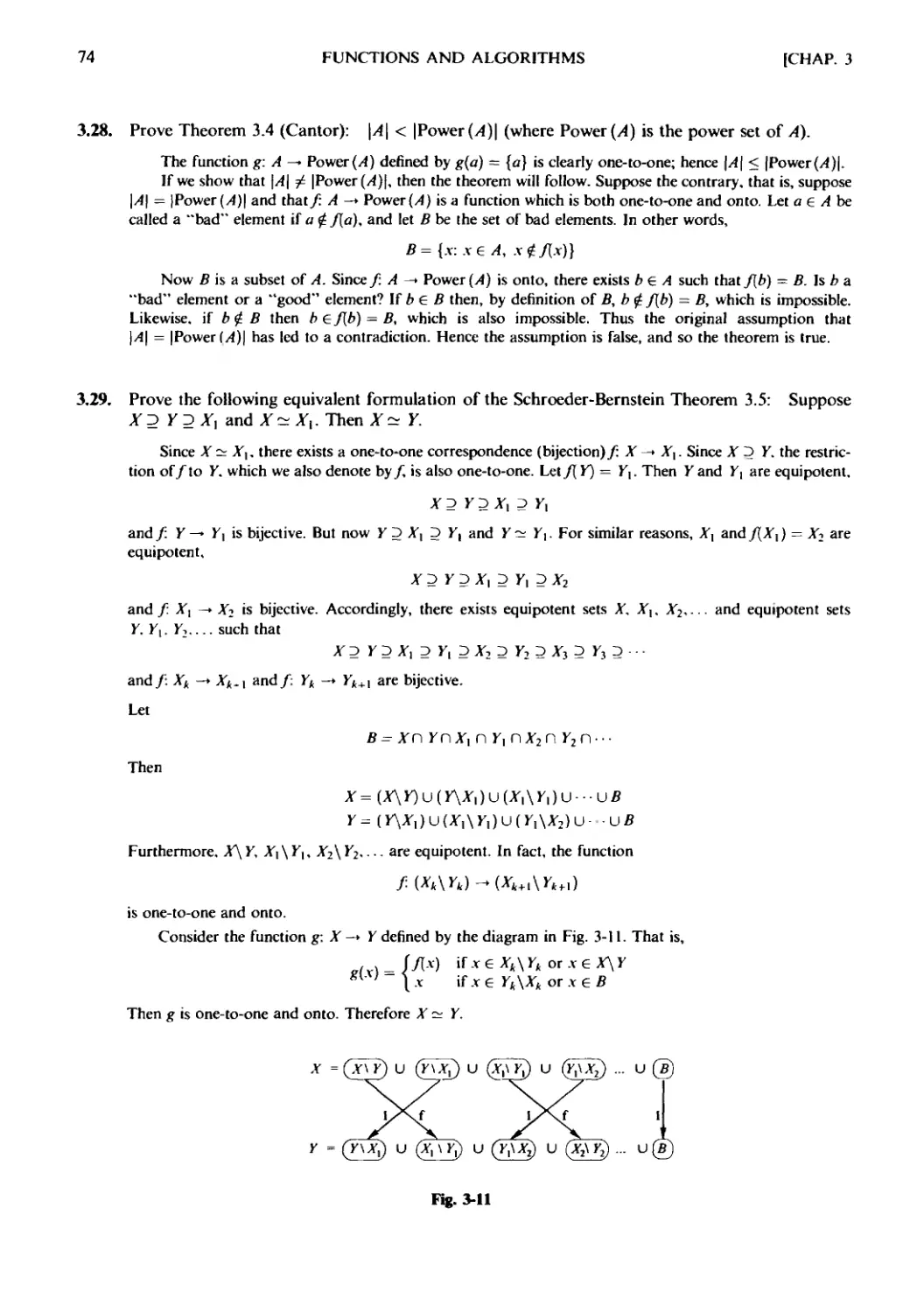
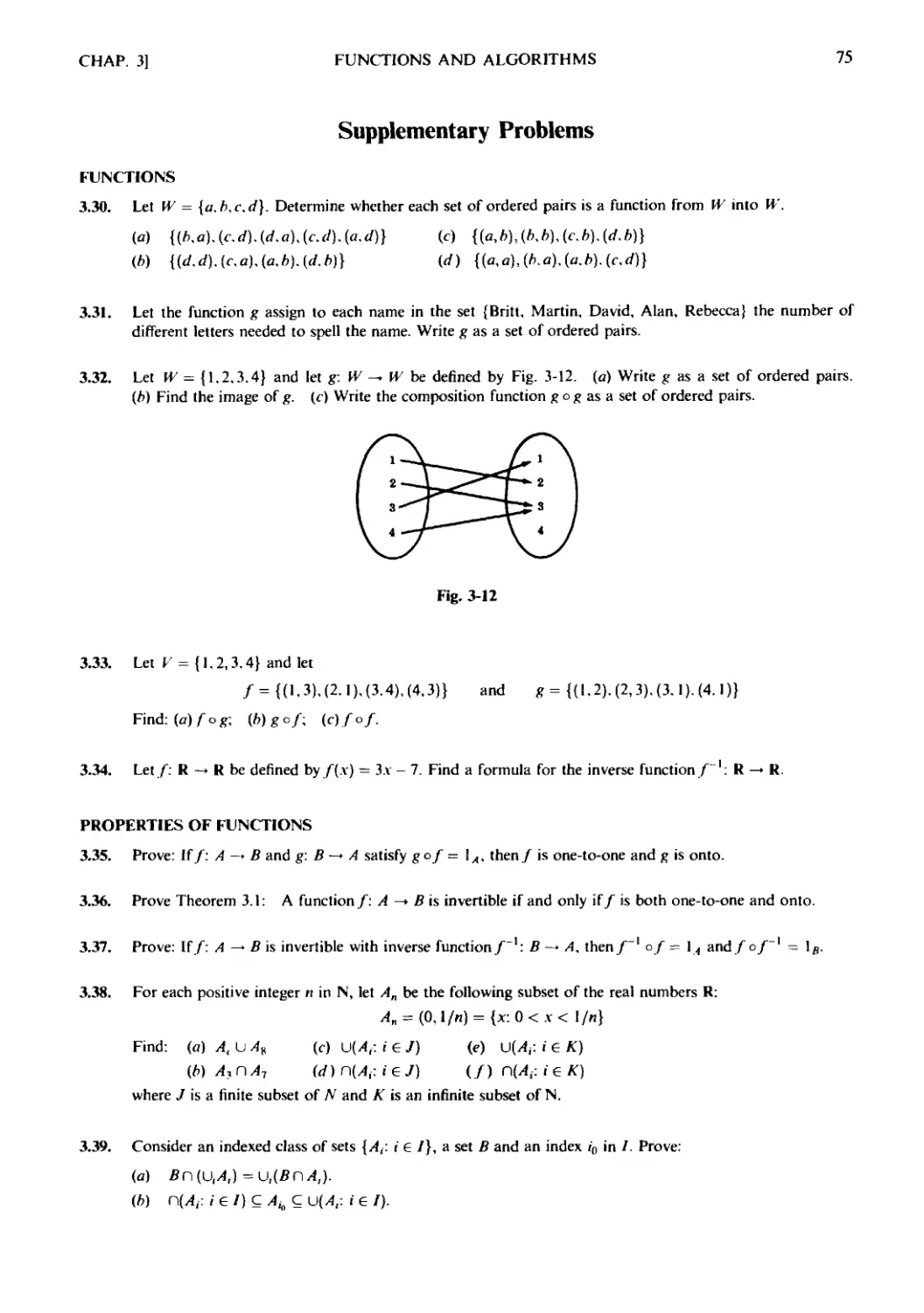
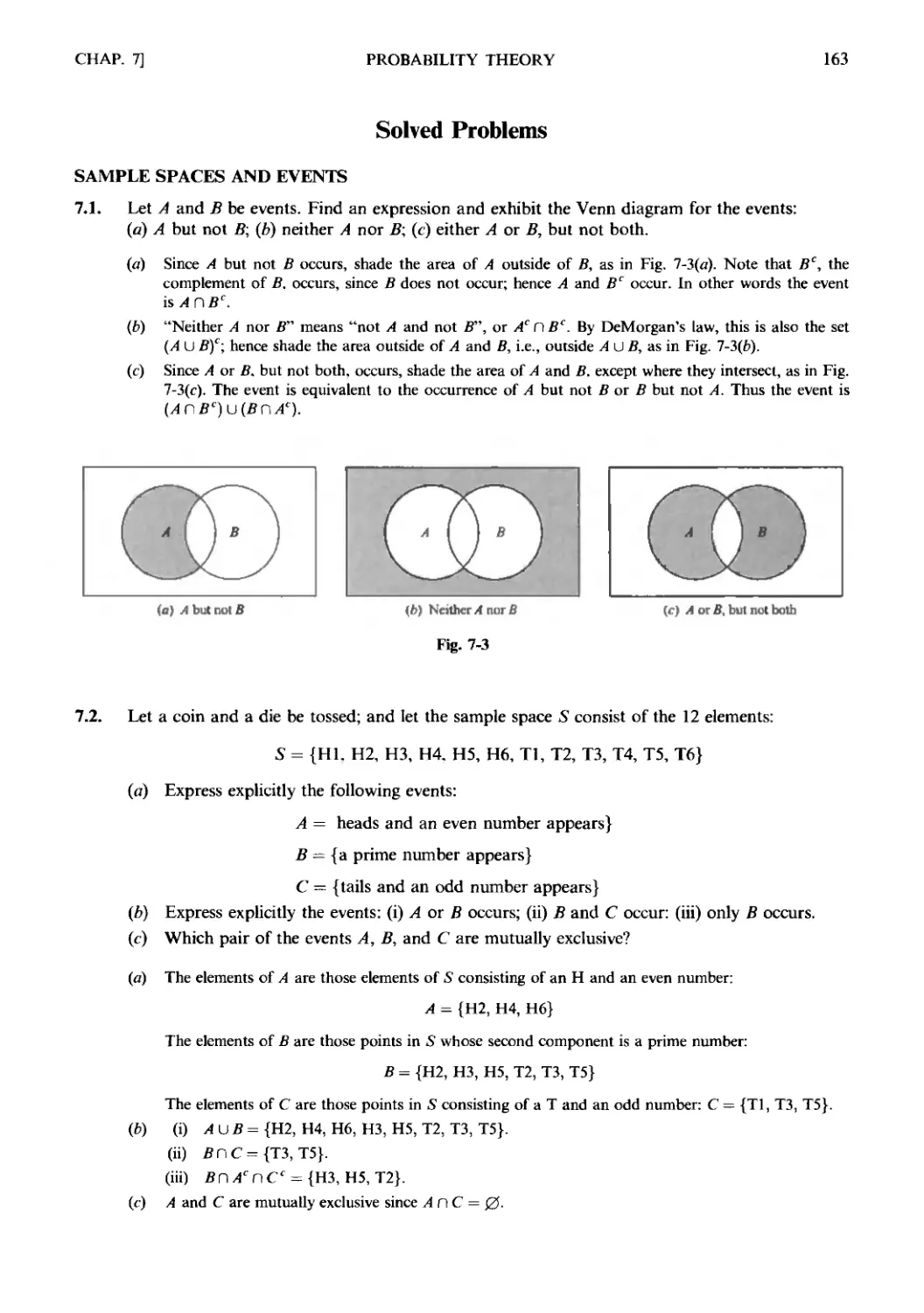
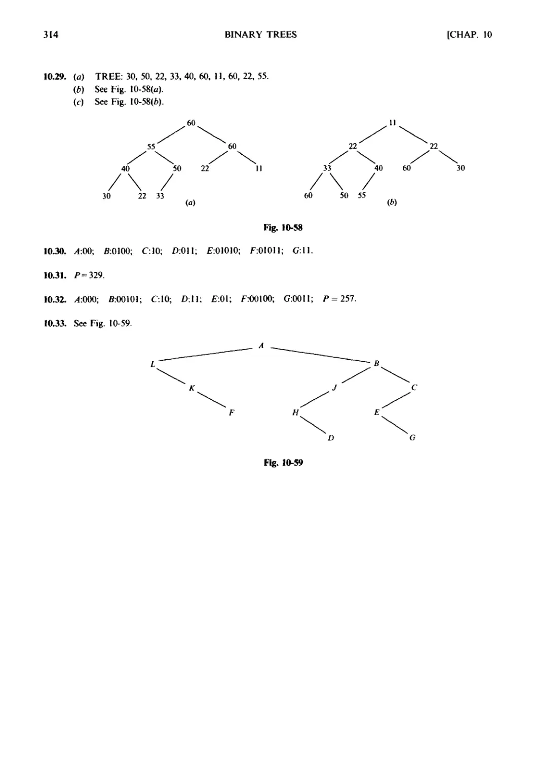
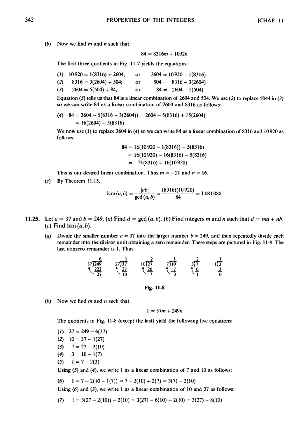
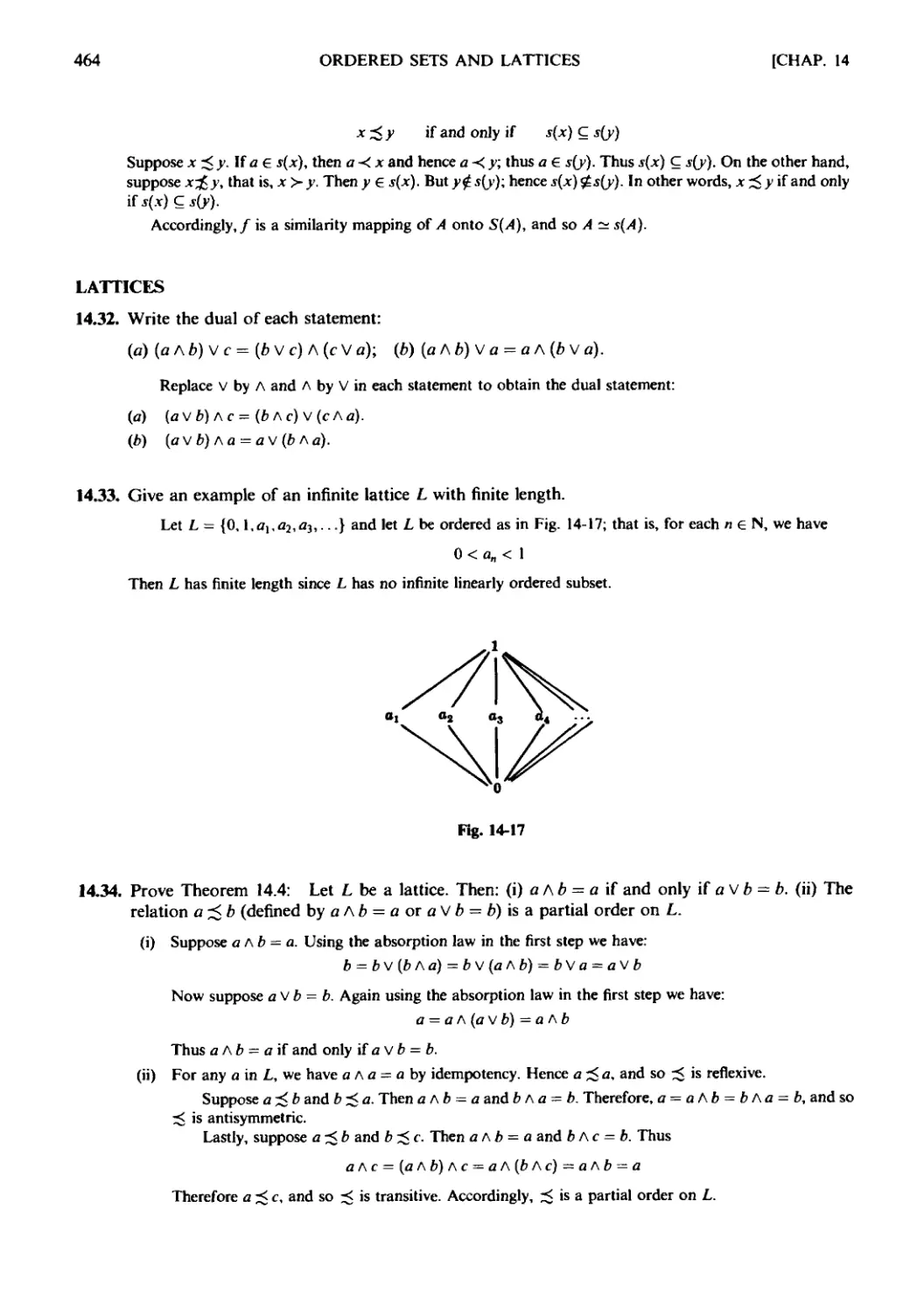
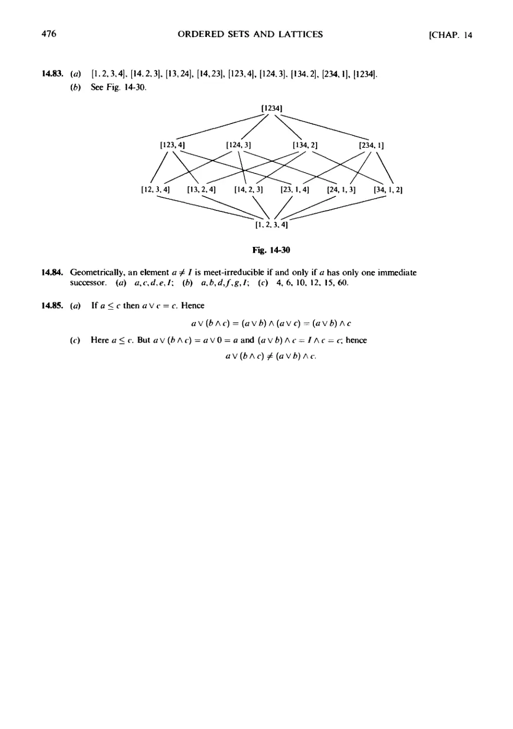
/


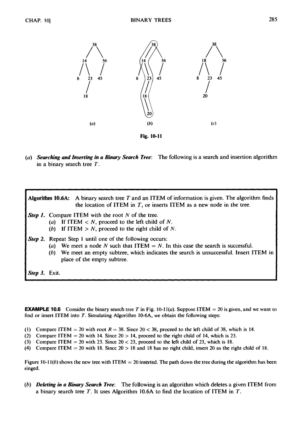


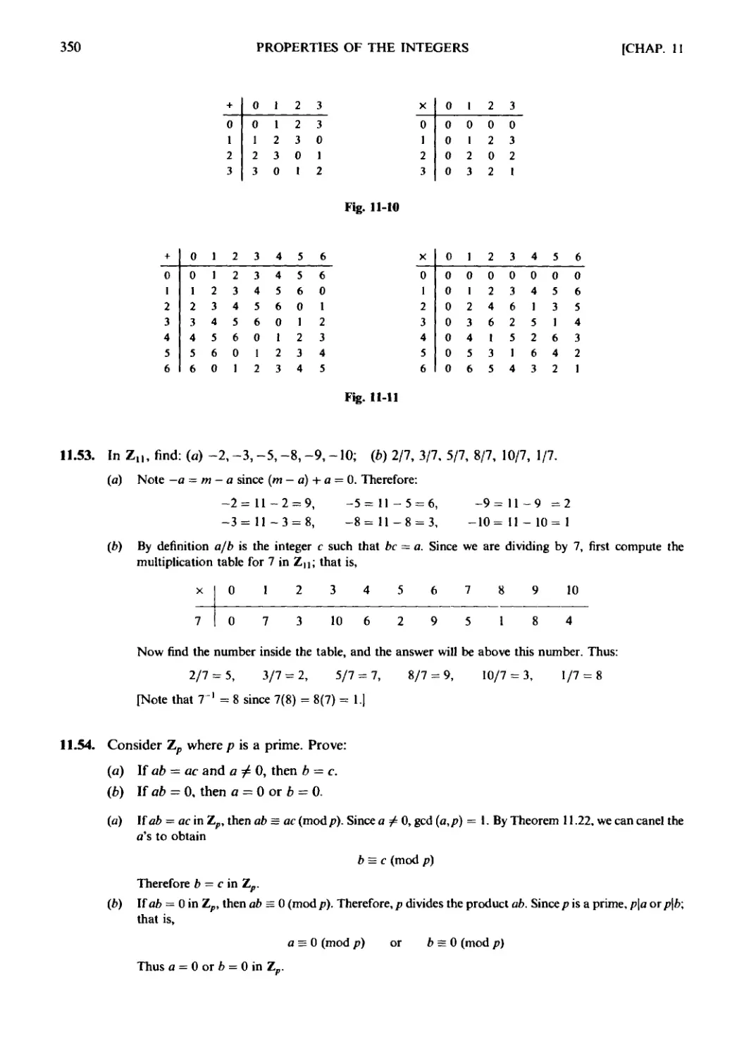


Текст
SCHAUM'S OUTLINE OF
THEORY AND PROBLEMS
of
DISCRETE
MATHEMATICS
Second Edition
SEYMOUR LIPSCHUTZ, Ph.D.
Temple University
MARC LARS LIPSON, Ph.D.
University of Georgia
SCHAUM'S OUTLINE SERIES
McGRAW-HILL
New York Washington, D.C. San Francisco Auckland Bogota" Caracas Lisbon
London Madrid Mexico City Milan Montreal New Delhi
San Juan Singapore Sydney Tokyo Toronto
SEYMOUR LIPSCHUTZ is on the mathematics faculty of Temple
University and formerly taught at the Polytechnic Institute of Brooklyn
College. He received his Ph.D. in 1960 at Courant Institute of Mathematical
Sciences of New York University. He is one of Schaum's most prolific
authors, and has also written Probability; Finite Mathematics, 2nd edition;
Linear Algebra, 2nd edition; Beginning Linear Algebra; Set Theory; and
Essential Computer Mathematics.
MARC LARS LIPSON is on the faculty of the University of Georgia and
formerly taught at Northeastern University and Boston University. He
received his Ph.D. in finance in 1994 from the University of Michigan. He
is also the coauthor of 2000 Solved Problems in Discrete Mathematics with
Seymour Lipschutz.
Schaum's Outline of Theory and Problems of
DISCRETE MATHEMATICS
Copyright ?-1997, 1976 by The McGraw-Hill Companies Inc. AH rights reserved. Printed in the
United States of America. Except as permitted under the Copyright Act of 1976, no part of this
publication may be reproduced or distributed in any forms or by any means, or stored in a data base
or retrieval system, without the prior written permission of the publisher.
45678910111213 1415 16 17 18 1920 BAWBAW99
ISBN 0-07-036045-7
Sponsoring Editors: Arthur Biderman. Barbara Gilson
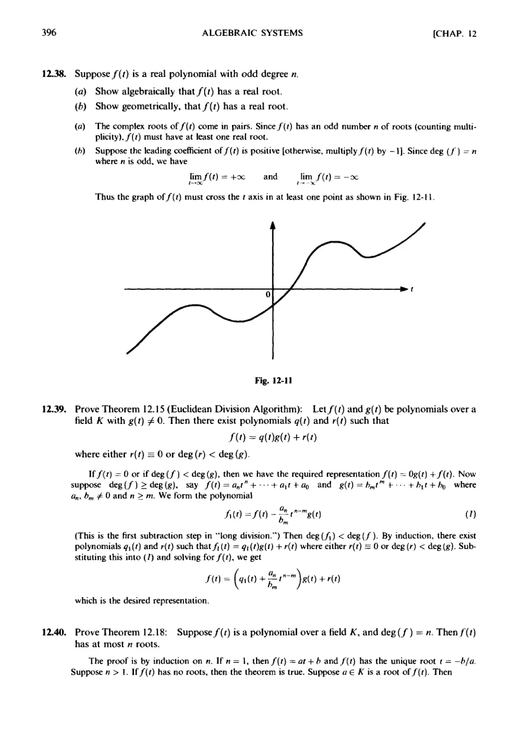
Production Supervisor: Claire Stanley
Editing Supervisor: Maureen Walker
Library of Congress Catalogtag-in-PubUcation Data
Lipschutz. Seymour.
Schaum's outline of theory and problems of discrete mathematics/
Seymour Lipschutz. Marc Lars Lipson—2nd ed.
p. cm.—(Schaum's outline series)
Includes index.
ISBN 0-07-038045-7 (pbk.)
1. Algebra, Abstract—Outlines, syllabi, etc. 2. Combinatorial
analysis—Outlines, syllabi, etc 3. Logic, Symbolic and
mathematical—Outlines, syllabi, etc. I. Lipson, Marc. II. Title.
QA162.L56 1997
512'02—dc21 97-19341
CIP
McGraw-Hill
A Division ofTheMcGnae-HiOCompanies
Preface
Discrete mathematics, the study of finite systems, has become increasingly
important as the computer age has advanced. The digital computer is basically a
finite structure, and many of its properties can be understood and interpreted within
the framework of finite mathematical systems. This book, in presenting the more
essential material, may be used as a textbook for a formal course in discrete mathe-
mathematics or as a supplement to all current texts.
The first three chapters cover the standard material on sets, relations, and func-
functions and algorithms. Next come chapters on logic, vectors and matrices, counting,
and probability. We than have three chapters on graph theory: graphs, directed
graphs, and binary trees. Finally there are individual chapters on properties of the
integers, algebraic systems, languages and machines, ordered sets and lattices, and
Boolean algebra. The chapter on functions and algorithms includes a discussion of
cardinality and countable sets, and complexity. The chapters on graph theory
include discussions on planarity, traversability, minimal paths, and Warshall's and
Huffman's algorithms. The chapter on languages and machines includes regular
expressions, automata, and Turing machines and computable functions. We empha-
emphasize that the chapters have been written so that the order can be changed without
difficulty and without loss of continuity.
This second edition of Discrete Mathmatics covers much more material and in
greater depth than the first edition. The topics of probability, regular expressions and
regular sets, binary trees, cardinality, complexity, and Turing machines and compu-
computable functions did not appear in the first edition or were only mentioned. This new
material reflects the fact that discrete mathematics now is mainly a one-year course
rather than a one-semester course.
Each chapter begins with a clear statement of pertinent definition, principles,
and theorems with illustrative and other descriptive material. This is followed by sets
of solved and supplementary problems. The solved problems serve to illustrate and
amplify the material, and also include proofs of theorems. The supplementary prob-
problems furnish a complete review of the material in the chapter. More material has
been included than can be covered in most first courses. This has been done to make
the book more flexible, to provide a more useful book of reference, and to stimulate
further interest in the topics.
Finally, we wish to thank the staff of the McGraw-Hill Schaum's Outline Series,
especially Arthur Biderman and Maureen Walker, for their unfailing cooperation.
Seymour Lipschutz
Marc Lars Lipson
Contents
Chapter/ SET THEORY 1
1.1 Introduction. 1.2 Sets and Elements. 1.3 Universal Set and Empty
Set. 1.4 Subsets. 1.5 Venn Diagrams. 1.6 Set Operations. 1.7 Alge-
Algebra of Sets and Duality. 1.8 Finite Sets, Counting Principle. 1.9 Classes
of Sets, Power Sets, Partitions. 1.10 Mathematical Induction.
Chapter 2 RELATIONS 27
2.1 Introduction. 2.2 Product Sets. 2.3 Relations. 2.4 Pictorial Repre-
Representations of Relations. 2.5 Composition of Relations. 2.6 Types of
Relations. 2.7 Closure Properties. 2.8 Equivalence Relations. 2.9 Par-
Partial Ordering Relations. 2.10 n-ary Relations.
Chapter 3 FUNCTIONS AND ALGORITHMS 50
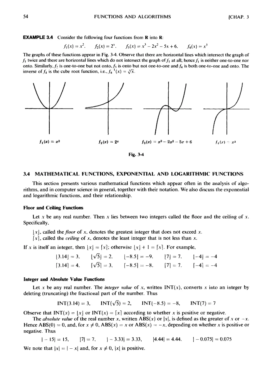
3.1 Introduction. 3.2 Functions. 3.3 One-to-One, Onto, and Invertible
Functions. 3.4 Mathematical Functions, Exponential and Logarithmic
Functions. 3.5 Sequences, Indexed Classes of Sets. 3.6 Recursively
Defined Functions. 3.7 Cardinality. 3.8 Algorithms and Functions.
3.9 Complexity of Algorithms.
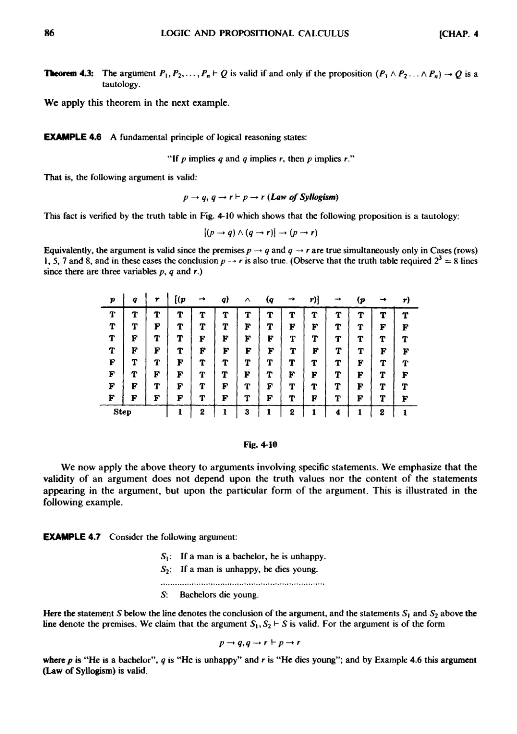
Chapter'/ LOGIC AND PROPOSITIONAL CALCULUS 78
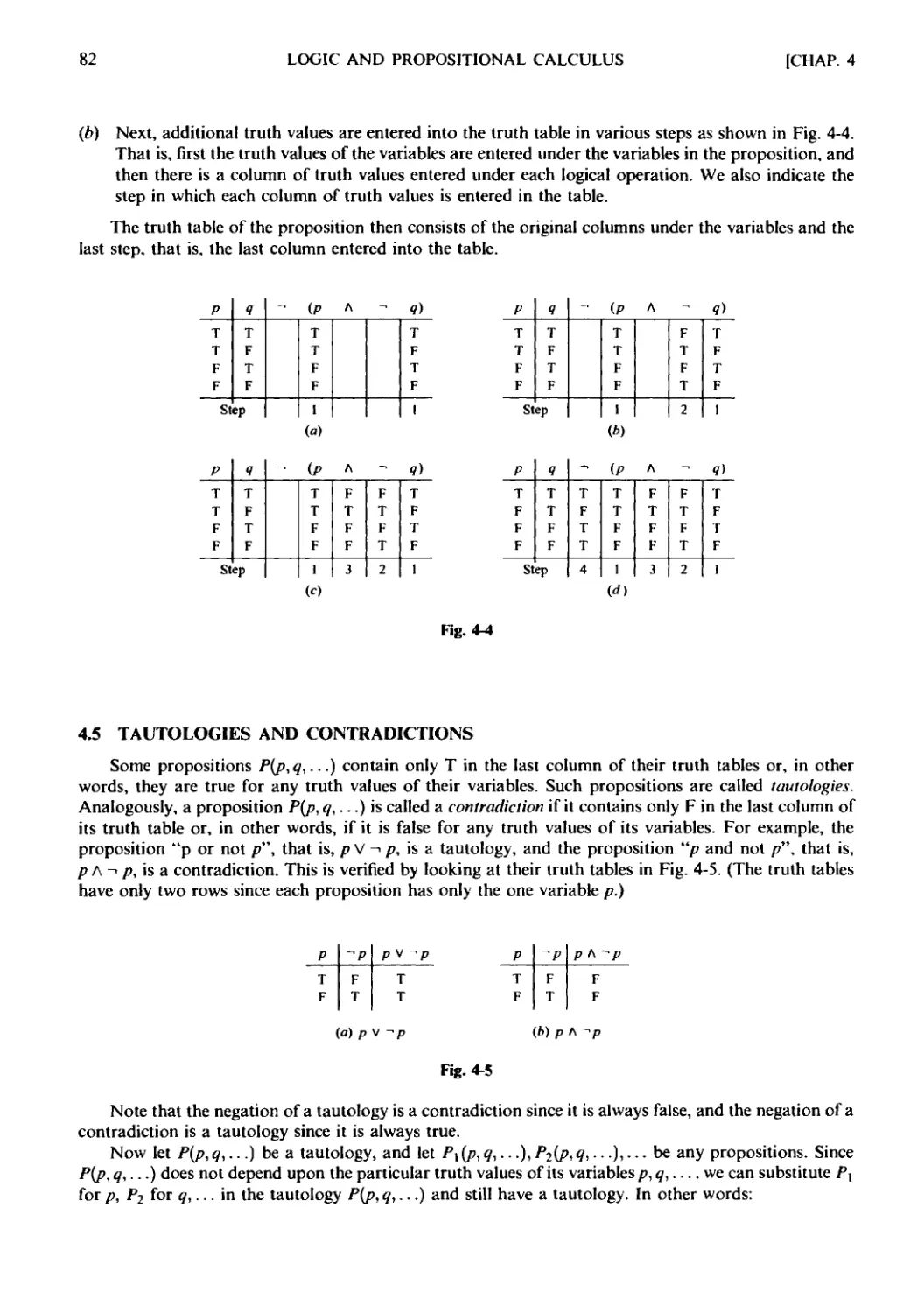
4.1 Introduction. 4.2 Propositions and Compound Propositions.
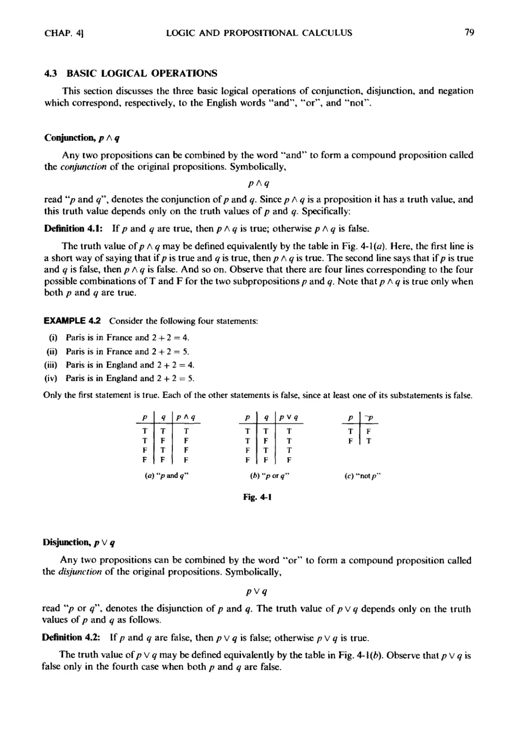
4.3 Basic Logical Operations. 4.4 Propositions and Truth Tables.
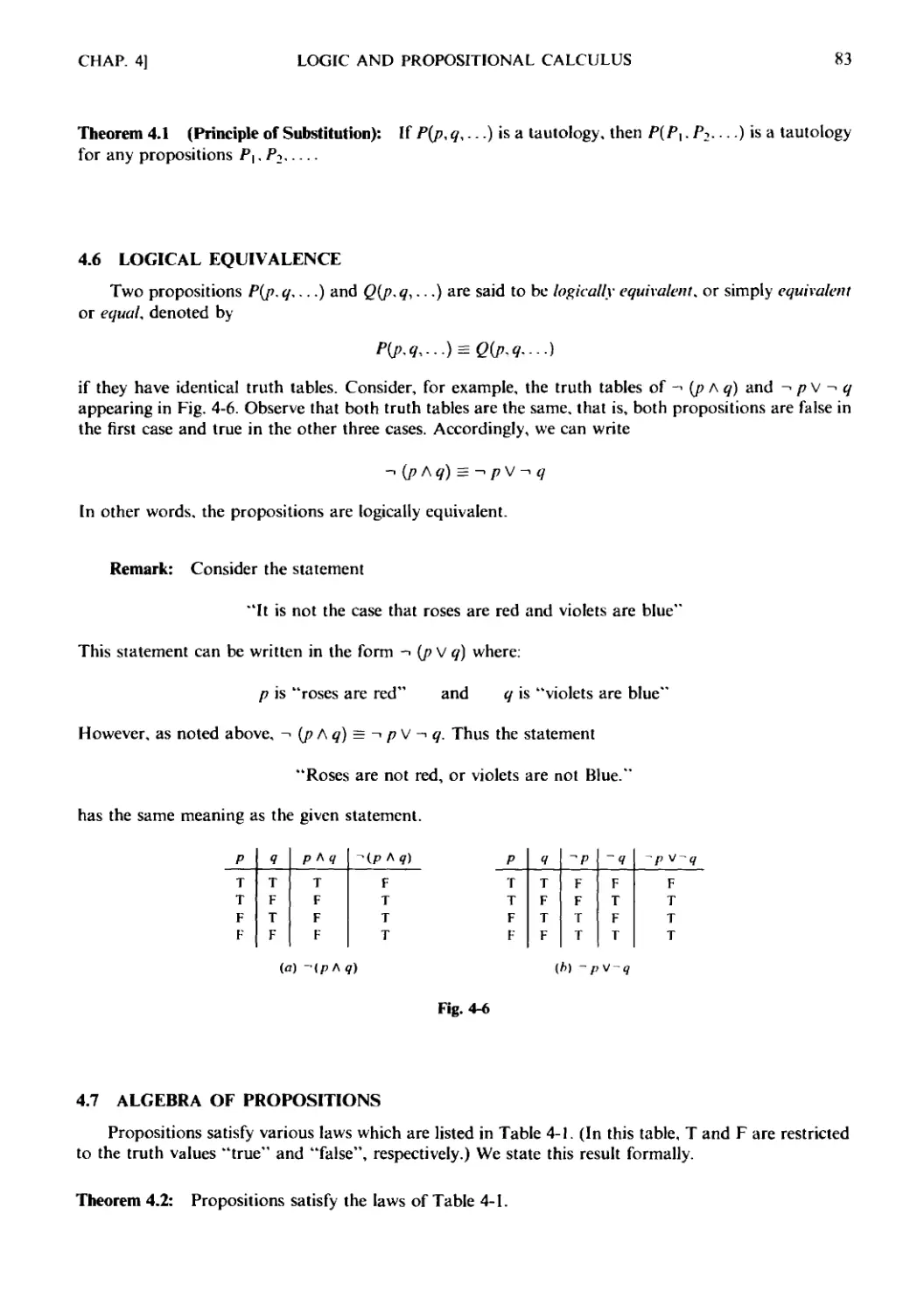
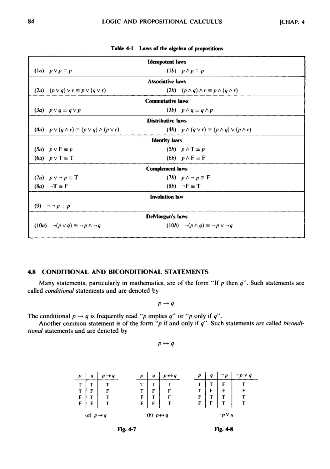
4.5 Tautologies and Contradictions. 4.6 Logical Equivalence.
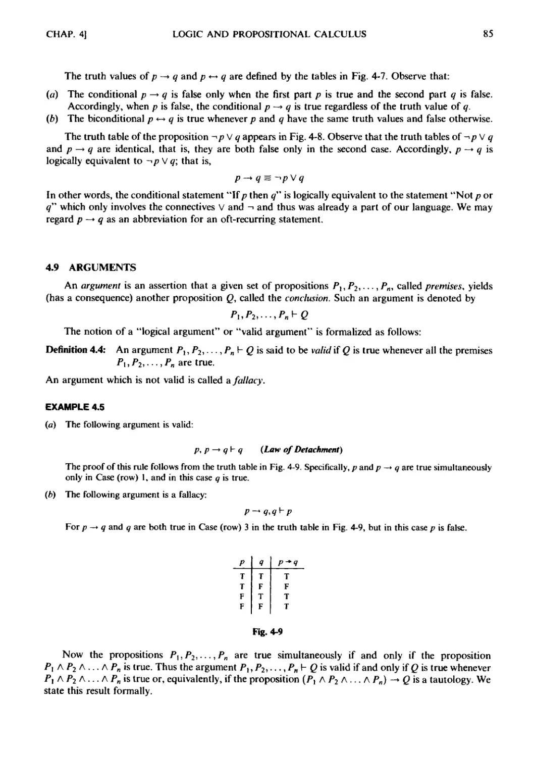
4.7 Algebra of Propositions. 4.8 Conditional and Biconditional State-
Statements. 4.9 Arguments. 4.10 Logical Implication. 4.11 Propositional
Functions, Quantifiers. 4.12 Negation of Quantified Statements.
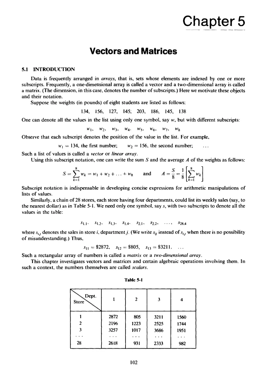
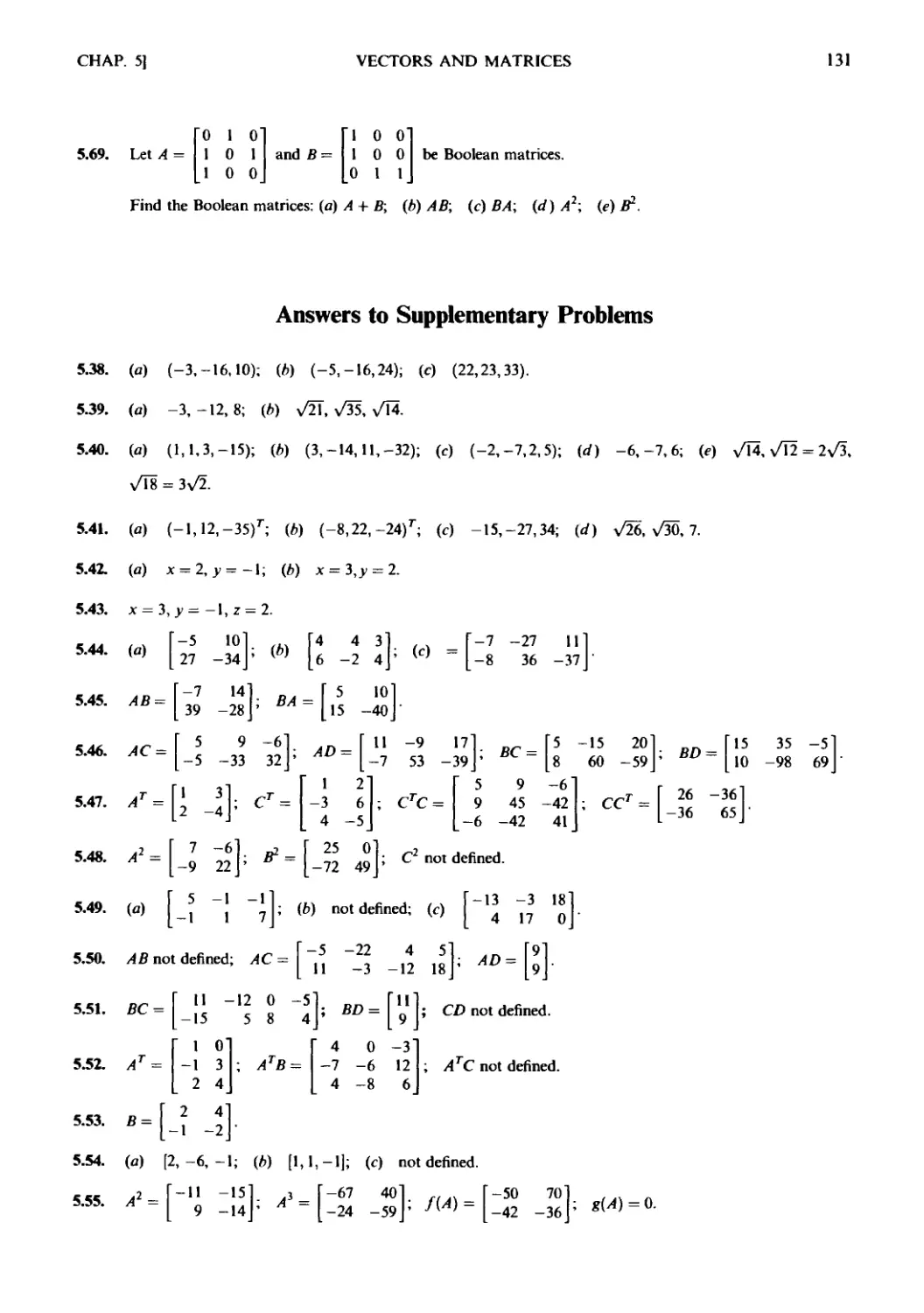
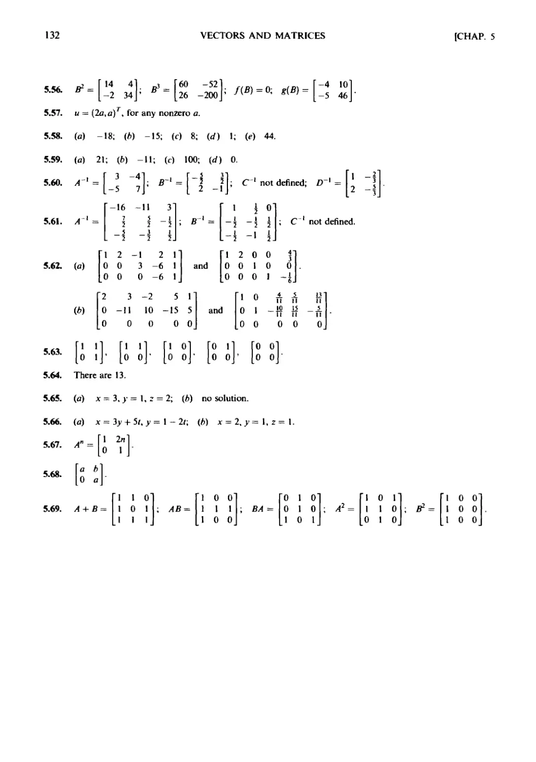
Chapter 5 VECTORS AND MATRICES 102
5.1 Introduction. 5.2 Vectors. 5.3 Matrices. 5.4 Matrix Addition
and Scalar Multiplication. 5.5 Matrix Multiplication. 5.6 Transpose.
5.7 Square Matrices. 5.8 Invertible (Nonsingular) Matrices, Inverses.
5.9 Determinants. 5.10 Elementary Row Operations, Gaussian Elimi-
Elimination. 5.11 Boolean (Zero-One) Matrices.
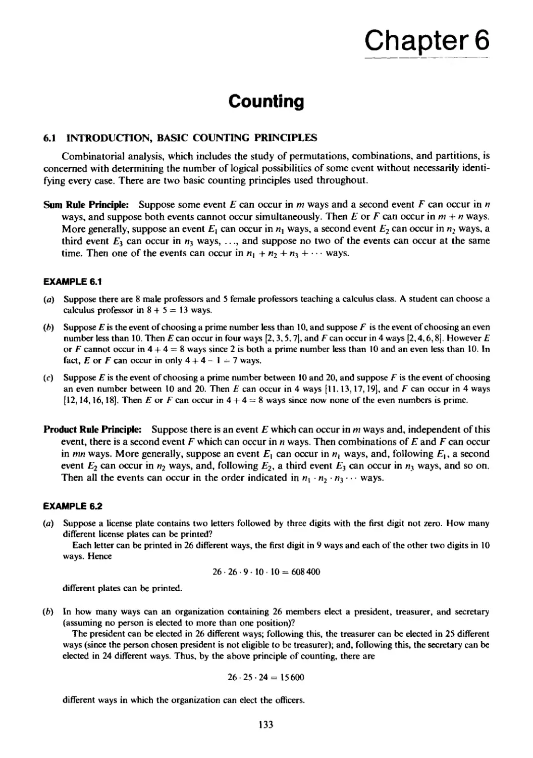
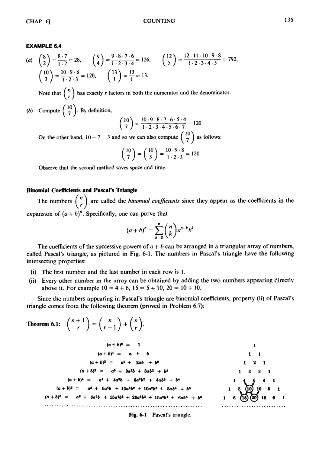
Chapter б COUNTING 133
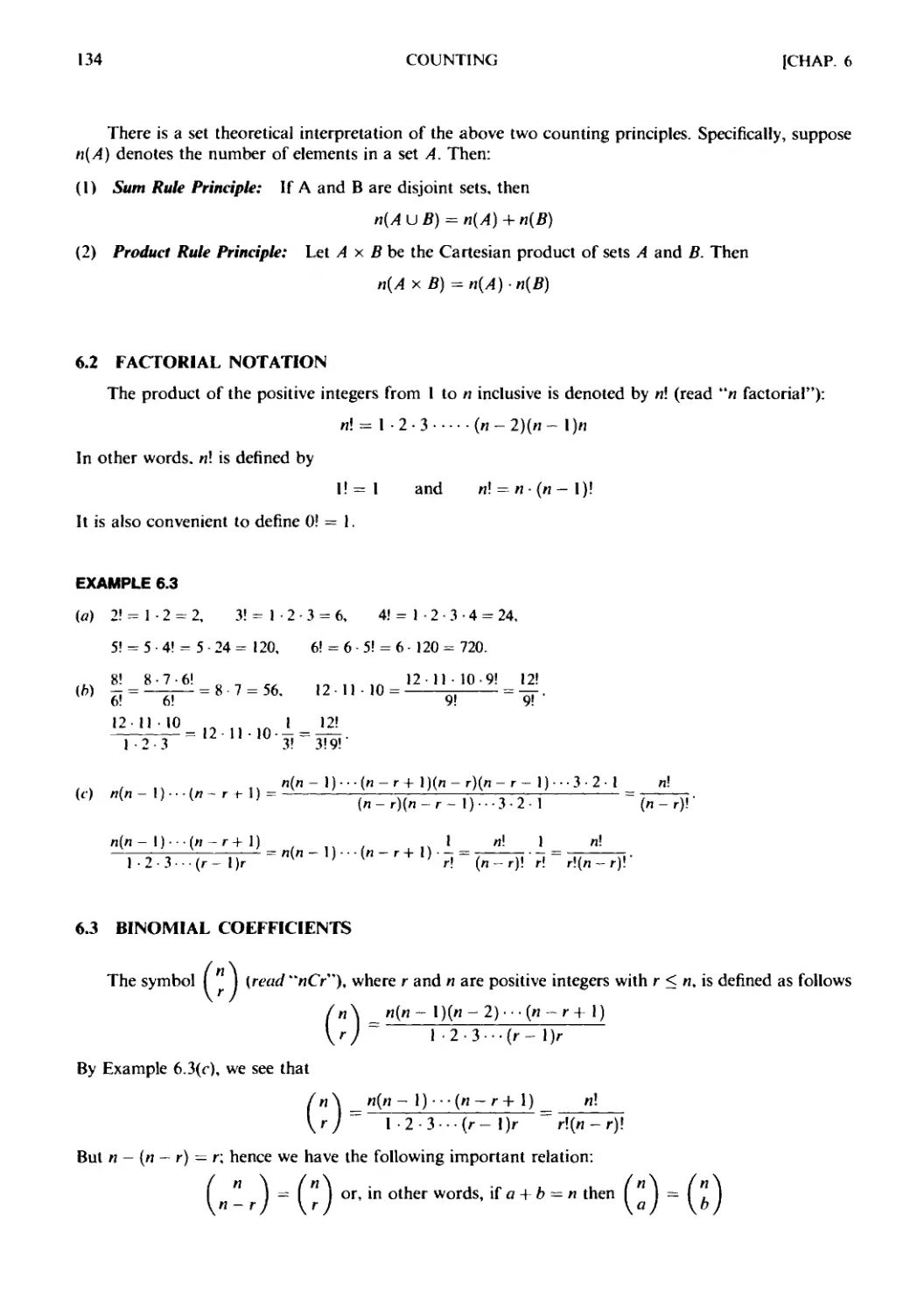
6.1 Introduction, Basic Counting Principles. 6.2 Factorial Nota-
Notation. 6.3 Binomial Coefficients. 6.4 Permutations. 6.5 Combina-
Combinations. 6.6 The Pigeonhole Principle. 6.7 The Inclusion Exclusion
Principle. 6.8 Ordered and Unordered Partitions.
Vll
Vlll
CONTENTS
Chapter 7 PROBABILITY THEORY 152
7.1 Introduction. 7.2 Sample Space and Events. 7.3 Finite Probability
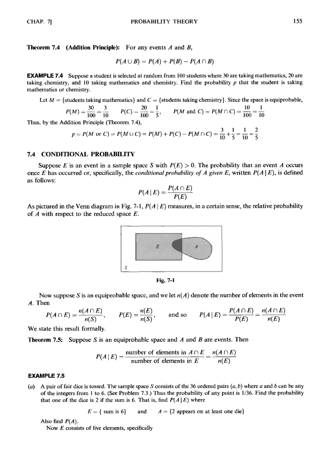
Spaces. 7.4 Conditional Probability. 7.5 Independent Events.
7.6 Independent Repeated Trials, Binomial Distribution. 7.7 Random
Variables.
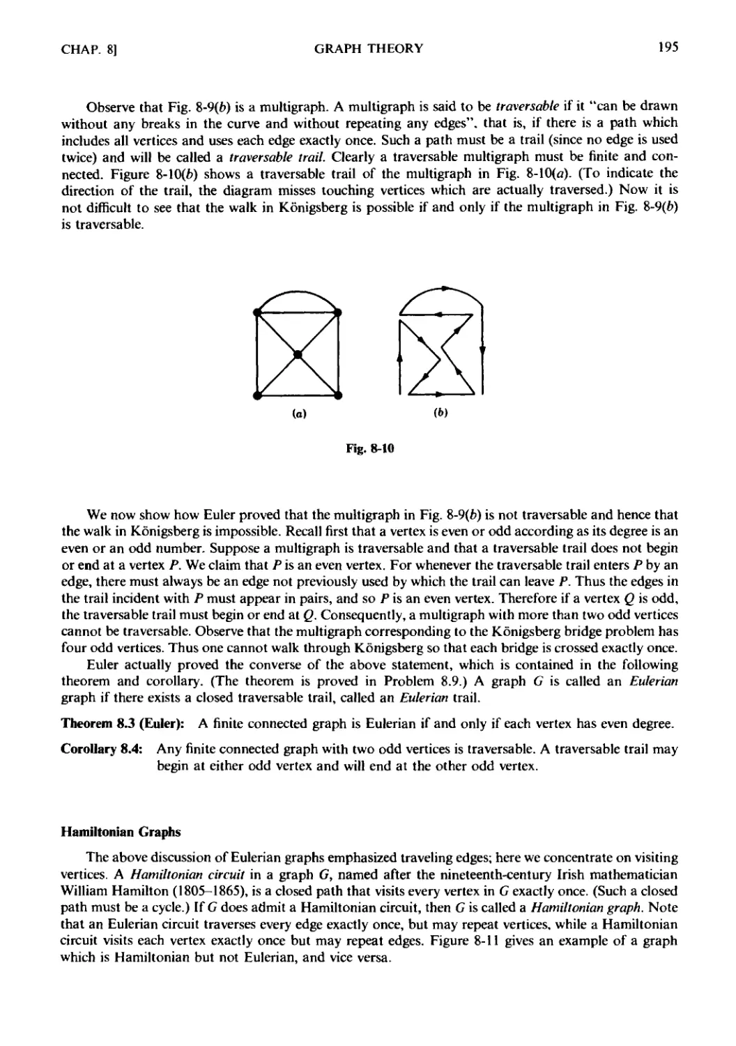
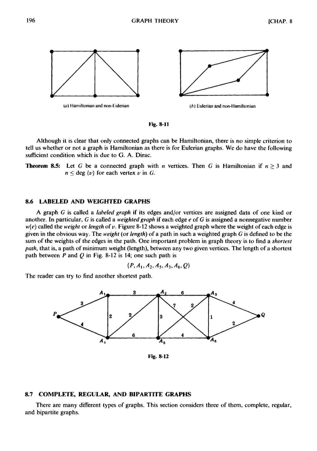
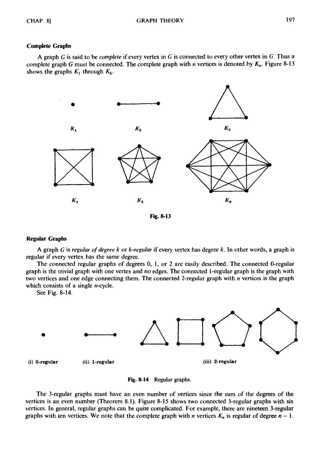
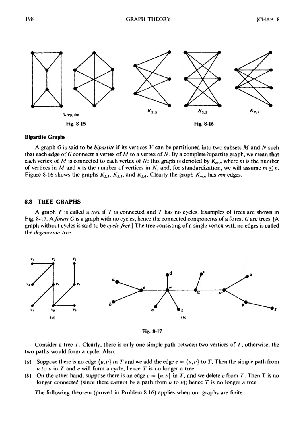
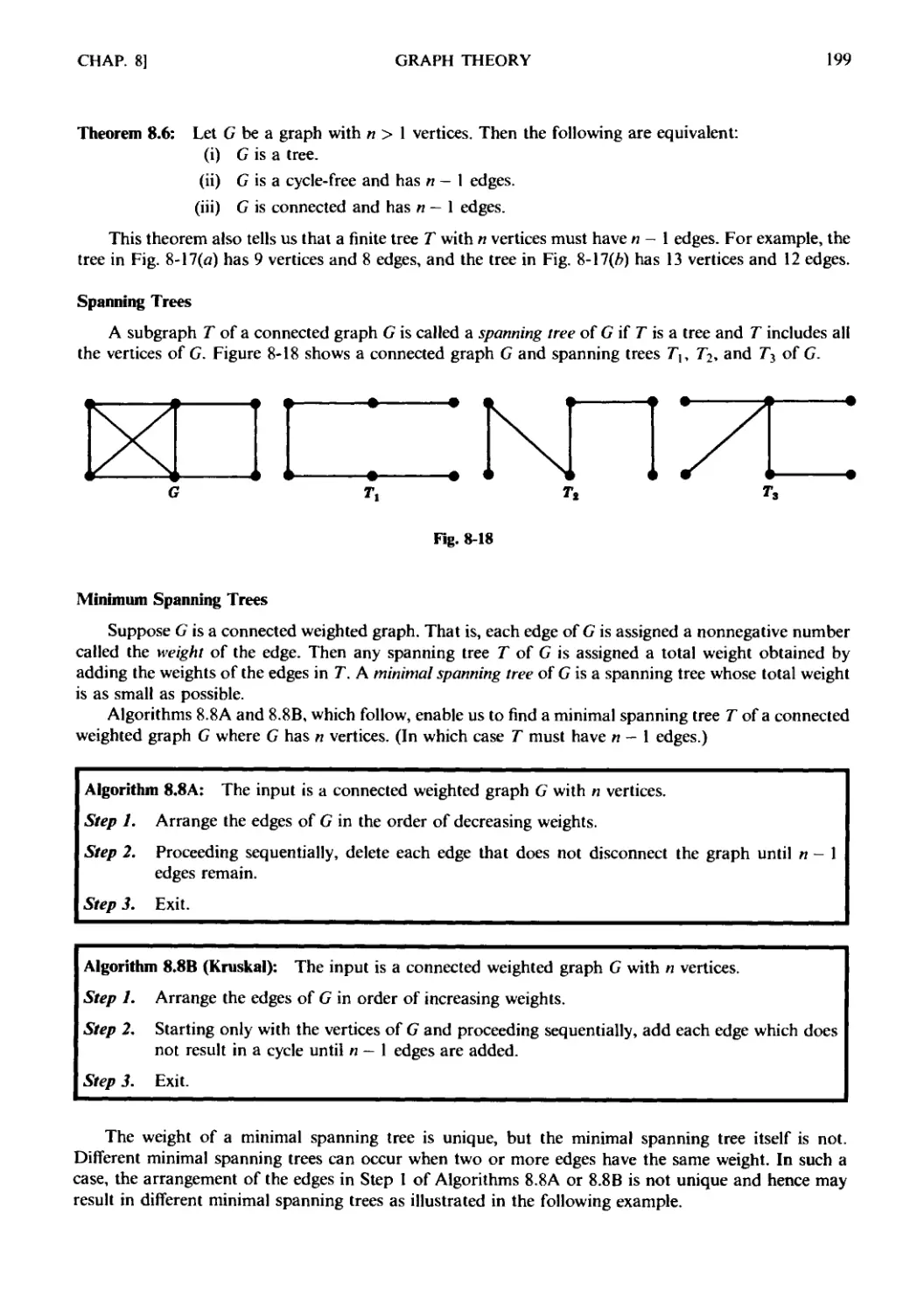
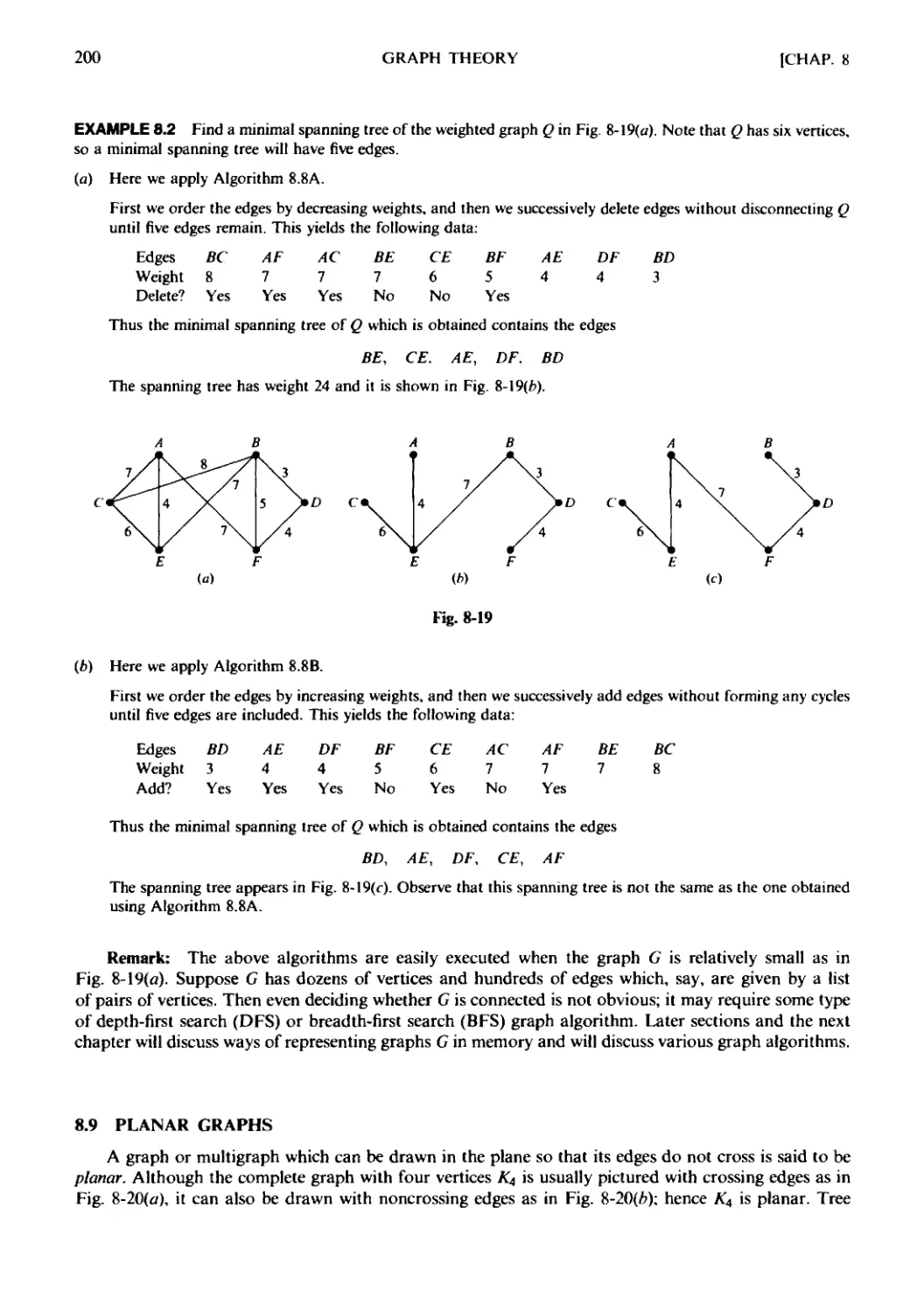
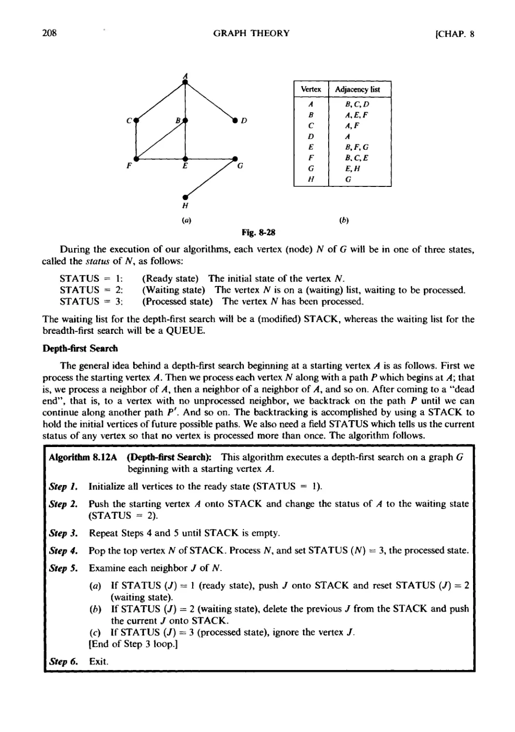
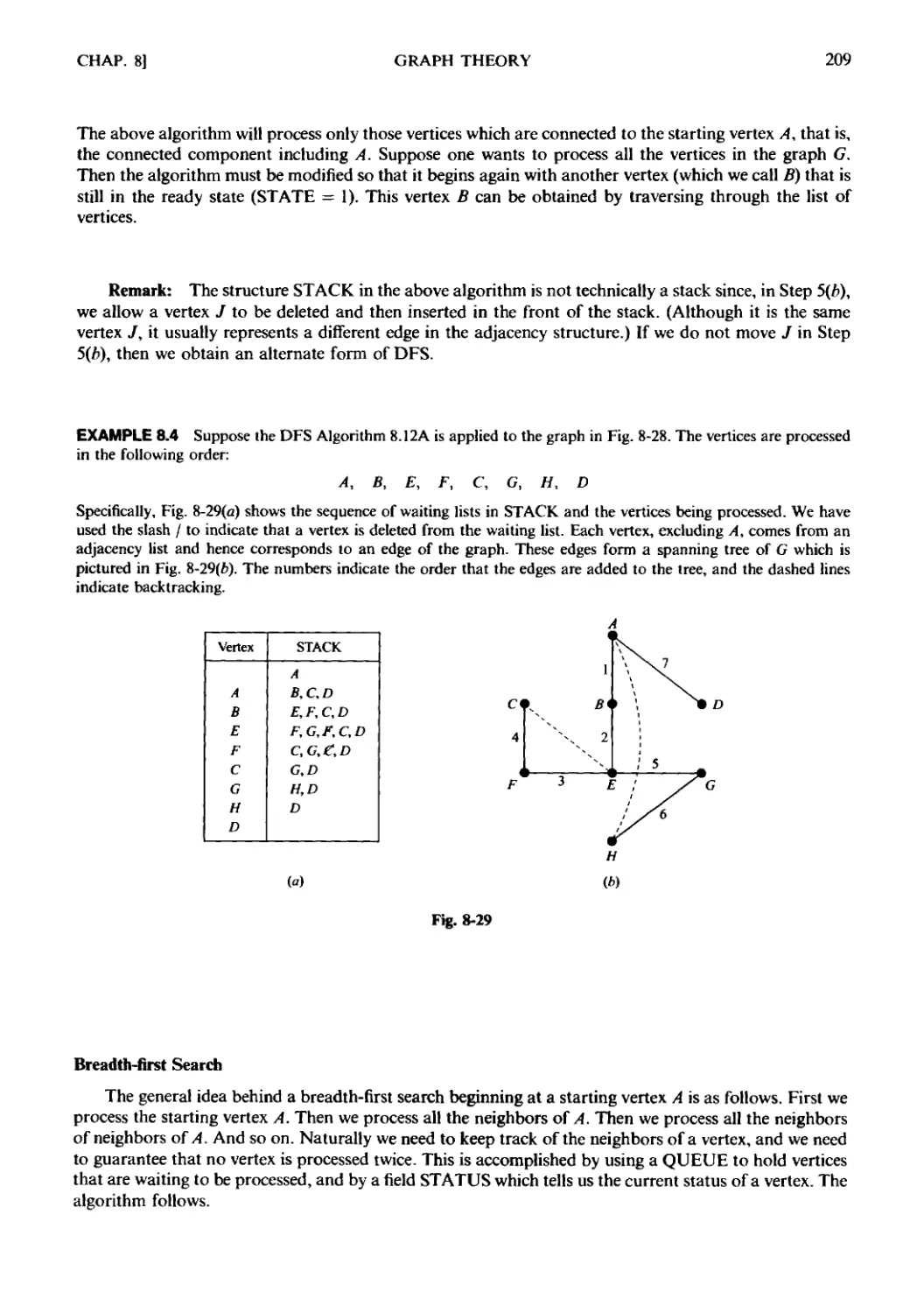
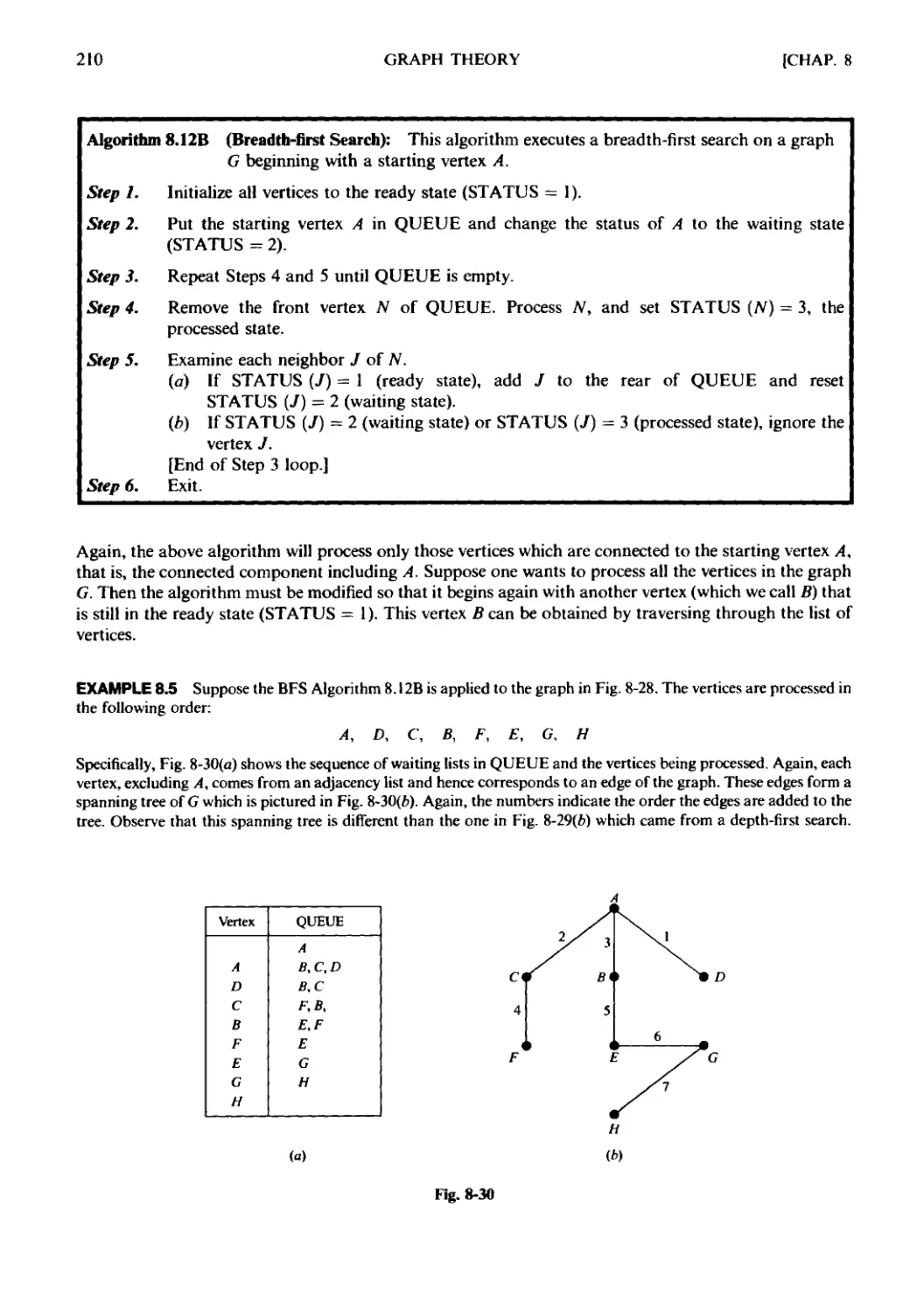
Chapter 8 GRAPH THEORY 188
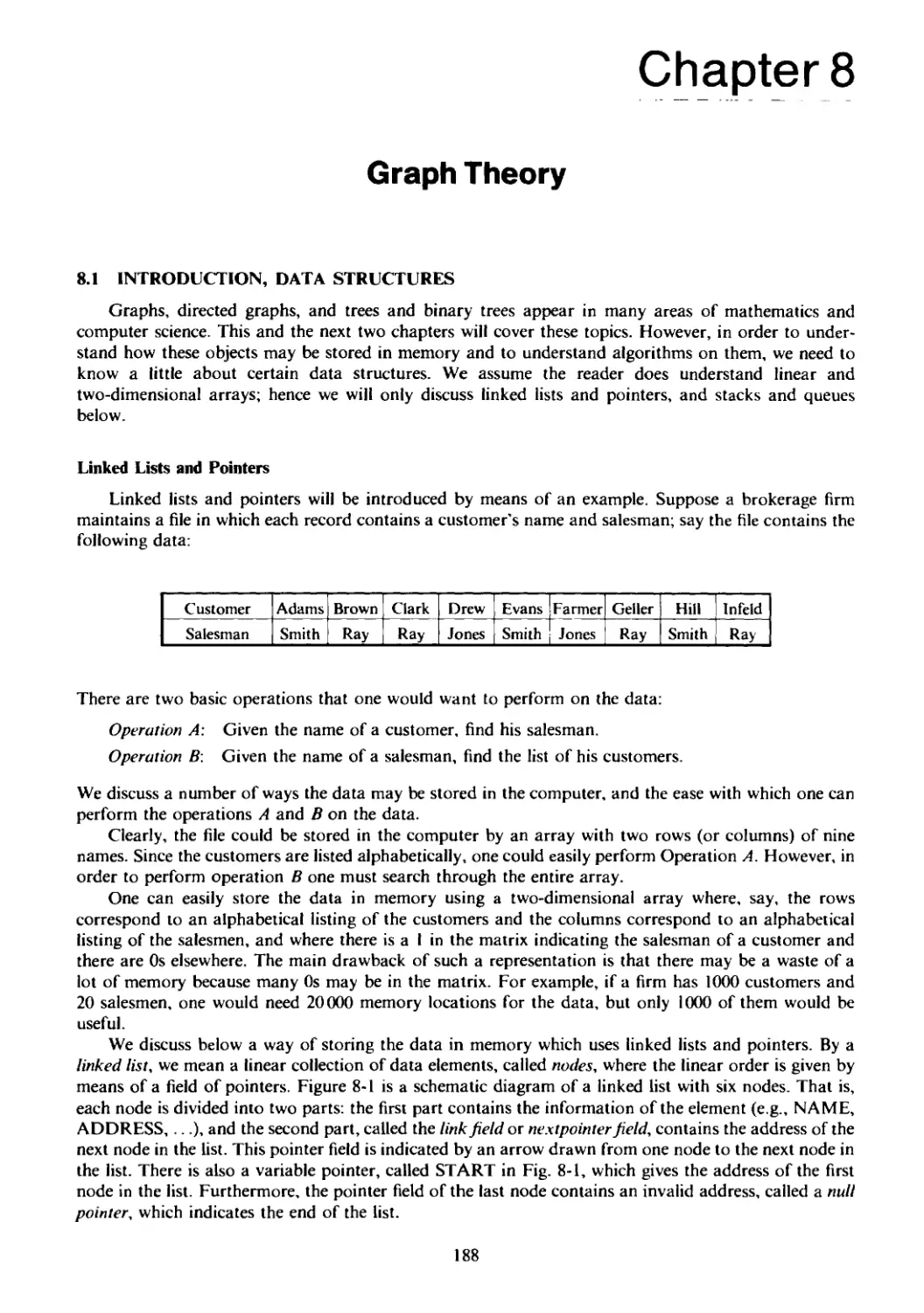
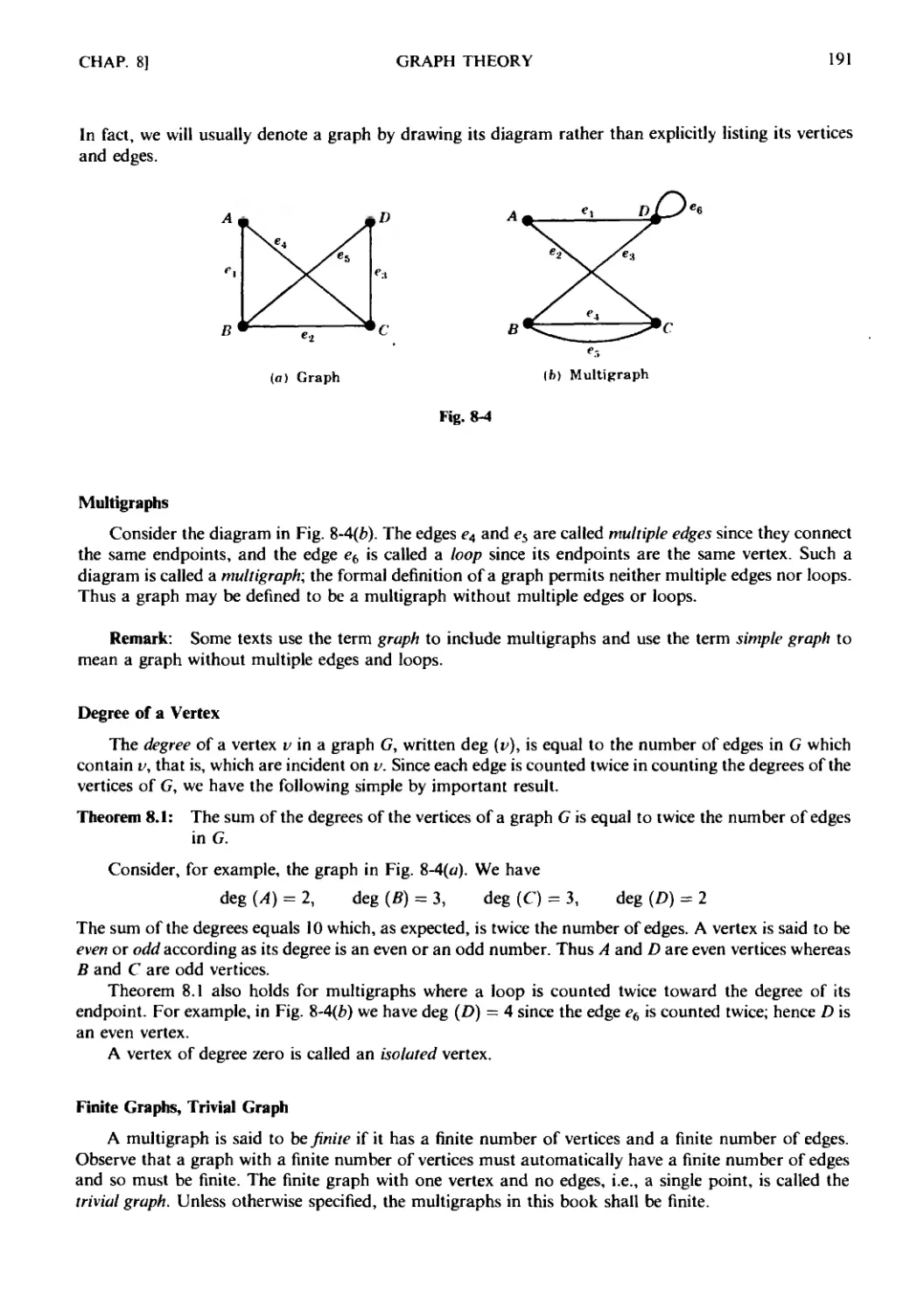
8.1 Introduction, Data Structures. 8.2 Graphs and Multigraphs.
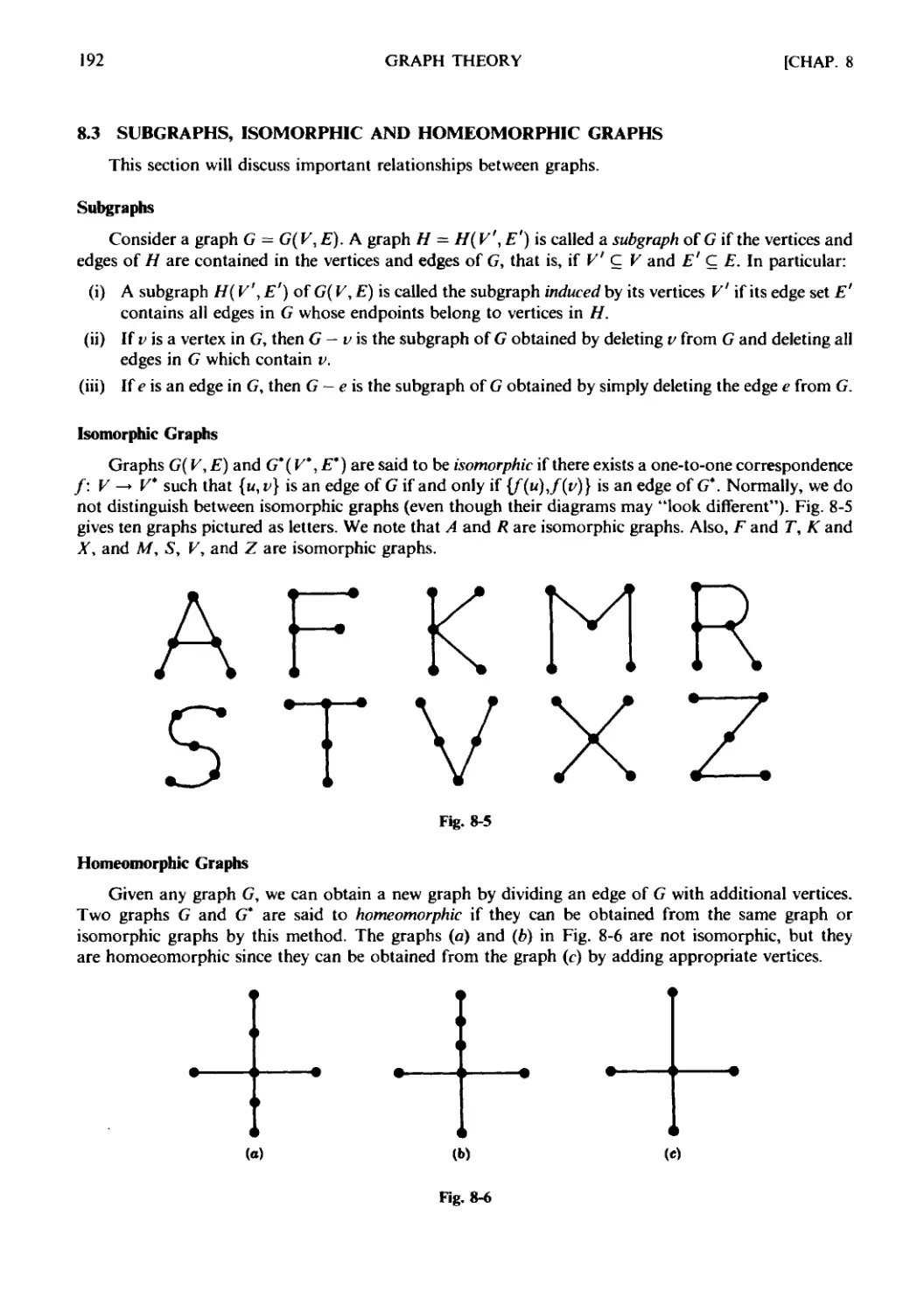
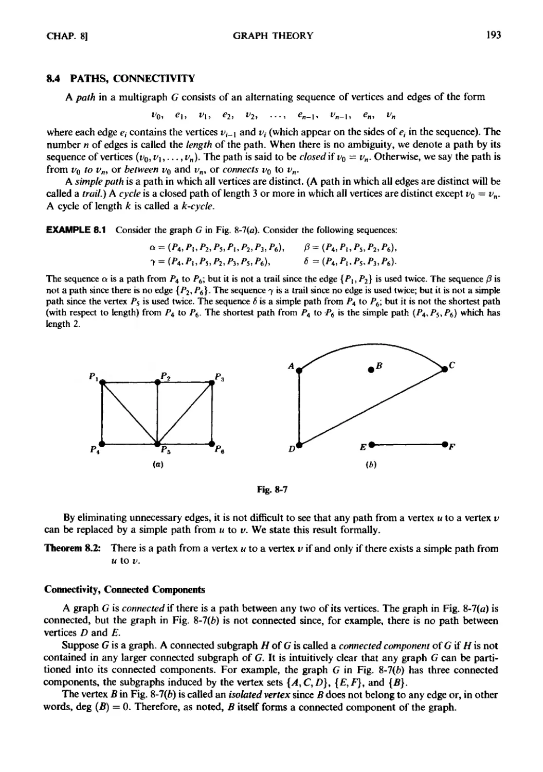
8.3 Subgraphs, Isomorphic and Homeomorphic Graphs. 8.4 Paths,
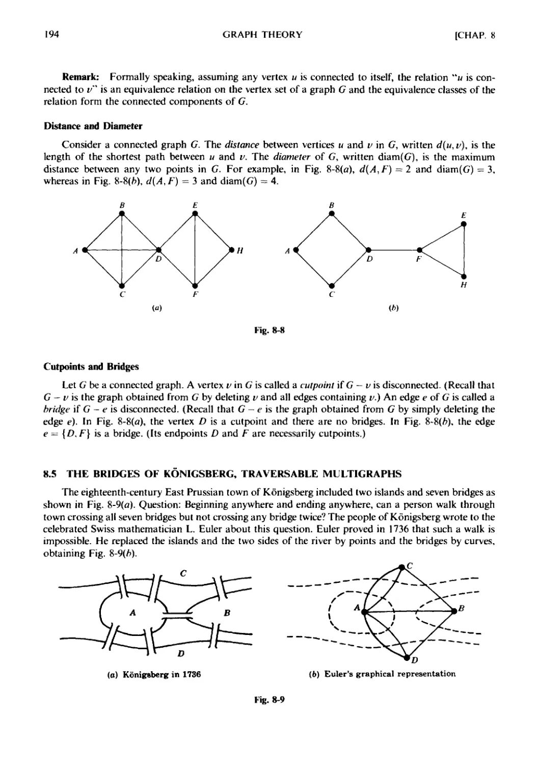
Connectivity. 8.5 The Bridges of Konigsberg, Traversable Multi-
graphs. 8.6 Labeled and Weighted Graphs. 8.7 Complete, Regular,
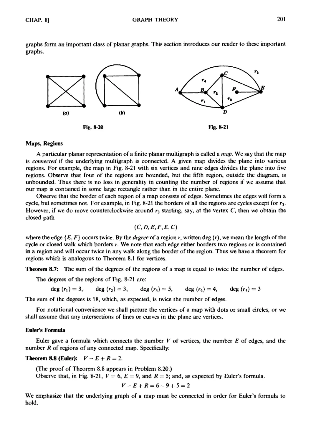
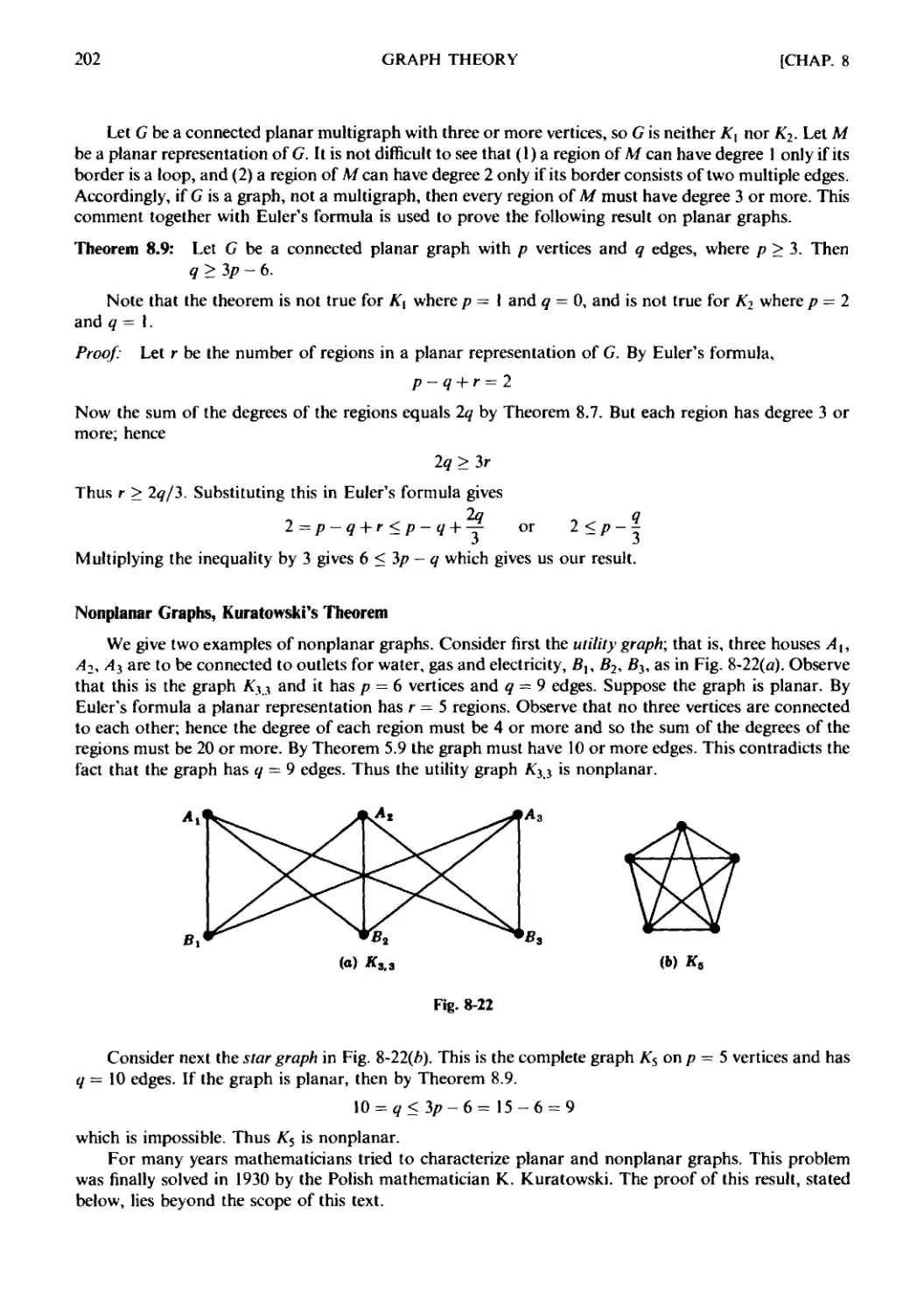
and Bipartite Graphs. 8.8 Tree Graphs. 8.9 Planar Graphs.
8.10 Graph Colorings. 8.11 Representing Graphs in Computer
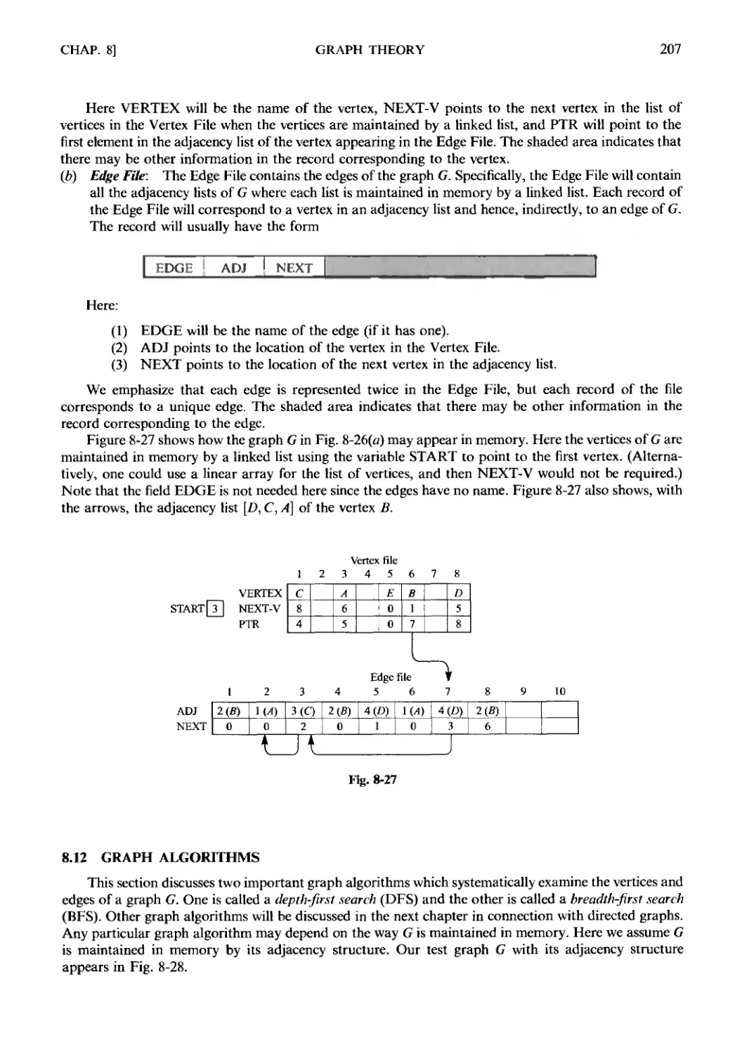
Memory. 8.12 Graph Algorithms.
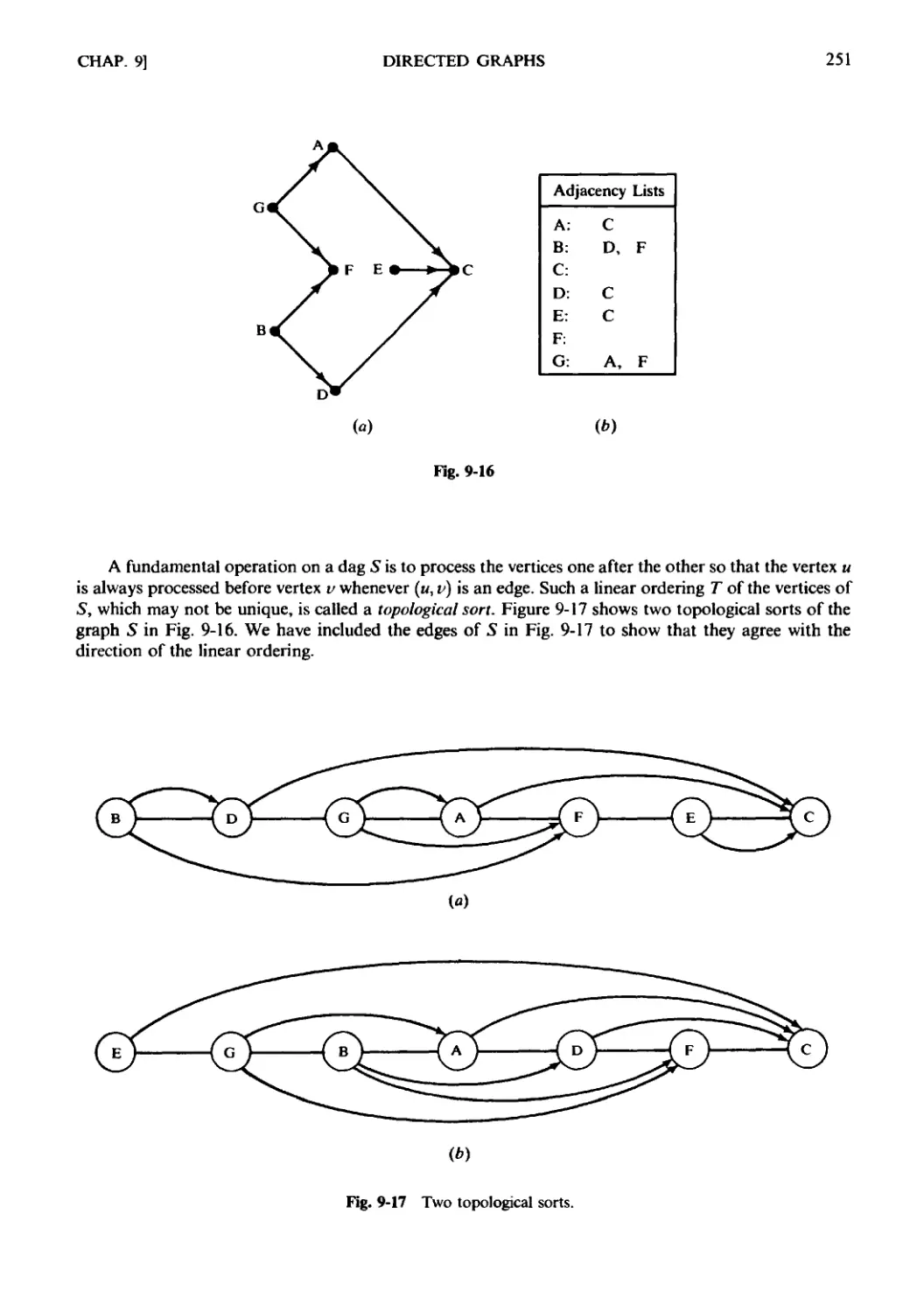
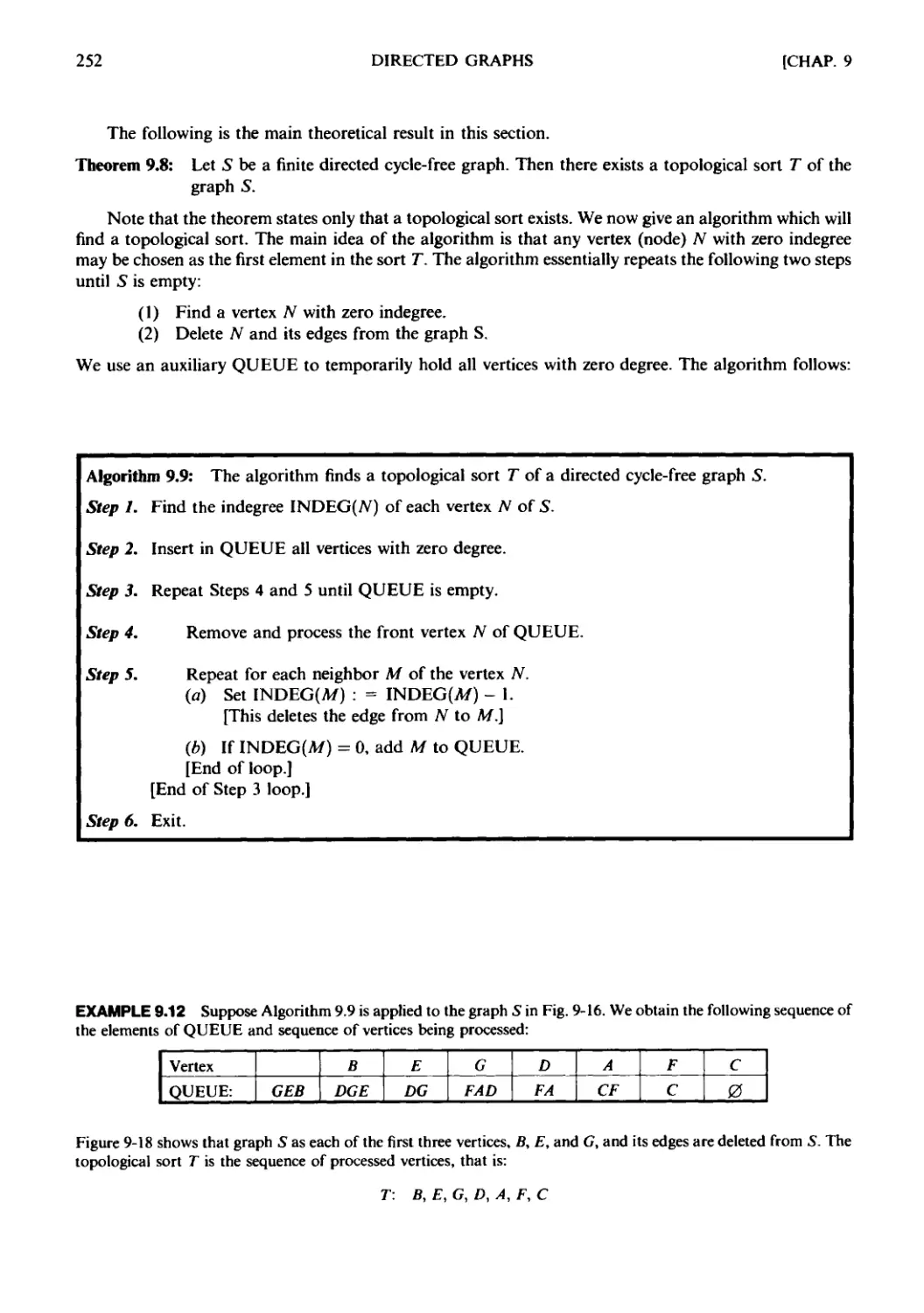
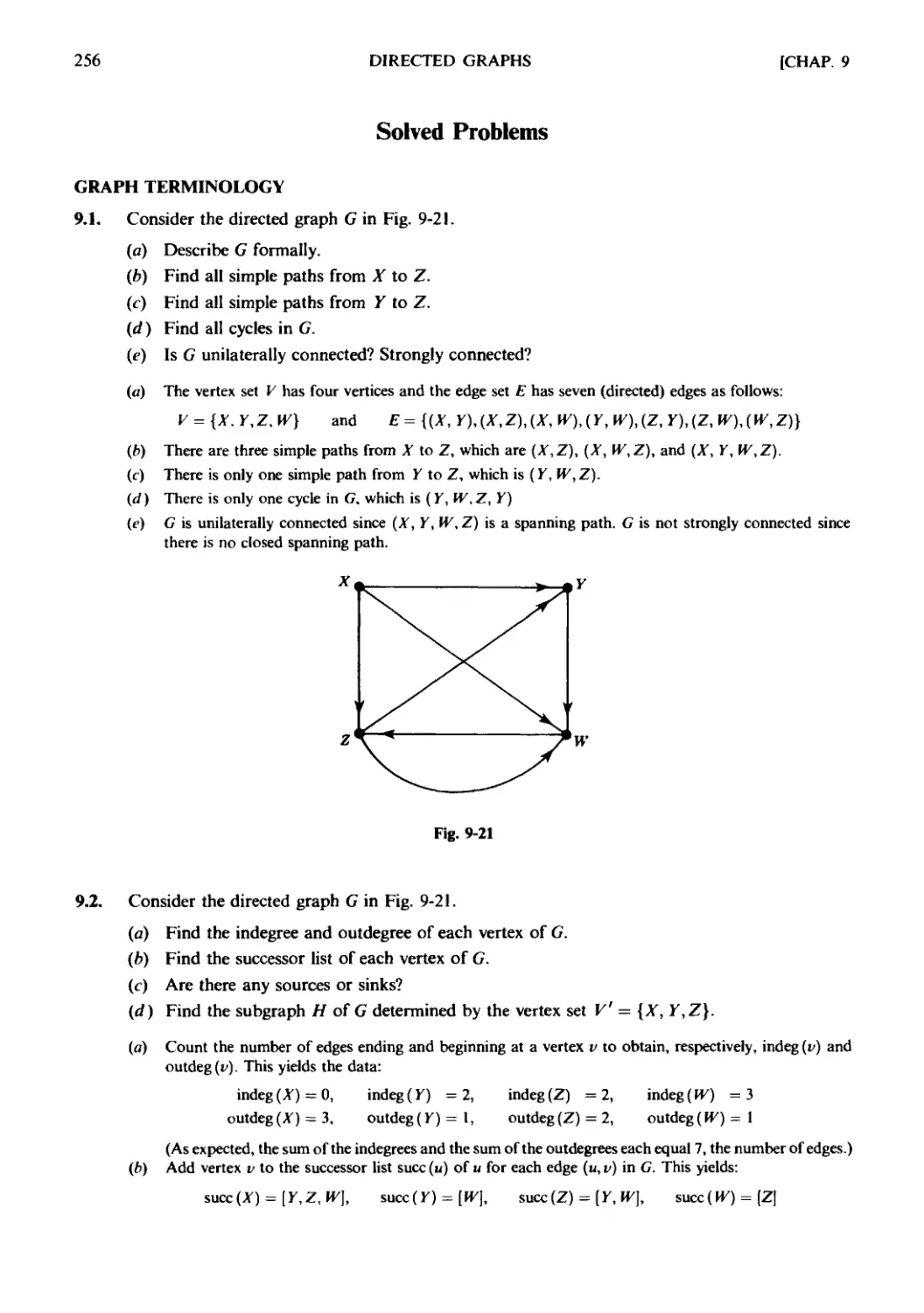
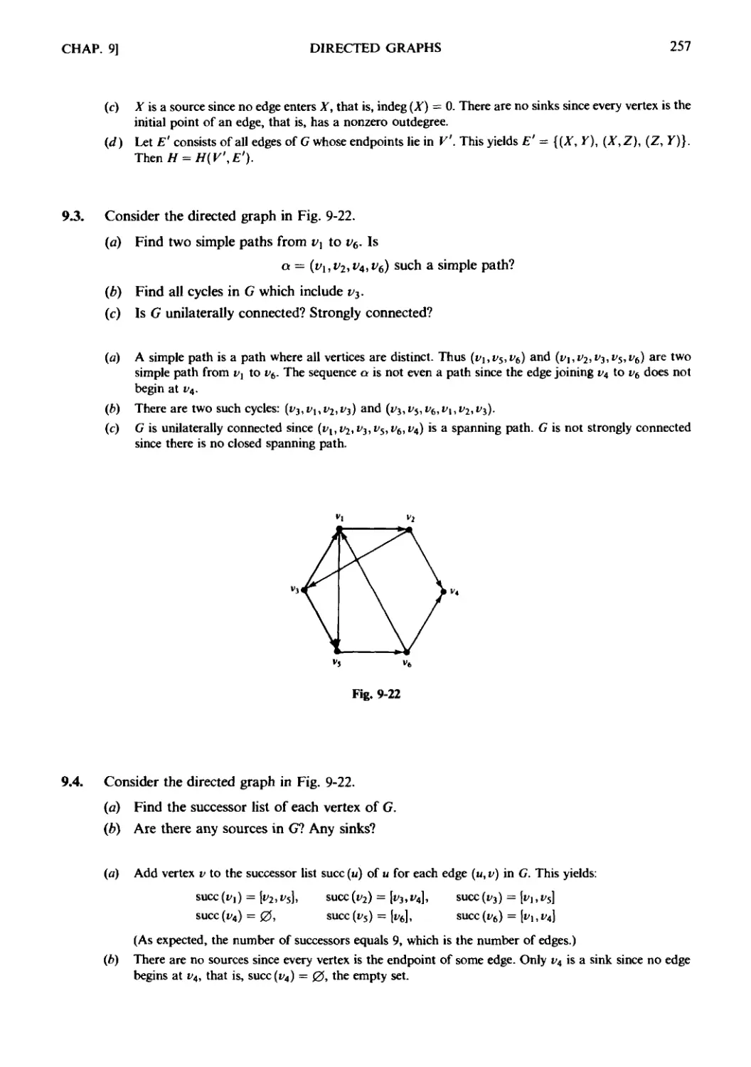
Chapter 9 DIRECTED GRAPHS 233
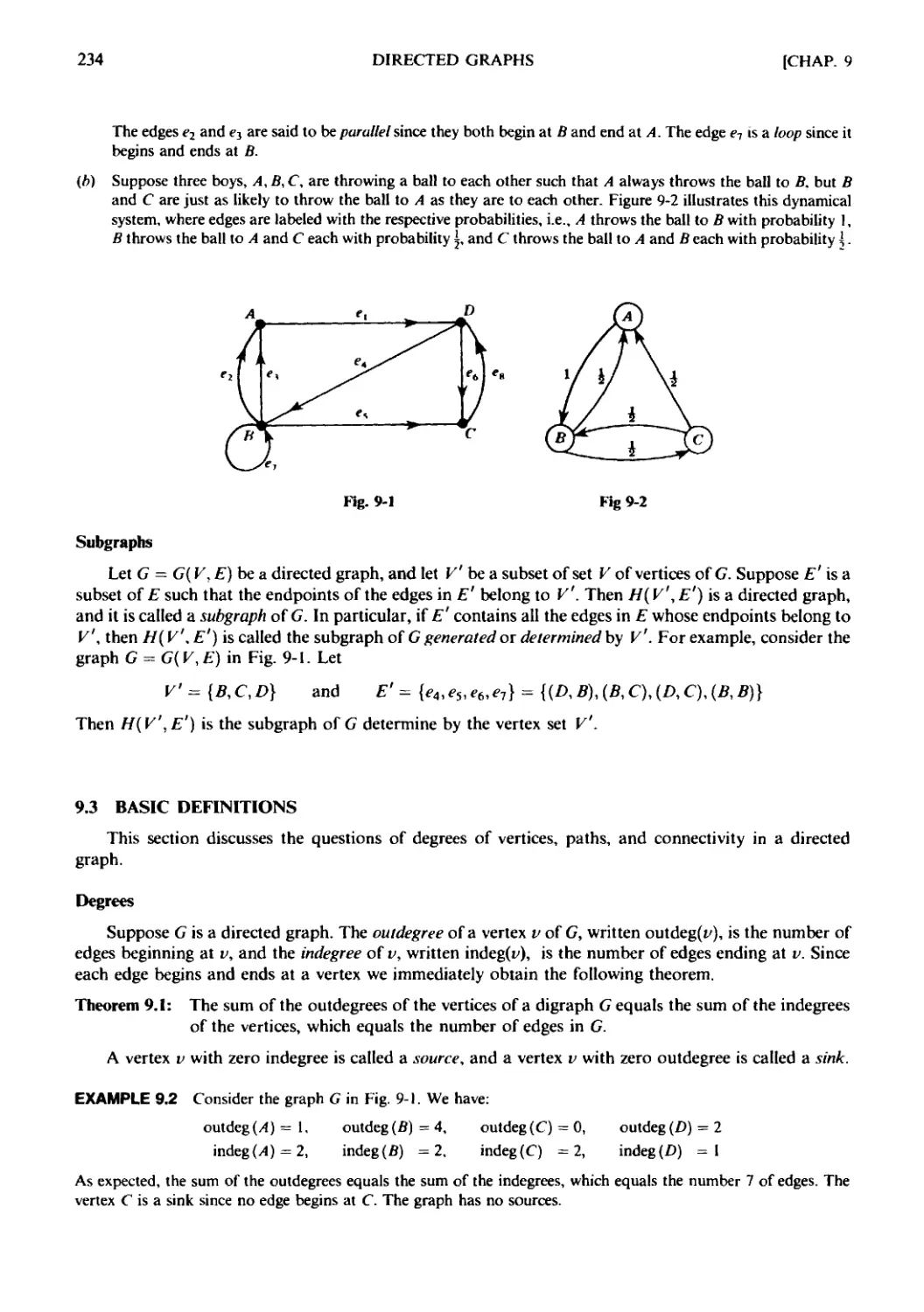
9.1 Introduction. 9.2 Directed Graphs. 9.3 Basic Definitions.
9.4 Rooted Trees. 9.5 Sequential Representation of Directed
Graphs. 9.6 Warshall's Algorithm; Shortest Paths. 9.7 Linked Repre-
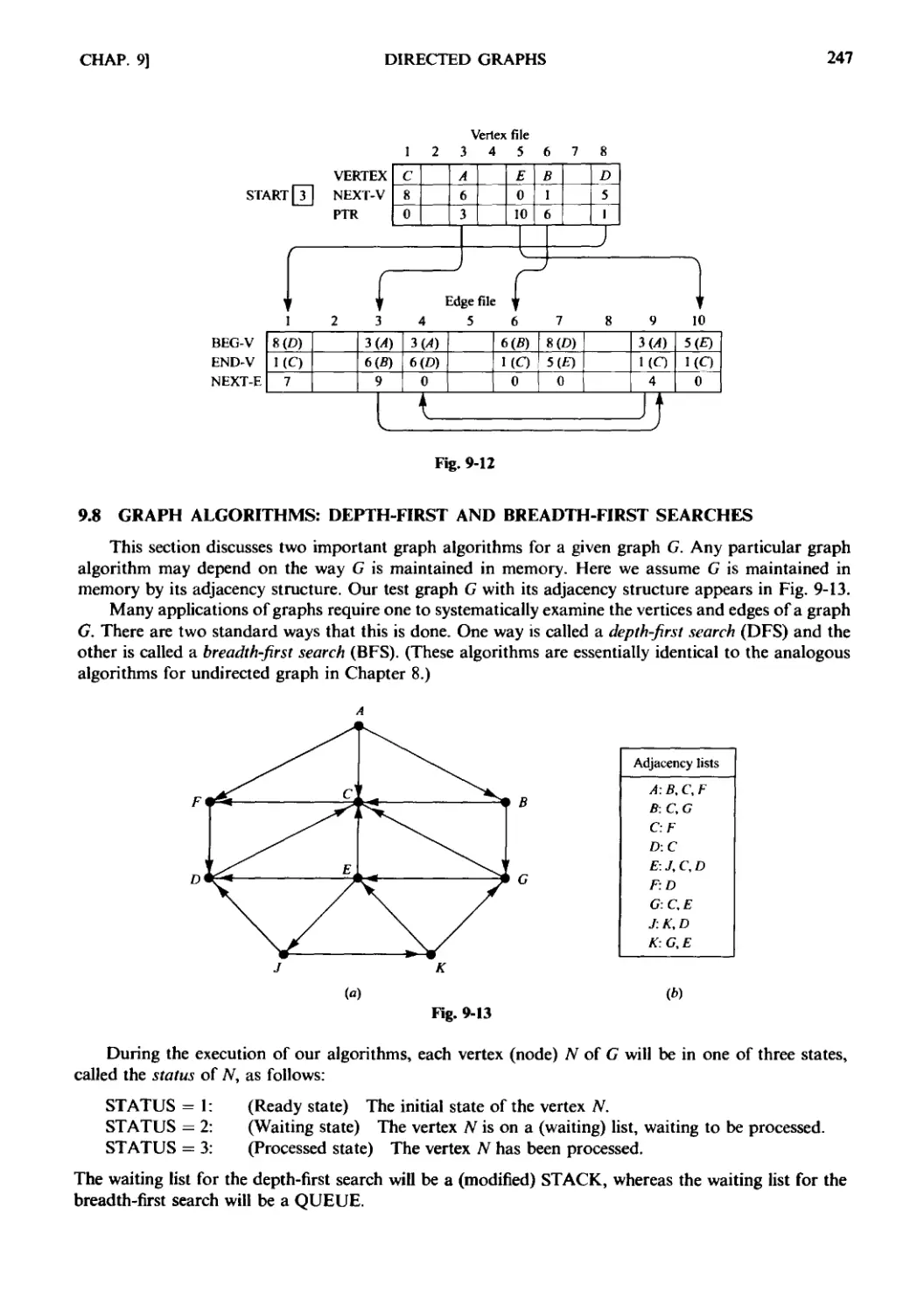
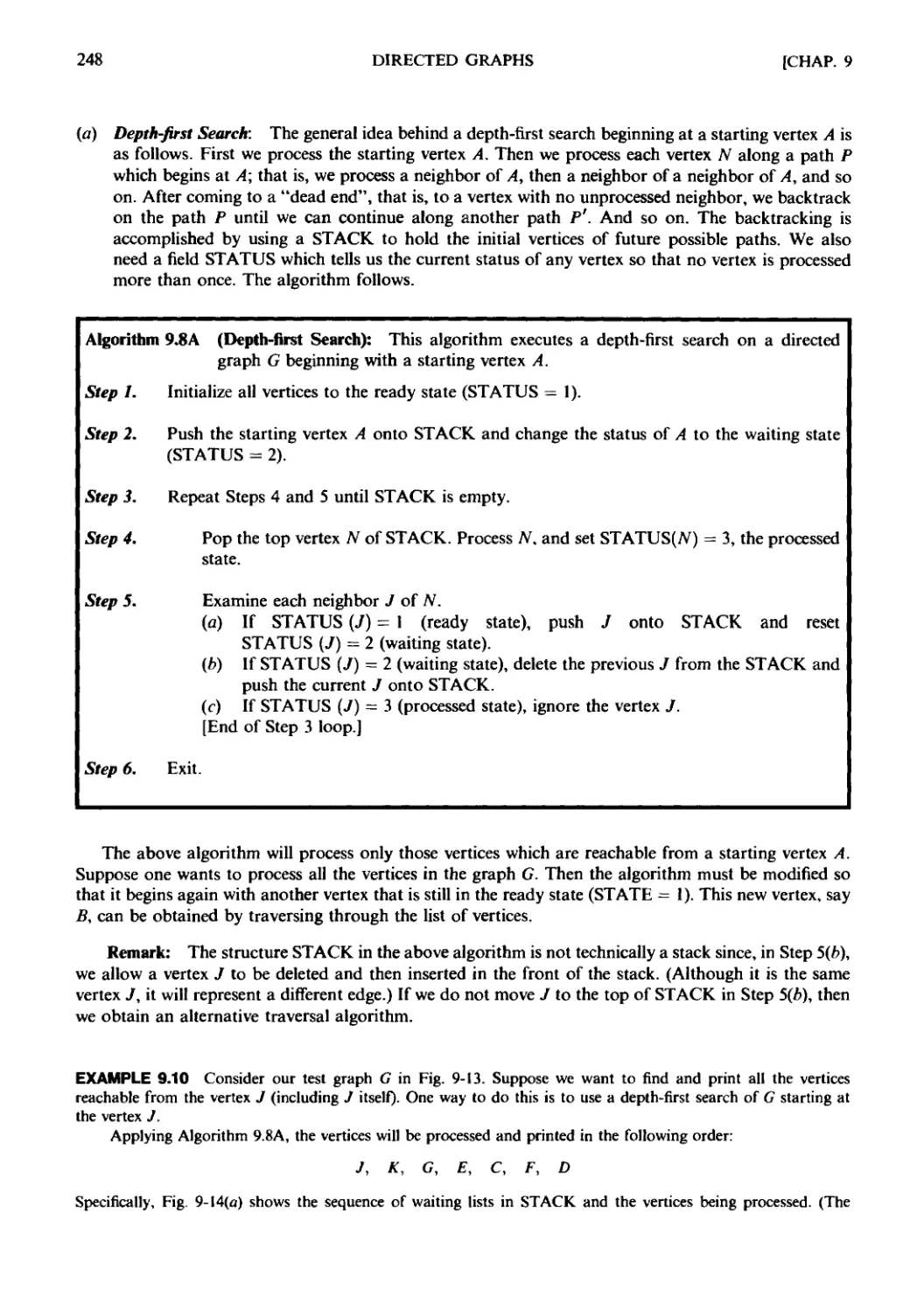
Representation of Directed Graphs. 9.8 Graph Algorithms: Depth-First and
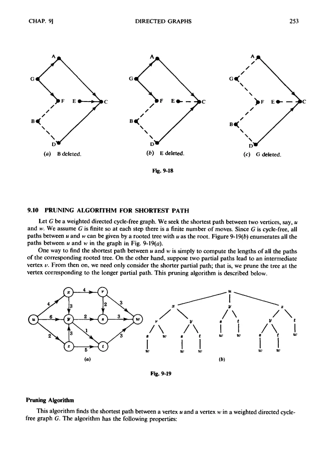
Breadth-First Searches. 9.9 Directed Cycle-Free Graphs, Topological
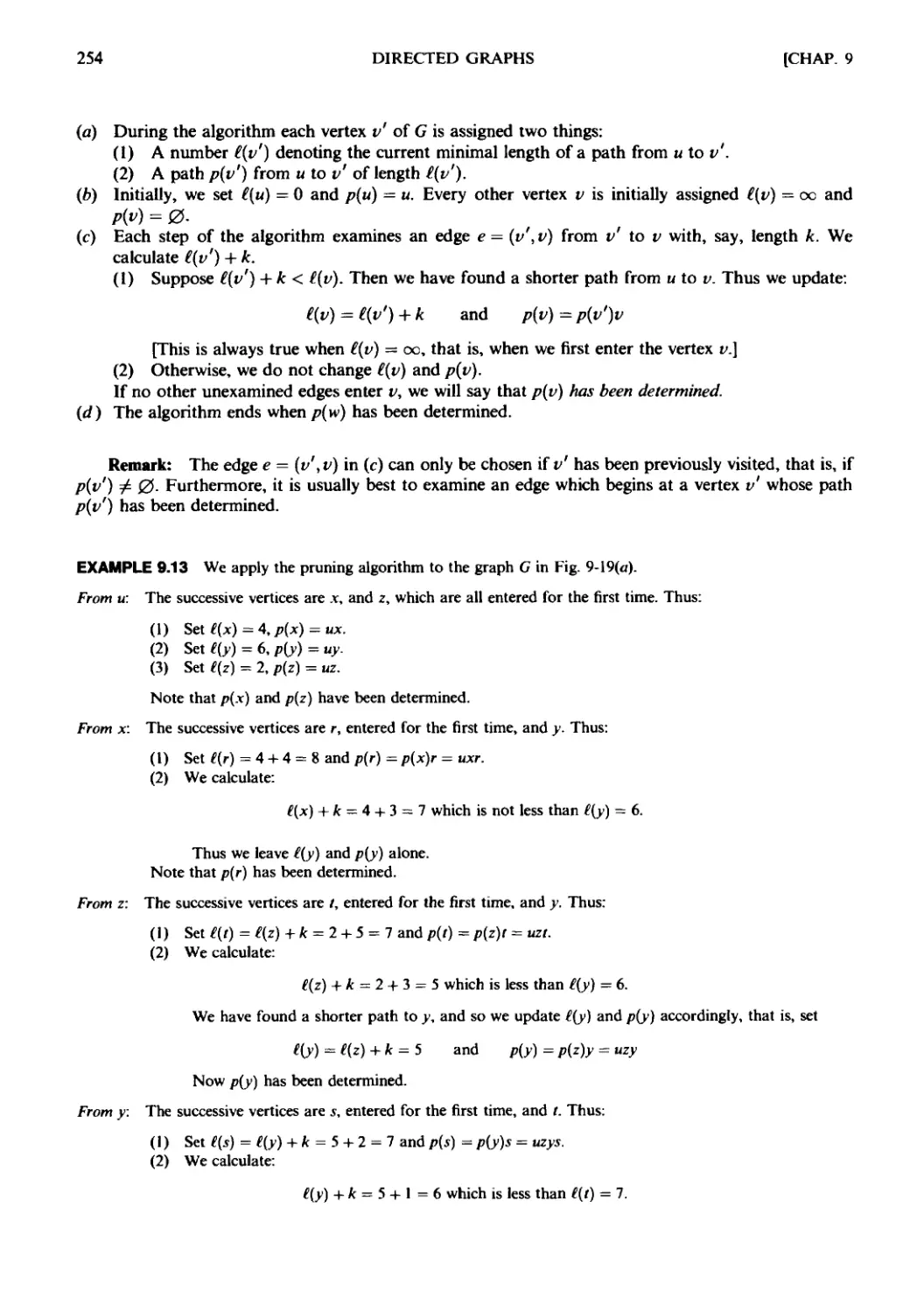
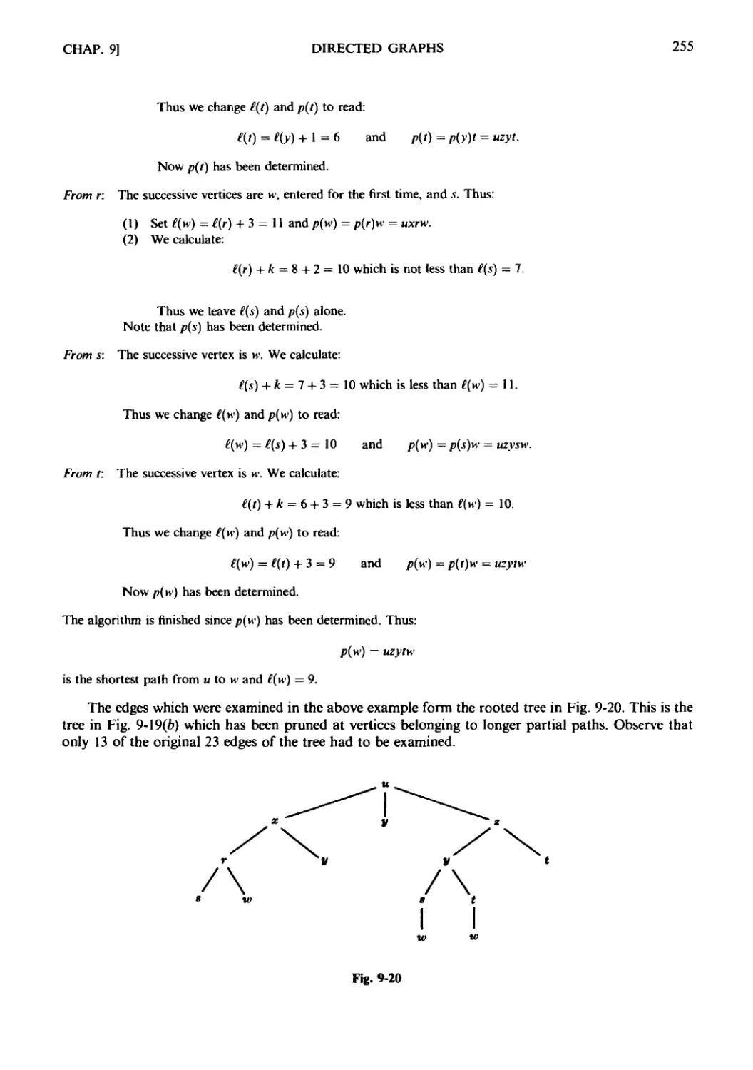
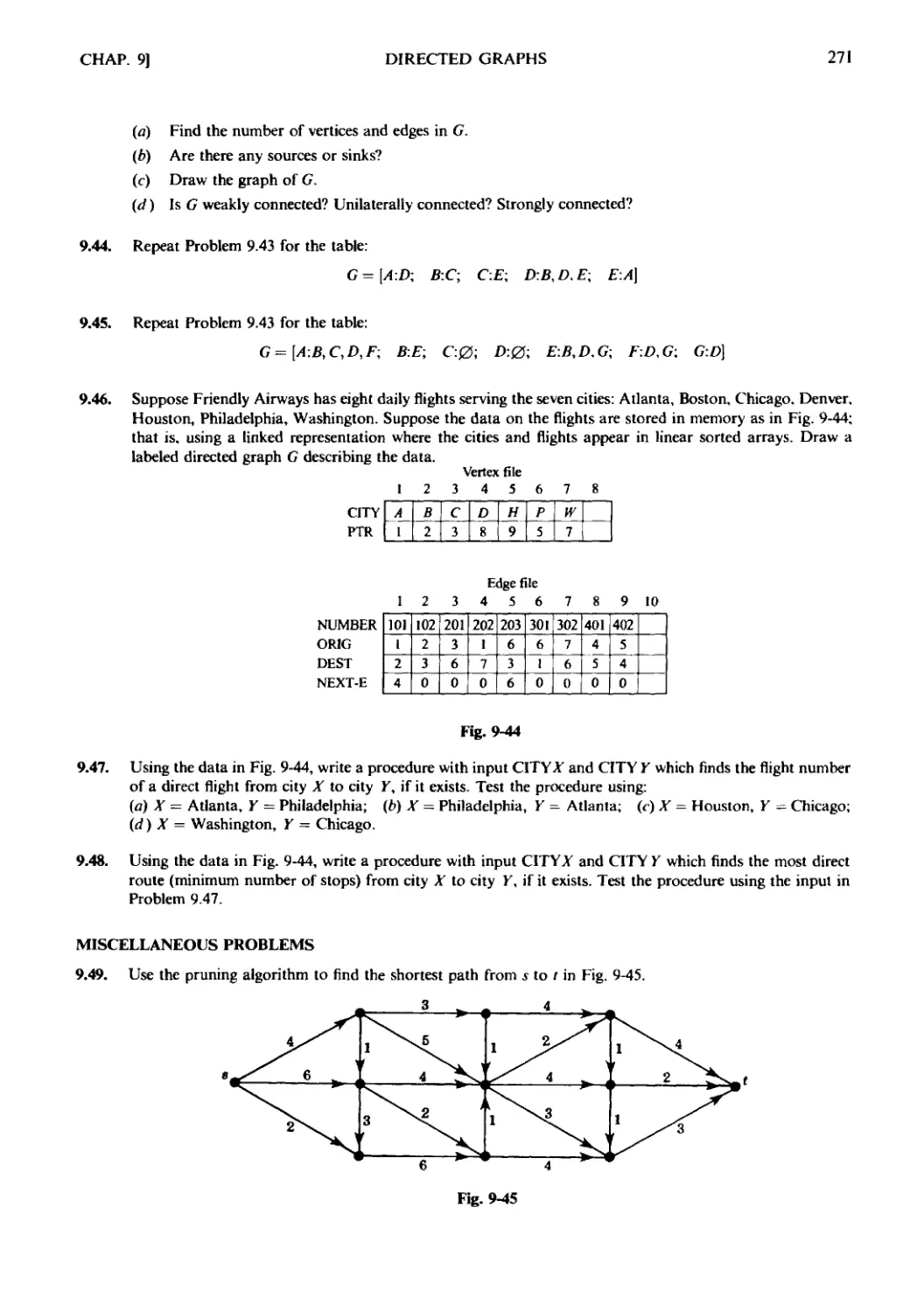
Sort. 9.10 Pruning Algorithm for Shortest Path.
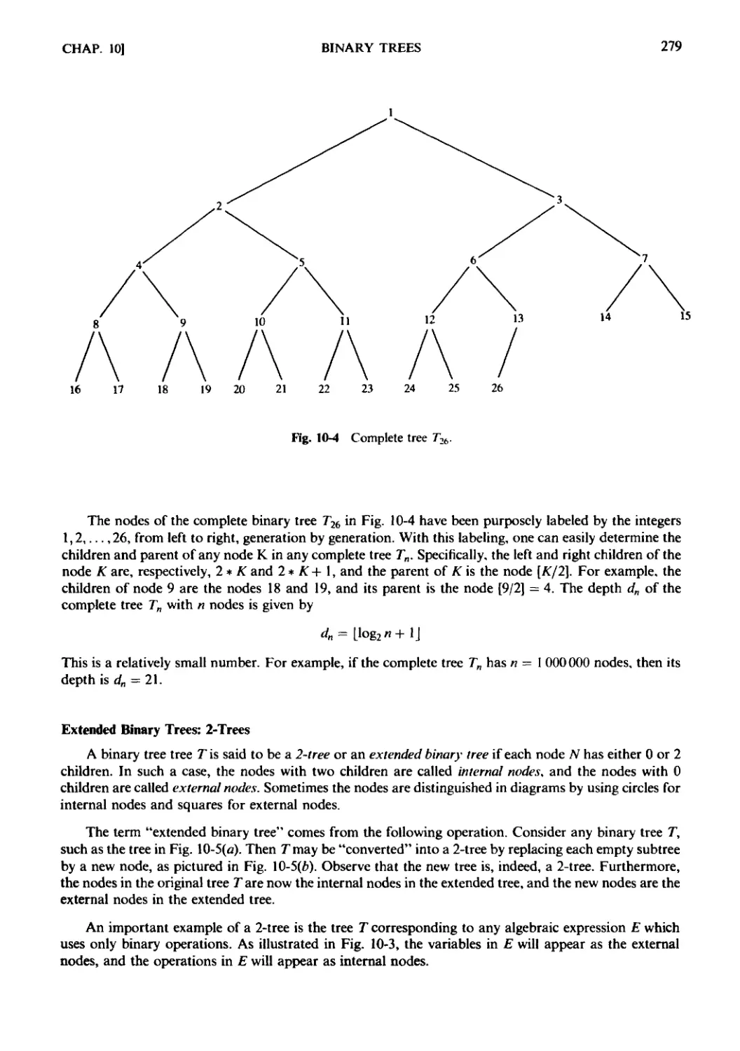
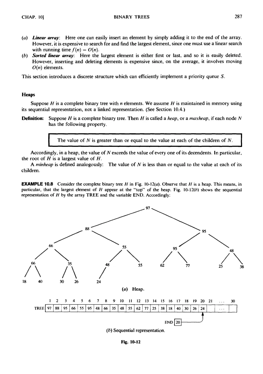
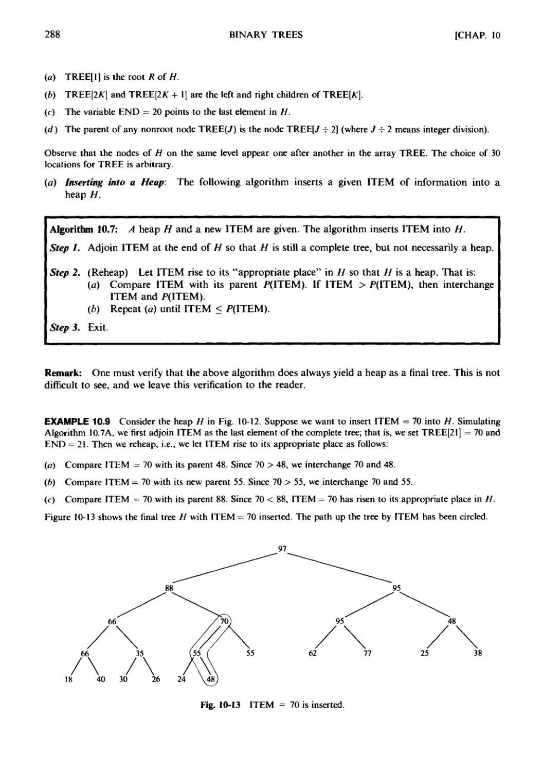
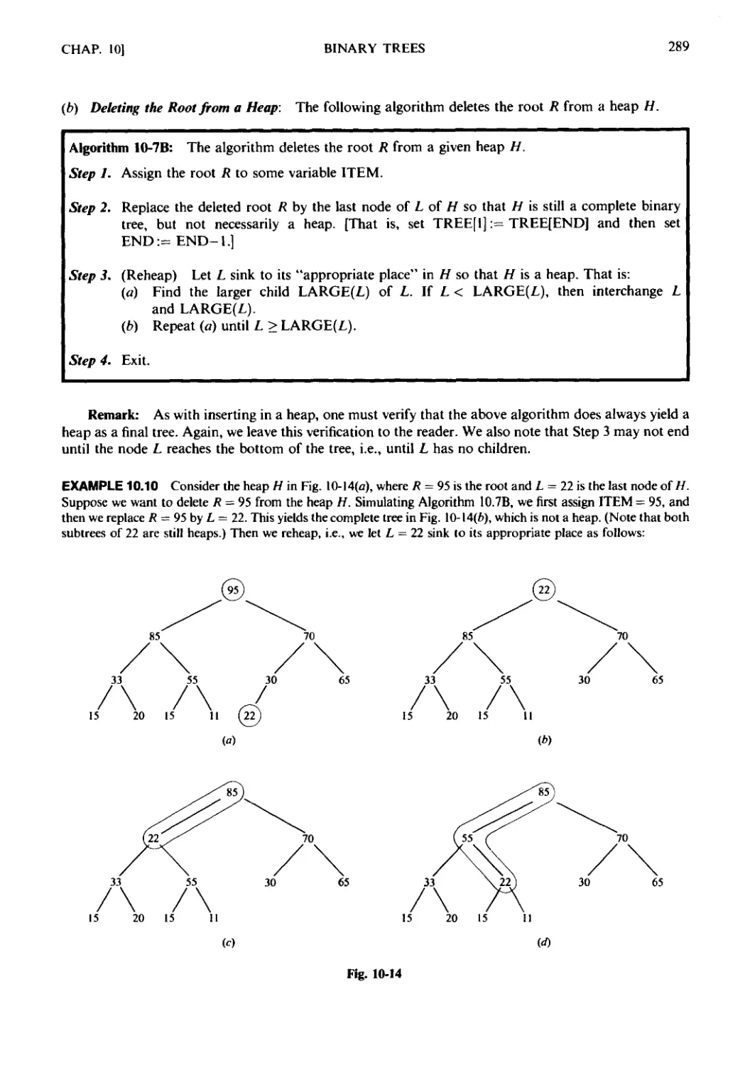
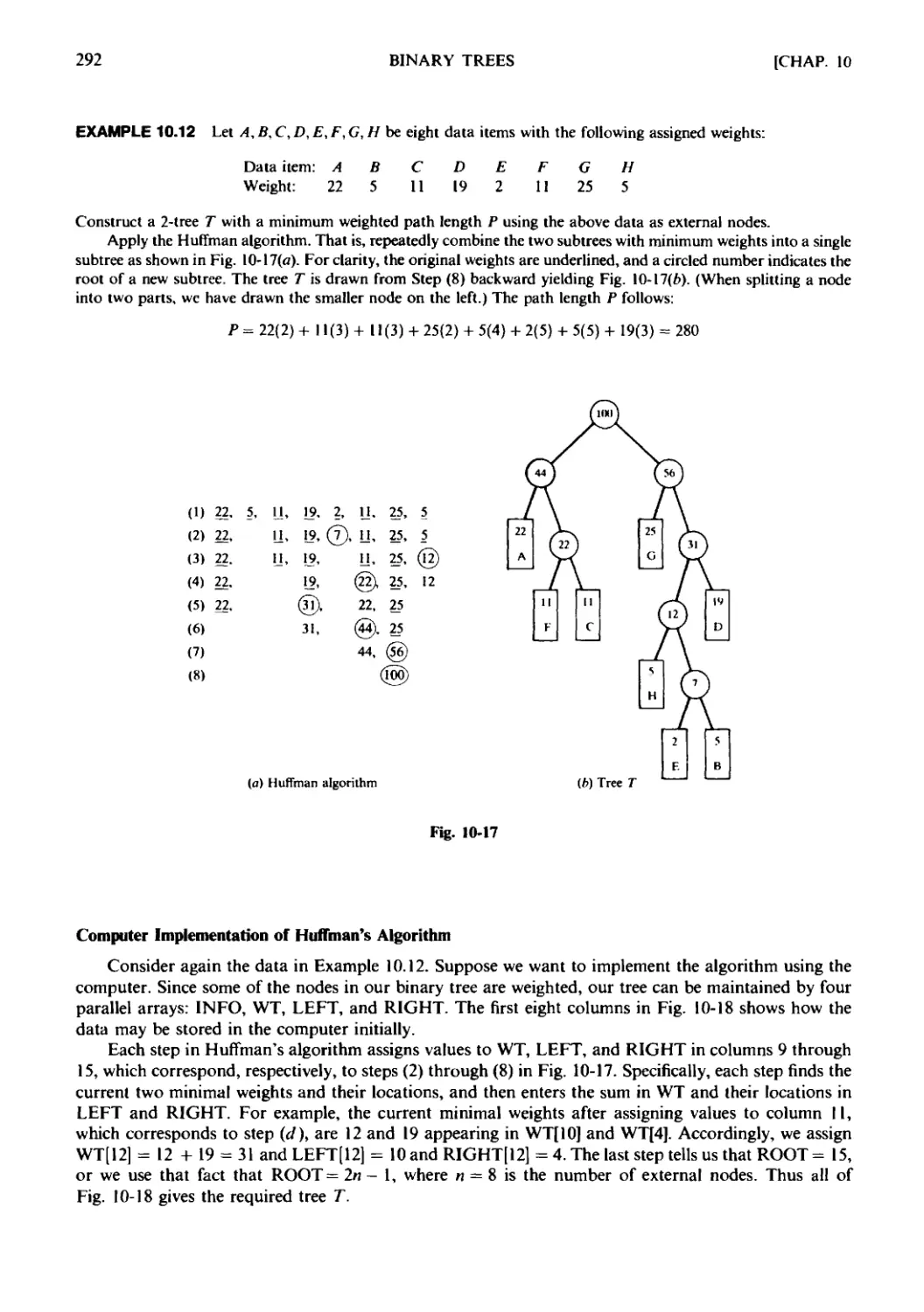
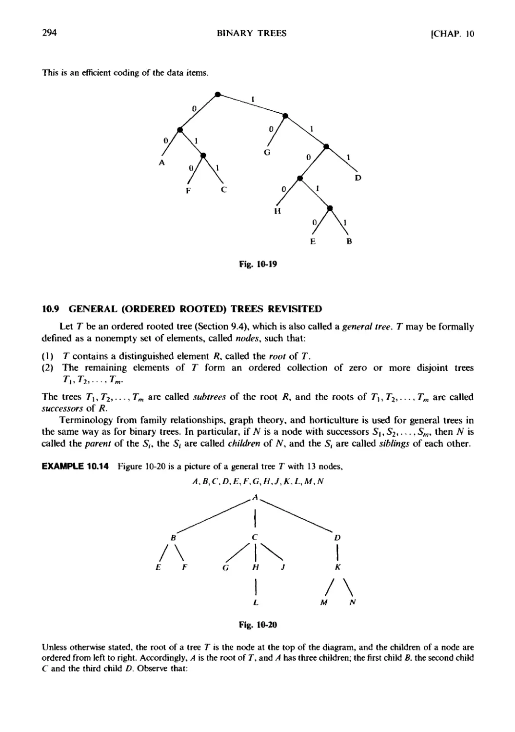
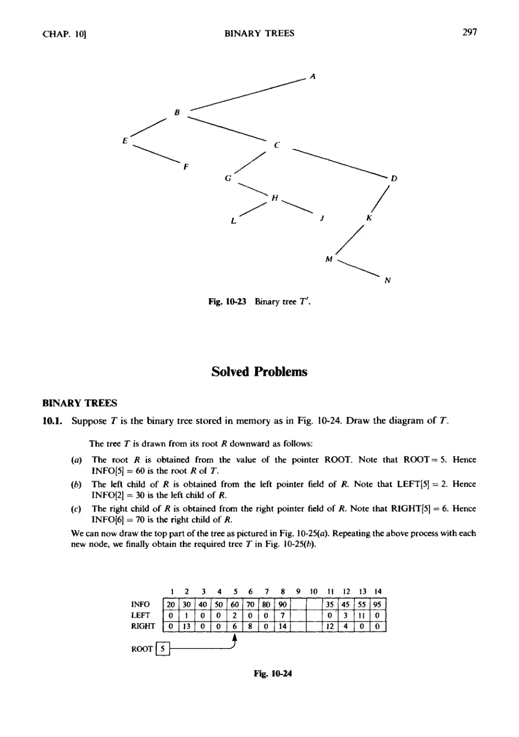
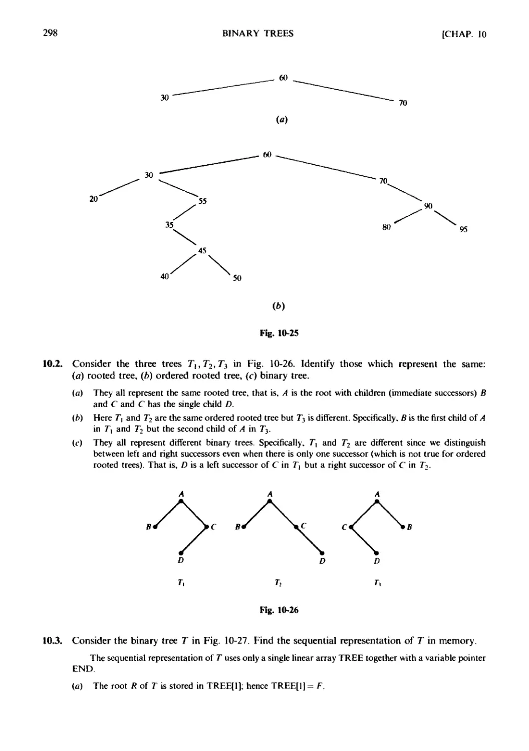
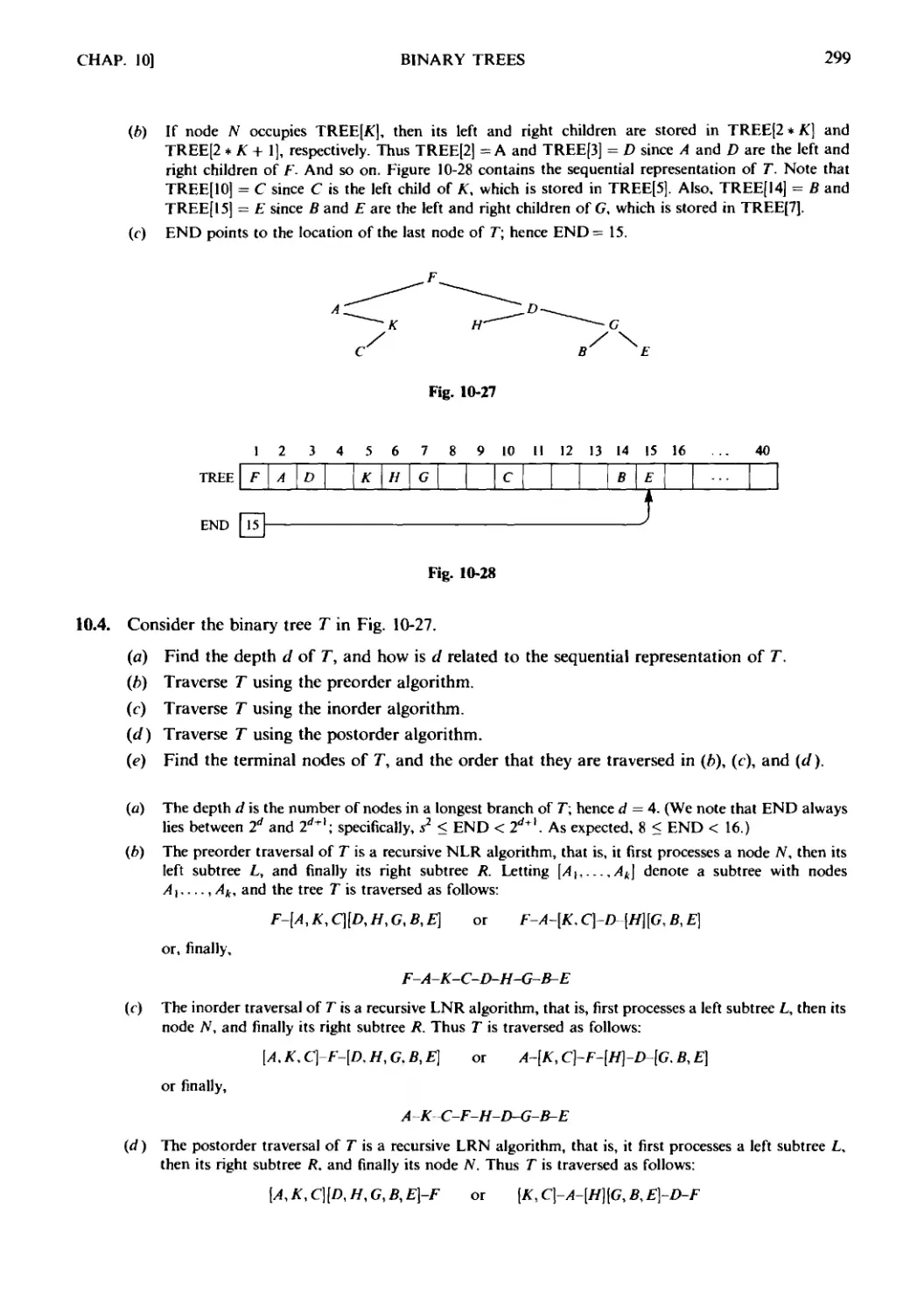
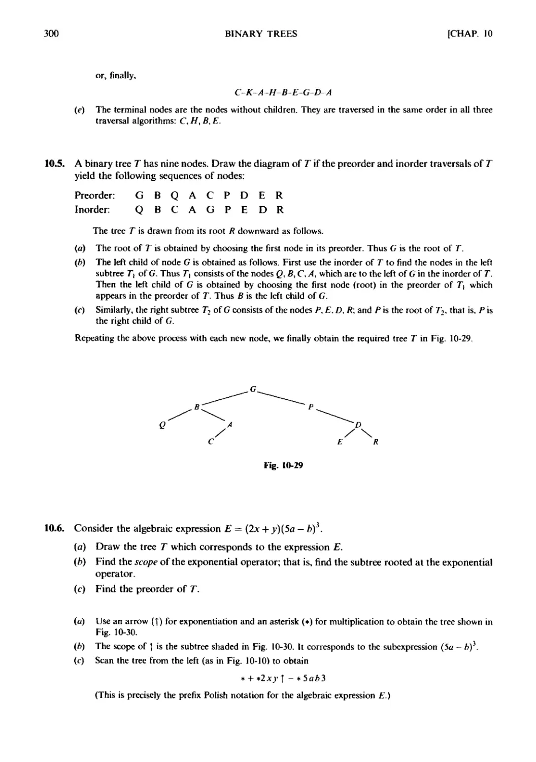
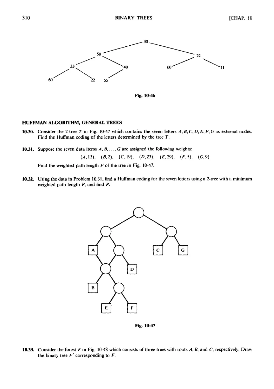
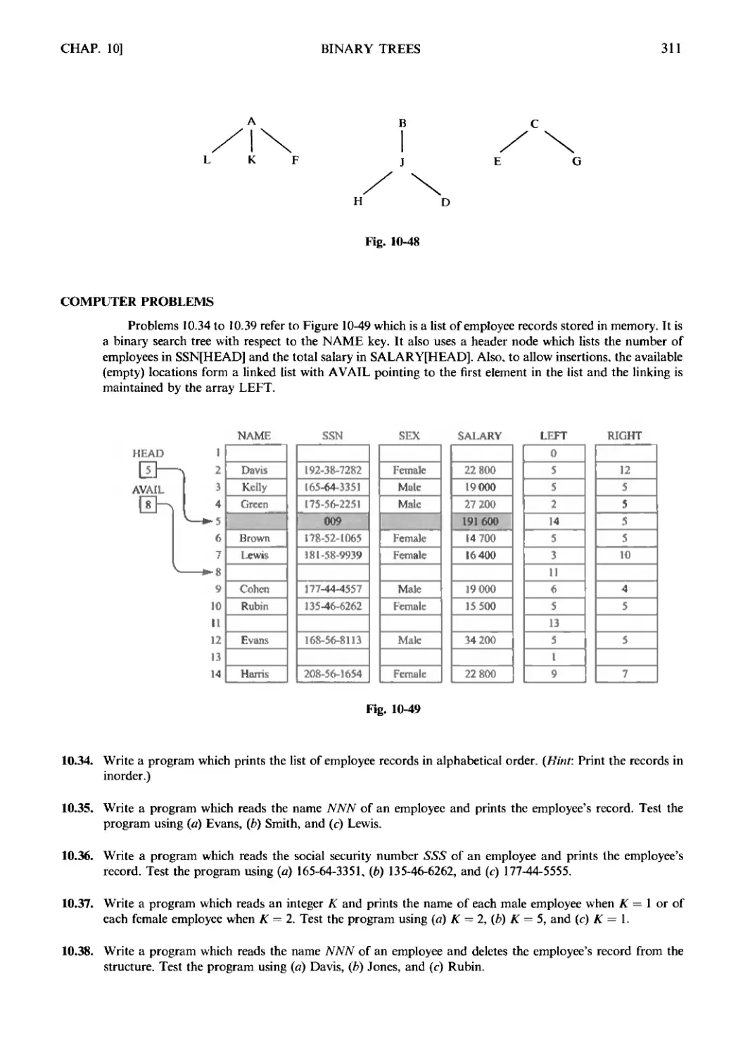
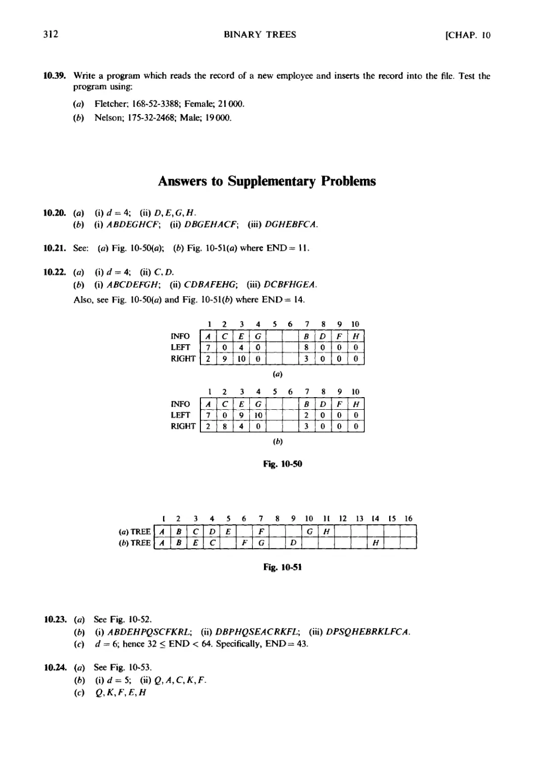
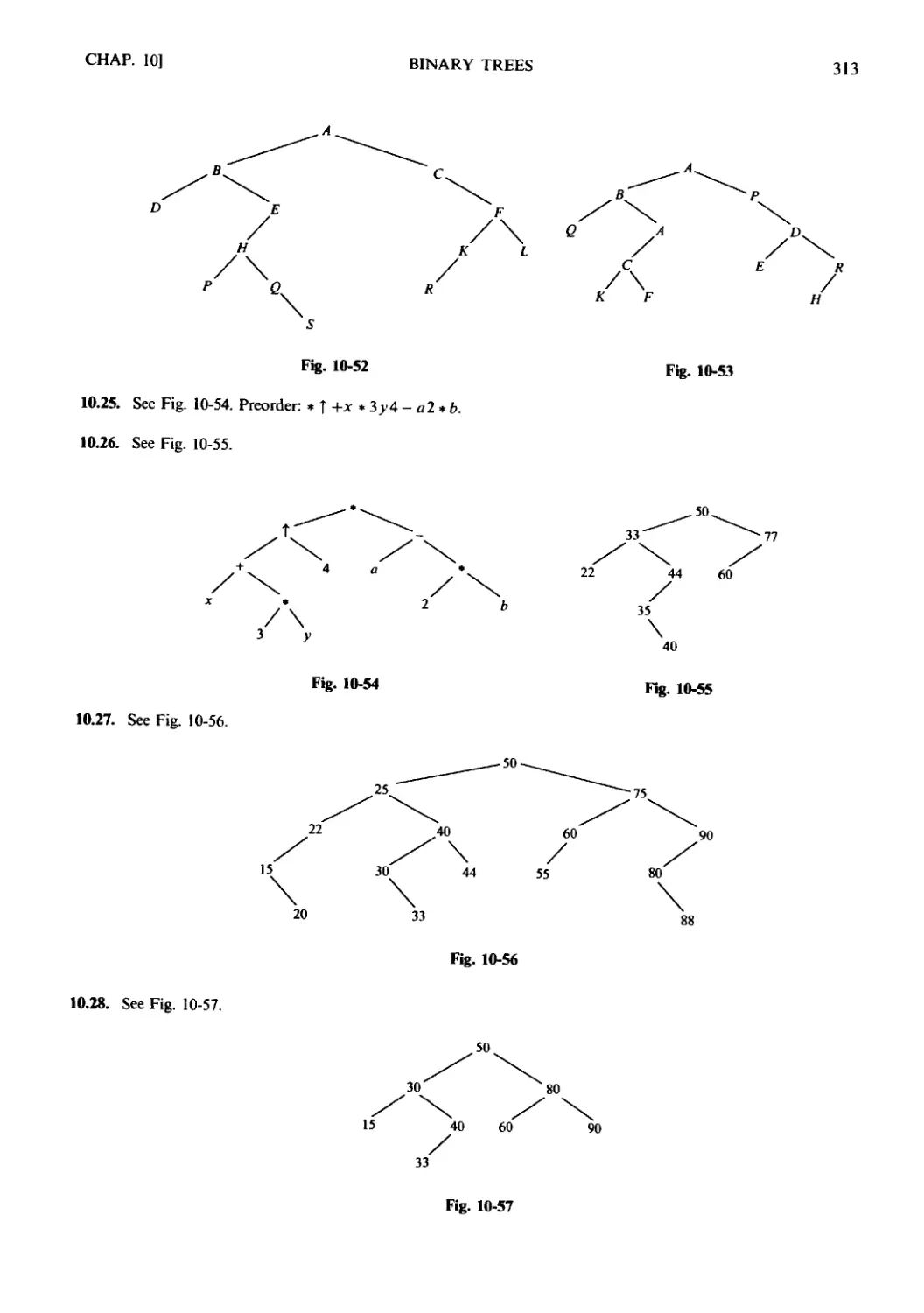
Chapter 10 BINARY TREES
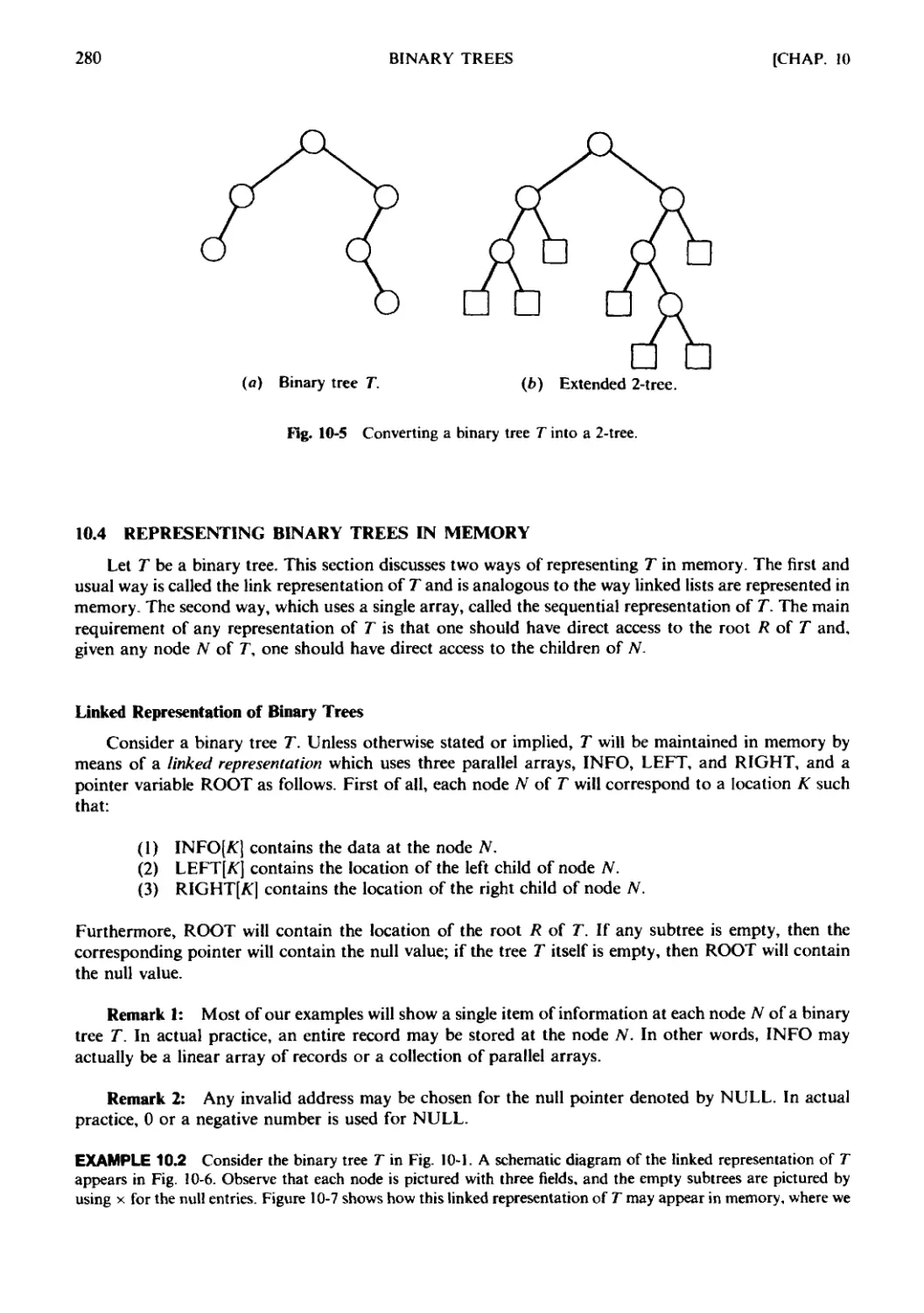
10.1 Introduction. 10.2 Binary Trees. 10.3 Complete and Extended
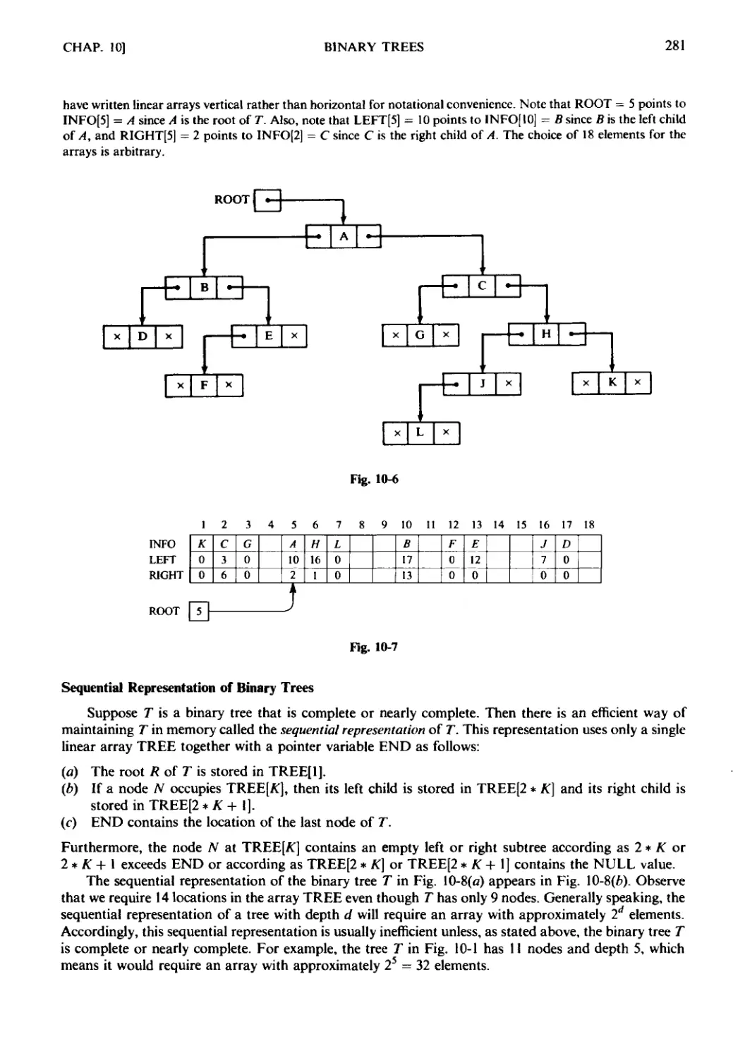
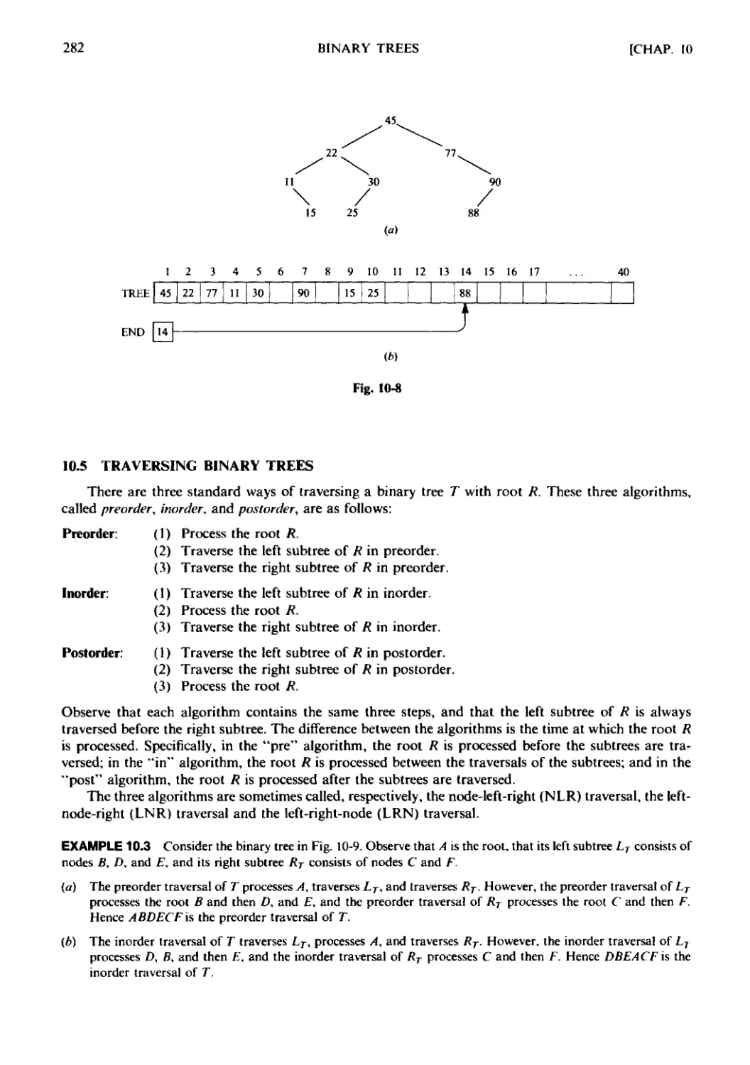
Binary Trees. 10.4 Representing Binary Trees in Memory. 10.5 Traver-
Traversing Binary Trees. 10.6 Binary Search Trees. 10.7 Priority Queues,
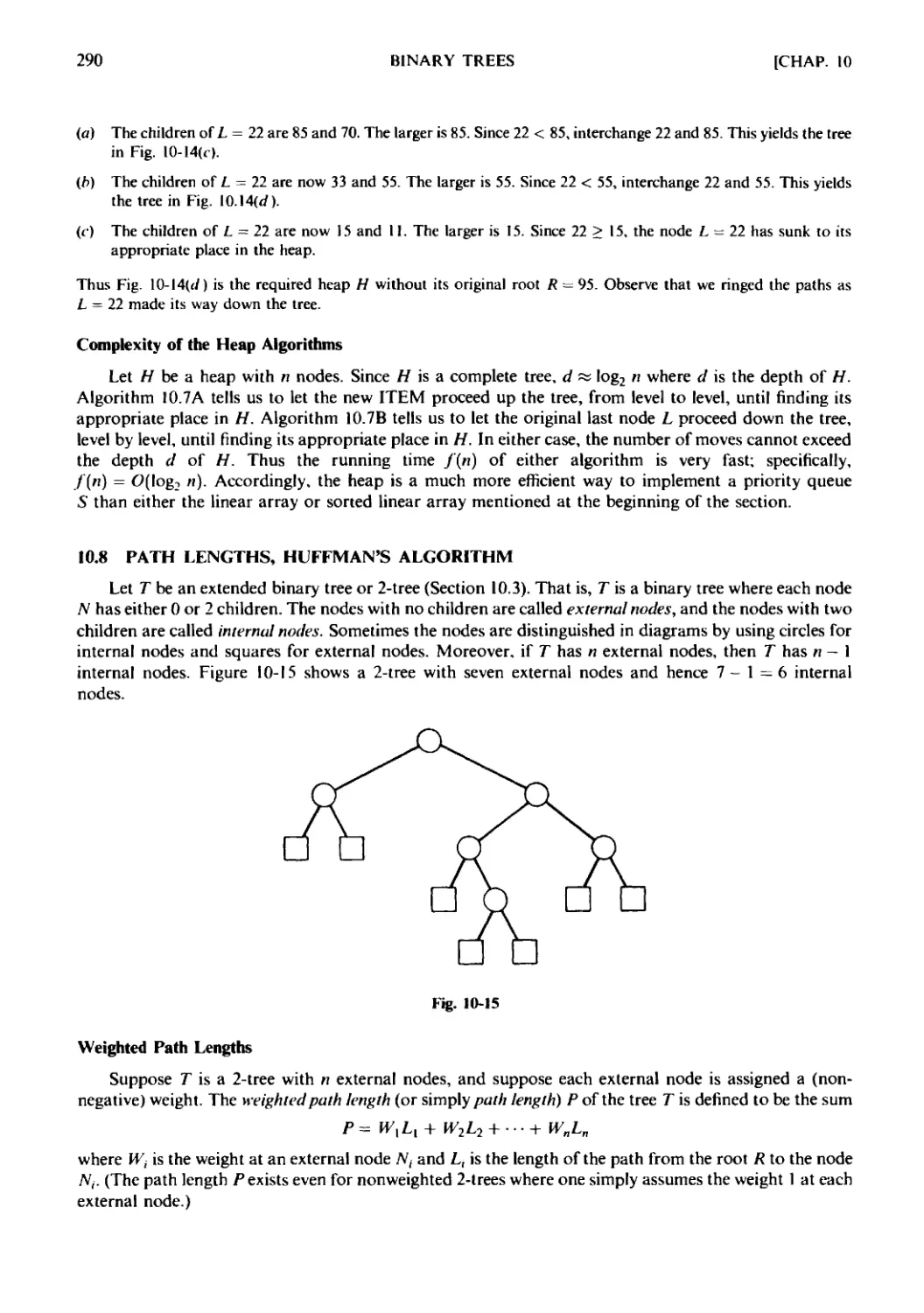
Heaps. 10.8 Path Lengths, Huffman's Algorithm. 10.9 General
(Ordered Rooted) Trees Revisited.
276
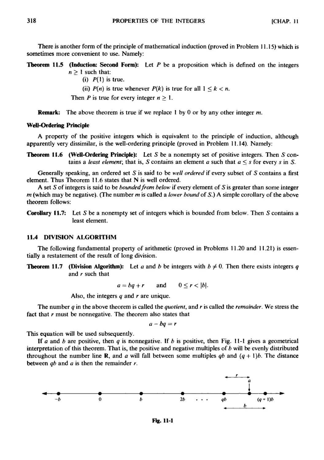
Chapter// PROPERTIES OF THE INTEGERS 315
11.1 Introduction. 11.2 Order and Inequalities, Absolute Value.
11.3 Mathematical Induction. 11.4 Division Algorithm. 11.5 Divis-
Divisibility, Primes. 11.6 Greatest Common Divisor, Euclidean Algorithm.
11.7 Fundamental Theorem of Arithmetic. 11.8 Congruence Relation.
11.9 Congruence Equations.
Chapter 12 ALGEBRAIC SYSTEMS 364
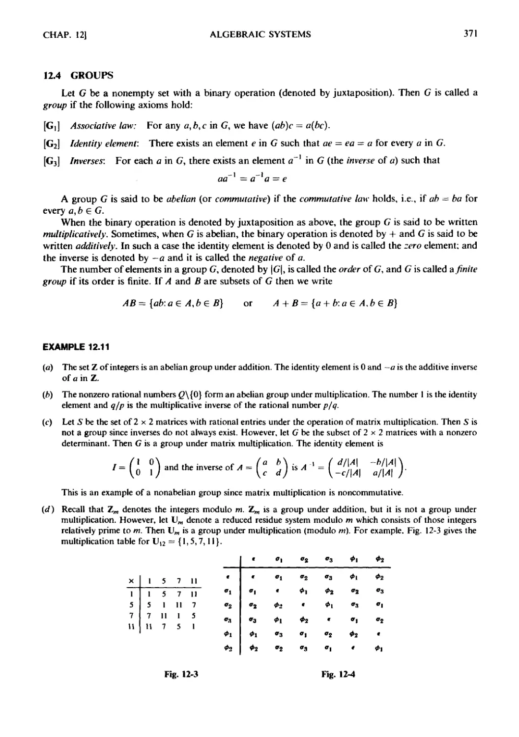
12.1 Introduction. 12.2 Operations. 12.3 Semigroups. 12.4 Groups.
12.5 Subgroups, Normal Subgroups, and Homomorphisms. 12.6 Rings,
Integral Domains, and Fields. 12.7 Polynomials over a Field.
CONTENTS ix
Chapter 13 LANGUAGES, GRAMMARS, MACHINES 405
13.1 Introduction. 13.2 Alphabet, Words, Free Semigroup. 13.3 Lan-
Languages. 13.4 Regular Expressions, Regular Languages. 13.5 Finite
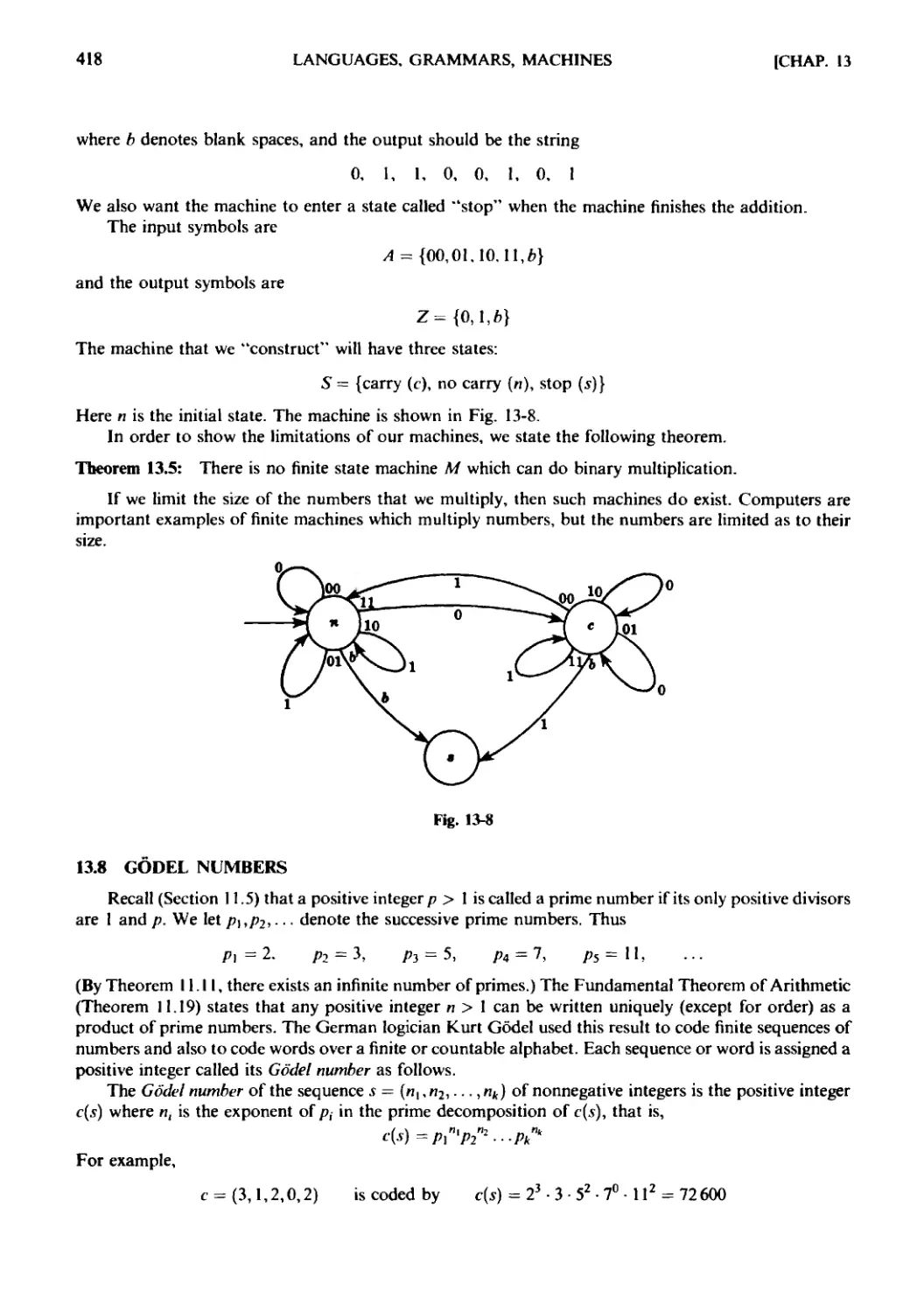
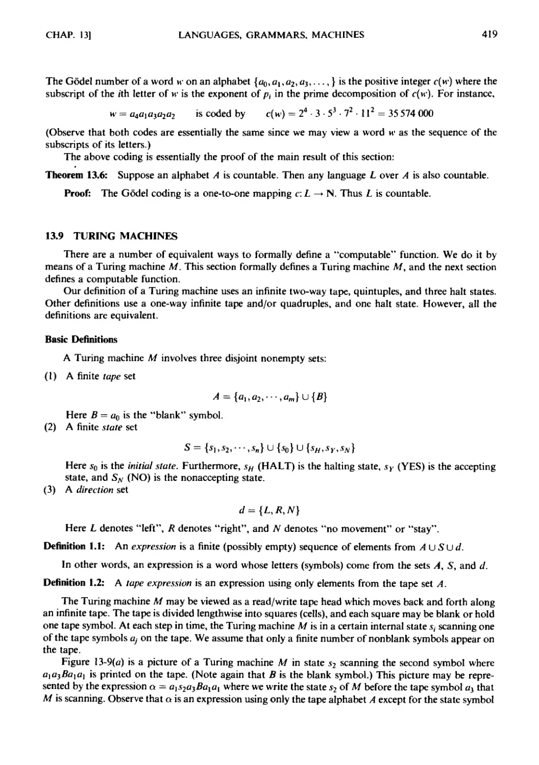
State Automata. 13.6 Grammars. 13.7 Finite State Machines.
13.8 Godel Numbers. 13.9 Turing Machines. 13.10 Computable
Functions.
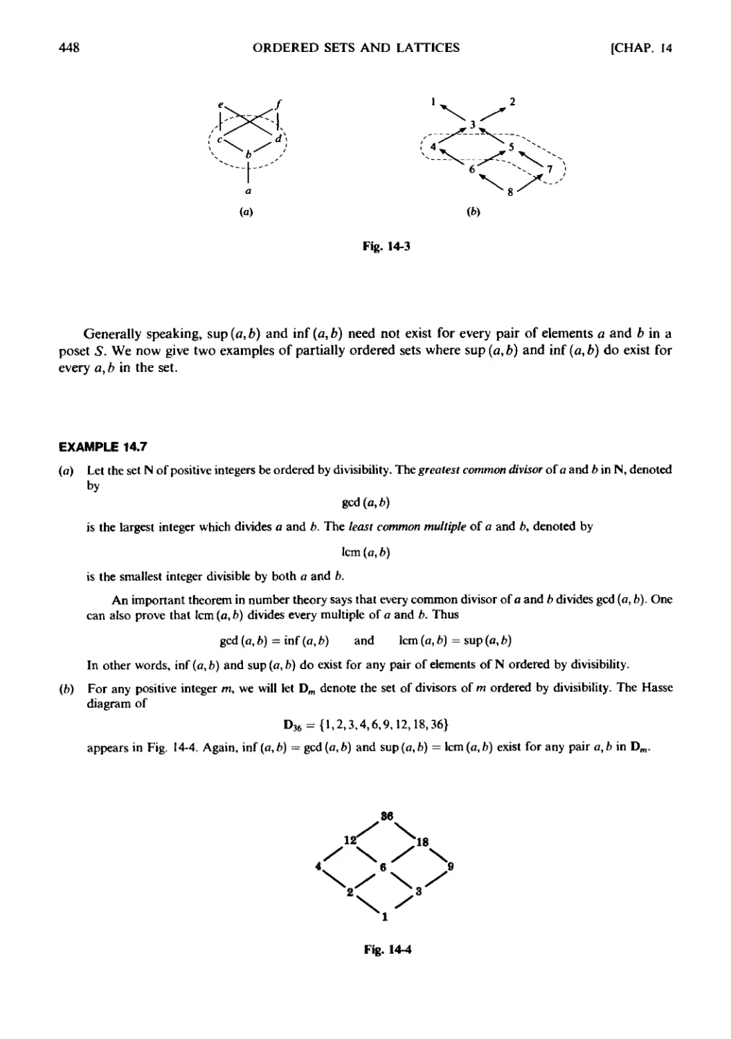
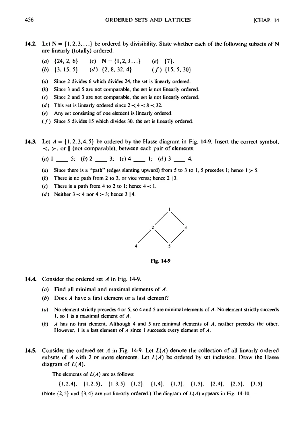
Chapter 14 ORDERED SETS AND LATTICES 442
14.1 Introduction. 14.2 Ordered Sets. 14.3 Hasse Diagrams of Par-
Partially Ordered Sets. 14.4 Consistent Enumeration. 14.5 Supremum
and Infimum. 14.6 Isomorphic (Similar) Ordered Sets. 14.7 Well-
Ordered Sets. 14.8 Lattices. 14.9 Bounded Lattices. 14.10 Distribu-
Distributive Lattices. 14.11 Complements, Complemented Lattices.
Chapter/5 BOOLEAN ALGEBRA 477
15.1 Introduction. 15.2 Basic Definitions. 15.3 Duality. 15.4 Basic
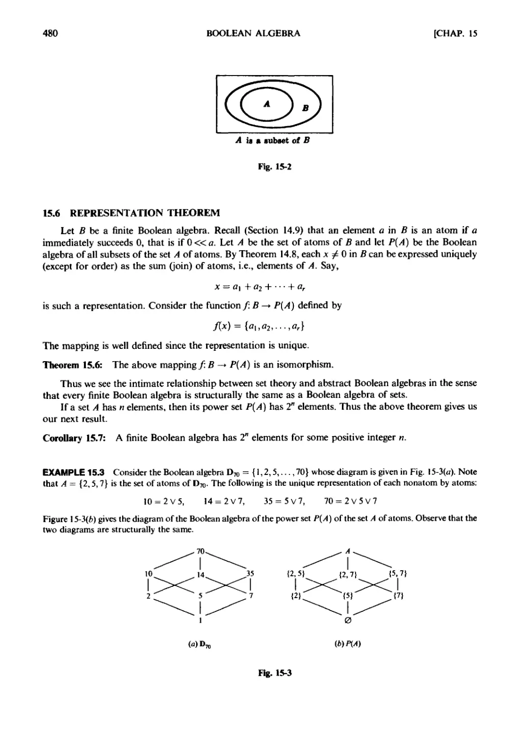
Theorems. 15.5 Boolean Algebras as Lattices. 15.6 Representation
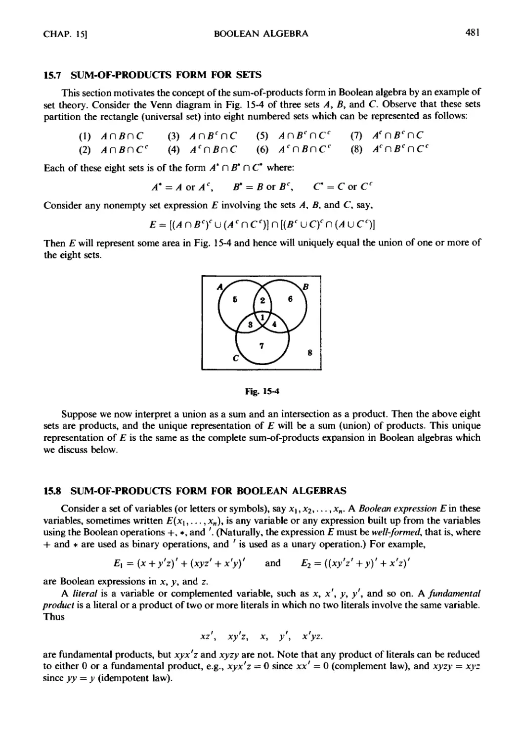
Theorem. 15.7 Sum-of-Products Form for Sets. 15.8 Sum-of-Products
Form for Boolean Algebras. 15.9 Minimal Boolean Expressions, Prime
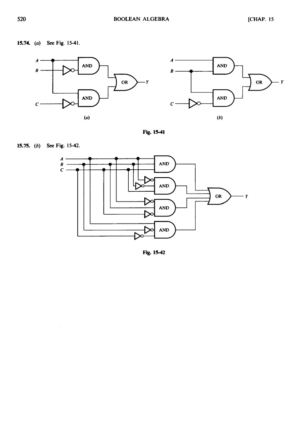
Implicants. 15.10 Logic Gates and Circuits. 15.11 Truth Tables, Bool-
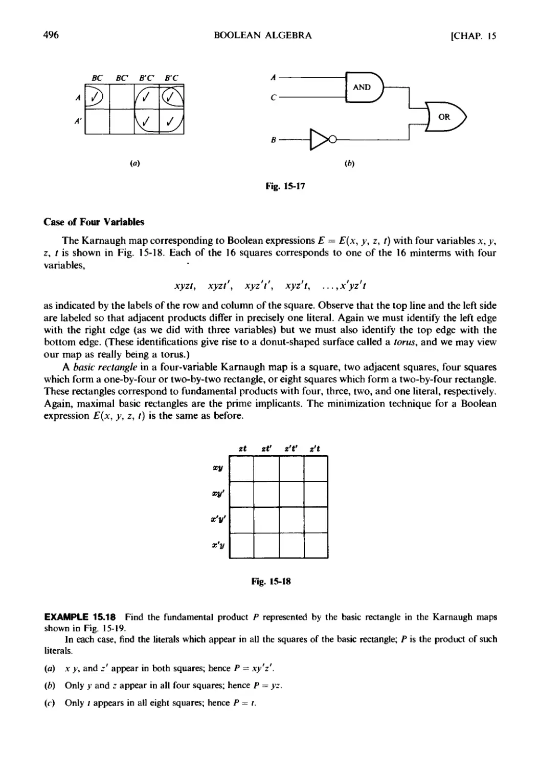
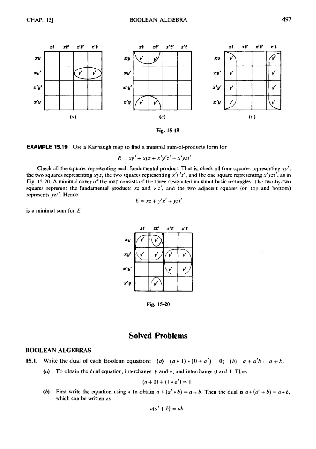
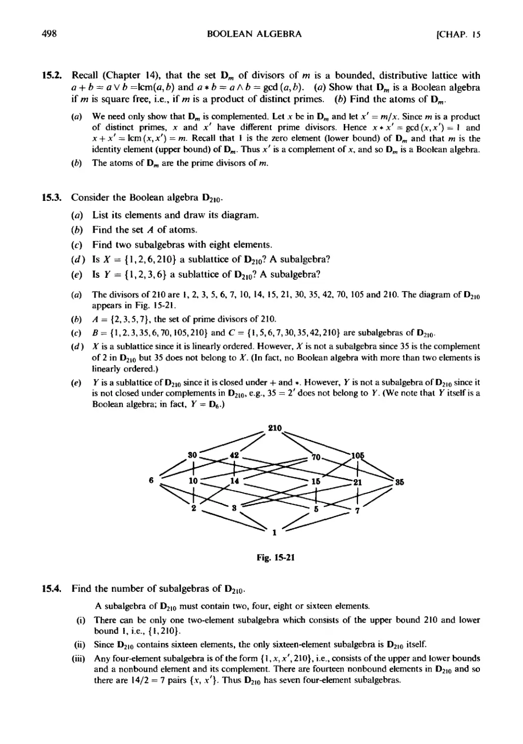
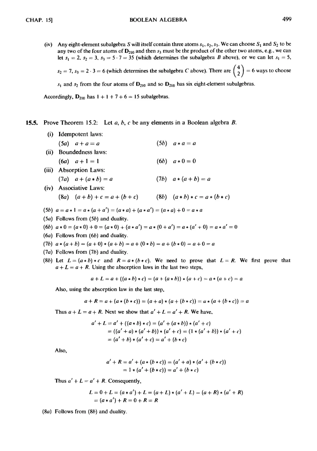
Boolean Functions. 15.12 Karnaugh Maps.
Index 521
SCHAVMS OUTLINE OF
THEORY AND PROBLEMS
of
DISCRETE
MATHEMATICS
Chapter 1
Set Theory
1.1 INTRODUCTION
The concept of a set appears in all mathematics. This chapter introduces the notation and terminol-
terminology of set theory which is basic and used throughout the text.
Though logic is formally treated in Chapter 4, we introduce Venn diagram representation of sets
here, and we show how it can be applied to logical arguments. The relation between set theory and logic
will be further explored when we discuss Boolean algebra in Chapter 15.
This chapter closes with the formal definition of mathematical induction, with examples.
1.2 SETS AND ELEMENTS
A set may be viewed as a collection of objects, the elements or members of the set. We ordinarily use
capital letters, A, B, X, Y,..., to denote sets, and lowercase letters, a, b, x, y, ..., to denote elements of
sets. The statement '"p is an element of A", or, equivalently, "/? belongs to A", is written
p€ A
The statement that p is not an element of A, that is, the negation of p € A, is written
p$A
The fact that a set is completely determined when its members are specified is formally stated as the
principle of extension.
Principle of Extension: Two sets A and В are equal if and only if they have the same members.
As usual, we write A = В if the sets A and В are equal, and we write A ^ В if the sets are not equal.
Specifying Sets
There are essentially two ways to specify a particular set. One way, if possible, is to list its members.
For example,
A = {a,e,i,o,u}
denotes the set A whose elements are the letters a, e, i, o, u. Note that the elements are separated by
commas and enclosed in braces { }. The second way is to state those properties which characterized the
elements in the set. For example,
В = {x: x is an even integer, л: > 0}
which reads "B is the set of x such that x is an even integer and x is greater than 0", denotes the set В
whose elements are the positive integers. A letter, usually л:, is used to denote a typical member of the set;
the colon is read as "such that" and the comma as "and".
EXAMPLE 1.1
(a) The set A above can also be written as
A = {x: x is a letter in the English alphabet, x is a vowel}
Observe that Ъ?А,е€А, and p ^ A.
(b) We could not list all the elements of the above set В although frequently we specify the set by writing
В = {2, 4, 6,...}
I
SET THEORY [CHAP. 1
where we assume that everyone knows what we mean. Observe that 8 e В but -7 ^ B.
(c) Let E = {x: x1 - 3.v + 2 = 0}. In other words, E consists of those numbers which are solutions of the equation
x2 - 3.v +2 = 0. sometimes called the solution set of the given equation. Since the solutions of the equation are
1 and 2, we could also write E = {1, 2}.
{d) Let E = {x: x2 - 3.v + 2 = 0}, F = {2, 1} and G = {1, 2, 2, 1, \). Then E = F = G. Observe that a set does
not depend on the way in which its elements are displayed. A set remains the same if its elements are repeated or
rearranged.
Some sets will occur very often in the text and so we use special symbols for them. Unless otherwise
specified, we will let
N = the set of positive integers: 1,2,3,...
Z = the set of integers: ..., -2, -1, 0, 1, 2, ...
Q = the set of rational numbers
R = the set of real numbers
С = the set of complex numbers
Even if we can list the elements of a set, it may not be practical to do so. For example, we would not
list the members of the set of people born in the world during the year 1976 although theoretically it is
possible to compile such a list. That is, we describe a set by listing its elements only if the set contains a
few elements; otherwise we describe a set by the property which characterizes its elements.
The fact that we can describe a set in terms of a property is formally stated as the principle of
abstraction.
Principle of Abstraction: Given any set U and any property P, there is a set A such that the elements of
A are exactly those members of U which have the property P.
1.3 UNIVERSAL SET AND EMPTY SET
In any application of the theory of sets, the members of all sets under investigation usually belong to
some fixed large set called the universal set. For example, in plane geometry, the universal set consists of
all the points in the plane, and in human population studies the universal set consists of all the people in
the world. We will let the symbol
U
denote the universal set unless otherwise stated or implied.
For a given set U and a property P, there may not be any elements of U which have property P. For
example, the set
S = {.v: .v is a positive integer, x2 — 3}
has no elements since no positive integer has the required property.
The set with no elements is called the empty set or null set and is denoted by
0
There is only one empty set. That is, if S and T are both empty, then S = T since they have exactly the
same elements, namely, none.
1.4 SUBSETS
If every element in a set A is also an element of a set B, then A is called a subset of B. We also say
that A is contained in В or that В contains A. This relationship is written
А С В or В Э А
CHAP. 1] SET THEORY
If A is not a subset of B, i.e., if at least one element of A does not belong to B, we write A ? Вот В ? А.
EXAMPLE 1.2
(a) Consider the sets
Л = {1.3,4.5,8,9} B= {1,2,3,5.7} C={1.5}
Then С С A and Г С В since 1 and 5, the elements of C, are also members of A and B. But В ? A since some
of its elements, e.g.. 2 and 7. do not belong to A. Furthermore, since the elements of A, B, and С must also
belong to the universal set U, we have that U must at least contain the set {1.2.3.4,5.6.7,8.9}.
ф) Let N, Z. Q, and R be defined as in Section 1.2. Then
NCZCQCR
(r) The set E = {2.4.6} is a subset of the set F = {6,2,4}, since each number 2, 4, and 6 belonging to E also
belongs to F. In fact, E = F. In a similar manner it can be shown that every set is a subset of itself.
The following properties of sets should be noted:
(i) Every set A is a subset of the universal set U since, by definition, all the elements of A belong to U.
Also the empty set 0 is a subset of A.
(ii) Every set A is a subset of itself since, trivially, the elements of A belong to A.
(iii) If every element of A belongs to a set B, and every element of В belongs to a set C, then clearly
every element of A belongs to C. In other words, if А С В and В С С, then А С С.
(iv) If А С В and ВС A, then A and В have the same elements, i.e., A = B. Conversely, if A = В then
А С В and В С A since every set is a subset of itself.
We state these results formally.
Theorem 1.1: (i) For any set A, we have 0 С А С U.
(ii) For any set A, we have АСА.
(iii) If А С В and В С С, then AC С.
(iv) Л = В if and only if А С 5 and 5 С Л.
If /1 С В, then it is still possible that A = B. When А С В but А -ф В, we say /1 is a proper subset of -B.
We will write А С В when /1 is a proper subset of B. For example, suppose
A = {1,3} 5={1,2,3}, C={1.3,2}
Then /1 and В are both subsets of C; but Л is a proper subset of С whereas В is not a proper subset of С
since B=C.
1.5 VENN DIAGRAMS
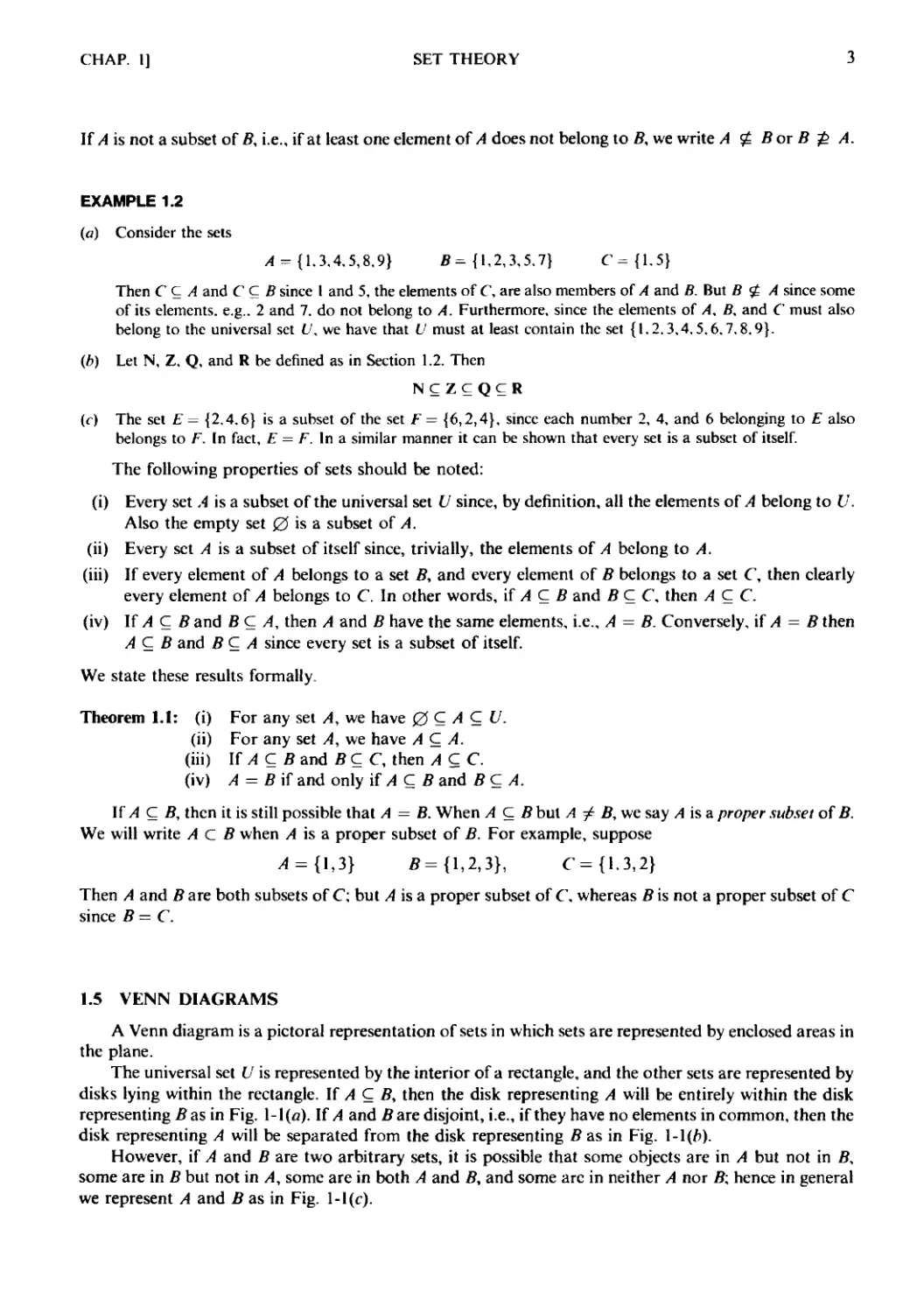
A Venn diagram is a pictoral representation of sets in which sets are represented by enclosed areas in
the plane.
The universal set U is represented by the interior of a rectangle, and the other sets are represented by
disks lying within the rectangle. If А С В, then the disk representing A will be entirely within the disk
representing В as in Fig. l-l(a). If A and В are disjoint, i.e., if they have no elements in common, then the
disk representing A will be separated from the disk representing В as in Fig. l-l(ft).
However, if A and В are two arbitrary sets, it is possible that some objects are in A but not in B,
some are in В but not in A, some are in both A and B, and some are in neither A nor B; hence in general
we represent A and В as in Fig. l-l(c).
SET THEORY
[CHAP. 1
(a) AQB
(b) A and В are disjoint
Fig. 1-1
Arguments and Venn Diagrams
Many verbal statements are essentially statements about sets and can therefore be described by Venn
diagrams.
Hence Venn diagrams can sometimes be used to determine whether or not an argument is valid.
Consider the following example.
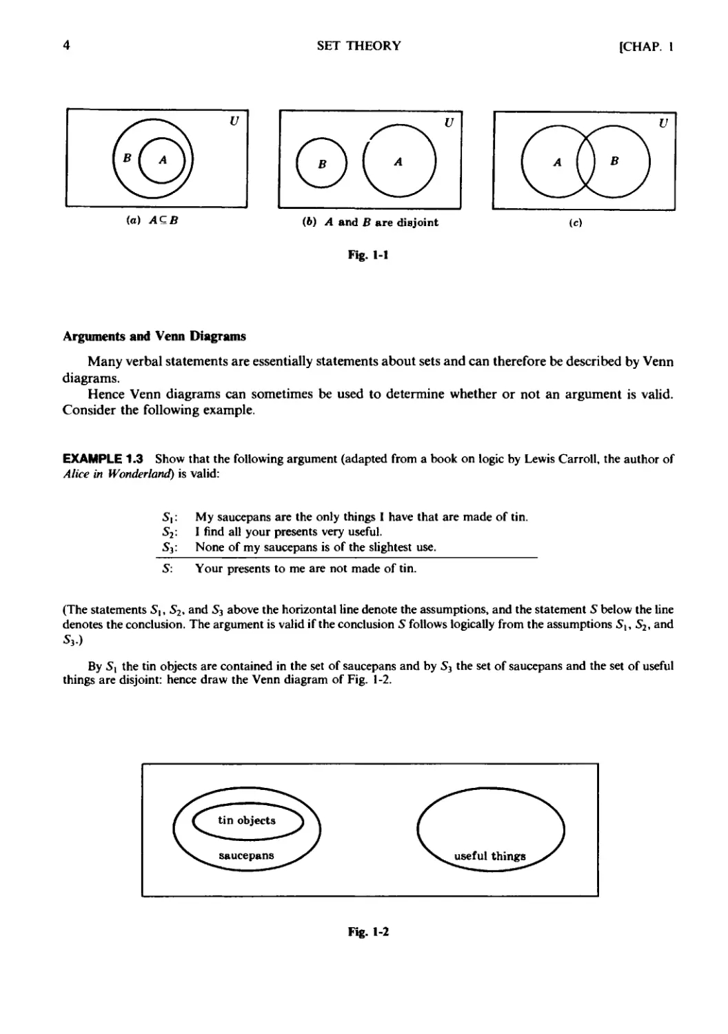
EXAMPLE 1.3 Show that the following argument (adapted from a book on logic by Lewis Carroll, the author of
Alice in Wonderland) is valid:
My saucepans are the only things I have that are made of tin.
I find all your presents very useful.
None of my saucepans is of the slightest use.
S: Your presents to me are not made of tin.
(The statements St, S2, and S3 above the horizontal line denote the assumptions, and the statement S below the line
denotes the conclusion. The argument is valid if the conclusion S follows logically from the assumptions S,, S2, and
S3.)
By S! the tin objects are contained in the set of saucepans and by S3 the set of saucepans and the set of useful
things are disjoint: hence draw the Venn diagram of Fig. I-2.
Fig. 1-2
CHAP. 1]
SET THEORY
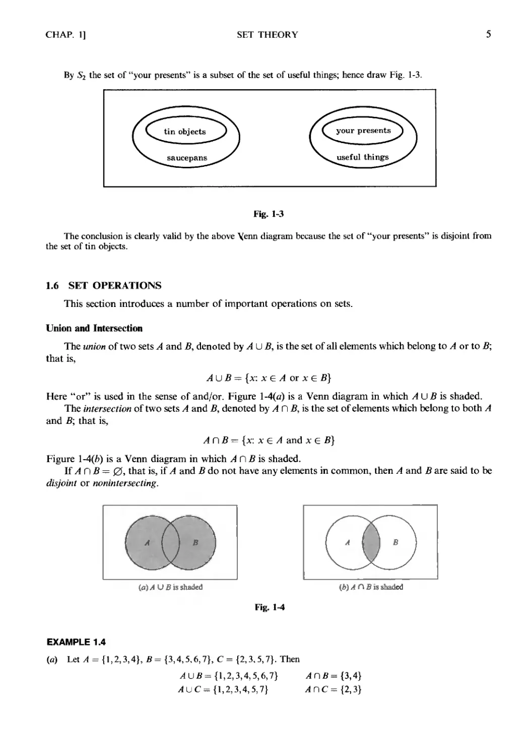
By S2 the set of "your presents" is a subset of the set of useful things; hence draw Fig. 1-3.
Fig. 1-3
The conclusion is clearly valid by the above \enn diagram because the set of "your presents" is disjoint from
the set of tin objects.
1.6 SET OPERATIONS
This section introduces a number of important operations on sets.
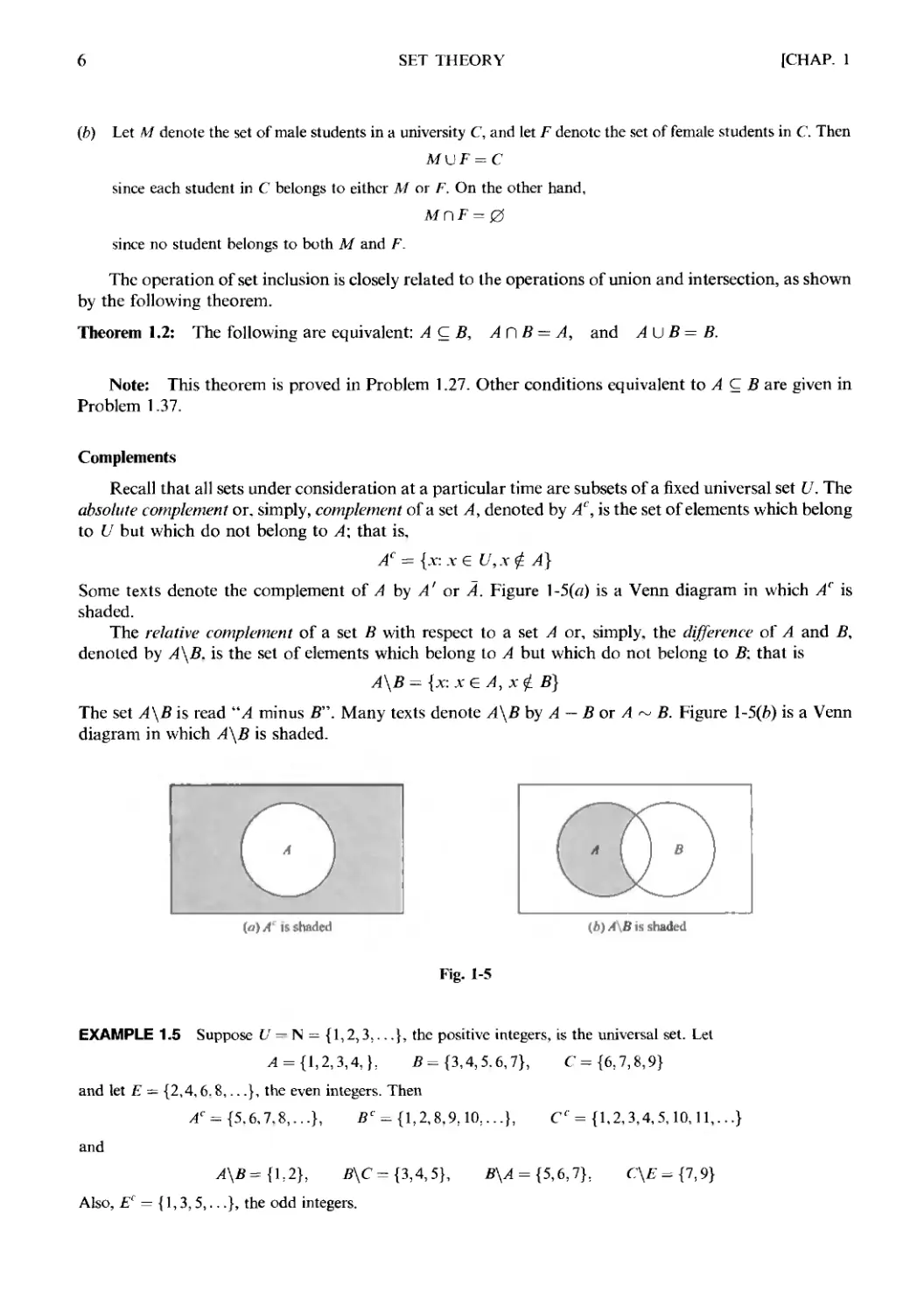
Union and Intersection
The union of two sets A and B, denoted by A U B, is the set of all elements which belong to A or to B;
that is,
A U В = {x: x e A or x G B)
Here "or" is used in the sense of and/or. Figure l-4(a) is a Venn diagram in which A U В is shaded.
The intersection of two sets A and B, denoted by А П B, is the set of elements which belong to both A
and B; that is,
А П В — {x: x e A and x e B)
Figure 1-4F) is a Venn diagram in which А П В is shaded.
If А П В — 0, that is, if A and В do not have any elements in common, then A and В are said to be
disjoint or nonintersecting.
GD
(a)/4 U fl is shaded
(Ь)АГ\В и shaded
Fig. 1-4
EXAMPLE 1.4
(a) Let A = {1,2,3,4}, В = {3,4,5,6,7}, С = {2,3,5,7}. Then
AL)B= {1,2,3,4,5,6,7} ADB={3,4}
A U C= {1,2,3,4,5,7} ЛПС={2,3}
SET THEORY
[CHAP. 1
{b) Let M denote the set of male students in a university C, and let F denote the set of female students in С Then
M U F = С
since each student in С belongs to either M or F. On the other hand,
since no student belongs to both M and F.
The operation of set inclusion is closely related to the operations of union and intersection, as shown
by the following theorem.
Theorem 1.2: The following are equivalent: A<Z B, Af) В = A, and A U В = В.
Note: This theorem is proved in Problem 1.27. Other conditions equivalent to А С В are given in
Problem 1.37.
Complements
Recall that all sets under consideration at a particular time are subsets of a fixed universal set U. The
absolute complement or, simply, complement of a set A, denoted by Ac, is the set of elements which belong
to U but which do not belong to A; that is,
Ac = {x:x? U,xi A}
Some texts denote the complement of A by A' or A. Figure l-5(o) is a Venn diagram in which A' is
shaded.
The relative complement of a set В with respect to a set A or, simply, the difference of A and B,
denoted by A\B. is the set of elements which belong to A but which do not belong to B: that is
= {x:xeA,x? B]
The set A\B is read "A minus B". Many texts denote A\B by A — В or A ~ B. Figure 1-5G?) is a Venn
diagram in which A\B is shaded.
(a) A i shaded
Ь)А В is shaded
Fig. 1-5
EXAMPLE 1.5 Suppose U — N = {1,2,3....}, the positive integers, is the universal set. Let
Л = {1,2,3,4,Ь ?={3,4,5.6,7}, С = {6,7,8,9}
and let E - {2,4,6.8,...}, the even integers. Then
Ac = {5,6,7,8,...}, Bv = {1,2,8,9,10:...}, Cc = {1,2, 3,4, 5,10,11,...}
and
A\B={\,2), B\C = {3,4,5}, B\A = {5,6J}.. C\E = {1,9)
Also, Ec = {1,3,5,...}, the odd integers.
CHAP. 1]
SET THEORY
Fundamental Products
Consider и distinct sets Ау,А2,---,А„. A fundamental product of the sets is a set of the form
where A*t is either At or A\. We note that A) there are 2" such fundamental products, B) any two such
fundamental products are disjoint, and C) the universal set U is the union of all the fundamental
products (Problem 1.64). There is a geometrical description of these sets which is illustrated below.
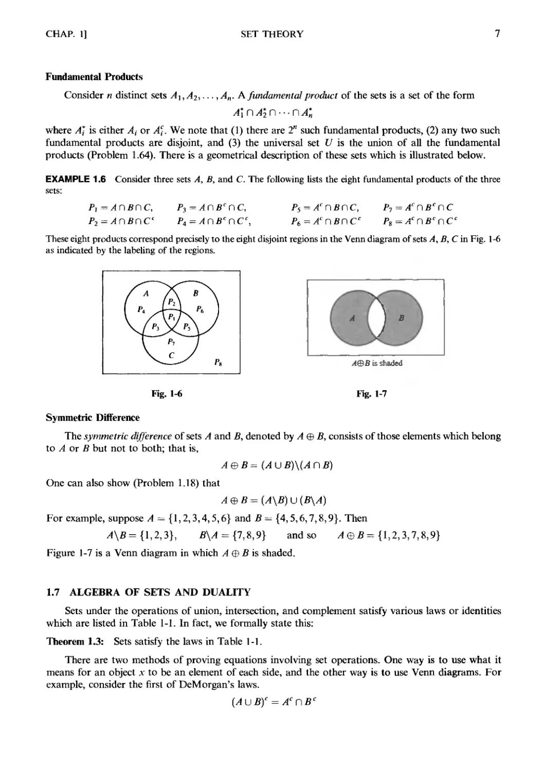
EXAMPLE 1.6 Consider three sets A, B, and C. The following lists the eight fundamental products of the three
sets:
P, = А П В П C,
Р2=АГ\ВПС1
Р3=АПВСПС,
Р5=АСПВПС,
Р6=АСПВПСС
Pi=AcnBcnC<:
These eight products correspond precisely to the eight disjoint regions in the Venn diagram of sets А, В, С in Fig. 1-6
as indicated by the labeling of the regions.
Fig. 1-6
Л©В is shaded
Fig. 1-7
Symmetric Difference
The symmetric difference of sets A and B, denoted by A ® B, consists of those elements which belong
to A or В but not to both; that is,
A © В = {A U B)\(A П B)
One can also show (Problem 1.18) that
A®B = [A\B) U {B\A)
For example, supposed = {1,2,3,4,5,6} and ? = {4,5,6,7,8,9}. Then
A\B= {1,2,3}, B\A = {7,8,9} and so A @B = {1,2,3,7,8,9}
Figure 1-7 is a Venn diagram in which A ® В is shaded.
1.7 ALGEBRA OF SETS AND DUALITY
Sets under the operations of union, intersection, and complement satisfy various laws or identities
which are listed in Table 1-1. In fact, we formally state this:
Theorem 1.3: Sets satisfy the laws in Table 1-1.
There are two methods of proving equations involving set operations. One way is to use what it
means for an object x to be an element of each side, and the other way is to use Venn diagrams. For
example, consider the first of DeMorgan's laws.
{A\JB)C = ACDBC
SET THEORY
[CHAP. 1
Table 1-1 Laws of the algebra of sets
(la)
Ba)
Ca)
Da)
Ea)
Fa)
(8a)
(9a)
A0a)
AUA = A
(A U В) U С = A U (В U С)
AUB-ВиА
A U (В П С) = (A U В) П (A L
ли[/= и
AUAC=U
Uc = 0
(AuBf = АСПВС
Idempotent laws
(lb) АПА = А
Associative laws
Commutative laws
Cb) АГВ = ВГ\А
Distributive laws
Identity laws
Eb) AnU = A
Fb) AC\0=0
Involution laws
(T\ (ACY — A
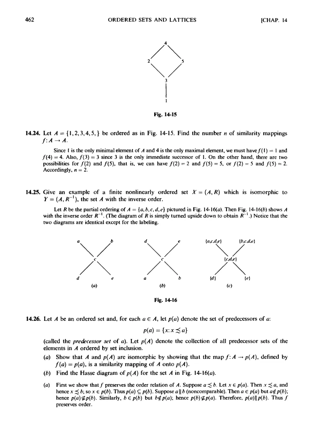
Complement laws
(8b) АПАС = 0
(9b) 0C=U
DeMorgan's laws
A0b) (А П B)c = ACUBC
Method 1: We first show that (A U B)c С /fc n ?c. If x e (A U B)c, then x<?AUB.
Thus xg A and x? B, and so x e Ac and x e Bc. Hence x e Ac П Bc.
Next we show that Ac П Вc С (A U B)c. Let x e Ac П Вc. Then x e Ac
and x e Bc, so x? A and x? B. Hence x? AUB,soxe{AU B)c.
We have proven that every element of (A U B)c belongs to Ac Г\В°
and that every element of Ac П B° belongs to {A U B)c. Together, these
inclusions prove that the sets have the same elements, i.e., that
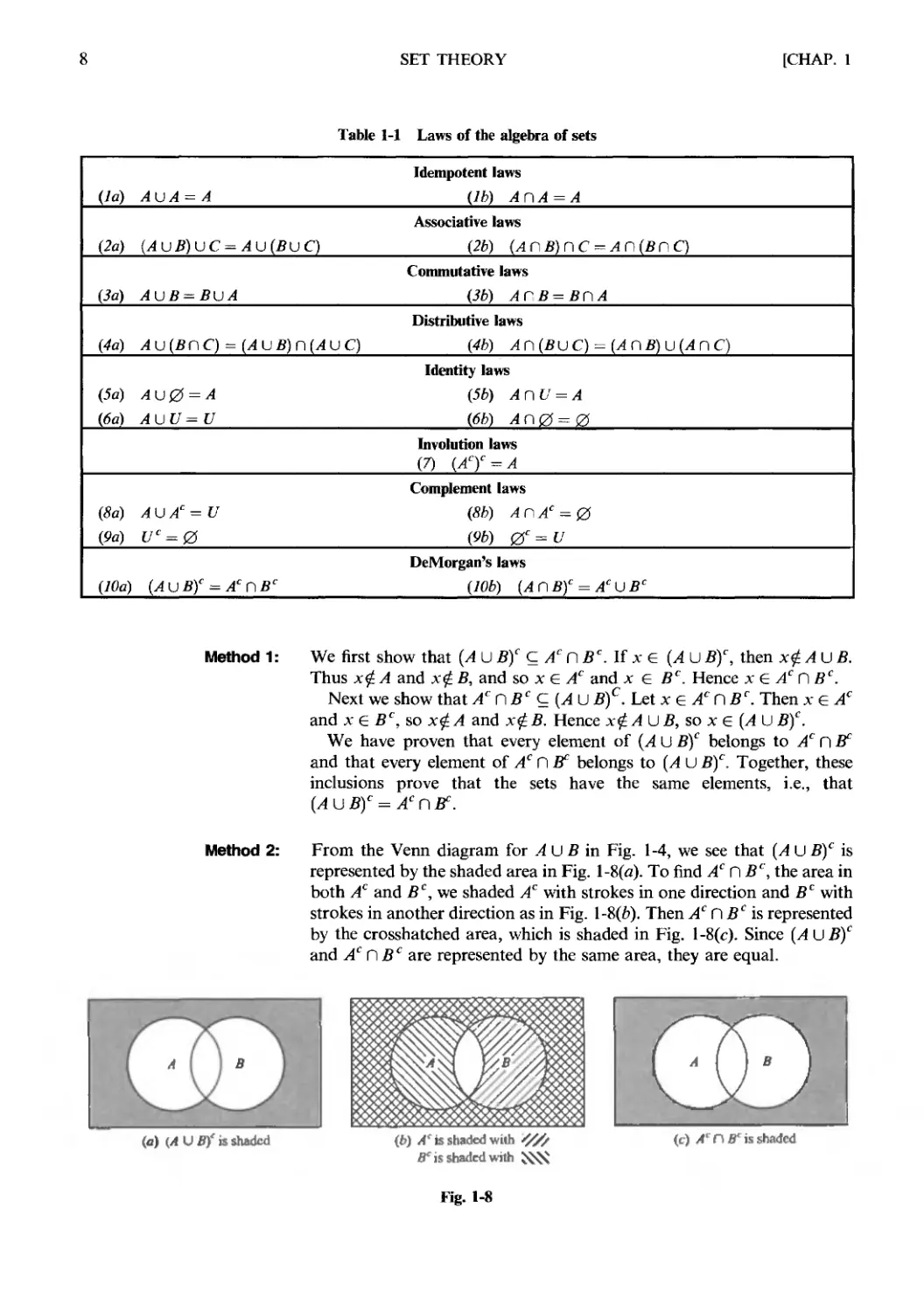
Method 2: From the Venn diagram for A U В in Fig. 1-4, we see that (A U B)c is
represented by the shaded area in Fig. l-8(a). To find Ac П Bc, the area in
both Ac and Bc,v/e shaded Ac with strokes in one direction and Bc with
strokes in another direction as in Fig. 1-8F). Then Ac П Bc is represented
by the crosshatched area, which is shaded in Fig. l-8(c). Since {A UB)C
and Ac П Bc are represented by the same area, they are equal.
(a) {A U В)' is shaded
(fc) A is shaded with
В is shaded with
Fig. 1-8
(c) A C\B is shaded
CHAP. 1]
SET THEORY
Duality
Note that the identities in Table 1-1 are arranged in pairs, as, for example, Ba) and Bb). We now
consider the principle behind this arrangement. Suppose E is an equation of set algebra. The dual E* of
E is the equation obtained by replacing each occurrence of U, П, U, and 0 in E by П, U, 0 and U,
respectively. For example, the dual of
(иг\А)и{ВПА)=А is @UA)n{BUA) = A
Observe that the pairs of laws in Table 1-1 are duals of each other. It is a fact of set algebra, called the
principle of duality, that, if any equation E is an identity, then its dual E* is also an identity.
1.8 FINITE SETS, COUNTING PRINCIPLE
A set is said to be finite if it contains exactly m distinct elements where m denotes some nonnegative
integer. Otherwise, a set is said to be infinite. For example, the empty set 0 and the set of letters of the
English alphabet are finite sets, whereas the set of even positive integers, {2,4,6,...}, is infinite.
The notation n(A) will denote the number of elements in a finite set A. Some texts use #(A), \А\ or
card(i4) instead of n(A).
Lemma 1.4: If A and В are disjoint finite sets, then A U В is finite and
n{A UB) = n(A) + n(B)
Proof. In counting the elements of A U B, first count those that are in A. There are n(A) of these. The
only other elements of A U В are those that are in В but not in A. But since A and В are disjoint, no
element of В is in A, so there are n{B) elements that are in В but not in A. Therefore,
n(A \JB) = n(A) + n(B).
We also have a formula for n(A U B) even when they are not disjoint. This is proved in Problem 1.28.
Theorem 1.5: If A and В are finite sets, then A U В and А П В are finite and
n{A UB) = n{A) + n(B) - n{A П B)
We can apply this result to obtain a similar formula for three sets:
Corollary 1.6: If A, B, and С are finite sets, then so is A U В и С, and
n[A U BU С) = п(А)+п{В) + п(С) - п(А П В) - п(А ПС)- п(ВПС) + п(АПВГ\С)
Mathematical induction (Section 1.10) may be used to further generalize this result to any finite
number of sets.
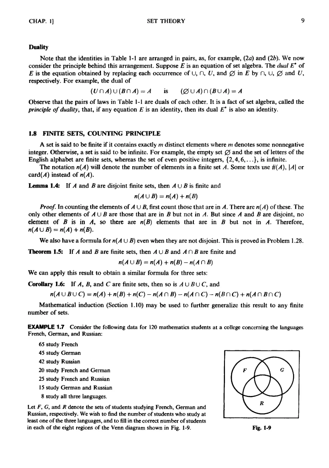
EXAMPLE 1.7 Consider the following data for 120 mathematics students at a college concerning the languages
French, German, and Russian:
65 study French
45 study German
42 study Russian
20 study French and German
25 study French and Russian
15 study German and Russian
8 study all three languages.
Let F, G, and R denote the sets of students studying French, German and
Russian, respectively. We wish to find the number of students who study at
least one of the three languages, and to fill in the correct number of students
in each of the eight regions of the Venn diagram shown in Fig. 1-9. Fig. 1-9
10
SET THEORY
[CHAP 1
n(FnGnR)
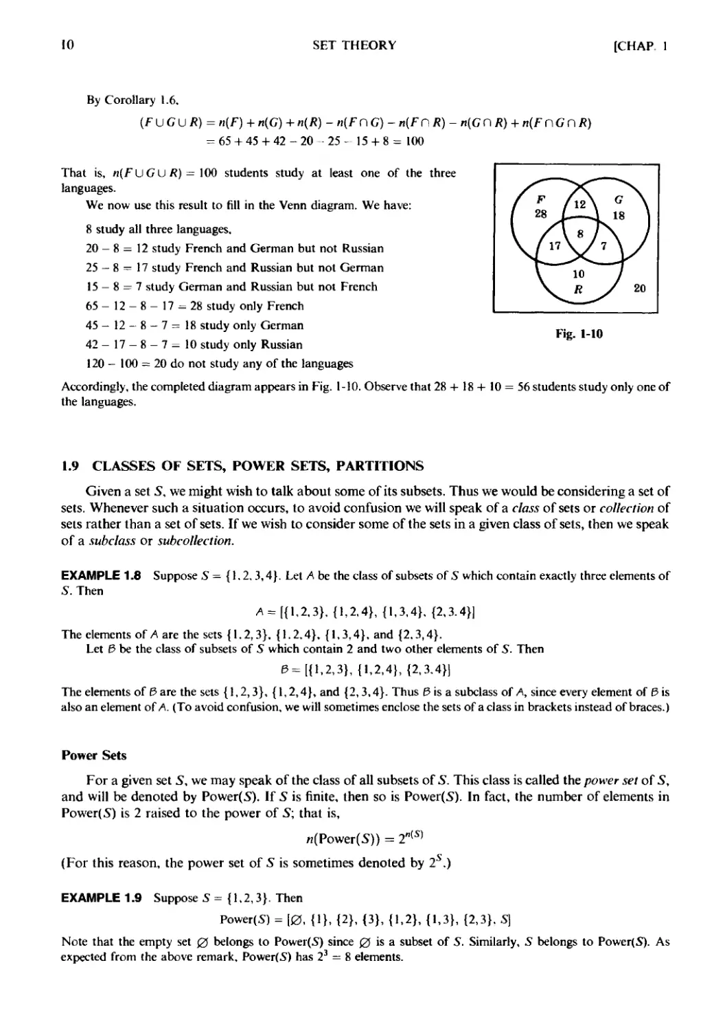
By Corollary 1.6.
(F U С U R) = n(F) + n(G) + n(R) - n(F П G) - n(F DR)-n(Gn1
= 65 + 45 + 42-20 25- 15 + 8=100
That is, n(FuGu/?) = 100 students study at least one of the three
languages.
We now use this result to fill in the Venn diagram. We have:
8 study all three languages.
20 - 8 = 12 study French and German but not Russian
25 - 8 = 17 study French and Russian but not German
15-8 = 7 study German and Russian but not French
65-12-8-17 = 28 study only French
45- 12-8-7= 18 study only German
42- 17-8-7= 10 study only Russian
120 - 100 = 20 do not study any of the languages
Accordingly, the completed diagram appears in Fig. 1-10. Observe that 28 + 18 + 10 = 56 students study only one of
the languages.
fF
1 28
\/
Г
A
17
4
/l2\
к 8 i
V
10
R
» ¦
-«s
G
L *8
7 \
-7
У
)
j
20
Fig. 1-10
1.9 CLASSES OF SETS, POWER SETS, PARTITIONS
Given a set 5, we might wish to talk about some of its subsets. Thus we would be considering a set of
sets. Whenever such a situation occurs, to avoid confusion we will speak of a class of sets or collection of
sets rather than a set of sets. If we wish to consider some of the sets in a given class of sets, then we speak
of a subclass or subcollection.
EXAMPLE 1.8 SupposeS= {1.2.3,4}. Let A be the class of subsets of S which contain exactly three elements of
S. Then
Л = [{1,2,3}, {1,2,4}, {1,3,4}, {2,3.4}]
The elements of A are the sets {1.2,3}, {1.2.4}, {1,3,4}, and {2.3,4}.
Let 3 be the class of subsets of S which contain 2 and two other elements of S. Then
0= [{1,2,3}, {1,2,4}, {2,3.4}]
The elements of б are the sets {1,2,3}, {1,2,4}, and {2,3,4}. Thus Pisa subclass of A, since every element of Pis
also an element of A. (To avoid confusion, we will sometimes enclose the sets of a class in brackets instead of braces.)
Power Sets
For a given set 5, we may speak of the class of all subsets of S. This class is called the power set of 5,
and will be denoted by Power(S). If 5 is finite, then so is Power(S). In fact, the number of elements in
Power(S) is 2 raised to the power of S; that is,
/j(PowerE)) = 2"(S)
(For this reason, the power set of 51 is sometimes denoted by 2s.)
EXAMPLE 1.9 Suppose S = {1,2,3}. Then
Power(S) = [0, {1}, {2}, {3}, {1,2}, {1,3}, {2,3}. S)
Note that the empty set 0 belongs to Power(S) since 0 is a subset of S. Similarly, S belongs to Power(S). As
expected from the above remark, Power(S) has 23 = 8 elements.
CHAP. 1]
SET THEORY
II
Partitions
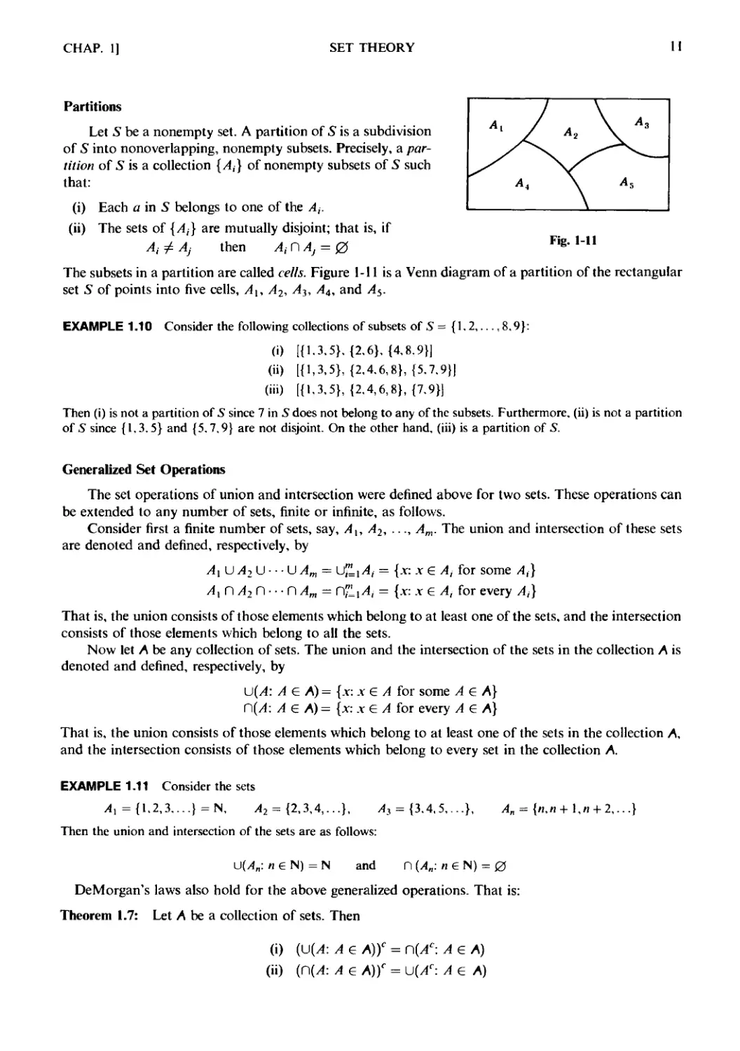
Let S be a nonempty set. A partition of S is a subdivision
of S into nonoverlapping, nonempty subsets. Precisely, a par-
partition of S is a collection {Д} of nonempty subsets of 5 such
that:
(i) Each a in 5 belongs to one of the At.
(ii) The sets of {Aj} are mutually disjoint; that is, if
At ф Aj then At DAj = 0
Fig. 1-11
The subsets in a partition are called cells. Figure 1-11 is a Venn diagram of a partition of the rectangular
set S of points into five cells, A\, A2, Л3, Ал, and As.
EXAMPLE 1.10 Consider the following collections of subsets of S = {1.2 8.9}:
(i) [{1.3.5}, {2,6}, {4,8.9}]
(ii) [{1,3,5}, {2,4.6,8}, {5.7.9}]
(iii) [{1.3,5}, {2,4,6,8}, {7.9}]
Then (i) is not a partition of S since 7 in S does not belong to any of the subsets. Furthermore, (ii) is not a partition
of S since {1.3.5} and {5.7.9} are not disjoint. On the other hand, (iii) is a partition of 5.
Generalized Set Operations
The set operations of union and intersection were defined above for two sets. These operations can
be extended to any number of sets, finite or infinite, as follows.
Consider first a finite number of sets, say, Ax, A2, ..., Am. The union and intersection of these sets
are denoted and defined, respectively, by
Ax U A2 U • • • U Am = U™ ,Л, = {.v: .v G A, for some Л,}
Ax П А2 П • • • П Am = C\ZiA, = {.v: .v G A, for every Aj}
That is, the union consists of those elements which belong to at least one of the sets, and the intersection
consists of those elements which belong to all the sets.
Now let A be any collection of sets. The union and the intersection of the sets in the collection A is
denoted and defined, respectively, by
U(v4: A G A) = {x: x G A for some A e A}
C\{A: A & A)— {x: x G A for every A € A}
That is, the union consists of those elements which belong to at least one of the sets in the collection A,
and the intersection consists of those elements which belong to every set in the collection A.
EXAMPLE 1.11 Consider the sets
/4, ={1.2,3....} =N, A2 = {2,3,4,...},
Then the union and intersection of the sets are as follows:
= {3.4,5,...}, А„ = {п,п +
U{An: n ? N) = N and П {А„: n € N) = 0
DeMorgan's laws also hold for the above generalized operations. That is:
Theorem 1.7: Let A be a collection of sets. Then
(i) (и(Л: A € A))c = П{АС: A G A)
(ii) (П(у4: A g A))c = U(AC: A G A)
12 SET THEORY [CHAP. 1
1.10 MATHEMATICAL INDUCTION
An essential property of the set
N = {1,2,3,...}
which is used in many proofs, follows:
Principle of Mathematical Induction I: Let P be a proposition defined on the positive integers N, i.e.,
P(n) is either true or false for each и in N. Suppose P has the following two properties:
(i) P{ 1) is true.
(ii) P(n + 1) is true whenever P(n) is true.
Then P is true for every positive integer.
We shall not prove this principle. In fact, this principle is usually given as one of the axioms when N
is developed axiomatically.
EXAMPLE 1.12 Let Я be the proposition that the sum of the first n odd numbers is и2; that is,
P(n): I + 3 + 5 + ... + Bn- \)=n2
(The nth odd number is In - 1, and the next odd number is 2n+ 1). Observe that P(n) is true for n = 1, that is,
P(\): 1 = I2
Assuming P(n) is true, we add 2n + 1 to both sides of P(n), obtaining
1 + 3 + 5 + ... + Bn- 1) + Bи + 1) = л2 + Bи+ 1) = (и+ IJ
which is P(n + 1). That is, P(n + 1) is true whenever P(n) is true. By the principle of mathematical induction, P is
true for all n.
There is a form of the principle of mathematical induction which is sometimes more convenient to
use. Although it appears different, it is really equivalent to the principle of induction.
Principle of Mathematical Induction II: Let P be a proposition defined on the positive integers N such
that:
(i) P{\) is true.
(ii) P{ri) is true whenever P(k) is true for all 1 < Ar < n.
Then P is true for every positive integer.
Remark: Sometimes one wants to prove that a proposition P is true for the set of integers
{a, a+ I, я + 2,...}
where a is any integer, possibly zero. This can be done by simply replacing 1 by a in either of the above
Principles of Mathematical Induction.
Solved Problems
SETS AND SUBSETS
1.1. Which of these sets are equal: {r, t,s), {s, t, r,s}, {t,s, t,r}, [s,r,s,t}l
They are all equal. Order and repetition do not change a set.
CHAP. 1] SET THEORY 13
1.2. List the elements of the following sets; here N = {1,2,3,...}.
(a) A = {x:xeN,3<x< 12}
(b) В = {x: x G N, x is even, x < 15}
(f) C={.v:.veN,4 + x=3}.
(a) A consists of the positive integers between 3 and 12; hence
A = {4,5,6,7,8,9,10,11}
(b) В consists of the even positive integers less than 15; hence
В ={2,4.6,8,10,12.14}
(c) There are no positive integers which satisfy the condition 4 + x = 3; hence С contains no elements. In
other words, С = 0, the empty set.
1.3. Consider the following sets:
0, Л = {1}, В={\,3}, C= {1,5,9}, D= {1,2,3,4,5},
?={1,3,5,7,9}, (/={1,2,...,8,9}
Insert the correct symbol С or ^ or between each pair of sets:
(a) 0,A (r) B,C («?) C,D (g) D,E
(b) А, В id) В, Е (/) С, Е (Л) D, U
(fi) 0C/4 because 0 is a subset of every set.
(b) А С В because 1 is the only element of A and it belongs to B.
(c) В ? С because 3 e В but 3 g С
(d) В ? E because the elements of В also belong to E.
(e) Cg D because 9 G С but 9 $. D.
(/) С С E because the elements of С also belong to E.
(g) DgE because 2 e D but 2 ? E.
(A) D С U because the elements of D also belong to V.
1.4. Show that A = {2,3,4,5} is not a subset of В = {x: x G N, x is even}.
It is necessary to show that at least one element in A does not belong to B. Now 3 G A and, since В
consists of even numbers, 3 ? B\ hence /4 is not a subset of A
1.5. Show that A = {2,3,4,5} is a proper subset of С = {1,2,3,..., 8,9}.
Each element of A belongs to С so А С С. On the other hand, 1 e С but \ ? A. Hence
Therefore Л is a proper subset of C.
SET OPERATIONS
Problems 1.6 to 1.8 refer to the universal set U = {1,2,..., 9} and the sets
A = {1,2,3,4,5}, C= {5,6,7,8,9}, ?={2,4,6,8}
?={4,5,6,7}, D= {1,3,5,7,9}, F= {1,5,9}
14 SET THEORY [CHAP. 1
1.6. Find:
(a) A U В and A n В (с) A U С and А П С (е) ? и ? and ? П ?
(b) BuDandBHD {d) DU E and DtlE (/) DU F and DP F
Recall that the union Л" и Y consists of those elements in cither X or Y (or both), and that the
intersection X n К consists of those elements in both X and У.
@) AUB = {1.2.3.4,5,6.7} ЛПВ={4,5}
(A) BUD= {1.3.4.5.6.7,9} finD = {5,7}
(<•) /fuf= {1,2.3,4.5.6,7,8,9} = U АПС={5]
(d) DnE = {1.2.3,4,5,6,7,8,9} = U DnE = 0
(f) ?u? = {2,4,6,8} = ? ?n? = {2.4.6,8} =E
(/) DUF= {1.3,5.7.9} =D DnF=(l,5.9} = F
Observe that F С Z); so by Theorem 1.2 we must have D U F = D and D П F = F.
1.7. Find: (a) A', Bl\ Dc, Ec; (b) A\B, B\A, D\E, F\D- (с) А © В, Сф?>, ?&F.
Recall that:
A) The complement Л" consists of those elements in the universal set U which do not belong to X.
B) The difference X\ Y consist of the elements in X which do not belong to Y.
C) The symmetric difference X Ф Y consists of the elements in A" or in Y but not in both X and Y.
Therefore:
(a) A1 = {6.7.8,9}; Bl = {1,2, 3.8,9};/)'= {2,4,6.8} = ?; ?' = {1,3. 5, 7,9} = D.
(b) A\B= {1.2.3}; B\A = {6.7}; D\E = {1.3.5.7.9} = D: F\D = 0.
(c) Л J-Д = {1.2.3,6,7}; C®D = {1.3.8.9}; ?ф?= {2.4.6.8. 1.5.9} = ?u?.
1.8. Find: (а) АП(ВиЕ); (b) {A\E)C\
(c) {AnD)\B; (d) (BnF)U(CtlE).
(a) First compute В U ? = {2.4, 5.6.7.8}. Then /1 П (B U ?) = {2.4. 5}.
(b) A\E= {1,3.5}. Then (A\Ef = {2.4,6,7,8.9}.
(c) AHD= {1.3.5}. Now (А П Z))\B = {1.3}.
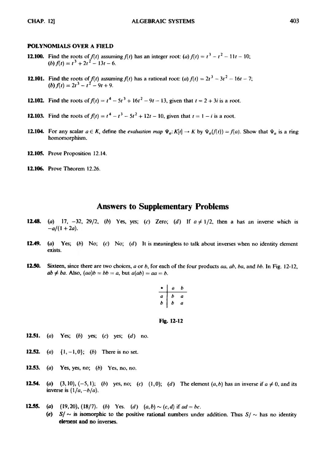
(d) BnF= {5} and Cn?= {6,8}. So (fin F) U (fn ?) = {5.6,8}.
1.9. Show that we can have А П В = Л П С without В = С.
Let A = {1.2}, Д= {2.3}, and С= {2.4}. Then А П В = {2} and А П С = {2}. Thus ,4 П В = Л П С
but В ф С.
VENN DIAGRAMS
1.10. Consider the Venn diagram of two arbitrary sets A and В in Fig. l-l(r). Shade the sets:
{а) АПВ1; {b) (B\A)C.
(a) First shade the area represented by A with strokes in one direction (///), and then shade the area
represented by Bc (the area outside B), with strokes in another direction (\\\). This is shown in Fig.
\-\2(u). The cross-hatched area is the intersection of these two sets and represents А Г\ В' and this is
shown in Fig. 1-12(Л). Observe that А П Bl = A\B. In fact. A\B is sometimes defined to be А П B'.
CHAP. 1]
SET THEORY
15
(a) A and ff are shaded
F) А П81 is shaded
Fig. 1-12
(b) First shade the area represented by B\A (the area of В which does not lie in A) as in Fig. 1-13(д). Then
the area outside this shaded region, which is shown in Fig. 1-13F), represents {B\A)C.
(а) В A is haded F) (B A) is shaded
Fig. 1-13
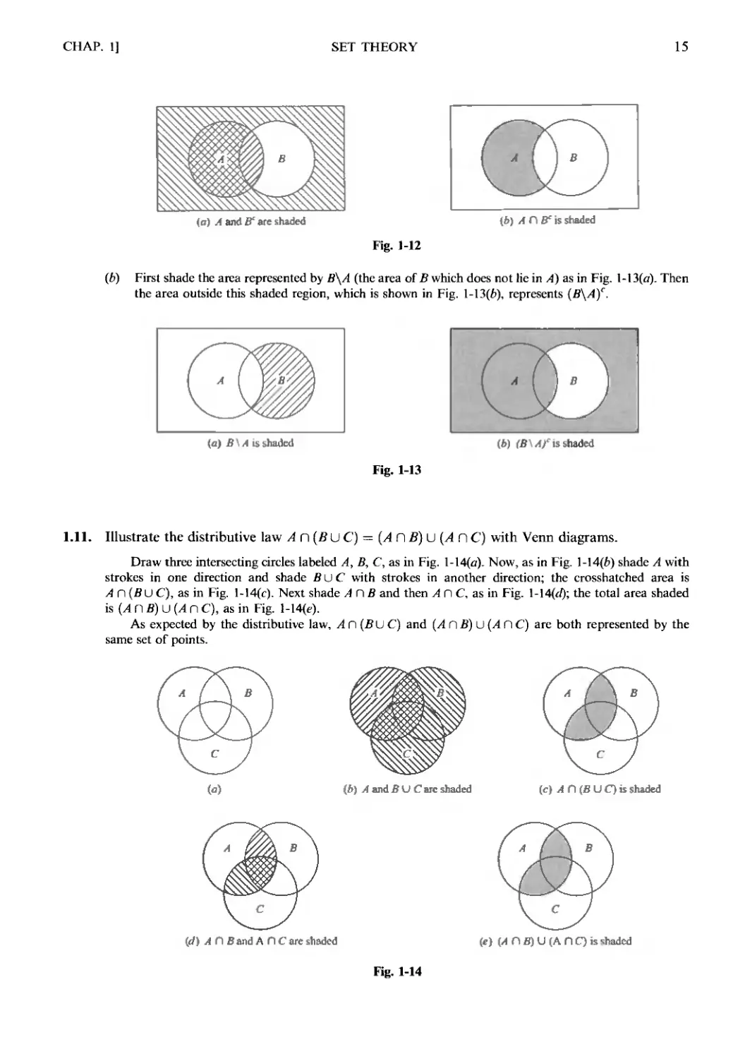
1.11. Illustrate the distributive law ^n(BUC)-(^nfi)U(/lnC) with Venn diagrams.
Draw three intersecting circles labeled А, В, С, as in Fig. 1-14(д). Now, as in Fig. 1-14F) shade A with
strokes in one direction and shade fluC with strokes in another direction; the crosshatched area is
А П {B U С), as in Fig. l-14(c). Next shade ^nfl and then А П C, as in Fig. l-14(d); the total area shaded
is (А n B) U {A n C), as in Fig. l-14(e).
As expected by the distributive law, An{BuC) and (АпВ)и(АП С) are both represented by the
same set of points.
b) A and В U Care shaded
(с) А П BUQbshaded
П Band А П С are shaded
(с) (Л П B) U (А П C) is shaded
Fig. 1-14
16
SET THEORY
[CHAP. 1
1.12. Determine the validity of the following argument:
Si: All my friends are musicians.
S2: John is my friend.
S3: None of my neighbors are musicians.
S: John is not my neighbor.
The premises St and S3 lead to the Venn diagram in Fig. 1-15. By S2, John belongs to the set of friends
which is disjoint from the set of neighbors. Thus S is a valid conclusion and so the argument is valid.
Fig. 1-15
FINITE SETS AND THE COUNTING PRINCIPLE
1.13. Determine which of the following sets are finite.
(a) A = {seasons in the year} (d) D = {odd integers}
(b) В = {states in the Union} (e) E = {positive integral divisors of 12}
(c) С = {positive integers less than 1} (/) F = {cats living in the United States}
(a) A is finite since there are four seasons in the year, i.e., n(A) = 4.
(b) В is finite because there are 50 states in the Union, i.e. n(B) = 50.
(c) There are no positive integers less than 1; hence С is empty. Thus С is finite and n(C) = 0.
(d) D is infinite.
(e) The positive integer divisors of 12 are 1, 2, 3, 4, 6, and 12. Hence E is finite and n{E) = 6.
(/) Although it may be difficult to find the number of cats living in the United States, there is still a finite
number of them at any point in time. Hence F is finite.
1.14. In a survey of 60 people, it was found that:
25 read Newsweek magazine
26 read Time
26 read Fortune
9 read both Newsweek and Fortune
11 read both Newsweek and Time
8 read both Time and Fortune
3 read all three magazines
(a) Find the number of people who read at least one of the three magazines.
(b) Fill in the correct number of people in each of the eight regions of the Venn diagram in Fig.
l-16(cr) where JV, T, and F denote the set of people who read Newsweek, Time, and Fortune,
respectively.
CHAP. 1]
SET THEORY
17
(c) Find the number of people who read exactly one magazine.
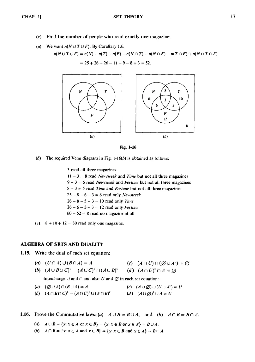
(a) We want n(N U T U F). By Corollary 1.6,
n(NL)TuF) = n(N) + n(T) + n(F) - n(N П T) - n(N П F) - n(T П F) + n(N n Г П F)
= 25 + 26 + 26 - 11 - 9 - 8 + 3 = 52.
V 8 /
\( 6
V
, 3 i
У
12
К
5
^\
T
10
v
7
/
8
(*)
Fig. 1-16
{b) The required Venn diagram in Fig. l-16(b) is obtained as follows:
3 read all three magazines
11-3 = 8 read Newsweek and Time but not all three magazines
9 — 3 = 6 read Newsweek and Fortune but not all three magazines
8 — 3 = 5 read Time and Fortune but not all three magazines
25 — 8 — 6 — 3 = 8 read only Newsweek
26-8-5-3= 10 read only Time
26-6-5 — 3= 12 read only Fortune
60 - 52 = 8 read no magazine at all
(c) 8 + 10 + 12 = 30 read only one magazine.
ALGEBRA OF SETS AND DUALITY
1.15. Write the dual of each set equation:
(a) (ипА)и(ВПА) = А (с) (А П U) П @ U Ac) - 0
(b) (AUBUCy = (AuC)cn(AUB)c (d) (AnU)cnA = 0
Interchange U and n and also U and 0 in each set equation:
(a) @UA)n(BL)A) = A (c) (A U0) U (U ПАс) = U
(b) (АПВПСУ = (АПС)си(АПВ)с (d) {A U 0)c U A = U
1.16. Prove the Commutative laws: (a) A U В = В U A, and (fe) АГ\В= ВПА.
(a) AU В = {x: x e A or x e B} = {x: x e В or x e A} = BU A.
(b) А П В = {x: x e A and x e B} = {*: л: € В and л: e A} = В П /4.
18 SET THEORY [CHAP. I
1.17. Prove the following identity. (AUB)n(AUBc) = A.
Statement Reason
1. (AUB)n(AUBc) = AU(BC\BC) Distributive law
2. fin Bc = 0 Complement law
3. (AVB)n(AUBc) = AU0 Substitution
4. A U 0 = A Identity law
5. {A U В) П {A U Bc) = A Substitution
1.18. Prove {A U B)\{A nfi) = (A\B) U (B\A). (Thus either one may be used to define A ® B.)
Using X\Y = X П Ус and the laws in Table 1-1, including DeMorgan's laws, we obtain:
(-4 U B)\(A ПВ) = (АиВ)П(АП B)c = {A U В) П (/4f U fif)
= (/in/)u(/infic)u(fln/)u(finfic)
= 0L)(AnBc)U{BOAc)\J0
= (АПВ1)и(ВП Ac) = (Л\Д) U
CLASSES OF SETS
1.19. Find the elements of the set A = [{1,2,3}, {4,5}, {6,7,8}].
A is a class of seis; its elements are the sets {1,2,3}, {4,5}, and {6,7,8}.
1.20. Consider the class A of sets in Problem 1.19. Determine whether each of the following is true or
false:
(a) 1 e A (c) {6,7,8} € A (e) 0 € A
(b) {1,2,3} С A (d) {{4,5}} С A (fHCA
(a) False. 1 is not one of the elements of A.
(A) False. {1.2,3} is not a subset of A; it is one of the elements of A.
(c) True. {6,7,8} is one of the elements of A.
(d) True. {{4, 5}}, the set consisting of the element {4, 5}, is a subset of A.
(e) False. The empty set is not an element of A, i.e., it is not one of the three sets listed as elements of A.
(/) True. The empty set is a subset of every set; even a class of sets.
1.21. Determine the power set Power(/4) of A — {a,b,c,d}.
The elements of Power(^) are the subsets of A. Hence
Power(/4)=[/4,{a,*,c}, {a,b,d}, {a,c,d}, {b,c,d}, {a,b}, {o,c},
{a,d}, {*,c}, {b,d}, {c,d}, {«}, {*}, {c}. [d},0]
As expected, Power(v4) has 24 = 16 elements.
1.22. Let 5 = {red, blue, green, yellow}. Determine which of the following is a partition of 5:
(a) P\ = [{red}, {blue, green}]. (c) P^ = [0, {red, blue}, {green, yellow}].
(b) P2 = [{red, blue, green, yellow}]. (d) Рл = [{blue}{red, yellow, green}.
CHAP. 1] SET THEORY 19
(a) No, since yellow does noi belong to any cell.
(b) Yes, since P2 is a partition of S whose only element is S itself.
(c) No, since the empty set 0 cannot belong to a partition.
(d) Yes, since each element of S appears in exactly one cell.
1.23. Find all partitions of 5 = {1,2,3}.
Note that each partition of S contains either 1, 2. or 3 cells. The partitions for each number of cells are
as follows:
A): [S\
B): [{1}. {2.3}]. [{2}. {1,3}]. [{3}. {1, 2}]
C): [{1}, {2}, {3}]
Thus we see that there are five different partitions of S.
MISCELLANEOUS PROBLEMS
1.24. Prove the proposition P that the sum of the first и positive integers is \n(n + 1); that is,
2
The proposition holds for n = 1 since
P{\) : 1 =|A)A + 1)
Assuming P(n) is true, we add n + 1 to both sides of P(n). obtaining
1 + 2 + 3 + ... + и + (и + 1) = i//(n + 1) + (/i -t- 1)
which is P(n + 1). That is, P(n + I) is true whenever P{n) is true. By the principle of induction, P is true for
all n.
1.25. Prove the following proposition (for n > 0):
P(n): 1 +2+22 + 23+ •¦ +2" = 2"*' - 1
P@) is true since 1 = 21 — 1. Assuming P(n) is true, we add 2"~' to both sides of P(n). obtaining
1 + 21 + 22 + • ¦ ¦ -t 2" -t 2"'' = 2"'' - 1 + I'
= 2B"")-l
which is Р(и + 1). Thus P(n + 1) is true whenever P(n) is true. By the principle of induction. P is true for all
n > 0.
1.26. Prove: {AD В) С А С (AU B) and (Л П В) С Д С (Л и В).
Since every element in А П Д is in both A and fi, it is certainly true that if .v e (-4 П B) then .v e -4: hence
(/fnfl)C A. Furthermore, if .v 6 A, then ,v 6 (^ U Д) (by the definition of AVJ B),so A Q(Ali B). Putting
these together gives {АПВ)САС(Аи В). Similarly, (АПВ)СВС(Аи В).
20 SET THEORY [CHAP. 1
1.27. Prove Theorem 1.2: The following are equivalent: А С В, А П В — A, and А и В = В.
Suppose А С В and let х е A. Then х е В, hence х е АПВ and /4 С А П Д. By Problem 1.26,
(/1 п В) С A. Therefore А п В = A. On the other hand, suppose АПВ = A and let x e A. Then
-v 6 (/1 П B), hence .v e A and x 6 B. Therefore, -4 С В. Both results show that А С В is equivalent to
АПВ = А.
Suppose again that А С В. Let л: e (A U B). Then x 6 /1 or x 6 B. If x G /4, then .v e В because /4 С В.
In either case, xefi. Therefore А и В С В. By Problem 1.26, fiC^Ufl. Therefore /lufl = fi. Now sup-
suppose Аи В = В and let x e A. Then x e /1 U В by definition of union sets. Hence x ? В = Аи В. Therefore
А С В. Both results show that А С В is equivalent to A U В = В.
Thus /1С В, /4ПВ=-4 and A U В = В are equivalent.
1.28. Prove Theorem 1.5: If Л and В are finite sets, then AUB and Л п В are finite and
n(A UB)= n(A) + n{B) - n(A П B)
If A and В are finite, then clearly An В and A U В are finite.
Suppose we count the elements of A and then count the elements of B. Then every element in А П В
would be counted twice, once in A and once in B. Hence
n(A U B) = n(A) + n(B) - n(A П B)
Alternatively, (Problem 1.36) A is the disjoint union of A\B and /1 n В, В is the disjoint union of В\Л
and АП B, and A U В is the disjoint union of A\B, А П B, and B\/4. Therefore, by Lemma 1.4,
n{A U В) = и(/4\В) + и(/4 П В) + и(В\/4)
= п(А\В) + и(Л П В) + и(В\/4) + п{А П В) - п{А П В)
= п(А) + п(В) - п(А П В)
Supplementary Problems
SETS AND SUBSETS
1.29. Which of the following sets are equal?
/4 = {.v:.v2-4.v + 3 = O}, С = {x: x g N,x < 3}, ?={l,2}, С ={3,1}
B={x: л2-Зх + 2 = 0}, ?={x:xeN,xisodd,x<5}, F={1,2,1}, //={1,1,3}
1.30. List the elements of the following sets if the universal set is t/ = {a,b,c,... ,y,z}. Furthermore, identify
which of the sets, if any, are equal.
A = {x: x is a vowel) С = {x: x precedes f in the alphabet}
В = {.v: .V is a letter in the word "little") D = {x: x is a letter in the word "title"}
1.31. Let A = {1,2 8,9}, B= {2,4,6,8}, C= {1,3,5,7,9}, D= {3,4,5}, ?={3,5}.
Which of the above sets can equal a set X under each of the following conditions?
(a) X and В are disjoint. (c) X С A but X<? С
(b) XC DbulX?B. (d) А'С С but X?A.
SET OPERATIONS
Problems 1.32 to 1.34 refer to the sets t/= {1,2,3,...,8,9} and A = {1,2,5,6}, B= {2,5,7}, C= {1,3,5,7,9}.
CHAP. 1]
SET THEORY
21
1.32. Find: (а) АПВ and А n C; (*) /4 и В and Д U С; (с) Лг and Cr.
1.33. Find: (a) /4\fi and A\C; (*) /feB and /4 ф С.
1.34. Find: (a) (AUC)\B; (b) (AUB)C; (c)
1.35. Let A = {o,*,c,4e}, fi = {в
Find:
(a) AUB (d) AH(BUD)
(*) fifiC (c) A(CUZ))
(с) C\D (Л (AHD)UB
. С = {blC,e,g,h}, D = {d,ej,g,h}.
(g) {AUD)\C (/) А Ф fi
(Л) BHCnD (к) A eC
(,) (C\A)\D (I) (A ® D)\B
1.36. Let A and В be any sets. Prove:
(a) /1 is the disjoint union of A\B and Л П В.
(*) /IUB is the disjoint union of A\B, АПВ, and B\A.
1.37. Prove the following:
(а) А С В if and only if А П Дf = 0.
(*) /4 С fi if and only if Ac U fi = U.
(c) AC В if and only if Bc С Лг.
(^/) /1 С fi if and only if A\B = 0.
(Compare results with Theorem 1.2.)
1.38. Prove the Absorption laws: (a) A U (А П B) = A; {b) А П (-4 U Д) = /1.
1.39. The formula Л\.в = А П fic defines the difference operation in terms of the operations of intersection and
complement. Find a formula that defines the union /4 и fi in terms of the operations of intersection and
complement.
VENN DIAGRAMS
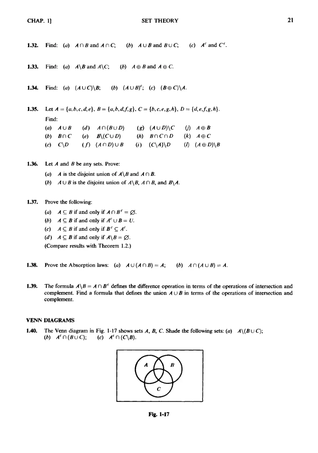
1.40. The Venn diagram in Fig. 1-17 shows sets А, В, С Shade the following sets: (a) A\(BuC);
(b) /fl(BuC); (с) АСП(С\В).
Fig. 1-17
22 SET THEORY [CHAP.
1.41. Use the Venn diagram Fig. 1-6 and Example 1.6 to write each set as the (disjoint) union of fundamental
products:
(а) АП(ВЬС), (/>) А'П(ВиС), [с) AU{B\C).
1.42. Draw a Venn diagram of sets А, В, С where А С B. sets В and С are disjoint, but A and С have elements in
common.
ALGEBRA OF SETS AND DUALITY
1.43. Write the dual of each equation:
(a) A U В = (В' П A')' ib) A = (Вс П A) U (А Г) В)
(с) Аи(АПВ) = A (d) (АО В) U (А' П B)U{AD В')U(A' ПВ') = U
1.44. Use the laws in Table 1-1 to prove each set identity:
(а) (АПВ)и{АГ\Вс) = А.
(Л) A U (Л П Д) = A.
(c) A\JB=(AC\B')\J{AlC\B)U(AC\B).
FINITE SETS AND THE COUNTING PRINCIPLE
1.45. Determine which of the following sets are finite:
(a) The set of lines parallel to the x axis
(b) The set of letters in the English alphabet
(c) The set of numbers which are multiples of 5
id) The set of animals living on the earth
(?) The set of numbers which are solutions of the equation:
л:7 + 26л18 - 17л" + 7л' - 10 = 0
(/) The set of circles through the origin @, 0)
1.46. Use Theorem 1.5 to prove Corollary 1.6: If A, B, and С are finite sets, then so is Аи Ви С and
n(A U BU C) = n(A) -i- n(B) + n{C) -п(АПВ) -п(АПС) - п(ВП С) + п(А Г) Вп С)
1.47. A survey on a sample of 25 new cars being sold at a local auto dealer was conducted to see which of three
popular options, air-conditioning (A), radio (Л), and power windows (W). were already installed. The
survey found:
15 had air-conditioning.
12 had radio.
11 had power windows.
5 had air-conditioning and power windows.
9 had air-conditioning and radio.
4 had radio and power windows.
3 had all three options.
Find the number of cars that had: (a) only power windows; (b) only air-conditioning; (<¦) only radio; (d)
radio and power windows but not air-conditioning; (e) air-conditioning and radio, but not power windows;
and (/) only one of the options; (g) at least one option; (A) none of the options.
CHAP. 1] SET THEORY 23
CLASSES OF SETS
1.48. Find the power set Power(-4) of A = {1.2.3.4.5}.
1.49. Given A = [{a, A}, {c}, {d,ej}\.
(a) State whether each of the following is true or false:
(i) деЛ, (ii) {c}QA, (iii) {d,e,f} 6 A. (iv) {{a,b}} С A, (v) 0 С A.
(b) Find the power set of A.
1.50. Suppose A is a finite set and n(A) = m. Prove that Power(-4) has 2"' elements.
PARTITIONS
1.51. Let X = {1,2,..., 8,9}. Determine whether or not each of the following is a partition of A':
(a) [{1,3,6}. {2,8}, {5,7,9}] (c) [{2,4, 5,8}, {1,9}, {3,6. 7}]
(*) [{1,5,7}, {2,4,8,9}, {3,5,6}] (d) [{1,2,7}. {3, 5}, {4,6.8.9}, {3, 5}]
1.52. Let 5 = {1,2,3,4,5,6}. Determine whether or not each of the following is a partition of 5:
(a) />, = [{1,2.3}. {1,4,5.6}] (c) P, = [{1.3,5}. {2,4}, {6}]
(b) P2 = [{1,2}, {3,5,6}] (d) />4 = [{1.3,5}, {2,4,6,7}]
1.53. Determine whether or not each of the following is a partition of the set N of positive integers:
(a) {{n: n > 5}, {n: n < 5}] (b) \{n: „ > 5}. {0}, {1, 2. 3,4,5}], (с) [{и: n2 > 11}, {n: n2 < 11}]
1.54. Let [A|, A2, Am] and [B{, B2, Bn\ be partitions of a set X. Show that the collection of sets
P = [А,:П By. i = 1 w, > = 1,... ,«]\0
is also a partition (called the cross partition) of X. (Observe that we have deleted the empty set 0.)
1.55. Let X = {1,2,3,..., 8,9}. Find the cross partition P of the following partitions of X:
P, =[{1,3,5,7,9}, {2,4.6,8}] and P2 = [{1, 2,3.4}. {5.7}, {6,8.9}
ARGUMENTS AND VENN DIAGRAMS
1.56. Use a Venn diagram to show that the following argument is valid:
S,: Babies are illogical.
S2: Nobody is despised who can manage a crocodile.
S3: Illogical people are despised.
S: Babies cannot manage crocodiles.
(This argument is adopted from Lewis Carroll, Symbolic Logic; he is also the author of Alice in Wonderland.)
24 SET THEORY [CHAP. 1
1.57. Consider the following assumptions:
S\: All dictionaries are useful.
S2: Mary owns only romance novels.
S3: No romance novel is useful.
Determine the validity of each of the following conclusions: (a) Romance novels are not dictionaries, (fc)
Mary does not own a dictionary, (c) All useful books are dictionaries.
INDUCTION
1.58. Prove: 2 + 4 + 6+ ¦+2n = n(n+ 1).
1.59. Prove: 1 + 4 + 7 + • ¦ ¦ + (Зл - 2) = 2лCи - I).
1.60. Prove:—— + —— + ——+¦+
1-3 3-5 5-7 Bи-1)Bи+1) 2и+Г
1.61. Prove: I +2 +3 + ... + и = .
6
MISCELLANEOUS PROBLEMS
1.62. Suppose N = {1,2,3,...} is the universal set and
A = {x:x<6}, fi={x:4<x<9}, С = {1,3,5,7,9}, D = {2,3,5,7,8}
Find: (а) АФВ; (b) ВфС; (с) А П [B®D); (d) (Л П Я) © (Л П/)).
1.63. Prove the following properties of the symmetric difference:
(i) A © (B © C) = (A © B) © С (Associative law),
(ii) A © В = В ф A (Commutative law),
(iii) If A © В = A © C, then fi = С (Cancellation law),
(iv) /4 П (В © С) = (Л П B) © (Л П C) (Distribution law).
1.64. Consider и distinct sets Л|, A2, ¦ ¦ ¦, А„ in a universal set U. Prove:
(a) There are 2" fundamental products of the n sets.
(b) Any two fundamental products are disjoint.
(c) U is the union of all the fundamental products.
Answers to Supplementary Problems
1.29. B=C=E = F;A=D = G = H.
1.30. A = {a,e, i, o,u}; В = D = {l,i,t,e}; С = {a,b,c,d,e}.
1.31. (а) С and E, (b) D and E, (с) А, В, D; {d) None.
1.32. (а) ЛПВ={2,5}; ЛпС={1,5}. (b) A U В = {1,2,5,6,7}; Bu С = {1,2,3,5,7,9}.
(с) Ас = {3,4,7,8,9}; Cc = {2,4,6,8}.
CHAP. 1]
SET THEORY
25
1.33. {a) A\B = {1,6}; A\C = {2,6}. (b) AS) B = {1,6,7}; Л ф С = {2,3,6,7,9}.
1.34. (а) (Л U C)\B= {1,3,6,9}. (b) (A U Bf = {3,4,8,9}. (с) (fi© C)\A = {3,9}.
1.35. (a) {a, b, c, d, e, f, g}; (b) {b, g}; (c) {b, c}; (d) {a, b, d, e}; (<?) {a};
(/) {a, b, d, e, f, g}; (g) {a, d, f}; (A) {g}; (i) 0; (/) {c, e, f, g}; (*) {a, d, y, h};
1.39. AUB=(Acr\Bc)c
1.40. See Fig. 1-18.
ie)
1.41. (о) (АПВПС)и(АПВПСс)и(АпВсПС)
(b) (Ac flfinCc)U(/nBnC)U {Ac ПВСГ\С)
(c) (АПВПС)и(АПВПСс)и[АПВсПС)и[АсПВПСс)и[АПВсПСс)
1.42. No such Venn diagram exists. If A and С have an element in common, say x, and А С В; then x must also
belong to B. Thus В and С must also have an element in common.
1.43. (о) АГ)В=(ВсиАс)с; (Ь) A = (Bc D A)n(AU В); (с) An(AUB) = A;
(d) (A U В) П (Лс U fi) П (Л U fic) П (Ac U fic) = 0.
1.45. (a) Infinite; (b) finite; (c) infinite; (rf) finite; (e) finite; (/) infinite.
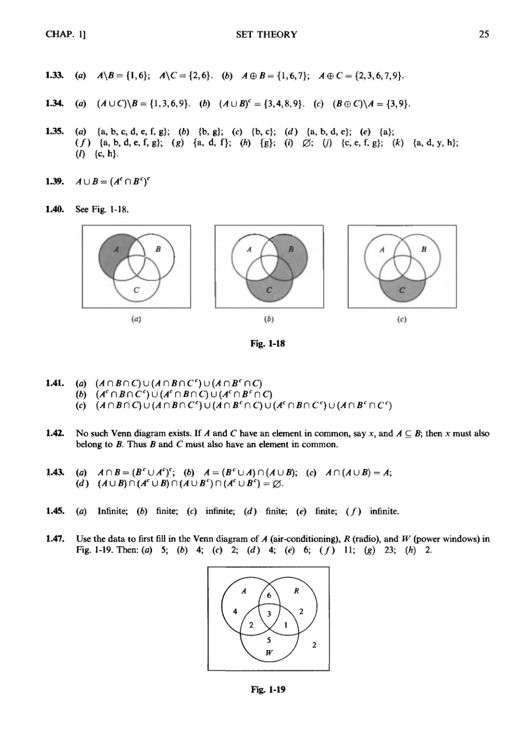
1.47. Use the data to first fill in the Venn diagram of A (air-conditioning), R (radio), and W (power windows) in
Fig. 1-19. Then: (fl) 5; (b) 4; (c) 2; (d) 4; (e) 6; (/) 11; fe) 23; (A) 2.
Fig. 1-19
26
SET THEORY
[CHAP. 1
1.48. Power(/4) has 25 = 32 elements as follows:
[0.{1}, {2}, {3}, {4}, {5}, {1,2}, {1,3}. {1,4}, {1,5}, {2,3}, {2,4}, {2,5}. {3,4}, {3,5}. {4,5}.
{1,2,3}, {1,2,4}, {1,2,5}, {2,3,4}, {2.3,5}, {3,4,5}, {1,3,4}. {1.3,5}, {1,4,5}. {2.4.5}. {1,2,3.4}.
{1,2,3.5}. {1.2.4.5}, {1,3,4.5}. {2.3,4,5},Л].
1.49. (a) (i) False; (ii) False; (iii) True; (iv) True; (v) True.
(b) Note n{A) = 3; hence Power(/4) has 23 = 8 elements:
Powers) = Ш{а,Ь}, {с}}, {{а,Ь}. {d,ej}], [{с}, {d.e.f}], [{я.6}]. \{c}}. [{d,e.f}\. 0}
1.50. Let лг be an arbitrary element in Power(/4). For each a e A, there are two possibilities: a g A or a ? A. But
there are m elements in A; hence there are 2 ¦ 2 ¦... ¦ 2 = 2™ different sets X. That is. Power(/4) has 2"'
elements.
1.51. (a) No, (b) no, (c) yes, (d) yes.
1.52. (a) No, (b) no. (r) yes, (rf) no.
1.53. (a) No, (/>) no, (c) yes.
1.55. />= [{1,3}. {5.7}. {9}. {2,4}, {8}]-
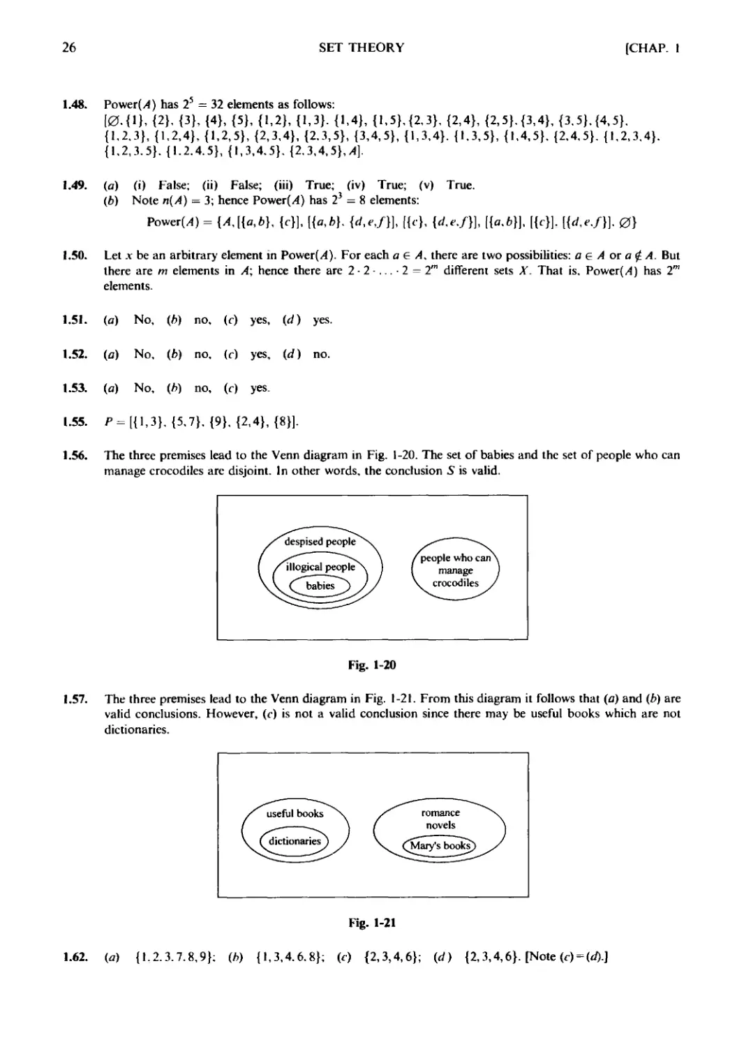
1.56. The three premises lead to the Venn diagram in Fig. 1-20. The set of babies and the set of people who can
manage crocodiles are disjoint. In other words, the conclusion S is valid.
'people whoсагЛ
manage
crocodiles
Fig. 1-20
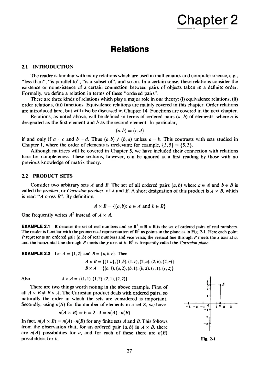
1.57. The three premises lead to the Venn diagram in Fig. 1-21. From this diagram it follows that (a) and (b) are
valid conclusions. However, (c) is not a valid conclusion since there may be useful books which are not
dictionaries.
Fig. 1-21
1.62. (a) {1.2.3.7.8,9}; (h) {1,3,4.6.8}; (c) {2,3,4,6}; (d) {2,3,4,6}. [Note (c) = (d).]
Chapter 2
Relations
2.1 INTRODUCTION
The reader is familiar with many relations which are used in mathematics and computer science, e.g.,
"less than", "is parallel to", "is a subset of, and so on. In a certain sense, these relations consider the
existence or nonexistence of a certain connection between pairs of objects taken in a definite order.
Formally, we define a relation in terms of these "ordered pairs".
There are three kinds of relations which play a major role in our theory: (i) equivalence relations, (ii)
order relations, (iii) functions. Equivalence relations are mainly covered in this chapter. Order relations
are introduced here, but will also be discussed in Chapter 14. Functions are covered in the next chapter.
Relations, as noted above, will be defined in terms of ordered pairs (a, b) of elements, where a is
designated as the first element and b as the second element. In particular,
(afb) = (c,d)
if and only if a = с and b = d. Thus (a, b) ф (b, a) unless a = b. This contrasts with sets studied in
Chapter 1. where the order of elements is irrelevant; for example, {3,5} = {5,3}.
Although matrices will be covered in Chapter 5, we have included their connection with relations
here for completeness. These sections, however, can be ignored at a first reading by those with no
previous knowledge of matrix theory.
2.2 PRODUCT SETS
Consider two arbitrary sets A and B. The set of all ordered pairs (a, b) where a e A and b e В is
called the product, or Cartesian product, of A and B. A short designation of this product is A x B, which
is read "A cross B". By definition,
A x В = {(a,b): a & A and b & B}
One frequently writes A2 instead of A x A.
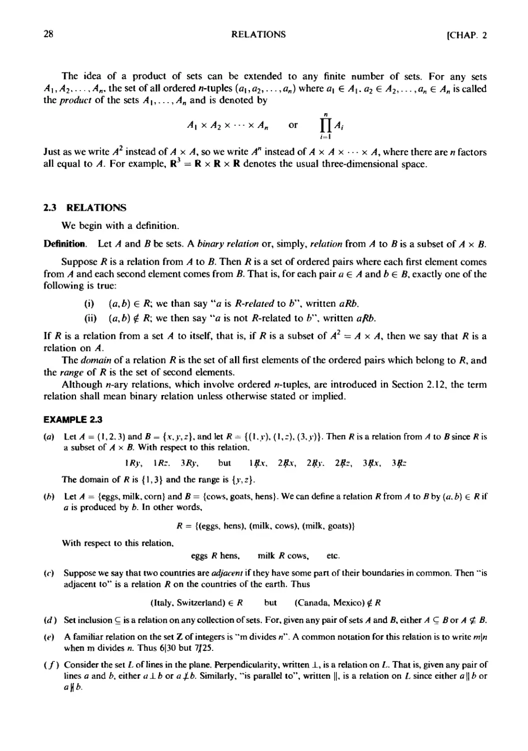
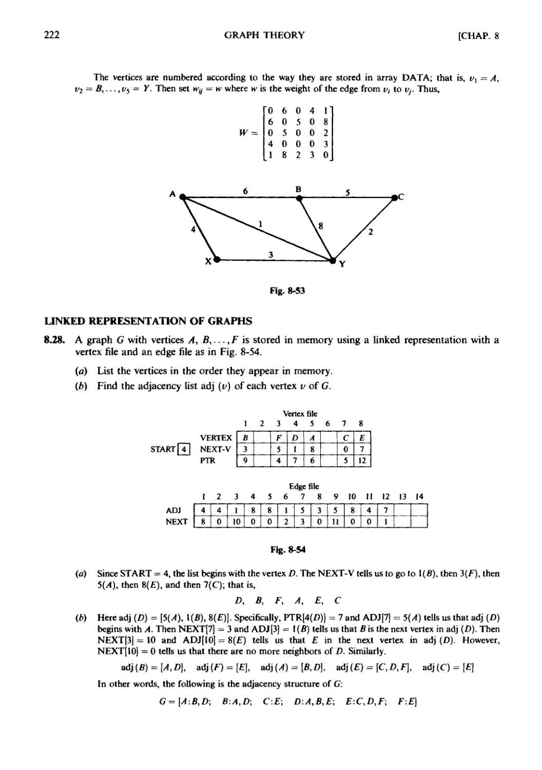
EXAMPLE 2.1 R denotes the set of real numbers and so R2 = R x R is the set of ordered pairs of real numbers.
The reader is familiar with the geometrical representation of R2 as points in the plane as in Fig. 2-1. Here each point
P represents an ordered pair {a, b) of real numbers and vice versa; the vertical line through P meets the x axis at a.
and the horizontal line through P meets the у axis at b. R2 is frequently called the Cartesian plane.
EXAMPLE 2.2 Let A = {1,2} and В = {а,Ь,с}. Then
AxB = {(l,a},(\,b),(\,c),B.a),B.b).B.c)}
Also ЛхЛ = {A.1).A.2),B.1),B.2)} s
There are two things worth noting in the above example. First of 2
all A x В ф В х A. The Cartesian product deals with ordered pairs, so
naturally the order in which the sets are considered is important.
Secondly, using n(S) for the number of elements in a set S, we have
—I—I—i—-
-S -2 -1C
-2
н—i-
In fact, n(A x B) — n{A) ¦ n[B) for any finite sets A and B. This follows
from the observation that, for an ordered pair (a, b) in A x B, there
are n(A) possibilities for a, and for each of these there are n{B)
possibilities for b. Fig. 2-1
27
28 RELATIONS [CHAP. 2
The idea of a product of sets can be extended to any finite number of sets. For any sets
A i, A2 An, the set of all ordered n-tuples {at, a2,..., an) where at 6 A,. a2 e A2,..., an e An is called
the product of the sets At,...,An and is denoted by
At x A2 x ¦¦¦ x An or
Just as we write A2 instead of A x A, so we write A" instead of A x A x ¦ ¦ ¦ x A, where there are n factors
all equal to A. For example, R3 = R x R x R denotes the usual three-dimensional space.
2.3 RELATIONS
We begin with a definition.
Definition. Let A and В be sets. A binary relation or, simply, relation from A to В is a subset of Ax B.
Suppose R is a relation from A to B. Then R is a set of ordered pairs where each first element comes
from A and each second element comes from B. That is, for each pair a e A and b e B, exactly one of the
following is true:
(i) (a, b) e R\ we than say "a is R-related to b", written aRb.
(ii) (a,b) g /?; We then say "a is not /?-related to b", written aRb.
If R is a relation from a set A to itself, that is, if R is a subset of A2 = A x A, then we say that Л is a
relation on A.
The domain of a relation R is the set of all first elements of the ordered pairs which belong to R, and
the range of R is the set of second elements.
Although и-агу relations, which involve ordered и-tuples, are introduced in Section 2.12, the term
relation shall mean binary relation unless otherwise stated or implied.
EXAMPLE 2.3
(a) Let A = A,2.3) and В = {x,y,z}, and let R= {(l.y), A,=), C,y)}. Then Л is a relation from A to В since Л is
a subset of A x B. With respect to this relation.
\Ry, \Rz. 3Ry, but l#.v, 2#л, 2Ry. 2R:, 3Rx, 3Rz
The domain of Л is {1,3} and the range is {у, г}.
(b) Let A = {eggs, milk, corn} and В = {cows, goats, hens}. We can define a relation R from A to В by (a. b) G Л if
a is produced by fc. In other words,
R = {(eggs, hens), (milk, cows), (milk, goats)}
With respect to this relation,
eggs R hens, milk R cows, etc.
(c) Suppose we say that two countries are adjacent if they have some part of their boundaries in common. Then "is
adjacent to" is a relation R on the countries of the earth. Thus
(Italy, Switzerland) e R but (Canada, Mexico) $. R
(d) Set inclusion С is a relation on any collection of sets. For, given any pair of sets A and B, either А С В or A ? B.
(e) A familiar relation on the set Z of integers is "m divides и". A common notation for this relation is to write m\n
when m divides и. Thus 6|30 but 7/25.
(/) Consider the set L oflines in the plane. Perpendicularity, written ±, is a relation on L. That is, given any pair of
lines a and b, either a A.b or aj-b. Similarly, "is parallel to", written ||, is a relation on L since either я|| b or
alb.
CHAP. 2]
RELATIONS
29
(g) Let A be any set. An important relation on A is that of equality.
{{a,a):aeA}
which is usually denoted by "=". This relation is also called the identity or diagonal relation on A and it will
also be denoted by Д^ or simply Д.
(A) Let A be any set. Then A x A and 0 are subsets of A x A and hence are relations on A called the universal
relation and empty relation, respectively.
Inverse Relation
Let R be any relation from a set A to a set B. The inverse of R, denoted by R ', is the relation from fi
to /4 which consists of those ordered pairs which, when reversed, belong to R; that is,
R~l = {(b,a): (a,b) € R}
For example, the inverse of the relation R = {(l,y), (l,z), C,j>)} from A = {1.2,3} to В = {x,y,z}
follows:
R-l = {(y,l), (z, I),(>'• 3)}
Clearly, if R is any relation, then (/?"')' = Л. Also, the domain and range of R~l are equal, respec-
respectively, to the range and domain of R. Moreover, if R is a relation on A, then R~l is also a relation on A.
2.4 PICTORIAL REPRESENTATIONS OF RELATIONS
First we consider a relation 5 on the set R of real numbers; that is, S is a subset of R2 = R x R.
Since R2 can be represented by the set of points in the plane, we can picture S by emphasizing those
points in the plane which belong to S. The pictorial representation of the relation is sometimes called the
graph of the relation.
Frequently, the relation S consists of all ordered pairs of real numbers which satisfy some given
equation
E{x,y)=0
We usually identify the relation with the equation; that is, we speak of the relation ?"(.v, v) = 0.
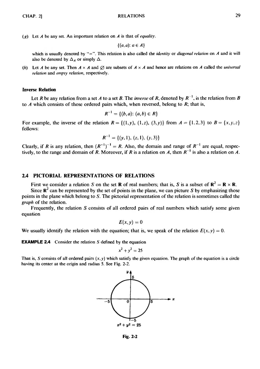
EXAMPLE 2.4 Consider the relation 5 defined by the equation
That is, 5 consists of all ordered pairs (x,y) which satisfy the given equation. The graph of the equation is a circle
having its center at the origin and radius 5. See Fig. 2-2.
Fig. 2-2
30
RELATIONS
[CHAP. 2
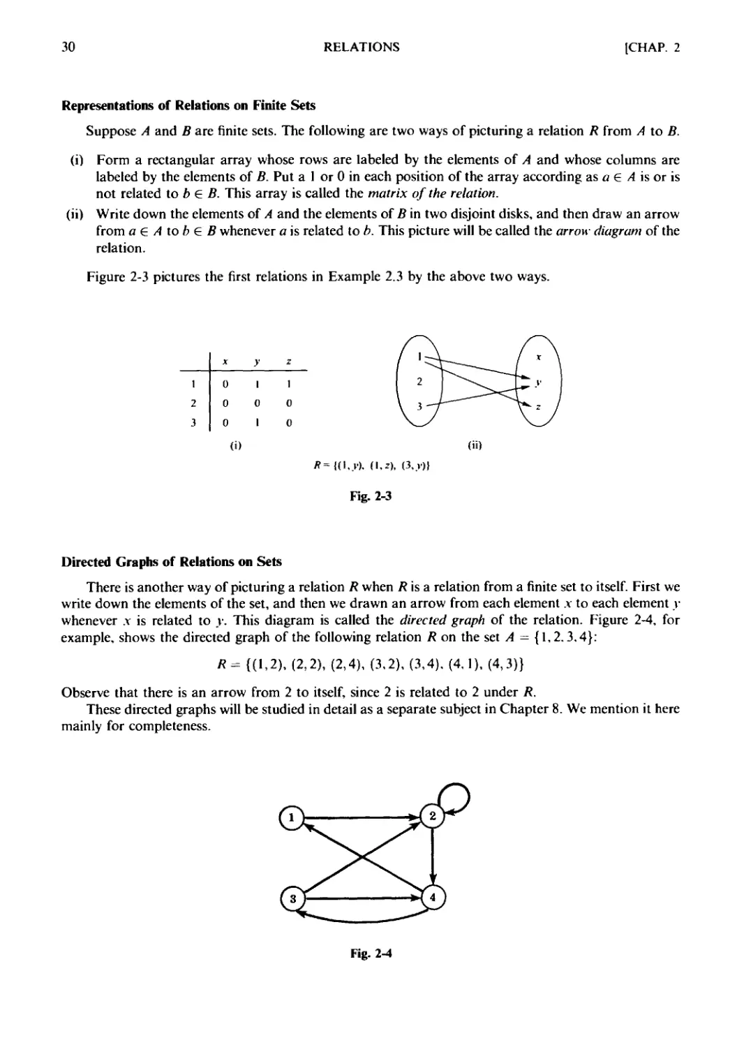
Representations of Relations on Finite Sets
Suppose A and В are finite sets. The following are two ways of picturing a relation R from A to B.
(i) Form a rectangular array whose rows are labeled by the elements of A and whose columns are
labeled by the elements of B. Put a 1 or 0 in each position of the array according as a e A is or is
not related to b e B. This array is called the matrix of the relation.
(ii) Write down the elements of A and the elements of В in two disjoint disks, and then draw an arrow
from a e A to b e В whenever a is related to b. This picture will be called the arrow diagram of the
relation.
Figure 2-3 pictures the first relations in Example 2.3 by the above two ways.
1
2
3
X
0
0
0
У
1
0
1
z
1
0
0
(i)
(ii)
/?=f(l..W. (I,г), C,v)}
Fig. 2-3
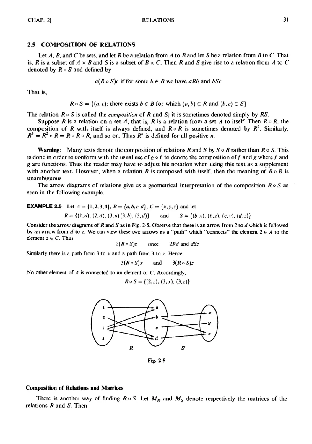
Directed Graphs of Relations on Sets
There is another way of picturing a relation R when R is a relation from a finite set to itself. First we
write down the elements of the set, and then we drawn an arrow from each element x to each element v
whenever x is related to v. This diagram is called the directed graph of the relation. Figure 2-4, for
example, shows the directed graph of the following relation R on the set A = {1,2.3.4}:
R = {A,2), B,2), B,4), C,2), C,4). D,1), D,3)}
Observe that there is an arrow from 2 to itself, since 2 is related to 2 under R.
These directed graphs will be studied in detail as a separate subject in Chapter 8. We mention it here
mainly for completeness.
Fig. 2-4
CHAP. 2] RELATIONS 31
2.5 COMPOSITION OF RELATIONS
Let A, B, and С be sets, and let R be a relation from A to В and let 5 be a relation from В to С That
is, R is a subset of A x В and S is a subset offixC Then R and S give rise to a relation from Л to С
denoted by Ro S and defined by
a(Ro S)c if for some ft e fi we have a/?ft and ftSc
That is,
RoS = {{a,c): there exists b e fi for which (a,ft) e Л and (ft.с) е S}
The relation Л о 5 is called the composition of /? and S; it is sometimes denoted simply by RS.
Suppose R is a relation on a set /4, that is, R is a relation from a set /4 to itself. Then Ro R, the
composition of R with itself is always defined, and RoR is sometimes denoted by /?2. Similarly,
R3 = R2 о R = RoRoR, and so on. Thus R" is defined for all positive n.
Warning: Many texts denote the composition of relations R and Shy S о R rather than Ro S. This
is done in order to conform with the usual use of g of to denote the composition of/ and g where/ and
g are functions. Thus the reader may have to adjust his notation when using this text as a supplement
with another text. However, when a relation R is composed with itself, then the meaning of Л о Л is
unambiguous.
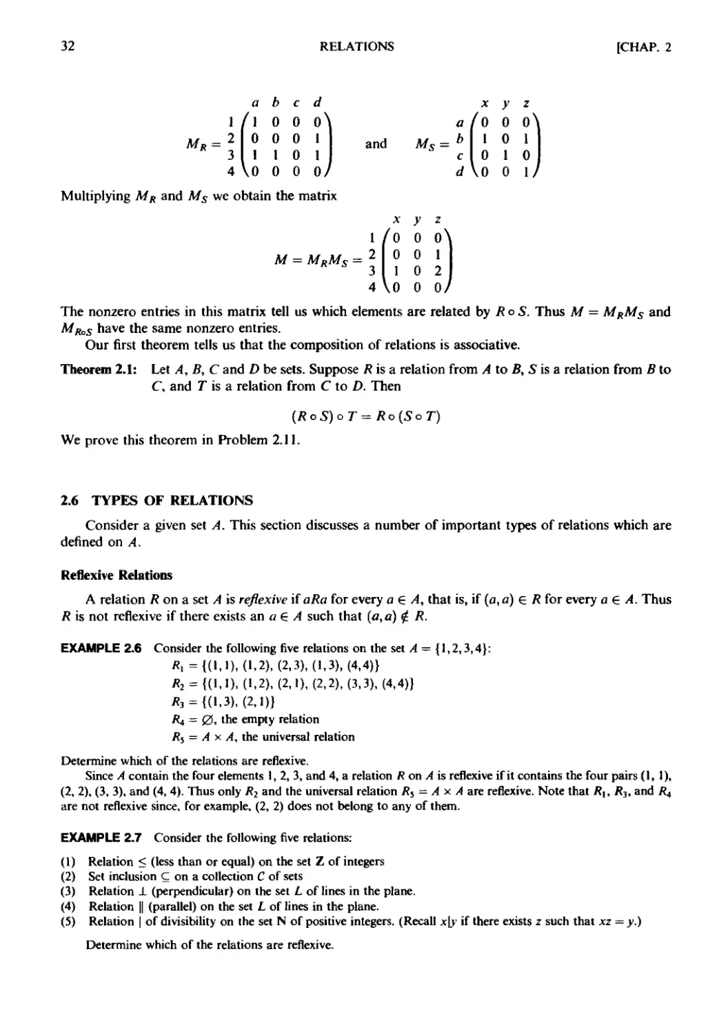
The arrow diagrams of relations give us a geometrical interpretation of the composition R о S as
seen in the following example.
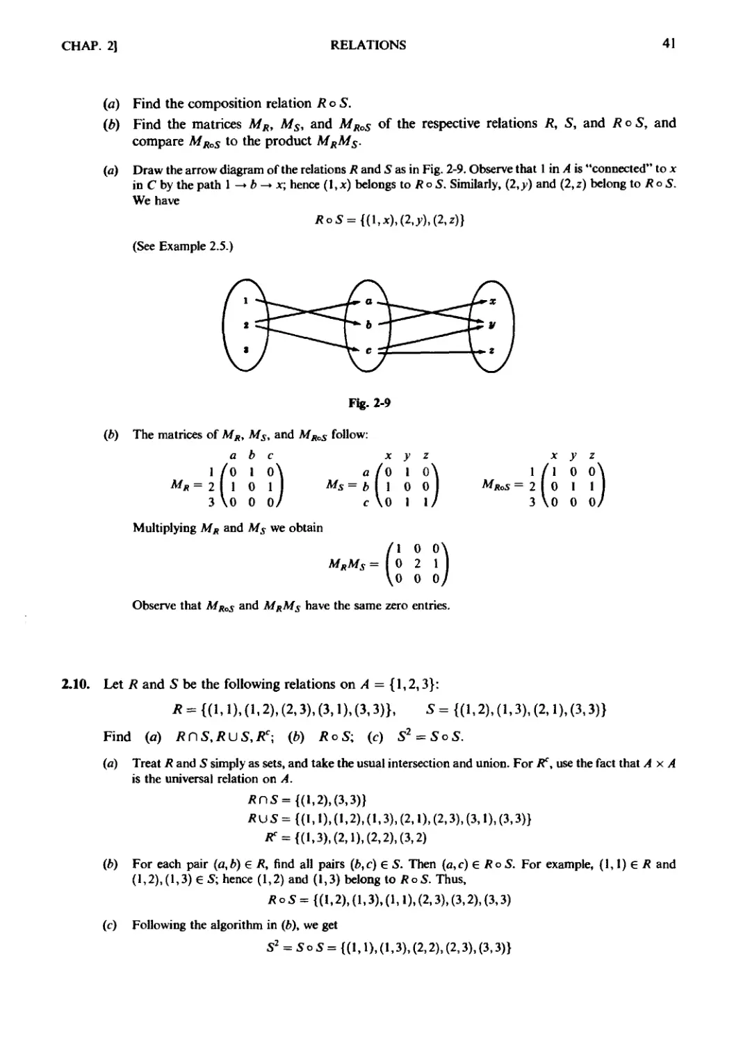
EXAMPLE 2.5 Let A = {1,2.3,4}, B={a,b,c,d), C= {x,y,z} and let
R=W,a), B,rf), (З.я)C,*), C,d)} and S = {(b.x), (b,z), (c.y). («/,=)}
Consider the arrow diagrams of R and 5 as in Fig. 2-5. Observe that there is an arrow from 2 to d which is followed
by an arrow from d to z. We can view these two arrows as a "path" which "connects" the element 2 e A to the
element z e C. Thus
2(RoS)z since 2Rd and dS:
Similarly there is a path from 3 to x and a path from 3 to z. Hence
3(/?oS).v and 3(/?oS)r
No other element of A is connected to an element of C. Accordingly.
Fig. 2-5
Composition of Relations and Matrices
There is another way of finding Ro S. Let MR and Ms denote respectively the matrices of the
relations R and S. Then
32
RELATIONS
[CHAP. 2
and
a
fs=b
с
x у z
f
0 0 0
1 0 1
0 1 0
,0 0 1.
1 j
-2
3
41
x
(o
0
1
U
У
0
0
0
0
z
0
1
2
0
3
4 VO 0 0 0/
Multiplying MR and Л/5 we obtain the matrix
M = MRMS =
The nonzero entries in this matrix tell us which elements are related by R о S. Thus M = MRMS and
MRoS have the same nonzero entries.
Our first theorem tells us that the composition of relations is associative.
Theorem 2.1: Let А, В, С and D be sets. Suppose R is a relation from A to B, S is a relation from В to
C, and T is a relation from С to D. Then
We prove this theorem in Problem 2.11.
2.6 TYPES OF RELATIONS
Consider a given set /4. This section discusses a number of important types of relations which are
defined on A.
Reflexive Relations
A relation R on a set A is reflexive if aRa for every a 6 A, that is, if (a, a) € /? for every a 6 /4. Thus
R is not reflexive if there exists an a 6 A such that (a, a) ? R.
EXAMPLE 2.6 Consider the following five relations on the set A = {1,2,3,4}:
Я, ={A,1), A.2), B,3), A,3), D,4)}
Л2 = {A,1). A,2), B,1), B,2), C,3), D,4)}
Л3 = {A,3), B,1)}
R4 = 0, the empty relation
/?5 = A x A, the universal relation
Determine which of the relations are reflexive.
Since A contain the four elements 1, 2, 3, and 4, a relation R on A is reflexive if it contains the four pairs A, 1),
B, 2), C, 3), and D, 4). Thus only R2 and the universal relation /?5 = A x A are reflexive. Note that Rt, R3, and ft,
are not reflexive since, for example, B, 2) does not belong to any of them.
EXAMPLE 2.7 Consider the following five relations:
A) Relation < (less than or equal) on the set Z of integers
B) Set inclusion С on a collection С of sets
C) Relation ± (perpendicular) on the set L of lines in the plane.
D) Relation || (parallel) on the set L of lines in the plane.
E) Relation | of divisibility on the set N of positive integers. (Recall x\y if there exists z such that xz = y.)
Determine which of the relations are reflexive.
CHAP. 2] RELATIONS 33
The relation C) is not reflexive since no line is perpendicular to itself. Also D) is not reflexive since no line is
parallel to itself. The other relations are reflexive; that is, x < x for every integer x in Z, А С A for any set A in C, and
n\n for every positive integer n in N.
Symmetric and Antisymmetric Relations
A relation R on a set A is symmetric if whenever aRb then bRa, that is, if whenever (a, b) e R then
(b,a) € R. Thus R is not symmetric if there exists a,b & A such that (a,b) e /? but (fe,a) ? /?.
EXAMPLE 2.8
(я) Determine which of the relations in Example 2.6 are symmetric.
R, is not symmetric since A,2) 6 /?, but B,1) ? /?,. /?3 is not symmetric since A,3) e /?3 but C,1) ? /?3. The
other relations are symmetric.
(fc) Determine which of the relations in Example 2.7 are symmetric.
The relation J- is symmetric since if line a is perpendicular to line b then b is perpendicular to a. Also, || is
symmetric since if line a is parallel to line b then b is parallel to a. The other relations are not symmetric. For
example, 3<4 but 4?3; {1,2} С {1,2,3} but {1,2,3} $? {1,2}, and 2|6 but 6/2.
A relation R on a set A is antisymmetric if whenever a/?fe and bRa then a = b, that is, if whenever
(a, fe), (fe, a) € R then a = b. Thus /? is not antisymmetric if there exist a,b € A such that (a, b) and (fe, a)
belong to R, but аф b.
EXAMPLE 2.9
(a) Determine which of the relations in Example 2.6 are antisymmetric.
R2 is not antisymmetric since A,2) and B, 1) belong to /?2, but 1 Ф 2. Similarly, the universal relation /?5 is
not antisymmetric. All the other relations are antisymmetric.
{b) Determine which of the relations in Example 2.7 are antisymmetric.
The relation < is antisymmetric since whenever a < b and b < a then a = b. Set inclusion С is antisym-
antisymmetric since whenever А С В and В С A then A = В. Also, divisibility on N is antisymmetric since whenever
m\n and n\m then m — n. (Note that divisibility on Z is not antisymmetric since 3| — 3 and —3|3 but 3 / -3.)
The relation L is not antisymmetric since we can have distinct lines a and b such that aLb and bLa. Similarly, ||
is not antisymmetric.
Remark: The properties of being symmetric and being antisymmetric are not negatives of each
other. For example, the relation R = {A,3), C,1), B,3)} is neither symmetric nor antisymmetric. On
the other hand, the relation R' = {A,1), B,2)} is both symmetric and antisymmetric.
Transitive Relations
A relation R on a set A is transitive if whenever aRb and bRc then aRc, that is, if whenever
(a,b), (b,с) е R then (a,c)eR. Thus R is not transitive if there exist a,b,ceA such that
(a,b), (b,c)€R but (a,c)? R.
EXAMPLE 2.10
(a) Determine which of the relations in Example 2.6 are transitive.
The relation R3 is not transitive since B,1), A,3) e /?3 but B,3)^ /?3. AH the other relations are
transitive.
(b) Determine which of the relations in Example 2.7 are transitive.
The relations <, C, and | are transitive. That is: (i) If a < b and b < c, then a < с (ii) If А С В and В С С,
then AC С. (iii) If a\b and b\c, then a\c.
34 RELATIONS [CHAP. 2
On the other hand the relation _L is not transitive. If a _L b and b J_ c, then it is not true that «ir. Since no
line is parallel to itself, we can have a\\band b \\a, but a}fa. Thus || is not transitive. (We note that the relation
"is parallel or equal to" is a transitive relation on the set L of lines in the plane.)
The property of transitivity can also be expressed in terms of the composition of relations. For a
relation R on A we define
R2 = R о R and, more generally, R" = R" о R
Then we have the following result.
Theorem 2.2: A relation R is transitive if and only if R" С R for n > 1.
2.7 CLOSURE PROPERTIES
Consider a given set A and the collection of all relations on A. Let Pbe a property of such relations,
such as being symmetric or being transitive. A relation with property P will be called a P-relation. The P-
closure of an arbitrary relation R on A, written P(R), is a P-relation such that
R С P(R) С 5
for every P-relation 5 containing R. We will write
reflexive(/?), symmetric(/?), and transitive(/?)
for the reflexive, symmetric, and transitive closures of R.
Generally speaking, P(R) need not exist. However, there is a general situation where P(R) will
always exist. Suppose P is a property such that there is at least one P-relation containing R and that
the intersection of any P-relations is again a P-relation. Then one can prove (Problem 2.16) that
P(R) = n(S: S is a P-relation and R С S)
Thus one can obtain P(/?) from the "top-down", that is, as the intersection of relations. However, one
usually wants to find P(R) from the "bottom-up", that is, by adjoining elements to R to obtain P(R).
This we do below.
Reflexive and Symmetric Closures
The next theorem tells us how to easily obtain the reflexive and symmetric closures of a relation.
Here AA — {(a,a): a € A} is the diagonal or equality relation on A.
Theorem 2.3: Let R be a relation on a set A. Then:
(i) RU AA is the reflexive closure of R.
(ii) R U R 'is the symmetric closure of R.
In other words, reflexive(/?) is obtained by simply adding to R those elements (a, a) in the diagonal
which do not already belong to /?, and symmetric(/?) is obtained by adding to R all pairs (b.a) whenever
(a, b) belongs to R.
EXAMPLE 2.11
(a) Consider the following relation R on the set A = {1,2,3,4}:
Л={A.1). A.3), B.4), C.1), C.3). D.3)}
Then
reflexive(/J) = Ли {B.2), D,4)} and symmetric^) = Ли {D,2), C,4)}
CHAP. 2] RELATIONS 35
(b) Consider the relation < (less than) on the set N of positive integers. Then
reflexive(<) =< иД =<= {(a.b): a < b)
symmetric(<) =< и > = {(a.b): a ^ b}
Transitive Closure
Let R be a relation on a set A. Recall that R2 = R о R and R" = R" ' о R. We define
1=1
The following theorem applies.
Theorem 2.4: R* is the transitive closure of a relation R.
Suppose A is a finite set with n elements. Then we show in Chapter 8 on directed graphs that
R* = R U R2 U ¦ ¦ • U R"
This gives us the following result.
Theorem 2.5: Let Л be a relation on a set A with n elements. Then
transitive(K) — R U R1 U ¦ • ¦ U R"
Finding transitive(/?) can take a lot of time when A has a large number of elements. An efficient way
for doing this will be described in Chapter 8. Here we give a simple example where A has only three
elements.
EXAMPLE 2.12 Consider the following relation R on A = {1.2,3}:
Л= {A,2). B.3). C.3)}
Then
R2 = ЛоЛ= {A.3).B,3)C.3)} and R3 = R2 о R = {A.3). B.3). C. 3)}
Accordingly.
transitive(/J) = RuR2uR3 = {A,2). B,3). C.3). A,3)}
2.8 EQUIVALENCE RELATIONS
Consider a nonempty set S. A relation R on S is an equivalence relation if R is reflexive, symmetric,
and transitive. That is, R is an equivalence relation on S if it has the following three properties:
A) For every a € 5, aRa.
B) If aRb, then bRa.
C) If aRb and bRc, then aRc.
The general idea behind an equivalence relation is that it is a classification of objects which are in some
way "alike". In fact, the relation "=" of equality on any set S is an equivalence relation; that is:
A) a — a for every a € S.
B) lfa = b, then b = a.
C) If a = b and b = r, then a = e.
Other equivalence relations follow.
36 RELATIONS [CHAP. 2
EXAMPLE 2.13
(a) Consider the set L of lines and the set T of triangles in the Euclidean plane. The relation "is parallel to or
identical to" is an equivalence relation on L, and congruence and similarity are equivalence relations on T.
(b) The classification of animals by species, that is, the relation "is of the same species as", is an equivalence
relation on the set of animals.
(c) The relation С of set inclusion is not an equivalence relation. It is reflexive and transitive, but it is not
symmetric since А С В does not imply ВС. A.
(d) Let m be a fixed positive integer. Two integers a and b are said to be congruent modulo m, written
a = b (mod m)
if m divides a - b. For example, for m = 4 we have 11 = 3 (mod 4) since 4 divides 11-3, and 22 s 6 (mod 4)
since 4 divides 22 - 6. This relation of congruence modulo m is an equivalence relation.
Equivalence Relations and Partitions
This subsection explores the relationship between equivalence relations and partitions on a non-
nonempty set S. Recall first that a partition P of S is a collection {/!,} of nonempty subsets of S with the
following two properties:
A) Each a e S belongs to some At.
B) If At ф Aj, then At П Aj = 0.
In other words, a partition P of 5 is a subdivision of 5 into disjoint nonempty sets. (See Section 1.9.)
Suppose R is an equivalence relation on a set S. For each a in S, let [a] denote the set of elements of
S to which a is related under R; that is,
[a] = {x: (a,x) e R}
We call [ a ] the equivalence class of a in S; any fee [a] is called a representative of the equivalence class.
The collection of all equivalence classes of elements of S under an equivalence relation R is denoted
by S/R, that is,
S/R = {[a]:a€S)
It is called the quotient set of 5 by R. The fundamental property of a quotient set is contained in the
following theorem.
Theorem 2.6: Let R be an equivalence relation on a set S. Then the quotient set S/R is a partition of S.
Specifically:
(i) For each a in S, we have a e [a].
(ii) [o] = [ft] if and only if (a,b)e R.
(iii) If [a] / [b], then [a] and [b] are disjoint.
Conversely, given a partition {A,} of the set S, there is an equivalence relation R on S
such that the sets Л, are the equivalence classes.
This important theorem will be proved in Problem 2.21.
EXAMPLE 2.14
(a) Consider the following relation R on 5 = {1,2,3}:
/?={(!, 1), A,2), B,1), B,2), C,3)}
CHAP. 2] RELATIONS 37
One can show that R is reflexive, symmetric, and transitive, that is, that R is an equivalence relation. Under the
relation R,
[1] = {1,2}, [2] = {1,2}, [3] = {3}
Observe that [1] = [2] and that S/R = {[1], [3]} is a partition of S. One can choose either {1,3} or {2,3} as a set
of representatives of the equivalence classes.
(b) Let Л5 be the relation on the set Z of integers defined by
x = y (mod 5)
which reads "x is congruent to у modulo 5" and which means that the difference .v - v is divisible by 5. Then Л5
is an equivalence relation on Z. There are exactly five equivalence classes in the quotient set Z/Rs as follows:
Ao = {...,-10,-5,0, 5,10,...}
/1, = {...,-9,-4, 1,6,11,...}
A2 = {...,-8,-3,2,7,12,...}
Л3 = {...,-7,-2, 3,8,13,...}
Ал = {...,-6,-1, 4, 9,14,...}
Observe that any integer .v, which can be uniquely expressed in the form x = 5q + r where 0 < r < 5, is a
member of the equivalence class Ar where r is the remainder. As expected, the equivalence classes are disjoint
and
Z = Ло U Л, U Л2 U Л3 и Л4
Usually one chooses {0,1,2,3.4} or {-2,-1,0,1,2} as a set of representatives of the equivalence classes.
2.9 PARTIAL ORDERING RELATIONS
This section defines another important class of relations. A relation R on a set S is called a partial
ordering or a partial order if R is reflexive, antisymmetric, and transitive. A set S together with a partial
ordering R is called a partially ordered set or poset. Partially ordered sets will be studied in more detail in
Chapter 14, so here we simply give some examples.
EXAMPLE 2.15
(a) The relation С of set inclusion is a partial ordering on any collection of sets since set inclusion has the three
desired properties. That is,
A) А С A for any set A.
B) If AC fland В С A, then/1 = В.
C) If А С В and В С С, then А С С.
(b) The relation < on the set R of real numbers is reflexive, antisymmetric, and transitive. Thus < is a partial
ordering.
{c) The relation "a divides b" is a partial ordering on the set N of positive integers. However, "a divides b" is not a
partial ordering on the set Z of integers since a\b and b\a does not imply a = b. For example. 3] - 3 and -3|3
but 3 ф -3.
2.10 л-ARY RELATIONS
All the relations discussed above were binary relations. By an n-ary relation, we mean a set of
ordered n-tuples. For any set S, a subset of the product set S" is called an n-ary relation on S. In
particular, a subset of Si is called a ternary relation on 5.
38
RELATIONS
[CHAP. 2
EXAMPLE 2.16
(a) Let L be a line in the plane. Then "betweenness" is a ternary relation R on the points of L; that is. (a. b. с) е R
if b lies between a and с on L.
(b) The equation ,v: + v2 + z1 = 1 determines a ternary relation T on the set R of real numbers. That is, a triple
(л, у,:) belongs to Г if {.v. r.r) satisfies the equation, which means (.v. г. г) is the coordinates of a point in R3 on
the sphere S with radius 1 and center at the origin О = @.0,0).
Solved Problems
ORDERED PAIRS AND PRODUCT SETS
2.1. Given: A = {1.2.3} and B = {a,b}. Find: {a) A x B\ (b) В х А; (с) В х В.
(a) A x В consists of all ordered pairs (л*, v) where .v G A and у € В. Hence
A x Д={A.а).A.Л).B.а).B.Л).C,я).C,Л)}
(b) В x A consists of all ordered pairs (y.x) where _»• € В and .v e A. Hence
ВхЛ = {(а.1).(в.2).(в.З).(А.1).(А.2).(А.З)}
(c) В х В consists of all ordered pairs (л. v) where x.y e B. Hence
fix B= {(a.a).(a.b).(b.a).(b.b)}
As expected, the number of elements in the product set is equal to the product of the numbers of the elements
in each set.
2.2. Given: A = {1,2}. В = {.v, v.z}, and С = {3,4}. Find: A x В х С
A x В x С consists of all ordered triplets (a.b.c) where a e A. b e В. с € С. These elements of
A x В x С can be systematically obtained by a so-called tree diagram (Fig. 2-6). The elements of
A x В x С are precisely the 12 ordered triplets to the right of the tree diagram.
Observe that n(A) = 2, n(B) = 3, and n(C") = 2 and, as expected,
n(.A x Bx C) = 12 ^ n(A)- n{B)-n(C)
3
4
3
4
3
4
3
4
3
4
3
4
A.x,
A.x,
A,1/,
A,1/,
A.2,
A.*,
B, ж,
B, ж,
B,1/,
B,1/.
B, г,
B,2,
3)
4)
3)
4)
3)
4)
3)
4)
3)
4)
3)
4)
Fig. 2-6
CHAP. 2] RELATIONS 39
2.3. Let A = {1,2},В ={a,b,c} and С = {c,d}. Find: (А хВ)П(А х С) and (BnQ.
We have
Hence
Since ВПС= {с},
Observe that (A x B) n (A x C) = A x (B n C). This is true for any sets А, В and С (see Problem 2.4).
2.4. Prove (A x B)n(A x Q = A x (ВП C).
(/4 x В) П (/1 x C) = {x,y)\ (x,y) e A x В and (*,>¦) e /4 x C}
= {(JC.J'): * ? А,у е В and jc e /!,>¦ € C}
= Ах(ВПС)
2.5. Find x and у given Bjc, jc + y) = F,2).
Two ordered pairs are equal if and only if the corresponding components are equal. Hence we obtain
the equations
2x = 6 and x + у = 2
from which we derive the answers x = 3 and у = — 1.
RELATIONS AND THEIR GRAPHS
2.6. Find the number of relations from A = {a, b, c} to В = {1,2}.
There are 3B) = 6 elements in A x B, and hence there are m = 26 = 64 subsets of A x B. Thus there are
m = 64 relations from /4 to Д.
2.7. Given A = {1,2,3,4} and В = {x,y,z}. Let /? be the following relation from A to B:
/?={(l,j),(l,z),C,>0,D,;c),D,z)}
(a) Determine the matrix of the relation.
(b) Draw the arrow diagram of R.
(c) Find the inverse relation Л of R.
(d) Determine the domain and range of R.
(a) See Fig. 2-7(a). Observe that the rows of the matrix are labeled by the elements of A and the columns
by the elements of B. Also observe that the entry in the matrix corresponding toa? A and b e В is 1 if
a is related to b and 0 otherwise.
{b) See Fig. 2-1 (b). Observe that there is an arrow from a e A to b € В iff a is related to b, i.e., iff (a, b) e R.
(c) Reverse the ordered pairs of R to obtain Л~':
*-| = {0',l),(z1l),(y13),(x,4),(z14)}
Observe that by reversing the arrows in Fig. 2.7(b) we obtain the arrow diagram of R~l.
40
RELATIONS
[CHAP. 2
(d) The domain of R, Dom(/?), consists of the first elements of the ordered pairs of R, and the range of R.
Ran(fl), consists of the second elements. Thus,
Dom(/?) = {1,3,4} and Ran(R) = {x,y,z}
(a)
Fig. 2-7
2.8. Let A = {1,2,3,4,6}, and let Л be the relation on A defined by "x divides y", written x\y. (Note
x\y iff there exists an integer z such that xz = y.)
(a) Write R as a set of ordered pairs.
(b) Draw its directed graph.
(c) Find the inverse relation R~l of /?. Can R~l be described in words?
(a) Find those numbers in A divisible by 1,2, 3, 4, and then 6. These are:
1|1, 1|2, 1|3, 1|4, 1|6, 2|2, 2|4, 2|6, 3|3, 3|6, 4|4, 6|6
Hence
Л = {A,1), A,2), A,3), A,4), A,6), B,2), B,4), B,6), C,3), C,6), D,4), F,6)}
(b) See Fig. 2-8.
(c) Reverse the ordered pairs of R to obtain R~':
Л-1 = {A,1),B,1),C,1),D,1),F,1),B,2),D,2),F,2),C,3),F,3),D,4),F,6)}
Л can be described by the statement "jc is a multiple of y".
Fig. 2-8
2.9. Let A = {1,2,3}, В = {a,b,c], and С = {x,y,z}. Consider the following relations R and 5 from
A to В and from В to C, respectively.
R={(l,b),B,a),B,c)} and S = {(a,y),(b,x),(c,y),{c,z)}
CHAP. 2]
RELATIONS
41
(a) Find the composition relation RoS.
(b) Find the matrices MR, Ms, and MRoS of the respective relations R, S, and RoS, and
compare MRoS to the product MRMS.
(a) Draw the arrow diagram of the relations R and 5 as in Fig. 2-9. Observe that 1 in A is "connected" to x
in С by the path 1 -» b -» x; hence A,jc) belongs to RoS. Similarly, B, y) and B, z) belong to R о S.
We have
(See Example 2.5.)
Fig. 2-9
(fc) The matrices of MR, Ms, and MRoS follow:
a b с
x у
у
1 /О 1 (Л Jo I 0\
2 1 Oil A/s = fc I 1 0 0 I
3\0 0 0/ с\0 1 1/
/1 0 0\
0 2 1
\0 0 0/
Multiplying Л/л and Ms we obtain
Observe that MRoS and MRM$ have the same zero entries.
2.10. Let R and S be the following relations on A = {1,2,3}:
Я = {A,1), A,2), B,3), C,1), C,3)}, S = {A,2), A,3), B,1), C,3)}
Find (a) RnS,Rl)S,Rc; (b) RoS; (c) S2 = SoS.
(a) Treat R and 5 simply as sets, and take the usual intersection and union. For Rc, use the fact that A x A
is the universal relation on A.
ЛП5={A,2),C,3)}
/?U 5 = {{1,1), A,2), A,3), B,1), B,3), C,1), C,3)}
tf = {A,3), B,1), B,2), C,2)
(b) For each pair (a,b) € R, find all pairs (b,c) e S. Then (a,c) e RoS. For example, A,1) e R and
A,2),A,3) e S; hence A,2) and A,3) belong to RoS. Thus,
(с) Following the algorithm in (b), we get
42 RELATIONS [CHAP. 2
2.11. Prove Theorem 2.1: Let А, В, С and D be sets. Suppose R is a relation from A to B, S is a relation
from Я to С and Г is a relation from С to /J>. Then (Ro S)oT = Ro(SoT).
We need to show that each ordered pair in (/? о S) о T belongs to R о (S о Г), and vice versa.
Suppose (a,d) belongs to [R о S) о Г. Then there exists a <• in С such that (a,c) e R о S and (erf) e Г.
Since (а, с) e R о S, there exists а * in В such that (a, b) G Я and F, с) e S. Since (fc, c) e S and (c, rf) e T,
we have (?.</) e So Г; and since (a,fc) e Л and F,d*) e So T. we have (a,rf) e Л о (So 7"). Therefore.
(Ло5) оГС Л о E о 7"). Similarly Ro (S о Т) С (Ro S) о Г. Both inclusion relations prove
(RoS) oT = Ro(SoT).
TYPES OF RELATIONS AND CLOSURE PROPERTIES
2.12. Consider the following five relations on the set A — {1,2,3}:
/? = {(U),A,2),A,3),C,3)} 0 = empty relation
S = {A.1), A,2), B,1), B,2), C,3) Ау.А = universal relation
Determine whether or not each of the above relations on A is: (a) reflexive; (ft) symmetric;
(c) transitive; (d) antisymmetric.
(a) R is not reflexive since 2 G A but B,2) ? R.I is not reflexive since C,3) ? T and, similarly, 0 is not
reflexive. S and A x A are reflexive.
(b) R is not symmetric since A.2) G R but B,1) ? R, and similarly T is not symmetric. S. 0, and Л х А
are symmetric.
(f) Г is not transitive since A.2) and B,3) belong to 7", but A.3) does not belong to T. The other four
relations are transitive.
(d) S is not antisymmetric since 1 ^ 2, and A,2) and B,1) both belong to S. Similarly, A x A is not
antisymmetric. The other three relations are antisymmetric.
2.13. Given A = {1,2,3,4}. Consider the following relation in A:
{a) Draw its directed graph.
(b) Is R (i) reflexive, (ii) symmetric, (iii) transitive, or (iv) antisymmetric?
(c) Find R2 = R о R.
(a) See Fig. 2-10.
(b) (i) R is not reflexive because 3 e A but 3^3, i.e., C,3) g R.
(ii) Л is not symmetric because 4Л2 but 2ft. 4, i.e., D,2) G Л but B,4) $ R.
(iii) R is not transitive because 4/?2 and 2/?3 but 4? 3, i.e., D,2) € Л and B.3) e Л but D,3) $ R.
(iv) Л is not antisymmetric because 2/?3 and ЗЛ2 but 2^3.
(c) For each pair {a.b) € R, find all (b,c) € R. Since (a,<?) G Л2,
CHAP. 2] RELATIONS 43
Fig. 2-10
2.14. Give examples of relations R on A = {1,2,3} having the stated property.
(a) R is both symmetric and antisymmetric.
(b) R is neither symmetric nor antisymmetric.
(c) R is transitive but RU R~l is not transitive.
There are several possible examples for each answer. One possible set of examples follows:
(a) Л={A.1).B,2)}.
(b) Л={A.2),B,1).B.3)}.
(c) Л={1,2)}.
2.15. Suppose С is a collection of relations S on a set A and let T be the intersection of the relation 5,
that is, T = n(S: S G C). Prove:
(л) If every S is symmetric, then T is symmetric.
(?>) If every S is transitive, then T is transitive.
(a) Suppose (a,b) € 7\ Then (a, b) e S for every S. Since each S is symmetric, (b.a) e S for every S.
Hence (b, a) € T and T is symmetric.
(b) Suppose (a. b) and (b, c) belong to T. Then (a, b) and (b. c) belong to S for every 5. Since each S is
transitive, (а, с) belongs to 5 for every 5. Hence, (a, c) € T and T is transitive.
2.16. Let R be a relation on a set A, and let P be a property of relations, such as, symmetry and
transitivity. Then P will be called Л-closable if P satisfies the following two conditions:
A) There is a P-relation S containing R.
B) The intersection of P-relations is a P-relation.
(a) Show that symmetry and transitivity are Л-closable for any relation R.
(b) Suppose P is Л-closable. Then P{R), the P-closure of R, is the intersection of all P-relations
S containing R, that is,
P(R) = n(S: S is a P-relation and R С S)
(a) The universal relation A x A is symmetric and transitive and A x A contains any relation Ron A. Thus
A) is satisfied. By Problem 2.15, symmetry and transitivity satisfy B). Thus symmetry and transivity
are Л-closable for any relation R.
(b) Let T - n(S: S is a P-relation and R С S). Since P is Л-closable, T is nonempty by A) and T is а Р-
relation by B). Since each relation S contains R, the intersection T contains R. Thus, Г is a P-relation
containing R. By definition, P(R) is the smallest P-relation containing R; hence P(R) С Т. On the
44 RELATIONS [CHAP. 2
other hand, P(R) is one of the sets 5 defining Г, that is, P(R) is a Р-relation and R С P(R). Therefore.
T С />(/?). Accordingly, /»(/?) = T.
2.17. Consider a set A = {a, b, c} and the relation R on A defined by
R={(a,a), (a,b), (b,c), (c,c)}
Find (a) reflexive(/?); (h) symmetric^/?); and (c) transitive(/?).
(a) The reflexive closure on R is obtained by adding all diagonal pairs of A x A to R which are not
currently in R. Hence,
reflexive(/?) = Ru{(b,b)} = {(a,a),(a,b),(h,b),(b,c),(c,c)}
(b) The symmetric closure on R is obtained by adding all the pairs in R~' to Л which are not currently in
R. Hence,
symmetric^) = Ru{{b,a),(c,b)} = {(a.a),{a.b),(b,a),(b,c),(c.b),(c,c)}
(c) The transitive closure on R, since A has three elements, is obtained by taking the union of R with
R2 = RoR and Л3 = Rо Rо R. Note that
R2 = Ro R = {{a,a),(a,b),{a.c).(b.c),(c,c)}
Ri = R о R о Л = {(a.a), (a,b), (a, c). (b, c), (c.c)}
Hence
transitive(/?) = ROR2URi = {(a,a),(a.b),(a,c),(h,c),(c,c)}
EQUIVALENCE RELATIONS AND PARTITIONS
2.18. Consider the Z of integers and an integer m > 1. We say that .v is congruent to v modulo m,
written
.v = у (mod m)
if .v — v is divisible by tn. Show that this defines an equivalence relation on Z.
We must show that the relation is reflexive, symmetric, and transitive.
(i) For any .v in Z we have .v = .v (mod m) because .v - ,v = 0 is divisible by m. Hence the relation is
reflexive.
(ii) Suppose a: = _v (mod m), so a: — _v is divisible by m. Then — (_v — y) — у — x is also divisible by m, so
у = x (mod m). Thus the relation is symmetric.
(iii) Now suppose .v = у (mod m) and у = z (mod m), so .v - у and у — z are each divisible by m. Then the
sum
(A-V) + (j-')=-V-r
is also divisible by m; hence x = г (mod m). Thus the relation is transitive.
Accordingly, the relation of congruence modulo m on Z is an equivalence relation.
2.19. Let A be a set of nonzero integers and let » be the relation on A x A defined by
(a, b) « {c,d) whenever ad = be
Prove that % is an equivalence relation.
We must show that & is reflexive, symmetric, and transitive,
(i) Reflexivity. We have (a, b) и (a, b) since ah = ba. Hence « is reflexive.
CHAP. 2] RELATIONS 45
(ii) Symmetry: Suppose (a,b) и {c,d). Then ad = be. Accordingly, cb = da and hence (c,d) = (a,b).
Thus, w is symmetric.
(iii) Transitivity: Suppose (a, b) ~ (c,d) and (c,d) w (e,/). Then ad = be and </ = de. Multiplying corre-
corresponding terms of the equations gives (ad)(cf) = {bc)(de). Canceling с ф 0 and d ф 0 from both sides
of the equation yields af = be, and hence {a,b) « (e,/). Thus sa is transitive. Accordingly, s» is an
equivalence relation.
2.20. Let Л be the following equivalence relation on the set A = {1,2,3,4,5,6}:
/? = {A,1),A,5),B,2),B,3),B,6),C,2),C,3),C,6),D,4),E,1),E,5),F.2),F,3),F,6)
Find the partition of A induced by R, i.e., find the equivalence classes of R.
Those elements related to 1 are 1 and 5 hence
[1] = {1,5}
We pick an element which does not belong to [1], say 2. Those elements related to 2 are 2, 3 and 6, hence
[2] = {2,3,6}
The only element which does not belong to [1] or [2] is 4. The only element related to 4 is 4. Thus
[4] = {4}
Accordingly,
[{1,5},{2,3,6},{4}]
is the partition of A induced by R.
2.21. Prove Theorem 2.6: Let R be an equivalence relation in a set A. Then the quotient set A/R is a
partition of A. Specifically,
(i) a G [a], for every a G A.
(ii) [a] = [h] if and only if (a,h) G R.
(iii) If [a] / [h], then [a] and [b] are disjoint.
Proof of (i): Since R is reflexive, {a,a) ? R for every a e A and therefore a e [a].
Proof of (ii): Suppose (a,b) e R. We want to show that [a] = [b]. Let .v e [b]\ then (b,x) 6 Л. But
by hypothesis (a,b) 6 R and so, by transitivity, {a,x) 6 /?. Accordingly a: 6 [a]. Thus [6] С [a]. To prove
that [а] С [/>), we observe that (a,b) e Л implies, by symmetry, that (b,a) e R. Then, by a similar argu-
argument, we obtain [а] С [b]. Consequently, [a] = [b].
On the other hand, if [a] = [fc], then, by (i), fc e [b] = [a]; hence (a,6) e Л.
Proof of (iii): We prove the equivalent contrapositive statement:
lf[a]n[b]?0 then [a] = [fc]
Н[а}П[Ь] ф 0, then there exists an element x ? A with .v e [а] П [fc]. Hence (а,л) е Л and (fc..v) e Л. By
symmetry, (.v.fc) G R and by transitivity, (a,6) G Л. Consequently by (ii), [a] = [fc].
2.22. Consider the set of words W = {sheet, last, sky, wash, wind, sit}. Find WjR where R is the
equivalence relation on W defined by either (a) "has the same number of letters as"; (h) "begins
with the same letter as".
(a) Those words with the same number of letters belong to the same cell; hence
W/R = [{sheet}, {last, wash, wind}, {sky, sit}].
(b) Those words beginning with the same letter belong to the same cell; hence
46 RELATIONS [CHAP. 2
W/R = [{sheet, sky, sit}, {last}, {wash, wind}].
PARTIAL ORDERING
2.23. Let t be any collection of sets. Is the relation of set inclusion С a partial order on (?
Yes, since set inclusion is reflexive, antisymmetric, and transitive. That is. for any sets А, В. С in ( we
have: (i) АСА: (ii) if А С В and В С A, then A = В; (iii) if А С В and ВС С, then /4 С С.
2.24. Consider the set Z of integers. Define a R h by Л = a for some positive integer r Show that /? is a
partial order on Z, that is. show that R is: (a) reflexive: (b) antisymmetric, (c) transitive.
(a) R is reflexive since a = a .
(b) Suppose aRb and bRa. say b = d and a = />'. Then u = (d)s = a". There are three possibilities: (i)
rs = 1, (ii) a = 1, and (iii) a = -I. If rs; = 1 then r = 1 and л = 1 and so a = b. If a = I then
h = Г = 1 = a, and, similarly, if b = 1 then a = 1. Lastly, if a = -I then A = -1 (since b Ф \) and
a = />. In all three cases, a — b. Thus R is antisymmetric.
(c) Suppose aRb and А Л с are, say, b = d and с = bs. Then с = (ar)J = o" and, therefore, a R c. Hence R
is transitive.
Accordingly, Л is a partial order on Z.
Supplementary Problems
RELATIONS
2.25. Let W = {Marc, Erik. Paul} and let V = (Erik, David). Find: (a) W x V\ {b) У x W, (c) V x V.
2.26. Let S = {a.b.c}, T = {b.c.d}, and W = {a,d}. Construct the tree diagram of S x T x W and then find
SxT x W.
2.27. Find л and v if: (а) (л + 2,4) = E,2л + y); (h) (y - 2,2.x + I) = (.v - l.v + 2).
2.28. Prove: (a) A x (fin C) = (A x B)f)(A x C); F) -4 x (fiu С) = (А х В) и [А х В).
2.29. Let Л be the following relation on A = {1,2,3,4}:
Л = {A.3),A,4),C,2).C.3),C.4)}
(a) Find the matrix MR of /?. (</) Draw the directed graph of R.
(b) Find the domain and range of R. (<?) Find the composition relation R о R.
(c) Find R '.
2.30. Let R and S be the following relations on В = {a,6, r, </}:
Л= {(a.a),(a.c).(c,b),(c,d).(d.b)\ and S = {(fc.a), (c,c),(c.d).(d.a)}
Find the following composition relations: (a) Ro S; (b) So R; (<¦) R о R\ (d) S о S.
2.31. Let Л be the relation on the positive integers N defined by the equation x + 3y = 12; that is.
Д={(л,у):.х + 3у= 12}
CHAP. 2] RELATIONS 47
(a) Write Л as a set of ordered pairs.
(b) Find: (i) domain of R, (ii) range of R, and (iii) /?"'.
(c) Find the composition relation R о R.
PROPERTIES OF RELATIONS
2.32. Each of the following defines a relation on the positive integers N:
A) "x is greater than y". C) x + j'=10.
B) "xy is the square of an integer". D) x + 4y = 10.
Determine which relations are (a) reflexive; (b) symmetric, (c) antisymmetric, (d) transitive.
2.33. Let R and 5 be relations on a set A. Assuming A has at least three elements, state whether each of the
following statements is true or false. If it is false, give a counterexample on the set A = {1,2.3}:
(a) If R and 5 are symmetric then RDS is symmetric.
(b) If R and 5 are symmetric then R U 5 is symmetric.
(c) If R and 5 are reflexive then R П 5 is reflexive.
{d) If Л and 5 are reflexive then R U 5 is reflexive,
(c) If R and 5 are transitive then R U 5 is transitive.
(/) If Л and 5 are antisymmetric then Ли5 is antisymmetric.
(g) If Л is antisymmetric, then R~l is antisymmetric.
(Л) If R is reflexive then R П /Г1 is not empty.
(() If R is symmetric then ЙПЯ is not empty.
2.34. Suppose R and 5 are relations on a set A and R is antisymmetric. Prove that R П S is antisymmetric.
EQUIVALENCE RELATIONS
2.35. Prove that if R is an equivalence relation on a set A, then R~' is also an equivalence relation on A.
2.36. Let 5 = {1,2, 3,..., 19,20}. Let R be the equivalence relation on 5 defined by x = у (mod 5), that is, .v - v is
divisible by 5. Find the partition of 5 induced by R, i.e., the quotient set S/R.
2.37. Let A = {1,2,3,.... 9} and let ~ be the relation on A x A defined by
(a,fc)~(c,«/) if a + d = b + c
(a) Prove that ~ is an equivalence relation.
(b) Find [B,5)], i.e., the equivalence class of B, 5).
Answers to Supplementary Problems
2.25. (a) W x V = {(Marc, Erik), (Marc, David), (Erik, Erik), (Erik, David), (Paul, Erik), (Paul, David)}.
(b) V x W = {(Erik, Marc), (David, Marc), (Erik, Erik), (David, Erik), (Erik, Paul), (David, Paul)}.
(c) У x V = {(Erik, Erik), (Erik, David), (David, Erik), (David, David)}.
48
RELATIONS
[CHAP. 2
2.26. The tree diagram of S x T x W is shown in Fig. 2-11. The set S x T x W is equal to
{(a, b, a), {a, b, d), (a, c, a), (a, c,d), (a, d, a), (a, d, d),
(b, b, a), (b, b, d), (b, c, a), (b, c, d), (ft, d, e), (ft, d, d),
(c, b, a), (c, b, d), (с, с, а), (с, с, d), (c, d, a), (c, d, d)}
Fig. 2-11
2.27. (a) x = 3;>=-2; (b) x = 2, >>=3.
2.29. (а)
'0 0 1
0 0 0 0
0 111
,0 0 0 0,
(fc) Domain = {1,3}, range = {2,3,4}.
(c) /Г' = {C,1), D,1), B,3), C,3), D,3)}.
(d) See Fig. 2-12.
(e) Л о л = {A,2), A,3), A,4), C,2), C,3), C,4)}.
Fig. 2-12
2.30. (a) RoS ={{.a,c),{a,d),{c,aUd,a)}.
(ft) S°R ={{b,a),(b,c),(c,b),(c,d),(d,a)y(d,c)}.
(c) RoR = {(a,a),(a,b),(a,c),(a,d),(c,b)}.
(d) SoS = {(c,c),{c,a),(c,d)}.
CHAP. 2] RELATIONS 49
2.31. (a) {(9,1), F,2), C,3)}
(ft) (i) {9,6,3}, (ii) {1,2,3}, (»0{A,9),B,6),C,3)}
(c) {C,3)}
2.32. (a) None; (b) B) and C); (c) (I) and D); (rf) all except C).
2.33. All are true except (e) R = {1,2)}, S = {B,3)} and (/) R = {A,2)}, S = {B,1)}.
2.36. [{1,6,11,16}, {2,7,12,17}, {3,8,13,18}, {4,9,14,19}, {5,10,15,20}]
2.37. (fc) {A,4),B,5),C,6),D,7),E,8),F,9)}
Chapter 3
Functions and Algorithms
3.1 INTRODUCTION
One of the most important concepts in mathematics is that of a function. The terms "map",
"mapping", "transformation", and many others mean the same thing; the choice of which word to
use in a given situation is usually determined by tradition and the mathematical background of the
person using the term.
Related to the notion of a function is that of an algorithm. The notation for presenting an algorithm
and a discussion of its complexity is also covered in this chapter.
3.2 FUNCTIONS
Suppose that to each element of a set A we assign a unique element of a set B; the collection of such
assignments is called a function from A into B. The set A is called the domain of the function, and the set
В is called the codomain.
Functions are ordinarily denoted by symbols. For example, let/denote a function from A into B.
Then we write
f: A^B
which is read: "/is a function from A into B", or "/takes (or; maps) A into B". If a G A, then Да) (read:
"/of a") denotes the unique element of В which/assigns to a; it is called the image of a under/, or the
value of/at a. The set of all image values is called the range or image of/ The image of/ A —> В is
denoted by Ran (/), Im (f) or ДА).
Frequently, a function can be expressed by means of a mathematical formula. For example, consider
the function which sends each real number into its square. We may describe this function by writing
Дх) = x2 or x i->.x2 or у — x2
In the first notation, x is called a variable and the letter/denotes the function. In the second notation, the
barred arrow >—> is read "goes into". In the last notation, .v is called the independent variable and у is
called the dependent variable since the value of у will depend on the value of .v.
Remark: Whenever a function is given by a formula in terms of a variable .v, we assume, unless it is
otherwise stated, that the domain of the function is R (or the largest subset of R for which the formula
has meaning) and the codomain is R.
EXAMPLE 3.1
(a) Consider the function f{x) = a:3, i.e.,/assigns to each real number its
cube. Then the image of 2 is 8, and so we may write f{2) = 8.
(b) Let / assign to each country in the world its capital city. Here the
domain of/ is the set of countries in the world; the codomain is the
list of cities of the world. The image of France is Paris; or, in other
words, /(France) = Paris.
(c) Figure 3-1 defines a function/from A = {a,b,c,d} into В = {r, s, i, u)
in the obvious way. Here
50
CHAP. 3] FUNCTIONS AND ALGORITHMS 51
The image of/ is the set of image values, {r,5,w}. Note that t does not belong ю the image of/ because / is not
the image of any element under /.
(d) Let A be any set. The function from A into A which assigns to each element that element itself is called the
identity function on A and is usually denoted by 1^ or simply 1. In other words.
for every element a in A.
(<?) Suppose 5 is a subset of A, that is, suppose S С A. The inclusion map or embedding of 5 into A, denoted by
i: S'-*A, is the function defined by
'(x) = v
for every x G S; and the restriction to S of any function/: A —> B. denoted by f\s, is the function from S to В
defined by
/W-v) =/(-v)
for every v e S.
Functions as Relations
There is another point of view from which functions may be considered. First of all, every function
/: A —> В gives rise to a relation from A to В called the graph off and defined by
Graph of/ = {(a,h): a e A.b=f(a)}
Two functions/: A —* В and g: A —> В are defined to be equal, written/ = g. if/(a) — g(a) for every
a G Л; that is, if they have the same graph. Accordingly, we do not distinguish between a function and its
graph. Now, such a graph relation has the property that each a in A belongs to a unique ordered pair
(a, b) in the relation. On the other hand, any relation f from A to В that has this property gives rise to a
function /: A —> B, where f(a) = h for each (a. b) in /. Consequently, one may equivalently define a
function as follows:
Definition: A function/: A —» В is a relation from A to В (i.e., a subset of A x B) such that each
a € A belongs to a unique ordered pair (a, b) in /.
Although we do not distinguish between a function and its graph, we will still use the terminology
"graph of/" when referring to/ as a set of ordered pairs. Moreover, since the graph of/ is a relation, we
can draw its picture as was done for relations in general, and this pictorial representation is itself
sometimes called the graph of /. Also, the defining condition of a function, that each a ? A belongs
to a unique pair (a, h) in/, is equivalent to the geometrical condition of each vertical line intersecting the
graph in exactly one point.
EXAMPLE 3.2
(a) Let/: A -> В be the function denned in Example 3.1 (c). Then the graph of/ is the following set of ordered
pairs:
{(a,s),(b,u),(c,r),(d,s)}
(b) Consider the following relations on the set A = {1,2, 3}:
/={A,3),B,3),C,1)
*={(!,2),C,1)}
A={A,3).B,1).A.2).C.1)}
/ is a function from A into A since each member of A appears as the firsi coordinate in exactly one ordered pair
in /; here /(I) = 3, /B) = 3 and /C) = 1. g is not a function from A into A since 2 e A is not the first
coordinate of any pair in g and so g does not assign any image to 2. Also h is not a function from A into A
52
FUNCTIONS AND ALGORITHMS
[CHAP. 3
since I e A appears as the first coordinate of two distinct ordered pairs in h, A,3) and A,2). If Л is to be a
function it cannot assign both 3 and 2 to the element 1 e A.
(c) By a real polynomial function, we mean a function /: R —> R of the form
f(x) = anx" +an ,.*""' +•¦•+ atx + a0
where the a, are real numbers. Since R is an infinite set, it would be impossible to plot each point of the graph.
However, the graph of such a function can be approximated by first plotting some of its points and then
drawing a smooth curve through these points. The points are usually obtained from a table where various
values are assigned to .v and the corresponding values of/(.v) are computed. Figure 3-2 illustrates this tech-
technique using the function /(.v) = .v2 - 2x — 3.
X
-2
-1
0
1
2
3
4
fix)
Б
0
-3
-4
-3
0
Б
Graph of f(x) = x2 - 2x - 3
Fig. 3-2
Composition Function
Consider functions f:A—*B and g: В —> С; that is, where the codomain of/ is the domain of g.
Then we may define a new function from A to C, called the composition of/ and g and written g of, as
follows:
{gof){a)=g{f{a))
That is, we find the image of a under/ and then find the image off [a) under g. This definition is not
really new. If we view/ and g as relations, then this function is the same as the composition of/ and g as
relations (see Section 2.6) except that here we use the functional notation g of for the composition of/
and g instead of the notation fog which was used for relations.
Consider any function f:A—*B. Then
fo\A=f and lBo/=/
where 1A and 1B are the identity functions on A and B, respectively.
3.3 ONE-TO-ONE, ONTO, AND INVERTIBLE FUNCTIONS
A function/: A —* В is said to be one-to-one (written 1-1) if different elements in the domain A have
distinct images. Another way of saying the same thing is that/ is one-to-one if f(a) =f(a') implies
a — a
CHAP. 3] FUNCTIONS AND ALGORITHMS 53
A function/: A —> В is said to be an onto function if each element of В is the image of some element
of A. In other words,/: A —> В is onto if the image of/ is the entire codomain, i.e., iff (A) = B. In such a
case we say that / is a function from A onto В or that / maps A onto B.
A function/: A —* В is invertible if its inverse relation/ ' is a function from В to A. In general, the
inverse relation/ may not be a function. The following theorem gives simple criteria which tells us
when it is.
Theorem 3.1: A function/: A —> В is invertible if and only if/ is both one-to-one and onto.
If/: A —> В is one-to-one and onto, then / is called a one-to-one correspondence between A and B.
This terminology comes from the fact that each element of A will then correspond to a unique element of
В and vice versa.
Some texts use the terms infective for a one-to-one function, surjective for an onto function, and
bijective for a one-to-one correspondence.
EXAMPLE 3.3 Consider the functions /,: A — В, /2: В — С, /3: С -> ?> and /4: ?> — ? defined by the
diagram of Fig. 3-3. Now/, is one-to-one since no element of В is the image of more than one element of A.
Similarly, / is one-to-one. However, neither /3 nor/4 is one-to-one since /3(r) =/3(u) and fA(v) =.Д(и-).
As far as being onto is concerned,^ and/3 are both onto functions since every element of С is the image under
fi of some element of В and every element of D is the image under/3 of some element of C, i.e., fi{B) = С and
/3(C) = D. On the other hand,/] is not onto since 3 e В is not the image under/, of any element of A, and/, is not
onto since a: e E is not the image under/4 of any element of D.
Thus /| is one-to-one but not onto, /3 is onto but not one-to-one and f4 is neither one-to-one nor onto.
However,/2 is both one-to-one and onto, i.e., is a one-to-one correspondence between A and B. Hence/2 is invertible
and/2 is a function from С to B.
Geometrical Characterization of One-to-One and Onto Functions
Since functions may be identified with their graphs, and since graphs may be plotted, we might
wonder whether the concepts of being one-to-one and onto have geometrical meaning. We show that the
answer is yes.
To say that a function/: A —> В is one-to-one means that there are no two distinct pairs {al,b) and
(a2,b) in the graph of/; hence each horizontal line can intersect the graph of/ in at most one point. On
the other hand, to say that / is an onto function means that for every b ? В there must be at least one
a G A such that {a, b) belongs to the graph of/; hence each horizontal line must intersect the graph of/
at least once. Accordingly, if/ is both one-to-one and onto, i.e. invertible. then each horizontal line will
intersect the graph of/ in exactly one point.
54
FUNCTIONS AND ALGORITHMS
[CHAP. 3
EXAMPLE 3.4 Consider the following four functions from R into R:
/i(a) = -v2. /2(-v) = 2\ /,(.v) = v' - 2.v2 - 5л + 6.
/4(.v) = .r'
The graphs of these functions appear in Fig. 3-4. Observe that there are horizontal lines which intersect the graph of
/i twice and there are horizontal lines which do not intersect the graph of f\ at all; hence/j is neither one-to-one nor
onto. Similarly, j\ is one-to-one but not onto,/? is onto but not one-to-one and /4 is both one-to-one and onto. The
inverse off\ is the cube root function, i.e.,/, '(л) = v^*-
/,(*) =
/.,<•>•)
Fig. 3-4
3.4 MATHEMATICAL FUNCTIONS, EXPONENTIAL AND LOGARITHMIC FUNCTIONS
This section presents various mathematical functions which appear often in the analysis of algo-
algorithms, and in computer science in general, together with their notation. We also discuss the exponential
and logarithmic functions, and their relationship.
Floor and Ceiling Functions
Let v be any real number. Then л lies between two integers called the floor and the ceiling of л.
Specifically.
[.vj, called the floor of .v, denotes the greatest integer that does not exceed x.
\x], called the ceiling of л, denotes the least integer that is not less than v.
If л is itself an integer, then [.vj = [л]; otherwise [vj 4 1 = [л]. For example,
L3.14|=3. |V5J=2. [-8.5] = -9. [7J = 7. [-4J = -4
[3.14] = 4. [v/51 = 3. [-8.51 = -8- [7] = 7. [-4] = -4
Integer and Absolute Value Functions
Let л be any real number. The integer value of x, written INT(.v), converts л into an integer by
deleting (truncating) the fractional part of the number. Thus
INTC.14) = 3, INT(>/5)=2, INT(-8.5) =-8, INTG) = 7
Observe that INT(.v) = [.vj or INT(.v) = [.v] according to whether .v is positive or negative.
The absolute value of the real number .v, written ABS(.v) or |.v|, is defined as the greater of л or -.v.
Hence ABS(O) = 0, and, for .v / 0, ABS(.v) — x or ABS(.v) = -.v. depending on whether .v is positive or
negative. Thus
|-15|=15, |7| = 7, |-3.33| = 3.33, |4.44| = 4.44. | - O.O75| = 0.075
We note that |.v| = | - .v| and, for ,v Ф 0, \x\ is positive.
CHAP. 3] FUNCTIONS AND ALGORITHMS 55
Remainder Function; Modular Arithmetic
Let к be any integer and let M be a positive integer. Then
к (mod M)
(read к modulo M) will denote the integer remainder when к is divided by M. More exactly. A: (mod M) is
the unique integer r such that
к — Mq + r where 0 < r < M
When к is positive, simply divide к by M to obtain the remainder r. Thus
25 (mod 7) = 4, 25 (mod 5) = 0, 35 (mod 11) = 2, 3 (mod 8) = 3
If к is negative, divide \k\ by M to obtain a remainder r'; then /c(mod Л/) = M — r' when r' / 0. Thus
-26 (mod 7) = 7 - 5 = 2, -371 (mod 8) = 8 - 3 = 5, -39 (mod 3) = 0
The term "mod" is also used for the mathematical congruence relation, which is denoted and defined
as follows:
a = b (mod M) if and only if M divides b - a
M is called the modulus, and a = b (mod M) is read "o is congruent to b modulo M". The following
aspects of the congruence relation are frequently useful:
0 = M (mod M) and a± M = a (mod M)
Arithmetic modulo M refers to the arithmetic operations of addition, multiplication, and subtraction
where the arithmetic value is replaced by its equivalent value in the set
{0,1,2,...,Л/-1}
or in the set
{1,2,3,....A/}
For example, in arithmetic modulo 12, sometimes called "clock" arithmetic,
6 + 9 = 3, 7x5 = 11, 1-5 = 8, 2+10 = 0=12
(The use of 0 or M depends on the application.)
Exponential Functions
Recall the following definitions for integer exponents (where m is a positive integer):
am = a-a---a[m times), a0 = 1, o"m = -^
Exponents are extended to include all rational numbers by defining, for any rational number m/n.
a'" =
For example,
2 = 16, 2 =1 = ^, ,25/ = 5 = 25
In fact, exponents are extended to include all real numbers by defining, for any real number x,
ax — lim a'', where r is a rational number
Accordingly, the exponential function/(x) — ax is defined for all real numbers.
56 FUNCTIONS AND ALGORITHMS [CHAP. 3
Logarithmic Functions
Logarithms are related to exponents as follows. Let b be a positive number. The logarithm of any
positive number .v to be the base b, written
represents the exponent to which
b must be
У = logt
are equivalent statements. Accordingly,
log2 8 = 3 since
log2 64 = 6 since
Furthermore, for any base b,
23 = 8;
26 = 64;
logfc 1 =
logt, b =
iogfc x
raised to obtain x.
, jc and
log,0 100 =
logl0 0.001
0 since
1 since
br ¦
= 2
I =
b°
bl
That
= X
-3
= 1
= b
is,
since
since
102 =
иг3
100
= 0.001
The logarithm of a negative number and the logarithm of 0 are not denned.
Frequently, logarithms are expressed using approximate values. For example, using tables or calcu-
calculators, one obtains
log|0 300 = 2.4771 and log^ 40 = 3.6889
as approximate answers. (Here e = 2.718281 )
Three classes of logarithms are of special importance: logarithms to base 10, called common loga-
logarithms; logarithms to base e, called natural logarithms; and logarithms to base 2, called binary logarithms.
Some texts write
In л for log,, л and lgx or Log x for log2 x
The term log .v, by itself, usually means logl0 .v; but it is also used for log,, x in advanced mathematical
texts and for log2 .v in computer science texts.
Frequently, we will require only the floor or the ceiling of a binary logarithm. This can be obtained
by looking at the powers of 2. For example,
[log2 100J = 6 since 26 = 64 and 27 = 128
[log2 10001 = ^ since 28 = 512 and 29 = 1024
and so on.
Relationship between the Exponential and Logarithmic Functions
The basic relationship between the exponential and the logarithmic functions
ftx) = b* and g{x) = logfc x
is that they are inverses of each other; hence the graphs of these functions are related geometrically. This
relationship is illustrated in Fig. 3-5 where the graphs of the exponential function J[x) = 2\ the loga-
logarithmic function g(x) = log2 x, and the linear function h(x) = x appear on the same coordinate axis.
Since f[x) = 2х and g(x) = log2 x are inverse functions, they are symmetric with respect to the linear
function h(x) = -v or, in other words, the line у — x.
Figure 3-5 also indicates another important property of the exponential and logarithmic functions.
Specifically, for any positive c, we have
g(c)<h(c)</{c)
CHAP. 3]
FUNCTIONS AND ALGORITHMS
57
In fact, as с increases in value, the vertical distances h(c) - g(c) and f(c) - g(c) increase in value.
Moreover, the logarithmic function g(x) grows very slowly compared with the linear function A(.v),
and the exponential function/(x) grows very quickly compared with h(.x).
У I
-l.
r-\
!/(*) = 2*
h{x) =
Fig. 3-5
3.5 SEQUENCES, INDEXED CLASSES OF SETS
Sequences and indexed classes of sets are special types of functions with their own notation. We
discuss these objects in this section. We also discuss the summation notation here.
Sequences
A sequence is a function from the set N = {1,2,3,...} of positive integers into a set A. The notation
а„ is used to denote the image of the integer n. Thus a sequence is usually denoted by
au a2, fl3,... or {а„: и G N} or simply {«„}
Sometimes the domain of a sequence is the set {0,1,2,...} of nonnegative integers rather than N. In such
a case we say n begins with 0 rather than 1.
A finite sequence over a set A is a function from {1,2,..., m) into A, and it is usually denoted by
a\,a2,...,am
Such a finite sequence is sometimes called a list or an m-tuple.
EXAMPLE 3.5
(a) The familiar sequences
and
¦ i i i
!'2'4'8
may be formally defined, respectively, by
а„= l/w and bn = 2'"
where the first sequence begins with и = I and the second sequence begins with n = 0.
(b) The important sequence 1, -1, I, -1, ... may be formally defined by
aB = (-l)n+l or, equivalently, by bn = (~l)"
where the first sequence begins with и = 1 and the second sequence begins with n = 0.
58 FUNCTIONS AND ALGORITHMS [CHAP. 3
(r) (Strings) Suppose a set A is finite and A is viewed as a character set or an alphabet. Then a finite sequence
over A is called a string or word, and it is usually written in the form ata2.. .am, that is, without parenthesis.
The number m of characters in the string is called its length. One also views the set with zero characters as a
string; it is called the empty string or null string. Strings over an alphabet A and certain operations on these
strings will be discussed in detail in Chapter 13.
Summation Symbol, Sums
Here we introduce the summation symbol J2 (tne Greek letter sigma). Consider a sequence
«i, a2, «з, Then the sums
я,+я2 + \-an and am + amt, + ¦ ¦ ¦ + an
will be denoted, respectively, by
aj and
The letter у in the above expressions is called a dummy index or dummy variable. Other letters frequently
used as dummy variables are i, k, s and /.
EXAMPLE 3.6
П
^ + a2b2 + ... + anbn
i
5
YJ2 = 22 + 32 + 42 + 52 = 4 + 9 + 16 + 25 = 54
J=2
n
Y^j = 1 + 2 + • ¦ ¦ + и
The last sum in Example 3.6 appears often. It has the value n{n + l)/2. That is.
Thus, for example.
Indexed Classes of Sets
Let / be any nonempty set, and let S be a collection of sets. An indexing function from / to S is a
function/: / —• S. For any / e /, we denote the image/(/) by A{. Thus the indexing function/ is usually
denoted by
{Aj-.iel} or M/Ье/ or simply {A,}
The set / is called the indexing set, and the elements of/ are called indices. If/ is one-to-one and onto, we
say that S is indexed by /.
The concepts of union and intersection are defined for indexed classes of sets by
Ul€,Aj = {x: x ? Aj for some / e /} and П,-е/Л, = {x: x ? A, for all / e /}
In the case thai / is a finite set, this is just the same as our previous definitions of union and intersection.
If / is N, we may denote the union and intersection by
AlUA2U-- and А^Г\А2Г\---
respectively.
CHAP. 3] FUNCTIONS AND ALGORITHMS 59
EXAMPLE 3.7 Let / be the set Z of integers. To each integer n we assign the following subset of R:
An = {x: x < n]
In other words, An is the infinite interval (—oc.n].) For any real number a. there exist integers /;t and n2 such that
tt[ < a < n2; so a € Л„, but a ? Ащ. Hence
a e UnAn but a$t\An
Accordingly,
UnAn = R but П„ An = 0
3.6 RECURSIVELY DEFINED FUNCTIONS
A function is said to be recursively defined if the function definition refers to itself. In order for the
definition not to be circular, the function definition must have the following two properties:
A) There must be certain arguments, called base values, for which the function does not refer to itself.
B) Each time the function does refer to itself, the argument of the function must be closer to a base
value.
A recursive function with these two properties is said to be well-defined.
The following examples should help clarify these ideas.
Factorial Function
The product of the positive integers from 1 to n, inclusive, is called "и factorial" and is usually
denoted by и!; that is,
и! = 1 -2-3---(и-2)(и- 1)и
It is also convenient to define 0! = 1, so that the function is defined for all nonnegative integers. Thus we
have
0! = 1, 1!=1, 2!=l-2 = 2. 31=1-2-3 = 6. 4! - 1-2 ¦ 3-4 = 24,
5!=l-2-3-4-5 = 120, 6!=l-2-3-4-5-6 = 720
and so on. Observe that
5! = 5-4! = 5-24= 120 and 6! = 6 • 5! = 6 • 120 = 720
This is true for every positive integer n; that is,
«! = «¦(«- 1)!
Accordingly, the factorial function may also be defined as follows:
Definition 3.1 (Factorial Function):
(a) Ifn = 0, then и! = 1.
(b) Ifw>0,
Observe that the above definition of n! is recursive, since it refers to itself when it uses (и — 1)!.
However:
A) The value of и! is explicitly given when n = 0 (thus 0 is a base value).
B) The value of и! for arbitrary n is defined in terms of a smaller value of n which is closer to the base
value 0.
Accordingly, the definition is not circular, or, in other words, the function is well-defined.
60 FUNCTIONS AND ALGORITHMS [CHAP. 3
EXAMPLE 3.8 Let us calculate 4! using the recursive definitions. This calculation requires the following nine steps:
A) 4! = 4-3!
B) 3! = 3 - 2!
C) 2! = 2 1!
D) I! = I 0!
E) 0! = I
F) l!=l 1 = 1
G) 2! = 2 ¦ 1 = 2
(8) 3! = 3 • 2 = 6
(9) 4! = 4 ¦ 6 = 24
That is:
Step 1. This defines 4! in terms of 3!, so we must postpone evaluating 4! until we evaluate 3! This postponement is
indicated by indenting the next step.
Step 2. Here 3! is defined in terms of 2!, so we must postpone evaluating 3! until we evaluate 2!
Step 3. This defines 2! in terms of l!
Step 4. This defines I! in terms of 0!
Step 5. This step can explicitly evaluate 0!, since 0 is the base value of the recursive definition.
Steps 6 to 9. We backtrack, using 0! to find 1!, using 1! to find 2!, using 2! to find 3!, and finally using 3! to find 4!
This backtracking is indicated by the "reverse" indention.
Observe that we backtrack in the reverse order of the original postponed evaluations.
Level Numbers
Let P be a procedure or recursive formula which is used to evaluate J\X) where / is a recursive
function and X is the input. We associate a level number with each execution of P as follows. The original
execution of P is assigned level 1; and each time P is executed because of a recursive call, its level is one
more than the level of the execution that made the recursive call. The depth of recursion in evaluating
f[X) refers to the maximum level number of P during its execution.
Consider, for example, the evaluation of 4! Example 3.8, which uses the recursive formula
и! = n(n - 1)!. Step 1 belongs to level 1 since it is the first execution of the formula. Thus:
Step 2 belongs to level 2; Step 3 to level 3, ...; Step 5 to level 5.
On the other hand. Step 6 belongs to level 4 since it is the result of a return from level 5. In other words,
Step 6 and Step 4 belong to the same level of execution. Similarly,
Step 7 belongs to level 3; Step 8 to level 2; and Step 9 to level 1.
Accordingly, in evaluating 4!, the depth of the recursion is 5.
Fibonacci Sequence
The celebrated Fibonacci sequence (usually denoted by Fo, F{,F2,...) is as follows:
0, 1, 1, 2, 3, 5, 8, 13, 21, 34, 55,...
That is, Fo = 0 and F{ = 1 and each succeeding term is the sum of the two preceding terms. For example,
the next two terms of the sequence are
34 + 55 = 89 and 55 + 89=144
A formal definition of this function follows:
CHAP. 3] FUNCTIONS AND ALGORITHMS 61
Definition 3.2 (Fibonacci Sequence):
(a) If n = 0 or n = 1, then Fn — n.
(b) If n > 1, then Fn = Fn_2 + F^,.
This is another example of a recursive definition, since the definition refers to itself when it uses Fn_i
and Fn^t. However:
A) The base values are 0 and 1.
B) The value of Fn is defined in terms of smaller values of n which are closer to the base values.
Accordingly, this function is well-defined.
Ackermann Function
The Ackermann function is a function with two arguments, each of which can be assigned any
nonnegative interger, that is, 0, 1, 2, .... This function is defined as follows:
Definition 3.3 (Ackermann Function):
(a) If m = 0, then A{m,n) = n + 1.
(b) If m ф 0 but n = 0, then A{m,n) = A{m -1,1).
(c) If m^O and n ^0, then A(m.n) = A(m - \.A{m,n- 1))
Once more, we have a recursive definition, since the definition refers to itself in parts (b) and (r).
Observe that A(m,n) is explicitly given only when m = 0. The base criteria are the pairs
@,0), @,1), @,2), @,3),..., @,«),...
Although it is not obvious from the definition, the value of any A(m,n) may eventually be expressed in
terms of the value of the function on one or more of the base pairs.
The value of/1A,3) is calculated in Problem 3.24. Even this simple case requires 15 steps. Generally
speaking, the Ackermann function is too complex to evaluate on any but a trivial example. Its impor-
importance comes from its use in mathematical logic. The function is stated here mainly to give another
example of a classical recursive function and to show that the recursion part of a definition may be
complicated.
3.7 CARDINALITY
Two sets A and В are said to be equipotent, or to have the same number of elements or the same
cardinality, written A ~ B, if there exists a one-to-one correspondence f: A —¦ B. A set A is finite if A is
empty or if A has the same cardinality as the set {1,2,..., n) for some positive integer n. A set is infinite if
it is not finite. Familiar examples of infinite sets are the natural numbers N, the integers Z, the rational
numbers Q, and the real numbers R.
We now introduce the idea of "cardinal numbers". We will consider cardinal numbers simply as
symbols assigned to sets in such a way that two sets are assigned the same symbol if and only if they have
the same cardinality. The cardinal number of a set A is commonly denoted by \A\, n(A), or card (A). We
will use \A\.
We use the obvious symbols for the cardinal numbers of finite sets. That is, 0 is assigned to the
empty set 0, and n is assigned to the set {1,2,...,и}. Thus \A\ = n if and only if A has the same
cardinality as {1,2,...,«}, which implies that A has n elements.
The cardinal number of the infinite set N of positive integers is No ("aleph-naught"). This symbol
was introduced by Cantor. Thus \A\ = Щ if and only if A has the same cardinality as N.
62 FUNCTIONS AND ALGORITHMS [CHAP. 3
EXAMPLE 3.9
(a) |{jf.>-.--}| = 3and|{l.3,5.7.9}| = 5.
(b) Let E = {2.4.6 }. the set of even positive integers. The function/: N -> E defined by J\n) = In is a one-to-
one correspondence between the positive integers N and E. Thus E has the same cardinality as N and so we may
write
If I = No
A set with cardinality Ko is said to be denumerable or countably infinite. A set which is finite or
denumerable is said to be countable. One can show that the set Q of rational numbers is countable. In
fact, we have the following theorem (proved in Problem 3.15) which we will use subsequently.
Theorem 3.2: A countable union of countable sets is countable.
In other words, if A{, A2, ¦. ¦ are each countable sets then the union
is also a countable set.
An important example of an infinite set which is uncountable, i.e., not countable, is given by the
following theorem which is proved in Problem 3.16.
Theorem 3.3: The set / of all real numbers between 0 and 1 is uncountable.
Inequalities and Cardinal Numbers
One also wants to compare the size of two sets. This is done by means of an inequality relation which
is denned for cardinal numbers as follows. For any sets A and B, we define \A\ < \B\ if there exists a
function /: A —» В which is one-to-one. We also write
Ml < \B\ if \A\ < \B\ but \A\ ф \B\
For example, |N| < |/|, where / = {x: 0 < .v < 1}, since the function/: N —> / defined by f[n) = \jn is
one-to-one, but |N| Ф \I\ by Theorem 3.3.
Cantor's theorem, which follows and which we prove in Problem 3.28, tells us that the cardinal
numbers are unbounded.
Theorem 3.4 (Cantor): For any set A, we have \A\ < \Power(A)\ (where Power(/1) is the power set of
A, i.e., the collection of all subsets of A).
The next theorem tells us that the inequality relation for cardinal numbers is antisymmetric.
Theorem 3.5 (Schroeder-Bernstein): Suppose A and В are sets such that
\A\ < \B\ and \B\ < \A\
Then \A\ = |fi|.
We prove an equivalent formulation of this theorem in Problem 3.29.
3.8 ALGORITHMS AND FUNCTIONS
An algorithm M is a finite step-by-step list of well-defined instructions for solving a particular
problem, say, to find the output f[X) for a given function / with input A'. (Here X may be a list or set
of values.) Frequently, there may be more than one way to obtain J\X), as illustrated by the following
examples. The particular choice of the algorithm M to obtain f[X) may depend on the "efficiency" or
"complexity" of the algorithm; this question of the complexity of an algorithm M is formally discussed
in the next section.
CHAP. 3] FUNCTIONS AND ALGORITHMS 63
EXAMPLE 3.10 (Polynomial Evaluation) Suppose, for a given polynomial Дх) and value .v = a, we want to find
Да), say,
Дх) = 2х3 -7хг+4х- 15 and я=5
This can be done in the following two ways.
(a) {Direct Method): Here we substitute a = 5 directly in the polynomial to obtain
Л5) = 2A25) - 7B5) + 4E) - 7 = 250 - 175 + 20 - 15 = 80
Observe that there are 3 + 2 + 1 = 6 multiplications and 3 additions. In general, evaluating a polynomial of
degree n directly would require approximately.
л + (л - I) + 1-1= г—- multiplications and n additions
(b) (Horner's Method or Synthetic Division): Here we rewrite the polynomial by successively factoring out .v (on
the right) as follows:
Дх) = Bjc2 - 7x + 4)x - 15 = ((Bx - 7)x + 4)x - 15
Then
Л5) = (CM + 4M- 15 =A9M- 15 = 95- 15 = 80
For those familiar with synthetic division, the above arithmetic is equivalent to the following synthetic division:
- 7 + 4-15
10 + 15 + 95
2 + 3+19+80
Observe that here there are 3 multiplications and 3 additions. In general, evaluating a polynomial of degree n
by Horner's method would require approximately
и multiplications and n additions
Clearly Horner's method (b) is more efficient than the direct method (a).
EXAMPLE 3.11 (Greatest Common Divisor) Let a and b be positive integers with, say, b <a; and suppose we
want to find d= GCD(a,b), the greatest common divisor of a and b. This can be done in the following two ways.
(a) (Direct Method): Here we find all the divisors of a, say by testing all the numbers from 2 to a/2, and all the
divisors of b. Then we pick the largest common divisor. For example, suppose a = 258 and b = 60. The divisors
of a and b follow:
« = 258; divisors: I, 2, 3, 6, 86, 129, 258
b= 60; divisors; 1, 2, 3, 4, 5, 6, 10, 12, 15, 20, 30, 60
Accordingly, d = GCDB58, 60) = 6.
(b) (Euclidean Algorithm): Here we divide о by Л to obtain a remainder rx. (Note r, < b.) Then we divide b by the
remainder rx to obtain a second remainder r2. (Note r2 < rt.) Next we divide rt by r2 to obtain a third
remainder r}. (Note r3 < r2.) We continue dividing rk by rk+i to obtain a remainder rt+2- Since
a > b> r, > r2 > r3... (¦)
eventually we obtain a remainder rm = 0. Then rm_, = GCD (a, b). For example, suppose a = 258 and b = 60.
Then:
A) Dividing a = 258 by b = 60 yields the remainder ri = 18.
B) Dividing b = 60 by r, = 18 yields the remainder r2 = 6.
C) Dividing r, = 18 by r2 = 6 yields the remainder r3 = 0.
Thus r2 = 6 = GCDB58,60).
64 FUNCTIONS AND ALGORITHMS [CHAP. 3
The Euclidean algorithm is a very efficient way to find the greatest common divisor of two positive
integers a and b. The fact that the algorithm ends follows from (*). The fact that the algorithm yields
d = GCD(a, b) is not obvious; it is discussed in Section 11.6.
3.9 COMPLEXITY OF ALGORITHMS
The analysis of algorithms is a major task in computer science. In order to compare algorithms, we
must have some criteria to measure the efficiency of our algorithms. This section discusses this important
topic.
Suppose M is an algorithm, and suppose n is the size of the input data. The time and space used by
the algorithm are the two main measures for the efficiency of M. The time is measured by counting the
number of "'key operations"; for example:
(a) In sorting and searching, one counts the number of comparisons.
(/>) In arithmetic, one counts multiplications and neglects additions.
Key operations are so defined when the time for the other operations is much less than or at most
proportional to the time for the key operations. The space is measured by counting the maximum of
memory needed by the algorithm.
The complexity of an algorithm M is the function/(и) which gives the running time and/or storage
space requirement of the algorithm in terms of the size n of the input data. Frequently, the storage space
required by an algorithm is simply a multiple of the data size. Accordingly, unless otherwise stated or
implied, the term "complexity" shall refer to the running time of the algorithm.
The complexity function /(и), which we assume gives the running time of an algorithm, usually
depends not only on the size n of the input data but also on the particular data. For example, suppose we
want to search through an English short story TEXT for the first occurrence of a given 3-letter word W.
Clearly, if W is the 3-letter word "the", then W likely occurs near the beginning of TEXT, so/(/i) will be
small. On the other hand, if W is the 3-letter word "zoo", then W may not appear in TEXT at all, so
f[n) will be large.
The above discussion leads us to the question of finding the complexity function /(и) for certain
cases. The two cases one usually investigates in complexity theory are as follows:
A) Worst case: The maximum value of/(и) for any possible input.
B) Average case: The expected value of/(и).
The analysis of the average case assumes a certain probabilistic distribution for the input data; one
possible assumption might be that the possible permutations of a data set are equally likely. The average
case also uses the following concept in probability theory. Suppose the numbers nt, n2 , щ occur with
respective probabilities p\,pi, ¦ - - ,Pk- Then the expectation or average value E is given by
E = ЩР} + П-2Р2 + ...+ Пкрк
These ideas are illustrated below.
Linear Search
Suppose a linear array DATA contains n elements, and suppose a specific ITEM of information is
given. We want either to find the location LOC of ITEM in the array DATA, or to send some message,
such as LOC = 0, to indicate that ITEM does not appear in DATA. The linear search algorithm solves
this problem by comparing ITEM, one by one, with each element in DATA. That is, we compare ITEM
with DATA[1], then DATA[2], and so on, until we find LOC such that ITEM = DATA[LOC].
The complexity of the search algorithm is given by the number С of comparisons between ITEM
and DATA[K]. We seek C(n) for the worst case and the average case.
CHAP. 3]
FUNCTIONS AND ALGORITHMS
65
A)
B)
Worst Case: Clearly the worst case occurs when ITEM is the last element in the array DATA or is
not there at all. In either situation, we have
C(it) = n
Accordingly, C(n) = и is the worst-case complexity of the linear search algorithm.
Average Case: Here we assume that ITEM does appear in DATA, and that is is equally likely to
occur at any position in the array. Accordingly, the number of comparisons can be any of the
numbers 1,2,3,..., n, and each number occurs with probability p — \jn. Then
С(и)= 1-1 + 2- + --+И-
n n n
= A+2 +
1
_ n(n + 1) 1 n + 1
- 2 n~ 2
This agrees with our intuitive feeling that the average number of comparisons needed to find the location
of ITEM is approximately equal to half the number of elements in the DATA list.
Remark: The complexity of the average case of an algorithm is usually much more complicated to
analyze than that of the worst case. Moreover, the probabilistic distribution that one assumes for the
average case may not actually apply to real situations. Accordingly, unless otherwise stated or implied,
the complexity of an algorithm shall mean the function which gives the running time of the worst case in
terms of the input size. This is not too strong an assumption, since the complexity of the average case for
many algorithms is proportional to the worst case.
Rate of Growth; Big О Notation
Suppose M is an algorithm, and suppose n is the size of the input data. Clearly the complexity/(«)
of M increases as n increases. It is usually the rate of increase of/(и) that we want to examine. This is
usually done by comparing/(«) with some standard function, such as
log2 n, n, n log2 и, и2
2"
The rates of growth for these standard functions are indicated in Fig. 3-6, which gives their approximate
values for certain values of n. Observe that the functions are listed in the order of their rates of growth:
the logarithmic function log2 и grows most slowly, the exponential function 2" grows most rapidly, and
the polynomial functions nc grow according to the exponent c.
П ^-v^
5
10
100
1000
logn
3
4
7
10
n
5
10
100
103
n logn
15
40
700
10<
n2
25
100
104
106
„3
125
103
106
10*
2"
32
103
1030
10300
Fig. 3-6 Rate of growth of standard functions.
The way we compare our complexity function/(и) with one of the standard functions is to use the
functional "big 0" notation which we formally define below.
66
FUNCTIONS AND ALGORITHMS
[CHAP. 3
Definition: Let f(x) and g{.x) be arbitrary functions defined on R or a subset of R. We say "/(.v) is of
order g(-v)", written
fix) = O(g(x))
if there exists a real number к and a positive constant С such that, for all x > k, we have
l/(-v)| < C\g(x)\
We also write
/(.v) - h(x) +- O{g{x)) when f{x) - h(x) = O(g(x))
(The above is called the "big O" notation since/(.v) = o(g(x)) has an entirely different meaning.)
Consider now a polynomial P(x) of degree m. Then we show in Problem 3.27 that P(x) = O(xm).
Thus, for example,
7л-л - 9л: + 4 = O(.v2) and 8.v3 - 576.Y2 + 832.Y- 248 = O(.v3)
Complexity of Well-known Algorithms
Assuming /(и) and g{n) are functions defined on the positive integers, then
/(и) = ОШ)
means that/(и) is bounded by a constant multiple of g(n) for almost all n.
To indicate the convenience of this notation, we give the complexity of certain well-known searching
and sorting algorithms in computer science:
(a) Linear search: O{n)
(b) Binary search: 0(log ri)
(c) Bubble sort: О(и2)
(d) Merge-sort: O(n\ogn)
Solved Problems
FUNCTIONS
3.1. State whether or not each diagram in Fig. 3-7 defines a function from A = {a, b, c} into
B={x.y.=}.
(a)
(a) No. There is nothing assigned to the element b e A.
(b) No. Two elements, .v and r, are assigned to с е А.
(c) Yes.
(c)
CHAP. 3]
FUNCTIONS AND ALGORITHMS
67
3.2. Let X = {1,2,3,4}. Determine whether or not each relation below is a function from X into X.
(a) /={B,3).A,4).B,1)C,2).D,4)}.
(b) s={C,l),D.2).(l,l)}.
(c) h = {B,1), C.4). A,4)- B.1). D.4)}.
Recall that a subset/ of X x X is a function/: X — X if and only if each a e X appears as the first
coordinate in exactly one ordered pair in /.
(a) No. Two different ordered pairs B, 3) and B, 1) in/ have the same number 2 as their first coordinate.
(Л) No. The element 2 € X does not appear as the first coordinate in any ordered pair in g.
(c) Yes. Although 2 6 A" appears as the first coordinate in two ordered pairs in Л, these two ordered pairs
are equal.
3.3. Let A be the set of students in a school. Determine which of the following assignments defines a
function on A.
(a) To each student assign his age. (c) To each student assign his sex.
(b) To each student assign his teacher. (d) To each student assign his spouse.
A collection of assignments is a function on A if and only if each element a in A is assigned exactly in
one element. Thus:
(a) Yes, because each student has one and only one age.
(Л) Yes, if each student has only one teacher; no, if any student has more than one teacher.
(c) Yes.
(d) No, if any student is not married; yes otherwise.
3.4. Sketch the graph of:
(a) /(.v) = .x2+.v-6
(b) g(x) = .v3 - 3.v2 - л- + 3
Set up a table of values for x and then find the corresponding values of the function. Since the functions
are polynomials, plot the points in a coordinate diagram and then draw a smooth continuous curve through
the points. See Fig. 3-8.
X
-4
-3
-2
-1
0
1
2
3
fix)
6
0
-4
-6
-6
-4
0
6
X
-2
-1
0
1
2
3
4
«(*>
-1Б
0
3
0
-3
0
15
Graph of/
Graph of g
Fig. 3-8
68 FUNCTIONS AND ALGORITHMS [CHAP. 3
3.5. Let the functions/: A —> В and g: В —» С be denned by Fig. 3-9. Find the composition function
gof.A^C.
Fig. 3-9
We use the definition of the composition function to compute:
te°/)(e) =*(/(<*)) =*(>•) =
Note that we arrive at the same answer if we "follow the arrows" in the diagram:
a —> у —» t, b —> x —> s, с —> у —> I
3.6. Let the functions / and g be denned by f{x) — 2л + 1 and g{x) = x2 - 2. Find the formula
denning the composition function g of.
Compute g of as follows: (g o/(.v) = g{ f(x)) = gB.v + I) = Bx + 1 J - 2 = 4x2 + 4.v - 1.
Observe that the same answer can be found by writing
v =/(*) = 2л + 1 and г = j?(v) = v2 - 2
and then eliminating v from both equations:
z = Г - 2 = B.v + IJ - 2 = 4.v2 + 4.v - 1
ONE-TO-ONE, ONTO, AND INVERTIBLE FUNCTIONS
3.7. Determine if each function is one-to-one.
(a) To each person on the earth assign the number which corresponds to his age.
(b) To each country in the world assign the latitude and longitude of its capital.
(c) To each book written by only one author assign the author.
(d) To each country in the world which has a prime minister assign its prime minister.
(a) No. Many people in the world have the same age.
(ft) Yes.
(c) No. There are different books with the same author.
(f/) Yes. Different countries in the world have different prime ministers.
3.8. Let the functions/: A — B, g: В -* С, and h: С -» D be denned by Fig. 3-10.
(a) Determine if each function is onto.
(b) Find the composition function hog of.
CHAP. 3]
FUNCTIONS AND ALGORITHMS
69
Fig. 3-10
(я) The function/: A —> В is not onto since 3 € В is not the image of any element in Л.
The function g: Z? —> С is not onto since z € С is not the image of any element in B.
The function h: С —> D is onto since each element in ?> is the image of some element of С
(b) Now я-» 2 — .v-» 4. A— 1 -»_>•-» 6, f-2-..v-.4. Hence Л og o/ = {(a. 4). (Л.6), (c.4)}.
3.9. Consider functions /: A —» fi and g: В —> C. Prove the following:
(a) If/ and g are one-to-one, then the composition function g of is one-to-one.
(b) If/ and g are onto functions, then gofis an onto function.
(o) Suppose (gof)(x) = (go/) (_»•); then g(/(.v)) = g(/(y)). Hence/(л) =/(v) because g is one-to-one.
Furthermore, .v = у since/ is one-to-one. Accordingly, go f is one-to-one.
(b) Let с be any arbitrary element of С Since g is onto, there exists a b € В such that g(b) = с. Since/ is
onto, there exists an a e A such that/(a) = b. But then
Hence each с е С is the image of some element a € A. Accordingly, g o/ is an onto function.
3.10. Let/: R —» R be defined by/(.v) = 2x - 3. Now/ is one-to-one and onto; hence/ has an inverse
function/ '. Find a formula for/ '.
Let v be the image of x under the function /:
.V=/(.v) = 2.v-3
Consequently, x will be the image of у under the inverse function/ '. Solve for x in terms of у in the above
equation:
Then/"'(.v) = 0'+ 3)/2. Replace у by x to obtain
.v + 3
which is the formula for / ' using the usual independent variable x.
3.11. Prove the following generalization of DeMorgan's law: For any class of sets {Л,}, we have
We have:
.ve(U,/i,)f
iff V, €l,x?A,. iff V, €/.-v e Л', iff x e П(/4[
Therefore, (U,/I,)f = Г\(А'. (Here we have used the logical notations iff for "if and only if and V for "for
all".)
70 FUNCTIONS AND ALGORITHMS [CHAP. 3
CARDINALITY
3.12. Find the cardinal number of each set.
(a) A = {a.b.c,...,y,z} {d) D = {10,20.30.40....}
(/>) в= {1,-3,5,11,-28} (e) ? = {6,7,8,9,...}
(c) С = {x: x e N, .v2 = 5}
(a) \A\ = 26 since there are 26 letters in the English alphabet.
(b) \B\ = 5.
(t) \C\ = 0 since there is no positive integer whose square is 5, i.e., since С is empty.
(d) \D\ = No because/: N —• D. defined by/(/i) = lOw, is a one-to-one correspondence between N and D.
(e) \E\ = No because g: N -^ E. defined by g(n) — n + 5 is a one-to-one correspondence between N and E.
3.13. Show that the set Z of integers has cardinality Ho.
The following diagram shows a one-to-one correspondence between N and Z:
N=1 2 34 56 78
i I I 1 I i 1 I ...
Z= 0 1-12-23-34 ...
That is. the following function/: N — Z is one-to-one and onto:
/2 if n is even
I - /j}/2 if n is odd
Accordingly. |Z| = |N| = No-
3.14. Let A\, A2,... be a countable number of finite sets. Prove that the union S = и,Л, is countable.
Essentially, we list the elements of A \, then we list the elements of A2 which do not belong to A,, then we
list the elements of Ay which do not belong to Ax or A2, i.e., which have not already been listed, and so on.
Since the A, are finite, we can always list the elements of each set. This process is done formally as follows.
First we define sets B^ B2.... where B, contains the elements of A, which do not belong to preceding
sets, i.e., we define
B,=/4, and Bk = Ak.\(Al и A2U ¦ ¦-U Ак_{)
Then the B, are disjoint and S = U,B,. Let bn,bi2 bim be the elements of B,. Then 5= {b^}. Let
f: S — N be defined as follows:
/(by) = nt| т mi + • ¦ ¦ + m, | +j
U Sis finite, then ? is countable. If S is infinite then/ is a one-to-one correspondence between ? and N. Thus
? is countable.
3.15. Prove Theorem 3.2: A countable union of countable sets is countable.
Suppose Al,A2, Ay,... are a countable number of countable sets. In particular, suppose a^.a^.a,,....
are the elements of A,. Define sets B:, B3, B4 as follows:
For example, B6 = {аM.а24,а1з,а42.а51}. Observe that each Bk is finite and
S = UiA, = UkBk
By the preceding problem UkBk is countable. Hence S = UtA, is countable and the theorem is proved.
CHAP. 3] FUNCTIONS AND ALGORITHMS 71
3.16. Prove Theorem 3.3: The set / of all real numbers between 0 and 1 inclusive is uncountable.
The set / is clearly infinite, since it contains I, j, 5, Suppose / is denumberable. Then there exists a
one-to-one correspondence/: N —¦ /. Let/A) = at, /B) = a2, ¦¦.; that is, / = {ах,а2,аъ,...}. We list the
elements ax, a2,... in a column and express each in its decimal expansion:
a, =
a2 = O.X2\X22X2iX2/i . . .
a3 =
where x,y e {0,1,2,..., 9}. (For those numbers which can be expressed in two different decimal expansions,
e.g., 0.2000000... = 0.1999999..., we choose the expansion which ends with nines.)
Let b = 0.>i>'2>'3>'4... be the real number obtained as follows:
2 if х„ = 1
Now b € /. But
b ф a, becausey\ ф хм
b ф a2 because >'2 ф х22
Ьфаъ because >'з Ф x33
Therefore b does not belong to / = {at,a2,.. ¦}. This contradicts the fact that be I. Hence the assumption
that / is denumerable must be false, so / is uncountable.
SPECIAL MATHEMATICAL FUNCTIONS
3.17. Find: (a) L7-5J; L-7-5J, [-18J; (b) [7.51J-7.5], [-18].
(a) By definition, [xj denotes the greatest integer that does not exceed x, hence [7.5J = 7, [-7.5J = -8,
[-I8J = -18.
(b) By definition, [x] denotes the least integer that is not less than x, hence [7.51 = 8, [-7.5] = —7,
[-181 = -18.
3.18. Find: (a) 25(mod 7); (b) 25(mod 5); (c) -35(mod 11); (d) -3(mod 8).
When к is positive, simply divide к by the modulus M to obtain the remainder r. Then r = к (mod M). If
к is negative, divide \k\ by M to obtain the remainder r'. Then A:(mod M) = M - r (when г ф 0). Thus:
(a) 25 (mod 7) = 4, (c) -35(mod 11) = 11 - 2 = 9,
(b) 25(mod5)=0, (d) -3 (mod 8) = 8 - 3 = 5.
3.19. Using arithmetic modulo M = 15, evaluate: (a) 9+13; {b) 7+11; (c) 4-9;
(d) 2-10.
Use a+ M = a (mod M):
(a) 9+13 = 22 = 22-15 = 7. (c) 4 - 9 =-5 =-5 + 15 = 10.
(b) 7+11 = 18=18-15 = 3. (d) 2- 10 =-8 =-8 + 15 = 7.
3.20. Simplify: (a) ^p^ Ф)
n! я(и-1)(я-2)---3-2-1 . , и! я(я-1)!
3Ijr =" °rS'mply -
="¦
72 FUNCTIONS AND ALGORITHMS [CHAP 3
„2
и(и-1)(И-2)-3-2-1
3.21. Evaluate: (a) Iog28; F) Iog264; (c) log10100; (</) log10 0.001.
(a) log2 8 = 3 since 23 = 8. (c) log10 100 = 2 since I02 = 100.
(i) log2 64 = 6 since 26 = 64. {d) log100.001 = -3 since 10 3 = 0.001.
Remark: Frequently, logarithms are expressed using approximate values. For example, using tables or
calculators, we obtain
log10 300 = 2.4771 and log, 40 = 3.6889
as approximate answers. (Here e = 2.718281 )
RECURSIVE FUNCTIONS
3.22. Let a and b be positive integers, and suppose 0 is defined recursively as follows:
O(a b) = [ ° if a<b
\ 2(° — b,b) -\- \ if b < a
(a) Find: (i) 0B,5), (ii) 0A2,5).
{b) What does this function 0 do? Find 0E861,7).
(a) (i) 2B, 5) = 0 since 2 < 5.
(ii) 2A2, 5) = 2G, 5) + 1
= [2B, 5) + 1] + 1 = 2B, 5) + 2
= 0 + 2 = 2.
(b) Each time b is subtracted from a. the value of 2 is increased by 1. Hence Q(a,b) finds the quotient when
a is divided by b. Thus 2E861,7) = 837.
3.23. Let n denote a positive integer. Suppose a function L is defined recursively as follows:
0 if и = 1
¦(L"/2J) + 1 ift>l
Find LB5) and describe what this function does.
Find L{25) recursively as follows:
LB5) = LA2)+ 1
= [LF) + 1] + I = LF) + 2
= [L(l) + 1] + 3 = L(l) +4 = 0 + 4 = 4
Each time n is divided by 2, then the value of L is increased by 1. Hence L is the greatest integer such that
2L <n
Accordingly, L(n) = [log2 «J
3.24. Use the definition of the Ackermann function to find ЛA,3).
We have the following 15 steps:
CHAP. 3] FUNCTIONS AND ALGORITHMS 73
(I) А(\,Ъ)=А{0,А{1,2))
B)
C)
D)
E)
F)
G)
(8)
(9)
A0)
(И)
A2)
A3) A(\,
A4)
A5) All,
/4A,2) = /4@,/4A,1))
ЛA,!) = Л@,ЛA,0))
/4A,0) = /4@,1)
/4@,1) = 1 + 1=2
/1A,0) = 2
/1A,1) = /1@,2)
/1@,2) = 2+1 =3
/1A,1) = 3
/4A,2) = /4@,3)
/4@.3) = 3+1 =4
/1A,2) =4
3) =/1@,4)
/4@,4) = 4+1 =5
3) = 5
The forward indention indicates that we are postponing an evaluation and are recalling the definition, and
the backward indention indicates that we are backtracking. Observe that (a) of the definition is used in Steps
5, 8, 11 and 14; (b) in Step 4; and (c) in Steps 1, 2 and 3. In the other steps we are backtracking with
substitutions.
MISCELLANEOUS PROBLEMS
3.25. Find the domain D of each of the following real-valued functions of a real variable:
(a) Ях)^~2~ to f(*)=y/2S=?.
(b) f{x) = x2 - 3x - 4. (</) f(x) = x2 where 0 < .v < 2.
When a real-valued function of a real variable is given by a formula/(jc), then the domain D consists of
the largest subset of R for which/(x) has meaning and is real, unless otherwise specified.
(a) / is not defined for x - 2 = 0, i.e., for x = 2; hence D - R\{2}.
(b) f is defined for every real number; hence D = R.
(c) / is not defined when 25 — x2 is negative; hence D — [-5,5] = {.v: -5 < x < 5}.
(d) Here, the domain of/ is explicitly given as D — {x: 0 < x < 2}.
3.26. For any n G N, let Dn = @, l/и), the open interval from 0 to l/и. Find:
(a)DjL)D7; F) Z>3 П Z>20; (c)DsUD,; (d)DsnD,.
(a) Since @,1/3) is a superset of @,1/7), D3 и D-, = ?>3.
(Л) Since @,1/20) is a subset of @,1/3), ?>3 n D20 = ?»2o-
(c) Let w = min (л, /), that is, the smaller of the two numbers s and I; then Dm is equal to Ds, or ?>, and
contains the other as a subset. Hence DS\JD, = Dm.
(d) Let M = max (s. l), that is, the larger of the two numbers s and /; then Ds П D, = DM.
3.27. Suppose P{n) = ао + щп + a2n2 -\ h amnm has degree m. Prove P(n) = О(ит).
Let b0 = \щ\,Ьх = \al\,...,bn = \am\. Then, for n > 1,
< (Ло + b{ + • • ¦ + bm)nm = Mnm
where M = |«0| + |a,| + - ¦ ¦ + \am\. Hence P(n) = O(/im).
For example, 5x3 + 3.v = O(x3) and x5 - 4000000X2 = O(x5).
74
FUNCTIONS AND ALGORITHMS
[CHAP. 3
3.28. Prove Theorem 3.4 (Cantor): \A\ < |Power (A)\ (where Power (A) is the power set of A).
The function g: A —• Power(/1) defined by g(a) = {a} is clearly one-to-one; hence \A\ < \Power(A)\.
If we show that \A\ Ф |Power(/l)|, then the theorem will follow. Suppose the contrary, that is, suppose
\A\ = |Power(/l)| and that/: A —» Power (A) is a function which is both one-to-one and onto. Let a e A be
called a "bad" element if a ? Да), and let В be the set of bad elements. In other words,
B={x:xeA, х?Дх)}
Now В is a subset of A. Since/ A —> Power (A) is onto, there exists b € A such that flb) = B. Is b a
"bad" element or a "good" element? If b e В then, by definition of B, b ? ДЬ) = В, which is impossible.
Likewise, if b ? В then ЬеДЬ) = В, which is also impossible. Thus the original assumption that
\A\ = |PowerM)| has led to a contradiction. Hence the assumption is false, and so the theorem is true.
3.29. Prove the following equivalent formulation of the Schroeder-Bernstein Theorem 3.5: Suppose
-Ii. Then X ~ Y.
Since X ~ A",, there exists a one-to-one correspondence (bisection)/: X -> A",. Since X 5 Y. the restric-
restriction of/to Y. which we also denote by/, is also one-to-one. Let Л Y) = K,. Then У and Yx are equipotent.
X 2 Y D A", 2 У,
and / У — У, is bijective. But now У Э A", 2 У, and У ~ У,. For similar reasons, A", and j\Xx) = X2 are
equipotent,
X 3 У 2 А", Э У, D Aj
and/ A", —• A is bijective. Accordingly, there exists equipotent sets X, A",, X2 and equipotent sets
Y.Y{.Y2.... such that
X 2 У 2 А", э У, Э A, 2 У2 3 A, Э Уз 3 - ¦ •
and/ A* -¦ A*., and/ У*
Let
Then
are bijective.
В = ATI УП А", П У, П А П У2 П •
A-= (Л'\У)и(У\*'1)и(А',\У,)и---иВ
У=(У\А-1)и(А'1\У1)и(У1\А-2)и- Ufi
Furthermore. X\Y, Xt\Y^ X2\Y2 are equipotent. In fact, the function
is one-to-one and onto.
Consider the function g: X —» У defined by the diagram in Fig. 3-11. That is.
*е УДА* or.veB
Then g is one-to-one and onto. Therefore X ^ Y.
X =
У =
V. U 1ХЛ Y.) U ГЛХ-,) ... U IB
Fig. 3-11
CHAP. 3] FUNCTIONS AND ALGORITHMS 75
Supplementary Problems
FUNCTIONS
3.30. Let W = {a.b,c.d}. Determine whether each set of ordered pairs is a function from W into W.
(a) {(b,al(cd).(d.a),(c.d).(a.d)} (c) {(a,b)Ab.b),(cb).{d.b)}
(b) {(d.d).(c.aUa.bUd.b)} (d) {(a, a), (ft. a), (</./>). (r.rf)}
3.31. Let the function g assign to each name in the set {Britt, Martin, David, Alan, Rebecca} the number of
different letters needed to spell the name. Write g as a set of ordered pairs.
3.32. Let W = {1.2,3.4} and let g: W — W be defined by Fig. 3-12. (a) Write g as a set of ordered pairs.
(/>) Find the image of g. (c) Write the composition function g о g as a set of ordered pairs.
Fig. 3-12
3.33. Let V = {1.2,3.4} and let
/={A,3),B.1),C.4),D,3)} and g = {A.2). B,3). C.1). D.1)}
Find: (a)f оg; {b)gof; (c)fof.
3.34. Let/: R —> R be defined by/(.v) = 3.v - 7. Find a formula for the inverse function/: R —* R.
PROPERTIES OF FUNCTIONS
3.35. Prove: If/: A —» В and g: В —» A satisfy go/ = 1^, then/ is one-to-one and g is onto.
3.36. Prove Theorem 3.1: A function/: A —» В is invertible if and only if/ is both one-to-one and onto.
3.37. Prove: If/: A —« В is invertible with inverse function/: В -+ A, then/~' o/ = \A and/o/~' = 1B.
3.38. For each positive integer n in N, let An be the following subset of the real numbers R:
/«„ = @.1/w) = {x: 0< x < 1/и}
Find: (a) At U Л8 (с) u(A,: i e J) (e) U(At: i e K)
(b) АгПА1 (d)n(At:i?J) (/) П(Л,-: i e AT)
where У is a finite subset of Л' and A" is an infinite subset of N.
3.39. Consider an indexed class of sets {At: i e I}, a set В and an index i0 in /. Prove:
(a) Bn{U,A,)=U,(BnA,).
(b) n(Af. i e /) С Аь С U(A,: i e /).
76 FUNCTIONS AND ALGORITHMS [CHAP. 3
3.40. For each positive integer и in N, let Dn be the following subset of N:
Dn = {и, 2л, Зи, 4л,...} = {multiples of л}
(a) Find: A) D2 П D7; B) D6 П Z)g; C) D3 U ZI2; D) D3 П Z),2.
(ft) Prove that n(Z),: i e 7) = 0 where У is an infinite subset of N.
CARDINAL NUMBERS
3.41. Find the cardinal number of each set:
(a) {Monday, Tuesday, ..., Sunday}
(ft) {x: x is a letter in the word "BASEBALL"}
(c) {x: x2 =9,2x = 8}
(d) The power set Power(/4) of A = {1,5,7,11}
(*>) Collection of functions from A = {a, b, c} into В = {1,2,3,4}
(/) Set of relations on A = {a, b, c}
3.42. Prove that:
(a) Every infinite set A has a denumerable subset D.
(b) Each subset of a denumerable set is finite or denumerable.
(f) If /1 and В are denumerable, then A x В is denumerable.
(rf) The set Q of rational numbers is denumerable.
3.43. Prove that: (a) \A x B\ = \B x A\. (/>) If А С В then |Л| < |B|. (с) If \A\ = |Д| then \P(A)\ = \Р(В)\.
3.44. Find the cardinal number of each set: (a) the collection X of functions from A = {a, b.c, d} into
В = {1,2, 3,4, 5}; (ft) the set Y of all relations on A = {a, ft, r, </}.
SPECIAL FUNCTIONS
3.45. Find: (a) [13.2J, [-0.17J, [34J; (ft) [13.21, [-0.171, [341.
3.46. Find: (a) 10(mod 3); (ft) 200(mod 20); (c) 5(mod 12); (d) 29(mod 6); (e) -347(mod 6);
(/) -555(mod 11).
3.47. Find: (uK!+4!; (ft) 3!C! + 2!); (c) 6!/5!; (d) 301/28!.
3.48. Evaluate: (a) log2 16; (ft) log3 27; (c) log,00.01.
MISCELLANEOUS PROBLEMS
3.49. Prove: The set P of all polynomials
p(x) =ao + a,x + ¦¦¦ + amx™
with integral coefficients, that is, where ao,ai,...,am are integers, is denumerable.
CHAP. 3] FUNCTIONS AND ALGORITHMS 77
3.50. Let a and ft be integers, and suppose Q(a, ft) is defined recursively by
if a<b
>(a - ft, ft + 2) + a if a > ft
Find QB,7), ?>E,3), and 6A5,2).
Answers to Supplementary Problems
3.29. (a) No; (ft) Yes; (c) No.
3.30. (a) Yes; (ft) No; (c) Yes; (d) No.
3.31. g = {(Britt, 4), (Martin, 6), (David, 4), (Alan, 3), (Rebecca, 5)}
3.32. (a) g= {A,2), B,3), C,1), D,3)}; (ft) {1,2,3};
(c) gog= {A,3), B,1), C,2), D,1)}.
3.33. (a) {(l,l),B,4),C,3),D,3). (ft) {A,1), B,2), C,1), D,1). (c) {A,4), B.3), C,3), D,4).
3.34. /-'(*) = i±2
3.38. (a) A5; (ft) A7; (c) Ar where r is the smallest integer in J; {d) As where s is the largest integer in
J; (e) Ar where r is the smallest integer in K\ (f) 0.
3.40. A) D,4: B) ZJ4; C) D3; D) Dn.
3.41. (a) 7; (ft) 5; (c) 0; {d) 16; (e) 43 = 64; (/) 29 = 512.
3.44. (a) 54 = 625; (ft) 216 = 65,536.
3.45. (a) 13,-1,34; (ft) 14,0,34.
3.46. (a) 1; (ft) 0; (c) 2; (d) 5. (e) 6-5=1; (/) 11-5 = 6.
3.47. (a) 30; (ft) 48; (c) 6; (</) 870.
3.48. (a) 4; (ft) 3; (c) -2.
3.49. tfi'nf: Lei f^ denote the set of all such polynomials p(x) such that m <k and each |а<| < т. Then P* is finite
and P = i
3.50. 6B,7) = 5, 2E,3) = 10, 2A5,2) =42.
Chapter 4
Logic and Propositional Calculus
4.1 INTRODUCTION
Many proofs in mathematics and many algorithms in computer science use logical expressions such
as
"IF p THEN q" or "IF Pl AND p2, THEN <y, OR q2"
It is therefore necessary to know the cases in which these expressions are either TRUE or FALSE: what
we refer to as the truth values of such expressions. We discuss these issues in this section.
We also investigate the truth value of quantified statements, which are statements which use the
logical quantifiers "for every" and "there exists".
4.2 PROPOSITIONS AND COMPOUND PROPOSITIONS
A proposition (or statement) is a declarative sentence which is true or false, but not both. Consider,
for example, the following eight sentences:
(i) Paris is in France. (v) 9 < 6.
(ii) 1 + 1=2. (vi) .v — 2 is a solution of .v2 = 4.
(iii) 2 + 2 = 3. (vii) Where are you going?
(iv) London is in Denmark. (viii) Do your homework.
All of them are propositions except (vii) and (viii). Moreover, (i), (ii), and (vi) are true, whereas (iii), (iv).
and (v) are false.
Compound Propositions
Many propositions are composite, that is, composed of subpropositions and various connectives
discussed subsequently. Such composite propositions are called compound propositions. A proposition
is said to be primitive if it cannot be broken down into simpler propositions, that is, if it is not composite.
EXAMPLE 4.1
(a) "Roses are red and violets are blue" is a compound proposition with subpropositions "Roses are red" and
"Violets are blue".
(ft) "John is intelligent or studies every night" is a compound proposition with subpropositions "John is intelli-
intelligent" and "John studies every night".
(c) The above propositions (i) through (vi) are all primitive propositions; they cannot be broken down into simpler
propositions.
The fundamental property of a compound proposition is that its truth value is completely determined
by the truth values of its subpropositions together with the way in which they are connected to form
the compound propositions. The next section studies some of these connectives.
78
CHAP. 4]
LOGIC AND PROPOSITIONAL CALCULUS
79
4.3 BASIC LOGICAL OPERATIONS
This section discusses the three basic logical operations of conjunction, disjunction, and negation
which correspond, respectively, to the English words "and", "or", and "not".
Conjunction, p Л q
Any two propositions can be combined by the word "and" to form a compound proposition called
the conjunction of the original propositions. Symbolically,
pf\q
read "p and q", denotes the conjunction of p and q. Since p Л q is a proposition it has a truth value, and
this truth value depends only on the truth values of p and q. Specifically:
Definition 4.1: If p and q are true, then p Л q is true; otherwise p Л q is false.
The truth value of p Л q may be defined equivalently by the table in Fig. 4-1 (a). Here, the first line is
a short way of saying that if p is true and q is true, then p Л q is true. The second line says that if p is true
and q is false, then p Л q is false. And so on. Observe that there are four lines corresponding to the four
possible combinations of T and F for the two subpropositions p and q. Note that p Л q is true only when
both p and q are true.
EXAMPLE 4.2 Consider the following four statements:
(i) Paris is in France and 2 + 2 = 4.
(ii) Paris is in France and 2 + 2=5.
(iii) Paris is in England and 2 + 2 = 4.
(iv) Paris is in England and 2 + 2 = 5.
Only the first statement is true. Each of the other statements is false, since at least one of its substatements is false.
p
T
T
F
F
Я
T
F
T
F
p Kq
T
F
F
F
P
T
T
F
F
4
T
F
T
F
p\lq
T
T
T
F
P
T
F
F
T
(a) "p and q"
(b) "p or q"
Fig. 4-1
(c)"notp"
Disjunction, p V q
Any two propositions can be combined by the word "or" to form a compound proposition called
the disjunction of the original propositions. Symbolically,
p\Jq
read "/> or q", denotes the disjunction of p and q. The truth value of p V q depends only on the truth
values of p and q as follows.
Definition 4.2: If p and q are false, then p V q is false; otherwise p V q is true.
The truth value of p V q may be defined equivalently by the table in Fig. 4-1 (b). Observe that p V q is
false only in the fourth case when both p and q are false.
80 LOGIC AND PROPOSITIONAL CALCULUS [CHAP. 4
EXAMPLE 4.3 Consider the following four statements:
(i) Paris is in France or 2 + 2 = 4.
(ii) Paris is in France or 2 + 2 = 5.
(iii) Paris is in England or 2 + 2 = 4.
(iv) Paris is in England or 2 + 2 = 5.
Only the last statement (iv) is false. Each of the other statements is true since at least one of its substatements is true.
Remark: The English word "or" is commonly used in two distinct ways. Sometimes it is used in the
sense of "p or q or both", i.e., at least one of the two alternatives occurs, as above, and sometimes it is
used in the sense of "p or q but not both", i.e., exactly one of the two alternatives occurs. For example,
the sentence "He will go to Harvard or to Yale" uses "or" in the latter sense, called the exclusive
disjunction. Unless otherwise stated, "or" shall be used in the former sense. This discussion points out
the precision we gain from our symbolic language: p V q is defined by its truth table and always means "p
and/or <?".
Negation, -> p
Given any proposition p, another proposition, called the negation of p, can be formed by writing "It
is not the case that..." or "It is false that..." before p or, if possible, by inserting in p the word "not".
Symbolically,
read "not p", denotes the negation of p. The truth value of -> p depends on the truth value of p as
follows.
Definition 4.3: If p is true, then -> p is false; and if p is false, then -> p is true.
The truth value of -i p may be defined equivalently by the table in Fig. 4-1 (c). Thus the truth value of
the negation of p is always the opposite of the truth value of p.
EXAMPLE 4.4 Consider the following six statements:
(ai) Paris is in France. (/>i) 2 + 2=5.
(a2) It is not the case that Paris is in France. (b2) It is not the case that 2 + 2 = 5.
(a3) Paris is not in France. (ft3) 2 + 2^5.
Then (a2) and (щ) are each the negation of (a^); and (b2) and (/>3) are each the negation of (/>i). Since (a,) is true,
(a2) and (a3) are false; and since (bi) is false, (b2) and (/>3) are true.
Remark: The logical notation for the connectives "and", "or", and "not" is not completely stan-
standardized. For example, some texts use:
p & q, p ¦ q or pq for p Л q
p + q for p V q
p'', p or ~ p for -i p
4.4 PROPOSITIONS AND TRUTH TABLES
Let P(p,q, ¦. ¦) denote an expression constructed from logical variables p, q, ..., which take on the
value TRUE (T) or FALSE (F), and the logical connectives Л, V, and -> (and others discussed subse-
subsequently). Such an expression P(p,q,. -.) will be called a proposition.
CHAP. 4]
LOGIC AND PROPOSITIONAL CALCULUS
81
The main property of a proposition P(p, q,...) is that its truth value depends exclusively upon the
truth values of its variables, that is, the truth value of a proposition is known once the truth value of each
of its variables is known. A simple concise way to show this relationship is through a truth table. We
describe a way to obtain such a truth table below.
Consider, for example, the proposition -> (p Л -< q). Figure 4-2(a) indicates how the truth table of
-i (p Л -i q) is constructed. Observe that the first columns of the table are for the variables p.q,... and
that there are enough rows in the table to allow for all possible combinations of T and F for these
variables. (For 2 variables, as above, 4 rows are necessary; for 3 variables, 8 rows are necessary; and, in
general, for n variables, 2" rows are required.) There is then a column for each "elementary" stage of the
construction of the proposition, the truth value at each step being determined from the previous stages
by the definitions of the connectives Л, V, -¦. Finally we obtain the truth value of the proposition, which
appears in the last column.
The actual truth table of the proposition -. (p Л -¦ q) is shown in Fig. 4-2(b). It consists precisely of
the columns in Fig. 4-2(a) which appear under the variables and under the proposition; the other
columns were merely used in the construction of the truth table.
p
т
т
F
F
Я
T
F
Т
Tl
-я
F
Т
F
Т
р Л -q
F
Т
F
F
-(рЛ -9)
Т
F
Т
т
р
т
т
F
F
9
Т
F
Т
F
~"(р л
т
F
Т
Т
(a)
(*>
Fig. 4-2
Remark: In order to avoid an excessive number of parentheses, we sometimes adopt an order of
precedence for the logical connectives. Specifically,
-i has precedence over л which has precedence over V
For example, -i p f\q means (-¦/>) Л q and not -> (p f\q).
Alternative Method for Constructing a Truth Table
Another way to construct the truth table for -¦ (p Л -> q) follows:
(a) First we construct the truth table shown in Fig. 4-3. That is, first we list all the variables and the
combinations of their truth values. Then the proposition is written on the top row to the right of its
variables with sufficient space so that there is a column under each variable and each connective in
the proposition. Also there is a final row labeled "Step".
p
T
T
F
F
Я
T
F
T
F
Step
(P
Л
-
я)
Fig. 4-3
82
LOGIC AND PROPOSITIONAL CALCULUS
[CHAP. 4
(b) Next, additional truth values are entered into the truth table in various steps as shown in Fig. 4-4.
That is, first the truth values of the variables are entered under the variables in the proposition, and
then there is a column of truth values entered under each logical operation. We also indicate the
step in which each column of truth values is entered in the table.
The truth table of the proposition then consists of the original columns under the variables and the
last step, that is, the last column entered into the table.
p
T
T
F
F
Я
T
F
T
F
Step
(P
T
T
F
F
1
Л
Я)
т
F
T
F
1
p
т
т
F
Tl
Я
T
F
T
F
Step
-
(P
T
T
F
F
1
Л
F
T
F
T
2
Я)
T
F
T
F
1
(a)
(b)
P
T
T
F
F
9
T
Tl
T
F
Step
(P
T
T
F
F
1
Л
Tl
T
F
F
3
Tl
T
Tl
T
2
Я)
T
F
T
F
1
P
T
F
F
F
Я
T
T
F
F
Step
T
F
T
T
4
(P
T
T
F
F
1
Л
F
T
F
F
3
F
T
F
T
2
Я)
T
F
T
F
1
(c)
Fig.
4.5 TAUTOLOGIES AND CONTRADICTIONS
Some propositions P(p,q,...) contain only T in the last column of their truth tables or, in other
words, they are true for any truth values of their variables. Such propositions are called tautologies.
Analogously, a proposition P(p, q,.-.) is called a contradiction if it contains only F in the last column of
its truth table or, in other words, if it is false for any truth values of its variables. For example, the
proposition "p or not p'\ that is, p V -> p, is a tautology, and the proposition "p and not p". that is,
p Л -i p, is a contradiction. This is verified by looking at their truth tables in Fig. 4-5. (The truth tables
have only two rows since each proposition has only the one variable p.)
P
T
F
-P
F
T
P
V -p
T
T
p
T
F
^P
F
T
p Л -p
F
F
(a) pV
Fig. 4-5
(fc)
Note that the negation of a tautology is a contradiction since it is always false, and the negation of a
contradiction is a tautology since it is always true.
Now let P(p,q,...) be a tautology, and let P^{p,q,...),P2{p,q, ¦¦¦),¦¦¦ be any propositions. Since
P(p, q,...) does not depend upon the particular truth values of its variables p, q, we can substitute P]
for p, P2 for q,... in the tautology P(p, q,...) and still have a tautology. In other words:
CHAP. 4]
LOGIC AND PROPOSITIONAL CALCULUS
83
Theorem 4.1 (Principle of Substitution): If P(p, q,...) is a tautology, then />(/>,. P2. ¦ • ¦) is a tautology
for any propositions P\. P2
4.6 LOGICAL EQUIVALENCE
Two propositions P{p.q ) and Q{p.q,...) are said to be logically equivalent, or simply equivalent
or equal, denoted by
if they have identical truth tables. Consider, for example, the truth tables of -¦ (p л q) and -¦ p\ -¦ q
appearing in Fig. 4-6. Observe that both truth tables are the same, that is, both propositions are false in
the first case and true in the other three cases. Accordingly, we can write
In other words, the propositions are logically equivalent.
Remark: Consider the statement
"It is not the case that roses are red and violets are blue"
This statement can be written in the form -> (/> V q) where:
p is "roses are red" and q is "violets are blue"
However, as noted above, -^{p/\q) = ^p\/->q. Thus the statement
"Roses are not red, or violets are not Blue."
has the same meaning as the given statement.
p A q
т
F
F
F
F
T
T
T
P
T
T
F
F
4
T
F
T
F
^P
F
F
T
T
~ q
F
T
F
T
-pV-q
F
T
T
T
(a) -
(h) -
Fig. 4-6
4.7 ALGEBRA OF PROPOSITIONS
Propositions satisfy various laws which are listed in Table 4-1. (In this table, T and F are restricted
to the truth values "true" and "false", respectively.) We state this result formally.
Theorem 4.2: Propositions satisfy the laws of Table 4-1.
84
LOGIC AND PROPOSITIONAL CALCULUS
[CHAP. 4
Table 4-1 Laws of the algebra of propositions
(la)
Ba)
Ca)
Da)
Ea)
Fa)
Ga)
(8a)
(9)
(IOa)
p\lp
{p\lq
p\lq
p\(q
pVT
^^p =
^{p\
= p
)vrE,vhvr)
= qVp
Л r) = (p V q) Л (/> V r)
eT
F
= p
Idempotent laws
A6) php=p
Associative laws
B6) (p/\q)/\r=p/\{q/\r)
Commutative laws
C6) p /\q = о hp
Distributive laws
D6) pf\(q\/r) = (pf\q)\/(pf\r)
Identity laws
E6) pf\T~p
F6) pl\F = F
Complement laws
G6) pA--p=F
(86) -.F = T
Involution law
DeMorgan's laws
A06) ->(p Л q) = ->/; V ->g
4.8 CONDITIONAL AND BICONDITIONAL STATEMENTS
Many statements, particularly in mathematics, are of the form "If p then q". Such statements are
called conditional statements and are denoted by
The conditional p —* q is frequently read "p implies q"s or "p only if q".
Another common statement is of the form "p if and only if q". Such statements are called bicondi-
biconditional statements and are denoted by
p
T
T
F
F
4
T
F
T
F
Р-+Я
T
F
T
T
(a)
p
T
T
F
F
Я
T
F
T
F
p++q
T
F
F
T
(fc)
Fig. 4-7
p
T
T
F
F
Я
T
F
T
F
^P
F
F
T
T
T
F
T
T
Fig. 4-8
CHAP. 4] LOGIC AND PROPOSITIONAL CALCULUS 85
The truth values of p —* q and p «-+ q are defined by the tables in Fig. 4-7. Observe that:
(a) The conditional p —> q is false only when the first part p is true and the second part q is false.
Accordingly, when p is false, the conditional p —> q is true regardless of the truth value of q.
(ft) The biconditional p «-> ^ is true whenever p and ^ have the same truth values and false otherwise.
The truth table of the proposition -i/> V q appears in Fig. 4-8. Observe that the truth tables of -<p V q
and p —> q are identical, that is, they are both false only in the second case. Accordingly, p —> q is
logically equivalent to ->p\/ q; that is,
p-> q= -^pVq
In other words, the conditional statement "If p then q" is logically equivalent to the statement "Not p or
q" which only involves the connectives V and -i and thus was already a part of our language. We may
regard p —• q as an abbreviation for an oft-recurring statement.
4.9 ARGUMENTS
An argument is an assertion that a given set of propositions Pl,P2,..., Pn, called premises, yields
(has a consequence) another proposition Q, called the conclusion. Such an argument is denoted by
The notion of a "logical argument" or "valid argument" is formalized as follows:
Definition 4.4: An argument Pu P2,... ,Р„ \- Q is said to be valid if Q is true whenever all the premises
Р\,РЪ..,Р„ are true.
An argument which is not valid is called a fallacy.
EXAMPLE 4.5
(a) The following argument is valid:
p, p —> q\- q {Law of Detachment)
The proof of this rule follows from the truth table in Fig. 4-9. Specifically, p and p —> q are true simultaneously
only in Case (row) 1, and in this case q is true.
(b) The following argument is a fallacy:
P — 9. Я •" P
For p —> q and q are both true in Case (row) 3 in the truth table in Fig. 4-9, but in this case p is false.
p
T
T
F
F
Я
T
F
T
F
Р-Я
T
F
T
T
Fig. 4-9
Now the propositions Pl,P2,...,Pa are true simultaneously if and only if the proposition
f, Л Р2 Л ... л Pn is true. Thus the argument Px, P2,..., Р„ \- Q is valid if and only if Q is true whenever
Pt A P2 A ... А Р„ is true or, equivalently, if the proposition (Рг A P2 A ... A Pn) —> Q'isa tautology. We
state this result formally.
86
LOGIC AND PROPOSITIONAL CALCULUS
[CHAP. 4
Theorem 4.3: The argument f,, P2,..., Р„ H Q is valid if and only if the proposition (/>) Л P2... Л Р„) — Q is a
tautology.
We apply this theorem in the next example.
EXAMPLE 4.6 A fundamental principle of logical reasoning states:
"If p implies q and q implies r, then p implies r."
That is, the following argument is valid:
p —> q, q —* r\- p—* r (Law of Syllogism)
This fact is verified by the truth table in Fig. 4-10 which shows that the following proposition is a tautology:
[(/> - f) Л (* -» r)] - (/> - r)
Equivalently, the argument is valid since the premises p —> q and q —> r are true simultaneously only in Cases (rows)
1, 5, 7 and 8, and in these cases the conclusion p —• r is also true. (Observe that the truth table required 23 = 8 lines
since there are three variables p, q and r.)
V
T
T
T
T
F
F
F
F
Я
T
T
F
F
T
T
F
F
r
T
F
T
F
T
F
T
F
Step
[(p
T
T
T
T
F
F
F
F
1
—»
T
T
F
F
T
T
T
T
2
Я)
T
T
F
F
T
T
F
F
1
л
T
F
F
F
T
F
T
T
3
(я
T
T
F
F
T
T
F
F
1
-
T
F
T
T
T
F
T
T
2
T
F
T
F
T
F
T
F
1
-
T
T
T
T
T
T
T
T
4
(P
T
T
T
T
F
F
F
F
1
T
F
T
F
T
T
T
T
г
r)
T
F
T
F
T
F
T
F
1
Fig. 4-10
We now apply the above theory to arguments involving specific statements. We emphasize that the
validity of an argument does not depend upon the truth values nor the content of the statements
appearing in the argument, but upon the particular form of the argument. This is illustrated in the
following example.
EXAMPLE 4.7 Consider the following argument:
Si: If a man is a bachelor, he is unhappy.
S2'. If a man is unhappy, he dies young.
S: Bachelors die young.
Here the statement S below the line denotes the conclusion of the argument, and the statements Si and S2 above the
line denote the premises. We claim that the argument St, S2 I- S is valid. For the argument is of the form
p->q,q-*r\-p->r
where p is "He is a bachelor", q is "He is unhappy" and r is "He dies young"; and by Example 4.6 this argument
(Law of Syllogism) is valid.
CHAP. 4] LOGIC AND PROPOSITIONAL CALCULUS 87
4.10 LOGICAL IMPLICATION
A proposition P(p,q,...) is said to logically imply a proposition Q(p,q ). written
/*(/>,?,...) =»e( a ?.-¦¦)
if Q{p,q,...) is true whenever P(p, q,...) is true.
EXAMPLE 4.8 We claim that p logically implies p\/ q. For consider the truth table in Fig. 4-11. Observe that p is
true in Cases (rows) 1 and 2, and in these cases p V q is also true. Thus p =s> pV q.
p
T
T
F
F
Я
T
F
T
F
pWq
T
T
T
F
Fig. 4-11
Now if Q(p., q,...) is true whenever P(p, q,...) is true, then the argument
is valid; and conversely. Furthermore, the argument P h Q is valid if and only if the conditional state-
statement P —> Q is always true, i.e., a tautology. We state this result formally.
Theorem 4.4: For any propositions P(p,qy...) and Q(p,q,...)< the following three statements are
equivalent:
(i) P(p,q, ¦ ¦ -) logically implies Q{p.q....).
(ii) The argument P(p,q,...)\-Q(p,q,...) is valid,
(iii) The proposition P(p,q, ...)-¦ Q{p,q,...) is a tautology.
We note that some logicians and many texts use the word "implies" in the same sense as we use
"logically implies", and so they distinguish between "implies" and "if... then". These two distinct
concepts are, of course, intimately related as seen in the above theorem.
4.11 PROPOSITIONAL FUNCTIONS, QUANTIFIERS
Let A be a given set. A propositional function (or: an open sentence or condition) defined on A is an
expression
which has the property that p(a) is true or false for each a € A. That is, p{x) becomes a statement (with a
truth value) whenever any element a e A is substituted for the variable .v. The set A is called the domain
of p(x), and the set Tp of all elements of A for which p(a) is true is called the truth set of p(x). In other
words,
Tp = {x: x e A, p(x) is true} or Tp = {.v: />(.y)}
Frequently, when A is some set of numbers, the condition p(x) has the form of an equation or inequality
involving the variable .v.
88 LOGIC AND PROPOSITIONAL CALCULUS [CHAP. 4
EXAMPLE 4.9 Find the truth set of each propositional function p(x) defined on the set N of positive integers.
(a) Let p(x) be "v + 2 > 7". Its truth set is
{x: xeN, x + 2>7} = {6,7.8....}
consisting of all integers greater than 5.
(b) Let p(x) be "v + 5 < 3". Its truth set is
{jr.reN, л- + 5<3} = 0
the empty set. In other words, p(x) is not true for any positive integer in N.
(c) Let p{x) be "x + 5 > 1". Its truth set is
{.r. v G N, л + 5 > 1} = N
Thus p{x) is true for every element in N.
Remark: The above example shows that if p(x) is a propositional function defined on a set A then
p(x) could be true for all x e A, for some x e A, or for no x e A. The next two subsections discusses
quantifiers related to such propositional functions.
Universal Quantifier
Let p(x) be a propositional function defined on a set A. Consider the expression
[VxeA)p[x) or V*p(.Y) D.1)
which reads "For every x in A, p(x) is a true statement" or, simply, "For all x, p{x)". The symbol
V
which reads "for all" or "for every" is called the universal quantifier. The statement D.1) is equivalent to
the statement
Tp = {x: x e A, p(.x)} = A D.2)
that is, that the truth set of p(x) is the entire set A.
The expression p{x) by itself is an open sentence or condition and therefore has no truth value.
However, V.v p{x), that is p(x) preceded by the quantifier V, does have a truth value which follows from
the equivalence of D.1) and D.2). Specifically:
I Qy: If {x: x e A, p(x)} = A then Vx p{x) is true; otherwise, Vx p(x) is false. I
EXAMPLE 4.10
(a) The proposition (Vw € N)(n f- 4 > 3) is true since
{n: n + 4>3} = {1,2,3....} =N
(/>) The proposition (Vn e N)(n + 2 > 8) is false since
{n:n + 2>8} = {7,8,...} ^N
(c) The symbol V can be used to define the intersection of an indexed collection {At: i e /} of sets A, as follows:
n(A,: i e /) = {x: V, € /, x e АД
CHAP. 4] LOGIC AND PROPOSITIONAL CALCULUS 89
Existential Quantifier
Letp(jc) be a propositional function defined on a set A. Consider the expression
(Зх е A)p(x) or Эх, р(х) D.3)
which reads "There exists an x in A such that p(x) is a true statement" or, simply, "For some x, p(x)".
The symbol
3
which reads "there exists" or "for some" or "for at least one" is called the existential quantifier. State-
Statement D.3) is equivalent to the statement
. Tp = {x:xeA,p(x)}^0 D.4)
i.e., that the truth set of p(x) is not empty. Accordingly, 3xp(x), that is, p(x) preceded by the quantifier
3, does have a truth value. Specifically.
I Qi- ^ {*• P{x)} Ф 0 then 3xp(x) is true; otherwise, 3xp(x) is false. I
EXAMPLE 4.11
(a) The proposition (Зле N)(n + 4 < 7) is true since {n: n + 4 < 7} = {1,2} ф 0.
(b) The proposition (Эй е N)(n + 6 < 4) is false since (n: n + 6 < 4} = 0.
(c) The symbol 3 can be used to define the union of an indexed collection {A(. i e /} of sets A, as follows:
и(Л,: i G I) = {x: 3/ e /. x € Л,}
Notation
Let A = {2,3,5} and let p(x) be the sentence "x is a prime number" or, simply ",v is prime". Then
"Two is prime and three is prime and five is prime" (*)
can be denoted by
/>B)Л/>C)Л/>E) or Л (а е A, p(a))
which is equivalent to the statement
"Every number in A is prime" or Va € A, p(a) (**)
Similarly, the proposition
"Two is prime or three is prime or five is prime."
can be denoted by
/>B)V/>C)V/»E) or V (a e A, p(a))
which is equivalent to the statement
"At least one number in A is prime" or За е A, p(a)
In other words
A(a e A, p(a)) = Va 6 A, p(a) and V (a e A, p(a)) = 3aeA, p(a)
Thus the symbols Л and V are sometimes used instead of V and 3.
Remark: If A were an infinite set, then a statement of the form (*) cannot be made since the
sentence would not end; but a statement of the form (**) can always be made, even when A is infinite.
90 LOGIC AND PROPOSITIONAL CALCULUS (CHAP. 4
4.12 NEGATION OF QUANTIFIED STATEMENTS
Consider the statement: "All math majors are male". Its negation reads:
"It is not the case that all math majors are male" or, equivalently,
"There exists at least one math major who is a female (not male)"
Symbolically, using M to denoted the set of math majors, the above can be written as
-¦(Vx e M) (.v is male) s C.v e M) (x is not male)
or, when p(x) denotes ".v is male",
= CxeM)-.p(x) or
The above is true for any proposition p(x). That is:
Theorem 4.5 (DeMorgan): -¦ (Vx 6 A)p(x) = (Зх е A)^p(x).
In other words, the following two statements are equivalent:
A) It is not true that, for all a G A, p(a) is true.
B) There exists an a e A such that p(a) is false.
There is an analogous theorem for the negation of a proposition which contains the existential
quantifier.
Theorem 4.6 (DeMorgan): -. Cx e A)p(x) = (Vx e A)->p(x).
That is, the following two statements are equivalent:
A) It is not true that for some a € A, p(a) is true.
B) For all a e A, p(a) is false.
EXAMPLE 4.12
(a) The following statements are negatives of each other:
"For all positive integers n we have n + 2 > 8"
"There exists a positive integer n such that n + 2 > 8"
(b) The following statements are also negatives of each other:
"There exists a (living) person who is 150 years old"
"Every living person is not 150 years old"
Remark: The expression ~>p(x) has the obvious meaning; that is:
"The statement ->р{а) is true when p(d) is false, and vice versa"
Previously, -> was used as an operation on statements; here -¦ is used as an operation on propositional
functions. Similarly, p(x) Л ^(x), read "p{x) and g(x)", is defined by:
"The statement p(a) Л q[a) is true when p[a) and q{a) are true"
Similarly, p(x) V q{x), read "p(x) or q(x)'\ is defined by:
"The statement p(a) V q(a) is true when p(a) or q(a) is true"
Thus in terms of truth sets:
(i) --p(.y) is the complement of p(x).
(ii) p(x) /\q(x) is the intersection of ^(x) and ^(x).
(iii) p(x) V ^(.y) is the union of p{x) and q(x).
CHAP. 4] LOGIC AND PROPOSITIONAL CALCULUS 91
One can also show that the laws for propositions also hold for propositional functions. For example, we
have DeMorgan's laws;
-,p(x)V-,q{x) and -*(p(x) V q(x)) = -./>(*) Л -,q(x)
Counterexample
Theorem 4.6 tells us that to show that a statement \/x,p(x) is false, it is equivalent to show that
3x~>p{x) is true or, in other words, that there is an element x0 with the property that p(x0) is false. Such
an element x0 is called a counterexample to the statement Vx,p(x).
EXAMPLE 4.13
(a) Consider the statement Vx G R, \x\ ^ 0. The statement is false since 0 is a counterexample, that is, |0| ¦? 0 is not
true.
(b) Consider the statement Vx € R, x2 > x. The statement is not true since, for example, ^ is a counterexample.
Specifically, 02 > { is not true, that is, (±J < \.
(c) Consider the statement Vx e N, x2 > x. This statement is true where N is the set of positive integers. In other
words, there does not exist a positive integer n for which n2 < n.
Propositional Functions with More Than One Variable
A propositional function (of n variables) defined over a product set A — A, x ... x An is an expres-
expression
р(хихъ...,хп)
which has the property Ihalp(ai,a2,--,an) is true or false for any и-tuple (ab .. .an) in A. For example,
x + 2y + 3z < 18
is a propositional function onN3=NxNxN. Such a propositional function has no truth value.
However, we do have the following:
Basic Principle: A propositional function preceded by a quantifier for each variable, for example,
Vx 3>>, p(x, y) or 3x Vy 3 z, p(x,y, z)
denotes a statement and has a truth value.
EXAMPLE 4.14 Let B= {1,2,3,...,9} and let p(x, y) denote "x +>¦= 10". Then p(x,y) is a propositional func-
function on A = B1 = Bx B.
(а) The following is a statement since there is a quantifier for each variable:
Vx 3>\ p(x,y), that is, "For every x, there exists а у such that x + у = 10"
This statement is true. For example, if x = 1, let у = 9; if x = 2, let v = 8, and so on.
(б) The following is also a statement:
3>'Vx, p(x.y), that is, "There exists а у such that, for every x, we have x +y = 10"
No such у exists; hence this statement is false.
Note that the only difference between (a) and (b) is the order of the quantifiers. Thus a different ordering of
the quantifiers may yield a different statement. We note that, when translating such quantified statements into
English, the expression "such that" frequently follows "there exists".
92 LOGIC AND PROPOSITIONAL CALCULUS [CHAP. 4
Negating Quantified Statements with More Than One Variable
Quantified statements with more than one variable may be negated by successively applying
Theorems 4.5 and 4.6. Thus each V is changed to 3 and each 3 is changed to V as the negation symbol
-¦ passes through the statement from left to right. For example,
^x3y3z,p[x,y,z)\ = 3x^[3y3z,p(x,y,z)} = 3xVy[-,3z,p(x,y,z)
= ЭхVyVz,-*(.*,>•,z)
Naturally, we do not put in all the steps when negating such quantified statements.
EXAMPLE 4.15
(a) Consider the quantified statement:
"Every student has at least one course where the lecturer is a teaching assistant"
Its negation is the statement:
"There is a student such that in every course the lecturer is not a teaching assistant"
(b) The formal definition that L is the limit of a sequence a\,a2,... follows:
V e > 0,3w0 € N. Vn > и0, \а„ - L\ < €
Thus L is not the limit of the sequence щ,а2,-.- when:
3e>0, VnoeN. Эй > и0, \а„ - L\ > e
Solved Problems
PROPOSITIONS AND LOGICAL OPERATIONS
4.1. Let p be "It is cold" and let q be "It is raining". Give a simple verbal sentence which describes
each of the following statements: (a) ->p; (ft) p л q; (c) pV q; (d) qV ~p.
In each case, translate Л, v, and ~ to read "and", "or", and "It is false that" or "not", respectively, and
then simplify the English sentence.
(a) It is not cold. (c) It is cold or it is raining.
(b) It is cold and raining. (d) It is raining or it is not cold.
4.2. Let p be "Erik reads Newsweek", let q be "Erik reads The New Yorker", and let r be "Erik reads
Time". Write each of the following in symbolic form:
(a) Erik reads Newsweek or The New Yorker, but not Time.
(ft) Erik reads Newsweek and The New Yorker, or he does not read Newsweek and Time.
(c) It is not true that Erik reads Newsweek but not Time.
(d) It is not true that Erik reads Time or The New Yorker but not Newsweek.
Use V for "or", Л for "and" (or, its logical equivalent, "but"), and -¦ for "not" (negation).
(a)(p\jq)l\^r\ (b){pAq)V->{pAr); (c) - [p A -. r); (d) -. [(r V q) A -. p].
CHAP. 4]
LOGIC AND PROPOSITIONAL CALCULUS
93
TRUTH VALUES AND TRUTH TABLES
4.3. Determine the truth value of each of the following statements:
(a) 4 + 2 = 5 and 6 + 3 = 9. (c) 4 + 5 = 9 and 1 + 2 = 4.
(b) 3 + 2 = 5 and 6+1 =7. (d) 3 + 2 = 5 and 4 + 7 = 11.
The statement "p and q" is true only when both substatements are true. Thus: (a) false; (b) true; (c) false:
(d) true.
4.4. Find the truth table of -¦ p Л q.
See Fig. 4-12, which gives both methods for constructing the truth table.
p
T
T
F
F
Я
T
F
T
F
^P
F
F
T
T
-p /\q
F
F
T
F
P
T
T
F
F
Я
T
F
T
F
Step
F
F
T
T
2
P
T
T
F
F
I
Л
F
F
T
F
3
Я
T
F
T
F
1
(я) Method 1
(fc) Method 2
Fig. 4-12
4.5. Verify that the proposition p V -¦ [p Л q) is tautology.
Construct the truth table of p v -> (p Л <?) as shown in Fig. 4-13. Since the truth value of p V
T for all values of/) and q, the proposition is a tautology.
Л <?) is
p
T
T
F
F
Я
T
F
T
F
T
F
F
F
F
T
T
T
pv -(рлд)
T
T
T
T
Fig. 4-13
4.6. Show that the propositions -¦ (p Aq) and -¦ p V -< q are logically equivalent.
Construct the truth tables for -> (рЛ g) and -> p v -> 9 as in Fig. 4-14. Since the truth tables are the same
(both propositions are false in the first case and true in the other three cases), the propositions -> (p f\q) and
-1 p\/ -1 q are logically equivalent and we can write
p
T
T
F
F
Я
T
F
T
F
P л<7
T
F
F
F
-{p*q)
F
T
T
T
(а)
p
T
T
F
F
Я
T
F
T
F
-^P
F
u.
T
T
F
T
F
T
-pM ^q
F
T
T
T
(b)
Fig. 4-14
94
LOGIC AND PROPOSITIONAL CALCULUS
[CHAP. 4
4.7. Use the laws in Table 4-1 to show that -¦ (/? V q)\J (-i p Aq) = -> p.
Statement Reason
A) -i (pVq) V {--p/\q) = (--рЛ-- q) V (--pAg) DeMorgan's law
B) = -¦ p Л (-¦ q V 9) Distributive law
C) = -¦ p Л Т Complement law
D) =-ip Identity law
CONDITIONAL STATEMENTS
4.8. Rewrite the following statements without using the conditional:
(a) If it is cold, he wears a hat.
(b) If productivity increases, then wages rise.
Recall that "If p then q" is equivalent to "Not p or q"\ that is, p —» q = -> p V q. Hence,
(a) It is not cold or he wears a hat.
(b) Productivity does not increase or wages rise.
4.9. Determine the contrapositive of each statement:
(a) If John is a poet, then he is poor;
(b) Only if Marc studies will he pass the test.
(a) The contrapositive of p —> q is -¦ q —> -¦ p. Hence the contrapositive of the given statement is
If John is not poor, then he is not a poet.
(b) The given statement is equivalent to "If Marc passes the test, then he studied". Hence its contrapositive
is
If Marc does not study, then he will not pass the test.
4.10. Consider the conditional proposition p —» q. The simple propositions q —> p, -< p —» -¦ q. and
-1 4 —* ¦"" P are called, respectively, the converse, inverse, and contrapositive of the conditional
p-»?. Which if any of these propositions are logically equivalent to p —» cp.
Construct their truth tables as in Fig. 4-15. Only the contrapositive -¦ q
the original conditional proposition p —» q.
' p is logically equivalent to
p
T
T
F
F
Я
T
F
T
F
F
F
T
T
-«7
F
T
F
T
Conditional
р->я
T
F
T
T
Converse
T
T
F
T
Inverse
-¦р- -"Я
т
т
F
т
Contrapositive
-¦ч — ^р
Т
F
Т
Т
Fig. 4-15
CHAP. 4]
LOGIC AND PROPOSITIONAL CALCULUS
95
4.11. Write the negation of each statement as simply as possible:
(a) If she works, she will earn money.
(b) He swims if and only if the water is warm.
(c) If it snows, then they do not drive the car.
(a) Note that
(b) Note that
following:
(р~>?M/)Л-^; hence the negation of the statement follows:
She works or she will not earn money,
(p «-> q) = p*->->q = ->p*->q; hence the negation of the statement is either of the
He swims if and only if the water is not warm.
He does not swim if and only if the water is warm.
(c) Note that ->
q. Hence the negation of the statement follows:
It snows and they drive the car.
ARGUMENTS
4.12. Show that the following argument is a fallacy: p —» q, -> p I—¦ q.
Construct the truth table for [(p —»^r) Л -> p] —» -¦ 9 as in Fig. 4-16. Since the proposiiion
[(p —* Я) A -¦ p] —» -> q is not a tautology, the argument is a fallacy. Equivalently, the argument is a fallacy
since in third line of the truth table p —> q and -¦ p are true but -¦ q is false.
T
T
F
F
Я
T
F
T
F
T
F
T
T
-P
F
F
T
T
(р-9)Л -p
F
F
T
T
-я
F
T
F
T
[{p-q) Л ^/>]--(?
T
T
F
T
Fig. 4-16
4.13. Determine the validity of the following argument: p —> q, -¦ q\—¦ p.
Construct the truth table for [{p —> q) Л -> q\ —> -¦ p as in Fig. 4-17. Since the proposition
[(p -* q) /\-< q] —> -• p is a tautology, the argument is valid.
p
T
T
F
F
Я
T
F
T
F
Step
Up
t
T
F
F
1
-
T
F
T
T
2
Я)
T
F
T
F
1
Л
F
F
F
T
3
F
T
F
T
2
Q]
T
F
T
F
1
T
T
T
T
4
F
F
T
T
2
P
T
T
F
F
1
Fig. 4-17
96
LOGIC AND PROPOSITIONAL CALCULUS
[CHAP. 4
4.14. Prove that the following argument is valid: p —» -i q, r —» q, r\—¦ p.
Construct the truth tables of the premises and conclusion as in Fig. 4-18. Now, p —» -¦ q, r —» q, and r
are true simultaneously only in the fifth row of the table, where -¦ p is also true. Hence, the argument is valid.
1
2
3
4
5
6
7
8
P
T
T
T
T
F
F
F
F
я
T
T
F
F
T
T
F
F
r
T
F
T
F
T
F
T
F
p--q
F
F
T
T
T
T
T
T
r-g
T
T
F
T
T
T
F
T
F
F
F
F
T
T
T
T
Fig. 4-18
4.15. Test the validity of the following argument:
If two sides of a triangle are equal, then the opposite angles are equal.
Two sides of a triangle are not equal.
The opposite angles are not equal.
First translate the argument into the symbolic form p —> q, -> p I—• q, where p is "Two sides of a
triangle are equal" and q is "The opposite angles are equal". By Problem 4.12, this argument is a fallacy.
Remark: Although the conclusion does follow from the second premise and axioms of Euclidean geometry, the
above argument does not constitute such a proof since the argument is a fallacy.
4.16. Determine the validity of the following argument:
If 7 is less than 4, then 7 is not a prime number.
7 is not less than 4.
7 is a prime number.
First translate the argument into symbolic form. Let p be is less than 4" and q be is a prime
number". Then the argument is of the form
Now, we construct a truth table as shown in Fig. 4-19. The above argument is shown to be a fallacy since, in
the fourth line of the truth table, the premises p —> -¦ q and -¦ p are true, but the conclusion q is false.
Remark: The fact that the conclusion of the argument happens to be a true statement is irrelevant to the fact
that the argument presented is a fallacy.
p
T
T
F
F
Я
T
F
T
F
F
T
F
T
F
T
T
T
^p
F
F
T
T
Fig. 4-19
CHAP. 4] LOGIC AND PROPOSITIONAL CALCULUS 97
QUANTIFIERS AND PROPOSITIONAL FUNCTIONS
4.17. Let A - {1,2,3,4,5}. Determine the truth value of each of the following statements:
(a) CxeA)(x + 3 = 10) (b) (VxeA)(x+3< 10)
(c) {3xeA){x + 3<5) (d) (Vx e Л)(* + 3 < 7)
(a) False. For no number in A is a solution to x + 3 = 10.
(b) True. For every number in A satisfies x + 3 < 10.
(c) True. For if x0 = 1, then x0 + 3 < 5, i.e., 1 is a solution.
(d ) False. For if x0 = 5, then x0 + 3 is not less than or equal 7. In other words. 5 is not a solution to the
given condition.
4.18. Determine the truth value of each of the following statements where U = {1,2,3} is the universal
set: (a) 3 x Vy, x2 < у + 1; {b) Vx 3y, x2 + y2 < 12; (c) V.v Vy, x2 + / < 12.
(a) True. For if x = 1, then 1, 2 and 3 are all solutions to 1 < у + 1.
(b) True. For each x0, let >¦ = 1; then Jtjj + I < 12 is a true statement.
(<?) False. For if x0 = 2 and Vo = 3, then Xq + yl < 12 is not a true statement.
4.19. Negate each of the following statements:
(a) 3x Vy, p(x,y); (b) 3xVy, p(x,y)\ (c) 3y 3x Vz, p(x,)\z).
Use -. Vx p(x) = Эх ^ p(x) and - Эх />(x) = Vx -. p(x):
(a) - (Эх Vy, p{x,y)) = Vx 3y - p(x^).
(ft) - (Vx Vy, p(x, v)) = Эх Э^ - р(х.^).
(с) - (Зу Эх Vz, p(x,j,z)) = V)- Vx 3z - p(x,j-,z).
4.20. Let/>(x) denote the sentence "x + 2 > 5". State whether or notp(.v) is a propositional function on
each of the following sets: (a) N, the set of positive integers; (b) M = {—I, -2, —3,...};
(с) С the set of complex number.
(a) Yes.
(b) Although p(x) is false for every element in M, p(.x) is still a propositional function on M.
(c) No. Note that 2/ + 2 > 5 does not have any meaning. In other words, inequalities are not defined for
complex numbers.
4.21. Negate each of the following statements: (a) All students live in the dormitories, (b) All mathe-
mathematics majors are males, (c) Some students are 25 (years) or older.
Use Theorem 4.5 to negate the quantifiers.
(a) At least one student does not live in the dormitories. (Some students do not live in the dormitories.)
(b) At least one mathematics major is female. (Some mathematics majors are female.)
(c) None of the students is 25 or older. (All the students are under 25.)
98 LOGIC AND PROPOS1TIONAL CALCULUS [CHAP. 4
Supplementary Problems
PROPOSITION AND LOGICAL OPERATIONS
4.22. Let p be "Audrey speaks French" and let q be "Audrey speaks Danish". Give a simple verbal sentence which
describes each of the following:
{a)pVq; {b)pAq; (с) р А ^ q; (d)-^pv^q; {e) - - p: (/)-(-p Л - <jr).
4.23. Let p denote "He is rich" and let q denote "He is happy". Write each statement in symbolic form using p and
q. Note that "He is poor" and "He is unhappy" are equivalent to -• p and -¦ q, respectively.
{a) If he is rich, then he is unhappy.
(b) He is neither rich nor happy.
(c) It is necessary to be poor in order to be happy.
(</) To be poor is to be unhappy.
4.24. Find the truth tables for: (a) p v -> q; (b) -• p Л -• q.
4.25. Verify that the proposition (p Л q) Л -. (p v q) is a contradiction.
ARGUMENTS
4.26. Test the validity of each argument:
(o) If it rains, Erik will be sick.
It did not rain.
Erik was not sick.
(b) If it rains, Erik will be sick.
Erik was not sick.
It did not rain.
4.27. Test the validity of the following argument:
If I study, then I will not fail mathematics.
If I do not play basketball, then I will study.
But I failed mathematics.
Therefore 1 must have played basketball.
4.28. Show that: (a) p /\q logically implies p «-> q, {b) p —» -¦ q does not logically imply p — q.
QUANTIFIERS
4.29. Let A = {1,2, 9,10}. Consider each of the following sentences. If it is a statement, then determine its
truth value. If it is a propositional function, determine its truth set.
(a) (V.ve A)Cye A)(x+y< 14). (c) (tee /4)(Vv € A)(x + у < 14).
(Л) (V.ve /1)(.y+v< 14). Ui) (lye A)(x + y< 14).
CHAP. 4]
LOGIC AND PROPOSITIONAL CALCULUS
99
4.30. Negate each of the following statements:
(a) If the teacher is absent, then some students do not complete their homework.
(b) All the students completed their homework and the teacher is present.
(c) Some of the students did not complete their homework or the teacher is absent.
4.31. Negate each of the statements in Problem 4.17.
4.32. Find a counterexample for each statement where U = {3,5,7.9} is the universal set: (a) Vx,x
(b) Vx, x is odd; (c) V.v, x is prime; (d) Vx, |x| = x.
> 7;
Answers to Supplementary Problems
• to read "and", "or", and "It is false that" or "not", respectively, and then
4.22. In each case, translate Л, v, and
simplify the English sentence.
(a) Audrey speaks French or Danish.
(b) Audrey speaks French and Danish.
(c) Audrey speaks French but not Danish.
(d) Audrey does not speak French or she does not speak Danish.
(e) It is not true that Audrey does not speak English.
(/) It is not true that Audrey speaks neither French nor Danish.
4.23. (a) p -» -> q; (b) -> p Л -¦ q; (<?) q -> -. p; (d) -¦ p —> -¦ q.
4.24. The truth tables appear in Fig. 4-20.
p
T
T
F
F
Я
T
F
T
F
^Я
F
T
F
T
pV -q
T
T
F
T
(a)
p
T
T
F
F
Я
T
F
T
F
^P
F
F
T
T
~Я
F
T
F
T
-рЛ -9
F
F
F
T
Fig. 4-20
(*)
4.25. It is a contradiction since its truth table in Fig. 4-21 is false for all values of p and q.
p
T
T
F
F
Я
T
F
T
F
pt\q
T
F
F
F
p\l q
T
T
T
F
F
F
F
T
(pbq)A^(pVq)
F
F
F
F
Fig. 4-21
100
LOGIC AND PROPOSITIONAL CALCULUS
[CHAP. 4
4.26. First translate the arguments into symbolic form using, say, p for "It rains" and q for "Erik is sick" as
follows:
(a) p -> q, -. p h -. q, (b) p -> q, -. q\- -i p
By Problem 4.12, argument (a) is a fallacy. By Problem 4.13, argument (b) is valid.
4.27. Letting p be "I study", q be "I fail mathematics", and r be "I play basketball", the given argument has the
form:
p-*^q,^r^>p,qY-r
Construct the truth tables as in Fig. 4-22 where the premises p —* -• q, -> r —» p, and q are true simultaneously
only in the fifth line of the table, and in that case the conclusion r is also true. Hence the arguments is valid.
4.29.
4.30.
p
T
T
T
T
F
F
F
F
Я
T
T
F
F
T
T
F
F
r
T
F
T
F
T
F
T
F
"Я
F
F
T
T
F
F
T
T
F
F
T
T
T
T
T
T
^" Г
F
T
F
T
F
T
F
T
T
T
T
T
T
F
T
F
Fig. 4-22
4.28. (a) Construct the truth tables of p Л q and p «-> q as in Fig. 4-23(a). Note that p Л q is true only in the first
line of the table where p *-* q is also true.
(b) Construct the truth tables of p «-» -¦ q and p —> 9 as in Fig. 4-23F). Note that p «-> -• 9 is true in the
second line of the table where p —* q is false.
p
T
T
F
F
Я
T
F
T
F
p l\q
T
F
F
F
Р*+Я
T
F
F
T
P
T
T
F
F
Я
T
F
T
F
^Я
F
T
F
T
F
T
T
F
р-*я
T
F
T
T
(a)
(b)
Fig. 4-23
(a) The open sentence in two variables is preceded by two quantifiers; hence it is a statement. Moreover, the
statement is true.
{b) The open sentence is preceded by one quantifier; hence it is a propositional function of the other variable.
Note that for every >¦ G A, xo + у < 14 if and only if x0 = 1,2, or 3. Hence the truth set is {1,2,3}.
(c) It is a statement and it is false: if .x0 = 8 and y0 = 9, then x0 + y0 < 14 is not true.
(d) It is an open sentence in x. The truth set is A itself.
(a) The teacher is absent and all the students completed their homework.
(b) Some of the students did not complete their homework or the teacher is absent.
(<?) All the students completed their homework and the teacher is present.
4.31.
(a) (Vxe
(b) {Эхе А)(х
(c) (Vx€
(d) (Bxe
> 10).
CHAP. 4] LOGIC AND PROPOSITIONAL CALCULUS 101
4.32. (a) Here 5, 7, and 9 are counterexamples.
(b) The statement is true; hence no counterexample exists.
(c) Here 9 is the only counterexample.
(d ) The statement is true; hence there is no counterexample.
Chapter 5
Vectors and Matrices
5.1 INTRODUCTION
Data is frequently arranged in arrays, that is, sets whose elements are indexed by one or more
subscripts. Frequently, a one-dimensional array is called a vector and a two-dimensional array is called
a matrix. (The dimension, in this case, denotes the number of subscripts.) Here we motivate these objects
and their notation.
Suppose the weights (in pounds) of eight students are listed as follows:
134, 156, 127, 145; 203, 186, 145, 138
One can denote all the values in the list using only one symbol, say и1, but with different subscripts:
If,, И'2, И'з, WA- И'5, И'6, И'7, H'g
Observe that each subscript denotes the position of the value in the list. For example,
if] = 134, the first number; и2 = 156, the second number;
Such a list of values is called a vector or linear array.
Using this subscript notation, one can write the sum S and the average A of the weights as follows:
к
S — VJ »f? = W\ + И'2 + . . . -+¦ И'8
*=1
and
Subscript notation is indispensable in developing concise expressions for arithmetic manipulations of
lists of values.
Similarly, a chain of 28 stores, each store having four departments, could list its weekly sales (say, to
the nearest dollar) as in Table 5-1. We need only one symbol, say s, with two subscripts to denote all the
values in the table:
¦51.1-
SIA-
where stJ denotes the sales in store /, department^'. (We write sv instead of s,j when there is no possibility
of misunderstanding.) Thus,
*,, =$2872, 512 = $805, sn = $3211. ...
Such a rectangular array of numbers is called a matrix or a two-dimensional array.
This chapter investigates vectors and matrices and certain algebraic operations involving them. In
such a context, the numbers themselves are called scalars.
Table 5-1
^s^Dept.
Store^v
1
2
3
28
1
2872
2196
3257
2618
2
805
1223
1017
931
3
3211
2525
3686
2333
4
1560
1744
1951
982
102
CHAP. 5] VECTORS AND MATRICES 103
5.2 VECTORS
By a vector u, we mean a list of numbers, say, ах,а2,...,а„. Such a vector is denoted by
U= (fl,,a2,-.-,«„)
The numbers a, are called the components or entries of u. If all the a, = 0, then и is called the zero vector.
Two such vectors, и and v, are equal, written и — v, if they have the same number of components and
corresponding components are equal.
EXAMPLE 5.1
(a) The following are vectors:
C,-4) F,8) @,0,0) B,3,4)
The first two vectors have two components, whereas the last two vectors have three components. The third
vector is the zero vector with three components.
(b) Although the vectors A,2,3) and B,3,1) contain the same numbers, they are not equal, since corresponding
components are not equal.
Vector Operations
Consider two arbitrary vectors и and v with the same number of components, say
u={ax,a2,...,an) and v = {bx,b2,. ..,bn)
The sum of и and v, written и + v, is the vector obtained by adding corresponding components from и
and v; that is,
u + v=(a{ + bua2 + b2,...,an + bn)
The scalar product or, simply, product, of a scalar к and the vector u, written ku, is the vector obtained by
multiplying each component of и by k; that is,
ku = {каъкаъ ... ,kan)
We also define
—u = — \(u) and и — v = и + (—v)
and we let 0 denote the zero vector. The vector -u is called the negative of the vector u.
The dot product or inner product of the above vectors и and v is denoted and defined by
и ¦ v — афу + a2b2 + h anbn
The norm or length of the vector и is denoted and defined by
\\u\\ = s/u^
We note that ||u|| = 0 if and only if и = 0; otherwise ||u|| > 0.
EXAMPLE 5.2 Let и = B,3, -4) and v = A, -5,8). Then
u+v=B+ 1,3-5,-4 4-8) = C,-2,4)
5м = E • 2, 5 ¦ 3, 5 ¦ (-4)) = A0,15, -20)
-i/=-l-A,-5,8) = (-1,5,-8)
2u-3v= D,6,-8) 4- (-3,15,-24) = A,21,-32)
uv=2- I +3- (-5) + (-4) -8 = 2 -15 -32 = -45
||u|| =
+ 32 + (-4J = x/4 + 9+16 = v/29
104
VECTORS AND MATRICES
[CHAP. 5
Vectors under the operations of vector addition and scalar multiplication have various properties,
e.g.,
k(u + v) = ku + kv
where к is a scalar and и and v are vectors. Many such properties appear in Theorem 5.1 (see Section
5.4), which also holds for vectors since vectors may be viewed as a special case of matrices.
Column Vectors
Sometimes a list of numbers is written vertically rather than horizontally, and the list is called a
column vector. In this context, the above horizontally written vectors are called row vectors. The above
operations for row vectors are denned analogously for column vectors.
EXAMPLE 5.3
(a) The following are column vectors:
Г
-3J1
The first two vectors have two components, whereas the last two have three components.
(Л) Let
1
2
-6
1.4
3
4
-19
and
-I
Then
2m - lv =
uv= 15-3
10
6
and
||m|| = v/25T9Tl6 = \/50 =
5.3 MATRICES
A matrix A is a rectangular array of numbers usually presented in the form
A =
«21
an
«22
а-,„
am2
The m horizontal lists of numbers are called the rows of A, and the n vertical lists of numbers its columns.
Thus the element aip called the if entry, appears in row / and column / We frequently denote such a
matrix by simply writing A = [ay].
A matrix with m rows and n columns is called an m by n matrix, written m x n. The pair of numbers
m and n is called the size of the matrix. Two matrices A and В are equal, written A = B, if they have the
same size and if corresponding elements are equal. Thus, the equality of two mxn matrices is equivalent
to a system of mn equalities, one for each corresponding pair of elements.
A matrix with only one row is called a row matrix or row vector, and a matrix with only one column
is called a column matrix or column vector. A matrix whose entries are all zero is called a zero matrix and
will usually be denoted by 0.
CHAP. 5]
VECTORS AND MATRICES
105
EXAMPLE 5.4
(a) The rectangular array A =
I -4
, ,. .. is a 2 х 3 matrix. Its rows are [1,-4,5] and [0,3,-2], and its
columns are L. I, ., _ .
(b) The 2x4 zero matrix is the matrix 0 = L. „ _ „ I.
(c) Suppose
\x + y 2z+t
[x-y z-t
3 7
1 5
Then the four corresponding entries must be equal. That is,
x + у = 3, x - у = 1, 2z + / = 7, z ¦
The solution of the system of equations is
x = 2, y=\, 2 = 4, f=-l
5.4 MATRIX ADDITION AND SCALAR MULTIPLICATION
Let A = [ay] and В — [by] be two matrices of the same size, say, m x n matrices. The sum of A and B,
written A + B, is the matrix obtained by adding corresponding elements from A and B. That is,
«11
«21
«12
«22
¦*l-
bn
«2л
«mi
am2 + bm2
The product of the matrix A by a scalar k, written к A or simply kA, is the matrix obtained by multi-
multiplying each element of A by A:. That is,
Щ\ ка\2
«21 ^«22
kam] kam2 ¦¦¦ Aomn
Observe that A + В and kA are also m x n matrices. We also define
-A = (-l)A and A-B= A + (-B)
The matrix —A is called the negative of the matrix A. The sum of matrices with different sizes is not
defined.
EXAMPLE 5.5 Let A =
I -2 3
0 4 5
8
-3 -
. Then
1+4 -2+6 3+8
0+1 4+(-3) 5 + (-7
5 4
11]
-2j
2A - ЪВ =
•,._ [3A) 3(-2) 3CI _[3 -6 9
iA~ [3@) 3D) 3E)J-[O 12 15
[2 -4 6] [ — 12 -18 -24] _ [-10 -22 -18]
[o 8 10] + [ -3 9 21J ~ [ -3 17 31J
106
VECTORS AND MATRICES
[CHAP. 5
Matrices under matrix addition and scalar multiplication have the following properties.
Theorem 5.1: Let А, В, С be matrices with the same size, and let к and k' be scalars. Then:
(i) (A + B) + C=A + (B+C) (v) k(A + B) = kA + kB.
(ii) A + 0 = 0 + A
(iii) A + {-A) = {-A) + 0 = A
(iv) A + В = В + A
(vi) (k +k')A=kA+k'A.
(vii) (kk')A = k(k'A).
(viii) IA - A.
Note first that the 0 in (ii) and (iii) refers to the zero matrix. Also, by (i) and (iv), any sum of matrices
requires no parentheses, and the sum does not depend on the order of the matrices. Furthermore, using
(vi) and (viii), we also have
= 2A,
A+A=3A.
Lastly, since и-component vectors may be identified with either 1 x n or n x 1 matrices, Theorem 5.1 also
holds for vectors under vector addition and scalar multiplication.
The proof of Theorem 5.1 reduces to showing that the ij entries on both sides of each matrix
equation are equal. (See Problem 5.10.)
5.5 MATRIX MULTIPLICATION
The product of matrices A and B, written AB, is somewhat complicated. For this reason, we first
begin with a special case. (The reader is referred to Section 3.5 for a discussion of the summation symbol
E, the Greek capital letter sigma.)
The product AB of a row matrix A = [a,-] and a column matrix В = [6,] with the same number of
elements is defined as follows:
AB= [aua2,...,an]
= axbx + a2b2
+ anbn =
k=\
That is, А В is obtained by multiplying corresponding entries in A and В and then adding all the
products. We emphasize that AB is a scalar (or a I x 1 matrix). The product AB is not defined when
A and В have different numbers of elements.
EXAMPLE 5.6
(a) [7,-4.5] 2 = 7C) + (-4)B) + 5C) = 21 - 8 - 5 =
-9
-2
5
= 24 + 9-16+15 = 32
(b) [6,-1,8,3]
We are now ready to define matrix multiplication in general.
CHAP. 5]
VECTORS AND MATRICES
107
Definition: Suppose A — [aik] and В — [bkj\ are matrices such that the number of columns of A is equal
to the number of rows of B; say, A is a m x p matrix and В is a p x n matrix. Then the
product AB is the m x n matrix whose //-entry is obtained by multiplying the /th row of A by
the yth column of B. That is,
b,,
Oil
«it
'11
*u
"P"A
where
cij = ai)by + aab2j Л V aipbpj = ?^aikbkj
k=l
We emphasize that the product AB is not defined if A is an m x p matrix and В is a q x n matrix,
where p Ф q.
EXAMPLE 5.7
(a) Find AB where A=\\ ?1 and В = Ц ® ~t\.
[2 -1J [5 -2 6J
Since A is 2 x 2 and В is 2 x 3, the product ЛВ is defined and А В is a 2 x 3 matrix. To obtain the first row
of the product matrix AB, multiply the first row A,3) of A times each column of B,
respectively. That is,
AB =
2+15 0-6 -4+181 Г17 -6
1
To obtain the second row of the product AB, multiply the second row B,-1) of A times each column of B,
respectively. Thus
AB =
\ 17 -6 14] _ [17 -6 14]
[4-5 0 + 2 -8-6J [-1 2 -14]
F) Suppose A = \ \ and В = . Then
5 + 0 6-4
15 + 0 18-8
5 2
15 10
23 341
-6 -8J
5+18 10 + 24]
0- 6 0- 8j
The above Example 5.6F) shows that matrix multiplication is not commutative, i.e., the products
AB and В A of matrices need not be equal.
Matrix multiplication does, however, satisfy the following properties:
Theorem 5.2: Let А, В, С be matrices. Then, whenever the products and sums are denned:
(i) [AB)C = A{BC) (associative law),
(ii) A{B + C) = AB + AC (left distributive law),
(iii) (B + C)A = В А + С A (right distributive law),
(iv) k(AB) = {kA)B = A{kB) where к is a scalar.
We note that QA = 0 and BO = 0 where 0 is the zero matrix.
108
VECTORS AND MATRICES
[CHAP. 5
Matrix Multiplication and Systems of Linear Equations
Any system S of linear equations is equivalent to the matrix equation
AX= В
where A is the matrix consisting of the coefficients, X is the column vector of unknowns, and В is the
column vector of constanis. (Here equivalent means that any solution of the system S is a solution to the
matrix equation AX = B, and vice versa.) For example, the system
5x - 6j + 8z = 9
is equivalent to
5 -6
Observe that the system is completely determined by the matrix
M = [A,B\
which is called the augmented matrix of the system.
1 2-3 4
5-6 8 9
-3
8
5.6 TRANSPOSE
The transpose of a matrix A, written AT, is the matrix obtained by writing the rows of A, in order, as
columns. For example,
1 2 3
4 5 6
1 4
2 5
3 6
and
[1,-3, -5]T =
Г
-3
-5
Note that if A is an m x n matrix, then i4risannxm matrix. In particular, the transpose of a row vector
is a column vector, and vice versa. Furthermore, if В = [bt]\ is the transpose of A — [a,-,], then />,, = a,, for
all / and/.
The transpose operation on matrices satisfies the following properties.
Theorem 5.3: Let A and В be matrices and к be a scalar. Then, whenever the sum and products are
defined:
= AT+BT.
(i) (A +
(ii) (kA)T = kAT, for к a scalar.
(iii) (AB)T = BTAT.
(iv) {AT)T = A.
We emphasize that, by (iii), the transpose of a product is the product of the transposes, but in the
reverse order.
5.7 SQUARE MATRICES
A matrix with the same number of rows as columns is called a square matrix. A square matrix with n
rows and n columns is said to be of order и, and is called an n-square matrix.
The main diagonal, or simply diagonal, of an и-square matrix A = [щ] consists of the elements
au,a22,...,am.
The и-square unit matrix, denoted by /„ or simply /, is the square matrix with ones along the
diagonal and zeros elsewhere. The unit matrix / plays the same role in matrix multiplication as the
number 1 does in the usual multiplication of numbers. Specifically,
AI = IA = A
for any square matrix.
CHAP. 5] VECTORS AND MATRICES 109
Consider, for example, the matrices
and
10 0 0
0 10 0
0 0 10
0 0 0 1
Both are square matrices. The first matrix is of order 3 and its diagonal consists of the elements 1, -4,
and 2. The second matrix is of order 4; its diagonal consists only of ones, and there are only zeros
elsewhere. Thus the second matrix is the unit matrix of order 4.
Algebra of Square Matrices
Let A be any square matrix. Then we can multiply A by itself. In fact, we can form all nonnegative
powers of A as follows:
A2 = AA, АЪ = А2А, ..., A"+l=A"A, ..., and A0 = / (when А ф 0)
Polynomials in the matrix A are also defined. Specifically, for any polynomial
f(x) = ао + щх + а2х2 + ¦¦¦+ а„х"
where the a, are scalars, we define f(A) to be the matrix
f{A) = aol + axA + a2A2 H 1- anA"
Note that f (A) is obtained from/(jc) by substituting the matrix A for the variable x and substituting the
scalar matrix aol for the scalar term a0. In the case that f (A) is the zero matrix, the matrix A is then
called a zero or root of the polynomial/(.v).
EXAMPLE 5.8 Suppose A = | ^ _*j. Then
7 -6] [1 2] _ [-11 38
-9 22 3 -4 ~ 57 -106
Suppose/(x) = 2x2 - 3x + 5. Then
nj\ ->
f^ = 2
Suppose g(x) = x1 + 3.x - 10. Then
j 3 j+> j [-27 6l
7 -61. Jl 2 _ Г. 01 _ 0 0
-4 Ш 0 I " 0 0
Thus A is a zero of the polynomial g{x).
5.8 INVERTIBLE (NONSINGULAR) MATRICES, INVERSES
A square matrix A is said to be inverlible (or nonsingular) if there exists a matrix В with the property
that:
AB — BA — /, the identity matrix
Such a matrix В is unique (Problem 5.24); it is called the/«verse of A and is denoted by A~l. Observe that
В is the inverse of A if and only if A is the inverse of B. For example, suppose
2 Я л п \ 3 -5
i 3 and H-l 2
по
VECTORS AND MATRICES
[CHAP. 5
Then
AB =
6-5 -10+10
3-3 -5 + 6
1 0
0 1
and
В А =
6-5 15—151 _ Г1 0
-2 + 2 -5+ 6 " 0 1
Thus A and В are inverses.
It is known that AB = / if and only if BA = /; hence it is necessary to test only one product to
determine whether two given matrices are inverses, as in the next example.
EXAMPLE 5.9
I 0 2] [-11 2 2]
2-13-4 0 1 =
4 18 6-1-1
-11
-22
-44
+ 04
+ 4 +
-44
12
18
48
2
4
8
rO
+ 0
+ 0
-2
-3
-8
2
4
8
4
—
+
0
1
1
-2
-3
-8
1
= 0
0
0
1
0
0
0
1
Thus the two matrices are invertible and are inverses of each other.
5.9 DETERMINANTS
To each и-square matrix A = [а0] we assign a specific number called the determinant of A and
denoted by det (A) or \A\ or
«II «12 •••
«21 «22
a\n
We emphasize that a square array of numbers enclosed by straight lines, called a determinant of order n,
is not a matrix but denotes the number that the determinant function assigns to the enclosed array of
numbers, i.e., the enclosed square matrix.
The determinants of order 1. 2. and 3 are denned as follows:
«II «12
«21 «22
«II «12 «13
«21 «22 «23
«31 «32 «33
= ац
= «I1«22«33+«12«23«3I +«13«21«32 -«13«22«3I - «12«2I«33 ~«ll«23«32
The following diagram may help the reader remember the determinant of order 2:
CHAP. 5]
VECTORS AND MATRICES
111
That is, the determinant equals the product of the elements along the plus-labeled arrow minus the
product of the elements along the minus-labeled arrow. There is an analogous way to remember a
determinant of order 3. For notational convenience we have separated the plus-labeled and minus-
labeled arrows:
We emphasize that there are no such diagrammatic tricks to remember determinants of higher order.
EXAMPLE 5.10
, v 5 4
2 3
= 5C) -4B) = 15-8 = 7,
2
-4
= 2F)- l(-4) = 12 + 4= 16.
(A)
2
4
5
I
6
1
3
-1
0
= 2F)@) + l(-l)E) + 3A)D) - 3F)E) -
= O-5+12-9O-O+2 = -8
General Definition of Determinants
The general definition of a determinant of order n is as follows:
det(A) = ]T sgn(cr)a,yi a2jl ¦ • • anjn
where the sum is taken over all permutations a = {jx ,j2, ¦¦ Jn} of {1,2,..., и}. Here sgn (a) equals +1
or -1 according as an even or an odd number of interchanges are required to change a so that its
numbers are in the usual order. We have included the general definition of the determinant function for
completeness. The reader is referred to texts in matrix theory or linear algebra for techniques for
computing determinants of order greater than 3. Permutations are studied in Chapter 6.
An important property of the determinant function is that it is multiplicative. That is:
Theorem 5.4: Let A and В be any и-square matrices. Then
det(AB) = utl{A) ¦ det(B)
The proof of the above theorem lies beyond the scope of this text.
Determinants and Inverses of 2 x 2 Matrices
Let A be an arbitrary 2x2 matrix, say,
A =
a b
с d
We want to derive a formula for A ', the inverse of A. Specifically, we seek 22 = 4 scalars, say
x\, Л> *2i Уъ such that
У\ Уг
1 О
0 I
or
axx
cx{
ax2 + by2
cx2 + dy2
1 О
О 1
112 VECTORS AND MATRICES [CHAP. 5
Setting the four entries equal, respectively, to the corresponding entries in the identity matrix yields four
equations which can be partitioned into two 2x2 systems as follows:
ax{ + byi = I, ax2 + by2 = 0,
cxx + dyx = 0, cx2 + dy2 = \
Observe that the augmented matrices of the two systems are as follows:
a b ll . Га b 0
, n and , ,
с d 0\ [c d 1
(Note that the original matrix A is the coefficient matrix of both systems.)
Suppose now \A | — ad - be Ф 0. Then we can uniquely solve the two systems for the unknowns
x\,y\, хг,уг obtaining
d d —c-c —b—b a a
*' = adbc=\AV У1 = ad be = \A\' *2=
ad-bc=\AV У1 = ad - be = \A\' *2= ad-bc=\A\' Уг = ad - be = Щ
Accordingly,
A-i-\a *Г-Г d'\A\ -*/и1__!_Г d ~b
[с d\ [-c/\A\ a/\A\\ \A\[-c a
In words: When \A\ Ф 0, the inverse of a 2 x 2 matrix A is obtained as follows:
A) Interchange the elements on the main diagonal.
B) Take the negatives of the other elements.
C) Multiply the matrix by \/\A\ or, equivalently, divide each element by \A\.
\2 31
For example, if A = 4 <- , then \A\ = -2 and so
5 -31 Г-?
On the other hand, if \A\ = 0, then we cannot solve for the unknowns xx,yi, x2, y2, and A~l would
not exist. Although there is no simple formula for inverses of matrices of higher order, this result does
hold true in general. Namely,
Theorem 5.5: A matrix A is invertible if and only if it has a nonzero determinant.
5.10 ELEMENTARY ROW OPERATIONS, GAUSSIAN ELIMINATION (OPTIONAL)
This section discusses the Gaussian elimination algorithm in the context of elementary row opera-
operations.
Elementary Row Operations
Consider a matrix A = [a^] whose rows will be denoted, respectively, by R{, R2, ..., Rm. The first
nonzero element in a row Rt is called the leading nonzero element. A row with all zeros is called a zero
row. Thus a zero row has no leading nonzero element.
The following operations on A are called the elementary row operations:
CHAP. 5] VECTORS AND MATRICES 113
[Ei] Interchange row Rt and row Rj. This operation will be indicated by writing: "Interchange Rt
and R/\
[E2] Multiply each element in a row Rt by a nonzero constant k. This operation will be indicated by
writing: "Multiply Rj by k".
[E3] Add a multiple of one row i?, to another row Rj or, in other words, replace Rj by the sum
kRj + Rj. This operation will be indicated by writing: "Add kR/ to Rj".
To avoid fractions, we may perform [E2] and [E3] in one step; that is, we may apply the following
operation:
[E] Add a multiple of one row Rj to a nonzero multiple of another row Л, or, in other words, replace Rj
by the sum kRt + k'Rj where к' Ф 0. We indicate this operation by writing: "Add kR, to k'Rj\
We emphasize that, in the row operations [E3] and [E], only row Rj is actually changed.
Notation: Matrices A and В are said to be row equivalent, written A ~ B, if matrix В can be obtained
from matrix A by using elementary row operations.
Echelon Matrices
A matrix A is called an echelon matrix, or is said to be in echelon form, if the following two
conditions hold:
(i) All zero rows, if any, are on the bottom of the matrix,
(ii) Each leading nonzero entry is to the right of the leading nonzero entry in the preceding row.
The matrix is said to be in row canonical form if it has the following two additional properties:
(iii) Each leading nonzero entry is 1.
(vi) Each leading nonzero entry is the only nonzero entry in its column.
The zero matrix 0, for any number of rows or columns, is a special example of a matrix in row
canonical form. The и-square identity matrix /„ is another example of a matrix in row canonical form.
A square matrix A is said to be in triangular form if its diagonal entries яи, а2г, ¦ ¦., а„„ are the
leading nonzero entries. Thus a square matrix in triangular form is a special case of an echelon matrix.
The identity matrix / is the only example of a square matrix which is in triangular form and in row
canonical form.
EXAMPLE 5.11 The following are echelon matrices whose leading nonzero entries have been circled:
10 3 0 0
0 0 0 \\ 0
0 0 0 0
(The zeros preceding and below the leading nonzero entries in an echelon matrix form a "staircase" pattern as
indicated above by the shading.) The third matrix is in row canonical form. The second matrix is not in row
canonical form since the third column contains a leading nonzero entry and another nonzero entry. The first matrix
is not in row canonical form since some leading nonzero entries are not I. The last matrix is in triangular form.
Gaussian Elimination in Matrix Form
Consider any matrix A. Two algorithms are given below. The first algorithm transforms the matrix
A into an echelon form (using only elementary row operations), and the second algorithm transforms the
echelon matrix into a matrix in row canonical form. (The two algorithms together are called Gaussian
elimination.)
0
0
0
3
0
0
0
2
1
0
0
0
1
0
0
4
3
0
0
5
2
0
6
0
2
0
114 VECTORS AND MATRICES [CHAP. 5
Algorithm 5.10A (Forward Elimination): The input is an arbitrary matrix A = [ay].
Step 1. Find the first column with a nonzero entry. If no such column exists, then EXIT. (We have
the zero matrix.) Otherwise, lety'i denote the number of this column.
(a) Arrange so that aXii -ф О. That is, if necessary, interchange rows so that a nonzero
entry appears in the first row in column _/,.
(b) Use O|7l as a pivot to obtain zeros below aijt. That is, for i > 1:
A) Setm= -aih/aXh.
B) Add aL, to Ц.
[This replaces row Л, by -(oj/,/°1/,)^i + /?,-•]
Step 2. Repeat Step 1 with the submatrix formed by all the rows, excluding the first row. Here we
let ji denote the first column in the submatrix with a nonzero entry. Hence, at the end of
Step 2, we have a2j2 / 0.
Step 3 to r + /. Continue the above process until the submatrix has no nonzero entry.
We emphasize that at the end of the algorithm the pivot (leading nonzero) entries will be
av,,aVl,...,arjr
where r denotes the number of nonzero rows in the matrix in echelon form.
Remark 1: The number in Step 1F),
an coefficient to be deleted
m = —- = ;
an pivot
is called the multiplier.
Remark 2: One could replace the operation in Step l(b) by
"Add -ay, Л, to a^R,"
This would avoid fractions if all the scalars were originally integers.
Algorithm 5.10B (Backward Elimination): The input is a matrix A = [a,-,] in echelon form with
pivot entries a,,,, a2J2, ¦ ¦ ¦ arJ
Step 1. (a) Multiply the last nonzero row Rr by l/arJr so that the pivot entry is equal to 1.
(b) Use arjr = 1 to obtain zeros above the pivot. That is, for / = r - 1, r — 2, ..., 1:
A) Set m = -afri.
B) Add mRr to R,.
In other words, apply the elementary row operations
"Add -airiRr to Л,"
[This replaces row R, by -air Rr + R,.]
Step 2 to r - 1. Repeat Step 1 for rows Rr^it Лг„2, • ¦ ¦, Л2.
Step r. Multiply Rt by l/aljr
EXAMPLE 5.12 Find the row canonical form of
A =
1
2
3
2
4
6
-3
-4
-6
1
6
9
2
10
13
CHAP. 5] VECTORS AND MATRICES 115
First reduce A to echelon form using Algorithm 10.5A. Specifically, use a,, = 1 as a pivot to obtain zeros below
flu, that is, apply the row operations "Add -2R\ to Л2" and "Add -ЗЛ| to R}. Then use a^j = 2 as a pivot to
obtain 0 below a2j, that is, apply the row operation "Add — \R2 to R}" This yields
12-3 1 2
0 0 24 6
j [OO 0 0-2
The matrix A is now in echelon form.
Now use Algorithm 10.5B to further reduce A to row canonical form. Specifically, multiply Л, by - ' so the
pivot entry 035 = 1, and then use a35 = 1 as a pivot to obtain zeros above it by the operations "Add -6Л3 to R2" and
"Add -2Л3 to Л,". This yields:
[12-3 1 2
0 0 2 4 6
0 0 0 0 1
[12-310
0 0 2 4 0
0 0 0 0 1
Multiply R2 by j so the pivot entry а2з = 1- and then use а2з = 1 as a pivot to obtain 0 above it by the operation
"Add ЗЛ, to Л,". This yields:
[12-3 10
Л-0 0 12 0
[00 0 0 l
The last matrix is the row canonical form of A.
Algorithms 10.5A and 10.5B show that any matrix is row equivalent to at least one matrix in row
canonical form. Actually, one proves in a course in linear algebra that such a matrix is unique. That is:
Theorem 5.6: Any matrix A is row equivalent to a unique matrix in row canonical form (called the row-
canonical form of A).
Matrix Solution of a System of Linear Equations
Consider a system 51 of linear equations or, equivalently, a matrix equation AX = В with augmented
matrix M = [A,B]. The system is solved by applying the above Gaussian elimination algorithm to M as
follows.
Part A (Reduction): Reduce the augmented matrix M to echelon form. If a row of the form
@,0,... ,0, b), with b Ф 0, appears, then stop. The system does not have a solution.
Part В (Back-Substitution): Further reduce the augmented matrix M to its row canonical form.
The unique solution of the system or, when the solution is not unique, the free variable form of the
solution is easily obtained from the row canonical form of M.
The following example applies the above algorithm to a system 51 with a unique solution. The cases
where S has no solution and where 51 has an infinite number of solutions are shown in Problems 5.32 and
5.31, respectively.
EXAMPLE 5.13 Solve the system:
x + 2y + z = 3
2x + 5y - z = -4
3* - 2y - z = 5
116
VECTORS AND MATRICES
[CHAP. 5
Reduce its augmented matrix M to echelon form and then to row canonical form as follows:
12 13
M= 2 5 -1 -4 ~ 0 I -3 -10 ~ 0 1 -3 -10
0 0 -28 -84
10 0 2]
0 10-1
0 0 1 3j
Thus the system has the unique solution x = 2, у = — 1, z = 3 or, equivalently, the vector и — B, -1,3). We note that
the echelon form of M already indicated that the solution was unique since it corresponded to a triangular system.
Inverse of an л х л Matrix
Consider an arbitrary 3x3 matrix A — [ay]. Finding A~x = [xi}] reduces to finding the solution of
three 3x3 systems of linear equations. The augmented matrices of these three systems follow:
cm
O|2
a22
an
«23
o33
1
0
0
0
1
0
1
«21
.°3I
C\2
an
«32
O23
«33
0
0
1
м о32 a33
Note that the original matrix A is the coefficient matrix of all three systems. Also note that the three
columns of constants form the identity matrix /. These three systems can be solved simultaneously by the
following algorithm, which holds for any n x n matrix.
Algorithm 5.10C: Find the inverse of an n x n matrix A.
Step 1. Form the n x In matrix M = [A, /]; that is, A is in the left half of M and the identity matrix
/ is in the right half of M.
Step 2. Row reduce M to an echelon form. If the process generates a zero row in the /1-half of Л/,
then stop {A has no inverse). Otherwise the /1-half is now in triangular form.
Step 3. Further row reduce M to the row canonical form
Л/-[/,?]
where / has replaced A in the left half of M.
Step 4. Set A~l — B, where В is the matrix that is now in the right half of M.
EXAMPLE 5.14 Find the inverse of
Form the matrix M = (A, I) and reduce M to echelon form:
I
0 2 ' I 0 0
M = 2 -I
3 |0 I 0
4 18,001
0
2 ' 1
-1 -1;-2
0 0"
1 0
1
0 i-4 0 1
2 ' 1 0 01
1 0
In echelon form, the left half of M is in triangular form; hence A is invertible. Further row reduce M to row
canonical form:
M ¦
1
0
0
0
-1
0
0
0
1
1-11
! 4
1 6
2
0
-1
2
-1
-1
1
0
0
0
1
0
0
0
1
1
1
1
1
1
-11
—4
6
2
0
-1
2
1
-1
CHAP. 5]
VECTORS AND MATRICES
117
The identity matrix is in the left half of the final matrix; hence the right half is A '. In other words,
"-11
5.11 BOOLEAN (ZERO-ONE) MATRICES
The binary digits or bits are the symbols 0 and 1. Consider the following operations on these digits:
+
0
1
0
0
1
1
1
1
X
0
1
0
0
0
1
0
1
Viewing these bits as logical values @ representing FALSE and 1 representing TRUE), the above
operations correspond, respectively, to the logical operations of OR (V) and AND (Л); that is,
V
F
T
F
F
T
T
T
T
л
F
T
F
F
F
T
F
T
(The above operations on 0 and 1 are called Boolean operations since they also correspond to the
operations of a Boolean algebra discussed in Chapter 15.)
Now let A — [ау] be a matrix whose entries are the bits 0 and 1 subject to the above Boolean
operations. Then A is called a Boolean matrix. The Boolean product of two such matrices is the usual
product except that now we use the Boolean operations of addition and multiplication. For example, if
Л = \\ Jand^J
then
О + O
One can easily show that if A and В are Boolean matrices, then the Boolean product AB can be obtained
by finding the usual product of A and В and then replacing any nonzero digit by 1.
Solved Problems
VECTORS
5.1. LetH = B,-7,1, f = (-3,0,4) and w = @,5,-8). Find:
(a) u + v; (b) v + w; (c) —3«; (d) -w.
(a) Add corresponding components:
и + v = B, -7,1) + (-3,0,4) = B - 3, -7 + 0,1 + 4) = (-1,-7,5)
(b) Add corresponding components:
v + w = (-3,0,4) + @,5, -8) = (-3 + 0,0 + 5,4 - 8) = (-3,5, -4)
(c) Multiply each component of и by the scalar —3:
-Зн =-3B,-7,1) = (-6,21,-3)
(d) Change the sign of each component or, equivalently, multiply each component by -1;
-w = -@,5, -8) = @,-5,8)
118
VECTORS AND MATRICES
[CHAP 5
5.2. Let u, v, and w be the vectors in Problem 5.1. Find: (а) Зн - 4f; (b) 2u + 3v — Sw.
First perform the scalar multiplication and then the vector addition.
(a) 3u-4v = 3B, -7,1) - 4(-3,0,4) = F, -21,3) + A2,0, -16) = A8, -21,-13).
(fc) 2u + 3v - 6w =
2B,-7,1) + 3(-3,0,4)- 5@,5,-8) = D,-14,2) + (-9,0,12) + 0,-25,40) = (-5,-39,54).
5.3. Let u, v, and w be the vectors in Problem 5.1. Find: (a) uv; (b) u- w; (c) v ¦ w.
Multiply corresponding components and then add:
(a) uv = 2(-3) - 7@) + 1 D) = -6 + 0 + 4 = -2.
(fc) и w = 2@) - 7E) + l(-8) = 0 - 35 - 8 = -43.
(c) v. w = -3@) + 0E) + 4(-8) = 0 + 0 - 32 = -32.
5.4. Find |M| where: (а) и = C, -12, -4); (b) и = B, -3,8, -7).
First find ||u||2 = и ¦ и by squaring the components and adding. Then ||u|| = yj\\u\\2.
(a) \\uf = CJ + (-12J + (-4J = 9 + 144+16= 169.
Hence ||u|| =-/169= 13.
(b) \\u\\2 = 4 + 9 + 64 + 49 = 126. Hence ||u|| = v/126.
5.5.
.-!)^ 1,4).
First multiply by the scalars x and у and then add:
x(l,l)+jB,-l) = (x,x) + By,-y) =
2y,x-y) = A,4)
Two vectors are equal only when their corresponding components are equal; hence set the corresponding
components equal to each other to obtain л: + 2y = 1 and x - у = 4. Finally, solve the system of equations
to obtain x = 3 and у = — 1.
5
5.6. Suppose н = | 3
-4
(a) 5u - 2v = 5 3
(b) -2u
-1
5
2
,w =
3"
-1
-2
a
-101
-6 +
8
25
15
-20
"}+ [1
-1 . Find: (о) 5н - 2v; (b) -
4J [-24
'¦in-'
+
MATRIX ADDITION AND SCALAR MULTIPLICATION
1 -1 2
[4 -I
5.7. Given A
(a) Add corresponding elements:
A and В = | J
' Find:
1 + 1
)
-5 + 3
-3 + 2
6 + (-5)
1-P-J
- 3w.
ЪА and ~4B
CHAP. 5]
VECTORS AND MATRICES
119
(b) Multiply each entry by the given scalar:
[3A) 3B) 3(-3)
3(-5) 3F)
-4C) -4(-5)
[3 6-91
~ [12 -15 18 J
-4 4 -8
0 -12 20
5.8. Find 2A - 3fi, where Л = R 5 _g| and Д = | _* ° Jj.
First perform the scalar multiplications, and then a matrix addition:
r2 -4
2/1 - ЪВ =
\2 -4 6] Г-9 0 —6] _ Г—7 -4 0]
[8 10 —12J [ 21 -3 -24j~[29 7 —36J
(Note that we multiply В by -3 and then add, rather than multiplying В by 3 and subtracting. This usually
avoids errors.)
5.9. Find x, y, z, t, where 3
x у
x 6
-1 It
z t
First write each side as a single matrix:
4
z + t
[3.v Ъу\ _ Г х + 4 .v+j + б]
3z 3/J - U + f-1 2r + 3 J
Set corresponding entries equal to each other to obtain the system of four equations.
3x = x + 4 2.v = 4
2r = f - 1
f = 3
Зг = г + f - 1
3; = 2f + 3
The solution is x = 2, у = 4, z = 1, t = 3.
5.10. Prove Theorem 5.1(v):
+ В) = кА + kB.
Let A — [a,y] and fi = [by]. Then the i/ entry of A + В is a,-, + ft,-,-. Hence к(ац + Ьи) is the ij entry of
fc(/l + B). On the other hand, the ij entries of kA and kB are A:a,y and kbir respectively. Thus ka4 + kb,t is the
iy entry. However, for scalars, к{щ + Ьц) = fca,-, + A:ftv. Thus k(A + Д) and kA + kB have the same ij entries.
Therefore, k(A + B) = kA + kB.
MATRIX MULTIPLICATION
5.11. Calculate: (a) [3,-2,5]
-4
(ft) [2,-1,7,4]
Multiply corresponding entries and then add:
5
-3
-6
9
(a) [3,-2,5] 1 =3F)-2(l) + 5(-4)=I8-2-20 = -4.
[2,-1,7,4]
= 10 + 3-42 + 36 = 7.
120 VECTORS AND MATRICES [CHAP. 5
5.12. Let (r x s) denote anrxs matrix. Find the sizes of those matrix products which are defined:
(a) Bx3)Cx4) (c) (Ix2)Cxl) (e) D x 4)C x 3)
(*) Dxl)(lx2) (rf) Ex2)Bx3) (/) B x 2)B x 4)
In each case the product is defined if the inner numbers are equal, and then the product will have the size
of the outer numbers in the given order:
(o) 2x4 (c) Not defined (e) Not defined
(fc) 4x2 (d) 5x3 (/) 2x4
5.13. Let A = \\ JA and В = \l _° ~* j. Find: (a) AB; (b) В A.
(a) Since A is 2 x 2 and В is 2 x 3, the product AB is defined and is a 2 x 3 matrix. To obtain the first row
of AB, multiply the first row [1,3] of A by the columns , , , , of B, respectively:
1 3 1 Г 2 0 -4 ]_ Г 1B)+ 3C) l@) + 3(-l) l(-4) + 3F)
2 1 J [ 3 -2 6\-[
Г2 + 9 0-6 -4+181 (1 -6 141
To obtain the entries in the second row of AB, multiply the second row [2, -1] of A by the columns of
B, respectively:
1 3 ][2 0 -4l [ H -6 14 I
2 -1 J|_3 -2 б] [4-3 0 + 2 -8-6J
Thus AB=\" -6 141
[ 1 2-14
(fc) Note that В is 2 x 3 and A is 2 x 2. Since the inner numbers, 3 and 2, are not equal, the product BA is
not defined.
(a) The first factor is 2 x 2 and the second is 2 x 2, so the product is defined and is a 2 x 2 matrix:
Г 1 6] [4 0] Г 4-М2 0+12l_[16 -6]
[-3 5j [2 -lj -[-12+10 O-5]~[-2 -5J
(*) The first factor is 2 x 2 and the second is 2 x 1, so the product is defined and is a 2 x 1 matrix:
(c) Now the first factor is 2 x 1 and the second is 2 x 2. Since the inner numbers 1 and 2 are different, the
product is not defined.
(d) Here the first factor is 2 x 1 and the second is 1 x 2, so the product is defined and is a 2 x 2 matrix:
1BI _ Г З 2
6C) 6B)J [18 12
CHAP. 5]
VECTORS AND MATRICES
121
(e) The first factor is 1 x 2 and the second is 2 x 1, so the product is defined and is a 1 x 1 matrix which we
typically write as a scalar:
= 2A) - l(-6) = 2 + 6 = 8
5.15. Prove Theorem 5.2(i): (AB)C = A(BC).
Let A - [а0], В = [bJk], and С = [ckl]. Furthermore, let AB = S = [sik] and ВС = T = [tj,].
Then
= anbik + aabjk + ¦¦¦+ aimbmk = ^ aifijk
+ ЬJс2, + ¦¦¦+ bJncnl =
Now, multiplying S by C, i.e., (AB) by C, the element in the rth row and /th column of the matrix
{AB)C is
sncu
(c=l
*=1 j=\
On the other hand, multiplying A by T, i.e., Л by fiC, the element in the /th row and /th column of the
matrix A(BC) is
^2
J=\
Since the above sums are equal, the theorem is proven.
TRANSPOSE
5.16. Find the transpose of each matrix:
A =
-2 3
8 -9 I'
B =
1 2 3
2 4 5
C= [1,-3,5,-7];
3 5 6
Rewrite the rows of each matrix as columns to obtain the transposes of the matrices:
2
-4
6
Г 1 71 [1 2 3]
AT=\-2 8 , BT = 2 4 5 , CT =
3-9 3 5 6
1
-3
5
-7
?>r=[2,-4,6]
(Note that BT = B; such a matrix is said to be symmetric. Note also that the transpose of the row vector С is
a column vector, and the transpose of the column vector D is a row vector.)
5.17. Let/1 =
3 _?
П з
To obtain AT, rewrite the rows of A as columns: AT — 2 -1
0 4
.Then
(а)
1+4+0 3-2+0
3-2+0 9+1 + 16
5 1
1 26
122
VECTORS AND MATRICES
[CHAP. 5
[1 31 г , , Г 1+9 2-3 0+12] [10 -1 12
(Ь) АТА=\2 -1 ; , 4=2-3 4+1 0-4 = -1 5 -4
0 4 L -I 0+I2 0-4 0+16 12 -4 16
5.18. Prove Theorem 5.3(iii): {AB)T = BTAT
Suppose A = [alk\ and В = [bkJ]. Then the ij entry of AB is
ai\b\j + aab2j H + a,mbm) (/)
Thus (/) is the/7 entry [reverse order] of (AB)T.
On the other hand, column j of В becomes row j of BT, and row i of A becomes column i of AT.
Consequently, the/7-entry of BTAT is
¦ + bm/air
Thus, (/lfi)r = BTAT, since corresponding entries are equal.
SQUARE MATRICES
5.19. Find the diagonal of each of the following matrices:
1 3 6
2-5 8
4-2 7
(b)B =
-4 / + 5 ' (C)C" 4 -5 6
(a) The diagonal consists of the elements from the upper left corner to the lower right corner of the matrix,
that is, the elements au< агг, ап. Thus the diagonal of A consists of the scalars 1, -5. and 7.
(fc) The diagonal consists of the pair \t — 2.t + 5].
(<•) The diagonal is defined only for square matrices.
5.20. Let A=
(а)
. Find: (а) А2; {Ь)АЪ.
1+8 2-6] Г 9 -4
9 _4] Г 9-16 -4 +34] _ |-7 30
-8 17 | 36 + 24 -16-51 ~ 60 -67
5.21. Let /(.v) = 2x3 - 4x + 5 and ^(д:) = x1 +2x~ 11. For the matrix A in Problem 5.20, find:
{а) ДА); (b)g(A).
(a) Compute/(/I) by first substituting A for v and 5/ for the constant term 5 in/(.v) = 2.v3 - 4.v + 5:
CHAP. 5]
VECTORS AND MATRICES
123
Then multiply each matrix by its respective scalar:
f(A)-\~14 *°] + \ "8l + f5 °
n> [120 -134j + [-16 12 J [O 5
Lastly, add the corresponding elements in the matrices:
Г-Н-4 + 5 60-8 + 0 1 _ [-13
[l20-16 + 0 -134+12 + 5J ~ [ 104 -
(b) Compute g(A) by first substituting A for x and 11/ for the constant term 11 in g(x) = x2 + 2x — 11:
9 -4
52
117
—11 0
0 -ll
0 0
(Since g(A) = 0, the matrix A is a zero of the polynomial g(x).)
DETERMINANTS AND INVERSES
5.22. Compute the determinant of each matrix:
(a)
4 51
-3 -2 '
(a)
Ф)
(c)
id)
Use the formula
4 5
-3 -2
-2 7
0 6
a-b b
b a + b
a-b a
a a + b
(b)
a b
-2 7
0 6
(c)
a-b
a + bV
(d)
a — b a
a a + b
= ad - be to obtain:
с d
= 4(-2)-5(-3) = -8+15 = 7.
= -2F) - 7@) = -12 + 0 = -12.
= (a - b)(a + b) - b2 = a2 - b2 - b2 = fl2 - 2*2.
= (a - *)(a + *) - a2 = a2 - b2 - a1 = -b2.
5.23. Find the determinant of each matrix:
{a)
(Hint: Use the diagram in Section 5.9)
(c)
2 -3 4
1 2 -3
-1 -2 5
(a)
(b)
(c)
1 2 3
4-2 3
0 5 -1
4 -1 -2
0 2-3
5 2 1
= 2 + 0 + 60-0-15 + 8 = 55.
= 8 + 15 + 0 + 20 + 24 + 0 = 67.
2 -3
2 -3
= 20-9-8 + 8-12 + 15= 14.
-1 -2
124
VECTORS AND MATRICES
[CHAP. 5
5.24. Find the inverse, if possible, of each matrix:
{a)A =
5 3
4 2
(b)B =
2 -3
-2 6
3 -9
For a 2 x 2 matrix, use the formula developed in Section 5.9.
(a) First find \A\ — 5B) - 3D) = 10 — 12 = -2. Next, interchange the diagonal elements, take the nega-
negatives of the nondiagonal elements, and multiply by \j\A\\
If
21-4
-1 \
2 -\
(b) First find |*| = 2C) - (-3)A) = 6 + 3 = 9. Next, interchange the diagonal elements, take the nega-
negatives of the nondiagonal elements, and multiply by \/\B\:
3 3
¦»l-l 2
i i
5 з
I 2
9 9
(<•) First find \C\ = -2(-9) - 6C) = 18 - 18 = 0. Since |C| = 0, С has no inverse
5.25. Find the inverse of A =
1 -2 2
2-3 6
1 1 7
Form the matrix M = (A, I) and row reduce M to echelon form:
1 0 0
("I -2 2 1 0 0
A/= 2 -3 6,0 1 0
I I 17H01
-2 [2
1 J2 -2 1 0
3 |5 -1 0 1
1-2 2 | 1 0 0]
0 1 2[-2 10
0 0-П5-31
In echelon form, the left half of M is in triangular form; hence A has an inverse. Further reduce M to row
canonical form:
M
0 0 ' 27 -16
0 1 0 [ 8 -5
О 1 i -5 3 —1J [0 0 1 i -5
The final matrix has the form [/, A~1]; that is, A~l is the right half of the last matrix. Thus
5.26. Find the inverse of В =
1 3 -4
1 5 -1
3 13 -6
Form the matrix M = [B, I] and row reduce M to echelon form:
3 -4'1 0 0'
5 -1 ! 0 1 0
3-4' 10 0
3 [ -1 1 0
6 i -3 0 1
1
0
0
3
2
0
~4
з[
Oi
1
-1
-1
0
1
-2
0
0
1
In echelon form, M has a zero row in its left half; that is, В is not row reducible to triangular form.
Accordingly, В has no inverse.
CHAP. 5]
VECTORS AND MATRICES
125
5.27. Let A be an invertible matrix with inverse B. In other words, AB = В A = /. Show that the inverse
matrix В is unique.
Let В, and B2 be any two inverses of matrix A. In other words, let ABt = BtA = I and AB2 = B2A = I,
then Bx = B,I = Bt(AB2) = (BiA)B2 = IB2 = B2.
5.28. Suppose A and В are invertible matrices of the same order. Show that А В is invertible and that
{AB)'1 =B]A~].
We have
(AB)(BTlA~l) = A{BBl)A~l = AIA ' = AA~l = I
and
= BlIB = BlB =
Thus, В~'Л~' is the inverse of AB; that is (AB)'1 = B~lA~l.
ECHELON MATRICES, ROW REDUCTION, GAUSSIAN ELIMINATION
5.29. Interchange the rows in each matrix to obtain an echelon matrix:
0 1-3 4 6
4 0 2 5-3
0 0 7-2 8
0 0 0 0 0
12 3 4 5
0 0 5-47
(a) Interchange the first and second rows.
(ft) Bring the zero row to the bottom of the matrix.
(f) No number of row interchange can produce an echelon matrix.
0 2 2 2 2
0 3 10 0
0 0 0 0 0
5.30. Row reduce the following matrix to echelon form:
1 2 -3 0
A =
2 4-22
3 6-43
Use an as a pivot to obtain zeros below Оц; that is, apply the row operations "Add —2Rt to R2" and
"Add -ЗЛ, to Л3". This yields the matrix
12-3 0]
0 0 4 2
0 0 5 3j
Now use о2з = 4 as a pivot to obtain a zero below а2ъ\ that is, apply the row operation "Add SR2 to 4/?3"
to obtain the matrix
Г1 2 -3 0]
0 0 4 2
0 0 0 2
which is in echelon form.
126
VECTORS AND MATRICES
[CHAP. 5
5.31. Which of the following echelon matrices are in row canonical form?
12-30 1
0 0 5 2-4
0 0 0 7 3
0 17-50
0 0 0 0 1
0 0 0 0 0
10 5 0 2
0 12 0 4
0 0 0 17
The first matrix is not in row canonical form since, for example, two leading nonzero entries are 5 and 7,
not 1. Also, there are nonzero entries above the leading nonzero entries 5 and 7. The second and third
matrices are in row canonical form.
5.32. Reduce the following matrix to row canonical form:
A =
1-2 3 12
1 14-13
2 5 9-28
First reduce A to echelon form by applying the operations "Add — Rt to R2" and "Add —2R\ to Л3,"
and then the operation "Add —3R2 to Л3". These operations yield
1
0
0
-2
3
9
3
1
3
1
-2
-4
2
1
4
1
~ 0
0
-2
3
0
3
1
0
1
-2
2
2
1
1
Now use back-substitution on the echelon matrix to obtain the row canonical form of A. Specifically, first
multiply Л3 by j to obtain the pivot a34 = 1, and then apply the operations "Add 2Л3 to Л2" and "Add -Л3
to Ri". These operations yield
-2 3 0 |"
3 10 2
0 0 1 i
Now multiply R2 by 3 making the pivot a22 = 1, and then apply the operation "Add 2R2 to Л," We obtain
-2
1
О \
о \
О О I ij
I 0
0 0 0 1
Since an = 1, the last matrix is the desired row canonical form of A.
Г7
6
2
I
5.33. Solve the following system using the augmented matrix M:
x + 3y~2z + t = 3
2x + by - 5z - 3t = 7
Reduce the augmented matrix M to echelon form and then to row canonical form:
1 3 —2 13] Г1 3 -2 13] [13 0-95
_ Г1 3 —2 13] Г1 3 -2 13] [13 0-9
[2 6 -5 -3 7J ~ [0 0 1 -5 lJ~Lo 0 1 -5
Write down the system corresponding to the row canonical form of M. that is,
x + 3y - 9f = 5
z - 5t = 1
The leading unknowns x and z in the echelon form of the system are called the basic variables, and the
remaining unknowns у and / are called the free variables. Transfer the free variables to the other side to
obtain the free-variable form of the solution:
CHAP. 5] VECTORS AND MATRICES 127
x = 5 - Ъу + 9/
z = 1 + 5t
The parametric form of the solution can be obtained by setting the free variables equal to parameters, say
у = a and t = b. This process yields
x = 5 - 3a + 9/, j- = a, z = 1 + 56, f = b or u = E - 3a + 9/, a, 1 + 5ft, ft)
(which is another form of the solution).
A particular solution of the system can now be obtained by assigning any values to the free variables (or
parameters) and solving for the basic variables using the free variable (or parametric) form of the solution.
For example, setting v = 2, r = 3, we obtain x = 26, z = 16. Thus
x = 26, у =2, z=!6, r = 3 or u = B6,2,16.3)
is a particular solution of the system.
5.34. Solve the following system using the augmented matrix M:
x + y-2z + 4t = 5
2x + 2y - 3z + t = 4
3x + 3y - 4z - It = 3
Reduce the augmented matrix M to echelon form and then to row canonical form:
| 1 0 -10 -7
° ° l ~7
(The third row of the second matrix is deleted since it is a multiple of the second row and will result in a zero
row.)
Write down the system corresponding to the row canonical form of M and then transfer the free
variables to the other side to obtain the free variable form of the solution:
x + y - Юг = -7 jc = -7—>¦+ lOr
and then
z- lt= -6 z = -6+ It
Here x and z are the basic variables and у and t are the free variables.
5.35. Solve the following system using the augmented matrix M:
x-2y + 4z = 2
2x-ly + 5z = 3
3x-4y + 6z = 7
First row reduce the augmented matrix M to echelon form:
1
0
•6-
1
0
-в—
—2
1
4
-7
-м-
5
-6
-42-
In echelon form, the third row corresponds to the degenerate equation
Ox + 0> + Oz = 3
Thus the system has no solution. (Note that the echelon form indicates whether or not the system has a
solution.)
128
VECTORS AND MATRICES
[CHAP. 5
MISCELLANEOUS PROBLEMS
5.36. Let A =
1
0
1
0
0
1
0'
1
0
and В —
"О
1
О
1
О
1
г
О
О
be Boolean matrices.
Find the Boolean products AB, BA, and A2.
Find the usual matrix product and then substitute 1 for any nonzero scalar. Thus:
0 1 1
AB= 0 1 0 ;
111
В А =
I 1 П
1 0 0 ;
0 0 1
Г1 0 0
A2 = 1 I 0
10 1
5.37. Let A = \ . , . (a) Find a nonzero column vector и = \ such that Аи = Ъи. (b) Describe
[4 -3J [y\
all such vectors.
(a) First set up the matrix equation Аи = Ъи and then write each side as a single matrix (column vector):
1 :
4 -;
and
х + Ъу] _ \Ъх
Лх-Ъу\ [Ъу
Set corresponding elements equal to each other to obtain a system of equations, and reduce the system
to echelon form:
x + Ъу = Зх 2х-Ъу = 0
Лх - Ъу = Ъу 4х - 6y = 0
to
2x - Ъу = 0
0 = 0
or 2x - Ъу = 0
The system reduces to one (nondegenerate) linear equation in two unknowns, and so it has an infinite
number of solutions. To obtain a nonzero solution, set у = 2, say; then x = 3. Thus и = [3,2]r is a
desired nonzero solution.
F) To find the general solution, set у = a, where a is a parameter. Substitute у = a into 2x - Ъу = 0 to
obtain .v = Ъа/2. Thus и = [За/2, а\т represents all such solutions.
Supplementary Problems
VECTORS
5.38. Let u = A,-2,4). v = C,5,1), »- = B,1,-3). Find: (а) Зы - 2r; (b) 4u - v - Зн-; (с) Ъи + Iv - 2w.
5.39. For the vectors in the preceding Problem 5.38, find:
(a)uv, uw, vw, (b) ||u||, \\v\\, \\w\\.
5.40. Let и = B,-1,0,-3), к = A,-1,-1,3), w = A,3,-2,2). Find: (a) 2u - 3r; {b) 5u - Ъь - 4w;
(c) -u + 2v - 2w; {d)uv, и ¦ w, v ¦ w; (e) ||u||, |M|, |M|.
5.41. Let и =
1
3
-4
, v =
'2~
1
5
, w = -2
. Find: (a) 5u — Ъv; (b) 2u + Av — бич (с) и ¦ v, и ¦ w, v ¦ w;
id) ||u||. imi. HI-
CHAP. 5] VECTORS AND MATRICES 129
5.42. Find x and у where: (a) xB,5) +^D,-3) = (8,33); (ft) x(l,4) +yB,-5) = G,2).
PI Г 21
5.43. Find x, y, z where x 2 I 4- y\ 5 + z
3 -1
1-T.1
MATRIX OPERATIONS
Problem 5.44 through 5.48 refer to the following matrices:
5.44. Find: (a) 5A - 2B; (ft) с + ?>; (с) 2с - 3?>.
5.45. Find: (a) AB; (ft) ЯЛ.
5.46. Find: (a) AC; (ft) AD; (с) ВС; (rf) fi?>.
5.47. Find: (a) AT; (ft) CT; (c) CrC; (rf) CCr.
5.48. Find: (a) A2 = AA; (ft) B2 = BB; (c) C2 = CC.
Problems 5.49 through 5.52 refer to the following matrices:
A =
5.49. Find: (a) A + B; F) A + С; (с) ЗА - 4B.
5.50. Find: (a) AB; (b) AC; (c) AD.
5.51. Find: (a) BC; (b) BD; (c) CD.
5.52. Find:(a)/lr; (b) ATB; (c) ATC.
5.53. Let A = , . Find а 2 x 3 matrix В with distinct entries such that AB — 0.
[3 6J
SQUARE MATRICES
5.54. Find the diagonal of each matrix:
-7 81 fl 2 -9
I. м Р ч -
(a) |3 -6 -5 |; (ft) |3 1 8|; (c) |J * J].
4 0-1 5-6-1
5.55. Let^= j j j j. Find:
(a) A2 and A3; (b)f{A), where/(x) = x3 - 2x2 - 5; (c) g{A), where g{x) = x2 - 3x + 17.
4 -2
5.56. LetB=[? l.
1 -6
(a) B2 and B3; F)/(B), where/(x) = x2 + 2x - 22; (c) g(B), where g(x) = x2 - 3x - 6.
5.57. Let /4 = , _ . Find a nonzero column vector и —\ such that Аи = 4u.
130
VECTORS AND MATRICES
[CHAP. 5
DETERMINANTS AND INVERSES
5.58. Compute the determinant of each matrix:
(a)
2 5
4 1
Ф)
1
-2
if)
5.59.
Compute the determinant of each matrix:
Г2 1 П ГЗ -2 -41
(fl) 0 5 -2 ; (ft) 2 5-1
1-3 4 0 6 1
5.60. Find the inverse of each matrix (if it exists):
-5
2
7 4
5 3
В
2 3
4 5
(с)
(d)
1 0
0 1
С =
4 -6
-2 3
(e)
-2 8
-5 -2
(d)
5 -2
6 -3
5.61. Find the inverse of each matrix (if it exists):
1
1
2
2
-1
7
5 ]:
-3
B =
1
0
1
-1
2
3
1
-2
-1
1
]], С- 2
2
5
12
3
-1
1
ECHELON MATRICES, ROW REDUCTION, GAUSSIAN ELIMINATION
5.62. Reduce A to echelon form and then to row canonical form, where:
112-1 21
2 4 1-2 3
3 6 2-6 5
Г2 3 -2 5 П
Ф) A = 3 -1 2 0 4.
[4 -5 6 -5 7j
5.63. Using only Os and Is, list all possible 2x2 matrices in echelon form.
5.64. Using only Os and Is, find the number of possible 3x3 matrices in row canonical form.
5.65. Solve each system using its augmented matrix M:
.v+ 2v-4z= -3 .v+ 2j-4z = 3
(a) 2.v+ 6j-5== 2 (b) 2x+ 6v-5z=IO
3x+lly-4z = 12 3.v+ \0y-6z= 14
5.66. Solve each system using its augmented matrix M:
(a) 3.v - 9v + 7: - f = 7
2.v - 6v + Iz + 4f = 7
MISCELLANEOUS PROBLEMS
5.67. Lei A= \\ 2A- Find A".
.v + 2 v + 3z = 7
X + 3у + Z = 6
2.v+ 6v+5r= 15
3.v+ 10r + 7z = 23
5.68. Matrices A and В are said to commute if AB = В A. Find all matrices | _ У \ which commute with „
CHAP. 5]
VECTORS AND MATRICES
131
( 10] [10 0]
5.69. Let A = I 1 0 1 and В = I 0 0 be Boolean matrices,
[l 0 oj [o 1 lj
Find the Boolean matrices: (a) A + B; (b) AB; (c) BA; (d) A2; (e) B2.
(a) (-l,12,-35)r; (ft) (-8,22,-24)г; (с) -15,-27,34; (d) >/26, \/30, 7.
(а) х = 2,> = -1; (ft) х = 3,>> = 2.
х = 3, у = —1, z = 2.
~5 101 (h\ [4 4 31 г Г~7 ~27 М1
27 -34' (й) 6 -2 4' W ~ -8 36 -37 Г
-7 14]
39 -28 '
5 10]
15 -40 Г
Answers to Supplementary Problems
5.38. (a) (-3,-16,10); (ft) (-5,-16,24); (c) B2,23,33).
5.39. (a) -3,-12,8; (ft) V^T, \/35, ¦/14-
5.40. (a) A,1,3,-15); (ft) C,-14,11,-32); (c) (-2,-7,2,5); (d) -6,-7,6; (e) v/14, /12 = 2ч/3,
5.41.
5.42.
5.43.
5.44.
5.45.
S.46.
5.47.
5.48.
5.49.
5.50.
5.51.
5.52.
5.53.
5.54.
5.55.
^C-I_5 _33 32 h AD~\-1 53 -39' BC~ 8 60 -59' B?> ~ 10 -98 69
1
5 9-6"
9 45 -42
-6 -42 41
1
-36 65 ¦
,2 [ 7 -6] _2 Г 25 0] _2 ...
^ =[-9 22j; ^=l-72 49j; C not defined-
{ ~7|; F) not denned; (c)
5-1-1
А В not defined; /4 С =
II -12 0 -5
-15 5 8 4
-13 -3 18]
4 ,? QJ.
П
Г 1 0]
"¦bit
2 4
Г 4 o -3
= -7 -6 12
4-8 6
; CZ> not defined.
; ATC not defined.
(a) [2,-6,-1; (ft) [1,1,-1]; (c) not denned.
-11 -15
A2 =
9 -1
3 f-67 40]. [-50 70]
='-24 -59J' /(/4)=[-42 -36j;
132
VECTORS AND MATRICES
[CHAP. 5
5.63.
5.68.
5.69.
-4 10
-5 46
5.57. и = Bа,а)т, for any nonzero a.
5.58. (a) -18; (b) -15; (c) 8; (d) 1; (e) 44.
5.59. (a) 21; (Ь) -11; (с) 100; (rf) 0.
-'-
5.61.
5.62. (a)
(*)
-I 1
-16 -11 3
I з
С ' not denned; ?>"' =
2 ~з
i
J о
i -I
5 5
l
С not defined.
[12-1 2 11
0 0 3 -6 1 and
[o 0 0-6 lj
'2 3-2 5 1
0 -11 10 -15 5
0 0 0 0 0
Г1 2 0 0 I]
0 0 10 0
Lo о о i -jj
and
1
0
0
0
1
0
II
-{?
0
II
If
0
13
n
5
II
0
1 1
0 1
1 1
о о
1 0
о о r
0 1
0 O
5.64. There are 13.
5.65. (a) x = 3. у = 1, 2 = 2; (ft) no solution.
5.66. (a)
5.67. A" =
(b) x = 2,y=l,z=l.
0 I
A2 =
Chapter 6
Counting
6.1 INTRODUCTION, BASIC COUNTING PRINCIPLES
Combinatorial analysis, which includes the study of permutations, combinations, and partitions, is
concerned with determining the number of logical possibilities of some event without necessarily identi-
identifying every case. There are two basic counting principles used throughout.
Sum Rule Principle: Suppose some event E can occur in m ways and a second event F can occur in n
ways, and suppose both events cannot occur simultaneously. Then E or F can occur inm + и ways.
More generally, suppose an event Ex can occur in щ ways, a second event E2 can occur in n2 ways, a
third event E3 can occur in щ ways, ..., and suppose no two of the events can occur at the same
time. Then one of the events can occur in nt + n2 + n$ + ¦ ¦ ¦ ways.
EXAMPLE 6.1
(a) Suppose there are 8 male professors and 5 female professors teaching a calculus class. A student can choose a
calculus professor in 8 + 5 = 13 ways.
(b) Suppose E is the event of choosing a prime number less than 10, and suppose F is the event of choosing an even
number less than 10. Then E can occur in four ways [2, 3,5.7], and F can occur in 4 ways [2,4,6,8]. However ?
or F cannot occur in 4 ¦+- 4 = 8 ways since 2 is both a prime number less than 10 and an even less than 10. In
fact, E or F can occur in only 4 + 4-1=7 ways.
(c) Suppose E is the event of choosing a prime number between 10 and 20, and suppose F is the event of choosing
an even number between 10 and 20. Then E can occur in 4 ways [11,13,17,19], and F can occur in 4 ways
[12,14,16,18]. Then E or F can occur in 4 + 4 = 8 ways since now none of the even numbers is prime.
Product Rule Principle: Suppose there is an event E which can occur in m ways and, independent of this
event, there is a second event F which can occur in n ways. Then combinations of E and F can occur
in mn ways. More generally, suppose an event ?| can occur in и, ways, and, following E,, a second
event E2 can occur in n2 ways, and, following E2, a third event Еъ can occur in и3 ways, and so on.
Then all the events can occur in the order indicated in «i ¦ n2 ¦ щ ¦ ¦ ¦ ways.
EXAMPLE 6.2
(а) Suppose a license plate contains two letters followed by three digits with the first digit not zero. How many
different license plates can be printed?
Each letter can be printed in 26 different ways, the first digit in 9 ways and each of the other two digits in 10
ways. Hence
26-26-9-10- 10 = 608400
different plates can be printed.
(б) In how many ways can an organization containing 26 members elect a president, treasurer, and secretary
(assuming no person is elected to more than one position)?
The president can be elected in 26 different ways; following this, the treasurer can be elected in 25 different
ways (since the person chosen president is not eligible to be treasurer); and, following this, the secretary can be
elected in 24 different ways. Thus, by the above principle of counting, there are
26-25-24= 15600
different ways in which the organization can elect the officers.
133
134 COUNTING [CHAP. 6
There is a set theoretical interpretation of the above two counting principles. Specifically, suppose
n(A) denotes the number of elements in a set A. Then:
A) Sum Rule Principle: If A and В are disjoint sets, then
n(A U В) = n{A) + n(B)
B) Product Rule Principle: Let A x ВЫ the Cartesian product of sets A and B. Then
n{A x B) =n{A)n{B)
6.2 FACTORIAL NOTATION
The product of the positive integers from 1 to n inclusive is denoted by и! (read "и factorial"):
и!= 1 -2-3 (и-2)(и- 1)и
In other words, и! is defined by
1! = 1 and и! = и • (и — 1)!
It is also convenient to define 0! = 1.
EXAMPLE 6.3
(e) 2! = 1 • 2 = 2, 3! = 1 • 2 • 3 = 6, 4! = 1 ¦ 2 • 3 • 4 = 24.
5! = 5 ¦ 4! = 5 ¦ 24 = 120, 6! = 6 ¦ 5! = 6 ¦ 120 = 720.
-.
(c) n(n-
1-2-3 3!
л(л - l)---(n — r+1)(л - г)(л - r — 1J---3-2-1 л!
(л-г)(л-г-!)¦•-3-2-1 (п-гу/
1 и
¦ = л(л-!)¦¦¦(«-r+1) ¦- =
1.2-3---(г-1)г ~"v" ' v ' r! (n-г)! r! r!(n-г)!"
6.3 BINOMIAL COEFFICIENTS
The symbol I I {read "nCr"), where r and и are positive integers with r < и, is defined as follows
/n\ _n(n~ 1)(и-2)--(и-г+1)
\r) 12 3 --.(r-l)r
By Example 6.3(c), we see that
\ н(и-1)---(н-г+1) и!
But и - (и - г) = r; hence we have the following important relation:
I ) = ( " ) or, in other words, if a + b = n then ( " 1 = ( " 1
\n-rj \rj \aj \bj
CHAP. 6]
COUNTING
135
EXAMPLE 6.4
(я)
(b) Compute
Note that ("] has exactly r factors in both the numerator and the denominator.
( _ 1. By definition,
/НЛ Ю-9-8-7-6-3-4
\7 ) 1-2-3-4-5-6-7
On the other hand, 10-7 = 3 and so we can also compute ( 1 as follows:
Observe that the second method saves space and time-
Binomial Coefficients and Pascal's Triangle
The numbers ( n ) are called the binomial coefficients since they appear as the coefficients in the
expansion of (a + b)". Specifically, one can prove that
The coefficients of the successive powers of a + b can be arranged in a triangular array of numbers,
called Pascal's triangle, as pictured in Fig. 6-1. The numbers in Pascal's triangle have the following
intersecting properties:
(i) The first number and the last number in each row is 1.
(ii) Every other number in the array can be obtained by adding the two numbers appearing directly
above it. For example 10 = 4 + 6, 15 = 5 + 10, 20 = 10 + 10.
Since the numbers appearing in Pascal's triangle are binomial coefficients, property (ii) of Pascal's
triangle comes from the following theorem (proved in Problem 6.7):
«=
(о + ЛI = о + b
= a* + 2ab + 6s
(a + Л)» = a» + 3a*b + Sab1 + 6»
4a»b
b*
(a + b)* = a» + Ьа*Ь + Wa'b* + 10a*b* + Бе*4 + Ь»
(а + Ъ)» = a» + 6a4> + 1ба«Ь* + 20а»Ь» + 16в*М + 6аЬ5
Fig. 6-1 Pascal's triangle.
136 COUNTING [CHAP. 6
6.4 PERMUTATIONS
Any arrangement of a set of и objects in a given order is called a permutation of the objects (taken all
at a time). Any arrangement of any r < и of these objects in a given order is called an r-permutation or a
permutation of the n objects taken r at a time. Consider, for example, the set of letters a, b, c, and d. Then:
(i) bdca, dcba and acdb are permutations of the four letters (taken all at a time);
(ii) bad, adb, cbd and bca axe permutations of the four letters taken three at a time;
(iii) ad, cb, da and bd are permutations of the four letters taken two at a time.
The number of permutations of и objects taken r at a time is denoted by
P(n,r),nPnPnj,P"r, or (n)r
We shall use P(n,r). Before we derive the general formula for P(n,r) we consider a particular case.
EXAMPLE 6.5 Find the number of permutations of six objects, say A,B,C, D, E, F, taken three at a time. In other
words, find the number of "three-letter words" using only the given six letters without repetitions.
Let the general three-letter word be represented by the following three boxes:
Now the first letter can be chosen in six different ways; following this, the second letter can be chosen in five different
ways; and, following this, the last letter can be chosen in four different ways. Write each number in its appropriate
box as follows:
Thus by the fundamental principle of counting there are 6 • 5 • 4 = 120 possible three-letter words without repetitions
from the six letters, or there are 120 permutations of six objects taken three at a time:
PF,3) = 120
Derivation of the Formula for P(n, r)
The derivation of the formula for the number of permutations of и objects taken r at a time, or the
number of r-permutations of и objects, P(n, r), follows the procedure in the preceding example. The first
element in an r-permutation of и objects can be chosen in и different ways; following this, the second
element in the permutation can be chosen in и - 1 ways; and, following this, the third element in the
permutation can be chosen in и - 2 ways. Continuing in this manner, we have that the rth (last) element
in the r-permutation can be chosen mn — (r — \) =n- r+ \ ways. Thus, by the fundamental principle
of counting, we have
P(n,r) =n{n- 1)(и-2)---(и-г+ 1)
By Example 6.3(c), we see that
Thus we have proven the following theorem.
и!
Theorem 6.2: P{n, r)
In the special case in which r = n, we have
P(n, n) = и(и — 1) (n — 2) • ¦ ¦ 3 ¦ 2 • 1 = n\
Accordingly, we have the following corollary.
CHAP. 6] COUNTING 137
Corollary 6.3: There are и! permutations of и objects (taken all at a time).
For example, there are 3! = 1-2-3 = 6 permutations of the three letters o, b, and с These are abc,
acb, bac, bca, cab, cba.
Permutations with Repetitions
Frequently we want to know the number of permutations of a multiset, that is, a set of objects some
of which are alike. We will let
P(n;n\,ti2,. ¦¦ ,nr)
denote the number of permutations of и objects of which пг are alike, #ь are alike, ..., nr are alike. The
general formula follows:
и!
Theorem 6.4: P(n;nun2,-.-,nr) = ——; .
i2r
We indicate the proof of the above theorem by a particular example. Suppose we want to form all
possible five-letter "words" using the letters from the word "BABBY". Now there are 5! = 120 permu-
permutations of the objects B[, A, B2, B3, Y, where the three Bs are distinguished. Observe that the following
six permutations
B,B2B3AY, B2B,B3AY, B3B,B2AY, B,B3B2AY, B2B3B,AY, B3B2B,AY,
produce the same word when the subscripts are removed. The 6 comes from the fact that there are
3! = 3 • 2 • 1 = 6 different ways of placing the three Bs in the first three positions in the permutation. This
is true for each set of three positions in which the Bs can appear. Accordingly there are
different five-letter words that can be formed using the letters from the word "BABBY".
EXAMPLE 6.6
(a) How many seven-letter words can be formed using the letters of the word "BENZENE"? We seek the number
of permutations of seven objects of which three are alike (the three Es), and two are alike (the two Ns). By
Theorem 6.4, the number of such words is
(b) How many different signals, each consisting of eight flags hung in a vertical line, can be formed from a set of
four indistinguishable red flags, three indistinguishable white flags, and a blue flag? We seek the number of
permutations of eight objects of which four are alike and three are alike. The number of such signals is
р/си,ч 8! 8-7-6-5-4-3-2-l
Я(М3)
4ТЗ!- 4- 32- 13- 21
=28°
6.5 COMBINATIONS
Suppose we have a collection of и objects. A combination of these n objects taken r at a time is any
selection of r of the objects where order does not count. In other words, an r-combination of a set of я
objects is any subset of r elements. For example, the combinations of the letters a, b, c, d taken three at a
time are
{a,b,c}, {a,b,d}, {a,c,d}, {b,c,d) or simply abc, abd, acd, bed
138
COUNTING
[CHAP. 6
Observe that the following combinations are equal:
abc, acb, bac, bca, cab, and cba
That is, each denotes the same set {a,b,c).
The number of combinations of и objects taken r at a time is denoted by C(n,r). The symbols „Cr,
Cnr. and C" also appear in various texts. Before we give the general formula for C(n,r), we consider a
special case.
EXAMPLE 6.7 Find the number of combinations of the four objects, a, b, c, d, taken three at a time.
Each combination consisting of three objects determines 3! = 6 permutations of the objects in the combination
as pictured in Fig. 6-2. Thus the number of combinations multiplied by 3! equals the number of permutations;
that is,
p(& x\
CD,3) ¦ 3! = PD,3) or CD,3) = v ' ;
But ЯD,3) = 4 3 2 = 24 and 3! = 6; hence CD, 3) = 4 as noted in Fig. 6-2.
Combination
abc
abd
acd
bed
Permutations
abc, acb, bac, bca, cab, cba
abd, adb, bad, bda, dab, dba
acd, adc, cad, cda, doc, dca
bed, bde, cbd, cdb, dbc, deb
Fig. 6-2
Formula for С (л, г)
Since any combination of и objects taken r at a time determines r\ permutations of the objects in the
combination, we can conclude that
P(n.r) = r\C{n,r)
Thus we obtain
Theorem 6.5: C{n, г) =
n\
г! г!(и - г)!
Recall that the binomial coefficient I " I was defined to be
We shall use C(#i, r) and
I ) i
r\(n - r)!
; hence
interchangeably.
EXAMPLE 6.8
(a) How many committees of three can be formed from eight people?
Each committee is, essentially, a combinaiion of the eight people taken three at a time. Thus the number of
committees that can be formed is
CHAP. 6] COUNTING 139
(b) A fanner buys 3 cows, 2 pigs and 4 hens from a man who has 6 cows, 5 pigs and 8 hens. How many choices
does the farmer have?
The fanner can choose the cows in I , J ways, the pigs in I _ J ways, and the hens in f . 1 ways.
Hence altogether he can choose the animals in
6.6 THE PIGEONHOLE PRINCIPLE
Many results in combinatorial theory come from the following almost obvious statement.
Pigeonhole Principle: If и pigeonholes are occupied by и + 1 or more pigeons, then at least one pigeon-
pigeonhole is occupied by more than one pigeon.
This principle can be applied to many problems where we want to show that a given situation can occur.
EXAMPLE 6.9
(a) Suppose a department contains 13 professors. Then two of the professors (pigeons) were born in the same
month (pigeonholes).
(b) Suppose a laundry bag contains many red, white, and blue socks. Then one need only grab four socks (pigeons)
to be sure of getting a pair with the same color (pigeonholes).
(c) Find the minimum number of elements that one needs to take from the set 5 = {1,2,3 9} to be sure that
two of the numbers add up to 10.
Here the pigeonholes are the five sets {1,9}, {2,8}, {3,7}, {4,6}, {5}. Thus any choice of six elements
(pigeons) of 5 will guarantee that two of the numbers add up to ten.
The Pigeonhole Principle is generalized as follows.
Generalized Pigeonhole Principle: If и pigeonholes are occupied by kn + 1 or more pigeons, where к is a
positive integer, then at least one pigeonhole is occupied by к + 1 or more pigeons.
EXAMPLE 6.10
(a) Find the minimum number of students in a class to be sure that three of them are born in the same month.
Here the n = 12 months are the pigeonholes and к + 1 = 3, or к = 2. Hence among any kn + 1 = 25
students (pigeons), three of them are born in the same month.
(b) Suppose a laundrybag contains many red, white, and blue socks. Find the minimum number of socks that one
needs to choose in order to get two pairs (four socks) of the same color.
Here there are и = 3 colors (pigeonholes) and к + 1 = 4, or к = 3. Thus among any kn + 1 = 10 socks
(pigeons), four of them have the same color.
6.7 THE INCLUSION-EXCLUSION PRINCIPLE
Let A and В be any finite sets. Then
n(A UB)= n(A) + n(B) - n{A П B)
In other words, to find the number n(A U B) of elements in the union А и В, we add n(A) and n(B) and
then we subtract n(A П B); that is, we "include" n{A) and n(B), and we "exclude" n(A П B). This follows
from the fact that, when we add n(A) and n(B), we have counted the elements of А Г) В twice. This
principle holds for any number of sets. We first state it for three sets.
140 COUNTING [CHAP. 6
Theorem 6.6: For any finite sets А, В, С we have
n(AuBUC) = n{A) + n(B) + n(C) - n(A П B) - n(A Г) C) - n(B ПС) + п{А Г) В ПС)
That is, we "include" n(A), n{B), и(С), we "exclude" n(A П В), п{А П С), и(ВПС), and
we include n(A Г\ВГ\С).
EXAMPLE 6.11 Find the number of mathematics students at a college taking at least one of the languages French,
German, and Russian given the following data:
65 study French 20 study French and German
45 study German 25 study French and Russian
42 study Russian 15 study German and Russian
8 study all three languages
We want to find n(F иСий) where F, G, and R denote the sets of students studying French, German, and Russian,
respectively.
By the inclusion -exclusion principle,
R) = n(F) + n(G) + n(R) - n(FnC) - n(Fn R) - n(G<~\R)
= 65 + 45 + 42 - 20 - 25 - 15 + 8 = 100
Thus 100 students study at least one of the languages.
Now, suppose we have any finite number of finite sets, say. At. A2. ..., Am. Let sk be the sum of the
cardinalities
of all possible /c-tuple intersections of the given m sets. Then we have the following general inclusion-
exclusion principle.
Theorem 6.7: n(A, и A2 U • ¦ ¦ и Am) = s, - s2 + s3 + (-1 )m~lsm.
6.8 ORDERED AND UNORDERED PARTITIONS
Suppose a bag A contains seven marbles numbered 1 through 7. We compute the number of ways we
can draw, first, two marbles from the bag, then three marbles from the bag, and lastly two marbles from
the bag. In other words, we want to compute the number of ordered partitions
[Ai,A2,A3]
of the set of seven marbles into cells A\ containing two marbles, /42 containing three marbles and A-$
containing two marbles. We call these ordered partitions since we distinguish between
[{1,2}, {3,4,5}, {6,7}] and [{6.7}. {3,4,5}, {1.2}]
each of which determines the same partition of A.
Now we begin with seven marbles in the bag, so there are I . I ways of drawing the first two
marbles, i.e., of determining the first cell A{; following this, there are five marbles left in the bag and so
there are ( 1 ways of drawing the three marbles, i.e., of determining the second cell A2; finally, there
I
B\
are two marbles left in the bag and so there are I I ways of determining the last cell A]. Hence there are
l_6 5^3 2J:
2ИЗД2/ ~ 1 -2' 1 -2-3 1-2
CHAP. 6] COUNTING 141
different ordered partitions of A into cells A { containing two marbles, A2 containing three marbles, and
A} containing two marbles.
Now observe that
7! 5! 2! 7!
2! 5! 3!2! 2!0! 2!3!2!
since each numerator after the first is canceled by the second term in the denominator of the previous
factor.
The above discussion can be shown to hold in general. Namely,
Theorem 6.8: Let A contain n elements and let nt, n2,..., nr be positive integers whose sum is и, that is,
и| + n2 + ¦ ¦¦ +nr = и. Then there exist
и!
щ\п2\щ\- ¦ nr\
different ordered partitions of A of the form [A\,A2,... ,Ar] where A\ contains n\
elements, A2 contains n2 elements, ..., and Ar contains nr elements.
We apply this theorem in the next example.
EXAMPLE 6.12 Find the number m of ways that nine toys can be divided between four children if the youngest
child is to receive three toys and each of the others two toys.
We wish to find the number m of ordered partitions of the nine toys into four cells containing 3. 2. 2, 2 toys
respectively. By Theorem 6.8,
9!
= 7560
3!2!2!2!
Unordered Partitions
Frequently, we want to partition a set A into a collection of subsets Ai, A2, ..., Ar where the subsets
are now unordered. Just as the number of permutations with repetitions was obtained from the number
of permutations by dividing by k\ when к objects were alike, so too we can obtain the number of
unordered partitions from the number of ordered partitions by dividing by k\ when к of the sets have
the same number of elements. This is illustrated in the next example, where we solve the problem in two
ways.
EXAMPLE 6.13 Find the number™ of ways that 12 students can be partitioned into three teams, Л,./12, and Ay.
so that each team contains four students.
Method 1: Let A denote one of the students. Then there are I , I ways to choose three other students to be on
the same team as A. Now let В denote a student who is not on the same team as A; then there are
ways to choose three students of the remaining students to be on the same team as B. The
(I)
remaining four students constitute the third team. Thus, altogether, the number of ways to partition
the students is
142 COUNTING [CHAP. 6
Method 2: Observe that each partition {AltA->,A3} of the students can be arranged in 3! = 6 ways as an ordered
12!
partition. By Theorem 6.8, there are ¦ = 34650 such ordered partitions. Thus there are
m = 34 650/6 = 5775 (unordered) partitions.
Solved Problems
FACTORIAL NOTATION AND BINOMIAL COEFFICIENTS
6.1. Compute 4!, 5!, 6!, and 7!.
4! = I ¦ 2 ¦ 3 • 4 = 24. 6! =1-2-345-6 = 6 E!) - 6 • A20) = 720.
5!= 1-2-3-4-5 = 5- D!) = 5 • B4) = 120. 7! = 7 ¦ F!) = 7 ¦ G20) = 5040.
13! 7!
6.2. Compute: (o) —; (b) —.
13! 13 12 11 10-98765-4321
(a) ТТГ П-10-9-8-7-6.5.4.3.2-. ='3-12=156.
Alternatively, this could be solved as follows:
13! 131211!
II! II!
(*) 77^ =
= 13 12= 156.
10! 10-9-8-7! 10 9 8 720'
6.3. Simplify: (e) —^—; (A) ^^.
n! n(n-l)(n-2)- -3-2-] , . , n\ n{n-\)\
{O) = =Я; alternatlVely=
alternativelv. (!±W = (" + 2^+'^! = (n + 2,(Л + 1) = „2 + 3, + 2.
ч! и!
6.4. Compute: (о) I \" \: {b)
Recall that there are as many factors in the numerator as in the denominator.
16 15-14 „„ ,., /l2\ 12 11 10 9 .„.
6.5. Compute: (a) ( ° j; (b) I * j.
, „ . S-7-6-5-4 r, . „ , , /'8^ /8\ 8-7-6
CHAP. 6] COUNTING 143
= M = — = 36.
Now (,|+(.|= + —r~. Multiply the first fraction by - and the second by — to obtain
\5/ \oy 5!ll! 6!10! 6 II
minator in both fr
/16N /164 _
V 5 ) + V 6 ) ~
the same denominator in both fractions; and then add:
6 - 16! 11-16! 6-16! 11 ¦ 16!
+
6-5!-11! 6!-11 10! 6!- 11! 6! 11!
6 • 16! + 11 • 16! _ F + 11) 16! _ 17 16! _ 17! _ ( 17
6!- II! ~ 6! 11! ~" 6!- 11! ~6! 11!
6.7. Prove Theorem 6.1: ("t') = (r-1) + (r)'
(The technique in this proof is similar to that of the preceding problem.)
Now [ " , I + I i = ¦; г- r- + -; ¦ ;¦ To obtain the same denominator in both
\r-]/ W (г-1)!-(л-г+1)! И(л-г)!
fractions, multiply the first fraction by - and the second fraction by -. Hence
/л \ r-n\ (л — r + 1) • n!
\r) = r(r- 1)!-(л-г+ 1)! + г!-(л-г+ 1)-(я-г)!
г ¦ п\ (л — г + 1) • л!
"r!(n-r+l)! r\(n-r f 1)!
г ¦ п\ + (п - г + 1) ¦ л! _ [г + (л - г + 1)] ¦ я!
" г!(л-г+ 1)! ~ г!(и-г+1)!
(л+ 1)л! _ (и+ 1)! (п+\
= г!(л-г+1)!~г!(и-г+ 1)!
PERMUTATIONS
6.8. There are four bus lines between A and B; and three bus lines between В and C. In how many
ways can a man travel (a) by bus from A to С by way of Bl (b) round-trip by bus from A to С by
way of ffl (c) round-trip by bus from A to С by way of B, if he does not want to use a bus line
more than once?
(a) There are four ways to go from A to В and three ways to go from В to C: hence there are 4 • 3 = 12
ways to go from A to С by way of B.
(b) There are 12 ways to go from A to С by way of B, and 12 ways to return. Hence there are 12 • 12 = 144
ways to travel round-trip.
(c) The man will travel from A to В to С to В to A. Enter these letters with connecting arrows as follows:
A—>B—*C—>B—>A
The man can travel four ways from A to В and three ways from В to C, but he can only travel two ways
from С to В and three ways from В to A since he does not want to use a bus line more than once. Enter
these numbers above the corresponding arrows as follows:
aA+b^c^b^a
Thus there are 4 ¦ 3 • 2 • 3 = 72 ways to travel round-trip without using the same bus line more than
once.
144 COUNTING [CHAP. 6
6.9. Suppose repetitions are not permitted, (a) How many three-digit numbers can be formed from the
six digits 2, 3, 5, 6, 7, and 9? (b) How many of these numbers are less than 400? (c) How many are
even?
In each case draw three boxes Q Q ? to represent an arbitrary number, and then write in each box
the number of digits that can be placed there.
(a) The box on the left can be filled in six ways; following this, the middle box can be filled in five ways;
and, lastly, the box on the right can be filled in four ways: [F] \b\ D]. Thus there are 6 ¦ 5 • 4 = 120
numbers.
(fc) The box on the left can be filled in only two ways, by 2 or 3, since each number must be less than 400;
the middle box can be filled in five ways; and, lastly, the box on the right can be filled in four
ways: [2] \b\ D]. Thus, there are 2 ¦ 5 • 4 = 40 numbers.
(c) The box on the right can be filled in only two ways, by 2 or 6, since the numbers must be even; the box
on the left can then be filled in five ways; and, lastly, the middle box can be filled in four ways:
^ Ш | Thus, there are 5 • 4 • 2 = 40 numbers.
6.10. Find the number of ways that a party of seven persons can arrange themselves: (a) in a row of
seven chairs; (b) around a circular table.
(a) The seven persons can arrange themselves in a row in7-6-5-4-3-2- 1 =7! ways.
(fc) One person can sit at any place in the circular table. The other six persons can then arrange themselves
in 6 • 5 • 4 • 3 • 2 • 1 = 6! ways around the table.
This is an example of a circular permutation. In general, n objects can be arranged in a circle in
(и- l)(« - 2) ¦ -3 ¦ 2 ¦ 1 =(и- l)!ways.
6.11. Find the number of distinct permutations that can be formed from all the letters of each word:
(a) RADAR; (b) UNUSUAL.
5!
(o) 7^prt = 30, since there are five letters of which two are R and two are A.
7!
(b) — = 840, since there are seven letters of which three are U.
6.12. In how many ways can four mathematics books, three history books, three chemistry books, and
two sociology books be arranged on a shelf so that all books of the same subject are together?
First the books must be arranged on the shelf in four units according to subject matter:
D П D ?- The box on the left can be filled by any of the four subjects; the next by any three
remaining subjects, the next by any two remaining subjects, and the box on the right by the last sub-
subject: U ^ Q[] [TJ. Thus there are 4 ¦ 3 • 2 • 1 =4! ways to arrange the books on the shelf according to
subject matter.
Now, in each of the above cases, the mathematics books can be arranged in 4! ways, the history books in
3! ways, the chemistry books in 3! ways, and the sociology books in 2! ways. Thus, altogether, there are
4! • 4! • 3! • 3! • 2! = 41 472 arrangements.
6.13. Find n if: (a) P[n, 2) = 72; (b) P{n, 4) = A,2P{n, 2); (c) 2P(n, 2) + 50 = P{2n, 2).
(a) Р(пЛ) = n(n - 1) = n2 - n; hence n2 - n = 72 or n1 - n - 72 = 0 or (n - 9)(n + 8) = 0. Since n must
be positive, the only answer is n = 9.
(b) P{nA) = n(n - l)(n - 2){n - 3) and /^,2) = n{n - 1). Hence
CHAP. 6] COUNTING 145
n(n - l)(n - 2)(n - 3) = 42n(n - \) or. if и^0,л/1, (n - 2)(и - 3) = 42
or n2-5n + 6 = 42 or и2-5и-36 = 0 or (n - 9)(n + 4) = 0
Since n must be positive, the only answer is n = 9.
(c) P(n, 2) = n(n - 1) = n1 - л and ЯBл, 2) = 2иBл - 1) = 4и2 - 2и. Hence
2(„2 - л) + 50 = 4п2 - Ъх or 2л2 - 2п + 50 = 4л2 - 2л or 50 = 2л2 or л2 = 25
Since n must be positive, the only answer is n = 5.
COMBINATIONS
6.14. In how many ways can a committee consisting of three men and two women be chosen from
seven men and five women?
The three men can be chosen from the seven men in / I ways, and the two women can be chosen from
the five women in ( . 1 ways. Hence the committee can be chosen in
(А(Л 1ЬЬ 5'4 ,«,
6.15. A bag contains six white marbles and five red marbles. Find the number of ways four marbles can
be drawn from the bag if (a) they can be any color; (b) two must be white and two red; (c) they
must all be of the same color.
(o) The four marbles (of any color) can be chosen from the eleven marbles in ( . J = — = 330
ways. ^ '
(b) The two white marbles can be chosen in ( _ J ways, and the two red marbles can be chosen in ( . 1
ways. Thus there are ( . J ( _ J = —- • -j— = 150 ways of drawing two white marbles and two red
marbles. У1 J У1 J 12 1-2
(c) There are ( . j = 15 ways of drawing four white marbles, and ( . 1 = 5 ways of drawing four red
marbles. Thus there are 15 + 5 = 20 ways of drawing four marbles of the same color.
6.16. How many committees of five with a given chairperson can be selected from 12 persons?
The chairperson can be chosen in 12 ways and, following this, the other four on the committee can be
chosen from the eleven remaining in ( j ways. Thus there are 12- ( J = 12 330 = 3960 such
committees. \ 4 / V /
ORDERED AND UNORDERED PARTITIONS
6.17. In how many ways can nine students be partitioned into three teams containing four, three, and
two students, respectively?
Since all the cells contain different numbers of students, the number of unordered partitions equals the
9!
number of ordered partitions, = 1260
6.18. There are 12 students in a class. In how many ways can the 12 students take four different tests if
three students are to take each test?
146
COUNTING
[CHAP. 6
Method 1: We seek the number of ordered partitions of the 12 students into cells containing three students each.
12!
By Theorem 6.8, there are
Method 2: There are
¦ = 369 600 such partitions.
3!3!3!3!
( , 1 ways to choose three students to take the first test; following this, there are I . ]
ways to choose three students to take the second test, and ( , ) ways to choose three students to
take the third test. The remaining students take the fourth test. Thus, altogether, there are
(з2)(з)(з)= B20)(84)B0) = 369600 ways for the students to take the tests.
6.19. In how many ways can 12 students be partitioned into four teams, Au A2, Л3, and A4, so that each
team contains three students?
Method 1: Observe that each partition {АХ,А2,А3,А4} of the students can be arranged in 4! = 24 ways as an
Method 2:
ordered partition. Since (see the preceding problem) there are
12!
3! 3! 3! 3!
= 369 600 such ordered
partitions, there are 369600/24 = 15 400 (unordered) partitions.
Let A denote one of the students. Then there are . ways to choose two other students to be on
the same team as A. Now let В denote a student who is not on the same team as A. Then there are
(8\
I ways to choose two students from the remaining students to be on the same team as B. Next let
С denote a student who is not on the same team as A or B. Then there are I . j ways to choose two
students to be on the same team as C. The remaining three students constitute the fourth team. Thus,
altogether, there are ( У ) (т ) B ) = E5)B8)('°) = l5400 ways to partition the students.
THE PIGEONHOLE PRINCIPLE
6.20. Assume there are и distinct pairs of shoes in a closet. Show that if you choose n + I single shoes at
random from the closet, you are certain to have a pair.
The n distinct pairs constitute n pigeonholes. The n 4 I single shoes correspond to n 4 I pigeons.
Therefore, there must be at least one pigeonhole with two shoes and thus you will certainly have drawn
at least one pair of shoes.
6.21. Assume there are three men and five women at a party. Show that if these people are lined up in a
row, at least two women will be next to each other.
Consider the case where the men are placed so that no two men are next to each other and not at either
end of the line. In this case, the three men generate four potential locations (pigeonholes) in which to place
women (at either end of the line and two locations between men within the line). Since there are five women
(pigeons), at least one slot will contain two women who must, therefore, be next to each other. If the men are
allowed to be placed next to each other or at the end of the line, there are even fewer pigeonholes and, once
again, at least two women will have to be placed next to each other.
CHAP. 6] COUNTING 147
6.22. Find the minimum number of students needed to guarantee that five of them belong to the same
class (Freshman, Sophomore, Junior, Senior).
Here the n = 4 classes are the pigeonholes and к + 1 = 5 so к = 4. Thus among any kn + 1 = 17
students (pigeons), five of them belong to the same class.
6.23. A student must take five classes from three areas of study. Numerous classes are offered in each
discipline, but the student cannot take more than two classes in any given area.
(a) Using the pigeonhole principle, show that the student will take at least two classes in one
area.
(b) Using the inclusion exclusion principle, show that the student will have to take at least one
class in each area.
(o) The three areas are the pigeonholes and the student must take five classes (pigeons). Hence, the student
must take at least two classes in one area.
(b) Let each of the three areas of study represent three disjoint sets. A, B, and C. Since the sets are disjoint.
m{A UBUC) = 5 = n(A) + n(B) + n(C). Since the student can take at most two classes in any area of
study, the sum of classes in any two sets, say A and B, must be less than or equal to four. Hence,
5 - [n(A] +n(B)] = n(C) > 1. Thus, the student must take at least one class in any area.
6.24. Let L be a list (not necessarily in alphabetical order) of the 26 letters in the English alphabet
(which consists of 5 vowels, A, E, I, O, U, and 21 consonants), {a) Show that L has a sublist
consisting of four or more consecutive consonants, (b) Assumming L begins with a vowel, say A.
show that L has a sublist consisting of five or more consecutive consonants.
(a) The five letters partition L into n = 6 sublists (pigeonholes) of consecutive consonants. Here к + 1 = 4
and so к = 3. Hence nk + 1 = 6C) + 1 = 19 < 21. Hence some sublist has at least four consecutive
consonants.
(fc) Since L begins with a vowel, the remainder of the vowels partition L into n = 5 sublists. Here к + 1 = 5
and so к = 4. Hence kn + I = 21. Thus some sublist has at least five consecutive consonants.
6.25. Find the minimum number n of integers to be selected from S = {1,2,.... 9} so that: («) the sum
of two of the n integers is even; (b) the difference of two of the n integers is 5.
(a) The sum of two even integers or of two odd integers is even. Consider the subsets {1,3,5,7.9} and
{2,4,6,8} of 5 as pigeonholes. Hence n = 3.
(b) Consider the five subsets {1,6}, {2,7}, {3,8}, {4,9}, {5} of 5as pigeonholes. Then и = 6 will guarantee
that two integers will belong to one of the subsets and their difference will be 5.
THE INCLUSION-EXCLUSION PRINCIPLE
6.26. There are 22 female students and 18 male students in a classroom. How many students are there
in total?
The sets of male and female students are disjoint; hence the total t = 22 + 18 = 40 students.
6.27. Of 32 people who save paper or bottles (or both) for recycling, 30 save paper and 14 save bottles.
Find the number m of people who (a) save both, (b) save only paper, and (r) save only bottles.
Let P and В denote the sets of people saving paper and bottles, respectively. By Theorem 6.7:
148 COUNTING [CHAP. 6
(a) т = п(РГ\В) = n(P) + n(B) - n(PU B) = 30 + 14 - 32 = 12.
(b) m = n(P\B) = n{P) - n{PC\ B) = 30 - 12= 18.
(c) m = n(B\P) = n{B) -n(PnB) = 14- 12 = 2.
6.28. Let А, В, C, D denote, respectively, art, biology, chemistry, and drama courses. Find the number
TV of students in a dormitory given the data:
12 take A, 5 take A and B, 3 take А, В, С,
20 take B, 7 take A and C, 2 take A, B, D,
20 take C, 4 take A and D, 2 take В. С D,
8 take D, 16 take В and C, 3 take A, C, D,
4 take В and D, 2 take all four,
3 take С and D, 71 take none.
Let T be the number of students who take at least one course. By the inclusion-exclusion principle
(Theorem 6.7),
T =*[ — s2 + S3 — S4. where
s{ = 12 + 20 + 20 + 8 = 60. s2 = 5 + 7 + 4 + 16 + 4 + 3 = 39
s3 = 3 + 2 + 2 + 3 = 10, s4 = 2
Thus T = 29, and N = 71 + T = 100.
6.29. Prove that if A and В are disjoint finite sets, A U В is finite and that
n(A UB) = n(A) + n(B)
In counting the elements of А и В. first count those that are in A. There are n(A) of these. The only
other elements of А и В are those that are in В but not in A. But since A and В are disjoint, no element of В is
in A, so there are n(B) elements that are in В but not in A. Therefore, n(A и В) — n(A) + n(B).
6.30. Prove Theorem 6.7 for two sets: n{A U B) = n{A) + n{B) - n{A П B).
In counting the elements of А и В we count the elements in A and count the elements in B. There are
n(A) in A and n(B) in B. However, the elements AD В were counted twice. Thus
n(A \JB)= n(A) V n(B) - n(A П B)
as required. Alternately, we have the disjoint unions
AUB= AU(B\A) and В = {An B)U(B\A)
Therefore, according to the previous problem
n(Al)B) =n(A) + n(B\A) and n(B) = n(A П B) + n(B\A)
Thus л(В\ А) = и(В) - л(Л П В) and hence
л(Л U В) = n(A) + п(В) - п(А П В)
as required.
CHAP. 6] COUNTING 149
Supplementary Problems
FACTORIAL NOTATION
я J- П
6.31.
(J):
PERMUTATIONS
6.33.
6.34. (a) How many automobile license plates can be made if each plate contains two different letters followed by
three different digits?
(b) Solve the problem if the first digit cannot be 0.
6.35. There are six roads between A and В and four roads between В and С Find the number of ways that one can
drive: (a) from A to С by way of B; (b) round-trip from A to С by way of B; (c) round-trip from A to С by
way of В without using the same road more than once.
6.36. Find the number of ways in which six people can ride a toboggan if one of a subset of three must drive.
6.37. (a) Find the number of ways in which five persons can sit in a row.
(b) How many ways are there if two of the persons insist on sitting next to one another?
(c) Solve part (a) assuming they sit around a circular table.
(d) Solve part (b) assuming they sit around a circular table.
6.38. Find the number of ways in which five large books, four medium-size books, and three small books can be
placed on a shelf so that all books of the same size are together.
6.39. (a) Find the number of permutations that can be formed from the letters of the word ELEVEN.
{b) How many of them begin and end with E?
(c) How many of them have the three Es together?
(d) How many begin with E and end with N?
6.40. (a) In how many ways can three boys and two girls sit in a row?
(b) In how many ways can they sit in a row if the boys and girls are each to sit together?
(c) In how many ways can they sit in a row if just the girls are to sit together?
COMBINATIONS
6.41. A woman has 11 close friends.
(o) In how many ways can she invite five of them to dinner?
(b) In how many ways if two of the friends are married and will not attend separately?
(c) In how many ways if two of them are not on speaking terms and will not attend together?
150 COUNTING [CHAP. 6
6.42. A woman has 11 close friends of whom six are also women.
(o) In how many ways can she invite three or more to a party?
(fc) In how many ways can she invite three or more of them if she wants the same number of men as women
(including herself)?
6.43. A student is to answer 10 out of 13 questions on an exam.
(a) How many choices has he?
(b) How many if he must answer the first two questions?
(c) How many if he must answer the first or second question but not both?
(d) How many if he must answer exactly three out of the first five questions?
(e) How many if he must answer at least three of the first five questions?
PARTITIONS
6.44. In how many ways can 10 students be divided into three teams, one containing four students and the others
three?
6.45. In how many ways can 14 people be partitioned into six committees where two of the committees contain
three members and the others two?
6.46. (a) Assuming that a cell can be empty, in how many ways can a set with three elements be partitioned into
(i) three ordered cells, (ii) three unordered cells?
{b) In how many ways can a set with four elements be partitioned into (i) three ordered cells, (ii) three
unordered cells?
MISCELLANEOUS PROBLEMS
6.47. A sample of 80 car owners revealed that 24 owned station wagons and 62 owned cars which are not station
wagons. Find the number к of people who owned both a station wagon and some other car.
6.48. Suppose 12 people read the Wall Street Journal ( W) or Business Week (B) or both. Given three people read
only the Journal and six read both, find the number к of people who read only Business Week.
6.49. Show that any set of seven distinct integers includes two integers, x and y, such that either x + у or x - у is
divisible by 10.
6.50. Consider a tournament in which each of n players plays against every other player and each player wins at
least once. Show that there are at least two players having the same number of wins.
Answers to Supplementary Problems
6.31. (a)n+l; (b) n{n ~ 1) = n2 - n; (с) 1/[и(и + 1)(и + 2)]; (d) (n - r)(n - r + 1).
6.32. {a) 10; {b) 35; (c) 91; (d) 15; (e) 1140; (/) 816.
6.33. Hints: (o) Expand A + 1)"; {b) Expand A - 1)".
6.34. (a) 26-25- 10 9 8 = 468000; FJ6-25-9-9-8 = 421200.
CHAP. 6] COUNTING 151
6.35. (a) 24; (b) 576; (e) 360.
6.36. 360.
6.37. (a) 120; (b) 48; (<) 24; (d) 12.
6.38. 3! 5! 4! 3!= 103680.
6.39. (a) 120; (b) 24; (c) 24; (d) 12.
6.40. (a) 120; {b) 24; (c) 48.
6.41. (a) 462; (ft) 210; (c) 252.
6.43. (o) 286; (fc) 165; (c) 110; (rf) 80; (e) 276.
6.46. (a) (i) 33 = 27 (each element can be placed in any of the three cells).
(ii) The number of elements in the three cells can be distributed as follows:
(a) [{3}, {0}, {0}]; (fc) [{2}, {1}, {0}]; (c) [{1}. {1}. {1}].
Thus, the number of partitions is I +¦ 3 + I =5.
(fc) (i) 34 = 81.
(ii) The number of elements in the three cells can be distributed as follows:
[a) [{4}, {0}, {0}]; (b) [{3}. {1}. {0}]; (c) [{2}. {2}. {0}]; [d) [{2}. {1}. {1}].
Thus, the number of partitions is 1 + 4 + 3 + 6 = 14.
6.47. By Theorem 6.7, к = 62 + 24 - 80 = 6.
6.48. Note WuB= (W\B) U(»Tlfi) U (B\ W) and the union is disjoint. Thus 12 = 3 + 6 + к or к = 3.
6.49. Let X = {x,, X2, ¦ ¦ ¦, x7} be a set of seven distinct integers and let rt be the remainder when ,v, is divided by
10. Consider the following partition of A':
//, = {*,: r, = 0} H2 = {*,: r, = 5}
Я, = {x,: n = 1 or 9} HA = {x,: r, = 2 or 8}
H5 = {x,: r, = 3 or 7} Hb = {x,: r, = 4 or 6}
There are six pigeonholes for seven pigeons. If д- and у are in H,, or in H2, then both x + у and л - v are
divisible by 10. If х and >• are in one of the other four subsets, then either x — у or .v + у is divisible by 10, but
not both.
6.50. The number of wins for a player is at least 1 and at most n — 1. These n - 1 numbers correspond to n - 1
pigeonholes which cannot accommodate n player-pigeons. Thus, at least two players will have the same
number of wins.
Chapter 7
Probability Theory
7.1 INTRODUCTION
Probability theory is a mathematical modeling of the phenomenon of chance or randomness. If a
coin is tossed in a random manner, it can land heads or tails, but we do not know which of these will
occur in a single toss. However, suppose we let 5 be the number of times heads appears when the coin is
tossed n times. As n increases, the ratio/ = sfn, called the relative frequency of the outcome, becomes
more stable. If the coin is perfectly balanced, then we expect that the coin will land heads approximately
50% of the time or, in other words, the relative frequency will approach \. Alternatively, assuming the
coin is perfectly balanced, we can arrrive at the value | deductively. That is, any side of the coin is as
likely to occur as the other; hence the chance of getting a head is 1 in 2 which means the probability of
getting a head is \. Although the specific outcome on any one toss is unknown, the behavior over the long
run is determined. This stable long-run behavior of random phenomena forms the basis of probability
theory.
A probabilistic mathematical model of random phenomena is defined by assigning "probabilities"
to all the possible outcomes of an experiment. The reliability of our mathematical model for a given
experiment depends upon the closeness of the assigned probabilities to the actual limiting relative
frequencies. This then gives rise to problems of testing and reliability, which form the subject matter
of statistics and which lie beyond the scope of this text.
7.2 SAMPLE SPACE AND EVENTS
The set 5 of all possible outcomes of a given experiment is called the sample space. A particular
outcome, i.e., an element in S, is called a sample point. An event A is a set of outcomes or, in other words,
a subset of the sample space S. In particular, the set {a} consisting of a single sample point a e Sis called
an elementary event. Furthermore, the empty set 0 and S itself are subsets of S and so are events; 0 is
sometimes called the impossible event or the null event.
Since an event is a set, we can combine events to form new events using the various set operations:
(i) A U В is the event that occurs iff A occurs or В occurs (or both),
(ii) А П В is the event that occurs iff A occurs and В occurs,
(iii) Ar, the complement of A, also written A, is the event that occurs iff A does not occur.
Two events A and В are called mutually exclusive if they are disjoint, that is, if А П В = 0. In other
words, A and В are mutually exclusive iff they cannot occur simultaneously. Three or more events are
mutually exclusive if every two of them are mutually exclusive.
EXAMPLE 7.1
(a) Experiment: Toss a die and observe the number (of dots) that appears on top.
The sample space S consists of the six possible numbers; that is.
S = {\. 2,3,4.5.6}
Let A be the event that an even number occurs, В that an odd number occurs, and С that a prime number
occurs; that is, let
A = {2,4,6}, B= {1,3,5}, C = {2,3.5}
Then
152
CHAP. 7] PROBABILITY THEORY 153
A U С = {2,3,4,5,6} is the event that an even or a prime number occurs.
BnC = {3,5} is the event that an odd prime number occurs.
Cc = {1,4,6} is the event that a prime number does not occur.
Note that A and В are mutually exclusive: А П В = 0. In other words, an even number and an odd number
cannot occur simultaneously.
(fc) Experiment: Toss a coin three times and observe the sequence of heads (T) and tails (T) that appears.
The sample space S consists of the following eight elements:
S = {HHH. HHT, HTH, HTT, THH, THT, TTH. TTT}
Let A be the event that two or more heads appear consecutively, and В that all the tosses are the same; that is,
let
A = {HHH, HHT, THH}. and B= {HHH, TTT}
Then А П В = {HHH} is the elementary event in which only heads appear. The event that five heads appear is
the empty set 0.
(c) Experiment: Toss a coin until a head appears, and then count the number of times the coin is tossed.
The sample space of this experiment isS = {1,2, 3 }. Since every positive integer is an element of 5. the
sample space is infinite.
Remark: The sample space S in Example 7. l(c), as noted, is not finite. The theory concerning such
samples space lies beyond the scope of this text. Thus, unless otherwise stated, all our sample spaces S
shall be finite.
7.3 FINITE PROBABILITY SPACES
The following definition applies.
Definition: Let S be a finite sample space, say S = {a],a2, ¦ ¦ ¦ ,an}. A finite probability space, or prob-
probability model, is obtained by assigning to each point a, in Sa real number p,. called the
probability of a,, satisfying the following properties:
(i) Each Pi is nonnegative, that is, pt > 0.
(ii) The sum of the p, is 1, that is, px + p2 + ¦ ¦ ¦ + pn = 1.
The probability of an event A written P(A), is then defined to be the sum of the probabilities
of the points in A.
The singleton set {o,} is called an elementary event and, for notational convenience, we write P(a,)
for P({fl,-}).
EXAMPLE 7.2 Experiment: Let three coins be tossed and the number of heads observed. [Compare with the above
Example 7.1 (ft).]
The sample space is S = {0,1,2,3}. The following assignments on the elements of 5 defines a probability space:
/>@)=|, P(\)=l ЯB)=|, РC)=|
That is, each probability is nonnegative, and the sum of the probabilities is 1. Let A be the event that at least one
head appears, and let В be the event that all heads or all tails appear; that is, let A ={1.2,3} and В = {0,3}. Then,
by definition,
1 + 1 + 1 = 1 and
154 PROBABILITY THEORY [CHAP. 7
Equiprobable Spaces
Frequently, the physical characteristics of an experiment suggest that the various outcomes of the
sample space be assigned equal probabilities. Such a finite probability space S, where each sample point
has the same probability, will be called an equiprobable space. In particular, if S contains n points, then
the probability of each point is \/n. Furthermore, if an event A contains r points, then its probability is
r{\/n) — r/n. In other words,
number of elements in A n(A) number of outcomes favorable to A
number of elements in S n(S) total number of possible outcomes
where n(A) denotes the number of elements in a set A.
We emphasize that the above formula for P(A) can only be used with respect to an equiprobable
space, and cannot be used in general.
The expression at random will be used only with respect to an equiprobable space; the statement
"choose a point at random from a set S" shall mean that every sample point in S has the same
probability of being chosen.
EXAMPLE 7.3 Let a card be selected from an ordinary deck of 52 playing cards. Let
A = {the card is a spade} and В = {the card is a face card}
(A face card is a jack, queen, or king.) We compute P(A), P(B), and P(A П B). Since we have an equiprobable space,
number of spades 13 1 number of face cards _ 12 _ 3
number of cards 52 4' number of cards 52 13
number of spade face cards 3
P(A ПВ) =
number of cards 32
Theorems on Finite Probability Spaces
The following theorem follows directly from the fact that the probability of an event is the sum of
the probabilities of its points.
Theorem 7.1: The probability function P defined on the class of all events in a finite probability space
has the following properties:
[P,] For every event A, 0< P{A) < 1.
[P2] P(S)=l.
[P3] If events A and В are mutually exclusive, then P(A U B) = P(A) -t- P(B).
The next theorem formalizes our intuition that if p is the probability that an event E occurs, then
1 - p is the probability that E does not occur. (That is, if we hit a target p = 1/3 of the times, then we
miss the target \ - p = 2/3 of the times.)
Theorem 7.2: Let A be any event. Then P(AC) = 1 - P(A).
The following theorem (proved in Problem 7.16) follows directly from Theorem 7.1.
Theorem 7.3: Let 0 be the empty set, and suppose A and В are any events. Then:
(ii) P{A\B) = P(A)~ Р{АПВ).
(iii) If А С В, then P{A) < P(B).
Observe that Property [P3] in Theorem 7.1 gives the probability of the union of events in the case
that the events are disjoint. The general formula (proved in Problem 7.17) is called the Addition
Principle. Specifically:
CHAP. 7]
PROBABILITY THEORY
155
Theorem 7.4 (Addition Principle): For any events A and B,
P{A U В) = P(A) + P{B) - P{A П B)
EXAMPLE 7.4 Suppose a student is selected at random from 100 students where 30 are taking mathematics, 20 are
taking chemistry, and 10 taking mathematics and chemistry. Find the probability p that the student is taking
mathematics or chemistry.
Let M = {students taking mathematics} and С = {students taking chemistry}. Since the space is equiprobable,
.? = 1, ПМ and C,= ~-- 10
= =
Thus, by the Addition Principle (Theorem 7.4),
7.4 CONDITIONAL PROBABILITY
Suppose E is an event in a sample space S with P{E) > 0. The probability that an event A occurs
once E has occurred or, specifically, the conditional probability of A given E, written P(A \ E), is defined
as follows:
P{A П E)
P{A\E) =
P{E)
As pictured in the Venn diagram in Fig. 7-1, P(A \ E) measures, in a certain sense, the relative probability
of A with respect to the reduced space E.
Fig. 7-1
Now suppose S is an equiprobable space, and we let n(A) denote the number of elements in the event
A. Then
P(A П E) =
n(A П E)
P(E) =
n{SY
and so P(A | E) =
n{S) '
We state this result formally.
Theorem 7.5: Suppose S is an equiprobable space and A and В are events. Then
number of elements in А П Е п(А П E)
P{A П E) _ n{A П E)
P{E) ~ n(E)
P(A\E) =
number of elements in E
n(E)
EXAMPLE 7.5
(a) A pair of fair dice is tossed. The sample space S consists of the 36 ordered pairs (o, b) where a and b can be any
of the integers from 1 to 6. (See Problem 7.3.) Thus the probability of any point is 1/36. Find the probability
that one of the dice is 2 if the sum is 6. That is, find P(A | E) where
E = { sum is 6} and A — {2 appears on at least one die}
Also find P(A).
Now E consists of five elements, specifically
156 PROBABILITY THEORY [CHAP. 7
?={A.5), B.4). C.3), D.2), E,1)}
Two of them, B,4) and D.2), belong to A; that is,
АПЕ={B.4). D,2)}
By Theorem 7.5, P(A | E) = 2/5.
On the other hand, A consists of 11 elements, specifically,
A = {B.1), B.2), B,3), B,4), B,5). B,6), A.2). 3.2). D,2), E,2), F,2)}
and S consists of 36 elements. Hence P(A) = 11 /36.
(b) A couple has two children; the sample space is S = {bb, bg.gb.gg} with probability 1/4 for each point. Find the
probability p that both children are boys if it is known that: (i) at least one of the children is a boy, (ii) the older
child is a boy.
(i) Here the reduced space consists of three elements, {bb.bg. gb}; hence p = j.
I
(ii) Here the reduced space consists of only two elements {bb. bg}; hence p = I
Multiplication Theorem for Conditional Probability
Suppose A and В are events in a sample space S with P(A) > 0. By definition of conditional
probability.
Multiplying both sides by P(A) gives us the following useful result:
Theorem 7.6 (Multiplication Theorem for Conditional Probability):
Р(АПВ) = Р(А)Р{В\А)
The multiplication theorem gives us a formula for the probability that events A and В both occur. It
can easily be extended to three or more events A}, Аъ ... Am; that is,
Р(А1ПА2П-ПАт) = Р(А1)- P{A2 \At) P(Am \A{ П А2 П - ¦ • П Am_{)
EXAMPLE 7.6 A lot contains 12 items of which four are defective. Three items are drawn at random from the lot
one after the other. Find the probability p that all three are nondefective.
The probability that the first item is nondefective is ^ since eight of 12 items are nondefective. If the first item is
nondefective, then the probability that the next item is nondefective is ^ since only seven of the remaining 11 items
are nondefective. If the first two items are nondefective, then the probability that the last item is nondefective is ^
since only 6 of the remaining 10 items are now nondefective. Thus by the multiplication theorem,
^~12 11 10 ~55
7.5 INDEPENDENT EVENTS
Events A and В in a probability space S are said to be independent if the occurrence of one of them
does not influence the occurrence of the other. More specifically, В is independent of A if P{B) is the
same as P(B\A). Now substituting P{B) for P{B\A) in the Multiplication Theorem
P{A ПВ)= P(A)P(B\A) yields
Р{АПВ) = P{A)P(B).
We formally use the above equation as our definition of independence.
CHAP. 7] PROBABILITY THEORY 157
Definition: Events A and В are independent if P(A ПВ) — P{A)P(B); otherwise they are dependent.
We emphasize that independence is a symmetric relation. In particular, the equation
P{A ПВ) = P(A)P{B) implies both P(B \ A) = P(B) and P{A | B) = P{A)
EXAMPLE 7.7 A fair coin is tossed three times yielding the equiprobable space
S = {HHH, HHT, HTH, HTT, THH, THT, TTH, TTT}
Consider the events:
A =¦ {first toss is heads} = {HHH, HHT, HTH, HTT}
В = {second toss is heads} = {HHH, HHT. THH. THT}
С = {exactly two heads in a row} = {HHT, THH}
Clearly A and В are independent events; this fact is verified below. On the other hand, the relationship between A
and С or В and С is not obvious. We claim that A and С are independent, but that В and С are dependent. We have
Also,
Р(ЛПЯ) = Р({ННН, ННТ})=|, Р(АПС) = P({HHT})=±) Р(ВПС) = />({HHT.
Accordingly,
P(A)P(B) = \Л = \=Р{АГ\В), and so A and В are independent
P(A)P(C) =i-i = i=P(/fnC), and so A and С are independent
P(B)P(C) = i ¦ i = 1 / Р(ВП С), and so В and С are dependent
Frequently, we will postulate that two events are independent, or the experiment itself will imply
that two events are independent.
EXAMPLE 7.8 The probability that A hits a target is ±, and the probability that В hits the target is |. Both shoot at
the target. Find the probability that at least one of them hits the target, i.e.. that A or В (or both) hit the target.
We are given that P(A) = ^ and P(B) = |, and we seek P(A U В). Furthermore, the probability that A or В hits
the target is not influenced by what the other does; that is, the event that A hits the target is independent of the event
that В hits the target, that is, P(A П B) = P(A)P(B). Thus
P{A UB) = P{A) + P{B) - P(A ПВ) = Р(А) + P(B) - P(A)P{B) = \ + § - (J) (f) = П
7.6 INDEPENDENT REPEATED TRIALS, BINOMIAL DISTRIBUTION
We have previously discussed probability spaces which were associated with an experiment repeated
a finite number of times, as the tossing of a coin three times. This concept of repetition is formalized as
follows:
Definition: Let S be a finite probability space. By the space of n independent repeated trials, we mean the
probability space Sn consisting of ordered «-tuples of elements of S, with the probability of
an «-tuple defined to be the product of the probabilities of its components:
158 PROBABILITY THEORY [CHAP. 7
EXAMPLE 7.9 Whenever three horses a, b, and с race together, their respective probabilities of winning are |, ^,
and i. In other words, S = {a,b,c} with P(a) = ^, P(b) = ^, and P(c) = ?. If the horses race twice, then the sample
space of the two repeated trials is
S2 = {aa, ab, ac. ba, bb, be, ca, cb, cc}
For notational convenience, we have written ac for the ordered pair (a, c). The probability of each point in Si is
P(aa) = P(a)P(a) = {([) = J, P(te) = i, P(ca) = ^
/>(afc) = Р(а)Р(Ь) = Из) = i P'AM ~ X P'"M ~ ~
P(ar) = /'(a)P(c)=|(i)=1L,
Thus the probability of с winning the first race and a winning the second race is P(ca) = ^.
Repeated Trials with Two Outcomes, Bernoulli Trials
Now consider an experiment with only two outcomes. Independent repeated trials of such an
experiment are called Bernoulli trials, named after the Swiss mathematician Jacob Bernoulli A654-
1705). The term independent trials means that the outcome of any trial does not depend on the previous
outcomes (such as, tossing a coin). We will call one of the outcomes success and the other outcome
failure.
Let p denote the probability of success in a Bernoulli trial, and so q = 1 - p is the probability of
failure. A binomial experiment consists of a fixed number of Bernoulli trials. The notation
B(n,p)
will be used to denote a binomial experiment with n trials and probability p of success.
Frequently, we are interested in the number of successes in a binomial experiment and not in the
order in which they occur. The following theorem (proved in Problem 7.38) applies.
Theorem 7.7: The probability of exactly к success in a binomial experiment B(n,p) is given by
P{k) = P{k successes) = (]j)/>V~*
The probability of one or more successes is 1 - q".
Here I . ) is the binomial coefficient, which is defined and discussed in Chapter 6.
EXAMPLE 7.10 A fair coin is tossed 6 times; call heads a success. This is a binomial experiment with n = 6 and
(a) The probability that exactly two heads occurs (i.e., к = 2) is
2
{b) The probability of getting at least four heads (i.e., к = 4, 5 or 6) is
15 6 1 II
A\6 I
- ) = —. so the probability of one or more heads
1) 64
CHAP. 7] PROBABILITY THEORY 159
Remark: The function P{k) for к = 0,1,2,...,n, for a binomial experiment B(n,p), is called the
binomial distribution since it corresponds to the successive terms of the binomial expansion:
The use of the term distribution will be explained later in the chapter.
7.7 RANDOM VARIABLES
Let S be a sample of an experiment. As noted previously, the outcome of the experiment, or the points in 5,
need not be numbers. For example, in tossing a coin the outcomes are H (heads) or T (tails), and in tossing a pair of
dice the outcomes are pairs of integers. However, we frequently wish to assign a specific number to each outcome of
the experiment. For example, in coin tossing, it may be convenient to assign 1 to H and 0 to T; or, in the tossing of a
pair of dice, we may want to assign the sum of the two integers to the outcome. Such an assignment of numerical
values is called a random variable. More generally, we have the following definition.
Definition: A random variable A' is a rule that assigns a numerical value to each outcome in a sample
space S.
We shall let Rx denote the set of numbers assigned by a random variable X, and we shall refer to Rx
as the range space.
Remark: In more formal terminology, A' is a function from S to the real numbers R, and Rx is the
range of X. Also, for some infinite sample spaces S, not all functions from S to R are considered to be
random variables. However, the sample spaces here are finite, and every real-valued function defined on
a finite sample space is a random variable.
EXAMPLE 7.11 A pair of fair dice is tossed. (See Problem 7.3.) The sample space S consists of the 36 ordered pairs
(a, b) where a and b can be any integers between 1 and 6; that is,
S={A.1). A.2) F.6)}
Let X assign to each point in S the sum of the numbers; then A* is a random variable with range space
^ = {2,3,4,5,6,7,8,9,10.11,12}
Let Y assign to each point the maximum of the two numbers; then У is a random variable with range space
R>= {1,2,3,4,5,6}
EXAMPLE 7.12 A box contains 12 items of which three are defective. A sample of three items is selected from the
box. The sample space S consists of the I , I = 220 different samples of size 3. Let X denote the number of
defective items in the sample; then A" is a random variable with range space Rx = {0.1.2. 3}.
Probability Distribution of a Random Variable
Let Rx = {л'|,л'2,... ,-v,} be the range space of a random variable X denned on a finite sample
space S. Then X induces an assignment of probabilities on the range space Rx as follows:
Pi — P[x,) = P(X = Xj) = sum of probabilities of points in S whose image is .v,
The set of ordered pairs (jC|,Pi),..., {x,,p,), usually given by a table
Pi
*2
Pi
X,
P,
is called the distribution of the random variable X.
160
PROBABILITY THEORY
[CHAP. 7
In the case that S is an equiprobable space, we can easily obtain the distribution of a random
variable from the following result.
Theorem 7.8: Let S be an equiprobable space, and let A' be a random variable on S with range space
Then
P. = p(-
number of points in S whose image is x,
number of points in S
EXAMPLE 7.13 Consider the random variable X in Example 7.11 which assigns the sum to the toss of a pair of
dice. We use Theorem 7.8 to obtain the distribution of X.
There is only one outcome A,1) whose sum is 2; hence PB) = ^. There are two outcomes, A,2) and B,1),
whose sum is 3; hence PC) = ^. There are three outcomes, A,3), B,2), C,1), whose sum is 4; hence PD) = ^.
Similarly PE) = ^, PF) = ^,..., PA2) = ^. The distribution of X consists of the points in Rx with their respective
probabilities; that is,
у
Pi
2
i
36
3
fe
4
X
5
M
6
7
6
36
8
9
4_
10
&
11
з!
12
-IS
EXAMPLE 7.14 Let X be the random variable in Example 7.12. We use Theorem 7.8 to obtain the distribution
/ 9 \ / 9 \
There are I , ) = 84 samples of size 3 with no defective items; hence P@) = Ц,. There are 31 . j = 108
samples of size 3 containing one defective item; hence P( 1) = Щ. There are
I . 1 ¦ 9 =
27 samples of size 3 contain-
containing two defective items; hence PB) = Щ^. There is only one sample of size 3 containing the three defective items;
hence /*C) = ^. The distribution of X follows:
Xi
p,
0
й
1
Ш
2
&
3
Remark: Let A" be a random variable on a probability space S = {aba2,... ,am), and ЫДх) be
any polynomial. Then ДА") is the random variable which assigns ДХ(а^) to the point a, or. in other
words, f[X~){a,) =ДХ(а{)). Accordingly, if A takes on the values л'|,-х2,...,л'п with respective probabil-
probabilities pi ,p2,. ¦. ,pn, then f[X) takes on the values f[.\\ ),fix2),... ,Дх„) where the probability qk oiyk is the
sum of those p,'s for which yk = Дл',).
Expectation of a Random Variable
Let A" be a random variable. There are two important measurements (or parameters) associated with
X, the mean of A\ denoted by ц or цх, and the standard deviation of X denoted by a or ax. The mean ц is
also called the expectation of X, written E(X~). In a certain sense, the mean fi measures the "central
tendency" of X, and the standard deviation a measures the "spread" or "dispersion" of X. (The mean is
sometimes called the average value since it corresponds to the average of a set of numbers where the
probability of a number is defined by the relative frequency of the number in the set.) This subsection
discusses the expectation ц = E(X) of A", and the next subsection discusses the standard deviation a
of X.
Let A" be a random variable on a probability space S = {ax,a2, ¦ ¦ ¦, am}. The mean or expectation of
X is defined by
U. = E(X) =
a2)
X(am)P(am) =
CHAP. 7]
PROBABILITY THEORY
161
In particular, if X is given by the distribution
Pi
*2
Pi
xn
Pn
then the expectation of X is
ц = E{X) = A-,p, + X2P2 + ¦¦¦ + Х„р„ =
(For notational convenience, we have omitted the limits in the summation symbol ?.)
EXAMPLE 7.15
(a) Suppose a fair coin is tossed six times. The number of heads which can occur with their respective probabilities
are as follows:
x,
Pi
0
—13 1
1
6
64
2
15
64
3
20
64
4
15
64
5
6
64
6
Then the mean or expectation or expected number of heads is
V- =
(g) + 4(If)
= 3
(b) Consider the random variable X in Example 7.12 whose distribution appears in Example 7.14. It gives the
possible numbers of defective items in a sample of size 3 with their respective probabilities. Then the expecta-
expectation of X or, in other words, the expected number of defective items in a sample of size 3, is
-=ад=
чш
=°-75
(с) Three horses a, b, and с are in a race; suppose their respective probabilities of winning are \, j, and j. Let X
denote the payoff function for the winning horse, and suppose X pays $2, $6, or $9 according as a, b, or с wins
the race. The expected payoff for the race is
E(X) = X(a)P(a) + X(b)P(b) + X(c)P[c)
-2@+6® 1-9A) =4.5
Variance and Standard Deviation of a Random Variable
Consider a random variable X with mean ц and probability distribution
X\
P\
x2
P2
Xl
Pi
xn
Pn
The variance Var(A') and standard deviation a of X are defined by
(.v2 - fxJp2
п = ?(a-, - fxJPi =
a=
The following formula is usually more convenient for computing Var(A') than the above:
Var(*) = x\p{ + х\рг + ¦ ¦ ¦ + x2nPn -(/ = Ex2pi -(/ = E{X2) - fj2
162
PROBABILITY THEORY
[CHAP. 7
Remark: According to the above formula, Var(A') = a2. Both a2 and a measure the weighted
spread of the values ,v, about the mean /j; however, a has the same units as ц.
EXAMPLE 7.16
(a) Let X denote the number of times heads occurs when a fair coin is tossed six times. The distribution of X
appears in Example 7.15(a), where its mean ц = 3 is computed. The variance of X is computed as follows:
Var(*) = @ - 3J J, + A - 3J ? + B - 3J g + • • • + F - 3) ± = 1.5
Alternatively:
Thus the standard deviation is a = \/T3 ss 1.225 (heads).
(/>) Consider the random variable X in Example 7.I5(ft), where its mean p. = 0.75 is computed. (Its distribution
appears in Example 7.14.) The variance of X is computed as follows:
^ - @.75J = 0.46
Thus the standard deviation is
Binomial Distribution
Consider a binomial experiment B(n,p). That is, B(n,p) consists of и independent repeated trials
with two outcomes, success or failure, andp is the probability of success. The number X of к successes is
a random variable with distribution appearing in Fig. 7-2.
к
P(k)
0
<f
1
2
n
Fig. 7-2
The following theorem applies.
Theorem 7.9: Consider the binomial distribution B(n,p). Then:
(i) Expected value E(X) — /i = np.
(ii) Variance Var(A') = a2 = npq.
(iii) Standard deviation a —
EXAMPLE 7.17
(a) The probability that a man hits a target isp = I/5. He fires 100 times. Find the expected number ц of times he
will hit the target and the standard deviation a.
Here p = \ and so q = |. Hence
1 / 14
H = np = 100 • - = 20 and a = Jnpq = J100 ¦ - ¦ - = 4
(b) Find the expected number E(X) of correct answers obtained by guessing in a five-question true false test.
Here p = i Hence E(X) = np = 5\ = 2.5.
CHAP. 7]
PROBABILITY THEORY
163
Solved Problems
SAMPLE SPACES AND EVENTS
7.1. Let A and В be events. Find an expression and exhibit the Venn diagram for the events:
(a) A but not B; (b) neither A nor В; (с) either A or B, but not both.
(a) Since A but not В occurs, shade the area of A outside of B, as in Fig. 7-3(a). Note that Bc, the
complement of B. occurs, since В does not occur; hence A and Bc occur. In other words the event
isADBc.
(b) "Neither A nor B" means "not A and not B", or Ac П Bc. By DeMorgan's law, this is also the set
(A U B)c; hence shade the area outside of A and B, i.e., outside A U B, as in Fig. 7-3F).
(c) Since A or B, but not both, occurs, shade the area of A and B. except where they intersect, as in Fig.
7-3(c). The event is equivalent to the occurrence of A but not В от В but not A. Thus the event is
(АПВс)и(ВПАс).
(a) A but not В
(fc) Neither A nor В
Fig. 7-3
(c) A or S, but not both
7.2. Let a coin and a die be tossed; and let the sample space S consist of the 12 elements:
S = {HI. H2, H3, H4. H5, H6, Tl, T2, T3, T4, T5, T6}
(a) Express explicitly the following events:
A = heads and an even number appears}
В = {a prime number appears}
С = {tails and an odd number appears}
(b) Express explicitly the events: (i) A or В occurs; (ii) В and С occur: (Hi) only В occurs.
(c) Which pair of the events A, B, and С are mutually exclusive?
(a) The elements of A are those elements of S consisting of an H and an even number:
A = {H2, H4, H6}
The elements of В are those points in S whose second component is a prime number:
В = {H2, H3, H5, T2, ТЗ, Т5}
The elements of С are those points in S consisting of a T and an odd number: С = {Tl, ТЗ, Т5}.
(b) (i) А и В = {H2, H4, Н6, НЗ, Н5, Т2, ТЗ, Т5}.
(ii) ЯПС={ТЗ, Т5}.
(iii) ВП Ас ПСС = {НЗ, Н5, Т2}.
(c) A and С are mutually exclusive since AnC = 0.
164 PROBABILITY THEORY [CHAP. 7
7.3. A pair of dice is tossed and the two numbers appearing on the top are recorded. Describe the
sample space 5, and find the number n(S) of elements in 5.
There are six possible numbers, 1, 2,..., 6, on each die. Hence n(S) = 6 ¦ 6 = 36, and S consists of the
36 pairs of numbers from 1 to 6. Figure 7-4 shows these 36 pairs of numbers in an array where each row has
the same first element and each column has the same second element.
A,1), A,2), A.3), A,4). A,5). A,6)
B,1), B,2), B,3), B,4), B,5), B,6)
C,1), C,2), C,3), C,4), C,5), C,6)
D, 1), D,2), D,3), D,4), D,5), D,6)
E,1), E,2), E,3), E,4), E,5), E,6)
F,1), F,2), F,3), F,4), F,5), F,6)
Fig. 7-4
7.4. Consider the sample space S in Problem 7.3. Find the number of elements in each of the following
events:
(a) A = {the two numbers are equal}.
(b) В = {the sum is 10 or more}.
(c) С = {5 appears on the first die}.
(d) D = {5 appears on at least one die}.
(e) E — {the sum is 7 or less}.
Use Fig. 7-4 to help count the number of elements which are in the event:
(a) /( = {A,1), B,2), ...,F,6)}, so n(A) = 6.
(b) B= {F,4), E,5), D,6), F,5), E,6), F,6)}, so n(B) = 6.
(c) С ={E, I), E,2)....,E,6),so«(C) = 6.
(d) There are six pairs with 5 as the first element, and six pairs with 5 as the second element. However,
E.5) appears in both places. Hence
n(D) = 6 + 6- 1 = 11
Alternatively, count the pairs in Fig. 7-4 which are in D to get n(D) =11.
(e) Let n{s) denote the number of pairs in S where the sum is s. The sum 7 appear on the diagonal of the
array in Fig. 7-4; hence n(l) = 6. The sum 6 appears directly below the diagonal, so иF) = 5. Similarly,
nE) = 4, иD) = 3, иC) = 2, and иB) = 1. Thus
n(S) = 6 + 5 + 4 + 3 + 2+1=21
Alternatively, иG) = 6 and there are 36 - 6 = 30 pairs remaining. Half of them have sums exceeding 7
and half of them have sums less than 7. Thus n(s) = 6+15 = 21.
FINITE EQUIPROBABLE SPACES
7.5. Determine the probability p of each event:
(a) An even number appears in the toss of a fair die.
(b) One or more heads appear in the toss of three fair coins.
(c) A red marble appears in random drawing of one marble from a box containing four white,
three red, and five blue marbles.
CHAP. 7] PROBABILITY THEORY 165
Each sample space S is an equiprobable space. Hence, for each event E, use
number of elements in E _ n(E)
number of elements in S n(S)
(a) The event can occur in three ways B, 4 or 6) out of 6 cases; hence p = % = i.
(b) Assuming the coins are distinguished, there are 8 cases:
HHH, HHT, HTH, HTT, THH, THT, TTH, TTT,
Only the last case is not favorable; hence p = 7/8.
(c) There are 4 + 3 + 5 = 12 marbles of which three are red; hence p - A = \.
7.6. A single card is drawn from an ordinary deck S of 52 cards. Find the probability p that:
(a) The card is a king.
(b) The card is a face card (jack, queen or king).
(c) The card is a heart.
(d) The card is a face card and a heart.
(e) The card is a face card or a heart.
Here n{S) = 52.
(a) There are four kings; hence /> = ?> = n ¦
(b) There are 4C) = 12 face cards; hence p = Щ = ^.
(c) There are 13 hearts; henceP = Щ = \-
(d) There are three face cards which are hearts; hence p = ^.
(e) Letting F = {face cards} and H = {hearts}, we have
n{FU H) = n(F) + n{H) - n{F П H) = 12+13-3 = 22
Hence p = Щ — ^.
7.7. Consider the sample space S in Problem 7.2. Assume the coin and die are fair; hence S is an
equiprobable space. Find: (a) P(A), P(B), P(C); (b) P(AU
Since S is an equiprobable space, use P(E) = n(E)/n(S). Here n(S) = 12. So we need only count the
number of elements in the given set.
(b) Р(АиВ)=±, Р(ВПС)=±, Р{ВГ)АСПСС) =^.
7.8. Two cards are drawn at random from an ordinary deck of 52 cards. Find the probability p that:
(a) both are spades; (b) one is a spade and one is a heart.
There are I _ 1 = 1326 ways to draw 2 cards from 52 cards.
(a) There are I 1 = 78 ways to draw 2 spades from 13 spades; hence
_ number of ways 2 spades can be drawn _ 78 _ 3
number of ways 2 cards can be drawn 1326 51
(b) There are 13 spades and 13 hearts, so there are 13 - 13 = 169 ways to draw a spade and a heart. Thus
166 PROBABILITY THEORY [CHAP. 7
7.9. A box contains two white socks and two blue socks. Two socks are drawn at random. Find the
probability p they are a match (same color).
There are ( _ 1 = 6 ways to draw two of the socks. Only two pairs will yield a match. Thus p = \ = \.
7.10. Five horses are in a race. Audrey picks two of the horses at random, and bets on them. Find the
probability p that Audrey picked the winner.
There are ( _ J = 10 ways to pick two of the horses. Four of the pairs will contain the winner.
FINITE PROBABILITY SPACES
7.11. A sample space S consists of four elements; that is, S = {аиа2,а3,а4}. Under which of the
following functions does S become a probability space?
(a) \
(b) P(e,)=i P{a2)=\ P{a3) = -\
(c) F(e,)=i РЫ=\ РЫ=\ \
(d) P{at)=l P(a2)=\ P(a3)=\ P(a4)=0
(a) Since the sum of the values on the sample points is greater than one, the function does not define S as a
probability space.
{b) Since Я(а3) is negative, the function does not define S as a probability space.
(c) Since each value is nonnegative and the sum of the values is one, the function does define S as a
probability space.
(d) The values are nonnegative and add up to one; hence the function does define 5 as a probability space.
7.12. A coin is weighted so that heads is twice as likely to appear as tails. Find P(T) and P(H).
Let P( T) = p; then P( H) = 2p. Now set the sum of the probabilities equal to one, that is, set p + 2p = 1.
Then p = ?. Thus P(H) = \ and P(T) = \.
7.13. A die is weighted so that the outcomes produce the following probability distribution:
Outcome
Probability
12 3 4 5 6
0.1 0.3 0.2 0.1 0.1 0.2
Consider the events:
A = {even number}, В ={2,3,4,5}, С = {д::х<3}, D = {x: x > 7}
Find the following probabilities:
(a) (i) P(A), (ii) P(B), (iii) P(C), (iv) P(D).
(b) P(AC), P(BC), P(CC), P(DC).
(c) (i)P(AHB), (n)P(AUQ. (ш)Р(ВПС).
CHAP. 7] PROBABILITY THEORY 167
(a) For any event, find P{E) by summing the probabilities of the elements in E. Thus:
(i) A = {2,4,6}, so P(A) = 0.3 + O.I + 0.2 = 0.6.
(ii) P{B) = 0.3 + 0.2 + 0.1 + 0.1 = 0.7.
(iii) С = {1,2}, so P(C) = 0.1+0.3 = 0.4.
(iv) D = 0, the empty set. Hence P(D) = 0.
(b) Use P(EC) = I - />(?) to get:
p(Ac) = 1 = 0.6 = 0.4, />(C) = 1 - 0.4 = 0.6
P(BC) = 1 - 0.7 = 0.3, P(DC) =1-0=1
(c) (i) -4n?={2,4},so/>(.4nfi)=0.3+0.1 =0.4.
(ii) ^UC={l,2,3,4,5} = {6}f,so/>(J4uC)= 1 -0.2 = 0.8.
(iii) BOC= {2},soP{Br\C)=0.3.
7.14. Suppose A and В are events with P(A) = 0.6, P(B) = 0.3, and P(A nfl) = 0.2. Find the prob-
probability that:
(a) A does not occur. (c) A or В occurs.
(b) В does not occur. (d) Neither A nor В occurs.
(a) />(not A) = P(AC) = 1 - P(A) = 0.4.
(b) />(not B) = P{BC) = I - P(B) = 0.7.
(c) By the Addition Principle,
P(A or fi) = P(A UB) = P(A) + P(B) - P(A П B)
= 0.6 + 0.3-0.2 = 0.7
(d) Recall [Fig. 7-3F)] that neither A nor Z? is the complement of A U B. Therefore,
/>(neither A nor B) = P{(A U fi)c) = 1 - P{A U B) = 1 - 0.7 = 0.3
7.15. Prove Theorem 7.2: Р(ЛГ) = 1 - P(A).
S = A\JAc where /1 and Ac are disjoint. Thus
1 = P(S) = />(Л и Ac) = P{A) + P(AC)
from which our result follows.
7.16. Prove Theorem 7.3: (i) P@) = O, (ii) P(A \B) = P{A) - P(A ПВ), (iii) If А С В, then
P(A) < P(B).
(i) 0 = 5* and />(S) = I. Thus P@) = 1-1=0.
(ii) As indicated by Fig. 7-5(a), A = (A \ B) U (А Л В) where /4 \ В and /1 П В are disjoint. Hence
From which our result follows,
(iii) If А С В, then, as indicated by Fig. 7-5F), B = A\J (B\A) where /4 and B\A are disjoint. Hence
Since /Ч^ХЛ) > 0, we have P(A) < P{B).
168
PROBABILITY THEORY
[CHAP. 7
(a) A is shaded
F) В is shaded
Fig. 7-5
( ) A U В is shaded
7.17. Prove Theorem (Addition Principle) 7.4: For any events A and B,
P{A U5) = Р(Л) + P{B) - Р(Л п В)
As indicated by Fig. 7-5(c), A\J В — (A\B) U В where A \ В and В are disjoint sets. Thus, using
Theorem 7.3(ii),
P{A UB) = P(A\B) + P(B) = P(A) - P(A ПВ) + Р(В)
= P{A) + P(B) - P(A П B)
CONDITIONAL PROBABILITY
7.18. Three fair coins, a penny, a nickel, and a dime, are tossed. Find the probability p that they are all
heads if: (a) the penny is heads; (b) at least one of the coins is heads.
The sample space has eight elements: S = {HHH, HHT, HTH, HTT, THH; THT, TTH, TTT}.
(a) If the penny is heads, the reduced sample space is A = {HHH, HHT, HTH, HTT}. Since the coins
are all heads in 1 of 4 cases, p = \-
(b) If one or more of the coins is heads, the reduced sample space is
fi={HHH, HHT, HTH, HTT, THH, THT, TTH}.
Since the coins are all heads in 1 of 7 cases, p = \-
7.19. A pair of fair dice is thrown. Find the probability p that the sum is 10 or greater if: (a) 5 appears
on the first die; (b) 5 appears on at least one die.
(a) If a 5 appears on the first die, then the reduced sample space is
A = {E,1), E,2), E,3), E,4), E,5), E,6)}
The sum is 10 or greater on two of the six outcomes: E,5), E,6). Hence p = | = ^.
(b) If a 5 appears on at least one of the dice, then the reduced sample space has eleven elements.
B= {E,1), E,2), E,3), E,4), E,5), E,6), A,5), B,5), C,5), D,5), F,5)}
The sum is 10 or greater on three of the eleven outcomes: E,5), E, 6), F,5). Hence p = j\-
CHAP. 7] PROBABILITY THEORY 169
7.20. In a certain college town, 25% of the students failed mathematics, 15% failed chemistry, and 10%
failed both mathematics and chemistry. A student is selected at random.
(a) If he failed chemistry, what is the probability that he failed mathematics?
(b) If he failed mathematics, what is the probability that he failed chemistry?
(c) What is the probability that he failed mathematics or chemistry?
(d) What is the probability that he failed neither mathematics nor chemistry?
(a) The probability that a student failed mathematics, given that he failed chemistry, is
C) 01° 2
(b) The probability that a student failed chemistry, given that he failed mathematics is
01° 2
-025-5
(c) By the Addition Principle (Theorem 7.4),
P{M и С) = P(M) + P(C) - P(M n С) = 0.25 + 0.15 - 0.10 = 0.30
(d) Students who failed neither mathematics nor chemistry form the complement of the set M U C, that is,
they form the set (M и C)c. Hence
P((M U C)f) = 1 - P(M U С) = 1 - 0.30 = 0.70
7.21. A pair of fair dice is thrown. If the two numbers appearing are different, find the probability p
that: (a) the sum is 6; (b) an ace appears; (c) the sum is 4 or less.
There are 36 ways the pair of dice can be thrown, and six of them, A, I), B, 2),..., F,6), have the same
numbers. Thus the reduced sample space will consist of 36 — 6 = 30 elements.
(a) The sum 6 can appear in four ways: A,5),B,4), D,2), E,1). (We cannot include C,3) since the
numbers, are the same.) Hence p = ^ = ^.
(b) An ace can appear in 10 ways: A,2), A,3),..., A,6) and B,1), C,1),..., F,1). Therefore p = $ = i.
(c) The sum of 4 or less can occur in four ways: C,1), A,3), B,1),A,2). Thus p = ^ = ^.
7.22. A class has 12 boys and four girls. Suppose three students are selected at random from the class.
Find the probability p that they are all boys.
The probability that the first student selected is a boy is 12/16 since there are 12 boys out of 16 students.
If the first student is a boy, then the probability that the second is a boy is 11/15 since there are 11 boys left
out of 15 students. Finally, if the first two students selected were boys, then the probability that the third
student is a boy is 10/14 since there are 10 boys left out of 14 students. Thus, by the multiplication theorem,
the probability that all three are boys is
P~ 1615T4~28
Another Method
There are CA6,3) = 560 ways to select three students out of the 16 students, and CA2,3) = 220 ways
to select three boys out of 12 boys; hence
_ 220 _ 11
P~560~28
Another Method
If the students are selected one after the other, then there are 16 • 15 • 14 ways to select three students.
170
PROBABILITY THEORY
[CHAP. 7
and 12 • II ¦ 10 ways to select three boys; hence
12-II 10
P =
II
16 15 14 28
7.23. Find P{B| A) if: (a) A is г subset of B; (b) A and В are mutually exclusive. (Assume P(A) > 0.)
(a) If Л is a subset of В [as pictured in Fig. 7-6(a)], then whenever A occurs В must occur; hence
P{B\ A) = I. Alternatively, if A is a subset of B, then АПВ = A; hence
P(A П B)
P(B\A) =
= 1
(b) If A and Z? are mutually exclusive, i.e., disjoint [as pictured in Fig. 7-6F)], then whenever A occurs В
cannot occur; hence P(B\ A) = 0. Alternatively, if A and В are disjoint, then АПВ = 0; hence
P(A П B) P(= 0) 0
P(B\A) =
P(A)
P(A) P(A)
= 0
(a) AC В
Fig. 7-6
INDEPENDENCE
7.24. The probability that A hits a target is ] and the probability that В hits a target is *. They both fire
at the target. Find the probability that: (a) A does not hit the target, (b) both hit the target; (c) one
of them hits the target; (rf) neither hits the target.
We are given P(A) = | and P(B) = ^ (and we assume the events are independent).
= I • I = ¦
(a) l
(b) Since the events are independent,
P(A and В) = Р(А П В) =
(f) By the Addition Principle (Theorem 7.4),
P(A or B) = Р(Л U В) = P(A) + P(B) - P{A П В) = \ + i - J, = ^
(</) We have
P (neither Л nor B) = P((A U Bf) =1 - P(/4 U B) = 1 - ^ = ?
7.25. Consider the following events for a family with children:
A = (children of both sexes}, В = {at most one boy}
(a) Show that A and В are independent events if a family has three children.
(b) Show that A and В are dependent events if a family has only two children.
CHAP. 7] PROBABILITY THEORY 171
(a) We have the equiprobable space S = {bbb, bbg, bgb, bgg, gbb, gbg, ggb, ggg}. Here
A = {bbg. bgb, bgg, gbb, gbg, ggb} and so P(A) =\ = \
В = {bgg, gbg. ggb. ggg} and so P(B) = g = i
А Л В = {bgg, gbg, ggb} and so P(A П B) = §
Since P(A)P(B) = I ¦ \ = | = />(/! П B), Л and В are independent.
(Л) We have the equiprobable space S = {bb, bg, gb, gg}. Here
A = {fcg. ?*>} and so P{A) = \
В = {bg, gb, gg} and so P{B) = 2
/4 П В = {fcg. gb} and so P(A Пй) = ]
Since Р(/1)Я(В) Ф Р(АГ\В), A and В are dependent.
7.26. Box A contains five red marbles and three blue marbles, and box В contains three red and two
blue. A marble is drawn at random from each box.
(a) Find the probability p that both marbles are red.
(b) Find the probability p that one is red and one is blue.
(a) The probability of choosing a red marble from A is | and from В is I. Since the events are independent,
P ~ 8 5 — 8-
(b) The probability p{ of choosing a red marble from A and a blue marble from В is | • ^ = |. The
probability p2 of choosing a blue marble from A and a red marble from В is | • | = ^. Hence
P=P\ +P2 =з + й = 35
7.27. Prove: If A and В are independent events, then Ac and Bc are independent events.
Let P(A) = x and />(B) = y. Then P(/)c) = 1 - x and P(BC) = 1 - v. Since A and В are independent.
П B) = P(A)P(B) = xy. Furthermore,
P(A U В) = />(Л) + />(B) - />(Л П В) = х + v - .vy
By DeMorgan's law, (A U В)' = Ас П Br; hence
Я(-4Г П Вг) = Я((Л и В)с) = I - Я(-4 U В) = 1 - х - у + ху
On the other hand,
P{AC)P(BC) = {l-x)(l-y)=l-x-y + xy
Thus Р(АСГ\ВС) = P(AC)P(BC), and so Ac and Bc are independent.
In similar fashion, we can show that A and Bc, as well as Ac and B, are independent.
REPEATED TRIALS, BINOMIAL DISTRIBUTION
7.28. Whenever horses a, b, c, d race together, their respective probabilities of winning are 0.2, 0.5, 0.1,
0.2. That is, S = {a,b,c,d} where P(a) = 0.2, P(b) = 0.5, P(c) = 0.1, and P(d) = 0.2. They race
three times.
(a) Describe and find the number of elements in the product probability space S^.
(b) Find the probability that the same horse wins all three races.
(c) Find the probability that a, b, с each win one race.
(a) By definition, X3=SxSxS= {{x,y,z): x,y,z? S] and
P{{X,y,z) = P(x)PLv)P(:)
Thus, in particular, 53 contains 43 = 64 elements.
172 PROBABILITY THEORY [CHAP. 7
(b) Writing xyz for (x, y, z), we seek the probability of the event
A = {aaa, bbb. ccc, ddd}
By definition
P(aaa) = @.2K = 0.008. P(ccc) = (O.IK = 0.001
P(bbb) = (O.5K = 0.125, P(ddd) = @.2K = 0.008
Thus P(A) = 0.0008 + 0.125 + 0.001 + 0.008 = 0.142.
(c) We seek the probability of the event
В — {abc, acb, bac, bca, cab. cba}
Every element in В has the same probability
@.2)@.5)@.1) = 0.01. Hence P(B) = 6@.01) = 0.06.
7.29. A fair coin is tossed three times. Find the probability that there will appear: (a) three heads;
(b) exactly two heads; (c) exactly one head; (d) no heads.
Let H denote a head and T a tail on any toss. The three tosses can be modeled as an equiprobable space
in which there are eight possible outcomes:
S = {HHH, HHT, HTH, HTT, THH, THT, TTH, TTT}
However, since the result on any one toss does not depend on the result of any other toss, the three tosses
may be modeled as three independent trials in which P(H) = \ and P(T) = ^ on any one trial. Then:
(a) />(three heads) = Я(ННН) = г Г 5 = Г
(b) ^(exactly two heads) = />(HHT or HTH or THH)
-I.i.i + I.i.i + l.I.I -1
~ 2 2 2 + 2 2 2 + 2 2 2 ~ 8
(c) As in (b), ^(exactly one head) = P(exactly two tails) = |.
(d) As in (a), />(no heads) = P(three tails) = \.
7.30. The probability that John hits a target is p = \. He fires n = 6 times. Find the probability that he
hits the target: (a) exactly two times; (b) more than four times; (c) at least once.
This is a binomial experiment with n = 6, p = \, and q = 1 — p = |; that is, BF,\). Accordingly, we use
Theorem 7.7.
(e) PB) = (^Ф2®* = 15C4)/D6) =i2i|^ 0.297.
Ф) PE) +¦ PF) = (^(iM(|)' + ЦN = ?+? = ?=&* 0.0046.
(<) P{0) = Ф6 =glSo^>0) = l-J| = ||^ 0.82.
7.31. Suppose 20% of the items produced by a factory are defective. Suppose four items are chosen at
random. Find the probability that: (a) two are defective; (b) three are defective; (c) none is
defective.
This is a binomial experiment with n = 4, p = 0.2 and q = 1 - p = 0.8: that is, ?D.0.2). Hence use
Theorem 7.7.
(a) PB) = ( \ Vo.2J(O.8J = 0.1536.
CHAP. 7] PROBABILITY THEORY 173
(b) />C) = ( з )@.2K@.8)' = 0.0256.
(c) P@) = @.8)" = 0.4095.
7.32. Team A has probability | of winning whenever it plays. Suppose A plays four games. Find the
probability p that A wins more than half of its games.
Here n = 4, p = 1 and q = 1 — p = \. A wins more than half its games if it wins three or four games.
Hence
7.33. A family has six children. Find the probability p that there are: (a) three boys and three girls;
(b) fewer boys than girls. Assume that the probability of any particular child being a boy is 5.
Here и = 6 and p = q = \-
(a) p = P(
(b) There are fewer boys than girls if there are zero, one, or two boys. Hence
p = Я@ boys) +Ж1 boy) +PB boys) = Q) + ( J) Q) + (^j Q)~Q) = il = 0.34
7.34. A certain type of missile hits its target with probability p = 0.3. Find the number of missiles that
should be fired so that there is at least an 80% probability of hitting the target.
The probability of missing the target is q = 1 — p = 0.7. Hence the probability that n missiles miss the
target is @.7)". Thus we seek the smallest n for which
1 - @.7)" > 0.8 or equivalents @.7)" < 0.2
Compute:
@.7)' = 0.7, @.7J = 0.49, @.7K = 0.343. @.7L = 0.2401. @.7M = 0.16807
Thus at least five missiles should be fired.
7.35. How many dice should be thrown so that there is a better than an even chance of obtaining a six?
The probability of not obtaining a six on n dice is (|)". Hence we seek the smallest n for which (|)" is less
than \. Compute as follows:
5\' 5 /5\2 25 /5\3 125 L /5\4 625 1
= ttt, but
•296 2
Thus four dice must be thrown.
7.36. A certain soccer team wins (W) with probability 0.6, losses (L) with probability 0.3, and ties (T)
with probability 0.1. The team plays three games over the weekend, (a) Determine the elements of
the event A that the team wins at least twice and does not lose; and find P(A). (b) Determine the
elements of the event В that the team wins, loses, and ties in some order; and find P(B).
(a) A consists of all ordered triples with at least two Ws and no Ls. Thus
A = {WWW, WWT, WTW, TWW}
174
PROBABILITY THEORY
[CHAP 7
Furthermore,
P(A) = />(WWW) + />(WWT) + />(WTW) + P(TWW)
= @.6)@.6)@.6) + @.6)@.6)@.1) -t @.6)@.1)@.6) + (
= 0.216 + 0.036 + 0.036 + 0.036 = 0.324
(b) Here B= {WLT, WTL, LWT, LTW, TWL, TLW}. Every element
@.6)@.3)@.1) = 0.018; hence P(B) = 6@.018) = 0.108.
in В has probability
7.37. A man fires at a target n = 6 times and hits it к — 2 times, (a) List the different ways that this can
happen. (/») How many ways are there?
(a)
(h)
List all sequences with two Ss (successes) and four Fs (failures):
SSFFFF, SFSFFF, SFFSFF, SFFFSF, SFFFFS, FSSFFF, FSFSFF, FSFFSF,
FSFFFS, FFSSFF, FFSFSF, FFSFFS, FFFSSF. FFFSFS, FFFFSS
There are 15 different ways as indicated by the list. Observe that this is equal to ( _ ] si
distributing к — 2 letters S among the и = 6 positions in the sequence. ^ '
since we are
7.38. Prove Theorem 7.7: The probability of exactly к successes in a binomial experiment B(n.p) is
given by
P(k) = P(k successes) = (? )pkq"~k
The probability of one or more successes is 1 — q".
The sample space of the n repeated trials consists of all и-tuples (i.e., и-element sequences) whose
components are either S (success) or F (failure). Let A be the event of exactly к successes. Then A consists
of all n-tuples of which к components are S and n-k components are F. The number of such и-tuples in the
event A is equal to the number of ways that к letters S can be distributed among the n components of an
и-tuple; hence A consists of C(n.k) = I , I sample points. The probability of each point in A is pkq"~k;
hence ^ '
In particular, the probability of no successes is
Thus the probability of one or more successes is 1 - </".
RANDOM VARIABLES, EXPECTATION
7.39. A player tosses two fair coins. He wins $2 if two heads occur, and $1 if one head occurs. On the
other hand, he loses $3 if no heads occur. Find the expected value E of the game. Is the game fair?
(The game is fair, favorable, or unfavorable to the player according as E = 0, E > 0 or E < 0.]
The sample space is 5 = {HH, HT. TH, TT} and each sample point has probability ?. For the player's
gain, we have
A-(HH) = $2.
and so the distribution of X is
A-(HT) =
p,
2
4
1
2
4
-3
1
CHAP. 7]
PROBABILITY THEORY
175
and E = E(X) = 2A) + 1 (|) - 3A) = $0.25
Since E(X) > 0, the game is favourable to the player.
7.40. Two numbers from 1 to 3 are chosen at random with repetitions allowed. Let X denote the sum of
the numbers, (a) Find the distribution of X. (b) Find the expectation E(X).
(a) There are nine equiprobable pairs making up the sample space S. X assumes the values 2. 3.4. 5.6 with
the following probabilities:
= />({(!, 3), B,2), C,
PE) =
Hence, the distribution is
РF) =
Р(х.)
2
i
9
3
2
9
4
3
9
5
2
9
6
9
F) The expected value E(X) is obtained by multiplying each value of .v by its probability and taking the
sum. Hence
E(X) = 2A) + 3®
5B) +6A) -| =
7.41. A coin is weighted so that P(H) = \ and P(T) = |. The coin is tossed three times. Let X denote
the number of heads that appear, (a) Find the distribution of A\ (b) Find the expectation E(X).
(a) The sample space is
5 = {HHH, HHT, HTH, HTT, THH, THT, TTH, TTT}
X assumes the values 0, 1, 2, 3 with the following probabilities:
PB) =/>(HHT, HTH. THH) = H • 4 +1 ¦ H +1 ¦ H = P
Hence, the distribution is as follows:
0
64
1
2
27
64
3
27
64
(Л) The expected value E{X) is obtained by multiplying each value of x by its probability and taking the
sum. Hence
7.42. You have won a contest. Your prize is to select one of three envelopes and keep what is in it. Each
of two of the envelopes contains a check for $30, but the third envelope contains a check for
$3000. What is the expectation E of your winnings (as a probability distribution)?
Let X denote your winnings. Then X = 30 or 3000, and />C0) = \ and Я(ЗООО) = \. Hence
1000= 1020
176
PROBABILITY THEORY
[CHAP. 7
7.43. A fair coin is tossed until a head or five tails occurs. Find the expected number E of tosses of the
coin.
The possible outcomes are
H, TH, TTH, TTTH, TTTTH, TTTTT
with respective probabilities (independent trials)
1 l1-J-*- Д13=1 (M4-J- W5--*- W5--L
2 ' \2J ~ 4' \2/ 8 ' \2/ ~ 16 ' \2) ~ 32 • Ы ~ 32
The random variable A" of interest is the number of tosses in each outcome. Thus
A-(H) =1, A-(TTH) =3, A-(TTTTH) = 5
A-(TH) = 2, ДГ(ТТТН) = 4, A-(TTTTT) = 5
and these X values are assigned the probabilities
ЯA) = Я(Н)=^, ЯC) = Я(ТТН) = |, ЯE) = Я(ТТТТН) + Я(ТТТТТ)
РB) = Р(ТН)=1 ЯD) = Я(ТТТН)=^! =X + X = 1L
Accordingly,
? = ?(J0=4 + 2.J + 3-i + 4.? + 5-&«1.9
7.44. A linear array EMPLOYEE has n elements. Suppose NAME appears randomly in the array,
and there is a linear search to find the location К of NAME, that is, to find К such that
EMPLOYEE^] = NAME. Let/(и) denote the number of comparisons in the linear search.
(a) Find the expected value of/(и).
(b) Find the maximum value (worst case) of f(n).
{a) Let X denote the number of comparisons. Since NAME can appear in any position in the array with
the same probability of l/и, we have X = 1,2,3,... ,и, each with probability l/и. Hence
(b) If NAME appears at the end of the array, then/(и) = п.
MEAN, VARIANCE, AND STANDARD DEVIATION
7.45. Find the mean /x = E(X), variance o2 = Var (A'), and standard deviation a = ax of each dis-
distribution:
(a)
Pi
2
i
3
I
11
i
6
Pi
1
0.4
3
0.1
4
0.2
5
0.3
(b)
Use the formulas,
/x = E(X) = xlPl +X2P2 + --- + xmPm = ZxiPi, J = Var(Jf) = E(X2) - /x2
E(X2) = x2pi + xlp2 + ¦¦¦+ xipm = T,x2Pi, o = ox= v/Var {X)
o = ox = ^Var (X)
{a) /x = Ex,A = 2(i)
E(X2) = Ел?А =
(|) = 26.
<r2 = Var(A-) = E(X2) - n2 = 26 - 42 = 10.
a = у/УаТЩ = \/Т0 = 3.2.
CHAP. 7]
PROBABILITY THEORY
177
(b) ц = Hx^ = 1 @.4) + 3@.1) + 4@.2) + 5@.3) = 3.
E(X2) = Exjp, = 1@.4) + 9@.1) + 16@.2) + 25@.3) = 12.
a2 = Var (A") = E(X2) - p2 = 12 - 9 = 3.
a = ^/Var (A") = y/3 = 1.7.
7.46. Five cards are numbered 1 to 5. Two cards are drawn at random. Let X denote the sum of the
numbers drawn.
(a) Find the distribution of X.
(b) Find the mean /i, variance a2 = Var (A"), and standard deviation a — ax of X.
(a) There are CE,2) = 10 ways of drawing two cards at random. The 10 equiprobable sample points, with
their corresponding X values, are shown below:
{1.2}
{2,4}
{1,3}
{2,5}
{1,4}
{3,4}
{1,5}
{3-5}
{2,3}
{4,5}
¦ 5
•9
Observe that the values of X are the seven numbers 3,4, 5, 6, 7, 8, and 9; of these 3,4, 8, and 9 are each
assumed at one sample point, while 5, 6, and 7 are each assumed at two sample points. Hence the
distribution of X is
x,
Pi
3
0.1
4
0.1
5
0.2
6
0.2
7
0.2
8
0.1
9
0.1
F) ц = E(X) - T.X/P, = 3@.1) + 4@.1) + 5@.2) + 6@.2) + 7@.2) + 8@.1) + 9@.1) = 6.
E(X2) - Vxfp, = 9@.1) + 16@.1) + 25@.2) + 36@.2) + 49@.2) +64@.1) + 81@.1) = 39.
Var (X) = E(X2) - (i2 = 39 - 62 = 3.
a = y/Var (A") = у/3 и 1.7.
7.47. A pair of fair dice is thrown. Let X denote the maximum of the two numbers which appear.
(a) Find the distribution of X.
(b) Find the mean //, variance a2 = Var (X), and standard deviation о = ax of X.
(a) The sample space 5 is the equiprobable space consisting of the 36 pairs of integers (д, b) where a and b
range from 1 to 6; that is,
(See Problem 7.3.) Since X assigns to each pair in S the larger of the two integers, the values of X are
the integers from 1 to 6. Observe:
(i) Only one pair A,1) give a maximum of 1; hence P{\) = j^.
(ii) Three pairs, A,2), B,2), B,1), give a maximum of 2; hence PB) = ^.
(iii) Five pairs, A,3), B,3), C.3), C,2), C,1), give a maximum of 3; hence ЯC) = ?.
Similarly, PD) = ?, P(S) = & PF) = &
Thus the distribution of X is as follows:
X;
Pi
1
36
2
3
&
4
В
5
&
6
И
36
178
PROBABILITY THEORY
[CHAP. 7
We find the expectation (mean) of X by multiplying each x, by its probability p, and then summing:
We find E(X7) by multiplying x? by p,- and taking the sum:
= l-X + 4.? + 9.f6+16.f6 + 25-? + 36.H = m«
Then
Var(X) = E(Xl) -Ц = 22.0 - D.5) = 1.75 and ax = vT75 ^1.3
7.48. A fair die is tossed. Let X denote twice the number appearing, and let К be 1 or 3 according as an
odd or even number appears. Find the distribution and expectation: (a) of X; (b) of Y.
The sample space is 5 = {1,2,3,4,5,6}, with each sample point having probability g.
(a) The images of the sample points are:
X(\) = 2, *B) = 4, A-C) = 6, A-D) = 8, *E) = 10, A"F) = 12
As these are distinct, the distribution of X is
x,
2
6
4
Ъ
6
i
8
g
10
6
12
6
Thus
(ft) The images of the sample points are:
K(l) = l, ^B) = 3, ^C)=1, ^D)=3, VE) = l, ^F)=3
The two K-values, 1 and 3, are each assumed at three sample points. Hence we have the distribution
Piy,)
1
6
3
3
6
Thus
7.49. Let A' and Y be random variables defined on the same sample space 5. Then Z = X + Y and
W = XY are also random variables on 5 defined by
Z{s) = {X+ Y)(s) = X(s) + Y(s) and W{s) = (XY)(s) = X(s) Y(s)
Let X and Y be the random variable in Problem 7.48.
(a) Find the distribution and expectation of Z = X + Y.
Verify that E(X + Y) = E(X) + E(Y).
(b) Find the distribution and expectation of W = XY.
The sample space is still S = {1,2,3,4,5,6}, and each sample point still has probability ?.
(a) Using (A" + Y)(s) = X(s) + Y(s) and the values of X and Y from Problems 7.48, we obtain:
(JT+ K)(l) = 2+1 =3, (X+ K)C)=6+l =7, (*+ K)E) = 10+1 = 11
(X+ Г)B) = 4 + 3 = 7, (Х+ K)D) = 8 + 3= 11, (X + Y)F) = 12 + 3 = 15
CHAP. 7]
PROBABILITY THEORY
179
The image set is {3,7,11,5}. The values 3 and 15 are each assumed at only one sample point and hence
have probability ?; the values 7 and 11 are each assumed at two sample points and hence have
probability ^. Thus the distribution of Z = X + Y is:
г,
3
1/6
7
2/6
11
2/6
15
1/6
Thus
E(X+Y) = E(Z) = ?z,./>(z,) =5 + ^ + ^ + ^ =
Moreover,
E(X +Y) = 9 = 7 + 2 = E(X) + E( Y)
F) Using (XY)(s) = X(s) Y(s), we obtain:
2, (XY)B) = 6(\) = 6. (ДГК)E) = 10A) = 10
(А'Г)B) = 4C)= 12, (AT)D) = 8C) = 24. (AT)F) = 12C) = 36
Each value of XY is assumed at just one sample point; hence the distribution of W — XY is:
/>K)
2
1/6
6
1/6
10
1/6
12
1/6
24
1/6
36
1/6
Thus
[Note E(XY) = 15 jt G)B) = E(X)E(Y).]
7.50. The probability that a man hits a target is p — 0.1. He fires n = 100 times. Find the expected
number /i of times he will hit the target, and the standard deviation a.
This is a binomial experiment B(n,p) where n = 100, p = 0.1. and q = 1 - p = 0.9. Accordingly, we
apply Theorem 7.9 to obtain
ц = пр= 100@.1)= 10 and a = Jnpq = ^100@.1 )@.9) = 3
7.51. A student takes an 18-question multiple-choice exam, with four choices per question. Suppose
one of the choices is obviously incorrect, and the student makes an "educated" guess of the
remaining choices. Find the expected number E(X) of correct answers, and the standard devia-
deviation a.
This is a binomial experiment B(n,p) where n = 18, p = j, and q = I - p — \. Hence
E(X) = np= 18-= 6
and
180 PROBABILITY THEORY [CHAP. 7
7.52. The expectation function E(X) on the space of random variables on a sample space 5 can be
proved to be linear, that is,
ОД +Х2 + --+.х„) = ОД) + Е(Х2) + ¦¦¦ + E(Xn)
Use this property to prove /i = np for a binomial experiment B(n,p).
On the sample space of и Bernoulli trials, let X, (for /= 1,2,...,n) be the random variable
which has the value 1 or 0 according as the /th trial is a success or a failure. Then each X, has the
distribution
X
P(x)
0
q
l
p
Thus E(X,) = 0(<y) + \(p) = p. The total number of successes in n trials is
X = X, + X2 + • • ¦ + Xn
Using the linearity property of E, we have
= ВД) + E(X2) + ¦ ¦¦ + E{Xn)
= p + p H +p = np
Supplementary Problems
SAMPLE SPACES AND EVENTS
7.53. Let A and В be events. Rewrite each of the following events using set notation: (a) A or not В occurs; (b) only
A occurs.
7.54. Let A, B, and С be events. Rewrite each of the following events using set notation: (a) A and В but not С
occurs; F) A or С but not В occurs; (c) none of the events occurs; (d) at least two of the events occur.
7.55. A penny, a dime, and a die are tossed.
(a) Describe a suitable sample space S. and find n(S).
(b) Express explicitly the following events:
A = {two heads and an even number}. В = {2 appears}
С = {exactly one heads and an odd number}
(c) Express explicitly the events: (i) A and B; (ii) only B; (iii) В and C.
FINITE EQUIPROBABLE SPACES
7.56. Determine the probability of each event:
(a) An odd number appears in the toss of a fair die.
(b) One or more heads appear in the toss of four fair coins.
(c) One or both numbers exceed 4 in the toss of two fair dice.
7.57. A student is chosen at random to represent a class with five freshman, eight sophomores, three juniors, and
two seniors. Find the probability that the student is: (a) a sophomore; (/>) a junior; (<•) a junior or a senior.
CHAP. 7]
PROBABILITY THEORY
181
7.58. One card is selected at random from 50 cards numbered 1 to 50. Find the probability that the number on the
card is: (o) greater than 10; (b) divisible by 5; (c) greater than 10 and divisible by 5; (d) greater than 10 or
divisible by 5.
7.59. Of 10 girls in a class, three have blue eyes. Two of the girls are chosen at random. Find the probability that:
(a) both have blue eyes; (b) neither has blue eyes; (c) at least one has blue eyes; (d) exactly one has blue eyes.
7.60. Ten students. A, B,..., are in a class. A committee of three is chosen at random to represent the class. Find
the probability that: (a) A belongs to the committee; (b) В belongs to the committee; (c) A and В belong to
the committee; (d) A or В belong to the committee.
7.61. Three bolts and three nuts are in a box. Two parts are chosen at random. Find the probability that one is a
bolt and one is a nut.
7.62. A box contains two white socks, two blue socks, and two red socks. Two socks are drawn at random. Find
the probability they are a match (same color).
7.63. Of 120 students, 60 are studying French, 50 are studying Spanish, and 20 are studying both French and
Spanish. A student is chosen at random. Find the probability that the student is studying: (a) French or
Spanish; (b) neither French nor Spanish; (c) only French; (d) exactly one of the two languages.
7.64. Three boys and three girls sit randomly in a row. Find the probability that: (a) the three girls sit together;
(b) the boys and girls sit in alternate seats.
FINITE PROBABILITY SPACES
7.65. Under which of the following functions does 5 = {a,,a2,aj} become a probability space?
(e) P(ai) = lP(a2)=±,P(a3) = l (с) ±^±
(b) l §
7.66. A coin is weighted so that heads is three times as likely to appear as tails. Find P(H) and P(T).
7.67. Three students A, B, and С are in a swimming race. A and В have the same probability of winning and each
is twice as likely to win as С Find the probability that: (а) В wins; F) С wins; (с) В от С wins.
7.68. Consider the following probability distribution:
Outcome
Probability
1
0.1
2
0.4
3
0.1
4
0.1
5
0.2
6
0.1
Find the following probabilities where:
A = {even number}, В ={2,3,4,5}, С ={1,2}
(a) P(A), P(B), P(C); (Ь)Р(АПВ), P(AUC), P(BnC).
7.69. Suppose A and В are events with P(A) = 0.7, P(B) = 0.5, and P(A Г\В) = О.4. Find the probability that:
(a) A does not occur; (b) A or В occurs; (c) A but not В occurs; (d) neither A nor В occurs.
7.70. Suppose A and В are events with P(A) = 0.6, P(BC) = 0.3, and P(A UB) = 0.8. Find:
(а)Р(АПВ); (Ь)Р(АПВС); (с) Р(АС П Bc); (d) P(A'V В').
182 PROBABILITY THEORY [CHAP 7
CONDITIONAL PROBABILITY, INDEPENDENCE
7.71. A fair die is tossed. Consider events A = {2,4,6}, В = {1,2}, С = {1.2,3.4}. Find:
(a) P(A and B) and P(A or C),
F)
(c)
(rf) P(B\C) and P(C\B).
(e) Are /1 and В independent? A and С? В and C?
7.72. A pair of fair dice is tossed. If the numbers appearing are different, find the probability that: (a) the sum is
even, (b) the sum exceeds nine.
7.73. Let A and В be events with P(A) = 0.6. P(B) = 0.3. and P(A nfl)= 0.2. Find:
); (b)P(A\B), (c) P{B\A).
7.74. Let A and В be events with P(A) = ±, P(B) = i, and P(AUB)={.
(a) Find P(A | ?) and P(B\A).
(b) Are /1 and В independent?
7.75. Let A and В be events with P(A) = 0.3, Я(Л U В) = 0.5, and Р(Д) = p. Find ;> if:
{a) A and fl are mutually disjoint: (/>) Л and В are independent; (с) Л is a subset of B.
7.76. Let A and В be independent events with P(A) = 0.3 and P(B) = 0.4. Find:
(a) P(A П B) and Я(Л U #); {b) P(A \ B) and P(B \A).
7.77. In a country club, 60% of the members play tennis, 40% play golf, and 20% play both tennis and golf. A
member is chosen at random.
(a) Find the probability she plays neither tennis nor golf.
(b) If she plays tennis, find the probability she plays golf.
(c) If she plays golf, find the probability she plays tennis.
7.78. Box A contains six red marbles and two blue marbles, and box В contains two red and four blue. A marble is
drawn at random from each box.
(а) Find the probability p that both marbles are red.
(б) Find the probability p that one is red and one is blue.
7.79. The probability that A hits a target is ^ and the probability that В hits a target is 5.
(а) If each fires twice, what is the probability that the target will be hit at least once?
(б) If each fires once and the target is hit only once, what is the probability that A hit the target?
7.80. Three fair coins are tossed. Consider the events:
A = {all heads or all tails), В = {at least two heads}, С = {at most two heads}
Of the pairs (Л, В), (А, С), and {В, С), which are independent? Which are dependent?
CHAP. 7]
PROBABILITY THEORY
183
REPEATED TRIALS, BINOMIAL DISTRIBUTION
7.81. Whenever horses a, b, and с race together, their respective probabilities of winning are 0.3,0.5. and 0.2. They
race three times.
(a) Find the probability that the same horse wins all three races.
(b) Find the probability that a, b, с each win one race.
7.82. The batting average of a baseball player is 0.300. He comes to bat four times. Find the probability that he
will get: (a) exactly two hits; F) at least one hit.
7.83. The probability that Tom scores on a three-point basketball shot is p = 0.4. He shoots и = 5 times. Find the
probability that he scores: (a) exactly two times; (b) at least once.
7.84. A team wins (W) with probability 0.5, loses (L) with probability 0.3, and ties (T) with probability 0.2. The
team plays twice, (a) Determine the sample space 5 and the probability of each elementary event. (/>) Find
the probability that the team wins at least once.
7.85. A certain type of missile hits its target with probability p = j. (a) If three missiles are fired, find the prob-
probability that the target is hit at least once. F) Find the number of missiles that should be fired so that there is
at least a 90% probability of hitting the target.
RANDOM VARIABLES
7.86. A pair of dice is thrown. Let X denote the minimum of the two numbers which occur. Find the distributions
and expectation of X.
7.87. A fair coin is tossed four times. Let X denote the longest string of heads. Find the distribution and
expectation of X-
7.88. A coin, weighted so that P(H) = | and P(T) = \, is tossed until a head or five tails occur. Find the expected
number of tosses of the coin.
7.89. The probability of team A winning any game is j. Suppose A plays В in a tournament. The first team to win
two games in a row or three games wins the tournament. Find the expected number of games in the
tournament.
7.90. A box contains 10 transistors of which two are defective. A transistor is selected from the box and tested
until a nondefective one is chosen. Find the expected number of transistors to be chosen.
7.91. A lottery with 500 tickets gives one prize of $100, three prizes of $50 each, and five prizes of $25 each.
(a) Find the expected winnings of a ticket. F) If a ticket costs $ 1, what is the expected value of the game?
7.92. A player tosses three fair coins. He wins $5 if three heads occur, $3 if two heads occur, and $1 if only one
head occurs. On the other hand, he loses $15 if three tails occur. Find the value of the game to the player.
MEAN, VARIANCE, AND STANDARD DEVIATION
7.93. Find the mean ц, variance cr, and standard deviation a of each distribution:
(b)
Xj
Pi
2
4
3
1
2
8
l
4
x,
Pi
-1
0.3
0
0.1
1
0.1
2
0.3
3
0.2
184
PROBABILITY THEORY
[CHAP. 7
7.94. Find the mean ц, variance a1, and standard deviation a of following two-point distribution where p + q =
a
P
b
q
7.95. Two cards are selected from a box which contains five cards numbered 1, 1, 2, 2, and 3. Let X denote the sum
and Y the maximum of the two numbers drawn. Find the distribution, mean, variance, and standard
deviation of the random variables: (я) X; (b) Y; (c) Z = X + Y; (d) W = XY. (See Problem 7.49 for
the definitions of Z = X + Y and W = XY.)
7.96. Team A has probability p = 0.8 of winning each time it plays. Let X denote the number of times A will win in
n = 100 games. Find the mean fi, variance a2, and standard deviation a of X.
7.97. An unprepared student takes a five-question true-false quiz and guesses every answer. Find the probability
that the student will pass the quiz if at least four correct answers is the passing grade.
7.98. Let A' be a binomially distributed random variable B{n,p) with E(X) = 2 and Var(A') = 1 Find n and p.
Answers to Supplementary Problems
7.53. (a) AUBC; (b) АПВС.
7.54. (я) АПВпС; (b) (Л U С) П B; (c) {A U flu B)c = А' П Вс П C";
(</) (ЛПВ)и(ЛпС)и(ЯпС).
7.55. (я) nE) = 24; S = {H,T} x {H,T} x {1,2,.. .,6}.
(b) A = {HH2, HH4, HH6}; В = {HH2, HT2, TH2, TT2};
C= {HT1, НТЗ, НТ5, THI, ТНЗ, ТН5}.
(c) (i) HH2; (ii) HT2, TH2, TT2; (iii) 0.
7.56.
7.57.
7.58.
7.59.
7.60.
7.61.
7.62.
7.63.
7.64.
(«)
(«)
(e)
({A
I
?•
(«)
(«)
e- №) ¦?;
ft; (*) A;
t №) i
A: (*) Й;
3/4; (fc) i;
[4C!)C!)l/6! =
(c)
(c)
(c)
@
@
@
I;
20
36-
ft-
-;
ft;
«n %¦
H) ft-
C) ft.
(«0 ft-
2C!)C!I/6!=^.
CHAP. 7]
PROBABILITY THEORY
185
7.65. (c)and(rf).
7.66.
7.67.
7.68.
7.69.
7.70.
7.71.
7.72.
7.73.
7.74.
7.75.
7.76.
7.77.
7.78.
7.79.
7.80.
7.81.
7.82.
7.83.
7.84.
7.85.
7.86.
(«) §; (ft) \; (c) \.
(a) 0.6,0.8,0.5; (b) 0.5,0.7,0.4.
(a) 0.3; (b) 0.8; (c) 0.2; (d) 0.2.
(a) 0.5; (b) O.I; (<r) 0.2; (rf) 0.5.
(a) I \; (b) l\; (c) i, |; (d) |,I; (e) yes.yes.no.
(«) g; (*) я-
(a) 0.7; (b) |; (c) \.
(а) Ь J; (ft) У^.
(a) 0.2; (ft) 3; (с) О.5.
(a) 0.12, 0.58; (b) A, ^.
(a) 20%: (fc) }j (c) ^.
(«) J; (ft) Й-
(«) |; (ft) \-
Only (A, B).
(a) 0.16; (b) 0.18.
(a) 6@.3J@.7J = 0.2646, (b) 1 - @.7L = 0.7599.
(a) 10@.4J@.6K = 0.2646; (b) 1 - @.6M = 0.7599.
(b) P(WW, WT, TW)=0.55.
(a) l-@3 = g (b) five times.
Pi
1
Xi
2
ft
3
7
36
4
5
6
SI-
186
PROBABILITY THEORY
[CHAP. 7
7.87.
x,
p,
0
h
1
7
16
2
5
16
3
16
4
7.OO. ^
7.89. f = 2.9.
7.90. 4f ~ 1-2.
7.91. (a) 0.75; (/>) -0.25.
7.92. 0.25.
7.93. (a) fi = 4. a- = 5.5. a = 2.3; (/.) /* = 1. <r = 2.4. a = 1.5.
7.94.
q\ a2 = pq(a ~ b)"; a = \a ~
7.95. (a)
Л-v.)
2
0.1
3
0.4
4
0.3
i/i
0.2
?(*¦) = 3.6; Var(A-) = 0.84; ax = 0.9.
(A)
1»-.)
1
0.1
2
0.5
3
0.4
,-= 0.64.
«¦)
3
0.1
1/1
0.4
6
0.1
7
0.2
8
0.2
?(Z) = 5.9: Var(Z) = 2.3; oz = 1.5.
CHAP. 7]
PROBABILITY THEORY
187
(«0
2
0.1
6
0.4
8
0.1
12
0.2
15
0.2
E(W) = 8.8; Var(W) = 17.6; aw = 4.2.
7.96. /i = 80; a2 =16; a = 4.
797 — — -2-
7.98. n = 6; p = ^.
Chapter 8
Graph Theory
8.1 INTRODUCTION, DATA STRUCTURES
Graphs, directed graphs, and trees and binary trees appear in many areas of mathematics and
computer science. This and the next two chapters will cover these topics. However, in order to under-
understand how these objects may be stored in memory and to understand algorithms on them, we need to
know a little about certain data structures. We assume the reader does understand linear and
two-dimensional arrays; hence we will only discuss linked lists and pointers, and stacks and queues
below.
Linked Lists and Pointers
Linked lists and pointers will be introduced by means of an example. Suppose a brokerage firm
maintains a file in which each record contains a customer's name and salesman; say the file contains the
following data:
Customer
Salesman
Adams
Smith
Brown
Ray
Clark
Ray
Drew
Jones
Evans
Smith
Farmer
Jones
Geller
Ray
Hill
Smith
Infeld
Ray
There are two basic operations that one would want to perform on the data:
Operation A: Given the name of a customer, find his salesman.
Operation B: Given the name of a salesman, find the list of his customers.
We discuss a number of ways the data may be stored in the computer, and the ease with which one can
perform the operations A and В on the data.
Clearly, the file could be stored in the computer by an array with two rows (or columns) of nine
names. Since the customers are listed alphabetically, one could easily perform Operation A. However, in
order to perform operation В one must search through the entire array.
One can easily store the data in memory using a two-dimensional array where, say, the rows
correspond to an alphabetical listing of the customers and the columns correspond to an alphabetical
listing of the salesmen, and where there is a I in the matrix indicating the salesman of a customer and
there are Os elsewhere. The main drawback of such a representation is that there may be a waste of a
lot of memory because many Os may be in the matrix. For example, if a firm has 1000 customers and
20 salesmen, one would need 20000 memory locations for the data, but only 1000 of them would be
useful.
We discuss below a way of storing the data in memory which uses linked lists and pointers. By a
linked list, we mean a linear collection of data elements, called nodes, where the linear order is given by
means of a field of pointers. Figure 8-1 is a schematic diagram of a linked list with six nodes. That is,
each node is divided into two parts: the first part contains the information of the element (e.g., NAME,
ADDRESS, ...), and the second part, called the link field or nextpointer field, contains the address of the
next node in the list. This pointer field is indicated by an arrow drawn from one node to the next node in
the list. There is also a variable pointer, called START in Fig. 8-1, which gives the address of the first
node in the list. Furthermore, the pointer field of the last node contains an invalid address, called a null
pointer, which indicates the end of the list.
188
CHAP. 8]
GRAPH THEORY
189
START
Nextpointer field of third node
Information part of third node
Fig. 8-1 Linked list with 6 nodes.
One main way of storing the original data, pictured in Fig. 8-2, uses linked lists. Observe that there
are separate (sorted alphabetically) arrays for the customers and the salesmen. Also, there is a pointer
array SLSM parallel to CUSTOMER which gives the location of the salesman of a customer; hence
operation A can be performed very easily and quickly. Furthermore, the list of customers of each
salesman is a linked list as discussed above. Specifically, there is a pointer array START parallel to
SALESMAN which points to the first customer of a salesman, and there is a array NEXT which points
to the location of the next customer in the salesman's list (or contains a 0 to indicate the end of the list).
This process is indicated by the arrows in Fig. 8-2 for the salesman Ray.
1
2
3
4
5
6
7
8
9
Customer
Adams
Brown
Clark
Drew
Evans
Farmer
Geller
Hill
Infeld
SLSM
3
2
2
1
3
1
2
3
2
NEXT
5
3
7
6
8
0
9
0
0
¦<
J
)
Salesman
Jones
Ray
Smith
START
4
2
1
Fig. 8-2
Operation В can now be performed easily and quickly; that is, one does not need to search through
the list of all customers in order to obtain the list of customers of a given salesman. The following is such
an algorithm (which is written in pseudocode).
Algorithm 8.1 The name of a salesman is read and the list of his customers is printed.
Step 1. Read XXX.
Step 2. Find К such that SALESMAN[K] = XXX. [Use binary search.]
Step 3. Set PTR : = START[/Q. [Initializes pointer PTR.]
Step 4. Repeat while PTR / NULL.
(a) Print CUSTOMERfPTR].
(b) Set PTR : = NEXT[PTR]. [Update PTR.]
[End of loop.]
Step 5. Exit.
190
GRAPH THEORY
[CHAP. 8
Stacks, Queues, and Priority Queues
There are data structures other than arrays and linked lists which will occur in our graph algorithms.
These structures, stacks, queues, and priority queues, are briefly described below.
(a) Stack: A stack, also called a last-in first-out (LIFO) system, is a linear list in which insertions and
deletions can take place only at one end, called the "top" of the list. This structure is similar in its
operation to a stack of dishes on a spring system, as pictured in Fig. 8-3(a). Note that new dishes are
inserted only at the top of the stack and dishes can be deleted only from the top of the stack.
(e) Stack of dishes.
(b) Queue waiting for a bus.
Fig. 8-3
(b) Queue: A queue, also called a first-in first-out (FIFO) system, is a linear list in which deletions can
only take place at one end of the list, the "front" of the list, and insertions can only take place at the
other end of the list, the "rear" of the list. The structure operates in much the same way as a line of
people waiting at a bus stop, as pictured in Fig. 8-3(fc). That is, the first person in line is the first
person to board the bus, and a new person goes to the end of the line.
(c) Priority queue: Let S be a set of elements where new elements may be periodically inserted, but
where the current largest element (element with the "highest priority") is always deleted. Then S is
called a priority queue. The rules "women and children first" and "age before beauty" are examples
of priority queues. Stacks and ordinary queues are special kinds of priority queues. Specifically, the
element with the highest priority in a stack is the last element inserted, but the element with the
highest priority in a queue is the first element inserted.
8.2 GRAPHS AND MULTIGRAPHS
A graph G consists of two things:
(i) A set V = V{G) whose elements are called vertices, points, or nodes of G.
(ii) A set E = E(G) of unordered pairs of distinct vertices called edges of G.
We denote such a graph by G( V, E) when we want to emphasize the two parts of G.
Vertices и and v are said to be adjacent if there is an edge e = {u, v}. In such a case, и and v are called
the endpoints of e, and e is said to connect и and v. Also, the edge e is said to be incident on each of its
endpoints и and v.
Graphs are pictured by diagrams in the plane in a natural way. Specifically, each vertex v in V is
represented by a dot (or small circle), and each edge e= {1/1,1/2)} 's represented by a curve which
connects its endpoints vl and v2. For example, Fig. 8-4(a) represents the graph G{ V, E) where:
(i) V consists of vertices А, В, С, D.
(ii) E consists of edges et = {A,B}, e2 = {B, C}, e3 = {C,D}, e4 = {A, C}, e5 = {B.D}.
CHAP. 8]
GRAPH THEORY
191
In fact, we will usually denote a graph by drawing its diagram rather than explicitly listing its vertices
and edges.
В
(a) Graph
(b) Multigraph
Fig. 8-4
Multigraphs
Consider the diagram in Fig. 8-4(fc). The edges e4 and еъ are called multiple edges since they connect
the same endpoints, and the edge eb is called a loop since its endpoints are the same vertex. Such a
diagram is called a multigraph; the formal definition of a graph permits neither multiple edges nor loops.
Thus a graph may be defined to be a multigraph without multiple edges or loops.
Remark: Some texts use the term graph to include multigraphs and use the term simple graph to
mean a graph without multiple edges and loops.
Degree of a Vertex
The degree of a vertex v in a graph G, written deg (v), is equal to the number of edges in G which
contain v, that is, which are incident on v. Since each edge is counted twice in counting the degrees of the
vertices of G, we have the following simple by important result.
Theorem 8.1: The sum of the degrees of the vertices of a graph G is equal to twice the number of edges
in G.
Consider, for example, the graph in Fig. 8-4(a). We have
deg (A) = 2, deg(B) = 3, deg (C) = 3, deg (D) = 2
The sum of the degrees equals 10 which, as expected, is twice the number of edges. A vertex is said to be
even or odd according as its degree is an even or an odd number. Thus A and D are even vertices whereas
В and С are odd vertices.
Theorem 8.1 also holds for multigraphs where a loop is counted twice toward the degree of its
endpoint. For example, in Fig. 8-4(fc) we have deg (D) = 4 since the edge e6 is counted twice; hence D is
an even vertex.
A vertex of degree zero is called an isolated vertex.
Finite Graphs, Trivial Graph
A multigraph is said to be finite if it has a finite number of vertices and a finite number of edges.
Observe that a graph with a finite number of vertices must automatically have a finite number of edges
and so must be finite. The finite graph with one vertex and no edges, i.e., a single point, is called the
trivial graph. Unless otherwise specified, the multigraphs in this book shall be finite.
192
GRAPH THEORY
[CHAP. 8
8.3 SUBGRAPHS, ISOMORPHIC AND HOMEOMORPHIC GRAPHS
This section will discuss important relationships between graphs.
Subgraphs
Consider a graph G = G( V, E). A graph H = H(V', ?"') is called a subgraph of G if the vertices and
edges of H are contained in the vertices and edges of G, that is, if V' С V and E' С Е. In particular:
(i) A subgraph H( V', Ef) of G{ V, E) is called the subgraph induced by its vertices V' if its edge set E'
contains all edges in G whose endpoints belong to vertices in H.
(ii) If v is a vertex in G, then G - v is the subgraph of G obtained by deleting v from G and deleting all
edges in G which contain v.
(iii) If f is an edge in G, then G - eis the subgraph of G obtained by simply deleting the edge e from G.
Isomorphic Graphs
Graphs G( V, E) and G"(V*,E") are said to be isomorphic if there exists a one-to-one correspondence
/: V —» F* such that {u,v} is an edge of G if and only if {f(u),f(v)} is an edge of G*. Normally, we do
not distinguish between isomorphic graphs (even though their diagrams may "look different"). Fig. 8-5
gives ten graphs pictured as letters. We note that A and R are isomorphic graphs. Also, F and T, К and
X, and M, S, V, and Z are isomorphic graphs.
A
S
IV!
R
VXZ
Fig. 8-5
Homeomorphic Graphs
Given any graph G, we can obtain a new graph by dividing an edge of G with additional vertices.
Two graphs G and G* are said to homeomorphic if they can be obtained from the same graph or
isomorphic graphs by this method. The graphs (a) and (b) in Fig. 8-6 are not isomorphic, but they
are homoeomorphic since they can be obtained from the graph (c) by adding appropriate vertices.
Fig. 8-6
(e)
CHAP. 8J
GRAPH THEORY
193
8.4 PATHS, CONNECTIVITY
A path in a multigraph G consists of an alternating sequence of vertices and edges of the form
Щ, e\, v\, e2, v2, .--, en_\, vn-\, е„, vn
where each edge et contains the vertices i^,_i and vt (which appear on the sides off, in the sequence). The
number n of edges is called the length of the path. When there is no ambiguity, we denote a path by its
sequence of vertices (v0, vu..., vn). The path is said to be closed if v0 = vn. Otherwise, we say the path is
from v0 to vn, or between v0 and vn, or connects v0 to vn.
A simple path is a path in which all vertices are distinct. (A path in which all edges are distinct will be
called a trail.) A cycle is a closed path of length 3 or more in which all vertices are distinct except vQ = vn.
A cycle of length к is called a k-cycle.
EXAMPLE 8.1 Consider the graph G in Fig. 8-7(a). Consider the following sequences:
a = {P4,Pl,P2,Pi,Pl,P2,P3,P6), P={Pt,Pi,Pi,P2,P6),
¦y=(P4,Pl,P5,P2,Pj,P5,P6), <5 = (Р4,Р1,Р5,Р3,Р6).
The sequence a is a path from P4 to P6; but it is not a trail since the edge {P,, P2] is used twice. The sequence C is
not a path since there is no edge {P2, P6]. The sequence 7 is a trail since no edge is used twice; but it is not a simple
path since the vertex P5 is used twice. The sequence 6 is a simple path from P4 to Pb; but it is not the shortest path
(with respect to length) from P4 to Pe. The shortest path from P4 to P6 is the simple path (P4, Ps, P6) which has
length 2.
D
Fig. 8-7
By eliminating unnecessary edges, it is not difficult to see that any path from a vertex и to a vertex v
can be replaced by a simple path from и to v. We state this result formally.
Theorem 8.2: There is a path from a vertex и to a vertex v if and only if there exists a simple path from
и to v.
Connectivity, Connected Components
A graph G is connected if there is a path between any two of its vertices. The graph in Fig. 8-7(a) is
connected, but the graph in Fig. 8-7F) is not connected since, for example, there is no path between
vertices D and ?.
Suppose G is a graph. A connected subgraph Я of G is called a connected component of G if Я is not
contained in any larger connected subgraph of G. It is intuitively clear that any graph G can be parti-
partitioned into its connected components. For example, the graph G in Fig. 8-7F) has three connected
components, the subgraphs induced by the vertex sets {A, C, D}, {E, F}, and {B}.
The vertex В in Fig. 8-7F) is called an isolated vertex since В does not belong to any edge or, in other
words, deg (B) = 0. Therefore, as noted, В itself forms a connected component of the graph.
194
GRAPH THEORY
[CHAP. 8
Remark: Formally speaking, assuming any vertex и is connected to itself, the relation "« is con-
connected to v" is an equivalence relation on the vertex set of a graph G and the equivalence classes of the
relation form the connected components of G.
Distance and Diameter
Consider a connected graph G. The distance between vertices и and v in G, written d(u, v), is the
length of the shortest path between и and v. The diameter of G, written diam(G), is the maximum
distance between any two points in G. For example, in Fig. 8-8(a), d(A,F) = 2 and diam(G) = 3,
whereas in Fig. 8-8(/?), d{A,F) = 3 and diam(G) = 4.
н
Fig. 8-8
Cutpoints and Bridges
Let G be a connected graph. A vertex v in G is called a cutpoint if G - v is disconnected. (Recall that
G — v is the graph obtained from G by deleting v and all edges containing v.) An edge e of G is called a
bridge if G - e is disconnected. (Recall that G - e к the graph obtained from G by simply deleting the
edge e). In Fig. 8-8(a), the vertex D is a cutpoint and there are no bridges. In Fig. 8-8(/?), the edge
e = {D, F} is a bridge. (Its endpoints D and F are necessarily cutpoints.)
8.5 THE BRIDGES OF KONIGSBERG, TRAVERSABLE MULTIGRAPHS
The eighteenth-century East Prussian town of Konigsberg included two islands and seven bridges as
shown in Fig. 8-9(a). Question: Beginning anywhere and ending anywhere, can a person walk through
town crossing all seven bridges but not crossing any bridge twice? The people of Konigsberg wrote to the
celebrated Swiss mathematician L. Euler about this question. Euler proved in 1736 that such a walk is
impossible. He replaced the islands and the two sides of the river by points and the bridges by curves,
obtaining Fig. 8-9(/>).
?=
(a) Konigsberg in 1736
(b) Euler's graphical representation
Fig. 8-9
CHAP. 8]
GRAPH THEORY
195
Observe that Fig. 8-9F) is a multigraph. A multigraph is said to be traversable if it "can be drawn
without any breaks in the curve and without repeating any edges", that is, if there is a path which
includes all vertices and uses each edge exactly once. Such a path must be a trail (since no edge is used
twice) and will be called a traversable trail. Clearly a traversable multigraph must be finite and con-
connected. Figure 8-10(fc) shows a traversable trail of the multigraph in Fig. 8-10(a). (To indicate the
direction of the trail, the diagram misses touching vertices which are actually traversed.) Now it is
not difficult to see that the walk in Konigsberg is possible if and only if the multigraph in Fig. 8-9F)
is traversable.
Fig. 8-10
We now show how Euler proved that the multigraph in Fig. 8-9(fc) is not traversable and hence that
the walk in Konigsberg is impossible. Recall first that a vertex is even or odd according as its degree is an
even or an odd number. Suppose a multigraph is traversable and that a traversable trail does not begin
or end at a vertex P. We claim that P is an even vertex. For whenever the traversable trail enters P by an
edge, there must always be an edge not previously used by which the trail can leave P. Thus the edges in
the trail incident with P must appear in pairs, and so P is an even vertex. Therefore if a vertex Q is odd,
the traversable trail must begin or end at Q. Consequently, a multigraph with more than two odd vertices
cannot be traversable. Observe that the multigraph corresponding to the Konigsberg bridge problem has
four odd vertices. Thus one cannot walk through Konigsberg so that each bridge is crossed exactly once.
Euler actually proved the converse of the above statement, which is contained in the following
theorem and corollary. (The theorem is proved in Problem 8.9.) A graph G is called an Eulerian
graph if there exists a closed traversable trail, called an Eulerian trail.
Theorem 8.3 (Euler): A finite connected graph is Eulerian if and only if each vertex has even degree.
Corollary 8.4: Any finite connected graph with two odd vertices is traversable. A traversable trail may
begin at either odd vertex and will end at the other odd vertex.
Hamiltonian Graphs
The above discussion of Eulerian graphs emphasized traveling edges; here we concentrate on visiting
vertices. A Hamiltonian circuit in a graph G, named after the nineteenth-century Irish mathematician
William Hamilton A805-1865), is a closed path that visits every vertex in G exactly once. (Such a closed
path must be a cycle.) If G does admit a Hamiltonian circuit, then G is called a Hamiltonian graph. Note
that an Eulerian circuit traverses every edge exactly once, but may repeat vertices, while a Hamiltonian
circuit visits each vertex exactly once but may repeat edges. Figure 8-11 gives an example of a graph
which is Hamiltonian but not Eulerian, and vice versa.
196
GRAPH THEORY
[CHAP. 8
(a) Hamiltonian and non-L'uIerian
(ft) Lulerian and non-1 lamiltonian
Fig. 8-11
Although it is clear that only connected graphs can be Hamiltonian, there is no simple criterion to
tell us whether or not a graph is Hamiltonian as there is for Eulerian graphs. We do have the following
sufficient condition which is due to G. A. Dirac.
Theorem 8.5: Let G be a connected graph with n vertices. Then G is Hamiltonian if n > 3 and
n < deg (v) for each vertex v in G.
8.6 LABELED AND WEIGHTED GRAPHS
A graph G is called a labeled graph if its edges and/or vertices are assigned data of one kind or
another. In particular, G is called a weighted graph if each edge e of G is assigned a nonnegative number
w(e) called the weight or length of v. Figure 8-12 shows a weighted graph where the weight of each edge is
given in the obvious way. The weight (or length) of a path in such a weighted graph G is defined to be the
sum of the weights of the edges in the path. One important problem in graph theory is to find a shortest
path, that is, a path of minimum weight (length), between any two given vertices. The length of a shortest
path between P and Q in Fig. 8-12 is 14; one such path is
The reader can try to find another shortest path.
3 ^Ai 6
Fig. 8-12
8.7 COMPLETE, REGULAR, AND BIPARTITE GRAPHS
There are many different types of graphs. This section considers three of them, complete, regular,
and bipartite graphs.
CHAP. 8]
GRAPH THEORY
197
Complete Graphs
A graph G is said to be complete if every vertex in G is connected to every other vertex in G. Thus a
complete graph G must be connected. The complete graph with n vertices is denoted by Kn. Figure 8-13
shows the graphs Kx through K6.
K,
Fig. 8-13
Regular Graphs
A graph G is regular of degree k or k-regular if every vertex has degree k. In other words, a graph is
regular if every vertex has the same degree.
The connected regular graphs of degrees 0, 1, or 2 are easily described. The connected 0-regular
graph is the trivial graph with one vertex and no edges. The connected 1-regular graph is the graph with
two vertices and one edge connecting them. The connected 2-regular graph with и vertices is the graph
which consists of a single и-cycle.
See Fig. 8-14.
(i) 0-regular
(ii) 1-regular
(iii) 2-regular
Fig. 8-14 Regular graphs.
The 3-regular graphs must have an even number of vertices since the sum of the degrees of the
vertices is an even number (Theorem 8.1). Figure 8-15 shows two connected 3-regular graphs with six
vertices. In general, regular graphs can be quite complicated. For example, there are nineteen 3-regular
graphs with ten vertices. We note that the complete graph with и vertices К„ is regular of degree и — 1.
198
GRAPH THEORY
[CHAP. 8
3-regular
Fig. 8-15
2.3
Fig. 8-16
Bipartite Graphs
A graph G is said to be bipartite if its vertices V can be partitioned into two subsets M and N such
that each edge of G connects a vertex of M to a vertex of N. By a complete bipartite graph, we mean that
each vertex of M is connected to each vertex of ./V; this graph is denoted by Kmn where m is the number
of vertices in M and n is the number of vertices in ./V, and, for standardization, we will assume m < n.
Figure 8-16 shows the graphs K2i, Kyi, and K1A, Clearly the graph Kmn has mn edges.
8.8 TREE GRAPHS
A graph T is called a tree if T is connected and T has no cycles. Examples of trees are shown in
Fig. 8-17. A forest G is a graph with no cycles; hence the connected components of a forest G are trees. [A
graph without cycles is said to be cycle-free.] The tree consisting of a single vertex with no edges is called
the degenerate tree.
V2 Vy
Fig. 8-17
Consider a tree T. Clearly, there is only one simple path between two vertices of T; otherwise, the
two paths would form a cycle. Also:
(a) Suppose there is no edge {м, v} in T and we add the edge e = {u, v} to T. Then the simple path from
и to v in T and e will form a cycle; hence T is no longer a tree.
(/>) On the other hand, suppose there is an edge e = {u, v} in T, and we delete e from T. Then T is no
longer connected (since there cannot be a path from и to v); hence T is no longer a tree.
The following theorem (proved in Problem 8.16) applies when our graphs are finite.
CHAP. 8]
GRAPH THEORY
199
Theorem 8.6: Let G be a graph with n > 1 vertices. Then the following are equivalent:
(i) G is a tree.
(ii) G is a cycle-free and has и — 1 edges,
(iii) G is connected and has и — 1 edges.
This theorem also tells us that a finite tree T with и vertices must have n - 1 edges. For example, the
tree in Fig. 8-17(a) has 9 vertices and 8 edges, and the tree in Fig. 8-17(/?) has 13 vertices and 12 edges.
Spanning Trees
A subgraph Г of a connected graph G is called a spanning tree of G if T is a tree and T includes all
the vertices of G. Figure 8-18 shows a connected graph G and spanning trees Tt, 74, and 7 of G.
Fig. 8-18
Minimum Spanning Trees
Suppose G is a connected weighted graph. That is, each edge of G is assigned a nonnegative number
called the weight of the edge. Then any spanning tree T of G is assigned a total weight obtained by
adding the weights of the edges in T. A minimal spanning tree of G is a spanning tree whose total weight
is as small as possible.
Algorithms 8.8 A and 8.8B, which follow, enable us to find a minimal spanning tree Г of a connected
weighted graph G where G has n vertices. (In which case T must have и - 1 edges.)
Algorithm 8.8A: The input is a connected weighted graph G with n vertices.
Step 1. Arrange the edges of G in the order of decreasing weights.
Step 2. Proceeding sequentially, delete each edge that does not disconnect the graph until и - 1
edges remain.
Step 3. Exit.
Algorithm 8.8B (Kruskal): The input is a connected weighted graph G with n vertices.
Step 1. Arrange the edges of G in order of increasing weights.
Step 2. Starting only with the vertices of G and proceeding sequentially, add each edge which does
not result in a cycle until n — 1 edges are added.
Step 3. Exit.
The weight of a minimal spanning tree is unique, but the minimal spanning tree itself is not.
Different minimal spanning trees can occur when two or more edges have the same weight. In such a
case, the arrangement of the edges in Step 1 of Algorithms 8.8A or 8.8B is not unique and hence may
result in different minimal spanning trees as illustrated in the following example.
200
GRAPH THEORY
[CHAP. 8
EXAMPLE 8.2 Find a minimal spanning tree of the weighted graph Q in Fig. 8-l9(a). Note that Q has six vertices,
so a minimal spanning tree will have five edges.
(a) Here we apply Algorithm 8.8A.
First we order the edges by decreasing weights, and then we successively delete edges without disconnecting Q
until five edges remain. This yields the following data:
Edges
Weight
Delete?
ВС
8
Yes
AF
7
Yes
AC
7
Yes
BE
7
No
CE
6
No
BF
5
Yes
AE
4
DF
4
BD
3
Thus the minimal spanning tree of Q which is obtained contains the edges
BE, CE. AE, DF. BD
The spanning tree has weight 24 and it is shown in Fig. 8-19F).
D С
D с
Fig. 8-19
(b) Here we apply Algorithm 8.8B.
First we order the edges by increasing weights, and then we successively add edges without forming any cycles
until five edges are included. This yields the following data:
Edges
Weight
Add?
BD
3
Yes
AE
4
Yes
DF
4
Yes
BF
5
No
CE
6
Yes
AC
7
No
AF
7
Yes
BE
7
ВС
8
Thus the minimal spanning tree of Q which is obtained contains the edges
BD, AE, DF, CE, AF
The spanning tree appears in Fig. 8-19(r). Observe that this spanning tree is not the same as the one obtained
using Algorithm 8.8A.
Remark: The above algorithms are easily executed when the graph G is relatively small as in
Fig. 8-19(a). Suppose G has dozens of vertices and hundreds of edges which, say, are given by a list
of pairs of vertices. Then even deciding whether G is connected is not obvious; it may require some type
of depth-first search (DFS) or breadth-first search (BFS) graph algorithm. Later sections and the next
chapter will discuss ways of representing graphs G in memory and will discuss various graph algorithms.
8.9 PLANAR GRAPHS
A graph or multigraph which can be drawn in the plane so that its edges do not cross is said to be
planar. Although the complete graph with four vertices K4 is usually pictured with crossing edges as in
Fig. 8-20(a), it can also be drawn with noncrossing edges as in Fig. 8-2O(/?); hence K4 is planar. Tree
CHAP. 8]
GRAPH THEORY
201
graphs form an important class of planar graphs. This section introduces our reader to these important
graphs.
Fig. 8-20
Maps, Regions
A particular planar representation of a finite planar multigraph is called a map. We say that the map
is connected if the underlying multigraph is connected. A given map divides the plane into various
regions. For example, the map in Fig. 8-21 with six vertices and nine edges divides the plane into five
regions. Observe that four of the regions are bounded, but the fifth region, outside the diagram, is
unbounded. Thus there is no loss in generality in counting the number of regions if we assume that
our map is contained in some large rectangle rather than in the entire plane.
Observe that the border of each region of a map consists of edges. Sometimes the edges will form a
cycle, but sometimes not. For example, in Fig. 8-21 the borders of all the regions are cycles except for r3.
However, if we do move counterclockwise around r3 starting, say, at the vertex C, then we obtain the
closed path
(C,D,E,F,E,C)
where the edge {E, F} occurs twice. By the degree of a region r, written deg (r), we mean the length of the
cycle or closed walk which borders r. We note that each edge either borders two regions or is contained
in a region and will occur twice in any walk along the border of the region. Thus we have a theorem for
regions which is analogous to Theorem 8.1 for vertices.
Theorem 8.7: The sum of the degrees of the regions of a map is equal to twice the number of edges.
The degrees of the regions of Fig. 8-21 are:
deg(r,) = 3, deg fa) = 3, deg fa) = 5, deg (r4) = 4, deg fa) = 3
The sum of the degrees is 18, which, as expected, is twice the number of edges.
For notational convenience we shall picture the vertices of a map with dots or small circles, or we
shall assume that any intersections of lines or curves in the plane are vertices.
Euler's Formula
Euler gave a formula which connects the number V of vertices, the number E of edges, and the
number R of regions of any connected map. Specifically:
Theorem 8.8 (Euler): V - E + R = 2.
(The proof of Theorem 8.8 appears in Problem 8.20.)
Observe that, in Fig. 8-21, V = 6, E = 9, and R = 5; and, as expected by Euler's formula.
V-E+R=6-9 +5=2
We emphasize that the underlying graph of a map must be connected in order for Euler's formula to
hold.
202
GRAPH THEORY
[CHAP. 8
Let G be a connected planar multigraph with three or more vertices, so G is neither K\ nor K2. Let M
be a planar representation of С It is not difficult to see that A) a region of M can have degree 1 only if its
border is a loop, and B) a region of M can have degree 2 only if its border consists of two multiple edges.
Accordingly, if G is a graph, not a multigraph, then every region of M must have degree 3 or more. This
comment together with Euler's formula is used to prove the following result on planar graphs.
Theorem 8.9: Let G be a connected planar graph with p vertices and q edges, where p > 3. Then
q > 3p - 6.
Note that the theorem is not true for Kt where p = I and q = 0, and is not true for K2 where p = 2
and q — I.
Proof: Let r be the number of regions in a planar representation of G. By Euler's formula,
p-q+r=2
Now the sum of the degrees of the regions equals 2q by Theorem 8.7. But each region has degree 3 or
more; hence
2q> Ъг
Thus r > 2^/3. Substituting this in Euler's formula gives
2o a
< p — ц Н or 2</> —
3 3
Multiplying the inequality by 3 gives 6 < Ър - q which gives us our result.
Nonplanar Graphs, Kuratowski's Theorem
We give two examples of nonplanar graphs. Consider first the utility graph; that is, three houses At,
A2, A$ are to be connected to outlets for water, gas and electricity, B,, B2, B^, as in Fig. 8-22(a). Observe
that this is the graph Ky3 and it has p = 6 vertices and q = 9 edges. Suppose the graph is planar. By
Euler's formula a planar representation has r = 5 regions. Observe that no three vertices are connected
to each other; hence the degree of each region must be 4 or more and so the sum of the degrees of the
regions must be 20 or more. By Theorem 5.9 the graph must have 10 or more edges. This contradicts the
fact that the graph has ц = 9 edges. Thus the utility graph K$ 3 is nonplanar.
(b)
Fig. 8-22
Consider next the star graph in Fig. 8-22(/>). This is the complete graph Ksonp = 5 vertices and has
ц = 10 edges. If the graph is planar, then by Theorem 8.9.
10 = tf< 3/7-6= 15-6 = 9
which is impossible. Thus K5 is nonplanar.
For many years mathematicians tried to characterize planar and nonplanar graphs. This problem
was finally solved in 1930 by the Polish mathematician K. Kuratowski. The proof of this result, stated
below, lies beyond the scope of this text.
CHAP. 8]
GRAPH THEORY
203
Theorem 8.10 (Kuratowski): A graph is nonplanar if and only if it contains a subgraph homeomorphic
to Къ з or K5.
8.10 GRAPH COLORINGS
Consider a graph G. A vertex coloring, or simply a coloring of G is an assignment of colors to the
vertices of G such that adjacent vertices have different colors. We say that G is и-colorable if there exists a
coloring of G which uses и colors. (Since the word "color" is used as a noun, we will try to avoid its use
as a verb by saying, for example, "paint" G rather than "color" G when we are assigning colors to the
vertices of G.) The minimum number of colors needed to paint G is called the chromatic number of G and
is denoted by x(G).
We give an algorithm by Welch and Powell for a coloring of a graph G. We emphasize that this
algorithm does not always yield a minimal coloring of G.
Algorithm 8.10 (Welch-Powell): The input is a graph G.
Step 1. Order the vertices of G according to decreasing degrees.
Step 2. Assign the first color C, to the first vertex and then, in sequential order, assign Ct to each
vertex which is not adjacent to a previous vertex which was assigned C,.
Step 3. Repeat Step 2 with a second color C2 and the subsequence of noncolored vertices.
Step 4. Repeat Step 3 with a third color C3, then a fourth color C4, and so on until all vertices are
colored.
Step 5. Exit.
EXAMPLE 8.3
(a) Consider the graph G in Fig. 8-23. We use the Welch-Powell Algorithm 8.10 to obtain a coloring of G. Ordering
the vertices according to decreasing degrees yields the following sequence:
46*
A
A
l\ \ /
A2 NJ
'/?
\ / /
I
4
Fig. 8-23
The first color is assigned to vertices A5 and At. The second color is assigned to vertices Ait AA, and Ag. The
third color is assigned to vertices A7, A2, and A6. All the vertices have been assigned a color, and so G is
204
GRAPH THEORY
[CHAP. 8
3-colorable. Observe that G is not 2-colorable since vertices Ax, A2, and Ay, which are connected to each other,
must be assigned different colors. Accordingly. \(G) = 3.
(b) Consider the complete graph К„ with n vertices. Since every vertex is adjacent to every other vertex. Kn requires
n colors in any coloring. Thus x(Kn) = n.
There is no simple way to actually determine whether an arbitrary graph is и-colorable. However,
the following theorem (proved in Problem 8.22) gives a simple characterization of 2-colorable graphs.
Theorem 8.11: The following are equivalent for a graph G:
(i) G is 2-colorable.
(ii) G is bipartite,
(iii) Every cycle of G has even length.
There is no limit on the number of colors that may be required for a coloring of an arbitrary graph
since, for example, the complete graph К„ requires n colors. However, if we restrict ourselves to planar
graphs, regardless of the number of vertices, five colors suffice. Specifically, in Problem 8.24 we prove:
Theorem 8.12: Any planar graph is 5-colorable.
Actually, since the 1850s mathematicians have conjectured that planar graphs are 4-colorable since
every known planar graph is 4-colorable. Kenneth Appel and Wolfgang Haken finally proved this
conjecture to be true in 1976. That is:
Four Color Theorem (Appel and Haken): Any planar graph is 4-colorable.
We discuss this theorem in the next subsection.
Dual Maps and the Four Color Theorem
Consider a map M, say the map M in Fig. 8-24(a). In other words, M is a planar representation of a
planar multigraph. Two regions of M are said to be adjacent if they have an edge in common. Thus the
regions r2 and r5 in Fig. 8-24(«) are adjacent, but the regions r3 and r5 are not. By a coloring of M we
mean an assignment of a color to each region of M such that adjacent regions have different colors. A
map M is n-colorable if there exists a coloring of M which uses n colors. Thus the map M in Fig. 8-24(a)
is 3-colorable since the regions can be assigned the following colors:
Г] red, r2 white,
red, r4 white, r$ red, r6 blue
Observe the similarity between this discussion on coloring maps and the previous discussion on coloring
graphs. In fact, using the concept of the dual map defined below, the coloring of a map can be shown to
be equivalent to the vertex coloring of a planar graph.
(a)
Fig. 8-24
CHAP. 8] GRAPH THEORY 205
Consider a map M. In each region of M we choose a point, and if two regions have an edge in
common then we connect the corresponding points with a curve through the common edge. These curves
can be drawn so that they are noncrossing. Thus we obtain a new map M*, called the dual of M, such
that each vertex of M' corresponds to exactly one region of M. Figure 8-24(/>) shows the dual of the map
of Fig. 8-24(я). One can prove that each region of M* will contain exactly one vertex of M and that each
edge of M* will intersect exactly one edge of M and vice versa. Thus M will be the dual of the map M*.
Observe that any coloring of the regions of a map M will correspond to a coloring of the vertices of
the dual map M*. Thus M is и-colorable if and only if the planar graph of the dual map M* is vertex n-
colorable. Thus the above theorem can be restated as follows:
Four Color Theorem (Appel and Haken): If the regions of any map M are colored so that adjacent
regions have different colors, then no more than four colors are required.
The proof of the above theorem uses computers in an essential way. Specifically, Appel and Haken
first showed that if the four color theorem was false, then there must be a counterexample among one of
approximately 2000 different types of planar graphs. They then showed, using the computer, that none
of these types of graphs has such a counterexample. The examination of each different type of graph
seems to be beyond the grasp of human beings without the use of a computer. Thus the proof, unlike
most proofs in mathematics, is technology dependent; that is, it depended on the development of high-
highspeed computers.
8.11 REPRESENTING GRAPHS IN COMPUTER MEMORY
There are two standard ways of maintaining a graph G in the memory of a computer. One way,
called the sequential representation of G, is by means of its adjacency matrix A. The other way, called the
linked representation or adjacency structure of G, uses linked lists of neighbors. Matrices are usually used
when the graph G is dense, and linked lists are usually used when G is sparse. (A graph G with m vertices
and n edges is said to be dense when m = O(n2) and sparse when m — O(n) or even O(n\ogn).)
Regardless of the way one maintains a graph G in memory, the graph G is normally input into the
computer by its formal definition, that is, as a collection of vertices and a collection of pairs of vertices
(edges).
Adjacency Matrix
Suppose G is a graph with m vertices, and suppose the vertices have been ordered, say, vt,v2,..., vm.
Then the adjacency matrix A = [ay] of the graph G is the m x m matrix defined by
1 if i>j is adjacent to t>j
. 0 otherwise
Figure 8-25(/>) contains the adjacency matrix of the graph G in Fig. 8-25(a) where the vertices are ordered
A, B, C, D, E. Observe that each edge {vhVj} of G is represented twice, by ay = 1 and a]{ = 1. Thus, in
particular, the adjacency matrix is symmetric.
а в с D E
А В С A Го 1 0 1 0
1 • в ioioi
С 0 1 0 0 0
I D 10 0 0 1
D E ? 0 1 0 1 0
(a) (b)
Fig. 8-25
206
GRAPH THEORY
[CHAP. 8
The adjacency matrix A of a graph G does depend on the ordering of the vertices of G, that is, a
different ordering of the vertices yields a different adjacency matrix. However, any two such adjacency
matrices are closely related in that one can be obtained from the other by simply interchanging rows and
columns. On the other hand, the adjacency matrix does not depend on the order in which the edges (pairs
of vertices) are input into the computer.
There are variations of the above representation. If G is a multigraph, then we usually let ay denote
the number of edges {vh vj}. Moreover, if G is a weighted graph, then we may let a,-,- denote the weight of
the edge {vj,vj}.
Linked Representation of a Graph G
Let G be a graph with m vertices. The representation of G in memory by its adjacency matrix A has a
number of major drawbacks. First of all it may be difficult to insert or delete vertices in G. The reason is
that the size of A may need to be changed and the vertices may need to be reordered, so there may be
many, many changes in the matrix A. Furthermore, suppose the number of edges is O{m) or even
O(wlogm), that is, suppose G is sparse. Then the matrix A will contain many zeros; hence a great
deal of memory space will be wasted. Accordingly, when G is sparse, G is usually represented in memory
by some type of linked representation, also called an adjacency structure, which is described below by
means of an example.
Consider the graph G in Fig. 8-26(a). Observe that G may be equivalently denned by the table in
Fig. 8-26(/>) which shows each vertex in G followed by its adjacency list, i.e., its list of adjacent vertices
{neighbors). Here the symbol 0 denotes an empty list. This table may also be presented in the compact
form
G = [A:B,D; B:A,C,D; C:B; D:A,B; E: 0}
where a colon ":" separates a vertex from its list of neighbors, and a semicolon ";" separates the different
lists.
Remark: Observe that each edge of a graph G is represented twice in an adjacency structure; that
is, any edge, say {A, B}, is represented by В in the adjacency list of A, and also by A in the adjacency list
of B. The graph G in Fig. 8-26(a) has four edges, and so there must be 8 vertices in the adjacency lists. On
the other hand, each vertex in an adjacency list corresponds to a unique edge in the graph G.
с
D
Vertex
A
В
С
D
E
Adjacency list
B,D
A,C,D
В
А, В
0
(a)
(b)
Fig. 8-26
The linked representation of a graph G, which maintains G in memory by using its adjacency lists,
will normally contain two files (or sets of records), one called the Vertex File and the other called the
Edge File, as follows.
(a) Vertex File: The Vertex File will contain the list of vertices of the graph G usually maintained by
an array or by a linked list. Each record of the Vertex File will have the form
vertex
next-v| ptr
CHAP. 8]
GRAPH THEORY
207
Here VERTEX will be the name of the vertex, NEXT-V points to the next vertex in the list of
vertices in the Vertex File when the vertices are maintained by a linked list, and PTR will point to the
first element in the adjacency list of the vertex appearing in the Edge File. The shaded area indicates that
there may be other information in the record corresponding to the vertex.
(b) Edge File: The Edge File contains the edges of the graph G. Specifically, the Edge File will contain
all the adjacency lists of G where each list is maintained in memory by a linked list. Each record of
the Edge File will correspond to a vertex in an adjacency list and hence, indirectly, to an edge of G.
The record will usually have the form
| EDGE
ADJ
NEXT
Here:
A) EDGE will be the name of the edge (if it has one).
B) ADJ points to the location of the vertex in the Vertex File.
C) NEXT points to the location of the next vertex in the adjacency list.
We emphasize that each edge is represented twice in the Edge File, but each record of the file
corresponds to a unique edge. The shaded area indicates that there may be other information in the
record corresponding to the edge.
Figure 8-27 shows how the graph G in Fig. 8-26(a) may appear in memory. Here the vertices of G are
maintained in memory by a linked list using the variable START to point to the first vertex. (Alterna-
(Alternatively, one could use a linear array for the list of vertices, and then NEXT-V would not be required.)
Note that the field EDGE is not needed here since the edges have no name. Figure 8-27 also shows, with
the arrows, the adjacency list [D, C, A] of the vertex B.
Vertex file
START 3
VERTEX
NEXT-V
PTR
1
С
8
4
2
3
A
6
5
4
i
E
' 0
, 0
6
в
1
7
7
8
D
5
8
ADJ
NEXT
1
2(B)
0
2
HA)
0
3
3(o
2
4
2(B)
0
Edge file
5 6
4(D)
1
\(A)
0
T
7
4(D)
3
8
2(B)
6
9
10
Fig. 8-27
8.12 GRAPH ALGORITHMS
This section discusses two important graph algorithms which systematically examine the vertices and
edges of a graph G. One is called a depth-first search (DFS) and the other is called a breadth-first search
(BFS). Other graph algorithms will be discussed in the next chapter in connection with directed graphs.
Any particular graph algorithm may depend on the way G is maintained in memory. Here we assume G
is maintained in memory by its adjacency structure. Our test graph G with its adjacency structure
appears in Fig. 8-28.
208
GRAPH THEORY
[CHAP. 8
Vertex
A
В
С
D
E
F
G
И
Adjacency list
B,C,D
A,E,F
A,F
A
B,F,G
B.CyE
E,H
G
(*)
Fig. 8-28
During the execution of our algorithms, each vertex (node) N of G will be in one of three states,
called the status of N, as follows:
STATUS = 1: (Ready state) The initial state of the vertex N.
STATUS = 2: (Waiting state) The vertex TV is on a (waiting) list, waiting to be processed.
STATUS = 3: (Processed state) The vertex N has been processed.
The waiting list for the depth-first search will be a (modified) STACK, whereas the waiting list for the
breadth-first search will be a QUEUE.
Depth-first Search
The general idea behind a depth-first search beginning at a starting vertex A is as follows. First we
process the starting vertex A. Then we process each vertex N along with a path P which begins at A; that
is, we process a neighbor of A, then a neighbor of a neighbor of A, and so on. After coming to a "dead
end", that is, to a vertex with no unprocessed neighbor, we backtrack on the path P until we can
continue along another path P'. And so on. The backtracking is accomplished by using a STACK to
hold the initial vertices of future possible paths. We also need a field STATUS which tells us the current
status of any vertex so that no vertex is processed more than once. The algorithm follows.
Algorithm 8.12A (Depth-first Search): This algorithm executes a depth-first search on a graph G
beginning with a starting vertex A.
Step 1. Initialize all vertices to the ready state (STATUS = 1).
Step 2. Push the starting vertex A onto STACK and change the status of A to the waiting state
(STATUS = 2).
Step 3. Repeat Steps 4 and 5 until STACK is empty.
Step 4. Pop the top vertex N of STACK. Process N, and set STATUS (N) = 3, the processed state.
Step 5. Examine each neighbor J of N.
(a) If STATUS (/) = 1 (ready state), push J onto STACK and reset STATUS (/) = 2
(waiting state).
(b) If STATUS (/) = 2 (waiting state), delete the previous J from the STACK and push
the current J onto STACK.
(c) If STATUS (/) = 3 (processed state), ignore the vertex /.
[End of Step 3 loop.]
Step 6. Exit.
CHAP. 8]
GRAPH THEORY
209
The above algorithm will process only those vertices which are connected to the starting vertex A, that is,
the connected component including A. Suppose one wants to process all the vertices in the graph G.
Then the algorithm must be modified so that it begins again with another vertex (which we call B) that is
still in the ready state (STATE = 1). This vertex В can be obtained by traversing through the list of
vertices.
Remark: The structure STACK in the above algorithm is not technically a stack since, in Step 5(b),
we allow a vertex / to be deleted and then inserted in the front of the stack. (Although it is the same
vertex /, it usually represents a different edge in the adjacency structure.) If we do not move / in Step
5(b), then we obtain an alternate form of DFS.
EXAMPLE 8.4 Suppose the DFS Algorithm 8.12A is applied to the graph in Fig. 8-28. The vertices are processed
in the following order:
A, B, E, F, C, G, H, D
Specifically, Fig. 8-29(a) shows the sequence of waiting lists in STACK and the vertices being processed. We have
used the slash / to indicate that a vertex is deleted from the waiting list. Each vertex, excluding A, comes from an
adjacency list and hence corresponds to an edge of the graph. These edges form a spanning tree of G which is
pictured in Fig. 8-29(ft). The numbers indicate the order that the edges are added to the tree, and the dashed lines
indicate backtracking.
Vertex
A
В
E
F
С
G
H
D
STACK
A
B,CD
E,F,C,D
F,G,r,C,D
C,G,CD
G,D
H,D
D
(a)
Fig. 8-29
Breadth-first Search
The general idea behind a breadth-first search beginning at a starting vertex A is as follows. First we
process the starting vertex A. Then we process all the neighbors of A. Then we process all the neighbors
of neighbors of A. And so on. Naturally we need to keep track of the neighbors of a vertex, and we need
to guarantee that no vertex is processed twice. This is accomplished by using a QUEUE to hold vertices
that are waiting to be processed, and by a field STATUS which tells us the current status of a vertex. The
algorithm follows.
210
GRAPH THEORY
[CHAP. 8
Algorithm 8.12B (Breadth-first Search): This algorithm executes a breadth-first search on a graph
G beginning with a starting vertex A.
Step 1. Initialize all vertices to the ready state (STATUS = 1).
Step 2. Put the starting vertex A in QUEUE and change the status of A to the waiting state
(STATUS = 2).
Step 3. Repeat Steps 4 and 5 until QUEUE is empty.
Step 4. Remove the front vertex N of QUEUE. Process N, and set STATUS (N) = 3, the
processed state.
Step 5. Examine each neighbor / of N.
(a) If STATUS (/) = 1 (ready state), add / to the rear of QUEUE and reset
STATUS (/) = 2 (waiting state).
(b) If STATUS (/) = 2 (waiting state) or STATUS (/) = 3 (processed state), ignore the
vertex J.
[End of Step 3 loop.]
Step 6. Exit.
Again, the above algorithm will process only those vertices which are connected to the starting vertex A,
that is, the connected component including A. Suppose one wants to process all the vertices in the graph
G. Then the algorithm must be modified so that it begins again with another vertex (which we call B) that
is still in the ready state (STATUS = 1). This vertex В can be obtained by traversing through the list of
vertices.
EXAMPLE 8.5 Suppose the BFS Algorithm 8.12B is applied to the graph in Fig. 8-28. The vertices are processed in
the following order:
A, D, C, B, F, E, G, H
Specifically, Fig. 8-3O(a) shows the sequence of waiting lists in QUEUE and the vertices being processed. Again, each
vertex, excluding A, comes from an adjacency list and hence corresponds to an edge of the graph. These edges form a
spanning tree of G which is pictured in Fig. 8-3O(ft). Again, the numbers indicate the order the edges are added to the
tree. Observe that this spanning tree is different than the one in Fig. 8-29(ft) which came from a depth-first search.
Vertex
A
D
С
В
F
E
G
H
QUEUE
A
B,C,D
B.C
F,B,
E,F
E
G
H
(a)
Fig. 8-30
CHAP. 8]
GRAPH THEORY
211
Solved Problems
GRAPH TERMINOLOGY
8.1. Consider Fig. 8-31. (a) Describe formally the graph G in the diagram, that is, find the set V{G) of
vertices of G and the set E(G) of edges of G. (b) Find the degree of each vertex and verify
Theorem 8.1 for this graph.
(a) There are five vertices so V(G) = {A,B,C,D,E}. There are seven pairs {x,y} of vertices where the
vertex x is connected with the vertex y; hence
(b) The degree of a vertex is equal to the number of edges to which it belongs; e.g., deg (A) = 3 since A
belongs to the three edges {A, B}, {A, C}, {A, D). Similarly,
deg (B) = 3, deg (C) = 4, deg (D) = 2, deg (?) = 2
The sum of the degrees of the vertices is
3 + 3 + 4-1-2 + 2= 14
which does equal twice the number of edges.
8.2. Consider the graph G in Fig. 8-32. Find: (a) all simple paths from A to F; (b) all trails from A to
F; (c) d(A,F); the distance from A to F; (d) diam(G), the diameter of G; (e) all cycles which
include vertex A; (/) all cycles in G.
(a) A simple path from A to F is a path such that no vertex, and hence no edge, is repeated. There are
seven such paths, four beginning with the edges {A,B} and three beginning with the ege {A.D}:
(A,B,C,F), {A,B,C,E,F), (A,B,E,F), {A,B,E,C,F)\
{A,D,E,F), (/4,A?,B,C,F), {A,D,E,C,F)
(ft) A trail from A to F is a path such that no edge is repeated. There are nine such trails, the seven simple
paths from (a) together with
(/4,D,?,B,C,?,F) and (А, Д?,С,В,?,?)
(с) There is a path, e.g., (A, B, C,F), from A to F of length 3 and no shorter path from A to F: hence
(d) The distance between any two vertices is not greater than 3, and the distance from A to F is 3; hence
diam (G) = 3.
(e) A cycle is a closed path in which no vertex is repeated (except the first and last). There are three cycles
which include vertex A:
(A,B,E,D), (A,B,C,E,D,A), (A,BX.F.E.D,A)
(/) There are six cycles in G; the three in (e) and
(B,C,E,B), (C,F,E,C), (B,C,F,E,B)
212
GRAPH THEORY
[CHAP. 8
8.3. Consider the multigraphs G in Fig. 8-33. (a) Which of them are connected? If a graph is not
connected, find its connected components, (b) Which are cycle-free (without cycles)? (c) Which
are loop-free (without loops)? id) Which are graphs?
(a) Only A) and C) are connected. B) is disconnected; its connected components are {A, D, E) and {В, С}.
D) is disconnected; its connected components are {A,B,E} and {C,D}.
(b) Only A) and D) are cycle-free. B) has the cycle (A, D, E, A), and C) has the cycle (А, В, Е, A)
(c) Only D) has a loop which is {B,B}.
(d) Only (I) and B) are graphs. Multigraph C) has multiple edges {A,E} and {A,E}\ and D) has both
multiple edges {CD} and {C,D} and a loop {B,B}.
Fig. 8-33
8.4. Let G be the graph in Fig. 8-34(a). Find: (a) all simple paths from A to C; (b) all cycles; (c)
subgraph H of G generated by V = {B,C,X, Y}; (d)G- Y; (<?) all cut points; (/) all bridges.
(a) There are two simple paths from A to C: (A, X, Y, C) and (A, X, B, Y, C).
(ft) There is only one cycle: (B, X, Y, B).
(c) As pictured in Fig. 8-34(fc), H consists of the vertices V' and the set E' of all edges whose end points
belong to K', that is,
E' = [{B, X}, {X, Y), {B,Y}, {C, Y}}
(d) Delete vertex Y from G and all edges which contain Y to obtain the graph G - Y in Fig. 8-34(f). (Note
У is a cutpoint since G - Y is disconnected.)
(e) Vertices A, X, and Y are cut points.
(/) An edge e is a bridge if G - e is disconnected. Thus there are three bridges: {/4,Z}, {A, X], and {C, Y].
(c)
Fig. 8-34
CHAP. 8]
GRAPH THEORY
213
8.5. Consider the graph G in Fig. 8-32. Find the subgraphs obtained when each vertex is deleted. Does
G have any cut points?
When we delete a vertex from G, we also have to delete all edges which contain the vertex. The six
graphs obtained by deleting each of the vertices of С are shown in Fig. 8-35. All six graphs are connected;
hence no vertex is a cut prints.
8.6. Show that the six graphs obtained in Problem 8.5 are distinct, that is, no two of them are
isomorphic. Also show that (B) and (C) are homeomorphic.
The degrees of the five vertices of any graph cannot be paired off with the degrees of any other graph,
except for (B) and (C). Hence none of the graphs is isomorphic except possibly (B) and (C).
However, if we delete the vertex of degree 3 in (B) and (C), we obtain distinct subgraphs. Thus (B) and
(C) are also nonisomorphic; hence all six graphs are distinct. However, {B) and (C) are homeomorphic since
they can be obtained, respectively, from the isomorphic graphs in Fig. 8-36 by adding appropriate vertices.
(C)
Fig. 8-36
TRAVERSABLE GRAPHS, EULER AND HAMILTONIAN CIRCUITS
8.7. Consider each graph G in Fig. 8-37. Which of them are traversable, that is, have Euler paths?
Which are Eulerian, that is, have an Euler circuit? For those that do not, explain why.
С is traversable (has an Euler path) if only 0 or 2 vertices have odd degree, and G is Eulerian (has an
Euler circuit) if all vertices are of even degree (Theorem 8.3).
(a) Traversable, since there are two odd vertices. The traversable path must begin at one of the odd vertices
and will end at the other.
(b) Traversable, since all vertices are even. Thus G has an Euler circuit.
(c) Since six vertices have odd degrees, G is not traversable.
214
GRAPH THEORY
[CHAP. 8
1 -)
X
1 «
(a)
Fig. 8-37
8.8. Which of the graphs G in Fig. 8-37 have a Hamiltonian circuit? If not, why not?
Graphs (a) and (c) have Hamiltonian circuits. (The reader should be able to easily find one of them.)
However, graph (b) has no Hamiltonian circuit. For if о is a Hamiltonian circuit, then a must connect the
middle vertex with the lower right vertex, then proceed along the bottom row to the lower right vertex, then
vertically to the middle right, but then is forced back to the central vertex before visiting the remaining
vertices.
8.9. Prove Theorem 8.3 (Euler):
even degree.
A finite connected graph G is Eulerian if and only if each vertex has
Suppose G is Eulerian and Г is a closed Eulerian trail. For any vertex v of G, the trail T enters and leaves
v the same number of times without repeating any edge. Hence v has even degree.
Suppose conversely that each vertex of G has even degree. We construct an Eulerian trail. We begin a
trail Г[ at any edge e. We extend Г[ by adding one edge after the other. If Г[ is not closed at any step, say, Г[
begins at и but ends at v ф и, then only an odd number of the edges incident on v appear in Tx; hence we can
extend Tx by another edge incident on v. Thus we can continue to extend Tx until Tt returns to its initial
vertex u, i.e., until 7", is closed. If Tt includes all the edges of G, then Г[ is our Eulerian trail.
Suppose Tt does not include all edges of G. Consider the graph H obtained by deleting all edges of Г[
from G. H may not be connected, but each vertex of H has even degree since Tx contains an even number of
the edges incident on any vertex. Since G is connected, there is an edge e' of H which has an endpoint и in
Г[. We construct a trail T2 in H beginning at и and using e . Since all vertices in H have even degree, we can
continue to extend 7~2 in H until T2 returns to и as pictured in Fig. 8-38. We can clearly put Tx and T2
together to form a larger closed trail in G. We continue this process until all the edges of G are used. We
finally obtain an Eulerian trail, and so G is Eulerian.
Fig. 8-38
CHAP. 8]
GRAPH THEORY
215
SPECIAL GRAPHS
8.10. Draw the graph AT2i5.
K2,$ consists of seven vertices partitioned into a set M of 2 vertices, say, ux and u2, and a set TV of 5
vertices, say, v\, v2, ..., v5, and all possible edges from a vertex u, to a vertex vy Thus there are 10 edges. The
graph appears in Fig. 8-39.
Fig. 8-39
8.11. Which connected graphs can be both regular and bipartite?
The bipartite graph Kmm is regular of degree m since each vertex is connected to m other vertices and
hence its degree is m. Subgraphs of Kmfn can also be regular if m disjoint edges are deleted. For example, the
subgraph of KA 4 shown in Fig. 8-40 is 3-regular. We can continue to delete m disjoint edges and each lime
obtain a regular graph of one less degree. These graphs may be disconnected, but in any case their connected
components have the desired properties.
Fig. 8-40
TREES, SPANNING TREES
8.12. Draw all trees with exactly six vertices.
There are six such trees which are exhibited in Fig. 8-41. The first tree has diameter 5, the next iwo
diameter 4, the next two diameter 3, and the last one diameter 2. Any other tree with 6 nodes is isormorphic
to one of these trees.
Fig. 8-41
216
GRAPH THEORY
[CHAP. 8
8.13. Find all spanning trees of the graph G shown in Fig. 8-42(a).
8.14.
There are eight such spanning trees as shown in Fig. 8-42(?). Each spanning tree must have 4 - 1 = 3
edges since G has four vertices. Thus each tree can be obtained by deleting two of the five edges of С This
can be done in 10 ways, except that two of the ways lead to disconnected graphs. Hence the above eight
spanning trees are all the spanning trees of G.
• f • ^- • • • •-
(a)
Fig. 8-42
Find a minimal spanning tree T for the weighted graph G in Fig. 8-43(a).
Since С has n = 9 vertices, T must have n - 1 = 8 edges. Apply Algorithm 8.8A, that is, keep deleting
edges with maximum length and without disconnecting the graph until only n - 1 = 8 edges remain. Alterna-
Alternatively, apply Algorithm 8.8B, that is, beginning with the nine vertices, keep adding edges with minimum
length and without forming any circle until n - 1 = 8 edges are added. Both methods give a minimum
spanning tree such as that shown in Fig. 8-43(i).
2
3
2
3
1
fS^ 1
1 \у>^
3
2
3
(a)
(b)
Fig. 8-43
8.15. Let G be a graph with more than one vertex. Prove the following are equivalent: (i) G is a tree, (ii)
Each pair of vertices is connected by exactly one simple path, (iii) G is connected; but G - e is
disconnected for any edge e of G. (iv) G is cycle-free, but if any edge is added to G then the
resulting graph has exactly one cycle.
(i) implies (ii). Let и and v be two vertices in G. Since G is a tree, G is connected so there is at least one
path between и and v. By Problem 8.37 there can only be one simple path between и and t/, otherwise G will
contain a cycle.
(ii) implies (Hi). Suppose we delete an edge e = {u, v} from G. Note e is a path from и to v. Suppose the
resulting graph G - e has a path P from и to v. Then P and e are two distinct paths from и to v, which
contradicts the hypothesis. Thus there is no path between м and v in G - e, so G - e is disconnected.
(iii) implies (iv). Suppose С contains a cycle С which contains an edge e = {м, i>}. By hypothesis, G is
connected but G' = G - e is disconnected, with и and v belonging to different components of С (Problem
CHAP. 8]
GRAPH THEORY
217
8.41). This contradicts the fact that и and v are connected by the path
P = С - e which lies in G'. Hence G is cycle-free. Now let x and у be
vertices of G and let H be the graph obtained by adjoining the edge
e = {x,y) to G. Since G is connected, there is a path P from x to у in
G; hence С = Pe forms a cycle in #. Suppose H contains another
cycle C'. Since G is cycle-free, C' must contain the edge e, say
C' = P'e. Then P and P' are two simple paths in G from x to .y.
(See Fig. 8-44.) By Problem 8.37, G contains a cycle, which contra-
contradicts the fact that G is cycle-free. Hence H contains only one cycle.
(iv) implies (i). Since adding any edge e = {x,y} to G produces
a cycle, the vertices x and у must already be connected in G. Hence G
is connected and by hypothesis G is cycle-free; that is, G is a tree.
8.16.
Prove Theorem 8.6: Let G be a finite graph with n > 1 vertices. Then the following are equiva-
equivalent, (i) G is a tree, (ii) G is a cycle-free and has n - 1 edges, (iii) G is connected and has n - 1
edges.
The proof is by induction on n. The theorem is certainly true for the graph with only one vertex and
hence no edges. That is, the theorem holds for и = 1. We now assume that n > 1 and that the theorem holds
for graphs with less than n vertices.
(i) implies (ii). Suppose G is a tree. Then G is cycle-free, so we only need to show that G has n - 1
edges. By Problem 8.38, G has a vertex of degree 1. Deleting this vertex and its edge, we obtain a tree T
which has n — 1 vertices. The theorem holds for T, so T has и - 2 edges. Hence G has n — 1 edges.
(ii) implies (iii). Suppose G is cycle-free and has и - 1 edges. We only need show that G is connected.
Suppose G is disconnected and has к components, Tl,...,Tk, which are trees since each is connected and
cycle-free. Say Г, has и, vertices. Note и, < и. Hence the theorem holds for Т„ so T, has и, - 1 edges. Thus
and
n = «[ + n2 H
и - 1 = (n, - 1) + (n2 - 1) H \-{nk- \) = nl-\-n2
-k = n-k
Hence к = i. But this contradicts the assumption that G is disconnected and has к > 1 components. Hence G
is connected.
(iii) implies (i). Suppose G is connected and has n — 1 edges. We only need to show that G is cycle-free.
Suppose G has a cycle containing an edge e. Deleting e we obtain the graph H = G - e which is also
connected. But H has n vertices and n — 2 edges, and this contradicts Problem 8.39. Thus G is cycle-free
and hence is a tree.
PLANAR GRAPHS
8.17. Draw a planar representation of each graph in Fig. 8-45, if possible.
С В
(a)
Fig. 8-45
218
GRAPH THEORY
[CHAP. 8
(a) Redrawing the positions of the vertices В and E, we get a planar representation of the graph, as in Fig.
8-46(o).
(b) This is not the star graph K5. This has a planar representation as in Fig. 8-46(A).
(<¦) This graph is nonplanar. The utility graph K3,3 is a subgraph, as shown in Fig. 8-46(<), where we have
redrawn the positions of С and F.
D'
(a)
(c)
8.18. Count the number V of vertices, the number E of edges and the number R of regions of each map
in Fig. 8-47 and verify Euler's formula. Also find the degree of the outside region.
(a)
(c)
(a) V = 4. E = 6. R = 4. Hence F-? + « = 4-6 + 4 = 2. Also d = 3.
(A) F = 6, ? = 9, A = 5;soF-? + fl = 6-9 + 5 = 2. Here d = 6 since two edges are counted twice.
(c) V = 5, E = 10, Л = 7. Hence ^-? + /f = 5-IO + 7 = 2. Here rf = 5.
8.19. Find the minimum number n of colors required to paint each map in Fig. 8-47.
(a) n = 4; (b) n= 3; (c) only two colors are needed, i.e., n = 2.
8.20. Prove Theorem 8.8 (Euler): V - E + R = 2.
Suppose the connected map M consists of a single vertex P as in Fig. 8-48(a). Then V = 1, E = 0, and
R = 1. Hence F - ? + R = 2. Otherwise M can be built up from a single vertex by the following two
constructions:
CHAP. 8]
GRAPH THEORY
219
A) Add a new vertex Q2 and connect it to an existing vertex Qx by an edge which does not cross any
existing edge as in Fig. 8-48F).
B) Connect two existing vertices Qx and Q2 by an edge e which does not cross any existing edge as in
Fig. 8-48(<).
Neither operation changes the value of V — E + R. Hence M has the same value of V — E + R as the map
consisting of a single vertex, that is, V — E + R = 2. Thus the theorem is proved.
Fig. 8-48
8.21. Use the Welch-Powell algorithm to paint the graph in Fig. 8-49, and find the chromatic number n
of the graph.
Fig. 8-49
First order the vertices according to decreasing degrees to obtain the sequence
H, A, D, F, В, С, Е, G
Proceeding sequentially, we use the first color to paint the vertices H, B, and then G. (We cannot paint A, D,
or F the first color since each is connected to H, and we cannot paini С or E the first color since each is
connected to either H or B.) Proceeding sequentially with the unpainted vertices, we use the second color to
paint the vertices A and D. The remaining vertices F, C, and E can be painted with the third color. Thus the
chromatic number n cannot be greater than 3. However, in any coloring, H, D, and E must be painted
different colors since they are connected to each other. Hence n — 3.
8.22. Prove Theorem 8.11: The following are equivalent for a graph G: (i) G is 2-colorable. (ii) G is
bipartite, (iii) Every cycle of G has even length.
(i) implies (ii). Suppose G is 2-colorable. Let M be the set of vertices painted the first color, and let N
be the set of vertices painted the second color. Then A/ and N form a bipartite partition of the vertices of G
since neither the vertices of M nor the vertices of N can be adjacent to each other since they are of the same
color.
220 GRAPH THEORY [CHAP. 8
(ii) implies (Hi). Suppose G is bipartite and M and N form a bipartite partition of the vertices of G. If a
cycle begins at a vertex и of, say, A/, then it will go to a vertex of N, and then to a vertex of A/, and then to N
and so on. Hence when the cycle returns to и it must be of even length. That is, every cycle of G will have
even length.
(Hi) implies (i). Lastly, suppose every cycle of G has even length. We pick a vertex in each connected
component and paint it the first color, say red. We then successively paint all the vertices as follows: If a
vertex is painted red, then any vertex adjacent to it will be painted the second color, say blue. If a vertex is
painted blue, then any vertex adjacent to it will be painted red. Since every cycle has even length, no adjacent
vertices will be painted the same color. Hence G is 2-colorable, and the theorem is proved.
8.23. Let G be a finite connected planar graph with at least three vertices. Show that G has at least one
vertex of degree 5 or less.
Let p be the number of vertices and q the number of edges of G, and suppose deg(u) > 6 for each vertex
и of G. But 2q equals the sum of the degrees of the vertices of G (Theorem 8.1); so 2q > 6p. Therefore
q > Ър > 3p - 6
This contradicts Theorem 8.9. Thus some vertex of G has degree 5 or less.
8.24. Prove Theorem 8.12: A planar graph G is 5-colorable.
Fig. 8-50
The proof is by induction on the number p of vertices of С If p < 5, then the theorem obviously holds.
Suppose p > 5, and the theorem holds for graphs with less than p vertices. By the preceding problem, G has a
vertex v such that deg (v) < 5. By induction, the subgraph G - v is 5-colorable. Assume one such coloring. If
the vertices adjacent to v use less than the five colors, than we simply paint v with one of the remaining colors
and obtain a 5-coloring of G. We are still left with the case that v is adjacent to five vertices which are painted
different colors. Say the vertices, moving counterclockwise about v, are vx,..., t/5 and are painted respec-
respectively by the colors C[,... ,c5. (See Fig. 8-50.)
Consider now the subgraph H of G generated by the vertices painted q and c3. Note H includes vx and
1/3. If t/| and 1/3 belong to different components of H, then we can interchange the colors q and c3 in the
component containing vx without destroying the coloring of G — v. Then t/[ and t/3 are painted by c3, с, can
be chosen to paint t/, and we have a 5-coloring of G. On the other hand, suppose vx and v$ are in the same
component of H. Then there is a path P from v\ to t/3 whose vertices are painted either cx or c3. The path P
together with the edges {v, t/[} and {f, f3} form a cycle С which encloses either t/2 or t/4. Consider now the
subgraph К generated by the vertices painted c3 or c4. Since С encloses v2 or t/4, but not both, the vertices v2
and 1/4 belong to different components of K. Thus we can interchange the colors c2 and c4 in the component
containing t/2 without destroying the coloring of G - v. Then v2 and t/4 are painted by c4, and we can choose
c2 to paint v and obtain a 5-coloring of G. Thus G is 5-colorable and the theorem is proved.
SEQUENTIAL REPRESENTATION OF GRAPHS
8.25. Find the adjacency matrix A = [ay] of each graph G in Fig. 8-51.
Set av = n if there are n edges {v,,Vj} and a,j = 0 otherwise. Hence:
CHAP. 8]
GRAPH THEORY
221
(a) A =
0 10 1
10I
0 10 1
1110
(b) A =
10 0)
0 0 2 1
0 2 0 0
110 1
[Since (a) has no multiple edges and no loops, the entries in A are either 0 or 1, and are 0 on the diagonal.]
Fig. 8-51
8.26. Draw the graph G corresponding to each adjacency matrix:
(a) A =
0 10 10
10 0 11
0 0 0 11
1110 1
0 1110
(b) A =
13 0 0
3 0 11
0 12 2
0 12 0
(a) Since A is a 5-square matrix, С has five vertices, say, vx, v2 ¦ ¦ ¦, t/5. Draw an edge from v, to Vj when
ац = 1. The graph appears in Fig. 8-52(a).
(b) Since A is a 4-square matrix, G has four vertices, say, f|,...,t/4. Draw и edges from v, to t/, when
ац = n. Also, draw n loops at i>, when au = n. The graph appears in Fig. 8-52(?).
(a)
(*)
Fig. 8-52
8.27. Consider the weighted graph G in Fig. 8-53. Suppose the vertices are stored in an array DATA as
follows:
DATA: A,B,C,X,Y
Find the weight matrix W = (wtj) of the graph G.
222
GRAPH THEORY
[CHAP. 8
The vertices are numbered according to the way they are stored in array DATA; that is, i/, = A,
v2 = B,..., t/5 = Y. Then set wy = w where w is the weight of the edge from t/,- to vj. Thus,
W =
0 6 0 4 1
6 0 5 0 8
0 5 0 0 2
4 0 0 0 3
18 2 3 0
Fig. 8-53
LINKED REPRESENTATION OF GRAPHS
8.28. A graph G with vertices A, B,...,F is stored in memory using a linked representation with a
vertex file and an edge file as in Fig. 8-54.
(a) List the vertices in the order they appear in memory.
(b) Find the adjacency list adj (v) of each vertex v of G.
Vertex file
START 4
VERTEX
NEXT-V
PTR
1
В
3
9
2
3
F
5
4
4
D
1
7
5
A
8
6
6
7
С
0
5
8
E
7
12
ADJ
NEXT
1
4
g
2
4
0
3
1
10
4
g
0
5
g
0
Edge file
6 7 8
I
2
5
3
3
0
9
5
11
10
g
0
11
4
0
12
7
I
13
14
Fig. 8-54
(a) Since START = 4, the list begins with the vertex D. The NEXT-V tells us to go to 1(B), then 3(F), then
5(A), then 8(?), and then 7(C); that is,
D, B, F, A, f, С
(b) Here adj (D) = \5(A), 1 (?), 8(?)]. Specifically, PTR[4@)] = 7 and ADJ[7] = 5{A) tells us that adj (?>)
begins with A. Then NEXT[7] = 3 and ADJ[3] = 1 (B) tells us that В is the next vertex in adj (D). Then
NEXT[3] = 10 and ADJ[10] = 8(f) tells us that E in the next vertex in adj (?>). However,
NEXT[10] = 0 tells us that there are no more neighbors of D. Similarly.
adj{B) = [A,D], adj (/¦) = [?], adj{A) = [B,D], adj (?) = [С, Д, П adj(C) = [?]
In other words, the following is the adjacency structure of G:
G=[A:B,D; B:A,D; C:E; D:A,B,E; E:C,D,F; F:E]
CHAP. 8]
GRAPH THEORY
223
8.29. Draw the diagram of the graph G whose linked representation appears in Fig. 8-54.
Use the vertex list obtained in Problem 8.28(a) and the adjacency lists obtained in Problem 8.28(?) to
draw the graph of G as in Fig. 8-55.
8.30. Exhibit the adjacency structure [AS] of the graph G in: (a) Fig. 8-31; (b) Fig. 8-32.
The adjacency structure of a graph G consists of the adjacency lists of the vertices where we use a
colon":" to separate a vertex from its adjacency list, and a semicolon ";" to separate the different lists. Thus:
(a) G=[A:B,C,D; B:A,C,E; C:A,B,D,E; D:A,Q E:B,C]
(b) G = [A:B,D- B:A,C,E\ C:B,E,F\ D:A,E; E:B,C,D,F; F.C.E]
GRAPH ALGORITHMS
8.31. Consider the graph G in Fig. 8-56.
(a) Find the adjacency structure of G.
(b) Find the order the vertices of G are processed using a DFS (depth-first search) algorithm
beginning at vertex A.
(a) List the neighbors of each vertex as follows:
G=[A:B,C,D; B:A,E; C:A; D:A,F; E:B,F,H; F:D,E,G; G:F,H; H:E,G]
(b) During the DFS algorithm, the first vertex N in STACK is processed and the neighbors of N (which
have not been previously processed) are then pushed onto STACK. Initially, the beginning vertex A is
pushed onto STACK. The following shows the sequence of waiting lists in STACK and the vertices
being processed:
Vertex
STACK
A
A
BCD
В
ECD
E
FHCD
F
DGHCD
D
GHC
G
HHC
H
С
С
In other words the vertices are processed in the order A,B,E, F, D, G, H, C.
224
GRAPH THEORY
[CHAP. 8
8.32. Find the order the vertices of the graph G in Fig. 8-56 are processed using a BFS (breadth-first
search) algorithm beginning at vertex A.
During the BFS algorithm, the first vertex N in QUEUE is processed and the neighbors of N (which
have not appeared previously) are then added onto QUEUE. Initially, the beginning vertex A is assigned to
QUEUE. The following shows the sequence of waiting lists in QUEUE and the vertices being processed:
Vertex
QUEUE
In other words the vertices are processed in the order A, B, C, D, E, F, H, G.
A
A BCD
В
CDE
С
DE
D
EF
E
FH
F
HG
H
G
G
Supplementary Problems
GRAPH TERMINOLOGY
8.33. Consider the graph in Fig. 8-57. Find: (a) the degree of each vertex (and verify Theorem 8.1); (b) all simple
paths from A to G; (c) all trails (distinct edges) from В to C; {d) d(A,C), the distance from A to C;
(e) diam(G), the diameter of G.
Fig. 8-57
8.34. Consider the graph in Fig. 8-57. Find: (a) all cycles, if any; (b) all cut points, if any; (c) all bridges, if any.
8.35. Consider the graph in Fig. 8-57. Find the subgraph H{V\ E1) generated by: (a) V1 = {B, C, D, E, F};
(b) V = {AX,E,G,H};(c) V' = {B,D,E,H}; (d) V = {C,F,G,H}.
Which of them are isomorphic? homeomorphic?
CHAP. 8]
GRAPH THEORY
225
8.36. Consider the multigraphs G in Fig. 8-58. (a) Which of them are connected? If they are not, find the number
of connected components, (b) Which are cycle-free (without cycles)? If they are not, find the number of
cycles, (c) Which are loop-free (without loops)? (d) Which are (simple) graphs?
8.37. Suppose a graph G contains two distinct paths from a vertex и to a vertex v. Show that С has a cycle.
8.38. Suppose G is a finite cycle-free graph with at least one edge. Show that G has at least two vertices of degree 1.
8.39. Show that a connected graph G with n vertices must have at least n - 1 edges.
8.40. Find the number of connected graphs with four vertices. (Draw them.)
8.41. Let G be a connected graph. Prove:
(a) If G contains a cycle С which contains an edge e; then G - e is still connected.
(b) If e = {u, v) is an edge such that G — e is disconnected, then ы and v belong to different components of
G-e.
8.42. Consider the following two steps on a graph G: A) Delete an edge. B) Delete a vertex and all edges
containing that vertex. Show that every subgraph H of a finite graph G can be obtained by a sequence
consisting of these two steps.
TRAVERSABLE GRAPHS, EULER AND HAMILTONIAN CIRCUITS
8.43. Consider each graph G in Fig. 8-59. Find an Euler (traversable) path or an Euler circuit, if it exists. If it does
not, why not?
(b)
(c)
Fig. 8-59
226
GRAPH THEORY
[CHAP. 8
8.44. Consider each graph G in Fig. 8-59. Find a Hamiltonian path or a Hamiltonian circuit, if it exists. If it does
not, why not?
8.45. Find the number of Hamiltonian circuits for the graph in Fig. 8-59(a).
8.46. Suppose G and G* are homeomorphic graphs. Show that С is traversable (Eulerian) if and only if G* is
traversable (Eulerian).
SPECIAL GRAPHS
8.47. Draw two 3-regular graphs with eight vertices.
8.48. Draw two 3-regular graphs with nine vertices.
8.49. Consider the complete graph Kn.
(a) Find the number m of edges in К„.
(b) Find the degree of each vertex in Kn.
(c) Find those values of n for which К„ is traversable.
(d) Find those vaues of n for which Kn is regular.
8.50. Consider the complete bipartite graph Kmjl.
(a) Find the diameter of Kmn.
(A) Find those Km „ which are traversable.
(c) Which of the graphs Km „ are isomorphic? homeomorphic?
TREES
8.51. Draw all trees with five or fewer vertices.
8.52. Find the number of trees with seven vertices.
8.53. Find the number of spanning trees in Fig. 8-60.
8.54. Find the weight of a minimum spanning tree in Fig. 8-61.
Fig. 8-60
8.55. Show that any tree is a bipartite graph.
8.56. Which complete bipartite graphs Kmn are trees?
Fig. 8-61
CHAP. 8]
GRAPH THEORY
227
PLANAR GRAPHS, MAPS, COLORING
8.57. Draw a planar representation of each graph G in Fig. 8-62, if possible; otherwise show that it has a subgraph
homeomorphic to K$ or Л"зз.
(b) (e)
Fig. 8-62
8.58. For the map in Fig. 8-63, find the degree of each region and verify that the sum of the degrees of the regions
is equal to twice the number of edges.
Fig. 8-63
8.59. Count the number V of vertices, the number E of edges, and the number R of regions of each map in
Fig. 8-64, and verify Euler's formula.
X
I (
> 1
(b)
(e)
(d)
Fig. 8-64
8.60. Find the minimum number of colors needed to paint the regions of each map in Fig. 8-64.
8.61. Draw the map which is dual to each map in Fig. 8-64.
8.62. Use the Welch-Powell algorithm to paint each graph in Fig. 8-65. Find the chromatic number n of the graph.
228
GRAPH THEORY
[CHAP. 8
H
В
H
D
Fig. 8-65
SEQUENTIAL REPRESENTATION OF GRAPHS
8.63. Find the adjacency matrix A of each graph in Fig. 8-66.
(c)
8.64. Draw the multigraph G corresponding to each of the following adjacency matrices:
0 2 0 1] p 1 1 2'
2 111. 10 0 0
0 10 1' W 1 0 0 2
1110 2 0 2 2
8.65. Suppose a graph G is bipartite. Show that one can order the vertices of G so that its adjacency matrix A has
the form:
A =
0 В
с о
LINKED REPRESENTATION OF GRAPHS
8.66. Suppose a graph G is stored in memory as in Fig. 8-67.
(a) List the vertices in the order in which they appear in memory.
(b) Find the adjacency structure of G, that is, find the adjacency list adj(f) of each vertex v of G.
CHAP. 8]
GRAPH THEORY
229
Vertex file
12 3 4 5 6 7 8
VERTEX
START (T) NEXT-V
PTR
С
0
2
F
5
11
E
1
6
A
8
12
В
3
4
D
4
1
ADJ
NEXT
1
7
0
2
7
10
3
4
0
4
5
7
Edge file
5 6 7
7
0
1
9
8
9
8
3
10
3
0
11
1
0
12
7
0
Fig. 8-67
8.67. Exhibit the adjacency structure (AS) of each graph G in Fig. 8-59.
8.68. Figure 8-68 shows a graph G representing six cities, A,B,...,F, connected by seven numbered highways, 22,
33,..., 88. Show how G can be maintained in memory using a linked representation with sorted arrays for
the cities and the numbered highways. (Note that VERTEX is a sorted array and so the field NEXT-V is not
needed.)
D
GRAPH ALGORITHMS
8.69. Consider the graph G in Fig. 8-57.
(a) Find the adjacency structure of G.
(b) Find the order the vertices of G are processed using a DFS (depth-first search) algorithm beginning at:
(i) vertex C; (ii) vertex B.
8.70. Find the order the vertices of the graph G in Fig. 8-57 are processed using a BFS (breadth-first search)
algorithm beginning at: (a) vertex C; (b) vertex B.
Answers to Supplementary Problems
8.33. (a) 2,4,3,2,2,2, 3,2; (b) ABG, ABFG, AEBG, AEBFG, (c) BGC, BFGC, BAEBGC, BAEBFGC;
(dK; (eL.
8.34. (a) ABEA, BFGB, CDHC, (b) B,C,G; (c) only {C,G}.
8.35. (a) E' = {BE, BF, CD}; (b) E' = {AE, FG,GC}; (c) E' = {BE,DH}; (d) E' = {FG,GC, CH).
Also, (a) and (b) are isomorphic, and (a), (b), and (c) are homeomorphic.
230
GRAPH THEORY
[CHAP. 8
8.36. (a) (iii) is connected, (i) and (ii) have two connected components; (b) none, (i) 1, (ii) 2, (iii) 1; (c) (i) and
(iii); (d)(iii).
8.38. Hint: Consider a maximal simple path a, and show that its endpoints have degree 1.
8.40. There are five of them, as shown in Fig. 8-69.
(о) (Ь) (с)
Fig. 8-69
8.42. First delete all edges in С not in H, then delete all vertrices in G not in H.
8.43. (a) Eulerian since all vertices are even: ABCDEACEBDA. (b) None, since four vertices are odd. (c) Euler
path beginning at В and ending at D (or vice versa): BADCBED.
8.44. (a) ABCDEA; (b) ABCDEFA; (c) none, since В or D must be visited twice in any closed path including all
vertices.
8.45. E-l)!/2=12.
8.46. Hint: Adding a vertex by dividing an edge does not change the degree of the original vertices and simply adds
a vertex of even degree.
8.47. The two 3-regular graphs in Fig. 8-70 are not isomorphic since (A) has a 5-cycle but (a) does not.
Fig. 8-70
8.48. None. The sum of the degrees of an r-regular graph with * vertices equals rs and it must be even.
8.49. (a) m = C(n, 2) = n(n - 1 )/2; (b) n - 1; (с) п = 2 and n odd; (d) all n.
8.50. (a) diam(ATi, ) = 1; all others have diameter 2.
(b) AT|,, Kt 2, and all Kmn where m and n are even.
(c) None are isomorphic; only K\\ and К\г are homeomorphic.
8.51. There are eight such trees, as shown in Fig. 8-71. The graph with one vertex and no edges is called the trivial
tree.
CHAP. 8]
GRAPH THEORY
231
(o)
(Ь)
(rf)
1
(Л
Fig. 8-71
8.52. Ten.
8.53. Fifteen.
8.54. 1 + 1 + 1 + 1 + 1+2 + 2 + 3=12.
8.56. m=\.
8.57. Only (a) is nonplanar, and Къъ is a subgraph.
8.58. The outside region has degree 8, and the other two regions have degree 5.
8.59. (a) 5, 8, 5; (b) 12, 17, 7; (c) 3, 6, 5; (d) 7, 12, 7.
8.60. (aK; FK; (c) 2; (rfK.
8.61. See Fig. 8-72.
(o)
(b)
Fig. 8-72
232
GRAPH THEORY
[CHAP. 8
8.62. (a) n = 3; (b) n = 4.
8.63. (a)
0 10 1
10 11
0 10 1
1110
8.64. See Fig. 8-73.
0
1
2
0
1
0
1
1
2
1
0
0
0'
1
0
0
; (с)
1110
10 0 2
10 0 0
0 2 0 0
(b)
Fig. 8-73
8.65. Let M and N be the two disjoint sets of vertices determining the bipartite graph G. Order the vertices in M
first and then those in N.
8.66. (a) B,F,A,D,E,C
{b) С = [A:B; B:A, C, D, E, C.F, D.B; E.B, F:C].
8.67. (a) Each vertex is adjacent to the other four vertices.
F) G=[A:B,D,F; B:A,C,E; C:B,D,F; D:A,C,E; E:B,D,F; F:A,C,E].
(c) G=[A:B,Di B:A,C,E; C:B,D; D:A,C,E; E:B,D].
8.68. See Fig. 8-74.
VERTEX
PTR
1
A
1
2
В
2
Vertex
3 4
С
9
D
14
tile
5
E
8
6
F
12
7
8
Edge file
NUMBER
ADJ
NEXT
1
22
2
13
2
22
1
5
3
33
6
0
4
33
5
0
S
44
4
7
6
44
2
0
7
55
5
11
a
55
2
3
9
66
6
0
10
66
3
4
11
77
6
0
12
77
2
10
IJ
88
4
0
14
88
I
6
15
Fig. 8-74
8.69. (a) G = [A:B,E; B:A,E,F,G; C:D,G,H, D:C,H\ E:A,B; F:B,G; G:B,C,F; H.C.D].
{b) {i)C,D,H,G,B.A,E,F; (ii) B, A, E,F,G,C,D,H.
8.70. (a)C,D,G,H,B,F,A,E; (b) B,A,E,F,G,C,D, H.
Chapter 9
Directed Graphs
9.1 INTRODUCTION
Directed graphs are graphs in which the edges are one-way. Such graphs are frequently more useful
in various dynamical systems such as digital computers or flow systems. However, this added feature
makes it more difficult to determine certain properties of the graph. That is, processing such graphs may
be similar to traveling in a city with many one-way streets.
Directed graphs have already appeared in Chapter 3 on relations. One may view certain directed
graphs as (binary) relations. For this reason, some texts discuss directed graphs in the context of
relations. In fact, here we will present an efficient algorithm for finding the transitive closure of a
relation.
This chapter gives the basic definitions and properties of directed graphs. Many of the definitions
will be similar to those in the preceding chapter on (nondirected) graphs. However, for pedagogical
reasons, this chapter will be mainly independent from the preceding chapter.
9.2 DIRECTED GRAPHS
A directed graph G or digraph (or simply graph) consists of two things:
(i) A set V whose elements are called vertices, nodes, or points.
(ii) A set ? of ordered pairs (u, v) of vertices called arcs or directed edges or simply edges.
We will write G(V, E) when we want to emphasize the two parts of G. We will also write V(G) and E(G)
to denote, respectively, the set of vertices and the set of edges of a graph G. (If it is not explicitly stated,
the context usually determines whether or not a graph G is a directed graph.)
Suppose e = (u, v) is a directed edge in a digraph G. Then the following terminology is used:
(a) e begins at и and ends at v.
(b) и is the origin or initial point of e, and v is the destination or terminal point of e.
(c) v is a successor of u.
(d) и is adjacent to v, and v is adjacent from u.
If м = v, then e is called a loop.
The set of all successors of a vertex и is important; it is denoted and formally defined by
succ (m) = {v G V: there exists {u,v) € E}
It is called the successor list or adjacency list of u.
A picture of a directed graph G is a representation of G in the plane. That is, each vertex и of G is
represented by a dot (or small circle), and each (directed) edge e = (и, v) is represented by an arrow or
directed curve from the initial point и of e to the terminal point v. One usually presents a digraph G by its
picture rather than explicitly listing its vertices and edges.
If the edges and/or vertices of a directed graph G are labeled with some type of data, then G is called
a labeled directed graph.
A directed graph G(V, E) is said to be finite if its set V of vertices and its set E of edges are finite.
EXAMPLE 9.1
(a) Consider the directed graph G pictured in Fig. 9-1. It consists of four vertices and seven edges as follows:
V(G) = {A,B,C,D}
E(G)= {*„..., M = {(A,D),(B,A),(B,A),(D,B),(B,CW,C)AB,B)}
233
234
DIRECTED GRAPHS
[CHAP. 9
The edges e2 and e3 are said to be parallel since they both begin at В and end at A. The edge e1 is a loop since it
begins and ends at B.
(b) Suppose three boys, A,B,C, are throwing a ball to each other such that A always throws the ball to B. but В
and С are just as likely to throw the ball to A as they are to each other. Figure 9-2 illustrates this dynamical
system, where edges are labeled with the respective probabilities, i.e., A throws the ball to В with probability 1,
В throws the ball to A and С each with probability i, and С throws the ball to A and В each with probability i.
Fig. 9-1
Fig 9-2
Subgraphs
Let G = G(V, E) be a directed graph, and let V' be a subset of set V of vertices of G. Suppose Ё is a
subset of E such that the endpoints of the edges in E' belong to V'. Then H{ V', ?') is a directed graph,
and it is called a subgraph of G. In particular, if E' contains all the edges in E whose endpoints belong to
V', then H(V', E') is called the subgraph of G generated or determined by V'. For example, consider the
graph G = G(V,E) in Fig. 9-1. Let
V'={B,C,D} and E'={e4,e5,e6,e1}
Then tf (V', E') is the subgraph of G determine by the vertex set V'.
9.3 BASIC DEFINITIONS
This section discusses the questions of degrees of vertices, paths, and connectivity in a directed
graph.
Degrees
Suppose G is a directed graph. The outdegree of a vertex v of G, written outdeg(f), is the number of
edges beginning at v, and the indegree of v, written indeg(y), is the number of edges ending at v. Since
each edge begins and ends at a vertex we immediately obtain the following theorem.
Theorem 9.1: The sum of the outdegrees of the vertices of a digraph G equals the sum of the indegrees
of the vertices, which equals the number of edges in G.
A vertex v with zero indegree is called a source, and a vertex v with zero outdegree is called a sink.
EXAMPLE 9.2 Consider the graph G in Fig. 9-1. We have:
outdeg (/)) = 2
outdeg(/4) = 1,
indeg(^) = 2,
outdeg (B) =4,
indeg(fl) =2,
outdeg (C) = 0,
indeg(C) =2,
indeg(Z)) = 1
As expected, the sum of the outdegrees equals the sum of the indegrees, which equals the number 7 of edges. The
vertex С is a sink since no edge begins at С The graph has no sources.
CHAP. 9] DIRECTED GRAPHS 235
Paths
Let G be a directed graph. The concepts of path, simple path, trail and cycle carry over from
nondirected graphs to G except that the directions of the edges must agree with the direction of the
path. Specifically:
(i) A (directed) path P in G is an alternating sequence of vertices and directed edges, say,
P= (vo,el,vl,e2,v2,... ,en,vn)
such that each edge et begins at v{^ and ends at vt. If there is no ambiguity, we denote P by its
sequence of vertices or its sequence of edges.
(ii) The length of the path P is n, its number of edges.
(iii) A simple path is a path with distinct vertices. A trail is a path with distinct edges,
(iv) A closed path has the same first and last vertices.
(v) A spanning path contains all the vertices of G.
(vi) A cycle (or circuit) is a closed path with distinct vertices (except the first and last).
(vii) A semipath is the same as a path except the edge e, may begin at vt_\ or v-, and end at the other
vertex. Semitrails and semisimple paths are analogously defined.
A vertex v is reachable from a vertex и if there is a path from и to v. If v is reachable from u, then (by
eliminating redundant edges) there must be a simple path from и to v.
EXAMPLE 9.3 Consider the graph G in Fig. 9-1.
(a) The sequence P| = (?>, С, B, A) is a semipath but not a path since (С, B) is not an edge; that is, the direction of
e5 = (C, B) does not agree with the direction of P,.
(b) The sequence P2 = (D, B, A) is a path from D to A since (D, B) and (B, A) are edges. Thus A is reachable from D.
Connectivity
There are three types of connectivity in a directed graph G:
(i) G is strongly connected or strong if, for any pair of vertices и and v in G, there is a path from wtoi;
and a path from v to u, that is, each is reachable from the other.
(ii) G is unilaterally connected or unilateral if, for any pair of vertices и and v in G, there is a path from
и to v or a path from v to u, that is, one of them is reachable from the other.
(iii) G is weakly connected or weak if there is a semipath between any pair of vertices и and v in G.
Let G' be the (nondirected) graph obtained from a directed graph G by allowing all edges in G to be
nondirected. Clearly, G is weakly connected if and only if the graph G' is connected.
Observe that strongly connected implies unilaterally connected, and that unilaterally connected
implies weakly connected. We say that G is strictly unilateral if it is unilateral but not strong, and we
say that G is strictly weak if it is weak but not unilateral.
Connectivity can be characterized in terms of spanning paths as follows:
Theorem 9.2: Let G be a finite directed graph. Then:
(i) G is strong if and only if G has a closed spanning path,
(ii) G is unilateral if and only if G has a spanning path,
(iii) G is weak if and only if G has a spanning semipath.
236
DIRECTED GRAPHS
[CHAP. 9
EXAMPLE 9.4 Consider the graph G in Fig. 9-!. It is weakly connected since the underlying nondirected graph is
connected. There is no path from С to any other vertex (i.e., С is a sink), so G is not strongly connected. However,
P = (B,A,D, C) is a spanning path, so G is unilaterally connected.
Graphs with sources and sinks appear in many applications (e.g., flow diagrams and networks). A
sufficient condition for such vertices to exist follows.
Theorem 9.3: Suppose a finite directed graph G is cycle-free, that is, contains no (directed) cycles. Then
G contains a source and a sink.
Proof: Let P = (ц>, vu...,vn) be a simple path of maximum length, which exists since G is finite.
Then the last vertex vn is a sink; otherwise an edge (vn, u) will either extend P or from a cycle if и = vt for
some /. Similarly, the first vertex V(, is a source.
9.4 ROOTED TREES
Recall that a tree graph is a connected cycle-free graph, that is, a connected graph without any
cycles. A rooted tree 7* is a tree graph with a designated vertex r called the root of the tree. Since there is a
unique simple path from the root r to any other vertex v in T, this determines a direction to the edges of
T. Thus T may be viewed as a directed graph. We note that any tree may be made into a rooted tree by
simply selecting one of the vertices as the root.
Consider a rooted tree T with root r. The length of the path from the root r to any vertex v is called
the level {от depth) oiv, and the maximum vertex level is called the depth of the tree. Those vertices with
degree 1, other than the root r, are called the leaves of T, and a directed path from a vertex to a leaf is
called a branch.
One usually draws a picture of a rooted tree T with the root at the top of the tree. Figure 9-3 show a
rooted tree T with root r and 10 other vertices. The tree has five leaves, d,f, h, i, andy. Observe that:
level (a) = 1, level (/) = 2, level (j) = 3
Furthermore, the depth of the tree is 3.
Fig. 9-3
The fact that a rooted tree Г gives a direction to the edges means that we can give a precedence
relationship between the vertices. Specifically, we will say that a vertex и precedes a vertex v or that v
follows и if there is a (directed) path from v to u. In particular, we say that v immediately follows и if (м, v)
is an edge, that is, if v follows и and is adjacent to u. We note that every vertex v, other than the root,
immediately follows a unique vertex, but that v can be immediately followed by more than one vertex.
For example, in Fig. 9-3, the vertexy follows с but immediately follows g. Also, both / andy' immediately
follow g.
A rooted tree T is also a useful device to enumerate all the logical possibilities of a sequence of
events where each event can occur in a finite number of ways. This is illustrated in the following example.
CHAP. 9]
DIRECTED GRAPHS
237
EXAMPLE 9.5 Suppose Marc and Erik are playing a tennis tournament such that the first person to win two
games in a row or who wins a total of three games wins the tournament. Find the number of ways the tournament
can proceed.
The rooted tree in Fig. 9-4 (where the root is on the left) shows the various ways that the tournament could
proceed. There are 10 leaves which correspond to the 10 ways that the tournament can occur:
MM, MEMM, MEMEM, MEMEE, MEE. EMM, EMEMM, EMEME, EMEE. ЕЕ
Specifically, the path from the root to the leaf describes who won which games in the particular tournament.
Fig. 9-4
Ordered Rooted Trees
Consider a rooted tree T in which the edges leaving each vertex are ordered. Then we have the
concept of an ordered rooted tree. One can systematically label (or address) the vertices of such a tree as
follows: We first assign 0 to the root r. We next assign 1,2,3,... to the vertices immediately following r
according as the edges were ordered. We then label the remaining vertices in the following way. If a is the
label of a vertex v, then a. 1, a.2,... are assigned to the vertices immediately following v according as the
edges were ordered. We illustrate this address system in Fig. 9-5, where edges are pictured from left to
right according to their order. Observe that the number of decimal points in any label is one less than the
level of the vertex. We will refer to this labeling system as the universal address system for an ordered
rooted tree.
1.2.1
3.2.2
3.2.1.1
Fig. 9-5
The universal address system gives us an important way of linearly describing (or storing) an
ordered rooted tree. Specifically, given addresses a and b, we let a < b if a is an initial segment of b,
i.e., if b = ax, or if there exist positive integers m and и with m < n such that
a = r.m.s
and
b = r.n.t
238
DIRECTED GRAPHS
[CHAP. 9
This order is called lexicographic order since it is similar to the way words are arranged in a dictionary.
For example, the addresses in Fig. 7-5 are linearly ordered as follows:
This lexicographic order is identical to the order obtained by moving down the leftmost branch of the
tree, then the next branch to the right, then the second branch to the right, and so on.
Algebraic Expressions and Polish Notation
Any algebraic expression involving binary operations, for example, addition, subtraction, multi-
multiplication and division, can be represented by an ordered rooted tree. For example, Fig. 9-6(a) represents
the arithmetic expression
(a-b)/((cxd) + e) (9.1)
Observe that the variables in the expression, a, b, c, d and e, appear as leaves, and the operations appear
as the other vertices. The tree must be ordered since a - b and b - a yield the same tree but not the same
ordered tree.
(a)
Fig. 9-6
The Polish mathematician Lukasiewicz observed that by placing the binary operational symbol
before its arguments, e.g.,
+ab instead of a + b
and
fed instead of c/d
one does not need to use any parentheses. This notation is called Polish notation in prefix form. (Analo-
(Analogously, one can place the symbol after its arguments, called Polish notation in postfix form.) Rewriting
(9.1) in prefix form we obtain
/ - ab+ x cde
Observe that this is precisely the lexicographic order of the vertices in its tree which can be obtained by
scanning the tree as in Fig. 9-6F).
CHAP. 9] DIRECTED GRAPHS 239
9.5 SEQUENTIAL REPRESENTATION OF DIRECTED GRAPHS
There are two main ways of maintaining a directed graph G in the memory of a computer. One way,
called the sequential representation of G, is by means of its adjacency matrix A. The other way, called the
linked representation of G, is by means of linked lists of neighbors. This section covers the first repre-
representation and shows how the adjacency matrix A of G can be used to easily answer certain questions of
connectivity in G. The linked representation will be covered in Section 9.7.
Suppose a graph G has m vertices (nodes) and n edges. We say G is dense if m = O(n2) and sparse if
m = O(n) or even if m = O(wlogn). The matrix representation of G is usually used when G is dense, and
linked lists are usually used when G is sparse. Regardless of the way one maintains a graph G in memory,
the graph G is normally input into the computer by its formal definition, that is, as a collection of vertices
and a collection of edges (pairs of vertices).
Remark: In order to avoid special cases of our results, we will always assume, unless otherwise
stated, that m > 1 where m is the number of vertices in our graph G. Therefore, G cannot be connected if
G has no edges.
Digraphs and Relations, Adjacency Matrix
Let G( V, E) be a simple directed graph, that is, a graph without parallel edges. Then E is simply a
subset of V x V, and hence ? is a relation on V. Conversely, if R is a relation on a set V, then G{ V, R) is
a simple directed graph. Thus the concepts of relations on a set and simple directed graphs are one and
the same. In fact, in Chapter 2, we already introduced the directed graph corresponding to a relation on
a set.
Suppose G is a simple directed graph with m vertices, and suppose the vertices of G have been
ordered and are called v\,v2,...,vm. Then the adjacency matrix A = [я,-,] of G is the m x m matrix
defined as follows:
if there is an edge (vh vj)
otherwise
Such a matrix A, which contains entries of only 0 or 1, is called a bit matrix or a Boolean matrix.
The adjacency matrix A of the graph G does depend on the ordering of the vertices of G; that is, a
different ordering of the vertices may result in a different adjacency matrix. However, the matrices
resuting from two different orderings are closely related in that one can be obtained from the other
by simply interchanging rows and columns. Unless otherwise stated, we assume that the vertices of our
matrix have a fixed ordering.
Remark 1: The adjacency matrix A = [a^] may be extended to directed graphs with parallel edges
by setting
ay = the number of edges beginning at vt and ending at v}
Then the entries of A will be nonnegative integers. Conversely, every m x m matrix A with nonnegative
integer entries uniquely defines a directed graph with m vertices.
Remark 2: If G is an undirected graph, then the adjacency matrix A of G will be a symmetric
matrix, i.e., ait = a,,- for every i and/ This follows from the fact that each undirected edge {u.v}
corresponds to two directed edges (u, v) and (v, u).
240
DIRECTED GRAPHS
[CHAP. 9
EXAMPLE 9.6 Consider the directed graph G in Fig. 9-7 with vertices X, Y, Z, W. Suppose the vertices are
ordered as follows:
V\ = X, v2 = Y, v3 = Z, v4 = W
Then the adjacency matrix A of G follows:
A =
0 0 0 1
10 11
10 0 1
10 10
Note that the number of l's in A is equal to the number (8) of edges.
Y
W
Fig. 9-7
Consider the powers Л, A2, A3,... of the adjacency matrix A = [ay] of a graph G. We will use the
notation:
aK(i,j) = the ij entry in the matrix AK
Note that a\(i,j) = a,-, gives the number of paths of length 1 from vertex v{ to vertex Vj. One can show
that a2(ij) gives the number of paths of length 2 from v{ to vr In fact, we prove in Problem 9.14 the
following general result.
Proposition 9.4: Let A be the adjacency matrix of a graph G. Then aK(iJ), the ij entry in the matrix AK,
gives the number of paths of length К from v( to vj.
EXAMPLE 9.7 Consider again the graph G in Fig. 9-7 whose adjacency matrix A is given in Example 9.6. The
powers А2, Аъ, and A* of A follow:
л.
А =
1
2
1
1
0
0
0
0
1
1
1
0
0"
2
1
2
з
А =
1
3
2
2
0
0
0
0
0
2
1
2
2
3
2
1
4
'2
5
3
3
0
0
0
0
2
3
2
1
1
5
3
4
Observe that агD,1) = 1, so there is a path of length 2 from f4 to v,. Also, a3B,3) = 2, so there are two paths of
length 3 from v2 to f3; and a4B,4) = 5, so there are five paths of length 4 from v2 to r4. (Here, v\ = X, v2= Y,
vi = Z, v4 = W.)
Remark: Suppose A is the adjacency matrix of a graph G, and suppose we now define the matrix Br
as follows:
Br = A + A2 + A3 + ¦ ¦ ¦ + Ar
Then the у entry of the matrix Br gives the number of paths of length г or less from vertex vt to vertex Vj.
CHAP. 9]
DIRECTED GRAPHS
241
Path Matrix
Let G = G(V,E) be a simple directed graph with m vertices t/bt/2,...,iv The path matrix or
reachability matrix of G is the /и-square matrix P = (p^) defined as follows:
_ f 1 if there is a path from vt to v}
PiJ ~ 10 otherwise
(The next subsection shows that the path matrix P may be viewed as the transitive closure of the relation
E on V.)
Suppose now that there is a path from vertex v( to vertex Vj in a graph G with m vertices. Then there
must be a simple path from vt to vj when v, Ф Vj, or there must be a cycle from vt to vj when vt = Vj.
Since G has m vertices, such a simple path must have length m - 1 or less, or such a cycle must have
length m or less. This means that there is a nonzero ij entry in the matrix
Bm = A + A2 + A3 + • • • + Am
where A is the adjacency matrix of G. Accordingly, the path matrix P and Bm have the same nonzero
entries. We state this result formally.
Proposition 9.5: Let A be the adjacency matrix of a graph G with m vertices, and let
Bm = A + A2 + A3 + ¦ - • + Am
Then the path matrix P and Bm have the same nonzero entries.
Recall that a directed graph G is said to be strongly connected if, for any pair of vertices и and v in G,
there is a path from и to v and from v to u. Accordingly, G is strongly connected if and only if the path
matrix P of G has no zero entries. This fact together with Proposition 9.5 gives the following result.
Proposition 9.6: Let A be the adjacency matrix of a graph G with m vertices, and let
Bm = A + A2 + A3 + ¦ ¦ ¦ + Am
Then G is strongly connected if and only if Bm has no zero entries.
EXAMPLE 9.8 Consider the graph G with m = 4 vertices in Fig. 9-7 where we let v, = X, v2 = Y, v3 = Z, v4 = W.
Adding the matrices A, A2, Ai, A* in Examples 9.6 and 9.7, we obtain the following matrix i?4, and, replacing the
nonzero entries in BA by 1, we obtain the path (reachability) matrix P of the graph G:
4 0 3 4
11 0 7 11
7 0 4 7
7 0 4 7
and
10 11
10 11
10 11
10 11
Examining the matrix B4 or P, we see zero entries; hence G is not strongly connected. In particular, we see that the
vertex v2= Y is not reachable from any of the other vertices.
Remark: The adjacency matrix A and the path matrix P of a graph G may be viewed as logical
(Boolean) matrices where 0 represents "False" and 1 represents "True". Thus the logical operations of л
(AND) and V (OR), whose values appear in Fig. 9-8, may be applied to the entries of A and P. These
operations will be used in the next section.
242
DIRECTED GRAPHS
[CHAP. 9
Л
0
1
0 1
0 0
0 1
V
0
1
0 1
0 I
1 1
(a) AND.
(b) OR.
Fig. 9-8
Transitive Closure and (be Path Matrix
Let Л be a relation on a finite set V with m elements. As noted above, the relation R may be
identified with the simple directed graph G = G{ V, R). Recall (Section 2.5) that the composition relation
R2 - R о R is defined by
R2 = {(M, v): 3 w e v such that (u, w) e R and (w, v) e R}
In other words, R2 consists of all pairs (u, v) such that there is a path of length 2 from и to v. Similarly:
RK = {(u, v): there is a path of length К from и to v).
The transitive closure R' of the relation R on V may now be viewed as the set of ordered pairs (u, v)
such that there is a path from и to v in the graph G. Accordingly, the path matrix P of G = G( V, R) is
precisely the adjacency matrix of the graph G' = G'(V, R*) which corresponds to the transitive closure
R'. Furthermore, by the above discussion, we need only look at simple paths of length ли - 1 or less and
cycles of length m or less. Accordingly, we have the following result which characterizes the transitive
closure R* of R.
Theorem 9.7: Let Л be a relation on a set К with m elements. Then:
(i) R* = R U R2 U • • • U К" is the transitive closure of R.
(ii) The path matrix P of G( V, R) is the adjacency matrix of G'( V, R*).
9.6 WARSHALL'S ALGORITHM; SHORTEST PATHS
Let G be a directed graph with m vertices, V\,v2,--.,vm. Suppose we want to find the path matrix P
of the graph G. Warshall gave an algorithm which is much more efficient than calculating the powers of
the adjacency matrix A. This algorithm is defined in this section, and a similar algorithm is used to find
shortest paths in G when G is weighted.
WarshaU's Algorithm
First we define ли-square Boolean matrices Po, Px,..., Pm as follows. Let Pk[i,j] denote the ij entry
of the matrix Pk. Then we define:
1 if there is a simple path from vt to Vj which does not use any other vertices except
= {
That is,
РгЫ = I
And so on.
possibly vi,v2,...,vk
0 otherwise
if there is an edge from vt to Vj
if there is a simple path from f, to v-} which does not use any other vertex except
possibly V\
'f there is a simple path from f, to Vj which does not use any other vertices except
possibly V\ and v2
CHAP. 9] DIRECTED GRAPHS 243
Observe that the first matrix Po = A, the adjacency matrix of G. Furthermore, since G has only m
vertices, the last matrix Pm — P, the path matrix of G.
Warshall observed that Pk[iJ] = 1 can occur only if one of the following two cases occurs:
A) There is a simple path from v-t to vj which does not use any other vertices except possibly V\,
v2,...,vk_i; hence
B) There is a simple path from vt to vk and a simple path from vk to Vj where each simple path does not
use any other vertices except possibly v\, v2,... ,vk_x; hence
Pft_,[i,*] = l and Pk
These two cases are pictured as follows:
A) v,--» >vj\ B) I/, —
Here
denotes part of a simple path which does not use any other vertices except possibly vu v2,. ¦., vk_\.
Accordingly, the elements of Pk can be obtained by
where we use the logical operations of л (AND) and V (OR). In other words we can obtain each entry in
the matrix Pk by looking at only three entries in the matrix Pk-\. Warshall's algorithm follows.
Algorithm 9.6 (WarshalFs Algorithm): A directed graph G with M vertices is maintained in memory
by its adjacency matrix A. This algorithm finds the (Boolean) path matrix P of the
graph G.
Step 1. Repeat for /, J - 1,2,..., M: [Initializes P.]
If A[I,J\ = 0, then: Set P[I,J]\ = 0;
Else: Set P\I,J\: = 1.
[End of loop.]
Step 2. Repeat Steps 3 and 4 for К = 1,2,..., M: [Updates P.]
Step 3. Repeat Step 4 for/ = 1,2,..., M:
Step 4. Repeat for J = l,2,...,M:
Set P[I,J\:= P[I,J] V (P[I,K\ Л P[K,J\).
[End of loop.]
[End of Step 3 loop.]
[End of Step 2 loop.]
Step 5. Exit.
244
DIRECTED GRAPHS
[CHAP. 9
Shortest-path Algorithm
Let G be a simple directed graph with m vertices, i/,,i/2,. ..,i/m- Suppose G is weighted; that is,
suppose each edge e of G is assigned a nonnegative number w(e) called the weight or length of e. Then G
may be maintained in memory by its weight matrix W = (и1,-,) denned by
{w(e) if there is an edge e from i/, to i/,
0
if there is no edge from v, to i/,
The path matrix F tells us whether or not there are paths between the vertices. Now we want to find a
matrix Q which tells us the lengths of the shortest paths between the vertices or, more exactly, a matrix
Q = Ы where
qtj = length of the shortest path from i/, to vj
Next we describe a modification of WarshalFs algorithm which efficiently finds us the matrix Q.
Here we define a sequence of matrices Qo,Qi,...,Qm (analogous to the above matrices
P0,Pi,..., Pm) where Qk[i,j], the ij entry of Qk, is denned as follows:
Qkl'J] = the smaller of the length of the preceding path from vt to v} or the sum of the lengths of the
preceding paths from i/, to vk and from vk to vj.
More exactly,
The initial matrix Qo is the same as the weight matrix W except that each 0 in W is replaced by oc (or a
very, very large number). The final matrix Qm will be the desired matrix Q.
EXAMPLE 9.9 Figure 9-9 shows a weighted graph G and its weight matrix W where we assume v, = R, vг = S,
v3 = T,vA = U.
и
W =
7 5 0 0
7 0 0 2
0 3 0 0
4 0 10
Fig. 9-9
Suppose we apply the modified Warshall's algorithm to our weighted graph G. We will obtain the matrices Qo,
Q\-> (?2> (?э. and QA in Fig. 9-10. (To the right of each matrix Qk in Fig. 9-10, we show the matrix of paths which
correspond to the lengths in the matrix Qk.) The entries in the matrix Qo are the same as the weight matrix Wexcept
each 0 in W is replaced by oo (a very large number). We indicate how the circled entries are obtained:
e,[4.2] = MIN(Go[4,2],Go[4,1] + GblU]) = MIN(oo,4 + 5) = 9
Ci[l,3] = MIN(ei[l,3],Ci[l,2] + GiP.3]) = MIN(oo,5 + oo) = oo
Cj[4.2] = MIN(?2[4,2],?2[4,3] + ?2[3,2]) = MIN(9,3+ I) =4
The last matrix QA = Q, the desired shortest-path matrix.
CHAP. 9] DIRECTED GRAPHS 245
RR
SR
—
UR
RR
SR
—
UR
RR
SR
TSR
UR
RR
SR
UR
RS
—
TS
—
RS
SRS
TS
URS
RS
SRS
TS
URS
RS
SRS
UTS
—
—
—
UT
—
—
UT
—
—
UT
—
UT
—
su
—
—
su
—
—
RSU
su
TSU
URS
RSU
SU
UTSI
rRR RS RSUT RSU
SR SURS SUT SU
kUR UTS UT UTSU;
Fig. 9-10
9.7 LINKED REPRESENTATION OF DIRECTED GRAPHS
Let G be a directed graph with m vertices. Suppose the number of edges of G is 0{m) or even
C(mlogm), that is, suppose G is sparse. Then the adjacency matrix A of G will contain many zeros;
hence a great deal of memory space will be wasted. Accordingly, when G is sparse, G is usually repre-
represented in memory by some type of linked representation, also called an adjacency structure, which is
described below by means of an example.
Consider the directed graph G in Fig. 9-11 (a). Observe that G may be equivalently defined by the
table in Fig. 9-1 \(b), which shows each vertex in G followed by its adjacency list, also called its successors
or neighbors. Here the symbol 0 denotes an empty list. Observe that each edge of G corresponds to a
unique vertex in an adjacency list and vice versa. Here G has seven edges and there are seven vertices in
the adjacency lists. This table may also be presented in the compact form
G=[A:B,C,D; B:C; C:0; D:C,E; E:C]
where a colon ":" separates a vertex from its list of neighbors, and a semicolon ";" separates the different
lists.
246
DIRECTED GRAPHS
[CHAP. 9
Fig. 9-11
Vertex
A
В
С
D
E
Adjacency list
B, C,D
С
0
C,E
С
ф) Adjacency lists of G
The linked representation of a directed graph G maintains G in memory by using linked lists for its
adjacency lists. Specifically, the linked representation will normally contain two files (sets of records),
one called the Vertex File and the other called the Edge File, as follows.
(a) Vertex File: The Vertex File will contain the list of vertices of the graph G usually maintained by
an array or by a linked list. Each record of the Vertex File will have the form
| VERTEX 1 NEXT-V 1 PTR
Here VERTEX will be the name of the vertex, NEXT-V points to the next vertex in the list of
vertices in the Vertex File, and PTR will point to the first element in the adjacency list of the vertex
appearing in the Edge File. The shaded area indicates that there may be other information in the
record corresponding to the vertex.
Edge File: The Edge File contains the edges of G and also contains all the adjacency lists of G
where each list is maintained in memory by a linked list. Each record of the Edge File will represent
a unique edge in G and hence will correspond to a unique vertex in an adjacency list. The record will
usually have the form
L
EDGE BEG-V END-V
NEXT-E
Here:
A)
B)
C)
D)
EDGE will be the name of the edge (if it has a name).
BEG-V points to location in the Vertex File of the initial (beginning) vertex of the edge.
END-V points to the location in the Vertex File of the terminal (ending) vertex of the edge.
The adjacency lists appear in this field.
NEXT-E points to the location in the Edge File of the next vertex in the adjacency list.
We emphasize that the adjacency lists consist of terminal vertices and hence are maintained by the
END-V field. The shaded area indicates that there may be other information in the record corresponding
to the edge. We note that the order of the vertices in any adjacency list does depend on the order in which
the edges (pairs of vertices) appear in the input.
Figure 9-12 shows how the graph G in Fig. 9-1 \{a) may appear in memory. Here the vertices of G are
maintained in memory by a linked list using the variable START to point to the first vertex. (Alterna-
(Alternatively, one could use a linear array for the list of vertices, and then NEXT-V would not be required.) The
choice of eight locations for the Vertex File and 10 locations for the Edge File is arbitrary. The addi-
additional space in the files will be used if additional vertices or edges are inserted in the graph. Figure 9-12
also shows, with arrows, the adjacency list [B, C,D] of the vertex A.
CHAP. 9]
DIRECTED GRAPHS
247
Vertex file
START 3
VERTEX
NEXT-V
PTR
1
С
8
0
2
3
A
6
3
4
Ь
E
0
10
6
В
1
6
7
8
D
5
1
Edge file
4 5 6
BEG-V
END-V
NEXT-E
8(D)
1(C)
7
3(/0
6(S)
9
3(Л)
6(D)
0
6(B)
l(O
0
8(D)
5(?)
0
3(/o
1(O
4
5(?)
1(Q
0
Fig. 9-12
9.8 GRAPH ALGORITHMS: DEPTH-FIRST AND BREADTH-FIRST SEARCHES
This section discusses two important graph algorithms for a given graph G. Any particular graph
algorithm may depend on the way G is maintained in memory. Here we assume G is maintained in
memory by its adjacency structure. Our test graph G with its adjacency structure appears in Fig. 9-13.
Many applications of graphs require one to systematically examine the vertices and edges of a graph
G. There are two standard ways that this is done. One way is called a depth-first search (DFS) and the
other is called a breadth-first search (BFS). (These algorithms are essentially identical to the analogous
algorithms for undirected graph in Chapter 8.)
Adjacency lists
А: В, С, F
B: C,G
C.F
D:C
E: J, C, D
F:D
G.C.E
J:K,D
K:G,E
Fig. 9-13
During the execution of our algorithms, each vertex (node) N of G will be in one of three states,
called the status of N, as follows:
STATUS = 1: (Ready state) The initial state of the vertex N.
STATUS — 2: (Waiting state) The vertex N is on a (waiting) list, waiting to be processed.
STATUS = 3: (Processed state) The vertex N has been processed.
The waiting list for the depth-first search will be a (modified) STACK, whereas the waiting list for the
breadth-first search will be a QUEUE.
248 DIRECTED GRAPHS [CHAP. 9
{a) Depth-first Search: The general idea behind a depth-first search beginning at a starting vertex A is
as follows. First we process the starting vertex A. Then we process each vertex N along a path P
which begins at A; that is, we process a neighbor of A, then a neighbor of a neighbor of A, and so
on. After coming to a "dead end", that is, to a vertex with no unprocessed neighbor, we backtrack
on the path P until we can continue along another path P1. And so on. The backtracking is
accomplished by using a STACK to hold the initial vertices of future possible paths. We also
need a field STATUS which tells us the current status of any vertex so that no vertex is processed
more than once. The algorithm follows.
Algorithm 9.8A (Depth-first Search): This algorithm executes a depth-first search on a directed
graph G beginning with a starting vertex A.
Step I. Initialize all vertices to the ready state (STATUS = 1).
Step 2. Push the starting vertex A onto STACK and change the status of A to the waiting state
(STATUS = 2).
Step 3. Repeat Steps 4 and 5 until STACK is empty.
Step 4. Pop the top vertex N of STACK. Process N. and set STATUS(N) = 3, the processed
state.
Step 5. Examine each neighbor J of N.
(a) If STATUS (/) = 1 (ready state), push J onto STACK and reset
STATUS (J) = 2 (waiting state).
(b) If STATUS (J) = 2 (waiting state), delete the previous J from the STACK and
push the current J onto STACK.
(c) If STATUS (J) = 3 (processed state), ignore the vertex J.
[End of Step 3 loop.]
Step 6. Exit.
The above algorithm will process only those vertices which are reachable from a starting vertex A.
Suppose one wants to process all the vertices in the graph G. Then the algorithm must be modified so
that it begins again with another vertex that is still in the ready state (STATE = 1). This new vertex, say
B, can be obtained by traversing through the list of vertices.
Remark: The structure STACK in the above algorithm is not technically a stack since, in Step 5(b),
we allow a vertex J to be deleted and then inserted in the front of the stack. (Although it is the same
vertex J, it will represent a different edge.) If we do not move J to the top of STACK in Step 5(b), then
we obtain an alternative traversal algorithm.
EXAMPLE 9.10 Consider our test graph G in Fig. 9-13. Suppose we want to find and print all the vertices
reachable from the vertex J (including J itself)- One way to do this is to use a depth-first search of G starting at
the vertex J.
Applying Algorithm 9.8A, the vertices will be processed and printed in the following order:
J, K, G, E, C, F, D
Specifically, Fig. 9-I4(a) shows the sequence of waiting lists in STACK and the vertices being processed. (The
CHAP. 9]
DIRECTED GRAPHS
249
slash / indicates that a vertex is deleted from the waiting list.) We emphasize that each vertex, excluding J,
comes from an adjacency list and hence it is the terminal vertex of a unique edge of the graph. We have
indicated the edge by prelabeling the terminal vertex with the initial vertex of the edge. For example,
JD
means D is in the adjacency list of J, and hence D is the terminal vertex of an edge beginning at J. These edges
form a rooted tree T with / as the root, which is pictured in Fig. 9-14(b). (The numbers indicate the order the
edges are added to the tree T). This tree T spans the subgraph G' of G consisting of vertices reachable from /.
'•B
Vertex
J
JK
KG
Gc
CF
FD
GE
STACK
J
JK,JD
KG,KEJD
GC,G\KE,KD
cfge kd
FD, GE, KD
GE
0
D*.
Fig. 9-14
(b) Breadth-first Search: The general idea behind a breadth-first search beginning at a starting vertex
A is as follows. First we process the starting vertex A. Then we process all the neighbors of A. Then
we process all the neighbors of neighbors of A. And so on. Naturally we need to keep track of the
neighbors of a vertex, and we need to guarantee that no vertex is processed twice. This is accom-
accomplished by using a QUEUE to hold vertices that are waiting to be processed, and by a field STATUS
which tells us the current status of a vertex. The algorithm follows.
Algorithm 9.8B (Breadth-first Search): This algorithm executes a breadth-first search on a directed
graph G beginning with a starting vertex A.
Step 1. Initialize all vertices to the ready state (STATUS = 1).
Step 2. Put the starting vertex A in QUEUE and change the status of A to the waiting state
(STATUS = 2).
Step 3. Repeat Steps 4 and 5 until QUEUE is empty.
Step 4. Remove the first vertex N of QUEUE. Process N, and set STATUS (N) = 3, the
processed state.
Step 5. Examine each neighbor J of N.
(a) If STATUS (J) = 1 (ready state), add J to the rear of QUEUE and reset
STATUS (J) = 2 (waiting state).
(b) If STATUS (J) = 2 (waiting state) or STATUS (J) = 3 (processed state), ignore
the vertex J.
[End of Step 3 loop.]
Step 6. Exit.
250
DIRECTED GRAPHS
[CHAP. 9
Again, the above algorithm will process only those vertices which are reachable from a starting
vertex A. Suppose one wants to process all the vertices in the graph G. Then the algorithm must be
modified so that it begins again with another vertex that is still in the ready state (STATE = 1). This
new vertex, say B, can be obtained by traversing through the list of vertices.
EXAMPLE 9.11 Consider our test graph G in Fig. 9-13. Suppose G represents the daily nights between cities, and
suppose we want to fly from city A to city / with the minimum number of stops. That is, we want to find a shortest
path P from A to J (where each edge has weight I). One way to do this is to use a breadth-first search of G starting at
the vertex A, and we stop as soon as / is encountered, that is, added to our waiting list.
Figure 9-15(a) shows the sequence of waiting lists in QUEUE and the vertices being processed up to the time
vertex J is encountered. We then work backwards from J to obtain the desired path
E>
or
В
which is pictured in Fig. 9-15F). Thus a flight from city A to city J will make three intermediate stops, at B, G, and
E. Note that the path does not include all of the vertices processed by the algorithm.
Vertex
A
AF
Ac
AB
FD
Bc
GE
QUEUE
A
AB,Al\Af
F°A",AC
F°AB
BG FD
BG
GE
EJ
F»-'
(a)
Fig. 9-15
9.9 DIRECTED CYCLE-FREE GRAPHS, TOPOLOGICAL SORT
Let 5 be a directed graph such that: A) each vertex i/, of 5 represents a task, and B) each (directed)
edge (m, v) of 5 means that the task и must be completed before beginning the task v. Suppose such a
graph 5 contains a cycle, say
P = (и, i/, w, u)
This means we must complete task и before beginning v, we must complete task v before beginning w,
and we must complete task и1 before beginning task u. Thus we cannot begin any of the three tasks in the
cycle. Accordingly, such a graph S, representing tasks and a prerequisite relation, cannot have any cycles
or, in other words, such a graph S must be cycle-free or acyclic. A directed acyclic (cycle-free) graph is
called a dag for short. Figure 9-16 is an example of such a graph.
CHAP. 9]
DIRECTED GRAPHS
251
Adjacency
A:
B:
C:
D:
E:
F:
G:
С
D,
С
С
A,
Lists
F
F
(a)
(b)
Fig. 9-16
A fundamental operation on a dag S is to process the vertices one after the other so that the vertex и
is always processed before vertex v whenever (u, v) is an edge. Such a linear ordering T of the vertices of
S, which may not be unique, is called a topological sort. Figure 9-17 shows two topological sorts of the
graph S in Fig. 9-16. We have included the edges of S in Fig. 9-17 to show that they agree with the
direction of the linear ordering.
(b)
Fig. 9-17 Two topological sorts.
252
DIRECTED GRAPHS
[CHAP. 9
The following is the main theoretical result in this section.
Theorem 9.8: Let 5 be a finite directed cycle-free graph. Then there exists a topological sort T of the
graph S.
Note that the theorem states only that a topological sort exists. We now give an algorithm which will
find a topological sort. The main idea of the algorithm is that any vertex (node) N with zero indegree
may be chosen as the first element in the sort T. The algorithm essentially repeats the following two steps
until S is empty:
A) Find a vertex N with zero indegree.
B) Delete N and its edges from the graph S.
We use an auxiliary QUEUE to temporarily hold all vertices with zero degree. The algorithm follows:
Algorithm 9.9: The algorithm finds a topological sort Г of a directed cycle-free graph S.
Step 1. Find the indegree INDEG(N) of each vertex N of S.
Step 2. Insert in QUEUE all vertices with zero degree.
Step 3. Repeat Steps 4 and 5 until QUEUE is empty.
Step 4. Remove and process the front vertex N of QUEUE.
Step 5. Repeat for each neighbor M of the vertex N.
(a) Set INDEG(M) : = INDEG(AZ) - 1.
[This deletes the edge from N to M.]
(b) If INDEG(M) = 0, add M to QUEUE.
[End of loop.]
[End of Step 3 loop.]
Step 6. Exit.
EXAMPLE 9.12 Suppose Algorithm 9.9 is applied to the graph S in Fig. 9-16. We obtain the following sequence of
the elements of QUEUE and sequence of vertices being processed:
Vertex
QUEUE:
СЕВ
В
DGE
E
DC
G
FAD
D
FA
A
CF
F
С
С
0
Figure 9-18 shows that graph S as each of the first three vertices. В, Е, and G, and its edges are deleted from 5. The
topological sort T is the sequence of processed vertices, that is:
T: B, ?, G, D, A, F, С
CHAP. 9]
DIRECTED GRAPHS
253
(а) В deleted.
(c) G deleted.
Fig. 9-18
9.10 PRUNING ALGORITHM FOR SHORTEST PATH
Let С be a weighted directed cycle-free graph. We seek the shortest path between two vertices, say, и
and w. We assume G is finite so at each step there is a finite number of moves. Since G is cycle-free, all
paths between и and w can be given by a rooted tree with и as the root. Figure 9-19F) enumerates all the
paths between и and w in the graph in Fig. 9-19(a).
One way to find the shortest path between м and w is simply to compute the lengths of all the paths
of the corresponding rooted tree. On the other hand, suppose two partial paths lead to an intermediate
vertex v. From then on, we need only consider the shorter partial path; that is, we prune the tree at the
vertex corresponding to the longer partial path. This pruning algorithm is described below.
w w
w w
(a)
(b)
Fig. 9-19
Pruning Algorithm
This algorithm finds the shortest path between a vertex и and a vertex w in a weighted directed cycle-
free graph G. The algorithm has the following properties:
254 DIRECTED GRAPHS [CHAP. 9
(a) During the algorithm each vertex v' of G is assigned two things:
A) A number l(v') denoting the current minimal length of a path from и to v'.
B) A path p{v') from и to v' of length t(v').
(b) Initially, we set ?(u) = 0 and p(u) = u. Every other vertex v is initially assigned ?(v) = oo and
p(v) = 0.
(c) Each step of the algorithm examines an edge e = (v', v) from v' to v with, say, length k. We
calculate ?(v') + k.
A) Suppose ?(v') + к < t(v). Then we have found a shorter path from и to v. Thus we update:
?(v) = ?(v') + к and p(v) = p{v')v
[This is always true when ?(v) = oo, that is, when we first enter the vertex v.]
B) Otherwise, we do not change ?(v) and p(y).
If no other unexamined edges enter v, we will say that p(v) has been determined.
(d) The algorithm ends when p(w) has been determined.
Remark: The edge e = (v',v) in (c) can only be chosen iff' has been previously visited, that is, if
p(v') ф 0. Furthermore, it is usually best to examine an edge which begins at a vertex v' whose path
p{v') has been determined.
EXAMPLE 9.13 We apply the pruning algorithm to the graph С in Fig. 9-19(a).
From u: The successive vertices are x, and г, which are all entered for the first time. Thus:
A) Set t(x) = 4, p(x) = их.
B) Set l{y) = 6, p(y) = uy.
C) Set t(z) = 2, p(z) = uz.
Note that p(x) and p(z) have been determined.
From x: The successive vertices are r, entered for the first time, and y. Thus:
A) Set l{r) = 4 + 4 = 8 and p(r) = p(x)r = uxr.
B) We calculate:
l(x) +k = 4 + 3 = 7 which is not less than ?(y) = 6.
Thus we leave ?{y) and p(y) alone.
Note that p(r) has been determined.
From z: The successive vertices are /, entered for the first time, and y. Thus:
A) Set ?(t) = ?{z) +* = 2 + 5 = 7and p(t) = p(z)t = uzt.
B) We calculate:
?{z) + ? = 2 + 3 = 5 which is less than ?{y) = 6.
We have found a shorter path to y, and so we update ?(y) and p(y) accordingly, that is, set
t(y) = ?{z) + k = 5 and p{y) = p(z)y = uzy
Now p(y) has been determined.
From y: The successive vertices are s, entered for the first time, and t. Thus:
A) Set ?{s) = ?(y) + fc = 5 + 2 = 7and p(s) = p(y)s = uzys.
B) We calculate:
i(y) + к = 5 + 1 = 6 which is less than ?(l) = 1.
CHAP. 9] DIRECTED GRAPHS 255
Thus we change ?(t) and p(t) to read:
Ф) = l(y) + 1=6 and p(i) = p(y)t = uzyt.
Now p(t) has been determined.
From r: The successive vertices are w, entered for the first time, and 5. Thus:
A) Set ?(w) = ?{r) + 3=11 and p{w) = p(r)w = uxrw.
B) We calculate:
t(r) + fc = 8 + 2=10 which is not less than l(s) = 7.
Thus we leave l(s) and p(s) alone.
Note that p(s) has been determined.
From s: The successive vertex is w. We calculate:
?(s) +Л = 7 + 3=10 which is less than ?{w) = 11.
Thus we change t(w) and p(w) to read:
f(w) = ?(s) + 3=10 and p(w) = p(s)w = uzysw.
From v. The successive vertex is и1. We calculate:
l{t) + ? = 6 + 3 = 9 which is less than ?(и) = 10.
Thus we change ?(w) and p(w) to read:
e{w) = (.(t) + 3 = 9 and p(w) = p(l)w = uzytw
Now p(w) has been determined.
The algorithm is finished since p(w) has been determined. Thus:
p(w) — uzytw
is the shortest path from и to w and t(w) = 9.
The edges which were examined in the above example form the rooted tree in Fig. 9-20. This is the
tree in Fig. 9-l9(h) which has been pruned at vertices belonging to longer partial paths. Observe that
only 13 of the original 23 edges of the tree had to be examined.
tv w
Fig. 9-20
256
DIRECTED GRAPHS
[CHAP. 9
Solved Problems
GRAPH TERMINOLOGY
9.1. Consider the directed graph G in Fig. 9-21.
(a) Describe G formally.
(b) Find all simple paths from X to Z.
(c) Find all simple paths from Y to Z.
(d) Find all cycles in G.
(e) Is G unilaterally connected? Strongly connected?
(a) The vertex set V has four vertices and the edge set E has seven (directed) edges as follows:
V = {X.Y,Z,W) and E={(X,Y),(X,Z),(X,W),(Y,W),(Z,Y),(Z,W),(W,Z)}
(b) There are three simple paths from X to Z, which are (X, Z), (A", W, Z), and {X, K, W, Z).
(c) There is only one simple path from Y to Z, which is (Y,fV,Z).
(d) There is only one cycle in G. which is (У, Jf, Z, У)
(e) G is unilaterally connected since (X, Y, fV, Z) is a spanning path. G is not strongly connected since
there is no closed spanning path.
Fig. 9-21
9.2. Consider the directed graph G in Fig. 9-21.
(a) Find the indegree and outdegree of each vertex of G.
(b) Find the successor list of each vertex of G.
(c) Are there any sources or sinks?
(d) Find the subgraph H of G determined by the vertex set V = {X, Y,Z}.
(a) Count the number of edges ending and beginning at a vertex v to obtain, respectively, indeg (v) and
outdeg(f). This yields the data:
indeg(A") = 0, indeg (Y) =2, indeg (Z) =2, indeg (W) =3
outdeg (X) = 3, outdeg (Y) = 1, outdeg (Z) = 2, outdeg (W) = I
(As expected, the sum of the indegrees and the sum of the outdegrees each equal 7, the number of edges.)
(b) Add vertex v to the successor list succ (u) of и for each edge (и, v) in G. This yields:
succ(A-) =
, W],
succ(Z) = [Г, W], succ(W) = [Z]
CHAP. 9]
DIRECTED GRAPHS
257
(c) A' is a source since no edge enters X, that is, indeg {X) = 0. There are no sinks since every vertex is the
initial point of an edge, that is, has a nonzero outdegree.
(</) Let E' consists of all edges of С whose endpoints lie in V. This yields E' = {(X, Y), (X,Z), (Z, Y)}.
Then H = H{V',E').
9.3. Consider the directed graph in Fig. 9-22.
(a) Find two simple paths from v\ to v6. Is
q = (t/[, v2,v4,v6) such a simple path?
(b) Find all cycles in G which include v3.
(c) Is G unilaterally connected? Strongly connected?
(a) A simple path is a path where all vertices are distinct. Thus (pi,ps,p6) and (vl,v2,v3,v5lv6) are two
simple path from p, to p6. The sequence a is not even a path since the edge joining p4 to p6 does not
begin at p4.
(?>) There are two such cycles: (p3, vx, p2, P3) and (vj, p5, p6, P|, P2, Pj).
(c) G is unilaterally connected since (p(, vlt p3, p5, p6, p4) is a spanning path. G is not strongly connected
since there is no closed spanning path.
9.4. Consider the directed graph in Fig. 9-22.
(a) Find the successor list of each vertex of G.
(b) Are there any sources in G? Any sinks?
(я) Add vertex p to the successor list succ (u) of и for each edge (u, v) in G. This yields:
succ (p,) = (p2, p5], succ (p2) = [p3, 1/4O succ (p3) = [p,, p5]
succ (p4) = 0, succ (p5) = [p6], succ (p6) = [p,, p4]
(As expected, the number of successors equals 9, which is the number of edges.)
F) There are no sources since every vertex is the endpoint of some edge. Only p4 is a sink since no edge
begins at p4, that is, succ(p4) = 0, the empty set.
258 DIRECTED GRAPHS [CHAP. 9
9.5. Consider the following directed graph G:
V(G) = {a,b,c,d,ej,g}
E(G) = {(a,a),(b,e),(a,e),(e,b),(g,c),(a,e),(d,f),(d,b),(g,g)}
(a) Identify any loops or parallel edges.
(b) Are there any sources in Gl
(c) Are there any sinks in Gl
(d) Find the subgraph H of G determined by the vertex set V' = {a, b, c, d}.
(«) A loop is an edge with the same initial and terminal points; hence (я, a) and (g, g) are loops. Two edges
are parallel if they have the same initial and terminal points. Thus [a, e) and (я, е) are parallel edges.
F) The vertex d is a source since no edge ends in d, that is, d does not appear as the second element in any
edge. There are no other sources.
(c) Both с and / are sinks since no edge begins at с or at /, that is, neither с nor / appear as the first
element in any edge. There are no other sinks.
(d) Let E' consist of all edges of G whose endpoints lie in V' = {я, b, c, d}. This yields E' = {(a,a), (d,b)}.
Then H = H{ V',?').
9.6. Let G be the directed graph with vertex set V{G) = {a, b, c, d, e} and the following successor lists:
succ(a) = \b, c], succ(fc) = 0, succ (c) = \d, e]
succ (d) = [a, b, e], succ (e) = 0
(a) List the edges of G. (Thus G is determined by its successor lists.)
(b) Is G weekly connected? Unilaterally connected? Strongly connected?
(я) Draw an edge (.v, v) whenever v € succ (.v). This yields:
E(G) = {(a,b), (а, с), {с,d), (c,e). (d, я), (d, b), (d, e)}
(b) Since h and e are sinks, there is no path from b to e or from e to b. Thus С is neither unilaterally nor
strongly connected. However, G is weakly connected, since (с, я, b, d, e) is a spanning semipath.
ROOTED TREES, ORDERED ROOTED TREES
9.7. Consider the rooted tree T in Fig. 9-23.
(a) Identify the path a from the root R to each of the following vertices, and find the level
number n of the vertex: (i) H: (ii) F; (iii) M.
(b) Find the siblings of E.
(<) Find the leaves of T.
(a) List the vertices while proceeding from R down the tree to the vertex. The number of vertices, other
than R, is the level number:
(i)o = (R,A,C,H), n = 3; (ii) a = (R,B.F), n = 2; (iii) a = (R,B,G,L, M), n = 4.
{b) The siblings of E are F and G since they all have the same parent B.
(c) The leaves are vertices with no children, that is, H, D, f, J, К, М, N.
CHAP. 9]
DIRECTED GRAPHS
259
H
Fig. 9-23
9.8. Consider this typical business situation. A company which sells its products in two major geo-
geographic regions is planning to introduce a new product. The normal procedure for product
introduction is as follows. First, the product is introduced in a very small test market in region
I. If the product fails, it is discontinued; if it succeeds, it is introduced in all of region I. If the
product is a success in region I, it is introduced in all of region II; if not, it is introduced in a small
test market in region II. Again, if it is successful, it is introduced to the entire region. Use a tree to
identify all the possible outcomes of the product introduction procedure.
The possible outcomes are described by the tree in Fig. 9-24. There are four possible outcomes as
indicated by the four branches from the root to the leaves of the tree (where now the root is on the left
of the tree):
A) The product is not successful in the first small market test of region I and is discontinued.
B) The product is successful in the first small test market, is successful in region I, and is introduced in
region II.
C) The product is successful in the first small test market but is not successful in region I. It is tested in the
small test market in region II, is not successful, and is discontinued.
D) The product is successful in the first small test market but is not successful in region I. It is tested in a
small test market in region II, is successful, and is introduced to that region.
Region II
Region I
Small
Region I
Region II
Discontinue
9.9. Figure 9-25 shows an ordered rooted tree T whose vertices are labeled using the universal address
system. Find the lexicographic order of the addresses of the tree T.
Since an ordered rooted tree T is usually drawn so that the edges are ordered from left to right as in
Fig. 9-25, the lexicographic order can be obtained by reading down the leftmost branch, then the second
branch from the left, and so forth. Accordingly, reading down the leftmost branch of T we obtain:
260
DIRECTED GRAPHS
[CHAP. 9
0, 1, 1.1, 1.1.1
The next branch is 1.2, so we add 1.2 to the list to obtain
0, 1, 1.1, 1.1.1, 1.2
Similarly, the next branch adds
1.3, 1.3.1, 1.3.1.1
to our list. Proceeding in this manner, we obtain
0, 1, 1.1, 1.1.1, 1.2, 1.3, 1.3.1, 1.3.1.1, 1.3.2, 2, 2.1, 2.2, 2.2.1.
Fig. 9-25
9.10. Consider the following addresses which are in random order:
1, 2.2.1, 3.2, 2.2.1.1, 1.1.1, 0, 2.1, 3.2.1.1,
3, 3.1, 2.2, 2.1.1, 3.2.1, 1.1, 3.2.1.2, 2, 1.1.2
{a) Place the addresses in lexicographic order.
(b) Draw the corresponding ordered rooted tree.
(я) The lexicographic order of the addresses is as follows:
0, 1, 1.1, 1.1.1, 1.1.2, 2, 2.1, 2.1.1, 2.2, 2.2.1,
2.2.1.1, 3, 3.1, 3.2 3.2.1, 3.2.1.1, 3.2.1.2
F) To draw the tree T associated with the given lexicographic order, start with the leftmost branch, then
add the branch next to it, and so forth. Thus draw the root 0 branching to 1, branching to 1.1, and then
branching to 1.1.1. Since 2 does not succeed 1.1.1 in the tree, this is the beginning of the next branch,
which is 2, 2.1, 2.1.1. Continuing in this manner yields the tree in Fig. 9-26.
0
1.1.1
1.1
3.2
3.2.1
2.2.1.1<
3.2.1.1 <
• 3.2.1.2
Fig. 9-26
CHAP. 9]
DIRECTED GRAPHS
261
SEQUENTIAL REPRESENTATION OF GRAPHS
9.11. Consider the graph G in Fig. 9-21. Suppose the vertices are stored in memory in an array DATA
as follows:
DATA: X, Y, Z, W
(a) Find the adjacency matrix A of the graph G.
(b) Find the path matrix P of G using powers of the adjacency matrix A.
(c) Is G strongly connected?
(я) The vertices (nodes) are normally ordered according to the way they appear in memory; that is, we
assume v\ = X, t>2 = Y, i>3 = Z, vA = W. The adjacency matrix A of С follows:
A =
0 111
0 0 0 1
0 10 1
0 0 10
Here я,у = 1 if there is an edge from v{ to v/, otherwise, at] — 0.
(b) Since G has four vertices, compute A2, A1, A*, and B4 = A + A1 + A3 + A*:
0
0
0
0
0
0
0
0
1
1
1
0
5
1
3
2
2
0
1
1
6
2
3
3
2
1
I
1
8
3
5
5
The path matrix P is now obtained by setting рц = 1 wherever there is a nonzero entry in the matrix A,.
Thus
(c) The path matrix shows that there is no path from v2 to vt. In fact, there is no path from any node to vx.
Thus G is not strongly connected.
9.12. Consider the adjacency matrix A of the graph G in Fig. 9-21 obtained in Problem 9.11. Find the
path matrix P of G using Warshall's algorithm rather than the powers of A.
Compute the matrices Po, Pu P2, P-j and PA where initially Pq = A and
Pk[iJ\ = Pk-i[iJ\ V (Pk-ilU) A Pk-i[k,j\)
That is,
Pk[i,j\ = 1 if Ft_,M = 1 or both Ft_,[/,ft] = 1 and F*_,[M = •
262
DIRECTED GRAPHS
[CHAP. 9
Then:
P, =
0
0
0
0
0
0
0
0
1
0
1
0
1
1
1
1
1 1
0 1
0 1
1 0
1 1
1 1
1 1
1 1
Observe that Po = P, = P2 = A. The changes in P3, occur for the following reasons:
P3D,2) = l because P2D,3) = l and P2C,2)=l
/>3D,4) = 1 because P2D,3) = l and P2C,4) = 1
The changes in P4 occur similarly. The last matrix, P4, is the required path matrix P of the graph G.
9.13. Draw a picture of the weighted graph G which is maintained in memory by the following vertex
array DATA and weight matrix W:
DATA: X, Y, S, T, W =
0 0 3 0
5 0 17
2 0 0 4
0 6 8 0
The picture appears in Fig. 9-27. The vertices are labeled by the entries in DATA. Also, if wv Ф 0, then
there is an edge from i>, to Vj with weight w,}. (We assume i>, = X, v2 = Y, vj = S, v4 = T, the order in which
the vertices appear in the array DATA.)
Fig. 9-27
9.14. Prove Proposition 9.4: Let A be the adjacency matrix of a graph G. Then aK(ij), the ij entry in
the matrix AK, gives the number of paths of length К from f, to Vj.
The proof is by induction on K. Note first that a path of length 1 from i>, to v, is precisely an edge
(vhVj). By definition of the adjacency matrix A, a^ij) = ai} gives the number of edges from v, to Vj. Hence
the proposition is true for К = 1.
Suppose К > 1. (Assume G has m nodes.) Since AK = AK~l A,
CHAP. 9]
DIRECTED GRAPHS
263
By induction, aK-1 (i, s) gives the number of paths of length К - 1 from vx to vs, and я, (s,j) gives the number
of paths of length 1 from vs to vj. Thus aK-i(i, s)a, (sj) gives the number of paths of length К from v, to vt
where vs is the next-to-last node. Thus all the paths of length К from i>,- to Vj can be obtained by summing up
the aK_i(i,s)al(s,j) for all s. That is, aK(i,j) is the number of paths of length К from v, to vr Thus the
proposition is proved.
LINKED REPRESENTATION OF GRAPHS
9.15. A weighted graph G with six vertices, A,B,...,F, is stored in memory using a linked representa-
representation with a vertex file and an edge file as in Fig. 9-28.
(a) List the vertices in the order they appear in memory.
(b) Find the successor list succ (v) of each vertex v.
Vertex file
START 3
VERTEX
NEXT-V
PTR
1
D
7
9
2
3
В
1
3
4
F
5
0
S
A
0
6
6
7
С
8
10
8
E
4
1
Edge file
BEG-V
END-V
NEXT-E
WEIGHT
1
8
1
0
3
2
5
4
5
4
3
3
7
7
2
4
5
5
3
0
6
6
5
1
2
3
7
3
1
0
1
8
9
1
8
0
2
10
7
8
0
5
Fig. 9-28
(a) Since START = 3, the list begins with the vertex B. Then NEXT-V tells us to go to l(D), then 7(C),
then ЦЕ), then 4(F), and then 5{A); that is,
B, D, С, Е, F, A
(b) Here succ (A) = \\ (Z>), 4(F), 3(fi)] = [Д F, B]. Specifically, PTR[5(y4)] = 6 and END-V[6] = 1 (D) tells
us that succ (A) begins with D. Then NEXT-E[6] = 2 and END-VB] = 4(F) tells us that F is the next
vertex in succ {A). Then NEXT-E[2] = 5 and END-V[5] = 3(fi) tells us that В is the next vertex in
succ(>4). However, NEXT-EJ5] = 0 tells us that there are no more successors of A. Similarly,
succ (B) = (C, D), succ (C) = [?], succ {D) = E, succ (E) = [D]
Furthermore succ (F) = 0, since PTR[4(F)] = 0. In other words,
С = [A:D,F,B; B:C,D; C.E, D:E; E.D, F:0]
9.16. Consider the weighted graph G whose linked representation appears in Fig. 9-28. Draw the graph
of G.
Use the successor lists obtained in Problem 9.16(i) and the weights of the edges in the Edge File in
Fig. 9-28 to draw the graph of G in Fig. 9-29.
264
DIRECTED GRAPHS
[CHAP 9
Fig. 9-29
9.17. Suppose a graph G is presented by the following table:
G=\X:Y,Z, W\ Y:X, Y, W; Z:Z,W; W\Z]
(a) Find the number of vertices and edges in G.
(b) Are there any sources or sinks?
(c) Draw the graph of G.
(a) The table tells us that there are four vertices, X, Y, Z, W, and that the outdegrees of the vertices are 3,
3, 2, and 1, respectively. Thus there are 3 + 3 + 2+1=9 edges.
(b) No vertex has zero outdegrees, so there are no sinks. Also, each vertex is a successor, hence there are no
sources.
(c) Using the adjacency lists, draw the graph G in Fig. 9-30.
W
Fig. 9-30
9.18. Suppose Friendly Airways has nine daily flights as follows:
103 Atlanta to Houston
106 Houston to Atlanta
201 Boston to Chicago
Describe the data by means of a labeled directed graph G.
203 Boston to Denver
204 Denver to Boston
301 Denver to Reno
305 Chicago to Miami
308 Miami to Boston
401 Reno to Chicago
The data are described by the graph G in Fig. 9-31 (where the flight numbers have been omitted for
notational convenience).
CHAP. 9]
DIRECTED GRAPHS
265
Chicago
Reno
Boston
Denver Atlanta
Houston «C ^S
Miami
Fig. 9-31
9.19. Describe how the graph G in Problem 9.18 may appear in memory using a linked representation
where the cities and flights appear in linear sorted arrays.
See Fig. 9-32 (where A,B,... denote, respectively, Atlanta, Boston,...). Note that there is no need for a
START variable since the cities form an array, not a linked list. We have also used ORIG (origin) and DEST
(destination) instead of BEG-V and END-V.
CITY
PTR
NUMBER
ORJG
DEST
NEXT-E
I
A
1
1
103
1
5
0
2
В
3
2
106
5
1
0
Vertex file
3 4 5
С
7
3
201
2
3
4
D
5
Я
2
6
M
8
Edge file
4 5 6
203
2
4
0
204
4
2
6
301
4
7
0
7
R
9
7
305
3
6
0
8
8
308
6
2
0
9 10
402
7
3
0
Fig. 9-32
9.20. Clearly, the data in Problem 9.18 may be efficiently stored in a file where each record contains
only three fields:
Flight Number, City of Origin, City of Destination
However, when there are many, many flights, such a representation does not easily answer the
following natural questions:
(i) Is there a direct flight from city X to city Г?
(ii) Can one fly from city X to city У?
(iii) What is the most direct route (minimum number of stops) from city X to city У?
Show how the answer, say, to (ii) may be more readily available if the data is stored in memory
using the linked representation of a graph as in Fig. 9-32.
One way to answer (ii) is to use a breadth-first or depth-first search algorithm to decide whether city Y is
reachable from city X. Such algorithms require the adjacency lists, which can easily be obtained from the
linked representation of a graph, but not from the above representation which uses only three fields.
266
DIRECTED GRAPHS
[CHAP. 9
MISCELLANEOUS PROBLEMS
9.21. Draw the multigraph G corresponding to the following adjacency matrix A which has non-
negative integer entries:
A =
0 2 0 1
0 0 11
2 110
0 0 11
Since A is a 4 x 4 matrix, С has four vertices, say, v,, v2,v3, v^. For each entry я,у draw at) arcs (directed
edges) from vertex v, to vertex vf to obtain the graph in Fig. 9-33.
Fig. 9-33
9.22. Consider the cycle-free directed graph S in Fig. 9-34. Find all possible topological sorts of S.
There are four possible topological sorts of S. Specifically, each sort 7" must begin with either a or b,
must end with e or/, and с and d must be the third and fourth elements, respectively. The four sorts follow:
Г, =
T2 =
= [b,a.c,d,f,e\
CHAP. 9]
DIRECTED GRAPHS
267
Supplementary Problems
GRAPH TERMINOLOGY
9.23. Consider the graph G in Fig. 9-35.
(я) Find the indegree and outdegree of each vertex.
(b) Are there any sources or sinks?
(c) Find all simple paths from v\ to v^.
(d ) Find all cycles in G.
(e) Find all paths of length 3 or less from щ to v3.
(/) Is G unilaterally connected? Strongly connected?
v2
Fig. 9-35 Fig. 9-36
9.24. Consider the graph G in Fig. 9-36.
(a) Are there any sources or sinks?
(b) Find all simple paths from vi to v4.
(c) Find a nonsimple path from v, to v^.
(d) Find all cycles in G which include v$.
9.25. Consider the graph G in Fig. 9-36.
(a) Find succ(fi), succ(f3), succ(f5), succ(f7).
(b) Find the subgraph H of G generated by: (i) {v,, v3, v5, v6}; (ii) {f2, f3, iv
9.26. Consider the graph G where
V(G) = {A,B,C.D.E} and ?(C) = {(/!./>), (B.C), (C,?), (ДВ), (AZ
(я) Express G by its adjacency table.
(/>) Does G have any loops or parallel edges?
(c) Find all simple paths from D to ?.
(rf) Find all cycles in G.
(e) Is G unilaterally connected? Strongly connected?
(/) Find the number of subgraphs of G with vertices C, D, E.
(g) Find the subgraph H of G generated by C, D, E.
9.27. Consider the graph in Fig. 9-37.
(a) Express G by its adjacency table.
(b) Does G have any sources or sinks?
(c) Find all simple paths from A to ?.
(d ) Find all cycles in G.
), (A?),
268
DIRECTED GRAPHS
[CHAP. 9
(?) Show that G is unilaterally connected by exhibiting a spanning path of G.
(/) Is G strongly connected?
Fig. 9-37
9.28. Draw a labeled graph G that represents the following situation. Three sisters, Barbara, Rose, and Susan,
each regularly telephone their mother Gertrude, though Gertrude calls only Rose. Susan will not call Rose,
though Rose continues to call Susan. Barbara and Susan will call each other, as will Barbara and Rose.
9.29. Let R be the relation (directed graph) on V = {2, 3,4,9,15} defined by "x is less than and relatively prime to
y". (a) Draw the diagram of the graph R. (b) Is R weakly connected? Unilaterally connected? Strongly
connected?
9.30. A directed graph G is complete if, for each pair of distinct vertices и and v, either (и, v) is an arc or (v, u) is an
arc. Show that a finite complete directed graph G has a path which includes all vertices. (This obviously
holds for nondirected complete graphs.) Thus G is unilaterally connected.
ROOTED TREES, ORDERED ROOTED TREES
9.31. Consider the rooted tree T in Fig. 9-38.
(a) Identify the path a from the root R to each of the following vertices, and find the level number of the
vertex: (i) D; (ii) J; (iii) G.
(b) Find the leaves of T.
(c) Assuming T is an ordered rooted tree, find the universal address of each leaf of 7".
Fig. 9-38
9.32. The following addresses are in random order:
2.1.1, 3.1, 2.1, 1, 2.2.1.2, 0, 3.2, 2.2, 1.1. 2, 3.1.1, 2.2.1, 3, 2.2.1.1
(a) Place the addresses in lexicographic order.
(b) Draw the corresponding rooted tree.
9.33. Consider the algebraic expression E =
CHAP. 9]
DIRECTED GRAPHS
269
(a) Draw the corresponding ordered rooted tree T, using an arrow (T) for exponentiation, an asterisk (*)
for multiplication, and a slash (/ ) for division.
(b) Use T to rewrite E in Polish prefix form.
SEQUENTIAL REPRESENTATION OF GRAPHS
9.34. Consider the graph G in Fig. 9-39.
{a) Find the adjacency matrix A and the path matrix P for G.
(b) Find nk for all к > 0 where nk denotes the number of paths of length к from v, to vA.
(c) Is G weakly connected? Unilaterally connected? Strongly connected?
Fig. 9-39
Fig. 9-40
9.35. Repeat Problem 9.34 for the graph in Fig. 9-40.
9.36. Let P be the path matrix for a graph G. Describe P when: (a) G is strongly connected; (b) G is unilaterally
connected.
9.37. Consider the graph G in Fig. 9-41 where, say, the array DATA: X, Y,Z,S, T maintains the vertices in
memory.
(я) Find the adjacency matrix A and the path matrix P of G.
(b) Find all cycles in G.
(c) Is G unilaterally connected? Strongly connected?
Fig. 9-42
270
DIRECTED GRAPHS
[CHAP. 9
9.38. Consider the weighted graph G in Fig. 9-42 where, say, the array DATA: X, Y, S, T maintains the vertices in
memory.
(a) Find the weight matrix W of G.
(b) Find the matrix Q of shortest paths using Warshall's algorithm.
9.39. Suppose a graph G is input by means of an integer Л/, representing the vertices 1, 2,..., M, and a list of N
ordered pairs of integers representing the edges of G. Write a procedure for each of the following:
(a) To find the M x M adjacency matrix A of the graph G.
(b) To use A and Warshall's algorithm to find the path matrix P of G.
Test the above using the following data:
(i) M = 5: N = 8; C.4), E.3), B,4), A,5), C,2), D,2). C.1), E,1)
(ii) M = b; N= 10; A,6), B,1), B,3), C,5), D,5), D,2), B,6), E,3), D,3). F,4)
9.40. Suppose a graph G is input by means of an integer M, representing the vertices 1,2, M. and a list of N
ordered triples (ahb{, wt) of integers such that (a,,b,) is an edge of G and u-, is its weight. Write a procedure
for each of the following:
(a) To find the M x M weight matrix W of the graph G.
(b) To use A and Warshall's algorithm to find the matrix Q of shortest paths between the vertices of G.
Test the above using the following data:
(i) M =4:N = 7: A.2.5), B.4,2). C,2,3). A,1,7), D,1.4). D,3,1)
(ii) M = 5: /V = 8: C,5,3), D,1,2). E.2,2), A,5.5), A,3.1). B,4,1), C,4,4), E,4,4)
LINKED REPRESENTATION OF GRAPHS
9.41. A weighted graph С with six vertices. А, В F. is stored in memory using a linked representation with a
vertex file and an edge file as in Fig. 9-43.
(o) List the vertices in the order they appear in memory.
(b) Find the successor list succ (v) of each vertex v.
START 7
VERTEX
NEXT-V
PTR
1
D
3
7
2
Vertex file
3 4 5
В
8
5
F
1
9
A
0
2
6
7
C
4
3
8
?
5
0
Edge file
BEG-V
END-V
NEXT-E
WEIGHT
1
5
8
0
5
2
5
7
1
2
3
7
5
12
1
4
S
3
1
0
3
6
7
1
0
2
7
1
5
10
4
8
9
4
8
11
1
10
1
4
0
3
11
4
3
0
4
12
7
8
6
1
Fig. 9-43
9.42. Consider the weighted graph G whose linked representation appears in Fig. 9-43. Draw the graph of G.
9.43. Suppose a graph G is presented by the following table:
G = [A-.B.C- B:C,D; C.C; D:B\ E:0\
CHAP. 9]
DIRECTED GRAPHS
271
(a) Find the number of vertices and edges in G.
(b) Are there any sources or sinks?
(c) Draw the graph of G.
(d) Is С weakly connected? Unilaterally connected? Strongly connected?
9.44. Repeat Problem 9.43 for the table:
G=[A:D; ВС; СЕ; D:B,D.E; E:A]
9.45. Repeat Problem 9.43 for the table:
G=[A:B,C,D,F; BE; C:0; Z>:0; E:B,D.G; F:D,G: G:D\
9.46. Suppose Friendly Airways has eight daily flights serving the seven cities: Atlanta, Boston, Chicago, Denver,
Houston, Philadelphia, Washington. Suppose the data on the flights are stored in memory as in Fig. 9-44;
that is, using a linked representation where the cities and flights appear in linear sorted arrays. Draw a
labeled directed graph G describing the data.
Vertex file
12 3 4 5 6 7 8
city"
PTR
NUMBER
OR1G
DEST
NEXT-E
A
1
1
101
1
2
4
В
2
2
102
2
3
0
С
3
3
201
3
б
0
D
8
Я
9
P
5
Edge file
4 5 6
202
1
7
0
203
6
3
6
301
6
1
0
W
7
7
302
7
6
0
8
401
4
5
0
9 10
402
5
4
0
Fig. 9-44
9.47. Using the data in Fig. 9-44, write a procedure with input CITY*" and CITY Y which finds the flight number
of a direct flight from city X to city Y, if it exists. Test the procedure using:
(a) X = Atlanta, Y = Philadelphia; (b) X = Philadelphia, Y = Atlanta; (c) X = Houston, Y = Chicago;
(d) X = Washington, Y = Chicago.
9.48. Using the data in Fig. 9-44, write a procedure with input CITY A' and CITY Y which finds the most direct
route (minimum number of stops) from city X to city K, if it exists. Test the procedure using the input in
Problem 9.47.
MISCELLANEOUS PROBLEMS
9.49. Use the pruning algorithm to find the shortest path from 5 to / in Fig. 9-45.
3 _ ^ 4
Fig. 9-45
272
DIRECTED GRAPHS
[CHAP. 9
9.50. Find a topological sort T of each of the following graphs:
(a) G = [A:Z; B:T; C:B, D:0; X:D; Y:X; Z:B,X, S:C,Z; T:0]
(b) G = [A:X,Z; B:A; C:S,T; D:Y; X:S,T; Y:B; Z:0; S.Y, T:0\
(c) G = [A:C,S; B:T,Z; C:0; D:Z; X:A; Y:A; Z:X,Y; S:0; T:Y]
Answers to Supplementary Problems
9.23. (a) Indegrees: 1, 1, 4, 3, 1; outdegrees: 2, 3, 1, 2, 2.
(b) None, (c) {v^v2,Vi), (f,,^,^,^), {vi,V2,tf3,vitv4).
(d) (f3,f5,f4,f3). (e) (vi,v-}),(v\,V2,vi),(vl,V2,V4,v-i],{vi,V2,vl,v-i). (/) Unilaterally, but not strongly.
9.24. (я) Sources: г,, {b) {vi,v6lv1,vA),{vi,v6,v1,V2,v2.v5,vi,vi), (c) (v,,v6,v7,v2,v6,vn,vA).
(d) {V4, f8.f7.f4), (. f8, f7> f2, V 5, f 3, f4).
9.25. (e) succ(l) = [6], succC) = [4,7], succE) = [3], succG) = [2,4].
(b) (i) A,6), E.3); (ii) B,6), F,7), G,2), C,7).
9.26. {a)G=[A:D; B.C. C.E, D:B,D,E; E:A\. (b) Loop: (?>,?>).
(c){D,E),{D,B,C,E). (d)(A,D,E,A),(A,D,B,C,E,A).
(<?) Unilaterally, and strongly. (/) and (g) H has three edges: (C, ?), (?>, ?),(?>,?>). There are 8 = 23 ways
of choosing some of the three edges; and each choice gives a subgraph.
9.27. (a) G = [A:B,C; B:E, CD; D:A,E; E:0]. (b) Sink: E. (c) (A,B,EI(A,C,D,E).
(d)(A,C.D,A). (e)(C.D,A,B,E). (/) No.
9.28. See Fig. 9-46.
9.29. (a) See Fig. 9-47. (b) Only weakly.
Barbara
Susan
Rose
Genrude
Fig. 9-46
Fig. 9-47
9.30. Hint: Suppose a = (f t,..., vm) is a longest path in G and does not include vertex u. If (u, v 1) is an arc, then
/3 = (u, a) extends a. Hence (vt,u) is an arc. If (u,v2) is also an arc, then P = (fbu,f2 ,fm) extends a;
hence (v2, u) is an arc. Similarly (f3, u),..., (fm, u) are arcs. Hence /? = (a, u) extends a. This contradicts the
maximality of a.
9.31. (a)(i)(R,A,D),2; (ii) (R,B,F,J), 3; (iii) (K,C,G), 2.
F) H,E,I,J,G. (с) НАЛА, EA.2, 7:2.1.1, 7:2.1.2, C:3.1,
9.32. (я) О, 1, 1.1, 2, 2.1, 2.1.1, 2.2, 2.2.1, 2.2.1.1, 2.2.1.2, 3, 3.1, 3.1.1. 3.2.
(b) Fig. 9-48.
CHAP. 9]
DIRECTED GRAPHS
273
9.33. (a) Fig. 9-49. (Ь)Е=[/^-*Зх*5г4*а +
о
Fig. 9-48
Fig. 9-49
9.34. (a) A =
0
0
0
0
1
0
0
0
1
1
0
0
0'
1
1
0
; P —
0 111
0 0 11
0 0 0 1
0 0 0 0
(b) 0,2,1,0,0,....
(c) Weakly and unilaterally.
9.35. (a) A =
0
0
0
0
1
0
1
2
1
0
1
0
0'
0
1
0
; " =
0 111
0 0 0 0
0 111
0 10 0
(b) 0,1,1,1
(V) Weakly and unilaterally.
9.36. Let P = \p,j\. For ;" /y, we have: (а)р^фО\ (b) either ptJ=? 0 or pJt Ф 0.
9.37. (a) A =
0
1
0
1
1
0
0
1
0
0
1
0
0
0
1
0
0
0
0
1
0
0
0
1
0
; p= i
1 1 0
1 1 0
1 1 0
l l l
l l l
0'
0
0
1
1
(b) iX,Z,Y,X).
(c) Unilaterally.
9.38. (a) A =
9.39. (i) A =
0
3
0
6
7
0
0
1
0
2
0
4
0
0
5
0
; Q =
0
0
l
0
l
0
0
1
1
0
0
0
0
0
1
0
1
1
0
0
Г
0
0
0
0
; P =
XYX XY XYS XYST
YX YSTY YS YST
STYX STY STYS ST
TX TY TYS TYST
11111
0 10 10
11111
0 10 10
11111
274
DIRECTED GRAPHS
[CHAP. 9
(ii) A =
9.40. (i) W =
0
1
0
0
0
0
7
0
0
4
0
0
0
1
0
0
5
0
3
0
0
1
0
1
1
0
0
0
0
1
0
0
0
0
0
1
0'
2
0
0
0
0
1
1
0
0
1
1
0
0
0
0
Q -
AA
BDA
1
1
0
1
0
1
CBDA
DA
1 1
1 1
0 1
1 1
0 1
1 1
AB
BDCB
CB
DCB
1 1 1
1 1 1
0 1 0
1 1 1
0 1 0
1 1 1
ABCD
BDC
CBDC
DC
ABD '
BD
CBD
DCBD
where
A,B,C,D are the vertices.
(ii) W =
0
0
0
2
0
0
0
0
0
2
1
0
0
0
0
0
1
4
0
4
5'
0
3
0
0
; C =
ACDA ACEB AC ACD ACE
BDA BDACEB BDAC BD BDACE
CD А СЕВ CD AC CD CE
DA DACEB DAC DACD DACEB
EDA EB EDAC ED EDACE
where A,B,C,D,E are the vertices.
9.41. (a)C,F,D,B,E,A; (b)[A:C,E; B.D; C:D,E,A; D:A,F; E:0; F:B,E].
9.42. See Fig. 9-50.
Fig. 9-50
9.43. (a) 5,6; (b) source, A; sink, С; (с) see Fig. 9-5l(a); (d) none.
9.44. (a) 5,6; (b) none; (c) see Fig. 9-51F); (d) all three.
9.45. (a) 7,11; (b) source, A\ sinks, C, D; (c) see Fig. 9-51 (c); (d) only weakly.
A
A A
• E
D
(c)
Fig. 9-51
CHAP. 9]
DIRECTED GRAPHS
275
9.46. See Fig. 9-52.
Washington
9.47. (a) No; (b) yes; (c) no; (d) no.
9.48. (a)AWP; (b) PA; (c) none; (d)WPC.
9.49. E,4,1,2,1,2,1,2,/).
*- Philadelphia
Fig. 9-52
Denver
4011 ) 402
Houston
9.50. Hint: First draw the graph, (a) ASYCZBXTD. (b) None, the graph is not cycle-free, e.g.,
(K, B, A, Jf, S, Y) is a cycle, (c) ZBTYXACSDZ.
Chapter 10
Binary Trees
10.1 INTRODUCTION
The binary tree is a fundamental structure in mathematics and computer science. Some of the
terminology of rooted trees, such as, edge, path, branch, leaf, depth, and level number, will also be
used for binary trees. However, we will use the term node, rather than vertex, with binary trees. We
emphasize that a binary tree is not a special case of a rooted tree; they are different mathematical objects.
10.2 BINARY TREES
A binary tree T is defined as a finite set of elements, called nodes, such that:
A) Г is empty (called the null tree or empty tree), or
B) T contains a distinguished node R, called the root of 7", and the remaining nodes of T form an
ordered pair of disjoint binary trees T{ and T2.
If T does contain a root R, then the two trees T{ and T2 are called, respectively, the left and right subtrees
of R. If Г| is nonempty, then its root is called the left successor of R\ similarly, it T2 is nonempty, then its
root is called the right successor of R.
The above definition of a binary tree T is recursive since T is defined in terms of the binary subtrees
7\ and T2. This means, in particular, that every node N of T contains a left and a right subtree, and
either subtree or both subtrees may be empty. Thus every node N in T has 0, 1, or 2 successors. A node
with no successors is called a terminal node. Thus both subtrees of a terminal node are empty.
Picture of a Binary Tree
A binary tree T is frequently presented by a diagram in the plane called a picture of T. Specifically,
the diagram in Fig. 10-1 represents a binary tree as follows:
(i) T consists of 11 nodes, represented by the letters A through L, excluding /.
(ii) The root of T is the node A at the top of the diagram.
(iii) A left-downward slanted line at a node N indicates a left successor of N; and a right-downward
slanted line at N indicates a right successor of N.
Accordingly, in Fig. 10-1:
CHAP. 10] BINARY TREES 277
(a) В is a left successor and С is a right successor of the root A.
(b) The left subtree of the root A consists of the nodes B, D, E, and F, and the right subtree of A
consists of the nodes C, G, H, J, K, and L.
(c) The nodes A, B, C, and H have two successors, the nodes E and / have only one successor, and the
nodes D, F, G, L, and К have no successors, i.e., they are terminal nodes.
Similar Binary Trees
Binary trees Г and T' are said to be similar if they have the same structure or, in other words, if they
have the same shape. The trees are said to be copies if they are similar and if they have the same contents
at corresponding nodes.
EXAMPLE 10.1 Consider the four binary trees in Fig. 10-2. The three trees (a), (c), and (d) are similar. In
particular the trees (a) and (c) are copies since they also have the same data at corresponding nodes. The tree (b)
is neither similar nor a copy of the tree (d) because, in a binary tree, we distinguish between a left successor and a
right successor even when there is only one successor.
'\ /\ /\ .F
D G H С D G
(Ь) (с)
Fig. 10-2
Algebraic Expressions
Consider any algebraic expression E involving only binary operations, such as
E=(a-b)/((c*d)+e)
E can be represented by means of the binary tree T pictured in Fig. 10-3. That is, each variable or
constant in E appears as an "internal" node in T whose left and right subtrees correspond to the
operands of the operation. For example:
(a) In the expression E, the operands of + are с * d and e.
(b) In the tree T, the subtrees of the node + correspond to the subexpressions с * d and e.
Clearly, every algebraic expression will correspond to a unique tree, and vice versa.
278 BINARY TREES [CHAP. 10
a b
/\
с d
E = (a~b)/((c*d) + e).
Fig. 10-3
Terminology
Terminology describing family relationships is frequently used to describe relationships between
the nodes of a tree T. Specifically, suppose N is a node in T with left successor 5| and right successor
S2- Then N is called the parent (or father) of 5, and 52. Analogously, S) is called the left child (от son) of
N, and 52 is called the right child (or son) of N. Furthermore, 5) and S2 are said to be siblings
(or brothers). Every node N in a binary tree T, except the root, has a unique parent, called the pre-
predecessor of N.
The terms descendant and ancestor have their usual meaning. That is, a node L is called a descendant
of a node N (and N is called an ancestor of L) if there is a succession of children from N to L. In
particular, L is called a fe// or п?Лг descendant of TV according to whether L belongs to the left or right
subtree of N.
Terminology from graph theory and horticulture is also used with a binary tree T. Specifically, the
line drawn from a node N of T to a successor is called an edge, and a sequence of consecutive edges is
called a path. A terminal node is called a leaf, and a path ending in a leaf is called a branch.
Each node in a binary tree T is assigned a /eve/ number, as follows. The root R of the tree Г is
assigned the level number 0, and every other node is assigned a level number which is 1 more than the
level number of its parent. Furthermore, those nodes with the same level number are said to belong to
the same generation.
The depth (or height) of a tree T is the maximum number of nodes in a branch of T. This turns out to
be 1 more than the largest level number of T. The tree T in Fig. 10-1 has depth 5.
10.3 COMPLETE AND EXTENDED BINARY TREES
This section considers two special kinds of binary trees.
Complete Binary Trees
Consider any binary tree T. Each node of T can have at most two children. Accordingly, one can
show that level r of T can have at most 2r nodes. The tree T is said to be complete if all its levels,
except possibly the last, have the maximum number of possible nodes, and if all the nodes at the last
level appear as far left as possible. Thus there is a unique complete tree Tn with exactly и nodes (we
are, of course, ignoring the contents of nodes). The complete tree T2e with 26 nodes appears in
Fig. 10-4.
CHAP. 10]
BINARY TREES
279
16 17 18 19 20 21 22 23 24 25 26
Fig. 10-4 Complete tree T2f>.
The nodes of the complete binary tree 726 in Fig. 10-4 have been purposely labeled by the integers
1,2,... ,26, from left to right, generation by generation. With this labeling, one can easily determine the
children and parent of any node К in any complete tree Г„. Specifically, the left and right children of the
node К are, respectively, 2 * К and 2 * К + 1, and the parent of К is the node [K/2]. For example, the
children of node 9 are the nodes 18 and 19, and its parent is the node [9/2] = 4. The depth dn of the
complete tree Tn with n nodes is given by
dn = |bg2«+ 1J
This is a relatively small number. For example, if the complete tree Tn has n = 1 000000 nodes, then its
depth is 4, = 21.
Extended Binary Trees: 2-Trees
A binary tree tree T is said to be a 2-tree or an extended binary tree if each node N has either 0 or 2
children. In such a case, the nodes with two children are called internal nodes, and the nodes with 0
children are called external nodes. Sometimes the nodes are distinguished in diagrams by using circles for
internal nodes and squares for external nodes.
The term "extended binary tree" comes from the following operation. Consider any binary tree T,
such as the tree in Fig. 10-5(a). Then Г may be "converted" into a 2-tree by replacing each empty subtree
by a new node, as pictured in Fig. \0-5(b). Observe that the new tree is, indeed, a 2-tree. Furthermore,
the nodes in the original tree Гаге now the internal nodes in the extended tree, and the new nodes are the
external nodes in the extended tree.
An important example of a 2-tree is the tree T corresponding to any algebraic expression E which
uses only binary operations. As illustrated in Fig. 10-3, the variables in E will appear as the external
nodes, and the operations in E will appear as internal nodes.
280 BINARY TREES [CHAP. 10
(я) Binary tree T. (fc) Extended 2-tree.
Fig. 10-5 Converting a binary tree T into a 2-tree.
10.4 REPRESENTING BINARY TREES IN MEMORY
Let Г be a binary tree. This section discusses two ways of representing T in memory. The first and
usual way is called the link representation of T and is analogous to the way linked lists are represented in
memory. The second way, which uses a single array, called the sequential representation of T. The main
requirement of any representation of T is that one should have direct access to the root R of T and,
given any node N of T, one should have direct access to the children of N.
Linked Representation of Binary Trees
Consider a binary tree T. Unless otherwise stated or implied, T will be maintained in memory by
means of a linked representation which uses three parallel arrays, INFO, LEFT, and RIGHT, and a
pointer variable ROOT as follows. First of all, each node N of T will correspond to a location К such
that:
A) INFO[A:] contains the data at the node N.
B) LEFT[tf] contains the location of the left child of node N.
C) RIGHTfA:] contains the location of the right child of node N.
Furthermore, ROOT will contain the location of the root R of T. If any subtree is empty, then the
corresponding pointer will contain the null value; if the tree T itself is empty, then ROOT will contain
the null value.
Remark 1: Most of our examples will show a single item of information at each node N of a binary
tree T. In actual practice, an entire record may be stored at the node N. In other words, INFO may
actually be a linear array of records or a collection of parallel arrays.
Remark 2: Any invalid address may be chosen for the null pointer denoted by NULL. In actual
practice, 0 or a negative number is used for NULL.
EXAMPLE 10.2 Consider the binary tree T in Fig. 10-1. A schematic diagram of the linked representation of T
appears in Fig. 10-6. Observe that each node is pictured with three fields, and the empty subtrees are pictured by
using x for the null entries. Figure 10-7 shows how this linked representation of T may appear in memory, where we
CHAP. 10]
BINARY TREES
281
have written linear arrays vertical rather than horizontal for notational convenience. Note that ROOT = 5 points to
INFO[5] = A since A is the root of T. Also, note that LEFT[5] = 10 points to INFO[10] = В since В is the left child
of A, and RIGHT[5] = 2 points to INFO[2] = С since С is the right child of A. The choice of 18 elements for the
arrays is arbitrary.
ROOT
X
D
X
I»
.|F
1
|
X
.|E|x
x G
H
J x
x К x
x L x
Fig. 10-6
INFO
LEFT
RIGHT
ROOT
1
a:
0
0
5
2
С
3
6
3
G
0
0
4
5
A
10
2
1
6
H
16
I
7
L
0
0
8
У
10
В
17
13
II
12
F
0
0
13
E
12
0
14
15
16
J
7
0
17
D
0
0
18
Fig. 10-7
Sequential Representation of Binary Trees
Suppose Г is a binary tree that is complete or nearly complete. Then there is an efficient way of
maintaining T in memory called the sequential representation of T. This representation uses only a single
linear array TREE together with a pointer variable END as follows:
(a) The root Л of Г is stored in TREE[1].
(b) If a node N occupies TREE[A:], then its left child is stored in TREE[2 * K] and its right child is
stored in TREE[2 * К + I].
(c) END contains the location of the last node of T.
Furthermore, the node N at TREE[AT] contains an empty left or right subtree according as 2 * К or
2 * К + 1 exceeds END or according as TREE[2 * K] or TREE[2 * К + 1] contains the NULL value.
The sequential representation of the binary tree T in Fig. 10-8(a) appears in Fig. 10-8F). Observe
that we require 14 locations in the array TREE even though T has only 9 nodes. Generally speaking, the
sequential representation of a tree with depth d will require an array with approximately 2d elements.
Accordingly, this sequential representation is usually inefficient unless, as stated above, the binary tree T
is complete or nearly complete. For example, the tree T in Fig. 10-1 has 11 nodes and depth 5, which
means it would require an array with approximately 25 = 32 elements.
282
BINARY TREES
[CHAP. 10
88
(a)
TREE
END
I
45
14
2
22
3
77
4
11
30
6
7
90
8
9
15
10
25
II
12
13 14
88
15
16
17
40
(b)
Fig. 10-8
10.5 TRAVERSING BINARY TREES
There are three standard ways of traversing a binary tree T with root R. These three algorithms,
called preorder, inorder, and postorder, are as follows:
Preorder: A) Process the root R.
B) Traverse the left subtree of R in preorder.
C) Traverse the right subtree of R in preorder.
Inorder: A) Traverse the left subtree of R in inorder.
B) Process the root R.
C) Traverse the right subtree of R in inorder.
Postorder: A) Traverse the left subtree of R in postorder.
B) Traverse the right subtree of R in postorder.
C) Process the root R.
Observe that each algorithm contains the same three steps, and that the left subtree of R is always
traversed before the right subtree. The difference between the algorithms is the time at which the root R
is processed. Specifically, in the "pre" algorithm, the root R is processed before the subtrees are tra-
traversed; in the "in" algorithm, the root R is processed between the traversals of the subtrees; and in the
"post" algorithm, the root R is processed after the subtrees are traversed.
The three algorithms are sometimes called, respectively, the node-left-right (NLR) traversal, the left-
node-right (LNR) traversal and the left-right-node (LRN) traversal.
EXAMPLE 10.3 Consider the binary tree in Fig. 10-9. Observe that A is the root, that its left subtree LT consists of
nodes B, D, and ?, and its right subtree RT consists of nodes С and F.
(a) The preorder traversal of T processes A, traverses LT, and traverses RT. However, the preorder traversal of LT
processes the root В and then D, and ?, and the preorder traversal of Rr processes the root С and then F.
Hence ABDECF is the preorder traversal of T.
(b) The inorder traversal of T traverses LT, processes A, and traverses RT. However, the inorder traversal of L-,
processes D, B, and then E. and the inorder traversal of RT processes С and then F. Hence DBEACF is the
inorder traversal of T.
CHAP. 10]
BINARY TREES
283
(c) The postorder traversal of T traverses LT, traverses Rr, and processes A. However, the postorder traversal of
LT processes D, E, and then B, and the postorder traversal of RT processes F and then C. Accordingly,
DEBFCA is the postorder traversal of T.
Fig. 10-9
EXAMPLE 10.4 Consider the binary tree T in Fig. Ю-Ю. The preorder traversal is as follows:
(Preorder)
ABDEFCGHJLK
This order is the same as the one obtained by scanning the tree from the left as indicated by the path in Fig. 10-10.
That is, one "travels" down the leftmost branch until meeting a terminal node, then one backtracks to the next
branch, and so on. In the preorder traversal, the rightmost terminal node, node K, is the last node scanned. Observe
that the left subtree of the root A is traversed before the right subtree, and both are traversed after A. The same is
true for any other node having subtrees, which is the underlying property of a preorder traversal.
The reader can verify by inspection that the other two ways of traversing the tree T in Fig. 10-10 are as follows:
(Inorder) DBFEAGCLJHK
(Postorder) DFEBGL JKHCA
''^a.<"-\ /".
V
Fig. 10-10
Remark: Observe that the terminal nodes, D, F, G, L, and K, of the binary tree in Fig. 10-10 are
traversed in the same order, from left to right, in all three traversals. We emphasize that this is true for
any binary tree T.
284 BINARY TREES [CHAP. 10
10.6 BINARY SEARCH TREES
This section discusses one of the most important data structures in computer science, a binary search
tree. This structure enables us to search for and find an element with an average running time
f(n) = O(log2 n), where n is the number of data items. It also enables us to easily insert and delete
elements. This structure contrasts with the following structures:
(a) Sorted linear array: Here one can search for and find an element with running time
f(n) = O(log2 n). However, inserting and deleting elements is expensive since, on the average, it
involves moving O(n) elements.
(b) Linked list: Here one can easily insert and delete elements. However, it is expensive to search and
find an element, since one must use a linear search with running time/(и) = O(n).
Although each node in a binary search tree may contain an entire record of data, the definition of
the tree depends on a given field whose values are distinct and may be ordered.
Definition: Suppose Г is a binary tree. Then T is called a binary search tree if each node NofT has the
following property:
The value of N is greater than every value in the left subtree of N and is less than every
value in the right subtree of N.
It is not difficult to see that the above property guarantees thai the inorder traversal of T will yield a
sorted listing of the elements of T.
Remark: The above definition of a binary search tree assumes that all the node values are distinct.
There is an analogous definition of a binary search tree T which admits duplicates, that is, in which each
node N has the following properties:
(a) N > M for every node M in a left subtree of iV.
(b) N < M for every node M in a right subtree of TV".
When this definition is used, the operations discussed below must be modified accordingly.
EXAMPLE 10.5 The binary tree T in Fig. I0-I l(a) is a binary search tree. That is, every node N in 7" exceeds every
number in its left subtree and is less than every number in its right subtree. Suppose the 23 were replaced by 35. Then
T would still be a binary search tree. On the other hand, suppose the 23 were replaced by 40. Then T would not be a
binary search tree, since 40 would be in the left subtree of 38 but 40 > 38.
CHAP. 10] BINARY TREES 285
/\ //A /\
14 56 A4 / 56 18 5
Л / Д\\ / /\
8 23 45 8 23 45 8 23 45
//
18 I 18 I 20
\20)
(a) (b) (c)
Fig. 10-11
(a) Searching and Inserting in a Binary Search Tree: The following is a search and insertion algorithm
in a binary search tree T.
Algorithm 10.6A: A binary search tree T and an ITEM of information is given. The algorithm finds
the location of ITEM in T, or inserts ITEM as a new node in the tree.
Step 1. Compare ITEM with the root N of the tree.
(a) If ITEM < iV, proceed to the left child of N.
(b) If ITEM > N, proceed to the right child of N.
Step 2. Repeat Step 1 until one of the following occurs:
(a) We meet a node iV such that ITEM = TV. In this case the search is successful.
(b) We meet an empty subtree, which indicates the search is unsuccessful. Insert ITEM in
place of the empty subtree.
Step 3. Exit.
EXAMPLE 10.6 Consider the binary search tree T in Fig. 10-I l(a). Suppose ITEM = 20 is given, and we want to
find or insert ITEM into T. Simulating Algorithm I0-6A, we obtain the following steps:
A) Compare ITEM = 20 with root R = 38. Since 20 < 38, proceed to the left child of 38. which is 14.
B) Compare ITEM = 20 with I4. Since 20 > I4, proceed to the right child of I4, which is 23.
C) Compare ITEM = 20 with 23. Since 20 < 23, proceed to the left child of 23, which is 18.
D) Compare ITEM = 20 with 18. Since 20 > 18 and 18 has no right child, insert 20 as the right child of 18.
Figure 10-11 (b) shows the new tree with ITEM = 20 inserted. The path down the tree during the algorithm has been
ringed.
{b) Deleting in a Binary Search Tree: The following is an algorithm which deletes a given ITEM from
a binary search tree T. It uses Algorithm 10.6A to find the location of ITEM in T.
286 BINARY TREES [CHAP. 10
Algorithm 10.6B: A binary search tree T and an ITEM of information is given. P(N) denotes the
parent of a node iV, and S(N) denotes the inorder successor of TV. The algorithm
deletes ITEM from T.
Step 1. Use Algorithm I0.6A to find the location of the node N which contains ITEM and keep track
of the location of the parent node P(N). (If ITEM is not in T, then STOP and Exit.)
Step 2. Determine the number of children of iV. There are three cases:
(a) N has no children. N is deleted from T by simply replacing the location of N in the
parent node P(N) by the NULL pointer.
{b) N has exactly one child M. N is deleted from T by replacing the location of N in the
parent node P{N) by the location of M. (This replaces N by M.)
(c) N has two children.
(i) Find the inorder successor S(N) of N.
(Then S(N) has no left child.)
(ii) Delete S(N) from T using (a) or (b).
(iii) Replace N by S(N) in T.
Step3. Exit.
Remark: Observe that case (iii) in Step 2(c) is more complicated than the first two cases. The
inorder successor S(N) of Л' is found as follows. From the node iV, move right to the right child of
iV, and then successively move left until meeting a node M with no left child. The node M is the inorder
successor S(N) of N.
EXAMPLE 10.7 Consider the binary tree T in Fig. 10-1 \{b). Suppose we want to delete ITEM = 14 from T. First
find the node N such that N = 14. Note N = 14 has two children. Moving right and then left, we find the inorder
successor S[N) = 18 of N. We delete S(N) = 18 by replacing it by its only child 20. then we replace N = 14 by
S(N) = 18. This yields the tree in Fig. 10-U(c).
Complexity of the Binary Search Tree Algorithms
Let Г be a binary tree with n nodes and depth d, and let/(n) denote the running time of either of the
above algorithms. Algorithm 10.6A tells us to proceed from the root R down through the tree T until
finding ITEM in T or inserting ITEM as a terminal node. Algorithm 10.6B tells us to proceed from the
root R down through the tree T to find ITEM and then to continue down the tree T to find the inorder
successor of ITEM. In either case, the number of moves cannot exceed the depth d of the tree. Thus the
running time/(и) of either algorithm depends on the depth d of the tree T.
Now suppose T has the property that, for any node N of T, the depths of the subtrees of N differ by
at most 1. Then the tree T is said to be balanced, and d ~ log2 n. Therefore, the running time/(и) of
either algorithm in a balanced tree is very fast; specifically, f(n) = O(log2 ri). On the other hand, as items
are added into a binary search tree T, there is no guarantee that T remains balanced. It could even
happen that d ~ n. In this case, f(n) would be relatively slow; specifically, f(n) = O(n). Fortunately,
there are techniques for rebalancing a binary search tree T as elements are added to T. Such techniques,
however, lie beyond the scope of this text.
10.7 PRIORITY QUEUES, HEAPS
Let S be a priority queue. That is, S is a set where elements may be periodically inserted and deleted,
but where the current largest element (element with highest priority) is always deleted. One may maintain
S in memory as follows:
CHAP. 10]
BINARY TREES
287
(a) Linear array. Here one can easily insert an element by simply adding it to the end of the array.
However, it is expensive to search for and find the largest element, since one must use a linear search
with running time/(n) = O{n).
(b) Sorted linear array: Here the largest element is either first or last, and so it is easily deleted.
However, inserting and deleting elements is expensive since, on the average, it involves moving
O(n) elements.
This section introduces a discrete structure which can efficiently implement a priority queue S.
Heaps
Suppose H is a complete binary tree with n elements. We assume H is maintained in memory using
its sequential representation, not a linked representation. (See Section 10.4.)
Definition: Suppose Я is a complete binary tree. Then Я is called a heap, or a maxheap, if each node N
has the following property.
The value of N is greater than or equal to the value at each of the children of N.
Accordingly, in a heap, the value of iV exceeds the value of every one of its decendents. In particular,
the root of Я is a largest value of H.
A minheap is defined analogously: The value of iV is less than or equal to the value at each of its
children.
EXAMPLE 10.8 Consider the complete binary tree H in Fig. 10-12(a). Observe that Я is a heap. This means, in
particular, that the largest element of H appear at the "top" of the heap. Fig. \0-\2(b) shows the sequential
representation of H by the array TREE and the variable END. Accordingly:
18 40 30 26
12 3 4 5 6 7 8 9 10 II 12 13 14 15 16 17 18 19 20 21
30
TREE 97 88 95 66 55 95 48 66 35 48 55 62 77 25 38 18 40 , 30 I 26 24
END 20
J
(b) Sequential representation.
Fig. 10-12
288
BINARY TREES
[CHAP. 10
(a) TREE[1] is the root R of H.
{b) TREE[2K] and TREE[2K + 1] are the left and right children of TREE[K].
(c) The variable END = 20 points to the last element in H.
(d) The parent of any nonroot node TREEG) is the node TREE[7 -=- 2] (where J -=- 2 means integer division).
Observe that the nodes of H on the same level appear one after another in the array TREE. The choice of 30
locations for TREE is arbitrary.
(a) Insetting into a Heap: The following algorithm inserts a given ITEM of information into a
heap H.
Algorithm 10.7: A heap H and a new ITEM are given. The algorithm inserts ITEM into H.
Step /. Adjoin ITEM at the end of H so that H is still a complete tree, but nol necessarily a heap.
Step 2. (Reheap) Let ITEM rise to its "appropriate place" in H so that Я is a heap. That is:
(a) Compare ITEM with its parent Д1ТЕМ). If ITEM > P(ITEM), then interchange
ITEM and />(ITEM).
(b) Repeat (a) until ITEM < F(ITEM).
Step 3. Exit.
Remark: One must verify that the above algorithm does always yield a heap as a final tree. This is not
difficult to see, and we leave this verification to the reader.
EXAMPLE 10.9 Consider the heap H in Fig. 10-12. Suppose we want to insert ITEM = 70 into H. Simulating
Algorithm 10.7A, we first adjoin ITEM as the last element of the complete tree; that is, we set TREE[21] = 70 and
END= 21. Then we reheap, i.e., we let ITEM rise to its appropriate place as follows:
(a) Compare ITEM = 70 with its parent 48. Since 70 > 48, we interchange 70 and 48.
(b) Compare ITEM = 70 with its new parent 55. Since 70 > 55, we interchange 70 and 55.
(c) Compare ITEM = 70 with its parent 88. Since 70 < 88, ITEM = 70 has risen to its appropriate place in H.
Figure 10-13 shows the final tree H with ITEM = 70 inserted. The path up the tree by ITEM has been circled.
18 40 30 26 24 \48
Fig. 10-13 ITEM = 70 is inserted.
CHAP. 10]
BINARY TREES
289
(b) Deleting the Root from a Heap: The following algorithm deletes the root R from a heap Я.
Algorithm 10-7B: The algorithm deletes the root R from a given heap Я.
Step 1. Assign the root R to some variable ITEM.
Step 2. Replace the deleted root R by the last node of L of Я so that Я is still a complete binary
tree, but not necessarily a heap. [That is, set TREE[I] := TREE[END] and then set
END:= END-1.]
Step 3. (Reheap) Let L sink to its "appropriate place" in Я so that Я is a heap. That is:
{a) Find the larger child LARGE(L) of L. If L < LARGE(L), then interchange L
and LARGE(L).
(b) Repeat (a) until L > LARGE(L).
Step 4. Exit.
Remark: As with inserting in a heap, one must verify that the above algorithm does always yield a
heap as a final tree. Again, we leave this verification to the reader. We also note that Step 3 may not end
until the node L reaches the bottom of the tree, i.e., until L has no children.
EXAMPLE 10.10 Consider the heap H in Fig. 10-14(а), where R - 95 is the root and L = 22 is the last node of H.
Suppose we want to delete R = 95 from the heap H. Simulating Algorithm 10.7B, we first assign ITEM = 95, and
then we replace R = 95 by L = 22. This yields the complete tree in Fig. 10-14F), which is not a heap. (Note that both
subtrees of 22 are still heaps.) Then we reheap, i.e., we let L = 22 sink to its appropriate place as follows:
/\ /\ л
15 20 15 11 B2
(a)
33 55 30 65 33 55 30 65
/\ /\
15 20 15 11
(b)
/\ /\
15 20 15 II
15 20 15 II
(c)
id)
Fig. 10-14
290 BINARY TREES [CHAP. 10
(a) The children of L = 22 are 85 and 70. The larger is 85. Since 22 < 85, interchange 22 and 85. This yields the tree
in Fig. 10-14(f).
(b) The children of L = 22 are now 33 and 55. The larger is 55. Since 22 < 55, interchange 22 and 55. This yields
the tree in Fig. 10.1
(c) The children of L = 22 are now 15 and II. The larger is 15. Since 22 > 15, the node L = 22 has sunk to its
appropriate place in the heap.
Thus Fig. 10-14^/) is the required heap H without its original root R = 95. Observe that we ringed the paths as
L = 22 made its way down the tree.
Complexity of the Heap Algorithms
Let H be a heap with n nodes. Since Я is a complete tree, d « log2 n where d is the depth of H.
Algorithm Ю.7А tells us to let the new ITEM proceed up the tree, from level to level, until finding its
appropriate place in H. Algorithm 10.7B tells us to let the original last node L proceed down the tree,
level by level, until finding its appropriate place in H. In either case, the number of moves cannot exceed
the depth d of H. Thus the running time f{n) of either algorithm is very fast; specifically,
f[n) = O(log2 n). Accordingly, the heap is a much more efficient way to implement a priority queue
S than either the linear array or sorted linear array mentioned at the beginning of the section.
10.8 PATH LENGTHS, HUFFMAN'S ALGORITHM
Let T be an extended binary tree or 2-tree (Section 10.3). That is, Г is a binary tree where each node
N has either 0 or 2 children. The nodes with no children are called external nodes, and the nodes with two
children are called internal nodes. Sometimes the nodes are distinguished in diagrams by using circles for
internal nodes and squares for external nodes. Moreover, if T has n external nodes, then T has n — 1
internal nodes. Figure 10-15 shows a 2-tree with seven external nodes and hence 7—1=6 internal
nodes.
Fig. 10-15
Weighted Path Lengths
Suppose Г is a 2-tree with n external nodes, and suppose each external node is assigned a (non-
negative) weight. The weighted path length (or simply path length) P of the tree T is defined to be the sum
P = WlLl
where Wt is the weight at an external node N-, and L, is the length of the path from the root R to the node
Nj. (The path length P exists even for nonweighted 2-lrees where one simply assumes the weight 1 at each
external node.)
CHAP. 10]
BINARY TREES
291
EXAMPLE 10.11 Figure 10-16 shows three 2-trees, Г,, Тъ and Тг, each having external nodes with the same
weights 2, 3, 5, and 11. The weighted path lengths of the three trees are as follows:
/>, = 2B) + 3B) + 5B) + 11 B) = 42
P2 = 2A) + 3C) + 5C) + 11B) = 48
/>, = 2C) + 3C) + 5B) + 11A) = 36
The quantities P\ and Я3 indicate that the complete tree need not give a minimum path length P, and the quantities
P2 and />3 indicate that similar trees need not give the same path lengths.
11
(
/
3
)
\
5
(b) T2.
Fig. 10-16
(c) 7V
Huffman's Algorithm
The general problem we want to solve is the following. Suppose a list of n weights is given, say,
H',,H'2, ...,И'„
Among all the 2-trees with n external nodes and with the given n weights, find a tree T with a minimum
weighted path length. (Such a tree T is seldom unique.) Huffman gave an algorithm to find such a tree T.
Huffman's algorithm, which follows, is recursively defined in terms of the number n of weights. In
practice, we use an equivalent iterated form of the Huffman algorithm which constructs the desired tree
T from the bottom up rather than from the top down.
Algorithm 10.8 (Huffman): The algorithm recursively finds a weighted 2-tree T with n given
weights и',, и'2,..., и'„ which has a minimum weighted path length.
Step 1. Suppose n — 1. Let T be the tree with one node N with weight wt, and then Exit.
Step 2. Suppose n > 1.
(a) Find two minimum weights, say и1, and Wj, among the n given weights.
(b) Find a tree T' which gives a minimum weighted path length for the n - 1 weights
(c) In the tree T', replace the external node
by the subtree
{d) Exit.
292
BINARY TREES
[CHAP. 10
EXAMPLE 10.12 Let A, B, C, D, ?, F, G, Н be eight data items with the following assigned weights:
Data item: A
Weight: 22
В
5
С
11
D
19
E
2
11
G
25
5
Construct a 2-tree 7" with a minimum weighted path length P using the above data as external nodes.
Apply the Huffman algorithm. That is, repeatedly combine the two subtrees with minimum weights into a single
subtree as shown in Fig. 10-17(я). For clarity, the original weights are underlined, and a circled number indicates the
root of a new subtree. The tree T is drawn from Step (8) backward yielding Fig. 10-17F). (When splitting a node
into two parts, we have drawn the smaller node on the left.) The path length P follows:
P = 22B) + 11C) + 11C) + 25B) + 5D) + 2E) + 5E) + 19C) = 280
A) 22. 5, И, 19. 2, U. 25, 5
B) 22,
C) 22.
D) 22.
E) 22,
F)
G)
(8)
IJ, 19,
I?,
31,
И, 25, 5
M, 25, ©
@, 25, 12
22, 25
@X 25
44, E6)
22
A
(
ч
/
и
F
2?
r\
\
11
с
(a) Huffman algorithm
(b) Tree T
25
G
(
/
H
(
4
12
(
1
2
F.
11
Л
к
1
\
D
)
\
s
В
Fig. 10-17
Computer Implementation of Huffman's Algorithm
Consider again the data in Example 10.12. Suppose we want to implement the algorithm using the
computer. Since some of the nodes in our binary tree are weighted, our tree can be maintained by four
parallel arrays: INFO, WT, LEFT, and RIGHT. The first eight columns in Fig. 10-18 shows how the
data may be stored in the computer initially.
Each step in Huffman's algorithm assigns values to WT, LEFT, and RIGHT in columns 9 through
15, which correspond, respectively, to steps B) through (8) in Fig. 10-17. Specifically, each step finds the
current two minimal weights and their locations, and then enters the sum in WT and their locations in
LEFT and RIGHT. For example, the current minimal weights after assigning values to column II,
which corresponds to step (d), are 12 and 19 appearing in WT[10] and WT[4]. Accordingly, we assign
WT[12] = 12 + 19 = 31 and LEFT[12] = 10 and RIGHT[12] = 4. The last step tells us that ROOT = 15,
or we use that fact that ROOT= 2и - 1, where n = 8 is the number of external nodes. Thus all of
Fig. 10-18 gives the required tree T.
CHAP. 10] BINARY TREES 293
12 3 4 5 6 7 8 9 10 11 12 13 14 15 16
INFO ABCDEFCH
WT 22 5 11 19 2 II 25 5 7 12 22 31 44 56 100
LEFT 00000000 586 10 17 13
RIGHT 00000000 2934 II 12 14
B) C D) E) F) G) (8)
ROOT 115 |
Fig. 10-18
Remark: During the execution of Huffman's algorithm we need to keep track of the current
weights and to find two of the minimal weights. This may be efficiently accomplished by maintaining
an auxiliary minheap, where each node contains a weight and its location in the tree. We use a minheap
rather than a maxheap since we want the node with the lowest weight to be on the top of the heap.
Application to Coding
Suppose a collection of n data items A\, A^..., An, are to be coded by means of strings of bits. One
way to do this is to code each item by an r-bit string where
n<2r
For example, a 48-character set may be coded in memory using 6-bit strings. One cannot use 5-bit strings
since 25 = 32 < 48.
Suppose the data items do not occur with the same probability. Then memory space and time may
be conserved by using variable-length strings, where items which occur frequently are assigned shorter
strings and items which occur infrequently are assigned longer strings. For example, country telephone
codes use this principle. The country code for United States is simply 1, for France is 33, and for Finland
is 358. This section discusses a coding using variable length that is based on the Huffman tree T for
weighted data items, that is, a 2-tree T with minimum path length P.
Huffman Code: Suppose n data items Ax, А2...,А„ are assigned weights, and suppose Г is a
Huffman tree for the data. Each edge in T is assigned 0 or 1 according as the edge points to a left
child or to a right child. The Huffman code assigns to each external node At the sequence of bits from the
root R of the tree T to the node At.
The above Huffman code has the "prefix" property, that is, the code of any item is not an initial
substring of the code of any other item. This means that there cannot be any ambiguity in decoding any
message using a Huffman code.
EXAMPLE 10.13 Consider again the eight data items A, B, C, D, E, F, G, H in Example 10-12. Suppose the weights
represent the percentage probabilities that the items will occur. Assigning bit labels to the edges in the Huffman tree
in Fig. 10-17(fc), we obtain the tree 7" in Fig. 10-19. The reader can verify that the tree T yields the following code:
Л:00 В: 11011, С: 011, D: 111
E: 11010, F: 010 G: 10, H: 1100
294
BINARY TREES
[CHAP. 10
This is an efficient coding of the data items.
Fig. 10-19
10.9 GENERAL (ORDERED ROOTED) TREES REVISITED
Let T be an ordered rooted tree (Section 9.4), which is also called a general tree. T may be formally
defined as a nonempty set of elements, called nodes, such that:
A) T contains a distinguished element R, called the root of T.
B) The remaining elements of T form an ordered collection of zero or more disjoint trees
Г„Г2,....Гт.
The trees 7*b T2, ¦. ¦, Tm are called subtrees of the root R, and the roots of TUT2, Tm are called
successors of R.
Terminology from family relationships, graph theory, and horticulture is used for general trees in
the same way as for binary trees. In particular, if N is a node with successors St,S2, Sm, then N is
called the parent of the 5,, the 5, are called children of N, and the S, are called siblings of each other.
EXAMPLE 10.14 Figure 10-20 is a picture of a general tree T with 13 nodes,
A,B,C. D, ?, F. G, H,У, K. L, M, N
.A.
E F
G H J
/\
M N
Fig. 10-20
Unless otherwise stated, the root of a tree T is the node at the top of the diagram, and the children of a node are
ordered from left to right. Accordingly, A is the root of T, and A has three children; the first child B. the second child
С and the third child D. Observe that:
CHAP. 10] BINARY TREES 295
(a) The node С has three children.
(b) Each of the nodes В and К has two children.
(c) Each of the nodes D and H has only one child.
(d) The nodes, E, F, G, L,J, M and N have no children.
The last group of nodes, those with no children, are called terminal nodes.
Remark: A binary tree T' is not a special case of a general tree T. They are two different objects.
The two basic differences follow:
A) A binary tree T' may be empty, but a general tree T is nonempty.
B) Suppose a node N has only one child. Then the child is distinguished as a left child or right child in
a binary tree T1, but no such distinction exists in a general tree T.
The second difference is illustrated by the trees Tt and T2 in Fig. 10-21. Specifically, as binary trees, Tt
and T2 are distinct trees, since В is the left child of A in the tree Tt but В is the right child of A in the tree
Г2. On the other hand, there is no difference between the trees Tx and T2 as general trees.
" CD
(fl) Tree T, (b) Tree 7,
1 2
Fig. 10-21
Forest
A forest Fis defined to be an ordered collection of zero or more distinct trees. Clearly, if we delete
the root R from a general tree T, then we obtain the forest F consisting of the subtrees of R (which may
be empty). Conversely, if F is a forest, then we may adjoin a node R to F to form a general tree T where
R is the root of T and the subtrees of R consist of the original trees in F.
Computer Representation of General Trees
Suppose Г is a general tree. Unless otherwise stated or implied, T will be maintained in memory by
means of a linked representation which uses three parallel arrays INFO, CHILD (or DOWN), and SIBL
(or HORZ), and a pointer variable ROOT as follows. First of all, each node NofT will correspond to a
location К such that:
A) INFO[/i:] contains the data at node N.
B) CHILD[A:] contains the location of the first child of N. The condition CHILD[A:] = NULL indi-
indicates that N has no children.
C) SIBLfA] contains the location of the next sibling of N. The condition SIBLfAT] = NULL indicates
that N is the last child of its parent.
296
BINARY TREES
[CHAP. 10
Furthermore, ROOT will contain the location of the root R of T. Although this representation may
seem artificial, it has the important advantage that each node N of T, regardless of the number of
children of N, will contain exactly three fields.
The above representation may easily be extended to represent a forest F consisting of trees
Tl,T2,..,Tm by assuming the roots of the trees are siblings. In such a case, ROOT will contain the
location of the root R{ of the first tree Tt; or when F is empty, ROOT will equal NULL.
EXAMPLE 10.15 Consider the general tree T in Fig. 10-20. Suppose the data of the nodes of T are stored in an
array INFO as in Fig. lO-22(a). The structural relationships of T are obtained by assigning values to the pointer
ROOT and the arrays CHILD and SIBL as follows:
(a) Since the root A of T is stored in INFO[2], set ROOT:= 2.
(b) Since the first child of A is the node B, which is stored in INFO[3], set CHILD[2]:= 3. Since A has no sibling, set
SIBL[2]: = NULL.
(c) Since the first child В is the node E, which is stored in INFOfl5], set CHILD[3]: = 15. Since node С is the next
sibling of В and С is stored in INFO[4], set SIBL[3]: = 4.
And so on. Figure 10-22F) gives the final values in CHILD and SIBL.
ROOT
INFO
CHILD
SIBL
I
1
2
A
2
3
о
3
в
3
15
4
4
4
6
16
5
5
6
С
6
0
7
7
Я
7
11
8
8
J
(
8
0
0
9
N
9
0
0
10
M
10
0
9
11
L
11
0
0
12
К
12
10
0
13
13
14
F
14
0
1 °
15
Е
15
0
И
16
D
16
12
0
Fig. 10-22
Correspondence between General Trees and Binary Trees
Suppose Г is a general tree. Then we may assign a unique binary tree T' to T as follows. First of all,
the nodes of the binary tree T' will be the same as the nodes of the general tree T, and the root of T' will
be the root of T. Let N be an arbitrary node of the binary tree T1. Then the left child of N in T' will be
the first child of the node N in the general tree T and the right child of N in T' will be the next sibling of
N in the general tree T.
The computer representation of the general tree T and the linked representation of the correspond-
corresponding binary tree T' are exactly the same except that the names of the arrays CHILD and SIBL for the
general tree T will correspond to the names of the arrays LEFT and RIGHT for the binary tree T'. The
importance of this correspondence is that certain algorithms that applied to binary trees, such as the
traversal algorithms, may now apply to general trees.
EXAMPLE 10.16 Consider the general tree T in Fig. 10-20. The reader can verify that the binary tree T' in
Fig. 10-23 corresponds to the general tree Г. Observe that by rotating counterclockwise the picture of T' in
Fig. 10-23 until the edges pointing to the right children are horizontal, we obtain a picture in which the nodes
occupy the same relative position as the nodes in Fig. 10-20. Furthermore, a computer representation of the binary
tree T' can be obtained by simply changing CHILD to LEFT and SIBL to RIGHT in the computer representation
of the general tree T in Fig. 10-22.
CHAP. 10]
BINARY TREES
297
Fig. 10-23 Binary tree T'.
Solved Problems
BINARY TREES
10.1. Suppose Г is the binary tree stored in memory as in Fig. 10-24. Draw the diagram of T.
The tree T is drawn from its root R downward as follows:
(a)
The root R is obtained from the value of the pointer ROOT. Note that ROOT = 5. Hence
INFO[5] = 60 is the root R of T.
The left child of R is obtained from the left pointer field of R. Note that LEFT[5] = 2. Hence
INFOB] = 30 is the left child of R.
The right child of R is obtained from the right pointer field of R. Note that RIGHT[5] = 6. Hence
INFO[6] = 70 is the right child of R.
We can now draw the top part of the tree as pictured in Fig. 10-25(a). Repeating the above process with each
new node, we finally obtain the required tree T in Fig. \0-25(b).
(b)
(c)
INFO
LEFT
RIGHT
ROOT
1
20
0
0
5
2
30
1
13
i
40
0
0
4
50
0
0
5
60
2
6
f
Ь
70
0
8
7
80
0
0
8
90
7
14
9
10
11
35
0
12
12
45
3
4
U
55
11
0
14
95
0
0
Fig. 10-24
298
BINARY TREES
[CHAP. 10
Fig. 10-25
10.2. Consider the three trees Tl,T2,Ti in Fig. 10-26. Identify those which represent the same:
(a) rooted tree, (b) ordered rooted tree, (c) binary tree.
(a) They all represent the same rooted tree, that is, A is the root with children (immediate successors) В
and С and С has the single child D.
(/>) Неге Г, and T2 are the same ordered rooted tree but 7 is different. Specifically, В is the first child of A
in Г, and T2 but the second child of A in Ту.
(с) They all represent different binary trees. Specifically, Г, and T2 are different since we distinguish
between left and right successors even when there is only one successor (which is not true for ordered
rooted trees). That is, D is a left successor of С in Tx but a right successor of С in T2.
D
л
О
D
Г,
Fig. 10-26
10.3. Consider the binary tree T in Fig. 10-27. Find the sequential representation of T in memory.
The sequential representation of T uses only a single linear array TREE together with a variable pointer
END
(a) The root Л of Г is stored in TREE[1]; hence TREE[1] = F.
CHAP. 10]
BINARY TREES
299
{b) If node N occupies TREE[K], then its left and right children are stored in TREEB * K] and
TREE[2 ¦ К + 1], respectively. Thus TREE[2] = A and TREE[3] = D since A and D are the left and
right children of F. And so on. Figure 10-28 contains the sequential representation of T. Note that
TREE[10] = С since С is the left child of K, which is stored in TREE[5]. Also, TREE[I4] = В and
TREE[15] = E since В and E are the left and right children of G, which is stored in TREE[7].
(f) END points to the location of the last node of T; hence END= 15.
у
Fig. 10-27
TREE
END
1
F
15
2
A
3
D
4
К
6
Я
7
С
8
9
10
С
И
12
13
14
в
\Ь
Е
)
16 ... 40
Fig. 10-28
10.4. Consider the binary tree T in Fig. 10-27.
(a) Find the depth d of T, and how is d related to the sequential representation of T.
(b) Traverse T using the preorder algorithm.
(c) Traverse T using the inorder algorithm.
(d) Traverse T using the postorder algorithm.
(e) Find the terminal nodes of T, and the order that they are traversed in (b), (c), and (d).
(a) The depth d is the number of nodes in a longest branch of T; hence d = 4. (We note that END always
lies between 2d and 2rf^'; specifically, s2 < END < 2d+l. As expected, 8 < END < 16.)
{b) The preorder traversal of Г is a recursive NLR algorithm, that is, it first processes a node N, then its
left subtree L, and finally its right subtree R. Letting [A j, Ak\ denote a subtree with nodes
A i...., Ak, and the tree T is traversed as follows:
or, finally.
F-[A, K, Q[D, #, С, В, Е] or F-A~[K, C]-D [H][G, В, Е]
F-A-K-C-D-H-G-B-E
(c)
The inorder traversal of Г is a recursive LNR algorithm, that is, first processes a left subtree L, then its
node N, and finally its right subtree R. Thus T is traversed as follows:
or finally,
\A.K,C] F-[D.H,G.B,E] or A-[K,C]-F-[H]-D-[G.B,E]
А К C-F-H-D-G-B-E
(d) The postorder traversal of Г is a recursive LRN algorithm, that is, it first processes a left subtree L,
then its right subtree R, and finally its node N. Thus T is traversed as follows:
[A,K,C][D,H,G,B,E]-F or [K,C\-A-[H][G,B,E]-D-F
300 BINARY TREES [CHAP. 10
or, finally,
C-K-A-H B-E-O-D-A
(e) The terminal nodes are the nodes without children. They are traversed in the same order in all three
traversal algorithms: С, Н, В, Е.
10.5. A binary tree T has nine nodes. Draw the diagram of T if the preorder and inorder traversals of T
yield the following sequences of nodes:
Preorder: GBQACPDER
Inorder: QBCAGPEDR
The tree T is drawn from its root R downward as follows.
(a) The root of T is obtained by choosing the first node in its preorder. Thus С is the root of T.
(b) The left child of node G is obtained as follows. First use the inorder of T to find the nodes in the left
subtree Tt of С Thus Tt consists of the nodes Q, B,C,A, which are to the left of G in the inorder of T.
Then the left child of G is obtained by choosing the first node (root) in the preorder of T\ which
appears in the preorder of T. Thus В is the left child of С
(c) Similarly, the right subtree T2 of С consists of the nodes P, E. D. R; and P is the root of T2. that is, P is
the right child of С
Repeating the above process with each new node, we finally obtain the required tree T in Fig. 10-29.
Fig. 10-29
10.6. Consider the algebraic expression E = Bx + y)Ea — b)y.
(a) Draw the tree T which corresponds to the expression E.
(b) Find the scope of the exponential operator; that is, find the subtree rooted at the exponential
operator.
(c) Find the preorder of T.
(a) Use an arrow (f) for exponentiation and an asterisk (*) for multiplication to obtain the tree shown in
Fig. 10-30.
(b) The scope of ] is the subtree shaded in Fig. 10-30. It corresponds to the subexpression Ea - fcK.
(c) Scan the tree from the left (as in Fig. 10-10) to obtain
¦ + *2xy1 - *5ab3
(This is precisely the prefix Polish notation for the algebraic expression E.)
CHAP. 10]
BINARY TREES
301
Fig. 10-30
10.7. Draw all possible nonsimilar trees T where:
(а) Г is a binary tree with three nodes.
(/>) Г is a 2-tree with four external nodes.
(a) There are five such trees, which are pictured in Fig. 10-31(a).
{b) Each 2-tree with four external nodes is determined by a binary tree with three nodes, that is, by a tree in
part (a). Thus there are five such trees which are pictured in Fig.
(a) Binary trees with 3 nodes.
(fe) Extended binary trees with 4 external nodes.
Fig. 10-31
BINARY SEARCH TREES, HEAPS
10.8. Consider the binary tree T in Fig. 10-25(/>)-
(a) Why is Г a binary search tree?
(b) Suppose ITEM = 33 is added to the tree. Find the new tree T.
(a) T is a binary search tree since each node N is greater than the values in its left subtree and less than the
values in its right subtree.
(b) Compare ITEM = 3 with the root, 60. Since 33 < 60, move to the left child, 30. Since 33 > 60, move to
the right child, 55. Since 33 < 55, move to the left child, 35. Now 33 < 35, but 35 has no left child.
302
BINARY TREES
[CHAP. 10
Hence add ITEM = 33 as a left child of the node 35 to give the tree in Fig. 10-32. The shaded edges
indicate the path down through the tree during the insertion.
20
Fig. 10-32
10.9. Suppose the following list of letters is inserted into an empty binary search tree:
J, R, D, G, W, E, M, H, P, A, F, Q
(a) Find the final tree T. (b) Find the inorder traversal of T.
(a) Insert the nodes one after the other to obtain the tree T in Fig. 10-33.
(b) The inorder traversal of T follows:
A, D, ?, F, G, H, J, M, P, Q, R, W
Observe that this is the alphabetical listing of the letters. [The inorder traversal of any binary search
tree T yields a sorted list of the nodes.]
Fig. 10-33
10.10. Consider the binary search tree T in Fig. 10-33. Describe the tree T after (a) the node M is
deleted, and (b) the node D is deleted.
(a) The node M has only one child, P. Hence delete M and let P become the left child of R in place of M.
(b) The node D has two children. Find the inorder successor of/), which is the node E. First delete E from
the tree, and then replace D by the node E.
Figure 10-34 shows the updated tree T.
CHAP. 10]
BINARY TREES
303
Fig. 10-34
Fig. 10-35
10.11. Suppose n data items Ax. Аъ...,AN are already sorted, i.e., At < A2 < ¦¦ ¦ < AN.
(a) If the items are inserted in order into an empty binary tree T, describe the final tree T.
(b) What is the depth d of the final tree T.
(c) Compare d with the average depth d* of a binary tree with n nodes for (i) n = 50;
(ii) n = 100; (iii) n = 500.
(a) The tree T will consist of one branch which extends to the right as pictured in Fig. 10-35.
(b) The branch of T has n nodes; hence d = n.
(c) It is known that d* = с log2 n, where си 1.4. Hence:
(i) dE0) = 50;rf*E0)=s9.
(i) dA00) = 100; <f A00) « 10.
(i) dE00) = 500; <f E00) « 12.
10.12. Consider the minheap H in Fig. 10-36(cr). (H is a minheap, since the smaller elements are on top of
the heap, rather than the larger elements.) Describe the heap after ITEM = 11 is inserted into H.
First insert ITEM as the next node in the complete tree, that is, as the left child of node 44. Then
repeatedly compare ITEM with its PARENT, and interchange ITEM and PARENT as long as ITEM <
PARENT. Since 11 < 44, interchange 11 and 44. Since 11 < 22, interchange 11 and 22. Since 11 > 8,
ITEM= 11 has found its appropriate place in the heap H. Figure 10-36(A) shows the final heap H. The
shaded edges indicate the path of TTEM up the tree.
8.
Fig. 10-36
304
BINARY TREES
[CHAP. 10
10.13. Consider the complete tree T with N = 6 nodes in Fig. 10-37, and assume T is stored sequentially
in an array A. Form a heap H out of T by repeatedly inserting A[J + 1] into the heap A [I] to A [J]
(as in Problem 10.12) for / = 1,2,...,N- 1.
16
18'
20
22
15 40
Fig. 10-37
Figure 10-38 shows the different steps. We explain each step separately.
(a) J = 1 and ITEM = A[2] = 18. Since 18 > 16, interchange 18 and 16.
(b) J = 2 and ITEM =A{7>] = 22. Since 22 > 18, interchange 22 and 18.
(c) / = 3 and ITEM = A[4] = 20. Since 20 > 16 but 20 < 22, interchange only 20 and 16.
(d) J = 4 and ITEM = A[5] = 15. Since 15 < 20, no interchanges take place.
(e) J = 5 and ITEM = A[6] = 40. Since 40 > 18 and 40 > 22, first interchange 40 and 18 and then inter-
interchange 40 and 22.
The tree is now a heap. The dotted edges indicate that an exchange has taken place. The unshaded area
indicates that part of the tree which forms a heap. Observe that the heap is created from the top down
(although individual elements move up the tree).
18
'
8
4
20 15 40
(a) ITEM IS
22
16 18
20 15 40
if>) ITEM 22
20
16
22
IS 40
18
(c) ITEM 20
22
20
с
18
40
20 22
16
15 40
15
16 IS 18
(<0 ITEM 40
Fig. 10-38
PATH LENGTHS, HUFFMAN'S ALGORITHM
10.14. Consider the weighted 2-tree T in Fig. 10-39. Find the weighted path length P of the tree T.
Multiply each weight Wt by the length Lt of the path from the root of T to the node containing the
weight, and then sum all such products to obtain P. Thus:
P = 4B) + 15D) + 25D) + 5C) + 8B) + 16B)
= 8 + 60 + 100 + 15 + 16 + 32 = 231
CHAP. 10]
BINARY TREES
305
Fig. 10-39
10.15. Suppose the six weights 4, 15, 25, 5, 8, 16 are given. Find a 2-tree with the given weights and a
minimum path length P. (Compare T with the tree in Fig. 10-39.)
Use the Huffman algorithm. That is, repeatedly combine the two subtrees with minimum weights into a
single subtree as follows:
(a) 4, 15, 25, 5, 8. 16
id) 25,
17,
(b) 15, 25, (9,) 8, 16
15, 25, A7,) 16
D2,) 31
G3!
(The circled number indicates the root of the new subtree in the step.) The tree T is drawn from Step (f)
backward, yielding Fig. 10-40. With the tree T compute:
P = 25B) + 4D) + 5D) + 8C) + 15B) + 16B)
= 50 + 16 + 20 + 24 + 30 + 32 = 172
(The tree in Fig. 10-39 has path length 231.)
Fig. 10-40
306
BINARY TREES
[CHAP. 10
10.16. Suppose data items A,B,C,D,E,F,G occur with the following probability distribution:
Date item: А В С D E F G
Probability: 10 30 5 15 20 15 5
Find a Huffman code for the data.
Apply the Huffman algorithm to find a 2-tree T with a minimum weighted path length P as follows:
(а) Ю, 30,
(ft) 10, 30,
(с) (го) зо,
(d) 20 30,
(e) (wk) 30,
(Л 40
5,
15, 20, 15,
15, 20, 15
15, 20, 15
(за) 20
30
(g) A00)
(Again, the circled number indicates the root of the new subtree in the step.) The tree T is drawn from Step
(g) backward, yielding Fig. 10-41. Assign bit labels to the branches of the tree Г, 0 to a left branch and 1 to a
right branch, as in Fig. 10.41. The tree T yields the following Huffman code:
A: 000 B: 11 C: 0010 D: 100 E: 01 F: 101 G. 0011
(
°/
10
A
'20J
'A
<
°/
5
с
20
?
(
30
В
0/ \ 1
15
D
15
F
V [
5
G
Fig. 10-41
GENERAL TREES
10.17. Consider the general tree T in Fig. 10-42(a). Find the corresponding binary tree T'.
The nodes of T' will be the same as the nodes of the general tree Г, and in particular, the root of T' will
be the same as the root of T. Furthermore, if TV is a node in the binary tree T', then its left child is the first
child of TV in Г and its right child is the next sibling of N in T. Constructing T' from the root down, we
obtain the tree in Fig. 10-42(?).
CHAP. 10]
BINARY TREES
307
Fig. 10-42
10.18. Suppose Г is a general tree with root R and subtrees TUT2,..., TM. The preorder and postorder
traversals of T are defined as follows:
Preorder: A) Process the root R.
B) Traverse the subtrees T\,T2, TM in preorder.
Postorder: A) Traverse the subtrees Т^,Т2,...,ТМ in postorder.
B) Process the root R.
Let T be the general tree in Fig. 10-42(a). Traverse T in: (a) preorder, (b) postorder.
Note that T has the root A and subtrees T\,T2, Тъ such that:
7"! consists of nodes В, С, D, E,L,M.
T2 consists of nodes F, G, H.
7 consists of nodes /, K.
(a) The preorder traversal of T consists of the following steps:
(i) Process root A.
(ii) Traverse Г, in preorder: Process nodes B, C, D, L, M, E.
(iii) Traverse T2 in preorder: Process nodes F, G. H.
(iv) Traverse 7 in preorder: Process nodes /. K.
Accordingly, the preorder traversal of T is as follows:
A, B, C, D, L, M, E, F, G, tf,
(b) The postorder traversal of T consists of the following steps:
(i) Traverse 7", in postorder: Process nodes C,L,M,D,E,B.
(ii) Traverse T2 in postorder: Process nodes G, H, F.
(iii) Traverse Г3 in postorder: Process nodes K,J.
(iv) Process root A.
Accordingly, the postorder traversal of T is as follows:
C, L, M, D, E, B, C, H, F, K,
К
L, A
10.19. Consider the binary tree T' in Fig. 10-42F). Find the preorder, inorder, and postorder traversals
of T'. Compare these traversals with the preorder and postorder traversals (which were obtained
in Problem 10.18) of the corresponding general tree T in Fig. 10-42(a).
308 BINARY TREES [CHAP. 10
Using the binary tree traversal algorithms in Section 10.5, we obtain the following traversals of T'\
Preorder: A, B, C, D, L, M, E, F, G, H, J, К
Inorder: C, L, M, D, E, B, G, H, F, K, L, A
Postorder: M, L, E, D, C, H, G, K, J, F. В, А
Observe that the preorder of the binary tree T' is identical to the preorder of the general T, and that the
inorder traversal of the binary tree T' is identical to the postorder traversal of the general tree T. There is no
natural traversal of the general tree T which corresponds to the postorder traversal of its corresponding
binary tree T'.
Supplementary Problems
BINARY TREES
10.20. Consider the binary tree T in Fig. IO-43(a).
(a) Find: (i) depth d оГ Т; (ii) the descendants of B.
(b) List the nodes of T in (i) preorder; (ii) inorder; (iii) postorder.
10.21. Consider the binary tree T in Fig. 10-43(a).
(a) Find the linked representation of T in memory. Assume the nodes of T are stored in a linear array
INFO with 10 locations as follows:
INFO[1] = A, INFO[2] = C, 1NFO[3] = E, INFO[4] = G
INFO[7] = B, INFO(81 = D, INFO[9] = F, INFO[10] = H
(b) Find the sequential representation of T in memory.
10.22. Repeat Problems 10.20 and 10.21 for the binary tree T in Fig. 10-43F).
(a) (b)
Fig. 10-43
10.23. Let T be the binary tree T stored in memory as in Fig. 10-44 where ROOT= 14.
(a) Draw the diagram of T.
(b) List the nodes of T in (i) preorder; (ii) inorder; (iii) postorder.
(c) Find the depth d of T, and find the minimum number of locations required for a linear array TREE if
T were stored sequentially in TREE.
CHAP. 10]
BINARY TREES
309
INFO
LEFT
RIGHT
1
H
4
11
2
R
0
0
3
4
P
0
0
5
В
18
7
6
7
?
1
0
8
9
С
0
10
10
F
15
16
11
Q
0
12
12
5
0
0
13
14
A
5
9
15
К
2
0
16
L
0
0
17
18
D
0
0
Fig. 10-44
10.24. Suppose the preorder and inorder traversals of a binary tree T yield the following sequence of nodes:
Preorder: G, B, Q, A, C, K, F, P, D, E, R, H
Inorder: Q, B, K, C, F, A, G, P, E, D, H, R
(a) Draw the diagram of T.
Ф) Find: (i) depth d of T; (ii) the decendants of B.
(c) List the terminal nodes of T.
10.25. Draw the 2-tree T which corresponds to the algebraic expression E = (x + 3jL(a - 2b), and find the pre-
preorder of T.
BINARY SEARCH TREES, HEAPS
10.26. Draw the final tree T if the following numbers are inserted into an empty binary search tree T:
50, 33, 44, 22, 77, 35, 60, 40
10.27. Consider the binary search tree T in Fig. 10-45. Suppose nodes 20, 55, 88 are added one after the other to T.
Find the final tree T.
10.28. Consider the binary search tree T in Fig. 10-45. Suppose nodes 22, 25, 75 are deleted one after the other from
T. Find the final tree T.
Fig. 10-45
10.29. Consider the complete tree T with N = 10 nodes in Fig. 10-46.
(a) Find the sequential representation of T in an array A in memory.
(b) Form a maxheap H out of T by repeatedly inserting A[J + 1] into the heap Л[1] to A\J\ (as was done in
Problem 10.13).
(c) Form a minheap H' (instead of a maxheap) out of T.
310
BINARY TREES
[CHAP. 10
Fig. 10-46
HUFFMAN ALGORITHM, GENERAL TREES
10.30. Consider the 2-tree T in Fig. 10-47 which contains the seven letters A,B,C.D,E,F,G as external nodes.
Find the Huffman coding of the letters determined by the tree T.
10.31. Suppose the seven data items A,B,...,G are assigned the following weights:
(А, 1Ъ), (Я, 2), (С, 19), (Z>,23), (?,29), (F,5), (С, 9)
Find the weighted path length P of the tree in Fig. 10-47.
10.32. Using the data in Problem 10.31, find a Huffman coding for the seven letters using a 2-tree with a minimum
weighted path length P, and find P.
D
С
G
В
/
E
О
/л
F
Fig. 10-47
10.33. Consider the forest F in Fig. 10-48 which consists of three trees with roots A, B, and C, respectively. Draw
the binary tree F' corresponding to F.
CHAP. 10]
BINARY TREES
311
G
H
D
Fig. 10-48
COMPUTER PROBLEMS
Problems 10.34 to 10.39 refer to Figure 10-49 which is a list of employee records stored in memory. It is
a binary search tree with respect to the NAME key. It also uses a header node which lists the number of
employees in SSNfHEAD] and the total salary in SALARYfHEAD]. Also, to allow insertions, the available
(empty) locations form a linked list with AVAIL pointing to the first element in the list and the linking is
maintained by the array LEFT.
HEAD
NAME
SSN
SEX
SALARY
LEFT
RIGHT
Davis
Kelly
Green
Brown
Lewis
Cohen
Rubin
Evans
Hams
192-38-7282
165-64-3351
175-56-2251
009
178-52-1065
181-58-9939
177-44-4557
135-»6-6262
168-56-8113
208-56- 654
Female
Male
Male
Female
Female
Male
E-emale
Male
Female
22 BOO
19000
27 200
191600
14 700
16400
19000
15 500
34 200
22 800
0
5
5
2
14
5
3
11
6
5
13
5
I
9
12
5
5
5
5
10
4
5
5
7
Fig. 10-49
10.34. Write a program which prints the list of employee records in alphabetical order. {Hint: Print the records in
inorder.)
10.35. Write a program which reads the name NNN of an employee and prints the employee's record. Test the
program using (a) Evans, (b) Smith, and (c) Lewis.
10.36. Write a program which reads the social security number SSS of an employee and prints the employee's
record. Test the program using (a) 165-64-3351, F) 135-46-6262, and (c) 177-44-5555.
10.37. Write a program which reads an integer К and prints the name of each male employee when К = 1 or of
each female employee when К = 2. Test the program using (а) К = 2, (?>) К = 5, and (с) К = 1.
10.38. Write a program which reads the name NNN of an employee and deletes the employee's record from the
structure. Test the program using (a) Davis, (b) Jones, and (c) Rubin.
312
BINARY TREES
[CHAP. 10
10.39. Write a program which reads the record of a new employee and inserts the record into the file. Test the
program using:
(a) Fletcher; 168-52-3388; Female; 21 000.
(b) Nelson; 175-32-2468; Male; 19000.
Answers to Supplementary Problems
10.20. (a) (i)rf = 4; (ii) D, E, G, H.
(b) (i) ABDEGHCF; (ii) DBGEHACF; (iii) DGHEBFCA.
10.21. See: (a) Fig. 10-50(a); (b) Fig. 10-51(a) where END= II.
10.22. (a) (i)rf = 4; (ii)CD.
(b) (i) ABCDEFGH; (ii) CDBAFEHG; (iii) DCBFHGEA.
Also, see Fig. 10-50(o) and Fig. 10-51F) where END= 14.
INFO
LEFT
RIGHT
INFO
LEFT
RIGHT
1
A
7
2
1
A
7
2
2
С
0
9
2
С
0
8
3
E
4
10
3
E
9
4
4
G
0
0
4
G
10
0
5
(o)
5
6
6
7
В
8
3
7
В
2
3
8
D
0
0
8
D
0
0
9
F
0
0
9
0
0
10
И
0
0
10
H
0
0
(b)
Fig. 10-50
(a) TREE
(fc)TREE
[
A
A
2
В
i
С
E
4
D
С
5
6
F
7
G
8
9
D
10
G
11
Я
12
13
14
Я
[5
16
Fig. 10-51
10.23. (о) See Fig. 10-52.
(b) (i) ABDEHPQSCFKRL; {ii) DBPHQSEACRKFL; (iii) DPSQHEBRKLFCA.
(c) rf = 6; hence 32 < END < 64. Specifically, END = 43.
10.24. (a) See Fig. 10-53.
(b) (i)rf=5; i>i)Q,A,C,K,F.
(c) Q,K,F,E,H
CHAP. 10]
BINARY TREES
313
H
К L
P Q
S
Fig. 10-52
10.25. See Fig. 10-54. Preorder: * 1 +x *3y4-a2*b.
10.26. See Fig. 10-55.
/
С
/\
К F
H
Fig. 10-53
+
4 a
А
з у
Fig. 10-54
10.27. See Fig. 10-56.
22
15
25
30
,50,
33'
¦77
22 44 60
35
\
40
Fig. 10-55
-50-
„40 60
44 55
20
33
10.28. See Fig. 10-57.
Fig. 10-56
50
30
'80
-75
90
80
15 40 60
33
Fig. 10-57
90
314
BINARY TREES
[CHAP. 10
10.29. (a) TREE: 30, 50, 22, 33, 40, 60, 11, 60, 22, 55.
(b) See Fig. 10-58(a).
(c) See Fig. 10-58F).
55
40
60
50 22
60
22'
'22
II
33
40 60
30 22 33
60 50 55
(a) (b)
Fig. 10-58
10.30. Л:00; fi:0100; C:10; 0:011; ?:01010; F:01011; G:ll.
10.31. P=329.
10.32. Л:000; 6:00101; C:IO; D:ll; ?:01; F:00100; G:O0M; P = 257.
10.33. See Fig. 10-59.
A
30
D
Fig. 10-59
Chapter 11
Properties of the Integers
11.1 INTRODUCTION
This chapter investigates some basic properties of the natural numbers (or positive integers), that is,
the set
N = {1,2,3,...}
and their "cousins", the integers, that is, the set
Z = {...,-2,-1,0,1,2,...}
(The letter Z comes from the word "Zahlen" which means numbers in German.)
The following simple rules concerning the addition and multiplication of these numbers are
assumed:
(a) Associative law for multiplication and addition:
(a + b) + с = a + (b + c) and (ab)c = a(bc)
(b) Commutative law for multiplication and addition:
a + b = b + a and ab = ba
(c) Distributive law:
a(b + c) — ab + ac
(d) Additive identity 0 and multiplicative identity 1:
a + 0 = 0 + a = a and a ¦ 1 = 1 • a = a
(e) Additive inverse -a for any integer a:
The next chapter shows that other mathematical structures have the above properties. One funda-
fundamental property which distinguishes the integers Z from other structures is the Principle of Mathema-
Mathematical Induction (Section 1.10) which we rediscuss here. We also state and prove (Problem 11.34) the
following theorem.
Fundamental Theorem of Arithmetic: Every positive integer n > 1 can be written uniquely as a product
of prime numbers.
This theorem already appeared in Euclid's Elements. Here we also develop the concepts and methods
which are used to prove this important theorem.
11.2 ORDER AND INEQUALITIES, ABSOLUTE VALUE
This section discusses the elementary properties of order and absolute value.
Order
Let a and b be integers. We say a is less than b, written
a < b
if the difference b — a is positive, that is, if b — a belongs to N.
315
316 PROPERTIES OF THE INTEGERS [CHAP. II
Observe that we define order in Z in terms of the positive integers N. All the usual properties of this
order relation are a consequence of the following two properties of N:
[P,] If a and b belong to N, then a + b and ab belong to N.
[P2] For any integer a, either a e N, a = 0, or -a e N.
The following notation is also used:
a > b, means b < a; read: a is greater than b.
a < h, means a < b or a = b; read: a is less than or equal to b.
a>b, means b < a; read: a is greater than or equal to b.
The relations <, >, < and > are called inequalities in order to distinguish them from the relation = of
equality.
The reader is certainly familiar with the representation of the integers as points on a straight line,
called the number line R, as follows:
•m • • • • • • • • • • • »-
-5 4-3-2-10 I 2 3 4 5
We note that a < b if and only if a lies to the left of b on the above number line. For example,
2 < 5; -6 < -3; 4 < 4; 5 > -8; 6 > 0; -7 < 0
We also note that a is positive iff a > 0, and a is negative iff a < 0. (Recall "iff" means "if and only if.)
Basic properties of the inequality relations follow.
Proposition 11.1: The relation < in Z has the following properties:
(i) a < a, for any integer a.
(ii) If a < b and h < a, then a = b.
(iii) If a < b and b < c, than a < с
Proposition 11.2: (Law of Trichotomy): For any integers a and b, exactly one of the following holds:
a < b, a = b, or a > b
Proposition 11.3: Suppose a <b, and let с be any integer. Then:
(i) a + с < b + с
(ii) ac < be when с > 0; but ac > be when с < 0.
(Problem 11.6 proves Proposition 11.3.)
Absolute Value
The absolute value of an integer a, written \a\, is formally defined by:
a, if a > 0
Accordingly, |o| > 0 except when a = 0. Geometrically speaking, |o| may be viewed as the distance
between the points a and 0. Also, \a — b\ = \b — a\ may be viewed as the distance between the points
a and b. For example:
(a) |-3| = 3;|7| = 7;|-13|=13
{b) |2 - 7| = | - 5| = 5 and [7 — 2| = |5| = 5
(c) |-3-8| = |-ll| =11
Some properties of the absolute value function follow. [Problems 11.7 and 8 prove (iii) and (iv).]
CHAP. 11] PROPERTIES OF THE INTEGERS 317
Proposition 11.4: Let a and b be any integers. Then:
(i) \a\ > 0, and \a\ = 0 iff a = 0.
(ii) -\a\<a<\a\.
(iii) \ab\ = \a\ \b\.
(iv)
(v)
11.3 MATHEMATICAL INDUCTION
The principle of mathematical induction stated below essentially asserts that the positive integers N
begin with the number I and the rest are obtained by successively adding 1. That is, we begin with I, then
2=1 + 1, then 3 = 2+1, then 4 = 3+1, and so on. The principle makes precise the vague phrase '"and
so on".
Principle of Mathematical Induction: Let S be a set of positive integers with the following two
properties:
(i) 1 belongs to S.
(ii) If к belongs to S, then к + 1 belongs to S.
Then S is the set of all positive integers.
We shall not prove this principle. On the contrary, when the set N of positive integers (natural
numbers) is developed axiomatically, this principle is given as one of the axioms.
There is an equivalent form of the above principle which is usually used when proving theorems:
Principle of Mathematical Induction: Let P be a proposition denned on the integers n > 1 such that:
(i) P(l) is true.
(ii) P(n + 1) is true whenever P(n) is true.
Then P is true for every integer n > 1.
EXAMPLE 11.1
(a) Let P be the proposition that the sum of the first n odd numbers is /Г; that is:
P(n): 1+3 + 5 + --- + Bи- 1) = /Г
(The nth odd number is 2n — 1 and the next odd number is In + 1.) P(ri) is clearly true for n = 1; that is:
P(l): 1 = I2
Suppose P(n) is true. (This is called the inductive hypothesis.) Adding In + 1 to both sides of P(/;) we obtain
1 + 3 + 5 + ¦ • ¦ + (In - 1) + (In + 1) = n2 + Bи + 1)
= (n+\J
which is P(n +1). We have shown that P(n + 1) is true whenever P(n) is true. By the principle of mathematical
induction, P is true for all n.
(b) The symbol /;! (read: n factorial) is defined as the product of the first n positive integers, that is,
1!=1, 2!= 1-2 = 2, 3!= 1-2-3 = 6, and so on
This may be formally defined as follows:
l.'=l and (n+l)! = (n+ l)(n!)forw> I
Observe that if S is the set of positive integers for which ! is denned, then S satisfies the two properties of
mathematical induction. Hence the above definition defines ! for every positive integer.
318 PROPERTIES OF THE INTEGERS [CHAP. 11
There is another form of the principle of mathematical induction (proved in Problem 11.15) which is
sometimes more convenient to use. Namely:
Theorem 11.5 (Induction: Second Form): Let P be a proposition which is defined on the integers
n > 1 such that:
(i) P{\) is true.
(ii) P(n) is true whenever P(k) is true for all 1 < к < п.
Then P is true for every integer n > 1.
Remark: The above theorem is true if we replace 1 by 0 or by any other integer m.
Well-Ordering Principle
A property of the positive integers which is equivalent to the principle of induction, although
apparently very dissimilar, is the well-ordering principle (proved in Problem 11.14). Namely:
Theorem 11.6 (Well-Ordering Principle): Let S be a nonempty set of positive integers. Then S con-
contains a least element; that is, S contains an element a such that a < s for every s in S.
Generally speaking, an ordered set S is said to be well ordered if every subset of S contains a first
element. Thus Theorem 11.6 states that N is well ordered.
A set S of integers is said to be bounded from below if every element of S is greater than some integer
m (which may be negative). (The number m is called a lower bound of S.) A simple corollary of the above
theorem follows:
Corollary 11.7: Let S be a nonempty set of integers which is bounded from below. Then S contains a
least element.
11.4 DIVISION ALGORITHM
The following fundamental property of arithmetic (proved in Problems 11.20 and 11.21) is essen-
essentially a restatement of the result of long division.
Theorem 11.7 (Division Algorithm): Let a and b be integers with b Ф 0. Then there exists integers q
and r such that
a = bq + r and 0 < r < \b\.
Also, the integers q and r are unique.
The number q in the above theorem is called the quotient, and r is called the remainder. We stress the
fact that r must be nonnegative. The theorem also states that
a - bq = r
This equation will be used subsequently.
If a and b are positive, then q is nonnegative. If b is positive, then Fig. 11-1 gives a geometrical
interpretation of this theorem. That is, the positive and negative multiples of b will be evenly distributed
throughout the number line R, and a will fall between some multiples qb and (q + 1 )b. The distance
between qb and a is then the remainder r.
-b 0 b 2b • • • qb (q*r \)b
Fig. 11-1
CHAP. 11] PROPERTIES OF THE INTEGERS 319
EXAMPLE 11.2
(a) Let a = 4461 and b = 16. We find q = 278 and r = 13, by by long division, say, as in Fig. 1 l-2(a). As expected.
4461 = 16B78)+ 13
That is, a = bq + r.
(b) Let a = -262 and b = 3. First we divide 262 by 3, say, as in Fig. 11-2F). This yields a quotient 87 and
remainder 1; hence
262 = 3(87) -f 1
We need a = -262, so we multiply by —1 obtaining
-262 = 3(-87) - 1
However, — 1 is negative and hence cannot be r. We correct this by adding and subtracting the value of b (which
is 3) as follows:
-262 = 3(-87) - 3 + 3 - 1 = 3(-88) + 2
Therefore, q = -88 and r = 2.
(c) Let b = 2. Then any integer a can be written in the form
a ~ Iq + r and 0 < r < 2
Thus r can only be 0 or 1. Thus every integer is of the form 2k or 2k + 1. The integers of the form 2k are called
even integers, while those of the form 2k + 1 are called odd integers. (Usually, an even integer is denned as an
integer divisible by 2, and all other integers are said to be odd. Thus the division algorithm proves that every
odd integer has the form 2A: + 1.)
278
16L461
32
126
Ш
141
128
13
87
3J62
24
22
21
1
(a) (b)
Fig. 11-2
11.5 DIVISIBILITY, PRIMES
Let a and b be integers with а Ф 0. Suppose ac — b for some integer с We then say that a divides b or
b is divisible by a and write
a\b
We may also say that b is a multiple of о or that a is a factor or divisor of b. If о does not divide b, we will
write a Л b.
320 PROPERTIES OF THE INTEGERS [CHAP. 11
EXAMPLE 11.3
(a) 3|6 since 3 ¦ 2 = 6; and -4|28 since (-4)(-7) = 28.
(b) The divisors:
(i) of 1 are ±1; (iv) of 5 are ±1 ±5;
(ii) of 2 are ±1, ±2; (v) of 7 are ±1, ±7;
(iii) of4are±l,±2, ±4; (vi) of 9 are ±1, ±3, ±9.
(c) If а ф 0, then a|0 since a ¦ 0 = 0.
(</) Every integer a is divisible by ±1 and -La. These are sometimes called the trivial divisors of a.
The basic properties of divisibility is stated in the next theorem (proved in Problem 11.28).
Theorem 11.8: Suppose a, b, с are integers,
(i) If a\b and b\c, then a\c.
(ii) If a\b then, for any integer x, a\bx.
(iii) If a\b and a\c, then a\(b + c) and a\(b — c).
(iv) If a\b and b Ф 0, then a = ±b or \a\ < \b\.
(v) If a\b and b\a, then \a\ = |*|, i.e., a = ±b.
(vi) If a\l, then a = ±1.
Putting (ii) and (iii) together, we obtain the following important result.
Corollary 11.9: Supose a\b and a\c. Then, for any integers .v and y, a\{bx + cy).
The expression bx + cy will be called a linear combination of b and с
Primes
A positive integer j> > 1 is called a prime number or a prime if its only divisors are ±1 and ±p, that is,
if p only has trivial divisors. If n > 1 is not prime, then n is said to be composite. We note (Problem 11.13)
that if n > 1 is composite then n = ab where 1 < a,b < n.
EXAMPLE 11.4
(a) The integers 2 and 7 are primes, whereas 6 = 2-3 and 15 = 3-5 are composite.
(b) The primes less than 50 follow.
2, 3, 5, 7, II, 13, 17, 19, 23, 29, 31, 37, 41, 43, 47
(c) Although 21, 24, and 1729 are not primes, each can be written as a product of primes:
21=3-7, 24 = 2-2-2-3 = 23-3, 1729 = 7- 13 19
The Fundamental Theorem of Arithmetic states that every integer n > 1 can be written as a product
of primes in essentially one way; it is a deep and somewhat difficult theorem to prove. However, using
induction, it is easy at this point to prove that such a product exists. Namely:
Theorem 11.10: Every integer n > I can be written as a product of primes.
Note that a product may consist of a single factor so that a prime p is itself a product of primes. •
We prove Theorem 11.10 here, since its proof is relatively simple.
Proof: The proof is by induction. Let n = 2. Since 2 is prime, n is a product of primes. Suppose
n > 2, and the theorem holds for positive integers less than n. If л is prime, then n is a product of primes.
If и is composite, then n = ab where a,b < n. By induction, a and b are products of primes; hence n = ab
is also a product of primes.
CHAP. 11] PROPERTIES OF THE INTEGERS 321
Euclid, who proved the Fundamental Theorem of Arithmetic, also asked whether or not there was a
largest prime. He answered the question thusly:
Theorem 11.11: There is no largest prime, that is, there exists an infinite number of primes.
Proof: Suppose ^here is a finite number of primes, say p\,P2, ¦ - • ,pm- Consider the integer
Since n is a product of primes (Theorem 11.10), it is divisible by one of the primes, say pk. Note that pk
also divides the product pyp2 ¦ -pm. Therefore pk divides
n-P\Pi-Pm= 1
This is impossible, and so n is divisible by some other prime. This contradicts the assumption that
/>b/>2> • • • i/>m are 'he only primes. Thus the number of primes is infinite, and the theorem is proved.
11.6 GREATEST COMMON DIVISOR, EUCLIDEAN ALGORITHM
Suppose a and b are integers, not both 0. An integer d is called a common divisor of a and b if d
divides both a and b, that is, if d\a and d\b. Note that 1 is a positive common divisor of a and b, and that
any common divisor of a and b cannot be greater than \a\ or \b\. Thus there exists a largest common
divisor of a and b; it is denoted by
gcd (o, b)
and it is called the greatest common divisor of a and b.
EXAMPLE 11.5
(a) The common divisors of 12 and 18 are ±1, ±2, ±3, ±6. Thus
gcd A2,18) =6
Similarly,
gcd A2,-18) = 6, gcd A2,-16) =4, gcd B9,15) = 1, gcdA4,49) = 7
(b) For any integer a, we have gcd A, a) = 1.
(c) For any prime p, we have
gcd (p,a) = p or gcd (p, a) = 1
according as p\a or p\a.
(d) Suppose a is positive. Then a\b if and only if gcd (a, b) = a.
The following theorem (proved in Problem 11.30) gives an alternative characterization of the great-
greatest common divisor.
Theorem 11.12: Let d be the smallest positive integer of the form ax + by. Then d — gcd (a, b).
Corollary 11.13: Suppose d = gcd (a, b). Then there exists integers x and у such that d = ax + by.
Another way to characterize the greatest common divisor, without using the inequality relation,
follows:
Theorem 11.14: A positive integer d = gcd {a,b) if and only if d has the following two properties:
A) d divides both a and b.
B) If с divides both a and b, then c\d.
322 PROPERTIES OF THE INTEGERS [CHAP. 11
Simple properties of the greatest common divisor follow.
(a) gcd(a,h) =gcd(b,a).
(b) If x > 0, then gcd {ax, bx) = x ¦ gcd (a, b).
(c) lfd = gcd (a, b), then gcd (a/d, bjd) = 1.
(d) For any integer x, gcd (a,b) = gcd (a,b + ax).
Euclidean Algorithm
Let a and b be integers, and let d — gcd {a, b). One can always find d by listing all the divisors of a
and then all the divisors of b and then choosing the largest common divisor. Letting n — \a\ + \b\ and
counting the number of divisions, the complexity of such an algorithm is f{n) = O(y/n). Also, we have
given no method to find the integers x and у such that
d= ax + by
This subsection gives a very efficient algorithm with complexity f[n) = O(log n) for finding both
d = gcd (a, b) and the above integers x and y.
This algorithm, called the Euclidean Algorithm, consists of repeatedly applying the division algo-
algorithm (long division). We illustrate the algorithm with an example.
EXAMPLE 11.6 Let a = 540 and b = 168. We find d= gcd (a,b) by dividing a by b and then repeatedly dividing
each remainder into the divisor until obtaining a zero remainder. These steps are pictured in Fig. 11-3. The last
nonzero remainder is 12. Thus
12 = gcd E40,168)
This follows from the fact that
gcd E40.168) = gcd A68.36) = gcd C6.24) = gcd B4.12) = 12
3
168M40
\ 504
^"~ 36
4
36I68
\ И4
^— 74
1
24K6
\ 24
12
2
12J4
24
0
Fig. 11-3
Next we find x and у such that
12 = 540.v+ 168v
The first three quotients in Fig. 11-3 yield the equations:
(/) 540 = 3A68)+ 36 or 36 = 540-3A68)
B) 168 = 4C6) + 24 or 24 = 168 - 4C6)
C) 36 =1B4)+12 or 12 = 36-1B4)
Equation C) tells us that 12 is a linear combination of 36 and 24. We use B) to replace 24 in C) so we can write 12 as
a linear combination of 168 and 36 as follows:
D) 12 = 36- 1A68-4C6)] = 36-1A68)+ 4C6)
= 5C6)- 1A68)
We now use (/) in D) so we can write 12 as a linear combination of 168 and 540 as follows:
12 = 5[540- 3A68)] -1A68)
= 5E4)- 15A68)-1A68)
= 5E40) - 16A68)
This is our desired linear combination. Thus x = 5 and у = —16.
CHAP. 11] PROPERTIES OF THE INTEGERS 323
Least Common Multiple
Suppose a and b are nonzero integers. Note that \ab\ is a positive common multiple of a and b. Thus
there exists a smallest positive common multiple of a and b; it is denoted by
lcm (a, b)
and it is called the least common multiple of a and b.
EXAMPLE 11.7
(a) lcm B,3) = 6; lcm D,6) = 12; lcm (9,10) = 90.
(b) For any positive integer a, we have lcm A, a) — a.
(c) For any prime p and any positive integer a,
lcm (p,a) — a or lcm (p, a) = ap
according as p\a or p\a.
(d) Suppose a and b are positive integers. Then a\b if and only if lcm (a, b) = b.
The next theorem gives an important relationship between the greatest common divisor and the least
common multiple.
Theorem 11.15: Suppose a and b are nonzero integers. Then
И
lcm (a, b) —
gcd(a,b)
11.7 FUNDAMENTAL THEOREM OF ARITHMETIC
This section discusses the Fundamental Theorem of Arithmetic. First we need the notion of
relatively prime integers.
Relatively Prime Integers
Two integers a and b are said to be relatively prime or coprime if
Accordingly, if a and b are relatively prime, then there exist integers x and у such that
ax + by = 1
Conversely, if ax + by = 1, then a and b are relatively prime.
EXAMPLE 11.8
(a) Observe that:
gcdA2,35) = 1, gcdD9,18) = 1, gcdB1,64) = 1, gcd(-28,45) = 1
(b) If p and q are distinct primes, then gcu (p,q) = 1.
(c) For any integer a, we have
gcd (a, a + 1) = 1
This follows from the fact that any common divisor of a and a + I must divide their difference (a + 1) — a = 1.
324 PROPERTIES OF THE INTEGERS [CHAP. 11
The relation of being relatively prime is particularly important because of the following results. We
will prove the second theorem here.
Theorem 11.16: Suppose gcd (a, b) = 1, and a and b both divide c. The ab divides c.
Theorem 11.17: Suppose a\bc, and gcd(a,b) = 1. Then a\c.
Proof: Since gcd (a, b) = 1, there exist x and у such that ax + by = 1. Multiplying by с yields
acx + bey = с
We have a\acx. Also, a\bcy since, by hypothesis, a\bc. Hence a divides the sum acx + bey = с
Corollary 11.18: Suppose a prime p divides a product ab. Then p\a or p\b.
This corollary dates back to Euclid. In fact, it is the basis of his proof of the Fundamental Theorem
of Arithmetic.
Fundamental Theorem of Arithmetic
Theorem 11.10 asserts that every positive integer is a product of primes. Can different products of
primes yield the same number? Clearly, we can rearrange the order of the prime factors, e.g.,
The Fundamental Theorem of Arithmetic (proved in Problem 11.35) says that this is the only way that
two "different" products can give the same number. Namely:
Theorem 11.19 (Fundamental Theorem of Arithmetic): Every integer n > 1 can be expressed uniquely
(except for order) as a product of primes.
The primes in the factorization of и need not be distinct. Frequently, it is useful to collect together all
equal primes. Then n can be expressed uniquely in the form
where the m, are positive and pi < Рг< ¦ •• < pr- This is called the canonical factorization of n.
EXAMPLE 11.9 Leta = 24 33 1 ¦ 11 - 13 and/> = 23 ¦ 32 ¦ 52 • 11 • 17. Find d = gcd (a,b) and m = \cm(a,b).
(a) First we find d = gcd (a, b). Those primes pt which appear in both a and b, i.e., 2, 3, and 11, will also appear in
d, and the exponent of p, in d will be the smaller of its exponents in a and b. Thus
/>) = 23-32-ll =792
(b) Next we find m = 1 cm (a, b). Those primes p, which appear in either a and b, i.e., 2, 3, 5, 7, II, 13, and 17 will
also appear in m, and the exponent of p, in m will be the larger of its exponents in a and b. Thus
= 24-33-52- 1113-17
We are so used to using numbers as if the Fundamental Theorem of Arithmetic were true that it may
seem as if it needs no proof. It is a tribute to Euclid, who first proved the theorem, that he recognized
that it does require proof. We emphasize the nontriviality of the theorem by giving an example of a
system of numbers which does not satisfy this theorem.
CHAP. 11] PROPERTIES OF THE INTEGERS 325
EXAMPLE 11.10 Let F be the set of positive integers of the form 3.v + I. Thus F consists of the numbers
I, 4, 7, 10, 13, 16, 19, 22,...
Note that the product of two numbers in F is again in F since
Our definition of primes makes perfectly good sense in F. The first few primes in F are:
4, 7, 10, 13, 19, 22, 25,...
Although 4 = 2-2, the number 2 is not in F. Thus 4 is prime in F since 4 has no factors except 1 and 4. Similarly 10,
22, 25, ... are primes in F. Note 100 = 3C3) + 1 belongs to F. However, 100 has two essentially different factoriza-
factorizations into primes of F; namely,
100 = 4-25 and 100=10-10
Thus there is no unique factorization into primes in F.
11.8 CONGRUENCE RELATION
Let m be a positive integer. We say that a is congruent to ft modulo m, written
a = ft (modulo m) or simply a = b (mod m)
if m divides the difference a - ft. The integer m is called the modulus. The negation of a = ft (mod m) is
written а ф b (mod tri). For example:
(i) 87 = 23 (mod 4) since 4 divides 87 - 23 = 64.
(ii) 67 = 1 (mod 6) since 6 divides 67 - 1 = 66.
(iii) 72 s -5 (mod 7) since 7 divides 72 - (-5) = 77.
(iv) 27 ф 8 (mod 9) since 9 does not divide 27 - 8 = 19.
Our first theorem (proved in Problem 11.40) states that congruence modulo m is an equivalence
relation.
Theorem 11.20: Let m be a positive integer. Then:
(i) For any integer a, we have a = a (mod m).
(ii) If a = b (mod m), then b = a (mod m).
(iii) If a = b (mod m) and b = с (mod m), then a = с (mod m).
Remark: Suppose m is positive, and a is any integer. By the Division Algorithm, there exists
integers q and r with 0 < r < m such that a = mq + r. Hence
mq = a - r or m\(a — r) or a = r (mod m)
Accordingly:
A) Any integer a is congruent modulo m to a unique integer in the set
{0,1,2,...,m-l}
The uniqueness comes from the fact that m cannot divide the difference of two such integers.
B) Any two integers a and b are congruent modulo m if and only if they have the same remainder when
divided by m.
326 PROPERTIES OF THE INTEGERS [CHAP. 11
Residue Classes
Since congruence modulo m is an equivalence relation, it partitions the set Z of integers into disjoint
equivalence classes called the residue classes modulo m. By the above remarks, a residue class consists of
all those integers with the same remainder when divided by m. Therefore, there are m such residue classes
and each residue class contains exactly one of the integers in the set of possible remainders,
{0.1.....1И-1}
Generally speaking, a set of m integers \a\, a2,..., am} is said to be a complete residue system modulo m if
each o, comes from a distinct residue class. Thus the integers from 0 to m - 1 form a complete residue
system. In fact, any m consecutive integers form a complete residue system modulo m.
The notation [x]m or simply [x\ is used to denote the residue class (modulo m) containing an integer
v, that is, those integers which are congruent to .v. In other words,
[x] = {a g Z: a = x (mod m)}.
Accordingly, the residue classes can be denoted by
[0], [1], [2], ..., [m-1]
or by using any other choice of integers in a complete residue system.
EXAMPLE 11.11 The residue classes modulo m = 6 follow:
[01 = {...,-18.-12,-6,0,6,12.18,...} [3] = {...,-l5.- 9,-3,3, 9,15,21,...}
[1] = {...,-17,-11,-5,1,7,13,19,...} [4] = {....-14,- 8,-2,4,10,16,22,...}
[2] = {....-16.-10.-4,2,8,14,20,...} [5] = {...,-13,- 7.-1.5,11,17,23,...}
Note that {-2. -1,0.1,2, 3} is also a complete residue system modulo m = 6.
Congruence Arithmetic
The next theorem (proved in Problem 11.41) tells us that, under addition and multiplication, the
congruence relation behaves very much like the relation of equality. Namely:
Theorem 11.21: Suppose a = с (mod m) and b = d (mod m). Then:
(i) a + b = с + d (mod m).
(ii) a- b = с¦ d (mod m).
Remark: Suppose p{x) is a polynomial with integral coefficients. If s = t (mod m), then using
Theorem 11.21 repeatedly we can show that p(s) = p(t) (mod m).
EXAMPLE 11.12 Observe that 2 = 8 (mod 6) and 5 s 41 (mod 6). Then:
(i) 2 + 5 = 8+41 (mod 6) or 7 = 49 (mod 6).
(ii) 2 • 5 = 8 41 (mod 6) or 10 = 328 (mod 6).
Suppose p{.\) = 3.v: - 7v + 5. Then
pB) = 12- 14 + 5 = 3 and p(8) = 192 - 56 + 5 = 141
Hence 3 s 141 (mod 6).
Arithmetic of Residue Classes
Addition and multiplication are defined for our residue classes modulo m as follows:
[a] + [b] = [a^b] and fa] • [b] = [ab]
CHAP. II]
PROPERTIES OF THE INTEGERS
327
For example, consider the residue classes modulo m = 6; that is,
[0], [1], [2], [3], [4], [5]
Then
[2]-[2] = [4], [2] ¦ [5] = [10] = [4]
The content of Theorem 11.21 tells us that the above definitions are well defined, that is, the sum and
product of the residue classes do not depend on the choice of representative of the residue class.
There are only a finite number m of residue classes modulo m. Thus one can easily write down
explicitly their addition and multiplication tables when m is small. Figure 11-4 shows the addition and
multiplication tables for the residue classes modulo m = 6. For notational convenience, we have omitted
brackets and simply denoted the residue classes by the numbers 0, 1,2, 3, 4, 5.
+
0
1
2
3
4
5
0
0
1
2
3
4
5
1
1
2
3
4
5
0
2
2
3
4
5
0
1
3
3
4
5
0
1
2
4
4
5
0
1
2
3
5
5
0
1
2
3
4
X
0
1
2
3
4
5
0
0
0
0
0
0
0
1
0
1
2
3
4
5
2
0
2
4
0
2
4
3
0
3
0
3
0
3
4
0
4
2
0
4
2
5
0
5
4
3
2
1
Fig. 11-4
Integers Modulo m, Zm
The integers modulo m, denoted by Zm, refers to the set
where addition and multiplication are defined by the arithmetic modulo m or, in other words, the
corresponding operations for the residue classes. For example, Fig. 11 -4 may also be viewed as the
addition and multiplication tables for Z6. This means:
There is no essential difference between Zm and the arithmetic of the residue
classes modulo w, and so they will be used interchangeably.
Cancelation Laws for Congruences
Recall that the integers satisfy the following:
Cancelation law: if ab = ac and а Ф 0, then b = c.
The critical difference between ordinary arithmetic and arithmetic modulo m is that the above
cancelation law is false for congruences. For example,
3-1=3-5 (mod 6) but I ф 5 (mod 6)
That is, we cannot cancel the 3 even through 3^0 (mod 6). However, we do have the following Modified Cancela-
Cancelation Law for our congruence relations.
Theorem 11.22 (Modified Cancelation Law): Suppose ab = ac (mod m) and gcd(o,w)= I. Then
b = с (mod m).
The above theorem is a consequence of the following more general result (proved in Problem 11.44).
Theorem 11.23: Suppose ab = ac (mod m) and d = gcd (a,m). Then b = с (mod m/d).
328 PROPERTIES OF THE INTEGERS [CHAP. 11
EXAMPLE 11.13 Consider the following congruence:
6 = 36 (mod 10) (])
Since 3 and the modulus 10 are relatively prime, we can divide both sides of (/) by 3, obtaining
2 s 12 (mod 10)
Observe that we cannot divide both sides of (/) by 6; that is,
I ф 6 (mod 10)
However, by Theorem 11.23, we can divide both sides of (/) by 6 if we also divide the modulus by 2 = gcd F,10).
That is,
1 = 6 (mod 5).
Remark: Suppose p is a prime. Then the integers 1 through p - 1 are relatively prime to p. Thus the
usual cancelation law does hold when the modulus is a prime p. That is:
If ab = ac (mod p) and a / 0 (mod p), then b = с (mod p).
Thus Zp, the integers modulo a prime p, plays a very special role in number theory.
Reduced Residue Systems, Euler Phi Function
The modified cancelation law. Theorem 11.22, is indicative of the special role played by those
integers which are relatively prime (coprime) to the modulus m. We note that a is coprime to m if
and only if every element in the residue class [a] is coprime to m. Thus we can speak of a residue
class being coprime to m.
The number of residue classes relatively prime to m or, equivalently, the number of integers between
1 and m (inclusive) which are relatively prime to m is denoted by
The function ф (m) is called the Euler phi function. The list of numbers between 1 and m which are
coprime to m or, more generally, any list of ф(т) incongruent integers which are coprime to m, is called
a reduced residue system modulo m.
EXAMPLE 11.14
{a) Consider the modulus m = 15. There are eight integers between 1 and 15 which are coprime to 15:
1, 2. 4, 7, 8, 11, 13, 14
Thus <p{ 15) = 8 and the above eight integers form a reduced residue system modulo 15.
(b) Consider any prime p. All the numbers 1,2,... ,p — 1 are coprime to p; hence ф(р) = p — 1.
A function/ with domain the positive integers N is said to be multiplicative if, whenever a and b are
relatively prime,
f(ab)=f(a)f(b)
The following theorem (proved in Problem 11.51) applies.
Theorem 11.24: Euler's phi function is multiplicative. That is, if о and b are relatively prime, then
ф{аЬ) = ф(а)ф(Ь).
CHAP. 11] PROPERTIES OF THE INTEGERS 329
11.9 CONGRUENCE EQUATIONS
A polynomial congruence equation or, simply, a congruence equation (in one unknown .v) is an
equation of the form
fl/ + v/''+--+"l+fl(|s0 (modm) (*)
Such an equation is said to be of degree n if а„ ф 0 (mod w).
Suppose s = t (mod m). Then 5 is a solution of (*) if and only if t is a solution of (*). Thus the number
of solutions of (*) is defined to be the number of incongruent solutions or, equivalently, the number of
solutions in the set
Of course, these solutions can always be found by testing, that is, by substituting each of the m numbers
into (*) to see if it does indeed satisfy the equation.
The complete set of solutions of (*) is a maximum set of incongruent solutions whereas the general
solution of (*) is the set of all integral solutions of (*). The general solution of (*) can be found by adding
all the multiples of the modulus m to any complete set of solutions.
EXAMPLE 11.15 Consider the equations:
(a) x2 + x + 1 = 0 (mod 4)
(b) x2 + 3 = 0 (mod 6).
(c) x2 - 1 = 0 (mod 8).
Here we find the solutions by testing.
(a) There are no solutions since 0, 1,2, and 3 do not satisfy the equation.
(b) There is only one solution among 0,1,..., 5 which is 3. Thus the general solution consists of the integers Ъ + 6k
where к € Z.
(c) There are four solutions, 1, 3, 5 and 7. This shows that a congruence equation of degree n can have more than n
solutions.
We emphasize that we are not only interested in studying congruence equations in order to find their
solutions; this can always be found by testing. We are mainly interested in developing techniques to help
us find such solutions, and a theory which tells us conditions under which solutions exist and the number
of such solutions. Such a theory holds for linear congruence equations which we investigate below. We
will also discuss the Chinese Remainder Theorem, which is essentially a system of linear congruences.
Remark 1: The coefficients of a congruence equation can always be reduced modulo m since an
equivalent equation, that is, an equation with the same solutions, would result. For example,
1 5x2 + 28jc + 14 = 0 (mod 6), 3x2 + 4x + 2 = 0 (mod 6), 3x2 - 2x + 2 = 0 (mod 6),
are equivalent equations since the coefficients are congruent modulo m = 6. Usually we choose coeffi-
coefficients between 0 and m — 1 or between — m/2 and w/2.
Remark 2: Since we are really looking for solutions of (*) among the residue classes modulo m
rather than among the integers, we may view (*) as an equation over Zm, the integers modulo m, rather
than an equation over Z, the integers. In this context, the number of solutions of (*) is simply the
number of solutions in Z_.
330 PROPERTIES OF THE INTEGERS [CHAP. 11
Linear Congruence Equation: ax = 1 (mod m)
First we consider the special linear congruence equation
ax = 1 (mod m) (**)
where а ф 0 (mod m). The complete story of this equation is given in the following theorem (proved in
Problem 11.65).
Theorem 11.25: If о and m are relatively prime, then ax = 1 (mod m) has a unique solution; otherwise it
has no solution.
EXAMPLE 11.16
(a) Consider the congruence equation
6.v = 1 (mod 33)
Observe that gcd F,33) = 3. Thus the equation has no solution.
(b) Consider the congruence equation
7.v = 1 (mod 9)
Here gcd G.9) = 1; hence the equation has a unique solution. Testing the numbers 0.1, 8. we find that
7D) = 28 = 1 (mod 9)
Thus .v = 4 is our unique solution. (The general solution is 4 + 9k for к е Z.)
Suppose a solution of (**) does exist, that is, suppose gcd (a, m) = 1, and suppose the modulus m is
large. Then the Euclidean algorithm can be used to find a solution of (**). Specifically, we use the
Euclidean algorithm to find xq and >'o such that
o.y0 + myo = 1
From this it follows that ax0 = 1 (mod m); that is, x0 is a solution to (**).
EXAMPLE 11.17 Consider the following congruence equation:
81.v= 1 (mod 256)
By observation or by applying the Euclidean algorithm to 81 and 256, we find that gcd (81,256) = 1. Thus the
equation has a unique solution. Testing may not be an efficient way to find this solution since the modulus m = 256
is relatively large. Hence, we apply the Euclidean algorithm to a = 81 and m = 256. That is, as in Example 11.6,
we find _v0 = -25 and y0 = 7 such that
This means that .v0 = -25 is a solution of the given congruence equation. Adding m = 256 to -25. we obtain the
unique solution
between 0 and 256.
Linear Congruence Equation: ax = b (mod m)
Now we consider the more general linear congruence equation
ax = b (mod w) (* * *)
where а ф 0 (mod m). We first consider the case (proved in Problem 11.66) where a and m are coprime.
CHAP. II] PROPERTIES OF THE INTEGERS 331
Theorem 11.26: Suppose a and m are relatively prime. Then ax = b (mod m) has a unique solution.
Moreover, if 5 is the unique solution to ax = I (mod m), then
x — bs
is the unique solution to ax = b (mod m).
EXAMPLE 11.18
(a) Consider the congruence equation
3.v = 5 (mod 8)
Since 3 and 8 are coprime, the equation has a unique solution. Testing the integers 0,1,..., 7, we find that
3G) = 21 s 5 (mod 8)
Thus x = 7 is the unique solution of the equation.
(b) Consider the congruence equation
33x = 38 (mod 280) (/)
Since gcdC3,280) = 1, the equation has a unique solution. Testing may not be an efficient way to find this
solution since the modulus m = 280 is relatively large. We apply the Euclidean algorithm to first find a solution
to
33x = I (mod 280) B)
That is, as in Example 11.6, we find дг0 = 17 and y0 = -2 to be a solution of
33x0 + 2S0y0 = 1
This means that 5 = 17 is a solution of equation B). Then
sb= 17C8) =646
is a solution of the original equation (/). Dividing 646 by m = 280, we obtain the remainder
which is the unique solution (/) between 0 and 280. (The general solution is 86 + 280Jt with к ? Z.)
The complete story of the general case of (* * *) is contained in the following theorem (proved in
Problem 11.67).
Theorem 11.27: Consider the equation ax = b (mod m) where d = gcd (a,m).
(i) Suppose d does not divide b. Then ax = b (mod m) has no solution.
(ii) Suppose d does divide b. Then ax = b (mod m) has d solutions which are all
congruent modulo M to the unique solution of
Ax = В (mod M)
where A = a/d, В — b/d, and M = m/d.
Observe that Theorem 11.26 applies to the equation Ax = В (mod M) in Theorem 11.27 since
gcd(/l,M) = 1.
332 PROPERTIES OF THE INTEGERS [CHAP. 11
EXAMPLE 11.19 Solve each congruence equation: (a) 4x = 9 (mod 14), (b) 8x = 12 (mod 28).
(a) Note gcd D,14) = 2. However, 2 does not divide 9. Hence the equation does not have a solution.
(b) Note that d = gcd (8,28) = 4, and d = 4 does divide 12. Thus the equation has d = 4 solutions. Dividing each
term in the equation by d = 4 we obtain the congruence equation
2.* = 3 (mod 7) (/)
which has a unique solution. Testing the integers 0,1,... ,6, we find that 5 is the unique solution of (/). We now
add up to d - 1 = 3 multiples of 7 to the solution 5 of (/) obtaining:
5 + 7=12, 5+ 2G) = 19, 5 + 3G) = 26
Accordingly, 5, 12, 19, 26 are the required d = 4 solutions of the original equation (b).
Remark: The solution of equation (У) in Example 11.19 was obtained by inspection. However, in
case the modulus m is large, we can always use the Euclidean algorithm to find its unique solution as in
Example 11.17. (See Problem 11.61.)
Chinese Remainder Theorem
An old Chinese riddle asks the following question.
Is there a positive integer .v such that when .v is divided by 3 it yields a remainder 2, when x
is divided by 5 it yields a remainder 4, and when л is divided by 7 it yields a remainder 6?
In other words, we seek a common solution of the following three congruence equations:
x = 2 (mod 3), -v = 4 (mod 5), .v = 6 (mod 7)
Observe that the moduli 3, 5 and 7 are pairwise relatively prime. (Moduli is the plural of modulus.) Thus
the following theorem applies; it tells us that there is a unique solution modulo M = 3 -5 • 7 = 105.
Theorem 11.28 (Chinese Remainder Theorem): Given the system
x = r((mod Ш]), ,v s r2(mod ra2), x = rk(mod mk) (*)
where the m, are pairwise relatively prime. Then the system has a unique solution
modulo M = m\m2 ¦ ¦ ¦ mk.
One can actually give an explicit formula for the solution of the system (*) in Theorem 11.28 which
we state as a proposition.
Proposition 11.29: Consider the system (*) of congruence equations. Let M = т\т2 ¦ -rnk and
,- M M M
M\ = —, M2 = —, ..., All = —
wi[ m2 mk
(Then each pair M, and m, are co-prime.) Let sl,s2,...,sk be the solutions, respec-
respectively, of the congruence equations
M[jc = 1 (modm,), M2x = 1 (mod w2), ¦ • • Mkx = 1 (rnodm^)
Then
Xq = Л/E|Г| + M2s2r2 + • - - + Mkskrk (**)
is a solution of the system (*).
We now solve the original riddle in two ways.
CHAP. 11] PROPERTIES OF THE INTEGERS 333
Method 1: First we apply the theorem to the first two equations,
(o) .v = 2 (mod 3) and {b) x = 4 (mod 5)
The theorem tells us there is a unique solution modulo M = 3 • 5 = 15. Adding multiples of the modulus
m — 5 to the given solution ,v = 4 of the second equation (/>), we obtain the following three solutions of
(b) which are less than 15:
4, 9, 14
Testing each of these solutions in equation (a), we find that 14 is the only solution of both equations.
Now we apply the same process to the two equations
(c) x= 14 (mod 15) and (d) x = 6 (mod 7)
The theorem tells us there is a unique solution modulo M = 15-7= 105. Adding multiples of the
modulus m = 15 to the given solution x = 14 of the first equation (c), we obtain the following seven
solutions of {b) which are less than 105:
14, 29, 44, 59, 74, 89, 104
Testing each of these solutions of (c) in the second equation (d), we find that 104 is the only solution of
both equations. Thus
x= 104
is the smallest positive integer satisfying all three equations, that is, which is a solution of the riddle.
Method 2: Using the above notation, we obtain
M = 3-5-7 =105, M, = 105/3 = 35, M2 = 105/5 = 21, M3 = 105/7 = 15
We now seek solutions to the equations
35.v = 1 (mod 3), 2\x = 1 (mod 5), 15.v = 1 (mod 7)
Reducing 35 modulo 3, reducing 21 modulo 5, and reducing 15 modulo 7, we obtain the system
2x = 1 (mod 3), x = 1 (mod 5), x = 1 (mod 7)
The solutions of these three equations are, respectively,
si - 2, s2 = 1, sj = 1
We now substitute into the formula (**) to obtain the following solution of our original system:
x0 = 35 • 2 • 2 + 21 • 1 • 4 + 15 1-6 = 314
Dividing this solution by the modulus M — 105, we obtain the remainder
jc= 104
which is the unique solution of the riddle between 0 and 105.
Remark: The above solutions sy = 2, s2 — 1, *3 = 1 were obtained by inspection. If the moduli are
large, we can always use the Euclidean algorithm to find such solutions as in Example 11.17.
334 PROPERTIES OF THE INTEGERS [CHAP. 11
Solved Problems
INEQUALITIES, ABSOLUTE VALUE
11.1. Insert the correct symbol, <, >, or =, between each pair of integers:
(a) 4 -7, (c) 32 5, (e) 32 9
(b) -2 -9, (d) -8 3, (/) 6 8
For each pair of integers, say a and b, determine their relative positions on the number line R; or,
alternatively, compute b - a, and write
a < b, a > b, or a = b
according as b - a is positive, negative, or zero. Hence:
(aL>-7; ф) -2 > -9; (с) З2 > 5; (Л)-8 < 3; (е) З2 = 9, 6 < 8.
11.2. Evaluate: (а) | - 4|, |3|, |0|; {Ь) \2 - 5|, | - 2 + 5|, | - 2 - 5|; (с) |5 - 8| + |2 - 4|,
(a) The absolute value is the magnitude of the number without regard to sign. Hence:
| - 4| = 4. |3| = 3. |0| = 0
{b) Evaluate inside the absolute value sign first:
|2-5| = |-3| = 3, |-2t-5| = |3| = 3. |-2-5| = |-7| = 7
(r) Evaluate inside the absolute value sign first:
|5 - 8| + |2 - 4| = | - 3| + | - 2| = 3 + 2 = 5
|4-3|-|3-9| = |l|-|-6|= l-6 = -5
11.3. Find the distance d between each pair of integers:
(a) 3 and-7; {b) -4 and 2; (c) 1 and 9; (d) -8 and -3; (e) 4 and -4; (/)-5and-8.
The distance d between a and b is given by d = \a - b\ = \h - a\. Alternatively, as indicated by Fig. 11 -5,
d = \a\ + \b\ when a and b have different signs, and d = \a\ - \b\ when a and b have the same sign and
\a\ > \b\.
Thus: (a) d = 3 + 7 = 10; (fc) d = 4 + 2 = 6; (c) d = 9 - 1 = 8: (</)</ = 8-3 = 5;
(<>)</= 4+ 4 = 8; (/)</ = 8-5 = 3.
a Oft а 6 0
(i) d = |e| + |fc| (ii) d = |a|-|6|
Fig. 11-5
11.4. Find all integers n such that: (a) 1 < 2л - 6 < 14; (fc) 2 < 8 - 3w < 18.
(a) Add 6 to the "three sides" to get 7 < In < 20. Then divide all sides by 2 (or multiply by \) to get
3.5 < n < 10. Hence
n = 4,5,6,7,8,9
CHAP. 11] PROPERTIES OF THE INTEGERS 335
Add -8 to the three sides to get -6 < -3n < 10. Divide by -3 (or multiply by -|) and, since -3 is
negative, change the direction of the inequality to get
2 > n > -3.3 or -3.3 < n < 2
Hence n = -3,-2,-1,0,1.
11.5. Prove Proposition 11.1 (iii): If a < b and b < e, then a < с
The proposition is clearly true when a = b and b = c. Thus we need only consider the case that a < h
and b < с Hence b — a and с - b are positive. Therefore, by property [P,] of the positive integers N, the
sum is also positive. That is,
(b - a) + (c - b) = с - a
is positive. Thus a < с and hence a < c.
11.6. Prove Proposition 11.3: Suppose a <b, and с is any integer. Then:
(i) a + с < b + c, (ii) ac < be when с > 0; but ac > be when e < 0.
The proposition is certainly true when a = b. Hence we need only consider the case when a <b, that
is, when b — a is positive.
(i) The following difference is positive:
(b + c) -(a + c) = b-a
Hence a + с < b+c.
(ii) Suppose с is positive. By property [P,] of the positive integers N, the following product is also
positive:
c(b — a) = be - ac
Thus ac < be. Now suppose с is negative. Then —r is positive, and the following product is also
positive:
(—c)(b — a) = ac -be
Accordingly, be < ac, whence ac > be.
11.7. Prove Proposition 11.4 (iii): \ab\ = \a\ \b\.
The proof consists of a case by case analysis.
(a) Suppose a = 0 or b = 0.
Then \a\ = 0 or \b\ = 0, and so \a\ \b\ = 0. Also ab = 0. Hence
\ab\ = 0 = И |Ь|
(b) Suppose a > 0 and b > 0.
Then \a\ = a and \b\ = b. Hence
\ab\ =ab = \a\ \b\
{c) Suppose a > 0 and b < 0.
Then \a\ = a and \b\ = —b. Also ab < 0. Hence
336 PROPERTIES OF THE INTEGERS [CHAP. 1 ]
(d) Suppose a < 0 and b > 0.
Then \a\ = -a and \b\ = b. Also ab < 0. Hence
(e) Suppose a < 0 and fc < 0.
Then \a\ = -a and |fc| = -b. Also a/> > 0. Hence
11.8. Prove Proposition 11.4 (iv): |а ± b\ < \a\ + \b\.
Now ab < \ab\ = \a\ \b\, and so 2a6 < 2\a\ \b\. Hence
(a + bf = a2 + 2a6 + b1 < \a\2 + 2\a\ \b\ + \b\2 = (|a| + |fc|J
But J(a + bJ = )a + b\. Thus the square root of the above yields \a + b\ < \a\ + \b\. Also.
MATHEMATICAL INDUCTION, WELL-ORDERING PRINCIPLE
11.9. Prove the proposition that the sum of the first n positive integers is n{n + l)/2; that is
P{n): 1+2 + ---+w = i«(«+1)
The proposition holds for n = 1 since
Assuming P(n) is true, we add n + 1 to both sides of P(n) obtaining
= Й(я+1)(и +2)]
which is P(n + 1). That is, P(n + 1) is true whenever P(ri) is true. By the principle of induction, P is true for
every n e N.
11.10. Prove the proposition P that the sum of the squares of the first n positive integers is
n(n+ 1)Bл+ 1)/6; that is
P( 1) is true since
6
Assuming P(n) is true, we add (n + \J to both sides of P(n), obtaining
CHAP. 11] PROPERTIES OF THE INTEGERS 337
(n +
(и +
(»+
(и +
1)[иBл
1)Bп2
6
6
6
+ 1)+6(и-
6
f In + 6)
2)B«+3)
1) + 1][2(п
+ D + I]
which is P(n + 1). Thus P(n + 1) is true whenever P{n) is true. By the principle of induction, P is true for
all n € N.
11.11. Suppose а ф 1. Let P be the proposition on n > 1 denned by
P(n): \+a + a2+ --+a"
a- 1
Show P is true for all n.
P(l) is true since
Assuming P(n) is true, we add a"+l to both sides of P(n), obtaining
• ¦ + an + an+i =
a - 1
a- 1
a- 1
which is P(n + 1). Thus P(n + 1) is true whenever P(n) is true. By the principle of induction, P is true for
all n 6 N.
11.12. Prove: If и e Z and и is a positive integer, then n > 1. (This is not true for the rational numbers
Q.) In other words, if P(n) is the statement that n > 1, then P(n) is true for every n e N.
Method 1: (Mathematical Induction)
P(n) holds for и = I since 1 > 1. Assuming P(n) is true, that is, n > 1, add 1 to both sides to obtain
n+\>2>1
which is P(n + 1). That is, P(n+ 1) is true whenever P(n) is true. By the principle of mathematical
induction, P is true for every n e N.
Method 2: (Well-ordering Principle)
Suppose there does exist a positive integer less than 1. By the well-ordering principle, there exists a least
positive integer a such that
0<fl < 1
Multiplying the inequality by the positive integer a we obtain
0< a2 <a
338 PROPERTIES OF THE INTEGERS [CHAP. 11
Therefore, a2 is a positive integer less than a which is also less than 1. This contradicts a's property of
being the least positive integer less than 1. Thus there exists no positive integer less than 1.
11.13. Suppose a and b are positive integers. Prove: (a) If b ф 1, then a < ab. (b) If ab = 1, then a = 1
and b = 1. (c) If n is composite, then n = ab where 1 < a,b < n.
(a) By Problem 11.12, b > 1. Hence b - 1 > 0, that is, b - 1 is positive. By the property [P,] of the
positive integers N, the following product is also positive:
a{b - 1) = ab - a
Thus a < ab, as required.
(b) Suppose b ф \. By (a), a < ab = 1. This contradicts Problem 11.12; hence b = 1. It then follows that
a= 1.
(c) If n is not prime, then n has a positive divisor a such that а Ф 1 and афп. Then n = ab where 6 ^ 1
and fc ф n. Thus, by Problem 11.12 and by part (a), 1 < a.b < ab = n.
11.14. Prove Theorem 11.6 (Well-ordering Principle): Let 5 be a nonempty set of positive integers.
Then 5 contains a least element.
Suppose A has no least element. Let M consist of those positive integers which are less than every
element of S. Then 1 e M; otherwise, 1 e S and 1 would be a least element of S. Suppose к е М. Then к is
less than every element of S. Therefore к + 1 e M; otherwise к + 1 would be a least element of S.
By the principle of mathematical induction M contains every positive integer. Thus S is empty. This
contradicts the hypothesis that S is nonempty. Accordingly, the original assumption that 5 has no least
element cannot be true. Thus the theorem is true.
11.15. Prove Theorem 11.5 (Induction: Second Form): Let P be a proposition denned on the integers
n > 1 such that:
(i) /'(l)istrue.
(ii) P{n) is true whenever P(k) is true for all 1 < к < п. Then P is true for all n > I
Let A be the set of integers n > 1 for which P is not true. Suppose A is not empty. By the well-ordering
principle, A contains at least element a0- By (i), a0 Ф 1.
Since a0 is the least element of A, P is true for every integer к where 1 < к < a0. By (ii), P is true for a0.
This contradicts the fact that a0 e A. Hence A is empty, and so P is true for every integer n > 1.
DIVISION ALGORITHM
11.16. For each pair of integers a and b, find integers q and r such that a = bq + r and 0 < r < \b\:
(a) a = 258 and b = 12; {b) a = 573 and b = -16.
(a) Here a and b are positive. Simply divide a by b, that is, 258 by 12, say, as in Fig. 1 l-6(a). Then q = 21
and г = 6.
{b) Here a is positive, but b is negative. Divide a by |6|, that is, 573 by 16, say, as in Fig. 11-6F). Then
573 = A6)C5) + 13 = 573 = (-16)(—35) + 13
Thus q = -35 and r = 13.
CHAP. 11]
21
12У258
24
18
12
6
PROPERTIES OF THE INTEGERS
35
165573"
48
93
80
13
27
14]Ж
28
101
98
3
25
17L33
34
93
85
8
339
(a) (b) (c) (d)
Fig. 11-6
11.17. For each pair of integers a and b, find integers q and r such that a = bq + r and 0 < r < |ft|:
(a) a = -381 and b = 14; (b) a = -433 and b = -17.
Here a is negative in each case, hence we have to make some adjustments to be sure that 0 < r < \b\.
(a) Divide \a\ = 381 by b = 14, say, as in Fig. ll-6(r). Then
381 = A4)B7) + 3 and so -381 = A4)(-27) - 3
But —3 is negative and cannot be the remainder r; hence we add and subtract b = 14 as follows:
-381 = A4)(-27) - 14 + 14 - 3 = A4)(-28) + 11
Thus q = -28 and r= 11.
(b) Divide \a\ = 433 by |6| = 17, say, as in Fig. 11-6(</). Then
433 = A7)B5) + 8 and so -433 = (-17)B5) - 8
But -8 is negative and cannot be the remainder r; we correct this by adding and subtracting |fc| = 17
as follows:
-433 = (-17)B5) - 17 + 17 - 8 = (-17)B6) + 9
Thus q = 26 and r = 9.
11.18. Prove each of the following statements:
(a) Any integer a is of the form 3k, 3k + 1, or 3k + 2.
(b) One of three consecutive integers is a multiple of 3.
(a) By the division algorithm
a = 3q + r with 0 < r < 3
From the last inequality, r = 0, 1, or 2. Hence
a = 3q, a = 3q+\, or a = 3q 4- 2
(b) Let the three consecutive integers be a, a + 1, and a + 2. By part (a), a = 3k or a = 3k + 1 or
a = 3k + 2. If a = 3k, then a is a multiple of 3. If a = 3k + 1, then
a + 2 = 3k+\+2 = 3(k+ 1)
Hence a + 2 is a multiple of 3. If a = 3fc + 2, then
в+1 =3* + 2+l=3(*+!)
Hence a + 1 is a multiple of 3.
340 PROPERTIES OF THE INTEGERS [CHAP. 11
11.19. Prove \Jl is not rational, that is, \Jl ф a/b where a and b are integers.
Suppose V2 is rational and V2 = a/b where a and b are integers reduced to lowest terms, i.e.,
gcd(a. b) = 1. Squaring both sides yields
2 = ^ or a2 = 2b2
Then 2 divides a2. Since 2 is a prime, 2|a. Say a = 2c. Then
2b2 = a2 = 4c2 or 62 = 2c2
Then 2 divides fc2. Since 2 is a prime 2\b. Thus 2 divides both a and 6. This contradicts the assumption that
gcd (a. b) = 1. Therefore, \/2 is not rational.
11.20. Prove Theorem 11.7 (Division Algorithm) for the case of positive integers. That is, assuming a
and h are positive integers, prove there exist nonnegative integers q and r such that
a~bq+r and 0<r<b (*)
If a < b, choose q = 0 and r = a. If a = b, choose q = 1 and r — 0. In either case, 9 and r satisfy (*).
The proof is now by induction on a. If a = 1 then a < b or a = b; hence the theorem holds when a = 1.
Suppose a > 6. Then a - b is positive and a - b < a. By induction, the theorem holds for a - b. Thus there
exists q' and r' such that
a - b = bq' + r' and 0 < r' < b
Then
a = V + fc + r'=/>(9'+ 1) + /
Choose q — q' + 1 and г = r'. Then q and г are nonnegative integers and satisfy (*).
11.21. Prove Theorem 11.7 (Division Algorithm): Let a and b be integers with b ^ 0. Then there exists
integers q and r such that
a — bq-\-r and 0 < r < |fc|
Also, the integers q and r are unique.
Let M be the set of nonnegative integers of the form a - xb for some integer x. If x = -\a\b, then
a — xb is nonnegative (Problem 11.78); hence M is nonempty. By the well-ordering principle, M has a least
element, say r. Since r e M, we have
г > 0 and r = a — qb
for some integer g. We need only show that r < \b\. Suppose r > |6|. Let r' = r - \b\. Then r' > 0 and also
r' < г because 6^0. Furthermore,
-(q+\)b, iffc<0
In either case, r' belongs to M. This contradicts the fact that r is the least element of M. Accordingly,
r < \b\. Thus the existence of q and r is proved.
We now show that q and r are unique. Suppose there exist integers q and r and q' and r' such that
a = bq + r and a = bq' + r' and 0 < r, r' < \b\
Then bq + r = bq' + r'; hence
CHAP. 11] PROPERTIES OF THE INTEGERS 341
Thus b divides r' - r. But \r' - r\ < \b\ since 0 < r, r' < \b\. Accordingly, r - r = 0. This implies q - q = 0
since b Ф 0. Consequently, r' = r and 9' = q; that is, 9 and r are uniquely determined by a and 6.
DIVISIBILITY, PRIMES, GREATEST COMMON DIVISOR
11.22. Find all positive divisors of: (a) 18; (b) 256 = 28; (c) 392 - 23 • 72.
(a) Since 18 is relatively small, we simply write down all positive integers (< 18) which divide 18. These
are:
1, 2, 3, 6, 9, 18
(b) Since 2 is a prime, the positive divisors of 256 = 28 are simply the lower powers of 2, i.e.,
2°, 2\ 22, 23, 2", 25, 26, 27, 28
In other words, the positive divisors of 256 are:
1, 2, 4, 8, 16, 32, 64, 128, 256
(c) Since 2 and 7 are prime, the positive divisors of 392 = 23 ¦ 72 are products of lower powers of 2 times
lower powers of 7, i.e.,
2°-7°, 21 -7°, 22-7°, 23-7°, 2°-7'. 21 -71, 22-7\ 23 • 71,
2°-72, 2'-72, 22-72, 23-72
In other words, the positive powers of 392 are:
1, 2, 4, 8, 7, 14, 28, 56, 49, 98, 196, 392.
(We have used the usual convention that n — 1 for any nonzero number n.)
11.23. List all primes between 50 and 100.
Simply list all numbers/» between 50 and 100 which cannot be written as a product of two positive
integers, excluding 1 and p. This yields:
51, 53, 57, 59, 61, 67, 71, 73, 79, 83, 87, 89, 91, 93, 97
11.24. Let a = 8316 and b= 10920.
(a) Find d = gcd (a, b), the greatest common divisor of a and b.
(b) Find integers m and n such that d — ma + nb.
(c) Find lcm (a, b), the least common multiple of a and b.
(a) Divide the smaller number a = 8316 into the large numer b = 10920, and then repeatedly divide each
remainder into the divisor until obtaining a zero remainder. These steps are pictured in Fig. 11-7. The
last nonzero remainder is 84. Thus
84 = gcd (8316, 10920)
1. 3 5 6
8316I0920 2604)8316 504J604 84M04
\ 8316 ¦ 7812 \ 2520 504
v^ 2604 4- 504 ^— 84 0
Fig. 11-7
342 PROPERTIES OF THE INTEGERS (CHAP. 11
(b) Now we find m and n such that
84 = 8316m + 1092л
The first three quotients in Fig. 11-7 yields the equations:
(/) 10920= 1(8316)+ 2604; or 2604=10920-1(8316)
B) 8316 = 3B604) + 504; or 504= 8316-3B604)
(J) 2604 = 5E04) + 84; or 84= 2604-5E04)
Equation (J) tells us that 84 is a linear combination of 2604 and 504. We use B) to replace 5044 in (J)
so we can write 84 as a linear combination of 2604 and 8316 as follows:
D) 84 = 2604 - 5(8316 - 3B604)) = 2604 - 5(8316) + 15B604)
= 16B604) - 5(8316)
We now use (/) to replace 2604 in D) so we can write 84 as a linear combination of 8316 and 10 920 as
follows:
84= 16A0920-1(8316))-5(8316)
= 16A0920)- 16(8316)-5(8316)
= -21(8316)+ 16A0920)
This is our desired linear combination. Thus m = -21 and n = 16.
(c) By Theorem 11.15,
84
11.25. Let a = 37 and b = 249. (a) Find d = gcd (a, b). (b) Find integers m and n such that d = ma + nb.
(c) Find lcm (a, b).
(a) Divide the smaller number я = 37 into the larger number b = 249, and then repeatedly divide each
remainder into the divisor until obtaining a zero remainder. These steps are pictured in Fig. 11-8. The
last nonzero remainder is 1. Thus
6 1 2 12 1
37j249~ 27K7 10J7 пЩ 3J7 l)T
\ 222 < 27 \ 20 ¦ _7 \ A 1
^-27 Mo v 7 v 3 vl 0
Fig. 11-8
(b) Now we find m and n such that
1 = 37m + 249n
The quotients in Fig. 11-8 (except the last) yield the following five equations:
(/) 27 = 249-6C7)
B) 10 = 37-1B7)
(i) 7 = 27-2A0)
D) 3 = 10-1G)
E) 1=7- 2C)
Using E) and D), we write 1 as a linear combination of 7 and 10 as follows:
F) 1 =7-2A0- 1G)) = 7-2A0)+2G) = 3G)-2A0)
Using F) and (i), we write 1 as a linear combination of 10 and 27 as follows:
G) 1 = 3B7 - 2A0)) - 2A0) = 3B7) - 6A0) - 2A0) = 3B7) - 8A0)
CHAP. 11] PROPERTIES OF THE INTEGERS 343
Using G) and B), we write 1 as a linear combination of 27 and 37 as follows:
(8) 1 = 3B7) - 8C7 - 1B7)) = 3B7) - 8C7) + 8B7) = 11B7) - 8C7)
Using (8) and (/), we write 1 as a linear combination of 37 and 249 as follows:
1 = 11B49 - 6C7)) - 8C7) = 11B49) - 66C7) - 8C7) = -74C7) + 11B49)
This is our desired linear combination. Thus m = —74 and л =11.
(с) By Theorem 11.15,
11.26. Find the unique factorization of each number:
(a) 135; (b) 1330; (c) 3105, (rfJ11
(a) 135 = 5-27 = 5-3-3-3 or 135 = 33 - 5.
(b) 1330 = 2-665 = 2-5-133 = 2-5-7-19.
(c) 3105 = 5 ¦ 621 = 5 ¦ 3 - 207 = 5 ¦ 3 ¦ 3 - 69 = 5 3 ¦ 3 ¦ 3 ¦ 23, or 3105 = 33 - 5 - 23.
(d) None of the primes 2, 3, 5, 7, 11, 13 divides 211; hence 211 cannot be factored, that is, 211 is a prime.
(Remark: We need only test those primes less than y/2ll.)
11.27. Let a = 23 ¦ 35 ¦ 54 ¦ 116 • 173 and b = 25 ¦ 53 ¦ 72 ¦ 114 ¦ 132. Find gcd {a, b) and 1cm {a,b).
Those primes pt which appear in both a and b will also appear in gcd (a, b). Furthermore, the exponent
of pi in gcd (a, b) will be the smaller of its exponents in a and b. Hence
- U4
Those primes pt which appear in either a or b will also appear in lcm (a, b). Also, the exponent of p, in
1cm (a, b) will be the larger of its exponent in a and b. Hence
lcm(a,fc)=25-35-54-72- II6- 132 ¦ 173
11.28. Prove Theorem 11.8: Suppose a, b, с are integers.
(i) If a\b and b\c, then a\c.
(ii) If a\b then, for any integer x, a\bx.
(iii) If a\b and a\c, then a\[b + c) and a\(b — c).
(iv) If a\b and b ф 0, then a = ±b or \a\ < \b\.
(v) If a\b and b\a, then \a\ = \b\, i.e., a = ±b.
(vi) If a|l, then a = ±\.
(i) If a\b and b\c, then there exist integers x and у such that ax = b and by = с Replacing b by ax, we
obtain axy = c. Hence a\c.
(ii) If a\b, then there exists an integer с such that ac = b. Multiplying the equation by x, we obtain
acx = bx. Hence a\bx.
(iii) If a\b and a\c, then there exist integers x and у such that ax = b and ay = c. Adding the equalities, we
obtain
ax + ay = b + с and so a(x + >•) = b + с
Hence a\(b + c). Subtracting the equalities, we obtain
ax - ay = b — с and so a(x - y) = b - c.
Hence a\(b - c).
344 PROPERTIES OF THE INTEGERS [CHAP. 11
(iv) If a\b, then there exists с such that ac = ft. Then
\b\ = \ac\ = \a\ \c\
By Problem 11.12(ft), either |c| = 1 or \a\ < \a\ \c\ = \b\. If \c\ = 1, then с = ±1; whence a = ±ft, as
required.
(v) If a\b, then a = ±b or |a| < \b\. If |a| < |ft|, ft/ a. Hence a = ±b.
(vi) If a|l, then a = ±1 or |a| < |1| = 1. By Problem 11.12(a), |a| > 1. Therefore, a = ±1.
11.29. A nonempty subset J of Z is called an /Tfea/ if J has the following two properties:
A) Ua,beJ, then a + b&J.
B) If a e J and n e Z, then na € J.
Let d be the least positive integer in an ideal J ф {0}. Prove that d divides every element of J.
Since J Ф {0}, there exists a € J with афО. Then -a = (— l)a e X Thus J contains positive elements.
By the well-ordering principle, J contains a least positive integer, so «/exists. Now let b e J. Dividing b by d,
the division algorithm tells us there exist ц and r such that
b = qd+r and 0 < r < d
Now, b.d^J and J is an ideal, hence b + (-q)d = r also belongs to J. By the minimality of d, we must have
r = 0. Hence d\b, as required.
11.30. Prove Theorem 11.12: Let d be the smallest positive integer of the form ax + by. Then
d=gcd{a,b).
Consider the set J = {ax + yb: x,y e Z}. Then
a = l(a) + 0(ft) е У and b = 0(a) + l(ft) e J
Also, suppose s,t (z J, say, * = л^а + y\b and r = x2a + >'2^- Then, for any «eZ,
f + r = (.V, + jc2)a + (>'i + Уг)Ь and ns = (njc,)a+ (n>i)b
also belong to J. Thus У is an ideal. Let d be the least positive element in J. We claim d — gcd (a, ft).
By the preceding Problem 11.28, d divides every element of J. Thus, in particular, d divides a and b.
Now suppose h divides both a and ft. Then h divides xa + yb for any x and y; that is, Л divides every element
of J. Thus h divides d, and so Л < </. Accordingly, t/ = gcd (a, ft).
11.31. Prove Theorem 11.16: Suppose gcd(a,fc) = 1, and a and b divide с Then ab divides с
Since gcd (a, ft) = 1, there exist x and у such that ax + by = 1. Since a\c and ft|c, there exist m and и such
that с = ma and с = «ft. Multiplying ax + by = I by с yields
ac.v + bey = с or a(nft)x + b{md)y = с or aft(nx + my) = с
Thus ab divides с
11.32. Prove Corollary 11.18: Suppose a prime p divides a product ab. Then p\a or p|fc.
Suppose p does not divide a. Then gcd (p,a) = 1 since the only divisors of/> are ±1 and ±p. Thus there
exist integers m and и such that 1 = mp + nq. Multiplying by ft yields ft = mpb + nab. By hypothesis, p\ab,
say, ab = cp. Then
b = mpb + nab = mpb + лс/> = p(mb + nc).
Hence p\b, as required.
CHAP. 11] PROPERTIES OF THE INTEGERS 345
11.33. Prove: (a) Supposep\q wherep and q are primes. Thenp = q. (b) Supposep\q\qz~ ¦ qr where
p and the #'s are primes. Then p is equal to one of the #'s.
(a) The only divisors of q are ±1 and ±q. Since p > 1, p = q.
(ft) Ifr= l,thenp = 9, by (a). Suppose r > 1.By Problem 11.32 (Corollary 11.18).p|g, от p\(q2-¦ qr).lf
p\qt, then p = 0| by (a). If not, then p|(?2 • • • Яг)- we repeat the argument. That is, we get p = q2 or
р|(<7з""" Qr)- Finally (or by induction) p must equal one of the q%s.
11.34. Prove the Fundamental Theorem of Arithmetic (Theorem 11.19): Every integer n > 1 can be
expressed uniquely (except for order) as a product of primes.
We already proved Theorem 11.10 that such a product of primes exists. Hence we need only show that
such a product is unique (except for order). Suppose
n =Р\Рг-Рк =Я\Чг---Я,
where the p's and <?'s are primes. Note that px \{q\ ¦ ¦ ¦ qr). By the preceding Problem 11.33, p, equals one of
the g's. We rearrange the g's so that px = q\. Then
Р\Рг---Рк=Р\Чг---Чг and so Рг-Рк=Яг-Яг
By the same argument, we can rearrange the remaining g's so that p2 = q2- And so on. Thus и can be
expressed uniquely as a product of primes (except for order).
CONGRUENCES
11.35. Which of the following are true?
(a) 446 = 278 (mod 7). {d) 473 = 369 (mod 26).
(b) 793 = 682 (mod 9). (e) 445 = 536 (mod 18).
(c) 269 = 413 (mod 12). (/) 383 = 126 (mod 15).
Recall a = b (mod m) if and only if m divides a - b.
(a) Method 1: Find the difference 446 - 278 = 168. Divide the difference 168 by the modulus m = 7.
The remainder is 0; hence the statement is true.
Method 2: Reduce each side modulo 7. Dividing 446 by 7 gives a remainder r = 5. and dividing 278
by 7 also gives a remainder r = 5. Hence 446 = 278 (mod 7).
(ft) Divide the difference 793 — 682 =111 by the modulus m = 9. The remainder is not 0; hence the
statement is false. (Alternatively, dividing 793 by 9 yields a remainder r = 1, but dividing 682 by 9
yields a remainder r = 6.)
(c) True; since 12 divides 269 - 413 = -144.
(d) True; since 26 divides 472 - 359 = 104.
(e) False; since 18 does not divide 445 — 536 = -91.
(/) False; since 15 does not divide 383 - 126 = 157.
11.36. Find the smallest nonnegative integer which is congruent modulo m = 8 to each of the following
numbers: (a) 379; (b) 695; (c) -578; (d) -285.
[The integer should be in the set {0.1,2,..., 7}.]
(a) Dividing 379 by m = 8 yields a remainder 3; hence
379 = 3 (mod 8)
346 PROPERTIES OF THE INTEGERS [CHAP II
(ft) Dividing 695 by m = 8 yields a remainder 7; hence
695 = 7 (mod 8)
(c) Dividing 578 by m = 8 yields a remainder 2; hence
-578 = -2 = 6 (mod 8)
(We obtain 6 by adding the modulus m = 8 to -2.)
(d) Dividing 285 by m = 8 yields a remainder 5; hence
-285 = -5 = 3 (mod 8)
11.37. Find the smallest integer in absolute value which is congruent modulo m — 7 to each of the
following numbers:
(a) 386; FJ57; (c)-192; (d) -466.
[The integer should be in the set {-3.-2,-1,0,1,2,3}.]
(a) Dividing 386 by m = 7 yields a remainder 1; hence
386=1 (mod 7)
(ft) Dividing 257 by m = 7 yields a remainder 5; hence
257 = 5 = -2 (mod 7)
(We obtain -2 by subtracting the modulus m — 1 from 5.)
(c) Dividing 192 by m = 7 yields a remainder 3; hence
-192 s -3(mod7)
(b) Dividing 466 by m = 7 yields a remainder 4; hence
-466 = -4 = 3 (mod 7)
(We obtain 3 by adding the modulus m = 7 to -4.)
11.38. Find all numbers between 1 and 100 which are congruent to 6 modulo m = 13, that is, find all x
such that 1 < x < 100 and
.Y = 6(mod 13)
Add multiples of the modulus m — 13 to the given number 6 to obtain:
6 + 0 = 6, 6+13=19. 19+13 = 32, 32+13 = 45
45 + 13 = 58, 58+13 = 71, 71 + 13 = 84, 84+13 = 97
That is,
6, 19, 32, 45, 58, 71, 84, 97
11.39. Find all numbers between -50 and 50 which are congruent to 21 modulo m — 12, that is, find all
x such that -50 < x < 50 and
x = 21 (mod 12)
Add and subtract multiples of the modulus m = 12 to the given number 21 to obtain:
21+0 = 21. 21 + 12 = 33, 33+12 = 46, 21-12 = 9
9 - 12 = -3, -3-12 = -15. -15-12 = -27, -27-12 =-39
That is,
-39, -27. -15, -3, 9, 21. 33. 46
CHAP. 11] PROPERTIES OF THE INTEGERS 347
11.40. Prove Theorem 11.20: Let m be a positive integer. Then:
(i) For any integer a, we have a = a (mod m).
(ii) If a = b (mod m), then b = a (mod w).
(iii) If a = b (mod m) and b = с (mod m), then a = с (mod w).
(i) The difference a - a = 0 is divisible by m\ hence a = a (mod /я).
(ii) If a = ft (mod ni), then m|(a - ft). Hence m divides -(a - b) = b - a. Therefore, b = a (mod m).
(iii) We are given m\(a - b) and m\(b — c). Hence /w divides the sum (a — b) + (b - c) = a - с Therefore,
a = с (mod m).
11.41. Prove Theorem 11.21: Suppose a = с (mod m) and b = d (mod w). Then:
(i) a + b = с + d (mod m).
(ii) ab = cd (mod m).
We are given that m\(a - c) and w|(fc — d).
(i) Then m divides the sum (a - c) + (b - </) = (a + ft) - (c + <f). Hence
c + d (mod /w)
(ii) Then /w divides the product b(a — c) — ab — be and m divides the product c(b — d) = be — cd. Thus m
divides the sum
(aft - ftc) + (be -cd) =ab- cd
Thus aft = cd (mod ni).
11.42. Prove: If a + b = a + c (mod m), then b = с (mod ni).
(That is, the cancelation law holds for addition modulo m.)
By hypothesis, m divides the difference (a + ft) - (a + c) = ft - c. Hence ft = с (mod m), as required.
11.43. Let d — gcd (a, b). Show that a/d and b/d are relatively prime.
There exists дг and у such that d = xa + yb. Dividing the equation by d, we get 1 = x(a/d) + y(b/d).
Hence a/d and b/d are relatively prime.
11.44. Prove Theorem 11.23: Suppose ab = ac (mod m) and d = gcd (a, m). Then b = с (mod /w/rf).
By hypothesis, m divides aft - ac = a(b - c). Hence, there is an integer x such that a(ft - c) = mx.
Dividing by d yields
(a/d)(b-c) = {m/d)x
Thus /w/a* divides (a/d)(b - c). Since mjd and a/</ are relatively prime, m/d divides ft - с That is, ft = с
(mod m/d), as required.
RESIDUE SYSTEMS, EULER PHI FUNCTION ф
11.45. For each modulo m, exhibit two complete residue systems, one consisting of the smallest non-
negative integers, and the other consisting of the integers with the smallest absolute values:
(a)m = 9; (b) m = 12.
348 PROPERTIES OF THE INTEGERS [CHAP. 11
In the first case choose {0,1,2,..., w - I}, and in the second case choose
{-(»!- l)/2 -1.0.1,...,(in- l)/2} or {-(|и-2)/2,...,-1,0,1.....«/2}
according as m is even or odd:
(a) {0,1,2.3,4,5.6,7,8} and {-4,-3.-2,-1,0,1,2,3,4}.
(ft) {0.1,2,3,4,5,6,7,8,9,10,11,12} and {-5,-4,-3,-2,-1,0,1,2,3,4,5,6}.
11.46. Exhibit a reduced residue system modulo m and find ф{т) where: (a) m = 9; (b) m — 12;
(c)m= 13; (d)m=\6.
Choose those positive numbers less than m and relatively prime to m. The number of such numbers is
ф(т).
(a) {1,2,4.5,7,8}; hence <6(9) = 6.
(ft) {1,5,7, II}; hence </>A2) = 4.
(c) {1,2,3.4,5,6,7,8,9,10,11,12}; hence <ftA3) = 12. [This is expected since ф[р) =p - 1 for any prime
P]
(</) {1,3,5,7,9,11,13,15}; hence 0A6) =8.
11.47. Recall Sm = {0,1,2,..., m - 1} is a complete residue system modulo m. Prove:
(a) Any m consecutive integers is a complete residue system modulo m.
(b) If gcd (a, m) = 1, then aSm = {0, a, 2a, 3a,..., (w - I )a} is a complete residue system mod-
modulo m.
(a) Consider any other sequence of m integers, say
{a,a+ I,a + 2, ...,a + (m - 1)}
The absolute value of the difference * of any two of the integers is less than m. Thus m does not divide
s, and so the numbers are incongruent modulo m.
(ft) Suppose ax s ay (mod m) where x,y e Sm. Since gcd (a, /w) = 1, the modified cancelation law The-
Theorem 11.23 tells us x = у (mod m). Since x,y e Sm, we must have .v = y. That is, aSm is a complete
residue system modulo m.
11.48. Exhibit a complete residue system modulo m = 8 consisting entirely of multiples of 3.
By Problem I1.47(ft), 3S8 = {0,3,6,9,12,15,18,21} is a complete residue system modulo m = 8.
11.49. Show that if p is a prime, then
Clearly, gcd {a,p") Ф 1 if and only if p divides a. Thus the only numbers between 1 and p" which are
not relatively prime to p" are the multiples of p, that is,
p. 2p. 3p, ..., / V)
There are p"~l such multiples of p. All the other numbers between 1 and p" are relatively prime to p". Thus
ф(р") = p" -p"~y =p" V-o
as claimed.
CHAP. 11] PROPERTIES OF THE INTEGERS 349
11.50. Find: (fl)<?(81),tf>A25),0G6); (*) *G2), 0C000).
(a) By Problem 11.49,
<ft(81) = 0C4) = 33B-l) = 27B) = 54
0A25) = 0E3) = 52E - 1) = 25D) = 100
ф{?) = 75G - 1) = 6G5)
(b) Use Theorem 11.24 that ф is multiplicative.
0G2) = 0C2 ¦ 23) = 0C2HB3) = 3C - 1) ¦ 22B - 1) = 24
</>C000) = 0C • 22 ¦ 53) = 0CHB2HE3) = 2 • 2 ¦ 52E - 1) = 400
11.51. Prove Theorem 11.24: If a and b are relatively prime, then ф(аЬ) = ф{а)ф{Ь).
Let a and b be coprime (relatively prime) positive integers, and let S be the set of numbers from 1 to ab
arranged in an array as in Fig. 11-9. That is, the first row of S is the list of numbers from 1 to a, the second
row is the list of numbers from a 4- 1 to 2a, and so on. Since a and b are coprime, any integer x is coprime to
ab if and only if it is coprime to both a and b. We find the number of such integers x in the array S.
Since па + к = к (mod a), each column in S belongs to the same residue class modulo a. Therefore,
any integer x in S is coprime to a if and only if x belongs to a column headed by an integer к which is
coprime to a. Thus there are ф(а) such columns since the first row is a residue system modulo a.
1 2 3 ... * ... a
o+l 0 + 2 O + 3 ... a+k ... la
2a + 1 2a + 2 2a + 3 ... 2a + * ... 3o
F-1H+1 (b-\)a + k .. ba
Fig. 11-9
Now let us consider an arbitrary column in the array S which consists of the numbers
к, а + к, 2а + к, 3a + k, ..., (b - l)a + к (*)
We claim that these b integers from a residue system modulo b, that is, no two of the integers are congruent
modulo b. Suppose
па + к = n'a + к (mod b) and so na = n'a (mod b)
But a and b are coprime, and so by the modified cancelation law
n = n (mod b)
However, и and n belong to {0,1,2,..., b — 1}. Thus n = n and (*) is a complete residue system modulo b.
Therefore, (*) contains exactly 0(fc) integers which are coprime to b.
We have shown that the array S contains ф(а) columns consisting of those integers which are coprime
to a, and each such column contains ф(Ь) integers which are coprime to b. Thus there are Ф(а)ф(Ь) integers
in the array S which are coprime to both a and b and hence are coprime to ab. Accordingly,
ф(аЪ) = ф(а)ф(Ь)
as required.
ARITHMETIC MODULO m, Zm
11.52. Exhibit the addition and multiplication tables for: (a) Z4; (b) Z7.
(a) See Fig. 11-10. (b) See Fig. 11-11.
350
PROPERTIES OF THE INTEGERS
[CHAP. II
+
0
1
2
3
0
0
1
2
3
1
1
2
3
0
2
2
3
0
I
3
3
0
1
2
Fig. 11-10
X
0
1
2
3
0
0
0
0
0
1
0
1
2
3
2
0
2
0
2
3
0
3
2
1
+
0
1
2
3
4
5
6
0
0
1
2
3
4
5
6
1
1
2
3
4
5
6
0
2
2
3
4
5
6
0
]
3
3
4
5
6
0
1
2
4
4
5
6
0
1
2
3
5
5
6
0
1
2
3
4
6
6
0
1
2
3
4
5
X
0
1
2
3
4
5
6
0
0
0
0
0
0
0
0
]
0
1
2
3
4
5
6
2
0
2
4
6
1
3
5
3
0
3
6
2
5
1
4
4
0
4
1
5
2
6
3
5
0
5
3
1
6
4
2
6
0
6
5
4
3
2
1
Fig. 11-11
11.53. In Z,,, find: (a) -2, -3, -5, -8, -9,-10; (*>) 2/7, 3/7. 5/7, 8/7, 10/7, 1/7.
(a) Note -a = m - a since (w - a) + a = 0. Therefore:
-2=11-2 = 9, -5=11-5 = 6, -9=11-9 =2
-3=11-3 = 8, -8=11-8 = 3, -10=11-10=1
(ft) By definition a/ft is the integer с such that ftc = a. Since we are dividing by 7, first compute the
multiplication table for 7 in Zn; that is,
X
7
0
0
1
7
2
3
3
10
4
6
t>
2
6
9
7
5
10
Now find the number inside the table, and the answer will be above this number. Thus:
2/7 = 5, 3/7 = 2, 5/7 = 7, 8/7 = 9, 10/7 = 3, 1/7 = 8
[Note that Tl = 8 since 7(8) = 8G) = 1.]
11.54. Consider Zp where p is a prime. Prove:
(a) If ab — ac and а ф 0, then b — с
(b) If ab = 0, then a = 0 or b = 0.
(a) If<5* = acin Zp, then aft = ac(modp). Sincea / 0, gcd (a,p) = I.By Theorem 11.22, we can canel the
a's to obtain
ft = с (mod p)
Therefore ft = с in Zp.
(ft) If ab = 0 in Zp, then aft s 0 (mod p). Therefore, p divides the product ab. Since p is a prime, p\a or p\b;
that is,
a = 0 (mod p) or ft = 0 (mod p)
Thus a = 0 or ft = 0 in Zp.
CHAP. 11] PROPERTIES OF THE INTEGERS 351
11.55. Consider а ф 0 in Zm where gcd (a, m) — 1. Show that a has a multiplicative inverse in Zm.
Since а ф 0 and gcd (a,m) = 1, there exists integers x and >> such that ax + my = 1 or ax - 1 = иг.
Thus m divides ax — 1 and hence ax = 1 (mod m). Reduce x modulo m to an element x' in Zm. Then
ax' = 1 in Zm.
11.56. Find a in Zm where (a) a = 37 and m = 249; (fc) a = 15 and m = 234.
(a) Find d = gcd C7,249), as in Problem 11.25. Since d - gcd C7,249) = 1, a'1 does exist. Find integers
x and у such that 37x + 249>- = 1. By Problem 11.25,
-74C7) +11B49)= 1 so -74C7) = 1 (mod 249)
Add m = 249 to -74 to obtain -74 + 249 = 175. Thus
(I75)C7) = 1 (mod 249)
Thus a~l — 175 in Z249.
(b) Find d = gcd A5.234) = 3. Thus d ф 1, and hence 15 has no multiplicative inverse in
11.57. Consider the following polynomials over Z7:
f(x)=6x3-5x2 + 2x-4, g(x) = 5x3 + 2x2 + 6x - 1, h{x) = Зл:2 - 2x - 5
F\n&.(a)f(x)+g(x)- (b)f{x)h{x).
Perform the operations as if the polynomials were over the integers Z, and then reduce the coefficients
modulo 7.
(a) We have:
6jc3 - Sx2 + 2x - 4
5x} + 2X2 + 6x - 4
1 Ijc3 - Зл-2 + 8л- - 5
(ft) We have:
or 4x3 - Злг2 + лг - 5 or 4лг3 + 4лГ + .v + 2
6л:3 - 5x2 + 2.x - 4
Ъх2-2х -5
I8x5-
—
15x4
12x4
+ 6x3
+ 10x3
-30x2
-12x2
-4^ +
+ 25X2-
8x
lO.v + 20
18х5 - 27х4 + 14х3 + 9л-2 - 2х + 20
or 4х5 - 6х4 + 2Х2 - 2х + 6
or 4х5 + х4 + 2л-2 + 5х + 6
352 PROPERTIES OF THE INTEGERS [CHAP. 11
CONGRUENCE EQUATIONS
11.58. Solve the congruence equation/(x) = 4л:4 - Зл-3 + 2x2 + 5x - 4 = 0 (mod 6).
Since the equation is not linear, we solve the equation by testing the numbers in a complete residue
system modulo 6. say,
{0,1,2,3,4,5}
We have:
-4^0 (mod 6)
/B) =64-24+ 8+10-4 = 54 = 0 (mod 6)
/C) = 324 - 81 + 18 + 15 - 4 = 272 = 2 ф 0 (mod 6)
/D) = 1024 - 192 + 32 + 20 - 4 = 880 = 4 ф 0 (mod 6)
/E) = 2500 - 375 + 50 + 25 - 4 = 2196 = 0 (mod 6)
Thus only 2 and 5 are roots off(x) modulo 6. That is, {2,5} is a complete set of solutions.
11.59. Solve the congruence equation
f(x) = 26л-4 - 31-v3 + 46jc2 - 76jc + 57 = 0 (mod 8)
First we reduce the coefficients of/(x) modulo 8 to obtain the equivalent congruence equation
g(x) = 2xA - 7.v3 + 6л-2 - 4.x: + 1 = 0 (mod 8)
Since 7 = — 1 (mod 8) and 6 = -2 (mod 8), we can further simplify our original equation to obtain the
equivalent congruence equation
h{x) = 2v4 + v3 - 2.V2 - 4.x + 1 = 0 (mod 8)
We test the numbers in a complete residue system modulo 8 and, in order to keep our arithmetic as simple
as possible, we choose
{-3,-2,-1,0,1,2,3,4}
(That is, we chose those numbers whose absolute value is minimal.) Substituting these numbers in h(x) we
obtain:
A(-3) = 130 = 2 (mod 8), A(l) =-2 = 6 (mod 8)
h{-2) = 25 = 1 (mod 8), AB) = 25 s I (mod 8)
*(-!)= 94 = 4 (mod 8), AC) = 160 s 0 (mod 8)
A@) = 91 = 1 (mod 8), AD) = 513 s 1 (mod 8)
Therefore, 3 is the only solution of/(.v) (mod 8).
11.60. Solve each linear congruence equation:
(a) 3x = 2 (mod 8); (b) 6л- = 5 (mod 9); (c) 4x = 6 (mod 10)
Since the moduli are relatively small, we find all the solutions by testing. Recall ax = b (mod m) has
exactly d = gcd (a, m) solution providing d divides b.
(a) Here gcd C,8) = I, hence the equation has a unique solution. Testing 0,1,2,..., 7, we find that
3F) = 18 s 2 (mod 8)
Ф) Here gcd F,9) = 3, but 3 does not divide 5. Hence the system has no solution,
(c) Here gcd D,10) = 2 and 2 divides 6; hence the system has two solutions.
CHAP. 11] PROPERTIES OF THE INTEGERS 353
Method 1: Testing 0,1,2,3,..., 9, we see that
4D) = 16 = 6 (mod 10) and 4(9) = 36 н 6 (mod 10)
Hence 4 and 9 are our two solutions.
Method 2: Divide the equation and the modulus by gcdD,10) = 2 to obtain the congruence
equation
2x = 3 (mod 5)
This has the unique solution x = 4 which is a solution of the original equation. Add the new modulus
S to this solution to get
jc=4 + 5 = 9
which is the second solution of the original equation. Hence 4 and 9 are our two solutions.
11.61. Solve the congruence equation 1092л: = 213 (mod 2295).
Testing is not an efficient way to solve this equation since the modulus m = 2295 is large. First use the
division algorithm to find d = gcd A092,2295) = 3. Dividing 213 by d = 3 yields 0 as a remainder; that is, 3
does divide 213. Thus the equation will have three (incongruent) solutions.
Divide the equation and the modulus m = 2295 by d = 3 to obtain the congruence equation
364* = 71 (mod 765) (*)
We know that 364 and 796 are relatively prime since we divided by d = gcd A092,2295) = 3; hence the
equation (¦) has a unique solution modulo 765. We solve (¦) by first finding the solution of the equation
364jc = 1 (mod 765) (**)
This solution is obtained by finding л- and / such that
364s + 765r = 1
This is done by using the division algorithm and "unraveling" (as in Problem 11.25).
2 9 I 5
364O65 37K64 3l]37 бЩ
\ 728 \ 333 \ 31 30
^-37 ^31 ^-6 1
Fig. 11-12
Specifically, divide a = 364 into m = 765, and repeatedly divide each remainder into the divisor as in
Fig. 11-12. The quotients in Fig. 11-12 yield the following four equations:
G) 37 = 765 - 2C64)
B) 31=364-9C7)
C) 6 = 37-1C1)
D) 1=31- 5F)
Using D) and C), write I as a linear combination of 31 and 37 as follows:
E) 1 =31-5C7-1C1)] =6C1)-5C7)
Using E) and B), write I as a linear combination of 364 and 37 as follows:
F) I = 6C64 - 9C7)] - 5C7) = 6C64) - 59C7)
Using F) and (/), write I as a linear combination of 364 and 795 as follows:
G) 1 = 6C64) - 59G65 - 2C64)] = 124C64) - 59G65)
Thus s = 124 and t = -59.
354 PROPERTIES OF THE INTEGERS [CHAP. 11
Accordingly, s= 124 is the unique solution of (*¦). Multiplying this solution s = 124 by 71 and
reducing modulo 765 we obtain
124G1) = 8804 = 389 (mod 765)
This is the unique solution of (*).
Lastly, we add the new modulus m = 765 to the solution .Vj = 389 two times to obtain the other two
solutions of the given equation:
.v2 = 389 + 765 = 1154, .v3 = 1154 + 765 = 1919
In other words, .v, = 389, x2 = 1154, x3 = 1919 form a complete set of solutions of the given equation
1092.x s 213 (mod 2295).
11.62. Solve the congruence equation 455jc = 204 (mod 469).
First use the division algorithm to find d = gcd D55,469) = 7. Dividing 204 by d = 7 yields 1 as a
remainder: that is, 7 does not divide 204. Thus the equation has no solution.
11.63. A boy sells apples for 12 cents each and pears for 7 cents each. Suppose the boy collected $3.21.
How many apples and pears did he sell?
Let .v denote the number of apples sold and у the number of pears sold. This gives the diophantine
equation
12.x+ 7>-= 321 (¦)
(It is a diophantine equation since x and у are restricted to nonnegative integers.] The equation (*) is
equivalent to the congruence equation
12v s 321 (mod 7)
Reducing this equation modulo 7 we obtain the equivalent equation
5.x = 6 (mod 7)
Testing 0,1 , 6, we obtain the unique solution
x = 4
We add multiples of the modulus m = l to 4 to obtain the possible values of .v and in each case we
substitute in (*) to obtain the corresponding value of y. This yields
.v = 4, v=39; .v=ll,.v = 27; x=18, v=15
Since 12B5) = 400 is larger than 321, x = 25 and any larger value for л: will yield a negative value of y.
Accordingly, there are three possible solutions:
4 apples, 39 pears; 11 apples, 27 pears; 18 apples, 15 pears
In other words,
,v = 4 + 7f and v=39-12/
is the general solution of (¦), and t = 0,1.2 are the only values of t which yield nonnegative values for both
.v and v.
11.64. Find the smallest positive integer x such that when x is divided by 3 it yields a remainder 2, when
.v is divided by 7 it yields a remainder 4, and when x is divided by 10 it yields a remainder 6?
We seek the smallest positive common solution of the following three congruence equations:
(a) x = 2 (mod 3); (b) x = 4 (mod 7); (с) х = Ь (mod 10)
CHAP. 11] PROPERTIES OF THE INTEGERS 355
Observe that the moduli 3, 7, and 10 are pairwise relatively prime. (Moduli is the plural of modulus.) The
Chinese Remainder Theorem (CRT) 11.28 tells us that there is a unique solution modulo the product
m = 3G) A0) = 210. We solve the problems in two ways.
Method 1: First we apply CRT to the first two equations,
(a) x = 2 (mod 3) and (b) x = 4 (mod 7)
We know there is a unique solution modulo M = 3 • 7 = 21. Adding multiples of the modulus m = 7 to the
given solution x = 4 of the second equation (Л), we obtain the following three solutions of (b) which are less
than 21:
4, 11, 18
Testing each of these solutions of (b) in the first equation (a), we find that 11 is the only solution of both
equations.
Now we apply the same process to the two equations
(с) x = 6 (mod 10) and (d) x= 11 (mod 21)
CRT tells us there is a unique solution modulo M = 21 ¦ 10 = 210. Adding multiples of the modulus m = 21
to the given solution x = 11 of the equation (d), we obtain the following 10 solutions of (d) which are less
than 210:
11, 32, 53, 74, 95, 116, 137, 158, 179, 210
Testing each of these solutions of (d) in the equation (c), we find that x = 116 is the only solution of
equation (c). Thus
x= 116
is the smallest positive integer satisfying all of the three given equations (a), (b), and (c),
Method 2: Using the notation of Proposition 11.29, we obtain
M= 3-7- 10 = 210, Mt = 210/3 = 70, M2 = 210/7 = 30, Мъ = 210/10 = 21
We now seek solutions to the equations
70* = 1 (mod 3), 30* = 1 (mod 7), 21* = 1 (mod 10)
Reducing 70 modulo 3, reducing 30 modulo 7, and reducing 21 modulo 10, we obtain the equivalent system
x = 1 (mod 3), 2x = 1 (mod 7), x = 1 (mod 10)
The solutions of these three equations are, respectively,
st = l, s2=4, 53=1
Substituting into the formula
x0 = M\S\rx + M2s2r2 H 1- Mkskrk
we obtain the following solution of our original system:
хь = 70-1-2 + 30-4-4 + 211-6 = 746
Dividing this solution by the modulus M = 210, we obtain the remainder
x= 116
which is the unique solution of the original system between 0 and 210.
356 PROPERTIES OF THE INTEGERS [CHAP. 11
11.65. Prove Theorem 11.25: If a and m are relatively prime, then ax = 1 (mod m) has a unique
solution; otherwise it has no solution.
Suppose x0 is a solution. Then m divides ax0 - 1, and hence there exists y0 such that my0 = ax0 - 1.
Therefore
ax0 + my0 = 1 (/)
and a and m are coprime (relatively prime). Conversely, if a and m are coprime, then there exist x0 and >o
satisfying (./), in which case x0 is a solution of ax = 1 (mod m).
It remains to prove that x0 's a unique solution modulo m. Suppose xx is another solution. Then
ax0 = 1 = axi (mod m)
Since a and m are coprime, the Modified Cancelation Law holds here, so
.v0 = xx (mod m)
Thus the theorem is proved.
11.66. Prove Theorem 11.26: Suppose a and m are relatively prime. Then ax = b (mod m) has a
unique solution. Moreover, if * is the unique solution of ax = 1 (mod /и), then x = bs is the
unique solution to ax = b (mod m).
By Theorem И .25 (proved in Problem 11.65), a unique solution s of ax = 1 (mod m) exists.
Hence ал = 1 (mod m) and so
a{bs) = {as)b = 1 ¦ b = b (mod m)
That is, л: = bs is a solution of ax = A (mod m). Suppose x0 and ,X| are two such solutions. Then
ax0 = b = ax i (mod m)
Since a and m are coprime, the Modified Cancelation Law tells us that xo = xt (mod m). That is, ax = b
(mod m) has a unique solution modulo m.
11.67. Prove Theorem 11.27: Consider the equation
ax = b(mod m) (*)
where d = gcd (а, /и), (i) If d does not divide b, then Eq. (*) has no solution, (ii) If d does
divide b, then Eq. (*) has d solutions which are all congruent modulo M to the unique solution
of
Ax = В (mod M) (**)
where A = a/d, В = h/d, and M = m/d.
(i) Suppose x0 is a solution of (*). Then ax0 = b (mod m), and so m divides ax0 — b. Thus there exists an
integer y0 such that my0 = ax0 - b or wj0 + axo = b. But d = gcd (a,m), and so d divides my0 + ах0.
That is, d divides b. Accordingly, if d does not divide b, then no solution exists.
(ii) Suppose x0 is a solution of (*). Then, as above,
myo + axo = b
Dividing through by d we get (**). Hence M divides Ax0 — В and so x0 is a solution of (**).
Conversely, suppose xt is a solution of (**). Then, as above, there exists an integer V| such that
Л/у, + Axt = В
Multiplying through by d yields
dMy\ + dAx\ = dB or my\ + axx = b
CHAP. 11] PROPERTIES OF THE INTEGERS 357
Therefore m divides ax, - b, whence xt is a solution of (*). Thus (**) have the same integer solution.
Let x0 be the unique smallest positive solutions of (**). Since m = dM,
x0, x0 + M, xo + 2Л/, x0 + ЗЛ/, ..., x0 + (d - \)M
are precisely the solutions of (**) and (¦) between 0 and m. Thus (*) has d solutions modulo m, and
all are congruent to x0 modulo M.
11.68. Prove the Chinese Remainder Theorem (Theorem 11.28.) Given the system
x = r\ (mod /Mj), x = r2 (mod m2), ..., x = rk (mod mk) A)
where the m, are pairwise relatively prime. Then the system has a unique solution modulo
M — ГП\ГП2 • • -ГПк.
Consider the integer
x0 = A/,s,r, + M2s2r2 + ¦¦¦ + Mkskrk
where Mt = M/nij and s, is the unique solution of Mfx = 1 (mod mx). Let у be given. For /' ф j, we have
mj\Mj and hence
Misji = 0 (mod nij)
On the other hand, MjS} = 1 (mod mf) and hence
MjSfj = r, (mod my)
Accordingly,
хо = О + --+0 + г> + 0+-- + О = г/ (mod mj)
In other words, x0 is a solution of each of the equations in (/).
It remains to show that x0 is the unique solution of the system (/) modulo M. Suppose xx is another
solution of all the equations in A). Then
x0 = Xj (mod ffi|), xq = Xj (mod w2), ..., x0 = xt (mod w^)
Hence mj\(xo — Xi), for each /. Since the m, are relatively prime, M = lcm(m,,m2,... ,mk) and so
M\(x0 -xt). That is,
xq = X| (mod Л/)
Thus the theorem is proved.
Supplementary Problems
ORDER AND INEQUALITIES, ABSOLUTE VALUE
11.69. Insert the correct symbol, <, >, or =, between each pair of integers:
(a) 2 -6 (c) -7 3 (e) 23 11 (g) -2 -7
(b) -3 -5 (d) -8 -1 (/) 23 -9 (A) 4 -9
11.70. Evaluate: (a) \ - 6|, |5], |0|; (A) |3 - 7|, | - 3 + 7|, | - 3 - 7|.
11.71. Evaluate: (e) |2-5| + |3 + 7|, |1-4| - |2-9|; (fc) |-4| + |2 - 3|, |-6 - 2| - |2-6|
11.72. Find the distance d between each pair of integers:
(a) 2 and -5; (b) -6 and 3; (c) 2 and 8; (d) -7 and -1; (e) 3 and -3; (/) -7 and -9.
358 PROPERTIES OF THE INTEGERS [CHAP. 11
11.73. Find all integers n such that: (a) 3 < 2и -4 < 10; (b) 1 < 6 - Ъп < 13.
11.74. Prove Proposition 11.1: (i) a < a. for any integer a; (ii) If a < b and b < a, then a — b.
11.75. Prove Proposition 11.2: For any integers a and b, exactly one of the following holds: a < b, a = b, or
a > b.
11.76. Prove: (a) 2a/> < a2 + fc2; (fc) ab + ac + be < a2 + b2 + c2.
11.77. Proposition 11.4: (i) |a| > 0, and }a\ = 0 iff a = 0. (ii) -\a\ < a < \a\. (v) | \a\ - \b\ | < \a± b\
11.78. Show that a - xb > 0 if b ? 0, and v = -\a\b.
MATHEMATICAL INDUCTION, WELL-ORDERING PRINCIPLE
11.79. Prove the proposition that the sum of the first n even positive integers is n{n + 1); that is,
P(n): 2 +
11.80. Prove the proposition that the sum of the first n cubes is equal to the square of the sum of the first n positive
integers; that is,
P(n): l3+23 + 33 + --+n3 = A +2 + -- +nJ
11.81. Prove: 1+4+7+¦-¦ + (Зи-2) = иCи - l)/2.
11.82. Prove: (a) cPam = a"+m; (b) (a")n = сГ; (с) {abf = cPb"
11.83. Prove: т—r + =—r+ т—г+ ¦¦¦+
11.84. Prove:
1-2 2-3 3-4 n(n + l) n+1
1-3 3-5 5-7 Bи-1)Bя+1) In + Г
11.85. Prove: , .3 + 3. 5 + 5.7 + "¦•+Bи_ 1)Bи+,} - 2Bи+,}-
11.86. Prove:
(a) .v"*1 - v"*1 = (x - y){xn + x" >¦ + л-"/ + • ¦ • + v").
(b) a"*1 f/>n+1 =(a + fc)(a"-fln
11.87. Prove: |Я(/4)| = 2" where |/(| = n. [Here f(/4) is the power set the finite set A with n elements.]
DIVISION ALGORITHM
11.88. For each pair of integers a and b, find integers q and r such that a — bq + r and 0 < r <
(a) a = 395 and b = 14. (с) о = -278 and b = 12.
(b) a = 608 and b = -17. (b) a= -417 and Л = -8.
11.89. Prove each of the following statements:
(a) Any integer a is of the form 5A:, 5k + 1, 5A: + 2, 5k + 3, or 5Л + 4.
(fc) One of five consecutive integers is a multiple of 5.
CHAP. 11] PROPERTIES OF THE INTEGERS 359
11.90. Prove each of the following statements:
(a) The product of any three consecutive integers is divisible by 6.
(b) The product of any four consecutive integers is divisible by 24.
11.91. Show that each of the following numbers is not rational: (a) \/3; (b) y/l.
11.92. Show that ^/p is not rational, where p is any prime number.
DIVISIBILITY, GREATEST COMMON DIVISORS, PRIMES
11.93. Find all possible divisors of: (a) 24; (b) 19683 = 39; (c) 432 = 24 ¦ 33.
11.94. List all prime numbers between 100 and 150.
11.95. Express as a product of prime numbers: (a) 2940; (fc) 1485; (c) 8712; (d) 319410.
11.96. For each pair of integers a and b, find d = gcd {a, b) and express d as a linear combination of a and b:
(a) a = 48, b = 356. (c) a = 2310, A = 168.
(b) a= 165, *= 1287. (</) a = 195, b = 968.
11.97. Find: (e) lcm E, 7); (A) lcm C,33); (c) lcm A2,28).
11.98. Suppose a = 5880 and b = 8316.
(a) Express a and A as products of primes
(fc) Find gcd (a, b) and lcm (a, A).
(c) Verify that lcm (a, 6) = (|afc|)/gcd (a, fc).
11.99. Prove: (a) If a|A, then a| - b, -a\b, and -e| - b. (b) If ac|6c, then b\c.
11.100. Prove:
(a) If n > 1 is composite, then n has a positive divisor d such that d < \Jn.
(A) If n > 1 is not divisible by a prime /> < y/n, then и is a prime.
11.101. Prove: (a) If am + bn = 1, then gcd(a.fc) = 1. (A) If a = 6g + r, then gcd (a, A) = gcd (b,r).
11.102. Prove: (a) gcd (a, a + A:) divides Л. (fc) gcd (a, a + 2) equals 1 or 2.
11.103. Prove:
(a) If a > 2 and Л > 1, then a* - 1 is composite.
ф) If n > 0 and 2" - 1 is prime, then n is prime.
11.104. Let и be a positive integer. Prove:
(a) 3 divides n if and only if 3 divides the sum of the digits of n.
(b) 9 divides n if and only if 9 divides the sum of the digits of n.
(c) 8 divides n if and only if 8 divides the integer formed by the last three digits of n.
360 PROPERTIES OF THE INTEGERS [CHAP. 11
11.105. Extend the definition of gcd and lcm to any finite set of integers, that is, for integers at, a2, ak, define:
(a) gcd(a,,a2 ak); (b) lcm (a,, a2l ¦ -,ak).
11.106. Prove: If a\\n and flb|"> • ¦ • >ak\ni tnen m\n where m = lcm(aj,.. ak).
11.107. Prove: There are arbitrarily large gaps between prime numbers, that is, for any positive integer k, there
exist к consecutive composite (nonprime) integers.
CONGRUENCES
11.108. Which of the following are true?
(a) 224 = 762 (mod 8). (c) 156 = -369 (mod 7).
(b) 582 = 263 (mod 11). (d) -238 s 483 (mod 13).
11.109. Find the smallest nonnegative integer which is congruent modulo m = 9 to each of the following numbers:
(a) 457; (b) 1578; (c) -366; (d) -3288.
[The integer should be in the set {0,1,2, 7,8}.]
11.110. Find the smallest integer in absolute value which is congruent modulo m = 9 to each of the following
numbers:
(a) 511; (b) 1329; (c) -625; (d) -2717.
[The integer should be in the set {-4,-3,-2,-1,0,1,2,3.4}.]
11.111. Find all numbers between I and 100 which are congruent to 4 modulo m = 11.
11.112. Find all numbers between -50 and 50 which are congruent to 12 modulo m = 9.
RESIDUE SYSTEMS, EULER PHI FUNCTION ф
11.113. For each modulo m, exhibit two complete residue systems, one consisting of the smallest nonnegative
integers, and the other consisting of the integers with the smallest absolute values: (a) m = 11; (A) m = 14.
11.114. Exhibit a reduced residue system modulo m and find ф(т) where: (a) m = 4; (b) m = 11; (с) т = 14;
(d)m= 15.
11.115. Exhibit a complete residue system modulo m = 8 consisting entirely of: (a) multiples of 5; (b) powers of 3.
11.116. Show that {12,22,32,... ,m2} is not a complete residue system modulo m for m > 2.
11.117. Find: (а) ф(Щ; (b) 0A2); (c) 0A5).
11.118. Find: (а) фC7); (b) <t>E6); (c) 0B" ¦ 76 ¦ 133).
11.119. Find the number s of positive integers less than 3200 which are coprime to 800.
CHAP. II] PROPERTIES OF THE INTEGERS 361
ARITHMETIC MODULO m, Zm
11.120. Exhibit the addition and multiplication tables for: (a) Z2; (b) Zg.
11.121. In Z,3, find: (a) -2, -3, -5, -9, -10, -11; (b) 2/9, 4/9, 5/9, 7/9, 8/9.
11.122. In Zl7, find: (a) -3, -5, -6, -8, -13, -15, -16; (b) 3/8, 5/8, 7/8, 13/8, 15/8.
11.123. Find a'1 in Zm where: (a) a = 15, m = 127; (b) a = 61, m = 124; (c) a = 12, m = 111.
11.124. Find the product /(x)g(x) for the following polynomials over Z5: f(x) = 4x3 — 2x2 + 3x - 1,
S(x) = 3x2 - x - 4
CONGRUENCE EQUATIONS
11.125. Solve each congruence equation:
(а) f(x) = 2x3 - x2 + 3.v + 1 = 0 (mod 5).
(б) g(x) = 3.x:4 - 2.x:3 + 5.v2 + x + 2 = 0 (mod 7).
(c) A(.x-) = 45.V3 - 37.v2 + 26* + 312 г 0 (mod 6).
11.126. Solve each linear congruence equation:
(a) Ix = 3 (mod 9); (b) 4хг6 (mod 14); (с) Ьх = 4 (mod 9).
11.127. Solve each linear congruence equation:
(a) 5x = 3 (mod 8); (fc) 6л = 9 (mod 16); (c) 9x = 12 (mod 21).
11.128. Solve each linear congruence equation:
(a) 37* = 1 (mod 249); (b) 195 = 23 (mod 968).
11.129. Solve each linear congruence equation:
(a) 132.x: = 169 (mod 735); (A) 48 = 284 (mod 356).
11.130. A puppet theater has only 60 seats. The admission to the theater is $2.25 per adult and $1.00 per child.
Suppose $117.25 was collected. Find the number of adults and children attending the performance.
11.131. Find the smallest positive solution of each system of congruence equations:
(a) x = 2 (mod 3), x = 3 (mod 5), x = 4 (mod 11).
(b) xs3 (mod 5), x s 4 (mod 7); x = 6 (mod 9).
11.132. Find the smallest positive solution of the following system of congruence equations:
x = 5 (mod 45); x = 6 (mod 49); x = 7 (mod 52)
362 PROPERTIES OF THE INTEGERS [CHAP. 1 ]
Answers to Supplementary Problems
11.69. (a) 2>-6; (/>) -3 >-5; (<•) -7 < 3; (d) -8 <-1. [e) 23 < 11; (/) 23 >-9;
(g) -2 > -7; (h) 4 > -9.
11.70. (a) 6, 5,0; (b) 4,4, 10.
11.71. (a) 3 +10= 13, 3-7 =-4; (b) 4+1=5,8-4 = 4.
11.72. (a) 7; (b) 9; (c) 6; (d) 6; (e) 6; (/) 3.
11.73. (a) 4,5,6; {b) -2.-1,0,1.
11.88. (a) </ = 28. г = 3; (fc) 9 = -15, г =13; (с) g = -24, r = 10; (d) 9 = 53, r = 7.
11.90. (a) One is divisible by 2 and one is divisible by 3.
(b) One is divisible by 4, another is divisible by 2, and one is divisible by 3.
11.93. (a) 1,2,3,4,6,12,24; (b) 3" for n = 0 to 9; (с) 7У for г = 0 to 4 and s = 0 to 3.
11.94. 101, 103, 107, 109, 113, 127, 131. 137, 139, 149.
11.95. (a) 2940 = 22 3 ¦ 5 • 72; (b) 1485 = 33 • 5 ¦ 11; (r) 8712 = 23 • 32 • 112;
(d) 319410 = 2-33-5-7- 13:.
11.96. (a) d = 4 = 5C56) - 37D8); (b) d = 33 = 8A65) - 1A287); (c) d = 42 = 14A68) - 1B310);
(d) </-= 1 = 139A95) -28(968).
11.97. (a) 35: (b) 33: (c) 84.
11.98. (a) o = 24-3-5-72, /> = 2: ¦ 33 • 7 ¦ 11.
(/>) gcd(a./>) = 22-3-7, lcm(a,A) = 24-33-5-72- 11 = 1 164240.
11.103. (a) Hint: ak - 1 = (a- 1)A +a + a1+-+ak ').
(/>) Яшг If n = a/>, then 2" - 1 = B")* - I.
11.107. (*+!)! +2. (*+l)! + 3, (*+l)! + 4 (k + 1)!+ (k + 1) are divisible by 2. 3, 4 k+l,
respectively.
11.108. (a) False: (b) true: (c) true: (d) false.
11.109. (a) 7; (/>) 2; (<•) 3; (J) 6.
11.110. (a) -2; (/>) -3; (c) -2; (й?) 1.
11.111. 4. 15, 26, 37, 48, 59, 70, 81, 92.
11.112. -42, -33. -24, -15, -6, 3. 12, 21, 30, 39, 48.
11.113. (a) {0,1 10} and {-5,-4 -1.0,1,.. .4, 5}.
(b) {0.1 13} and {-6.-5 -1.0.1 6,7}.
CHAP. 11] PROPERTIES OF THE INTEGERS 363
11.114. (a) {1,3}; (b) {1,2,. ..,10}; (c) {1,3,5,9,11,13}; (d) {1,2,4,7,8.11,13,14}.
11.115. (a) {5,10,15,20,25,30,35,40}; (b) {3,9,27,81,243,729,2187,6561}.
11.116. m-\ = -\ (mod m) and so (m - IJ = (-1J = I2 (mod m).
11.117. (a) 0A0) = 4; (b) 0A2) =4; (c) 0A5) = 8.
11.118. (a) 0C7) = 2 • 36; (b) 0E6) = 4-55; (c) 0B4 • 76 • 133) = B3)F • 75)A2 • 132).
11.119. 0(8000) = 0B5 • 52) = 24 ¦ 4 ¦ 5 = 320. Hence s = 4C20) = 1280.
11.121. (a) -2=11,-3=10,-5 = 8,-9 = 4,-10 = 3,-11=2,
(b) {Hint: First compute the multiplication table for 9 modulo 13.)
2/9 = 6,4/9=12,5/9 = 2,7/9 = 8,8/9=11.
11.122. (a) -3=14,-5=12,-6=11,-8 = 9,-13 = 4,-15 = 2.
tf>) 3/8 = 11, 5/8 = 7, 7/8 = 3, 13/8 = 8, 15/8 = 4.
11.123. (a) a = 17; (b) a = 61; (c) a does not exist.
11.124. f(x)g(x) = 2x5 + 2x2 - .v + 4.
11.125. (a) 1,3,4; (b) 2,-2: (c) 0,2,3,-1.
11.126. (a) 3; (b) 5,12; (c) no solution.
11.127. (a) 7; (A) no solution; (c) 6,13,20.
11.128. (a) 175; (A) 293.
11.129. (a) No solution; (b) 43, 132, 221, 310.
11.130. 12 adults and 47 children, or 3 adults and 51 children.
11.131. (a) 158; (b) 123.
11.132. 31415.
Chapter 12
Algebraic Systems
12.1 INTRODUCTION
This section investigates some of the major algebraic systems in mathematics: semigroups, groups,
rings, and fields. We also define the notion of a homomorphism and the notion of a quotient structure.
We begin with the formal definition of an operation, and discuss various types of operations.
12.2 OPERATIONS
The reader is familiar with the operations of addition and multiplication of numbers, union and
intersection of sets, and the composition of functions. These operations are denoted as follows:
a + b = c, ab = c, AuB=C, АГ\В=С, gof = h.
In each situation, an element (с, C, or h) is assigned to an original pair of elements. In other words, there
is a function which assigns a unique element to any given pair of elements. We now make this notion
precise.
Definition: Let S be a nonempty set. An operation on S is a function * from S x S into S. In such a
case, we usually write
a * b or sometimes ab
instead of *{a,b). The set 5 and an operation * on S is denoted by (S, *) or simply S when
the operation is understood.
Remark: An operation * from S x S into 5 is sometimes called a binary operation. A unary
operation is a function from S into S. For example, the absolute value |«] of an integer и is a unary
operation on Z, and the complement Ac of a set A is a unary operation on the power set P(X) of a set X.
A ternary C-ary) operation is a function from S x S x S into S. More generally, an n-ary operation is a
function from S x S x ¦ ¦ x S(n factors) into S. Unless otherwise stated, the word operation shall mean
binary operation. We will also assume that our underlying set S is nonempty.
Suppose S is a finite set. Then an operation * on S can be presented by its operation (multiplication)
table where the entry in the row labeled a and the column labeled b is a * b.
Suppose S is a set with an operation *, and suppose A is a subset of S. Then A is said to be closed
under * if a * b belongs to A for any elements a and b in A.
EXAMPLE 12.1 Consider the set N of positive integers.
(a) Addition (+) and multiplication (x) are operations on N. However, subtraction (—) and division (/) are not
operations on N since the difference and the quotient of positive integers need not be positive integers. For
example, 2-9 and 7/3 are not positive integers.
(b) Let A and В denote, respectively, the set of even and odd positive integers. Then A is closed under addition and
multiplication since the sum and product of any even numbers are even. On the other hand, В is closed under
multiplication but not addition since, for example, 3 + 5 = 8 is even.
EXAMPLE 12.2
(a) Lei 5 = {0,1, -1}. Then addition + is not an operation on 5 since the sum I + I is not an element of S. On the
other hand, multiplication is an operation on S.
364
CHAP. 12]
ALGEBRAIC SYSTEMS
365
(b) Let S denote the collection of all integer 2x2 matrices:
a b
с d
Then matrix addition and matrix multiplication are operations on S. Let A and В be the subsets of 5 consisting,
respectively, of all matrices of the form
a b
с 0
and
Then A is closed under matrix addition but not matrix multiplication, e.g.,
On the other hand, В is closed under the operations of matrix addition and matrix multiplication.
EXAMPLE 12.3 Let S = {a,b.c,d}. The tables in Fig. 12-1 define operations * and - on S. Note that * can be
defined by the formula
x * у = x
where x and у are any elements of S.
*
a
b
с
d
a
a
b
с
d
b
a
b
с
d
с
a
b
с
d
d
a
b
с
d
a
b
с
d
a
a
b
с
d
b
b
a
b
a
с
с
a
a
a
d
d
b
a
a
Fig. 12-1
Properties of Operations
This subsection lists a number of important properties of our operations.
A) Associative and Commutative Laws:
An operation * on a set S is said to be associative or to satisfy the associative law if, for any elements
a, b, с in S, we have
(a * b) * с = a * (b * c)
Generally speaking, if an operation is not associative, then there may be many ways to form a product.
For example, the following shows five ways to form the product abed:
((ab)c)d, (ab)(cd), (a(bc))d, a((bc)d), a(b{cd))
If the operation is associative, then the following theorem (proved in Problem 12.7) applies.
Theorem 12.1: Suppose * is an associative operation on a set S. Then any product ax * a2 * ¦ ¦ ¦ * а„
requires no parenthesis, that is, all possible products are equal.
An operation * on a set 5 is said to be commutative or satisfy the commutative law if
a * b = b * a
for any elements a, b in S.
EXAMPLE 12.4
(a) Consider the set Z of integers. Addition and multiplication of integers are associative and commutative. On the
other hand, subtraction is nonassociative. For example,
(8 - 4) - 3 = 1 but 8 - D - 3) = 7
Moreover, subtraction is noncommutative since, for example, 3-7/7 — 3.
366 ALGEBRAIC SYSTEMS [CHAP. 12
Consider the operation of matrix multiplication on the set M of n-square matrices. One can prove (Section 5.5)
that matrix multiplication is associative. On the other hand, matrix multiplication is noncommutative. For
example,
I 2] [5 6] Г 5 2] . Г5 6] [I 2l [23 34]
3 4J[o -2H.5 10 j but [О -2jb 4j = [-6 -в]
(c) Consider the exponential operation a * b = ab on the set N of positive integers. The operation is nonassociative.
For example,
B * 2) * 3 = B2K = 43 = 64 but 2 * B * 3) = 22' = 28 = 256
Moreover, ¦ in noncommutative. For example.
2*3 = 23 =8 but 3*2 = 32 = 9
(d) Consider the operation on S = {a,b,c,d} defined by the table in Fig. 12-1F). The operation is nonassociative.
For example,
(b ¦ c) ¦ с = a ¦ с = с but b ¦ (c ¦ c) = b ¦ a = b
Moreover, the operation is noncommutative. For example, b ¦ с = a but с ¦ b = b.
B) Identity Element and Inverses:
Consider an operation * on a set S. An element e in S is called an identity element for * if, for any
element a in S,
More generally, an element e is called a left identity or a right identity according as e*a = a or a*e = a
where a is any element in S. The following theorem applies.
Theorem 12.2: Suppose e is a left identity and / is a right identity for an operation on a set S. Then
*=/¦
The proof is very simple. Since e is a left identity, ef=f; but since/is a right identity, ef= e. Thus
e =/. This theorem tells us, in particular, that an identity element is unique, and that if an operation has
more than one left identity then it has no right identity, and vice versa.
Suppose an operation * on a set S does have an identity element e. The inverse of an element a in S is
an element b such that
If the operation is associative, then the inverse of a, if it exists, is unique (Problem 12.3). Observe that if b
is the inverse of a, then a is the inverse of b. Thus the inverse is a symmetric relation, and we can say that
the elements a and b are inverses.
Notation: If the operation on 5 is denoted by a * b, a x b, a ¦ b or ab, then S is said to be written
multiplicatively and the inverse of an element a in S is usually denoted by a. Sometimes, when S is
commutative, the operation is denoted by + and then S is said to be written additively. In such a case, the
identity element is usually denoted by 0 and is called the zero element; and the inverse is denoted by —a
and is called the negative of a.
EXAMPLE 12.5
(a) Consider the rational numbers Q. Under addition, 0 is the identity element, and -3 and 3 are (additive)
inverses since
On the other hand, under multiplication, I is the identity element, and -3 and — ] are (multiplicative) inverses
since
,_„.(_¦)_(_¦).,-„_,
Note 0 has no multiplicative inverse.
CHAP. 12] ALGEBRAIC SYSTEMS 367
(b) Consider the set S = [a,b,c,d] under the operation defined by Fig. 12-1F). Note that the element a is an
identity element. Also, note that dd = a, so d is its own inverse. Furthermore, dc = cd= a and so с and d are
also inverses. Thus the inverse of d is not unique. (This means that the operation cannot be associative.)
C) Cancelation Laws:
An operation * on a set S is said to satisfy the left cancelation law if
a* b = а* с implies b = с
and is said to satisfy the right cancelation law if
b*a = c* a implies b = с
Addition and subtraction of integers in Z and multiplication of nonzero integers in Z do satisfy both the
left and right cancelation laws. On the other hand, matrix multiplication does not satisfy the cancelation
laws. For example, suppose
Then AB = AC = D, but ВфС.
12.3 SEMIGROUPS
Let S be a nonempty set with an operation. Then S is called a semigroup if the operation is
associative, [f the operation also has an identity element, then 5 is called a monoid.
EXAMPLE 12.6
(a) Consider the positive integers N. Then (N, +) and (N, x) are semigroups since addition and multiplication on
N are associative. In particular, (N, x) is a monoid since it has the identity element I. However, (N. +) is not a
monoid since addition in N has no zero element.
(b) Let 5 be a finite set, and let F(S) be the collection of all functions/ S —> S under the operation of composition
of functions. Since the composition of functions is associative, F(S) is a semigroup. In fact, F(S) is a monoid
since the identity function is an identity element for F(S).
(c) Let S = {a,b,c,d}. The multiplication tables in Fig. 12-1 define operations ¦ and ¦ on S. Note that * can be
defined by the formula x*y = x for any x and у in S. Hence
{x*y)*z = x*z = x and .v * (y * :) = .v * у = x
Therefore, * is associative and hence (S, *) is a semigroup. On the other hand, • is not associative since, for
example,
(b ¦ c) ¦ с = a ¦ с = с but b ¦ [c ¦ c) = b ¦ a = b
Thus (S, ¦) is not a semigroup.
Free Semigroup, Free Monoid
Let A be a nonempty set. A word w on A is a finite sequence of its elements. For example,
м = ababbbb = abab* and v — baccaaaa = Ьас2ал
are words on A = {a, b, c}. (We write a2 for aa, a3 for aaa, and so on.) The length of a word w, denoted
by /(w), is the number of elements in w. Thus /(«) = 7 and l(v) = 8.
The concatenation of words и and г> on a set A, written и * v or uv, is the word obtained by writing
down the elements of и followed by the elements of v. For example,
uv = (ababA)(bac2a4) = ababsc2a*
368 ALGEBRAIC SYSTEMS [CHAP. 12
Now let F = F{A) denote the collection of all words on A under the operation of concatenation.
Clearly, for any words u, v, w, the words (uv)w and u(vw) are identical; they simply consist of the
elements of u, v, w written down one after the other. Thus F is a semigroup; it is called the free semigroup
on A, and the elements of A are called the generators of F.
The empty sequence, denoted by A, is also considered as a word on A. However, we do not assume
that A belongs to the free semigroup F = F(A). The set of all words on A including A is frequently
denoted by A*. Thus A* is a monoid under concatenation; it is called the free monoid on A.
Subsemigroups
Let A be a nonempty subset of a semigroup 5. Then A is called a subsemigroup of S if A itself is a
semigroup with respect to the operation on S. Since the elements of A are also elements of S, the
associative law automatically holds for the elements of A. Therefore, A is a subsemigroup of S if and
only if A is closed under the operation on З1.
EXAMPLE 12.7
(a) Let A and В denote, respectively, the set of even and odd positive integers. Then (A, x) and (B, x) are
subsemigroups of (N, x) since A and В are closed under multiplication. On the other hand, (-4,+) is a
subsemigroup of (N, +) since A is closed under addition, but (B, +) is not a subsemigroup of (N, +) since В
is not closed under addition.
(b) Consider the free semigroup F on the set A = {a, b]. Let H consist of all even words, that is, words with even
length. The concatenation of two such words is also even. Thus H is a subsemigroup of F.
Congruence Relations and Quotient Structures
Let S be a semigroup and let ~ be an equivalence relation on 5. Recall that the equivalence relation
~ induces a partition of S into equivalence classes where [a] denotes the equivalence class containing the
element a in S, and that the collection of equivalence classes is denoted by 5/ ~ .
Suppose that the equivalence relation ~ on S has the following property:
If a ~ a' and b ~ b', then ab ~ a'b'. I
Then ~ is called a congruence relation on S. Furthermore, we can now define an operation on the
equivalence classes by
[a] * [b] = [a * b] or, simply, [a] [b] = [ab]
Furthermore, this operation on S/ ~ is associative; hence S/ ~ is a semigroup. We state this result
formally.
Theorem 12.3: Let ~ be a congruence relation on a semigroup S. Then S/ ~, the equivalence classes
under ~, form a semigroup under the operation
\a)[b] = [ab]
This semigroup S/ ~ is called the quotient of S by ~ .
EXAMPLE 12.8
(a) Let F be the free semigroup on a set A. Define и ~ и if и and и have the same length. Then ~ is an equivalence
relation on F. Furthermore, suppose и ~ и and г> ~ v\ say,
e(u)=e(u')=m and l(v)=l(v') = n
Then t(uv) = l(u'v') = m + n, and so uv ~ u'v'. Thus ~ is a congruence relation on F.
CHAP. 12]
ALGEBRAIC SYSTEMS
369
(b) Consider the integers Z and a positive integer m > 1. Recall (Section 11.8) that we say that a is congruent to b
modulo m, written
a = b (mod m)
if m divides the difference a - b. Theorem 11.20 states that this relation is an equivalence relation on Z.
Furthermore, Theorem 11.21 tells us that if a = с (mod m) and b = d (mod m) then
a + b = с + d (mod /и) and ofc = «/ (mod m)
In other words, this relation is a congruence relation on Z.
Homomorphism of Semigroups
Consider two semigroups (S, *) and (S', *'). A function /: S —> S' is called a semigroup homo-
homomorphism or, simply, a homomorphism if
/(o * 6) =/(o) *'/(*) or, simply f(ab) = f(a]f(b).
Suppose/ is also one-to-one and onto. Then/ is called an isomorphism between S and 5'; and S and S'
are said to be isomorphic semigroups, written S « Sr.
EXAMPLE 12.9
(a) Let F be the free semigroup on a set A, and let Z denote the integers under addition. Suppose
/: F — Z is denned by f(w) = ?(*•)
Then / is a homomorphism since t(uv) = ?(u) + l(v). That is, for any words u, v in F,
f(uv) = t(uv) = t(u) + t{v) =/(u) +f(v)
Observe that the operation in F is written multiplicatively, whereas the operation in Z is addition.
(b) Figure I2-2(o) gives the addition table for Z4, the integers modulo 4 under addition; and Fig. 12-2F) gives the
multiplication table for S = {1,3,7,9} in Z10. (We note that 5 is a reduced residue system for the integers Z
modulo 10.) Let/:Z4 -> S be defined by
/@) = I, /A) = 3, /B) = 9, /C) = 7
One can show that/ is a homomorphism. Since/ is also one-to-one and onto,/ is an isomorphism. Thus Z4
and 5 are isomorphic semigroups.
+
0
1
2
3
0
0
1
2
3
1
1
2
3
0
2
2
3
0
1
3
3
0
1
2
(c)
X
1
3
7
9
1
1
3
7
9
3
3
9
1
7
7
7
1
9
3
9
9
7
3
1
Fig. 12-2
(c) Let M be the set of all 2 x 2 matrices with integer entries. The determinant of any matrix A =
denoted and defined by det (A) = \A\ = ad — be. One proves in Linear Algebra that the determinant is a
multiplicative function, that is, for any matrices A and B,
del(AB)=det{A)del(B)
370 ALGEBRAIC SYSTEMS [CHAP. 12
Thus the determinant function is a semigroup homomorphism on (M, x), the matrices under matrix multi-
multiplication. On the other hand, the determinant function is not additive, that is, for some matrices,
det (A + В) ф del {A) + det (B)
Thus the determinant function is not a semigroup homomorphism on (M, +).
(d) Let ~ be a congruence relation on a semigroup S. Let ф: S —> S/ ~ be the natural mapping from 5 into the
factor semigroup S/ ~ defined by
ф(а) = [а]
That is, each element a in 5 is assigned its equivalence class [a]. Then ф is a homomorphism since
ф(аЬ) = \ab] = \a][b} = ф(а)ф(Ь)
Fundamental Theorem of Semigroup Homoraorphisms
Recall that the image of a function f:S —» S', written f(S) or Im/, consists of the images of the
elements of S under /; that is,
Im/ ={be S': there exists a G S for which/(a) = b}
The following theorem (proved in Problem 12.8) is fundamental to semigroup theory.
Theorem 12.4: Let/:S -»S'bea semigroup homomorphism. Let a ~ b if/(a) =f{b). Then:
(i) ~ is a congruence relation on S.
(ii) S/ ~ is isomorphic to f(S).
EXAMPLE 12.10
(a) Let F be the free semigroup on A = {a,b}. The function/: F —> Z defined by
/(и) = t(u)
is a homomorphism. Note/(f) = N. Thus F/ ~ is isomorphic to N.
(b) Let M be the set of 2 x 2 matrices with integer entries. Consider the determinant function det: M —> Z. For any
integer a, we have
Thus the image of det is Z. By Theorem 12.4, M/ ~ is isomorphic to Z.
Semigroup Products
Let (Si,*i) and (S2, *г) be semigroups. We form a new semigroup S = St <g> S2, called the direct
product of Sj and S2, as follows.
A) The elements of S come from S\ x S2, that is, the elements of S are ordered pairs (a.b) where
ae St and b G S2-
B) The operation * in S is denned componentwise, that is,
(в,4)*(в',6') = (в*|в',6*24') or simply {a,b){a',b') = (aa',bb')
One can easily show (e.g., as in Problem 12.5(a)) that the above operation is associative.
CHAP. 12]
ALGEBRAIC SYSTEMS
371
12.4 GROUPS
Let G be a nonempty set with a binary operation (denoted by juxtaposition). Then G is called a
group if the following axioms hold:
[G|] Associative law: For any a,b,c in G, we have (ab)c — a{bc).
[G2] Identity element: There exists an element e in G such that ae = ea = a for every a in G.
[G3] Inverses: For each a in G, there exists an element a~' in G (the inverse of a) such that
ааГ = а" а — е
A group G is said to be abelian (or commutative) if the commutative law holds, i.e., if a/> = 6a for
every a,b G С
When the binary operation is denoted by juxtaposition as above, the group G is said to be written
multiplicatively. Sometimes, when G is abelian, the binary operation is denoted by + and G is said to be
written additively. In such a case the identity element is denoted by 0 and is called the zero element; and
the inverse is denoted by —a and it is called the negative of a.
The number of elements in a group G, denoted by \G\, is called the order of G, and G is called a finite
group if its order is finite. If A and В are subsets of G then we write
AB= {ab:a€ A,b€ B) or A + В = {а + Ь:а 6 A.b G В}
EXAMPLE 12.11
(a) The set Z of integers is an abelian group under addition. The identity element is 0 and -a is ihe additive inverse
of a in Z.
(b) The nonzero rational numbers C?\{0} form an abelian group under multiplication. The number I is the identity
element and q/p is the multiplicative inverse of the rational number p/q.
(c) Let 5 be the set of 2 x 2 matrices with rational entries under the operation of matrix multiplication. Then S is
not a group since inverses do not always exist. However, let G be the subset of 2 x 2 matrices with a nonzero
determinant. Then G is a group under matrix multiplication. The identity element is
, /I 0\ .... . (a b\ . , , ( dl\A\ -hl\A\\
I = n I and the inverse of A = , ) is A ' = '' '. /Л, I •
\0 \) \c d) \-c/\A\ a/\A\ )
This is an example of a nonabelian group since matrix multiplication is noncommutative.
(d) Recall that Ът denotes the integers modulo m. Zm is a group under addition, but it is not a group under
multiplication. However, let Um denote a reduced residue system modulo m which consists of those integers
relatively prime to m. Then Um is a group under multiplication (modulo m). For example. Fig. 12-3 gives the
multiplication table for U12 = {1,5,7,11}.
X
1
5
7
11
1
1
5
7
11
5
5
1
11
7
7
7
11
1
5
11
11
7
5
1
с
«1
«2
°Я
Ф1
ф.
t
с
«1
<ч
+2
«1
'1
«
ф..
Ф\
«3
«г
«2
ф,
€
Фг
«1
«л
°з Фг
°з Ф\
Фг «2
Ф1 °з
°2 Фг
"\ *
Фг
Фг
'3
°2
€
Ф\
Fig. 12-3
Fig. П-Л
372 ALGEBRAIC SYSTEMS [CHAP. 12
Symmetric Group SK
A one-to-one mapping о of the set {1,2,...,«} onto itself is called a permutation. Such a permuta-
permutation is denoted by
\J\ Ji h ¦¦¦ Jn.
where j, = a{i).
The set of all such permutations is denoted by Sn, and there are и! = 1 ¦ 2 и of them. The
composition and inverses of permutations in Sn belong to Sn, and the identity function e belongs to Sn.
Thus Sn forms a group under composition of functions called the symmetric group of degree n.
The symmetric group S3 has 3! = 6 elements as follows:
/1 2 3\ /12 3\ /1 2
€=\l 2 3> a2=b 2 \У Фх = \2 3
/1 2 3\ /1 2 3\ ,/^12
°x~\\ 3 2J' a3~l2 1 ЪУ Ф2'{з 1
The multiplication table of S3 appears in Fig. 12-4.
МАР(Л), PERM(/4), and AVT(A)
Let Л be a nonempty set. The collection MAP(A) of all functions (mappings)/:/» —» A is a semi-
semigroup under composition of functions; it is not a group since some functions may have no inverses.
However, the subsemigroup PERM(/4) of all one-to-one correspondences of A with itself (called per-
permutations of A) is a group under composition of functions.
Furthermore, suppose A contains some type of geometric or algebraic structure; for example, A may
be the set of vertices of a graph, or A may be an ordered set or a semigroup. Then the set Al)T(A) of all
isomorphisms of A with itself (called automorphisms of A) is also a group under compositions of
functions.
12.5 SUBGROUPS, NORMAL SUBGROUPS, AND HOMOMORPHISMS
Let Я be a subset of a group G. Then H is called a subgroup of G if H itself is a group under the
operation of G. Simple criteria to determine subgroups follow.
Proposition 12.5: A subset H of a group G is a subgroup of G if:
(i) the identity element e e H;
(ii) H is closed under the operation of G, i.e. if a, b € H, then ab e Я; and
(iii) Я is closed under inverses, that is, if a G Я, then a"' G Я
Every group G has the subgroups {e} and G itself. Any other subgroup of G is called a nontrivial
subgroup.
Cosets
If Я is a subgroup of G and a G G, then the set
Яа = {/ia: Л G H)
is called a right coset of Я. (Analogously, аЯ is called a fe// содаг of Я.) We have the following important
results (proved in Problems 12.17 and 12.19).
Theorem 12.6: Let Я be a subgroup of a group G. Then the right cosets Ha form a partition of G.
CHAP. 12] ALGEBRAIC SYSTEMS 373
Theorem 12.7 (Lagrange): Let Я be a subgroup of a finite group G. Then the order of Я divides the
order of G.
One can actually show that the number of right cosets of Я in G, called the index ofH in G, is equal
to the number of left cosets of H in G; and both numbers are equal to |G| divided by \H\.
Normal Subgroups
The following definition applies.
Definition: A subgroup Я of G is a normal subgroup if a~x На С Я for every a G G. Equivalently, Я is
normal if aH = Ha for every a 6 G, i.e., if the right and left cosets coincide.
Note that every subgroup of an abelian group is normal.
The importance of normal subgroups comes from the following result (proved in Problem 12.24).
Theorem 12.8: Let Я be a normal subgroup of a group G. Then the cosets of Я form a group under
coset multiplication
(aH)(bH) = abH
This group is called the quotient group and is denoted by G/H.
Suppose the operation in G is addition or, in other words, G is written additively. Then the cosets of
a subgroup Я of G are of the form a + H. Moreover, if Я is a normal subgroup of G, then the cosets
form a group under coset addition, that is,
(a + H) + (b + H) = (a + b) + H
EXAMPLE 12.12
(a) Consider the permutation group S3 of degree 3 which is investigated above. The set H = {f, <r,} is a subgroup
of S3. Its right and left cosets follow:
Right Cosets Left Cosets
H={t,a1} H={e,ol}
Нф1 = {ф1,а2} Ф\Н = {фиаъ}
Нф2 = {Фг,оъ} <$>гН = {Ф2, ^2}
Observe that the right cosets and the left cosets are distinct; hence H is not a normal subgroup of S3.
(b) Consider the group G of 2 x 2 matrices with rational entries and nonzero determinant. [See Example 12.11 (c).]
Let H be the subset of G consisting of matrices whose upper-right entry is zero; i.e., matrices of the form
C!)
Then Я is a subgroup of G since H is closed under multiplication and inverses and / e H. However, H is not a
normal subgroup since, for example,
(i '
does not belong to H.
On the other hand, let К be the subset of G consisting of matrices with determinant I. One can show that К
is also a subgroup of G. Moreover, for any matrix X in G and any matrix A in K, we have
det(X~1AX)= 1
Hence X~lAX belongs to K, so К is a normal subgroup of G.
374 ALGEBRAIC SYSTEMS [CHAP. 12
Integers Modulo m
Consider the group Z of integers under addition. Let H denote the multiples of 5, that is,
Я= {...,-10,-5,0,5,10,...}
Then Я is a subgroup (necessarily normal) of Z. The cosets of H in Z follow:
0 = 0 + Я=Я= {...,-10,-5,0,5,10,...}
б=1 + Я={...,-9,-4,1,б,П1...}
2 = 2 + Я={...,-8,-3,2,7,12,...}
3 = 3 + Я={...,-7,-2,3,8,13,...}
4 = 4+Я={..., -6,-1,4,9,14,...}
By the above Theorem 12.8, Z/H = {0,1,2,3,4} is a group under coset addition; its addition table
appears in Fig. 12-5.
This quotient group Z/Я is referred to as the integers modulo 5 and is frequently denoted by Z5.
Analogously, for any positive integer n, there exists the quotient group Zn called the integers modulo n.
+
0
I
2
3
4
0
I
2
3
4
1
1
2
3
4
6
г
2
3
4
б
1
3
4
б
1
2
4
4
б
1
2
3
Fig. 12-5
Cyclic Subgroups
Let G be any group and let a be any element of G. As usual, we define a0 = e and d+1 — da.
Clearly, d" -d = d"+n and (a)" = a", for any integers m and и. All the powers of a,
...,о,а~2,о"',е,а,а2,о3,...
form a subgroup of G called the cyc/ic #гомр generated by a, and will be denoted by gp(a). Suppose that
the powers of a are not distinct, say d= d with, say, r > s. Then d's = e where r — .s > 0. The smallest
positive integer m such that d" — e is called the order of a and will be denoted by \a\. If \a\ = m, then its
cyclic subgroup gp(a) has m elements given by
For example, consider the element ф^ in the symmetric group S3 discussed above. We have
ф\ - фи Ф\ = Фг, Ф\=Ф2-Ф\=?
Hence |0|| = 3 and gptyi) — \е,Ф\,ФгА- Observe that |0,| divides the order of 53. This is true in
general; that is, for any element о in a group G we have that \a\ equals the order of gp(a) which divides
\G\ by Lagrange's Theorem 12.7. We also remark that a group G is said to be cyclic if it has an element a
such that G = gp(a).
Generating Sets, Generators
Consider any subset A of a group G. Let gp(A) denote the set of all elements x in G such that x is
equal to a product of elements where each element comes from the set A U A'1 (where Ax denotes the
set of inverses of elements of A). That is,
gp(A) = {xeG:x = Ьфг ¦¦¦bm where each b, e A U A~l}
Then gp(A) is a subgroup of G with generating set A. In particular, A is said to generate the group G if
CHAP. 12] ALGEBRAIC SYSTEMS 375
G = gp(A), that is, if every g in G is a product of elements from A U A '. We say Л is a minimal set of
generators of G if A generates G and if no set with fewer elements than A generates G. For example, the
permutations a = ax and b = фх form a minimal set of generators of the symmetric group S3 (Fig. 12-4)
since:
? = a , <T| = a, oi = ab, a^ = ab , ф\ = b, ф2 = b
and moreover, 53 is not cyclic and so it cannot be generated by one element.
Homomorphisms
A mapping/from a group G into a group G' is called a homomorphism if
Да/>) =Да)ДЬ)
for every a,b e G. In addition, if/is one-to-one and onto, then/is called an isomorphism and G and G'
are said to be isomorphic, written G ~ G'.
If/:G —» G' is a homomorphism, then the kernel of/, written Ker/ is the set of elements whose
image is the identity element e' of G'\ that is,
Ker/= {a e G-.Да) = e'}
Recall that the image of/, written J\G) or Im/, consists of the images of the elements under/; that is,
Im/= {b e G'\ there exists a e G for which Да) = b).
The following theorem (proved in Problem 12.21) is fundamental to group theory.
Theorem 12.9: Let/. G —> G' be a homomorphism with kernel K. Then К is a normal subgroup of G,
and the quotient group G/K is isomorphic to f\G).
EXAMPLE 12.13
(a) Let G be the group of real numbers under addition, and let G' be the group of positive real numbers under
multiplication. The mapping/: G —» G' defined by Да) = 2" is a homomorphism because
In fact, / is also one-to-one and onto; hence С and С' are isomorphic.
(b) Let G be the group of nonzero complex numbers under multiplication, and let G1 be the group of nonzero real
numbers under multiplication. The mapping/ G —> G1 defined by f\z) = |z| is a homomorphism because
AzlZ2) = |z,z2| = |z,I \z2\ =Лм)Л-2)
The kernel К of/consists of those complex numbers z on the unit circle, i.e., for which |r| = 1. Thus G/K is
isomorphic to the image of/, i.e., to the group of positive real numbers under multiplication.
(c) Let a be any element in a group G. The function/Z —» G defined byJ{n) = a" is a homomorphism since
Дт + n) = a™+" = d" ¦ (Г = J[m) -Ди)
The image of/is gp{a), the cyclic subgroup generated by a. By Theorem 12.9.
gp(a) ~ Z/K
where К is the kernel of F. If К = {0}, then gp(a) c^ Z. On the other hand, if m is the order of a, then
A^ = {multiples of m\, and so gp(a) ~ Zm. In other words, any cyclic group is isomorphic to either the integers
Z under addition, or to Zm, the integers under addition modulo m.
376 ALGEBRAIC SYSTEMS [CHAP. 12
12.6 RINGS, INTEGRAL DOMAINS, AND FIELDS
Let Л be a nonempty set with two binary operations, an operation of addition (denoted by +) and
an operation of multiplication (denoted by juxtaposition). Then R is called a ring if the following axioms
are satisfied:
[Ri] For any a,b,c e R, we have (a + b) + с = a + (b + c).
[R2] There exists an element 0 e R, called the zero element, such that a + 0 = 0 + a = o for every
ae R.
[R3] For each a € R there exists an element -a e R, called the negative of a, such that
[R4] For any a,b g R, we have a + b = b + a.
[R5] For any a,b,c € R, we have (ab)c = a(bc).
[R6] For any a,b,c e R, we have (i) a(b + c) = ab + at, and (ii) (b + c)a = ba + ca.
Observe that the axioms [R,] through [R4] may be summarized by saying that R is an abelian group
under addition.
Subtraction is defined in R by a - b = a + (~b).
It can be shown (see Problem 12.29) that a - 0 = 0 ¦ a = 0 for every a e R.
A subset S of R is a subring of R if S itself is a ring under the operations in R. We note that S is a
subring of R if (i) OgS, and (ii) for any a,b € S, we have a- b e S and afc e S.
Special Kinds of Rings: Integral Domains and Fields
This subsection defines a number of different kinds of rings, including integral domains and fields.
R is called a commutative ring if ab = ba for every a,b g R.
R is called a ring with an identity element 1 if the element 1 has the property that a ¦ 1 = 1 ¦ a = a for
every element a G R. In such a case, an element a € /? is called a unif if a has a multiplicative inverse, that
is, an element a in Л such that aa~l = a~la= 1.
R is called a rwg with zero divisors if there exist nonzero elements a,b ? R such that ab = 0. In such a
case, a and b are called zero divisors.
Definition: A commutative ring R is an integral domain if R has no zero divisors, i.e., if ab = 0 implies
a = 0 or b = 0.
Definition: A commutative ring Я with an identity element 1 (not equal to 0) is afield if every nonzero
а е /? is a unit, i.e., has a multiplicative inverse.
A field is necessarily an integral domain; for if ab = 0 and а Ф 0, then
We remark that a field may also be viewed as a commutative ring in which the nonzero elements form a
group under multiplication.
EXAMPLE 12.14
(a) The set Z of integers with the usual operations of addition and multiplication is the classical example of an
integral domain (with an identity element). The units in Z are only 1 and — 1, that is, no other element in Z has
a multiplicative inverse.
(b) The set Zm = {0,1,2, m — 1} under the operation of addition and multiplication modulo m is a ring; it is
called the ring of integers modulo m. If m is a prime, then Zm is a field. On the other hand, if m is not a prime
then Zm has zero divisors. For instance, in the ring Z6.
2-3 = 0 but 2^0 (mod 6) and 3^0 (mod 6)
CHAP. 12] ALGEBRAIC SYSTEMS 377
(c) The rational numbers Q and the real numbers R each form a field with respect to the usual operations of
addition and multiplication.
(d) Let M denote the set of 2 x 2 matrices with integer or real entries. Then M is a noncommutative ring with zero
divisors under the operations of matrix addition and matrix multiplication. M does have an identity element,
the identity matrix.
(e) Let R be any ring. Then the set R[x] of all polynomials over R is a ring with respect to the usual operations of
addition and multiplication of polynomials. Moreover, if R is an integral domain then R[x] is also an integral
domain.
Ideals
A subset У of a ring R is called an ideal in R if the following three properties hold:
(i) 0 e /-
(ii) For any a,b € J, we have a- b e J.
(iii) For any r e R and a e J, we have ra, ar e J.
Note first that У is a subring of R. Also, У is a subgroup (necessarily normal) of the additive group
of R. Thus we can form the collection of cosets
{a + J: a e R}
which forms a partition of R.
The importance of ideals comes from the following theorem which is analogous to Theorem 12.7 for
normal subgroups.
Theorem 12.10: Let У be an ideal in a ring R. Then the cosets {a + J: a e R} form a ring under the coset
operations
(a + J) + (b + J)=a + b + J and (a + J)(b + J) = ab + J
This ring is denoted by R/J and is called the quotient ring.
Now let R be a commutative ring with an identity element 1. For any a€ R, the set
(a) = {ra: r e R} = aR is an ideal, it is called the principal ideal generated by a. If every ideal in R is
a principal ideal, then R is called a principal ideal ring. In particular, if R is also an integral domain, then
R is called a principal ideal domain (PID).
EXAMPLE 12.15
(a) Consider the ring Z of integers. Then every ideal J in Z is a principal ideal, that is, J = (w) = wZ, for some
integer m. Thus Z is a principal ideal domain (PID). The quotient ring Zm = Z/(w) is simply the ring of integers
modulo m. Although, Z is an integral domain (no zero divisors), the quotient ring Zm may have zero divisors,
e.g., 2 and 3 are zero divisors in Z6.
(b) Let R be any ring. Then {0} and R are ideals. In particular, if Л is a field, then {0} and R are the only ideals.
(c) Let К be a field. Then the ring K[x] of polynomials over К is a PID (principal ideal domain). On the other hand,
the ring K\x,y] of polynomials in two variables is not a PID.
(d) Let M be the ring of 2 x 2 matrices with integer entries. Let J consists of all matrices of the form
Го «1
[o b\
Note that: (i) 0 e J. (ii) For any a,beJ, we have a-beJ. (iii) For any r e M and a e /, we have ra e J; that
is, RJCJ. However, JR g J. Thus J is not an ideal. (It is called a left ideal.)
378 ALGEBRAIC SYSTEMS [CHAP. 12
Ring Homomorphisms
A mapping/ from a ring R into a ring R' is called a ring homomorphism or, simply, homonwrphism if
f(a + b) =/(fl) +/(fc), /(oft) =/
for every a,b € R. In addition, if/ is one-to-one and onto, then/ is called an isomorphism and Л and Я'
are said to be isomorphic, written R ~ /?'.
If/: Л —» Я' is a homomorphism, then the kernel of/, written Ker/, is the set of elements whose
image is the zero element 0 of R'\ that is,
Ker/ ={r€R: f(r) = 0}
The following theorem (analogous to Theorem 12.9 for groups) is fundamental to ring theory.
Theorem 12.11: Let/: R —» R' be a ring homomorphism with kernel K. Then A" is an ideal in R, and the
quotient ring R/K is isomorphic to f(R).
Divisibility in Integral Domains
Now let D be an integral domain. We say that b divides a in D if a = be for some с е D. An element
и e D is called a un/7 if и divides 1, i.e., if и has a multiplicative inverse. An element b e D is called an
associate of a € D if b = ua for some unit и ? D. A nonunit p € D is said to be irreducible if p = ab
implies a or fc is a unit.
An integral domain D is called a unique factorization domain (UFD) if every nonunit a € D can be
written uniquely (up to associates and order) as a product of irreducible elements.
EXAMPLE 12.16
(a) The ring Z of integers is the classical example of a unique factorization domain. The units of Z are 1 and -1.
The only associates of и € Z are n and —и. The irreducible elements of Z are the prime numbers.
{b) The set D = {a + b\/T3 : a,b integers} is an integral domain. The units of D are ±1. 18±5vT3 and
-18 ± S>/n. The elements 2, 3 - vT3 and -3 vT3 are irreducible in D. Observe thai
4 = 2 • 2 = C - /П)(-3 - /П)
Thus D is not a unique factorization domain. (See Problem 12.99.)
12.7 POLYNOMIALS OVER A FIELD
This section investigates polynomials whose coefficients come from some integral domain or field K.
In particular, we show that polynomials over a field К have many of the same properties as the integers.
Basic Definitions
Let К be an integral domain or a field. Formally, a polynomial f over К is an infinite sequence of
elements from К in which all except a finite number of them are 0; that is,
/=(...,0,en auaQ) or, equivalent^, /(/) = ant" + ¦ ¦ + aQ
where the symbol t is used as an indeterminate. The entry ak is called the kth coefficient off. If n is the
largest integer for which an Ф 0, then we say that the degree off is n, written deg (/) = n. We also call а„
the leading coefficient off, and, if а„ — 1, we call/ a monic polynomial. On the other hand, if every
coefficient of/ is 0 then/ is called the zero polynomial, written/ = 0. The degree of the zero polynomial
is not defined.
CHAP. 12] ALGEBRAIC SYSTEMS 379
Let K\t] be the collection of all polynomials J[ t) over K. Addition and multiplication are defined in
K[t\ as follows. Suppose
ant" + --- + aQ and g(t) = bmtm + ¦¦¦ + b0
Then the sumf+ g is the polynomial obtained by adding corresponding coefficients; that is, if m < n, then
M +g(t) = аиг" + ¦¦¦+ {am + bm)tm + ¦ ¦ ¦ + (a, + ft,)/ + (a0 + b0)
Furthermore, the product of/ and g is the polynomial
/I'M') = (anbjtn+m + • • • + (аЛ + Oobi)t + («0*0)
That is,
к
tn+m
At)g(t) = cn+mtn+m + ¦ ¦ ¦ + cxt + c0 where ck = ^аЛ_, = aubk + a,^_, + ¦ ¦ ¦ + akb0
1=0
The set К of scalars is viewed as a subset of ЛЭД. Specifically, we identify the scalar a0 e К with the
polynomial
оо or a0 = (-.., 0,0,a0)
Then the operators of addition and scalar multiplication are preserved by this identification; that is,
(...>O,flto) + (...,OA) = (---.O1eb + Ad) and (...,0,<%) ¦(-•-,O,flb&o) = (...,O,ao*b)
Thus, the mapping Ф: X —> K[t\ defined by Ф(а0) = a0 is an 15отофЬ15т which embeds К into
Theorem 12.12: Let К be an integral domain. The A^f] under the operations of addition and multi-
multiplication of polynomials is a commutative ring with an identity element 1.
The following simple result has important consequences.
Lemma 12.13: Suppose /and g are polynomials over an integral domain K. Then
The proof follows directly from the definition of the product of polynomials. That is, suppose
/(r) = ant" + ¦ ¦ ¦ + aQ and g(t) = bmtm + ¦ ¦ ¦ + b0, where an Ф 0 and bm ф 0. Then
j\i)g(i) = anbmtm+n+ terms of lower degree
Also, since К is an integral domain with no zero divisors, anbm ф 0. Thus
deg(/g) = m + n = deg(/) + deg(g)
and the lemma is proved.
The following proposition lists many properties of our polynomials. [Recall that a polynomial g is
said to divide a polynomial/if there exists a polynomial h such that/(/) = g(t)h{t)\
Proposition 12.14: Let К be an integral domain and let/and g be polynomials over K.
(i) K[t] is an integral domain.
(ii) The units of АЭД are the units in K.
(iii) If g divides /, then deg (g) < deg (/) or/= 0.
(iv) If g divides/and/divides g, then/(f) = kg(t) where Л is a unit in K.
(v) If d and d' are monic polynomials such that d divides d' and d' divides d, then
d=d'.
380 ALGEBRAIC SYSTEMS [CHAP. 12
Euclidean Algorithm, Roots of Polynomials
This subsection discusses the roots of a polynomial/(r), where we now assume the coefficients of
f(t) come from a field K. Recall that a scalar a e К is a root of a polynomial/(r) if/(a) = 0. First we
begin with an important theorem which is very similar to a corresponding theorem for the integers Z.
Theorem 12.15 (Euclidean Division Algorithm): Let/(/) and g(t) be polynomials over a field К with
g(t) ф 0. Then there exist polynomials q(t) and r(t) such that
where either r(t) = 0 or deg (r) < deg (g).
The above theorem (Proved in Problem 12.39) formalizes the process known as "long division". The
polynomial q(t) is called the quotient and the polynomial r(t) is called the remainder when/(?) is divided
by g{t).
Corollary 12.16 (Remainder Theorem): Suppose /(/) is divided by g(t) = t - a. Then f(a) is the
remainder.
The proof follows from the Euclidean Algorithm. That is, dividing/(r) by t - a we get
fit) = q(t)(t - a) + r(t)
where deg(r) < deg(r - a) = 1. Hence r(t) = r is a scalar. Substituting / = a in the equation for/(r)
yields
f(d) = tf(a)(a - a) + г = ?(?) ¦ 0 + r = r
Thus /(a) is the remainder, as claimed.
Corollary 12.16 also tells us that/(a) = 0 if and only if the remainder r = r(t) = 0. Accordingly:
Corollary 12.17 (Factor Theorem): The scalar a e К is a root of/(r) if and only if t - a is a factor of
fit)-
The next theorem tells us the number of possible roots of a polynomial.
Theorem 12.18: Suppose/(r) is a polynomial over a field K, and deg(/) = n. Then/(r) has at most и
roots.
The following theorem is the main tool for finding rational roots of a polynomial with integer
coefficients.
Theorem 12.19: Suppose a rational number p/q (reduced to lowest terms) is a root of the polynomial
where all the coefficients an,..., щ, aQ are integers. Then p divides the constant term a0
and q divides the leading coefficient an. In particular, if с = p/q is an integer, then с
divides the constant term a0.
EXAMPLE 12.17
(a) Suppose/(/) = /3 + Г - 81 + 4. Assuming/(/) has a rational root, find all the roots of/(r).
Since the leading coefficient is 1, the rational roots of/(r) must be integers from among ±1, ±2, ±4. Note
/(I) ф 0 and/(-l) / 0. By synthetic division, or dividing by t - 2, we get
1 + 1-8 + 4
2 + 6-4
1 + 3-2 + 0
CHAP. 12] ALGEBRAIC SYSTEMS 381
Therefore / = 2 is a root and Дг) = (t - 2)(t2 + 3/ - 2). Using the quadratic formula for t2 + 3/ - 2 = 0, we
obtain the following roots of/1»:
1 = 2, t = (-3 + л/Г7)/2, t = (-3 - vT7)/2
(A) Suppose Л(г) = r4 - 2r3 + Ш — 10. Find all the real roots of h(t) assuming there are two integer roots.
The integer roots must be among ±1, ±2, ±5, ±10. By synthetic division (or dividing by t - 1 and then
t + 2) we get
I
-2
1
1
- 2
1
— 1
- 2
+ 0 +
— 1 —
- 1 +
+ 6 -
11 -
1 +
10 +
10
10
10
0
1-3 + 5+0
Thus t = 1 and t = -2 are roots and h(t) = (t - 1)(/ + 2)(r - 3r + 5). The quadratic formula with t1 - 3/ + 5
tells us that there are no other real roots. That is, t = 1 and t = -2 are the only real roots of h(t).
K\t\ as a PID and UFD
The following theorems apply.
Theorem 12.20: The ring K[t\ of polynomials over a field AT is a principal ideal domain (PID). If J is an
ideal in K\t], then there exists a unique monic polynomial d which generates J, that is,
every polynomial/in У is a multiple of d.
Theorem 12.21: Let/and g be polynomials in K\t], not both zero. Then there exists a unique monic
polynomial d such that:
(i) d divides both/and g.
(ii) If d' divides/and g, then d! divides d.
The polynomial d in the above theorem is called the greatest common divisor of/and g, written
d= gcd (f,g). If d= 1, then/and g are said to be relatively prime.
Corollary 12.22: Let d be the greatest common divisor of/and g. Then there exist polynomials m and n
such that d = mf+ ng. In particular, if/and g are relatively prime, then there exist
polynomials m and n such that mf+ ng = 1.
A polynomial p e K[t] is said to be irreducible if p is not a scalar and if p =fg implies /or g is a
scalar. In other words, p is irreducible if its only divisors are its associates (scalar multiples).
Lemma 12.23: Suppose p e K[t\ is irreducible. If p divides the product J*g of polynomials/and g in K[t\,
then p divides/or p divides g. More generally, if p divides the product/|/2 • • ¦/„ of n
polynomials, then p divides one of them.
The next theorem states that the polynomials over a field form a unique factorization domain
(UFD).
Theorem 12.24 (Unique Factorization Theorem): Let/be a nonzero polynomial in K[t\. Then/can be
written uniquely (except for order) as a product
/= W2 • • Pn
where к € К and the p's are monic irreducible polynomials in K\t].
382 ALGEBRAIC SYSTEMS [CHAP. 12
Fundamental Theorem of Algebra
The proof of the following theorem lies beyond the scope of this text.
Fundamental Theorem of Algebra: Any nonzero polynomial Дг) over the complex field С has a root in
C. Thus/{/) can be written uniquely (except for order) as a product
where к and the r, are complex numbers and deg (/) — n.
The above theorem is certainly not true for the real field R. For example, f{t) = t2 + 1 is a poly-
polynomial over R, but J{t) has no real root.
The following theorems apply.
Theorem 12.25: Suppose fit) is a polynomial over the real field R, and suppose the complex number
z = a + Ы, b Ф 0, is a root of/(r). Then the complex conjugate z = a - hi is also a root
off{t). Hence
c[t) = (/ - z)(t -z) = t2- 2at + a2 + b2
is a factor of flt).
Theorem 12.26: Let f(t) be a nonzero polynomial over the real field R. Then/(/) can be written uniquely
(except for order) as a product
where к e R and the pt{t) are real monic polynomials of degree 1 or 2.
EXAMPLE 12.18 Let/I» = r4 - 3f3 + 6r2 + 25r - 39. Find all the roots of Д/) given that r = 2 + 3i is a root.
Since 2 + 3i is a root, then 2 - 3i is a root and c(t) = Г - 4r + 13 is a factor of f\i). Dividing f\t) by c(r) we get
The quadratic formula with t2 + t — 3 gives us the other roots off(t). That is, the four roots of f\t) are as follows:
r = 2 + 3/, f = 2-3i, » = (—!-§- vT3)/2, r = (-1 - v/l3)/2
Solved Problems
OPERATIONS AND SEMIGROUPS
12.1. Consider the set N of positive integers, and let * denote the operation of least common multiple
(lcm) on N.
(a) Find 4* 6, 3*5, 9*18, and 1 *6.
(b) Is (N, *) a semigroup? Is it commutative?
(c) Find the identity element of *.
(d) Which elements in N, if any, have inverses and what are they?
(a) Since x * у means the least common multiple of x and y, we have:
4*6=12, 3*5=15, 9*18=18, 1*6 = 6
(b) One proves in number theory that (a * b) * с = a * (b * c), i.e., that the operation of lcm is associative,
and that a*b = b*a, i.e., that the operation of lcm is commutative. Hence (N, *) is a commutative
semigroup.
CHAP. 12] ALGEBRAIC SYSTEMS 383
(c) The integer 1 is the identity element since lcm(l,a) = a for any positive integer a, i.e.,
1 * a = a * 1 = a for any a e N.
(d) Since lcm(a, h) = 1 if and only if a = I and b — 1, the only number which has an inverse is I and it is
its own inverse.
12.2. Consider the set Q of rational numbers, and let * be the operation on Q defined by
a*b — a + b-ab
(a) Find 3*4, 2 * (-5) and 7 * ±.
(b) Is (Q, *) a semigroup? Is it commutative?
(c) Find the identity element for *.
(d) Do any of the elements in Q have an inverse? What is it?
(a) 3*4 = 3 + 4-3-D) = 3 + 4-12 = -5.
2 * (-5) = 2 + (-5) - 2 • (-5) = 2 - 5 + 10 = 7.
7*> = 7 + i-7(i) = 4.
(b) We have:
(a * b) * с = (a + b — ab) * с
= (a + b -ab)+c - (a + b- ab)c
= a + b — ab + с — ас — be + abc
= a + b + c-ab-ac-bc + abc
a*(b*c) = a* (b + с — be)
= a+ (b + c ~bc)-a(b + c -be)
— a + b + c — be — ab — ac + abc
Hence * is associative and (Q, *) is a semigroup. Also,
a*b = a + b — ab = b + a — ba = b * a
Hence (Q, *) is a commutative semigroup,
(c) An element e is an identity element if a * e — a for every a e Q. Compute as follows:
a * e — a, a + e — ae = a, e — ea = 0, e( 1 — a) = 0, e = 0
Accordingly, 0 is the identity element.
(rf) In order for e to have an inverse x, we must have a * x — 0 since 0 is the identity element by Part (e).
Compute as follows:
a * x = 0, a + x -ax = 0, a- ax — x, a = x(a - 1), x = a/(a - 1)
Thus if a / 1, then a has an inverse and it is a/(a — 1).
12.3. Let S be a semigroup with identity e, and let b and 6' be inverses of a. Show that b = b', that is,
that inverses are unique if they exist.
We have:
b* (a* b') = b*e = b and (b* a) * b' = e * b' = b'
Since S is associative, (b * a) * b' = b * (a* b'); hence b = b'.
384 ALGEBRAIC SYSTEMS [CHAP. 12
12.4. State whether or not each of the following six subsets of the positive integers N is closed under
the operation of multiplication:
(a) Л = {0,1}- (d) D={2,4,6,...} = {л:* is even}.
(b) B={1.2}. (e) E= {1,3,5,...} = [x:x is odd}.
(c) C={.v:.visprime}. (/) F= {2,4,8,...} = .v:x = 2й,и е N}.
Which of the six sets, if any, are closed under the operation of addition?
(a) We have:
0-0 = 0, 0-1=0, 1-0 = 0, 1-1 = 1
Hence A is closed under multiplication.
(b) Since 2-2 = 4, which does not belong to B, the set В is not closed under multiplication.
(c) Note that 2 and 3 are prime but 2 • 3 = 6 is not prime; hence С is not closed under multiplication.
(d) The product of even numbers is even; hence D is closed under multiplication.
(e) The product of odd numbers is odd; hence E is closed under multiplication.
(/) Since 2r ¦ 2s = 2r+\ F is closed under multiplication.
Since the sum of two even integers is even, the set D is closed under addition. However, each of the other
sets is not closed under addition since, for example,
1 + 1 = 2 g Л, 3 + 5 = 8 g C, 2 + 4
I + 2 = 3 g B, I + 3 = 4 g ?
12.5. Let 5 = N x N. Let ¦ be the operation on S denned by (a,b) * (a',b') = (aa',bb').
{a) Show that * is associative. (Hence 5 is a semigroup.)
(b) Define/: E,*) —> (Q, x) Ъу Да, b) = a/b. Show that/is a homomorphism.
(c) Find the congruence relation ~ in S determined by the homomorphism / i.e., x ~ у if
J\x) =Ду). (See Theorem 12.4.)
(d) Describe S/ ~. Does S/ ~ have an identity element? Does it have inverses?
Suppose .V = (a.b),y = (c, d),z = {e,f).
(a) We have
(xy)z = (ac,bd) * (e,f) = \(ac)e, (bd)J\
x(yz) = (a,b) * (ce,df) = \a(ce).b(df)}
Since a, b, c, d, e,f, are positive integers, (ac)e = a(ce) and (bd)f= b[df)
Thus (xy)z = x(yz) and hence * is associative. That is, (S, *) is a semigroup.
(*) We have:
J[x*y) =A°c,bd) = (ec)/(W) = (a/h){c/d) =Л*Ш
Thus/is a homomorphism.
(c) Suppose /j» =Av)- Then
- = - and hence ad — be.
b d
Thus / determines the congruence relation ~ on S defined by (a, b) ~ (c, d) if ad= be.
(d) The image of/is Q+, the set of positive rational numbers. By Theorem 12.3, 5/ ~ is isomorphic to
Q+. Thus S/ ~ does have an identity element, and every element has an inverse.
CHAP. 12] ALGEBRAIC SYSTEMS 385
12.6. Let S = N x N. Let * be the operation on S defined by
(a,b)*(a',b') = (a + a',b + b')
(a) Show that * is associative. (Hence S is a semigroup.)
{b) Define/: E, *) -+ (Z, +) by/(a,b) = a - b. Show that/ is a homomorphism.
(c) Find the congruence relation ~ in S determined by the homomorphism /, i.e., x ~ у if
fix) =/(>>). (See Theorem 12.4.)
(d) Describe S/ ~. Does S/ ~ have an identity element? Inverses?
Suppose л: = (a, 6), у = {c,d), z = (e,f).
(a) We have
(xy)z = (a + c,b + d)* (e,f) = [(a + c) + e, (b + </) +/]
x(yz) = (a,b) * (c + e.d +f) = [a + (c + e),b+ (d +f)}
Since a, 6, c, d, e,f are positive integers,
(a + c) + e = a + (c + e) and (ft + </)+/ = Л + (d +/)
Thus (jcy)z = x(yz) and hence * is associative. That is, (S, *) is a semigroup,
(ft) We have:
f(x * y) =f(a +c,b + d) = (a + c)-(b + d) = (a-b) + (c-d) =f(x)f{y)
Thus/ is a homomorphism.
(c) Suppose/(jc) =/()'). Then a- b = с - d and hence a + d = b + d. Thus/ determines the congruence
relation ~ on S defined by
(d) The image of/ is all of Z since every integer is the difference of two positive integers. Therefore, by
Theorem 12.3, S/ ~ is isomorphic to Z. Thus S/ ~ does have an identity element, and every element
has an (additive) inverse.
12.7. Prove Theorem 12.1: Suppose * is an associative operation on a set S. Then any product
ax* аг* ¦¦¦ *а„ requires no parenthesis, that is, all possible products are equal.
The proof is by induction on n. Since n is associative, the theorem holds for n = 1,2, and 3. Suppose
n > 4. We use the notation:
and [a, a2 ¦¦ an] = any product
We show \ахаг ¦•¦а„] = {a^ ¦¦•an) and so all such products will be equal. Since {a^ ¦¦•an\ denotes some
product, there exists an r < n such that [a|O2 ¦ ¦ • on] = \a\a2 ¦ ¦ ¦ ar][ar-n • • ¦ о„]. Therefore, by induction,
[aia2 ¦ • ¦ ал] = [a\a2 ¦ ¦¦ ar)Kn ¦¦¦an) = \aia2~- ar](ar+] ¦¦ ¦ а„)
= [a, ¦ • • ar]((«r+i ¦ ¦' «,-iW = (fai •" ¦ ar](ar-i ¦ • ¦ а„-\ Ж
= [a\ ¦ ¦ ¦ an-\]an = (a\ ¦¦¦ani)an = (ala2-an)
Thus the theorem is proved.
12.8. Prove Theorem 12.4: Let/: S —> 5' be a semigroup homomorphism. Let a ~ b iff(a) =f(b).
Then: (i) ~ is a congruence relation, (ii) 5/ ~ is isomorphic to f{S).
(i) First we show that ~ is an equivalence relation. Since/(a) =/(a), we have a ~ a. If a ~ ft, then
/(a) =/(ft) or/(ft) =/(a) and hence ft ~ a. Lastly, if a ~ ft and ft ~ c, then f{a)=f(b) and
/(ft) =/(c), and hence/(a) =/(c). Thus a ~ c. That is, ~ is an equivalence relation. Suppose now
a ~ a' and b ~ A'. Then/(a) =f{a') and/(ft) =f{b'). Since/ is a homomorphism,
386 ALGEBRAIC SYSTEMS [CHAP. 12
/(aft) =№№ =f{a')f{b') =f(a'b')
Therefore ab ~ a'b'. That is, ~ is a congruence relation.
(ii) Define Ф: S/ ~-»/(S) by Ф([а]) =/(a). We need to prove: A) Ф is well-defined, that is, Ф([о]) e/(S),
and if [a] = [/>] then/([a]) =/([?]). B) Ф is an isomorphism, that is, Ф is a homomorphism, one-to-one
and onto.
A) Proof that Ф is well-defined: We have Ф([а)) =f{a). Since a e S, we have f{a) e/(S). Hence
Ф([а]) e/(S), as required. Now suppose [a] = [A]. Then a ~ fc and hence /(a) =/(/>). Thus
That is, Ф is well-defined.
B) Proof that Ф is an isomorphism: Since/ is a homomorphism,
Щф\) = ЩаЬ] =f(ab) =f(a)f(b) = Щ\а))Щ[Ь\)
Hence Ф is a homomorphism. Suppose Ф([а]) = Ф([А]). Then/(a) =/F), and so a ~ A. Thus [a] = [Л]
and Ф is one-to-one. Lastly, let у ef(S). Then, /(a) = у for some я € S. Hence Ф([а]) =/(a) = v.
Thus Ф is onto /(S). Accordingly, Ф is an isomorphism.
GROUPS
12.9. Consider the symmetric group 53 whose multiplication table is given in Fig. 12-4.
(a) Find the order and the group generated by each element of 53.
(b) Find the number and all subgroups of 53.
(c) Let A — {ст,.^} ar|d В— {ФиФг}- Find AB, оъА, and Ааъ.
(d) Let H = gp{a\) and К = gp(cr2}. Show that HK is not a subgroup of 53.
(e) Is 5, cyclic?
(a) There are six elements: A)<, B)ax, C) пг, D)<73, E)<*,, FH2. Find the powers of each element .x until
v" = f. Then |.v| = n, and yp(.v) = {f,.v,.v2 .v"' '}. Note .v1 = x, so we need only begin with n = 2
when -v / f.
A) f1 = e; so |e| = 1 and^(f) = {f}.
B) o\ = t; hence |G,| =2 and gp(at) = {t,O]}
C) a\ = e; hence |t72| = 2 and gp(cr2) = {e.^}-
D) Gз = f; hence |G,| = 2 and g/?(o-3) = {t.c3}.
E) <?I = (?2. 0? = <?2<t>\ = (' hence |p|| = 3 and gp((pt) = {e.0i,02}-
F) Ф1 = «!>,, 0| = Ф1Ф2 = «; hence |<?>2| = 3 and gp(<Ji) = {(.Ф2,Ф\}-
{b) First of all, //1 = {e} and //2 = S3 are subgroups of S3. Any other subgroup of S3 must have order 2
or 3 since its order must divide S1, = 6. Since 2 and 3 are prime numbers, these subgroups must be
cyclic (Problem 12.65) and hence must appear in part (a). Thus the other subgroups of S3 are
Hy = {e, tr, }, H4 = {e.o2}, //5 = {e.пг}, Нь = {e,Фх,фг)
Accordingly, Sy has six subgroups,
(c) Multiply each element of A by each element of B:
Hence AB= {о^п2,оъ}.
Multiply <T3 by each element of A:
<p|, аъаг = Ф2' hence
CHAP. 12]
ALGEBRAIC SYSTEMS
387
Multiply each element of A by <73:
ахаъ = фъ а2аъ=фи hence Ааъ = {фиф2}
(d) H = {е,<Т|}, К = {е,ет2} and then HK = {e,aua2^i}. which is not a subgroup of S3 since HK has
four elements.
(e) S3 is not cyclic since S3 is not generated by any of its elements.
12.10. Consider the group G = {1,2,3,4,5,6} under multiplication modulo 7.
(a) Find the multiplication table of G.
{b) Find 2-',3-\б.
(c) Find the orders and subgroups generated by 2 and 3.
(d) Is G cyclic?
(a) To find a * b in С find the remainder when the product ab is divided by 7. For example, 5 ¦ 6 = 30
which yields a remainder of 2 when divided by 7; hence 5 * 6 = 2 in С The multiplication table of G
appears in Fig. 12-6.
(b)
(c)
Note first that 1 is the identity element of G. Recall that a is that element of G such that aa = I
Hence 2 ' =4, 3 ' = 5 and 6 = 6.
We have 21 = 2, 22 = 4, but 23 = I. Hence |2| = 3 and gpB) = {1,2,4}. We have 31 = 3, 32 = 2,
33 = 6, 34 = 4, 35 = 5, 36 = 1. Hence |3| = 6 and gpC) = G.
(d) G is cyclic since G = gpC).
•
1
2
8
4
Б
в
1
1
2
S
4
Б
6
2
2
4
6
1
S
Б
S
S
6
2
Б
1
4
4
4
1
Б
2
в
S
Б
Б
8
1
в
4
2
в
в
Б
4
3
2
1
Fig. 12-6
12.11. Let G be a reduced residue system modulo 15, say,
G= {1,2,4,7,8,11,13,14}
(the set of integers between 1 and 15 which are coprime to 15). Then G is a group under
multiplication modulo 15.
(a) Find the multiplication table of G.
(b) Find2"', 7, 1Г1.
(c) Find the orders and subgroups generated by 2, 7, and 11.
(d) Is G cyclic?
(a) To find a * b in C, find the remainder when the product ab is divided by 15. The multiplication table
appears in Fig. 12-7.
(b) The integers r and 5 are inverses if r*s = 1. Hence 2~' = 8, 7"' = 13, II = 11.
388
ALGEBRAIC SYSTEMS
[CHAP. 12
(c) We have 22 = 4, 23 = 8, 24 = 1. Hence |2| = 4 and gpB) = {1,2,4,8}. Also, 72 = 4, 73 = 4 ¦ 7 = 13,
74=13*7 = 1. Hence |7| = 4 and gpG) = {1.4,7,13}. Lastly, 112=1. Hence |11| = 2 and
(d) No, since no element generates G.
*
1
2
4
7
8
11
13
14
1
1
2
4
7
g
11
13
14
2
2
4
8
14
1
7
11
13
4
4
8
1
13
2
14
7
11
7
7
14
13
4
11
2
1
8
8
g
1
2
11
4
13
14
7
11
11
7
14
2
13
1
8
4
13
13
11
7
1
14
g
4
2
14
14
13
11
8
7
4
2
1
Fig. 12-7
12.12. Let a and r be the following elements of the symmetric group S6:
a =
1 and т = I
Find: 7w, от, ст2, and ст '. (Since r and <r are functions, тст means apply it and then т.)
The effect of a and then r on 1,2,..., 6 is pictured in Fig. 12-8(a); the effect of т and then a on 1,2,..., 6
is pictured in Fig. 12-8F); and the effect of и and then о again on 1,2,..., 6 is pictured in Fig. 12-8(c). Thus
2 3
52
4 5
64
з) "(
3 4
3 2
), ..-(
2 3
3 6
We obtain a ' by interchanging the top and bottom rows of a and then rearranging:
1 5
2 3
6 2
5 6
\ _ /
) ~ \
12 3 4 5 6
111111
3 15 4 6 2
111111
15 2 6 4 3
(a)
12 3 4 5 6
12 3 4 5 6
111111
5 3 16 2 4
111111
6 5 3 2 14
(*)
Fig. 12-8
111111
3 15 4 6 2
111111
5 3 6 4 2 I
(c)
12.13. Let 5 be the square in the plane R2 pictured in Fig. 12-9, with its center at the origin 0. Note that
the vertices of 5 are numbered counterclockwise from 1 to 4. (a) Define the group G of symme-
symmetries of S. (b) List the elements of G. (c) Find a minimum set of generators of G.
(a) A symmetry a of S is a rigid one-to-one correspondence between S and itself. (Here rigid means that
distances between points do not change.) The group G of symmetries of S is the set of all symmetries
of S under composition of mappings.
CHAP. 12]
ALGEBRAIC SYSTEMS
389
2 a
3
i
0
1 1
4
Fig. 12-9
(b) There are eight symmetries as follows. For a = 0°, 90°, 180°, and 270°, let o(a) be the symmetry
obtained by rotating S about its center a degrees, and let t(q) be the symmetry obtained by reflecting
S about the у axis and then rotating S about its center a degrees. Note that any symmetry a of S is
completely determined by its effect on the vertices of S and hence a can be represented as a permuta-
permutation in S4. Thus:
O@°) :
/1 2 3 44
\l 2 3 4)'
2 3
1 4
ст(90°) =
<тB7О°) =
г(90°) =
тB7О°) =
12 3 4
2 3 4 1
12 3 4
4 12 3
1 2 3
3 2 1
стA80°) =
гA80с) =
2 3 4
4 1 2
1 2 3 4
3 2 \
)•
)¦
2 3 4'
4 3 2.
(с) Let а = ст(90°) and b = т@°). Then a and b form a minimum set of generators of G. Specifically,
о@°) = а*, a(90°) = a, оAЖ)=а2, оBЖ) = о3
T@°) = b, t(90°) = ba, rA80°) = ba2, rB7O°) = bo*
and G is not cyclic so it is not generated by one element. (One can show that the relations a4 = e.
b2 = e, and bab = a'1 completely describe G.)
12.14. Let H and К be groups, (a) Define the direct product G = H x К of H and K. (fc) What is
identity element and the order of G = H x К? (с) Describe and find the multiplication table of
the group G = Z2 x Z2.
(a) Let G = H >. K, the Cartesian product of Я and A", with the operation * defined componentwise by
Then С is a group (Problem 12.73), called the direct product of H and K.
(b) The element e = (ew, e*) is the identity element of G, and \G\ = \H\ \K\.
(c) Since Z2 has two elements, G has four elements. Let
e = @,0), a = A,0), ft = @,1), с =A,1)
The multiplication table of С appears in Fig. 12-10. Note that G is abelian since the table is symmetric.
Also,
a = e, b — e, с = е
Thus G is not cyclic, and hence G ф Z*.
390 ALGEBRAIC SYSTEMS [CHAP. 12
*
e
a
b
с
e
e
a
b
с
a
a
e
с
b
b
b
с
e
a
с
с
Ь
a
e
Fig. 12-10
12.15. Let G be a group and let A be a nonempty set.
(a) Define the meaning of the statement "G acts on A".
(b) Define the stabilizer Ha of an element ae A.
(c) Show that Ha is a subgroup of G.
(a) Let PERM(/1) denote the group of all permutations of A. Let Ф: G — PERM(v4) be any homomorph-
homomorphism. Then С is said to act on A where each element g in G defines a permutation g: A —> A by
(Frequently, the permuation g: A —> A is given directly and hence the homomorphism Ф is implicitly
defined.)
(b) The stabilizer Ha of a e Л consists of all elements of С which fix a, that is,
Ha = {geG:g{a)=a}
(c) Since e(a) = a, we have e e Ha. Suppose g, g' e Ho. Then (g#')(a) = g(^'(a)) = g(a) = a; hence
SS' G //„. Also. g~'(°) = a since g(a) = a; hence g~' e Wo. Thus Ha is a subgroup of G.
12.16. Let 5 = R2, the Cartesian plane. Find the stabilizer Ha of a = A,0) in S where G is the following
group acting on 5:
(а) G = Z x Z and G acts on 5 by
g(x, v) = (jt+ w, v + w) where g = (m, n)
That is, each element g of G is a translation of 5.
(б) G = (R.+) and G acts on S by
g(*.v) = (x cos g- v sing, x sin # + _v cos g)
That is, each element g of G rotates 5 about the origin by an angle g.
(a) Let g = (m,n). Then
g(o) =g(l,0) = (l+«,!») = A,0) =o
if and only if g = @,0). Thus Ho consists only of the identity element @,0) of С
(b) Any rotation which is a multiple of 2ж fixes a; hence //„ = {2nr. r e Z}.
12.17. Prove Theorem 12.6: Let Я be a subgroup of a group G. Then the right cosets Ha form a
partition of G.
Since e e H,a = ea e Ha\ hence every element belongs to a coset. In fact, a e //a. Now suppose Ha and
/#> are not disjoint. Say с е //а П Hb. The proof is complete if we show that Ha = Hb.
CHAP. 12] ALGEBRAIC SYSTEMS 391
Since с belongs to both Ha and Hb, we have с = hxa and с = h2b, where huh2 e H. Then hxa = h2b, and
so a = h^h2b. Let х е Wo. Then
x = h$a — h^hi]h2b
where Л3 e Я. Since Я is a subgroup, hjhY*h2 e H; hence x e Hb. Since x was any element of Ha, we have
Яа С Hb. Similarly, Hb С Яа. Both inclusions imply Ha = Hb, and the theorem is proved.
12.18. Let Я be a finite subgroup of G. Show that Я and any coset Ha have the same number of
elements.
Let Я = {Льh2,... ,hk), where H has Jt elements. Then Ha = {Л,а,Л2а,... ,hka]. However. hta = hp
implies Л,- = Л,; hence the к elements listed in Ha are distinct. Thus Я and Ha have the same number of
elements.
12.19. Prove Theorem 12.7 (Lagrange): Let Я be a subgroup of a finite group G. Then the order of Я
divides the order of G.
Suppose H has r elements and there are j right cosets; say
НаК,Наъ...,На5
By Theorem 12.6, the cosets partition G and by Problem 12.18, each coset has r elements. Therefore G has
rs elements, and so the order of H divides the order of G.
12.20. Let G be a group of order p where p is a prime. Find all subgroups of G.
By Lagrange's theorem, the order of a subgroup Я of G divides the order of G. Hence \H\ = 1 or p.
Thus {e} and G, itself, are the only subgroups of G.
12.21. Let G be a finite group of order n. Show that a" = e for any element a e G.
Suppose m is the order of g(a). Then d" = e. Also, by Lagrange's theorem m divides n, say n = mr. Then
a" = a"" = (am)r = er = e
12.22. Prove: Every subgroup of a cyclic group G is cyclic.
Since G is cyclic, there is an element a in С such that G = gp(a). Let Я be a subgroup of G. If H = {e},
then Я = gp(e) and is cyclic. Otherwise, Я contains a nonzero power of я. Since Я is a subgroup, it must be
closed under inverses and so contains positive powers of a. Let m be the smallest positive power of a such
that am belongs to H. We claim that b = am generates H. Let л: be any other element of Я; since л: belongs to
G we have x = a" for some integer n. Dividing n by m we get a quotient q and a remainder r, i.e.,
n = mq + r
where 0 < r < m. Then
а" = атч+г = атя-а'= Ь" ¦ ar so ar = b^a"
But a", b € H. Since Я is a subgroup, A~*a" e Я, which means ar e H. However, m was the smallest
positive power of a belonging to Я. Therefore r = 0. Hence a" = b4. Thus ft generates Я, and so Я is cyclic.
392 ALGEBRAIC SYSTEMS [CHAP. 12
12.23. Let Я be a subgroup and let К be a normal subgroup of a group G. Prove that HK is a subgroup
of G.
We must show that e e HK and that HK is closed under multiplication and inverses. Since H and К are
subgroups, e e H and e € K. Hence e = e ¦ e belongs to HK. Suppose x,y ? HK. Then x = htkt and
у = /J^2 where ht,h2 ? H and /f| Д2 ? K. Then
xy = /iifc|A2^2 = Л|йг(Л2'^1^2)^2
Since К is normal. AJ'/С|Л2 e K; and since // and К are subgroups, A,A2 e // and (Aj'fc2/b)/t2 e K. Thus
-VI e //AT, and so #K is closed under multiplication. We also have that
x ' = (*,/t,r' = kt 'A,' = hi](htktlh-[l)
Since AT is a normal subgroup /ii^f'AJ"' belongs to AT. Also Aj belongs to H. Therefore .v ' e HK, and
hence HK, is closed under inverses. Consequently, HK is a subgroup.
12.24. Prove Theorem 12.8: Let Я be a normal subgroup of a group G. Then the cosets of H in G
form a group under coset multiplication defined by {аН)(ЬН) = аЬН.
Coset multiplication is well-defined, since
(aH)(bH) = a{Hb)H = a(bH)H = ab(HH) = abH
(Here we have used the fact that H is normal, so Hb = bH, and, from Problem 12.61, that HH = H.)
Associativity of coset multiplication follows from the fact that associativity holds in С. Н is the identity
element of G/H, since
(aH)H = a{HH) = aH and H[aH) = (Ha)H = (aH)H = aH
Lastly, a~'' H is the inverse of aH since
(a~lH)(aH) =a]aH = eH = H and (aH)(a~* H) = аа^Н = <>// = //
Thus G/// is a group under coset multiplication.
12.25. Suppose/: G -» G' is a group homomorphism. Prove: (o)/(f) = e'; (b)f{a ') =/(a)"'.
(a) Since e = ее and / is a homomorphism, we have
/(e)=/(ee)=/W/W
Multiplying both sides byf(e) ' gives us our result.
(b) Using part (a) and that aa ' = a 'a = e, we have
e'=/(e)=/(oi-I)=/(fl)/(fl-1) and е'=Де)=Да-1а) =/(«"')/(«)
Hence/(a) is the inverse of /(a); that is,/(a"') =/(a)~'.
12.26. Prove Theorem 12.9: Let/: G —> G' be a homomorphism with kernel K. Then AT is a normal
subgroup of G, and G/K is isomorphic to the image of/. (Compare with Problem 12.8, the
analogous theorem for semigroups.)
Proof that К is normal: By Problem 12.19,/(e) = e', so e ? K. Now suppose a, b ? К and g ? G. Then
Да) = e' and/F) = e. Hence
ДаЬ)=Да)ДЬ)=е'е' = е'
*) =f(g)f(aV(g'l)=f(g)e'f(gr] = e'
Hence ab,a l, and gag belong to K, so A! is a normal subgroup.
CHAP. 12] ALGEBRAIC SYSTEMS 393
Proof that G/K ~ H, where H is the image off: Let ф: G/K-^H be defined by
ф(Ка) = f(a)
We show that ф is well-defined, i.e., if Ka = Kb then ф{Ка) = ф(КЬ). Suppose Ka = Kb. Then ab~x e К
(Problem 12.61). Then/(afc-') = e\ and so
f(a)f(bTl =f{a)f(b'1) =f{ab~l)=e'
Hence/(a) =f(b), and so ф[Ка) = ф(КЬ). Thus ф is well-defined. We next show that ф is a homomorph-
ism:
ф(КаКЬ) = ф(КаЬ) =f(ab) =f(a)f{b) = ф(Ка)ф(КЬ)
Thus 0 is a homomorphism. We next show that ф is one-to-one. Suppose ф(Ка) = ф(КЬ). Then
№=№ or f(a)f(b)-l=e' or f(a)f(b-]) = e' or /(ab-')=e'
Thus ab~l e K, and by Problem 12.61 we have Ka = Kb. Thus ф is one-to-one. We next show that ф is onto.
Let h e H. Since H is the image of/, there exists a eG such that/(a) = h. Thus ф(Ка) = /(a) = A, and so ф
is onto. Consequently G/K = H and the theorem is proved.
12.27. Let G be a group and let g? G. Define a function g: G —* G by g(x) = gxg~l. Show that g is an
isomorphism of G onto G, i.e., show that:
(o) g is a homomorphism, (fc) g is one-to-one, (c) g is onto.
(a) We have g(xy) = gxyg ' = (gxg~')(g>'g~l) = g(x)g(>')- Hence g is a homomorphism.
(A) Suppose g(x) = g(y). Then gxg~' = gyg~*¦ By cancelation, дс = у. Thus g is one-to-one.
(c) Suppose z e G. Then g(g~'zg) = gg~'zgg~l = z. Hence g is onto.
RINGS, INTEGRAL DOMAINS, FIELDS
12.28. Consider the ring Zl0 = {0,1,2,..., 9} of integers modulo 10.
(a) Find the units of Z10.
(b) Find-3, -8, and3"'.
(c) Let/(x) = 2x2 + 4x + 4. Find the roots of/(x) over Zlo.
(a) By Problem 12.83 those integers relatively prime to the modulus m = 10 are the units in Zl0. Hence
the units are 1, 3, 7, and 9.
(b) By —a in a ring R we mean that element such that a + (-a) = (-a) + a = 0. Hence -3 = 7 since
3 + 7 = 7 + 3 = 0 in Z]0. Similarly —8 = 2. By a in a ring /? we mean that element such that
a-a~x = a~x ¦ a = 1. Hence 3~' = 7 since 3-7 = 7-3= 1 in Z)o.
(c) Substitute each of the ten elements of Z10 into/(x) to see which elements yield 0. We have:
Д0) =4, /B)=0, /D) = 2, /F)=0, /(8) =4
/(l) = 0, /C)=4, /E) =4, /G)=0, /(9) = 2
Thus the roots are 1, 2, 6 and 7. (This example shows that a polynomial of degree n can have more
than n roots over an arbitrary ring. This cannot happen if the ring is a field.)
12.29. Prove that in a ring R: (i) a ¦ 0 = 0 • a = 0; (ii) a(-b) = {-a)b = -ab; (Hi) (- l)a = -a (when
Л has an identity element 1).
(i) Since 0 = 0 + 0, we have
a-0 = a@ + 0) = a-0 + a-0
Adding -(a ¦ 0) to both sides yields 0 = a ¦ 0. Similarly 0 ¦ a = 0.
394 ALGEBRAIC SYSTEMS [CHAP. 12
(ii) Using b + {-b) = (-ft) + b = 0, we have
ab + a(-b) = a(b + {-b)) = a ¦ 0 = 0
я(-/>) + я* = я((-6) + 6) = a ¦ 0 = О
Hence a(-b) is the negative of ab; that is, я(-Л) = -ab. Similarly, (-a)b = -aft.
(iii) We have
я + (-1)я= 1я + (-1)я=A + (-1))а = 0о = 0
Hence (-1)я is the negative of я; that is, (-1)я = -я.
12.30. In an integral domain D, show that if ab = ac with а Ф 0 then b = c.
Since яЛ = ас we have
я/> - ас = 0 and so a(b - с) = О
Since я ^ 0, we must have b — с = 0, since Z) has no zero divisors. Hence b = c.
12.31. Suppose У and К are ideals in a ring R. Prove that У П К is an ideal in R.
Since У and К are ideals, 0 e У and 0 e AT. Hence 0 e У П AT. Now let я. * e У n AT and let reA. Then
я, Л e У and я. ft e К. Since J and К are ideals,
a — b, ra, ar e J and я - Л, га, аг ? К
Hence a - b, ra, ar e J п К. Therefore J П К is an ideal.
12.32. Let У be an ideal in a ring R with an identity element 1. Prove: (a) If 1 e У then У = R. (b) If
any unit и € J then У = R.
(a) If 1 e У then for any r e R we have r • 1 e У or г е У. Hence У = R.
(ft) If u e У then к"' ¦ к е У or 1 e У. Hence У = Л by part (a).
12.33. Prove: (a) A finite integral domain D is a field.
(/>) Zp is a field where p is a prime number.
(c) (Fermat) If p is prime, then ap =a (mod p) for any integer a.
(a) Suppose D has л elements, say D = {fli.fl3 я„}. Let a be any nonzero element of D. Consider then
elements
яя,. яя2. ..., яя„
Since я Ф 0, we have яя, = оя, implies я, = я, (Problem 12.30). Thus the n elements above are distinct,
and so they must be a rearrangement of the elements of D. One of them, say aak, must equal the
identity element 1 of D; that is, aak = 1. Thus я* is the inverse of a. Since я was any nonzero element
of D. we have that D is a field.
(ft) Recall Zp = {0,1.2,... ,p - 1}. We show that Zp has no zero divisors. Suppose a * b = 0 in Z.p; that
is, oft = 0 (mod p). Then p divides ab. Since p is prime, p divides я or p divides 6. Thus я = 0 (mod p)
or ft s 0 (mod p); that is, я = 0 or ft = 0 in Zp. Accordingly, Zp has no zero divisors and hence Zp is an
integral domain. By part (a), Zp is a field.
(c) If p divides a, then я = 0 (mod p) and so яр = я = 0 (mod p). Suppose p does not divide a, then a may
be viewed as a nonzero element of Zp. Since Zp is a field, its nonzero elements form a group С under
multiplication of order p — 1. By Problem 12.21, ap~s = 1 in Zp. In other words, a*1 s 1 (mod p).
Multiplying by я gives ap = a (mod p), and the theorem is proved.
CHAP. 12] ALGEBRAIC SYSTEMS 395
POLYNOMIALS OVER A FIELD
12.34. Suppose/(/) = f3 - 2? - bt - 3. Find the roots of/(f) assuming/(f) has an integer root.
The integer roots of/(r) must be among ±1, ±3. Note/A) Ф 0. Using synthetic division, or dividing by
t + 1, we get:
-1
1-2-6-3
-1+3 + 3
1-3-3 + 0
Therefore i = — 1 is a root and f(t) = (t + \)(t2 — 3t — 3). We can now use the quadratic formula on
t1 - 3f - 3 to obtain the following three roots of/(r):
/ = -1, t = C + %/2T)/2, r = C - ч/2Т)/2
12.35. Suppose /(/) = 2t3 - 3r2 - bt - 2. Find all the roots of f{t) knowing that /(r) has a rational
root.
division (or dividing by 2i + 1),
The rational roots of/(f) must be among ±1, ±2, ±j. Testing each possible root, we get, by synthetic
2-3-6-2
-1 + 2 + 2
2-4-4 + 0
Therefore t = - 5 is a root and
f(i) = (t + i)Bf2 - 4f - 4) = Bf + I )(r - 2f - 2)
We can now use the quadratic formula on t2 - 2r — 2 to obtain the following three roots of f(t):
t = -\. r = 1 + л/3, r = 1 - л/5
12.36. Let/(r) = r4 - 3r3 + 3r2 + 3r - 20. Find all the roots of/(r) given that t = 1 + 2/: is a root.
Since 1 + 2/ is a root, then 1 - 1i is a root and c(f) = t2 - It + 5 is a factor of/(r). Dividing/(r) by c(
we gel
The quadratic formula with t2 - t - 4 gives us the other roots of/(f). That is, the four roots of/(f) follow:
r=l+2/, t=l-2i, t = A + VT7)/2, r = (l
12.37. Let /: = Zg. Find all roots of/(r) = t2 + bt.
Here Z8 = {0,1,2, .... 7}. Substitute each element of Z8 into/(r) to obtain:
/@) = 0, /B)=0, /D) = 0, /F) = 0
Then/(f) has four roots, t = 0,2,4.6. (Theorem 12.21 does not hold here since К is not a field.)
396
ALGEBRAIC SYSTEMS
[CHAP. 12
12.38. Suppose f(t) is a real polynomial with odd degree n.
(a) Show algebraically that/(f) has a real root.
(b) Show geometrically, that/(f) has a real root.
(a) The complex roots of/(f) come in pairs. Since/(f) has an odd number n of roots (counting multi-
multiplicity), f(t) must have at least one real root.
(/?) Suppose the leading coefficient of/(r) is positive [otherwise, multiply/(r) by -1]. Since deg (/) = n
where n is odd, we have
lim/"(r) = +oc and Iim fit) = -oc
Thus the graph of/(r) must cross the t axis in at least one point as shown in Fig. 12-11.
-¦¦ t
Fig. 12-11
12.39. Prove Theorem 12.15 (Euclidean Division Algorithm): Let/(?) and g(t) be polynomials over a
field К with g(t) Ф 0. Then there exist polynomials q{t) and r(t) such that
/(') = q{i)g(t) + r{i)
where either r(t) = 0 or deg(r) < deg(#).
If/(r) = 0 or if deg(/) < deg(g), then we have the required representation f(t) = Og(t) +/{t). Now
suppose deg(/) > deg(g), say f{t) = ant" + |-я,г-(-я0 and g{t) = bmtm ^ +t,i + ^ where
on, bm Ф 0 and n > m. We form the polynomial
an
(This is the first subtraction step in "long division.") Then deg(/i) < deg(/). By induction, there exist
polynomials qs (t) and r(t) such that/, (/) = qx (t)g(l) + r(t) where either r(t) = 0 or deg (r) < deg (g). Sub-
Substituting this into (/) and solving for/(r), we get
which is the desired representation.
12.40. Prove Theorem 12.18: Suppose/(/) is a polynomial over a field K, and deg(/) = n. Then /(/)
has at most n roots.
The proof is by induction on n. If n = 1, then/(r) = at + b and/(f) has the unique root I = -bja.
Suppose n > 1. If/(f) has no roots, then the theorem is true. Suppose a e К is a root of/{r). Then
CHAP. 12] ALGEBRAIC SYSTEMS 397
Л0 = (<-«)*(') (')
where deg(g) = и - I. We claim that any other root offit) must also be a root of g(t). Suppose b ф a is
another root oif(t). Substituting t = b in (/) yields 0 = J[b) = (b — a)g(b). Since К has no zero divisors, and
b — а Ф 0, we must have g(b) = 0. By induction, g(r) has at most n - 1 roots. Thus^r) has at most n - 1
roots other than a. T\\usf[t) has at most n roots.
12.41. Prove Theorem 12.19: Suppose a rational number p/q (reduced to lowest terms) is a root of the
polynomial
where all the coefficients an,... ,й1,Оо are integers. Then p divides the constant term a0 and q
divides the leading coefficients an. In particular, if с = p/q is an integer, then с divides the
constant term a0.
Substitute 1 = p/q into^r) = 0 to obtain an(p/q)" н 1-я, [pjq) + Oq = 0. Multiply both sides of the
equation by q" to obtain
^ p'-tq2 + ¦¦¦ + atpqn ' + aoq" = 0 A)
Since p divides all of the first n terms of (/), p must divide the last term a^q ". Assuming p and q are relatively
prime, p divides я0- Similarly, q divides the last n terms of (/). hence q divides the first term а„р". Since p and
q are relatively prime, q divides а„.
12.42. Prove Theorem 12.20: The ring K\i\ of polynomials over a field AT is a principal ideal domain
(PID). If J is an ideal in K[t], then there exists a unique monic polynomial d which generates J,
that is, every polynomial/in J is a multiple of d.
Let d be a polynomial of lowest degree in J. Since we can multiply d by a nonzero scalar and still
remain in J, we can assume without loss in generality that dis a monic polynomial. Now suppose/e J. By
the division algorithm there exist polynomials q and r such that f=qd+r where either r = 0 or
deg(r) < deg(d). Now/, d ? J implies qd? J and hence r =/- qde J. But d is a polynomial of lowest
degree in J. Accordingly, r = 0 and/= qd, that is, rf divides/. It remains to show that d is unique. If d' is
another monic polynomial which generates J, then d divides d' and d' divides d. This implies that d = d',
because d and d' are monic. Thus the theorem is proved.
12.43. Prove theorem 12.21: Let/and g be polynomials in K\t), not both the zero polynomial. Then
there exists a unique monic polynomial d such that: (i) d divides both/and g. (ii) If d' divides/
and g, then d' divides d.
The set / = {mf+ ng: m,n? K[t\} is an ideal. Let d be the monic polynomial which generates /. Note
/,? e /; hence d divides /and g. Now suppose d' divides/and g. Let J be the ideal generated by d'. Then
f,g e J and hence / с J. Accordingly, d ? J and so d' divides d as claimed. It remains to show that d is
unique. If dx is another (monic) greatest common divisor of/and g, then d divides d\ and d\ divides d. This
implies that d = d\ because d and d\ are monic. Thus the theorem is proved.
12.44. Prove Corollary 12.22: Let d be the greatest common divisor of/and g. Then there exist
polynomials m and n such that d = mf+ ng. In particular, if /and g are relatively prime, then
there exist polynomials m and n such that mf+ ng = 1.
From the proof of Theorem 12.21 in Problem 12.43, the greatest common divisor d generates the ideal
/ = {mf+ ng: m,ne K[t]. Thus there exist polynomials m and n such that d = mf+ ng.
398 ALGEBRAIC SYSTEMS [CHAP. 12
12.45. Prove Lemma 12.23: Suppose p 6 K[t] is irreducible. If p divides the product/ij of polynomials
/, g e K[t], then p divides/or/> divides g. More generally, if p divides the product fyf2 ¦ ¦ fn of n
polynomials, then p divides one of them.
Suppose p divides fg but not/. Since p is irreducible, the polynomials/and p must then be relatively
prime. Thus there exist polynomials m, n e fC[t] such that mf+ np = 1. Multiplying this equation by g, we
obtain mfg + npg = g. But p divides fg and so mfg, and p divides npg; hence p divides the surag= mfg + npg.
Now suppose p divides/,/2 • • •/„. If p divides/,, then we are through. If not, then by the above result p
divides the product/2 ¦ ¦ fn- By induction on n, p divides one of the polynomials f2, ¦ ¦ ¦ ,/„. Thus the lemma is
proved.
12.46. Prove Theorem 12.24 (Unique Factorization Theorem): Let/be a nonzero polynomial in K\t].
Then/can be written uniquely (except for order) as a product/= кр\рг • ¦ ¦ pn where к е К and
the p's are monic irreducible polynomials in K\t\.
We prove the existence of such a product first. If/is irreducible or if/6 K, then such a product clearly
exists. On the other hand, suppose/= gh where g and A are nonscalars. Then g and A have degrees less than
that of/. By induction, we can assume g = kxgsgi ¦ ¦ ¦ gr, and A = k2hlh2 ¦ ¦ ¦ A, where /t,. k2 e К and the g, and
hj are monic irreducible polynomials. Accordingly,/= (ksk2)gxg2 ¦ ¦ grhfh2 ¦ hs is our desired representa-
representation.
We next prove uniqueness (except for order) of such a product for/ Suppose
f=kp,pi- pn^k'qlq2-qm where к,к' е К
and the pv. ¦ ¦ ¦ ,pn,qf, ¦ ¦ •. qm are monic irreducible polynomials. Now pt divides k'qi ¦ ¦ ¦ qm. Since px is
irreducible it must divide one of the g's by Lemma 12.23. Say px divides qt. Since p{ and qt are both
irreducible and monic, p\ = q\. Accordingly, kp2 -pn-= k'q2 ¦ ¦ ¦ qm. By induction, we have that n = m and
p2 = q2, ¦ ¦ ¦ ,pn = qm for some rearrangement of the qr We also have that к = к'. Thus the theorem is
proved.
12.47. Prove Theorem 12.25: Suppose/(r) is a polynomial over the real field R, and suppose the
complex number z = a + hi, b ф 0, is a root of f[t). Then the complex conjugate f = a - Ы is
also a root o{f[t). Hence
c(t) = (/ - z)(t -z) = t2 - 2at + a2 + b2
is a factor ofj\t).
Since deg (c) = 2, there exist <7(r) and real numbers M and N such that
f\l) = c(l)q(l) + MI + N A)
Since z = a + Ы is a root of f[t) and r(r), we have, by substituting 1 = a + bi in (/).
f[z) = c(z)q(z) + M(z) + n or 0 = 0q(z) + M(z) + N or M{a + bi) + N=G
Thus Ma + N = 0 and Mb = 0. Since * / 0, we must have M = 0. Then 0+/V=0or/V = 0. Accordingly,
Л0 = c(i)q(i) and г = a - bi is a root off[t).
Supplementary Problems
OPERATIONS AND SEMIGROUPS
12.48. Let * be the operation on the set R of real numbers defined by a*b = a + b + 2ab.
(a) Find 2*3, 3*(-5), and 7* A/2).
CHAP. 12] ALGEBRAIC SYSTEMS 399
(b) Is (R, *) a semigroup? Is it commutative?
(c) Find the identity element.
(d) Which elements have inverses and what are they?
12.49. Let A be a nonempty set with the operation * defined by a*b = a, and assume A has more than one
element, (я) Is A a semigroup? (b) Is A commutative? (c) Does A have an identity element? (d) Which
elements, if any, have inverses and what are they?
12.50. Let A = {a,b}. Find the number of operations on A, and exhibit one which is neither associative nor
commutative.
12.51. Let A = {..., -9, -6, -3.0,3.6,9,...}, i.e., the multiples of 3. Is A closed under: (a) addition, (/>) multi-
multiplication, (c) subtraction, (d) division (except by 0)?
12.52. Find a set A of three numbers which is closed under: (a) multiplication, (b) addition.
12.53. Let S be an infinite set. Let A be the collection of finite subsets of S and let В be the collection of infinite
subsets of S.
(a) Is A closed under: (i) union; (ii) intersection, (iii) complements?
(b) Is В closed under: (i) union, (ii) intersection, (iii) complements?
12.54. Let S = Q x Q, the set of ordered pairs of rational numbers, with the operation * defined by
{a.b) * (*,>') = {ax, ay + b)
(a) Find C,4)* A,2) and (-1,3)* E,2).
(b) Is S a semigroup? Is it commutative?
(c) Find the identity element of S.
(d) Which elements, if any, have inverses and what are they?
12.55. Let S = N x N, the set of ordered pairs of positive integers, with the operation * defined by
(a) Find C,4) * A,5) and B,1) * D,7).
(b) Show that * is associative. [Hence S is a semigroup.]
(c) Define/: (S, *) —> (Q, -t-) by/(я, ft) = ajb. Show that/ is a homomorphism.
(d) Find the congruence relation ~ in S determined by the homomorphism /.
(e) Describe S/ ~. Does S/ ~ have an identity element? Does it have inverses?
GROUPS
12.56. Consider Z20 = {0,1,..., 19} under addition modulo 20. Let H be the subgroup generated by 5.
(a) Find the elements and order of H. (b) Find the cosets of H in Z20-
12.57. Consider G = {1,5,7,11,13,17} under multiplication modulo 18.
(a) Construct the multiplication table of G.
(b) Find 5-',7-', and 17 '.
(c) Find the order and group generated by: (i) 5, (ii) 13.
(d) Is G cyclic?
400 ALGEBRAIC SYSTEMS [CHAP. 12
12.58. Consider G = {1,5,7,11} under multiplication modulo 12. (я) Find the order of each element, (b) Is G
cyclic? (c) Find all subgroups.
12.59. Consider the symmetric group S4. Let
1 2 3 4\ (\ 2 3 4
(]4 2 ij and /3=(V2 4 3 i
(a) Find a/3, /3a, a2, and q4.
(ft) Find the orders of а, Д and аД
12.60. Prove the following results for a group С
(я) The identity element e is unique.
(ft) Each я in С has a unique inverse a'1.
(с) (я) = я, (я/>) ' = b~la~l and, more generally, (я,я2 • -ак)~1 = я*' • -ai 'яГ1.
(*/) aft = or implies Л = с, and ba = ca implies b = c.
(e) For any integers r and 5, we have dd = a14"* and (dM = ds.
(/) С is abelian if and only if (a*J = a2b2 for all a, b ? G.
12.61. Let Я be a subgroup of С Prove: (я) H = Ha if and only if я e H. (b) Ha = #/> if and only if я* e Я.
(с) НН = Я.
12.62. Prove Proposition 12.5: A subset Я of a group С is a subgroup of G if: (я) е е Я, and (ft) for all я. ft € Я,
we have яЛ, я~' е Я.
12.63. Let G be a group.
(я) Prove that the intersection of any number of subgroups of С is a subgroup of С
(ft) Suppose A is a subset of G. Prove gp(A) is equal to the intersection of all subgroups of С containing A.
(c) Prove that the intersection of any number of normal subgroups of G is a normal subgroup of G.
12.64. Suppose G is an abelian group. Show that any factor group G/H is also abelian.
12.65. Suppose \G\ = p, where p is a prime. Prove: (а) С has no subgroups except G and {e}. (b) G is cyclic and
every element я ф e generates С
12.66. Show that G = {I, — 1, i, -/} is a group under multiplication, and show that G ~ Z4 by giving an explicit
isomorphism /: G —> Z4.
12.67. Let Я be a subgroup of С with only two right cosets. Show that Я is normal.
12.68. Let S be the regular polygon with n sides, and let С be the group of symmetries of S. (я) Find the order of
G. (ft) Show that С is generated by two elements a and b such that d" = e, ft2 = e, and ft"'oft = а. (С is
called the dihedral group.)
12.69. Suppose a group G acts on a set S, say by the homomorphism Ф:С —* PERM(S).
(я) Prove that, for any s e S: (i) e(s) = s, and (ii) {gg'){s) = g{g'{s)) where g,g e G.
(ft) The orbit Gs of any s ? Sis defined by Gs = {g(s): g e G}. Show that the orbits form a partition of S.
(c) Show that \GS\ = [G:HS], the number of cosets of the stabilizer Hs of s in G. [Recall
CHAP. 12] ALGEBRAIC SYSTEMS 401
12.70. Let G be an abelian group and let n be a fixed positive integer. Show that the function/: G -+ G defined by
Да) = a " is a homomorphism.
12.71. Let G be the multiplicative group of complex numbers z such that \z\ = 1, and let R be the additive group of
real numbers. Prove G ~ R/Z.
12.72. Suppose И and N are subgroups of G with N normal. Show that: (a) HN is a subgroup of G. (b) Я П N is a
normal subgroup of Я. (c) Я/(Я П /V) ~
12.73. Let Я and /f be groups. Let G be the product set H x К with the operation
(h,k)*(h',k') = (hh',kk')
(a) Show that G is a group (called the direct product of H and K).
(b) Let H' = Я x {e}. Show that: (i) //' =* H\ (ii) //' is a normal subgroup of G; (iii) G/H' =* K.
RINGS
12.74. Consider the ring Zl2 = {0,1,..., 11} of integers modulo 12.
(я) Find the units of ZJ.
(b) Find the roots of Дх) = x2 +4x + 4 over Z12.
(c) Find the associates of 2.
12.75. Consider the ring Z30 = {0,1,..., 29} of integers modulo 30.
(a) Find -2, -7 and -11. (b) Find 7~', II and 26"'.
12.76. Show that in a ring Л:
(я) (-a)(-fc) = ab\ (b) (-1)(-1) = 1, if R has an identity element 1.
12.77. Suppose a2 — a for every a € R. (Such a ring is called a Boolean ring). Prove that R is commutative.
12.78. Let Л be a ring with an identity element 1. We make R into another ring R' by defining
a®b = a + b+ I and a*b = ab + a + b
(я) Verify that R' is a ring, (b) Determine the 0-element and the l-element of /?'.
12.79. Let G be any (additive) abelian group. Define a multiplication in G by a ¦ b = 0 for every a,b e G. Show
that this makes G into a ring.
12.80. Let У and A: be ideals in a ring R. Prove that J + К and JnK are also ideals.
12.81. Let Л be a ring with an identity element. Show that (a) = [ra: r e R} is the smallest ideal containing a.
12.82. Show that Л and {0} are ideals of any ring R.
12.83. Prove:
(a) The units of a ring R form a group under multiplication.
(b) The units in Zm are those integers which are relatively prime to m.
12.84. For any positive integer m, verify that wZ = {rm:r e Z} is a ring. Show that 2Z and 3Z are not iso-
morphic.
402 ALGEBRAIC SYSTEMS [CHAP. 12
12.85. Prove Theorem 12.10: Let У be an ideal in a ring R. Then the cosets {a + J: a € R) form a ring under the
coset operations
(a •(- J) + {b + J) = a + b + У and (a + J){b + J) - ab + J
12.86. Prove Theorem 12.11: Let/: R —> R' be a ring homomorphism with kernel A". Then К is an ideal in R, and
the quotient ring R/K is isomorphic \.o/[R).
12.87. Let У be an ideal in a ring R. Consider the (canonical) mapping/: R —» R/J defined Ъу Да) = a + J. Show
that: (a)/is a ring homomorphism; (A)/is an onto mapping.
12.88. Suppose У is an ideal in a ring R. Show that:
(a) If R is commutative, then R/J is commutative.
(b) If R has a unity element 1 and 1 ? У, then 1 + R is a unity element for R/J.
INTEGRAL DOMAINS AND FIELDS
12.89. Prove that if л2 = 1 in an integral domain D, then x = -1 or x = 1.
12.90. Let R ф {0} be a finite commutative ring with no zero divisors. Show that R is an integral domain, i.e., that
R has an identity element 1.
12.91. Prove that F = {a + b\fl\ a, b rational} is a field.
12.92. Prove that F = {a + b\/2: a, b integers} is an integral domain but not a field.
12.93. A complex number a + bi where a, b are integers is called a Gaussian integer. Show that the set С of
Gaussian integers is an integral domain. Also show that the units are ±1, ±i.
12.94. Let Л be an integral domain and let У be an ideal in R. Prove that the factor ring R/J is an integral domain
if and only if У is a prime ideal. (An ideal У is prime if У / R and if ab e У implies a e У or b € У.]
12.95. Let Л be a commutative ring with an identity element 1, and let У be an ideal in R. Prove that the factor ring
R/J is a field if and only if У is a maximal ideal. (An ideal J is maximal if У Ф R and no ideal К lies strictly
between У and R, that is, if У С А" С Я then У = К or К = Л.)
12.96. Let D be the ring of real 2x2 matrices of the form , . Show that D is isomorphic to the complex
field C, whence D is a field. •• ° J
12.97. Show that the only ideal in a field К is {0} or К itself.
12.98. Suppose/ К —¦ К' is a homomorphism from a field A" to a field A"'. Show that/is an embedding; that is,/is
one-to-one. [We assume/A) / 0.]
12.99. Consider the integral domain D = {a + *vT3:a, b integers}. [See Example 12.16F)]. If a = a + bVl3, we
define N(a) = a2 - \3b2. Prove: (i) N(aP) = N(a)N(C). (ii) a is a unit if and only if N(a) = ±1. (iii)
Among the units of D are ± 1, 18 ± 5i/i3; and -18 ± 5%/13. (iv) The numbers 2, 3 - y/U and -3 - vT5
are irreducible.
CHAP. 12] ALGEBRAIC SYSTEMS 403
POLYNOMIALS OVER A FIELD
12.100. Find the roots o{J\t) assuming f[t) has an integer root: (a) f[t) - t3 - t2 - 11 r - 10;
(b)At) — t3 + 2r2 — 13c - 6.
12.101. Find the roots off(t) assuming/I» has a rational root: (a) f[t) = 2«3 - it2 - \6t - 7;
12.102. Find the roots o{f(t) = /4 - 5r3 + 16/2 - 9r - 13, given that t = 2 + 3< is a root.
12.103. Find the roots off[t) = t* - r3 - 5r2 -t- \2t - 10, given that r = 1 — i is a root.
12.104. For any scalar ae K, define the evaluation map Фо: K\t] -> К by Фо(Дг)) =/Ifl)- Show that *fl is a ring
homomorphism.
12.105. Prove Proposition 12.14.
12.106. Prove Theorem 12.26.
Answers to Supplementary Problems
12.48. (a) 17, -32, 29/2, (b) Yes, yes; (c) Zero; (d) If a/1/2, then a has an inverse which is
-e/(l+2e).
12.49. (a) Yes; (ft) No; (c) No; (rf) It is meaningless to talk about inverses when no identity element
exists.
12.50. Sixteen, since there are two choices, a or b, for each of the four products aa, ab, ba, and bb. In Fig. 12-12,
ab Ф ba. Also, (aa)b = bb = a, but a(ab) = aa = b.
a
b
a
b
b
Ь
a
a
Fig. 12-12
12.51. (a) Yes; (b) yes; (c) yes; (d) no.
12.52. (a) {1,-1,0}; (Л) There is no set.
12.53. (a) Yes, yes, no; (b) Yes, no, no.
12Л». (a) C,10), (—5, I); (/>) yes.no; (c) A,0); (rf) The element (я, ft) has an inverse if а ф 0, and its
inverse is (l/я, — b/a).
\USS. (a) A9,20), A8/7). (b) Yes. (d) {a,b) ~ (c,d) if ad = be.
(«) S/ ~ is isomorphic to the positive rational numbers under addition. Thus S/ ~ has no identity
element and no inverses.
404
ALGEBRAIC SYSTEMS
[CHAP. 12
12.56. (a) H = {0,5,10,15} and \H\ = 3.
(*) H, 1+tf = {1,6,11,16}, 2 + tf ={2,7,12,17}, 3 + tf ={3,8,13,18}, 4 + H = {4,9,14,19}.
12.57. (a) See Fig. 12-13
(*) 5 ' = II, 7 ' = 13, 17"' = 17.
(c) (i) gp(S) = G, |5| = 6; (i
(d) Yes, since G = gpE).
X
1
5
7
11
13
17
1
1
5
7
11
13
17
5
5
7
17
1
11
13
7
7
17
13
5
1
11
11
11
1
5
13
17
7
13
13
11
1
17
7
5
17
17
13
11
7
5
1
Fig. 12-13
12.58. (a) |1| = 1. |5|=2, |7| = 2, |11| = 2; (*) No; (c) G,{1), {1,7}, {1,5}, {1,11}.
12.59. (a)
1 2 3 4
з 1 4 2
1 2 3 4
2 1 4 3
_,
1 2 3 4
. 2 3
1 2 3 4
2 3 4\
3 1 2>
(*) |q| = 4, |/5*| = 3, |q0 = 4.
12.66. /(l)=0; /@ = 1; /(-1) = 2; /(-/) = 3.
12.74. (a) 1,5,7,11; {b) 4,10; (c) {2,10}.
12.75. (a) -2 = 28,-7 = 23,-11 = 19.
{b) 7~l = 13, II ' = II, 26 ' does not exist since 26 is not a unit.
12.77. Show -a = a using a + a = (a + aJ. Then show ab = -ba by a + b = (a + ЛJ.
12.78. F) -1 is the 0-element, and 0 is the l-element.
12.96. Let/:D -» С map " into a + W. Show/ is an isomorphism.
12.98. Hint: Use Problem 12.97.
12.100. (a) -2, C ± v/29)/2; (fc) 3, (-5± vT7)/2.
12.101. (a) - i. 1 ± 2л/2; (b) §, (-l±vTI)/2
12.102. 2±3i"; A±^)/2.
12.103. l±i; (-I±v^2T)/2.
Chapter 13
Languages, Grammars, Machines
13.1 INTRODUCTION
One may view a digital computer as a "machine" M with the following properties. At each step in
time, M is in a certain "internal state", M reads some "input", M prints some "output" which depends
only on its internal state and the input, and then, possibly, M changes its internal state. There are various
ways to formalize the notion of a machine M, and there exists a hierarchy of such machines.
One may also define a "computable" function in terms of a special kind of a machine M (Turing
machine) which yields a nonnegative integer output M(n) for any given nonnegative integer input n.
Since most data may be coded by such integers, the machine M can handle most kinds of data.
This chapter is devoted to these and related topics.
13.2 ALPHABET, WORDS, FREE SEMIGROUP
Consider a nonempty set A of symbols. A word or string w on the set A is a finite sequence of its
elements. For example, the sequences
и = ababb and v = accbaaa
are words on A = {a,b,c}. When discussing words on A, we frequently call A the alphabet, and its
elements are called letters. We will also abbreviate our notation and write a2 for aa, a3 for aaa, and so on.
Thus, for the above words, и = abab2 and v = ac2ba3.
The empty sequence of letters, denoted by A (Greek letter lambda) or e (Greek letter epsilon), or 1, is
also considered to be a word on A, called the empty word. The set of all words on A is denoted by A*.
The length of a word u, written |w| or l(u), is the number of elements in its sequence of letters. For the
above words и and v. we have I(u) = 5 and X(v) = 7. Also, /(A) = 0, where A is the empty word.
Remark: Unless otherwise stated, the alphabet A will be finite, the symbols w, v, w will be reserved
for words on A, and the elements of A will come from the letters я, b, с
Concatenation
Consider two words и and v on alphabet A. The concatenation of и and v, written uv, is the word
obtained by writing down the letters of и followed by the letters of y. For example, for the above words и
and v, we have
uv = ababbaccbaaa = аЬаЬ2ас2Ьа*
As with letters, we define u2 = uu, u3 = uuu, and, in general, w"+l = uu", where и is a word.
Clearly, for any words u, v, w, the words {uv)w and u{yw) are identical, they simply consist of the
letters of м, v, w written down one after the other. Also, adjoining the empty word before or after a word
и does not change the word u. In other words:
Theorem 13.1: The concatenation operation for words on an alphabet A is associative. The empty word
A is an identity element for the operation.
(Generally speaking, the operation is not commutative, e.g., uv / vu for the above words и and v.)
Subwords, Initial Segments
Consider any word и = ахп2 ¦ ¦ -а„ on an alphabet A. Any sequence w = ajaJ+l ¦ ¦ a^ is called a
subword of 14. In particular, the subword w = ахаг- • ¦ a^, beginning with the first letter of u. is called
405
406 LANGUAGES, GRAMMARS, MACHINES [CHAP. 13
an initial segment of u. In other words, w is a subword of и if и = vx wv2, and w is an initial segment of и if
и = wv. Observe that Л and и are both subwords of и since и = Am.
Consider the word и = abca. The subwords and initial segments of и follow:
A) Subwords: Л, a, b, c, ab, be, ca, abc, bca, abca.
B) Initial segments: A, a, ab, abc, abca.
Observe that the subword w = a appears in two places in u. The word ac is not a subword of и even
though all its letters belong to u.
Free Semigroup, Free Monoid
Let F denote the set of all nonempty words from an alphabet A with the operation of concatenation.
As noted above, the operation is associative. Thus F is a semigroup; it is called the free semigroup over A
or the free semigroup generated by A. One can easily show that F satisfies the right and left cancelation
laws. However, F is not commutative when A has more than one element. We will write FA for the free
semigroup over A when we want to specify the set A.
Now let M = A* be the set of all words from A including the empty word A. Since A is an identity
element for the operation of concatenation, M is a monoid, called the free monoid over A.
13.3 LANGUAGES
A language L over an alphabet A is a collection of words on A. Recall that A* denotes the set of all
words on A. Thus a language L is simply a subset of A*.
EXAMPLE 13.1 Let A = {a,b}. The following are languages over A.
(a) Li={a,ab,ab\...}. (с) Ц = {ambm:m > 0}.
(b) L2 = {amb":m > 0, n > 0}. (rf) Ц = {bmab":m > 0, n > 0}.
One may verbally describe these languages as follows.
(a) Lf consists of all words beginning with an a and followed by zero or more b's.
(b) Li consists of all words beginning with one or more a's followed by one or more b's.
(c) Z.j consists of all words beginning with one or more a's and followed by the same number of b's.
(d) Z-4 consists of all words with exactly one a.
Operations on Languages
Suppose L and M are languages over an alphabet A. Then the "concatenation" of L and Л/, denoted
by LM, is the language defined as follows:
LM = {uv: и e L, v e M}
That is LM denotes the set of all words which come from the concatenation of a word from L with a
word from M. For example, suppose
Lx = {a,b2} L2 = {a2,ab,b3}, L3 = {a\a\ab,...}
Then
LiL2 = {a\a2b,ab3,b2a2,b2ab,b5}
LiLi = {a\a\a1,...,b2a2,b2a\b2ab,...}
ULX ={a2,ab2,b2a,bA}
Clearly, the concatenation of languages is associative since the concatenation of words is associative.
CHAP. 13] LANGUAGES, GRAMMARS, MACHINES 407
Powers of a language L are defined as follows:
L° = {A}, L1 = L, L2 = LU Lm+] = LmL for m > 1.
The unary operation L* (read "Z. star") of a language L, called the Kleene closure of L because Kleene
proved Theorem 13.2, is defined as the infinite union
ЭС
L* = L° U Ll U L2 U • • ¦ = I I L*
The definition of L* agrees with the notation A * which consists of all words over A. Some texts define L+
to be the union of Ll, L2,..., that is, L+ is the same as L* but without the empty word A.
13.4 REGULAR EXPRESSIONS, REGULAR LANGUAGES
Let A be a (nonempty) alphabet. This section defines a regular expression r over A and a language
L(r) over A associated with the regular expression r. The expression r and its corresponding language
L(r) are defined inductively as follows.
Definition: Each of the following is a regular expression over an alphabet A.
A) The symbol "A" (empty word) and the pair "( )" (empty expression) are regular
expressions.
B) Each letter a in A is a regular expression.
C) If r is a regular expression, then (/•*) is a regular expression.
D) If Г| and r2 are regular expressions, then (rj V r2) is a regular expression.
E) If ri and r2 are regular expressions, then (rtr2) is a regular expression.
All regular expressions are formed in this way.
Observe that a regular expression r is a special kind of a word (string) which uses the letters of A and
the five symbols
( ) * v A
We emphasize that no other symbols are used for regular expressions.
Definition: The language L(r) over A defined by a regular expression r over A is as follows:
A) L(A) = {A} and L(( )) = 0, the empty set.
B) L(a) = {a}, where a is a letter in A.
C) L(r*) = (L(r))* [the Kleene closure of L{r)\.
D) L(rY V r2) = L(r\) U L(r2) (the union of the languages).
E) Цг|Г2) = ?(Г|)Цг2) (the concatenation of the languages).
Remark: Parentheses will be omitted from regular expressions when possible. Since the concatena-
concatenation of languages and the union of languages are associative, many of the parentheses may be omitted.
Also, by adopting the convention that " * " takes precedence over concatenation, and concatenation
takes precedence over "v", other parentheses may be omitted.
Definition: Let L be a language over A. Then L is called a regular language over A if there exists a
regular expression r over A such that L = L(r).
EXAMPLE 13.2 Let A = {a, b]. Each of the following is an expression r and its corresponding language L(r):
(a) Let r = a*. Then L(r) consists of all powers of a, i.e., all words in a (including the empty word A).
(b) Let r = aa*. Then L(r) consists of all positive powers of a, i.e., all words in a excluding the empty word.
408 LANGUAGES, GRAMMARS, MACHINES [CHAP. 13
(c) Let r = aVb*. Then L(r) consists of a or any word in b, that is,
L(r) = {a,X,b,b2,...}
(d) Let r = (a V *)•. Note Ца У b) = {a} U {*} = A; hence L(r) = A*, all words over /4.
(e) Let r=(uV b)*bb. Then L(r) consists of the concatenation of any word in A with bb, that is, all words ending
in*2.
(/) Let r = a/\b*. L(r) does not exist since r is not a regular expression. (Note Л is not one of the symbols used for
regular expressions.)
EXAMPLE 13.3 Consider the following languages over A = {a, b}:
(а) Ц = {tTb": m > 0, n > 0}
(*) L2 = {bmabn: m > 0, n > 0}
(c) L3 = {d"bm: m > 0}.
Find a regular expression r over A = {a, b} such that L, = L(r) for i = 1,2,3.
(a) L\ consists of those words beginning with one or more a's followed by one or more 6*s. Hence we can set
r = aa*bb*. Note that r is not unique; for example, r = a*abb* is another solution.
(b) L2 consists of all words which begin with one or more 6's followed by a single a which is then followed by one
or more b's, that is, all words with exactly one a which is neither the first nor the last letter. Hence r = bb*abb*
is a solution.
(c) L3 consist of all words beginning with one or more a's followed by the same number of b's. There exists no
regular expression r such that L3 = L(r); that is, L3 is not a regular language. The proof of this fact appears in
Example 13.7.
13.5 FINITE STATE AUTOMATA
A finite state automaton (FSA) or, simply, an automaton M consists of five parts:
A) A finite set (alphabet) A of inputs.
B) A finite set S of (internal) states.
C) A subset Y of S (whose elements are called accepting or "yes" states).
D) An initial state s0 in 5.
E) A next-state function F from S x A into 5.
Such an automaton M is denoted by M — {A,S, Y,so,F) when we want to indicate its five parts.
(The plural of automaton is automata.)
Some texts define the next-state function F: S x A —> S in E) by means of a collection of functions
fa: S —» S, one for each a e A; that is, each input a may be viewed as causing a change in the state of the
automaton M. Setting F(s,a) —fa{s) shows that both definitions are equivalent.
EXAMPLE 13.4 The following defines an automaton M with two input symbols and three states:
A) A = {a, b), input symbols.
B) S = {so.*b*2}> internal states.
C) Y = {s0,л,}, "yes" states.
D) sq, initial state.
E) Next-state function F:S x A —> S denned by
F{s0, a) = so, F{st, a) = s0, F{s2, a) = s2
F{s0, b)=su F{st,b)=s2, F{s2, b)=s2
The next-state function F is frequently given by means of a table as in Fig. 13-1.
CHAP. 13]
LANGUAGES, GRAMMARS, MACHINES
409
а Ь
So
So
«2
Fig. 13-1
State Diagram of an Automaton M
An automaton M is usually defined by means of its state diagram D = D(M) rather than by listing
its five parts. The state diagram D = D(M) is a labeled directed graph as follows.
A) The vertices of D(M) are the states in 5 and an accepting state is denoted by means of a double
circle.
B) There is an arrow (directed edge) in D(M) from state Sj to state sk labeled by an input a if
F(sj, a) = sk or, equivalently, iffa(sj) = sk.
C) The initial state s0 is indicated by means of a special arrow which terminates at s0 but has no initial
vertex.
For each vertex Sj and each letter a in the alphabet A, there will be an arrow leaving 5, which is
labeled by a; hence the outdegree of each vertex is equal to number of elements in A. For notational
convenience, we label a single arrow by all the inputs which cause the same change of state rather than
having an arrow for each such input.
The state diagram D = D(M) of the automaton M in Example 13.1 appears in Fig. 13-2. Note that
both a and b label the arrow from s2 to s2 since F(s2,a) = s2 and F(s2,b) = s2. Note also that the
outdegree of each vertex is 2.
Fig. 13-2
Language L{M) Determined by an Automaton M
Each automaton M with input alphabet A defines a language over A, denoted by L(M), as follows.
Let w = п]п2 ¦ ¦ ¦ am be a word on A. Then w determines a sequence of states
where s0 is the initial state and f ($,-_ i, a,-) = s, for i > 1. In other words, W determines the path
p= (so> ai, Si,a2, s2,...,am, sm)
in the state diagram graph D{M).
We say that M recognizes the word w if the final state sm is an accepting state in Y. The language
L{M) of M is the collection of all words from A which are accepted by M.
410 LANGUAGES, GRAMMARS. MACHINES [CHAP. 13
EXAMPLE 13.5
(a) Determine whether or not the automaton M in Fig 13-2 accepts the word w where:
(I) w = ababba: B) w = baab. C) w = A.
A) Use Fig. 13-2 and the word w = ababba to obtain the path
_, a b a b h a
P = so~> s0 -> Si -» s0 — s, -» s2 -» s2
The final state s2 is not in У; hence и- is not accepted by M.
B) The word и- = baab determines the path
„ baab
P = So-*Si -* S0 -* S0 -» .5,
The final state .5] is in У; hence w is accepted by M.
C) Here the final state is the initial state s0 since w is the empty word. Since s0 is in У, A is accepted by M.
(И) Describe the language L{M) of the automaton M in Fig. 13-2.
ЦМ) will consist of all words w from A which do not have two successive b's. This comes from the
following facts:
A) We can enter the state s2 only after two successive b's.
B) We can never leave s2-
C) The state s2 is the only rejecting (nonaccepting) state.
The fundamental relationship between regular languages and automata is contained in the following
theorem (whose proof lies beyond the scope of this text).
Theorem 13.2 (Kleene): A language L over an alphabet A is regular if and only if there is a finite state
automaton M such that L — L{M).
The star operation L* on a language L is sometimes called the Kleene closure of L since Kleene first
proved the above basic result.
EXAMPLE 13.6 Let A = {a,b}. Construct an automaton M which will accept precisely those words from A which
end in two b's.
Since b1 is accepted, but not A or b, we need three states, .sc, the initial state, and .Si and s2 with an arrow labeled
b going from s0 to .v, and one from st to s2. Also, s2 is an accepting state, but not s0 and s\. This gives the graph in
Fig. 13-3(«). On the other hand, if there is an «, then we want to go back to jc, and if we are in .vi and there is a
b, then we want to stay in s2. These additional conditions give the required automaton M which is shown in Fig.
13-3F).
Ь f\ b
S\ I ¦ И I '2
w
Fig. 13-3
CHAP. 13] LANGUAGES, GRAMMARS, MACHINES 411
Pumping Lemma
Suppose an automaton M over A has к states, and suppose w = ata2 ¦ ¦ ¦ а„ is a word over A accepted
by M such that \w\ = n > k, the number of states. Let
be the corresponding sequence of states determined by the word w. Since n> k, two of the states in P
must be equal, say s, = Sj where i < j. Let
* = axa2 ¦¦¦ai, y = ai+x ¦¦¦aJ, z = aJ+] ¦ ¦ ¦ а„
As shown in Fig. 13-4, xy ends in st = sy, hence xym also ends in sr Thus, for every m, wm = xymz ends in
sn, which is an accepting state.
Fig. 13-4
The above discussion proves the following important result.
Theorem 13.3 (Pumping Lemma): Suppose M is an automaton over A such that:
(i) M has к states.
(ii) M accepts a word w from A where |и>| > к.
Then w = xyz where, for every positive m, wm = xymz is accepted by M.
The next example gives an application of the Pumping Lemma.
EXAMPLE 13.7 Show that the language L = {ambm:m positive} is not regular.
Suppose L is regular. Then, by Theorem 13.2, there exists a finite state automaton M which accepts L. Suppose
M has Л states. Let w = akbk. Then \w\ > k. By the Pumping Lemma (Theorem 13.3), w = xyz where v is not empty
and и>2 = xy2z is also accepted by M. If у consists of only a's or only b's, then n'2 will not have the same number of
a's as b's. If у contains both a's and b's, then w2 will have a's following b's. In either case vv2 does not belong to L,
which is a contradiction. Thus L is not regular.
13.6 GRAMMARS
Figure 13-5 shows the grammatical construction of a specific sentence. Observe that there are:
A) various variables, e.g., (sentence), (noun phrase), ...;
B) various terminal words, e.g., "The", "boy", ...;
C) a beginning variable (sentence); and
D) various substitutions or productions, e.g.
(sentence) —* (noun phrase) (verb phrase)
(object phrase) —» (article) (noun)
(noun) —» apple
The final sentence only contains terminals, although both variables and terminals appear in its con-
construction by the productions. This intuitive description is given in order to motivate the following
definition of a grammar and the language it generates.
412
LANGUAGES, GRAMMARS, MACHINES
[CHAP. 13
(sentence)
(noun phrase)
(verb phrase)
(article)
(noun phrase)
(verb)
(object phrase)
(adjective)
The
little
(noun)
boy
(article)
ate
an
(noun)
apple.
Fig. 13-5
A phrase structure grammar or. simply, a grammar G consists of four parts:
A) A finite set (vocabulary) V.
B) A subset T of V whose elements are called terminals; the elements of N = V \ T are called non-
nonterminals or variables.
C) A nonterminal symbol S called the start symbol.
D) A finite set P of productions. A production is an ordered pair (q,/3) usually written a —> 3, where a
and д are words in V. Each production in P must contain at least one nonterminal on its left side.
Such a grammar G is denoted by G — G( V, T. S, P) when we want to indicate its four parts.
The following notation, unless otherwise stated or implied, will be used for our grammars. Terminals
will be denoted by italic lower case Latin letters, a,b,c,..., and nonterminals will be denoted by italic
capital Latin letters, A.B,C,... with S as the start symbol. Also, Greek letters, a, /3,... will denote words
in V, that is, words in terminals and nonterminals. Furthermore, we will write
{j3l,32,...,iik) instead of a —> #,, a —> 02,
a
0k,
Remark: Frequently, we will define a grammar G by only giving its productions, assuming impli-
implicitly that S is the start symbol and that the terminals and nonterminals of G are only those appearing in
the productions.
EXAMPLE 13.8 The following defines a grammar G:
V = {A.B.S.a.b}. T={a.b}, P = {S -^ AB.A - Aa.B
with S as the start symbol. The productions may be abbreviated as follows:
S^AB, A^(Aa,a), В — (Bb.b)
Bb.A -^a.B^h}
Language L(G) of a Grammar G
Suppose n- and »¦' are words over the vocabulary set V of a grammar G. We write
H' ==> И1
if и-' can be obtained from w by using one of the productions; that is. if there exists words и and v such
that w = uav and и-' = ujlv and there is a production a —»/3. We write
w =>=> и1 or w => и1
if if' can be obtained from if using a finite number of productions.
CHAP. 13] LANGUAGES, GRAMMARS, MACHINES 413
Now let G be a grammar with terminal set T. The language of G, denoted by L(G), consists of all
words in T that can be obtained from the start symbol 5 by the above process; that is,
L(G)= {we Г":S =>=> и-}
EXAMPLE 13.9 Consider the grammar G in Example 13.8. Observe that w = a2*4 can be obtained from the start
symbol S as follows:
S =ф- А В =ф- АаВ =ф- ааВ =Ф- ааВЬ =Ф- ааВЬЬ => aaBbbb =ф- aabbbb = a2b*
Here we used the productions 1, 2,4, 3, 3, 3, 5, respectively. Thus we can write S =>=Ф- a2b*. Hence w = a2bA belongs
to L(G). More generally, the production sequence I, 2 (r times), 4, 3 {s times), 5 will produce the word w = datfb
where r and .s are nonnegative integers. On the other hand, no sequence of productions can produce an a after a b.
Accordingly,
L(G) = {cTb":m and n positive integers}
That is, the language L(G) of the grammar G consists of all words which begin with one or more as. followed by one
or more tfs.
EXAMPLE 13.10 Find the language L(G) over {a,b,c} generated by the grammar G with productions
S —> aSb, aS —* Aa, Aab —> с
First we must apply the first production one or more times to obtain the word w = a"Sb" where n > 0. To
eliminate S, we must apply the second production to obtain the word w' = amAabbm where m = n - 1 > 0. Now we
can only apply the third production to finally obtain the word w" = amcbm where m > 0. Accordingly,
L(G) = {amcbm:m nonnegative}
That is, L(G) consists of all words with the same nonnegative number of a's and b's separated by a c.
Types of Grammars
Grammars are classified according to the kinds of production which are allowed. The following
grammar classification is due to Noam Chomsky.
A Type 0 grammar has no restrictions on its productions. Types 1, 2, and 3 are denned as follows:
A) A grammar G is said to be of Type 1 if every production is of the form a —> P where |a| < |/?| or of
the form a —» A.
B) A grammar G is said to be of Type 2 if every production is of the form A —»/3, i.e., where the left
side is a nonterminal.
C) A grammar G is said to be of Type 3 if every production is of the form A —> a or A —> aB, i.e., where
the left side is a single nonterminal and the right side is a single terminal or a terminal followed by a
nonterminal, or of the form S —> Л.
Observe that the grammars form a hierarchy; that is, every Type 3 grammar is a Type 2 grammar,
every Type 2 grammar is a Type 1 grammar, and every Type 1 grammar is a Type 0 grammar.
Grammars are also classified in terms of context-sensitive, contex-free, and regular as follows.
(a) A grammar G is said to be context-sensitive if the productions are of the form
aAa —* aCa
The name "context-sensitive" comes from the fact that we can replace the variable A by 0 in a word
only when A lies between a and a'.
414 LANGUAGES, GRAMMARS, MACHINES [CHAP. 13
(b) A grammar G is said to be context-free if the productions are of the form
A-+0
The name "context-free" comes from the fact that we can now replace the variable A by 3 regard-
regardless of where A appears.
(c) A grammar G is said to be regular if the productions are of the form
A -» a, A — aB, S -> A
Observe that a contex-free grammar is the same as a Type 2 grammar, and a regular grammar is the same
as a Type 3 grammar.
A fundamental relationship between regular grammars and finite automata follows.
Theorem 13.4: A language L can be generated by a Type 3 (regular) grammar G, if and only if there
exists a finite automaton M which accepts L.
Thus a language L is regular iff L = L(r) where r is a regular expression iff L = L(M) where M is a
finite automaton iff L = L(G) where G is a regular grammar. (Recall that iff is an abbreviation for "if
and only if.)
EXAMPLE 13.11 Consider the language L = {a"bn- n > 0}.
(a) Find a contex-free grammar С which generates L.
Clearly the grammar С with the following productions will generate G:
S -> ab, S — aSb
Note that С is a context-free language since each left side is a nonterminal.
(b) Find a regular grammar С which generates L.
By Example 13.7, L is not a regular language. Thus L cannot be generated by a regular grammar.
Derivation Trees of Context-free Grammars
Consider a contex-free (Type 2) grammar G. Any derivation of a word w in L(G) can be represented
graphically by means of an ordered, rooted tree T, called a derivation or parse tree. For example, let G be
the contex-free grammar with the following productions:
S -> aAB, A -> Bba, В -> 6Я, В -> с
The word и> = acbabc can be derived from S as follows:
S => аЛВ — a(Bba)B => acfcafi =>• acba(bB) => acbabc
One can draw a derivation tree T of the word w as indicated by Fig. 13-6. Specifically, we begin
with S as the root and then add branches to the tree according to the production used in the
derivation of w. This yields the completed tree T which is shown in Fig. 13-6(e). The sequence of
leaves from left to right in T is the derived word w. Also, any nonleaf in T is a variable, say A, and
the immediate successors (children) of A form a word a where A —¦ a is the production of G used in
the derivation of w.
CHAP. 13]
LANGUAGES, GRAMMARS, MACHINES
415
в
(d) В - 6B
Fig. 13-6
Backus-Naur Form
There is another notation, called the Backus-Naur form, which is sometimes used for describing the
productions of a contex-free (Type 2) grammar. Specifically:
(i) :: = is used instead of -* .
(ii) Every nonterminal is enclosed in brackets ( ).
(iii) All productions with the same nonterminal left-hand side are combined into one statement with all
the right-hand sides listed on the right of :: =, separated by vertical bars.
For instance, the productions A -* aB, A —> b, A —> ВС are combined into the one statement:
(A) :: = a(B)\b\(B){C)
Machines and Grammars
Theorem 13.4 tells us that the regular languages correspond to the finite state automata (FSA).
There are also machines, more powerful than the FSA, which correspond to the other grammars.
(a) Pushdown Automata: A pushdown automaton P is similar to a FSA except that P has an auxiliary
stack which provides an unlimited amount of memory for P. A language L is recognized by a
pushdown automaton P if and only if L is context-free.
(b) Linear Bounded Automata: A linear bounded automaton В is more powerful than a pushdown
automaton. Such an automaton В uses a tape which is linearly bounded by the length of the input
word и1. A language L is recognized by a linear bounded automaton В if and only if L is context-
sensitive.
(c) Turing Machine: A Turing machine M, named after the British mathematician Alan Turing, uses
an infinite tape; it is able to recognize every language L that can be generated by any phase-
structure grammar G. In fact, a Turing machine M is one of a number of equivalent ways to define
the notion of a "computable" function.
The discussion of the pushdown automata and the linear bounded automata lies beyond the
scope of this text. We will discuss Turing machines in Section 13.8.
416
LANGUAGES, GRAMMARS, MACHINES
[CHAP. 13
13.7 FINITE STATE MACHINES
A finite state machine (FSM) is similar to a finite state automaton (FSA) except that the finite state
machine "prints" an output using an output alphabet distinct from the input alphabet. The formal
definition follows.
A finite state machine (or complete sequential machine) M consists of six parts:
A) A finite set A of input symbols.
B) A finite set S of "internal" states.
C) A finite set Z of output symbols.
D) An initial state s0 in S.
E) A next-state function / from S x A into S.
F) An output function g from S x A into Z.
Such a machine M is denoted by M = M(A,S,Z,so,f,g) when we want to indicate its six parts.
EXAMPLE 13.12 The following defines a finite state machine M with two input symbols, three internal states, and
three output symbols:
A) A = {a,b].
B) S={jo,si,j2}
C) Z = {.v,v,;}.
D) Initial state s0.
E) Next-state function/: S x A —> S defined by
F) Output function g: S x A
f{so.a)=su
f(so,b) =s2,
Z defined by
g{so,a)=x,
g(so,b) = y,
/(*!.
g(S\
a)
b)
.a)
,b)
= *1,
= v,
— J1
/(*2.
f(s2,<
a)=s0
b)=st
a) = z
b)= у
State Table and State Diagram of a Finite State Machine
There are two ways of representing a finite state machine M in compact form. One way is by a table
called the state table of the machine M, and the other way is by a labeled directed graph called the state
diagram of the machine M.
The state table combines the next-state function/ and the output function g into a single table which
represent the function F:SxA—>SxZ defined by
For instance, the state table of the machine M in Example 13.12 is pictured in Fig. 13-7(a). The states are
listed on the left of the table with the initial state first, and the input symbols are listed on the top of the
table. The entry in the table is a pair (sk,zr) where sk —f(shaj) is the next state and zr = g(shaj) is the
output symbol. One assumes that there are no output symbols other than those appearing in the table.
F
•vo
s\
S2
a
s,.
s2.
%
X
X
X
b
s2. у
s,,y
s,.y
(o)
Fig. 13-7
CHAP. 13] LANGUAGES, GRAMMARS, MACHINES 417
The state diagram D = D(M) of a finite state machine M = M(A, S, Z,so,f,g) is a labeled directed
graph. The vertices of D are the states of M. Moreover, if
F(st, aj) = (sk, zr), that is, /($,-, aj) = sk and g(sh aj) = z,
then there is an arc (arrow) from 5, to sk which is labeled with the pair aj, zr. We usually put the input
symbol a} near the base of the arrow (near 5,) and the output symbol zr near the center of the arrow. We
also label the initial state s0 by drawing an extra arrow into s0. For instance, the state diagram of the
machine M in Example 13.12 appears in Fig. 13-7F).
Input and Output Tapes
The above discussion of a finite state machine M does not show the dynamic quality of M. Suppose
M is given a string (word) of input symbols, say
We visualize these symbols on an "input tape"; the machine M "reads" these input symbols one by one
and, simultaneously, changes through a sequence of states
V = S$SxS-i- ¦ ¦ Sm
where s0 is the initial state, while printing a string (word) of output symbols
w = zlz2---zm
on an "output tape". Formally, the initial state s0 and the input string и determine the strings v and и1 by
s, =/($,_!, a,-) and Zj = g(s,_i, Oj)
where / = 1,2,... ,m.
EXAMPLE 13.13 Consider the machine M in Fig. 13-7, that is, Example 13.12. Suppose the input is the word
и = abaab
We calculate the sequence v of states and the output word w from the state diagram as follows. Beginning at the
initial state s0 we follow the arrows which are labeled by the input symbols as follows:
a.x /\z a,x a.z b,y
*0 -* *\ -* s\ ~* S2 -> -«О — -*2
This yields the following sequence v of states and output word w.
v = sqS\S\s-iSqS2 and w = xzxzy
Binary Addition
This subsection describes a finite state machine M which can do binary addition. By adding O's at
the beginning of our numbers, we can assume that our numbers have the same number of digits. If the
machine is given the input
1101011
+ 0111011
then we want the output to be the binary sum
10100110
Specifically, the input is the string of pairs of digits to be added:
II, 11, 00, 11, 01, 11, 10, b
418 LANGUAGES, GRAMMARS, MACHINES [CHAP. 13
where b denotes blank spaces, and the output should be the string
0, 1, 1, 0, 0, 1, 0, 1
We also want the machine to enter a state called "'stop" when the machine finishes the addition.
The input symbols are
A = {00,01,10.11,6}
and the output symbols are
Z= {0,1,6}
The machine that we "construct" will have three states:
S = {carry (c), no carry (n), stop (s)}
Here n is the initial state. The machine is shown in Fig. 13-8.
In order to show the limitations of our machines, we state the following theorem.
Theorem 13.5: There is no finite state machine M which can do binary multiplication.
If we limit the size of the numbers that we multiply, then such machines do exist. Computers are
important examples of finite machines which multiply numbers, but the numbers are limited as to their
size.
Fig. 13-8
13.8 GODEL NUMBERS
Recall (Section 11.5) that a positive integer p > 1 is called a prime number if its only positive divisors
are 1 and p. We let p\,pi, ¦ ¦ • denote the successive prime numbers. Thus
P]=2. /?2 = 3, Pj = 5, Pn = 1, Ps=lh
(By Theorem 11.11, there exists an infinite number of primes.) The Fundamental Theorem of Arithmetic
(Theorem 11.19) states that any positive integer n > 1 can be written uniquely (except for order) as a
product of prime numbers. The German logician Kurt Godel used this result to code finite sequences of
numbers and also to code words over a finite or countable alphabet. Each sequence or word is assigned a
positive integer called its Godel number as follows.
The Godel number of the sequence s — (n{, n2, ¦ ¦ ¦, nk) of nonnegative integers is the positive integer
c(s) where n, is the exponent of p, in the prime decomposition of c{s), that is,
Ф)=л|"аЧ2---л|*
For example,
с = C,1,2,0,2) is coded by ф) = 23 • 3 ¦ 52 • 7° - II2 = 72600
CHAP. 13] LANGUAGES, GRAMMARS. MACHINES 419
The Godel number of a word и- on an alphabet {a0, a,, a2, щ,..., } is the positive integer c(w) where the
subscript of the rth letter of w is the exponent of pt in the prime decomposition of c(w). For instance,
H = fl4fl,fl3fl2fl2 is coded by c(w) = 24 ¦ 3 • 53 - 72 ¦ II2 = 35 574 000
(Observe that both codes are essentially the same since we may view a word и1 as the sequence of the
subscripts of its letters.)
The above coding is essentially the proof of the main result of this section:
Theorem 13.6: Suppose an alphabet A is countable. Then any language L over A is also countable.
Proof: The Godel coding is a one-to-one mapping c: L —> N. Thus L is countable.
13.9 TURING MACHINES
There are a number of equivalent ways to formally define a "computable" function. We do it by
means of a Turing machine M. This section formally defines a Turing machine M, and the next section
defines a computable function.
Our definition of a Turing machine uses an infinite two-way tape, quintuples, and three halt states.
Other definitions use a one-way infinite tape and/or quadruples, and one halt state. However, all the
definitions are equivalent.
Basic Definitions
A Turing machine M involves three disjoint nonempty sets:
A) A finite tape set
A = {abfl2,-
Here В = a0 is the "blank" symbol.
B) A finite state set
S={suSi,---,sn}u{s0}\j{sH,sr,sN}
Here s0 is the initial state. Furthermore, sH (HALT) is the halting state, sY (YES) is the accepting
state, and SN (NO) is the nonaccepting state.
C) A direction set
d = {L,R,N}
Here L denotes "left", R denotes "right", and TV denotes "no movement" or "stay".
Definition 1.1: An expression is a finite (possibly empty) sequence of elements from A U S U d.
In other words, an expression is a word whose letters (symbols) come from the sets A, S, and d.
Definition 1.2: A tape expression is an expression using only elements from the tape set A.
The Turing machine M may be viewed as a read/write tape head which moves back and forth along
an infinite tape. The tape is divided lengthwise into squares (cells), and each square may be blank or hold
one tape symbol. At each step in time, the Turing machine M is in a certain internal state s, scanning one
of the tape symbols a,- on the tape. We assume that only a finite number of nonblank symbols appear on
the tape.
Figure 13-9(a) is a picture of a Turing machine M in state s2 scanning the second symbol where
a\a^Ba\a\ is printed on the tape. (Note again that В is the blank symbol.) This picture may be repre-
represented by the expression a = а^гаъВахах where we write the state s2 of M before the tape symbol аъ that
M is scanning. Observe that a is an expression using only the tape alphabet A except for the state symbol
420
LANGUAGES, GRAMMARS. MACHINES
[CHAP. 13
s2 which is not at the end of the expression since it appears before the tape symbol a3 that M is scanning.
Figure 13-9 shows two other informal pictures and their corresponding picture expressions.
(a) (b) (c)
Fig. 13-9
We give formal definitions.
Definition 1.3: A picture a is an expression of the form
q = Ps,akQ
where P and Q are tape expressions (possibly empty).
Definition 1.4: Let a = PstakQ be a picture. We say that the Turing machine M is in state .v, scanning the
letter ak and that the expression on the tape is the expression PakQ, that is, a without its
state symbol s,.
As mentioned above, at each step in time the turing machine M is in a certain state s, and is scanning
a tape symbol ak. The Turing machine M is able to do the following three things simultaneously:
(i) M erases the scanned symbol ak and writes in its place a tape symbol a( (where we permit af = ak).
(ii) M changes its internal states st to a state л, (where we permit лу = л,),
(iii) M moves one square to the left, moves one square to the right, or does not move at all.
The above action by M may be described by a five-letter expression called a quintuple which we define
below.
Definition 1.5: A quintuple q is a five-letter expression of the following form:
D
</= (Sj.ak,af,Sj, < R >)
Ы
That is, the first letter of q is a state symbol, the second is a tape symbol, the third is a tape symbol,
the fourth is a state symbol, and the last is a direction symbol L, R, or N.
Next we give a formal definition of a Turing machine.
Definition 1.6: A Turing machine M is a finite set of quintuples such that:
(i) No two quintuples begin with the same first two letters.
(ii) No quintuple begins with sH, .sY, or ,vv.
Condition (i) in the definition guarantees that the machine M cannot do more than one thing at any
given step, and condition (ii) guarantees that M halts in state sf/, sY, or %.
The following is an alternative equivalent definition.
Definition 1.6': A Turing machine M is a partial function from
,Sj-,-s,v} x A into A x S x d
The term partial function simply means that domain of M is a subset of .S\{.Stf,5y..vv} x A.
CHAP. 13] LANGUAGES, GRAMMARS, MACHINES 421
The action of the Turing machine described above can now be formally defined.
Definition 1.7: Let a and 0 be pictures. We write
a-»/?
if one of the following holds where a, b, с are tape letters and P and Q are tape expres-
expressions (possibly empty):
(i) q = PsiCiQ, 0 = PsfiQ and M contains the quintuple q = s(abSjN.
(ii) q = PSjacQ, 0 = PbSjCQ and M contains the quintuple q = SiobsjR.
(iii) q = PcSjdQ. 3 = PsjcbQ and M contains the quintuple q = stabsjL.
(iv) a = Ps/a, 0 = PbSjB and M contains the quintuple q — SjabsjR.
(v) q = SjaQ, 0 = SjBbQ and M contains the quintuple q — SjdbsjL.
Observe that, in all five cases, M replaces a on the tape by b (where we permit b — a), and M changes
its state from 5, to лу (where we permit Sj — st). Furthermore:
(i) Here M does not move,
(ii) Here M moves to the right,
(iii) Here M moves to the left.
(iv) Here M moves to the right; however, since M is scanning the rightmost letter, it must add the
blank symbol В on the right.
(v) Here M moves to the left; however, since M is scanning the leftmost letter, it must add the blank
symbol В on the left.
Definition 1.8: A picture a is said to be terminal if there is no picture 0 such that a —> 0.
In particular, any picture a in one of the three halt states must be terminal since no quintuple begins
with 5H, sy, or sN.
Computing with a Turing Machine
The above is a static (one-step) description of a Turing machine M. Now we discuss its dynamics.
Definition 1.9: A computation of a turing machine M is a sequence of pictures q0, a,,..., am such that
q,_i —» a,, for / = 1,... ,m, and am is a terminal picture.
In other words, a computation is a sequence
q0 — q, -> a2 -* ^m
which cannot be extended since am is terminal. We will let term{a) denote the final picture of a
computation beginning with a. Thus term(ct0) = am in the above computation.
Turing Machines with Input
The following definition applies.
Definition 1.10: An input for a Turing machine M is a tape expression W. The initial picture for an
input W is a(W) where a{W) = s0W.
Observe that the initial picture q( W) of the input W is obtained by placing the initial state s0 in front
of the input tape expression W. In other words, the Turing machine M begins in its initial state s0 and it
is scanning the first letter of W.
422 LANGUAGES, GRAMMARS, MACHINES [CHAP. 13
Definition 1.11: Let M be a Turing machine M and let W be an input. We say M halts on W if there is a
computation beginning with the initial picture a{W).
That is, given an input W, we can form the initial picture a( W) = s0W and apply M to obtain the
sequence
Two things can happen:
A) M halts on W. That is, the sequence ends with some terminal picture ar.
B) M does not halt on W. That is, the sequence never ends.
Grammars and Turing Machines
Turing machines may be used to recognize languages. Specifically, suppose M is a Turing machine
with tape set A. Let L be the set of words Win A such that M halts in the accepting state sY when W is
the input. We will then write L = L(M), and we will say that M recognizes the language L. Thus an input
Wdoes not belong to L(M) if M does not halt on Wor if M halts on W but not in the accepting state sY.
The following theorem is the main result of this subsection; its proof lies beyond the scope of this
text.
Theorem 13.7: A language L is recognizable by a Turing machine M if and only if L is a type 0
language.
Remark: The reason for three halt states is that sY and s^ are used for recognizing languages,
whereas sw is used for computations discussed in the next section.
EXAMPLE 13.14 Suppose a Turing machine M with tape set A = {a, b. c] contains the following four quintuples:
</, = soaasoR, q2 = sobbsoR, qy = saBBsNR, q4 = soccsYN.
(a) Suppose W = Ща.Ь.с) is an input without any <-'s.
By the quintuples qt and </i, M stays in state s0 and moves to the right until it encounters a blank symbol B.
Then M changes its state to the nonaccepting state sN and halts.
(b) Suppose W = W(a,b.c) is an input with at least one с symbol.
By the quintuple q4, when M initially meets the first с in W it changes its state to the accepting state by sY
and halts.
Thus M recognizes the language L of all words W in a.b,c with at least one letter c. That is, L = L{M).
13.10 COMPUTABLE FUNCTIONS
Computable functions are defined on the set of nonnegative integers. Some texts use N to denote this
set. We use N to denote the set of positive integers, so we will use the notation
No = {0,1,2,3,...}
Throughout this section, the terms number, integer, and nonnegative integer are used synonymously.
The preceding section described the way a Turing machine M manipulates and recognizes character
data. Here we show how M manipulates numerical data. First, however, we need to be able to represent
our numbers by our tape set A. We will write 1 for the tape symbol at and Г for 111 - • -1, where 1 occurs
n times.
CHAP. 13] LANGUAGES, GRAMMARS, MACHINES 423
Definition 2.1: Each number n will be represented by the tape expression (ri) where (ri) = l"+l. Thus
D) = 11111 = I5, @) = l, B) = 111 = I3.
Definition 2.2: Let E be an expression. Then [E] will denote the number of times 1 occurs in E. Thus
[11 Bs2ai 111 Ba4] = 5, [a4s2Ba2] = 0, and [(n)] = n + 1.
Definition 2.3: A function/: No —> No is computable if there exists a Turing machine M such that, for
every integer n, M halts on (ri) and
/(и) = [term(a((n)))]
We then say that M computes f.
That is, given a function/ and an integer n, we input (ri) and apply M. If Л/ always halts on (ri) and
the number of Is in the final picture is equal to/(n), then/ is a computable function and we say that M
computes /.
EXAMPLE 13.15 The function/(«) = n + 3 is computable. The input is И*7 = l"+1. Thus we need only add two Is
to the input. A Turing machine M which computes/ follows:
M = {<Уь?2.<Уз} = {«ьИ^оЛ ^BU^L, stB\sHN}
Observe that:
A) q\ moves the machine M to the left.
B) q2 writes 1 in the blank square B, and moves M to the left.
C) <уз writes 1 in the blank square B, and halts M.
Accordingly, for any positive integer n,
soln+l - s0B[n+l -. SlB\n+2 - swln+3
Thus Л/ computes/(«) = n + 3. It is clear that, for any positive integer k, the function/(и) —n+k is computable.
The following theorem applies.
Theorem 13.8: Suppose/:N0 —» No and g:N0 —> No are computable. Then the composition function
h = g o/ is computable.
We indicate the proof of this theorem here. Suppose Mf and Mg are the Turing machines which
compute/ and g, respectively. Given the input (n), we apply Mf to (n) to finally obtain an expression E
with [E] =f(n). We then arrange that E = so\f(n). We next add 1 to E to obtain E' = sol\f{n) and apply
Mg to E'. This yields E" where \E"\ = g(/(w)) = (g o/)(w), as required.
Functions of Several Variables
This subsection defines a conputable function f(nt,n2,...,nk) of к variables. First we need to
represent the list m = (п^п2,...,пк) in our alphabet A.
Definition 2.4: Each list m = (nx,n2,.. -,nk) of к integers is represented by the tape expression (m)
where
{т) = {Щ)В(п2)В-.В(пк)
Thus (B,0,4)) = 11151511111 = l^l^l5.
Definition 2.5: A function f(n{,n2,... ,n*) of к variables is computable if there is a Turing machine M
such that, for every list m = {n^,n2,.. .,пк), М halts on (m) and
f(m) = [tetm(e(M))l
We then say that M computes f.
The definition is analogous to Definition 2.3 for one variable.
424 LANGUAGES, GRAMMARS, MACHINES [CHAP. 13
EXAMPLE 13.16 The addition function/(/n, n) = m + n is computable. The input is W = \m+iB\n+i. Thus we
need only erase two of the I s. A Turing machine M which computes / follows:
Observe that:
A) 9i erases the first 1 and moves M to the right.
B) If m Ф 0, then q2 erases the second 1 and halts M.
C) If m ф 0, 9з moves M to the right past the blank space B.
D) q4 erases the 1 and halts M.
Accordingly, if m ^ 0 we have:
but if m = 0 and m + n = n, we have
so\B\n+l -
Thus M computes/(m, и) = m + n.
Solved Problems
WORDS
13.1. Consider the words и = a2balb2 and v = bab2. Find: (a) uv; (b) vu; (c) v2.
Write the letters of the first word followed by the letters of the second word:
(a) uv = {а2ЬаъЬ2){ЬаЬ2) = JbJtfab1.
(b) vu = (ЬаЬ2){<^ЬаъЬ2) = ЬаЬ2а2Ьа*Ь2.
(c) v2 = w = (ЬаЬ2)(ЬаЬ2) = ЬаЬъаЬ2.
13.2. Find \u\, \v\, \uv\, \vu\, |t/2| for the words и and v in Problem 13.1.
Count the number of letters in each word to obtain:
\u\ = 8, \v\ = 4, \uv\ = 12, \vu\ = 12, \v2\ = 8
13.3. Suppose и = a2b and v = b ab. Find: (a) uf u; (b) Am, uA, mAi/.
(a) Write down the letters in u. then v, and finally и to obtain uf« = a2b*aba2b.
(b) Since A is the empty word, Xu = uX = u = a b and «Af = uv = a2b4ab.
13.4. Let w = afecd. (a) Find all subwords of w. (b) Which of them are initial segments?
(a) The subwords are:
A, a. b, c, d, ab. be, cd, abc, bed. w = abed
We emphasize that v = acd is not a subword of w even though all its letters belong to w.
(b) The initial segments are A, a. ab. abc. w = abed.
CHAP. 13] LANGUAGES, GRAMMARS. MACHINES 425
13.5. For any words и and v, show that: (a) \uv\ — \u\ + \v\; (b) \uv\ — \vu\.
(a) Suppose \u\ = r and |i>| = s. Then uv will consist of the r letters of к followed by the s letters off; hence
\uv\ = r + s= \u\ + \v\.
(b) Using (a) yields |w| = \u\ + \v\ = \v\ + \u\ = \vu\.
13.6. Suppose \u\ = n. Find the number of initial segments of u.
Say и = a\a2-• ¦ an. Then there are n + 1 initial segments: uk = а\а2---аь, for к = 1,2,...,и, and A.
13.7. What, if any, is the difference between the free semigroup on an alphabet A and the free monoid
on Л?
The free semigroup on A is the set of all nonempty words in A under the operation of concantenation; it
does not include the empty word A. On the other hand, the free monoid on A does include the empty word A.
LANGUAGES
13.8. Let A = {a, b}. Describe verbally the following languages over A (which are subsets of A*):
(a) Ll={(ab)r":m>0}.
(b) L2 = {ab(fba':r,s,t>0}.
(c) L3 = {a2bma3:m>0}.
(a) Z-| consists of words w = ababab ¦ -ab, that is, beginning with a, alternating with b, and ending with b.
(b) L2 consists of all words with exactly two b's.
(c) Z-3 consists of all words beginning with a and ending with a3 with one or more 6's between them.
13.9. Let A: = {a,ab,a2} and L = {b2,aba) be languages over A = {a,b}. Find: (a) KL; (b) LL.
(a) Concatenate words in A" with words in L to obtain KL = {аЬ2,а2Ьа,аЬ*,аЬаЬа,а2Ь2,а*Ьа}.
(b) Concatenate words in L with words in L to obtain LL — {b*,b2aba,abab2,aba2ba}.
13.10. Consider the language L = {ab, c} over A = {a, b, c}. Find: (a) L°; (b) L3; (c) L2.
(a) L° = {A}, by definition.
(b) Form all three-word sequences from L to obtain
L = {ababab, ababc, abcab, abc2, cabab, cabc, c2ab, c3}
(c) The negative power of a language is not defined.
13.11. Let A = {a,b,c}. Find L* where: (a) L = {b2}; (b) L = {a,b}; (c) L = {a,b,c3}.
(a) L* consists of all words b" where n is even (including the empty word A).
(b) L* consists of words in a and b.
(c) L* consists of all words from A with the property that the length of each maximal subword composed
entirely of c's is divisible by 3.
426 LANGUAGES, GRAMMARS, MACHINES [CHAP. 13
13.12. Consider a countable alphabet A = {ax,a2,...}. Let Lk be the language over A consisting of those
words и1 such that the sum of the subscripts of the letters in к is equal to k. For example,
и- = а2ат,аъаьал belongs to Lts. (a) Find L4. (b) Show that Lk is finite, (c) Show that A* is
countable, (d) Show that any language over A is countable.
(a) No letter а„ with n > 4 can be used in L4. Also, no word in L4 can have more than four letters. Thus we
obtain the following list:
(b) Only a finite number of the a's that is, aua2 ak. can be used in Lk and no word in Lk can have more
than к letters. Thus Lk is finite.
(c) A' is the countable union of the finite sets Lk; hence A* is countable.
(d) L is a subset of the countable set A*; hence L is also countable.
REGULAR EXPRESSIONS, REGULAR LANGUAGES
13.13. Let A = {a.b.c}. Describe the language L{r) for each regular expression:
(a) r = ab'c'; (b) r = a" V b' V c*.
L(r) consists of all words w in a, b, с such that:
(a) и1 contains exactly one a which is the first letter:
(b) w is a word only in a or only in b or only in c, that is,
L(r) = {A. a, a2 b. b2 c.c2....}
13.14. Let A = {a. b}. Describe the language L(r) where:
(a) r = abb'a; (b) r = b'ab'ab'; (с) г = ab' Л а*.
(a) L(r) consists of all words beginning and ending in a and enclosing one or more fc's.
(b) L(r) consists of all words with exactly two a's.
(c) Here r is not a regular expression since Л is not one of the symbols adjoined to A for forming regular
expressions.
13.15. Let A = {a.b.c} and let »v = ac. State whether or not w belongs to L(r) where:
(a) r = ab'c'; (b) r = (a'b V <•)*•
(a) Yes, since w = aXc and A € L{b") and с € L(c').
(/>) No. Note L(a'b) consists of words a "b. Thus if a appears in a word in L(r), then a can only be followed
by an a or b, not by с
13.16. Let A = {a,b,c} and let w — abc State whether or not w belongs to L(r) where:
(a) r = a' V (b Vf)'; (b) r = a*(b V c)*.
(a) No. Here L(r) consists of word in a or words in b and c.
(A) Yes, since a e L(a') and 6c e (b V c)\
13.17. Let A = {a.b}. Find a regular expression r such that L(r) consists of all words w where:
(а) и- begins with a2 and ends with b2; (b) w contains an even number of a's.
(a) Let r = a2(a\/b)"b2.
(h) Note s — b'ab'ab' consists of all words with exactly two a's. Then let r = s* = (b'ab'ab')'.
CHAP. 13]
LANGUAGES, GRAMMARS, MACHINES
427
FINITE AUTOMATA, FINITE STATE MACHINES
13.18. Let M be the automaton with the following input set A, state set S, and accepting ("yes") state
set Y:
A = {a,b}, S= {s0, s,, s2), y={s]}
Suppose 50 is the initial state of M, and next state function F of M is given by the table in
Fig. 13-10(a).
(a) Draw the state diagram D = D(M) of M.
(Jo) Describe the language L = L(M) accepted by M.
(a) The state diagram D appears in Fig. 13-10F). The vertices of D are the states with a double circle
indicating an accepting state. If F(sj,x) = sk, then there is a directed edge from sy to sk labeled by the
input symbol x. Also, there is a special arrow which terminates at the initial state s0.
(b) L(M) consists of all words w with exactly one b. Specifically, if an input word и1 has no 6's, then it
terminates in s0 and if w has two or more b's then it terminates in s2. Otherwise и1 terminates in st,
which is the only accepting state.
F
so
S2
a
b
s\
(a)
(b)
Fig. 13-10
13.19. Let A = {a,b}. Construct an automaton M which will accept precisely those words from A which
have an even number of a's. For example, aababbab, aa, bbb, ababaa will be accepted by M, but
ababa, aaa, bbabb will be rejected by M.
We need only two states, *0 and s{. We assume that M is in state s0 or st according as the number of a's
up to the given step is even or odd. (Thus s0 is an accepting state, but s\ is a rejecting state.) Then only a will
change the state. Also, s0 is the initial state. The state diagram of M is shown in Fig. 13-11.
Fig. 13-11
Fig. 13-12
13.20. Let A — {a,b}. Construct an automaton M which will accept those words from A which begin
with an a followed by (zero or more) b's.
See Fig. 13-12.
428
LANGUAGES. GRAMMARS, MACHINES
[CHAP. 13
13.21. Describe the words и- in the language L accepted by the automaton M in Fig. 13-13.
The system can reach the accepting state s2 only when there exists an a in и- which follows a b.
13.22. Describe the words w in the language L accepted by the automaton M in Fig. 13-14.
Each a in и1 does not change the state of the system, whereas each b in w changes the state from s, to s,+ \
(modulo 4). Thus и1 is accepted by M if the number n of b's in vr is congruent to 3 modulo 4. that is, where
« = 3.7.11
Fig. 13-13
Fig. 13-14
13.23. Suppose L is a language over A which is accepted by the automaton M = {A, S, Y, s0, F). Find an
automaton N which accepts V, that is, those words from A which do not belong to L.
Simply interchange the accepting and rejecting states in M to obtain .V. Then и- will be accepted in the
new machine N if and only if w is rejected in M, i.e., if and only if w belongs to L'. Formally,
N = {A.S,S\Y,so,F).
13.24. Let M = {A,S, Y,so,F) and M' = {A,S', Y',sq,F') be automata over the same alphabet A
which accept the languages L(M) and L(M') over A, respectively. Construct an automaton N
over A which accepts precisely L(M) П L(M').
Let 5 ж 5' be the set of states of N. Let (s, s') be an accepting state of N if s and s' are accepting states
in M and M', respectively; and let (яоЛо) be the initial state of N. The next-state function of Лг,
G: (S x S') x A -> E x 5'), denned as
G((j,*').fl) = (F(j,a),FV.a))
Then N will accept precisely those words in L(M) n L(M').
13.25. Repeat Problem 13.24 except now let N accept precisely L(M) и L(M').
Again, let 5 x S' be the set of states of N and let (so,so) be the initial state of Лг. Now let
E x Y')U(Y x S') be the accepting states in N. The next-state function G is again denned by
Then Лг will accept precisely those words in L(M) и L(M').
13.26. Let M be the finite state machine with state table appearing in Fig. 13-15(a).
(a) Find the input set A, the state set S, the output set Z, and the initial state.
(b) Draw the state diagram D = D(M) of M.
(r) Suppose и- = ааЬаЬааЪЪаЬ is an input word (string). Find the corresponding output word v.
CHAP. 13]
LANGUAGES, GRAMMARS, MACHINES
429
(a) The input symbols are on the top of the table, the states are listed on the left, and the output symbols
appear in the table. Thus:
A = {a,b} S={so,s,,s2,si}, Z={x,y,z}
The state s0 is the initial state since it is the first state listed in the table.
(b) The state diagram D = D(M) appears in Fig. 13-15F). Note that the vertices of D are the states of M.
Suppose
F(Sj.aj) = (sk,z,), that is, /(*,-,ey)=st and g(st,aj) = zr
Then there is a directed edge from s, to sk labeled by the pair a;, zr. Usually, the input symbol e, is put
near the base of the arrow (near st) and output symbol r, is put near the center of the arrow.
(c) Starting at the initial state *0, we move from state to state by the arrows which are labeled, respectively,
by the given input symbols as follows:
si
h Ь
— «2 ->
The output symbols on the above arrows yield the required output word v = xyxzzyzyxxz.
s,,x
S2,X
(a)
Fig. 13-15
GRAMMARS
13.27. Define: (a) context-free grammar; (b) regular grammar.
(a) A context-free grammar is the same as a Type 2 grammar, that is, every production is of the form
A —> C, that is, the left side is a single variable and the right side is a word in one or more symbols.
(b) A regular grammar is the same as a Type 3 grammar, that is, every production is of the form A —> a or
A —»aB, that is, the left side is a single variable and the right side is either a single terminal or a
terminal followed by a variable.
13.28. Find the language L(G) generated by the grammar G with variables S, A, B, terminals a, fe, and
productions S -+ aB, В — b, В -» ЬА, А — aB.
Observe that we can only use the first production once since the start symbol 5 does not appear
anywhere else. Also, we can only obtain a terminal word by finally using the second production. Otherwise
we alternately add a's and b's using the third and fourth productions. In other words,
L(G) = {(ab)" = ababab ¦ ¦ ¦ ab:n € N}
13.29. Let L be the set of all words in a and b with an even number of a's. Find a grammar G which will
generate L.
We claim that the grammar G with the following productions will generate L:
S-*aA, S -» ЬВ, В^ЬВ, В -. aA, A-> aB, A ~> ЬА, А -* а, В -* b
430 LANGUAGES, GRAMMARS, MACHINES [CHAP. 13
Observe that the sum of the a's and ^'s in any word a either remains the same or is increased by 2 when any
production is applied to a. Thus any word и- in the terminals a and b which is derived from 5 must contain
an even number of a's. In other words L(G) С L. On the other hand, it is clear which productions should be
used to print any word v in Ц that is, we use S —> aA or 5 —> bB according as v begins with a or b, and we
use A —> aB or В —> aA if any subsequent letter is an a, and we use A —> bA or В —> bB if any subsequent
letter is a b. For the last letter of v we use -4 —> a or Z? —> 6. Thus Z-(G) = L.
13.30. Determine the type of grammar G which consists of the productions:
(a) S -> яЛ, Л -> aAB, В -> b, A — a.
(b) S -> aAB, AB -> bB, В ^ b, A -* aB.
(c) S — aAB, AB-^a,A->b,B-> AB.
(d) S ->aB, B->bA, B->b, B-->a, A ->aB,A ->a.
(a) Each production is of the form A —> a, i.e., a variable on the left; hence С is a context-free or Type 2
grammar.
(b) The length of the left side of each production does not exceed the length of the right side; hence С is a
Type 1 grammar.
(c) The production AB —> a means G is a Type 0 grammar.
(d) G is a regular or Type 3 grammar since each production has the form A —» a or A —> aB.
13.31. Let L be the language on A = {a,b} which consists of all words w with exactly one b, that is,
L={b,db, bcf, arbas:r>0, s>0}.
(a) Find a regular expression r such that L = L(r).
(b) Find a regular grammar G which generates the language L.
(a) Let r = a'ba. Then L(r) = L.
(b) The regular grammar С with the following productions generates L:
S->(b,aA), A^>(b,aA,bB), В — {a.aB)
That is, the letter b can only appear once in any word derived from S. G is regular since it has the
required form.
13.32. Let L be the language on A = {a,b,c) which consists of all words of the form w = dbsc' where
r, s, t > 0, that is, a's followed by b's followed by c's.
(a) Find a regular expression r such that L = L(r).
(b) Find a regular grammar G which generates the language L.
(a) Let r = aa'bb'cc'. Then L = L(r).
(b) The regular grammar G with the following productions generates L:
S-*aA, А — (аА,ЬВ), В - (ЬВ,с,сС), С-* (c,cC)
13.33. Consider the regular grammar G with productions
S-+aA, A-^aB. В — bB, B^a
(a) Find the derivation tree of the word w = aaba.
(b) Describe all words w in the language L generated by G.
(a) Note first that w can be derived from 5 as follows:
5 => aA => a(aB) => aa(bB) => aaba
Figure 13-16 shows the corresponding derivation tree.
CHAP. 13] LANGUAGES, GRAMMARS, MACHINES 431
(b) Using the production 1, then 2, then 3, r times, and 4 will derive the word и- = aab'a where r > 0. No
other word can be derived from 5.
Fig. 13-16 Fig. 13-17
13.34. Figure 13-17 is the derivation tree of a word w in the language L of a context-free grammar
G. (a) Find w. (b) Which terminals, variables, and productions must lie in C?
(a) The sequence of leaves from left to right yields the word и- = ababbbba.
(b) The leaves show that a and b must be terminals, and the internal vertices show that 5 and A must be
variables with S the starting variable. The children of each variable show that 5 — AbS. A — aS.
S —> ba, and A —> b must be productions.
13.35. Does a derivation tree exist for any word w derived from the start symbol S in a grammar G?
No. Derivation trees only exist for Type 2 and 3 grammars, that is, for context-free and regular
grammars.
13.36. Rewrite each grammar G in Problems 13.30 in Backus-Naur form.
The Backus-Naur form only applies to context-free grammars (which includes regular grammars). Thus
only (a) and (d) can be written in Backus-Naur form. The form is obtained as follows:
(i) Replace —> by :: =.
(ii) Enclose nonterminals in brackets { ).
(iii) All productions with the same left-hand side are combined in one statement with all the right-hand
sides listed on the right of :: = separated by vertical bars.
Accordingly:
(a) {S) :: = a{A), (A) :: = a{A){B)\a, (B) :: = b.
(d) (S) :: = a{B), (B) ¦: = b{A)\b\a, (A) :: = a{B)\a.
TURING MACHINES
13.37. Let M be a Turing machine. Determine the picture a corresponding to each situation:
(a) M is in state s3 and scanning the third letter of the tape expression и- — aabca.
(b) M is in state s^ and scanning the last letter of the tape expression w = abca.
(c) The input is the tape expression w = 14/?12.
The picture a is obtained by placing the state symbol before the tape letter being scanned. Initially, M is
in state so scanning the first letter of an input. Thus:
{a) a = aasjbca (b) a = abcs2a; (c) a = s01111 B\ 1.
432 LANGUAGES, GRAMMARS, MACHINES [CHAP. 13
13.38. Suppose a = aas2ba is a picture. Find 0 such that a —> 0 if the Turing machine M has the
quintuple q where:
(a) g = s2basjL; (b) q = s2bbs3R; (c) q = s2bas2N; (d) q = s^absiL.
(a) Here M erases b and writes a, changes its state to s\, and moves left. Thus 0 = asxaaa.
(b) Here M does not change the scanned letter b, changes its state to s3, and moves right. Thus 0 = aabs^a.
(c) Here M erases b and writes a, keeps its state s2, and does not move. Thus 0 = aas2aa.
(d) Here о has no effect on a since о does not begin with Sib.
13.39. Let A = {a, h} and let L = {arb5: r > 0, s > 0}, that is, L consists of all words W beginning with
one or more a's and followed by one or more fe's. Find a Turing machine M which recognizes L.
The strategy is that we want M to A) move right over all the a's, B) move right over the b\ and C) halt
in the accepting state sy when it meets the blank symbol B. The following quintuples do this:
9i = soaasiR. q2 = i^asifi, q3 = s{bbs2R, q^ = s2bbs2R. q5 = s2BBsyR
Specifically, q\ and q2 do A), qj and q4 do B), and qs does C).
However, we also want M to nonaccept an input word W which does not belong to L. Thus we also
need the quintuples
qt = s0BBsNR, q1 = sobbsNR, q% = sxBBs^R, q9 = s2aasNR
Note that qt is used if the input W = A = B, the empty word; q-, is used if the input W is an expression
beginning with b; q% is used if the input W only contains a's; and q9 is used if the input W contains the letter
a following a letter b.
13.40. Find a Turing machine M which recognizes the language L = (ab)* = {{ab)":n > 0}.
Given an input W, the strategy is to have M erase the first a, the last b, the first a, the last b, and so on.
If all the letters are erased, then M accepts W since W belongs to L. Otherwise, we want M to nonaccept
(reject) W. Accordingly, M will need the following 17 quintuples:
A) M in the initial state s0 erases the first a and enters state st, or M accepts W if W = A or rejects W if W
begins with b:.
9i = soaBs\R, q2 = s0BBsYR, g3
B) Л/ in state Si moves rightward through the a's until M either meets b and enters state s2. or M rejects W
if there is no b:
04 = S\aas\R, q5 = Sibbs2R, qb = s^BBs^R
C) M in state s2 moves rightward through the b's until M either meets В and then enters state s3 and
moves left, or M rejects W if M meets an a:
qi — s2bbs2R, <7g
D) M in state *3 erases the last 6 and then enters state s4 and moves left:
9io = SybBs^L
E) M in s4 halts in state sr (success) if M meets B, or M moves left past the rightmost b in state ss:
F) Л/ in state s$ moves leftward through the b's until M either meets a or rejects И7 if there is a S:
0,3 = s5bbs5L, 0I4 = Sjaas6Z,, ql5 = s5BBsNL
G) Л/ in state Лб moves leftward through the a's and returns to the initial state s0 when meeting B:
0I6 = sbaas6L, qxl = sbBBs0R
CHAP. 13] LANGUAGES, GRAMMARS, MACHINES 433
COMPUTABLE FUNCTIONS
13.41. Find (m) if: (a) m = 5; (b) m = D,0,3); (с) т = C, -2,5).
Recall (n) = Г+| = 11" and {(и,,и2,...,иг)) = {щ)В{п2)В- ¦¦ B(nr). Thus:
(a) (m)= I6 = 111111.
(c) (w) is not defined for negative integers.
13.42. Find [?] for the expressions:
(a) E = a\\s2Bb\\\.
(b) E = aasjbb.
(c) ? = (m) where m = D,1,2).
(d) ?= (w) where m — (Я|,я2,...,яг).
Recall that [?] counts the number of Is in E. Thus:
(a) [?] = 5.
(ft) I?]=o.
(c) [?] = 10 since ?= 15Д12Д13.
(d) \E\ = n, + n2 ч h и, + r since the number of Is contributed by each и* to E is и* + 1.
13.43. Let/ be the function/(и) = я - 1 when n > 0 and/@) = 0. Show that/ is computable.
We need to find a Turing machine M which computes/. Specifically, we want M to erase two of the Is
in the input (и) when n > 0, but only one 1 when и = 0. This is accomplished with the following quintuples:
9i = so\Bs[R, q2 = S[BBS[jN, q$ = S[ \BS[jN
Here q\ erases the first 1 and moves M right. If there is only one 1, then M is now scanning a blank symbol В
and q2 tells the computer to halt. Otherwise, q3 erases the second 1 and halts M.
13.44. Let/ be the function f(x,y) = y. Show that/ is computable.
We need to find a Turing machine M which computes/. Specifically, we want M to erase all the Is from
(x) and one of the Is from (y)- This is accomplished with the following quintuples:
9i = s01 Bs0R, q2 = s0BBs[ R, qj = S[ 1 BsHN
Here q\ erases all the Is in (x) while moving M to the right. When M scans the diving blank B, q2 changes
the state of M from s0 to *i and moves M right. Then q3 erases the first 1 in (y) and halts M.
Supplementary Problems
WORDS
13.45. Consider the words и = аЬ2а* and v = aba2b2. Find: (a) uv; (b) vu; (c) u2; (d) Au; (e) v\v.
13.46. For the words и = ab2a3 and f = aba2b2, find: |u|, |i>|, \uv\, \vu\, and |f2|.
13.47. Let w = abcde. (a) Find all subwords of w. (b) Which of them are initial segments?
13.48. Suppose и = axa2 ¦ ¦ ¦ ar, and the ak are distinct. Find the number n of subwords of u.
434 LANGUAGES, GRAMMARS. MACHINES [CHAP. 13
LANGUAGES
13.49. Let L = {a2,ab} and К = {a, ab, b2}. Find: (a) LK; (b) KL. (c) L V K; (d)Kv L.
13.50. Let L = {<f,ab}. Find: (a) L°; (b) L2; (c) /A
13.51. Let A = {a,b,c}. Describe V if: (a) L = {a2}; (b)L = {a,b2}; (c) L = {a,A2,c3}.
13.52. Does (L2)' = (L*J? If not, how are they related?
13.53. Consider a countable alphabet A = {a{, a2 ,-¦¦}¦ Let L* be the language over A consisting of those words
w such that the sum of the subscripts of the letters in w is equal to k. (See Problem 13.12.) Find:
(e)L,; {b)U-
REGULAR EXPRESSIONS, REGULAR LANGUAGES
13.54. Let A = {a, A, c). Describe the language L(r) for each regular expression:
(a)r = ab'c\ (b)r = {abvc)'; {c)r = ab\Jc\
13.55. Let A = {a, b]. Find a regular expression r such that L(r) consists of all words w where:
(a) w contains exactly three as.
(b) The number of as is divisible by 3.
(c) w begins and ends in b, and bab is never a subword of w; i.e., wherever a occurs in w, its exponent is 2 or
more.
13.56. Let A = {a,b,c} and let w — ac. State whether or not w belongs to L(r) where:
(a)r = a'bc*\ (b)r = a'b'c\ (c) r = (ab V c)'.
13.57. Let /4 = {a, b,c} and let w = abc. State whether or not и- belongs to L(r) where:
(a) r = ab'(bc)'\ (b) r = a'v(bv c)'; (c) a'b(bc V c2)*.
FINITE AUTOMATA
13.58. Let A = {a,b}. Construct an automaton M such that L(M) will consist of those words where the number of
b's is divisible by 3. (Hint: Three states are needed.)
13.59. Let A = {a,b}. Construct an automaton M such that L(M) will consist of those words и- which begin with a
and end in b.
13.60. Let A = {a,b]. Construct an automaton M which will accept the language L(M) = {arbs: r > 0, s > 0}.
13.61. Let A = {a,b}. Construct an automaton M which will accept the language L(M) = {brabs:r > 0, s > 0}.
13.62. Let A = {a, b}. Construct the automaton M such that L(M) will consist of those words where the number of
a's is divisible by 2 and the number of A's is divisible by 3. (Hint: Use Problems 13.19, 13.58, and 13.24.)
13.63. Find the language L(M) accepted by the automaton M in Fig. 13-18.
CHAP. 13]
LANGUAGES, GRAMMARS, MACHINES
435
Fig. 13-18
FINITE STATE MACHINES
13.64. Let M be the finite state machine with state table appearing in Fig. 13-19.
(a) Find the input set A, the state set S, the output set Z, and the initial state of M.
(b) Draw the state diagram D = D(M) of M.
(c) Find the output word v if the input is the word и- = a2b2ab2a2b.
а Ь
Fig. 13-19
Fig. 13-20
13.65. Let M be the finite state machine with input set A = {a,b, c}, output set Z = {.v. .»¦.-} and state diagram
D = D(M) in Fig. 13-20. (a) Construct the state table of M. (b) Find the output word v if the input is the
word w = ca2b2ac2ab.
13.66. For each machine in Fig. 13-21 with input set A = {a. b} and output set Z = {x.y.:}. find the output word v
if the input is the word и- = abaib2ab1a1ba2.
Fig. 13-21
436 LANGUAGES, GRAMMARS, MACHINES [CHAP. 13
GRAMMARS
13.67. Determine the type of grammar G which consists of the productions:
(a) S — aAB; S — AB; A — а; В -» ft.
(ft) S -» aB; В -. ЛВ; аЛ — ft; A — а; В — ft.
(с) 5 — afi; в — ftfi; В — ft/i; /1 — а; В -. ft.
13.68. Find a regular grammar С which generates the language L which consists of all words in a and ft such that no
two as appear next to each other.
13.69. Find a context-free grammar G which generates the language L which consists of all words in a and ft with
twice as many a's as ft's.
13.70. Find a grammar G which generates the language L which consists of all words of the form a" ha" with n > 0.
13.71. Show that the language G in Problem 13.70 is not regular. (Hint: Use the Pumping Lemma.)
13.72. Describe the language L = L(G) where G has the productions S —> a/4. /1 —> ftft/4, /4 —> с
13.73. Describe the language L = L(G) where G has the productions S -> aSb, Sb —• ft/4, oft/4 —> с
13.74. Write each grammar С in Problem 13.67 in Backus-Naur form.
13.75. Let G be the context-free grammar with productions S —> (a.aAS) and A —> ftS. (a) Write С in Backus-
Naur form, (ft) Find the derivation tree of the word n- = abaabaa.
13.76. Figure 13-22 is the derivation tree of a word »• in a language L of a context-free grammar G.
(a) Find и-, (ft) Which terminals, variables, and productions must belong to G?
Fig. 13-22
TURING MACHINES
13.77. Let M be a Turing machine. Determine the picture a corresponding to each situation:
(a) M is in state «2 and scanning the third letter of the tape expression ir = abbaa.
(ft) M is in state 53 and scanning the last letter of the tape expression ir = aabb.
(c) The input is the word W = a3ft3.
(d) The input is the tape expression W = {C, 2)).
13.78. Suppose « = absiaa is a picture. Find ii such that a —• [1 if the Turing machine M has the quintuple q where:
(a) q = s2absiR. (ft) q = s2aas}L. (c) q = s2abs2N
(d) q = s2abS)L. {e) q = syabsiR. (f)q = s2aas2N.
CHAP. 13] LANGUAGES, GRAMMARS, MACHINES 437
13.79. Repeat Problem 13.78 for the picture n = s2aBab.
13.80. Find distinct pictures a and /3 and a Turing machine M such that the sequence
a -> /? — a -> /?
does not terminate.
13.81. Suppose n — /J, and a -> 02- Must 3, = /32?
13.82. Suppose 0 = 0A^) for some input W, and suppose a —> в —> о. Сап Л/ recognize Wn.
13.83. Let /4 = {a, b). Find a Turing machine M which recognizes the language L = {afc": w > 0}. that is. where L
consists of all words W beginning with one a and followed by one or more b's.
13.84. Let A = {a, b}. Find a Turing machine M which recognizes the finite language L — {a. a~}. that is, where L
consists of the first two nonzero powers of a.
COMPUTABLE FUNCTIONS
13.85. Find <m) if: (a) m = 6; (b)m = E,0, 3,1); (c) m = @,0,0); {d) m = B.3, -1).
13.86. Find [E] for the expressions: (a) E = 11 ls2afllfil 11; (A) E = al lfa, fi?; (c) E = («1) where ш = B. 5.4).
13.87. Let/ be the function/(w) = w - 2 when w > 1 and/(w) = 0 when n = 0 or 1. Show that/ is computable.
13.88. Let/ be the function/(.v, )•) = .v. Show that/ is computable.
Answers to Supplementary Problems
13.45. (a)uv = ab2a4ba2b2; (b) uv = aba2'b2ab2cr'; (c) u2 = ab2a*b2a; (d) \u = и = ab2a:
(e)v\v = v2 = aba2b2aba2b2.
13.46. |м| = 6; И =6; M = M=12; |r2| = 12.
13.47. (a) A, a, b, c, d, e. ab, be, cd, de, abc, bed, cde, abed, bede, w = abede.
(b) A, a, ab, abc, abed, и- = abede.
13.48. If м ^ A, then
w= l+[r + (r- l) + --- + 2 + l]= 1+/-(/-+l)/2
If и = A, then и = 1.
13.49. (a) O:= {а3. аъЬ. a2b2, aba, abab, ab*}.
(b) KL = {a*. a2b, aba2, abab, b2a2, b2ab).
(c) LVA:= {a2, ab, a, ab. b2}.
(d) К Л L not defined.
13.50. (a) L° = {A}.
(ft) L2 = {а*.аъЬ.аЬа2,аЬаЬ}.
(с) L3 = {a6, a5ft, aW, (?bab. aba*, abaib, ababa2, ababab).
438
LANGUAGES, GRAMMARS, MACHINES
[CHAP. 13
13.51. (a) V - {o":n is even}.
(b) All words и1 in a and b with only even powers of b.
(c) All words in a, b, с with each power of b even and each power of с a multiple of 3.
13.52. No. (L2)* С (ГJ.
13.53. (а) а\С1\ах, а,а2, агах, аъ.
(b) alalalalal, ala]ala2, ci\aia2al, ala2atal,
13.54. (a) L(r) = {abnc:n>0}.
(fc) All words in x and с where x = ab.
(c) L(r) = ab\j{c":n>0}.
13.55. (a)r = b'ab'ab'ab'; (b) r = (b'ab'ab'ab')' (с) г = bb'a{a\J b)'ab'b.
13.56. (a) No; (A) yes; (c) no.
13.57. (a) Yes; (b) no; (c) no.
13.58. See Fig. 13-23.
13.59. See Fig. 13-24.
13.60. See Fig. 13-25.
Fig. 13-23
Fig. 13-24
Fig. 13-25
CHAP. 13]
LANGUAGES, GRAMMARS. MACHINES
439
13.61. See Fig. 13-26.
Fig. 13-26
13.62. See Fig. 13-27.
Fig. 13-27
13.63. L(M) consists of all words и1 which contain aabb as a subword.
13.64. (a) A = (a,b), S — {so,s,,s2,.S3}, Z = {x,y,z}, and s0 is the initial state.
(b) See Fig. 13-28.
(c) v = у zyzxzxyz.
13.65. (a) See Fig. 13-29. (b) v = xy2xzixyx.
4*
F
s0
¦si
a
s,,x
s,,y
i,.r
Si
¦Si
^2
Л
,z
.vc,.r
Fig. 13-28
13.66. (a) v = xyzxy2z2x1z1y2\ (b) v = zyxy1 zx2zxy2xy.
13.67. (a) Type 2; (fc) Type 0; (c) Type 3.
13.68. S- (a,b,aB,bA), A — (bA,ab,a,b), В-> (b,bA).
Fig. 13-29
440 LANGUAGES, GRAMMARS, MACHINES [CHAP. 13
13.69. S-+(AAB, ABA, BAA), A -> (a, BAA A, ABAA, AABA, AAAB),
B-»(fc, BBAA, BABA,aBAAB, ABAB, AABB).
13.70. S-^(aSa,b).
13.72. L={ab2nc:n>0}.
13.73. L =
13.74. (a)
(A) Not defined for Type 0 language.
(c) (S) :: = a{B), (B) :: = b{B)\b{A), (A):: = a\b.
13.75. (a) <S> :: = a\a(A){S), {A) ::= b{S); (b) See Fig. 13-30.
Fig. 13-30
13.76. (a) w = aababa; (b) S -> aAB, A -+ aB, В -> ba.
13.77. (a) a = abs2baa; (b) a = aabs^b; (c) q = soaaabbb; (d) a = s01111 B\ 11.
13.78. (a) p = abbsta; (b) 0 = as^baa; (c) 0 = abs2ba; (d) 0 = as^bba; (e) a is not changed by 9;
(/)/? = a = abs2aa.
13.79. (a) /J = fo,fiafc; (A) /3 = s2BaBab; (c) 0 = s2bBab\ (dH = s^BbBab; (e) a is not changed by q;
13.80. a = squ; 0 = sxb, qx = SQabsxN; q2 = SfBas0N.
13.81. Yes.
13.82. No, since a—»/3 —» a —•/?—•¦¦¦ never ends.
13.83. g, = s0BBshR (NO); q2 = subbsNR (NO);
93 = sOflfl-S|Л; 94 = SiBBsNR (NO);
<?5 = s,aasNR (NO); q6 = s,bbs2R; q1 = s2bbs2R;
(NO); ?9 = s2BBsYR (YES).
13.84. ^, = s0BBsNR (NO); ?2 = Sobbs^R (NO);
93 = j0flfl*i^; 04 = i\BBsYR (accepts);
9s = s,bbst/R (NO); ft, = s,aas2R;
qn = s2BBsYR (YES); ?8 = s2aasNR (NO);
(NO).
CHAP. 13] LANGUAGES, GRAMMARS, MACHINES 441
13.85. (а)<6> = 17; (b) H = 16BIBI*B12; (c) (m) = IBIBI; (d) not defined.
13.86. (e)[?] = 7; (*>)[?] = 2; (c) [?] = 14.
13.87. Strategy: Erase first three Is:
0i = .SqI&i Д. *2 = s,BBsHN (halt), ?3 = s, \Bs2R,
qt = s2BBsHN (halt), qb =
13.88. Strategy: Erase first 1 and then all Is after B.
ql=s0\BslR, q-i =л,1Ь,Л, q^
q4 = s2\BsjR, q5 = s^BsjR, q6 = SjBBshN (halt)
Chapter 14
Ordered Sets and Lattices
14.1 INTRODUCTION
Order and precedence relationships appear in many different places in mathematics and computer
science. This chapter makes these notions precise. We also define a lattice, which is a special kind of an
ordered set.
14.2 ORDERED SETS
Suppose Л is a relation on a set S satisfying the following three properties:
[O|] (Reflexive) For any a G S, we have a R a.
[O2] (Antisymmetric) If a Rb and bRa, then a = b.
[O2] (Transitive) If a Rb and b Rc, then a Rс
Then R is called a partial order or, simply an order relation, and R is said to define a partial ordering of S.
The set S1 with the partial order is called a partially ordered set or, simply, an ordered set or poset. We
write (S, R) when we want to specify the relation R.
The most familiar order relation, called the usual order, is the relation < (read "less than or equal")
on the positive integers N or, more generally, on any subset of the real numbers R. For this reason, a
partial order relation is usually denoted by <; and
is read "a precedes b". In this case we also write:
a < b means a •< b and аф b\ read "я strictly precedes b".
b>a means a<b\ read ""b succeeds a".
b~> a means a-<b\ read "b strictly succeeds a".
3&. "^. St. and У~ are self-explanatory.
When there is no ambiguity, the symbols <, <, >, and > are frequently used instead of <, -<, >, and
>, respectively.
EXAMPLE 14.1
(a) Let 5 be any collection of sets. The relation С of set inclusion is a partial ordering of S. Specifically, А С A for
any set A: if А С В and В С A then A = B, and if А С В and fiCC then А С С
(b) Consider the set N of positive integers. We say "a divides b'\ written a\b, if there exists an integer с such that
ac = b. For example, 2 14. 3 I 12. 7B1. and so on. This relation of divisibility is a partial ordering of N.
(c) The relation "|" of divisibility is not an ordering of the set Z of integers. Specifically, the relation is not
antisymmetric. For instance, 2 | — 2 and —2 |2, but 2 Ф —2.
(d) Consider the set Z of integers. Define a Rb if there is a positive integer r such that b = a''. For instance, 2 Л 8
since 8 = 2". Then Л is a partial ordering of Z.
Dual Order
Let < be any partial ordering of a set 5. The relation >, that is, a succeeds b, is also a partial
ordering of 5; it is called the dual order. Observe that a < b if and only if b > a; hence the dual order > is
the inverse of the relation <, that is, > = ;<"'.
442
CHAP. 14] ORDERED SETS AND LATTICES 443
Ordered Subsets
Let A be a subset of an ordered set S, and suppose a, be A. Define a < b as elements of A whenever
a < b as elements of S. This defines a partial ordering of A called the induced order on Л The subset A
with the induced order is called an ordered subset of 5. Unless otherwise stated or implied, any subset of
an ordered set S will be treated as an ordered subset of S.
Quasi-order
Suppose -< is a relation on a set S satisfying the following two properties:
[QJ (Irreflexive) For any a G A, we have a-fca.
[Q2] (Transitive) If a < b, and b < c, then a < с
Then -< is called a quasi-order on 5".
There is a close relationship between partial orders and quasi-orders. Specifically, if < is a partial
order on a set S and we define a -< b to mean о < b but a^b, then -< is a quasi-order on S. Conversely,
if -< is a quasi-order on a set S and we define a < b to mean a -< b or a = b, then ;< is a partial order on
S. This allows us to switch back and forth between a partial order and its corresponding quasi-orders
using whichever is more convenient.
Comparability, Linearly Ordered Sets
Suppose a and b are elements in a partially ordered set S. We say a and b are comparable if
a < b or b < a
that is, if one of them precedes the other. Thus a and b are noncomparable, written
if neither a < b nor b < a.
The word "partial" is used in defining a partially ordered set S since some of the elements of S need
not be comparable. Suppose, on the other hand, that every pair of elements of S are comparable. Then 5
is said to be totally ordered or linearly ordered, and S is called a chain. Although an ordered set S may not
be linearly ordered, it is still possible for a subset A of S to be linearly ordered. Clearly, every subset of a
linearly ordered set S must also be linearly ordered.
EXAMPLE 14.2
(a) Consider the set N of positive integers ordered by divisibility. Then 21 and 7 are comparable since 7121. On the
other hand, 3 and 5 are noncomparable since neither 3 | 5 nor 5 | 3. Thus N is not linearly ordered by divisibility.
Observe that A = {2,6,12,36} is a linearly ordered subset of N since 216, 6112 and 121 36.
(b) The set N of positive integers with the usual order < (less than or equal) is linearly ordered and hence every
ordered subset of N is also linearly ordered.
(<?) The power set P(A) of a set A with two or more elements is not linearly ordered by set inclusion. For instance,
suppose a and h belong to A. Then {a} and {b} are noncomparable. Observe that the empty set 0, {a}, and A
do form a linearly ordered subset of P(A) since 0 С {а} С A. Similarly, 0, {b}, and A form a linearly ordered
subset of P(A).
444 ORDERED SETS AND LATTICES [CHAP 14
Product Sets and Order
There are a number of ways to define an order relation on the Cartesian product of given ordered
sets. Two of these ways follow:
(a) Product Order: Suppose S1 and T are ordered sets. Then the following, is an order relation on the
product set 5x7", called the product order:
{a,b)<(a',b') if a< a' and b < b'
(b) Lexicographical Order. Suppose 5 and T are linearly ordered sets. Then the following is an order
relation on the product set S x T, called the lexicographical or dictionary order:
{a, b) < (a', b') if a < b or if a = a' and b < b'
This order can be extended to S\ x Si x ¦ ¦ • x S1,, as follows:
{aua2. ¦ ¦ ¦ ,а„) < {a'x.a'i,... ,a'n) if a, = a/ for /= 1,2,...,/:- I and ak < a'k
Note that the lexicographical order is also linear.
Kleene Closure and Order
Let A be a (nonempty) linearly ordered alphabet. Recall that A*, called the Kleene closure of A,
consists of all words и- on A, and | w | denotes the length of и. Then the following are two order relations
on A'.
(a) Alphabetical (Lexicographical) Order: The reader is no doubt familiar with the usual alphabetical
ordering of A'. That is:
(i) A < и\ where A is the empty word and и1 is any nonempty word.
(ii) Suppose и = аи' and v = bv' are distinct nonempty words where a,b g A and u', v' g A'.
Then
u<v if a < b or if a — h but и < v'
(Л) Short-lex Order: Here A' is ordered first by length, and then alphabetically. That is, for any
distinct words u, v in A*,
u<v if | м | < | f | or if | м | = | f | but и precedes v alphabetically
For example, "to" precedes "and" since |to| = 2 but |and| = 3. However, "an" precedes "to" since
they have the same length, but "an" precedes "to" alphabetically. This order is also called the free
semigroup order.
14.3 HASSE DIAGRAMS OF PARTIALLY ORDERED SETS
Let 51 be a partially ordered set, and suppose a, h belong to 5. We say that a is an immediate
predecessor of b. or that b is an immediate successor of a, or that b is a cover of a, written
a « b
if a < b but no element in 5 lies between a and b, that is, there exists no element с in 5 such that
a < с < b.
Suppose S1 is a finite partially ordered set. Then the order on 5 is completely known once we know
all pairs a, b'mS such that a « b, that is, once we know the relation « on 5. This follows from the fact
that л < v if and only if л « у or there exist elements ai,a2,...,am in S such that
л « «( « a2 « ¦ ¦ • « am « v
CHAP. 14] ORDERED SETS AND LATTICES 445
The Hasse diagram of a finite partially ordered set 5 is the directed graph whose vertices are the
elements of S1 and there is a directed edge from a to b whenever a « b in 5. (Instead of drawing an
arrow from a to b, we sometimes place b higher than a and draw a line between them. It is then
understood that movement upwards indicates succession.) In the diagram thus created, there is a direc-
directed path from vertex x to vertex у if and only if л < у. Also, there can be no (directed) cycles in the
diagram of S1 since the order relation is antisymmetric.
The Hasse diagram of a poset S1 is a picture of S; hence it is very useful in describing types of
elements in S. Sometimes we define a partially ordered set by simply presenting its Hasse diagram. We
note that the Hasse diagram of a poset 5 need not be connected.
Remark: The Hasse diagram of a finite poset 5 turns out to be a directed cycle-free graph (DAG)
studied in Section 9.9. The investigation here is independent of the previous investigation. Here we
mainly think of order in terms of "less than" or "greater than" rather than in terms of directed adjacency
relations. Accordingly, there will be some overlap in the content.
EXAMPLE 14.3
(a) Let A = {1,2,3.4,6.8.9,12,18.24} be ordered by the relation ".v divides v". The diagram of A is given in
Fig. I4-l(a) (Unlike rooted trees, the direction of a line in the diagram of a poset is always upward.)
(b) Let В = {a,b,c,d,e}. The diagram in Fig. 14-1 (b) defines a partial order on В in the natural way. That is.
d < b, d < a, e < с and so on.
(c) The diagram of a finite linearly ordered set, i.e., a finite chain, consists simply of one path. For example.
Fig. 14-l(c) shows the diagram of a chain with five elements.
A
8 Ji 18
?
vy /\
i
(«) F) (c)
Fig. 14-1
EXAMPLE 14.4 A partition of a positive integer m is a set of positive integers whose sum is in. For instance, there
are seven partitions of m = 5 as follows:
5, 3-2, 2-2-1, 1-1-1-1-1, 4-1, 3-1-1, 2-1-1-1
We order the partitions of an integer m as follows. A partition P\ precedes a partition Pi if tr|e integers in Px can be
added to obtain the integers in Л or, equivalently, if the integers in P2 can be further subdivided to obtain the
integers in P,. For example,
2-2-1 precedes 3-2
since 2 + 1 = 3. On the other hand, 3-1-1 and 2 - 2 - 1 are noncomparable.
Figure 14-2 gives the Hasse diagram of the partitions of m = 5.
446 ORDERED SETS AND LATTICES [CHAP. 14
3-1-1
Fig. 14-2
Minimal and Maximal, and First and Last Elements
Let 5 be a partially ordered set. An element a in S1 is called a minimal element if no other element of
S1 strictly precedes (is less than) a. Similarly, an element b in S1 is called a maximal element if no element
of 5 strictly succeeds (is larger than) b. Geometrically speaking, a is a minimal element if no edge enters a
(from below), and b is a maximal element if no edge leaves b (in the upward direction). We note that S1
can have more than one minimal and more than one maximal element.
If 5 is infinite, then 5 may have no minimal and no maximal element. For instance, the set Z of
integers with the usual order < has no minimal and no maximal element. On the other hand, if S1 is finite,
then S must have at least one minimal element and at least one maximal element.
An element a is S1 is called a first element if
a<x
for every element x in 5, that is, if a precedes every other element in S1. Similarly, an element b in S1 is
called a last element if
У<Ь
for every element у in S, that is, if b succeeds every other element in S1. We note that S can have at most
one first element, which must be a minimal element, and S1 can have at most one last element, which must
be a maximal element. Generally speaking, S1 may have neither a first nor a last element, even when S1 is
finite.
EXAMPLE 14.5
(a) Consider the three partially ordered sets in Example 14-3 whose Hasse diagrams appear in Fig. 14-1.
(i) A has two maximal elements 18 and 24 and neither is a last element. A has only one minimal element, 1,
which is also a first element,
(ii) В has two minimal elements, d and e, and neither is a first element. В has only one maximal element, a,
which is also a last element.
(iii) The chain has one minimal element, .v, which is a first element, and one maximal element, v, which is a last
element.
(b) Let A be any nonempty set and let P(A) be the power set of A ordered by set inclusion. Then the empty set 0 is
a first element of P(A) since, for any set X, we have 0 С X. Moreover, A is a last element of P(A) since every
element Y of P(A) is, by definition, a subset of A, that is, Y С А.
14.4 CONSISTENT ENUMERATION
Suppose S1 is a finite partially ordered set. Frequently we want to assign positive integers to the
elements of S1 in such a way that the order is preserved. That is, we seek a function /: 5 —> N so that if
a <b then/(a) <f(b). Such a function is called a consistent enumeration of S. The fact that this can
always be done is the content of the following theorem.
CHAP. 14] ORDERED SETS AND LATTICES 447
Theorem 14.1: There exists a consistent enumeration for any finite poset A.
We prove this theorem in Problem 14.15. In fact, we prove that if S has n elements then there exists a
consistent enumeration/: S —> {1,2,...,и}.
We emphasize that such an enumeration need not be unique. For example, the following are two
such enumerations for the poset in Fig. 14-1
(i) f(d) = 1, f{e) = 2, f{b) = 3, /(c) = 4, f{a) = 5.
(ii) g(e) = 1, g(d) = 2, g(c) = 3, g(b) = 4, g[a) = 5.
However the chain in Fig. 14-l(c) admits only one consistent enumeration if we map the set into
{1,2,3,4,5}. Specifically, we must assign:
2, h{z) = 3, *(«*) = 4, A(") = 5
14.5 SUPREMUM AND INFIMUM
Let A be a subset of a partially ordered set S. An element M in S is called an upper bound of A if M
succeeds every element of A, i.e., if, for every x in A, we have
x<M
If an upper bound of A precedes every other upper bound of A, then it is called the supremum of A and is
denoted by
sup{A)
We also write sup (au..., an) instead of sup (A) if A consists of the elements ax,..., an. We emphasize
that there can be at most one sup (A); however, sup (A) may not exist.
Analogously, an element m in a poset S is called a lower bound of a subset A of S1 if m precedes every
element of A, i.e., if, for every у in A, we have
If a lower bound of A succeeds every other lower bound of A, then it is called the infimum of A and is
denoted by
or
if A consists of the elements аи...,а„. There can be at most one inf (A) although inf (A) may not exist.
Some texts use the term least upper bound instead of supremum and then write lub (A) instead of
sup (A), and use the term greatest lower bound instead of infimum and write gib {A) instead of inf {A).
If A has an upper bound we say A is bounded above, and if A has a lower bound we say A is bounded
below. In particular, A is bounded if A has an upper and lower bound.
EXAMPLE 14.6
(a) Let S = {a, b, c, d, e,f] be ordered as pictured in Fig. 14-3(o), and let A = {b, c, d}. The upper bounds of A are
e and/ since only e and/ succeed every element in A. The lower bounds of A are a and b since only a and b
precede every element of A. Note that e and/ are noncomparable; hence sup (A) does not exist. However, b
also succeeds o. hence inf(/l) = b.
(b) Let S = {1,2,3,..., 8} be ordered as pictured in Fig. 14-3(b), and let A = {4,5,7}. The upper bounds of A are
1, 2, and 3, and the only lower bound is 8. Note that 7 is not a lower bound since 7 does not precede 4. Here
sup(/l) = 3 since 3 precedes the other upper bounds I and 2. Note that inf(/l) = 8 since 8 is the only lower
bound.
448 ORDERED SETS AND LATTICES [CHAP. 14
'\^!
'х-
a
(a)
Fig. 14-3
Generally speaking, sup {a, b) and inf (a, b) need not exist for every pair of elements a and b in a
poset S1. We now give two examples of partially ordered sets where sup (a, b) and inf (a, b) do exist for
every a,b in the set.
EXAMPLE 14.7
(a) Let the set N of positive integers be ordered by divisibility. The greatest common divisor of a and b in N, denoted
by
gcd(o,*)
is the largest integer which divides a and b. The least common multiple of о and b, denoted by
1cm (a, b)
is the smallest integer divisible by both a and b.
An important theorem in number theory says that every common divisor of о and b divides gcd (a, b). One
can also prove that 1cm (a, b) divides every multiple of a and b. Thus
gcd (a, ft) = inf (a, b) and lcm (a, b) = sup (a, b)
In other words, inf (a, b) and sup (a, b) do exist for any pair of elements of N ordered by divisibility.
(b) For any positive integer m, we will let Dm denote the set of divisors of m ordered by divisibility. The Hasse
diagram of
D36 = {1,2,3,4,6,9,12,18,36}
appears in Fig. 14-4. Again, inf (a,b) = gcd (a,b) and sup(a,b) = lcm(a,b) exist for any pair a,b in Dm.
Ч/3
Fig. 14-4
CHAP. 14] ORDERED SETS AND LATTICES 449
14.6 ISOMORPHIC (SIMILAR) ORDERED SETS
Suppose X and Y are partially ordered sets. A one-to-one (injective) function /: X —» Y is called a
similarity mapping from A" into Y if/ preserves the order relation, that is, if the following two conditions
hold for any pair a and a' in A':
A) l{a<a'thcnf(a)<f(a').
B) If a || a' (noncomparable), then f{a) \\f{b).
Accordingly, if A and В are linearly ordered, then only A) is needed for/ to be a similarity mapping.
Two ordered sets X and Y are said to be isomorphic or similar, written
A"~ Y
if there exists a one-to-one correspondence (bijective mapping) f:X-*Y which preserves the order
relations, i.e., which is a similarity mapping.
EXAMPLE 14.8 Suppose X = {1,2,6,8,12} is ordered by divisibility and suppose Y = {a.b,c,d,e} is isomorphic
to X; say, the following function / is a similarity mapping from X onto Y:
/={A,6), B,d), F, ft), (8,c), A2, a)}
Draw the Hasse diagram of Y.
The similarity mapping preserves the order of the initial set X and is one-to-one and onto. Thus the mapping
can be viewed simply as a relabeling of the vertices in the Hasse diagram of the initial set X. The Hasse diagrams for
both X and Y appear in Fig. 14-5.
12 a
Fig. 14-5
14.7 WELL-ORDERED SETS
We begin with a definition.
Definition: An ordered set S1 is said to be well-ordered if every subset of S1 has a first element.
The classical example of a well-ordered set is the set N of positive integers with the usual order <.
The following facts follow from the definition.
A) A well-ordered set is linearly ordered. For if a,b, E S, then {a,b} has a first element; hence a and b
are comparable.
B) Every subset of a well-ordered set is well-ordered.
C) If X is well-ordered and Y is isomorphic to X, then Y is well-ordered.
D) All finite linearly ordered sets with the same number n of elements are well-ordered and are all
isomorphic to each other. In fact, they are all isomorphic to {1,2,... ,и} with the usual order <.
E) Every element a e S, other than a last element, has an immediate successor. For, let M(a) denote
the set of elements which strictly succeed a. Then the first element of M{a) is the immediate
successor of a.
450 ORDERED SETS AND LATTICES [CHAP. 14
EXAMPLE 14.9
(a) The set Z of integers with the usual order < is linearly ordered and every element has an immediate successor
and an immediate predecessor, but Z is not well-ordered. For example, Z itself has no first element. However,
any subset of Z which is bounded from below is well-ordered.
{b) The set Q of rational numbers with the usual order < is linearly ordered, but no element in Q has an immediate
successor or an immediate predecessor. For if a, b e Q, say a < h, then (a + b)/2 e Q and
a + b
a<^~<b
(c) Consider the disjoint well-ordered sets
A = {1,3,5,...,} and В = {2,4,6,...}
Then the following ordered set
S= {A;B}= {1.3,5,...;2,4,6,...}
is well-ordered. Note that, besides the first element I, the element 2 does not have an immediate predecessor.
Notation: Here and subsequently, if A, B,... are disjoint ordered sets, then {A; B;...} means the
set A U Z?U ... ordered positionwise from left to right; that is. the elements in the same set keep their
order, and any element in a set on the left precedes any element in a set on its right. Thus every element
in A precedes every element in B, and so on.
Transfinite Induction
First we restate the principle of mathematical induction. (See Section 1.10 and 11.3.)
Principle of Mathematical Induction: Let A be a subset of the set N of positive integers with the
following two properties:
(i) I eA.
(ii) If n e A, then n + 1 e A.
Then A = N.
The above principle is one of Peano's axioms for the natural numbers (positive integers) N. There is
another form which is sometimes more convenient to use. Namely:
Principle of Mathematical Induction (Second Form): Let A be a subset of N with the following two
properties:
(i) 1 e A.
(ii) If к belongs to A for 1 < к < n, then n e A.
Then A = N.
The second form of induction is equivalent to the fact that N is well-ordered (Theorem 11.6). In fact,
there is a somewhat similar statement which is true for every well-ordered set.
Principle of Transfinite Induction: Let A be a subset of a well-ordered set S1 with the following two
properties:
(i) a0 e A.
(ii) \fs{a) С A, then a e A.
Then A - S.
Here a0 is the first element of S, and s(a), called the initial segment of a, is denned to be the set of all
elements of 5 which strictly precede a.
CHAP. 14] ORDERED SETS AND LATTICES 451
Axiom of Choice, Well-Ordering Theorem
Let {At: i € /} be a collection of nonempty disjoint sets. We assume every At CIA function
f:{Aj} —* X is called a choice function if f{At) — a, € At. In other words, / "chooses" a point a, € At
for each set A,.
The axiom of choice lies at the foundations of mathematics and, in particular, the theory of sets.
This "innocent looking" axiom, which follows, has as a consequence some of the most powerful and
important results in mathematics.
Axiom of Choice: There exists a choice function for any nonempty collection of nonempty disjoint sets.
One of the consequences of the axiom of choice is the following theorem, which is attributed to
Zermelo.
Well-Ordering Theorem: Every set S can be well-ordered.
The proof of this theorem lies beyond the scope of this text. Moreover, since all of our structures are
finite or countable, we will not need to use this theorem. Ordinary mathematical induction suffices.
14.8 LATTICES
Let L be a nonempty set closed under two binary operations called meet and join, denoted respec-
respectively by Л and V. Then L is called a lattice if the following axioms hold where a, b, с are elements in L:
[Lj] Commutative law:
(la) aAb = bAa (\b) avb=bva
[L2] Associative law:
Ba) (аЛЬ)Лс = аЛ(ЬЛс) Bb) (aV b)V с = oV (bV c)
[L3] Absorption law:
(За) а Л (a V b) = a Cb) aV(aAb) =a
We will sometimes denote the lattice by (L, Л, V) when we want to show which operations are involved.
Duality and the Idempotent Law
The dual of any statement in a lattice (L, Л, V) is denned to be the statement that is obtained by
interchanging Л and V. For example, the dual of
ah(b\Ja)=a\Ja is oV (ЬЛа) = аЛа
Notice that the dual of each axiom of a lattice is also an axiom. Accordingly, the principle of duality
holds; that is:
Theorem 14.2 (Principle of Duality): The dual of any theorem in a lattice is also a theorem.
This follows from the fact that the dual theorem can be proven by using the dual of each step of the
proof of the original theorem.
An important property of lattices follows directly from the absorption laws.
Theorem 14.3 (Idempotent Law): (i) а Л a = a, (ii) a V a = a.
The proof of (i) requires only two lines:
а Л а = а Л (a V (а Л b)) (using Cb))
= a (using (За))
The proof of (ii) follows from the above principle of duality (or can be proved in a similar manner).
452 ORDERED SETS AND LATTICES [CHAP 14
Lattices and Order
Given a lattice L, we can define a partial order on L as follows:
a <b if a t\b = a
Analogously, we could define
a<b if a V b — h
We state these results in a theorem.
Theorem 14.4: Let L be a lattice. Then:
(i) а Л b — a if and only if a V b — b.
(ii) The relation a < b (defined by а Л b = a or a V b = b) is a partial order on L.
Now that we have a partial order on any lattice L, we can picture L by a diagram as was done for
partially ordered sets in general.
EXAMPLE 14.10 Let С be a collection of sets closed under intersection and union. Then (C,n.u) is a lattice. In
this lattice, the partial order relation is the same as the set inclusion relation. Figure 14-6 shows the diagram of the
lattice L of all subsets of {a. b, c}.
{о,Ь>
{с}
We have shown how to define a partial order on a lattice L. The next theorem tells us when we can
define a lattice on a partially ordered set P such that the lattice will give back the original order on P.
Theorem 14.5: Let P be a poset such that the inf (a, h) and sup (a, b) exist for any a, h in P. Letting
a /\b = inf (a, b) and a V b = sup (a, b)
we have that (P, Л, V) is a lattice. Furthermore, the partial order on P induced by the
lattice is the same as the original partial order on P.
The converse of the above theorem is also true. That is, let L be a lattice and let ¦< be the induced
partial order on L. Then inf (a, b) and sup (a, b) exist for any pair a, b in L and the lattice obtained from
the poset {L, <) is the original lattice. Accordingly, we have the following:
Alternate Definition: A lattice is a partially ordered set in which
a /\b = inf (a, b) and a V b = sup (a, b)
exist for any pair of elements a and b.
We note first that any linearly ordered set is a lattice since inf (a, b) = a and sup (a, b) = b whenever
a~<b. By Example 14.7, the positive integers N and the set Dm of divisors of m are lattices under the
relation of divisibility.
CHAP. 14] ORDERED SETS AND LATTICES 453
Sublattices, Isomorphic Lattices
Suppose M is a nonempty subset of a lattice L. We say M is a sublattice of L if M itself is a lattice
(with respect to the operations of L). We note that M is a sublattice of L if and only if M is closed under
the operations of Л and V of L. For example, the set Dm of divisors of ж is a sublattice of the positive
integers N under divisibility.
Two lattices L and L' are said to be isomorphic if there is a one-to-one correspondence/: L -* L'
such that
f(aAb) = Да) Л/(b) and Да V b) = Да) Vf(b)
for any elements a, b in L.
14.9 BOUNDED LATTICES
A lattice L is said to have a lower bound 0 if for any element л in L we have 0 < x. Analogously, L is
said to have an upper bound I if for any л in L we have x < I. We say L is bounded if L has both a lower
bound 0 and an upper bound /. In such a lattice we have the identities
for any element a in L.
The nonnegative integers with the usual ordering,
0< 1 <2< 3<4<...
have 0 as a lower bound but have no upper bound. On the other hand, the lattice P(U) of all subsets of
any universal set U is a bounded lattice with U as an upper bound and the empty set 0 as a lower
bound.
Suppose L = {a,, a2,..., а„} is a finite lattice. Then
a\ V 02 V ¦ ¦ ¦ V а„ and ax Л а2 Л ¦ • • Л а„
are upper and lower bounds for L, respectively. Thus we have
Theorem 14.6: Every finite lattice L is bounded.
14.10 DISTRIBUTIVE LATTICES
A lattice L is said to be distributive if for any elements a, b, с in L we have the following:
[L4] Distributive law:
Da) а Л {b Vc) = (а Лb) V {а Л с) Db) a V (b Ac) = (a Vb) Л (a Vc)
Otherwise, L is said to be nondistributive. We note that by the principle of duality the condition Da)
holds if and only if Db) holds.
Figure 14-7(a) is a nondistributive lattice since
aV(/)Af) = aVO = fl but (a V b) Л (a V c) = I Л с = с
Figure 14-7F) is also a nondistributive lattice. In fact, we have the following characterization of such
lattices.
Theorem 14.7: A lattice L is nondistributive if and only if it contains a sublattice isomorphic to
Fig. 14-7(a) or (b).
The proof of this theorem lies beyond the scope of this text.
454 ORDERED SETS AND LATTICES [CHAP. 14
a a
/\ I
/\
(в) (Ь)
Fig. 14-7 Fig. 14-8
Join Irreducible Elements, Atoms
Let L be a lattice with a lower bound 0. An element a in L is said to he join irreducible if a = x V v
implies a — x or a = y. (Prime numbers under multiplication have this property, i.e., ifp = ab then/) = a
or p = b where p is prime.) Clearly 0 is join irreducible. If a has at least two immediate predecessors, say,
b\ and b2 as in Fig. 14-8(я), then a = b\ V b2, and so a is not join irreducible. On the other hand, if a has a
unique immediate predecessor c. then а Ф sup (b\, b2) = b\ V b2 for any other elements bt and b2 because
с would lie between the b's and a as in Fig. 14-8F). In other words, а ф 0, is join irreducible if and only if
a has a unique immediate predecessor. Those elements which immediately succeed 0, called atoms, are
join irreducible. However, lattices can have other join irreducible elements. For example, the element с in
Fig. 14-7(я) is not an atom but is join irreducible since a is its only immediate predecessor.
If an element a in a finite lattice L is not join irreducible, then we can write a = btv b2. Then we can
write b\ and b2 as the join of other elements if they are not join irreducible; and so on. Since L is finite we
finally have
a = diV d2V -V dn
where the d's are join irreducible. If dt precedes dt then d,V d; = dt; so we can delete the d, from the
expression. In other words, we can assume that the </'s are irredundant, i.e., no d precedes any other d.
We emphasize that such an expression need not be unique, e.g., / = aV b and / = b V с in both lattices in
Fig. 14-7. We now state the main theorem of this section (proved in Problem 14.38).
Theorem 14.8: Let L be a finite distributive lattice. Then every a in L can be written uniquely (except
for order) as the join of irredundant join irreducible elements.
Actually this theorem can be generalized to lattices with finite length, i.e., where all linearly ordered
subsets are finite. (Problem 14.33 gives an infinite lattice with finite length.)
14.11 COMPLEMENTS, COMPLEMENTED LATTICES
Let L be a bounded lattice with lower bound 0 and upper bound /. Let a be an element of L. An
element .v in L is called a complement of a if
a V .v = / and aA.v = 0
Complements need not exist and need not be unique. For example, the elements a and с are both
complements of b in Fig. 14-7(я). Also, the elements v, r, and и in the chain in Fig. 14-1 have no
complements. We have the following result.
CHAP. 14] ORDERED SETS AND LATTICES 455
Theorem 14.9: Let L be a bounded distributive lattice. Then complements are unique if they exist.
Proof: Suppose x and у are complements of any element a in L. Then
aVx = I, aVy = I, aAx — 0, aAy = 0
Using distributivity,
x = x V 0 = x V {а Л у) = (х V а) Л (x V y) — I Л (x V y) = x V >'
Similarly,
Thus
x = x V>» = >> Vx —y
and the theorem is proved.
Complemented Lattices
A lattice L is said to be complemented if L is bounded and every element in L has a complement.
Figure 14-7(fc) shows a complemented lattice where complements are not unique. On the other hand, the
lattice P(U) of all subsets of a universal set U is complemented, and each subset A of U has the unique
complement Ac = U\A.
Theorem 14.10: Let L be a complemented lattice with unique complements. Then the join irreducible
elements of L, other than 0, are its atoms.
Combining this theorem and Theorems 14.8 and 14.9, we get an important result.
Theorem 14.11: Let L be a finite complemented distributive lattice. Then every element a in L is the join
of a unique set of atoms.
Remark: Some texts define a lattice L to be complemented if each a in L has a unique complement.
Theorem 14.10 is then stated differently.
Solved Problems
ORDERED SETS AND SUBSETS
14.1. Suppose the set N = {1,2,3,...} of positive integers is ordered by divisibility. Insert the correct
symbol, <, >, or || (not comparable), between each pair of numbers:
(a) 2 8; (b) 18 24; (c) 9 3; (d) 5 15.
(a) Since 2 divides 8, 2 precedes 8, i.e., 2 < 8.
(b) 18 does not divide 24, and 24 does not divide 18; hence 181| 24.
(c) Since 9 is divisible by 3, 9 >- 3.
(d) Since 5 divides 15, 5 < 15.
456 ORDERED SETS AND LATTICES [CHAP. 14
14.2. Let N = {1,2,3,...} be ordered by divisibility. State whether each of the following subsets of N
are linearly (totally) ordered.
(a) {24,2,6} (c) N={1,2,3...} (e) {7}.
(b) {3,15,5} (d) {2, 8, 32, 4} (/) {15, 5, 30}
(a) Since 2 divides 6 which divides 24, the set is linearly ordered.
(/>) Since 3 and 5 are not comparable, the set is not linearly ordered,
(f) Since 2 and 3 are not comparable, the set is not linearly ordered.
(d) This set is linearly ordered since 2 < 4 -< 8 < 32.
(e) Any set consisting of one element is linearly ordered.
(/) Since 5 divides 15 which divides 30, the set is linearly ordered.
14.3. Let A — {1,2,3,4,5} be ordered by the Hasse diagram in Fig. 14-9. Insert the correct symbol,
-<, >-, or || (not comparable), between each pair of elements:
(a) 1 5: {b) 2 3; (c) 4 1; (d) 3 4.
(a) Since there is a "path" (edges slanting upward) from 5 to 3 to 1,5 precedes 1; hence 1 >- 5.
(fc) There is no path from 2 to 3, or vice versa; hence 21| 3.
(c) There is a path from 4 to 2 to 1; hence 4 -< 1.
(d) Neither 3 < 4 nor 4 > 3; hence 3 || 4.
Fig. 14-9
14.4. Consider the ordered set A in Fig. 14-9.
(a) Find all minimal and maximal elements of A.
(b) Does A have a first element or a last element?
(a) No element strictly precedes 4 or 5, so 4 and 5 are minimal elements of A. No element strictly succeeds
1, so 1 is a maximal element of A.
(fc) A has no first element. Although 4 and 5 are minimal elements of A, neither precedes the other.
However, 1 is a last element of A since 1 succeeds every element of A.
14.5. Consider the ordered set A in Fig. 14-9. Let L(A) denote the collection of all linearly ordered
subsets of A with 2 or more elements. Let L(A) be ordered by set inclusion. Draw the Hasse
diagram of ЦА).
The elements of L(A) are as follows:
{1,2,4}, {1,2,5}, {1,3,5} {1,2}, {1,4}, {1,3}, {1,5}, {2,4}, {2,5}. {3,5}
(Note {2,5} and {3,4} are not linearly ordered.) The diagram of L(A) appears in Fig. 14-10.
CHAP. 14]
ORDERED SETS AND LATTICES
457
A.2,4)
{1,2,5}
{1,3,5}
{1,4} {2,4} {1,2} {2,5} {1,5} {1,3} {3,5}
Fig. 14-10
14.6. Prerequisites in college is a familiar partial ordering of available classes. We say A « В if course
A is a prerequisite for course B. Consider the mathematics courses and their prerequisites given in
Fig. 14-1 l(a). Draw the Hasse diagram for the partial ordering of these classes.
Math 101 must be on the bottom of the diagram since it is the only course with no prerequisites. Since
Math 201 and Math 250 only require Math 101, we have Math 101 <? Math 201 and Math 101 <? Math 250;
hence draw a line slanting upward from Math 101 to Math 201 and one from Math 101 to Math 250.
Continuing this process, we obtain the Hasse diagram in Fig. 14-1 \(b).
500
Class
Math 101
Math 201
Math 250
Math 251
Math 340
Math 341
Math 450
Math 500
Prerequisites
None
Math 101
Math 101
Math 250
Math 201
Math 340
Math 201, Math 250
Math 450, Math 251
(a)
Fig. 14-11
14.7. Consider the ordered set С of mathematics classes in Fig. 14-11.
(a) Find all minimal and maximal elements of С
(b) Does С have a first element or a last element?
(a) No element strictly precedes Math 101 so Math 101 is a minimal element of C. No element strictly
succeeds Math 341 or Math 500, so each is a maximal element of C.
(b) Math 101 is a first element of С since it precedes every other element of С However, С has no last
element. Although Math 341 and Math 500 are maximal elements, neither is a last element since neither
precedes the other.
14.8. Consider the set {N = {1,2,3,...} of positive integers. Every number in N can be written
uniquely as a product of a nonnegative power of 2 times an odd number. Suppose a and a'
are positive integers such that
a = 2rBs+l) and a' =2r'Bs'+l)
where r and 5 are nonnegative integers. We define:
a<a if r < r' or if r = r' but s < s'
458
ORDERED SETS AND LATTICES
[CHAP. 14
Insert the correct symbol, -< or >-, between each of the following pairs of numbers:
(a) 5 14; (b) 6 9; (c) 3 20; (d) 14 21.
The elements of N can be listed as in Fig. 14-12. The first row consists of the odd numbers, and the
second row of 2 times the odd numbers, the third row of 22 = 4 times the odd numbers, and so on. Then
a < a' if a is in a higher row than a', or if a and a' are in the same row but a comes before a' in the row.
Thus:
(«M<14; (bN>9: (c) 3 > 20; (rfI4>21.
0
1
2
0
i
2
4
1
3
6
12
2
5
10
20
i
7
14
28
4
9
18
36
5
11
22
44
6
13
26
52
7
15
30
60
Fig. 14-12
PRODUCT SETS AND ORDER
14.9. Suppose N~ = N x N is given the product order (Section 14.2) where N has the usual order <.
Insert the correct symbol, -<, >, or || (not comparable), between each of the following pairs of
elements of N x N:
(a) E,7)_G.1) <<¦) E,5)_D,8) (e) G,9)_D.1)
(b) D.6)_D,2) (rf) A,3) A,7) (/) G,9)_(8.2)
Here (a.b) < (a1, b') provided a < a' and b < b'. Hence (a,b) < (a1, b') if a < a' and b < b' or if a < a'
and b < b'. Thus:
(a) || since 5 < 7 but 7 > 1. (c) || since 5 > 4 and 5 < 8. (e) > since 7 > 4 and 9 > 1.
(b) > since 4 > 4 and 6 > 2. (d) < since 1 < 1 and 3 < 7. (/) || since 7 < 8 and 9 > 2.
14.10. Repeat Problem 14.9 using the lexicographical ordering of N =NxN.
Here (a.b) < (a'.b1) if a < a' or if a = a' but b < b'. Thus:
(a) < since 5 < 7. (c) > since 5 > 4. (e) > since 7 > 4.
(b) > since 4 = 4 and 6 > 2. (rf) < since 1 = 1 but 3 < 7. (/) -< since 7 < 8.
14.11. Suppose the English alphabet A = [a,b,c, ¦ --,_y,;} is given the usual (alphabetical) order, and
suppose A" = A x A is given the product order. Insert the correct symbol, <, >-, or \\ (not
comparable), between each of the following two-letter words (viewed as elements of A x A):
{a) ex at (c) ex c: (e) ex dx
(b) ex by (d) ex rs (/) ex cs
since с < d and .v < x.
(o) >- since с > a and л > i. (c) -< since с < с and x < :. (e)
(/>) || since с > b but ,v < y. (d) \\ since с < r but x > s. (f)> since с > с and v > s.
CHAP. 14] ORDERED SETS AND LATTICES 459
14.12. Repeat Problem 14.11 using the lexicographical (dictionary) ordering of A2 = A x A.
(a) >- since с > a. (c) -< since с = с and x < z. (e) < since с <d.
(b) > since c> b. (d) < since с < r. (/) > since с = с and x > s.
14.13. Consider the English alphabet A — {a,b,c,... ,y,z} with the usual (alphabetical) order. Suppose
A*, consisting of all words in A, is given the lexico-length (free semigroup) order. Sort the
following elements of A*:
went, forget, to, medicine, me, toast, melt, for, we, arm
First order the elements by length and then order them lexicographically (alphabetically):
me, to, we, arm, for, melt, went, toast, forget, medicine
14.14. Repeat Problem 14.13 using the usual (alphabetical) ordering of A*.
The usual ordering yields:
arm, for, forget, me, medicine, melt, to, toast, we, went
CONSISTENT ENUMERATIONS
14.15. Let S = {a,b,c,d,e} be ordered as in Fig. 14.13. Find all possible consistent enumerations
/:S-{1,2,3,4,5}.
Since a is the only minimal element/(a) = 1, and since e is the only maximal element/(e) = 5. Also
f(b) = 2 since b is the only successor of a. The choices for с and d are/(c) = 3 and/(d) = 4 or vice versa.
Thus there are two possible enumerations, which follow:
(i) f(a) = I, /(*) = 2, /(c) = 3, f{d) = 4, f(e) = 5
(ii) f(a) = 1, f{b) = 2, f(c) = 4, f(d) = 3, f(e) = 5
We emphasize that we usually cannot recreate the original partial order from a given consistent enumera-
enumeration.
Fig. 14-13
14.16. Prove Theorem 14.1: Suppose S is a finite poset with n elements. Then there exists a consistent
enumeration /: S —* {1,2,..., n].
The proof is by induction on the number n of elements in S. Suppose n = 1, say S = {s}. Then/(s) = 1
is a consistent enumeration of S. Now suppose n > 1 and the theorem holds for posets with fewer than и
elements. Let a in 5 be a minimal element. [Such an element a exists since S is finite.] Let T = S\{a}. Then T
460 ORDERED SETS AND LATTICES [CHAP. 14
is a finite poset with n — 1 elements and hence, by induction, T admits a consistent enumeration; say
g:T-> {1.2,...,n- 1}. Define/:S-{1,2 «} by
if v = a
М-И, if.v/a
Then / is the required consistent enumeration.
14.17. Suppose a student wants to take all eight mathematics courses in Problem 14.6, but only one per
semester.
(a) Which choice or choices does she have for her first and for her last (eighth) semester?
(b) Suppose she wants to take Math 250 in her first year (first or second semester) and Math 340
in her senior year (seventh or eighth semester). Find all the ways that she can take the eight
courses.
(a) By Fig. 14-11, Math 101 is the only minimal element and hence must be taken in the first semester, and
Math 341 and 500 are the maximal elements and hence one of them must be taken in the last semester.
(b) Math 250 is not a minimal element and hence must be taken in the second semester, and Math 340 is
not a maximal element so it must be taken in the seventh semester and Math 341 in the eighth semester.
Also Math 500 must be taken in the sixth semester. The following gives the three possible ways to take
the eight courses:
[101,250.251,201,450,500,340.341]
[101,250.201.251.450,500.340.341]
[101.250.201,450.251. 500.340.341]
UPPER AND LOWER BOUNDS, SUPREMUM AND INFIMUM
14.18. Let S = {a,b,c,d,e,f,g} be ordered as in Fig. 14-I4(a), and let X = {c,d,e}.
(a) Find the upper and lower bounds of X.
{b) Identify sup (X), the supremum of A\ and inf (X), the infimum of X, if either exists.
The elements e, /, and g succeed every element of A"; hence e.f, and g are the upper bounds of X. The
element a precedes every element of X; hence it is the lower bound of X. Note that b is not a lower bound
since h does not precede c; in fact, b and с are not comparable.
Since e precedes both f and g, we have e = sup (A"). Likewise, since a precedes (trivially) every lower
bound of A", we have a — inf (A"). Note that sup (A") belongs to X but inf (A") does not belong to X.
ib)
Fig. 14-14
CHAP. 14] ORDERED SETS AND LATTICES 461
14.19. Let S = { 1,2,3,...,8} be ordered as in Fig. 14-14(fc), and let A = {2,3.6}.
(a) Find the upper and lower bounds of A.
(b) Identify sup(^) and inf (A) if either exists.
(a) The upper bound is 2, and the lower bounds are 6 and 8.
(b) Here sup (A) = 2 and inf (A) = 6.
14.20. Repeat Problem 14.19 for the subset В = {1,2,5}.
(a) There is no upper bound for В since no element succeeds both 1 and 2. The lower bounds are 6. 7, 8.
(b) Trivially, sup(/l) does not exist since there are no upper bounds. Although A has three lower bounds,
inf (-4) does not exist since no lower bound succeeds both 6 and 7.
14.21. Consider the set Q of rational numbers with the usual order <, and consider the subset D of Q
defined by
D = {x:x e Q and 8 < .r < 15}
(a) Is D bounded above or below? (b) Do sup(D) and inf (D) exist?
(a) The subset D is bounded both above and below. For example, 1 is a lower bound and 100 an upper
bound.
(b) sup (D) does not exist. Suppose, on the contrary, sup (?)) = .v. Since -УТ5 is irrational, .v > -УТ5.
However, there exists a rational number у such that -У\5 < у < x. Thus у is also an upper bound
for D. This contradicts the assumption that .v = sup(D). On the other hand, inf(D) does exist.
Specifically, inf (?)) = 2.
ISOMORPHIC (SIMILAR) SETS, SIMILARITY MAPPINGS
14.22. Suppose a poset A is isomorphic (similar) to a poset В and/: A —* В is a similarity mapping. Are
the following statements true or false?
(a) An element a e A is a first (last, minimal, or maximal) element of A if and only if/(a) is а
first (last, minimal, or maximal) element of B.
(b) An element a e A immediately precedes an element a' € A, that is, a <Si a', if and only if
Да) <</(a').
(c) An element a € A has r immediate successors in A if and only if f(a) has r immediate
successors in B.
All the statements are true; the order structure of A is the same as the order structure of B.
14.23. Let S be the ordered set in Fig. 14-13. Suppose A = {1,2,3,4,5} is isomorphic to S and
is a similarity mapping from S to A. Draw the Hasse diagram of A.
The similarity mapping/ preserves the order structure of S and hence/ may be viewed simply as a
relabeling of the vertices in the diagram of S. Thus Fig. 14-15 shows the Hasse diagram of A.
462 ORDERED SETS AND LATTICES [CHAP. 14
1
Fig. 14-15
14.24. Let A = {1,2,3,4,5,} be ordered as in Fig. 14-15. Find the number n of similarity mappings
f-.A^A.
Since I is the only minimal element of A and 4 is the only maximal element, we must have/( I) = 1 and
/D) =4. Also,/C) = 3 since 3 is the only immediate successor of 1. On the other hand, there are two
possibilities for /B) and /E), that is. we can have /B) = 2 and /E) = 5, or /B) = 5 and /E) = 2.
Accordingly, n = 2.
14.25. Give an example of a finite nonlinearly ordered set X = (A, R) which is isomorphic to
Y = {A, /?"'), the set A with the inverse order.
Let R be the partial ordering of A = {a,b,c,d,e} pictured in Fig. 14-16(a). Then Fig. 14-16F) shows A
with the inverse order R~l. (The diagram of R is simply turned upside down to obtain /Г1.) Notice that the
two diagrams are identical except for the labeling.
{a,c.d,e\
d e a b \d) [e\
(а) (Ь) (с)
Fig. 14-16
14.26. Let A be an ordered set and, for each a e A, let p(a) denote the set of predecessors of a:
p{a) = {x:x<a}
(called the predecessor set of a). Let p(A) denote the collection of all predecessor sets of the
elements in A ordered by set inclusion.
(a) Show that A and p(A) are isomorphic by showing that the map/:Л —>p{A), defined by
f[a) = p{a), is a similarity mapping of A onto p{A).
(b) Find the Hasse diagram of p(A) for the set A in Fig. 14-16(я).
(a) First we show that/ preserves the order relation of A. Suppose a < b. Let x e p(a). Then .v < a, and
hence x < b; so x e p(b). Thus p(a) С p(b). Suppose a \\ b (noncomparable). Then a e p(a) but a? p(b);
hence p(a)?p(b). Similarly, b € p(b) but b?p(a); hence p(b)<?p{a). Therefore, p(a)\\p(b). Thus/
preserves order.
CHAP. 14] ORDERED SETS AND LATTICES 463
We now need only show that/ is one-to-one and onto. Suppose у e p(A). Then у = p(a) for some
a e A. Thus/(a) = p(a) = ysofis onto p(A). Suppose а Ф b. Then a < />, h < a or a \\ b. In the first
and third cases, b e p(b) but b?p(a), and in the second case a e p(a) but a$p{h). Accordingly, in all
three cases, we have p(a) Фp{b). Therefore/ is one-to-one.
Consequently,/ is a similarity mapping of A onto p{A) and so A ~p(A).
{b) The elements of p{A) follow:
p(a) = {a,c,d,e}. p{b) = {b,c,d,e}, p(c)={c,d,e}, p(d) = {d}. p(e) = {e}
Figure 14-16(c) gives the diagram of p(A) ordered by set inclusion. Observe that the diagrams in
Fig. 14-16(a) and (c) are identical except for the labeling of the vertices.
WELL-ORDERED SETS
14.27. Prove the Principle of Transfinite Induction: Let A be a subset of a well-ordered set S with the
following two properties: (i) а$ € A. (ii) If s(a) С A then a?/f. Then A = S.
(Here a0 is the first element of A, and s(a) is the initial segment of a, i.e., the set of all elements strictly
preceding a.) Suppose А Ф S. Let В = S\A. Then В ф 0. Since S is well-ordered, В has a first element h0.
Each element x e s(b0) precedes b0 and hence does not belong to B. Thus every .v e s(b0) belongs to A; hence
s{b(j) С A. By (ii), b0 e A. This contradicts the assumption that b0 e S\A. Thus the original assumption that
А Ф S is not true; in other words A = S.
14.28. Let 5 be a well-ordered set with first element a0. Define a limit element of 5.
An element b € S is a limit element if b Ф- a0 and b has no immediate predecessor.
14.29. Let S - (N, <) be ordered as in Problem 14.8. (See Fig. 14-12.) Does 5 have any limit elements?
As indicated by Fig. 14-12, every power of 2, that is, 1,2.4.8 has no immediate predecessor, and
hence is a limit element of S.
14.30. Let S be a well-ordered set. Let /: S —* S be a similarity mapping of S into S. Prove that, for
every a e S, we have a <f(a).
Let D = {.*:/(*)-<*}. If D is empty, then the statement is true. Suppose D / 0. Since D is well-
ordered, D has a first element, say do. Since ^ e Д we have/(rf0) -< 4)- Since/ is a similarity mapping:
< do implies /(/Ш) -< /(do)
Thus/D)) also belongs to D. But/(rf0) < 4) and /(do) e О contradicts the fact that do is the first element of
D. Hence the original assumption that D / 0 leads to a contradiction. Therefore D is empty and the
statement is true.
14.31. Let A be a well-ordered set. Let s(A) denote the collection of all initial segments s(a) of elements
a € A ordered by set inclusion. Prove A is isomorphic to s(A) by showing that the map
f:A~* s(A), defined by f{a) — s{a), is a similarity mapping of A onto s(A). (Compare with
Problem 14.26.)
First we show that/ is one-to-one and onto. Suppose у e s(A). Then у = s(a) for some a e A. Thus
f(a) = s(a) = y, so/ is onto s(A). Suppose x фу. Then one precedes the other, say. x <y. Then x e s{y).
But д- ?.ч(х). Thus s(x) Ф s(y). Therefore,/ is also one-to-one.
We now need only show that / preserves order, that is.
464 ORDERED SETS AND LATTICES [CHAP. 14
x<y if and only if s(x) С s(y)
Suppose x < y. If a e s(x), then a < x and hence a < y; thus a e s(y). Thus j(x) С jQ'). On the other hand,
suppose x-?y, that is, x>y. Then>> e s(x). But у ?s(y); hence s(x)?s(y). In other words, x <y if and only
Accordingly,/ is a similarity mapping of A onto S(/l), and so A ~ s(A).
LATTICES
14.32. Write the dual of each statement:
{а) (а Л b) V с = (b V с) Л (с V a); {b) (a A b) V a = а Л (b V a).
Replace v by Л and л by V in each statement to obtain the dual statement:
(fl) (flVfc)AC= (fcAc) V(cAfl).
(i) (flVfc) Afl = <3V(fcAa).
14.33. Give an example of an infinite lattice L with finite length.
Let L = {0,1,fl,,fl2,fl3,...} and let L be ordered as in Fig. 14-17; that is, for each n e N, we have
0 < an < 1
Then L has finite length since L has no infinite linearly ordered subset.
14.34. Prove Theorem 14.4: Let L be a lattice. Then: (i) a A b = a if and only if a V b - b. (ii) The
relation a < b (defined by а л b = a or a V b = 6) is a partial order on L.
(i) Suppose a /\b = a. Using the absorption law in the first step we have:
=bv (a/\b) = bVa = aV b
Now suppose avb = b. Again using the absorption law in the first step we have:
a = a/\(avb)=a/\b
Thus а Л b = a if and only if a v b = b.
(ii) For any a in L, we have a A a = a by idempotency. Hence a ;< a, and so < is reflexive.
Suppose a < b and fc < a. Then a r\b = a and b ha = b. Therefore, a = a/\b = b f\a = b, and so
< is antisymmetric.
Lastly, suppose a¦<b and fc;<с Then ar\b = a and b f\c = b. Thus
Therefore a < c, and so < is transitive. Accordingly, < is a partial order on L.
CHAP. 14] ORDERED SETS AND LATTICES 465
14.35. Which of the partially ordered sets in Fig. 14-18 are lattices?
A partially ordered set is a lattice if and only if sup (x,j) and inf (x,y) exist for each pair x,y in the set.
Only (c) is not a lattice since {a, b) has three upper bounds, c, d and /, and no one of them precedes the other
two, i.e., sup(fl,fc) does not exist.
\
o о °
(а) (Ь) (с)
Fig. 14-18
14.36. Consider the lattice L in Fig. 14-18(a).
(a) Which nonzero elements are join irreducible?
(b) Which elements are atoms?
(c) Which of the following are sublattices of L:
(d) Is L distributive?
(e) Find complements, if they exist, for the elements, a, b and с
(/) Is L a complemented lattice?
(a) Those nonzero elements with a unique immediate predecessor are join irreducible. Hence a, b, d, and e
are join irreducible.
(b) Those elements which immediately succeed 0 are atoms, hence a and b are the atoms.
(c) A subset L' is a sublattice if it is closed under Л and v. L, is not a sublattice since о v b = c, which does
not belong to L,. The set L4 is not a sublattice since с Л d = a does not belong to L4. The other two
sets, Li and L3, are sublattices.
(d) L is not distributive since M = {0,я,d,e,I] is a sublattice which is isomorphic to the nondistributive
lattice in Fig. 14-7(a).
(e) We have а Л e = 0 and а у e = I, so a and e are complements. Also /> and d are complements. However,
с has no complement.
(/) L is not a complemented lattice since с has no complement.
14.37. Consider the lattice M in Fig. 14-18F).
(a) Find the nonzero join irreducible elements and atoms of M.
(b) Is M distributive?
(c) Is M complemented?
(a) The nonzero elements with a unique predecessor are a, fc, and d, and of these three only a and b are
atoms since their unique predecessor is 0.
(b) M is distributive since M does not have a sublattice isomorphic to one of the lattices in Fig. 14-7.
466 ORDERED SETS AND LATTICES [CHAP. 14
(c) M is not complemented since b has no complement. Note a is the only solution to b Л ,v = 0 but
b\l a = сф I.
14.38. Prove Theorem 14.8: Let L be a finite distributive lattice. Then every a in L can be written
uniquely (except for order) as the join of irredundant join irreducible elements.
Since L is finite we can write a as the join of irredundant join irreducible elements as we discussed in
Section 14.9. Thus we need to prove uniqueness. Suppose
a - fc, v b2 v • • • v br = c, v c2 V • • ¦ v cs
where the b's are irredundant and join irreducible and the c's are irredundant and irreducible. For any given i
we have
b,:<(fc, vb2 v• • • vbr) = (c, vc2 v • ¦ • vcs)
Hence
bi = bt л (с, v c2 v • • • v cs) = (bi л с,) v (b, л с2) v • ¦ • v (b, л cs)
Since bj is join irreducible, there exists aj such that b,—b,r\ cJt and so fc, ¦< cr By a similar argument, for cy
there exists a bk such that c,<bu- Therefore
which gives bj = Cj = b^ since the b's are irredundant. Accordingly, the b's and r's may be paired off. Thus
the representation for a is unique except for order.
14.39. Prove Theorem 14.10: Let L be a complemented lattice with unique complements. Then the join
irreducible elements of L, other than 0, are its atoms.
Suppose a is join irreducible and is not an atom. Then a has a unique immediate predecessor b ф 0. Let
b' be the complement of b. Since ft/Owe have b' ф I. If a precedes b', then b<a-<b', and so b f\b' = />',
which is impossible since b /\b' = 1. Thus я does not precede b', and so а л fc' must strictly precede a. Since A
is the unique immediate predecessor of a, we also have that a /\b' precedes b as in Fig. 14-19. But а Л b'
precedes b'. Hence
(,) b' = 0
Thus aAb' = 0. Since a v fc = я, we also have that
a v b' = (a v fc) v b' = a v (b v fc') = я v / = /
Therefore b' is a complement of a. Since complements are unique, a = b. This contradicts the assumption
that b is an immediate predecessor of a. Thus the only join irreducible elements of L are its atoms.
аЛЬ'
Fig. 14-19
CHAP. 14]
ORDERED SETS AND LATTICES
467
Supplementary Problems
ORDERED SETS AND SUBSETS
14.40. Let A = {1,2,3,4,5,6} be ordered as in Fig. 14-20(a).
(a) Find all minimal and maximal elements of A.
(b) Does A have a first or last element?
(c) Find all linearly ordered subsets of/), each of which contains at least three elements.
1
1
6
(a)
4
(c)
Fig. 14-20
14.41. Let В = {a,b.c,d,e,f} be ordered as in Fig. 14-20F).
(a) Find all minimal and maximal elements of B.
(b) Does В have a first or last element?
(c) List two and find the number of consistent enumerations of В into the set {1.2,3,4.5,6}.
14.42. Let С — {1,2,3,4} be ordered as in Fig. 14-20(c). Let L(C) denote the collection of all nonempty linearly
ordered subsets of С ordered by set inclusion. Draw a diagram of L(C).
14.43. Draw the diagrams of the partitions of m (see Example 14.14) where: (a) m = 4: (b) m = 6.
14.44. Let Dm denote the positive divisors of m ordered by divisibility. Draw the Hasse diagrams of:
(fl)DI2; (fc)Dl5; (c) D16; (d) D17.
14.45. Let 5 = {a, b, c, d, e,f] be a poset. Suppose there are exactly six pairs of elements such that the first
immediately precedes the second as follows:
f«a, f«d, e«b, с «If, e«c, b «/
(a) Find all minimal and maximal elements of 5.
(b) Does S have any first or last element?
(c) Find all pairs of elements, if any, which are noncomparable.
14.46. State whether each of the following is true or false and, if it is false, give a counterexample.
(a) If a poset S has only one maximal element a, then о is a last element.
(b) If a finite poset 5 has only one maximal element a, then a is a last element.
(c) If a linearly ordered set 5 has only one maximal element a, then a is a last element.
14.47. Let S = {a, A, c, d, e} be ordered as in Fig. 14-21 (a).
(a) Find all minimal and maximal elements of S.
(b) Does S have any first or last element?
(c) Find all subsets of S in which с is a minimal element.
(d ) Find all subsets of S in which с is a first element.
(e) List all linearly ordered subsets with three or more elements
468
ORDERED SETS AND LATTICES
[CHAP. 14
(a)
ib)
Fig. 14-21
14.48. Let S = {a,b.c.d,e,f} be ordered as in Fig. 14-2l(fc).
(a) Find all minimal and maximal elements of S.
(b) Does S have any first or last element?
(c) List all linearly ordered subsets with three or more elements.
14.49. Let S = {a, b, с d, e,f, g} be ordered as in Fig. 14-14(a). Find the number n of linearly ordered subsets of S
with: (a) four elements; (b) five elements.
14.50. Let S = {1,2, 7,8} be ordered as in Fig. 14-14F). Find the number n of linearly ordered subsets of S
with: (a) five elements; (b) six elements.
CONSISTENT ENUMERATIONS
14.51. Let S = {a,b,c.d.e} be ordered as in Fig. !4-2l(a). List all consistent enumerations of S into {1.2,3,4.5}.
14.52. Let S = {a, b, c, d,e,f] be ordered as in Fig. 14-21F). Find the number n of consistent enumerations of S
into {1,2,3.4.5.6}.
14.53. Suppose the following are three consistent enumerations of an ordered set A = {a,h.c,d}\
Assuming the Hasse diagram D of A is connected, draw D.
ORDER AND PRODUCT SETS AND KLEENE CLOSURES
14.54. Let M = {2.3.4 } and let M2 = M x M be ordered as follows;
(a,b)<(t\d) ifa\candh<d
Find all minimal and maximal elements of M x M.
14.55. Consider the English alphabet A = {a,b,c,...,y,z} with the usual (alphabetical) order. Recall that the
Kleene closure A' consists of all words in A. Let L consist of the following elements in A':
gone, or. arm, go, an, about, gate, one, at, occur
(a) Sort L according to the short-lex order, i.e., first by length and then alphabetically.
(b) Sort L alphabetically.
CHAP. 14] ORDERED SETS AND LATTICES 469
14.56. Consider the ordered sets A and В appearing in Fig. 14-20(a) and (b), respectively. Suppose S = A x В is
given the product order, i.e.,
(a.b)<(a\b') \fa<a' and b<b'
Insert the correct symbol. <, >, or ||, between each pair of elements of S:
(fl) D,fc) B,*) (ft) C,e) F,/)
@ E,d) (I.a) (</) F,0 B,A)
14.57. Suppose N = {1.2,3,...} and A = {a,b, c,...,y,z} are given the usual orders, and S = N x A is ordered
lexicographically. Sort the following elements of S:
B,r). (l,r), B,0. О.ЛО, D. ft), D,z), C,fc) B. a)
UPPER AND LOWER BOUNDS, SUPREMUM AND INFIMUM
14.58. Let S = {a,b,c.d,ej,g} be ordered as in Fig. 14-14(a). Consider the subset A = {a.c.d} of S
(a) Find the set of upper bounds of A. (c) Does sup (A) exist?
(b) Find the set of lower bounds of A. (d) Does inf (-4) exist?
14.59. Repeat Problem 14.58 for subset B= {b*c,e} of S.
14.60. Let S = {1,2,..., 7,8} be ordered as in Fig. 14-14(fc). Consider the subset A = {3.6.7} of S.
(a) Find the set of upper bounds of A. (c) Does sup (-4) exist?
(b) Find the set of lower bounds of A. (d) Does inf (/)) exist?
14.61. Repeat Problem 14.60 for the subset В = {1,2.4,7} of S.
14.62. Consider the set Q of rational numbers with the usual order <. Let A = {x:x e Q and 5 < .v3 < 27}.
(a) Is A bounded above or below?
(b) Do sup(-4) and inf (-4) exist?
14.63. Consider the set R of real numbers with the usual order <. Let A = {x: x € Q and 5 < .r' < 27}.
(a) Is A bounded above or below?
(b) Do sup (A) and inf (-4) exist?
ISOMORPHIC (SIMILAR) SETS, SIMILARITY MAPPINGS
14.64. Let S be the ordered set in Fig. 14-21 (a). Suppose A = {1,2,3,4,5} is isomorphic to S and the following is a
similarity mapping from S into A:
/={(a,l), (*,4), (c,5), (d,2), (*,3)}
Draw the Hasse diagram of A.
14.65. Find the number of nonisomorphic posets with three elements a, b, c, and draw their diagrams.
14.66. Find the number of connected nonisomorphic posets with four elements o, b, c, d. and draw their diagrams.
14.67. Find the number of similarity mappings f:S—>S if S is the ordered set in: (a) Fig. 14-20(a);
(/)) Fig. 14-20F): (O F'g- 14-20@.
470 ORDERED SETS AND LATTICES [CHAP. 14
14.68. Show that the isomorphism relation A ~ В for ordered sets is an equivalence relation, that is: (a) A ~ A for
any ordered set A. (b) If A ~ B, then В ~ Л. (c) If -4 ~ В and В ~ C, then A ~ C.
WELL-ORDERED SETS
14.69. Suppose the union S of the sets A = {а1,а2,аъ }, B= {b1,b2,b3t...}, С = [cl,c2,c-i,...} is ordered as
follows:
S={A; B; C} = {aua2,... ,/>,.fc2 c,,c2,...}
(a) Show that S is well-ordered,
(fc) Find all limit elements of S.
(c) Show that S is not isomorphic to N = { 1,2 } with the usual order < .
14.70. Let A = {a, b, c} be linearly ordered by a < b < c, and let N = {1,2,...} be given the usual order < .
(a) Show that S = {-4; N} is isomorphic to N.
(b) Show that S' = {N; -4} is not isomorphic to N.
14.71. Suppose A is a well-ordered set under the relation <, and suppose A is also well-ordered under the inverse
relation >. Describe A.
14.72. Suppose A and В are well-ordered isomorphic sets. Show that there is only one similarity mapping/: A —» B.
14.73. Let S be a well-ordered set. For any a e S, the set s(a) = {x: x < a} is called an initial segment of a. Show
that S cannot be isomorphic to one of its initial segments. (Hint: Use Problem 14.30.)
14.74. Suppose s(a) and s(b) are distinct initial segments of a well-ordered set S. Show that s(a) and s(b} cannot be
isomorphic. (Hint: Use Problem 14.73.)
LATTICES
14.75. Consider the lattice L in Fig. 14-22(a). (a) Find all sublattices with five elements, (b) Find all join-
irreducible elements and atoms, (c) Find complements of a and b, if they exist, (d) Is L distributive?
Complemented?
Fig. 14-22
14.76. Consider the lattice M in Fig. 14-22(fc). (a) Find join-irreducible elements, (b) Find the atoms, (c) Find
complements of a and b, if they exist, (d) Express each x in M as the join of irredundant join-irreducible
elements, (e) Is M distributive? Complemented?
CHAP. 14]
ORDERED SETS AND LATTICES
471
14.77. Consider the bounded lattice L in Fig. 14-23(a).
(a) Find the complements, if they exist, of e and/.
(fc) Express / in an irredundant join irreducible decomposition in as many ways as possible.
(c) Is L distributive?
(d) Describe the isomorphisms of L with itself.
14.78. Consider the bounded lattice L in Fig. 14-23F).
(a) Find the complements, if they exist, of a and /.
(b) Express / in an irredundant join irreducible decomposition in as many ways as possible.
(c) Is L distributive?
(d) Describe the isomorphisms of L with itself.
14.79. Consider the bounded lattice L in Fig. 14-23(c).
(a) Find the complements, if they exist, of a and c.
(b) Express / in an irredundant join irreducible decomposition in as many ways as possible.
(c) Is L distributive?
(d) Describe the isomorphisms of L with itself.
b с
f
(a)
Fig. 14-23
14.80. Consider the lattice D^ = {1,2,3,4.5,6,10,12, 15,20,30,60}, the divisors of 60 ordered by divisibility.
(a) Draw the diagram of D^. (b) Which elements are join irreducible? Atoms? (c) Find complements
of 2 and 10, if they exist, (d) Express each number x as the join of a minimum number of irredundant join
irreducible elements.
14.81. Consider the lattice N of positive integers ordered by divisibility, (a) Which elements are join
irreducible? (b) Which elements are atoms?
14.82. Show that the following "weak" distributive laws hold for any lattice:
(a) a v (b л с) < (a v b) л (a v c).
(fc) af\(byc) > {aKb) v(uAc).
472
ORDERED SETS AND LATTICES
[CHAP. 14
14.83. Let S = {1,2,3,4}. Using the notation [12,3,4] = [{1,2}, {3}, {4}], three partitions of S are:
P, =[12,3,4], P2 = [12,34], P3 = [13,2,4]
(a) Find the other nine partitions of S.
(fc) Let L be the collection of 12 partitions S ordered by refinement, i.e., P, < P, if each cell of P, is a subset
l
of a cell of Pr For example P[ < P2, but />2 an^ P3 are noncomparable. Show that L is a bounded
lattice and draw its diagram.
14.84. An element a in a lattice L is said to be meet-irreducible if a = x Л j implies a = .rora= v. Find all meet-
irreducible elements in: (a) Fig. 13-22(a); (b) Fig. 14-22(fc); (c) D^ (see Problem 14.80).
14.85. A lattice Л/ is said to be modular if whenever a < с we have the law
a v (b л с) = (a v b) л с
(a) Prove that every distributive lattice is modular.
(b) Verify that the nondistributive lattice in Fig. 14-7(fc) is modular; hence the converse of (a) is not true.
(c) Show that the nondistributive lattice in Fig. 14-7(a) is nonmodular. [In fact, one can prove that every
nonmodular lattice contains a sublattice isomorphic to Fig. 14-7(a).]
14.86. Let Я be a ring. Let L be the collection of all ideals of R. For any ideals J and К of Л, we define:
JVK = J + K and JAK =JDK
Prove that L is a bounded lattice.
Answers to Supplementary Problems
14.40. (a) Minimal, 4 and 6; maximal, 1 and 2. (b) First, none; last, none. (<¦) {1,3,4}, {1,3,6}. {2,3.4},
{2.3,6}, {2.5,6}.
14.41. (a) Minimal, d and/; maximal, a. (b) First, none; last, a. (c) There are eleven: dfebca. dfecba. dfceba,
fdebca, fdecba, fdceba, fedbca, fedcba, fcdeba, fecdba, fcedba.
14.42. See Fig. 14-24.
{1.3,4)
{2.3,4)
{1,3) {1,4) {3.4} {2,3} {2,4}
{2}
CHAP. 14]
ORDERED SETS AND LATTICES
473
14.43. See Fig. 14-25.
3-1
2-2
2-1-1
1-1-1-1
Fig. 14-25
14.44. See Fig. 14-26.
12
1
N
(a)
•1Б
16
8
I
4
1
17
(«0
Fig. 14-26
14.45. Hint: Draw the diagram of S. (a) Minimal, e; maximal, a, d. (b) First, e; Last, none, (c) {a,d}, {b, c}.
14.46. (a) False. Example: N и {a} where I « a, and N ordered by <. (b) True, (c) True.
14.47. (a) Minimal, a; maximal, d and e. (b) First, a; last, none, (c) Any subset which contains с and omits a;
that is: c, cfc, cd, ce, cbd, cbe, cde, cbde. (d) c, cd, ce, cde. (e) abd, acd, ace.
14.48. (a) Minimal, a and b; maximal, e and/, (b) First, none; last, none, (с) асе, ac/, fcce, fee/, fe^f.
14.49. (a) Four, (fc) None.
14.50. (a) Six. (fc) None.
14.51. abede, abced, acbde, acbed, acebd.
14.52. Eleven.
14.53. a « b, a « с, с « d.
14.54. Minimal, (p, 2) where p is a prime. Maximal, none.
474
ORDERED SETS AND LATTICES
[CHAP. 14
14.55. (a) an, at, go, or, arm, one, gate, gone, about, occur.
(b) an, about, arm, at, gate, go, gone, occur, one, or.
14.56.
||; (b) >; (c) ||; (d) <.
14.57. Ic, ly, 2a, 2c, 2z, 3b, 4b, 4z
14.58. (a) e.f.g: (b) a: (c) sup(A)=e; (d) mf(A)=a.
14.59. (a) e, f, g; (b) none; (c) sup (B) = e; (d) none.
14.60. (a) 1,2,3; (b) 8; (c) sup(/l) = 3; (d) inf(/4) =
14.61. (a) None; F) 8; (c) none; (d) inf(fl) = 8.
14.62. (a) Both; F) sup(>l) = 3; inf (v4) does not exist.
14.63. (a) Both; (b) sup(>l) = 3; inf(Л) = \/5.
14.64. See Fig. 14-27.
Fig. 14-27
14.65. Four: (\)a,b,c; B)a,b«.c; C) a <C b, a <C c;
14.66. Four: See Fig. 14-28.
A)
a
B)
Fig. 14-28
C)
a
D)
14.67. (a) One: identity mapping; (b) one; (c) two.
CHAP. 14] ORDERED SETS AND LATTICES 475
14.69. (b) bt, сi. (с) N has no limit points.
14.70. (a) Define/:S-> N by f(a) = l,/F) = 2,/C) = 3,/(w) = w + 3.
(b) The element a is a limit point of S', but N has no limit points.
14.71. A is a finite linearly ordered set.
14.75. (a) Six: Oabdl, Oacdl, Oadel, Obcef, Oacel, Ocdel.
(b) (i)a,b,e,0; (b) (li) a,b,c.
(c) с and e are complements of a. b has no complement.
(d) No. No.
14.76. (a) a, b, c, g, 0. (b) a, b, с. (с) a: g; b: none.
(d) I = aVg,f = aVb = aVc, e = b\/ cy d = aV c. Other elements are join irreducible, (e) No. No.
14.77. (a) e has none; / has b and c.
(b) I = cVdVf = bVcVf = bvd V/.
(c) No, since decompositions are not unique.
(d) Two: 0, d, e,f, I must be mapped into themselves. Then F = \L, identity map on L, or F = {(b,c)
14.78. (д) д has с; с has a and 6. F) / = oVc = /iVc.
(c) No. (d) Two: 0, c, d, / must be mapped into themselves. Then/ = 1L or/ = {(a,6), (?>,«)}•
14.79. (a) a has <?, с has b and <?. F) I = a\J e = bV с = cV e.
(c) No. (d) Two: 0, d, I are mapped into themselves. Then/ = 1L or/ = {(a,b), (b,a), (c,d), (d,c)}
14.80. (a) See Fig. 14-29. (fc) 1, 2, 3, 4, 5. The atoms are 2, 3 and 5. (c) 2 has none, 10 has 3.
{d) 6O = 4V3V5, 3O = 2V3V5, 20 = 4v5; 15 = 3v5, 12 = 3v4, 10 = 2v5, 6 = 2 V3.
Fig. 14-29
14.81. (a) Powers of primes and 1; (b) primes.
476
ORDERED SETS AND LATTICES
[CHAP. 14
14.83. (a) [1.2,3,4], [14.2.3], [13,24], [14,23], [123,4], [124,3]. [134.2], [234,1], [1234].
(b) See Fig. 14-30.
[1234]
[12.3.4] [13,2,4] [14,2,3] [23.1,4] [24,1,3] [34,1,2]
[1.2.3.4]
Fig. 14-30
14.84. Geometrically, an element а Ф I is meet-irreducible if and only if a has only one immediate
successor, {a) a,c,d,e,I; (b) a,b,d,f,g,f\ (c) 4,6,10,12,15,60.
14.85. (a) If a < с then aVr = f. Hence
a v (b Л с) = (a v b) Л (a v c) = {a v b) Л с
(с) Неге а < с. But а V (Ь Л с) = а V 0 = a and (а V Ь) Л г = / Л с = с; hence
aV (b/\c) ф (а V А) Л <¦.
Chapter 15
Boolean Algebra
15.1 INTRODUCTION
Both sets and propositions satisfy similar laws, which are listed in Tables 1-1 and 4-1 (in Chapters 1
and 4, respectively). These laws are used to define an abstract mathematical structure called a Boolean
algebra, which is named after the mathematician George Boole A813-1864).
15.2 BASIC DEFINITIONS
Let Б be a nonempty set with two binary operations + and *, a unary operation ', and two distinct
elements 0 and 1. Then В is called a Boolean algebra if the following axioms hold where a, b, с are any
elements in B:
[в,]
[В2]
[Вз]
[В4]
Commutative laws:
(la) a + b = b + a
Distributive laws:
Ba) a + (b*c) = (a + b)*(a + c)
Identity laws:
Ca) a + 0 = a
Complement laws:
Da) a + a' = 1
(Щ
Bb)
(ЪЬ)
Db)
a * b = b * a
a * (b + c) = (a* b) + (a* c)
a* 1 = a
a *a' = 0
We will sometimes designate a Boolean algebra by (B, +,*,', 0,1) when we want to emphasize its six
parts. We say 0 is the zero element, 1, is the unit element, and a is the complement of a. We will usually
drop the symbol * and use juxtaposition instead. Then Bb) is written a(b + c) — ab + ac which is the
familiar algebraic identity of rings and fields. However, Ba) becomes a + be — (a + b)(a + c), which is
certainly not a usual identity in algebra.
The operations +. *, and ' are called sum, product, and complement, respectively. We adopt the
usual convention that, unless we are guided by parentheses, ' has precedence over *, and * has pre-
precedence over +. For example,
a + b * с means a + (b * c) and not (a + b) * с a * h' means a * (h1) and not (a * b)'
Of course when a + b * с is written a + be then the meaning is clear.
EXAMPLE 15.1
(a) Let В = {0,1}, the set of bits (binary digits), with the binary operations of + and * and the unary operation '
defined by Fig. 15-1. Then В is a Boolean algebra. (Note ' simply changes the bit, i.e., Г = 0 and 0' = 1.)
+
1
0
1
1
1
0
1
0
*
1
0
1
1
0
0
0
0
Fig. 15-1
(b) Let B" = BxBx--xB(w factors) where the operations of +, *, and ' are defined componentwise using
Fig. 15-1. For notational convenience, we write the elements of B" as w-bit sequences without commas, e.g.,
л = 110011 and j = 111000 belong to B6. Hence
л+;= 111011, x*y= 110000, .v' = 001100
Then B" is a Boolean algebra. Here 0 = 000 • • • 0 is the zero element, and 1 = 111 ¦• 1 is the unit element. We
note that B" has 2" elements.
477
478 BOOLEAN ALGEBRA [CHAP. 15
(c) Let D70 = {1,2,5,7.10,14,35,70,}, the divisors of 70. Define +, *, and ' on D70 by
a + b = \cm(a,b). a * b = gcd(a,6), a = —
a
Then D70 is a Boolean algebra with 1 the zero element and 70 the unit element.
(d) Let С be a collection of sets closed under the set operations of union, intersection, and complement. Then С is a
Boolean algebra with the empty set 0 as the zero element and the universal set U as the unit clement.
Subalgebras, Isomorphic Boolean Algebras
Suppose С is a nonempty subset of a Boolean algebra B. We say С is a subalgebra of Б if С itself is a
Boolean algebra (with respect to the operations of B). We note that С is a subalgebra of В if and only if
С is closed under the three operations of B, i.e., +, *, and '. For example, {1,2,35,70} is a subalgebra of
D70 in Example 15.1 (c).
Two Boolean algebras В and B' are said to be isomorphic if there is a one-to-one correspondence
f:B —» B' which preserves the three operations, i.e., such that
= №+№, f(a*b)=f(a)*f(b) and f(a')=f(a)'
for any elements, a, b in B.
15.3 DUALITY
The dual of any statement in a Boolean algebra В is the statement obtained by interchanging the
operations + and *, and interchanging their identity elements 0 and 1 in the original statement. For
example, the dual of
A +a)*(b + 0) = b is (<O*a) + (b* 1) =b
Observe the symmetry in the axioms of a Boolean algebra B. That is, the dual of the set of axioms of В is
the same as the original set of axioms. Accordingly, the important principle of duality holds in B.
Namely,
Theorem 15.1 (Principle of Duality): The dual of any theorem in a Boolean algebra is also a theorem.
In other words, if any statement is a consequence of the axioms of a Boolean algebra, then the dual
is also a consequence of those axioms since the dual statement can be proven by using the dual of each
step of the proof of the original statement.
15.4 BASIC THEOREMS
Using the axioms [B\] through [B4], we prove (Problem 15.5) the following theorem.
Theorem 15.2: Let a, b, с be any elements in a Boolean algebra B.
(i) Idempotent laws:
Ea) a + a = a Eb) a * a = a
(ii) Boundedness laws:
Fa) a + 1 = 1 Fb) a * 0 = 0
(iii) Absorption laws:
Ga) a+(a*b)=a Gb) a*(a + b) = a
(iv) Associative laws
(8a) (a + b) + с = a + (b + с) (Щ (a * b) * с = a * (b * c)
CHAP. 15] BOOLEAN ALGEBRA 479
Theorem 15.2 and our axioms still do not contain all the properties of sets listed in Table 1-1. The
next two theorems give us the remaining properties.
Theorem 15.3: Let a be any element of a Boolean algebra B.
(i) (Uniqueness of Complement) If a + x = 1 and a * x = 0, then x = a'.
(ii) (Involution law) (a')' = a.
(iii) (9a) 0'=l. (9b) Г = 0.
Theorem 15.4 (DeMorgan's laws): A0a) (a + b)' = a' *b'. {№) (a*b)' = a' + b'.
We prove these theorems in Problems 15.6 and 15.7.
15.5 BOOLEAN ALGEBRAS AS LATTICES
By Theorem 15.2 and axiom [Bi], every Boolean algebra В satisfies the associative, commutative and
absorption laws and hence is a lattice where + and * are the join and meet operations, respectively. With
respect to this lattice, a + 1 = 1 implies a < 1 and a * 0 = 0 implies 0 < a, for any element a ? B. Thus В
is a bounded lattice. Furthermore, axioms [B2] and [B4] show that В is also distributive and comple-
complemented. Conversely, every bounded, distributive, and complemented lattice L satisfies the axioms [BJ
through [B4]. Accordingly, we have the following
Alternate Definition: A Boolean algebra ? is a bounded, distributive and complemented lattice.
Since a Boolean algebra В is a lattice, it has a natural partial ordering (and so its diagram can be
drawn). Recall (Chapter 14) that we define a < b when the equivalent conditions a + b — b and a* b = a
hold. Since we are in a Boolean algebra, we can actually say much more.
Theorem 15.5: The following are equivalent in a Boolean algebra:
(/) a + b = b, B) a*b = a, C) a' + b=\, D) a*b' = 0
Thus in a Boolean alegbra we can write a <b whenever any of the above four conditions is known
to be true.
EXAMPLE 15.2
(a) Consider a Boolean algebra of sets. Then set A precedes set В if A is a subset of B. Theorem 15.4 states that if
А С В, as illustrated in the Venn diagram in Fig. 15-2, then the following conditions hold:
A) AuB=B. C) ACUB=U.
B) AC\B=A. D)
(/>) Consider the Boolean D70. Then a precedes b if a divides b. In such a case, \cm(a,b) = b and gcd(a./>) = a.
For example, let a = 2 and b = 14. Then the following conditions hold:
A) lcmB,14) = 14. C) lcmB'. 14) = lcmC5,14) = 70.
B) gcdB,14) = 2. D) gcdB,14') = gcdB,5) = l.
480
BOOLEAN ALGEBRA
[CHAP. 15
15.6 REPRESENTATION THEOREM
Let Б be a finite Boolean algebra. Recall (Section 14.9) that an element a in В is an atom if a
immediately succeeds 0, that is if 0 « a. Let A be the set of atoms of В and let P(A) be the Boolean
algebra of all subsets of the set A of atoms. By Theorem 14.8, each x / 0 in В can be expressed uniquely
(except for order) as the sum (join) of atoms, i.e., elements of A. Say,
x = a\ +a2-\ \- ar
is such a representation. Consider the function/ В —» P(A) defined by
Дх) = {ax,a2,...,ar}
The mapping is well defined since the representation is unique.
Theorem 15.6: The above mapping/: В —» P(A) is an isomorphism.
Thus we see the intimate relationship between set theory and abstract Boolean algebras in the sense
that every finite Boolean algebra is structurally the same as a Boolean algebra of sets.
If a set A has n elements, then its power set P(A) has 2" elements. Thus the above theorem gives us
our next result.
Corollary 15.7: A finite Boolean algebra has 2" elements for some positive integer n.
EXAMPLE 15.3 Consider the Boolean algebra D70 = {1,2,5,..., 70} whose diagram is given in Fig. 15-3(«). Note
that A = {2,5,7} is the set of atoms of D70. The following is the unique representation of each nonatom by atoms:
1O = 2V5, 14=2V7,
= 5v7,
7O = 2v5v7
Figure 15-3F) gives the diagram of the Boolean algebra of the power set P{A) of the set A of atoms. Observe that the
two diagrams are structurally the same.
14 3:
XX!
{2,5}
Fig. 15-3
CHAP. 15]
BOOLEAN ALGEBRA
481
15.7 SUM-OF-PRODUCTS FORM FOR SETS
This section motivates the concept of the sum-of-products form in Boolean algebra by an example of
set theory. Consider the Venn diagram in Fig. 15-4 of three sets A, B, and C. Observe that these sets
partition the rectangle (universal set) into eight numbered sets which can be represented as follows:
A) АПВПС C) АПВСПС E) АПВСПСС G) АСГ\ВСПС
B) АПВПСС D) АСПВПС F) АСПВПСС (8) АСПВСПСС
Each of these eight sets is of the form А* n В* n С where:
A* = AovAc, B* = BoxBc, C = CotCc
Consider any nonempty set expression E involving the sets A, B, and C, say,
E = [(А П Bc)c U {A c П Cc)} П \{BC U C)c П {A U Cc)}
Then E will represent some area in Fig. 15-4 and hence will uniquely equal the union of one or more of
the eight sets.
Fig. 15-4
Suppose we now interpret a union as a sum and an intersection as a product. Then the above eight
sets are products, and the unique representation of E will be a sum (union) of products. This unique
representation of E is the same as the complete sum-of-products expansion in Boolean algebras which
we discuss below.
15.8 SUM-OF-PRODUCTS FORM FOR BOOLEAN ALGEBRAS
Consider a set of variables (or letters or symbols), say X\, x2,..., х„. A Boolean expression E in these
variables, sometimes written Е(хг,..., х„), is any variable or any expression built up from the variables
using the Boolean operations +, *, and '. (Naturally, the expression E must be well-formed, that is, where
+ and * are used as binary operations, and ' is used as a unary operation.) For example,
and
= ((xy'z'+y)'
are Boolean expressions in x, y, and z.
A literal is a variable or complemented variable, such as x, x', у, у', and so on. A fundamental
product is a literal or a product of two or more literals in which no two literals involve the same variable.
Thus
xz', xy'z, x, y', x'yz.
are fundamental products, but xyx'z and xyzy are not. Note that any product of literals can be reduced
to either 0 or a fundamental product, e.g., xyx'z = 0 since xx = 0 (complement law), and xyzy = xyz
since yy — у (idempotent law).
482 BOOLEAN ALGEBRA [CHAP. 15
A fundamental product Pl is said to be contained in (or included in) another fundamental product fS
if the literals of Px are also literals of P2- For example, x'z is contained in x'yz, but x'z is not contained
in xy'z since x' is not a literal of xy'z. Observe that if P\ is contained in P2, say P2 = P{ * Q, then, by the
absorption law.
Thus, for instance, x'z + x'yz = x'z.
Definition: A Boolean expression E is called a sum-of-products expression if ? is a fundamental product
or the sum of two or more fundamental products none of which is contained in another.
Definition: Let E be any Boolean expression. A sum-of-products form of E is an equivalent Boolean
sum-of-products expression.
EXAMPLE 15.4 Consider the expressions
E{ =xz' + y'z + xyz' and E2 = xz' + x'yz' + xy'z
Although the first expression Ex is a sum of products, it is not a sum-of-products expression. Specifically, the
product .xz' is contained in the product xyz'. However, by the absorption law, E\ can be expressed as
E\ — xz' + y'z + xyz' = .xz' + xyz' + y'z = xz' + y'z
This yields a sum-of-products form for E\. The second expression E2 is already a sum-of-products expression.
Algorithm for Finding Sum-of-Products Forms
The following four-step algorithm uses the Boolean algebra laws to transform any Boolean
expression E into an equivalent sum-of-products expression:
Algorithm 15.8A: The input is a Boolean expression E. The output is a sum-of-products expres-
expression equivalent to E.
Step 1. Use DeMorgan's laws and involution to move the complement operation into any
parenthesis until finally the complement operation only applies to variables. Then E
will consist only of sums and products of literals.
Step 2. Use the distributive operation to next transform E into a sum of products.
Step 3. Use the commutative, idempotent, and complement laws to transform each product in E
into 0 or a fundamental product.
Step 4. Use the absorption and identity laws to finally transform E into a sum-of-products
expression.
EXAMPLE 15.5 Suppose Algorithm 15.8A is applied to the following Boolean expression:
E = ((.xy)'z)'((.x'+:)(}¦'+ z'))'
Step I. Using DeMorgan's laws and involution, we obtain
E = (xy" + -')((.v' -*_-)' + (v' + -"')') = {xy + z%xz' + к)
E now consists only of sums and products of literals
Step 2. Using the distributive laws, we obtain
E = xy.xz' + .xyyz + xz':' + yzz'
E now is a sum of products.
Step 3. Using the commutative, idempotent, and complement laws, we obtain
E = xyz' +xyz f xz' + 0
Each term in E is a fundamental product or 0.
CHAP. 15] BOOLEAN ALGEBRA 483
Step 4. The product ac is contained in abc'; hence, by the absorption law,
xz' + (xz' *y) = xz'
Thus we may delete abc' from the sum. Also, by the identity law for 0, we may delete 0 from the sum.
Accordingly,
E = xyz + xz'
E is now represented by a sum-of-products expression.
Complete Sum-of-Products Forms
A Boolean expression E = E(x{,х2,...,х„) is said to be a complete sum-of-products expression if E
is a sum-of-products expression where each product P involves all the n variables. Such a fundamental
product P which involves all the variables is called a minterm, and there is a maximum of 2" such
products for n variables. The following theorem applies.
Theorem 15.8: Every nonzero Boolean expression E = E(xux2,. --,х„) is equivalent to a complete
sum-of-products expression and such a representation is unique.
The above unique representation of E is called the complete sum-of-products form of E. Recall that
Algorithm 15.8A tells us how to transform ? into a sum-of-products form. The following algorithm
shows how to transform a sum-of-products form into a complete sum-of-products form.
Algorithm 15.8B: The input is a Boolean sum-of-products expression E = E(xt, x2, ¦ ¦ ¦, х„). The
output is a complete sum-of-products expression equivalent to E.
Step 1. Find a product P in E which does not involve the variable xh and then multiply P by
Xj + x'i, deleting any repeated products. (This is possible since х, + л/ = 1, and
P+P = P.)
Step 2. Repeat Step I until every product P in E is a minterm, i.e., every product P involves all
the variables.
EXAMPLE 15.6 Express E(x,y,z) = x(y'z)' in its complete sum-of-products form.
(a) Apply Algorithm 15.8A to E to obtain
E = x(y'z)' = x(y + z') = xy + xz'
Now E is represented by a sum-of-products expression.
(b) Apply Algorithm 15.8B to obtain
E = xy(z + z) + xz'{y + y') = xyz + xyz' + xyz' + xy'z'
= xyz + xyz' + xy'z'
Now E is reprsented by its complete sum-of-products form.
Warning: The terminology in this section has not been standardized. The sum-of-products form
for a Boolean expression E is also called the disjunctive normal form or DNF of ?. The complete sum-of-
products form for E is also called the full disjunctive normal form, or the disjunctive canonical form, or the
minterm canonical form of E.
15.9 MINIMAL BOOLEAN EXPRESSIONS, PRIME IMPLICANTS
There are many ways of representing the same Boolean expression E. Here we define and investigate
a minimal sum-of-products form for E. We must also define and investigate prime implicants of E since
484 BOOLEAN ALGEBRA [CHAP. 15
the minimal sum-of-products involves such prime implicants. Other minimal forms exist, but their
investigation lies beyond the scope of this text.
Minimal Sum-of-Products
Consider a Boolean sum-of-products expression E. Let EL denote the number of literals in E
(counted according to multiplicity), and let Es denote the number of summands in E. For instance,
suppose
E = xyz' + x'y't + xy'z't \- x'yzt
Then EL = 3 + 3+4 + 4= 14 and Es = 4.
Suppose E and F are equivalent Boolean sum-of-products expressions. We say E is simpler than F if:
(i) EL < FL and Es < FL, or (ii) EL < FL and Es < FL
We say E is minimal if there is no equivalent sum-of-products expression which is simpler than E. We
note that there can be more than one equivalent minimal sum-of-products expressions.
Prime Implicants
A fundamental product P is called a prime implicanl of a Boolean expression E if
P+E = E
but no other fundamental product contained in P has this property. For instance, suppose
t = xy \ xyz + .v yz
One can show (Problem 15.15) that:
xz' + E=E but х + ЕфЕ and -' + E ф Е
Thus xz is a prime implicant of E.
The following theorem applies.
Theorem 15.9: A minimal sum-of-products form for a Boolean expression ? is a sum of prime
implicants of E.
The following subsections give a method for finding the prime implicants of E based on the notion
of the consensus of fundamental products. This method can then be used to find a minimal sum-of-
products form for E. Section 15.12 gives a geometric method for finding such prime implicants.
Consensus of Fundamental Products
Let P\ and P2 be fundamental products such that exactly one variable, say xk, appears uncomple-
uncomplemented in one of P\ and P2 and complemented in the other. Then the consensus of P\ and P2 is the
product (without repetitions) of the literals of P\ and the literals of P2 after xk and x'k are deleted. (We do
not define the consensus of P\ = .v and P2 — x'.)
The following lemma (proved in Problem 15.19) applies.
Lemma 15.10: Suppose Q is the consensus of P, and P2. Then P, + P2 + Q = P, + P2.
EXAMPLE 15.7 Find the consensus Q of P, and P2 where:
(a) P, = xyz's and P2 = xy't.
Delete у and v' and then multiply the literals of Px and P2 (without repetition) to obtain Q = xz'st.
(b) P, = xy' and P2 = y.
Deleting у and v' yields Q = .v.
CHAP. 15] BOOLEAN ALGEBRA 485
(c) />, = x'yz and P2 = x'yt.
No variable appears uncomplemented in one of the products and complemented in the other. Hence P\ and
P2 have no consensus.
(d) P,= x'yz and P2 = xyz'.
Each of v and z appear complemented in one of the products and uncomplemented in the other. Hence P,
and Pi have no consensus.
Consensus Method for Finding Prime Implicants
The following algorithm, called the consensus method, is used to find the prime implicants of a
Boolean expression.
Algorithm 15.9A (Consensus Method): The input is a Boolean expression
E = f, + P2 + ¦ ¦ ¦ + Pm where the Ps are fundamental products. The output
expresses E as a sum of its prime implicants (Theorem 15.11).
Step 1. Delete any fundamental product P, which includes any other fundamental product P}.
(Permissible by the absorption law.)
Step 2. Add the consensus of any P, and Pj providing Q does not include any of the Ps.
(Permissible by Lemma 15.10.)
Step 3. Repeat Step 1 and/or Step 2 until neither can be applied.
The following theorem gives the basic property of the above algorithm.
Theorem 15.11: The consensus method will eventually stop, and then E will be the sum of its prime
implicants.
EXAMPLE 15.8 Let E = xyz + x'z' + xyz' + x'y'z + x'yz'. Then:
E = xyz + x'z' + xyz' + x'y'z {x'yz' includes x'z')
= xyz + x'y' + xyz' + x'y'z + xy (consensus of xyz and xyz')
= x'z' + x'y'z + xy {xyz and xyz' include xy)
= x'z' + x'y'z + xy + x'y' (consensus of x'z' and x'y'z)
= x'z' + xy + x'y' (x'y'z includes x'y')
— x'z' + xy + x'y' + yz' (consensus of x'z' and .vv)
Now neither step in the consensus method will change E. Thus E is the sum of its prime implicants, which appear in
the last line, that is, x'z', xy, x'y', and yz'.
Finding a Minimal Sum-of-Products Form
The consensus method (Algorithm 15.9A) can be used to express a Boolean expression ? as a sum of
all its prime implicants. Using such a sum, one may find a minimal sum-of-products form for E as
follows.
Algorithm 15.9B: The input is a Boolean expression E — Pt + P2 + \- Pm where the Ps are all
the prime implicants of E. The output expresses ? as a minimal sum-of-pro-
sum-of-products.
Step 1. Express each prime implicant P as a complete sum-of-products.
Step 2. Delete one by one those prime implicants whose summands appear among the sum-
mands of the remaining prime implicants.
486 BOOLEAN ALGEBRA [CHAP. 15
EXAMPLE 15.9 We apply Algorithm 15.9B to
E = x'z' -t- .vv + л V + yz'
(By Example 15.8, E is now expressed as the sum of all its prime implicants.)
Step 1. Express each prime implicant of ? as a complete sum-of-products to obtain:
x'z' = x'z'lv + y')=x'yz' + x'y'z'
xy = xy(z + z') = xyz + xyz'
x'y' = x'y'(z + z') = x'y'z + x'y'z'
I If l\ tit
yz = yz (x + x ) = xyz + x yz
Step 2. The summands of x'z' are x'yz and x'y'z' which appear among the other summands. Thus delete x'z' to
obtain
Е = хул х'у' + yz'
The summands of no other prime implicant appear among the summands of the remaining prime implicants, and
hence this is a minimal sum-of-products form for E. In other words, none of the remaining prime implicants is
superfluous, that is, none can be deleted without changing E.
15.10 LOGIC GATES AND CIRCUITS
Logic circuits (also called logic networks) are structures which are built up from certain elementary
circuits called logic gates. Each logic circuit may be viewed as a machine L which contains one or more
input devices and exactly one output device. Each input device in L sends a signal, specifically, a bit
(binary digit),
0 or 1
to the circuit L, and L processes the set of bits to yield an output bit. Accordingly, an w-bit sequence may
be assigned to each input device, and L processes the input sequences one bit at a time to produce an
и-bit output sequence. First we define the logic gates, and then we investigate the logic circuits-
Logic Gates
There are three basic logic gates which are described below. We adopt the convention that the
lines entering the gate symbol from the left are input lines and the single line on the right is the output
line.
(a) OR Gate: Figure 15-5(a) shows an OR gate with inputs A and В and output Y — A + В where
"addition" is defined by the "truth table" in Fig. 15-5(b). Thus the output Y = 0 only when inputs
A = 0 and В = 0. Such an OR gate may have more than two inputs. Figure 15-5(c) shows an OR
gate with four inputs, A, B, C, D, and output Y = A + B + C + D. The output Y ~ 0 if and only if
all the inputs are 0.
Suppose, for instance, the input data for the OR gate in Fig. I5-I5(c) are the following 8-bit
sequences:
Л = 10000101, В =10100001, С = 00100100, ?>= 10010101
CHAP. 15]
BOOLEAN ALGEBRA
487
The OR gate only yields 0 when all input bits are 0. This occurs only in the 2nd, 5th, and 7th
positions (reading from left to right). Thus the output is the sequence Y — 10110101.
A
В
-*—*v
I OR > Y=A + B
-LZs
(a) OR gate
A
,
0
0
В
0
1
0
(A)
A + B
,
I
0
A
В
С
D
Y=A+B+C*D
(O
Fig. 15-5
(b) AND Gate: Figure 15-6(a) shows an AND gate with inputs A and В and output Y = А В (or
simply Y = AB) where "multiplication" is defined by the "truth table" in Fig. 15-6(/>). Thus the
output Y = I when inputs A = 1 and В = 1; otherwise Y = 0. Such an AND gate may have more
than two inputs. Figure 15-6(c) shows an AND gate with four inputs, А, В, С, D, and output
Y = А В ¦ С ¦ D. The output Y = 1 if and only if all the inputs are I.
Suppose, for instance, the input data for the AND gate in Fig. 15-6(c) are the following 8-bit
sequences:
= 11100111,
01111011, C = 01110011, Z> = 11101110
The AND gate only yields 1 when all input bits are 1. This occurs only in the 2nd, 3rd, and 7th
positions. Thus the output is the sequence Y = 01100010.
A.
B.
AND
-Y = A-B
A
1
1
0
0
В
1
0
1
0
AB
1
0
0
0
(a) AND gate
(A)
A'B-C-D
Fig. 15-6
(c) NOT Gate: Figure 15-7(a) shows a NOT gate, also called an inverter, with input A and output
Y = A' where "inversion", denoted by the prime, is defined by the "truth table" in Fig. 15-7(/>). The
value of the output Y = A' is the opposite of the input A; that is. A' = 1 when /1 = 0 and A' = 0
when A = 1. We emphasize that a NOT gate can have only one input, whereas the OR and AND
gates may have two or more inputs.
(a) NOT gate
A
1
0
A'
0
1
(*)
Fig. 15-7
488
BOOLEAN ALGEBRA
[CHAP. 15
Suppose, for instance, a NOT gate is asked to process the following three sequences:
Ax = 110001, A2= 10001111, Aj = 101100111000
The NOT gate changes 0 to 1 and 1 to 0. Thus
/1,' = 001110, Ai = 01110000, Л3 =010011000111
are the three corresponding outputs.
Logic Circuits
A logic circuit L is a well-formed structure whose elementary components are the above OR, AND,
and NOT gates. Figure 15-8 is an example of a logic circuit with inputs А, В, С and output Y. A dot
indicates a place where the input line splits so that its bit signal is sent in more than one direction.
(Frequently, for notational convenience, we may omit the word from the interior of the gate symbol.)
Working from left to right, we express Y in terms of the inputs А, В, С as follows. The output of the
AND gate is A B, which is then negated to yield (A B)'. The output of the lower OR gate is A' 4- C,
which is then negated to yield (A1 + C)'. The output of the OR gate on the right, with inputs {A ¦ B)' and
{A' 4 C)', gives us our desired representation, that is,
Fig. 15-8
Logic Circuits as a Boolean Algebra
Observe that the truth tables for the OR, AND, and NOT gates are respectively identical to the truth
tables for the propositions p V q (disjunction, "p or q"), p l\q (conjunction, "p and q"), and ->p (nega-
(negation, "not /?"), which appear in Section 4.3. The only difference is that 1 and 0 are used instead of T and
F. Thus the logic circuits satisfy the same laws as do propositions and hence they form a Boolean
algebra. We state this result formally.
Theorem 15.12: Logic circuits form a Boolean Algebra.
Accordingly, all terms used with Boolean algebras, such as, complements, literals, fundamental
products, minterms, sum-of-products, and complete sum-of-products, may also be used with our logic
circuits.
AND-OR Circuits
The logic circuit L which corresponds to a Boolean sum-of-products expression is called an AND-
OR circuit. Such a circuit L has several inputs, where:
A) Some of the inputs or their complements are fed into each AND gate.
B) The outputs of all the AND gates are fed into a single OR gate.
C) The output of the OR gate is the output for the circuit L.
CHAP. 15]
BOOLEAN ALGEBRA
489
The following illustrates this type of a logic circuit.
EXAMPLE 15.10 Figure 15-9 is a typical AND-OR circuit with three inputs А, В, С and output Y. We can easily
express У as a Boolean expression in the inputs А, В, С as follows. First we find the output of each AND gate:
(a) The inputs of the first AND gate are A, B, C; hence A ¦ В ¦ С is the output.
(b) The inputs of the second AND gate are A, B', C; hence A ¦ B' ¦ С is the output.
(c) The inputs of the third AND gate are A' and B; hence A' ¦ В is the output.
Then the sum of the outputs of the AND gates is the output of the OR gate, which is the output Y of the circuit.
Thus:
Y = ABC + AB'C + A'B
A
В
С
У
AND
AND
AND V-
Fig. 15-9
NAND and NOR Gates
There are two additional gates which are equivalent to combinations of the above basic gates.
(a) A NAND gate, pictured in Fig. 15-10(a), is equivalent to an AND gate followed by a NOT gate.
(b) A NOR gate, pictured in Fig. 15-10F), is equivalent to an OR gate followed by a NOT gate.
The truth tables for these gates (using two inputs A and B) appear in Fig. 15-10(c). The NAND and
NOR gates can actually have two or more inputs just like the corresponding AND and OR gates.
Furthermore, the output of a NAND gate is 0 if and only if all the inputs are 1, and the output of a
NOR gate is I if and only if all the inputs are 0.
A
в
NAND
A
1
1
0
0
В
1
0
1
0
NAND
0
1
1
1
NOR
0
0
0
1
(a) NAND gate
(i) NOR gate
Fig. 15-10
(c)
Observe that the only difference between the AND and NAND gates and between the OR and NOR
gates is that the NAND and NOR gates are each followed by a circle. Some texts also use such a small
490 BOOLEAN ALGEBRA [CHAP. 15
circle to indicate a complement before a gate. For example, the Boolean expressions corresponding to
the two logic circuits in Fig. 15-11 are as follows:
(a) Y = {A'B)', (b) Y = (A' + B' + C)'
A
В
(о) (Ь)
Fig. 15-11
15.11 TRUTH TABLES, BOOLEAN FUNCTIONS
Consider a logic circuit L with n - 3 input devices А, В, С and output Y, say
Y = ABC + AB'C+A'B
Each assignment of a set of three bits to the inputs А, В, С yields an output bit for Y. All together there
are 2" = 23 = 8 possible ways to assign bits to the inputs as follows:
000, 001, 010, 011, 100, 101, 110, 111
The assumption is that the sequence of first bits is assigned to A, the sequence of second bits to B, and
the sequence of third bits to С Thus the above set of inputs may be rewritten in the form
/1=00001111, 5 = 00110011, С = 01010101
We emphasize that these three 2" = 8-bit sequences contain the eight possible combinations of the input
bits.
The truth table T = T(L) of the above circuit L consists of the output sequence Y that corresponds
to the input sequences А, В, С This truth table T may be expressed using fractional or relational
notation, that is, T may be written in the form
T(A, B,C)=Y or T(L) = [A, B,C:Y]
This form for the truth table for L is essentially the same as the truth table for a proposition discussed in
Section 4.4. The only difference is that here the values for А, В, С, and Y are written horizontally,
whereas in Section 4.4 they are written vertically.
Consider a logic circuit L with n input devices. There are many ways to form n input sequences
A], A2 А„ so that they contain the 2" different possible combinations of the input bits. (Note that
each sequence must contain 2" bits.) One assignment scheme is as follows:
A-,
Assign 2" ' bits which are 0s followed by 2" ' bits which are 1 s.
Repeatedly assign 2" " bits which are 0s followed by 2" bits which are Is.
Repeatedly assign 2" 3 bits which are 0s followed by 2"~3 bits which are Is.
And so on. The sequences obtained in this way will be called special sequences. Replacing 0 by 1 and 1 by
0 in the special sequences yields the complements of the special sequences.
Remark: Assuming the input are the special sequences, we frequently do not need to distinguish
between the truth table
T{L) = [Al,A2,...,AH; Y]
and the output Y itself.
CHAP. 15] BOOLEAN ALGEBRA 491
EXAMPLE 15.11
(a) Suppose a logic circuit L has n = 4 inputs devices A, B, C, D. The 2" = 24 = 16-bit special sequences for A, B,
C, D follow:
A =0000000011 111 111, С = 00110011001100110011
В = 0000111100001 111, D = 01010101010101010101
That is:
A) A begins with eight 0s followed by eight Is. (Here 2" = 23 = 8.)
B) В begins with four 0s followed by four Is, and so on. (Here 2"~~ = 2~ = A.)
C) С begins with two 0s followed by two Is, and so on. (Here 2 = 21 = 2.)
D) D begins with one 0 followed by one 1, and so on. (Here 2" 4 = 2° = 1.)
(b) Suppose a logic circuit L has n = 3 inputs devices А, В, С The 2" = 23 = 8-bit special sequences for А, В, С
and their complements A', B', C' are as follows:
Л = 00001111, 8 = 00110011, C = 01010101
Л'= 11110000, ^' = 11001100, C' = 10101010
The following is a three-step algorithm for finding the truth table for a logic circuit L where the
output Y is given by a Boolean sum-of-products expression in the inputs.
Algorithm 15.11: The input is a Boolean sum-of-products expression Y = Y(At, A2,¦ ¦ ¦)¦
Step 1. Write down the special sequences for the inputs Au A2,... and their complements.
Step 2. Find each product appearing in Y. (Recall that a product A'i • X2 ¦ ¦ ¦ = 1 in a position if
and only if all the Xt, X2, ¦ ¦ ¦ have I in the position.)
Step 3. Find the sum Y of the products. (Recall that a sum A'i + X2 + ¦ ¦ ¦ — 0 in a position if and
only if all the A'i . X2,... have 0 in the position.)
EXAMPLE 15.12 Algorithm 15.11 is used to find the truth table T = T(L) of the logic circuit L in Fig. 15.9 or,
equivalently, of the above Boolean sum-of-products expression
Y = ABC+AB'C+A'B
A) The special sequences and their complements appear in Example 15.1 \(b).
B) The products are as follows:
А В С = 00000001, A ¦ В' ¦ С = 00000100, A' ¦ В = 00110000
C) The sum is Y = 00110101.
Accordingly,
ДООООПП, 00110011, 01010101) = 00110101
or simply T(L) = 00110101 where we assume the input consists of the special sequences.
Boolean Functions
Let ? be a Boolean expression with n variables xlt x2, ¦ ¦ ¦ ,х„. The entire discussion above can also
be applied to E where now the special sequences are assigned to the variables xx, x2,..., х„ instead of the
input devices A^, A2,..., А„. The truth table T = T(E) of E is denned in the same way as the truth table
T — T(L) for a logic circuit L. For example, the Boolean expression
E = xyz + xy'z + x'y
which is analogous to the logic circuit L in Example 15.12, yields the truth table
Г@0001Ш, 00110011, 01010101) = 00110101
or simply T(E) — 00110101, where we assume the input consists of the special sequences.
492 BOOLEAN ALGEBRA [CHAP. 15
Remark: The truth table for a Boolean expression E = E(x\, x2, ¦ ¦ ¦ ,xn) with n variables may also
be viewed as a "Boolean" function from B" into B. [The Boolean algebras B" and В = {0,1} are defined
in Example 15.1] That is, each element in B" is a list of и bits which when assigned to the list of variables
in E produces an element in B. The truth table T(E) of E is simply the graph of the function.
EXAMPLE 15.13
(a) Consider Boolean expressions E = E(x,y,z) with three variables. The eight minterms (fundamental products
involving all three variables) are as follows:
xyz, xyz', xy'z, x'yz, xy'z', x'yz', x'y'z'
The truth tables for these minterms (using the special sequences for x,y,z) follow:
xy: = 00000001, xyz' = 00000010, xy'z = 00000100, x'yz = 00001000
xy'z' = 00010000, x'yz' = 00100000, x'y'z = 01000000, x'y'z' = 10000000
Observe that each minterm assumes the value 1 in only one of the eight positions.
(b) Consider the Boolean expression E = xyz' + x'yz + x'y'z. Note that ? is a complete sum-of-products expres-
expression containing three minterms. Accordingly, the truth table T = T(E) for E, using the special sequences for
.v, y, z, can be easily obtained from the sequences in part (a). Specifically, the truth table T(E) will contain
exactly three Is in the same positions as the Is in the three minterms in E. Thus
Г@00011П. 00110011, 01010101) =01001010
or simply T(E) = 01001010.
15.12 KARNAUGH MAPS
Karnaugh maps, where minterms involving the same variables are represented by squares, are
pictorial devices for finding prime implicants and minimal forms for Boolean expressions involving at
most six variables. We will only treat the cases of two, three, and four variables. In the context of
Karnaugh maps, we will sometimes use the terms "squares" and "minterm" interchangeably. Recall that
a minterm is a fundamental product which involves all the variables, and that a complete sum-of-
products expression is a sum of minterms.
First we need to define the notion of adjacent products. Two fundamental products P, and P2 are
said to be adjacent if Py and P2 have the same variables and if they differ in exactly one literal. Thus there
must be an uncomplemented variable in one product and complemented in the other. In particular, the
sum of two such adjacent products will be a fundamental product with one less literal.
EXAMPLE 15.14 Find the sum of adjacent products Px and P2 where:
(a) P = xyz' and P2 = xy'z'.
P, + P2 = xyz' + xy'z' = xz'(y + >') = xz'(l) = лг'
(b) P, = x'yzt and P2 = x'yz't.
/>, + p, = x'y:t + x'yz't = x'yt(z + z') - x'yt{\) = x'yt
U) Pi = x'yzt and P2 = xyz I.
Here Px and P2 are not adjacent since they differ in two literals. In particular,
Pt +P2= x'yzt + xyz't = (л' + x)y(z + ;')/=(!) v( 1 )t = yt
(d) P, = xyz' and P2 = xyzt.
Here P\ and P2 are not adjacent since they have different variables. Thus, in particular, they will not appear as
squares in the same Karnaugh map.
CHAP. 15]
BOOLEAN ALGEBRA
493
Case of Two Variables
The Karnaugh map corresponding to Boolean expressions E = E(x, y) with two variables x and у is
shown in Fig. 15-12(a). The Karnaugh map may be viewed as a Venn diagram where x is represented by
the points in the upper half of the map, shaded in Fig. 15-12(/>), and у is represented by the points in the
left half of the map, shaded in Fig. 15-12(c). Thus x is represented by the points in the lower half of the
map, and y' is represented by the points in the right half of the map. Accordingly, the four possible
minterms with two literals.
xy, xy
x'y'
are represented by the four squares in the map, as labeled in Fig. \5-l2(d). Note that two such squares
are adjacent, as defined above, if and only if the squares are geometrically adjacent (have a side in
common).
X
x'
У
X
X
V
У
У У
X
X
*У
X
ХУ
xy
tb) x shaded ( )>¦ shaded
Fig. 15-12
Any complete sum-of-products Boolean expression E(x, y) is a sum of minterms and hence can be
represented in the Karnaugh map by placing checks in the appropriate squares. A prime implicant of
E(x, y) will be either a pair of adjacent squares in E or an isolated square, i.e., a square which is not
adjacent to any other square of E(x, y). A minimal sum-of-products form for E(x, y) will consist of a
minimal number of prime implicants which cover all the squares of E(x, y) as illustrated in the next
example.
EXAMPLE 15.15 Find the prime implicants and a minimal sum-of-products form for each of the following
complete sum-of-products Boolean expressions:
(a) Ex = xy + xy'; (b) E2=xy + x'y + x
This can be solved by using Karnaugh maps as follows:
(с) Еъ = xy + x'y'
(a) Check the squares corresponding to xy and xy' as in Fig. 15-13(a). Note that E\ consists of one prime
implicant, the two adjacent squares designated by the loop in Fig. 15-13(a). This pair of adjacent squares
represents the variable x, so x is a (the only) prime implicant of E\. Consequently, E\ = x is its minimal
sum.
У
У
X
х'
У
У
X
х'
У
(а)
(Ь)
Fig. 15-13
494
BOOLEAN ALGEBRA
[CHAP. 15
(b) Check the squares corresponding to xy, x'y, and x'y' as in Fig. 15-13(fc). Note that E2 contains two pairs of
adjacent squares (designated by the two loops) which include all the squares of E2. The vertical pair represents
у and the horizontal pair represents x'\ hence у and x are the prime implicants of E2. Thus E2 = x + у is its
minimal sum.
(c) Check the squares corresponding to xy and x'y' as in Fig. 15-13(c). Note that ?3 consists of two isolated
squares which represent xy and x'y'; hence xy and x'y' are the prime implicants of E3 and Еъ = xy + x'y' is its
minimal sum.
Case of Three Variables
The Karnaugh map corresponding to Boolean expressions E = E(x, y, z) with three variables x, y, z
is shown in Fig. 15-14(a). Recall that there are exactly eight minterms with three variable:
i ii i i ii iii ii
xyz, xyz , xy z , xy z, x yz, x yz , xyz, xyz
These minterms are listed so that they correspond to the eight squares in the Karnaugh map in the
obvious way.
Furthermore, in order that every pair of adjacent products in Fig. 15.14(a) are geometrically adja-
adjacent, the right and left edges of the map must be identified. This is equivalent to cutting out, bending, and
gluing the map along the identified edges to obtain the cylinder pictured in Fig. 15-14(?) where adjacent
products are now represented by squares with one edge in common.
y'z y'z'
X
x'
yz
yz'
У'г'
y'z
(a)
(b)
Fig. 15-14
Viewing the Karnaugh map in Fig. 15-14(a) as a Venn diagram, the areas represented by the
variables x, v, and z are shown in Fig. 15-15. Specifically, the variable x is still represented by the points
in the upper half of the map, as shaded in Fig. 15-15(a), and the variable у is still represented by the
points in the left half of the map, as shaded in Fig. 15-15F). The new variable z is represented by the
points in the left and right quarters of the map, as shaded in Fig. 15-15(c). Thus x', y', and z' are
represented, respectively, by points in the lower half, right half, and middle two quarters of the map.
X
X
vz
yz
уг
X
X
У*
vz
yz
z
X
X
yz
yz
>
yz
(a) x shaded
[b)y shaded
Fig. 15-15
(c)*r shaded
By a basic rectangle in the Karnaugh map with three variables, we mean a square, two adjacent
squares, or four squares which form a one-by-four or a two-by-two rectangle. These basic rectangles
correspond to fundamental products of three, two, and one literal, respectively. Moreover, the
CHAP. 15]
BOOLEAN ALGEBRA
495
fundamental product represented by a basic rectangle is the product of just those literals that appear in
every square of the rectangle.
Suppose a complete sum-of-products Boolean expression E — ?(.v, y, :) is represented in the Kar-
Karnaugh map by placing checks in the appropriate squares. A prime implicant of E will be a maximal basic
rectangle of E, i.e., a basic rectangle contained in E which is not contained in any larger basic rectangle
in E. A minimal sum-of-products form for E will consist of a minimal cover of E, that is, a minimal
number of maximal basic rectangles of E which together include all the squares of E.
EXAMPLE 15.16 Find the prime implicants and a minimal sum-of-products form for each of the following
complete sum-of-products Boolean expressions:
(a) Ei = xyz + xyz' + x'yz' + x'y'z.
(b) E2 = xyz + xyz' + xy'z + x'y: + x'y'z.
(c) ?3 = xyz + xyz' + x'yz' + x'y'z' + x'y'z.
This can be solved by using Karnaugh maps as follows:
(a) Check the squares corresponding to the four summands as in Fig. 15-16(я). Observe thai Ex has three prime
implicants (maximal basic rectangles), which are circled; these are xy, yz', and x'y':. All three are needed to
cover ?,; hence the minimal sum for Ex is
?, = xy + yz' + x'y'z
(b) Check the squares corresponding to the five summands as in Fig. 15-16F). Note that E2 has two prime
implicants, which are circled. One is the two adjacent squares which represents vv, and the other is the two-
by-two square (spanning the identified edges) which represents z. Both are needed to cover E2, so the minimal
sum for E2 is
E2 = xy + z
(c) Check the squares corresponding to the five summands as in Fig. 15-16(r). As indicated by the loops, ?3 has
four prime implicants, xy, yz', x'z', and x'y'. However, only one of the two dashed ones. i.e.. one of yz' or .v'r'.
is needed in a minimal cover of ?3. Thus ?3 has two minimal sums:
?3 = xy + yz' + x'y' = xy + .v'r' f .v'r'
X
x'
yz' у г'
Wl
У'г
X
X'
yz
(?\
уг'
у'г'
y'z
f
(Ь) Е,
yz уг' у'г' y'z
(с) Е,
Fig. 15-16
EXAMPLE 15.17 Design a three-input minimal AND-OR circuit L with the following truth table:
T= [А. В, С; L] = [00001111, 00110011, 01010101: 11001101)
From the truth table we can read off the complete sum-of-products form for L (as in Example 15.10):
L = A'B'C' + A'B'C + AB'C' + AB'C + ABC
The associated Karnaugh map is shown in Fig. 15-17(я). Observe that L has two prime implicants, B' and AC, in its
minimal cover; hence L = B' + AC is a minimal sum for L. Figure 15-17(fc) gives the corresponding minimal AND-
OR circuit for L.
496
BOOLEAN ALGEBRA
[CHAP. 15
A
A'
ВС
V)
ВС
B'C
/•
B'C
(?\
•—1>
{a)
Case of Four Variables
(*)
Fig. 15-17
The Karnaugh map corresponding to Boolean expressions E = E(x, y, z, t) with four variables x, y,
z, t is shown in Fig. 15-18. Each of the 16 squares corresponds to one of the 16 minterms with four
variables.
xyzt, xyzt ,
xyz't', xyz't, ...,x'yz't
as indicated by the labels of the row and column of the square. Observe that the top line and the left side
are labeled so that adjacent products differ in precisely one literal. Again we must identify the left edge
with the right edge (as we did with three variables) but we must also identify the top edge with the
bottom edge. (These identifications give rise to a donut-shaped surface called a torus, and we may view
our map as really being a torus.)
A basic rectangle in a four-variable Karnaugh map is a square, two adjacent squares, four squares
which form a one-by-four or two-by-two rectangle, or eight squares which form a two-by-four rectangle.
These rectangles correspond to fundamental products with four, three, two, and one literal, respectively.
Again, maximal basic rectangles are the prime implicants. The minimization technique for a Boolean
expression E(x, y, z, t) is the same as before.
xy'
x'y'
x'y
zt
zt'
z't'
z't
Fig. 15-18
EXAMPLE 15.18 Find the fundamental product P represented by the basic rectangle in the Karnaugh maps
shown in Fig. 15-19.
In each case, find the literals which appear in all the squares of the basic rectangle; P is the product of such
literals.
(a) x y, and z appear in both squares; hence P = xy'z .
(b) Only у and z appear in all four squares; hence P = yz.
(c) Only / appears in all eight squares; hence P = i.
CHAP. 15]
BOOLEAN ALGEBRA
497
xy'
x'y'
x'y
zt
zt'
z'V
z't
zt zt' z'V z't
D
J
XV
xy'
x'y'
x'y
zt
/
zt'
z'V
z't
xy
xy'
x'y
(") ib) (c)
Fig. 15-19
EXAMPLE 15.19 Use a Karnaugh map to find a minimal sum-of-products form for
E = xy' + xyz + x'y'z' + x'yzl'
Check all the squares representing each fundamental product. That is, check all four squares representing vv'.
the two squares representing xyz, the two squares representing x'y'z', and the one square representing x'vzt'. as in
Fig. 15-20. A minimal cover of the map consists of the three designated maximal basic rectangles. The two-by-two
squares represent the fundamental products xz and y'z', and the two adjacent squares (on top and bottom)
represents yzt'. Hence
E = xz + y'z' + yzt'
is a minimal sum for E.
zt zt' z'V z't
x'y'
Fig. 15-20
Solved Problems
BOOLEAN ALGEBRAS
15.1. Write the dual of each Boolean equation: (a) (a* I) * @ + a) = 0; (b) a + a'b = a + b.
(a) To obtain the dual equation, interchange + and *, and interchange 0 and 1. Thus
(b) First write the equation using * to obtain a + (a' * b) = a + b. Then the dual is a * {a' + b) = a * b,
which can be written as
a(a' + b) = ab
498
BOOLEAN ALGEBRA
[CHAP. 15
15.2. Recall (Chapter 14), that the set Dm of divisors of m is a bounded, distributive lattice with
a + b = aVb =Icm(a,b) and a*b = aAb = gcd(a,b). (a) Show that Dm is a Boolean algebra
if m is square free, i.e., if m is a product of distinct primes, (b) Find the atoms of Dm.
(a) We need only show that Dm is complemented. Let .v be in Dm and let .v' = m/x. Since m is a product
of distinct primes, x and x' have different prime divisors. Hence x* x = gcd(x,x') = 1 and
x + x' = 1ст(х,д:') = m. Recall that 1 is the zero element (lower bound) of Dm and that m is the
identity element (upper bound) of Dm. Thus x' is a complement of x, and so Dm is a Boolean algebra.
(b) The atoms of Dm are the prime divisors of m.
15.3. Consider the Boolean algebra D210.
(й) List its elements and draw its diagram.
(b) Find the set A of atoms.
(c) Find two subalgebras with eight elements.
(d) Is X = {1,2,6,210} a sublattice of D2,0? A subalgebra?
(e) Is Y = {1,2,3,6} a sublattice of D2l0? A subalgebra?
(a) The divisors of 210 are 1, 2, 3, 5, 6, 7, 10, 14, 15, 21, 30, 35, 42, 70, 105 and 210. The diagram of D210
appears in Fig. 15-21.
A = {2,3,5,7}, the set of prime divisors of 210.
(b)
(c)
id)
(e)
B= {1,2,3,35,6,70,105,210} and С = {1,5,6,7,30,35,42,210} are subalgebras of D210.
A" is a sublattice since it is linearly ordered. However, X is not a subalgebra since 35 is the complement
of 2 in D21o but 35 does not belong to X. (In fact, no Boolean algebra with more than two elements is
linearly ordered.)
У is a sublattice of D2io since it is closed under + and *. However, Y is not a subalgebra of D2io since it
is not closed under complements in D2l0, e.g., 35 = 2' does not belong to У. (We note that Y itself is a
Boolean algebra; in fact, Y = D6.)
210
Fig. 15-21
15.4. Find the number of subalgebras of D2[0.
A subalgebra of D2|0 must contain two, four, eight or sixteen elements.
(i) There can be only one two-element subalgebra which consists of the upper bound 210 and lower
bound 1, i.e., {1,210}.
(ii) Since D2|0 contains sixteen elements, the only sixteen-element subalgebra is D2io itself.
(iii) Any four-element subalgebra is of the form {\,x, x', 210}, i.e., consists of the upper and lower bounds
and a nonbound element and its complement. There are fourteen nonbound elements in D210 and so
there are 14/2 = 7 pairs {.v, _v'}. Thus D210 has seven four-element subalgebras.
CHAP. 15] BOOLEAN ALGEBRA 499
(iv) Any eight-element subalgebra 5 will itself contain three atoms s,, s2, s-^. We can choose Sx and Si to be
any two of the four atoms of D2io and then s^ must be the product of the other two atoms, e.g., we can
let 5, = 2, s2 = 3, -?з = 5 - 7 = 35 (which determines the subalgebra В above), or we can let st = 5,
s2 = 7, i3 = 2 • 3 = 6 (which determines the subalgebra С above). There are f - I = 6 ways to choose
Sj and s2 from the four atoms of D2io and so D2io has six eight-element subalgebras.
Accordingly, D2io has 1 + 1 + 7 + 6 = 15 subalgebras.
15.5. Prove Theorem 15.2: Let a, b, с be any elements in a Boolean algebra B.
(i) Idempotent laws:
Ea) a + a — a Eb) a*a = a
(ii) Boundedness laws:
Fa) a + 1 = 1 {6b) a*0 = 0
(iii) Absorption Laws:
Ga) a + (a * b) = a Gb) a*(a + b) = a
(iv) Associative Laws:
(8a) (a + b) + c = a + (b + c) (Щ (a*b) *c = a* (b* c)
Eb) a = a * 1 = a * (a + a') = {a * a) + (a * a') = (a * a) + 0 = a * a
Ea) Follows from Eb) and duality.
Fb) я»0=(а«0) + 0=(й*0) + (а*я')=а*@ + й') = а*(я'1-0)=а*а' = 0
Fa) Follows from Fb) and duality.
Gb) a*(a + b) = (a + 0)*(a + b) = a+@*b) = a + (b*0) = a + 0 = a
Ga) Follows from Gb) and duality.
(Sb) Let L = (a * b) * с and R = a * (b ¦ c). We need to prove that L = R. We first prove that
a + L = a + R. Using the absorption laws in the last two steps,
a + L = a + ((a * b) * c) = (a + (a * b)) * (a + c) = a * (a + с) = а
Also, using the absorption law in the last step,
a + R = a + (a * (b * c)) = (a + a) * (a + (b * c)) = a * (a + (b * с)) = а
Thus a + L = a + R. Next we show that a' + L = a' + R. We have,
a' + L = a' + ((a * b) * c) = (a' + (a*b))*(a' + c)
= ((a' + a)* (a' + b)) * (a' + c) = (I * (a' + b)) * (a' + c)
= (a' + b)* (a' + c) = a' + (b*c)
Also,
a'+R = a' + (a*(b*c)) = (a' + a)* (a' + (b * c))
= \*(a' + (b*c)) = a' + (b*c)
Thus a' + L = a' + R. Consequently,
L = 0 + L = (a * a') + L = (a + L) * (a + L) = (a + R) * (a' + R)
= (a*a') + R = 0 + R = R
(8a) Follows from (86) and duality.
500 BOOLEAN ALGEBRA [CHAP. 15
15.6. Prove Theorem 15.3: Let a be any element of a Boolean algebra B.
(i) (Uniqueness of Complement) If a + x = 1 and a * x = 0, then л = a'.
(ii) (Involution Law) (a')' — a
(Ш) (9a) 0'=l. (9b) \'=0.
(i) We have:
a' = a' + 0 = a' + (a * x) = (a' + a) * {a' + л) = 1 ¦ (a' + x) = a' + x
Also,
л = .v -t- 0 = x (- (a * a') - (x + a) * (x + a') = 1 * (.v + a') = x -+- a'
Hence x = x + a' = a' + x = a'.
(ii) By definition of complement, a + a = 1 and a * a' = 0. By commutativity, a + a — 1 and a * a = 0.
By uniqueness of complement, a is the complement of «', that is, a — («')'.
(iii) By boundedness law Fa), 0+1 = 1, and by identity axiom Cb), 0*1 = 0. By uniqueness of comple-
complement. 1 is the complement of 0, that is, 1 = 0'. By duality, 0 = 1'.
15.7. Prove Theorem 15.4: (DeMorgan's laws): A0a) {a + b)' = a' * b'. (\0b) (a*b)' = a' + b'.
to show that (a + b) + (a' */>')= 1 and (a + b) * (a' ¦?>') = (
a'* b' = (a + b'). We have:
(a + b) + (a * b') = b + a + (a * b') = h + (a + a') *(a + 6'
A0a) We need to show that (a + b) + (a' * />') = 1 and (a + b) * (a' ¦ b') = 0; then by uniqueness of com-
complement, a' * b' = (a + b'). We have:
Also,
(a + b) * (a' * b') = {(a + b) * a') * b'
= ({a * a') + (b* a')) * b' = @ + (b * a')) * b'
= {b*a')*b' = {b*b')*a' = 0 * a' = 0
Thus a'*b' = {a + b)'.
A0*) Principle of duality (Theorem 15.1).
15.8. Prove Theorem 15.5: The following are equivalent in a Boolean algebra:
{1) a + b = b, B) a*b = a, C) a' + b=l, D) a*b' = 0.
By Theorem 14.4, (/) and B) are equivalent. We show that (/) and C) are equivalent. Suppose (/) holds.
Then
a' + b = a' + (o f b) = (a' + a) + b = 1 + b = 1
Now suppose C) holds. Then
a + b = 1 * (o ¦«- b) = (a f b) * (a + b) = (a' * a) + b = 0 + b = b
Thus (/) and C) are equivalent.
We next show that C) and D) are equivalent. Suppose C) holds. By DeMorgan's law and involution,
0= V = {a' + b')' = a"*b' = a*b'
Conversely, if D) holds then
1 = 0' = (a ¦ b')' = a' + b" = a' + b
Thus C) and D) are equivalent. Accordingly, all four are equivalent.
CHAP. 15] BOOLEAN ALGEBRA 501
15.9. Prove Theorem 15.6: The mapping /: В —> P(A) is an isomorphism where В is a Boolean
algebra, P{A) is the power set of the set A of atoms, and
f(x) = {aua2,...,an}
where x = ax + ¦ ¦¦ + а„ is the unique representation of a as a sum of atoms.
Recall (Chapter 14) that if the a's are atoms then af = a, but я,-ау = 0 for а, Ф ar Suppose .v, у are in В
and suppose
x = a, -\ har + b,-i h bs
y = bi +•¦¦ + bs
where
A = {ai,... ,ar,b,,... ,bs,c,,... ,c,,du ... ,dk}
is the set of atoms of B. Then
Hence
x + >• = a] H m, + bt н 1- bs + с, ч \-c,
xy = bx H \-bs
= {fl,,...,e(.,bi,...,bJ}u{b,,...,bJ,c, c,}
= {*¦,-•. A}
= {fl!,..., ar,*,,..., *s} П {*, fcs, c,,..., c,}
=f(x)nf(y)
Let
у = ct + h c, + dx Л \-dk. Then x + у = 1 and xy = 0, and so >• = .v'
Thus
Since the representation is unique,/ is one-to-one and onto. Hence/ is a Boolean algebra isomorphism.
BOOLEAN EXPRESSIONS
15.10. Reduce the following Boolean products to either 0 or a fundamental product:
(a) xyx'z; (b) xyzy; (c) xyz'yx; (d) xyz'yx'z.
Use the commutative law x * у = у * x, the complement law .v * x' = 0, and the idempotent law
x * x = x:
(a) zyx'z = xx'yz = Oyz = 0
(b) xyzy - xyyz = xyz.
(c) xyz'yx = xxyyz' = xyz'.
(d) xyz'yx'z' = xx'yyz'z = Oyz' = 0.
502 BOOLEAN ALGEBRA [CHAP. 15
15.11. Express each Boolean expression E(x,y,z) as a sum-of-products and then in its complete sum-of-
products form: (a) E = x(xy' + x'y + y'z); (b) E = z{x' + y) + y'.
First use Algorithm 15.8A to express ? as a sum-of-products, and then use Algorithm 15.8B to express
? as a complete sum-of-products.
(a) First we have E = xxy' + xx'y + xy'z = xy' + xy'z. Then
? = xy'(z + z') + xy'z = xy'z + xy'z' + xy'z - xy'z + xy'z'
(b) First we have
E = z(x' +y) +y' = x'z + yz+y'
Then
E = x'z + yz + y' = x'z(y + y')+ yz(x + x') + y'{x + x'){z + z')
= x'yz + x'y'z + xyz + x'yz + xy'z + xy'z' + x'y'z + x'y'z
= xyz + xy'z + xy'z' + x'yz + x'y'z + x'y'z'
15.12. Express E(x,y,z) = (x' + y)' + x'y in its complete sum-of-products form.
We have E = (x' + y)' + x'y = xy' + x'y, which would be the complete sum-of-products form of ? if ?
were a Boolean expression in x and y. However, it is specified that ? is a Boolean expression in the three
variables x, y, and z. Hence,
E = xy' + x'y = xy'(z + z') + x'y(z + z') = xy'z + xy'z' + x'yz + x'yz'
is the complete sum-of-products form of ?.
15.13. Express each Boolean expression E(x,y, z) as a sum-of-products and then in its complete sum-of-
products form: (a) E = y(x + yz)'; (b) E — x(xy + y' + x'y).
(a) E = y{x'(yz)') = yx'(y' + z') = yx'y' + x'yz' = x'yz'
which already is in its complete sum-of-products form.
(b) First we have ? = xxy + xy' + xx'y = xy + xy'. Then
? = xy(z + z') + xy'(z + z') = xyz + xyz' + xy'z + xy'z'
15.14. Express each set expression E(A, В, С) involving sets А, В, С as a union of intersections:
(а) Е = {АиВ)сГ\{СсиВ); ф) E = {ВП Cf П {Ас П C)c
Use Boolean notation, ' for complement, + for union and ¦ (or juxtaposition) for intersection, and then
express ? as a sum of products (union of intersections).
(a) E=(A + B)'(C + B) = A'B'(C' + B) = A'B'C' + А'В'В = А'В'С or ? = A c П Вс П Cc.
(b) E = (BC)'(A' + C)' = (B' + C')(AC') = AB'C' + AC' огЕ=(АПВсП Cc) U(An Cc).
15.15. Let E = xy' + xyz'+ x'yz'. Prove that (a) xz + E = E; (b) х + ЕфЕ; (с) z' + ЕфЕ.
Since the complete sum-of-products form is unique, A + E = ?, where А ф 0, if and only if the sum-
mands in the complete sum-of-products form for A are among the summands in the complete sum-of-
products form for ?. Hence, first find the complete sum-of-products form for ?:
CHAP. 15] BOOLEAN ALGEBRA 503
E = xy\z + z') + xyz + x'yz = xy'z + xy'z + .vvz' + x'yz'
> (a) Express xz' in complete sum-of-products form:
Since the summands of xz' are among those of E, we have xr' + E = E.
(b) Express x in complete sum-of-products form:
x = x(y + y')(z + z') = xyz + xvr' + xy'z + xy'z'
The summand xyz of x is not a summand of E; hence x + E ф Е.
(c) Express z' in complete sum-of-products form:
z' = z'(x + x')(y + /) = xyz' + xy'z' + .v V + x'y'z'
The summand л:'yV of z' is not a summand of E; hence г' + Е ф Е.
MINIMAL BOOLEAN EXPRESSIONS, PRIME IMPLICANTS
15.16. For any Boolean sum-of-products expression ?, we let EL denote the number of literals in E
(counting multiplicity) and Es denote the number of summands in E. Find EL and Es for each of
the following:
(a) E = xy'z + x'z' +yz' + x. (c) E = xyt' + x'y'zt + xz't.
(b) E = x'y'z + xyz + y + yz' + x'z. (d) E = (xy'+ z)' + xy'.
Simply add up the number of literals and the number of summands in each expression:
(a) EL = 3 + 2 + 2 + 1 - 8, Es = 4.
(b) EL = 3 + 3+ 1+2 + 2= 11, Es = 5.
(c) EL = 3 + 4 + 3 = 10, Es = 3.
(d) Because E is not written as a sum of products, EL and Es are not defined.
15.17. Given that E and F are equivalent Boolean sum-of-products, define:
(a) E is simpler than F; (b) E is minimal.
(a) E is simpler than F if EL < FL and Es < Fs, or if EL < FL and Es < Fs.
(b) E is minimal if there is no equivalent sum-of-products expression which is simpler than E.
15.18. Find the consensus Q of the fundamental products Py and F2 where:
(a) P} = xy'z', P2 = xyt. (c) P} = xy'z', P2 = x'y'zt.
(b) P, = xyz'i, P2 = xzt. (d) P, = xyz', P2 = xz't.
The consensus Q of P[ and P2 exists if there is exactly one variable, say лг*, which is complemented in
one of /", and P2 and uncomplemented in the other. Then Q is the product (without repetition) of the literals
in P] and P2 after xk and x* have been deleted.
(a) Delete y' and у and then multiply the literals of Px and P2 (without repetition) to obtain Q = xz'i.
(b) Deleting z' and z yields Q = xyt.
(c) They have no consensus since both x and z appear complemented in one of the products and uncom-
uncomplemented in the other.
(d) They have no consensus since no variable appears complemented in one of the products and uncom-
uncomplemented in the other.
504 BOOLEAN ALGEBRA [CHAP. 15
15.19. Prove Lemma 15.10: Suppose Q is the consensus of P] and P2. Then Px + P2 + Q = P\ + P2.
Since the literals commute, we can assume without loss of generality that
P]=a]a2-ar,t, P2 = Ьф2 ¦ - bst', Q = ахаг ¦ ¦¦ агЬфг ¦ ¦ ¦ bs
Now, Q = Q(t + t') = Qt + Qt'. Because Qt contains P]t P\+Qt = P\; and because Qt' contains P2,
p2 + Qt' = p2. Hence
Qt' = (/>, + Qt) + (P2 + Qt1) = P,+P2
15.20. Let E = xy' + xyz' + x'yz'. Find: (a) the prime implicants of E; {b) a minimal sum for E.
(a) Apply Algorithm 15.9A (consensus method) as follows:
E = xy' + xyz' + x'yz' + xz' (consensus of xy' and xyz')
= xy' + x'yz' + xz' (xyz' includes xz')
= xy' + x'yz' + xz' + yz' (consensus of x'yz' and xz')
= xy' + xz' + yz' (x'yz' includes yz')
Neither step in the consensus method can now be applied. Hence xy', xz', and yz' are the prime
implicants of E.
(b) Apply Algorithm 15.9B. Write each prime implicant of E in complete sum-of-products form obtaining:
xy' = xy'(z + z') = xy'z + xy'z'
xz' = xz'(y +y') = xyz' + xy'z'
yz = yz(x + x) = xyz + x'yz
Only the summands xyz' and xy'z' of xz' appear among the other summands and hence xz' can be
eliminated as superfluous. Thus E = xy' + yz' is a minimal sum for E.
15.21. Let E = xy + y't + x'yz' + xy'zt'. Find: (a) prime implicants of E; (b) minimal sum for E.
(a) Apply Algorithm 15.9A (consensus method) as follows:
E = xy +y't + x'yz' + xy'zt' + xzt' (consensus of xy and xy'zt')
= xy+ y't + x'yz' + xzt' (xy'zt' includes xzt')
= xy + y't + x'yz' + xzt' + yz (consensus of xy and x'yz)
= xy + y't + xzt' + yz' (x'yz' includes yz')
= xy + y't + xzt' + yz' + xt (consensus of xy and y't)
= xy + y't + xzt' + yz' + xt + xz (consensus of xzt' and xt)
= xy + y't+yz' + xt + xz (xzt' includes xz)
= xy + y't + yz' + xt + xz + z' (consensus of y't and yz')
Neither step in the consensus method can now be applied. Hence the prime implicants of E are xy, y't,
yz', xt, xz, and z't.
(b) Apply Algorithm 15.9B, that is, write each prime implicant in complete sum-of-products form and then
delete one by one those which are superfluous, i.e. those whose summands appear among the other
summands. This finally yields
E = y't + xz + yz'
as a minimal sum for E.
CHAP. 15]
BOOLEAN ALGEBRA
505
LOGIC GATES
15.22. Express the output У as a Boolean expression in the inputs А, В, С for the logic circuit in:
(a) Fig. 15-22(a); (b) Fig. \5-22(b).
(a) The inputs to the first AND gate are A and B' and to the second AND gate are B' and C. Thus
Y = AB' + B'C.
(b) The inputs to the first AND gate are A and B' and to the second AND gate are A' and C. Thus
Y = AB' + A'C.
(a)
(*)
Fig. 15-22
15.23. Express the output У as a Boolean expression in the inputs А, В, С for the logic circuit in
Fig. 15-23.
The output of the first AND gate is А'ВС, of the second AND gate is AB'C', and of the last AND gate
is AB'. Thus
Y = A'BC+AB'C' + AB'
A -
B-
C
>>
Fig. 15-23
15.24. Express the output У as a Boolean expression in the inputs А, В, С for the logic circuit in:
(a) Fig. 15-24(a); (b) Fig. 15-24F).
(a) The output of the AND gate is ВС and so the inputs to the NOR gate are A and ВС. Thus (A + ВС)' is
the output of the NOR gate. Therefore, the inputs to the OR gate are {A + ВС)' and B; hence
Y = {A + BC)' + B.
506
BOOLEAN ALGEBRA
[CHAP. 15
(b) The output of the NAND gate is (A'B)' and the output of the NOR gate is (A + C)'. Thus
Y = {A'B)' + (A + C)'.
(a)
Fig. 15-24
15.25. Express the output У as a Boolean expression in the inputs A and В for the logic circuit in
Fig. 15-25.
Here a small circle in the circuit means complement. Thus the output of the three gates on the left are
AB\ (A f B)\ and (A'B)' Hence
Y =
)' + (A'B)'
A
В
AND
AND jO-
Fig. 15-25
15.26. Draw the logic circuit L with inputs А, В, С and output Y which corresponds to each Boolean
expression:
(a) Y = ABC + А'С + B'C'; (/>) Y = AB'C + ABC' + AB'C'.
These are sum-of-products expressions. Thus L will be an AND-OR circuit which has an AND gate for
each product and one OR gate for the sum. The required circuits appear in Fig. 15-26(a) and (b).
CHAP. 15]
BOOLEAN ALGEBRA
507
A-
B-
c-
AND V
AND V
(b) Y =
+AB'C
Fig. 15-26
TRUTH TABLES
15.27. Find the ouptut sequence Y for an AND gate with inputs А, В, С (or equivalently for Y = ABC)
where:
(a) A = 111001; В = 100101; С = 110011.
(b) A = 11111100; B= 10101010; С = 00111100.
(c) А =00111111; B= 11111100; C= 11000011.
The output Y = 1 for an AND gate if and only if there are l's in all the positions of the input sequences.
Thus:
(a) Only the first and last positions have l's in all three sequences. Hence Y = 100001.
(b) Only the third and fifth positions (reading from left to right) have l's in all three sequences. Thus
Y = 00101000.
(c) No position has l's in all three sequences. Thus Y = 00000000.
15.28. Find the output sequence Y for an OR gate with inputs А, В, С (or equivalently for
Y = A + B+Q where:
(a) A = 100001; В = 100100; С = 110000.
(b) A = \ 1000000; В = 10101010; С = 00000011.
(c) Л =00111111; В= 11111100; С= 11000011.
The output Y = 0 for an OR gate if and only if there are 0's in all the positions of the input sequences.
Thus:
(a) Only the third and fifth positions have 0's in all three sequences. Hence Y = 110101.
ib) Only the fourth and sixth positions (reading from left to right) have 0's in all three sequences. Thus
У = 11101011.
(с) No position has 0's in all three sequences. Thus Y = 11111111.
15.29. Find the output sequence Y for a NOT gate with input A or, equivalently, for Y - A', where:
(а) Л =00111111; (b)A = 11111100; (с) А = 11000011.
The NOT gate changes 0 to 1 and 1 to 0. Hence:
(a) A'= 11000000; (b) A' = 00000011; (c) ^4' =00111100.
508 BOOLEAN ALGEBRA [CHAP. 15
15.30. Consider a logic circuit L with и = 5 inputs A, B, C, ?>, E or, equivalently, consider a Boolean
expression E with five variables .V|, x2, x3, x4, x5.
(a) Find the special sequences for the variables (inputs).
(b) How many different ways can we assign a bit @ or 1) to each of the n = 5 variables?
(c) What is the main property of the special sequences?
(a) All sequences have length 2" = 25 = 32. They will consist of alternating blocks of 0s and Is where the
lengths of the blocks are 2" ' = 24 = 16 for .*,, 2" 2 = 23 = 8 for .t2.... ,2" 5 = 2° = 1 for .t5. Thus:
t, = 00000000000000001111111111111111
x2 = 00000000111111110000000011111111
хъ = 00001111000011110000111100001111
x4 = 00110011001100110011001100110011
x5 = 01010101010101010101010101010101
(b) There are two ways, 0 or 1, to assign a bit to each variable, and so there are 2" = 2" = 32 ways of
assigning a bit to each of the и = 5 variables.
(c) The 32 positions in the special sequences give all the 32 possible combinations of bits for the five
variables.
15.31. Find the truth table T = T{E) for the Boolean expression E = E{x,y,z) where:
(a) E = xz + x'y; (b) E = xy'z + xy + z'.
The special sequences for the variables x, y, z and their complements follow:
x = 00001111, > =00110011, г = 01010101
x = 11110000, >-' = 11001100, г'=10101010
(a) Here xz = 00000101 and x'y = 00110000. Then E = xz + x'y = 00110101. Thus
Г@0001111, 00110011, 01010101) = 00110101
or simply T(E) = 00110101 where we assume the input consists of the special sequences.
(b) Here xv'z = 00000100, xy = 00000011, and ;'= 01010101. Then ? = xy'z + xy + z = 01010111.
Thus
Г@0001111. 00110011, 01010101) =01010111
15.32. Find the truth table T = T(E) for the Boolean expression E = E(x. y, z) where:
(a) E = xyz + x'yz; (b) E = xyz + xy'z + xy'z.
Here ? is a complete sum-of-products expression which is the sum of minterms. Example 15.13 gives the
truth tables for the minterms (using the special sequences). Each minterm contains a single 1 in its truth
table; hence the truth table off will have Is in the same positions as the Is in the minterms in E. Thus:
(a) T(E)= 00001010; (b) T(E) = 01000101
15.33. Find the truth table T = T(E) for the Boolean expression
E = E(x, y, z) = (x'y)'yz' + x'(yz + z')
CHAP. 15]
BOOLEAN ALGEBRA
509
First express ? as a sum-of-products:
E = (x + y')yz + x'yz + x'z' = xyz' + y'yz + x'yz + x'z'
= xyz'+ x'yz + x'z'
Now express E as a complete sum-of-products:
E = xyz' + x'yz + x'z'(y + y')
= xyz'+ x'yz + x'yz'+x'y'z'
As in Problem 15.32, use the truth tables for the minterms appearing in Example 15.13 to obtain
T(E) = 10101010.
15.34. Find the Boolean expression E = ?(jc, y, z) corresponding to the truth table:
(a) T{E)= 01001001; (b) T{E) = 00010001.
Each 1 in T(E) corresponds to the minterm with the 1 in the same position (using the truth tables for
the minterms appearing in Example 15.13). For example, the 1 in the second position corresponds to x'y'z
whose truth table has a single 1 in the second position. Then E is the sum of these minterms. Thus:
(a) E = x'y'z + x'yz + xyz'; (b) E = xy'z' + xyz
(Again we assume the input consists of the special sequences.)
KARNAUGH MAPS
15.35. Find the fundamental product P represented by each basic rectangle in the Karnaugh map in
Fig. 15-27.
In each case find those literals which appear in all the squares of the basic rectangle: then P is the
product of such literals.
(a) x' and z' appear in both squares; hence P = x'z'.
ib) x and z appear in both squares; hence P = xz.
(c) Only z appears in all four squares; hence P = z.
yz
yz'
y'z'
(a)
y'z
X
x'
yz
2>
vz'
v'z'
(b)
Fig. 15-27
y'z
X
x'
yz
VZ'
y'z'
y'z
V.
(c)
15.36. Let Л be a basic rectangle in a Karnaugh map for four variables x, y, z, t. State the number of
literals in the fundamental product P corresponding to R in terms of the number of squares in R.
P will have one, two, three, or four literals according as R has eight, four, two, or one squares.
15.37. Find the fundamental product P represented by each basic rectangle R in the Karnaugh map in
Fig. 15-28.
In each case find those literals which appear in all the squares of the basic rectangle; then P is the
product of such literals. (Problem 15.36 indicates the number of such literals in P.)
510
BOOLEAN ALGEBRA
[CHAP. 15
(a) There are two squares in /?, so P has three literals. Specifically, x', у', t' appear in both squares; hence
P = x у t .
(b) There are four squares in R, so P has two literals. Specifically, only y' and t appear in all four squares;
hence P = y't.
(c) There are eight squares in R, so P has only one literal. Specifically, only v appears in all eight squares;
hence P = y.
zl
zf
z't' z't
xy
xy'
x'y
xy
xy'
x'y'
x'y
zt
>]
<)
zt'
z't
zt
(<
xy
xy'
x'Y
x'y
Zl
О
zt'
/
/
z't'
/
/
z't
0
(a)
Ф)
Fig. 15-28
(c)
15.38. Let E be the Boolean expression given in the Karnaugh map in Fig. 15-29.
(a) Write E in its complete sum-of-products form. F) Find a minimal form for E.
(a) List the seven fundamental products checked to obtain
? = xyz't' + xyz't + xy'zt + xy'zt' + x'y'zi +x'y'zt' + x'yz't'
(b) The two-by-two maximal basic rectangle represents y'z since only у and z appear in all four squares.
The horizontal pair of adjacent squares represents xyz', and the adjacent squares overlapping the top
and bottom edges represent yz't'. As all three rectangles are needed for a minimal cover,
E = y'z + xyz' + yz't'
is the minimal sum for E.
xy
xy'
«v
x'y
xt
tf
4
t't
Fig. 15-29
15.39. Consider the Boolean expressions Ex and E2 in variables x, y, z, t which are given by the
Karnaugh maps in Fig. 15-30. Find a minimal sum for (a) Et; (b) E2.
{a) Only y' appears in all eight squares of the two-by-four maximal basic rectangle, and the designated pair
of adjacent squares represents xzt'. As both rectangles are needed for a minimal cover.
?, = >•' + xzt'
is the minimal sum for E\.
CHAP. 15]
BOOLEAN ALGEBRA
511
(b) The four corner squares form a two-by-two maximal basic rectangle which represents yt, since only у
and t appear in all the four squares. The four-by-one maximal basic rectangle represents x'y', and the
two adjacent squares represent y'zt'. As all three rectangles are needed for a minimal cover,
E2 =yt +x'y' + y'zt'
is the minimal sum for E2.
xt xt' x't' x't
xy
xy'
x'y
Fig. 15-30
4
ft
xy
xy'
x'y'
x'y
xt
У
tt'
x't'
x't
0
И
15.40. Consider the Boolean expressions Ex and E2 in variables x, y, z, t which are given by the
Karnaugh maps in Fig. 15-31. Find a minimal sum for (a) Ex; (b) E2.
(a) There are five prime implicants, designated by the four loops and the dashed circle. However, the
dashed circle is not needed to cover all the squares, whereas the four loops are required. Thus the four
loops give the minimal sum for Ex; that is,
?, = xzt' + xy'z + x'y'z + x'z't'
(b) There are five prime implicants, designated by the five loops of which two are dashed. Only one of the
two dashed loops is needed to cover the square x'y'z't'. Thus there are two minimal sums for E2 as
follows:
E2 = x'y + yt + xy't' + y'zt' = x'y + yt + xy't1 + x'z't'
xy
xy'
x'v'
x'y
xt
xt'
x'V
n't
ft
(a)E,
Fig. 15-31
512
BOOLEAN ALGEBRA
[CHAP. 15
15.41. Use a Karnaugh map to find a minimal sum for:
(a) Ex = x'yz + x'yz't + y'zi' + xyzt' + xy'z't'.
(b) E2 = y't' + у z't + x'y'zt + yzt'.
(a) Check the two squares corresponding to each of x'yz and y'zt', and check the square corresponding to
each of x'yz't, xyzt', and xy'z't'. This gives the Karnaugh map in Fig. 15-32(a). A minimal cover
consists of the three designated loops. Thus a minimal sum for Et follows:
?, = zt' + xy't' + x'yt
(b) Check the four squares corresponding to zt', check the two squares corresponding to each of y'z't and
yzt', and check the square corresponding to x'y'zt. This gives the Karnaugh map in Fig. 15-32F). A
minimal cover consists of the three designated maximal basic rectangles. Thus a minimal sum for Ei
follows:
E2 = zt' + xy't' -f x'yt
zt zt' z't' z't
xy
xy'
x'y'
x'y
4—
xy
xy'
x'y'
x'y
zt
</
zt'
Pi
z't'
z't
Fig. 15-32
15.42. Find a minimal sum-of-products form for the Boolean expression E with the following truth
tables:
(a) Г@0001111,00110011,01010101) = 10100110.
(b) Г@0001111,00110011,01010101) = 00101111.
(a) From the given truth table T (and the truth tables in Example 15.13 for the minterms in variables x, y,
z) we can read off the complete sum-of-products form for E:
E = x'y'z' + x'yz' + xy'z + xyz
Its Karnaugh map appears in Fig. 15-33(a). There are three prime implicants, as indicated by the three
loops, which form a minimal cover of E. Thus a minimal form for E follows:
E = yz + x'z + xy'z
(b) From the given truth table we can read off the complete sum-of-products form for E:
E = x'yz' + x'yz + xy'z + xyz' + xyz
Its Karnaugh map appears in Fig. 15-33F). There are two prime implicants, as indicated by the two
loops, which form a minimal cover of ?. Thus a minimal form for E follows:
E = xz + y
CHAP. 15]
BOOLEAN ALGEBRA
513
(a)
yz
(Л
xJ
0
0
Ф)
Fig. 15-33
Supplementary Problems
BOOLEAN ALGEBRAS
15.43. Write the dual of each Boolean expression:
(a) a(a' + b) = ab.
(b) (a+l)(a + 0)=a.
(c) (a + b)(b + c)=ac + b.
15.44. Consider the lattices Dm of divisors of m (where m > 1).
(a) Show that Dm is a Boolean algebra if and only if m is square-free, that is, if m is a product of distinct
primes.
(b) If Dm is a Boolean algebra, show that the atoms are the distinct prime divisors of m.
15.45. Consider the following lattices: (a) D2o; (b) D55; (c) D99; (d) D,30. Which of them are Boolean
algebras, and what are their atoms?
15.46. Consider the Boolean algebra D|,o. (a) List its elements and draw its diagram, (b) Find all its sub-
algebras, (c) Find the number of sublattices with four elements, (d) Find the set A of atoms of
D,,o. (e) Give the isomorphic mapping/: Dll0 —» P{A) as defined in Theorem 15.6.
15.47. Let В be a Boolean algebra. Show that:
(a) For any x in B, 0 < x < 1.
(b) a <b if and only if b' < a'.
15.48. An element x in a Boolean algebra is called a maxterm if the identity 1 is its only successor. Find the
maxterms in the Boolean algebra D2io pictured in Fig. 15-21.
15.49. Let В be a Boolean algebra, (a) Show that complements of the atoms of В are the maxterms. (b) Show
that any element x in В can be expressed uniquely as a product of maxterms.
15.50. Let В be a 16-element Boolean algebra and let 5 be an 8-element subalgebra of B. Show that two of the
atoms of 5 must be atoms of B.
15.51. Let В = (В, +, *, ',0, 1) be a Boolean algebra. Define an operation Л on В (called the symmetric difference)
by
Prove that R = (В, Д, *) is a commutative Boolean ring. (See Section 12.6 and Problem 12.77.)
514 BOOLEAN ALGEBRA [CHAP. 15
15.52. Let Л = (Л, 0, ) be a Boolean ring with identity 1 ф 0. Define
л' = 1 © x, x + у = x © у Ф х ¦ у, х * у = х ¦ у
Prove that В = (Л, +, *, '. 0, 1) is a Boolean algebra.
BOOLEAN EXPRESSIONS, PRIME IMPLICANTS
15.53. Reduce the following Boolean products to either 0 or a fundamental product:
(a) xy'zxy'; {b) xyz'sy'ls; (c) xy'xz'ty'; (d) xyz'ty'l.
15.54. Express each Boolean expression E(x,)\z) as a sum-of-products and then in its complete sum-of-products
form:
(a) E = x(xy'+x'y f/z). (Л) E = (x + y'z)(y + z'). (c) E = (x'+ y)'+ y'z.
15.55. Express each Boolean expression E(x,y,z) as a sum-of-products and then in its complete sum-of-products
form:
(a) E=(x'y)'(x'+xyz'). ф) Е=(х+у)'(ху')'. (с) Е = y(x + yz)''.
15.56. Find the consensus Q of the fundamental products />, and P2 where:
(a) Pt = лт'г, P2 = xyl. (c) /», = xy'zl. P2 = xyz'.
(b) Pl=xy:'l'. P2=xzt'. (d) Pi=xy'l,P2 = xzl.
15.57. For any Boolean sum-of-products expression E, we let EL denote the number of literals in E (counting
multiplicity) and Es denote the number of summands in E. Find EL and Es for each of the following:
(a) E = xyz'i + x'yi + xy':t. (b) E = xyzt + xl'+ x'y't + yt.
15.58. Apply the consensus method (Algorithm 15.9A) to find the prime implicants of each Boolean expression:
(a) E, = .vvV + x'y + x'y'z' + x'yz.
Ф) E2 = xy' + x'z't + xyzt' + x'y'zt'.
(c) ?, = xyzt + xyz't' + xz't' + x'y'z' + x'yz'I.
15.59. Find a minimal sum-of-products form for each of the Boolean expressions in Problem 15.58.
LOGIC GATES, TRUTH TABLES
15.60. Express the output У as a Boolean expression in the inputs А, В, С for the logic circuit in:
(a) Fig. 15-34(а); (b) Fig. 15-34F).
CHAP. 15]
BOOLEAN ALGEBRA
515
AND V
AND V
(a)
Fig. 15-34
15.61. Express the output У as a Boolean expression in the inputs А, В, С for the logic circuit in:
(a) Fig. 15-35(a); (*) Fig. 15-35F).
A
В
с-ч
m • •—с
У
у
У
(Ь)
Fig. 15-35
15.62. Draw the logic circuit L with inputs А, В, С and output Y which corresponds to each Boolean expression:
(a) Y = AB'C + AC' + B'C. (b) Y = А'ВС + А'ВС' + ABC'
15.63. Find the output sequence Y for an AND gate with inputs А, В, С (or equivalently for Y — ABC) where:
(a) A = 110001; В = 101101; С = 110011.
(*) A =01111100; B= 10111010; C = 00111100.
(c) A =001 111 10; В = 01 111 100; С =11110011.
15.64. Find the output sequence Y for an OR gate with inputs А, В, С (or equivalently for Y = A + В + С) where:
(a) A = 100011; В = 100101; С = 1000001.
(*) A = 10000001; B = 00100100; С = 00000011.
(с) А =00111100; B= 11110000; С = 10000001.
516
BOOLEAN ALGEBRA
[CHAP. 15
15.65. Find the output sequence Y for a NOT gate with input A or, equivalently, for Y = A', where:
(a) /1 = 11100111; (*) A = 10001000; (c) /1 = 11111000.
15.66. Consider a logic circuit L with n = 6 inputs /4, Я, C, ?>, ?, /\ or, equivalently, consider a Boolean expression
E with six variables xt, x2, x3, x4, x5t x6.
(a) How many different ways can we assign a bit @ or I) to each of the n = 6 variables?
(b) Find the first three special sequences for the variables (inputs).
15.67. Find the truth table T = T(E) for the Boolean expression E = E(x, y, z) where:
(a) E = xy + x'z. (b) E = xyz' +y + xy'.
15.68. Find the truth table T = T(E) for the Boolean expression E = E(x, y, z) where:
(a) E = x'yz + x'y'z. (b) E = xyz' + xy'z' + x'y'z'.
15.69. Find the Boolean expression E = E(x, y, z) corresponding to the truth tables:
(a) T(E) = 10001010; (b) T{E) = 00010001; (r) T{E) = 00110000.
15.70. Find all possible minimal sums for each Boolean expression E given by the Karnaugh maps in Fig. 15-36.
yx yx' y'x' y'z yx yx' y'x' y'z yx yx' y'x' y'z
X
x'
X
x'
X
x'
<
(а) (Ь) (с)
Fig. 15-36
15.71. Find all possible minimal sums for each Boolean expression E given by the Karnaugh maps in Fig. 15-37.
zt zV x't' x't
zt xf x'f x't
xy
*v'
x'y'
X'V
xy
XV'
x'y'
x'y
xy
xy'
x'y'
x'y
zt
/
/
xt
\?
/
/
x't'
(e)
(b)
Fig. 15-37
15.72. Use a Karnaugh map to find a minimal sum for each Boolean expression:
(a) E = xy + x'y + x 'y'. (b) E = x + x'yz + xy'z'.
15.73. Find a minimal sum for each Boolean expression:
(a) E = y'z + y'z'l' + z't. (b) E = y'zt + xzi' +xy'z.
(c)
CHAP. 15]
BOOLEAN ALGEBRA
517
15.74. Use Karnaugh maps to redesign each logic circuit L in Fig. 15-38 so that it becomes a minimal AND-OR
circuit.
A-
B-
c-
AND
AND V
(b)
Fig. 15-38
15.75. Suppose three switches А, В, С are connected to the same hall light. At any moment a switch may be "up"
denoted by I or "down" denoted by 0. A change in any switch will change the parity (odd or even) of the
number of I s. The switches will be able to control the light if it associates, say, an odd parity with the light
being "on" (represented by 1), and an even parity with the light being "ofT" (represented by 0).
(a) Show that the following truth table satisfies these conditions:
T(A, B, C) = 7@0001111,00110011,01010101 )= 01101001
(b) Design a minimal AND-OR circuit L with the above truth table.
Answers to Supplementary Problems
15.43. (a) a + a'b =
(b) a • 0 + a • 1 = a.
(c) ab + be = (a + c)b.
15.45. (*) D55; atoms 5 and 11. (d) DI30; atoms 2, 5 and 13.
15.46. (a) There are eight elements 1, 2, 5, 10, 11, 22, 55, 110. See Fig. 15-39(a).
(b) There are five subalgebras: {1,110}, {1,2,55,110}, {1,5,22,110}, {1,10,11,110}, D,,o.
(c) There are 15 sublattices which include the above three subalgebras.
(«/) A = {2,5,11}.
(e) See Fig. 15-390).
518
BOOLEAN ALGEBRA
[CHAP. 15
ЛИК
TxX!
'по
1 2 5 11 10 22 55 110
HIM I II
0, {2}, {5}, {II}, {2,5}, {2. 11}.{5,|1},Л
(fc)/:D110- -P(A)
Fig. 15-39
15.48. Maxterms: 30, 42, 70, 105
15.49. (b) Hint: Use duality.
15.53. (я) xy'z; (b) 0; (c) xy'z't; (d) 0.
15.54. (a) E = xy' + xy'z = xy'z' + x/z.
(*) E = xy + xz' = xyz + xyz' + xy'z'.
(c) E = xy' +y'z = xy'z + xy'z' +x'y'z.
15.55. (a) E = xyz' + x'y' =
(b) E = *'/ = xy'z + х'/z'.
(c) E = x'yz'.
+ x'y'z + x'y'z'.
15.56. (a) C = xz/. (*) Q = xyt'. (c) and (J) Does not exist.
15.57. (a) EL=\l,Es = 3.
= 11, ?s = 4.
15.58. (а) х'у, x'z, y'z'.
(b) ху , xzt , у zt ,
(c) xyzt, xz't', y'z't', x'y'z', x'z't.
xy', xzt', y'zt\ x'z't, y'z't.
15.59. (a) E = x'y + x'z'.
Ф) E = xy' +xzt'+ x'z't + y'z't.
(c) E = xyzt + xz't'+ x'y'z'+ x'z't.
15.60. (a) Y = A'BC+A'C' + BC'; (b) A + В + С + A'BC + AB'C'.
15.61. (a) Y = {AB')' + (A' + B+C)' + AC
(b) Y = (A'BC)'+ A'BC' + (AB'C)' + AB'C'
CHAP. 15]
BOOLEAN ALGEBRA
519
15.62. See Fig. 15-40.
A-
B-
C-
AND
>1
OR V- Г
AND
У
Fig. 15-40
15.63. (a) У =100001; (fc) У = 00111000; (с) Y = 00110000.
15.64. (я) Y =100111; (*) У =10100111; (с) Y =11111101.
15.65. (a) /«' = 00011000; 0>) /«' = 01110111; (c) A' =00000111.
15.66. (a) 2n = 26 = 64.
(Ь) л:, =000-00111 11 C2 zeros) C2 ones).
x2 = @0000000000000001111111111111111J.
x3 = @00000001 111 111 IL.
15.67. (a) T(E) =01010011; (*) T(E) = 00111111.
15.68. (a) T(E) = 01000000; (*) T(E) = 10001010.
15.69. Use truth tables for minterms in Example 15.13.
(a) E = x'y'z' + xyz' + xyz'.
(b) E = xy'z + xyz.
(c) E = x'yz + xy'z1.
15.70. (a) E = xy' +x'y + yz = xy' +x'y + xz'.
(b) E = xy' + x'y + z.
(c) E = x' + z.
15.71. (a) E = x'y + zt' + xz't + xy'z = x'y + zt' + xz't + xy't.
(b) E = yz+yt' +zt' + xy'z'.
(c) E = x'y+yt + xy't' + x'zt = x'y + yt + xy't' + y'zt.
15.72. (a) E = x'+y; (b) E^xz'+yz.
15.73. (a) E = y' + z't; (b) E = xy' + zt' +y'zt.
(b)
520
BOOLEAN ALGEBRA
[CHAP. 15
15.74. (a) See Fig. 15-41.
A
В
OR ) ?
(a)
Fig. 15-41
15.75. (b) See Fig. 15-42.
AND
>1
AND j
Fig. 15-42
Index
Abelian group, 371
Absolute value, 54, 316
Absorption law, 451
Abstraction, Principle of, 2
Accepting (yes) states, 408
Ackermann function, 61
Acyclic, 250
Address, 237
Adjacency:
matrix, 205, 239
structure (AS), 206, 245
Adjacent:
fundamental products, 492
regions, 204
vertices, 190, 233
Aleph-naught, Щ, 61
Algebra:
Boolean, 477
Fundamental Theorem of, 382
Algebra of:
matrices, 109
propositions, 83
sets, 7, 17
Algebraic expression, 277
Algorithms, 62-66
complexity of, 64
division, 318
Euclidean, 63, 322, 380
Alphabet, 405
Ancestor, 278
AND gate, 487
AND-OR circuit, 488
Antisymmetric relation, 33
Apple-Haken Theorem, 204
Arcs, 233
Arguments, 4, 23, 85
Array, 102
Associates, 379
Associative operations, 365
Atoms, 454
Augmented matrix, 108
AUT(-)(automorphisms), 372
Automaton, 408
linear bounded, 415
pushdown, 415
Automorphism, 372
Average case, 64
Backus-Naur form, 415
Base value, 59
Basic rectangle, 494, 496
maximal, 495
Bernoulli trials, 158
BFS (breadth-first-search), 209, 247
Biconditional statement, 84
Big О notation, 65
Bijective function, 53
Binary:
addition, 417
digit, 117,477
operation, 364
relation, 28
search, 66
Binary search tree, 284
complexity of algorithms, 286
Binary tree, 276
complete, 277
extended, 279
similar, 277
Binomial:
coefficients. 134
distribution, 159
Bipartite graphs, 198
Bits, 477
Boolean:
algebra, 477-486
expression, 481
minimal, 483
function, 491
matrix, 117, 239
ring, 401
subalgebra, 478
Bounded:
lattices, 453
sets, 447
Breadth-first-search, 209, 247
Bridge (in a graph), 194
Bubble sort, 66
C, complex numbers, 2
C(n,r) (combinations), 138
Cancelation law, 367
for congruences, 327
Cantor, 61
theorem, 62, 74
521
522
INDEX
Cardinal numbers, 61 62, 70
inequalities, 62
Carroll, Lewis, 4
Cartesian product, 27
Ceiling function, 54
Chain, 443
Children, 278, 294
Chinese Remainder Theorem, 332, 357
Choice, Axiom of, 451
Chromatic number, 203
Circuit, 193, 235
Hamiltonian. 195
logic, 486
Classes of sets, 10, 18
residue, 326
Closed path, 193, 235
Closure, Kleene, 444
Closure of relations, 34, 42
transitive, 242
Code, 293
Huffman, 293
Codomain, 50
Colored:
graphs, 203
maps, 223
Column, 104
Combinations, 137, 145
Commutative operation, 365
group, 371
Comparable elements, 443
Complement:
in a Boolean algebra, 477
in a lattice, 454
of a set, 6
Complemented lattice, 454
Complete:
binary tree, 278
graph, 197
sum-of-products form, 483
Complex numbers C, 2
Complexity of algorithms. 64
in a binary search tree, 286
in a heap, 286
Composition:
of functions, 52
of relations, 32
Compound statement, 78
Computable function, 422-424, 433
Computer representation:
of binary trees, 280
of directed graphs, 239
of graphs, 205
Concatenation, 405
Conclusion, 85
Conditional probability, 155, 168
Conditional statement, 84
Congruence relation, 325, 345
arithmetic, 326
equations, 329
Conjunction, 79
Connected graph, 193
components, 193
map, 201
strongly, 235
unilaterally, 235
weakly, 235
Consensus, 484
method, 485
Consistent enumeration, 446, 459
Context-free grammar, 414
Context-sensitive grammar, 413
Contradiction, 82
Contrapositive statement, 95
Converse statement. 95
Coprime, 323
Coset, 372
Countable set, 62
Counterexample, 91
Counting principle, 9, 133
Cover, minimal. 495
Cross partition, 23
Cutpoint, 194
Cycle, 193, 235
Hamiltonian, 195
Cycle-free, 199
Cyclic group, 374
Dm,478
d(u,v) (distance), 194
Dag (directed acyclic graph), 250
Degree:
of a polynomial, 378
of a region, 201
of a vertex, 191, 234
DeMorgan's law, 8. 11, 90, 479
Dense graph, 205
Denumerable set, 62
Depth:
of a binary tree, 278
of recursion, 60
Depth-first-search, 209, 247
Derivation tree, 414
Descendant, 278
Detachment, Law of, 85
Determinants, 110-112
Diagonal of a matrix, 108
Diagram:
Hasse, 444
state, 409, 416
Venn, 3, 14
Diameter of a graph, 194
Dictionary order, 444
Digraph (directed graph), 233-235
matrix of, 239
INDEX
523
Dihedral group, 400
Direct product of groups, 401
Directed graph, 233-235
of a relation, 30
Disjoint sets, 5
Disjunction (or), 79
Disjunctive normal form, 483
Distance between vertices, 194
Distribution, 159
binomial, 162
Distributive lattice, 454
Divisibility, 378
of integers, 319, 341
of polynomials, 379
Division algorithm, 318, 338
Domain:
of a function, 50
of a relation, 28
Domain (integral), 376
Dot product, 103
Dual:
map, 204
order, 442
Duality:
in a Boolean algebra, 478
in a lattice, 451
Principle of, 9, 17,451,478
E(G) (edges in a graph), 190
Echelon matrix, 113, 125
Edge, 190, 233
parallel, 234
file, 206, 246
Element of a set, 1
Elimination, Gaussian, 112, 125
Empty:
relation, 29
set 0, 2
word, 405
Endpoints, 190
Equality:
of functions, 50
of matrices, 104
of sets, 1
Equality relation, 29
Equipotent, 61
Equiprobable space, 154, 164
Equivalence:
class, 36
relation, 35, 44, 47
Equivalence, logical, 83
Euclidean algorithm, 63, 322, 380
Euler:
formula, 201, 322
phi function, 328, 347
Eulerian graph, 195
trail, 195
Event (probability), 152
elementary, 152
independent, 156, 170
Existential quantifier, 88
Expectation, 64, 160, 174
Exponential function, 55
Expression, 419
algebraic, 277
regular, 407
Extended binary tree, 279
Extension, Principle of, 1
External node, 279, 290
Factor Theorem, 380
Factorial, 59, 134
Fibonacci sequence, 60
Field, 376, 393
File, 246
edge, 206
vertex, 206
Finite:
graph, 191
probability space, 153
set, 9, 16
state automaton (FSA), 408, 427
state machine, 416
First element, 446
Floor function, 54
Forest, 198, 295
Four Color Theorem, 204
Free semigroup, 367, 406
order, 444
Function, 60-71
computable, 422-424, 433
next-state, 408
polynomial, 52
rate of growth, 65
recursively defined, 59
Fundamental product, 7, 481
adjacent, 492
Gates, logic, 486
Gaussian elimination, 112
gcd(a,?>) (greatest common divisor), 321
General tree, 294-295
Generators of a group, 374
Godel number, 418
Grammar, 411, 429
types of, 413
Graph, 188
adjacency structure (AS), 206, 245
bipartite, 198
complete, 197
connected, 193
directed, 233-235
of a function, 51
labeled, 196, 233
524
INDEX
Graph (Cont.):
matrix of, 205
planar, 200-203
regular, 197
of a relation, 29
weighted, 196
Greatest common divisor, 63, 321
Group, 371, 386
cyclic, 374
homomorphisms, 375
quotient, 373
symmetric, 372
Growth of functions, rate of, 65
Hamiltonian graph, 195
cycle, 195
Hasse diagram, 444
Heap, 287-290
Homeomorphic graphs, 192
Homomorphism:
of groups, 375
of rings, 378
of semigroups, 369
Horner's method, 63
Huffman's algorithm, 291
code. 293
/„ (identity matrix), 108
Ideal, 377
Idempotenl laws, 8, 451
Identity:
element, 366
function, 51
matrix, 108
relation, 29
Image of a function, 50, 375
Implication, logical. 87
Impossible event, 152
Incidence, 190
Inclusion map, 51
Inclusion-Exclusion Principle, 139
Indegree, 234
Independent:
events, 156, 170
repeated trials, 151, 171
Index of a subgroup, 373
Indexed sets, 58
Induction, mathematical, 12, 317, 450
transfinite, 450
Inequalities, 315, 334
Infimum (inf), 447, 460
Infinite set, 61
Initial state, 408, 419
Injective function, 53
Inner product, 103
Inorder traversal, 282
Input (in a Turing machine), 421
Integer value, 54
Integers, 315-323
modulo w, 327, 374, 376
Integral domain, 376
Internal nodes, 277, 290
Intersection of sets, 5, 11
Inverse:
element, 366
function, 53
matrix, 109, 116
order, 442
relation, 29
Invertible:
functions, 53, 68
matrices, 109
Irreducible element:
in a lattice, 454
in a ring, 378
Irredundant decompositions, 454
Isolated vertex, 191
Isomorphic:
Boolean algebras, 478
graphs, 192
groups, 375
lattices, 453
ordered sets, 449
rings, 378
semigroups, 309
Join, 451
irreducible, 454
Kn (complete graph), 197
Kmn (complete bipartite graph), 198
Karnaugh maps, 492 497
Kernel (Ker), 375
Kleene, 410
closure, 410, 444
Konigsberg bridges problem, 194
Kuratowski's theorem, 202
Labeled graph, 196
digraph, 233
Lagrange Theorem, 373
Language, 406, 425
regular, 407, 413
types of, 413
Last element, 446
Lattice, 451 453
lcm(a, b) (least common multiple), 323
Least common multiple, 323
Length:
of a path, 193,235
of a vector, 103
of a word, 405
Level, 60, 236
Lexicographical order, 238, 444
INDEX
525
Linear:
equations, 107, 115
order, 443
search, 64, 66
Linear bounded automata, 415
Linearly ordered, 443
Linked list, 188
List, 57
linked, 188
Literal, 481
LNR traversal, 282
Logarithmic functions, 56
Logic, 78-92, 486
circuits, 486
gates, 486
Logical:
equivalence, 83
implication, 87
operations, 79
Loop, 191, 234
Lower bound, 447
LRN traversal, 282
Machine:
finite state, 416
Turing, 419, 431
Map, 201
dual, 204
MAP (•), 372
Mapping of sets, 50, 372
Mathematical induction, 12
Matrices, 104-110
determinant of, 110
inverse of, 109
multiplication, 106
square, 108
Matrix, 104 110
adjacency, 205, 239
augmented, 108
Boolean, 23
path, 241
reachability, 241
of a relation, 30
Maximal:
element, 446
ideal, 402
rectangle, 495
Maxterm, 513
Mean, 160, 176
Meet, 451
Member of a set, 1
Merge-sort, 66
Minimal:
Boolean expressions, 483
cover, 495
element, 446
path, 196
Minimal (Com.):
spanning tree, 199
Minterm, 483
Modular arithmetic, 55, 337
Monic polynomial, 378
Monoid, 367
Multigraph, 191
Multiplication of matrices, 106
Mutually exclusive events, 152
N (positive integers), 2, 315-318
n(-) (number of elements), 9
n-ary relation, 37
NAND gate, 489
Negation, 80
of a quantifier, 90
Neighbor, 245
Next-state function, 408
NLR traversal, 282
Nodes, 188. 233, 276
external, 279
internal, 281
Nonplanar graph, 202
Nonsingular matrix, 109
NOR gate, 489
Norm, 103
Normal subgroup, 373
NOT gate, 487
Null set 0, 2
tree, 276
Number, cardinal. 61
One-to-one:
correspondence, 53
function, 52
Onto function, 53
Operations, 364
set, 5, 13
OR gate, 486
Order, 315,442
in a Boolean algebra, 479
dual, 442
of an element, 374
of a group, 371
inequalities, 315
Ordered:
pairs, 27
partitions, 140, 145
rooted tree, 237
set, 442
Ordering, partial, 37, 442
Outdegree, 234
P(n,r) (permutations), 136
Parallel arcs, 235
Parametric form, 127
Parent, 278, 294
526
INDEX
Partially ordered set, 37, 442
Partition:
ordered, 140
of a positive integer, 445
of a set, 11,23,36,44
Pascal's triangle, 135
Path in a graph, 193, 235
matrix, 241
minimal, 196
shortest, 196
simple, 193
PERM (•), 372
Permutations, 136, 372
with repetition, 137
PID (Principal Ideal Domain), 377
Pigeonhole principle, 139
Pivot, 114
Planar graphs, 200-203
colorings, 203
Pointer, 188
Polish notation, 238
Polynomial, 378 382
function, 52
monic, 378
roots of, 380
Poset (partially ordered set), 37, 442
Positive integers N, 2, 315-318
Postfix form, 238
Postorder traversal, 282
Power set, 10, 18
Precedes, 442
Prefix form, 238
Premises, 85
Preorder traversal, 282
Prime implicant, 402, 484
Prime number, 320
Principal ideal, 377
Priority queue, 190, 286
Probability, 152-162
conditional, 155
Product:
direct, 401
fundamental, 481
order, 444
rule, 133
set, 27
Production in a grammar, 412
Proper subset, 3
Proposition, 78-82
truth table of, 80
Propositional:
calculus, 78-85
function, 87
Pruning algorithm, 253
Pumping Lemma, 411
Pushdown automata, 415
Q (rational numbers), 2
Quantifiers, 87-92
negation of, 90
Quasi-order, 443
Queue, 190
priority, 190, 286
Quintuple (Turing machine), 420
Quotient
group, 373
semigroup, 368
set, 36
R (real number system), 2, 316
Random variable, 159-162
Range:
of a function, 50
of a relation, 28
Rate of growth, 65
Reachable vertex, 235
matrix, 241
Real:
line R, 316
number system R, 2
Recognition of words, 409
Recursively defined functions, 59, 72
Reduced residue system, 328
Reflexive relation, 32
Region of a map, 201
Regular:
expression, 407
grammar, 414
graph, 197
language, 407
Relation, 27-38
closure of, 34
congruence, 325
equivalence, 35
graph of, 29
matrix of, 30
Relative:
complement, 6
frequency, 152
Relatively prime, 328
Remainder:
function, 55
Theorem, 380
Repeated trials, 157, 171
Ring, 376-378
of polynomials, 378-382
Root:
of a binary tree, 276
of a polynomial, 380
of a tree, 236
Rooted trees, 236
ordered, 237
Row (of a matrix), 104
canonical form, 113
INDEX
527
Row (of a matrix) (Com.):
equivalence, 113
operations, 112, 125
reduction, 112
Sample space, 152
Scalar, 10, 379
multiplication, 105
Schroeder-Bernstein Theorem, 62, 74
Search:
binary, 66
breadth-first, 247
depth-first, 247
Search tree, binary, 284
Semigroup, 367
Sequences, 57
Fibonacci, 60
Sets, 1-11
algebra of, 7
countable, 62
finite, 9
indexed, 57
ordered, 442
product, 27, 444
quotient, 36
Short-lex order, 444
Shortest path, 196
algorithm, 244
Similar:
binary trees, 277
ordered sets, 449
Similarity mapping, 449
Simple:
graph, 191
path, 193, 239
Sink, 234
Sort, topological, 251
Source, 234
Spanning tree, 199
Special sequences, 490
Square matrices, 108-112
Stack, 190
Standard deviation, 160
Star graph, 202
State, 408, 419
diagram, 409, 416
table, 416
Strings, 58
Strongly connected. 235
Subgroup, 372
normal, 373
Subsemigroup, 368
Subset, 2
proper, 3
Substitution, Principle of, 83
Subtree, 276
Subword, 405
Succeeds, 442
Success, 158
Successor, 233, 444
list, 233
Sum rule, 133
Sum-of-products, 481
complete, 483
Summation symbol E, 58
Supremum (sup), 447
Surjective function, 53
Syllogism, Law of, 86
Symmetric-
difference, 7
group, 371
matrix, 121
relation, 33
Synthetic division, 63
Tables, truth, 80, 490
Tape (Turing machine), 417
expression, 419
Tautology, 82
Terminal in a grammar, 411
Terminal node, 276
Ternary relation, 37
Totally ordered set, 443
Trail, 193
traversable, 195
Transfinite induction, 450
Transitive relation, 33
closure of, 35
Transpose of a matrix, 108
Traversable:
multigraph, 195
trail, 195
Traversal of binary trees, 282
Tree, 198
binary, 276
derivation, 414
diagram, 38
general, 294
ordered, 237
rooted, 236
spanning, 199
Triangular form, 113
Trivial graph, 191
Truth:
tables, 80-82, 490
values, 78
Turing machine, 413, 431
Types of grammars, 413
UFD (unique factorization domain), 379
Unilaterally connected, 235
Union of sets, 5
Unique factorization domain, 379
528
Unit:
in a Boolean algebra, 379
matrix /„, 108
in a ring, 376
Unity (identity) element in a ring, 376
Universal:
address system, 237
quantifiers, 88
set {/, 2
Upper bound, 453
Usual order, 442
Utility graph, 202
V(G), 190
Valid arguments, 4
Variable, 50
in a grammar, 412
random, 159
Variance, 161
Vectors, 102-105
Venn diagram, 3
Vertex, 190, 233
file, 246
isolated, 191
INDEX
Warshall's algorithm, 242
Weakly connected, 235
Weighted:
graph, 196
path length, 290
Welch-Powell algorithm, 203
Well-ordered set, 449
principle, 318
Word, 405
empty, 405
Worst case, 64
Yes (accepting) states, 408
Z (integers), 2, 315
Zm (integers modulo m), 327
Zero:
divisor, 376
element, 477
matrix, 104
vector, 103