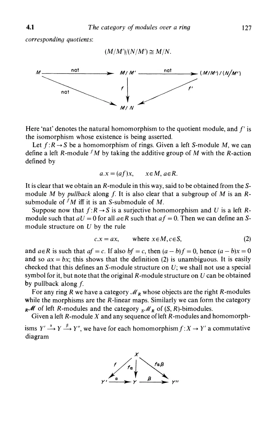
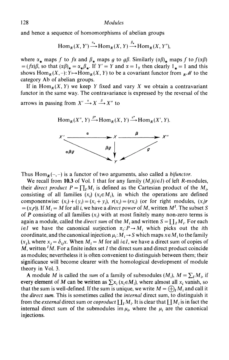
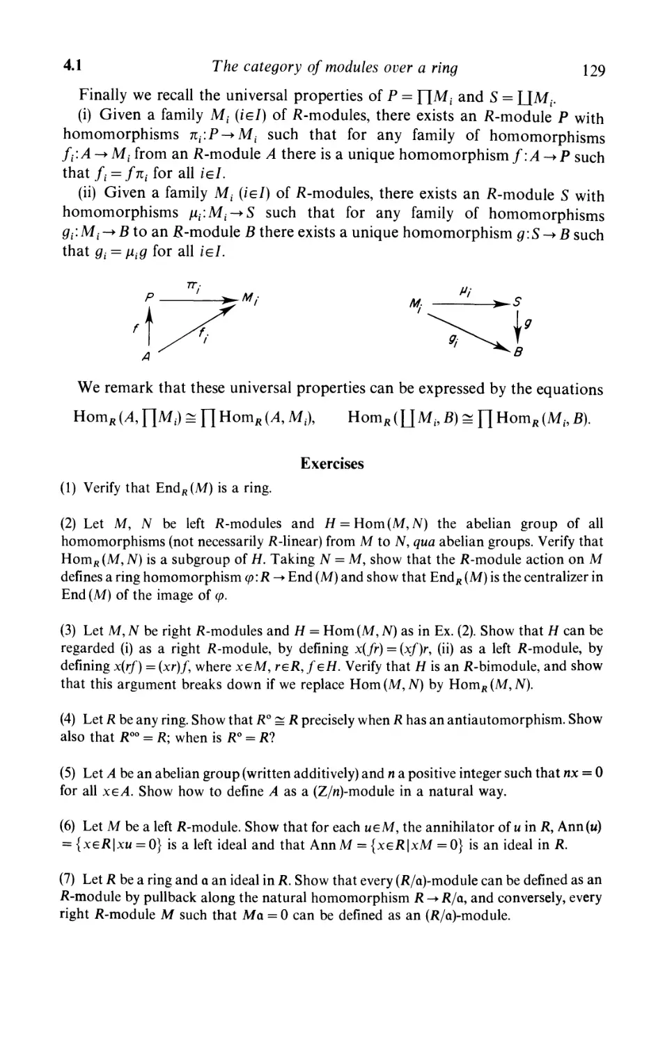
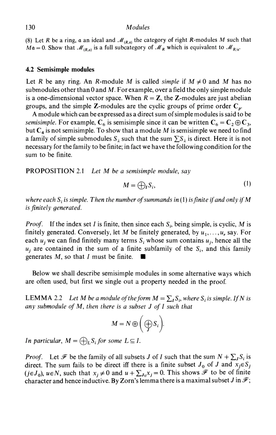
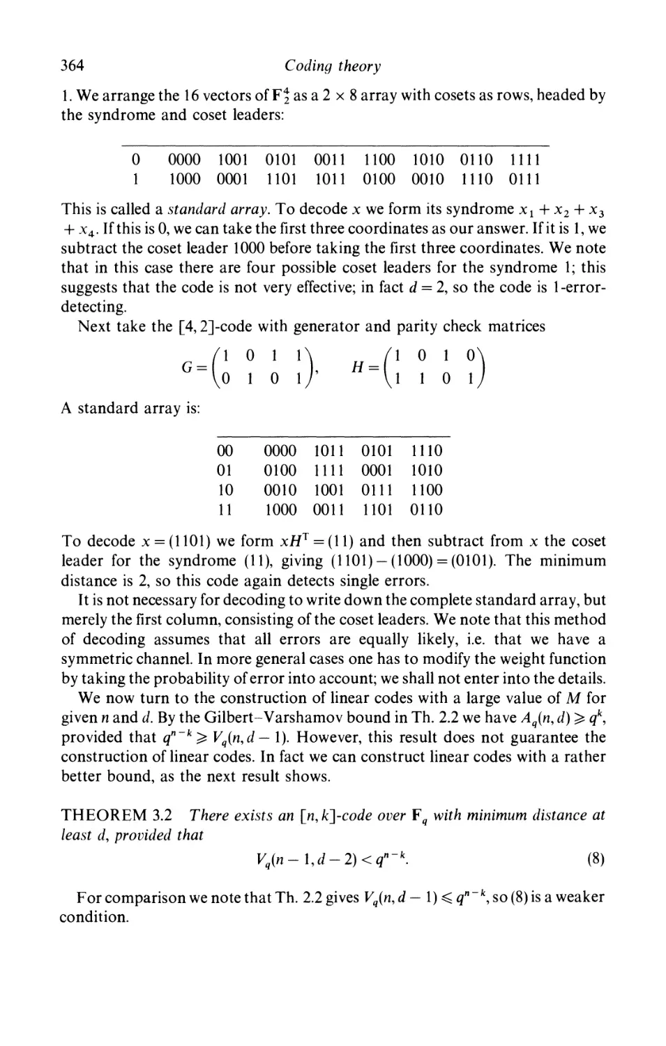
/


Автор: P. M. Cohn
Теги: mathematics algebra higher mathematics john wiley and sons university college london
Год: 1989

Текст
Algebra
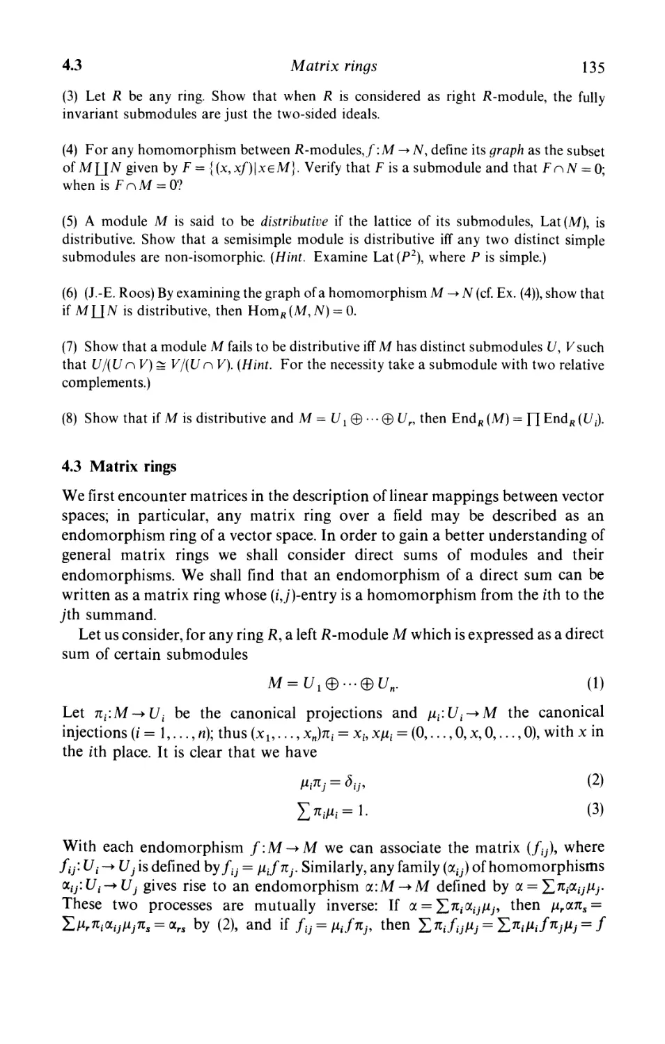
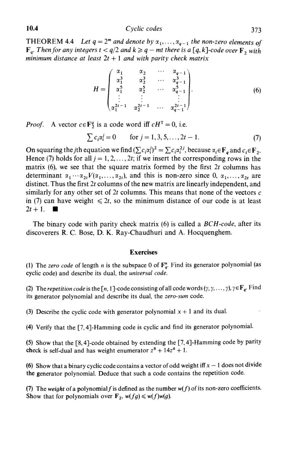
Second Edition
Volume 2
P. M. COHN, FRS
University College London
JOHN WILEY & SONS
Chichester • New York • Brisbane • Toronto • Singapore
Copyright © 1989 by John Wiley & Sons Ltd.
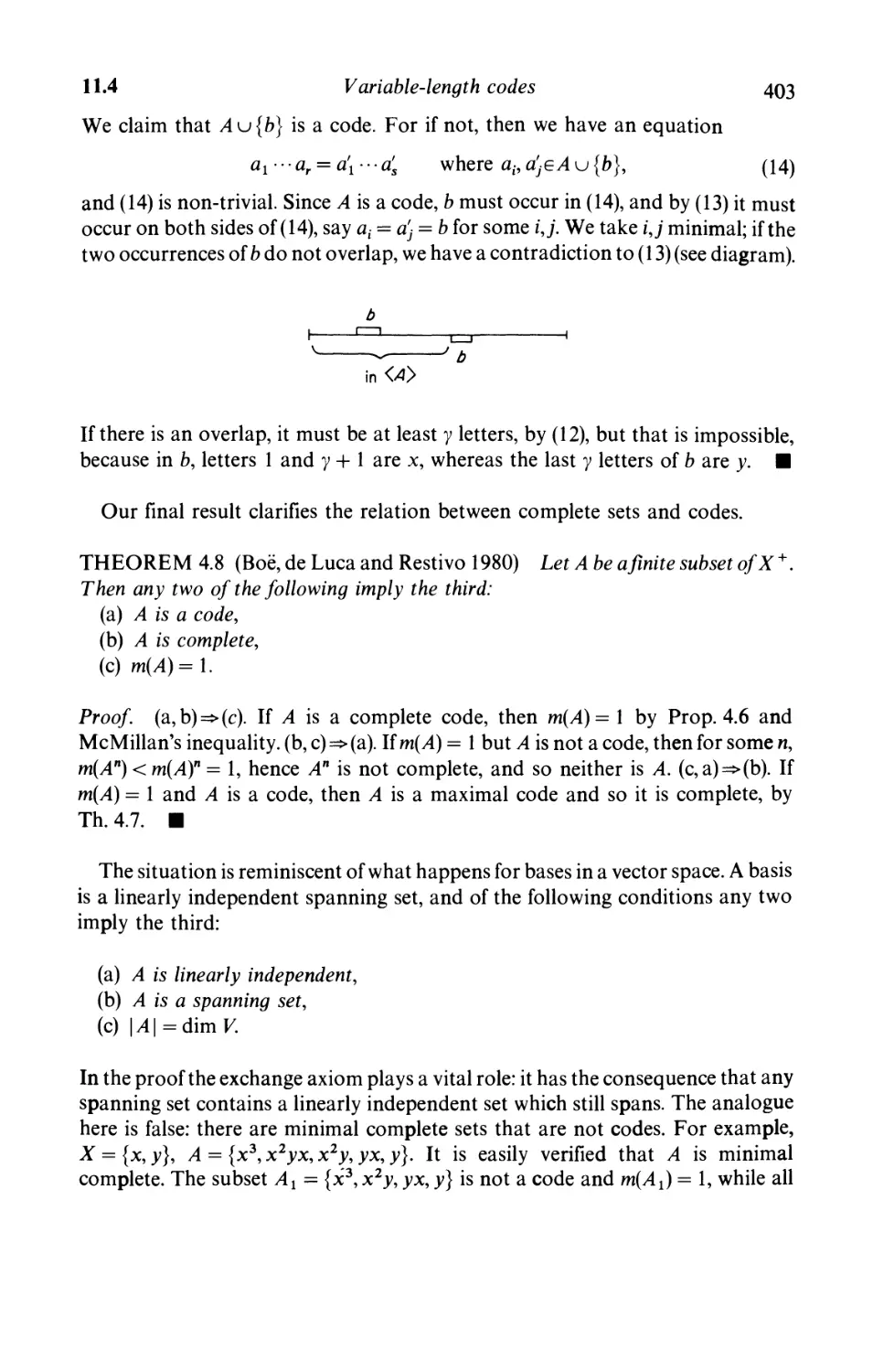
All rights reserved.
No part of this book may be reproduced by any means,
or transmitted, or translated into a machine language
without the written permission of the publisher.
Library of Congress Cataloging-in-Publication Data
(Revised for vol. 2)
Cohn, P. M. (Paul Moritz)
Algebra.
Includes indexes.
Bibliography: v. 2, p.
1. Algebra. I. Title.
QA154.2.C63 1982 512.9 81-21932
ISBN 0 471 10168 0 (v. 1)
ISBN 0 471 10169 9 (pbk.: v. 1)
ISBN 0 471 92234 X (v. 2)
ISBN 0 471 92235 8 (pbk.: v. 2)
British Library Cataloguing in Publication Data
Cohn, P. M. (Paul Moritz)
Algebra.-2nd ed.
Vol.2
1. Abstract algebra
I. Title
512'.02
ISBN 0 471 92234 X
ISBN 0 471 92235 8
Phototypesetting by Thomson Press (India) Ltd., New Delhi
Printed in Great Britain at The Bath Press, Avon
Contents
Preface to the Second Edition ix
From the Preface to the First Edition xi
Conventions on terminology xiii
Table of interdependence of chapters (Leitfaden) xv
1 Sets
1.1 Finite, countable and uncountable sets 1
1.2 Zorn's lemma and well-ordered sets 8
1.3 Categories 16
1.4 Graphs 21
Further exercises 27
2 Lattices
2.1 Definitions; modular and distributive lattices 30
2.2 Chain conditions 38
2.3 Boolean algebras 45
2.4 Mobius functions 54
Further exercises 58
3 Field theory
3.1 Fields and their extensions 62
3.2 Splitting fields 69
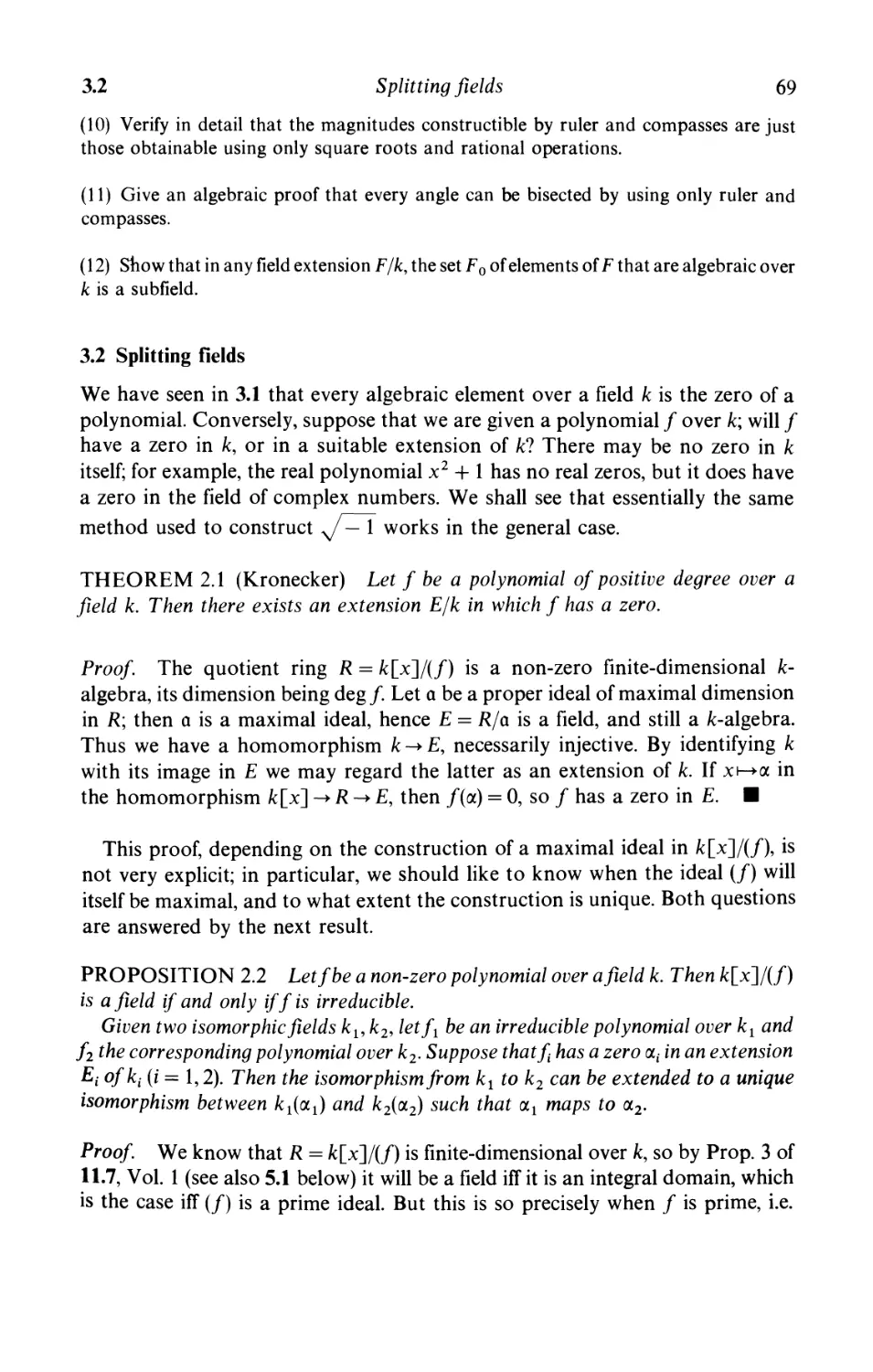
3.3 The algebraic closure of a field 74
3.4 Separability 77
3.5 Automorphisms of field extensions 80
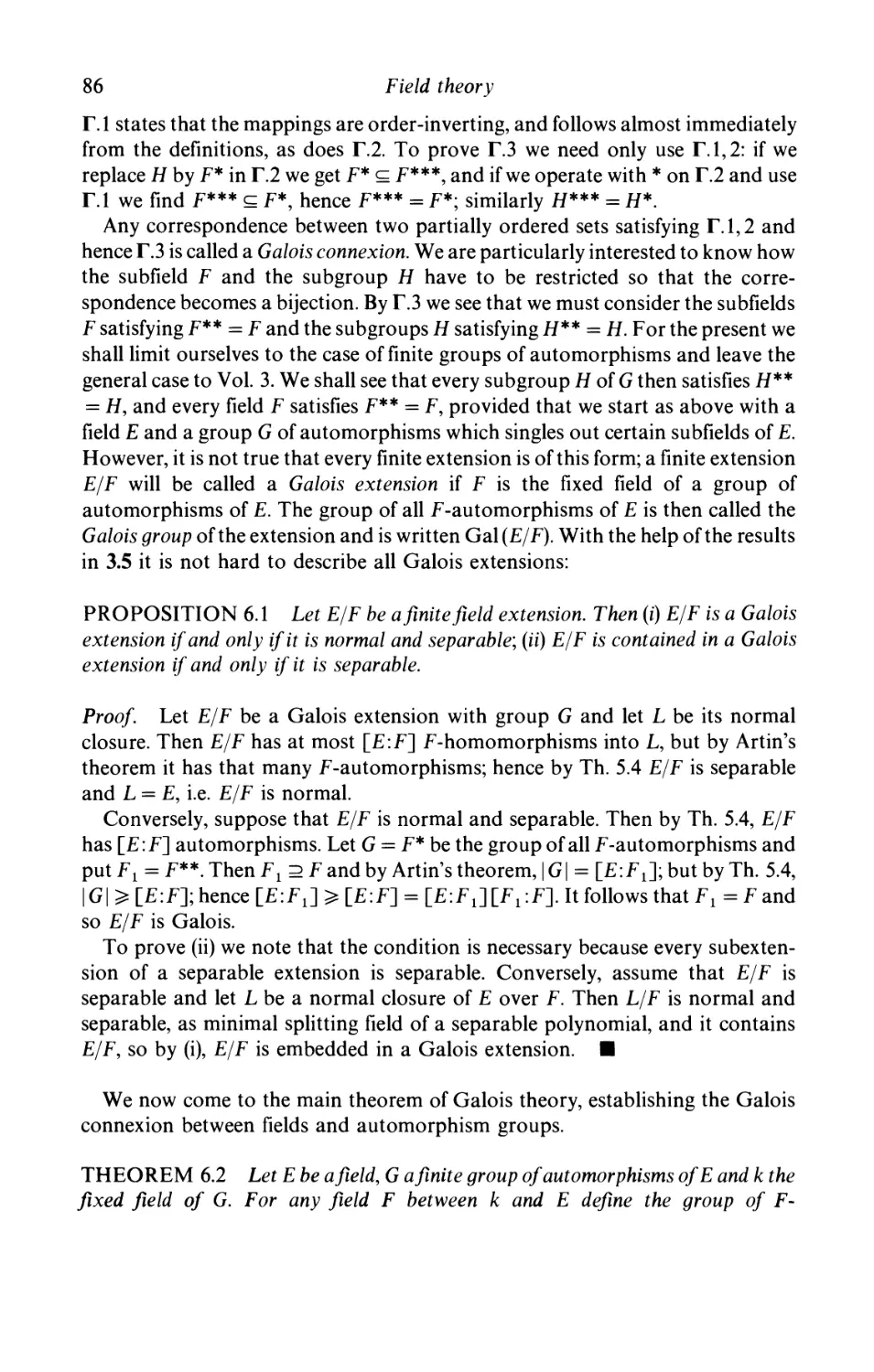
3.6 The fundamental theorem of Galois theory 85
3.7 Roots of unity 91
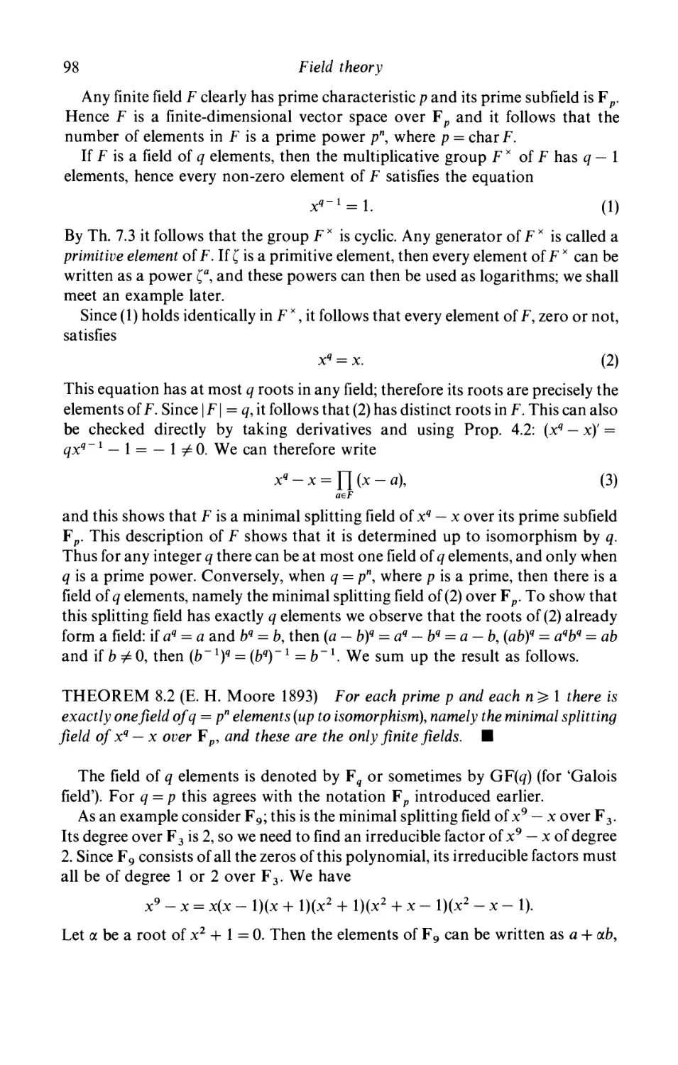
3.8 Finite fields 97
3.9 Primitive elements; norm and trace 102
3.10 Galois theory of equations 107
v
vi Contents
3.11 The solution of equations by radicals 113
Further exercises 121
4 Modules
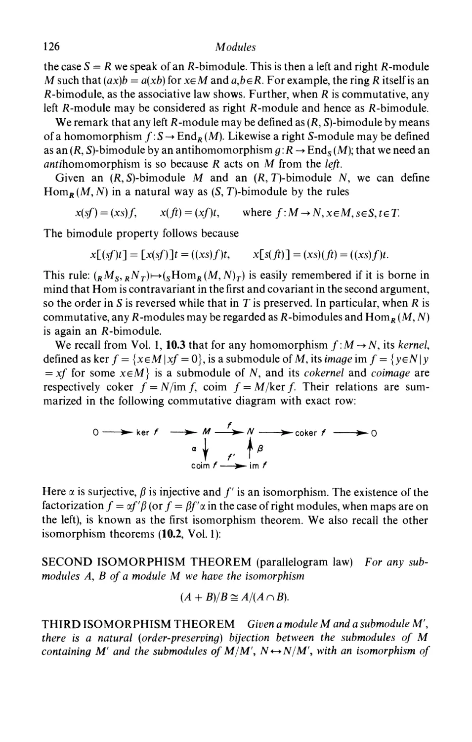
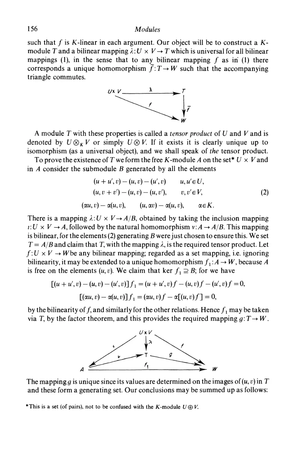
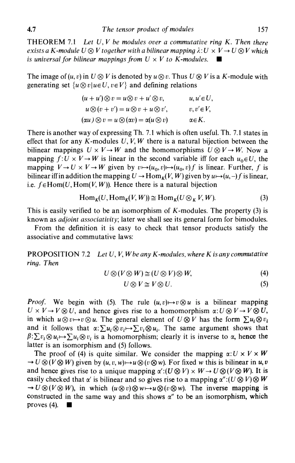
4.1 The category of modules over a ring 124
4.2 Semisimple modules 130
4.3 Matrix rings 135
4.4 Free modules 140
4.5 Projective and injective modules 146
4.6 Duality of finite abelian groups 152
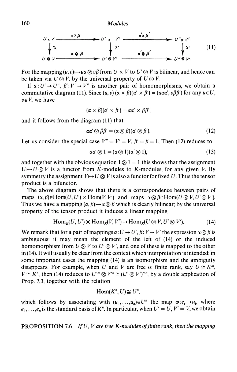
4.7 The tensor product of modules 155
Further exercises 163
5 Rings and algebras
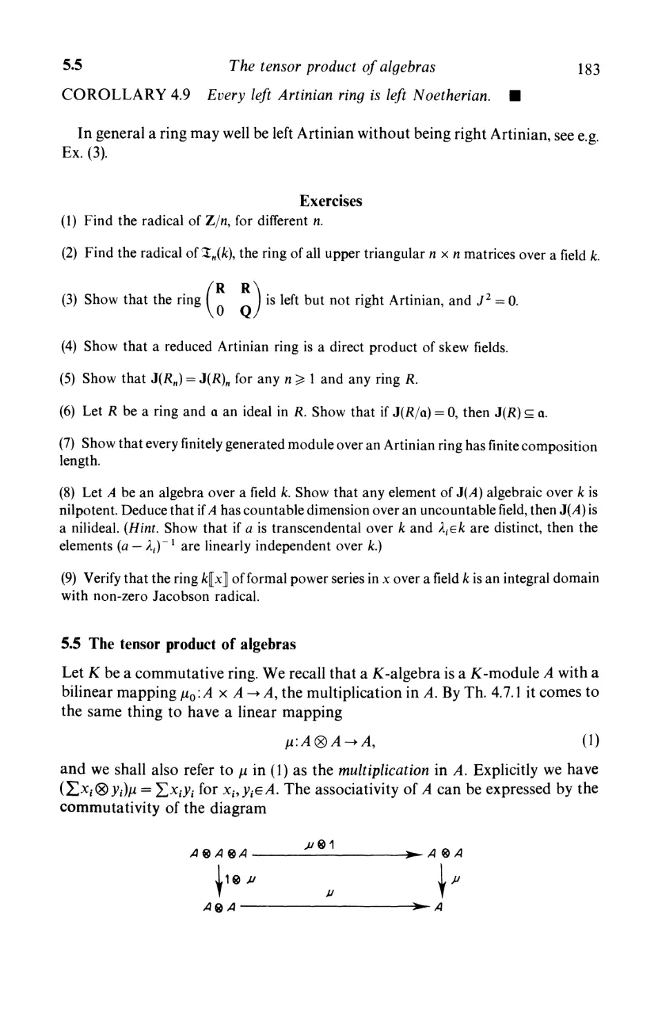
5.1 Algebras: definition and examples 165
5.2 Direct products of rings 170
5.3 The Wedderburn structure theorems 174
5.4 The radical 178
5.5 The tensor product of algebras 183
5.6 The regular representation; norm and trace 187
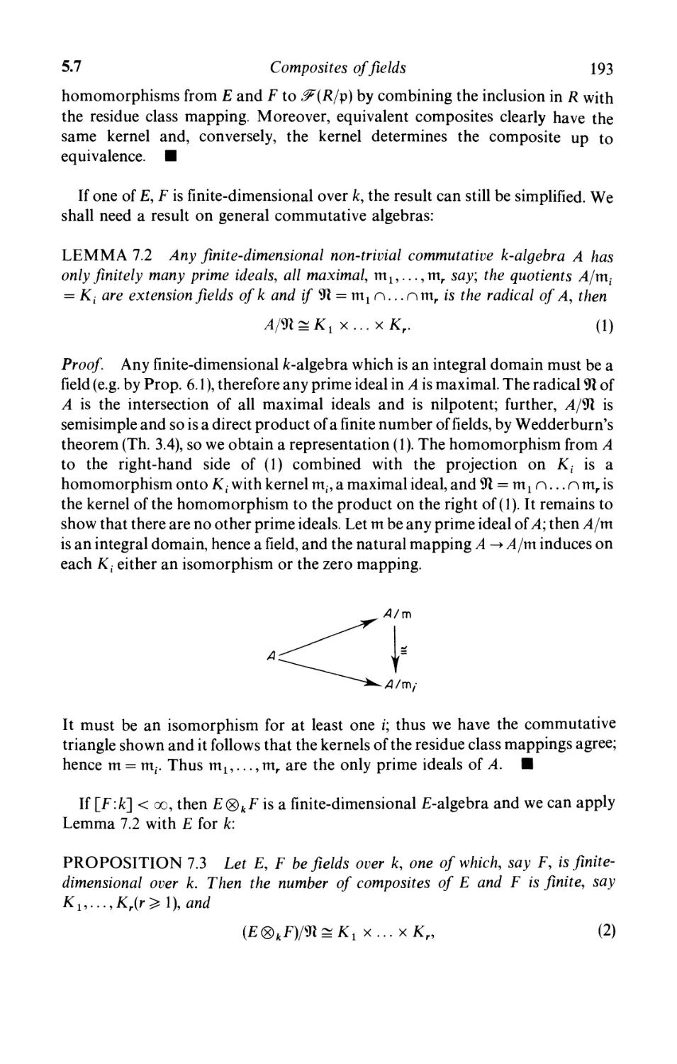
5.7 Composites of fields 191
Further exercises 195
6 Quadratic forms and ordered fields
6.1 Inner product spaces 197
6.2 Orthogonal sums and diagonalization 200
6.3 The orthogonal group of a space 204
6.4 Witt's cancellation theorem and the Witt group of a field . 208
6.5 Ordered fields 212
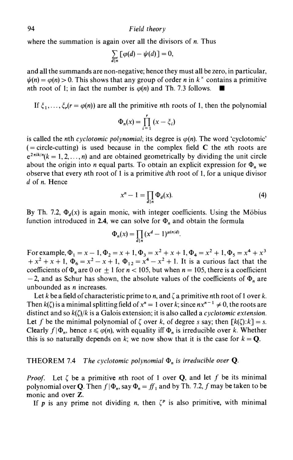
6.6 The field of real numbers 215
Further exercises 220
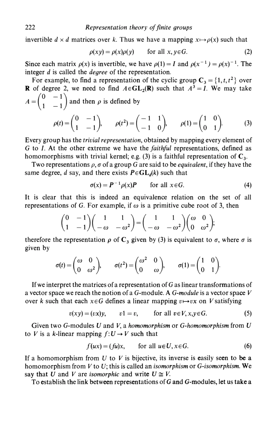
7 Representation theory of finite groups
7.1 Basic definitions 221
7.2 The averaging lemma and Maschke's theorem 226
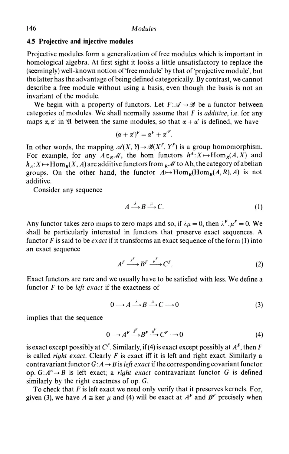
7.3 Orthogonality and completeness 229
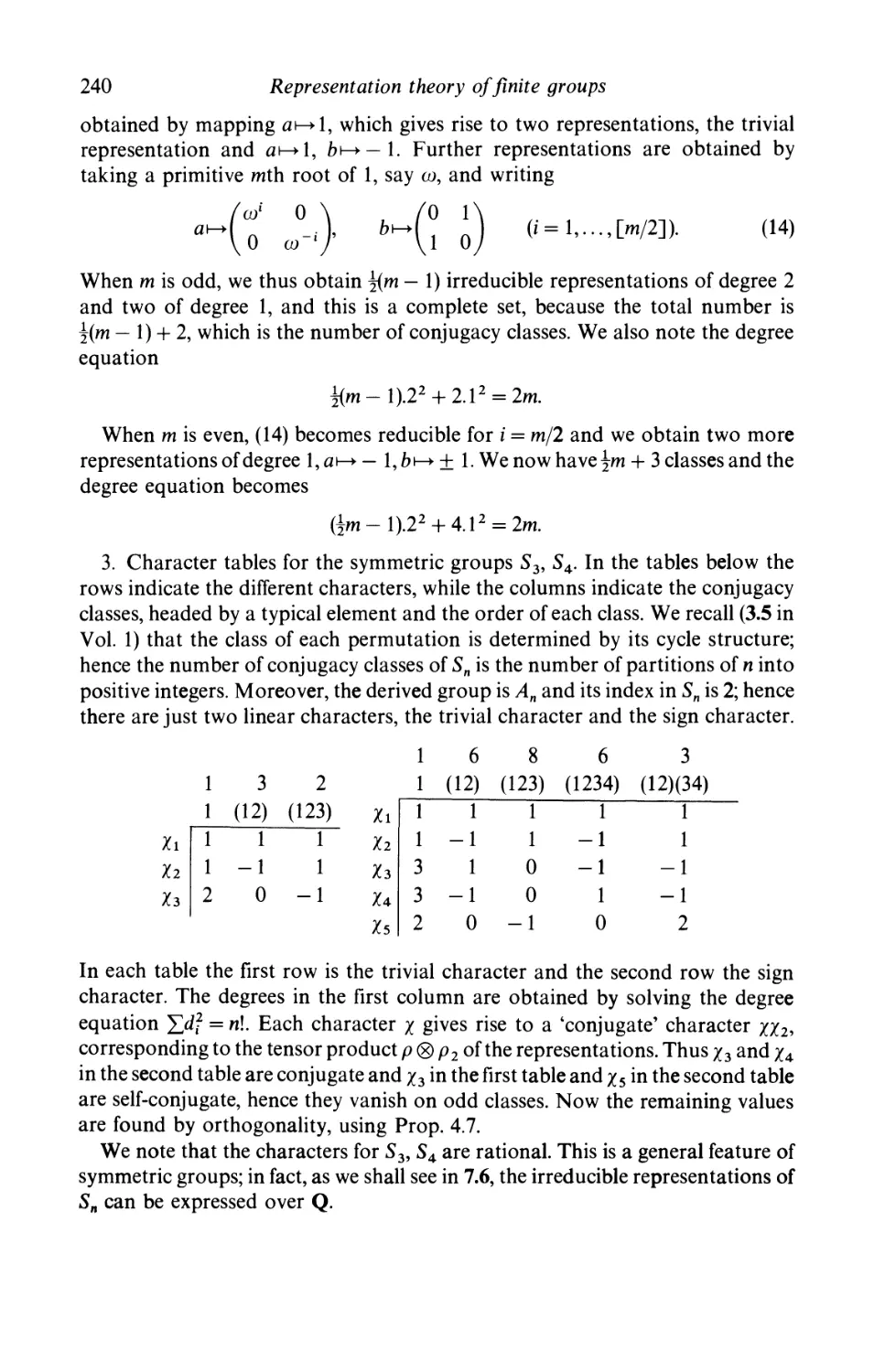
7.4 Characters 233
7.5 Complex representations 241
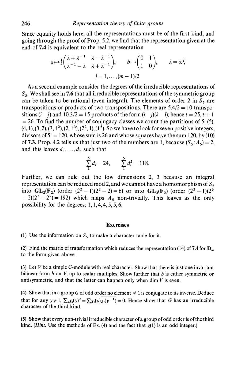
16 Representations of the symmetric group 247
7.7 Induced representations 253
7.8 Applications: the theorems of Burnside and Frobenius . . 258
Further exercises 262
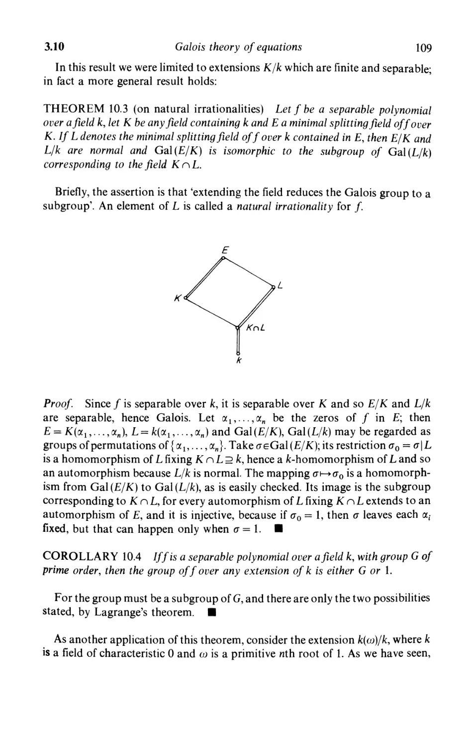
Contents vii
8 Valuation theory
8.1 Divisibility and valuations 264
8.2 Absolute values 269
8.3 The p-adic numbers 280
8.4 Integral elements 289
8.5 Extension of valuations 294
Further exercises 302
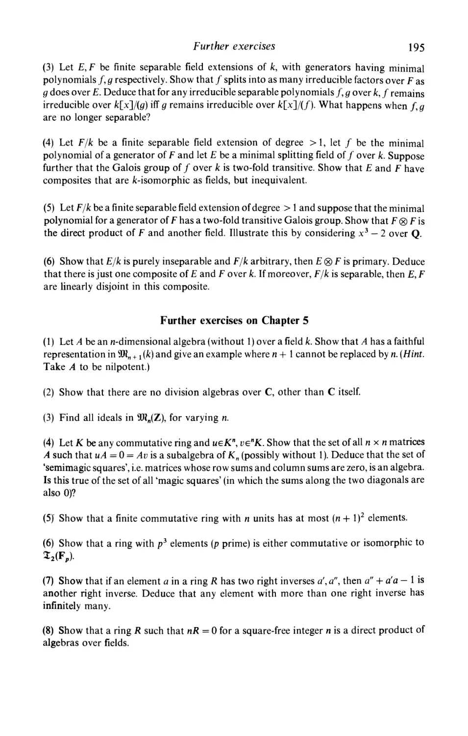
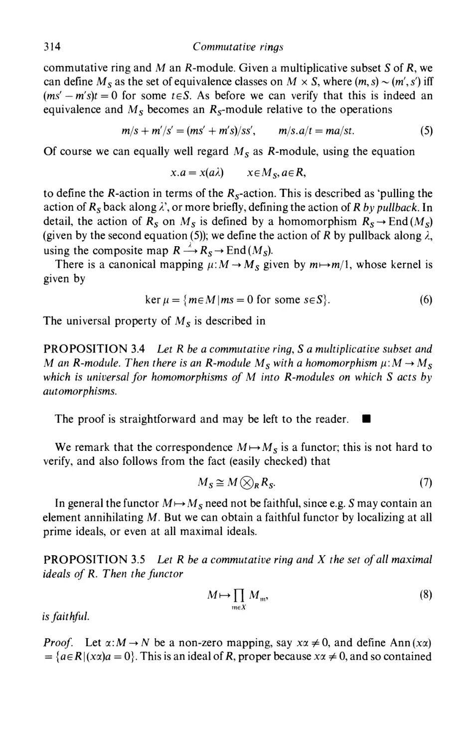
9 Commutative rings
9.1 Operations on ideals 305
9.2 Prime ideals and factorization 307
9.3 Localization 310
9.4 Noetherian rings 317
9.5 Dedekind domains 319
9.6 Modules over Dedekind domains 329
9.7 Algebraic equations 334
9.8 The primary decomposition 338
9.9 Dimension 345
9.10 The Hilbert Nullstellensatz 350
Further exercises 353
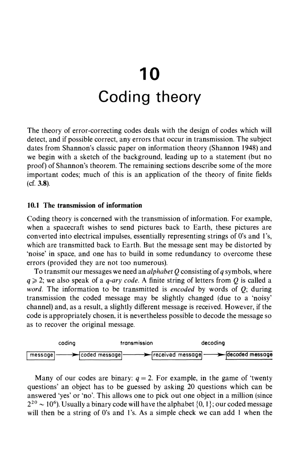
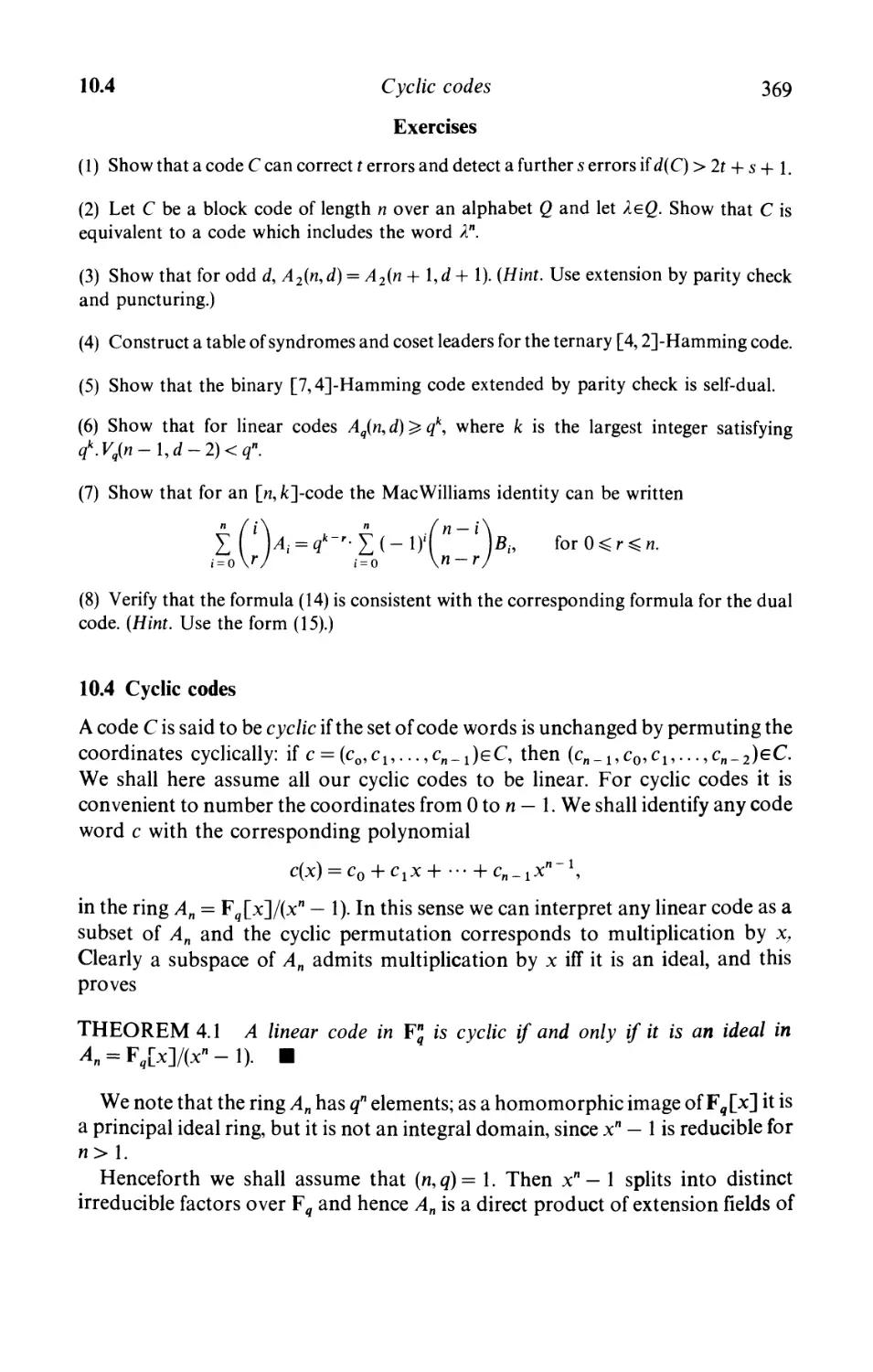
10 Coding theory
10.1 The transmission of information 356
10.2 Block codes 358
10.3 Linear codes 361
10.4 Cyclic codes 369
10.5 Other codes 374
Further exercises 378
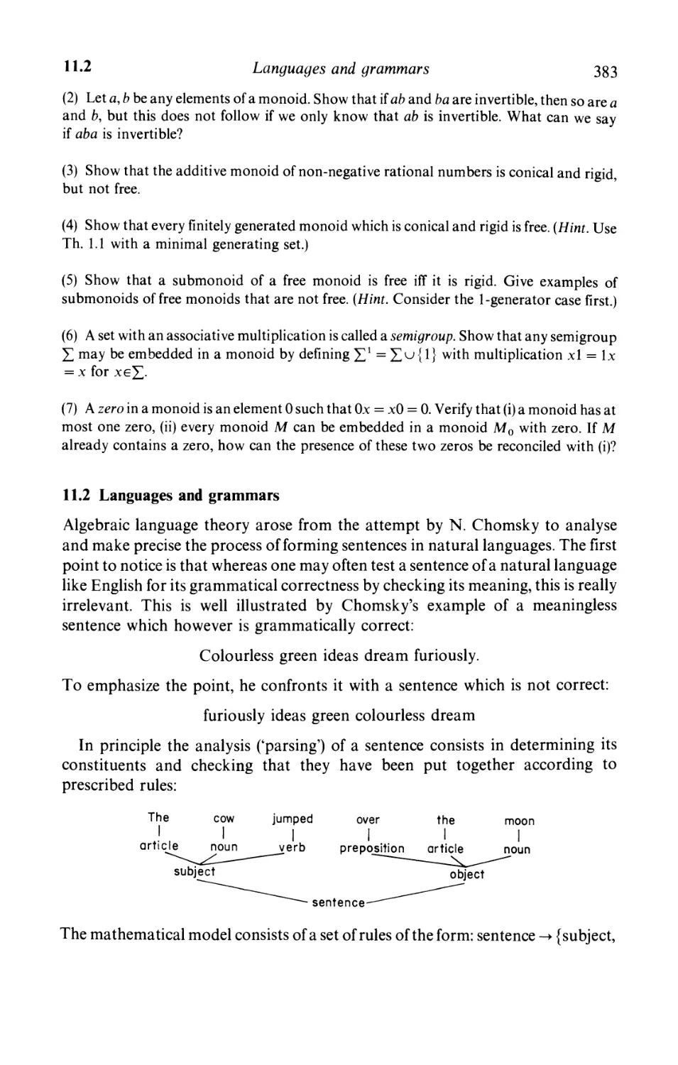
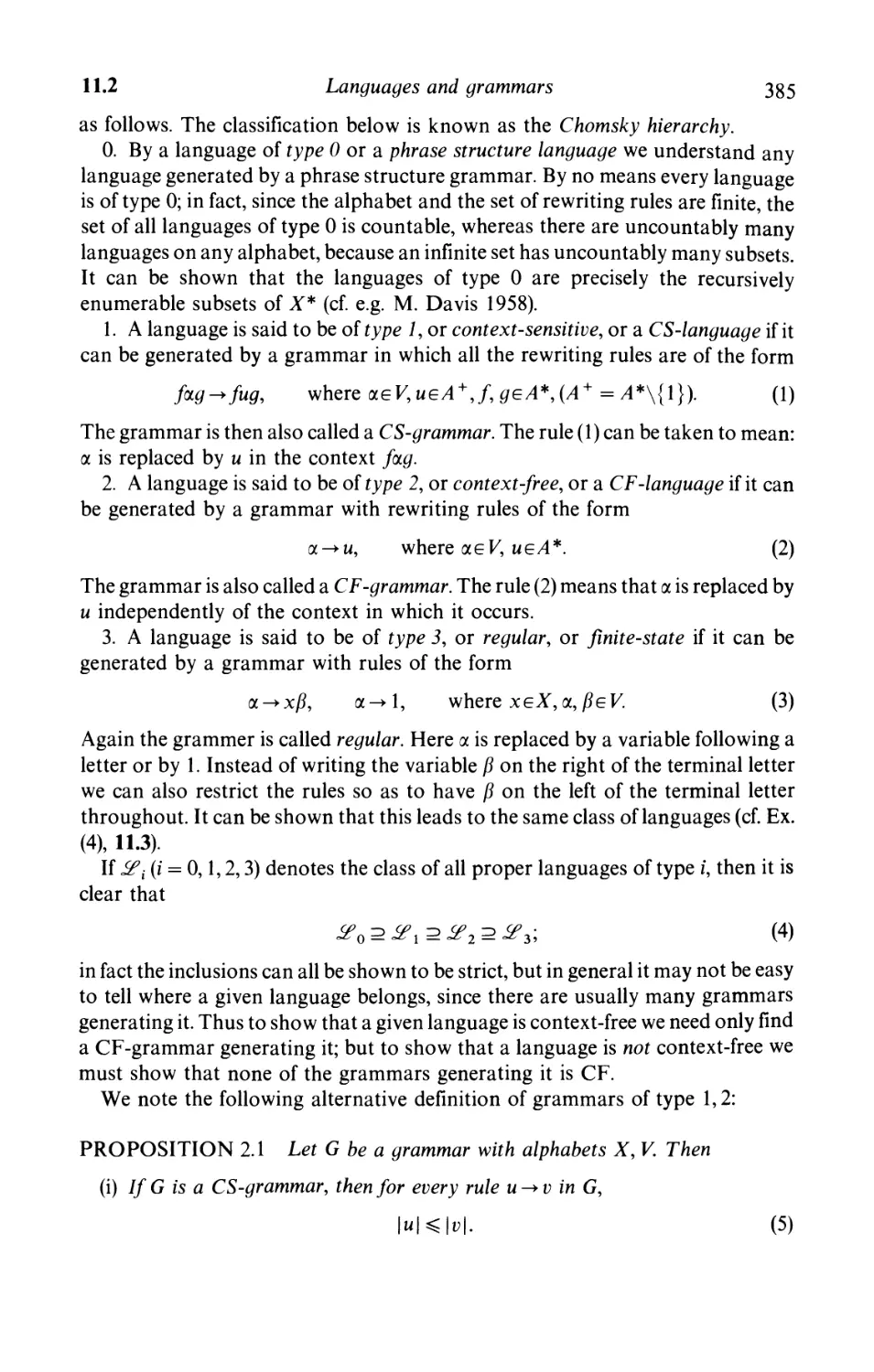
11 Languages and automata
11.1 Monoids and monoid actions 379
11.2 Languages and grammars 383
11.3 Automata 387
11.4 Variable-length codes 395
11.5 Free algebras and formal power series rings 404
Further exercises 413
Bibliography 415
List of notations 418
Index 421
Preface to the Second
Edition
Ever since the publication in 1977 of the First Edition of Algebra Vol. 2,1 have
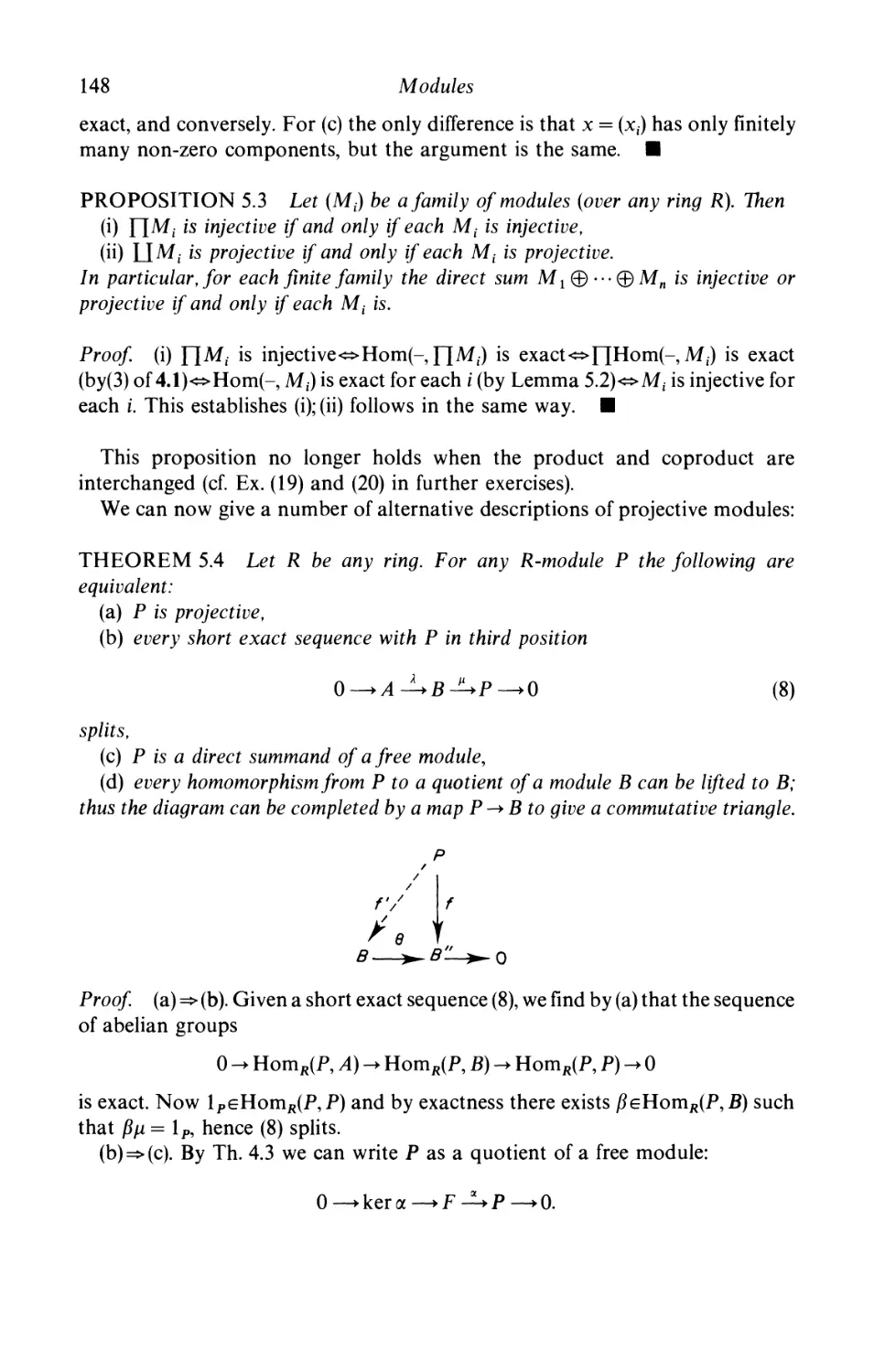
been conscious of the many quite basic parts of algebra that had been omitted or
inadequately treated. Besides the traditional topics this also included such parts
of applied algebra as coding theory, which not only provides an excellent
illustration of the way algebraic methods and results are used, but also in its turn
has influenced the development of field theory. So when the chance to prepare a
revised edition presented itself, I decided to rewrite Vol. 2 completely, to take
account of these additions. The resulting increase in material necessitated a
division into two further volumes, making three in all. This arrangement should
suit the user, who in the new Vol. 2 will find topics for third-year undergraduate
courses, while the projected Vol. 3 will be devoted to postgraduate work.
The present volume includes the whole of four chapters from the old Vol. 2,
about half of another four, while the rest are represented by smaller proportions.
The introductory chapters, on sets and lattices, omit the Peano axioms, but
sections on graphs and categories have been added. This is followed by a chapter
on field theory, covering Galois theory as well as the notion of algebraic closure.
Next come modules, rings and algebras; here many examples and constructions
are given, but the theory is only taken as far as the Wedderburn theorems and the
radical. A chapter on quadratic forms and ordered fields deals with the more
elementary parts from the old Vol. 2, while the chapters on valuations and
commutative rings are included in their entirety. But even where the organization
has remained the same, there have been many changes of detail; these consist
mainly-in amplifying and where possible simplifying the proofs, but also in further
examples and illustrations. Some results of intrinsic interest or importance have
been added, among them HensePs lemma, Ramsey's theorem and the continuity
criterion for p-adic functions.
In addition there are three new chapters. Ch. 7 on representation theory
replaces the old seven-page sketch. It allows a more leisurely pace, as well as a
wider range, including the symmetric group and induced representations, with
the theorems of Frobenius and Burnside as applications. Ch. 10 is an
introduction to block codes; of course only a small selection could be presented, but, it is
IX
X
Preface to the Second Edition
hoped, enough to whet the reader's appetite. Finally Ch. 11 deals with algebraic
language theory and the related topics of variable-length codes, automata and
power series rings. Again it is only possible to take the first steps in the subject, but
we go far enough to show how techniques from coding theory are used in the
study of free algebras.
Throughout, an effort has been made to base the development on Vol. 1.
Definitions and key properties are usually recalled in some detail, but not
necessarily on their first occurrence; the reader can easily trace explanations
through the index. As before, there are numerous exercises (though no solutions),
and some historical references.
A number of colleagues have read and commented on parts of the manuscript:
M. P. Drazin, W. A. Hodges, F. C. Piper, M. L. Roberts, B. A. F. Wehrfritz; I
should like to thank them for their help. Mark Roberts in particular read the
manuscript as well as the proofs, and saved me from a number of errors. I am
also indebted to numerous correspondents who have pointed out errors or
suggested improvements. It goes without saying that any such correspondence
relating to the present volume will always be welcome.
My final thanks go to the staff of John Wiley and Sons, who have, as always,
been helpful and efficient in getting the volume published.
University College London P. M. Cohn
February 1989
From the Preface to the First
Edition
Vol. 1 of this work was intended to cover the first two years of an undergraduate
course, and there is fairly general agreement on the topics to be included. At the
third-year level and beyond there is a much wider range of optional topics, and
the element of personal choice enters in a greater measure. The present volume
includes a variety of algebraic topics that are useful elsewhere, important in their
own right, or that fairly quickly lead to interesting results (preferably all three). To
a large extent the selection follows the tradition set by v.d. Waerden's classic
treatise, but some departures are clearly necessary, the main ones here being
homological algebra, lattices and non-commutative Noetherian rings.
The material presented may be grouped roughly into three parts of four
chapters each*. The first part deals with basic topics: numbers (natural and
transfinite), modular and distributive lattices, tensor products and graded rings
(with the Golod-Shafarevich theorem as an application) and an introduction to
homological algebra. Here 'introduction' means an account which goes far
enough to describe Ext and Tor for the category of modules, show their use in
group theory and prove the syzygy theorem (a la Roganov), but stopping short of
Kunneth-type theorems or direct and inverse limits. On the other hand, injective
and flat modules are studied more fully than is customary in elementary texts, to
give the reader a feel for them. The basic notions of category theory are explained
as they are needed; this seemed more appropriate than having a separate chapter
on categories.
The next part, on fields, has a chapter on Galois theory and one on further field
theory, mainly infinite field extensions, but also a little on skew fields. This is
followed by real fields (Artin-Schreier theory) and quadratic forms, in an account
which develops the Witt ring far enough to exhibit the link with orderings of a
field. The third part, on rings, begins with valuations, a formal study of divisibility
in fields. A chapter on Artinian rings presents the Jacobson theory (radical and
semiprimitivity, density theorem) as well as semiperfect rings and a glimpse of
As explained in the new Preface, the present volume covers about half the material in the old Vol. 2;
the remainder will be included in the projected Vol. 3.
XI
Xll
Preface to the First Edition
group representations, by way of application. It also includes the basic facts on
central simple algebras (the Brauer group) and Hochschild cohomology. The
chapter on commutative rings emphasizes the links with algebraic geometry and
goes as far as the Nullstellensatz. In a slightly different direction, earlier chapters
are put to use in a discussion of Dedekind domains and finitely generated
modules over them. The final chapter, on Noetherian and Pi-rings, brings
Goldie's and Posner's theorems and some of the recent work of Amitsur,
Razmyslov, Rowen and M. Artin on rings with polynomial identities.
My aim throughout has been to present the basic techniques of the subject in
their simplest form, but to develop them far enough to obtain significant results.
Many topics, such as Morita theory, duality, representation theory, were merely
touched on. Other large fields, such as group theory, have been excluded entirely;
to go beyond what was done in Vol. 1 would have given the book a rather
specialized character. Inevitably the choice of topics is influenced by the author's
interests but it should not be (and in this case has not been) dictated by them. The
book was fun to write (at least for the first five years) and, I hope, will be fun to
read.
Bedford College
August 1976
P. M. Cohn
Conventions on terminology
We recall that all rings (and monoids) have a unit-element or one, i.e. a neutral
element for multiplication, usually denoted by 1. By contrast an algebra (over a
coefficient ring) need not have a 1, although it usually does in the present volume.
A ring is trivial if 1 =0; this means that it consists of 0 alone. An element a of a ring
R is called a zerodivisor if a # 0 and ab = 0 or ba = 0 for some b # 0; a non-
zerodivisor is an element a ^ 0 such that ab^O.ba^O for all b ^ 0. Thus each
element of a ring is either a zerodivisor, a non-zerodivisor or 0, and these three
possibilities are mutually exclusive. A non-trivial ring without zerodivisors is
called an integral domain; this term is not taken to imply commutativity. A ring in
which the non-zero elements form a group under multiplication is called a skew
field or division ring; in the commutative case this reduces to a field. In any ring R
the set of non-zero elements is denoted by Rx; this notation is mainly used for
integral domains, where Rx is a monoid. A skew field finite-dimensional over
its centre is called a division algebra; this use of the term was agreed at the
Amitsur Conference, Ramat Gan, 1989. The term 'algebra' by itself is not taken
to imply finite dimensionality.
If G is a group and H a subgroup, then the subsets xH of G are called the right
cosets ofH in G, and a subset T of G containing one element from each right coset
is called a left transversal of H in G; this is also known as a complete set of coset
representatives ofH in G. We write H < G to indicate that H is a normal subgroup
of G, and for a subset X of G, < X > is the subgroup generated by X; similarly for
submodules.
If 5 is a set, a property is said to hold for almost all members of 5 if it holds for all
but a finite number of members of S. If T is a subset of 5, its complement in S is
written S\T.
As a rule mappings are written on the right; in particular this is done when
mappings have to be composed, so that ajS means: first a, then /?. If a is a mapping
from a set S and Tis a subset of 5, then the restriction of a to Tis denoted by a| T.
References to the bibliography are by name of author and date. All results in a
given section are numbered consecutively, e.g. in 4.2 we have Prop. 2.1,
Lemma 2.2, Theorem 2.3, which are so referred to in Ch. 4, but as Prop. 4.2.1, etc.,
elsewhere. As in Vol. 1, we use iff as an abbreviation for 'if and only if and ■
indicates the end (or absence) of a proof.
Xlll
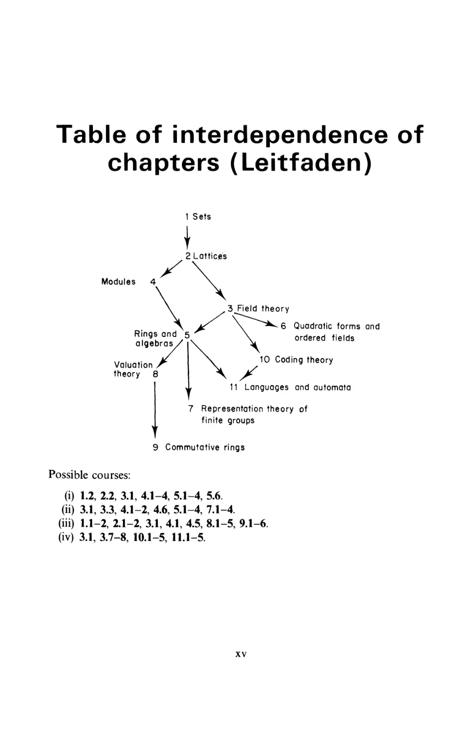
Table of interdependence of
chapters (Leitfaden)
1 Sets
\
2 Lattices
Modules 4
Valuation
theory 8
Rings and 5
algebras
3^Field theory
6 Quadratic forms and
ordered fields
10 Coding theory
X
11 Languages and automata
7 Representation theory of
finite groups
9 Commutative rings
Possible courses:
(i) 1.2, 2.2, 3.1, 4.1-4, 5.1-4, 5.6.
(ii) 3.1, 3.3, 4.1-2, 4.6, 5.1-4, 7.1-4.
(iii) 1.1-2, 2.1-2, 3.1, 4.1, 4.5, 8.1-5, 9.1-6
(iv) 3.1, 3.7-8, 10.1-5, 11.1-5.
xv
1
Sets
Much of algebra can be done using only very little set theory; all that is needed is a
means of comparing infinite sets, and the axiom of choice in the form of Zorn's
lemma. These topics occupy the first two sections. This is followed by an outline
of the notions of categories needed later; this adds little to what was said in Vol. 1
but it forms a base on which later chapters and Vol. 3 can build. The chapter ends
with an introduction to graph theory. This is an extensive theory and all that can
be done here is to present a few basic results which convey the flavour of the topic,
some of which will be used later.
1.1 Finite, countable and uncountable sets
The primary purpose of the natural numbers is to count. In essence counting
serves to compare the 'numerousness' or 'number of elements' of two sets. When
Man Friday wanted to tell Robinson Crusoe that he had seen a boat with 17 men
in it, he did this by exhibiting another 17-element set, and he could do this without
being able to count up to 17. Even for a fully numerate person it may be easier to
compare two sets rather than to count each; e.g. in a full lecture room a brief
glance may suffice to convince us that there are as many people as seats. This
suggests that it may be easier to determine when two sets have the same 'number
of elements' than to find that number. Let us call two sets equipotent if there is a
bijection between them. This relation of equipotence between sets is an
equivalence relation on any given collection of sets*, so in order to compare two
sets, we may compare each to a set of natural numbers. A set S is said to be finite,
of cardinal n, if S is equipotent to the set {1,2,..., n) consisting of the natural
numbers from 1 to n. By convention the empty set, having no elements, is
reckoned among the finite sets; its cardinal is 0 and it is denoted by 0.
It is clear that two finite sets are equipotent if they have the same cardinal, and
this may be regarded as the basis of counting. It is also true that sets of different
finite cardinals are not equipotent. This may seem intuitively obvious; we shall
assume it here and defer to Vol. 3 its derivation from the axioms for the natural
*We avoid speaking about the collection of all sets, as that would bring us dangerously close to the
paradoxes mentioned in Vol. 1, Ch. 1. In any case we shall have no need to do so.
2
Sets
numbers. More generally, we shall assume that for any natural numbers m, n, if
there is an injective mapping from {1,2,..., m} to {1,2,..., w}, then m < n. Let us
abbreviate {1,2,..., v} by [v], for any veN. It follows that if there is a bijection
between [m] and [w], then m ^ n and n ^ m, hence m = n. Thus for any finite set,
the natural number which indicates its cardinal is uniquely determined. The
contrapositive form of the above assertion states that if m > n, then there can be
no injective mapping from [m] to [ft]. A more illuminating way of expressing this
observation is Dirichlet's celebrated
BOX PRINCIPLE (Schubfachprinzip) Ifn+l objects are distributed over n
boxes, then some box must contain more than one of the objects.
Although intuitively obvious, this principle is of great use in number theory
and elsewhere.
Having given a formal definition of finite sets, we now define a set to be infinite if
it is not finite. Until relatively recent times the notion of'infinity' was surrounded
by a good deal of mystery and uncertainty, even in mathematics. Thus towards
the middle of the 19th century, Bolzano propounded as a paradox the fact that (in
modern terms) an infinite set might be equipotent to a proper subset of itself. A
closer study reveals that every infinite set has this property, and this has even been
taken as the basis of a definition of infinite sets; it certainly no longer seems a
paradox. The work of Cantor, Dedekind and others from 1870 onwards
has dispelled most of the uncertainties, and though mysteries remain, they will
not hamper us in the relatively straightforward use we shall make of the
theory.
In order to extend the notion of counting to infinite sets, we associate with
every set X, finite or not, an object \X\ called its cardinal or cardinal number,
defined in such a way that two sets have the same cardinal iff they are equipotent.
Such a definition is possible because, as we have seen, equipotence is an
equivalence relation on any collection of sets.
A non-empty finite set has a natural number as its cardinal; the empty set has
cardinal 0. All other sets are infinite; their cardinals are said to be transfinite, or
infinite. In particular, the set N of all natural numbers is infinite; its cardinal is
denoted by K0. The letter aleph, K, the first of the Hebrew alphabet, is
customarily used for infinite cardinal numbers. A set of cardinal K0 is also said to
be countable (or enumerable); thus A is countable iff there is a bijection from N to
A. If a set A is countable, we can write it in the form
A = {aua2,a3,...}, (1)
where the a, are distinct. Such a representation of A is called an enumeration of A,
and a proof that a set is countable will often consist in giving an enumeration.
Sometimes the term 'enumeration' is used for a set written as in (1) even if the at
are not distinct; in that case we can always produce a strict enumeration by going
1.1 Finite, countable and uncountable sets 3
through the sequence and omitting all repetitions. The set so obtained is finite or
countable.
Many sets formed from countable sets are again countable, as our first result
shows.
THEOREM 1.1 Any subset and any quotient set of a countable set is finite or
countable. If A and B are countable sets, then the union A\jB and Cartesian product
A x B are again countable; more generally, the Cartesian product of any finite
number of countable sets is countable. Further, a countable union of countable sets is
countable and the collection of all finite subsets of a countable set is countable.
We recall that a quotient set of A is the set of all blocks, i.e. equivalence classes,
of some equivalence on A.
Proof Any countable set A may be taken in the form (1); if A' is a subset, we go
through the sequence al,a2,... of elements of A and omit all terms not in A' to
obtain an enumeration of A'. If A" is a quotient set, and x\-+x is the natural
mapping from A to A", then {dl,d2,...} is an enumeration of A", possibly with
repetitions; hence A" is countable (or finite).
Next let A be given by (1) and let B = {bl,b2,...}', then AkjB may be
enumerated as {a1,b1,a2,b2,...}, where repetitions (which may occur if
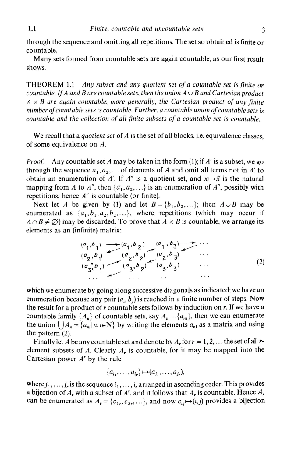
AnB ^ 0) may be discarded. To prove that A x Bis countable, we arrange its
elements as an (infinite) matrix:
(2)
which we enumerate by going along successive diagonals as indicated; we have an
enumeration because any pair (ah bj) is reached in a finite number of steps. Now
the result for a product of r countable sets follows by induction on r. If we have a
countable family {An} of countable sets, say An = {ani}, then we can enumerate
the union (JAn = {ani\n, ieN} by writing the elements ani as a matrix and using
the pattern (2).
Finally let A be any countable set and denote by Ar for r = 1,2,.. .the set of all r-
element subsets of A. Clearly Ar is countable, for it may be mapped into the
Cartesian power Ar by the rule
{ah,...,air}*-+{ah,...,ajr),
wheref!,... ,jr is the sequence il9...9ir arranged in ascending order. This provides
a bijection of Ar with a subset of Ar, and it follows that Ar is countable. Hence Ar
can be enumerated as Ar = {clr, c2r,...}, and now c0-i->(i,f) provides a bijection
4
Sets
between At uA2u... and N2. Thus the collection of all non-empty finite subsets
of A is countable, and adding 0 as a further member we still have a countable
set. ■
With the help of this result many sets can be proved to be countable which do
not at first sight appear to be so. Thus the set Z of all integers can be written as a
union of N = {1,2,3,...} and N' = {0, - 1, - 2,...}; both N and N' are countable,
hence so is Z. The set Q + of all positive rational numbers is countable, as image of
N2 under the mapping (a, b)\-+ab~x. Now Q itself can be written as the union of
the set of positive rational numbers, the negative rational numbers and 0;
therefore Q is countable. The set of all algebraic numbers (cf. Ch. 3 below) is
countable: for a given degree n, the set of all monic equations of degree n over Q is
equipotent to Q", if we map
(a1,...,an)i->xn + a1xn"1 H h an = 0.
Each equation has at most n complex roots, so the set Sn of all roots of equations
of degree n is countable, and now the set of all algebraic numbers is 5t u 52 u...,
which is again countable.
At this point a newcomer might be forgiven for thinking that perhaps every
infinite set is countable. If that were so, there would of course be no need for an
elaborate theory of cardinal numbers. In fact the existence of uncountable sets is
one of the key results of Cantor's theory, and we shall soon meet examples of such
sets.
Our next task is to extend the natural order on N to cardinal numbers. If a, jS
are any cardinals, let A, B be sets such that |A | = a, \B\ = /?. We shall write a ^ jS
whenever there is an injective mapping from A to B. Whether such a mapping
exists clearly depends only on a, jS and not on A, B themselves, so the notation is
justified. Further, a ^ a holds for all a, because the identity mapping on A is
injective, and since the composition of two injections is an injection, it follows
that a ^ /?, jS ^ y implies a < y. Thus we have a preordering; this will in fact turn
out to be a total ordering (i.e. for any cardinals a, jS, either a < /? or jS ^ a), but for
the moment we content ourselves with proving that it is an ordering, i.e. that' ^'
is antisymmetric. In terms of sets we must establish
THEOREM 1.2 (Schroder-Bernstein theorem) Let A, B be any sets and
f:A-+B, g:B-+A any injective mappings. Then there is a bijection h:A-+B.
Proof. By alternating applications off and g we produce an infinite sequence of
successive images starting from aeA:a,afafg,afgf Further, each element
aeA is the image of at most one element of B under g, which may be written ag~ \
and each beB is the image of at most one element bf~1 of A under /, so from aeA
we obtain a sequence of inverse images which may or may not break off: ag~~ \
ag~1f~i, If we trace a given element aeA as far back as possible we find one
1.1
Finite, countable and uncountable sets
5
of three cases: (i) there is a first 'ancestor' in A, i.e. a0eA\Bg, such that a = a0(fg)n
for some n ^ 0; (ii) there is a first ancestor in B, i.e. b0eB\Af, such that a = b0(gf)ng
for some ft ^ 0; (iii) the sequence of inverse images continues indefinitely.
Each element of A comes under exactly one of these headings, and likewise
each element of B. Thus A is partitioned into three subsets Al9 A2, A3; similarly B
is partitioned into Bx = Axf,B2 = A2g~x and£3 = A3f = A3g~1. It is clear that
the restriction of / to A1 is a bijection between At and Bl9 for each element of £t
comes from one element in A t. For the same reason the restriction of g to B2
provides a bijection between B2 and A2, and we can use either / restricted to A3
or g restricted to B3 to obtain a bijection between A3 and B3. Thus we have found
a bijection between At and Bt (i = 1,2,3) and putting these together we obtain a
bijection between A and B. ■
This proof is essentially due to J. Konig (in 1906).
The sum and product of cardinals may be defined as follows. Let a, jS be any
cardinals, say a = |A |, jS = |B|, and assume that Ac\B — 0. Then |A uB| depends
only on a,/?, not on A,B and we define
a + jS = |Au£|.
Similarly we put
ajSHA x fl|.
It is easy to verify that these operations satisfy the commutative and associative
laws, and a distributive law, as in the case of natural numbers. Moreover, for finite
cardinals these operations agree with the usual operations of addition and
multiplication. On the other hand, the cancellation law does not hold, thus we
may have a + jS = a' + jS or ajS = a'jS for a ^ a', and there is nothing corresponding
to subtraction or division. In fact, it can be shown that if a, jS ^ 0 and at least one
of a, jS is infinite, then
a + jS = ajS = max{a,jS}. (3)
For any cardinals a,jS we define jSa as \BA\, where A,B are sets such that \A\
= a, \B\ = jS and £A denotes the set of all mappings from A to B. It is again clear
that jSa is independent of the choice of A, B, and we note that for finite cardinals, /?a
has its usual meaning: if A has m elements and B has n elements, then there is a
choice of n elements to which to map each element of A, and these choices are
independent, so in all there are n.n...n (m factors) choices. Of course this
interpretation applies only to finite sets.
If B is a 1-element set, then so is BA, for any set A: each element of A is mapped
to the unique element of B, and this applies even if A is empty, for a mapping
A -> B is defined as soon as we have specified the images of the elements of A; so
when A = 0, nothing needs to be done. When B is empty, then so is BA, unless
6
Sets
also A = 0, for there is nowhere for the elements of A to map to. Hence we have
I-1. C = {° «"** (4)
[ 1 if a = 0.
Let us now assume that B has more than one element. Then we necessarily have
\BA\>\A\. (5)
For let b, V be distinct elements of B\ we can map A to BA by the rule a\-*8a, where
fib if x = a,
a~\b' ifx#a.
This mapping is injective because for a ^ a', <5fl differs from 8a> at a. It is a
remarkable fact that the inequality (5) is always strict. As usual we write a < /}
or jS > a to mean 'a < jS and a # /T.
THEOREM 1.3 For any cardinals a, /?, i/j? > 1, £hen a < jSa. irc particular,
a < 2a (6)
for arcy cardinal a.
Proof. We have just seen that a <jSa and it only remains to show that equality
cannot hold. Taking sets A, B such that | A | = a, | £ | = /}, we shall show that there
is no surjective mapping from A to BA; it then follows that these sets are not
equipotent. Thus let f:A -+BA be given; in detail, / associates with each aeA a
mapping from A to B, which may be denoted by fa. We must show that / is not
surjective, i.e. we must find g:A-+B such that g ^ fa for all aeA. This may be done
very simply by constructing a mapping g to differ from fa at a. By hypothesis, B
has at least two elements, say b, b\ where b ^ V. We put
a JV ifafa = b,
\b otherwise.
Then g is well-defined and for each aeA, g ^ fa because ag # afa. ■
If in this theorem we take A to be countable and B a 2-element set, simply
denoted by 2, then 2A is again infinite, but uncountable. Moreover, we can in this
way obtain arbitrarily large cardinals by starting from any infinite cardinal a and
forming in succession 2a, 22,
Theorem 1.3 again illustrates the dangers of operating with the 'set of all sets'. If
we could form the union of all sets, U say, then U would contain 2U as a subset,
hence |2U|<|U|, in contradiction to Th. 1.3. This paradox was discussed by
Burali-Forti and others in the closing years of the 19th century, and it provided
the impetus for much of the axiomatic development that followed. Any axiomatic
system now in use is designed to avoid the possibility of such paradoxes. For our
1.1
Finite, countable and uncountable sets
7
purposes it is sufficient to note that we can avoid the paradoxes by not admitting
constructions involving 'all sets' without further qualification.
We conclude with some applications of Th. 1.3. Given any set A, we denote by
^(A) the set whose members are all the subsets of A; e.g. &(0) = {0}, ^{{x})
= {0, {*} }• This set ^(A) is often called the power set of A; it is equipotent with
2A. To obtain a bijection we associate with each subset C of A its characteristic
function xce2A; taking 2 = {0,1}, we have
( v fl ifxeC,
lc[X)~\Q ifx^C.
It is easily seen that the mapping C\-^Xc provides a bijection between £P(A) and
2A. The inverse mapping is obtained by associating with each fe2A the inverse
image of 1: If'1 = {xeA\xf = 1}. Now Th. 1.3 shows the truth of the following:
COROLLARY 1.4 No set A is equipotent with its power set. More precisely,
given any set A, there is no surjection from A to gP{A). ■
As a further application we determine the cardinal of the set R of all real
numbers. This cardinal is usually denoted by c and is called the cardinal (or power)
of the continuum.
PROPOSITION 1.5 c - 2K°.
Proof. Firstly we can replace R by the open interval (0,1) = {xeR|0 < x < 1},
for there is a bijection, e.g. xh~4[(1 + x2)1/2 +x](1 + x2)_1/2, or
xi—^[1 +sin(tan-1x)]. If we express each number in the binary scale:
a = 0.ala2... {at = 0 or 1), then a\->fa, where fa(n) = an, is a mapping (0, l)-»2N
which is injective, for distinct numbers have distinct binary expansions. Indeed,
some have more than one, e.g. 0.0111... = 0.1000..., but we can achieve
uniqueness by excluding representations in which only finitely many digits are 0.
It follows that c < 2K°. On the other hand, there is an injective mapping from 2N to
(0,1), obtained by mapping fa, defined as before, to 0.ata2... in the decimal scale;
thus the image consists of the real numbers between 0 and 1 whose decimal
expansion contains only 0's and l's. This shows that 2*° < c, and the desired
equality follows. ■
It was conjectured by Cantor that c is the least cardinal greater than K0; this is
known as Cantor's continuum hypothesis (CH). In 1939 Godel showed that it is
consistent with the usual axioms of set theory; thus if the usual system of axioms
(which we have not given explicitly) is consistent, then it remains consistent when
CH is added. In 1963 P. J. Cohen showed CH to be independent of the usual
axioms of set theory. Thus if the negation of CH is added to the axioms of set
theory, we again get a consistent system. This means that within the usual system
Of set theory CH is undecidable.
8 Sets
Exercises
(1) Show that the set of all intervals in R with rational endpoints is countable.
(2) Let A be an infinite set, A' a finite subset and B its complement in A. By picking a
countable subset of B show that \A\ = |B| without using eqn. (3).
(3) Let A be an uncountable set, A' a countable subset and B its complement in A. Show
that |A| = |B| without assuming eqn. (3).
(4) Fill in the details of the following proof that the interval (0,1) is uncountable: If the real
numbers in binary form (as in the proof of Prop. 1.4) could be enumerated a{l\ a{2\.., we
can find a number not included in the enumeration by putting a = O.b^- • •, where bn = 0
or 1 according as a(n) has 1 or 0 in the nth place. (This is Cantor's diagonal argument: bn is
chosen so as to differ from the diagonal term a™.)
(5) Show that the set of all real functions in the interval [0,1] has cardinal greater than the
cardinal of the continuum. What about the subset of continuous functions?
(6) Show that for any cardinals a, /?, y, if y i=- 0 and a ^ /?, then ay ^ /?y.
(7) Show that a'0y = (a/i)\ aV = olp + \ (xp)7 = xPy.
(8) Let /:R ->Q be such that x^y implies xf^ yf. Show that there is an interval in which
/ is constant.
1.2 Zorn's lemma and well-ordered sets
In 1.1 we have already defined the relation a ^ /} for cardinals and we have shown
in Th. 1.2 that it is a partial ordering. Let us recall that a set S is said to be partially
ordered if there is a binary relation ^, called a partial ordering, defined on 5 with
the following properties:
0.1 x ^xfor all xeS {reflexivity),
0.2 x^y and y^z imply x^z for all x,y,zeS (transitivity),
0.3 x<y and y^x imply x = y for all x,yeS (antisymmetry).
If only 0.1-2 hold, we speak of a preordering.
If' ^ ' is a partial ordering on a set S, we shall write x < y to mean 'x ^ y and
x ^ y\ and we write x ^ y, x > y for y ^ x, y < x respectively. As is easily verified,
the opposite ordering' ^' again satisfies 0.1-3 and so is again a partial ordering.
Thus any general statement about partially ordered sets has a dual, which is
obtained by interpreting the original statement for the oppositely ordered set.
This principle of duality can often be used to shorten proofs.
Two elements x, y in a partially ordered set S are said to be comparable if x < y
or y < x. A subset of S in which any two elements are comparable is called a chain
1.2
Zorris lemma and well-ordered sets
9
or also totally ordered. A subset in which no two elements are comparable is
called an anti-chain. For example, the set of natural numbers N is totally ordered
for the usual ordering by magnitude, and partially ordered with respect to
divisibility: a\b iff b = ac for some ceN. For the divisibility ordering on N the set
of all prime numbers is an anti-chain.
In any partially ordered set S an element c is a greatest element if x < c for all
xeS, while c is maximal if c < x for no xeS. Thus a greatest element is maximal but
the converse need not hold. A greatest element, if it exists, is clearly unique, unlike
a maximal element. Least and minimal elements are defined dually; e.g. N with its
usual ordering has a least element, but no greatest element, while Q has neither a
least nor a greatest element.
An upper bound of a subset X of S is an element beS such that x < b for all xeX;
here b may or may not belong to X. Lower bounds are defined dually, and a set is
bounded if it has both an upper and a lower bound.
We now take up the question of the comparability of cardinals left open in the
last section, i.e. whether the ordering of cardinals is in fact total. In terms of sets
the question is whether, given two sets A,B, we can find an injective mapping
from one of them to the other. In intuitive terms one might try to answer this
question by choosing an element from each of A and B, say al9bl9 and pairing
them off, then choosing another pair of elements a2eA,b2eB and pairing them
off, and so on. For sets that are at most countable this solves the problem, but we
have seen that there are uncountable sets, and here the procedure adopted is
rather more problematic. One way to overcome the difficulty is to introduce the
concept of a well-ordering:
An ordered set A is said to be well-ordered if every non-empty subset of A has a
least element.
A well-ordered set is always totally ordered, as we see by applying the
definition to 2-element subsets. It is also clear from the definition that any subset
of a well-ordered set is again well-ordered. A countable set may be well-ordered
simply by enumerating its elements, e.g. the natural order of the positive integers
is a well-ordering, but there are many other well-orderings which do not put
the countability into evidence, e.g. {2,3,4,..., 1}, where the order intended is
that in which the numbers are written, or {1,3,5,...,2,4,6,...} or even
{1,2,4,6,...3,9,15,21,...5,25,35,...7,49,...}. By contrast, the negative
numbers in their natural order form a set which is not well-ordered, although we can
well-order it, e.g. by writing it in the opposite order.
For well-ordered sets it is possible to prove the comparability in a strong
form. Let us call a subset A' of an ordered set A a lower segment if ueA', v^u
implies veA'. This definition can be used for any ordered set, not necessarily well-
ordered, or even totally ordered. In particular, for any element aeA, the set
(a) = {xeA|x < a} is a lower segment in A; in a well-ordered set A every lower
segment not the whole of A is of this form, for if A' is a proper lower segment of A
and a is the first element of A\A', then A' = \a).
10
Sets
Two ordered sets A, B are said to be order-isomorphic or of the same order-type
if there is a bijection between them which preserves the ordering, f:A -» B such
that x ^ yoxf < yf-
LEMMA 2.1 A well-ordered set cannot be order-isomorphic to one of its proper
lower segments.
Proof. Let A be well-ordered, | a) a proper lower segment and let f:A -»| a) be an
order-isomorphism. Then clearly af < a; let a0 be the least element of A such that
a0f < a0. If we apply / to this inequality and recall that / preserves the order, we
find that a0ff < a0f so we have found an earlier element with the same property,
namely a0f This contradiction shows that / cannot exist. ■
We now show that any two well-ordered sets can be compared.
THEOREM 2.2 Let A, B be two well-ordered sets. Then one of them is order-
isomorphic to a lower segment of the other.
Proof Let us call a pair of elements aeA and beB matched if the corresponding
lower segments \a) and \b) are order-isomorphic. Two distinct lower segments of
A cannot be order-isomorphic, for one of them will be a lower segment of the
other, and this would contradict Lemma 2.L It follows that any element of B can
be matched against at most one element of A and vice versa. Let A' be the set of
elements of A that can be matched against elements of B, and B' the set of
elements of B matched against elements of A. Then A' and B' are order-
isomorphic, as we see by using the correspondence provided by the matching.
Moreover, A' is a lower segment of A, for if aeA' and a1 < a, let a be matched to
beB; then at is matched to the element of |*b) which corresponds to it under the
isomorphism between \a) and \b). Similarly B' is a lower segment of B. If A' ^ A,
then A' = |a') for some a'eA; likewise, if B' # B, then B' = \b') for some b'eB, and
by construction there is an order-isomorphism between \a') and \b% so that a' and
b' are matched. But this is a contradiction, because a'$\a'); therefore we have
either A' = A or B' = B (or both) and the conclusion follows. ■
The problem of comparing cardinals is thus reduced to the problem of well-
ordering sets. If every set could be well-ordered, Th.2.2 would tell us that any two
cardinals are comparable. Now it was proved by Zermelo (in 1908) that every set
can be well-ordered, but he had to make an assumption which was somewhat less
intuitive than the other axioms used; this is the following:
AXIOM OF CHOICE Given a family of non-empty sets {A^ieI there exists a
function which associates with each set A{ a member of A-v
1.2
Zorns lemma and well-ordered sets
11
At first sight this is an innocent-sounding assumption, which acquires its force
from the fact that it applies to collections of sets with arbitrary indexing set; only
for finite families {Al9..., An} is no axiom needed. The axiom may be illustrated
by the following example due to Bertrand Russell. A certain millionaire has
infinitely many pairs of shoes and infinitely many pairs of socks. He wants to pick
out one shoe from each pair: this causes no problems; he simply picks the left shoe
each time. But when he wants to pick a sock from each pair, he needs the axiom of
choice.
In some respects the axiom of choice occupies a position analogous to the
parallel axiom in geometry (although set theory without the axiom of choice is
not as interesting as non-Euclidean geometry). Like the continuum hypothesis it
has been proved consistent with and independent of the other axioms of set
theory (by K. Godel in 1939 and P. J. Cohen in 1963 respectively).
A logical step at this point would be to prove that every set can be well-ordered,
using the axiom of choice. In fact we shall introduce another axiom, known as
Zorn's lemma, which is equivalent to the axiom of choice, and use it to prove the
well-ordering theorem. This seems more appropriate in the present context, for it
is Zorn's lemma rather than the axiom of choice that is used in algebra; we shall
meet many examples later on.
ZORN'S LEMMA Let A be a partially ordered set. If every chain in A has an
upper bound, then A has a maximal element.
A partially ordered set is said to be inductive if every chain in it has an upper
bound. In particular, such a set must be non-empty, as we see by taking an upper
bound of the empty chain. In this terminology Zorn's lemma states that every
partially ordered set which is inductive has a maximal element.
This statement sounds plausible, but any attempt at a direct proof soon
encounters the situation typical of the axiom of choice. The actual derivation of
Zorn's lemma from the axiom of choice can be found in most books on set theory.
For an excellent account we refer to Kaplansky (1972). Below, in Th. 2.3, we shall
prove the well-ordering theorem (W) on the basis of Zorn's lemma (Z), and it is
easy to prove the axiom of choice (C) from the well-ordering theorem: if {X J is
any family of non-empty sets, well-order [jXt and assign to each Xt the element
of it which comes first in the well-ordering. Thus C=>Z, Z=>W, W=>C; so the
three assertions, C, Z, W are all equivalent.
Later on we shall meet many situations where the hypotheses of Zorn's lemma
are satisfied; for the moment we shall give an illustration where the hypotheses do
not hold. Let A be an infinite set and let & be the collection of all its finite subsets,
partially ordered by inclusion. It is clear that 3F has no maximal element, and by
Zorn's lemma this means that & must contain chains which have no upper bound
in &\ such chains are of course easily found. In verifying the hypotheses of Zorn's
12
Sets
lemma it is important to test arbitrary chains and not merely ascending
sequences, as is shown by examples (cf. Ex. (3)).
THEOREM 2.3 Every set can be well-ordered.
Proof. The idea of the proof is to consider well-orderings of parts of the given
set, make these well-orderings into a partially ordered set and show it to be
inductive, so that Zorn's lemma can be applied.
Given a set A, let W be the collection of all subsets of A that can be well-
ordered; if a subset can be well-ordered in more than one way we list all the
versions separately. For example, any finite subset of A can be well-ordered
(usually in more than one way); this shows that iV is not empty (even if A = 0, iV
contains the set 0 as member). We order iV by writing X ^ Y for X, Yeii^
whenever X is a subset of Y and the inclusion mapping from X to Y is an order-
isomorphism of X with a lower segment of 7; in particular, the ordering of X is
then the same as that induced by Y. It is clear that this defines a partial ordering
on W and we have to show that W is inductive. Let {Xk) be a chain in W, where
k runs over an indexing set (not necessarily countable); thus for any k, \i either Xk
is a lower segment of X^ or X^ is a lower segment of Xx. To get an upper bound for
this chain we put X = {JXk and define an ordering on X as follows: let x, y eX and
choose an index k such that x,yeXx. If x < y in the ordering of Xh then the same
is true in the ordering of X^ for any \i such that x, y el^; for of Xh X^ one is a
lower segment of the other, with the same ordering. Thus we may without
ambiguity put x < y in X if this holds in some Xh and the relation on X so defined
is easily seen to be a well-ordering of X, with each Xk as a lower segment. Hence X
is an upper bound of the given chain in W, and this shows W to be inductive.
We can now apply Zorn's lemma and obtain a maximal element X' in iV. We
claim that X' = A; for if not, then there exists zeA\X'. We form X" = X'kj {z}
into a well-ordered set by taking the given order on X' and letting z follow all of
X'. Then X" is a member of iV which is strictly greater than X', contradicting the
maximality of X'. Hence X' = A and this is the desired well-ordering of A. ■
This result allows us to conclude that any two cardinals can be compared; thus
the relation' <' is a total ordering of cardinals. But we can say rather more than
this. Th. 2.2 and 2.3 suggest a classification of well-ordered sets according to their
order-type. Thus with every well-ordered set A we associate a symbol a, called its
ordinal number or order-type, or simply ordinal, such that two well-ordered sets
have the same ordinal precisely when they are order-isomorphic. Further, we can
define a relation a ^ /} between ordinals, whenever a set of type a is order-
isomorphic to a lower segment of a set of type /}. This is a well-defined relation on
any set of ordinals, clearly transitive and by Lemma 2.1 antisymmetric, i.e. an
ordering, which is total by Th. 2.2. In fact it is a well-ordering (cf. Ex. (7)).
With each ordinal number a a cardinal number |a| may be associated, namely
1.2
Zorns lemma and well-ordered sets
13
the cardinal of a well-ordered set of ordinal a. This is an order-preserving
mapping from ordinals to cardinals, but not injective: to each finite cardinal there
corresponds just one ordinal of the same type, but an infinite cardinal always
corresponds to many different ordinals. However, we obtain a well-defined
mapping by assigning to each cardinal the least ordinal which corresponds to it.
For example, a countable set, N say, may be well-ordered as 1,2,3,...; this order-
type is denoted by co and is the least countable ordinal. Another ordering, not
isomorphic to the first, is 2,3,4,..., 1; it is denoted by co + 1. Similarly, n + 1,
n + 2,..., 1,2,..., n has ordinal co + n. The type of 1,3,5,..., 2,4,6,... is written
co + co, and generally, given ordinals a, /?, we define a + /? as the type of a well-
ordered set of type a followed by one of type /?. It is easily checked that such an
arrangement gives rise to a well-ordered set whose type depends only on a and /?.
We observe that the addition of ordinal numbers is still associative, but no longer
commutative: 1 + co = co ^ co + 1.
We shall write 2co for co + co and generally nco for co + co + • • • + co to n terms.
The limit of the sequence co, 2co, 3co,..., i.e. the first ordinal following all of them,
is written co2. We shall not pursue this topic further except to mention that every
ordinal number a can be written in just one way as
a = atcoai + a2coa2 + • • • + arcoar,
where r, ax,..., ar are natural numbers and at,..., ar is a decreasing sequence of
ordinal numbers (for a proof see e.g. Sierpifiski (1956)).
There is a particular situation allowing Zorn's lemma to be applied which
frequently occurs in algebra. Let S be a set and P a property of certain subsets of 5;
by a P-set we shall understand a subset with the property P. A property P of
subsets of 5 is said to be of finite character if any subset T of S is a P-set precisely
when all finite subsets of T are P-sets. For example, if 5 is a partially ordered set,
then 'being totally ordered' is a property of finite character: a subset T of S is
totally ordered iff every 2-element subset of T is totally ordered. On the other
hand, being well-ordered is not a property of finite character in ordered sets,
because every finite subset of a totally ordered set is well-ordered, but the set itself
need not be well-ordered.
For a property of finite character there is always a maximal subset with this
property:
PROPOSITION 2.4 Let S be a set and P a property of subsets of S. If P is a
property of finite character, then the collection of all P-sets in S has a maximal
member.
Proof The result will follow by Zorn's lemma, if we can show that the set 3F of
all P-sets in S is inductive. Let {Ta} be a chain of P-sets and write T= (J Ta. If T
fails to have the property P, then there is a finite subset {xx,..., xr} of T which
does not have P. Let x,eTa.; since the Ta form a chain, there is a largest among the
14
Sets
sets Tai,..., Tar, say T. But then T ^ {xl9..., xr}, so T does not have P, which is
a contradiction. This shows J^ to be inductive, and by Zorn's lemma it has a
maximal member, and this is the desired maximal F-set. ■
For well-ordered sets there is a form of induction known as the principle of
transfinite induction. This is embodied in the remark (which practically
reproduces the definition) that any non-empty subset of a well-ordered set has a least
element. Let us pause briefly to examine how a transfinite induction proof looks
in practice. One can distinguish three kinds of ordinals: an ordinal number fi may
have an immediate predecessor a, so that fi = a + 1, or it may have no immediate
predecessor. In that case it is either the first ordinal 1, or it is the first ordinal after
an infinite set of ordinals, in which case it is called a limit ordinal Thus our three
classes are (i) 1, (ii) ordinals which have an immediate predecessor, and (iii) limit
ordinals.
Now let A be a well-ordered set; if its ordinal is t, the set may be indexed by the
ordinals less than v.A = {aa}a<T. Suppose that a subset X of A satisfies the
following conditions: (i) axeX\ (ii) if aaeX, then aa + 1eX; and (iii) if k is a limit
ordinal less than t, and aaeX for all a < k, then akeX.
Then X = A. For if X were a proper subset of A, let ap be the least element of
A\X. Then jS > 1, by (i); if jS has an immediate predecessor a, then aaeX and jS =
a + 1, hence by (ii), xpeX9 a contradiction. So /? must be a limit ordinal and by
definition, xaeX for all a < jS. Hence by (iii), a^eX, again a contradiction. This
proves that X = A, as asserted.
This analysis allows us to give an explicit description of well-ordered sets.
PROPOSITION 2.5 Any well-ordered set A consists of a well-ordered set of
countable sequences, possibly followed by a finite sequence.
Proof. Consider the set L of limit ordinals of A, together with the first element.
This is a well-ordered set, and each keL which does not come last in L is the first of
a countable sequence. If L has no last element, then A consists of a family of
countable sequences indexed by L. If L has a last element, then this is the first of a
countable or finite sequence. Thus in either case A has the required form. ■
We conclude this section with a proof of a special case of a formula mentioned
earlier, eqn. (3) of 1.1.
PROPOSITION 2.6 For any infinite cardinal a,
K0a = a. (1)
Proof. We shall need the associative law of multiplication of cardinal numbers:
(ab)c = a(bc). This is easily proved by observing that each side may be regarded as
1.2
Zorn's lemma and well-ordered sets
15
the cardinal number of the product set A x B x C, where A, B, C are sets of
cardinals a, b, c respectively.
In the case where a = X0, (1) states that N2 is equipotent with N, and this was
proved in Th. 1.1. Secondly if a is of the form N0b, for some cardinal b, then by the
associative law,
K0a = K0(K0b) = K20b = K0b = a,
which proves (1) in this case. We complete the proof by showing that every
infinite cardinal is of the form N0b. This amounts to showing that every infinite set
A is equipotent with a set of the form Nx5, for a suitable set B.
Let A be an infinite set. By Th. 2.3 A can be well-ordered, and by Prop. 2.5, A
consists of a well-ordered set of countable sequences, possibly followed by a finite
sequence. Since A is infinite, at least one infinite sequence occurs, and we may
rearrange A by taking the finite sequence from the end and putting it in front of
the first sequence. The set A now consists entirely of countable sequences, i.e. well-
ordered sequences of type co. If they are indexed by a set B, it follows that A is
equipotent with Nx5, and this is what we had to show. ■
Exercises
(1) Show that the axiom of choice is equivalent to the following axiom: Every surjective
mapping has a left inverse.
(2) Let Q> be a partial ordering relation on a set A. Show that there is a total order <b' on A
such that Q> ~ Q>'.
(3) Let A be an uncountable set and <F the collection of all its countable subsets. Show that
every ascending (countable) sequence of members of ^ has an upper bound in J*\ but that
& has no maximal element.
(4) Show that any totally ordered set X has a well-ordered subset Y (where the ordering of
Y is that induced by X) with the property: For each xeX there exists ye Y such that x ^ y.
(5) Determine all order-automorphisms (i.e. order-preserving permutations) of Z.
(6) Find a well-ordering of the set Z of all integers. Find well-orderings of N of type 2oj,
2oj+1,oj2 + 1.
(7) Show that the set of all lower segments of a well-ordered set is well-ordered by
inclusion. Deduce that any set of ordinals is well-ordered by ^.
(8) Check that a + p is well-defined and satisfies the associative law.
(9) Ordinal multiplication may be defined by taking, for any ordinals a, ft sets A, B of type
a, P respectively, and denoting by a/? the ordinal of the product A x B, ordered
16
Sets
lexicographically. Show that this multiplication is well-defined, and that it agrees with the
following recursive definition: (i) 1/? = ft (ii) (a + 1)/? = a/? + ft (iii) if A is a limit ordinal,
then X$ = sup{yft y < i}.
(10) Show that (a + fty = ay + £y, a(£y) = (afty, but that in general, a(£ + y) # a£ + ay.
(Hmt. For the inequality take ft y finite and a infinite.)
(11) From the recursive definition in Ex. (9) show that if a < ft y > 0, then ay < fty. Deduce
that y t* 0 and ay = /?y implies a = ft give examples to show that ya = y/? does not imply
a = /?.
(12) Show that if /? is a limit ordinal, then so is a + ft for any ordinal a. Is /? + a necessarily
a limit ordinal? If a > 0 and /? is a limit ordinal, show that a/? is a limit ordinal.
1.3 Categories
The notions of category and functor were introduced in 4.9 of Vol. 1, but in view
of their importance we recall their definitions in some detail and describe some of
their simpler properties. A category srf consists of a class of objects and a class of
morphisms or maps. With each morphism a two objects are associated, its source
and target; if they are X, Y respectively, we write a:I->7orI-->- Yand say: a
goes from X to 7. The collection of all morphisms from X to Y is written
Hom^(X, Y) or stf(X, Y). Further, we can combine certain morphisms. Given
a: X -> Y, ft Y -> Z, so that the target of a is the source of ft we can compose a and
jS to a morphism from X to Z, denoted by aft These objects and morphisms are
subject to the following rules:
C.1 sf(X, Y) is a set and j*(X, Y)nsf(X\ Y') = 0 unless X = X\Y= Y'.
C.2 If<x:X-+Y,P:Y-+Z,y:Z-+T,sothat (a/?)y and a(jSy) are both defined, then
(a)S)y = a(M
C.3 For each object X there exists a morphism \X\X-+X such that for each
a:X-> Y, we have lxa = aly = a.
It is easily seen that lx is uniquely determined by these properties; it is called
the identity morphism for X. Any morphism with a two-sided inverse is an
isomorphism; two objects are isomorphic if there is an isomorphism between
them.
Obvious examples of categories are Ens, the category of sets and mappings;
more precisely, the morphisms in this case are triples (a, X, 7), where the source
and target are named, to distinguish (a, X, Y) from (a, X, Y'\ where Y' is a subset
of Y containing the image of X under a. Similarly we have Gp, the category of
groups and homomorphisms; Top, the category of topological spaces and
continuous mappings; Rg, the category of rings and homomorphisms. For each
ring jR we have a category MR whose objects are all right jR-modules, while the
1.3
Categories
17
morphisms are all K-homomorphisms; the category RJi of left K-modules is
defined correspondingly.
As we saw in Vol. 1 (p. 9), we cannot speak of the set of all sets without rapidly
reaching contradictions; the simplest way out of this dilemma is to refer to the
class of all sets, and to keep a distinction between classes and sets. A set may be
thought of as a 'small' class; in this sense a category is said to be small if the class of
its objects is a set. The categories listed above, Ens, Gp, Top, Rg, MR, RM, are not
small. But any group (more generally, any monoid) can be regarded as a category
with a single object, with multiplication consequently everywhere defined; this
provides an example of a small category.
Given a category si, a subcategory 01 is a collection of objects and morphisms
of si which forms a category with respect to the composition in sJ\ Thus
0b{X, Y) c si(X, Y) for any ^-objects X, Y; if equality holds here, 0b is called elJuII
subcategory. Thus a full subcategory is determined once we have specified the
objects.
From every category si we obtain another category si°, called its opposite, by
reversing all the arrows. Thus si° has the same objects as si and to every si-
morphism a:X-+Y there corresponds a morphism a°:Y->X in si°, with
multiplication (a/J)° = jS°a°, whenever both sides are defined.
A functor F from one category si to another, 01, is a function F which assigns
to each ^-object X a ^-object XF and to each j^-morphism a:I->ral-
morphism aF:XF -+X'F such that
F. 1 // ajS is defined in si, then aF-jSF is defined in 01 and
F.2 \FX = 1xf, for each si-object X.
Thus a functor may be described succinctly as a homomorphism of categories.
More precisely, the functor F defined above is called covariant; by a contravariant
functor one understands a functor G from si to 0b which assigns to each j/-object
X a ^-object XG and to each ^-morphism ol:X->X' a .^-morphism aG:X,G
-+XG (note the reversed order) such that F.2 holds, while FA is replaced by
F. 1° If olP is defined in si then jSG-aG is defined in 0b and equals (a/?)G.
Thus a contravariant functor from 'si to 0b may be described as an
antihomomorphism from si to 0b, or also as a homomorphism from si° to 01 (or
from si to 0b°).
:? As an example of a functor we have the derived group G' of a group G, viz. the
subgroup generated by all commutators x~1y~1xy (x, vgG). For every
homomorphism/: G -> // there is a homomorphism /': G' -> //', obtained by restriction
from /, and it is clear that (fg)' = f'g', Y = 1.
18
Sets
In any ring R we define U(R) to be the group of units of R. Given a ring
homomorphism /:K->5, we again have an induced homomorphism f:JJ(R)
-> U(S), and U is a functor from Rg to Gp. On the other hand, the centre of a
group cannot be regarded as a functor; if the centre of G is denoted by Z(G\ then a
homomorphism G-+H need not map Z(G) into Z(H\ as we see by taking G to be
an abelian subgroup of H not contained in Z(H\ for a suitable group H.
All the categories mentioned above are concrete, in the sense that there is a
functor F to Ens, such that the induced mapping of hom-sets (X, Y)
-> Ens(XF, YF) is injective. This functor F, associating with each group, ring, etc.,
its underlying set, is called the forgetful functor.
Given two categories stf, $ and two functors 5, T from stf to ^, we define a
natural transformation from 5 to T as a family of ^-morphisms cpx:Xs-+XT
for each ^-object X, such that for any j^-morphism f\X-+Y we have
fS(Pr = (PxfT-
fS
XS ^ YS
\4> \4>
7 ^;r
A natural transformation with a two-sided inverse which is again a natural
transformation is called a natural isomorphism. Here 5 and T were assumed
covariant throughout, but the same definition applies when both 5 and T are
contravariant.
Examples. If V is a finite-dimensional vector space over a field /c, and V*
= Hom(K, k) is the dual space, then dim V = dim V* and so the spaces V, V* are
isomorphic, but the isomorphism is not natural (it depends on the choice of bases
in V, V*). On the other hand, there is a natural isomorphism between V and its
bidual K**. Let us write <x,a> for the value of aeK* at xeV and (fa) for the
value of feV** at aeK*. Then a natural transformation from V to K** is given
by
xi—>x, where xeV** is defined by (x,a)= <x,a>. (1)
We observe that we cannot expect to find a natural transformation from V to V*
because the correspondence Fi—> K* is a contravariant functor. Now it can be
shown that for finite-dimensional vector spaces the correspondence (1) is a
natural isomorphism (cf. 4.6).
As another example, consider, for any group G, the quotient Gab = G/G'. It is
easily shown (cf. Vol. 1, p. 267) that Gab is the universal abelian homomorphic
image of G, in the sense that Gab is abelian and there is a homomorphism vG:G
->Gflfc such that any homomorphism f:G-+A to an abelian group A can be
1.3
Categories
19
uniquely factored as / = vG/', where /': Gah -> A. Here vG is a natural homomor-
phism from G to Gab (cf. Vol. 1, p. 267).
Two categories stf, $ are said to be isomorphic if there is a functor T: sd -► ^ with
an inverse, i.e. a functor S:$-+stf, such that ST = 1, TS = 1. For example, the
category of abelian groups is isomorphic to the category of Z-modules; it is well-
known that every abelian group may also be considered as a Z-module and vice
versa. Nevertheless the notion of isomorphism between categories is rather
restrictive; it leaves out of account the fact that isomorphic objects in a category
are for many purposes interchangeable. For this reason the following notion of
equivalence is more useful:
Two categories s/, $ are said to be equivalent if there are two covariant
functors T:s/-+@, S\$-+s4 such that TS is naturally isomorphic to the identity
functor on ja/, and similarly ST is naturally isomorphic to the identity on 01.
When this holds for contravariant functors, stf and 01 are called dual or anti-
equivalent. For example, the reversal op.stf -+stf° is a duality.
Any functor T.stf-+$ defines for each pair of ^-objects X, Y & mapping
s4(X,Y)-+®(XT,YT\ (2)
T is calledfaithful if (2) is injectiveju// if (2) is surjective and dense if each ^-object
is isomorphic to one of the form XT, for some ^-object X. For an equivalence
functor T, (2) is a bijection, so in this case T is full and faithful, and clearly it is also
dense. Conversely, suppose that T is full, faithful and dense. Then (2) is an
isomorphism; moreover, for each ^-object Z we can by density find an j^-object
Zs such that ZST = Z, and now we can use the isomorphism (2) to transfer any
map between ^-objects to a map between the corresponding ^-objects. Thus we
obtain
PROPOSITION 3.1 A functor is an equivalence if and only if it is full, faithful and
dense. ■
To illustrate the result, let k be a field and consider vecfc, the category of all
finite-dimensional vector spaces over k with linear mappings as morphisms. In
vecfc we have the subcategory colfc consisting of all column vectors over fe, i.e. all
spaces kn (n ^ 0). Let us choose, for each vector space V of dimension n, an
Isomorphism 0v:V-+kn. Define T:colfc -> vecfc as the inclusion functor and S: vecfc
~>colfc as follows: Vs = kn, where n = dimV, and given /:L/->K, we put fs
= 0y lf0v. This definition ensures that 6 is a natural transformation from vecfc to
colk. We may without loss of generality take 6V to be the identity when V = kn. In
that case we have TS = 1, while ST is naturally isomorphic to 1, via 9. Thus vecfc is
equivalent to colfc. We observe that colfc is a small category, so vecfc is equivalent to
* small category, though not itself small. We also note that we cannot choose a
smaller category than colfc, for it has only one object of any given isomorphism
20
Sets
type. A category with this property is said to be skeletal, and for any category, a
skeletal subcategory equivalent to it is called its skeleton. It is clear that any
category has a skeleton, for we can always choose a subcategory by taking one
copy from each isomorphism class of objects.
We also recall the universal mapping property (Vol. 1, p. 108f.). An initial
object in a category si is an object / in si such that there is just one morphism
from / to any j^-object; thus si(I,X) always has just one element and in
particular the only map / -> / is the identity on /. A category may have more than
one initial object, but they are all isomorphic. For if/, /' are both initial, then there
exist unique morphisms a:/-►/',/?:/'-► J; hence a/J:/->/ must be the identity on
/, and likewise /fa is the identity on /'; therefore a is an isomorphism. An initial
object in the opposite category si° is called a final object of si. What we have
proved can be stated as follows.
PROPOSITION 3.2 In any category any two initial (or any two final) objects are
isomorphic, by a unique isomorphism. M
As an illustration consider the universal mapping property for free groups.
Given any set X, we take Fx to be the free group on X. It has the property that
there is a mapping v:X-+Fx and any mapping f.X-^G to a group G can be
factored uniquely by v, thus /= vf for a homomorphism f:Fx-+G. This is a
well known property of free groups, the universal mapping property (Vol. 1,
p. 296). If U:Gp-»Ens is the forgetful functor from groups to sets, we can, for a
fixed set X, form the category (X, Gpu) whose objects are maps from X to Gu, the
set underlying a group G, and whose morphisms are commutative triangles
arising from homomorphisms f:G->H. This is the comma category based on X
and U. The free group Fx with the canonical map X -> Fx may be described as an
initial object in the comma category. By Prop. 3.2, Fx is unique up to
isomorphism.
As a further illustration we recall from Vol. 1 (p. 250) the factor theorem for
groups; the proof is an easy verification (cf. p. 251, Vol. 1).
THEOREM 3.3 Given any group G and a normal subgroup N ofG, there exists a
group G/N (the quotient ofG by N) and a homomorphism v.G-^G/N (the natural
homomorphism) which is universal for homomorphisms ofG with kernel containing
N. In detail, every homomorphism f:G->H such that N c ker / can be factored
uniquely by v, / = vf. Here f is injective if and only if N = ker/. ■
Exercises
(1) Show that the set N0 consisting of all the natural numbers and 0 can be defined as a
category, which is equivalent to the category of all finite sets and mappings. Verify that it is
a skeleton.
1.4
Graphs
21
(2) Show that Ab is a full subcategory of Gp, and that Rg is a subcategory of'rings which
may lack 1', but not full.
(3) Show that if I is a small category and rf is any category, then there is a category
Fun (l,srf) whose objects are functors from / to jrf, while the morphisms are natural
transformations.
(4) Let / be a small category. Show that the functor from 7° to Fun (/, Ens) which maps X
to /(X,-) is full and faithful.
(5) Let jtf be a small category and for any ^-objects X, Y write X ^ Y iff sf(X, Y) ^ 0.
Show that ' ^' is a preordering on the object set of jrf. Verify that, conversely, any
preordered set can be made into a small category by introducing a morphism a:x->y
whenever x ^ y. Show that any skeleton of the resulting category is an ordered set.
(6) Find a category with a skeleton which is not small.
1.4 Graphs
Many problems both in mathematics and elsewhere can best be solved
diagrammatically; the diagrams involved are more or less subtle reformulations
of the problem, and the efforts to solve these problems have given rise to the
theory of graphs. We can do no more here than present the beginnings of the
theory, but it seems appropriate to do so since the methods are often algebraic
and graphs are increasingly being used in other parts of mathematics as well as in
algebra itself.
A graph Y consists of a pair of sets V, E. The members of V are the points or
vertices of T while the members of E are its edges. With each edge of E two points
are associated, its endpoints. Here the endpoints of an edge need not be distinct; if
they coincide, the edge is a loop. Two edges may have the same pair of (distinct)
endpoints, giving a multiple edge. Two vertices are adjacent if they are joined by an
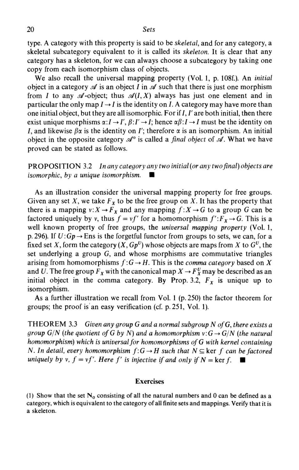
edge. Some simple examples are illustrated here, where the first two represent
simple graphs, i.e. graphs without loops or multiple edges. Given a graph T
= {K, £}, if V is a subset of V and E' is a subset of £ such that any edge in E has its
endpoints in V, then {V, E'} is again a graph, called a subgraph of T. A subgraph
P is said to be/w// if for any vertices p, q in P all edges between p and q in T belong
to P.
;.-■ Let S be any set; by the complete graph C(S) on S we understand the graph with
S as vertex set and an edge between each distinct pair of vertices. Every simple
graph r = {F, E} is clearly a subgraph of C{V)\ the graph with vertex set V and the
set of edges of C(V) that are not in T is written P and called the complementary
graph of P
22
Sets
Examples
1. In a group of six people it is always possible to find either three people who
know each other or three people who are all strangers to each other.
In order to prove this statement we represent the six individuals by points and
join any two points representing acquaintances by an edge. We thus obtain a
graph T, the 'acquaintanceship graph' of our group, and we have to show that
either T contains three edges forming a triangle, or its complement F does so.
Take a vertex px; it is adjacent to each of the other five points in just one of T, F.
Hence it must be adjacent to three points in one of these graphs, say in T it is
adjacent to P2.P3.P4- If two of p2,p3,p4 are adjacent in T, then these two vertices
together with pl form a triangle in T; otherwise P2.P3.P4 form a triangle in F.
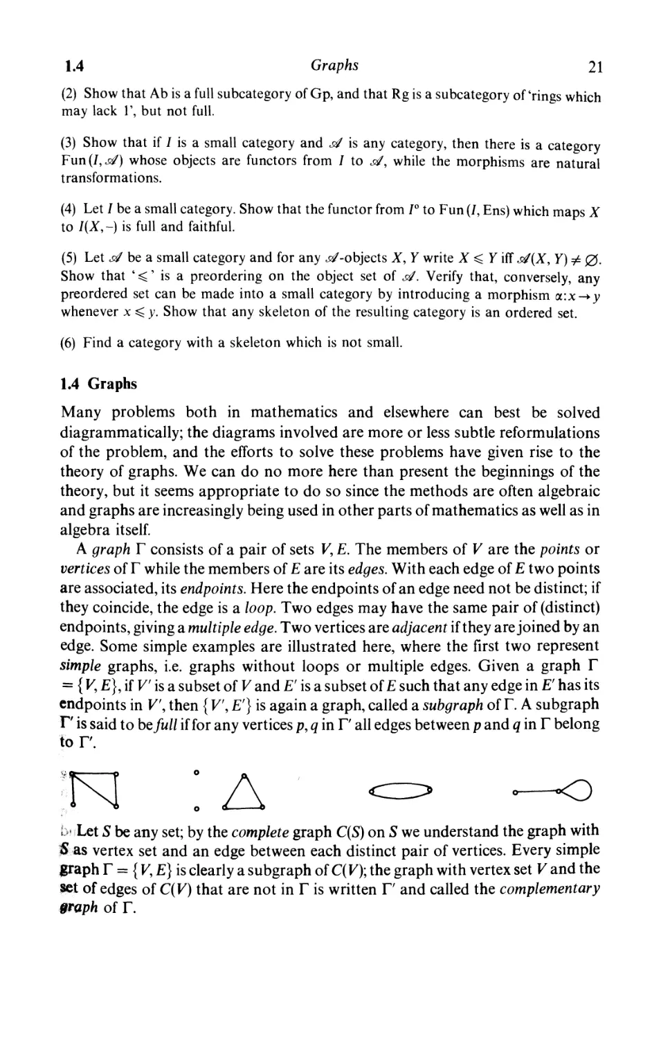
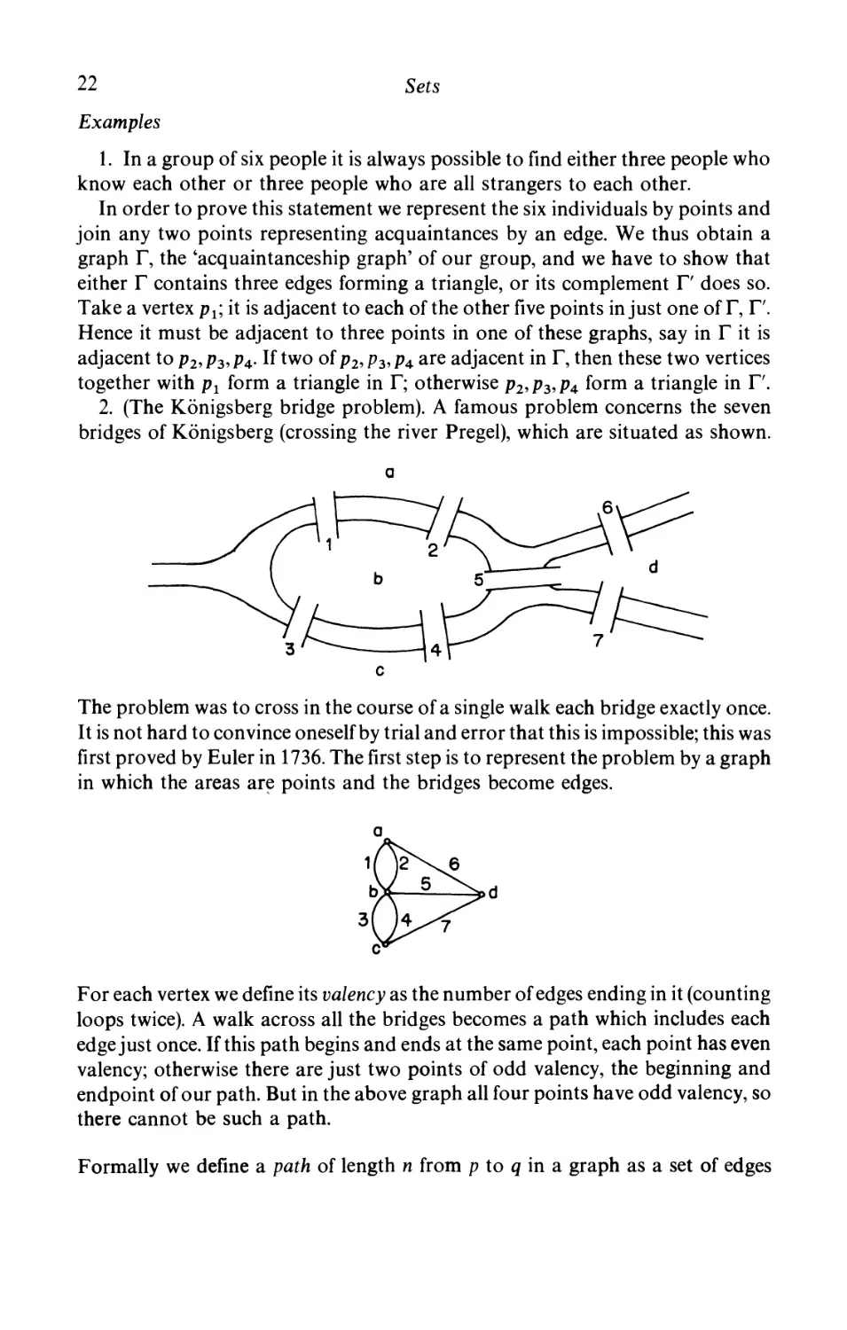
2. (The Konigsberg bridge problem). A famous problem concerns the seven
bridges of Konigsberg (crossing the river Pregel), which are situated as shown.
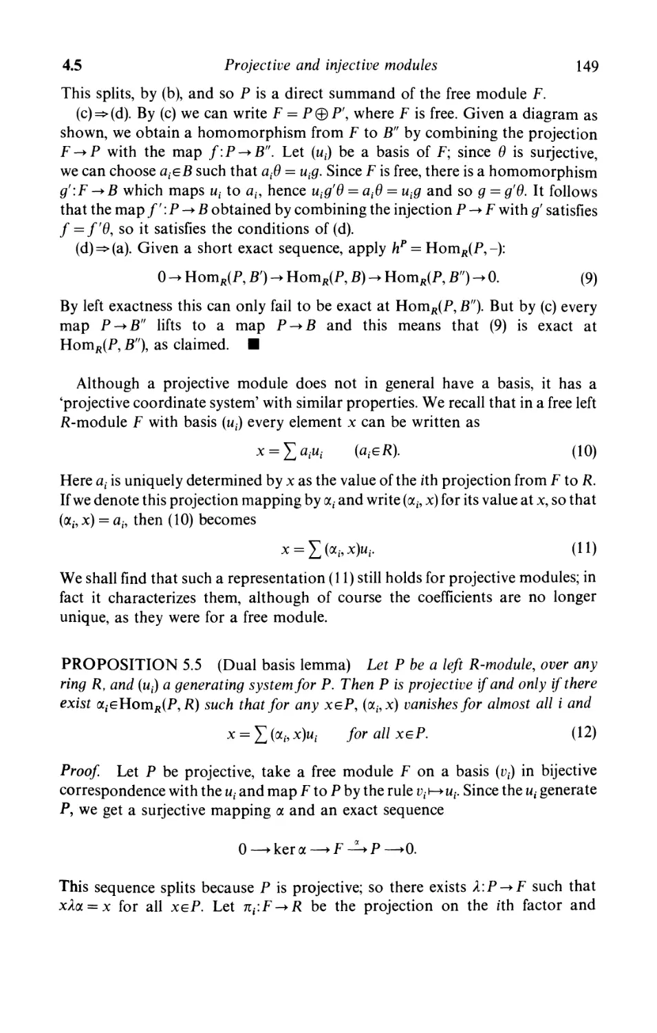
c
The problem was to cross in the course of a single walk each bridge exactly once.
It is not hard to convince oneself by trial and error that this is impossible; this was
first proved by Euler in 1736. The first step is to represent the problem by a graph
in which the areas are points and the bridges become edges.
For each vertex we define its valency as the number of edges ending in it (counting
loops twice). A walk across all the bridges becomes a path which includes each
edge just once. If this path begins and ends at the same point, each point has even
valency; otherwise there are just two points of odd valency, the beginning and
endpoint of our path. But in the above graph all four points have odd valency, so
there cannot be such a path.
Formally we define a path of length n from p to q in a graph as a set of edges
1.4
Graphs
23
e1,...,en such that e{ has endpoints pt_u p{ and p0 = p,pn = q. A path from p to
p is called a cyde and a graph without cycles (of positive length) is said to be
acyclic.
We note that every finite partially ordered set may be considered as a graph by
drawing an edge from p to q ifq covers p, i.e. p < q but p < x < q for no x. In fact we
thus obtain a directed graph or digraph, i.e. a graph in which the endpoints for
each edge form an ordered pair, the initial vertex and the final vertex; the edges in
a digraph are also called arrows and a finite digraph is sometimes called a quiver.
In a digraph only paths are allowed which go in the direction of each arrow.
Such a graph clearly defines a small category in which the vertices are the objects
and the paths are the morphisms.
It is clear that the digraph derived from an ordered set is acyclic; conversely,
given any acyclic digraph T, we can define a partially ordered set on the vertex set
of T by writing p ^ q whenever there is a path from p to q. Thus finite partially
ordered sets may be identified with directed acyclic graphs. Our first result,
though nominally about ordered sets, is really graph-theoretical in nature.
THEOREM 4.1 (Dilworth's theorem) Let S be a finite partially ordered set.
Then the minimum number of disjoint chains into which S can be decomposed is the
width of S, i.e. the maximum number of elements in an anti-chain of S.
Proof We use induction on |5|. Suppose that m is the width of 5; clearly we
cannot express S as a disjoint union of fewer than m chains, and we have to show
that S can be expressed as a disjoint union of m chains. Let S' be the set obtained
by omitting a minimal element c from S. Then S' has width m', where m! = m — 1
or m' = m.
(i) m! = m — 1. By the induction hypothesis S' can be written as a disjoint union
of m — 1 chains, hence S = S' u {c} can be written as a disjoint union of m chains.
(ii) m' = m. Using again induction on | S|, we can write S' as a disjoint union of
m chains, say S' = Cx u • • • u Cm. Let bt be the least element in Ct; then {b^..., bm}
is an anti-chain, but {bu...,bm,c} contains m + 1 elements and so cannot be an
anti-chain. Thus c is comparable with bt for some i, say i = 1, and since c is
minimal in 5, we have c < bv Put C\ = C1u {c}; then S = C\ u C2 u • • • u Cm and
this expresses S as a union of m disjoint chains, as claimed. ■
Dilworth's theorem can be used to prove P. Hall's theorem on distinct
representatives:
TOEOREM 4.2 (P. Hall's theorem) Let Sl9..., Sm be subsets of a finite set T.
Then there is a family of distinct elements au...,am in T such that a^Si provided
that the intersection of any k of the subsets St contains at least k elements (k
-l,2,...,in).
24
Sets
Proof. Let T = {al9..., an) and define a partial ordering on the set W consisting
of all the St and a} by writing x < y precisely when x = y or y = St and x = a^eSj.
Suppose that we have an anti-chain in W\
{Si,..., Sr, a^..., as}. (1)
By hypothesis Sl n ••• nSr contains at least r elements, which must be distinct
from al5..., as because (1) is an anti-chain. It follows that r + s^n, and so every
anti-chain in W has at most n elements; in fact this bound is reached for
{al5..., an}. By Th. 4.1 we can decompose our set W into n disjoint chains. Each S,
is in just one of the chains and each chain contains an a,. Thus OyeS, and we have a
system of distinct representatives. ■
Remarks
1. Let Sl5...., Sm and Tl5..., Tn be two families of disjoint subsets of a set. If
any k of the St between them meet at least k of the 7} then we can find a^Si such
that distinct a, belong to distinct T's. For example, in a finite group G with a
subgroup // we can take the St to be the left cosets and the 7} to be the right cosets.
We thus obtain a set of common representatives for the left and right cosets of H
(this was Hall's original purpose in proving his theorem).
2. The assertion of Th.4.2 has been formulated more picturesquely by P.
Halmos as the 'marriage theorem': In a group of m men and n women, if any k men
between them are acquainted with at least k of the women, then each man can be
married off to an acquaintance.
A graph is said to be connected if any two of its points can be joined by a path; if,
moreover, there is a unique path joining any two points, the graph is called a tree.
Clearly a tree can also be characterized as a connected graph which is acyclic. It is
an important fact that any connected graph contains a tree which includes all its
vertices.
THEOREM 4.3 Let T be a connected graph. Then there is a subgraph T0
including all the vertices ofY which is a tree. Moreover, for any finite tree(V, E) we
have
\V\ = \E\ + 1. (2)
Proof. We observe that a graph Tx is a tree iff any full subgraph on finitely many
vertices is a tree, for if T1 contains a cycle, this already appears in a finite
subgraph, and if T1 fails to be connected, then the same is true of a full 2-element
subgraph. It follows by Prop. 2.4 that T contains a maximal subgraph T0 which is
a tree (i.e. a maximal subtree). We claim that T0 contains all vertices of T. For
otherwise there is a vertex p adjacent to a vertex in T0 but not itself in T0. Since T
is connected, there is an edge e from p to ger0. Then the graph obtained by
1.4
Graphs
25
adjoining p and the edge e to T0 is still a tree, but it contains T0 as a proper
subtree, contradicting the maximality of the latter. Thus T0 contains all vertices
of T and it is the required tree.
Now let r = {V, E} be a finite tree; in T we can find a vertex p0 which is adjacent
to only one other vertex. To find p0 we start from any vertex of T along a path and
continue as far as possible without traversing an edge more than once. As long as
all the vertices we reach have valency greater than 1 we can continue, and we
never pass a vertex twice because T is a tree. Since T is finite, this process must
come to a halt, and it can only do so when we reach a vertex of valency 1; this is the
required vertex p0. If we omit p0 and the single edge ending at p0 from T we obtain
a tree F = {V,£'} with fewer vertices than F By induction we have | V'\ = \E'\
+ 1, and since \V\ = \V\ + 1, |£| = |£'| + 1, we obtain (2). ■
Our final result in this section, Ramsey's theorem, is a far-reaching
generalization of an earlier example involving the acquaintanceship graph (p. 22). For
brevity let us call a set or a subset consisting of r elements an r-set, respectively an
r-subset, and write 3?r(S) for the set of all r-subsets of S; for example, every r-set
has exactly one r-subset and one 0-subset. The earlier example showed that if the
collection of all 2-subsets of a 6-set S is partitioned in any way into two disjoint
sets Al9 A2, then either S contains a 3-subset all of whose 2-subsets lie in A t or it
contains a 3-subset all of whose 2-subsets lie in A2. In terms of graphs, if in a
complete graph on six vertices each edge is painted either blue or red, then there is
a complete subgraph on three vertices in which all edges have the same colour.
More generally, given integers p,q^2, there exists an integer N such that if in a
complete graph on N vertices the edges are painted blue or red, then there is either
a complete blue subgraph on p vertices or a complete red subgraph on q vertices.
This is just the special case r = 2 of the following theorem:
THEOREM 4.4 (Ramsey's theorem) Let pl, p2, r be integers such that 0 ^ r ^ p{
(i = 1,2). Then there exists an integer N(pl,p2,r) with the following property: If in
any set S of at least N(pl,p2,r) elements the family of r-subsets is partitioned into
two disjoint sets A l and A2, then for i = 1 or 2, S contains a pr subset all of whose r-
subsets lie in Av
In symbols we have 0>r(S) = AluA2, AlnA2 = 0, and the assertion is that
there is a prsubset T of S such that 0>r(T) c A. for i = 1 or 2.
Proof We shall use induction on r, and for given r, on p1 and p2. For r = 0 the
result holds trivially: there is only one 0-subset of any set and this lies in A X or A2.
We may therefore assume that r > 0.
Firstly we note that N(pl9 r,r) = pv For if 5 has at least pt( ^ r) elements, and
the family of r-subsets of 5 has been partitioned into disjoint sets Al and A2, then
cither A2 ^ 0 and so 5 contains an r-subset whose unique r-subset lies in A2, or
26
Sets
A2 = 0 and any pt-subset of 5 has all its r-subsets in At. This shows that
N{pl9 r, r)< p1 and it is easily seen that the inequality here cannot be strict. Now a
similar argument shows that N(r9pl9r) = p2.
We put q1 =N(p1 — l,p2,r), q2 = N(pl9p2 — l,r) and claim that
N(Pi,p2,r)^N(q1,q2,r- 1)+ 1. For let 5 be a set with at least N(ql9q2,r - 1)+ 1
elements and let Al9 A2 be a given partition of the family of r-subsets of 5. Fix
c0eS, write 5' = S\{c0} and define a partition {Bl9B2} of the family of (r — 1)-
subsetsofS'by taking an (r — l)-subset T to Bt whenever Tu{c0}eAj. Since 5'has
at least N(ql9q29r — 1) elements, we can apply the induction hypothesis. Two
cases can arise: (i) S' has a qx -subset U all of whose (r — l)-subsets are in Bv If U
contains a p2-subset all of whose r-subsets lie in A2, then the conclusion follows.
Otherwise, by the definition of ql9 U has a (pt — l)-subset whose r-subsets are all
in Al9 and adjoining c0 we get a /^-subset all of whose r-subsets are in At. The
second case (ii) is that S' has a g2-subset all whose (r — l)-subsets are in B2\ this
can be dealt with by symmetry, so the conclusion holds for S. M
The least value of N(pl9p29r) is sometimes called the Ramsey number. For
example, the example given earlier shows that JV(3,3,2) ^ 6, and it is easily
checked that equality holds here. For r = 1 we have N(pl9p2,1) = pt + p2 — 1 and
the theorem states that when a set of at least pt + p2 — 1 elements is partitioned
into two disjoint subsets Al9 A2, then A{ has at least px elements for either i = 1
or 2.
Exercises
(1) Construct all simple graphs with four edges and no isolated points (there are 11, up to
isomorphism). Construct all trees with five edges (there are six).
(2) Let S be a partially ordered set in which each chain and each anti-chain is finite. Define
1(a) for aeS as the minimum of the lengths of maximal chains below a, and show that An
= {aeS\l(a) = n} is an anti-chain. By considering the maximal elements of 5, write S as a
union of a finite number of the An and hence show that S must be finite.
(3) Prove Dilworth's theorem in the infinite case: Every partially ordered set of width m
can be written as the disjoint union of m chains.
(4) Prove Konig's lemma: Every infinite connected graph in which all points have finite
valency has an infinite path. (Hint. Choose pl9 p2» • • •»Pn so trmt there is a path along these
points and pn can be connected to infinitely many points by paths not passing through
p„_ j.) Show that the result need not hold if there is at least one point of infinite valency.
(5) Let r be a finite graph, not necessarily connected but for which each connected
component is a tree (such T is sometimes called a 'forest'). Show that F has | V\ —1£|
connected components. (Hint. Use induction on the number of edges.)
Further exercises
27
(6) Show that N(p,<?,0) = max {p,<?}, N(p,q,\) = p + q-l, N{p,q,2)^l ].
(7) Show that of five points in a plane, no three of which are collinear, there are four that
form vertices of a convex quadrilateral.
(8) Given n points in a plane of which no three are collinear, show that if all the
quadrilaterals formed from these points are convex, then there is a convex n-gon with these
points as vertices.
(9) Show that, for any n, if at least N(n, 5,4) points in the plane are given, no three of which
are collinear, then there are n points in the given set forming a convex n-gon. (Erdos-
Szekeres. For n = 3 take N = 3; otherwise use Th. 4.4 and Exs. (7)-(8).)
(10) Show that there is a number N = N{pl,...,pt,r) such that if for any set of at least N
elements the family of subsets is partitioned into disjoint sets Al9...,At then, for some
i = 1,..., t, S contains a prsubset all of whose r-subsets lie in At.
(11) Show that if the r-subsets of an infinite set 5 are partitioned into disjoint sets
A!,..., At then there is an infinite subset of 5 whose r-subsets all lie in A,-, for some i {Hint.
Adapt the proof of Th. 4.4.)
(12) Show that an infinite partially ordered set contains an infinite chain or an infinite
anti-chain. {Hint. Use Ex.(ll).)
Further exercises on Chapter 1
(1) Show that the union of a finite family of finite sets is finite.
(2) Show that if a, /? are cardinals of which at least one is infinite, then a + fi = max {a, /?}.
(3) Show that a set is finite iffevery collection of subsets has either a maximal or a minimal
member.
(4) (Sierpihski) A collection T of sets will (in this exercise) be called a tower if 0eT and
X, YeT=>X\j YeT. Show that a set A is finite iff A belongs to every tower T such that
{x}eTforall xeA.
(5) Prove that Zorn's lemma is equivalent to Hausdorff's maximal principle: Given a
collection A of sets, any chain in A is contained in a maximal chain.
(6) (Tarski) Show that a set is finite iff it can be ordered so that both the ordering and its
opposite are well-orderings.
(7) Define an upper segment in an ordered set as a lower segment in the opposite ordering.
Verify that the upper segments are precisely the complements of the lower segments. If a set
28
Sets
A is well-ordered, and order-isomorphic to every non-empty upper segment of itself, what
can be said about A? Show that A cannot be of type 2co.
(8) Let A be a countable set. Show that the set of all equivalences on A with finitely many
equivalence classes is uncountable, but the subset of those equivalences in which only one
class is infinite is countable.
(9) Let 5 be a set of n elements and # = {C,-} a collection of subsets of 5 such that C, ^ C}
for / ^j and C^nCj ^ 0. Show that # has at most 2"~1 members.
(10) Let A be a well-ordered set. Show that any interval of the form {xeA\a ^ x < b] is
order-isomorphic to a lower segment of A.
(11) Let 5 be a set of n elements. Show that ^(S) has n\ maximal chains and that each r-
subset of 5 is contained in exactly r\(n — r)\ maximal chains. Show further that if ^(5) has
an anti-chain containing vr r-subsets, then
Deduce Sperner's lemma: The maximal length of any anti-chain in ^(5) is the number of
[n/2]-subsets in 5 (D. Lubell).
(12) (Yoneda's lemma) Let F:^->Ens be a functor and for any peXF define a natural
transformation p:hx = sf(X, -)-F by the rule: if ae^(X, Y), then ai->paF maps
Yhx{ = jtf{X, Y)) to YF. Verify that this is indeed a natural transformation and prove that
the resulting mapping A:F->Nat (hx,F) to the set of all natural transformations is an
isomorphism. (Hint. Define the inverse t\-^(\x)teXf.)
(13) Let r be a graph and A a subgraph. The graph Ac whose edges are the edges of T not in
A and whose vertices are the vertices of T that are either not in A or incident with an edge of
r not in A is called the complement of A in T. Show that Acc is obtained from A by deleting
the vertices of A that are incident with an edge of T not in A but not incident with any edge
in A.
(14) Show that in any finite graph the number of points of odd valency is even.
(15) A finite graph is said to be Eulerian if it is connected and has a closed path (i.e. cycle)
including each edge once. Show that a connected graph is Eulerian iff each vertex has even
valency. Find a condition for a graph to have a path (not necessarily closed) that includes
each edge just once.
(16) For any finite graph Y = (V, E) define p0 as the number of its connected components
and pj as the least number of edges which need to be removed to make each component into
a tree. Show that | K| - | £| = p0 ~ Pi • Show also that if v{x) is the valency of xe V, then
IWx)-2] = 2(p1-p0).
xeV
Further exercises
29
(17) Let 5 be a finite set and ^ a family of subsets of 5 whose union is 5 itself. The
intersection graph of J^ is defined as the simple graph with <F as vertex set, and where X,
YetF are joined by an edge whenever X ^ Y and X n Y ^ 0. Show that every finite
simple graph is the intersection graph of an appropriate family of sets.
(18) Let r be a finite graph and for each vertex p define d(p)'as the length of the longest
simple path starting at p. Show that for a tree, d(p) assumes its least value either at a single
vertex or at several adjacent vertices.
(19) With every finite graph T one associates its adjacency matrix A, a square matrix
whose rows and columns are indexed by the vertices of T and whose (ZJ)-entry is the
number of edges from / toy. Show that A is symmetric and that T is connected iff there is no
permutation matrix P such that P~lAP is the diagonal sum of two matrices. Interpret the
entries of A".
(20) Deduce Zorn's Lemma from the well-ordering theorem.
2
Lattices
The subsets of a set permit operations quite similar to those performed on
numbers. If for the moment we denote the union of two subsets A, B by A + B and
their intersection by AB, a notation which will not be used later (despite some
historical precedents), then we have laws like AB = BA, A(B + C) = AB + AC,
similar to the familiar laws of arithmetic, as well as new laws such as A + A = A,
A + £C = (A + B)(A + C). The algebra formed in this way is called a Boolean
algebra, after G. Boole who introduced it around the middle of the 19th century,
and who made the interesting observation that Boolean algebras could also be
used to describe the propositions of logic.
The more general notion of a lattice was first used by Dedekind to study the
relations between ideals in rings of numbers. The lattice concept helps to unify a
number of disparate ideas and this chapter deals with the basic properties of
lattices and Boolean algebras. The latter have recently found applications in
switching theory, but we shall not enter on this aspect. We shall concentrate on
applications to algebra, and describe such important ideas as chain conditions
and Mobius functions in the general setting of partially ordered sets.
2.1 Definitions; modular and distributive lattices
The definitions relating to ordered sets, recalled in 1.2, form the foundation for
much that follows. Whereas sets of numbers, like N or Q, are totally ordered, this
property is not shared by most partially ordered sets. Examples are the set <?(A) of
all subsets of a set A (with more than one element) relative to inclusion, or the set
N of natural numbers relative to divisibility. In both these cases any two elements
have a least upper bound or supremum, briefly sup: given x, y, there exists z such
that (i) x ^ z, y ^ z and (ii) x ^ z', y ^ z' implies z < z'. Dually any two elements
have a greatest lower bound or inflmum, briefly inf, defined similarly. Thus if X
and Y are subsets of A, their sup is X u Y and their inf is Xr\Y; if m, n are natural
numbers, their sup (relative to divisibility) is their least common multiple while
their inf is their highest common factor.
A partially ordered set in which any two elements have a supremum and an
infimum is called a lattice. The sup of x, y is written x v y and is called the join of x
and y; their inf is written x a y and is called the meet of x and y. It is clear that the
2.1
Definitions; modular and distributive lattices
31
lattice concept is self-dual, so that the dual of a lattice, obtained by reversing the
ordering, is again a lattice. As examples of lattices we have the set N of natural
numbers under divisibility, as well as £P(A\ the set of all subsets of A under
inclusion; further, every totally ordered set is trivially a lattice, with x a y = x,
x v y = y if x ^ y.
Partially ordered sets are often represented as directed graphs: the elements of
the set form the vertices, and edges are drawn so that a ^ b holds precisely when b
is higher than a and there is a descending path from b to a. Such diagrams are
mainly used for finite sets; for N or Z the structure can be hinted at in a partial
diagram, but the case of Q or R would be more difficult. Some examples are given
in Figs. 1-3, where Figs. 1 and 2 are lattices, but not Fig. 3.
Fig. 1
Fig. 2
Fig. 3
A lattice may be regarded as a set with two binary operators, v and a . These
operators satisfy a number of laws, reminiscent of the laws governing addition
and multiplication of numbers, and these laws can be used to give an alternative
definition of lattices.
PROPOSITION 1.1 Let L be a lattice. Then for any a,b,ceL,
av(bvc) = (avb)vc, a a (b a c) = (a a b) a c {associative law) (1)
* av b = bv a, a Ab = b a a (commutative law) (2)
a a (a v b) = a, av(aAb) = a, (absorptive law), (3)
av a = a, a a a = a (idempotent law). (4)
Conversely, if L is a set with two binary operators v, a satisfying (l)-(3), then (4)
also holds and a partial ordering may be defined on L by the rule
a^b if and only if avb = b.
(5)
Relative to this ordering L is a lattice such that the join of a, bis aw b and the meet is
a a b.
32
Lattices
Proof. By the definition of a v b as sup we see that the unique sup of a, b can be
written either as a v b or as b v a, and a similar remark applies to a a b, hence
(2). Likewise the sup of a, b, c may be written a v (£> v c) or (a v b) v c, hence (1).
Now (3) holds because aAb^a^avb, and (4) is a trivial consequence of the
definition, but we observe that it also follows from (3): if in the first eqn. (3) we
replace b by a a a we get a = a a \_a v (a a a)] = a a a, by the second eqn. (3). This
proves the first idempotent law; the second follows by duality.
Now let L be a set with two operators v, a satisfying (l)-(3); then (4) also
holds, as we have just seen, and moreover,
avb = boaAb = a. (6)
For if a v b = b, then by (3), a = a a (a v b) = a a b, and the converse follows by
duality (and the commutative law (2)). If we define the relation' ^' by (5) we have
a partial ordering: if a ^ b, b ^ c, then av b = b,b v c = c\ hence by (1), c = b v c
= (a v b) v c = a v (b v c) = a v c, so a ^ c. Further, a ^ a by (4), and if a ^ b,
b ^ a, then b = avb = bva = a, by (2).
By the definition of a ^ b and (2), a v b is an upper bound of a, b. If c is another
upper bound, then a ^ c, b ^ c, hence c = avc = bvc, and soc = av(Kc)
= (a v b) v c, i.e. avb^c, which shows a v b to be the least upper bound, i.e. the
sup. Now by duality and (6) it follows that the inf of a, b is a a b. M
Any subset of an ordered set 5 is again ordered, but it need not be a lattice, even
if 5 is one. Guided by Prop. IT, we define a sublattice of a lattice L as a subset M
which admits the operators v, a of L, i.e. given a, beM, we have a v b, a a beM.
It is clear that M is again a lattice. In terms of the partial ordering the definition
may be expressed as follows: M is a sublattice of L, if for any a, beM, their sup and
inf (taken in L) again lie in M. We note that it may very well be possible for a
subset of L to be a lattice without being a sublattice of L. For example, let L be a
group, ^(G) the set of all subsets of G and Lat (G) the set of all subgroups of G. As
we shall soon see, Lat(G) is again a lattice with respect to the ordering by
inclusion, as is ^(G), but Lat(G) is not usually a sublattice of ^(G), because the
union H u K of two subgroups need not be a subgroup.
It is clear from the definition that in a lattice L any intersection of sublattices is
again a sublattice. Thus we can define the sublattice generated by a subset X of L
as the intersection of all sublattices containing X. As in the case of subgroups, this
sublattice can be obtained by repeated application of the lattice operations to the
elements of X.
As for groups or rings we define a homomorphism of lattices as a mapping f:L
-> L between lattices L, L such that
(a v b)f = afw bf, (a a b)f = af a bf. (7)
It is clear that a lattice-homomorphism preserves the ordering: a ^ b implies
af < bf, but not every order-preserving mapping between lattices is a lattice-
2.1
Definitions; modular and distributive lattices
33
homomorphism. For example, the mapping ac: x i—► x v c (for a fixed element c) in
any lattice is order-preserving:
a^b => a v c ^b v c, (8)
and although ac satisfies the first eqn. (7), it does not generally satisfy the second
(this is in fact the distributive law, to be discussed later). However, an order-
preserving bijection with an order-preserving inverse between lattices is always a
lattice-isomorphism, because the sets are then order-isomorphic and the lattice
operations can be defined in terms of the ordering (as in (5)).
In any lattice each finite (non-empty) subset has a sup and an inf, as an easy
induction shows. Explicitly, the sup and inf of a u..., an are given by
aY v ••• v an and at a ••• a an
respectively. Here we may omit brackets, by associativity, and the order of the
factors is immaterial, by commutativity.
The notions of sup and inf can also be defined for infinite subsets, but they will
not necessarily exist in a general lattice. A lattice L in which every subset has a sup
and an inf is said to be complete. In particular such a lattice L has a greatest
element (supL or inf0), denoted by 1, and a least element (infL or sup0),
denoted by 0. For example, every finite lattice is complete and so is ^(A), for any
set A. The following criterion for completeness is often useful:
PROPOSITION 1.2 IfL is a partially ordered set such that every subset has an
inf, then L is a complete lattice.
For, given X c L, let Y be the set of all upper bounds of X in L and set y = inf Y.
Any element of X is a lower bound of Y, hence x ^ y for all xeX. If also x ^ z for
all xeX, then ze Y, by the definition of Y and so y ^ z; therefore y = sup X. ■
For example, the set of all subgroups of a group G is partially ordered by
inclusion and if {HA} is a family of subgroups, then their intersection f)Hk is
again a subgroup; thus every subset of our set has an inf. Applying Prop.L2, we
see that it is a complete lattice, which we denote by Lat (G). The inf of a family
{H}} of subgroups is their intersection, while their sup is the least subgroup
containing all the Hk, i.e. the subgroup generated by all the Hk. We see that
although the inf in Lat(G) is the same as in ^(G), the sup in general is not. In a
similar way the submodules of an R-module M form a lattice Lat^ (M), with A n B
as meet and A + B as join.
Many of the lattices we shall meet in the sequel have the following property,
called the modular law:
a v (b a c) = (a v b) a c for all a, b, ceL such that a ^ c. (9)
A lattice L satisfying (9) is said to be modular (Dedekind's name was 'Dualgruppe
34
Lattices
vom Modultypus'). For example, let G be a group and consider the set J^ifi) of
all normal subgroups of G. This is a lattice for the ordering by inclusion, with
H a K = HnK, H v K = HK. In fact it is a modular lattice, i.e
A{BnC) = ABnC, whenever A c C. (10)
For we have A,Br\C^AB,C, hence A(BnC)^ABnC. Now take ceABnC,
say c = ab, where aeA, be£; then b = a~iceC, hence beBr\C and so
c = abeA(£nC).
The lattice of a// subgroups of a group will not in general be modular, and
H v K need not equal HK (cf. Ex. (10)). The relation (10) holds more generally for
normal subgroups with operators, in particular it holds for submodules of a
module (which accounts for the name of (9)).
To see why modular lattices are more tractable, let us return to a general lattice
L for a moment. With a,beL such that a ^ b we can associate the interval
[a,b] = {xeL\a^x ^b}.
Such an interval need not be a chain, but it is always a sublattice of L, with least
element a and greatest element b. More generally, for any a, beL we can form the
intervals I = \_a a b,a] and J = [b,a v b]. Let us define a mapping a:/-> J by
a.xi—>x v b,
and a mapping fi:J->I by
j3:yi—►); a a.
For any xe/we have xajS = (x \/ b) a a. Here x ^ a; hence if L is modular, then
xafi = (x v b) a a = x v (b a a) = x. Thus aj? = 1 and dually j?a = 1, i.e. in a
modular lattice the mappings a, /} are mutually inverse. Since a and /} are both
order-preserving, it follows that I and J are isomorphic as lattices. But in concrete
cases the explicit form of the mappings a, /} often tells us more than this.
Let us call two intervals I and J that are related as in Fig. 4 perspective, and two
intervals related by a series of perspectivities projective. The second isomorphism
theorem of group theory (Vol. 1, p. 252 and 4.1 below) shows that in the lattice
jV{G) of all normal subgroups of G, perspective intervals define isomorphic
quotients. Hence the same is true of projective intervals and the usual proof of
the Schreier refinement theorem (Vol. 1, p. 257) shows that any two normal
chains have refinements in which corresponding intervals are projective, and
hence define isomorphic quotient groups (however, this theorem does not
operate within ^T(G)).
To obtain a criterion for modularity, let us call two elements x, y in an interval
[a, b~] complementary and call each a relative complement (in [a, b~]) of the other if
xAy = a, xw y = b.
PROPOSITION 1.3 A lattice L is modular if and only if for each interval I ofL,
2.1 Definitions; modular and distributive lattices 35
any two elements of I which are comparable and have a common complement in I are
equal
a c
ay b
7\ ^^ b
a^b
Fig. 4 Fig. 5
Proof Given a, b, c in any lattice L, if a ^ c, then av(bAc)^avb and
a v (b a c) ^ c, hence
a v (b a c)<(a v b) a c. (11)
Therefore L is non-modular iff the inequality (11) is strict for at least one triple
{a,b,c) such that a ^ c. When a = c, the two sides of (11) are equal by the
absorptive law (3), so we may assume that a < c. Suppose first that strict
inequality holds in (11). Put a' = a v (b a c\d = {aw b) ac\ then by (11)
a^a'<d^c, (12)
and bAc' = bA(avb)Ac = bAc, a'vb = av(bAc)vb = avb. Moreover,
c' ^a v b, hence b v d < a v b^b v d by (11); therefore b v d = av b, and
dually, a' a b = b a c. This shows that a' and c' have the common complement b
in \b a c,aw b\ and by (12) they are comparable but distinct (cf. Fig. 5).
Conversely, if a\ d are distinct elements which are comparable and have a
common complement in [w,u], say a' Ab = d Ab = u, a'vb = dvb = v and
w ^ a' < d ^ v, then
fl'v(/)A c') = a' < d = (a' v b) a d,
hence L is not modular. ■
The property characterizing modularity involves only five elements, namely
the endpoints of the interval, an element and its two complements. Thus we have
COROLLARY 1.4 A lattice is modular if and only if it does not contain a
sublattice isomorphic to the pentagon lattice in Fig. 6. ■
For example, the lattice of Fig. 1 is modular, but not that of Fig. 2.
If A is any set, then a lattice of subsets of A, i.e. a sublattice of ^(A), is modular,
36
Lattices
but not every modular lattice can be represented as a lattice of subsets. For
example, the Klein 4-group gp {a,b\a2 = b2 = (ab)2 = 1} has the subgroup
lattice shown in Fig. 7 (the 'diamond' lattice), but it cannot be represented as a
lattice of subsets, as the reader can discover by a little experimentation.
<I>
Fig. 6 Fig. 7
It turns out that the lattices ^(A) satisfy a further law not holding in the
diamond lattice, namely the distributive law. There are two dual forms of this
law, which however are equivalent; moreover they imply the modular law. Before
proving this fact we note that in any lattice we have avb^aAc, b a c and
c ^ a a c, b a c for any a, b, c; hence
(a v b) a c ^ (a a c) v (b a c). (13)
Now the distributive law is expressed by equality in (13). More precisely we have
the following:
PROPOSITION 1.5 In any lattice L the following conditions are equivalent
(a) (a v b) a c = (a a c) v (b a c) for all a, b, ceL;
(a*) (a a b) v c = (a v c) a (b v c) for all a, b, ceL;
(jS) (a v b) a c ^ a v (b a c) for all a, b, ceL.
Proof If (a) holds, then
(a v b) a c = {a a c) v (b a c) ^ a v (b a c),
i.e. (/?). Conversely, assume (jS):(a v b) a c ^ a v (b a c). Applying a c to both
sides and using (jS) again, we obtain
(a v b) a c ^ l(b a c) v a] a c < (b a c) v (a a c).
The reverse inequality holds by (13), hence we obtain (a). Thus (a) o(jS), and since
(jS) is self-dual, we also have (a*)o(jS). ■
A lattice satisfying the three equivalent conditions of this proposition is said to
be distributive', specifically, either (a) or (a*) is called the distributive law. From ((1)
it is clear that every distributive lattice is modular.
There is a criterion for distributivity analogous to Prop. 1.3: a lattice is
distributive iff relative complements in any interval are unique. We shall only
need the necessity of this condition.
2.1 Definitions; modular and distributive lattices 37
PROPOSITION 1.6 In a distributive lattice, relative complements in any
interval are unique.
Proof. Let a /\b = d /\b = u, a v b = a' v b = v; then
a = a a v = a a (a' v b) = (a a a') v (a a b) = a a a';
hence a ^ a'. By symmetry a' ^ a and hence a' = a. ■
If we single out the five elements involved we obtain the following alternative
formulation:
A lattice is distributive if and only if it does not contain a sublattice isomorphic to
the pentagon lattice in Fig. 6 or the diamond lattice in Fig. 7.
For a proof of this criterion see Birkhoff (1967) or Cohn (1981) (see also Ex. (12)
below).
Exercises
(1) In any lattice, if a ^ a\ b ^ b\ then aw b ^af v b\ a a b ^a a b'.
(2) Find the smallest partially ordered set in which any two elements have an upper bound
and a lower bound but which is not a lattice.
(3) Find all lattices on at most five elements. Which of them are anti-isomorphic with
themselves? Which admit a non-identity automorphism? Which are modular, or
distributive?
(4) Show that the least element 0 in a lattice (if it exists) is characterized by0Ax = 0,0vx
= x, and give a corresponding characterization of the greatest element.
(5) Let L be a modular lattice. Show that if a, b, ceL satisfy a a {b v c) = {a a b) v {a a c),
then the sublattice generated by a,b,c is distributive.
(6) Show that in any modular lattice the sublattice generated by two chains is distributive.
(7) Let L be a system with two binary operators v, a and a particular element 1 in L
satisfying (i) a a a = a, (ii) a v 1 = 1 v a = 1, (iii) a a 1 = 1 a a = a, (iv) a a (b v c)
= (a a b) v (a a c), {b v c) a a = {b a a) v (c a a) for all a, b, ceL. Show that L is a
distributive lattice with greatest element 1.
(8) Show that in a topological space the closed sets form a complete distributive lattice.
(9) (O.Ore) Show that, for any group G, Lat (G) is distributive iff G is locally cyclic (i.e. any
finitely generated subgroup is cyclic).
38
Lattices
(10) Let G = Sym4,tf = {1,(1 2)},K = {1,(1 2 3 4)}; show that G is generated by H
and K, and deduce that H v K ^ HK, where H v Kis the join of H and K in Lat (G). Show
that Lat(G) is not modular.
(11) Show, by examining the lengths of maximal chains in Lat(Alt4), that this lattice is
not modular.
(12) Show that in any lattice L,
(x a v) v (v a z) v (z a x) ^ (x v v) a (v v z) a (z v x) for all x, v, zeL, (i)
with equality iff L is distributive. Denote the two sides of (i) by u, v respectively and put
x' = (xad)v u, y' = (yAi))v w, z'-(zad)v u. If Lis modular but not distributive, choose
x,y,zeL such that the inequality (i) is strict and verify that u,v,x',y',z' form a diamond
lattice. Deduce that a modular lattice is distributive iff it does not contain a diamond
lattice as sublattice.
2.2 Chain conditions
Although most of the lattices we shall meet are infinite, many of them satisfy
finiteness conditions; these take several equivalent forms. We state them for any
partially ordered set:
PROPOSITION 2.1 In any partially ordered set S the following conditions are
equivalent:
(a) (Ascending chain condition) Every ascending chain becomes stationary: if
a1^a2^---, (!)
then there exists n0 such that am = anfor all m,n^ n0.
(b) Every strictly ascending chain terminates: if
al<a2<--, (2)
then the chain has only finitely many terms.
(c) (Maximum condition) Every non-empty subset ofS has a maximal element.
Proof (a)=>(b) follows because any chain (2) can become stationary only by
terminating. To prove (b) => (c), let M be a non-empty subset of 5. Pick a t e M; if a t
is not maximal in M, we can find a2eM such that a2 > al9 and generally, for each
aneM, either an is maximal or there exists an+1 eM such that an+1 > an. Thus we
obtain a chain (2) which must terminate, by (b), and the last element is maximal in
M.
(c)=> (a). Given (1), let an be maximal in the set {al9 a2,...}, then an ^ am for all m,
hence an = an+1 = •••, so (1) becomes stationary. ■
We note that the axiom of choice was used in the deduction (b)=>(c); it can be
shown that this is indispensable. Thus without the axiom of choice the maximum
2.2
Chain conditions
39
condition is stronger than the ascending chain condition, but in the presence of
the axiom of choice both are equivalent (cf. Hodges 1974).
There is a useful induction principle holding in sets with maximum condition:
PROPOSITION 2.2 (Noetherian induction) Let S be a partially ordered set
with maximum condition. If X is a subset ofS which contains any element a of S
whenever it contains all elements xeS such that x > a, then X = S.
For, consider the complement X' of X in S. If X' ^ 0, let c be a maximal
element of X'. Then any x > c must be in X, hence by hypothesis, ceX, which
contradicts the fact that ceX'. Therefore X' is empty, and X = S, as claimed. ■
By duality we obtain from Prop. 2.1 the equivalence of the minimum condition
and (two forms of) the descending chain condition, and as in Prop. 2.2 we obtain
an induction principle for sets with minimum condition. For well-ordered sets, i.e.
totally ordered sets with minimum condition, this is just the principle of
transfinite induction.
Every finite ordered set clearly satisfies both maximum and minimum
conditions; the converse is false, as any infinite set shows whose elements are all
incomparable. Even for modular lattices the converse need not hold (cf. Ex.(2)),
but it does hold for distributive lattices, as we shall see in 2.3. For the moment we
shall describe the modular lattices satisfying both chain conditions. Given a chain
C between certain points p, q, any chain from p to q which includes C is called a
refinement of C; clearly C is a maximal chain from p to q iff it has no proper
refinement.
PROPOSITION 2.3 In a partially ordered set S with both chain conditions,
every chain is finite and can be refined by inserting further terms to a maximal chain
between the given endpoints.
Proof. By the minimum condition, every chain in S has a minimal element,
necessarily unique. Given a chain C in S, let a1 be its least element, and generally
define ax as the least element of C\{au...,av^.1}. Then
ai < a2 < '"<> (3)
and by the maximum condition this chain terminates. If the last term is an, it
follows that C = {au...,an}, hence C is finite. Next, given a chain (3), let bx be
minimal in S such that a1<bl^ a2. If bx <a2, we choose b2eS such that b2 is
minimal subject to b1<b2^ a2. Continuing in this way, we obtain a chain
a1<b1<b2< ••• ^a2>
which cannot be refined further. By the maximum condition it must terminate,
which can happen only when bk = a2 for some k. We now have a maximal chain
40
Lattices
from at to a2; by induction on the number of terms in (3) we can find a maximal
chain from a2 to a„, and together with the part found this provides a maximal
chain from ax to an. ■
Let us define the length of a chain as the number of its links, thus
a = a0 < at < • • • < an = b (4)
has length n. In general there is no reason why two maximal chains between given
endpoints should have the same length. For example, in the pentagon lattice of
Fig. 6 there are two maximal chains in the lattice of lengths 2 and 3. But if we have
two chains between points a and b in a modular lattice, then the proof of the
Schreier refinement theorem (Vol. 1, p. 257) shows that they have refinements
whose links can be paired off in such a way that corresponding links are
projective. In particular, if both chains are maximal, it follows that both have the
same length. Thus we have
PROPOSITION 2.4 Let Lbea modular lattice and a^binL such that there is a
maximal chain from a to b, of length n. Then every chain between a and b has length
at most n, and every maximal chain between a and b has length exactly n. ■
In view of this result we can define the length of a modular lattice as the
supremum of the lengths of its chains. Modular lattices of finite length can be
described as follows:
COROLLARY 2.5 A modular lattice has finite length if and only if it satisfies
both chain conditions.
Proof. Clearly any modular lattice of finite length satisfies both chain
conditions. Conversely, if a modular lattice L satisfies both chain conditions, take
a maximal element c in L. Then x ^ c v x = c for any xeL, hence c is in fact the
greatest element 1 in L, and dually L has a least element 0. By Prop. 2.4, there is a
maximal chain from 0 to 1; this is finite, of length n say, and no chain can be
longer. ■
A modular lattice has finite length if there is an element c such that all chains
below c are finite, and likewise all chains above c. But sometimes we shall want the
corresponding assertion when only one of the chain conditions holds.
PROPOSITION 2.6 Let L be a modular lattice and ceL. Denote by Lc, CL the
sublattices of elements ^ c and ^ c respectively. If both Lc and CL satisfy the
maximum condition, then so does L.
Proof Let
al^a2^-- (5)
2.2
Chain conditions
41
be an ascending chain in L. Then a1Ac^a2AC^'"> and by hypothesis this
becomes stationary. Likewise for a1 v c ^ a2 v c ^ •••; thus we may choose n0
such that for m,n^n0
amAC~anAc — u say, amv c — anv c = v say.
Hence am, an have a common complement c in [w, u], and since am ^ a„ for ra ^ n, it
follows by Prop. 1.3 that am = an for ra, n^n0, so (5) becomes stationary, as
claimed. ■
The results of this section can be applied to modules over a ring by observing
that, for any R-module M, the set of all submodules forms a lattice, Lat (M) say,
under the partial ordering by inclusion, with intersection as meet and sum (not
union) as join. As we have seen in 2.1 (cf. also Vol. 1, p. 256), this lattice is modular,
and the Jordan-Holder theorem and Schreier refinement theorem proved in
Vol. i were based on this fact.
An R-module M is said to be Noetherian (after E. Noether) if Lat(M) satisfies
the maximum condition, and Artinian (after E. Artin) if Lat(M) satisfies the
minimum condition. If we apply this terminology to R itself, regarded as a right
R-module, we obtain the notion of a right Noetherian or right Artinian ring, as a
ring with maximum or minimum condition respectively on right ideals. Left
Noetherian and Artinian rings are defined similarly, using left ideals.
The maximum condition for modules can be stated in another way:
PROPOSITION 2.7 An R-module M is Noetherian if and only if all its
submodules are finitely generated.
Proof =>. Let N be any submodule of M and choose xl,x2,...eN such that on
writing Nt■ = xxR + • • -^- xi^1R, we have xt^Nt. Then
0 = N1czN2cz-..- (6)
by the ascending chain condition this must break off, at iVr say, and this means
that N = Nr, so N is finitely generated.
<=. Given an ascending chain (6) of submodules in M, write N = ^iV,- and
choose a finite generating set xl9..., xr of N. If xtENv. and v = max {vl9..., vr},
then xteNv for / = 1,..., r, hence Nv = N and (6) breaks off; this shows M to be
Noetherian. ■
If a ring R is right Noetherian (or Artinian), then any cyclic right R-module,
being of the form R/a for some right ideal a of R, is again Noetherian (or Artinian),
because the submodules of R/a are in natural (order-preserving) bijection with
the right ideals of R containing a, by the third isomorphism theorem (4.1 below
and Vol. 1, pp. 253, 303). But we can say more than this:
42
Lattices
THEOREM 2.8 Let R be a right Noetherian (resp. Artinian) ring. Then any
finitely generated right R-module is again Noetherian (resp. Artinian).
Proof. We have just seen that the result holds for cyclic modules. Now use
induction on the number of generators of M: let M be generated by n elements
and denote by M' the submodule generated by n — 1 of these. Then M" = M/M' is
cyclic and we have the exact sequence
0-M'-M-M"-0.
Assume that R is right Noetherian; then Lat(M') satisfies the maximum
condition, by the induction hypothesis, and Lat(M") satisfies the maximum
condition because M" is cyclic. Now the lattice of submodules of M containing
M' corresponds to Lat (M") (by the third isomorphism theorem) and so satisfies
the maximum condition; hence by Prop. 2.6, Lat(M) satisfies the maximum
condition and this proves M to be Noetherian. The Artinian case is proved
similarly. ■
In a principal right ideal domain every right ideal is certainly finitely generated,
hence we have
COROLLARY 2.9 Over a principal right ideal domain every finitely generated
right module is Noetherian. ■
A finitely generated module over any ring has an important maximality
property, which follows from Zorn's lemma (in the form Prop. 1.2.4).
PROPOSITION 2.10 Let R be any ring and M a finitely generated R-module.
Then every proper submodule of M is contained in a maximal proper submodule.
Proof. Let M be generated by uu..., ur. Given a proper submodule N, consider
the set # of all subsets X of M which together with N generate a proper
submodule. A set Xt fails to lie in # precisely if u1,...,ur each is a linear
combination of elements of Xx and N, and this condition involves only finitely
many elements of Xv Therefore Xx lies in # precisely when all its finite subsets lie
in ^ so ^ is of finite character. Hence there is a maximal subset X in #; the
submodule generated by X u N again lies in # and so by maximality is equal to
X, and now X is the desired maximal proper submodule containing N. ■
This result may be applied to R itself. As right R-module, R is generated by the
single element 1 and the submodules are right ideals. By a maximal right ideal is
meant a right ideal maximal in the set of all proper right ideals. Similarly for left
ideals and for two-sided ideals, regarding R as R-bimodule. Then we obtain
2.2
Chain conditions
43
THEOREM 2.11 (KrulPs theorem) Let R be any ring. Then any proper right
ideal is contained in a maximal right ideal. In particular, every non-trivial ring has
maximal right ideals. A corresponding result holds for left ideals, and for two-sided
ideals. ■
This result makes essential use of the existence of a unit element in rings; in the
absence of 1 it need not hold (cf. Ex. (9)).
In lattices with a chain condition there is a decomposition lemma which is
frequently used. It is convenient to formulate it more generally for ordered
monoids (cf. 3.1 in Vol. 1, or Ch. 11 below). By a partially ordered monoid we
understand a monoid which is partially ordered as a set and such that x ^ x\
y^y' implies xy ^ x'y'. We shall further require the condition
xy ^ x, xy^ y. (7)
Examples are lattices with 1 and with x a y as operation, or N with the ordering
opposite to the usual one. An element c in such a monoid is called irreducible if
c ^ 1 and c cannot be written as a product of two elements that are > c.
LEMMA 2.12 (decomposition lemma) Let M be a partially ordered monoid
satisfying the maximum condition and (7). Then every element ofM can be written as
a product of irreducible elements.
Proof. Denote by I the subset of elements of S which cannot be expressed as a
product of a finite number of irreducible elements; we have to show that I is
empty. If I ^ 0, take a maximal element c in I; then c cannot be irreducible and
c ^ 1 because 1 is the product of the empty family. Hence c = ab for some a > c,
b > c. By the maximality of c, a and b are products of irreducible elements, say
a = a1--ar,b = b1-bs and it follows that c = al"-arbl-"bs. This contradicts the
choice of c and it shows that 1 = 0. Thus every element of S is a product of
irreducible elements. ■
Examples
1. Let L be a lattice with maximum condition. Then L has a greatest element 1
and it satisfies the hypothesis of the lemma with respect to the operation x a y. In
this case the irreducible elements are called meet-irreducible and the lemma tells
us that in L every element can be written in the form
c = a1 a ••• a ar, where at is meet-irreducible.
2. Dually, if the operation is x v y, the irreducible elements are called join-
irreducible. Hence in a lattice with minimum condition every element can be
written as
c = b1 v ••• v br, where bt is join-irreducible.
44
Lattices
3. In N the minimum condition holds for the usual ordering and xy ^ x, v; the
irreducible elements in this case are the prime numbers, so we can apply the
lemma to deduce that every natural number can be written as a product of prime
numbers. Later in Ch. 9 we shall apply Lemma 2.12 in a similar situation, which
generalizes this case.
In a partially ordered set with minimum condition there is a relation between
anti-chains and lower segments which is sometimes useful.
PROPOSITION 2.13 Let S be a partially ordered set with minimum condition.
Then there is a natural bijection between lower segments and anti-chains: To each
lower segment L there corresponds the anti-chain L° consisting of all minimal
elements of the complement L of L; to each anti-chain A there corresponds the
complement of the upper segment [A| generated by A, A° = [A|\
Proof. From the definitions it is clear that for any lower segment L we have
L ^ L°°. If X(£L, then xeL', hence by the minimum condition there is a minimal
element a of L such that a < x, so xe[L°| and therefore x<£L°°. Now take an anti-
chain A; then it is again clear that A ^ A°°. To prove equality here we note that
A° = [A |'; hence for any xeA°°, x is a minimal element of A°' = [A|. By definition
this means that x ^ a for some aeA, but by the minimality of x, x = a, so xeA, as
claimed. ■
Our final result does not strictly deal with a chain condition but it is a
construction arising from an ascending chain of groups.
PROPOSITION 2.14 Let {Gn} be a sequence of groups such that Gn is a
subgroup ofGn+1. Then the union [JGn is a group with each Gn as subgroup.
Proof On the union G = [J Gn we can define a group structure in just one way.
Namely if x,yeG, then xeGr, yeGs where r^s say. Hence x,yeGs and the
product xv is defined in Gs. Moreover, for any n ^ s, Gs is a subgroup of G„, so the
product x>' is the same in Gn as in Gs. In this way we define a multiplication on G
and it is easily checked that G is a group with respect to this multiplication, with
each Gn as subgroup. ■
It is clear that a corresponding result holds for sequences of rings, or of fields.
Exercises
(1) Show that a partially ordered set in which each chain has at most m and each anti-
chain at most n elements, has at most mn elements.
(2) Given an example of an infinite modular lattice of length 2.
2.3
Boolean algebras
45
(3) Let M be a finitely generated module (over any ring). Show that the union of any
countable strictly ascending sequence of submodules without last term is a proper
submodule.
(4) Show that a module (over any ring) is finitely generated iff it cannot be expressed as a
union of a well-ordered chain without last term of proper submodules. Deduce another
proof of Props. 2.7 and 2.10. Does the result still hold if instead of chains we take countable
ascending sequences of proper submodules?
(5) Show that a lattice in which every lower segment is principal satisfies the maximum
condition.
(6) Show that every quotient of a finitely generated module is finitely generated, but not
necessarily every submodule.
(7) Give an example of a non-zero Z-module without proper maximal submodules.
(8) Let R be a non-trivial ring such that every right ^-module is free. Show that R is a skew
field. (Hint. See Th. 4.4.8.)
(9) Show that the 'ring without T defined on the additive group of rational numbers by the
multiplication xy = 0 has no maximal ideals.
(10) Prove without the axiom of choice that in a module with maximum condition all
submodules are finitely generated.
2.3 Boolean algebras
We have seen that in any distributive lattice complements in an interval, when
they exist, are unique. Thus if L is a distributive lattice with 0 and 1 in which every
element has a complement, we can regard the process of associating with each
element x its complement x' as a unary operator (i.e. an operator with one
argument). A complemented distributive lattice with greatest and least element is
called a Boolean algebra (after G. Boole). Thus a Boolean algebra is a set with two
binary operators v, a , a unary operator ' and constants 0, 1, satisfying the laws
(l)-(4) of 2.1 and the distributive law, as well as the equations
xax' = 0, x v x' = 1. (1)
Clearly 0' = 1, 1' = 0, and since x' is the unique complement of x,
x" = x. (2)
We note the following consequence, known as De Morgans laws:
(x a y)' = xf v /, (x v y)' = x' a /. (3)
For we have (xf v y') a(xaj) = [x' a(xaj;)]v[/a(xa y)~] = 0, and
46
Lattices
(x' v y') v (x a y) = [(*' v y') v x~\ a [(*' vj;')vy] = l. Hence x' v _y' is the
complement of x a y and we obtain the first of eqns. (3); the second follows by duality.
We also note
x^y o x a y' = 0 o x' v y= 1. (4)
For if x ^ y, then x a y' ^ _y a y' = 0, hence xa/ = 0. Conversely, if x a / = 0,
then xvy = (xv]/)Al=(xvy)A(yvy) = (xA/)v]; = y, and so x ^y. This
proves the first equivalence in (4); the second follows by applying (3).
Examples
1. The set of all subsets 0>(X) of any set X is a Boolean algebra if we put 0 = 0,
1 = X and for Ye^(X) take Y' to be the complement of 7in X. More generally,
any system of subsets of X closed under complements and finite unions is a
Boolean algebra; the closure under finite intersections follows by (3) and 0, 1 are
present as the empty union and its complement. This is merely a subalgebra of
&(X\ also called afield of sets in X.
Let X be any infinite set. Then the subalgebra of 0>(X) generated by all the finite
subsets of X consists of all the finite subsets of X and their complements, called
the cofinite subsets of X.
We remark that a sublattice of 0>(X) need not be a Boolean algebra, because it
may not be closed under complements.
2. In any interval [a, b~\ = I of a distributive lattice L, the set of elements of I
which have a complement in I forms a Boolean algebra.
3. The 2-element lattice is a Boolean algebra. If the elements are a, b and
av b = b say, then a < b, and we get a Boolean algebra by putting a = 0,b=l,
0' = 191' = 0. This lattice will usually be denoted by 2. The 1 -element lattice is also
a Boolean algebra, called the trivial algebra; it is usually excluded from
consideration. Thus 2 is the smallest non-trivial Boolean algebra.
4. Let R be any ring. Then the set &(R) of all central idempotents of R (i.e.
elements x in the centre such that x2 = x) is a Boolean algebra under the
operations
x a y = xy, x v y = x + y — xy, x' = 1 — x.
This example will be taken up again in Prop. 3.1.
5. The set of all propositions in logic (cf. 1.1 in Vol. 1) forms a Boolean algebra,
taking a , v to be conjunction and disjunction respectively, and x' the negation
—i x, and for 1,0 propositions T, F known to be true and false respectively (e.g.
T = 'someone is looking at this page now' and F = T). As we saw in Vol. 1, each
proposition A has a truth-value /(A), and it is easily verified that / is a
homomorphism of the Boolean algebra of all propositions into 2.
The next result shows that every Boolean algebra may be obtained as the algebra
of idempotents of some commutative ring R; in fact R may be chosen to consist
2.3
Boolean algebras
47
entirely of idempotents. Let us define a Boolean ring as a ring satisfying the
identity
x2 = x. (5)
Such a ring is necessarily commutative. For we have 2x = (2x)2 = Ax2 = Ax, hence
2x = 0 and so
x = — x. (6)
Next we have x + y = (x + y)2 = x2 + xy + yx + y2; hence xy + yx = 0, i.e. by (6)
xy = yx.
Thus every Boolean ring is commutative and of characteristic 2.
PROPOSITION 3.1 (i) Given any ring R, the set $(R) of its central idempotents
forms a Boolean algebra relative to the operations
x a y = xy, x v y = x + y — xy, xf = 1 — x. (7)
(ii) On any Boolean algebra B define the two operations
x + y = {x a y') v (x' a y), xy = x a y. (8)
Then B forms a Boolean ring &(B) relative to these operations.
Moreover, &{3?(B)) ^ B for any Boolean algebra B and 01{0$(R)) ^ R for any
Boolean ring R.
The first operation (8) is called the symmetric difference of x and y; in the case
where B = 0>(X), Y + Z represents the subset of X consisting of all elements that
are either in Y or in Z but not in both (this is also called 'addition mod 2').
Proof. The verification that &(R) is a Boolean algebra relative to the operations
(7) and that 01(B) is a Boolean ring relative to the operations (8) is routine and may
be left to the reader.
Now let B be a Boolean algebra and put Bx= &(@(B)). Since @(B) is a
Boolean ring, Bx and B are the same set, and both are Boolean algebras with the
same definition of a . In B1 we have x' = 1 — x; from (8) and the fact that $(B) is a
Boolean ring we see that 1 — x = (1 a x') v (0 a x) = x'. So x a y and x' agree on B and
Bl9 hence so does xvj; = (x'a /)'.
Next take a Boolean ring R and put Rx = 0t{0$(R)\ Again R and RX are the
same set; both are Boolean rings with the same definition of product, and if + t
denotes the sum in Rl9 then we have x +t y = x(\ — y) + (1 — x)y = x + y;
therefore Rx ^R, as we had to show. Vt
It is clear that the Boolean algebra homomorphisms correspond precisely to
ring homomorphisms; we have here an example of a category equivalence (cf. 1.3):
48
Lattices
M and $ are mutually inverse functors defining an equivalence between the
categories of Boolean rings and Boolean algebras.
It is clear that the duality holding in general lattices extends to Boolean
algebras. Thus from any law holding in Boolean algebras we obtain another law
by interchanging v, a and 0, 1.
Given Boolean algebras A and B, by a dual homomorphism one understands
a mapping f:A->B such that
x'f = (xf)\ (x v y)f = xf A yf (x a y)f = xf v yf. (9)
Dual isomorphisms, etc., are defined similarly. From De Morgan's laws (3) we see
that every Boolean algebra admits a dual automorphism, the natural duality,
defined by the complementation mapping: xi—>x'. In a non-trivial Boolean
algebra this duality has no fixed point, and its square is the identity; this shows
that every finite (non-trivial) Boolean algebra has an even number of elements.
The Boolean algebra 2 possesses a remarkable property, its functional
completeness: we shall find that every function of n variables on 2 with values in 2
can be expressed as a Boolean polynomial. Here a Boolean polynomial in
x!,..., xn is defined by the following rules:
1. Each xt is a Boolean polynomial.
2. If u is a Boolean polynomial, then so is u'.
3. // w, v are Boolean polynomials, so are u v v and u a v.
For example, (xx a x'2)' v (x'3 a xt) is a Boolean polynomial. Two Boolean
polynomials are said to be equal if we can pass from one to the other by applying
the laws of Boolean algebras, viz. (l)-(4) of 2.1 and eqns. (l)-(3) above. It is clear
that equal Boolean polynomials are equal as functions on any Boolean algebra;
below we shall prove a converse: two Boolean polynomials which define the same
function on a given non-trivial Boolean algebra must be equal as polynomials.
Clearly it will be enough to prove this for the smallest non-trivial algebra 2. The
result is proved by finding a normal form for polynomials, which is shown to be
unique; more precisely, we shall find two normal forms dual to each other.
To describe these normal forms, let us define a minterm in xt,..., xn as
I1a--aI„, where X{ is x{ or x\ (i=l,...,n). (10)
Now a Boolean polynomial / is said to be in disjunctive normal form if it has the
form
/=/iV-v/„ (11)
where each fx is a minterm in xl5..., xn. For example the disjunctive normal form
for x\ a x2 is x\ a x2 while for xx v x2 it is (xx a x2) v (x\ a x2) v (xx a x2).
Dually we define a maxterm in xl9..., xn as
X1V'--vXn, where Zt is Xj or xj (/=l,...,n), (12)
2.3 Boolean algebras 49
and the conjunctive normal form for / is
/=/lA".A/n (13)
where each fx is a maxterm in xl9...,xn. For example the conjunctive normal
form for x\ a x2 is (x\ v x2) a (x\ v x2) a (xt v x2), while for x1 v x2 it is
xt v x'2. With these definitions we have
LEMMA 3.2 Any Boolean polynomial in xl9...,xn is equal to a polynomial in
disjunctive normal form, and likewise to a polynomial in conjunctive normal form.
Proof Let p be any Boolean polynomial in xl9..., xn. By the distributive law we
can write p as a disjunction (11), where each fx is a conjunction of some of
xl9..., xn, x\,..., x'n. By the idempotent law we can omit repetitions and if both xt
and x\ occur in/A, then/A is 0 and so may be omitted, and xj' can be replaced by xt.
In order to obtain a disjunction of minterms we order the variables in/A (by the
commutative law), say in ascending order; if neither xt nor x\ occurs, then since
fk = (fk A xt) v (fk A *S), we can replace fx by fx a xt and fx a x\. In this way we
obtain an expression (11) for p, where each fx is a minterm in xl9..., xn, so p has
been expressed in disjunctive normal form. The result for conjunctive normal
forms follows by duality. ■
Let us consider a minterm (10). It takes on the value 1 for just one set of values
in 2n, viz. a = (al9...,an), where
1 jo ifxt. = x;, v ;
From (14) we see that for each n-tuple ae2n there is just one minterm taking the
value 1 at a and 0 elsewhere; this minterm will be denoted by sa. Thus sa is the
characteristic function of the 1-point subset {a} of 2n. More generally, if 5 is any
subset of 2n, then its characteristic function can be written as a Boolean
polynomial:
Z5=Ve, (15)
aeS
Now any function/: 2n -» 2 is the characteristic function of a subset of 2n, namely
lf~1 = {ae2n\f(a)=l}. Hence (15) can be used to express /as a Boolean
polynomial; moreover this expression is unique, since / is completely determined
by If'1. Thus every function on 2 can be represented by exactly one Boolean
polynomial in disjunctive normal form. A dual argument applies to conjunctive
normal forms. Let us sum up our conclusion:
THEOREM 3.3 Each Boolean polynomial is equal to a unique expression in
disjunctive normal form (11) and to a unique expression in conjunctive normal form
50
Lattices
(13) and it defines a function on each Boolean algebra. Moreover, on the Boolean
algebra 2, every function ofn variables is given by a Boolean polynomial but on any
Boolean algebra of more than two elements there are functions not represented by
Boolean polynomials.
We have seen that every Boolean polynomial can be put in disjunctive normal
form (Lemma 3.2) and that every function on 2 has a unique expression in
disjunctive normal form. This shows that the disjunctive normal form is unique
(since it is unique on 2). Now the number of mappings from 2n to 2 is 22n, so this
must be the number of expressions in disjunctive normal form (this is also easily
verified directly). But on a Boolean algebra with b elements there are bb" functions
of n arguments, so for b > 2 not all of them can be written as Boolean
polynomials. ■
The fact that on 2 every function is a Boolean polynomial is expressed by
saying that 2 is functionally complete.
As an example consider the function given by the table
000 001 010 100 011 101 110 111
0 110 0 0 0 1
The corresponding polynomial in disjunctive normal form is
(x a y' a z) v (x' a y' a z) v (x a y a z).
We note that this may be simplified to give (/ a z) v (x a y a z) or also
(x' a y' a z) v (x a z). Thus uniqueness holds only for the full disjunctive normal
form, where each variable occurs in each minterm.
We also note the interpretation of Th. 3.3 in terms of the propositional calculus
(Example 5, p. 46). It states that every assignment of truth values to n
propositions can be realized by a propositional function of n variables.
An important help in understanding finite Boolean algebras is a representation
theorem which shows them to have the form &>(X) for finite sets X. We shall
establish this result in the slightly more general context of distributive lattices. Let
P be a partially ordered set and denote by P* the set of its lower segments. Each
element c of P defines a principal lower segment | c] = {xeP\x ^ c}; by identifying
c with |c] we may regard P as a subset of P*. It is clear that P* is a lattice with
union and intersection as its operations; thus it is a sublattice of ^(P) and hence is
distributive. In this way every partially ordered set can be embedded in a
distributive lattice. It is a remarkable fact that every finite distributive lattice is of
this form.
THEOREM 3.4 Let Lbe a distributive lattice of finite length. Then there is a
finite partially ordered set P, unique up to order-isomorphism, such that L ^ P*.
2.3 Boolean algebras 51
Moreover, if P and L correspond in this way, then the length of L equals the
number of elements of P.
Proof Denote by L* the set of all join-irreducible elements of L, partially
ordered by inclusion. By Lemma 2.12, each ceL can be represented by the set of
all join-irreducible elements below it, and the sets of join-irreducible elements
occurring in this way are just the lower segments of L*; thus Lis order-isomorphic
to the set L* * of these lower segments, as claimed.
To show that P is uniquely determined by P* we shall verify that P** ^ P.
Consider aeP*; by definition, a is a lower segment in P. If al9...,ar are the
different maximal elements of a, then xea iff x ^ ax or • -or x ^ ar. Hence
a = |ai] v "■ v|ar],
and it follows that a is join-irreducible in P* iff it is principal. Thus P**, the set of
join-irreducible elements of P, is just the set of principal lower segments of P. But
the latter is order-isomorphic to P, as we saw; therefore p** ^p, as claimed.
Finally, if P and L correspond and P has n elements, then we can form a
maximal chain in L by picking a minimal element ax eP, next a minimal element
a2 in P\{ai} and so on; therefore each maximal chain in L has length n. ■
It is not hard to see that this correspondence between ordered sets and lattices
is a contravariant functor in each direction, providing a duality, i.e. an anti-
equivalence, between the category of finite partially ordered sets and order-
homomorphisms and finite distributive lattices and lattice-homomorphisms.
Here the natural isomorphism from P to P** takes the following form. With each
xeP we associate an element xeP** defined as a mapping P*-»2 by
x(a) = xa for all aeP*.
By definition of P*, if x ^ y in P, then xa ^ ya for all aeP*, hence x(a) ^ y(a), and
so x ^ y. This shows that the natural mapping P -» P** is an order-isomorphism.
In a similar way it can be shown that the natural mapping L-+L** is a lattice-
isomorphism.
In any pair P, L that correspond, P is generally simpler than L. For example,
the free distributive lattice on three generators has length 6 and consists of 18
elements. The corresponding partially ordered set is the three-cornered crown:
V:xl
Other examples of partially ordered sets and their corresponding lattices are
given below:
52
Lattices
\/ /\ o
Let L be a distributive lattice of finite length n. By Th. 3.4, the set L* of its join-
irreducible elements has n elements and L is isomorphic to a sublattice of 2L*. In
particular it follows that L is finite:
COROLLARY 3.5 Any distributive lattice L of finite length n is a sublattice of
£P(P), where P, the set of join-irreducible elements ofL, has n elements. In particular,
\l\k2\ m
The bound can be attained, since for a totally unordered set P of n elements 2P,
the set of all order-homomorphisms from P to 2, has exactly 2n elements.
Every Boolean algebra is a distributive lattice and it is natural to ask which
partially ordered sets correspond to finite Boolean algebras in the duality of
Th. 3.4. This is answered by the next result. To state it let us define an atom in a
Boolean algebra as an element a such that a > 0 but no element x satisfies a > x
> 0. It is clear that any atom is join-irreducible; conversely, if p is join-irreducible,
then p + 0 and since p = p a 1 = p a (a v a') = (p a a) v (p a a') for any aeL, we
have either p = p a a, i.e. p ^ a, or p = p a a', i.e. p ^ a', and so p a a = 0.
Therefore a cannot satisfy 0 < a < p, and it follows that p is an atom.
THEOREM 3.6 Let L be a finite distributive lattice and P = L* the associated
partially ordered set. Then L is complemented (and hence a Boolean algebra) if and
only ifP is totally unordered. Hence any finite Boolean algebra, of length n, has 2n
elements and is isomorphic to 0*(A), where A, the set of its atoms, has n elements.
Proof If P is totally unordered, every subset of P is a lower segment, hence
P* ^ ^(P), and this is the Boolean algebra of all subsets of P, with 2n elements.
Conversely, if Lis a Boolean algebra, then the join-irreducible elements are just its
atoms, as we have just seen, and it is clear that the atoms of L form a totally
unordered set. ■
Theorem 3.6 (or rather, the Boolean algebra case of Th. 3.4) has been
o
2.3 Boolean algebras 53
generalized to arbitrary Boolean algebras by M. H. Stone, whose representation
theorem establishes a duality between the category of all Boolean algebras and
the category of all Boolean spaces, i.e. totally disconnected Hausdorff spaces. The
space corresponding to a Boolean algebra B is the set of homomorphisms B -> 2,
as subset of 2B with the product topology, while the algebra corresponding to a
space T is the set of continuous mappings T->2, as subset of the product 2r.
Exercises
(1) In any Boolean algebra show that (x v y) a (x' v z) = (x' a y) v (x a z).
(2) Show that in (9) the first two formulae imply the third.
(3) Prove the general distributive law:
( VflfJAf V bj)= V {atAbj),
for any finite sets /, J.
(4) Show that any Boolean algebra with ascending chain condition is finite.
(5) Show that in any Boolean algebra x + y = (x v y) + (x a y), where addition has been
defined by (8).
(6) Express the following functions in conjunctive normal form for x, y, z:
(i) (x a y' a z) v (x a y a z') v (x a y' a z) v (x' a y);
(ii) (x a y a z') v (x' a/az)v(xa/a z') v (x' a/a z') v (x' a y a z); and for x,
y, z, u:
(iii) (x' a y a z) v (y' a z) v (x' a z a u) v (z a u').
(7) Verify that for any finite distributive lattice L, the natural mapping L -> L** is a lattice
isomorphism.
(8) Show that a finite partially ordered set P is order-isomorphic to F* precisely when it is
totally ordered.
(9) Show that two Boolean algebras with the same (finite) number of elements are
isomorphic.
(10) In a Boolean algebra let a ^ x ^ b; show that (x' v a) a b is a relative complement of x
in [a, b~\. Verify that for an element x with a complement x' in a modular lattice this
remains true, but not in general lattices.
(11) Show that a Boolean ring R is simple iff/? ^ 2. Deduce that an ideal / in a Boolean
ring R is a maximal ideal iff R/I ^ 2.
(12) Let B be a Boolean algebra. Show that for a,beB there is a homomorphism of B into 2
54
Lattices
which maps a to 1 and b to 0, unless a ^ b. Deduce that B can be embedded in 27, for some
set /.
2.4 Mobius functions
With each partially ordered set we can associate an algebra, its incidence algebra,
which turns out to be useful in answering enumeration questions. The following
brief account is based on the elegant treatment by G.-C. Rota (1964).
Let P be a partially ordered set and consider the collection J>P of square
matrices with entries in R (or any given commutative integral domain), whose
rows and columns are indexed by P:
A = (atj), where atj = 0 unless i ^j (UjeP). (1)
For example, if P = {a, b, c} with a<c,b < c, and the matrices of J>P are indexed
by P in the order a, b, c, then JP consists of all upper triangular 3x3 matrices (1)
with al2 = 0. For any finite P an easy induction shows that the elements of P can
be arranged as a sequence so that i precedes j whenever i ^j, but this is not
essential for our purpose (it means in effect that A in (1) can be written as an upper
triangular matrix).
If P is finite, so that the matrices in J> P have finitely many rows and columns, JP
is closed under the usual addition and multiplication of matrices and so forms
a linear algebra over R, called the incidence algebra of P. Thus let A = (a0),
B = (by), C = (c^eJp] if C = AB, then
Cik = Y.aipj* (2)
j
and here it is enough to confine the summation to the indices) such that i ^j ^ /c,
by (1). For example, for a totally ordered set P,J>P is just the set of all upper
triangular matrices. We can also allow P to be infinite, provided that each interval
[i, k] is finite, for then the summation (2) contains only finitely many non-zero
terms, for any pair U &■ A partially ordered set in which all intervals are finite will
be called locally finite. We begin by noting conditions for a matrix in J P to be
invertible.
PROPOSITION 4.1 Let P be a locally finite partially ordered set and JP its
incidence algebra. Then A eJP is invertible if and only if all its diagonal elements are
invertible.
Proof. Let A = (atj) have the inverse A ~l = (a'{j). Then by (2),
*«%=i; (3)
hence the condition is necessary. When it holds, we can define a'n by (3). Given
U keP, i < k, assume that a'0- has already been defined for all j such that i <j < k;
2.4
Mobius functions
55
then we can determine a'ik uniquely from
EflW = °> (4)
for the only unknown term in (4) is a'ik and it occurs with the coefficient akk, which
is invertible by hypothesis. In this way we can determine a'ik for all i ^ /e, and
together with the equation a'ik = 0 when i ^ k this defines A' = (a'ik) uniquely to
satisfy A'A = L Hence A' is the required inverse. ■
We note that when A = (ai}) is given and A "1 = (a^), then a'hk depends only on
the values of atj for ij in the interval [h, k~\. As an example for Prop. 4.1, consider
the zeta-matrix Z = (ztj) defined by
lJ [0 otherwise.
By Prop. 4.1, Z has an inverse Z~ \ also denoted by M and called the Mobius
matrix. Its importance stems from its use in the inversion formula.
THEOREM 4.2 (Mobius inversion formula) Let P be a locally finite partially
ordered set with a greatest element. Given any function f(i) on P, define g by the
equation
0(0= E/w (5)
Then on writing Z-1 =(mij), we have
/(0 = Zm^(/) = Z^K, (6)
To prove (6) we note that (5) can be written as g = Zf, where / = (f(i)) is
regarded as a column vector, and similarly for g, and the summation is over the
interval [i,co], where w is the greatest element of P. It follows that f=Z~lg
= Mg, and this is the first eqn. (6). The second equation follows similarly, by
regarding /, g as row vectors. ■
As an illustration consider the set N of natural numbers, partially ordered by
divisibility; this is infinite, but locally finite, with greatest element 1, if we set i ^j
whenever j | i. The Z-matrix is ztj = 1 if/| i and 0 otherwise. Since ztj only depends
on i/j, we shall write ztj = £(«//); then C(") = 1 for all neN and C(<x) = 0 for aeQ\N.
The inverse M = (ml7) can again be written fi(i/j), where n(n\ called the Mobius
function, is given by
f(— l)r if n is the product of r distinct primes,
[0 if n is divisible by the square of a prime.
To establish (7), we note the formula J^z^m^ = Sik; translated to £ and /i, this
56 Lattices
becomes
X«r)/4s) = <5nl.
rs = n
Hence we obtain
/i(l)=l, J>(d) = 0 forn>l.
d\n
Given n > 1, let us single out a prime p dividing n and write n = mp\ where p][m.
Then
0 = Z tf d) = X Mc) + fi(cp) + • ■ ■ + Mcpr)],
d|n c\m
and this will be satisfied if for each factor c of m, the sum shown vanishes. Taking
t = 1 we find fi(cp) = — /i(c), and for t > 1, /i(cp') = 0, and this leads to (7), by an
induction on n.
Th. 4.2 in this case reduces to the classical Mobius inversion formula:
Let f be any function on N. If g is defined by the equation
g(n) = Zf(d),
d\n
then f is given in terms of g by the formula
f(n) = £ g(d)fi(n/d), or also f(n) = £ n(d)g(n/d).
d\n d\n
The simplest partially ordered set with more than one element is the 2-element
set 2. Its incidence algebra consists of all triangular 2x2 matrices; in particular,
We can regard 2 as ^(\J\ where U is a 1-element set. More generally, let 5 be any
finite set and consider 0>(S). We assert that for X £ Y c S,
mXY = (-l)m-W (8)
For if we determine mXY by (4), we have mXY = — Zmxz> where the summation is
over all Z such that X _: Z <= Y. Put | Y\ — \X\ = r and assume the result for
values less than r. There are ( . ) subsets Z such that X^Z^Y and \Z\ = \X\ = i;
therefore by the induction hypothesis,
mXY= -1 +([)-(£) + - + (- Dr(,/i)^"1)'-*1 -!)' = (- !)r,
and so (8) follows.
2.4
Mobius functions
57
The Mobius inversion formula of Th. 4.2 can be applied to 0>(S) as follows. Let
fx be any function on ^(S) and put
Gx = Z A-
Then by (6) and (8), we have
/*=I(-Dm-'*W (9)
Y^X
Let us put
Gr= Z 9* (10)
|Z|=r
Then on taking X = 0 in (9) we find, if |S| = n,
/0 = Go-G1 + G2-...+(-irGn. (11)
This is known as the sieve principle or the principle of inclusion-exclusion. If we
think of 5 as a number of properties which a collection of objects may or may not
possess, and fx is the number of objects having precisely the properties in X, then
gx is the number of objects having at least the properties in X (and possibly
others). Now (11) states that to find the number of objects having none of the
given properties we take the number of objects, subtract, for each property, the
number of objects having that property; then for each pair of properties, add the
objects having these properties (because they will have been subtracted twice); for
each triple of properties, subtract To give an example, of two dozen suitors
arriving at the Royal Court, 12 were short, 11 were fair, 14 were plain, three
were short and fair, seven were short and plain, four were fair and plain, and none
were all three. By (10) we see that of the 24 suitors, 24-(12+ 11 4-14) +
(3 + 7 + 4) = 1 was tall, dark and handsome.
Exercises
(1) An interviewer questioned 47 people and reported: 22 were male, 18 were married, 19
were retired, five were male and married, four retired and married and two male and
retired. How would you test these data for their reliability?
(2) Show that the Mobius matrix for {1,2,..., n} with the natural order is / - N, where
N = (nij)>nij = djn.1.
(3) Find the Mobius matrices of
58
Lattices
(4) Let SUS2 be two partially ordered sets and S = SlxS2 with the ordering
(xls x2) ^ (yls y2) iff x, ^ y,- (i = 1,2). Show that if ft is the Mobius function for Sh then the
Mobius function \i for 5 is given by fj.(il9 i2'Ji,J2) = A*iO"i J 1)^2 J2)- Deduce another proof
of (8).
(5) A function / on N is called multiplicative iff(ab) =f(a)f(b) whenever a, b are coprime.
Prove from the definition that the Mobius function on M is multiplicative, and hence
derive (7).
(6) For any multiplicative function /onN show that
d\n p\n
where p runs over all the primes.
Show that the Euler function (p(n) indicating the number of integers less than and prime
to n satisfies ^d\n(p(d) = n, and is multiplicative. Deduce that cp(n) = nY\(l—p~1), where
the product is taken over all primes p dividing n.
(7) Prove that the elements of a finite partially ordered set P can be arranged as a sequence
al,a2,...,a„so that a, < aj implies i <j, and show that the number of ways of doing this is
equal to the number of maximal chains in P* (the set of lower segments in P).
(8) Show that the inverse of the ^-function f(s) - J>~s is f(s)~l = T,n(n)n~s, where fi(n) is
the Mobius function.
(9) Show that for any finite partially ordered set, Z = I + N, where N is a nilpotent matrix.
Hence obtain the formula M = I — N + N2 — • • • for the Mobius matrix. What happens in
the case of an infinite (but locally finite) set?
Deduce that mu = S( ~ l)v^v> where Av is the number of chains of length v from i to j and
A0=L
(10) Show that for any locally finite partially ordered set the number of chains from i toj is
the (ZJ)-entry of(2-Z)_1.
Further exercises on Chapter 2
(1) Let ^ be a family of subsets of a set 5 and assume that # is closed under arbitrary
intersections. Prove that ^ is a lattice, but not in general a sublattice of ^(5).
(2) Let L be a complete lattice and / an order-homomorphism of L into itself. Define A
= {xeL|x ^ xf}\ show that if a = sup A, then af is an upper bound for A, and deduce that
af=a. Show that the fixed points of/ again form a complete lattice with respect to the
order induced by L. Is this lattice necessarily a sublattice of L?
(3) Let A, B be partially ordered sets such that A is order-isomorphic to a lower segment of
B and B is order-isomorphic to an upper segment of A. Show that there is a bijection f:A
-*B such that x < y =>x/ ^yf for all x,yeA. Deduce the Schroder-Bernstein theorem (cf.
Further exercises
59
1.2). (Hint. If g:A ->£, h:B-+A are the given order-homomorphisms and ^(A) is the set of
all lower segments of A, define x6 = {(xg)'h)' for xe^(A\ where' denotes the complement.
Verify that 6 is an order-homomorphism of a complete lattice and use Ex. (2).)
(4) Let A, B be totally ordered sets. Show that if A is order-isomorphic to a lower segment
of B and B is order-isomorphic to an upper segment of A, then A, B are order-isomorphic.
(5) Show that the finite unions of half-closed intervals [a, b), including (— oo, b) and [a, oo),
form a field of sets in R.
(6) A partially ordered set is said to be graded if there is a function f(x) with integer values
such that x < y=>f(x) < f(y) and if y covers x (i.e. x < y and there is no element between x
and y) then f(y) =f(x) + 1. In any partially ordered set 5 with least element 0, define the
height function h(x) as the sup of lengths of chains from 0 to x. Show that all maximal chains
between the same endpoints have the same length iff 5 is graded by h. Moreover, in this
case all bounded chains are finite.
(7) Show that in a modular lattice, if h is defined as in Ex. (6), then h(x v y) + h(x a y)
= h(x) + h(y). Conversely, show that in a lattice of finite length this condition implies
modularity.
(8) A lattice L is said to be lower semimodular if whenever a covers h and c(h ^ c), then h and
c both cover h a c. Show that in a lower semimodular lattice the height function h satisfies
h(x v y) + h(x a y) ^ h(x) + h( y).
Show that the lattice of subgroups of a finite p-group is lower semimodular. (Hint. Use
Th. 3 of 9.8 on p. 289 of Vol. 1: Every maximal subgroup of a group of order pm has order
pm~l, and observe that (B.BnC) = (BC.C) for any subgroups B, C)
(9) Show that a complemented modular lattice is Noetherian iff it is Artinian. Does this
remain true if modularity is not assumed?
(10) A subset of a lattice is called an ideal if it is a lower segment and is closed under v; it is
principal if it has the form |a] = {xeL|x ^ a). Show that the ideals form a lattice and the
principal ideals form a sublattice isomorphic to L. Show that if L satisfies the ascending
chain condition, then every ideal is principal.
(11) Show that any injective endomorphism of an Artinian module is an automorphism,
and dually any surjective endomorphism of a Noetherian module is an automorphism.
Give examples to show that Artinian and Noetherian cannot be interchanged.
(12) Show that a module M is finitely generated iff the set of all finitely generated
submodules of M has a maximal element.
(13) Show that in a finitely generated module M any generating set contains a finite subset
which generates M.
(14) Show that every non-trivial commutative ring has a homomorphism onto a field.
60
Lattices
(15) Let R be a ring which is not right Noetherian. Show that among the right ideals of R
that are not finitely generated there is a maximal one.
(16) Let V be a three-dimensional space over F2 and Xt (i= 1,2,3) the set of all vectors
with /-component ^0. Show that the lattice of subsets generated by Xl9X2,X3 has 18
elements (this is the free distributive lattice on three free generators; cf. Ch. 1 of Vol. 3).
(17) Verify that a subset of a Boolean algebra is an ideal iff it is an ideal of the
corresponding Boolean ring. Show that an ideal in &(S) is maximal iff for each subset X of
5 the ideal contains either X or its complement. (Hint. Use Ex. (11) of 2.3.)
(18) (E. V. Huntington) Let A be a set with a binary operator v and a unary operator' and
define a a b = (a' v b'). Show that if (i) a v b = b v a, (ii) a v (b v c) = (a v b) v c and (iii)
(a a b) v (a a b') = a, then A is a Boolean algebra.
(19) (M. Sheffer) Let A be an algebra with a binary operator a\b and define a' = a\a,
awb = (a\b)\ a Ab = a'\b'. Show that if this operation satisfies (i) (b\a)\(b'\a) = a,
(ii) [(c'|a)|(b'|a)]' = a|(b|c) and (iii) for some eeA and all aeA, e\a = a\ then A is a
Boolean algebra with respect to these operations.
(20) Show that any two countably infinite Boolean algebras without atoms are
isomorphic.
(21) Show that for any partially ordered set P, the set P* of lower segments is a distributive
lattice and there is a natural order-homomorphism P-+P**.
(22) Let B be a Boolean algebra. Show that B ^ [0, a] x [0, a'], for any aeB. Deduce that 2
is the only indecomposable Boolean algebra, and that any finite Boolean algebra has the
form 2".
(23) Show that in any modular lattice of finite length, [a a b, a] and [b, a v b] have the
same length. Deduce that if a is the join of n atoms, then [0, a] has length at most n.
(24) Let P be a finite partially ordered set and L= P* the corresponding distributive
lattice. Show that P and L have isomorphic automorphism groups.
(25) Let P„ be the set of all rational numbers whose denominators are divisible at most by
powers of the first n primes. Show that each P„ is a ring and that P„_ x is a subring of Pn.
What is (JF„?
(26) (W. H. Gottschalk) For any Boolean polynomial f(x) = f(xls...,x„) show that the
operations a:/(x)i—►/(x)' and P'-f(x)\-^f(x') are automorphisms. Show that the group
generated by a, p is the Klein 4-group.
(27) Let X be an infinite set and & the collection of all finite subsets. Show that & is an
ideal in 0>(X) and verify that 0^{X)j^ has no atoms and is not complete, as a lattice.
Further exercises
61
(28) A Boolean algebra is called atomic if every element > 0 contains an atom. Show that a
complete atomic Boolean algebra is isomorphic to 0>(A), where A is the set of its atoms; in
particular, every finite Boolean algebra is of this form (cf. Th. 3.6).
(29) Show that any generating set of T as Boolean ring has cardinal at least log2 r, and that
this estimate is best possible.
(30) Fix r^ 1 and for i= l,...,r define ei:2r->2 as the ith coordinate function; thus if
a = (at\ then aet = ar For any aelr denote by sa the projection of 22r on the factor
corresponding to a. Show that epa = a} and deduce that every mapping from {el9...,er}to
a Boolean algebra B extends to a unique homomorphism from 22r to B. Show also that 22r
is generated byel9...,er. (This is the universal mapping property for 22r, characterizing it
as the free Boolean algebra on el9...,er; cf. Ch. 1 of Vol. 3.)
(31) Let P be a finite partially ordered set with Mobius matrix M. Show that the Mobius
matrix of the set with the opposite ordering (and the same indexing of rows and columns) is
MT, the transpose of M.
(32) (L. Weisner) Let L be a finite lattice and b > 0 in L. Show that the Mobius matrix
satisfies, for any aeL,
Z ™ox = 0.
xvb = a
(33) Let 5 be a set of n elements and for X <= 5 let f(X) be the number of permutations of 5
whose set of fixed points is precisely X. Show that the number of permutations fixing every
point of X is £/(T), where the sum is over all Y^X. Deduce that the number of
derangements of 5, i.e. permutations without fixed point, is
n! £(-l)'/v!.
v = 0
(Thus the probability that a permutation has no fixed point is, for large n, close to e~J.)
(34) Let G be a finite abelian group and consider the Mobius matrix M = (mAB) for
Lat (G). Show that mAB vanishes unless A _; B, and in that case it depends only
on the quotient group B/A. Writing mAB = fi(B/A), show that if G = Gl x • • x Gr
is the representation of G as the direct product of its primary components, then
MG) = MGi)-"KGrl and for a p-group C,//(C) = (- \)Y(k~l)l2 or 0 according as C is
elementary abelian, of order pk say, or not.
3
Field theory
The study of algebraic equations goes back to antiquity; the Babylonians knew
two millenia BC how to solve quadratic equations as well as some particular
cases of higher degrees, but the general solution of cubic and quartic equations
was not accomplished until the 16th century. This gave rise to much activity to try
to solve equations of higher than the fourth degree; here 'solving' means giving a
formula, involving repeated radicals, for the roots in terms of the coefficients (the
custom of using letters for the coefficients had been introduced by F. Viete in
1591). After several abortive attempts it was gradually realized that such a
formula might not exist, and this was finally proved by N. H. Abel in 1826. Within
a few years E. Galois developed the correspondence between equations and the
groups of permutations of their roots, which shed a very clear light on the subject.
The theory of Galois forms the core of modern field theory, and it leads to an
explicit description of field extensions.
Until Steinitz's fundamental paper of 1910 the complications arising in finite
characteristic had not been contemplated, for although finite fields also went
back to Galois, their algebraic extensions offered no difficulty. Today the
problems of 'inseparability' arise mainly in algebraic geometry over a finite field;
our account here will deal only with the basic facts, reserving a fuller treatment for
Vol. 3.
3.1 Fields and their extensions
We recall (2.4 and 6.1 in Vol. 1) that a field is a ring in which 1 + 0 and every
nonzero element has an inverse. It follows that a field F has exactly two ideals, 0 and
F, and hence every homomorphism from a field to a non-trivial ring is injective
(because the kernel is a proper ideal). Obvious examples of fields are the rational
numbers Q and, for every prime number p, the field ¥p = Z/p of p elements
(Vol. 1,2.4).
Let us also recall the notion of characteristic, basic in all that follows. In any
field F consider the multiples of 1:1,1 + 1, 1 + 1 + 1,.... We abbreviate these
expressions as 1,2.1,3.1,... and remark that two cases can arise:
(i) n.\ ^ 0 for all n > 0. Then F is said to have characteristic 0. In this case the
homomorphism n\-+n.l provides an embedding of Z in F; since F is a field, we can
3.1
Fields and their extensions
63
invert the elements n. 1 and so form the subfield P generated by 1. This is the prime
subfield of F; clearly it is isomorphic to Q. It is contained in every subfield of F and
so is the least subfield.
(ii) For some n > 0 we have n.\ = 0. Let n0 be the least positive integer such
that n0.l = 0; clearly n0 > 1. If n0 = rs, then (r.l)(s.l) = 0 and (rs).l = 0; hence
r.\ = 0 or sA = 0, say the former. Then r ^ n0 by the definition of n0 and this shows
that n0 is a prime number, p say. This prime number is called the characteristic of
F in this case; thus for any field the characteristic is either 0 or a prime number.
When F has prime characteristic p, the elements 0,1,2.1,...,(p — l).l already
form a subfield P, isomorphic to ¥p, which is the prime subfield now. We can sum
up our results as follows:
THEOREM 1.1 Every field F has a least subfield P, the prime subfield ofF, which
is contained in every subfield ofF. Either (i) F has characteristic 0 and P = Q, or (ii)
F has characteristic p, a prime number, and then P = ¥p. ■
We shall sometimes denote the characteristic of F by char F.
Let F be a field and fe a subfield; we shall also describe fe as the ground field, F as
an extension of fe and write* F/k for the field F considered as an extension of k.
This way of considering a field is often useful. In the language of 11.7 of Vol. 1 (cf.
also 5.1 below) F is a /c-algebra and, in particular, it is a vector space over k. Its
dimension is called the degree of F over k and is written [F:fe] or dimk F; we shall
use this notation sometimes even if F is only a vector space. The dimension is a
positive integer or oo; for example, [C:R] = 2, [R:Q] = oo, and of course for
every field fe, [fe:fe] = 1. By a finite extension one understands an extension of
finite degree. We remark that for every extension F/k, F and k have the same
prime subfield, and hence the same characteristic.
Let F/k be a finite extension, of degree n say. Then there is a basis ux,..., un for F
over k and relative to this basis each element aeF can be uniquely expressed in the
form
a = £a,w„ where a,efe. (1)
In order to know F completely we need only know k and the expressions (1) for
the n2 products utUp but it is not particularly easy to work with these n2
expressions and we shall soon find a simpler way of describing the extension F/k.
A k-homomorphism (of extensions of k) is a homomophism which is /c-linear, or
equivalently, one which reduces to the identity on fe.
The following product formula is a basic tool in the study of field extensions.
PROPOSITION 1.2 Let F/k be afield extension. Given any vector space Vover
F, we can regard V also as a vector space over fe, its dimension \_V:k] is finite if and
*The risk of confusion with quotient rings R/a. is small since fields have no non-trivial quotient
rings.
64 Field theory
only if both [K:F] and [F:/c] are finite, and when this is so, we have
[V:k] = lV:F]\.F:k]. (2)
Proof. Suppose first that F/k is finite, with a basis ul,...,um say, and that Vis
finite-dimensional over F, with basis vu...,vn. For clarity we shall use latin
suffixes for the range 1,..., m of the first basis, and greek suffixes for the range
1,..., n of the F-basis of V. Thus the ui form a basis for F/k and the vk form an F-
basis of V; we shall prove that the set of products utvk is a /c-basis for V. This will
prove that \_V:k] = mn, and (2) follows in this case.
Let xeV; since V is spanned by the vk over F, we have
x = Z^a^a f°r some akeF. (3)
We express each ak in terms of the u{. ak = Y.^xi11^ where aAle/c, and insert these
values in (3):
This shows that the mn products utvk span V over k. To prove their linear
independence, let us assume a relation
Yjz^iVi = °- (4)
On writing ak = 2Xu"i> we see lnat this *s of the form Y,axvx = ^ where aAeF, and
hence by the linear independence of the vk we have aA = 0 (X = l,...,n). This
means that Y.^xiui = 0 f°r a^ K and since the ut are linearly independent over /c, we
conclude that aki = 0 for all A, i. Hence the relation (4) is trivial and it follows that
the utvk are linearly independent over k; this then shows that they form a /c-basis
for V.
We observe that in order to prove that the utvk are linearly independent we
needed only the linear independence of the sets {wj, {vk}, not the fact that they
were bases. This means that for any m linearly independent elements of F over k
and any n linearly independent elements of V over F we can construct mn linearly
independent elements of Kover k. Suppose now that Kis of finite dimension N
over fe; then N is a bound for the number of elements in a linearly independent set
of vectors in Kover fe; hence mn^N and it follows that both [K:F] and [Fife] are
finite. Thus [Fife] is finite iff both [7:F] and [Fife] are, and when this is so, (2)
holds. ■
We note particularly the case where V is an extension field E of F. Thus
whenever we have a tower of fields
J(Cfc£, (5)
then we have the product formula:
[Fife] = [FiF] [Fife], (6)
whenever either side is finite.
3.1
Fields and their extensions
65
As in the case of Lagrange's theorem for groups (Vol. 1, p. 53), this has the
useful consequence that for any tower of fields as in (5), the degree [F:/c] is a
divisor of [F:fe]. For example, an extension E/k of prime degree has no proper
subextensions. However, an extension without proper subextensions need not be
of prime degree; examples are easily constructed with the help of Galois theory, as
we shall see in 3.6.
Consider any field extension F/k. Given elements al5...,an of F, we write
fe[at,...,an] for the subring generated by al5..., an over k and fc(al5...,an) for the
subfield generated by al5...,an over fe. For a finite extension we actually have
equality:
fc(a1,...,an) = fc[a1,...,an], (7)
for the right-hand side is a finite-dimensional /c-algebra without zerodivisors, so
the multiplication by any non-zero element c is a linear transformation which is
injective and hence invertible (cf. also Vol. 1, p. 359). Thus any non-zero element
has an inverse and the right-hand side of (7) is a field, necessarily equal to the left-
hand side.
Let us take a closer look at a simple extension, n = 1. Such an extension has the
form fe(a), where aeF. Consider first the subring fe[a]; we have a unique fe-
homomorphism X from the polynomial ring fe[x] to /c[a] which maps x to a. This
is clearly surjective and it gives rise to the exact sequence
0->ker^->fe[x]^fe[a]->0. (8)
There are two cases to consider:
(i) X is injective; it is then an isomorphism: /c[a] = fe[x]. In this case we say that
a is transcendental over k. The field of fractions fe(a) of /c[a] is called a purely
transcendental extension of k.
(ii) X is not injective; in this case a is called algebraic over fe. For complex
numbers these terms are used with reference to the rational numbers Q
as ground field; e.g. yjl and yj — 1 are algebraic numbers, while e and n are
transcendental.
We observe that in (8) the kernel of X represents the set of all polynomials in x
which vanish for x = a. Thus a is algebraic precisely when it satisfies a non-trivial
polynomial equation over fe. If a is the kernel of X, then by (8), fe[a] ^ fe[x]/a. We
claim that fe[a] is finite-dimensional over fe. For a, being a non-zero ideal,
contains a polynomial / = c0xn + ct x""x H V cn which is non-zero, say c0 ^ 0.
By definition we have
coa"+--- + cn = 0, (9)
and since we can divide by c0, this equation shows a" to be linearly dependent on
1, a,..., a""1 over fe. On multiplying (9) by a, we see that a"+ * is linearly dependent
on a,a2,...,a" and hence on l,a,...,a"_1. An easy induction shows that all
powers of a are linearly dependent on 1, a,..., a""x and since fe[a] is spanned by
the powers of a over fe, it follows that fe[a] is finite-dimensional over fe. By the
66
Field theory
previous remark we see that /c[a] is already a field. When (9) holds, a is called a
root of the equation / = 0; it is a zero (or also a root) of /.
To study the kernel of k more closely, we recall from 10.6 of Vol. 1 (p. 326) that
it is a principal ideal,"generated by a monic polynomial. Explicitly, let p be a
nonzero polynomial of least degree with a as zero; then any /eker k can be written as
f = pq + r, where deg r < deg p. Putting x = a, we find 0 = /(a) = p(a)g(a) +
r(a) = r(a). Thus a is a zero of r, and by the minimality of deg p,r must vanish, so
that f = pq and ker k = (p). Hence ker k is generated by the polynomial of least
degree with a as zero. If this polynomial p has degree n, then /c[a] is spanned by
l,a,...,an_1 and these elements are also linearly independent over fe; for any
dependence would give an equation of degree less than n satisfied by a. Thus
1, a,..., an ~l form a basis of /c[a] and we see that [/c[a]: fe] = n = deg p. We note
that p may always be taken monic, and it is then uniquely determined. For if a
satisfied two different monic equations of degree n, it would also satisfy their
difference, an equation of lower degree, contradicting the minimality of n. The
monic polynomial p of least degree satisfied by a is called the minimal polynomial
for a over fe, and deg p is called the degree of a over fe. We summarize these results
as follows.
PROPOSITION 1.3 Let E/k be any field extension and <xeE. Either
(i) a is transcendental over fe; then fe(a) ^ fe(x), where x is an indeterminate, or
(ii) a is algebraic over fe. In that case fe(a) = fe[a] and if p is the minimal
polynomial for a over fe, of degree n, then p is irreducible over k and fe(a) = fe[x]/(p),
[fe(a):fe] = n. Moreover, p is uniquely determined as the monic polynomial of least
degree satisfied by a.
It only remains to prove that p is irreducible (i.e. an atom in fe[x], cf. Vol. 1,
p. 153). This follows because degp ^ 1 and if p = fg, then
0 = p(a) = /(a)#(a),
hence /(a) = 0 or g(a) = 0; therefore either f or g has degree at least n and the
other factor then has degree 0, i.e. it is a unit. Hence p is indeed irreducible. ■
Of course over a larger field p may become reducible; e.g. over fe[a], p has the
factor x — a, and this does not lie in fe[x] unless aefe and p has degree 1.
An extension E/k is called algebraic if all its elements are algebraic over fe;
otherwise it is called transcendental (thus a transcendental extension may well
contain algebraic elements). It is clear that every finite extension is algebraic, for if
[£:fe] =n, then for any ae£, the extension fe(a)/fe has a degree dividing n, by
Prop. 1.2. However, not every algebraic extension is finite, as we shall see in 3.3.
But there is a converse for finitely generated extensions:
PROPOSITION 1.4 Let E/k be an extension generated by a finite number of
3.1
Fields and their extensions
67
algebraic elements over k. Then \_E:k~] is finite; in particular, the sum and product of
algebraic elements are algebraic.
Proof. Suppose that E is generated by al5...,ar over k. By induction on r,
[/c(a2,...,ar):/c] < oo and since a1 is algebraic over /c, it is algebraic over
/c(a2,...,ar), so [F:/c(a2,...,ar)] < oo. Hence by the product formula (Prop. 1.2)
we find that \_E:k] < oo, as claimed. It follows that any element of E is algebraic
over /c; in particular, this holds for at + a2,ata2. ■
COROLLARY 1.5 An extension is algebraic if it is generated by algebraic
elements.
For assume that E/k is generated by a set A of algebraic elements, and let ceE.
Then c lies in the subextension generated by a finite subset of A, say
cefe(a1,...,ar), where a,eA. Since the a,- are algebraic, fe(a1,...,ar) is finite over k
and so c is algebraic over fc, as claimed. ■
As an application of the product formula (6) we briefly indicate how to prove
the impossibility of certain geometrical constructions. In Euclid's Elements the
only allowable constructions are by ruler and compasses. This enables us to
construct from a given length all multiples and their submultiples, i.e. all lengths
commensurate with a given length. This means that all rational numbers can be
constructed. Next, using the fact that a triangle inscribed in a circle on a diameter
as base is right-angled, we can extract square roots of differences of squares (by
Pythagoras' theorem); hence we can find arbitrary square roots by the formula
c = [(c+l)/2]2-[(c-l)/2]2.
Each time we extract a square root, we enlarge our field by an extension of degree
2, if at all. Therefore all extensions reached in this way have as degree a power of 2.
It follows that a real number a is constructible by ruler and compasses—it
'admits quadrature'—only when its degree over Q is a power of 2. This condition,
that [Q(a):Q] = 2m, though necessary, is not sufficient for constructibility; we
shall meet the precise condition later, in Ex. (1) of 3.11.
With the help of the above remark several ruler-and-compass constructions
proposed in ancient Greece can be shown to be insoluble.
(i) Quadrature of the circle. This is the problem of constructing a square
equal in area to the area of a circle of radius 1. What has been said shows that n
would have to be algebraic over Q of degree 2m, for some m ^ 0. In fact it was
proved by Lindemann in 1882 that n is transcendental over Q, so the quadrature
of the circle is impossible. The proof that n is transcendental will not be given
here, cf. Jacobson (1985) or Lang (1984).
(ii) Duplication of the cube (Delian problem). The oracle at Delos revealed
that to avert a plague, it would be necessary to double the size of a certain altar,
68
Field theory
built in the shape of a cube. Since a cube of side a has volume a3, this entailed the
solution of the equation (ax)3 = 2a3, or x3 = 2. This is an equation of degree 3,
irreducible over Q, so 21/3 does not admit quadrature*.
(iii) Trisection of an angle. Let a be a given angle and write a = 3jS. Then we
must solve cos (3jS) = cos a = k say, or 4 cos3 jS — 3 cos jS = k, i.e.
4x3 - 3x - k = 0.
For example, for k = \(ol = 60°) the equation becomes, on putting y = 2x,
v3 - 3y - 1 = 0.
This equation is irreducible over Q, as we see by putting y = z + 1 and applying
Eisenstein's criterion to the resulting equation (cf. Vol. 1, p. 167). It follows that
the angle 60° cannot be trisected by ruler and compasses.
Of course, none of these impossibility proofs affect the practical constructi-
bility, which is possible to any degree of accuracy.
Exercises
(1) Find a basis for Q(>/2, >/3)/Q. Find the minimal polynomial for J2 + ^/3 and use it
to show that Q(,/2, J3) = Q(^/2 + ^3).
(2) Let k{x) be the field of rational functions in an indeterminate x. Show that every
element of k(x) which is not in k is transcendental over k.
(3) Show that every automorphism of a field leaves the prime subfield elementwise fixed.
(4) Let F/k be a field extension and a a homomorphism of F into a field F'. Show that
[F':kr\ = \F\k~\.
(5) Show that an endomorphism of F/k, as /c-algebra, is a field endomorphism of F leaving
k elementwise fixed.
(6) Show that if F/k is a field extension of finite degree, then every endomorphism of F/k is
an automorphism. Give examples to show that this may fail to hold for arbitrary
extensions; does it hold for arbitrary algebraic extensions?
(7) Show that a field extension is algebraic iff every subalgebra is a field.
(8) Show that for k £ E c F, if F/E and E/k are algebraic, then so is F/k.
(9) Show that k(x)/k{(x3 + 2)/{x2 + x - 1)), where x is an indeterminate, is algebraic and
find a basis.
♦It is reported that at first a new altar in the shape of a cube with twice the side of the old altar was
built, whereupon the plague got worse!
3.2
Splitting fields
69
(10) Verify in detail that the magnitudes constructible by ruler and compasses are just
those obtainable using only square roots and rational operations.
(11) Give an algebraic proof that every angle can be bisected by using only ruler and
compasses.
(12) Show that in any field extension F/k, the set F0 of elements of F that are algebraic over
k is a subfield.
3.2 Splitting fields
We have seen in 3.1 that every algebraic element over a field k is the zero of a
polynomial. Conversely, suppose that we are given a polynomial / over /c; will /
have a zero in /c, or in a suitable extension of /c? There may be no zero in k
itself; for example, the real polynomial x2 + 1 has no real zeros, but it does have
a zero in the field of complex numbers. We shall see that essentially the same
method used to construct ■N/—1 works in the general case.
THEOREM 2.1 (Kronecker) Let f be a polynomial of positive degree over a
field k. Then there exists an extension E/k in which f has a zero.
Proof. The quotient ring R = fc[x]/(/) is a non-zero finite-dimensional fc-
algebra, its dimension being deg/. Let a be a proper ideal of maximal dimension
in R; then a is a maximal ideal, hence E = R/a is a field, and still a /c-algebra.
Thus we have a homomorphism k -> F, necessarily injective. By identifying k
with its image in E we may regard the latter as an extension of fc. If x\-*a in
the homomorphism fc[x] -► R -► F, then /(a) = 0, so / has a zero in E. ■
This proof, depending on the construction of a maximal ideal in fc[x]/(/), is
not very explicit; in particular, we should like to know when the ideal (/) will
itself be maximal, and to what extent the construction is unique. Both questions
are answered by the next result.
PROPOSITION 2.2 Letf be a non-zero polynomial over afield k. Then fe[x]/(/)
is a field if and only iff is irreducible.
Given two isomorphic fields kuk2, letft be an irreducible polynomial over /ct and
f2 the corresponding polynomial over k2. Suppose thatfi has a zero a, in an extension
Ei ofki (i = 1,2). Then the isomorphism from kx to k2 can be extended to a unique
isomorphism between /ct(ai) and fc2(a2) such that at maps to a2.
Proof. We know that R = fc[x]/(/) is finite-dimensional over k, so by Prop. 3 of
11.7, Vol. 1 (see also 5.1 below) it will be a field iff it is an integral domain, which
is the case iff (/) is a prime ideal. But this is so precisely when / is prime, i.e.
70
Field theory
irreducible (because /c[x] is a unique factorization domain (UFD), cf. Vol. 1,
p. 158 or 9.2 below).
For the second part let k be a field isomorphic to k1 and k2 and let (pf.k -> kt be
two isomorphisms such that <p[" 1<p2 is the given isomorphism between kx and fc2.
Further denote by / the polynomial over k which corresponds to fi over ki under
the isomorphism <pf. The isomorphism <px extends to a unique homomorphism
cp\\k[x~\ -► feiCaJ that maps x to at. Since /^o^) = 0, this homomorphism maps
/(x) to 0, and so can be factored by the natural homomorphism /c[x] -> fc[x]/(/)
to give a homomorphism Ax :fe[x]/(/)-> fe^aj, by the factor theorem (Th. 1.3.3).
A[x] /(f)
Clearly this is surjective, and since / is irreducible, the left-hand side is a field.
Hence ker Xt = 0, so Xx is injective and so is an isomorphism. The residue class of
x (mod /), say x, maps to at under this isomorphism. Similarly there is an
isomorphism A2:fc[x]/(/)->fc2[a2] mapping x to a2, and therefore X{XX2 *s an
isomorphism from fe^aj to fe2[a2] extending q>± xcp2 and mapping at to a2. It is
plainly unique since it is prescribed on a generating set of kx\jx{\. ■
With the help of this result we see more clearly what happens in the
construction of a root for a given equation /= 0 (Th. 2.1). Given a polynomial /
over fc, we split off an irreducible factor p, say /= pg. Then F = fc[x]/(p) is a field,
and denoting the residue class of x in F by a, we have p(a) = 0, hence
/(a) = p((x)g((x) = 0. For example, over the real field R, the polynomial x2 + 1
is irreducible, and it leads to the construction of the complex numbers in the form
C = R[x]/(x2 + 1).
We note that the construction of an extension E in which a given polynomial /
has a zero is not usually unique, but depends on which irreducible factor of / is
chosen. Thus if we are given / = x4 — 4 over Q, we have the factorization
x4_4 = (x2 + 2)(x2-2),
where the factors on the right are irreducible over Q, and correspondingly there
are two non-isomorphic extensions of Q containing a root of x4 — 4 = 0. On the
other hand, the equation x4 + 1 = 0 is irreducible over Q and so all extensions
generated by a root of this equation over Q are isomorphic.
Over the complex numbers every non-constant polynomial has a zero; this is
the content of the 'fundamental theorem of algebra', which will be proved in 3.3. It
follows that every irreducible polynomial over C is linear (cf. 6.7 in Vol 1, where
3.2
Splitting fields
71
fields with this property were called 'algebraically closed'). Now whatever the
field, by repeating Kronecker's construction (Th. 2A) we can split any
polynomial into linear factors. We shall now carry out this process in detail, but first
we need a definition.
Given a polynomial / over a field /c, suppose that in some extension E/k, f can
be expressed as a product of linear factors:
f=a0(x - at)... (x - a„) (al5..., a„e£, a0ekx). (1)
Then we shall say: / splits over F, and E is called a splitting field of / over k. If/
splits over E but over no smaller field, then E is called a minimal splitting field off
over k. Given any splitting field E of/, we need only take /c(al9..., an), where the
a's are as in (1), to obtain a minimal splitting field. We now show that splitting
fields always exist and the minimal ones are unique up to isomorphism.
THEOREM 2.3 Let k be afield and fa non-zero polynomial in /c[x]. Then there
exists a splitting field of f over k. If deg f= n, then any minimal splitting field E
satisfies [E\k~\ < n\.
Further, let k! be afield isomorphic to k,f the polynomial over k! corresponding to
fover k and E' a minimal splitting field for f over k\ Then the given isomorphism
between k and k! can be extended to an isomorphism between E and E.
Proof Existence: We begin by factorizing / over k:
f=PlP2--P» (2)
where each pt is irreducible over k. If each pt is linear, then k is itself a splitting field
of/; otherwise we adjoin a zero of some non-linear factor ph using Th. 2.L In the
resulting extension we can write pl as the product of a linear factor and another
factor, so we have increased the number of linear factors in a complete
factorization of / If there is another non-linear factor left, we repeat the
procedure; after a finite number of steps we obtain an extension in which / splits
completely and this is the desired splitting field. To estimate the degree of the
extension, at the ith stage we have at least i linear factors, so the irreducible factor
to be split has degree at most n — i, and the degree increases by a factor of at most
n — i. We start at stage 0, so the degree is at most n(n — 1)... 2A = n\ as claimed.
Uniqueness: We use induction on the degree [F:/c]. If this is 1, then E = k,
E' = k and there is nothing to prove. If [E:k~] > 1, then some pi in (2), say pt, has
degree greater than 1, and /' has a corresponding factorization /'=p\...p'r
over k'. Take any zero a of p1 in E and any zero a' of p\ in £'; by Prop. 2.2,
fc[a] g fc'[a'] and [£:/e] = [£:/c[a]] [Jfc[a]:fc] > [£:/e[a]]. Clearly E is a minimal
splitting field for / over /c[a] and E' is a minimal splitting field for /' over /e^a'];
hence by induction, E ^ E under the isomorphism mapping /c[a] to /e'[a']- ■
72
Field theory
Examples
1. x4 + 1 = 0. Let 9 be a root over Q; then so are - 9, 9~x and -9~\ and these
roots are distinct, for 9 # - 0, because 0^0 and if 9 = ± 9~ \ then 92 = ± 1,
hence #4 + 1 = 2 ^ 0. Thus we have a complete factorization
x4 + 1 = (x - 0)(x + 9){x - 0" x)(x + 9~x)
over Q(0); the latter is therefore a minimal splitting field. We remark that every
automorphism of Q(0) can be described by a permutation of the roots of x4 4- 1
= 0; the group of all these permutations is the Galois group of the extension
Q(0)/Q, to be studied later on, in 3.6. The same holds over Fp, the field of p
elements, when p ^ 2. For p = 2, x4 + 1 = (x + l)4 splits already over F2.
2. x3 — 2 = 0. Over the complex numbers we have
x3 — 2 = (x — a)(x — coa)(x — co2a),
where a = ^2, w = (- 1 + ^-^3 )/2. Clearly Q(a, coa) = Q(co, a) is a splitting field,
but neither Q(a) nor Q(co) will do, for Q(a) is real and Q(co) does not contain a. We
note that [Q(co,a):Q] = 6, for co,a have degrees 2,3 respectively over Q; hence
[Q(co,a):Q] is a multiple of 6, and it equals 6 because it is spanned by
l,a,a2,co,coa,coa2 over Q.
Splitting fields naturally lead to an important class of extensions.
DEFINITION A field extension E/k is said to be normal if it is algebraic and
every irreducible polynomial over k which has a zero in E splits completely
in E.
It should be noted that normality is a property of extensions, not of fields. If
fccf c £ and E/k is normal, then E/F is also normal, but F/k need not be. For
example, in the second of the above examples, Q(co, a)/Q is normal and so is
Q(co, a)/Q(a), but Q(a)/Q is not, because x3 — 2 has a zero in Q(a) without splitting
completely. Our next result provides a description of the finite normal
extensions.
PROPOSITION 2.4 A finite extension E/k is normal if and only if it is a minimal
splitting field of a polynomial over k.
Proof Suppose that £ is a minimal splitting field for a polynomial / over k
and denote the zeros of / in E by al9..., a„. Given any irreducible polynomial
p over k which has a zero p in £, we have to show that p splits in E. Let /?' be
another zero of p in some extension of E; we shall show that p'eE. Since p is
irreducible over /c, we have k(p) ^ k{fi'\ by Prop. 2.2. Now E is clearly also a
splitting field of/ over k{p\ while E(p') is a splitting field of/ over k(fi\ and as
3.2
Splitting fields
73
minimal splitting fields they are isomorphic and [fc(/J):fc] = [k(P'):k], [£:&(/?)] =
[_E{P):k{P)~\- Hence
[£:k] = [£:k(j»)][kOJ):k]
= [£(/»'):*(/»')] [*(/»'):*]
But F is a subspace of £(/?'); since both have the same degree over k, we have
E = E(P% and so P'eE, as claimed.
Conversely, let E/k be a finite normal extension. We can write E = /c(al9..., an),
taking e.g. a basis of F over k for the a's. Let p{ be the minimal polynomial of af
over /c; by hypothesis each p,- splits into linear factors over E. Hence the same is
true of f=p1...pn and E is generated by the zeros of /; hence it is a minimal
splitting field of / over k. ■
In exactly the same way one can show that a general extension is normal iff it is
a minimal splitting field for a set of polynomials.
Given any finite extension F/k, say F = fc(a1,...,an), let p{ be the minimal
polynomial for at over k and put f=Pi...pn. Any normal extension of k
containing F must be a splitting field of/ over k\ if E is a minimal splitting field, it
is normal over k and is contained in any normal extension containing F. Thus E/k
may be described as the least normal extension containing F/k; it is called the
normal closure of F/k. The construction shows that it is unique up to F-
isomorphism. It may also be described as the field obtained by adjoining to F all
the zeros of all irreducible polynomials over k which have a zero in F. Let us note
another useful property of normal extensions.
COROLLARY 2.5 Given a tower of finite extensions k^F ^ E, if E/k is normal,
then any k-homomorphism (p:F-+E extends to a k-automorphism of E.
Proof By Prop. 2.4 E is a minimal splitting field of a polynomial / over k, hence
also over F. Write F' = F(p; then E is also a minimal splitting field off over F'. By
Th. 2.3, the isomorphism (p:F-+Ff can be extended to an automorphism of £,
which must leave k pointwise fixed, because q> does. ■
Two elements or two subextensions of a normal extension E/k are said to be
conjugate if there is a fc-automorphism of E which transforms one into the other.
We observe that a subextension is normal precisely when it is equal to all its
conjugates (cf. Th. 6.2 below). This definition shows the truth of
COROLLARY 2.6 In a finite normal extension F/k the conjugates of a given
element are permuted transitively by the k-automorphisms of F. ■
74 Field theory
Exercises
(1) Find the degree of a minimal splitting field off over Q in the following cases: (i) / = x4
- 1, (ii) /= x4 + 1, (iii) /= x4 + 2, (iv) /= x4 + 4.
(2) Find the degree of a minimal splitting field of x6 + 1 over Q and over F2.
(3) Show that a minimal splitting field over k for a polynomial of degree n is generated over
k by any n — 1 of its zeros.
(4) Show that x4 - 2x2 - 2 is irreducible over Q, and find two pairs of zeros which
generate non-isomorphic extensions.
(5) Find the normal closure of Q(81/w) over Q.
(6) Show that if E and F are normal extensions of k within a field U, then £F, the subfield
generated by E and F, and F n F are normal over k.
(7) Show that the field generated by a root of x4 - 2 = 0 over Q is not normal. Deduce that
a normal extension of a normal extension need not be normal .
(8) Show that E is a normal closure of F/k iff E®kF is a direct product of [F./c] fields
isomorphic to E (cf. 4.7 for tensor products).
3.3 The algebraic closure of a field
In 3.2 we defined a splitting field for any polynomial. More generally let & be any
set of polynomials over a field K. An extension E/k will be called a splitting field
for the set J* if every fe^ splits completely over E. As before we can define
minimal splitting fields and it is easily seen that £ is a minimal splitting field for
the set & iff each fe^ splits over E and E is generated over k by the set of all
zeros of all the members of J*\ If J* is finite, say & = {fu... ,/J, then we can
replace it by the product/ = fl...fr. Any splitting field for/l5..., fr over k is just
a splitting field for /, and we are in the case considered in 3.2. As we noted after
Prop. 2.4, an extension E/k is normal iff it is a minimal splitting field for some set
of polynomials over k.
A field k is said to be algebraically closed (as in Vol. 1, p. 165) if every
polynomial over k splits already in k. This can also be expressed by saying that k is
its own splitting field for the set of all polynomials over it.
Every algebraically closed field is infinite. This follows by the argument used in
Euclid's theorem to show the existence of an infinity of prime numbers
(Vol. 1, p. 29):
THEOREM 3.1 Every algebraically closed field is infinite.
3.3 The algebraic closure of a field 75
Proof. If k is a finite field, consider the polynomial
/=i+n(x-4
aek
f has positive degree and f(a) = 1 for all aek, so / has no zeros in k; hence /c
cannot be algebraically dosed. ■
We shall see later (in 3.8) that the product n(* _ a) is xq ~ x> where q is the
number of elements of the finite field.
Let k be a field. By an algebraic closure of k we understand an extension E of k
which is algebraic and which is algebraically closed. Our aim in this section will
be to show that every field k has an algebraic closure and this is unique up to
isomorphism over k. We begin by establishing the isomorphism property for
splitting fields.
PROPOSITION 3.2 Let k be any field and 3F a set of polynomials over k. Then
any two minimal splitting fields of & over k are isomorphic.
For the finite case this was proved in Th. 2.3. In the general case we shall give two
proofs.
First proof. Denote by E, E' the two minimal splitting fields. Let 3F be indexed
by A and for any subset I of A write Ej for the subfield of £ generated by the zeros
of all/^Ae/); in particular EA = E. Now consider the set of all pairs (£/9 cpj\ where
(pj'.Ej-^E' is a /c-homomorphism; this set is partially ordered by the rule
(Ej, (pj) < (Ej, (pj) iff Ej c Ej, (pj = (pj\Ej. Our set is clearly inductive: given any
chain {(£/9 <p7)}, we take as its upper bound the union (J Ej with the union of the
(pj as homomorphism. As upper bound of the empty chain we have (/c, 1). By
Zorn's lemma there is a maximal element (Ej9 cpj). If J ^ A, take ^eA\J and let
Er be the minimal splitting field of/A in E over £,. By Prop. 2.2 this exists and the
homomorphism cpy.Ej-^ E' can be extended to a homomorphism of E3, into E'.
But this contradicts the maximality of (Ej, (p3\ hence J = A and we have a
homomorphism cp: E -> E'. Now every/e J* splits over E and the zeros of all these
polynomials are mapped by (p again to zeros of all the/eJ^ in £'; but these zeros
generate E' over k, hence cp is an isomorphism. ■
The second proof is shorter and uses tensor products; these are defined in 4.7,
but for the proof below we note that if A,B are /c-algebras, with bases {wj {vj}
then A®B is a /c-algebra with a basis consisting of symbols Ui®Vj which
multiply by the rule: (x®y)(x'®y') = xx'®yy'.
Second proof Form the tensor product E®E' over k. This is a non-zero
commutative ring. Its quotient by a maximal ideal p is a field F = (E ® E')/p and
76
Field theory
we have homomorphisms of F, E into F. Denote their images by El9 E\
respectively; each of El9 E\ as a minimal splitting field is generated by the zeros of
all the polynomials in F; hence Ex = E\ and it follows that E^E. M
Now it is not hard to show the existence of a splitting field. Suppose first that
the set of polynomials is countable: fl9 f2,— We put E0 = k and define En
recursively as a minimal splitting field of fn over £„_ t. Then £„_ t c En and the
union of all the En9 formed as in Prop. 2.2.14, is the required field. This method can
be adapted to deal with the general case. Thus given a family of polynomials
indexed by any set A, take any finite subset I of A and denote by/7 the product of
the/A for Xel. By Th. 2.3 we have a minimal splitting field Ej offj over fe and for
/cj there is an embedding £7-* £j. By making an obvious identification we can
regard F7 as a subfield of Ej and we thus have a set {F7} of fields, partially ordered
by inclusion. Moreover, this set is directed, i.e. given El9 E3 there is a finite set K
(viz. K = IkjJ) such that Et c EK, E3 c EK. As a consequence we can define a field
structure on the union E of all the Et such that each Et is a subfield. Given x, yeF,
say xe£7, veFj, we can find Fx to contain F/9 Fj and in EK we can form x 4- y, xy,
x~ * (if x ^ 0); the verification that F forms indeed a field is straightforward and
may be left to the reader. We sum up the result as follows:
PROPOSITION 3.3 For every set F of polynomials over a field k there is a
minimal splitting field, unique up to isomorphism. ■
Remark. We have shown that any two minimal splitting fields of a given set of
polynomials are isomorphic, by an isomorphism which reduces to the identity
on the ground field. However, this isomorphism is by no means unique; in fact,
the study of the different possible isomorphisms constitutes the subject of Galois
theory, which will be treated in 3.6 (and, in the infinite case, in Vol. 3).
We can now prove the existence of an algebraic closure.
THEOREM 3.4 Let k be afield. Then a minimal splitting field Qfor the set of all
polynomials over k is an algebraic closure of k.
Proof. Since Q is generated by algebraic elements over fe, it is algebraic, by
Cor. 1.5. Let f be a polynomial over Q and denote by E the subfield of Q
generated over k by the coefficients off. Since E is finitely generated over fe, it has
finite degree. Let E be a minimal splitting field of / over E; then [F':fe]
= [£':£][£:fe], and this is again finite. Hence the zeros of/ in E are zeros of
some polynomial g over fe; but g splits over Q, so these zeros lie in Q and / splits
over Q, as we had show. ■
Although Th. 3.4 provides algebraically closed fields in profusion, it does not
3.4
Separability
11
tell us whether a given field such as C, the complex numbers, is algebraically
closed. As already mentioned, this is the case, and there are many proofs of this
fact. A very simple one, using complex function theory, is based on Liouville's
theorem: if a polynomial / has no complex zero, then f(z)~x is finite throughout
the complex plane and bounded as z-*oo, hence (by Liouville's theorem) a
constant. Other more topological proofs are based on the notion of the degree of
a mapping. If / does not vanish, then the map
zi-/(z) (1)
of the 2-sphere (Riemann sphere) into itself omits at least one point from the
image, and hence can be deformed into a constant map. But if / has degree n (as a
polynomial), this map can also be deformed into the map z\-+zn. This would mean
that the latter map can be deformed into the constant map, which contradicts the
fact that the degree is preserved by deformation.
Whatever method is chosen, the completeness of the complex numbers has to
be used at some stage. In Vol. 3 we shall present another proof, which is more
algebraic and uses a minimum of topological properties of the real or complex
numbers.
Exercises
(1) Show that the algebraic closure of a countable field is again countable.
(2) Let k be a field and F/k an algebraic extension. Show that if every finite algebraic
extension of k admits a /c-homomorphism into F, then F is an algebraic closure of k.
(3) Show that over a finite field there are irreducible polynomials of arbitrarily high
degree.
3.4 Separability
Let k be a field of prime characteristic p. The mapping
x\^xp (1)
is an endomorphism, for we have
(xy)p = xpyp, P=l, (x + y)p = xp + yp. (2)
Here the last equation holds because the binomial coefficient ( I is divisible
by p for l<r<p—1. The mapping (1) is sometimes called the Frobenius
endomorphism; as endomorphism of a field it is necessarily injective. If it is also
surjective, and hence an automorphism, the field k is said to be perfect. Thus k
is perfect iff every element is a pth power, where p = char k; in addition, every
78
Field theory
field of characteristic 0 is perfect, by definition. As an example of perfect fields
of non-zero characteristic we have
THEOREM 4.1 Every finite field is perfect.
For if k is finite, then any injective mapping of k into itself must be a bijection
(Lemma 3 of 1.3, p. 15, Vol. 1). ■
As an example of an imperfect field consider k(x\ the field of rational functions in
an indeterminate x over a field of prime characteristic. Clearly the indeterminate
x is not a pth power in k(x). If we write kp for the image of k under the Frobenius
mapping, then
k(x)p = kp(xp).
For example if k is a finite field, then kp = k and k(x)p consists of all rational
functions in xp.
In order to study extensions of imperfect fields we need to consider the
multiplicities of zeros of polynomials more closely. Let/ be a monic polynomial
of degree n over a field k. In any minimal splitting field E of / we have
/ = (x-aip...(x-a,r,
where al9...,a, are the distinct zeros of/ and m, their multiplicities. Let E' be
another minimal splitting field of /; this is isomorphic to £, by Th. 2.3, and if
a,h->a; under the isomorphism, then we have in E'
/=(x-a'1r...(x-a;r.
Thus the multiplicities are independent of the choice of the splitting field.
As we know from 6.8 of Vol. 1, we can test / for multiple zeros by finding its
formal derivative /'. We recall that for / = a0 4- ax x 4- —V anxn this is defined as
f' = a1+ 2a2x 4- —I- nanxn~l. We also recall the familiar rules (which suffice to
define it uniquely): (/ + g)' = /' 4- g\ (af)' = af'(aek), (fig)' =f'g 4- fg\ x' = 1.
In terms of the derivative we have the following test for multiple zeros, which
can be carried out entirely within the ground field:
PROPOSITION 4.2 Let k be any field andfek[_x\ where deg / >0. Then the
zeros off (in some splitting field off) are simple if and only iff is prime to its
derivative /'.
The proof (cf. Vol. 1, p. 169) rested on the observation that for any a in any
extension of fc,
/ = (x-a)2^ + (x-a)/'(a) + /(a),
hence (x —a)2|/ iff /(a) =/'(a) = 0, i.e. / and /' have (x — a) as common
factor. ■
3.4
Separability
79
A polynomial is said to be separable if all its zeros (in some splitting field) are
simple. If we apply Prop. 4.2 to an irreducible polynomial we find
COROLLARY 4.3 An irreducible polynomialf over afield k is separable unless
f = 0. In particular, over afield of characteristic 0 every irreducible polynomial is
separable.
For assume that f'^0 and put d = (f /'). Then degd ^deg/' <deg/; hence
d, as a proper factor of an irreducible polynomial /, has degree 0, i.e. d = 1 and
so / is prime to /'; this ensures that / is separable, by Prop. 4.2. If char fe = 0,
then /' = 0 means that / is of degree 0, contradicting the irreducibility. This
proves the second part. ■
This tells us all we need to know in characteristic 0, but the case of prime
characteristic is more complicated.
LEMMA 4.4 Let k be afield of prime characteristic p. For any polynomial f over
k, f = 0 if and only iff(x) = g(xp) for some polynomial g.
Proof Let /= X^x1; if/' = 0> tnen *ai = 0 and it follows that ai = 0 for p\i.
Hence / must have the form
/ = a0 + apxp + a2px2p + • • • 4- aspxsp = g(xp). (3)
Conversely it is clear that any / of the form (3) satisfies /' = 0. ■
To illustrate the lemma we remark that xp — a has zero derivative, and in fact if
a$kp, then this polynomial has no zero in fe, for over its splitting field it takes the
form (x — a)p, where a = olp.
An element a of an algebraic extension F/k is called separable over k if its
minimal polynomial over k is separable. If every element of F is separable over k
we call F/k a separable extension. With the help of perfect fields we can describe
separable extensions:
PROPOSITION 4.5 Over a perfect field every algebraic extension is separable.
Conversely, if every algebraic (or even every finite) extension ofk is separable, then k
is perfect.
Proof For characteristic 0 there is nothing to prove: in that case every field is
perfect and every algebraic extension is separable. So we may take the
characteristic p to be prime.
Let k be a perfect field and / any irreducible polynomial over fe. If / is not
separable, then /' = 0, hence f(x) = g(xp), say
f = a0 + a1xp+ -- + arxpr.
80
Field theory
By hypothesis k is perfect, so at = bf for some btek, and now
f=bp0 + bp1xp+-- + bPxpr
= (b0 + b1x+ -+brxr)p\
but this contradicts the irreducibility of/. Hence every irreducible polynomial is
separable and it follows that every algebraic extension is separable.
Conversely, if every finite extension is separable, take aek and consider a
splitting field of xp — a. If b is a zero, then xp — a = (x — b)p; thus all zeros coincide,
and xp — a is therefore reducible. An irreducible factor can only have one zero and
so must be linear, hence bek, and a = bpekp; this shows k to be perfect. ■
Exercises
(1) Show that every finite extension of a perfect field is perfect.
(2) Show that if / is irreducible over /c, then all its zeros have the same multiplicity.
(3) Show that over a field of characteristic p, xp — a is either a pth power of a linear
polynomial or irreducible.
(4) Show that a field of characteristic p cannot have n distinct »nth roots of 1 unless pjfn.
(5) Let k be a field of prime characteristic p. Show that if an element a in an extension
of k is separable over /c(ap), then ae/c(ap). Deduce another proof of the converse of
Prop. 4.5.
(6) Let / be a polynomial over a field of characteristic zero. Show that / has an m-fold
zero iff/, /',..., fim ~1} have a common factor. Verify that this still holds for characteristic
p if p ^ m; what happens if p < m?
(7) Let F/k be any extension of prime characteristic p and write k0 — {aeF|apre/c for
some r^O}. Show that k0 is a subfield of F and if F is perfect, then so is /c0, but no
smaller field containing k is perfect. Show that any automorphism of F/k leaves k0
elementwise fixed.
3.5 Automorphisms of field extensions
Galois theory may be described as the study of field extensions by means of their
automorphisms. A basic aim is to show that under suitable conditions an
extension of degree n has just n automorphisms. In this section we shall show that
there cannot be more than n automorphisms, and in the next section we shall find
the conditions for equality. Although Galois developed his theory to deal with
roots of equations, the theory was expressed by Dedekind in terms of field
extensions, by means of two key lemmas on automorphisms. The first gives an
3.5
Automorphisms of field extensions
81
upper bound on the number of /c-automorphisms of a finite extension of /c; we
shall state the result more generally for homomorphisms, since it is no harder
to prove in this form.
Consider any family of homomorphisms o^E -> E (i = 1,..., r) between fields,
regarded as /c-algebras. It will be convenient to write such homomorphisms as
exponents. We obtain a /c-linear mapping from E to E by forming a linear
combination of these homomorphisms with coefficients in E:
Y,0i&i'-xi-*Y<x<rioLi (xeE9 a,e£').
Of course this need not be a homomorphism. We claim that it is a non-zero
mapping except in trivial cases, namely (i) if all the at vanish, or (ii) if at = oj and
LEMMA 5.1 (Dedekind's lemma) Any set of distinct homomorphisms of a field
E into another field E is linearly independent over E.
Proof. Let {<rj be a family of distinct homomorphisms. If they are linearly
dependent, let us take a minimal linearly dependent subset, al9...,ar say, where
a1 is linearly dependent on <r2,..., <xr:
r
xai = Y,xtTi(Xi f°r aU xe£> where a,e£'. (1)
2
Replace x by xy in (1):
xffl yai = £ x°y%. (2)
2
Now multiply (1) by yai and subtract the result from (2):
fjx<Ti(yai-yai)ai = 0.
2
This holds for all xeF, but by hypothesis, <r2,..., or are linearly independent, so
[yai - yai)at = 0. Since at # (jl5 it follows that at = 0 for all i # 1, and (1) reduces to
the form xffl = 0; putting x = 1, we find 1 = 0, a contradiction. ■
COROLLARY 5.2 Given two extensions E, E ofk, if [£: fc] = n, then there are at
most n k-homomorphisms from E to E.
Proof Let ul9..., un be a /c-basis of F, and suppose that there are n + 1 distinct fc-
homomorphisms cr0,..., crn. Then the n equations in the n + 1 unknowns xf:
5>J%- = 0 (7=l,...,n)
i
have a non-zero solution x, = cf in F (Cor. 3 to Th. 1 of 5.1, Vol. 1). Any aeE has
82
Field theory
the form a = ^oljUj, hence
Zfl*<c« = Y£L*iuifici = YL*M?)ci = 0,
and this contradicts the lemma. ■
We note that when E' = E, any homomorphism is necessarily an
automorphism (as injective endomorphism of a finite-dimensional vector space). We are
specially interested in the case where the number of /c-automorphisms of E is
exactly n—by Cor. 5.2 it cannot be larger. Let us consider some examples to
illustrate the situation.
Examples.
1. [C:R] =2. Here there are two automorphisms, the identity and complex
conjugation: a\-*d.
2. Q(a)/Q, where a is the real root of x3 = 2. Here [Q(a):Q] = 3, but there are
no automorphisms other than the identity, for Q(a) contains only one root of
x3 = 2, which is necessarily mapped to a root of the same equation by any
automorphism, and must therefore stay fixed. The number of automorphisms
falls short of the possible total of three because (as we shall see in a moment) the
extension is not normal. If we go over to the normal closure Q(a, co), where co is a
root of x3 = 1, but co ^ 1, we find six automorphisms of Q(a,co), and in fact Q(a)
has three Q-homomorphisms into Q(a, co).
3. Let k be a field of characteristic p ^ 0, F = k(t) the field of rational functions
in an indeterminate t and a a root of the equation xp = t. Then F(a)/F has only one
automorphism and in fact there is at most one F-homomorphism of F(a) into any
field, because a must map to a root of xp = t. This equation has at most one root,
and the automorphism is determined once the image of a is fixed. Here the
number of automorphisms falls short because the extension is inseparable.
These examples suggest that in order to get the maximum number of
automorphisms of F/k we need to take F/k normal and separable, and this will be
carried out in the next section. As a matter of fact, from any extension F/k we can
form the normal closure, and this will be separable whenever F/k is; but when F/k
is inseparable, there is nothing we can do to get 'enough' automorphisms. These
ideas are made precise in Th. 5.4 below, which is preceded by a lemma on the
extension of homomorphisms. Two extensions F/k and F'/k! will be called
isomorphic if there is an isomorphism F ^ F' and k maps to k! in this isomorphism.
LEMMA 5.3 Let F/k be a finite extension and E/k a normal extension. If there is
a k-homomorphism cp:F -*E9 then any k-homomorphism of a subextension ofF into
E can be extended to a k-homomorphism of F into E.
Proof. Let k^D^F and let d:D-*E be a /c-homomorphism. If D #F, take
3.5
Automorphisms of field extensions
83
aeF\D and let / be the minimal polynomial of a over D; then / is irreducible over
D and the corresponding polynomial fO is irreducible over D' = DO. Let g be the
minimal polynomial of a over k; since g(a) = 0, we have /1 g, hence (applying 9) we
find that f9\g. Now g has a zero in E, viz. acp, therefore it splits completely and so
fO also splits over E. If a' is any zero of fO in E, then by Prop. 3.2, there is an
isomorphism from D(a)/D to D'(a')/D', in which a maps to a'. So 6 has been
extended to a homomorphism of D(a) into F, and after a finite number of steps we
reach the required homomorphism F -> E. ■
We now come to the promised result, showing that any separable extension has
enough homomorphisms into a normal closure:
THEOREM 5.4 Let F/k be an extension of finite degree n and F'/k' an isomorphic
extension; say q>\F = F' is an isomorphism and
cp0:k^k', (3)
where (p0 = (p\k. If E'/k' is a normal extension containing F'/k', then there are at
most n homomorphisms F ->E' which extend the isomorphism (p0 in (3), and the
normal closure of F'/k' in E'/k' is the field generated by the images of these
homomorphisms.
Moreover, the following conditions on the extension F/k are equivalent:
(a) there are exactly n = [F:/c] homomorphisms from F to E' extending (p0,
(b) F/k is separable,
(c) F/k is generated by separable elements.
Proof By Cor. 5.2 there are at most n homomorphisms F->E' extending (p0.
Let E" be the subfield of E' generated by the images of F. Then E" ~> F' and we
have to show that E"/k' is normal. By construction, E" is generated by the
homomorphic images in E' of elements of F. Take any aeF, let/be its minimal
polynomial over k, and denote by /' its image under (p0. Then /' is irreducible
over k' and has a zero in E', hence it splits completely over E'. If a' is any zero off
in £', then k(a)/k is isomorphic to k'(a')/k' and by Lemma 5.3 this isomorphism
extends to a homomorphism of F into £'; hence a' as the image of a lies in E".
Moreover, E" is generated by all such elements a'; thus E" is generated over k' by
all the zeros of the polynomials corresponding to minimal polynomials of
elements of F, and so E"/k' is normal, as claimed.
(a) => (b). To prove that F/k is separable we must show that each element of F is
separable over k. Let aeF have minimal polynomial /over k, of degree r. If a is not
separable, then the number 5 of distinct zeros of / in a splitting field is less than r.
In particular, there are only 5 homomorphisms of /c(a) into E', for each such
homomorphism is determined by the image of a. Each of these homomorphisms
extends in at most [F:/c(a)] = n/r ways to a homomorphism of F into E', by
84
Field theory
Cor. 5.2. Hence there are s.n/r < n homomorphisms in all, which contradicts (a).
(b)=>(c) is clear.
To prove (c)=>(a), let F = k(au..., ar), where each a, is separable over k. If at
has the minimal polynomial fx of degree nx over /c, then the corresponding
polynomial over k' has n1 zeros and we obtain nx homomorphisms kia^-^E' by
mapping at to one of these zeros. Now F//c(at) is separably generated and by
induction on the degree, any homomorphism of /c(at) into E extends in n/n1
= [F:/c(at)] ways to a homomorphism of F into E. Hence the isomorphism (p0
extends in nl.n/n1 = n ways to a homomorphism of F into E, as claimed. ■
In the next section we shall study the case of separable normal extensions in
more detail; for the moment we shall prove a result which ensures the existence of
a sufficient supply of automorphisms under rather different conditions. This is
known as Artin's theorem, although it also goes back to Dedekind, cf. Dedekind
(1964 p. 50).
THEOREM 5.5 (Artin's theorem) Let E be afield, G a group of automorphisms
ofE and k the set of elements of E fixed by G. Then k is a subfield ofE and E has finite
degree over k if and only if G is finite. In this case
[£:*] = I G|. (4)
Proof. That k is a field is easily checked. By Cor. 5.2, | G \ ^ [E: fe], and it remains
to establish equality. When G is infinite, this is clear, so let | G \ = r and assume that
we have r + 1 elements of E that are linearly independent over k: u0,...,ur.
Consider the r equations in the r + 1 unknowns xf
YJu<]xj = 0 for all oeG. (5)
They have a non-trivial solution Xj = a} in E. We pick a solution with the fewest
non-zero terms; if a0 ^ 0, say, we can solve for the term in u0:
r
uo = X tfbj for some b^E and all oeG. (6)
i
For o = 1, (6) reads u0 = YMpp so not aHtne bj lie in /c, by the linear independence
of the w's over /c, say b1^k. By the definition of k there exists reG such that
b\ ^ bx. Now replace o in (6) by ox~1, apply z and note that o runs over G as
oz~l does:
ul=Yjuajb) for all oeG. (7)
i
Subtracting (7) from (6), we obtain
iui(bj-b))=o.
i
3.6
The fundamental theorem of Galois theory
85
This is a shorter relation than (6), and is non-trivial, because b\ ^buso we have a
contradiction. It follows that [F./c] ^ r, and this proves equality in (4). ■
Exercises
(1) Show that Dedekind's lemma holds for any set of homomorphisms of a group G into
the multiplicative group of a field, i.e. verify that the additive structure of £ is not involved.
(2) Use Artin's theorem to show that for any field E with n distinct automorphisms, if k is
the fixed field of this set of automorphisms, then [£:/c] ^ n.
(3) Find the fixed field F of the rational function field k{x) under the automorphisms
xh-> 1 — x, xh-> 1/x; show that the degree is 6. Verify that (x2 — x + l)3/(x2 — x)2 lies in F
and use this fact to find an equation for x over F.
(4) Let F be a perfect field; show that the set of elements fixed under all automorphisms of
F is a perfect subfield.
(5) Let £ be a field, G a group of automorphisms and k the fixed field. Show that any aeE is
algebraic over k iff it lies in a finite G-orbit.
(6) Let E/k be a normal extension. Show that an element of £, of degree r over /c, has at
most r conjugates over /c, with equality iff it is separable.
3.6 The fundamental theorem of Galois theory
Let E be any field and G a group of automorphisms of E. With each subgroup H of
G we associate a subset of E:
H* = {xeE\xa = x for all oeH).
Thus H* is the set of elements fixed by H. It is easily seen to be a subfield of £,
called the fixed field of the subgroup H. For example, 1* = £, and for any
subgroup H of G, H* clearly contains G*.
Similarly, with each subfield F of E we associate a subset of G, consisting of all
the elements leaving F elementwise fixed:
F* = {oeG\x° = x for all xeF}.
Again it is easily verified that F* is a subgroup of G, called the group of F-
automorphisms in G. Thus, writing <F(E) for the set of all subfields of E and $(G)
for the set of all subgroups of G, we have mappings $(G) -* 1F(E) and J^(F)
-> ^(G). These mappings satisfying the rules
TA FtcF2=>F*^F*, {Fte^(E)\
Hl c H2 =>//* 2 H\ {Hte^{G)\
T.2 FczF**, H^H**,
r.3 f*** = f* jj*** = £j*
86
Field theory
T.l states that the mappings are order-inverting, and follows almost immediately
from the definitions, as does T.2. To prove T.3 we need only use T.l,2: if we
replace H by F* in T.2 we get F* ^ F***, and if we operate with * on T.2 and use
TA we find F*** c F*, hence F*** = F*; similarly H*** = H*.
Any correspondence between two partially ordered sets satisfying T.l,2 and
hence T.3 is called a Galois connexion. We are particularly interested to know how
the subfield F and the subgroup H have to be restricted so that the
correspondence becomes a bijection. By T.3 we see that we must consider the subfields
F satisfying F** = F and the subgroups H satisfying H** = H. For the present we
shall limit ourselves to the case of finite groups of automorphisms and leave the
general case to Vol. 3. We shall see that every subgroup HofG then satisfies H**
= H, and every field F satisfies F** = F, provided that we start as above with a
field E and a group G of automorphisms which singles out certain subfields of E.
However, it is not true that every finite extension is of this form; a finite extension
E/F will be called a Galois extension if F is the fixed field of a group of
automorphisms of E. The group of all F-automorphisms of E is then called the
Galois group of the extension and is written Gal (E/F). With the help of the results
in 3.5 it is not hard to describe all Galois extensions:
PROPOSITION 6.1 Let E/F be a finite field extension. Then (i) E/F is a Galois
extension if and only if it is normal and separable; (ii) E/F is contained in a Galois
extension if and only if it is separable.
Proof Let E/F be a Galois extension with group G and let L be its normal
closure. Then E/F has at most [F:F] F-homomorphisms into L, but by Artin's
theorem it has that many F-automorphisms; hence by Th. 5.4 E/F is separable
and L = F, i.e. E/F is normal.
Conversely, suppose that E/F is normal and separable. Then by Th. 5.4, E/F
has [F:F] automorphisms. Let G = F* be the group of all F-automorphisms and
put Ft = F**. Then F1 2 F and by Artin's theorem, \G\ = [F:Ft]; but by Th. 5.4,
\G\> [F:F]; hence [F.FJ ^ [F:F] = [F.FJ [Ft :F]. It follows that Ft = F and
so E/F is Galois.
To prove (ii) we note that the condition is necessary because every subexten-
sion of a separable extension is separable. Conversely, assume that E/F is
separable and let L be a normal closure of F over F. Then L/F is normal and
separable, as minimal splitting field of a separable polynomial, and it contains
F/F, so by (i), E/F is embedded in a Galois extension. ■
We now come to the main theorem of Galois theory, establishing the Galois
connexion between fields and automorphism groups.
THEOREM 6.2 Let E be afield, G a finite group of automorphisms ofE and k the
fixed field of G. For any field F between k and E define the group of F-
3.6
The fundamental theorem of Galois theory
87
automorphisms in G as
F* = {oeG\xa = x for all xeF},
and for any subgroup H of G define the fixed field of H as
H* = {xeE\x* = x for all aeH).
Then the mappings Fi—>F*, Hh^H* define a Galois connexion between the set of all
subgroups of G and the set of all fields between k and F, which is an order-inverting
bijection.
E 1
t \
F H
t i
k G
Proof We have to show that if** = H and F** = F. Let H* = F; then E/F is
Galois, by definition, and H** ~> H. Moreover, H*** = H* = F and hence, by
Artin's theorem, \H\ = [£:F] = \H**\; therefore H** = H.
Secondly, given F, since E/k is normal separable, by Prop. 6.1, so is E/F;
therefore it is Galois, i.e. F = H* for some H c G. It follows that F** = H***
= H* = F. M
We note the correspondence between group orders and field degrees:
COROLLARY 6.3 Let E/k be a Galois extension with group G, and let the
subfield F correspond to the subgroup H. Then
\H\ = lE:Fl (G:H) = [F:kl
Proof By Artin's theorem, [F:fe] = |G\, [£:F] = \H\; now the result follows by
division. ■
Next we note that conjugate extensions correspond to conjugate subgroups,
and normal extensions correspond to normal subgroups.
COROLLARY 6.4 Let E/k be Galois with group G and let Hu H2 be any
subgroups, corresponding to subfields Fu F2. Then Ft and F2 are conjugate under
an automorphism creG if and only if H1 and H2 are conjugate subgroups of G:
H2 = cr"1 H^o. In particular, F/k is normal if and only if H = F* is a normal
subgroup of G and when this is so, then Gal (F/k) = G/H.
Proof By definition, teH1oxt = x for all xeFv Let F2 = F?; then for any
veF2, ya~leFu hence y°~lr = y°~ \ i.e. y°~lr<T = y, which means that o~lxoeH2.
Thus a~1H1(j^H2 and since Fa2l = Fl, it follows that oH2o~l c/fl5 i.e.
<t~1H1g = H2. Retracing our steps, we obtain the converse.
88
Field theory
If F corresponds to H, then F/k is normal iff it coincides with all its conjugates,
i.e. Fa = F for all creG, and this holds precisely when o~lHa = H for all creG, i.e.
H <\ G. In this case we can define a homomorphism from G to N = Gal (F/k) by
restricting each automorphism of E to F. Each oeG maps F into itself and so
defines an element, d say, of N\ clearly the mapping o\-*o is a homomorphism. By
Cor. 2.5, each automorphism of F/k extends to an automorphism of E/k, so
every element of N is in the image. To determine the kernel, we note that a = 1
iff o fixes F, i.e. oeH. Thus N £ G/H, as asserted. ■
This result in particular makes it clear why not every extension is Galois: to a
given separable extension F/k there correspond in general several conjugate
extensions, and the relation between them is described by a family of conjugate
subgroups of Gal (E/k), where E is the normal closure of F/k. In fact it was this
situation which first led to an understanding of the concept of a normal subgroup
(which is due to Galois). We also record a condition for the conjugacy of elements;
we recall that two elements of an extension are conjugate if they lie in the same G-
orbit.
COROLLARY 6.5 Two elements of a Galois extension E/k are conjugate if and
only if they have the same minimal polynomial over k.
This is an immediate consequence of Prop. 2.2 and Cor. 2.5. ■
We give some examples to illustrate these results.
Examples
1. Quadratic extensions. An extension F/k is said to be quadratic if [F:/c] = 2.
In this case F is generated by an element of degree 2 over k (in fact any element of
F\k will do), and any polynomial of degree 2 with a zero in F splits in F, so the
extension must be normal. If cceF\k has the minimal polynomial x2 + ax + b,
then over F we have x2 + ax + b = (x — cc)(x — /?), where /? = — a — a. We see that
the extension is separable unless char fe = 2 and a = 0.
2. The symmetric group as Galois group. Let k be any field and write E
= k(xl9..., xn), where the xt are independent indeterminates. Then E admits the
symmetric group G of all permutations of xl9..., xn as automorphism group. Its
fixed field F consists of all symmetric functions in the x's over k. Let cl9..., en be
the elementary symmetric functions in the x's; then clearly F ~> k(ex,..., en) and
xl9..., xn are roots of the equation
xn-e1xn-1+-+(-l)nen = 0. (1)
Hence £ is a minimal splitting field of this equation over k(el9...9 en); as such its
degree is at most nl by Th. 2.3. But we saw that there are n\ automorphisms of
E/k(eu...,en)9 namely G. Hence F = k(el9...,en) and [F:F] = nl In particular, it
follows that every symmetric function in xu...9xn is a rational function in
3.6
The fundamental theorem of Galois theory
89
el9..., en. This is almost the fundamental theorem on symmetric functions (which
asserts that every symmetric polynomial in the x's is a polynomial in the e's, cf. 6.9
of Vol. 1).
This example also shows that every finite group occurs as the Galois group of
some extension. For any finite group is isomorphic to a subgroup of some
symmetric group G, by Cayley's theorem (Vol. 1, p. 62). Take E/F as above with
Gal (E/F) = G; then each subgroup H of G is the Galois group of an extension
E/K, where K is the fixed field of H. Here we were able to prescribe E, but not X,
so the following question remains: Given a field fe and a group G, does there exist a
Galois extension E/k with group G? In general the answer is 'no', e.g. for fc = C,
but for Q we can always find a Galois extension with the symmetric group, as we
shall see in 3.11 below. However, many unsolved questions remain, even when
fe = Q
We can now answer a question raised in 3.1, by giving an example of an
extension of prescribed degree, without proper subextensions. All we need is to
find, for any given n, a finite group with a maximal subgroup of index n. This is
provided by Sn, the symmetric group of degree n, and T, the stabilizer of a symbol.
Clearly (Sn: T) = n; if H is a subgroup such that T <= H c Sn, then H contains T as
well as a permutation moving the symbol fixed by T; hence it acts transitively and
so, by the orbit formula (p. 54, Vol. 1), n = (H:T). It follows that H = Sn and this
shows T to be a maximal subgroup. If as in the above example we take F
= k(el9 ...9en) with indeterminates et and adjoin a single root of the equation (1),
we obtain an extension of degree n without a proper subextension.
3. In general, if we adjoin a root of an equation/ = 0, we do not get a normal
extension, i.e. adjoining one root will usually not be enough to split / into linear
factors. If it does, i.e. if we get a splitting field of/by adjoining a single (suitably
chosen) zero of/, the equation/ = 0 is said to be normal over fe. In example 1 we
saw that every quadratic equation is normal, and earlier we noted x3 — 2 = 0 as
an example of an equation which is not normal over Q.
As an example of a normal equation, consider
x3 _ 3x _ i = o.
It may be verified that if 9 is any root, then so is — (6 + 1)~1. Taken over Q, the
equation is irreducible, hence o\Qv^> — (0 + 1)_1 defines an automorphism of
Q(0)/Q. It is easily checked that <r2:0h- - 1 - 9~X and o3 = 1. Thus a has order 3
and we have found three automorphisms of Q(0)/Q. Since the degree is 3, this is
the most we can have and Q(0)/Q is a Galois extension.
4. So far all our extensions have been finite; to end with, here is an example of
what can happen in the infinite case. Let fe be any field of characteristic 0, and F
= k(t) the field of rational functions in an indeterminate t. On F we have two
automorphisms, each of order 2:
tr.rh- - u fixed field: fe(r2),
t:th->l - U fixed field: k(t2 - t).
90
Field theory
The least field containing both k(t2) and k(t2 — t) is clearly k(t), while
k(t2)nk(t2 — t) = k. To see this, let us take / in the intersection, say f = g/h,
where g, h are coprime polynomials in t. By hypothesis, faz = /, hence gazh = haxg.
On comparing degrees we see that gaz = kg, where kek (because g and h are
coprime), and a comparison of leading terms shows that k = 1. Thus gaz = g and
/iffr = h. Now az:t\-+t — 1; hence if a is a root of g(x) = 0, then so is a — 1, and
by induction, so is a — n, for all neN. Therefore if g has positive degree (and
hence a zero in some extension field), it has infinitely many zeros, a contradiction.
Thus degg = 0; similarly deg/i = 0, and it follows that k is the fixed field of the
group generated by o and t. But in fact k is already the fixed field of the cyclic
group generated by or, which is clearly smaller, so we no longer have a bijection
between subgroups and subfields. Nevertheless there is a Galois connexion for
infinite extensions; this will be dealt with in Vol. 3.
Galois' main results in the theory of equations were published in a memoir in
1846 (some 14 years after his death, at the age of 20, as the result of a duel). Even
after this long delay, his results appeared very novel and it took many years before
they were properly assimilated and further developed. The treatment of Galois
theory by Dedekind (in the famous Xlth supplement to the 1894 edition of
Dirichlet's Vorlesungen tiber Zahlentheorie) emphasized the field rather than the
equation and gave the theory its modern linear' form. It is also the basis of the
account by Artin (1948) which has served as a model for most subsequent
expositions of the theory, including this one.
Exercises
(1) Let k be a field of characteristic not 2. Show that any extension of degree 2 over k is
separable and can be generated by a root of an equation x2 = a, where a is an element of k
not a square. Conversely, any such equation is separable and has roots ± a; show that the
/c-automorphisms are 1 and b + cf.ct-+b — ccc(b,cek).
(2) Let k be of characteristic 2. Show that any separable extension of degree 2 over k can be
generated by a root of an equation x2 + x + a = 0, where ae/c; conversely, any such
equation is separable over k and has roots a, a + 1. Show that the automorphisms are
1 and b + ac\—>b + c + ac(b, cek).
(3) Let k be of characteristic 2. Show that any inseparable element a of degree 2 over k
satisfies an equation x2 + a = 0, where a is an element in k not a square, and conversely,
any such equation is inseparable over k with a single root.
(4) Let E/k be a Galois extension, F a field between k and £, and G the subgroup of
Gal (E/k) mapping F into itself. Show that G is the normalizer of Gal (E/F) in Gal (E/k) and
describe G/Gal(£/F).
3.7
Roots of unity
91
(5) Let E/k be a Galois extension with group G and Nt a subextension with group
G.^GaUE/N.) (i= 1,2). Show that G = G1xG2 iff NJk is Galois and NlnN2 = k,
N1N2 = E.
(6) Let x J,..., x„ be independent indeterminates and let F be the fixed field in k(xu..., x„)
under the group of all permutations of all the x's. Show that x, has degree i over
F(x,+ ^..., x„), and deduce that the monomials x^1 • • • xr„n (0 ^ r, ^ i — 1) form a basis of
k{xl9...,x„) over F.
(7) Let k be a field of prime characteristic p and F = k(t) the rational function field. Show
that the group of automorphisms generated by o\ t\-* — t, t : th-+I —tis finite. Find the fixed
field F0 and the minimal equation of t over F0.
(8) Let / be a polynomial over a field k and let £ be a minimal splitting field for/. Show
that the automorphisms of E/k permute the zeros of/transitively iff / is a power of an
irreducible polynomial.
3.7 Roots of unity
In factorizing polynomials we shall need Gauss's lemma; this was proved in Vol. 1
(p. 165), but we shall recall it below, in a slightly different form.
Let A be an integral domain. An element p of A is called a prime if it is not zero
or a unit and if p\ab implies p\a or p\b, for any a, be A. A domain in which every
non-zero element is either a unit or a product of primes is called a unique
factorization domain (UFD); in such a ring any prime factorization of a given
element is unique up to the order of the factors and associates (cf. Vol. 1, p. 158 or
9.3 below). Let A be a UFD and consider an element / of the polynomial ring
A[x]. By taking out common factors of the coefficients we can write f = afl9
where aeA and fx is a polynomial whose coefficients have no common factor;
such /t is called primitive. Now Gauss's lemma, as stated in Vol. 1 (p. 165)
asserted that over a UFD the product of two primitive polynomials is primitive.
We shall prove the form below, from which this easily follows:
LEMMA 7.1 (Gauss's lemma) Let A be an integral domain. Then any prime of A
stays prime in A[x].
Proof. Let p be a prime in A; we have to show that p\fg=>p\f or p\g for
fgeA\_x]. Write A = A/(p) and denote the residue class mappingon A\_x] by
/•-►/. Since p is prime, A is again an integral domain, hence so is A[x]. If p\fg,
then fg = 0, hence /= 0 or g = 0, because A[x] is an integral domain. But this
means that p\f or p\g, as we had to show. ■
Given a ring A and a ring B containing A, we shall say that A is inert in B if for
ceA, such that c = ab for some a,beB, there exists a unit u in B such that
92
Field theory
au, u lbeA. This just means that every factorization of c in B can be 'pulled down'
to A; in particular, if c is unfactorable in A, it remains so over B.
THEOREM 7.2 Let A be a UFD with field of fractions K. Then A[x] is inert in
Klxl
Proof Let feA\_x] and suppose that f = gh for some g,heK[x~\. By taking a
common denominator of the coefficients of g we can find a0eA such that cc0g has
coefficients in A. On dividing by any common factor we find aeK such that
gx = (xg is a primitive polynomial over A. Similarly there exists fleK such that
hi = [Ih is primitive. Write a/? = a/b, where a, b are coprime elements of A. Then
-f = (xPgh = g1h1,
hence af = bg1h1. We claim that a must be a unit. For if not, then there is a prime
p dividing a. Hence p\bg1h1 but p\b, because a,b are coprime, and p\gu plhl
because gx,hx are primitive. This contradicts Gauss's lemma, hence a is a unit.
Now afib = a, and ag = gx, a~Ah = a~ 1b^h = a~1bh1 have coefficients in A, and
this is what we had to show. ■
Applied to Z this result shows that any polynomial over Z which can be
factorized over Q can also be factorized over Z. In particular, if a monic
polynomial over Z can be factorized over Q, we can take all the factors to be
monic with coefficients in Z. Another consequence is the familiar fact that any
rational root of an equation with integer coefficients
ao^ + a!*""1 + ... + a„ = 0 (ateZ) (1)
has a denominator dividing a0 and a numerator dividing an.
By an nth root of 1 (or of unity) we understand any root of the equation
xn=l. (2)
The basic fact is that this equation, like any equation of degree n, cannot have
more than n roots in any field (Th. 3, Cor. 1 of 6.6, Vol. 1). We ask: When does it
have precisely n roots? In a splitting field (2) has distinct roots provided that
xn — 1 is prime to its derivative, nxn_1, and clearly this is the case iff
nxn~l ^0.
Thus (2) has distinct roots whenever the characteristic is prime to n. In the case
when char k = p and n = n'p\ (ri, p) = 1, we have xn — 1 = (xn — l)p\ so (2) is then
equivalent to the equation
xn'=l.
We shall therefore assume in what follows that the characteristic of the field is
3.7
Roots of unity
93
prime to n. We also recall the basis theorem for finite abelian groups (9.7 in
Vol. 1), stated in multiplicative form for convenience:
Every finite abelian group can be written as a direct product of cyclic groups,
A = CX x ••• x Cr, (3)
and if \Ct\ = yh then yt\yi+l.
For any finite group G the exponent is defined as the least positive integer v such
that xv = 1 for all xeG. Then it is clear that the abelian group A in (3) has
exponent yr, and the representation (3) shows that A has an element of order yr,
viz. any generator of Cr.
THEOREM 7.3 In any field k, the roots of the equation xn = 1 form a cyclic
group under multiplication, whose order is a divisor of n.
Proof Clearly the roots form a group, G say, namely a subgroup of the
multiplicative group kx of k. If G has exponent v, then v|n and G has at most v
elements, because the equation xv = 1 has at most v roots in k. By what has been
said, G contains an element of order v and therefore G is cyclic ■
By a primitive nth root of 1 one understands a field element whose
multiplicative order is precisely n. In the above proof the elements which form
generators of G are precisely the primitive vth roots of 1.
Alternative proof. We now give a second proof of Th. 7.3, more elementary and
more explicit. It will be enough to show that any finite subgroup G of kx is cyclic
Let | G | = n; then the elements of G all satisfy (2). Thus k contains n nth roots of 1
and we have to find a primitive nth root. For any d\n denote by ij/(d) the number of
primitive dth roots of 1 in k. If there is a primitive dth root, say £, then the roots of
xd = 1 are the different powers of C, and just (p(d) of these are primitive dth roots.
Here cp{d\ Euler's function, is the number of integers in the range 1,2,..., d that
are prime to d. Thus we see that ij/(d) is either 0 or (p(d). Now we observe the
following:
(i) For each d\n there are just (p(n/d) integers x in the range 1 ^ x < n such that
(x, n) = d, and as d ranges over all divisors of n, every number from 1 to n is
counted exactly once. Hence
where the summation is over all the divisors d of n.
(ii) Every nth root of 1 is a primitive dth root for some d\n. Since there are
altogether n nth roots of 1 in /c, by hypothesis, we find
n = X>(d),
94
Field theory
where the summation is again over all the divisors of n. Thus
£|>(d)-*(<*)] = <>,
d\n
and all the summands are non-negative; hence they must all be zero, in particular,
{//(n) = (p(n) > 0. This shows that any group of order n in fe* contains a primitive
nth root of 1; in fact the number is (p(n) and Th. 7.3 follows. ■
If £l9..., £r(r = (p(n)) are all the primitive nth roots of 1, then the polynomial
i=l
is called the nth cyclotomic polynomial; its degree is (p(n). The word 'cyclotomic'
(= circle-cutting) is used because in the complex field C the nth roots are
Q2nik/n(k = 1,2,..., n) and are obtained geometrically by dividing the unit circle
about the origin into n equal parts. To obtain an explicit expression for Q)n we
observe that every nth root of 1 is a primitive dth root of 1, for a unique divisor
d of n. Hence
x"-i = n>-M- (4)
d\n
By Th. 7.2, 0>d(x) is again monic, with integer coefficients. Using the Mobius
function introduced in 2.4, we can solve for <bn and obtain the formula
*n(x)=n(^~i)'i("/d)-
d\n
For example, $! = x- 1,02 = x + 1,03 = x2 + x + 1,04 = x2 + 1,05 = x4 + x3
+ x2 + x + 1, 06 = x2 — x + 1, G>12 = x4 — x2 + 1. It is a curious fact that the
coefficients of $>„ are 0 or + 1 for n < 105, but when n = 105, there is a coefficient
— 2, and as Schur has shown, the absolute values of the coefficients of $>„ are
unbounded as n increases.
Let k be a field of characteristic prime to n, and ( a primitive nth root of 1 over k.
Then fc(£) is a minimal splitting field of xn = 1 over fe; since nxn"x ^ 0, the roots are
distinct and so k(Q/k is a Galois extension; it is also called a cyclotomic extension.
Let / be the minimal polynomial of £ over fe, of degree s say; then [fe(C):fe] = s.
Clearly /|On, hence s ^ <p(n), with equality iff $>„ is irreducible over fe. Whether
this is so naturally depends on fe; we now show that it is the case for k = Q.
THEOREM 7.4 The cyclotomic polynomial 0>n is irreducible over Q.
Proof. Let £ be a primitive nth root of 1 over Q, and let / be its minimal
polynomial over Q. Then /10>n, say On = ffx and by Th. 7.2, / may be taken to be
monic and over Z.
If p is any prime not dividing n, then (p is also primitive, with minimal
3.7
Roots of unity
95
polynomial g, say. Thus f(x) and g(xp) have a common zero £ and so
0(x") = /(*«*)• (6)
We claim that / and g have a common zero. For if not, then the zeros of / and g
are distinct zeros of xn — 1, and so
xn - I = f(x)g(x)k(x). (7)
Now both (6) and (7) have integer coefficients, so we can reduce them mod p. As a
polynomial over Fp, the right-hand side of (7) has distinct zeros, because its
derivative is nxn~l=£0 (mod p). But (6), taken mod p, becomes
f(x)h(x) = g(xp) = g(x)p, so that / and g have a common zero modp, a
contradiction.
Thus we have shown that / and g have a common zero, and by irreducibility,
taking them both to be monic, we find that / = g. This means that /(£) = 0 implies
f(£p) = 0. This holds for any prime p not dividing n, and by induction, for any m
prime to n. Since /(() = 0, it follows that /((m) = 0 for all m prime to n. Hence / has
(p(n) distinct zeros, and so / = $>„, i.e. $>„ is irreducible, as claimed. ■
We note that over Fp, $>„ may become reducible. For example, if n = 12 and
p= 11, then 012 = x4-x2 + 1 =(x2-5x+ l)(x2 + 5x + 1), while for p= 13,
x4 — x2 + 1 = (x — 2)(x + 2)(x — 6)(x + 6). This is not surprising, for as we shall see
below, G>12 becomes reducible over 0(^/3) and 3 = 52 (mod 11), 3 = 42 (mod 13).
Next we examine the Galois group of a cyclotomic extension. For any integer n,
let us write \J(n) for the multiplicative group of the prime residue classes mod n,
i.e. the group of units ofZ/n. By the definition of (p(n) we have |U(n)| = (p(n). Now
if C is a primitive nth root of 1 over Q, then the other primitive nth roots are of the
form £m, where m runs over the prime residue classes mod n. Thus the
automorphisms of Q(C)/Q are given by
a,:C^Cm (meU(n)).
Clearly aras = ars, so the mapping mh->am is a homomorphism of U(n) onto
Gal(Q(()/Q), and since both groups have the same order, they are isomorphic.
Thus we have
THEOREM 7.5 The Galois group of the cyclotomic extension defined by 0>n over
Q is isomorphic to U(n), the group of units of Z/n. ■
This shows in particular that the Galois group of a cyclotomic extension is
abelian. Kronecker has shown that, conversely, every abelian extension of Q is
contained in a cyclotomic extension (Weber 1963, Vol. II, p. 762).
As an example of a cyclotomic extension, let us take n = 12, <p(12) = 4. The
prime residue classes are 1,5,7,11, and the group Gal (Q(0/Q)is generated by the
set {a,0}, where a:C^C5, P.t^C. We note that ajS.C^C35 =Cn, thus G is the
96 Field theory
Klein 4-group. There are three subgroups of order 2 corresponding to three
quadratic extensions. We find them as follows: (3 = i is left fixed by a and (4 =
(— 1 + ^/— 3)/2 is left fixed by /?, hence we have the between-fields Q(i), CK^/—3),
and 0(^/3). Hence Q(i) is generated by i, a primitive fourth root of 1, hence a root
of x12 = 1; similarly for Q(>/— 3). However, the field Q(>/3) is not generated by
a twelfth root of 1, for the only such roots contained in it are ±1.
Q(V^3)
Let us consider $>„ over ¥p where p is a prime not dividing n. Then xn — 1 is
separable over ¥p and the primitive nth roots of 1 in ¥p are roots of 0>n(x) = 0,
where this equation may now be reducible. We first determine when Q)n has a
linear factor over Fp, or, what is the same, when ¥p contains a primitive nth root
of 1.
PROPOSITION 7.6 The finite field ¥p contains a primitive nth root of 1 if and
only if p = 1 (mod n).
Proof Any element c of ¥p satisfies cp~x = 1, so if c has order n, then n\p — 1.
Conversely, when n\p — 1, then since ¥p is cyclic of order p — 1, by Th. 7.3, it
follows that ¥p contains an element of order n. ■
From this remark it is easy to deduce a special case of Dirichlet's theorem on
primes in arithmetic progressions. This states that for any coprime integers m, n
there are infinitely many primes of the form nr + m (reN). Most proofs require the
theory of the (-function or other analytical methods, but for m = 1 there is a
simple direct proof:
THEOREM 7.7 For any positive integer n there are infinitely many primes
congruent to 1 (mod n).
Proof. Assume that the number of such primes is finite, say pl9...,pr. Put
a = npr--pr and let teZ; then ®n(at) = 0>„(0) = ± 1 (mod a), hence a
= np1---pr\Q)n(at)+ 1. As t-»oo, 3>n(a£)-»oo, so we have 0>n(at) # + 1 for large
enough t. Therefore 0>n(at) is then divisible by a prime p, and since n\a and
Q(/)
3.8 Finite fields 97
a | G>„(aO + 1, n is prime to p. This means that at is a primitive nth root of 1 in Fp, i.e.
it has multiplicative order n (mod p), hence p = 1 (mod n), by Prop. 7.6, and p ^ p.
because 3>n(at) = 0 (modp), Q)n(at) = ± 1 (modp,), i = 1,..., r. Thus p is another
prime = 1 (mod n). ■
Exercises
(1) Let G be a finite group in which there are at most n elements of order dividing n, for any
n. Show that G is cyclic.
(2) Find 0>„ torn = 18, 24, 50.
(3) Let p be a prime, v a positive integer and q = p\r = pv~l. Show that <&q{x) = 1 + xr
+ x2r+---+x(p-1)r.
(4) Show that <S>m is irreducible over a minimal splitting field of <t>n over Q iff the highest
common factor of m and n is 1 or 2.
(5) Prove that 0„(1) = n^("/d), where d ranges over all divisors of n. Deduce that 0„(1) is
0,p or 1 according as n is 1, pv (p a prime) or divisible by at least two primes.
(6) Solve x2 = 2 over F5.
(7) Let p, q be distinct primes. Show that xq — 1 splits into linear factors over Fp iffp = 1
(mod q).
(8) Show that XM^) = Snl, SIM^)I = 2*, where each time the sum is over all divisors of n,
and k is the number of distinct prime factors of n.
(9) Show that for given M the number of integers n such that cp{n) < M is finite. Deduce
that any finitely generated field extension of Q contains only finitely many roots of 1.
3.8 Finite fields
A field with a finite number of elements is called a finite field, or also a Galois field,
after its discoverer. The alternative name is used in some books to avoid
confusion with finite extensions.
Let V be an n-dimensional vector space over Fp9 the field of p elements. If
ul9...,un is a basis of V, then each element of V is unique of the form ^a,-^,
where ateFp. Since each coefficient can assume p values independently, we obtain
pn elements in all:
LEMMA 8.1 An n-dimensional vector space over Fp has pn elements. ■
Clearly this does not depend on p being prime, so a corresponding result holds
for any finite field.
98
Field theory
Any finite field F clearly has prime characteristic p and its prime subfield is ¥p.
Hence F is a finite-dimensional vector space over ¥p and it follows that the
number of elements in F is a prime power pn, where p = char F.
If F is a field of q elements, then the multiplicative group F * of F has q — 1
elements, hence every non-zero element of F satisfies the equation
xq~1 = l. (1)
By Th. 7.3 it follows that the group Fx is cyclic Any generator of Fx is called a
primitive element of F. If (is a primitive element, then every element of F * can be
written as a power (a, and these powers can then be used as logarithms; we shall
meet an example later.
Since (1) holds identically in F *, it follows that every element of F, zero or not,
satisfies
xq = x. (2)
This equation has at most q roots in any field; therefore its roots are precisely the
elements of F. Since \F\ = q, it follows that (2) has distinct roots in F. This can also
be checked directly by taking derivatives and using Prop. 4.2: (xq — x)' =
qxq~l — 1 = — 1 -^ 0. We can therefore write
xq-x = Y\(x-a), (3)
aeF
and this shows that F is a minimal splitting field of xq — x over its prime subfield
¥p. This description of F shows that it is determined up to isomorphism by q.
Thus for any integer q there can be at most one field of q elements, and only when
q is a prime power. Conversely, when q = pn, where p is a prime, then there is a
field of q elements, namely the minimal splitting field of (2) over ¥p. To show that
this splitting field has exactly q elements we observe that the roots of (2) already
form a field: if aq = a and bq = b, then (a - b)q = aq - bq = a - b, (ab)q = aqbq = ab
and if b # 0, then (b~1)q = (bq)~l = b~ \ We sum up the result as follows.
THEOREM 8.2 (E. H. Moore 1893) For each prime p and each n ^ 1 there is
exactly one field ofq = pn elements (up to isomorphism), namely the minimal splitting
field of xq — x over Fp, and these are the only finite fields. ■
The field of q elements is denoted by ¥q or sometimes by G¥(q) (for 'Galois
field'). For q = p this agrees with the notation ¥p introduced earlier.
As an example consider F9; this is the minimal splitting field of x9 — x over F3.
Its degree over F3 is 2, so we need to find an irreducible factor of x9 — x of degree
2. Since F9 consists of all the zeros of this polynomial, its irreducible factors must
all be of degree 1 or 2 over F3. We have
X9_X = X(X_ 1)(x + 1)(x2 + 1)(x2 + x_ 1)(x2 _x_ {y
Let a be a root of x2 + 1 = 0. Then the elements of F9 can be written as a 4- ab,
3.8
Finite fields
99
where a, b = 0,1,2; in fact since a2 = — 1, we can regard the elements of F9 as
'complex numbers' over F3.
In this example a is not primitive, because a4 = 1, but a + 1 is primitive. Writing
( = a + 1, we have the following index table, where the second row lists the power
of C representing the entry in the first row, i.e. the logarithm to base (:
X
logx
1
0
2
4
a
6
2a
2
a + 1
1
a + 2
7
2a+1
3
2a+ 2
5
For example, (a + l)(2a + 1) = C-C3 = C4 = 2. Operating with powers of (
simplifies multiplication, but addition is now more work. For example, the equation (a
+ 2) + (a + 1) = 2a becomes (7 + ( = (2. To facilitate addition one defines a
function Z(n) (the 'Zech logarithm') on the range {0,1,..., q — 1} by (Z(n) = £n + 1
and uses the formula
ia + rb = r2(a-b) + b
For example, since Z(6) = 1, we have C + t = C1 +Z(6) = £2-
Let us determine the automorphisms of Fq, where q = pn. As minimal splitting
field of xq = x, ¥q is normal and separable over Fp, hence Fq/Fp is a Galois
extension, and from 3.6 we know that there are [Fq:Fp] = n automorphisms. In
this special case we can describe them explicitly. Firstly we have the Frobenius
mapping
a:ah-ap, (4)
which is an automorphism, because ¥q is finite (Th. 4.1). The fixed field of a is the
set of solutions of xp = x, i.e. F Iterating a, we obtain
a .ah
nPr
and this is the identity on ¥q iff n\r. Thus a has order n, and its powers are the n
automorphisms of ¥q/¥p; there can be no more since | Gal (F,/Fp) | = [Fq:Fp] = n.
THEOREM 8.3 Let q = pn, where p is a prime and n^\. Then ¥q is a Galois
extension of ¥p with cyclic Galois group of order n, generated by the Frobenius
mapping (4). ■
For any d ^ 1, every finite field ¥q has an extension of degree d, namely the
minimal splitting field of xqd — x, and as in the proof of Th. 8.2 we see that this
extension is unique up to isomorphism. Since each extension is generated by a
primitive element, its minimal polynomial has degree d over ¥q; thus ¥q has an
irreducible polynomial in each degree d. All these extensions are separable, by
Prop. 4.5. Moreover, every finite extension is normal, for its normal closure has a
cyclic Galois group, whose subgroups are therefore all normal. Thus every finite
extension of a finite field is Galois.
To find the subextensions of F„, where q = pn, we need only look for the
100
Field theory
subgroups of C„, the cyclic group of order n. As we know (3.4 of Vol. 1), they
correspond to the factors of n: if n = dm, then there is a unique subgroup of order
d, generated by am, with corresponding subfield ¥pm. Thus we obtain
THEOREM 8.4 For any prime power q = pm and any integer d the field ¥q has an
irreducible polynomial of degree d, and so has an extension of degree d, namely ¥qd,
and any two extensions of degree d are F^isomorphic. Moreover, ¥pm is embeddable
in ¥pn if and only ifm\n; thus the subfields of ¥pn correspond to the factors ofn. When
m\n, Fpm is the unique subfield of order pm in ¥pn and ¥pn/¥pm is a Galois extension
with cyclic Galois group of order n/m, generated by ocm, where a is the Frobenius
mapping (4). ■
One of the major applications of the theory of finite fields is coding theory,
which forms the subject of Ch. 10.
Finite fields share with the 2-element Boolean algebra the property of being
functionally complete (Th. 2.3.3), thus every function can be represented by a
polynomial:
PROPOSITION 8.5 Every finite field is functionally complete. More precisely,
any function on ¥q can be represented by a unique polynomial of degree at most q — 1
in each variable.
Proof. We have to show that every mapping f:Fq->Fq is a polynomial. For
n = 1 this follows by the Lagrange interpolation formula (Vol. 1, p. 185). In fact
we have the point function 1 — (x — a)q~1, which is 1 at ae¥q and 0 elsewhere,
and which leads to the explicit formula
/(*)= lf(a)V-(x-ay-ll (5)
aeFq
For general n we have similarly,
f{xl,...,xn) = YJf{al,...,an)X\l\-(xi-aiy-'l (6)
i= 1
where the sum is taken over all (at,..., an)e¥q. For the product on the right of (6)
is 1 when x( = a{(i = 1,..., n) and 0 otherwise. Further, (6) is of degree < q in each
x{\ if we had two such polynomials for /, their difference would be a polynomial of
degree < q vanishing on all of ¥q, i.e. on q values, which is only possible when this
difference is zero. ■
We end this section with the remarkable result obtained by Wedderburn in
1905 that all finite division rings are commutative. The proof given here is due to
Witt (1931). We recall the result of an exercise from Ch. 2 of Vol. 1: If q9m9n are
positive integers such that q > 1 and qm — 1 \qn — 1, then m\n. For we can write
3.8
Finite fields
101
n = ma + b, where 0 ^ b ^ m, by the division algorithm. Then (modqm — 1) we
have qn = qmaqb = qb, and this can only be 1 if b = 0.
THEOREM 8.6 (Wedderburn) Every finite division ring is commutative.
Proof. Let E be a finite division ring. Its centre k must be a finite field, with q
elements, say, and taking a basis for E over /c, we see that \E\ = qn, where n
= [F:/c]. Let us consider the multiplicative group Ex of F; it has order qn — 1. If
ae£\/c, then the centralizer of a is a proper division subalgebra C of E, of order qd
say. The group C * has order qd — 1 and since it is a subgroup of Ex, we must have
</ — 1 \qn — 1. By the remark made earlier this is possible only if d\n. Now the
conjugates (in the group sense) of a in Ex correspond to the cosets of C * in Ex;
hence the number of conjugates is (qn — l)/{qd — 1). This accounts for all elements
of Ex outside the centre, while the centre has order q — 1. Since the conjugacy
classes form a partition of Ex, we obtain the equation
q»-i=q-\+Y^_z±^ (7)
where the sum on the right is taken over various proper divisors d of n (possibly
repeated). Now consider the cyclotomic polynomial On(x). It is a factor of
(xn — \)/(xd — 1) for every proper factor d of n, hence the integer r = On(g) divides
each term in the sum on the right of (7), as well as the left-hand side. Therefore
r\q-\. (8)
But r = Q>n(q) = n(<7_ 0, where ( runs over the primitive nth roots of 1. Taking
the roots to be complex numbers, we see that for n > l,\q — £\ > q — I, and hence
r> q— 1. This contradicts (8), hence n = 1, and so E = k is commutative. ■
Exercises
Unless otherwise specified, p is a prime and q a prime power.
(1) How many elements of Fq are generators? How many are primitive?
(2) Show that for q = /?", xq — x considered over Fp has irreducible factors of degree n but of
no higher degree.
(3) Show that an irreducible polynomial of degree r over Fq is a factor of xqn — x iff r\n.
Deduce that xq" — x = Ylfi(x), where /,- runs over all monic irreducible polynomials whose
degrees divide n. Show that if tr is the number of such polynomials, then 2>£r = <f, and
deduce a formula for tr in terms of q, r and the Mobius function.
(4) Show that xp - x - a(a ^ 0) is irreducible over Fp. Over Fq, where q = p", show that
xp — x — a is irreducible iff it has no linear factor. (Hint. If a is a zero, then so is a + 1.)
102 Field theory
(5) Let p be a non-zero prime ideal in the ring Z[i] of Gaussian integers (Vol. 1, p. 184 or
9.5 below). Show that Z[i]/p is a finite field; further show that the only fields that can occur
are of p or p2 elements, where p is prime. Describe the quotient rings by the ideals (7), (2 + i),
(5); which are fields?
(6) For any r > 0, denote by Sr the sum of the rth powers of the elements of Fq. If q — 1 /r,
find yeF* such that / ^ 1, and deduce that Sr = 0. Prove the formula
j-1 if,-!,,,
[0 otherwise.
(7) Put k = Fq, where q = p\ take/1,...,/rG/c[x1,...,x„] such that £ deg/,-< h anci iet
V be the subset of kn consisting of the common zeros of all the /'s. Verify that P =
11(1 ~/?_1) is the characteristic function for V, i.e. for any £ = (£!,...,£„ )e/c",
For any fek[xl,...,xn] write S(/) for the sum £/(£) taken over all £e/c". Deduce that
| V\ = S(P) (mod p), and by expressing F as a linear combination of monomials x\l ...xrnn
with ]£/,• < n{q — 1) and using Ex. (6), show that 5(F) = 0. Deduce that the number of points
on Kis divisible by p. If the /,- are homogeneous, they have at least one common solution 0,
hence V is then non-empty (Chevalley-Warning).
(8) Show that every quadratic form in at least three variables over Fq vanishes at a point
other than 0 (in particular, 'every conic over a finite field has a rational point').
(9) Let co be a primitive (p — l)th root of 1 in Fp. Show that the affine group G:xh-+ax + b,
a, beFp, a ^ 0, is generated by the mappings xr = x + 1 and xp = cox, and the subgroup
generated by x is normal in G. Prove that every automorphism of G is inner.
3.9 Primitive elements; norm and trace
We have seen that a finite field extension F/k, regarded as a /c-algebra, may be
completely described in terms of k and the basis products u-xu-y It is therefore in
our interest to choose the basis in as simple a form as possible. In particular we
shall examine the case when F is simple, i.e. generated by a single element over fe.
Such a generating element for F is called a primitive element over k. We have seen
in 3.1 that in this case F has a /c-basis of the form 1, a,..., an~1. We shall find that
every finite separable extension is simple, but some preparation is necessary.
Firstly we recall the density property from Vol. 1, p. 163: For any non-zero
polynomial / in xl9..., xr over an infinite field k there exist cu..., crek such that
f(cl9..., cr) ^ 0. For r = 1 this follows because a polynomial of degree n cannot
vanish at more than n points; for r > 1 the result follows by looking at the
coefficients of the powers x\ and using induction on r. Secondly we need an
almost obvious remark on the Galois correspondence:
3.9
Primitive elements; norm and trace
103
LEMMA 9.1 Let E/k be a Galois extension with group G and consider a subgroup
H ofG with corresponding subfield F. Given al9..., areF, we have /c(al9..., ar) = F
if and only if the group leaving each of al9..., ar fixed is equal to H.
For if Hx is the subgroup fixing a 1,..., ar, then H t corresponds to /c(a t,..., ar)
and so Hx = H iff fe(a1,...,ar) = F. ■
We can now show that finite separable extensions are simple:
THEOREM 9.2 (theorem of the primitive element) If F is a finite separable
extension of k then F has a primitive element, i.e. there exists jSeF such that
F = ktf).
Proof. When k is finite, then so is F and the conclusion certainly holds by
Th. 7.3. We may therefore take k to be infinite.
Let E be a normal closure of F over /c, with Galois group G, and let H be the
subgroup corresponding to F. If F = /c(al9..., ar), then H is the fixed group of
(x.1,..., ar and we have to find jSeF with fixed group exactly H. Since any jSeF has
fixed group containing H, this means that every element of G\H must move jS.
Adjoin indeterminates tl9...,tr and consider A = £(x.-£.-. Any geG acts by
Xa = Xaf £;> so G moves X iff o£H. Hence
By density we can specialize tt to ctek such that (p(cl,...,cr) ^0. So if j3 = Za.cn
then 0ff # jS for a^H, and it follows that F = fc(/?). ■
A closer analysis shows that any finite extension k(cc1,..., ar)//c, where all but at
most one of the at is separable, is still simple (Ex. (3)), but there are examples of
non-simple extensions generated by two elements (Ex. (5)). The situation is
clarified by the following criterion for an extension to be simple.
THEOREM 9.3 (Steinitz) A finite extension F/k is simple if and only if the
number of fields between F and k is finite.
Proof Assume that F = /c(a) and let / be the minimal polynomial for a over k.
For any field E between F and k denote by pE the minimal polynomial for a over
E. It follows that pE\f and we have a correspondence E\-+pE between subfields
and factors of/. Since a polynomial of degree n has at most 2n monic factors (as we
see by looking at a complete factorization in a splitting field), we need only show
that the correspondence E\-+pE is injective, i.e. that E is determined by pE.
Given E and pE as above, let E' be the field obtained by adjoining the
coefficients of pE to k. Then E' c £ and pE is irreducible over £', hence [F:£]
= [F:Fr] = degp£, and it follows that E' = E. Thus E is determined by pE and we
104
Field theory
have shown that when F/k is simple, of degree n, there are at most 2n intermediate
fields.
Conversely, assume that there are only finitely many fields between F and k.
The case where k is finite has been dealt with in Th. 9.2, so we may take k to be
infinite.
Given a, jSeF and ae/c, write ya = a + ajS. As a runs through /c, we get an infinite
family {ya}, but by hypothesis there are only finitely many fields between k and F,
so there exist a,bek, a^b such that k(ya) = k(yb) = E, say. Then ya,ybeE, and
solving the equations
a + aP = ya,
a + bfi = yb,
for a,/J we find a,/?eF and hence
F = fc(a, jS) = fc(y), where y = ya.
Here a, /? were arbitrary in F, so we see that any extension /c(a, jS) of k is simple.
Now choose aeF such that its degree [fe(a):fe] is maximal. If /c(a)^F, take
P$F\k(<x). By what has been shown, we have fe(a) <= fe(a, /J) = fc(y) for some yeF,
and this contradicts the maximality of fe(a). Hence fe(a) = F, as we wished to
show. ■
This result shows again that every separable extension is simple, for it is
contained in a Galois extension, by Prop. 6.1, and the intermediate fields of the
latter correspond to the subgroups of the Galois group.
With every element a of an algebraic extension we can associate two elements
of the ground field, its trace and norm, analogous to the trace and determinant of
an endomorphism, and in fact equal to the latter for the endomorphism aR of right
multiplication. For the present we shall limit ourselves to separable extensions
and leave the general case to 5.6 below. Thus let F/k be a separable extension of
degree n, Lany Galois extension of k containing F, and a1 = 1, a2, • • •, <*n lne n
/c-homomorphisms of F into L. If G = Gal (L/fe) and H is the subgroup
corresponding to F, then (G:H) = n and ol9...,on is a right transversal of H in G, i.e.
G has the coset decomposition G = (Jf/ov We recall that for any aeF, the
elements aCTl = a, a*2, ...,aan are the conjugates of a; they need not lie in F but do
so whenever F/k is normal. We define two mappings from F to k as follows:
NF/k(x) = N(*) = Y\*°>9 (1)
TF/k(a)=T(a) = 2X«. (2)
JV(a) is called the norm and T(a) the trace of a. Both lie in fe, for any teG permutes
the n cosets: Ho^HOii. Hence the elements ccaiT (i= l,...,n) agree with the
elements a*1 except for order, and so iV(a)T = JV(a), T(a)T = T(a). The following
formulae are an immediate consequence of the fact that the ot in (1), (2) are
3.9
Primitive elements; norm and trace
105
automorphisms:
JV(<xjB) = JV(a)JV(jB), T(a + j») = T(a) + T(j»),
iV(xa) = A" JV(a), T( Aa) = / T(a), (/ e k\
JV(1)=1, T(l) = n.
We note that although we needed a Galois extension L to define the norm and
trace, actual values are independent of the choice of L: the norm and trace can
be defined in terms of any Galois extension containing F and the outcome will be
the same. This is easily verified directly but also follows from Prop. 9.4 below. We
note the important
TRANSITIVITY FORMULAE IfE^F^k are separable extensions, then for
any aeF,
NE,M = NF/k(NE/F(cc)\ TE/k(a) = TF/k(TE/F(a)). (3)
Proof of (3). Denote by L/k any Galois extension containing E/k. Let al9...9an
be the /c-homomorphisms of F into L and extend at to an automorphism of L,
again denoted by ot (Cor. 2.5). Further, let zx,..., xm be the F-homomorphisms of
E into L. Every /c-homomorphism q> of E into L, when restricted to F, agrees with
some ah hence q>o^l leaves F pointwise fixed and so (pafx = t, for somef. Thus
(p = xfi for a unique pair of indices (j, i). Now
TEIM = 2>tj" = Z TF/k (<*") = TF/k(TE/F(cc)\
j
and similarly for JV(a). ■
PROPOSITION 9.4 IfF/k is a separable extension of degree n and aeF has the
minimal polynomial xr + alxr~1 -h ••• + ar, t/ien
NF/k(a) = [( - lK]"/r, Tf/k(a) = - (n/r)at. (4)
This follows by applying the transitivity formula to the tower k c fe(a) c F; the
latter also shows that r\n. ■
The trace can be used to define an inner product on E which is often useful. Let
us put
T(x,y)=TF/k(xy). (5)
By the properties of the trace this is bilinear and symmetric; thus we have an inner
product defined on F with values in fe. Its usefulness derives from the fact that it is
non-singular:
PROPOSITION 9.5 For any separable extension F/k, the inner product defined
by (5) is non-singular.
106 Field theory
Proof. We need only show that the matrix T(uh Uj) of the form (5) relative to a
basis ul9...9un of F over k is non-singular (cf. 8.2 in Vol. 1 or 6.1 below). Let
ol9...9on be the /c-homomorphisms of F into a normal closure F; then
T{uiUj) = Y^uacua^
V
Hence the matrix (T^w,)) has the form
(T(utUj)) = DDr, where D = (div), div = u°? (6)
Now by Dedekind's lemma (Lemma 5.1), the system of equations
rx-xv=o
V
has only the trivial solution xv = 0 over F, hence D and with it (T^w,)) is non-
singular, as claimed. ■
The value of det (T(uiUj)) is called the discriminant of the extension F/k. It is not
quite independent of the choice of basis; when we change the basis, the
discriminant is multiplied by the square of an element of the ground field. So
strictly speaking, the discriminant is a coset of the subgroup of squares in kx. If
every element in k is a square, this tells us nothing; but for example, over a real
field, if the discriminant for a given basis is positive, then it is positive for all bases.
In conclusion we record a useful property of norms and traces of finite fields.
PROPOSITION 9.6 Let k be a finite field. Then for any finite field extension F/k
the trace and norm are surjective.
Proof The trace is a /c-linear function from F to fc, and it is non-zero, by
Prop. 9.5, hence it is surjective (because the image is one-dimensional). Here we
have not used the fact that the field is finite, but merely that we have a Galois
extension.
To prove that every element of k is a norm we observe that F/k is a Galois
extension, with cyclic group generated by z:x\-*xq9 where q = \k\. Let [F./c] = n,
and consider the homomorphism N:Fx-+kx. We have N(a) = a\ where
t = 1 + q + 1- qn~x = (qn — \)/(q — 1); hence ker N consists of the solutions in
F of ar=l. Thus |keriV|^r, and so \imN\^(qn-l)/t = q-I. Since |/cx| =
q — 1, we must have im N — /cx, and this shows N to be surjective. ■
Exercises
(1) Find a primitive element for Q(^/2, ^/3, */5).
(2) Let F/k be a separable extension of degree n. Show that an element of F is primitive iffit
has n conjugates in a normal closure of E/k.
3.10 Galois theory of equations 107
(3) By examining the proof of Th. 9.3 show that if a is algebraic and ft is separable over /c,
then /c(a, /?)//c is simple. Deduce that k(ax,..., ar)//c is simple provided that all but at most
one of the a's are separable over k.
(4) Use Ex. (3) to show that if a non-simple finite extension exists, then there is one
generated by two elements.
(5) Let k be a field of prime characteristic p, E = /c(x, y) the field of rational functions in two
indeterminates x, y and write F = /c(xp, yp). Show that every element of E has degree 1 or p
over F; deduce that E/F is not simple. Find infinitely many fields between E and F.
(6) Let F/k be a separable extension of degree n. Show that the n elements au...,anoiF
form a basis iff (T(a{a-)) is non-singular.
(7) Show that if F/k is a Galois extension, then a l,..., an is a basis iff the matrix (af) is non-
singular, where the columns correspond to the different elements o of the group Gal {F/k).
(8) Let k be a finite field and F/k a finite extension. Show that every /c-linear map from
F to k has the form Aa:xh->T(ax), for a unique aeF.
(9) Let / be a separable polynomial of degree n, irreducible over fe, and let a be a zero in a
splitting field. By taking a basis of the form 1, a,... ,a"~ 1 for fe(a) over /c, show that the
discriminant of fe(a) over A: can be written as a product of two Vandermonde determinants
(cf. p. 191 ff, Vol. 1). Deduce that the discriminant is the product of the squares of the
differences of the roots of/ = 0.
3.10 Galois theory of equations
We have seen that Galois theory may be described as the analysis of field
extensions by means of automorphism groups. However, originally it was
associated with the solution of equations, and in this section we shall describe the
connexion. It is based on the fact that every polynomial equation f(x) = 0 over a
field k defines a minimal splitting field E and if / is separable, E/k is a Galois
extension. In particular, in characteristic 0 (the only case considered classically)
all finite extensions are separable. Even in finite characteristic the separable case
is the most important. For example, in algebraic number theory the residue class
fields for prime ideals are finite fields, and hence perfect. The inseparable case
arises mostly in algebraic geometry.
Consider a separable polynomial / over fe, and let E be a minimal splitting field.
Then
E = k(<xu...,<xn),
where al5..., an are the roots of / = 0 in E. The Galois group G = Gal (E/k) is also
called the group of the equation /=0 over fe. Any automorphism of E/k is
completely determined by its effect on £ = {«!,••-,«„}; moreover it must send
108
Field theory
any root to another root, so it maps X into itself, and being invertible, it
therefore defines a permutation of X- Thus any automorphism of E/k can be
specified completely by the permutation of £ it induces, and so Gal (E/k) is
isomorphic to a subgroup of Symn, the symmetric group of degree n. Of course it
will not in general be the whole of Symn, e.g. any (xt which lies in k must stay fixed.
As an example consider the equation x3 — 2 = 0 over Q. If a is a root and co is a
primitive cube root of 1, then F = Q(a,co) is a minimal splitting field. Any
permutation of the roots defines an automorphism of F, hence the group is the full
symmetric group, in agreement with the fact that [F:Q] = 6. Over Q(co) the same
equation has the cyclic group of order 3: the roots a,aco, aco2 can be permuted
cyclically, but not in any other way, while over Q(a) we have the cyclic group of
order 2: we can only interchange aco and aco2, while a remains fixed.
We first note a criterion for irreducibility in terms of the Galois group.
THEOREM 10.1 Let f be a separable polynomial over k. Then f is irreducible
over k if and only if its group acts transitively on the roots.
Proof Let al5..., a„ be the roots of /= 0 in some splitting field E. Its group G
acts by permutations on the set of roots. Assume first that / is irreducible over k\
then for each i = 2,..., n, /c(at) ^ k(at) under a /e-isomorphism which maps at to ai5
by Prop. 2.2. This /c-isomorphism can be extended to a /c-automorphism of F, by
Cor. 2.5. Thus we obtain an element of G mapping a1 to at and so G is transitive.
Conversely, if G is transitive, and p is the minimal polynomial for at over /c,
then p(at) = 0. By transitivity there exists for each i, 2 ^ i ^ n, a o in G such that a"
= (xt. Hence p(at) = p(a\) = [p(at )Y = 0, so at is also a root of p = 0. This holds for
all i, so all the a's are roots of p = 0, and since the roots are distinct, p must agree
with / except for a constant factor. Thus / is irreducible over /c, as claimed. ■
To explore the connexion between the group and the equation we need to
know how the group changes when the field is enlarged. We begin by translating
the second isomorphism theorem of group theory to fields. Let us recall the
statement (Th. 4 of 9.1, p. 252, Vol. 1 or 4.1 below): Given a group G with
subgroups H, N, where N<\G, we have HnN <\H and
HN/N^H/(HnN).
PROPOSITION 10.2 Given a Galois extension E/k, let K and L be fields
between E and k such that L/k is normal (and hence Galois). Write Gal (E/k) = G
and let H, N be the subgroups corresponding to K and L, respectively. Then KL/K
is normal with group Gal (KL/K) ^ HN/N.
Here KL stands for the subfield of E generated by K and L. The proof follows
because E/KL has group HnN, which is normal in H, so that KL/K is normal
with group H/(H nN)^ HN/N. ■
3.10
Galois theory of equations
109
In this result we were limited to extensions K/k which are finite and separable;
in fact a more general result holds:
THEOREM 10.3 (on natural irrationalities) Let f be a separable polynomial
over afield k, let K be any field containing k and E a minimal splitting field off over
K. If L denotes the minimal splitting field off over k contained in E, then E/K and
L/k are normal and Ga\(E/K) is isomorphic to the subgroup of Gal(L//c)
corresponding to the field KnL.
Briefly, the assertion is that 'extending the field reduces the Galois group to a
subgroup'. An element of L is called a natural irrationality for /.
Proof Since / is separable over k, it is separable over K and so E/K and L/k
are separable, hence Galois. Let alv..,aB be the zeros of / in E; then
E = K(ax,..., a„), L = k((x1,..., a„) and Gal (E/K), Gal (L/k) may be regarded as
groups of permutations of {al5..., an}. Take aeGal (E/K); its restriction oQ = o\ L
is a homomorphism of L fixing K n L ~? k, hence a /e-homomorphism of L and so
an automorphism because L/k is normal. The mapping o\->o0 is a
homomorphism from Gal (£/JQ to Gal (L/fe), as is easily checked. Its image is the subgroup
corresponding to KnL, for every automorphism of L fixing KnL extends to an
automorphism of E, and it is injective, because if o0 = 1, then a leaves each
affixed, but that can happen only when a=\. ■
COROLLARY 10.4 Iff is a separable polynomial over afield k, with group G of
prime order, then the group of f over any extension of k is either G or 1.
For the group must be a subgroup of G, and there are only the two possibilities
stated, by Lagrange's theorem. ■
As another application of this theorem, consider the extension k(co)/k, where k
is a field of characteristic 0 and a> is a primitive nth root of 1. As we have seen,
110
Field theory
Q(co)/Q is abelian, i.e. a Galois extension with abelian group, and k may be
regarded as an extension of Q; hence k(a>)/k is an abelian extension. This is still
true in prime characteristic p as long as p\n.
When we have a permutation group G, we can always form the subgroup G + of
all even permutations; this is a subgroup of index 1 or 2 in G. Correspondingly we
have, for every equation over /c, an extension of degree 1 or 2 which we now
identify.
THEOREM 10.5 Let k be a field of characteristic not 2 and f a separable
polynomial over k. Denote the roots off = 0ina splitting field by at,..., an and form
d=Y\((Xi-(Xjy
IfG is the group off regarded as permutation group of the roots, then the group G +
of even permutations corresponds to the field k(3).
Proof Let D be the fixed field of G+. Clearly D 3 k and 3eD, hence k{S) c D.
Further, [D./c] = (G:G + ) = 1 or 2; if this index is 1, then k(3) = k and there is
nothing to prove, so assume that [D:/c] = 2 and take jSeD\/c. Then there is a
permutation a, necessarily odd, such that jSff ^ jS. But then 3a = — <5, hence
k cz k(3) ^ D, and since [D:/c] = 2, it follows that D = k(3\ as we wished to
prove. ■
We remark that the discriminant A of / equals
(-it* n («,-«/)=a2-
Hence we obtain
COROLLARY 10.6 The discriminant A of f is a square in k if and only if the
group of f over k consists of even permutations only. ■
Examples.
1. The quadratic equation x2 + px + q = 0 (in characteristic not 2) has
discriminant A = p2 — Aq. The group over k has order 1 or 2 according as A is or is not a
square in k.
2. Consider the cubic / = x3 4- px2 + qx + r. If/ is reducible, it must have a
linear factor: / = (x — a)#, where ae/c and # is a quadratic, to which we can apply
(1). If/is irreducible, the group is transitive, and so is either Sym3 or Alt3.
Which it is depends on the discriminant A= -4p3r + p2q2 + \Spqr-4q3-21r2.
We conclude this section by examining a special case going back to Lagrange,
the cyclic extensions. An extension F/k is said to be cyclic if it is Galois, with cyclic
Galois group. For example, every finite extension of a finite field is cyclic, as we
3.10 Galois theory of equations 111
have seen in 3.8. By a radical extension we understand a simple extension /c(a)//c,
where a is a root of a binomial equation irreducible over k:
xn = a, where ae/c,
and n is prime to char k. Clearly radical extensions will be of importance in the
explicit solution of equations; our first observation is that they are closely related
to cyclic extensions.
PROPOSITION 10.7 Let k be afield containing a primitive nth root of \ (and
hence of characteristic prime to n). Then an extension F/k of degree n is radical if
and only if F/k is cyclic.
Proof Let w be a primitive nth root of 1 in k. If F = /c(a), where ccn = ae/c, then
the equation xn = a has distinct roots a, aco,..., acon"1 in F, and any
automorphism of F/k has the form
cr:ah->ao/(<T),
where i(o) is some integer prime to n. It is easily checked that the mapping o\-+i(a)
is a homomorphism from Gal(F//c) to C„, in fact an isomorphism, since it is
injective and both sides have the same order n. This shows F/k to be a cyclic
extension.
Conversely, if F/k is cyclic of degree n, with group generated by <r, let us take
aeF and form the 'Lagrange resolvent'
(co,a) = a + co"V + co"V2 + ••• +co1"VTn~1.
By Dedekind's lemma this is non-zero for some aeF, and
(co, olY = co(co, a). (1)
Hence (co,a)ne/c, and by (1), (co,a) has distinct conjugates, so there are n distinct
automorphisms of/c((co,a))//c, the minimal equation of (co,a) has degree n over k
and/c((co,a)) = F. ■
In case n is a prime number p, we need not assume that co lies in the ground field
and we can say rather more:
THEOREM 10.8 Let k be afield, p a prime number and consider the equation
xp = a, where a ek. (2)
Either (2) has a linear factor or it is irreducible over /c, according as a is or is not a pth
power in k.
Proof If a is a pth power, say a = bp, then xp - a has the linear factor x-b. Thus
if xp — a is irreducible over /c, a cannot be a pth power in k.
112
Field theory
Conversely, suppose that xp — a is reducible over k. A splitting field of (2)
contains a pth root of a, say a. If char k = p, then xp — a = (x — a)p and by
hypothesis some factor (x — a)r lies in /e[x], where 0 < r < p. Here the coefficient of
xr~1 is - ra, hence ae/e and so a = ap is a pth power in k. If char k # p, then any
splitting field will also contain a primitive pth root of 1, say co. Now by hypothesis
xp — a has a non-trivial factorization over k:
xp-a=fg,
where /, g are monic of positive degrees r, s respectively and r + s = p. The
constant term of / is a product of r roots acov and hence is of the form b = a'co^
where a>l = 1. Thus bp = apr = ar, and since 0 < r < p, there exist u,veZ such that
ru + pi? = 1. It follows that a = aruapv = bpttapi; = (buav)p, which shows a to be a pth
power in /c, as claimed. ■
If k contains a primitive pth root of 1, then (2) is either irreducible or it splits
completely into linear factors, by Prop. 10.7, but in general this need not be so.
For example, if a = 21/3, then
x3 — 2 = (x — a)(x2 + ax 4- a2),
and here the second factor on the right is irreducible over Q(a), for its zeros are not
real.
We remark that in the case of Prop. 10.7, we have (co1, a)a = col'(col, a), hence the
nth powers of the resolvents are in the ground field. For an equation of prime
degree p, the pth powers of the resolvents formed from the roots satisfy an
equation of degree p - 1 whose coefficients are rational functions of a root of an
equation of degree (p — 2)! over the ground field. This is at the basis of Lagrange's
method of solving cubics (cf. Ex. (8), 3.11 below). However, when p = 5, the
resolvent has degree 3! = 6, so the method cannot be used for p ^ 5, and as we
shall see in 3.11 below, the general equation of degree 5 or higher cannot be
solved by radicals.
Exercises
(1) Let / be an irreducible polynomial over k. Show that in a normal extension of fc, /splits
(if at all) into factors that are all of the same degree and are conjugate over k.
(2) Let F/k be a Galois extension with group G. Show that if the adjunction of a to k
reduces G to a subgroup H, then the degree of a is a multiple of (G:H).
(3) Show that an equation is normal iff all its roots can be expressed rationally in terms of a
single one.
(4) Show that if a satisfies the equation x3 — 3x + 1 = 0, then so does a2 — 2. Hence find its
group and solve the equation over Q in terms of radicals. (Hint. Put x = u + v.)
3.11
The solution of equations by radicals
113
(5) Show that an abelian transitive permutation group acts regularly (i.e. each
permutation either moves all symbols or none). Deduce that an irreducible equation with abelian
group is normal.
(6) Suppose that x4 - ax2 + b = 0 is irreducible over Q. If k is an extension containing no
root, show that over k the group is C4 if a2/b — 1 is a square in /c, the Klein 4-group if b is a
square, C2 if both hold and the dihedral group of order 8 if neither holds. Find the group of
x4 — 2 over Q.
(7) Let k be a field and p a prime different from char k. Show that for any ae/c, the equation
xp = a splits into linear factors over k iff a is a pth power and k contains a primitive pth root
of 1.
(8) Let k be a field of prime characteristic p and F/k a cyclic extension of degree p. Show
that if a is a generating automorphism, then the linear transformation S.cly->ol — ol°
is nilpotent, and hence find an element a in the kernel of S2 but not of S. Show that
P = a/(a* — a) satisfies f}a = /? + 1; deduce that /? satisfies an equation xp — x — a = 0.
(9) Let V=(tt.ii~1) be the Vandermonde matrix formed from the roots a, of a separable
equation of degree n. By evaluating det(FTF) show that the discriminant is the
determinant of (st+7_2), where sr is the rth power sum of the roots.
3.11 The solution of equations by radicals
The familiar method of solving quadratic equations by completing the square
was known in antiquity. Examples of cubics were solved by Diophantos
(AD 300); the complete solution is due to Scipio Ferro (1515) and Niccolo
Tartaglia, published by Cardano in his Ars Magna (1545) (cf. Ore 1953). This was
soon followed by the general solution of the quartic equation (due to Ferrari, later
also Gregory) and attempts continued during the 17th century to obtain the
solution of the general quintic by radicals. At the end of the 18th century P.
Ruffini published what was claimed to be a proof of the impossibility of solving
the general quintic by radicals; the proof was incomplete, although it contained
some of the ideas utilized later. This result was finally proved rigorously by N. H.
Abel in 1826. His proof becomes much easier to understand with the help of
Galois theory, which was developed partly with the object of giving a precise
classification of the equations soluble by radicals.
An equation /= 0 is said to be soluble by radicals over a given field /c, if there
exists a finite tower of radical extensions
k = k0czkl c ••• c/cr, (1)
such that / splits completely in kr; (1) is then called a root tower for / over k.
We can now establish the connexion with soluble groups; we recall from Vol. 1
114
Field theory
(Th. 3,9.5, p. 268) that a finite group is soluble iff it has a composition series with
factors of prime order, or equivalently, one with abelian factors.
THEOREM 11.1 (Galois) An equation f= 0 over afield k of characteristic 0 is
soluble by radicals if and only if the group of f over k is soluble.
Proof Assume that / has a soluble group, of order n say; we shall use induction
on n to show that / is soluble by radicals. In the first place, xn — 1 has an abelian,
hence soluble, group of order (p(n) < n, by Th. 7.5. By induction we can find a root
tower (1) such that kr contains a primitive nth root of 1. Now / has a soluble group
over fe, and by Th. 10.3, the group off over kr is a subgroup, which is still soluble,
and so has a normal chain of subgroups with cyclic factors. This corresponds to a
tower of fields
kr cz kr + t cz • • • cz km
where fe^/fe,- _ t is cyclic of order dividing n and hence is radical, by Prop. 10.7. Thus
/= 0 is soluble by radicals.
Conversely, let /= 0 be soluble by radicals and consider a root tower (1) for /,
where [ki'-K-i] is prime for i = l,...,r. If [fer:fe] = n, let w be a primitive nth
root of 1 and replace the tower (1) by
fccKoC^c.-.c^ where Kt = k^w). (2)
By Th. 10.8, the steps which have not become trivial are still radical of prime
degree. We now extend this tower to a Galois extension as follows. We know that
KJk is Galois. If K2/K1 is a minimal splitting field of xp — a, aeKu we adjoin all
the roots of all equations xp = a\ where t ranges over Gal^/fe). This gives a
Galois extension containing K2 which can be reached by a root tower.
Continuing in this way we get another root tower (2) in which KJk is Galois.
Again by Prop. 10.7, Ki/Ki_1 is cyclic while K0/k is abelian; hence Ga\(KJk) has
a normal chain with abelian factors and so is soluble. Moreover, Kr contains a
minimal splitting field E of f over fe; now Gal (E/fe) is a homomorphic image of
Gal(Kr/fe) and so is soluble. ■
We have seen in Vol. 1 (p. 269f.) that the symmetric groups of degree 3 and 4 are
soluble, hence every equation of degree 3 or 4 is soluble. On the other hand the
symmetric group Sym5 is insoluble, since Alt5 is simple. In Th. 4, 9.5 of Vol. 1
(p. 269) we proved more generally that Altn is simple for n ^ 5; for the case n = 5
this may be seen directly as follows. We first list the 120 elements of Sym5 by
conjugacy classes—Ct: 1; C2: I I = 10 elements of type (1 2); C3:2( I = 20
elements of type (12 3); C4: 30 elements of type (1 2 3 4); C5: 15 elements of type
(1 2) (3 4); C6:20 elements of type (1 2 3) (4 5); C7:24 elements of type (12 3 4 5). The
alternating group contains Cu C3, C5, C7 and here Cl9 C3, C5 remain conjugacy
3.11
The solution of equations by radicals
115
classes, while C7 splits into two classes of 12 each. We thus obtain as class
equation for Alt5:
60=1+20+15+12+12. (3)
For a normal subgroup we have to find a union of conjugacy classes including Cl5
and thus some of the numbers on the right of (3), including 1, have to add up to a
factor of 60; this is easily seen to be impossible except for the trivial cases 1, 60.
This shows Alt5 to be simple, and it shows incidentally that no Symn for n > 5 can
be soluble, because every subgroup of a soluble group is again soluble.
As we saw in 3.6, the general quintic
x5-e1x4 + e5 = 0 (4)
has the symmetric group over k(eu...,e5), where the e's are independent
indeterminates; it is therefore insoluble. To be precise, we can reduce the group to
Alt5 by adjoining the square root of the discriminant, but no further reduction
is possible, because Alt5 is simple.
It is also possible to construct equations with symmetric group over Q. To do
so we first show that when an equation over Z is reduced mod p, its group is
replaced by a subgroup.
THEOREM 11.2 Let A be a UFD with field of fractions X, and let p be a prime
ideal of A, so that A = A/p is an integral domain, whose field of fractions is denoted
by k. Iff is a monic polynomial over A, J the corresponding polynomial over A, where_
fis separable, then f is separable and if its group over K is G, then the group T off
over k is a subgroup of G, as a permutation group of the roots.
Proof It is clear that if/and/' have a common factor, then so do/and/',
hence / must be separable. Let us denote its zeros in a splitting field E over K by
olu...,a„ and with indeterminates tu...,tn put X = YJ-P-v For any permutation a
of 1,2,..., n we define the action of a on X by
^ = E'*-ia< = Eta.. (5)
Next form the polynomial
(p = Y\(X-n
a
where a ranges over all n\ permutations of 1,2,..., n. Clearly its coefficients are
symmetric functions in the a's and so belong to K(tl9..., tn). In fact it is clear from
the construction that the coefficients are polynomials in the fs with coefficients in
A. Let us factorize q> over A[tu...yt^\:
<P = <Pl<P2-<Pr (6)
By inertia (Th. 1.2) the <p( are irreducible over K(tu..., tn). Since X is a zero of q>, it
must be a zero of some cph say (px(X) = 0. We claim that the group G of/ over K is
116
Field theory
precisely the group of all permutations which map <px into itself. For let creG; then
o maps X to Xa, satisfying the same irreducible equation. Hence <px and q>\ have a
common factor and so coincide. Conversely, if q>\ = (pu then Xa is again a zero of
(pu hence creG.
We now pass to the residue class ring A and obtain a factorization
<P = <Pi..-<Pr',
of course the factors <pt on the right may well be reducible over fc. The
permutations of G are precisely the permutations transforming <px into itself while
any other permutation maps <px to (pt(i ^ 1). The permutations of T transform an
irreducible factor of <pl5 viz. that containing x — X, into itself, and so must
transform <px into itself. Hence V is a subgroup of G. ■
We shall apply this result with A = Z. Given feZ\_x] and a prime p, let us
factorize / (mod p). If / = fx... /r (mod p), where /f is irreducible of degree dh then
the group of/ contains a permutation whose cycle structure is du d2,..., dr. For
the group T of/(mod p) is cyclic, as Galois group of an extension of finite fields.
The orbits of T correspond to the irreducible factors of / so the generating
permutation of T consists of a dt -cycle, a d2 -cycle,..., a dr-cycle, as claimed. It
follows that if/ has a factorization into irreducible factors of degrees dl,d2,...,dr
(modp), then the group of /contains a permutation of type dl,d2,...,dr.
We shall also need a result on generating sets for Sym,..
LEMMA 11.3 Any transitive subgroup of Symn containing a 2-cycle and an
(n — l)-cyc/e is the whole group.
Proof. Let H be the subgroup; by suitable numbering we can write the (n — 1)-
cycle as p = (2 3... n). Since H is transitive, we can take the 2-cycle to include 1,
say (li). By conjugating with p we obtain (12), (13),...,(1 n) and these
transpositions generate the whole group. ■
We can now construct equations with symmetric group over Q.
THEOREM 11.4 For every n^l there is an irreducible equation of degree n over
Q whose group is the symmetric group of degree n.
Proof. For any prime p and any n ^ 1 there are irreducible polynomials of
degree n over Fp, by Th. 8.4. We choose three polynomials over Z as follows. f1 is
a product of an irreducible factor of degree n — 1 by a linear factor (mod 2), and f2
a product of an irreducible quadratic factor and n — 2 linear factors (mod 3). Both
/l5 f2 may be taken monic; then 3/t — 2/2 is again monic and is congruent to f1
(mod 2) and to f2 (mod 3). The same is true of
/ = 3/!-2/2 + 6/3,
3.11
The solution of equations by radicals
111
for any polynomial /3 of degree n — 1 over Z. We now choose f3 so that all
coefficients of / after the first are divisible by 5, but the absolute term is not
divisible by 25. Then / is irreducible, by Eisenstein's criterion, hence its group is
transitive. By Th. 11.2 and the remark following it, the group contains an (n — 1)-
cycle and a transposition, and therefore, by Lemma 11.3, it must be the whole of
Sym„. ■
By these methods it can also be shown that for any n ^ 1 there is an equation
over Q whose group is the alternating group of degree n. But it is still an open
question whether every finite group occurs as the Galois group of an extension of
Q
Returning to ruler-and-compass constructions (3.1), we see that the elements of
a Galois extension are constructible whenever the Galois group is a 2-group, for
since any 2-group is soluble (Vol. 1, p. 291), there is then a root tower in which all
steps have degree 2. This has an application to the construction of a regular n-
gon.
We need to solve the equation 0>n(x) = 0, for if ( is a root, then cos (2n/n) =
i(C + C ~* )• By Th. 7.5, its group is abelian of order (p(n). Writing n = Y\pJ\ we have
(p(n) = YlPii~1(Pi — 1)> and tnis is a power of 2 precisely when each odd prime
divisor occurs at most once and has the form p = 2r + 1. If r has an odd factor, say
r = cd, where d is odd, then 2r + 1 is divisible by 2C + 1, hence for a prime, r has to
be a power of 2. The primes of the form Fm = 22™ + 1 are called Fermat primes; the
first few are 3, 5,17,257, 65 537, but it is not known whether there are others (F5
was proved composite by Euler in 1732).
THEOREM 11.5 A regular n-gon can be constructed by ruler and compasses
precisely when each odd prime factor of n occurs only once and is a Fermat
prime. ■
This result was essentially known to Gauss, who gave an explicit construction
of the regular heptadecagon in 1796 (at the age of 19).
For irreducible equations of prime degree there is another criterion for
solubility, also due to Galois. In these cases the group has a rather remarkable
form, whose description depends on the following result.
PROPOSITION 11.6 Let Gbea transitive permutation group of prime degree p.
Then the following conditions are equivalent:
(a) G is soluble;
(b) G has a transitive normal subgroup T of order p which is its own centralizer;
(c) G can be written as a group of affine transformations over Fp:
xa = ax + b (modp), (a^O(modp)), (7)
which includes the subgroup T of all translations, xi—►* + b;
118
Field theory
(d) every element ^ I of G fixes at most one symbol
When this is so, G has a cyclic subgroup M such that MT=G,M nT= 1, and the
order ofM divides p — 1. Every non-trivial normal subgroup ofG has the form NT,
where N is a subgroup of M.
Proof. We remark that as a transitive group of prime degree p, G has order
divisible by p. Further, it may be regarded as a subgroup of Symp which has order
p!, so the highest power of p dividing | G \ is the first. Hence any Sylow p-subgroup
of G has order p.
We begin by proving the equivalence of (a), (b) and (c).
(a)=>(b). Let N < G; since G is transitive, it permutes the orbits under the action
of N transitively, so they must all have the same size. But the total number of
symbols permuted is a prime, hence each orbit of N has either 1 symbol or p
symbols, i.e. N is either the trivial group or it acts transitively. Now G is soluble,
hence any minimal normal subgroup is elementary abelian, by Th. 5,9.6, p. 276 of
Vol. 1. Such a subgroup is transitive and of degree p, so it must be the Sylow p-
subgroup T of G, which is therefore normal and contained in every non-trivial
normal subgroup N of G. The subgroup T is of order p and hence cyclic. Let t be a
generator; as a permutation this is a p-cycle. If ereG commutes with t, then o is a
permutation of p symbols which commutes with the p-cycle t. But the only such
permutations are the powers of t, therefore Tis its own centralizer.
(b)=>(c). By hypothesis T is of order p, hence cyclic. Let t be a generator of T;
then for any oeG there exists aeZ such that
(J-lT(J = Ta. (8)
Moreover, a is determined uniquely (mod p). We denote the unique residue class
determined by a (mod p) in (8) by aa\ then
c^aa (9)
is a homomorphism from G to Fpx. If aa = 1, then a~lxa = t and so creT by
hypothesis; conversely, if oe T, then aa = 1, so the kernel of (9) is T. Let us number
the symbols permuted as 0,1,..., p — 1 in such a way that tv maps 0 to v. Then xz
= x + 1 and xxa = xai\ i.e. (x + \f = xa + a. Taking x = 0, we find 1" = 0" + a,
hence by induction on x,
xa = ax 4- b, where b = 0". (10)
(c)=>(a) is clear: the translations form a cyclic normal subgroup T in G with
quotient isomorphic to a subgroup of Fp .
(c)=>(d). The affine transformation (7), where a ^ 1, leaves at most one symbol
fixed, because the congruence ax + b = x does not hold identically and so has at
most one solution.
(d)=>(b). By the orbit formula (Th. 1 of 3.6, p. 63, Vol. 1), the 'average number'
of symbols fixed by a permutation is the number of orbits, which is 1. Since the
3.11
The solution of equations by radicals
119
identity fixes p symbols, and the other permutations fix at most one symbol, there
are exactly p — 1 permutations fixing no symbol. Each is necessarily a cycle of
length p; if one of them is denoted by t, the others are powers of t and the
subgroup T generated by t has order p. Since there are no other p-cycles in G, T is
normal in G, and if ereG satisfies ox = tct, then either o fixes no symbol and so lies
in T, or o fixes a; then o also fixes a1 ^ a, and so a = 1. Thus T is its own centralizer
in G.
Finally let G be as in (c) and let M be the subgroup of multiplications in G. Then
M n T = 1 and MT = G, as is easily seen, and M is isomorphic to a subgroup of
Fp and therefore has order dividing p — 1. Every non-trivial normal subgroup of
G contains T and so these normal subgroups correspond to the subgroups of
G/T^M. M
We remark that having prime degree is a strong condition on G. The group G is
the whole affine group Afft(Fp) precisely when G is doubly transitive (i.e.
transitive on ordered pairs of symbols). To apply the above result, suppose that
we have an irreducible equation of prime degree p. Its group is transitive of degree
p, by Th. 10.1, and condition (d) means that any permutation fixing two roots
fixes all, so by the fundamental theorem (Th. 6.2), all roots can be expressed
rationally in terms of any two, whenever the equation is soluble. Thus we obtain
from Prop. 11.6 Galois' criterion for the solubility of equations of prime degree:
THEOREM 11.7 Let
f = 0 (11)
be an irreducible equation of prime degree p over afield k of characteristic 0, and let
Ebea minimal splitting field off Then (11) is soluble by radicals if and only ifE can
be generated over k by any two roots of (11). When this is so, its group is a group of
affine transformations mod p including all translations, there is a cyclic extension F
of k over which E has degree p, and every proper normal subextension of E/k is
contained in F. M
To apply the above results we construct some equations with group Sym5
over Q.
Examples
1. The equation
x5+10x3-15 = 0
is irreducible by Eisenstein's criterion; it is x5 — 1 (mod 2), which is x — 1 times an
irreducible factor of degree 4, and it is x5 + x3 (mod 3), which is x3 times an
irreducible factor of degree 2. By Th. 11.2 its group must be Sym5.
2. Consider the equation
f(x) = x5-5x+l=0. (12)
120
Field theory
This is again irreducible by Eisenstein's criterion, as we see by putting x = y — 1.
By Descartes' rule (Vol. 1, p. 172), (12) has at most three real roots, and in fact
/( —2), /(— 1), /(l),/(2) have signs —,+,—,+ respectively, hence there are
exactly three real and two complex roots. If (12) were soluble, all its roots could be
expressed rationally in terms of any two, by Th. 11.7; choosing two real roots, we
obtain a contradiction. Thus the group is Alt5 or Sym5 and the former can be
ruled out because complex conjugation interchanges the complex roots and so is
an odd permutation.
Exercises
(1) Show that a real algebraic number admits quadrature iff the Galois group of its
minimal equation over Q is a 2-group.
(2) Carry out the construction of a regular w-gon for n = 3, 4, 5, 6.
(3) Show that the binomial equation x" = a is soluble over Q but not necessarily abelian.
Describe the group when n is prime, using Th. 11.7.
(4) Show that the equation xp — x — t = 0 is not soluble by radicals over Fp(t% though its
group is cyclic
(5) Show that if a separable equation over a field of prime characteristic p is soluble by
radicals, then its group G is soluble (of order at most p(p— 1)) and the converse holds when
all prime factors of \G\ are less than p.
(6) Show that a transitive permutation group G of prime degree p contains a cycle of length
p. If G also contains a transposition, then it must be the full symmetric group. (Hint. G
contains an element of order p.)
(7) Show that x4 — 5 = 0 has the dihedral group of order 8 over Q.
(8) Let / = 0 be a cubic with roots als a2, a3 over a field k containing a primitive cube root
oo of 1. Verify that 0 = (a1 + a2a> + a3a>2)3 is of degree 1 or 2 over /c, and show that
k c k(6) c /c(01/3) = /c(a1,a2) is a root tower for the equation. What is the analogue for
quartics? Show that for a quartic, (at — a2 + a3 — a4)2 has degree 1 or 3.
(9) Let / = 0 be a quartic over a field k with a primitive sixth root of 1, and denote its roots
in some splitting field by als..., a4. Write y = oc1 + a2, P = ol1ol2 + a3a4 and let S be the
square root of the discriminant. Show that k c k(S) c k(d, /?) c k(S, ft y) c /c(a1? a2, a3) is a
root tower.
(10) Let / = 0 be a quintic with roots ol1 ,..., a5 and denote by a> a primitive fifth root of 1.
Show that in general 6 = (o^ + a2a> H + a5a>4)5 has degree dividing 24, but when / is
irreducible and soluble, then 9 has degree dividing 4.
Further exercises
121
Further exercises on Chapter 3
(1) Let F{ and F2 be subfields of a field E. Show that if Fx c F2 and [E.F^] < oo, then
[£:F,] ^ [F:F2], with equality iff F, = F2.
(2) Show that if/c _; Ff _= F and F, is finite over /c (i = 1,2), then the subfield L generated by
F! and F2 is finite over /c.
(3) Show that Q(^/2,^/— 1) is a normal extension of Q and that x4 — 2x2 + 9 = 0 is a
normal equation for it (i.e. the minimal equation of a primitive element; this is also called
the resolvent).
(4) Prove that /c[x] is a UFD by using splitting fields.
(5) Let F/k be a finite extension and F perfect. Show that k is perfect.
(6) Let k be a field of prime characteristic p and a:xh->xp the Frobenius mapping. Show
that there is a strictly descending tower of subfields /c_ima_ima22..., whose
intersection k0 is a perfect subfield of /c, and show that every perfect subfield of k is
contained in k0.
(7) (Konig-Rados) Consider the equation
a0 + a1x + ••• + aq_2x«~2 = 0, (i)
over Fq. By examining the product of the Vandermonde matrix with rows 1, /?,..., fiq~2
(PeF*) and the circulant matrix whose rows are cyclic permutations of the coefficients
a0, ctl,..., ccq _ 2, show that the number of non-zero roots of (i) in Fq is q — 1 — r, where r is
the rank of the circulant matrix.
(8) Show that in a Galois extension of odd order the discriminant is a square. Conversely,
show that in a cyclic Galois extension of even order the discriminant is not a square.
(9) Let k be a finite field and n > 1. Show that there is an irreducible polynomial of degree n
over k in which the coefficient of x is non-zero. (Hint. Consider the equation for x_1.)
(10) Let F/k be a finite extension and \k\ = q. Show that T(aq) = T(a) for all aeF. Deduce
that T(a) = 0 iff the equation xq - x — a = 0 has a root in F.
(11) (Kronecker) Let f = 0 be an irreducible equation over Q of odd prime degree p.
Show that if / is soluble by radicals, then the number of its real roots is either 1 or p.
Moreover, when p = 3 (mod 4), the number of real roots is 1 or p according as the
discriminant is negative or positive.
(12) Let F/k be a Galois extension. If <reGal{F/k), a * 1, find al9..., aH, bl9..., b„eF such
that Y*ai{bi — bai)=\. Show that for b0 = 1 and suitably chosen a0,
2>A = i, I>b? = o.
o o
122
Field theory
By doing this for each a ^ 1 and multiplying the results together, obtain
M1,...,Mr,u1,...,ureFsuch that Y.uivl = ^io- (This property can be used to characterize a
notion of Galois extension of commutative rings, cf. Chase etal (1965).)
(13) Let p be a prime and n an integer prime to p. Show that 0„(xp) = <Dp„(x)<D„(x). What
happens if p\ri!
(14) (Vahlen-Capelli) Let F/k be a separable extension, say F = /c(a), where a has the
minimal polynomial / over /c, and for any polynomial g over k let a complete factorization
of g(x) — a over F be
g(x)-oc = Y[gi(x).
Using the formula f(x) = N(x — a), prove that
f(g(x)) = UN(di(x))> (»)
where the norm is relative to the extension F(x)/k(x). If p(x) is an irreducible factor of
f(g(x)) over /c, show that g;(x)|p(x) for some i, and hence by passing to a splitting field of/
over k, deduce that N(gf(x))|p(x). Use this fact to prove that (ii) is a complete factorization
of /(g(x)) over k\ in particular, show that /(g(x)) is irreducible over k iff g(x) — a is
irreducible over F.
(15) (Vahlen-Capelli) Show that x" = a (where n > 1, a # 0) is reducible over a field k iff
either (i) a = bd tor some bek andd|w, d> 1, or (ii)4|»nand a= — 4c4. (For case (ii) use the
identity x4m + 4c4 = (x2m - 2cxm + 2c2)(x2m + 2cxm + 2c2). In the other direction use
induction on n and Ex. (14); note also the identity w4 + v4 + (u — vf = 2[m3 + v3)/
(u + v)f.)
(16) (E. Artin) Let k be a field of characteristic 0 and K/k a finite extension. Show that if K
is algebraically closed then [X:/c] ^ 2 and K = /c(N/— 1). (The fact that char k = 0 can
actually be proved from the other assumptions. Hint. Use Ex. (15).)
(17) An equation is said to be reciprocal if with a, 1/a is also a root. Show that if an
irreducible equation over Q has a complex root of absolute value 1, then the equation is
reciprocal of even degree.
(18) Show that the group of a reciprocal equation of degree 2m or 2m + 1 is of order at
most 2m.m!. Determine the possible groups for a reciprocal quartic
(19) Let / = 0 be an irreducible cubic over Q with three real roots. Show that there is no
root tower for / = 0 consisting entirely of real fields. (This is the 'casus irreducibilis\ which
expresses the fact that in this case none of the roots can be expressed in terms of real
radicals alone, in contrast to the case of a cubic with only one real root.)
(20) Let E/k be separable of degree r. If E = k((x) and /?e£, find a polynomial/ over k
of degree less than r such that f$ = /(a). (Hint. Use Lagrange interpolation, given that
/(<*) = P.)
Further exercises 123
M
(21) Let p be a prime and a an integer. The Legendre symbol I — 1 is defined as 0 if p\a, 1 if
x2 = a (mod p) has a solution and — 1 otherwise; in the last two cases a is a quadratic residue
(resp. non-residue) mod p. Taking a to be an integer modp, verify that the map of F * into
C2 given by ai—►( - I is a homomorphism. Let p be an odd prime and z a generator of the
multiplicative group F^ . Show that z{p~1)/2 = — 1 and hence deduce Euler's criterion: For
any d prime to p, d{p~l)/2 = ( - )(modp).
(22) Let p, g be distinct odd primes and denote by w a primitive pth root of 1 in an
extension of Fq. For any aeFpx define the Gaussian sum (in an extension of Fq) as
xe¥p
Prove (i) x(a) = (- ]t(1), (ii) t(1)* = t(<?), (iii) t(1)2 = (- \)(p~ 1)/2p. (Hint. Evaluate J>flX and
use Euler's criterion.)
(23) For any odd w, put e(w) = (n - l)/2 (mod 4). Use Ex. (22) to show that r(\)q~l = ( -
\P
By evaluating T(\)q~{ = [t(1)2](9~ 1)/2 in two ways, prove the law of quadratic reciprocity:
q/\p/
(24) For any odd «, put co(n) = (n2 - l)/2 (mod 8). Let a be a primitive eighth root of 1 in an
extension of F_ and put ^ = a + a-1. Show that fl2 = 2, and using the Frobenius
endomorphism xh->xp and Euler's criterion to evaluate fip * in two ways, prove that I - I
= (-l)w(p). (This formula, together with the law of quadratic reciprocity and Euler's
criterion, enables one to evaluate Legendre symbols, e.g.
(if)=(ft)=(&)=(&)(&)=-&)=-(*)=-1.
thus x2 = 29 (mod 43) has no solution.)
4
Modules
Modules are to a general ring what vector spaces are to a field, but whereas a
vector space over a given field is determined up to isomorphism by its dimension,
there is a much greater multiplicity of modules. Another way of regarding
modules is as abelian groups (written additively) with operators. This means that
much of general group theory applies, and after recalling the isomorphism
theorems (proved in Ch. 9 of Vol. 1) we treat a number of special situations.
Semisimple modules come closest to vector spaces; they are direct sums of simple
modules, but we have to bear in mind that over a given ring there may be more
than one type of simple module. In the free modules we have another
generalization of vector spaces. The homological treatment of module theory
requires the notions of projective and injective module, and they can usefully be
introduced here, as they will occur again later in Ch. 9, although their main use
will be in Vol. 3. Other important notions introduced here are those of matrix
ring and tensor product.
4.1 The category of modules over a ring
Let R be any ring (as always, with 1). We recall from Ch. 10, Vol. 1 that a right R-
module is an abelian group M with a mapping from M x R to M, (x, r)h^xr, such
that
MA (x + y)r = xr + yr, x, yeM,
M.2 x(r + s) = xr + xs, r,seR,
M.3 x(rs) = (xr)s,
M.4 xl=x.
Of these rules MA states that each reR defines an endomorphism of the abelian
group M, so that we have a mapping from R to the endomorphism ring of M, q>: R
->End(M), and M.2-4 just state that cp is a ring homomorphism. Thus a module
is essentially an abelian group with operators, and the notions of submodule and
generating set are defined as in that case and will not be repeated.
If in place of M.3 we have x(rs) = (xs)r, we shall usually write r.x instead of xr, so
that our module now satisfies, instead of M.3,
4.1
The category of modules over a ring
125
M.3° {rs).x = r.(s.x).
This is called a left R-module, in contrast to the right R-modules satisfying M.3. If
we define the opposite ring ofR as the ring R° whose additive group is the same as
that of R, but with multiplication
x. y = yx,
then we can say: a left R-module is a right R°-module and a right R-module is a
left R°-module. In other words, changing the side from which a ring operates on a
module corresponds to a reversal of the order of multiplication in the ring. This
means that instead of using an R°-module we can take the coefficients on the
other side, so as to get an R-module. Of course when the ring R is commutative,
then R° = R; in this case the difference between left and right R-modules is purely
notational. We sometimes write RM resp. MR to indicate that M is a left resp.
right R-module.
If M and N are right R-modules, an R-homomorphismf:M-+ N, also called an
R4inear map, is a map / satisfying
f(x + y) = fx + fy, f(xr) = (fx)r, xeM, reR.
Here we have written / on the left, on the opposite side from the ring coefficients.
We shall usually follow this practice; thus a homomorphism of left modules will
be written on the right. This convention is chiefly of use for endomorphisms,
which again form a ring, but it is not always possible to adhere to it rigidly
(e.g. in the case of bimodules). We shall frequently use left modules, so as to be
able to put maps on the right.
If M, N are left R-modules and /, g are homomorphisms from M to N, then so is
the map / + g defined by
x(f + 9) = xf + xg;
in this way the set HomR (M, N) of all R-homomorphisms from M to N becomes
an abelian group. When R is commutative, this is actually an R-module, taking rf
to be defined by
x.(rf) = rx.f = r{xf).
For general rings this is no longer so; we shall meet the appropriate
generalization in a moment. The set HomR (M, M) of all endomorphisms of M is denoted
by Endjj (M). We recall that it is a ring, using the composition of endomorphisms
as multiplication.
Let R, S be rings and let M be an abelian group which is both a left R-module
and a right S-module, such that
(rx)s = r(xs) for all xeM, reR, seS. (1)
Then M is said to be an (R, S)-bimodule, and we indicate this by writing RMS. In
126
Modules
the case S = R we speak of an R-bimodule. This is then a left and right R-module
M such that (ax)b = a(xb) for xeM and a,beR. For example, the ring R itself is an
R-bimodule, as the associative law shows. Further, when R is commutative, any
left R-module may be considered as right R-module and hence as R-bimodule.
We remark that any left R-module may be defined as (R, S)-bimodule by means
of a homomorphism f:S-> EndR (M). Likewise a right S-module may be defined
as an (R, S)-bimodule by an antihomomorphism g:R-+ Ends (M); that we need an
ann'homomorphism is so because R acts on M from the left.
Given an (R, S)-bimodule M and an (R, T)-bimodule N, we can define
Homu (M, N) in a natural way as (5, T)-bimodule by the rules
x(sf) = (xs)f x(ft) = (xf)t, where f:M-+N,xeM,seS,teT.
The bimodule property follows because
xl(sf)t] = M*/)]' = ((xs)f)t, xls(ftn = (xs)(ft) = ((xs)f)t.
This rule: (RMs,RNT)\-^(sHomR(M,N)T) is easily remembered if it is borne in
mind that Horn is contravariant in the first and covariant in the second argument,
so the order in 5 is reversed while that in T is preserved. In particular, when R is
commutative, any R-modules may be regarded as R-bimodules and HomR (M, N)
is again an R-bimodule.
We recall from Vol. 1, 10.3 that for any homomorphism /:M->iV, its kernel,
defined as ker / = {xeM\xf = 0}, is a submodule of M, its image im / = {yeN\y
= xf for some xeM} is a submodule of N, and its cokernel and coimage are
respectively coker / = JV/im /, coim / = M/ker /. Their relations are
summarized in the following commutative diagram with exact row:
0 >- ker f >- M >- N >- coker f >- 0
a 1 ♦ &
coim f >-im f
Here a is surjective, /} is injective and /' is an isomorphism. The existence of the
factorization / = a/7? (or / = /J/'a in the case of right modules, when maps are on
the left), is known as the first isomorphism theorem. We also recall the other
isomorphism theorems (10.2, Vol. 1):
SECOND ISOMORPHISM THEOREM (parallelogram law) For any sub-
modules A, B of a module M we have the isomorphism
{A + B)/B^A/{AnB).
THIRD ISOMORPHISM THEOREM Given a module M and a submodule M',
there is a natural {order-preserving) bisection between the submodules of M
containing M' and the submodules of M/M\ N+-+N/M', with an isomorphism of
4.1 The category of modules over a ring
corresponding quotients:
(M/Mf)/(N/Mf) ^ M/N.
127
nat
M/ N
nat
(M/M>)/{N/m')
Here 'nat' denotes the natural homomorphism to the quotient module, and /' is
the isomorphism whose existence is being asserted.
Let f:R -> 5 be a homomorphism of rings. Given a left S-module M, we can
define a left R-module fM by taking the additive group of M with the R-action
defined by
a.x = {af)x, xeM, aeR.
It is clear that we obtain an R-module in this way, said to be obtained from the S-
module M by pullback along /. It is also clear that a subgroup of M is an R-
submodule of fM iff it is an S-submodule of M.
Suppose now that f:R-+S is a surjective homomorphism and U is a left R-
module such that aU = 0 for all aeR such that af = 0. Then we can define an 5-
module structure on U by the rule
c.x = ax, where xeM,ceS,
(2)
and aeR is such that af = c. If also bf = c, then (a — b)f = 0, hence (a — b)x = 0
and so ax = bx; this shows that the definition (2) is unambiguous. It is easily
checked that this defines an S-module structure on U; we shall not use a special
symbol for it, but note that the original R-module structure on U can be obtained
by pullback along /.
For any ring R we have a category JiK whose objects are the right R-modules
while the morphisms are the K-linear maps. Similarly we can form the category
RM of left R-modules and the category sJiR of (5, R)-bimodules.
Given a left R-module X and any sequence of left R-modules and homomorph-
isms Y' -
diagram
Y —► Y", we have for each homomorphism/:X -> Y' a commutative
fafi
128
Modules
and hence a sequence of homomorphisms of abelian groups
HomR (X, Y') -X HomR {X, Y) -A HomR (X, Y"),
where a^ maps / to fa and /?* maps g to #/?. Similarly (a/?)+ maps / to /(a/?)
= (/a)jS, so that (a/?)^ = a+jS+. If Y' = Y and a = ly then clearly 1„. = 1 and this
shows HomR(X,-): Yh->HomR(X, Y) to be a covariant functor from KJi to the
category Ab of abelian groups.
If in HomR(X, Y) we keep Y fixed and vary X we obtain a contravariant
functor in the same way. The contravariance is expressed by the reversal of the
arrows in passing from I'-->I —► X" to
HomR (X\ Y) --+ HomR (X, Y) -^-> HomR (X\ Y).
Thus Homfi(-,-) is a functor of two arguments, also called a bifunctor.
We recall from 10.3 of Vol. 1 that for any family (Mt)(iel) of left R-modules,
their direct product P = TliMi is defined as the Cartesian product of the Mh
consisting of all families (x£) (x£eMf), in which the operations are defined
componentwise: (xf) + ()>*) = (xt + )>;)> r(xi) = (rxi) (or f°r rignt modules, (xf)r
= (xjr)). If Mt = M for all i, we have a direct power of M, written M7. The subset S
of P consisting of all families (xf) with at most finitely many non-zero terms is
again a module, called the direct sum of the Mt and written S =L1/Mi. For each
ieJ we have the canonical surjection 7cf :P->Mf which picks out the /th
coordinate, and the canonical injection pii\Ml -> S which maps xeMt to the family
(Xj), where x, = <50x. When Mt = M for all /eJ, we have a direct sum of copies of
M, written 7M. For a finite index set I the direct sum and direct product coincide
as modules; nevertheless it is often convenient to distinguish between them; their
significance will become clearer with the homological development of module
theory in Vol. 3.
A module M is called the sum of a family of submodules (Mf), M = Y,iMh if
every element of M can be written as £x; (xteMt), where almost all x, vanish, so
that the sum is well-defined. If the sum is unique, we write M = @iMt and call it
the direct sum. This is sometimes called the internal direct sum, to distinguish it
from the external direct sum or coproduct LI/M,. It is clear that \\Mt is in fact the
internal direct sum of the submodules im/^, where the fit are the canonical
injections.
4.1
The category of modules over a ring
129
Finally we recall the universal properties of P = YIMi and S = \jMt.
(i) Given a family Mt (iel) of R-modules, there exists an R-module P with
homomorphisms n^P-^Mi such that for any family of homomorphisms
fi\A-^Mi from an R-module A there is a unique homomorphism/: A-►? such
that ft = fnt for all iel.
(ii) Given a family Mt (iel) of R-modules, there exists an R-module S with
homomorphisms /if:Mf->S such that for any family of homomorphisms
gi\Mi-^B to an S-module B there exists a unique homomorphism g.S-^B such
that gff = /ifgf for all iel.
We remark that these universal properties can be expressed by the equations
Horn, (A, l\Mt) * n Hom* (>*> Mt), Horn, ([J M, B) * f] Hom* (M*> *)•
Exercises
(1) Verify that EndR(M) is a ring.
(2) Let M, N be left R-modules and H = Hom(M,N) the abelian group of all
homomorphisms (not necessarily R-linear) from M to N, qua abelian groups. Verify that
HomR (M, N) is a subgroup of H. Taking N = M, show that the /^-module action on M
defines a ring homomorphism q>:R-> End (M) and show that End^ (M) is the centralizer in
End(M) of the image of (p.
(3) Let M, N be right R-modules and H = Hom(M, N) as in Ex. (2). Show that H can be
regarded (i) as a right R-module, by defining x(fr) = (x/)r, (ii) as a left /^-module, by
defining x{rf) = (xr)f, where xeM, reR.feH. Verify that H is an K-bimodule, and show
that this argument breaks down if we replace Horn (M, N) by HomK (M, N).
(4) Let R be any ring. Show that R° ^ R precisely when R has an antiautomorphism. Show
also that R°° = R; when is R° = K?
(5) Let A be an abelian group (written additively) and n a positive integer such that nx = 0
for all xeA. Show how to define A as a (Z/w)-module in a natural way.
(6) Let M be a left K-module. Show that for each weM, the annihilator of u in R, Ann(w)
= {xe/?|xw = 0} is a left ideal and that AnnM = {xeR\xM = 0} is an ideal in R.
(7) Let R be a ring and a an ideal in R. Show that every (K/a)-module can be defined as an
K-module by pullback along the natural homomorphism R -> R/a, and conversely, every
right K-module M such that Ma = 0 can be defined as an (K/a)-module.
130
Modules
(8) Let R be a ring, a an ideal and Jt(RA) the category of right K-modules M such that
Ma = 0. Show that J({K a) is a full subcategory of JiR which is equivalent to JtR/a.
4.2 Semisimple modules
Let R be any ring. An R-module M is called simple if M ^ 0 and M has no
submodules other than 0 and M. For example, over a field the only simple module
is a one-dimensional vector space. When R = Z, the Z-modules are just abelian
groups, and the simple Z-modules are the cyclic groups of prime order Cp.
A module which can be expressed as a direct sum of simple modules is said to be
semisimple. For example, C6 is semisimple since it can be written C6 = C2 ©C3,
but C4 is not semisimple. To show that a module M is semisimple we need to find
a family of simple submodules Sx such that the sum £SA is direct. Here it is not
necessary for the family to be finite; in fact we have the following condition for the
sum to be finite.
PROPOSITION 2.1 Let M be a semisimple module, say
M = ®,Sh (1)
where each Si is simple. Then the number ofsummands in (I) is finite if and only ifM
is finitely generated.
Proof. If the index set I is finite, then since each Sh being simple, is cyclic, M is
finitely generated. Conversely, let M be finitely generated, by ul9...,ur say. For
each Uj we can find finitely many terms St whose sum contains uj9 hence all the
Uj are contained in the sum of a finite subfamily of the St, and this family
generates M, so that I must be finite. ■
Below we shall describe semisimple modules in some alternative ways which
are often used, but first we single out a property needed in the proof.
LEMMA 2.2 Let M be a module of the form M = Z/S;, where St is simple. IfN is
any submodule of M, then there is a subset J of I such that
M=N®(®s\
In particular, M = @LStfor some L^I.
Proof Let $F be the family of all subsets J of I such that the sum N + Y,jSt is
direct. The sum fails to be direct iff there is a finite subset J0 of J and XjeSj
(jeJ0), ueN, such that Xj # 0 and u + Y,j0xj = °- This shows & to be of finite
character and hence inductive. By Zorn's lemma there is a maximal subset J in J^;
4.2
Semisimple modules
131
with this set J the sum P = N + Y,jSj is direct. For any Sk, PnSkis either Sk or 0; if
it is 0, then the sum N + Y,j$j + $k is still direct, contradicting the maximality of
J. Hence PnSk = Sk for all /c, so P ~> £Sk = M, and hence P = M, as claimed. The
final assertion is the case N = 0. ■
Let us recall that a submodule N of a module M is said to be complemented in M
if there is a submodule JV' such that M = N®Nf. Here JV' is called a complement of
iV in M; generally it will not be unique, but it is unique up to isomorphism,
because N' = M/N, by the second isomorphism theorem. We remark that when
M = N@N\ then for any submodule P containing N we have P = MnP =
(N + N')nP = N + (N'nP), by the modular law, and Nn(N'nP) = 0, hence
P = N©(iV'nP); this shows that JV is also complemented in P.
THEOREM 2.3 Let R be any ring. For any R-module M the following are
equivalent:
(a) M is semisimple,
(b) M is a sum of simple modules,
(c) every submodule of M is complemented.
Proof, (a) => (b) is clear. To prove (b) => (c), let M = £7 Sh where each St is simple.
For any submodule N of M we have, by Lemma 2.2, a subset J of / such that
M = N®(©jSj)', hence ®jS7 is a complement of JV in M.
(c) =>(a). Let S be the sum of all simple modules in M; we first show that M = S.
For if not, then M = S®T, where T ^ 0. Let N be a non-zero cyclic submodule of
T; by Prop. 2.2.10 there exists a maximal proper submodule N' of N: N' has a
complement in M, and by the remark preceding the theorem, N' also has a
complement in N, say N = Nf®P. Since P = JV/JV', P is simple and it is contained
in T; thus P^SnT, which is a contradiction. This shows that T = 0 and so
S = M. If we now apply Lemma 2.2 with N = 0 to the sum S of simple modules,
we obtain M as a direct sum of simple modules. ■
COROLLARY 2.4 IfM = 0/Si5 where St is simple, then any submodule N ofM
has a complement of the form @K^ifor some subset K of I, and
N ^ 0 Si9 where K' = I\K. (2)
K'
In particular, if N is simple, then N ^ Stfor some iel.
Proof. By Lemma 2.2 we have M = N©(0xS;) for some K^I; thus
N' = 0xSj is a complement of AT. Since we also have M = (0k^)©(0xS;), it
follows that N ^ M/N' ^ 0*^ and (2) follows. When N is simple, K' reduces to
a single element and so N ^ St in this case. ■
132
Modules
As an example that the isomorphism (2) cannot always be strengthened to
equality, take a simple module P and in P2 define the submodules Fx =
{(x,0)\xeP}, P2 = {(0,x)\xeP}, P3 = {(x,x)\xeP}. Clearly P2 = Pl®P2 =
px ©F3 = F2 ©F3, and Px ^ P2 ^ F3, but these submodules are all different.
This example also illustrates the point that to prove the directness of a sum £Fj of
more than two terms it is not enough to have PinPj = 0 for i #f, we must have
^0(1^,^ = 0, or at least Pin(^1-lPj) = 0.
The form of (2), together with the fact that every quotient of M is isomorphic to
a submodule, shows the truth of
COROLLARY 2.5 If M is semisimple, then so is every submodule and every
quotient of M. ■
We observe that all of (a)-(c) in Th. 2.3 are lattice conditions, but they are not
equivalent in all lattices. Thus (a)o(b) in any lattice and (b)o(c) in any modular
lattice of finite length, but in general neither of (b), (c) implies the other. Thus (c)
but not (b) is self-dual, and in the lattice of ideals of Z the dual of (b) but not of (c)
holds. To find an example satisfying (c) but not (b), let B be the Boolean algebra of
all subsets of an infinite set S, and $F the ideal of all finite subsets. Then B/tF is
again a Boolean algebra, hence a complemented distributive lattice, but it has no
atoms, so (c) holds, but not (b).
Condition (c) of Th. 2.3 may also be expressed by saying that any exact
sequence 0-» Af-» M-» M/Af-» 0 splits; in other words, every short exact
sequence with middle term M splits. We recall that the short exact sequence
0-M'-->M^M"-0
is said to split, or be split exact, if im / = ker g, and this module im / is
complemented in M. This is equivalent to either of the following conditions:
(a) There is an R-homomorphism f'\M-+M' such that ff = 1 M>; this mapping
/' is called a right inverse or retraction for /.
(b) There is an K-homomorphism g'\M"-+M such that g'g=\M"\ lne
mapping g' is called a left inverse or a section for g.
Clearly (a), (b) hold when im /is complemented; conversely, in case (a) we have
M = im/®ker/' and in case (b) M = kerg®\mg', as is easily verified.
Over a field (even skew) the simple modules are just the one-dimensional vector
spaces; since every vector space can be written as a sum of one-dimensional
spaces, it follows that over a field every module (= vector space) is semisimple. In
particular, this proves the existence of a basis for any vector space, even infinite-
dimensional. For if V = @/Si and ut is a generator of the simple module Sh then
{ui}iei is a basis of V, as is easily checked.
For an arbitrary ring R the theory of semisimple modules is quite similar to the
theory of vector spaces over a field. The main difference is that there may be more
4.2
Semisimple modules
133
than one type of simple module. We shall say that two simple R-modules have the
same type if they are isomorphic. A semisimple R-module is said to be isotypic if it
can be written as a sum of simple modules all of the same type. In any R-module
M the sum of all simple submodules is called the socle of M; thus the semisimple
modules are those that coincide with their socle. The sum of all simple
submodules of a given isomorphism type a is called the a-socle of M or also a type
component in M.
Let M be any R-module; a submodule N of M is said to be fully invariant in M if
it admits (i.e. is mapped into itself by) all R-endomorphisms of M. We note that
for an R-module M, the set S = EndR (M) is just the centralizer in End (M) of the
image of R defining the R-action on M, so a subgroup N of M is a fully invariant
submodule iff it admits R and S. In a semisimple module the fully invariant
submodules are easily described: they are sums of type components.
THEOREM 2.6 Let R be a ring and M an R-module. Then
(i) for any type cc the cc-socle is an isotypic submodule ofM containing all simple
submodules of type a, and the socle is the direct sum of the cc-soclesjor different cc;
(ii) any sum of type components in M is fully invariant in M; when M is
semisimple, the converse holds: a fully invariant submodule is a sum of type
components]
(iii) if M is semisimple and S is the centralizer of the R-action, then M is also
semisimple as S-module.
Proof, (i) Denote the a-socle of M by Ha. By Th. 2.3, Ha is semisimple, and it
contains all simple submodules of type a, by definition. By Cor. 2.4, any
submodule is a sum of modules of type a, hence Har\(^p^aHp) = 0, so the sum
Y,Ha is direct.
(ii) Let Ha again be the a-socle of M, say Ha = ^Pi9 where the Pt are all the
simple modules of type a. For any K-endomorphism/ of M we have HJ = £Pj/;
each P J is a homomorphic image of Ph hence either 0 or simple of type a, so in any
case PJ c Ha. Hence HJ c Ha9 i.e. Ha is fully invariant. It follows that any sum
of type components is fully invariant.
Now let N be a fully invariant submodule of a semisimple module M. To show
that N is a sum of type components of M we need only show: if P is a simple
submodule of N and Q a simple submodule of M such that Q = P, then Q ^ N. If
Q = P, this is clear; otherwise P n Q = 0, because the intersection must be a proper
submodule of both; hence P + Q is direct and M = P © Q © U, for some U, by
Th. 2.3(c). Let /:P --> Q be the given isomorphism and define a mapping 9:M -* M
by
6:x + y + zh^xf + yf'1 + z, where xeP,yeg,zeU.
Clearly 6 is an R-endomorphism, hence NO c AT, and P^N, therefore g =
P0 c N. Thus JV contains with P the whole a-socle of M and so is a sum of
type components of M.
134
Modules
(iii) Let us write M as left R-, right S-module. We have M = XxS, where x
runs over all elements of all simple R-submodules, for every element of M is a sum
of such elements. Now the result will follow if we show that xS is simple or 0. Let
yexS, y^O, say y = xs. Then for any aeR, the mapping ax\-+axs = ay is a
homomorphism Rx-^Ry, which is surjective and Ry^O. Hence it is an
isomorphism, so there is also an R-homomorphism which maps y to x. As in (ii)
we can find an R-endomorphism of M which maps y to x. Hence yS contains x,
therefore yS = xS and so xS is indeed simple. ■
COROLLARY 2.7 Let Mbea semisimple R-module and express M as the sum of
its (x-socles: H = @aHa. Then
EndR(M) = Y\EndR(Ha). (3)
a
Proof. Any family (/a), where fa is an endomorphism of Ha, defines an
endomorphism f of M and it is clear that the correspondence (/«)»->/ is an
injective homomorphism from the right- to the left-hand side in (3). In the other
direction consider/eEndR(M); since each Ha is fully invariant, it is mapped to
itself by /. If the restriction of / to Ha is denoted by fa then / is just the
endomorphism defined by the family (/a). Thus the homomorphism found is
surjective and (3) is established. ■
In any semisimple module M the simple components in a direct decomposition
are determined up to isomorphism; on the other hand the decomposition
M = £Ha into a-socles is unique (not merely up to isomorphism).
PROPOSITION 2.8 Let M be a finitely generated semisimple R-module. Then
any two direct decompositions of M into simple modules have the same number of
terms, and for suitable numbering corresponding terms are isomorphic.
Proof Let M = Ft ©•••©?„ = gt© •••©2m be two direct decompositions
into simple submodules, where the number of terms is finite, by Prop. 2.1. By
Cor. 2.4, <2i=F; for some j, say ;=1, and moreover, P2®-'-®Pn-
Qi@ "- ©6m- Now tne result follows by induction on n. ■
Later, in 4.4 below, we shall see that this result holds quite generally, without
assuming M to be finitely generated.
Exercises
(1) Show in detail how Th. 2.3 may be used to prove the existence of a basis in any vector
space over a field.
(2) Show that the socle of any module is semisimple.
4.3
Matrix rings
135
(3) Let R be any ring. Show that when R is considered as right R-module, the fully
invariant submodules are just the two-sided ideals.
(4) For any homomorphism between R-modules,/:M -> N, define its graph as the subset
of M]_[N given by F = {{x,xf)\xeM}. Verify that F is a submodule and that FnN — 0;
when is FnM = 01
(5) A module M is said to be distributive if the lattice of its submodules, Lat (M), is
distributive. Show that a semisimple module is distributive iff any two distinct simple
submodules are non-isomorphic (Hint. Examine Lat (F2), where P is simple.)
(6) (J.-E. Roos) By examining the graph of a homomorphism M -+N (cf. Ex. (4)), show that
if M\JN is distributive, then HomR (M, N) = 0.
(7) Show that a module M fails to be distributive iff M has distinct submodules U, Ksuch
that U/(U n V) ^ V/(Un V). (Hint. For the necessity take a submodule with two relative
complements.)
(8) Show that if M is distributive and M = Ul 0 • • • 0 Un then EndR (M) = n EndR (Ut).
4.3 Matrix rings
We first encounter matrices in the description of linear mappings between vector
spaces; in particular, any matrix ring over a field may be described as an
endomorphism ring of a vector space. In order to gain a better understanding of
general matrix rings we shall consider direct sums of modules and their
endomorphisms. We shall find that an endomorphism of a direct sum can be
written as a matrix ring whose (ij)-entry is a homomorphism from the ith to the
fth summand.
Let us consider, for any ring R, a left R-module M which is expressed as a direct
sum of certain submodules
M=U10-..0Un. (1)
Let TtiiM-tUi be the canonical projections and /i^Uf-^M the canonical
injections (i = 1,..., n); thus (xl5..., x^n^ = xh xfit = (0,..., 0, x, 0,..., 0), with x in
the ith place. It is clear that we have
fiiUj = 5ij9 (2)
l¥i=l. (3)
With each endomorphism f.M-^M we can associate the matrix (fi}\ where
fif Ui -► Uj is defined by/0 = \ijny Similarly, any family (a0) of homomorphisms
aij:Ui-+Uj gives rise to an endomorphism a:M->M defined by <x = T,nflijlij'
These two processes are mutually inverse: If a = X^»aijMy» lnen tirans =
2.HrKi<*ijV]ns = <*rs bY (2)> and if fu = nJnj, then 5>»/».//f/ = Z^^/^^ = /
136
Modules
by (3). Moreover, the families (ftj) are added and multiplied 'matrix
fashion': (/ + g)tj = /xf(/ + g)n} = fijuj + /x^. = fu + gtj and (fg)ik = \ijgnk =
H^if^jMnk = l.fijQjk- Thus we obtain
THEOREM 3.1 Let R be any ring. IfM is a left R-module, expressed as a direct
sum: M = Ut ©•••©£/„, with projections Tii\M-^Ui and injections pi^U^M,
then the elements ofEndR(M) can be written as matrices (fj), where j\yVrf-+ Uj9
with the usual addition and multiplication of matrices. ■
In particular, when all the summands are isomorphic, then M = U", and we
obtain
COROLLARY 3.2 Let R be a ring, U a left R-module and S = EndR{U). Then
for any n ^ 1 we have
EndR(Un)^Wn(S). ■ (4)
Here Un means the direct sum of n copies of U. It is most convenient to write its
elements as rows; then it is clear how the matrix ring sJJi„(S) operates from the right
on these rows. Generally, if V is an (R, S)-bimodule, R acting on the left and S on
the right, we write mV" for the set of all m x n matrices with entries in V. This is
acted on from the left by $Rm(K) and from the right by SIW„(S), and it is easily
verified to be an ($ftm(R), SR„(S))-bimodule. In the special case m = 1 we write x Vn
simply as Vn, as remarked earlier. Similarly in the case n=lwe write mV for the
set of column vectors. The same notation mRn is used in the case of a ring R; when
m = n, we have ^Jln(R), which is also denoted by Rn. For example, R is itself an R-
bimodule, as we saw, and mRn becomes an (Rm, RJ-bimodule in this way.
Let us return to the case considered in Cor. 3.2. Writing ei} = n{\i-p we obtain
from (2), (3) the equations
eijeki = Sjkeih Y.eu=L (5)
It follows that the etj are just the familiar matrix units in (EndR (U))„; thus ei} is the
matrix with 1 in the (ij')-position and 0 elsewhere. The isomorphism (4) is given
explicitly by
a<-»(a0), where atj = faceup cc = £ np.Vj\iy
It is worth remarking that matrix rings can be defined in terms of their matrix
units. To state the result we recall that in any ring R the centralizer of a subset X is
the set {reR\rx = xr for all xeX}. This is easily seen to be a subring of R. In
particular the centralizer of R itself is just its centre.
PROPOSITION 3.3 Let R be any ring with n2 elements etj satisfying (5). Then
R = Cn, where C is the centralizer in R of the etj.
4.3
Matrix rings
137
Proof. Given aeR, we define au = ^veviaejv. Then since ejvekl = dvkejh we have
<*ifki = Hveviaejvekl = ekiaen and eklai} = f,ekleviaejv = ekiaejh hence a0eC.
Moreover, Y.aifv} =zllexiaejxeij = Heuaejj = a- Conversely, given a matrix (a.y)
over C, we define a = ^aijeij and then find that ^Eeviaejv = ^exiarsersejv =
Y.arsexiersejx = aijHexx = avy Thus we have indeed a bijection a<->(a0) and this is
easily seen to be an isomorphism. ■
It is clear that any ring homomorphism /: K -> L induces a homomorphism of
matrix rings Kn-+Ln; we simply map (atj) to (atjf). We also have a converse:
COROLLARY 3.4 Let f.R-^S be a ring homomorphism. If R is a full matrix
ring, say R = Kn, then S has the form S = Ln for some ring L, and there is a
homomorphism (p\K-^L, which induces f.
Note particularly that / does not have to be surjective, for the conclusion to
hold.
Proof. Let ei} be the matrix units in R and write e\} = etjf The e'V] again satisfy
the equations (5), hence S is a matrix ring; moreover, the centralizer of the eij9 K
say, maps to the centralizer of the e\-} in S, L say, and this mapping (p:K-+L
induces /; the details may be left to the reader. ■
Let A, B be rings and M an (A, £)-module. Then we can form a ring which is
most easily expressed in matrix form
(A M
R = {0 B
Thus the elements of R are 2 x 2 matrices I ), aeA, beB, meM, with the
usual matrix operations:
a m\ fa! m'\ (a + d m + m'
+
0 bj \0 b'J \ 0 b + b'
a m\( d m'\ fad am'+ mb'
0 bj\0 b'J \0 bb'
The ring structures on A and B and the module structure on M ensure that R is
again a ring. It will be called the triangular matrix ring formed from A, B and M.
This construction is often useful in forming asymmetric counter-examples. We
note the ideal structure of R:
PROPOSITION 3.5 Let A, B be rings, M an (A, B)-bimodule and let R be the
triangular matrix ring formed from A, B, M. Given any left A-submodule N of
138 Modules
A © M and any left ideal b ofB satisfying Mb c N9 the set N © b is a /e/T idea/ o/K
and every left ideal of R is of this form.
Proof Let I be a left ideal of R and consider a typical element ( I. Then I
contains the products
'a 0\/x y\ fax ay\ /0 m\fx y\ /0 mz
(6)
0 0/VO zj \0 OF \0 0/VO z) VO 0
o o\(x y\_/o o
0 fejlo z)~\0 bz
(x y\
Taking a = 1, b = 1, we see that I contains each row of I ; thus we have
\° zj
I = N © b, where N denotes the set of first rows and b the set of second rows. The
equations (6) further show that AN c N, Bb c b and Mb c N; hence I is of the
required form. Conversely, it is clear from (6), that any set of this form is a left
ideal. ■
By the symmetry of the construction a similar result holds for right ideals.
We now return to the situation of Cor. 3.2. There we considered Un as left K-
module and found an endomorphism ring of the form Sn. But we can also
consider Un as left Rn-module, and then its endomorphism ring turns out to be S.
In this case we shall write nU and visualize the elements as column vectors; here
we shall moreover find a correspondence between submodules. If M is an R-
module, we shall write LatR(M) for the lattice of all K-submodules of M.
THEOREM 3.6 Let Mbea left R-module and write S = EndR (M). Then nM may
be regarded as a left Rn-module in a natural way, and
EndRn (nM)_^S. (7)
Moreover, there is a lattice-isomorphism
LatR(M)^LatRnrM), (8)
and (R, Sysubbimodules correspond to (Rn, SYsubbimodules under this isomorphism.
Proof, In determining the endomorphism ring of RM we may replace R by its
image in End(M); thus S is the centralizer of R in End(M). Let etj be the matrix
units in End(nM); together with R they generate a ring isomorphic to Rn in
End(nM), and EndRn(nM) is the centralizer of R and the eiy By Cor. 3.2, the
centralizer of R is just Sn, so the required endomorphism ring is the centralizer of
the etj in Sn, i.e. S itself; this proves (7).
4.3
Matrix rings
139
Now any R-submodule N of M corresponds to an Rn-submodule nN of nM, and
the correspondence
Nh->nN (9)
is clearly order-preserving. To establish (8) we need only show that (9) has an
inverse which is also order-preserving. Consider the projection on the first factor
n^Mv^M. (10)
With any R„-submodule of nM this associates an R-submodule of M, and we
claim that this is the required inverse. If we take an R-submodule N of M and
apply first (9) and then (10), we evidently get back to N. Now let P be any Kn-
submodule of nM; each projection n{ maps P to an R-submodule Nt of M, but all
these submodules agree: Nf = Nl9 because P admits Rn. This becomes clear if we
think of the elements of P as column vectors, acted on by Rn from the left. It
follows that P = nNl9 and since the 5-action on M and on nM is unaffected by R,
it follows that S-submodules correspond under (8); therefore (R, S)-bimodules
correspond to (Rn, S)-bimodules. ■
We can go beyond Th. 3.6 and obtain an equivalence between the categories of
left K-modules and left Kn-modules. For any MeRJ? consider the functors
Mh->nM = HomR (R\ M), (11)
and for PeRnJi,
Pv^P" = HomRn(nK,P) = elxP. (12)
The functorial property is clear and we have (nM)q ^ M and n(P*) ^ P. This shows
that the functors (11) and (12) provide an equivalence between the categories KJt
and RnJt, for any ring R and any n ^ 1.
Two rings R, S with the property that KM and sJt are equivalent categories are
said to be Morita-equivalent; it can be shown that this happens iff MK is
equivalent to Jts. What we have shown above can be expressed by saying that
any ring R is Morita-equivalent to the full matrix ring Rn, for all n. In general R
may be Morita-equivalent to rings not of the form Rn (e.g. when R is itself a matrix
ring), but there is an important case where this is the only possibility; this will be
discussed in 5.1. A general discussion of Morita-equivalence will be reserved for
Vol. 3.
Exercises
(1) Verify that in a full matrix ring R„ the centralizer of the matrix units e0 is precisely R.
Show also that e^R^n ^ R.
(2) Let R be a ring with two elements m, v such that u2 = v2 = 0, uv + vu = 1. Show that
R = S2, where S is the centralizer of m, v.
140
Modules
(3) Show that there is a natural bijection between the two-sided ideals of R and (R, Rn)-
subbimodules of R", and likewise between two-sided ideals of Rn and (R, R„)-subbimodules
of R". Deduce that there is a natural bijection between the ideals of R and those of Rn.
(4) Find the centre of the triangular matrix ring £„(R).
(5) Show that if K is a skew field, then Wln(K) for any n > 1 is a simple ring (cf. 5.3).
(6) Let X be a skew field and n^ 1. Show that any family of (non-zero) orthogonal
idempotents in Kn has at most n members. {Hint. Consider direct sums in Kn.)
(A B\
(7) Let A c B be rings and R = I 1, where B is regarded as (A, B)-bimodule. Describe
the left and right ideals of R. {Hint. Take first the case where B is a field.)
(8) (Goodearl) Given rings A c B and a bimodule A UB, consider the triangular matrix ring
[A U\
R = [ ). For any modules MA, NBanda5-modulehomomorphism/:M® AB-^> N,
we can define M © N as a right R-module by the rule
fa u\
(m, n)[ \ = {ma,f{m®u) + nb).
Verify that this is indeed an R-module and show that every R-module is of this form.
4.4 Free modules
The theory of vector spaces over a field derives its relative simplicity from the fact
that every vector space has a basis. As we have seen in 4.2, this holds even for
vector spaces over skew fields, whether finite-dimensional or not. But it fails for
general rings, and this leads to the notion of a free module, already briefly
encountered in 10.4 of Vol. 1.
We recall that in any left /^-module M, a family of elements xl9..., xn is called
linearly independent if for any ate# the relation 2Xocf = 0 holds only when
at = • • • = oin = 0. More generally, an infinite family is said to be linearly independent
if every finite subfamily is linearly independent; explicitly this means that the
family (xA) is linearly independent if for any family (aA) of elements of R, almost all
zero, the relation Zo^Xa = 0 holds only when aA = 0 for all /. A linearly
independent generating set is called a basis and a module is said to be free if it has
a basis. It is clear that any basis of a free module is a minimal generating set, i.e. a
generating set such that no proper subset generates the whole module.
For any set I there is a free left K-module F7 with a basis of cardinal |/|, unique
up to isomorphism. It is obtained by taking the direct sum of |/| copies of R;
explicitly F7 consists of all families of elements of R indexed by I, with almost all
components zero, with componentwise addition and multiplication by elements
of R. If the family with //-component SXfl (A,/ie7) is denoted by ux, then (aA)eF7
4.4
Free modules
141
can be uniquely written as £aAwA and this shows that the uk form a basis of F7.
Any other free R-module F' with basis (vx) of the same cardinal is isomorphic to F7
via the correspondence ZaAwA<->ZaAt?A.
Free modules can also be characterized by their universal property:
THEOREM 4.1 Let R be any ring. Then for any set I there is a left R-module Ft
with a map (p:I ->F7 which is universal for mappings into R-modules, i.e. given any
mapping f:I->M into an R-module, there is a unique homomorphism f'.Fl-+M
such that f = (pf. The module F7 is in fact free on the image of I under (p.
Proof. Let us define F7 as above, as the free module on a basis (ux)(XeI). Given
any map /:/ -> M, if there is a homomorphism f'\Fl -> M of the required form,
then clearly ukf = Xf(XeI); hence we must have
Ea^y=Ea^/). (i)
This shows that at most one such homomorphism can exist. Now it is easily
checked that the equation (1) indeed defines a homomorphism /' with the desired
properties. ■
As a useful consequence we have
COROLLARY 4.2 Any short exact sequence
0-^M'-4M-4M%0, (2)
in which M" is free, is split exact.
Proof. To show that (2) splits it is enough to find a left inverse of /?. Let I be a
basis of M"; since jS is surjective, we can for each Xel find xkeM mapped to X by jS.
The mapping Xh+xx extends to a homomorphism P':M" -> M, by Th. 4.1, and /?'/?
= 1, by the definition of /?'. Hence the sequence (2) splits, as we had to show. ■
The importance of free modules stems from the fact that every module can be
expressed as a homomorphic image of a free module.
THEOREM 4.3 Let R be any ring and M an R-module. Then there is a free R-
module F with a submodule G such that M ^ F/G.
Proof Let M be a left module, say, with generating family (aA), (Xel). Take a
free left .R-module F with basis ux (Xel); the mapping X\-+ax extends to a
homomorphism /:ZaAwAh-)>ZaAaA9 which is surjective, because the aA generate M.
Hence G = ker/ is a submodule of F such that M ^ F/G. ■
142
Modules
It is clear that a module M is finitely generated iff it can be written as F/G,
where F is free and finitely generated. If M ^ F/G, where F and G are both finitely
generated, we say that M is finitely presented; if we merely know that G is finitely
generated, M is said to be finitely related.
We now turn to the question of comparing the cardinals of different bases of a
given free module. In the case of vector spaces this cardinal is uniquely defined
and is just the dimension of the space. We shall find that for most of the rings
encountered here the cardinal is again unique, but this does not hold universally.
We therefore consider briefly under what circumstances exceptions can occur.
A free R-module F with a basis of cardinal y is said to have rank y; if all its bases
have the same rank, F is said to have unique rank. In the first place we note that
any free module which is not finitely generated always has unique rank. This
result actually holds in a somewhat more general form. For any subset X of a left
R-module M we shall denote by RX the submodule of M generated by X.
PROPOSITION 4.4 Let M be a left R-module with a minimal generating set X.
IfX is infinite, of cardinal a, then any generating set ofM has cardinal at least a. In
particular, M is not finitely generated and any two minimal generating sets have the
same cardinal.
Proof Let Y be any generating set of M, of cardinal jS. Every ye Y is a linear
combination of a finite number of elements from X, hence there is a finite subset
Xy of X such that yeRXy. We assert that
X=[jXy. (3)
yeY
For clearly [jXy c X, and R\ [JXy J is a submodule containing Y and hence
equal to M. Thus [JXy is a generating set, equal to X, by the minimality of the
latter. If Y were finite, (3) would express X as a finite union of finite sets, which
contradicts the fact that X is infinite. Hence Y must be infinite and from (3) and
Prop. 1.2.6,
a = \X\^\Xy\^K0(3 = (3.
This shows that Y has cardinal at least a. If Y is also minimal, then by
interchanging the roles of X and Y we see that jS ^ a, hence jS = a. ■
With the help of this result we can also establish the general form of Prop. 2.8.
COROLLARY 4.5 Any two decompositions of a semisimple module into simple
summands have the same number of terms and for suitable indexing corresponding
terms are isomorphic.
4.4
Free modules
143
Proof. Suppose first that M is an isotypic module, say M = ©/Sf. Take a
nonzero element ut of Sf; then the family {wf} generates M and it is clearly a minimal
generating set. If M = ®jTj is another decomposition, then |/| = |J|, because
any two minimal generating sets are equipotent, by Prop. 4.4. This proves the
result for isotypic modules, since St- = 7) in this case. In the general case we can
write M as a direct sum of type components: M = ©Ha; given any expression of
M as a direct sum of simple modules, if we group all terms of a given type a
together we find the a-socle Ha. Hence in any decomposition the number of terms
of type a is uniquely determined as the cardinal of a minimal generating set of
H.. ■
A ring R is said to have the invariant basis property or invariant basis number
(IBN) if every free left R-module has unique rank. By Prop. 4.4 we need only
consider finite rank; for a free module F of unique rank r we shall write rk(F) = r.
Most rings commonly encountered have IBN, and exceptions are usually
reckoned among the pathology of rings (cf. Ex. (2)). A trivial example is given by
the trivial ring: here 1 = 0, so the only module is 0 and 0m ^ 0n for all m, n. This case
will usually be excluded in what follows.
Occasionally a stronger condition than IBN is needed. A ring R is said to be
weakly finite if every generating set of n elements of Rn is linearly independent. Let
R be any ring and suppose that Rn has a generating set of m elements, for some
m, n. Then we have a surjective homomorphism P:Rm-+Rn, giving rise to an exact
sequence
0-K^URm-->Rn-0, (4)
which splits by Cor. 4.2. Thus we have
Rm^K®Rn. (5)
In terms of matrices, let B be the m x n matrix describing the mapping jS in (4), and
A the n x m matrix describing the splitting homomorphism, so that AB = In. We
can now restate the conditions for IBN and weak finiteness:
PROPOSITION 4.6 (i) For any ring R the following conditions are equivalent:
(a) R has invariant basis number;
(b) Rm^Rn^m = n;
(c) if AenRm, BemRn and AB = I,BA = /, then m = n.
(ii) For any ring R, the following are equivalent:
(a) R is weakly finite;
(b) Rn^K®Rn=>K = 0;
(c) if A, BeRn and AB = 7, then BA = I.
Moreover, any non-trivial weakly finite ring has IBN.
144
Modules
Proof, (i) (b) is practically a restatement of the definition (a). The isomorphism
Rm ^ Rn is described by matrices as in (c), so the condition for IBN is that m — n.
(ii) To say that an n-element generator set of Rn is linearly independent just
amounts to the assertion that K = 0, and the condition K = 0 holds precisely
when PP' = 1, i.e. BA = L
Finally, if IBN fails and R # 0, then we have Rm ^ Rn for some m ^ n, say m > n.
Then Rn^Rm~n®Rn and by (ii) (b) it follows that R is not weakly finite. ■
It is clear that the trivial ring is weakly finite, but does not have IBN. For
examples of rings with IBN that are not weakly finite, see Cohn (1966). We
remark that a ring R with the property ab=l^>ba=l is sometimes called
'directly finite', 'v.Neumann-finite' or 'inverse symmetric'.
The next result assures us that many of the rings we shall meet are in fact
weakly finite (and hence also have IBN).
THEOREM 4.7 (i) If a ring is weakly finite or has IBN, the same is true of the
opposite ring.
(ii) Any commutative ring is weakly finite.
(iii) Any Artinian or Noetherian ring is weakly finite.
(iv) If R is weakly finite, the same holds for any subring.
(v) Given a ring homomorphism f.R-^S, if S has IBN, then so does R.
Proof (i) follows by remarking the symmetry of the conditions (c) in Prop. 4.6.
To prove (ii) we note that when AB = I over a commutative ring, then (det A)
(det B) = 1, hence A is invertible and AB = BA = I.
(iii) Suppose that R fails to be weakly finite; then for some n ^ 1, Rn ^ K © Rn
with K ^ 0, hence Rn is isomorphic to a proper submodule of itself. By repetition
this leads to an infinite descending chain of submodules in Rn, which cannot exist
if R is left Artinian, by Th. 2.2.8. Similarly, if Rn ^ K ® Rn, we can represent Rn as a
proper homomorphic image of itself and, when we repeat the process, the kernels
of these homomorphisms form an infinite ascending chain of submodules of Rn,
which cannot exist when R is left Noetherian.
To establish (iv) we use the criterion (ii) (c) of Prop. 4.6, which is clearly
inherited by subrings. Finally, to prove (v) suppose that R does not have IBN and
let A, B be a pair of rectangular (non-square) matrices over R such that AB = I,
BA = I. Applying /, we obtain a pair of non-square matrices Af, Bf satisfying the
same equations, hence IBN also fails for S, and (v) is proved. ■
We conclude this section by noting that any ring other than a field has non-free
modules. It is convenient to include several equivalent conditions. In any ring R, if
ab = 1, we call a a left inverse of b and b a right inverse of a.
THEOREM 4.8 Let Rbea non-trivial ring. Any element ofR is a unit provided it
4.4
Free modules
145
has a unique left inverse. Moreover the following conditions on R are equivalent:
(a) every left R-module is free,
(b) every cyclic left R-module is free,
(c) R is simple as left R-module,
(d) every non-zero element of R has a left inverse,
(e) R is a skew field;
(a°)-(e°) the left-right analogues of(a)-(e).
Proof If ab = 1, then (a + ba- \)b = ab + bab - b = 1 + b - b = 1, so by the
uniqueness of left inverses, ba=\, and therefore b is a unit.
(a) => (b) is clear. To prove (b) => (c), let a be a maximal left ideal of R. We have an
exact sequence
0->ct->R->F->0,
where F is cyclic and hence free, thus F ^ R/a. Since a was maximal, F is simple,
and as cyclic free module, F ^ R, therefore R is simple as left R-module.
(c)=>(d). Take c # 0 in R. Then Re = R, hence be = 1 for some beR and hence c
has a left inverse.
(d) => (e). Any non-zero element c has a left inverse b and since b # 0, it has a left
inverse a. Now ab = bc=\, hence a = a.bc = ab.c = c, so c = a and bc = cb=\.
This shows R to be a skew field. Now (e)=>(a) because over a skew field every
module is free, as we saw in 4.2, and the equivalence to (a°)-(e°) follows by the
symmetry of (e). ■
Exercises
(1) Verify that the trivial ring is weakly finite but does not have IBN.
(2) Let V be an infinite-dimensional vector space over a field k and put R = Endk(K). Show
that R2 ^ R as right ^-modules and deduce that R does not have IBN.
(3) Show that in any non-trivial ring R without IBN there exist positive integers h,k such
that Rm s Rn iff either m = n or m, n ^ h and m =s « (mod fc). (tf mr. Take (h, h + fc) to be
the first pair (m,n) in the lexicographic ordering such that m^n and Rm^/?".)
(4) Let R be a ring which does not have IBN. Show that there is an integer h such that every
finitely generated /^-module can be generated by an h-element set.
(5) Show that for any ring R the following are equivalent: (a) there is no bound on the
number of generators of a finitely generated K-module; (b) for all m,n,Rn^K® Rm implies
n ^ m; (c) for any AemRn, BenRm, if AB = /, then n ^ m.
(6) A ring with the equivalent properties of Ex. (5) is sometimes said to possess UGN
(unbounded generating number). Show that any non-trivial weakly finite ring has UGN,
and any ring with UGN has IBN. (It can be shown that a ring has UGN iff some non-zero
homomorphic image is weakly finite, cf. e.g. Cohn (1985, p. 8).)
146
Modules
4.5 Projective and injective modules
Projective modules form a generalization of free modules which is important in
homological algebra. At first sight it looks a little unsatisfactory to replace the
(seemingly) well-known notion of Tree module' by that of'projective module', but
the latter has the advantage of being defined categorically. By contrast, we cannot
describe a free module without using a basis, even though the basis is not an
invariant of the module.
We begin with a property of functors. Let F.j/-*^ be a functor between
categories of modules. We shall normally assume that F is additive, i.e. for any
maps a, a' in ^1 between the same modules, so that a + a' is defined, we have
(a + a')F = aF + a'F.
In other words, the mapping jrf(X, Y) -► &(XF, YF) is a group homomorphism.
For example, for any AeRJf, the horn functors hA:X\-+HomR(A,X) and
hA: X i-> UomR(X, A) are additive functors from KM to Ab, the category of abelian
groups. On the other hand, the functor Ah->HomR(HomR(A, R), A) is not
additive.
Consider any sequence
A^B^UC. (1)
Any functor takes zero maps to zero maps and so, if k\i = 0, then ?/.fiF = 0. We
shall be particularly interested in functors that preserve exact sequences. A
functor F is said to be exact if it transforms an exact sequence of the form (1) into
an exact sequence
AfJL>B*jL>cf. (2)
Exact functors are rare and we usually have to be satisfied with less. We define a
functor F to be left exact if the exactness of
0-^/1^jBAc^0 (3)
implies that the sequence
0->/^f-4Cf-.0 (4)
is exact except possibly at CF. Similarly, if (4) is exact except possibly at AF, then F
is called right exact. Clearly F is exact iff it is left and right exact. Similarly a
contravariant functor G: A -► B is left exact if the corresponding covariant functor
op. G:A°-># is left exact; a right exact contravariant functor G is defined
similarly by the right exactness of op. G.
To check that F is left exact we need only verify that it preserves kernels. For,
given (3), we have A s ker \i and (4) will be exact at AF and BF precisely when
4.5
Projective and injective modules
147
AF ^ ker //. Similarly F is right exact iff it preserves cokernels. Further, a
contravariant functor is left exact iff it maps cokernels to kernels and right exact
iff it maps kernels to cokernels.
THEOREM 5.1 For any module category KJi the functor HomR(-,-) is left
exact in each argument.
Proof For any \i.B -* C the kernel of the induced mapping fihM:BhM -► ChM is
the set of homomorphisms f\M-^B annihilated by /*, i.e. the maps that factor
uniquely through ker/i = A. Thus ker(//M) = (ker/i)/,M, as claimed. Similarly, for
any X.A^B we have
ker(;>) = (coker A)*". ■
M
The lack of exactness expressed in Th. 5.1 lends importance to the following
DEFINITION A module P is called projective if the covariant functor
hp = HomR(P, -) is exact; a module I is called injective if the conlravariant
functor ht = HomR(-, I) is exact.
In checking exactness, the following lemma will be useful.
LEMMA 5.2 Given a family of modules and homomorphism
«. Pi
i4._>B._>CI., (5)
the following conditions are equivalent.
(a) all the sequences (5) are exact;
(b) the sequence
UA^m-m (6)
is exact;
(c) the sequence
LK-Lto-nc« (?)
is exact.
Proof. Take xeY[Bh say x = (xt), and write (x = Yl(*bP = T\Pi- We nave
'x/? = O'o'Xifii = 0 for all i\ and 'x = ya for some y^IJAiO
lxi = yi(xi for some v^eA/. Hence if (5) is exact for all i, then (6) is also
148 Modules
exact, and conversely. For (c) the only difference is that x = (x() has only finitely
many non-zero components, but the argument is the same. ■
PROPOSITION 5.3 Let (Mt) be a family of modules {over any ring R). Then
(i) YlMt is injective if and only if each Mt is injective,
(ii) LIM; is projective if and only if each Mt is projective.
In particular, for each finite family the direct sum M1©---©Mn is injective or
projective if and only if each Mi is.
Proof, (i) T\Mi is injectiveoHom(-,n^) is exactof]Hom(-,M;) is exact
(by(3) of 4.1)oHom(-, M;) is exact for each i (by Lemma 5.2)oMt is injective for
each i. This establishes (i); (ii) follows in the same way. ■
This proposition no longer holds when the product and coproduct are
interchanged (cf. Ex. (19) and (20) in further exercises).
We can now give a number of alternative descriptions of projective modules:
THEOREM 5.4 Let R be any ring. For any R-module P the following are
equivalent:
(a) P is projective,
(b) every short exact sequence with P in third position
0—»A--+£--+P—»0 (8)
splits,
(c) P is a direct summand of a free module,
(d) every homomorphism from P to a quotient of a module B can be lifted to B;
thus the diagram can be completed by a map P-^Bto give a commutative triangle.
P
r/ \f
B ^B'1-+^Q
Proof (a) => (b). Given a short exact sequence (8), we find by (a) that the sequence
of abelian groups
0 -► HomR(P, A) -► HomR(P, B) -► HomR(P, P) -► 0
is exact. Now lPeHomR(P,P) and by exactness there exists j3eHomR(P,£) such
that pfi=lP, hence (8) splits.
(b)=>(c). By Th. 4.3 we can write P as a quotient of a free module:
0—>kera—>F-->P—>0.
4.5
Projective and injective modules
149
This splits, by (b), and so P is a direct summand of the free module F.
(c)=>(d). By (c) we can write F = P®P\ where F is free. Given a diagram as
shown, we obtain a homomorphism from F to B" by combining the projection
F->P with the map f\P-+B". Let (ut) be a basis of F; since 9 is surjective,
we can choose ateB such that afi = utg. Since F is free, there is a homomorphism
g':F -+B which maps ut to ah hence utg'0 = aft = utg and so g = g'O. It follows
that the map f':P-+B obtained by combining the injection P-+F with g' satisfies
/ =/'0, so it satisfies the conditions of (d).
(d)=>(a). Given a short exact sequence, apply hp = HomR(F,-):
0 -► HomR(F, B') -► HomR(F, B) -► HomR(P, B") -► 0. (9)
By left exactness this can only fail to be exact at HomR(P, B"). But by (c) every
map P-^B" lifts to a map P->B and this means that (9) is exact at
HomR(P, B"), as claimed. ■
Although a projective module does not in general have a basis, it has a
'projective coordinate system' with similar properties. We recall that in a free left
R-module F with basis (ut) every element x can be written as
x = ^aiui (ateR). (10)
Here at is uniquely determined by x as the value of the ith projection from F to R.
If we denote this projection mapping by at and write (<xb x) for its value at x, so that
(af, x) = ah then (10) becomes
x = X(a»5*)w»- (11)
We shall find that such a representation (11) still holds for projective modules; in
fact it characterizes them, although of course the coefficients are no longer
unique, as they were for a free module.
PROPOSITION 5.5 (Dual basis lemma) Let P be a left R-module, over any
ring R, and (u) a generating system for P. Then P is projective if and only if there
exist a£eHomR(P, R) such that for any xeP, (ochx) vanishes for almost all i and
x = X (a»» x)ui for a^ xeP- (12)
Proof Let P be projective, take a free module F on a basis (vt) in bijective
correspondence with the ut and map F to P by the rule v^u^ Since the u{ generate
P, we get a surjective mapping a and an exact sequence
0—»kera—»F--+P—»0.
This sequence splits because P is projective; so there exists k:P-+F such that
xka = x for all xeP. Let n^F-tR be the projection on the ith factor and
150
Modules
put at = Xn^.P-^R. Then (af,x) = 0 for almost all i because this is true for nt.
Hence if xeP, by (11) applied to F, we have
x = xkL = [£ (ni9 xX)v J a
= X(<Xi,x)M».
Conversely, given (12), a homomorphism f\P-+B" and a surjection 9\B-+B" as
in Th. 5.4(d), choose ateB to satisfy af0 = utf9 and define f'\P-+B by the rule
x/' = X(an x)ar Then /' is an K-homomorphism: (rx)f = £(af, rx)ai =
5Mai> *)#. = K*/')> and the diagram commutes: x/'0 = (Z(a.> *K-)0 =
£(a£, x)u-f = (Z(at-, x)m£)/ = xf ■
The case when the family (ut) is finite is worth stating separately:
COROLLARY 5.6 The module P is a direct summand of Rn if and only if there
exist ul9...9uneP9 al9...,aneHomR(F,R) such that (12) holds. M
This means in particular: if P is finitely generated, by n elements say, then it is
projective iff it is a direct summand of Rn. For example, a cyclic module is a direct
summand of R iff it is projective; but a left ideal of R may well be projective
without being a direct summand of R (because it is not principal).
Examples
1. Let k be a field (possibly skew). Then every /c-module is free and hence
projective; moreover every projective module (in fact every module) is free.
2. R = Z. Every projective module is free (because every subgroup of a free
abelian group is free). More generally, over a principal ideal domain R every
submodule of a free R-module is free (cf. Vol. 1, Prop. 1 of 10.6, p. 326, for the case
of finite rank; Ex. (18), Further exercises for the general case), hence 'projective'
and Tree' mean the same in this case.
3. For any coprime integers m9n we have Z/mn = Z/m©Z/n, by the Chinese
remainder theorem (Vol. 1, p. 34). Regarding the summands on the right as
(Z/mn)-modules, we see that they are projective, but they are not free, because the
number of elements in a free (Z/mn)-module is divisible by mn.
4. A commutative integral domain in which all ideals are projective is called a
Dedekind domain (cf. 9.5 below). Every commutative principal ideal domain is
Dedekind, but not conversely; thus the ring of integers in Q(^— 5) is a non-
principal Dedekind domain.
For injective modules there is a precise analogue of Th. 5.4(a), (b), (d), but not (c);
this will not be needed here, and so is reserved for Vol. 3. For the present we note
that a module I is injective iff every homomorphism A' -► I, where A' c A, can be
extended to a homomorphism A -► I. Thus the diagram shown can be completed
by a map A -► I to make the triangle commutative.
4.5 Projective and injective modules 151
0 >^A' >^A
This follows because the property stated is equivalent to the exactness of the
sequence
Hom(A, /) -► Hom(A', /) -► 0.
The condition for I to be injective can still be simplified: we have to extend a
homomorphism from a submodule of A into I to a homomorphism A -► I. Since
we can ascend to A by adjoining one element at a time, we need only postulate
extendability to modules with cyclic quotients. This idea is made precise in
THEOREM 5.7 (Baer's criterion) Let Rhea ring and I a left R-module. Then I
is injective if and only if every homomorphism a -► I, where a is a left ideal ofR, can be
extended to a homomorphism R-^I.
Proof The remark just made shows the condition to be necessary. Suppose that
it holds and let an R-module A with a submodule A' be given, with a
homomorphism f:A'->L We partially order the extensions of/ with domain in
A by writing f1 </2 whenever the domain of f2 contains that of fx and fl9 f2
agree on the latter. These extensions form an inductive family, as is easily checked;
hence by Zorn's lemma there is a maximal one / A -► 7. If A ^ A, take aeA\A and
put B = A + Ra. The set a = {reR\raeA} is a left ideal of R and the map /0:a -► /
defined by rf0 = (ra)/is a homomorphism from a to I. By hypothesis it can be
extended to R, i.e. there exists uel such that rf0 = ru. Now write
(x + ra)f =xf + ru (xeA, reR).
This is well-defined, for if x + ra = 0, then rea and so xf+ru = x/+ (ra)f=
(x + ra)/ = 0. Clearly it is a homomorphism of B into I and this contradicts the
maximality of A. Therefore A = A and / has been extended to A. ■
Let R be any integral domain; a left R-module M is said to be divisible if the
equation in x:
u = ax (ueM, aeRx) (13)
always has a solution in M. Every injective module is divisible: the map
rai-»ra(reR) is a homomorphism Ra-^M; if M is injective, this extends to a
homomorphism R-^M, and if 1 h->x in this homomorphism, then x is a solution
of (13). We shall examine the precise relationship between injective and divisible
modules in Vol. 3; for the moment we shall show that the converse holds over a
principal ideal domain:
152
Modules
PROPOSITION 5.8 Every injective module over an integral domain is divisible.
Over a principal ideal domain the converse holds: every divisible module is injective.
It only remains to prove the converse; by Th. 5.7 we must show that for a
divisible module M, any homomorphism of a left ideal a of R into M extends to a
homomorphism of R into M. Let a = Ra and a\-^u; then the homomorphism
ct->M is given by /: ra\—>ru. By divisibility the equation (13) has a solution x±
say. Now the map fl\rv-^rxl is a homomorphism extending /, for we have
(ra)f1 = raxx = ru. ■
In particular this tells us what the injective Z-modules are. Examples of
divisible abelian groups are Q and Z(p°°), the group of all pnth roots of unity,
n = 1,2, It can be shown that every divisible abelian group is a direct sum of
groups of the above types. We shall not stop to show this as it will not be needed in
the sequel (cf. Fuchs (1970) and Ex. (5) below).
Exercises
(1) Show that any finitely generated projective module is finitely presented. Show that a
finitely related projective module is a direct sum of a finitely presented module and a free
module.
(2) Show that if M is a finitely generated module over a Noetherian ring R, then
M* = Hom^M, R) is again finitely generated.
(3) Show that any quotient of a divisible module is again divisible.
(4) Show that a torsion-free divisible module over a commutative integral domain is
injective. (M is torsion-free if rx = 0, 0 ^ xeM =>r = 0.)
(5) Show that a divisible abelian p-group is a direct sum of copies of Z(p°°); show that a
torsion-free divisible abelian group is a direct sum of copies of Q. Hence determine the
structure of a general divisible abelian group.
(6) Let / be an injective left R-module and a an ideal in R. Show that the submodule of /
annihilated by a is injective as (R/a)-module.
4.6 Duality of finite abelian groups
Let G be an abelian group, written multiplicatively. By a character on G one
understands a homomorphism of G into the multiplicative group of non-zero
complex numbers, x:G-*Cx. The characters of G can again be multiplied and
form a group
G = Hom(G,Cx),
4.6
Duality of finite abelian groups
153
called the character group or dual of G. For example, if G = C„ is cyclic of order n,
with generator s, and x\ Cn -> C * is a character, then co = x(s) satisfies the equation
con = 1, and conversely, every function x(sl) = co1, where co is an nth root of 1, is a
character of C„. Further, the mapping xh->x(s) is a homomorphism from G to C *.
In particular, choosing for x(s) a primitive nth root of 1, we obtain a generator for
C„, clearly of order n; thus we see that Cn = U„, where U„ is the group of nth roots
of 1 in C *. This shows C„ to be again cyclic of order n.
Let us now write our abelian group additively and put T = R/Z. We observe
that T, the additive group of real numbers (mod 1), is isomorphic to the
multiplicative group of complex numbers of modulus 1, via the mapping xn->exp
(27rix). Since T is divisible, it is injective as Z-module and it follows that the
functor Ah->A = Homz(A, T) is exact, so for any subgroup B of A we have the
exact sequence
0->A/B->A->J§->0. (1)
Using these facts, we easily obtain
THEOREM 6.1 Every finite abelian group is isomorphic to its dual:
A^A. (2)
For the cyclic case has been checked above. In general we can write A =
A1 x ... x Ar, where each A{ is cyclic, by the basis theorem for abelian groups.
Now it is easily seen that
Hom(£ x C,T) s Hom(£,T) x Hom(C,T),
i.e. B x C ^ B x C. By induction it follows that A ^ At x ... x Ar and we have
seen that A{ = Ab therefore A ^ A, as claimed. ■
We note that the isomorphism depends essentially on the choice of basis in A;
there is no natural transformation from A to A. However, we observe that there is
a natural transformation
a:A->A, (3)
of A^into its bidual (i.e. second dual), defined as follows. Given xeA, we define
axeA by the rule
a*:x|-*x(x)- (4)
This is a homomorphism from A to T, as is easily checked. We thus have an
element olx of A, for each xeA, and it is clear that the mapping xn->ax is a
homomorphism from A to A, indicated by (3). To show that a is a natural
transformation, take a homomorphismpf abelian groups f:A-+B. It induces a
homomorphism J.B-+A and hence f:A-+B, and we have a diagram as shown
below.
154
Modules
>^B
Here / is defined by the equation
a*/= ax/; (5)
to say that a is natural means that this diagram commutes, which is just the
condition (5).
To find the kernel of a we note that ax = 0 means: x(x) = 0 for all xeA. Now if
x ^ 0, then there is a character X\ on the subgroup generated by x which does not
vanish on x, and by (1), Xi can be extended to a character on A. Therefore we can
find xeA such that x(x) ^ 0, and this shows ax in (4) to be non-zero when x ^ 0.
Hence the mapping (3) is injective, for any abelian group A.
Suppose now that A is finite; then A and A have the same order, by Th. 6A,
and hence a is then an isomorphism. If we only know that A is finite, then so is A,
and since (3) is injective in any case, we again find that A is finite. Thus we have
THEOREM 6.2 Let A be an abelian group. If either A or A is finite, then so is the
other and (3) is an isomorphism. ■
We observe that for a finite abelian group A, of exponent m say, every character
takes values in Um, the group of mth roots of 1; hence A may then also be defined
as Horn (A, Um). For this reason all that has been said still applies if we take Q/Z
instead of R/Z; we remark that Q/Z is just the torsion subgroup of R/Z.
We conclude by noting the orthogonality relations of characters. Here G is
taken to be multiplicative and the values are taken in Cx.
THEOREM 6.3 Let G be a finite abelian
(i) for any x, i/seG,
(l/n)Zx(xmx-1) =
xeG
(ii) for any x,yeG,
(i/n)Zx(x)x(y-1) = \1n J*!*
Proof (i) For x=ll/ tne result is clear because x(x)X(x *) = X(xx~*) = 1-
Otherwise take aeG such that x{a) ^ ij/(a) and replace x by ax. Since ax runs over
X a
group of order n. Then
1 ifx = \l/
0 ifx±*\
4.7 The tensor product of modules 155
G as x does, we have
£ Xixmx- *) = £ l{ax)yjj{x-'a-') = X(a)yjj{a- ^ xM^x"x).
Hence [1 — x(a)^(al)JLx(x)^(x x) = 0> and here the first factor is not zero, by
the choice of a, hence ZzMi/K* *) = 0. This proves (i). Now (ii) follows by
applying the result to G and using Th. 6.2. ■
Exercises
(1) Let G be a finite abelian group and H a subgroup. Show that the annihilator of H in G is
a subgroup of G of order (G:H).
(2) Show that for any field K (even skew) the correspondence Kh-> V* = HomK( F, K) is an
exact contravariant functor from left to right vector spaces.
(3) Let R be a ring and T an R-bimodule. For any left R-module M define
M* = Homi?(M, T) as right R-module; further, for N c M define N1 as the submodule of
M* annihilating N and for P c M* define P1 as the submodule of M annihilating P. Show
that the correspondence N1-+N1, Ph-+PL is a Galois connexion.
(4) Let R be a commutative ring and Tan R-module which is injective and such that
M* ^ 0 whenever M ^ 0 (Tis an injective cogenerator). Show that any submodule N of M
satisfies N11 = N.
(5) Let (p be a non-trivial character on the additive group of a finite field F. Show that
every character a of F has the form a = afe, where ab(x) = (p(bx).
(6) Let a be a character of the additive group and /? a character of the multiplicative group
of Fr Show that a(x) = a(- x), P(x) = P(x~ *). Show further that
I xeFq I
unless a or /? is trivial; the sum is 0 — 1 if both are trivial, 0 if a is trivial and — 1 if /? is trivial.
(Hint. Evaluate the square.)
4.7 The tensor product of modules
The tensor product may be defined for any pair of bimodules, but before doing
this we shall examine the simpler case of modules over a commutative ring. This
will help us to understand the general case; it is also enough for many
applications.
Let K be a commutative ring and U,V,W any K-modules. We shall write
U, V, W as left modules, although, as we have seen, it is only a matter of notation
whether a module over a commutative ring is regarded as a left or right module.
We want to consider bilinear mappings from U, V to W, i.e. mappings
f:UxV-+W, (1)
156
Modules
such that / is X-linear in each argument. Our object will be to construct a K-
module T and a bilinear mapping k\ U x V-> T which is universal for all bilinear
mappings (1), in the sense that to any bilinear mapping / as iri (1) there
corresponds a unique homomorphism f:T-+W such that the accompanying
triangle commutes.
u* v * w r
A module T with these properties is called a tensor product of U and V and is
denoted by U®KV or simply U®V. If it exists it is clearly unique up to
isomorphism (as a universal object), and we shall speak of the tensor product.
To prove the existence of T we form the free K-module A on the set* U x V and
in A consider the submodule B generated by all the elements
(u + w', v) — (w, v) — (w', v) u,u'eU,
(u, v + v') — (u, v) — (u, v'), v, v' e V, (2)
(au,v) — a(u,v), (u, av) — a(w, v), aeK.
There is a mapping l:L/x K-»A/#, obtained by taking the inclusion mapping
r.U x V ->A, followed by the natural homomorphism v:A ->A/#. This mapping
is bilinear, for the elements (2) generating B were just chosen to ensure this. We set
T = A/B and claim that T, with the mapping A, is the required tensor product. Let
f:UxV-+ Wbe any bilinear mapping; regarded as a set mapping, i.e. ignoring
bilinearity, it may be extended to a unique homomorphism f1:A-^W, because A
is free on the elements (u, v). We claim that ker fx 2 B; for we have
[(m + u', v) - (m, v) - (u\ vj] /i = (m + m', v)f- (m, i;)/ - (w', i;)/ = 0,
[(aw, t?) - a(w, i0]/\ = (aw, i;)/ - a[(w, v)f\ = 0,
by the bilinearity of/, and similarly for the other relations. Hence fx may be taken
via T, by the factor theorem, and this provides the required mapping g:T-+W.
The mapping g is unique since its values are determined on the images of (w, v) in T
and these form a generating set. Our conclusions may be summed up as follows:
*This is a set (of pairs), not to be confused with the IC-module (7© V.
4.7
The tensor product of modules
157
THEOREM 7.1 Let U, V be modules over a commutative ring K. Then there
exists a K-module U ® V together with a bilinear mapping X\U x V-+U ®V which
is universal for bilinear mappings from U x V to K-modules. ■
The image of (u, v) in U ® V is denoted by u ® v. Thus U ® V is a K-module with
generating set {w® u|weU, t?eK} and defining relations
(u + u')®v = u®v + u'®v9 u,u'eU,
u®(v + vf) = u®v + u®v\ v,v'eV,
(au)®v = u®(av) = a(u®v) aeK.
There is another way of expressing Th. 7.1 which is often useful. Th. 7.1 states in
effect that for any K-modules U, V, W there is a natural bijection between the
bilinear mappings U xV-^W and the homomorphisms U®V-+W. Now a
mapping f:Ux V-+W is linear in the second variable iff for each u0eU, the
mapping V-+U x V-+W given by v\-*(u0,v)\->(u0,v)f is linear. Further, / is
bilinear iff in addition the mapping U -> Homx( V, W) given by u\-*(u, -)/ is linear,
i.e. /eHom(U, Hom(F, W)\ Hence there is a natural bijection
Homx(U,Homx(K W))^HomK(U®K V, W). (3)
This is easily verified to be an isomorphism of K-modules. The property (3) is
known as adjoint associativity, later we shall see its general form for bimodules.
From the definition it is easy to check that tensor products satisfy the
associative and commutative laws:
PROPOSITION 7.2 Let U, V, Wbe any K-modules, where K is any commutative
ring. Then
U®(V®W)^(U®V)®W, (4)
U®V^V®U. (5)
Proof We begin with (5). The rule (w, v)\-*v®u is a bilinear mapping
U x V-+V®U, and hence gives rise to a homomorphism a:U®V-+V®U,
in which u®v\-+v®u. The general element of U®V has the form XX®t\-
and it follows that a^Mi^^Z^®^ The same argument shows that
P'!lvi®ui\-*,Eui<g)vi is a homomorphism; clearly it is inverse to a, hence the
latter is an isomorphism and (5) follows.
The proof of (4) is quite similar. We consider the mapping a:U x V xW
-+ U ® (V® W) given by (w, v, w)h->m ® (v ® w). For fixed w this is bilinear in w, v
and hence gives rise to a unique mapping a':(U®V) x W-> U® (V® W). It is
easily checked that a' is bilinear and so gives rise to a mapping a":(U ® V)® W
-*U®(V®W\ in which (u®v)®w\-+u®(v®w). The inverse mapping is
constructed in the same way and this shows a" to be an isomorphism, which
proves (4). ■
158
Modules
We observe that it is possible to define U ® V® W directly by the universal
property for trilinear mappings, and a similar proof will show that it is
isomorphic to either of the modules in (4). The same holds for more than three
factors; this is just the generalized associative law (Vol. 1, p. 43). We shall
therefore omit brackets in repeated tensor products.
Next we prove a 'distributive' law:
PROPOSITION 7.3 For any K-modules U, V, V" we have
U®(V'®V")^U®V ® U®V". (6)
Proof. We show that the module on the right of (6) satisfies the universal
property of the tensor product. A bilinear mapping from U x (V ® V") is given
by (u,v\v")\-+(u®v\u®v"\ If f:U x(V'®V")-+W is any bilinear mapping,
then
(u9v'®v")f = (u,v')f+{u,v")f,
and the expression on the right can be regarded as a mapping from
U ® V ® U ® V"\ thus / is uniquely factored by the standard bilinear mapping,
and the result follows. ■
The definition of the tensor product by a universal property is useful for
proving the existence of mappings from U ® V to a K-module, for we need only
find the appropriate bilinear mapping from U x V. It also has the merit of
generality; but the definition is not such that it allows the structure of U ® Fto be
read off. For example, if r, s are coprime integers, then Z/r ® Z/s = 0. To prove
this we proceed as follows. Since r,s are coprime, there exist m, n such that
mr + ns= 1. Now for any aeZ/r, be Z/s we have
a®b = mr(a ® b) + ns(a ®b) = m(ra ® b) + n(a ® sb) = 0.
It follows that Z/r ® Z/s = 0, because the tensor product is generated by
elements of the form a ® b.
It is important to bear in mind that the general element of U®Vis not of the
form u®v, but is a sum of such terms: ^ut® vt. For example, if V is a free K-
module, with basis eu..., en, then every element of U ® V can be written uniquely
in the form YMi®^i ("»e^i ie- U®Kn^ Un. To prove this, let us first take the
case n = 1:
U®K^U. (7)
We have a bilinear mapping 9:(u,X)\-+uX from U x K to U, and if f:U x K
-+W is any bilinear mapping, then (u,X)f = (uk, 1)/, hence f=0f, where
/':mi->(m, 1)/, and clearly /' is the only mapping with this property. Thus U
satisfies the universal property of Th. 7.1 and (7) follows. Now U®Kn^Un
follows by induction on n, using the distributive law (Prop. 7.3). Thus we obtain
4.7 The tensor product of modules 159
PROPOSITION 7.4 For any K-module U, the tensor product with a free K-
module of rank n is a direct sum of n copies of U:
U®Kn^Un. ■ (8)
By symmetry a corresponding result holds for the first factor, and combining
the two, we obtain
COROLLARY 7.5 // U and V are free K-modules of finite rank, say U ^ Km,
V^Kn, then U ® V^ Kmn. In particular, this applies for finite-dimensional vector
spaces over afield, and we then have
dim( U ® V) = dim U. dim V. ■
Explicitly, if el9...,em is a basis for U and fu...,fn a basis for V, then the
elements ei®fj(i = l,...,m,f= l,...,n) form a basis for JJ®V.
We record the property noted before (7), namely the independence property of
the tensor product:
Let U be any K-module and V a free K-module with basis eu...,en. Then every
element of U ®V can be uniquely expressed in the form
Y^ui®ei> where uteU. (9)
Caution is needed in applying this result. Thus if £". ® vt = 0 in U ® V, and the
v( are linearly independent over K, it does not follow that the u( must vanish. If the
submodule generated by the vt is denoted by V (so that the vt form a basis
for V'\ then all we can conclude is that the ut all vanish if £". ® vt = 0 in U ® V.
Now the inclusion V'-^V induces a homomorphism
U®V'-+U®V, (10)
which however may not be injective. For example, the inclusion map 2Z -> Z is
injective, but it does not remain so on tensoring with Z/2. If Z/2, Z, 2Z are
generated by e, /, /' respectively, then (Z/2) <g> Z, (Z/2) <g> 2Z are both isomorphic
to Z/2, by (7), with generators e®fe®f respectively. But /' maps to If and
e®f'\-^e®2f = 2e®f = 0. Thus (10) is the zero mapping in this case. A more
precise analysis of this phenomenon will be undertaken in Vol. 3. For the moment
we note that (10) is certainly injective if V is a direct summand in V, by Prop. 7.3;
so in that case we can identify U ® V with its image in U ® V. We note that this
always holds when K is a field.
Let us next consider the effect of the tensor product on homomorphisms. Given
any K-linear maps a:U->U', P:V->V, there is a unique K-linear map
a®p:U® V-+U'®V such that the left-hand square of the diagram below
commutes:
160
Modules
qx/3 qxj8
Ux V ^U' x I/' >- U'\ V
>
V
a« (11)
f a ® £ T a® £
t/8/ >~U'%V *^U"*V-
For the mapping (w, u)i-*Ma ® y/J from U x F to U' ® F is bilinear, and hence can
be taken via U ® J/, by the universal property of U ® V.
If a':U'-►£/", f}'\V'-+V" is another pair of homomorphisms, we obtain a
commutative diagram (11). Since (w, t?) (a x /?)(a' x /?') = (waa', t^^y?') for any ueU,
veV, we have
(a x j8)(a' x j8') = aa' x j8j8',
and it follows from the diagram (11) that
aa'®j?j3' = (a®jS)(a'®j3'). (12)
Let us consider the special case V" = V = V, /?' = jS = 1. Then (12) reduces to
aa'®l=(a®l)(a'®l), (13)
and together with the obvious equation 1 ® 1 = 1 this shows that the assignment
Uh->U® V is a functor from K-modules to K-modules, for any given V. By
symmetry the assignment V\-+ U ® V is also a functor for fixed U. Thus the tensor
product is a bifunctor.
The above diagram shows that there is a correspondence between pairs of
maps {a,p)eHom{U,Uf)xHom(V,V) and maps a® j?eHom(U® V, W® V).
Thus we have a mapping (a, /?)h->a ® jS which is clearly bilinear; by the universal
property of the tensor product it induces a linear mapping
Homx(U, V)® UomK(V, V) -> Homx(U ® 7, t/' ® V'\ (14)
We remark that for a pair of mappings a: U -> £/', /?: F-> V the expression a ® jS is
ambiguous: it may mean the element of the left of (14) or the induced
homomorphism from U ® V to U' ® F, and one of these is mapped to the other
in (14). It will usually be clear from the context which interpretation is intended; in
some important cases the mapping (14) is an isomorphism and the ambiguity
disappears. For example, when U and V are free of finite rank, say U ^ Km,
V^K\ then (14) reduces to Ufm® V'n ^ {U'®V')m\ by a double application of
Prop. 7.3, together with the relation
Hom{Kn,U)^Un,
which follows by associating with (uu...,un)eUn the map (pie^u^ where
ei9... ,en is the standard basis of Kn. In particular, when U' = U, V = V, we obtain
PROPOSITION 7.6 IfU, V are free K-modules of finite rank, then the mapping
4.7 The tensor product of modules 161
(14) induces the isomorphism
Endx( U) ® Endx( V) ^ Endx( U ® V). ■
When we come to consider tensor products over a non-commutative ring, the
corresponding construction leads in the first instance to abelian groups rather
than modules. Thus let R be any ring, U a right and V a left R-module, and for any
abelian group W consider mappings
f:U®V-+W
which are biadditive, i.e. additive in each argument, and Rebalanced, i.e.
f(ur,v) = f(u,rv) for all ueU,veV,reR.
We can again construct U®RV, now merely an abelian group, universal for
^-balanced biadditive maps from U x V to abelian groups. The existence is
proved as before, U ® V = A/B, where A is the free abelian group on U x V and B
is the subgroup generated by
(u + u\ v) — (w, v) — (u\ v\ u, u' e U,
(u, v + v') — (w, v) — (w, v% v, v' e V,
(ur,v) — (u,rv), reR.
Suppose now that U is an (5, R)-bimodule and V is an (R, T)-bimodule. Then the
tensor product U ® V just defined may be regarded as an (5, T)-bimodule in the
following way. Take seS and consider the mapping Xs: U x K-> U ® V defined by
As:(w, v)h^su®v.
Clearly this is biadditive and balanced; e.g. to prove the latter, we have
s(ur)®v = (su)r®v = su®rv, by the bimodule property of U. It follows that Xs
induces a homomorphism U ® V-> U ® V which is simply denoted by s; thus we
have
s(£ui®vi) = YJsui®vi. (15)
If we do this for each seS, we obtain a left S-module structure on U ® V, for we
have, for any s,s'eS,
(ss')(u ®v) = (ss')u ®v = s(s' u)®v = s[s'u ® i?] = s(s\u ® v)),
and of course l(u®v) = u®v. Similarly we can define a right T-module structure
on U ® V such that (u ® v)t = u ® vt for t e T, and U ® V is an (5, 7>bimodule,
because
s[(w ® v)t] = s\_u ® vt] = su®vt = (su ® v)t = [s(w ® v)]t.
Given any (5, T)-bimodule W, we can as before regard any homomorphism
/: U x K-> W which is 5-linear in the first, T-linear in the second argument and
162
Modules
R-balanced, as defining for each ueU a T-linear map fu:v\-+(u, v)f. The set of all
these T-linear maps has a natural (S, R)-bimodule structure induced from
Homr(F, W) and the map u\-+fu is a homomorphism of (5, K)-bimodules:
urv~+fur and (ur,v)f = (u,rv)f because / is R-balanced. Thus the natural
homomorphism (3) leads to an isomorphism of S-bimodules, again called adjoint
associativity:
HomT(U(g)R V, W)*HomR(U,Homj(V9 W)) (SUR,RVT,SWT). (16)
By symmetry we likewise have an isomorphism of T-bimodules
Homs(U(X)R V, W) ^ HomR(KHoms(U, W)\ (17)
Exercises
(1) Define U ® K® W directly by the universal property for trilinear mappings and show
that it is isomorphic to U ® (K® W). Do the same for products of more than three factors.
(2) Give a direct proof that Hom(U,Hom(F, W)) ^ Hom(F,Hom(U, W)\ for K-modules
17, V, W.
(3) Let A be a commutative integral domain with field of fractions K. Show that for any A-
module U the kernel of the natural homomorphism U -> K ® U is the torsion submodule
of U, i.e. {ueU\oiu = 0 for some cteA*}.
(4) Show that tensor products preserve infinite direct sums, but not necessarily direct
products. Thus prove that (U^«)® V = U(Ui® V), but the natural mapping (Yl^i)® V
->n(U,® V) need not be an isomorphism. (Hint. Take U, = Z/21', ieN, V = Q.)
(5) Let U = Z/2 with basis u and V = Z2 with basis eue2. Verify that v1 = ex + e2,v2 =
el — e2 are linearly independent and m®i;1 — m®t;2 = 0, but u ^0.
(6) Let U, V be K-modules and U* = Hom(U,K), V* = Horn (V,K) their duals. Find a
natural homomorphism U*® F*->(U® V)* and give conditions on U and V under
which this is an isomorphism.
(7) Show that there is a natural homomorphism U* ® F->Hom(U, V) under which axu
corresponds to the map uf-*(a,u)u. Verify that this is an isomorphism if U is free of finite
rank.
(8) Show that for any K-module U, the mapping a x wh-><a, u) defines a homomorphism
U* ® U ->X. Verify that if U is free of finite rank, this defines a linear map End(U)->K,
which is just the trace.
(9) Write down the matrix multiplication implicit in (12) and deduce that det(A® B) =
(det A)"(det B)m, tr(A ® B) = tr A. tr B.
(10) Show that for infinite-dimensional spaces (14) need not be surjective.
Further exercises
163
Further exercises for Chapter 4
(1) Let R be a ring such that in any left /^-module any maximal linearly independent set is a
basis. Give a direct proof that R is a skew field.
(2) Let R be a ring such that in any torsion-free left /^-module, given any linearly
dependent set, one (suitably chosen) element of the set is a linear combination of the rest.
Show that R is a local ring (i.e. the set of all non-units is an ideal).
(3) Let M be a left K-module with annihilator a = {xeR\xM = 0}. Show that if M is
Noetherian, then R/a is left Noetherian.
(4) Show that any module of finite composition length is finitely generated.
(5) Let 0 -> Mt ->... -> Mr -> 0 be an exact sequence of modules. Show that if each module
M, has finite length ti then £( — \)iti = 0. Show that this still holds if the length is replaced
by the multiplicity of a given type of simple module in a composition series.
(6) Show that if/ is an idempotent endomorphism of a module M, then M = im /© ker /.
(7) For which integers n is Z/n semisimple as Z-module?
(8) A module M is said to be an essential extension of a submodule N if N meets every
nonzero submodule non-trivially. Show that a semisimple module cannot be an essential
extension of a proper submodule.
(9) Show that a module is an essential extension of its socle iff every non-zero submodule
contains a simple submodule. Deduce that over an Artinian ring every module is an
essential extension of its socle. Give an example of a Noetherian module which is not an
essential extension of its socle.
(10) Let M = ®7P,- be a direct sum of modules (not necessarily simple) and for A cz I
write Y,a for the sum of all P{ with ieA. Show that Z^^Zb = Ha^b for any subsets A,B
of I.
(11) Show that the submodules of a module M have unique complements iff M is
semisimple and each a-socle is simple.
(12) A module is called semi-Artinian if every non-zero quotient contains a simple
submodule. Show that a module which is Noetherian and semi-Artinian has finite
composition length.
(13) Show that a left K-module is simple iff it is isomorphic to R/a, for some maximal left
ideal a of R.
(14) Let R be a commutative ring in which 1 has infinite additive order (e.g. a field of
characteristic 0). By comparing traces of matrices show that R has IBN.
164
Modules
(15) Show that Homfi (K, M) s M, for any K-module M.
(16) Show that Horn (Z/r, Z/s) s Z/d, where d = (r, s).
(17) Show that Q®ZQ = Q, A®ZQ = 0 for any abelian torsion group A.
(18) Let i? be a principal ideal domain. Show that a submodule of a free
/^-module is free. (Hint. Use the projections on R and apply transfinite induction.)
(19) (R. Baer) Fix a prime p and in Z denote by B the subgroup of elements (at) such that
for any m ^ 0 almost all the at are divisible by pm. Assuming that ZN is free, show that B is
free of uncountable rank; show that B/pB is elementary abelian of countable order and
obtain a contradiction. Deduce that ZN is not free.
(20) Show that over a Noetherian ring any direct sum of injective modules is injective (the
Noetherian condition is necessary as well as sufficient, cf. Vol. 3).
(21) Show that for any finitely generated projective K-module P, HomR(P,M)^
P*®RM, where P* = HornR(P,R). (Hint. Establish a natural transformation and take
P = Rn.)
5
Rings and algebras
Historically the first rings to be studied (in the second half of the 19th century)
were the rings of integers in algebraic number fields. At about the same time
the theory of algebras began to develop; its most important landmarks were the
Wedderburn structure theorems for semisimple algebras, and the study of the
radical. The theories merged when it was realized that the Wedderburn theorems
could be stated more generally for Artinian rings. This is the form in which the
results will be presented here; the formulation for general rings (Jacobson radical
and density theorem) will be reserved for Vol. 3.
5.1 Algebras: definition and examples
Most of our rings have a coefficient ring; this is often given as a field, so that the
ring under consideration is a vector space. But is convenient to frame the
definitions more generally; all we need to impose on the coefficient ring is
commutativity. At a later stage we shall see how even this restriction can be lifted.
Thus let K be a commutative ring; by a K-algebra we understand a ring A
which is also a K-module, such that the multiplication in A is bilinear. Explicitly
we have, in addition to the ring laws,
ax.y = x.ay = a(xy), for any x, ye A, aeK. (1)
For example, K itself is always a K-algebra in a natural way. Let us also note
that any ring R may be regarded as a Z-algebra by putting
na = a + a+--+a (n terms), (—n)a=—na, aeR, neN. (2)
It is easily verified that R becomes a Z-algebra in this way.
A homomorphism of K-algebras is a ring homomorphism which is K-linear, and
a subalgebra of a K-algebra A is a subring admitting multiplication by all the
elements of K. For example, the centre of A, defined as C = {zeA \zx = xz for all
xeA} is a subalgebra of A, as is easily checked.
From (1) we find by taking y = 1 that x.al = ax, while x = 1 gives al.y = ay.
Therefore
al.x = x.al = ax, xeA, cceK.
166 Rings and algebras
Taking x = /?l, we further obtain al.jSl = a(/?l) = a/U. These rules, together
with the equations (a + P)A = al + jSl and 1.1 = 1, which hold in any K-module,
show that the map an->al is a homomorphism of K into the centre of A.
Conversely, given any ring R and a homomorphism / from K to the centre of R,
we can define R as a K-algebra by putting
ax = (af)x, xeR, aeK.
This shows a K-algebra A to be nothing more than a ring with a homomorphism
from K to the centre of A. In particular, any ring whose centre contains K as a
subring may be regarded as a K-algebra.
Sometimes a K-algebra is defined more generally as a K-module A with a
bilinear multiplication. What we described above is the special case when A is
associative and has a 1, and so is a ring. Occasionally we shall want to consider
the term in this more general sense, but when nothing is said to the contrary, K-
algebras are understood to be associative with 1.
We remark that for a K-algebra A lacking a 1, we can always adjoin a 1 by
forming the direct sum K © A with the multiplication
(a,a)(P,b) = (aP,<xb + Pa + ab), a,beA, aJeK. (3)
The resulting K-algebra is denoted by Ax; it has the one (1,0) and is associative if
A is.
A K-algebra A is said to be augmented if there is an algebra homomorphism
E.A-^K. The kernel of e is an ideal of A, called the augmentation ideal
Augmented algebras may be described as follows.
THEOREM 1.1 A K-algebra A is augmented if and only if the homomorphism
an->al (aeK) is an embedding and A contains an ideal a such that
A = a®KA. (4)
Proof Assume that A is an augmented K-algebra, and write a = ker s for the
augmentation ideal. Since e is a homomorphism, we have (al)a = a, so KA, the
image of K in A, is isomorphic to K. Clearly anKA =0 and for any xeA,
(x — xeA)e = xe = 0, hence we have the direct sum (4).
Conversely, when A contains an ideal a and a copy KA of K such that (4) holds,
then the projection on KA is an augmentation, as is easily verified. ■
We observe that for any algebra A without a 1 the algebra A \ formed as in (3) is
augmented. Conversely, given an augmented algebra as in (4), we have A = a1; the
verification is straightforward and may be left to the reader.
If our coefficient ring is a field /c, any /c-algebra A is a vector space over k and so
has a basis {ut} say. Every element of A can then be uniquely expressed in the
form 2>/M»(a»efc, almost all 0). In particular, the multiplication in A is described
5.1
Algebras: definition and examples
167
completely by the products u{uy These take the form
UiUj = Y.yiJrUr 7y>efc.
The elements yijr are called the structure constants of A. They determine the
algebra structure completely, by bilinearity, but it must be remembered that (i)
the yijr depend on the choice of the basis in A, and (ii) the yijr cannot be assigned
arbitrarily, for they will need to satisfy certain equations to ensure that A is
associative and has a 1.
We recall that a ring is called a division ring or a skew field if every non-zero
element is a unit, i.e. it has an inverse. A finite-dimensional /c-algebra which is a
skew field is also called a division algebra.
Let us give some examples of K-algebras (where K is any commutative
ring):
1. Let V be any K-module and put A = Endx(F). We can regard A as a K-
module by defining for feA, af:x\-^a(xf) = (ax)/. With this definition it is easily
checked that A is indeed a K-algebra. In particular, when Fis the free K-module
of rank n,V= Kn, then A ^ $ftn(^0, the full n x n matrix ring over K (this is easily
verified directly but also follows from Th. 1.3 below and Cor. 4.3.2).
2. £n(K), the set of all upper triangular n xn matrices over K, i.e. matrices
C = (c^), where ctj = 0 for i >j.
3. Let M = {u^iel} be a monoid and take A to be the free K-module on M as
basis, with multiplication u-Uj = ur as in M. By linearity this defines a
multiplication on A and it is not hard to see that A becomes a K-algebra in this way. The
associativity follows from the associativity in M, and the unit element in M is also
the 1 for A. This algebra A is usually denoted by KM and is called the monoid
algebra on M; in particular, for a group G we obtain the group algebra KG. The
mapping £'.Y,0Liuiv-^Yj%i *s an augmentation for KM. The following are particular
cases of this construction.
3.i Let M = {1, x, x2,...} consist of all powers of a single element x. Then M is
the infinite cyclic monoid and KM consists of all polynomials in x over K, with
the usual multiplication, thus KM ^ K[x].
3.ii Let G be the infinite cyclic group, with generator x say. The group algebra
is K[x, x"1], the ring of all Laurent polynomials in the indeterminate x.
3.iii Let G = Cn be the cyclic group of order n, with generator u. Then KCn
consists of all 'polynomials' a0 + atw 4- —I- an_ xun~x with the usual
multiplication, but subject to un = 1.
4. Any subring of C, the complex numbers, contains Z and so is a Z-algebra.
Given aeC, consider Z[a], the subring generated by a. As abelian group this is
not usually finitely generated; it is so precisely when a satisfies an equation
xn + a1xn"1H- ... + a„ = 0, where ateZ. (5)
For if a satisfies (5), then we can express all powers of a as linear combinations of
168
Rings and algebras
1, a, a2,..., an~l, so Z[a] is then finitely generated as abelian group. The converse
also holds, as we shall see in 8.4. A complex number satisfying a monic equation
(5) with integer coefficients is called an algebraic integer. Since the conjugates
satisfy the same equation, they are again algebraic integers (though they need not
lie in Z[a]). By Gauss's lemma (Lemma 3.7.1) the irreducible polynomial with
integer coefficients satisfied by a is again monic, hence it follows that the trace and
norm of an algebraic integer are rational integers, i.e. they lie in Z.
5. Finite-dimensional algebras over a field. Let k be a field and A an
n-dimensional /c-algebra with basis ul9...,un. As we have seen, A is completely
determined by the n3 structure constants yijr If we choose the basis so that wt = 1,
then
while the associativity is expressed by the equations
V V
6. Any Boolean ring may be regarded as an F2-algebra, as we saw in 2.3.
Let A be an n-dimensional algebra over a field k and consider the right
multiplication in A,
pa\x\-+xa (xeA). (6)
This is a /c-linear mapping and hence can be represented by an n x n matrix over k.
By a matrix representation, or simply a representation, one understands a /c-
algebra homomorphism into a full matrix ring over k. Now the right
multiplication pa is a representation of A, as is easily checked. It is called the regular
representation of A; more precisely, it is the right regular representation, the left
regular representation being given by ka\x\-+ax. Strictly speaking, X is an
ant/representation, because we have
Kb = KK- (7)
To describe pa explicitly, if a = ^a^, then
Pa'-Ui^Y.UiaJUJ = Za^U'vWv
jv
Hence pa is represented by the matrix
(Pa)ij = Zav7rvi
v
relative to the basis {wj. We further note that pA is faithful, i.e. its kernel as a
homomorphism is 0. For if pa = 0, then a= l.a= \pa = 0. We thus obtain the
analogue of Cayley's theorem for groups:
THEOREM 1.2 Let A be an n-dimensional algebra over afield k. Then A is
isomorphic to a subalgebra of the matrix ring Wn(/c). ■
5.1
Algebras: definition and examples
169
The regular representation can of course be defined for any K-algebra as a
subring of Endx(A), or indeed for any ring. It turns out that the rings of left and
right multiplications are each others' centralizers in End(K). This is an important
result, best stated for general rings:
THEOREM 1.3 Let R be any ring and regard R as left R-module over itself, by left
multiplication. Then
EndR(RR)^R. (8)
Similarly, EndR(RR) ^ R°. Moreover, if R is a K-algebra, then (8) is a K-algebra
isomorphism.
Proof Consider the mapping p:a\-+pa from R to End^ (RR), where pa is given by
(6). The image is in End^ (RR) because (bx)a = b(xa) for any beR, and it is easily
verified that pa + b = pa + pb, pab = papb, px = 1, and if R is a K-algebra, then
Pcta = aPa f°r oceK. We have already seen that p is injective, and it only remains
to prove surjectivity. Let 9eEndR(RR), say 19 = c. Then for all xeR,x6 = (x.l)6
= x.19 = xc = xpc, hence 8 = pc and this shows p to be surjective; therefore it is an
isomorphism. The assertion for k follows similarly, but we have an anti-
isomorphism this time, because of (7). ■
The result may also be expressed by saying that for any ring R, the
multiplication rings pR, kR are subrings of End(K) and are centralizers of each
other.
We can now give the description, promised in 4.3, of a class of rings whose only
Morita-equivalents are the full matrix rings.
THEOREM 1.4 Let Rbe a ring such that every finitely generated projective R-
module is free. Then the rings Morita-equivalent to R are precisely the full matrix
rings Wln(R),n= 1,2,...
Proof We saw in 4.3 that Rn is always Morita-equivalent to R. Conversely,
suppose that 5 is Morita-equivalent to R; then the categories sJt and RJi are
equivalent, and finitely generated projective modules in these categories
correspond to each other, for being projective is a categorical property and so is being
finitely generated: a module is finitely generated iff it cannot be written as the
union of a chain of proper submodules. By hypothesis every finitely generated left
R-module has the form Rn, for some n. If 5 corresponds to Rn under the category
equivalence, then these modules have isomorphic endomorphism rings. Now
EndR(RR)^R, by Th. 1.3, hence by Cor. 4.3.2, 5_^Ends(sS)^
EndR(Rn)^mn(R). M
A ring with IBN having the property of Th. 1.4 is sometimes called projective-
free.
170
Rings and algebras
Exercises
(1) Show that every K-algebra (for any commutative ring K) on a single generator is
commutative, and is a homomorphic image of the polynomial ring X[x].
(2) Show that every two-dimensional R-algebra has a basis l,w, where u2 is either 0 or 1
or — 1, and verify that no two of these are isomorphic. Classify all two-dimensional k-
algebras (i) with 1, (ii) without 1.
(3) Let A be a /c-algebra without 1, where k is a field of characteristic not 2, and suppose
that x2 = 0 for all xeA. Show that xyz = 0 for all x,y,zeA.
(4) Show that the group algebra of every finite non-trivial group has zerodivisors.
(5) Let 5 be a semigroup and kS its semigroup algebra over a field k (defined as for
monoids). Show that if kS has a 1, then so does 5.
(6) Let R be any ring and K a commutative ring. Show that R ®ZK is a X-algebra and that
the map h:R-+R®zK given by ri->r® 1 is a ring homomorphism such that for any ring
homomorphism f:R->A9 where A is a K-algebra, there is a unique K-algebra
homomorphism f':R®K-+A such that /= Xf.
(7) Verify that the equations (2) define a Z-algebra structure on any ring.
(8) Show that in any non-trivial ring R, ifaxa = a has a unique solution for each aeR, then
R is a skew field.
(9) Find a non-trivial ring R such that Wl2(R) ^ R. (Hint. Use Ex. (2) of 4.4 and Th. 1.4.)
(10) Let k be a field. Show that (i) a non-zero /c-algebra A contains an isomorphic copy of k
in its centre and (ii) any ring R whose centre contains a subfield isomorphic to k can be
defined as a /c-algebra. Examine what goes wrong if R contains a subfield isomorphic to /c,
but not contained in the centre of R.
5.2 Direct products of rings
Let (Ri\ iel, be any family of rings. Its direct product is the ring obtained by
forming the Cartesian product
and defining all operations componentwise, thus (xf) + (v£) = (x; + vf), (xf)(vf)
= (x^i), 1 = (If), where 1£ is the one of Rt. It is easily seen that R is again a ring; the
natural projections n^R-^ Rt are homomorphisms, while the injections Hi'.Ri -> R
preserve addition and multiplication, but not the 1, and so are not
homomorphisms. For the same reason the images of the Rt in R are not subrings, although
they are ideals in R.
5.2 Direct products of rings 171
We shall mainly be interested in finite direct products; they may be described as
follows:
THEOREM 2.1 Let Rx,...,Rtbe any rings and denote their direct product by R,
with natural projections n^R-tRi and injections fi^R^R. Then at = im fit is an
ideal in R and
R = al®-®at. (2)
Moreover,
aiaj = 0 ifi^j, a^^a^ (3)
Conversely, any ring R of the form (2), where each af is an ideal in R, may be
expressed as a direct product of rings R1,...,Rt, where Rt is isomorphic to ah qua
ring*.
Proof We have seen that a finite direct product of abelian groups is isomorphic
to their direct sum. Hence in the finite case, (2) follows from (1). Now whenever (2)
holds, then a^j c ct^na, because the af are ideals in R, and since ct^na, = 0 for i ^j,
(3) follows. Conversely, any ring of the form (2) is a direct product of the at as
abelian groups, and (3) ensures that each af is an ideal in R and the multiplication
is performed componentwise. Moreover, the natural homomorphism from R
with kernel ^j^fij nas image at which is therefore a ring Rt say, and so
«sn«i. ■
Let R be a ring with ideals cl9...,cr and write #< = R/ct. Then we have the
natural homomorphisms f.R-^Ri which can be combined to give a
homomorphism
f'R^URf (4)
Explicitly we have f:x\-^(xf1,...,xf). We ask: When is (4) an isomorphism?
This is answered by the next result, which generalizes the Chinese remainder
theorem (Th. 5,2.3, p. 34 of Vol. 1). In a ring R, two submodules U, V (e.g. ideals)
will be called comaximal if U + V= R; for left (or right) ideals this holds precisely
when let/+ V.
THEOREM 2.2 Let R be a ring with ideals cl5..., cr. Put R( = R/ct and letf:
R -* Yl&i be the homomorphism (4). Then
(i) / is injective if and only if f] cf = 0,
(ii) / is surjective if and only if the cf are pairwise comaximal.
*On account of (2), R used to be called the direct sum of the /?, by some authors, but this is rather
misleading when rings with 1 are considered, as is the case here.
172 Rings and algebras
Proof, (i) Clearly ker / = n ker f{ = f] cf. (ii) If / is surjecti ve, take xeR mapping
to(l,0,...,0);thenx = 1 (modct),x = 0(modc2), so 1 = 1 — x + xeq + c2, hence
c1 and c2 are comaximal; similarly for other pairs ch c,-. Conversely, assume that
the Cj are pairwise comaximal and put
since c1H-ci = K for i>l, there exist x^c^^-ec,- such that x£H-y;=l, and
therefore y2...yf = (1—x2)...(l—xf)= 1 (mod q) and y2---yteCLu so ci + ai
= R. It follows that there exists exeR which maps to (1,0,...,0) under /. By
symmetry there exists e{eR mapping to an element with the ith component 1 and
the rest 0. Now for any au...,ateR, ^aiei\-*(a1fl9..., atft\ hence / is surjecti ve,
as claimed. ■
In the decomposition (2) the unit element e{ of af is idempotent: ef = ef; central:
etx = xet for all xeR; and distinct e's are orthogonal: e!ej = 0 for i ^j. Moreover,
their sum is 1:
e1 + ...+ef=l. (5)
Thus a direct decomposition (2) of R yields a decomposition of 1 as a sum of
pairwise orthogonal central idempotents. Conversely, let R be a ring in which 1
admits a decomposition (5) as a sum of pairwise orthogonal central idempotents.
Then at = etR is an ideal in R for which (2) and (3) hold, so R is then a direct
product of the ah by Th. 2.L This proves
PROPOSITION 2.3 For any ring R the representations (2) ofR as a finite direct
product correspond to the decompositions of 1 as a sum of pairwise orthogonal
central idempotents. ■
A central idempotent e is said to be centrally primitive if e ^ 0 and e cannot be
written in the form e = u + v, where u, v are central idempotents and uv = 0,
w, v t* 0. Clearly a non-zero ring R is indecomposable (into a direct product of
several factors) iff 1 is centrally primitive in R.
Any decomposition (5) with a maximal number of terms has centrally primitive
summands. Such maximal decompositions exist in any Noetherian or Artinian
ring (but need not exist in general rings). For let R be Noetherian say, and choose
a direct decomposition R = a1 © a\ in which a\ is a (proper) maximal ideal Then
a1 will be directly indecomposable. Next write a\ = a2 © ct2, where a2 is maximal
among ideals strictly contained in a\. Continuing in this way, we obtain a
sequence of decompositions
since R is Noetherian, the ascending chain of ideals a t © • • • © at (t = 1,2,...) must
break off and we conclude that a't = 0 at some stage. Clearly each at is directly
5.2
Direct products of rings
173
indecomposable (by the maximality property of aj), so we have achieved the
desired decomposition of R. In an Artinian ring we proceed similarly, choosing a(
minimal + 0 at each stage. Then the a't form a descending chain which must again
break off. So in either case we obtain a decomposition of R as a direct product of
indecomposable rings. Such a decomposition must be unique, for if
where all the ai9 bj are indecomposable as rings, then a1=a1b1©---©a1bs and by
indecomposability axbj # 0 for just one suffix j, say j = 1. Hence at = a^ and
similarly axbx = bl9 so at =bt. Now a2© •••©(!, = b2© •••©bs, for each side is
the annihilator of at in R. By induction on t we have 5 = t and for suitable
numbering,.}; = bf. Thus we have
PROPOSITION 2.4 Any Artinian or Noetherian ring can be written in just one
way as a direct product of a finite number of indecomposable rings; the factors are
uniquely determined as the ideals generated by the centrally primitive central
idempotents. ■
In rings without finiteness conditions the direct product decomposition (1) may
be replaced by a representation of R as a sheaf of simpler rings over a certain
topological space, the decomposition space of R. This is defined as the Boolean
space associated with the Boolean algebra of central idempotents in R (cf. Pierce
1967).
Exercises
(1) In any ring R define the additive exponent as the additive order of 1 (if finite). If R has
additive exponent n, show that nR = 0, and R can be written as a direct product of rings
whose additive exponents are prime powers.
(2) Show that if e is a non-zero idempotent in R, then for any xeR,e + ex(\ — e) is another
non-zero idempotent. Deduce that e is central iff it commutes with every idempotent in R.
(3) Show that any two decompositions of 1 into sums of pairwise orthogonal central
idempotents have a common refinement (obtained by decomposing the terms further, resp.
taking the products of the idempotents from the two decompositions). Deduce that a
decomposition with a maximal number of terms is unique.
(4) Show that if R is a reduced ring (i.e. a ring with no non-zero nilpotent elements), then
every idempotent in R is central.
(5) A ring R is said to be strongly regular if for each aeR, the equation xa2 = a has a
solution. Show that R is strongly regular iff every principal (left or) right ideal is genereated
by a central idempotent. (Hint. Show that R is reduced and compute (axa - a)2.)
174
Rings and algebras
(6) A ring is called completely primary if every element of it is either invertible or nilpotent.
Show that every Artinian commutative ring can be written as a finite direct product of
completely primary rings. (Hint. If ceR is neither invertible nor nilpotent, find aeR and
neN such that ac" is an idempotent ^ 0,1.)
(7) Let k be a field and al9..., a„ distinct elements of k. Show that the ideals (x — a,) are
pairwise comaximal in /c[x]; hence find, for any fjl9..., P„ek, a polynomial / in /c[x] such
that /= ft (mod (x — a,)). Deduce the Lagrange interpolation formula in the form /
= Zfte,-, where et is the unique polynomial of degree at most n — 1 determined by e,(x)(x
— a,) = cj(x\ the constant c{ being chosen so that efai) = 1. Deduce that the e{ are pairwise
orthogonal idempotents whose sum is 1.
5.3 The Wedderburn structure theorems
We now come to one of the central results of ring theory, giving an explicit
description of simple and semisimple Artinian rings. A ring R is called simple if
R # 0 and R has no ideals other than 0 or R. R is called left semisimple if it is
semisimple as left K-module over itself. Below we shall see that a left semisimple
ring is also right semisimple and (left and right) Artinian, so we just speak of
semisimple rings. By contrast there are simple rings that are not Artinian.
We begin with a lemma which is fundamental in much that follows.
LEMMA 3.1 (Schur's lemma) Let R be any ring. If M is a simple R-module,
then Endfl (M) is a skew field.
Proof. We have to show that every non-zero endomorphism of M is an
automorphism. Let a:M-»M be a non-zero endomorphism. Then ker a is a
submodule of M; since a # 0, it follows that ker a # M, and so by simplicity,
ker a = 0. Similarly, im a is a submodule, non-zero and hence equal to M.
Therefore a is bijective and its inverse is easily seen to be an endomorphism. Thus
every non-zero endomorphism of M has an inverse, so EndR(M) is a skew
field. ■
We begin by describing simple Artinian rings:
THEOREM 3.2 (Wedderburn's first structure theorem) For any ring R the
following conditions are equivalent:
(a) R is simple and left Artinian,
(b) R is left semisimple and all simple left R-modules are isomorphic,
(c) R £ 3Jl„(K), where K is a skew field and n ^ 1,
(a°)-(c°) the right-hand analogues o/(a)-(c).
Moreover, the integer n in (c) is unique and K is unique up to isomorphism.
Proof (a)=>(b). Let Rx be a minimal left ideal of R. By the simplicity of R we
5.3
The Wedderburn structure theorems
175
have R = RxR = ^Rxah where at ranges over R. The left ideal Rxat is a
homomorphic image of Rx, by the map rx\-^rxat; hence by the minimality of Rx,
either Rxat = 0 or Rxat ^ Rx. Hence R is a sum of left ideals isomorphic to Rx and
by Th. 4.2.3, a direct sum, so (b) holds. Further, any simple ^-module is a quotient
of R by a left ideal, hence isomorphic to a minimal left ideal.
(b) =>(c). Since R is finitely generated (by 1) as left ^-module, and semisimple by
hypothesis, it is a direct sum of finitely many left ideals, all isomorphic among
themselves. Let U be a minimal left ideal and suppose that R ^ Un. By Schur's
lemma, K = EndR(U) is a skew field; by Cor. 4.3.2, EndR(Un) ^ Wln(K); and by
Th. 1.3, EndR(RR)^R; hence R^Wln(K)9 as claimed. Here n is uniquely
determined as the composition length of RR, while K is unique up to isomorphism
as the endomorphism ring of the unique simple left R-module type.
(c)=>(a). Kn = Wln(K) has finite dimension as left K-space; every left ideal is a
subspace, so the descending chain condition holds and Kn is left Artinian. To
show that Kn is simple, take any a = (a0) + 0, say ars + 0. Then eiraesja~1 = eip
hence the the ideal generated by a contains all the etj and so coincides with Kn.
This shows Kn to be simple.
Finally, since condition (c) is left-right symmetric, (a°) and (b°) also hold, and
again imply (c). ■
COROLLARY 3.3 Any simple Artinian ring is an algebra over afield.
For Wln(K) is an algebra over the centre of K. ■
This result actually holds without the Artinian hypothesis (Ex. (9)).
Next we turn to semisimple rings.
THEOREM 3.4 (Wedderburn's second theorem) Every left semisimple ring is a
finite direct product of full matrix rings over skew fields:
R*mHl(Kl)x...xWlnr(Kr)9 (1)
where the n{ and the isomorphism types of the K{ are determined by R. Conversely,
every ring of the form (1) is semisimple; in particular, every left semisimple ring is
right semisimple and (left and right) Artinian. Moreover, two minimal left ideals ofR
are isomorphic if and only if they lie in the same factor on the right of(l).
Proof. Since R is left semisimple and finitely generated as left ideal, we have
R = H1®---®Hr, where Hr s/?', It being a minimal left ideal and different Fs
being non-isomorphic. By Schur's lemma, EndR(Ii) = Kt is a skew field,
Endjt^^aW^^,) and using Th. 1.3 and Cor. 4.2.7, we have
R*EndRUR)zn**m(Kd'
Here nt and the isomorphism type of K{ is determined by the type component Ht
of R, which itself is unique, as we have seen in 4.2.
176
Rings and algebras
Conversely, for any skew field K and any n ^ 1, we have Wln(K) ^ In, where / is a
minimal left Kn-module, represented for example by a single column of the matrix
ring y)ln{K). Hence n^n.(^i) = © IV is left semisimple. It has finite composition
length and so is left Artinian. By the evident symmetry of yJln(K) it is also right
semisimple and right Artinian. ■
For finite-dimensional algebras there is a stronger conclusion, for which we
shall need a sharper form of Schur's lemma:
LEMMA 3.5 Let k be an algebraically closed field, R a k-algebra and U a simple
R-module which is a finite-dimensional k-space. Then EndR(U) = k.
Proof As .R-module, U is also a /e-module and by hypothesis it is finite-
dimensional, so each #-endomorphism a of U represented by a matrix p(a). Since
k is algebraically closed, p(a) has an eigenvalue k in k. Thus p(a) — kA is singular,
and it defines an endomorphism of U, which by Schur's lemma can only be the
zero map. Hence p(a) = kA and so EndR(U) ^ k. ■
PROPOSITION 3.6 Let k be an algebraically closed field. Then any finite-
dimensional k-algebra which is semisimple is a direct product of full matrix rings
over k.
Proof If we go through the proof of Th. 3.4, we now find that each It is a finite-
dimensional /c-space, hence by Lemma 3.5, End^/^/c and the conclusion
follows from Th. 3.4. ■
Ths. 3.2 and 3.4 were proved by J. H. M. Wedderburn in 1908 for finite-
dimensional /c-algebras. In 1928 E. Artin made the observation that these
theorems were valid more generally for any rings satisfying the ascending and
descending chain conditions on right ideals. E. Noether remarked in 1929 that
Th. 3.2 needed only the descending chain condition. Then in 1939 C. Hopkins
proved that in any ring the ascending chain condition is a consequence of the
descending chain condition (cf. 5.4 below). Thus any Artinian ring is necessarily
Noetherian (here the presence of a unit element is essential). For this reason the
Wedderburn theorems are now usually stated for Artinian rings. I. Schur first
proved the lemma that bears his name in his dissertation in 1901, where he gave a
simplified treatment of group representations, a topic we shall take up in Ch. 7.
From the description of semisimple rings in Th. 3.4 we easily derive other
conditions which are sometimes useful.
THEOREM 3.7 For any ring R the following conditions are equivalent:
(a) R is semisimple,
(b) every left R-module is semisimple,
5.3 The Wedderburn structure theorems 177
(c) every left R-module is projective,
(d) every left R-module is injective,
(a°)-(d°) the right-hand analogues o/(a)-(d).
Proof (a)o(b). (a) is a special case of (b); when (a) holds, then every direct sum of
copies of R is semisimple, hence so is every homomorphic image, but this includes
every ^-module, by Th. 4.4.3.
(b)o(c)<^(d). By Th. 4.2.3, (b) holds iff every short exact sequence of left R-
modules splits, and this is equivalent to each of (c), (d). Now the right-hand
analogues follow by the symmetry of (a). ■
Let R be a simple Artinian ring, say R ^ $Rr(K). Every left ^-module is a direct
sum of copies of the unique simple left ^-module. If the number of copies in the
direct sum is a, we may define the dimension of M over R as
[M:K]=--a. (2)
r
This is either a rational number with denominator roroo. Here the
normalization has been chosen so that [R:K] = 1. In a similar way the dimension of a
module over a semisimple ring could be defined as an m-tuple of rational
numbers, but this will not be needed.
Exercises
(1) Show that in the full matrix ring over a skew field, Wl„{K), each row is a minimal right
ideal and each column is a minimal left ideal
(2) For any ring R and any n ^ 1, show that the centre of Wln(R) is isomorphic to the centre
ofR.
(3) Show that the centre of a semisimple ring is a direct product of fields. Show that if the
centre of a semisimple ring R is a field, then R is simple.
(4) Let R be a semisimple ring such that the endomorphism ring of any simple K-module is
commutative. Show that R° ^ R, even though R° need not equal R (the latter equality
holds iff R is commutative).
(5) Show that the dimension of a module M over a simple ring R, as defined in (2), is a non-
negative integer iff M is finitely generated free.
(6) Let R = TYiWl^Ki). Show that every finitely generated K-module M is defined up to
isomorphism by an r-tuple of rational numbers a = (al9..., ar) such that n^eN. What is
the condition on a for M to be free?
178
Rings and algebras
(7) Show that every homomorphic image of a semisimple ring is again semisimple, but
that this need not hold for every subring.
(8) Show that every right ideal in a semisimple ring is generated by an idempotent, which is
central iff the ideal is two-sided.
(9) Let R be a simple ring. Show that any two non-zero elements of R have the same
additive order A, which is either 0 or a prime number. Verify that R may be defined as a
F-algebra, where P is the prime field of characteristic L
(10) Show that if R is left Artinian, (or left Noetherian) and n ^ 1, then so is Wln{R).
5.4 The radical
In general an Artinian ring need not be semisimple, but we shall find that there is a
uniquely determined largest' homomorphic image which is semisimple. The
kernel of this homomorphism is called the radical To see the form this takes let us
consider for a moment the commutative case. From Th. 3.4 it is clear that a
commutative Artinian ring is semisimple iff it is a direct product of fields. The
simplest case is that where R is a homomorphic image of a polynomial ring /c[x], k
being a field. This is a principal ideal domain (cf. 10.5 in Vol. 1), so every ideal has
the form (/), where / is a polynomial in x over k. Let
f = PV-P?
be a complete factorization of / into irreducible factors pt (where the pt are
distinct). By the Chinese remainder theorem, Th. 2.2, we have
R = klx]/(f)= Y\klx]/(p?),
i=l
and this is a direct product of fields iff at = ••• = ar = 1. It follows that the
largest semisimple homomorphic image of R is klx]/(p1...pr). We note that if
u denotes the residue class (mod/) of wefc[x], then pl---prm = 09 where m =
max^,...,^}. Thus Pi~-pr is nilpotent and we see that R is semisimple
whenever it has no nilpotent elements apart from 0. We shall soon see that this
condition always holds for commutative Artinian rings, but it certainly does not
hold generally in this form, since e.g. the 2x2 matrix ring over a field is
semisimple and yet contains the nilpotent element e12. What is required is a
nilpotent ideal; the ideal generated by el2 is not nilpotent because it contains the
non-zero idempotent ex \—exlelx. An ideal a is said to be nilpotent if a" = 0 for
some n, where a" is the sum of all terms axa2... a„, atea. We shall find that the
radical in an Artinian ring can be characterized as the sum of all nilpotent ideals.
This will be proved in Th. 4.5 below, but to do so it will be convenient to define the
notion of radical in quite general rings. First we consider what happens in the
Artinian case.
5.4
The radical
179
THEOREM 4.1 Every Artinian ring R contains a unique ideal 91 such that (i)
R/W. is semisimple and (ii) any ideal c of R such that R/c is semisimple has the
property that c => 91.
The ideal 91 determined in this way is called the radical of R.
Proof. If a is any maximal ideal of R, then the quotient R/a is simple Artinian,
because the ideals of R/a correspond to the ideals of R that contain a. Given any
maximal ideals al9a2,... of R, we can form the descending chain
Q1DQ1na2^a1na2na3D..., (1)
where at each stage ar +1 is chosen so that at n... n ar £ ar +1, to ensure that the
inclusion in (1) is proper. Since R is Artinian, the chain (1) must break off, so for
some r, 91 = at na2n... nar contains all maximal ideals of R. Since the a( are
distinct and maximal, they are pairwise comaximal, so by Th. 2.2 we have
i= 1
Each factor on the right is simple Artinian, hence R/Wt is semisimple. If c is any
ideal of R such that R/c is semisimple, then c can be expressed as an intersection of
maximal ideals of R; we need only take the ideals of R corresponding to the
maximal ideals of R/c. Thus c = f]bh where each bt is maximal. Since bt => 91, it
follows that c => 91. Thus 91 has the required properties, and it is clear that 91 is
uniquely determined by (i) and (ii). ■
The proof of Th. 4.1 shows that the radical of an Artinian ring R may be defined
as the intersection of all maximal ideals of R. From the structure of semisimple
rings it is clear that the radical may also be defined as the intersection of all
maximal left ideals, or equivalently as the intersection of all maximal right ideals.
This property was used by Jacobson in 1945 (taking up an earlier idea of Pedis),
to study the radical in general rings. In fact there are several equivalent properties
of the radical which will also be needed, and we begin by introducing them.
LEMMA 4.2 Let R be any ring. For an element aeR the following conditions are
equivalent:
(a) for each simple left R-module M, aM = 0,
(b) a belongs to each maximal left ideal of R,
(c) 1 — xa has a left inverse for all xeR,
(d) 1 — xay has an inverse for all x,yeR,
(a°)-(d°) the right-hand analogues of (a)-(d).
Proof, (a) => (b). Let m be a maximal left ideal of R. Then R/m is a simple left R-
module, hence a(R/m) = 0 by (a), i.e. aR c m, and so aem.
180
Rings and algebras
(b)=>(c). Assume that (b) holds but not (c). Then for some xeR, 1 — xa has no
left inverse, i.e. l<£R(l — xa). By Krull's theorem (Th. 2.2.11) there is a maximal left
ideal m ~? R(l — xa), thus 1 — xaem, and by (b), a em; hence xaem and 1 = 1 — xa
+ xaem, a contradiction.
(c) =>(a). Let M be a simple left ^-module. Given weM, if au ^ 0, then Ran = M
by simplicity, hence u = xau for some xeR, i.e. (1 — xa)u = 0, and by (c) it follows
that u = 0. Hence au = 0 for all ueM and (a) holds.
Now (d) => (c) trivially; we complete the proof by showing that (a) + (c) => (d). By
(a), aM = 0 for any simple module M, hence for any yeR, ayM c aM = 0, i.e. ay
satisfies (a) and hence (c). Thus 1 — xay has a left inverse 1 — b say:
(l-b)(l-xay)=l. (2)
This may be written as b = (b — \)xay, hence bM = 0 for any simple M; therefore b
satisfies (a) and hence (c), so 1 — b has a left inverse 1 — c:
(1—c)(l — b)= 1. (3)
By (2), (3)
1 — c = (1 — c)(l — b)(l — xay) = 1 — xay,
hence c = xay and now (2), (3) show 1 — b to be the inverse of 1 — xay.
This proves that (a)-(d) are equivalent; now the symmetry follows because (d) is
left-right symmetric. ■
We note that if 1 — a has the inverse 1 — a', then
a + a! = ad = a! a. (4)
Such an element a' is uniquely determined by a; it is called the quasi-inverse of a. In
any ring R the set J(R) of all aeR satisfying one (and hence all) of (a)-(d) is called
the Jacobson radical of R. By the remarks following Th. 4.1 it is clear that J(R)
coincides with the radical in an Artinian ring. We now give another proof of this
fact which helps to clarify the relation between the two ways of defining the
radical.
THEOREM 4.3 Let Rbea left (or right) Artinian ring and J = J(R) its Jacobson
radical. Then R/J is semisimple and J is the least ideal with semisimple quotient.
Proof. Pick maximal left ideals ll9l2,...inR such that Ir ^ It n... n Ir _ t as far as
possible. Then
R id It -> It n I2 ->... -> I! n... nIr, (5)
and since R is Artinian, the chain eventually breaks off, say at the rth stage. This
means that every maximal left ideal contains ^n.-.n!,., which therefore
coincides with J. If any lh 1 ^ i ^ r, contains the intersection of the others, we omit
5.4
The radical
181
it; so we may take the intersection It n.. .nlr to be irredundant, i.e. no lt can be
omitted. We now have lt ^ at- = f)j± i\j and it follows that ai-\-li = R, because I; is
maximal. Furthermore, ainli= f)jlj = J and
l1n...nli_1/lln...nli^(l1n...nli_1 + li)/li = R/li,
where It n... nlf_ t and If are comaximal by the maximality of lt. Since R/lt is a
simple module, this shows that the chain (5) has simple quotients and hence has
finite composition length. Moreover, aJJ ^ (at + !;)/!; = R/li9 hence aJJ is simple,
and the sum S(a./^) is direct, for if ^ea^ satisfies £xf = 0 (mod J), then xt eat n It
= J, hence xx = 0 (mod J), and similarly for each xt. This shows R/J = © (at/J) to
be semisimple.
J is the least ideal with this property, for if c is such that R/c is semisimple, then
there are left ideals bt minimal above c such that R/c = © (bjc). Clearly, if
&i = Z;*iD;> tnen #/ui = (ui + Di)/Ui = Di/(ui nDi) = DiM an(l this is simple,
hence bt is maximal and similarly for bt = Xj ^ .-&,•• By definition of J, bj =? J, hence
c = P)bf =? J, as we had to show. ■
This theorem describes the structure of R/J in the Artinian case. It remains to
examine J itself; in particular we wish to identify J in the Artinian case as the
maximal nilpotent ideal. We firstly note that every nilpotent element has a quasi-
inverse. For any x satisfies
(1 - x)(l +x + x2 + ... + x"_1) = (l+x + x2 + ... + xn~ x)(l - x) = 1 - x\
This shows that if xn = 0, then 1 — x has an inverse, i.e. x has a quasi-inverse. By a
nilideal one understands an ideal in which every element is nilpotent; every
nilpotent ideal is clearly a nilideal, but the converse need not hold.
PROPOSITION 4.4 Every left or right nilideal of a ring R is contained in J{R).
In particular, this holds for every nilpotent (left or right) ideal.
The proof is immediate from the above remarks and condition (d) of
Lemma 4.2. ■
We can now give the promised description of the radical in an Artinian ring.
THEOREM 4.5 In any left [or right) Artinian ring R the sum of all nilpotent
ideals is itself a nilpotent ideal, the radical J, and R/J is semisimple. Moreover, R
itself is semisimple if and only if it has no nilpotent ideals other than zero.
Proof By Prop. 4.4, J = J(R) contains all nilpotent left or right ideals and R/J is
semisimple, by Th. 4.3, while no smaller ideal has this property. To complete the
proof it therefore only remains to show that J itself is nilpotent. We have
J^J2^... and since R is left Artinian, equality must hold at some stage:
182
Rings and algebras
jk = jk+i ^e put j _ jfc so tnat p _ j. our ajm wjjj foQ to snow tnat / _
0. If / # 0, let n be a minimal left ideal subject to In # 0. Then for some aen,
/a ^ 0, and I(Ia) = I2a = la, hence by the minimality of n, la = n. In particular,
a = xa for some xe/, so (1 - x)a = 0, but xe J, hence by Lemma 4.2(c), a = 0,
which is a contradiction. Therefore I = Jk = 0, as claimed. ■
We note an important consequence of Lemma 4.2 which is often useful.
LEMMA 4.6 (Nakayama's lemma) Let R be any ring and M a finitely generated
non-zero left R-module. Then J(R)M # M.
Proof. Since M is non-zero finitely generated, it has a maximal proper
submodule M' (Prop. 2.2.10), and M/M' is simple. By Lemma 4.2(a), a(M/NT) = 0
for all aeJ(R), hence J(R)M c M' and so J(K)M # M. ■
We record another form of Nakayama's lemma, which is also used:
COROLLARY 4.7 Let R be any ring, M a finitely generated left R-module and N
a submodule of M. If JM + N = M, where J = J(R\ then N = M.
For we need only apply Lemma 4.6 to M/N. By hypothesis J(M/N) = M/N,
and M/N is finitely generated, hence M/N = 0, i.e. N = M. ■
We conclude this section by showing that every Artinian ring is Noetherian
(Hopkins' theorem).
THEOREM 4.8 Let R be a left Artinian ring and M a left R-module. Then the
following conditions are equivalent:
(a) M is Artinian,
(b) M is Noetherian,
(c) M has a composition series.
Proof. The quotient A = R/J of R by the radical J = J(R) is semisimple;
moreover J is nilpotent, say Jk = 0. We form the chain of submodules
M^JM^ J2M =>... => JkM = 0. (6)
Each quotient Fi = Ji~lM/JiM is annihilated by J and so may be regarded as an
A-module, and ft-submodules and A-submodules are the same. As A-module, Ft
is semisimple, by Th. 3.7. Now if M is Artinian, then each Ft is Artinian and as
semisimple Artinian A-module it has a composition series. By composing all
these series we obtain a composition series for M. Hence (a)=>(c); similarly
(b)=>(c), and the reverse implications are clear. ■
Applying the result to R itself, we obtain
5.5 The tensor product of algebras 183
COROLLARY 4.9 Every left Artinian ring is left Noetherian. ■
In general a ring may well be left Artinian without being right Artinian, see e g
Ex. (3).
Exercises
(1) Find the radical of Z/w, for different n.
(2) Find the radical of 2„(/c), the ring of all upper triangular n x n matrices over a field k.
/R R\
(3) Show that the ring I 1 is left but not right Artinian, and J2 = 0.
(4) Show that a reduced Artinian ring is a direct product of skew fields.
(5) Show that 3(R„) = 3(R)„ for any n ^ 1 and any ring R.
(6) Let R be a ring and a an ideal in R. Show that if 3(R/a) = 0, then 3{R) ~ a.
(7) Show that every finitely generated module over an Artinian ring has finite composition
length.
(8) Let A be an algebra over a field k. Show that any element of 3(A) algebraic over k is
nilpotent. Deduce that if A has countable dimension over an uncountable field, then 3(A) is
a nilideal. (Hint. Show that if a is transcendental over k and Xtek are distinct, then the
elements (a — Xt)~l are linearly independent over k)
(9) Verify that the ring k\x\ of formal power series in x over a field k is an integral domain
with non-zero Jacobson radical.
5.5 The tensor product of algebras
Let K be a commutative ring. We recall that a K-algebra is a K-module A with a
bilinear mapping fi0:A x A -> A, the multiplication in A. By Th. 4.7.1 it comes to
the same thing to have a linear mapping
/i:A(x)A->A, (1)
and we shall also refer to /i in (1) as the multiplication in A. Explicitly we have
(5.X-® vf)/i = Xx,-)^ for x£, vfeA. The associativity of A can be expressed by the
commutativity of the diagram
AQA%A >- A %A
A%A >~A
184
Rings and algebras
and the existence of a unit element e of A is expressed by the commutativity of the
diagram
Further, if the multiplication is commutative, this is expressed by the
commutativity of the diagram
A ® A
->-/! ® A
where t is the transposition
x\x®yv^y®x.
(2)
Given two K-algebras A, B, we can define their tensor product as a K-algebra
in a natural fashion. Let x\B®A-+ A®B be defined as in (2), for xeB, ye A;
this gives rise to the permutation map T1 = l®T®l:A®#®A®#-»
A®A®B®B, where
(a! ® bx ® a2 ® b2)Tt = a! ® a2 ® bt (x) b2.
If we combine this with the multiplications \i of A and v of £, we obtain a linear
mapping
7T = T x (/i ® V)! A ® B (X) A ® B -> A ® B.
(3)
We claim that this multiplication is associative whenever \i and v are. Put
C = A®£; then (3) can be written 7r:C®C-+C and for any a^eA, bteB we
have
(a1®b1®a2®b2®a3®b3)(n® l)n = {a1a2®b1b2®a3® b3)n
= {a1a2)a3®(b1b2)b3.
Applying (l®7r)7r, we obtain al(a2a3)®b1(b2b3), which is the same, by the
associativity in A and B. Since the elements on the left span C®C®C, the
associativity of n follows. In a similar way we can show that C is commutative
whenever A and B are. When A has a unit element e, then the mapping
b\-+e® b
(4)
is a homomorphism from B to A ® B; likewise for a one in B, and if A, B have ones
e, f say, then e ®f is a one for C. We sum up these results in
5.5
The tensor product of algebras
185
THEOREM 5.1 Let K be a commutative ring and A, B any K-algebras. Then
A® Bis again a K-algebra, which is associative, commutative or has a unit element
whenever this is so for A and B. ■
In what follows we shall assume that our algebras are associative and have a
one. Even when A has a one e, (4) need not be an embedding (cf. Ex. (5)), but this is
so if K is a field and A ^ 0, for in that case A has a basis including e and the
subspace spanned by e is a direct summand in A, so we can apply Prop. 4.7.3.
Examples
1. Let K be a field and E an extension field of K. If A is any K-algebra, then
A ® E is an algebra over E, of dimension [A:K]. Explicitly, if ul9..., un is a K-
basis of A, then the elements ux ® 1,..., un ® 1 form a basis of A ® F over F.
Regarded as an F-algebra, A ® E is denoted by A£ and is called the algebra
obtained from A by extension of the ground field to E.
2. Let A = Wr(K) be a full matrix ring over K. Then A has a basis etj (i,j =
l,...,r) over K (the 'matrix units'), with the multiplication rule
ei}ekl = Sjken.
For any K-algebra B, the tensor product A ® B is a free B-module with the same
basis as A, hence
^(K)®£^STCr(£).
In particular, if B = Wls(K), then the right-hand side becomes
mr{^ls{K))^mrs{K), for the elements of Wlr(Wls{K)) are r x r matrices whose
entries are s x s matrices over K. Thus we find
mr(K)®ms(K)^mrs(K). (5)
As a module isomorphism this already follows from Prop. 4.7.5.
There is a simple criterion for an algebra to be a tensor product which is often
useful. Let C be an algebra over a field k, and let U9 V be subspaces of C; then U
and V are said to be linearly disjoint over K if for any linearly independent
elements ut in U and ^ in V, the elements w^ in C are linearly independent over k.
Clearly this just means that the natural mapping
U® J/->C
induced by the mapping (w, v)\-+uv is injective. Now the criterion can be stated as
follows:
PROPOSITION 5.2 Let C be an algebra over afield k. Given subalgebras A, B of
C, if (i) A and B are linearly disjoint, (ii) AB = C and (iii) A and B commute
elementwise, then C ^ A®B.
186 Rings and algebras
Proof. The mapping (x, y)i—>xy from A x B to C is bilinear and so induces a k-
linear mapping from A®Bio C. This is injective by (i), surjective by (ii) and a
homomorphism by (iii). ■
Next we shall describe centralizers in a tensor product. In any ring R the
centralizer of a subset X is defined as the set
C(X)={yeR\xy = yx for all xeX}.
As we have seen in 4.3, C(X) is a subring of K; when R is a K-algebra, C(X) is
again a K-algebra.
We shall also need a formula for intersections in a tensor product. Let U9 V be
any K-modules (where K is a commutative ring) and let U', V be direct
summands in U, V respectively, so that V ®V,JJ ® V, U' ® V may be regarded
as submodules of U® V, by Prop. 4.7.3. Then
U'®VnU®V'=U'®V\ (6)
For we can write U = U' ® U", V = V ® V"\ hence U ® V =
U'®V'®U'®V"®U"®V'®U"®V" = W1®W2®W3®W4 say. Now the
left-hand side of (6) isf^e^n^©^) and this is clearly Wl9 so (6) holds.
PROPOSITION 5.3 Let Al9 A2be algebras over afield k, let Bt be a subalgebra
ofAt and B\ the centralizer ofBt in A-v Then the centralizer ofB1 ®B2inA1®A2 is
B\®B'2.
Proof. Let us denote by C the centralizer of Bx ® B2 in Ax ® A2. It is clear that
B\®B'2^C, (7)
where we have identified B\ ® B'2 with its image in At ® A2. By the above remark
this is justified because k is a field.
It remains to prove equality in (7). Let {^} be a basis of A2. Then every element
of At ® A2 can be uniquely written in the form £af ® vh where aieAl. Given any
beB1, we have
(Yjai®vi)(b®l)-(b®l)(Yjai®vi) = Y,(aib-bai)®vi. (8)
If Hai ®vieC, then the left-hand side of (8) is 0, hence atb = bah and this holds for
all beB^ therefore ateB\9 and so Y,ai®vieB\®A2. Thus C^B\®A2 and
similarly C ^ A1 ®B'2; it follows that
C^(A1®Bf2)n{B\®A2) = B\® £'2,
by (6) above. Together with (7) this shows that C = B\®B'2 as claimed. ■
If we take Bt = Ah B\ is the centre of At and we obtain
5.6
The regular representation; norm and trace
187
COROLLARY 5.4 // A1,A2 are algebras over afield with centres Zt, Z^
respectively, then the centre of A1 ®A2 is Z1(S)Z2- ■
Exercises
(1) Show that if A,£ are finitely generated K-algebras, then so is A®B.
(2) Let A be a K-algebra and x an indeterminate over A. Show that A[x] ^ A®K[x\.
(3) Let Z[i] be the ring of Gaussian integers (obtained by adjoining a root i of x2 + 1 = 0
to Z). Show that R®zZ[i] = C.
(4) Let B be an algebra with unit element 1. Verify that the map from A to A <g) B defined by
x\-+x® 1 is a homomorphism.
(5) Let A = Z/2, as Z-algebra and B = Z. Verify that the natural homomorphism
B -> A (x) £ is not an embedding.
(6) Fill in the details in the proof of Th. 5.1.
(7) Let A, B be algebras with unit elements ^ 0 over a field, but not assumed to be
associative. Show that if A (x) B is associative, then so are A and B.
(8) Let A be a /c-algebra, where k is a field, and let £ be an extension field of k. Show that
A (x) E may be defined by taking a multiplication table of A in terms of a basis over k and
regarding it as a multiplication table over E.
(9) Let A, B be K-algebras. Given a right A-module U and a left (A ® B)-module K show
that (U®KB)®A0BV^ U®AV. (Hint. Use (7) of 4.7 and the associative law.)
5.6 The regular representation; norm and trace
Let A be a finite-dimensional /c-algebra. We have seen in 5.1 that A has a faithful
matrix representation over /c, the regular representation p. If wl5..., un is a basis of
A, then the regular representation a\-+p(a) = (pl7(a)) is given by the equations
The matrix of the regular representation is still dependent on the choice of basis in
A, but we get an invariant in A by taking the characteristic polynomial
det(x/ - p(a)) = xn + XxxT~x + ••• + K- W
Here the first and last coefficients are just the trace and the determinant of p(a),
apart from sign. We define the trace of a, TA/k(a\ and the norm of a, NAjk{a\ as
TA/k(a)=-l1=tr(p(a)l
NA/k(a) = (-inn = det(p(a)).
188
Rings and algebras
More briefly we often write T(a), N(a) when no confusion is possible. The
properties of the trace and determinant of a matrix lead immediately to the
formulae:
T(a + b)= T{a) + T{b\ T(ka) = kT{a\
T(ab)=T(ba), T(\) = n, a9beA9Aek. (2)
N(ab) = N(a)N(b), N{Aa) = AnN(a), N(\) = 1.
As a first application we obtain a criterion for zerodivisors in A in terms of the
norm:
PROPOSITION 6.1 Let A be a finite-dimensional algebra over a field k and
ceA. Then the following conditions are equivalent:
(a) c is a non-zerodivisor in A,
(b) c is a unit in A,
(c) N(c)*0.
In particular every finite-dimensional algebra without zerodivisors is a division
algebra.
Proof (a)=>(b). If [A:fc] = n, then the elements l,c,c2,...,c" are linearly
dependent over /c, so we have an equation
y0cr + ylcr~l + •■• +7r = 0, yfefc, not all 0.
Choose an equation of least degree r; then since c is a non-zerodivisor, yr # 0, and
on dividing by it, we may assume that yr = 1. Then — (y0cr_1 + ••• + yr- i) is an
inverse for c in A.
(b)=>(c). If c is a unit, then 1 = N(cc~x) = N(c)N(c~ l\ hence N(c) # 0.
(c)=>(a). If N(c) # 0, then the matrix p(c) of the regular representation is non-
singular, hence the mapping x\-+xc is injective, i.e. c is a non-zerodivisor. ■
To establish the usual transitivity formulae we shall need a lemma.
LEMMA 6.2 Let F/k be afield extension of degree r and denote by p the regular
representation of F in k; thus p:F->3Rr(k) is a homomorphism. Denote by pn the
induced homomorphism Wn{F)-^^Rnr(k). Then for any CeWn(F),
tr(pn(C)) = tr(p(tr(C))), (3)
det(pB(C)) = det(p(det(C))). (4)
Proof. By definition p(c) is an r x r matrix over fe; its entries will be written pkfl(c).
Writing C = (c0-), we have on the left of (3), Y,Pu(cn\ and on the right T,P^(Lcu\
and these two expressions are equal, by the linearity of the functions pxx.
Next consider (4). Since both sides are unchanged on replacing C by PlCP,
we may, on passing to an algebraic closure of F, replace C by a triangular matrix.
Now pn(C) is a block triangular matrix, with r x r blocks p{cu) on the main
5.6
The regular representation; norm and trace
189
diagonal and zeros below it; hence on taking a Laplace expansion by the first r
rows and using induction on n, we obtain det p(cl t).det p{c22)• •. det p{cnn) on the
left of (4). On the right we have detp(c1 iC21...cnr), and these results agree,
because p is a homomorphism. Thus (4) holds over an algebraic closure of F, and
hence over F itself. ■
Let F/k be a field extension of degree r and A an F-algebra of dimension n. Then
we may regard A as a /c-algebra of dimension rn, by Prop. 3.1.2. We can therefore
define norm and trace for A as an F-algebra and as a /c-algebra; they are related by
the
TRANSITIVITY FORMULAE
TF/k(TA/F(c))=TA/k(c\ (5)
NF/k(NA/F(c)) = NA/k(c). (6)
Proof. If pA/F denotes the regular representation of A over F, regarded as a
homomorphism A-»$ft„(F), then we clearly have
P Aiuic) = pF/k(pA/F(c)). (7)
In (3) let us take C = pA/F{c); the left-hand side can by (7) be written tr {pA/k(c)) and
this is just TA/k(c). The right-hand side is tr pF/k{TA/F(c)) = TF/k(TA/F(c)), and so (5)
is established. Now (6) follows in the same way from (4), putting again
C = Paif{c\ M
As an example let us calculate the norm and trace in a field extension. Let E/k
be a field extension of degree r and take ceE of degree s over k. The minimal
equation for c has the form
x, + A1xI-1 + -..+AI = 0. (8)
The extension k(c)/k is of degree s, and the matrix p(c) of c in the regular
representation satisfies (8), hence a comparison of degrees shows that the minimal
polynomial is also the characteristic polynomial of p(c). More explicitly we can
see this by taking the basis 1, c,..., cs~1 of k(c)/k. In terms of this basis we have
. _(V+1 if i < s — 1,
CC~j-^1cs-1 XM if i = s— 1.
Hence the matrix for c is
/ 0 1 0 ■■■ 0 0 \
0 0 1 ~. 0 0
0 0 6 .» 0 1
190
Rings and algebras
This is just the companion matrix of the minimal polynomial. Its trace is — Xx and
its determinant is (—l)sXs. Since [£:/c(c)] = r/s, we have, by transitivity,
TElk(c) = *-(- h\ NElk(c) = [(- 1)%YIS.
These formulae show that for a separable field extension the definitions of norm
and trace given here coincide with those given in 3.9.
More generally, given any representation of a /c-algebra, o.A ->5Rr(/c), we can
define its trace and norm as
Trff (x) = Tr (<r(x)), Nm,(x) = det (<r(x)),
and they will again satisfy laws corresponding to (2). The trace defines a quadratic
form Trff(x2) on A, which is non-singular iff
det(Tr,(MiM,.))#0 (9)
for a basis ul,...,u„ of A. Such a representation will sometimes allow us to
recognize when the algebra is semisimple.
PROPOSITION 6.3 Let a be a representation of an algebra A over k. If the
quadratic form Trff is non-singular, then A is semisimple.
Proof. We first note that if an element c of A is nilpotent, then so is <r(c), hence its
trace is zero, thus Trff(c) = 0. Suppose that A is not semisimple; then its radical is
non-zero and if a basis vl9...,vn of A is chosen so that v1,...,vr is a basis of
J(A)(r ^ 1), then vxvt is nilpotent for all i\ hence the first row of the matrix
^Ta(vivi) is zero> and so the form Trff is singular. ■
This sufficient condition for semisimplicity is also necessary for a faithful
representation in characteristic 0 (cf. Ex. (4)).
In any commutative algebra the sum and product of two nilpotent elements is
again nilpotent, but neither of these assertions holds in the general case. In these
circumstances it is somewhat surprising that the nilpotence of an algebra follows
from the existence of a nilpotent basis. This is the content of the next result, due to
Wedderburn in 1937. Note that, although the proof depends on a trace argument,
it holds in any characteristic.
THEOREM 6.4 Let A be a finite-dimensional algebra over a field k and B a
subalgebra with a basis consisting of nilpotent elements. Then B is nilpotent.
Proof. We remark that the conclusion shows that B cannot contain 1, but this is
not obvious at the outset. Let C be the subalgebra of A generated by B and 1; thus
if uj,..., un is the nilpotent basis of B, then C is spanned by 1, wl5..., un. To prove
that B is nilpotent it will be enough to show that B is contained in every maximal
ideal of C, for then B £ J(C) and the conclusion follows by the nilpotence of J(C)
5.7
Composites of fields
191
(Th. 4.5). Suppose then that there is a maximal ideal m of C not containing B.
Then m + B = C and C/m ^ B/(Bnm). If C = C/m and x denotes the residue
class of x (modm), then the simple algebra C is spanned by uu...,un and for
suitable renumbering, wl5..., ur is a basis. Each ^ is again nilpotent, so we have a
simple algebra with a nilpotent basis; we shall show that this leads to a
contradiction. Let E be an algebraically closed field containing /c; then CE is a
simple £-algebra, hence isomorphic to $Jtf(£) for some t. Let Tr be the trace
function on the matrix ring 9Wf(E); for any nilpotent element w, Tr (u) = 0, and
since there is a basis of nilpotent elements, Tr (x) = 0 for all xeWflt(E), by linearity.
But Tr(etl)^0, and so we have reached a contradiction. Hence B is
nilpotent. ■
We remark that the regular representation on $Rf(£) would give T(e11) = t, and
so cannot be used in finite characteristic. In fact the trace function used here is the
'reduced trace' which we shall meet again in Vol. 3.
Exercises
(1) Show that the norm and trace of the full matrix algebra Wln(k) are given by
N{A) = (det A)", T(A) = n.tr(A). Find the norm and trace for the algebra X„(k) of
upper triangular matrices.
(2) Find the norm and trace for the group algebra of C„, the cyclic group of order n.
Likewise for the Klein 4-group V = <a,b\a2 = b2 = (ab)2 = 1 >.
(3) Show that in characteristic 0 a matrix A is nilpotent iff tr (Ar) = 0 for r = 1,2,....
(4) Let o be a faithful representation of a /c-algebra A, where char k = 0 (e.g. the regular
representation). Show that the set n = {x e A | Tra (xa) = 0 for all ae A} is a nilpotent ideal of
A. Deduce that if A is semisimple, then Trff is non-singular.
(5) Let F/k be an inseparable field extension of characteristic p. Given ceF, let cq, where
q = pr, be the least power of c which is separable over k and write E = k(cq), \_F\E~] = s.
Show that TF/k(c) = sTE/k(c\ NF/k(c) = NE/k(c)s. (This exercise defines norm and trace for
arbitrary finite field extensions in terms of the special case given in 3.9.)
(6) Show that for a purely inseparable field extension of degree r > 1, N(c) = c\ T(c) = 0.
(7) Show that a field extension F/k of finite degree is separable iff there is an element c in F
such that T(c) ^ 0.
5.7 Composites of fields
We shall apply the results found in 5.4 to study the composites of two fields. Given
two fields with a common subfield k, we can always find a common extension field
of E and F: the tensor product R = E®kF is a non-zero commutative algebra,
192
Rings and algebras
and if m is a maximal ideal, then R/m = K is a field, which has homomorphisms of
£, F into K, given by xh->x® 1, vh->1 ® y, where xeE, yeF and the bar denotes
the residue class modm. Like every homomorphism between fields, these
mappings are embeddings, so E and F have been embedded in K. At this point
three questions arise. Firstly we shall want to know how far K is determined by E
and F; secondly we may ask under what conditions E ® F is itself a field or at least
an integral domain; and thirdly there is the question of the role played by the
common subfield k.
The third point is easily dealt with. If two fields E and F are to be subfields of a
third, they must have the same characteristic, hence their prime subfields are
isomorphic and so may be identified. This shows that it represents no loss of
generality to assume that E and F have a common subfield. The second question
will be answered in Vol. 3 and we now turn to the first question, concerning the
different possible composites; we have to begin by defining this term.
Let F, F be two extension fields of k. By a composite of E and F over k we
understand a field extension K/k with /c-homomorphisms E-+K,F-+K such that
K is generated (as a field) by the images of E and F. Two composites K and K' are
said to be equivalent over k if there is a /c-isomorphism f\K-+K' such that the
diagram shown commutes.
Our first result gives a survey of the different composites. Given an integral
domain R, we shall write ^F(R) for its field of fractions. An ideal a in a
commutative ring R is said to be prime if R/a is an integral domain (cf. 9.2). Since
an integral domain is non-trivial, this means in particular that a prime ideal must
be proper.
THEOREM 7.1 Let K be any field and F, F two extension fields ofk. Then there
exists a composite of E and F over k. Moreover, the equivalence classes of
composites ofE and F over k correspond to the different prime ideals inR = E®kF.
Proof We have already seen that composites arise as homomorphic images of
R by maximal ideals, which exist by Krull's theorem (Th. 2.2.11). Now let a
composite of E and F be given, say a:£-»K, j3:F-»K. Then there is a
homomorphism y:R-+K, given by y = a® jS. If p = kery, then R/p is embedded
in X, hence an integral domain, so p is a prime ideal in R, and from the definition
of K we see that K = ^(R/p). Conversely, every prime ideal p of R gives rise to a
composite ^(R/p) of E and F in this way. For ^{R/p) is a field and we have /c-
5.7
Composites of fields
193
homomorphisms from E and F to <F(R/p) by combining the inclusion in R with
the residue class mapping. Moreover, equivalent composites clearly have the
same kernel and, conversely, the kernel determines the composite up to
equivalence. ■
If one of E, F is finite-dimensional over k, the result can still be simplified. We
shall need a result on general commutative algebras:
LEMMA 7.2 Any finite-dimensional non-trivial commutative k-algebra A has
only finitely many prime ideals, all maximal, m1,...,mr say; the quotients A/m,-
= K{ are extension fields ofk and if 91 = ml n... rvmr is the radical of A, then
A/9l^Kl x...xKr. (1)
Proof Any finite-dimensional /c-algebra which is an integral domain must be a
field (e.g. by Prop. 6.1), therefore any prime ideal in A is maximal. The radical 91 of
A is the intersection of all maximal ideals and is nilpotent; further, A/91 is
semisimple and so is a direct product of a finite number of fields, by Wedderburn's
theorem (Th. 3.4), so we obtain a representation (1). The homomorphism from A
to the right-hand side of (1) combined with the projection on Kt is a
homomorphism onto K{ with kernel m-, a maximal ideal, and 91 = ml n... n mr is
the kernel of the homomorphism to the product on the right of (1). It remains to
show that there are no other prime ideals. Let m be any prime ideal of A; then A/m
is an integral domain, hence a field, and the natural mapping A -> A/m induces on
each K{ either an isomorphism or the zero mapping.
It must be an isomorphism for at least one i; thus we have the commutative
triangle shown and it follows that the kernels of the residue class mappings agree;
hence m = m£. Thus ml5..., mr are the only prime ideals of A. ■
If [F./c] < oo, then E®kF is a finite-dimensional F-algebra and we can apply
Lemma 7.2 with E for k:
PROPOSITION 7.3 Let E, F be fields over k, one of which, say F, is finite-
dimensional over k. Then the number of composites of E and F is finite, say
Kl,...,Kr(r^\\and
(E®kF)/9l^K1 x...xKr,
(2)
194
Rings and algebras
where 91 is the radical ofE®kF. In particular, F, F have a single composite precisely
if E®F has a prime ideal consisting ofnilpotent elements. ■
Specializing further, let us take F/k to be a simple extension, say F = fe(a), where
a has minimal polynomial / over k. Then F = fe[x]/(/), so we have an exact
sequence
0->(/)->fe[x]->F->0.
Tensoring with E we obtain
0->(/)->£[x]->£®F-0,
and so E ® F ^ E[x]/(f). Let the decomposition of / into irreducible factors over
E be / = p i1... p?r; then the maximal ideals in E ® F are (pt), i = 1,..., r, and their
intersection is 91 = (pt... pr)/(f). In particular, if F//c is separable, then all the a's
are 1 and 91 = 0. In that case (2) shows that
[£®F:£] = £[*,■:£]-
j
Now [£®F:F] = [Fife], hence we obtain
COROLLARY 7.4 If F/k is a finite separable field extension, E/k is an arbitrary
field extension and K1,...,Kr are the inequivalent composites of E and F over fe,
then the Kt correspond to the irreducible factors over E of the minimal polynomial
for a generator of F over fe, and
E®kF^K1 x... xKr;
moreover, [Fife] = £i[K,-:£r|.
This follows from what has been said, if we remember that any finite separable
field extension is simple (3.9). ■
When F is a Galois extension and E = F, then the minimal polynomial for a
generator of F over fe splits into linear factors over F (because F is normal over fe);
hence we obtain
COROLLARY 7.5 If F/k is a finite Galois extension of degree n, then
F®kF _^Ft x ... x F„, where F^F. ■
Exercises
(1) Show that if E®kF is a field, then either E or F must be algebraic over k.
(2) Show that two fields can be embedded in the same field iff they have the same
characteristic.
Further exercises
195
(3) Let £, F be finite separable field extensions of /c, with generators having minimal
polynomials /, g respectively. Show that / splits into as many irreducible factors over F as
g does over E. Deduce that for any irreducible separable polynomials /, g over k, f remains
irreducible over k[x\/(g) iff g remains irreducible over k[x\/(f). What happens when /,g
are no longer separable?
(4) Let F/k be a finite separable field extension of degree >1, let / be the minimal
polynomial of a generator of F and let £ be a minimal splitting field of/ over k. Suppose
further that the Galois group of / over k is two-fold transitive. Show that E and F have
composites that are /c-isomorphic as fields, but inequivalent.
(5) Let F/k be a finite separable field extension of degree > 1 and suppose that the minimal
polynomial for a generator of F has a two-fold transitive Galois group. Show that F <g) F is
the direct product of F and another field. Illustrate this by considering x3 — 2 over Q.
(6) Show that E/k is purely inseparable and F/k arbitrary, then E <g) F is primary. Deduce
that there is just one composite of E and F over k. If moreover, F/k is separable, then F, F
are linearly disjoint in this composite.
Further exercises on Chapter 5
(1) Let A be an ^-dimensional algebra (without 1) over a field k. Show that A has a faithful
representation in 9W„ +1 (k) and give an example where n + 1 cannot be replaced by n. {Hint.
Take A to be nilpotent.)
(2) Show that there are no division algebras over C, other than C itself.
(3) Find all ideals in 9ffl„(Z), for varying n.
(4) Let K be any commutative ring and ueK", ve"K. Show that the set of all nxn matrices
A such that uA = 0 = Av is a subalgebra of K„ (possibly without 1). Deduce that the set of
'semimagic squares', i.e. matrices whose row sums and column sums are zero, is an algebra.
Is this true of the set of all 'magic squares' (in which the sums along the two diagonals are
also 0)?
(5)' Show that a finite commutative ring with n units has at most (w + l)2 elements.
(6) Show that a ring with p3 elements (p prime) is either commutative or isomorphic to
S2(F„).
(7) Show that if an element a in a ring R has two right inverses a\ a", then a" + a'a — 1 is
another right inverse. Deduce that any element with more than one right inverse has
infinitely many.
(8) Show that a ring R such that nR = 0 for a square-free integer n is a direct product of
algebras over fields.
196
Rings and algebras
(9) Show that ( I is left but not right Noetherian.
(10) Let A be a /c-algebra, where k is a field of prime characteristic p, and define a trace
function on A as a linear function f:A-+k such that f(ap) = f(a)p. Show that any trace
function vanishes on the radical.
(11) Show that if R( is a ring with centre Ch then Yl^i has centre LIC,
(12) Let A be a commutative algebra (not necessarily with 1) and define its duplicate as
A' = A®A/D, where D = {x®y - v®x|x,yeA}. Show that A' = A2©C, where C is
isomorphic to the annihilator of A; in particular for algebras with 1, A' = A. What happens
if this definition is applied to a non-commutative algebra?
(13) Show that the tensor product of augmented algebras is again augmented.
(14) Show that an algebra (possibly without 1) is augmented iff it has an ideal of
codimension 1 not containing A2.
(15) A vector a = (al,.. .,an)eR" is called stochastic if 0 ^ a, ^ 1 and Y.ai = 1- A matrix is
stochastic if its rows are stochastic and an algebra A is stochastic if it has a basis (called a
natural basis) ut such that in the regular representation p(ut) is stochastic. Show that a basis
is natural iff it is obtained from a natural basis by transformation by a stochastic matrix.
Show that an algebra is stochastic iff it is augmented and the convex hull of the elements
satisfying £(x) = 1 is a simplex closed under multiplication.
(16) Show that an algebra A is semisimple provided that the trace with respect to some
representation o satisfies dQt(Yva(uivj)) # 0, where {wj, {vj} are any two bases of A. By
taking as bases for the group algebra kG of a finite group G the elements ul9...,u„ofG and
«,~1,...,«B"1> show that kG is semisimple whenever char/c/|G| (Maschke's theorem,
cf. 7.2).
6
Quadratic forms and ordered fields
In Ch. 8 of Vol. 1 we met inner product spaces and obtained a classification of
such spaces over the real and complex numbers. We now take up the subject
again in a somewhat more general context and look at the properties of quadratic
forms over a general field, and its group of isometries. We also briefly discuss the
related topic of ordered fields, leading to a construction of the real numbers, but
the more detailed study of quadratic forms, in particular their invariants, the
Clifford algebra of a form and the Witt ring of a field, will be left to Vol. 3.
6.1 Inner product spaces
Let k be a field. By an inner product space we understand a pair (V9 b) consisting of
a finite-dimensional vector space V over k and a symmetric bilinear form b on V,
i.e. a mapping
b:Vx K-/c,
which is symmetric: b(x, y) = b(y, x); and bilinear:
b((xx + jSy, z) = ccb(x, z) + /to(y, z), b(x, ccy + fiz) = (xb(x, y) + (ib(x, z).
There is a second way of defining inner product spaces, in terms of quadratic
forms. By a quadratic form on a given vector space V over k we understand a
mapping q:V-+k such that
Q.l q(ax) = a2q(x) for all xe V and aefc,
Q.2 q(x + y) — q(x) — g(y) = bq(x, y) is a bilinear form on V.
Clearly the function bq in Q.2 is symmetric; it is called the associated bilinear form,
and it can be used to define an inner product structure on V. If char fe ^ 2, then
every symmetric bilinear form b is associated with a quadratic form, namely
b = bq9 where q = ^b(x, x). This follows because any bilinear form b on V satisfies
b(x + y, x + y) - b{x, x) - b(y, y) = b(x, y) + b{y, x).
When b is symmetric, this reduces to 2b(x, y), so in that case bq(x,y) = q(x + y)
— g(x) — g(y) = b(x, y). So in characteristic not 2 there is complete equivalence
198
Quadratic forms and ordered fields
between quadratic forms and symmetric bilinear forms, and we shall use both
interchangeably. To be precise, we shall use b(x, y) and q(x) = b(x, x), so that
b(x9y) = ±lq(x + y)-q(x)-q(y)l (1)
In characteristic 2 we can still associate with each quadratic form a bilinear
form (as in Q.2) and each quadratic form can be expressed as b(x, x) for some
bilinear form b (cf. Ex. (3)), but now b cannot in general be chosen to be
symmetric. In what follows we shall mainly concentrate on the case char k ^ 2.
Let V be an inner product space. Relative to a basis eu..., en of V, its form b is
determined by the coefficients a(j = b(eh ej), for if x = Y,£ieb v = Yflieb lnen by
linearity we have b{x, y) = X^o'^r In matrix form this can be written as
b(x,y) = £Ar1\ (2)
where £ = (^1,...,c^II),r\ = (rjl9...,rin) and T denotes transposition. Since b is
symmetric, A is a symmetric matrix, i.e. AT = A. Conversely, any symmetric
matrix A defines a symmetric bilinear form on V by the formula (2).
If the basis of V is changed, let the new coordinates of x, y be the rows £', rj\
where £ = £'P, r\ = n'P for some invertible matrix P (describing the change of basis
in V). Then b(x, y) = <f AyT - £AnT = ^PAPTn,T. Since this holds for all £', v[ we
conclude that
A = PAPT, where P is invertible. (3)
Two matrices A, A' related as in (3) are said to be congruent; what we have said
shows that the matrices of the form b in different coordinate systems are
congruent. Conversely, if b is represented by the matrix A in one coordinate
system and A' is congruent to A, say (3) holds, then transformation by P will
define a new basis, relative to which b has the matrix A'. This proves
PROPOSITION 1.1 Two matrices represent the same bilinear form in different
coordinate systems if and only if they are congruent. ■
The result holds for any bilinear forms, symmetric or not; for symmetric forms
in characteristic not 2, the matrices can also be chosen to be symmetric.
Moreover, given two matrices A, A' related as in (3), if one of them is symmetric,
then clearly so is the other.
An isometry between two inner product paces V, V (or also between their
forms) is an isomorphism f'.V-^V which transforms the form of Vinto that of
V'\ thus if the forms are b, V respectively, then
b'(xf, yf) = b(x, y) for all x,yeV.
Equivalently (in characteristic not 2), if the quadratic forms in V, V are q9 q'
respectively, then q'(xf) = q(x) for all xeV. We shall then say that the spaces V9 V
are isometric and write V = V. Relative to suitable bases the bilinear forms in
6.1
Inner product spaces
199
spaces that are isometric are represented by the same matrix; hence two spaces
with given bases are isometric iff the matrices of the forms relative to these bases
are congruent.
Let (V, b) be an inner product space. Any subspace U of V is again an inner
product space, the form being b\ U, the restriction of the form b to U.
Two vectors x9 y e V are said to be orthogonal if b(x, y) = 0; by the symmetry of b
this is a symmetric relation. For any subset S of V we define its orthogonal space as
S1 = {xeV\b(x9y) = 0 for all yeS}. (4)
It is easily seen that S1 is a subspace of V; this holds for any subset S of V, although
we shall mainly use (4) when S is itself a subspace. In particular, the subspace VL is
called the radical of V; it consists of all vectors orthogonal to all of V If V1 ^ 0,
then the form b (or also the space V) is called singular, otherwise Kis non-singular
or regular. In Vol. 1, inner product spaces were regular by definition, but here it is
more appropriate not to make this restriction.
Let V be an inner product space whose form relative to a basis is given by (2).
The radical of Kis obtained by solving the equations b(x, e,) = 0, i.e. £A = 0. These
equations have a non-trivial solution precisely when A is singular, so we obtain
PROPOSITION 1.2 An inner product space is singular if and only if the matrix
of its form (relative to any basis of the space) is singular. M
Let V be a regular space and U any subspace. If v1,..., v„ is a basis of V9 chosen
so that vl9..., vr is a basis of U, then a vector x = ^aivi is orthogonal to U iff
0 = b(x, Vj) = ^ oiibivi, vj) j = 1,..., r. (5)
By hypothesis the n x n matrix (b(vi9 Vj)) is regular, hence the n xr matrix
consisting of the first r columns has rank r. Therefore the system (5) has rank r and
the space of solutions has dimension n — r. This proves the first part of
PROPOSITION 1.3 If Vis a regular inner product space and U is any subspace
of V, then
dim U + dim U1 = dim V, (6)
and
U11 = U. (7)
To establish (7) we note that by (6), dim U + dim U1 = dim U1 + dim I/11,
hence dim U11 = dim U. Since clearly U c [711, it follows that U11 = U. ■
We note that UnU1 need not be 0; whether it is will depend on whether U is
regular in the induced metric. We shall deal with this case in the next section.
For a regular space the determinant of the matrix, though not itself invariant,
200
Quadratic forms and ordered fields
provides an invariant of the space. By (3) we have the relation
detA' = detA.(detF)2. (8)
Here (det P)2 can assume the value of any non-zero square in the field k. If we
denote this set of squares by kx 2, then by (8) each regular inner product space V
determines a unique element of the factor group kx /kx 2, namely the residue class
of det A. This is called the determinant of the space V, or also of the form b.
Finally we remark that by fixing one of the arguments in an inner product, we
obtain a linear functional on the space, i.e. an element of V* = Homk(K, k). The
inner product b of V thus defines a mapping
(pb:V-+ V*, given by x\-^b(x, —).
This mapping is linear, as is easily seen. It is injective iff b is regular; since V* and
V have the same dimension, q>b is then an isomorphism.
Exercises
(1) Let V be an inner product space. Show that for each ue V the mapping Au:x\->b{x, u) is
an element of V* and that the mapping (p:u\-+Xu is an isomorphism iff V is regular.
Examine the case where the coefficient ring is not a field.
(2) Let V be an inner product space and Ul9U2 subspaces. Show that
(i) Ux <= U2=>U|3 U2, (ii) U! <= U|!(iii) U!= U\LL.
(3) Given a quadratic form q on a space V in characteristic 2, find a bilinear form b on V
such that q{x) = b(x, x). Find the conditions on q for which b can be chosen syrnmetric (as
well as bilinear).
(4) Show that any quadratic form q satisfies q(x + y) + q{x — y) = 2[g(x) + g(y)].
(5) Let V be a regular inner product space and Ul9U2 subspaces. Show that {U1 + U2)1
= U±n U2, (U! n U2)1 = U\ + U12.
6.2 Orthogonal sums and diagonalization
Let V and V be inner product spaces with quadratic forms q and q' respectively;
their orthogonal sum is defined as the direct sum of the spaces V and V with the
quadratic form Q defined by
Q(x + x') = q(x) + q(x'\ xeV9x'eV. (1)
It is easily checked that Q is a quadratic form on V © K'; the inner product space
so defined is written VI V. Clearly V is orthogonal to V; moreover, if q, q' have
matrices A, A', then Q has the matrix
(0 i)
6.2 Orthogonal sums and diagonalization 201
It follows that det Q = det q.dct q'.
The next result is useful in decomposing a space into an orthogonal sum. Note
that the space itself is not required to be regular, only the subspace.
LEMMA 2.1 Let V be an inner product space and U a subspace which is regular
(under the inner product induced from V). Then
V=U±U1. (2)
Proof. Let el9..., er be a basis of U; given xeV, we write
x = Z &i + y, (3)
and try to solve the equations
Y£iKWj) = K*>ej)> (4)
which express that b(y, e-) = 0 for ally, and so y e U1. Since U is regular, the matrix
(b(eh e-j) is invertible, hence the system (4) has a unique solution £l9..., £... Since x
in (3) was arbitrary in V, this proves that V = U + U1; the sum is direct because U
is regular and so U n U1 = 0, and it is clearly orthogonal. ■
When we have a decomposition of V of the form (2), U1 is called the orthogonal
complement of U.
In characteristic not 2, every inner product space is an orthogonal sum of one-
dimensional spaces. In essence this was already proved in Vol. 1 (Th. 2, 8.2).
Below we state this result in the present terminology and, in view of its
importance, briefly recall the proof.
THEOREM 2.2 Every inner product space over afield of characteristic not 2 is
an orthogonal sum of one-dimensional spaces.
Proof. Let V be the space, with quadratic form q. If q = 0, the result is clear;
otherwise take eleVsuch that q(e 1) ^ 0 and let U be the subspace spanned by et.
Then U is regular and by Lemma 2.1, V= U1 U1. Now the result follows by
induction on dim V, because dim U1 < dim V. ■
In terms of matrices this means that every symmetric matrix in characteristic
not 2 is congruent to a diagonal matrix. For example, for the matrix I J we
have
G DC 1X-: HI °)
We see that char k ^ 2 is essential for this example.
If we write V as an orthogonal sum of one-dimensional spaces and take an
202
Quadratic forms and ordered fields
adapted basis el9...,en, this is called an orthogonal basis of V; relative to this basis
the quadratic form on V has a diagonal matrix diag(al9...,an). Let us write
<a1,...,a„> (5)
for the inner product space with a matrix of this form; by Th. 2.2 every inner
product space (in char ^ 2) can be expressed in the form (5). In particular, <a>
denotes a one-dimensional space with the form ax2; the n-dimensional space with
the form Xax? is (a,a,...,a}. This will occasionally be written as <an>; the
notation will mainly be used for a = 0 or 1, so the risk of ambiguity is slight. We
observe that for any cl9...,cnekx, <al9...,an> = (c21a1,...,c2an}.
From the proof of Th. 2.2 we see that if q(e1) = a^0, then V = <a> 1 V\ for
some space V. Let us say the quadratic form q represents aek ifq{x) = a for some
x ^ 0. Then we can express the conclusion as follows:
COROLLARY 2.3 Let Vbe an inner product space with quadratic form q. If q
represents a^O, then F=(a)lF, for some subspace V of V ■
It is often easier to work with regular spaces; this is achieved by the following
reduction.
PROPOSITION 2.4 Let V be an inner product space and let V0 be a complement
of V1 in V (as vector space). Then
V=V01V\ (6)
The subspace V0 is regular and is determined up to isometry by V.
Proof Clearly V0 is orthogonal to V1, hence (6) follows. Moreover, Vq = V1
and this meets V0 in 0, so V0 is regular. Now since b(x, y) vanishes for x or y in V1,
we can define the quotient V/V1 with the natural homomorphism x\-+x from V
to V/V1 as an inner product space by putting b(x, y) = b(x, y). With this definition
it is clear that V/V1 = V0, so the latter is unique up to isometry. ■
The space V0 in Prop. 2.4 is called the regular part of V; its dimension is the rank
of V or also of the quadratic form q, written rk q. In view of this result we can
mainly restrict ourselves to regular forms. We note the following criterion for
isometry:
COROLLARY 2.5 Let k be afield of characteristic not 2, in which every element
is a square. Then two inner product spaces over k are isometric if and only if they
have the same dimension and the same rank.
The condition is clearly necessary; since <a> ^ < 1 > for any aekx, any space of
dimension n and rank r is isometric to <lr,0n_r>, hence the condition is also
sufficient. ■
6.2
Orthogonal sums and diagonalization
203
In particular this solves the classification problem for any algebraically closed
field of characteristic not 2.
The last result can be generalized as follows. A quadratic form is said to be
universal if it represents every non-zero element of the field.
LEMMA 2.6 Let k be afield of characteristic not 2. If every inner product space
of rank v is universal (for some v ^ 1), then every inner product space of dimension n
is isometric to <a1,...,ar, ls,0n_r_s>, where al9...,ar are non-squares in k and
r < v.
Proof Clearly <c> ^ < 1 > for any non-zero square c in /c, therefore any inner
product space V is isometric to <a1,...,ar, ls,0n_r_s>, where the a's are non-
squares. We shall use induction on r. For r < v there is nothing to prove, so
assume that r ^ v. Then <a1,...,ar> represents 1, by hypothesis, so by Cor. 2.3,
we have V^ <a'2,...,a^, ls + 1,0n"r"s> and we can now apply induction on r to
complete the proof. ■
As an application let us take a finite field k of odd characteristic. In this case the
hypothesis of Lemma 2.6 holds for v = 2. To establish this fact we must show that
any binary quadratic form over k is universal; thus we have to solve the equation
ax2 + by2 = c (7)
for any a,b,cekx. Let A be the set of all elements ax2 (xek) and B the set of all
elements c — by2 (yek). If the field k has q elements, it contains (q + l)/2 squares,
because the group endomorphism x\-+x2 of/c * has a kernel of order 2. Hence A, B
have (q+ l)/2 elements each and so AnB^=0. This provides a solution for
(7).
Applying Lemma 2.6, we see that every quadratic form over a finite field of
characteristic not 2 has the form <a, lr,0s>. For a regular form this becomes
<a, 1""l >. Now either a is a square; then we just have < 1">. Or a is not a square;
then the previous form cannot be simplified. We note that the determinant of
<a, F~l > is a, so we can decide to which case our form belongs by looking at the
determinant. We sum up the results as
THEOREM 2.7 Two regular forms over a finite field of odd characteristic are
isometric if and only if they have the same rank and determinant. More precisely, if I
is any non-square in k, then any regular form of rank n is isometric to <P> or
<A, 1"_1> according as the determinant is or is not I. ■
Exercises
(1) Verify that the function Q defined in (1) is a quadratic form on V® V.
204
Quadratic forms and ordered fields
(2) Show that (in char ^ 2) a regular quadratic form which represents 0 is universal. {Hint.
If2>,a? = 0, put x1 = a1(l + 0,*,■ = «,■( 1 -t),i = 29...,n.)
(3) Show that a regular quadratic form < at,..., a„ > represents a ^ 0 iff < av,..., a„, — a)
represents 0.
(4) Show that two binary quadratic forms (i.e. of dimension 2) in characteristic ^ 2 are
isometric iff they have the same determinant and there exists aekx which is represented by
both.
(5) Let V be a three-dimensional inner product space of characteristic 2 whose bilinear
form has the matrix
a 0 0\
0 0 1
0 1 0/
where a ^ 0. Find an orthogonal basis. (Hint. Take a basis including (1,1,1)T.)
(6) An inner product space Fin characteristic 2 with form b is said to be alternating if
b(x, x) = 0 for all xeV. Use the proof of Th. 2.2 and Ex. (5) to show (by induction on dim V)
that every inner product space whose form is not alternating has an orthogonal basis.
(7) Let V be an inner product space of characteristic 2. Show that the set / = {xeV\q{x)
= 0} is a subspace containing the radical and give examples where these two subspaces are
distinct. Prove Th. 2.2 in the case I = V1.
6.3 The orthogonal group of a space
Let V be an inner product space; the isometries of V with itself are called
orthogonal transformations. Clearly they form a group, called the orthogonal
group and denoted by 0(V), or 0(K, q) if the quadratic form q is to be emphasized.
The elements of 0(V) are the vector space automorphisms 0 of V such that q(x0)
= q(x) for all xeV. In terms of matrices, if q has the matrix A (relative to some
fixed basis of V), then 0(V) consists of all invertible matrices X such that
XAXT = A. (1)
When V is regular, we see from (1) by taking determinants that (det X)2 = 1, hence
det X = ±1. The special orthogonal group SO(K) is defined as the subgroup of
0(V) consisting of all isometries of determinant 1. Its elements are the proper
orthogonal transformations, also called rotations; the elements of 0(V) not in
SO(K) are called improper. By taking A diagonal in (1) we see that when — 1 is not
a square, there are always improper orthogonal transformations, so that SO(K) is
then a subgroup of index 2 in 0(V).
In the special case of a space with the standard quadratic form ^xf the
6.3
The orthogonal group of a space
205
condition (1) for a matrix X to be orthogonal reduces to
XXT = L
The set of all n x n matrices over k satisfying this condition is usually denoted by
On(/c) and is also called the orthogonal group of degree n over k, with the subgroup
SO„(/c) of proper orthogonal matrices.
It is clear that isometric spaces have isomorphic orthogonal groups. Explicitly,
if a: V-> V is an isometry, then the map 0i-*a~ X0a is an isomorphism from 0(V)
to 0(V).
A vector x ^ 0 in an inner product space V is said to be isotropic if q(x) = 0;
otherwise x is anisotropic. A subspace U of Vis isotropic if it contains an isotropic
vector, anisotropic otherwise. If every non-zero vector in U is isotropic, this means
(in characteristic not 2) that the inner product restricted to U vanishes identically;
in that case U is said to be totally isotropic.
Let us now take a closer look at the orthogonal group 0(V) of an inner product
space V. Throughout we shall suppose that char k ^ 2 and that V is regular.
Any aeO(K) such that a2 = 1 is called an involution. Such transformations may
be obtained as follows. Let V = U1 U' be an orthogonal sum decomposition; we
define the reflexion with respect to (U, U) as the linear transformation of V which
maps each xeU to — x and leaves U' point wise fixed. Clearly this is an
orthogonal transformation whose square is 1, i.e. it is an involution.
Conversely, let a be an involution an V and put
U+ = {xeV\xa = x}9 U_ = {xeV\xa = — x}.
ThenU+nU_ = 0, because char k ^2, and V= U+ + U_, since every xeKcan be
written as x = u + v, where u = (x + xa)/2, v = (x — xol)/2, and clearly ueU+,
veU_. Finally, ifxeU + ,yeU_ then b(x, v) = b(xa, va) = — b(x, v); hence b(x, v)
= 0 and so V= U _ 1U +. This shows that every involution is in fact a reflexion.
A reflexion with respect to (U, U') is said to be of type p if dim U = p. If we use
a basis of V adapted to the decomposition V= U1 U', then a is represented by a
diagonal matrix with p — l's and n — p l's, where n = dim V. For example, a
reflexion of type 2 in Euclidean 3-space is a rotation through an angle n.
The reflexions of type 1 are particularly important: they consist of reflexions in
a hyperplane and the general reflexion can be expressed as a product of reflexions
of type 1. To obtain an explicit formula for the reflexion with respect to (w, w1),
where ue V is an anisotropic vector, consider the mapping
o"u:xh->x — X(x)u,
where k is a linear function of x. This is a linear transformation of V and it will be
orthogonal iff g(x) = g(x - ku) = g(x) - 2kb(x9 u) + q(u)k2. Excluding the trivial
case k = 0, we see that the condition for an isometry is kq(u) — 2b(x, u) = 0; hence
206
Quadratic forms and ordered fields
is an orthogonal transformation. It is called the symmetry with respect to u. By
using a basis adapted to the decomposition F=(w)_Lw1 we see that it is the
reflexion with respect to (u^u1): the vectors along u are reversed while the
hyperplane of vectors orthogonal to u remains fixed. This makes it clear that the
symmetries are just the reflexions of type 1. A reflexion of type p is described in a
suitable orthogonal basis el9...,en by et\-* — et(i = l,...,p), ei\-+ei(i =
p + 1,..., n). But this can be written as oex... oGp, hence every reflexion can be
written as a product of symmetries. The reflexions in turn generate 0(V)\ to
establish this fact we first show that any anisotropic vector can be transformed
into any other vector of the same length by a reflexion.
LEMMA 3.1 In an inner product space V(in characteristic ^ 2) let u, v be vectors
such that q(u) = q(v) ^ 0. Then there is a reflexion of V which maps u to v.
Proof Since q(u) = q(v), the vectors x = (u + v)/2, y = (u — v)/2 are orthogonal,
as is easily checked, and they cannot both be isotropic, because q(u) ^ 0. Let X, Y
be the spaces spanned by x,y respectively; if q(x) ^0, then V= XIX1 and the
reflexion with respect to (X1, X) maps u = x + y to v = x- v; if q(y) ^ 0, then
V = Y1 Y1 and the reflexion with respect to (Y, Y1) maps u to v. ■
THEOREM 3.2 Let V be a regular inner product space (in characteristic ^ 2)
of dimension n. Then any orthogonal transformation in V can be written as a product
of at most n reflexions.
Proof Let a e 0( V) and choose an anisotropic vector e1eV. Then q(e 1) = q(e 1 a),
hence by Lemma 3.1 there is a reflexion (j1 such that e1(jl = eta, and so olo1 leaves
et fixed. It follows that aa1 also maps V = e\ into itself, but dim V = n — 1, so by
induction on n we can write olo1 \ V = a'n... <t'2, where o\ is a reflexion in V. Each o\
can be extended to a reflexion oi of V which leaves et fixed. Then ao,1o,2...o"n
leaves ex fixed, as well as every vector in V. Hence it must be the identity, and so
a = on • • • cr1, as we wished to show. ■
Since every reflexion is a product of at most n symmetries, we have the
COROLLARY 3.3 Every orthogonal transformation on an n-dimensional
regular space (in characteristic not 2) is a product of at most n2 symmetries. ■
This bound can still be improved: if we examine the proof of Lemma 3.1 we see
that the reflexion there can be taken to be of type 1 or 2, so the bound n2 can be
replaced by 2n. But there is a more precise result: the Cartan-Dieudonne theorem
states that every orthogonal transformation on an n-dimensional space can be
written as a product of at most n symmetries, cf. e.g. Artin (1957). For example, in
three dimensions every orthogonal transformation is a product of at most three
6.3
The orthogonal group of a space
207
symmetries and a proper orthogonal transformation is a product of at most two
symmetries; each leaves a plane fixed and these two planes meet in a line, so the
transformation must leave a line fixed, i.e. it is a rotation about that line.
Let a be any orthogonal transformation and u an anisotropic vector in 7 Then
for any xeV, x and xou are symmetric with respect to w, hence xol and xacrua are
symmetric with respect to wa, and so (xou)<x = x<xouaL. Thus we obtain
dua = a~1(jua. (3)
Since 0(7) is generated by the symmetries ou, its derived group 0(7)' is
generated by all commutators of symmetries c~xo~lauov = (ouav)2. For the
subgroup H generated by all (ouov)2 is normal in 0(7), by (3), and any two
symmetries commute (mod H), hence 0{V)/H is abelian, while clearly H ^ 0(7)';
therefore H = 0(V). We can also express 0(7)' in terms of rotations as long as
dim 7 is not too small:
THEOREM 3.4 Let V be a regular inner product space (in characteristic ^ 2).
Then the derived group 0(V)' of the orthogonal group is generated by all {crucrv)2
(u,veV). If dim 7> 2, then 0(7)' = SO(7)'.
Proof The first part has been shown and it is clear that SO(7)' ^ 0(7)', so it
only remains to show that {ouov)2 is a product of commutators of rotations. When
dim 7 is odd, — 1 is an improper orthogonal transformation and {ouav)2 =
[(■~°"tt)(""°"i;)]2 is tne required representation. There remains the case when
dim 7 is even, and so dim V ^ 4. We note that if w is a vector orthogonal to w, then
GuGw°u = aw hence ou commutes with ow. Thus if we can find an anisotropic
vector w orthogonal to u and v, then (ouav)2 = (auaw-avow)2, and this is the desired
expression of (ouav)2 as commutator of two rotations. It remains to show that
such a vector w can always be found. If this is not the case, then every vector
orthogonal to u and v is isotropic. Let U be the subspace spanned by u and v, then
U1 is totally isotropic, hence U1 ^U11 = U9 and dim U1 = n-dim U ^
n — 2 ^ 2, so U = U1 is totally isotropic, which contradicts the fact that
tf(n)#0. ■
We shall see later that when dim 7=2, then SO(7) is abelian, but 0(7) need
not be (cf. Ex. (4)).
Exercises
(1) Show that a product of r symmetries on an ^-dimensional space leaves fixed a subspace
of dimension at least n — r. Deduce that there are orthogonal transformations which
cannot be written as a product of fewer than n symmetries.
(2) Show that when dim V— n, then O(F) can be generated by all reflexions of type n — 1.
What can be said about other types?
208
Quadratic forms and ordered fields
(3) Show that the reflexion in Lemma 3.1 can be taken to be of type 1 or 2. (Hint. If g(y) = 0,
take a reflexion with respect to (H,HL), where H is a two-dimensional anisotropic
subspace containing y and orthogonal to x.)
(4) Find all fields k and dimensions n for which 0„(/c) can be commutative.
(5) Show that any orthogonal transformation in the centre of O(V) leaves any anisotropic
vector fixed or reverses it. Deduce that the centre of 0{V) is {1, — 1}.
6.4 Witt's cancellation theorem and the Witt group of a field
We have seen in Th. 2.2 that the matrix of a quadratic form can always be taken in
diagonal form, for a suitable choice of basis. However, this is not always the most
convenient form, particularly as the diagonal elements of the matrix are not
invariants, and the relation between different diagonal matrices is not
straightforward. We shall return to this point in Vol. 3, but for the moment consider a
different way of decomposing an inner product space. This is the theory
developed by E. Witt in 1937, which leads to an invariant of the space; moreover,
these invariants form an abelian group, the Witt group associated with the field k.
We begin with a cancellation theorem which is often useful.
THEOREM 4.1 (Witt's cancellation theorem) Let V be an inner product space
(in characteristic ^ 2) and Vl9 V2 regular subspaces. If Vx = V2, then V\ ^ V2.
Proof Assume first that Vu V2 are one-dimensional, spanned by vl9 v2
respectively, where q(v1) = q(v2) ^ 0. By Lemma 3.1 there is an orthogonal
transformation 0 mapping vl to v2; hence 0 also maps V\ to V2, so these spaces are
isometric, as claimed.
In general we have V=V1lVjl = V2lV12, by Lemma 2.1. Now we may take
Vl = V2 = (al,...,ary, by Th. 2.2, and applying the case just proved to <at > we
obtain
<a2,...,ary±Vi*<a2,...,ary±Vi
and now the result follows by induction on dim V±. H
We observe that the result may be stated in the form
U IW^U 1W2^W1^W2.
This form accounts for the name 'cancellation theorem'. In characteristic
2 the result does not hold: let H be a two-dimensional inner product
space with matrix f J; then H^<1,1> in characteristic 2, but
< 1 > 1H s < 1,1,1 > £ < 1 > 1 < 1,1 >, by Ex. (5) of 6.2. However, the cancellation
6.4
Witt's cancellation theorem
209
theorem does hold in characteristic 2 for alternating forms (cf. Ex. (5) of Further
exercises).
For any field k we can define a monoid M(k) as follows: the elements of M(k) are
the isometry classes of regular inner product spaces over k. If the class of V is
written [K], we can define an addition by the formula
[U] + [K] = [U1K]. (1)
If U ^ U\ V^ V\ then [/1K_[/'1 V'\ this shows the right-hand side of (1) to
depend only on [U], [K] and not on U, V themselves; so the addition of classes is
well-defined. The operation is clearly associative, so we obtain a monoid in this
way, with the class of the zero space as the neutral element. Now Th. 4.1 shows
that this monoid M(k) satisfies cancellation.
Th. 4.1 leads to a further reduction; to describe it we must first look at the
spaces which are to be regarded as 'trivial'. Let us define a hyperbolic plane as a
two-dimensional regular isotropic space. Such a space may also be characterized
as follows:
PROPOSITION 4.2 For any two-dimensional inner product space V in
characteristic not 2, the following conditions are equivalent:
(a) V is a hyperbolic plane,
(b) V has a basis w, v such that b(u, v)=\, q{u) = q(v) = 0,
(c) 7^<1,-1>,
(d) V has determinant — 1 (mod kx 2).
A basis w, v as in (b) is called a hyperbolic pair for V.
Proof. (a)=>(b). Let u be an isotropic vector and complete it to a basis w, v' of V.
Then b(u,v)^0, because Vis regular, and on multiplying v' by a suitable scalar
we may assume that b(u, v') = 1. Now for any ae/c, b(v' — aw, v' — aw) = q(v') — 2a
and we can choose a so that the right-hand side is 0; then w and v = v' — aw form a
hyperbolic pair for V.
(b)=>(c). If u, v is a hyperbolic pair, then e = (u + v)/2, f=(u — v)/2 is an
orthogonal basis and q(e) = — q(f) = 1.
(c) => (d) is clear; to prove (d) => (a) we have by Th. 2.2, V = < a, b >, where - ab is
a square, say —ab = c2. Then — a2b = c2a and now ax2 + by2 = 0 for x = c, v = a,
so V is isotropic. ■
From (b) or (c) it is clear that a hyperbolic plane is unique up to isometry.
In studying the monoid M(fc) we shall regard orthogonal sums of hyperbolic
planes as trivial. The reason for this will become clear when we come to deal with
Clifford algebras (in Vol. 3): hyperbolic planes are the spaces whose Clifford
algebras are full matrix rings. Orthogonal sums of hyperbolic planes may be
defined more simply as split spaces. An inner product space Kis said to be split if it
210 Quadratic forms and ordered fields
is regular and has a subspace U (the splitting space) such that U1 = U. It is clear
that an orthogonal sum of hyperbolic planes is split: if
^-Hll-lHr, (2)
where each Ht is a hyperbolic plane, with hyperbolic pair uh v{ say, write U for the
subspace spanned by u1,..., ur. Then it is clear that U is totally isotropic, hence
U^U1. If x = '£oiiui + '£PiviGU\ then 0 = &(x,Wj) = ft, hence x = ^iuieU.
This shows that U1 c {/, so that U splits K
The fact that, conversely, every split space is of the form (2), follows from the
next result, which is slightly more general.
THEOREM 4.3 Any regular inner product space V (in characteristic # 2) can be
written in the form
Ks^l-IH.IU, (3)
where Hl9...,Hr are hyperbolic planes and U is an anisotropic space. Here r is
uniquely determined as the maximal dimension of a totally isotropic subspace of V
and U is determined up to isometry.
This decomposition (3) is called the Witt decomposition of V, and the integer r is
called the Witt index of V. The subspace U is called the anisotropic part of V.
Proof Let W be any totally isotropic subspace of V, with basis ux,..., us and
choose v1 g Ksuch that b(u1,v1)^0, b(uh vx) = 0 for i > 1; since Kis regular, this is
always possible. The subspace H x spanned by u1,vlis regular and it contains the
isotropic vector u1, hence it is a hyperbolic plane, and by Lemma 2.1 we have the
decomposition
V=H1±V,
where V = H\. Now V contains u2,..., us; hence by induction on s there exist
v2,...,vseV such that uhvt span a hyperbolic plane Ht and we have a
decomposition
V=H1±H2±-±HS±U. (4)
If U is isotropic, we can split off more hyperbolic planes, and the process ends
when we reach a component U which is anisotropic. Thus we always reach a
decomposition (3) where U is anisotropic, and by construction r ^ s. It is clear
that V given by (3) contains a totally isotropic subspace of dimension r, hence r is
uniquely determined as the maximal dimension of a totally isotropic subspace of
V. Finally, U is unique up to isometry by the Witt cancellation theorem. ■
If V itself is split, by a subspace W of dimension r, and we take a decomposition
(3) of V, then since W1 = W, we have U = 0 and hence we obtain
6.4 Witt's cancellation theorem 211
COROLLARY 4.4 Any split space in characteristic # 2 is an orthogonal sum of
hyperbolic planes. ■
For any field k of characteristic not 2 we now define the Witt group W(k) as
follows. In the monoid M(k) let us identify any two classes [F], [K'] whose spaces
have anisotropic parts that are isometric. Writing again [F] for the class of V, we
now have
[F] = [K']oKlmH_K,ln//,
where nH stands for the orthogonal sum of n hyperbolic planes. We thus obtain a
monoid W(k), which is in fact a group. For if V is an /i-dimensional space with
regular form q, and V is the space with form — q, then we can by Th. 2.2 write
Vr^<a1,...,an>, r^<-a1,...,-an>; therefore FlK^(a1,-a1,..,a„,
— an>. Now <at, — at> is regular isotropic, hence a hyperbolic plane, and so
VI V ^ n/L It follows that [F] has the inverse - [K] = [F], so W(/c) is indeed a
group, called the Witt group. Clearly it is an invariant of the field k. For example,
for an algebraically closed field the Witt group is of order 2; for the real field R,
quadratic forms can be classified by n — 2v, where v is the index, hence we have
W(R) ^ Z. In Vol. 3 we shall see that a ring structure can be defined on W(k\
giving the Witt ring of k.
By examining the proof of Th. 4.3 we obtain a useful result on extending partial
isometries:
THEOREM 4.5 (Witt's extension theorem) Let V be a regular inner product
space (in characteristic ^ 2) and W a subspace of V. Then any isometric mapping
9\ W-+ V can be extended to an orthogonal transformation of V.
Proof. Let W0 be the radical of W and write W= W01X. Here X is regular, so
by Lemma 2.1, V= XIX1. Now X1 2 W0 and as in the proof of Th. 4.3 we can
write yl = Ziy, where Z is a regular subspace split by WQ. Since X ^ Xd, we
have by Th. 4.1, X1^(Xd)±; but (X6)1 => We0 because W0 is orthogonal to X.
Therefore we can write (X0)1 = Z' ± Y\ where Z' is a regular subspace split by
^.Letw1,...,wsbeabasisofH^0andwriteZ = H1l--lHs,Z, = H,1l---lH;,
where Ht has the hyperbolic pair (uh vt) and H\ has the hyperbolic pair (wf, v'{). The
mapping ut\-► wf, v^v'i is an isometry Z-+Z' whose restriction to W0 agrees with
9; thus we have extended 9 to the regular space U = X±Z. Again we have
U ^ Ue, so U1 ^ (UV and this latter isomorphism gives the desired extension of
0 to all of V=U±U1. M
Exercises
(1) Show that a space V is split iff it is regular and has a linear mapping a into itself such
that q(x) + <?(xa) = 0 for all xeV.
212 Quadratic forms and ordered fields
(2) Show that an orthogonal transformation of a split space which is the identity on a
maximal totally isotropic subspace is a rotation.
(3) Show that a hyperbolic plane has exactly two isotropic lines (i.e. every isotropic vector
is proportional to one of exactly two vectors). Show also that each vector of a hyperbolic
pair uniquely determines the other.
(4) Show that an orthogonal transformation of a hyperbolic plane is a symmetry iff it
interchanges the two isotropic lines.
(5) For any hyperbolic plane H show that SO(H) = kx. Describe the orthogonal group of
H. What is the orthogonal group of H 1<0>?
(6) Prove Th. 4.5 in the special case where W (as well as V) is regular. When can the
orthogonal transformation in Th. 4.5 be chosen to be a rotation?
(7) Give a direct proof (not using Th. 4.3) that any two split spaces of the same dimension
are isomorphic.
(8) Give a proof of Th. 4.1 using Th. 4.5.
6.5 Ordered fields
By an ordered ring we understand a non-trivial ring R with a total ordering ' >'
which is preserved by the ring operations, in the sense that the following rules
hold:
O.l x > x', v >y'=>x + y> x' + y',
0.2 x>0,y>0=>xy>0.
If in 0.2 we replace x, y by x — x', y — y' and rearrange the result, using O.l, we
obtain the more general rule
0.2' x > x', y > y' => xy + x'y' > xy' + x'y.
In discussing the ordering on R we shall, as usual, write 'x ^ y' to mean 'x > y or
x = y' and use ^, < for the opposite ordering. We shall call x positive or negative
according as x > 0 or x < 0.
For any element a of an ordered ring we define the absolute value by
. . f a if<i>0,
N = |-a ifa<0.
Clearly \a\ ^ 0 with equality iff a = 0, and we have the triangle inequality
|a + b|<|fl| + IH (1)
6.5
Ordered fields
213
as well as the multiplicativity rule
\ab\ = \a\.\b\. (2)
Of these, (2) is an immediate consequence of the formula \a\ = ^Ja2. To prove (1)
we remark that this clearly holds (with equality) when a, b have the same sign. If
a^O^bsay, then a + b < a < a — b = \a\ + \b\ and —a — b^ — b^a — b = \a\
+ \b\, hence (1) follows in this case. By symmetry (1) also holds when b^O^a.
An ordered ring can also be described by its positive cone. In any ring R, a cone
is a subset P containing 1 but not 0, and containing with any x, v also x + y, xy.
For example, in an ordered ring R, the set of all positive elements
P={xgR\x>0}
is a cone, called the positive cone of R. Moreover, since R is totally ordered, it has
the property that
each xgR lies in just one of the sets {0},P, — P = { — x\xgP}. (3)
Conversely, every cone satisfying (3) defines an ordering on R: we put x > y iff
x — yeP.
We note that any ordered ring, and more generally any ring with a cone, is non-
trivial, i.e. 1 # 0.
PROPOSITION 5.1 Any ordered ring is an integral domain, and the square of
any non-zero element is positive/.
Proof. Let R be an ofdered ring; then 1^0 by definition. Given
x, yeR, x, y ^ 0, if x, v > 0, then xy > 0. Similarly if x, v < 0, then — x, — v > 0 and
so x v = (— x)( — v) > 0. There remains the case when x, v have opposite signs, say
x > 0 > v. Then x, — v > 0, hence — x v = x( — v) > 0, and so xy < 0; similarly if x
< 0 < v, then xy < 0. In each case xy ^ 0, hence R is an integral domain. In
particular, when x = v, the last two cases cannot occur and x2 > 0. ■
For the rest of this section all our rings will be commutative. Thus an ordered
commutative ring R is an integral domain, and hence has a field of fractions K.
We claim that there is just one way of ordering K so as to extend the ordering oiR,
namely by the rule:
For any a.bsR, where b^0,a/b>0 in Kiffab> 0. (4)
In the first place, since a/b.b2 = ab and b2 > 0, any ordering on K which extends
that on R must satisfy (4). It remains to show that (4) defines an ordering. It is well-
defined, for if a/b = a'/b' then ab' = bd and hence abb'1 = a'b2b'. It follows that ab
> Ooabb'2 > 0oa'b2b' > Ooa'b' > 0. Further, it clearly defines a trichotomy
on K as in (3), and if a^j >0,a2b2 > 0,then(a1b2 + a2b1)bib2 = alb1b\ -h a2b2b\
214
Quadratic forms and ordered fields
> 0,ala2b1b2 = a1b1.a2b2 > 0. This shows that if the fractions f = aifbi satisfy f
>0(i = 1,2), then fx+f2> 0, fj2 > 0.
We also note that 1, 1 + 1,... are all > 0, hence R and with it K must be of
characteristic 0. The result may be summed up as
THEOREM 5.2 Any ordered commutative ring is an integral domain of
characteristic 0. The ordering can be extended to an ordering of its field of fractions in just
one way. ■
As an example consider the integers Z; in any ordering 1,1 + 1,... must all be
positive, and since these numbers and their negatives, with 0, exhaust Z, there is
only one way of ordering Z, namely the familiar 'natural' ordering of the integers.
By Th. 5.2 the same applies to Q and we have
COROLLARY 5.3 There is only one way of making Q into an ordered field,
namely by the usual ordering. ■
The real numbers R also admit only one ordering, but for a different reason:
every square must be positive (or 0), and since the squares, their negatives and 0
exhaust R, no other ordering is possible apart from the usual one. We shall return
to this point in Vol. 3. An example of a field with different orderings is Q(a), where
a is a root of x2 = 2. There are two ways of embedding this field into R, mapping a
to y/l or to — yjl, and correspondingly two ways of ordering it.
Two ordered rings R,R' are said to be order-isomorphic if there is a ring
isomorphism xi—>x' from R to R' which preserves the ordering, i.e. x > 0ox' > 0;
clearly it is enough to require that x > 0 => x' > 0. For example, the prime subfield
of any ordered field K is order-isomorphic to Q; we also say that there is an order-
embedding of Q in K.
Exercises
(1) Show that in any ordered field, a > b > 0 implies b~1 > a'1.
(2) Let K be an ordered field. Given a, fleKy show that if a < /?, then there exists yeK such
that (x<y < p. (This property, that between any two elements of K a third can be found, is
expressed by saying that K is dense in itself.)
(3) Let K be an ordered field. Show that the polynomial ring K[x] can be ordered by
taking as positive cone the set of all polynomials with positive highest coefficient; hence
obtain an ordering of the rational function field K(x). Compare this with the ordering on
K(x) obtained by taking the polynomials with positive coefficient of lowest term as positive
cone.
6.6
The field of real numbers
215
(4) Show that the mapping Q(x)->R defined by xi—>n provides an ordering of Q(x);
compare this with the orderings obtained in Ex. (3).
(5) Show that a skew field D can be ordered iffDx has a subgroup of index 2 closed under
addition.
6.6 The field of real numbers
There are essentially two distinct ways of constructing the real numbers: (a)
Dedekind's method of completion by cuts and (b) Cantor's method of sequences.
Of these (a) is logically the simpler, while (b) corresponds more closely to the
practical way of approximating real numbers. For us (b) has the further
advantage of making it easier to define the algebraic operations; we shall
therefore concentrate on (b). Later on, when we come to study valuations (in
Ch. 8), we shall find that the same construction can be used for the p-adic
numbers.
Let K be an ordered field. By a null sequence in K we understand a sequence
{an} (aneK) such that for any e > 0 in K there exists n0eN such that | an| < e for all
n > n0. As usual in analysis we also say 'an converges to 0 as n tends to oo' and
write ta,.-->0, or 1iman = 0\ A sequence {an} is said to converge to aeK,an-+a, if
an — a -> 0, and we shall call a the limit of the sequence; it is clear that the limit, if it
exists, is unique.
The following is a familiar necessary condition for the convergence of a
sequence, which does not mention the value of the limit:
CAUCHY'S CONDITION If a sequence {an} converges to a limit, then the
double sequence {cmn}, where cmn = am — aw converges to 0.
In detail this means: given e > 0, there exists n0 such that \am — an\ < e for all
m,n>n0. This condition follows easily from the definitions by the triangle
inequality.
We shall call {an} a Cauchy sequence if \am — an\ ->0; thus Cauchy's condition
states that every convergent sequence is a Cauchy sequence. The converse need
not hold, e.g. the rational numbers 1, 1.4, 1.41, 1.414,.. obtained in calculating
successive approximations to Jl form a Cauchy sequence, but they are not
convergent within Q. The case where the converse holds is an important property
of fields, and we make the
DEFINITION An ordered field is said to be complete if every Cauchy
sequence is convergent.
Although an ordered field need not be complete, it always has a completion,
constructed in a canonical fashion, as in the process that leads from Q to R. If K is
216
Quadratic forms and ordered fields
any ordered field, a subfield K' is called dense in K if between any two elements of
K there is an element of K'. An embedding as a dense subfield is called a dense
embedding.
THEOREM 6.1 Let K be an ordered field. Then there exists a complete ordered
field K and a dense order-embedding k.K-^K such that to each order-embedding
f:K-+L into a complete ordered field L there corresponds a unique order-
embedding f':K-+L such that f = Xf.
This is just the universal property of completions; to prove it in detail is
somewhat lengthy (although not difficult). We therefore outline the main steps
and leave some of the verifications to the reader.
Let R be the set of all Cauchy sequences in K; this is a subset of XN, the set of all
sequences in K. Now KN is a ring, the direct power of X, and R is clearly a subring,
the operations being carried out componentwise: {an} ±{bn} = {an±bn}. Since
every constant sequence is clearly a Cauchy sequence, we can regard X as a
subfield ofR by mapping ceK to the constant sequence c,c,.... Consider the set n
of all null sequences in R\ we claim that this is an ideal in R. Let us show e.g. if
[an}GR,{bn}Gn, then {anbn}sn. Since {an} is a Cauchy sequence, there exists n0
such that | am — an | < 1 for all m, n > /i0, hence | am \ < \ ano | + 1 for m > n0. It follows
that \am\ ^ M, where
M = max{|fl1|,|fl2|,...,|flno_1|,|flllo| + l};
thus every Cauchy sequence is bounded, Now b„-»0, hence for any £ >0, \bn\
<e/M for n> nl9 so \anbn\ <efor n >/i1,i.e. anbn->0. This proves that {anbn}En,
and the remaining properties of n are established similarly.
We claim that n is a maximal ideal in R. For n is proper, e.g. the constant
sequence 1,1,... is a Cauchy sequence but not a null sequence. Moreover, if {an}
is a Cauchy sequence which is not null, then it has an inverse (mod n). To prove
this fact let {an} be not null; then by definition there exists psK, p > 0, such that to
each n there corresponds ri >n with \an>\^ p. Since {an} is Cauchy, there exists n0
such that \am — an\ < p/2 for all m, n > n0. Choose any n>n0 and take ri > n as
before; then
Wn\^\an>\-\an-an.\>pl2.
Therefore the sequence a~l is bounded for n > n0. If we define
f 1 for n < n0,
n [a'1 for n>n0,
then {bn} is a Cauchy sequence and {anbn} converges to 1, i.e.
{an}-{b„} = 1 (modn). This shows n to be maximal.
6.6 The field of real numbers 217
Hence R/n is a field, which we denote by X. We write X for the natural
homomorphism K-+R-+ R/n obtained by mapping aeX to the residue class of
the constant sequence a, a, — Like every homomorphism between fields, this is
an embedding, and we shall identify X with its image in X.
It is clear how to extend the ordering to K: given agX, represented by a Cauchy
sequence {a„}, either this is a null sequence, or there exists s > 0 and n0 such that
an > s for n > n0, or there exists nx such that an< — s for n > n1. Moreover, all
Cauchy sequences representing a have the same property and accordingly we set
a = 0, a > 0 or a < 0. We leave the reader to verify that X is dense in X. Now given a
Cauchy sequence {a„} in X, either a„ is constant from some n onwards; then it is a
Cauchy sequence in X, and so it converges to a limit in X. Or {a„} contains
infinitely many distinct terms; in that case, omitting repetitions, we may assume
all the ccn to be distinct. For each n we can choose a„eX to lie between a„ and <xn+1;
the resulting sequence {an} is easily seen to be a Cauchy sequence in X which has a
limit a in X. Clearly lim an = lim an = a, and this shows X to be complete.
Finally let /: X -> L be an order-embedding in a complete field L. Any element a
of X is obtained as the limit of a Cauchy sequence {an} in X; it is easily seen that
{anf} is a Cauchy sequence in L, and so has a limit /?, say. Any other Cauchy
sequence tending to a differs from {a„} by a null sequence, hence its image in L
again tends to b\ therefore b depends only on a and we may put ccf = b. Now the
reader may verify without difficulty that /' is an order-embedding such that
/ = If and that it is the only mapping satisfying this equation. ■
The field X whose existence is proved in Th. 6.1 is called the completion of K\
since it is obtained as the solution of a universal problem, it is determined up to
order-isomorphism by the properties listed in Th. 6.1. For example, if we take
K = Q, then K = R
The real numbers, as ordered field, have other important properties which can
also be used to characterize them. Below we briefly look at two of them.
An ordered field K is said to be archimedean if for any asK there exists neN
such that n> a. We note that this is so precisely when Q is dense in K. For if Q is
dense in K and a < 0 in X, then 1 > a. If a > 0 in X, then 0 < (2a)"l < a~\ hence
there exists oceQ such that (2a)"x <a<a_1,soifa = m/n, then a < n/m ^ n; this
shows X to be archimedean. Conversely, assume that X is archimedean and let
0 < a < b in X. Then (b - a)"1 < n for some neN, hence 0 < 1/n < b - a; further,
na<m for some meN. With the least such m we have (m— l)//i^a, hence
m/n < a -f .n"x < a + (b — a) = b, and so we have a < m/n <b. If a < b < 0, we
can find oceQ between — b and —a and so a < — a < b, while for a < 0 < b we
can take a = 0. Thus
PROPOSITION 6.2 An ordered field X is archimedean if and only if the prime
subfield Q is dense in X. ■
218
Quadratic forms and ordered fields
In particular this result shows R to be archimedean. If K is an ordered subfield
of R, then Q is again dense in K, so K is archimedean. Conversely, if K is any
archimedean ordered field, then Q is dense in K, and now the proof of Th. 6,1
shows that there is an order-embedding of K in R. Thus we have proved
THEOREM 6.3 Any ordered subfield ofR is archimedean, and conversely, any
archimedean ordered field is order-isomorphic to a subfield ofR. ■
Clearly no proper subfield of R is complete; we therefore have
COROLLARY 6.4 Any complete archimedean ordered field is isomorphic to
R. ■
A second important property of the real numbers is the upper bound property.
In any partially ordered set S the supremum of any subset X, when it exists, is
unique. It may or may not be a member of X, e.g. {0,-1,-2,...} and
{— 1, — 1/2,1/3,...} both have the supremum 0, which belongs to the first set but
not to the second. A set is said to be bounded above if it has an upper bound.
In terms of upper bounds we can characterize the real numbers by the
UPPER BOUND PROPERTY Every non-empty subset that is bounded above
has a least upper bound.
We observe that any ordered field possessing the upper bound property is
archimedean. For if ccgK but n^cc for all neN, then the set N = {1,2,...} is
bounded above and so has a supremum y, say. It follows that y — 1 < y, hence y
— 1 < n for some neN, and so y < n + 1, which contradicts the definition of y. It
follows that n > a for some neN and so K is archimedean, as asserted.
We can now give a characterization of the real numbers in terms of the upper
bound property.
THEOREM 6.5 The field R of real numbers possesses the upper bound property,
and any ordered field with the upper bound property is order-isomorphic to R.
Proof. Let X be any set of real numbers, bounded above. If X has a greatest
element a, then a = sup X. Otherwise let Y be the set of all its upper bounds and
X' the complement of Y in R. Then X c X' and the members of X' may be
characterized as the numbers that are exceeded by some member of X. Moreover,
every number in X' is less than every number in Y. Since they are complementary,
we can for each n = 1,2,... find a2n-1eX\a2neY such that
l«2n-l - a2n\ < 1/", A2n - 3 < <*2n - 1 < <*ln < a2n~2-
Clearly {an} is a Cauchy sequence; let a be its limit. If neN, then a + 1/n is an
6.6
The field of real numbers
219
upper bound for X, for it exceeds some a2r and so is in Y, while a — \/n is less than
some a2r-i and so lies in X'. It follows that a = supX, so the upper bound
property holds for R.
Now let K be any ordered field possessing the upper bound property. By the
remark preceding the theorem, we see that K is archimedean, and hence, by
Th. 6.3, order-isomorphic to a subfield of R. We may therefore identify K with a
subfield of R; clearly K contains Q as subfield. But every element a of R may be
expressed as supremum of some subset A of Q, and A also has a supremum a' say
in K, by the upper bound property. Clearly a < a'; if the inequality were strict, we
could find aeQ such that a<a<a', and this would contradict the fact that
a' = sup A in K. Hence a' = a, and it follows that K = R. ■
Now we can establish the intermediate value property of the real numbers used
in 6.8 of Vol. 1.
PROPOSITION 6.6 Given a polynomial/in R[x] and olJeR such that a<pjf
/(a)/(/?) < 0, then there exists y eR such that a < y < /? andf(y) = 0.
Proof. By hypothesis /(a),/(j?) have opposite signs, and we may assume that
/(a) < 0 </(/?), replacing / by — / if necessary. Let A be the set of real numbers t
such that t < p and f(t) < 0. This set contains a, is bounded above (by /?) and so
has a supremum, y say, where a ^ y < /?. This means that for y < t < /?, f(t) ^ 0,
but if t < y, we can find tx such that t<tx<y and f(t^< 0. Now express f(y + x)
as a polynomial in x:
f(y + x) = a0xn + • • • + an, where an = f(y).
If an t* 0, then the right-hand side has the same sign as an for sufficiently small x.
But we have seen that f(t) changes sign in every interval about y, hence an = 0, i.e.
f(y) = o. m
The proof shows incidentally that / is continuous; this can of course also be
established directly.
Exercises
(1) Show that an archimedean ordered field has no order-preserving automorphism other
than the identity.
(2) Let K be an ordered field, algebraic over a subfield E. Show that if E is archimedean,
then so is K.
(3) Fill in the details omitted in the proof of Th. 6.1.
220
Quadratic forms and ordered fields
(4) Adapt the proof of Th. 6.3 to prove that every archimedean ordered division ring is
commutative.
(5) Show that if an ordered field K has an archimedean subfield dense in X, then K is itself
archimedean.
(6) Show that the ordered fields constructed in Ex. (3) of 6.5 are not archimedean. Use the
method of Ex. (4) of 6.5 to find uncountably many distinct archimedean orderings on Q(x).
Further exercises on Chapter 6
(1) Let V be an n-dimensional inner product space over a field k of characteristic # 2. The
rank of the quadratic form q on V is defined as dim V/V1. Show that q has rank r iff over
a suitable extension of k, q can be reduced to the form <alf...,ar,0"_r>, where
flf- # 0.
(2) Show that the reflexion with respect to (U, U1), followed by that for (U1, U), where U is
any regular subspace, is multiplication by — 1.
(3) Show that the quadratic form on a hyperbolic plane (in characteristic # 2) is universal.
(4) Show that a hyperbolic plane in characteristic 2 is totally isotropic. Determine the
orthogonal group in this case.
(5) Prove the analogue of Witt's cancellation theorem (Th. 4.1) for alternating bilinear
forms.
(6) Let k be a field of characteristic # 2 and a an element of k not a square. Write E = /c(a),
where a is a root of x2 = a. Show that the proper orthogonal group of the /e-space < 1, a}
is isometric to the group of elements of E of norm 1, modulo the group of squares of k.
Deduce that SO(F) is abelian. Show that 02(/c) is non-abelian.
(7) Let V be a regular inner product space and u any non-zero vector in V. Show that the
vectors uQ(0eO(V)) span V except when k = F3 and dim V= 2.
(8) Prove the uniqueness of the limit of a convergent sequence from the definitions.
(9) In any ordered field K the subset A = {aeK\\a\ ^ n for some neN} is a subring whose
non-units form an ideal m, the set of inverses of elements of K\A. Show that A/m has a
natural ordering and is isomorphic to a subfield of R.
(10) Given a polynomial / over R and a < b in R, show that there exists ceR,a<c <b,
such that f(b) -f(a) = (b- a)f'(c).
7
Representation theory of
finite groups
Although much of the theory of finite-dimensional algebras had its origins in the
theory of group representations, it seems simpler nowadays to develop the theory
of algebras first and then use it to give an account of group representations. This
theory has been a powerful tool in the deeper study of groups, especially the
modular theory (representations over a field of finite characteristic), which has
played a key role in the classification of finite simple groups. The theory also has
important applications to physics: quantum mechanics describes physical
systems by means of states which are represented by vectors in Hilbert space
(= infinite-dimensional complete unitary space). Any group which may act on the
system, such as the rotation group or a permutation group of the constituent
particles, acts by unitary transformations on this Hilbert space and any finite-
dimensional subspace admitting the group leads to a representation of the group.
If we know the irreducible representations of our group, this will often allow us to
classify these spaces.
Of course an introductory chapter like the present one is not the place to
develop modular representations, nor the applications to physics. The plan of
the chapter is as follows. The first four sections give a concise account of the
theory, based on the Wedderburn theorems of Ch. 5; they include the basic results
on orthogonality and completeness and explain the role of characters. Over the
complex numbers some simplifications can be made and they are described next.
The rest of the chapter deals with representations and characters of the symmetric
group, and describes induced representations, an important technique which is
illustrated by the theorems of Frobenius and Burnside.
7.1 Basic definitions
Let G be any group (not necessarily finite). By a representation of G over a field k
one understands a homomorphism
p:G-GLd(fc), (1)
where GLd(k) is the general linear group of degree d over /c, i.e. the group of all
222
Representation theory of finite groups
invertible d x d matrices over k. Thus we have a mapping xi—>p(x) such that
p(xy) = p(x)p(y) for all x, y e G. (2)
Since each matrix p(x) is invertible, we have p(l) = I and p(x~l) = p(x)~*. The
integer d is called the degree of the representation.
For example, to find a representation of the cyclic group C3 = {1, t, t2} over
R of degree 2, we need to find AGGL2(R) such that A3 = I. We may take
/0 -1\
A = I J and then p is defined by
*>-(!::> ^-(Hi) *>-(„?} »
Every group has the trivial representation, obtained by mapping every element of
G to I. At the other extreme we have the faithful representations, defined as
homomorphisms with trivial kernel; e.g. (3) is a faithful representation of C3.
Two representations p, a of a group G are said to be equivalent, if they have the
same degree, d say, and there exists Pg GLd(k) such that
a(x) = P1 p(x)P for all x e G. (4)
It is clear that this is indeed an equivalence relation on the set of all
representations of G. For example, if co is a primitive cube root of 3, then
\l -lj\-(0 -CO2) \-(0 -(O2J\0 (O2/
therefore the representation p of C3 given by (3) is equivalent to <r, where a is
given by
If we interpret the matrices of a representation of G as linear transformations of
a vector space we reach the notion of a G-module. A G-module is a vector space V
over k such that each xgG defines a linear mapping dkdx on Vsatisfying
v(xy) = (vx)y, v\=v, for all veV, x,yeG. (5)
Given two G-modules U and V, a homomorphism or G-homomorphism from U
to V is a /c-linear mapping f:U-+V such that
/(MX) = (/m)x, for all u e U, x g G. (6)
If a homomorphism from U to K is bijective, its inverse is easily seen to be a
homomorphism from V to U; this is called an isomorphism or G-isomorphism. We
say that U and K are isomorphic and write U ^V.
To establish the link between representations of G and G-modules, let us take a
7.1
Basic definitions
223
finite-dimensional G-module V, with basis vl9...,vd over k. The action of G on V
is completely described by the equations
vix = Ydpij{x)vj (xeG), (7)
j
where pi7(x)g/c, and it is easily checked that the matrices p(x) = (pij{x)) form a
representation of G; we shall say that the G-module V with the basis vu...,vd
affords the representation p. Conversely, given a representation p = (p^) of G of
degree d and a d-dimensional vector space V over /c, we can turn V into a G-module
by defining the action of xgG on a basis vu...,vdby (7) and generally putting
The verification that this provides a G-module is straightforward and may be left
to the reader.
To see that the operations of passing between representations and modules are
mutually inverse we need to examine the effect of a change of basis on the
representation. Let V be a G-module affording the representation p relative to a
basis vu...,vd. Thus the equations (7) hold, which may be written concisely as
vx = p(x)v, (8)
where v = (vu..., vd)T stands for the column of basis vectors vu...,vd. Suppose
that u = (uu..., ud)T is a second basis of V, affording the representation a, so that
ux = g(x)u. (9)
If the matrix of transformation from u to v is denoted by P, we have
v = Pu, u = P~1v. (10)
Hence
a(x)u = ux = (P~ lv)x = P" \vx) = P" xp{x)v = P" lp(x)Pu.
It follows that
a(x) = p-lp(x)P; (11)
thus p and c are equivalent, and what we have shown is that different bases of a
G-module afford equivalent representations. Moreover, since P may be any
invertible matrix, we see that representations of G that are equivalent are afforded
by the same G-module, for suitable bases. Further, if two G-modules afford the
same representation, they must be isomorphic. For take the modules to be V, W
with bases v = (vl9..., vd)T, w = (wl5..., wd)T and let
vx = p(x)v, wx = p(x)w.
Then the mapping Za/y/|->,Za/H;i *s easily verified to be a G-isomorphism between
V and W. It follows that isomorphic modules afford equivalent representations,
for by changing the bases in one of the modules we can make the representations
equal. Thus we have proved
224
Representation theory of finite groups
PROPOSITION 1.1 For any group G there is a natural bisection between
equivalence classes of representations and isomorphism classes of G-modules. ■
By this result we can use G-modules and representations of G interchangeably;
we shall examine various concepts from both points of view, but first we must
clarify the connexion with modules over a ring, discussed in Ch. 4. In order to do
this we shall use the notion of a group algebra introduced in 5.1.
Let G be any group and kG its group algebra over k. We can form modules over
/cG, as for any ring, and it is clear that a /cG-module is also a G-module.
Conversely, a G-module V becomes a /cG-module by the rule
where the summation is over xeG. Given a G-module V, we can define a
submodule as for modules over a ring, as a subspace V of V admitting the G-
action, i.e. such that vxeV for veV, xeG. Alternatively we may regard Kas kG-
module and look for its /cG-submodules; clearly they are just the G-submodules of
V. Likewise the homomorphisms between G-modules are nothing other than the
module homomorphisms between /cG-modules.
Let us now examine the form taken by the representations corresponding to
submodules. We consider a G-module V with a submodule V. If vu..., vd is a
basis of V, adapted to V\ say vu..., vt(t < d) is a basis of V and the action is given
by (8), then for i ^ t we have v(xe V and so p{J{x) = 0 for i < t <j. Thus p has the
form
V 0(x) p (x)J
We note that p' is a representation afforded by V, while p" is afforded by the
quotient module V/V relative to the basis vt +19..., vd, where u denotes the residue
class of u. Both p' and p" are sometimes called subrepresentations of p.
We note that if the basis of V is chosen so that the last t members form a basis of
V (instead of the first t), then p takes the form
(p'\x) 9(x)\
p{x) = { o ,(*)>
A representation is said to be reducible if it is equivalent to a representation of the
form (12), where 0 < t < d. Thus p is reducible iff the corresponding G-module V
has a non-zero proper submodule, i.e. it is not simple. In the contrary case, when
V is simple, the representation is called irreducible.
If p can be written in the form of a diagonal sum:
nM (P'(x) 0 \
7.1
Basic definitions
225
it is said to be completely reduced. Clearly this corresponds to V being directly
decomposable. We observe that any finite-dimensional G-module V has a
composition series:
V=Vo^V1^V2^-^Vr = 0,
such that K,_. JV{ is simple. The corresponding representation can then be taken
in the form
fPi(x) 0
If p is completely reducible, i.e. we can find an equivalent representation of the
form (13) in which * = 0, this means that the corresponding G-module is a direct
sum of simple modules, i.e. semisimple.
Just as for modules over a ring we can define left G-modules; they are vector
spaces V with a G-action v\-*xv such that
x(yv) = (xy)v, lv = v.
However, any such left G-module may be regarded as a right G-module by
defining v.x = x~1v(xeG). For we have v.(xy) = (xyylv = (y~1x~1)v =
y~1(x~1v) = v" \v.x) = (v.x).y = v.(xy).
In terms of the group algebra this may be expressed as follows: the group
algebra kG has an antiautomorphism *, i.e. a linear mapping satisfying
(ab)* = b*a*, given by
G/y^Ecyr1. (14)
Now any left /cG-module V becomes a right /cG-module on putting v.a = a*v.
We remark that the mapping defined by (14) has the property a** = a. An
antiautomorphism whose square is the identity is called an involution; thus kG is
an algebra with an involution.
Exercises
(1) Let G be a group and consider the regular representation of kG (defined by right
multiplication). Show that this representation always has the trivial representation xi-*l
as a subrepresentation.
(2) Let k be a field containing a primitive nth root of 1, say co (hence of characteristic 0 or
prime to n) and let C„ be the cyclic group of order n, with generator t. Show that pk:f\-*(okr
is a representation of degree 1 of C„ for fc = 0, l,...,n—1. Show that if p is any
representation of C„ over /c, then p(t) can be transformed to diagonal form. Deduce that p
can be written as a direct sum of copies of the pk.
(13)
(3) Show that if p is any representation of a group G, then p defined as p(x) = p(x l)T is
226 Representation theory of finite groups
again a representation of G (it is called the contragredient of p). What are the conditions for
p to coincide with p?
(4) Let G be a group and p, 3 representations of G, where c3 is of degree 1. Show that dp is
again a representation of G, and this is irreducible iff p is.
(5) Let p be an irreducible representation of a (finite) p-group G, acting on a vector space V
over a field k of characteristic p. Show that V contains a vector v ^ 0 which is fixed under
the action of G. Show that the matrices p(x) (xeG) have a common eigenvector and deduce
that p must be the trivial representation. (Hint. Use the fact that p(x) — 1 is nilpotent; a
matrix p(x) with this property is called unipotent.)
(6) Let G be a p-group and k a field of characteristic p. Suppose that G acts transitively on a
finite set S and let V be the /e-space on S as basis, with the G-action defined by the
permutations of S. Show that V has a unique maximal submodule; deduce that V is
indecomposable, but not simple, unless it is one-dimensional
(7) Let p be an irreducible representation of a finite group G over a field of characteristic p.
Show that if the degree of p is d, then any normal subgroup of index pd lies in the kernel of p.
Deduce that if p is faithful, then G has a non-trivial normal p-subgroup.
7.2 The averaging lemma and Maschke's theorem
For a closer study of representations we need to assume that our group is finite
and we shall make this assumption from now on. The first important fact to note
is that for a finite group every representation over a field of characteristic 0 is
completely reducible.
THEOREM 2.1 (Maschke's theorem, 1899) Let G be a finite group and k afield
of characteristic 0 or not dividing \G\. Then every representation of G over k is
completely reducible.
Proof Let p be a representation of G and suppose that p is reduced:
V 0(x) p {x)J
where p\ p" are subrepresentations of degrees d\ d" respectively. To establish
complete reducibility it is enough to find a d" x d! matrix p such that
V(x) 0 \(l 0\/J 0W(jc) 0
9(x) p"{x))\p IJ [p l)\ 0 p"(x),
When we multiply out, only the (2, l)-block gives anything new:
9(x) = pp'(x)~p"(x)p, (2)
7.2 The averaging lemma and Maschke's theorem 227
and we shall complete the proof by finding a matrix \i to satisfy this equation. By
substituting from (1) in the relation p(xy) = p(x)p(y) we obtain the following
equation for 9(x):
6(xy) = 0(x)p'(y) + p"(x)0(y). (3)
Writing \G\ = m and noting that m #0 in /c, by hypothesis, we have
m0(x) = p(x)pWO'-1)
= Z^(x}')-p"(x)%)]p'(y-1)-
y
Put z = xv; then y~1=z~1x, and as v runs over G, so does z, for fixed x. Hence we
can rewrite the last sum as
^6(2)^(2-1x)-YdP"(x)9(y)p'(y-i),
z y
so
m9(x) = Y,0(z)p'(z- VM - IP"(*)0( v)p'( v-J),
and this has the form (2), if we abbreviate m~1Y,y&(y)p'(y~l) as M- ■
In view of its importance we shall give a second proof of this result, or rather,
restate the same proof in module terms. The essential step is a lemma which is also
useful elsewhere, but we shall first need to introduce some notation. If U, V are G-
modules and a is a mapping from U to V, we shall write cc:U —► K, cc:U —►Kto
k G
indicate that a is /c-linear or a G-homomorphism respectively. The space of all k-
linear mappings from U to V is denoted by Homfc((7, V) and the subspace of
G-homomorphisms by HomG((7, V).
In the next lemma we shall (exceptionally) write mappings between right G-
modules on the right, so for a: U —>V the condition for a G-homomorphism is
k
that
(ux)a = (uol)x for all ueU, xeG.
LEMMA 2.2 (Averaging lemma) Let G be a finite group and k a field of
characteristic 0 or prime to\G\. Given any two G-modules U, Vand cc:U —>V, the
k
mapping
a^wHGr1^"*"1)*)* (4)
X
is a G-homomorphism from U to V. Moreover,
(i) if a. is a G-homomorphism, then a* = a,
(ii) if(x: U —> V, j3: V—> W9 then (oipf = a*jS,
k G
(iii) if<x:U—+V,l}:V—>W, then (a/8)* = ajS*.
G k
228 Representation theory of finite groups
Proof. Let us fix a e G and write v = xa, x = ya ~1. Then as one of x, v runs over
G, so does the other. Now for a: U —► V, we have
k
\G\.uoi*a= Y,ux~i(xxa= Yjuay~ly-y = |G|.waa*. (5)
x y
This shows a* to be a G-homomorphism. If a is a G-homomorphism, each term in
the sum in (5) is uaa = uaa, so a* = a in this case and (i) follows. Now let
p:V—+W; then
r G
|G|.w(aj?)* = £>x" Vx = £>x" W = I G|.Ma*i8.
Hence (ii) follows; (iii) is proved similarly. ■
We note that if neither a nor /? is a G-homomorphism, there is nothing we can
say. We can now prove the module form of Maschke's theorem, which states that
every module extension splits, or equivalently, that the group algebra kG is
semisimple.
THEOREM 2.3 (Maschke's theorem, form 2) Let G be a finite group and k a
field of characteristic 0 or prime to \G\. Then kG is semisimple.
Proof. We shall show that every (finite-dimensional) G-module is semisimple, or
equivalently, that every short exact sequence of G-modules
0_,K'-4F-4r-40 (6)
splits. Such a sequence certainly splits as a sequence of /c-spaces; for this just
means that V as /c-subspace of V has a vector space complement. Thus we have a
/c-linear splitting map y: V-+ V. We have ay = \v,\ therefore 1 = 1* = (ay)* = ay*,
and so y* is the desired G-homomorphism splitting the sequence (6). ■
Exercises
(1) Let G be a finite group and V a finite-dimensional G-module over a field of
characteristic prime to \G\. Show that if G acts trivially on every simple composition factor
of Kthen the G-action on Kis trivial.
(2) For G = Cp and k = Fp define a two-dimensional space V with basis vu v2 as G-module
by v^t = vl 4- v2, v2t = v2, where t is a generator of Cp. Verify that V is not semisimple;
calculate the corresponding representation.
(3) Show that the infinite cyclic group has, over a field of charcteristic 0, a faithful two-
dimensional representation which is not completely reducible.
7.3
Orthogonality and completeness
229
(4) Let G be a finite group and k a field of characteristic dividing \G\. Show that the element
z = £pc is central and nilpotent; deduce that kG not semisimple.
(5) Let k be a field of characteristic p and G a finite group. Show that for any element g of p-
power order g - 1 is nilpotent in kG. Deduce that for a finite p-group G the radical of kG is
the augmentation ideal. (Hint. Find a basis of nilpotent elements for the radical and use
Th. 5.6.4).
7.3 Orthogonality and completeness
The representation theory of finite groups was developed by Frobenius in the
1880s and 1890s, using the determinant of the matrix of a general group element
in the regular representation. I. Schur in his dissertation (1901) greatly simplified
the theory using his lemma (in the form given below) and the averaging lemma
2.2. We begin by recalling Schur's lemma in a slightly more explicit form.
LEMMA 3.1 (Schur's lemma for algebraically closed fields) Let k be an
algebraically closed field, A a k-algebra and U, V any two simple A-modules, finite-
dimensional over k. Then
nomAu,v) = {0 otherw.se (i)
Proof. Let a:(7-> Kbe a non-zero homomorphism. Since (7, Fare simple, we
have ker a = 0, im a = V, so a is an isomorphism, and this proves the second line.
Now the first case follows as in Lemma 5.3.5. ■
We remark that the argument used in the above proof will also show that any
division algebra A over an algebraically closed field k is just k itself. For A is simple
as left A-module, finite-dimensional over /c, and we can write A = EndA(AA) by
Th. 5.1.3, so A £ k by Lemma 3.1.
Let G be a finite group; we shall define an inner product on the group algebra
kG by the rule
(Yja(x)x^b(y)y) = \G\~^^~iMxy (2)
It is clear that this product is bilinear; it is not symmetric, but satisfies the
equation
{0,f) = {f*,g*)> (3)
where* is the involution defined by (14) of 7.1. The product is regular, i.e. non-
degenerate: if (/,x) = 0 for all xeG, then f(x~x) = 0 for all xeG and so / = 0. Of
course from the point of view of the inner product (2) the multiplication on kG is
immaterial, and kG may be thought of as the space of all functions on G.
230 Representation theory of finite groups
Our next aim is to show that the different representation coefficients, regarded
as functions on G, are orthogonal.
THEOREM 3.2 (Orthogonality relations for representations) Let G be a finite
group and k an algebraically closed field of characteristic 0 or prime to\G\. If p, a
are irreducible representations of degrees c, d respectively, then we have the
relations
\r\-iv / -u <\ i° if p and a are inequivalent,
Thus different representation coefficients are orthogonal. We note that the
alternatives on the right of (4) are not exhaustive: the representations p, a may be
equivalent but distinct. In that case (4) will not apply (but of course we can use (4)
even then, after transforming one of p, a into the other).
Proof. Take spaces U, V affording p, a with bases wl5..., wc, t;l5..., vd and let
0LjB:U —► Vbe the linear mapping defined by
Jy k
Ui*jP = SijVp-
Explicitly the (i, g)-entry of the matrix for ajp is
(<*jP)iq = sij5pq; (5)
by Lemma 2.2, a*p is a G-homomorphism from U to K, and its matrix is given by
applying * to (5):
\G\-(*jp)iq= Z Pihix'^hjSprO^X)
h,r,x
= Zpo-(x"1)(Tp«(x)-
x
If p, 0- are inequivalent, then a*p = 0 by Lemma 3.1, and this proves the first line of
(4).
Next we take p = a. By Lemma 3.1, a*p = ljpek, hence we have
YdPij(x~1)ppq(x) = lGl-W (6)
To find /JP we put g = i and sum over i:
\G\.d.Xjp = YjPpi(x)pij{x-i) = ljppj{\) = \G\.djp.
i,x x
By the hypothesis on k we can divide by |G|, hence d^O ink and ^ = d" lSjp.
Inserting this value in (6) we obtain the second line of (4). ■
To illustrate the result, let us take the trivial representation for a. Then cr(x) = 1
7.3 Orthogonality and completeness 231
for all xgG and we find that every non-trivial irreducible representation p of G
satisfies
£>0{x) = 0 for all ij. (7)
X
More generally, if p is any representation, we can take it to be completely reduced,
and we then see that (7) holds precisely when p does not contain the trivial
representation.
In terms of the inner product (2) the relations (4) may be written
(Pip(TPq) = ^sjPSiq or°;
thus after normalizing them we obtain an orthonormal set of functions; in
particular their number cannot exceed dim/cG = |G|. Hence we have
COROLLARY 3.3 The coefficients ofinequivalent irreducible representations of
G are linearly independent; hence the number of such representations is finite, and if
their degrees are du...,dt then
L#<|G|. ■ (8)
Our next task is to show that equality holds in (8) if we take enough
representations. This means that every /c-valued function on G can be written as a
linear combination of irreducible representation coefficients; this is expressed by
saying that these coefficients form a complete system of functions on G.
To see this, let us go back to the group algebra kG. We have seen that this is
semisimple, hence a direct product of full matrix rings over skew fields. But as we
saw, the only skew field finite-dimensional over k is k itself, because k is
algebraically closed. Thus kG is a direct product of full matrix rings over k:
kG^f\mdt(k). (9)
Here each factor provides an irreducible representation of G, of degree db and
these representations are inequivalent because the product is direct, so the
coefficients corresponding to different factors are linearly independent. On
counting dimensions in (9) we obtain the desired equality
ldf = \G\. (10)
We can also take the regular representation of G, i.e. we take kG as G-module
under right multiplication by G. Each irreducible representation pt occurs dt
times, corresponding to the df rows of the corresponding matrix. Thus we again
obtain the equation (10).
Let G be a group and (7, V any G-modules. Then U ® Fmay be defined as a G-
232
Representation theory of finite groups
module by the equation
(u®v)g = ug®vg.
Since the right-hand side is bilinear in u and v, this defines an action and U ® V is
easily verified to be a G-module. If the representations afforded by (7, V are p, a
relative to bases wl5...,wm,vu...,vn respectively, then
hence the representation of G afforded by U ® V is the tensor product of the
matrices: p ® a. When G is finite, then by Maschke's theorem, each representation
is a diagonal sum of irreducible ones, and if p1,...,pr are the inequivalent
irreducible representations of G, it is enough to determine the products pi ® py
We have
Pi®Pj= YaQijkPk, (11)
k
where the gijk are non-negative integers, indicating how often a given
representation pk occurs in the tensor product.
For each representation p of G we define its kernel as
K = {xeG\p(x) = I}.
Thus K is a normal subgroup of G and G has a faithful irreducible representation
iff some irreducible representation has trivial kernel. This need not be so, but in
any case we have
THEOREM 3.4 For any finite group G the intersection of the kernels of all the
irreducible representations is trivial
For the regular representation of G is faithful; since it is a direct sum of
irreducible representations, the conclusion follows. ■
Exercises
(1) Find all irreducible representation of S3 by reducing the regular representation.
(2) Show that for any representation p of a group G the set N = {xeG|det p(x) = 1} is a
normal subgroup of G with cyclic quotient group.
(3) Let G be a finite group, k an algebraically closed field of characteristic 0
and p, er inequivalent irreducible representations of G of degrees c,d. Show that for any
cxd matrix T, 1ZxP(x~l)T(r(x) = 0. Further show that for a dxd matrix T,
ZMx-1)To(x) = dl.\G\.Tr(T)J.
(4) Show that if pv,... ,pr are irreducible pairwise inequivalent representations of a group
7.4
Characters
233
and p = 0 c,p„ then the centralizer of p has dimension £c?. Use this fact to obtain another
proof of (10).
(5) Let G be a finite group and let d be the degree of an irreducible representation of G o ver
Z (i.e. a homomorphism G -> GLd(Z)). Show that every prime dividing d must also divide
|G|.
7.4 Characters
A one-dimensional representation is also called a linear character or simply a
character if we are dealing with an abelian group. Such characters have already
been discussed in 4.6, and the results proved there will be used freely. We recall
that an irreducible representation of an abelian group over C (an algebraically
closed field) is necessarily one-dimensional, by Schur's lemma. For a non-abelian
group there will always be irreducible representations of degrees greater than 1
(cf. Prop. 4.2 below) and the definition then runs as follows. Given any
representation p of a group G over C, its character is defined as
X(x) = trp(xl xcG, (1)
where tr denotes the trace of the matrix p(x); thus if p(x) = (pij(x)\ then
tTp(x) = Y,iPu(x). When x and p are related as in (1), p is said to afford the
character /. For example, any representation of degree 1 is its own character; in
particular, the function Xi(x) = 1 f°r aH xcG is the character afforded by the
trivial representation, and is called the trivial or also the principal character.
Some obvious properties of characters are collected in
PROPOSITION 4.1 The character of a representation is independent of the
choice of basis, i.e. equivalent representations have the same character. Moreover,
each character is a class function on G, i.e. it is constant on conjugacy classes'.
X(y~lxy) = x(xl x,yeG. (2)
The degree ofx is /(l) and for any element x in G of order n, x(x) is a sum of nth roots
of l.
If PuPi we any representations with the characters x^Xi tnen tne characters
afforded by p1®p2 and px ®
Pi are Xi + Xi and X\Xi respectively.
Proof. Let x be the character of p\ any equivalent representation has the form
T ~ 1p(x)T and since tr (BA) = tr (AB) for any square matrices of the same size, we
have
tr(T-1p(x)T) = trp(xl
so both p and T~xpT afford the same character. For the same reason,
trp(y" lxy) = tr(p(y)" 1p(x)p(y)) = trp(x), and (2) follows. *(1) equals the degree
234
Representation theory of finite groups
because char C = 0, while A = p(x) satisfies An = I if xn = 1. Thus A satisfies an
equation with distinct roots and so can be transformed to diagonal form over C;
its diagonal elements k again satisfy kn = 1, so they are nth roots of 1, and i(x) is
the sum of these diagonal elements.
The final assertions follow because tx(A®B) = trA + irB and tr(A®#) =
trA. tr£. ■
The next result may be regarded as a generalization of Th. 4.6.1 on the duality
of abelian groups.
PROPOSITION 4.2 For any finite group G the number of linear characters is
(G: G'), where G' is the derived group. Hence every non-abelian group has irreducible
representations of degree greater than 1.
Proof Every homomorphism a:G-»Cx corresponds to a homomorphism
from G/G' to Cx and conversely. But as we have seen in 4.6, the number of such
homomorphisms is | G/G' | = | G/G' \=(G: G'\ ■
In 7.3 we defined an inner product on kG\ we shall now see how in the case of
k = C we can define a hermitian inner product on CG. Let us put
(/,flf) = |G|"1l7Mflf(x). (3)
X
Since every character a is a sum of roots of 1, we have cc(x) = ct(x~x). Hence for
characters the formula (3) can also be written
(a,j?) = |G|-1Xa(x-1)i?(x); (4)
thus in this case it agrees with the inner product introduced in 7.3. From the
orthogonality relations in Th. 3.2 we obtain the following orthogonality relations
for irreducible characters, by putting) = i, q = p in (4) of 7.3 and summing over i
and p:
Thus under the metric (4) the irreducible characters form an orthonormal system.
Suppose that all the irreducible representations of G are pu... ,pr with characters
Xi, • • • ,Xr Any representation of G is equivalent to a direct sum of irreducible ones,
by complete reducibility (Th. 2.1):
p = v1p10...0vrpr.
Hence its character is/ = v1/1 + ...+ vrxr and here vt- is given by
7.4
Characters
235
using (5). This shows that any representation of G (over C) is determined up to
equivalence by its charcter. For example, the regular representation fx(x)\ay-^ax
has this form: [i = © d{p{ and so we again find
|G|=ji(l) = £<*?.
The inner product (4) can also be expressed directly in terms of the modules
affording the representation:
PROPOSITION 4.3 Let G be a finite group and U, V any G-modules over an
algebraically closed field k, affording representations with characters a,/?
respectively. Then
(a,/J) = dimk(HomG(l/,K)). (6)
Proof Suppose first that U, V are simple. Then by Lemma 3A the right-hand
side of (6) is 1 or 0 according as U, V are or are not isomorphic, and this is just the
value of the left, by (5). Now the general case follows because every G-module is a
direct sum of simple G-modules. ■
The number on the right of (6) is also called the intertwining number of U and V.
Above we have found the character of the regular representation, and it is not
difficult to obtain an explicit expression for it. Sometimes we shall want an
expression for the character of the representation afforded by a given right ideal
of the group algebra. Since the latter is semisimple, each right ideal is generated by
an idempotent, and the next result expresses the character in terms of this
idempotent.
PROPOSITION 4.4 Let G be a finite group, A = kG its group algebra and
I = eAa right ideal in A, with idempotent generator e = £e(x)x. Then the character
afforded by I is
X(g) = Tde(xg-lx-1);
X
more generally, we have for any be A,
X(b) = Yde(xv-lx-1)b(v).
x,v
Proof Consider the operation p(b):a\->eab, representing the projection on I
followed by the right regular representation. We have
a. p(b) = eab = £ e(uv "l w "l )a(w)b(v). u. (7)
Now x.p(b) = ^ypxy(b)y9 by expressing p in terms of the natural basis; hence on
236
Representation theory of finite groups
putting a = x, u = y in (7), we find
pxy(b) = lle{yv-1x-1)b{v)-
Therefore the character afforded by / is
X(b) = tr(p(b)) = £ pjb) = Z e(xv~ lx~ ')b[v\ ■
X X,V
So far we have regarded the characters as functions on G; but as we saw in
Prop. 4.1, they are really class functions and we may regard them as functions on
the set of all conjugacy classes of G. We shall now interpret the orthogonality
relations in this way and in the process find that the number of irreducible
characters of G is equal to the number of conjugacy classes.
Our first remark is that a(x)(xeG) is a class function iff the element a = £a(x)x
lies in the centre of the group algebra. For we have
y~10y = Za(x)v~lxv = Za(vzv~1)z f°r a" vgG;
y z
hence
y~xay = a for all yeGoa(yzy~l) = a(z) for all y,ztG.
Thus an element a = £a(x)x lies in the centre of kG iff a(x) is constant on
conjugacy classes. This just means that we can write a = Y.axcx where cA is the sum
of all elements in a given conjugacy class CA. It follows that these class sums cA
form a basis for the centre of kG. This proves the first part of our next result:
THEOREM 4.5 Let G be a finite group and k an algebraically closed field of
characteristic 0 or prime to \ G\. An element a = £a(x)x ofkG lies in the centre if and
only ifa(x) is a class function. Moreover, the class sums ckform a basis of the centre
ofkG and the irreducible characters over kform a basis for the class functions; thus if
Xi,-..,Xrare tne different irreducible characters, then any class function cconG may
be written in the form
« = E(x..«)x.- (8)
i
Hence the number of irreducible characters equals the number of conjugacy classes
ofG.
To complete the proof we denote the number of irreducible characters by r and
the number of conjugacy classes by s; as we have seen, s is the dimension of the
centre of kG. Now kG is a direct product of r full matrix rings over k. Each matrix
ring has a one-dimensional centre (cf. 4.3) and the centre of the direct product is
easily seen to be the direct product of the centres. Hence the centre of kG is r-
dimensional over /c, and it follows that r = s. The characters are independent, by
the orthogonality relation (5), hence they form a basis, which is orthonormal, by
(5), and we therefore have (8). ■
7.4
Characters
237
Let us consider the multiplication table for the basis c,,... ,cs of the centre of
kG. Any product of classes C^C^ is a union of a number of classes, hence we have
c^ = L)v.cv, (9)
v
where the yXtlv are non-negative integers. If p is any irreducible representation
of G, then p(cA) = t/a7 by Schur's lemma, where nkek. Let x denote the character
of p, d its degree and write hx=\Ck\. Taking characters in the last equation,
we find
hxXU) = 1*d. (10)
If we apply p to (9) we obtain nkn^ = Y^x^^ and it follows that rj^ is a root of the
equation
det (xl - r„) = 0, where r„ = (yA/lv). (11)
This shows f/M to be an algebraic integer. Further, (10) shows that for each
irreducible character /, h^x^/d is a root of (11); since (11) is of degree r, its roots
are the values h^xt^di for the different irreducible characters of G.
As a consequence of this development we can show that the degrees of the
irreducible representations divide the group order, if we are willing to use a result
from Ch. 8.
PROPOSITION 4.6 For any finite group G the degree of each irreducible
representation over C divides |G|.
Proof. Let x be an irreducible character and d its degree. As a sum of roots of 1, x
is an algebraic integer, and so is hAZ(A)M as we saw above. By the orthogonality
relation (5) we have
L d X d9
and since sums and products of algebraic integers are integral (cf. 8.4), it follows
that \G\/d is integral, as we had to show. ■
We note that the relations (5) can be written |G|"1i;Ax{A)X^)^ = ^u> where
hx = \Cx\. This tells us that the r x r matrix ([hj \ G \ ] l,2x\X)) is unitary; hence so is
its conjugate transpose and we have
When X # p, we can omit hA, and so we obtain the second orthogonality relation
for characters:
238 Representation theory of finite groups
PROPOSITION 4.7 For any finite group G, if ^A) is the value of the ith
irreducible character on the class CA and \Ck\ = hk, then
yya)7<,)_J|G|/^ ifA = * m
k1' Xi \ 0 if/l^/i.
The character of a representation may also be used to describe its kernel:
PROPOSITION 4.8 Let G be a finite group and p a representation ofG over C
with character x- Then the kernel of p is given by
Kp={xeG\x(x) = X(\)}.
Proof Denote the degree of p by d, so that /(l) = d. If xgG has order n, then x is
represented by a matrix p(x), whose eigenvalues are nth roots of 1. Thus we have
X(x) = wl + —hcod, where co? = 1.
Since #(x) = /(l) = d, it follows that
d = |co! + —hcod| < |co! | + —h |cod| = d.
Here equality must hold, which is possible only if col = •••=cod and since
£coi = d, each coj must be 1. Since p(x) satisfies an equation with distinct roots, it
can be diagonalized (by Th. 5,11.2, p. 343 of Vol. 1). Hence p(x) = I and so x is in
the kernel of p. The converse is clear. ■
Combining this result with Th. 3.4, we obtain
COROLLARY 4.9 Let G be a finite group. Given xeG, if x(x) = x(\) for all
irreducible characters x of G, then x=\. ■
As a final result on characters we give a formula for characters of permutation
modules. By a permutation module for a group G we understand a G-module V
with a basis B on which G acts by permutations. The character afforded by V, #(x),
is just the number of points of B fixed by xgG. Suppose that G is transitive on B
and let H be the stabilizer of a point peB. Then each point of B is fixed by \H\
elements, for its stabilizer is conjugate to H. Recalling that | B \ = (G: H) (cf. p. 54 of
Vol. 1), we therefore have
£x(*) = |fl|.|H| = |G|.
X
For general permutation modules we can apply the result to each orbit and
obtain
PROPOSITION 4.10 Let G be a finite permutation group acting on a set B and
7.4
Characters
239
denote the character afforded by the corresponding permutation module by %. Then
£x(x) = n.|G|, (12)
X
where n is the number of orbits. ■
An elaboration of this argument allows us to evaluate (/, /).
THEOREM 4.11 Let G be a transitive permutation group, denote by H the
stabilizer of a point and let r be the number of double cosets in the decomposition
G = [J Hs(H. If x is the character afforded by the corresponding permutation
module, then
tez) = |Gr1Zz(x)2 = r. (13)
Proof Let G act on B and consider the action of H on B. We may replace B by
the coset decomposition with respect to H\ G = [JHxk. Here each orbit of H
corresponds to a double coset Hs(H. Now take aeG, say a = hs{h\ where h, h'sH.
If x(a) = t, then a leaves t cosets Hxk fixed, i.e. aex^ lHxk for t values of L Now the
action of xllHxk on B yields r.\H\ for the sum of its characters, by Prop. 4.10.
There are (G.H) such conjugates, so taking all these characters, we obtain
r.\H\.(G:H) = r.\G\. The character sum includes each value /(a), and if x(a) = t,
this term occurs t times, so in all we obtain £x(a)2, i-e- (13). ■
Examples. We end this section with some examples of representations and
characters; throughout, k is algebraically closed of characteristic 0.
1. Let A be a finite abelian group. Then kA is a commutative semisimple
algebra, hence a direct product of copies of /c, and all its irreducible
representations are of degree 1. We take a basis al9..., am of A (in multiplicative notation),
where ax has order nh and denote by et any primitive nfth root of 1; then for any
integers vl5..., vm, the mapping
/7<*1 /7am|__.p<XlVl p<XmVm
al "'am ^+£l •••em
is a representation. We get distinct characters for nt different values of vh and the
nl...nm characters so obtained are all different and constitute all the irreducible
characters of A (cf. Th. 4.6A).
2. Consider Dm, the dihedral group of order 2m, with generators a, b and
defining relations am = 1, b2 = 1, b~1ab = a"1. Every element can be uniquely
expressed in the form aabp9 where 0 ^ a < m, 0 ^ /? < 2. It is easily verified that the
conjugacy classes are for odd m: {a\a"r}, r = 1,... ,%m - 1), {1}, {aab}; and for
even m: {ar,a"r},r = l,...,im-1, {l},{am/2},{a2ab},{a2a+1fc}. Further it may be
checked that the index of the derived group in Dm is 2 when m is odd and 4 when m
is even.
To find the representations of Dm, we have a homomorphism Dm->C2
240
Representation theory of finite groups
obtained by mapping ai—>1, which gives rise to two representations, the trivial
representation and ai—► 1, b\—► — 1. Further representations are obtained by
taking a primitive mth root of 1, say co, and writing
When m is odd, we thus obtain %m — 1) irreducible representations of degree 2
and two of degree 1, and this is a complete set, because the total number is
|(m — 1) + 2, which is the number of conjugacy classes. We also note the degree
equation
i(m-l).22 + 2.12 = 2m.
When m is even, (14) becomes reducible for i = m/2 and we obtain two more
representations of degree 1, ai—► — 1, bi—► ± 1- We now have^m + 3 classes and the
degree equation becomes
(im-l).22 + 4.12 = 2m.
3. Character tables for the symmetric groups S3, 54. In the tables below the
rows indicate the different characters, while the columns indicate the conjugacy
classes, headed by a typical element and the order of each class. We recall (3.5 in
Vol. 1) that the class of each permutation is determined by its cycle structure;
hence the number of conjugacy classes of Sn is the number of partitions of n into
positive integers. Moreover, the derived group is An and its index in Sn is 2; hence
there are just two linear characters, the trivial character and the sign character.
16 8 6 3
13 2 1 (12) (123) (1234) (12)(34)
1 (12) (123)
Xi
ll
X3
1
1
2
1
-1
0
1
1
-1
Xi
ll
X3
n
Is
l
l
3
3
2
T~
-l
l
-l
0
r~
i
0
0
-i
i
-l
-l
i
0
j
i
-l
-l
2
In each table the first row is the trivial character and the second row the sign
character. The degrees in the first column are obtained by solving the degree
equation £d2 = w!. Each character x gives rise to a 'conjugate' character xii,
corresponding to the tensor product p®p2 of the representations. Thus #3 and #4
in the second table are conjugate and #3 in the first table and Xs in the second table
are self-conjugate, hence they vanish on odd classes. Now the remaining values
are found by orthogonality, using Prop. 4.7.
We note that the characters for 53, S4 are rational. This is a general feature of
symmetric groups; in fact, as we shall see in 7.6, the irreducible representations of
Sn can be expressed over Q.
7.5 Complex representations 241
Exercises
(1) Verify the calculations in the above examples, and make a character table for the
quaternion group of order 8.
(2) Show that any two elements x, y of a group G are conjugate iff %(x) — %(y) for all
irreducible characters x-
(3) Show that any character which is zero on all elements ^ 1 of G is a multiple of the
regular representation.
(4) Show that if S = {x1?..., xn} is a transitive G-set, then the vector space spanned by the
Xi — Xj is a G-module affording a representation which does not contain the trivial
representation.
(5) Let x he a character of a finite group G over a field of characteristic 0. Show that
(X,x) is a positive integer.
(6) Let p be an irreducible representation of degree d of G, with character x- Show that
the simple factor of the group algebra corresponding to p has unit element e given by
\G\.e = d.Zx(x-l)x.
(7) If gijk is defined as in (11) in 7.3, show that gijk = (XiXp Xk\ Use Prop. 4.7 to evaluate the
sum of all the gfjk and deduce the formula Ytijkduk = I GMLxK 1- Show that the value of this
sum for S3 is 11 and for S4 is 43, and verify the formula in these cases.
(8) Let G be a finite group with irreducible characters Xi,..., & and U a G-module with
basis ul...,um. Show that the character afforded by the G-module U ® U ®... ® U (n
factors) is Jjitxb where nt is the coefficient of tn in | G| " ll£xXi(x) det (I - tp(x))~ \ p being the
representation afforded by U. Deduce that the number of invariants of degree n in the w's is
the coefficient oft" in |G|_12;det(/ - tp(x))~l (Molien 1897).
7.5 Complex representations
When we restrict our representations to be over the complex numbers, several
simplifications can be made. In the first place we can then confine attention to
unitary representations; secondly, by examining the different types of irreducible
representations we obtain an estimate for the sum of their degrees in terms of the
number of elements of order 2 in the group.
Throughout this section we only consider complex representations, thus we
take C as our ground field. We recall that a square matrix P over C is said to be
unitary if PPH = I, where PH = PT is the transpose of the complex conjugate of P.
The d x d unitary matrices over C form a group, the unitary group, written Vd(C).
By a unitary representation of G we understand a homomorphism G -> Ud(C). In
the special case where the representation is real, we have an orthogonal
representation because Ud(C)nGLd(R) = Od(R\ the orthogonal group.
242
Representation theory of finite groups
Any G-module U affording a unitary representation of G has a hermitian
metric defined on it which is invariant under G. Thus there is a positive definite
hermitian form (w, v) on U:
(ku + k'u', v) = k(u, v) + k\u', v), (v, u) = (w, v), (w, w) > 0 for u # 0, (1)
which in addition satisfies
(wx, t;x) = (w, v) for all w, t; e (7, x e G. (2)
For, given a unitary representation p, relative to the basis t;l5..., vd of (7, let us
define a hermitian form by writing (vh Vj) = du. If the vectors w, v have coordinate
rows a,/?, then (u,v) = ol/1h and (wx, t;x) = ap(x)(/?p(x))H = ap(x)p(x)Hj?H = a/?H,
because p(x)p(x)H = 7 by unitarity. Conversely, if we have a positive definite
hermitian form satisfying (2), then transformation by x preserves the metric and
so must be unitary.
Any unitary representation is completely reducible. To verify this assertion we
take the corresponding module U. If W is any submodule, then its orthogonal
complement W1 = {we U\(u, w) = 0 for all we W} is again a G-submodule and is
complementary to W. In terms of representations we can also verify this fact by
noting that a reduced matrix p(x) must be fully reduced, because its transpose is
plx^1}.
The importance of unitary representations is underlined by the following
result, which incidentally provides another proof of Maschke's theorem.
PROPOSITION 5.1 Every complex representation of a finite group G Is
equivalent to a unitary representation; every real representation Is equivalent to an
orthogonal representation.
Proof Let p be the representation of G and U a G-module affording p. We have
to find a positive definite hermitian form on U which is invariant under U. Take
any positive definite hermitian form h(w, v) on U and define
(w, v) = £ h(ux, vx).
xeG
For any aeG we have
(wa, va) = £h(wax, vax) = Y,n(uy^ vy) = (w> ^)-
x y
Thus (w, v) is invariant under G, and it is clearly positive definite hermitian, as a
sum of such forms. On choosing an orthonormal basis, we obtain the desired
unitary representation; starting from a real representation, we obtain an
orthogonal representation of G. ■
In dealing with unitary representations, we usually restrict equivalence to be by
unitary matrices. Thus two unitary representations p, a are unitarily equivalent if
7.5 Complex representations 243
a(x) = Pp(x)P~1 for a unitary matrix P. For irreducible representations this is
automatic, for if p, a are equivalent, we have a(x)S = Sp(x) for an invertible matrix
S. Taking hermitian conjugates, we have 5Hc(x)H = p(x)HSH, hence
p(x)SHS = p(x)SHa(x)Ha(x)S = p(x)p(x)HSHSp(x) = SHSp(x).
Since p is irreducible, we have SHS = XI by Schur's lemma, and here X > 0, because
SHS is positive definite. Writing X = p2 (p > 0) and T = p~ lS, we obtain a unitary
matrix T such that c(x)= Tp(x)T~1.
The irreducible complex representations may be classified as follows. Let p be
an irreducible complex representation (not necessarily unitary). If p is equivalent
to a real representation, it is said to be of the first kind. If p is not of the first kind,
but is equivalent to its conjugate p, it is said to be of the second kind, in the
remaining case p is of the third kind. Our next result shows how to distinguish the
first two of these cases. In the proof we shall need the elementary fact that a
symmetric unitary matrix can always be written as the square of a symmetric
unitary matrix. We recall the proof.
Let P be symmetric and unitary; as a unitary matrix P is similar to a diagonal
matrix, say S~lPS = D for a unitary matrix 5, and
SDS'1 =P = PT = (ST)~lDST,
i.e. STSD = DSTS. Now D is diagonal and again unitary, so its diagonal elements
have absolute value 1 and we can find a unitary diagonal matrix E such that
E2 = D and
STSE = ESTS. (3)
Put Q = SES'1; then Q is unitary, because E is, and Q2 = SE2S~1 = P. Moreover,
QT = (S'tyiES7 = SES~l by (3), hence QT = Q, so Q is also symmetric.
PROPOSITION 5.2 Let p be a complex irreducible representation ofG such that
M*j = P~lp(x)P for some PgU,(C). (4)
Then either PT = P and p is of the first kind, or PT = — P and p is of the second
kind.
Proof Taking complex conjugates in (4) we have p(x) = PTp(x) (PT)~\ because
F-1=PH = FT; therefore
PTP~1p(x) = PT~p(x)p-1 = p(x)PTP~\
hence PTP~X = XI, so PT = XP. Transposing, we find P = XPT = X2P, hence X2 = 1
and so X = ± 1. This shows that either PT = P or PT = - P.
Now it is clear from (4) that P cannot be of the third kind, so it is enough to
show that p is of the first kind iff PT = P. If p is of the first kind, then there is a
244 Representation theory of finite groups
matrix L such that L~1p(x)L is real for all xgG, hence by (4),
ITl p(x)L = L~ 1~p(x)L= LlPl p(x)PL.
It follows that PLL'1 commutes with p(x) and so PLL'1 = a/, i.e. P = aLL"1.
Now if FT= -P, then P~1=PH= -P and so I = PP~1= -aLL~\aLh~l
= — ctdil, which is a contradiction. Therefore FT = P in this case.
Conversely, assume that FT = P. Then P is symmetric unitary and by the above
remark, P = Q2, where Q is symmetric unitary. Hence Q = QH = Q ~\ and
Q~1p(x)Q = QP~1p(x)PQ~1 = Q~1p(x)Q. Therefore p is equivalent to a real
representation, and so is of the first kind. ■
If in Prop. 5.2, p is of the second kind and its degree is denoted by d, we have
FT = - P, hence det P = (- 1 )d det P, and it follows that (- 1 )d = 1. Hence d must
be even and we have
COROLLARY 5.3 Any complex irreducible representation of the second kind
has even degree. ■
For any character % of G let us define its indicator as
v(z) = |G|-1 £z(*2). (5)
xeG
The three kinds of irreducible representation may be described in terms of the
indicator:
THEOREM 5.4 Let x be a complex irreducible character of a finite group G and
v(x) its indicator as in (5). Then x is of the first kind ifv(x) = 1, of the second kind if
v(z) = — 1 and of the third kind if v(x) = 0.
Proof. Let p be a representation affording x and denote its degree by d. We may
take p to be unitary, and then have
\G\.v(x) = YJpii(x2)=YJYjPij(x)pji(x)
i,x ij x
U x
If p is of the third kind, p and p are inequivalent and then. v(#) = 0 by the
orthogonality relations (Th. 3.2). If p is of the first kind, we may assume that
p = p\ in that case
\G\.v(x)= ^ Pij(x)pij(x-l)=YJSjidij.\G\/d=\Gl
and hence v(/) = 1. Finally, if p is of the second kind, then by Prop. 5.2 there is a
unitary matrix P such that PT = — P and P~1p(x)P = p(x); hence on writing
7.5 Complex representations 245
p = (PiJ\ P~l = (qt]) we have, again by the orthogonality relations,
v(x) = \G\-1ZZpij(x)qirpJx-i)psj = d-^qirPs.djrdis
Thus v(x) = — 1, as we wished to show. ■
Finally we show how the indicator is related to the solutions of the equation
x2 = a in G.
PROPOSITION 5.5 Let G be a finite group. Given aeG, let t(a) be the number of
solutions of the equation x2 = a in G. If Xi>-->Xr are tne different complex
irreducible characters of G, then
t(a)= iv(Xi)Xi(a). (6)
Proof It is clear that t(a) is a class function on G, so it can be written in
the form t(a) = J^cixi(a\ and it only remains to show that cf = v(x£). The sets
T(a) = {xgG\x2 = a} form a partition of G, and we have by Th. 4.5, using (8) to
determine the coefficient c{.
\G\.Ci=Yt(aWd)=Y. I X^)
aeG xeT(a)
xeG
by (5). Since the indicator is always real, it follows that ci = v(/l), as we had to
show. ■
Let us apply this result for a = 1. In this case &( 1) = d{ is the degree of Xv Bearing
in mind that v(#) < 1, with equality precisely when x is of the first kind, by Th. 5.4,
we obtain
COROLLARY 5.6 Ift is the number of elements of order 2 in G, and the degrees
of its complex irreducible representations are du...,dn then
f+l = Ivte)^l4 (7)
with equality if and only if all the irreducible characters are of the first kind. ■
As an example consider Dm, the dihedral group of order 2m, where m is odd. We
saw that there are (m — l)/2 characters of degree 2 and two linear characters, and
there are m elements of order 2, viz. a*b in the notation of 7.4. The inequality (7) in
this case reads
m+ 1 <i(m- 1).2 + 2.1.
246
Representation theory of finite groups
Since equality holds here, all the representations must be of the first kind, and
going through the proof of Prop. 5.2, we find that the representation given at the
end of 7.4 is equivalent to the real representation
;=l,...,(m-l)/2.
As a second example consider the degrees of the irreducible representations of
S5. We shall see in 7.6 that all irreducible representations of the symmetric group
can be taken to be rational (even integral). The elements of order 2 in S5 are
transpositions or products of two transpositions. There are 5.4/2 = 10
transpositions (i j) and 10.3/2 = 15 products of the form (i j)(k /); hence t = 25, t + 1
= 26. To find the number of conjugacy classes we count the partitions of 5: (5),
(4,1), (3,2), (3,12), (2,13), (22,1), (15). So we have to look for seven positive integers,
divisors of 5! = 120, whose sum is 26 and whose squares have the sum 120, by (10)
of 7.3. Prop. 4.2 tells us that just two of the numbers are 1, because (S5:A5) = 2,
and this leaves dl9...,d5 such that
idt = 2A, fd? = 118.
1 1
Further, we can rule out the low dimensions 2, 3 because an integral
representation can be reduced mod 2, and we cannot have a homomorphism of S5
into GL2(F2) (order (22 - 1)(22 - 2) = 6) or into GL3(F2) (order (23 - 1)(23
— 2)(23 — 22) = 192) which maps A5 non-trivially. This leaves as the only
possibility for the degrees; 1,1,4,4,5,5,6.
Exercises
(1) Use the information on S5 to make a character table for it.
(2) Find the matrix of transformation which reduces the representation (14) of 7.4 for Dm
to the form given above.
(3) Let V be a simple G-module with real character. Show that there is just one invariant
bilinear form b on V, up to scalar multiples. Show further that b is either symmetric or
antisymmetric, and that the latter can happen only when dim V is even.
(4) Show that in a group G of odd order no element # 1 is conjugate to its inverse. Deduce
that for any v#l, Z»X»(y)2 = ZXi(}te(y_1) = 0. Hence show that G has an irreducible
character of the third kind.
(5) Show that every non-trivial irreducible character of a group of odd order is of the third
kind. (Hint. Use the methods of Ex. (4) and the fact that x(\) is an odd integer.)
7.6
Representations of the symmetric group
247
7.6 Representations of the symmetric group
In principle all the irreducible representations of a finite group can be obtained by
taking the regular representation and reducing it completely. This is a lengthy
undertaking, but for certain types of groups there are more direct methods. We
shall describe such a method for symmetric groups; it is due mainly to Frobenius
and A. Young, with some simplifications by J. von Neumann.
We recall that the symmetric group of degree w, S„, is the group of all
permutations of 1,2,..., n. It has order n\ and each permutation can be written as
a product of disjoint cycles, e.g.
(\ 2345678 9\
(75681924 j)"*2 5 ' ™ 6 "><4 8>
The cycles commute, so we can arrange them by decreasing length. If the lengths
are al5..., ah, we may thus suppose that
ai +a2 + h«ji-w, (1)
and
a1 ^a2 ^ ••• ^ah. (2)
If X1 of the cCi are 1, X2 are 2, etc., we can also write 1 Al2A2 • • • rXr (where r is the largest
at) for the set of a's. This is called the cycle structure of the permutation. Two
permutations have the same cycle structure iff they are conjugate: If
/ = (fll'-'0(fl«i + l-,-flai+«a)--,(""fln)>
9 = (b1~'bai)(bai + 1—b(ll+ai2) — ( — bn)9
then g = p~1fp, where p-.a^b^ Hence two permutations with the same cycle
structure are conjugate; the converse is clear.
It follows that the number of conjugacy classes of Sn equals the number of
sequences (al5..., aj of positive integers satisfying (1) and (2); by Th. 4.5 this is
also the number of inequivalent irreducible representations of Sn. To get a
complete system of irreducible representations of Sn we need only construct for
each sequence (al5..., a J an irreducible representation, such that representations
corresponding to different sequences are inequivalent. This will be our aim in
what follows.
We shall write a h n to indicate that a = (al5..., a J is a descending partition on
n, as in (1), (2). To each such partition there corresponds a diagram of n squares
arranged in h rows of at squares in the fth row. For example
(4,32,1)
248
Representation theory of finite groups
2 6 5
1 3 I
4l
This is called a Young diagram and is again denoted by a. Since ahn,we can write
the numbers 1 to n in these squares (in some order). The result is called a Young
tableau. For example
(3,2,1)
We see that for each diagram there are n\ distinct tableaux. If Ta is a Young
tableau and geSn, then Tag denotes the tableau obtained from Ta by applying g.
We can let each Young tableau represent a permutation by regarding the rows
as cycles. In this way the tableau just illustrated represents the permutation
(2 6 5)(1 3). If Ta represents g0 in this way, then Tag represents g~ 1g0g, as is
easily verified.
We now fix a tableau Ta and define two subgroups of Sn as follows: Pa is the set
of all permutations leaving each symbol in its row, briefly the set of row
permutations of Ta; and Qa is the set of all permutations leaving each symbol in its
column, the set of column permutations of Ta. Here Fa and Qa depend of course on
the tableau Ta and not merely on the diagram a. For example, for the above
tableau Pa is generated by (2 6), (2 6 5), (1 3), while Qa is generated by
(2 1), (2 1 4), (3 6). If we apply g to Ta and use the remark made earlier, we
obtain
LEMMA 6.1 LetT^bea Young tableau with groups P^Qa and let gGSn. Then the
groups for Tag are g'1 Pag and g'1 Qag. ■
Let A be the group algebra of Sn (over the rational numbers, say) and write e{g)
or eg for the sign of the permutation g. Writing p, q for the typical elements of Pa,
Qa respectively, we define two elements of A, the sum of the row permutations and
the alternating sum of the column permutations:
/<*=£?> 0«=Em- (3)
P q
LEMMA 6.2 Let Ta be a Young tableau andfa,ga as in (3), and write \Pa\ = ra,
|ga| = sa. Then
PL = LP = L forpcP„ (4)
19* = 9<A = W* ft>rqeQ„ (5)
fl = rJ» 9l = s*9a- (6)
Proof. We have pfa = XPpp' = Zp' = /«, W* = 2>A'M' = 0» which estab"
lishes half of (4), (5); the other half follows similarly. Now fl = T.ppL = Z/«
= rJa, gl = Y,eqqga = Y,g* = saga. m
7.6
Representations of the symmetric group
249
Next comes a basic combinatorial lemma on which everything else depends.
We order the partitions lexicographically, by writing a > /? if the first non-zero
difference af — /?£ is positive (where a or jS is completed by O's if necessary). This
provides a total ordering of the set of all partitions.
LEMMA 6.3 Let a,/?h/i and take any tableaux Ta,T'^. Ifa^fi and no two
numbers in the same row ofTa occur in the same column ofT'p, then (i) a = /? and (ii)
T'p = Taqpfor some pGFa, qzQa.
Some care is needed here, for we have abused notation by writing Pa instead of
the more accurate P(Ta). In fact we shall take Fa, Qa to be the groups associated
with Ta and write P'p, Q'p for the groups of T'p.
Proof. Since a ^ /?, we have a1^ p1. The first row of Ta has olx numbers, which
must be in different columns of T'p, so pl ^ al5 i.e. p1 = ax. Now for a certain
column permutation q\eQ'p we can bring these numbers into the top row, though
possibly in a different order from that in Ta.
Leaving out the top row in T'pq\, Ta we can repeat the argument, showing that
p2 = (x2 and finding q'2 such that Vfiq\q'2 has the same numbers as Ta in the second
row as well as in the top row. After h steps (if a has h parts) we get q' = q\q2 -q'h
such that T'fiq' differs from Ta only by a row permutation: T'pq' = Tjp, where pePa,
q'eQ'p. Now Ta= T'pq'p'1, hence
Q* = (q'p-1r1Q'fiq'p-1=pQ'i,p-u,
it follows that q = pq'~1p~1£Qor Therefore qp = pq'~l and we have T'p = Taqp, as
claimed, with pGFa, geQa. ■
COROLLARY 6.4 Gwe/i a, j8r-w a/id a/iv tableaux Ta, 7J,, if a > /?, then
fax~lgfix = 0 for all xeSn, (7)
A^ = 0. (8)
Froo/. We begin by showing that
/a^ = 0 foroi>p. (9)
By Lemma 6.3 there must be two numbers i, k which lie in the same row of Ta and
in the same column of T'fi. Write t = (i k); then/ar =/a, ^ = - gfi, hence/^
— foi^Qfi = —fa9fi an(l (9) follows. Now x~1gpx corresponds to the tableau Tpx
and (7) follows by applying (9) with g'p = x~lg^x. Replacing x"1 by y and
multiplying by v on the right, we have faygp = 0, and now (8) follows by
summing. ■
250 Representation theory of finite groups
Given a Young tableau Ta, let us put
K = f*9z= Z£^- (10)
Clearly ha ^0, because the coefficient of 1 is 1:
M1)=L (11)
We may consider ha as an operator, symmetrizing the rows and antisymmetrizing
the columns; it is called the Young symmetrizer associated with the tableau Ta.
PROPOSITION 6.5 Let ha be the Young symmetrizer associated with a tableau
Ta. Then the relation
pasqq = a for all pePa,qeQa (12)
holds for a = ha, and any as A satisfying (12) must be of the form a = kha, where X is a
scalar. Moreover,
habhp = 0 for a > /? and any be A, (13)
habha = fiha for any btA. (14)
Proof. By (4), pf.g. = faga9 while (5) yields f.g.q = eqfaga9 hence (12) holds for
a = ha. Now let a = £a(x)x satisfy (12). Then
X £qa(x)pxq = £ a(x)x for all p g Pa, q e Qa. (15)
X
Comparing coefficients for x = pq, we find
eqa(\) = a(pq); (16)
we claim that a(x) = 0 when x is not of the form pq. Consider Ta and Ta = Tax~x;
by Lemma 6.3 there are two numbers;, k in the same row in Ta and in the same
column in Ta (because Ta is not of the form Taqp). Put t = (j k); then we have
tePa, teQa, where Qa corresponds to Ta\ therefore texQax~l or also x~1txeQa.
In (15) let us take p = t, q = x~1tx; comparing the coefficient of x we find
(-\)a(x) = a(x\
hence a(x) = 0. Together with (16) this shows that a = a(l).^pqeq = a(l).h(X as
claimed.
Now when a > /?, then by Cor. 6.4, habhp = fagabf^gp£faAg^ = 0. This proves
(13); and (14) follows because habha satisfies (12). ■
We now obtain the irreducible representations of Sn by expressing the group
algebra as a direct sum of minimal right ideals.
THEOREM 6.6 With each Young diagram cc let us associate one definite Young
7.6
Representations of the symmetric group
251
tableau Ta and construct the corresponding Young symmetrizer ha as element of the
group algebra A = QS„:
Then the la = haA are simple submodules for the right regular representation ofSn;
they are pairwise non-isomorphic and afford a complete system of irreducible
representations for Sn.
Proof Let us show that F = haA is a minimal right ideal of A. Given a right ideal
m satisfying m ^ /a? we have mha ^ 7aha ^ Qha. We distinguish two cases, (i) mha
= Qha. Then r = haA = mhaA ^ m, hence la = m. (ii) mha = 0. Then m2 = m/a
= mhaA = 0, so m2 = 0 and therefore m = 0. It follows that r is minimal and the
representation induced by the regular representation is irreducible.
We next show that 7a, Ip are not isomorphic for a ^ /?. Suppose that a > /? say.
By Cor. 6.4, haAhfi = 0, hence Fhp = 0, but Fha # 0, because ha # 0. Now the
number of distinct diagrams is the number of partitions of w, which is just the
number of conjugacy classes of S„, as we have seen; hence by Th. 4.5, we have a
complete set of irreducible representations. ■
It still remains to calculate the irreducible characters. By Prop. 6.5 we have
K = ^K (17)
therefore ea = \i~ 1ha is an idempotent and the right ideal of A generated by ea is a
minimal right ideal. To find fia consider the operator of left multiplication by ha on
I\ By (17) this is
^0 = /vL (18)
On the other hand, for aela, aA(ha) = haa = ZMMt;~ 1)a(t;)-M» hence the matrix of
A(ha) (in the natural basis) is given by
4#a) = Mvx_1),
and so tr (k(hj) = Zha(xx ~1) = Ttha(\) = '£\=n\,by(\ 1). A comparison with (18)
shows that n\ = tr (k(h^) = da/ia, where da is the degree of the representation. Thus
we obtain
Ma = n\/da.
Recalling Prop. 4.4, we find that the corresponding character is given by
^W = §ZMyx-1r1)- (19)
From this formula it is possible to calculate xa explicitly in terms of the
partition a of w; we shall give the result here without proof and refer to Weyl (1939,
Ch. VII) for details.
252
Representation theory of finite groups
Let xGSn have the cycle structure ft = (lPl2P2-'tPt); since the value of a
character x at x depends only on /?, we shall write it as /(/?). Let xl5..., xh be any
variables and denote the Vandermonde determinant formed from them by
writing down the terms of the main diagonal:
This is an alternating function of the x's, briefly denoted by A in what follows.
More generally, for any positive integers al5...,afc the function
formed in the same way, is an alternating function of the x's, zero unless all the a's
are in descending order, and it may be written as S(a1,...,ajl)A, where S as
quotient of two alternating functions is symmetric in the x's. Such a function S is
called a bialternant or S-function.
Given a = (a1,...,ah)l-n, let us write r1 =al +(h— 1), r2 = a2 + (h — 2),...,
rh = cch. We define the power sums in the x's as st = Xx'v and for a given
P = (p!,..., pt) satisfying £ipi = n put a(fi) = s{1sp22 • • • sPt. With these notations we
have the following relation for the characters of Sn corresponding to partitions
into at most h parts:
^vr1 A'2 ••• xl\ = YxM\Ai A1 - x?i. (20)
a
Thus #a(/?) is the coefficient oixrfxr£ '-xrhh in the expansion of the left-hand side of
(20). On dividing by A we may write (20) as
*(/?) = I **(/?)% i, •••,**); (2i)
a
this shows that xJiP) is the coefficient of x\lxa^ • • • x£h in the expansion of the left-
hand side of (21). Further, the degree of the irreducible character xa is given by
Exercises
(1) A group is called ambivalent if each element is conjugate to its inverse. Such a group, if
non-trivial, must have even order. Show that the symmetric group Sn of any degree n is
ambivalent. (It can be shown that the alternating group An is ambivalent precisely when
n= 1,2,5,6,10,14.)
(2) Compute the characters of 54, S5 by the methods of this section.
(3) For each partition a of n define the conjugate partition as a', where aj is the number of
parts of a that are ^ i. Describe the relation between the Young diagrams of a and a', and
show that a" = a.
(4) Show that the character corresponding to the conjugate partition is given by x*' = %>
where e is the sign character.
7.7
Induced representations
253
(5) Show that for n^4,Sn has at least two irreducible representations of degree n — 1, and
show that for n = 6 it has four.
(6) Show that any irreducible representation of Sn of degree greater than 1 is faithful except
the representation corresponding to 22 for n = 4.
7.7 Induced representations
There are various relations between the representations of a group and those of
its subgroups which are often needed. In the first place, if G is a group and H a
subgroup, then each G-module Kis an //-module by restriction of the action to //.
This //-module is denoted by res£ V or res V or also VH; if the representation
afforded by V is p, then the corresponding representation of VH is written
resgp or pH.
We next describe a process of passing from a representation of a subgroup of
G to one of G. Let H be a subgroup of finite index r in G and consider a right
//-module U. From it we can form a right G-module
indG U=UG=U(g)HkG, (1)
called the induced G-module. To find the representation afforded by UG we note
that the subspace U ® H = {u ® 11 ue U} of UG is an //-module in a natural way:
for any hsH we have (w®l)h = wh®l. More generally we can define the
subspace U®Ha = {u®a\ueU} of (1) as an //"-module, where//a = a~lHa, by
the rule
(w®a)x = uaxa~l®a for xg//a.
This is well-defined because axa'^tH precisely when xgH°. When U®Ha is
considered as right //"-module in this way we shall denote it by Ua.
Now take a coset representation of G:
G = Htlv--vHtr. (2)
With its help we can write (1) as
UG=U®Ht1@"'®U®Htr=Utl®"-®Utr. (3)
Each Uh is an //^-module and under the action of G these terms are permuted
among themselves.
Given xgG, we can for each I = 1,...,r find a unique heH and p, 1 ^ \x < r,
such that tAx = faM. Then we have
(u®tx)x = uh®tfl;
this shows how the action of x permutes the terms in (3), as well as acting on each.
To find the representation afforded by I/G, let us take a basis ul9..., un of U and let
P(h) = (Pijih)) (heH) be the corresponding representation of//. Then the elements
ut®tk form a basis of UG and we have, for any xeG,
{Ui ® tk)x = ut ® txx = u{ ® htp
254 Representation theory of finite groups
where \i is chosen so that tkxt~l = IieH. Hence we find
{ui®tk)x=YJPij{h)uj®t^
j
Thus from a representation (p(h)) of degree d we obtain the induced
representation (p(tkxt~1)) of degree rd, where r = (G:H). We note that this representation
consists of r d x d blocks, one in each row and one in each column:
pg-
\prl-prr)
where
\p(txxt;1) \ttxxt;leH,
p _
A/l [0 otherwise.
This is called the induced representation and is denoted by ind£ p or pG. Hence if
the character of p is a, then pG has the character ind£ a = aG, given by
aG(x) = tr(pG(x))
= ZtrFAA
A
= Xtr(p(tAxtA-1)),
where the sum is over all A such that tkxtll£H. Let us define d on G by
\cl(x) if xgH
[0 otherwise.
Bearing in mind that cc(h) = tr(p(h)), we can rewrite the equation for aG(x) as
aG(x)=Yjd(txxtk1). (4)
A
Since a is a class function on H, we have (x(htkxtk 1h~1) = (x(tkxtk x) for any IieH. It
follows that
|tf|.oeG(x)= ZZ<i(htxXt;lh-1)
heH A
geG
If we define a^ by cc9(x) = d{gxg~l\ we can express this as a formula
aG = |H|-1Xa'. (5)
We remark that for any class function a on H this formula defines a class function
aG on G. To illustrate (5), consider the case H = 1. There is only one character,
namely the trivial character 1. We see from (1) that the induced representation is
just the regular representation of G. More generally, let us take an arbitrary
subgroup H of G but take the trivial character lH on H. Then we obtain as
7.7 Induced representations 255
induced character
indg(lH(x)) = nJC,
where for any xeG, nx is the number of elements tkxt~A x(k = 1,... ,r) that lie in H.
It is clear from (1) that ind£ is a covariant functor; thus
indG(U 0 U') ^ indg U ® indg[/'. (6)
Further, if X c # c G, then U®KkG^U®K kH®HkG\ hence
ind£(ind£U)_and£L/. (7)
It follows that for any character a of X (indeed, for any class function),
(aH)G = aG. (8)
The following important relation between induction and restriction was
proved by Frobenius in 1898:
THEOREM 7.1 (Frobenius reciprocity theorem) Let G be a finite group and H
a subgroup.
(i) Given a G-module V and an H-module U, we have the natural isomorphism:
HomH(I/, resg V) ^ HomG(indg U, V). (9)
(ii) //a, /? are class functions on H, G respectively and aG = ind^a is defined as in
(5), then
fares* P)H = (indfaP)(h (10)
where the subscripts denote the groups on which the scalar products are taken.
Proof. By adjoint associativity (cf. 4.7), we have
HomG(ind U, V) ^ HomG(U ®HkG, V)
^ HomG (fcG, Hom„ (U, res V)
_^Hom//(U,resF).
This establishes (9). For (10) we have
xeG x,g
= \G\-l\H\-lYJd(x9)W)
= |H|-1Ia(x)^)
xeH
= (ct,resHP)H.
256
Representation theory of finite groups
When a, /? are characters, (10) is of course an immediate consequence of (9). Since
every class function is a linear combination of characters, this provides another
proof of (10). ■
We next derive a formula due to Mackey in 1951, which describes the effect of
inducing and then restricting a representation. Before stating it let us recall that
for any group G with subgroups H, K we have a double coset decomposition
G={jHaiK (11)
into disjoint sets. It is obtained by letting the direct product H x K act on G by the
rule x\->h~1xk for xgG, (h, k)eH x K. Each orbit has the form HaK, for some
aeG, and (11) is the partition of G into its orbits. The element (h,k)GH x K leaves
aeG fixed iff h~1ak = a, i.e. k = a~1ha; hence the stabilizer of a is HanK, and so
we obtain the following formula for the size of a double coset:
\HaK\ = \H\.\K\/\HanK\.
THEOREM 7.2 (Mackey) Let G be a finite group, H, K subgroups ofG and (11)
a double coset decomposition of G for H, K. If V is any H-module and Ht = Hai n X,
then
resKindg(K) = ©in^res^F"'). (12)
i
Hence if en is the character of the representation afforded by V and en9 is again defined
by ol9(x) = a(x9~ \for x,x9eH, then
res* indg(a) = 2>dg, reS//i(aa'). (13)
Proof. Take a coset decomposition G = [J Ht of G for H\ then ind£K= © V\
and for fixed i, the set {Ht\tGHatK} is an orbit for the action of X on the coset
space G/H. Hence we obtain
indfIV=®Wh
where Wi=®{V^teHa^} is a K-module. Fix a = ai and put W= Wt. For any
y,zEK we have
Hay = Hazoyz~1GHanK = D, say.
Hence if X = (J D v is a coset decomposition of K over D, then HaK = [j Hay,
and so HaK = [JHay. Now
^=©(K®av)=©Kav;
here V® a = Va is an H"-module, hence also a D-module, and we have
W=((Va)Df = md«,(Va)D,
7.7 Induced representations 257
by the definition of induced module. Now (12) follows by summing over i and
restricting to X, and (13) follows by taking characters in (12). ■
Let us apply this result in the special case K = H.
PROPOSITION 7.3 Let G be a finite group, H a subgroup with double coset
decomposition G=[j Haft, and a a character of H. Then the induced character
ind^a is irreducible if and only if a is irreducible and (a% resH.(a))H. = 0/or all at$H,
where Ht = HainH.
Proof Write ft = ind^a; by Frobenius reciprocity (10) we have
(P9P)G = (*,TesHP)H9 (14)
and by Mackey's formula (13),
resHj8 = £indgjesHl(aflO.
i
Applying Frobenius reciprocity once again, we have
(a, indg, resH, (afl'))H = (resHi(a), cca%t = dt say.
Substituting into (14), we obtain
i
If the double coset H = HH is represented by a 1, then d l = (a, a) ^ 1. For /? to be
irreducible, we must have (/?, j8)G = 1, i.e. d1 = 1 and dv = 0 for / > 1, and these are
just the conditions stated. ■
In particular, when H is normal in G, then Hf = H, resH.a = a and we find
COROLLARY 7.4 Let G be a finite group and H a normal subgroup. For any
character a of H, ind£ a is irreducible if and only if cl is irreducible and different
from aa for all a$H. ■
Exercises
(1) Show that if N <\ G and a is a class function on N, then indjja vanishes outside N.
(2) Let a be a character of a subgroup H of G and define aG as in (5). Show directly that
(aG> X)g is a non-negative integer for every irreducible character x of G, and deduce that a
is a character of G.
(3) Given a group G with subgroup H and characters a, /? on H, G respectively, show that
indg(a,resw0) = (indga)£.
258 Representation theory of finite groups
(4) Given a group G and subgroups H, K, show that if a, /? are characters on H, K
respectively, then
(indg a, indgffiG=X(ax^ Vn^.
where x~ ly runs over a set of double coset representatives.
(5) (A. H. Clifford) Let G be a finite group and H a normal subgroup. Show that if V is a
simple G-module and U a simple H-submodule of V(qua H-module), then Ux is a simple
H-module for each xeG. Deduce that Kis semisimple as H-module. Show also that for
each simple H-type a the a-socle of V has the same length.
7.8 Applications: the theorems of Burnside and Frobenius
In this section we shall apply the earlier work to prove some results of pure group
theory. In the first place we have the /^-theorem of Burnside, which states that
any finite group whose order is divisible by only two distinct primes is soluble.
This was proved by Burnside in 1904 using character theory; for odd primes a
purely group theoretic proof was found by Thompson about 1960, but this is far
more complicated.
Let G be a finite group; we denote its conjugacy classes again by {CA} and
denote the sum of the elements in CA (in the group algebra kG) by cA and their
number by hk. We recall from (10) of 7.4 that for any irreducible character x of
degree d,
hkx{k) = nA (i)
where rjk is given by p{ck) = rjkI,p being the corresponding representation.
Further we saw in 7.4 that both xU) and rjk are algebraic integers.
LEMMA 8.1 Let G be a finite group, p a complex irreducible representation ofG
of degree d with character x and let CA be a conjugacy class ofG with hk elements. If
hk is prime to d, then either x vanishes on CA or p(x) = c. 1 for all x£Ck,for some
cgC.
Proof We have #(A) = cof + —h cod, where each a>i is a root of 1; hence | x{k) I < d,
with strict inequality unless all the c^ are equal. In the latter case the elements of
CA are represented by scalars; otherwise we have \x(X)/d\ < 1, and the same holds
for all conjugates of xU) over Q. Since d is prime to hA, there exist integers a, b such
that ahx + bd= 1, and so
X^ = (ahk + bd)xiX) = adnk + bdxu\ by (1),
= d{ank + bx{k\
Now both rjk and xU) are algebraic integers, hence so is x(A)/a\ and the same holds
for its conjugates. Therefore the norm iV(/(A)/d) is an integer; as we have seen, it is
7.8 Applications: the theorems of Burnside and Frobenius 259
less than 1 in absolute value, so N{x(X)/d) = 0, and it follows that xU) = 0, as
claimed. ■
This lemma has the following important consequence. We recall that for any
element x of a finite group G the number of conjugates of x in G is the index
{G:CX) where Cx is the centralizer of x in G (cf. Vol. 1, p. 55). In what follows we
understand by a simple group a simple non-abelian group.
THEOREM 8.2 (Burnside) If a finite group G has a conjugacy class CA # {1}
consisting of pm elements, where p is a prime, then G cannot be simple.
Proof If m = 0, then the unique element in CA lies in the centre of G, so G has a
non-trivial centre and cannot be simple. We may therefore assume that m ^ 1. Let
du..., dr be the degrees of the irreducible representations of G; we have seen in
(10) in 7.3 that
X«*? = |G|, (2)
and here the right-hand side is divisible by p, because pm = \ Ck\ is the index of a
centralizer. On the left of (2) we have dx = 1, so two cases can arise. Either there
are more linear representations of G; since their number is (G\G'\ we have G' czG
in this case by Prop. 4.2, and so G is not simple. Or there are representations p{ of
G of degree d{ > 1 and prime to p. Choose such a representation p{ and take xgCx;
by Lemma 8.1, either x\X) = 0 or pt(x) is a scalar. In the latter case either pt is
not faithful or x lies in the centre of G; each time it follows that G is not simple.
This only leaves the alternative x\X) = 0. Thus for any character Xj we have either
xf] = 0 or x^ = 0 (modp), except for j = 1, when x\l) = ZiA) = 1. But by
orthogonality we have £jX{/]xf] = 0, hence 1 = 0(mod p), which is a contradiction. ■
Now it is an easy matter to deduce the solubility condition.
THEOREM 8.3 (Burnside) Every group of order p*qp, where p, q are primes, is
soluble.
Proof Let Q be a Sylow ^-subgroup; its order is qp. If j8 = 0, the result follows
because G is then a p-group and so has a conjugacy class with pm elements, hence
by Th. 8.2, G is not simple (in any case this is a well-known fact, proved in 9.8,
p. 291 of Vol. 1). Otherwise take x ^ 1 in the centre of Q (which we know is non-
trivial, cf. Th. 3 of 9.8, Vol. 1). The centralizer C of x in G contains Q, hence
{G:C) = pm, where m < a. It follows that x has pm conjugates. By Th. 8.2, G cannot
be simple, and now an induction on | G | shows G to be soluble. ■
Secondly we prove a result of Frobenius in 1901 on the existence of
complements in a group. If G is any group and H, K are subgroups such that
260
Representation theory of finite groups
HnK = l, HK = G, then each of H, X is called a complement of the other; this
term is used particularly when one of H, X is normal in G. The main result is
preceded by a lemma which is used in the proof.
LEMMA 8.4 Let G be a finite group and H a non-trivial subgroup such that
HxnH=l for x$H. If cc is a class function on H such that a(l) = 0 and
olg = ind^a, then (aG)H = a and for any class function /? on H, (aG, fiG)G = (a, fi)H.
Proof We have aG(l) = (G:H)a(l) = 0, by hypothesis. Let us fix hsH, such that
h ^ 1. Then by definition, we have
aG(h) = |/f|-1Xa(n (3)
xeG
Consider a term in this sum; if cc(hx) ^ 0, then hx e Hx n H, so x e H and cc(hx) = cc{h).
Thus all the non-zero terms in the sum on the right of (3) are a(h), and there is a
term for each xgH. Hence
aG(fc) = |H|-1Xa('ix) = a(H
xsH
and this proves the first assertion. For any other class function /? on H, Frobenius
reciprocity gives (aG, /?G)G = ((aG)H, p)H = (a, fi)H, by what has been proved. ■
The actual result of Frobenius can be stated in two equivalent forms, in terms
of permutation groups or abstractly.
THEOREM. 8.5 (Frobenius) Let G be a finite transitive permutation group such
that no element ^ 1 has more than one fixed point. Then the elements without fixed
point, together with 1, form a normal subgroup N of G.
The normal subgroup N is called the Frobenius kernel. We remark that if H is
the stabilizer of a point, then NH = G by transitivity (see the proof below), while
NnH = 1 from the hypothesis of the theorem. Thus N is a complement of H, and
the theorem may also be stated in the following form:
THEOREM 8.6 Let G be a finite group with a subgroup H such that
HxnH=\ forallx$H, (4)
i.e. H intersects each of its conjugates in 1 and is its own normalizer. Then H has a
normal complement in G.
A subgroup H with the property (4) is called a Frobenius subgroup. So Th. 8.6
states that every Frobenius subgroup has a normal complement.
Proof Let us first show the equivalence of Ths. 8.5 and 8.6. Under the
hypotheses of Th. 8.5 let H be the stabilizer of a point. If H < G, then all points
7.8 Applications: the theorems of Burnside and Frobenius 261
have the same stabilizer. In that case H = G or 1 and the conclusion follows with
N = 1 or G respectively, so we may exclude this case. Further, the conditions of
Th. 8.5 mean that any xgG\H moves the point fixed by H to another point, not
fixed by any element in H+ (where H+ = H\{1}), so that HxnH = 1, while the
elements moving all points make up precisely the set G\ [j Hx. Conversely, given
the hypotheses of Th. 8.6, we see on taking the coset representation on G/H that
no element ^ 1 fixes more than one point and the elements moving all points
comprise the complement of the union of all the conjugates of H in G. If they,
together with 1, form a subgroup (and this is what we have to prove), then it must
be a complement of H in G.
Let us denote this set, viz. (G\ [ J Hx) u {1}, by N. It is clear that N is a normal
set (i.e. a union of conjugacy classes), and writing \G\ = w, \H\ = m,n = mr, we have
| M\ = n — r(m — 1) = r, so if N is a subgroup, it will be a complement because
r = (G:H) and clearly H nN = 1. So all we need show is that N is a subgroup.
We shall obtain it as the kernel of a certain representation.
Let a be any class function on H and put a = a — a(l). lH, where lH is the trivial
character on H. Then a(l) = 0, and aG is a class function on G. Put
a* = aG + a(l)AG. (5)
Then
(a*,a*)G = (aG,aG)G + 2a(l)(aG, 1G)G + a(l)2
= (a,a)// + 2a(l)(a,l//)// + a(l)2,
by Lemma 8.4. Hence
(a*, a*)G = (a + a(l)lH, a + a(l)lH)H = (a, a)H.
If a is an irreducible character, then a* is either a character or a difference of
characters of G, i.e. a wrtwa/ character, and moreover (a*,a*)G = (cc,a)H = 1, so
either a* or — a* is an irreducible character of G; in fact it must be a*, because
a*(l) = aG(l) + a(l) > 0. Further we have by Lemma 8.4,
resHa* = reside + ^1)1^ = a + ^1)1^ = a.
Now consider K = Qkera*, where the intersection is taken over all irreducible
characters a on H and ker indicates the kernel of the corresponding
representation. Then K<\G and for any irreducible character a on H and xgH n K we have
a(x) = a*(x) = a*(l);
hence HnK = 1 by Cor. 4.9. Since X is normal, we also have Hxr\K = 1 for all
xeG, and so K^N. Here equality holds, for if xeiV+, then x<£Hy for all yeG,
hence aG(x) = 0 for all irreducible characters a of H. So in that case a*(x) = a*(l)
by (5), and so xeK by Prop. 4.8. This shows that N = K and it proves N to be a
subgroup. ■
So far no proof of this result without representation theory is known, although
special cases (e.g. for soluble groups) have been proved in this way. Burnside has
262
Representation theory of finite groups
shown that the Sylow p-subgroups of the Frobenius subgroup are either cyclic
or, in case p = 2, generalized quaternion groups, and Thompson has shown that
the Frobenius kernel is nilpotent, cf. Huppert (1967).
Exercises
(1) Let the finite group G be a split extension of N by a subgroup H. Show that H is a
Frobenius subgroup iff H acts freely on N + , i.e. for any xeN + ,heH+,xh ^x.
(2) Let G be a finite group with a Frobenius subgroup H. Show that under the action of H
on the coset space G/H there is one orbit of length 1, while all the others have length \H\,
Deduce that \H\ divides (G:H) — 1 and that the Frobenius kernel N has order prime to its
index.
(3) Show that if a conjugacy class C of a non-trivial goup G has pm elements, where p is
prime, then the set C~lC generates a proper normal subgroup of G.
(4) Let G be a Frobenius group, acting on a set of order pm, where p is a prime. Give a direct
proof of the existence of a Frobenius kernel.
(5) A subgroup K of a finite group G is called a Hall subgroup if its order is prime to its
index. Show that every normal Hall subgroup of G is characteristic in G.
(6) Verify that in a dihedral group of order 2m, where m is odd, the cyclic subgroup of order
m is a Frobenius kernel.
Further exercises on Chapter 7
(1) Let G be a soluble group of order divisible by a prime p. If N = Gi-JGf is a chief factor
of order pr of G (cf. Th. 5 of 9.6, p. 276 of Vol. 1), show that the action of G on N induced by
inner automorphisms is a representation of degree r over the field Fp of p elements.
(2) Show that an irreducible representation of a p-group over a field of characteristic p is
necessarily trivial. Find a (reducible) representation of degree 2 of Cp over Fp which is
faithful.
(3) Show that any representation of a finite group G over Q is equivalent to a
representation over Z. (Hint. Take a basis (ut) of the representation module, let N be a
common denominator for all the representation coefficients and consider the subgroup A
of^ZUi generated by all the expressions Nutx (xeG). Show that A is again a G-module and
find a Z-basis for it.)
(4) Show that in an irreducible representation of a finite group G over an algebraically
closed field k, each element of the centre of G is represented by a scalar matrix. Show that
this holds even if k is not algebraically closed but contains a primitive |G|th root of 1.
Further exercises
263
(5) Show that if G is a group with a faithful irreducible representation over a field of
characteristic 0, then the centre of G must be cyclic. (Hint. Use Ex. (4) to prove first the
special case where the ground field contains a primitive |G|th root of 1.)
(6) Show that for a permutation representation of G with character x the number of orbits
is fc 1g)> where 1G is the trivial character.
(7) Show that if a character # of a faithful representation assumes r distinct values on G,
then the Vandermonde determinant (xwi) is non-zero. Deduce that every irreducible
character is a constituent of at least one of lG>/6#2> ••>/ *•
(8) Show that a doubly transitive permutation representation is the sum of the trivial
representation and one other irreducible representation. (Hint. The stabilizer must be
transitive. Now use Th. 4.11 and the orthogonality relations.)
(9) For each representation p(x) = (pij(x)) of degree d define d2 elements of the group
algebra as Pij = J^Pij(x)x. Show that the orthogonality relations may be stated as
follows. For any irreducible representations p, o that are inequivalent, Pifpq = 0, while
PijPpq = {\G\ld)6jppiq.
(10) (J. A. Green) Show that if Kis an irreducible G-module over a finite field F, then
E = EndG (V) is a finite field. Further \{\E\ = q, then V®V®~-®V(n factors) has exactly
(qn — \)/(q - 1) irreducible submodules.
(11) Let G be a finite group and X = (x\X)) its character table. Show that any
automorphism of G induces a permutation of the rows of X, and a permutation of the
columns, where the effect of a on I is defined by x*(x) = &(*")• If F(a)> S(a) are tne
permutation matrices describing the effects of a on the rows and columns of X respectively,
then Xa = P(ol)X = XQ(ol). Deduce that P(a), g(a) are conjugate and hence have the same
trace. Hence show that for any group A of automorphisms acting on G the number of
orbits of the set of irreducible characters is the same as the number of orbits of the
conjugacy classes of G under the action of A.
(12) Let G be a Frobenius group with kernel K and complement H. Show that for any non-
trivial irreducible character a of K, ind£a is an irreducible character of G. (Hint. Consider
the group of automorphisms of K induced by H; show that ceH+ fixes no conjugacy class
t* {1} of K, and use Ex. (11) to show that for any non-trivial character x of K,xc # X- Now
apply reciprocity to show that ind£ is irreducible.)
(13) Let G, X, H be as in Ex. (12). Show that any irreducible character x of G is either trivial
on K or induced up from an irreducible character \j/ of K. Deduce that for such #, \j/ and any
ceH,resGHx(c) = SclW).\H\.
(14) Show that the affine group A = \ffl(Fq) of all transformations xv-^ax
+ b(a,beFq,a^0) is a Frobenius group with the translation group as kernel and the
stabilizer of 0 as complement.
8
Valuation theory
Valuation theory may be described as the study of divisibility (in commutative
rings) in its purest form, but that is only one aspect. The general formulation leads
to the introduction of topological concepts like completion, which provides a
powerful tool. It also emphasizes the parallel with the absolute value on the real
and complex numbers. After the initial definitions we shall prove the essential
uniqueness of the absolute value on R and C (in 8.2), and go on to describe the p-
adic numbers, before looking at simple cases of the extension problem.
8.1 Divisibility and valuations
Let R be an integral domain with field of fractions X; our object will be to study
the divisibility in R. We note that the divisibility relation can be defined for X as
well by writing for any a,bsKx,a\b (a divides b) whenever b = ac for some cgR.
This relation is reflexive and transitive, thus it is a preordering of Xx. Moreover,
this preordering is preserved by multiplication:
a\b^>ad\bd for all a,b,dgXx,
and so Xx may be regarded as a preordered group. It is not generally ordered,
because a\b,b\a need not imply a = b\ but if we define
a~b whenever a\b and b\a,
then we obtain an equivalence on Xx. Its classes are just the classes of associated
elements in Xx and these classes form a partially ordered group T. If v(a) denotes
the class of aeXx, then a\—>v{a) is a homomorphism from Xx to r. We shall write
the operation in V as addition and put v(a) < v(b) or v(b) ^ v(a) to indicate that
a | b. Then the mapping v satisfies the conditions:
V.l v(a\v(b)^y=>v(a + b)^y, forallyET,
V.2 v(ab) = v(a) + v{b\
V.3 aGRov(a)^0.
It is convenient to have v defined on the whole of X, including 0. To achieve
this we shall introduce a symbol oo satisfying 00+7=00, while y < 00 for all
8.1
Divisibility and valuations
265
jeT. If we now put v(0) = oo, then V. 1-3 hold for all a,bsK and yEru{oo}.
Of course this is just a formal device, designed to ensure that our formulae hold
without exception; in defining v we can ignore v(0) since its value is prescribed.
Given a field K, it is clear that any function v from Kx to a partially ordered
group r, satisfying V. 1,2, determines the subset R = {xeK\v(x)^0}, which is
easily seen to be a subring, and V. 3 holds for this R. So here we have another
way of describing R, which stresses the divisibility in R. In general this offers
no advantage over the usual description, but it suggests looking at rings for
which T has a particularly simple form.
An important simplification is obtained by assuming T to be totally ordered.
Then V. 1 can be replaced by
V.r v(a + b)^ min {v(a\ v(b)}.
In this case v is called a valuation on K and K is valuated. Thus a valuation on K is
a mapping v:Kx ->T to a totally ordered group T, together with v(0)= oo,
satisfying V. 1' and V. 2. The ring R defined by V. 3 is then called the valuation
ring, or the ring of valuation integers. It is easy to characterize valuation rings
directly:
PROPOSITION 1.1 Let K be afield. Then a subring V ofK is a valuation ring in
K if and only if for any xgK x , either xeV or x~1eV.
Proof Let v be a valuation on X and V— {xeK\v(x) ^ 0} the ring of integers.
Then for any xgXx, v(x) + v(x~1) = v(xx~1) = v(l) = 0'9 hence either v(x)^0
or v(x~x) ^ 0, so Vsatisfies the given condition. Conversely, let Fbe a subring of
K satisfying this condition and denote by T the group of classes of associated
elements, defined as above. Then for any value y in T, y = v(x) for some xeKx,
Now either xgVotx'1 g Kand accordingly y ^ 0 or - y ^ 0; this means that T is
totally ordered. ■
Frequently the value group T will be still further restricted. Thus if T = R, we
speak of a real-valued valuation. When T = Z, the simplest non-trivial case, we
speak of a principal valuation; this is sometimes called a discrete rank 1 valuation.
Every field has the trivial valuation, given by
/ . fO if x t*0,
^) = |oo ifx = 0.
Examples. Here are other examples, important in what follows:
1. The p-adic valuation on Q. Every rational number can, up to sign, be
written uniquely as a product of powers of different primes. Fix a prime p;
for any aeQx let pv (where vgZ) be the exact power of p occurring in a and define
266
Valuation theory
v(a) = v. This is easily seen to be a valuation, called the p-adic valuation. For
example, taking p = 3, we have t;(lll) = 1, t;(10/9) = — 2. We remark that this
valuation is completely determined by its values on Z. This is a general property:
If X is the field of fractions of an integral domain A, then any valuation defined on
A has a unique extension to K (cf. Ex. (2)).
2. On k(x), the field of rational functions in x over a field /c, a valuation
may be defined by writing any element cp of k(x)x in reduced form:
<P =//&/, 0efc[>l (f,0)= h and setting v(<p) = degg-deg f. The integers in
this valuation are the rational functions remaining finite at oo. Other valuations
are obtained by singling out an irreducible polynomial p over k and defining
the value of cp as the exponent of p in a complete factorization of cp. In particular,
for k = C (or any algebraically closed field) any irreducible polynomial has the
form x — a (up to a constant factor) and the integers for the corresponding
valuation are the rational functions that remain finite at x = a. Thus the
valuations we have found correspond to the different places on the Riemann
sphere.
In what follows we shall mainly be concerned with principal valuations; although
some of the results will hold for the general case, we shall not always mention
this fact explicitly.
If v is a principal valuation on a field X, then the image v(Kx) is a subgroup of
Z. It is either 0, when v is trivial, or it is of the form v(K x) = rZ for some r > 0,
and hence is isomorphic to Z. In that case (\/r)v(x) is again a valuation, this
time with value group exactly Z. We call the valuation normalized if the value
group is the whole of Z and express the preceding statement by saying: every
non-trivial valuation can be normalized. Nevertheless, it is not always expedient
to normalize our valuations; e.g. a normalized valuation on K may be non-trivial
on a subfield F and yet not normalized on F.
We now turn to consequences of the definition. As in every homomorphism
of groups, the neutral element is preserved, i.e. v(\) = 0. It follows that
t;(-l) = 0 and v(-x) = v{x) for all x, (1)
for v(- 1) + v(- 1) = v((- l)2) = i;(l) = 0, hence v(- 1) = 0, and now v(-x) =
v(—l) + v(x) = v(x).
The following relation will be frequently needed.
LEMMA 1.2 For any x, v in afield with a valuation v,
v(x — y) ^ min {v(x), v(y)}, (2)
and here the inequality is strict unless v(x) = v(y).
Proof. From V.F we have v(x — y)>min {v(x\ v( — y)} = min {v(x\ v(y)}, by (1),
and this proves (2). If v(x) # v{ v), say v{x) > v{y\ then v(y) ^ min {v(x\ v(x - y)}
and v(x~y)> v(y) by (2), hence v{x -y) = v{y). Similarly if v(y)> v(x). ■
8.1 Divisibility and valuations 267
By an easy induction we find that v(51n1ai)^mm{v(a1\...,v(an)}9 and hence
we obtain, as in Lemma 1.2,
n
If Yjai = 0' tneU V(ai) = V(aj) f0r SOme l ^J- (3)
If we think of v(x) as indicating the degree of divisibility of x by a certain
prime, property (2) is obvious. Later (in 8.2) we shall meet a less obvious
interpretation.
We have already seen that associated with every valuation v there is a ring
V={xgK\v(x)^0}9
the ring of valuation integers. The set of all non-units in this ring is
P = {xgK\v(x)>0};
this is easily verified to be an ideal, by VA', 2, and it is maximal, since a proper
ideal cannot contain any units. Moreover, it is the unique maximal ideal of V.
The quotient ring V/p is easily seen to be a field X, called the residue class field of
the valuation v.
If v is the trivial valuation, then V = X, p = 0 and the residue class field is
just K itself. Leaving this case aside, we may characterize the valuation rings
of principal valuations as follows:
PROPOSITION 1.3 Let K be afield with a valuation v and valuation ring V.
Then v is a principal valuation if and only if V is a principal ideal domain, and
in that case K contains an element p such that
Kx = <p> x U,
where <p> is the (multiplicative) cyclic group on p and U is the group of units
of V. Thus every element a of Kx has the form a = pnu, where hgZ and
ueU, and if v is normalized, then v(a) = w; aeV if and only ifn^O.
The element p is called a uniformizer or also a prime element of v; it is
determined up to a unit factor.
Proof Let v be a principal valuation and take an element p of least positive
value. By taking v to be normalized we may assume that v(p) = 1; hence for any
aeKx, if v(a) = neZ, then v(ap~n) = v(a) - nv(p) = 0, so ap~" = ugU, and we can
therefore write a = pnu, where n = v(a), ugU. It is clear that the representation is
unique once p has been chosen. Moreover, V is principal; all its ideals have the
form 0 or (pn\ n^O.
Conversely, assume that V is principal; then its maximal ideal can be written
268
Valuation theory
in the form (p). We claim that f)(jf) = 0. For if not, suppose that f)(jf) = (q);
then q = anp" for all n ^ 0, hence qp~l = anpn"l for all n ^ 1, so qp~* g P)(p") = (g),
say qp~l = qb, q(\ — pb) = 0. But g ^ 0, hence pb = 1, a contradiction, and this
shows that f](p") = 0. Now take atKx; by what has been proved, a$(pn + l) for
some w. Choose the least such w; then aG(pn), so a = p"w, we V, and here w is a unit,
for if ug(p\ we would have ae(p" + 1). Thus we have expressed a in the form
a = pnu (ueU\ and this form is unique, for if pnu = pmv, where u,vgU and n ^ m,
say, then pn~m = vu~1eU, hence /i = m, t; = w. It follows that t;(a) = nv(p) for
asKx, and t; is normalized ifft?(p) = 1. ■
A valuation ring which is also a principal ideal domain but not a field is called a
principal valuation ring. This term (due to Mumford) seems preferable to the usual
term for such rings: 'discrete valuation rings of rank 1'.
Two valuations vu v2 on a field K are said to be equivalent if there is an order-
isomorphism 0 between their value groups such that v2(x) = v^x)6 for all xgK. It
is clear from this definition that equivalent valuations have the same valuation
ring:
THEOREM 1.4 On any field K there is a bisection between the equivalence
classes of valuations on K and valuation rings in K. In this correspondence principal
valuation rings correspond to principal valuations. ■
We have already briefly mentioned some examples of valuations. Generally, in
any UFD R with field of fractions X, we can write each element of Kx in the form
a = up*\..p*/ faeZ),
where pl5... ,pr are pairwise non-associated atoms of R. We single out an atom p
and write a = pva\ where a' is prime to p (i.e. the exponent of p in the factorization
of a' is 0). If we now put v(a) = v, this provides a valuation on K associated with the
atom p, called again the p-adic valuation on K. Here the valuation ring V is the set
of all elements pV, with n ^ 0, i.e. the set of elements with denominator
prime to p, while the maximal ideal in V is the set of all elements with numerator
divisible by p.
In the particular case R = Z we get a p-adic valuation for each prime number p
(introduced by K. Hensel in 1908). The elements of V are then called p-adic
integers', e.g. 5/24 is a 7-adic integer, but not a 3-adic integer. No other valuations
exist on Q, by
PROPOSITION 1.5 The only non-trivial valuations on Q are the p-adic
valuations.
Proof By Th. 1.4 it is enough to determine all valuation rings on Q. Let V be a
valuation ring on Q, with maximal ideal p say. Since 1 e V, it follows that ZcK
Now Z n p is a prime ideal in Z; either Z n p = 0, then every non-zero element of Z
8.2
Absolute values
269
is a unit in V, so V = Q and the valuation is trivial. Or Z n p = pZ for some prime
number p; then every neZ is either divisible by p or prime to p, and hence is a unit
in V. This means that we have the p-adic valuation on Q. ■
If we examine what makes this proof work, we find that it depends essentially
on the fact that Z is a principal ideal domain; e.g. the proof also applies to the
polynomial ring k\_x] over a field k. Here the valuations of the field of fractions
k(x) which are trivial on k are the p-adic valuations for the different irreducible
polynomials p in /c[x], and one extra valuation is associated with the degree. For
let V be a valuation ring in k(x) containing k and assume first that xeK; then
/c[x] c V, and the same argument as in the proof of Prop. 1.5 shows that the
valuation is associated with some irreducible polynomial, because every maximal
ideal of /c[x] has such a polynomial as generator. If x <£ V, then y = x~leV and the
same conclusion holds with x replaced by v. Moreover, yep, so if we are given
/= a0 + axx + ... + anx" (an # 0), then /= (a0yn + .. .an)y~n, and so v(f) = - n.
Thus we get an extra valuation v(f) = — deg/. In particularly, when k is
algebraically closed, then the valuations correspond to the elements of/c, together
with a point 'at infinity', as we have seen in the case k = C. The residue class
field is k at each point, while the valuation indicates the order of the function
at the given place: if / = (x — cc)nu or / = x~"u, n indicates the order to which
/ vanishes at a or at oo.
Exercises
(1) Show that a finite field has only the trivial valuation.
(2) Let t? be a mapping from a commutative ring R to a totally ordered group V (with
v(0) = oo) such that V. V and V.2 hold. Show that R is an integral domain and if K is
its field of fractions, then there is exactly one extension of v to a valuation on X, defined
by v(a/b) = v(a) - v(b).
(3) Show that the relation a | b in an integral domain R is an ordering iff 1 is the only unit in
R. Give examples of such rings.
(4) Show that a principal ideal domain with a single maximal ideal is either a principal
valuation ring or a field.
(5) Show that every automorphism of the additive group of R which preserves the natural
order is of the form xi—>>bc, where X > 0. Deduce that two real-valued valuations vl9 v2 are
equivalent iff t?2(x) = kv^x) for all xgK and a fixed k > 0.
8.2 Absolute values
It is possible to interpret a valuation as a distance function. This is a fruitful
approach, which enables us to introduce metric notions such as completion. We
begin with a quite general definition.
270
Valuation theory
Let R be a commutative ring. An absolute value on R is a real-valued function
xi—>|x| on R such that
AT |x + y|^|x| + |y| (triangle inequality),
A.2 |xy| = |x|-|y|,
A.3 |x| ^ 0 with equality iffx = 0.
Any non-trivial ring R with an absolute value, briefly a valued ring, is an
integral domain. For 1 # 0 by definition, and x,y # 0, then |xy| = |x|. \y\ # 0, hence
xy ^ 0. Conversely, any integral domain has an absolute value: we put
, , J1 ifx*0' m
W = J0 ifx = 0. (1)
This is called the trivial absolute value, all others are non-trivial A field with the
trivial absolute value is said to be discretely valued, or discrete. If K is a field with
a real-valued valuation v, then we can define an absolute value on X by putting
|x| = 2-v(x).
A.2,3 are immediate, while AT holds in the stronger form
AT' |x + y| ^max{|x|,|y|} (ultrametric inequality).
As in Lemma 1,2 we derive from AT' the consequence
|x — y\ <max{|x|,|y|}, with equality unless |x| = \y\. (2)
Geometrically this may be expressed by saying that 'all triangles are isosceles'.
An absolute value is called non-archimedean if it satisfies AT', archimedean
otherwise. If | | is non-archimedean, then by setting v(x) = — log2 |x| we obtain a
valuation; hence the non-archimedean absolute values just correspond to the
real-valued valuations, with the trivial absolute value corresponding to the trivial
valuation. An example of an archimedean absolute value is the usual absolute
value on Q, or more generally, the absolute value defined on any archimedean
ordered field, as in 6.6.
The following criterion for a non-archimedean absolute value is often useful. In
the proof we shall need an elementary limit: for any real positive a,
lim(l+na)1/n=l. (3)
n-* oo
To prove (3) we note that (1 + na)1^ ^ 1 for all n; further, for any S > 0 we
have (1 + S)n ^ 1 4- na for all sufficiently large n (by the binomial theorem), and so
(1 + noi)lln < 1 + (3. Since S was arbitrary, (3) follows.
PROPOSITION 2.1 For any absolute value \ \ on afield K the following
8.2
Absolute values
conditions are equivalent:
(a) | | is non-archimedean,
(b) |n.l|<l for allnzZ,
(c) |n.l| is bounded for all weN.
Proof. (a)=>(b). If| | is non-archimedean, then | n.\ | <max{|l|,...,|l|} = l,so
(b) holds. (b)=>(c) is clear, and to prove (c)=>(a), suppose that |n.l |< M for all
heN; then for any x,yeK we have
^MMlyr1.
Hence
|x + yr^(n+l)M.max{|xr,|yr}.
Taking nth roots, we find
|x + y\ < (1+ n)1/nM1/nmax {|x|, |y|};
letting n tend to oo and remembering (3), we obtain the ultrametric inequality,
hence| | must be non-archimedean. ■
Since (c) clearly holds in finite characteristic, we deduce
COROLLARY 2.2 A field with an archimedean absolute value must be of
characteristic 0. ■
If R is a ring with an absolute value | |, we can define a metric on R by putting
d(x,y) = |x —y|. This makes R into a metric space; the ring operations are
continuous by A. 1,2, so that we have a topological ring. We shall indicate how to
form the completion of such a ring, rather in the fashion in which R was formed
from Q in 6.6. The same method applies, because the construction in 6.6
depended not on the ordering of Q but only on the ordering of the absolute
values. We shall sketch the method, using the fact that R is already known to be
complete.
As in 6.6, we shall say that a sequence {cv} of elements ofR converges to ceR if
\cv — c\ -»0 as v -» oo. By a Cauchy sequence we understand a sequence {cv} such
that |cM — cv| -> 0 as /x, v -> oo. As before we see that every convergent sequence is a
Cauchy sequence; if the converse holds, R is said to be complete with respect to the
absolute value. To form the completion we take the set C of all Cauchy sequences
over R and verify that this is a ring under componentwise addition and
multiplication, with the constant sequences (av = a for all v) as a subring
isomorphic to R. The sequences convergent to 0, the null sequences, again form an
ideal n in C; here we use the fact that for every Cauchy sequence {cv} the sequence
\cv\ is bounded. Let us embed R in C by identifying aeR with the constant
\x + y\n = \(x + yY\ =
HiVH
272
Valuation theory
sequence {a,a,...}. Then Rnn = 0, so if we set R = C/n, we have a mapping
R-+C-+ C/n = R, which is an embedding, because the kernel is R n n = 0, by the
second isomorphism theorem.
We extend the absolute value to R by putting \{cv}\ = lim|cv|; by the
completeness of R this defines an absolute value on R, which extends the given
absolute value on R. Moreover, R is dense in R, i.e. every element of R is a limit of
elements of R. Suppose further that R is a field; then so is R. For if cgR, say
c = limcv, and c ^ 0, then as in 6.6 we can show that c~1 is bounded for all
v> v0 and c^1 — c^1 = c~1(cy — c^c'1 -+0 as /i, v-> oo, and so {c~1}(v> v0)
is again a Cauchy sequence, convergent to the element c~l of R. It only remains
to show that R is complete and is determined up to isomorphism by R: this
follows as before. Summing up, we have
THEOREM 2.3 Let Rhea commutative absolute valued ring. Then there exists a
complete absolute valued ring R and an embedding R-+R preserving absolute
values, such that the image is dense in R, and R is uniquely determined by R, up to
(metric) isomorphism. If R is afield, then so is R. ■
The ring R is again called the completion of R with respect to the absolute value.
For example, consider Q with the p-adic valuation vp, for a given prime p. The
completion is called the field ofp-adic numbers and is denoted by Qp. The elements
x of Qp such that vp(x) ^ 0 form a subring Zp, the ring of p-adic integers. The
elements of Qp may be written in the form of a series
oo
a= X flfP* (0<a;<p). (4)
i= -k
If a^ = 0 for i < 0, we have an element of Zp. The finite series form a subring of Zp
isomorphic to Z; here (4) reduces to the expression of an ordinary integer in the
base of p.
We note that if the absolute value on a field K corresponds to a principal
valuation, then the value groups for K and its completion K are the same; for v(K)
is a discrete subgroup of R, hence closed, and v(a) = lim v(av) whenever ax-+aeK.
The residue class field likewise is unchanged by completion: let V, V be the
valuation rings and p, p' their maximal ideals in X, K respectively. Then V ^ V,
p £ p'; since Vnp' ^ p and KnpVKwe have Vnp' = p by the maximality of
the latter, and V + p' = V\ because any cg V can be written c = c0 + cl5 where
c0gK, c,Gpf. Hence V'/p' = {V + p')/p' ^ V/(Vnp') = V/p.
We have seen that an absolute value defines a topology. Two absolute values on
a field K are said to be equivalent if they induce the same topology on K. Any
absolute value on a field inducing the discrete topology must be trivial: if | | is
not trivial, then for some aeX, \a\ # 0,1, hence a # 0 and x = aorx = a~1 satisfies
|x| < 1; it follows that xn -»0. The relation between equivalent absolute values can
be described quite explicitly as follows:
8.2
Absolute values
273
PROPOSITION 2.4 Let | |l5 | \2be any two non-trivial absolute values on a
field K. Then the following conditions are equivalent:
(a) | |j is equivalent to \ |2,
(b) |x|x < l=>|x|2 < 1 far all xeK,
(c) |x|j = |x|2 /or a// xgX, a/id some real constant y.
The third condition shows that the notion defined here agrees with the
definition of equivalence of valuations given in 8.1. We also note that not every
value of y in (c) will give an absolute value. Given an absolute value | |, the
function |x|7 is again an absolute value for 0 < y < 1, and in certain cases (e.g. if
| | is non-archimedean) y may be taken > 1, but not always.
Proof (a)=>(b). If (a) holds and |x|x < 1, then x"-»0 in the | \1 -metric, hence
also in the | |2-metric, and so |x|2 < 1.
(b)=>(c). We first show that (b) is in fact symmetric, i.e.
|x|2<lo|x|1<l. (5)
Ifthis were not so, then for some aeX, \a\2 < 1 and|a|x ^ 1, or on writing b = a~l,
|&l!< 1 and |5|2 > l.ChoosecGXsuchthatO<|c|1< 1; then by (b),0 < \c\2 < 1,
hence \bnc\x < 1 for all ,0 0, so \bnc\2< 1, i.e. I^l2<k_1|2 f°r aU "> which is
possible only if \b\2 < 1. This contradiction shows that (5) holds.
Let us write ft(x) = — log |x|£ (i = 1,2); then (5) takes the form
/iM>0o/2(x)>0, (6)
and we must show that/2(x) = cfx(x\ bearing in mind that ft(xv) = ft(x) + fi(y\
by the definition and A.2. Take aeKx such that/^a) > 0; then for any xeK and
integers m, n we have
f1(x)>(m/n)f1{a) o f1(xna~m)>0
o f2(xna~m)>0
o f2(x)>(m/n)f2{a).
Thus for all rational r we have
/iM>^i(fl) o fi(x)>rf2(a).
Letting r tend to /i(x)//i(a) from below, we find that
/2W>/1(x)
/2(a) "/i(a)'
by symmetry we have equality here, thus
fi(*)Ji(a)_
274
Valuation theory
for all xgX, which shows that (c) holds. Finally, to prove that (c)=>(a), we clearly
have for any y >0, \av\x -»0o|av|^ ->0. ■
Just as this result shows that equivalent absolute values are very much alike, so
the next shows that inequivalent ones are very different.
THEOREM 2.5 (Approximation theorem, Artin-Whaples 1945) Let | | x,...,
| \n be non-trivial absolute values on afield K which are pairwise inequivalent.
Then for any a^...,aneK and any e > 0, there exists ccgK such that
| a —«,!,<£ for i=l,...,w.
Proof First we observe that for any absolute value | |, as r-» oo,
/ ar \ JO if|a|<l,
hm{T^) = {l if|a|>l. (?)
Our next objective is to find cgK such that
\c\x>\, |c|,<l for i = 2,...,n. (8)
Since | |x and | |2 are inequivalent, we can by Prop. 2.4 find aeK such that |a|x
> 1 ^ \a\2 and btK such that |b|j < 1 < \b\2. Now c = ab~l satisfies \c\1 > 1
> |c|2. This is (8) in case n = 2; we may therefore take n > 2 and use induction on
n. By hypothesis there exists atK such that \a\l > 1 > \a\t(i = 3,...,n) and there
exists bgK such that |b|x > 1 > \b\2. Either \a\2 < l;thenweputcr = ar/?;now|cr|1
> 1 > |cr|2 for all r, and if r is large enough, then \cr\t < 1 for i = 3,...,n also. Or
\a\2> l;thenweputcr = arb/(l + ar). By (7), asr-> oo, Ic-.^ -»|/>li > l,|cr|2-»|b|2
< 1, |cr|,-»0 (i = 3,...,/t), hence (8) is satisfied by c = cr when r is large enough.
Take c satisfying (8); from (7) it follows that the sequence cr/(l + cr) tends to 1 at
| | j and to 0 at | \t for i = 2,..., n. Thus, given d > 0, and 1 ^ i < w, we can find
WjGX such that \ut — l|f <5, [u^ < d for j ^ i. We take such w, for i= l,...,wand
put a = Y.aiuv Then
|a-^1^1^(11,-1)1,+ X WjU^KdnM,
where M = maxtj {| a,-! J. So by choosing S < s/nM we obtain the required element
a. ■
COROLLARY 2.6 If\ | x,..., | |r are inequivalent non-trivial absolute values,
then there is no relation
|x|r11-|x|;"=l forallxeK,
except the trivial one, where rx = ••• = rn = 0.
8.2
Absolute values
275
For if rl ^0 say, choose xgK so that \x\1 is small and |x— 1|.. is small for
i = 2,..., n. Then | x | •' is near 1 for i > 1 and the given relation cannot hold. ■
By contrast, for infinitely many absolute values there is a product formula of
this form (see Ex. (6)).
Later we shall study methods of extending absolute values to extension fields,
and it is convenient to treat the existence and uniqueness separately. The
uniqueness can be proved under quite general conditions, namely for any finite-
dimensional space over a complete valued field. We digress briefly to introduce
the necessary definitions.
Let X be a field with an absolute value | |. A normed vector space over K is a
vector space V over K with a function xi—► ||x|| taking values in R and satisfying
the following conditions:
NT ||x + vK II-x|| + ||v|| for all x,yeV,
N.2 ||ax|| =|a|-||x|| for xeV, aeX,
N.3 || x || ^ 0, with equality if and only if x = 0.
Clearly any field extension, with an absolute value extending that of K, is a
normed vector space. Moreover, any finite-dimensional vector space over K has
at least one norm, the cubical norm, defined as follows. Pick a basis el9...,enm V
and for x = IXef define || x || = max {|ol1 |,..., | an |}. It is straightforward to verify
that this is a norm. We can define convergence, Cauchy sequences and
completeness in Kas in the case of fields, using the norm in place of the absolute
value. Then we have
PROPOSITION 2.7 Let Vbea normed space of finite dimension over a complete
absolute valued field K. Then V is complete and its topology is induced by any
cubical norm on V; thus the topology on V is uniquely determined.
Proof We first show that V is complete in the cubical norm. Let eu..., en be
a basis of V and let x(v) = 2>jv)ef be a Cauchy sequence: || x(/l) - x(v) || -»0, hence
I a!"* - ajv) | -»0 for i = 1,..., n. By the completeness of X, lim a jv) = a£ exists in K.
Put x = Xa^-; then |at - ajv) | -> 0 as v -> oo (i = 1,..., n\ hence || x - x(v) || ->0,
i.e. x(v)-»x, and so V is indeed complete in the cubical norm defined by the et.
Now let N(x) be any norm on V; we must show that this defines the same
topology as the cubical norm || ||. We use induction on dim V, which is finite by
hypothesis. For dim V = 0 there is nothing to prove, so let dim V > 0. In the first
place, if x = IX^, then
Af(xKXAf(a^^
Thus N(x) < c || x || for a fixed c, hence convergence in the cubical topology entails
convergence in the N-topology (i.e. the cubical topology is finer than the N-
276
Valuation theory
topology). Conversely, let {x(v)} be a sequence such that N(x(v))-+0 and suppose
that || x(v) || ^ 0. Write x(v) = £a}v)e„ so that || x(v) || = max, {| a<-v) |}. If | a<-v) | -» 0, for
each U we would have ||x(v)||-»0. This is not so, hence for some i, say i = 1,
|aj.v)|-/>0; going over to a subsequence, we may assume that |a(xv)| ^e for some
e > 0 and all v. We write v(v) = (a^)" xx(v) = Ej8|v)e£, where j?^ - 1 by
construction. Then
N(/v)) = \ol[v)\~ lN(x{v)) ^ e~ 'Nix^l
hence again N(y(v)) -> 0, and so Y!2p\v) et~^ —e1in the N-topology. But e2,..., en
span an (n — l)-dimensional subspace; by induction this has a unique topology
and is complete, hence closed. Thus e1 belongs to the subspace spanned by
e2,..., en, a contradiction. Therefore || x(v) || -»0 and the result follows. ■
Any discrete space is necessarily complete; hence we have
COROLLARY 2.8 A finite-dimensional normed space over a discrete field is
itself discrete. ■
As a further consequence we have the uniqueness property of extensions.
THEOREM 2.9 Let K be a complete valued field and L a finite algebraic
extension field of K. Then the absolute value on K has at most one extension to L,
and L is complete.
Proof Let | | be the absolute value on K and let | |l5| |2 be two absolute
values on L extending | |. By Prop. 2.7 both induce the same topology on L, and
L is complete in this topology. If | | is trivial, then K is discrete, hence so is L and
| |l51 |2 are both trivial. Otherwise we have \x\x = \x\y2 for all xeL and some y,
by Prop. 2.4, and there exists asK such that |a| ^ 0,1. Taking x = a we see that
y=l, hence | |1 = | |2. ■
Any absolute value on a finite field must be trivial, since the topology is
discrete. More directly, in a field of q elements, every x ^0 satisfies x9'1 = 1,
hence \x\q~1 = \ and so |x| = l. More generally, this clearly holds for any
algebraic extension of a finite field.
We end this section by determining all complete valued fields with archi-
medean absolute value, following Ostrowski (with simplifications by E. Artin). It
turns out that besides the two well-known examples of R and C there are no
others.
THEOREM 2.10 (Ostrowski's first theorem) Any non-trivial absolute value on
Q is equivalent either to the usual absolute value or to a p-adic valuation.
Proof Let / be any absolute value on Q. Iff is non-archimedean, then the
8.2 Absolute values 277
corresponding valuation must be p-adic for some prime p, as we have seen in
Prop. 1.5. So we may assume that / is archimedean. We observe that for any
meN, f(n) < /(l) + • • • + /(l) = n, hence
f(n)^\n\ for all neZ. (9)
Given any integers m, n > 1, we express m in the base of n:
m = a0 + aln+ —h av/iv, where 0 ^ at < n, av # 0. (10)
In particular, m^nv and so
logm
v<r^- (n)
log n K '
By (10), f(m) < /(fl0) + /(fl^/W + ••• + f(ay)f(n)\ but f{at) < a, < n, therefore
/(m)^[l+/(n)+-+/(nn.
According as /(/i) ^ 1 or > 1, we replace all terms in the brackets by the first or
last term and so obtain
/(m)<n(l + v)max{l,/(n)v}.
By (11) we can rewrite this as
f(m) < n( 1 + y^ Ymax {l,/(n)logm/log"}.
In this formula replace m by mr and then take rth roots:
(r'lo2 m\^r
1+ , 1 •max(l,/(n)logm/log"}.
logn /
Letting r -» oo and remembering (3), we obtain
f(m) < max{l,/(n)logm/logn}. (12)
Since / is archimedean, we know that f(n0) > 1 for some w0, by Prop. 2.1. Taking
m = n0, we see that f(n) > 1 for all n > 1, so we can rewrite (12) as
/(m)^/(n)logm/log",
i.e.
log f(m) <log/(w)
logm "" log/i
By symmetry we have equality, say both sides equal y. Then log /(m) = y-log m for
278
Valuation theory
all m 2* 1, i.e. f(m) = my. It follows that f(-m) = f(m) = my and f(m/n)y = (m/n)y,
hence / is equivalent to the usual absolute value on Q, as claimed. ■
It remains to determine the archimedean absolute values on arbitrary fields. As
a complete proof from first principles is rather long (and the result is not needed
elsewhere in the book), we shall merely indicate how this follows from standard
results in analysis.
THEOREM 2.11 (Ostrowski's second theorem) Let K be afield with an
archimedean absolute value for which K is complete. Then K ^ R or K ^ C, and the
absolute value is equivalent to the usual absolute value.
Proof Let / be the given absolute value on K. By Cor. 2.2, K has characteristic
0 and so contains Q as a subfield. Moreover, since / is archimedean, f(n) > 1 for
some n, so / is non-trivial on Q and by Th. 2.10 there exists oceR such that
\x\=f(x)< (13)
for all xeQ. We shall use (13) to define | | over the whole of K\ this extends the
usual absolute value of Q and, moreover, it satisfies the triangle inequality on X.
For we have
f(x + v) < f(x) + f[y) < 2 max {/(x),/(y)},
hence by (13).
|x + y|^2a-max{|x|,|y|}.
By repeated application we have for any xteK,
|x1 + -+x2r|^(2r)a-max{|x1|,...,|x2r|}. (14)
Given x 1,..., xn e X, we can choose r so that 2r"1 < n< 2r. If we apply (14) with
this value of r, we get
l*i + •••+xj^(2n)a-max{|x1|,...,|xj}.
In particular,
\a + b\n--
£(:>*-'
<[2(«+l)]«.max^|a|M")|fl|--i|ft|,...,|ft|'
<[2(«+l)]«.(|a| + |£>|)».
Taking nth roots, we have
\a + b\^l2(n+l)rn(\a\ + \b\),
8.2
Absolute values
279
and letting /i-» oo, we obtain (by (3)),
|a + &|^|a| + |&| for all a,bGX.
Thus we have an extension of | | to X satisfying the triangle inequality as well as
being multiplicative. Since X is complete, it must contain R. If x2 + 1 = 0 has a
root in X, we adjoin this root to R and find that C _= X. If not, we adjoin a root i of
x2 + l = 0 to X and obtain C c x(i), and we have to show that X = C or X(i) = C
respectively. In either case we have a complete normed space over C, where in the
second case the norm is given by
||X + iv||-:(|x|2 + |v|2)1/2.
It is easily seen that this is indeed a norm on X(i). By Prop. 2.7 X(i) is then a
complete space and it only remains to show that a field X which is a complete
normed space over C is C itself (Gelfand-Mazur theorem). We shall outline the
proof, referring e.g. to Rudin (1966) for details.
Suppose that ceX, c^C; then c — cc^O for all aeC and so (c —a)"1 is an
element of X for each oceC. We consider linear functionals on X, i.e. C-linear
mappings from X to C. Such a functional / is bounded if |/(x)| < y || x || for some
constant y depending on/. When X is finite-dimensional over C, it is algebraic
over C and hence X = C, because C is algebraically closed. In the infinite-
dimensional case / is bounded iff it is continuous, or equivalently if the
hyperplane ker/ is closed. Given beK*, we can find / such that f(b) #0, by
constructing a closed hyperplane not containing b, and this can be done by Zorn's
lemma (this is the assertion of the Hahn-Banach theorem).
Now return to (c — a)"1, and consider f((c — a)"1), for a bounded linear
functional/. This is an analytic function of a for all aeC and it is bounded as
a-> oo, hence by Liouville's theorem it is a constant, so for any a, /?eC,
/((c-a)-1-(c-i8)-1) = /((c-a)-1)-/((c-i8)-1) = 0.
Since this holds for all / we must have (c - a)~1 - (c - p)~* = 0, which is a
contradiction when a ^ /J. ■
Exercises
(1) Show that an absolute value N(x) on a field satisfies the triangle inequality whenever
N(x) < 1 =>N(1 + x) ^ 2, and it is ultrametric if N(x) < 1 =>N(x + 1)^.1.
(2) In a non-archimedean metric show that two balls either are disjoint or one is contained
in the other.
(3) Let | | be a non-archimedean absolute value. Show that if an infinite series 2>„ is
convergent and \an\ < \ay \ for all n > 1, then H>J = \ax | (this is called the principle of
domination).
280
Valuation theory
(4) On a field with a non-archimedean absolute value, an infinite series is convergent iff the
nth term tends to 0.
(5) Show that the trivial valuation of a field has no non-trivial extension to an algebraic
extension field.
(6) Show that the absolute values on Q can be normed so that Yli\a\i = 1 f°r au a ^ 0. Do
the same for k(x\ where k is a finite field.
(7) Show that every non-trivial subgroup of R is either of the form aZ, where a > 0, or is
dense in R. Deduce that every discrete R-valued valuation is principal.
(8) Let F be a complete field for an archimedean absolute value. Show directly (without
using Ostrowski's theorem) that 1 + a is a square whenever 4\a\ < |4|.
8.3 The p-adic numbers
The definition of the p-adic field Qp as a completion of Q in 8.2 suggests that the
methods of analysis may be applicable. This is indeed the case, as was first
observed by Hensel, and in this section we look at ways of solving equations over
Qp. Throughout this section, p will be a fixed prime number, arbitrary except
when otherwise specified. The p-adic valuation on Qp will be denoted by v or vp.
Every natural number a has a p-adic expansion, i.e. we can express it in the
base p:
a = a0 + a1p-\-a2p2 + —V arpr (0^at<p). (1)
In terms of the valuation vp we can think of a as being obtained by successive
approximations: a0, a0 + axp,..., a. Similarly, the general element of Zp can be
written as an infinite series
b = b0 + b1p + b2p2 + --\ (2)
it is the limit of the sequence of integers formed by its partial sums b0,
bo + brf,.... For the elements of Qp we also have to allow a finite number
of negative powers of p:
c = c_/cp~fc + c1-kp1~fc+--- + c_1p-1+c0 + c1p+---. (3)
For example, when p = 7, we have
- l =6 + 6.7 + 6.72 + ---. (4)
Rational numbers are in Z7 as long as their denominator is prime to 7. Thus to
find the 7-adic expansion of 1/2 we have 1/2 = (— 6 + 7)/2 = — 3 + \.l = — 3
- 3.7-3.72-., hence
^ = ^I = 4_i7 = 4 + 3J + 172 + ...> (5)
8.3
The p-adic numbers
281
With the help of this expansion we can solve x2 = 2 in Z7, using the binomial
theorem. We have x2 = 2 precisely when (2x)2 = 8 = 1+7, hence 2x = (1 + 1)1/2,
and
x-i(l+7)^=2i(^2)-7".
The latter is an element of Z7, as we see by using (5). We shall soon meet a
systematic way of solving such equations.
Clearly Zp is a principal valuation ring, the ideal of non-units being generated
by p. If we adjoin an inverse for p, we obtain Qp = Zp[p"*]. Let us write U for the
group of units of Zp\ then every xgQp can be uniquely written in the form
x = pvu, where v = v(x) and we U,
and of course xgZp iff v ^ 0.
If in (2) we ignore all terms after pn" *, we obtain an integer mod p"; thus we have
a natural homomorphism £„: Zp -* Z/p" which consists in mapping b, given by (2),
to the residue class (modp") of b0 + bxp + •• ■ + bn.1p"~1. Clearly en is surjective,
with kernel p"Zp, so we have an exact sequence
0-Zp^Zpiz/p^0, . (6)
where p" indicates multiplication by pn. In particular this shows that
ZplpnZp^Z/pn. (7)
Let us consider polynomials with coefficients in Qp. On multiplying by a
suitable power of p we may assume the coefficients to lie in Zp. Moreover, we can
always arrange for the polynomial to be primitive', in the present case this means
that at least one of the coefficients is a unit. If we apply en to the coefficients of/, we
obtain a polynomial with coefficients in Z/p" which we shall denote by enf.
Suppose that the equation enf = 0 has a solution in Z/p" for all n; we wish to show
that / = 0 has a solution in Zp.
Let
an = an0 + anlp + ••• + a^.^"'1 (0 < atJ < p)
be a root of enf = 0. Then we have an infinite sequence of integers
0i =0io>
02=020 + ^21?, (8)
a3 = a30 + a31p + a32p2,
Consider the numbers in the first column on the right: a10,a20,...; they can
assume only finitely many values 0,1,... ,p — 1, so at least one of these values
282
Valuation theory
must occur infinitely often. By choosing an appropriate subsequence of the
equations (8) we may therefore assume that a10 = a20 = ••• = b0, say. Next
consider the sequence of coefficients of p in the equations that remain: a2i,a3U...;
again we can pass to an infinite subsequence in which all the coefficients of p are
the same, say bv Continuing in this way, we obtain a p-adic integer
b = b0 + b1p+ •••,
with the property that for each n0 there is an n > n0 such that snb = an and hence
snf(b) = 0. Thus f(b) = 0 (mod p") for arbitrarily large w, and it follows that
f(b) = 0. This establishes
PROPOSITION 3.1 Le£/eZp[x], where p is any prime number. If the equation
enf = 0 has a root in Z/pnfor all n, thenf=0 has a root in Zp. More generally, this
applies for polynomials in several variables. ■
For the benefit of readers who have met inverse limits we remark that instead of
forming Zp as a completion we can also construct it as an inverse limit of the rings
Z/pn. Each of the latter, being finite, is compact and the diagonal argument in the
proof of Prop. 3.1 can also be used to deduce the compactness of Zp from this fact.
In practice it is not necessary to solve each of the equations enf = 0; it suffices to
solve one or two and then improve the approximation by a method analogous to
the Newton-Fourier rule (Vol. 1,6.8). We state the essential step separately in the
next lemma, where /' as usual denotes the derivative of /.
LEMMA 3.2 Given feZp[x], suppose that aeZp satisfies f (a) = 0 (modp") and
v(/'(a)) = r-> where 0^2r<n. Then /} = a —/(a)//'(a) is in Zp,
f(P) = 0(modp" + 1\ v(/'(j8)) = r,
and
P = a (mod pn~r).
Proof. We write /} = a + ypn~r and try to determine yGZp. To this end consider
f(cc + h)\ if we regard this as a polynomial in h and expand it in powers of h, we
obtain
/(a + h)= /(a) + hf(a) + h2g(h\ where geZp[_x]. (9)
The form of the coefficient of h follows by Taylor's theorem, but we note that a
straightforward application of Taylor's theorem to derive (9) would not make it
clear that g has integral coefficients.
If we now put h = ypn~r in (9), we get
m=m+pn-rym+p2n-2rc,
for some cgZp. By hypothesis, /(a) = apn, /'(a) = up\ where aeZp and weU, the
unit group of Zp. Hence /(/?) = [a + yu + pn~ 2rc]pn\ we can solve a + yu = 0 (mod
8.3
The p-adic numbers
283
p) for 7, because u is a unit, and with this value for y we have/(/?) = 0 (modp" + 1)
and P = a (modp"~r). The last congruence shows that f'(fi) = f'((x) (modp"~r),
hence /'(/?) = pru (modp"~r), and since n — r>r, we see that v(/'(/?)) = r. It is
easily seen that y = — a/u, and this gives the stated value for /?. ■
Explicitly, if a is an approximate zero of /, then a — /(a)//'(a) is a better
approximation.
By iteration we obtain the general result:
THEOREM 3.3 Let feZp[x1,...,xm], a = (al5...,am)eZ™ te swcfc rfcaf
/(a) = 0(modp").
Suppose that for some j,r(\ <f<m,0^2r < w), v(DJ-/(a)) = r, w/zere D,-/ is t/ie
partial derivative with respect to Xj. Then there is a zero /? = (/?l5..., j8J o// w Z™
a/id j8f = a.- (mod p"~r).
Froo/. Assume first that m= 1. We apply the lemma to a(0) = a and obtain
a(1)GZp such that a(1) = a(0)(modp""r) and /(a(1)) = 0 (mod pn + l\ v(/'(a(1))) = r.
By induction on k we obtain a sequence {a(fc)} such that
a(fc+1) = a(fc)(modp" + ,c-r), (10)
and further f((x(k)) = 0 (modp" + /c), v(/'(a(fc))) = r- The congruence (10) shows that
{a(fc)} is a Cauchy sequence; its limit /? satisfies /(j8) = 0,P = ol (modp""r), and this
is what we had to prove.
Now the general case is easily deduced by writing /i(x)
= f(ccu...,0Lj-1,x,0Lj+1,...,aj and applying the result just proved to fv ■
When n = 1, r = 0, we obtain the usual form of Newton's rule:
COROLLARY 3.4 Let /eZp[x] and let J be the polynomial obtained by
reducing the coefficients modp, thus J = e1f. Then every simple zero of fin Z/p
can be lifted to a zero in Zp. ■
For multiple zeros this breaks down, e.g. x2 + 1 = 0 has a root (mod 2), but no
root in Z2. A look at Th. 3.3 suggests that we reduce mod 4 (not mod 2), and
indeed, x2 + 1 = 0 (mod 4) has no solutions. In the case of a double zero of /,
Th. 3.3 tells us that we need to start from a root a of/(x) = 0 (mod p3) when p # 2,
and for p = 2 find a root of f(x) = 0 (mod 4).
We now examine the structure of Qp more closely. We know already that
Qp = Z x (7, by Prop. 1.3, and it remains to describe the group of units U. Each
element of U is of the form
u = a0 + axp + a2p2 + • • •, 1 < a0 < P> 0 ^ a,- < p (i > 0).
Consider the natural homomorphism U -* Z/p" obtained by ignoring powers of p
284 Valuation theory
higher than pn~1. The kernel is the set Un=l+ p"Zp and we have the chain
i/=i/0di/1di/2d-, ni/"=L (n)
U! is called the group of 1-units ('Einseinheiten'); they are the p-adic units that are
congruent to 1 (mod/?). We note that the first factor group in the series (11) is
isomorphic to the multiplicative group of ¥p while the remaining factors are
isomorphic to the additive group of Fp:
U0/t/i=F;, UJUn + 1*Fp (n>0).
For when n > 0, we have (1 + pnx)(\ + pny) = 1 + pn(x + v) (modpn+1).
Next consider the equation
xp~l = L (12)
It has p — 1 roots in Fp, all distinct, and so each can be lifted uniquely to a solution
in Zp. Thus (12) has p — 1 roots in Zp\ these roots form a subgroup Lof U, called
the set of multiplicative representatives of F^ in Zp. We assert that
U = LxUv (13)
For any xgU can be written c(l + axp + •••)eLU1, and this representation
is unique, because the only element of L with constant term 1 is 1, so that
LnU1 = \. This establishes (13).
It remains to find the structure of U {, here we need a homomorphism from the
additive to the multiplicative group of Qp. In the case of R such a mapping is
provided by the exponential function. Now expx can still be defined as a power
series over Qp, but it will no longer converge for all x, because the coefficients l//i!
do not tend to 0 as n -► oo. Instead we shall use the binomial series. We shall need
LEMMA 3.5 For any zeZp and weN, f )eZp.
Proof. Given any integer N, we can write z = zN + pNz\ where zNeZ and z'gZp.
Now for any polynomial/, f(x) —f(y) = (x — y)g(x, v), where g is a polynomial in
x and v which only depends on/. Taking x = z, v = zN, f(x) = 1 j, we find that
©-(V)-'"''*-"* ,l4)
Here the coefficients of # lie in Qp and depend only on n, not on N, so for large
enough N the right-hand side of (14) lies in Zp. Since clearly I N \tZp, we have
leZ,,, as claimed. ■
8.3 The p-adic numbers 285
Now consider the binomial series in Zp:
0+P)* = I (*)>"■ (15)
By the lemma I \tZp, hence the series converges for all xeZp, and as in
elementary analysis one proves that
(i+p)x(i+p)'=(i+/>ry.
So we have a homomorphism (p:Zp^U1 given by xi—►( 1 + p)x. To find the kernel,
we write x = apr + • • •, where a ^ 0 (mod p). Then
(1 + py = l + xp + J * Jp2 + ... = 1 + apr +' (modpr + 2),
at least for p # 2. This is impossible if (1 + p)* = 1, hence the mapping cp is injective
for p # 2. When p = 2, suppose that (1 + p)x = 1; then 1 = (1 + 2)2x = (1 + 23)x,
and now we can argue as before: if x = alr -\—, a ^ 0 (mod 2), then (1 + 23)x =
1 + a2r + 3 (mod 2r + 4), which is again a contradiction. Thus we have an injection
even for p = 2.
The mapping cp:Zp^U1 induces homomorphisms
cpn:Zp^UJUn + l (n = 0,l,...),
and it is clear from the previous argument that ker cpn = pnZp for p # 2. Hence the
induced mapping
is an injection for p # 2. Here both sides have the same finite order p", hence <?„ is
an isomorphism. In particular, this shows (pn and with it cpn to be surjective. It
follows from the construction of Ux that <p:Zp-* Ux is surjective, hence it is an
isomorphism. This proves the case p # 2 of
THEOREM 3.6 For any odd prime p,Zp^Ul9 while for p = %Z2^U2 and
Ui-<-I>xl/2-
It only remains to consider the case p = 2. The formula (15) still applies and it
gives an injection Z2^>UU but this is no longer surjective. We note that now
UJU3 is not cyclic: (1 + 2)2 = 1 (mod23), so UJU3 is isomorphic to the 4-group.
Instead of cp we shall use the mapping i^:Z2 -> U2 given by
*M = (1+4)"=E(*)22
Clearly this is injective, and as before we get an isomorphism
il/„:Z2/2"Z2^U2/Un+2.
286 Valuation theory
Hence \jj is an isomorphism, and clearly U1 = U2x< — 1>. ■
If we combine the expression for U1 obtained in this theorem with earlier
results, we obtain
COROLLARY 3.7 The multiplicative structure ofQp is given by
Q^ZxZ.xC,.! /orp^2,
Q2x=ZxZ2xC2. ■
The study of functions on Qp shows many features quite different from the
familiar case of functions on R. We shall not go into detail, but content ourselves
with giving a criterion for the continuity of functions on Zp (cf. K. Mahler (1981)).
Let / be any function on Zp with values in Qp. With / we associate a series of
coefficients {a„}, defined as
a.= E (-!)'(£)/(»-*)• (16)
These are just the iterated differences of /at 0; let us define the translation
operator T by
Tf(x) = f{x+l)9
and the difference operator D as T — 1:
Df(x) = (T-l)f{x)=f{x+l)-f(x).
Then (16) is equivalent to the formula
an = Dnf(0).
We remark that the definition of an uses only the values off on N; moreover, we
regain the f(n) by the formula
/<»> =?(*)*• (17)
For on substituting the values of ak we find
I (£ V/(0) = (1 + D)V(O) = 7-/(0) = f(n).
Now the continuity criterion states that / is continuous iff the an tend to 0:
THEOREM 3.8 A function f from N to Qp is continuous if and only if its
coefficients an, given by (16) tend to 0 as n -* oo. Moreover, when this is so, then f has
a unique continuous extension f* to Zp, given by
/*W= I (*)»-• (18)
8.3
The p-adic numbers
287
Proof. Let us state the condition for /to be continuous; since Zp is compact,
continuity and uniform continuity mean the same thing on Zp:
f is continuous on Zp iff, given seN, there exists teN such that
v(f(x)-f(y)) > s for all x,yeZp such that v(x - y)^t, (19)
and of course the same condition applies if/is only defined on Z. In particular, iff
is periodic* with period p\ then f(x) = f(y) whenever v(x - v) ^ t, and it follows
that such a function is always continuous. We begin by proving the result for
periodic functions; thus we show that for a periodic function/, with period pl say,
the coefficients an = Dnf(0) tend to 0. The translation operator T, restricted to the
space of functions with period q = p\ satisfies Tq = 1; hence by the binomial
theorem,
D* = (T - \)q = Tq + pG - 1 = pG,
where G is an operator with integer coefficients. It follows that Dqs = psGs and for
any n > qs,
an = Dnf(0) = ps(GsDn-qsf)(0\
because/has period q. Since D, G have integer coefficients, it follows that v(an) ^ s
for n ^ prs, and so an -* 0, as claimed.
Next we show that any continuous function can be approximated by periodic
functions with sufficiently small period. Let/be continuous, so that (19) holds,
and fixs ^ 1. For each xgZp there is a unique rational integer g(x) in the range
0^g(x)<ps (20)
such that
v(f(x)-g(x))>s. (21)
Since/is continuous, we can choose t so that (19) holds; if x, veZp are such that
v(x — y)^t, then by (19) and the definition of g, we have
v(flf(x) - g(y)) > min {v(/(x) - g(x)\ v(/(x) -/(v)), v(/( v) - g(y))} > s.
Thus g(x) = g(y) (modps), and by (20) it follows that g(x) = g(y). On writing v =
x + q we have g(x + q) = g(x), so gf has period q, and from (21) we see that
it approximates/
If fg have coefficients a„, bn respectively, then by (21) and Lemma 3.5,
v(^-W = v^(-l)fc(")[/(«-/c)-^-/c)])
>s.
* From another point of view such a function can be described as a step function.
288 Valuation theory
Since g has period q, bn -* 0, so for large enough n, v(an) ^ s. But s was arbitrary, so
this shows that an -* 0, as claimed.
Conversely, if {a„} are the coefficients for/and an -* 0, then the series (18) for/*
converges for all xeZp, because ( )eZp by Lemma 3.5, and it is continuous, for,
given seN, we can choose n0 such that v(an) ^ s for n>n0 and then choose v(x — v)
so large that vf ( 1 —( J j^sfor n= 1,2,...,n0. Comparing (17) and (18), we
see that /* agrees with / on N. It follows that / is continuous and /* is its
extension to Zp, unique because N is dense in Zp. ■
Exercises
(1) Solve x3 = 4 in Z5, Z2, Z3 when possible.
(2) How can the positive expression (5) be reconciled with the negative expression for 1/2
in the line above? (Hint. Remember (4).)
(3) Show that exp x converges for v(x) > l/(p - 1). Use exp instead of the binomial function
to prove Th. 3.6. (Hint. Show first that v(n\) = [nip] + [rc/p2] + • • •, where [£] is the greatest
integer ^ £.)
(4) Show that a p-adic number Y,aiPl ls rational iff the a{ from some index onwards are
periodic. Describe the set of all p-adic numbers represented by a finite series Y*a\Px-
(5) Show that the equation x2 + 1 = 0 is irreducible over Q2. (Hint. Try x = a + 2b.) Do the
same for x2 — 2 = 0.
(6) Let p be an odd prime. Show that if a, ft are units in Zp, then olx2 + fiy2 = 1 has a
solution in Zp. Deduce that two regular quadratic forms/, g of the same rank over Qp are
equivalent iffdet/and detg define the same residue class in Qpx/Qpx 2.
(7) Let xeQp have the form x = pnu (neZ, ue U). Show that x is a square iff n is even and u
is a quadratic residue mod p when p is odd, and u = 1 (mod 8) when p = 2. Hence find
q;/q;2
(8) Let p 7^ 2 and v(a{) = v(a2) = v(a3). Show that axx2 + a2*2 + a3xlls isotropic over Qp.
Deduce that any quadratic form in at least five variables over Qp is isotropic. Conclude
that Qp cannot be ordered.
(9) Let/be a p-adic function with coefficients an. Show that Y,f(n)xn = (1 + t)Y,antn, where
r = x(l— x)~l. Deduce that the function g defined by g(n) = (— l)nan has coefficients
b„=(»ir/w.
8.4
Integral elements
289
8.4 Integral elements
Let S be any commutative ring and R a subring of S. An element of S is said to be
integral over R if it satisfies a monic equation with coefficients in R:
xn + alxn~1 + ...+an = 0 {ateR). (1)
This generalizes the definition of an algebraic integer given in 5.1, which was
the special case R = Z. Even in that case we have, besides the obvious instances
such as y/2, also integers like \(— 1 + v/— 3), which arises as root of x3 = 1.
There are several equivalent ways of expressing the definition, which are often
useful:
PROPOSITION 4.1 Let R^S be rings. For any cgS the following conditions
are equivalent:
(a) c is integral over R,
(b) K[c] is finitely generated as R-module,
(c) there is a finitely generated Rsubmodule M ofS with zero annihilator in R[c],
such that cM c: M.
When c is a unit in S, all are equivalent to
(d) ceKCc"1].
Proof. (a)=>(b). Let c satisfy (1); we claim that K[c] is generated as K-module
by 1, c, c2,..., cn ~1. For it is clearly generated by all the powers cv, and for v ^ n we
have on multiplying (1) for x = c by cv~" and rearranging:
c*=-(a1cv-1 + - + ancv-n).
By induction on v this expresses all powers of c in terms of 1, c,..., c"~l. We note
that when c is a unit in 5, we find in the same way
c= -(a^ +a2c~l + ••• +ancl~n). (2)
Thus when a unit c of 5 is integral over R, then cgfl[c-1]. Conversely, if
cg/?[c_1], we have an equation of the form (2) with atGR, and this can be
rearranged as (1) (with x = c); hence c is then integral over R. This shows that
(a)o(d) when c is a unit in S.
(b)=>(c) is clear, since K[c] is a submodule of the required sort, and to prove
(c)=>(a), let M be generated by uu...9un. Then
cui = Yuaijuji where a^sR.
Hence Zj(c<50- - a^Uj = 0; if we write A = (a0) and multiply by adj (cl - A), we
obtain
det(c/-4)1^ = 0, i= l,...,n.
290
Valuation theory
By hypothesis, the annihilator of all the ut in K[c] is 0, and it follows that
det(c/ — A) = 0, which on expansion gives a monic equation for c over R. ■
Given a ring S with a subring R, S is said to be integral over R if every element of
S is integral over R. We note that if cl5..., cneS are such that ct is integral over
R[cl9...9ci-1'] (i= l,...,w), then fl[c!,...,cj is integral over R. For on writing
Rt = R[_cl9...9Ci~]9 we may, by induction on w, assume that /?„_! is finitely
generated as K-module, say Rn-1 = Zi^ma- Bv hypothesis, K„ is finitely generated
as Rn-t -module, say Rn = Si^n-1^' hence K„ = ^Ru^v^ and this shows K„ to be
generated by the rs elements ukv^ over R. It follows that all the elements of
Rn = /?[cl5..., c„] are integral over K. This fact has a useful consequence:
COROLLARY 4.2 Let S be a ring and R a subring ofS. Then the elements ofS
that are integral over R form a subring containing R. ■
The subring R of all elements of S integral over R is called the integral closure of
R in S, and R is said to be integrally closed in S if R = R. Generally an integral
domain is called 'integrally closed' (without qualification) if it is integrally closed
in its field of fractions. For example, Z[v/— 1] is integrally closed, as is easily
seen, but Z[v/— 3] is not, for its integral closure contains the element
i(-i+y-^).
There is a close connexion between the integral closure and general valuation
rings; to describe it we shall need an existence lemma for valuation rings, which is
also useful elsewhere. On any field X we consider pairs P = (R, a) consisting of a
subring R of X and a proper ideal a in R. Given two such pairs Pt = (Rh at)
(i = 1,2), we shall say that P1 dominates P2, in symbols P1 ^ P2, if R1.2 R2 and
LEMMA 4.3 Let K be afield, R a subring ofK and a a non-zero proper ideal in R.
Then there is a subring V with an ideal p such that (K, p) is maximal among pairs
dominating (R, a). Further, any such maximal pair(V, p) consists of a valuation ring
7* K and its maximal ideal.
Proof The family of pairs dominating (R, a) is clearly inductive and so by Zorn's
lemma it has a maximal element (K, p). It remains to show that Kis a valuation
ring in K and p its maximal ideal. Let ceK; we must show that ceVov c~1eV.
Assume the contrary; then since c£V, we have V[_c] 3 K, and if the ideal p'
generated by p in V[c] is proper, then (K[c],p') > (K,p), which contradicts the
maximality. Hence p' = K[c], i.e. we have an equation
1=00 + 0^+ •••+amcm, atGp. (3)
Similarly, since c~l$V, we have an equation
1 = b0 + V l + ~' + Kc'\ bjGp. (4)
8.4 Integral elements 291
We may assume that wi, n are chosen to be as small as possible, and by symmetry
we may take m ^ n. Multiplying (4) by cm we get
(l-b0)cm = b1cm~l + ••• + bncm~n. (5)
If we now multiply (3) by 1 — b0 and substitute for (1 — b0)cm from (5), we obtain
an equation of the form (3), but with a lower value of m. This is a contradiction,
and it shows that either core"1 lies in V, i.e. V is a valuation ring in X. Further, p
is a maximal ideal of V, by the maximality of the pair (K, p). Finally, V # X, for if
V = X, then its maximal ideal would be 0 and so could not contain a. ■
In this lemma we assumed that a # 0. If a = 0, we can still apply the lemma,
replacing a by any non-zero ideal, as long as R is not a field. Even when R is a field,
if X is transcendental over R, we can enlarge R to a subring K[x] not a field and
proceed as before. However, if R is a field and X is algebraic over R, then any
subring between R and X is a field; that case any pair dominating (R, 0) is of the
form (L, 0), where L is a field between R and X.
We can now characterize the integral closure of a subring as follows.
THEOREM 4.4 Let X be afield and A a subring. Then the integral closure A of A
in X is the intersection of all general valuation rings of X containing A.
Proof Let {Vk} be the family of all valuation rings in X that contain A, and
denote by pA the maximal ideal of Vx. If c is integral over A, then either c = 0 or its
monic equation over A may be written
l+a1c~1 + ---+anc~,, = 0. (6)
Suppose that c$Vk; then c'^Gp^ and now (16) shows that lepA, a contradiction;
hence csf] Vx. Conversely, if c is not integral over A, then c # 0 and by Prop. 4.1,
c<£A[c-1], hence {c'1) is a proper ideal in A[c-1]. By Lemma 4.3 there exists a
valuation ring V =2 A[c_1] with maximal ideal containing (c_1). It follows that
c<£V, so c^P) KA; therefore we have A = f] Vk as claimed. ■
We observe that Th. 4.4 provides another proof that the elements of a field
integral over a given subring themselves form a ring. The theorem also shows that
a subring of a field X is integrally closed iffit is the intersection of all the valuation
rings containing it. Here it is of course important to include all valuations, not
merely the principal ones.
We note that a UFD may also be described as the intersection of the valuation
rings associated with the various atoms. Hence we have
COROLLARY 4.5 A unique factorization domain is integrally closed {in its field
of fractions). ■
292
Valuation theory
For some applications it is useful to have a characterization of real-valued
valuations. This is given by
THEOREM 4.6 Let X be afield with a subring V. Then Vis the valuation ring of a
non-trivial real-valued valuation on X if and only if Vis a maximal subring of K
which is not afield.
Proof Let V be the valuation ring of a non-trivial real-valued valuation v on X,
and let p be its maximal ideal. Any ring strictly containing V contains an element
c such that v(c) < 0. Now for any xeX there exists weN such that nv(c) < v{x\
hence v(xc~") > 0, so a = xc~"eKand therefore x = cnaeV\_c]. Hence V[_c] = X
and this shows V to be a maximal proper subring of X.
Conversely, let Kbe a maximal subring of X, not a field. By Lemma 4.3, V is a
valuation ring. We complete the proof by showing that its value group V is
archimedean ordered, for then it can be embedded in R (cf. 6.6). Let a, beV,
a~l$V\ then t;[a_1] = X, hence/?-1 = ca~" for some cgFand somen ^0, and so
v(anb~1) = v(c) ^ 0, i.e. nv(a) ^ v{b). Thus T is indeed archimedean ordered and we
can embed V in R by fixing aeT, a > 0, and defining
cp(fl) = inf {m/n\maL ^ w/?}.
Hence v is equivalent to a real-valued valuation. ■
Another important consequence of Lemma 4.3 is the extension theorem; to
describe it we need yet another way of looking at valuations.
Let X be a field. By a place of X in a field k we understand a mapping
(p:X-»/cu{oo},
such that kcp ~1 = V is a subring of X and the restriction cp \ V is a ring
homomorphism. Thus with the usual operations on oo, we have
(x — y)q> = xq> — yep, \q>=\, (xy)cp = xcp.ycp,
whenever the right-hand side is defined (i.e. different from O.oo and oo — oo). The
set kq> ~1 is called the set of elements where cp is finite.
For example, a valuation on X, with valuation ring V and maximal ideal p,
defines a place on the residue class field K/p, which is finite on V. Conversely, if cp
is a place of X in k and Kis the set where cp is finite, then if x <fc V, we have x ~1 e V, for
otherwise we should have 1 = xcp.x~1cp = oo.oo = oo, a contradiction. Hence Fis
a valuation ring and cp | V: V -* V/p is the residue class homomorphism. It is clear
that two places cpt:K^ kt {i = 1,2) correspond to the same valuation iff there is an
isomorphism (x:ki^k2 such that cp^ = cp2; in this case the places are said to be
equivalent. The situation is summed up in
PROPOSITION 4.7 The valuations on afield X correspond to the places ofK,
with equivalent valuations corresponding to equivalent places. ■
8.4
Integral elements
293
For the next result we need a special case of localization, which forms the
subject of 9.3. We shall describe this briefly here and refer the reader who wants to
know more to 9.3.
Let R be a ring and S a subset of R. A ring homomorphism/: R -► Rf is called S-
inverting if it maps the elements of S to invertible elements in R'. It is easily seen
that the set of all elements inverted by a given homomorphism is multiplicative, i.e.
it contains 1 and is closed under multiplication. If R is an integral domain with
field of fractions X, and S is a multiplicative subset of R, then the set
Rs = {xgK\x = a/u, where aGR,usS}
is easily seen to be a subring of X containing R; it is called the ring of fractions with
denominators in S. In particular, when S is the complement of a prime ideal p, then
Rs is a local ring, i.e. the set of all non-units forms an ideal. In this case one usually
writes (somewhat illogically) Rp to mean Rs; the risk of confusion is small, since
the multiplicative set S does not usually contain 0, whereas p always does.
THEOREM 4.8 (Extension theorem) Let X be afield containing a subring A
and letf.A^ E be a homomorphism of A into afield E. Then f can be extended to a
place of X.
Proof Write p = ker/and S = A\p; then/is S-inverting and so can be extended
to a homomorphism of the local ring Ap into E. If Ap is a field and X is algebraic
over it, then we can extend/further to X, by Lemma 3.5.3. Otherwise there exists
by Lemma 4.3 (and the remark following it) a valuation ring Kwith maximal ideal
m dominating Ap and its maximal ideal pl5 say. Thus mnAp 3 p1 and in fact
equality holds here, because every element of Ap not in px is a unit. Thus we have
l//m
t
the diagram shown: here Ap/pl is a subfield of V/m, hence the embedding can be
extended to one of V/m in a field F 3 E, and this is a place of X in F. ■
A closer analysis shows that the field F can be taken within an algebraic closure
of £, but this fact will not be needed here.
Exercises
(1) Verify that Z[^/-T] is integrally closed.
(2) Let R ~ S be rings. Shw that an element c integral over R is a non-zerodivisor iff the
constant term in the monic equation of least degree for c is a non-zerodivisor in S.
294
Valuation theory
(3) Let R a R' be integral domains such that R' is integral over R. Show that for every
prime ideal p of R there is a prime ideal ^ of R' such that tynR = p.
(4) Let K/k be a finitely generated field extension. Show that there exists a valuation trivial
on k but non-trivial on K iff K/k is not algebraic.
(5) In Lemma 4.3 show that if a is prime, then p can be chosen so that pnR = a. (Hint. See
the proof of Th. 4.8.)
(6) Let A be an integral domain, integrally closed in its field of fractions K. Show that for
any monic polynomials/, g over K, if/geA[x], then/, geA[x~\. Give an example to show
that the condition (on integral closure) cannot be omitted.
(7) Let A be an integrally closed domain and Lany field containing A. If a1,...,a„eLare
such that for each i= 1,..., n there exists mfeN such that a™1 = /(a1?..., an), where / is a
polynomial of degree < mf with coefficients in A, then au..., an are integral over A. Deduce
that any extension of A finitely generated as A-module is integral over A.
8.5 Extension of valuations
We now turn to ways of extending a valuation given on a field to a larger field.
There are essentially two cases to consider, the algebraic and the transcendental
extensions. It is possible to treat both at once, but we shall take these cases
separately, since it is then possible to deal with the algebraic case more simply,
while the transcendental case can be treated more explicitly.
Let L/K be any field extension, and let v be a valuation on X, with an extension
w to L. We shall write V, p, V for the valuation ring, maximal ideal and value
group of v, and W, ^, A for the corresponding entities for w. Clearly we have
T = v(K) = w{K) c w{L) = A, hence T is a subgroup of A. The index
(A:r) = * (1)
is always denoted by e and is called the ramification index. Next we have
tynV = p, hence the natural homomorphism
V/p^W/y (2)
is an embedding; so denoting the residue class fields by X, L respectively, we see
that L is an extension of K. The degree
[!:«]=/ (3)
is called the residue degree. From the properties of the index and degree it is clear
that both the ramification index and the residue degree are multiplicative under
extensions.
For example, let X = Q, L = QC^/2). The 2-adic valuation v2 has an extension
to L for which e = 2, / = 1 (2 is 'ramified' in L). If p is an odd prime, either 2 is a
quadratic residue modp (i.e. x2 = 2 (mod/?) has a solution); then 2 is a square in
8.5 Extension of valuations 295
Qp and vp has two extensions to L, and e = f = 1. Or 2 is a quadratic non-residue
mod p; then 2 is not a square in Qp (p is 'inert' in L); now vp has just one extension
to L, e=\, f = 2 and the residue field is enlarged from ¥p to Fp(v/2). This
illustrates the general situation to be described in Th. 5.7 below.
In comparing the values of v and w the following relation is often useful: Let
w1,...,wreWr be such that their residues mod^P, ulv..,.i. say, are linearly
independent over K = V/p. Then we claim that for any al5...,areX, we have
w(a1w1 + —\-arur) = min{v(ai),..., v(ar)}. (4)
To prove this assertion we may assume, after appropriate renumbering, that
v(ol])='~= v(ctk) < v(oij)(j > k), so that cci/aig V for all /. Since ut # 0, it follows
that w(Ui) = 0, so that left-hand side of (4) has a value ^ ^(aj. If this value is
> ^(aj, then after dividing by cc1 and reducing mod^P we get
"i + (a2/ai) u2 + • • • + («,./«!) wr = 0.
This contradicts the linear independence of the uf over K and it establishes
equality in (4).
An important relation between e and /is given by
THEOREM 5.1 Let L/K be a finite field extension of degree n, and let v be a
valuation on K with an extension w to L. Then the ramification index e and residue
degree f satisfy the relation
ef^n. (5)
// v is real-valued, or principal, or trivial, then so is w.
If moreover K is complete and v is principal, then equality holds in (5).
Proof Denote the valuation rings of X, L by V, W respectively, so that
WnK=V, and denote by p, ^ the corresponding maximal ideals. Let
wl5..., urG W be such that their residues mod ^ are linearly independent over V/p,
and take nu..., tisgL such that the wfo) are incongruent mod F, the value group
of v. We assert that the rs elements u(itj are linearly independent over K. For if
there is a relation
YJ0Lijui7tj = 0, where a0eX, (6)
let us write aj = ZiMi«y>so tnat (6) reads Yajnj = 0. If the a} are not all zero, it
follows that w(ahnh) = w(aknk) for some h, k, 1 < h < k < s. This means that
w(^h/nk) — w(nh) — w(nk) = w(ak) ~ w(ah)- Here the right-hand side is in F, by (4),
but the left-hand side is not, which is a contradiction. Hence all the a{ vanish, and
so, again by (4), the ay must also vanish, which shows the uinj to be linearly
independent. It follows that rs ^ n; in particular, e and / must be finite and taking
s = e, r = f, we obtain (5).
From the definition of e it follows that eA c r, where A is the value group of w;
296
Valuation theory
thus if T is embedded in R, so is A, and if T _: z, then by renormalizing we can
ensure that T c eZ; it follows that eA ^ eZ, i.e. A ^ Z. If v is trivial, then T = 0,
hence eA = 0 and so w is also trivial.
Now assume that v is principal and X is complete. Then so is L, as a finite-
dimensional X-space, by Prop. 2.7. Let n, H be uniformizers for v, w respectively;
then every element of L can be written as
x = IaJT,
where af belongs to a transversal of the residue class field L in W. Instead of the
powers IT we can also use n\ Hn\..., IP "l n\ and instead of a transversal of L in
W we can take elements u 1,..., uf of W such that u A,..., uf form a basis of L over
X and use £afwf, where the af run over a transversal of X in K Then every element
of L may be written
x= £ JX^IIV, where aMWGX.
i= — N /iv
This shows that Lis spanned by the e/elements i^IT over X. Hence [L:X] < e/
and it follows that we have equality in (5). ■
We begin by looking at transcendental extensions; here we need not postulate
completeness, nor even assume that the valuation is principal.
PROPOSITION 5.2 Let X be afield with a valuation v and residue class field X.
IfK(t) is a purely transcendental extension ofK, then there is just one extension ofv
to K(t) such that t remains transcendental over X. This valuation on K(t) has the
same value group as v and has the residue class field K(t).
The valuation on K(t) determined in this way is called the Gaussian extension of
v to K(t).
Proof. If there is such an extension w of v, then on X[t] it is given by
w(a0 + axt + ••• + antn) = min {v(a0),...,v(an)}, (7)
by (4). This is already enough to determine w on the field of fractions K(t). Thus
there can be at most one such extension, and there is one, since w given by (7)
clearly satisfies all the conditions. It is clear from (7) that v and w have the same
value group. Further, the residue class field clearly contains X(t), and for any
element f/g such that w(f/g)>0 we can find ueK(t), ueK(t) such that
w(f/d —J*) > 0; this is most easily seen by writing f/g as a Laurent series in t. This
shows K(t) to be the residue class field. ■
Next we prove that extensions always exist in the algebraic case.
8.5
Extension of valuations
297
PROPOSITION 5.3 Let L/K be afield extension of finite degree and let v be a
valuation on K. Then v has an extension to L; moreover, any such extension is real-
valued, principal or trivial whenever v is.
Ifv is real-valued and K is complete, then there is a unique extension w ofv to L,
given in terms of the norm by
w{y) = lL:KY'v(NLIK{y)) for ycL. (8)
Proof We already know from Th. 5.1 that if v is real-valued, principal or trivial,
then so is any extension to L. It only remains to prove the existence.
Let V be the valuation ring oft; on K. Then V c L and by the extension theorem
(Th. 4.8) the natural homomorphism V -► V/p = K can be extended to a place of L
in an extension field of K. This gives the required valuation on L. When K is
complete (for a real-valued valuation v), then the extension w to L is unique, by
Th. 2.9. Now take any yeL, suppose that / is its minimal polynomial over X, of
degree n say, and let E be a splitting field of/ over L; w has a unique extension to
E, still denoted by w. Over E we can write / = II(x — yf), where y1=y, say. Since /
is irreducible over K, we have K(yt) = K(y) for i = 1,..., n, hence by uniqueness,
w(7i) = w(y) and so tiNK(y)/K(y)) = Hw(yi) = nw(yy If we put [L:K] = r/i, then
v(NL/K(y)) = rv{NK(y)/K(y)) = rnw(y) and on dividing by rn this yields (8). ■
We observe that this result has an analogue in the archimedean case: then K
must be R or C, by Ostrowski's second theorem, and [L:K] is 1 or 2. The only
non-trivial case is that where K = R, L = C and the absolute value on C is
given by
ll*||= |xx|1/2,
which is the multiplicative analogue of (8).
The following necessary condition for irreducibility over a complete field is an
easy consequence of Prop. 5.3.
COROLLARY 5.4 Let K be afield, complete under a real-valued valuation v. If
f = a0x" + a^x"'1 + ••• + an is an irreducible polynomial over K, then
v{ai)^mm{v(a0),v{an)}' (9)
Proof Suppose first that v(a0)< v(an), so that v{aja0)^0, and consider the
monic polynomial a^f. If its zeros in a splitting field E are a!,...,(*,,, and w
denotes the unique extension of v to E, then
w{oii) = -v{an/a0)^0.
Hence the elementary symmetric functions of the af are integers, and so
298
Valuation theory
v(ai/a0) ^ 0, i.e. v(at) ^ v(a0\ and this proves (9) in this case. When v(a0) > v(an\ we
can make a reduction to the previous case by the substitution y = 1/x, hence (9)
holds generally. ■
For complete fields there is a useful method of lifting factorizations over the
residue class field, known as Hensel's lemma. It is usually proved by a somewhat
lengthy verification; but it can be obtained more directly from Th. 4.8 and
Th. 2.9 (asserting the existence and uniqueness of extensions). We single out the
essential step as a lemma.
We remark that a polynomial / over a valuation ring V is primitive (i.e. its
coefficients have no common factor) precisely when its image in the residue class
field V/p is non-zero.
LEMMA 5.5 Let K be a complete field under a real-valued valuation v, with
valuation ring V, maximal ideal p and residue class field V/p = K. Write a\—>afor
the residue class map V-+ V/p. If
/ = a0x" + a1xn_1 + •••+an (10)
is any irreducible primitive polynomial over V, then one of the following three cases
will arise:
(i) a0,an are both units and f is a power of an irreducible polynomial,
(ii) a0 is a unit andf — a0xn,
(iii) an is a unit andf = an.
Proof Suppose first that a0 is a unit. Let E be a splitting field off over K and w
the unique extension of v to E. We write W for the valuation ring of w in E and ty
for its maximal ideal, so that its residue class field is W/ty = E. If a is an
automorphism of E over K and yGF, then w(y°) = w(y) because ya and y are
conjugate over K. This shows that o maps W into itself, and likewise % so it
induces an automorphism a of W/ty = E over K. Now / is irreducible over V,
hence it is also irreducible over X, by inertia (Th. 3.7.2), and if its zeros are
«!,...,«„, then
n
by Prop. 5.3/This shows that af e W and we can therefore factorize the image / of
/ over E as / = flollt*"~ ^)- ^or an^ *>Jlnere *s an automorphism a of E/K such
that a? = (Xj, hence aj = a,-, and so the zeros of/are permuted transitively by the
automorphisms of E/K. It follows that /is a power of an irreducible polynomial.
If an is a unit, we are in case (i), while for anep, /has the factor x and so it must be a
power of x, and we have (ii). Now suppose that a0 is a non-unit. Since / is
primitive, some ai is a unit, hence an is a unit by (9). Consider g{y) = ynf(y~l); this
8.5
Extension of valuations
299
is again irreducible and case (ii) applies because the highest coefficient is a unit,
while the constant term is not, so g = any"; therefore f = an. ■
THEOREM 5.6 (Hensel's lemma) Let K be a complete field for a real-valued
valuation v, with valuation ring V, maximal ideal p and residue class field V/p = K.
Given a primitive polynomial f over V, suppose that g0,h0eV[x] are such that
J = GoK (11)
and that g0,h0 are relatively prime and g0 is monic; then there exist unique
polynomials g,heV[x] such that g is monic and g,h satisfy
f = gK Q = 9o, h = h0. (12)
Moreover degg = degg0-
Proof We factorize / over V[x] as / = n WS where the p{ are distinct and
irreducible over V, hence by inertia also irreducible over K. Since / is primitive,
each Pi is primitive, and by Lemma 5.5, either pi = 7rf for some irreducible
polynomial 7rf over K and st ^ 1 (cases (i), (ii)), or p{ = 71^K (case (hi)).
Suppose first that the highest coefficient off is a unit. On dividing by it we may
take / monic, and all the p( (and hence the 7^) may also be taken monic We have
GoK = n7n?Sl and since ¥01 Ho are relatively prime we can number the pt so that
Go = n 1 n?s\ K = nr+1 n?Sil nere tne nt nee(l not be distinct, but if nt = Tij then
i,j ^ t or i, j > t. Hence there is just one way to satisfy (12), namely by putting
9 = Tl\p?,h = n?+iPii-
If the highest coefficient of / is a non-unit, then case (iii) will occur, i.e. pt€K for
some i. Now we can number the p's so that p 1,..., pu are monic, while pu + x,..., pm
have a non-unit as highest coefficient, and of course u < m. We can further
renumber the px,..., pu so that g0 = fl 1 n?s\ K = YIT+1 nT\ where t ^ u. Now
there are several ways of satisfying (12), by taking one or more of the factors
pu + j,...,pm to g, but if g is to be monic, we must have g = OiP\\ n = YIT+1P?-
This then is the unique solution; since g = g0 and both g, g0 are monic, they have
the same degree. ■
We remark that in the proof of Hensel's lemma we assumed the field K to be
complete. This is a 'topological' condition, involving limiting processes; thus the
completion of a field generally has a higher cardinal than the field itself.
Sometimes it is preferable, instead of completeness, to assume the conclusion of
Hensel's lemma. A field with this property is called henselian, and every field with
a real-valued valuation has a least henselian extension, its 'henselization'. This is
obtained by a purely algebraic process, analogous to forming the algebraic
closure. We also note that a field K is henselian iff its valuation has a unique
extension to any finite field extension (cf. Endler (1972) and Ex. (9)).
We next consider algebraic extensions of incomplete fields. From 5.7 we recall
300
Valuation theory
that for two fields F, F over a common subfield /c, such that F/k is separable of
degree w, we have
E®kF^K, x... xKr, (13)
where K1,..., Kr are the different composites of E and F; each is a field containing
a copy of F and of F. Let ccgF and write /, #> for the characteristic polynomial of a
over k, and of its image in Kt over E respectively. Then f = g1...gr', for by
definition f(x) = det {xl — A), where A = (al7) and at;f = Y,aijvj f°r a basis t^,..., vn
of F/k. Clearly / is also the characteristic polynomial of a as an element of E ® F
over F, because the v's will be a basis for F ® F over F. We now change the basis in
E (g> F by choosing a basis adapted to the decomposition on the right of (13). Each
Kt is mapped into itself by a, hence we have /* = g1... gr. In particular, comparing
last coefficients and second coefficients in this equation we find
W«) = n^1/£(4 (14)
TF/k(*) = Z,TKt/E(*). (15)
With these preparations we can describe the relation between the ramification
indices and residue degrees which takes the place of (5) in the incomplete case:
THEOREM 5.7 Let k be afield with a principal valuation v, and let K/k be a
separable extension of degree n. Then there are r extensions wl,...,wrofvtoK,
where 1 ^ r ^ w, and ifwt has ramification index et and residue degreef, then
YeJt = n. (16)
Moreover, if k, K have completions k, Kt under v, wf respectively, then
k®kK^K, x...xKr. (17)
Proof. Since we are dealing with principal valuations whose restrictions to k are
all equal, two extensions of v to K are equivalent iff they are actually equal.
If K is a completion of K with respect to a valuation w extending v, then k is
isomorphic to a subfield to K. We shall identify it with its image; then kK is a
dense subset of K, but since K/k is finite, it is a complete £-space by Prop. 2.7, so
K = kK. Conversely, given a composite K = kK, there is by Prop. 5.3 a unique
valuation w on K extending the valuation v defined on k, and K is complete by
Prop. 2.7. Since k is dense in fc, K is dense in K, so K is the completion of K with
respect to the restriction of w to K. Thus we have a bijection between the
valuations of K extending v and the composites of k and K.
By (13) we have a decomposition of the form (17), where the Kt are the
composites of k and K, and hence are the completions of X with respect to the
different valuations extending v.
Finally let [Ki:k'] = nt. For a principal valuation the residue class field and
value group are not affected by passing to completions, hence by Th. 5.1, nt = ejt
zndby (\l),n = [K:k-] = [k®K:k-]=Xni = ZeJi. ■
8.5
Extension of valuations
301
We again observe that this result has an analogue for archimedean absolute
values. There I = R or C and if e.g. R®X = K1 x ••• x Kn we then have
[Kj-:R] = 1 or 2 according as Kt is real or complex.
For Galois extensions the statement of Th. 5.7 can be simplified:
COROLLARY 5.8 If in Th. 5.7 K/k is Galois, then the automorphisms ofk® K
induced by Gal (K/k) permute the Kt transitively. Hence e{ = e, ft = f independently
ofi, and
LK:k]=efr9
where r is the number of extensions of v to K.
This will follow if we can show that for some cGGal(X//c), w1 =aw2, i.e.
Wj(x) = w2(x<T) for all xgK. To this end consider the valuations of X defined by
xi—► w1(x(T), xi—► w2(x(T),
as a ranges over Gal(X//c) = G. If these two sets of valuations are disjoint, then by
the approximation theorem there exists aeK such that w^a") > 0, w2{a<T — 1) > 0
for all geG. Hence w2(a*) = 0 and v(N{a)) = 2>2(aff) = 0, but also v(N(a))
= Zvvi(a(T)>0, which is a contradiction. Hence the sets are not disjoint, say
w^x") = w2(xT) for some o, tgG, and so w1 = o~1-tw2 as desired. This shows that
the K( are permuted transitively and the rest is clear. ■
We remark that the factors r, /, e correspond to the three kinds of extension:
decomposition, residue class field extension and ramification respectively (cf.
Vol. 3).
Exercises
(1) Let K be a field with a principal valuation. Show that the residue class field has the
same characteristic as K iff the valuation is trivial on the prime subfield of K.
(2) Prove the first part of Prop. 5.3 for real-valued valuations by finding a maximal proper
subring containing the valuation ring of v and using Th. 4.6.
(3) Use Prop. 5.2 and Th. 4.4 to show that if a domain R is integrally closed, then so is the
polynomial ring R[x].
(4) Let K be a valued field with residue class field k of characteristic 0. Show that K
contains a subfield k0 isomorphic to k and mapped to k by the residue class mapping. (Hint.
Use Lemma 3.2.)
(5) Let K be a valued field with valuation v and consider the rational function field K(t). If
x is another generator, say x = (at + b)(ct + d)~ \ find the conditions under which x and t
define the same Gaussian extension of v.
302
Valuation theory
(6) Let K be a field with a principal valuation v and let K(t) be the rational function field.
With a positive real number X define for f = a0 + alt-\ \-antn, a function w(/) =
minf {v(at) + i'A}. Show that w is a valuation on K[t] which can be extended to K(t).
Determine its value group and residue class field.
(7) Let E/K be a field extension of degree n and suppose that E is complete under a
principal valuation v. Denote the valuation rings in K, E by V, W and their residue class
fields by K, E. Show that if E/K is a separable extension then Wis a free K-module with
basis l,a,...,a"_1 for a suitable oleW. (Hint. Use Th. 5.1 and the fact that a separable
extension is simple.)
(8) Use Hensel's lemma to find a root of x5 = 2 in Q7.
(9) Let K be a field with a real-valued valuation v such that i? has a unique extension to any
finite extension of K. Show that formula (8) of Prop. 5.3 holds, and that Cor. 5.4,
Lemma 5.5 and Th. 5.6 all still hold. (This exercise suggests that we can obtain the
henselization of K by taking each irreducible polynomial / over K, primitive and with
coefficients in V, say, and if/can be factorized into relatively prime factors over X, say
/ = gh, adjoining enough elements from the algebraic closure of K to K to enable us to lift
g, h to X; cf. Endler (1972).)
(10) Let K be a field with a real-valued valuation v. Show that v has a unique extension to
any purely inseparable extension of K.
Further exercises on Chapter 8
(1) Let r be any totally ordered abelian group. Verify that the group algebra kV (for any
field k) is an integral domain. (If V is written additively, it is convenient to write the
elements of kV as formal 'polynomials' £caxa, where caek, aeT, with rule xaxp = xa + /?.)
Show that the field of fractions K ofkV has a valuation with value group T. Determine the
valuation ring and maximal ideal of this valuation. Examine the particular case r = Z.
(2) Show that Th. 2.3 still holds for non-commutative rings.
(3) Show that a function / from Zp to Qp takes integer values on Z iff all its coefficients
Dnf(0) are integers.
(4) Show that Qp and Qq for distinct primes p,q are not isomorphic. (Hint. Look for
solutions of x2 = p.)
(5) Let £, F, G be fields, let a be a place of E in F and ft a place of F in G. Show that a/?
(suitably defined) is a place of E in G.
(6) Let k cz K be fields and V a minimal valuation ring in K containing k. Using Ex. (5),
show that the corresponding place is algebraic over k. Use Zorn's lemma to show that such
minimal valuation rings always exist. Deduce that if A is a subring of a field K, then any
Further exercises
303
homomorphism of A into an algebraically closed field E can be extended to a place of K
in E.
(7) Let A be an integral domain and X its field of fractions. We call A completely integrally
closed in X if for any xeK for which there exists d # 0 in X such that dx"eA for all n > 0, it
is true that xeA. Verify that a completely integrally closed ring is integrally closed, and
show that the intersection of any set of principal valuation rings is completely integrally
closed.
(8) Show that a valuation ring is completely integrally closed iff its value group is
archimedean ordered (cf. Ex. (7) and 6.6).
(9) A finite extension E/K of complete valued fields is said to be totally ramified if
[F:X] = e is the ramification index. Given an extension E/K with a principal valuation v
and with uniformizers p, n in X, E respectively, show that E/K is totally ramified iff n
satisfies an equation xe + axpxe~l H h ae_ xpx + aep = 0, where v(at) > 0 for i = 1,...,
e — 1, i?(ae) = 0, and E = X(7t). (Such an equation is called an Eisenstein equation, and the
corresponding polynomial is an Eisenstein polynomial.)
(10) (a) Show that any polynomial over Q close (in the usual absolute value) to a
polynomial with n simple real zeros itself has n simple real zeros, (b) Show that a
polynomial over Q close (in the p-adic valuation) to an Eisenstein polynomial for the prime
p is itself Eisenstein and hence irreducible, (c) For any integers 0 ^ n ^ m construct an
irreducible polynomial over Q of degree m with exactly n real zeros.
(11) (Krasner's lemma) Let L be a complete field under a non-archimedean absolute value
and K a complete subfield. Given a, fieL, where a is algebraic over K and /? is separable
algebraic over X(a), show that if a is closer to ft than are any of the conjugates of ft over X,
then P is fixed under all automorphisms of X(a,/?)/X(a) and deduce that /?eX(a).
(12) Let K be a complete valued field. Show that if / is monic, irreducible and separable
over X, then any polynomial g sufficiently close to / is also irreducible, and to any zero a of
/ there corresponds a zero /? of g such that X(a) = K(fi).
(13) Let K be an algebraically closed field with a real-valued valuation. Show that its
completion X is again algebraically closed. (Hint. First show that the zeros of a polynomial
are continuous functions of the coefficients. Now any polynomial / over K may be
approximated by polynomials fv over X, and if/ is separable of degree d, then the zeros of
these polynomials fv can be arranged in d Cauchy sequences.)
(14) Let X be a complete valued field and F its algebraic closure. Show that the valuation
has a unique extension to F, which is real-valued if the original valuation was so, and in
that case the completion of F is again algebraically closed.
(15) In the algebraic closure F of Qp take any sequence (an) such that ar is a power of as for
r ^ s (e.g. ar could be taken to be a primitive (H)th root of 1); denote the degree of ar over Qp
304
Valuation theory
by nr. Show that for any n < nr and any heN there exists k> h such that ar satisfies no
congruence of degree n (modp*). Deduce the existence of a sequence of integers kx<k2
< ... such that ar satisfies no congruence of degree < nr (mod pkr\ and hence show that the
series 1£arpkr converges to an element transcendental over Qp. Deduce that F is not
complete (its completion is algebraically closed, by Ex. (13)).
9
Commutative rings
Commutative ring theory has its origins in number theory and algebraic
geometry in the 19th century. Today it is of particular importance in algebraic
geometry, and there has been an interesting interaction of algebraic geometry and
number theory, using the methods of commutative algebra. Here we can do no
more than describe the basic techniques and take the first steps in the subject.
Throughout this chapter all rings will be commutative, unless otherwise stated.
9.1 Operations on ideals
Historically the first ring to be studied was the ring Z of integers; the term 'ring'
was first used by Hilbert (1897) in his 'Zahlbericht' for a ring of algebraic integers
(Zahlring). In Z every ideal is principal; in fact ideals were first introduced (by
Kummer) as 'ideal numbers' in rings of algebraic integers which lacked unique
factorization. In Z we can from any two numbers a, b form their highest common
factor (HCF; also greatest common divisor, GCD) (a, b), their product ab and
their least common multiple (LCM) [a,b]. These operations correspond to
operations on ideals in any ring.
We shall denote ideals in a ring R by small gothic letters a, b, c, If a is
an ideal in a commutative ring R, generated by elements au...,an, we write
a = (al5..., aj; the elements of a are all the linear combinations Y/tai (rie^)- *n
particular, when n = 1, a is principal; thus (a) consists of all elements ra {reR).
Given ideals a, b in R, we define their sum as
a + b = {x + y|xea, yeb}.
It is easily seen that this is an ideal, the least ideal containing a and b. If a, b are
principal, say a = (a), b = (/?), then their sum, if principal, has the form (d), where d
is an HCF of a and b. For example in Z, (36) + (10)I = (2); on the other hand in
Z[x], (x) + (2) = (x, 2) and this cannot be simplified.
Similarly the product is defined as
ab = {Jjxiyi\xiea,yieb}.
This operation is again associative and commutative, so that ideals form a
commutative monoid under multiplication, with (1) = R as neutral element. A
306 Commutative rings
third operation is the intersection anb, which corresponds to the LCM when all
ideals are principal.
Let us note the form these definitions take for finitely generated ideals.
If a = (a1,...,ar), b = (bu...,bs), then a + b = (a1,...,ar,b1,...,bs), while
ab = (albua1b2,-.-,albs,a2bl,...,arbs). This shows in particular that the sum
and product of finitely generated ideals are again finitely generated. By contrast
there is no simple expression for anb, and it need not be finitely generated, even
when both a and b are. But we note that there is a short exact sequence relating
anb to a 4- b:
O->anb^+a0b^->a + b->O. (1)
Here fi is defined as (x,y)// = x —y (xea,yeb) and ker// = anb; this is easily
verified and may be left to the reader.
There is also a form of division for ideals. Given ideals a, b, we define
a:b = {xE#|xb ^a}.
The reader will have no difficulty in verifying that this is an ideal. This is so even if
b is an arbitrary subset of R, not necessarily an ideal. Thus for any subset S of R we
have
a:S=f]{a:{x)\xGS}.
The addition, multiplication and intersection of ideals are associative and
commutative and satisfy the distributive law: a(b 4- c) = ab 4- ac, as is easily
checked. Division is related to the other operations by the formulae:
(a:b)bcQca:b, (2)
(nai):b = n(a,-:b), a:(£b,) = (>*,), (3)
(a:b):c = a:bc. (4)
For example, to prove (4), we have for any xgR,
xe(a:b):c<=>xc c a:b<=>xbc^ a<=>xea:bc. The other rules are established
similarly.
Exercises
(1) Prove the formulae (2)-(4).
(2) Show that (anb)(a + b)c ab, and give an example in Z[x] where the inequality is
strict.
(3) Show that (a 4 c)(b -f- c) _ ab + c, and give examples where the inequality is strict.
(4) Let a, b be finitely generated ideals in an integral domain. Show that if a 4 b is principal
then anb is finitely generated. (Hint. Use the exact sequence (1).)
9.2
Prime ideals and factorization
307
(5) Let K = k(x, y, z {, z2,...), where k is a field and x, y, z{ are indeterminates. Show that in
the /c-subalgebra of K generated by x, y, zb xy~lz{(i = 1,2,...) neither (x)n(y) nor(x):(y) is
finitely generated.
9.2 Prime ideals and factorization
When discussing unique factorization domains, briefly UFDs, in Vol. 1 we
defined atoms and primes. We recall that an atom in an integral domain R is a
non-unit which cannot be written as a product of two non-units, and a prime is an
element p, not zero or a unit, such that for any a,beR, p\ab implies p\a or p\b.
Here p\a {'p divides a') means that a = pc for some ceR. Any prime is necessarily
an atom and in a UFD the converse holds; in fact a UFD may be characterized as
an integral domain with the properties:
(i) every element not zero or a unit can be written as a product of atoms;
(ii) every atom is prime.
An integral domain is said to be atomic if it satisfies (i). We note that a UFD may
also be characterized as an integral domain in which every element not zero or a
unit can be written as a product of primes. Moreover, an atomic domain in which
the sum of any two principal ideals is principal is a UFD (Th. 3 of 10.5, p. 321;
Vol. 1).
In the study of algebraic number theory it was found that rings of algebraic
integers always satisfy (i) but not necessarily (ii), and so they may not be UFD's;
certain pairs of elements a, /? failed to have an HCF, so that (a, /J) was non-
principal. It was this fact that led Kummer and Dedekind to develop ideal theory.
Here the analogue of an atom is a maximal ideal, i.e. an ideal which is maximal
among proper ideals (cf. 2.2). Even more important is the notion of prime ideal. In
any commutative ring R, a prime ideal is a proper ideal p such that xyep implies
xep or yep; note that R itself is not a prime ideal. To illustrate the definition, an
element p is prime iff (p) is a non-zero prime ideal. An illustration of non-principal
prime ideals is the following chain of prime ideals in the polynomial ring
/c[xl9..., xj, where k is a field:
0c(x1)c=(x1,x2)c: ••• c:(x1,x2,...,xj.
We note that an ideal p in a ring R is prime iff R/p is an integral domain. Since p is
maximal iff R/p is a field, we deduce
PROPOSITION 2.1 In a commutative ring R every maximal ideal is prime. In
particular, every non-trivial commutative ring has prime ideals.
To obtain the second assertion we note that a non-trivial ring has maximal
ideals, by Krull's theorem (Th. 2.2.11). ■
308
Commutative rings
Krull's theorem has a useful generalization. Let us call a subset S of R
multiplicative if \gS and x, yeS implies xyeS.
THEOREM 2.2 Let Rbe a commutative ring, S a multiplicative subset and a an
ideal of R disjoint from S. Then there exists an ideal m in R which contains a, is
disjoint from S and is maximal with respect to these properties. Any such ideal m is
prime.
Proof. Let s/ be the set of all ideals a' with the properties a' =? a, a' n S = 0. s/ is
inductive, for if {cA} is a chain of ideals in j/, their union c is an ideal containing a
(of course, if the chain is empty, then c = a). If c n S # 0, let x e c n 5; then x e cA for
some A and so cAn S ^ 0, a contradiction. Thus s/ is inductive; by Zorn's lemma
it has a maximal member m and this is an ideal with the required properties.
Now let m be as stated and assume b, c<£m, be Em. By the maximality of
m, (m + (/?))nS # 0, say s = /w + xeS, where i/eK, xetu, and similarly
t = cv 4- veS, where i;eK, yEm. Then S contains
st = (bu + x)(cv + y) = bcuv 4- x(cv 4- y) 4- /n/yEm,
and this contradicts the fact that mnS = 0. Therefore b, c^m implies bc^m and
since IeS, l^m; this shows m to be prime. ■
If S is a multiplicative subset o(R such that 0<£S, then we can apply Th. 2.2 with
a = 0 and obtain
COROLLARY 2.3 Given a multiplicative set S not containing 0 in a commutative
ring R, there exist ideals in R that are maximal subject to being disjoint from S. ■
As examples of multiplicative sets we mention (i) the multiplicative set
generated by an element / of R, i.e. {1, /, /2,...}, (ii) the complement of a prime
ideal and (iii) the set 1 4- a = {1 4- a\aea), where a is any ideal.
A multiplicative set S is said to be saturated xiabsS implies atS. Since ab = ba,
it then also follows that beS. Clearly the complement of any prime ideal is
multiplicative and saturated. In the opposite direction we have
PROPOSITION 2.4 Let R be a commutative ring and S a subset. Then S is
multiplicative and saturated if and only if its complement R\S is a union of prime
ideals.
Proof Clearly the complement of any union of prime ideals is multiplicative and
saturated. Conversely, if S is multiplicative and saturated, let a$S; then ab$S for
all bsR, hence (a)nS = 0, so by Th. 2.2 there is a prime ideal p containing a and
disjoint from S. It follows that the union of all prime ideals disjoint from S is
precisely R\S. ■
9.2
Prime ideals and factorization
309
We can also use Th. 2.2 to describe the intersection of all prime ideals in a ring.
PROPOSITION 2.5 In a commutative ring R, the set 9t of all nilpotent elements
is an ideal, equal to the intersection of all prime ideals.
Proof We have to show that
w=o a)
where the intersection is over all prime ideals of R. If ag% then a" = 0 for some
n ^ 1. Hence for any prime ideal p, anep, therefore asp; thus 9t ^ P|p. Now let
a$9l; then aVO for all n^ 1, hence 0<£{l,a,a2,...} and by Th. 2.2 there is a
prime ideal p disjoint from {1, a, a2,...}. Hence the right-hand side of (1) does not
contain a and it follows that we have equality. ■
The ideal 9t consisting of all nilpotent elements of R is called the nilradical of R.
Given any ideal a of R, we can define the radical of a in K as
v/a = {xG^lx^Ga for some n^\}.
Thus ^/cTis the inverse image, under the natural homomorphism R -»R/a, of the
nilradical of R/a. Applying Prop. 2.5, and bearing in mind that the prime ideals
of R/a are images of prime ideals of R, by the third isomorphism theorem, we see
that v/a is the intersection of all prime ideals containing a.
In terms of prime ideals there is another criterion for unique factorization.
THEOREM 2.6 An integral domain is a unique factorization domain if and only if
every non-zero prime ideal contains a prime element.
Proof In any domain R let S be the set of all products of prime elements and
units. Clearly S is multiplicative; it is also saturated, for if abeS, say ab = pl--pr
(Pi prime), then pl\ab, hence pl\a or pl\b, say the former, a = p1a1. Then axb =
P2'"Pr\ now by an induction on r we see that a1,bGS, hence also a = pxax eS, so S
is indeed saturated. By Prop. 2.4 its complement is a union of prime ideals. But
any prime element belongs to 5, so the prime ideals disjoint from S contain no
prime elements. Hence if R satisfies the conditions of the theorem, then S consists
of all non-zero elements and so R is then a UFD.
Conversely, let R be a UFD and p a non-zero prime ideal. Take 0 # «ep; by
unique factorization, a = p1---pn where p{ is prime, r ^ 1 and px ->prep, hence
PiGp for some i, because p is a prime ideal. This shows the condition to be
necessary. ■
In a UFD every minimal non-zero prime ideal is principal. For let p be a
minimal non-zero prime ideal and p a prime element in p; then 0 <= (p) c p9 hence
310
Commutative rings
p = (p), by minimality, and so p is principal. In Noetherian rings the converse
holds: a Noetherian domain in which each minimal non-zero prime ideal is
principal is a UFD (cf. e.g. Nagata 1962).
Exercises
(1) Show that >Jy/a = yVand ^/a" = ^/a, for any n ^ 1.
(2) Show that ^(ab) = ^(a n b) = Ja n ^/b and ^(a + b) = ^(^ + V^)-
(3) Show that in an Artinian ring every prime ideal is maximal.
(4) Show that the intersection (and union) of any chain of prime ideals is again prime.
Deduce the existence of minimal prime ideals in any non-trivial ring.
(5) Show that if am = bn = 0, then (a + b)m+n~l = 0. Hence give a direct proof that the set of
all nilpotent elements in a commutative ring is an ideal.
(6) Show that an ideal a in a ring R is prime iff it is proper and for any ideals b, c in R,
b, c => a implies be fa.
(7) Show that for any ideal a in a Noetherian ring, (^/a)" c a, for some n depending on a.
Give an example to show that this may fail without the Noetherian condition.
(8) Let R be a ring and 9t its nilradical. Show that the following conditions are equivalent:
(a) R/$l is an integral domain, (b) ab = 0 => a2 = 0 or b2 = 0, (c) xy = 0 => x or y is nilpotent.
9.3 Localization
When we constructed the field of fractions of an integral domain in Ch. 6 of
Vol. 1, we found the essential property of the set of denominators to be its closure
under multiplication. Let us now take any commutative ring R, not necessarily an
integral domain, and let S be a multiplicative subset of R. Then we can construct
fractions a/s with denominators in S as follows. We define a relation on the
product set R x S by setting
(a, s) ~ (a', s')o(as' — sa')t = 0 for some teS. (1)
This relation is clearly reflexive and symmetric; to prove that it is transitive, let
(a, s) ~ (a', s') and (a\ s') ~ (a", s"), say (as' — sa')t = 0, (a's" — s'a")t' = 0, where
t,t'eS. Then we have
(as" — sa")s'tt' = as's"tt' — sa's"tt' + sa's"tt' — sa"s'tt'
= (as' — sa')t.s"t' + (a's" — s'a")t'.st
= 0.
9.3
Localization
311
Since s'tt'eS, this proves that (a, s) ~ (a", s"). The proof shows why we had to
introduce t in the definition (1). If S consists entirely of non-zerodivisors, we can
replace the condition in (1) by as' — sa' = 0, and the definition reduces essentially
to that given in 6.2, p. 141 of Vol. 1.
Thus the relation' ~' defined by (1) is reflexive, symmetric and transitive and so
is an equivalence on R x S. Let us write - or a/s for the equivalence class
s
containing (a, s) and define addition and multiplication by the rules
a a' as' + sa' a a' ad
- + - = —> -T = — (2)
s s ss s s ss
It is routine to verify that these operations are well-defined and that the set Rs of
all equivalence classes forms a ring under the operations (2), with 0/1 as zero and
1/1 as unit element. The natural mapping A:R->RS given by
A:x\-*x/\ (3)
is clearly a homomorphism which maps every element of S to a unit in Rs, for if
sgS, then (s/l)(l/s) = s/s= 1. This ring Rs is called the ring of fractions with
denominators in S.
Given any ring R and a subset X ofR, we say that a homomorphism/:/* -» R' is
X-inverting if it maps the elements of X to invertible elements of R'. As we have
just seen, the homomorphism (3) is .S-inverting, but we can say more than that:
THEOREM 3.1 Let Rbe a commutative ring and S a multiplicative subset ofR.
Then there exists a ring Rs and a homomorphism X:R-*RS which is universal S~
inverting, i.e. it is S-inverting and for every S-inverting homomorphism f: R-+R'
there is a unique homomorphism f':Rs->R' such that f = Xf. Moreover, this
property determines Rs up to isomorphism.
The elements ofRs can be written as fractions a/s (aeR, sgS), where a/s = a'/s' if
and only if (as' — sa')t = Ofor some teS; the addition and multiplication in Rs are
defined by (2) and X is given by (3), with kernel
ker^= {aGR\at = 0for some teS}.
Proof. We saw that X as defined in (3) is ^-inverting. Now let /: R -> R' be any 5-
inverting homomorphism and define a mappingfl:R x S-*R' by
(a,s)f1=(af)(sfy1.
This is possible because/is 5-inverting, and/x takes the same value on equivalent
pairs: if (as' - sa')t = 0, then (af.s'f-sf.a'f)tf = 0 and hence af.(sf)~~1
= aX(s'/)~1. Thus we obtain a well-defined mapping f':Rs->R' by putting
(a/s)f = af.(sf)~ K This mapping is easily seen to be a homomorphism, using (3),
312
Commutative rings
and it has the property
(a/\)f = af (4)
i.e. kf = f Moreover, it is the only such mapping, for (4) determines the values of
f on the elements a/1 and its value on \/s must then be the inverse of its value on
s/1. The uniqueness of Rs follows as usual by universality. Finally take aekerA;
by (3) this means that a/1 = 0/1, i.e. at = 0 for some teS. ■
We see in particular that the mapping k:R->Rs is injective precisely when S
consists of non-zerodivisors. For example, when R is an integral domain and
S = Rx, then Rs is just the field of fractions, as constructed in 6.2, Vol. 1. At the
other extreme, if OeS, then a/s = 0 for all aeR, seS, because (a.l — s.0)0 = 0;
hence Rs = 0. Leaving this trivial case aside, we may suppose that 0<£S.
An important application is to the case where S is the complement of a prime
ideal p. Here one often writes Rp in place of Rs, as we have done in 8.4. The ring Rp
just constructed is a local ring; in the canonical homomorphism R-+Rp the prime
ideal p of R corresponds to the unique maximal ideal of Rp consisting of all the
non-units. This ring Rp is also called the local ring of R at p, and the process of
forming Rp is called localization.
It is essential to be clear about the distinction between R/p and R . In rough
terms we may think of R/p as being obtained from R by 'putting the elements in p
equal to 0', while R is formed by 'making the elements outside p invertible'. These
two rings arise whenever we have a homomorphism from a ring into a field, f:R
-»k say, such that k is generated, as field, by the image of/. The kernel of this
homomorphism is a prime ideal p say, and there are two ways of analysing /,
which form a commutative diagram:
T
/?/p
We can either take R/p, an integral domain, and form its field of fractions, or we
can take the local ring Rp and form the quotient by its maximal ideal, called the
residue class field ofRp. Each time we get the same field k. Although one habitually
uses the first route, it turns out that the second route (via Rp) is easier to generalize
to non-commutative rings (cf. Cohn 1985, Ch. 7).
It is important to know the relation between ideals in R and in Rs. With every
ideal a in R we associate an expanded ideal as or ae of Rs generated by the image
ak:
,~ /i
■*-*
oe = {a/s\aea, seS}.
9.3 Localization 313
To verify that ae is an ideal, we note that if a/s, a' /s'ecf, then a/s + a'/s' =
(as' + sa')/ss'Eae and for any b/teRs, a/s.b/t = ab/stGae. Now take an ideal 91 in
Rs and define the corresponding contracted ideal in R by
9T = 9U-1 = {xeK|xAE9I}.
Clearly this is an ideal, and the next result shows when these operations are
inverse:
PROPOSITION 3.2 Let Rbe a commutative ring, S a multiplicative subset and
Rs the corresponding ring of fractions, with the natural homomorphism A\R->RS.
Then
(i) for any ideal 91 of Rs, 9Te = 91,
(ii) for any ideal aofR,a^ aec, with equality if and only if no element ofS is a
zerodivisor on R/a.
When the condition (ii) holds, we shall say that S is a-regular. Thus S is
a-regular iff for any sgS, xgR, sxsa implies xea.
Proof (i) 9Te is the ideal of Rs generated by (aiA-1)^; clearly (9U_ l)X <= 91,
hence 9lce c 91 and we must prove the reverse inclusion. Let a/se9l; then ag9lc
and a/sG9lce, hence 91 = 9Ice as claimed.
(ii) For any xea, x/leae and so xeaec; this shows that a c aec. Now assume
that a = aec or more generally, a = 91c for some ideal 91 of Rs and let sxea, where
xgR, sgS. Then sx/\ t=9l, hence x/1 = sx/sg91, so xea; this shows that S must be
a-regular. Conversely, if S is a-regular, then xeaec<=>x/l Gae<=>x/1 = a/s for some
aea, sgS. This means that (xs — a)t = 0 for some te5, hence xstGa and by
regularity we may cancel st and find that xea. Thus aec^a, and equality
follows. ■
This result shows that there is a bijection between the ideals of Rs and the ideals
a of R for which S is a-regular. In particular, if a is a prime ideal, S is a-regular iff
Sna = 0 and we obtain
COROLLARY 3.3 With the notation of Prop. 3.2 the correspondence 9Ii->2lc is
a bijection between the prime ideals ofRs and the prime ideals ofR disjoint from S. In
particular, for any prime ideal p of R the correspondence 9li—>9lc is a bijection
between the prime ideals of Rp and the prime ideals of R contained in p. ■
This result shows that the localization of a local ring need not be local (e.g.
invert x + v in the power series ring fc[x, v]). But this does hold for local Bezout
domains, i.e. valuation rings.
The formation of fractions can also be extended to modules. Let R be a
314
Commutative rings
commutative ring and M an R-module. Given a multiplicative subset S of R, we
can define Ms as the set of equivalence classes on M x S, where (m, s) ~ (m', s') iff
(ms' —m's)t = 0 for some te S. As before we can verify that this is indeed an
equivalence and Ms becomes an Rs-module relative to the operations
m/s + m' /s' = (ms' + m's)/ss\ m/s.a/t = ma/st. (5)
Of course we can equally well regard Ms as .R-module, using the equation
x.a = x(aX) xgMs, cieR,
to define the R-action in terms of the Reaction. This is described as 'pulling the
action of Rs back along X\ or more briefly, defining the action of R by pullback. In
detail, the action of Rs on Ms is defined by a homomorphism Rs -»End (Ms)
(given by the second equation (5)); we define the action of R by pullback along /,
using the composite map R—►Rs->End(Ms).
There is a canonical mapping fx:M->Ms given by m\—►m/l, whose kernel is
given by
ker^x = {meM|ms = 0 for some seS). (6)
The universal property of Ms is described in
PROPOSITION 3.4 Let Rbe a commutative ring, S a multiplicative subset and
M an R-module. Then there is an R-module Ms with a homomorphism \i\M -»Ms
which is universal for homomorphisms of M into R-modules on which S acts by
automorphisms.
The proof is straightforward and may be left to the reader. ■
We remark that the correspondence M\—>MS is a functor; this is not hard to
verify, and also follows from the fact (easily checked) that
Ms^M0RRs. (7)
In general the functor M\->MS need not be faithful, since e.g. S may contain an
element annihilating M. But we can obtain a faithful functor by localizing at all
prime ideals, or even at all maximal ideals.
PROPOSITION 3.5 Let Rbe a commutative ring and X the set of all maximal
ideals of R. Then the functor
MH[]Mm, (8)
meX
is faithful.
Proof Let a:M -»N be a non-zero mapping, say xa # 0, and define Ann (xcx)
= {aGR\(xa)a = 0}. This is an ideal of R, proper because xa # 0, and so contained
9.3
Localization
315
in some meX. Hence xa^ker (N -»Nm) and so the induced mapping am:Mm -» N
is non-zero; this shows (8) to be faithful. ■
For any K-module M, the set of prime ideals p in R such that Mp # 0 is called
the support of M, written Supp(M). By (6) any xeM maps to zero in M iff
Ann(x) £ p. Hence we see that for a finitely generated K-module M, Supp(M)
consists of those p for which p =2 Ann (M).
A further useful property of our functor is given by
PROPOSITION 3.6 Let Rbe a commutative ring and S a multiplicative subset.
Then the localization functor M\->MS is exact.
Proof. Given a sequence
A-->£--»C, (9)
exact at B, consider the corresponding sequence
AS^BS^CS. (10)
We have to show that im as = ker fis. Clearly as/?s = 0; conversely, let b/seBs and
suppose that (b/s)Ps = 0, i.e. bp/s = 0. Then b(l.t = 0 for some teS, hence (bi)p = 0.
By exactness of (9), bt = ace for some aeA and so b/s = (a/st)cts, and this shows (10)
to be exact. ■
If we recall (7), we see that tensoring with Rs is an exact functor, by Prop. 3.6.
This is expressed by saying that Rs as left K-module is flat, a fact which can also be
verified directly (cf. Vol. 3).
We end this section with a useful relation between factorization in R and in Rs.
The first part is well-known, the converse is essentially due to Nagata.
THEOREM 3.7 Let R be an integral domain and S a multiplicative subset ofR x.
(i) IfR is a UFD, then so is Rs. (ii) IfR is an atomic domain, S consists of products of
primes and Rs is a UFD, then R is a UFD.
Proof, (i) We may regard R as a subring of Rs, because the natural mapping X: R
-> Rs is injective, and since the elements of S are units in Rs, every element of Rs is
associated in Rs to an element of R. In R each element has a factorization into
primes, so (i) will follow if we show that every prime p in R either becomes a unit in
Rs or it stays prime, depending on whether or not p divides an element of S.
Ifp\seS9 then clearly p becomes a unit in Rs. Otherwise let p\ab in Rs; here a, b
may be taken in R, by passing to associates. Then ab = pd9 where d = c/s (ceR,
seS\ hence abs = pc. By hypothesis, pjs, but p is prime in R9 hence p| a or p | b9 and
316
Commutative rings
this shows that p is prime in Rs. Thus every element of Rs has a factorization into
primes, and this shows Rs to be a UFD.
(ii) We must show that every atom in R is prime. Thus let p be an atom in R;
we claim that either p remains an atom in Rs or it becomes a unit. For let p = ab in
Rs\ we shall show that a or b is a unit in #5. Write a = a'/s, b = b'/t, where a\ b'eR,
s, teS, so that pst = a'b'. By hypothesis st can be written as a product of primes:
st = ql--qr and pq1--qr = a'b'. Each gf divides either a' or b' in K, and cancelling
them one by one we obtain
p = a"b", (11)
where a", b" are the quotients of a\ b' respectively, after division by the g's. In Rs
all the g's are units, hence a" is associated to a! and so also to a within Rs; similarly
b" is associated to b in Rs. Now p is an atom in R; by (11) either a" or b" is a unit,
and accordingly, a or b is a unit in Rs. This shows p to be an atom or a unit in Rs.
We now treat these two cases separately:
(a) p remains an atom in Rs, hence p is prime in Rs because the latter is a UFD.
If p I ab in #, then p \ ab in #5, hence p divides a or b in Ks, say the former: a = pd,
d = c/s (ceR, seS), so
as = pc. (12)
Now s is a product of primes in R: s = s1 • • • sr say, and no st divides p in R, for if s{ | p,
then p would be associated to st in R and so would become a unit in Rs, which is
not the case. Hence by (12), s(|c in K for i = 1,..., r and cancelling sl5..., sr in turn
from (12), we are left with the equation a = pc\ i.e. p\a in R. This shows p to be
prime in R.
(/?) p becomes a unit in Rs. Then p divides some seS, say s = pc, and on
cancelling the prime factors of s one by one we find that p is divisible by (and hence
associated to) some prime factor s' of s; therefore p is itself prime. ■
Our aim is to show that a polynomial ring over a UFD is again a UFD. We
recall Gauss's lemma (Lemma 3.7.1): If A is an integral domain, then every prime
in A stays prime in A[x].
THEOREM 3.8 If R is a UFD, then so is the polynomial ring K[x].
Proof. Let K = RR* be the field of fractions of R; by the Euclidean algorithm
K[x] is a UFD (Th. 6,6.5, p. 159 of Vol.1). Now X[x] = R[x]R« and Rx consists
of products of primes, because R is a UFD. Moreover, by Gauss's lemma, these
primes stay prime in K[x]. It only remains to show that K[x] is atomic. Given
/ = a0xn + • • • + a„ (a0 # 0), if a0 can be written as a product of k prime factors,
then/can be factorized into at most k + n non-unit actors, for the leading term of
each factor must either contain x or a non-unit factor of a0. Thus K[x] satisfies all
the conditions of Th. 3.7 relative to the multiplicative set .Rx, and so i*[x] is a
UFD, as claimed. ■
9.4 Noetherian rings 317
Since a field is trivially a UFD, we obtain by induction,
COROLLARY 3.9 For any field /c, the polynomial ring k[xu..., xj in a number
of indeterminates is a UFD. ■
Exercises
(1) Show that the set inverted in a homomorphism R->R' is multiplicative and saturated.
(2) Show that every ring of fractions of Z/n has the form Z/m. When n is given, what
integers m can occur?
(3) Let R be a ring and S a multiplicative set. Show that if R is Noetherian, then so is Rs.
(4) Let a be an ideal in R and S a multiplicative subset. Show that in Rs, Qa)s = y/as.
(5) Prove the isomorphism (7) by defining a bilinear mapping from M and Rs to Ms.
(6) Verify that for a finitely generated K-module M, Supp (M) consists of the prime ideals
of R containing Ann (M). Give an example to show that this fails for general K-modules.
(7) Let M be an K-module and A, B submodules of M. Show that A c B iff Am £ flm for all
maximal ideals m of K.
(8) Let R be an integral domain with field of fractions K, so that every localization of/? is
embedded in K. Show that f]Rm = R, where m runs over all maximal ideals of R. (Hint.
Apply Prop. 3.5 to the /Minear maps from R to K/R.)
(9) In Prop. 3.2 show that aec = {aeR\saea for some seS}.
(10) Show that the following are equivalent, for any ring R: (a) Rp is a domain for each
prime ideal p, (b) i?m is a domain for each maximal ideal m, (c) if ab = 0 in /?, then Ann (a)
and Ann(b) are comaximal in R.
9.4 Noetherian rings
We recall from 2.2 that a ring K is Noetherian if every ascending chain of ideals
breaks off, or equivalently, if every ideal is finitely generated. For example, any
principal ideal domain is Noetherian, and so are many of the rings encountered in
number theory and algebraic geometry.
In a Noetherian ring R the nilradical 91 is nilpotent, i.e. there exists an integer
n such that W = 0. For let 91 = (a1,...,aP) and suppose that a?i + 1=0; write
v = £v, and consider 9iv + 1. It is generated by the products of v + 1 factors ah
hence some a{ must occur to a power ^ vf + 1 and so each product is zero; thus
9iv+1 = 0. More generally this argument shows that for any ideal a of R, some
power of ^a is contained in a.
318
Commutative rings
PROPOSITION 4.1 Every Noetherian domain is atomic.
Proof. We must show that every element not zero or a unit can be expressed as a
product of a finite number of atoms. Let S be the set of all units and products of
atoms in R; if R contains a non-zero element c not in 5, choose such c subject to
the further condition that the ideal (c) is maximal among all principal ideals (c')
with c'$S. Then c is not an atom or a unit, so we can write c = ab, where
(c) cz (a), (b). By the maximality of c it follows that a, be5, say a = a1---ar,b =
b1"-bs where the ah b} are atoms (or units). But then c = al~-arbl'-bsES, which
is a contradiction. Hence S = Rx, and so R is atomic. ■
We remark that this result is just an instance of the decomposition lemma
(Lemma 2.2.12), but it seemed clearer to have a separate proof.
The most important source of Noetherian rings is the following result.
THEOREM 4.2 (Hilbert basis theorem) Let Rbe a Noetherian ring. Then the
polynomial ring R[x] is again Noetherian.
Proof. (H. Sarges) We assume that A = K[x] is not Noetherian and show that R
cannot be Noetherian. Let a be an ideal in A which is not finitely generated, and
take a non-zero polynomial/^ of least degree in a. By induction, if we have found
/i> • • • >Aea>we take/fc+! ea\Xi/»4 of least possible degree. Since a is not finitely
generated, we thus obtain an infinite sequence of polynomials/l5/2,... in a. Let
fi have degree n{ and leading coefficient at. We have n1 ^ n2 < • • • by construction;
we claim that
a1Rcza1R-\-a2Rcz •• (1)
is an infinite ascending chain, which will contradict the fact that R is Noetherian.
If the chain (1) breaks off, we have ak + 1 =EiaA f°r some bteR, but then
fk + l — X/lxnfc+1~',,fef would be an element in a\£i/tA of degree less than /ifc + 1,
which contradicts the definition of/fc + 1. This establishes the result. ■
By induction on n we obtain
COROLLARY 4.3 If R is Noetherian, then so is /?[xl5...,xj, In particular,
/c[x1?..., xj is Noetherian for any field k and any n^l. ■
Of course this result does not extend to infinitely many indeterminates; thus for
any non-zero ring R we have
R czRlxJcz Rlxu x2]cz-..
and we can form the union ^[x^ x2,... ] as a polynomial ring in countably many
9.5 Dedekind domains 319
indeterminates xf (ieN). This is an integral domain ifR is, but it is not Noetherian
for the ideal (xl5x2,...) is not finitely generated.
PROPOSITION 4.4 Let K be a commutative Noetherian ring. Then any
commutative ring R which is finitely generated as K-algebra is Noetherian.
Proof. Let R be generated by cl5..., cn over K. Then R is a homomorphic image
of the polynomial ring X[x1,...,xJ obtained by mapping x(\->ch say
R^K[xl9..., xn]/a. Thus the ideals of R correspond to the ideals of X[xl5..., xj
which contain a, and hence satisfy the maximum condition, because the
polynomial ring does. ■
Exercises
(1) Prove Prop. 4.1 by considering the monoid of classes of associated elements and
applying Lemma 2.2.12.
(2) Show that if/? is a Noetherian ring, then so is R{xJ, the ring of formal power series in x.
(3) Show that the polynomial ring /c[x1? x2,... ] in countably many indeterminates over a
field k is a UFD.
(4) Let R be a ring and a!,...,ar ideals of R such that (°)a. = 0. Show that if R/at is
Noetherian for each i, then R is Noetherian.
(5) Let a be a finitely generated ideal in a ring R. Show that if a2 = a, then a is generated by
a single idempotent element.
(6) Show that the relation a = Ann (b) between ideals a and b in a ring R defines a Galois
connexion which is a lattice anti-isomorphism between annihilator ideals. Show that if
every ideal of R is the annihilator of a finite set, then R is Artinian.
9.5 Dedekind domains
The phenomenon of non-unique factorization was first encountered by E.
Kummer in his work on Fermat's last theorem, a famous conjecture which states
that the equation
xn + yn = z", where n > 2, (1)
has no solution in non-zero integers x, y, z. It was asserted by Fermat without
proof and no proof is known, despite intensive efforts over 350 years. It should be
remarked however, that the impossibility of (1) has been proved for a very large
number of values of n (certainly for all n < 100 000). Moreover, G. Faltings in 1983
showed that for any n ^ 3 there are at most a finite number of solutions with x, y, z
coprime.
320
Commutative rings
An early method of attack was to factorize the left-hand side of (1) in Z[(n],
where £„ is a primitive nth root of 1. If Z[C„] is a UFD, this leads to a proof of
Fermat's last theorem for this value of n. But in general Z[C„] is not a UFD, and
Kummer's investigations of such rings led him to the creation of his theory of
'ideal numbers' and hence Dedekind to his ideal theory. One of Kummer's
discoveries was that every non-zero ideal in Z[C] can be written uniquely as a
finite product of prime ideals. Later, Dedekind showed that the same is true in the
ring of integers of any algebraic number field, i.e. the integral closure of Z in a
finite extension field of Q. This property is also of interest in algebraic geometry,
where it describes the rings of non-singular curves.
Before examining these rings abstractly let us look at some concrete examples.
In Vol. 1 (Th. 1 of 10.5, p. 319) we saw that every Euclidean domain is a UFD; this
enables us to show that the ring Z[i] of Gaussian integers is a UFD. We shall do
this by verifying that the ring is Euclidean with respect to the usual norm
N(x + iv) = x2 + v2.
We have to show that for any a,/?eZ[i], b ^0, there exists c such that
N(a - be) < N(b). (2)
We note that Z[i] is the precise ring of integers in Q(i). On dividing by b and
remembering that N is multiplicative, we obtain N(a/b — c) < 1. In other words,
we have to show that for each yeQ(i) there exists cgZ[i] such that
N(y-c)<l. (3)
Put y = x + iy, where x, y are rational numbers. Every rational number is within j
of an integer, so we can find rational integers w, v such that | x — w | < i, |y — t; |< i,
and on writing c = u + it;, we have
N(y-c) = (x-u)2 + (y-v)2^i + ± = ±<l.
Thus (3) is established and Z[i] is Euclidean. The same method can be used on the
ring of integers in Q(^/—d), for d = 2, 3, 7, 11 (cf. Ex. (6)).
Next consider Q(yJ— 5); its ring of integers is Z[^/ —5], and we have
6 = 2.3 = (1 + V^X1 - y/^). (4)
By considering norms we see that 2,3,1 + ^J — 5 are atoms. For example,
N(2) = 4, so if 2 is composite, then a proper factor must have norm 2, but the
equation u2 + 5v2 = 2 has no solutions in integers. Similarly for 3, 1 ± yj — 5;
hence (4) represents two distinct factorizations of 6, and this shows that Z[y/— 5]
is not a UFD. However, the ideal (6) can be expressed uniquely as a product of
maximal ideals
(6) = (2,1 + y^i)2.(3,1 + yr5).(3,1 - J^5)-
9.5
Dedekind domains
321
We begin with the most general case. Let o be an integral domain and K its field
of fractions. By a fractional ideal of o we understand an o-submodule 91 of A such
that
zo_=9l^Wo, for some z,ueKx. (5)
We note that (5) certainly holds when 0 # 91 ^ o. Thus an ordinary ideal a of o is a
fractional ideal iff it is non-zero; the non-zero ideals of o will be called the integral
ideals. The usual multiplication can be defined for fractional ideals:
9H3 = {2>(y(|xie8l,.yleS}, (6)
and it is clear from (5) that this product is again a fractional ideal. Hence in any
integral domain o the fractional ideals form a monoid (with o itself as neutral),
which will be denoted by I = I(o).
For each fractional ideal 91 we can define an 'inverse'
(o:9I)={xeK|x9I<=o}.
If zo_=$lcWo, then u'lo c(o:9l)^z_1o, and if ceo, then x9l ^ o implies
cx9l c xs2l c o. This shows that (o:9l) is again a fractional ideal. Any fractional
ideal 91 satisfies
9l(o: 91) co, (7)
but here equality need not hold. If it does hold, then 91 is said to be invertible and
we also write 91"l in place of (o:9l). For example, any non-zero principal ideal ao
is invertible, with inverse a' 1o. We remark that if 9123 = o for some fractional
ideal 23, then 23 c (o:9I), hence o = 9123 c 9I(o:9I), and it follows that 9l(o:9I) = o,
so that 91 is then invertible. Thus the invertible fractional ideals are just the units
of 7(o).
We note that in an integral domain o an ideal is isomorphic to o iffit is non-zero
principal; further, any fractional ideal is isomorphic to an integral ideal, for if
91 c uo, then w" x9l ^ o and the ideals 91, u~ x9l are isomorphic via the mapping
x\-^u'1x.
We first give some characterizations of Dedekind domains, including one in
homological terms.
PROPOSITION 5.1 For any integral domain o, the following conditions are
equivalent:
(a) the set I(o) of fractional ideals is a group under the multiplication (6),
(b) every fractional ideal of o is invertible,
(c) every integral ideal of o is invertible,
(d) every ideal of o is projective.
Moreover, any ring satisfying (a)-(d) is Noetherian.
322
Commutative rings
Proof. (a)o(b)=>(c) are clear.
(c)=>(d). Let a be an ideal in o; we may assume that a # 0. By hypothesis a is
invertible, say ab = o. Hence there exist atGa, b^b (i'=l,...,n) such that
Yaibi = 1 and abt c o. It follows that multiplication by bi defines a homomorph-
ism ct-»o. Now for any xea, /?,xeo and
x = Yjai(bix); (8)
therefore, by the dual basis lemma (Prop. 4.5.5), a is finitely generated projective.
(d)=>(a). Let (a,-), (/f)(feJ) be dual bases for the projective ideal a; thus
* = !**(./;,*). (9)
Given x, yea, we have for any i g/, (/i5 x)y = (/t, xy) = (/i5 y)x. If x # 0, we can
write b^ = (/i5 x)x~ *; the b,- lie in X, almost all are 0 and bty = (fh y) for all yea;
hence bfa c o and (9) reduces to (8). Dividing by x we have £afbf = 1, so on
putting b = £bjO, we nave ab = o, and this shows a to be invertible.
This proves (a)-(d) to be equivalent; moreover, we saw that every invertible
ideal is finitely generated, so o must be Noetherian. ■
We remark that the proof shows an ideal in an integral domain to be invertible
iff it is non-zero projective.
An integral domain satisfying any of these equivalent properties is called a
Dedekind domain. It is clear from (c) or (d) that any principal ideal domain is a
Dedekind domain. A ring in which every ideal is projective is also called
hereditary; thus Dedekind domains may be described as hereditary integral
domains.
If S is a multiplicative set in a Dedekind domain o, then the ideals of the ring of
fractions os correspond to the contracted ideals of o, by Prop. 3.2. Using (c) of
Prop. 5.1, we obtain
COROLLARY 5.2 Let o be a Dedekind domain and S a multiplicative subset.
Then os is again a Dedekind domain. ■
Dedekind domains have been characterized by E. Noether as Noetherian
integrally closed domains in which all non-zero prime ideals are maximal. To
prove this result we need a variant of the decomposition lemma (Lemma 2.2.12),
which has a similar proof.
LEMMA 5.3 Any ideal a of a non-trivial Noetherian ring R contains a finite
product of non-zero prime ideals:
a 3 Pi... pr, where pt- is a prime ideal # 0,
unless a = 0 and R is an integral domain, or a = R and R is a field.
9.5
Dedekind domains
323
Proof. Assume the contrary and let a be a 'maximal offender', i.e. a is maximal
among the ideals that do not contain a finite product of non-zero prime ideals. If
a = R, there is nothing to prove, since every ring not zero or a field has non-zero
prime ideals. If a # jR, then either a is prime, but then a = 0 and this leads to the
excluded case, or there exist bl5b2=>a such that b^ ^ a. By maximality,
bl^pl...pr, b22pr+1...ps where the pt are non-zero prime ideals. Hence
a^b1b2^Pi--.ps; this is a contradiction, and it establishes the desired
conclusion. ■
We can now state E. Noether's result; it is convenient to include several
characterizations.
THEOREM 5.4 Let o be an integral domain. Then the following conditions are
equivalent:
(a) o is a Dedekind domain,
(b) o is Noetherian and om is a principal valuation ring (or afield) for all maximal
ideals m of o,
(c) o is Noetherian, integrally closed and every non-zero prime ideal is maximal,
(d) every non-zero prime ideal of o is invertible.
Proof, (a) =>(b). Let o be a Dedekind domain; by Prop. 5.1 it is Noetherian, and
by Cor. 5.2, om is a Dedekind domain, for any maximal ideal m of o. By
Prop. 5.1(c), if a,beom are non-zero and 21 = aom + bom, then a(om:9I) + b(om'M)
= om. But this ring is local, so one of the two ideals must be the whole ring. If
a(omM) = om, then a_1e(om:9l) and so a~1beom. Thus either a~lb or b~xa is in
om, so om is a valuation ring; being Noetherian, it is either a field or a principal
valuation ring.
(b) => (c). Assume (b), thus o is Noetherian and for every maximal ideal m, om is a
valuation ring. If xeom, say x = a/s, where a,seo, s<£m, then se(o:xo) and so
on(o:xo) meets o\m. It follows that if xe(°)om, then on(o:xo) meets the
complement of each maximal ideal and so must be the whole of o, hence
(o.xo) =2 o, and soxgo. This shows that o = f] om, and so o is integrally closed, by
Th. 8.4.4. Finally, if p is a non-zero prime ideal of o, then p is contained in a
maximal ideal m and so pom is a non-zero prime ideal in om, which can only be
mom, by (b); therefore p = m by Cor. 3.3 and (c) follows.
(c) =>(d). Let p be a non-zero prime ideal of o and let 0 # aep. By Lemma 5.3 we
have (a)^pl---pr, where the pt are non-zero prime ideals. Let us choose r
minimal; since p^(a)^pl~-pr and p is prime, we have p^pt for some i, say
i = 1. By (c), Pi is maximal, so p = pt and by the minimality of r we can find
bep2--pr such that b$(a). However, bp c(d),i.e. a~lbp c o, so a~ 1be(o:p). Now
p^(o:p)p^o, so (o:p)p is p or o. If (o:p)p = p, then a~1bp = p, and by
Prop. 8.4.1(c), a'1 bis then integral over o. Since o is integrally closed, this means
324
Commutative rings
that a~ 1bEo, but this contradicts the fact that b$(a). Therefore (o:p)p = o and p is
invertible, as claimed in (d).
(d)=>(a). Suppose that (d) holds and (a) fails. Then the set 0> of non-invertible
integral ideals of o is non-empty. Under the ordering by inclusion 0> is inductive,
for if {aA} is a chain in 0> and a = (JaA is invertible, then it is finitely generated and
so a = aA for some X, a contradiction. Thus 0> is inductive and by Zorn's lemma it
has a maximal member m, say. By (d), m is not prime or o, so there exist a, b$m
such that abexn, thus bexn:(a) => m. By the maximality of m, m + (a) and m:(a)
are invertible, hence so is a(m:(a)) = mn(a). Now consider the short exact
sequence
O^mn(fl)im0(a)->m + (^O, (10)
where (x, yd)\i = x — ya. The third term m + (a) is invertible and hence projective;
therefore (10) splits and we have m© (a) ^ [mn(a)] © [m + (a)]. Here the right-
hand side is projective, hence m is projective, which is a contradiction. It follows
that &> is empty, as we had to show. ■
The advantage of Dedekind domains over UFDs is that the former survive
finite integral extensions, whereas the latter may not, as we saw at the beginning
of this section. We now apply Noether's characterization to prove that a finite
separable integrally closed integral extension of a Dedekind domain is again
Dedekind; this still holds in the inseparable case, but with a different proof
(cf. Ex. (8)).
THEOREM 5.5 Let o be a Dedekind domain with field of fractions K. Given a
finite separable extension L of X, the integral closure O of o in L is again a
Dedekind domain.
Proof The ring © is integrally closed by construction. To show that non-zero
prime ideals are maximal, let ^ c ty' be prime ideals in O such that ^Sno
= fno. If xg^S', take a monic equation for x over o and consider it mod^:
x" -ha!*""1 + —ha„ = 0 (mod^P), where atGo.
Choose such a congruence for which n has its least value. We have a„e^'no
= *Pno, hence x(xn~x +axxn~2 + ••• -han-Je^S, and since ^ is prime, we have
jcg^S by the minimality of n. This shows that ^' = ^. Since every non-zero prime
ideal of o is maximal, the same holds for O.
It remains to show that O is Noetherian. Let wl5..., un be a X-basis for L; on
multiplying by suitable elements of K we may assume that w^gD. Since the trace
T(xy) is a non-singular pairing on L (cf. Prop. 3.9.5), we can find a dual basis
t?l5..., vn relative to T; thus we have T^Vj) = 8i}. Now if xeO, we have x = IX^
for some afeX, and in fact cct= r(Mfx)Go, hence O £ ^ovt. Therefore O is a
9.5
Dedekind domains
325
submodule of a finitely generated o-module, and since o is Noetherian, it follows
that every ideal in O is finitely generated, hence O is Noetherian. ■
As a consequence, the ring O of integers of an algebraic number field L is a
Dedekind domain, since Z is clearly a Dedekind domain with field of fractions Q.
Similarly the ring of functions integral over /c[x] in a finite separable extension of
k(x) is also a Dedekind domain.
We now come to the unique factorization property of Dedekind domains
mentioned at the beginning of this section; in fact this provides another
characterization.
THEOREM 5.6 For any integral domain o, the following properties are
equivalent:
(a) o is a Dedekind domain,
(b) every integral ideal of o can be expressed uniquely as a finite product of
maximal ideals,
(c) every integral ideal ofo can be expressed as a finite product of prime ideals.
Proof, (a) => (b). Let o be a Dedekind domain and I0 the set of integral ideals of o
which can be expressed as a finite product of maximal ideals. Clearly I0 contains
o, as the empty product. If some integral ideal does not belong to J0, let a be a
maximal such ideal; this exists because o is Noetherian. Since a^o,acmcofor
some maximal ideal m. By Prop. 5.1(c), a = mb for some integral ideal b, and since
7(o) is a group, we have a # b. Thus a c b; be/0 by the maximality of a, and hence
a = mbe/0, a contradiction. Thus every integral ideal can be expressed as a finite
product of maximal ideals. Any such expression is unique, for if px • • • pr = qx • • • qs,
then since px ^qx -'qs and px is prime, we have Pi 2q,- for some i. But q£ is
maximal, so px = qt and we may cancel these terms, because I(o) is a group. By
induction it follows that r = s and the expression is unique up to the order of the
factors, and this proves (b).
(b)=>(c) is clear. To prove (c) =>(a), we first show that any invertible prime ideal
p of o is maximal. If p is not maximal, then there exists ago such that p cz p + (a)
c= o, and by (c) we can write p + (a) = pl-pr,p + (a2) = qx • • • qs, where ph q,- are
prime ideals containing p. In 5 = o/p we then have (a) = Pi •••pr5 (^)2 = <h '"Qs
= p\ • ■ • pr2. Let ft be minimal among the ph qp say ft = p1. Since px 2 q,- for some;,
we find that Pi = qy and so px = qy. Further, px is invertible as factor of the
invertible ideal (a) and so may be cancelled. By induction we find that s = 2r and
each fa is equal to two of the qy, thus we have {p1'-pr)2 = qx •••q,. It follows that
pcip + (a)2 = ip + (a)Y^p2 + (a);
since a$p, we have pn(a) = p.{a), and so
p = pn(p2 + (a)) = p2 + (pn(a)) = p2 + p.(a).
326
Commutative rings
Since p is invertible, we can cancel it and find p + (a) = o, which is a contradiction.
This shows p to be maximal.
Now let m be any non-zero prime ideal of o. If 0 # a e m, then m => (a) = p x • • • pr,
hence m =2 pt- for some i. But pt as factor of (a) is invertible, hence maximal and so
m = pt, which shows m to be invertible. Thus every non-zero prime ideal of 0 is
invertible, and so 0 is Dedekind, by Th. 5.4. ■
In spite of this unique factorization property Dedekind domains by no means
include all UFDs, as is clear from Cor. 5.8 below.
COROLLARY 5.7 A ring R is a principal ideal domain if and only if it is a UFD
in which all non-zero prime ideals are maximal.
Proof. The condition is clearly necessary. When it holds, we see from the
remarks following Th. 2.6 that every minimal non-zero prime ideal in a UFD is
principal. Hence every non-zero prime ideal oiR is principal, so invertible, and by
Th. 5.4, R is a Dedekind domain. By Th. 5.6, every non-zero ideal can be written
as a product of (principal) prime ideals, and so is principal; thus R is a principal
ideal domain. ■
As a further consequence we have
COROLLARY 5.8 A Dedekind domain is a UFD if and only if it is a principal
ideal domain. ■
We can also use Th. 5.6 to describe the group of fractional ideals more closely:
PROPOSITION 5.9 In a Dedekind domain 0 the set 7(o) of fractional ideals is a
free abelian group on the non-zero prime ideals.
Proof Let {m} be the set of all non-zero prime ideals of 0 and take a fractional
ideal $1 c Uo. For some D^Owe have vugo and veo, hence v$l^o and we can
write v$l = Y\mem, (v) = Y\n/n\ where em, fm>0 and $1 = Ylmem~fm, hence the m's
generate 7(o). If there is a relation between them, we may write this as
Y\mam = Ylmb"\ where am, bm ^ 0; by Th. 5.6, am = bm9 hence the m are indeed
free generators of I(o). ■
We can now give a precise description of the valuations on a Dedekind domain.
Let 0 be a Dedekind domain, not a field, and K its field of fractions. For each
maximal ideal p of 0 there is a mapping £>p:Kx-»Z given by vp(u) = ev if
(w) = nm<?m- It is easily verified that vp is a valuation on 0, called the p-adic
valuation. Let us show that every non-trivial valuation v whose valuation ring
contains 0 is of this form. Let V be the valuation ring oft; and m its maximal ideal;
9.5
Dedekind domains
327
then p = m n o is a prime ideal of o, and p^O, because v is non-trivial. By
Th. 5.4(b), pp is a principal valuation ring, and op c J/ - X. By Th. 8.4.6, o is a
maximal valuation ring of X, so op = K and it follows that v is equivalent to v
With this information we can derive an approximation theorem which
strengthens Th. 8.2.5.
THEOREM 5.10 (Strong approximation theorem) Let o be a Dedekind domain
with field of fractions K. Given any non-trivial inequivalent valuations ylv..,yrono,
«!,...,nreZ and x1,...,xrEK, there exists xgK such that vt(x — x()^ nt for
i= 1,..., r and v(x) > 0 for any valuation v on o not equivalent to any vt.
Proof Without loss of generality we may assume that nt ^ 0 (i = 1,..., r). By the
remark preceding the theorem we know that v( = vp for non-zero prime ideals
pl5..., pr of o. Let us write xt = yts~x, where yt, seo. We have (s) = E[p"p(s)> so
vp{s) = 0 for almost all p, and by increasing r we may assume that vp(s) = 0 for
vv^vu...,vr. We put mt = n{ + uf(s); the p™1 are clearly pairwise comaximal, so by
Th. 5.2.2, there exists vgo such that y = yt (mod p™1). Now it follows that x = ys~1
has all the desired properties. ■
COROLLARY 5.11 If in Th. 5.10 the vt are normalized valuations, then there
exists xgK such that v^x) = nt and v(x) ^ 0 for all other valuations v.
For we can find x(gK such that ^(x,) = nt; by the theorem there exists xeK
such that vt(x — xt) > nh hence v^x) = v^x^ = nv ■
Let o be a Dedekind domain with field of fractions K. The group 7(o) has a
subgroup consisting of the principal ideals, and the corresponding quotient
group is called the ideal class group of o, written C(o). The mapping which
associates with each element a of Kx the fractional ideal (a) gives rise to an exact
sequence
l-»U->/Cx -►/(<))-►C(o)-*l,
where U denotes the group of units of o. It is clear that o is a principal ideal
domain precisely when C(o) = 1, so this group measures the departure from being
principal. It is a remarkable fact, proved by Kummer in 1847, that the ring of
integers in an algebraic number field has a finite ideal class group (cf. e.g. Lang
1970). By contrast, the class groups of general Dedekind domains include all
abelian groups (cf. Fossum 1973). The structure of U was determined by Dirichlet,
who showed that for an algebraic number field with rl real and 2r2 complex
conjugates, U is the direct product of a finite cyclic group and a free abelian group
of rank r1+r2— 1.
If L is a finite extension of K and O is the integral closure of o in L, then by
Th. 5.5 and Ex. (8), O is again a Dedekind domain. For any non-zero prime ideal
328
Commutative rings
p in o we can write pD = ^ j1 • • • <PJ:r, et > 0. Thus p splits into a finite number of
prime ideals in O; we indicate this by writing ^Pf|p. If ef > 1, p is said to be ramified
at <Pt; in fact ei is the ramification index of the extension of the p-adic valuation on
K to the *Pradic valuation on L. The homomorphism from I(o) to 7(D) defined by
a\->aD is called the conorm mapping; in terms of the free generators it sends p to
n^Pf1- Further it maps principal ideals to principal ideals, and so induces a
homomorphism C(o)-»C(D), which may be summed up in the commutative
diagram
Exercises
(1) Show that if ab = (c) # 0 is principal (in an integral domain), then a is invertible, and
express its inverse in terms of b and c.
(2) Show that in the ring k[x, y] the ideal (x, y) is not invertible. (Hint. Find (o:(x,y)).)
(3) Let d be a square-free integer and let O be the ring of integers in Q(^Jd), i.e. the integral
closure of Z in Q(^/d). Show that if d = 2,3 (mod 4), O has a Z-basis 1, yjd, and if d = 1
(mod 4), O has a Z-basis 1,(1 + vd)/2. Determine the ramified primes in each case.
(4) Show that for an odd prime p, the p-adic valuation on Q has two extensions to
Q[y/— 1) if p= 1 (mod 4) and one if p = 3 (mod 4). Show that all such extensions are
unramified. By decomposing p into prime ideals over Z[x/— 1] show that p can be written
as a sum of two squares iffp = 1 (mod 4) or p = 2 (Fermat). (Hint. Recall that U(p) is a cyclic
group.)
(5) Show that the group of units in the ring of integers in Q^—d), for a square-free
positive integer d is C2 = {± 1} except when d = 1 or 3, and determine the group in these
cases.
(6) Show that the ring of integers in Q(^/—d) is Euclidean with respect to the usual norm,
ford = 2,3,7,ll.
(7) Show that the ring o of integers in Q(^— d) is not Euclidean for any function (p
(satisfying (p(ab) ^ (p(a) for a, b # 0), when d = 5ord> 11 and d is square-free. (Hint. Take y
not zero or a unit, with minimal (p(y) and show that | o/yo | = N(y); deduce that y must be a
unit.)
(8) Let o be a Dedekind domain with field of fractions K, let L be a finite extension of K
and let O be the integral closure of o in L. Prove that O is a Dedekind domain. (Hint. By
9.6
Modules over Dedekind domains
329
Th. 5.5 reduce to the purely inseparable case, say L = Kl/q. Since K = Kq, the image ol/q of
o is a Dedekind domain such that ol/qL = O. If 51 is a fractional ideal in O, then we have
Xfljbf = x> where a(e% 6fG(o1/fl:3l), because o1/<? is Dedekind. Now raise this equation to
the qth power.)
(9) For any field k of characteristic not 2 show that the /c-algebra generated by x, y with
the defining relation x2 + y2 = 1 is a Dedekind domain, but the /c-algebra generated by
x, y, z with the defining relation x2 + y2 + z2 = 1 is not. Find the class group of k[x, y]/
x2 + y2-l).
(10) Let o be a Dedekind domain with field of fractions K. Show that any ring between o
and K is a Dedekind domain.
(11) Let K be a field and F a family of principal valuations such that (i) for any xeK,
v(x) ^ 0 for almost all veF and (ii) given v, v'eF and N > 0, there exists oleK such that
v(ol — 1)>N, v'(oi)>N, and w(a)^0 for all w^i;,!;'. If K is the intersection of the
corresponding valuation rings, show how to describe a fractional ideal in terms of the
valuations in F. Deduce that the fractional ideals form a group, and hence R is a Dedekind
domain.
9.6 Modules over Dedekind domains
We have seen that an integral domain is Dedekind iff it is hereditary. This also
leads to a convenient description of projective modules.
PROPOSITION 6.1 Every finitely generated projective module over a Dedekind
domain can be written as a direct sum of modules isomorphic to ideals.
We remark that the ideals can be taken to be integral since every fractional
ideal is isomorphic to an integral ideal.
Proof Let M be a finitely generated projective o-module; M is a submodule of a
free module which may be taken to have finite rank, say M c or. We project on the
last factor o and denote the image, an ideal of o, by a. Thus we obtain an exact
sequence
O-^M'-^M-^a-^O, (1)
where M' = ker X = M n or"x. By induction on r, M' is isomorphic to a direct sum
of ideals, and since a is projective, the sequence (1) splits and we obtain the desired
decomposition for M. ■
We note that the proof shows every submodule of a free module of finite rank to
be projective; this actually holds for all submodules of free modules, and it
accounts for the name 'hereditary'.
330
Commutative rings
To study modules over Dedekind domains more closely we need a reduction
theorem, which allows us in many cases to replace the ring by a principal ideal
domain (PID).
PROPOSITION 6.2 A Dedekind domain with only finitely many prime ideals is
principal
Proof. Let o be a Dedekind domain whose non-zero prime ideals are pl5..., pr
and denote by vt the valuation associated with p.. Given any integers
nl5..., nr ^ 0, there exists aeo such that v{(a) = nh by the strong approximation
theorem (Th. 5.10), and clearly
(fl) = p"i1-prBr;
hence every ideal of o is principal. ■
COROLLARY 6.3 Let obea Dedekind domain and a an integral ideal of o. Then
o/a is a principal ideal ring.
Proof Write a = p"11 •- p"r, where the pt- are the distinct prime ideals containing
a. Let S be the set of elements which become units mod a, i.e. elements x such that
a + (x) = o. Then S is multiplicative and os is a domain whose group of fractional
ideals is freely generated by pl5..., pr Hence it is a Dedekind domain with finitely
many prime ideals, and so is a PID, by Prop. 6.2. Now the natural homomorph-
ism o -* o/a is 5-inverting, and hence can be taken via os, and as homomorphic
image of os, o/a is principal. ■
Of course o/a will not in general be a domain; in fact it has zerodivisors unless it
is a field (the case r=l,n1 = 1).
COROLLARY 6.4 Every integral ideal a of a Dedekind domain o can be
generated by two elements, one of which may be chosen arbitrarily as non-zero
element of a. Moreover, this element may be chosen prime to a given element, itself
prime to a.
Proof Take O^aea; then a/(a) is an ideal of o/a and therefore principal;
if a = (b) (mod(a)), then a = (a,b). Moreover, given ceo, prime to a, we have
cu + a= 1 for some ueo, aea and we can start with this a. ■
COROLLARY 6.5 Let a, b be fractional ideals in a Dedekind domain o with field
of fractions K, and suppose that b is integral. Then there exists ueK* such that
ua + b = o. (2)
Proof. Choose ceKx such that ca integral. Then ca/cab is an ideal in o/cab,
9.6
Modules over Dedekind domains
331
and hence is principal: ca = (v) + cab. On multiplying by (ca) l we obtain
(vc'1)^1 +b = o, and now (2) follows if we put u = vc~1 and replace a by
a"1. ■
We recall from Vol. 1, p. 326, that an R-module M, for any integral domain R,
is called a torsion module if for each xeM there exists reRx such that xr = 0; if
xr = 0 for xeM, reR implies x = 0 or r = 0, M is called torsion-free. We shall find
that the theory of finitely generated modules over Dedekind domains runs
parallel to the theory for principal ideal domains, with projective modules taking
the place of free modules. Over a PID every finitely generated torsion-free module
is free (Th. 2, Cor. of 10.6, p. 328, Vol. 1) and here we have a precise analogue.
PROPOSITION 6.6 A finitely generated module over a Dedekind domain is
torsion-free if and only if it is projective.
Proof. Let o be the ring and K its field of fractions. If M is projective, then it is a
submodule of a free module and hence torsion-free. Conversely, let M be finitely
generated torsion-free. Then the natural mapping
M-»M(g)0K (3)
is an embedding, and M ® K is a finitely generated K-module, hence isomorphic
to K\ for some r ^ 0. Let M be generated by wl5..., un and let c be a common
denominator for the expressions of the images of the ut in the embedding (3). Then
cM ^ or, hence M is isomorphic to a submodule of a free module; since o is
hereditary, it follows that M is projective (cf. the remark after Prop. 6.1). ■
For any module M over an integral domain R, the set tM = {xeM\xr = 0 for
some r eR x} is easily seen to be a submodule; moreover, it is a torsion module, the
quotient M/tM is torsion-free, and these properties determine tM uniquely. It is
called the torsion submodule of M.
COROLLARY 6.7 Let M be a finitely generated module over a Dedekind domain
o. Then M = tM®P, where P is a torsion-free submodule of M.
For we have the exact sequence
0->tM->M->M/tM->0;
here M/tM is torsion-free, and finitely generated because M is; hence it is
projective and so the sequence splits: M = tN@P, where P ^ M/tM. ■
This result shows that we may consider the torsion part and the torsion-free
part separately; we begin with the torsion part. Thus let M be a finitely generated
torsion module. If uu...,un is a generating set and n£ is the annihilator of
332 Commutative rings
Ui(i= l,...,/i), then n = nl'-nn annihilates every element of M. Let S be the
set of elements of o prime to n; then for any seS there exists teo and aen such that
st + a= 1, hence
xsf = x for all xeM.
Thus the action of s on M is an automorphism with inverse t. It follows that the
natural mapping
M->M®os (4)
is an isomorphism of abelian groups. More precisely, (4) provides a natural
transformation from o-modules to os-modules, which for modules annihilated by
n is an isomorphism. Now by Prop. 6.2, os is a PID, so we can apply the basis
theorem for modules over PIDs (Th. 2 of 10.6, p. 327 of Vol. 1) and obtain
M®os^os/(a1)0-..0os/(ar),
where at\ai+1, and this decomposition is unique up to isomorphism. It follows
that M admits a corresponding decomposition into cyclic o-modules, with ideals
of o corresponding to the at. Thus we obtain
THEOREM 6.8 Any finitely generated torsion module M over a Dedekind
domain o is a direct sum of cyclic o-modules:
M * o/ax © ••• 0o/ar, at 2 a£+1, (5)
and this decomposition is unique up to isomorphism. ■
As in the principal case we can, for any torsion module (indeed for any module),
define for each non-zero prime ideal p, the p-primary part
Mp = {xeM\xpn = 0 for some n ^ 1},
and in the same way as for PIDs (Th. 3, 10.6, p. 328 of Vol. 1) prove
PROPOSITION 6.9 Any torsion module M over a Dedekind domain is a direct
sum of its primary parts, in a unique way:
M=®Mr
and when M is finitely generated, only finitely many terms on the right are different
from zero. ■
It remains to classify the torsion-free modules. This is done in the next theorem,
which is essentially due to Steinitz (1912). Before stating it we note a lemma which
is needed in the proof.
LEMMA 6.10 Let R be an integral domain with field of fractions K. If a, b are
9.6 Modules over Dedekind domains 333
fractional ideals of R and
f:a^b
is a homomorphism of R-modules, then there exists cgK such that xf = cx. In
particular, f is either zero or injective.
Proof For a,xea we have
af.x = {ax)f = xf.a.
Fix a^O and write c = af.a'1; then cgK and xf = ex. ■
In particular we see that a ^ b iff a = cb for some ceK* .
THEOREM 6.11 Let 0 be a Dedekind domain. Any finitely generated torsion-
free o-module has the form or © a, where a is an ideal, and
or © a ^ os © b o r = s and a ^ b.
More explicitly, if al5..., ar, bl5..., bs are any fractional ideals, then
a1©---©ar^b1©---©b5 o r = s and ar-ar^b1---bs. (6)
Proof By Props. 6.6 and 6.1, any finitely generated torsion-free module is a
direct sum of ideals. Let us first prove the necessity of the conditions in (6), In
Lemma 6.10 we have seen that any homomorphism a-->b is obtained by
multiplying by an element of K, hence any homomorphism
y:a1©---©ar-->b1©---©bs
is obtained by multiplying by an s x r matrix over K:bt = Zcoar Clearly y is an
isomorphism iff the matrix C = (cfj.) has an inverse; in particular we must then
have r = s. We claim further that in this case
b^.b^detCK.-.a,. (7)
For, given a}ea}, we have CyOjebj, hence (det C) al •••ar c b1 >-br. By symmetry
we have the reverse inclusion, and hence equality in (7). This proves the necessity
of the conditions (in either formulation); we observe that it holds in any integral
domain, not necessarily Dedekind.
To establish the converse we shall show that a1 © •••©ar ^or"1©a1---ar;
clearly the desired conclusion follows from this. Considered first the case r = 2:
a©b^o©ab. (8)
On multiplying b by an element of K we may assume that b is integral, and then by
Cor. 6.5 we may further assume that a + b = o. Then we have an exact sequence
0-*ker,i->a®b-->o->0, (9)
334 Commutative rings
where X:(x, y)\—>x — v and ker X = a n b = ab, because a, b are comaximal. Now (9)
splits and so we obtain (8). It follows that
a1©---©ar^o©a1a2©a3©---©ar^or~1©a1---ar,
by induction on r, which is what we had to show. ■
The result may be summed up by saying that a complete set of invariants for the
projective module a1 © • • • © ar consists of the integer r and the isomorphism class
of the fractional ideal al--ar.
Exercises
(1) Show that every projective module over a Dedekind domain, which is countably but
not finitely generated is free. (This actually holds without the countability restriction, by a
theorem of Kaplansky (1958).)
(2) Show that if the definition of torsion-free module in the text is applied to general rings,
then a ring which is not an integral domain has no non-zero torsion-free modules. (Over a
general ring R a module is sometimes called torsion-free if multiplication by any non-
zerodivisor of R is injective, but we shall have no need to use this definition.)
(3) Show that any module over a Dedekind domain has the form M = I@E, where / is
injective and E has no non-zero injective submodules.
(4) Let o be a Dedekind domain and K its field of fractions. Show that for any prime ideal
p # 0 the p-primary part of K/o is indecomposable injective. It is called a module of type
p00.
Show that every divisible o-module is a direct sum of a X-space and of modules of type
p00, for different p. Deduce that every divisible o-module is injective.
(5) Show that a finitely generated indecomposable module over a Dedekind domain o is
either torsion-free or of type o/p".
9.7 Algebraic equations
Algebraic geometry may be defined as the study of the solutions of polynomial
equations over fields. An equation/(x) = 0 in one variable has a finite number of
roots, but the solutions of an equation in several variables form an algebraic
variety, e.g. the equation x2 + v2 = 1 defines a circle in the (x, v)-plane. Our task
will be to explain how rings arise in this context.
Let K be a commutative ring and consider a system of polynomial equations
over K, in the indeterminates xl9..,xn. This means that we have a family of
equations
E: /A(x1,...,xn) = 0 (*gj),
(1)
9.7
Algebraic equations
335
where the left-hand sides are members of the polynomial ring X[xj,..., xj. Let L
be a K-algebra; by a solution of the system E in L we understand an n-tuple
(a!,..., an) of elements of L such that/A(al5..., an) = 0 for all Xel. The set of all
such solutions is denoted by VL(E).
Two systems E and F in the same variables over K are said to be equivalent if
VL{E) = VL(F) for all K-algebras L. Among all systems equivalent to E there is a
maximal one, namely the ideal generated by E in the polynomial ring:
THEOREM 7.1 Let E be a system of equations in xu...,xn over K, denote
by a the ideal of K[xu...,xn~\ generated by the left-hand sides of E and put
A = K[xu..., x J/a. Then each solution ofE in a K-algebra L may be described by
a K-algebra homomorphismfrom A to L and the mapping so obtained is a natural
bijection:
VL(E)^HomK(AL). (2)
A is called the function ring or coordinate ring of the system E.
The proof consists essentially in verifying the universal property of A: any
homomorphism A-»L gives rise to a homomorphism <p:K\_x1,...,xn]->L
mapping E to 0. If cp maps
x^it, (3)
then (€u...,£n) is the corresponding solution. Conversely, let (£u...,€n) be a
solution of the system E in L and let cp be the unique K-algebra homomorphism
from K[xu..., x„] to L defined by (3); then E ^ ker cp, because (€l9..., £n) was a
solution of E. Hence cp can be factorized by the natural homomorphism
K[x1?..., xJ -> A to give a homomorphism A -> L, and these two constructions
are evidently mutually inverse. ■
A system E is said to be consistent if it has a solution in some non-trivial X-
algebra, i.e. VL(E) # 0 for some L # 0; otherwise F is inconsistent. From Th. 7.1
we obtain
COROLLARY 7.2 A system E of equations over K is consistent if and only if the
ideal generated by the left-hand sides is proper in X[x1,...,xJ.
For the ideal in question is proper iff the algebra A in Th. 7.1 is non-trivial.
Now assume VL{E) # 0; then by Th. 7.1, Horn (A, L) # 0 for some non-trivial L,
hence A # 0. Conversely, when A # 0, then KA(£) = Horn (A, A) # 0, since there
is always the identity mapping. ■
We can apply the Hilbert basis theorem and obtain
PROPOSITION 7.3 Let Kbea Noetherian ring. Then every system of equations
in xu...9xn over K is equivalent to a finite system.
336
Commutative rings
Proof. By the Hilbert basis theorem (Th. 4.2) i? = X[xlv..,xn]is Noetherian.
Let E be any subset oiR and a the ideal generated by E. As a system of equations,
E is equivalent to a, and since R is Noetherian, we can write a = (/l5... ,/r), so a is
equivalent to the finite system /l5... ,/r ■
Th. 7.1 leads to a correspondence between systems of equations and function
rings which have their counterparts in the geometrical objects formed by the
solution sets. Thus let k be a field and E a system of equations inx1,...,xn over k.
If Lis a field containing /c, then VL(E\ the set of solutions of E in L, is a subset of L".
When k is a subfield of the real numbers and n = 2 or 3, we thus obtain a
representation of E in the plane or in space, and the geometric language suggested
by this example is used even when n > 3 and the coordinates lie in a general
field.
To give an illustration, the equation
x2 + y2 = 1 (4)
defines a circle in the plane and its function ring is generated by x, y over /c, subject
to the relation (4). This function ring is Noetherian, by Prop. 4.4, but not a UFD,
for x2 has the two factorizations x.x = (1 — y)(l + y), and it is not hard to show
(e.g. using the norm over k(x)) that x, 1 + y, 1 — y are atoms in the ring, but not
primes.
The circle in space corresponding to (4) is given by the system
x2 + y2=l, z = 0.
Clearly it has the same function ring as the circle in the plane. The geometric
object may also consist of several parts, e.g. the system
x(x2 + y2 + z2 - 1) = y(x2 + y2 + z2 - 1) = 0 (5)
consists of a sphere and a line (the z-axis).
Let us consider more closely the correspondence between subsets of n-
dimensional space and ideals in R = fc[xl5..., xJ. For simplicity we shall work
over k itself (rather than an extension), so that our space is kn. To each subset E of
R there corresponds the set Vk(E\ or simply V(E\ of solutions in k. A subset of kn is
said to be closed or an algebraic set if it has the form V(E) for some E^R.
Likewise with each subset S of kn we associate the set I(S) of all polynomials
vanishing on 5, and thus obtain a Galois connexion:
V(E) = {pekn\f(p) = OfoTa\\feEl
I{S)={fcR\f(p) = 0 for all pcS}.
It is clear that I{S) is an ideal in R; moreover, it coincides with its own radical, for if
frGl(S\ then/(p)r = 0 for all pcS and so/(p) = 0, i.e./e/(S). By Prop. 7.3, every
algebraic set can be defined by a finite set of equations.
9.7 Algebraic equations 337
As in every Galois connexion we have the following rules:
(i) K/(S)=>S, 7K(o)=>a,
(ii) Sx e S2*>I(S1) => /(S2), ax c a2 => K^) 2 K(a2),
(iii) / VI{S) = 7(5), VI V(a) = V{a).
Proof, (i) feI{S) means that/(p) = 0 for all peS, hence pgS implies pGVI(S);
similarly for the other inclusion.
(ii) lf/(p) = 0 for all peS2, then this holds for all peSu hence /(Si).2 J(S2);
again the second relation follows similarly.
Now (iii) follows from (i) and (ii), as we have seen in 3.6. ■
What has been proved shows that the relation f(p) = 0 defines an order-
inverting bijection between the subsets of kn of the form V(a), the algebraic sets,
and the subsets oiR of the form I(S). We have seen that each I(S) is an ideal equal
to its own radical; later we shall find, as a consequence of the Hilbert
Nullstellensatz, in 9.10, that over an algebraically closed field, every ideal equal to
its own radical is of this form.
We observe that the descending chains of closed sets in kn correspond to
ascending chains of ideals in fc[xl5..., x J, and since the latter ring is Noetherian,
the ideal chains break off. It follows that kn satisfies the descending chain
condition on closed subsets. Of course the ascending chain condition will not
generally hold, since e.g. every finite set is closed.
A closed set S in kn is said to be reducible if S = 0 or S = S1 u S2, where Sl9 S2
are proper closed subsets of 5; otherwise it is called irreducible or a variety. Thus
the circle (4) is a variety, but the sphere- and-line (5) is reducible. However, even a
variety may consist of several pieces in real space (cf. Ex. (5)). There is a simple
algebraic criterion for reducibility:
PROPOSITION 7.4 A closed set S in k" is irreducible if and only ifI(S) is a prime
ideal in /c[x1,...,xj.
Proof. Write a = I{S) and suppose that a is not prime; if S = 0, there is nothing
to prove; otherwise a is proper and there exist/l5/2£a butflf1£a. Hence there
exist pl9 p2cS such that/fe) # 0. Put St = V{a + (/J) (i = 1,2); then St is closed
and a proper subset of 5. Moreover, S1vS2 = V{{a + {f1)){a + {f2))) =
v(a2 + (/1/2)) = S,soS is reducible. Conversely, suppose that S = Sxu S2, where
S( a S and S£ is closed, and write a£ = /(S,). Then a£ => a, hence there exists/£ea£\a.
Now fif2ea1na2 = o, and this shows that a is not prime. ■
If V is a variety in /c", then I(V) is a prime ideal and hence there is an extension
field F of k containing the function ring of K, viz. the field of fractions of
k[xl9...,x„]/!{¥). If ^ is the image of xt in F under the natural homomorphism,
338
Commutative rings
then every point of 7 can be obtained by 'specializing' the point (%!,..., £n)eFn
(in a sense which needs to be made precise); this point is therefore called a generic
point of 7 Conversely, any algebraic set with a generic point is a variety, e.g. a
generic point for the circle (4) is ((1 - t2)/{l + t2), 2t/{l + t2)).
Exercises
(1) Show that a system of equations is consistent iff it has a common solution over some
field.
(2) Show that every algebraic set in kn can be written as a union of a finite number of
irreducible sets. (Hint. Use the Hilbert basis theorem.)
(3) Show that over an algebraically closed field k, the irreducible subsets of k2 are points,
curves and k2.
(4) Find the function ring of the hyperbola xy = 1 (over a field of characteristic not 2), and
compare it with that of a straight line.
(5) Verify that the curve y2 = x3 — x is irreducible, but consists of two pieces (in the real
plane).
(6) Find the function ring of the 'semicubical parabola' y2 = x3, and show that it is not
integrally closed. Find the integral closure, and a curve of which it is the function ring.
(7) Verify that V(ab) = V(a)u 7(b), 7((JaA)= f| V(ak\ 7({1}) = 0, 7({0}) = fc". (This
means that the algebraic sets form the closed sets of a topology on kn, known as the Zariski
topology, cf. 9.10.)
(8) Show that every covering by open sets of kn has a finite subcovering. (This is known as
quasicompactness of kn.)
9.8 The primary decomposition
In Z or, more generally, in any UFD, each non-zero element has a factorization
into primes:
a = up\l -"parr (u a unit, p{ distinct primes, o^ > 0, r ^ 0). (1)
In terms of ideals this can be written as
(fl) = (rt1)n..-n(pfO- (2)
Of course (2) is less precise than (1), but it has the advantage of holding for a much
wider class of rings. We shall find that a decomposition of this form is true for any
Noetherian ring. For fc[xl5...,xj this was proved in 1905 by E. Lasker (also
world chess champion from 1894 to 1921) and extended to general Noetherian
9.8
The primary decomposition
339
rings by E. Noether in 1921. Following Bourbaki we shall derive a decomposition
for modules, which of course include ideals as a special case.
Let R be a commutative ring and M an K-module. A prime ideal p of R is said to
be associated to M if it occurs as annihilator of an element: p = Ann(w) for some
ugM. The set of all associated primes of M is denoted by Ass(M) (the
'assassinator' of M). If p = Ann(w), the mapping xi—>ux of R into M shows that
R/p is embedded in M, hence p is associated to M iff R/p is embedded in M. We
also note that Ass(R/p) = {p}, since every non-zero element of R/p has
annihilator p.
PROPOSITION 8.1 Let M be any R-module; any maximal member of the set of
annihilators of non-zero elements of M is a prime ideal.
Proof. The annihilator of w ^ 0 is a proper ideal. Suppose that p = Ann (u) is
maximal and let abep,a$p. Then ua # 0, uab = 0, hence be Ann (ua) => p. By the
maximality of p we have equality, hence bep and this shows p to be prime. ■
Of course there may be no such maximal elements (cf. Ex. (3)), but if R is
Noetherian and M # 0, then we can be sure of such maximal annihilators, and
they will be prime, by Prop. 8.1. Together with the obvious fact that Ass(0) = 0,
this proves
COROLLARY 8.2 Let R be a Noetherian ring. Then for any R-module M,
Ass (M) = 0 if and only if M = 0. ■
Let us call aeKa zerodivisor on M if it annihilates some non-zero element of M.
Since every annihilator is contained in some maximal annihilator, we obtain
COROLLARY 8.3 Let Rbea Noetherian ring and M an R-module. Then the set
of zerodivisors on M is (J{p|pEAss(M)}. ■
Let M be an K-module and M' a submodule; we have the formula
Ass (M') c Ass (M) c Ass (M') u Ass (M/M'). (3)
The first inclusion is clear. To prove the second, let pgAss(M) and suppose that
p = Ann (u). Either uRr\M' # 0, and since any non-zero element of uR ^ R/p has
annihilator p, we see that pe Ass (M'). Or uRr\M' = 0, in which case the natural
mapping M -»M/M\ restricted to uR, is injective, so uR is embedded in M/M'
and pe Ass (M/M'). ■
We remark that Ass (M) is the set of prime ideals which equal some Ann (x)
(xgM), while Supp(M) is the set of prime ideals which contain some Ann(x)
(xeM). A Noetherian module M has finite length iff Ass(M), or equivalently,
Supp (M), consists entirely of maximal ideals.
340
Commutative rings
We can now show that for a finitely generated module M over a Noetherian
ring, Ass (M) is finite. More precisely, we have
PROPOSITION 8.4 Let Rbe a Noetherian ring and M a finitely generated R-
module. Then there is a chain of submodules
0 = MocM1c-cMr = M, (4)
such that MJMi-x = R/ptfor some prime ideal pt of R, and
Ass(M)c{Pl,...,Pr}.
Proof. For M = 0 there is nothing to prove. Otherwise M has a submodule M1
of the form R/p, by Cor. 8.2, and we can take p1 = p. If we have found a chain
M1 a M2 c ••• c Mr with Mi/Mi^1 ^ R/pf and Mr # M, then M/Mr has a sub-
module of the form R/p, where pGAss(M/Mr), say Mr+1/Mr ^ R/p. We can then
put pr+i=p and by induction obtain a chain (4) of the required form. Now by
another induction we have from (3),
Ass(M) c Ass(M1/M0)u ••• u AsslM./M,.!) = {pu...,pr}. ■
Let M be an R-module; an element as R is said to be locally nilpotent on M if for
each xeM there exists /i = n(x) such that xa" = 0. If M is finitely generated, by
wl9..., wr say, and utani = 0, then by taking n = max {nl5..., nr) we find that an
annihilates M, so in this case the action of a on M is nilpotent.
When R is Noetherian, we observe that a is locally nilpotent on M
iff a g P| {p I p g Ass (M)}. For if a is locally nilpotent, then for any pe Ass (M), a"Gp
for some n, hence asp. Conversely, if a is not locally nilpotent, then there exists
xgM such that xan ^ 0 for all n. Among such x choose one, say xl5 with maximal
annihilator p = Ann(xj). We claim that p is prime. Clearly p # K; if bcGp, then
Xjbc = 0, hence cgAnn(jqb) 3 p. Either Xjba" # 0 for all n\ then by maximality
cGp. Or xxban = 0 for some n, in which case bG Ann (x^") ^ p, and x1all.am # 0 for
all m, so bGp, again by maximality. This shows that p is prime. Clearly pgAss(M)
and a<fcp. This proves
PROPOSITION 8.5 For a Noetherian ring R and any R-module M, an element
a of R is locally nilpotent on M if and only if aef) {p|pG Ass (M)}. ■
Let R be a Noetherian ring and M an R-module. A submodule Q of M is said to
be primary (in M) if Ass (M/Q) consists of a single element. If Ass (M/Q) = {p}, we
also say that Q is p-primary. In particular, this defines primary ideals in R. Thus
an ideal q in R is primary precisely if q # K and every zerodivisor in R/q is
nilpotent; then Jq = p is a prime ideal and q is p-primary. For example, in Z, the
p-primary ideals are (pr), r = 1,2,..., but in general the p-primary ideals need not
be powers of p, e.g. in /c[x, y], (x, y2) is (x, y)-primary, but (x, y2) # (*, y)r for all r.
9.8 The primary decomposition 34 \
Neither is it true that each power of a prime ideal is necessarily primary (cf.
Ex. (6)).
LEMMA 8.6 Let R be a Noetherian ring and M an R-module. IfQu...,Qrare
submodules of M which are p-primary for the same p, then Qx n ••• r\Qr is also p-
primary.
Proof We have a natural homomorphism
M/{Qi n • • • n Qr) - M/Q, © • • • 0 M/Qr, (5)
obtained by composing the mappings from the left-hand side to M/Q(. If the
module on the right is written N, then Ass (N) = {p} by (3), and since (5) is clearly
injective, the same holds for the module on the left, hence 61 n---nQr is p-
primary, as claimed. ■
Our objective will be to obtain an embedding of our module into a direct sum
of quotients by primary submodules:
M-^M/Q1®-.®M/Qr. (6)
Such a mapping clearly exists for any primary submodules Ql5..., Qr, and (6) will
be injective precisely when
Gin-nG, = 0. (7)
Such a representation of 0 as intersection of primary submodules is called a
primary decomposition in M. To show that such decompositions exist let us define
a submodule N of M to be meet-reducible if N = M or N = N1nN2, where
Nt 3 N; otherwise N is meet-irreducible. By the decomposition lemma
(Lemma 2.2.12), any submodule of a Noetherian module can be written as a finite
intersection of meet-irreducible submodules. It remains to observe that meet-
irreducible modules are primary:
LEMMA 8.7 Let R be a Noetherian ring and M any R-module. Then any meet-
irreducible submodule N of M is primary.
Proof. We assume that N is not primary and show it to be meet-reducible. If N is
not primary in M and M ^N, then Ass (M/N) contains at least two primes pl5 p2
say; hence M has submodules Nt ^ R/p(. Every element of N(\N has annihilator
ph hence NlnN2 = N, and this shows N to be meet-reducible, as claimed. ■
Thus we find that every finitely generated module over a Noetherian ring has a
primary decomposition (7). Of course the decomposition will not usually be
unique, e.g. some terms in (6) might be redundant. To obtain some uniqueness we
shall modify (6) as follows. Firstly, using Lemma 8.6, we collect together primary
342
Commutative rings
submodules for the same prime ideal, so that if Q( is prprimary, all the p( are
distinct. Secondly, we may suppose that
QaftQj, m
for if this were not so, we could omit Qt from (8) without affecting the result. If the
family {Qi,.,Qr} satisfies these two conditions, the primary decomposition is
called irredundant. For such decompositions we have the following first
uniqueness theorem:
THEOREM 8.8 Let R be a Noetherian ring and M a finitely generated R-
module. Then there is a primary decomposition in M:
0 = Qi n • • • n Qr, where Q{ is prprimary, (9)
and (9) may be chosen irredundant, i.e. so that the p{ are distinct and (8) holds. When
this is so, the pt are uniquely determined as the members of Ass (M).
Proof. We have seen that decompositions (9) always exist, and that we can
modify such a decomposition so as to become irredundant. As a result we have
the embedding (6) and it follows that Ass(M)^ {pl5...,pr}. For r < 1 there is
nothing to prove. If r > 1, put N = Q2 n • • • n Qr; then N # 0 by irredundancy.
We have N = N/(QxnN) ^ (Qi + AO/Qi ^ M/Qu hence Ass (AT) <~ Ass(M/Q J
= {Pi}, so Pj is associated with N and hence with M; similarly for the other
p.- ■
For an ideal a in R we can by taking M = R/a in Th. 8.8 obtain the usual
primary decomposition for a, generalizing (2):
a = qx n ••• nqr, where c\t is prprimary. (10)
It follows that
Va = Pln-"nPr (11)
In particular, taking a = 0 and remembering the definition of the pt as
annihilators, we obtain the
COROLLARY 8.9 In a Noetherian ring R the nilradical 91 can be written as
intersection of finitely many prime ideals: 91 = f]\ph and then \J\Pi is the set of all
zerodivisors in R. ■
Theorem 8.8 does not tell us whether the primary components of a are unique,
and in general the answer is 'no'. Thus in the polynomial ring /c[x, y] we have
(x2, x y) = (x) n (x, y)2 = (x) n (x2, y).
The primary component for (x) is the same in each decomposition, but not that
9.8
The primary decomposition
343
for (x,y). Geometrically this ideal defines the v-axis and the origin with an
'infinitesimal arrow', represented by a nilpotent in the local ring. Without trying
to make this idea more precise, we note that it was the non-maximal geometrical
component which failed to be unique. To obtain a more precise uniqueness result,
we shall need a lemma which is also useful elsewhere.
LEMMA 8.10 (i) In any ring R, if p is a prime ideal and
P2H«i. (12)
i= 1
then p => a£ for some i. Moreover, ifp = f] ty, then p = af for some i.
(ii) In any ring R, if
a^UP.'. (13)
where each p( is a prime ideal, then a <= Pifor some i.
Note that in (ii), (J pf is not generally an ideal, and the result is false with £pf in
place of (J p(.
Proof (i) Suppose that p ^ a£ for all i, and choose xfea,-\p. Then
x = x1'~xnef)ai but x<£p because p is prime; this contradicts (12). If moreover,
p = P| ah then p c at for all i, and by what has already been proved, equality
must hold for some i.
(ii) We use induction on w, the case n = 1 being trivial. Let a £ pt- for all i; by
induction, for each i, a $ (J^ £pj, hence there exists x.-ea, xf<£p; for all; ^ U and so
xfGPi by (13). Consider y = xx + x2 • • • x„; by construction xfgq, so yea. But xx epl5
^•••^n^PiJ so yiV\ and for i> 1, x^p, while x2-x„Epi, so again y£pf. Hence
a £ (Jpt., a contradiction, and the result follows. ■
For any ideal a of R, the minimal terms in Ass (R/a) are called the minimal or
isolated components of a, while the other terms are said to be embedded. For
example, in the above example, (x,y) is an embedded prime ideal and (x) is
isolated. More generally, a subset £ of Ass(K/a) is called isolated if any
peAss (R/a) such that p^p'sl,, satisfies peS; in other words, Z is a lower
segment in Ass (R/a).
We remark that the isolated primes of a are precisely the primes that are
minimal among the primes containing a. For if p is any prime containing a, then
p 2 a = f] qh p = Jp 2 y/ f] q, = f] ph hence p^pt for some i, by Lemma 8.10.
We can now state the second uniqueness theorem.
THEOREM 8.11 Let a = qx n • • • n qr be an irredundant primary decomposition
of an ideal a in any ring R, and let yjqt = pt be the associated prime ideal. If
344
Commutative rings
{ptl,..., pit} is an isolated subset, then qhn---n qit is independent of the choice of
the decomposition for a. In particular, for any minimal component ph qt- is uniquely
determined.
Proof To simplify the notation, let us number the p's so that the isolated subset
is {Pi,...,pf}. The set S = R\p1U"-upt is multiplicative and by hypothesis, if
ptnS = 0, then p^pju •••up,, hence i^t. Thus S meets pt + 1,...,pr and no
others. Now form Rs\ since ptnS = 0 for i < t, we have qfc = qh (cf. Prop. 3.2)
while for i > t, ptnS # 0. Take acp^S; then an£c\t for some w, but a" is a unit in
Ks, hence (qf)s = (1) and it follows that
os = (qi)s^""^((lr)s, aec = qln---nqt.
This provides a description which is independent of the decomposition. ■
If p is a prime ideal in R and 5 = R\p, then (pr)snK = p(r) is sometimes called
the symbolic rth power of p; we note that it is the p-primary component of pr.
Exercises
(1) Find all possible primary decompositions of (x2, xy) in /e[x, y]. Do the same in Z[x, y].
(2) Show that the members of Ass (M) can also be defined as the ideals a for which there is
a submodule Lof M such that a = Ann(L') for every non-zero submodule L of L.
(3) Let K = fc[x1? x2, •.. ] and take M to be the /^-module generated by elements w1? w2,...
with defining relations urxs — 0 (s ^ r). Show that Ass (M) has no maximal elements.
(4) Let R be a ring and S a multiplicative subset. Show that for any /^-module M, any
maximal ideal of the form Ann(w) (0 # ueM) and disjoint from S is prime. By taking a
Noetherian localization of K show that such maximal ideals exist, and deduce that
Ass (M) ^ 0 unless M = 0.
(5) In a ring K let q, be prprimary (i = 1,2), where px 3 p2 but neither of q1? q2 contains the
other. Show that a = qx n q2 is not primary although ab = 0 (mod a) implies ar = 0 or bs = 0
(mod a) for some r, s. (An ideal a with this property is sometimes called quasiprimary.)
(6) Consider the mapping/:/c[x, y,z] ->fc[f] given by xi-+t3, yi->t4, zi—►r5. Show that its
kernel is p = (y2 — xz, yz — x3, z2 — x2y). Verify that p is prime and that p2 is quasiprimary
but not primary.
(7) Show that if Q1? Q2 are primary, neither contains the other and Qx n Q2 is p-primary,
then Qx, Q2 are both p-primary.
(8) Show that if N = A n £ is an irredundant primary decomposition and £ c 2?1? then B is
meet-reducible.
9.9 Dimension 345
(9) Show that in Lemma 8. lO(ii) the conclusion still holds if all but at most two of the p; are
prime.
(10) Show that if a has no embedded components, then peAss(K/a) iff a c p, a c a:p.
(11) Show that a ring has a unique prime ideal iff it is completely primary (i.e. every non-
unit is nilpotent).
(12) Let R be a Noetherian ring and M a finitely generated /^-module. Show that if an ideal
a consists entirely of zerodivisors on M, then there exists ueM, u ^ 0, such that wa = 0.
(13) Let R be the function ring of the quadric xy = z2. Show that p = (x, z) is a prime ideal
but that p2 is not primary.
(14) In any ring R, if q is p-primary, show that for any ideal a, (i) if a c q, then q: a = (1), (ii) if
a£p, then q:a = q, (iii) if a c p but a£q, then qcq:ac (1). Deduce that if a has the
irredundant primary decomposition (10), then for any ideal b, a:b = a iff b ^ p, for all i.
(15) Let R be a ring and a an ideal. Show that if mr c a c m for some maximal ideal m and
some r ^ 1, then a is m-primary.
9.9 Dimension
The dimension of an algebraic variety may be defined as the maximum length of a
chain of sub varieties. Since varieties correspond to prime ideals in the coordinate
ring (Prop. 7.4), this suggests defining the dimension of a commutative ring in
terms of chains of prime ideals.
In any commutative ring R, consider a chain of prime ideals
PocPlc,',cPr (!)
This chain is said to have length r; note that r is the number of links in the chain.
Now the Krull dimension, or simply dimension, of R, written dim R, is defined as
the supremum of the lengths of chains of prime ideals in R (possibly infinite). For
example, any field has dimension 0, dimZ = 1; more generally, any PID has
dimension 1, and as we shall see in 9.10, dim k[xx,..., xj = n.
Our first aim is the observation that an integral extension does not raise the
dimension; this will follow from the going-up theorem.
Let R be a ring, R' a ring containing R as a subring and such that R' is integral
over R. We shall say more briefly: R' is an integral extension of R; here neither R
nor R' need be an integral domain. We first examine the behaviour of integral
extensions under formation of quotient rings and rings of fractions.
PROPOSITION 9.1 Let R' be an integral extension ofR. Then (i) i/2l is an ideal
in R' and a = %nR, then R'/M is an integral extension of R/a, (ii) if S is a
multiplicative subset of R, then R's is an integral extension of Rs.
346
Commutative rings
Proof, (i) The inclusion R-+R' induces a homomorphism R/a •-> R'/$l, given by
at—>a, with kernel (21 n K)/a = 0, hence an injection. Let ^eR'/^X, say ^ = x, where
xeK' satisfies the monic equation xn + ^x"" * + —h an = 0 (ajG/*); on reducing
mod 91 this becomes £n + a^""* + —h a„ = 0, a monic equation for <!;, which is
therefore integral over R/a.
(ii) It is clear that the induced mapping Rs •-> R's is injective, for any element of
Rs has the form a/s, aeR,seS, and a/s = 0 iff at = 0 for some re5. Now consider
an element of R's, say x/s, where xeR\ seS. If x satisfies the equation x" + ayxn~y
-I (- a„ = 0, then x/s = y satisfies yn + ai/s.y""x + —h a„/sn = 0, and aJs'eRs,
so x/s is integral over i*s. ■
The key lemma for what follows is the next result:
LEMMA 9.2 Let R' be an integral extension of R and assume that R' is an
integral domain. Then R' is afield if and only if R is afield.
Proof. Assume that R is a field and let yeR', y ^ 0; then y satisfies an equation
yn + ayyn"l + —h an = 0, where a^R, and since R' is an integral domain, we may
take a„^0. It follows that a~leR, and so v"1 = - a~y(yn~y + axyn~2 + •••
+ an_1)efl/.
Conversely, if K' is a field, take xeK, x ^ 0; then x~1eR' and so we have an
equation x"m + c1x1_m + ••• + cm = 0, where cteR. Therefore x"1 = — (cl +c2x
+ --- + cmxm-1)eK. ■
For arbitrary integral extensions this yields
COROLLARY 9.3 Let R' be an integral extension ofR, ty a prime ideal in R' and
p = tynR. Then ty is maximal in R' if and only ifp is maximal in R.
For R'/ty is an integral domain, integral over R/p by Prop. 9.1, so we can apply
the lemma. ■
Given RaR' and ideals p, ^3 in R, R' respectively, we shall say that ^3 lies over p
if<$nR = p.
COROLLARY 9.4 Let R' be an integral extension ofR and let pbea prime ideal
in R.Ifty^ ty' are two prime ideals in R' both lying over p, then ty' = *P; thus the
prime ideals lying over a given prime ideal of R are pairwise incomparable.
Proof. Put S = R\p; then R's is integral over Rs (= Rp) and the latter is a local
ring with maximal ideal ps. If m, m' are the extensions of ^, ^ to R's, then both
contract to ps in Rs, so by Cor. 9.3 both are maximal. But m ^ m', hence they are
equal and ^3 = m n R' = m' n R' = S$'. ■
9.9
Dimension
347
The essential idea of this proof already occurred in the proof of Th. 5.5 (cf. the
proof of Lemma 9.2 above).
The existence of prime ideals lying over a given prime ideal is assured by
LEMMA 9.5 Let R' be an integral extension ofR and let p be a prime ideal in R.
Then there exists a prime ideal ty in R' lying over p.
Proof. Put S = R\p and form Rs, R's with canonical mappings k:R ->Rs, k':R'
-» R's. If m is any maximal ideal in R!s, then m n Rs is maximal in Rs, by Cor. 9.3,
so m n Rs = ps. Now the inverse image of m in R' is a prime ideal: ^3 = mk'" \ and
by the commutativity of the diagram shown, we have S$ n R = p, so ty is the
desired prime ideal. ■
r- x:—^rs
t , t
R ^Rs
THEOREM 9.6 (Going-up theorem) Let R! be an integral extension of R.
Given a chain of prime ideals in R:
PicPoc-cPm (2)
and a chain
^c^c-c^, (m^n), (3)
in R\ where ^PinR = pi(i=l,..., m), we can find prime ideals tym+15..., tyn to
extend the chain (3).
Proof When m = 0, the second chain is absent and we can find ^ lying over px
by Lemma 9.5. Now let m ^ 1, put R = R/pm R' = R'/tym, so that R' is_an integral
domain, integral over R, and pm + 1 =pm+i/pm is a prime ideal of R. Then by
Lemma 9.5 there is a prime ideal <J3m + x in R' lying over pm+v The inverse image of
$m+1 in R' is a prime ideal ^m+1 containing tym such that ^m+lnR = pm + 1.
Now the result follows by induction on m. ■
With the help of this result it is easy to show that integral extensions preserve
the dimension.
COROLLARY 9.7 // R' is an integral extension of R, then dim R' = dim R.
Proof Let <P0 c V>i c * * • c tyr be a prime ideal chain of length r in R' and put
Pi = tyi<^R', then by Cor. 9.4, the pf are distinct and we get a chain
P0CPlC*"CPr (4)
348
Commutative rings
in R; this shows that dim R' ^ dim R. Conversely, over any chain (4) in R we can
by Th. 9.6 find a chain in R' and so dim R' = dim R. ■
A natural question at this point concerns the relation between dimR and
dim R[x], where x is an indeterminate. Given a prime ideal chain of length r in R,
say (4), let % be the ideal of K[x] generated by pf; then K[x]/^pf = (R/vd [x]; since
the latter is an integral domain, ^ is a prime ideal. Likewise <pf + (x) is prime,
because R[x]/(% + (x)) ^ R/pt. Thus
$0c^c..c^c^ + (x) (5)
is a prime ideal chain of length r + 1 in fl[x], for the inclusions in (5) are clearly
proper. It follows that
dimK[x]>dimK+l. (6)
For Noetherian rings equality holds in (6) (cf. Matsumura 1985, Nagata 1962),
but not in general (Seidenberg).
It is easy to determine the zero-dimensional rings completely. For this task we
shall need
LEMMA 9.8 Let Rbe a ring in which 0 can be written as a product of maximal
ideals. Then any R-module is Artinian if and only if it is Noetherian.
Proof. Assume that m1 •••mr = 0, where the mt are maximal ideals of R, not
necessarily distinct, and for any K-module M consider the chain
M ^Mm1 _?Mm1m2 3 ••• 3 M\nl ••mr = 0. (7)
Write /ct = R/ra{, since mt is maximal in R, k{ is a field, and the quotient M/Mm1
can be considered as a kx-module, i.e. a vector space over fex; for two elements oiR
have the same effect on M/Mm1 if they are congruent modm^ Such a vector
space is finite-dimensional iff it satisfies the maximum condition on subspaces, or
equivalently the minimum condition, so we have a composition series from M to
Mml iff the modules between M and Mm1 satisfy the maximum or minimum
condition. The other links in the chain (7) can be treated similarly, hence M has a
composition series (of K-modules) iff it satisfies the maximum or the minimum
condition on submodules. ■
THEOREM 9.9 Let Rbe a commutative ring. Then R is Artinian if and only ifR
is Noetherian and zero-dimensional.
Proof. Suppose that R is Artinian. We first note that an Artinian domain is a
field, for if aeR, a ^0, then (a)^(a2) 2 ••• is a descending chain, which must
terminate, say (ar) = (ar+l\ hence ar = ar+lb, and so ab = 1. It follows that in an
Artinian ring any prime ideal is maximal, hence dim R = 0. Further, R is
Noetherian by Hopkins' theorem (Cor. 5.4.9).
9.9
Dimension
349
Conversely, when R satisfies the conditions, take a primary decomposition of
0,0 = q^n-'-nq^ This shows that R has finitely many minimal prime ideals
Pi = y/^il but each pt is also maximal because dim R = 0. So 91 = p x n • • • n pr is the
nilradical, and since R is Noetherian, 9Zfc = 0 for some /c, (cf. 9.4), so again
(Pi '"Pr)k = 0, and by Lemma 9.8, we find that R is Artinian. ■
To study one-dimensional rings we first look at the form taken by the primary
decomposition. We recall from 5.2 that for a family of pairwise comaximal ideals,
their intersection equals their product. Moreover, if yja, yjb are comaximal, then
so are a, b. For if a -h b is proper, it is contained in some maximal ideal m, say, thus
a c m, and so yja £ yjm = m, and similarly yjb ^ m, but this contradicts the
comaximality of yja and yjb.
PROPOSITION 9.10 In a Noetherian domain of dimension 1, every non-zero
ideal can be written uniquely as a product of primary ideals with distinct radicals.
Proof. Any non-zero ideal a has a primary decomposition Q = q1n--nqr
which may be taken irredundant, so the pt = yjqt are all distinct. The p.- are
nonzero, hence maximal, and so coprime. By the remark preceding Prop. 9.10 the qt
are pairwise comaximal, hence a = q x • • • qr. If we also have a = q\ • • • q^, where the
y/q'i are distinct, then this is q\ n • • • n q's and here the qj are uniquely determined as
the isolated components of a, hence s = r and the qj and q.- coincide except for
order. ■
To get a more precise description we want to be able to say that the qf are
actually powers of prime ideals; for this to hold the ring must be integrally closed
and we thus again reach the class of Dedekind domains (9.5).
THEOREM 9.11 A Noetherian domain of dimension 1 is Dedekind if and only if
every primary ideal is a prime power.
Proof. Let R be a one-dimensional Noetherian domain in which every primary
ideal is a prime power. By Prop. 9.10 every non-zero ideal is then uniquely
expressible as a product of powers of distinct prime ideals, hence R is then a
Dedekind domain, by Th. 5.6. Conversely, let R be a Dedekind domain and a ^ 0
an ideal. By Th. 5.6 we can write a = p"1 •••p"r, where the pt- are maximal and
nt > 0. Clearly yja = px • • • pr, so a is primary iff r = 1, and then a is a power of a
prime ideal. ■
Exercises
(1) Let 5 be an integral domain and R a subring. If a ^ 0 is a finitely generated ideal in R
and ceS is such that ca i~ a, then c is integral over R.
350 Commutative rings
(2) Let R' be an integral domain and R a subring and define the conductor of R in R' as
f = {xe/?|xK' c R). Show that f is the largest ideal in R which is also an ideal in R'. Let f be
the conductor of a ring in its integral closure; show that for any multiplicative set S in R, if
f n 5 7^ 0, then Ks is integrally closed. Is the converse true?
(3) Give an example of a local ring of infinite dimension.
(4) Show that the ring /c[x1? x2,... \x{x} = 0 for i ^;] is zero-dimensional but not Artinian
(so not Noetherian).
(5) Show that an Artinian ring has only finitely many prime ideals. (Hint. Use
Lemma 8.10.) Deduce that any Artinian (commutative) ring is a finite direct product of
local rings.
(6) Let K be a field and k a subfield. Show that if K is finitely generated as /e-algebra, then
K is algebraic over k.
(7) Let R be a Noetherian ring and a an ideal of R. Show that R/a has finite length as R-
module iff the associated prime ideals are all maximal. Show that the same holds for a
finitely generated R-module M iff every ideal in Supp(M) is maximal.
(8) Give a direct proof that dim fc[x1?..., xj > n.
9.10 The Hilbert Nullstellensatz
We now return to the subject of 9.7; our object will be to establish a bijection
between algebraic sets and radical ideals. We begin with a lemma on finitely
generated extensions of fields.
LEMMA 10.1 (Noether normalization lemma) Let R be an integral domain,
finitely generated as a ring over a field k. Then there exist x1,...,xlle/?,
algebraically independent over fc, such that R is integral over /c[x1,...,x,l].
Proof. Let R be generated by yi,...,ym over /c; if the y's are algebraically
independent, there is nothing to prove. Otherwise there will be a relation
/(v!,-..,vj = 0. We write
Zi = yi-yri~1 (i = 2,...,m),
where the integer r is to be determined. Then our relation becomes
f(yi,z2 + /i,..., zm + /r~1) = o. (i)
Each monomial Yly^ in / gives rise to a term y\, where
c = /7l + r/72 + ---+rm-1/7m, (2)
plus terms in z{ but of lower degree in yx. We now choose r so that all sums (2)
9.10
The Hilbert Nullstellensatz
351
corresponding to the different terms in / are distinct; this can be done by avoiding
the positive integers t satisfying the equations 2y ~ 1(bi - b\) = 0, corresponding
to terms Y\ybi\ Y\ybi in /. Then (1) is an equation for yx over /c[z2,...,zTO] which
after multiplying by an element of k becomes monic, because by construction only
a single term in / contributes to the leading term in yx; hence yx is integral over
/c[z2,...,zm]. Now the result follows by induction on m and the transitivity of
integral dependence. ■
COROLLARY 10.2 For any field k and indeterminates xx,..., x„,
dim /c[x!,..., x„] = n.
Proof. Write R = k[xu..., x„]; we know from (6) of 9.9 that dim R ^ n. Now let
0 = p0 <= Pi <=•••<= Pr (3)
be a prime ideal chain in R and consider R = R/px. If a \-> a is the residue class
map, then R is generated by xl9...,xn over k and by Lemma 10.1, there exist
yl9...,ymeR, algebraically independent over /c, such that R is integral over
5 = /c[v1,...,vm]. Moreover, the x, are algebraically dependent, because pl ^0,
hence m < n. Using induction on w, Cor. 9.7 and the chain (3), we obtain
n>m = dim S = dim R^r—1,
hence r ^ n and it follows that dim R = n. ■
The Nullstellensatz (literally: zero-point theorem or solution-set theorem)
shows that a family of polynomials over an algebraically closed field has a
common solution whenever the ideal they generate in the polynomial ring is
proper.
THEOREM 10.3 (Nullstellensatz, weak form) Let k be an algebraically closed
field. Then each maximal ideal m in R = fe[xl5... ,xn] has the form
m = (*! — &!,...,xn — an), where CL{ek. (4)
In particular, V(a) ^ 0 for any proper ideal a of R.
Proof The ideal m given by (4) is maximal, because it is the kernel of the
surjective mapping xt\-xxt from R to k.
Conversely, let m be a maximal ideal in R. Then K = R/xn is a field, finitely
generated as /c-algebra; hence by Lemma 10.1, K is integral over k\_yu..., vr], for
suitable vl5..., vr algebraically independent over k. By Lemma 9.2, /c[vl5..., vr]
is a field, which means that r = 0, so K is integral over /c, i.e. algebraic; but k is
algebraically closed, hence K = k. If xt\->cLtek in the natural homomorphism
from R to R/m = /c, then m 2 (xx - al5..., x„ - a J. Here the right-hand side is
maximal, so equality holds and m has the form (4).
352
Commutative rings
Now let a be any proper ideal in R. Then a <= m for some maximal ideal m,
hence V(a) => K(m) = (a) # 0. ■
It is now an easy matter to deduce that every radical ideal is of the form I(S) for
some subset S of k":
THEOREM 10.4 (Nullstellensatz, full form) Let R = k[xl,...,xn] be a
polynomial ring, where k is an algebraically closed field. Then for any ideal a in R,
IV(a) = y/a.
Proof ('Rabinowitsch trick') Clearly Ja^IV(a\ for if V(a) = S and fe^Ja,
then frea say, and so f((x)r = 0 for all oleS, hence /(a) = 0, i.e. fel(S).
Conversely, assume that /(a) = 0 for all aeK(a); we have to show that fe^/a.
We form the ring R' = #[x0] in a further indeterminate x0 and in it consider the
ideal b = aR' + (1 — x0/). If b were proper, it would have a zero a, by Th. 10.3.
This means in particular, that all elements of a vanish at a, so /(a) = 0; but also
1 - a0/(a) = 0, a contradiction. Hence b is improper, i.e. if a = (gu..., gt),
1 = £ g.n. + (1 - x0f)h, where h, h{eR'.
Let us replace x0 by 1//; then the second term on the right reduces to 0, while each
ht is now a polynomial in xl9...,xn and l/f If we clear the denominators, we
obtain an equation
fr = Y.gih'n where fejeK.
Thus frea and so fe^ja, as we wished to show. ■
We thus have an order-reversing bijection between the closed sets on kn and
radical ideals in k[xl,...,xn]. Moreover, the closed sets satisfy the following
relations:
a) n^)=nzal),
(ii) Viaju V(a2) = Via.na,) = Vfr^),
(iii) V(0) = k\ V(1) = 0.
These relations are easily verified, and they show that the sets of the form V(a)
may be regarded as the closed sets of a topology on kn. This is called the Zariski
topology. Although very different from the classical topologies (it is non-
Hausdorff), it is useful in discussing relations in kn. For example, a subset S of kn is
said to be dense in kn if its closure (in the Zariski topology) is the whole of kn\ this
means that any polynomial vanishing on S vanishes on all of kn. If / is a non-zero
polynomial over an infinite field /c, then the points where / does not vanish form a
dense subset of kn. This is just a restatement of the density property for algebraic
inequalities (cf. Vol. 1, p. 163).
Further exercises
353
Exercises
(1) Show that the Nullstellensatz holds for any function ring of an algebraic set in the
following form: Let /c[X] be the function ring of a subset X of kn, where k is algebraically
closed. If fek\_X~\ vanishes at all the points of X where gj,...,gr vanish, then
fej(g,,..., gr).
(2) Let /, gek[X~\, the function ring of an algebraic set X over an algebraically closed field
k. Show that if f/g is defined at each point of X, then there exists /ze/c[AT] such that / = gh.
(Hint. Write f/g = fx/gx, where fx, gx are defined at the point xeX, and use the fact that the
gx are elements of k[X~\ which have no common zero.)
(3) Show that the Nullstellensatz is false over any field that is not algebraically closed.
(4) Let R be an integral domain generated by x{,..., xn over a ring A. Show that there are
polynomials ux,..., ur in the xt with integer coefficients which are algebraically
independent, and a non-zero element aeA such that K[a_1] is integral over A[a~l,uu...,ur~\.
(5) Show that if a ring R is finitely generated (over Z or a field), then its Jacobson radical is
nilpotent.
(6) Given a direct proof of the Nullstellensatz for primary ideals and deduce the general
form by applying Th. 9.9 and the fact that for any p-primary ideal q over a Noetherian ring,
pr c q cz p for some r.
Further exercises on Chapter 9
(1) Let m, n be positive integers. When is it true that (m):(n) = (m/n)! When is (m):(n) = (m)?
What other cases can arise?
(2) Show that the set of all zerodivisors and 0 in any (commutative) ring is a union of prime
ideals.
(3) Let R be a reduced ring. In fl[x], if/g = 0, where/ = J^atx\ g = Zbj^ show that
atbj = 0 for all i, j.
(4) (M. Zafrullah) Show that the set of all polynomials in an indeterminate x over the real
numbers, with rational constant term, is an atomic integral domain, but not a UFD.
(5) Let us call a polynomial full if the ideal generated by its coefficients is the whole ring.
Show that for any ring R and any f,geR[x~\, fa is full iff/ and g are both full.
(6) Let S be the set of all full polynomials in fl[x]. Show that S is a multiplicative set which
contains no zerodivisors. (Hint. Recall from Vol. 1, p. 183, that if /e/?[x] is a zerodivisor,
then it annihilates an element of R.) Deduce that if R is a local ring, then so is i?[x]s.
(7) (M. Nagata) Let q(xx,..., xn) be a non-singular quadratic form in n ^ 5 variables over
354
Commutative rings
C. Show that the ring R = C[xl,...,xn]/(q) is a UFD. (Hint. Write q as x{x2
+ qi(x3,...,xn), where qx is irreducible; now use Th. 3.7.)
(8) Show that an infinite UFD with a finite group of units has infinitely many primes.
(9) Let R be a ring and S a multiplicative set. Given a finitely presented /^-module M and
any homomorphism cp:Ms^> Ns, where N is any /^-module, find a homomorphism f:M
-+N and seS such that (x/\)cp = xf/s for all xeM. Deduce that a finitely presented R-
module is M-projective iff Mp is free for all maximal ideals p.
(10) Let R be a ring and M a finitely generated /^-module. Show that if a is an ideal such
that Ma = M, then there exists aea such that 1 + a annihilates M. (Hint. lfu = (ul,...,un) is
a row of elements generating M, find a matrix C over a such that uC = u and hence obtain
M.det(7 - C) = 0.) Deduce a proof of Nakayama's lemma for commutative rings
(Lemma 5.4.6).
(11) Let R be a Noetherian ring, a an ideal in R and M a finitely generated /^-module.
Defining Mw = f] Ma", show that Mw = {xeM|x(l — a) = 0 for some aea}. Deduce that if
M^^N^M, then Mw = Nw. (Hint. Use Ex. (10).)
(12) (KrulPs intersection theorem) Let R be a Noetherian ring and a an ideal. Show that
P| an = 0 iff there is no zerodivisor = 1 (mod a). Deduce that (i) in a Noetherian domain
every proper ideal a satisfies f]a" = 0, and (ii) in a Noetherian local ring the maximal ideal
m satisfies f)rnn = 0.
(13) Let o be a Dedekind domain with field of fractions K, let L be a finite separable
extension of K, and O the integral closure of o in L. For any subset X of L define the
complementary set X' as X' = {yeL\T(xy)eofor a\\ xeX}, where T is the trace TL/K. Show:
(i)Xf is an o-submodule of L, (ii) X c Y^X' 2 r, (iii) zX c X^zX' c A", (iv) (zX)'
= z" 1Ar/. Deduce that the complementary set of a fractional ideal is again a fractional
ideal, and if O = o[a] and / is the minimal polynomial of a over o, then (O')-1 = (/'(a)),
where /' is the usual derivative. (Here (£)')"l is called the different.) (Hint. 1, a,..., a""l is an
o-basis of O. If f(x)/(x — a) = b0 + b i x + • • • + b„ _ t x" ~1, use the Lagrange interpolation
formula to show that the bj'/'(a) form a dual basis.)
(14) Show that an ideal maximal among the non-finitely generated ideals in a ring is prime.
Deduce I. S. Cohen's theorem, that if all the prime ideals of a ring are finitely generated,
then the ring is Noetherian. Similarly, prove that if all the prime ideals of a ring are
principal, then the ring is a principal ideal ring. (Hint. Recall the proof of Th. 5.4(d) => (a).)
(15) Prove the identity (a + b + c)(bc + ca + ab) = (b + c)(c + a)(a + b) between ideals in
any (commutative) ring. Deduce that R is a Dedekind domain if it is a Noetherian domain
in which every 2-generator ideal ^ 0 is invertible (Dedekind).
(16) Show that in a UFD an ideal is projective iff it is principal.
(17) Let o be a Dedekind domain distinct from its field of fractions K. Show that a non-
Further exercises
355
zero o-submodule of K is a fractional ideal iff it is finitely generated. Give an example of a
non-zero o-submodule of K which is not a fractional ideal.
(18) Show that if o is a Dedekind domain and a an integral ideal of o, then o/a is Artinian.
(19) Let o be a ring and f:a -> M a homomorphism from an invertible ideal a into an o-
module M, Show that if Y.at^i = 1, where atea, btea~\ then the mapxi—>>5]a./.b.x is a
homomorphism from o to M. Deduce that every divisible module over a Dedekind domain
is injective.
(20) Show that for a Dedekind domain o, the monoid of projectives under direct sums has
cancellation and so has a group of fractions K0(o). Show that K0(o) becomes a ring under
the tensor product and that K0(o) ^ Z © C(o), where C(o) is the projective class group, i.e.
the quotient of K0(o) by the submonoid of free modules, with zero-multiplication. (Hint.
Use (8) of 9.6 to verify the isomorphism.)
(21) Let R be the function ring over k of an algebraic set X. Show that the functions which
vanish at a given point p of X form a prime ideal p in R, and that R, (the 'local ring at p')
may be interpreted as the ring of functions defined at p.
(22) A mapping f:X-+Y between algebraic sets X, Y is said to be regular if for any
polynomial function p on Y, the map x\-+p(xf) is a polynomial function on X. Verify that
the correspondence which assigns to each algebraic set its function ring is a contravariant
functor from algebraic sets and regular mappings to /c-algebras and homomorphisms.
Show that injective homomorphisms correspond to regular mappings with dense image
(in the sense of the Zariski topology). Verify that the projection of the hyperbola xy = 1 on
the x-axis has a dense image but is not surjective.
(23) Let R be a ring and S a multiplicative subset. For any /^-module M show that pt-^ps
defines an injection from the subset of Ass(M) consisting of primes disjoint from S to
Ass(Ms). Moreover, this is a bijection when R is Noetherian.
(24) Show that Ass(M) c Supp(M) for any module M. Further show that if R is
Noetherian, then Ass(M) and Supp(M) have the same minimal members.
(25) Let Ass(M) = S'vS", where S'nS" = 0. Show that the family & of submodules W
such that Ass(M') c S' is inductive. Verify that for a maximal M' in J^, Ass(M/M') £ S".
Deduce that then Ass(M') = S', Ass(M/M') = S".
(26) Let/lv..,/m be any polynomials in x{,...,xn over an algebraically closed field K.
Show that the equations ft = ■ • • = fm = 0 may have no solution in any extension field of X,
but when they do have a solution in some extension, then they already have a solution in
K.
(27) Show that if a is any ideal in k[x {,..., xn~\, where k is an algebraically closed field, then
a = f] {m | m maximal ideal and m 3 a}. (Geometrically this states that an algebraic variety
is the union of its points.)
10
Coding theory
The theory of error-correcting codes deals with the design of codes which will
detect, and if possible correct, any errors that occur in transmission. The subject
dates from Shannon's classic paper on information theory (Shannon 1948) and
we begin with a sketch of the background, leading up to a statement (but no
proof) of Shannon's theorem. The remaining sections describe some of the more
important codes; much of this is an application of the theory of finite fields
(cf. 3.8).
10.1 The transmission of information
Coding theory is concerned with the transmission of information. For example,
when a spacecraft wishes to send pictures back to Earth, these pictures are
converted into electrical impulses, essentially representing strings of 0's and l's,
which are transmitted back to Earth. But the message sent may be distorted by
'noise' in space, and one has to build in some redundancy to overcome these
errors (provided they are not too numerous).
To transmit our messages we need an alphabet Q consisting of q symbols, where
q ^ 2; we also speak of a q-ary code. A finite string of letters from Q is called a
word. The information to be transmitted is encoded by words of Q; during
transmission the coded message may be slightly changed (due to a 'noisy'
channel) and, as a result, a slightly different message is received. However, if the
code is appropriately chosen, it is nevertheless possible to decode the message so
as to recover the original message.
coding transmission decoding
message
^Icoded messagel >Hreceived message! ^-(decoded message
Many of our codes are binary: q = 2. For example, in the game of 'twenty
questions' an object has to be guessed by asking 20 questions which can be
answered 'yes' or 'no'. This allows one to pick out one object in a million (since
220 ~ 106). Usually a binary code will have the alphabet {0,1}; our coded message
will then be a string of 0's and l's. As a simple check we can add 1 when the
10.1
The transmission of information
357
number of l's in the coded message is odd and 0 when it is even. If the received
message contains seven l's we know that a mistake has occurred and we can ask
for the message to be repeated (if this is possible). This is the parity check', it will
show us when an odd number of errors occurs, but it does not enable us to correct
errors, as is possible by means of more elaborate checks. Before describing ways
of doing this we shall briefly discuss the question of information content,
although strictly speaking this falls outside our topic. The rest of this section will
not be used in the sequel and can be omitted without loss of continuity.
It is intuitively clear that the probability of error can be made arbitrarily small
by adding sufficiently many checks to our message, and one might expect that this
will make the tramsmission rate also quite small. However, a remarkable theorem
due to Shannon asserts that every transmission channel has a capacity C, usually
a positive number, and for any transmission rate less than C the probability of
error can be made arbitrarily small. Let us briefly explain these terms.
The information content of a message is determined by the likelihood of the
event it describes. Thus a message describing a highly probable event (e.g. 'the cat
is on the mat') has a low information content, while for an unlikely message ('the
cow jumped over the moon') the information content is large. If the probability of
the event described by the message is p, where 0 ^p < 1, we shall assign as a
measure of the information
-log2p. (!)
Here the minus sign is included to make the information positive and the
logarithm is chosen to ensure that the resulting function is additive. If
independent messages occur with probabilities pup2 then the probability that
both occur is pxp2 and here the information content is
-logp1p2= -logp1-logp2.
All logs are taken to the base 2 and the unit of information is the bit (= binary
digit). Thus if we use a binary code and 0,1 are equally likely, then each digit
carries the information —log(l/2)= 1, i.e. one bit of information.
Suppose we have a channel transmitting our binary code in which a given
message, consisting of blocks of k bits, is encoded into blocks of n bits; the
information rate of this system is said to be
R = k/n. (2)
We assume further that the probability of error, x say, is the same for each digit;
this is the binary symmetric channel. When an error occurs, the amount of
information lost is — logx, so on average the information lost per digit is
— x.logx. But when no error occurs, there is also some loss of information
(because we do not know that no error occurred); this is (x — l).log(l — x). The
total amount of information lost per digit is therefore
H(x)= — x.logx — (1 — x).log(l — x).
358
Coding theory
This is also called the entropy, e.g. H(0.1) = 0.469, H(0.01) = 0.0808. The channel
capacity, in bits per digit, is the amount of information passed, i.e.
C(x) = 1 - H{x).
Thus C(0.1) = 0.531, C(0.01) = 0.9192. We note that C(0) = 1; this means that for
x = 0 there is no loss of information. By contrast, C(l/2) = 0, thus when there is an
even chance of error, no information can be sent. The fundamental theorem of
coding theory, proved by Shannon in 1948, states that for any <5, e > 0, there exist
codes with information rate R greater than C(x) — e, for which the probability of
error is less than S. In other words, information flows through the channel at
nearly the rate C(x) with a probability of error that can be made arbitrarily small.
Here the information rate of the code is represented by (2). More generally, if there
are M different code words, all of length n, then R = (log M)/n. For a binary code
there are 2k words of length k, so log M = k and the rate reduces to k/n.
Exercises
(1) How many questions need to be asked to determine one object in 109 if the reply is one
of three alternatives?
(2) In the binary symmetric channel with probability of error 1, no information is lost, i.e.
C(l) = 1. How is this to be interpreted?
(3) If n symbols are transmitted and the probability of error in one of them is x, show that
the probability of k errors is I )x*(l — x)n~k.
10.2 Block codes
Most of our codes in this chapter will be block codes, that is codes in which all
code words have the same number of letters. This number, n say, is called the
length of the code. Thus a block code of length n in an alphabet Q may be thought
of as a subset of Qn. For any x, yeQn we define the distance (also called the
Hamming distance) between x and v, written d{x, v), as the number of positions in
which x and v differ, e.g. d(pea, pod) = 2. We note that this function satisfies the
usual axioms of a metric space:
MA d(x, y) ^ 0, with equality iffx= v,
M.2 d(x,y) = d(y,x),
M.3 d(x, y) + d{ v, z) ^ d(x, z) (triangle inequality).
MA-2 are clear, and M.3 follows because if v differs in r places from x and in s
places from z, then x and z can differ in at most r + s places.
10.2
Block codes
359
Let C be a block code which is g-ary of length n. The least distance d = d(C)
between code words of C is called the minimum distance of C. If the number of
code words in C is M, then C is called a g-ary (n, M, d)-code, or an (n, *, d)-code, if
we do not wish to specify M. For successful decoding we have to ensure that the
code words are not too close together: if d(x, v) is large, this means that x and v
differ in many of the n places, and x is unlikely to suffer so many changes in
transmission that v is received. Thus our aim will be to find codes for which d is
large. Our first result tells us how a large value of d allows us to detect and correct
errors. A code is said to be r-error-detecting {correcting) if for any word differing
from a code word u in at most r places we can tell that an error has occurred (resp.
find the correct code word u).
We shall define the r-sphere about xgQ" as the sphere of radius r with centre x:
Br{x)={yeQn\d(x,y)^r}. (1)
Clearly it represents the set of all words differing from x in at most r places.
PROPOSITION 2.1 A code with minimum distance d can (i) detect up to d — 1
errors, and (ii) correct up to [(d — l)/2] errors.
Here [£] denotes the greatest integer < £.
Proof, (i) If x is a code word and s errors occur in transmission, then the
received word x' will be such that d(x, x') = s. Hence if 0 < s < d, x' cannot be a
code word and it will be noticed that an error has occurred.
(ii) If e ^ [(d - l)/2], then 2e + 1 < d and it follows that the e-spheres about the
different code words are disjoint. For if x, v are code words and ueBe(x)nBe(y),
then
2e ^ d(x, u) + d{u, v) ^ d(x, v) ^ d ^ 2e + 1,
which is a contradiction. Thus for any word differing from a code word x in at
most e places there is a unique nearest code word, namely x. ■
For example, the parity check code mentioned in 10.1 has minimum distance 2
and it will detect single errors, but will not correct errors.
Proposition 2.1 puts limits on the number of code words in an error-correcting
code. Given n, d, we denote by A(n, d) or Aq(n, d) the largest number of code words
in a g-ary code of length n and minimum distance d; thus Aq(n, d) is the largest M
for which a <?-ary (n, M, d)-code exists. A code for which this maximum is attained
is also called an optimal code, any optimal (n, M, d)-code is necessarily maximal,
i.e. it is not contained in an {n,M + l,d)-code.
To obtain estimates for Aq(n,d) we need a formula for the number of elements
in Br(x). This number depends on q, n, r but not on x; it is usually denoted by
Vq(n, r). To find its value let us count the number of words at distance i from x.
360
Coding theory
These words differ from x in i places, and the values at these places can be any one
of q — 1 letters, so there are I . I (q — l)1 ways of forming such words. If we do this
for i = 0,1,..., r and add the results, we obtain
V(n,r)=Vq(n,r)=\ + (^(q-\) + ("Xq-\Y + ■■■ +("\q-\y. (2)
A set of spheres is said to cover Qn or form a covering if every point of Qn lies in at
least one sphere. It is called a packing if every point of Q" lies in at most one sphere
(i.e. the spheres are non-overlapping). We note that
qr = Vq(r,r) ^ Vq{n,r) ^ Vq(n,n) = q\
THEOREM 2.2 Given integers g ^ 2, n, d, put e = [(d — l)/2]. Then the number
Aq(n,d) of code words in an optimal (n, *,d)-code satisfies
qn qn
T/, \ 7z < Aq(n, d) ^ -f—. (3)
Vq(n,d-\) Vq(n,e)
Proof. Let C be an optimal (n, M, d)-code; then C is maximal, and it follows that
no word in Qn has distance ^ d from all the words of C, for such a word would
allow us to enlarge the code, and so increase M. Hence every word of Qn is within
distance at most d — 1 of some word of C; thus the (d — l)-spheres about the code
words as centres cover Q" and so M.V(N,d — \)^q", which gives the first
inequality in (3).
On the other hand, we have 2e + 1 ^ d, so the spheres Be(x), as x runs over an
(n, M, d)-code, are disjoint and hence form a packing of Qn. Therefore
M. V(n, e) ^ q", and the second inequality in (3) follows. ■
The above proof actually shows that a code with qn/ V(n, d — 1) code words and
minimum distance d can always be constructed; we shall not carry out the
construction yet, since we shall see in 10.3 that it can always be realized by a linear
code.
The first inequality in (3) is called the Gilbert- Varshamov bound, and the second
is the sphere-packing or Hamming bound. A code is said to be perfect if, for some
e ^ 1, the e-spheres with centres at the code words form both a packing and a
covering of Qn. Such a code is an (rc, M, 2e + l)-code for which M. V(n, e) = qn, so it
is certainly optimal. It is characterized by the property that every word of Q" is
nearer to one code word than to any of the others. To give an example, any code
consisting of a single code word, or of the whole of Q" is perfect. For q = 2 and odd
n (with alphabet {0,1}) the binary repetition code {0", T} is also perfect. These are
the trivial examples; we shall soon meet non-trivial ones.
There are several ways of modifying a code to produce others, possibly with
better properties. Methods of extending codes will be discussed in 10.3, when we
10.3
Linear codes
361
come to linear codes. For the moment we observe that from any (n, M, d)-code C
we obtain an (n — 1, M, d')-code, where d' = d or d — 1, by deleting the last symbol
of each word. This is called puncturing the code C. If we consider all words of C
ending in a given symbol and take this set of words with the last symbol omitted,
we obtain an (n — l,M',d')-code, where M'^M and d'^d. This is called
shortening the code C. Of course we can also puncture or shorten a given code by
operating on any position other than the last one.
Exercises
(1) Show that Aq(n, 1) = q", Aq(n, n) = q.
(2) Use the proof of Th. 2.2 to construct an (n,qn/Vq(n,d - l),d)-code, for any q ^ 2, n
and d.
(3) Show that there is a binary (8,4,5)-code, and that this is optimal.
(4) (The Singleton bound) Prove that Aq(n,d)^qH~d+l. (Hint. Take an optimal (n, M,d)-
code and puncture it repeatedly.)
10.3 Linear codes
By a linear code one understands a code with the finite field F^ as alphabet, such
that the set of code words forms a subspace. A linear code which is a /c-
dimensional subspace of an rc-dimensional space over F^ will be called an [n, /c]-
code over ¥q. Thus any [n,/c]-code over F^ is a linear (n, qk, d)-code for some d.
The number of non-zero entries of a vector x is called its weight w(x); hence for a
linear code we can write
d(x, v) = w(x - v). (1)
A linear (n, M, d)-code has the advantage that to find d we need not check all the
\M(M — 1) distances between code words but only the M weights. Moreover, to
describe an [n, /c]-code C we need not list all qk code words but just give a basis of
the subspace defining C. The k xn matrix whose rows form the basis vectors js
called a generator matrix of C; clearly its rank is k.
A matrix over a field is called left full if its rows are linearly independent, right
full if its columns are linearly independent. For a square matrix these concepts are
of course equivalent (Prop. 2 of 4.7, p. 98, Vol. 1) and we then speak of a full
matrix. Thus a generator matrix of a linear code is left full, and any left full k xn
matrix over F^ forms a generator matrix of an [n, /c]-code.
Let C be an [n, /c]-code with generator matrix G. Any code word is a linear
combination of the rows of G, since these rows form a basis for the code. Thus to
encode a message ue¥kq we multiply it by G:
u\->uG.
362 Coding theory
1 0 1
For example, for the simple parity check code with generator matrix .
this takes the form
(ul9u2)^—^(u1,u2,u1 + u2).
For any [rc,/c]-code we define the dual code C1 as
C1 = {ycFnq\xyT = 0 for all xgC}.
Since any xgC has the form x=uG (mgFJ), the vectors v of C1 are obtained as the
solutions of the system G vT = 0. Here G has rank k, therefore C1 is an (n — fc)-
dimensional subspace of Fq; thus C1 is an [rc, rc — /c]-code. It is clear from the
definition that C11 = C. When n is even, it may happen that C1 = C; in that case C
is said to be self-dual For example, the binary code with generator matrix
o i i o)1S selMuaL
Generally, if G, H are generator matrices for codes C, C1 that are mutually
dual, we have
GHT = 0; (2)
since G, H are both left full, it follows that the sum of their ranks is n and by the
theory of linear equations (cf. Ch. 5, Vol. 1),
x = uG for some uGFqoxHT = 0, (3)
y = vH for some v£¥q~koyG1 = 0. (4)
A generator matrix H for C1 is called a parity check matrix for C. For example,
when G = ( ), then H = {\ 1 1). For any code word x we form
^0 11,
xHT = xl + x2 + x3; if this is non-zero, an error has occurred. Our code detects
one error, but no more (as we have already seen). Before introducing more
elaborate codes we shall describe a normal form for the generator and parity
check matrices.
Two block codes are said to be equivalent if one can be obtained from the other
by permuting the n places of the code symbols and (in the case of a linear code) by
multiplying the symbols in a given place by a non-zero scalar. For a generator
matrix of a linear code these operations amount to (i) permuting the columns and
(ii) multiplying a column by a non-zero scalar. We can of course also change the
basis and this will not affect the code. This amounts to performing elementary
operations on the rows of the generator matrix (and so may affect the encoding
rules). We recall that any matrix over a field may be reduced to the form
10.3
Linear codes
363
by elementary row operations and column permutations (Vol. 1, p. 117), and for a
left full matrix the zero rows are clearly absent. Hence we obtain
THEOREM 3.1 Any [rc, k]-code is equivalent to a code with a generator matrix
of the form
G = (I P), (6)
where P is a h x (n — h) matrix. ■
It should be emphasized that, whereas the row operations change merely the
basis, the column permutations may change the code (to an equivalent code).
More precisely, an [n, /c]-code has a generator matrix of the form (6) iff the first k
columns of its generator matrix are linearly independent. This condition is
satisfied in most practical cases. If we use a generator matrix G in the standard
form (6) for encoding, the code word uG will consist of the message symbols
ul9...,uk followed by n — k check symbols.
The standard form (6) for the generator matrix of C makes it easy to write down
the parity check matrix; its standard form is
H = (-P In_k)\ (7)
For we have GHT = P — P = 0, and since H is left full, HT is right full, thus of rank
n — /c, and it follows that the rows of H form a basis for the dual code C1.
The process of decoding just consists in finding the code word nearest to the
received word. Let us see how the parity check matrix may be used here. We have
an [n,/c]-code C with parity check matrix H. For any vector xG¥nq the vector
xHTe¥nq~k is called the syndrome of x. By (3), the syndrome of x is 0 precisely when
xeC. More generally, two vectors x, x'eFJJ are in the same coset of C iff
xHT = x'H1. Thus the syndrome determines the coset: if a vector x in C is
transmitted and the received word v is x + e, then v and e have the same
syndrome. To 'decode' v, i.e. to find the nearest code word, we choose a vector/of
minimum weight in the coset of C containing v and then replace y by v — /. Such a
vector/ of minimum weight in its coset need not be unique; we choose such an /in
each coset and call it the coset leader. The process described is called syndrome,
decoding.
For example consider a binary [4,3]-code with generator matrix
/l 0 0 1\
G= 0 1 0 1 .
V0 0 1 l)
To encode a vector we have
(uuU2,U3)lr->(u1,U2,U3,U1 +U2 + U3).
The parity check matrix is H = (1 1 1 1). The possible syndromes are 0 and
364
Coding theory
1. We arrange the 16 vectors of F* as a 2 x 8 array with cosets as rows, headed by
the syndrome and coset leaders:
0 0000 1001 0101 0011 1100 1010 0110 1111
1 1000 0001 1101 1011 0100 0010 1110 0111
This is called a standard array. To decode x we form its syndrome xx + x2 + x3
+ x4. If this is 0, we can take the first three coordinates as our answer. If it is 1, we
subtract the coset leader 1000 before taking the first three coordinates. We note
that in this case there are four possible coset leaders for the syndrome 1; this
suggests that the code is not very effective; in fact d = 2, so the code is 1 -error-
detecting.
Next take the [4,2]-code with generator and parity check matrices
A standard array is:
00 0000 1011 0101 1110
01 0100 1111 0001 1010
10 0010 1001 0111 1100
11 1000 0011 1101 0110
To decode x = (1101) we form xHT = (11) and then subtract from x the coset
leader for the syndrome (11), giving (1101) —(1000) = (0101). The minimum
distance is 2, so this code again detects single errors.
It is not necessary for decoding to write down the complete standard array, but
merely the first column, consisting of the coset leaders. We note that this method
of decoding assumes that all errors are equally likely, i.e. that we have a
symmetric channel. In more general cases one has to modify the weight function
by taking the probability of error into account; we shall not enter into the details.
We now turn to the construction of linear codes with a large value of M for
given n and d. By the Gilbert-Varshamov bound in Th. 2.2 we have Aq(n, d) ^ qk,
provided that q"~k^ Vq{n,d — 1). However, this result does not guarantee the
construction of linear codes. In fact we can construct linear codes with a rather
better bound, as the next result shows.
THEOREM 3.2 There exists an \n,k~\-code over F^ with minimum distance at
least d, provided that
Vq(n-ld-2)<q"-k. (8)
For comparison we note that Th. 2.2 gives Vq{n, d - 1) ^ qn ~fc, so (8) is a weaker
condition.
10.3
Linear codes
365
Proof. Let C be any [n, /c]-code over Fq with parity check matrix H. Each vector
x in C satisfies x/f T = 0; this equation means that the entries of x define a linear
dependence between the rows of HT, i.e. the columns of H. We require a code for
which the minimum distance is at least d, i.e. no vector in C has weight less than d;
this will follow if no d — 1 columns of H are linearly dependent.
To construct such a matrix H we need only choose successively n vectors in
"~kFq such that none is a linear combination of d — 2 of the preceding ones. In
choosing the rth column we have to avoid the vectors that are linear
combinations of at most d — 2 of the preceding r — 1 columns. We count the
/r-l\
vectors to be avoided by picking S < d — 2 columns in I J ways and choosing
the coefficients in {q — l)s ways. Hence the number of vectors to be avoided is
.+('7'),-„+(-'),-.^...+(-;)(,-.r.
= Vq(r-l,d-2).
Thus we can adjoin an rth column, provided that Vq(r — 1, d — 2) < q"~k. By (8)
this holds for r = 0,1,..., rc, so we can form the required parity check matrix H.
This proves the existence of a code with the required properties since it is
completely determined by H. ■
Let us examine the case d = 3. If rc,g are such that
Vq(nA) = qn-\ (9)
then (8) holds for d = 3, because K^ is an increasing function of its arguments; so
when (9) holds, we can construct an [n, /c]-code C with minimum distance 3. This
means that the 1-spheres about the code words are disjoint, and since by (9),
qk.Vq(n, l) = qn, it follows that our code is perfect. These codes are known as
Hamming codes. The equation (9) in this case reduces to 1 + n(q — 1) = qn~k, i.e.
Thus a Hamming code has the property that any two columns of its parity check
matrix are linearly independent. In any code with odd minimum distance d = 2e
+ 1 every error pattern of weight at most e is the unique coset leader in its coset,
because two vectors of weight ^ e have distance < 2e and so are in different
cosets. For a perfect code all coset leaders are of this form. Thus in a Hamming
code each vector of weight 1 is the unique vector of least weight in its coset. Now
the number of cosets is qn/qk = qn~k. Omitting the zero coset we see from (10) that
we have just n(q — 1) non-zero cosets and these are represented by taking as coset
leaders the n(q — 1) vectors of weight 1. This makes a Hamming code particularly
easy to decode: given xeFJJ, we calculate xHT. If x has a single error (which is all
366
Coding theory
we can detect), then xHT = y/f J, where H} is thefth column of H and ye¥q. Now
the error is corrected by subtracting y from the fth coordinate of x.
The simplest non-trivial case is the binary [3, l]-code with generator and
parity check matrices
It consists in repeating each code word three times. The information rate is
H0.33.
The next case of the Hamming code, the binary [7,4]-code, is one of the
best-known codes and one of the first to be discovered (in 1947). Its generator
and parity check matrices are
H
Here the information rate is 4/7 = 0.57.
From any g-ary [n,/c]-code C we can form another code
C={(x1,x2,...,xn, -£xi)|xeC},
called the extension of C by parity check. If C has odd minimum distance d, then C
has minimum distance d + 1 and its parity check matrix H is obtained from that
of C by bordering it first with a zero column and then a row of l's. From an
(w, M, d)-code we thus obtain an (n + 1, M, d + l)-code, and we can get C back by
puncturing C (in the last column).
Theorem 3.2 implicitly gives a lower bound for d in terms of q, n, /c, but it does
not seem easy to make this explicit. However, we do have the following upper
bound for d.
PROPOSITION 3.3 (Plotkin bound) Let C be a linear [n,k]-code over ¥q.
Then the minimum distance d of C satisfies
(l
0
0
i 0
0
1
0
0
0
0
1
0
0
0
0
1
0 1 l^j
1 0 1
1 1 0
1 1 l]
0 11110 0^
10 110 10
1 1 0 1 0 0 \)
qk-l
d^ ^ k , . (11)
Proof. C contains qk — 1 non-zero vectors; their minimum weight is d, hence the
sum of their weights is at least d{qk — 1). Consider the contribution made by the
different components to this sum. If all vectors in C have zero first component,
this contribution is 0; otherwise write Cx for the subspace of vectors in C whose
first component is zero. Then C/Cl ^Fq and so \Cl\ = qk~1. Thus there are
qk — qk~y vectors with non-zero first component. In all there are n components,
and their total contribution to the sum of the weights is at most n(qk — qk~y).
Hence d(qk - 1)< n(qk -qk~l) and (11) follows. ■
10.3
Linear codes
367
Sometimes a more precise measure than the minimum distance is needed. This
is provided by the weight enumerator of a code C, defined in terms of the weights of
the code words as
A(z)=YJzMa) = Y.Ai^
aeC
where At is the number of code words of weight i in C. A basic result, the
Mac Williams identity, relates the weight enumerator of a code to that of its dual.
This is useful for finding the weight enumerator of an [w, /c]-code when k is close to
n, so that n — k is small. We begin with a lemma on characters in fields. Here we
understand by a character on a field F a homomorphism from the additive group
of F to the multiplicative group of complex numbers, non-trivial if it takes values
other than 1. By the duality of abelian groups (4.6) every finite field has non-trivial
characters x and Zz(a) = 0 by orthogonality to the trivial character (Th. 4.6.3).
LEMMA 3.4 Let x be a non-trivial character of (¥q, +) and define
f(u) = £ xiuvT)zw(v\ where uEFnq. (12)
Then for any code C,
YJf(u) = \C\.B(z\ (13)
ueC
where B(z) is the weight enumerator of the dual code C1 and \C\is the number of code
words in C.
Proof We have
I /(«) = Z I Jrt™ V0" = I ^v) 1 X(uvT).
ueC "eCygpJj ueFJ ueC
For vgC1 the second sum on the right is | C|. If v<£C1, then uvT takes every value in
F^ the same number of times, and we have Xl(uvT) = N-Zz(a) = 0, because x is
non-trivial. Hence the right-hand side reduces to \C\.B(z). ■
We can now derive the formula for the weight enumerator of the dual code,
THEOREM 3.5 (MacWilliams identity) Let C be an [n,k]-code over Fq with
weight enumerator A(z) and let B(z) be the weight enumerator of the dual code C .
Then
B(z) = ,-[l+(,-l)z]".^rJ~^). (14)
Proof. Let us extend the weight to F^ by treating it as a one-dimensional vector
368
Coding theory
space; thus w(a) = 1 for aeF* and w(0) = 0. Next, defining f(u) as in (12), we have
f(u)=YtzlM9d}l(LuiVi)
ve¥"q
= i n zMvt)AuiVi)
veFnql~l
If u( = 0, the sum in this expression is 1 + (q — l)z, while for wf # 0 it is
l+z£»)=l-z.
Hence we obtain
f(u) = (1 - z)w(M)[ 1 + (q - 1 )z]n" w{u\
Substituting into (13) and remembering that \C\ = qk, we obtain (14). ■
Sometimes it is more convenient to use A(z) in its homogeneous form, defined
by A(x,y) = A(yx~1)xn = ^Aixn~iyi. Then (14) takes the form
B(x,y) = q-kA(x + (q-\)y,x-y). (15)
To illustrate Th. 3.5, consider the binary Hamming code C of length n = 2k — 1
and dimension n — k over F2. Its dual code has as generator matrix the parity
check matrix H of C, whose columns are all the non-zero vectors in F2. Hence any
non-zero linear combination of the rows of H = (hu) has the ith coordinate
a1feli + a2fe2i+---+aAi-
This vanishes for 2fc~1 — 1 columns (forming with 0 a (k— l)-dimensional
subspace), and so is non-zero for the remaining 2k~l columns. Hence every
nonzero vector in the dual code C1 has exactly 2k ~1 non-zero components, and so
B(z) = 1 + nz(n + l)/2. By Th. 3.5, the weight enumerator of the Hamming code is
A(z) = 2~k{ [1 + (q - l)z]" + n[l +{q- l)z](""1)/2(l - z)(" +1)/2}.
The weight enumerator is used in computing probabilities of transmission
error. In any code C, an error, changing a code word x to v = x + e, will be
detected provided that v is not a code word. Thus the error will go undetected if
yeC or, equivalently, if eeC. If the channel is binary symmetric, with probability
p of symbol error, then the probability of the error vector e being of weight i is
p\\ -p)n~l. Thus the probability Pun(C) that an incorrect code word will be
received is independent of the code word sent and is
p»n(Q=5>,p'(i - pf=^jz-pY - py-
10.4 Cyclic codes 369
Exercises
(1) Show that a code C can correct t errors and detect a further s errors if d(C) > It + s + 1.
(2) Let C be a block code of length rc over an alphabet Q and let A eg. Show that C is
equivalent to a code which includes the word X".
(3) Show that for odd d, A2(«,d) = A2(n + l,d + 1). (tfmt. Use extension by parity check
and puncturing.)
(4) Construct a table of syndromes and coset leaders for the ternary [4,2]-Hamming code.
(5) Show that the binary [7,4]-Hamming code extended by parity check is self-dual.
(6) Show that for linear codes Aq(n, d) ^ qk, where k is the largest integer satisfying
qk.Vq(n-\,d-2)<qn.
(7) Show that for an [n, /c]-code the Mac Williams identity can be written
V ( l )Ai = qk~r- V ( - m H ~ l W for 0 ^ r ^ n.
i = oW i = o \n-rj
(8) Verify that the formula (14) is consistent with the corresponding formula for the dual
code. (Hint. Use the form (15).)
10.4 Cyclic codes
A code C is said to be cyclic if the set of code words is unchanged by permuting the
coordinates cyclically: if c = (cQ,c1,...,cn_1)GC, then (c„_1,c0,c1,...,c,I_2)eC.
We shall here assume all our cyclic codes to be linear. For cyclic codes it is
convenient to number the coordinates from 0 to n — 1. We shall identify any code
word c with the corresponding polynomial
C(x) = C0 + CXX+ hC,,-!*""1,
in the ring An = F^[x]/(x" — 1). In this sense we can interpret any linear code as a
subset of An and the cyclic permutation corresponds to multiplication by x;
Clearly a subspace of An admits multiplication by x iff it is an ideal, and this
proves
THEOREM 4.1 A linear code in FJJ is cyclic if and only if it is an ideal in
^- = F,W/(x"-l). ■
We note that the ring An has q" elements; as a homomorphic image of Fg[x] it is
a principal ideal ring, but it is not an integral domain, since x" — 1 is reducible for
n>\.
Henceforth we shall assume that (n,q)= 1. Then xn — 1 splits into distinct
irreducible factors over Fq and hence An is a direct product of extension fields of
370
Coding theory
¥q (Cor. 5.7.4). By Th. 4.1 every cyclic code over ¥q can be generated by a
polynomial g. Here g can be taken to be a factor of xn — 1, since we can replace it
by ug — v(x" — 1) without affecting the code. As a monic factor of x" — 1 the
generator of a cyclic code is uniquely determined. We record an expression for the
generator matrix in terms of the generator polynomial:
THEOREM 4.2 Let C be a cyclic code of length n with generator polynomial
g = gO + Q\X+'-+QrXr (0r=l)-
Then dim(C) = n — r and a generator matrix for C is given by
gr 0 0 ... ()\
dr-i Gr 0 ••• 0
00 01 02 ••• 9r)
Proof. We have gr = 1 and by considering the last r columns we see that G is left
full. The n — r rows represent the code words g,xg,...,x"~r~1g and we have to
show that the linear combinations are just the code words. This is clear since the
code words are of the form ag, where a is a polynomial of degree <n — r. ■
We next derive a parity check matrix for the cyclic code C. This is done most
easily in terms of an appropriate polynomial. Let C be a cyclic [w, /c]-code with
generator polynomial g. Then g is a divisor of xn — 1, so there is a unique
polynomial h satisfying
g(x)h(x) = xn-l. (1)
h is called the check polynomial of C. Clearly it is monic, and its degree is n — deg g
= n — (n — k) = k. A cyclic code is called maximal if its generator polynomial is
irreducible; if its dual is a maximal cyclic code, it is called minimal or irreducible.
It is now an easy matter to describe a parity check matrix; to simplify the notation
we shall use = to indicate equality in An.
THEOREM 4.3 Let C be a cyclic [n,k]-code with check polynomial
h = h0 + hxx + ••• + hkxk
Then
(i) aeC if and only if ah = 0,
(ii) a parity check matrix for C is
(hk fct_, ... h0 0 0
H\o K - K K o
1 0 0 ••■ hk Vi /jt_2
G =
do di
0 </o
0 0
0\
o
10.4 Cyclic codes 37 \
(iii) the dual code C1 is cyclic, generated by the reciprocal of the check
polynomial for C:
h = hk + hk_lx + ••■ + h0xk.
Proof (i) By definition, cgC iff c = ag. By (l)#h = 0, hence if cgC, then
ch = agh = 0. Conversely, if ch = 0, then ch is divisible by x" — 1 = gh, hence c is
divisible by g.
(ii) On multiplying the ith row of G by the fth row of H, we obtain
Qoh-i+j + QiK-i+j-i + ~'+0k-i+jK> (2)
and this vanishes, as the coefficient of xk~i+J in gh. Thus GHT = 0, and since H is a
left full r xn matrix, it is indeed a parity check matrix for C.
(iii) By comparing the form of H with that for G, we see that h is a generator
polynomial for C1. ■
We go on to describe how generator and check polynomials are used for coding
and decoding a cyclic code. Let C be a cyclic [w, /c]-code with generator
polynomial g of degree r = n — k and check polynomial h of degree k. Given a
message a = a0a1 --ak_ iGFj, we regard this as a polynomial a = £a;Xl of degree
< k over Fr We encode a by multiplying it by g: we obtain the polynomial u = ag
of degree < w. We note that any code word ^ 0 has degree at least r = degg.
For any polynomial / of degree < n we calculate its syndrome S(f) by
multiplying the coefficients of / by the rows of the parity check matrix H. The
result is
(fh)k,{fh)k + 1,...9(fh)n.1, (3)
where for any polynomial cp in x, </>,- denotes the coefficient of xl. To represent (3)
as a polynomial, we take the polynomial part of x~\fh\ ignoring powers beyond
cr-1. This can also be achieved by reducing fh (mod x" — 1) to a polynomial of
degree < n and then taking the quotient of the division by xk:
fh = xkS(f) + p, where deg p < k. (4)
Since deg/ < n, the highest possible power infh is xn + k~1. When reduced this
becomes xk~x and so does not affect the quotient in (4). Therefore S(f) is indeed
the syndrome off and as before, S(f) = 0 precisely when / has the form ag. By
reducing fh mod x" — 1, we obtain a representative of degree < n; hence S(f) is of
degree < n — /c = r, as one would expect.
Now we choose for each possible syndrome u a coset leader L(u) of least weight.
To decode a word / we compute its syndrome S(f) and subtract the
corresponding coset leader: / - LS(f) is a code word, so we have (/ — LS(f))h —
a(xn — 1), for some a, and this a is the required decoding off For example, x7 —
1 = (x — l)(x3 + x2 + l)(x3 + x + 1) is a complete factorization over F2. Let us
take g = x3 + x + 1, h = x4 + x2 + x + 1, r = 3, k = 4. Suppose we encode x2 + x,
372
Coding theory
obtaining the code word (x2 + x)(x3 + x + 1) = x5 + x4 + x3 + x. Owing to
errors in transmission this is received as x5 + x4 + x. We have x5 + x4 + x =
(x2 + x)(x3 + x + l) + x3, so the coset leader is x3, and adding this to the
received word we have x5 + x4 + x3 + x. Now (x5 + x4 + x3 + x)(x4 + x2
+ x + 1) = (x2 + x)(x3 + x + 1), so our message is decoded as x2 + x.
Sometimes it is useful to choose the generator for a cyclic code in a different
way. We saw in Cor. 5.7.4 that An = Fq[x]/(xn — 1) is a direct product of fields, say
An = Kl x ••• x K,,
where K{ corresponds to the irreducible factor ft of x"— 1. The generator
polynomial of a cyclic code C is the product of certain of the /,-, say (in suitable
numbering) fx,..., fs. If et denotes the unit element in Kh then e = ex + • • • + es is
an element of An which is idempotent and which can also be used for the code. For
the polynomials corresponding to code words are the elements of Kj x ••• x Ks
and these are the elements ceA„ such that c = ce. Thus every cyclic code has an
idempotent generator; of course this will in general no longer be a factor of xn — 1.
To find the idempotent generator, suppose that C is a cyclic code with generator
polynomial g and check polynomial h, so that gh = x" — 1. Since g, h are coprime,
there exist polynomials u,v such that ug + vh=\. It follows that ug is the
idempotent generator, for we have (ug)2 = ug(\ — vh) = ug. For example, in the
above example the idempotent generator is xg = x4 + x2 + x.
To give examples of cyclic codes, let us again consider the binary [n,n — /c]-
Hamming code. Its parity check matrix is k x n and its columns are all the
nonzero vectors of fcF2, for they are distinct; hence any two are linearly independent,
and there are n = 2k — 1 of them. Let us write q = 2k and consider F^ as a vector
space over F2; this is a /c-dimensional space, so the columns of the above parity
check matrix are represented by the non-zero elements of ¥q. If these elements are
(x1,...,(xq_1, we can regard
(aj,...,^.!) (5)
as a parity check matrix for the Hamming code. This will correct one error, and it
seems plausible that we can correct more errors by including further rows,
independent of (5).
To obtain such rows we recall that for any n distinct elements cu..., cn over a
field, the Vandermonde matrix
/ 1 1 - 1
K(c1,c2,...,cn) =
C\ C2 '" Cn
2 2 2
c\ c\ ••• c„
t nn - 1 rn-\ ^ rn - 1
is non-singular; in fact its determinant is W^jic, - c,) (Vol. 1, p. 192).
10.4
Cyclic codes
373
THEOREM 4.4 Let q = 2m and denote by al9..., ocq_ i the non-zero elements of
Fq. Then for any integers t < q/2 and k^q — mt there is a [g, \C\-code over F2 with
minimum distance at least 2t + 1 and with parity check matrix
H =
( «1
«?
A
a?'"1
«2
a\
^
ar1 •
••• a^-i\
••• <4-i
•• a«-i
.. ry2'"1/
(6)
Proo/. A vector cgFq2 is a code word iff c/fT = 0, i.e.
Xcvx/ = 0 forf= 1,3,5,...,2r-l. (7)
On squaring thefth equation we find (Zcfa/)2 = Zc^-a2-7', because o^-eF^ and ct£¥2.
Hence (7) holds for all j = 1,2,..., 2t; if we insert the corresponding rows in the
matrix (6), we see that the square matrix formed by the first It columns has
determinant cc1 •••a2fF(a1,...,a2f), and this is non-zero since 0, a1,...,a2f are
distinct. Thus the first It columns of the new matrix are linearly independent, and
similarly for any other set of It columns. This means that none of the vectors c
in (7) can have weight < It, so the minimum distance of our code is at least
2t+l. ■
The binary code with parity check matrix (6) is called a BCH-code, after its
discoverers R. C. Bose, D. K. Ray-Chaudhuri and A. Hocquenghem.
Exercises
(1) The zero code of length n is the subspace 0 of FJ. Find its generator polynomial (as
cyclic code) and describe its dual, the universal code.
(2) The repetition code is the [n, l]-code consisting of all code words (y, y,..., y), yeFr Find
its generator polynomial and describe its dual, the zero-sum code.
(3) Describe the cyclic code with generator polynomial x + 1 and its dual.
(4) Verify that the [7,4]-Hamming code is cyclic and find its generator polynomial.
(5) Show that the [8,4]-code obtained by extending the [7,4]-Hamming code by parity
check is self-dual and has weight enumerator z8 + 14z4 + 1.
(6) Show that a binary cyclic code contains a vector of odd weight iff x — 1 does not divide
the generator polynomial. Deduce that such a code contains the repetition code.
(7) The weight of a polynomial/ is defined as the number w(f) of its non-zero coefficients.
Show that for polynomials over F2, w(fg) < w(/)w(g).
374
Coding theory
10.5 Other codes
There are many other codes adapted to various purposes, and it is neither
possible nor appropriate to include the details here. But it may be of interest to
make a brief mention of some of them.
(i) Goppa codes. In (7) of 10.4 we can take the elements of Fq to be
af 1,...,a^"_11. Then the defining equations for the BCH-code take the form
T,ici(X^J = ^ (7 = 1,2,..., 2r), or equivalently, Xoc.xX J = 0. This can also be
written
£^- = 0 (mod*2'), (1)
x — af
and it leads to the following generalization.
DEFINITION Let ^ be a polynomial of degree t over ¥qm and let
a0,...,an_lGFqm be such that g(at)^0 (i = 0,...,n— 1). The Goppa code with
Goppa polynomial g is defined as the set of all vectors c = (c0,cl,...,cn_l)
satisfying
1^T^ = ° i^dg(x)). (2)
We see that Goppa codes are linear but not necessarily cyclic. In order to find a
parity check matrix for the Goppa code we recall that in the special case of the
BCH-code this was obtained by writing
(x-a.)-1-: -^xV^O-^V2')-
The coefficients of xJ (taken mod x2t) form the entries of the (j + l)th row in the
parity check matrix. We have
= -g(<x) *• (mod#(x)), (3)
x — a x — a
and here the right-hand side is a polynomial in x; it is therefore the unique
polynomial congruent (modg) to (x — a)"1. So in order to express (2) as a
polynomial in x we can proceed as follows: if g(x) = Y.Qix\ tnen
g(x)-g(y) v • .
= LQi+j+ixy;
x —y
further write g(ai)~1=hi. Then (2) becomes ZcAj = 0> where hVj
= hiY,gv+j+iXjavi. Thus the matrix (hfj.) is
Mr Mr ■•• K-\9t »
M&-1 +&<*(>) K-\(9t-\+9t*n-l)
KK(9l+ 02*0 + '••+ ^a'o"1) fc„-l(01 + 9l<*n-l + — +9t<*l,~-\))
10.5
Other codes
375
By elementary row transformations (remembering that gt # 0) we find
( K K - K-i \
\ h0a0 hla1 ••• hn.1(xn.1
We see again that any t columns are linearly independent, hence the Goppa
code has minimum distance > t and its dimension is ^ n — mt. There are several
methods of decoding Goppa codes, based on the Euclidean algorithm (cf.
McEliece 1977) and on work of Ramanujan (cf. Hill 1985).
(ii) Let C be any block code of length n. We obtain another code, possibly the
same, by permuting the n places in any way. The permutations which do not
change C form a subgroup of Sym„, the group of C, which may be denoted by
G(C). For example, for a cyclic code the group contains all translations
i\->i + r(mod/i). If s is prime to w, we have the permutation
Hs:i\-+si (mod/i). (4)
We remark that /is is an automorphism of An = Ff7[x]/(xn — 1). For if a(x) = Xapc1,
then afis = YaixSi = fl(*s)> andtne operation a(x)\->a(xs) is clearly an endomorph-
ism; since s is prime to w, fis has finite order dividing <p(w), and so is an
automorphism.
A QR-code is a cyclic code of length n, an odd prime, which admits the
permutation (4) of its places, where s is a quadratic residue mod n. We shall
examine a particular case of QR-codes, following essentially van Lint (1982). Let
n again be an odd prime and q a prime power such that q is a non-zero quadratic
residue mod n. We write Q for the set of all non-zero quadratic residues mod n, N
for the set of all quadratic non-residues and let a be a primitive nth root of 1 in an
extension of ¥q. Write E = ¥q(oc) and put
0oM = El (* ~ a')> 0iM = El (* ~ °0-
reQ reN
Then
xn-l =(x-l)gf0Mr^iW.
The Galois group of E/¥q is generated by x\->xq. Since geg, this operation
permutes the zeros of g0, as well as those of g^ therefore g0 and gx have their
coefficients in ¥q. We note that /is interchanges gf0 and gliiseN, hence the codes
with generators g0 and gfx are equivalent. We shall be particularly interested in the
QR-code generated by g0; our aim will be to find restrictions on the maximum
distance d. We recall from Ex. (24) of Ch. 3 that 2 is a quadratic residue mod n iff
n = + 1 (mod 8), and that - 1 is a quadratic residue mod n iff n = 1 (mod 4). We
shall also need a lemma on weights; for a polynomial / (regarded as a code word)
the weight w(f) is of course just the number of non-zero coefficients.
376
Coding theory
LEMMA 5.1 Let f be a polynomial over ¥q such thatf{\) ^0. Then (1 + x + •••
+ x""1)/ has weight at least n. If q = 2 and deg/ < w, then (1 + x + ••• + xn~1)f
has weight exactly n.
Proof. By the division algorithm, / = (x — 1 )u + c, where c = /(1) ^ 0. It follows
that
(l+x+---+x"-1)/ = (x"-l)t/ + (l+x+-.-+x"-1)c. (5)
Suppose that w(u) = r; then the right-hand side has at least r terms of degree ^ w,
while the terms in w can cancel at most r terms in (1 + x + • • • + x""* )c. So the total
weight is ^ r + (w — r) = w.
If <7 = 2 and deg/ < w, we again have (5), where now deg u<n—\. Each
nonzero term in u will cancel a term in 1 + x 4- •• • + x"-1, and this is exactly
compensated by the corresponding term in xV Hence there are exactly n terms
on the right of (5). ■
PROPOSITION 5.2 Let C be a QR-code with generator g0 and let c = c(x) be a
code word in C such that c(\) ^0. Then
w(c)2 ^ n. (6)
Moreover, ifn= — \ (mod4), then
w(c)2 - w(c) + 1 ^ n. (7)
If further, q = 2 and n = — 1 (mod 8), then
w(c)= - l(mod4). (8)
Proof The polynomial c{x) is divisible by g0 but not by x — 1, because c(l) # 0.
For suitable s, /is will transform c(x) into a polynomial c*(x) divisible by gx and
again not by x— 1. This means that cc* is a multiple of ^q^j = 1 +x + —hx""1,
so by the lemma, w(cc*) ^ n. Now (6) follows because w(cc*) ^ w(c)w(c*) = w(c)2.
If n = — 1 (mod 4), then — 1 gN and so the operation xi—► — x transforms g0
into gx; thus c(x)c(x"1) is divisible by g0gl. Now corresponding terms in c{x) and
c(x"1) give rise to a term of degree 0 in c(x)c(x~x), so there are at most w(c)2 — w(c)
-h 1 terms in all and (7) follows.
Finally assume that n = — 1 (mod 8) and q = 2; then (7) applies. Further, any
code word c has degree < n; hence on writing r = degc, we have xrc(x_1)c(x)
= fGoGu where / is a polynomial of degree < n. By the lemma, this product has
weight exactly n, and writing d = w(c), we have d2 — d + 1 ^ n. Now consider how
terms in c(x)c(x_1) can cancel. We have c = ^xr\ c(x~1) = Y,x~ri and a pair of
terms in the product will cancel if r, — r, = rk — rt. But in this case r, — ri = rl — rk
and another pair will cancel, so that the terms cancel in fours. Hence we have
d2 - d + 1 - 4r = n; therefore d2 ~d = 2 (mod 4), hence d = - 1 (mod 4). ■
10.5
Other codes
377
Let us now take q = 2. Then the condition that q is a quadratic residue mod n
gives n = ± 1 (mod 8). Consider the polynomial
re<2
Since 0(x)2 = £x2r = 0(x), it follows that 0 is idempotent. In particular, for the
primitive element a of E we have 0(a)2 = 0(a), hence 0(a) is 0 or 1. For any rsQ we
have 6((xr) = 0(a), while for rcN, 0(ar) + 0(a) = £i" V = 1. If 0(a) = 1, replace a by
as, where seN; since (s, w) = 1, as is again a primitive nth root of 1 and 0(as) = 0.
Thus for suitable choice of a we have 0(a) = 0. It follows that
0(00 = ] 1 ifieJV,
(n-l)/2 if i = 0.
If n = 1 (mod8), then 0(af) vanishes exactly when ieQu {0}, so the code is then
generated by (x — \)g0. Similarly, if n = 1 (mod 8), then 0(af) vanishes when ieQ, so
in this case the generator is g0.
Let C(n) be the binary code defined in this way, and C(n) its extension by parity
check. It can be shown that the group of C(n) is transitive on the n + 1 places.
(These places may be interpreted as the points on the projective line over ¥„ and
the group is then the the projective special linear group, cf. van Lint (1982, p. 88).)
Consider a word ceC of minimum weight d. Since the group is transitive, we may
assume that the last coordinate in C (the parity check) is 1. This means that c has
odd weight d, say, and so c{\) = 1. Hence by Prop. 5.2, d = — 1 (mod 4) and d2 — d
+ 1 >n.
For example, for n = l we obtain the [7,4]-Hamming code; here d = 3. A
second (and important) example is the case n = 23. Here
g0 = x11 +x9 + x7 + x6 + x5 + x+ 1.
Since 23 = — 1 (mod 8), g0 is a generator for this code, which is known as the [23,
l2]-Golay code. Since d2 - d + 1 ^ 23 and d = - 1 (mod 4), it follows that d ^ 7,
so the 3-spheres about the code words form a packing. On checking their size, we
note the remarkable fact that
This shows that C(23) is a perfect code, with minimum distance d = 7. The
extended code C is of length 24, with minimum distance 8, giving rise to the Leech
lattice (a particularly close sphere packing in 24 dimensions). The symmetry
group of a point in this lattice in R24 is the first Conway group 0 ("dotto") of
order 222.39.54.72.11.13.23 - 8.3 x 10¹⁸. The quotient by its centre (which has
order 2) is the sporadic simple group known as -1, discovered in 1968 by J. H.
Conway (cf. Conway and Sloane 1988).
378
Coding theory
Exercises
(1) Construct the ternary [11,6]-Golay code and verify that it is perfect. Find its weight
enumerator.
(2) Construct the extended ternary [12,6] -Golay code and find its weight enumerator. Is it
self-dual?
(3) A binary self-dual code is called doubly-even if all weights of code words are divisible by
4. Show that the extended [8,4]-Hamming code is doubly even. Show that if there is a
[2/c, k~]-code which is doubly even, then k = 0 (mod4).
(4) Show that the extended binary [24, 12]-Golay code is doubly-even. Find its weight
enumerator.
Further exercises on Chapter 10
(1) (The Plotkin bound) Prove that for any g-ary block code, if d > On, where 6 = 1 — q~l,
then Aq(n, d) < d/(d — On). (Hint. Write the words of a maximal (n, M, d)-code as an M x n
matrix and compute the sums of the distances between distinct words in two ways, along
rows and along columns.)
(2) Deduce the Plotkin bound of Prop. 3.3 from the general Plotkin bound of Ex. (1).
(3) Show that the binary [n, /c]-Hamming code has a parity check matrix whose columns
are the numbers 1 to 2" — 1 in binary notation.
(4) Show that the weight enumerator A(z) of the Hamming code satisfies the differential
equation (1 - z2)A" + (1 + nz)A = (1 + z)n.
(5) Examine linear g-ary codes with the property that for any code word
c = (c0,cu...,cn- J, L(c) = (Ac„_1,c0,...,c„_2) is again a code word, where A is a fixed
element of Fq. In particular consider the case kn = 1.
(6) Show that for a self-dual code the homogeneous weight enumerator is invariant under
the transformations
(x,y)^(lx + (q- IW/y/qAx-yVy/q), (x,y)»-*(x,(uy),
where of = 1. Show that for q = 2 the group generated by these transformations has order
16. What is the order for general cp.
(7) Show that the weight enumerator of any binary self-dual code is a combination of
gl=z2 + \ and g2 = z8 + 14z4+l (the Gleason polynomials). (Hint. Apply Molien's
theorem (Ex. (8) of 7.4) to Ex. (6).)
(8) In any ISBN book number <xl • • • a10 the final digit is chosen so that S^ak — 0 (mod 11)
(using digits 0,1,...,9,X). Show that this allows single errors and transpositions to be
detected, but not necessarily a total reversal (writing the number back to front).
11
Languages and automata
Many problems in mathematics consist in the calculation of a number or
function, and our task may be to classify the different types of calculation that can
arise. This can be done very effectively by describing simple machines which could
carry out these calculations. Of course the discussion is entirely theoretical (we
are not concerned with building the machines), but it is no accident that this way
of thinking became current in the age of computers; A. M. Turing, one of the
pioneers of digital computers, used just this method in 1936 to attack decision
problems in logic, by introducing the class of 'computable functions', i.e.
functions that could be computed on a Turing machine. This development has
had many consequences, most of them outside our scope. However, the simplest
machines, automata, have an immediate algebraic interpretation. In the algebraic
study of languages one uses simple sets of rules ('grammars') to derive certain
types of languages, not mirroring all the complexity of natural languages, but
more akin to programming languages. It turns out that these languages can also
be described in terms of the machines needed to generate them, and in this chapter
we give a brief introduction to algebraic languages and automata.
The natural mathematical concept to describe languages is the free monoid,
and we begin with a discussion of monoids and their actions. The monoid ring of
a free monoid is a free associative algebra, an object of independent interest,
which in turn can be used to study languages; so a brief account of free algebras
and their completions (free power series rings) is included. This is also the natural
place to study variable-length codes, which in their turn have influenced the
development of free monoids and free algebras.
11.1 Monoids and monoid actions
We recall from Vol. 1 (3.1) that a monoid is a set M with a binary operation
x, yh->xv and a distinguished element 1, the neutral element or also unit element,
such that
MA x(yz) = (xy)z for all x, y,zeM (associative law),
M.2 xl = lx = x.
380
Languages and automata
Groups form the particular case where every element has an inverse. As an
example of a monoid other than a group we may take, for any set A, the set
Map (A) = AA of all mappings of A into itself, with composition of mappings as
multiplication. Many of the concepts defined for groups have a natural analogue
for monoids; e.g. a submonoid of a monoid M is a subset of M containing 1 and
admitting multiplication. A homomorphism between monoids M, N is a mapping
f :M-+N such that (xy)f = xfyf \Mf = lN for x, yeM. Here we had to assume
explicitly that the unit element is preserved by/; for groups this followed from the
other condition. A generating set of a monoid M is a subset X such that every
element of M can be written as a product of a number of elements of X. For
example, the set N of natural numbers is a monoid under multiplication, with
neutral element the number 1; here a generating set is given by the set of all prime
numbers, for every positive integer can be written as a product of prime numbers,
with 1 expressed as the empty product. Likewise the set N0 = Nu {0} is a monoid
under addition, with neutral element 0 and generating set {1}.
An example of particular importance for us in the sequel is the following
monoid. Let X be any set, called the alphabet, and denote by X* the set of all finite
sequences of elements of X:
w = x1x2---xr, x{eX,r^0. (1)
Here we include the empty sequence, written as 1. We define multiplication in X*
as juxtaposition:
(xl-~xr)(y1---ys) = xl'~xryl---ys. (2)
The associative law is easily verified, and it is also seen that the empty sequence 1
is the neutral element. X* is called the free monoid on X. We remark that when
X = 0, X* reduces to the trivial monoid consisting of 1 alone. This case will usually
be excluded in what follows. Apart from this trivial case the simplest free monoid
is that on a one-element set {x} say. The elements are 1, x, x2,..., with the usual
multiplication. We see that {x}* is isomorphic to N0, the monoid of non-negative
integers under addition, by the rule /i<->x". Since the expression (1) for an element
w of a free monoid is unique, the number r of factors on the right is an invariant of
w, called its length and written \w\.
The name Tree monoid' is justified by the following result:
THEOREM 1.1 Every monoid is a homomorphic image of a free monoid.
Proof Let M be any monoid and A a generating set. Take a set A' in bijective
correspondence with A and write F for the free monoid on A'. We have a mapping
/ :F -»M defined by
(a'1~-a'r)f = a1-~ar, (3)
where a'++a is the given correspondence between A' and A. Since every element of
11.1
Monoids and monoid actions
381
F can be written as a product a\--- a'r in just one way, / is well-defined by (3). It is
surjective, because A generates M, and / is easily seen to be a homomorphism,
using (2). ■
Just as groups can be represented by permutations, so can monoids be realized
by means of mappings. If M is any monoid, then by an M-set or a set with an M-
action we understand a set S, with a mapping from SxMtoS, written (s, x)i—>sx,
such that
5.1 s(xy) = (sx)y for all seS, x,ytM,
5.2 s\=s.
Writing for the moment Rx for the mapping s\->sx of S into itself, we can express
ST, 2 as
Rxy = RxRy, R, = L (4)
This just amounts to saying that the mapping R:x\->RX is a monoid
homomorphism of M into Map (S). For example, M itself is an M-set, taking the
multiplication in M as M-action. This is sometimes called the regular
representation of M. We can use it to obtain the following analogue of Cayley's theorem for
groups (Th. 5 of 3.5, p. 62, Vol. 1):
THEOREM 1.2 Every monoid can be faithfully represented as a monoid of
mappings.
Proof Given a monoid M, we take the regular representation of M. If this is
xh+px, then p is a homomorphism from M to Map(M), by what has been said,
and if px = py, then x= l.px= l.py = y, hence the homomorphism is
injective. ■
Let us return to a general monoid M and an M-set S. By Th. 1A we can write M
as a homomorphic image of a free monoid X*, for some set X. Thus we have a
homomorphism
**->M->Map(S);
this shows that any set S with an M-action can also be regarded as a set with an
^*-action, where X corresponds to a generating set of M.
A free monoid has several remarkable properties, which can also be used to
characterize it. A monoid M is called conical if xy = 1 =>x = v = 1; M is said to
have cancellation or be a cancellation monoid if for all x, yeM, xu = yu or ux = uy
for some ugM implies x = v. Further, M is rigid if it has cancellation and
whenever ac = bd there exists zeM such that either a = bz or b = az. We observe
that any free monoid is conical and rigid; the first property is clear from (2),
382
Languages and automata
because the product in (2) cannot be 1 unless r = s = 0. To prove cancellation we
note that in any element xx •••xr # 1 the leftmost factor xl is unique, as is the
rightmost factor xr. Thus xl--'Xr = yl--ys can hold only if r = s and xt = yt
(i = 1,..., r). It follows that when xu = yu, say
xr-xrwr- •ut = yl—ysul—u„
then both sides have the same length and xt■ = yt (i = 1,..., r = s); therefore xt • • • xr
— Vi • • • vr; a similar argument applies when ux = uy. To prove rigidity, let ac = bd,
say a = xl-xr, b = vx ••• vs, c = ul-uh, d = vl-vk. Then we have
Xi---xrul---uh = yl---ysvl---vk.
By symmetry we may assume that r^s; then xl= yl,...,xr = yr, and hence
fc = X! •••xryr+i ••• ys = az, where z= vr+1 -vs. This shows a free monoid to be
rigid. We remark that when ac = bd, then a = bz or b = az according as | a \ is ^ or
By a unit in a monoid M we understand an element u such that t; exists in M
satisfying wt; = 1, vu = 1. For example, in a conical monoid the only unit is 1.
When M has cancellation, it is enough to assume one of these equations, say
uv=\; for then (vu)v = v(uv) = t;l = It;, hence vu = 1 by cancellation, and similarly
if vu= 1. Let us define an atom as a non-unit which cannot be expressed as a
product of two non-units (as in rings). For example, in a free monoid the atoms
are just the elements of length 1. This shows incidentally that in a free monoid the
free generating set is uniquely determined as the set of all atoms. We now have the
following characterization of free monoids:
THEOREM 1.3 Let F be a monoid and X the set of all its atoms. Then F is free,
on X as free generating set, if and only if F is conical and rigid, and is generated
by X.
Proof. We have seen that in a free monoid these conditions are satisfied.
Conversely, assume that they hold; we shall show that every element of F can be
written in just one way as a product of elements of X. Any aeF can be expressed
as such a product in at least one way, because X generates F. If we have
a = xix1--xr = yi---ys, xhy^X,
then by rigidity, xl = ylb or yl = xlb for some beF, say the former holds. Since
xl5 Vi are atoms, b must be a unit and so b = 1 because F is conical. Thus xx = yx
and we can cancel this factor and obtain x2---xr = y2-•• ys. By induction on
max (r, s) we find r — 1 = s — 1, i.e. r = s and x2 = v2,..., xr = vr. Thus F is indeed
free on X, as we had to show. ■
Exercises
(1) Show that every finite cancellation monoid is a group.
11.2
Languages and grammars
383
(2) Let a, b be any elements of a monoid. Show that if ab and ba are invertible, then so are a
and b, but this does not follow if we only know that ab is invertible. What can we say
if aba is invertible?
(3) Show that the additive monoid of non-negative rational numbers is conical and rigid,
but not free.
(4) Show that every finitely generated monoid which is conical and rigid is free. (Hint. Use
Th. 1.1 with a minimal generating set.)
(5) Show that a submonoid of a free monoid is free iff it is rigid. Give examples of
submonoids of free monoids that are not free. (Hint. Consider the 1-generator case first.)
(6) A set with an associative multiplication is called a semigroup. Show that any semigroup
]T may be embedded in a monoid by defining X1 = £u{l} with multiplication xl = \x
= x for xe]T.
(7) A zero in a monoid is an element 0 such that Ox = xO = 0. Verify that (i) a monoid has at
most one zero, (ii) every monoid M can be embedded in a monoid M0 with zero. If M
already contains a zero, how can the presence of these two zeros be reconciled with (i)?
11.2 Languages and grammars
Algebraic language theory arose from the attempt by N. Chomsky to analyse
and make precise the process of forming sentences in natural languages. The first
point to notice is that whereas one may often test a sentence of a natural language
like English for its grammatical correctness by checking its meaning, this is really
irrelevant. This is well illustrated by Chomsky's example of a meaningless
sentence which however is grammatically correct:
Colourless green ideas dream furiously.
To emphasize the point, he confronts it with a sentence which is not correct:
furiously ideas green colourless dream
In principle the analysis ('parsing') of a sentence consists in determining its
constituents and checking that they have been put together according to
prescribed rules:
The cow jumped over the moon
J,i i i i i
article noun verb preposition article noun
The mathematical model consists of a set of rules of the form: sentence -»{subject,
384
Languages and automata
verb}, noun -► cow, etc., which will lead to all the sentences of the language and no
others. This amounts to reading the above diagram from the bottom upwards.
In order to write our sentences we need a finite (non-empty) set X, our alphabet.
As we have seen, the free monoid on X is the set X* of all strings of letters from X,
also called words in X (with a multiplication, which we ignore for the moment). By
a language on X we understand any subset of X*. Here we do not distinguish
between words and sentences; we can think of an element of X* as a message, with
a particular symbol of X as a blank space, to separate the words of the message.
We single out a particular language by prescribing a set of rules according to
which its sentences are to be formed. These rules constitute the grammar of the
language and are formally defined as follows.
A phrase structure grammar or simply grammar G consists of three sets of data:
(i) An alphabet X; its letters are also called terminal letters.
(ii) A set V of clause-indicators or variables, including a symbol a for a
complete sentence. We write A = X u V.
(iii) A finite set of rewriting rules: u^>v, where w, veA* and u contains at least
one variable, i.e. u$X*.
A string of letters from A, i.e. a member of A* is called terminal if it lies in X*,
non-terminal otherwise. The rewriting rule u^v is applied by replacing a string
fug over A by fvg. To obtain a sentence in our language we start from a and apply
the rewriting rules until no variables (clause-indicators) are left. If the resulting
terminal string is /, we write g^> -►/ and call the sequence of rules applied a
derivation of/, while / itself is a sentence of the language. In this way we obtain the
language L(G) generated by the given grammar; it consists of all the strings on X
that are sentences of the language. A language is called proper if it does not
include the empty word 1.
In giving examples, we shall use latin letters for the terminal letters and greek
letters for the variables. With this convention it is not necessary to mention the
alphabets X, V separately.
Examples
1. L= {xn\n^ 1}. Rules: <t->x, g^gx. We shall write this more briefly as
<7-*x; gx. A typical derivation is g^>gx^>gx2^>gx3 ^>x4. Similarly the language
{xmr + ns\m,n^0} is generated by the rules g-+oxr\gxs\ 1.
2. L= {x/l-OO}, also written xv*. Rules: a^x\ay.
3. L = {xmyn | m, n > 0}. Rules: g -► xg\ ay\ 1.
4. L={xmyn\0^m^n}. Rules: g-► xgv;gv; 1.
5. L={xnzyn\n^0}. Rules: <7->x<jy;z.
6. The empty language L = 0 has the rule g -► o\
7. The universal language L = X* has the rules g^gx; \(xgX).
This notion of language is of course too wide to be of use and one singles out
certain classes of languages by imposing conditions on the generating grammar,
11.2
Languages and grammars
385
as follows. The classification below is known as the Chomsky hierarchy.
0. By a language of type 0 or a phrase structure language we understand any
language generated by a phrase structure grammar. By no means every language
is of type 0; in fact, since the alphabet and the set of rewriting rules are finite, the
set of all languages of type 0 is countable, whereas there are uncountably many
languages on any alphabet, because an infinite set has uncountably many subsets.
It can be shown that the languages of type 0 are precisely the recursively
enumerable subsets of X* (cf. e.g. M. Davis 1958).
1. A language is said to be of type 1, or context-sensitive, or a CS-language if it
can be generated by a grammar in which all the rewriting rules are of the form
fag^fug, where (xcV,uEA + ,f, #EA*,(A + = A*\{1}). (1)
The grammar is then also called a CS-grammar. The rule (1) can be taken to mean:
a is replaced by u in the context fag.
2. A language is said to be of type 2, or context-free, or a CF-language if it can
be generated by a grammar with rewriting rules of the form
a-»w, where ccgV, weA*. (2)
The grammar is also called a CF-grammar. The rule (2) means that a is replaced by
u independently of the context in which it occurs.
3. A language is said to be of type 3, or regular, or finite-state if it can be
generated by a grammar with rules of the form
a-►*/?, a-*l, where xgX,a,/3eV. (3)
Again the grammer is called regular. Here a is replaced by a variable following a
letter or by 1. Instead of writing the variable /? on the right of the terminal letter
we can also restrict the rules so as to have /? on the left of the terminal letter
throughout. It can be shown that this leads to the same class of languages (cf. Ex.
(4), 11.3).
If S£{ (i = 0,1,2,3) denotes the class of all proper languages of type i, then it is
clear that
js?0 2 js?! => js?2 => ^3; (4)
in fact the inclusions can all be shown to be strict, but in general it may not be easy
to tell where a given language belongs, since there are usually many grammars
generating it. Thus to show that a given language is context-free we need only find
a CF-grammar generating it; but to show that a language is not context-free we
must show that none of the grammars generating it is CF.
We note the following alternative definition of grammars of type 1,2:
PROPOSITION 2.1 Let G be a grammar with alphabets X, V. Then
(i) // G is a CS-grammar, then for every rule u^>v in G,
\u\^\v\.
(5)
386
Languages and automata
(ii) If G is a CF-grammar, then for every rule u^v in G,
M = i. (6)
Conversely, if G satisfies (5), (6) resp., then there is a CS-grammar, resp. a CF-
grammar generating L(G).
Proof (i) Let G be a CS-grammar; any rule in G has the form fag -* fug, where
w^l, hence \u\ ^ 1 and so \fug\ >\f\ + l + \g\ = \fag\, and (5) follows.
Conversely, when (5) holds for every rule, we can achieve the effect of u -* v by replacing
the letters in u one at a time by a letter in v, taking care to leave a (new) variable
until last. To give a typical example, if u = ulau2u3, v = vx ••v5, we replace u^v
by the rules ulCLu2u3^viPu2u3^viPu2v5^viPv^v5^v, where /? does not occur
elsewhere, (ii) It is clear from the definition of a CF-language that its rules are
characterized by (6); the details may be left to the reader. ■
Sometimes one may wish to include the empty word in a proper language; this
is most easily done by replacing any occurrence of g on the right of a rule by a new
variable X, say, for each rule with a on the left add the same rule with a replaced by
X on the left and adding the rule o^> 1. For example, to generate the language
{xnzyn, 11 n ^ 0} we modify the example 5 above: g -* xXy; \,X^> xXy\ z. If we just
add a -* 1 to the rules of 5, we would also get x v.
From an improper CF-language L we can obtain a proper CF-language L\{ 1}
by replacing in any CF-grammar for L, any rule a -► 1 by /? -► w, where w runs over
all words obtained from derivations of the form, /? -* -► w, where u contains a, by
replacing a in u by 1. For example, the language {xmyn\m + n > 0} is given by
a -* xg\ gv; v; x.
Looking at the examples given earlier, we see that 1,2 and 3 are regular, as well
as 6 and 7. Examples 4 and 5 are context-free, but not regular, as we shall see in
11.3. We conclude with an example of a CS-language which is not context-free, as
Prop. 3.6 will show.
Example
8. {x"z"y"\n^0} has the generating grammar g^xgX/li; xz\x\ 1, \iX^>X\i,
zX^>z2, n^>y. The first two rules generate all the words xnzpL(Xpi)n~l, the fourth
moves the X's past the ju's next to z and the next replaces each X by z. Finally each \i
is replaced by v. To obtain the same language without 1 we simply omit the rule
Exercises
(1) Find a regular grammar to generate the set of all words of even length in X.
(2) Show that each finite language is regular.
(3) Show that if L, L are any languages of type i ( = 0, 1, 2 or 3), then so is LuL',
LL' = {uv\ugL, vgL'} and Lop obtained from L by writing each word in reverse order.
11.3
Automata
387
(4) Show that if L is regular, then so is L*, the language whose words are all the finite
strings of words from L.
(5) Show that regular languages form the smallest class containing all finite languages and
closed under union, product and *.
(6) Show that every context-free language can be generated by a CF-grammar G with the
property: for each non-terminal variable a there is a derivation a -> u (ueX*) and for each
terminal letter x there is a derivation a -+ u, where u includes x.
(7) Show that for any CF-grammar G = (X, V) there is a CF-grammar G' producing the
same language as G such that (i) G' contains no rule a->/?, where a,/?eV, (ii) if JJfi) is
improper, then G' contains the rule a -+ 1 but no other rules with 1 on the right-hand side
and (iii) no rule has a occurring on the right. Thus all rules of G' have the form a -> 1, a -> x
or a->/, where /e(IuF\{(jj)+, |/| ^ 2.
(8) Show that for a given CF-grammar G there exists a CF-grammar G' producing the
same language as G, with rules a -+ xf, fe V* and possibly a -+ 1 (Greibach normal form).
11.3 Automata
Logical machines form a convenient means of studying recursive functions. In
particular, Turing machines lead precisely to recursively enumerable sets, and so
correspond to grammars of type 0, as mentioned earlier. These machines are
outside the scope of this book and will not be discussed further, but we would
expect the more restricted types 1-3 of grammars to correspond to more special
machines. This is in fact the case and in this section we shall define the types of
machines corresponding to these grammars and use them to derive some of their
properties.
A sequential machine M is given by three sets and two functions describing its
action. There is a set S of states as well as two finite alphabets: an input X and an
output Y. The action is described by a transition function S:S x X^S and an
output function X:S x X -► Y. To operate the machine we start from a given state s
and input x; then the machine passes to the state <5(s, x) and produces the output
A(s, x). In general the input will not just be a letter but a word w on X. The machine
reads w letter by letter and for each letter x in w gives out vg Y according to the
output function X, while passing through the different states in accordance with
the transition function S. The output is thus a word on Y, of the same length as w,
obtained as follows. Define mappings S':SxX*^S, 2':SxI*^7* by the
equations
8'(s,l) = s, d%ux) = d(d'(s,u),x) scS,xcX,ueX*, (1)
k'(s, 1) = 1, V(s, ux) = ^'(s, u)A(S'(s, u), x). (2)
These equations define S\ X by induction on the length of words. It is clear that
S\ X extend b, X respectively and so we may without risk of confusion omit the
388
Languages and automata
primes from b\X. From (1) it is clear that
b(s, 1) = s, S(s,uv) = S(S(s,u),v) sgS,u,vgX*,
(3)
so the mapping S just defines an action of the free monoid X* on S. We note that
this holds even though no conditions were imposed on 8.
It is clear from this definition that a machine is completely specified by the set of
all quadruples of the form (s,x,^(s,x),(5(s,x)). Sometimes it is preferable to start
from a more general notion. Let S, X, Y be as before and define an automaton A
as a set of quadruples
p = p(A) cSx! xYxS. (4)
The members of P are called its edges; each edge (s, x, y, s') has an initial state s,
input x, output v and final state s'. For a sequential machine each pair (s,x)e
S x X determines a unique edge (s, x, y, s') and whenever our set P of edges is such
that
C for each pair (s,x)eS x X there exist a unique yeY and s'eS such that
(s,x,y,s')eP,
then we can define X, S by writing y = A(s, x\ s' = S(s, x) and we have a sequential
machine. Two edges are consecutive if the final state of the first edge is also
the initial state of the second. By a path for A we understand a sequence
w = (wl5..., un) of consecutive edges
ui = (si-1,xhyi,si).
Its length is n, s0 is the initial and s„ the final state, xl-xn its i/ipwt label and
vx ••• v„ its output label. It is clear how an automaton can be represented by a
graph with the set S of states as vertex set, each edge being labelled by its input
and output. Sometimes one singles out two subsets 7, F of 5; a path is called
successful if its initial state is in / and its final state in F. The set L(A) of all input
labels of successful paths is a subset of X*, called the behaviour of A, or also the set
accepted by A. We note that the output does not enter into the behaviour;
when the output is absent (so that P now consists of triples (s,x,s')), A is called
an acceptor. As an example consider the acceptor with states s0, sl5 s2, input
^ = {x, v} and transition function
s
s7
*1
s2
X
w
*2
*2
_J
s2
Si
s2
11.3
Automata
389
The graph is as shown. If / = {s0}, F = {s^, then the behaviour is xv*; for
/ = {s0}, F = {s2} the behaviour is xv*xJf*u yX*.
An automaton is said to be complete if it satisfies condition C above (so that we
have a sequential machine), and the set / of initial states consists of a single state.
To operate a complete acceptor we take any word in X* and use it as input with
the machine in state /; this may or may not lead to a successful path, i.e. a path
ending in F. We shall be interested in its behaviour, i.e. the set of input labels
corresponding to successful paths. For example, the above example is a complete
acceptor; we note how its graph makes it very easy to compute its behaviour.
In constructing an acceptor it is usually convenient not to demand
completeness, although complete acceptors are easier to handle. Fortunately there is a
reduction allowing us to pass from one to the other.
PROPOSITION 3.1 For each acceptor A there is a complete acceptor B with the
same behaviour. If A is finite (i.e. with finite set of states), then so is B.
Proof Let the set of states for A be S, with initial state set / and final state set F.
We take B to be on the same alphabet as A, with state set the set of all subsets of 5,
initial state {/} and final set of states all sets meeting F. The transition function for
B is given by S(U, x) = K, where V consists of all states v such that (w, x, v) is an edge
in A for some ue U. It is clear that B has the same behaviour as A, and it is easily
seen to be complete. ■
We remark that every subset Y of X* is the behaviour of some acceptor; we
take X* as state set, 1 as initial state and Y as final set of states, with right
multiplication as the transition function. Our aim is to describe the behaviour of
finite acceptors; we shall find that this consists precisely of all regular languages.
To prove this result we shall need to construct a 'minimal' acceptor for a given
language.
We shall use the notation (S, f, F) for a complete acceptor, where S is the set of
states, i is the initial state and F is the final set of states; the alphabet is usually
denoted by X and so will not be mentioned explicitly, and the transition function
is indicated by juxtaposition; thus instead of <5(s, x) = s' we write sx = s'. A state s
in an acceptor A = (S, i, F) is said to be accessible if there is a path from i to s,
coaccessible if there is a path from s to a state in F. As far as the behaviour of A is
concerned, we can clearly neglect any states that are not both accessible and
coaccessible. If every state of A is both accessible and coaccessible, then A is called
trim.
Given two acceptors A, A' with state sets S, S\ we define a state homomorphism
from A to A' as a map f:S^S' such that (s,x,t)eA=>(sf,x,tf)eA'. If / has an
inverse which is also a state homomorphism, / is called an isomorphism. To give
an example, let us put
Ls = {veX*\s.veF};
390
Languages and automata
thus Ls consists of the set of words which give a successful path with s as initial
state. Two states s, t are called separable if Ls # L„ inseparable otherwise. By
identifying any pairs of inseparable states we obtain a state homomorphism to an
acceptor with fewer states. If any two distinct states are separable, the acceptor is
said to be reduced. Now it is clear that from any acceptor we can find a state
homomorphism to a reduced acceptor by identifying all pairs of inseparable
states. Thus every acceptor (finite or infinite) has a homomorphic image which is
reduced; moreover, the behaviour of this image is the same as that of the original
acceptor.
For every subset Y of X* we can define a reduced acceptor A(Y) whose
behaviour is Y. The states of A(Y) are the non-empty sets
u-1Y={vcX*\uvcY},
where u ranges over X*. The initial state is 1"l Y = Y and the final states are the
states u~lY containing 1. The transition function is defined by
Z.w = w_1Z, where ueX. (5)
This is a partial function (i.e. not everywhere defined) since u~lZ may be empty,
but it is single-valued. If for u we take a word in X, we have, by induction on the
length of w,
weZ.ux = (Zm)xoxweu~1ZouxweZ.
This shows that (5) holds for any ueX*. As a consequence we have
wgL(A(Y))o 1 g Y.woweY,
showing that the behaviour of A(Y) is indeed Y. We shall call A(Y) the minimal
acceptor for Y, its properties follow from
THEOREM 3.2 Let A = (SJ,F) be a trim acceptor and put Y = L(A), the
behaviour of A. Then there is a state homomorphism <p:A-»A(Y) to the minimal
acceptor for Y which is surjective on states, given by
cp:s\->Ls = {vcX*\s.vcF}. (6)
Proof Since A is trim, any state s in S is accessible, so iu = s for some ugX*',
further, s is coaccessible, so sveF for some veX* and it follows that Ls defined by
(6) is non-empty. Thus q> is well-defined. To show that it is a homomorphism we
have to verify that when s.x = t, then Ls.x = Lt. But we have
wGLs.xoxwELsos.xwEFowELt;
so cp is indeed a homomorphism. It is surjective, because if u~x Y ^ 0, then there
is a successful path in A with label uv, where veY. Now
vgu xYouvg Yosv = mvgFovgLs;
11.3 Automata 391
thus u~lY = Ls and this shows (6) to be surjective. ■
As we have seen, for any subset Y of X* there is a reduced acceptor with
behaviour Y, taking this to be A in Th. 3.2, we find cp in this case to be an
isomorphism, by the definition of'reduced'. It follows that A(Y) must be reduced:
COROLLARY 3.3 The minimal acceptor for any subset of X* is reduced. ■
Of course this is also not hard to verify directly.
We can now establish
THEOREM 3.4 A language is regular if and only if it is the precise set accepted
by a finite acceptor.
Proof. Let A = (S, i, F) be a finite acceptor with behaviour Y and write the
transition function as S for clarity. As our grammar G = {X, V, -*}, we take X to
be the input of A and V = S, the set of states, with a = i, the initial state. For each
state a in S and xgX we include in G the rule
ol^xP if(5(a,x) = j3, (7)
and for each final state co we include the rule co-»l. Given any word
w = xx • -xr, let us put <5(i,x1) = s1,...,<5(sr_1,xr) = sl.. Then the rules (7) include
i->x1s1,...,sr_1 ->xrsr, hence a^x1s1 ^x1x2s2-> >xx -xrsr. If sreF, then
sr-> 1 and xx -xr is included in L(G). On the other hand, if xx • -xreL(G),
consider the rules in G: they are all of the form a -► x/? or a -* 1 and the number of
variables is constant in the application of the former rule and decreases by 1 when
the latter is applied. Thus any derivation of xl- -xr must be of the form
i^xlsl, sx -►x2s2,...,sr_1 ->xrsr, sr-»l. This means that <5(sfc_1,xfc) = sk
(k= l,...,r) and sreF, so x1--xr is accepted by A.
Conversely, let G be a regular grammar, with derived language L(G). For our
acceptor A we take the alphabet X of G as input and the set V of variables as state
set, with a as initial state and a triple (a, x, /}) for each rule a -► x/}, while the final
state set consists of all a such that a -► 1. Then it is clear that the derivations of G
correspond precisely to the successful paths in A; the details may be left to the
reader. Hence L(G) is the set accepted by A. ■
The acceptor constructed in the proof may not be complete, but it is trim
provided that any superfluous variables have been removed from G. It follows by
Th. 3.2 that for a regular language the minimal acceptor is finite. This provides a
practical way of determining whether a language is regular: Y is a regular
language iff its minimal acceptor A(Y) is finite. We illustrate this result by some
examples.
392
Languages and automata
Examples.
1. {xy"\n ^ 0}. The minimal acceptor has states s0 = xy* and sx = y*, and its
operation is given by the table:
X
y
s0
«1
sl
Si
The initial state is s0 and the final state is sv The behaviour is easily read off from
the graph.
2. {xny\n^ 0}. Here the states are s0 = x*y and sl = {1}, with initial state s0
and final state s^.
X
y
s0
s0
Si
sl
"1
3. {xyiOO}. We have the states s0 = {xy> ^0}, sx = {xy+1|" ^0},
s2 = {xy + 2|n^0},...,£0 = {l}, rx = {y}, £2{y2},.... The initial state is s0 and
the final states are s0, t0, while the operations are given by:
X
y j
s0
Si
Si
s2
'o
s2 •
s3
'l
' 'o
h
to
to -
^1
It should be clear from these examples how the behaviour of an acceptor may be
read off from its graph. We note that in none of the cases is the acceptor
complete; the transition function, though single-valued, is not everywhere
defined. But this does not impair its usefulness; in any case we could replace it by a
complete acceptor, using Prop. 3.1. Sometimes it is easier to test for regularity by
means of the following necessary condition.
PROPOSITION 3.5 Let L be an infinite regular language on X. Then there
exist W,y, w"EX*,y # 1, such that Wynw"gL for n= 1,2,... .
Proof. Since L is regular, there is an acceptor A for L, with a finite number, n say,
of states. The language Lis infinite on a finite alphabet, so it contains a word w of
length > n. The acceptor reads w letter by letter, moving from state to state as it
reads. Since there are more than n steps, two of these states must be the same; say
s1 occurs twice. If y is the portion read between the first time and the second time
in sl5 then w = WyW and y # 1. Clearly our machine will also accept w'y2w'\ and
generally Wynw"\ thus Wynw"eL. ■
11.3
Automata
393
For context-free languages there is a condition similar to that in Prop. 3.5; this
is sometimes known as the pumping lemma:
PROPOSITION 3.6 Let Gbea C¥-grammar. Then there exist integers p, q such
that every word w of length greater than p in L(G) can be written as w = w'uzvw",
where uv^l, \uzv\ ^ q and w'u"zv"w"gL(G) for all w ^ 1.
Proof The rules of G are all of the form a -► t, teA*. Let the number of variables
be k and choose p so large that every word wgL(G) of length ^ p has more than k
steps in its derivation. Each of these steps has the form a -► t\ hence some variable
occurs twice, so the part of the derivation from the first to the second occurrence
of a reads a -* ► uctv, where uv ^ 1. It follows that w = w'uzvw", where a occurs
only once in the derivation a-> ►z, which therefore has at most k steps.
Therefore uzv has bounded length, and by repeating the steps between a and uav
we obtain w'unzvnw" for all n ^ 1. ■
Proposition 3.5 shows that the language {x"zy"} which we saw to be context-
free, is not regular, and Prop. 3.6 shows that {xnynzn} is not context-free.
Let us return to the example {xnzyn}\ we have just seen that it is not regular, and
so cannot be obtained from a finite acceptor. Intuitively we can see that a finite
acceptor does not have the means of comparing the exponents of x and y. To
make such a comparison requires a memory of some kind, and we shall now
describe a machine with a memory capable of accepting CF-languages. The
memory to be described is of a rather simple sort, a Tirst-in, last-out' store, where
we only have access to the last item in the store.
A pushdown acceptor (PDA for short) is an acceptor which in addition to its set
of states S and input alphabet X has a set Z of store symbols, with initial symbol k0
and a transition function (5:Sx^xI-»Sx£*; but for a given triple of
arguments there may be several or no values. At any stage the machine is
described by a triple (sh w,a), where s^S, wgX*, oceI*. We apply S to the triple
consisting of s„ the first letter of w and the last letter of a. If w = xw\ a = cf!k say,
and (spfl) is a value of 8(si9x,X), then
(si9 xw\ vl'X) -* (sp w', ol'P)
is a possible move. Thus the effect of S is to move into state sy, remove the initial
factor x from w and replace the final letter X of a by /?. We say that a word w on X is
accepted by the machine if, starting from (s0, w, X0), there is a series of moves to
take us to (sr, 1, y), where s0 is the initial and sr a final state. With this definition we
have
THEOREM 3.7 The context-free languages constitute the precise class of sets
accepted by pushdown acceptors. ■
394
Languages and automata
We shall not give the proof here (cf. Arbib 1969), but as an example we describe
a PDA for {x"y"\n^ 0}. Its states are s0, sl5 s2, where s0 is initial and s2 final. The
store symbols are X (initial symbol), /i, v. We give the values for 8(sh.,.) in the form
of a table for each s£:
X a v
v
S0/l S0/IV S0V2
S2/l Sx
Si
X
y
X fJL
s2//
V
Si
Blanks and the remaining values (for s2) are undefined. To see how xny" is
accepted, but no other strings, we note how the store acts as a memory,
remembering how many factors x have been taken off. If we think of the store as
arranged vertically, at each stage we remove the topmost symbol and add a
number of symbols to the top, rather like a stack of plates in a cafeteria; this
explains the name.
By a somewhat more elaborate process, with a tape on which the input is
written (a linear-bounded' automaton) one can devise a class of machines which
accept precisely all the CS-languages (cf. Landweber 1963). These machines are
more special than Turing machines in that their tape length is bounded by a linear
function of the length of the input word.
Finally we note the following connexion with monoids:
THEOREM 3.8 A language L on X is regular if and only if there is a
homomorphismf:X* ->M to a finite monoid M such that Lis the complete inverse
image of a subset N of M:L = f~l(N).
Proof Given a regular language Lon X, we have a finite acceptor A which
accepts precisely L. Now A defines an action of X* on the set S of states of A. Thus
we have a homomorphism f:X*^>Map(S). If P is the subset of Map(S) of
all mappings taking s0 into the set F of final states, then wgL iff w/eP; thus
L = f~1(P\ and by definition Map (S) is a finite monoid. Thus the condition
is satisfied.
Conversely, given f:X* ->M with L = f~x(N) for some N c M, we consider
the acceptor A consisting of the alphabet X, state set M, action S(a, x) = a.(xf\
(aeM,xEX\ with neutral element 1 as initial state and N as set of final states. The
language accepted by A is just L. ■
Exercises
(1) Find the languages generated by the following grammars: (i) a -> <r2;x; y, (ii) a -> <73;x;y,
(iii) a~*a2;xay;yax;\, (iv) a-+xax;xyx;x.
(2) Find a CF-grammar on x, y generating the set of all words in which x is immediately
followed by y.
11.4
Variable-length codes
395
(3) Find a grammar on x, y generating the set of all words in which each left factor has at
least as many x's as y's. Is this a CF-language?
(4) A grammar with rules of the form a ->x, a ->/to; is sometimes called /e/f regular, while a
grammar with rules of the form a -> x, a -> x/f is called right regular. Show that every
language generated by a left regular grammar can also be generated by a right regular
grammar. (Hint. Interpret the words of the language as circuits in the acceptor graph; a left
and a right regular grammar correspond to the two senses of traversing these loops.)
(5) Show that every CF-language in one letter is regular.
(6) Show that a language on a one-letter alphabet {xn\nel} is regular iff the set / of
exponents is ultimately periodic.
(7) Construct a PDA for the set of palindromes with 'centre marker', i.e. L(G\ where
G: o -> xax; yay; z. (Hint. Put one half of the word in store and then match the other half.)
(8) Find a PDA for the set of even palindromes G:<r -> xax;yay; {.(Hint. Construct a PDA
to 'guess' the centre.)
(9) An automaton A is called deterministic (resp. total) if for each seS, xeX there exists at
most (resp. at least) one pair yeY, s'eS such that (s,x,y,s')eP(A). For any A define its
reverse A° as the automaton with state set S, input Y, output X and P(A°) as the set of all
(s', y, x, 5) such that (5, x, y, s')eA. Show that A° is deterministic whenever A is reduced.
(10) A complete automaton A with N states sl,...,sN can be described by a set of N x N
matrices P(x|y) (xeX, ye Y) where the (i, y')-entry of P(x|y) is 1 if <5(sf, x) = y and A(sf, x) = sp
and 0 otherwise. Define P(u\v) recursively for ueX*, veY* by P(wx|i;y) = P(u\v)P(x\y)9
P(u\v) = 0 if \u\ # |4 Show that P(uu'\vv') = P(u\v)P(u'\v'). Further put P(x) = ^,P(x\y)
and write n for the row vector whose ith component is 1 if st is the initial state and 0
otherwise; further write / for the column vector with component 1 for a final and 0 for a
non-final state. Show that for any ueX*, nP(u)f is 1 if u is accepted and 0 otherwise.
(11) With the notation of Ex. (10), put T = E*F(*); verify that the (i, y>entry of Tn is the
number of words of length n in X which give a path from s, to sr Show that if k(n) denotes
the number of words of length n accepted, then the length generating function
L(f) = ^(n)tn satisfies Ut) = n(I - tT)'lf. Use the characteristic equation of T to find
a recursion formula for X(n).
11.4 Variable-length codes
The codes studied in Ch. 10 were block codes, where each code word has the same
length. However, in practice different letters occur with different frequencies and
an efficient code will represent the more frequently occurring letters by the
shorter code words; e.g. in Morse code, the letters e, t which are among the most
commonly occurring are represented by a dot and a dash respectively. For this
396
Languages and automata
reason it is of interest to have codes in which the code words have varying lengths.
In this section we shall describe such codes; the main problem is to design the
code so as to ensure that messages can be uniquely decoded. Of course we can
only take the first steps in the subject, but these will include results which are of
interest and importance in general coding theory, besides leading to a better
understanding of free monoids and free algebras.
Let X = {xl5..., xr} be our alphabet and X* the free monoid on X. Any subset
A of X* generates a submonoid, which we write as (X). By a code on X we
understand a subset A of X* such that every element of < A > can be uniquely
factorized into elements of A. Thus if we< A > and
w = al-am = bi-'b„ ai9bjGA9
then m = n and ai = bi,i=l,..., n.
For example, X itself is a code; more generally, Xn, the set of all products of
length n (for any given n ^ 1), is a code. Further, any subset of a code is a code. The
set {x, xv, yx} is not a code, because the word xyx = xy.x = x.yx has two distinct
factorizations.
Our first problem is how to recognize codes. If A is not a code, then we have an
equality between two distinct words in A, and by cancellation we may take this to
be of the form
au = bv, where a,beA,u,ve(Ay.
If we express everything in terms of X we find by the rigidity of X*,
either a = bz or b = az, for some zeX*.
If a = bz say, we say that b is a prefix of a. Let us define a prefix set as a subset of X*
in which no element is a prefix of another. For example, {1} is a prefix set; any
prefix set A 7^ {1} cannot contain 1, because 1 is a prefix of any other element
ofl*.
What we have just found is that if A is not a code (and A # {1}), then A is not a
prefix, set; thus we have
PROPOSITION 4.1 Every prefix set # {1} is a code. ■
By a prefix code we shall understand a prefix set # {1}. To give an example,
{v,xv,x2v,x3v} is a prefix set and hence a prefix code. We can think of this
example as the alphabet 1, x, x2, x3 with y as place marker.
By symmetry we define a suffix set as a subset of X* in which no element is a
suffix, i.e. right-hand factor, of another. Now the left-right symmetry of the
notion of code shows that every suffix set # {1} is a code; such a code will be called
a suffix code. Since there exist suffix codes which are not prefix, e.g. {x, xv}, we see
that the converse of Prop. 4.1 is false. In fact there exist procedures for
determining whether a given subset of X* is a code, but they are quite lengthy and
11.4
Variable-length codes
397
will not be given here (the Sardinas-Patterson algorithm; cf Lallement 1979,
Berstel and Perrin 1985). In any case, prefix codes are of particular interest in
coding theory, since any message in a prefix code can be deciphered reading
letter-by-letter from left to right (it is a 'zero-delay' code). This property actually
characterizes prefix codes, for if a code is not prefix, say a = bz, where a, b are
both code words, then at any occurrence of b in a message we have to read past
this point to find out whether a or b is intended.
On any monoid M we can define a preordering by left divisibility:
u^vov = uz for some zeM. (1)
Clearly this relation is reflexive and transitive; we claim that when M is conical,
with cancellation, then ' ^' is antisymmetric, so that we have a partial ordering.
For if u ^ v, v^u, then v = uz, u = vz\ hence v = uz = vz'z, so z'z = 1 by
cancellation, and since M is conical, we conclude that z = z' = 1.
We shall be particularly interested in the ordering (1) on free monoids. In that
case the set of left factors of any element u is totally ordered, by rigidity, and since
the length of chains of factors is bounded by |w|, the ordering satisfies the
minimum condition. In terms of the ordering (1) on a free monoid, a prefix set is
just an anti-chain, and by Prop. 2.2.13 there is a natural bijection between anti-
chains and lower segments. Here a lower segment' is a subset containing with any
element all its left factors; such a set, if non-empty, is called a Schreier set; it is clear
that every Schreier set contains 1.
Let us describe explicitly the correspondence of Prop. 2.2.13, as applied to
prefix sets and Schreier sets: if C is a prefix set in X*, then the corresponding
Schreier set is the complement of CX* in X*; for a Schreier set P the
corresponding prefix set is the set of minimal elements in the complement of P.
A prefix set C is said to be right large if CX* meets wX* for every weX*. By the
rigidity of X* this just amounts to saying that every element of X* is comparable
with some element of C. Hence the Schreier set corresponding to a right large
prefix set C consists precisely of the proper left factors of elements of C. To sum up
these relations we need one more definition. In any monoid a product AB of
subsets A, B is said to be unambiguous if each element c of AB can be written in just
one way as c = ab, where aeA, beB.
PROPOSITION 4.2 Let X* be the free monoid on a finite alphabet X. Then
there is a natural bisection between prefix sets and Schreier sets: to each prefix set C
corresponds P = X*\CX* and to each Schreier set P corresponds the set C of
minimal elements in X*\P, and we have the unambiguous product
c*p. ///////? <r (2)
398
Languages and automata
Moreover, P is finite if and only if C is finite and right large.
Proof The description of each of P, C in terms of the other follows by
Prop. 2.2.13. Thus C is the set of minimal elements in X*\P; since 1 eP, any such
minimal element must have the form px (peP, xgX\ and moreover, px$P. Hence
C = PX\P = {px\pcP,xcX,px$P}. (3)
Now to establish (2) take weX*; either weP or w has a maximal proper left factor
p in P. In the latter case w = pxu, where xeX and px$P\ therefore pxeC by (3).
Further \u\ < |w|, so by induction on the length, ueC*P, hence weC*P and (2)
follows. Now if
w = u1---urp = v1---vsq, where p,qeP,ui9VjGC,
then since C is prefix, wx = vx; hence we can cancel u1 and conclude by induction
on r that r = s,ui = vi, i=l,...,r, p = q. This shows (2) to be unambiguous.
Suppose that P is finite; then so is C, by (3). Given wgX*, either wgP; then some
right multiple of w is not in P, because the length of elements in P is bounded. A
least such element c is a right multiple of w in C, so w < c. Or w<£P; then since 1 eP,
there is a minimal left factor c of w not in P and this is again in C, so c ^ w. This
shows C to be right large.
Conversely, suppose that C is finite right large and let P be the corresponding
Schreier set. Given weX*, either vv^c or w<c for some ceC, and the first
alternative is excluded for members of P. Thus P consists of all proper left factors
of elements of C and this is again a finite set. ■
For a closer study of codes it is useful to have a numerical measure for the
elements of X*. By a measure on X* we understand a homomorphism \i of X*
into the multiplicative monoid of positive real numbers, such that
£."(*)=1. (4)
xeX
Clearly fi(\)= 1 and the values of \i on X can be assigned arbitrarily as positive
real numbers, subject only to (4); once this is done, \i is completely determined on
X* by the homomorphism property. For example, writing m(x) = r~x, we obtain
the uniform measure on X*:
m(w) = r~H.
Any measure \i on X* can be extended to subsets by putting
fi(A)= 5>(4
aeA
We note that /i(A) is a real number ^ 0 or oo, and p(X) = 1 by (4). For a product of
11.4 Variable-length codes 399
subsets we have
fi(AB)^fi(AMBl (5)
with equality if the product is unambiguous. To prove (5), let us first take A, B
finite, say A = {al9..., am}, B = {bu..., bn). We have
Z Katbj) = Z KadKbj) = (Z /^))(Z tf^X
and here each member of AB occurs just once if AB is unambiguous, and
otherwise more than once, so we obtain (5) in this case, with equality in the
unambiguous case. In general (5) holds for any finite subsets A', B' of A, B by what
has been shown. Therefore n(A'B') < /i(A)/i(#), and now (5) follows by taking the
limit.
In particular, for any code C the product CC is unambiguous by definition,
hence on writing C2 = CC, etc., we have
tiC") = KCr, n=l,2„... (6)
Let us apply (6) to X; we have fi(X) = 1 by (4), and X is clearly a code, hence we
obtain
fi(Xn) =1 for all n > 1. (7)
We shall need an estimate of /i(A) for finite sets A.
LEMMA 4.3 If A is a finite subset of X+ and \i is any measure on X*, then
/i(A)^max{|a||aGA}. (8)
Proof Since A is finite, the right-hand side of (8) is finite, say it equals d. Then
A^XuX2v--.vXd, and so
itA) < AX) + KX2) + ''' + A**) = d,
by (7). ■
From this lemma we can obtain a remarkable inequality satisfied by codes,
which indicates that to be a code, a set must not be too large.
McMILLAN INEQUALITY Let C be any code on X*. Then for any measure \i
on X we have
tfCKL (9)
Proof Consider first the case where C is finite and let max {| c | \ce C] = d. Then
by (6), (8),
li(Cy = ii(Cn)^nd,
400
Languages and automata
since the elements of Cn have length at most nd. Taking nth roots, we find that
fi(C)^(nd)1/n. Here d is fixed; letting /i-»oo, we have (/id)1/n-»l, therefore
/i(C) ^ 1. In the general case, every finite subset of C is a code and so satisfies (9),
hence this holds for C itself. ■
Of course the condition (9) is by no means sufficient for a code. For if X
= {x, v}, /i(x) = p, fi( v) = q, consider e.g. A = {xy, yx, xy2x}. Clearly A is not a
code, but since p + g = 1, we have pg ^ 1/4, hence /i(A) = 2pg + p2q2 ^ 1/2 + 1/16
<1.
A code on X is said to be maximal if it is not a proper subset of a code on X.
Maximal codes always exist by Zorn's lemma, since the property of being a code
is of finite character. The above inequality provides a convenient test for
maximality:
PROPOSITION 4.4 Let C be a code on X. If fx(C) = lfor some measure /i, then
C is a maximal code.
Proof. Suppose that C is not a maximal code. Then we can find a code B
containing C and another element b, say. We have fi(B) ^ /i(C) + n(b) > 1, and this
contradicts (9). ■
For example, X and more generally Xn for any n is a maximal code.
Although the inequality (9) is not sufficient to guarantee that C is a code, there
is a sense in which this inequality leads to a code. This is expressed in the next
result, which gives a construction for codes with prescribed uniform measure.
THEOREM 4.5 Let nun2,... be any sequence of positive integers. Then there
exists a code A = {a1? a2,...} with \a{\ = n{ in an alphabet ofr letters if and only if
r-m + r-n2 + ... ^ i (Kraft-McMillan inequality). (10)
We remark that the left of (10) is just the uniform measure of A.
Proof. The necessity of (10) is clear by (9) and the above remark. Conversely,
assume that (10) holds, take the n{ to be ordered by size: nx ^ n2 ^ •••, and let
X = {0,1,..., r - 1} be the alphabet. Define the partial sums of (10):
sk = r~ni + ••• +r""k-1,
and for each sk define an integer
pk = rn*sk = rnk~ni + ••• + rnk~nk- \
Each pk is an integer and since sk < 1 by (10), we have
0 ^ pk < rnk.
11.4
Variable-length codes
401
Now we take ak to be the element of X* formed by expressing pk in the scale of r,
with enough 0's prefixed to bring the length up to nk:
ak = axa2 •••a„k = a^"1 + a2r"k"2 + ••• + <xnk_ir + a„k, a^I.
We claim that A = {al5 a2,...} is a code of the required type. The lengths are right
by construction, and we shall complete the proof by showing that A is a prefix
code. If a} is a prefix of ah j < U then as is obtained from at by cutting off the last
n{ — rij digits. Thus Pj is the greatest integer in the fraction
-^ = j*JSi>i»>(Sj + r-"') = pj+l9
but this is a contradiction. Thus A is indeed a prefix code. ■
For example, take r = 3 and consider the sequence 1,1,2,2,3,3,3. We have
I^A) = 1/3 + 1/3 + 1/9 + 1/9 + 1/27 + 1/27 + 1/27 = 1, so we have a maximal
code. It is given by the table:
k 1 2 3 4 5 6 7
nk 1 1 2 2 3 3 3
pfc 0 1 6 7 24 25 26
afc 0 1 20 21 220 221 222
The construction of ak given in Th. 4.5 can be described by the rule: choose the
least number in the ternary scale which is not a prefix of 222 and which has no
at(i < k) as a prefix.
We have seen that codes are certain subsets of X* that are not too large; we
now introduce a class of subsets that are not 'too small', in order to study the
interplay between these classes. A subset A of X* is said to be complete if the
submonoid generated by it meets every ideal of X*, i.e. every word in X* occurs as
a factor in some word in <A>:
**w**n<A> ± 0 for all wcX*.
PROPOSITION 4.6 Let A be a finite complete subset of X* and let m be the
uniform measure on X. Then m(A) ^ 1.
Proof If 1EA, the result is clear, because m(l) = 1, so we may assume that 1 $A.
Let d be the maximal length of words in A and put
fk = \(A}nXk\;
thus fk is the number of words in < A > of length k. We claim that
2d r»
Hfn+k>jT-T for all n>\, where r = \X\. (11)
402 Languages and automata
To prove (11), consider Xn\ by the completeness of A, each word in Xn is a factor of
a word in < A >, whose length can be taken to lie between n and n + 2d. In a word
of length n + k there are at most k + 1 different factors of length w, so the words in
<A > with length in the interval [n, n + 2d] have at most Xod(/c + l)fn+k factors of
length n. It follows that
2d
(2</+1) x/n+t ^ 2>+1)/„+^ m-=m = rn,
fc = 0
and rearranging this inequality we obtain (11).
Now let ak be the number of products of elements in A that are of total length /c;
thus ak counts the number of occurrences in < A >, and hence ak ^ fk, with equality
iff A is a code. We have
00 00 fi
s=i it = i r
and so
00 f
k = 1 r
2d 2d
k=0 k=0
by (11). This latter series diverges, hence m(A) ^ 1, as claimed. ■
We next establish a connexion with codes:
THEOREM 4.7 (Schutzenberger) Any maximal code is complete.
Proof. Let A be a code which is not complete; we shall show how to enlarge it. If
1^1 = 1, any non-empty set is complete, so we have A = 0 and then X is a larger
code. When | X \ > 1, we have to find b$A such that A u {b} is a code. Since A is not
complete, there is a word ceX* such that Z*cZ*n<A> = 0. One might be
tempted at this point to adjoin c to A, but this leads to problems because c might
intersect itself; we shall construct b to avoid this (see the figure below). Let \c\ = y
and put c = xc\ where xgX. Choose v ^ x in X and put
b = cxyy = xc'xyy. (12)
From the definition of c it is clear that
X*bX*n<A> = 0.
(13)
11.4
Variable-length codes
403
We claim that Au{b} is a code. For if not, then we have an equation
a1---ar = a\--a's where ahdjtAu{b}, (14)
and (14) is non-trivial. Since A is a code, b must occur in (14), and by (13) it must
occur on both sides of (14), say ai = a) = b for some ij. We take i,j minimal; if the
two occurrences of b do not overlap, we have a contradiction to (13) (see diagram).
b
I ■=■ c=i 1
v ~ ' b
in <A>
If there is an overlap, it must be at least y letters, by (12), but that is impossible,
because in b, letters 1 and y + 1 are x, whereas the last y letters of b are v. ■
Our final result clarifies the relation between complete sets and codes.
THEOREM 4.8 (Boe, de Luca and Restivo 1980) Let A be a finite subset ofX+.
Then any two of the following imply the third:
(a) A is a code,
(b) A is complete,
(c) m(A)=l.
Proof (a,b)=>(c). If A is a complete code, then m(A)= 1 by Prop. 4.6 and
McMillan's inequality, (b, c)=>(a). If m(A) = 1 but A is not a code, then for some n,
m(An) < m(A)n = 1, hence A" is not complete, and so neither is A. (c,a)=>(b). If
m(A) = 1 and A is a code, then A is a maximal code and so it is complete, by
Th. 4.7. ■
The situation is reminiscent of what happens for bases in a vector space. A basis
is a linearly independent spanning set, and of the following conditions any two
imply the third:
(a) A is linearly independent,
(b) A is a spanning set,
(c) |A|=dimK
In the proof the exchange axiom plays a vital role: it has the consequence that any
spanning set contains a linearly independent set which still spans. The analogue
here is false: there are minimal complete sets that are not codes. For example,
X = {x, v}, A = {x3,x2yx,x2y, yx, v}. It is easily verified that A is minimal
complete. The subset A1 = {x3, x2y, yx, y] is not a code and m(Al) = 1, while all
404
Languages and automata
other proper subsets of A are codes. What can be shown is the following (cf. Boe,
de Luca and Restivo 1980):
A minimal complete set is a code iff all its proper subsets are codes.
For finite codes the converse of Th. 4.7 holds: every finite complete code is
maximal (this follows from Th. 4.8 and Prop. 4.4), but there are infinite complete
codes which are not maximal (cf. Ex. (5)); this also shows that Th. 4.8 does not
extend to infinite sets.
Exercises
(1) Determine which of the following are codes: (i) {xy, xy2, y2}, (ii) {x2, xy, x2y, xy2, y2},
(iii) {x2,xy2,x2y,xy3,y2, yx}.
(2) Construct a code for r = 2 and the sequence 1,2,3, Likewise for r = 4 and the
sequence 1,1,1,2,2,2,3,3,3,
(3) Let X be an alphabet, G a group and/:X* -> G a homomorphism. Show that for any
subgroup H of G, Hf ~ 1 is a free submonoid of X*, and its generating set is a maximal code
which is bifix (i.e. prefix and suffix). Such a code is called a group code.
(4) Let X be an alphabet and wx(w) the x-length of ueX*. Show that for any integer m the
mapping/:wi—>wx(w) (mod m) is a homomorphism from X* to Z/ra and describe the group
code 0/_1. Show that for m = 2, Ar = {x,y}, 0/_1 = {y}u{xy*x}; find 0g_1 where
g:u\—>wx(u) (mod 3).
(5) Let X = {x, y}. Show that S(u) = wx(u) — wy(u) is a homomorphism to Z. Describe the
corresponding group code D (this is known as the Dyck code). Show that D is complete and
remains complete if any one element is omitted.
(6) Let/: X* -> 7* be an injective homomorphism of free monoids. Show that if A is a code
in X*, then Af is a code in Y*; if £ is a code in 7* then Bf1 is a code in X*.
(7) Let A, £ be any codes in X*. Show that A" is a code for all n ^ 1, but AB need not be a
code.
11.5 Free algebras and formal power series rings
There is a further way of describing languages, namely as formal power series.
This is in some respects the simplest and most natural method. Let X be a finite
alphabet and k a commutative field. By a formal power series in X over k we
understand a function/on X* with values in k. The value of/at ueX* is denoted
by (/, u), and / itself may be written as a series
/ = !(/,«)".
(1)
11.5 Free algebras and formal power series rings 405
Here (/, u) is called the coefficient of u and, in particular, (/, 1) is called the constant
term of /.
Series are added and multiplied by the rules
tf + g9u) = (f9u) + (g9u)9 (2)
(fg,u)= £ (f,y)(g9z). (3)
yz = u
Since each element oiX* has only a finite number of factors, the sum in (3) is finite,
so/gf is well-defined. The set of all these power series is denoted by k « X »; it is
easily seen to form a /c-algebra with respect to these operations. For each power
series / its support is defined as
D(f) = {ueX*\(f9u)*0}.
Thus u lies in the support off precisely if it occurs in the expression (1) for/. The
elements of finite support are called polynomials in X\ they are in fact just
polynomials, i.e. /c-linear combinations of products of elements of X, but care
must be taken to preserve the order of the factors, since the elements of X do not
commute. These polynomials form a subalgebra k(X}9 called the free k-algebra
on X. We remark that k < X > can also be defined as the monoid algebra of X*, in
analogy to the group algebra.
For each power series/we define its order o(f) as the minimum of the lengths of
terms in its support. The order is a positive integer or zero, according as (/ 1) is or
is not zero. For a polynomial / we can also define the degree d(f); it is the
maximum of the lengths of terms in its support. If all the terms of/have the same
length r, so that o(f) = d(f) = r, then / is said to be homogeneous of degree r.
We remark that if u is a series of positive order, we can form the series
u* = 1 +u + u2 + •••.
The infinite series on the right 'converges' because if o(u) = r, then for any given d,
un contributes only if rn ^ d. Thus in calculating the terms of degree d in u* we
need only consider un for w = 0, l,...,[d/r]. We also note that w* satisfies the
equations
u*u = uu* = u* — 1.
Hence (1 — u)u* = w*(l — u) = 1, so w* is the inverse of 1 — u:
(l-uyl = u* = f,un. (4)
0
It is easily verified that /c<X> has the familiar universal property: every
mapping cp:X->A into a /c-algebra A can be extended in just one way to a
homomorphism ^:/c<X>-*A.Asaconsequence every /c-algebracan be written
as a homomorphic image of a free /c-algebra, possibly on an infinite alphabet. Of
course free algebras on an infinite alphabet are defined in exactly the same way;
406
Languages and automata
for power series rings there are several different possible definitions, but this need
not concern us here, as we shall only consider the case of a finite alphabet.
The free algebra k < X > may be regarded as a generalization of the polynomial
ring /c[x], to which it reduces when X consists of a single element x. The
polynomial ring is of course well-known and has been thoroughly studied. The
main tool in its study is the Euclidean algorithm; this allows one to prove that
/c[x] is a principal ideal domain (PID) and a unique factorization domain (UFD)
(Vol. 1, p. 319ff.). The UF-property extends to polynomials in several
(commuting) variables, as we saw in 9.3, but there is no analogue to the principal ideal
property in this case. For the non-commutative polynomial ring k(X} the UF-
property persists, albeit in a more complicated form, and we shall have no more
to say about it here (cf. Cohn 1985, Ch. 3 and Ex. (3)). The principal ideal
property generalizes as follows. Let us define a right free ideal ring, right fir for
short, as a ring R with invariant bases number (IBN) in which every right ideal is
free as right K-module; left firs are defined similarly, and a left and right fir is
called a fir. In the commutative case a fir is just a PID and the fact that /c[x] is a
PID generalizes to the assertion that k(X} is a fir. This is usually proved by
means of the weak algorithm, a generalization of the Euclidean algorithm, to
which it reduces in the commutative case. We shall not enter into the details (cf.
Cohn 1985, Ch. 2) but confine ourselves below to giving a direct proof that k(X}
is a fir. This method, similar to the technique used to prove that subgroups of free
groups are free, is due to J. Lewin; our exposition follows essentially Berstel and
Reutenauer (1984) (cf. also Cohn 1985, Ch. 6).
THEOREM 5.1 Let F = k(X}be the free algebra on a finite set X over afield k
and let a be any right ideal ofF. Then there exists a Schreier set P in X* which is
maximal k-linearly independent (mod a). If C is the corresponding prefix set,
determined as in Prop. 4.2, then for each ceC there is an element of a:
fc = c~Ya Xc.pP (peP, ac,pe/c)
where the sum ranges over all peP, but has only finitely many non-zero terms for
each ceC, such that a is free as right F-module on thefc (ceC) as basis. Similarly for
left ideals, and F is a fir.
Proof. The monoid X* is a /c-basis of F, hence its image in F/a is a spanning set
and it therefore contains a basis of F/a as /c-space. Moreover, we can choose this
basis to be a Schreier set, by building it up according to length. Thus if Pn is a
Schreier set which forms a basis for all elements of F of degree at most n (mod a),
then the set PnX spans the space of elements of degree at most n + 1 and by
choosing a basis from it we obtain a Schreier set Pn+l containing Pn and forming
a basis (mod a) for the elements of degree at most n + 1. In this way we obtain a
Schreier set P = (J Pn which is maximal /c-linearly independent (mod a) and hence
a /c-basis. Let C be the corresponding prefix set. For each ceC the set Pu{c} is
11.5
Free algebras and formal power series rings
407
still a Schreier set, but by the maximality of P it is linearly dependent mod a, say
where the sum ranges over P and almost all the cccp vanish. We claim that every
element beF can be written as
b = Z fcGc + ZPPP> where &eF, Ppek, (6)
and the sums range over C and P respectively. By linearity it is enough to prove
this when b is a monomial. When beP, this is clear; we need only take fip = 1 for
p = b and the other coefficients zero. When b$P, we can by Prop. 4.2 write fc =
cw for some ceC. By (5) we have
fe = /> + Iac>ppw. (7)
For any peP, either pweP or pu = c1u1 where cxeC and hence |p| < \cll \ux\
< \u\. In the first case we have achieved the form (6); in the second case we use
induction on \u\ to express c1u1 in the same form. Thus we can reduce all the
terms on the right of (7) to the form (6) and the conclusion follows.
We claim that the elements (5) form the desired basis of a. To show that they
generate a, let us take bea and apply the natural homomorphism F-»F/a.
Writing the image of r as r, we have
Since the p are linearly independent by construction, we have pp = 0, so b = Y*f&c
and it follows that the/c generate a. To prove their linear independence, assume
that Y^fcQc = 0, where not all the gc vanish. Then by (5)
Y.cQc= Y.^pPGc (8)
Take a word w of maximal length occurring in some gc, say in gCo. Since C is a
prefix code, c0w occurs with a non-zero coefficient X on the left of (8). Hence
where \icp is the coefficient of c0w in pgc. Now the relation c0w = pu can hold only
when p is a proper left factor of c0, hence | p | < | c01, | u \ > \ w \ and this contradicts
the defmiton of w. This contradiction shows that the/c are linearly independent,
so they form a basis of a, which is therefore a free right ideal. By symmetry every
left ideal is free, and F clearly has IBN, since we have a homomorphism F->/c,
obtained by setting X = 0. This shows F to be a fir. ■
We recall the equation X* = C*P obtained in Prop. 4.2. In the power series
ring this may be rewritten as (1 - X)"1 = (1 - C)" XP, where X, C, P are now the
sums of the corresponding sets. On multiplying up, we obtain 1 — C = P(l — X\
or
C = P*-(P-l). (9)
408
Languages and automata
This tells us again that the prefix set C consists of all products px(peP,xeX)
which are not in P. In the case where P and hence C is finite, we obtain
COROLLARY 5.2 LetF = k(X} be the free algebra as in Th. 5.1 and a a right
ideal If\X\ = d and a has finite codimension r in F, then its rank (as free ¥-module) is
finite, say n, and is given by
n-\=r(d-\). (10)
This follows from the formula 1 — C = P(\ — X) on replacing each element of X
by 1. ■
We remark that (10) is analogous to Schreier's formula for the rank of a
subgroup of a free group; it is known as the Schreier-Lewin formula.
We now turn to consider the power series ring. To describe the structure of
k <(X y we recall that a local ring is a ring R in which the set of all non-units forms
an ideal m. Clearly m is then the unique maximal ideal of R, and R/m is a skew
field, called the residue class field of R.
PROPOSITION 5.3 The power series ring k <(X > on any finite set X over afield
k is a local ring with residue class field k. Its maximal ideal consists of all elements
with zero constant term.
Proof. The mapping X ->0 defines a homomorphism of /c<(X> onto /c, hence
the kernel m, consisting of all elements with zero constant term, is an ideal in
/c<X)>. It follows that k<{Xy/m ^ fc, and m contains no invertible element. To
complete the proof we need only show that every element not in m has an inverse.
Consider first an element with constant term 1, say / = 1 — w, where o(u) > 0. By
(4) we have/"1 =(1 — w)"1 = u*.
In general/has a constant term X ^ 0. Then//"1 has constant term 1 and so it
has an inverse g; it follows that/has the inverse X~lgJorfX~lg=l and similarly
r1gf = gfV1 = l. M
A power series / is called rational if it can be obtained from elements of k < X >
by a finite number of operations of addition, multiplication and inversion of series
with non-zero constant terms. The rational series form a subring of /c<(Ar>,
denoted by /crat<X>, as we shall see in Prop. 5.4 below, and the method of
Prop. 5.3 shows that /crat<X> is again a local ring.
Let us note that any square matrix A over /crat<^> is invertible provided that
its constant term is invertible over k. To prove this fact, we write A = A0 + B,
where A0 is over k and B has no constant term. By hypothesis A0 is invertible over
/c, and on writing Ao lA = I + Ao 1B we reduce the problem to the case where
A0 = I. Now A is a matrix whose diagonal elements are units, while the other
entries are non-units. We shall use induction on the size of A. By row operations
11.5
Free algebras and formal power series rings
409
we can reduce the (1, l)-entry of A to 1, and subtracting suitable multiples of the
first row from the others, we reduce the other elements of the first column to 0.
We now have a matrix
1 a
0 A'
and here A' again has units on the main diagonal and non-units elsewhere. By
induction we can invert A' and so accomplish the task of inverting A. We shall use
this result to obtain a criterion for the rationality of a power series.
PROPOSITION 5.4 (Schutzenberger) The set kTat(X} of rational series is a
subalgebra ofk^Xy. Moreover, for any fek^Xy the following conditions are
equivalent:
(a) / is rational,
(b) f = u1 is the first component of the solution of a system
u = Bu + b, (11)
where B is a matrix and b a column over k(X},Bis homogeneous of degree 1 and b
has degree at most 1,
(c) f = u1 is a component of the solution of a system
Fu = b, (12)
where F is a matrix and b a column over k < X >, and F has invertible constant term.
We remark that (11) can also be written as
(I~B)u = b; (13)
thus it has the form (12), where F now has constant term I and has no term of
degree higher than 1.
Proof (a)=>(b). We shall show that the set of elements satisfying (b) forms a
subalgebra of /c<X> containing /c<X>, in which every series of order 0 is
invertible. It then follows that this subalgebra contains krat(X}.
It is clear that aekvX is the solution of u1 = a. Given/, g, suppose that/ = ul9
where u is the solution of (11), and g = vu where v is the solution of v = Cv + c,
where C satisfies the same conditions as B in (11). We shall rewrite these equations
as (I - B)u = b,(I - C)v = c. Then / - g is the first component of the solution of
the system
(V|"7-'c °R)
where ex = (1,0,...,0)T and Bx is the first column of B; for (14) is satisfied by
410
Languages and automata
w = {u1 — v1, w2,...,wm, vl9...9vn)T. In (14) the matrix on the left is not of the
required form, but it can be brought to the form of a matrix with constant term I
(and no term of degree higher than 1) by subtracting row m + 1 from row 1 to get
rid of the coefficient 1 in the (l,m + Imposition.
Similarly, fg is the first component of the solution of
I-B
0
b 0\ /0\
TTcMcl' (15)
for (15) is satisfied by w = (u1vl9u2v1,...,umvl9 vl9...9vn)T. If b has a non-zero
constant term, we can bring (15) to the required form by subtracting appropriate
multiples of row m + 1 from row 1,..., row m.
It remains to invert a series of order 0 or, what comes to the same thing (after
what has been shown), a series with constant term 1. Let/have zero constant
term and suppose that f = ul9 where u satisfies (11). We shall invert 1 +/ by
finding an equation for g, where (1 — g)(l +/)= 1. We may assume that b
= (0,..., 0,1)T by writing (11) in the form
I-B
0
-b\fu\ /0
1 7U7 Vi
subtracting multiples of column 29...9n— 1 from column n to reduce the constant
term of b to 0, and adding corresponding multiples of 1 to the components of u.
This leaves ul unchanged and it is sufficient: b1 already has zero constant term
because this is true of uv Thus our system now has the form (after a change of
notation)
(I-B)u = enf
and here n > 1, because ux has zero constant term. Let Enl be the matrix with 1 in
the (n, Imposition and 0's elsewhere. Then we have
(I-B + Enl)u = en(l+u1). (16)
But we can also solve the system
(I-B + Enl)v = e„ (17)
and we can again bring the matrix on the left to the required form by subtracting
the first row from the last, without affecting the solution. Comparing (16) and (17),
we find that
u = v(\ + wx).
In particular, ul = v^l + wx), hence (1 - ^(l +u1)=l+u1—u1 = l, so we
have found a left inverse for 1 + u1. By uniqueness it is a two-sided inverse, which
is what we had to find. This then shows that the set of components of solutions of
systems (11) is a ring containing k(X} and admitting inversion when possible.
11.5
Free algebras and formal power series rings
411
(b) =>(c) is clear, and to prove (c) =>(a) we must show that the solution of (12) has
rational components. We have seen that the matrix I — B has an inverse whose
entries are rational, hence the same is true of u = (I — B)~1b.
We have now shown (a)-(c) to be equivalent, and the elements satisfying (11)
form a subring containing k < X >, hence a subalgebra. It follows that /crat < X > is a
subalgebra in which all series of order 0 have inverses. ■
With every language L on the alphabet X we associate a power series /L, its
characteristic series, defined by
if \ J1 ifwEL'
\J) \\ufL.
In this way the language is described by a single element of k « X ». Our main
object will be to characterize the regular and context-free languages.
THEOREM 5.5 (Schutzenberger) A language on X is regular if and only if its
characteristic series is rational
Proof Let L be a regular language. Then L is generated by a grammar with rules
of the form
a-*xj8, a-»v; (18)
moreover, each word of L has a single derivation. Let us number the variables of
the grammar as ul9...,un, where ul = c, and number the terminal letters as
*!,...,xr. The rules (18) may be written as
« = 2>j8 + 2>, (19)
where the summations are over all the right-hand sides of rules with a on the left.
If we express (19) in terms of the w's and x's, we find
ut^btjuj + bt (20)
to generate the language we replace a = ul by the right-hand side in (20) and
continue replacing each Uj by the corresponding right-hand side. We thus obtain
power series fl9...,fn such that ut = f satisfies (20), and fx is the characteristic
series of L; clearly f1 is rational.
Conversely, if the characteristic series for L is rational, then it is given as a
component of the solution of the system (20), where the bu are linear
homogeneous in the x, and the bt are of degree at most 1. We take the grammar of
L in the form ux -* xkUj if xk occurs in btj and ut -* 1 if b{ has a non-zero constant
term. This ensures that the derivations give precisely the words of L, thus L is
regular. ■
412
Languages and automata
For example, consider the language {xyn}, with the grammar o^>oy9x. Its
characteristic series is obtained by solving the equation u = uy + x, i.e. u =
x{\-y)-'=Yxf-
Next we consider the problem of characterizing context-free languages. For
this purpose we define another subalgebra of the power series ring. An element /
oik«X » issaidtobea/#ebra/cifitisoftheform/ = a + w1,whereaG/candw1 is
the first component of the solution of a system of equations
u^cpifax) /= l,...,n, (21)
where q>t is a (non-commutative) polynomial in the w's and x's without constant
term or linear term in the w's. The set of all algebraic elements is denoted by
/calg<X>; we shall now show that it is a subalgebra of k « X ».
PROPOSITION 5.6 Any system (21), where each cpt is a polynomial without
constant term or linear term in the w's, has a unique solution in k«X» with
components of positive order, and the set kalg{X} is a subalgebra and a local ring,
each element of order 0 being invertible.
Proof Writing u\v) for the component of degree v of uh we find, by equating
homogeneous components in (21),
uW = q>W(u,x).
Here <p(fv) is the sum of all terms of degree v in cpt. By hypothesis, for any term uf]
occurring in <jpjv) we have \i < v, so the components wjv) are uniquely determined in
terms of the u{f] with \i < v, while w[-0) = 0, again by hypothesis. Thus (21) has a
unique solution of positive order.
liUi = cpi(u9x){i = l,...,m), Vj = ^(m,x)(/= l,...,w)are two such systems, then
to show that u1—vl9 ulvl,Y.u\ =(1 — Wi)"1 are algebraic, we combine the above
systems of equations for ub v} with the equation w = q>1 — ij/l9 w = q>1\l/l9 w = cp1
+ wrw respectively. This shows that we have a subalgebra. Moreover, the
elements of order 0 are invertible, so we have a local ring. ■
It is clear that we have the inclusions
fc<X>cfcrat<X>cfcaIg<X>cfc«X»; (22)
that the inclusions are strict is easily seen, by considering the case where X
consists of a single letter.
We now come to the promised characterization of context-free languages.
THEOREM 5.7 (Schutzenberger) A language L in an alphabet X is context-free
if and only if its characteristic series is algebraic.
Proof Let L be context-free, generated by a grammar with the rules ut -* wik9
Further exercises
413
where wik is a word in the w's and x's, and u1 = a is the sentence symbol. If there is a
rule of the form ut -* uj9 we replace it by the rules ut -► /, where / runs over the
right-hand sides of all the rules u,--* wj7c. We now write
"i = <Pi(w>x)> (23)
where <pf(u, x) is the sum of the right-hand sides of all the rules with ui on the left.
On solving the system (23) we obtain for u1 the series fL, hence fL is algebraic.
Conversely, assume that fL is algebraic, given by ul9 where u is the solution of
(23). Then the language L is obtained by applying all the rules ut -► w, where w
runs over all the words in the support of cp^u, x); hence Lis context-free, as we had
to show. ■
To give an example, the language {xnyn} has the characteristic series u = ^xnyn,
which is obtained by solving the equation
u = 1 + xu v.
Exercises
(1) Adapt the proof of Th. 5.1 to the case of an infinite alphabet.
(2) Verify that the prefix set associated with a right ideal of finite codimension in a free
algebra is a maximal code.
(3) Factorize the element xyzyx + xyz + zyx + xyx + x + z of F = k(x, y, z> in all
possible ways. (It can be shown that any two complete factorizations of an element of F
have the same number of terms, and these terms can be paired off in such a way that
corresponding terms are 'similar', where a, b are similar if F/aF ^ F/bF.)
(4) Show that in R<x, y> the element xy2x + xy + yx + x2 + 1 is an atom, but it does not
remain one under extension of R to C.
(5) Show that every CF-language in one letter is regular.
(6) Show that the inclusions in (22) are strict.
(7) Define the Hankel matrix of a power series / as the infinite matrix H(f) indexed by X*,
whose (w, i?)-entry is (/, uv). Show that / is rational iff H(f) has finite rank.
Further exercises on Chapter 11
(1) Let A be an infinite set and M(A) the set of all injective mappings of A into itself such
that the complement of the image is infinite. Show that M(A) is a semigroup admitting
right cancellation and right division (writing mappings on the right), i.e. given a, peM(A\
the equation olx = P has a unique solution.
414
Languages and automata
(2) Show that two elements of a free monoid commute iff they can be written as powers of
the same element.
(3) Let F be a free monoid. Show that if mi? = vw, then there exist a, beF such that u = ab,
w = ba, v = (ab)ra = a(ba)r.
(4) Let C be the monoid on a, b as generating set with defining relation ba = 1. Show that
each element of C can be written uniquely as arb\ r, s ^ 0. (Hint. Define C as set of
mappings of N2 into itself by the rules: (ra, n)a = (ra, n - 1) if n ^ 1, (ra, 0)a = (m + 1,0),
(m,n)b = (m,n+ 1), and verify that this is a faithful representation, i.e. distinct mappings
have distinct images. C is called the bicyclic monoid)
(5) Show that any CF-language can be generated by a grammar whose rules are all of the
form a -> fiy or a -> x(a, ft ye K, xe X). (Hmr. Use induction on the lengths of the right-hand
sides of all rules not of this form. This is called the Chomsky normal form)
(6) A grammar is called self-embedding if it includes a derivation a -> Mat;, where mi? ^ 1 and
(xeV. Show that a language L is regular iff there is a CF-grammar generating L which is not
self-embedding.
(7) Show that every language of type 0, 2, 3 is closed under substitution: if L has type v
(= 0,2,3) with alphabet X = {x,,..., xr} and x. is replaced by a language of type v with an
alphabet Y disjoint from X, then the resulting language is of type v on X u Y. A CS-
language is closed under substitution provided that the language substituted is proper.
(8) Show that a CF-language satisfies the following strengthening of the pumping lemma
(sometimes called the iteration lemma): If L is context-free, there exists an integer p such
that for any word w of length | w | ^ p and any partition (v,,..., v5) of | w | such that v3 > 0
and either v2 > 0 or v4 > 0, there is a factorization w = vl--v5 with |i?,-| = v,- and
vlvn2v3vlv5eLfor all n. Use the result to verify that L = {a*bc} u {apbancan\p prime, n ^ 0}
is not context-free but satisfies the conditions of the pumping lemma (cf. Berstel 1979).
(9) Show that the generating set of a maximal free submonoid of a free monoid is a
maximal code.
(10) Show that a subset C of X* is a code iff the submonoid generated by C has the
characteristic series (1 - C)~ 1.
(11) Verify that the power series ring on X may be interpreted as the incidence algebra
of X* when the latter is partially ordered by right divisibility (cf. 2.4). (Hint. Define
fu,v = (/»2) if m = zv and 0 otherwise.) Hence deduce Prop. 5.3 from Prop. 2.4.1.
Bibliography
This is primarily a list of books where the topics are pursued further (and which
were often used as sources); it also includes papers referred to in the text as well as
a small selection of articles having a bearing on the text.
General
(Including items referred to in more than one chapter.)
Bourbaki, N., Algebre, Chs. 1-10, 1961-80, Hermann, Paris, later Masson, Paris.
Bourbaki, N., Elements d'Histoire de M athematiques, 1984, Masson, Paris.
Cohn, P. M., Free Rings and Their Relations (2nd edn), LMS Monographs No. 19, 1985,
Academic Press, New York.
Jacobson, N., Basic Algebra I (2nd edn), 1985, II, 1980, Freeman, San Francisco.
Lang, S., Algebra (2nd edn), 1984, Addison-Wesley, Reading, MA.
Lidl, R. and Pilz, G., Applied Abstract Algebra, 1984, Springer, Berlin.
Mac Lane, S. and Birkhoff, G., Algebra (3rd ednl 1988. Chelsea. New York,
v. d. Waerden, B. L., Algebra I, II, 1971, 1976, Springer, Berlin.
Weber, H., Lehrbuch der Algebra I—III, 1898-1908, Teubner, Leipzig, reprinted 1963,
Chelsea, New York.
Chapters 1-2
Barwise, J. (ed.), Handbook of Logic, 1977, North-Holland, Amsterdam.
Birkhoff, G., Lattice Theory (3rd edn), 1967, AMS, Providence, RI.
Cohen, P. J., Set Theory and the Continuum Hypothesis, 1966, Benjamin, New York.
Cohn, P. M., Universal Algebra (2nd edn), 1981, Reidel, Dordrecht.
Hodges, W. A., Six impossible rings, J. Algebra 31 (1974), 218-44.
Kaplansky, I., Set Theory and Metric Spaces, 1972, Allyn and Bacon, Boston.
Mac Lane, S., Categories for the Working Mathematician, 1971, Springer, Berlin.
Rota, G.-C, On the foundations of combinatorial theory I. Mobius functions, Z. Wahrsch.
2 (1964), 340-68.
Sierpihski, W., Cardinal and Ordinal Numbers, 1956, Pan. Wyd. Nauk, Warsaw.
Chapter 3
Artin, E., Galois Theory, Notre Dame Math.Lectures No. 2, 1948, Notre Dame, Indiana.
Chase, S. U., Harrison, D. K. and Rosenberg, A., Galois Theory and Cohomology Theory of
Commutative Rings, Memoirs of the AMS No. 52, 1965, AMS, Providence, RI.
416
Bibliography
Dedekind, R., Uber die Theorie der ganzen algebraischen Zahlen, 1964, Vieweg,
Braunschweig.
Galois, E., Oeuvres Mathematiques, 1951, Gauthier-Villars, Paris.
Ore, O., Cardano the Gambling Scholar, 1953, Princeton Univ. Press Princeton, NJ.
Steinitz, E., Algebraische Theorie der Korper, J. reine angew. Math. 137 (1910), 167-309;
reprinted 1930, Teubner, Leipzig 1950, Chelsea, New York.
Witt, E., Ober die Kommutativitat endlicher Schiefkorper, Hamb. Abh. 8 (1931), 315-22.
Chapters 4-5
Anderson, F. W. and Fuller, K. R., Rings and Categories of Modules, 1973, Springer,
Berlin.
Cohn, P. M., Some remarks on the invariant basis property, Topology 5 (1966), 215-228.
Fuchs, L., Abelian Groups I, II, 1970, 1973, Academic Press, New York.
Pierce, R. S., Modules Over Commutative Regular Rings, Memoirs of the AMS No. 70,
1967, AMS, Providence, RI.
Rowen, L. H., Ring Theory I, II, 1988, Academic Press, New York.
Chapter 6
Artin, E., Geometric Algebra, 1957, Interscience, New York.
Lam, T. Y., The Algebraic Theory of Quadratic Forms (2nd printing, revised), 1980,
Benjamin-Cummings, New York.
Scharlau, W., Quadratic and Hermitian Forms, 1985, Springer, Berlin.
Chapter 7
Curtis, C. W. and Reiner, I., Methods of Representation Theory I, II, 1981, 1987, John
Wiley & Sons, New York.
Feit, W., The Representation Theory of Finite Groups, 1982, North-Holland, Amsterdam.
Huppert, B., Endliche Gruppen I, 1967, Springer, Berlin.
Serre, J.-P., Representations Lineaires des Groupes Finis (2nd edn), 1971, Hermann, Paris.
Weyl, H., The Classical Groups, 1939, Princeton Univ. Press Princeton, NJ.
Chapters 8-9
Endler, O., Valuation Theory, 1972, Springer, Berlin.
Fossum, R. M., The Divisor Class Group of a Krull Domain, 1973, Springer, Berlin.
Hilbert, D., Bericht uber die Theorie der algebraischen Zahlkorper, Jahrber. DMV iv,
1897; reprinted in Vol. 1 of the collected works.
Kaplansky, I., Projective modules, Ann. Math. 68 (1958), 372-7.
Lang, S., Algebraic Number Theory, 1970, Addison-Wesley, Reading, MA.
Mahler, K., p-adic Numbers and their Functions, Second Edn, 1981, Cambridge University
Press, Cambridge.
Matsumura, H., Commutative Rings, 1985, Cambridge Univ. Press Cambridge.
Nagata, M., Local Rings, 1962, Interscience, New York.
Rudin, W., Real and Complex Analysis, 1966, McGraw-Hill, New York.
Steinitz, E., Rechteckige Systeme und Moduln in algebraischen Zahlkorpern I, II, Math.
Ann. 71 (1911), 328-54, 72 (1912) 297-345.
Bibliography
All
Chapters 10-11
Arbib, M. A., Theories of Abstract Automata, 1969, Prentice-Hall, Englewood Cliffs, NJ.
Berstel, J., Transductions and Context-Free Languages, 1979, Teubner, Stuttgart.
Berstel, J. and Perrin, D., Theory of Codes, 1985, Academic Press, New York.
Berstel, J. and Reutenauer, C, Les Series Rationnelles et Leurs Langages, 1984, Masson,
Paris.
Boe, J. M., de Luca, A. and Restivo, A., Minimal completable sets of words, Theor
Comput. Sci. 12 (1980), 325-32.
Cohn, P. M., Algebraic language theory, Bull. Lond. Math. Soc. 7 (1975), 1-29.
Conway, J. H. and Sloane, N. J. A., Sphere Packings, Lattices and Groups, 1988, Springer,
Berlin.
Davis, M., Computability and Unsolvability, 1958, McGraw-Hill, New York.
Eilenberg, S., Automata, Languages and Machines A-C, 1974-78, Academic Press, New
York.
Herman, G. T. and Rozenberg, G., Developmental Systems and Languages, 1975, North-
Holland, Amsterdam.
Hill, R., Introduction to Coding Theory, 1985, Oxford University Press, Oxford.
Lallement, G., Semigroups and Combinatorial Applications, 1979, John Wiley & Sons, New
York.
Landweber, P. S., Three theorems on phrase-structure grammars of type 1, Inform.
Control 6 (1963), 131-6.
van Lint, J. H., Introduction to Coding Theory, 1982, Springer, Berlin.
Lothaire, M., Combinatorics on Words, Encycl. of Math, and its Applications Vol. 17,
1983, Addison-Wesley, Reading, MA.
McEliece, R. J., The Theory of Information and Coding, Encycl. of Math, and its
Applications Vol. 3, 1977, Addison-Wesley, Reading, MA.
Shannon, C. E., A mathematical theory of communication, Bell Syst. Tech. J. 27 (1948),
379-423, 623-56; reprinted in Slepian, D. (ed.), Key Papers in the Development of
Information Theory, 1974, IEEE Press, New York.
List of notations
The number indicates the page where the term is first used or defined. When no
page number is given, the term is defined in Vol. 1.
Number
N
No
Z
Q
Q+
R
C
um
Z(p«)
Z/n
U(n)
F,
zP
Qp = zp
systems
i>-
']
the natural numbers
the natural numbers with 0
the integers
the rational numbers
the non-negative rational numbers
the real numbers
the complex numbers
the group of mth roots of unity 153
the group of all p"th roots of 1, for w = 1,2,...
the integers mod n
the group of units mod/i 95
the field of q elements 98
the p-adic integers 272
the p-adic numbers 272
Set theory
0
1*1
0>{X)
X\Y
Yx
No
the empty set 1
the cardinal of the set X 2
the power set (set of all subsets) of X 1
the complement of Y in X
the set of all mappings from X to Y 5
aleph-null, the cardinal of N 2
Number theory
max (a, b) the larger of a, b
min (a, b) the smaller of a, b
List of notations
a\b a divides b 264, 305
(a, b) highest common factor (HCF) of a and b 305
l>, b] least common multiple (LCM) of a and b 305
M greatest integer not exceeding x 359
<5;j Kronecker delta
Kn) Mobius function 55
0>m cyclotomic polynomial 94
(p(m) Euler function 93
Group theory
Symn or Sn the symmetric group of degree n
Alt,, or An the alternating group of degree n
sgn a the sign of the permutation a
C„ the cyclic group of order n 153
Dm the dihedral group of order 2m 239
G + the set of elements # 1 in G
G' the derived group
N <\G N is a normal subgroup of G
^(G) the set of normal subgroups of G
(G:H) the index of H in G
GLn(,R) the general linear group over a ring R 221
O(K), SO(K) the orthogonal (special orthogonal) group on an inner
product space K241
U„(C) the unitary group over C 241
Aff„(/c) the affine group over a field k
Rings and modules
mVn the space of all m x n matrices over V 136
mV the space of m-component column vectors in V (=mV1) 136
Vn the space of /i-component row vectors in V (=iVn) 136
Wln(R) or Rn the /i x /i matrix ring over R 136
Lat(M) the lattice of all submodules of M 138
Horn (17, V) the set of all homomorphisms from U to V 125
End (17) the ring of all endomorphisms of U 124
U®V the tensor product of U and K 156
tM the torsion submodule of M 331
R° the opposite ring 125
Rx the set of all non-zero elements in an integral domain
A1 the augmented algebra 166
Ann(X) the annihilator of X 129
Ass(M) the assassinator of M 339
420
List of notations
Supp (M) the support of M 315
Rs or Rp localization of R at S (or at the complement of p) 31 If.
ja the radical of an ideal a 309
X[X] the polynomial ring on X over X 307
K{X} the formal power series ring on X over X 183
X < X > the free X-algebra on X 405
X<(X> the free power series algebra on X over X 405
sJiR the category of (5, K)-bimodules 127
AE the algebra obtained from A by extending the groundfield to
E 185
X* the free monoid on X 380
X+ **\{1} 385
Field theory
[K:/c] or dimfc V dimension of the /c-space V 63
/c(a) the field generated by a over k 65
/c[a] the ring generated by a over k 65
Gal(£/F) group of the Galois extension E/F 86
TE/F(x) trace of x 104
NE/F(x) norm of x 104
(71 V orthogonal sum of inner product spaces 200
U1 orthogonal complement 201
< a!,..., an > quadratic form (in diagonal form) 202
Index
Abel, N. H., 62, 113
Absolute value, 212, 270
Absorptive law, 31
ACC (= ascending chain condition), 38
Acceptor, 388
Accessible, 389
Acquaintanceship graph, 22
Acyclic, 23
Additive category, functor, 146
Adjacent, adjacency matrix, 21, 29
Adjoint associativity, 157, 162
Affine group, 102, 117, 119, 263
Afford, 223
Aleph, 2
Algebra, 165
Algebraic, 65 f
Algebraic closure, 74 f
Algebraic integer, 168, 289
Algebraic power series, 412
Algebraic set, 336
Almost all, xiii
Alphabet, 356, 380, 384
Alternating form, 204
Anisotropic, 205,210
Annihilator, 129
Anti-chain, 9
Antihomomorphism, 126
Approximation theorem, 274, 327
Archimedean absolute value, 270
Archimedean ordering, 217
(Archimedes, 287-212 BC)
Arrow, 23
Artin, E. (1898-1962), 41, 90,176, 274,
276
Artinian module, ring, 41
Artin's theorem, 84
Ascending chain condition, 38
Assassinator, 339
Associated prime ideals, Ass(M), 339
Associativity, adjoint, 157
Atom, 52, 307, 382
Atomic Boolean algebra, 61
Atomic integral domain, 307
Augmentation ideal, map, 166
Augmented algebra, 166
Automaton, 388
Averaging lemma, 227
Axiom of choice, 10
Baer's criterion, 151
(Baer,R., 1902-79)
Balanced map, 161
Basis, 140
BCH-code, 373
Behaviour, 388
Bernstein, F. (1878-1956), 4
Berstel,J.(1941- ), 406, 414
Bialternant, 252
Bicyclic monoid, 414
Bidual, 153
Bifix,404
Bifunctor, 128
Bilinear form, 197
Bimodule, 125
Binary symmetric channel, 357
Bit, 357
Block code, 358
Boe,J.M.,403f
Bolzano, B. (1781-1848), 2
Boolean algebra, ring, 45 ff
Bose,R. C.,372
Bound,bounded, 9
Box principle, 2
Burali-Forti paradox, 6
(Burali-Forti, C, 1861-1931)
Burnside'sp^-theorem, 258 f
Cancellation law, 381
422
Index
Cantor, G., 2, 7
Cantor's diagonal argument, 8
Cardano,G. (1501-76), 113
Cardinal, 1 f
Cartan,E. (1869-1951), 206
Casus irreducibilis, 122
Category, 16
Cauchy sequence, 215, 271
Centralizer, centre, 136, 165, 186
CF-grammar, -language, 385
Chain, 8
Chain condition, 38
Channel capacity, 358
Character, 152, 233
Character group, 153
Characteristic of a field, ring, 62 f
Characteristic function, 7, 49
Characteristic series, 411
Check polynomial, 370
Chinese remainder theorem, 150, 171
Chomsky, N. (1928- ),383
Chomsky hierarchy, 385
Chomsky normal form, 414
Class, 17
Clause-indicator, 384
Clifford, W. K. (1845-79), 209
Coaccessible, 389
Code, 356, 396
{see also under the particular type of
code)
Cofinite subset, 46
Cohen's theorem, 354
Cohen, I. S. (1917-55)
Cohen, P. J. (1934- ),7, 11
Coimage, cokernel, 126
Comaximal, 171
Comma category, 20
Comparable, 8
Complementary subgroup), 131, 260
Complementary graph, 21
Complete graph, 21
Complete lattice, 33
Complete ordered field, 215
Complete valued field, 271
Completely integrally closed, 303
Completely primary ring, 174
Completely reducible, 225
Completion, 217, 272
Composite of fields, 192
Concrete category, 18
Conductor, 350
Cone, 213
Congruent matrices, 198
Conical monoid, 381
Conjugate, 104,252
Conjunctive normal form, 49
Connected graph, 24
Conorm, 328
Consistent system, 335
Context-free, sensitive, 385
Continuum hypothesis, 7
Contracted ideal, 313
Contragredient, 226
Contravariant, 17
Converge, 215
Conway, J. H. (1932- ),377
Coordinate ring, 335
Coproduct, 128
Coset leader, 363
Countable, 2
Covariant, 17
Covering, 360
CS-grammar, -language, 385
Cubical norm, 275
Cycle, 23, 247
Cyclic code, 369
Cyclic extension, 110
Cyclotomic polynomial, 94
DCC (= descending chain condition), 38
Decomposition lemma, 43, 318, 322
Dedekind, J. W. R. (1831-1916), 2, 33,
80,84,90,320,354
Dedekind domain, 150, 322
Dedekind's lemma, 81
Degree, 63, 66, 222, 405
Degree of field extension, 63
Delian problem, 67
De Morgan laws, 45
(De Morgan, A., 1806-71)
Dense, 19,214,216
Density property, 352
Derivation of a sentence, 384
Derivative of a polynomial, 78
Determinant of inner product space, 200
Diamond lattice, 36
Dieudonne,J. (1906- ),206
Difference operator, 286
Different, 354
Digraph, 23
Dilworth's theorem, 23
(Dilworth,R. P.,1914- )
Index
423
Dimension of a ring, 345
Dimension of a module, 177
Diophantos (ca. 250 AD), 113
Direct product of rings, modules, 128,
168
Direct sum, power, 128
Directed graph, set, 23
Dirichlet,P. G.L.,96,327
Dirichlet box principle, 2
Discriminant, 106
Disjunctive normal form, 48
Distributive lattice, law, 36
Distributive module, 135
Divisible, 151
Division algebra, ring, 167
Dominate, 290
Dual basis, 149
Dual code, 362
Dual homomorphism, 48
Dual of a category, 19
Duality, 8, 48,153
Duplication of the cube, 67
Dyckcode, 404
Edge, 21, 388
Einseinheiten, 284
Eisenstein equation, 303
Embedded component, 343
Empty set, 1
Endpoint, 21
Entropy, 358
Enumerable, 2
Equipotent, 1
Equivalence of absolute values, 272
Equivalence of categories, 19
Equivalence of representations, 222
Equivalence of valuations, 268
Erdos, P. (1913- ),27
Error-correcting and -detecting, 359
Essential extension, 163
Euclid, 67
Euclidean domain, 320
Euler, L., 22, 117
Euler function, 58, 93
Eulerian graph, 28
Euler's criterion, 123
Exact functor, 146
Expanded ideal, 312
Exponent, 93
Extension, of fields, 63
Extension theorem of valuations, 293
Faithful functor, 19
Faithful module, representation, 168
222
Faltings, G. (1954- ), 319
Fermat primes, 117
Fermat's last theorem, 319 f
Ferrari, L. (1522-65), 113
Ferro, S. del (1465-1526), 113
Field of sets, 46
Final object, 20
Final vertex, 23
Finite, 1,292
Finite character, 13
Finite field, 97
Finite (field) extension, 63
Finite state language, 385
Finitely presented, related, 142
Fir (= free ideal ring), 406
Fixed field, 85
Flat module, 315
Forgetful functor, 18
Fractional ideal, 321
Fractions, 310
Free algebra, 405
Free ideal ring, 406
Free module, 140
Free monoid, 380
Frobenius, G., 229, 247, 259 f
Frobenius endomorphism, 77
Frobenius kernel, subgroup, 260
Frobenius reciprocity formula, 255
Frobenius' theorem, 260
Full functor, 19
Full matrix, 361
Full subcategory, 17
Full subgraph, 21
Fully invariant, 133
Function ring, 335
Functionally complete, 50,100
Functor, 17
Fundamental theorem of algebra, 70
Fundamental theorem of Galois theory,
86
Galois, E. (1811-32), 62, 80, 90
Galois connexion, 86 f, 336 f
Galois' criterion, 114
Galois extension, group, 86 ff
Gaussian extension of a valuation, 296
Gaussian integer, 102
Gaussian sum, 123
424
Index
Gauss's lemma, 91, 316
General linear group, 221
Generating set, 124, 380
Generator matrix, 361
Generic point, 338
Gilbert-Varshamov bound, 360
G6del,K. (1906-78), 7,11
Going-up theorem, 347
Golaycode, 377
Goodearl,K. R.,140
Goppacode, 374
Grammar, 384
Graph, 21 ff, 135
Greatest, 9
Gregory, J. (1638-75), 113
Greibach normal form, 387
Ground field, 63
Group algebra, 167
Group code, 404
Group of an equation, 107
Hall subgroup, 262
Hall's theorem, 23
(Hall, P., 1904-82)
Halmos.P.R. (1916- ),24
Hamming bound, 360
Hamming code, 365 f
Hamming distance, 358
(Hamming, R. W., 1915- )
Hankel matrix, determinant, 413
(Hankel, H, 1839-73)
Hensel.K. (1861-1941), 280
Henselization, 299
Hensel's lemma, 298 f
Hereditary ring, 322, 329
Hilbert basis theorem, 318
Hilbert Nullstellensatz, 351 f
(Hilbert, D., 1862-1943)
Hocquenghem, A., 373
Hodges, W. A. (1941- ), 139
Homogeneous, 405
Hopkins, C. (1902-39), 176
Hopkins' theorem, 182
Huntington, E. V. (1874-1952), 60
Hyperbolic pair, plane, 209
IBN ( = invariant basis number), 143
Ideal (in a lattice), 59
Ideal class group, 327
Ideal numbers, 305, 320
Idempotent, 46, 172
Identity morphism, 16
Image, 126
Incidence algebra, 54
Inclusion-exclusion, 57
Indecomposable ring, 172
Independence property of tensor
product, 159
Index of a quadratic form, 210
Indicator of a character, 244
Induced module, representation, 253 f
Induction, transfinite, 14
Inductive ordered set, 11
Inert extension, 911
Inf (= infimum), 30
Infinite, 2
Information rate, 357
Initial object, 20
Initial vertex, 23
Injective module, 147
Inner product space, 197
Input, 387
Integers, 289 f
Integral closure, 290
Integral extension, 345
Integral ideal, 321
Intermediate value property, 219
Intersection graph, 29
Intertwining number, 235
Interval, 34
Invariant basis number, 143
Invertible ideal, 321
Inverting, 293, 311
Involution, 205, 225
Irreducible, 43, 224, 337
Irredundant, 181,342
ISBN book number, 378
Isolated component, 343
Isometry, 198
Isomorphism of categories, 19
Isomorphism of field extensions, 82
Isomorphism theorems, 126
Isotropic, 205
Isotypic, 133
Iteration lemma, 414
Jacobson,N.(1910- ), 179
Jacobson radical, 180
Join, 30
Join-irreducible, 43
Kaplansky, I. (1917- ),334
Index
42
Kernel, 126, 232
Kinds of complex representation, 243
Konig's lemma (Konig, D.), 26
Konig, J. (1849-1913), 5
Konigsberg bridge problem, 22
Kraft-McMillan inequality, 400
Krasner's lemma (Krasner, M.), 303
Kronecker, L.,69,95, 121
Krull dimension, 345
Krull intersection theorem, 354
Krull's theorem, 43, 307 f
(Krull, W., 1899-1971)
Kummer, E. (1810-93), 305, 319 f, 327
Lagrange resolvent, 111
Language,384
Lasker, E. (1868-1941), 338
Lattice, 30
Laurent polynomial, series, 167
(Laurent, P. A., 1803-54)
Law of quadratic reciprocity, 123
Least, 9
Leech lattice (Leech, L), 377
Legendre symbol, 123
Length of a chain, lattice, 40
Lewin, J. (1940- ),406
Limit ordinal, 14
Lindemann, C. L. F. (1852-1939), 67
Linear character, 233
Linear code,361
Linearly dependent, 140
Linearly disjoint, 185
Local ring, 312, 408
Localization, 312
Locally finite, 54
Locally nilpotent, 340
Loop,21
Lower bound, 9
Lower segment, 9
Luca,A. De,403f
Machine, 387
Mackey, G. W. (1916- ),256
McMillan, B., 399 f
MacWilliams identity (MacWilliams,
F.J.),367
Marriage theorem, 24
Maschke's theorem, 196, 226, 228, 242
(Maschke,H, 1853-1908)
Matrix ring, 135 ff
Matrix units, 136, 185
Maximal, minimal, 9
Maximal right ideal, 42
Maximum condition, 38
Maxterm, 48
Measure, 398
Meet, 30
Meet-irreducible, 43, 341
Minimal generating set, 140
Minimal polynomial, 66
Minimum condition, 39
Minterm, 48
Mobius function, inversion, 55 f
(Mobius, A. F., 1790-1868)
Modular law, lattice, 33
Module, 124 ff, 222
Molien's theorem, 241, 378
(Molien,T., 1861-1941)
Monoid, 379
Moore, E. H. (1862-1932), 98
Morita equivalence (Morita, K.), 139,
169
Morphism, 16
Multiplication, 183
Multiplicative set, 293, 308
Multiplicative system of representatives,
284
Nagata,M.(1927- ),353
Nagata's theorem, 315
Nakayama's lemma, 182, 354
(Nakayama,T., 1912-64)
Natural irrationality, 109
Natural isomorphism, transformation, 18
Negative, 212
Neumann, J. von (1903-57), 247
Newton-Fourier rule, 282 f
Nilideal, 181
Nilpotent, 178
Nilradical, 309
Noether, E. (1882-1935), 176, 322 f, 339
Noether normalization lemma, 350
Noetherian induction, 39
Noetherian module, ring, 41, 317
Non-singular quadratic form, 199
Norm, 104,187
Normal closure, 73
Normal equation, 89
Normal extension, 72
Normalized valuation, 266
Normed vector space, 275
Null sequence, 215, 271
426
Index
Nullstellensatz (= solution set theorem),
351 f
Object, 16
Opposite category, 17
Opposite ring, 125
Optimal code, 359
Order isomorphism, type, 10, 214
Order of a power series, 405
Ordered field, ring, 212
Ordering, 8
Ordinal number, 12
Orthogonal basis, 202
Orthogonal complement, 201
Orthogonal group, transformation, 204 f,
241
Orthogonal idempotents, 172
Orthogonality relation, 230
Ostrowski's first and second theorems,
276,278
(Ostrowski, A., 1893-1986)
Output, 387
p-adic integer, valuation, 268, 272
Packing, 360
Parallelogram law, 126
Parity check, 357, 362
Partial order, 8
Path, 22, 388
PDA (= pushdown acceptor), 393
Pentagon lattice, 35 f
Perfect code, 360
Perfect field, 77
Perlis,S.(1913- ), 179
Permutation module, 238
Phrase-structure grammar, 384 f
PID (= principal ideal domain), 330 f,
406
Pierce, R. S. (1927- ), 173
Place, 292
Plotkin bound (Plotkin, M.), 366, 378
Point, 21
Positive cone, 213
Power of the continuum, 7
Power series, 183, 404
Power set, 7
Prefix set, code, 396
Preordering, 8
Primary decomposition, 341
Primary submodule, ideal, 332, 340
Prime, 91, 267, 307
Prime ideal, 192,307
Prime subfield, 63
Primitive element, 98, 102 f
Primitive idempotent, 172
Primitive polynomial, 91, 281
Primitive root of unity, 93
Principal character, 233
Principal ideal, 305
Principal valuation (ring), 265, 268
Principle of domination, 279
Product formula, 64
Projective coordinate system, 149
Projective-free, 169
Projective module, 147
Proper orthogonal, 204
Pullback, 127, 314
Pumping lemma, 393
Puncturing, 361
QR-code, 375
Quadratic extension, 88
Quadratic form, 197
Quadratic residue, 123
Quadrature of the circle, 67
Quasi-inverse, 180
Quiver, 23
Rabinowitsch trick, 352
Radical extension, 111
Radical of an ideal, 309
Radical of an inner product space, 199
Radical of a ring, 171 f
Ramification index, 294, 328
Ramsey number, theorem, 25 f
(Ramsey, F. P., 1903-30)
Rank of a free module, 142
Rank of a quadratic form, 202
Rational power series, 408
Ray-Chaudhuri, D. K., 373
Reciprocal equation, 122
Reduced acceptor, 390
Reduced ring, 173
Reducible algebraic set, 337
Reducible representation, 224
Reflexion, 205
Regular language, 385
Regular quadratic form, 199
Regular representation, 168, 381
Represent, 202
Representation, 168, 221
Residue class field, 267, 312, 408
Residue degree, 294
Resolvent, 111 f, 121
Restivo, A.,403f
Retraction, 132
Reutenauer, C.,406
Rewriting rules, 384
Rigid monoid, 381
Root, 66
Root tower, 113
Rota, G.-C. (1932- ),54
Rotation, 204
Ruffini, P. (1765-1822), 113
Ruler-and-compass construction, 67,117
Russell, B. A. W., 11
S-function, 252
Sarges,H.,318
Saturated multiplicative set, 308
Schreier-Lewin formula, 408
Schreier refinement theorem, 34, 41
Schreierset,397,406
Schroder-Bernstein theorem, 4, 58
(Schroder, E., 1841-1902)
Schubfachprinzip (= box principle), 2
Schur, I., 94, 176,229
Schur's lemma, 174, 176, 229
Schutzenberger, M.-P. (1923- ), 402,
409,411f
Section, 132
Seidenberg, A.,348
Self-embedding, grammar, 414
Semi-Artinian module, 163
Semimodular (upper, lower), 59
Semisimple module, 130, 225
Semisimple ring, 174
Sentence, 384
Separable extension, polynomial, 79
Separable states, 390
Sequential machine, 386
Shannon, C. E. (1916- ), 356 ff
Sheffer, H. M. (1883-1964), 60
Shortening, 361
Sierpiriski, W. (1882-1969), 13, 27
Sieve principle, 57
Simple field extension, 65,102
Simple module, 130
Simple ring, 174
Singleton bound, 361
Singular quadratic form, 199
Skeleton, 20
Skew field, 167
Index 42
Small category, 17
Socle, 133
Solubility criterion, 114, 119
Solution, 335
Source, 16
Special orthogonal group, 204
Sperner's lemma, 28
(Sperner, E., 1903-80)
Sphere packing bound, 360
Split exact sequence, 132
Split inner product space, 209
Splitting field, 71, 74
Standard array, 364
State, 387 ff
Steinitz, E. (1871-1928), 103, 332
Stochastic matrix, algebra, 196
Stone, M. H. (1903- ), 53
Strong approximation theorem, 327
Structure constants, 167
Successful path, 388
Suffix, 396
Sup (= supremum), 30
Support of a module, 315
Support of a power series, 405
Symbolic prime power, 344
Symmetric difference, 47
Symmetrizer, 250
Symmetry, 206
Syndrome decoding, 363
Szekeres, G., 27
Target, 16
Tartaglia, N. (1499-1557), 113
Tensor product, 156
Terminal letter, 384
Thompson, J. G., 258, 262
Torsion-free, 152, 331
Torsion (sub)module, 331
Totally ordered, 9
Tower of fields, 64
Trace, 104, 187
Transcendental, 65 f
Transfinite, 2
Transfinite induction, 14
Transition function, 387
Transitivity formula, 105,189
Tree,24
Triangle inequality, 212, 270, 358
Triangular matrix ring, 137, 167
Trim automaton, 389
Trisection of an angle, 68
428
Index
Trivial, 46, 222, 233, 265
Turing machine, 379, 394
(Turing, A.M., 1912-54)
Type component, 133
Type of a language, 385
Type of a module, 133, 334
UFD (= unique factorization domain),
91, 307, 315 ff, 326, 406
UGN (= unbounded generating
number), 145
Ultrametric inequality, 270
Unambiguous, 397
Uniform measure, 398
Uniformizer, 267
Unipotent, 226
Unit, 382
Unitary group, representation, 241
Universal mapping property, 20, 61
Universal quadratic form, 203
Upper bound, 9
Upper bound property, 218
Valency, 22
Valuation (ring), 265
Valued ring, field, 270
Vandermonde determinant, matrix,
107,113,372
Variety, 337
Vertex, 21
Viete,F. (1540-1603), 62
Weakly finite ring, 143
Wedderburn, J. H. M. (1882-1948), 176,
190
Wedderburn theorem (finite fields), 100 f
Wedderburn theorem (semisimple rings).
174 f
Weight, 361
Weight enumerator, 367
Well-ordered, 9
Well-ordering theorem, 12
Whaples,G. (1914-81), 274
Witt, E. (1911- ), 100, 208
Witt cancellation theorem, 208
Witt decomposition, index, 210
Witt extension theorem, 211
Witt group, ring, 211
Word, 384
Yoneda's lemma (Yoneda, N.), 28
Young, A. (1873-1940), 247
Young diagram, tableau, 248
Young symmetrizer, 250
Zariski topology, 338, 352
(Zariski,O., 1899-1986)
Zech logarithm, 99
Zermelo, E., 10
Zero, 66
Zero-delay code, 397
Zerodivisor, 339
Zeta function, matrix, 55, 58
Zorn's lemma, 11
(Zorn,M.,1906- )