Game Theory for Applied
Economists
Robert Gibbons
Princeton University Press
Princeton, New Jersey

Copyright © 1992 by Princeton University Press
Published by Princeton University Press, 41 William Street,
Princeton, New Jersey 08540
All Rights Reserved
Library of Congress Cataloging-in-Publication Data
Gibbons, R. 1958-
Game theory for applied economists / Robert Gibbons.
p cm.
Includes bibliographical references and index.
ISBN 0-691-04308-6 (CL)
ISBN ISBN 0-691-00395-5 (PB)
1. Game theory. 2. Economics, Mathematical. 3. Economics-Mathematical
Models. I. Title.
HB144.G49 1992
330'.01'5193-dc20 92-2788
CIP
This book was composed with I^TgX by Archetype Publishing Inc, P.O. Box 6567,
Champaign, IL 61821.
Princeton University Press books are printed on acid-free paper and meet the
guidelines for permanence and durability of the Committee on Production Guide-
Guidelines for Book Longevity of the Council on Library Resources.
Printed in the United States
10 9876543
Outside of the United States and Canada, this book is available through Harvester
Wheatsheaf under the title A Primer in Game Theory.

Contents
Static Games of Complete Information 1
1.1 Basic Theory: Normal-Form Games and Nash
Equilibrium 2
l.l.A Normal-Form Representation of Games .... 2
1.1.B Iterated Elimination of Strictly Dominated
Strategies 4
1.1 .C Motivation and Definition of Nash Equilibrium 8
1.2 Applications 14
1.2. A Cournot Model of Duopoly 14
1.2.B Bertrand Model of Duopoly 21
1.2.C Final-Offer Arbitration 22
1.2.D The Problem of the Commons 27
1.3 Advanced Theory: Mixed Strategies and
Existence of Equilibrium 29
1.3.A Mixed Strategies 29
1.3.B Existence of Nash Equilibrium 33
1.4 Further Reading 48
1.5 Problems 48
1.6 References 51
Dynamic Games of Complete Information 55
2.1 Dynamic Games of Complete and Perfect
Information 57
2.1.A Theory: Backwards Induction 57
2.1.B Stackelberg Model of Duopoly 61
2.1.C Wages and Employment in a Unionized Firm 64
2.1.D Sequential Bargaining 68
2.2 Two-Stage Games of Complete but Imperfect
Information 71

viii CONTENTS
2.2.A Theory: Subgame Perfection 71
2.2.B Bank Runs 73
2.2.C Tariffs and Imperfect International
Competition 75
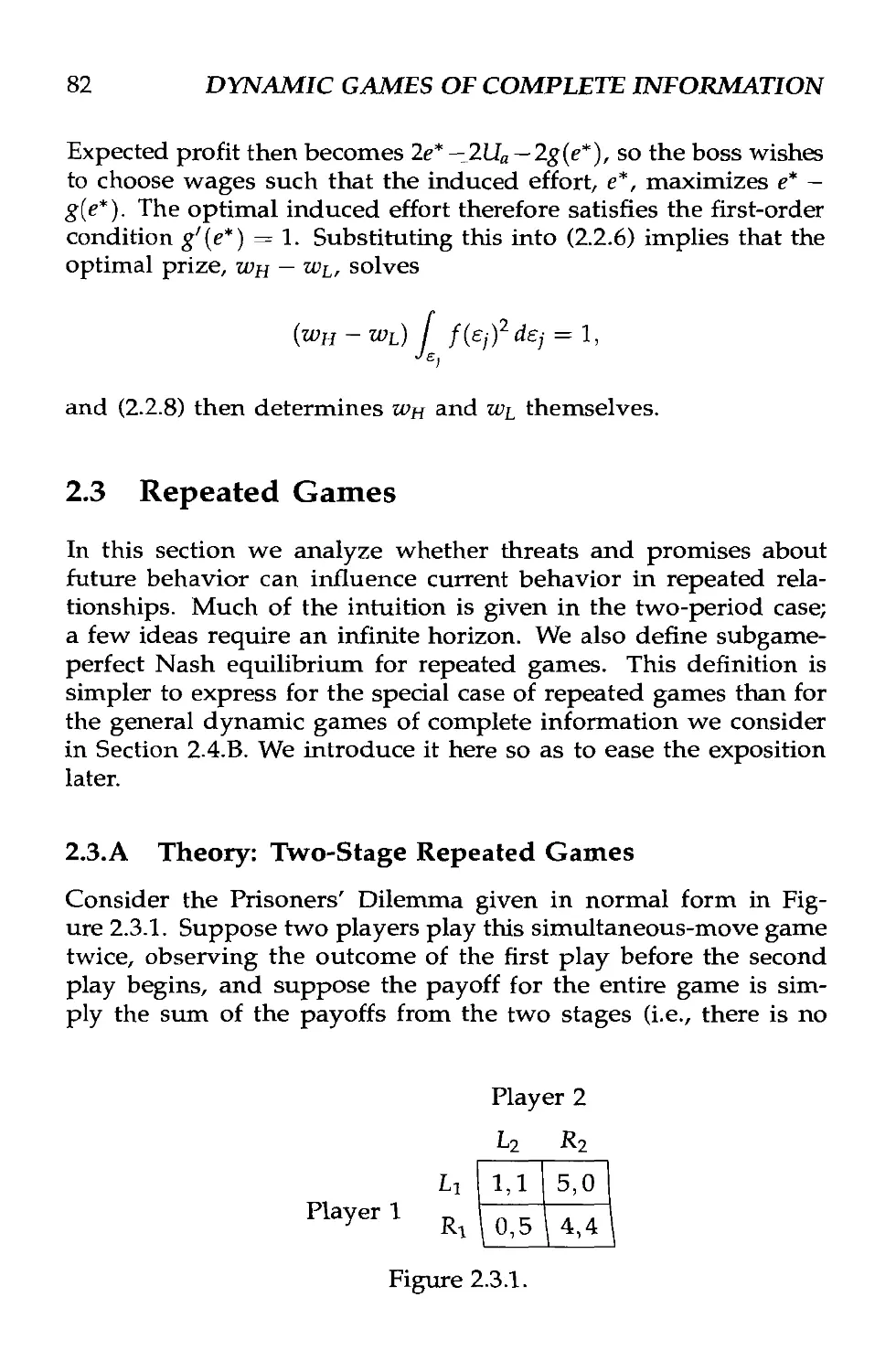
2.2.D Tournaments 79
2.3 Repeated Games 82
2.3.A Theory: Two-Stage Repeated Games 82
2.3.B Theory: Infinitely Repeated Games 88
2.3.C Collusion between Cournot Duopolists .... 102
2.3.D Efficiency Wages 107
2.3.E Time-Consistent Monetary Policy 112
2.4 Dynamic Games of Complete but
Imperfect Information 115
2.4.A Extensive-Form Representation of Games . . 115
2.4.B Subgame-Perfect Nash Equilibrium 122
2.5 Further Reading 129
2.6 Problems 130
2.7 References 138
3 Static Games of Incomplete Information 143
3.1 Theory: Static Bayesian Games and Bayesian Nash
Equilibrium 144
3.1.A An Example: Cournot Competition under
Asymmetric Information 144
3.1.B Normal-Form Representation of Static
Bayesian Games 146
3.1.C Definition of Bayesian Nash Equilibrium . . .149
3.2 Applications 152
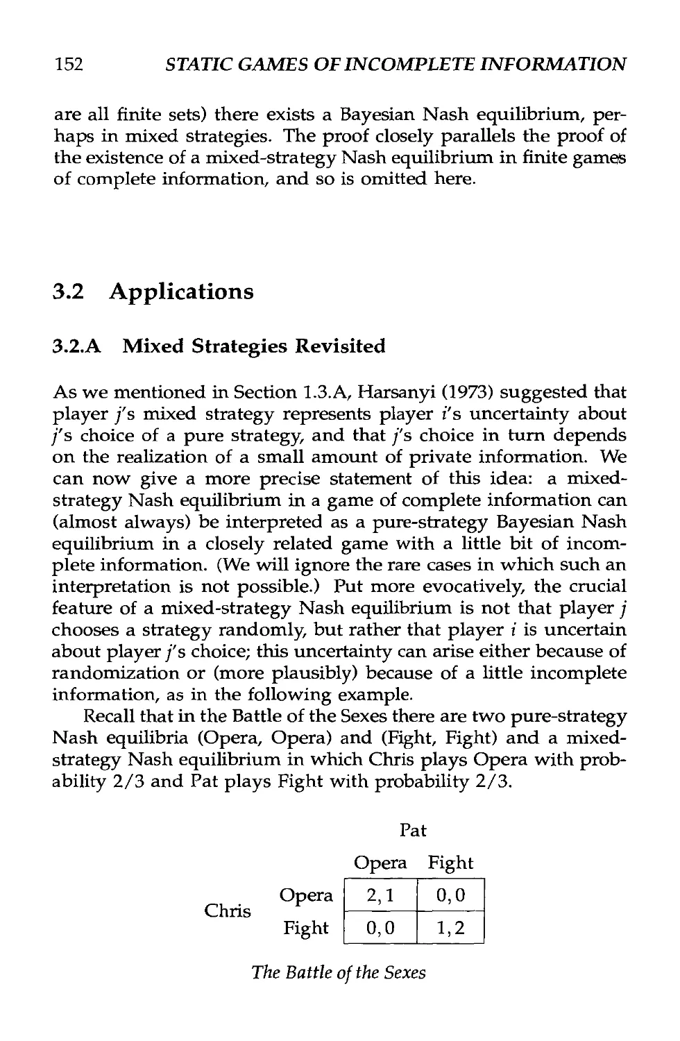
3.2.A Mixed Strategies Revisited 152
3.2.B An Auction 155
3.2.C A Double Auction 158
3.3 The Revelation Principle 164
3.4 Further Reading 168
3.5 Problems 169
3.6 References 172
4 Dynamic Games of Incomplete Information 173
4.1 Introduction to Perfect Bayesian Equilibrium 175
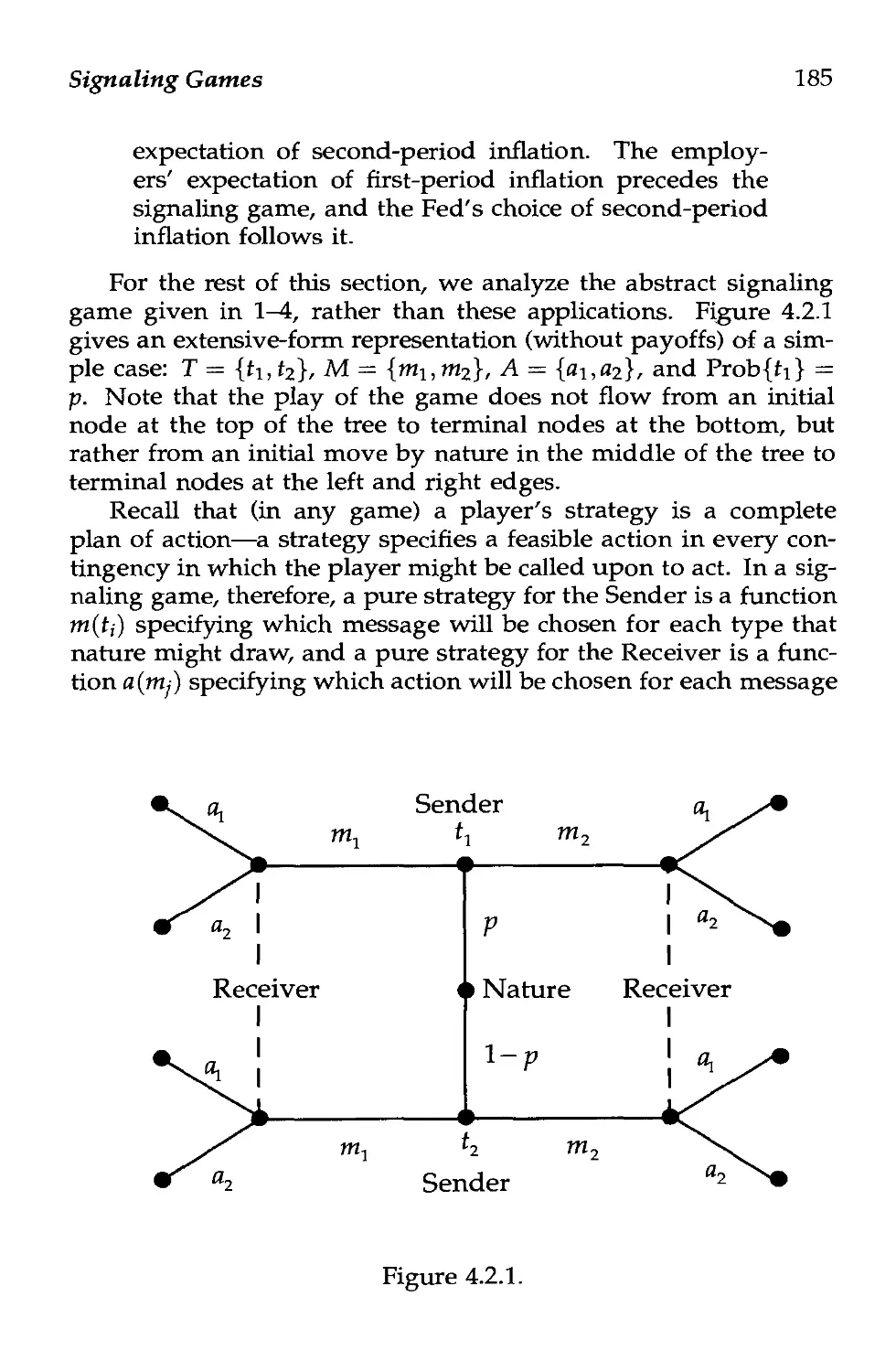
4.2 Signaling Games 183
4.2.A Perfect Bayesian Equilibrium in Signaling
Games 183

Contents ix
4.2.B Job-Market Signaling 190
4.2.C Corporate Investment and Capital Structure . 205
4.2.D Monetary Policy 208
4.3 Other Applications of Perfect Bayesian
Equilibrium 210
4.3.A Cheap-Talk Games 210
4.3.B Sequential Bargaining under Asymmetric
Information 218
4.3.C Reputation in the Finitely Repeated
Prisoners' Dilemma 224
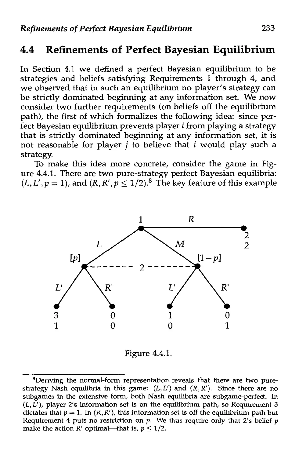
4.4 Refinements of Perfect Bayesian Equilibrium 233
4.5 Further Reading 244
4.6 Problems 245
4.7 References 253
Index 257

Preface
Game theory is the study of multiperson decision problems. Such
problems arise frequently in economics. As is widely appreciated,
for example, oligopolies present multiperson problems — each
firm must consider what the others will do. But many other ap-
applications of game theory arise in fields of economics other than
industrial organization. At the micro level, models of trading
processes (such as bargaining and auction models) involve game
theory. At an intermediate level of aggregation, labor and finan-
financial economics include game-theoretic models of the behavior of
a firm in its input markets (rather than its output market, as in
an oligopoly). There also are multiperson problems within a firm:
many workers may vie for one promotion; several divisions may
compete for the corporation's investment capital. Finally, at a high
level of aggregation, international economics includes models in
which countries compete (or collude) in choosing tariffs and other
trade policies, and macroeconomics includes models in which the
monetary authority and wage or price setters interact strategically
to determine the effects of monetary policy.
This book is designed to introduce game theory to those who
will later construct (or at least consume) game-theoretic models
in applied fields within economics. The exposition emphasizes
the economic applications of the theory at least as much as the
pure theory itself, for three reasons. First, the applications help
teach the theory; formal arguments about abstract games also ap-
appear but play a lesser role. Second, the applications illustrate the
process of model building — the process of translating an infor-
informal description of a multiperson decision situation into a formal,
game-theoretic problem to be analyzed. Third, the variety of ap-
applications shows that similar issues arise in different areas of eco-
economics, and that the same game-theoretic tools can be applied in

xii PREFACE
each setting. In order to emphasize the broad potential scope of
the theory, conventional applications from industrial organization
largely have been replaced by applications from labor, macro, and
other applied fields in economics.1
We will discuss four classes of games: static games of com-
complete information, dynamic games of complete information, static
games of incomplete information, and dynamic games of incom-
incomplete information. (A game has incomplete information if one
player does not know another player's payoff, such as in an auc-
auction when one bidder does not know how much another bidder
is willing to pay for the good being sold.) Corresponding to these
four classes of games will be four notions of equilibrium in games:
Nash equilibrium, subgame-perfect Nash equilibrium, Bayesian
Nash equilibrium, and perfect Bayesian equilibrium.
Two (related) ways to organize one's thinking about these equi-
equilibrium concepts are as follows. First, one could construct se-
sequences of equilibrium concepts of increasing strength, where
stronger (i.e., more restrictive) concepts are attempts to eliminate
implausible equilibria allowed by weaker notions of equilibrium.
We will see, for example, that subgame-perfect Nash equilibrium
is stronger than Nash equilibrium and that perfect Bayesian equi-
equilibrium in turn is stronger than subgame-perfect Nash equilib-
equilibrium. Second, one could say that the equilibrium concept of in-
interest is always perfect Bayesian equilibrium (or perhaps an even
stronger equilibrium concept), but that it is equivalent to Nash
equilibrium in static games of complete information, equivalent
to subgame-perfection in dynamic games of complete (and per-
perfect) information, and equivalent to Bayesian Nash equilibrium in
static games of incomplete information.
The book can be used in two ways. For first-year graduate stu-
students in economics, many of the applications will already be famil-
familiar, so the game theory can be covered in a half-semester course,
leaving many of the applications to be studied outside of class.
For undergraduates, a full-semester course can present the theory
a bit more slowly, as well as cover virtually all the applications in
class. The main mathematical prerequisite is single-variable cal-
calculus; the rudiments of probability and analysis are introduced as
needed.
1A good source for applications of game theory in industrial organization is
Tirole's The Theory of Industrial Organization (MIT Press, 1988).

Preface xiii
I learned game theory from David Kreps, John Roberts, and
Bob Wilson in graduate school, and from Adam Brandenburger,
Drew Fudenberg, and Jean Tirole afterward. I owe the theoreti-
theoretical perspective in this book to them. The focus on applications
and other aspects of the pedagogical style, however, are largely
due to the students in the MIT Economics Department from 1985
to 1990, who inspired and rewarded the courses that led to this
book. I am very grateful for the insights and encouragement all
these friends have provided, as well as for the many helpful com-
comments on the manuscript I received from Joe Farrell, Milt Harris,
George Mailath, Matthew Rabin, Andy Weiss, and several anony-
anonymous reviewers. Finally, I am glad to acknowledge the advice and
encouragement of Jack Repcheck of Princeton University Press and
financial support from an Olin Fellowship in Economics at the Na-
National Bureau of Economic Research.

Game Theory for Applied Economists

Chapter 1
Static Games of Complete
Information
In this chapter we consider games of the following simple form:
first the players simultaneously choose actions; then the players
receive payoffs that depend on the combination of actions just cho-
chosen. Within the class of such static (or simultaneous-move) games,
we restrict attention to games of complete information. That is, each
player's payoff function (the function that determines the player's
payoff from the combination of actions chosen by the players) is
common knowledge among all the players. We consider dynamic
(or sequential-move) games in Chapters 2 and 4, and games of
incomplete information (games in which some player is uncertain
about another player's payoff function—as in an auction where
each bidder's willingness to pay for the good being sold is un-
unknown to the other bidders) in Chapters 3 and 4.
In Section 1.1 we take a first pass at the two basic issues in
game theory: how to describe a game and how to solve the re-
resulting game-theoretic problem. We develop the tools we will use
in analyzing static games of complete information, and also the
foundations of the theory we will use to analyze richer games in
later chapters. We define the normal-form representation of a game
and the notion of a strictly dominated strategy. We show that some
games can be solved by applying the idea that rational players
do not play strictly dominated strategies, but also that in other
games this approach produces a very imprecise prediction about
the play of the game (sometimes as imprecise as "anything could

2 STATIC GAMES OF COMPLETE INFORMATION
happen"). We then motivate and define Nash equilibrium—a so-
solution concept that produces much tighter predictions in a very
broad class of games.
In Section 1.2 we analyze four applications, using the tools
developed in the previous section: Cournot's A838) model of im-
imperfect competition, Bertrand's A883) model of imperfect com-
competition, Farber's A980) model of final-offer arbitration, and the
problem of the commons (discussed by Hume [1739] and others).
In each application we first translate an informal statement of the
problem into a normal-form representation of the game and then
solve for the game's Nash equilibrium. (Each of these applications
has a unique Nash equilibrium, but we discuss examples in which
this is not true.)
In Section 1.3 we return to theory. We first define the no-
notion of a mixed strategy, which we will interpret in terms of one
player's uncertainty about what another player will do. We then
state and discuss Nash's A950) Theorem, which guarantees that a
Nash equilibrium (possibly involving mixed strategies) exists in a
broad class of games. Since we present first basic theory in Sec-
Section 1.1, then applications in Section 1.2, and finally more theory
in Section 1.3, it should be apparent that mastering the additional
theory in Section 1.3 is not a prerequisite for understanding the
applications in Section 1.2. On the other hand, the ideas of a mixed
strategy and the existence of equilibrium do appear (occasionally)
in later chapters.
This and each subsequent chapter concludes with problems,
suggestions for further reading, and references.
1.1 Basic Theory: Normal-Form Games and Nash
Equilibrium
l.l.A Normal-Form Representation of Games
In the normal-form representation of a game, each player simul-
simultaneously chooses a strategy, and the combination of strategies
chosen by the players determines a payoff for each player. We
illustrate the normal-form representation with a classic example
— The Prisoners' Dilemma. Two suspects are arrested and charged
with a crime. The police lack sufficient evidence to convict the sus-
suspects, unless at least one confesses. The police hold the suspects in

Basic Theory 3
separate cells and explain the consequences that will follow from
the actions they could take. If neither confesses then both will be
convicted of a minor offense and sentenced to one month in jail.
If both confess then both will be sentenced to jail for six months.
Finally, if one confesses but the other does not, then the confes-
confessor will be released immediately but the other will be sentenced
to nine months in jail—six for the crime and a further three for
obstructing justice.
The prisoners' problem can be represented in the accompany-
accompanying bi-matrix. (Like a matrix, a bi-matrix can have an arbitrary
number or rows and columns; "bi" refers to the fact that, in a
two-player game, there are two numbers in each cell—the payoffs
to the two players.)
Prisoner 2
Prisoner
1
Mum
Fink
Mum
-1
0
-1
-9
Fink
-9, 0
-6,-6
The Prisoners' Dilemma
In this game, each player has two strategies available: confess
(or fink) and not confess (or be mum). The payoffs to the two
players when a particular pair of strategies is chosen are given in
the appropriate cell of the bi-matrix. By convention, the payoff to
the so-called row player (here, Prisoner 1) is the first payoff given,
followed by the payoff to the column player (here, Prisoner 2).
Thus, if Prisoner 1 chooses Mum and Prisoner 2 chooses Fink, for
example, then Prisoner 1 receives the payoff -9 (representing nine
months in jail) and Prisoner 2 receives the payoff 0 (representing
immediate release).
We now turn to the general case. The normal-form representation
of a game specifies: A) the players in the game, B) the strategies
available to each player, and C) the payoff received by each player
for each combination of strategies that could be chosen by the
players. We will often discuss an n-player game in which the
players are numbered from 1 to n and an arbitrary player is called
player i. Let S, denote the set of strategies available to player i
(called i's strategy space), and let s, denote an arbitrary member of
this set. (We will occasionally write s, e S, to indicate that the

4 STATIC GAMES OF COMPLETE INFORMATION
strategy s,- is a member of the set of strategies S,.) Let (si,... ,sn)
denote a combination of strategies, one for each player, and let
M,- denote player i's payoff function: m,(si,...,sn) is the payoff to
player i if the players choose the strategies (si,... ,sn). Collecting
all of this information together, we have:
Definition The normal-form representation of an n-player game spec-
specifies the players' strategy spaces S\,...,Sn and their payoff functions
«i,... ,un. We denote this game by G = {Si,..., Sn;u\,... ,un}.
Although we stated that in a normal-form game the players
choose their strategies simultaneously, this does not imply that the
parties necessarily act simultaneously: it suffices that each choose
his or her action without knowledge of the others' choices, as
would be the case here if the prisoners reached decisions at ar-
arbitrary times while in their separate cells. Furthermore, although
in this chapter we use normal-form games to represent only static
games in which the players all move without knowing the other
players' choices, we will see in Chapter 2 that normal-form repre-
representations can be given for sequential-move games, but also that
an alternative—the extensive-form representation of the game—is
often a more convenient framework for analyzing dynamic issues.
l.l.B Iterated Elimination of Strictly Dominated
Strategies
Having described one way to represent a game, we now take a
first pass at describing how to solve a game-theoretic problem.
We start with the Prisoners' Dilemma because it is easy to solve,
using only the idea that a rational player will not play a strictly
dominated strategy.
In the Prisoners' Dilemma, if one suspect is going to play Fink,
then the other would prefer to play Fink and so be in jail for six
months rather than play Mum and so be in jail for nine months.
Similarly, if one suspect is going to play Mum, then the other
would prefer to play Fink and so be released immediately rather
than play Mum and so be in jail for one month. Thus, for prisoner
i, playing Mum is dominated by playing Fink—for each strategy
that prisoner / could choose, the payoff to prisoner i from playing
Mum is less than the payoff to i from playing Fink. (The same
would be true in any bi-matrix in which the payoffs 0, —1, -6,

Basic Theory 5
and —9 above were replaced with payoffs T, R, P, and S, respec-
respectively, provided that T > R > P > S so as to capture the ideas
of temptation, reward, punishment, and sucker payoffs.) More
generally:
Definition In the normal-form game G = {S\,... ,Sn;u\,...,un},let
s- and s-' be feasible strategies for player i (i.e., s- and s'( are members of
Sj). Strategy sj is strictly dominated by strategy s" if for each feasible
combination of the other players' strategies, i's payoff from playing s- is
strictly less than i's payoff from playing s'/:
Uj(s\ , . . . , S,_! , s'j, S,+l, . .. , Sn) < M,-(Sl, — ,S,-_i, S", S(+i ,...,Sn) (DS)
for each (s\,..., s,_i, s,+i,... ,sn) that can be constructed from the other
players' strategy spaces Si,..., S,-_i, S,-+i ,...,Sn.
Rational players do not play strictly dominated strategies, be-
because there is no belief that a player could hold (about the strate-
strategies the other players will choose) such that it would be optimal
to play such a strategy.1 Thus, in the Prisoners' Dilemma, a ratio-
rational player will choose Fink, so (Fink, Fink) will be the outcome
reached by two rational players, even though (Fink, Fink) results
in worse payoffs for both players than would (Mum, Mum). Be-
Because the Prisoners' Dilemma has many applications (including
the arms race and the free-rider problem in the provision of pub-
public goods), we will return to variants of the game in Chapters 2
and 4. For now, we focus instead on whether the idea that rational
players do not play strictly dominated strategies can lead to the
solution of other games.
Consider the abstract game in Figure 1.1.1.2 Player 1 has two
strategies and player 2 has three: Si = {Up, Down} and S2 =
{Left, Middle, Right}. For player 1, neither Up nor Down is strictly
'A complementary question is also of interest' if there is no belief that player 1
could hold (about the strategies the other players will choose) such that it would
be optimal to play the strategy S/, can we conclude that there must be another
strategy that strictly dominates s,? The answer is "yes," provided that we adopt
appropriate definitions of "belief" and "another strategy," both of which involve
the idea of mixed strategies to be introduced in Section 1 3 A.
2Most of this book considers economic applications rather than abstract exam-
examples, both because the applications are of interest in their own right and because,
for many readers, the applications are often a useful way to explain the under-
underlying theory. When introducing some of the basic theoretical ideas, however,
we will sometimes resort to abstract examples that have no natural economic
interpretation

STATIC GAMES OF COMPLETE INFORMATION
Player 2
Player 1
Up
Down
Left Middle Right
1,0
0,3
1,2
0,1
0,1
2,0
Figure 1.1.1
dominated: Up is better than Down if 2 plays Left (because 1 > 0),
but Down is better than Up if 2 plays Right (because 2 > 0). For
player 2, however, Right is strictly dominated by Middle (because
2 > 1 and 1 > 0), so a rational player 2 will not play Right.
Thus, if player 1 knows that player 2 is rational then player 1 can
eliminate Right from player 2's strategy space. That is, if player
1 knows that player 2 is rational then player 1 can play the game
in Figure 1.1.1 as if it were the game in Figure 1.1.2.
Player 2
Left Middle
Player 1
Up
Down
Figure 1.1.2.
1,0
0,3
1,2
0,1
In Figure 1.1.2, Down is now strictly dominated by Up for
player 1, so if player 1 is rational (and player 1 knows that player 2
is rational, so that the game in Figure 1.1.2 applies) then player 1
will not play Down. Thus, if player 2 knows that player 1 is ra-
rational, and player 2 knows that player 1 knows that player 2 is
rational (so that player 2 knows that Figure 1.1.2 applies), then
player 2 can eliminate Down from player l's strategy space, leav-
leaving the game in Figure 1.1.3. But now Left is strictly dominated
by Middle for player 2, leaving (Up, Middle) as the outcome of
the game.
This process is called iterated elimination of strictly dominated
strategies. Although it is based on the appealing idea that ratio-
rational players do not play strictly dominated strategies, the process
has two drawbacks. First, each step requires a further assumption

Basic Theory
Player 2
Left Middle
Player 1 Up
1,0
1,2
Figure 1.1.3.
about what the players know about each other's rationality If
we want to be able to apply the process for an arbitrary number
of steps, we need to assume that it is common knowledge that the
players are rational. That is, we need to assume not only that all
the players are rational, but also that all the players know that all
the players are rational, and that all the players know that all the
players know that all the players are rational, and so on, ad in-
finitum. (See Aumann [1976] for the formal definition of common
knowledge.)
The second drawback of iterated elimination of strictly domi-
dominated strategies is that the process often produces a very impre-
imprecise prediction about the play of the game. Consider the game in
Figure 1.1.4, for example. In this game there are no strictly dom-
dominated strategies to be eliminated. (Since we have not motivated
this game in the slightest, it may appear arbitrary, or even patho-
pathological. See the case of three or more firms in the Cournot model
in Section 1.2.A for an economic application in the same spirit.)
Since all the strategies in the game survive iterated elimination of
strictly dominated strategies, the process produces no prediction
whatsoever about the play of the game.
C
R
0,4
4,0
3,5
4,0
0,4
3,5
5,3
5,3
6,6
M
B
Figure 1.1.4.
We turn next to Nash equilibrium—a solution concept that
produces much tighter predictions in a very broad class of games.
We show that Nash equilibrium is a stronger solution concept

8 STATIC GAMES OF COMPLETE INFORMATION
than iterated elimination of strictly dominated strategies, in the
sense that the players' strategies in a Nash equilibrium always
survive iterated elimination of strictly dominated strategies, but
the converse is not true. In subsequent chapters we will argue that
in richer games even Nash equilibrium produces too imprecise a
prediction about the play of the game, so we will define still-
stronger notions of equilibrium that are better suited for these
richer games.
1.1.C Motivation and Definition of Nash Equilibrium
One way to motivate the definition of Nash equilibrium is to argue
that if game theory is to provide a unique solution to a game-
theoretic problem then the solution must be a Nash equilibrium,
in the following sense. Suppose that game theory makes a unique
prediction about the strategy each player will choose. In order
for this prediction to be correct, it is necessary that each player be
willing to choose the strategy predicted by the theory. Thus, each
player's predicted strategy must be that player's best response
to the predicted strategies of the other players. Such a prediction
could be called strategically stable or self-enforcing, because no single
player wants to deviate from his or her predicted strategy. We will
call such a prediction a Nash equilibrium:
Definition In the n-player normal-form game G = {S\,...,Sn)U\,...,
un}, the strategies (s\,...,s*)area Nash equilibrium if, for each player
i, s* is (at least tied for) player i's best response to the strategies specified
for the n - 1 other players, (s\,..., s*_i, s*+1,..., s*):
U/(Si , - . . , S*_i,S,*,S;+1, . . . ,Sn)
>uI-(s1*,...,sr_1)sI-,sr+1,...,s*) (NE)
for every feasible strategy s, in S,; that is, s* solves
max Ui[S],...,s,-_j,s,-,s,-1 j,... ,sn)
s,gS,
To relate this definition to its motivation, suppose game theory
offers the strategies (s[,... ,s'n) as the solution to the normal-form
game G = {Si,... ,Sn;M],.. .,«„}. Saying that (s\,... ,s'n) is not

Basic Theory 9
a Nash equilibrium of G is equivalent to saying that there exists
some player i such that sj is not a best response to (s[,..., s'i_1, s[+],
... ,s'n). That is, there exists some s" in S, such that
wi(sl> • • • , S,-_i,Sf,S,-+1, . .. ,Sn) < Uj[Si, . . . , Sj_i,S; , S,-+], . . . ,SM).
Thus, if the theory offers the strategies (s[,.. ¦ ,s'n) as the solution
but these strategies are not a Nash equilibrium, then at least one
player will have an incentive to deviate from the theory's predic-
prediction, so the theory will be falsified by the actual play of the game.
A closely related motivation for Nash equilibrium involves the
idea of convention: if a convention is to develop about how to
play a given game then the strategies prescribed by the conven-
convention must be a Nash equilibrium, else at least one player will not
abide by the convention.
To be more concrete, we now solve a few examples. Consider
the three normal-form games already described—the Prisoners'
Dilemma and Figures 1.1.1 and 1.1.4. A brute-force approach to
finding a game's Nash equilibria is simply to check whether each
possible combination of strategies satisfies condition (NE) in the
definition.3 In a two-player game, this approach begins as follows:
for each player, and for each feasible strategy for that player, deter-
determine the other player's best response to that strategy. Figure 1.1.5
does this for the game in Figure 1.1.4 by underlining the payoff
to player j's best response to each of player /'s feasible strategies
If the column player were to play L, for instance, then the row
player's best response would be M, since 4 exceeds 3 and 0, sa
the row player's payoff of 4 in the (M, L) cell of the bi-matrix is
underlined.
A pair of strategies satisfies condition (NE) if each player's
strategy is a best response to the other's—that is, if both pay-
payoffs are underlined in the corresponding cell of the bi-matrix
Thus, (B, R) is the only strategy pair that satisfies (NE); likewise
for (Fink, Fink) in the Prisoners' Dilemma and (Up, Middle) in
3In Section 1.3.A we will distinguish between pure and mixed strategies. We
will then see that the definition given here describes pure-strategy Nash equilibria,
but that there can also be mixed-strategy Nash equilibria Unless explicitly noted
otherwise, all references to Nash equilibria in this section are to pure-strategy
Nash equilibria.

10
STATIC GAMES OF COMPLETE INFORMATION
M
C
R
0,4
4,0
3,5
4,0
0,4
3,5
5,3
5,3
6,6
Figure 1.1.5.
Figure 1.1.1. These strategy pairs are the unique Nash equilibria
of these games.4
We next address the relation between Nash equilibrium and
iterated elimination of strictly dominated strategies. Recall that
the Nash equilibrium strategies in the Prisoners' Dilemma and
Figure 1.1.1—(Fink, Fink) and (Up, Middle), respectively—are the
only strategies that survive iterated elimination of strictly domi-
dominated strategies. This result can be generalized: if iterated elimina-
elimination of strictly dominated strategies eliminates all but the strategies
(s\,.. .,s*), then these strategies are the unique Nash equilibrium of
the game. (See Appendix 1.1.C for a proof of this claim.) Since it-
iterated elimination of strictly dominated strategies frequently does
not eliminate all but a single combination of strategies, however,
it is of more interest that Nash equilibrium is a stronger solution
concept than iterated elimination of strictly dominated strategies,
in the following sense. If the strategies (s\,.. .,s*) are a Nash equi-
equilibrium then they survive iterated elimination of strictly domi-
dominated strategies (again, see the Appendix for a proof), but there
can be strategies that survive iterated elimination of strictly dom-
dominated strategies but are not part of any Nash equilibrium. To see
the latter, recall that in Figure 1.1.4 Nash equilibrium gives the
unique prediction (B, R), whereas iterated elimination of strictly
dominated strategies gives the maximally imprecise prediction: no
strategies are eliminated; anything could happen.
Having shown that Nash equilibrium is a stronger solution
concept than iterated elimination of strictly dominated strategies,
we must now ask whether Nash equilibrium is too strong a so-
solution concept. That is, can we be sure that a Nash equilibrium
4This statement is correct even if we do not restrict attention to pure-strategy
Nash equilibrium, because no mixed-strategy Nash equilibria exist in these three
games See Problem 1 10

Basic Theory 11
exists? Nash A950) showed that in any finite game (i.e., a game in
which the number of players n and the strategy sets Si,..., S,, are
all finite) there exists at least one Nash equilibrium. (This equi-
equilibrium may involve mixed strategies, which we will discuss in
Section 1.3.A; see Section 1.3.B for a precise statement of Nash's
Theorem.) Cournot A838) proposed the same notion of equilib-
equilibrium in the context of a particular model of duopoly and demon-
demonstrated (by construction) that an equilibrium exists in that model;
see Section 1.2.A. In every application analyzed in this book, we
will follow Cournot's lead: we will demonstrate that a Nash (or
stronger) equilibrium exists by constructing one. In some of the
theoretical sections, however, we will rely on Nash's Theorem (or
its analog for stronger equilibrium concepts) and simply assert
that an equilibrium exists.
We conclude this section with another classic example—The
Battle of the Sexes. This example shows that a game can have mul-
multiple Nash equilibria, and also will be useful in the discussions of
mixed strategies in Sections 1.3.B and 3.2.A. In the traditional ex-
exposition of the game (which, it will be clear, dates from the 1950s),
a man and a woman are trying to decide on an evening's enter-
entertainment; we analyze a gender-neutral version of the game. While
at separate workplaces, Pat and Chris must choose to attend either
the opera or a prize fight. Both players would rather spend the
evening together than apart, but Pat would rather they be together
at the prize fight while Chris would rather they be together at the
opera, as represented in the accompanying bi-matrix.
Pat
Opera Fight
Opera
Chris
Fight
The Battle of the Sexes
Both (Opera, Opera) and (Fight, Fight) are Nash equilibria.
We argued above that if game theory is to provide a unique
solution to a game then the solution must be a Nash equilibrium.
This argument ignores the possibility of games in which game
theory does not provide a unique solution. We also argued that
2,1
0,0
0,0
1,2

12 STATIC GAMES OF COMPLETE INFORMATION
if a convention is to develop about how to play a given game,
then the strategies prescribed by the convention must be a Nash
equilibrium, but this argument similarly ignores the possibility of
games for which a convention will not develop. In some games
with multiple Nash equilibria one equilibrium stands out as the
compelling solution to the game. (Much of the theory in later
chapters is an effort to identify such a compelling equilibrium
in different classes of games.) Thus, the existence of multiple
Nash equilibria is not a problem in and of itself. In the Battle
of the Sexes, however, (Opera, Opera) and (Fight, Fight) seem
equally compelling, which suggests that there may be games for
which game theory does not provide a unique solution and no
convention will develop.5 In such games, Nash equilibrium loses
much of its appeal as a prediction of play.
Appendix l.l.C
This appendix contains proofs of the following two Propositions,
which were stated informally in Section l.l.C. Skipping these
proofs will not substantially hamper one's understanding of later
material. For readers not accustomed to manipulating formal def-
definitions and constructing proofs, however, mastering these proofs
will be a valuable exercise.
Proposition A In the n-player normal-form game G = {Si,...,Sn;
u\ ,...,«„}, if iterated elimination of strictly dominated strategies elimi-
eliminates all but the strategies (s\,..., s*), then these strategies are the unique
Nash equilibrium of the game.
Proposition B In the n-player normal-form game G = {S\,...,Sn;
«!,..., u,,}, if the strategies (sj,..., s*) are a Nash equilibrium, then they
survive iterated elimination of strictly dominated strategies.
5In Section 1 3 B we describe a third Nash equilibrium of the Battle of the
Sexes (involving mixed strategies) Unlike (Opera, Opera) and (Fight, Fight), this
third equilibrium has symmetric payoffs, as one might expect from the unique
solution to a symmetric game; on the other hand, the third equilibrium is also
inefficient, which may work against its development as a convention Whatever
one's judgment about the Nash equilibria in the Battle of the Sexes, however,
the broader point remains- there may be games in which game theory does not
provide a unique solution and no convention will develop

Basic Theory 13
Since Proposition B is simpler to prove, we begin with it, to
warm up. The argument is by contradiction. That is, we will as-
assume that one of the strategies in a Nash equilibrium is eliminated
by iterated elimination of strictly dominated strategies, and then
we will show that a contradiction would result if this assumption
were true, thereby proving that the assumption must be false.
Suppose that the strategies (S|,... ,s*) are a Nash equilibrium
of the normal-form game G = {Si,..., Sn; U\,..., un), but suppose
also that (perhaps after some strategies other than {s\,..., s*) have
been eliminated) s* is the first of the strategies (sj,...,s*) to be
eliminated for being strictly dominated. Then there must exist a
strategy s" that has not yet been eliminated from S, that strictly
dominates s*. Adapting (DS), we have
"i(Sl, - - -, S/_i, S*, Sj+i, — ,Sn)
..,Sn) A.1.1)
for each (si,..., s;_i, s,-+i,..., sn) that can be constructed from the
strategies that have not yet been eliminated from the other players'
strategy spaces. Since s* is the first of the equilibrium strategies to
be eliminated, the other players' equilibrium strategies have not
yet been eliminated, so one of the implications of A.1.1) is
Uj\Sl,.. . ,Si_l,Si ,S,+1,. .. ,Sn)
;'..,s;). A.1.2)
But A.1.2) is contradicted by (NE): s* must be a best response to
(sj,... ,s*_],s*+1,... ,s*), so there cannot exist a strategy s" that
strictly dominates s*. This contradiction completes the proof.
Having proved Proposition B, we have already proved part of
Proposition A: all we need to show is that if iterated elimination
of dominated strategies eliminates all but the strategies (sj, , s*)
then these strategies are a Nash equilibrium; by Proposition B, any
other Nash equilibria would also have survived, so this equilib-
equilibrium must be unique. We assume that G is finite.
The argument is again by contradiction. Suppose that iterated
elimination of dominated strategies eliminates all but the strategies
(sj,... ,s*) but these strategies are not a Nash equilibrium. Then
there must exist some player i and some feasible strategy s, in S,
such that (NE) fails, but s,- must have been strictly dominated by
some other strategy s,' at some stage of the process. The formal

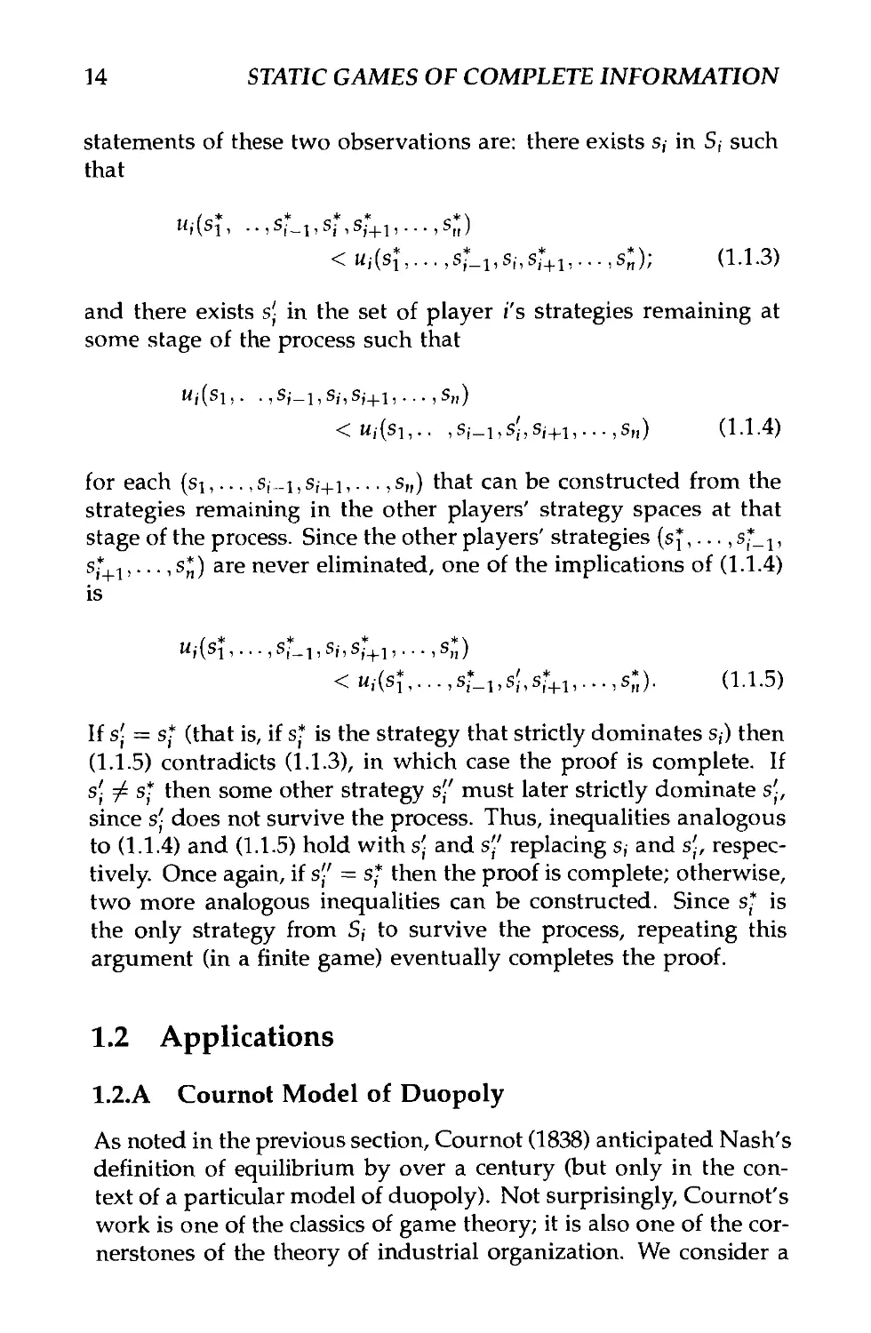
14 STATIC GAMES OF COMPLETE INFORMATION
statements of these two observations are: there exists s,- in S,- such
that
u,-(sT, ..,s;_1,s?,sr+1,...,s;)
<m,(si,...,s*_1,s!-,s*+1,...,s*); A.1.3)
and there exists sj in the set of player i's strategies remaining at
some stage of the process such that
..,s,,) A.1.4)
for each (si,..., s,-_i, s,-+i,..., s,,) that can be constructed from the
strategies remaining in the other players' strategy spaces at that
stage of the process. Since the other players' strategies (sj,..., s*_i,
s*+1,..., s*) are never eliminated, one of the implications of A.1.4)
is
M;(Sj, ... , S,-—i, Sj,S,-_|_i, . . . ,Sn)
< w,(s1*,...,s*_1,s;,s*+1,...,s*). A.1.5)
If sj = s* (that is, if s* is the strategy that strictly dominates s,) then
A.1.5) contradicts A.1.3), in which case the proof is complete. If
sj ^ s* then some other strategy s-' must later strictly dominate sj,
since sj does not survive the process. Thus, inequalities analogous
to A.1.4) and A.1.5) hold with s- and s" replacing s, and s\, respec-
respectively. Once again, if s" = s* then the proof is complete; otherwise,
two more analogous inequalities can be constructed. Since s* is
the only strategy from S, to survive the process, repeating this
argument (in a finite game) eventually completes the proof.
1.2 Applications
1.2.A Cournot Model of Duopoly
As noted in the previous section, Cournot A838) anticipated Nash's
definition of equilibrium by over a century (but only in the con-
context of a particular model of duopoly). Not surprisingly, Cournot's
work is one of the classics of game theory; it is also one of the cor-
cornerstones of the theory of industrial organization. We consider a

Applications 15
very simple version of Cournot's model here, and return to vari-
variations on the model in each subsequent chapter. In this section
we use the model to illustrate: (a) the translation of an informal
statement of a problem into a normal-form representation of a
game; (b) the computations involved in solving for the game's
Nash equilibrium; and (c) iterated elimination of strictly domi-
dominated strategies.
Let q\ and qi denote the quantities (of a homogeneous product)
produced by firms 1 and 2, respectively. Let P(Q) = a — Q be the
market-clearing price when the aggregate quantity on the market
is Q = q\ + qi (More precisely, P(Q) = a - Q for Q < a, and
P(Q) = 0 for Q > a.) Assume that the total cost to firm i of
producing quantity q< is C,(^,) = cq\. That is, there are no fixed
costs and the marginal cost is constant at c, where we assume
c < a. Following Cournot, suppose that the firms choose their
quantities simultaneously.6
In order to find the Nash equilibrium of the Cournot game,
we first translate the problem into a normal-form game. Recall
from the previous section that the normal-form representation of
a game specifies: A) the players in the game, B) the strategies
available to each player, and C) the payoff received by each player
for each combination of strategies that could be chosen by the
players. There are of course two players in any duopoly game—
the two firms. In the Cournot model, the strategies available to
each firm are the different quantities it might produce. We will
assume that output is continuously divisible. Naturally, negative
outputs are not feasible. Thus, each firm's strategy space can be
represented as S; = [0, oo), the nonnegative real numbers, in which
case a typical strategy s, is a quantity choice, qt > 0. One could
argue that extremely large quantities are not feasible and so should
not be included in a firm's strategy space. Because P(Q) = 0 for
Q > a, however, neither firm will produce a quantity qi > a.
It remains to specify the payoff to firm i as a function of the
strategies chosen by it and by the other firm, and to define and
6We discuss Bertrand's A883) model, in which firms choose prices rather than
quantities, in Section 1 2 B, and Stackelberg's A934) model, in which firms choose
quantities but one firm chooses before (and is observed by) the other, in Sec-
Section 2 l.B Finally, we discuss Friedman's A971) model, in which the interaction
described in Cournot's model occurs repeatedly over time, in Section 2.3.C

16 STATIC GAMES OF COMPLETE INFORMATION
solve for equilibrium. We assume that the firm's payoff is simply
its profit. Thus, the payoff w,(s,-,Sj) in a general two-player game
in normal form can be written here as7
*i{qi, 1j) = m\P{m + qj) - c] = qM - (qi + qj) - c].
Recall from the previous section that in a two-player game in nor-
normal form, the strategy pair (s^s^) is a Nash equilibrium if, for
each player i,
u{{st,sJ)>Ui{Si,sJ) (NE)
for every feasible strategy s, in S,. Equivalently, for each player i,
s* must solve the optimization problem
max m,-(s;,s*)
s,-eSj '
In the Cournot duopoly model, the analogous statement is that
the quantity pair (q^ql) is a Nash equilibrium if, for each firm i,
q* solves
max Ki(qi,q*) = max qt[a - (</,¦ + qj)-c].
Assuming q* < a - c (as will be shown to be true), the first-order
condition for firm i's optimization problem is both necessary and
sufficient; it yields
Thus, if the quantity pair (q,,^) *s to be a Nash equilibrium, the
firms' quantity choices must satisfy
and
7Note that we have changed the notation slightly by writing m,(s,-, Sj) rather
than Ui(si,s2). Both expressions represent the payoff to player i as a function of
the strategies chosen by all the players. We will use these expressions (and their
n-player analogs) interchangeably.

Applications 17
Solving this pair of equations yields
a — c
q\ = <& =
which is indeed less than a — c, as assumed.
The intuition behind this equilibrium is simple. Each firm
would of course like to be a monopolist in this market, in which
case it would choose qt to maximize tt,((J,, 0)—it would produce
the monopoly quantity qm = (a - c)/2 and earn the monopoly
profit 7r,((jm,0) = (fl — cJ/4. Given that there are two firms, aggre-
aggregate profits for the duopoly would be maximized by setting the
aggregate quantity q\ + q2 equal to the monopoly quantity qm, as
would occur if qt = qm/2 for each i, for example. The problem
with this arrangement is that each firm has an incentive to devi-
deviate: because the monopoly quantity is low, the associated price
P{qm) is high, and at this price each firm would like to increase its
quantity, in spite of the fact that such an increase in production
drives down the market-clearing price. (To see this formally, use
A.2.1) to check that qm/2 is not firm 2's best response to the choice
of qm/2 by firm 1.) In the Cournot equilibrium, in contrast, the ag-
aggregate quantity is higher, so the associated price is lower, so the
temptation to increase output is reduced—reduced by just enough
that each firm is just deterred from increasing its output by the
realization that the market-clearing price will fall. See Problem 1.4
for an analysis of how the presence of n oligopolists affects this
equilibrium trade-off between the temptation to increase output
and the reluctance to reduce the market-clearing price.
Rather than solving for the Nash equilibrium in the Cournot
game algebraically, one could instead proceed graphically, as fol-
follows. Equation A.2.1) gives firm i's best response to firm /s
equilibrium strategy, q*-. Analogous reasoning leads to firm 2's
best response to an arbitrary strategy by firm 1 and firm l's best
response to an arbitrary strategy by firm 2. Assuming that firm l's
strategy satisfies q\ < a- c, firm 2's best response is
KO) { )
likewise, it q2 < a - c then firm l's best response is

18
STATIC GAMES OF COMPLETE INFORMATION
(O,a-c)
(a-c,O)
Figure 1.2.1.
As shown in Figure 1.2.1, these two best-response functions inter-
intersect only once, at the equilibrium quantity pair {q\,q\)-
A third way to solve for this Nash equilibrium is to apply
the process of iterated elimination of strictly dominated strategies.
This process yields a unique solution—which, by Proposition A
in Appendix l.l.C, must be the Nash equilibrium {q\,q\)- The
complete process requires an infinite number of steps, each of
which eliminates a fraction of the quantities remaining in each
firm's strategy space; we discuss only the first two steps. First, the
monopoly quantity qm = (a — c)/2 strictly dominates any higher
quantity. That is, for any x > 0, 7r,(c/m,<7;) > 7r,(tjm + x,qj) for all
qj > 0. To see this, note that if Q = qm + x + q] < a, then
a- c \a - c
and
a — c ] [a — c ]
+ x\ — x- q,\ = iri{
and if Q = qm + x + qj > a, then P(Q) - 0, so producing a smaller

Applications 19
quantity raises profit. Second, given that quantities exceeding qm
have been eliminated, the quantity (a - c)/4 strictly dominates
any lower quantity. That is, for any x between zero and (a - c)/4,
¦7r,[(o — c)/4,<fy] > nj[(a - c)/4 - x,qj] for all qj between zero and
(a - c)/2. To see this, note that
(a — c \ a - c [3(« - c)
and
a-c
^y~ + x-
After these two steps, the quantities remaining in each firm's
strategy space are those in the interval between (a — c)/4 and
(a — c)/2. Repeating these arguments leads to ever-smaller inter-
intervals of remaining quantities. In the limit, these intervals converge
to the single point q* = (a — c)/3.
Iterated elimination of strictly dominated strategies can also be
described graphically, by using the observation (from footnote 1;
see also the discussion in Section 1.3.A) that a strategy is strictly
dominated if and only if there is no belief about the other players'
choices for which the strategy is a best response. Since there are
only two firms in this model, we can restate this observation as:
a quantity <?, is strictly dominated if and only if there is no belief
about qj such that qt is firm i's best response. We again discuss only
the first two steps of the iterative process. First, it is never a best
response for firm i to produce more than the monopoly quantity,
qm = (a—c)/2. To see this, consider firm 2's best-response function,
for example: in Figure 1.2.1, ^2(^1) equals qm when q\ = 0 and
declines as q\ increases. Thus, for any qj > 0, if firm 1 believes
that firm j will choose qj, then firm i's best response is less than or
equal to qm; there is no qj such that firm i's best response exceeds
qm. Second, given this upper bound on firm j's quantity, we can
derive a lower bound on firm i's best response: if qj < (a — c)/2,
then R,(cj;) > (a — c)/4, as shown for firm 2's best response in
Figure I.2.2.8
'These two arguments are slightly incomplete because we have not analyzed

20
STATIC GAMES OF COMPLETE INFORMATION
q2
@,(a-c)/4)
<(a-c)/2,0) (a-c,0)
Figure 1.2.2.
As before, repeating these arguments leads to the single quantity
qf = (a - c)/3.
We conclude this section by changing the Cournot model so
that iterated elimination of strictly dominated strategies does not
yield a unique solution. To do this, we simply add one or more
firms to the existing duopoly. We will see that the first of the
two steps discussed in the duopoly case continues to hold, but
that the process ends there. Thus, when there are more than two
firms, iterated elimination of strictly dominated strategies yields
only the imprecise prediction that each firm's quantity will not
exceed the monopoly quantity (much as in Figure 1.1.4, where no
strategies were eliminated by this process).
For concreteness, we consider the three-firm case. Let Q_,
denote the sum of the quantities chosen by the firms other than
i, and let 7r,(q,-,Q_1) = q{(a - qt - Q_; - c) provided q{ + Q_,- < a
(whereas tt,^,, Q_,-) = —cqi if qi + Q-i > a). It is again true that the
monopoly quantity qm = (a - c)/2 strictly dominates any higher
quantity. That is, for any x > 0, iri(qm, Q_,-) > n{qm +x,Q_,-) for
all Q_, > 0, just as in the first step in the duopoly case. Since
firm i's best response when firm i is uncertain about <jy. Suppose firm i is uncertain
about fy but believes that the expected value of qy is E(<j,-). Because 7r,(<jj,ij;) is
linear in q;, firm i's best response when it is uncertain in this way simply equals
its best response when it is certain that firm ; will choose E(fy)—a case covered
in the text

Applications 21
there are two firms other than firm i, however, all we can say
about Q_f is that it is between zero and a — c, because qj and q^
are between zero and (a — c)/2. But this implies that no quantity
qi > 0 is strictly dominated for firm i, because for each 9, between
zero and (a — c)/2 there exists a value of Q_, between zero and
a — c (namely, Q_; = a — c — lqt) such that q\ is firm i's best response
to Q-i- Thus, no further strategies can be eliminated.
1.2.B Bertrand Model of Duopoly
We next consider a different model of how two duopolists might
interact, based on Bertrand's A883) suggestion that firms actu-
actually choose prices, rather than quantities as in Cournot's model.
It is important to note that Bertrand's model is a different game
than Cournot's model: the strategy spaces are different, the pay-
payoff functions are different, and (as will become clear) the behavior
in the Nash equilibria of the two models is different. Some au-
authors summarize these differences by referring to the Cournot and
Bertrand equilibria. Such usage may be misleading: it refers to the
difference between the Cournot and Bertrand games, and to the
difference between the equilibrium behavior in these games, not
to a difference in the equilibrium concept used in the games. In
both games, the equilibrium concept used is the Nash equilibrium defined
in the previous section.
We consider the case of differentiated products. (See Prob-
Problem 1.7 for the case of homogeneous products.) If firms 1 and 2
choose prices p\ and P2, respectively, the quantity that consumers
demand from firm i is
where b > 0 reflects the extent to which firm i's product is a sub-
substitute for firm ;'s product. (This is an unrealistic demand function
because demand for firm i's product is positive even when firm i
charges an arbitrarily high price, provided firm ; also charges a
high enough price. As will become clear, the problem makes sense
only if b < 2.) As in our discussion of the Cournot model, we as-
assume that there are no fixed costs of production and that marginal
costs are constant at c, where c < a, and that the firms act (i.e.,
choose their prices) simultaneously.
As before, the first task in the process of finding the Nash equi-
equilibrium is to translate the problem into a normal-form game. There

22 STATIC GAMES OF COMPLETE INFORMATION
are again two players. This time, however, the strategies available
to each firm are the different prices it might charge, rather than
the different quantities it might produce. We will assume that
negative prices are not feasible but that any nonnegative price can
be charged—there is no restriction to prices denominated in pen-
pennies, for instance. Thus, each firm's strategy space can again be
represented as S, = [0, oo), the nonnegative real numbers, and a
typical strategy s, is now a price choice, p, > 0.
We will again assume that the payoff function for each firm is
just its profit. The profit to firm i when it chooses the price p,- and
its rival chooses the price py is
*i(PhPj) = 1i(j>i,Pj)\Pi ~ c\ = [« - Pi + bPj]\Pi - c\-
Thus, the price pair (p{, p\) is a Nash equilibrium if, for each firm i,
p* solves
max tt; (pi, p*) = max [a - pt + bpj} \p{ - c].
0<p;<oo ' 0<p,<oo '
The solution to firm i's optimization problem is
Pi = 2(fl + bP/+c)-
Therefore, if the price pair (p\,p%) is to be a Nash equilibrium, the
firms' price choices must satisfy
V\ = ^ifl + 'bp*2+c)
and
Solving this pair of equations yields
a + c
pj = pi =
1.2.C Final-Offer Arbitration
2-b'
Many public-sector workers are forbidden to strike; instead, wage
disputes are settled by binding arbitration. (Major league base-

^Applications 23
ball may be a higher-profile example than the public sector but is
substantially less important economically.) Many other disputes,
including medical malpractice cases and claims by shareholders
against their stockbrokers, also involve arbitration. The two ma-
major forms of arbitration are conventional and final-offer arbitration.
In final-offer arbitration, the two sides make wage offers and then
the arbitrator picks one of the offers as the settlement. In con-
conventional arbitration, in contrast, the arbitrator is free to impose
any wage as the settlement. We now derive the Nash equilib-
equilibrium wage offers in a model of final-offer arbitration developed
by Farber A980).9
Suppose the parties to the dispute are a firm and a union and
the dispute concerns wages. Let the timing of the game be as
follows. First, the firm and the union simultaneously make offers,
denoted by Wf and wu, respectively. Second, the arbitrator chooses
one of the two offers as the settlement. (As in many so-called static
games, this is really a dynamic game of the kind to be discussed
in Chapter 2, but here we reduce it to a static game between the
firm and the union by making assumptions about the arbitrator's
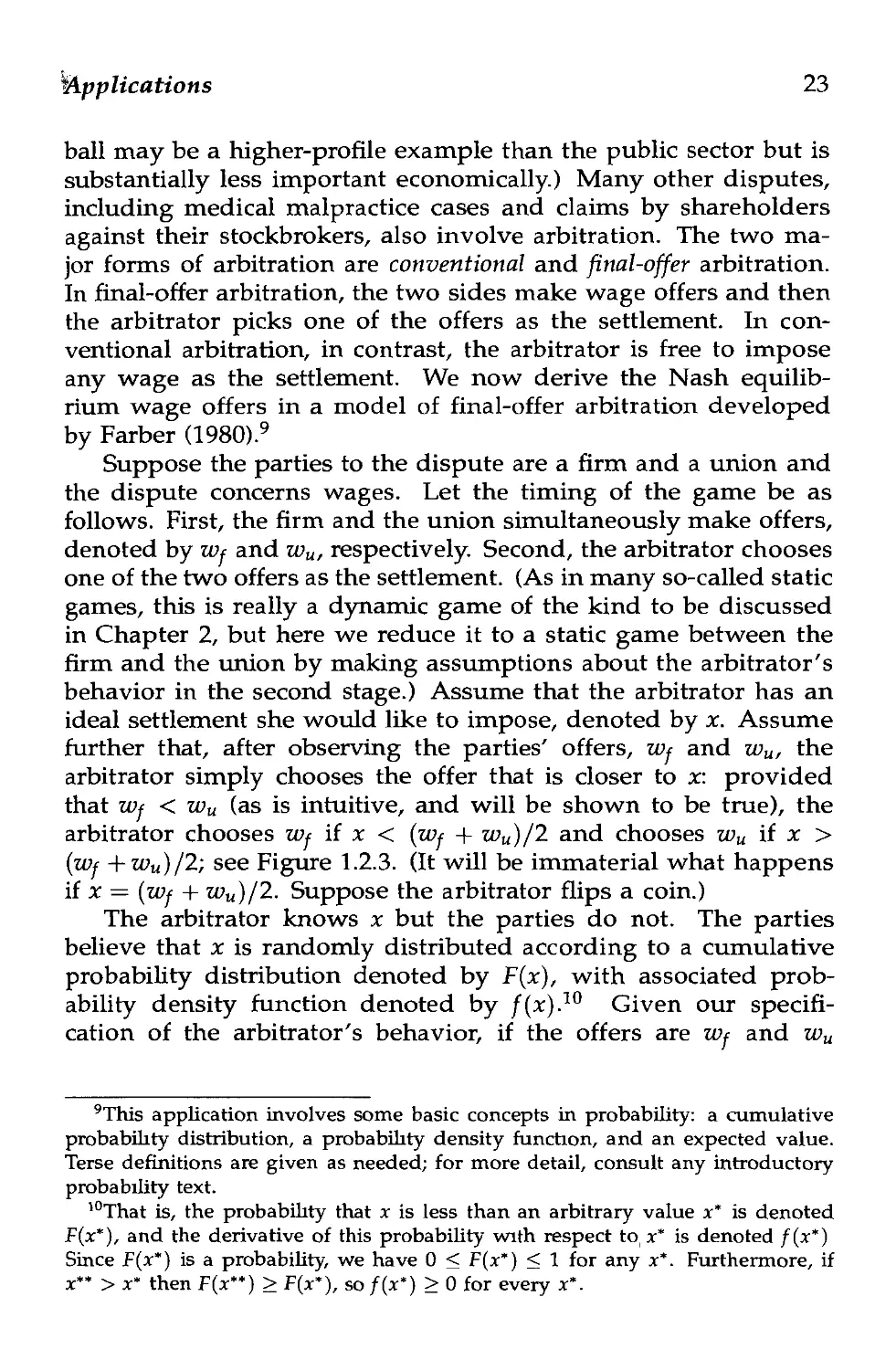
behavior in the second stage.) Assume that the arbitrator has an
ideal settlement she would like to impose, denoted by x. Assume
further that, after observing the parties' offers, Wf and wu, the
arbitrator simply chooses the offer that is closer to x: provided
that Wf < wu (as is intuitive, and will be shown to be true), the
arbitrator chooses Wf if x < (wf + wu)/2 and chooses wu if x >
(Wf + wu)/2; see Figure 1.2.3. (It will be immaterial what happens
if x — (wf + wu)/2. Suppose the arbitrator flips a coin.)
The arbitrator knows x but the parties do not. The parties
believe that x is randomly distributed according to a cumulative
probability distribution denoted by F(x), with associated prob-
probability density function denoted by /(x).10 Given our specifi-
specification of the arbitrator's behavior, if the offers are Wf and wu
9This application involves some basic concepts in probability: a cumulative
probability distribution, a probability density function, and an expected value.
Terse definitions are given as needed; for more detail, consult any introductory
probability text.
10That is, the probability that x is less than an arbitrary value x* is denoted
Fix*), and the derivative of this probability with respect to x* is denoted /(**)
Since F(x") is a probability, we have 0 < F(x") < 1 for any x*. Furthermore, if
x** > x* then F(x") > F{x*), so /(**) > 0 for every x*.

24
STATIC GAMES OF COMPLETE INFORMATION
wf chosen
w,, chosen
vo,,
(zuf+wu)/2
Figure 1.2.3.
then the parties believe that the probabilities Prob{zty chosen} and
Prob{u>u chosen} can be expressed as
chosen} = Prob [x <
= F
and
Prob{^« chosen} = 1 - F
M
Thus, the expected wage settlement is
¦ Prob{t^ chosen} + wu ¦ Prob{a;u chosen}
We assume that the firm wants to minimize the expected wage
settlement imposed by the arbitrator and the union wants to max-
maximize it.

Applications 25
If the pair of offers (wf,w*) is to be a Nash equilibrium of the
game between the firm and the union, if? must solve11
flUf + TV* \ [ fwf+ivt
min wf ¦ F [ -t + w* . \i _p I -JL
and w* must solve
max wj
Wu I
Thus, the wage-offer pair (wt,w*) must solve the first-order con-
conditions for these optimization problems,
and
(We defer considering whether these first-order conditions are suf-
sufficient.) Since the left-hand sides of these first-order conditions are
equal, the right-hand sides must also be equal, which implies that
that is, the average of the offers must equal the median of the
arbitrator's preferred settlement. Substituting A.2.2) into either of
the first-order conditions then yields
that is, the gap between the offers must equal the reciprocal of
the value of the density function at the median of the arbitrator's
preferred settlement.
"In formulating the firm's and the union's optimization problems, we have
assumed that the firm's offer is less than the union's offer. It is straightforward
to show that this inequality must hold in equilibrium.

26 STATIC GAMES OF COMPLETE INFORMATION
In order to produce an intuitively appealing comparative-static
result, we now consider an example. Suppose the arbitrator's pre-
preferred settlement is normally distributed with mean m and vari-
variance cr2, in which case the density function is
(In this example, one can show that the first-order conditions given
earlier are sufficient.) Because a normal distribution is symmetric
around its mean, the median of the distribution equals the mean
of the distribution, m. Therefore, A.2.2) becomes
= m
2
and A.2.3) becomes
*_ * = J_
Wu Wf f{m)
so the Nash equilibrium offers are
and Wf =m-d—.
Thus, in equilibrium, the parties' offers are centered around the
expectation of the arbitrator's preferred settlement (i.e., m), and
the gap between the offers increases with the parties' uncertainty
about the arbitrator's preferred settlement (i.e., cr2).
The intuition behind this equilibrium is simple. Each party
faces a trade-off. A more aggressive offer (i.e., a lower offer by
the firm or a higher offer by the union) yields a better payoff if
it is chosen as the settlement by the arbitrator but is less likely
to be chosen. (We will see in Chapter 3 that a similar trade-off
arises in a first-price, sealed-bid auction: a lower bid yields a
better payoff if it is the winning bid but reduces the chances of
winning.) When there is more uncertainty about the arbitrator's
preferred settlement (i.e., o2 is higher), the parties can afford to
be more aggressive because an aggressive offer is less likely to be
wildly at odds with the arbitrator's preferred settlement. When
there is hardly any uncertainty, in contrast, neither party can afford
to make an offer far from the mean because the arbitrator is very
likely to prefer settlements close to m.

Applications 17
1.2.D The Problem of the Commons
Since at least Hume A739), political philosophers and economists
have understood that if citizens respond only to private incentives,
public goods will be underprovided and public resources overuti-
lized. Today, even a casual inspection of the earth's environment
reveals the force of this idea. Hardin's A968) much cited paper
brought the problem to the attention of noneconomists. Here we
analyze a bucolic example.
Consider the n farmers in a village. Each summer, all the
farmers graze their goats on the village green. Denote the number
of goats the ith farmer owns by gi and the total number of goats
in the village by G = g\ + ¦ ¦ ¦ + gn. The cost of buying and caring
for a goat is c, independent of how many goats a farmer owns.
The value to a farmer of grazing a goat on the green when a
total of G goats are grazing is v(G) per goat. Since a goat needs
at least a certain amount of grass in order to survive, there is
a maximum number of goats that can be grazed on the green,
Gmax: v(G) > 0 for G < Gmax but v(G) = 0 for G > Gmax. Also,
since the first few goats have plenty of room to graze, adding one
more does little harm to those already grazing, but when so many
goats are grazing that they are all just barely surviving (i.e., G is
just below Gmax), then adding one more dramatically harms the
rest. Formally: for G < Gmax,u'(G) < 0 and v"{G) < 0, as in
Figure 1.2.4.
During the spring, the farmers simultaneously choose how
many goats to own. Assume goats are continuously divisible.
A strategy for farmer i is the choice of a number of goats to
graze on the village green, g,-. Assuming that the strategy space
is [0, oo) covers all the choices that could possibly be of interest
to the farmer; [0, Gmax) would also suffice. The payoff to farmer i
from grazing gi goats when the numbers of goats grazed by the
other farmers are (gi,..., g,_i, g,-+i,..., gn) is
gi v(gi + ¦¦¦+ gi-i + gt + gi+1l + ¦•¦+?„)- cgt. A.2.4)
Thus, if (gl,... ,gjj) is to be a Nash equilibrium then, for each i,
g* must maximize A.2.4) given that the other farmers choose
(gi > • • •»gt-1 > g*+i > • • • > gn) • The first-order condition for this opti-
optimization problem is
v(gi + g-i) + giv'igi + g-i) - c = 0, A.2.5)

28
STATIC GAMES OF COMPLETE INFORMATION
v
Figure 1.2.4.
where g*_{ denotes gj + ¦ • • + g?_t + g,*+1 + ¦ ¦ ¦ + g*. Substituting
g* into A.2.5), summing over all n farmers' first-order conditions,
and then dividing by n yields
-G*v'(G*)-c = O,
A.2.6)
where G* denotes gj + ¦ • • + g*. In contrast, the social optimum,
denoted by G**, solves
max Gv(G) - Gc,
the first-order condition for which is
A.2.7)
Comparing A.2.6) to A.2.7) shows12 that G* > G**: too many
goats are grazed in the Nash equilibrium, compared to the social
optimum. The first-order condition A.2.5) reflects the incentives
faced by a farmer who is already grazing g; goats but is consider-
12Suppose, to the contrary, that G* < G*\ Then v(G') > v(G"), since v' < 0.
Likewise, 0 > v'(G") > v'(Gr*), since v" < 0. Finally, G*/n < G". Thus, the
left-hand side of A.2.6) strictly exceeds the left-hand side of A.2.7), which is
impossible since both equal zero.

Advanced Theory 29
ing adding one more (or, strictly speaking, a tiny fraction of one
more). The value of the additional goat is v(g{ + g!_,) and its cost
is c. The harm to the farmer's existing goats is v>(gi+g*Li) per goat,
or giv'(gi +g*_t) in total. The common resource is overutilized be-
because each farmer considers only his or her own incentives, not
the effect of his or her actions on the other farmers, hence the
presence of G*v'(G*)/n in A.2.6) but G**v'(G**) in A.2.7).
1.3 Advanced Theory: Mixed Strategies and
Existence of Equilibrium
1.3.A Mixed Strategies
In Section 1.1.C we defined S, to be the set of strategies available
to player i, and the combination of strategies (s*,...,s*) to be a
Nash equilibrium if, for each player i, s* is player i's best response
to the strategies of the n — 1 other players:
w,(si,.. .,s*_-i,sj, s*+1,... ,s*) >ut(s*,... .s-L^s/.s*^,... ,s*) (NE)
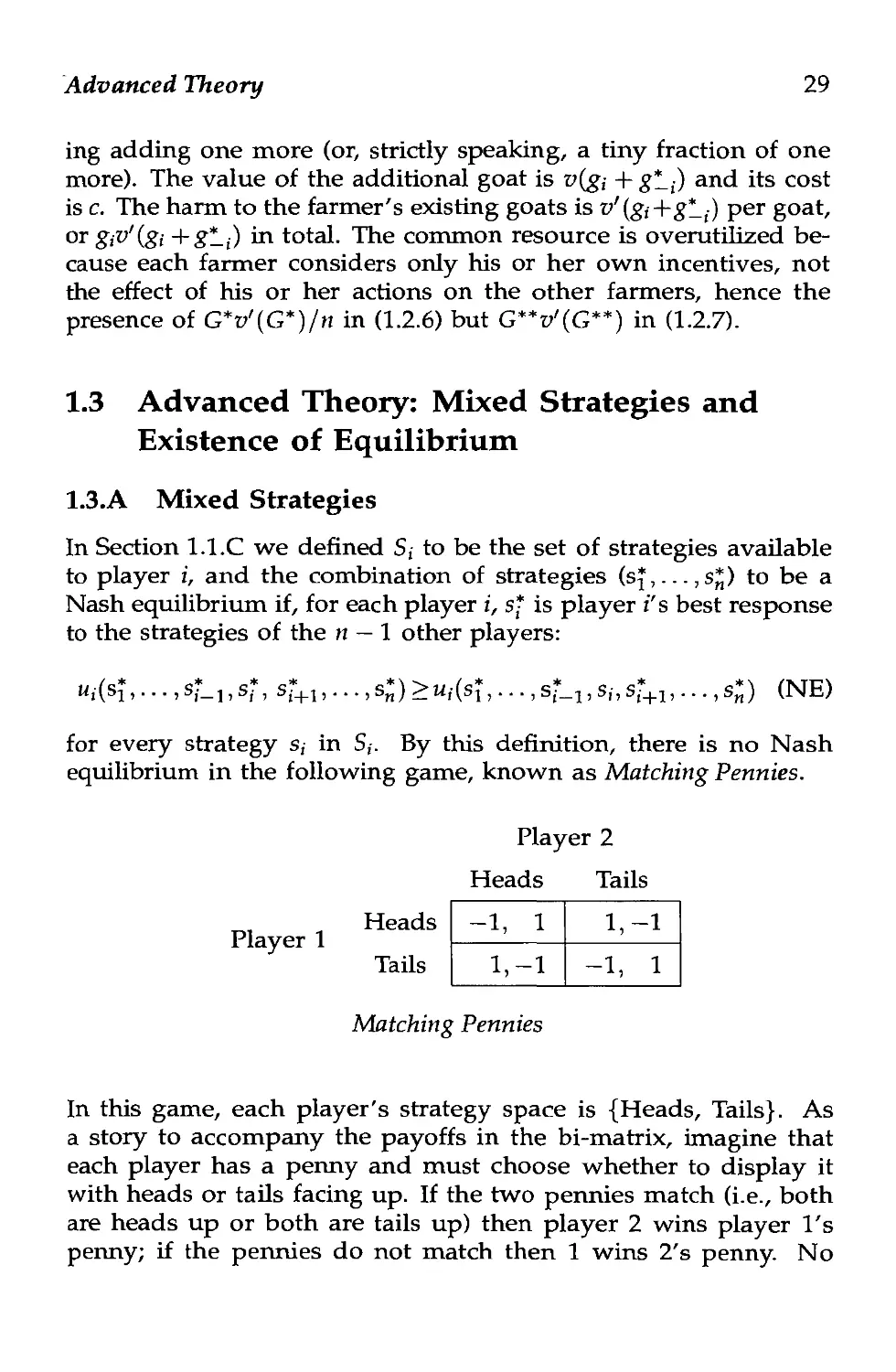
for every strategy s,- in S,-. By this definition, there is no Nash
equilibrium in the following game, known as Matching Pennies.
Player 2
Heads Tails
Heads
Player 1
Tails
Matching Pennies
In this game, each player's strategy space is {Heads, Tails}. As
a story to accompany the payoffs in the bi-matrix, imagine that
each player has a penny and must choose whether to display it
with heads or tails facing up. If the two pennies match (i.e., both
are heads up or both are tails up) then player 2 wins player I's
penny; if the pennies do not match then 1 wins 2's penny. No
-1, 1
1,-1
1,-1
-1, 1

30 STATIC GAMES OF COMPLETE INFORMATION
pair of strategies can satisfy (NE), since if the players' strategies
match—(Heads, Heads) or (Tails, Tails)—then player 1 prefers to
switch strategies, while if the strategies do not match—(Heads,
Tails) or (Tails, Heads)—then player 2 prefers to do so.
The distinguishing feature of Matching Pennies is that each
player would like to outguess the other. Versions of this game also
arise in poker, baseball, battle, and other settings. In poker, the
analogous question is how often to bluff: if player i is known never
to bluff then z's opponents will fold whenever i bids aggressively,
thereby making it worthwhile for i to bluff on occasion; on the
other hand, bluffing too often is also a losing strategy. In baseball,
suppose that a pitcher can throw either a fastball or a curve and
that a batter can hit either pitch if (but only if) it is anticipated
correctly. Similarly, in battle, suppose that the attackers can choose
between two locations (or two routes, such as "by land or by sea")
and that the defense can parry either attack if (but only if) it is
anticipated correctly.
In any game in which each player would like to outguess the
other(s), there is no Nash equilibrium (at least as this equilib-
equilibrium concept was defined in Section 1.1.C) because the solution
to such a game necessarily involves uncertainty about what the
players will do. We now introduce the notion of a mixed strategy,
which we will interpret in terms of one player's uncertainty about
what another player will do. (This interpretation was advanced
by Harsanyi [1973]; we discuss it further in Section 3.2.A.) In the
next section we will extend the definition of Nash equilibrium
to include mixed strategies, thereby capturing the uncertainty in-
inherent in the solution to games such as Matching Pennies, poker,
baseball, and battle.
Formally, a mixed strategy for player i is a probability distri-
distribution over (some or all of) the strategies in S,. We will hereafter
refer to the strategies in S,- as player f's pure strategies. In the
simultaneous-move games of complete information analyzed in
this chapter, a player's pure strategies are the different actions the
player could take. In Matching Pennies, for example, S, consists
of the two pure strategies Heads and Tails, so a mixed strategy
for player i is the probability distribution (q, 1 — q), where q is
the probability of playing Heads, 1 — q is the probability of play-
playing Tails, and 0 < q < 1. The mixed strategy @,1) is simply the
pure strategy Tails; likewise, the mixed strategy A,0) is the pure
strategy Heads.

Advanced Theory 31
As a second example of a mixed strategy, recall Figure 1.1.1,
where player 2 has the pure strategies Left, Middle, and Right.
Here a mixed strategy for player 2 is the probability distribution
(q, r, 1 — q — r), where q is the probability of playing Left, r is the
probability of playing Middle, and 1 — q — r is the probability of
playing Right. As before, 0 < q < 1, and now also 0 < r < 1 and
0 < q + r < 1. In this game, the mixed strategy A/3,1/3,1/3) puts
equal probability on Left, Middle, and Right, whereas A/2,1/2,0)
puts equal probability on Left and Middle but no probability on
Right. As always, a player's pure strategies are simply the lim-
limiting cases of the player's mixed strategies—here player 2's pure
strategy Left is the mixed strategy A,0,0), for example.
More generally, suppose that player i has K pure strategies:
Sj = {sn,... ,S{k}- Then a mixed strategy for player i is a prob-
probability distribution (pn,...,pae), where p,* is the probability that
player i will play strategy s,*, for k—l,...,K. Since p,* *s a proba-
probability, we require 0 < p# < 1 for k = 1,..., K and pn + - ¦ ¦ + puc = 1 •
We will use p,- to denote an arbitrary mixed strategy from the set
of probability distributions over S,, just as we use s, to denote an
arbitrary pure strategy from S,.
Definition In the normal-form game G = {Si,..., Sn;u-i,... ,un},sup-
,un},suppose S{ = {sji,... ,Sjk}. Then a mixed strategy for player Us a probability
distribution pi ~ (pn,..., p^), where 0 < p,* < 1 for k = 1,..., K and
We conclude this section by returning (briefly) to the notion of
strictly dominated strategies introduced in Section 1.1.B, so as to
illustrate the potential roles for mixed strategies in the arguments
made there. Recall that if a strategy s, is strictly dominated then
there is no belief that player i could hold (about the strategies
the other players will choose) such that it would be optimal to
play S{. The converse is also true, provided we allow for mixed
strategies: if there is no belief that player i could hold (about
the strategies the other players will choose) such that it would be
optimal to play the strategy s,-, then there exists another strategy
that strictly dominates s,.13 The games in Figures 1.3.1 and 1.3.2
13Pearce A984) proves this result for the two-player case and notes that it holds
for the M-player case provided that the players' mixed strategies are allowed to be
correlated—that is, player i's belief about what player j will do must be allowed
to be correlated with i's belief about what player k will do. Aumann A987)

32
STATIC GAMES OF COMPLETE INFORMATION
Player 1 M
B
Player 2
L R
3,—
0,—
1,—
0,—
3,—
1,—
Figure 1.3.1.
show that this converse would be false if we restricted attention
to pure strategies.
Figure 1.3.1 shows that a given pure strategy may be strictly
dominated by a mixed strategy, even if the pure strategy is not
strictly dominated by any other pure strategy. In this game, for
any belief (q, 1 — q) that player 1 could hold about 2's play, l's best
response is either T (if q > 1/2) or M (if q < 1/2), but never B.
Yet B is not strictly dominated by either T or M. The key is that
B is strictly dominated by a mixed strategy: if player 1 plays T
with probability 1/2 and M with probability 1/2 then l's expected
payoff is 3/2 no matter what (pure or mixed) strategy 2 plays, and
3/2 exceeds the payoff of 1 that playing B surely produces. This
example illustrates the role of mixed strategies in finding "another
strategy that strictly dominates s,."
Player 2
L R
Player 1 M
B
Figure 1.3.2.
3,—
0,—
2,—
0,—
3,—
2,—
suggests that such correlation in j's beliefs is entirely natural, even if / and fc
make their choices completely independently: for example, i may know that
both j and k went to business school, or perhaps to the same business school,
but may not know what is taught there.

Advanced Theory 33
Figure 1.3.2 shows that a given pure strategy can be a best
response to a mixed strategy, even if the pure strategy is not a
best response to any other pure strategy. In this game, B is not a
best response for player 1 to either L or R by player 2, but B is
the best response for player 1 to the mixed strategy (q, 1 — q) by
player 2, provided 1/3 < q < 2/3. This example illustrates the role
of mixed strategies in the "belief that player i could hold."
1.3.B Existence of Nash Equilibrium
In this section we discuss several topics related to the existence of
Nash equilibrium. First, we extend the definition of Nash equi-
equilibrium given in Section 1.1.C to allow for mixed strategies. Sec-
Second, we apply this extended definition to Matching Pennies and
the Battle of the Sexes. Third, we use a graphical argument to
show that any two-player game in which each player has two
pure strategies has a Nash equilibrium (possibly involving mixed
strategies). Finally, we state and discuss Nash's A950) Theorem,
which guarantees that any finite game (i.e., any game with a fi-
finite number of players, each of whom has a finite number of
pure strategies) has a Nash equilibrium (again, possibly involving
mixed strategies).
Recall that the definition of Nash equilibrium given in Section
l.l.C guarantees that each player's pure strategy is a best response
to the other players' pure strategies. To extend the definition to in-
include mixed strategies, we simply require that each player's mixed
strategy be a best response to the other players' mixed strategies.
Since any pure strategy can be represented as the mixed strategy
that puts zero probability on all of the player's other pure strate-
strategies, this extended definition subsumes the earlier one.
Computing player f's best response to a mixed strategy by
player ;' illustrates the interpretation of player ;'s mixed strategy
as representing player f's uncertainty about what player / will do.
We begin with Matching Pennies as an example. Suppose that
player 1 believes that player 2 will play Heads with probability q
and Tails with probability 1 — q; that is, 1 believes that 2 will play
the mixed strategy (q, l — cj). Given this belief, player l's expected
payoffs are q ¦ (—1) + A - q) ¦ 1 = 1 - 1q from playing Heads and
q¦ 1 + A -q) ¦ (-1) = 2q-l from playing Tails. Since 1 - 1q > 1q-1
if and only if q < 1/2, player l's best pure-strategy response is

34 STATIC GAMES OF COMPLETE INFORMATION
Heads if q < 1/2 and Tails if q > 1/2, and player 1 is indifferent
between Heads and Tails if q =¦ 1/2. It remains to consider possible
mixed-strategy responses by player 1.
Let (r, 1 — r) denote the mixed strategy in which player 1 plays
Heads with probability r. For each value of q between zero and
one, we now compute the value(s) of r, denoted r*(q), such that
(r, 1 - r) is a best response for player 1 to (q, 1 — q) by player 2.
The results are summarized in Figure 1.3.3. Player l's expected
payoff from playing (r, 1 — r) when 2 plays (q, 1 — q) is
rq ¦ (-1) + r{\ - q) • 1 + A - r)q ¦ 1 + A - r)(l - q) • (-1)
= Bq - 1) + rB - Aq), A.3.1)
where r<7 is the probability of (Heads, Heads), r(l — q) the probabil-
probability of (Heads, Tails), and so on.14 Since player l's expected payoff
is increasing in r if 2 — 4q > 0 and decreasing in r if 2 — 4q < 0,
player l's best response is r — 1 (i.e., Heads) if q < 1/2 and r — 0
(i.e., Tails) if ^ > 1/2, as indicated by the two horizontal segments
of r*(q) in Figure 1.3.3. This statement is stronger than the closely
related statement in the previous paragraph: there we considered
only pure strategies and found that if q < 1/2 then Heads is the
best pure strategy and that if q > 1/2 then Tails is the best pure
strategy; here we consider all pure and mixed strategies but again
find that if q < 1/2 then Heads is the best of all (pure or mixed)
strategies and that if q > 1/2 then Tails is the best of all strategies.
The nature of player l's best response to (q, 1 — q) changes
when q = 1/2. As noted earlier, when q = 1/2 player 1 is indif-
indifferent between the pure strategies Heads and Tails. Furthermore,
because player l's expected payoff in A.3.1) is independent of r
when q = 1/2, player 1 is also indifferent among all mixed strate-
strategies (r, 1 — r). That is, when q = 1/2 the mixed strategy (r, 1 — r)
14The events A and B are independent if Prob{A and B} = Prob{A}-Prob{B}.
Thus, in writing rq for the probability that 1 plays Heads and 2 plays Heads,
we are assuming that 1 and 2 make their choices independently, as befits the
description we gave of simultaneous-move games. See Aumann A974) for the
definition of correlated equilibrium, which applies to games in which the players'
choices can be correlated (because the players observe the outcome of a random
event, such as a coin flip, before choosing their strategies).

Advanced Theory
35
(Heads) 1
(Tails)
1/2 1 q
(Tails) (Heads)
Figure 1.3.3.
is a best response to (q, 1 — q) for any value of r between zero
and one. Thus, r*(l/2) is the entire interval [0,1], as indicated
by the vertical segment of r*(q) in Figure 1.3.3. In the analysis
of the Cournot model in Section 1.2.A, we called Ri(qj) firm i's
best-response function. Here, because there exists a value of q
such that r*{q) has more than one value, we call r*{q) player I's
best-response correspondence.
To derive player i's best response to player ;'s mixed strategy
more generally, and to give a formal statement of the extended def-
definition of Nash equilibrium, we now restrict attention to the two-
player case, which captures the main ideas as simply as possible.
Let / denote the number of pure strategies in Si and K the number
in S2. We will write Si = {sn,¦¦¦,sy} and S2 = {S21,• •.,S2k}, and
we will use sy and s^ to denote arbitrary pure strategies from Si
and S2, respectively.
If player 1 believes that player 2 will play the strategies (S21,...,
with the probabilities (^21, • • ¦, Vnd then player I's expected

36 STATIC GAMES OF COMPLETE INFORMATION
payoff from playing the pure strategy sy is
K
A.3.2)
and player l's expected payoff from playing the mixed strategy
Pi = (pn,---,Pi/) is
=i
7 K
prP/) 0-3-3)
/=1 Jt=l
where piy • P2* *s the probability that 1 plays Si; and 2 plays s^.
Player l's expected payoff from the mixed strategy p\, given in
A.3.3), is the weighted sum of the expected payoff for each of the
pure strategies {s\i,...,s\j}, given in A.3.2), where the weights
are the probabilities (pn,..., pij). Thus, for the mixed strategy
(pu,..., py) to be a best response for player 1 to 2's mixed strategy
pi, it must be that py > 0 only if
fc=l fc=l
for every syi in Si. That is, for a mixed strategy to be a best
response to pi it must put positive probability on a given pure
strategy only if the pure strategy is itself a best response to pi.
Conversely, if player 1 has several pure strategies that are best
responses to pi, then any mixed strategy that puts all its probabil-
probability on some or all of these pure-strategy best responses (and zero
probability on all other pure strategies) is also a best response for
player 1 to p>2-
To give a formal statement of the extended definition of Nash
equilibrium, we need to compute player 2's expected payoff when
players 1 and 2 play the mixed strategies p\ and pi respectively. If
player 2 believes that player 1 will play the strategies (sn,..., si/)
with the probabilities (pu,... ,py), then player 2's expected pay-

Advanced Theory 37
off from playing the strategies (s2i,..., S2k) with the probabilities
V2(Pi,
Given V\{p\,p2) and v2(p\,p2) we can restate the requirement of
Nash equilibrium that each player's mixed strategy be a best re-
response to the other player's mixed strategy: for the pair of mixed
strategies ip\,p2) to be a Nash equilibrium, p\ must satisfy
P2) A -3-4)
for every probability distribution p\ over Si, and p\ must satisfy
V2(pl,pl)>v2(p*1,p2) A-3.5)
for every probability distribution p2 over S2.
Definition In the two-player normal-form game G = {Si, S2;«i, u2},
the mixed strategies (p\, p\) are a Nash equilibrium if each player's mixed
strategy is a best response to the other player's mixed strategy: A.3.4) and
A.3.5) must hold.
We next apply this definition to Matching Pennies and the Bat-
Battle of the Sexes. To do so, we use the graphical representation of
player z's best response to player ;'s mixed strategy introduced in
Figure 1.3.3. To complement Figure 1.3.3, we now compute the
value(s) of a, denoted a*(r), such that (q, 1 — q) is a best response
for player 2 to (r, 1 — r) by player 1. The results are summarized in
Figure 1.3.4. If r < 1/2 then 2's best response is Tails, so q*(r) = 0;
likewise, if r > 1/2 then 2's best response is Heads, so q*(r) = 1.
If r = 1/2 then player 2 is indifferent not only between Heads and
Tails but also among all the mixed strategies (q, 1 — a), so <j*(l/2)
is the entire interval [0,1].
After flipping and rotating Figure 1.3.4, we have Figure 1.3.5.
Figure 1.3.5 is less convenient than Figure 1.3.4 as a representation

38
STATIC GAMES OF COMPLETE INFORMATION
(Heads) 1
(Tails)
1/2 1 r
(Tails) (Heads)
Figure 1.3.4.
(Heads) 1
(Tails)
1/2
(Tails)
(Heads)
Figure 1.3.5.

Advanced Theory
39
(Heads)
1/2
(Tails)
r*(q)
q*(r)
1/2
(Tails)
1 q
(Heads)
Figure 1.3.6.
of player 2's best response to player l's mixed strategy, but it can
be combined with Figure 1.3.3 to produce Figure 1.3.6.
Figure 1.3.6 is analogous to Figure 1.2.1 from the Cournot anal-
analysis in Section I.2.A. Just as the intersection of the best-response
functions R-2(c]i) and Ri(qi) gave the Nash equilibrium of the
Cournot game, the intersection of the best-response correspon-
correspondences r*(q) and q*(r) yields the (mixed-strategy) Nash equilib-
equilibrium in Matching Pennies: if player i plays A/2,1/2) then
A/2,1/2) is a best response for player ;', as required for Nash
equilibrium.
It is worth emphasizing that such a mixed-strategy Nash equi-
equilibrium does not rely on any player flipping coins, rolling dice,
or otherwise choosing a strategy at random. Rather, we interpret
player /'s mixed strategy as a statement of player z's uncertainty
about player j's choice of a (pure) strategy. In baseball, for ex-
example, the pitcher might decide whether to throw a fastball or a
curve based on how well each pitch was thrown during pregame
practice. If the batter understands how the pitcher will make a
choice but did not observe the pitcher's practice, then the batter
may believe that the pitcher is equally likely to throw a fastball or a
curve. We would then represent the batter's belief by the pitcher's

40 STATIC GAMES OF COMPLETE INFORMATION
mixed strategy A/2,1/2), when in fact the pitcher chooses a pure
strategy based on information unavailable to the batter. Stated
more generally, the idea is to endow player j -with a small amount
of private information such that, depending on the realization of
the private information, player j slightly prefers one of the rele-
relevant pure strategies. Since player i does not observe j's private
information, however, i remains uncertain about j's choice, and
we represent z's uncertainty by j's mixed strategy. We provide a
more formal statement of this interpretation of a mixed strategy
in Section 3.2.A.
As a second example of a mixed-strategy Nash equilibrium,
consider the Battle of the Sexes from Section 1.1.C. Let (q, 1 — q) be
the mixed strategy in which Pat plays Opera with probability q,
and let (r, 1 — r) be the mixed strategy in which Chris plays Opera
with probability r. If Pat plays (q, 1 - q) then Chris's expected
payoffs are q -2 + A — q) ¦ 0 — 2q from playing Opera and q ¦ 0 +
A — q) ¦ 1 — \~q from playing Fight. Thus, if q > 1/3 then Chris's
best response is Opera (i.e., r = 1), if q < 1/3 then Chris's best
response is Fight (i.e., r = 0), and if q = 1/3 then any value of
r is a best response. Similarly, if Chris plays (r, 1 — r) then Pat's
expected payoffs are r ¦ 1 + A — r)-0 = r from playing Opera and
r - 0 + A - r) ¦ 2 = 2A - r) from playing Fight. Thus, if r > 2/3 then
Pat's best response is Opera (i.e., q = 1), if r < 2/3 then Pat's best
response is Fight (i.e., q = 0), and if r = 2/3 then any value of q
is a best response. As shown in Figure 1.3.7, the mixed strategies
(q,l - q) = A/3,2/3) for Pat and (r,l - r) = B/3,1/3) for Chris
are therefore a Nash equilibrium.
Unlike in Figure 1.3.6, where there was only one intersection
of the players' best-response correspondences, there are three in-
intersections of r*(q) and q*{r) in Figure 1.3.7: (q = 0,r = 0) and
(q = l,r = 1), as well as (q = 1/3,r = 2/3). The other two inter-
intersections represent the pure-strategy Nash equilibria (Fight, Fight)
and (Opera, Opera) described in Section l.l.C.
In any game, a Nash equilibrium (involving pure or mixed
strategies) appears as an intersection of the players' best-response
correspondences, even when there are more than two players, and
even when some or all of the players have more than two pure
strategies. Unfortunately, the only games in which the players'
best-response correspondences have simple graphical representa-
representations are two-player games in which each player has only two

Advanced Theory
41
(Opera) 1
2/3
(Fight)
r*{q)
q*(r)
1/3
(Fight)
(Opera)
Figure 1.3.7.
Player 2
Left Right
Player 1
Up
Down
Figure 1.3.8.
x,—
strategies. We turn next to a graphical argument that any such
game has a Nash equilibrium (possibly involving mixed strate-
strategies).
Consider the payoffs for player 1 given in Figure 1.3.8. There
are two important comparisons: x versus z, and y versus w. Based
on these comparisons, we can define four main cases: (i) x > z and
y > w, (ii) x < z and y < w, (iii) x > z and y < w, and (iv) x < z
and y > w. We first discuss these four main cases, and then turn
to the remaining cases involving x = z or y = w.

42
STATIC GAMES OF COMPLETE INFORMATION
(Down)
(Up) 1
(Left)
1 q
(Right)
(Down)
(Left)
Case (i)
Case (ii)
Figure 1.3.9.
In case (i) Up strictly dominates Down for player 1, and in
case (ii) Down strictly dominates Up. Recall from the previous
section that a strategy s, is strictly dominated if and only if there
is no belief that player i could hold (about the strategies the other
players will choose) such that it would be optimal to play s,. Thus,
if {q, 1 — q) is a mixed strategy for player 2, where q is the prob-
probability that 2 will play Left, then in case (i) there is no value of
q such that Down is optimal for player 1, and in case (ii) there is
no value of a such that Up is optimal. Letting (r, 1 — r) denote
a mixed strategy for player 1, where r is the probability that 1
will play Up, we can represent the best-response correspondences
for cases (i) and (ii) as in Figure 1.3.9. (In these two cases the
best-response correspondences are in fact best-response functions,
since there is no value of q such that player 1 has multiple best
responses.)
In cases (iii) and (iv), neither Up nor Down is strictly domi-
dominated. Thus, Up must be optimal for some values of q and Down
optimal for others. Let q' = (w — y)/(x — z + w — y). Then in
case (iii) Up is optimal for q > q' and Down for q < q', whereas in
case (iv) the reverse is true. In both cases, any value of r is optimal
when q = q'. These best-response correspondences are given in
Figure 1.3.10.

Advanced Theory
43
(Up)
(Down)
(Down)'
(Left)
Case (Hi)
1
(Left) (Right)
Case (iv)
Figure 1.3.10.
Since q' = 1 if x — z and q' = 0 if y = w, the best-response
correspondences for cases involving either x = z or y = w are L-
shaped (i.e., two adjacent sides of the unit square), as would occur
in Figure 1.3.10 if q' = 0 or 1 in cases (iii) or (iv).
Adding arbitrary payoffs for player 2 to Figure 1.3.8 and per-
performing the analogous computations yields the same four best-
response correspondences, except that the horizontal axis mea-
measures r and the vertical q, as in Figure 1.3.4. Flipping and rotating
these four figures, as was done to produce Figure 1.3.5, yields
Figures 1.3.11 and 1.3.12. (In the latter figures, r1 is defined anal-
analogously to q' in Figure 1.3.10.)
The crucial point is that given any of the four best-response cor-
correspondences for player 1, r*(q) from Figures 1.3.9 or 1.3.10, and
any of the four for player 2, q*(r) from Figures 1.3.11 or 1.3.12, the
pair of best-response correspondences has at least one intersec-
intersection, so the game has at least one Nash equilibrium. Checking all
sixteen possible pairs of best-response correspondences is left as
an exercise. Instead, we describe the qualitative features that can
result. There can be: A) a single pure-strategy Nash equilibrium;
B) a single mixed-strategy equilibrium; or C) two pure-strategy
equilibria and a single mixed-strategy equilibrium. Recall from
Figure 1.3.6 that Matching Pennies is an example of case B), and
from Figure 1.3.7 that the Battle of the Sexes is an example of

44
STATIC GAMES OF COMPLETE INFORMATION
(Up) 1
(Down)
(Left) (Right)
Case (i)
(Up) 1
(Down)
(Left) (Right)
Case (ii)
Figure 1.3.11.
(Down)
(Up) 1
(Down)
(Left)
(Left)
(Right)
Case (in)
Case (iv)
Figure 1.3.12.

Advanced Theory
45
Figure 1.3.13.
case C). The Prisoners' Dilemma is an example of case A); it re-
results from combining case (i) or (ii) of r*(q) with case (i) or (ii)
or q*(r).15
We conclude this section with a discussion of the existence
of a Nash equilibrium in more general games. If the above ar-
arguments for two-by-two games are stated mathematically rather
than graphically, then they can be generalized to apply to n-player
games with arbitrary finite strategy spaces.
Theorem (Nash 1950): In the n-player normal-form game G =
{Si,..., Sn; u\,..., «„}, if n is finite and S; is finite for every i then there
exists at least one Nash equilibrium, possibly involving mixed strategies.
The proof of Nash's Theorem involves a fixed-point theorem.
As a simple example of a fixed-point theorem, suppose f(x) is
a continuous function with domain [0,1] and range [0,1]. Then
Brouwer's Fixed-Point Theorem guarantees that there exists at
least one fixed point — that is, there exists at least one value x*
in [0,1] such that f(x*) — x*. Figure 1.3.13 provides an example.
15The cases involving x = z or y = w do not violate the claim that the pair of
best-response correspondences has at least one intersection. On the contrary, in
addition to the qualitative features described in the text, there can now be two
pure-strategy Nash equilibria without a mixed-strategy Nash equilibrium, and a
continuum of mixed-strategy Nash equilibria.

46 STATIC GAMES OF COMPLETE INFORMATION
Applying a fixed-point theorem to prove Nash's Theorem in-
involves two steps: A) showing that any fixed point of a certain
correspondence is a Nash equilibrium; B) using an appropriate
fixed-point theorem to show that this correspondence must have
a fixed point. The relevant correspondence is the n-player best-
response correspondence. The relevant fixed-point theorem is due
to Kakutani A941), who generalized Brouwer's theorem to allow
for (well-behaved) correspondences as well as functions.
The n-player best-response correspondence is computed from
the n individual players' best-response correspondences as fol-
follows. Consider an arbitrary combination of mixed strategies
(pi,...,pn). For each player i, derive f's best response(s) to the
other players' mixed strategies (pi,..., p,_i, p,+i,..., pn)- Then con-
construct the set of all possible combinations of one such best response
for each player. (Formally, derive each player's best-response
correspondence and then construct the cross-product of these n
individual correspondences.) A combination of mixed strategies
(pi,...,p*) is a fixed point of this correspondence if (pj,...,p*)
belongs to the set of all possible combinations of the players' best
responses to (pj,... , p*). That is, for each i, p* must be (one of)
player i's best response(s) to (pi, ..., p*{_x, p*+1, ..., p?), but this
is precisely the statement that (p*, ..., p*) is a Nash equilibrium.
This completes step A).
Step B) involves the fact that each player's best-response cor-
correspondence is continuous, in an appropriate sense. The role of
continuity in Brouwer's fixed-point theorem can be seen by mod-
modifying f{x) in Figure 1.3.13: if f(x) is discontinuous then it need
not have a fixed point. In Figure 1.3.14, for example, f(x) > x for
all x < x1, but /(*') < x' for x > x'.16
To illustrate the differences between/(x) in Figure 1.3.14 and a
player's best-response correspondence, consider Case (iii) in Fig-
Figure 1.3.10: at q = q', r*(q') includes zero, one, and the entire
interval in between. (A bit more formally, r*(q') includes the limit
of r*(q) as q approaches q' from the left, the limit of r*(q) as q
approaches q' from the right, and all the values of r in between
these two limits.) If f(x') in Figure 1.3.14 behaved analogously to
16The value of f{x') is indicated by the solid circle. The open circle indicates
that f(x') does not include this value The dotted line is included only to indicate
that both circles occur at x = x'; it does not indicate further values oif{x').

'Advanced Theory
47
x
Figure 1.3.14.
player l's best-response correspondence r*(q'), then f(x') would
include not only the solid circle (as in the figure) but also the
open circle and the entire interval in between, in which case f(x)
would have a fixed point at x'.
Each player's best-response correspondence always behaves
the way r*(q') does in Figure 1.3.14: it always includes (the appro-
appropriate generalizations of) the limit from the left, the limit from the
right, and all the values in between. The reason for this is that,
as shown earlier for the two-player case, if player i has several
pure strategies that are best responses to the other players' mixed
strategies, then any mixed strategy p, that puts all its probability
on some or all of player z's pure-strategy best responses (and zero
probability on all of player i's other pure strategies) is also a best
response for player i. Because each player's best-response corre-
correspondence always behaves in this way, the n-player best-response
correspondence does too; these properties satisfy the hypotheses
of Kakutani's Theorem, so the latter correspondence has a fixed
point.
Nash's Theorem guarantees that an equilibrium exists in a
broad class of games, but none of the applications analyzed in
Section 1.2 are members of this class (because each application
has infinite strategy spaces). This shows that the hypotheses of
Nash's Theorem are sufficient but not necessary conditions for an

48
STATIC GAMES OF COMPLETE INFORMATION
equilibrium to exist—there are many games that do not satisfy
the hypotheses of the Theorem but nonetheless have one or more
Nash equilibria.
1.4 Further Reading
On the assumptions underlying iterated elimination of strictly
dominated strategies and Nash equilibrium, and on the inter-
interpretation of mixed strategies in terms of the players' beliefs, see
Brandenburger A992). On the relation between (Cournot-type)
models where firms choose quantities and (Bertrand-type) mod-
models where firms choose prices, see Kreps and Scheinkman A983),
who show that in some circumstances the Cournot outcome occurs
in a Bertrand-type model in which firms face capacity constraints
(which they choose, at a cost, prior to choosing prices). On arbitra-
arbitration, see Gibbons A988), who shows how the arbitrator's preferred
settlement can depend on the information content of the parties'
offers, in both final-offer and conventional arbitration. Finally, on
the existence of Nash equilibrium, including pure-strategy equi-
equilibria in games with continuous strategy spaces, see Dasgupta and
Maskin A986).
1.5 Problems
Section 1.1
1.1. What is a game in normal form? What is a strictly dominated
strategy in a normal-form game? What is a pure-strategy Nash
equilibrium in a normal-form game?
1.2. In the following normal-form game, what strategies survive
iterated elimination of strictly dominated strategies? What are the
pure-strategy Nash equilibria?
M
R
2,0
3,4
1,3
1,1
1,2
0,2
4,2
2,3
3,0

Problems 49
1.3. Players 1 and 2 are bargaining over how to split one dollar.
Both players simultaneously name shares they would like to have,
Si and S2, where 0 < si,s2 < 1. If Si + S2 < 1, then the players
receive the shares they named; if Si + s2 > 1, then both players
receive zero. What are the pure-strategy Nash equilibria of this
game?
Section 1.2
1.4. Suppose there are n firms in the Cournot oligopoly model.
Let q j denote the quantity produced by firm i, and let Q = c\\ 4- • +
qn denote the aggregate quantity on the market. Let P denote the
market-clearing price and assume that inverse demand is given
by P{Q) = a — Q (assuming Q < a, else P = 0). Assume that the
total cost of firm / from producing quantity q\ is C,(^,) = cqx. That
is, there are no fixed costs and the marginal cost is constant at c,
where we assume c < a. Following Cournot, suppose that the
firms choose their quantities simultaneously. What is the Nash
equilibrium? What happens as n approaches infinity?
1.5. Consider the following two finite versions of the Cournot
duopoly model. First, suppose each firm must choose either half
the monopoly quantity, qm/2 = (a - c)/4, or the Cournot equilib-
equilibrium quantity, qc = (a — c)/3. No other quantities are feasible.
Show that this two-action game is equivalent to the Prisoners'
Dilemma: each firm has a strictly dominated strategy, and both
are worse off in equilibrium than they would be if they cooper-
cooperated. Second, suppose each firm can choose either qm/2, or qc,
or a third quantity, q''. Find a value for q' such that the game is
equivalent to the Cournot model in Section 1.2.A, in the sense that
(qc,qc) is a unique Nash equilibrium and both firms are worse off
in equilibrium than they could be if they cooperated, but neither
firm has a strictly dominated strategy.
1.6. Consider the Cournot duopoly model where inverse demand
is P(Q) = a - Q but firms have asymmetric marginal costs: c\
for firm 1 and cj for firm 2. What is the Nash equilibrium if
0 < c, < a/2 for each firm? What if Cj < c2 < a but 2c2 > a + c\?
1.7. In Section 1.2.B, we analyzed the Bertrand duopoly model
with differentiated products. The case of homogeneous products

50 STATIC GAMES OF COMPLETE INFORMATION
yields a stark conclusion. Suppose that the quantity that con-
consumers demand from firm i is a — p,- when p,- < p., 0 when p,- > pj,
and (a - p,)/2 when p, = pj. Suppose also that there are no fixed
costs and that marginal costs are constant at c, where c < a. Show
that if the firms choose prices simultaneously, then the unique
Nash equilibrium is that both firms charge the price c.
1.8. Consider a population of voters uniformly distributed along
the ideological spectrum from left (x = 0) to right (x = 1). Each of
the candidates for a single office simultaneously chooses a cam-
campaign platform (i.e., a point on the line between x = 0 and x = 1)
The voters observe the candidates' choices, and then each voter
votes for the candidate whose platform is closest to the voter's
position on the spectrum. If there are two candidates and they
choose platforms X\ = .3 and x2 = .6, for example, then all
voters to the left of x — 45 vote for candidate 1, all those to
the right vote for candidate 2, and candidate 2 wins the elec-
election with 55 percent of the vote. Suppose that the candidates
care only about being elected—they do not really care about their
platforms at all! If there are two candidates, what is the pure-
strategy Nash equilibrium? If there are three candidates, exhibit
a pure-strategy Nash equilibrium. (Assume that any candidates
who choose the same platform equally split the votes cast for that
platform, and that ties among the leading vote-getters are resolved
by coin flips.) See Hotelling A929) for an early model along these
lines.
Section 1.3
1.9. What is a mixed strategy in a normal-form game? What is a
mixed-strategy Nash equilibrium in a normal-form game?
1.10. Show that there are no mixed-strategy Nash equilibria in
the three normal-form games analyzed in Section 1.1—the Prison-
Prisoners' Dilemma, Figure 1.1.1, and Figure 1.1.4.
1 11. Solve for the mixed-strategy Nash equilibria in the game in
Problem 1.2.

References
51
1.12. Find the mixed-strategy Nash equilibrium of the following
normal-form game.
T
R
2,1
1,2
0,2
3,0
1.13. Each of two firms has one job opening. Suppose that (for
reasons not discussed here but relating to the value of filling each
opening) the firms offer different wages: firm i offers the wage Wj,
where {\/2)w\ < w2 < 2w\. Imagine that there are two workers,
each of whom can apply to only one firm. The workers simulta-
simultaneously decide whether to apply to firm 1 or to firm 2. If only one
worker applies to a given firm, that worker gets the job; if both
workers apply to one firm, the firm hires one worker at random
and the other worker is unemployed (which has a payoff of zero).
Solve for the Nash equilibria of the workers' normal-form game.
(For more on the wages the firms will choose, see Montgomery
[1991].)
Worker 2
Apply to Apply to
Firm 1 Firm 2
Worker 1
Apply to Firm 1
Apply to Firm 2
102,117,
\w2, \w2
1.14. Show that Proposition B in Appendix l.l.C holds for mixed-
as well as pure-strategy Nash equilibria: the strategies played with
positive probability in a mixed-strategy Nash equilibrium survive
the process of iterated elimination of strictly dominated strategies.
1.6 References
Aumann, R. 1974. "Subjectivity and Correlation in Randomized
Strategies." journal of Mathematical Economics 1:67-96.

52 STATIC GAMES OF COMPLETE INFORMATION
1976. "Agreeing to Disagree." Annals of Statistics
4:1236-39.
1987. "Correlated Equilibrium as an Expression of
Bayesian Rationality." Econometrica 55:1-18.
Bertrand, J. 1883. "Theorie Mathematique de la Richesse So-
ciale." Journal des Savants 499-508.
Brandenburger, A. 1992. "Knowledge and Equilibrium in
Games." Forthcoming in Journal of Economic Perspectives.
Cournot, A. 1838. Rech.erch.es sur les Principes Mathematiques de
la Theorie des Richesses. English edition: Researches into the Mathe-
Mathematical Principles of the Theory of Wealth. Edited by N. Bacon. New
York: Macmillan, 1897.
Dasgupta, P., and E. Maskin. 1986. "The Existence of Equi-
Equilibrium in Discontinuous Economic Games, I: Theory." Review of
Economic Studies 53:1-26.
Farber, H. 1980. "An Analysis of Final-Offer Arbitration." Jour-
Journal of Conflict Resolution 35:683-705.
Friedman, J. 1971. "A Noncooperative Equilibrium for Su-
pergames." Review of Economic Studies 28:1-12.
Gibbons, R. 1988. "Learning in Equilibrium Models of Arbi-
Arbitration." American Economic Review 78:896-912.
Hardin, G. 1968. "The Tragedy of the Commons." Science
162:1243-48.
Harsanyi, J. 1973. "Games with Randomly Disturbed Payoffs:
A New Rationale for Mixed Strategy Equilibrium Points." Inter-
International Journal of Game Theory 2:1-23.
Hotelling, H. 1929. "Stability in Competition." Economic Jour-
Journal 39:41-57.
Hume, D. 1739. A Treatise of Human Nature. Reprint. London:
J. M. Dent. 1952.
Kakutani, S. 1941. "A Generalization of Brouwer's Fixed Point
Theorem." Duke Mathematical Journal 8:457-59.
Kreps, D., and J. Scheinkman. 1983. "Quantity Precommitment
and Bertrand Competition Yield Cournot Outcomes." Bell Journal
of Economics 14:326-37.
Montgomery, J. 1991. "Equilibrium Wage Dispersion and In-
Interindustry Wage Differentials." Quarterly Journal of Economics 106:
163-79.
Nash, J. 1950. "Equilibrium Points in n-Person Games." Pro-
Proceedings of the National Academy of Sciences 36:48—49.

References 53
Pearce, D. 1984. "Rationalizable Strategic Behavior and the
Problem of Perfection." Econometrica 52:1029-50.
Stackelberg, H. von. 1934. Marktform und Gleichgewicht. Vi-
Vienna: Julius Springer.

Chapter 2
Dynamic Games of
Complete Information
In this chapter we introduce dynamic games. We again restrict at-
attention to games with complete information (i.e., games in which
the players' payoff functions are common knowledge); see Chap-
Chapter 3 for the introduction to games of incomplete information^ In
Section 2.1 we analyze dynamic games that have not only com-
complete but also perfect information, by which we mean that at each
move in the game the player with the move knows the full history
of the play of the game thus far. In Sections 2.2 through 2.4 we
consider games of complete but imperfect information: at some
move the player with the move does not know the history of the
game.
The central issue in all dynamic games is credibility. As an
example of a noncredible threat, consider the following two-move
game. First, player 1 chooses between giving player 2 $1,000 and
giving player 2 nothing. Second, player 2 observes player l's
move and then chooses whether or not to explode a grenade that
will kill both players. Suppose player 2 threatens to explode the
grenade unless player 1 pays the $1,000. If player 1 believes the
threat, then player l's best response is to pay the $1,000. But
player 1 should not believe the threat, because it is noncredible:
if player 2 were given the opportunity to carry out the threat,

56 DYNAMIC GAMES OF COMPLETE INFORMATION
player 2 would choose not to carry it out. Thus, player 1 should
pay player 2 nothing.1
In Section 2.1 we analyze the following class of dynamic games
of complete and perfect information: first player 1 moves, then
player 2 observes player l's move, then player 2 moves and the
game ends. The grenade game belongs to this class, as do Stack-
elberg's A934) model of duopoly and LeontiePs A946) model of
wage and employment determination in a unionized firm. We
define the backwards-induction outcome of such games and briefly
discuss its relation to Nash equilibrium (deferring the main discus-
discussion of this relation until Section 2.4). We solve for this outcome
in the Stackelberg and Leontief models. We also derive the analo-
analogous outcome in Rubinstein's A982) bargaining model, although
this game has a potentially infinite sequence of moves and so does
not belong to the above class of games.
In Section 2.2 we enrich the class of games analyzed in the
previous section: first players 1 and 2 move simultaneously, then
players 3 and 4 observe the moves chosen by 1 and 2, then play-
players 3 and 4 move simultaneously and the game ends. As will be
explained in Section 2.4, the simultaneity of moves here means that
these games have imperfect information. We define the subgame-
perfect outcome of such games, which is the natural extension of
backwards induction to these games. We solve for this outcome
in Diamond and Dybvig's A983) model of bank runs, in a model
of tariffs and imperfect international competition, and in Lazear
and Rosen's A981) model of tournaments.
In Section 2.3 we study repeated games, in which a fixed group
of players plays a given game repeatedly, with the outcomes of all
previous plays observed before the next play begins. The theme
of the analysis is that (credible) threats and promises about future
behavior can influence current behavior. We define subgame-perfect
Nash equilibrium for repeated games and relate it to the backwards-
induction and subgame-perfect outcomes defined in Sections 2.1
and 2.2. We state and prove the Folk Theorem for infinitely re-
1 Player 1 might wonder whether an opponent who threatens to explode a
grenade is crazy. We model such doubts as incomplete information—player 1 is
unsure about player 2's payoff function See Chapter 3

Dynamic Games of Complete and Perfect Information 57
peated games, and we analyze Friedman's A971) model of col-
collusion between Cournot duopolists, Shapiro and Stiglitz's A984)
model of efficiency wages, and Barro and Gordon's A983) model
of monetary policy.
In Section 2.4 we introduce the tools necessary to analyze a
general dynamic game of complete information, whether with per-
perfect or imperfect information. We define the extensive-form repre-
representation of a game and relate it to the normal-form representation
introduced in Chapter 1. We also define subgame-perfect Nash
equilibrium for general games. The main point (of both this sec-
section and the chapter as a whole) is that a dynamic game of com-
complete information may have many Nash equilibria, but some of
these may involve noncredible threats or promises. The subgame-
perfect Nash equilibria are those that pass a credibility test.
2.1 Dynamic Games of Complete and Perfect
Information
2.1.A Theory: Backwards Induction
The grenade game is a member of the following class of simple
games of complete and perfect information:
1. Player 1 chooses an action a\ from the feasible set A\.
2. Player 2 observes d\ and then chooses an action a2 from the
feasible set A2.
3. Payoffs are Ui(«i,a2) and u2(ai,a2).
Many economic problems fit this description.2 Two examples
2Player 2's feasible set of actions, A2, could be allowed to depend on player l's
action, a.\. Such dependence could be denoted by ^(flj) or could be incorporated
into player 2's payoff function, by setting u2(ai,a2) — —00 for values of a2 that
are not feasible for a given a\. Some moves by player 1 could even end the game,
without player 2 getting a move; for such values of d\, the set of feasible actions
Ai(fl\) contains only one element, so player 2 has no choice to make.

58 DYNAMIC GAMES OF COMPLETE INFORMATION
(discussed later in detail) are Stackelberg's model of duopoly and
Leontief's model of wages and employment in a unionized firm.
Other economic problems can be modeled by allowing for a longer
sequence of actions, either by adding more players or by allowing
players to move more than once. (Rubinstein's bargaining game,
discussed in Section 2.1.D, is an example of the latter.) The key
features of a dynamic game of complete and perfect information
are that (i) the moves occur in sequence, (ii) all previous moves
are observed before the next move is chosen, and (iii) the play-
players' payoffs from each feasible combination of moves are common
knowledge.
We solve a game from this class by backwards induction, as
follows. When player 2 gets the move at the second stage of the
game, he or she will face the following problem, given the action
fli previously chosen by player 1:
max u2(a1,a2).
Assume that for each a\ in A\, player 2's optimization problem has
a unique solution, denoted by R2(ai). This is player 2's reaction
(or best response) to player l's action. Since player 1 can solve 2's
problem as well as 2 can, player 1 should anticipate player 2's
reaction to each action a\ that 1 might take, so l's problem at the
first stage amounts to
max «!(«!, R2(«i))-
flGA
Assume that this optimization problem for player 1 also has a
unique solution, denoted by a\. We will call \a\,R2(a%)') the back-
wards-induction outcome of this game. The backwards-induction
outcome does not involve noncredible threats: player 1 anticipates
that player 2 will respond optimally to any action a\ that 1 might
choose, by playing R2{a.\); player 1 gives no credence to threats
by player 2 to respond in ways that will not be in 2's self-interest
when the second stage arrives.
Recall that in Chapter 1 we used the normal-form represen-
representation to study static games of complete information, and we fo-
focused on the notion of Nash equilibrium as a solution concept
for such games. In this section's discussion of dynamic games,
however, we have made no mention of either the normal-form
representation or Nash equilibrium. Instead, we have given a

Dynamic Games of Complete and Perfect Information 59
verbal description of a game in (l)-C), and we have defined the
backwards-induction outcome as the solution to that game. In
Section 2.4.A we will see that the verbal description in (l)-C)
is the extensive-form representation of the game. We will relate
the extensive- and normal-form representations, but we will find
that for dynamic games the extensive-form representation is of-
often more convenient. In Section 2.4.B we will define subgame-
perfect Nash equilibrium: a Nash equilibrium is subgame-perfect
if it does not involve a noncredible threat, in a sense to be made
precise. We will find that there may be multiple Nash equilib-
equilibria in a game from the class defined by (l)-C), but that the only
subgame-perfect Nash equilibrium is the equilibrium associated
with the backwards-induction outcome. This is an example of
the observation in Section 1.1.C that some games have multiple
Nash equilibria but have one equilibrium that stands out as the
compelling solution to the game.
We conclude this section by exploring the rationality assump-
assumptions inherent in backwards-induction arguments. Consider the
following three-move game, in which player 1 moves twice:
1. Player 1 chooses L or R, where L ends the game with payoffs
of 2 to player 1 and 0 to player 2.
2. Player 2 observes l's choice. If 1 chose R then 2 chooses
1/ or R', where 1/ ends the game with payoffs of 1 to both
players.
3. Player 1 observes 2's choice (and recalls his or her own choice
in the first stage). If the earlier choices were R and R' then 1
chooses L" or R", both of which end the game, L" with pay-
payoffs of 3 to player 1 and 0 to player 2 and R" -with analogous
payoffs of 0 and 2.
All these words can be translated into the following succinct game
tree. (This is the extensive-form representation of the game, to be
defined more generally in Section 2.4.) The top payoff in the pair
of payoffs at the end of each branch of the game tree is player l's,
the bottom player 2's.

60 DYNAMIC GAMES OF COMPLETE INFORMATION
To compute the backwards-induction outcome of this game,
we begin at the third stage (i.e., player l's second move). Here
player 1 faces a choice between a payoff of 3 from L" and a payoff
of 0 from R", so L" is optimal. Thus, at the second stage, player 2
anticipates that if the game reaches the third stage then 1 will play
L", which would yield a payoff of 0 for player 2. The second-stage
choice for player 2 therefore is between a payoff of 1 from L' and
a payoff of 0 from R', so V is optimal. Thus, at the first stage,
player 1 anticipates that if the game reaches the second stage then
2 will play V, which would yield a payoff of 1 for player 1. The
first-stage choice for player 1 therefore is between a payoff of 2
from L and a payoff of 1 from R, so L is optimal.
This argument establishes that the backwards-induction out-
outcome of this game is for player 1 to choose L in the first stage,
thereby ending the game. Even though backwards induction pre-
predicts that the game will end in the first stage, an important part
of the argument concerns what would happen if the game did
not end in the first stage. In the second stage, for example, when
player 2 anticipates that if the game reaches the third stage then 1
will play L", 2 is assuming that 1 is rational. This assumption may
seem inconsistent with the fact that 2 gets to move in the second
stage only if 1 deviates from the backwards-induction outcome of
the game. That is, it may seem that if 1 plays R in the first stage
then 2 cannot assume in the second stage that 1 is rational, but
this is not the case: if 1 plays R in the first stage then it cannot
be common knowledge that both players are rational, but there

Dynamic Games of Complete and Perfect Information 61
remain reasons for 1 to have chosen R that do not contradict 2's
assumption that 1 is rational.3 One possibility is that it is common
knowledge that player 1 is rational but not that player 2 is ratio-
rational: if 1 thinks that 2 might not be rational, then 1 might choose
R in the first stage, hoping that 2 will play R' in the second stage,
thereby giving 1 the chance to play L" in the third stage. Another
possibility is that it is common knowledge that player 2 is rational
but not that player 1 is rational: if 1 is rational but thinks that 2
thinks that 1 might not be rational, then 1 might choose R in the
first stage, hoping that 2 will think that 1 is not rational and so play
R' in the hope that 1 will play R" in the third stage. Backwards
induction assumes that l's choice of R could be explained along
these lines. For some games, however, it may be more reasonable
to assume that 1 played R because 1 is indeed irrational. In such
games, backwards induction loses much of its appeal as a predic-
prediction of play, just as Nash equilibrium does in games where game
theory does not provide a unique solution and no convention will
develop.
2.1.B Stackelberg Model of Duopoly
Stackelberg A934) proposed a dynamic model of duopoly in which
a dominant (or leader) firm moves first and a subordinate (or
follower) firm moves second. At some points in the history of
the U.S. automobile industry, for example, General Motors has
seemed to play such a leadership role. (It is straightforward to
extend what follows to allow for more than one following firm,
such as Ford, Chrysler, and so on.) Following Stackelberg, we will
develop the model under the assumption that the firms choose
quantities, as in the Cournot model (where the firms' choices are
simultaneous, rather than sequential as here). We leave it as an
exercise to develop the analogous sequential-move model in which
firms choose prices, as they do (simultaneously) in the Bertrand
model.
The timing of the game is as follows: A) firm 1 chooses a
quantity c\\ > 0; B) firm 2 observes cj\ and then chooses a quantity
3Recall from the discussion of iterated elimination of strictly dominated strate-
strategies (in Section 1.1.B) that it is common knowledge that the players are rational
if all the players are rational, and all the players know that all the players are
rational, and all the players know that all the players know that all the players
are rational, and so on, ad infmitum.

62 DYNAMIC GAMES OF COMPLETE INFORMATION
c\i > 0; C) the payoff to firm i is given by the profit function
Mii^j) = qi[P(Q) - c],
where P(Q) = a — Q is the market-clearing price when the aggre-
aggregate quantity on the market is Q = q\ + q2, and c is the constant
marginal cost of production (fixed costs being zero).
To solve for the backwards-induction outcome of this game, we
first compute firm 2's reaction to an arbitrary quantity by firm 1.
solves
max 7T2(<7i, q2) = max q2[a -q\-q2- c],
which yields
provided q\ < a — c. The same equation for R2{q\) appeared
in our analysis of the simultaneous-move Cournot game in Sec-
Section 1.2.A. The difference is that here R2(q\) is truly firm 2's reac-
reaction to firm l's observed quantity, whereas in the Cournot analysis
#2(<?i) is firm 2's best response to a hypothesized quantity to be
simultaneously chosen by firm 1.
Since firm 1 can solve firm 2's problem as well as firm 2 can
solve it, firm 1 should anticipate that the quantity choice q\ will
be met with the reaction #2(^1 )• Thus, firm l's problem in the first
stage of the game amounts to
max 7ri(<7i,jR2(<7i)) = max ^[a -q\- R2(qi) - c]
a-q-y-c
= max qx ,
<7i >0 2
which yields
* a — c n /• *\ a — c
q\ = — and Mq*) = —^~
as the backwards-induction outcome of the Stackelberg duopoly
game.4
4Just as "Cournot equilibrium" and "Bertrand equilibrium" typically re-
refer to the Nash equilibria of the Cournot and Bertrand games, references to

Dynamic Games of Complete and Perfect Information 63
Recall from Chapter 1 that in the Nash equilibrium of the
Cournot game each firm produces (a — c)/3. Thus, aggregate quan-
quantity in the backwards-induction outcome of the Stackelberg game,
3(fl — c)/4, is greater than aggregate quantity in the Nash equilib-
equilibrium of the Cournot game, 2 (a — c)/3, so the market-clearing price
is lower in the Stackelberg game. In the Stackelberg game, how-
however, firm 1 could have chosen its Cournot quantity, (a — c) /3, in
which case firm 2 would have responded with its Cournot quan-
quantity. Thus, in the Stackelberg game, firm 1 could have achieved its
Cournot profit level but chose to do otherwise, so firm l's profit in
the Stackelberg game must exceed its profit in the Cournot game.
But the market-clearing price is lower in the Stackelberg game, so
aggregate profits are lower, so the fact that firm 1 is better off im-
implies that firm 2 is worse off in the Stackelberg than in the Cournot
game.
The observation that firm 2 does worse in the Stackelberg than
in the Cournot game illustrates an important difference between
single- and multi-person decision problems. In single-person deci-
decision theory, having more information can never make the decision
maker worse off. In game theory, however, having more informa-
information (or, more precisely, having it known to the other players that
one has more information) can make a player worse off.
In the Stackelberg game, the information in question is firm l's
quantity: firm 2 knows q\, and (as importantly) firm 1 knows that
firm 2 knows q\. To see the effect this information has, consider
the modified sequential-move game in which firm 1 chooses a\,
after which firm 2 chooses qi but does so without observing q\. If
firm 2 believes that firm 1 has chosen its Stackelberg quantity c\\ =
(a—c)/2, then firm 2's best response is again Riitfi) = (a—c)/4. But
if firm 1 anticipates that firm 2 will hold this belief and so choose
this quantity, then firm 1 prefers to choose its best response to
(a — c)/4—namely, 3 (a — c)/8—rather than its Stackelberg quantity
(a — c)/2. Thus, firm 2 should not believe that firm 1 has chosen its
Stackelberg quantity. Rather, the unique Nash equilibrium of this
"Stackelberg equilibrium" often mean that the game is sequential- rather than
simultaneous-move. As noted in the previous section, however, sequential-move
games sometimes have multiple Nash equilibria, only one of which is associated
with the backwards-induction outcome of the game. Thus, "Stackelberg equilib-
equilibrium" can refer both to the sequential-move nature of the game and to the use
of a stronger solution concept than simply Nash equilibrium.

64 DYNAMIC GAMES OF COMPLETE INFORMATION
modified sequential-move game is for both firms to choose the
quantity (a — c)/3—precisely the Nash equilibrium of the Cournot
game, where the firms move simultaneously.5 Thus, having firm 1
know that firm 2 knows cj\ hurts firm 2.
2.1.C Wages and Employment in a Unionized Firm
In Leontief's A946) model of the relationship between a firm and a
monopoly union (i.e., a union that is the monopoly seller of labor
to the firm), the union has exclusive control over wages, but the
firm has exclusive control over employment. (Similar qualitative
conclusions emerge in a more realistic model in which the firm
and the union bargain over wages but the firm retains exclusive
control over employment.) The union's utility function is U(w, L),
where w is the wage the union demands from the firm and L is
employment. Assume that U(w, L) increases in both w and L. The
firm's profit function is n(w, L) = R(L) — wL, where R(L) is the
revenue the firm can earn if it employs L workers (and makes the
associated production and product-market decisions optimally).
Assume that R(L) is increasing and concave.
Suppose the timing of the game is: A) the union makes a wage
demand, w; B) the firm observes (and accepts) w and then chooses
employment, L; C) payoffs are U(w,L) and n(w,L). We can say
a great deal about the backwards-induction outcome of this game
even though we have not assumed specific functional forms for
U(w,L) and R(L) and so are not able to solve for this outcome
explicitly.
First, we can characterize the firm's best response in stage B),
L*(w), to an arbitrary wage demand by the union in stage A), w.
Given w, the firm chooses L* (w) to solve
max tt(w, L) = max R(L) — wL,
L>0 V L>0
the first-order condition for which is
R'(L) -w = 0.
5This is an example of a claim we made in Section 1.1.A: in a normal-form
game the players choose their strategies simultaneously, but this does not imply
that the parties necessarily act simultaneously; it suffices that each choose his or
her action without knowledge of the others' choices. For further discussion of
this point, see Section 2 4.A.

Dynamic Games of Complete and Perfect Information
65
R
L*(w)
Figure 2.1.1.
To guarantee that the first-order condition R'(L) — w = 0 has a
solution, assume that R'@) = oo and that R'(oo) = 0, as suggested
in Figure 2.1.1.
Figure 2.1.2 plots L*(w) as a function of w (but uses axes that
ease comparison with later figures) and illustrates that L* (w) cuts
each of the firm's isoprofit curves at its maximum.6 Holding L
fixed, the firm does better when w is lower, so lower isoprofit
curves represent higher profit levels. Figure 2.1.3 depicts the
union's indifference curves. Holding L fixed, the union does better
when w is higher, so higher indifference curves represent higher
utility levels for the union.
We turn next to the union's problem at stage A). Since the
union can solve the firm's second-stage problem as well as the firm
can solve it, the union should anticipate that the firm's reaction
to the wage demand w will be to choose the employment level
6The latter property is merely a restatement of the fact that L* (w) maximizes
tt(L, w) given w. If the union demands w', for example, then the firm's choice of
L amounts to the choice of a point on the horizontal line w = zu' The highest
feasible profit level is attained by choosing L such that the isoprofit curve through
(L, w') is tangent to the constraint w = w'.

66
DYNAMIC GAMES OF COMPLETE INFORMATION
firm's isoprofit curves
Figure 2.1.2.
w
union's indifference curves
Figure 2.1.3.
L*(w). Thus, the union's problem at the first stage amounts to
max U(w, L*(w)).
w>0
In terms of the indifference curves plotted in Figure 2.1.3, the

Dynamic Games of Complete and Perfect Information
67
union's indifference
curve
w
L * (w*)
L*(w)
Figure 2.1.4.
union would like to choose the wage demand w that yields the
outcome (w, L*(w)) that is on the highest possible indifference
curve. The solution to the union's problem is w*r the wage de-
demand such that the union's indifference curve through the point
(w*,L*(w*)) is tangent to L*(w) at that point; see Figure 2.1.4.
Thus, (w*,L*(w*)) is the backwards-induction outcome of this
wage-and-employment game.
It is straightforward to see that (w*,L*(w*)) is inefficient: both
the union's utility and the firm's profit would be increased if w
and L were in the shaded region in Figure 2.1.5. This inefficiency
makes it puzzling that in practice firms seem to retain exclusive
control over employment. (Allowing the firm and the union to
bargain over the wage but leaving the firm with exclusive con-
control over employment yields a similar inefficiency.) Espinosa and
Rhee A989) propose one answer to this puzzle, based on the fact
that the union and the firm negotiate repeatedly over time (of-
(often every three years, in the United States). There may exist an
equilibrium of such a repeated game in which the union's choice
of u> and the firm's choice of L lie in the shaded region of Fig-
Figure 2.1.5, even though such values of w and L cannot arise as the
backwards-induction outcome of a single negotiation. See Sec-
Section 2.3 on repeated games and Problem 2.16 on the Espinosa-Rhee
model.

68
DYNAMIC GAMES OF COMPLETE INFORMATION
w
Jf.
w*
¦_^*-x
V
^^^^ firm's iso
^^^^^^ curve
\L * (w)
f (w*) L
Figure 2.1.5.
2.1.D Sequential Bargaining
We begin with a three-period bargaining model from the class
of games analyzed in Section 2.1.A. We then discuss Rubinstein's
A982) model, in which the number of periods is (potentially) infi-
infinite. In both models, settlement occurs immediately—protracted
negotiations (such as strikes) do not occur. In Sobel and Taka-
hashi's A983) model of sequential bargaining under asymmetric
information, in contrast, strikes occur with positive probability in
the unique (perfect Bayesian) equilibrium; see Section 4.3.B.
Players 1 and 2 are bargaining over one dollar. They alternate
in making offers: first player 1 makes a proposal that player 2
can accept or reject; if 2 rejects then 2 makes a proposal that 1
can accept or reject; and so on. Once an offer has been rejected, it
ceases to be binding and is irrelevant to the subsequent play of the
game. Each offer takes one period, and the players are impatient:
they discount payoffs received in later periods by the factor 8 per
period, where 0 < 6 < I.7
7The discount factor 6 reflects the time-value of money A dollar received at
the beginning of one period can be put in the bank to earn interest, say at rate r
per period, and so will be worth \+r dollars at the beginning of the next period
Equivalently, a dollar to be received at the beginning of the next period is worth
only 1/A + r) of a dollar now Let S = 1/A + r) Then a payoff it to be received
in the next period is worth only Sir now, a payoff v to be received two periods

Dynamic Games of Complete and Perfect Information 69
A more detailed description of the timing of the three-period
bargaining game is as follows.
(la) At the beginning of the first period, player 1 proposes to take
a share s\ of the dollar, leaving 1 - s\ for player 2.
(lb) Player 2 either accepts the offer (in which case the game
ends and the payoffs Sj to player 1 and 1 — si to player 2
are immediately received) or rejects the offer (in which case
play continues to the second period).
Ba) At the beginning of the second period, player 2 proposes
that player 1 take a share S2 of the dollar, leaving \ - Si for
player 2. (Note the convention that s( always goes to player
1, regardless of who made the offer.)
Bb) Player 1 either accepts the offer (in which case the game
ends and the payoffs S2 to player 1 and 1 — S2 to player 2
are immediately received) or rejects the offer (in which case
play continues to the third period).
C) At the beginning of the third period, player 1 receives a share
s of the dollar, leaving 1 - s for player 2, where 0 < s < 1.
In this three-period model, the third-period settlement (s, 1 - s) is
given exogenously. In the infinite-horizon model we later consider,
the payoffs in the third period will represent player l's payoff in
the game that remains if the third period is reached (i.e., if the
first two offers are rejected).
To solve for the backwards-induction outcome of this three-
period game, we first compute player 2's optimal offer if the sec-
second period is reached. Player 1 can receive s in the third period by
rejecting player 2's offer of S2 this period, but the value this period
of receiving s next period is only 6s. Thus, player 1 will accept S2
if and only if S2 > 6s. (We assume that each player will accept an
offer if indifferent between accepting and rejecting.) Player 2's
second-period decision problem therefore amounts to choosing
from now is worth only 62ir now, and so on The value today of a future payoff
is called the present value of that payoff

70 DYNAMIC GAMES OF COMPLETE INFORMATION
between receiving 1—6s this period (by offering S2 = 6s to player 1)
and receiving 1 — s next period (by offering player 1 any S2 < 6s).
The discounted value of the latter option is 6A — s), which is less
than the 1 — 6s available from the former option, so player 2's
optimal second-period offer is s| = 6s. Thus, if play reaches the
second period, player 2 will offer s? and player 1 will accept.
Since player 1 can solve player 2's second-period problem as
well as player 2 can, player 1 knows that player 2 can receive
1 - s| in the second period by rejecting player l's offer of si this
period, but the value this period of receiving 1 — s| next period
is only 6A - s|). Thus, player 2 will accept 1 — si if and only
if 1 - si > 6A - s|), or S! < 1 - 6A - s|). Player l's first-period
decision problem therefore amounts to choosing between receiving
1 - EA — s|) this period (by offering 1 — s\ — 6A — sjj) to player 2)
and receiving s| next period (by offering any 1 — si < 6A — sj) to
player 2). The discounted value of the latter option is 6s% — 62s,
which is less than the 1 — 6A — s|) = 1 — 6A — 6s) available from
the former option, so player l's optimal first-period offer is s| =
1 — 6A — sj) = 1 — 6A — 6s). Thus, in the backwards-induction
outcome of this three-period game, player 1 offers the settlement
(s*, 1 — s*) to player 2, who accepts.
Now consider the infinite-horizon case. The timing is as de-
described previously, except that the exogenous settlement in step C)
is replaced by an infinite sequence of steps Ca), Cb), Da), Db), and
so on. Player 1 makes the offer in odd-numbered periods, player 2
in even-numbered; bargaining continues until one player accepts
an offer. We would like to solve for the backwards-induction out-
outcome of the infinite-horizon game by working backwards, as in
all the applications analyzed so far. Because the game could go
on infinitely, however, there is no last move at which to begin
such an analysis. Fortunately, the following insight (first applied
by Shaked and Sutton 1984) allows us to truncate the infinite-
horizon game and apply the logic from the finite-horizon case:
the game beginning in the third period (should it be reached) is
identical to the game as a whole (beginning in the first period)—in
both cases, player 1 makes the first offer, the players alternate in
making subsequent offers, and the bargaining continues until one
player accepts an offer.
Since we have not formally defined a backwards-induction out-
outcome for this infinite-horizon bargaining game, our arguments

Two-Stage Games of Complete but Imperfect Information 71
will be informal (but can be made formal). Suppose that there
is a backwards-induction outcome of the game as a whole in
which players 1 and 2 receive the payoffs s and 1 — s, respec-
respectively. We can use these payoffs in the game beginning in the
third period, should it be reached, and then work backwards to
the first period (as in the three-period model) to compute a new
backwards-induction outcome for the game as a whole. In this
new backwards-induction outcome, player 1 will offer the settle-
settlement (f(s),l —/(s)) in the first period and player 2 will accept,
where /(s) = 1 — 6A — 6s) is the share taken by player 1 in the
first period of the three-period model above when the settlement
(s, 1 — s) is exogenously imposed in the third period.
Let sh be the highest payoff player 1 can achieve in any back-
backwards-induction outcome of the game as a whole. Imagine using
Sh as the third-period payoff to player 1, as previously described:
this will produce a new backwards-induction outcome in which
player l's first-period payoff is /(sh). Since f(s) = 1 — 6 + 62s
is increasing in s, f(sn) is the highest possible first-period payoff
because Sh is the highest possible third-period payoff. But sh is
also the highest possible first-period payoff, so/(sh) = sh- Parallel
arguments show that f(si) = sj,, where sl is the lowest payoff
player 1 can achieve in any backwards-induction outcome of the
game as a whole. The only value of s that satisfies /(s) = s is
1/A + 6), which we will denote by s*. Thus, sh — si = s*, so there
is a unique backwards-induction outcome in the game as a whole:
in the first period, player 1 offers the settlement (s* = 1/A + 6),
1 — s* — 6/A + 6)) to player 2, who accepts.
2.2 Two-Stage Games of Complete but Imperfect
Information
2.2.A Theory: Subgame Perfection
We now enrich the class of games analyzed in the previous sec-
section. As in dynamic games of complete and perfect information,
we continue to assume that play proceeds in a sequence of stages,
with the moves in all previous stages observed before the next
stage begins. Unlike in the games analyzed in the previous section,

72 DYNAMIC GAMES OF COMPLETE INFORMATION
however, we now allow there to be simultaneous moves within
each stage. As will be explained in Section 2.4, this simultaneity
of moves within stages means that the games analyzed in this sec-
section have imperfect information. Nonetheless, these games share
important features with the perfect-information games considered
in the previous section.
We will analyze the following simple game, which we (unin-
spiredly!) call a two-stage game of complete but imperfect infor-
information:
1. Players 1 and 2 simultaneously choose actions a.\ and a2 from
feasible sets A\ and A2, respectively.
2. Players 3 and 4 observe the outcome of the first stage, (a\, a2),
and then simultaneously choose actions a3 and a4 from fea-
feasible sets A3 and A4, respectively.
3. Payoffs are Ui(ai,a2,a3,ai) for i = 1,2,3,4.
Many economic problems fit this description.8 Three examples
(later discussed in detail) are bank runs, tariffs and imperfect inter-
international competition, and tournaments (e.g., competition among
several vice presidents in a firm to be the next president). Other
economic problems can be modeled by allowing for a longer se-
sequence of stages, either by adding players or by allowing players
to move in more than one stage. There could also be fewer play-
players: in some applications, players 3 and 4 are players 1 and 2; in
others, either player 2 or player 4 is missing.
We solve a game from this class by using an approach in the
spirit of backwards induction, but this time the first step in work-
working backwards from the end of the game involves solving a real
game (the simultaneous-move game between players 3 and 4 in
stage two, given the outcome from stage one) rather than solving
a single-person optimization problem as in the previous section.
To keep things simple, in this section we will assume that for each
feasible outcome of the first-stage game, (a\,a2), the second-stage
game that remains between players 3 and 4 has a unique Nash
equilibrium, denoted by {a%,{a\,a2),a\{a\,a2)). In Section 2.3.A (on
8As in the previous section, the feasible action sets of players 3 and 4 in the
second stage, A3 and A4, could be allowed to depend on the outcome of the first
stage, (fli,«2) In particular, there may be values of @1,02) that end the game.

Two-Stage Games of Complete but Imperfect Information 73
repeated games) we consider the implications of relaxing this as-
assumption.
If players 1 and 2 anticipate that the second-stage behavior of
players 3 and 4 will be given by (a| {a\, a-i), a\ (a.\, a?)), then the first-
stage interaction between players 1 and 2 amounts to the following
simultaneous-move game-
1. Players 1 and 2 simultaneously choose actions a\ and a-i from
feasible sets A\ and A-i, respectively.
2. Payoffs are ut(at,a2,a%(ai,a2),a|(ai,a2)) for i = 1,2.
Suppose (flj,a|) is the unique Nash equilibrium of this simultan-
simultaneous-move game. We will call (a^a^a^a^a^),^^! j^)) the
subgame-perfect outcome of this two-stage game. This outcome is
the natural analog of the backwards-induction outcome in games
of complete and perfect information, and the analogy applies to
both the attractive and the unattractive features of the latter. Play-
Players 1 and 2 should not believe a threat by players 3 and 4 that the
latter will respond with actions that are not a Nash equilibrium
in the remaining second-stage game, because when play actually
reaches the second stage at least one of players 3 and 4 will not
want to carry out such a threat (exactly because it is not a Nash
equilibrium of the game that remains at that stage). On the other
hand, suppose that player 1 is also player 3, and that player 1 does
not play a\ in the first stage: player 4 may then want to reconsider
the assumption that player 3 (i.e., player 1) will play cC^{ci\,a2) in
the second stage.
2.2.B Bank Runs
Two investors have each deposited D with a bank. The bank has
invested these deposits in a long-term project. If the bank is forced
to liquidate its investment before the project matures, a total of 1r
can be recovered, where D > r > D/2. If the bank allows the
investment to reach maturity, however, the project will pay out a
total of 2R, where R > D.
There are two dates at which the investors can make with-
withdrawals from the bank: date 1 is before the bank's investment
matures; date 2 is after. For simplicity, assume that there is no
discounting. If both investors make withdrawals at date 1 then
each receives r and the game ends. If only one investor makes

74
DYNAMIC GAMES OF COMPLETE INFORMATION
a withdrawal at date 1 then that investor receives D, the other
receives 2r — D, and the game ends. Finally, if neither investor
makes a withdrawal at date 1 then the project matures and the
investors make withdrawal decisions at date 2. If both investors
make withdrawals at date 2 then each receives R and the game
ends. If only one investor makes a withdrawal at date 2 then that
investor receives 2R — D, the other receives D, and the game ends.
Finally, if neither investor makes a withdrawal at date 2 then the
bank returns R to each investor and the game ends.
In Section 2.4 we will discuss how to represent this game for-
formally. For now, however, we will proceed informally. Let the
payoffs to the two investors at dates 1 and 2 (as a function of their
withdrawal decisions at these dates) be represented by the follow-
following pair of normal-form games. Note well that the normal-form
game for date 1 is nonstandard: if both investors choose not to
withdraw at date 1 then no payoff is specified; rather, the investors
proceed to the normal-form game at date 2.
withdraw
don't
withdraw
don't
withdraw
r,r
2r-D,D
don't
D,2r-D
next stage
Date 1
withdraw don't
R,R
D,2R-D
2R - D, D
R,R
Date 2
To analyze this game, we work backwards. Consider the nor-
normal-form game at date 2. Since R > D (and so 2R — D > R),
"withdraw" strictly dominates "don't withdraw," so there is a
unique Nash equilibrium in this game: both investors withdraw,
leading to a payoff of (R,R)- Since there is no discounting, we
can simply substitute this payoff into the normal-form game at
date 1, as in Figure 2.2.1. Since r < D (and so 2r —D < r), this one-
period version of the two-period game has two pure-strategy Nash

Two-Stage Games of Complete but Imperfect Information
75
withdraw
don't
withdraw
r,r
2r-D,D
don't
D,2r-
R,R
D
Figure 2.2.1.
equilibria: A) both investors withdraw, leading to a payoff of (r, r);
B) both investors do not withdraw, leading to a payoff of (R,R).
Thus, the original two-period bank-runs game has two subgame-
perfect outcomes (and so does not quite fit within the class of
games defined in Section 2.2.A): A) both investors withdraw at
date 1, yielding payoffs of (r, r); B) both investors do not with-
withdraw at date 1 but do withdraw at date 2, yielding payoffs of
(R, R) at date 2.
The first of these outcomes can be interpreted as a run on
the bank. If investor 1 believes that investor 2 will withdraw
at date 1 then investor l's best response is to withdraw as well,
even though both investors would be better off if they waited until
date 2 to withdraw. This bank-run game differs from the Prisoners'
Dilemma discussed in Chapter 1 in an important respect: both
games have a Nash equilibrium that leads to a socially inefficient
payoff; in the Prisoners' Dilemma this equilibrium is unique (and
in dominant strategies), whereas here there also exists a second
equilibrium that is efficient. Thus, this model does not predict
when bank runs will occur, but does show that they can occur as
an equilibrium phenomenon. See Diamond and Dybvig A983) for
a richer model.
2.2.C Tariffs and Imperfect International Competition
We turn next to an application from international economics. Con-
Consider two identical countries, denoted by i = 1,2. Each country
has a government that chooses a tariff rate, a firm that produces
output for both home consumption and export, and consumers
who buy on the home market from either the home firm or the
foreign firm. If the total quantity on the market in country i is
Qi, then the market-clearing price is P,(Q,) = a — Q,. The firm
in country i (hereafter called firm i) produces hi for home con-
consumption and e,- for export. Thus, Q, = hj + ey. The firms have a

76 DYNAMIC GAMES OF COMPLETE INFORMATION
constant marginal cost, c, and no fixed costs. Thus, the total cost
of production for firm i is QGz;,e,-) = c(/z,- + e,). The firms also
incur tariff costs on exports: if firm i exports e, to country ;' when
government / has set the tariff rate tj, then firm i must pay f;-e,- to
government j.
The timing of the game is as follows. First, the governments
simultaneously choose tariff rates, ti and ti. Second, the firms
observe the tariff rates and simultaneously choose quantities for
home consumption and for export, (h\,e\) and {hi,e-i). Third, pay-
payoffs are profit to firm i and total welfare to government i, where
total welfare to country i is the sum of the consumers' surplus9
enjoyed by the consumers in country i, the profit earned by firm i,
and the tariff revenue collected by government i from firm ;':
¦Ki(ti, tj, hi, eu hj, ej) = [a- (hi + e;-)]/z,- + [a - (e{ + hj)]e{
- c(h{ + e{) - tjeu
Wi(ti, tj, hj, eu hj, ej) = -Q-+ n(th tj, ht, eu hj, ej) + t\-e;-.
Suppose the governments have chosen the tariffs t\ and ti. If
(h\,e\,h\,e1?) is a Nash equilibrium in the remaining (two-market)
game between firms 1 and 2 then, for each z, (h*,e*) must solve
max m(ti,tj,hi,ei:hj,ej).
Since tt,(t,, tj, hj, ej, hj, ej) can be written as the sum of firm z's prof-
profits on market i (which is a function of /z, and ej alone) and firm z's
profits on market ; (which is a function of ei, hj, and tj alone),
firm z's two-market optimization problem simplifies into a pair of
problems, one for each market: h* must solve
max hj la — (hi + ef) — c],
hi>0 '
and e* must solve
max e,-[fl - (e,- + hj) - c] — tjet.
9 If a consumer buys a good for price p when she would have been willing to
pay the value v, then she enjoys a surplus of v — p. Given the inverse demand
curve Pj(Qj) = a — Q,, if the quantity sold on market i is Q,, the aggregate
consumer surplus can be shown to be A/2)Q?.

Two-Stage Games of Complete but Imperfect Information 77
Assuming ej<a — c, we have
n = \{a-ef-c), B.2.1)
and assuming hj < a — c — tj, we have
et = \{a-hj-c-tj). B.2.2)
(The results we derive are consistent with both of these assump-
assumptions.) Both of the best-response functions B.2.1) and B.2.2) must
hold for each i = 1,2. Thus, we have four equations in the four un-
unknowns (h^e^h^e^). Fortunately, these equations simplify into
two sets of two equations in two unknowns. The solutions are
K = a-^}i and e! = ^^i. B.2.3)
Recall (from Section 1.2.A) that the equilibrium quantity cho-
chosen by both firms in the Cournot game is (a — c)/3, but that this
result was derived under the assumption of symmetric marginal
costs. In the equilibrium described by B.2.3), in contrast, the gov-
governments' tariff choices make marginal costs asymmetric (as in
Problem 1.6). On market i, for instance, firm z's marginal cost is c
but firm/'s is c+tj. Since firm/'s cost is higher it wants to produce
less. But if firm ; is going to produce less, then the market-clearing
price will be higher, so firm i wants to produce more, in which
case firm j wants to produce even less. Thus, in equilibrium, h*
increases in t\ and e* decreases (at a faster rate) in to as in B.2.3).
Having solved the second-stage game that remains between
the two firms after the governments choose tariff rates, we can
now represent the first-stage interaction between the two gov-
governments as the following simultaneous-move game. First, the
governments simultaneously choose tariff rates fi and ti. Second,
payoffs are V<li(ti^tj,h\,e\^h\,e\^) for government i — 1,2, where h*
and e* are functions of ?, and tj as described in B.2.3). We now
solve for the Nash equilibrium of this game between the govern-
governments.
To simplify the notation, we will suppress the dependence of
hf on t, and ef on fy: let Wf(t,,t;) denote W,^,^,^^^^,^), the
payoff to government i when it chooses the tariff rate to govern-
government j chooses tj, and firms i and / then play the Nash equilibrium

78 DYNAMIC GAMES OF COMPLETE INFORMATION
given in B.2.3). If {t\,tD is a Nash equilibrium of this game be-
between the governments then, for each i, t* must solve
max W* (?,•,**)•
But W*(tiJ*) equals
B(g - c) - tjf {a-c + tjf (a-c-2tfJ ti(a-c-2ti)
18 + 9 + 9 + 3
so
* _ a-c
' " 3
for each i, independent of f*. Thus, in this model, choosing a
tariff rate of {a — c) /3 is a dominant strategy for each government.
(In other models, such as when marginal costs are increasing, the
governments' equilibrium strategies are not dominant strategies.)
Substituting t* = t* = (a - c)/3 into B.2.3) yields
K = ^ and e* = ^
as the firms' quantity choices in the second stage. Thus, the
subgame-perfect outcome of this tariff game is (?f = t% = (a —c)/3,
h*=h*= 4(« - c)/9, e* = e\ = (a - c)/9).
In the subgame-perfect outcome the aggregate quantity on each
market is 5(a — c)/9. If the governments had chosen tariff rates
equal to zero, however, then the aggregate quantity on each mar-
market would have been 2 (a — c)/3, just as in the Cournot model.
Thus, the consumers' surplus on market i (which, as noted ear-
earlier, is simply one-half the square of the aggregate quantity on
market i) is lower when the governments choose their dominant-
strategy tariffs than it would be if they chose zero tariffs. In fact,
zero tariffs are socially optimal, in the sense that t\ = ti — 0 is the
solution to
max
so there is an incentive for the governments to sign a treaty in
which they commit to zero tariffs (i.e., free trade). (If negative
tariffs—that is, subsidies—are feasible, the social optimum is for
the governments to choose t\ = t2 = — (« — c), which causes the

Two-Stage Games of Complete but Imperfect Information 79
home firm to produce zero for home consumption and to export
the perfect-competition quantity to the other country.) Thus, given
that firms i and ; play the Nash equilibrium given in B.2.3) in the
second stage, the first-stage interaction between the governments
is a Prisoners' Dilemma: the unique Nash equilibrium is in dom-
dominant strategies and is socially inefficient.
2.2.D Tournaments
Consider two workers and their boss. Worker i (where i = 1
or 2) produces output y,- = e,- + e,-, where e, is effort and e, is noise.
Production proceeds as follows. First, the workers simultaneously
choose nonnegative effort levels: e, > 0. Second, the noise terms
e\ and ?2 are independently drawn from a density f(e) with zero
mean. Third, the workers' outputs are observed but their effort
choices are not. The workers' wages therefore can depend on their
outputs but not (directly) on their efforts.
Suppose the workers' boss decides to induce effort from the
workers by having them compete in a tournament, as first ana-
analyzed by Lazear and Rosen A981).10 The wage earned by the win-
winner of the tournament (i.e., the worker with the higher output) is
wn'r the wage earned by the loser is w^. The payoff to a worker
from earning wage w and expending effort e is u{w, e) = w — g(e),
where the disutility of effort, g(e), is increasing and convex (i.e.,
g'(e) > 0 and g"(e) > 0). The payoff to the boss is y\ +1/2 —ioh — wl-
We now translate this application into the terms of the class
of games discussed in Section 2.2.A. The boss is player 1, whose
action a.\ is choosing the wages to be paid in the tournament,
Wh and wl. There is no player 2. The workers are players 3
and 4, who observe the wages chosen in the first stage and then
simultaneously choose actions a^ and a^, namely the effort choices
e\ and e-i ¦ (We later consider the possibility that, given the wages
chosen by the boss, the workers prefer not to participate in the
tournament and accept alternative employment instead.) Finally,
the players' payoffs are as given earlier. Since outputs (and so
also wages) are functions not only of the players actions but also
10To keep the exposition of this application simple, we ignore several technical
details, such as conditions under which the worker's first-order condition is
sufficient. Nonetheless, the analysis involves more probability than others thus
far. The application can be skipped without loss of continuity

80 DYNAMIC GAMES OF COMPLETE INFORMATION
of the noise terms e\ and &2, we work with the players' expected
payoffs.
Suppose the boss has chosen the wages wh and w^. If the
effort pair (e^ej) *s to be a Nash equilibrium of the remaining
game between the workers then, for each i, e* must maximize
worker z's expected wage, net of the disutility of effort: ef must
solve11
max zvH Prob{y,-(e,-) > yj{ef)} + wL Prob{y,(<?;) < y,-(e*)} - g(et)
= (wH - wL) Prob {y,-(e,-) > yj(e*)} +wL- g{et), B.2.4)
where y,-(e,-) = e, + ?,-. The first-order condition for B.2.4) is
{y.te) > y;(e*)}
a;L) — i— = g'(ei). B.2.5)
That is, worker i chooses e, such that the marginal disutility of ex-
extra effort, g'(ej), equals the marginal gain from extra effort, which
is the product of the wage gain from winning the tournament,
wh — u>Lr and the marginal increase in the probability of winning.
By Bayes' rule,12
Prob{yI-(eI-) > y;(e*)} = Prob{e,- > e* + ?j - e{}
Prob{e; > ef + e] - e; | e}}f(e}) d?j
nIn wnting B.2.4), we assume that the noise density/(e) is such that the event
that the workers' outputs are exactly equal happens with zero probability and so
need not be considered in worker i's expected utility. (More formally, we assume
that the density f(e) is atomless.) In a complete description of the tournament, it
would be natural (but immatenal) to specify that the winner is determined by a
coin flip or (equivalently, in this model) that both workers receive (u>h + wi)/2.
12Bayes' rule provides a formula for P(A | B), the (conditional) probability that
an event A will occur given that an event B has already occurred. Let P(A), P(B),
and P(A, B) be the (prior) probabilities (i.e., the probabilities before either A or B
has had a chance to take place) that A will occur, that B will occur, and that both
A and B will occur, respectively Bayes' rule states that P(A \ B) = P(A,B)/P(B).
That is, the conditional probability of A given B equals the probability that both
A and B will occur, divided by the prior probability that B will occur.

Two-Stage Games of Complete but Imperfect Information 81
so the first-order condition B.2.5) becomes
(wH - wL) f f(e* - e,- + ?;)/(?;) dej = gffa).
In a symmetric Nash equilibrium (i.e., e* = e| = e*), we have
(wH - wL) f f(ejJ d?j = g'(e*). B.2.6)
Since g(e) is convex, a bigger prize for winning (i.e., a larger value
of wh — wl) induces more effort, as is intuitive. On the other hand,
holding the prize constant, it is not worthwhile to work hard when
output is very noisy, because the outcome of the tournament is
likely to be determined by luck rather than effort. If e is normally
distributed with variance a2, for example, then
which decreases in a, so e* indeed decreases in a.
We now work backwards to the first stage of the game. Sup-
Suppose that if the workers agree to participate in the tournament
(rather than accept alternative employment) then they will re-
respond to the wages wh and Wl by playing the symmetric Nash
equilibrium characterized by B.2.6). (We thus ignore the possibil-
possibilities of asymmetric equilibria and of an equilibrium in which the
workers' effort choices are given by the corner solution e\ = e2 — 0,
rather than by the first-order condition B.2.5).) Suppose also that
the workers' alternative employment opportunity would provide
utility Ua. Since in the symmetric Nash equilibrium each worker
wins the tournament with probability one-half (i.e., Prob{y,(e*) >
Vj(e*)} = 1/2)/ if the boss intends to induce the workers to partic-
participate in the tournament then she must choose wages that satisfy
\wH + \wL - g(e*) > Ua. B.2.7)
Assuming that Ua is low enough that the boss wants to induce
the workers to participate in the tournament, she therefore chooses
wages to maximize expected profit, 2e* —wh—ivl, subject to B.2.7).
At the optimum, B.2.7) holds with equality:
wL = !Ua + 2g{e*) - wH. B.2.8)

82 DYNAMIC GAMES OF COMPLETE INFORMATION
Expected profit then becomes 2e* — 2Ua — 2g(e*), so the boss wishes
to choose wages such that the induced effort, e*, maximizes e* —
g(e*). The optimal induced effort therefore satisfies the first-order
condition g'(e*) = 1. Substituting this into B.2.6) implies that the
optimal prize, wu — ioi, solves
(wH - wL) / f(e;Jd?j = 1,
and B.2.8) then determines wH and wL themselves.
2.3 Repeated Games
In this section we analyze whether threats and promises about
future behavior can influence current behavior in repeated rela-
relationships. Much of the intuition is given in the two-period case;
a few ideas require an infinite horizon. We also define subgame-
perfect Nash equilibrium for repeated games. This definition is
simpler to express for the special case of repeated games than for
the general dynamic games of complete information we consider
in Section 2.4.B. We introduce it here so as to ease the exposition
later.
2.3.A Theory: Two-Stage Repeated Games
Consider the Prisoners' Dilemma given in normal form in Fig-
Figure 2.3.1. Suppose two players play this simultaneous-move game
twice, observing the outcome of the first play before the second
play begins, and suppose the payoff for the entire game is sim-
simply the sum of the payoffs from the two stages (i.e., there is no
Player 2
Player 1
Figure 2.3.1.
1,1
0,5
5,0
4,4

Repeated Games
83
Player 1
Player 2
L2 R2
2,2
1,6
6,1
5,5
Figure 2.3.2.
discounting). We will call this repeated game the two-stage Pris-
Prisoners' Dilemma. It belongs to the class of games analyzed in Sec-
Section 2.2.A. Here players 3 and 4 are identical to players 1 and 2,
the action spaces A3 and A4 are identical to A\ and Ai, and the
payoffs Mi(fli,fl2,«3,«4) are simply the sum of the payoff from the
first-stage outcome (#1,^2) and the payoff from the second-stage
outcome @3, a±). Furthermore, the two-stage Prisoners' Dilemma
satisfies the assumption we made in Section 2.2.A: for each fea-
feasible outcome of the first-stage game, {a.\-,a-i), the second-stage
game that remains between players 3 and 4 has a unique Nash
equilibrium, denoted by {a\(a.\,a-L),a\(a.\,a-i)). In fact, the two-
stage Prisoners' Dilemma satisfies this assumption in the following
stark way. In Section 2.2.A we allowed for the possibility that the
Nash equilibrium of the remaining second-stage game depends on
the first-stage outcome—hence the notation (#3 (fli,^),^! 0*1,^2))
rather than simply (aj,a|). (In the tariff game, for example, the
firms' equilibrium quantity choices in the second stage depend
on the governments' tariff choices in the first stage.) In the two-
stage Prisoners' Dilemma, however, the unique equilibrium of the
second-stage game is (Li, L2), regardless of the first-stage outcome.
Following the procedure described in Section 2.2.A for comput-
computing the subgame-perfect outcome of such a game, we analyze the
first stage of the two-stage Prisoners' Dilemma by taking into ac-
account that the outcome of the game remaining in the second stage
will be the Nash equilibrium of that remaining game—namely,
(Li, L2) with payoff A,1). Thus, the players' first-stage interac-
interaction in the two-stage Prisoners' Dilemma amounts to the one-shot
game in Figure 2.3.2, in which the payoff pair A,1) for the second
stage has been added to each first-stage payoff pair. The game in
Figure 2.3.2 also has a unique Nash equilibrium: (Li, L2). Thus,
the unique subgame-perfect outcome of the two-stage Prisoners'

84 DYNAMIC GAMES OF COMPLETE INFORMATION
Dilemma is (L\, L2) in the first stage, followed by (I4, L2) in the
second stage. Cooperation—that is, {R\, R2)—cannot be achieved
in either stage of the subgame-perfect outcome.
This argument holds more generally. (Here we temporarily
depart from the two-period case to allow for any finite number
of repetitions, T.) Let G = {A\,..., An; u\,...,un} denote a static
game of complete information in which players 1 through n si-
simultaneously choose actions a.\ through an from the action spaces
A\ through An, respectively, and payoffs are u\(a\,...,an) through
un(ai,... ,an). The game G will be called the stage game of the
repeated game.
Definition Given a stage game G, let G(T) denote the finitely repeated
game in which G is played T times, with the outcomes of all preceding plays
observed before the next play begins. The payoffs for G(T) are simply the
sum of the payoffs from the T stage games.
Proposition If the stage game G has a unique Nash equilibrium then,
for any finite T, the repeated game G(T) has a unique subgame-perfect
outcome: the Nash equilibrium ofG is played in every stage}3
We now return to the two-period case, but consider the pos-
possibility that the stage game G has multiple Nash equilibria, as in
Figure 2.3.3. The strategies labeled L; and M, mimic the Prisoners'
Dilemma from Figure 2.3.1, but the strategies labeled R, have been
added to the game so that there are now two pure-strategy Nash
equilibria: (L\, hi), as in the Prisoners' Dilemma, and now also CRi,
R2). It is of course artificial to add an equilibrium to the Prisoners'
Dilemma in this way, but our interest in this game is expositional
rather than economic. In the next section we will see that in-
infinitely repeated games share this multiple-equilibria spirit even if
the stage game being repeated infinitely has a unique Nash equi-
equilibrium, as does the Prisoners' Dilemma. Thus, in this section we
13 Analogous results hold if the stage game G is a dynamic game of complete
information. Suppose G is a dynamic game of complete and perfect information
from the class denned in Section 2.1.A. If G has a unique backwards-induction
outcome, then C(T) has a unique subgame-perfect outcome: the backwards-
induction outcome of G is played m every stage. Similarly, suppose G is a two-
stage game from the class defined in Section 2 2.A If G has a unique subgame-
perfect outcome, then G(T) has a unique subgame-perfect outcome: the subgame-
perfect outcome of G is played in every stage.

Repeated Games
85
U
Mi
L2 M2 R2
1,
o,
o,
1
5
0
5,
4,
o,
0
4
0
0,
o,
3,
0
0
3
Figure 2.3.3.
analyze an artificial stage game in the simple two-period frame-
framework, and thereby prepare for our later analysis of an economi-
economically interesting stage game in the infinite-horizon framework.
Suppose the stage game in Figure 2.3.3 is played twice, with
the first-stage outcome observed before the second stage begins.
We will show that there is a subgame-perfect outcome of this re-
repeated game in which the strategy pair (Mi, M2) is played in the
first stage.14 As in Section 2.2.A, assume that in the first stage the
players anticipate that the second-stage outcome will be a Nash
equilibrium of the stage game. Since this stage game has more
than one Nash equilibrium, it is now possible for the players
to anticipate that different first-stage outcomes will be followed
by different stage-game equilibria in the second stage. Suppose,
for example, that the players anticipate that CRi, R2) will be the
second-stage outcome if the first-stage outcome is (Mi, M2), but
that (Li, L2) will be the second-stage outcome if any of the eight
other first-stage outcomes occurs. The players' first-stage inter-
interaction then amounts to the one-shot game in Figure 2.3.4, where
C,3) has been added to the (Mi, M2)-cell and A,1) has been added
to the eight other cells.
There are three pure-strategy Nash equilibria in the game in
Figure 2.3.4: (La, L2), (Mi, M2), and CRX, R2). As in Figure 2.3.2,
14Strictly speaking, we have defined the notion of a subgame-perfect outcome
only for the class of games defined in Section 2.2.A. The two-stage Prisoner's
Dilemma belongs to this class because for each feasible outcome of the first-
stage game there is a unique Nash equilibrium of the remaining second-stage
game. The two-stage repeated game based on the stage game in Figure 2.3.3
does not belong to this class, however, because the stage game has multiple
Nash equilibria. We will not formally extend the definition of a subgame-perfect
outcome so that it applies to all two-stage repeated games, both because the
change in the definition is minuscule and because even more general definitions
appear in Sections 2.3.B and 2.4.B.

86
DYNAMIC GAMES OF COMPLETE INFORMATION
u
L2 M2 R2
2,2
1,6
1,1
6,1
7,7
1,1
1,1
1,1
4,4
Figure 2.3.4.
Nash equilibria of this one-shot game correspond to subgame-
perfect outcomes of the original repeated game. Let ((w,x), (y,z))
denote an outcome of the repeated game—(w, x) in the first stage
and (y,z) in the second. The Nash equilibrium (I4, L2) in Fig-
Figure 2.3.4 corresponds to the subgame-perfect outcome ((Li,L2),
(Li,L2)) in the repeated game, because the anticipated second-
stage outcome is (Li, L2) following anything but (Mi, M2) in the
first stage. Likewise, the Nash equilibrium (Ri, R2) in Figure 2.3.4
corresponds to the subgame-perfect outcome ((Ri,R2), (Li,L2)) in
the repeated game. These two subgame-perfect outcomes of the
repeated game simply concatenate Nash equilibrium outcomes
from the stage game, but the third Nash equilibrium in Figure 2.3.4
yields a qualitatively different result: (Mi, M2) in Figure 2.3.4 cor-
corresponds to the subgame-perfect outcome ((Mi,M2), (Ri,R2)) in
the repeated game, because the anticipated second-stage outcome
is (Ri, R2) following (Mi, M2). Thus, as claimed earlier, coop-
cooperation can be achieved in the first stage of a subgame-perfect
outcome of the repeated game. This is an example of a more gen-
general point: if G = {Ai,...,An;ui,...,«„} is a static game of com-
complete information with multiple Nash equilibria then there may be
subgame-perfect outcomes of the repeated game G(T) in which,
for any t < T, the outcome in stage t is not a Nash equilibrium
of G. We return to this idea in the infinite-horizon analysis in the
next section.
The main point to extract from this example is that credible
threats or promises about future behavior can influence current
behavior. A second point, however, is that subgame-perfection
may not embody a strong enough definition of credibility. In de-
deriving the subgame-perfect outcome ((Mi,M2), (Ri,R2)), for ex-
example, we assumed that the players anticipate that (Ri, R2) will
be the second-stage outcome if the first-stage outcome is (Mi, M2)

Repeated Games
87
Qi
M2 R2 P2
1,
o,
o,
o,
o,
1
5
0
0
0
5,0
4,4
0,0
0,0
0,0
0,
0,
3,
0,
0,
0
0
3
0
0
0,
0,
0,
4,
0,
0
0
0
i
0
o,
o,
o,
o,
1
2'
0
0
0
0
4
Figure 2.3.5.
and that {L\, L2) will be the second-stage outcome if any of the
eight other first-stage outcomes occurs. But playing (L\, L2) in the
second stage, with its payoff of A,1), may seem silly when (Ri,
R2), with its payoff of C,3), is also available as a Nash equilib-
equilibrium of the remaining stage game. Loosely put, it would seem
natural for the players to renegotiate.15 If (Mi, M2) does not occur
as the first-stage outcome, so that (L\, L2) is supposed to be played
in the second stage, then each player might reason that bygones
are bygones and that the unanimously preferred stage-game equi-
equilibrium (Ri, R2) should be played instead. But if {R-y, R2) is to
be the second-stage outcome after every first-stage outcome, then
the incentive to play (Mi, M2) in the first stage is destroyed: the
first-stage interaction between the two players simply amounts to
the one-shot game in which the payoff C,3) has been added to
each cell of the stage game in Figure 2.3.3, so L, is player z's best
response to My.
To suggest a solution to this renegotiation problem, we con-
consider the game in Figure 2.3.5, which is even more artificial than
the game in Figure 2.3.3. Once again, our interest in this game is
expositional rather than economic. The ideas we develop here to
address renegotiation in this artificial game can also be applied to
renegotiation in infinitely repeated games; see Farrell and Maskin
A989), for example.
15This is loose usage because "renegotiate" suggests that communication (or
even bargaining) occurs between the first and second stages. If such actions are
possible, then they should be included in the description and analysis of the
game. Here we assume that no such actions are possible, so by "renegotiate" we
have in mind an analysis based on introspection.

88 DYNAMIC GAMES OF COMPLETE INFORMATION
This stage game adds the strategies P, and Q; to the stage
game in Figure 2.3.3. There are four pure-strategy Nash equilibria
of the stage game: (Li, L2) and (Ri, R2), and now also (Pi, P2)
and (Qi, Q2). As before, the players unanimously prefer (R], R2)
to (Li, L2). More importantly, there is no Nash equilibrium (x,y)
in Figure 2 3.5 such that the players unanimously prefer (x, y) to
(Pi, P2), or (Q,, (&), or CRi, ?2)- We say that (Rx, R2) Pareto-
dominates (L\, L2), and that (Pi, P2), (Q\, Qi), and (Rlr R2) are on
the Pareto frontier of the payoffs to Nash equilibria of the stage
game in Figure 2.3.5.
Suppose the stage game in Figure 2.3.5 is played twice, with
the first-stage outcome observed before the second stage begins.
Suppose further that the players anticipate that the second-stage
outcome will be as follows: (R\, R2) if the first-stage outcome is
(Mi, M2); (Pi, Pi) if the first-stage outcome is (Mi, w), where w
is anything but M2; (Qi, Qz) if the first-stage outcome is (x,M2),
where x is anything but Mi; and (Ri, R2) if the first-stage outcome
is (y, z), where y is anything but Mi and z is anything but M2. Then
((Mi,M2), (Ri,R2)) is a subgame-perfect outcome of the repeated
game, because each player gets 4 + 3 from playing M,- and then R,
but only 5 + 1/2 from deviating to L,- in the first stage (and even
less from other deviations). More importantly, the difficulty in the
previous example does not arise here. In the two-stage repeated
game based on Figure 2.3.3, the only way to punish a player for
deviating in the first stage was to play a Pareto-dominated equi-
equilibrium in the second stage, thereby also punishing the punisher.
Here, in contrast, there are three equilibria on the Pareto frontier—
one to reward good behavior by both players in the first stage, and
two others to be used not only to punish a player who deviates
in the first stage but also to reward the punisher. Thus, if punish-
punishment is called for in the second stage, there is no other stage-game
equilibrium the punisher would prefer, so the punisher cannot be
persuaded to renegotiate the punishment.
2.3.B Theory: Infinitely Repeated Games
We now turn to infinitely repeated games. As in the finite-horizon
case, the main theme is that credible threats or promises about fu-
future behavior can influence current behavior. In the finite-horizon
case we saw that if there are multiple Nash equilibria of the stage

Repeated Games 89
game G then there may be subgame-perfect outcomes of the re-
repeated game G(T) in which, for any t < T, the outcome of stage t is
not a Nash equilibrium of G. A stronger result is true in infinitely
repeated games: even if the stage game has a unique Nash equi-
equilibrium, there may be subgame-perfect outcomes of the infinitely
repeated game in which no stage's outcome is a Nash equilibrium
of G.
We begin by studying the infinitely repeated Prisoners' Dilem-
Dilemma. We then consider the class of infinitely repeated games analo-
analogous to the class of finitely repeated games defined in the previous
section: a static game of complete information, G, is repeated in-
infinitely, with the outcomes of all previous stages observed before
the current stage begins. For these classes of finitely and infinitely
repeated games, we define a player's strategy, a subgame, and
a subgame-perfect Nash equilibrium. (In Section 2.4.B we define
these concepts for general dynamic games of complete informa-
information, not just for these classes of repeated games.) We then use
these definitions to state and prove Friedman's A971) Theorem
(also called the Folk Theorem).16
Suppose the Prisoners' Dilemma in Figure 2.3.6 is to be re-
repeated infinitely and that, for each t, the outcomes of the t - 1
preceding plays of the stage game are observed before the tth stage
begins. Simply summing the payoffs from this infinite sequence
of stage games does not provide a useful measure of a player's
payoff in the infinitely repeated game. Receiving a payoff of 4 in
every period is better than receiving a payoff of 1 in every period,
for example, but the sum of the payoffs is infinity in both cases.
Recall (from Rubinstein's bargaining model in Section 2.1.D) that
the discount factor 6 = 1/A + r) is the value today of a dollar to
be received one stage later, where r is the interest rate per stage.
Given a discount factor and a player's payoffs from an infinite
16The original Folk Theorem concerned the payoffs of all the Nash equilibria
of an infinitely repeated game This result was called the Folk Theorem be-
because it was widely known among game theorists in the 1950s, even though
no one had published it. Friedman's A971) Theorem concerns the payoffs of
certain subgame-perfect Nash equilibria of an infinitely repeated game, and so
strengthens the original Folk Theorem by using a stronger equilibrium concept—
subgame-perfect Nash equilibrium rather than Nash equilibrium The earlier
name has stuck, however. Friedman's Theorem (and later results) are sometimes
called Folk Theorems, even though they were not widely known among game
theorists before they were published

90
DYNAMIC GAMES OF COMPLETE INFORMATION
Player 2
L2 R2
1,1
0,5
5,0
4,4
Player 1
Figure 2.3.6.
sequence of stage games, we can compute the present value of the
payoffs—the lump-sum payoff that could be put in the bank now
so as to yield the same bank balance at the end of the sequence.
Definition Given the discount factor 6, the-present value of the infinite
sequence of payoffs ir-y, tt2, tt3, ... is
We can also use 6 to reinterpret what we call an infinitely re-
repeated game as a repeated game that ends after a random number
of repetitions. Suppose that after each stage is played a (weighted)
coin is flipped to determine whether the game will end. If the
probability is p that the game ends immediately, and therefore
1 — p that the game continues for at least one more stage, then a
payoff 7r to be received in the next stage (if it is played) is worth
only A — p)tt/A + r) before this stage's coin flip occurs. Likewise,
a payoff n to be received two stages from now (if both it and the
intervening stage are played) is worth only A — pJ7r/(l + rJ be-
before this stage's coin flip occurs. Let S = A — p)/(l + r). Then the
present value tv\ + 6n2 + S2ir3 + ¦ ¦ ¦ reflects both the time-value of
money and the possibility that the game will end.
Consider the infinitely repeated Prisoners' Dilemma in which
each player's discount factor is 6 and each player's payoff in the
repeated game is the present value of the player's payoffs from
the stage games. We will show that cooperation—that is, (R\,
R2)—can occur in every stage of a subgame-perfect outcome of
the infinitely repeated game, even though the only Nash equilib-
equilibrium in the stage game is noncooperation—that is, (I4, L2). The
argument is in the spirit of our analysis of the two-stage repeated
game based on Figure 2.3.3 (the stage game in which we added a

Repeated Games 91
second Nash equilibrium to the Prisoners' Dilemma): if the players
cooperate today then they play a high-payoff equilibrium tomor-
tomorrow; otherwise they play a low-payoff equilibrium tomorrow. The
difference between the two-stage repeated game and the infinitely
repeated game is that here the high-payoff equilibrium that might
be played tomorrow is not artificially added to the stage game but
rather represents continuing to cooperate tomorrow and thereafter.
Suppose player i begins the infinitely repeated game by co-
cooperating and then cooperates in each subsequent stage game if
and only if both players have cooperated in every previous stage.
Formally, player z's strategy is:
Play R{ in the first stage. In the tth stage, if the outcome
of alH — 1 preceding stages has been (R\, R2) then play
Ri; otherwise, play L,. l
This strategy is an example of a trigger strategy, so called because
player i cooperates until someone fails to cooperate, which triggers
a switch to noncooperation forever after. If both players adopt
this trigger strategy then the outcome of the infinitely repeated
game will be (Ri, R2) in every stage. We first argue that if 6 is
close enough to one then it is a Nash equilibrium of the infinitely
repeated game for both players to adopt this strategy. We then
argue that such a Nash equilibrium is subgame-perfect, in a sense
to be made precise.
To show that it is a Nash equilibrium of the infinitely repeated
game for both players to adopt the trigger strategy, we will assume
that player i has adopted the trigger strategy and then show that,
provided 6 is close enough to one, it is a best response for player ;'
to adopt the strategy also. Since player i will play L, forever once
one stage's outcome differs from (R\, R2), player ;'s best response
is indeed to play Lj forever once one stage's outcome differs from
(#i, #2)- It remains to determine player ;'s best response in the
first stage, and in any stage such that all the preceding outcomes
have been (Rlr R2). Playing Ly will yield a payoff of 5 this stage
but will trigger noncooperation by player i (and therefore also by
player/) forever after, so the payoff in every future stage will be 1.
Since 1 + 5 + 62 -\ = 1/A — 6), the present value of this sequence
of payoffs is
5 + 6-1 +62-l + --- = 5 + -A- .
l—o

92 DYNAMIC GAMES OF COMPLETE INFORMATION
Alternatively, playing Rj -will yield a payoff of 4 in this stage and
will lead to exactly the same choice between L; and Rj in the next
stage. Let V denote the present value of the infinite sequence of
payoffs player ; receives from making this choice optimally (now
and every time it arises subsequently). If playing Rj is optimal
then
V = 4 + 6V,
or V = 4/A — 6), because playing Rj leads to the same choice next
stage. If playing Ly is optimal then
1 1-6'
as derived earlier So playing Rj is optimal if and only if
or 6 > 1/4. Thus, in the first stage, and in any stage such that
all the preceding outcomes have been (Rj, R2), player ;'s optimal
action (given that player i has adopted the trigger strategy) is Rj if
and only if 6 > 1/4. Combining this observation with the fact that
j's best response is to play Lj forever once one stage's outcome
differs from (Ri, R2), we have that it is a Nash equilibrium for
both players to play the trigger strategy if and only if 8 > 1/4.
We now want to argue that such a Nash equilibrium is sub-
game-perfect. To do so, we define a strategy in a repeated game,
a subgame in a repeated game, and a subgame-perfect Nash equi-
equilibrium in a repeated game. In order to illustrate these concepts
with simple examples from the previous section, we will define
them for both finitely and infinitely repeated games. In the previ-
previous section we defined the finitely repeated game G(T) based on a
stage game G — {Ai,..., An; u\,..., un}—a static game of complete
information in which players 1 through n simultaneously choose
actions a\ through an from the action spaces A\ through An, re-
respectively, and payoffs are Hi(fli, • • • ,fln) through un(a\,... ,an). We
now define the analogous infinitely repeated game.17
17One can of course also define a repeated game based on a dynamic stage
game. In this section we restrict attention to static stage games so as to present
the main ideas m a simple way The applications in Sections 2.3.D and 2.3.E are
repeated games based on dynamic stage games.

Repeated Games 93
Definition Given a stage game G, let G(oo,8) denote the infinitely
repeated game in which G is repeated forever and the players share the
discount factor 8. For each t, the outcomes of thet — \ preceding plays of the
stage game are observed before the tth stage begins. Each player's payoff
in G(oo, 8) is the present value of the player's payoffs from the infinite
sequence of stage games.
In any game (repeated or otherwise), a player's strategy is a
complete plan of action—it specifies a feasible action for the player
in every contingency in which the player might be called upon to
act. Put slightly more colorfully, if a player left a strategy with
his or her lawyer before the game began, the lawyer could play
the game for the player without ever needing further instructions
as to how to play. In a static game of complete information, for
example, a strategy is simply an action. (This is why we described
such a game as G = {Si,... ,Sn;«i,. ..,«„} in Chapter 1 but can
also describe it as G = {A\,..., An; U\,..., un } here: in a static game
of complete information, player z's strategy space S, is simply the
action space A,.) In a dynamic game, however, a strategy is more
complicated.
Consider the two-stage Prisoners' Dilemma analyzed in the
previous section. Each player acts twice, so one might think that
a strategy is simply a pair of instructions (b,c), where b is the
first-stage action and c is the second-stage action. But there are
four possible first-stage outcomes—(Li, L2), (L\, R2), CRi, L2), and
(jRi, R2)—and these represent four separate contingencies in which
each player might be called upon to act. Thus, each player's strat-
strategy consists of five instructions, denoted (v, w, x, y, z), where v is
the first-stage action and w, x, y, and z are the second-stage actions
to be taken following the first-stage outcomes (Lj, L2), (L\, R2), (R\,
L2), and (Ri, R2), respectively. Using this notation, the instructions
"play b in the first stage, and play c in the second stage no matter
what happens in the first" are written (b,c,c,c,c), but this nota-
notation also can express strategies in which the second-stage action is
contingent on the first-stage outcome, such as (b,c,c,c,b), which
means "play b in the first stage, and play c in the second stage
unless the first-stage outcome was (.Ri, R2), in which case play b."
Likewise, in the two-stage repeated game based on Figure 2.3.3,
each player's strategy consists of ten instructions—a first-stage ac-
action and nine contingent second-stage actions, one to be played fol-
following each possible first-stage outcome. Recall that in analyzing

94 DYNAMIC GAMES OF COMPLETE INFORMATION
this two-stage repeated game we considered a strategy in which
the player's second-stage action was contingent on the first-stage
outcome: play M, in the first stage, and play L, in the second stage
unless the first-stage outcome was (Mi, M2), in which case play
R{ in the second stage.
In the finitely repeated game G(T) or the infinitely repeated
game G(oo, 6), the history of play through stage t is the record of the
players' choices in stages 1 through t. The players might have
chosen (flu,... ,ani) in stage 1, (fli2, ••• ,a»2) m stage 2, ..., and
(a\t,...,ant) in stage t, for example, where for each player i and
stage s the action ais belongs to the action space A{.
Definition In the finitely repeated game G(T) or the infinitely repeated
game G(oo, 6), a player's strategy specifies the action the player will take
in each stage, for each possible history of play through the previous stage.
We turn next to subgames. A subgame is a piece of a game—
the piece that remains to be played beginning at any point at which
the complete history of the game thus far is common knowledge
among the players. (Later in this section we give a precise defini-
definition for the repeated games G(T) and G(oo, 8); in Section 2.4.B, we
give a precise definition for general dynamic games of complete
information.) In the two-stage Prisoners' Dilemma, for example,
there are four subgames, corresponding to the second-stage games
that follow the four possible first-stage outcomes. Likewise, in
the two-stage repeated game based on Figure 2.3.3, there are nine
subgames, corresponding to the nine possible first-stage outcomes
of that stage game. In the finitely repeated game G(T) and the
infinitely repeated game G(oo,<5), the definition of a strategy is
closely related to the definition of a subgame: a player's strategy
specifies the actions the player will take in the first stage of the
repeated game and in the first stage of each of its subgames.
Definition In the finitely repeated game G(T), a subgame beginning at
stage t + 1 is the repeated game in which G is played T — t times, denoted
G(T — t). There are many subgames that begin at stage t + 1, one for each
of the possible histories of play through stage t. In the infinitely repeated
game G(oo, 6), each subgame beginning at stage t + 1 is identical to the
original game G(oo, 6). As in the finite-horizon case, there are as many
subgames beginning at stage t + 1 ofG @0,6) as there are possible histories
of play through stage t.

Repeated Games 95
Note well that the tth stage of a repeated game taken on its
own is not a subgame of the repeated game (assuming t < T in
the finite case). A subgame is a piece of the original game that
not only starts at a point where the history of play thus far is
common knowledge among the players, but also includes all the
moves that follow this point in the original game. Analyzing the
tth stage in isolation would be equivalent to treating the tth stage
as the final stage of the repeated game. Such an analysis could
be conducted but would not be relevant to the original repeated
game.
We are now ready for the definition of subgame-perfect Nash
equilibrium, which in turn depends on the definition of Nash equi-
equilibrium. The latter is unchanged from Chapter 1, but we now
appreciate the potential complexity of a player's strategy in a dy-
dynamic game: in any game, a Nash equilibrium is a collection of
strategies, one for each player, such that each player's strategy is
a best response to the other players' strategies.
Definition (Selten 1965): A Nash equilibrium is subgame-perfect if
the players' strategies constitute a Nash equilibrium in every subgame.
Subgame-perfect Nash equilibrium is a refinement of Nash equilib-
equilibrium. That is, to be subgame-perfect, the players' strategies must
first be a Nash equilibrium and must then pass an additional test.
To show that the trigger-strategy Nash equilibrium in the in-
infinitely repeated Prisoners' Dilemma is subgame-perfect, we must
show that the trigger strategies constitute a Nash equilibrium on
every subgame of that infinitely repeated game. Recall that every
subgame of an infinitely repeated game is identical to the game as
a whole. In the trigger-strategy Nash equilibrium of the infinitely
repeated Prisoners' Dilemma, these subgames can be grouped into
two classes: (i) subgames in which all the outcomes of earlier
stages have been (R\, R2), and (ii) subgames in which the out-
outcome of at least one earlier stage differs from CRi, R2). It the
players adopt the trigger strategy for the game as a whole, then
(i) the players' strategies in a subgame in the first class are again
the trigger strategy, which we have shown to be a Nash equilib-
equilibrium of the game as a whole, and (ii) the players' strategies in a
subgame in the second class are simply to repeat the stage-game
equilibrium {L\,L,2) forever, which is also a Nash equilibrium of

96
DYNAMIC GAMES OF COMPLETE INFORMATION
payoff to player 2
@,
5)
\iinr
D
Si
E
,4)
,0)
payoff to
player 1
Figure 2.3.7.
the game as a whole. Thus, the trigger-strategy Nash equilibrium
of the infinitely repeated Prisoners' Dilemma is subgame-perfect.
We next apply analogous arguments in the infinitely repeated
game G(oo,6). These arguments lead to Friedman's A971) Theo-
Theorem for infinitely repeated games. To state the theorem, we need
two final definitions. First, we call the payoffs (x\,... ,xn) feasi-
feasible in the stage game G if they are a convex combination (i.e., a
weighted average, where the -weights are all nonnegative and sum
to one) of the pure-strategy payoffs of G. The set of feasible pay-
payoffs for the Prisoners' Dilemma in Figure 2.3.6 is the shaded region
in Figure 2.3.7. The pure-strategy payoffs A,1), @,5), D,4), and
E,0) are feasible. Other feasible payoffs include the pairs (x,x)
for 1 < x < 4, which result from weighted averages of A,1) and
D,4), and the pairs (y, z) for y + z = 5 and 0 < y < 5, which
result from weighted averages of @,5) and E,0). The other pairs
in (the interior of) the shaded region in Figure 2.3.7 are weighted
averages of more than two pure-strategy payoffs. To achieve a
weighted average of pure-strategy payoffs, the players could use
a public randomizing device: by playing (L\, R2) or (R\, L2) de-
depending on a flip of a (fair) coin, for example, they achieve the
expected payoffs B.5,2.5).

Repeated Games 97
The second definition we need in order to state Friedman's
Theorem is a reseating of the players' payoffs. We continue to
define each player's payoff in the infinitely repeated game G(oo, 8)
to be the present value of the player's infinite sequence of stage-
game payoffs, but it is more convenient to express this present
value in terms of the average payoff from the same infinite sequence
of stage-game payoffs—the payoff that would have to be received
in every stage so as to yield the same present value. Let the
discount factor be 6. Suppose the infinite sequence of payoffs
7Ti, 7T2,7T3,... has a present value of V. If the payoff -n were received
in every stage, the present value would be tt/A — 8). For ir to be
the average payoff from the infinite sequence ttj,^,^, ... with
discount factor 8, these two present values must be equal, so it =
V(l — 8). That is, the average payoff is A — 6) times the present
value.
Definition Given the discount factor 8, the average payoff of the infi-
infinite sequence of payoffs tt\ , tt2, tt3, ... is
t=l
The advantage of the average payoff over the present value is that
the former is directly comparable to the payoffs from the stage
game. In the Prisoners' Dilemma in Figure 2.3.6, for example,
both players might receive a payoff of 4 in every period. Such
an infinite sequence of payoffs has an average payoff of 4 but
a present value of 4/A — 8). Since the average payoff is just a
reseating of the present value, however, maximizing the average
payoff is equivalent to maximizing the present value.
We are at last ready to state the main result in our discussion
of infinitely repeated games:
Theorem (Friedman 1971): Let G be a finite, static game of complete
information. Let [e\,..., en) denote the payoffs from aNash equilibrium of
G, and let {x\,..., xn) denote any other feasible payoffs from G. If x\ > e,-
for every player i and if 8 is sufficiently close to one, then there exists a
subgame-perfect Nash equilibrium of the infinitely repeatedgame G(oo, 8)
that achieves {x\,..., xn) as the average payoff.

98
DYNAMIC GAMES OF COMPLETE INFORMATION
payoff to player 2
@,5)
D,4)
E,0)
payoff to
player 1
Figure 2.3.8.
The proof of this theorem parallels the arguments already given
for the infinitely repeated Prisoners' Dilemma, so we relegate it
to Appendix 2.3.B. It is conceptually straightforward but slightly
messier notationally to extend the Theorem to well-behaved stage
games that are neither finite nor static; see the applications in the
next three sections for examples. In the context of the Prisoners'
Dilemma in Figure 2.3.6, Friedman's Theorem guarantees that any
point in the cross-hatched region in Figure 2.3.8 can be achieved as
the average payoff in a subgame-perfect Nash equilibrium of the
repeated game, provided the discount factor is sufficiently close
to one.
We conclude this section by sketching two further develop-
developments in the theory of infinitely repeated games, both of which
are obscured by the following special feature of the Prisoners'
Dilemma. In the (one-shot) Prisoners' Dilemma in Figure 2.3.6,
player i can guarantee receiving at least the Nash equilibrium
payoff of 1 by playing L,. In a one-shot Cournot duopoly game
(such as described in Section 1.2.A), in contrast, a firm cannot
guarantee receiving the Nash-equilibrium profit by producing the
Nash-equilibrium quantity; rather, the only profit a firm can guar-
guarantee receiving is zero, by producing zero. Given an arbitrary
stage game G, let r, denote player i's reservation payoff—the largest

Repeated Games 99
payoff player i can guarantee receiving, no matter what the other
players do. It must be that r, < e, (where e, is player z's Nash-
equilibrium payoff used in Friedman's Theorem), since if r, were
greater than e,-, it would not be a best response for player i to play
his or her Nash-equilibrium strategy. In the Prisoners' Dilemma,
r, = ei, but in the Cournot duopoly game (and typically), r, < er.
Fudenberg and Maskin A986) show that for two-player games,
the reservation payoffs (r\, rj) can replace the equilibrium payoffs
(e\, 62) in the statement of Friedman's Theorem. That is, if (x\,
X2) is a feasible payoff from G, with X{ > r,- for each i, then for
8 sufficiently close to one there exists a subgame-perfect Nash
equilibrium of G(oo, 8) that achieves (x\, X2) as the average payoff,
even if X{ < e, for one or both of the players. For games with more
than two players, Fudenberg and Maskin provide a mild condition
under which the reservation payoffs {r\,..., rn) can replace the
equilibrium payoffs (e-j,..., en) in the statement of the Theorem.
A complementary question is also of interest: what average
payoffs can be achieved by subgame-perfect Nash equilibria when
the discount factor is not "sufficiently close to one"? One way to
approach this question is to consider a fixed value of 8 and de-
determine the average payoffs that can be achieved if the players
use trigger strategies that switch forever to the stage-game Nash
equilibrium after any deviation. Smaller values of 8 make a pun-
punishment that will begin next period less effective in deterring a
deviation this period. Nonetheless, the players typically can do
better than simply repeating a stage-game Nash equilibrium. A
second approach, pioneered by Abreu A988), is based on the idea
that the most effective way to deter a player from deviating from a
proposed strategy is to threaten to administer the strongest credi-
credible punishment should the player deviate (i.e., threaten to respond
to a deviation by playing the subgame-perfect Nash equilibrium
of the infinitely repeated game that yields the lowest payoff of
all such equilibria for the player who deviated). In most games,
switching forever to the stage-game Nash equilibrium is not the
strongest credible punishment, so some average payoffs can be
achieved using Abreu's approach that cannot be achieved using
the trigger-strategy approach. In the Prisoners' Dilemma, how-
however, the stage-game Nash equilibrium yields the reservation pay-
payoffs (that is, e, = r,-), so the two approaches are equivalent. We
give examples of both of these approaches in the next section.

100 DYNAMIC GAMES OF COMPLETE INFORMATION
Appendix 2.3.B
In this appendix we prove Friedman's Theorem. Let (ael,..., am)
be the Nash equilibrium of G that yields the equilibrium payoffs
(e\,...,en). Likewise, let {ax\,... ,axn) be the collection of actions
that yields the feasible payoffs (x\,...,xn). (The latter notation is
only suggestive because it ignores the public randomizing device
typically necessary to achieve arbitrary feasible payoffs.) Consider
the following trigger strategy for player f:
Play axi in the first stage. In the tth stage, if the outcome
of allf — 1 preceding stages has been (ax\,..., axn) then
play axf, otherwise, play ae{.
If both players adopt this trigger strategy then the outcome of
every stage of the infinitely repeated game will be (ax\,... ,axn),
¦with (expected) payoffs (jc\,...,xn). We first argue that if 8 is close
enough to one, then it is a Nash equilibrium of the repeated game
for the players to adopt this strategy. We then argue that such a
Nash equilibrium is subgame-perfect.
Suppose that all the players other than player i have adopted
this trigger strategy. Since the others will play {ae\,... ,fle,;-i,
ae,;+i, ¦ • • ,aen) forever once one stage's outcome differs from
(axi,..., axn), player f's best response is to play ae\ forever once one
stage's outcome differs from (axi,... ,axn). It remains to determine
player f's best response in the first stage, and in any stage such
that all the preceding outcomes have been (azi,... ,axn). Let adi be
player f's best deviation from (ax\,... ,axn). That is, adi solves
max Ui{ax\,... ,axi-i,ai,axi+1,... ,axn).
Let dj be f's payoff from this deviation: d, = «,•(«*!, • •• ,cix,i-\iadii
ax,i+i, ¦ ¦ ¦ ,fl»i)- (Again, we ignore the role of the randomizing de-
device: the best deviation and its payoff may depend on which
pure strategies the randomizing device has prescribed.) We have
d{ > Xi = Ui(axi,... ,axj_i,axi,ax>i+i,... ,axn) > et = Ui(aei,...,aen).
Playing adi will yield a payoff of dt at this stage but will trig-
trigger (flei,..., fle;,_i, aei+i,..., aen) by the other players forever after,
to which the best response is ae, by player i, so the payoff in

Repeated Games 101
every future stage will be e,. The present value of this sequence
of payoffs is
dt + S -ei + 81 ¦ e,-H = d{ + ^ re,-.
(Since any deviation triggers the same response by the other play-
players, the only deviation we need to consider is the most profitable
one.) Alternatively, playing axi will yield a payoff of x, this stage
and will lead to exactly the same choice between a^ and aXI- in
the next stage. Let F, denote the present value of the stage-game
payoffs player i receives from making this choice optimally (now
and every time it arises subsequently). If playing aXi is optimal,
then
Vi = Xi + SVu
or V{ = X{/A — 6). If playing a^ is optimal, then
as derived previously. (Assume that the randomizing device is
serially uncorrelated. It then suffices to let d,- be the highest of the
payoffs to player z's best deviations from the various pure-strategy
combinations prescribed by the randomizing device.) So playing
aXi is optimal if and only if
6
^ d' + T^8eh
or
6i
di - e,-
Thus, in the first stage, and in any stage such that all the preceding
outcomes have been (axi,... ,axn), player z's optimal action (given
that the other players have adopted the trigger strategy) is axi if
and only if 6 > (di — Xi)/(d{ — e,).
Combining this observation with the fact that i's best response
is to play fle, forever once one stage's outcome differs from (ax\,...,
a-xn), we have that it is a Nash equilibrium for all the players to
play the trigger strategy if and only if
8 > max -~ .
d

102 DYNAMIC GAMES OF COMPLETE INFORMATION
Since d, > x,- > eir it must be that (d,-x,)/(d,—e,) < 1 for every i, so
the maximum of this fraction across all the players is also strictly
less than one.
It remains to show that this Nash equilibrium is subgame-
perfect. That is, the trigger strategies must constitute a Nash equi-
equilibrium in every subgame of G(oo, 6). Recall that every subgame of
G(oo,<5) is identical to G(oo,8) itself. In the trigger-strategy Nash
equilibrium, these subgames can be grouped into two classes:
(i) subgames in which all the outcomes of earlier stages have been
(fl.ii,... ,axn), and (ii) subgames in which the outcome of at least
one earlier stage differs from (axi,... ,axn). If the players adopt
the trigger strategy for the game as a whole, then (i) the players'
strategies in a subgame in the first class are again the trigger strat-
strategy, which we have just shown to be a Nash equilibrium of the
game as a whole, and (ii) the players' strategies in a subgame in
the second class are simply to repeat the stage-game equilibrium
(aei,... ,aen) forever, which is also a Nash equilibrium of the game
as a whole. Thus, the trigger-strategy Nash equilibrium of the
infinitely repeated game is subgame-perfect.
2.3.C Collusion between Cournot Duopolists
Friedman A971) was the first to show that cooperation could be
achieved in an infinitely repeated game by using trigger strategies
that switch forever to the stage-game Nash equilibrium follow-
following any deviation. The original application was to collusion in a
Cournot oligopoly, as follows.
Recall the static Cournot game from Section 1.2.A: If the aggre-
aggregate quantity on the market is Q = q\ +c\2, then the market-clearing
price is P(Q) = a — Q, assuming Q < a. Each firm has a marginal
cost of c and no fixed costs. The firms choose quantities simulta-
simultaneously. In the unique Nash equilibrium, each firm produces the
quantity (a — c)/3, which we will call the Cournot quantity and
denote by qc- Since the equilibrium aggregate quantity, 2(a — c)/3,
exceeds the monopoly quantity, qm = (a—c)/2, both firms would be
better off if each produced half the monopoly quantity, qi = qm/2.
Consider the infinitely repeated game based on this Cournot
stage game when both firms have the discount factor S. We now
compute the values of 6 for which it is a subgame-perfect Nash
equilibrium of this infinitely repeated game for both firms to play

Repeated Games 103
the following trigger strategy:
Produce half the monopoly quantity. qm/2, in the first
period. In the tth period, produce qm/2 if both firms
have produced qm/2 in each of the t — 1 previous peri-
periods; otherwise, produce the Cournot quantity, qc-
Since the argument parallels that given for the Prisoners' Dilemma
in the previous section, we keep the discussion brief.
The profit to one firm when both produce qm/2 is (a — cJ/8,
which we will denote by 7rm/2. The profit to one firm when both
produce qc is (a — cJ/9, which we will denote by ttq- Finally, if
firm i is going to produce qm/2 this period then the quantity that
maximizes firm ;'s profit this period solves
max (a - qf - ~qm - cj qf.
The solution is qj = 3(a — c)/8, with associated profit of 9(a—cJ/64,
which we denote by nd ("d" for deviation). Thus, it is a Nash
equilibrium for both firms to play the trigger strategy given earlier
provided that
YZTg ' 2Km -7Vd + Y^6 ' 7I"C' B.3.2)
analogous to B.3.1) in the Prisoners' Dilemma analysis. Substitut-
Substituting the values of 7rm, 7rd, and nc into B.3.2) yields 6 > 9/17. For
the same reasons as in the previous section, this Nash equilibrium
is subgame-perfect.
We can also ask what the firms can achieve if 6 < 9/17. We
will explore both approaches described in the previous section.
We first determine, for a given value of 8, the most-profitable
quantity the firms can produce if they both play trigger strategies
that switch forever to the Cournot quantity after any deviation.
We know that such trigger strategies cannot support a quantity as
low as half the monopoly quantity, but for any value of 8 it is a
subgame-perfect Nash equilibrium simply to repeat the Cournot
quantity forever. Therefore, the most-profitable quantity that trig-
trigger strategies can support is between qm/2 and qc- To compute
this quantity, consider the following trigger strategy:
Produce q* in the first period. In the tth period, pro-
produce q* if both firms have produced q* in each of the

104 DYNAMIC GAMES OF COMPLETE INFORMATION
t — \ previous periods; otherwise, produce the Cournot
quantity, qc-
The profit to one firm if both play q* is {a — 2q* — c)q*, -which we
will denote by it* . If firm i is going to produce q* this period, then
the quantity that maximizes firm ;'s profit this period solves
max (a - q] - q* - c)qf.
The solution is qj = (a — q* — c)/2, with associated profit of (a —
q* — cJ/4, which we again denote by nd. It is a Nash equilibrium
for both firms to play the trigger strategy given above provided
that
1 , 6
Solving the resulting quadratic in q* shows that the lowest value
of q* for which the trigger strategies given above are a subgame-
perfect Nash equilibrium is
9-56 . ,
()
which is monotonically decreasing in 6, approaching qm/2 as 6
approaches 9/17 and approaching qc as 5 approaches zero.
We now explore the second approach, which involves threaten-
threatening to administer the strongest credible punishment. Abreu A986)
applies this idea to Cournot models more general than ours us-
using an arbitrary discount factor; we simply show that Abreu's
approach can achieve the monopoly outcome in our model when
6 = 1/2 (which is less than 9/17). Consider the following "two-
phase" (or "carrot-and-stick") strategy:
Produce half the monopoly quantity, qm/2, in the first
period. In the tth period, produce qm/2 if both firms
produced qm/2 in period t — 1, produce qm/2 if both
firms produced x in period t — 1, and otherwise pro-
produce x.
This strategy involves a (one-period) punishment phase in which
the firm produces x and a (potentially infinite) collusive phase in
which the firm produces qml2. If either firm deviates from the
collusive phase, then the punishment phase begins. If either firm

Repeated Games 105
deviates from the punishment phase, then the punishment phase
begins again. If neither firm deviates from the punishment phase,
then the collusive phase begins again.
The profit to one firm if both produce x is (a—2x—c)x, which we
will denote by tt(x). Let V(x) denote the present value of receiving
7r(x) this period and half the monopoly profit forever after:
V(x) = n(x) + —- • -7rm.
If firm i is going to produce x this period, then the quantity that
maximizes firm ;'s profit this period solves
max (a — qj — x — c)cfj.
The solution is qj = (a — x — c)/2, with associated profit of (a — x —
cJ/4, which we denote by irdv{x), where dp stands for deviation
from the punishment.
If both firms play the two-phase strategy above, then the sub-
games in the infinitely repeated game can be grouped into two
classes: (i) collusive subgames, in which the outcome of the pre-
previous period was either (qm/2, qm/2) or (x, x), and (ii) punishment
subgames, in which the outcome of the previous period was nei-
neither (qm/2, qm/2), nor (x,x). For it to be a subgame-perfect Nash
equilibrium for both firms to play the two-phase strategy, it must
be a Nash equilibrium to obey the strategy in each class of sub-
subgames. In the collusive subgames, each firm must prefer to receive
half the monopoly profit forever than to receive irj this period and
the punishment present value V(x) next period:
l . B.3.3)
1-6 2
In the punishment subgames, each firm must prefer to adminis-
administer the punishment than to receive 7rdp this period and begin the
punishment again next period:
. B.3.4)
Substituting for V(x) in B.3.3) yields
Wj 7Td ~ 2

106 DYNAMIC GAMES OF COMPLETE INFORMATION
That is, the gain this period from deviating must not exceed the
discounted value of the loss next period from the punishment.
(Provided neither firm deviates from the punishment phase, there
is no loss after next period, since the punishment ends and the
firms return to the monopoly outcome, as though there had been
no deviation.) Likewise, B.3.4) can be rewritten as
6 \2Wm ~ W^XH ~
with an analogous interpretation. For S — 1/2, B.3.3) is satisfied
provided x/(a - c) is not between 1/8 and 3/8, and B.3.4) is sat-
satisfied if x/{a - c) is between 3/10 and 1/2. Thus, for 8 = 1/2, the
two-phase strategy achieves the monopoly outcome as a subgame-
perfect Nash equilibrium provided that 3/8 < x/(a — c) < 1/2.
There are many other models of dynamic oligopoly that en-
enrich the simple model developed here. We conclude this section
by briefly discussing two classes of such models: state-variable
models, and imperfect-monitoring models. Both classes of mod-
models have many applications beyond oligopoly; for example, the
efficiency-wage model in the next section is an example of imper-
imperfect monitoring.
Rotemberg and Saloner A986, and Problem 2.14) study col-
collusion over the business cycle by allowing the intercept of the
demand function to fluctuate randomly across periods. In each
period, all firms observe that period's demand intercept before tak-
taking their actions for that period; in other applications, the players
could observe the realization of another state variable at the begin-
beginning of each period. The incentive to deviate from a given strategy
thus depends both on the value of demand this period and on the
likely realizations of demand in future periods. (Rotemberg and
Saloner assume that demand is independent across periods, so the
latter consideration is independent of the current value of demand,
but later authors have relaxed this assumption.)
Green and Porter A984) study collusion when deviations can-
cannot be detected perfectly, rather than observing the other firms'
quantity choices, each firm observes only the market-clearing price,
which is buffeted by an unobservable shock each period. In this
setting, firms cannot tell whether a low market-clearing price oc-
occurred because one or more firms deviated or because there was an
adverse shock. Green and Porter examine trigger-price equilibria,

Repeated Games 107
in which any price below a critical level triggers a punishment
period during which all firms play their Cournot quantities. In
equilibrium, no firm ever deviates. Nonetheless, an especially bad
shock can cause the price to fall below the critical level, triggering
a punishment period. Since punishments happen by accident, in-
infinite punishments of the kind considered in the trigger-strategy
analysis in this section are not optimal. Two-phase strategies of
the kind analyzed by Abreu might seem promising; indeed, Abreu,
Pearce, and Stacchetti A986) show that they can be optimal.
2.3.D Efficiency Wages
In efficiency-wage models, the output of a firm's work force de-
depends on the wage the firm pays. In the context of developing
countries, higher wages could lead to better nutrition; jn devel-
developed countries, higher wages could induce more able workers to
apply for jobs at the firm, or could induce an existing work force
to work harder.
Shapiro and Stiglitz A984) develop a dynamic model in which
firms induce workers to work hard by paying high wages and
threatening to fire workers caught shirking. As a consequence of
these high wages, firms reduce their demand for labor, so some
workers are employed at high wages while others are (involuntar-
(involuntarily) unemployed. The larger the pool of unemployed workers, the
longer it would take a fired worker to find a new job, so the threat
of firing becomes more effective. In the competitive equilibrium,
the wage w and the unemployment rate u just induce workers
not to shirk, and firms' labor demands at w result in an unem-
unemployment rate of exactly u. We study the repeated-game aspects
of this model (but ignore the competitive-equilibrium aspects) by
analyzing the case of one firm and one worker.
Consider the following stage game. First, the firm offers the
worker a wage, w. Second, the worker accepts or rejects the
firm's offer. If the worker rejects w, then the worker becomes self-
employed at wage wq. If the worker accepts w, then the worker
chooses either to supply effort (which entails disutility e) or to
shirk (which entails no disutility). The worker's effort decision is
not observed by the firm, but the worker's output is observed by
both the firm and the worker. Output can be either high or low;

108 DYNAMIC GAMES OF COMPLETE INFORMATION
for simplicity, we take low output to be zero and so write high
output as y > 0. Suppose that if the worker supplies effort then
output is sure to be high, but that if the worker shirks then output
is high with probability p and low with probability 1 — p. Thus,
in this model, low output is an incontrovertible sign of shirking.
If the firm employs the worker at wage w, then the players'
payoffs if the worker supplies effort and output is high are y — w
for the firm and w — e for the worker. If the worker shirks, then
e becomes 0; if output is low, then y becomes 0. We assume that
y — e > Wq > py, so that it is efficient for the worker to be employed
by the firm and to supply effort, and also better that the worker
be self-employed than employed by the firm and shirking.
The subgame-perfect outcome of this stage game is rather bleak:
because the firm pays w in advance, the worker has no incentive to
supply effort, so the firm offers w — 0 (or any other w < w0) and
the worker chooses self-employment. In the infinitely repeated
game, however, the firm can induce effort by paying a wage w in
excess of wq and threatening to fire the worker if output is ever
low. We show that for some parameter values, the firm finds it
worthwhile to induce effort by paying such a wage premium.
One might wonder why the firm and the worker cannot sign
a compensation contract that is contingent on output, so as to
induce effort. One reason such contracts might be infeasible is
that it is too difficult fdr a court to enforce them, perhaps because
the appropriate measure of output includes the quality of output,
unexpected difficulties in the conditions of production, and so
on. More generally, output-contingent contracts are likely to be
imperfect (rather than completely infeasible), but there will remain
a role for the repeated-game incentives studied here.
Consider the following strategies in the infinitely repeated
game, which involve the wage w* > Wq to be determined later. We
will say that the history of play is high-wage, high-output if all pre-
previous offers have been w*, all previous offers have been accepted,
and all previous outputs have been high. The firm's strategy is
to offer w = w* in the first period, and in each subsequent period
to offer w = w* provided that the history of play is high-wage,
high-output, but to offer w = 0 otherwise. The worker's strategy
is to accept the firm's offer if w > wq (choosing self-employment
otherwise) and to supply effort if the history of play, including the
current offer, is high-wage, high-output (shirking otherwise).

Repeated Games 109
The firm's strategy is analogous to the trigger strategies ana-
analyzed in the previous two sections: play cooperatively provided
that all previous play has been cooperative, but switch forever
to the subgame-perfect outcome of the stage game should coop-
cooperation ever break down. The worker's strategy is also analo-
analogous to these trigger strategies, but is slightly subtler because the
worker moves second in the sequential-move stage game. In a
repeated game based on a simultaneous-move stage game, devi-
deviations are detected only at the end of a stage; when the stage
game is sequential-move, however, a deviation by the first mover
is detected (and should be responded to) during a stage. The
worker's strategy is to play cooperatively provided all previous
play has been cooperative, but to respond optimally to a devia-
deviation by the firm, knowing that the subgame-perfect outcome of
the stage game will be played in all future stages. In particular, if
w ^ w* but w > w0, then the worker accepts the firm's offer but
shirks.
We now derive conditions under which these strategies are a
subgame-perfect Nash equilibrium. As in the previous two sec-
sections, the argument consists of two parts: (i) deriving conditions
under which the strategies are a Nash equilibrium, and (ii) show-
showing that they are subgame-perfect.
Suppose the firm offers w* in the first period. Given the firm's
strategy, it is optimal for the worker to accept. If the worker
supplies effort, then the worker is sure to produce high output,
so the firm will again offer w* and the worker will face the same
effort-supply decision next period. Thus, if it is optimal for the
worker to supply effort, then the present value of the worker's
payoffs is
Ve = (w* -e) + 6Ve,
or Ve — (w* — e)/(l — 6). If the worker shirks, however, then
the worker will produce high output with probability p, in which
case the same effort-supply decision will arise next period, but the
worker will produce low output with probability 1 — p, in which
case the firm will offer w — 0 forever after, so the worker will be
self-employed forever after. Thus, if it is optimal for the worker to
shirk, then the (expected) present value of the worker's payoffs is

110 DYNAMIC GAMES OF COMPLETE INFORMATION
or Vs = [A - 8)w* + 6A - p)wo]/(l - <5p)(l - S). It is optimal for
the worker to supply effort if Ve > Vs, or
W=7e = «* + 0 + w^)e (Z3-5)
Thus, to induce effort, the firm must pay not only wo+e to compen-
compensate the worker for the foregone opportunity of self-employment
and for the disutility of effort, but also the wage premium A —
6)e/6(l — p). Naturally, if p is near one (i.e., if shirking is rarely
detected) then the wage premium must be extremely high to in-
induce effort. If p = 0, on the other hand, then it is optimal for the
worker to supply effort if
—}—(w*-e)>w* + -^—-zv0, B.3.6)
l—o l—o
analogous to B.3.1) and B.3.2) from the perfect-monitoring anal-
analyses in the previous two sections, B.3.6) is equivalent to
w* > w0 + A + -^— J e,
which is indeed B.3.5) with p = 0.
Even if B.3.5) holds, so that the worker's strategy is a best re-
response to the firm's strategy, it must also be worth the firm's while
to pay w*. Given the worker's strategy, the firm's problem in the
first period amounts to choosing between: A) paying w = w*,
thereby inducing effort by threatening to fire the worker if low
output is ever observed, and so receiving the payoff y—zv* each pe-
period; and B) paying w = 0, thereby inducing the worker to choose
self-employment, and so receiving the payoff zero in each period.
Thus, the firm's strategy is a best response to the worker's if
y - w* > 0. B.3.7)
Recall that we assumed that y — e > w0 (i.e., that it is efficient for
the worker to be employed by the firm and to supply effort). We
require more if these strategies are to be a subgame-perfect Nash
equilibrium: B.3.5) and B.3.7) imply

Repeated Games 111
which can be interpreted as the familiar restriction that 8 must be
sufficiently large if cooperation is to be sustained.
We have so far shown that if B.3.5) and B.3.7) hold, then the
specified strategies are a Nash equilibrium. To show that these
strategies are subgame-perfect, we first define the subgames of the
repeated game. Recall that when the stage game has simultaneous
moves, the subgames of the repeated game begin between the
stages of the repeated game. For the sequential-move stage game
considered here, the subgames begin not only between stages but
also within each stage—after the worker observes the firm's wage
offer. Given the players' strategies, we can group the subgames
into two classes: those beginning after a high-wage, high-output
history, and those beginning after all other histories. We have
already shown that the players' strategies are a Nash equilibrium
given a history of the former kind. It remains to do so given
a history of the latter kind: since the worker will never supply
effort, it is optimal for the firm to induce the worker to choose
self-employment; since the firm will offer w = 0 in the next stage
and forever after, the worker should not supply effort in this stage
and should accept the current offer only if w > wq.
In this equilibrium, self-employment is permanent: if the
worker is ever caught shirking, then the firm offers w = 0 for-
forever after; if the firm ever deviates from offering w — w*, then
the worker will never supply effort again, so the firm cannot af-
afford to employ the worker. There are several reasons to question
whether it is reasonable for self-employment to be permanent. In
our single-firm, single-worker model, both players would prefer to
return to the high-wage, high-output equilibrium of the infinitely
repeated game rather than play the subgame-perfect outcome of
the stage game forever. This is the issue of renegotiation intro-
introduced in Section 2.3.A. Recall that if the players know that pun-
punishments will not be enforced, then cooperation induced by the
threat of such punishments is no longer an equilibrium.
In the labor-market context, the firm may prefer not to rene-
renegotiate if it employs many workers, since renegotiating with one
worker may upset the high-wage, high-output equilibrium still be-
being played (or yet to begin) with other workers. If there are many
firms, the question becomes whether firm / will hire workers for-
formerly employed by firm i. It may be that firm j will not, because
it fears upsetting the high-wage, high-output equilibrium with its

112 DYNAMIC GAMES OF COMPLETE INFORMATION
current workers, just as in the single-firm case. Something like
this may explain the lack of mobility of prime-age, white-collar
male workers among large firms in Japan.
Alternatively, if fired workers can always find new jobs that
they prefer to self-employment, then it is the wage in those new
jobs (net of any disutility of effort) that plays the role of the self-
employment wage wq here. In the extreme case in which a fired
worker suffers no loss at all, there are no punishments for shirking
available in the infinitely repeated game, and hence no subgame-
perfect Nash equilibrium in which the worker supplies effort. See
Bulow and Rogoff A989) for an elegant application of similar ideas
in the context of sovereign debt: if an indebted country can repli-
replicate the long-term loans it receives from creditor countries by
making short-term cash-in-advance transactions in international
capital markets, then there are no punishments for default avail-
available in the infinitely repeated game between debtor and creditor
countries.
2.3.E Time-Consistent Monetary Policy
Consider a sequential-move game in which employers and work-
workers negotiate nominal wages, after which the monetary authority
chooses the money supply, which in turn determines the rate of in-
inflation. If wage contracts cannot be perfectly indexed, employers
and workers will try to anticipate inflation in setting the wage.
Once an imperfectly indexed nominal wage has been set, how-
however, actual inflation above the anticipated level of inflation will
erode the real wage, causing employers to expand employment
and output. The monetary authority therefore faces a trade-off
between the costs of inflation and the benefits of reduced unem-
unemployment and increased output that follow from surprise inflation
(i.e., inflation above the anticipated level).
As in Barro and Gordon A983), we analyze a reduced-form
version of this model in the following stage game. First, em-
employers form an expectation of inflation, ire. Second, the monetary
authority observes this expectation and chooses actual inflation, n.
The payoff to employers is — (tt — 7reJ. That is, employers simply
want to anticipate inflation correctly; they achieve their maximum
payoff (namely, zero) when it = ne. The monetary authority, for
its part, would like inflation to be zero but output (y) to be at its

Repeated Games 113
efficient level (y*). We write the payoff to the monetary authority
as
U(n,y) = -cn2-(V-y*J,
where the parameter c > 0 reflects the monetary authority's trade-
tradeoff between its two goals. Suppose that actual output is the fol-
following function of target output and surprise inflation:
where b < 1 reflects the presence of monopoly power in product
markets (so that if there is no surprise inflation then actual out-
output will be smaller than would be efficient) and d > 0 measures
the effect of surprise inflation on output through real wages, as
described in the previous paragraph. We can then rewrite the
monetary authority's payoff as
W(tt, 7re) = -C7T2 - [(& - l)y* + d(ir - ne)}2.
To solve for the subgame-perfect outcome of this stage game,
we first compute the monetary authority's optimal choice of it
given employers' expectation 7re. Maximizing W(tc, 7Te) yields
**W = FTd*[A ~%* + d*e]- B'3'8)
Since employers anticipate that the monetary authority will choose
ir*(iTe), employers choose ire to maximize — [7r*Gre) — 7re]2, which
yields 7r*(-7re) = 7re, or
where the subscript s denotes "stage game." Equivalently, one
could say that the rational expectation for employers to hold is
the one that will subsequently be confirmed by the monetary au-
authority, hence 7r*Gre) = 7re, and thus ixe = tts. When employers
hold the expectation ?re = nS/ the marginal cost to the monetary
authority from setting n slightly above ?rs exactly balances the
marginal benefit from surprise inflation. In this subgame-perfect
outcome, the monetary authority is expected to inflate and does
so, but would be better off if it could commit to having no infla-
inflation. Indeed, if employers have rational expectations (i.e, it — ne),

114 DYNAMIC GAMES OF COMPLETE INFORMATION
then zero inflation maximizes the monetary authority's payoff (i.e.,
W(ir, tt6) = —ctt2 — (b — lJi/*2 when tt = -Ke, so tt — 0 is optimal).
Now consider the infinitely repeated game in which both play-
players share the discount factor 6. We will derive conditions under
which tt = 7re = 0 in every period in a subgame-perfect Nash
equilibrium involving the following strategies. In the first period,
employers hold the expectation ne = 0. In subsequent periods
they hold the expectation ?re = 0 provided that all prior expecta-
expectations have been ire — 0 and all prior actual inflations have been
n = 0; otherwise, employers hold the expectation ne = ws—the
rational expectation from the stage game. Similarly, the mone-
monetary authority sets tt — 0 provided that the current expectation is
ire = 0, all prior expectations have been ire = 0, and all prior actual
inflations have been tt = 0; otherwise, the monetary authority sets
7T = 7T*(ne)—its best response to the employers' expectation, as
given by B.3.8).
Suppose employers hold the expectation ixe = 0 in the first pe-
period. Given the employers' strategy (i.e., the way employers up-
update their expectation after observing actual inflation), the mon-
monetary authority can restrict attention to two choices: A) n = 0,
which will lead to ire = 0 next period, and hence to the same de-
decision for the monetary authority next period; and B) tt = tt*@)
from B.3.8), which will lead to ire = tts forever after, in which
case the monetary authority will find it optimal to choose w = tvs
forever after. Setting m = 0 this period thus results in the payoff
W@,0) each period, while setting it = tt*@) this period results in
the payoff W(tt*@), 0) this period, but the payoff W(tts, tts) forever
after. Thus, the monetary authority's strategy is a best response
to the employers' updating rule if
1 W@,0)> WGr*@),0) + -^-WGrs,7rs), B-3.9)
-i c
which is analogous to B.3.6).
Simplifying B.3.9) yields 6 > c/Bc + d2). Each of the pa-
parameters c and d has two effects. An increase in d, for example,
makes surprise inflation more effective in increasing output, and
so makes it more tempting for the monetary authority to indulge in
surprise inflation, but for the same reason an increase in d also in-
increases the stage-game outcome tts, which makes the punishment
more painful for the monetary authority. Likewise, an increase

Dynamic Games of Complete but Imperfect Information 115
in c makes inflation more painful, which makes surprise inflation
less tempting but also decreases ?rs. In both cases, the latter effect
outweighs the former, so the critical value of the discount factor
necessary to support this equilibrium, c/Bc + d2), decreases in d
and increases in c.
We have so far shown that the monetary authority's strategy is
a best response to the employers' strategy if B.3.9) holds. To show
that these strategies are a Nash equilibrium, it remains to show
that the latter is a best response to the former, which follows from
the observation that the employers obtain their best possible pay-
payoff (namely, zero) in every period. Showing that these strategies
are subgame-perfect follows from arguments analogous to those
in the previous section.
2.4 Dynamic Games of Complete but
Imperfect Information
2.4.A Extensive-Form Representation of Games
In Chapter 1 we analyzed static games by representing such games
in normal form. We now analyze dynamic games by representing
such games in extensive form.18 This expositional approach may
make it seem that static games must be represented in normal
form and dynamic games in extensive form, but this is not the
case. Any game can be represented in either normal or extensive
form, although for some games one of the two forms is more
convenient to analyze. We will discuss how static games can be
represented using the extensive form and how dynamic games can
be represented using the normal form.
Recall from Section 1.1.A that the normal-form representation
of a game specifies: A) the players in the game, B) the strategies
available to each player, and C) the payoff received by each player
for each combination of strategies that could be chosen by the
players.
Definition The extensive-form representation of a game specifies:
A) the players in the game, Ba) when each player has the move, Bb) what
18We give an informal description of the extensive form For a precise treat-
treatment, see Kreps and Wilson A982).

116 DYNAMIC GAMES OF COMPLETE INFORMATION
each player can do at each of his or her opportunities to move, Bc) what
each player knows at each of his or her opportunities to move, and C) the
payoff received by each player for each combination of moves that could be
chosen by the players.
Although we did not say so at the time, we analyzed several games
represented in extensive form in Sections 2.1 through 2.3. The
contribution of this section is to describe such games using game
trees rather than words, because the former are often simpler both
to express and to analyze.
As an example of a game in extensive form, consider the fol-
following member of the class of two-stage games of complete and
perfect information introduced in Section 2.1.A:
1. Player 1 chooses an action «i from the feasible set A\ —
2. Player 2 observes a\ and then chooses an action a2 from the
set A2 = {L',R'}.
3. Payoffs are U\(a-[,a2) and M2(«i,«2)/ as shown in the game
tree in Figure 2.4.1.
R
V/ \R' V/ \R'
Payoff to Player 1: 3 12 0
Payoff to Player 2: 12 10
Figure 2.4.1.

Dynamic Games of Complete but Imperfect Information 117
This game tree begins with a decision node for player 1, where 1
chooses between L and R. If player 1 chooses L, then a decision
node for player 2 is reached, where 2 chooses between V and R'.
Likewise, if player 1 chooses R, then another decision node for
player 2 is reached, where 2 chooses between L' and R'. Following
each of player 2's choices, a terminal node is reached (i.e., the game
ends) and the indicated payoffs are received.
It is straightforward to extend the game tree in Figure 2.4.1 to
represent any dynamic game of complete and perfect information
—that is, any game in which the players move in sequence, all
previous moves are common knowledge before the next move is
chosen, and the players' payoffs from each feasible combination
of moves are common knowledge. (Continuous action spaces, as
in the Stackelberg model, or an infinite horizon, as in the Rubin-
Rubinstein model, present graphical but not conceptual difficulties.) We
next derive the normal-form representation of the dynamic game
in Figure 2.4.1. We then conclude this section by showing that
static games can be given extensive-form representations, and by
describing how to construct extensive-form representations of dy-
dynamic games with complete but imperfect information.
As the numbering conventions in the definitions of the normal
and extensive forms suggest, there is a close connection between
a player's feasible strategies (item 2) given in the normal form
and the description of when a player moves, what he or she can
do, and what he or she knows (items 2a, 2b, and 2c) in the ex-
extensive form. To represent a dynamic game in normal form, we
need to translate the information in the extensive form into the
description of each player's strategy space in the normal form.
To do this, recall the definition of a strategy given (informally) in
Section 2.3.B:
Definition A strategy for a player is a complete plan of action—it spec-
specifies a feasible action for the player in every contingency in which the player
might be called on to act.
It may seem unnecessary to require a player's strategy to specify a
feasible action for every contingency in which the player might be
called upon to move. It will become clear, however, that we could
not apply the notion of Nash equilibrium to dynamic games of
complete information if we allowed a player's strategy to leave the
actions in some contingencies unspecified. For player; to compute

118 DYNAMIC GAMES OF COMPLETE INFORMATION
a best response to player z's strategy, j may need to consider how
i would act in every contingency, not just in the contingencies i or
; thinks likely to arise.
In the game in Figure 2.4.1, player 2 has two actions but four
strategies, because there are two different contingencies (namely,
after observing L by player 1 and after observing R by player 1)
in which player 2 could be called upon to act.
Strategy 1: If player 1 plays L then play U, if player 1 plays
R then play U, denoted by (L',L').
Strategy 2: If player 1 plays L then play I/, if player 1 plays
R then play R', denoted by (L',R').
Strategy 3: If player 1 plays L then play R', if player 1 plays
R then play V, denoted by (R',L').
Strategy 4: If player 1 plays L then play JR', if player 1 plays
R then play R', denoted by {R',R').
Player 1, however, has two actions but only two strategies: play
L and play R. The reason player 1 has only two strategies is that
there is only one contingency in which player 1 might be called
upon to act (namely, the first move of the game, when player 1
will certainly be called upon to act), so player l's strategy space
is equivalent to the action space A\ = {L,K}.
Given these strategy spaces for the two players, it is straightfor-
straightforward to derive the normal-form representation of the game from
its extensive-form representation. Label the rows of the normal
form with player l's feasible strategies, label the columns with
player 2's feasible strategies, and compute the payoffs to the play-
players for each possible combination of strategies, as shown in Fig-
Figure 2.4.2.
Having now demonstrated that a dynamic game can be rep-
represented in normal form, we turn next to showing how a static
(i.e., simultaneous-move) game can be represented in extensive
form. To do so, we rely on the observation made in Section l.l.A
(in connection with the Prisoners' Dilemma) that the players need
not act simultaneously: it suffices that each choose a strategy with-
without knowledge of the other's choice, as would be the case in the
Prisoners' Dilemma if the prisoners reached decisions at arbitrary
times while in separate cells. Thus, we can represent a (so-called)

Dynamic Games of Complete but Imperfect Information
119
Player 1
Player 2
L
R
3,
2,
L')
1
1
3,
0,
R')
1
0
(R'i
i,
2,
L')
2
1
1,
0,
R!
2
0
)
Figure 2.4.2.
simultaneous-move game between players 1 and 2 as follows.
1. Player 1 chooses an action a\ from the feasible set A\.
2. Player 2 does not observe player l's move but chooses an
action «2 from the feasible set Ai.
3. Payoffs are «i(ai,«2) and ^2(^1 , #2)-
Alternatively, player 2 could move first and player 1 could then
move without observing 2's action. Recall that in Section 2.1.B
we showed that a quantity-choice game with this timing and in-
information structure differs importantly from the Stackelberg game
with the same timing but an information structure in which firm 2
observes firm l's move, and we argued that this sequential-move,
unobserved-action game has the same Nash equilibrium as the
simultaneous-move Cournot game.
To represent this kind of ignorance of previous moves in an
extensive-form game, we introduce the notion of a player's infor-
information set.
Definition An information set for a player is a collection of decision
nodes satisfying:
(i) the player has the move at every node in the information set, and
(ii) when the play of the game reaches a node in the information set, the
player with the move does not know which node in the information
set has (or has not) been reached.
Part (ii) of this definition implies that the player must have the
same set of feasible actions at each decision node in an information

120 DYNAMIC GAMES OF COMPLETE INFORMATION
Prisoner 1
Mum / ^y Fink
Prisoner 2 /^ n. Prisoner 2
Mum / \ Fink Mum / \ Fink
4 0 5 1
4 5 0 1
Figure 2.4.3.
set, else the player would be able to infer from the set of actions
available that some node(s) had or had not been reached.
In an extensive-form game, we will indicate that a collection
of decision nodes constitutes an information set by connecting the
nodes by a dotted line, as in the extensive-form representation of
the Prisoners' Dilemma given in Figure 2.4.3. We will sometimes
indicate which player has the move at the nodes in an information
set by labeling each node in the information set, as in Figure 2.4.3;
alternatively, we may simply label the dotted line connecting these
nodes, as in Figure 2.4.4. The interpretation of Prisoner 2's infor-
information set in Figure 2.4.3 is that when Prisoner 2 gets the move,
all he knows is that the information set has been reached (i.e., that
Prisoner 1 has moved), not which node has been reached (i.e.,
what she did). We will see in Chapter 4 that Prisoner 2 may have
a conjecture or belief about what Prisoner 1 did, even if he did
not observe what she did, but we will ignore this issue until then.
As a second example of the use of an information set in rep-
representing ignorance of previous play, consider the following

Dynamic Games of Complete but Imperfect Information 121
Figure 2.4.4.
dynamic game of complete but imperfect information:
1. Player 1 chooses an action a\ from the feasible set A\
2. Player 2 observes a\ and then chooses an action a2 from the
feasible set A2 = {L',R'}.
3. Player 3 observes whether or not (#1,^2) = {R,R') and then
chooses an action a^ from the feasible set A3 — {L",R"}.
The extensive-form representation of this game (with payoffs ig-
ignored for simplicity) is given in Figure 2.4.4. In this extensive
form, player 3 has two information sets: a singleton information
set following R by player 1 and R' by player 2, and a nonsin-
gleton information set that includes every other node at which
player 3 has the move. Thus, all player 3 observes is whether or
not (ai,a2) = (R,R').
Now that we have defined the notion of an information set,
we can offer an alternative definition of the distinction between
perfect and imperfect information. We previously defined perfect
information to mean that at each move in the game the player
with the move knows the full history of the play of the game thus
far. An equivalent definition of perfect information is that every
information set is a singleton; imperfect information, in contrast,

122 DYNAMIC GAMES OF COMPLETE INFORMATION
means that there is at least one nonsingleton information set.19
Thus, the extensive-form representation of a simultaneous-move
game (such as the Prisoners' Dilemma) is a game of imperfect in-
information. Similarly, the two-stage games studied in Section 2.2.A
have imperfect information because the actions of players 1 and 2
are simultaneous, as are the actions of players 3 and 4. More gen-
generally, a dynamic game of complete but imperfect information can
be represented in extensive form by using nonsingleton informa-
information sets to indicate what each player knows (and does not know)
when he or she has the move, as was done in Figure 2.4.4.
2.4.B Subgame-Perfect Nash Equilibrium
In Section 2.3.B we gave the general definition of subgame-perfect
Nash equilibrium. We applied the definition only to repeated
games, however, because we defined a strategy and a subgame
only for repeated games. In Section 2.4.A we gave the general
definition of a strategy. We now give the general definition of a
subgame, after which we will be able to apply the definition of a
subgame-perfect Nash equilibrium to general dynamic games of
complete information.
Recall that in Section 2.3.B we informally defined a subgame
as the piece of a game that remains to be played beginning at
any point at which the complete history of the game thus far is
common knowledge among the players, and we gave a formal
definition for the repeated games we considered there. We now
give a formal definition for a general dynamic game of complete
information, in terms of the game's extensive-form representation.
Definition A subgame in an extensive-form game
(a) begins at a decision node n that is a singleton information set (but
is not the game's first decision node),
(b) includes all the decision and terminal nodes following n in the game
tree (but no nodes that do not follow n), and
"This characterization of perfect and imperfect information in terms of single-
singleton and nonsingleton information sets is restricted to games of complete infor-
information because, as we will see in Chapter 4, the extensive-form representation of
a game with perfect but incomplete information has a nonsingleton information
set In this chapter, however, we restrict attention to complete information.

Dynamic Games of Complete but Imperfect Information 123
(c) does not cut any information sets (i.e., if a decision node n' follows n
in the game tree, then all other nodes in the information set contain-
containing n' must also follow n, and so must be included in the subgame).
Because of the parenthetical remark in part (a), we do not count the
whole game as a subgame, but this is only a matter of style: drop-
dropping that parenthetical remark from the definition would have no
effect in what follows.
We can use the game in Figure 2.4.1 and the Prisoners' Dilemma
in Figure 2.4.3 to illustrate parts (a) and (b) of this definition.
In Figure 2.4.1 there are two subgames, one beginning at each
of player 2's decision nodes. In the Prisoners' Dilemma (or any
other simultaneous-move game) there are no subgames. To illus-
illustrate part (c) of the definition, consider the game in Figure 2.4.4.
There is only one subgame; it begins at player 3's decision node
following R by player 1 and R' by player 2. Because of part (c),
a subgame does not begin at either of player 2's decision nodes
in this game, even though both of these nodes are singleton infor-
information sets.
One way to motivate part (c) is to say that we want to be able
to analyze a subgame on its own, and we want the analysis to be
relevant to the original game. In Figure 2.4.4, if we attempted to
define a subgame beginning at player 2's decision node following
L by player 1, then we would be creating a subgame in which
player 3 is ignorant about player 2's move but knows player l's
move. Such a subgame would not be relevant to the original game
because in the latter player 3 does not know player l's move but
instead observes only whether or not {a.\,a2) = (R,R'). Recall the
related argument for why the tth stage game in a repeated game
taken on its own is not a subgame of the repeated game, assuming
t < T in the finite case.
Another way to motivate part (c) is to note that part (a) guar-
guarantees only that the player with the move at node n knows the
complete history of the game thus far, not that the other players
also know this history. Part (c) guarantees that the complete his-
history of the game thus far is to be common knowledge among all
the players, in the following sense: at any node that follows n, say
n', the player with the move at n' knows that the play of the game
reached node n. Thus, even if n' belongs to a nonsingleton infor-
information set, all the nodes in that information set follow n, so the
player with the move at that information set knows that the game

124 DYNAMIC GAMES OF COMPLETE INFORMATION
has reached a node that follows n. (If the last two statements seem
awkward, it is in part because the extensive-form representation
of a game specifies what player i knows at each of z's decision
nodes but does not explicitly specify what i knows at ;'s decision
nodes.) As described earlier, Figure 2.4.4 offers an example of how
part (c) could be violated. We can now reinterpret this example:
if we (informally) characterized what player 3 knows at player 2's
decision node following L by player 1, we would say that 3 does
not know the history of the game thus far, because 3 has subse-
subsequent decision nodes at which 3 does not know whether 1 played
L or R.
Given the general definition of a subgame, we can now ap-
apply the definition of subgame-perfect Nash equilibrium from Sec-
Section 2.3.B.
Definition (Selten 1965): A Nash equilibrium is subgame-perfect if
the players' strategies constitute a Nash equilibrium in every subgame.
It is straightforward to show that any finite dynamic game of
complete information (i.e., any dynamic game in which each of a
finite number of players has a finite set of feasible strategies) has
a subgame-perfect Nash equilibrium, perhaps in mixed strategies.
The argument is by construction, involving a procedure in the
spirit of backwards induction, and is based on two observations.
First, although we presented Nash's Theorem in the context of
static games of complete information, it applies to all finite normal-
form games of complete information, and we have seen that such
games can be static or dynamic. Second, a finite dynamic game
of complete information has a finite number of subgames, each of
which satisfies the hypotheses of Nash's Theorem.20
20To construct a subgame-perfect Nash equilibrium, first identity all the small-
smallest subgames that contain terminal nodes in the original game tree (where a
subgame is a smallest subgame if it does not contain any other subgames). Then
replace each such subgame with the payoffs from one of its Nash equilibria.
Now think of the initial nodes in these subgames as the terminal nodes in a
truncated version of the original game. Identify all the smallest subgames in
this truncated game that contain such terminal nodes, and replace each of these
subgames with the payoffs from one of its Nash equilibria. Working backwards
through the tree in this way yields a subgame-perfect Nash equilibrium because
the players' strategies constitute a Nash equilibrium (in fact, a subgame-perfect
Nash equilibrium) in every subgame.

Dynamic Games of Complete but Imperfect Information 125
We have already encountered two ideas that are intimately re-
related to subgame-perfect Nash equilibrium: the backwards-induc-
tion outcome defined in Section 2.1.A, and the subgame-perfect
outcome defined in Section 2.2.A. Put informally, the difference is
that an equilibrium is a collection of strategies (and a strategy is a
complete plan of action), whereas an outcome describes what will
happen only in the contingencies that are expected to arise, not
in every contingency that might arise. To be more precise about
the difference between an equilibrium and an outcome, and to il-
illustrate the notion of subgame-perfect Nash equilibrium, we now
reconsider the games denned in Sections 2.1.A and 2.2.A.
Definition In the two-stage game of complete and perfect information de-
defined in Section 2.1.A, the backwards-induction outcome is
(«i)) but the subgame-perfect Nash equilibrium is [a\, R2 («i)).
In this game, the action a^ is a strategy for player 1 because
there is only one contingency in which player 1 can be called
upon to act—the beginning of the game. For player 2, however,
#2@*) is an action (namely, 2's best response to a*) but not a
strategy, because a strategy for player 2 must specify the action
2 will take following each of l's possible first-stage actions. The
best-response function R2(ai), on the other hand, is a strategy for
player 2. In this game, the subgames begin with (and consist solely
of) player 2's move in the second stage. There is one subgame
for each of player l's feasible actions, a-i in A\. To show that
(«j,R2(fli)) is a subgame-perfect Nash equilibrium, we therefore
must show that (a^,R2(ai)) is a Nash equilibrium and that the
players' strategies constitute a Nash equilibrium in each of these
subgames. Since the subgames are simply single-person decision
problems, the latter reduces to requiring that player 2's action be
optimal in every subgame, which is exactly the problem that the
best-response function i?2(«i) solves. Finally, (aj ,i?2(«i)) is a Nash
equilibrium because the players' strategies are best responses to
each other: a\ is a best response to Rzi^i)—that is, a\ maximizes
ui(ai,R2(ai)), and R2(fli) is a best response to a^—that is, #2(^1)
maximizes u2(a*, 02)•
The arguments are analogous for the games considered in Sec-
Section 2.2.A, so we do not give as much detail.
Definition In the two-stage game of complete but imperfect informa-
information defined in Section 2.2.A, the subgame-perfect outcome is (a*,^,

126 DYNAMIC GAMES OF COMPLETE INFORMATION
«!(«!,al),^^*,*?!)) but the subgame-perfect Nash equilibrium is
In this game, the action pair (a^(aJ,a|),«|(«i,#2)) *s tne Nash equi-
equilibrium of a single subgame between players 3 and 4 (namely, the
game that remains after players 1 and 2 choose (a^a^)), "whereas
C3@1,02)^4(^1,02)) is a strategy for player 3 and a strategy for
player 4—complete plans of action describing a response to every
feasible pair of moves by players 1 and 2. In this game, the sub-
games consist of the second-stage interaction between players 3
and 4, given the actions taken by players 1 and 2 in the first stage.
As required for a subgame-perfect Nash equilibrium, the strategy
pair (aj(ai,a2),al(ai,a2)) specifies a Nash equilibrium in each of
these subgames.
We conclude this section (and this chapter) with an example
that illustrates the main theme of the chapter: subgame-perfection
eliminates Nash equilibria that rely on noncredible threats or prom-
promises. Recall the extensive-form game in Figure 2.4.1. Had we en-
encountered this game in Section 2.1.A, we would have solved it
by backwards induction, as follows. If player 2 reaches the de-
decision node following L by player 1, then 2's best response is to
play R' (which yields a payoff of 2) rather than to play L' (which
yields a payoff of 1). If 2 reaches the decision node following R by
player 1, then 2's best response is to play 1/ (which yields a pay-
payoff of 1) rather than to play R' (which yields a payoff of 0). Since
player 1 can solve player 2's problem as well as 2 can, l's problem
at the first stage amounts to choosing between L (which leads to
a payoff of 1 for player 1, after player 2 plays R') and R (which
leads to a payoff of 2 for player 1, after player 2 plays I/). Thus,
player l's best response to the anticipated behavior by player 2 is
to play R in the first stage, so the backwards-induction outcome
of the game is (R, I/), as indicated by the bold path beginning at
player l's decision node in Figure 2.4.5. There is an additional
bold path emanating from player 2's decision node following L
by player 1. This partial path through the game tree indicates
that player 2 would have chosen R' if that decision node had been
reached.
Recall that the normal-form representation of this game was
given in Figure 2.4.2. If we had encountered this normal-form
game in Section 1.1 .C, we would have solved for its (pure-strategy)
Nash equilibria. They are (R, (R',I/)) and (L,(R',R')). We can

Dynamic Games of Complete but Imperfect Information 127
V / \ R' L / \R!
Figure 2.4.5.
now compare these Nash equilibria in the normal-form game in
Figure 2.4.2 with the results of the backwards-induction procedure
in the extensive-form game in Figure 2.4.5: the Nash equilibrium
(R, (R',L')) in the normal-form representation corresponds to all
the bold paths in Figure 2.4.5. In Section 2.1.A we called (R,L')
the backwards-induction outcome of the game. It would be nat-
natural to call (R, (R',Lf)) the backwards-induction Nash equilibrium
of the game, but we will use more general terminology and call
it the subgame-perfect Nash equilibrium. The difference between
the outcome and the equilibrium is that the outcome specifies only
the bold path beginning at the game's first decision node and con-
concluding at a terminal node, whereas the equilibrium also specifies
the additional bold path emanating from player 2's decision node
following L by player 1. That is, the equilibrium specifies a com-
complete strategy for player 2.
But what about the other Nash equilibrium, (L,(R',R')O In
this equilibrium, player 2's strategy is to play R' not only if player T
chooses L (as was also the case in the first Nash equilibrium) but
also if player 1 chooses R. Because R' (following R) leads to a pay-
payoff of 0 for player 1, player l's best response to this strategy by
player 2 is to play L, thereby achieving a payoff of 1 for player 1
(after player 2 chooses R'), which is better than 0. Using loose but

128 DYNAMIC GAMES OF COMPLETE INFORMATION
evocative language, one might say that player 2 is threatening to
play R' if player 1 plays R. (Strictly speaking, there is no oppor-
opportunity for 2 to make such a threat before 1 chooses an action. If
there were, it would be included in the extensive form.) If this
threat works (i.e., if 1 chooses to play L), then 2 is not given the
opportunity to carry out the threat. The threat should not work,
however, because it is not credible: if player 2 were given the op-
opportunity to carry it out (i.e., if player 1 played R), then player 2
would decide to play L' rather than R'. Put more formally, the
Nash equilibrium (L, (R',R')) is not subgame-perfect, because the
players' strategies do not constitute a Nash equilibrium in one of
the subgames. In particular, player 2's choice of R' is not optimal
in the subgame beginning at (and consisting solely of) player 2's
decision node following R by player 1.
In a game of complete and perfect information, backwards in-
induction eliminates noncredible threats. Because every information
set is a singleton, each decision node in the tree represents a con-
contingency that could arise in which a player would be called upon
to act. The process of working backwards through the extensive
form, node by node, thus amounts to forcing each player to con-
consider carrying out each threat the player might make. In a game of
imperfect information, however, things are not so simple, because
such a game involves at least one nonsingleton information set.
One could try the same approach: work backwards through the
extensive form and eventually reach a decision node that is con-
contained in a nonsingleton information set. But forcing the player
to consider what he or she would do if that decision node were
reached is not equivalent to forcing the player to consider a con-
contingency that could arise in which the player would be called on
to act, because if that information set is reached by the play of
the game then the player does not know whether or not that de-
decision node has been reached, precisely because the decision node
is contained in a nonsingleton information set.
One way to handle the problem of nonsingleton information
sets in backwards induction is to work backwards through the ex-
extensive form until one encounters a nonsingleton information set,
but skip over it and proceed up the tree until a singleton informa-
information set is found. Then consider not only what the player with the
move at that singleton information set would do if that decision
node were reached, but also what action would be taken by the

Further Reading 129
player with the move at each of the nonsingleton information sets
that has been skipped. Roughly speaking, this procedure yields a
subgame-perfect Nash equilibrium. A second way to handle the
problem is to work backwards through the extensive form until
one encounters a nonsingleton information set. Then force the
player with the move at that information set to consider what he
or she would do if that information set were reached. (Doing this
requires that the player have a probability assessment concerning
which node in the information set has been reached. Such an as-
assessment will of course depend on the players' possible moves
higher up the game tree, so one pass through the tree from the
bottom up cannot yield a solution using this method.) Roughly
speaking, this procedure yields a perfect Bayesian equilibrium; see
Chapter 4.
2.5 Further Reading
Section 2.1: On wages and employment in unionized firms, see
Espinosa and Rhee A989; Problem 2.10) for a model of repeated
negotiations, and Staiger A991) for a model of a single negotia-
negotiation in which the firm can choose whether to bargain over wages
and employment or over only wages. On sequential bargaining,
see Fernandez and Glazer A991) for a Rubinstein-style model of
bargaining between a firm and a union, with the new feature that
the union must decide whether to go on strike after either it or the
firm rejects an offer. There are multiple efficient subgame-perfect
equilibria, which in turn support inefficient subgame-perfect equi-
equilibria (i.e., equilibria involving strikes), even though there is com-
complete information. Osborne and Rubinstein's A990) book surveys
many game-theoretic bargaining models, relates them to Nash's
axiomatic approach to bargaining, and uses bargaining models as
a foundation for the theory of markets.
Section2.2: On bank runs, see Jacklin and Bhattacharya A988).
McMillan's A986) book surveys the early applications of game
theory to international economics; see Bulow and Rogoff A989)
for more recent work on sovereign debt. On tournaments, see
Lazear A989; Problem 2.8) for a model in which workers can both
increase their own outputs and sabotage others', and see Rosen
A986) on the prizes necessary to maintain incentives in a sequence

130 DYNAMIC GAMES OF COMPLETE INFORMATION
of tournaments in which losers in one round do not proceed to
the next.
Section 2.3: Benoit and Krishna A985) analyze finitely repeated
games. On renegotiation, see Benoit and Krishna A989) for finitely
repeated games and Farrell and Maskin A989) for infinitely re-
repeated games and a review of the literature. Tirole A988, Chap-
Chapter 6) surveys dynamic oligopoly models. Akerlof and Yellen's
A986) book collects many of the important papers on efficiency
wages and provides an integrative introduction. On monetary
policy, see Ball A990) for a summary of the stylized facts, a re-
review of existing models, and a model that explains the time-path
of inflation.
Section 2.4: See Kreps and Wilson A982) for a formal treatment
of extensive-form games, and Kreps A990, Chapter 11) for a more
discursive account.
2.6 Problems
Section 2.1
2.1. Suppose a parent and child play the following game, first
analyzed by Becker A974). First, the child takes an action, A, that
produces income for the child, Ic{A), and income for the parent,
Ip(A). (Think of Iq(A) as the child's income net of any costs of the
action A.) Second, the parent observes the incomes Iq and IP and
then chooses a bequest, B, to leave to the child. The child's payoff
is LZ(/C + B); the parent's is V(IP - B) +kU(Ic + B), where k > 0 re-
reflects the parent's concern for the child's well-being. Assume that:
the action is a nonnegative number, A > 0; the income functions
Ic(A) and Ip(A) are strictly concave and are maximized at Aq > 0
and Ap > 0, respectively; the bequest B can be positive or nega-
negative; and the utility functions U and V are increasing and strictly
concave. Prove the "Rotten Kid" Theorem: in the backwards-
induction outcome, the child chooses the action that maximizes
the family's aggregate income, Ic(A) + Ip(A), even though only
the parent's payoff exhibits altruism.
2.2. Now suppose the parent and child play a different game,
first analyzed by Buchanan A975). Let the incomes Iq and Ip
be fixed exogenously. First, the child decides how much of the

Problems 131
income Iq to save (S) for the future, consuming the rest (Jq — S)
today. Second, the parent observes the child's choice of S and
chooses a bequest, B. The child's payoff is the sum of current
and future utilities: Ui(Ic - S) + LT2(S + B). The parent's payoff
is V(IP - B) + k[Ui(Ic - S) + U2(S + B)]. Assume that the utility
functions Hi, U2, and V are increasing and strictly concave. Show
that there is a "Samaritan's Dilemma": in the back wards-induction
outcome, the child saves too little, so as to induce the parent to
leave a larger bequest (i.e., both the parent's and child's payoffs
could be increased if S were suitably larger and B suitably smaller).
2.3. Suppose the players in Rubinstein's infinite-horizon bargain-
bargaining game have different discount factors: 6\ for player 1 and 62
for player 2. Adapt the argument in the text to show that in the
backwards-induction outcome, player 1 offers the settlement
(?
to player 2, who accepts.
2.4. Two partners would like to complete a project. Each partner
receives the payoff V when the project is completed but neither
receives any payoff before completion. The cost remaining before
the project can be completed is R. Neither partner can commit to
making a future contribution towards completing the project, so
they decide to play the following two-period game: In period one
partner 1 chooses to contribute c\ towards completion. If this con-
contribution is sufficient to complete the project then the game ends
and each partner receives V. If this contribution is not sufficient
to complete the project (i.e., c\ < R) then in period two partner 2
chooses to contribute c2 towards completion. If the (undiscounted)
sum of the two contributions is sufficient to complete the project
then the game ends and each partner receives V. If this sum is
not sufficient to complete the project then the game ends and both
partners receive zero.
Each partner must generate the funds for a contribution by
taking money away from other profitable activities. The optimal
way to do this is to take money away from the least profitable al-
alternatives first. The resulting (opportunity) cost of a contribution
is thus convex in the size of the contribution. Suppose that the

132 DYNAMIC GAMES OF COMPLETE INFORMATION
cost of a contribution c is c2 for each partner. Assume that part-
partner 1 discounts second-period benefits by the discount factor 8r
Compute the unique backwards-induction outcome of this two-
period contribution game for each triple of parameters {V, R,<5};
see Admati and Perry A991) for the infinite-horizon case.
2.5. Suppose a firm wants a worker to invest in a firm-specific
skill, S, but the skill is too nebulous for a court to verify whether
the worker has acquired it. (For example, the firm might ask the
worker to "familiarize yourself with how we do things around
here," or "become an expert on this new market we might enter.")
The firm therefore cannot contract to repay the worker's cost of
investing: even if the worker invests, the firm can claim that the
worker did not invest, and the court cannot tell whose claim is
true. Likewise, the worker cannot contract to invest if paid in
advance.
It may be that the firm can use the (credible) promise of a
promotion as an incentive for the worker to invest, as follows.
Suppose that there are two jobs in the firm, one easy (E) and the
other difficult (D), and that the skill is valuable on both jobs but
more so on the difficult job: yoo < J/eo < J/es < yDS, where yty is the
worker's output in job i (= E or D) when the worker's skill level
is j (= 0 or S). Assume that the firm can commit to paying different
wages in the two jobs, we and wjj, but that neither wage can be less
than the worker's alternative wage, which we normalize to zero.
The timing of the game is as follows: At date 0 the firm chooses
we and wr> and the worker observes these wages. At date 1 the
worker joins the firm and can acquire the skill S at cost C. (We
ignore production and wages during this first period. Since the
worker has not yet acquired the skill, the efficient assignment is
to job E.) Assume that yos ~ 2/eo > C, so that it is efficient for
the worker to invest. At date 2 the firm observes whether the
worker has acquired the skill and then decides whether to promote
the worker to job D for the worker's second (and last) period of
employment.
The firm's second-period profit is y,y — u>i when the worker is
in job i and has skill level /. The worker's payoff from being in
job i in the second period is a;,- or Wj — C, depending on whether
the worker invested in the first period. Solve for the backwards-
induction outcome. See Prendergast A992) for a richer model.

Problems 133
Section 2.2
2.6. Three oligopolists operate in a market with inverse demand
given by P{Q) = a - Q, where Q = q\ + qi + <?3 and <?, is the
quantity produced by firm i. Each firm has a constant marginal
cost of production, c, and no fixed cost. The firms choose their
quantities as follows: A) firm 1 chooses q\ > 0; B) firms 2 and 3
observe q\ and then simultaneously choose q% and q^, respectively.
What is the subgame-perfect outcome?
2.7. Suppose a union is the sole supplier of labor to all the firms
in an oligopoly, such as the United Auto Workers is to General
Motors, Ford, Chrysler, and so on. Let the timing of moves be
analogous to the model in Section 2.1.C: A) the union makes a
single wage demand, w, that applies to all the firms; B) the firms
observe (and accept) w and then simultaneously choose employ-
employment levels, Li for firm i; C) payoffs are (w — wa)L for the union,
where wa is the wage that union members can earn in alternative
employment and L = L\ + - ¦ -+Ln is total employment in the union-
unionized firms, and profit tt(u?, L,) for firm i, where the determinants
of firm i's profit are described next.
All firms have the following production function: output equals
labor; qi = L,-. The market-clearing price is P(Q) = a — Q when
the aggregate quantity on the market is Q = q\ + ¦ • ¦ + qn- To keep
things simple, suppose that firms have no costs other than wages.
What is the subgame-perfect outcome of this game? How (and
why) does the number of firms affect the union's utility in the
subgame-perfect outcome?
2.8. Modify the tournament model in Section 2.2.D so that
worker i's output is y; = ez — A/2)sj + e,, where Sj > 0 represents
sabotage by worker j, and worker i's disutility of (productive and
destructive) effort is g(e,) +g(s,), as in Lazear A989). Show that the
optimal prize % — wl is smaller than when there is no possibility
of sabotage (as in the text).
2.9. Consider two countries. At date 1, the countries both have
such high tariffs that there is no trade. Within each country, wages
and employment are determined as in the monopoly-union model
in Section 2.I.C. At date 2, all tariffs disappear. Now each union
sets the wage in its country but each firm produces for both mar-
markets.

134
DYNAMIC GAMES OF COMPLETE INFORMATION
Assume that in each country inverse demand is P(Q) =a — Q,
where Q is the aggregate quantity on the market in that country.
Let the production function for each firm be q = L, so that wages
are the firm's only cost, and let the union's utility function be
U(w, L) = (w — wo)L, where xvq is the workers' alternative w^ge.
Solve for the backwards-induction outcome at date 1.
Now consider the following game at date 2. First, the two
unions simultaneously choose wages, w-\ and wi. Then the firms
observe the wages and choose production levels for the domestic
and foreign markets, denoted by h{ and e, for the firm in country i.
All of firm z's production occurs at home, so the total cost is Wj(hj+
e,). Solve for the subgame-perfect outcome. Show that wages,
employment, and profit (and therefore also the union's utility and
consumer surplus) all increase when the tariffs disappear. See
Huizinga A989) for other examples along these lines.
Section 2.3
2.10. The accompanying simultaneous-move game is played
twice, with the outcome of the first stage observed before the sec-
second stage begins. There is no discounting. The variable x is greater
than 4, so that D,4) is not an equilibrium payoff in the one-shot
game. For what values of x is the following strategy (played by
both players) a subgame-perfect Nash equilibrium?
Play Qi in the first stage. If the first-stage outcome is
(Qi/ Qz), play P{ in the second stage. If the first-stage
outcome is (y, Q2) where y ^ Qi, play .R, in the second
stage. If the first-stage outcome is (Ch, z) where z ^ Q2/
play Si in the second stage. If the first-stage outcome
is (y, z) where y ^ Q\ and z ^ Q2, play P,- in the second
stage.
-Pi
Qi
Ri
Si
1J2
2,
0,
o,
0,-
2
X
0
1
Qi
x, 0
4, 4
0, 0
0,-1
K
-1,
-1,
0,
-1,
2
0
0
2
-1
s2
0,0
0,0
0,0
2,0

Problems
135
2.11. The simultaneous-move game (below) is played twice, with
the outcome of the first stage observed before the second stage be-
begins. There is no discounting. Can the payoff D,4) be achieved
in the first stage in a pure-strategy subgame-perfect Nash equilib-
equilibrium? If so, give strategies that do so. If not, prove why not.
M
B
R
3,1
2,1
1,2
0,0
1,2
0,1
5,0
3,1
4,4
2.12. What is a strategy in a repeated game? What is a subgame
in a repeated game? What is a subgame-perfect Nash equilibrium?
2.13. Recall the static Bertrand duopoly model (with homoge-
homogeneous products) from Problem 1.7: the firms name prices simul-
simultaneously; demand for firm i's product is a — p;- if p, < pj, is 0
if pi > pj, and is (a - p,-)/2 if p,- = pf, marginal costs are c < a.
Consider the infinitely repeated game based on this stage game.
Show that the firms can use trigger strategies (that switch forever
to the stage-game Nash equilibrium after any deviation) to sustain
the monopoly price level in a subgame-perfect Nash equilibrium
if and only if 6 > 1/2.
2.14. Suppose that demand fluctuates randomly in the infinitely
repeated Bertrand game described in Problem 2.13: in each period,
the demand intercept is an with probability -k and «?, (< an) with
probability 1 — 7r; demands in different periods are independent.
Suppose that each period the level of demand is revealed to both
firms before they choose their prices for that period. What are the
monopoly price levels (pn arid pi) for the two levels of demand?
Solve for 8*, the lowest value of 8 such that the firms can use
trigger strategies to sustain these monopoly price levels (i.e., to
play pi when demand is «„ for i — H,L) in a subgame-perfect
Nash equilibrium. For each value of 6 between 1/2 and 6*, find
the highest price p(8) such that the firms can use trigger strategies
to sustain the price p(8) when demand is high and the price pi

136 DYNAMIC GAMES OF COMPLETE INFORMATION
when demand is low in a subgame-perfect Nash equilibrium. (See
Rotemburg and Saloner 1986.)
2.15. Suppose there are n firms in a Cournot oligopoly. Inverse
demand is given by P(Q) = a — Q, where Q = Cj\ + ¦ ¦ ¦ + qn. Con-
Consider the infinitely repeated game based on this stage game. What
is the lowest value of 6 such that the firms can use trigger strate-
strategies to sustain the monopoly output level in a subgame-perfect
Nash equilibrium? How does the answer vary with n, and why?
If 6 is too small for the firms to use trigger strategies to sus-
sustain the monopoly output, what is the most-profitable symmet-
symmetric subgame-perfect Nash equilibrium that can be sustained using
trigger strategies?
2.16. In the model of wages and employment analyzed in Sec-
Section 2.1.C, the backwards-induction outcome is not socially effi-
efficient. In practice, however, a firm and a union negotiate today
over the terms of a three-year contract, then negotiate three years
from today over the terms of a second contract, and so on. Thus,
the relationship may be more accurately characterized as a re-
repeated game, as in Espinosa and Rhee A989).
This problem derives conditions under which a subgame-
perfect Nash equilibrium in the infinitely repeated game is Pareto-
superior to the backwards-induction outcome of the one-shot
game. Denote the union's utility and the firm's profit in the
backwards-induction outcome of the one-shot game by U* and
7T*, respectively. Consider an alternative utility-profit pair A7, n)
associated with an alternative wage-employment pair (w, L). Sup-
Suppose that the parties share the discount factor S (per three-year
period). Derive conditions on (w, L) such that A) (U, ir) Pareto-
dominates (U*,ir*) and B) (U,tt) is the outcome of a subgame-
perfect Nash equilibrium of the infinitely repeated game, where
(Lf*,7r*) is played forever following a deviation.
2.17. Consider the following infinite-horizon game between a
single firm and a sequence of workers, each of whom lives for
one period. In each period the worker chooses either to expend
effort and so produce output y at effort cost c or to expend no ef-
effort, produce no output, and incur no cost. If output is produced,
the firm owns it but can share it with the worker by paying a
wage, as described next. Assume that at the beginning of the

Problems 137
period the worker has an alternative opportunity worth zero (net
of effort cost) and that the worker cannot be forced to accept a
wage less than zero. Assume also that y > c so that expending
effort is efficient.
Within each period, the timing of events is as follows: first the
worker chooses an effort level, then output is observed by both
the firm and the worker, and finally the firm chooses a wage to
pay the worker. Assume that no wage contracts can be enforced:
the firm's choice of a wage is completely unconstrained. In a one-
period game, therefore, subgame-perfection implies that the firm
will offer a wage of zero independent of the worker's output, so
the worker will not expend any effort.
Now consider the infinite-horizon problem. Recall that each
worker lives for only one period. Assume, however, that at the
beginning of period t, the history of the game through period ? — 1
is observed by the worker who will work in period t. (Think of
this knowledge as being passed down through the generations
of workers.) Suppose the firm discounts the future according to
the discount factor 8 per period. Describe strategies for the firm
and each worker in a subgame-perfect equilibrium in the infinite-
horizon game in which in equilibrium each worker expends effort
and so produces output y, provided the discount factor is high
enough. Give a necessary and sufficient condition for your equi-
equilibrium to exist.
Section 2.4
2.18. What is a strategy (in an arbitrary game)? What is an in-
information set? What is a subgame (in an arbitrary game)?
2.19. In the three-period version of Rubinstein's bargaining model
analyzed in Section 2.1.D, we solved for the backwards-induction
outcome. What is the subgame-perfect Nash equilibrium?
2.20. Consider the following strategies in the infinite-horizon ver-
version of Rubinstein's bargaining model. (Recall the notational con-
convention that the offer (s,l — s) means that Player 1 will get s and
Player 2 will get 1 — s, independent of who made the offer.) Let
s* = 1/A + 6). Player 1 always offers (s*,l - s*) and accepts an
offer (s,l — s) only if s > 6s*. Player 2 always offers A — s*,s*)
and accepts an offer (s, 1 — s) only if 1 — s > 6 s*. Show that these

138 DYNAMIC GAMES OF COMPLETE INFORMATION
strategies are a Nash equilibrium. Show that this equilibrium is
subgame-perfect.
2.21. Give the extensive-form and normal-form representations
of the grenade game described in Section 2.1. What are the pure-
strategy Nash equilibria? What is the backwards-induction out-
outcome? What is the subgame-perfect Nash equilibrium?
2.22. Give the extensive- and normal-form representations of the
bank-runs game discussed in Section 2.2.B. What are the pure-
strategy subgame-perfect Nash equilibria?
2.23. A buyer and seller would like to trade. Before they do,
the buyer can make an investment that increases the value he or
she puts on the object to be traded. This investment cannot be
observed by the seller, and does not affect the value the seller
puts on the object, which we normalize to zero. (As an example,
think of one firm buying another. Some time before the merger,
the acquirer could take steps to change the products it plans to
introduce, so that they mesh with the acquired firm's products
after the merger. If product development takes time and product
life cycles are short, there is not enough time for this investment
by the acquirer to occur after the merger.) The buyer's initial
value for the object is v > 0; an investment of I increases the
buyer's value to v +1 but costs I2. The timing of the game is as
follows: First, the buyer chooses an investment level I and incurs
the cost I2. Second, the seller does not observe I but offers to
sell the object for the price p. Third, the buyer accepts or rejects
the seller's offer: if the buyer accepts, then the buyer's payoff is
v +1 - p — I2 and the seller's is p; if the buyer rejects, then these
payoffs are —I2 and zero, respectively. Show that there is no pure-
strategy subgame-perfect Nash equilibrium of this game. Solve
for the mixed-strategy subgame-perfect Nash equilibria in which
the buyer's mixed strategy puts positive probability on only two
levels of investment and the seller's mixed strategy puts positive
probability on only two prices.
2.7 References
Abreti, D. 1986. "Extremal Equilibria of Oligopolistic Supergames."
Journal of Economic Theory 39:191-225.

References 139
1988. "On the Theory of Infinitely Repeated Games
with Discounting." Econometrica 56:383-96.
Abreu, D., D. Pearce, and E. Stacchetti. 1986. "Optimal Cartel
Equilibria with Imperfect Monitoring." Journal of Economic Theory
39:251-69.
Admati, A., and M. Perry. 1991. "Joint Projects without Com-
Commitment." Review of Economic Studies 58:259-76.
Akerlof, G., and J. Yellen, eds. 1986. Efficiency Wage Models
of the Labor Market. Cambridge, England: Cambridge University
Press.
Ball, L. 1990. "Time-Consistent Policy and Persistent Changes
in Inflation." National Bureau of Economic Research Working Pa-
Paper #3529 (December).
Barro, R., and D. Gordon. 1983. "Rules, Discretion, and Rep-
Reputation in a Model of Monetary Policy." Journal of Monetary Eco-
Economics 12:101-21.
Becker, G. 1974. "A Theory of Social Interactions." Journal of
Political Economy 82:1063-93.
Benoit, J-P., and V. Krishna. 1985. "Finitely Repeated Games."
Econometrica 53:905-22.
1989. "Renegotiation in Finitely Repeated Games."
Harvard Business School Working Paper #89-004.
Buchanan, J. 1975. "The Samaritan's Dilemma." In Altruism,
Morality, and Economic Theory, E. Phelps, ed. New York: Russell
Sage Foundation.
Bulow, J., and K. Rogoff. 1989. "Sovereign Debt: Is to Forgive
to Forget?" American Economic Review 79:43-50.
Diamond, D., and P. Dybvig. 1983. "Bank Runs, Deposit In-
Insurance, and Liquidity." Journal of Political Economy 91:401-19.
Espinosa, M., and C. Rhee. 1989. "Efficient Wage Bargaining
as a Repeated Game." Quarterly Journal of Economics 104:565-88.
Farrell, J., and E. Maskin. 1989. "Renegotiation in Repeated
Games." Games and Economic Behavior 1:327-60.
Fernandez, R., and J. Glazer. 1991. "Striking for a Bargain
Between Two Completely Informed Agents." American Economic
Review 81:240-52.
Friedman, J. 1971. "A Non-cooperative Equilibrium for Su-
pergames." Review of Economic Studies 38:1-12.
Fudenberg, D., and E. Maskin. 1986. "The Folk Theorem in
Repeated Games with Discounting and Incomplete Information."

140 DYNAMIC GAMES OF COMPLETE INFORMATIOM
Econometrica 54:533-54.
Green, E., and R. Porter. 1984. "Noncooperative Collusion
Under Imperfect Price Information." Econometrica 52:87-100.
Huizinga, H. 1989. "Union Wage Bargaining and Industry
Structure." Stanford University, Mimeo.
Jacklin, O, and S. Bhattacharya. 1988. "Distinguishing Panics
and Information-based Bank Runs: Welfare and Policy Implica-
Implications." Journal of Political Economy 96:568-92.
Kreps, D. 1990. A Course in Microeconomic Theory. Princeton,
NJ: Princeton University Press.
Kreps, D., and R. Wilson. 1982. "Sequential Equilibrium."
Econometrica 50:863-94.
Lazear, E. 1989. "Pay Equality and Industrial Politics." Journal
of Political Economy 97:561-80.
Lazear, E., and S. Rosen. 1981. "Rank-Order Tournaments as
Optimum Labor Contracts." Journal of Political Economy 89:841-64.
Leontief, W. 1946. "The Pure Theory of the Guaranteed Annual
Wage Contract." Journal of Political Economy 54:76-79.
McMillan, J. 1986. Game Theory in International Economics. Chur,
Switzerland: Harwood Academic Publishers.
Osborne, M., and A. Rubinstein. 1990. Bargaining and Markets.
San Diego: Academic Press.
Prendergast, C. 1992. "The Role of Promotion in Inducing Spe-
Specific Human Capital Acquisition." Forthcoming in Quarterly Jour-
Journal of Economics.
Rosen, S. 1986. "Prizes and Incentives in Elimination Tourna-
Tournaments." American Economic Review 76:701-15.
Rotemberg, J., and G. Saloner. 1986. "A Supergame-Theoretic
Model of Business Cycles and Price Wars during Booms." Ameri-
American Economic Review 76:390—407.
Rubinstein, A. 1982. "Perfect Equilibrium in a Bargaining Model."
Econometrica 50:97-109.
Selten, R. 1965. "Spieltheoretische Behandlung eines Oligopol-
modells mit Nachfragetragheit." Zeitschrift fur Gesamte Staatswis-
senschaft 121:301-24.
Shaked, A., and J. Sutton. 1984. "Involuntary Unemployment
as a Perfect Equilibrium in a Bargaining Model." Econometrica
52:1351-64.
Shapiro, C, and J. Stiglitz. 1984. "Equilibrium Unemployment
as a Discipline Device." American Economic Review 74:433- -44.

References 141
Sobel, ]., and I. Takahashi. 1983. "A Multistage Model of
Bargaining." Review of Economic Studies 50:411-26.
Stackelberg, H. von 1934. Marktform und Gleichgewicht. Vienna:
Julius Springer.
Staiger, D. 1991. "Why Do Union Contracts Exclude Employ-
Employment?" Stanford University, Mimeo.
Tirole, J. 1988. The Theory of Industrial Organization. Cambridge:
MIT Press.

Chapter 3
Static Games of Incomplete
Information
This chapter begins our study of games of incomplete information,
also called Bayesian games. Recall that in a game of complete infor-
information the players' payoff functions are common knowledge. In
a game of incomplete information, in contrast, at least one player
is uncertain about another player's payoff function. One common
example of a static game of incomplete information is a sealed-bid
auction: each bidder knows his or her own valuation for the good
being sold but does not know any other bidder's valuation; bids
are submitted in sealed envelopes, so the players' moves can be
thought of as simultaneous. Most economically interesting Bayes-
Bayesian games, however, are dynamic. As we will see in Chapter 4,
the existence of private information leads naturally to attempts by
informed parties to communicate (or mislead) and to attempts by
uninformed parties to learn and respond. These are inherently
dynamic issues.
In Section 3.1 we define the normal-form representation of a
static Bayesian game and a Bayesian Nash equilibrium in such
a game. Since these definitions are abstract and a bit complex,
we introduce the main ideas with a simple example—Cournot
competition under asymmetric information.
In Section 3.2 we consider three applications. First, we provide
a formal discussion of the interpretation of a mixed strategy given
in Chapter 1: player ;'s mixed strategy represents player i's uncer-
uncertainty about ;'s choice of a pure strategy, and j's choice depends on

144 STATIC GAMES OF INCOMPLETE INFORMATION
the realization of a small amount of private information. Second,
we analyze a sealed-bid auction in which the bidders' valuations
are private information but the seller's valuation is known. Fi-
Finally, we consider the case in which a buyer and a seller each
have private information about their valuations (as when a firm
knows a worker's marginal product and the worker knows his
or her outside opportunity). We analyze a trading game called a
double auction: the seller names an asking price and the buyer
simultaneously names an offer price; trade occurs at the average
of the two prices if the latter exceeds the former.
In Section 3.3 we state and prove the Revelation Principle, and
briefly suggest how it can be applied in designing games when
the players have private information.
3.1 Theory: Static Bayesian Games and Bayesian
Nash Equilibrium
3.1.A An Example: Cournot Competition under
Asymmetric Information
Consider a Cournot duopoly model with inverse demand given
by P(Q) = a — Q, where Q = q\ + c\2 is the aggregate quantity
on the market. Firm l's cost function is C\{c\\) = cq\. Firm 2's
cost function, however, is C2O72) = chcj2 with probability 0 and
?2(92) = cLcj2 with probability 1—9, where cL < cH. Furthermore,
information is asymmetric: firm 2 knows its cost function and
firm l's, but firm 1 knows its cost function and only that firm 2's
marginal cost is ch with probability 9 and cl with probability 1 — 6.
(Firm 2 could be a new entrant to the industry, or could have just
invented a new technology.) All of this is common knowledge:
firm 1 knows that firm 2 has superior information, firm 2 knows
that firm 1 knows this, and so on.
Naturally, firm 2 may want to choose a different (and pre-
presumably lower) quantity if its marginal cost is high than if it is
low. Firm 1, for its part, should anticipate that firm 2 may tailor
its quantity to its cost in this way. Let #>(ch) and <?2(cl) denote
firm 2's quantity choices as a function of its cost, and let q\ de-
denote firm l's single quantity choice. If firm 2's cost is high, it will

Theory 145
choose cj2 (ch) to solve
max [{a - q\ - q2) ~ cH)q2-
Similarly, if firm 2's cost is low, q|(ci) will solve
max [(a - q\ - q2) - cL}q2.
Finally, firm 1 knows that firm 2's cost is high with probability 6
and should anticipate that firm 2's quantity choice will be q2{cn)
or G|(cl), depending on firm 2's cost. Thus, firm 1 chooses q\ to
solve
max 0[(a - q1 - q*2{cH)) - c]qx + A - 0)[(a ~qx~ q*2(cL)) - c\qx
so as to maximize expected profit.
The first-order conditions for these three optimization prob-
problems are
9[a
a*( 1
-12(ch)
a
a
+ (
-Hi-
2
i -2.)i.
and
fi — 2
Assume that these first-order conditions characterize the solutions
to the earlier optimization problems. (Recall from Problem 1.6
that in a complete-information Cournot duopoly, if the firms' costs
are sufficiently different then in equilibrium the high-cost firm
produces nothing. As an exercise, find a sufficient condition to
rule out the analogous problems here.) The solutions to the three
first-order conditions are
a - 2cH + c 1 - d
o 6
a - 2cL + c 6
3 -(cH-cL),
and
„ a - 2c + 9cH + A - 6»)cL

146 STATIC GAMES OF INCOMPLETE INFORMATION
Compare q^cu), (J2.(cl)' an& <7i to the Cournot equilibrium un-
under complete information with costs c\ and c^. Assuming that the
values of C\ and ci are such that both firms' equilibrium quanti-
quantities are both positive, firm i produces q* — (a — 2c,- + Cy)/3 in this
complete-information case. In the incomplete-information case, in
contrast q^icti) is greater than (a — 2c^ + c)/3 and q^i^L) is less
than (a — 2cl + c) /3. This occurs because firm 2 not only tailors
its quantity to its cost but also responds to the fact that firm 1
cannot do so. If firm 2's cost is high, for example, it produces less
because its cost is high but also produces more because it knows
that firm 1 will produce a quantity that maximizes its expected
profit and thus is smaller than firm 1 would produce if it knew
firm 2's cost to be high. (A potentially misleading feature of this
example is that q\ exactly equals the expectation of the Cournot
quantities firm 1 would produce in the two corresponding games
of complete information. This is typically not true; consider the
case in which firm i's total cost is Cjqj, for example.)
3.1.B Normal-Form Representation of Static Bayesian
Games
Recall that the normal-form representation of an n-player game
of complete information is G = {S\...Sn;u\...un}, where S,- is
player i's strategy space and u,(si,..., sn) is player i's payoff when
the players choose the strategies (si,..., sn). As discussed in Sec-
Section 2.3.B, however, in a simultaneous-move game of complete
information a strategy for a player is simply an action, so we can
write G = {A\... An; u\ ...un}, where A, is player i's action space
and «i(ai,... ,an) is player i's payoff when the players choose the
actions («!,...,«„). To prepare for our description of the timing of
a static game of incomplete information, we describe the timing of
a static game of complete information as follows: A) the players si-
simultaneously choose actions (player i chooses a,- from the feasible
set Af), and then B) payoffs m,(«i, ... ,an) are received.
We now want to develop the normal-form representation of a
simultaneous-move game of incomplete information, also called a
static Bayesian game. The first step is to represent the idea that
each player knows his or her own payoff function but may be
uncertain about the other players' payoff functions. Let player i's
possible payoff functions be represented by u;(ai,..., an; t,), where

theory 147
li is called player i's type and belongs to a set of possible types
(or type space) T,. Each type t{ corresponds to a different payoff
function that player i might have.
As an abstract example suppose player i has two possible pay-
payoff functions. We would say that player i has two types, irl and
t\i, that player i's type space is T, = {^nfo}/ and that player i's two
payoff functions are Ui(ai,...,an;tn) and u,-(ai,... ,an;ti2). We can
use the idea that each of a player's types corresponds to a different
payoff function the player might have to represent the possibility
that the player might have different sets of feasible actions, as fol-
follows. Suppose, for example, that player i's set of feasible actions
is {a, b} with probability q and {a, b, c} with probability 1 — q. Then
we can say that i has two types (tn and t,2, where the probability
of tn is q) and we can define i's feasible set of actions to be {a, b, c}
for both types but define the payoff from taking action c to be — oo
for type tn-
As a more concrete example, consider the Cournot game in
the previous section. The firms' actions are their quantity choices,
q\ and q2- Firm 2 has two possible cost functions and thus two
possible profit or payoff functions:
qr,cL) = [(a -q\- q2) - cL]q2
and
Firm 1 has only one possible payoff function:
tti(<7i,<?2;c) = [(a -qi- q2) - c\qx.
We say that firm 2's type space is T2 = {cl,ch} and that firm I's
type space is T\ = {c}.
Given this definition of a player's type, saying that player i
knows his or her own payoff function is equivalent to saying that
player i knows his or her type. Likewise, saying that player i may
be uncertain about the other players' payoff functions is equivalent
to saying that player i may be uncertain about the types of the
other players, denoted by ?_,• = (t\,..., ti-\, U+i,..., tn). We use
T_, to denote the set of all possible values of ?_,, and we use the
probability distribution p,(?_, | ?;) to denote player i's belief about
the other players' types, t-i, given player i's knowledge of his
or her own type, tj. In every application analyzed *in Section 3.2

148 STATIC GAMES OF INCOMPLETE INFORMATION
(and in most of the literature), the players' types are independent,
in which case p,(f_, | tj) does not depend on tj, so we can write
player i's belief as p,-(t_,-). There are contexts in which the players'
types are correlated, however, so we allow for this in our definition
of a static Bayesian game by writing player i's belief as p,(t_, | tj)}
Joining the new concepts of types and beliefs with the familiar
elements of the normal-form representation of a static game of
complete information yields the normal-form representation of a
static Bayesian game.
Definition The normal-form representation of an n-player static
Bayesian game specifies the players' action spaces A\,..., An, their type
spacesT-i,..., Tn, their beliefs p\,... ,pn, and their payoff functions u^,...,
un. Player i's type, tj, is privately known by player i, determines player
i's payoff function, Uj(a\,... ,an; tj), and is a member of the set of possible
types, Tj. Player i's belief p,(f_; | tj) describes i's uncertainty about the
n — \ other players' possible types, t_,-, given i's own type, tj. We denote
this game by G = {Ax,..., An; Tx,..., Tn; p^,..., pn; u\ ,...,«„}.
Following Harsanyi A967), we will assume that the timing of a
static Bayesian game is as follows: A) nature draws a type vector
t — (t\,...,tn), where f, is drawn from the set of possible types
T,-; B) nature reveals tj to player i but not to any other player;
C) the players simultaneously choose actions, player i choosing a,
from the feasible set Aj\ and then D) payoffs Wj(«i,... ,an;tj) are
received. By introducing the fictional moves by nature in steps A)
and B), we have described a game of incomplete information as a
game of imperfect information, where by imperfect information we
mean (as in Chapter 2) that at some move in the game the player
with the move does not know the complete history of the game
thus far. Here, because nature reveals player i's type to player i
but not to player / in step B), player / does not know the complete
history of the game when actions are chosen in step C).
Two slightly more technical points need to be covered to com-
complete our discussion of normal-form representations of static Bayes-
1 Imagine that two firms are racing to develop a new technology. Each firm's
chance of success depends in part on how difficult the technology is to develop,
which is not known Each firm knows only whether it has succeeded and not
whether the other has. If firm 1 has succeeded, however, then it is more likely
that the technology is easy to develop and so also more likely that firm 2 has suc-
succeeded Thus, firm I's belief about firm 2's type depends on firm I's knowledge
of its own type.

Theory 149
ian games. First there are games in which player i has private
information not only about his or her own payoff function but
also about another player's payoff function. In Problem 3.2, for
example, the asymmetric-information Cournot model from Sec-
Section 3.1 .A is changed so that costs are symmetric and common
knowledge but one firm knows the level of demand and the other
does not. Since the level of demand affects both players' payoff
functions, the informed firm's type enters the uninformed firm's
payoff function. In the n-player case we capture this possibility
by allowing player i's payoff to depend not only on the actions
(«!,...,«„) but also on all the types (ti,..., fM). We write this pay-
payoff as U;(fli,..., «„;*!,...,*„).
The second technical point involves the beliefs, Pi{t-i \ f,).
We will assume that it is common knowledge that in step A) of
the timing of a static Bayesian game, nature draws a type vector
t = (ti,..., tn) according to the prior probability distribution p(t)
When nature then reveals /, to player i, he or she can compute the
belief p,(t_, | ti) using Bayes' rule:2
Furthermore, the other players can compute the various beliefs
that player i might hold, depending on i's type, namely pt{t-i \ ti)
for each t, in T,. As already noted, we will frequently assume that
the players' types are independent, in which case p,(t_,) does not
depend on f, but is still derived from the prior distribution p(t).
In this case the other players know i's belief about their types.
3.1.C Definition of Bayesian Nash Equilibrium
We now want to define an equilibrium concept for static Bayesian
games. To do so, we must first define the players' strategy spaces
2Bayes' rule provides a formula for P(A | B), the (conditional) probability that
an event A will occur given that an event B has already occurred Let P(A), P(B),
and P(A, B) be the (prior) probabilities (i e, the probabilities before either A or B
has had a chance to take place) that A will occur, that B will occur, and that both
A and B will occur, respectively. Bayes' rule states that P(A \ B) = P{A, B)/P(B)
That is, the conditional probability of A given B equals the probability that both
A and B will occur, divided by the prior probability that B will occur.

150 STATIC GAMES OF INCOMPLETE INFORMATION
in such a game. Recall from Sections 2.3.13 and 2.4.B that a player's
strategy is a complete plan of action, specifying a feasible action
in every contingency in which the player might be called on to
act. Given the timing of a static Bayesian game, in which nature,
begins the game by drawing the players' types, a (pure) strategy
for player i must specify a feasible action for each of player /s
possible types.
Definition In the static Bayesian game G = {A\,..., An; T\,..., Tn;
pi,..., pn; «i,... ,un}, a strategy for player i is a function s,(?,), where
for each type ti in T,-, s,(?,) specifies the action from the feasible set Ai that
type tj would choose if drawn by nature.
Unlike (both static and dynamic) games of complete information,
in a Bayesian game the strategy spaces are not given in the normal-
form representation of the game. Instead, in a static Bayesian
game the strategy spaces are constructed from the type and action
spaces: player z's set of possible (pure) strategies, Sj, is the set
of all possible functions with domain T; and range A,. In a sepa-
separating strategy, for example, each type tj in T, chooses a different
action a, from /4;. In a pooling strategy, in contrast, all types choose
the same action. This distinction between separating and pooling
strategies will be important in our discussion of dynamic games
of incomplete information in Chapter 4. We introduce the distinc-
distinction here only to help describe the wide variety of strategies that
can be constructed from a given pair of type and action spaces, T,
and A{.
It may seem unnecessary to require player z's strategy to spec-
specify a feasible action for each of player z's possible types. After
all, once nature has drawn a particular type and revealed it to a
player, it may seem that the player need not be concerned with
the actions he or she would have taken had nature drawn some
other type. On the other hand, player i needs to consider what
the other players will do, and what they will do depends on what
they think player z will do, for each t\ in T,. Thus, in deciding
what to do once one type has been drawn, player i will have to
think about what he or she would have done if each of the other
types in T, had been drawn.
Consider the asymmetric-information Cournot game in Sec-
Section 3.1.A, for example. We argued that the solution to the game
consists of three quantity choices: q$(cH), qfai)' anc* <7i- In terms

Theory 151
of the definition of a strategy just given, the pair (^2(cH),<?2(ci))
is firm 2's strategy and a\ is firm l's strategy. It is easy to imag-
imagine that firm 2 will choose different quantities depending on its
cost. It is equally important to note, however, that firm l's sin-
single quantity choice should take into account that firm 2's quantity
will depend on firm 2's cost in this way. Thus, if our equilibrium
concept is to require that firm l's strategy be a best response to
firm 2's strategy, then firm 2's strategy must be a -pair of quantities,
one for each possible cost type, else firm 1 simply cannot compute
whether its strategy is indeed a best response to firm 2's.
More generally, we would not be able to apply the notion of
Nash equilibrium to Bayesian games if we allowed a player's
strategy not to specify what the player would do if some types
were drawn by nature. This argument is analogous to one from
Chapter 2: it may have seemed unnecessary to require player i's
strategy in a dynamic game of complete information to specify a
feasible action for each contingency in which player i might be
called on to move, but we could not have applied the notion of
Nash equilibrium to dynamic games of complete information if
we had allowed a player's strategy to leave the player's actions
in some contingencies unspecified.
Given the definition of a strategy in a Bayesian game, we turn
next to the definition of a Bayesian Nash equilibrium. In spite
of the notational complexity of the definition, the central idea is
both simple and familiar: each player's strategy must be a best
response to the other players' strategies. That is, a Bayesian Nash
equilibrium is simply a Nash equilibrium in a Bayesian game.
Definition In the static Bayesian game G = {A\,..., An; T\,..., Tn;
pi,...,pn;ui,...,un}, the strategies s* = (sj,..., s*) area (pure-strategy)
Bayesian Nash equilibrium if for each player i and for each of i's types
t{ in T{, s* (tj) solves
max Yl ui(s\(h), ¦¦¦, sr_iO*-i),fl;, s*+1(ti+1),... ,s*{tn); f )#(*_,• \ ?,)•
That is, no player wants to change his or her strategy, even if the change
involves only one action by one type.
It is straightforward to show that in a finite static Bayesian game
(i.e., a game in which n is finite and (A\,..., An) and (Ti,..., Tn)

152
STATIC GAMES OF INCOMPLETE INFORMATION
are all finite sets) there exists a Bayesian Nash equilibrium, per-
perhaps in mixed strategies. The proof closely parallels the proof of
the existence of a mixed-strategy Nash equilibrium in finite games
of complete information, and so is omitted here.
3.2 Applications
3.2.A Mixed Strategies Revisited
As we mentioned in Section 1.3.A, Harsanyi A973) suggested that
player y's mixed strategy represents player z's uncertainty about
;'s choice of a pure strategy, and that ;'s choice in turn depends
on the realization of a small amount of private information. We
can now give a more precise statement of this idea: a mixed-
strategy Nash equilibrium in a game of complete information can
(almost always) be interpreted as a pure-strategy Bayesian Nash
equilibrium in a closely related game with a little bit of incom-
incomplete information. (We will ignore the rare cases in which such an
interpretation is not possible.) Put more evocatively, the crucial
feature of a mixed-strategy Nash equilibrium is not that player j
chooses a strategy randomly, but rather that player i is uncertain
about player j's choice; this uncertainty can arise either because of
randomization or (more plausibly) because of a little incomplete
information, as in the following example.
Recall that in the Battle of the Sexes there are two pure-strategy
Nash equilibria (Opera, Opera) and (Fight, Fight) and a mixed-
strategy Nash equilibrium in which Chris plays Opera with prob-
probability 2/3 and Pat plays Fight with probability 2/3.
Pat
Opera Fight
Chris
Opera
Fight
The Battle of the Sexes
2,1
0,0
0,0
1,2

Applications 153
Now suppose that, although they have known each other for
quite some time, Chris and Pat are not quite sure of each other's
payoffs. In particular, suppose that: Chris's payoff if both at-
attend the Opera is 2 + tc, where tc is privately known by Chris;
Pat's payoff if both attend the Fight is 2 + tp, where tp is pri-
privately known by Pat; and tc and tp are independent draws from
a uniform distribution on [0,x]. (The choice of a uniform distri-
distribution on [0,x] is not important, but we do have in mind that
the values of tc and tp only slightly perturb the payoffs in the
original game, so think of x as small.) All the other payoffs are
the same. In terms of the abstract static Bayesian game in nor-
normal form G = {Ac,Ap;Tc,Tp;pc,pp;uc,up}, the action spaces are
Ac — Ap = {Opera, Fight}, the type spaces are Tc = Tp = [0, x], the
beliefs are pc{tp) = pP(tc) = 1/x for all tc and tp, and the payoffs
are as follows.
Pat
Opera Fight
Opera
Chris
Fight
The Battle of the Sexes with Incomplete Information
We will construct a pure-strategy Bayesian Nash equilibrium
of this incomplete-information version of the Battle of the Sexes in
which Chris plays Opera if tc exceeds a critical value, c, and plays
Fight otherwise and Pat plays Fight if tp exceeds a critical value,
p, and plays Opera otherwise. In such an equilibrium, Chris plays
Opera with probability (x — c)/x and Pat plays Fight with proba-
probability (x — p)/x. We will show that as the incomplete information
disappears (i.e., as x approaches zero), the players' behavior in this
pure-strategy Bayesian Nash equilibrium approaches their behav-
behavior in the mixed-strategy Nash equilibrium in the original game
of complete information. That is, both (x — c)/x and (x — p)/x
approach 2/3 as x approaches zero.
Suppose Chris and Pat play the strategies just described. For
a given value of x, we will determine values of c and p such
that these strategies are a Bayesian Nash equilibrium. Given Pafs
2 + tc,l
0,0
0,0
1,2 + tp

154 STATIC GAMES OF INCOMPLETE INFORMATION
strategy, Chris's expected payoffs from playing Opera and from
playing Fight are
and
respectively. Thus playing Opera is optimal if and only if
tc>--3 = c. C.2.1)
Similarly, given Chris's strategy, Pat's expected payoffs from play-
playing Fight and from playing Opera are
and
I X J X X '
respectively. Thus, playing Fight is optimal if and only if
tp > -c - 3 = p. C.2.2)
Solving C.2.1) and C.2.2) simultaneously yields p — c and p2 +
3p — x — 0. Solving the quadratic then shows that the probability
that Chris plays Opera, namely (x — c)/x, and the probability that
Pat plays Fight, namely (x — p)/x, both equal
which approaches 2/3 as x approaches zero. Thus, as the incom-
incomplete information disappears, the players' behavior in this pure-
strategy Bayesian Nash equilibrium of the incomplete-information
game approaches their behavior in the mixed-strategy Nash equi-
equilibrium in the original game of complete information.

Applications 155
3.2.B An Auction
Consider the following first-price, sealed-bid auction. There are
two bidders, labeled i = 1,2. Bidder i has a valuation Vj for the
good—that is, if bidder i gets the good and pays the price p, then
i's payoff is Vj — p. The two bidders' valuations are independently
and uniformly distributed on [0,1]. Bids are constrained to be
nonnegative. The bidders simultaneously submit their bids. The
higher bidder wins the good and pays the price she bid; the other
bidder gets and pays nothing. In case of a tie, the winner is
determined by a flip of a coin. The bidders are risk-neutral. All
of this is common knowledge.
In order to formulate this problem as a static Bayesian game,
we must identify the action spaces, the type spaces, the beliefs, and
the payoff functions. Player i's action is to submit a (nonnegative)
bid, i>,, and her type is her valuation, i?,-. (In terms of the abstract
game G = {A\,Ai;T\,Ti;p\,pi)U\,u-i\, the action space is Aj —
[0, oo) and the type space is T; = [0, lj.) Because the valuations
are independent, player i believes that Vj is uniformly distributed
on [0,1], no matter what the value of v,. Finally, player i's payoff
function is
To derive a Bayesian Nash equilibrium of this game, we be-
begin by constructing the players' strategy spaces. Recall that in a
static Bayesian game, a strategy is a function from types to actions.
Thus, a strategy for player i is a function b,(fr) specifying the bid
that each of i's types (i.e., valuations) would choose. In a Bayesian
Nash equilibrium, player I's strategy bi(ui) is a best response to
player 2's strategy b2{v2), and vice versa. Formally, the pair of
strategies (b(v-i),b(v2)) is a Bayesian Nash equilibrium if for each
vi in [0,1], bi(Vi) solves
max {vi - bi)Prcto{bi > bj(vj)} + -(p,- - b,-)Prob{bf- = bf(vj)}.
We simplify the exposition by looking for a linear equilibrium:
) = «i + c\V\ and b2{v2) = a2 + c2vi. Note well that we are
fa - bi)/2 if bi = bj,

156 STATIC GAMES OF INCOMPLETE INFORMATION
not restricting the players' strategy spaces to include only linear
strategies. Rather, we allow the players to choose arbitrary strate-
strategies but ask whether there is an equilibrium that is linear. It turns
out that because the players' valuations are uniformly distributed,
a linear equilibrium not only exists but is unique (in a sense to be
made precise). We will find that fe;(o,-) = f,/2. That is, each player
submits a bid equal to half her valuation. Such a bid reflects the
fundamental trade-off a bidder faces in an auction: the higher the
bid, the more likely the bidder is to win; the lower the bid, the
larger the gain if the bidder does win.
Suppose that player j adopts the strategy bj(vj) = cij + CjVj. For
a given value of Vj, player i's best response solves
max (vj — bi)Prob{bi > «,- + c<Vj},
h
where we have used the fact that Probjfc,- = bj{vj)} = 0 (because
bj(vj) = cij + CjVj and cy is uniformly distributed, so bj is uniformly
distributed). Since it is pointless for player i to bid below player j's
minimum bid and stupid for i to bid above j's maximum bid, we
have fly < b{ < cij + Cj, so
f fa — a; 1 bi — a;
Prob{b,- > fly + CjVj} = Prob < Vj < '- \ = '- .
{ ci J ci
Player i's best response is therefore
bi\i) \
{ aj if Vi < aj.
If 0 < ay < 1 then there are some values of vi such that Vi < fly, in
which case b,-(t>,-) is not linear; rather, it is flat at first and positively
sloped later. Since we are looking for a linear equilibrium, we
therefore rule out 0 < fly < 1, focusing instead on fly > 1 and fly < 0.
But the former cannot occur in equilibrium: since it is optimal for
a higher type to bid at least as much as a lower type's optimal
bid, we have Cj > 0, but then fly > 1 would imply that bjty) > Vj,
which cannot be optimal. Thus, if &,-(»;) is to be linear, then we
must have fly < 0, in which case b;(u,-) = (vj + «y)/2, so at = fly/2
and c{ = 1/2.
We can repeat the same analysis for player / under the assump-
assumption that player i adopts the strategy b,-(u,-) = a, + Qt;,-. This yields

Applications 157
a; < 0, cij = flj/2, and c;- = 1/2. Combining these two sets of results
then yields a; = fly = 0 and c; = c; = 1/2. That is, b,-(o,-) == f;/2, as
claimed earlier.
One might wonder whether there are other Bayesian Nash
equilibria of this game, and also how equilibrium bidding changes
as the distribution of the bidders' valuations changes. Neither of
these questions can be answered using the technique just applied
(of positing linear strategies and then deriving the coefficients that
make the strategies an equilibrium): it is fruitless to try to guess all
the functional forms other equilibria of this game might have, and
a linear equilibrium does not exist for any other distribution of val-
valuations. In the Appendix, we derive a symmetric Bayesian Nash
equilibrium,3 again for the case of uniformly distributed valua-
valuations. Under the assumption that the players' strategies are strictly
increasing and differentiable, we show that the unique symmetric
Bayesian Nash equilibrium is the linear equilibrium already de-
derived. The technique we use can easily be extended to a broad
class of valuation distributions, as well as the case of n bidders.4
Appendix 3.2.B
Suppose player ; adopts the strategy b(-), and assume that ?>(•) is
strictly increasing and differentiable. Then for a given value of vir
player i's optimal bid solves
max (vt - bi)Prob{bi > b(vA}.
Let b~^{bj) denote the valuation that bidder; must have in order to
bid bj. That is, b~l(bj) = Vj if bj = b(vj). Since Vj is uniformly dis-
distributed on [0,1], Prob{b; > b(vj)} = Prob^-1 (b,-) > v}} = k (*>.¦_)•
The first-order condition for player i's optimization problem is
therefore
-b-\bi) + (v{ - b,.) Ab-i(b.) = o.
3A Bayesian Nash equilibrium is called symmetric if the players' strategies
are identical That is, in a symmetric Bayesian Nash equilibrium, there is a single
function b(Vi) such that player I's strategy bi(»i) is b(vi) and player 2's strategy
b2(v2) is b{vt), and this single strategy is a best response to itself. Of course,
since the players' valuations typically will be different, their bids typically will
be different, even if both use the same strategy.
4Skipping this appendix will not hamper one's understanding of what follows.

158 STATIC GAMES OF INCOMPLETE INFORMATIOH
This first-order condition is an implicit equation for bidder i's best
response to the strategy b( ) played by bidder j, given that bid-
bidder i's valuation is i>;. If the strategy b(-) is to be a symmetric
Bayesian Nash equilibrium, we require that the solution to the
first-order condition be b(vj): that is, for each of bidder i's possi-
possible valuations, bidder i does not wish to deviate from the strategy
b(-), given that bidder / plays this strategy. To impose this re-
requirement, we substitute b\ = b(vj) into the first-order condition,
yielding:
-b-\b{vi)) + (vf - HvM^b-^Hvi)) = 0.
Of course, b~1(b(pi)) is simply u,-. Furthermore, d{b~1(b(vi))}/dbi =
\/b'{vi). That is, d{b~* (&,¦)}/dfo,- measures how much bidder i's val-
valuation must change to produce a unit change in the bid, whereas
b'(v{) measures how much the bid changes in response to a unit
change in the valuation. Thus, b(-) must satisfy the first-order
differential equation
which is more conveniently expressed as b'(vi)vj + b(v{) = u,-. The
left-hand side of this differential equation is precisely d{b(vi)vi}/dv{.
Integrating both sides of the equation therefore yields
b{vi)Vi = -vf + k,
where k is a constant of integration. To eliminate k, we need
a boundary condition. Fortunately, simple economic reasoning
provides one: no player should bid more than his or her valuation.
Thus, we require b(vj) < v\ for every p,-. In particular, we require
b@) < 0. Since bids are constrained to be nonnegative, this implies
that b@) = 0, so k = 0 and b(V{) — Vj/2, as claimed.
3.2.C A Double Auction
We next consider the case in which a buyer and a seller each have
private information about their valuations, as in Chatterjee and
Samuelson A983). (In Hall and Lazear [1984], the buyer is a firm
and the seller is a worker. The firm knows the worker's marginal

Applications 159
product and the worker knows his or her outside opportunity. See
Problem 3.8.) We analyze a trading game called a double auction.
The seller names an asking price, ps, and the buyer simultaneously
names an offer price, pb- If pb > Ps, then trade occurs at price
p = (Pb + Ps)/2; if Pb < ps, then no trade occurs.
The buyer's valuation for the seller's good is vb, the seller's is
vs. These valuations are private information and are drawn from
independent uniform distributions on [0, 1]. If the buyer gets the
good for price p, then the buyer's utility is vb — p; if there is no
trade, then the buyer's utility is zero. If the seller sells the good
for price p, then the seller's utility is p—vs; if there is no trade, then
the seller's utility is zero. (Each of these utility functions measures
the change in the party's utility. If there is no trade, then there is
no change in utility. It would make no difference to define, say,
the seller's utility to be p if there is trade at price p and vs if there
is no trade.)
In this static Bayesian game, a strategy for the buyer is a func-
function pb(vb) specifying the price the buyer will offer for each of the
buyer's possible valuations. Likewise, a strategy for the seller is a
function ps(vs) specifying the price the seller will demand for each
of the seller's valuations. A pair of strategies {pb(vb),ps(vs)} is a
Bayesian Nash equilibrium if the following two conditions hold.
For each vb in [0,1], pb{vb) solves
ma Pii^bsMiP^j
where E[ps(vs) | pb > Ps(^s)] is the expected price the seller will
demand, conditional on the demand being less than the buyer's
offer of pb. For each vs in [0,1], ps(vs) solves
^ \ps + E\pb(vb)^Pb(vb)>Ps] _ ^J Froh{pb{Vb) > ps}) C.2.4)
where E\pb(vb) | Pb(vb) > Ps] is the expected price the buyer will of-
offer, conditional on the offer being greater than the seller's demand
of ps.
There are many, many Bayesian Nash equilibria of this game.
Consider the following one-price equilibrium, for example, in
which trade occurs at a single price if it occurs at all. For any
value x in [0,1], let the buyer's strategy be to offer x if vb > x and

160
STATIC GAMES OF INCOMPLETE INFORMATION
— JJ
Figure 3.2.1.
to offer zero otherwise, and let the seller's strategy be to demand
x if vs < x and to demand one otherwise. Given the buyer's strat-
strategy, the seller's choices amount to trading at x or not trading, so
the seller's strategy is a best response to the buyer's because the
seller-types who prefer trading at x to not trading do so, and vice
versa. The analogous argument shows that the buyer's strategy
is a best response to the seller's, so these strategies are indeed a
Bayesian Nash equilibrium. In this equilibrium, trade occurs for
the (vs,Vb) pairs indicated in Figure 3.2.1; trade would be efficient
for all (vs,vi,) pairs such that Vf, > vs, but does not occur in the
two shaded regions of the figure.
We now derive a linear Bayesian Nash equilibrium of the dou-
double auction. As in the previous section, we are not restricting the
players' strategy spaces to include only linear strategies. Rather,
we allow the players to choose arbitrary strategies but ask whether
there is an equilibrium that is linear. Many other equilibria exist
besides the one-price equilibria and the linear equilibrium, but the

Applications 161
linear equilibrium has interesting efficiency properties, which we
describe later.
Suppose the seller's strategy is ps(vs) — as + csvs. Then ps is
uniformly distributed on [as,as + cs], so C.2.3) becomes
. _ - «s
max
the first-order condition for which yields
2 1
C.2.5)
Thus, if the seller plays a linear strategy, then the buyer's best
response is also linear. Analogously, suppose the buyer's strategy
is pb(vb) — ab+cbvb. Then pb is uniformly distributed on [ab,ab+cb]r
so C.2.4) becomes
•b + cb - ps
the first-order condition for which yields
2 1
Ps = ^vs + ~(«b +cb)- C.2.6)
3 3
Thus, if the buyer plays a linear strategy, then the seller's best
response is also linear. If the players' linear strategies are to be
best responses to each other, C.2.5) implies that Cb — 2/3 and
ab = as/3, and C.2.6) implies that cs = 2/3 and as = (ab + cb)/3.
Therefore, the linear equilibrium strategies are
.,21 ,
Pb(^b) = 3^ + ^2 C.2.7)
and
Ps(*s) = §*« + ?, C.2.8)
as shown in Figure 3.2.2.
Recall that trade occurs in the double auction if and only if
Pb > Ps- Manipulating C.2.7) and C.2.8) shows that trade occurs
in the linear equilibrium if and only if vb > vs + A/4), as shown in
Figure 3.2.3. (Consistent with this, Figure 3.2.2 reveals that seller-
types above 3/4 make demands above the buyer's highest offer.

162
STATIC GAMES OF INCOMPLETE INFORMATION
Ps'Pb
1
1/4
/\
1/4
i
i
i
3/4
3/4
1
Figure 3.2.2.
Pb(l) = 3/4, and buyer-types below 1/4 make offers below the
seller's lowest offer, ps@) = 1/4.)
Compare Figures 3.2.1 and 3.2.3—the depictions of which val-
valuation pairs trade in the one-price and linear equilibria, respec-
respectively. In both cases, the most valuable possible trade (namely,
vs — 0 and Vf, = 1) does occur. But the one-price equilibrium
misses some valuable trades (such as vs = 0 and vb — x — e, where
? is small) and achieves some trades that are worth next to noth-
nothing (such as vs = x — e and vb — x + e). The linear equilibrium, in
contrast, misses all trades worth next to nothing but achieves all
trades worth at least 1/4. This suggests that the linear equilibrium
may dominate the one-price equilibria, in terms of the expected
gains the players receive, but also raises the possibility that the
players might do even better in an alternative equilibrium.
Myerson and Satterthwaite A983) show that, for the uniform
valuation distributions considered here, the linear equilibrium
yields higher expected gains for the players than any other Bayes-

Applications
163
Figure 3.2.3.
ian Nash equilibria of the double auction (including but far from
limited to the one-price equilibria). This implies that there is no
Bayesian Nash equilibrium of the double auction in which trade
occurs if and only if it is efficient (i.e., if and only if vy > vs). They
also show that this latter result is very general: if v\, is continuously
distributed on [xb,yb] and vs is continuously distributed on [xs,ys],
where ys > x^ and y\, > xs, then there is no bargaining game the
buyer and seller would willingly play that has a Bayesian Nash
equilibrium in which trade occurs if and only if it is efficient. In
the next section we sketch how the Revelation Principle can be
used to prove this general result. We conclude this section by
translating the result into Hall and Lazear's employment model:
if the firm has private information about the worker's marginal
product (m) and the worker has private information about his
or her outside opportunity (v), then there is no bargaining game
that the firm and the worker would willingly play that produces
employment if and only if it is efficient (i.e., m>v).

164 STATIC GAMES OF INCOMPLETE INFORMATION
3.3 The Revelation Principle
The Revelation Principle, due to Myerson A979) in the context
of Bayesian games (and to others in related contexts), is an im-
important tool for designing games when the players have private
information. It can be applied in the auction and bilateral-trading
problems described in the previous two sections, as well as in a
wide variety of other problems. In this section we state and prove
the Revelation Principle for static Bayesian games. (Extending the
proof to cover dynamic Bayesian games is straightforward.) Be-
Before doing so, however, we sketch the way the Revelation Principle
is used in the auction and bilateral-trading problems.
Consider a seller who wishes to design an auction to maxi-
maximize his or her expected revenue. Specifying the many different
auctions the seller should consider could be an enormous task. In
the auction in Section 3.2.B, for example, the highest bidder paid
money to the seller and received the good, but there are many
other possibilities. The bidders might have to pay an entry fee.
More generally, some of the losing bidders might have to pay
money, perhaps in amounts that depend on their own and others'
bids. Also, the seller might set a reservation price—a floor below
which bids will not be accepted. More generally, the good might
stay with the seller with some probability, and might not always
go to the highest bidder when the seller does release it.
Fortunately, the seller can use the Revelation Principle to sim-
simplify this problem dramatically, in two ways. First, the seller can
restrict attention to the following class of games:
1. The bidders simultaneously make (possibly dishonest) claims
about their types (i.e., their valuations). Bidder i can claim
to be any type r,- from z's set of feasible types T,, no matter
what i's true type, tj.
2. Given the bidders' claims (t\,..., rn), bidder i pays x,(ti,...,
Tn) and receives the good with probability cji{r\,..., rn). For
each possible combination of claims {t\, ... ,rw), the sum of
the probabilities q\ (t\,..., rn) + ¦ ¦ ¦ + (\n(j\,..., rn) must be
less than or equal to one.
Games of this kind (i.e., static Bayesian games in which each
player's only action is to submit a claim about his or her type)
are called direct mechanisms.

The Revelation Principle 165
The second way the seller can use the Revelation Principle is
to restrict attention to those direct mechanisms in which it is a
Bayesian Nash equilibrium for each bidder to tell the truth—that
is, payment and probability functions {x\ (ti ,..., rn),..., xn(t\ ,...,
rn); <Ji (ri,..., Tn),..., <?„(t-i ,..., rn)} such that each player i's equi-
equilibrium strategy is to claim r,(?,) = ?,• for each ?,• in T,. A direct
mechanism in which truth-telling is a Bayesian Nash equilibrium
is called incentive-compatible.
Outside the context of auction design, the Revelation Principle
can again be used in these two ways. Any Bayesian Nash equilib-
equilibrium of any Bayesian game can be represented by a new Bayesian
Nash equilibrium in an appropriately chosen new Bayesian game,
where by "represented" we mean that for each possible combi-
combination of the players' types (t\,...,tn), the players' actions and
payoffs in the new equilibrium are identical to those in the old
equilibrium. No matter what the original game, the new Bayesian
game is always a direct mechanism; no matter what the origi-
original equilibrium, the new equilibrium in the new game is always
truth-telling. More formally:
Theorem (The Revelation Principle) Any Bayesian Nash equilib-
equilibrium of any Bayesian game can be represented by an incentive-compatible
direct mechanism.
In the auction analyzed in Section 3.2.B we assumed that the
bidders' valuations are independent of each other. We also as-
assumed (implicitly, in the definition of the bidders' valuations)
that knowing bidder ;'s valuation would not change bidder i's
valuation (although such knowledge typically would change i's
bid). We characterize these two assumptions by saying that the
bidders have independent, private values. For this case, My-
erson A981) determines which direct mechanisms have a truth-
telling equilibrium, and which of these equilibria maximizes the
seller's expected payoff. The Revelation Principle then guaran-
guarantees that no other auction has a Bayesian Nash equilibrium that
yields the seller a higher expected payoff, because such an equilib-
equilibrium of such an auction would have been represented by a truth-
telling equilibrium of a direct mechanism, and all such incentive-
compatible direct mechanisms were considered. Myerson also
shows that the symmetric Bayesian Nash equilibrium of the

166 STATIC GAMES OF INCOMPLETE INFORMATION
auction analyzed in Section 3.2.B is equivalent to this payoff-maxi-
payoff-maximizing truth-telling equilibrium (as are the symmetric equilibria
of several other well-known auctions).
As a second example of the Revelation Principle in action, con-
consider the bilateral trading problem described in Section 3.2.C. We
analyzed one possible trading game the buyer and seller could
play—the double auction. In that game, if there is trade then the
buyer pays something to the seller, while if there is no trade then
there is no payment, but there are again many other possibili-
possibilities. There could be payments (from the buyer to the seller, or
vice versa) even if there is no trade, and the probability of trade
could be strictly between zero and one. Also, the rule for deter-
determining whether trade is to occur could require that the buyer's
offer exceed the seller's demand by a certain (positive or negative)
amount; this amount could even vary depending on the prices the
parties name.
We can capture these possibilities by considering the follow-
following class of direct mechanisms: the buyer and the seller simul-
simultaneously make claims about their types, rb and rs, after which
the buyer pays the seller x(rf,, ts), which could be positive or neg-
negative, and the buyer receives the good with probability ?7G7,, ts).
Myerson and Satterthwaite determine which direct mechanisms
have a truth-telling equilibrium. They then impose the constraint
that each type of each party be willing to play the game (i.e., that
each type of each party have an equilibrium expected payoff no
less than the payoff that type could achieve by refusing to play—
namely, zero for each buyer type and ts for the seller type ts).
Finally, they show that none of these incentive-compatible direct
mechanisms have trade with probability one if and only if trade
is efficient. The Revelation Principle then guarantees that there
is no bargaining game the buyer and seller would willingly play
that has a Bayesian Nash equilibrium in which trade occurs if and
only if it is efficient.
To give a formal statement and proof of the Revelation Princi-
Principle, consider the Bayesian Nash equilibrium s* = (sj,..., s*) in the
static Bayesian game G = {Ai,... ,An;T\,... ,Tn;pi,... ,pn;u-i,...,
un}. We will construct a direct mechanism with a truth-telling
equilibrium that represents s*. The appropriate direct mechanism
is a static Bayesian game with the same type spaces and beliefs
as G but with new action spaces and new payoff functions. The

The Revelation Princip le 167
new action spaces are simple. Player i's feasible actions in the di-
direct mechanism are (possibly dishonest) claims about i's possible
types. That is, player i's action space is T,. The new payoff func-
functions are more complicated. They depend not only on the original
game, G, but also on the original equilibrium in that game, s*.
The crucial idea is to use the fact that s* is an equilibrium in G to
ensure that truth-telling is an equilibrium of the direct mechanism,
as follows.
Saying that s* is a Bayesian Nash equilibrium of G means that
for each player i, s* is i's best response to the other players' strate-
strategies (s*,..., s*_1, s*+1,..., s*). More specifically, for each of i's types
f, in r,-, s* (tj) is the best action for i to choose from A{, given that the
other players' strategies are {s\,..., s*_j, s*+1,..., s*). Thus, if i's
type is t{ and we allow i to choose an action from a subset of A, that
includes s* (?,-), then i's optimal choice remains s*(t,), again assum-
assuming that the other players' strategies are (sj,... .sjl^s*^,... ,s*).
The payoff functions in the direct mechanism are chosen so as to
confront each player with a choice of exactly this kind.
We define the payoffs in the direct mechanism by substituting
the players' type reports in the new game, r — (ri,... ,rn), into
their equilibrium strategies from the old game, s*, and then sub-
substituting the resulting actions in the old game, s*(t) = (sf(ri),...,
s*(rn)), into the payoff functions from the old game. Formally, i's
payoff function is
Vi(T,t)=Ui[S*(T),t],
where t = {t\,..., tn). One could imagine these payoffs occurring
because a neutral outsider approaches the players and makes the
following speech:
I know you already know your types and were about
to play the equilibrium s* in the game G. Here is a
new game to play—a direct mechanism. First, each
of you will sign a contract that allows me to dictate
the action you will take when we later play G. Sec-
Second, each of you will write down a claim about your
type, r,-, and submit it to me. Third, I will use each
player's type report in the new game, r;, together with
the player's equilibrium strategy from the old game, s*,
to compute the action the player would have taken in

168 STATIC GAMES OF INCOMPLETE INFORMATION
the equilibrium s* if the player's type really were r,-—
namely, s?(tj). Finally, I will dictate that each of you
to take the action I have computed for you, and you
will receive the resulting payoffs (which will depend
on these actions and your true types).
We conclude this section (and the proof of the Revelation Prin-
Principle) by showing that truth-telling is a Bayesian Nash equilib-
equilibrium of this direct mechanism. By claiming to be type t; from
Tj, player i is in effect choosing to take the action s*(tj) from
A{. If all the other players tell the truth, then they are in ef-
effect playing the strategies [s\,..., s*_t, s*+],..., s*). But we argued
earlier that if they play these strategies, then when z's type is tj
the best action for i to choose is s* (?,-). Thus, if the other play-
players tell the truth, then when z's type is U the best type to claim
to be is tj. That is, truth-telling is an equilibrium. More for-
formally, it is a Bayesian Nash equilibrium of the static Bayesian
game {Tt,..., Tn; T-i,..., Tn;p\, ¦ ¦ • ,pn;»i, • • •, vn} for each player i
to play the truth-telling strategy r,(t,) = tj for every tj in T,-.
3.4 Further Reading
Myerson A985) offers a more detailed introduction to Bayesian
games, Bayesian Nash equilibrium, and the Revelation Principle.
See McAfee and McMillan A987) for a survey of the literature on
auctions, including an introduction to the winner's curse. Bulow
and Klemperer A991) extend the auction model in Section 3.2.B to
produce an appealing explanation of rational frenzies and crashes
in (say) securities markets. On employment under asymmetric
information, see Deere A988), who analyzes a dynamic model in
which the worker encounters a sequence of firms over time, each
with its own privately known marginal product. For applications
of the Revelation Principle, see Baron and Myerson A982) on reg-
regulating a monopolist with unknown costs, Hart A983) on implicit
contracts and involuntary unemployment, and Sappington A983)
on agency theory.

Problems 169
3.5 Problems
Section 3.1
3.1. What is a static Bayesian game? What is a (pure) strategy in
such a game? What is a (pure-strategy) Bayesian Nash equilibrium
in such a game?
3.2. Consider a Cournot duopoly operating in a market with in-
inverse demand P(Q) = a — Q, where Q = q\ + q2 is the aggregate
quantity on the market. Both firms have total costs c,(<j,) = cqi,
but demand is uncertain: it is high (a = a^) with probability 6
and low (a = «l) with probability 1 — 0. Furthermore, information
is asymmetric: firm 1 knows whether demand is high or low, but
firm 2 does not. All of this is common knowledge. The two firms
simultaneously choose quantities. What are the strategy spaces for
the two firms? Make assumptions concerning an, a-h, 9, and c such
that all equilibrium quantities are positive. What is the Bayesian
Nash equilibrium of this game?
3.3. Consider the following asymmetric-information model of
Bertrand duopoly with differentiated products. Demand for firm i
is qi(pi, pj) = a — pi — b\- pj. Costs are zero for both firms. The sen-
sensitivity of firm i's demand to firm j's price is either high or low.
That is, bi is either bn or b^, where bn > b^ > 0. For each firm,
bi — ??h with probability 6 and b{ — bt with probability 1 — 9, in-
independent of the realization of bj. Each firm knows its own b,- but
not its competitor's. All of this is common knowledge. What are
the action spaces, type spaces, beliefs, and utility functions in this
game? What are the strategy spaces? What conditions define a
symmetric pure-strategy Bayesian Nash equilibrium of this game?
Solve for such an equilibrium.
3.4. Find all the pure-strategy Bayesian Nash equilibria in the
following static Bayesian game:
1. Nature determines whether the payoffs are as in Game 1 or
as in Game 2, each game being equally likely.
2. Player 1 learns whether nature has drawn Game 1 or Game 2,
but player 2 does not.

170
STATIC GAMES OF INCOMPLETE INFORMATION
3. Player 1 chooses either T or B; player 2 simultaneously chooses
either L or R.
4. Payoffs are given by the game drawn by nature.
T
B
L
1,1
0,0
R
0,0
0,0
Game 1
B
R
0,0
0,0
0,0
2,2
Game 2
Section 3.2
3.5. Recall from Section 1.3 that Matching Pennies (a static game
of complete information) has no pure-strategy Nash equilibrium
but has one mixed-strategy Nash equilibrium: each player plays
H with probability 1/2.
Player 1
H
Player 2
H T
1,-1
-1, 1
-1, 1
1,-1
Provide a pure-strategy Bayesian Nash equilibrium of a corre-
corresponding game of incomplete information such that as the incom-
incomplete information disappears, the players' behavior in the Bayesian
Nash equilibrium approaches their behavior in the mixed-strategy
Nash equilibrium in the original game of complete information.
3.6. Consider a first-price, sealed-bid auction in which the bid-
bidders' valuations are independently and uniformly distributed on
[0,1]. Show that if there are n bidders, then the strategy of bid-
bidding (n — V)/n times one's valuation is a symmetric Bayesian Nash
equilibrium of this auction.
3.7. Consider a first-price, sealed-bid auction in which the bid-
bidders' valuations are independently and identically distributed ac-

Problems 171
cording to the strictly positive density /(o,-) on [0,1]. Compute a
symmetric Bayesian Nash equilibrium for the two-bidder case.
3.8. Reinterpret the buyer and seller in the double auction ana-
analyzed in Section 3.2.C as a firm that knows a worker's marginal
product (m) and a worker who knows his or her outside opportu-
opportunity (v), respectively, as in Hall and Lazear A984). In this context,
trade means that the worker is employed by the firm, and the price
at which the parties trade is the worker's wage, w. If there is trade,
then the firm's payoff is m — w and the worker's is w; if there is
no trade then the firm's payoff is zero and the worker's is v.
Suppose that m and v are independent draws from a uniform
distribution on [0,1], as in the text. For purposes of comparison,
compute the players' expected payoffs in the linear equilibrium
of the double auction. Now consider the following two trading
games as alternatives to the double auction.
Game I: Before the parties learn their private information, they
sign a contract specifying that if the worker is employed by the
firm then the worker's wage will be w, but also that either side
can escape from the employment relationship at no cost. After the
parties learn the values of their respective pieces of private infor-
information, they simultaneously announce either that they Accept the
wage w or that they Reject that wage. If both announce Accept,
then trade occurs; otherwise it does not. Given an arbitrary value
of w from [0,1], what is the Bayesian Nash equilibrium of this
game? Draw a diagram analogous to Figure 3.2.3 showing the
type-pairs that trade. Find the value of w that maximizes the sum
of the players' expected payoffs and compute this maximized sum.
Game II: Before the parties learn their private information, they
sign a contract specifying that the following dynamic game will
be used to determine whether the worker joins the firm and if so
at what wage. (Strictly speaking, this game belongs in Chapter 4.
We will anticipate the spirit of Chapter 4 by arguing that this
game can be solved by combining the lessons of this chapter with
those of Chapter 2.) After the parties learn the values of their
respective pieces of private information, the firm chooses a wage
w to offer the worker, which the worker then accepts or rejects.
Try to analyze this game using backwards induction, as we did
for the analogous complete-information games in Section 2.1.A, as
follows. Given w and v, what will the worker do? If the firm

172 STATIC GAMES OF INCOMPLETE INFORMATION
anticipates what the worker will do, then given m what will the
firm do? What is the sum of the players' expected payoffs?
3.6 References
Baron, D., and R. Myerson. 1982. "Regulating a Monopolist with
Unknown Costs." Econometrica 50:911-30.
Bulow, J., and P. Klemperer. 1991. "Rational Frenzies and
Crashes." Stanford University Graduate School of Business Re-
Research Paper #1150.
Chatterjee, K., and W. Samuelson. 1983. "Bargaining under
Incomplete Information." Operations Research 31:835-51.
Deere, D. 1988. "Bilateral Trading as an Efficient Auction over
Time." Journal of Political Economy 96:100-15.
Hall, R., and E. Lazear. 1984. "The Excess Sensitivity of Layoffs
and Quits to Demand." Journal of Labor Economics 2:233-57.
Harsanyi, J. 1967. "Games with Incomplete Information Played
by Bayesian Players Parts III and III." Management Science 14:159-
82, 320-34, 486-502.
1973. "Games with Randomly Disturbed Payoffs: A
New Rationale for Mixed Strategy Equilibrium Points." Interna-
International Journal of Game Theory 2:1-23.
Hart, O. 1983. "Optimal Labour Contracts under Asymmetric
Information." Review of Economic Studies 50:3-35.
McAfee, P., and J. McMillan. 1987. "Auctions and Bidding."
Journal of Economic Literature 25:699—738.
Myerson, R. 1979. "Incentive Compatability and the Bargain-
Bargaining Problem." Econometrica 47:61-73.
1981. "Optimal Auction Design." Mathematics of Oper-
Operations Research 6:58-73.
1985. "Bayesian Equilibrium and Incentive Compat-
Compatibility: An Introduction." In Social Goals and Social Organization.
L. Hurwicz, D. Schmeidler, and H. Sonnenschein, eds. Cambridge:
Cambridge University Press.
Myerson, R., and M. Satterthwaite. 1983. "Efficient Mecha-
Mechanisms for Bilateral Trading." Journal of Economic Theory 28:265-81.
Sappington, D. 1983. "Limited Liability Contracts between
Principal and Agent." Journal of Economic Theory 29:1-21.

Chapter 4
Dynamic Games of
Incomplete Information
In this chapter we introduce yet another equilibrium concept—
perfect Bayesian equilibrium. This makes four equilibrium concepts
in four chapters: Nash equilibrium in static games of complete in-
information, subgame-perfect Nash equilibrium in dynamic games
of complete information, Bayesian Nash equilibrium in static games
of incomplete information, and perfect Bayesian equilibrium in
dynamic games of incomplete information. It may seem that we
invent a brand new equilibrium concept for each class of games
we study, but in fact these equilibrium concepts are closely re-
related. As we consider progressively richer games, we progres-
progressively strengthen the equilibrium concept, in order to rule out im-
implausible equilibria in the richer games that would survive if we
applied equilibrium concepts suitable for simpler games. In each
case, the stronger equilibrium concept differs from the weaker con-
concept only for the richer games, not for the simpler games. In partic-
particular, perfect Bayesian equilibrium is equivalent to Bayesian Nash
equilibrium in static games of incomplete information, equivalent
to subgame-perfect Nash equilibrium in dynamic games of com-
complete and perfect information (and in many dynamic games of
complete but imperfect information, including those discussed in
Sections 2.2 and 2.3), and equivalent to Nash equilibrium in static
games of complete information.
Perfect Bayesian equilibrium was invented in order to refine
(i.e., strengthen the requirements of) Bayesian Nash equilibrium

174 DYNAMIC GAMES OF INCOMPLETE INFORMATION
in the same way that subgame-perfect Nash equilibrium refines
Nash equilibrium. Just as we imposed subgame perfection in dy-
dynamic games of complete information because Nash equilibrium
failed to capture the idea that threats and promises should be
credible, we now restrict attention to perfect Bayesian equilibrium
in dynamic games of incomplete information because Bayesian
Nash equilibrium suffers from the same flaw. Recall that if the
players' strategies are to be a subgame-perfect Nash equilibrium,
they must not only be a Nash equilibrium for the entire game
but must also constitute a Nash equilibrium in every subgame.
In this chapter we replace the idea of a subgame with the more
general idea of a continuation game—the latter can begin at any
complete information set (whether singleton or not), rather than
only at a singleton information set. We then proceed by analogy:
if the players' strategies are to be a perfect Bayesian equilibrium,
they must not only be a Bayesian Nash equilibrium for the en-
entire game but must also constitute a Bayesian Nash equilibrium in
every continuation game.
In Section 4.1 we informally introduce the main features of
a perfect Bayesian equilibrium. To do so, we temporarily adopt
a second (complementary) perspective that reverses the empha-
emphasis above: perfect Bayesian equilibrium strengthens the require-
requirements of subgame-perfect Nash equilibrium by explicitly analyz-
analyzing the players' beliefs, as in Bayesian Nash equilibrium. This
second perspective arises because, following Harsanyi A967), we
describe a game of incomplete information as though it were a
game of imperfect information—nature reveals player f's type to
i but not to /', so player / does not know the complete history of
the game. Thus, an equilibrium concept designed to strengthen
Bayesian Nash equilibrium in dynamic games of incomplete in-
information also can strengthen subgame-perfect Nash equilibrium
in dynamic games of complete but imperfect information.
In Section 4.2 we analyze the most widely applied class of
games of incomplete information: signaling games. Stated abstractly,
a signaling game involves two players (one with private informa-
information, the other without) and two moves (first a signal sent by the
informed player, then a response taken by the uninformed player).
The key idea is that communication can occur if one type of the
informed player is willing to send a signal that would be too ex-
expensive for another type to send. We first define perfect Bayesian

Introduction to Perfect Bayesian Equilibrium 175
equilibrium for signaling games and describe the various kinds of
equilibria (corresponding to various degrees of communication,
from zero to complete) that can exist. We then consider Spence's
A973) seminal model of job-market signaling, as well as Myers
and Majluf's A984) model of corporate investment and Vickers'
A986) model of monetary policy.
In Section 4.3 we describe other applications of perfect Bayes-
Bayesian equilibrium. We begin with Crawford and Sobel's A982) anal-
analysis of cheap-talk games (i.e., signaling games in which all messages
are free), applications of which include presidential veto threats,
policy announcements by the Federal Reserve, and communica-
communication (or "voice") in organizations. In cheap-talk games, the ex-
extent of communication is determined by the commonality of the
players' interests, rather than by the costs of signals for different
types. We then study Sobel and Takahashi's A983) sequential bar-
bargaining model, in which a firm must tolerate a strike in order to
demonstrate that it cannot afford to pay high wages (cf., Rubin-
Rubinstein's complete-information bargaining model in Section 2.1.D,
in which strikes do not occur in equilibrium). Finally, we explore
Kreps, Milgrom, Roberts, and Wilson's A982) landmark account
of the role of reputation in achieving rational cooperation in the
finitely repeated Prisoners' Dilemma (cf., the Proposition in Sec-
Section 2.3.A concerning the unique subgame-perfect Nash equilib-
equilibrium of a finitely repeated game based on a stage game with a
unique Nash equilibrium).
In Section 4.4 we return to theory. Although this is the fi-
final section in the book, it serves more as an indication of what
might come next than as the culmination of the material we have
covered. We describe and illustrate two (successive) refinements
of perfect Bayesian equilibrium, the second of which is Cho and
Kreps' A987) Intuitive Criterion.
4.1 Introduction to Perfect Bayesian Equilibrium
Consider the following dynamic game of complete but imperfect
information. First, player 1 chooses among three actions—L, M,
and R. If player 1 chooses R then the game ends without a move
by player 2. If player 1 chooses either L or M then player 2 learns
that R was not chosen (but not which of L or M was chosen) and

176
DYNAMIC GAMES OF INCOMPLETE INFORMATION
2
1
0
0
0
2
Figure 4.1.1.
Player 2
V R'
0
1
Player 1 M
R
2,1
0,2
1,3
0,0
0,1
1,3
Figure 4.1.2.
then chooses between two actions, L' and R', after which the game
ends. Payoffs are given in the extensive form in Figure 4.1.1.
Using the normal-form representation of this game given in
Figure 4.1.2, we see that there are two pure-strategy Nash equilib-
equilibria—(L,Lr) and (R,R'). To determine whether these Nash equilib-
equilibria are subgame-perfect, we use the extensive-form representation
to define the game's subgames. Because a subgame is defined to
begin at a decision node that is a singleton information set (but is
not the game's first decision node), the game in Figure 4.1.1 has
no subgames. If a game has no subgames then the requirement of
subgame-perfection (namely, that the players' strategies constitute
a Nash equilibrium on every subgame) is trivially satisfied. Thus,

Introduction to Perfect Bayesian Equilibrium 177
in any game that has no subgames, the definition of subgame-
perfect Nash equilibrium is equivalent to the definition of Nash
equilibrium, so in Figure 4.1.1 both (L, I/) and (R, R') are subgame-
perfect Nash equilibria. Nonetheless, (R,R') clearly depends on
a noncredible threat: if player 2 gets the move, then playing V
dominates playing R', so player 1 should not be induced to play
R by 2's threat to play R' if given the move.
One way to strengthen the equilibrium concept so as to rule
out the subgame-perfect Nash equilibrium (R,R') in Figure 4.1.1
is to impose the following two requirements.
Requirement 1 At each information set, the player with the move must
have a belief about which node in the information set has been reached
by the play of the game. For a nonsingleton information set, a belief
is a probability distribution over the nodes in the information set; for a
singleton information set, the player's belief puts probability one on the
single decision node.
Requirement 2 Given their beliefs, the players' strategies must be se-
sequentially rational. That is, at each information set the action taken by
the player with the move (and the player's subsequent strategy) must be
optimal given the player's belief at that information set and the other play-
players' subsequent strategies (where a "subsequent strategy" is a complete
plan of action covering every contingency that might arise after the given
information set has been reached).
In Figure 4.1.1, Requirement 1 implies that if the play of the game
reaches player 2's nonsingleton information set then player 2 must
have a belief about which node has been reached (or, equivalently,
about whether player 1 has played L or M). This belief is repre-
represented by the probabilities p and 1 — p attached to the relevant
nodes in the tree, as shown in Figure 4.1.3.
Given player 2's belief, the expected payoff from playing R' is
p ¦ 0 + A — p) ¦ 1 = 1 — p, while the expected payoff from playing V
is p ¦ 1 + A — p) ¦ 2 = 2 — p. Since 2 — p > 1 — p for any value of p,
Requirement 2 prevents player 2 from choosing R'. Thus, simply
requiring that each player have a belief and act optimally given
this belief suffices to eliminate the implausible equilibrium (R, R')
in this example.
Requirements 1 and 2 insist that the players have beliefs and
act optimally given these beliefs, but not that these beliefs be rea-

178 DYNAMIC GAMES OF INCOMPLETE INFORMATION
[p]
V
Figure 4.1.3.
sonable. In order to impose further requirements on the players'
beliefs, we distinguish between information sets that are on the
equilibrium path and those that are off the equilibrium path.
Definition For a given equilibrium in a given extensive-form game, an
information set is on the equilibrium path if it will be reached with posi-
positive probability if the game is played according to the equilibrium strategies,
and is off the equilibrium path if it is certain not to be reached if the game
is played according to the equilibrium strategies (where "equilibrium" can
mean Nash, sub game-perfect, Bayesian, or perfect Bayesian equilibrium).
Requirement 3 At information sets on the equilibrium path, beliefs are
determined by Bayes' rule and the players' equilibrium strategies.
In the subgame-perfect Nash equilibrium (L, L') in Figure 4.1.3,
for example, player 2's belief must be p = 1: given player l's
equilibrium strategy (namely, L), player 2 knows which node in
the information set has been reached. As a second (hypothetical)
illustration of Requirement 3, suppose that in Figure 4.1.3 there
were a mixed-strategy equilibrium in which player 1 plays L with
probability qx, M with probability qi, and R with probability 1 —

Introduction to Perfect Bayesian Equilibrium 179
qi — <]2- Then Requirement 3 would force player 2's belief to be
P = 91/(91+<fe).
Requirements 1 through 3 capture the spirit of a perfect Bayes-
Bayesian equilibrium. The crucial new feature of this equilibrium con-
concept is due to Kreps and Wilson A982): beliefs are elevated to the
level of importance of strategies in the definition of equilibrium.
Formally, an equilibrium no longer consists of just a strategy for
each player but now also includes a belief for each player at each
information set at which the player has the move. The advan-
advantage of making the players' beliefs explicit in this way is that, just
as in earlier chapters we insisted that the players choose credible
strategies, we can now also insist that they hold reasonable be-
beliefs, both on the equilibrium path (in Requirement 3) and off the
equilibrium path (in Requirement 4, which follows, and in others
in Section 4.4).
In simple economic applications—including the signaling game
in Section 4.2.A and the cheap-talk game in Section 4.3.A—Require-
4.3.A—Requirements 1 through 3 not only capture the spirit but also constitute
the definition of perfect Bayesian equilibrium. In richer economic
applications, however, more requirements need to be imposed
to eliminate implausible equilibria. Different authors have used
different definitions of perfect Bayesian equilibrium. All defini-
definitions include Requirements 1 through 3; most also include Re-
Requirement 4; some impose further requirements.2 In this chapter,
1 Kreps and Wilson formalize this perspective on equilibrium by defining se-
sequential equilibrium, an equilibrium concept that is equivalent to perfect Bayesian
equilibrium in many economic applications but in some cases is slightly stronger.
Sequential equilibrium is more complicated to define and apply than perfect
Bayesian equilibrium, so most authors now use the latter. Some who do so (im-
(imprecisely) refer to the equilibrium concept they apply as sequential equilibrium.
Kreps and Wilson show that in any finite game (i.e, any game with a finite num-
number of players, types, and possible moves) there exists a sequential equilibrium;
this implies that in any finite game there exists a perfect Bayesian equilibrium.
2To give a sense of the issues not addressed by Requirements 1 through 4,
suppose players 2 and 3 have observed the same events and then both observe a
deviation from the equilibrium by player 1. In a game of incomplete information
in which player 1 has private information, should players 2 and 3 hold the same
belief about player l's type; in a game of complete information, should players 2
and 3 hold the same belief about earlier unobserved moves by player 1? Similarly,
if players 2 and 3 have observed the same events and then player 2 deviates from
the equilibrium, should player 3 change his or her belief about player l's type,
or about l's unobserved moves?

180 DYNAMIC GAMES OF INCOMPLETE INFORMATION
we take Requirements 1 through 4 to be the definition of perfect
Bayesian equilibrium.3
Requirement 4 At information sets off the equilibrium path, beliefs are
determined by Bayes' rule and the players' equilibrium strategies where
possible.
Definition A perfect Bayesian equilibrium consists of strategies and
beliefs satisfying Requirements 1 through 4.
It would of course be useful to give a more precise statement
of Requirement 4—one that avoids the vague instruction "where
possible." We will do so in each of the economic applications an-
analyzed in subsequent sections. For now, we use the three-player
games in Figures 4.1.4 and 4.1.5 to illustrate and motivate Require-
Requirement 4. (The top, middle, and bottom payoffs are for players 1, 2,
and 3, respectively.)
This game has one subgame: it begins at player 2's singleton
information set. The unique Nash equilibrium in this subgame
between players 2 and 3 is (L,R'), so the unique subgame-perfect
Nash equilibrium of the entire game is (D,L,R'). These strategies
and the belief p = 1 for player 3 satisfy Requirements 1 through 3.
They also trivially satisfy Requirement 4, since there is no infor-
information set off this equilibrium path, and so constitute a perfect
Bayesian equilibrium.
Now consider the strategies (A,L,L'), together with the be-
belief p = 0. These strategies are a Nash equilibrium—no player
wants to deviate unilaterally. These strategies and belief also sat-
satisfy Requirements 1 through 3—player 3 has a belief and acts opti-
optimally given it, and players 1 and 2 act optimally given the subse-
subsequent strategies of the other players. But this Nash equilibrium is
not subgame-perfect, because the unique Nash equilibrium of the
game's only subgame is (L,R'). Thus, Requirements 1 through 3
do not guarantee that the player's strategies are a subgame-perfect
Nash equilibrium. The problem is that player 3's belief (p = 0)
3Fudenberg and Tirole A991) give a formal definition of perfect Bayesian equi-
equilibrium for a broad class of dynamic games of incomplete information. Their
definition addresses issues like those raised in footnote 2. In the simple games
analyzed in this chapter, however, such issues do not arise, so their definition is
equivalent to Requirements 1 through 4 Fudenberg and Tirole provide condi-
conditions under which their perfect Bayesian equilibrium is equivalent to Kreps and
Wilson's sequential equilibrium.

Introduction to Perfect Bayesian Equilibrium
181
[pi
V
Figure 4.1.4.
is inconsistent with player 2's strategy (L), but Requirements 1
through 3 impose no restrictions on 3's belief because 3's infor-
information set is not reached if the game is played according to the
specified strategies. Requirement 4, however, forces player 3's be-
belief to be determined by player 2's strategy: if 2's strategy is L
then 3's belief must be p = 1; if 2's strategy is R then 3's belief
must be p = 0. But if 3's belief is p — 1 then Requirement 2 forces
3's strategy to be R', so the strategies (A, L, L') and the belief p = 0
do not satisfy Requirements 1 through 4.
As a second illustration of Requirement 4, suppose Figure 4.1.4
is modified as shown in Figure 4.1.5: player 2 now has a third pos-
possible action, A', which ends the game. (For simplicity, we ignore
the payoffs in this game.) As before, if player l's equilibrium
strategy is A then player 3's information set is off the equilib-
equilibrium path, but now Requirement 4 may not determine 3's belief
from 2's strategy. If 2's strategy is A' then Requirement 4 puts
no restrictions on 3's belief, but if 2's strategy is to play L with

182 DYNAMIC GAMES OF INCOMPLETE INFORMATION
[p]
L'
Figure 4.1.5.
probability G1, R with probability ^2/ and A' with probability 1 —
<7i — ^2/ where ^ + q2 > 0, then Requirement 4 dictates that 3's
belief be p = q\f{q\ + q2).
To conclude this section, we informally relate perfect Bayes-
ian equilibrium to the equilibrium concepts introduced in earlier
chapters. In a Nash equilibrium, each player's strategy must be a
best response to the other players' strategies, so no player chooses
a strictly dominated strategy. In a perfect Bayesian equilibrium,
Requirements 1 and 2 are equivalent to insisting that no player's
strategy be strictly dominated beginning at any information set.
(See Section 4.4 for a formal definition of strict dominance begin-
beginning at an information set.) Nash and Bayesian Nash equilibrium
do not share this feature at information sets off the equilibrium
path; even subgame-perfect Nash equilibrium does not share this
feature at some information sets off the equilibrium path, such
as information sets that are not contained in any subgame. Per-
Perfect Bayesian equilibrium closes these loopholes: players cannot
threaten to play strategies that are strictly dominated beginning at
any information set off the equilibrium path.

Signaling Games 183
As noted earlier, one of the virtues of the perfect Bayesian equi-
equilibrium concept is that it makes the players' beliefs explicit and so
allows us to impose not only Requirements 3 and 4 but also further
requirements (on beliefs off the equilibrium path). Since perfect
Bayesian equilibrium prevents player i from playing a strategy
that is strictly dominated beginning at an information set off the
equilibrium path, perhaps it is not reasonable for player / to be-
believe that player i would play such a strategy. Because perfect
Bayesian equilibrium makes the players' beliefs explicit, however,
such an equilibrium often cannot be constructed by working back-
backwards through the game tree, as we did to construct a subgame-
perfect Nash equilibrium. Requirement 2 determines a player's
action at a given information set based in part on the player's be-
belief at that information set. If either Requirement 3 or 4 applies
at this information set, then it determines the player's belief from
the players' actions higher up the game tree. But Requirement 2
determines these actions higher up the game tree based in part
on the players' subsequent strategies, including the action at the
original information set. This circularity implies that a single pass
working backwards through the tree (typically) will not suffice to
compute a perfect Bayesian equilibrium.
4.2 Signaling Games
4.2.A Perfect Bayesian Equilibrium in Signaling Games
A signaling game is a dynamic game of incomplete information
involving two players: a Sender (S) and a Receiver (R). The
timing of the game is as follows:
1. Nature draws a type t{ for the Sender from a set of feasible
types T = {t-i,..., t{\ according to a probability distribution
p(ti), where p(t,-) > 0 for every i and p(t\) + ¦ ¦ ¦ + p(tj) = 1.
2. The Sender observes tt and then chooses a message m.j from
a set of feasible messages M = {nt\,..., mj}.
3. The Receiver observes ntj (but not ?,) and then chooses an
action ak from a set of feasible actions A = {a.\,... ,0.%.}.
4. Payoffs are given by Us(ti,ntj,ak) and UR(ti,mj,ak).

184 DYNAMIC GAMES OF INCOMPLETE INFORMATION
In many applications, the sets T, M, and A are intervals on the
real line, rather than the finite sets considered here. It is straight-
straightforward to allow the set of feasible messages to depend on the
type nature draws, and the set of feasible actions to depend on
the message the Sender chooses.
Signaling models have been applied extremely widely in eco-
economics. To suggest the breadth of possible applications, we briefly
interpret the formal structure in 1—4 in terms of the three applica-
applications to be analyzed in Sections 4.2.B through 4.2.D.
In Spence's A973) model of job-market signaling, the
Sender is a worker, the Receiver is the market of pros-
prospective employers, the type is the worker's productive
ability, the message is the worker's education choice,
and the action is the wage paid by the market.
In Myers and Majluf's A984) model of corporate in-
investment and capital structure, the Sender is a firm
needing capital to finance a new project, the Receiver
is a potential investor, the type is the profitability of the
firm's existing assets, the message is the firm's offer of
an equity stake in return for financing, and the action
is the investor's decision about whether to invest.
In some applications, a signaling game is embedded within a
richer game. For example, there could be an action by the Re-
Receiver before the Sender chooses the message in step 2, and there
could be an action by the Sender after (or while) the Receiver
chooses the action in step 3.
In Vickers's A986) model of monetary policy, the Fed-
Federal Reserve has private information about its willing-
willingness to accept inflation in order to increase employ-
employment, but the model is otherwise a two-period version
of the complete-information repeated game analyzed in
Section 2.3.E. Thus, the Sender is the Federal Reserve,
the Receiver is the market of employers, the type is
the Fed's willingness to accept inflation in order to in-
increase employment, the message is the Fed's choice of
first-period inflation, and the action is the employers'

Signaling Games
185
expectation of second-period inflation. The employ-
employers' expectation of first-period inflation precedes the
signaling game, and the Fed's choice of second-period
inflation follows it.
For the rest of this section, we analyze the abstract signaling
game given in 1—4, rather than these applications. Figure 4.2.1
gives an extensive-form representation (without payoffs) of a sim-
simple case: T = {h,t2}, M = {mi,m2}, A = {ai,a2}, and Prob{^} =
p. Note that the play of the game does not flow from an initial
node at the top of the tree to terminal nodes at the bottom, but
rather from an initial move by nature in the middle of the tree to
terminal nodes at the left and right edges.
Recall that (in any game) a player's strategy is a complete
plan of action—a strategy specifies a feasible action in every con-
contingency in which the player might be called upon to act. In a sig-
signaling game, therefore, a pure strategy for the Sender is a function
m{ti) specifying which message will be chosen for each type that
nature might draw, and a pure strategy for the Receiver is a func-
function fl(my) specifying which action will be chosen for each message
Nature Receiver
Sender
Figure 4.2.1.

186 DYNAMIC GAMES OF INCOMPLETE INFORMATION
that the Sender might send. In the simple game in Figure 4.2.1,
the Sender and the Receiver both have four pure strategies.
Sender Strategy 1: Play m\ if nature draws t\ and play nt\ if
nature draws t2.
Sender Strategy 2: Play m\ if nature draws t\ and play mi if
nature draws ti.
Sender Strategy 3: Play mi if nature draws t\ and play m\ if
nature draws ti.
Sender Strategy 4: Play mi if nature draws t\ and play mi if
nature draws ti.
Receiver Strategy 1: Play a\ if the Sender chooses m\ and play
a\ if the Sender chooses mi.
Receiver Strategy 2: Play a\ if the Sender chooses m\ and play
ai if the Sender chooses mi.
Receiver Strategy 3: Play ai if the Sender chooses m\ and play
a\ if the Sender chooses mi.
Receiver Strategy 4: Play ai if the Sender chooses m\ and play
(?2 if the Sender chooses mi.
We call the Sender's first and fourth strategies pooling because each
type sends the same message, and the second and third separating
because each type sends a different message. In a model with more
than two types there are also partially pooling (or semi-separating)
strategies in which all the types in a given set of types send the
same message but different sets of types send different messages.
In the two-type game in Figure 4.2.1 there are analogous mixed
strategies, called hybrid strategies, in which (say) ti plays vt\\ but
ti randomizes between nt\ and mi.
We now translate the informal statements of Requirements 1
through 3 in Section 4.1 into a formal definition of a perfect Bayes-
ian equilibrium in a signaling game. (The discussion of Figure 4.1.5
implies that Requirement 4 is vacuous in a signaling game.) To
keep things simple, we restrict attention to pure strategies; hybrid
strategies are briefly discussed in the analysis of job-market sig-
signaling in the next section. We leave it as an exercise to define a
Bayesian Nash equilibrium in a signaling game; see Problem 4.6.

Signaling Games 187
Because the Sender knows the full history of the game when
choosing a message, this choice occurs at a singleton information
set. (There is one such information set for each type nature might
draw.) Thus, Requirement 1 is trivial when applied to the Sender.
The Receiver, in contrast, chooses an action after observing the
Sender's message but without knowing the Sender's type, so the
Receiver's choice occurs at a nonsingleton information set. (There
is one such information set for each message the Sender might
choose, and each such information set has one node for each type
nature might have drawn.) Applying Requirement 1 to the Re-
Receiver yields:
Signaling Requirement 1 After observing any message nij from M, the
Receiver must have a belief about which types could have sent mj. Denote
this belief by the probability distribution /x(f, | nij), where p(t; | nij) > 0
for each t, in T, and
?>(*,¦ | my) = 1.
f,-€T
Given the Sender's message and the Receiver's belief, it is straight-
straightforward to characterize the Receiver's optimal action. Applying
Requirement 2 to the Receiver therefore yields:
Signaling Requirement 2R For each mj in M, the Receiver's action
a* {mj) must maximize the Receiver's expected utility, given the belief /x(f,
my) about which types could have sent mj. That is, a* (nij) solves
max YlviU I mj)UR(ti,mi,ak)
"keA
Requirement 2 also applies to the Sender, but the Sender has com-
complete information (and hence a trivial belief) and also moves only
at the beginning of the game, so Requirement 2 is simply that the
Sender's strategy be optimal given the Receiver's strategy:
Signaling Requirement 2S For each t,- in T, the Sender's message
m*(tj) must maximize the Sender's utility, given the Receiver's strategy
a*(nij). That is, m*(tj) solves
max Us(r;,my,a*(my)).

188 DYNAMIC GAMES OF INCOMPLETE INFORMATION
Finally, given the Sender's strategy m*(ti), let Tj denote the set
of types that send the message trij. That is, f, is a member of
the set Tj if m*(t{) = trij. If 1) is nonempty then the information
set corresponding to the message rtij is on the equilibrium path;
otherwise, my is not sent by any type and so the corresponding
information set is off the equilibrium path. For messages on the
equilibrium path, applying Requirement 3 to the Receiver's beliefs
yields:
Signaling Requirement 3 For each nij in M, if there exists t{ in T such
that m*{ti) = m.j, then the Receiver's belief at the information set corre-
corresponding to ntj must follow from Bayes' rule and the Sender's strategy:
Definition A pure-strategy perfect Bayesian equilibrium in a signal-
signaling game is a pair of strategies m* (?,¦) and a*(nij) and a belief fi(tf \ nij)
satisfying Signaling Requirements A), BR), BS), and C).
If the Sender's strategy is pooling or separating then we call the
equilibrium pooling or separating, respectively.
We conclude this section by computing the pure-strategy per-
perfect Bayesian equilibria in the two-type example in Figure 4.2.2.
Note that each type is equally likely to be drawn by nature; we
use (p, 1 — p) and (q, 1 — q) to denote the Receiver's beliefs at his
or her two information sets.
The four possible pure-strategy perfect Bayesian equilibria in
this two-type, two-message game are: A) pooling on L; B) pool-
pooling on R; C) separation with t-[ playing L and *i playing R; and
D) separation with t\ playing R and t2 playing L. We analyze
these possibilities in turn.
1. Pooling on L: Suppose there is an equilibrium in which
the Sender's strategy is (L,L), where (m',m") means that type t\
chooses m! and type ^ chooses m". Then the Receiver's infor-
information set corresponding to L is on the equilibrium path, so the
Receiver's belief (p, 1 — p) at this information set is determined by
Bayes' rule and the Sender's strategy: p = .5, the prior distribu-
distribution. Given this belief (or any other belief, in fact), the Receiver's

Signaling Games
189
u
R
.5
Nature
.5
[1-p]
R
Figure 4.2.2.
best response following L is to play u, so the Sender types ti and t2
earn payoffs of 1 and 2, respectively. To determine whether both
Sender types are willing to choose L, we need to specify how the
Receiver would react to R. If the Receiver's response to R is u,
then type ti's payoff from playing R is 2, which exceeds t\'s payoff
of 1 from playing L. But if the Receiver's response to R is d then
t\ and t2 earn payoffs of zero and 1 (respectively) from playing R,
whereas they earn 1 and 2 (respectively) from playing L. Thus, if
there is an equilibrium in which the Sender's strategy is (L,L) then
the Receiver's response to R must be d, so the Receiver's strategy
must be (u,d), where (a1, a") means that the Receiver plays a' fol-
following L and a" following R. It remains to consider the Receiver's
belief at the information set corresponding to R, and the optimal-
ity of playing d given this belief. Since playing d is optimal for the
Receiver for any q < 2/3, we have that the [(L,L), (u,d),p = .5,q]
is a pooling perfect Bayesian equilibrium for any q < 2/3.
2. Pooling on R: Next suppose the Sender's strategy is (R,R).
Then q = .5, so the Receiver's best response to R is d, yielding
payoffs of 0 for t\ and 1 for t2- But t\ can earn 1 by playing L,

190 DYNAMIC GAMES OF INCOMPLETE INFORMATION
since the Receiver's best response to L is u for any value of p, so
there is no equilibrium in which the Sender plays (R,R).
3. Separation, with t\ playing L: If the Sender plays the sepa-
separating strategy (L, R) then both of the Receiver's information sets
are on the equilibrium path, so both beliefs are determined by
Bayes' rule and the Sender's strategy: p = 1 and q = 0. The
Receiver's best responses to these beliefs are u and d, respec-
respectively, so both Sender types earn payoffs of 1. It remains to check
whether the Sender's strategy is optimal given the Receiver's strat-
strategy (u,d). It is not: if type t2 deviates by playing L rather than R,
then the Receiver responds with u, earning t2 a payoff of 2, which
exceeds t2s payoff of 1 from playing R.
4. Separation, with t\ playing R: If the Sender plays the sepa-
separating strategy (R, L) then the Receiver's beliefs must be p = 0 and
q = 1, so the Receiver's best response is (u,u) and both types earn
payoffs of 2. If t\ were to deviate by playing L, then the Receiver
would react with u; t\'s payoff would then be 1, so there is no
incentive for t\ to deviate from playing R. Likewise, if t2 were to
deviate by playing R, then the Receiver would react with u; t2s
payoff would then be 1, so there is no incentive for t2 to deviate
from playing L. Thus, [(R,L),(u,u),p = 0,q = 1] is a separating
perfect Bayesian equilibrium.
4.2.B Job-Market Signaling
The enormous literature on signaling games begins with Spence's
A973) model, which preceded both the widespread use of exten-
extensive-form games to describe economic problems and the definition
of equilibrium concepts such as perfect Bayesian equilibrium. In
this section we restate Spence's model as an extensive-form game
and then describe some of its perfect Bayesian equilibria; in Sec-
Section 4.4 we apply a refinement of perfect Bayesian equilibrium to
this game. The timing is as follows:
1. Nature determines a worker's productive ability, r\, which
can be either high (H) or low (L). The probability that r\ = H
is q.
2. The worker learns his or her ability and then chooses a level
of education, e > 0.

Signaling Games 191
3. Two firms observe the worker's education (but not the work-
worker's ability) and then simultaneously make wage offers to the
worker.4
4. The worker accepts the higher of the two wage offers, flip-
flipping a coin in case of a tie. Let w denote the wage the worker
accepts.
The payoffs are: w - c(rj,e) to the worker, where c(r],e) is the cost
to a worker with ability 77 of obtaining education e; 3/G7, e) — w to
the firm that employs the worker, where 3/G7, e) is the output of a
worker with ability rj who has obtained education e; and zero to
the firm that does not employ the worker.
We will focus (to some extent here and more so in Section 4.4)
on a perfect Bayesian equilibrium in which firms interpret educa-
education as a signal of ability and so offer a higher wage to a worker
with more education. The irony of Spence's A973) paper was that
wages may increase with education in this way even if education
has no effect on productivity (i.e., even if the output of a worker
with ability rj is 3/G7), independent of e). Spence's A974) paper
generalizes the argument to allow for the possibility that output
increases not only with ability but also with education; the analo-
analogous conclusion is then that wages increase with education more
than can be explained by the effect of education on productivity.
We follow this more general approach.5
It is a well-established fact that wages are higher (on average)
for workers with more years of schooling (see Mincer [1974], for
example). This fact makes it tempting to interpret the variable e
as years of schooling. In a separating equilibrium we might think
of a low-ability worker as getting a high school education and a
high-ability worker a college education. Unfortunately, interpret-
interpreting e as years of schooling raises dynamic issues not addressed
in the simple game in 1-4, such as the possibility that a firm will
make a wage offer after a worker's freshman year in college (i.e.,
4The presence of two firms in the Receiver's role puts this game slightly
outside the class of games analyzed in the previous section, but see the discussion
preceding equation D.2.1).
5Formally, we assume that high-ability workers are more productive (i.e.,
y(H,e) > y(L,e) for every e), and that education does not reduce productivity
(i.e., ye(r7,e) > 0 for every 77 and every e, where ye(v,e) is the marginal produc-
productivity of education for a worker of ability 77 at education e).

192 DYNAMIC GAMES OF INCOMPLETE INFORMATION
after a low-ability worker is supposed to have left school but be-
before a high-ability worker is supposed to have done so). In a richer
game, the worker might choose each year whether to accept the
best current offer or to return to school for another year. Noldeke
and van Damme A990) analyze a richer game along these lines
and show that: (i) there are many perfect Bayesian equilibria; (ii)
after applying a refinement that is closely related to the refinement
we will apply in Section 4.4, only one of these equilibria survives;
and (iii) this surviving equilibrium is identical to the only equilib-
equilibrium of the simple game in 1—4 that survives after we apply the
refinement in Section 4.4. Thus, we could loosely interpret e as
years of schooling in the simple game in 1-i, because the results
are the same in the richer game.
Instead, we will sidestep these dynamic issues by interpreting
differences in e as differences in the quality of a student's perfor-
performance, not as differences in the duration of the student's school-
schooling. Thus, the game in 1-4 could apply to a cohort of high school
graduates (i.e., workers with exactly 12 years of education), or to
a cohort of college graduates or MBAs. Under this interpretation,
e measures the number and kind of courses taken and the caliber
of grades and distinctions earned during an academic program
of fixed length. Tuition costs (if they exist at all) are then inde-
independent of e, so the cost function c(rj, e) measures nonmonetary
(or psychic) costs: students of lower ability find it more difficult
to achieve high grades at a given school, and also more difficult
to achieve the same grades at a more competitive school. Firms'
use of education as a signal thus reflects the fact that firms hire
and pay more to the best graduates of a given school and to the
graduates of the best schools.
The crucial assumption in Spence's model is that low-ability
workers find signaling more costly than do high-ability workers.
More precisely, the marginal cost of education is higher for low-
than for high-ability workers: for every e,
ce(L,e) > ce{H,e),
where ce(r),e) denotes the marginal cost of education for a worker
of ability r] at education e. To interpret this assumption, consider
a worker with education e\ who is paid wage w\, as depicted in
Figure 4.2.3, and calculate the increase in wages that would be
necessary to compensate this worker for an increase in education

Signaling Games
193
Figure 4.2.3.
from e\ to e^. The answer depends on the worker's ability: low-
ability workers find it more difficult to acquire the extra education
and so require a larger increase in wages (to wl, rather than only
to wh) to compensate them for it. The graphical statement of
this assumption is that low-ability workers have steeper indiffer-
indifference curves than do high-ability workers—compare 1^ to In in the
figure.
Spence also assumes that competition among firms will drive
expected profits to zero. One way to build this assumption into
our model would be to replace the two firms in stage C) with a sin-
single player called the market that makes a single wage offer w and
has the payoff —[1/G7, e) ~~ wJ- (Doing so would make the model
belong to the class of one-Receiver signaling games defined in the
previous section.) To maximize its expected payoff, as required by
Signaling Requirement 2R, the market would offer a wage equal
to the expected output of a worker with education e, given the
market's belief about the worker's ability after observing e:
w(e) = M(H I e) ¦ y{H,e) + [1 - n(H | e)] ¦ y(L,e),
D.2.1)
where fi(H | e) is the market's assessment of the probability that
the worker's ability is H. The purpose of having two firms bidding

194 DYNAMIC GAMES OF INCOMPLETE INFORMATION
against each other in stage C) is to achieve the same result without
resorting to a fictitious player called the market. To guarantee that
the firms will always offer a wage equal to the worker's expected
output, however, we need to impose another assumption: after
observing education choice e, both firms hold the same belief about
the worker's ability, again denoted by /j,(H | e). Since Signaling
Requirement 3 determines the belief that both firms must hold
after observing a choice of e that is on the equilibrium path, our
assumption really is that the firms also share a common belief after
observing a choice of e that is off the equilibrium path. Given this
assumption, it follows that in any perfect Bayesian equilibrium
the firms both offer the wage w(e) given in D.2.1)—just as in the
Bertrand model in Section 1.2.B the firms both offer a price equal
to the marginal cost of output. Thus, D.2.1) replaces Signaling
Requirement 2R for this section's two-Receiver model.
To prepare for the analysis of the perfect Bayesian equilibria of
this signaling game, we first consider the complete-information
analog of the game. That is, we temporarily assume that the
worker's ability is common knowledge among all the players,
rather than privately known by the worker. In this case, com-
competition between the two firms in stage C) implies that a worker
of ability r/ with education e earns the wage w[e) = y(rj,e). A
worker with ability r/ therefore chooses e to solve
max y(rj,e) -c(rj,e).
Denote the solution by e*(r/), as shown in Figure 4.2.4, and let
iv*(r1)=y[r),e*{i1)}.
We now return (permanently) to the assumption that the
worker's ability is private information. This opens the possibility
that a low-ability worker could try to masquerade as a high-ability
worker. Two cases can arise. Figure 4.2.5 depicts the case in which
it is too expensive for a low-ability worker to acquire education
e* (H), even if doing so would trick the firms into believing that the
worker has high ability and so cause them to pay the wage zv*(H).
That is, in Figure 4.2.5, w*(L) - c[L,e*(L)] > w*(H) - c[L,e*(H)].
Figure 4.2.6 depicts the opposite case, in which the low-ability
worker could be said to envy the high-ability worker's complete-
information wage and education level—that is, w* (L)—c[L, e*(L)] <
w*(H) — c[L,e*(H)]. The latter case is both more realistic and (as
we will see) more interesting. In a model with more than two

Signaling Games
w
IV
indifference
curves for
Figure 4.2.4.
a;*(L)
Figure 4.2.5.

196
DYNAMIC GAMES OF INCOMPLETE INFORMATION
w
zv*(H)
w*(L)
y(H,e)
y{L,e)
e*(L) e*(H)
Figure 4.2.6.
values of the worker's ability, the former case arises only if each
possible value of ability is sufficiently different from the adjacent
possible values. If ability is a continuous variable, for example,
then the latter case applies.
As described in the previous section, three kinds of perfect
Bayesian equilibria can exist in this model: pooling, separating,
and hybrid. Each kind of equilibrium typically exists in profu-
profusion; we restrict attention to a few examples. In a pooling equilib-
equilibrium both worker-types choose a single level of education, say ep.
Signaling Requirement 3 then implies that the firms' belief after
observing ep must be the prior belief, /z(H | ep) = q, which in turn
implies that the wage offered after observing ep must be
= q- y(H, ev) + {\ - q) ¦ y(L, ep).
D.2.2)
To complete the description of a pooling perfect Bayesian equilib-
equilibrium, it remains (i) to specify the firms' belief ^(H \ e) for out-of-
equilibrium education choices e ^ ep, which then determines the
rest of the firms' strategy w(e) through D.2.1), and (ii) to show that

Signaling Games 197
both worker-types' best response to the firms' strategy w(e) is to
choose e = ep. These two steps represent Signaling Requirements 1
and 2S, respectively; as noted earlier, D.2.1) replaces Signaling Re-
Requirement 2R in this two-Receiver model.
One possibility is that the firms believe that any education level
other than ev implies that the worker has low ability: /i(H | e) = 0
for all e =fi ep. Although this belief may seem strange, nothing
in the definition of perfect Bayesian equilibrium rules it out, be-
because Requirements 1 through 3 put no restrictions on beliefs off
the equilibrium path and Requirement 4 is vacuous in a signaling
game. The refinement we apply in Section 4.4 does restrict the Re-
Receiver's belief off the equilibrium path in a signaling game; indeed,
it rules out the belief analyzed here. In this analysis of pooling
equilibria we focus on this belief for expositional simplicity, but
also briefly consider alternative beliefs.
If the firms' belief is
{0 for e ^ ev
^ v D.2.3)
q for e = ep
then D.2.1) implies that the firms' strategy is
w{e)=
wp for e — ep.
A worker of ability rj therefore chooses e to solve
max a)(e)-c(i),e). D.2.5)
The solution to D.2.5) is simple: a worker of ability 77 chooses
either ep or the level of education that maximizes y{L,e) — c(r],e).
(The latter is precisely e*(L) for the low-ability worker.) In the
example depicted in Figure 4.2.7, the former is optimal for both
worker types: the low-ability worker's indifference curve through
the point [e*(L),w*(L)] lies below that type's indifference curve
through (ep, wp), and the high-ability worker's indifference curve
through the point (ep, wp) lies above the wage function w = y(L, e).

198
DYNAMIC GAMES OF INCOMPLETE INFORMATION
w
y(H,e)
qy(H,e)
+ (l-q)y(L,e)
y(L,e)
w*(L)
Figure 4.2.7.
In summary, given the indifference curves, production functions,
and value of ep in Figure 4.2.7, the strategy [e(L) = ep, e(H) — ev\ for
the worker and the belief fj,(H \ e) in D.2.3) and the strategy w{e)
in D.2.4) for the firms are a pooling perfect Bayesian equilibrium.
Many other pooling perfect Bayesian equilibria exist in the ex-
example defined by the indifference curves and production functions
in Figure 4.2.7. Some of these equilibria involve a different edu-
education choice by the worker (i.e., a value of ev other than the one
in the figure); others involve the same education choice but dif-
differ off the equilibrium path. As an example of the former, let e
denote a level of education between ep and e', where e' in Fig-
Figure 4.2.7 is the level of education at which the low-ability worker's
indifference curve through (e*(L),w*(L)) crosses the wage function
w = q-y(H, e) + A — q) -y(L, e). If we substitute e for ep in D.2.3) and
D.2.4) then the resulting belief and strategy for the firms together
with the strategy [e(L) = e,e(H) = e] for the worker are another
pooling perfect Bayesian equilibrium. As an example of the latter,
suppose the firms' belief is as in D.2.3) except that any level of

Signaling Games 199
education above e" is taken to mean that the worker is a random
draw from the ability distribution:
{0 for e < e" except for e = ep
q for e = ep
q for e > e",
where e" in Figure 4.2.7 is the level of education at which the
high-ability worker's indifference curve through the point (ep, wp)
crosses the wage function w — q ¦ y(H,e) + A — q) ¦ y(L,e). The
firms' strategy is then
{y(L, e) for e < e" except for e = ev
wp for e = ev
p for e > e".
This belief and strategy for the firms and the strategy (e(L) —
ep,e(H) = ep) for the worker are a third pooling perfect Bayesian
equilibrium.
We now turn to separating equilibria. In Figure 4.2.5 (the
no-envy case), the natural separating perfect Bayesian equilib-
equilibrium involves the strategy [e(L) = e*(L),e(H) — e*(H)\ for the
worker. Signaling Requirement 3 then determines the firms' be-
belief after observing either of these two education levels (namely,
/x[H I e*(L)] = 0 and /x[H | e*(H)] = 1), so D.2.1) implies that
w[e*{L)] = w*(L) and w[e*{H)\ = w*{H). As in the discussion of
pooling equilibria, to complete the description of this separating
perfect Bayesian equilibrium it remains: (i) to specify the firms'
belief /j,(H \ e) for out-of-equilibrium education choices (i.e., values
of e other than e*(L) or e*(H)), which then determines the rest of
the firms' strategy w{e) from D.2.1); and (ii) to show that the best
response for a worker of ability 77 to the firms' strategy w(e) is to
choose e = e*(r))-
One belief that fulfills these conditions is that the worker has
high ability if e is at least e* (H) but has low ability otherwise:
f 0 fore<e*(H)
\e)={ D.2.6)
[ 1 fore>e*(H).

200 DYNAMIC GAMES OF INCOMPLETE INFORMATION
The firms' strategy is then
j,(L,e) tore<e>(H)
[ (H) fore>e*(H).
Since e* (H) is the high-ability worker's best response to the wage
function w = y(H, e), it is also the best response here. As for the
low-ability worker, e*(L) is that worker's best response when the
wage function is w = y(L,e), so w*(L) — c[L,e*(L)] is the highest
payoff that worker can achieve here among all choices of e < e*(H).
Since the low-ability worker's indifference curves are steeper than
those of the high-ability worker, w*(H) — c[L,e*(H)] is the highest
payoff the low-ability worker can achieve here among all choices
of e > e*(H). Thus, e*(L) is the low-ability worker's best response
because w*(L) - c[L,e*(L)} > w*(H) - c[L,e*(H)} in the no-envy
case.
We hereafter ignore the no-envy case. As suggested previ-
previously, Figure 4.2.6 (the envy case) is more interesting. Now the
high-ability worker cannot earn the high wage w{e) = y(H, e) sim-
simply by choosing the education e* (H) that he or she would choose
under complete information. Instead, to signal his or her abil-
ability the high-ability worker must choose es > e*(H), as shown in
Figure 4.2.8, because the low-ability worker will mimic any value
of e between e*(H) and es if doing so tricks the firms into be-
believing that the worker has high ability. Formally, the natural
separating perfect Bayesian equilibrium now involves the strat-
strategy [e(L) = e*(L),e(H) — es] for the worker and the equilibrium
beliefs fi[H \ e*(L)] = 0 and n[H \ es] = 1 and equilibrium wages
w[e*(L)] = w*(L) and w(es) — y(H,es) for the firms. This is the only
equilibrium behavior that survives the refinement we will apply
in Section 4.4.
One specification of the firms' out-of-equilibrium beliefs that
supports this equilibrium behavior is that the worker has high
ability if e > es but has low ability otherwise:
{0 for e < es
1 for e > es.

Signaling Games
201
w
y(H,es)
w*(H)
w*(L)
i
e*(L)
hjl /
~-Jr
e*(H) es e
y(H,e)
y(L,e)
Figure 4.2.8.
The firms' strategy is then
w(e) =
y(L,e) iore<es
y(H,e) fore>es.
Given this wage function, the low-ability worker has two best re-
responses: choosing e*(L) and earning w*{L), and choosing es and
earning y(H,es). We will assume that this indifference is resolved
in favor of e*(L); alternatively, we could increase es by an arbi-
arbitrarily small amount so that the low-ability worker would strictly
prefer e*(L). As for the high-ability worker, since es > e*(H),
choices of e > es are inferior to es. Since the low-ability worker's
indifference curves are steeper than the high-ability worker's, the
latter's indifference curve through the point (es,y(H, es)) lies above
the wage function w = y(L, e) for e < es, so choices of e < es are
also inferior. Thus, the high-ability worker's best response to the
firms' strategy w{e) is es.
As with pooling equilibria, there are other separating equilibria
that involve a different education choice by the high-ability worker
(the low-ability worker always separates at e* (L); see below), and
still other separating equilibria that involve the education choices

202 DYNAMIC GAMES OF INCOMPLETE INFORMATION
e*(L) and es but differ off the equilibrium path. As an example
of the former, let e be an education level greater than es but suffi-
sufficiently small that the high-ability worker prefers to signal his or
her ability by choosing e than to be thought to have low ability:
y(H,e) — c(H,e) is greater than y(L,e) — c(H,e) for every e. If we
substitute e for es in /j,(H \ e) and w(e) accompanying Figure 4.2.8,
then the resulting belief and strategy for the firms together with
the strategy [e(L) = e*(L),e(H) = e] for the worker are another sep-
separating perfect Bayesian equilibrium. As an example of the latter,
let the firms' belief for education levels strictly between e* (H) and
es be strictly positive but sufficiently small that the resulting strat-
strategy w(e) lies strictly below the low-ability worker's indifference
curve through the point (e*(L),w*(L)).
We conclude this section with a brief discussion of hybrid equi-
equilibria, in which one type chooses one education level with cer-
certainty but the other type randomizes between pooling with the
first type (by choosing the first type's education level) and sepa-
separating from the first type (by choosing a different education level).
We analyze the case in which the low-ability worker randomizes;
Problem 4.7 treats the complementary case. Suppose the high-
ability worker chooses the education level eh (where the subscript
"h" connotes hybrid), but the low-ability worker randomizes be-
between choosing e/, (with probability tt) and choosing ei (with prob-
probability 1 — ?r). Signaling Requirement 3 (suitably extended to allow
for mixed strategies) then determines the firms' belief after observ-
observing e^ or e^: Bayes' rule yields6
and the usual inference after separation yields /i(H | e^) = 0.
Three observations may help interpret D.2.8): first, since the high-
ability worker always chooses ej, but the low-ability worker does
so only with probability tt, observing e^ makes it more likely that
the worker has high ability so fj,(H | e^) > q; second, as tt ap-
approaches zero the low-ability worker almost never pools with the
high-ability worker so /x(H | e^) approaches one; third, as -k ap-
approaches one the low-ability worker almost always pools with the
high-ability worker so /z(H | e^) approaches the prior belief q.
6Recall from footnote 2 in Chapter 3 that Bayes' rule states that P(A | B) =
P{A, B)/P(B). To derive D.2.8), restate Bayes' rule as P{A, B) = P{B \ A) P(A) so
that P(A | B) = P(B | A) ¦ P(A)/P{B)

Signaling Games 203
When the low-ability worker separates from the high-ability
worker by choosing ei, the belief /j,(H | eL) = 0 implies the wage
w{eL) = y(L,ei). It follows that eL must equal e*(L): the only
education choice at which the low-ability worker can be induced
to separate (whether probabilistically as here, or with certainty
as in the separating equilibria discussed earlier) is that worker's
complete-information education choice, e*(L). To see why this is
so, suppose the low-ability worker separates by choosing some
eL ^ e*(L). Such separation yields the payoff y(L,eL) — c(L,ei),
but choosing e*(L) would yield a payoff of at least y[L,e*(L)] -
c[L,e*(L)] (or more if the firms' belief /j,[H \ e*(L)] is greater than
zero), and the definition of e*(L) implies thaty[L,e*(L)]—c[L,e*(L)]
> y(L,e) — c(L,e) for every e ^ e*(L). Thus, there is no education
choice ei ^ e* (L) such that the low-ability worker can be induced
to separate by choosing e^.
For the low-ability worker to be willing to randomize between
separating at e*(L) and pooling at eh, the wage w{eh) = wh must
make that worker indifferent between the two:
w*(L) - c[L,e*(L)} =wh- c(L,eh). D.2.9)
For Wh to be an equilibrium wage for the firms to pay, however,
D.2.1) and D.2.8) imply
For a given value of eh, if D.2.9) yields w^ < y(H, eh), then D.2.10)
determines the unique value of ?r consistent with a hybrid equilib-
equilibrium in which the low-ability worker randomizes between e*(L)
and efi, while if w^ > y(H, e^), then there does not exist a hybrid
equilibrium involving e?,.
Figure 4.2.9 implicitly illustrates the value of n consistent with
the indicated value of eh. Given e>,, the wage w^ solves D.2.9),
so the point {e^w^) is on the low-ability worker's indifference
curve through the point [e*(L),w*(L)]. Given wh < y(H,eh), the
probability r solves r-y(H, e^)+(l—r)-y(L,e^) = w^. This probability
is the firms' equilibrium belief /x(H | e/,), so D.2.8) implies tt =
q(l — r)/r(l — q). The figure also illustrates that the constraint
Wh < y(H,e},) is equivalent to e^ < es, where es is the education
chosen by the high-ability worker in the separating equilibrium
in Figure 4.2.8. Indeed, as e^ approaches es, r approaches one, so

204 DYNAMIC GAMES OF INCOMPLETE INFORMATION
H
w*(L)
y(H,e)
ry{H,e)
+ (l-r)y(L,e)
qy(H,e)
y(L,e)
Figure 4.2.9.
7T approaches zero. Thus, the separating equilibrium described in
Figure 4.2.8 is the limit of the hybrid equilibria considered here.
To complete the description of the hybrid perfect Bayesian
equilibrium in Figure 4.2.9, let the firms' belief be that the worker
has low ability if e < e;, but otherwise has high ability with prob-
probability r and low ability with probability 1 — r:
e) =
0 for e <
r for e >
The firms' strategy is then
w(e) =
for e <
r-y(H,e) + (l-r)-y(L,e) for e > eh.

Signaling Games 205
It remains only to check that the worker's strategy (e(L) = e^ with
probability n, e(L) = e*(L) with probability 1 - tt; e(H) = e^) is a
best response to the firms' strategy. For the low-ability worker,
the optimal e < e^ is e*(L) and the optimal e > eh is e^. For the
high-ability worker, e^ is superior to all alternatives.
4.2.C Corporate Investment and Capital Structure
Consider an entrepreneur who has started a company but needs
outside financing to undertake an attractive new project. The en-
entrepreneur has private information about the profitability of the
existing company, but the payoff of the new project cannot be dis-
disentangled from the payoff of the existing company—all that can be
observed is the aggregate profit of the firm. (We could allow the
entrepreneur to have private information about the profitability
of the new project, too, but this would be an unnecessary compli-
complication.) Suppose the entrepreneur offers a potential investor an
equity stake in the firm in exchange for the necessary financing.
Under what circumstances will the new project be undertaken,
and what will the equity stake be?
To translate this problem into a signaling game, suppose that
the profit of the existing company can be either high or low: tt = L
or H, where H > L > 0. To capture the idea that the new project
is attractive, suppose that the required investment is I, the payoff
will be R, the potential investor's alternative rate of return is r,
and R > 1A + r). The timing and payoffs of the game are then as
follows:
1. Nature determines the profit of the existing company. The
probability that tt = L is p.
2. The entrepreneur learns tt and then offers the potential in-
investor an equity stake s, where 0 < s < 1.
3. The investor observes s (but not tt) and then decides either
to accept or to reject the offer.
4. If the investor rejects the offer then the investor's payoff is
1A + r) and the entrepreneur's payoff is tt. If the investor

206 DYNAMIC GAMES OF INCOMPLETE INFORMATION
accepts s then the investor's payoff is s(ir + R) and the en-
entrepreneur's is A — s)(?r + R).
Myers and Majluf A984) analyze a model in this spirit, although
they consider a large firm (with shareholders and a manager)
rather than an entrepreneur (who is both the manager and the sole
shareholder). They discuss different assumptions about how the
shareholders' interests might affect the manager's utility; Dybvig
and Zender A991) derive the optimal contract for the shareholders
to offer the manager.
This is a very simple signaling game, in two respects: the
Receiver's set of feasible actions is extremely limited, and the
Sender's set of feasible signals is larger but still rather ineffec-
ineffective (as we will see). Suppose that after receiving the offer s the
investor believes that the probability that it = L is q. Then the
investor will accept s if and only if
s[qL + A - q)H + R] > 7A + r). D.2.11)
As for the entrepreneur, suppose the profit of the existing company
is it, and consider whether the entrepreneur prefers to receive the
financing at the cost of an equity stake of s or to forego the project.
The former is superior if and only if
s < -^ . D.2.12)
In a pooling perfect Bayesian equilibrium, the investor's belief
must be q = p after receiving the equilibrium offer. Since the
participation constraint D.2.12) is more difficult to satisfy for tt =
H than for tt = L, combining D.2.11) and D.2.12) implies that a
pooling equilibrium exists only if
7A+ r) ^ D.2-13)
pL + A - p)H + R - H + R '
If p is close enough to zero, D.2.13) holds because R > J(l + r). If
p is close enough to one, however, then D.2.13) holds only if
R-I(l+r)> fA + ^H ~ L- D.2.14)

Signaling Games 207
Intuitively, the difficulty with a pooling equilibrium is that the
high-profit type must subsidize the low-profit type: setting q = p
in D.2.11) yields s > 1A + r)/\pL + A - p)H + R], whereas if the
investor were certain that tt = H (i.e., q = 0) then he or she would
accept the smaller equity stake s > 1A +r)/(H + R). The larger eq-
equity stake required in a pooling equilibrium is very expensive for
the high-profit firm—perhaps so expensive as to make the high-
profit firm prefer to forego the new project. Our analysis shows
that a pooling equilibrium exists if p is close to zero, so that the
cost of subsidization is small, or if D.2.14) holds, so that the profit
from the new project outweighs the cost of subsidization.
If D.2.13) fails then a pooling equilibrium does not exist. A sep-
separating equilibrium always exists, however. The low-profit type
offers s = 1A +r)/(L+R), which the investor accepts, and the high-
profit type offers s < 1A + r)/(H + R), which the investor rejects.
In such an equilibrium, investment is inefficiently low: the new
project is certain to be profitable, but the high-profit type foregoes
the investment. This equilibrium illustrates the sense in which the
Sender's set of feasible signals is ineffective: there is no way for
the high-profit type to distinguish itself; financing terms that are
attractive to the high-profit type are even more attractive to the
low-profit type. As Myers and Majluf observe, the forces in this
model push firms toward either debt or internal sources of funds.
We conclude by briefly considering the possibility that the en-
entrepreneur can offer debt as well as equity. Suppose the investor
accepts the debt contract D. If the entrepreneur does not declare
bankruptcy then the investor's payoff is D and the entrepreneur's
is 7T + R — D; if the entrepreneur does declare bankruptcy then the
investor's payoff is -k + R and the entrepreneur's is zero. Since
L > 0, there is always a pooling equilibrium: both profit-types
offer the debt contract D = 7A + r), which the investor accepts.
If L were sufficiently negative that R + L < 1A + r), however,
then the low-profit type could not repay this debt so the investor
would not accept the contract. A similar argument would apply
if L and H represented expected (rather than certain) profits. Sup-
Suppose the type ir means that the existing company's profit will be
¦k + K with probability 1/2 and tt — K with probability 1/2. Now if
L-K + R < 1A +r) then there is probability 1/2 that the low-profit
type will not be able to repay the debt D = 1A + r) so the investor
will not accept the contract.

208 DYNAMIC GAMES OF INCOMPLETE INFORMATION
4.2.D Monetary Policy
In this section we add private information to a two-period version
of the repeated monetary-policy game analyzed in Section 2.3.E.
As in Spence's model, there are many pooling, hybrid, and sepa-
separating perfect Bayesian equilibria. Since we discussed such equi-
equilibria in detail in Section 4.2.B, we only sketch the main issues
here. See Vickers A986) for the details of a similar two-period
analysis, and Barro A986) for a multiperiod reputation model.
Recall from Section 2.3.E that the monetary authority's one-
period payoff is
W(tt, ire) = -ex2 - [(b - l)y* + d(n - tt?)]2,
where -k is actual inflation, 7re is employers' expectation of infla-
inflation, and y* is the efficient level of output. For employers, the
one-period payoff is — (tt — ¦KeJ. In our two-period model, each
player's payoff is simply the sum of the player's one-period pay-
payoffs, W^Trf) + WGr2,7r|) and -(tti - -rrfJ - (n2 - 7rfJ, where nt
is actual inflation in period t and ?rf is employers' expectation (at
the beginning of period t) of inflation in period t.
The parameter c in the payoff function WGr,7re) reflects the
monetary authority's trade-off between the goals of zero inflation
and efficient output. In Section 2.3.E this parameter was common
knowledge. We now assume instead that this parameter is pri-
privately known by the monetary authority: c = S or W (for "strong"
and "weak" at fighting inflation), where S > W > 0. The timing
of the two-period model is therefore as follows:
1. Nature draws the monetary authority's type, c. The proba-
probability that c = W is p.
2. Employers form 7rf, their expectation of first-period inflation.
3. The monetary authority observes ?rf and then chooses actual
first-period inflation, -k\.
4. Employers observe n\ (but not c) and then form ttj, their
expectation of second-period inflation.
5. The monetary authority observes tt| and then chooses actual
second-period inflation, W2-

Signaling Games 209
As noted in Section 4.2.A, there is a one-period signaling game em-
embedded in this two-period monetary-policy game. The Sender's
message is the monetary authority's first-period choice of infla-
inflation, tx\, and the Receiver's action is employers' second-period
expectation of inflation, tt|. Employers' first-period expectation
of inflation and the monetary authority's second-period choice of
inflation precede and follow the signaling game, respectively.
Recall that in the one-period problem (i.e., in the stage game
of the repeated game analyzed in Section 2.3.E) the monetary au-
authority's optimal choice of n given employers' expectation ixe is
The same argument implies that if the monetary authority's type
is c then its optimal choice of tt2 given the expectation tt| is
Anticipating this, if employers begin the second period believing
that the probability that c = W is q, then they will form the expec-
expectation 7r|(<7) that maximizes
- q[*HA, W) - Trf]2 - A - <M*2 (*S. S) - Trf]2. D.2.15)
In a pooling equilibrium, both types choose the same first-
period inflation, say n*, so employers' first-period expectation
is ir\ = 7T*. On the equilibrium path, employers begin the sec-
second period believing that the probability that c = W is p and so
form the expectation 7r|(p). Then the monetary authority of type c
chooses its optimal second-period inflation given this expectation,
namely ttj? ["!(?) > c\r thus ending the game. To complete the de-
description of such an equilibrium, it remains (as usual) to define
the Receiver's out-of-equilibrium beliefs, to compute the associ-
associated out-of-equilibrium actions using D.2.15), and to check that
these out-of-equilibrium actions do not create an incentive for any
Sender-type to deviate from the equilibrium.
In a separating equilibrium, the two types choose different
first-period inflation levels, say %w and ns, so employers' first-
period expectation is n{ = pirw + A — p)^s- After observing ttw,
employers begin the second period believing that c — W and so

210 DYNAMIC GAMES OF INCOMPLETE INFORMATION
form the expectation tt|A); likewise, observing tts leads to ^
In equilibrium, the weak type then chooses tt^tt^I), W] and the
strong type tt^ [tt|@), S], ending the game. To complete the descrip-
description of such an equilibrium it remains not only to specify the Re-
Receiver's out-of-equilibrium beliefs and actions and to check that no
Sender-type has an incentive to deviate, as above, but also to check
that neither type has an incentive to mimic the other's equilibrium
behavior. Here, for example, the weak type might be tempted to
choose tts in the first period, thereby inducing tt^O) as the em-
employers' second-period expectation, but then choose ttJ [tt| @), W]
to end the game. That is, even if ttj is uncomfortably low for the
weak type, the ensuing expectation tt^O) might be so low that the
weak type receives a huge payoff from the unanticipated inflation
ttj [712@), W] — 7r|@) in the second period. In a separating equilib-
equilibrium, the strong type's first-period inflation must be low enough
that the weak type is not tempted to mimic the strong type, in spite
of the subsequent benefit from unanticipated second-period infla-
inflation. For many parameter values, this constraint causes its to be
lower than the inflation level the strong type would choose under
complete information, just as the high-ability worker overinvests
in education in a separating equilibrium in Spence's model.
4.3 Other Applications of Perfect Bayesian
Equilibrium
4.3.A Cheap-Talk Games
Cheap-talk games are analogous to signaling games, but in cheap-
talk games the Sender's messages are just talk—costless, non-
binding, nonverifiable claims. Such talk cannot be informative in
Spence's signaling game: a worker who simply announced "My
ability is high" would np^be believed. In other contexts, however,
cheap talk can be informative. As a simple example, consider the
likely interpretation of the phrase "Hey, look out for that bus!" In
applications of greater economic interest, Stein A989) shows that
policy announcements by the Federal Reserve can be informative
but cannot be too precise, and Matthews A989) studies how a
veto threat by the president can influence which bill gets through
Congress. In addition to analyzing the effect of cheap talk in a
fixed environment, one also can ask how to design environments

Other Applications of Perfect Bayesian Equilibrium 211
to take advantage of cheap talk. In this vein, Austen-Smith A990)
shows that in some settings debate among self-interested legisla-
legislators improves the social value of the eventual legislation, and Far-
rell and Gibbons A991) show that in some settings unionization
improves social welfare (in spite of the employment distortion de-
described in Section 2.1.C) because it facilitates communication from
the work force to management.
Cheap talk cannot be informative in Spence's model because all
the Sender's types have the same preferences over the Receiver's
possible actions: all workers prefer higher wages, independent of
ability. To see why such uniformity of preferences across Sender-
types vitiates cheap talk (both in Spence's model and more gener-
generally), suppose there were a pure-strategy equilibrium in which one
subset of Sender-types, T\, sends one message, m\, while another
subset of types, T2, sends another message, mi- (Each T, could
contain only one type, as in a separating equilibrium, or many
types, as in a partially pooling equilibrium.) In equilibrium, the
Receiver will interpret m, as coming from T, and so will take the
optimal action given this belief; denote this action by a,. Since all
Sender-types have the same preferences over actions, if one type
prefers (say) a.\ to ai, then all types have this preference and will
send m\ rather than mi, thereby destroying the putative equilib-
equilibrium. In Spence's model, for example, if one cheap-talk message
led to a high wage but another cheap-talk message led to a low
wage, then workers of all ability levels would send the former
message, so there cannot exist an equilibrium in which cheap talk
affects wages.
Thus, for cheap talk to be informative, one necessary condition
is that different Sender-types have different preferences over the
Receiver's actions. A second necessary condition, of course, is that
the Receiver prefer different actions depending on the Sender's
type. (Both signaling and cheap talk are useless if the Receiver's
preferences over actions are independent of the Sender's type.) A
third necessary condition for cheap talk to be informative is that
the Receiver's preferences over actions not be completely opposed
to the Sender's. To anticipate a later example, suppose that the
Receiver prefers low actions when the Sender's type is low and
high actions when the Sender's type is high. If low Sender-types
prefer low actions and high types high actions, then communica-
communication can occur, but if the Sender has the opposite preference then

212 DYNAMIC GAMES OF INCOMPLETE INFORMATION
communication cannot occur because the Sender would like to
mislead the Receiver. Crawford and Sobel A982) analyze an ab-
abstract model that satisfies these three necessary conditions. They
establish two intuitive results: loosely put, more communication
can occur through cheap talk when the players' preferences are
more closely aligned, but perfect communication cannot occur un-
unless the players' preferences are perfectly aligned.
Each of the economic applications just described—cheap talk
by the Fed, veto threats, information transmission in debate, and
union voice—involves not only a simple cheap-talk game but also
a more complicated model of an economic environment. Analyz-
Analyzing one of these applications would require us to describe not only
the former game but also the latter model, which would divert at-
attention from the basic forces at work in all cheap-talk games. In
this section, therefore, we depart from the style of the rest of the
book and analyze only abstract cheap-talk games, leaving the ap-
applications as further reading.
The timing of the simplest cheap-talk game is identical to the
timing of the simplest signaling game; only the payoffs differ.
1. Nature draws a type f, for the Sender from a set of feasible
types T — {h,... ,tj} according to a probability distribution
p(ti), where p(f,-) > 0 for every i and p{t{) -\ \- p{t{) — 1.
2. The Sender observes f, and then chooses a message nij from
a set of feasible messages M = {m\,..., nij}.
3. The Receiver observes nij (but not ?,) and then chooses an
action a^ from a set of feasible actions A = {a\,... ,uk}.
4. Payoffs are given by LZs(f/,fl/t) and U^{ti,a^).
The key feature of such a cheap-talk game is that the message
has no direct effect on either the Sender's or the Receiver's pay-
payoff. The only way the message can matter is through its informa-
information content: by changing the Receiver's belief about the Sender's
type, a message can change the Receiver's action, and thus indi-
indirectly affect both players' payoffs. Since the same information can
be communicated in different languages, different message spaces
can achieve the same results. The spirit of cheap talk is that any-
anything can be said, but formalizing this would require M to be a
very large set. Instead, we assume that M is (just) rich enough to

Other Applications of Perfect Bayesian Equilibrium 213
say what needs to be said; that is, M — T. For the purposes of this
section, this assumption is equivalent to allowing anything to be
said; for the purposes of Section 4.4 (refinements of perfect Bayes-
Bayesian equilibrium), however, the assumption must be reconsidered.
Because the simplest cheap-talk and signaling games have the
same timing, the definitions of perfect Bayesian equilibrium in the
two games are identical as well: a pure-strategy perfect Bayesian
equilibrium in a cheap-talk game is a pair of strategies m* (t{) and
a*(nij) and a belief /x(f,- | my) satisfying Signaling Requirements A),
BR), BS), and C), although the payoff functions UR(ti,nij,ak) and
Us(ti,nij,ak) in Signaling Requirements BR) and BS) are now
equivalent to UR(ti,ak) and Us{ti,ak), respectively. One difference
between signaling and cheap-talk games, however, is that in the
latter a pooling equilibrium always exists. Because messages have
no direct effect on the Sender's payoff, if the Receiver will ignore
all messages then pooling is a best response for the Sender; be-
because messages have no direct effect on the Receiver's payoff, if
the Sender is pooling then a best response for the Receiver is to
ignore all messages. Formally, let a* denote the Receiver's optimal
action in a pooling equilibrium; that is, a* solves
It is a pooling perfect Bayesian equilibrium for the Sender to play
any pooling strategy, for the Receiver to maintain the prior belief
p(t{) after all messages (on and off the equilibrium path), and for
the Receiver to take the action a* after all messages. The interest-
interesting question in a cheap-talk game therefore is whether nonpooling
equilibria exist. The two abstract cheap-talk games discussed next
illustrate separating and partially pooling equilibria, respectively.
We begin with a two-type, two-action example: T = {ti, t^},
Prob(tL) — p, and A — {aL,an}- We could use a two-type, two-
message, two-action signaling game analogous to Figure 4.2.1 to
describe the payoffs in this cheap-talk game, but the payoffs from
the type-action pair (t;,flfc) are independent of which message was
chosen, so we instead describe the payoffs using Figure 4.3.1. The
first payoff in each cell is the Sender's and the second the Re-
Receiver's, but this figure is not a normal-form game; rather, it sim-
simply lists the players' payoffs from each type-action pair. As in
our earlier discussion of necessary conditions for cheap talk to be

214 DYNAMIC GAMES OF INCOMPLETE INFORMATION
y,o
aH
Figure 4.3.1.
informative, we have chosen the Receiver's payoffs so that the
Receiver prefers the low action («l) when the Sender's type is
low (ti) and the high action when the type is high. To illustrate
the first necessary condition, suppose both Sender-types have the
same preferences over actions: x > z and y > w, for example, so
that both types prefer ul to «h- Then both types would like the
Receiver to believe that t = ti, so the Receiver cannot believe such
a claim. To illustrate the third necessary condition, suppose the
players' preferences are completely opposed: z > x and y > w, so
that the low Sender-type prefers the high action and the high type
the low action. Then ti would like the Receiver to believe that
t = tn and tu would like the Receiver to believe that t = ti, so the
Receiver cannot believe either of these claims. In this two-type,
two-action game, the only case that satisfies both the first and the
third necessary conditions is x > z and y > w—the players' inter-
interests are perfectly aligned, in the sense that given the Sender's type
the players agree on which action should be taken. Formally, in a
separating perfect Bayesian equilibrium in this cheap-talk game,
the Sender's strategy is [m(tL) = tL,m{tn) = tH], the Receiver's
beliefs are /j,(tL \ tL) — 1 and ^{tL \ tH) = 0, and the Receiver's
strategy is [a(ti) = fli.,fl(fH) = «h]- For these strategies and beliefs
to be an equilibrium, each Sender-type t, must prefer to announce
the truth, thereby inducing the action a,, rather than to lie, thereby
inducing fly. Thus, a separating equilibrium exists if and only if
x > z and y > w.
Our second example is a special case of Crawford and Sobel's
model. Now the type, message, and action spaces are continuous:
the Sender's type is uniformly distributed between zero and one
(formally, T = [0,1] and p(t) = 1 for all t in T); the message space
is the type space (M = T); and the action space is the interval
from zero to one (A = [0,1]). The Receiver's payoff function is
UR(t,a) = -(a - tJ and the Sender's is Us(t,a) = -[a - (t + b)]2,

Other Applications of Perfect Bayesian Equilibrium 215
so when the Sender's type is t, the Receiver's optimal action is
a — t but the Sender's optimal action is a = t + b. Thus, dif-
different Sender-types have different preferences over the Receiver's
actions (more specifically, higher types prefer higher actions), and
the players' preferences are not completely opposed (more specif-
specifically, the parameter b > 0 measures the similarity of the players'
preferences—when b is closer to zero, the players' interests are
more closely aligned).
Crawford and Sobel show that all the perfect Bayesian equilib-
equilibria of this model (and of a broad class of related models) are equiv-
equivalent to a partially pooling equilibrium of the following form: the
type space is divided into the n intervals [0, X\), [x\, x2),.. ¦, [xn-\, 1];
all the types in a given interval send the same message, but types
in different intervals send different messages. As noted earlier,
a pooling equilibrium (n — 1) always exists. We will show that,
given the value of the preference-similarity parameter b, there is a
maximum number of intervals (or "steps") that can occur in equi-
equilibrium, denoted n*(b), and partially pooling equilibria exist for
each n = 1,2,... ,n*(b). A decrease in b increases n*(b)—in this
sense, more communication can occur through cheap talk when
the players' preferences are more closely aligned. Also, n*(b) is
finite for all b > 0 but approaches infinity as b approaches zero—
perfect communication cannot occur unless the players' prefer-
preferences are perfectly aligned.
We conclude this section by characterizing these partially pool-
pooling equilibria, starting with a two-step equilibrium (n = 2) as an
illustration. Suppose all the types in the interval [0,Xi) send one
message while those in [xi,l] send another. After receiving the
message from the types in [0,xi), the Receiver will believe that
the Sender's type is uniformly distributed on [0,x\), so the Re-
Receiver's optimal action will be X\j2; likewise, after receiving the
message from the types in [xi, 1], the Receiver's optimal action will
be (x\ + l)/2. For the types in [0,Xi) to be willing to send their
message, it must be that all these types prefer the action xi/2 to
the action (x\ + l)/2; likewise, all the types above x\ must prefer
fa + l)/2 to xi/2.
Because the Sender's preferences are symmetric around his or
her optimal action, the Sender-type t prefers x\/2 to (xi+l)/2 if the
midpoint between these two actions exceeds that type's optimal
action, t+b (as in Figure 4.3.2), but prefers (*i +l)/2 to x\/2 if t + b

216 DYNAMIC GAMES OF INCOMPLETE INFORMATION
midpoint
Us(tf a)
Figure 4.3.2.
exceeds the midpoint. Thus, for a two-step equilibrium to exist,
x\ must be the type t whose optimal action t + b exactly equals the
midpoint between the two actions:
1 + 1
+ {,= - \Zi.
or x\ = A/2) — 2b. Since the type space is T = [0,1], x^ must
be positive, so a two-step equilibrium exists only if b < 1/4; for
b > 1/4 the players' preferences are too dissimilar to allow even
this limited communication.
To complete the discussion of this two-step equilibrium, we
address the issue of messages that are off the equilibrium path.
Crawford and Sobel specify the Sender's (mixed) strategy so that
no such messages exist: all types t < x\ choose a message ran-
randomly, according to a uniform distribution on [0,^i); all types
t > x\ choose a message randomly, according to a uniform distri-
distribution on [jti, 1]. Since we assumed M = T, there are no messages
that are sure not to be sent in equilibrium, so Signaling Require-
Requirement 3 determines the Receiver's belief after all possible messages:
the Receiver's belief after observing any message from [0,Xi) is

Other Applications of Perfect Bayesian Equilibrium 217
that t is uniformly distributed on [0,x-[), and the Receiver's be-
belief after observing any message from [x\, 1] is that t is uniformly
distributed on [*i,l]. (The use of uniform distributions in the
Sender's mixed strategy is entirely separate from the assumption
of a uniform distribution of the Sender's type; the Sender's mixed
strategy could just as well use any other strictly positive proba-
probability density over the indicated intervals.) As an alternative to
Crawford and Sobel's approach, we could specify a pure strat-
strategy for the Sender but choose appropriate beliefs for the Receiver
off the equilibrium path. For example, let the Sender's strategy
be that all types t < x\ send the message 0 and all types t > x\
send the message X\, and let the Receiver's out-of-equilibrium be-
belief after observing any message from @,xi) be that t is uniformly
distributed on [0,xi), and after observing any message from (xi, 1]
be that t is uniformly distributed on [x\, 1].
To characterize an n-step equilibrium, we repeatedly apply the
following observation from the two-step equilibrium: the upper
step, [*i,l], is 4b longer than the lower step, [0,x-i). This obser-
observation follows from the fact that, given the Sender's type (t), the
Sender's optimal action (t + b) exceeds the Receiver's optimal ac-
action (?) by b. Thus, if two adjacent steps were of equal length, the
boundary type between the steps (x-i in the two-step equilibrium)
would strictly prefer to send the message associated with the up-
upper step; indeed, the types slightly below the boundary would
also prefer this. The only way to make the boundary type indif-
indifferent between the two steps (and thereby make the types above
and below the boundary strictly prefer their respective steps) is to
make the upper step appropriately longer than the lower step, as
follows.
If the step [Xfc_i,xjt) is of length c (i.e., xk — xk_^ = c), then
the Receiver's optimal action associated with this step—namely,
{xk+xk^\) /2—is (c/2)+b below the optimal action for the boundary
type Xk—namely, xk + b. To make the boundary type xk indifferent
between the steps [xk-i,xk) and [xk,xk+i), the Receiver's action
associated with the latter step must be (c/2) + b above the optimal
action for xk:
or

218 DYNAMIC GAMES OF INCOMPLETE INFORMATION
Thus, each step must be 4b longer than the last.
In an n-step equilibrium, if the first step is of length d, then
the second must be of length d + Ab, the third of length d + 8b, and
so on. The nth step must end exactly at t = 1, so we must have
d + (d + 4b) + ¦ • • + [d + (n - 1L6] = 1.
Using the fact that 1 + 2 H \-(n-l)=n(n- l)/2, we have
n-d + n{n-l)-2b = \. D.3.1)
Given any n such that n(n — l)-Zb < 1, there exists a value of d that
solves D.3.1). That is, for any n such that n(n — 1) • 2b < 1, there
exists an n-step partially pooling equilibrium, and the length of
its first step is the value of d that solves D.3.1). Since the length
of the first step must be positive, the largest possible number of
steps in such an equilibrium, n*(b), is the largest value of n such
that n(n — 1) • 2b < 1. Applying the quadratic formula shows that
n*(b) is the largest integer less than
I [l + ^/l + B/6)
Consistent with the derivation of the two-step equilibrium, n* (b) =
1 for b > 1/4: no communication is possible if the players' prefer-
preferences are too dissimilar. Also, as claimed earlier, n*(b) decreases
in b but approaches infinity only as b approaches zero: more com-
communication can occur through cheap talk when the players' prefer-
preferences are more closely aligned, but perfect communication cannot
occur unless the players' preferences are perfectly aligned.
4.3.B Sequential Bargaining under Asymmetric
Information
Consider a firm and a union bargaining over wages. For sim-
simplicity, assume that employment is fixed. The union's reservation
wage (i.e., the amount that union members earn if not employed
by the firm) is wr. The firm's profit, denoted by tt, is uniformly dis-
distributed on [ttl, tth], but the true value of tt is privately known by
the firm. Such private information might reflect the firm's supe-
superior knowledge concerning new products in the planning stage, for
example. We simplify the analysis by assuming that wr = 717, = 0.

Other Applications of Perfect Bayesian Equilibrium 219
The bargaining game lasts at most two periods. In the first
period, the union makes a wage offer, w\. If the firm accepts
this offer then the game ends: the union's payoff is w\ and the
firm's is it — w\. (These payoffs are the present values of the wage
and (net) profit streams that accrue to the players over the life of
the contract being negotiated—typically three years.) If the firm
rejects this offer then the game proceeds to the second period.
The union makes a second wage offer, Wi. If the firm accepts this
offer then the present values of the players' payoffs (as measured
in the first period) are 8u>i for the union and <5(tt — zt?2) for the
firm, where 8 reflects both discounting and the reduced life of the
contract remaining after the first period. If the firm rejects the
union's second offer then the game ends and payoffs are zero for
both players. A more realistic model might allow the bargaining
to continue until an offer is accepted, or might force the parties
to submit to binding arbitration after a prolonged strike. Here we
sacrifice realism for tractability; see Sobel and Takahashi A983)
and Problem 4.12 for an infinite-horizon analysis.
Defining and deriving a perfect Bayesian equilibrium is a bit
complicated in this model, but the eventual answer is simple and
intuitive. We therefore begin by sketching the unique perfect
Bayesian equilibrium of this game.
• The union's first-period wage offer is
If the firm's profit, it, exceeds
* 2Wl 2-6
then the firm accepts w\; otherwise, the firm rejects w*.
If its first-period offer is rejected, the union updates its belief
about the firm's profit: the union believes that -n is uniformly
distributed on [0,7r*].
The union's second-period wage offer (conditional on w\ be-
being rejected) is
* ir? 2-6

220 DYNAMIC GAMES OF INCOMPLETE INFORMATION
• If the firm's profit, tt, exceeds w\ then the firm accepts the
offer; otherwise, it rejects it.
Thus, in each period, high-profit firms accept the union's offer
while low-profit firms reject it, and the union's second-period be-
belief reflects the fact that high-profit firms accepted the first-period
offer. (Note the slight change in usage here: we will refer inter-
interchangeably to one firm with many possible profit types and to
many firms each with its own profit level.) In equilibrium, low-
profit firms tolerate a one-period strike in order to convince the
union that they are low-profit and so induce the union to offer a
lower second-period wage. Firms with very low profits, however,
find even the lower second-period offer intolerably high and so
reject it, too.
We begin our analysis by describing the players' strategies and
beliefs, after which we define a perfect Bayesian equilibrium. Fig-
Figure 4.3.3 provides an extensive-form representation of a simplified
version of the game: there are only two values of tt (ttj, and tth),
and the union has only two possible wage offers (wl and zvh).
In this simplified game, the union has the move at three infor-
information sets, so the union's strategy consists of three wage offers:
the first-period offer, w\, and two second-period offers, w2 after
wi = Wh is rejected and w2 after w\ = wL is rejected. These three
moves occur at three nonsingleton information sets, at which the
union's beliefs are denoted (p, 1 — p), (q, 1 — c\), and (r, 1 — r), re-
respectively. In the full game (as opposed to the simplified game
in Figure 4.3.3), a strategy for the union is a first-period offer w\
and a second-period offer function wiiyo\) that specifies the offer
il>2 to be made after each possible offer w\ is rejected. Each of
these moves occurs at a nonsingleton information set. There is
one second-period information set for each different first-period
wage offer the union might make (so there is a continuum of such
information sets, rather than two as in Figure 4.3.3). Within both
the lone first-period and the continuum of second-period infor-
information sets, there is one decision node for each possible value of
n (so there is a continuum of such nodes, rather than two as in
Figure 4.3.3). At each information set, the union's belief is a prob-
probability distribution over these nodes. In the full game, we denote
the union's first-period belief by hi(tt), and the union's second-
period belief (after the first-period offer w\ has been rejected) by

Other Applications of Perfect Bayesian Equilibrium
221
Nature
0 wL 0
0 7tL - wL 0
wA- u
n n ° w<- °
nH-wH 0 nH-wL 0 nH-wL 0 nL-wL 0
Figure 4.3.3.

222 DYNAMIC GAMES OF INCOMPLETE INFORMATION
A strategy for the firm involves two decisions (in either the
simplified or the full game). Let A\{w\ | tt) equal one if the firm
would accept the first-period offer u>\ when its profit is tt, and
zero if the firm would reject w\ when its profit is tt. Likewise,
let Ai(wi | 7r,wi) equal one if the firm would accept the second-
period offer u>i when its profit is it and the first-period offer was
w\, and zero if the firm would reject n?2 under these circumstances.
A strategy for the firm is a pair of functions \A\ (w\ \ -it), Ai (u>i \
¦n,W])]. Since the firm has complete information throughout the
game, its beliefs are trivial.
The strategies [w\, 1^2(^1)] and [A\{u>\ | 7r),A2(w2 | n,wi)] and
the beliefs [MiC71") > ^2A" I w\)\ are a perfect Bayesian equilibrium,if
they satisfy Requirements 2, 3, and 4 given in Section 4.1. (Re-
(Requirement 1 is satisfied by the mere existence of the union's be-
beliefs.) We will show that there is a unique perfect Bayesian equilib-
equilibrium. The simplest step of the argument is to apply Requirement 2
to the firm's second-period decision A2(w2 | t, w>i): since this is the
last move of the game, the optimal decision for the firm is to accept
W2 if and only if tt > w-i; ui\ is irrelevant. Given this part of the
firm's strategy, it is also straightforward to apply Requirement 2
to the union's second-period choice of a wage offer: Wi should
maximize the union's expected payoff, given the union's belief
^2G1" I w\) and the firm's subsequent strategy ^2A^2 I k,w\). The
tricky part of the argument is to determine the belief ^(^ I ^1)/
as follows.
We begin by temporarily considering the following one-period
bargaining problem. (We will later use the results of this problem
as the solution to the second period of the two-period problem.) In
the one-period problem, suppose the union believes that the firm's
profit is uniformly distributed on [0, ttj], where for the moment it\
is arbitrary. If the union offers w then the firm's best response is
clear: accept w if and only if ¦n > w. Thus, the union's problem
can be stated as:
max w ¦ Prob{firm accepts w} + 0 • Prob{firm rejects w},
where Prob{firm accepts w} = (tt^ — w)/it\ for the relevant range
of wage offers (namely, 0 < w < ir{). The optimal wage offer is
therefore w*(iti) = -k\/2.
We now return (permanently) to the two-period problem. We
show first that, for arbitrary values of u>\ and W2, if the union offers

Other Applications of Perfect Bayesian Equilibrium 223
w\ in the first period and the firm expects the union to offer w2
in the second period, then all firms with sufficiently high profit
will accept w\ and all others will reject it. The firm's possible
payoffs are n — w\ from accepting w\,8(tc — W2) from rejecting w\
and accepting u>2, and zero from rejecting both offers. The firm
therefore prefers accepting ui\ to accepting w-i if tt—w\ > 6(ir—w2),
or
w\ — 8w2 *,
n > 1g = n*(w-i,w2),
and the firm prefers accepting W\ to rejecting both offers if tt —
W\ > 0. Thus, for arbitrary values of u>\ and w2, firms with
7T > max{7r*(ii?i,iU2),w{\ will accept W\ and firms with
-K < max{7r*(wi,W2),io-[} w^ill reject w\. Since Requirement 2 dic-
dictates that the firm act optimally given the players' subsequent
strategies, we can derive A\ (w\ | tt) for an arbitrary value of w\:
firms with tt > max{7r*(w?i, W2), w{\ will accept w\ and firms w^ith
¦k < max{Tr*(wi,W2), W\} w^ill reject W\, where W2 is the union's
second-period wage offer 1^2(^1).
We can now derive ^(n \ w\), the union's second-period be-
belief at the information set reached if the first-period offer w\ is
rejected. Requirement 4 implies that the correct belief is that n
is uniformly distributed on [0, ir{w\)\, where ir(w\) is the value
of 7T such that the firm is indifferent between accepting w\ and
rejecting it but accepting the union's optimal second-period offer
given this belief—namely w*{ir{w{)) = ¦k(w{)/2, as computed in
the one-period problem. To see this, recall that Requirement 4
dictates that the union's belief be determined by Bayes's rule and
the firm's strategy. Thus, given the first part of the firm's strat-
strategy A\{w\ I tt) just derived, the union's belief must be that the
types remaining in the second period are uniformly distributed
on [0,tti], where vri = rs\ax{ir*(w\,W2),Wi} and w2 is the union's
second-period wage offer w2(w\). Given this belief, the union's
optimal second-period offer must be w* (ttj ) = tti /2, which yields
an implicit equation for iz\ as a function of w\:
To solve this implicit equation, suppose w-[ > 7r*(zt>1,7r1/2). Then

224 DYNAMIC GAMES OF INCOMPLETE INFORMATION
7T! — W\, but this contradicts u>\ > ir*{w\,iri/2). Therefore, w\ <
7r*(itfi,7ri/2), so tti = 7r*(itfi,7r1/2), or
2-6 and ~^~"-2-6
We have now reduced the game to a single-period optimiza-
optimization problem for the union: given the union's first-period wage of-
offer, w\, we have specified the firm's optimal first-period response,
the union's belief entering the second period, the union's opti-
optimal second-period offer, and the firm's optimal second-period re-
response. Thus, the union's first-period wage offer should be chosen
to solve
max W\ ¦ Prob{firm accepts W\}
8wi{w\) ¦ Prob{firm rejects w\ but accepts
+ 6 ¦ 0 Prob{firm rejects both w\ and }
ma
+
Note well that Prob{firm accepts W\} is not simply the probability
that 7r exceeds w\; rather, it is the probability that tt exceeds ir\(w\):
Prob{firm accepts w{\ =
7TH
The solution to this optimization problem is w\, given at the be-
beginning of the analysis, and 7r{ and w\ are then given by 7ri(iy*)
and wi (w*), respectively.
4.3.C Reputation in the Finitely Repeated Prisoners'
Dilemma
In the analysis of finitely repeated games of complete information
in Section 2.3.A, we showed that if a stage game has a unique
Nash equilibrium, then any finitely repeated game based on this
stage game has a unique subgame-perfect Nash equilibrium: the
Nash equilibrium of the stage game is played in every stage, after
every history. In contrast to this theoretical result, a great deal of
experimental evidence suggests that cooperation occurs frequently
during finitely repeated Prisoners' Dilemmas, especially in stages
that are not too close to the end; see Axelrod A981) for references.

Other Applications of Perfect Bayesian Equilibrium 225
Kreps, Milgrom, Roberts, and Wilson A982) show that a reputation
model offers an explanation of this evidence.7
The simplest exposition of such a reputation equilibrium in the
finitely repeated Prisoners' Dilemma involves a new way of mod-
modeling asymmetric information. Rather than assume that one player
has private information about his or her payoffs, we will assume
that the player has private information about his or her feasible
strategies. In particular, we will assume that with probability p
the Row player can play only the Tit-for-Tat strategy (which be-
begins the repeated game by cooperating and thereafter mimics the
opponent's previous play), while with probability 1 — p Row can
play any of the strategies available in the complete-information re-
repeated game (including Tit-for-Tat). Following common parlance,
we will call the latter Row-type "rational." The expositional ad-
advantage of this formulation follows from the fact that if Row ever
deviates from the Tit-for-Tat strategy then it becomes common
knowledge that Row is rational.
The Tit-for-Tat strategy is simple and appealing. Also, it was
the winning entry in Axelrod's prisoners' dilemma tournament.
Nonetheless, some may find it unappealing to assume that a player
may have only one strategy available, even if it is an attractive
strategy. At the cost of some expositional simplicity, one could
instead assume that both Row-types can play any strategy, but
with probability p Row's payoffs are such that Tit-for-Tat strictly
dominates every other strategy in the repeated game. (The expo-
exposition becomes more complicated under this assumption because
a deviation from Tit-for-Tat does not make it common knowledge
that Row is rational.) Such payoffs differ from those typically as-
assumed in repeated games: to make it optimal to mimic the Column
player's previous play, Row's payoffs in one stage must depend
on Column's move in the previous stage. As a third possibility
(again at the expense of expositional simplicity), one could allow
a player to have private information about his or her stage-game
payoffs, but insist that the payoff in a stage depend only on the
7We showed in Section 2.3.B that cooperation can occur in the infinitely re-
repeated Prisoners' Dilemma. Some authors refer to such an equilibrium as a
"reputation" equilibrium, even though both players' payoffs and opportunities
are common knowledge. For clarity, one might instead describe such an equi-
equilibrium as based on "threats and promises," reserving the term "reputation" for
games where at least one player has something to learn about another, as in this
section.

226 DYNAMIC GAMES OF INCOMPLETE INFORMATION
moves in that stage, and that the total payoff for the repeated
game be the sum of the payoffs in the stage games. In particular,
one could assume that with probability p Row's best response to
cooperation is cooperation Kreps, Milgrom, Roberts, and Wilson
(hereafter KMRW) show that one-sided asymmetric information
of this kind is not sufficient to produce cooperation in equilib-
equilibrium; rather, finking occurs in every stage, just as under complete
information. They also show, however, that if there is two-sided
asymmetric information of this kind (i.e., if there is also probabil-
probability q that Column's best response to cooperation is cooperation)
then there can exist an equilibrium in which both players cooper-
cooperate until the last few stages of the game.
To reiterate, we will assume that with probability p Row can
play only the Tit-for-Tat strategy. The spirit of KMRW's analysis
is that even if p is very small (i.e., even if Column has only a tiny
suspicion that Row might not be rational), this uncertainty can
have a big effect, in the following sense. KMRW show that there
is an upper bound on the number of stages in which either player
finks in equilibrium. This upper bound depends on p and on the
stage-game payoffs but not on the number of stages in the re-
repeated game. Thus, in any equilibrium of a long enough repeated
game, the fraction of stages in which both players cooperate is
large. (KMRW state their result for sequential equilibria, but their
arguments also apply to perfect Bayesian equilibria.) Two key
steps in KMRW's argument are: (i) if Row ever deviates from Tit-
for-Tat then it becomes common knowledge that Row is rational,
so neither player cooperates thereafter, so the rational Row has an
incentive to mimic Tit-for-Tat; and (ii) given an assumption on the
stage-game payoffs to be imposed below, Column's best response
against Tit-for-Tat would be to cooperate until the last stage of the
game.
To provide a simple look at the forces at work in KMRW's
model, we will consider the complement of their analysis: rather
than assume that p is small and analyze long repeated games, we
will assume that p is large enough that there exists an equilibrium
in which both players cooperate in all but the last two stages of
a short repeated game. We begin with the two-period case. The
timing is:
1. Nature draws a type for the Row player. With probability p,
Row has only the Tit-for-Tat strategy available; with proba-

Other Applications of Perfect Bayesian Equilibrium 227
bility 1 — p, Row can play any strategy. Row learns his or
her type, but Column does not learn Row's type.
2. Row and Column play the Prisoners' Dilemma. The players'
choices in this stage game become common knowledge.
3. Row and Column play the Prisoners' Dilemma for a second
and last time.
4. Payoffs are received. The payoffs to the rational Row and
to Column are the (undiscounted) sums of their stage-game
payoffs. The stage game is given in Figure 4.3.4.
To make this stage game a Prisoners' Dilemma, we assume that
a > 1 and b < 0. KMRW also assume that a + b < 2, so that (as
claimed in (ii) above) Column's best response against Tit-for-Tat
would be to cooperate until the last stage of the game, rather than
to alternate between cooperating and finking.
Column
Cooperate Fink
Cooperate
Row
Fink
Figure 4.3.4.
As in the last period of a finitely repeated Prisoners' Dilemma
under complete information, finking (F) strictly dominates coop-
cooperating (C) in the last stage of this two-period game of incomplete
information, both for the rational Row and for Column. Since
Column will surely fink in the last stage, there is no reason for
the rational Row to cooperate in the first stage. Finally, Tit-for-Tat
begins the game by cooperating. Thus, the only move to be deter-
determined is Column's first-period move (X), which is then mimicked
by Tit-for-Tat in the second period, as shown in the equilibrium
path in Figure 4.3.5.
By choosing X = C, Column receives the expected payoff p ¦ 1 +
A — p) ¦ b in the first period and p ¦ a in the second period. (Since
Tit-for-Tat and the rational Row choose different moves in the first
period, Column will begin the second period knowing whether
1,1
a,b
b,a
0,0

228
DYNAMIC GAMES OF INCOMPLETE INFORMATION
t = 1 f = 2
Tit-for-Tat
Rational Row
Column
C X
F F
X F
Figure 4.3.5.
Tit-for-Tat
Rational Row
Column
t
C
C
c
t = 2
C
F
C
t = 3
C
F
F
Figure 4.3.6.
Row is Tit-for-Tat or rational. The expected second-period payoff
p-a reflects Column's uncertainty about Row's type when deciding
whether to cooperate or fink in the first period.) By choosing
X = F, in contrast, Column receives p ¦ a in the first period and
zero in the second. Thus, Column will cooperate in the first period
provided that
p+(l-p)b> 0. D.3.2)
We hereafter assume that D.3.2) holds.
Now consider the three-period case. Given D.3.2), if Column
and the rational Row both cooperate in the first period then the
equilibrium path for the second and third periods will be given by
Figure 4.3.5, with X = C and the periods relabeled. We will derive
sufficient conditions for Column and the rational Row to cooperate
in the first period, as shown in the three-period equilibrium path
in Figure 4.3.6.
In this equilibrium, the payoff to the rational Row is 1 + a and
the expected payoff to Column is 1 +p+ A —p)b+pa. If the rational
Row finks in the first period then it becomes common knowledge

Other Applications of Perfect Bayesian Equilibrium 229
t=\ t=2 t=3
Tit-for-Tat
Rational Row
Column
C F F
C F F
F F F
Figure 4.3.7.
that Row is rational, so both players fink in the second and third
periods. Thus, the total payoff to the rational Row from finking
in the first period is a, which is less than the equilibrium payoff
of 1 + a, so the rational Row has no incentive to deviate from the
strategy implicit in Figure 4.3.6.
We next consider whether Column has an incentive to deviate.
If Column finks in the first period then Tit-for-Tat will fink in
the second period, and the rational Row will fink in the second
period because Column is sure to fink in the last period. Having
finked in the first period, Column must then decide whether to
fink or cooperate in the second period. If Column finks in the
second period, then Tit-for-Tat will fink in the third period, so
play will be as shown in Figure 4.3.7. Column's payoff from this
deviation is a, which is less than Column's equilibrium expected
payoff provided that
1 + p + A - p)b + pa > a.
Given D.3.2), a sufficient condition for Column not to play this
deviation is
l+pa>a. D.3.3)
Alternatively, Column could deviate by finking in the first pe-
period but cooperating in the second, in which case Tit-for-Tat would
cooperate in the third period, so play would be as shown in Fig-
Figure 4.3.8. Column's expected payoff from this deviation is a+b+pa,
which is less than Column's equilibrium expected payoff provided
that
1 + p + A - p)b + pa > a + b + pa.

230
DYNAMIC GAMES OF INCOMPLETE INFORMATION
t=l t=2 t=3
Tit-for-Tat
Rational Row
Column
C F C
C F F
F C F
Figure 4.3.8.
b=-P/a-p)
Figure 4.3.9.
Given D.3.2), a sufficient condition for Column not to play this
deviation is
a + b<\. D.3.4)
We have now shown that if D.3.2), D.3.3), and D.3.4) hold then
the play described in Figure 4.3.6 is the equilibrium path of a per-
perfect Bayesian equilibrium of the three-period Prisoners' Dilemma.
For a given value of p, the payoffs a and b satisfy these three in-
inequalities if they belong to the shaded region of Figure 4.3.9. As p
approaches zero, this shaded region vanishes, consistent with the
earlier observation that in this section we analyze equilibrium co-
cooperation in short games with high values of p, whereas KMRW

Other Applications of Perfect Bayesian Equilibrium 231
focus on long games with low values of p. On the other hand,
if p is high enough to support cooperation in a short game, it
certainly is high enough to do so in a long game. Formally, if
a, b, and p satisfy D.3.2), D.3.3), and D.3.4), then for any finite
T > 3 there exists a perfect Bayesian equilibrium in the T-period
repeated game in which the rational Row and Column both co-
cooperate until period T — 2, after which periods T — 1 and T are as
described in Figure 4.3.5. See Appendix 4.3.C for a proof of this
claim.
Appendix 4.3.C
For brevity, we will refer to a perfect Bayesian equilibrium of a
T-period repeated Prisoners' Dilemma as a cooperative equilibrium
if the rational Row and Column both cooperate until period T — 2,
after which periods T — 1 and T are as described in Figure 4.3.5.
We will show that if a, b, and p satisfy D.3.2), D.3.3), and D.3.4),
then there exists a cooperative equilibrium for every finite T > 3.
We argue by induction: given that for each t = 2,3,...,T — 1 there
exists a cooperative equilibrium in the r-period game, we show
there exists a cooperative equilibrium in the T-period game.
We first show that the rational Row has no incentive to deviate
from a cooperative equilibrium in the T-period game. If Row
were to fink in any period t < T — 1, it would become common
knowledge that Row is rational, so Row would receive a payoff
of a in period t and zero in each period thereafter. But Row's
equilibrium payoff is one in periods t through T — 2 and a in
period T - 1, or (T — t — 1) + a, so finking is not profitable for any
t < T — 1. The argument concerning Figure 4.3.5 implies that the
rational Row has no incentive to deviate in periods T — 1 or T.
We next show that Column has no incentive to deviate. The
argument concerning Figure 4.3.5 implies that Column has no in-
incentive to deviate by cooperating until period T — 2 and then fink-
finking in period T — 1; the argument concerning Figure 4.3.6 implies
that Column has no incentive to deviate by cooperating until pe-
period T — 3 and then finking in period T — 2. We therefore need
to show that Column has no incentive to deviate by cooperating
until period t — 1 and then finking in period t, where 1 < t < T — 3.
If Column finks in period t, Tit-for-Tat will fink in period
t + 1, so the rational Row also will fink in period t + 1 (because

232 DYNAMIC GAMES OF INCOMPLETE INFORMATION
finking strictly dominates cooperating in the t + 1st stage game,
after which finking from t + 2 to T yields a payoff of at least zero,
whereas cooperating at t + 1 would make it common knowledge
that Row is rational, resulting in a payoff of exactly zero from
t + 2 to T). Since Tit-for-Tat and the rational Row both cooperate
until period t and then both fink in period t + \, Column's belief
at the beginning of period t + 2 is that the probability that Row
is Tit-for-Tat is p. Therefore, if Column cooperates in period t + 1
then the continuation game beginning with period t + 2 -will be
identical to a r-period game with r = T—(? + 2) + l. By the induc-
induction hypothesis, a cooperative equilibrium exists in this r-period
continuation game; assume it is played. Then Column's payoff in
periods t through T from finking in period t and cooperating in
period t + 1 is
a + b + [T - (f + 2) - 1] + p + A - p)b + pa,
which is less than Column's equilibrium payoff in periods t
through T,
2 + [T - (t + 2) - 1] + p + A - p)b + pa. D.3.5)
We have so far shown that Column has no incentive to deviate
by cooperating until period t — 1, finking in period t, and then
cooperating in period t + 1, given that the cooperative equilibrium
will be played in the continuation game beginning with period
t + 2. More generally, Column could cooperate until period t — 1,
fink in periods t through t + s, and then cooperate in period t +
s + 1. Three cases are trivial: A) if t + s = T (i.e., Column never
cooperates after finking at t) then Column's payoff is a in period
t and zero thereafter, which is less than D.3.5); B) if t + s + 1 — T
then Column's payoff from t through T is a + b, which is worse
than in A); and C) if t + s + 1 = T - 1 then Column's payoff
from t through T is a + b + pa, which is less than D.3.5). It remains
to consider values of s such that t + s + l<T — 1. As in the
case of s = 0 above, there exists a cooperative equilibrium in the
continuation game beginning in period t+s+2; assume it is played.
Then Column's payoff in periods t through T from playing this
deviation is
a + b + [T - (t + s + 2) - 1] + p + A - p)b + pa,
which is again less than D.3.5).

Refinements of Perfect Bayesian Equilibrium 233
4.4 Refinements of Perfect Bayesian Equilibrium
In Section 4.1 we defined a perfect Bayesian equilibrium to be
strategies and beliefs satisfying Requirements 1 through 4, and
we observed that in such an equilibrium no player's strategy can
be strictly dominated beginning at any information set. We now
consider two further requirements (on beliefs off the equilibrium
path), the first of which formalizes the following idea: since per-
perfect Bayesian equilibrium prevents player i from playing a strategy
that is strictly dominated beginning at any information set, it is
not reasonable for player / to believe that i would play such a
strategy.
To make this idea more concrete, consider the game in Fig-
Figure 4.4.1. There are two pure-strategy perfect Bayesian equilibria:
(L, L', p = 1), and (R, R',p< 1/2).8 The key feature of this example
ip]
V
3
1
0 1
0 0
Figure 4.4.1.
0
1
8Denving the normal-form representation reveals that there are two pure-
strategy Nash equilibria in this game: (L,L') and (R,R'). Since there are no
subgames in the extensive form, both Nash equilibria are subgame-perfect. In
(L, L'), player 2's information set is on the equilibrium path, so Requirement 3
dictates that p = 1. In {R,R'), this information set is off the equilibrium path but
Requirement 4 puts no restriction on p. We thus require only that 2's belief p
make the action R' optimal—that is, p < 1/2.

234 DYNAMIC GAMES OF INCOMPLETE INFORMATION
is that M is a strictly dominated strategy for player 1: the payoff
of 2 from .R exceeds both of the payoffs that player 1 could receive
from playing M—0 and 1. Thus, it is not reasonable for player 2 to
believe that 1 might have played M; formally, it is not reasonable
for 1 — p to be positive, so p must equal one. If the belief 1 — p > 0
is not reasonable, then neither is the perfect Bayesian equilibrium
(R,R',p < 1/2), leaving (L,L',p = 1) as the only perfect Bayesian
equilibrium satisfying this requirement.
Two other features of this example deserve brief mention. First,
although M is strictly dominated, L is not. If L were strictly dom-
dominated (as would be the case if player l's payoff of 3 were, say,
3/2) then the same argument would imply that it is not reasonable
for p to be positive, implying that p must be zero, but this would
contradict the earlier result that p must be one. In such a case,
this requirement would not restrict player 2's out-of-equilibrium
beliefs; see the formal definition below.
Second, the example does not precisely illustrate the require-
requirement described initially, because M is not just strictly dominated
beginning at an information set but also strictly dominated. To see
the difference, recall from Section l.l.B that the strategy s't is strictly
dominated if there exists another strategy s, such that, for each pos-
possible combination of the other players' strategies, i's payoff from
playing s, is strictly greater than the payoff from playing sj. Now
consider an expanded version of the game in Figure 4.4.1, in which
player 2 has a move preceding l's move in the figure, and has two
choices at this initial move: either end the game or give the move
to 1 at l's information set in the figure. In this expanded game, M
is still strictly dominated beginning at l's information set, but M
is not strictly dominated because if 2 ends the game at the initial
node then L, M, and R all yield the same payoff.
Since M is strictly dominated in Figure 4.4.1, it is certainly not
reasonable for player 2 to believe that 1 might have played M, but
strict dominance is too strong a test, and hence yields too weak a
requirement. (Since more strategies are strictly dominated begin-
beginning at an information set than are strictly dominated, requiring
that j not believe that i might have played one of the former strate-
strategies puts more restrictions on j's beliefs than would requiring that
/ not believe that i might have played one of the latter strate-
strategies.) In what follows, we adhere to the requirement as originally
stated: player / should not believe that player i might have played

Refinements of Perfect Bayesian Equilibrium 235
a strategy that is strictly dominated beginning at any information
set. We now state this requirement formally.
Definition Consider an information set at which player i has the move.
The strategy s'{ is strictly dominated beginning at this information set
if there exists another strategy s,- such that, for every belief that i could hold
at the given information set, and for each possible combination of the other
players' subsequent strategies (where a "subsequent strategy" is a complete
plan of action covering every contingency that might arise after the given
information set has been reached), i's expected payoff from taking the action
specified by s, at the given information set and playing the subsequent
strategy specified by s,- is strictly greater than the expected payoff from
taking the action and playing the subsequent strategy specified by s-.
Requirement 5 If possible, each player's beliefs off the equilibrium path
should place zero probability on nodes that are reached only if another player
plays a strategy that is strictly dominated beginning at some information
set.
The qualification "If possible" in Requirement 5 covers the case
that would arise in Figure 4.4.1 if jR dominated both M and L,
as would occur if player I's payoff of 3 were 3/2. In such a
case, Requirement 1 dictates that player 2 have a belief, but it is
not possible for this belief to place zero probability on the nodes
following both M and L, so Requirement 5 would not apply.
As a second illustration of Requirement 5, consider the signal-
signaling game in Figure 4.4.2. As in Section 4.2.A, the Sender strategy
(mf, m") means that type t\ chooses message m' and type t?_ chooses
m", and the Receiver strategy (a',a") means that the Receiver
chooses action a' following L and a" following R. It is straightfor-
straightforward to check that the strategies and beliefs [(L, L), (u,d),p = -5,q]
constitute a pooling perfect Bayesian equilibrium for any q > 1/2.
The key feature of this signaling game, however, is that it makes
no sense for t\ to play R. Formally, the Sender's strategies (R, L)
and (R, R)—that is, the strategies in which 11 plays R—are strictly
dominated beginning at the Sender's information set correspond-
corresponding to t\.9 Thus, the fi-node in the Receiver's information set fol-
following R can be reached only if the Sender plays a strategy that is
'Since the Sender's information set corresponding to ti is a singleton infor-
information set, the Sender's beliefs play no role in the definition of strict dominance
beginning at this information set. Showing that (R,L) and {R,R) are strictly
dominated beginning at this information set then amounts to exhibiting an alter-

236
DYNAMIC GAMES OF INCOMPLETE INFORMATION
[l-p]
R [q]
.5
Nature Receiver
.5
R
1,0
0,1
2,1
0,0
Figure 4.4.2.
strictly dominated beginning at an information set. Furthermore,
the f2-node in the Receiver's information set following R can be
reached by a strategy that is not strictly dominated beginning at
an information set, namely (L,R). Requirement 5 therefore dic-
dictates that q = 0. Since [(L,L), (u,d),p = .5,q] is a perfect Bayesian
equilibrium only if q > 1/2, such an equilibrium cannot satisfy
Requirement 5.
An equivalent way to impose Requirement 5 on the perfect
Bayesian equilibria of the signaling game defined in Section 4.2.A
is as follows.
Definition In a signaling game, the message nij from M is dominated
for type t\from T if there exists another message my from M such that t,'s
lowest possible payoff from my is greater than tj's highest possible payoff
from my.
mm Us{thmy,ak) > max Us{tumbak).
ak€A ' a*€A '
native strategy for the Sender that yields a higher payoff for t\ for each strategy
the Receiver could play. (L,R) is such a strategy: it yields at worst 2 for *i,
whereas (R,L) and (R,R) yield at best 1.

Refinements of Perfect Bayesian Equilibrium 237
Signaling Requirement 5 If the information set following nij is off the
equilibrium path and nij is dominated for type t{ then (if possible) the
Receiver's belief fj,(tt | ntj) should place zero probability on type tt. (This
is possible provided mj is not dominated for all the types in T.)
In the game in Figure 4.4.2, the separating perfect Bayesian equilib-
equilibrium [(L,R), (u,u),p = l,q = 0] satisfies Signaling Requirement 5
trivially (because there are no information sets off this equilibrium
path). As an example of an equilibrium that satisfies Signaling
Requirement 5 nontrivially, suppose that the Receiver's payoffs
when type ti plays R are reversed: 1 from playing d and 0 from u,
rather than 0 and 1 as in Figure 4.4.2. Now [(L,L), (u,d),p = .5,^]
is a pooling perfect Bayesian equilibrium for any value of q, so
[(L,L),(u,d),p = .5,q = 0] is a pooling perfect Bayesian equilib-
equilibrium that satisfies Signaling Requirement 5.
In some games, there are perfect Bayesian equilibria that seem
unreasonable but nonetheless satisfy Requirement 5. One of the
most active areas of recent research in game theory has concerned
the twin questions of (i) when a perfect Bayesian equilibrium is
unreasonable and (ii) what further requirement can be added to
the definition of equilibrium to eliminate such unreasonable per-
perfect Bayesian equilibria. Cho and Kreps A987) made an early and
influential contribution to this area. We conclude this section by
discussing three aspects of their paper: A) the "Beer and Quiche"
signaling game, which illustrates that unreasonable perfect Bayes-
Bayesian equilibria can satisfy Signaling Requirement 5; B) a stronger
(but by no means the strongest possible) version of Signaling Re-
Requirement 5, called the Intuitive Criterion.} and C) the application
of the Intuitive Criterion to Spence's job-market signaling game.
In the "Beer and Quiche" signaling game, the Sender is one of
two types: t\ = "wimpy" (with probability .1) and t2 = "surly"
(with probability .9). The Sender's message is the choice of whether
to have beer or quiche for breakfast; the Receiver's action is the
choice of whether or not to duel with the Sender. The qualitative
features of the payoffs are that the wimpy type would prefer to
have quiche for breakfast, the surly type would prefer to have
beer, both types would prefer not to duel with the Receiver (and
care about this more than about which breakfast they have), and
the Receiver would prefer to duel with the wimpy type but not
to duel with the surly type. (Thus, with more conventional labels
for the types, messages, and actions, this game could be a model

238
DYNAMIC GAMES OF INCOMPLETE INFORMATION
1,1 «l duel
duel ^ 0,1
Figure 4.4.3.
of entry deterrence, much like Milgrom and Roberts [1982].) In
the extensive-form representation in Figure 4.4.3, the payoff from
having the preferred breakfast is 1 for both Sender types, the ad-
additional payoff from avoiding a duel is 2 for both Sender types,
and the payoff from a duel with the wimpy (respectively, surly)
type is 1 (respectively, —1) for the Receiver; all other payoffs are
zero.
In this game, [(Quiche, Quiche), (not, duel), p — .9,q] is a pool-
pooling perfect Bayesian equilibrium for any q > 1/2. Furthermore,
this equilibrium satisfies Signaling Requirement 5, because Beer is
not dominated for either Sender type. In particular, the wimpy
type is not guaranteed to do better by having Quiche (at worst
a payoff of 1) than by having Beer (at best a payoff of 2). On
the other hand, the Receiver's belief off the equilibrium path does
seem suspicious: if the Receiver unexpectedly observes Beer then
the Receiver concludes that the Sender is at least as likely to be
wimpy as surly (i.e., q > 1/2), even though (a) the wimpy type
cannot possibly improve on the equilibrium payoff of 3 by having
Beer rather than Quiche, while (b) the surly type could improve
on the equilibrium payoff of 2, by receiving the payoff of 3 that

Refinements of Perfect Bayesian Equilibrium 239
would follow if the Receiver held a belief q < 1/2. Given (a) and
(b), one might expect the surly type to choose Beer and then make
the following speech:
Seeing me choose Beer should convince you that I am
the surly type: choosing Beer could not possibly have
improved the lot of the wimpy type, by (a); and if
choosing Beer will convince you that I am the surly
type then doing so will improve my lot, by (b).
If such a speech is believed, it dictates that q = 0, which is incom-
incompatible with this pooling perfect Bayesian equilibrium.
We can generalize this argument to the class of signaling games
defined in Section 4.2.A; this yields Signaling Requirement 6.
Definition Given a perfect Bayesian equilibrium in a signaling game,
the message mj from M is equilibrium-dominated for type tj from T if
t/s equilibrium payoff, denoted U* (ti), is greater than t/s highest possible
payoff from m.j:
U*{ti) > max Us(ti,mj,ak).
akeA '
Signaling Requirement 6 ("The Intuitive Criterion," Cho and
Kreps 1987): If the information set following mj is off the equilibrium
path and mj is equilibrium-dominated for type ti then (if possible) the Re-
Receiver's belief n(tj | mj) should place zero probability on type tj. (This is
possible provided mj is not equilibrium-dominated for all the types in T.)
"Beer and Quiche" shows that a message my can be equilibrium-
dominated for t{ without being dominated for ?,. If nij is dom-
dominated for ti, however, then m; must be equilibrium-dominated
for ti, so imposing Signaling Requirement 6 makes Signaling Re-
Requirement 5 redundant. Cho and Kreps use a stronger result due
to Kohlberg and Mertens A986) to show that any signaling game
from the class defined in Section 4.2.A has a perfect Bayesian equi-
equilibrium that satisfies Signaling Requirement 6. Arguments in this
spirit are sometimes said to use forward induction, because in inter-
interpreting a deviation—that is, in forming the belief fj,(t{ \ nij)—the
Receiver asks whether the Sender's past behavior could have been
rational, whereas backwards induction assumes that future behav-
behavior will be rational.
To illustrate Signaling Requirement 6, we apply it to the envy
case of the job-market signaling model analyzed in Section 4.2.B.

240
DYNAMIC GAMES OF INCOMPLETE INFORMATION
/ T T \
y{H,es)
w*(L)
e*
i
i
(D
h
*1
/
e
^^
s e
y(H,e)
y{L,e)
Figure 4.4.4.
Recall that there are enormous numbers of pooling, separating,
and hybrid perfect Bayesian equilibria in this model. Strikingly,
only one of these equilibria is consistent with Signaling Require-
Requirement 6—the separating equilibrium in which the low-ability work-
worker chooses his or her complete-information level of education and
the high-ability worker chooses just enough education to make the
low-ability worker indifferent about mimicking the high-ability
worker, as illustrated in Figure 4.4.4.
In any perfect Bayesian equilibrium, if the worker chooses ed-
education e and the firms subsequently believe that the probability
that the worker has high ability is ix(H \ e), then the worker's wage
will be
w(e) = fi(H \ e) ¦ y(H, e) + [1 -
e)} ¦ y{L, e).
Thus, the low-ability worker's utility from choosing e*(L) is at
least y[L,e*(L)] — c[L,e*(L)], which exceeds that worker's utility
from choosing any e > es, no matter what the firms believe af-
after observing e. That is, in terms of Signaling Requirement 5,
any education level e > es is dominated for the low-ability type.

Refinements of Perfect Bayesian Equilibrium 241
Roughly speaking, Signaling Requirement 5 then implies that the
firms' belief must be fx(H | e) = 1 for e > es, which in turn implies
that a separating equilibrium in which the high-ability worker
chooses an education level e > es cannot satisfy Signaling Require-
Requirement 5, because in such an equilibrium the firms must believe that
n{H | e) < 1 for education choices between es and e. (A precise
statement is: Signaling Requirement 5 implies that fj,(H \ e) = 1 for
e > es provided that e is not dominated for the high-ability type,
but if there exists a separating equilibrium in which the high-
ability worker chooses an education level e > es then education
choices between es and e are not dominated for the high-ability
type, so the argument goes through.) Therefore, the only sep-
separating equilibrium that satisfies Signaling Requirement 5 is the
equilibrium shown in Figure 4.4.4.
A second conclusion also follows from this argument: in any
equilibrium that satisfies Signaling Requirement 5, the high-ability
worker's utility must be at least y(H,es) — c(H,es). We next show
that this conclusion implies that some pooling and hybrid equilib-
equilibria cannot satisfy Signaling Requirement 5. There are two cases,
depending on whether the probability that the worker has high
ability (q) is low enough that the wage function w — q ¦ y(H, e) +
A — q) ¦ y(L, e) lies below the high-ability worker's indifference
curve through the point [es,y(H,es)\.
We first suppose that q is low, as shown in Figure 4.4.5. In this
case, no pooling equilibrium satisfies Signaling Requirement 5, be-
because the high-ability worker cannot achieve the utility y(H,es) —
c(H,es) in such an equilibrium. Likewise, no hybrid equilibrium
in which the high-ability worker does the randomizing satisfies
Signaling Requirement 5, because the (education, wage) point at
which pooling occurs in such an equilibrium lies below the wage
function w — q ¦ y(H, e) + A — q) ¦ y(L, e). Finally, no hybrid equi-
equilibrium in which the low-ability worker does the randomizing
satisfies Signaling Requirement 5, because the (education, wage)
point at which pooling occurs in such an equilibrium must be
on the low-ability worker's indifference curve through the point
[e*(L),w*(L)], as in Figure 4.2.9, and so lies below the high-ability
worker's indifference curve through the point [es,y(H, es)]. Thus,
in the case shown in Figure 4.4.5, the only perfect Bayesian equi-
equilibrium that satisfies Signaling Requirement 5 is the separating
equilibrium shown in Figure 4.4.4.

242
DYNAMIC GAMES OF INCOMPLETE INFORMATION
w
y(H,es)
w*(L)
y(H,e)
qy(H,e)
+ O--q)y(L,e)
y{L,e)
Figure 4.4.5.
We now suppose that q is high, as shown in Figure 4.4.6.
As before, hybrid equilibria in which the low-ability type does
the randomizing cannot satisfy Signaling Requirement 5, but now
pooling equilibria and hybrid equilibria in which the high-type
does the randomizing can satisfy this requirement if the pooling
occurs at an (education, wage) point in the shaded region of the
figure. Such equilibria cannot satisfy Signaling Requirement 6,
however.
Consider the pooling equilibrium at ep shown in Figure 4.4.7.
Education choices e > e' are equilibrium-dominated for the low-
ability type, because even the highest wage that could be paid
to a worker with education e, namely y(H,e), yields an (edu-
(education, wage) point below the low-ability worker's indifference
curve through the equilibrium point (ep,wp). Education choices
between e' and e" are not equilibrium-dominated for the high-
ability type, however: if such a choice convinces the firms that
the worker has high ability, then the firms will offer the wage
y(H,e), which will make the high-ability worker better off than
in the indicated pooling equilibrium. Thus, if e' < e < e" then
Signaling Requirement 6 implies that the firms' belief must be

Refinements of Perfect Bayesian Equilibrium
243
w
y(H,es)
w*(L)
e*(L)
y(H,e)
qy(H,e)
+ (l-q)y(L,e)
y(L,e)
Figure 4.4.6.
w
y(H,es)
wp
w*(l)
y(H,e)
qy(H,e)
+ (l-q)y(L,e)
y(L,e)
e*(L) ep e'e'
Figure 4.4.7.

244 DYNAMIC GAMES OF INCOMPLETE INFORMATION
fi(H | e) = 1, which in turn implies that the indicated pooling equi-
equilibrium cannot satisfy Signaling Requirement 6, because in such
an equilibrium the firms must believe that fi(H \ e) < 1 for edu-
education choices between e' and e". This argument can be repeated
for all the pooling and hybrid equilibria in the shaded region of
the figure, so the only perfect Bayesian equilibrium that satisfies
Signaling Requirement 6 is the separating equilibrium shown in
Figure 4.4.4.
4.5 Further Reading
Milgrom and Roberts A982) offer a classic application of signaling
games in industrial organization. In financial economics, Bhat-
tacharya A979) and Leland and Pyle A977) analyze dividend pol-
policy and management share ownership (respectively) using signal-
signaling models. On monetary policy, Rogoff A989) reviews repeated-
game, signaling, and reputation models, and Ball A990) uses (un-
observable) changes in the Fed's type over time to explain the
time-path of inflation. For applications of cheap talk, see the
Austen-Smith A990), Farrell and Gibbons A991), Matthews A989),
and Stein A989) papers described in the text. Kennan and Wilson
A992) survey theoretical and empirical models of bargaining un-
under asymmetric information, emphasizing applications to strikes
and litigation. Cramton and Tracy A992) allow a union to choose
whether to strike or hold out (i.e., continue working at the previ-
previous wage); they show that holdouts occur frequently in the data,
and that such a model can explain many of the empirical findings
on strikes. On reputation, see Sobel's A985) "theory of credibility,"
in which an informed party is either a "friend" or an "enemy" of
an uninformed decision maker in a sequence of cheap-talk games.
Finally, see Cho and Sobel A990) for more on refinement in sig-
signaling games, including a refinement that selects the efficient sep-
separating equilibrium in Spence's model when there are more than
two types.

Problems 245
4.6 Problems
Section 4.1
4.1. In the following extensive-form games, derive the normal-
form game and find all the pure-strategy Nash, subgame-perfect,
and perfect Bayesian equilibria.
a.
[p]
b.
[p]
4.2. Show that there does not exist a pure-strategy perfect Bayes-
Bayesian equilibrium in the following extensive-form game. What is the

246
DYNAMIC GAMES OF INCOMPLETE INFORMATION
mixed-strategy perfect Bayesian equilibrium?
1 R
V
3
0
Section 4.2
0
1
0
1
3
0
4.3. a. Specify a pooling perfect Bayesian equilibrium in which
both Sender types play R in the following signaling game.
u
U
R
.5
Nature
.5
t2 R
Receiver
b. The following three-type signaling game begins with a move
by nature, not shown in the tree, that yields one of the three types

Problems
247
with equal probability. Specify a pooling perfect Bayesian equilib-
equilibrium in which all three Sender types play L.
1,1
1,0
2,1
0,0
1,1
0,0
u
Receiver
u
Receiver
u
R
A/3)
R
A/3)
R
A/3)
Receiver
I d
Receiver
0,1
0,0
1,1
1,0
0,0
2,1

248
DYNAMIC GAMES OF INCOMPLETE INFORMATION
4.4. Describe all the pure-strategy pooling and separating perfect
Bayesian equilibria in the following signaling games.
a.
u
Receiver
R
.5
Nature
.5
R
Receiver
b.
u
Receiver
R
.5
i
Nature Receiver
.5
R
0,0
4,1

Problems
249
4.5. Find all the pure-strategy perfect Bayesian equilibria in Prob-
Problem 4.3 (a) and (b).
4.6. The following signaling game is analogous to the dynamic
game of complete but imperfect information in Figure 4.1.1. (The
types t\ and ti are analogous to player l's moves of L and M
in Figure 4.1.1; if the Sender chooses R in the signaling game
then the game effectively ends, analogous to player 1 choosing R
in Figure 4.1.1.) Solve for (i) the pure-strategy Bayesian Nash
equilibria, and (ii) the pure-strategy perfect Bayesian equilibria of
this signaling game. Relate (i) to the Nash equilibria and (ii) to
the perfect Bayesian equilibria in Figure 4.1.1.
u
h r
1,3
.5
Nature
.5
I
I
Receiver
I
I
I
R
> 1,3
a
4.7. Draw indifference curves and production functions for a
two-type job-market signaling model. Specify a hybrid perfect
Bayesian equilibrium in which the high-ability worker random-
randomizes.
Section 4.3
4.8. Solve for the pure-strategy perfect Bayesian equilibria in the
following cheap-talk game. Each type is equally likely to be drawn
by nature. As in Figure 4.3.1, the first payoff in each cell is the
Sender's and the second is the Receiver's, but the figure is not a

250
DYNAMIC GAMES OF INCOMPLETE INFORMATION
normal-form game; rather, it simply lists the players' payoffs from
each type-action pair.
0,1
1,0
0,0
0,0
1,2
0,0
0,0
1,0
2,1
4.9. Consider the example of Crawford and Sobel's cheap-talk
model discussed in Section 4.3.A: the Sender's type is uniformly
distributed between zero and one (formally, T = [0,1] and p(t) — 1
for all t in T); the action space is the interval from zero to one
(A = [0,1]); the Receiver's payoff function is UR(t,a) = -(a - tJ;
and the Sender's payoff function is Us{t,a) = — [a — (t + b)]2. For
what values of b does a three-step equilibrium exist? Is the Re-
Receiver's expected payoff higher in a three- or a two-step equi-
equilibrium? Which Sender-types are better off in a three- than in a
two-step equilibrium?
4.10. Two partners must dissolve their partnership. Partner 1
currently owns share s of the partnership, partner 2 owns share 1 —
s. The partners agree to play the following game: partner 1 names
a price, p, for the whole partnership, and partner 2 then chooses
either to buy l's share for ps or to sell his or her share to 1 for
p(l — s). Suppose it is common knowledge that the partners' val-
valuations for owning the whole partnership are independently and
uniformly distributed on [0,1], but that each partner's valuation
is private information. What is the perfect Bayesian equilibrium?
4.11. A buyer and a seller have valuations Vy, and vs. It is common
knowledge that there are gains from trade (i.e., that vj, > vs), but
the size of the gains is private information, as follows: the seller's
valuation is uniformly distributed on [0,1]; the buyer's valuation
vb = k ¦ vs, where k > 1 is common knowledge; the seller knows vs
(and hence Vj,) but the buyer does not know Vf, (or vs). Suppose
the buyer makes a single offer, p, which the seller either accepts
or rejects. What is the perfect Bayesian equilibrium when k < 2?
When k > 2? (See Samuelson 1984.)

Problems 251
4.12. This problem considers the infinite-horizon version of the
two-period bargaining game analyzed in Section 4.3.B. As before,
the firm has private information about its profit (tt), which is uni-
uniformly distributed on [O,tto], and the union makes all the wage
offers and has a reservation wage wr — 0.
In the two-period game, the firm accepts the union's first offer
(w\) if 7r > 71"!, where the profit-type ir\ is indifferent between (i) ac-
accepting w\ and (ii) rejecting w\ but accepting the union's second-
period offer AV2), and wi is the union's optimal offer given that
the firm's profit is uniformly distributed on [O,tti] and that only
one period of bargaining remains. In the infinite-horizon game, in
contrast, wi will be the union's optimal offer given that the firm's
profit is uniformly distributed on [0, tti] and that an infinite num-
number of periods of (potential) bargaining remain. Although tt\ will
again be the profit-type that is indifferent between options (i) and
(ii), the change in iw2 will cause the value of n\ to change.
The continuation game beginning in the second period of the
infinite-horizon game is a rescaled version of the game as a whole:
there are again an infinite number of periods of (potential) bar-
bargaining, and the firm's profit is again uniformly distributed from
zero to an upper bound; the only difference is that the upper
bound is now -k\ rather than -kq. Sobel and Takahashi A983) show
that the infinite-horizon game has a stationary perfect Bayesian
equilibrium. In this equilibrium, if the firm's profit is uniformly
distributed from zero to ir* then the union makes the wage of-
offer w(n*) = bn*, so the first offer is biro, the second biri, and so
on. H the union plays this stationary strategy, the firm's best re-
response yields -k\ — ciro,^ = cir\, and so on, and the expected
present value of the union's payoff when the firm's profit is uni-
uniformly distributed from zero to tt* is V(ir*) = dir*. Show that
b = 2d, c = 1/[1 + vT=), and d = [y/T^S - A - 6)]/26.
4.13. A firm and a union play the following two-period bargain-
bargaining game. It is common knowledge that the firm's profit, it, is uni-
uniformly distributed between zero and one, that the union's reserva-
reservation wage is wr, and that only the firm knows the true value of tt.
Assume that 0 < wr < 1/2. Find the perfect Bayesian equilibrium
of the following game:
1. At the beginning of period one, the union makes a wage
offer to the firm, u>\.

252 DYNAMIC GAMES OF INCOMPLETE INFORMATION
2. The firm either accepts or rejects w\. If the firm accepts W\
then production occurs in both periods, so payoffs are 1w\
for the union and 2(n — u>\) for the firm. (There is no dis-
discounting.) If the firm rejects w\ then there is no production
in the first period, and payoffs for the first period are zero
for both the firm and the union.
3. At the beginning of the second period (assuming that the
firm rejected w{), the firm makes a wage offer to the union,
w2. (Unlike in the Sobel-Takahashi model, the union does
not make this offer.)
4. The union either accepts or rejects w%. If the union ac-
accepts u>2 then production occurs in the second period, so
second-period (and total) payoffs are w^ for the union and
7T — u>i for the firm. (Recall that first-period payoffs were
zero.) If the union rejects wi then there is no production.
The union then earns its alternative wage, wr, for the second
period and the firm shuts down and earns zero.
4.14. Nalebuff A987) analyzes the following model of pre-trial
bargaining between a plaintiff and a defendent. If the case goes
to trial, the defendant will be forced to pay the plaintiff an amount
d in damages. It is common knowledge that d is uniformly dis-
distributed on [0,1] and that only the defendant knows the true value
of d. Going to trial costs the plaintiff c < 1/2 but (for simplicity)
costs the defendant nothing.
The timing is as follows: A) The plaintiff makes a settlement
offer, s. B) The defendant either settles (in which case the plain-
plaintiff's payoff is s and the defendant's is —s) or rejects the offer. C) If
the defendant rejects s then the plaintiff decides whether to go to
trial, where the plaintiff's payoff will be d — c and the defendant's
—d, or to drop the charges, in which case the payoff to both players
is zero.
In stage C), if the plaintiff believes that there exists some d*
such that the defendant would have settled if and only if d > d*,
what is the plaintiff's optimal decision regarding trial? In stage B),
given an offer of s, if the defendant believes that the probability
that the plaintiff will go to trial if s is rejected is p, what is the
optimal settlement decision for the defendant of type d? Given
an offer s > 2c, what is the perfect Bayesian equilibrium of the
continuation game beginning at stage B)? Given an offer s < 2c?

References 253
What is the perfect Bayesian equilibrium of the game as a whole
if c < 1/3? If 1/3 < c < 1/2?
4.15. Consider a legislative process in which the feasible policies
vary continuously from p = 0 to p — 1. The ideal policy for the
Congress is c, but the status quo is s, where 0 < c < s < 1; that is,
the ideal policy for Congress is to the left of the status quo. The
ideal policy for the president is t, which is uniformly distributed
on [0,1] but is privately known by the president. The timing is
simple: Congress proposes a policy, p, which the president either
signs or vetoes. If p is signed then the payoffs are — (c — pJ for
the Congress and — (t — pJ for the president; if it is vetoed then
they are —(c — sJ and — (t — sJ. What is the perfect Bayesian
equilibrium? Verify that c < p < s in equilibrium.
Now suppose the president can engage in rhetoric (i.e., can
send a cheap-talk message) before the Congress proposes a policy.
Consider a two-step perfect Bayesian equilibrium in which the
Congress proposes either pL or pn, depending on which message
the president sends. Show that such an equilibrium cannot have
c < Pl < Ph < s. Explain why it follows that there cannot be
equilibria involving three or more proposals by Congress. Derive
the details of the two-step equilibrium in which c — pt < Ph < s:
which types send which message, and what is the value of pu?
(See Matthews 1989.)
Section 4.4
4.16. Consider the pooling equilibria described in Problem 4.3 (a)
and (b). For each equilibrium: (i) determine whether the equilib-
equilibrium can be supported by beliefs that satisfy Signaling Require-
Requirement 5; (ii) determine whether the equilibrium can be supported
by beliefs that satisfy Signaling Requirement 6 (The Intuitive Cri-
Criterion).
4.7 References
Austen-Smith, D. 1990. "Information Transmission in Debate."
American Journal of Political Science 34:124-52.
Axelrod, R. 1981. "The Emergence of Cooperation Among Ego-
Egoists." American Political Science Review 75:306-18.

254 DYNAMIC GAMES OF INCOMPLETE INFORMATION
Ball, L. 1990. "Time-Consistent Policy and Persistent Changes
in Inflation." National Bureau of Economic Research Working Pa-
Paper #3529 (December).
Barro, R. 1986. "Reputation in a Model of Monetary Policy
with Incomplete Information." Journal of Monetary Economics 17:3—
20.
Bhattacharya, S. 1979. "Imperfect Information, Dividend Pol-
Policy, and the 'Bird in the Hand' Fallacy." Bell Journal of Economics
10:259-70.
Cho, I.-K., and D. Kreps. 1987. "Signaling Games and Stable
Equilibria." Quarterly Journal of Economics 102:179-222.
Cho, I.-K., and J. Sobel. 1990. "Strategic Stability and Unique-
Uniqueness in Signaling Games." Journal of Economic Theory 50:381-413.
Cramton, P., and J. Tracy. 1992. "Strikes and Holdouts in Wage
Bargaining: Theory and Data." American Economic Review 82: 100-
21.
Crawford, V., and J. Sobel. 1982. "Strategic Information Trans-
Transmission." Econometrica 50:1431-51.
Dybvig, P., and J. Zender. 1991. "Capital Structure and Divi-
Dividend Irrelevance with Asymmetric Information." Review of Finan-
Financial Studies 4:201-19.
Farrell, J., and R. Gibbons. 1991. "Union Voice." Mimeo,
Cornell University.
Fudenberg, D., and J. Tirole. 1991. "Perfect Bayesian Equi-
Equilibrium and Sequential Equilibrium." Journal of Economic Theory
53:236-60.
Harsanyi, J. 1967. "Games with Incomplete Information Played
by Bayesian Players, Parts I, II, and III." Management Science 14:159-
82, 320-34, 486-502.
Kennan, J., and R. Wilson. 1992. "Bargaining with Private
Information." forthcoming in Journal of Economic Literature.
Kohlberg, E., and J.-F. Mertens. 1986. "On the Strategic Stabil-
Stability of Equilibria." Econometrica. 54:1003-38.
Kreps, D., and R. Wilson. 1982. "Sequential Equilibrium."
Econometrica 50:863-94.
Kreps, D., P. Milgrom, J. Roberts, and R. Wilson. 1982. "Ra-
"Rational Cooperation in the Finitely Repeated Prisoners' Dilemma."
Journal of Economic Theory 27:245-52.
Leland, H., and D. Pyle. 1977. "Informational Asymmetries,
Financial Structure, and Financial Intermediation." Journal of Fi-

References 255
nance 32:371-87.
Matthews, S. 1989. "Veto Threats: Rhetoric in a Bargaining
Game." Quarterly Journal of Economics 104:347-69.
Milgrom, P., and J. Roberts. 1982. "Limit Pricing and Entry
under Incomplete Information: An Equilibrium Analysis." Econo-
metrica 40:443-59.
Mincer, J. 1974. Schooling, Experience, and Earnings. New York:
Columbia University Press for the NBER.
Myers, S., and N. Majluf. 1984. "Corporate Financing and In-
Investment Decisions When Firms Have Information that Investors
Do Not Have." Journal of Financial Economics 13:187-221.
Nalebuff, B. 1987. "Credible Pretrial Negotiation." Rand Journal
of Economics 18:198-210.
Noldeke, G., and E. van Damme. 1990. "Signalling in a Dy-
Dynamic Labour Market." Review of Economic Studies 57:1-23.
Rogoff, K. 1989. "Reputation, Coordination, and Monetary Pol-
Policy." In Modern Business Cycle Theory. R. Barro, ed. Cambridge:
Harvard University Press.
Samuelson, W. 1984. "Bargaining Under Asymmetric Informa-
Information." Econometrica 52:995-1005.
1985. "A Theory of Credibility." Review of Economic
Studies 52:557-73.
Sobel, J., and I. Takahashi. 1983. "A Multistage Model of
Bargaining." Review of Economic Studies 50:411-26.
Spence, A. M. 1973. "Job Market Signaling." Quarterly Journal
of Economics 87:355-74.
1974. "Competitive and Optimal Responses to Sig-
Signaling: An Analysis of Efficiency and Distribution." Journal of
Economic Theory 8:296-332.
Stein, J. 1989. "Cheap Talk and the Fed: A Theory of Imprecise
Policy Announcements." American Economic Review 79:32-42.
Vickers, J. 1986. "Signalling in a Model of Monetary Policy
with Incomplete Information." Oxford Economic Papers 38:443-55.

Index
Abreu, D., 99, 104, 107
Admati, A., 132
Akerlof, G., 130
arbitration: conventional, 23; in-
information content of offers, 48;
Nash equilibrium wage offers
in final-offer, 23-26
asymmetric information: in Cournot
duopoly model, 144—46; in finitely
repeated Prisoners' Dilemma,
224-32; Problems 3.2, 3.3,169;
Problem 4.12, 251; in sequen-
sequential bargaining model, 218-24.
See also incomplete informa-
information; private information
auction: double, 158-63; labor-
market reinterpretation of dou-
double: Problem 3.8,171-72; sealed-
bid, 155-58
Aumann, R., 7, 31-32n, 34nl4
Austen-Smith, D., 211, 244
average payoff, 97
Axelrod, R., 224
backwards induction: in dynamic
game of complete and per-
perfect information, 58; in dy-
dynamic game of incomplete in-
information, Problem 3.8, 171-
72; in perfect Bayesian equi-
equilibrium, 183; in subgame-perfect
Nash equilibrium, 124, 128;
underlying assumptions of, 59-
61. See aZso backwards-induction
outcome
backwards-induction outcome: 56;
in dynamic game of complete
and perfect information, 58;
in infinite-horizon bargaining
model, 70-71; Problems 2.1-
2.5,130-32; in Stackelberg duo-
duopoly game, 62; in stage game,
84nl3; in three-period bargain-
bargaining game, 69-70; in wage and
employment game, 67. See
also backwards induction; out-
outcome; subgame-perfect Nash
equilibrium
Ball, L., 130, 244
bank-run game, 72, 73-75; Prob-
Problem 2.22, 138
bargaining game, finite horizon:
with asymmetric information,
218-24; backwards-induction
outcome of, 68-70; Problem
2.19,137; Problems 4.10-4.14,
250-53
bargaining game, infinite horizon:
backwards-induction outcome
of Rubinstein's, 70-71; Prob-
Problems 2.3, 2.20, 131, 137-38
Baron, D., 168
Barro, R., 57, 112, 208
baseball, mixed strategies in, 30,
39-40
battle, mixed strategies in, 30
Battle of the Sexes: example of
game with multiple Nash equi-
equilibria, 11-12; example of mixed-
strategy Nash equilibrium, 12n5,

258
INDEX
40—45, 152; with incomplete
information, 153-54
Bayesian game, 143. Seealso game
of incomplete information; in-
incomplete information
Bayesian game, dynamic. See bar-
bargaining game; cheap-talk game;
perfect Bayesian equilibrium;
reputation; signaling game
Bayesian game, static: auction,
155-58; direct mechanism, 164;
double auction, 158-63; normal-
form representation of, 146-
49; Problems 3.1-3.8, 169-72.
See also Bayesian Nash equi-
equilibrium; Revelation Principle
Bayesian Nash equilibrium: in
auction, 155; in Battle of the
Sexes with incomplete infor-
information, 153-54; denned, 149-
52; in double auction, 159; flaw
in, 174; incentive-compatible,
165; linear, in auction, 155-
57; linear, in double auction,
160-61; one-price, in double
auction, 159-60; Problems 3.-
3.8, 169-72; relation of per-
perfect Bayesian equilibrium to,
173-74; in Revelation Princi-
Principle, 165; in signaling game,
Problem 4.6, 249; symmetric,
in auction, 157-58, 165-66,
157n3. Seealso Bayesian game;
incomplete information; per-
perfect Bayesian equilibrium
Bayes' rule, 80,149n2,178,202n6
Becker, G., 130
beliefs: in perfect Bayesian equi-
equilibrium, 179, 183; in refine-
refinements of perfect Bayesian equi-
equilibrium, 233-43; at singleton
and nonsingleton information
sets, 177; in static Bayesian
game, 147—49. See also imper-
imperfect information; incomplete
information
Benoit, J.-P, 130
Bertrand, J., 2, 15n6
Bertrand duopoly game, 21-22,
61; with asymmetric informa-
information: Problem 3.3, 169; with
homogeneous products: Prob-
Problem 1.7, 49-50; in repeated
games: Problems 2.13, 2.14,
135. See also duopoly game
Bertrand equilibrium, 62n4
best-response correspondence: as
best-response function, 42—43;
defined, 35; graphical repre-
representations of, 35, 38, 42-44;
intersections of, 39,41; n-player,
46-47
best-response function, 35-37; Ijest-
response correspondence as,
42—43; in Cournot duopoly
game, 17-21, 39; as strategy,
125; in tariff game, 77
Bhattacharya, S., 129, 244
bi-matrix, 3
bluffing, in poker, 30
Brandenburger, A., 48
Brouwer's Fixed-Point Theorem,
45-46
Buchanan, J., 130
Bulow, J., 112, 129, 168
carrot-and-stick strategy, 104-6
Chatterjee, K., 158
cheap-talk game, 175,210-18; par-
partially pooling equilibria in,
215-18; perfect Bayesian equi-
equilibrium in, 175, 213; Problems
4.8,4.9,4.15, 249-50, 253; tim-
timing of, 212. See also Bayesian
game; perfect Bayesian equi-
equilibrium; signaling game
Cho, I.-K., 175, 237, 239, 244
collusion: in dynamic Cournot

Index
259
duopoly, 102-6; in dynamic
duopoly models, 106-7. See
also repeated game
common knowledge, 7; in asym-
asymmetric-information Cournot
duopoly game, 144; in game
of complete and perfect in-
information, 117,143; of player's
payoff function, 1; of player's
rationality, 7, 59-61
common-resource problem, 27-
29
competition, international, 72
complete information, 1,143. See
also incomplete information
continuation game, 174,232; Prob-
Problems 4.12, 4.14, 251, 252
convention, about how to play a
game: possibility of no con-
convention, 12n5, 61; relation to
Nash equilibrium, 9, 12
cooperation: in efficiency-wage
model, 108-9; in finitely re-
repeated games with complete
information, 84-87; in finitely
repeated Prisoners' Dilemma
with asymmetric information,
224-32; in infinitely repeated
games, 90-91, 102-4, 225n7.
See also repeated game
correlated equilibrium, 34nl4
correspondence. See best-response
correspondence
Cournot, A., 2, 11
Cournot duopoly/oligopoly game:
with asymmetric information:
143,144-46,147,150-51, Prob-
Problem 3.2, 169; with complete
information: 14-21, 61-64, 77-
78, 145-16, Problems 1.4-1.6,
49; in repeated games, 102—
7, Problem 2.15, 136. See also
duopoly game
Cournot equilibrium, 62n4
Cramton, P. 244
Crawford, V. 175, 212, 250
credibility in dynamic games, 55.
See also threats and promises
Dasgupta, P., 48
decision node: in extensive-form
game, 117, 119-21. See also
beliefs; imperfect information;
information set; terminal node
decision theory, single- vs. multi-
person, 63
Deere, D., 168
Diamond> D., 56, 75
direct mechanism, 164; for dou-
double auction, 166; incentive-com-
incentive-compatible, 165, truth telling in,
165-68. See also Revelation Prin-
Principle
discount factor, 68-69n7, 89-90;
effect of low values of, 99,103-
6; in infinitely repeated games,
93,97
dominated message. See Signal-
Signaling Requirement 5
dominated strategy. See strictly
dominated strategy
duopoly game. See Bertrand duo-
duopoly game; Cournot duopoly/
oligopoly game; imperfect-mon-
imperfect-monitoring games; Stackelberg duo-
duopoly game; state-variable games
Dybvig, P., 56, 75, 206
dynamic game: of complete and
perfect information, 57; of com-
complete but imperfect informa-
information, 72,120-21; of incomplete
information, 174-75; strategy
in, 93,117. See also backwards
induction; extensive-form game;
perfect Bayesian equilibrium;
repeated game; subgame-per-
fect Nash equilibrium

260
INDEX
efficiency-wage game, 107-12, Prob-
Problem 2.17, 136
equilibrium. See Bayesian Nash
equilibrium; hybrid equilib-
equilibrium; linear equilibrium; Nash
equilibrium; partially pooling
equilibrium; perfect Bayesian
equilibrium; pooling equilib-
equilibrium; separating equilibrium;
subgame-perfect Nash equi-
equilibrium
equilibrium-dominated message.
See Signaling Requirement 6
equilibrium path: beliefs at in-
information sets on the, 178; be-
beliefs at information sets off the,
180; definition of, 178 See
also perfect Bayesian equilib-
equilibrium; refinement; subgame-
perfect Nash equilibrium
Espinosa, M., 67, 129, 136
expectations: in monetary-poli-
monetary-policy repeated game, 112-15; in
monetary-policy signaling game,
208-10. See also rational ex-
expectations
extensive-form game, 4, 115-17;
Problems 2.21, 2.22,138; rela-
relation to normal form, 118-19.
See also decision node; infor-
information set; normal-form game
Farber, H., 2, 23
Farrell, J., 87, 120, 211, 244
feasible payoff, 96
Fernandez, R., 129
fixed-point theorem, 45-47
Folk Theorem, 56,89nl6. See also
Friedman's Theorem
forward induction, 239
Friedman, J., 15n6, 57, 97, 102
Friedman's Theorem, 89; proof
of, 98, 100-102; statement of,
97
Fudenberg, D., 99, 180n3
game, finite: 33, 45, 179nl. See
also repeated game, finite
game, representation of: extensive-
form representation, 115-16;
normal-form representation, 3—
4, 146-49. See also extensive-
form game; normal-form game
game of complete and perfect in-
information, 57-61,125. Seealso
backwards induction; repeated
game; subgame-perfect Nash
equilibrium
game of complete but imperfect
information, 174-83, 233-35;
two-stage, 71-73, 125-26. See
also imperfect information; per-
perfect Bayesian equilibrium; re-
repeated game; subgame-perfect
Nash equilibrium
game of incomplete information,
143, 174. See also Bayesian
game; Bayesian Nash equi-
equilibrium; cheap-talk game; in-
incomplete information; perfect
Bayesian equilibrium; signal-
signaling game
game-theoretic problem, 4
game tree, 59, 116-17. See also
extensive-form game
Gibbons, R., 48, 211, 244
Glazer, J., 129
Gordon, D., 57, 112
Green, E., 106
grenade game: as game of com-
complete and perfect information,
57; noncredible threat in, 55-
56; Problem 2.21,138. Seealso
threats and promises
Hall, R., 158,171
Hardin, G., 27
Harsanyi, J., 30, 148, 152, 174

Index
261
Hart, O., 168
Hotelling, H., 50
Huizinga, H., 134
Hume, D., 2, 27
hybrid equilibrium. See perfect
Bayesian equilibrium, hybrid
hybrid strategy, 186
ignorance of previous play, 120-
21. See also imperfect infor-
information
imperfect information: in bank-
run game, 73-75; defined, 55;
dynamic game with, 72; in
finitely repeated games, 82-
88; in infinitely repeated games,
88-102,102-6; in tariff game,
75-79; in tournament game,
79-82. See also beliefs; game
of complete but imperfect in-
information; incomplete infor-
information; information set; per-
perfect Bayesian equilibrium; per-
perfect information, subgame-per-
fect Nash equilibrium
imperfect-monitoring games, 106-
7, 107-12
incentive compatibility, 165-66
incomplete information: in cheap-
talk games, 210-18; doubts about
rationality as, 56nl; in rein-
terpretation of mixed-strategy
Nash equilibrium, 40,152-54;
in signaling games, 183—210,
233-43; in static game, 146-
49. See also asymmetric infor-
information; Bayesian Nash equi-
equilibrium; complete information;
imperfect information; perfect
Bayesian equilibrium; private
information; reputation; Rev-
Revelation Principle
information: in single- vs. multi-
person decision theory, 63. See
also asymmetric information;
complete information; imper-
imperfect information; incomplete
information; perfect informa-
information; private information
information set: defined, with ex-
examples, 119-21, in definition
of imperfect information, 121-
22; in definition of perfect in-
information, 121; nonsingleton,
122,128-29,174,177,187. See
also beliefs; decision node; equi-
equilibrium path; imperfect infor-
information; incomplete informa-
information
Intuitive Criterion. See Signaling
Requirement 6
iterated elimination of strictly dom-
dominated strategies, 4-8, 12-14;
in Cournot oligopoly games,
18—21. See also strictly domi-
dominated strategy
Jacklin, C, 129
Kakutani, S., 46
Kakutani's Theorem, 46, 47
Kennan, J., 244
Klemperer, P., 168
KMRW (Kreps, Milgrom, Roberts,
Wilson) model, 226-31
Kohlberg, E., 239
Kreps, D., 48, 115nl8, 130, 175,
179, 225, 237, 239
Krishna, V., 130
Lazear, E., 56, 79, 129, 133, 158,
171
Leland, H., 244
Leontief, W., 56, 58, 64
McAfee, P., 168
McMillan, J., 129, 168
Majluf, N., 175, 184, 206
Maskin, E., 48, 87, 99, 130

262
INDEX
Matching Pennies game, 29; best-
response correspondence in,
35; expected payoffs in, 33;
mixed strategies in, 30; mixed-
strategy Nash equilibrium in,
37-39; outguessing in, 30
Matthews, S., 210, 244, 253
Mertens, J.-E, 239
Milgrom, P., 175, 225, 238, 244
Mincer, J., 191
mixed strategy: definition of, 30-
31; Problems 1.9-1.14, 50-51;
Problem 2.23, 138; Problem
3.5, 170; Problem 4.2, 245-46;
reinterpretation of, 40, 152-
54. See also Nash equilibrium;
Nash's Theorem; pure strat-
strategy; strategy
Montgomery, J., 51
Myers, S., 175, 184, 206
Myerson, R., 162, 164, 165, 168
Nalebuff, B., 252
Nash, J., 2, 11, 45
Nash equilibrium: in bank-run
game, 74-75; in Bertrand duo-
duopoly game, 21; in Cournot duo-
duopoly game, 16-18; definition
of, in mixed strategies, 37; def-
definition of, in pure strategies,
8; examples of, 9-10; existence
of, in finite game, 33, 45; in
final-offer arbitration game, 23-
26; flaw in, 174; in infinitely
repeated games, 91-92, 100-
102, 103, 109-11, 114-15; in
Matching Pennies game, 37-
39; mixed-strategy, 10n4, 37-
45; motivation for, 8-9; mul-
multiple, 11; with noncredible threats
or promises, 55,126-29; nonex-
istence of pure-strategy, 29; Prob-
Problems 1.4-1.8, 49-50; Problem
2.21, 138; reinterpretation of
mixed-strategy, 40,152-54; re-
relation to iterated elimination
of strictly dominated strate-
strategies, 10-11, 12-14, 18-21; in
two-stage games of complete
but imperfect information, 72-
73, 74, 76, 78, 80-81; in two-
stage repeated games, 83, 85-
86. See also Bayesian Nash
equilibrium; convention; iter-
iterated elimination of strictly dom-
dominated strategies; perfect Bayes-
Bayesian equilibrium; subgame-per-
fect Nash equilibrium
Nash's Theorem, 33, 45,124; ex-
extension of, 48; proof of, 45-47
node. See decision node; termi-
terminal node
Noldeke, G., 192
normal-form game: definition of,
for game of complete infor-
information, 3-4; definition of, for
static game of incomplete in-
information, 146—49; Problems
2.21, 2.22, 138; Problem 4.1,
245; relation to extensive-form
game, 118-19; translation of
informal statement of prob-
problems into, 15-16, 21-22, 153,
155. See also extensive-form
game
Osborne, M., 129
outcome, compared to equilib-
equilibrium, 125. SeeaZsobackwards-
induction outcome, subgame-
perfect outcome
outguessing, 30
Pareto frontier, 88
partially pooling equilibrium: in
cheap-talk game, 213; in Craw-
ford-Sobel game, 215. See also
perfect Bayesian equilibrium

Index
263
payoff functions: in static Bayes-
ian game, 146, 149; in static
game of complete information, 4
payoffs: common knowledge of,
117,143; determined by strate-
strategies, 2; expected from mixed
strategies, 36; uncertainty about,
143, 146—47. See also average
payoff; feasible payoff; reser-
reservation payoff
Pearce, D., 31,107
perfect Bayesian equilibrium: def-
definition of, 180; definition of,
in cheap-talk game, 213; def-
definition of, in signaling game,
186; in dynamic games of com-
complete but imperfect informa-
information, 175-83; in dynamic games
of incomplete information, 173-
74; in finitely repeated Pris-
Prisoners' Dilemma with asym-
asymmetric information, 224-32; in-
informal construction of, 129;
Problems 4.1,4.5,4.6,4.8,4.10-
4.15, 248-50, 251-53; refine-
refinements of, 233—44; in sequen-
sequential bargaining with asymmet-
asymmetric information, 218-24. See
also bargaining game; beliefs;
cheap-talk game; hybrid equi-
equilibrium; partially pooling equi-
equilibrium; pooling equilibrium;
refinement; Requirements 1-
4; separating equilibrium; se-
sequential equilibrium; signal-
signaling game; subgame-perfect Nash
equilibrium
perfect Bayesian equilibrium, hy-
hybrid: in job-market signaling
game, 202-5; Problem 4.7, 249
perfect Bayesian equilibrium, mixed-
strategy: Problem 4.2, 245-46
perfect Bayesian equilibrium, pool-
pooling: in capital-structure sig-
signaling game, 206-7; in cheap-
talk game, 213; definition of,
in signaling game, 188; ex-
example of, 189; in job-market
signaling game, 196-99; in mone-
monetary-policy signaling game, 209;
Problems 4.3, 4.4, 4.16, 246-
48, 253
perfect Bayesian equilibrium, sep-
separating: in capital-structure sig-
signaling game, 207, in cheap-
talk game, 214; definition of,
in signaling game, 188; ex-
example of, 190; in job-market
signaling game, 199-202; in
monetary-policy signaling
game, 209-10; Problem 4.4, 248
perfect information: defined, 55,
121-22; dynamic game with,
57. See also backwards induc-
induction; dynamic game of com-
complete and perfect information;
imperfect information; sub-
subgame-perfect Nash equilibrium
Perry, M., 132
poker, 30
pooling equilibrium. See partially
pooling equilibrium; perfect
Bayesian equilibrium, pooling
pooling strategy, 150, 186. See
also perfect Bayesian equilib-
equilibrium, pooling
Porter, R., 106
prediction: from backwards in-
induction, 59-61; from game the-
theory, 8-9; Nash equilibrium as,
7-8
Prendergast, C, 132
present value, 90
Prisoners' Dilemma: cooperation
in, 90-92, 224-32; dominated
strategy in, 4; extensive-form
representation of, 120; finitely
repeated, 82-84; finitely re-

264
INDEX
peated with asymmetric in-
information, 224-32; infinitely
repeated, 89-91, 95-96; Nash
equilibrium in, 10; normal-form
representation of, 2-3; reser-
reservation payoff in, 83-84; Tit-
for-Tat strategy in, 225; trig-
trigger strategy in, 91
private information: in auction,
155-58; designing games with,
164, in double auction, 158-
63; Problems 3.6-3.8, 170-72.
See also asymmetric informa-
information; Bayesian Nash equilib-
equilibrium; incomplete information;
perfect Bayesian equilibrium;
Revelation Principle
probability: density function, 23n9;
distribution, 23n9; in mixed
strategies, 30-31; of repeated
game ending, 90. See also Bayes'
rule; beliefs
punishment, 88; accidental trig-
triggering of, 106-7; strongest cred-
credible, 99,104-6. Seealso carrot-
and-stick strategy; imperfect-
monitoring games; trigger strat-
strategy
pure strategy: definition of, 93,
117; in dynamic game of com-
complete information, 93; Prob-
Problem 2.18, 137; Problems 3.1,
3.3,169; in repeated game with
complete information, 94; in
signaling game, 185-86; in static
Bayesian game, 150. See also
mixed strategy; strategy
Pyle, D., 244
rational expectations, 113
rational players, 4-7
rationality assumptions, in back-
backwards induction, 59-61
refinement: of Nash equilibrium,
95; of perfect Bayesian equi-
equilibrium, 175,192,197, 200, 233,
244; Problem 4.16, 253
renegotiation, 87-88, 111
repeated game, finite: with com-
complete information, 82-88; def-
definition, 84; Prisoners' Dilemma
with incomplete information,
224-32; renegotiation in, 87-
88
repeated game, infinite: 88-102;
defined, 93; payoffs in, 96-
99; strategy in, 94; subgame
in, 94; trigger strategy in, 91.
See also average payoff; coop-
cooperation; collusion; discount fac-
factor; feasible payoff; Folk The-
Theorem; reservation payoff; sub-
game-perfect Nash equilibrium;
trigger strategy
reputation: comparison to Folk
Theorem, 225-27; in finitely
repeated Prisoners' dilemma,
224-32. See also incomplete
information; repeated game
Requirements 1-4, for perfect
Bayesian equilibrium, 177-83,
186-88, 197, 222-23, 233
Requirement 5, for refinement of
perfect Bayesian equilibrium,
235
reservation payoff, 98-99
Revelation Principle: in auction
design, 164-65; in double auc-
auction, 166; formal statement of,
165. See also direct mecha-
mechanism; incentive compatibility;
private information
Rhee, C, 67, 129, 136
Roberts, J., 175, 225, 238, 244
Rogoff, K., 112, 129, 244
Rosen, S., 56, 79, 129
Rotemberg, J., 106, 136

Index
265
Rotten Kid Theorem, 130
Rubinstein, A., 129
Rubinstein's bargaining game, 56,
58, 68, 89, 117; Problems 2.3,
2.19, 2.20, 131, 137
Saloner, G., 106, 136
Samaritan's Dilemma, 131
Samuelson, W., 158, 250
Sappington, D., 168
Satterthwaite, M., 162
Scheinkman, J., 48
sealed-bid auction, 143
Selten, R., 95, 124
separating equilibrium. See per-
perfect Bayesian equilibrium, sep-
separating
sequential equilibrium, 179nl, 180n3.
See also perfect Bayesian equi-
equilibrium
sequential rationality, 177
Shaked, A., 70
Shapiro, C, 57, 107
signaling game: 174-75,179; capital-
structure game, 205-7; defi-
definition of, 183-90; job-market
game, 190-205; monetary-policy
game, 208-10; Problems 4.3-
4.7, 246-49; refinements of per-
perfect Bayesian equilibrium in,
235-44. See also Bayesian game;
cheap-talk game; perfect Bayes-
Bayesian equilibrium
Signaling Requirements 1, 2R, 2S,
3 (for perfect Bayesian equi-
equilibrium in signaling game): 186-
88, 233n8; applications of, 193-
94,196-97; 199; 202; in cheap-
talk game, 213
Signaling Requirement 5 (for re-
refinement of perfect Bayesian
equilibrium), 237, 239, 240-
42; Problem 4.16, 253
Signaling Requirement 6 (for re-
refinement of perfect Bayesian
equilibrium), 239-40, 242-44;
Problem 4.16, 253
Sobel, J., 68, 175, 212, 219, 244,
250, 251
Spence, A. M., 175,184,190,191-
93
Stacchetti, E., 107
Stackelberg, H. von, 15n6
Stackelberg duopoly game, 56, 58,
61-64, 117, Problem 2.6, 133.
See also duopoly game
Stackelberg equilibrium, 62-63n4
stage game: in finitely repeated
game with complete informa-
information, 84; in finitely repeated
game with incomplete infor-
information, 224; in Friedman's The-
Theorem, 97; in infinitely repeated
game, 89, 93; with multiple
Nash equilibria, 84-88; sequen-
sequential-move, 109, 111. See also
repeated game
Staiger, D., 129
state-variable game, 106-7
static game: of complete infor-
information, 1-2; of incomplete in-
information, 143—44. See also Bayes-
Bayesian Nash equilibrium; Nash
equilibrium; normal-form game;
stage game
Stein, J., 210, 244
Stiglitz, J., 57, 107
strategy. See beliefs; carrot-and-
stick strategy; equilibrium;
mixed strategy; pure strategy;
strictly dominated strategy; trig-
trigger strategy
strategy space: in auction, 155;
in Bertrand duopoly game, 21;
in Cournot duopoly game, 15;
in dynamic game of complete
information, 118; in game of

266
INDEX
complete information, 3; in
linear equilibrium, 155—56,160;
Problems 3.2,3.3,169; in static
game of complete information,
93; in static game of incom-
incomplete information, 149-50. See
also extensive-form game;
normal-form game
strictly dominated strategy, def-
definition of, 5. See also iterated
elimination of strictly domi-
dominated strategies
subgame: definition in extensive-
form game, 122-24; definition
in finitely and infinitely re-
repeated games, 94; in efficiency-
wage model, 111; in Folk The-
Theorem, 102; in infinitely repeated
Cournot duopoly, 105; in in-
infinitely repeated Prisoners'
Dilemma, 95; in monetary-policy
game, 115. See also backwards
induction; continuation game;
subgame-perfect Nash equi-
equilibrium
subgame-perf ect Nash equilibrium,
59, 91-92, 100, 124-26; defi-
definition of, 95, 124; Problems
2.10-2.13,2.19-2.23,134-35,136-
37. See also backwards induc-
induction; backwards-induction out-
outcome; Nash equilibrium; subgame-
perfect outcome; perfect Bayes-
ian equilibrium
subgame-perfect outcome: in bank-
run game, 75; in dynamic game
of complete but imperfect in-
information, 73; in efficiency-
wage stage game, 108; in mone-
monetary-policy stage game, 113;
Problems 2.6-2.9, 133-34; re-
relation to subgame-perfect Nash
equilibrium, 125—26; in tariff
game, 78; in two-stage repeated
game, 83, 85-86, 88. See also
backwards-induction outcome;
subgame-perfect Nash equi-
equilibrium
Sutton, J., 70
Takahashi, I., 68,175, 219, 251
tariff game, 75-79; Problem 2.9,
133-34
terminal node: in extensive-form
game, 117; in subgame, 124n20.
See also decision node; exten-
extensive-form game
threats and promises, credibility
of, 56, 57, 86, 88, 126
Tirole, J., xii, 130, 180n3 ^
Tit-for-Tat strategy, in repeated
Prisoners' Dilemma, 225-28
tournament, 72, 79-82,129; Prob-
Problem 2.8, 133
Tracy, J., 244
trigger strategy, 91, 95,100, 103-
4,106-7. See also repeated game
type: in auction, 155; in capital-
structure signaling game, 184;
in cheap-talk game, 212; in
job-market signaling game, 184;
in monetary-policy signaling
game, 184; in signaling game,
183; in static Bayesian game,
147, 149. See also incomplete
information
type space: in Battle of the Sexes
with incomplete information,
153; in Coumot game with
asymmetric information, 147;
in static Bayesian game, 147,
148
van Damme, E., 192
Vickers, J., 175, 184, 208
wages and employment in a union-
unionized firm, 64; with many firms,

Index 267
Problem 2.7,133; in repeated
game, Problem 2.16, 136
Wilson, R., 115nl8,130,175, 179,
225, 244
Yellen, J., 130
Zender, J., 206