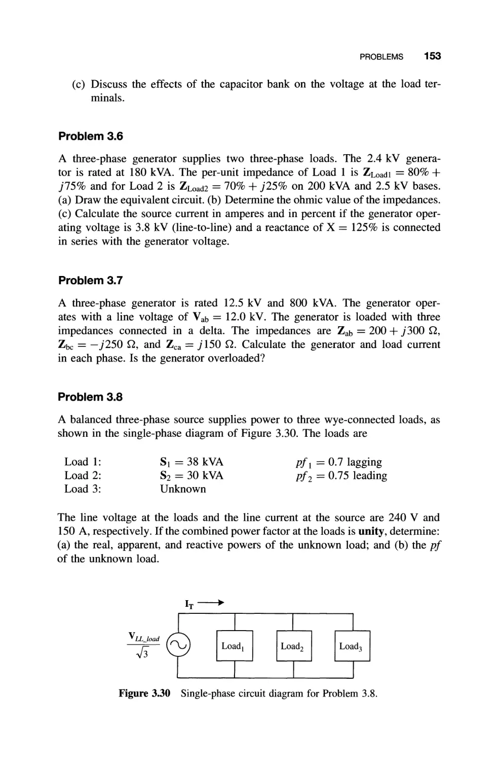
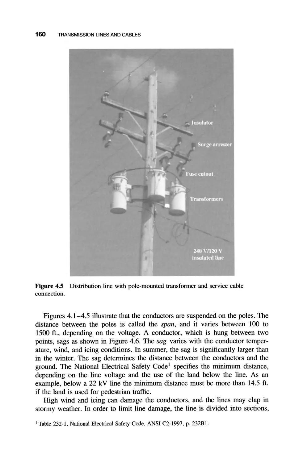
/


Автор: Karady G.G. Holbert K.E.
Теги: transport electrical engineering john wiley and sons electricity electrical energy
ISBN: 0-471-47652-8
Год: 2005


Текст
ELECTRICAL ENERGY
CONVERSION
AND TRANSPORT
IEEE Press
445 Hoes Lane
Piscataway, NJ 08854
IEEE Press Editorial Board
Stamatios V. Kartalopoulos, Editor in Chief
M. Akay
J. B. Anderson
R. J. Baker
J. E. Brewer
M. E. El-Hawary
R. Leonardi
M. Montrose
M. S. Newman
F. M. B. Peri era
C. Singh
S. Tewksbury
G. Zobrist
Kenneth Moore, Director of IEEE Book and Information Services (BIS)
Catherine Faduska, Senior Acquisitions Editor
Anthony VenGraitis, Project Editor
Technical Reviewers
M. E. El-Hawary, Dalhousie University
Peter W. Sauer, University of Illinois at Urbana-Champaign
OTHER BOOKS IN THE IEEE PRESS SERIES ON POWER ENGINEERING
Electric Power Systems: Analysis and Control
Fabio Saccomanno
2003 Hardcover 728pp 0-471-23439-7
Understanding Power Quality Problems: Voltage Sags and Interruptions
Math H. J. Bollen
2000 Hardcover 576pp 0-7803-4713-7
Principles of Electric Machines with Power Electronic Applications,
Second Edition
M. E. El-Hawary
2002 Hardcover 496pp 0-471- 20812-4
Analysis of Electric Machinery and Drive Systems, Second Edition
Paul C. Krause, Oleg Wasynczuk, and Scott D. Sudhoff
2002 Hardcover 624pp 0-471-14326-X
ELECTRICAL ENERGY
CONVERSION
AND TRANSPORT
An Interactive Computer-Based
Approach
George G. Karady
Keith E. Holbert
IEEE Power Engineering Society, Sponsor
au
""EM
lUlU &
ON PO'NER
ENGINEERING
IEEE Press Series on Power Engineering
Mohamed E. El-Hawary, Series Editor
cplEEE
.
IEEE PRESS
ro WI LEY-
INTERSCIENCE
A JOHN WILEY & SONS, INC., PUBLICATION
Copyright @ 2005 by the Institute of Electrical and Electronics Engineers. All rights reserved.
Published by John Wiley & Sons, Inc., Hoboken, New Jersey.
Published simultaneously in Canada.
No part of this publication may be reproduced, stored in a retrieval system, or transmitted in any
form or by any means, electronic, mechanical, photocopying, recording, scanning, or otherwise,
except as permitted under Section 107 or 108 of the 1976 United States Copyright Act, without
either the prior written permission of the Publisher, or authorization through payment of the
appropriate per-copy fee to the Copyright Clearance Center, Inc., 222 Rosewood Drive, Danvers,
MA 01923, 978-750-8400, fax 978-646-8600, or on the web at www.copyright.com. Requests to
the Publisher for permission should be addressed to the Permissions Department, John Wiley &
Sons, Inc., 111 River Street, Hoboken, NJ 07030, (201) 748-6011, fax (201) 748-6008.
Limit of Liability/Disclaimer of Warranty: While the publisher and author have used their best
efforts in preparing this book, they make no representations or warranties with respect to the
accuracy or completeness of the contents of this book and specifically disclaim any implied
warranties of merchantability or fitness for a particular purpose. No warranty may be created or
extended by sales representatives or written sales materials. The advice and strategies contained
herein may not be suitable for your situation. You should consult with a professional where
appropriate. Neither the publisher nor author shall be liable for any loss of profit or any other
commercial damages, including but not limited to special, incidental, consequential, or other
damages.
For general information on our other products and services please contact our Customer Care
Department within the U.S. at 877-762-2974, outside the U.S. at 317-572-3993 or
fax 317-572-4002.
Wiley also publishes its books in a variety of electronic formats. Some content that appears in
print, however, may not be available in electronic format.
Library of Congress Cataloging-in-Publication Data is available.
ISBN 0-471-47652-8
Printed in the United States of America.
10 9 8 7 6 5 4 3 2
CONTENTS
PREFACE
xiii
1 ELECTRIC POWER SYSTEM 1
1.1 Electrical Network 2
1.1.1 Transmission System 3
1.1.2 Distribution System 4
1.2 Electric Generation Stations 5
1.3 Fossil Power Plants 8
1.3.1 Fuel Storage and Handling 8
1.3.2 Boiler 9
1.3.3 Turbine 15
1.3.4 Generator and Electrical System 17
1.3.5 Combined Cycle Plants 20
1.4 Nuclear Power Plants 21
1.4.1 Nuclear Reactor 22
1.4.2 Pressurized Water Reactor 25
1.4.3 Boiling Water Reactor 26
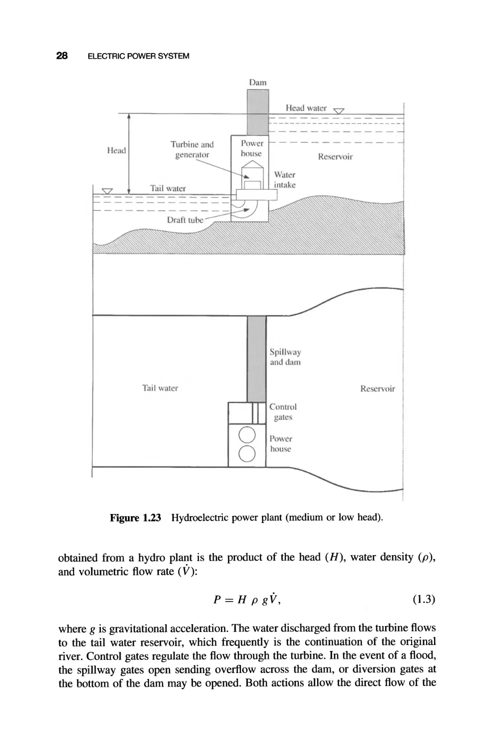
1.5 Hydroelectric Power Plants 27
1.5.1 Low Head Hydro Plants 29
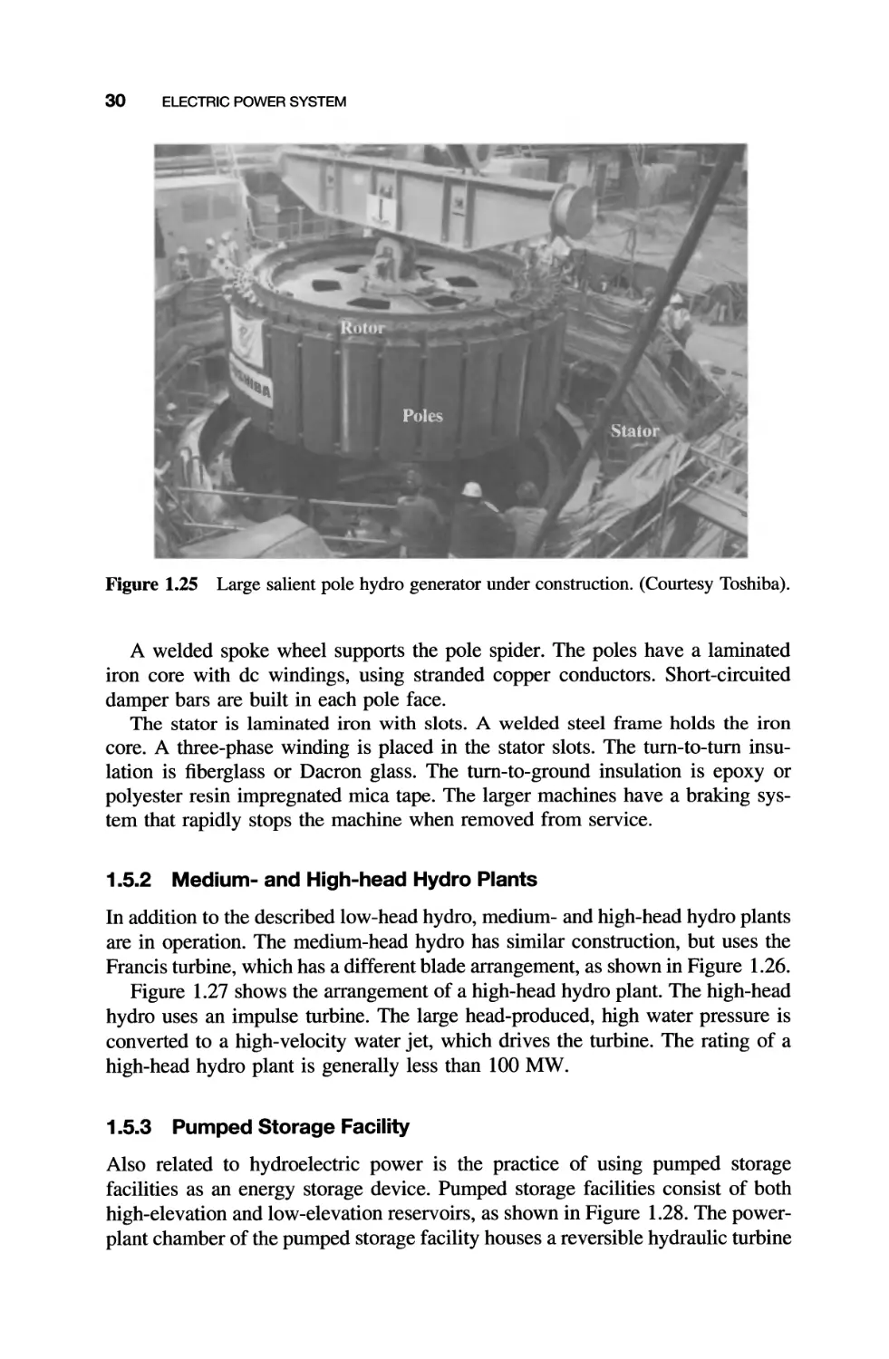
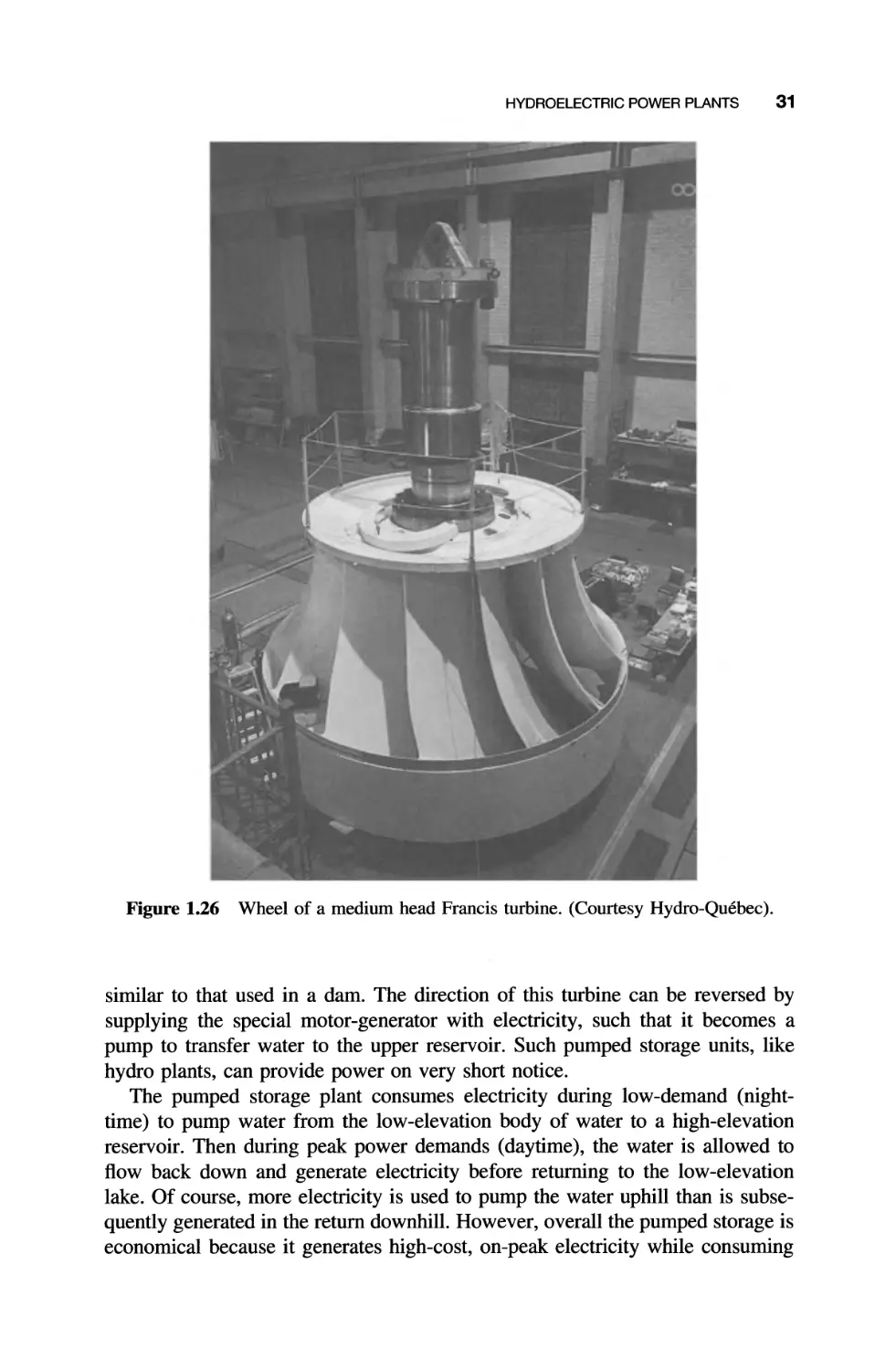
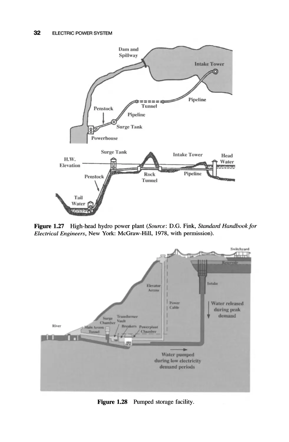
1.5.2 Medium- and High-head Hydro Plants 30
1.5.3 Pumped Storage Facility 30
1.6 Distribution System 33
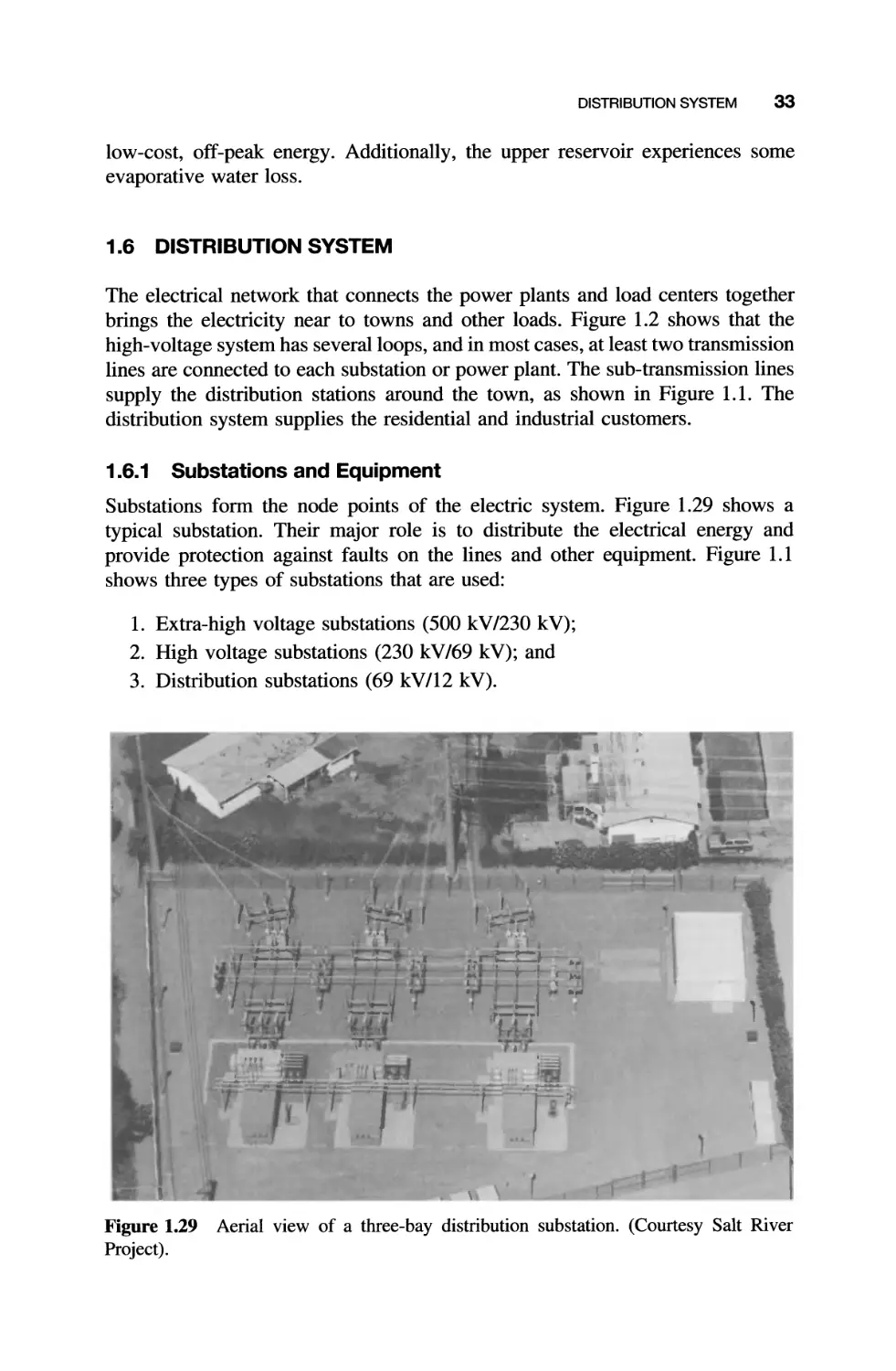
1.6.1 Substations and Equipment 33
v
vi CONTENTS
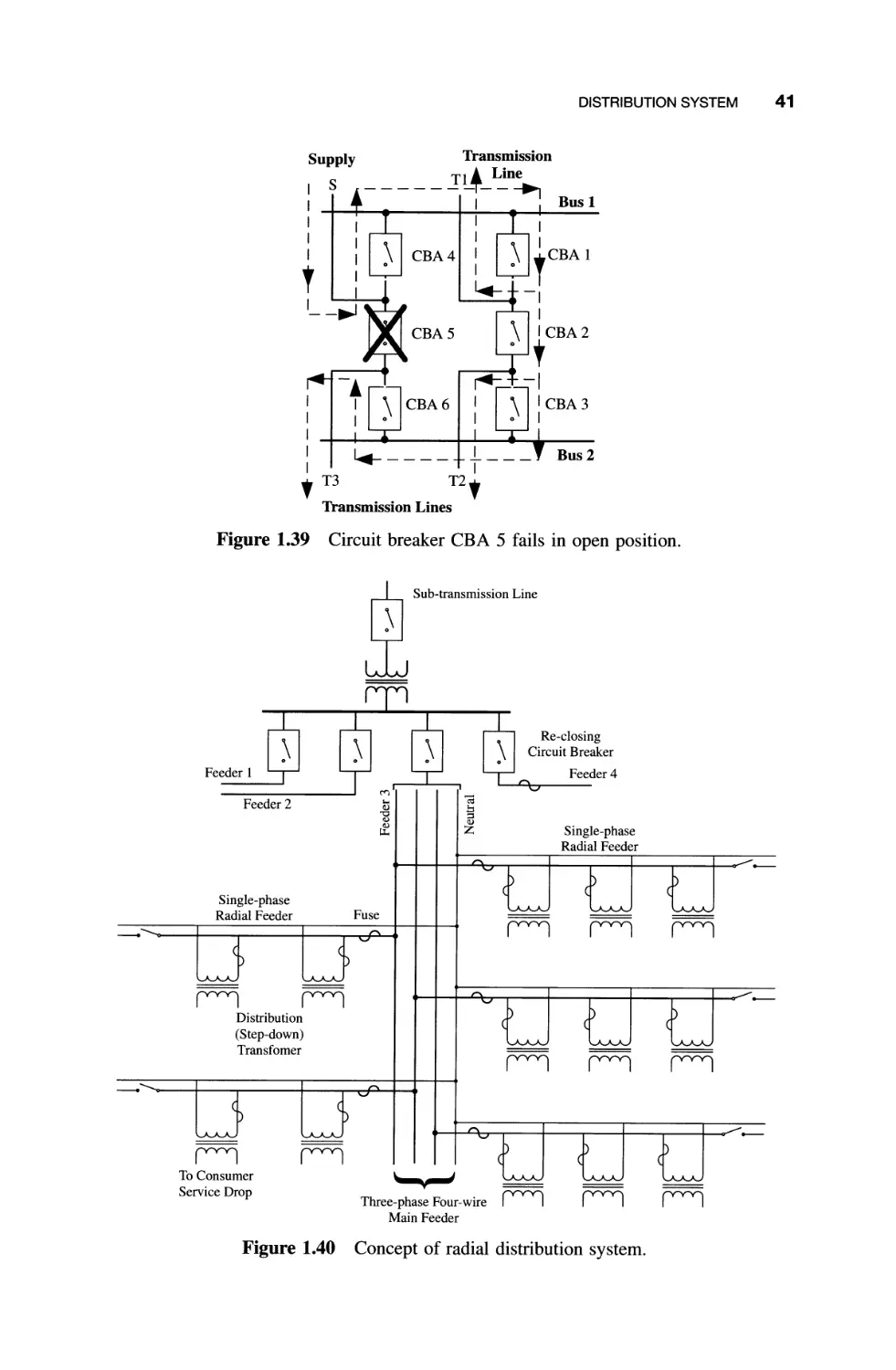
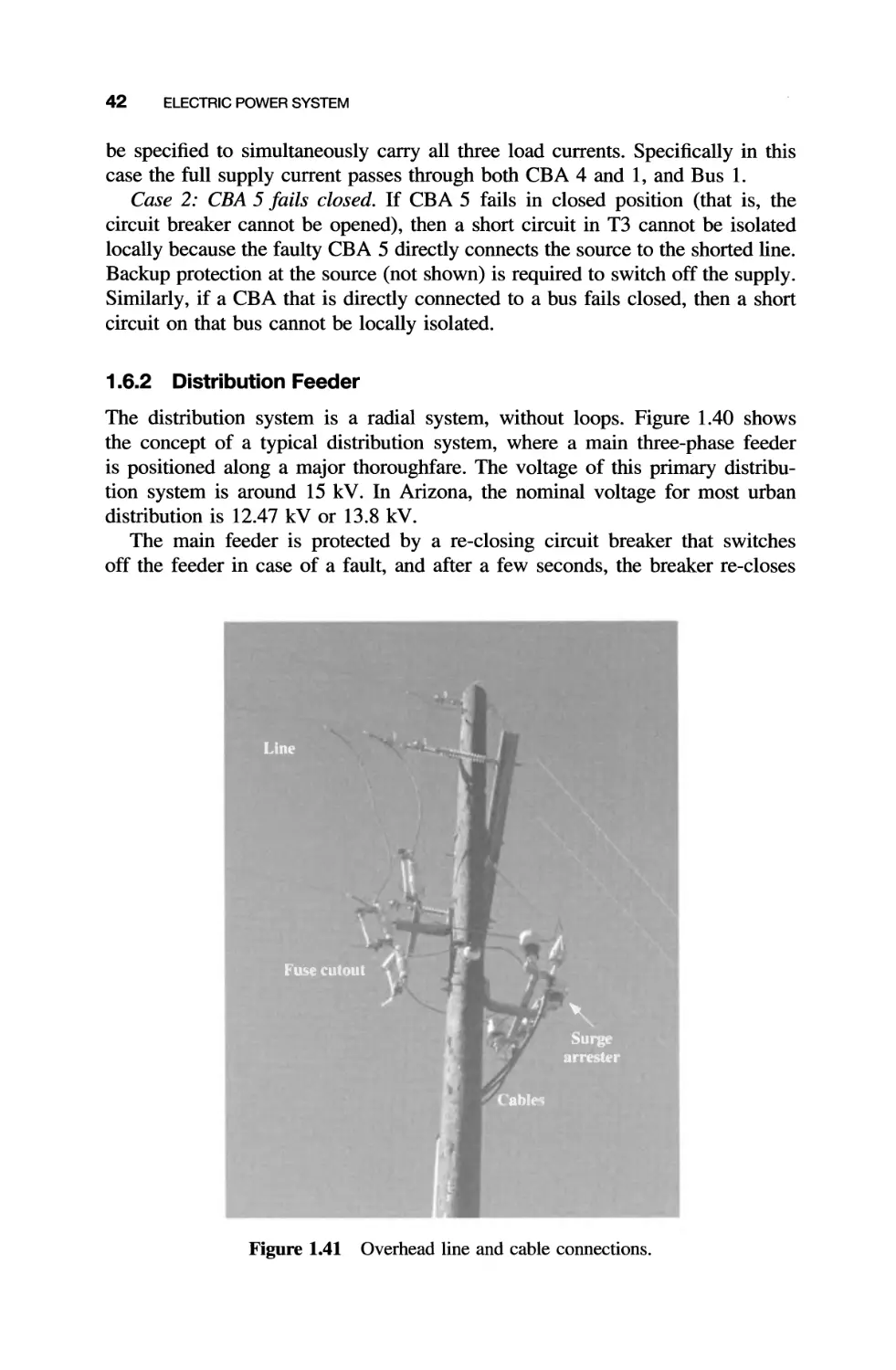
1.6.2 Distribution Feeder
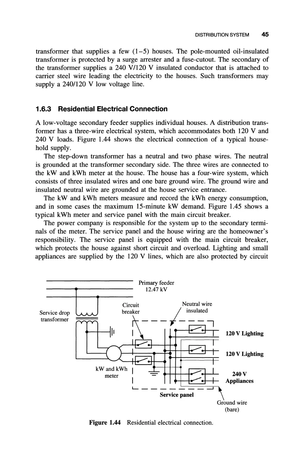
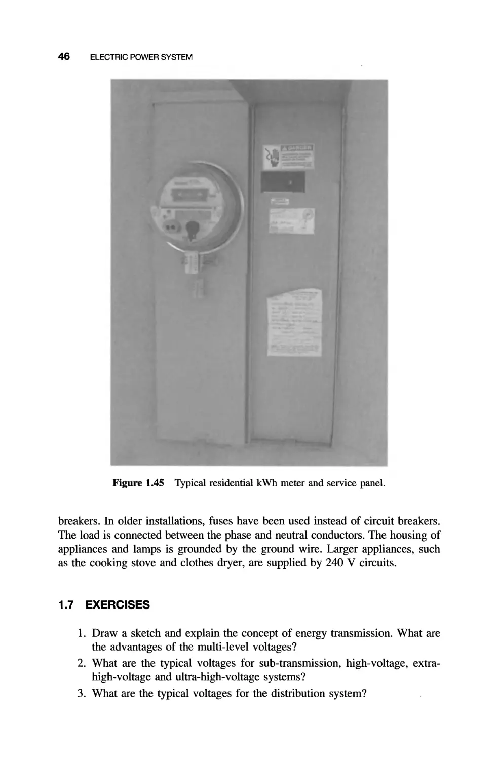
1.6.3 Residential Electrical Connection
1.7 Exercises
1.8 Problems
42
45
46
47
2 SINGLE-PHASE CIRCUITS 49
2.1 Circuit Analysis Fundamentals 49
2.1.1 Basic Definitions and Nomenclature 49
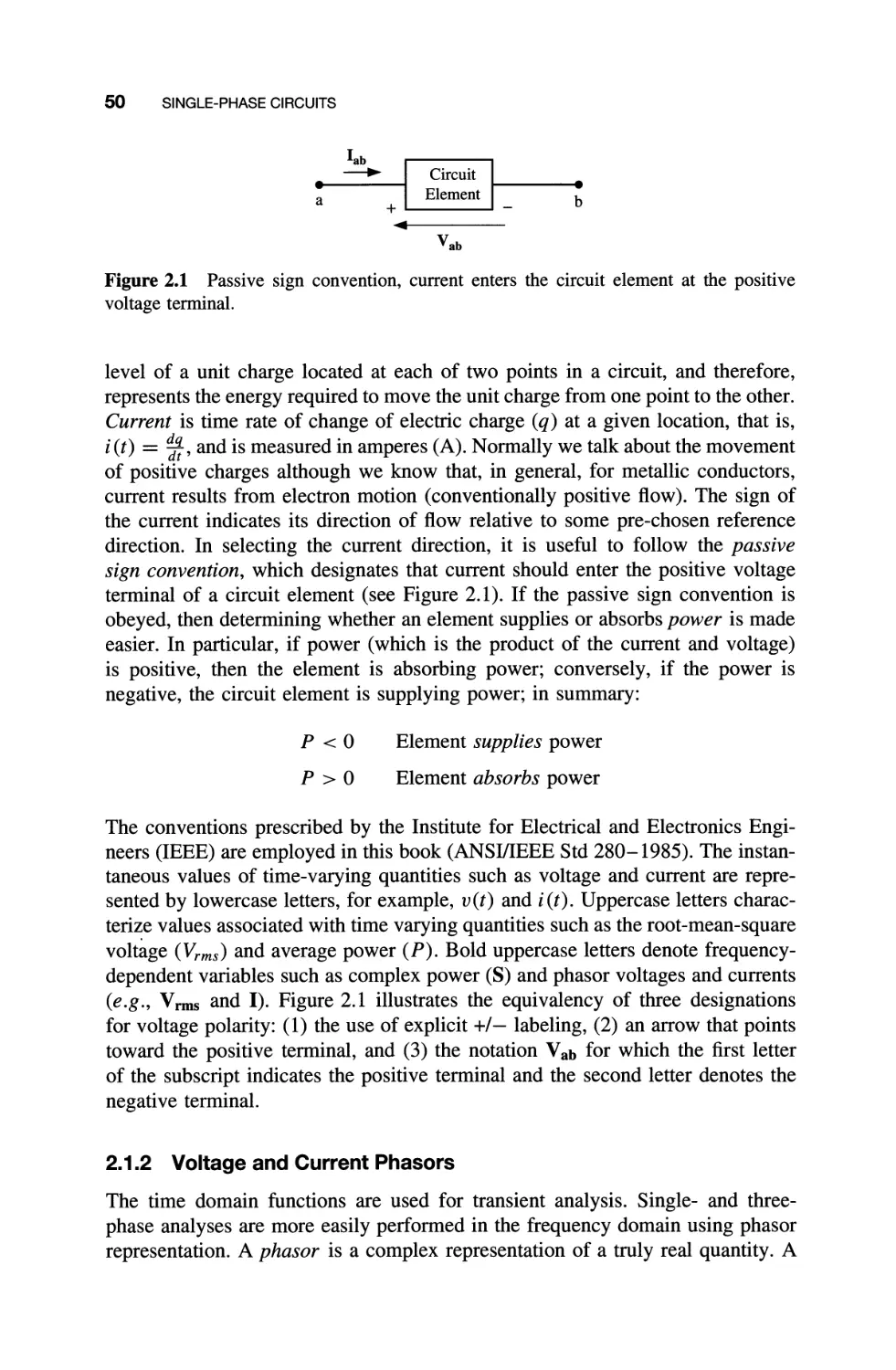
2.1.2 Voltage and Current Phasors 50
2.2 Impedance 51
2.2.1 Series Connection 53
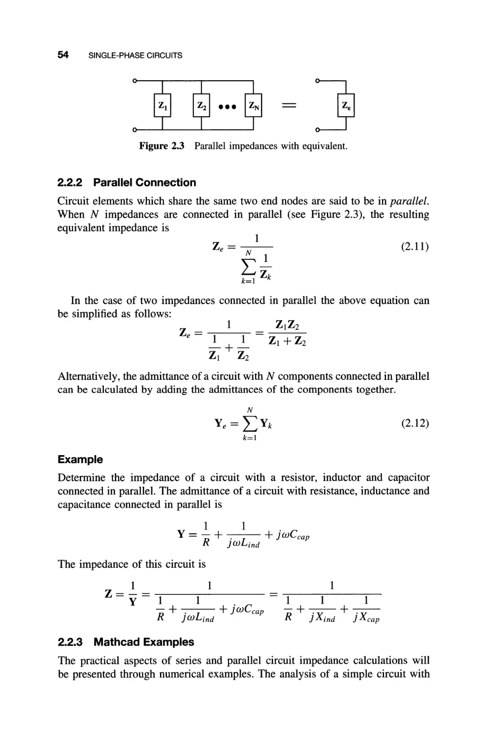
2.2.2 Parallel Connection 54
2.2.3 Mathcad Examples 54
2.2.4 MATLAB Examples 57
2.2.5 Delta-wye Transformation 60
2.3 Power 61
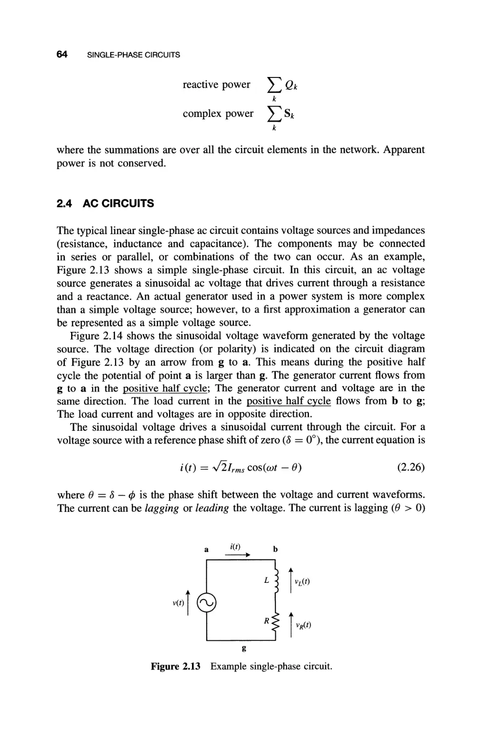
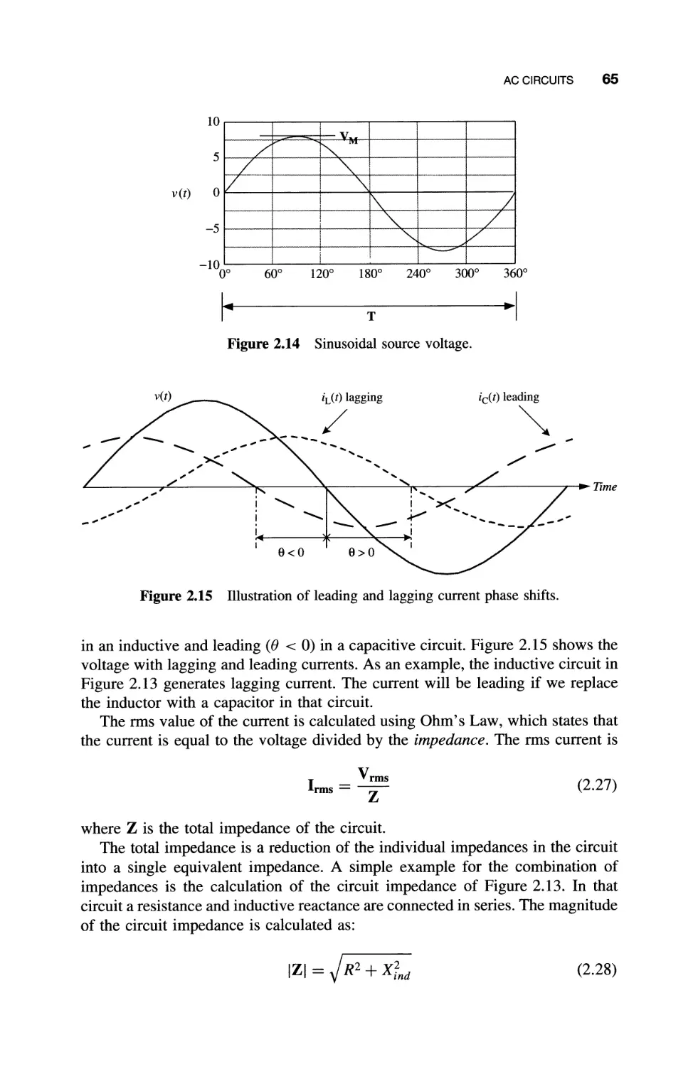
2.4 AC Circuits 64
2.5 Basic Laws 70
2.5.1 Kirchhoff's Current Law 70.
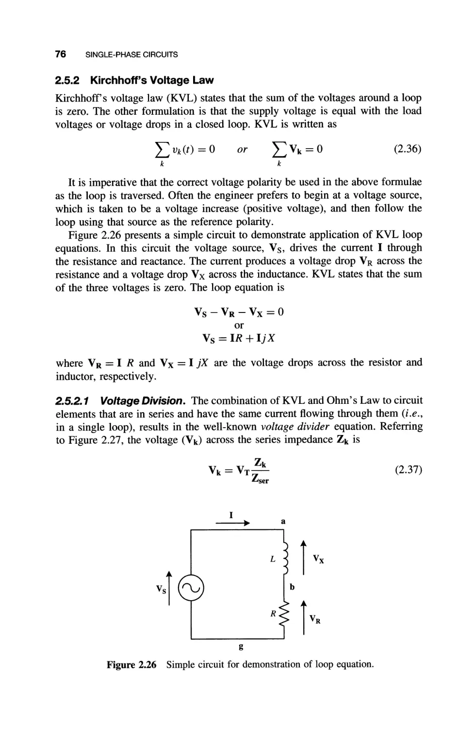
2.5.2 Kirchhoff's Voltage Law 76
2.5.3 Thevenin's Theorem 79
2.5.4 Loads 80
2.6 Applications of Single-phase Circuit Analysis 81
2.6.1 Analysis of Transmission Line Operation 81
2.6.2 Generator Supplies a Constant Impedance Network 87
Through a Line
2.6.3 Power Factor Improvement 90
2.7 Summary 92
2.8 Exercises 93
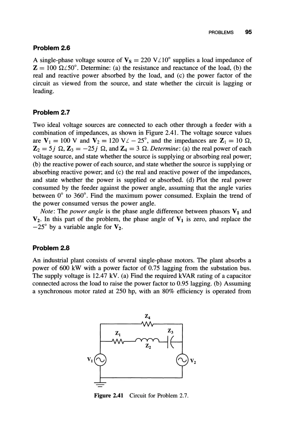
2.9 Problems 93
3 THREE-PHASE CIRCUITS
3.1 Three-phase Quantities
3.2 Wye-connected Generators
3.3 Wye-connected Loads
3.3.1 Balanced Wye Load (Four-wire System)
3.3.2 Unbalanced Wye Load (Four-wire System)
3.3.3 Wye-connected Three-wire System
97
97
101
106
108
109
111
CONTENTS vii
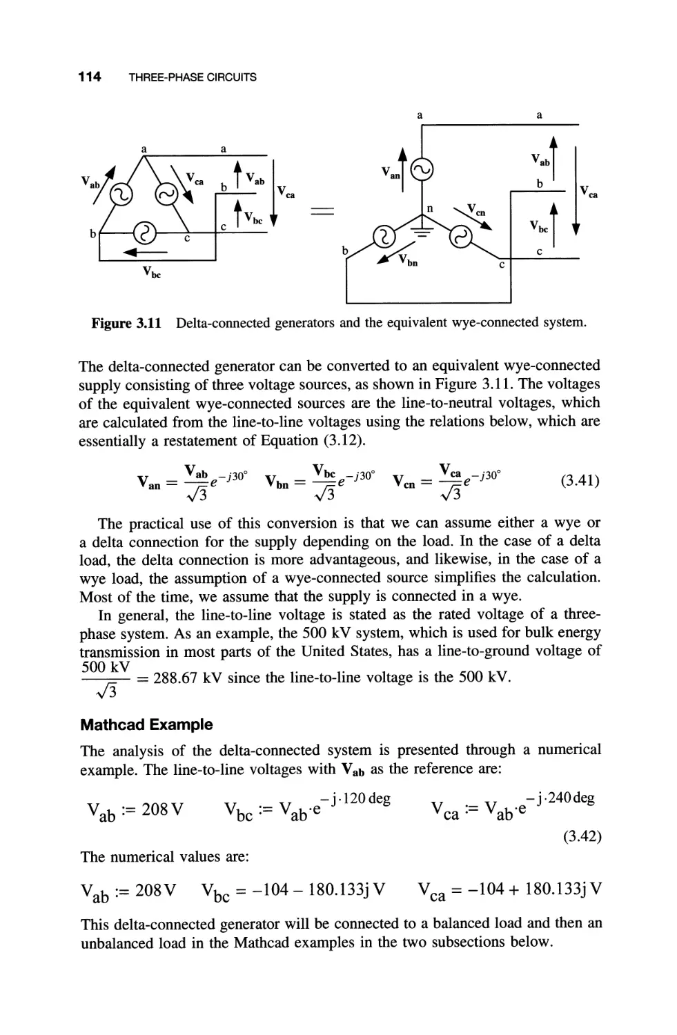
3.4 Delta-connected System 113
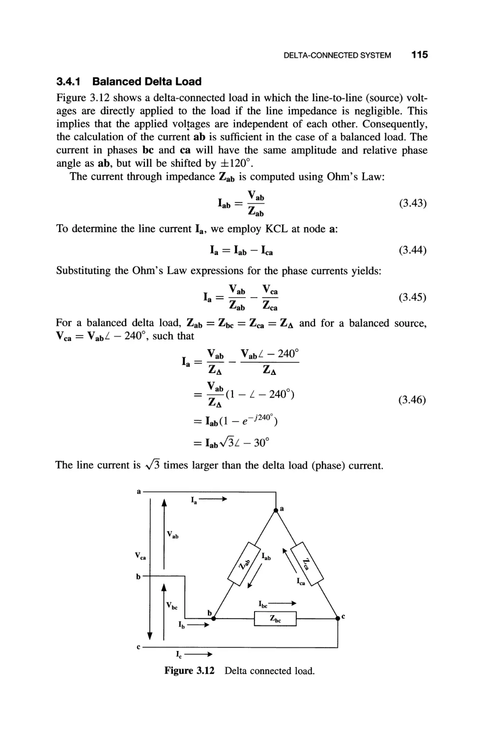
3.4.1 Balanced Delta Load 115
3.4.2 Unbalanced Delta Load 118
3.5 Summary 119
3.6 Three-phase Power Measurement 120
3.6.1 Four-wire System 121
3.6.2 Three-wire System 122
3.7 Mathcad Examples 123
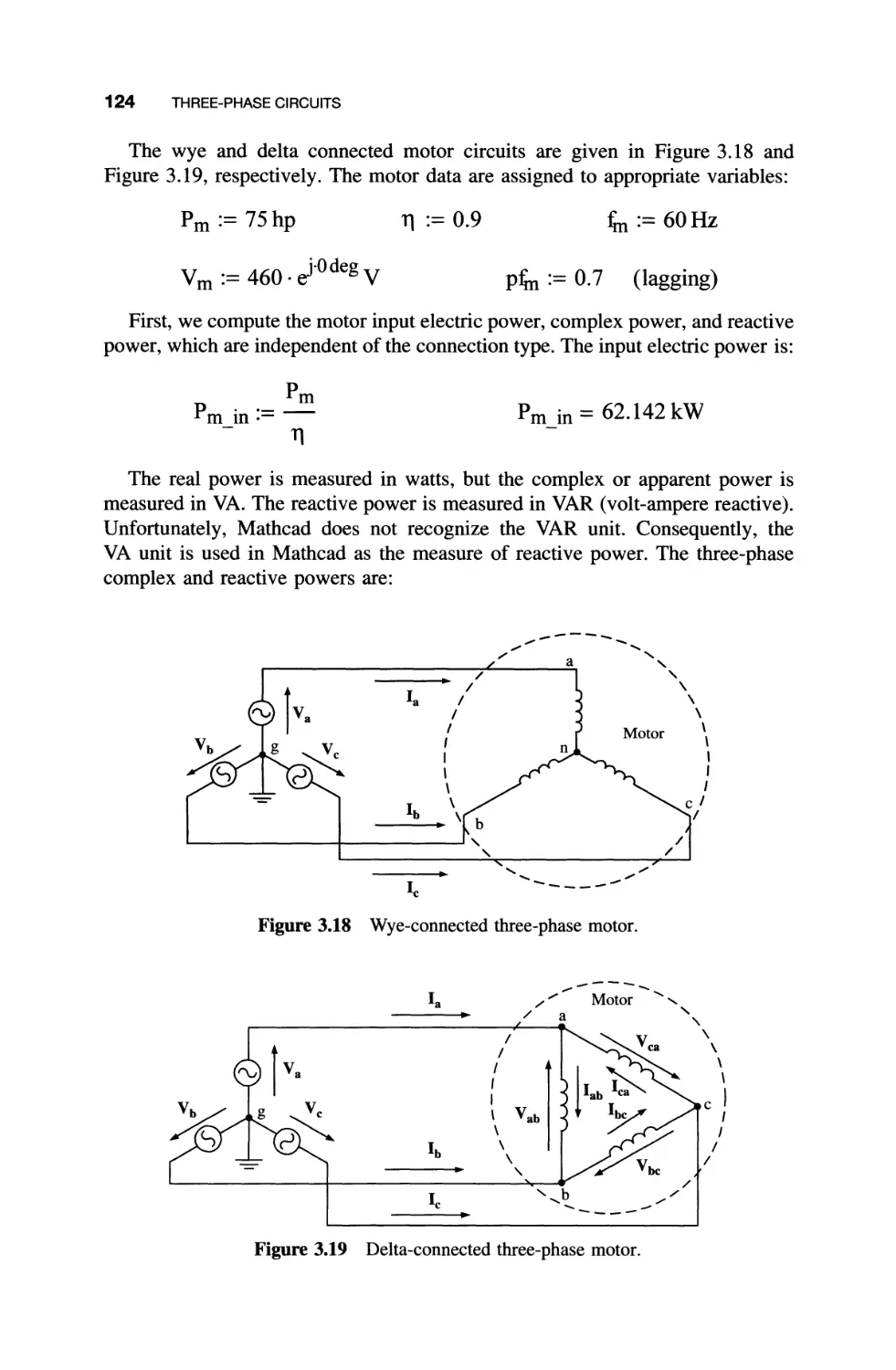
3.7.1 Analysis of Motor Operation in Delta and Wye 123
Configurations
3.7.2 Two Three-phase Loads Connected in Parallel 126
3.8 Per Unit System 128
3.9 MATLAB Examples 134
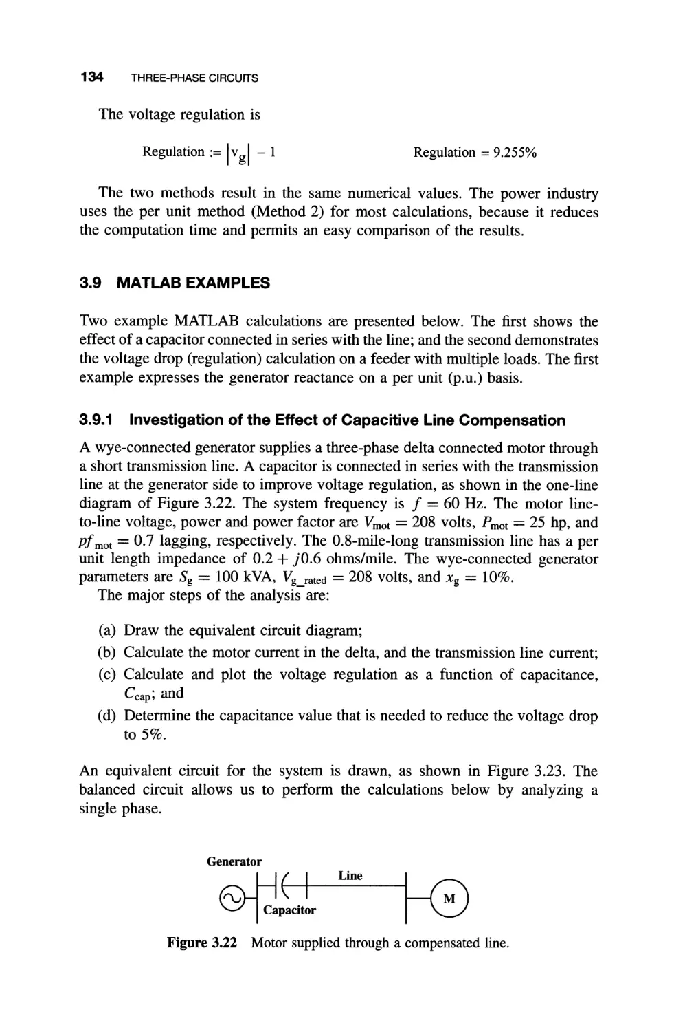
3.9.1 Investigation of the Effect of Capacitive Line 134
Compensation
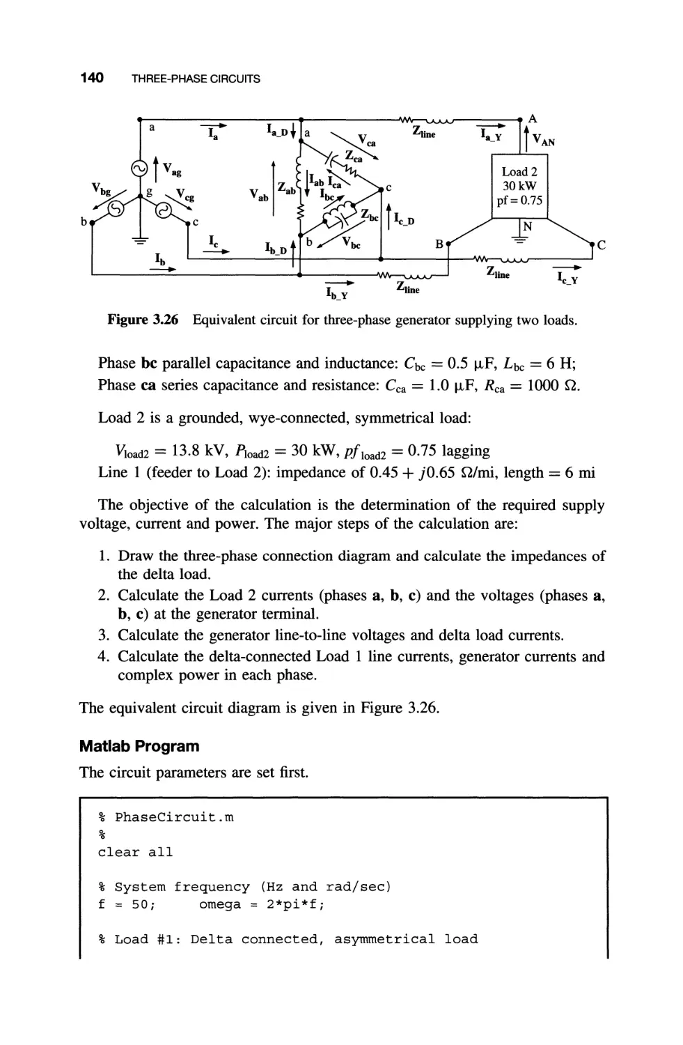
3.9.2 Three-phase Feeder with Two Loads 139
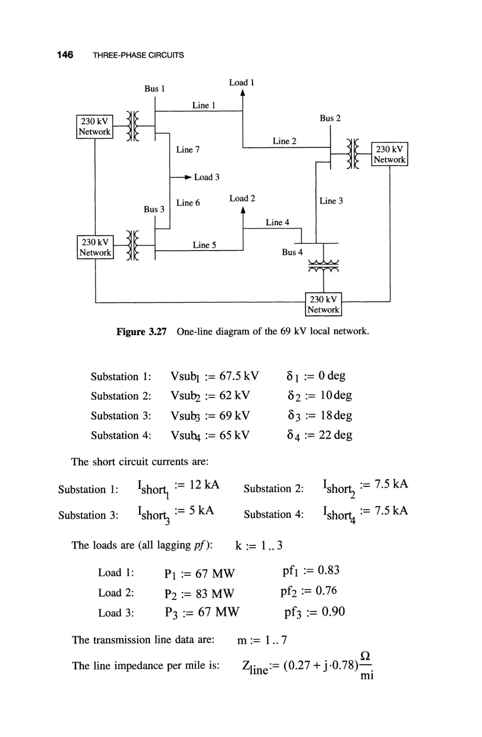
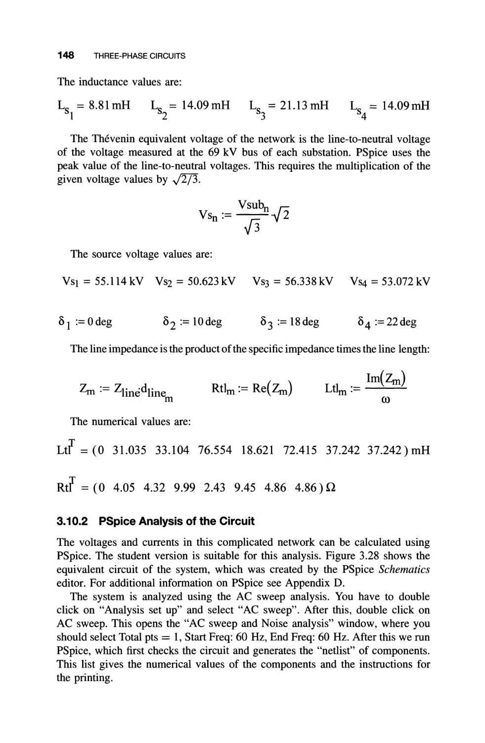
3.10 PSpice Example 145
3.10.1 Calculation of Equivalent Circuit Parameters 145
3.10.2 PSpice Analysis of the Circuit 148
3.11 Exercises 151
3.12 Problems 151
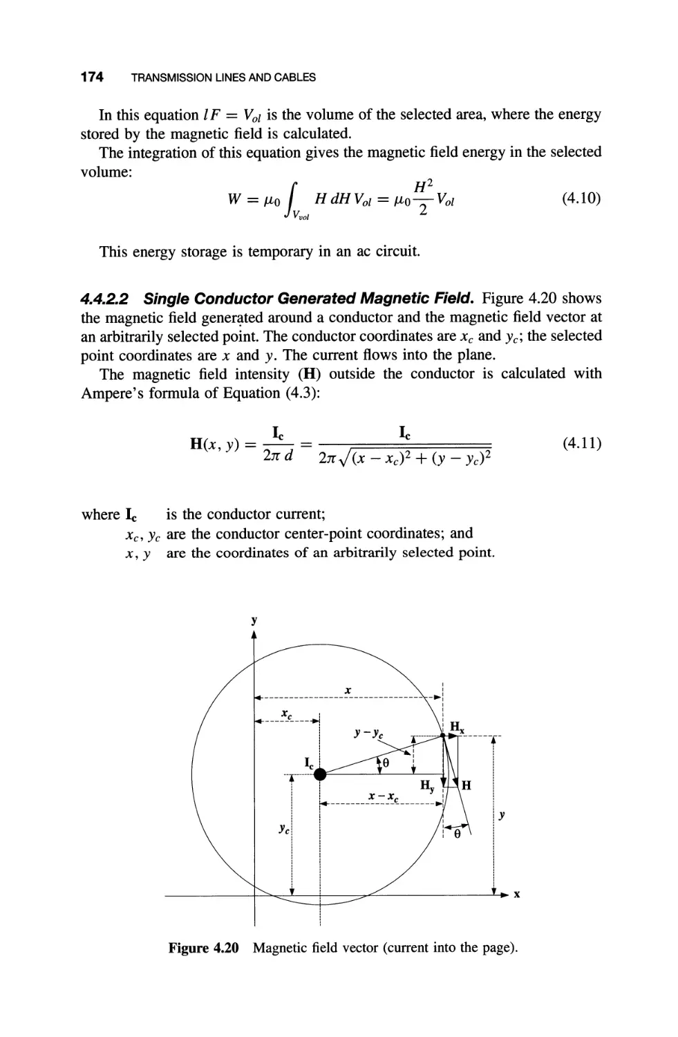
4 TRANSMISSION LINES AND CABLES 155
4.1 Construction 156
4.2 Components of the Transmission Lines 163
4.2.1 Towers and Foundations 163
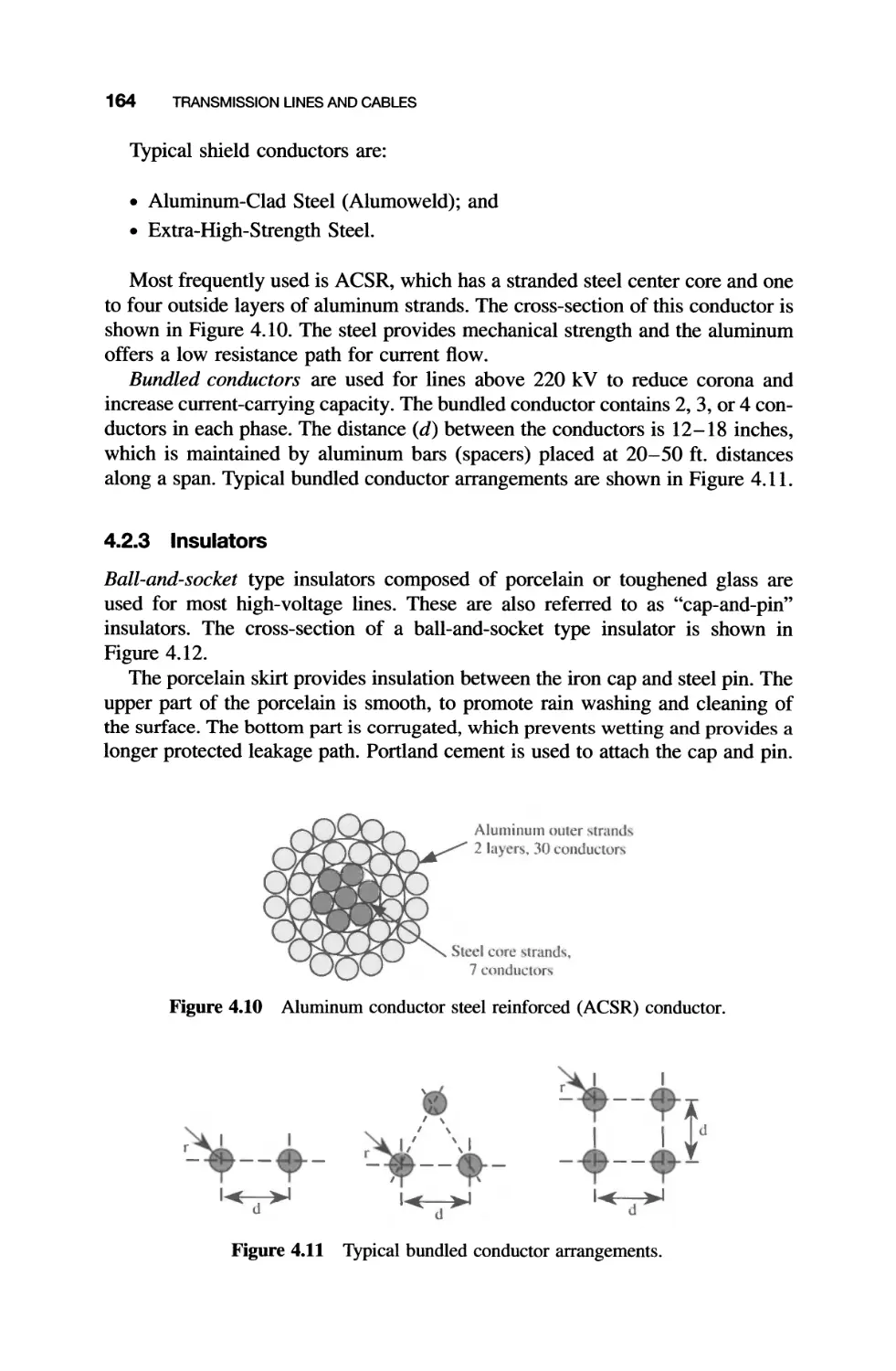
4.2.2 Conductors 163
4.2.3 Insulators 164
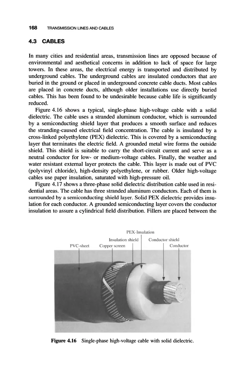
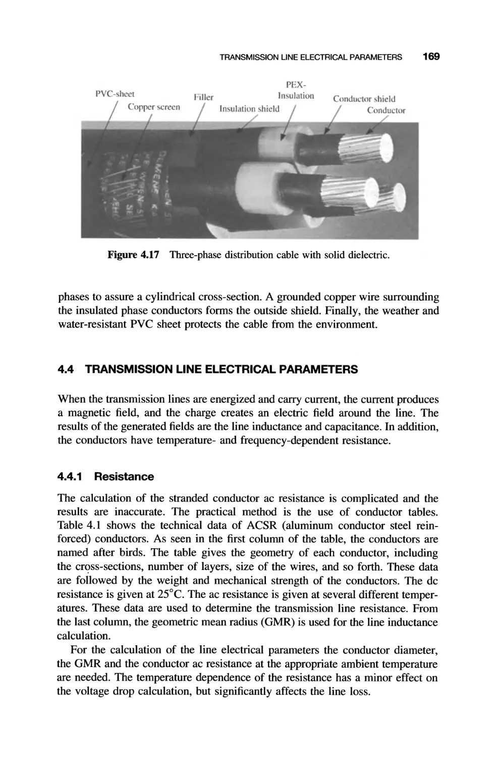
4.3 Cables 168
4.4 Transmission Line Electrical Parameters 169
4.4.1 Resistance 169
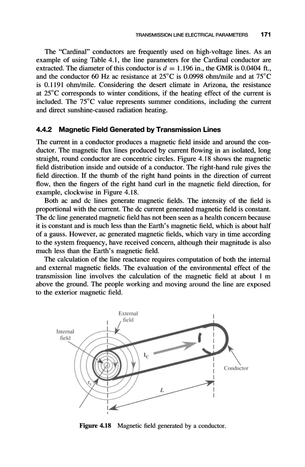
4.4.2 Magnetic Field Generated by Transmission 171
Lines
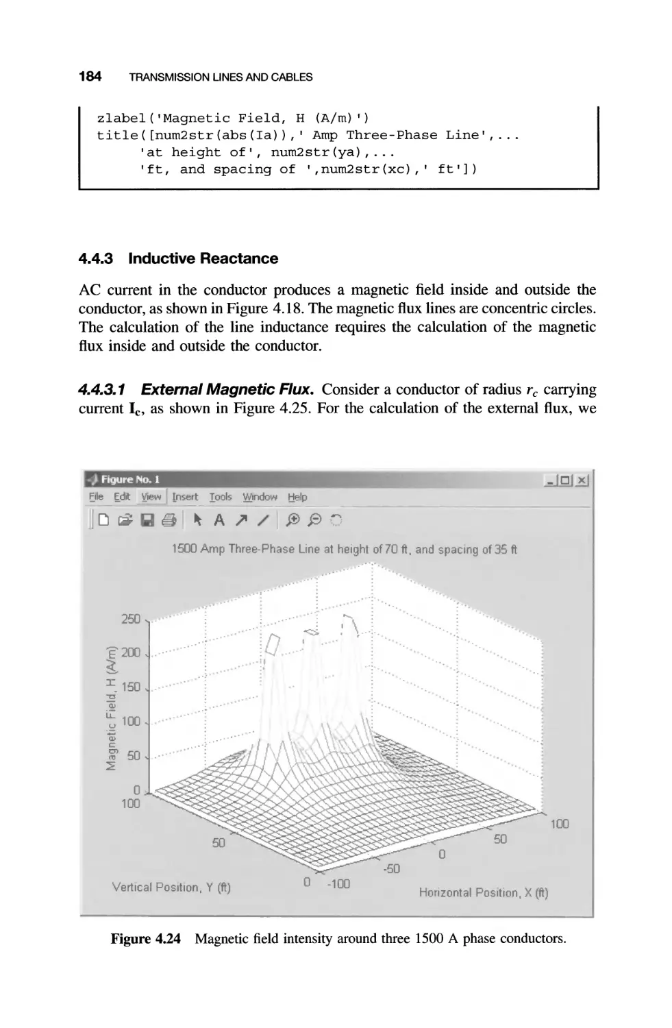
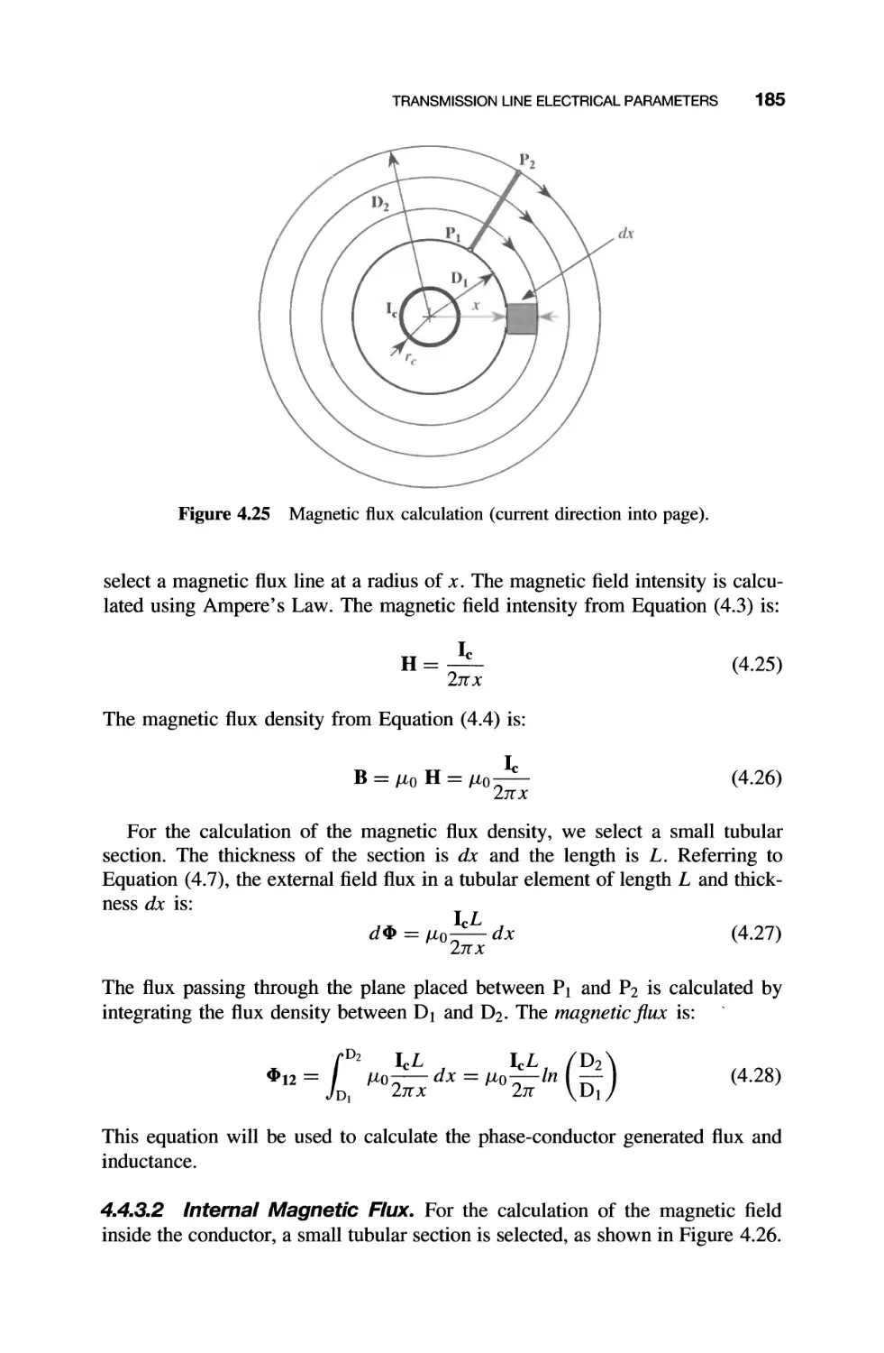
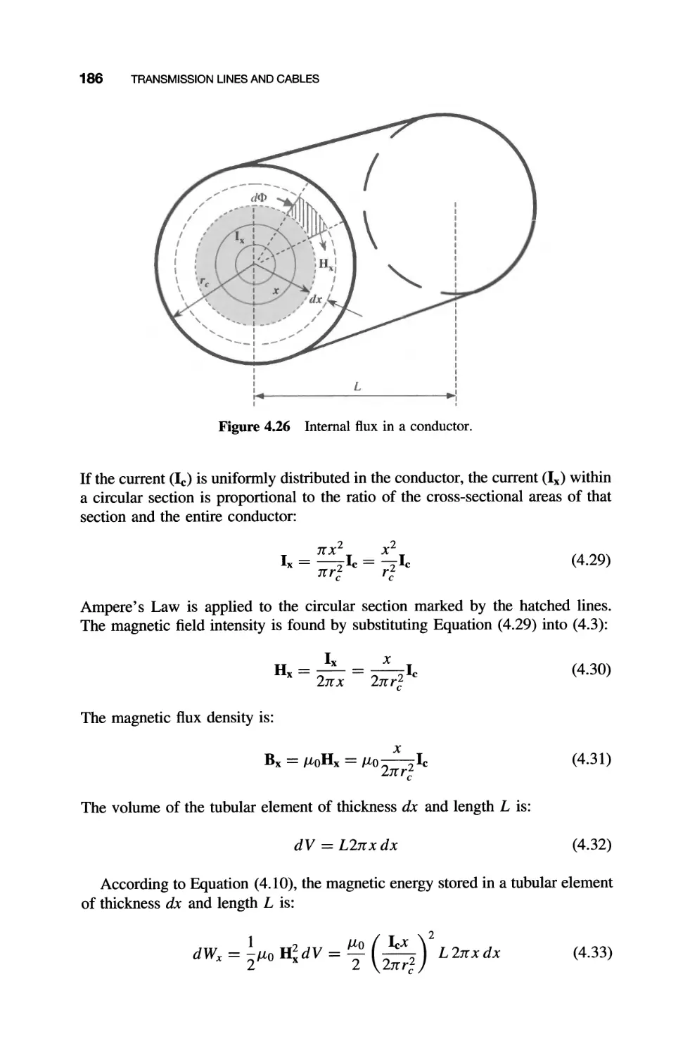
4.4.3 Inductive Reactance 184
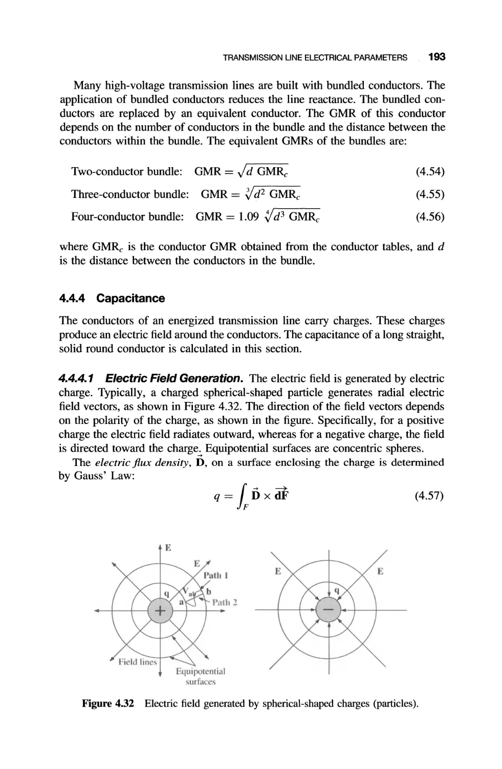
4.4.4 Capacitance 193
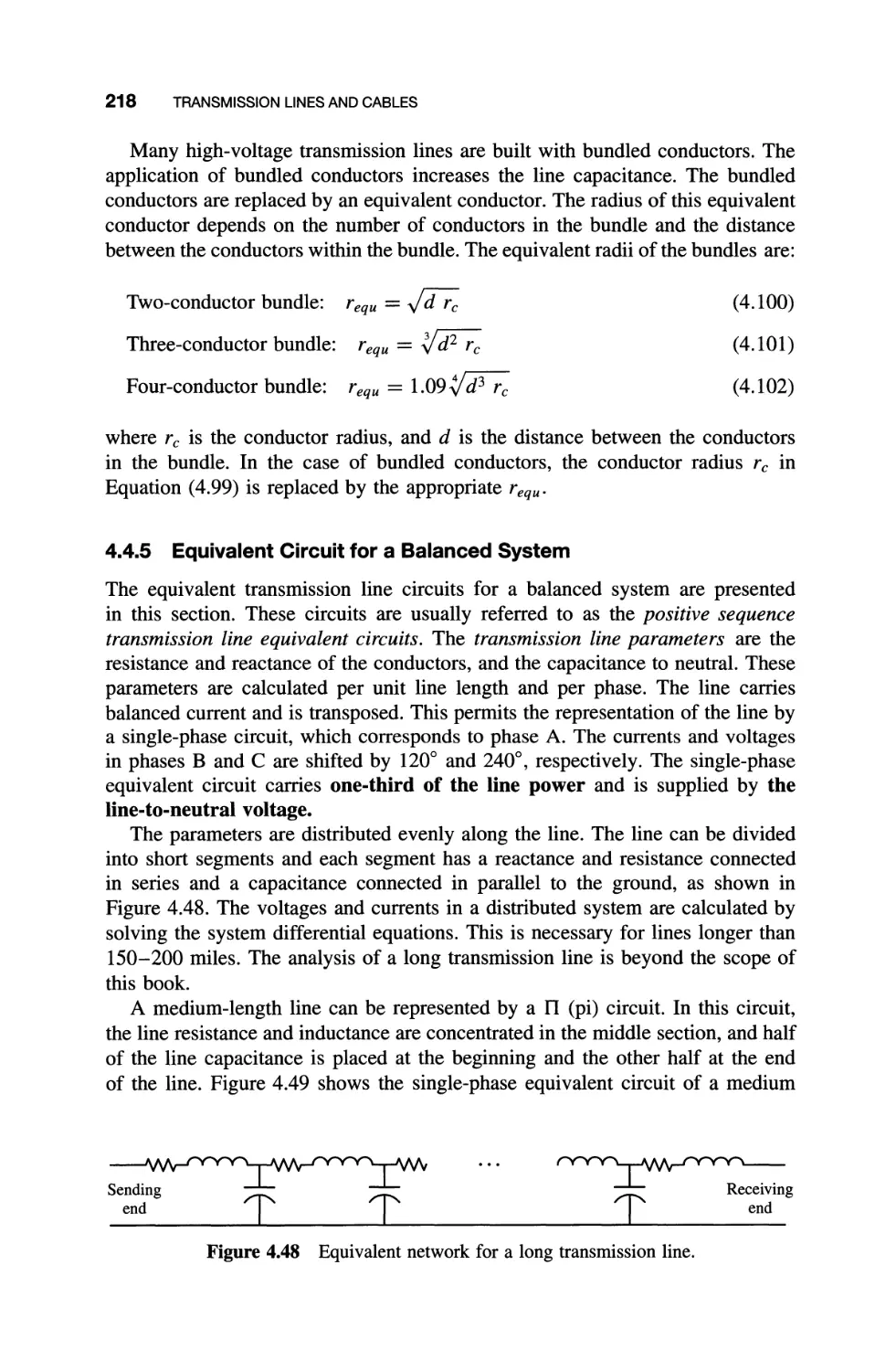
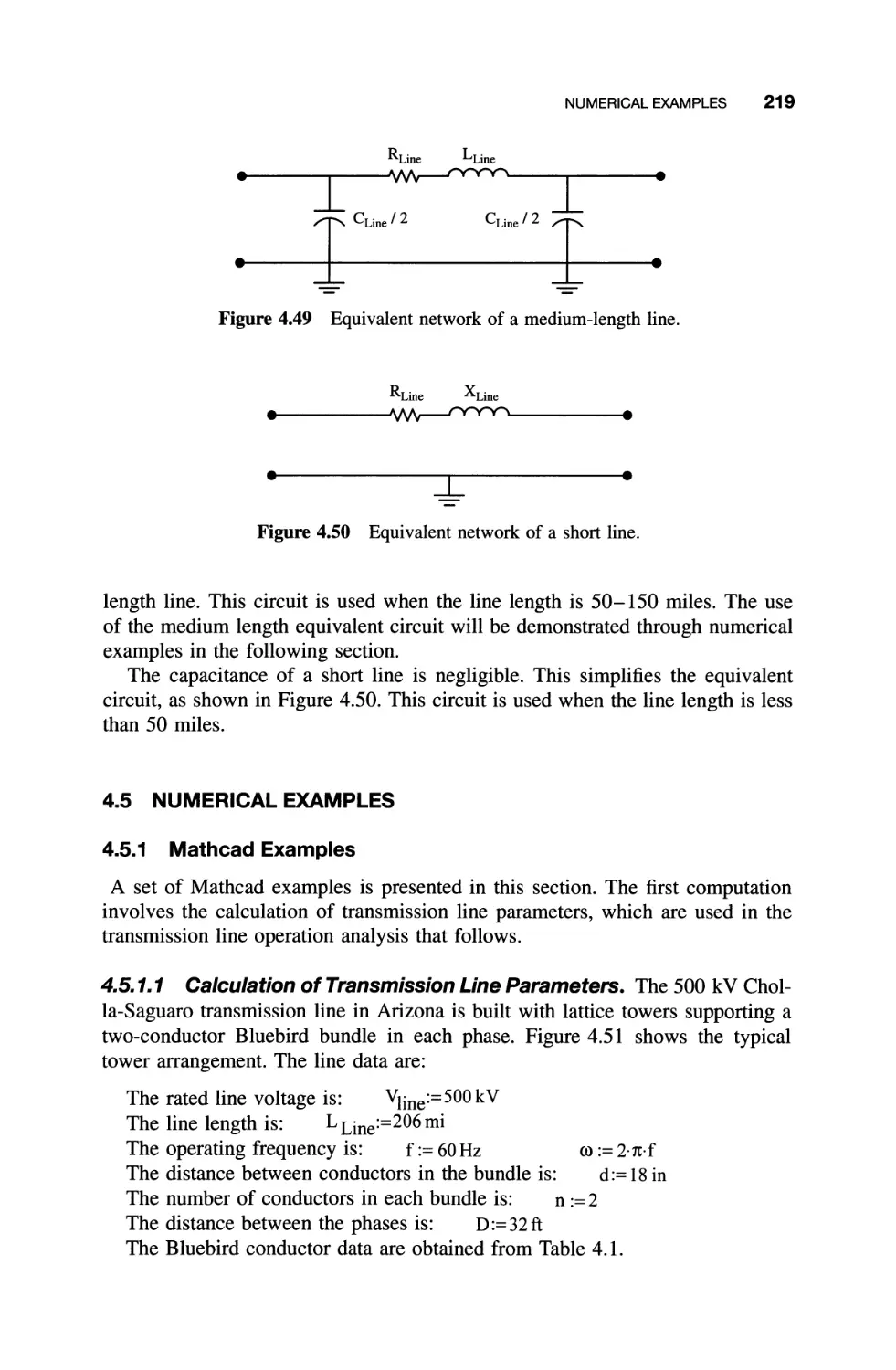
4.4.5 Equivalent Circuit for a Balanced System 218
4.5 Numerical Examples 219
4.5.1 Mathcad Examples 219
viii CONTENTS
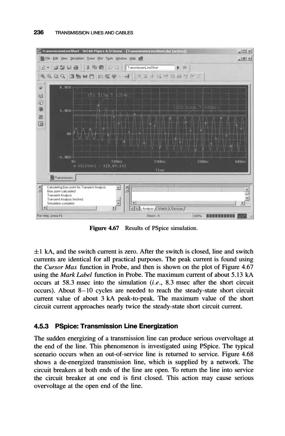
4.5.2 PSpice: Transient Short Circuit Current in
Transmission Lines
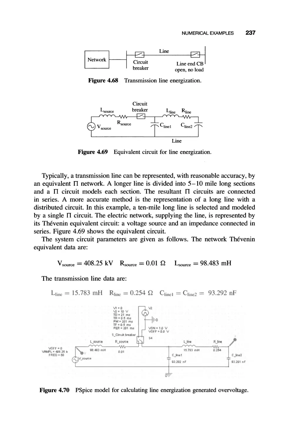
4.5.3 PSpice: Transmission Line Energization
4.6 Exercises
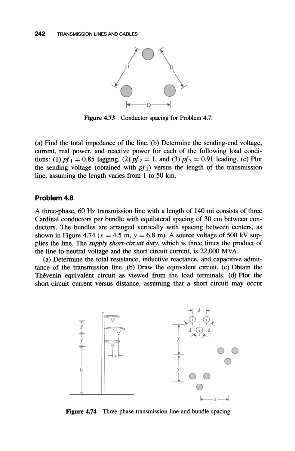
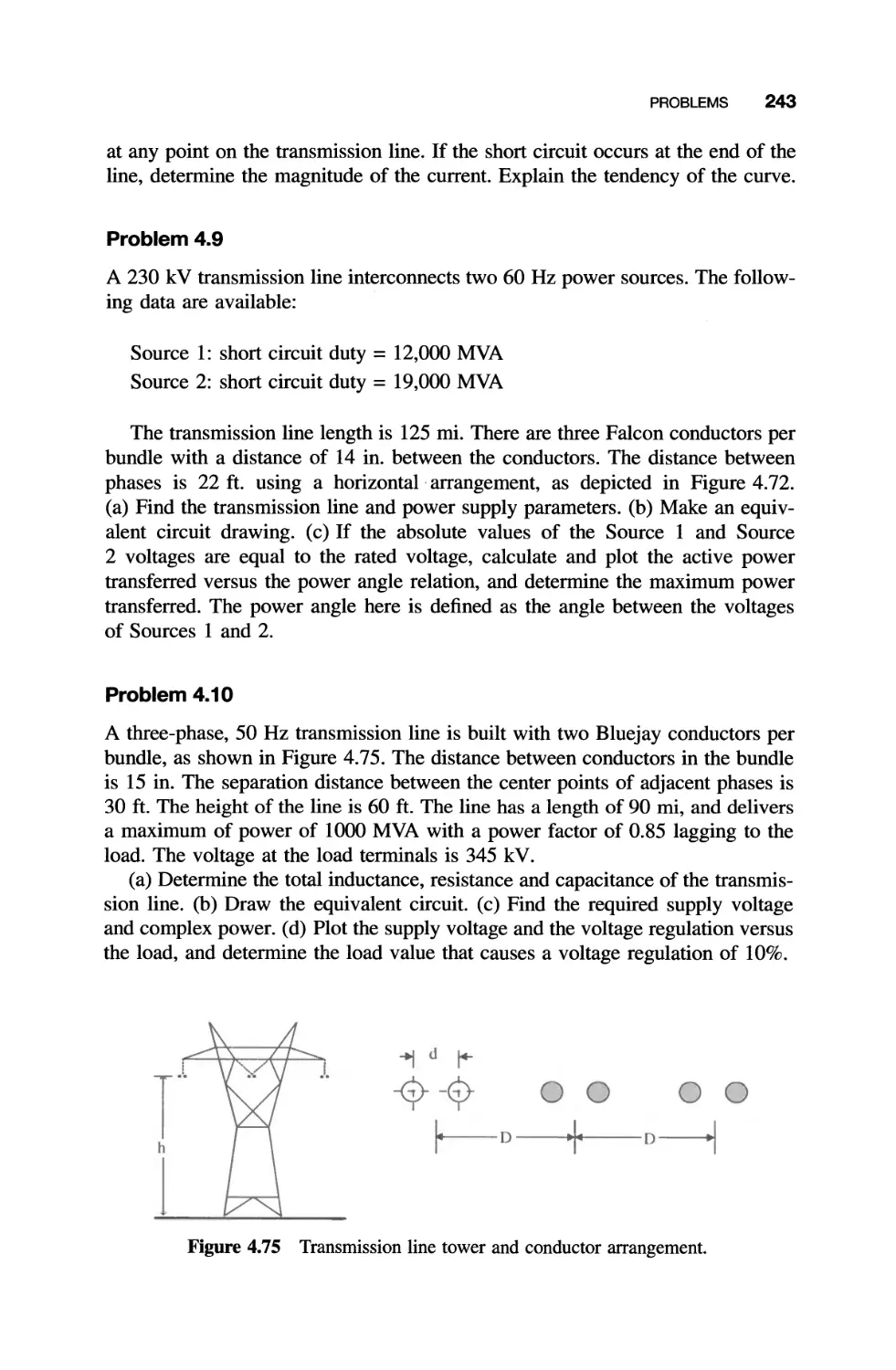
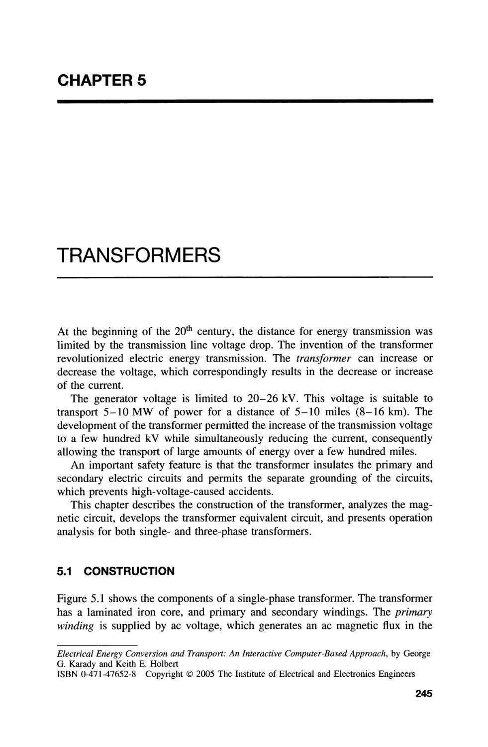
4.7 Problems
234
236
239
240
5 TRANSFORMERS 245
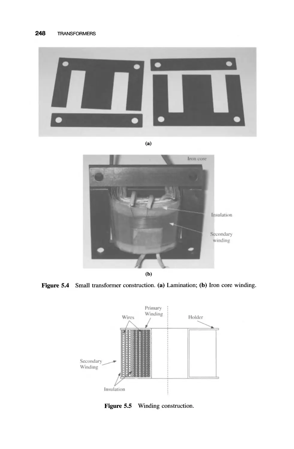
5.1 Construction 245
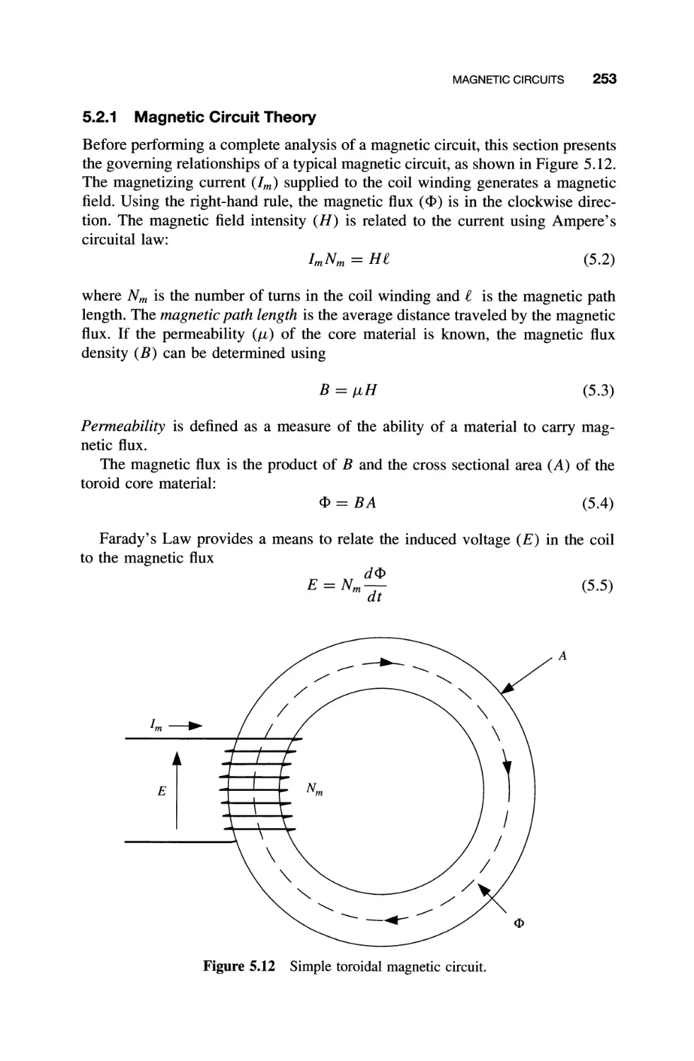
5.2 Magnetic Circuits 251
5.2.1 Magnetic Circuit Theory 253
5.2.2 Magnetic Circuit Analysis 254
5.2.3 Magnetic Energy 260
5.2.4 Magnetization Curve 261
5.2.5 Magnetic Circuit with Air Gap 262
5.2.6 Magnetization Curve Modeling 265
5.2.7 Demonstration of the Use of B(H) Equations 267
5.2.8 Magnetic Circuit with Parallel Paths 269
5.3 Single-phase Transformers 273
5.3.1 Ideal Transformer 273
5.3.2 Real Transformer 283
5.3.3 Operation Analysis 284
5.3.4 Determination of Equivalent Transformer Circuit 289
Parameters
5.3.5 Transformers in Parallel 294
5.4 Three-phase Transformers 298
5.4.1 Wye-wye Connection 300
5.4.2 Wye-delta Connection 305
5.4.3 Delta-wye Connection 308
5.4.4 Delta-delta Connection 309
5.4.5 Summary 310
5.4.6 Analysis of Three-phase Transformer Configurations 310
5.4.7 Equivalent Circuit Parameters of a Three-phase 319
Transformer
5.4.8 General Program for Computing Transformer 322
Parameters
5.4.9 Analysis of Three-phase Transformer Operation in a 325
System
5.4.10 Analysis of Three-phase Delta-wye Transformer 332
Operation in a System
CONTENTS ix
5.5 Exercises 336
5.6 Problems 338
6 SYNCHRONOUS MACHINES 344
6.1 Construction 344
6.1.1 Round Rotor Generator 344
6.1.2 Salient Pole Generator 346
6.1.3 Exciter 351
6.2 Operating Concept 352
6.3 Generator Application 359
6.3.1 Loading 359
6.3.2 Reactive Power Regulation 359
6.3.3 Synchronization 360
6.3.4 Static Stability 360
6.4 Induced Voltage and Synchronous Reactance Calculation 374
6.4.1 Induced Voltage Calculation 375
6.4.2 Synchronous Reactance Calculation 380
6.5 Mathcad Analysis of a Synchronous Generator 388
6.6 MATLAB Analysis of Static Stability 393
6.7 MATLAB Analysis of Generator Loading 399
6.8 PSpice Simulation of Generator Transients 405
6.9 Exercises 413
6.10 Problems 414
7 INDUCTION MOTORS 418
7.1 Introduction 418
7.2 Construction 418
7.2.1 Stator 420
7.2.2 Rotor 422
7.3 Three-phase Induction Motor 424
7.3.1 Operating Principle 424
7.3.2 Equivalent Circuit 429
7.3.3 Motor Performance 432
7.3.4 Performance Analyses 434
7.3.5 Mathcad Example of a Motor Driving a Pump 442
7.3.6 Determination of Motor Parameters by Measurement 443
7.3.7 MATLAB Induction Motor Parameters 448
7.4 MATLAB Induction Motor Example 450
7.5 MATLAB Motor-driven Fan 460
X CONTENTS
7.6 Single-phase Induction Motor 465
7.6.1 Operating Principle 466
7.6.2 Single-phase Induction Motor Performance Analysis 469
7.7 Exercises 476
7.8 Problems 478
8 DC MACHINES 483
8.1 Construction 483
8.2 Operating Principle 487
8.2.1 DC Motor 487
8.2.2 DC Generator 489
8.2.3 Equivalent Circuit 491
8.2.4 Excitation Methods 493
8.3 Operation Analyses 494
8.3.1 Separately Excited Machine 495
8.3.2 Shunt Machine 501
8.3.3 Series Motor 510
8.3.4 Summary 515
8.4 Mathcad Example of Battery Supplying DC Shunt Motor 516
8.5 MATLAB Example of Battery Supplying Car Starter 521
8.6 MATLAB Example of Series Motor Driving a Pump 526
8.7 Mathcad Example of Series Motor with Brush and Copper 531
Losses
8.8 Exercises 533
8.9 Problems 534
9 INTRODUCTION TO MOTOR CONTROL AND POWER 538
ELECTRONICS
9.1 Concept of DC Motor Control 538
9.2 Concept of AC Induction Motor Control 543
9.3 Semiconductor Switches 549
9.3.1 Diode 549
9.3.2 Thyristor 552
9.3.3 Gate Turn-off Thyristor 556
9.3.4 Metal-oxide-semiconductor Field-effect Transistor 558
9.3.5 Insulated Gate Bipolar Transistor 558
9.3.6 Summary 559
9.4 Rectifiers 559
9.4.1 Simple Passive Diode Rectifiers 560
9.4.2 Single-phase Controllable Rectifiers 566
CONTENTS xi
9.4.3 Firing and Snubber Circuits 584
9.4.4 Three-phase Rectifiers 585
9.5 Inverters 587
9.5.1 Voltage Source Inverter with Pulse Width 590
Modulation
9.5.2 Line-commutated Thyristor-controlled Inverter 593
9.5.3 High-voltage DC Transmission 596
9.6 PSpice Simulation of Single-phase Bridge Converter 597
9.6.1 PSpice Circuit Model 597
9.6.2 Circuit Simulation 600
9.7 DC Shunt Motor Control Example 603
9.8 Single-phase Induction Motor Control Example 607
9.9 Exercises 611
9.10 Problems 612
10 ELECTROMECHANICAL ENERGY CONVERSION 616
10.1 Magnetic and Electric Field-generated Forces 616
10.1.1 Electric Field-generated Force 617
10.1.2 Magnetic Field-generated Force 617
10.2 Calculation of Electromagnetic Forces 622
10.2.1 Actuator 627
10.2.2 Transducers 630
10.2.3 Permanent Magnet-generated Field 631
10.3 Exercises 637
10.4 Problems 637
APPENDIX A: INTRODUCTION TO MATHCAD 642
A.l Worksheet and Toolbars 642
A.l.l Text Regions 644
A.l.2 Calculations 644
A.2 Functions 647
A.2.1 Repetitive Calculations 649
A.2.2 Defining a Function 650
A.2.3 Plotting a Function 650
A.2.4 Minimum and Maximum Function Values 652
A.3 Equation Solvers 653
A.3.1 Root Equation Solver 653
A.3.2 Find Equation Solver 654
A.4 Vectors and Matrices 655
xii CONTENTS
APPENDIX B: INTRODUCTION TO MATLAB
B.l Desktop Tools
B.2 Operators, Variables and Functions
B.3 Vectors and Matrices
B.4 Colon Operator
B.5 Repeated Evaluation of an Equation
B.6 Plotting
B.7 Basic Programming
659
659
661
662
664
665
665
668
APPENDIX C: FUNDAMENTAL UNITS AND CONSTANTS
C.l Fundamental Units
C.2 Fundamental Physical Constants
670
670
674
APPENDIX D: INTRODUCTION TO PSPICE
D.l Obtaining and Installing PSpice
D.2 Using PSpice
D.2.1 Creating a Circuit
D.2.2 Simulating a Circuit
D.2.3 Analyzing Simulation Results
675
675
676
676
677
678
PROBLEM SOLUTIONS
680
BIBLIOGRAPHY
688
INDEX
690
PREFACE
This book provides material for an undergraduate course covering the basic con-
cepts of electric energy conversion and transport, which is a fundamental part
of electrical engineering. Every electrical engineer should know why a motor
rotates and how energy is generated and transported. In addition, electric energy
generation and transport is a major component of the national infrastructure.
The maintenance and development of this essential industry requires well-trained
engineers who are able to use modem computation techniques to analyze electric
systems and understand the theory of electrical energy conversion.
Engineering education has improved significantly during the last decade because
of advancements in technology and the increasing use of personal computers. Engi-
neering educators have also recognized the need to transform students from passive
listeners in the classroom to active learners. The paradigm shift is from a teacher-
centered delivery approach to that of a learner-centered environment.
Computer-equipped classrooms and the computer aptitude of students open
up new possibilities to improve engineering education by changing the deliv-
ery method. We suggest the interactive presentation of the material, where the
students are actively engaged in the lectures. This book is designed to sup-
port active learning, especially in a computer-based classroom environment. The
computer-assisted teaching method increases student mastery of the course mate-
rial because they participate in its development. The primary goal of this approach
is to increase student learning through their active involvement; secondarily, stu-
dents' interest in power engineering is enhanced because of their own attraction to
computer technologies. This interactive approach provides students with a better
understanding of the theory and the development of solid problem-solving skills.
As many universities and instructors firmly favor the use of one software pack-
age versus another, this book applies Mathcad, MATLAB and Pspice throughout;
xiii
xiv PREFACE
thus allowing the instructor to choose the software employed. Appendices intro-
duce the basic use of these three programs. The extensive computer use permits
the solution of complex problems that are not easily solvable by hand compu-
tations with calculators. In fact, the experienced instructor will find that their
students are able to solve complicated problems that were previously too dif-
ficult at this level. This is a significant modernization of the classical topic of
energy conversion. Students familiar with the application of modem computa-
tional techniques to electrical power applications are better prepared to meet the
needs of industry.
The authors suggest a presentation ordering in the classroom that parallels the
textbook. Specifically, the course material may be divided into topical units. The
typical time for a unit is about one week in the case of a three-credit-hour course.
A suggested one-semester timeline is
Week
Chapter
Topical Unit
1
2
3
4
5
6
7
8
9
10
11
12
13
14
15
16
1
2
3
3
4
4
4
5
5
6
6
7
8
9
9
10
Power system components
Single-phase circuits
Three-phase circuits
Per unit system
Transmission lines: resistance, inductance, capacitance
Short and medium line voltage models
AC magnetic circuits
Single-phase transformers
Three-phase transformers
Synchronous machines
Rotating flux, induced voltage and torque
Induction motors
DC machines
Introduction to power electronics
Concept of motor control using rectifiers and inverters
Electromechanical energy conversion
Here, we present a brief overview of the suggested instructional technique
for a representative day in the classroom. The basis of the approach is that
after introducing the hardware and theory, the basic equations and their practi-
cal application are developed jointly with the students using computers. Having
di vided the particular topic into sections, the instructor outlines each step of the
analysis, and students then proceed to develop the equation(s) using herlhis com-
puter. While students are working together, the instructor is free to move about
the classroom, answer student questions and assess the student understanding.
After allowing students sufficient time to complete the process and reach con-
clusions, the instructor confirms the results and the students make corrections,
if needed. This procedure leads to student theory development and analysis of
performance-learner centered education.
PREFACE XV
Through the computer utilization, a seamless integration of theory and appli-
cation is achieved, thereby increasing student interest in the subject material.
The textbook derivation of the system equations and the operational analyses are
presented using numerical examples. The numerical examples support the theory
and provide deeper understanding of the physical phenomena. In addition, the
use of the computer provides immediate feedback to the student.
Again, paralleling the classroom activities, each chapter first describes the
hardware associated with that topic, for example, the construction and compo-
nents are presented using drawings and photographs. This is followed by the
theory and the physics of the material of that chapter together with the develop-
ment of an equivalent circuit. The major emphasis of the chapters is the operation
analyses. The questions at the end of each chapter are open-ended to promote
deeper investigation by the reader.
The interactive method is also applicable in a self-learning environment. In
this case, the text outlines each step. The reader is encouraged to initially ignore
the solution given in the text, but instead derive the equation and calculate the
value using his/her computer. The reader then compares his/her equation with
the correct answers. This process is continued until the completion of the unit.
This textbook facilitates interactive teaching of the material. Through the stu-
dents' active participation, learning is enhanced. The advantages of method are:
1. Better understanding of the material because the students participate in the
development;
2. Development of problem solving ability;
3. Simultaneously learning the practical engineering application of the mate-
rial using computerized methods accepted by industry;
4. Extending the students' attention span and maintaining their interest during
the lecture. This method eliminates the boredom, which inhibits students
at the end of most lectures;
5. The students analyze the results and draw the conclusions, which enhance
learning;
6. The students gain experience with the general-purpose calculation programs
that are frequently used by industry.
The authors recommend the book to faculty who want to modernize their
electric power curriculum. The book is also intended for engineers interested
in increasing their knowledge of electrical power and computer-based problem
solving skills. Such knowledge may open up or expand employment opportunities
in the electrical power industry.
HOW TO USE THIS BOOK EFFECTIVELY
This textbook differs noticeably from others in that the classical derivations are
combined with numerical examples. In doing so, the reader is not only provided
xvi PREFACE
with the general analytical expressions as the theoretical development proceeds,
but in addition, the concurrent numerical results assist the student in developing
a feel for the correct magnitude of various parameters and variables. The authors
have found Mathcad particularly well suited to this approach. Regardless of which
software the reader chooses to use, we recommend that the reader first familiarize
herself/himself with the material in Appendix A (Introduction to Mathcad), since
Mathcad expressions are used throughout the text. This will allow the reader to
reap the full benefit of this delivery method.
CHAPTER 1
ELECTRIC POWER SYSTEM
The purpose of the electric power system is to generate, transmit and distribute
electrical energy. Frequently a three-phase alternating current (ac) system is used
for generation and transmission of the electric power. The frequency of the volt-
age and current is 60 Hz in the United States and some Asian countries, and is
50 Hz in Europe, Australia and parts of Asia.
The major components of the power system are:
. power plants, which generate the electricity,
. transmission lines, which transport and distribute the energy,
. substations with switchgear, which provide protection and form node
points, and
. loads, which consume the energy.
Figure 1.1 shows the major components of the electric power system.
This chapter describes the construction of the electric transmission and dis-
tribution system; provides short descriptions of fossil, nuclear and hydropower
plants; discusses the substation equipment including circuit breaker disconnect
switch, and so forth; and describes the low voltage distribution system including
residential electrical connection.
Electrical Energy Conversion and Transport: An Interactive Computer-Based Approach, by George
G. Karady and Keith E. Holbert
ISBN 0-471-47652-8 Copyright @ 2005 The Institute of Electrical and Electronics Engineers
1
2 ELECTRIC POWER SYSTEM
--------r----------------------------,
i Jin :: i
I BB I
I PO" cr Plant I I
I II (JO L. V Tr.sn mi ion f- xtra-High- Vult.age Suh taliun I
= = = = = = = ='=- -=- -=- -:;1 (5U01230L.V) / I
COll1l11crci.V [;; D 1 I 1 I fml1smiss"tII Tr. :::' illn '\ :
Indu,trI.s1 \ .
('",,"mer . . .! _ _ II S slem 'I - I
.111 II 1>1 'Iri but IOn Sub tation I
Urh.sn .111 IIDI DIStribution I (69/12 kV) 69 L. V Sublr.sn m' lOn fflF/( I :
ClJstomm 1111,.
11111 III S)stem
11111111 III I III (12 kV) L
III III . 1II I III l_-_-_-_-_-_-_-_--=-_-_-I High-VuhagcSub wt1(ln I
1IIIII 11111111 Di tribuliunLinc (hcrhc=.sd I (230/69kV) I
I III II 1I11I I=.=. =. =. =. _ -DI lnbuliun II I
111111111 t.:nderground Cable Tr.m furfllerll
I I I I
a , 10 Other
a _ _ _ _ DB R I I
Re,idcnli.tI ---. ----: I Iligh-VolI.sg-
Cu,lomer . .Undergruund Re adentlal I Sub'latlon I
L _ _ _ _ _ _ _ .2?l stnhut J( lmn ro r _ _ _ _ Cu t le!... _ _ _ _I L.. _ _ _ _ _ _ _ _ _ _ J
Figure 1.1 Overview of the electric power system.
1.1 ELECTRICAL NETWORK
Power plants convert the chemical energy in coal, oil or natural gas, or the
potential energy of water, or nuclear energy into electrical energy. In fossil and
nuclear power plants, the thermal energy is converted to high-pressure high-
temperature steam that drives a turbine that is mechanically connected to an
electric generator. In a hydroelectric plant, the water falling through a head drives
the turbine-generator set. The generator produces electric energy in the form
of voltage and current. The generator voltage is around 15-25 kV, which is
insufficient for long-distance transmission of the power. The voltage is increased
and simultaneously the current is reduced by a transformer at the generation
station to permit long-distance energy transportation. In Figure 1.1, the voltage
is increased to 500 kV, and an extra-high-voltage line carries the energy to a
faraway substation, which is usually located on the outskirts of a large town or in
the center of several large loads. For example, in Arizona a 500 kV transmission
line connects the Palo Verde Nuclear Generating Station to the Kyrene substation,
which supplies a large part of Phoenix (see Figure 1.2).
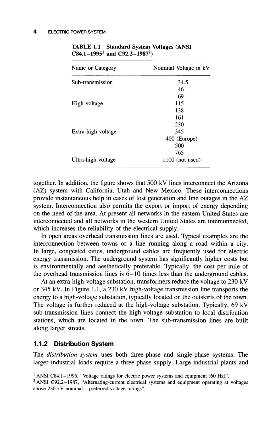
The electric power network is divided into separate transmission and distri-
bution systems based on the voltage level. The system voltage is described by
the root-mean-square (rms) value of the line-to-line voltage, which is the voltage
between phase conductors. The standard transmission line and sub-transmission
voltages are listed in Table 1.1. The line voltage of the transmission system in
the United States is between 115 kV and 765 kV. The ultra-high voltage lines
of 1100 kV are not in commercial use although experimental lines were built.
The 345 kV to 765 kV transmission lines are the extra-high-voltage (EHV) lines,
ELECTRICAL NETWORK 3
Tn San
Di.:go
To Salt Lake City
ln
Colorado
Glen C.m)on
To I o
\ngcles
- 500kV
345-360 kV
- 230-287 kV
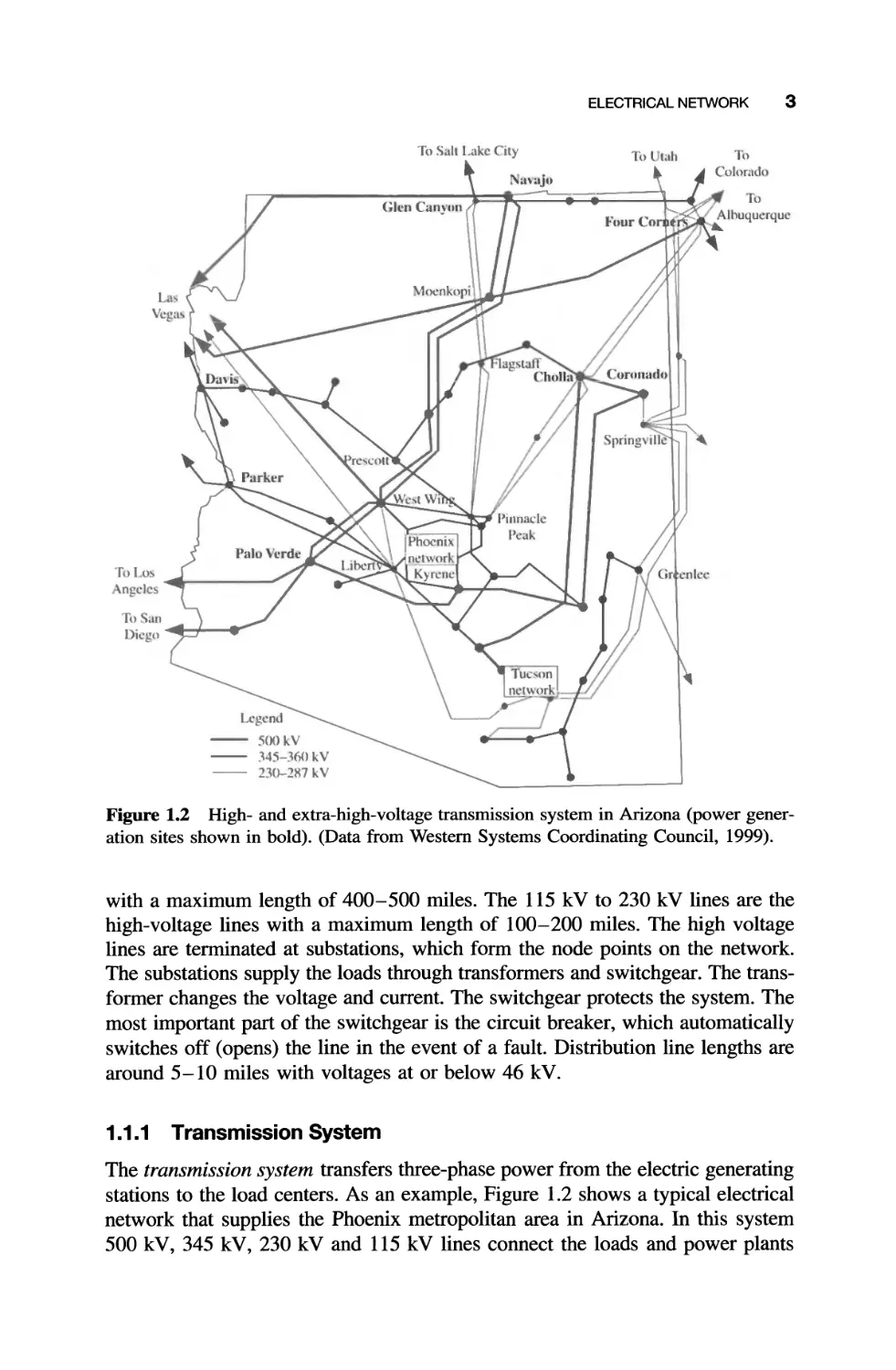
Figure 1.2 High- and extra-high-voltage transmission system in Arizona (power gener-
ation sites shown in bold). (Data from Western Systems Coordinating Council, 1999).
with a maximum length of 400-500 miles. The 115 kV to 230 kV lines are the
high-voltage lines with a maximum length of 100-200 miles. The high voltage
lines are terminated at substations, which form the node points on the network.
The substations supply the loads through transformers and switchgear. The trans-
former changes the voltage and current. The switchgear protects the system. The
most important part of the switchgear is the circuit breaker, which automatically
switches off (opens) the line in the event of a fault. Distribution line lengths are
around 5-10 miles with voltages at or below 46 kV.
1.1.1 Transmission System
The transmission system transfers three-phase power from the electric generating
stations to the load centers. As an example, Figure 1.2 shows a typical electrical
network that supplies the Phoenix metropolitan area in Arizona. In this system
500 kV, 345 kV, 230 kV and 115 kV lines connect the loads and power plants
4 ELECTRIC POWER SYSTEM
TABLE 1.1 Standard System Voltages (ANSI
C84.1-199S 1 and C92.2-1987 2 )
Name or Category
Nominal Voltage in kV
Sub-transmission
34.5
46
69
115
138
161
230
345
400 (Europe)
500
765
1100 (not used)
High voltage
Extra-high voltage
Ultra-high voltage
together. In addition, the figure shows that 500 kV lines interconnect the Arizona
(AZ) system with California, Utah and New Mexico. These interconnections
provide instantaneous help in cases of lost generation and line outages in the AZ
system. Interconnection also permits the export or import of energy depending
on the need of the area. At present all networks in the eastern United States are
interconnected and all networks in the western United States are interconnected,
which increases the reliability of the electrical supply.
In open areas overhead transmission lines are used. Typical examples are the
interconnection between towns or a line running along a road within a city.
In large, congested cities, underground cables are frequently used for electric
energy transmission. The underground system has significantly higher costs but
is environmentally and aesthetically preferable. Typically, the cost per mile of
the overhead transmission lines is 6-10 times less than the underground cables.
At an extra-high-voltage substation, transformers reduce the voltage to 230 kV
or 345 kV. In Figure 1.1, a 230 kV high-voltage transmission line transports the
energy to a high-voltage substation, typically located on the outskirts of the town.
The voltage is further reduced at the high-voltage substation. Typically, 69 kV
sub-transmission lines connect the high-voltage substation to local distribution
stations, which are located in the town. The sub-transmission lines are built
along larger streets.
1.1.2 Distribution System
The distribution system uses both three-phase and single-phase systems. The
larger industrial loads require a three-phase supply. Large industrial plants and
1 ANSI C84.1-1995, "Voltage ratings for electric power systems and equipment (60 Hz)".
2 ANSI C92.2-1987, "Alternating-current electrical systems and equipment operating at voltages
above 230 kV nominal-preferred voltage ratings".
ELECTRIC GENERATION STATIONS 5
factories are supplied directly by a sub-transmission line or a dedicated distribu-
tion line. Ordinary residences are supplied by a single-phase system.
The voltage is reduced at the distribution substation that supplies several distri-
bution lines that deliver the energy along streets. The distribution system voltage
is less than or equal to 46 kV. The most popular distribution voltage in the
United States is the 15 kV class. The actual voltage varies. Typical examples
for the 15 kV class are 12.47 kV and 13.8 kV. As an example in Figure 1.1, a
12 kV distribution line is connected to a 12 kV cable, which supplies commer-
cial or industrial customers. The figure also shows that 12 kV cables supply the
downtown area in a large city.
The residential areas also can be supplied by a 12 kV cable through step-
down transformers, as shown in Figure 1.1. Each distribution line supplies several
step-down transformers distributed along the line. The distribution transformer,
frequently mounted on a pole or placed in the yard of a house, reduces the voltage
to 240/120 V. Short-length low-voltage lines supply the homes, shopping centers
and other local loads.
1.2 ELECTRIC GENERATION STATIONS
An electric generating station converts the chemical energy of gas, oil and coal,
or nuclear fuel to electric energy. In the late 1800s, reciprocating steam engines
were used to drive generators and produce electricity. The more efficient steam
boiler-turbine system replaced the steam engine around the turn of the 19 th century.
The steam boiler bums fuel in a furnace. The heat generates steam that drives the
turbine-generator set. Typically, the steam turbine and generator are mounted on a
common platform/foundation and the shafts are connected together. The turbine-
driven generator converts the mechanical rotational energy to electrical energy.
Figure 1.3 shows a steam turbine and electric generator with its exciter unit.
In the beginning, oil was the most frequently used fuel. Increased petroleum
costs, owing to increased gasoline consumption by automobiles, elevated coal
to the primary fuel for electricity generation. However, environmental concerns
(e.g., sulfur dioxide generation, acid rain, dust pollution, and ash-handling prob-
lems) of coal burning have curtailed the building of new coal-fired power plants.
Recently, natural gas has emerged as the power plant fuel of choice due to three
factors. First, natural gas bums cleaner making plant siting and adherence to envi-
ronmental regulations easier. Second, natural gas is available in large quantities
at a reasonable price. Third, significant increases in plant thermal efficiency have
been achieved using combined cycle plants that utilize gas turbine technology
advances from the aerospace industry. The thermal efficiency is defined as
Pe plant net electric power (energy) output
17th = - = (1.1)
Qth plant thermal power (energy) input
Historically, the hydroelectric power plants developed nearly simultaneously
with the thermal power plants. The river water level is increased by a dam, which
6 ELECTRIC POWER SYSTEM
..
l
- -
- .
Turhlne
.
(;cnl'rafor
Fxcitcr
.....
"
Figure 1.3 Steam turbine and electric generator with exciter. (Courtesy Siemens).
creates a head. The head-generated pressure difference produces fast-flowing
water that drives a hydraulic turbine, which turns the generator. The generator
converts the mechanical energy to electrical energy.
After World War II, electricity generation from nuclear power plants emerged.
More than 500 nuclear plants operate worldwide. In these plants, atomic fis-
sion is produced using enriched uranium. The fission chain reaction heats water
and produces steam. The steam drives the turbine and generator. In the last
two decades, environmental considerations and nuclear power plant capital costs
stopped the building of new plants in the United States and curtailed the operation
of existing plants.
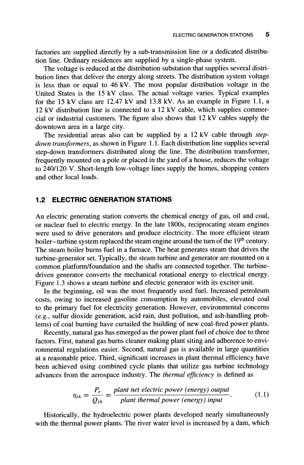
Coal, nuclear, natural gas and hydro power plants generate most of the elec-
tricity in the United States. A breakdown of electricity generation in the United
States for 2000 is given in Figure 1.4. At the present time other energy genera-
tion approaches such as wind, solar, geothermal and biomass produce very little
of the electricity consumed in the United States. Typical technical data of power
plants are presented in Table 1.2.
Economics drives the selection of an appropriate power generation scheme
for the given situation. A utility may need additional generation during high
electricity demand hours (peak load) or the new power may be needed 24 hours
a day (base load). Base load is that load below which the demand never falls, that
is, the base load must be supplied 100% of the time. The peaking load occurs
less than about 15% of the time; the intermediate load is between 15% to 85%
of the time.
In calculating the cost of electricity production ( /kW.hr), the energy cost is
broken into three categories:
1. Capital: land, equipment, construction, interest;
ELECTRIC GENERATION STATIONS 7
2. Operational and maintenance (O&M): wages, maintenance, some taxes and
insurance; and
3. Fuel costs.
Costs are often expressed in mills per kilowatt-hour (kW.hr) where 1,000 mills
equal $1. Since costs are expressed on a per kW.hr basis, a high capacity factor
is desired so the capital cost is spread out. The capacity factor is the ratio of
energy produced during some time interval to the energy that could have been
Natural Gas
16' (
Ilydroelectric
7 .2( (
Nuclear
20((
/
Munu:ipal Solid
\Vastc and Landfill
Ga 0.6(
Petroleum
2.9
\Vood
I .Oc c
Other \Va\tc
0.1 r
Other
2.6 r
Wind
\ :
\ 0.02 c c
Other Gas and
\Va,tc Heat OA('(
Coal
52('(
Geothermal
0...1 (
Figure 1.4 Net electricity generation in the United States for year 2000. (Data from
Annual Energy Review 2000, Energy Information Administration).
TABLE 1.2 Power Plant Technical Data
Equivalent
Plant Construction Forced
Typical Capital Lead Fuel Outage O&M Cost
Generation Size Cost Time Cost Fuel Rate Fixed Variable
Type (MW) ($/kWe) (yrs) ($/MBtu) Type ( days/yr) ($/kVV/yr) ($ h)
Nuclear 1200 2400 10 1.25 Uranium 20 25 8
Pulverized coal 500 1400 6 2.25 Coal 12 20 5
steam
Atmospheric 400 1400 6 2.25 Coal 14 17 6
fluidized bed
Gas turbine 100 350 2 4.00 Nat. gas 7 1 5
Combined cycle 300 600 4 4.00 N at. gas 8 9 3
Coal-gasification 300 1500 6 2.25 Coal 12 25 4
combined cycle
Pumped storage 300 1200 6 5 5 2
hydro
Conventional 300 1700 6 3 5 2
hydro
Source: H.G. Stoll: Least Cost Electric Utility Planning, 1989, John Wiley & Sons, Reprinted by permission.
8 ELECTRIC POWER SYSTEM
produced at net rated power (Pe) during the same period (T), that is,
energy produced during time interval, T
CF = T .
1 Pe(t)dt
( 1.2)
Fuel costs are generally proportional to the plant output so the related energy cost
is constant. The capital and O&M costs generally dictate how a plant is used on
the grid (hydroelectric units are an exception to the following):
Loading
Capital Costs
O&M Costs
Example Plants
Base
Peak
High
Low
Low
High
Coal, Nuclear
Oil
Natural gas is used frequently for intermediate load plants.
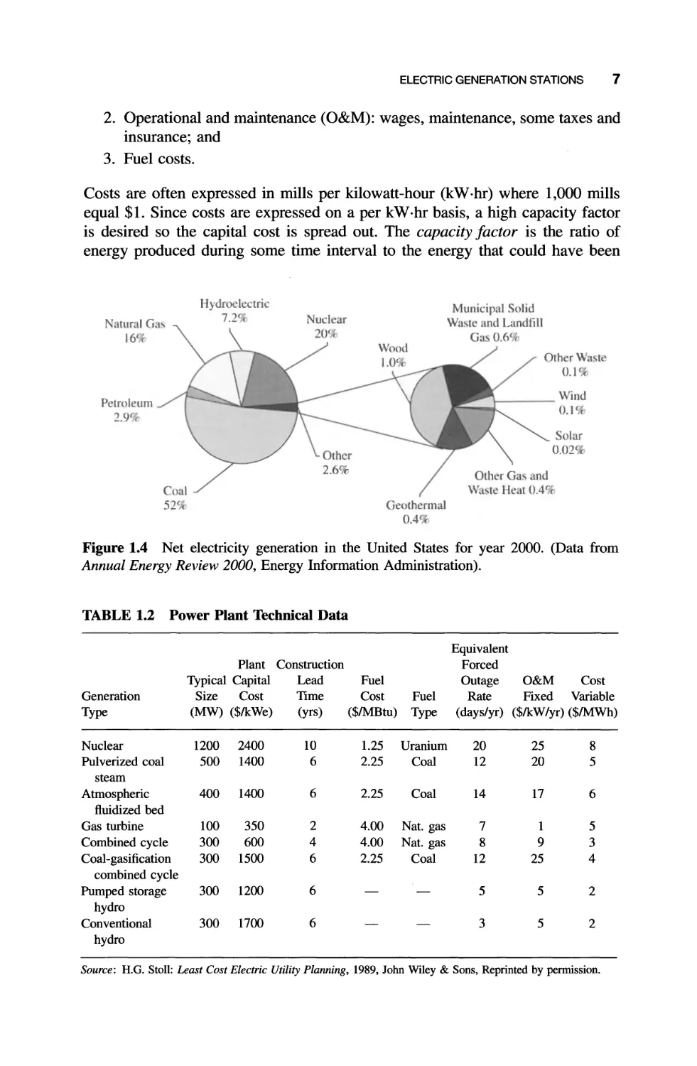
1.3 FOSSIL POWER PLANTS
Fossil power plants Include coal-fired, oil-fired, and natural gas fueled power
plants. Figure 1.5 shows an aerial view of a small generating station in Arizona.
The major components of a thermal power plant are
. Fuel storage and handling;
. Boiler;
. Turbine;
. Generator and electrical system.
1.3.1 Fuel Storage and Handling
Coal is transported by long coal trains with special railcars, or by barge if the
power plant is at a river or seaside. The railcars are tipped and the coal dropped
into a dumper. Conveyer belts carry the coal to an open-air coal yard. The coal
yard stores several weeks of supply. Additional conveyer belts move the coal
into the power plant where the coal is fed through hoppers to large mills. The
mills pulverize the coal to a fine powder. The coal powder is mixed with air
and injected to the boiler through burners. The mixture is ignited as it enters
the furnace.
Oil and liquefied natural gas are also transported by rail, or pipelines. The
power plant stores this fuel in large steel tanks, holding several days of supply.
The oil is pumped to the burners. The burners atomize the oil and mix the small
oil particles with air. The mixture is injected into the furnace and ignited.
FOSSIL POWER PLANTS 9
S\\ itd1) ard
8oill"r. tu rhinc
und encrat()rs
'
.
Gas I .
'",-
C olin ttt" crs
Figure 1.5 Aerial view of a small generating station (Kyrene Generation Station). (Cour-
tesy Salt River Project).
The natural gas, also mixed with air, is fed to the boiler through the burners,
which ignite the mixture as it enters the furnace. Natural gas is the easiest of the
fossil fuels to burn as it mixes well with air and it burns cleanly with little ash.
1.3.2 Boiler
Figure 1.6 shows the flow diagram of a boiler. The boiler is an inverted U-shaped
steel structure. The walls of the boiler are covered by water tubes. The major
systems of a boiler are
. Fuel injection system;
. Air-flue gas system;
. Water-steam system; and
. Ash handling system;
which are discussed below.
1.3.2.1 Fuel Injection System. Natural gas, atomized oil or pulverized coal
is mixed with primary air by the nozzles in the burners and injected into the
furnace. The mixture is ignited either by the high heat in the boiler or by an oil
or gas torch.
10 ELECTRIC POWER SYSTEM
Electrical Pu\\cr
\\ater Generator
\\'.111
R heater
Steam
Condenser
::J :J
1 1 1 1 .; g
g
RUml"r "5
" ..-
.50 I--eed\\ater
pum(') Flue
Fuel ga
Economi/cr tack
\\ ater hcater Frc.;h Cooling \\',Hcr
c
A,h h.mdhng
)
Air
hcall"r
Precipitator
Fabric tilter
so:! Scruhhcr
Air
Q. Air
I--orccd
draft fan
I-uel
pump
I-uel
Fced"ater
Figure 1.6 Flow diagram of a drum type steam boiler.
Secondary air is pumped into the boiler to assure complete burning of the fuel.
The burning fuel produces a high-temperature (around 3000°F) combustion gas
in the boiler, which heats the water in the tubes covering the walls by convection
and radiative heat transfer. The high heat evaporates the water and produces
steam, which is collected in the steam drum.
1.3.2.2 Water-steam System. A large water pump drives the feedwater
through a high-pressure water heater (not shown in Figure 1.6) and the econo-
mizer. Steam removed from the turbine heats the high-pressure feedwater heater.
The hot flue gas heats the economizer. The water is pre-heated to 400-500°F.
The high-pressure and high-temperature feedwater is pumped into the steam
drum. Insulated tubes (called downcomers) located outside the boiler connect the
steam drum to the header at the bottom of the boiler. The water flows through
the downcomer tubes to the header. The header distributes the water among the
riser tubes covering the furnace walls. The water circulation is assured by the
density difference between the water in the downcomer and riser tubes.
FOSSIL POWER PLANTS 11
The burning fuel evaporates the water and produces steam. The saturated
steam is separated in the steam drum. The superheater dries the saturated steam
and increases its temperature to around 1000°F. The superheated steam drives
the high-pressure turbine. The steam exhausted from the high-pressure turbine is
reheated by the flue gas heated reheater. The intermediate-pressure and/or low-
pressure turbines are driven by the re-heated steam. The steam exhausted from
the turbine is condensed into water in the condenser. The condensation generates
vacuum, which extracts the steam from the turbine.
A de aerator is built in the condenser to remove the air from the condensed
water. This is necessary because the air (oxygen) in the water produces corrosion
of the pipes. The power plant loses a small fraction of water during operation.
This necessitates that the gas-free condensed water is mixed with purified feed-
water that replaces the water loss. The mixture is pumped back to the boiler
through the high-pressure feedwater heater and economizer. It can be seen that
the boiler has a closed water circuit. The replacement feedwater is highly puri-
fied and chemically treated. The use of highly purified water reduces corrosion
in the system.
The condenser is a heat exchanger, where the steam condenses in tubes, which
are cooled by water from a nearby source. Heat dissipation techniques include:
. Once-through cooling to a river, lake, or ocean;
. Cooling ponds including spray ponds; and
. Cooling towers.
The former method is the least expensive but can result in thermal pollution.
Thermal pollution is the introduction of waste heat into bodies of water support-
ing aquatic life. The addition of heat reduces the water's ability to hold dissolved
gases, including oxygen which aquatic life requires; although aquatic life growth
is usually enhanced by warm water. To avoid thermal pollution the latter two
methods have been employed. A cooling pond, and its smaller, specialized ver-
sion-the spray pond, are man-made lakes. In a spray pond, the water is pumped
through nozzles to generate fine spray. The evaporation cools the water as it falls
back to the pond.
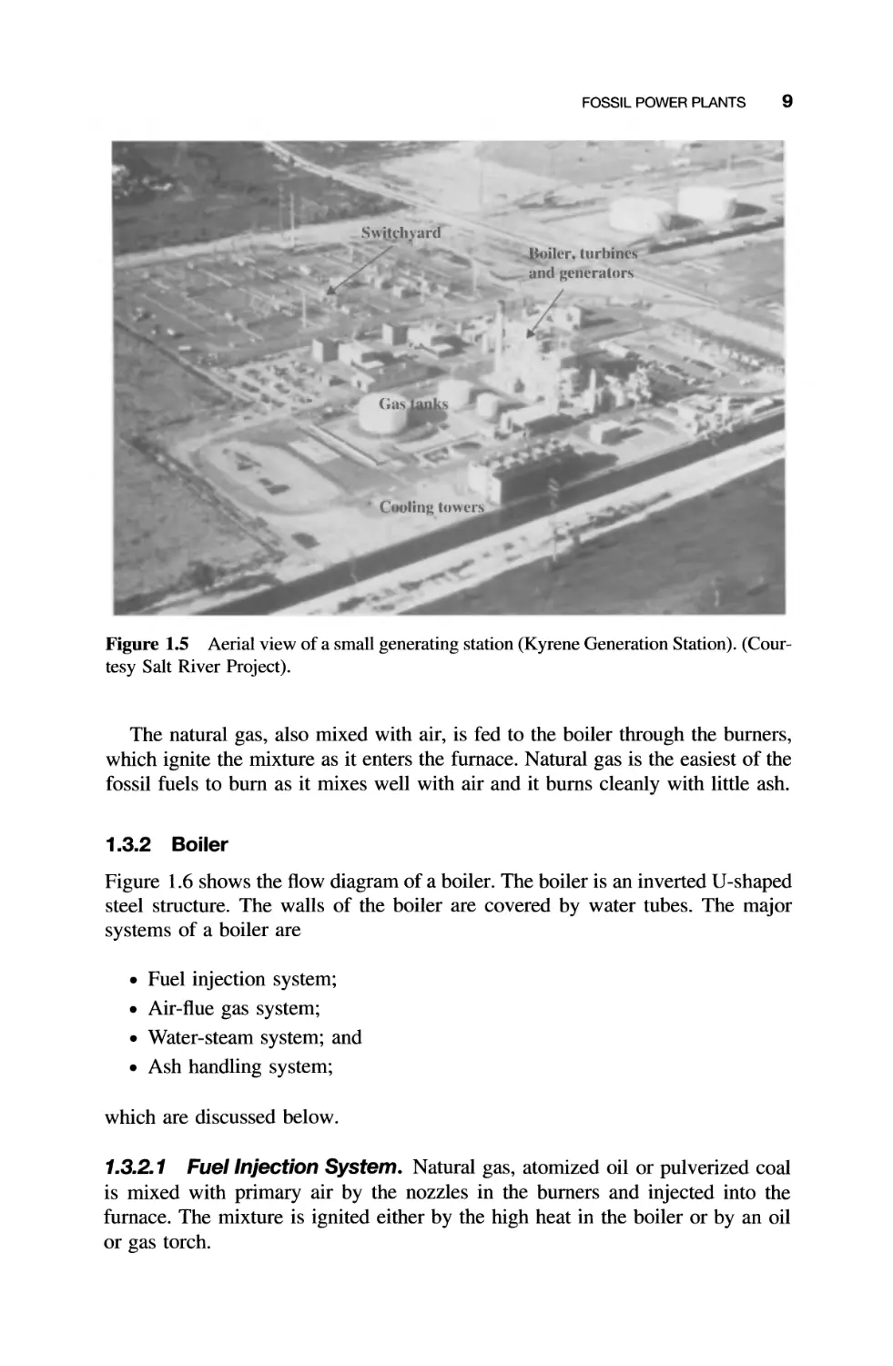
Most cooling towers are of the wet (vs. dry) variety that employs direct water-
to-air contact that can cool more efficiently from the evaporation but which suffers
water loss. Another classification of cooling towers is the air draft mechanism:
natural versus mechanical draft. The natural draft towers are large, tall struc-
tures whereas mechanical draft towers are shorter and employ either forced or
induced draft fans. Most cooling towers are filled with a latticework of horizontal
bars (see Figure 1.7). The baffling within the tower increases the water surface
area for more efficient cooling. The warm water is sprayed on the latticework
at the top of the tower. The water slowly drifts from the top of the tower to
the bottom through the bars. Simultaneously, fans and/or the natural-draft drive
air from the bottom of the tower to the top. The evaporation cools the water
efficiently.
12 ELECTRIC POWER SYSTEM
Water I ntlow
Vap()r Outflow
f f f f
Mechanical "an
HaUling
I!! '. .."!! ". !. ! ..
t::::J t::::J
---. 4-
Air ---. [=:J [=:J V [=:J CJ .- Air
V
In tlO\\ ---. c:::::J [=:J V c:::::J t:::J .- I nllu"
:::::::
----+ [=:J c:::1 V [=:J [=:J ...-
;:2 I I V c:::J
::::::::: - -=- -=- -=- -=- -=- L Water
----=-=-=-- - - - - - - ---.
Drift I Return
Elilninator,
(a)
f f f f f
Vapor
Out tlO\\
Drift
Eliminators
Air '"
(nllo\\
Banlin
D CJ
c::J CJ
CJ CJ
r::J t::J
D D
CJ [:=J
CJ CJ
CJ CJ
Air
Innu\\
========f-======-
Water (nflo\\,
(b)
Figure 1.7 Wet cooling towers (a) Cross-flow induced draft tower; (b) Hyperbolic nat-
ural draft tower.
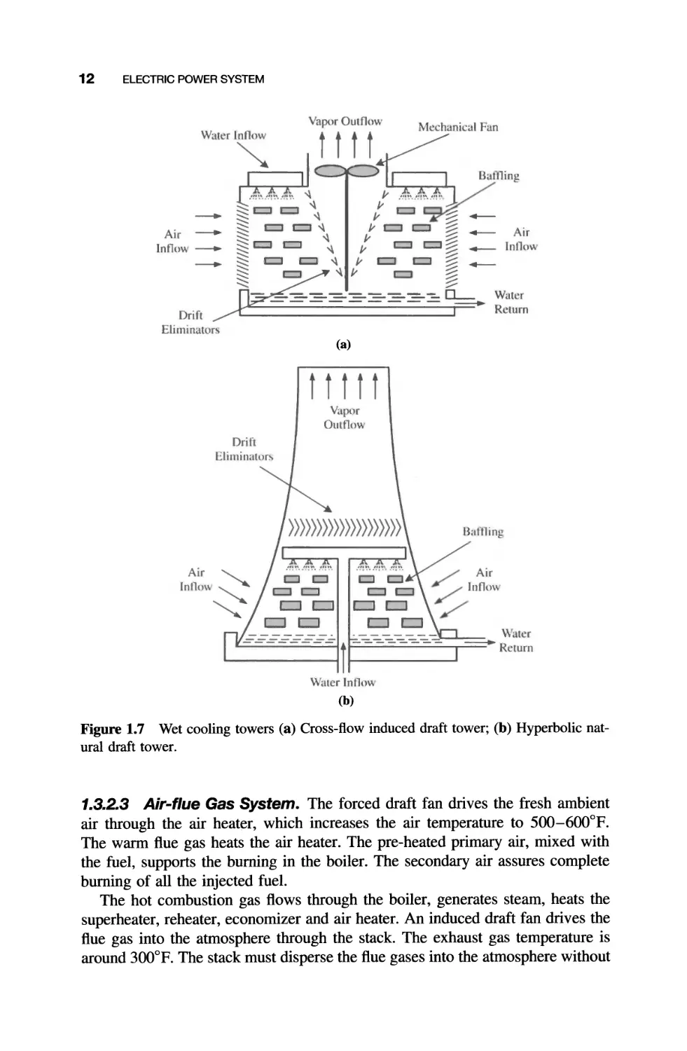
1.3.2.3 Air-flue Gas System. The forced draft fan drives the fresh ambient
air through the air heater, which increases the air temperature to 500-600 o P.
The warm flue gas heats the air heater. The pre-heated primary air, mixed with
the fuel, supports the burning in the boiler. The secondary air assures complete
burning of all the injected fuel.
The hot combustion gas flows through the boiler, generates steam, heats the
superheater, reheater, economizer and air heater. An induced draft fan drives the
flue gas into the atmosphere through the stack. The exhaust gas temperature is
around 300 o P. The stack must disperse the flue gases into the atmosphere without
FOSSIL POWER PLANTS 13
disturbing the environment. This requires filters to remove harmful chemicals and
particles, and sufficient stack height that assures that the residual pollution in the
flue gas is distributed over a large area without causing dangerous concentrations
of pollutants.
Particulate emissions (e.g., fly ash) from burning have historically received the
greatest attention since they are easily seen leaving smokestacks. For a pulverized
coal unit, 60%-80% of the ash leaves the furnace with the flue gas. Two emission
control devices for flyash are the traditional fabric filters and the more recent
electrostatic precipitators. The fabric filters are large baghouse filters having a
high maintenance cost since the cloth bags have a life of only 18 to 36 months,
although the bags can be temporarily cleaned by shaking or back flushing with
air. These fabric filters are inherently large structures resulting in a large pressure
drop, which reduces the plant efficiency.
Electrostatic precipitators have a collection efficiency of 99%, but do not
work well for flyash with a high electrical resistivity (as commonly results from
combustion of low-sulfur coal). In addition, the designer must avoid allowing
unburned gas to enter the electrostatic precipitator since the gas could be ignited.
A side view of an electrostatic precipitator is shown in Figure 1.8. The flue gas,
laden with flyash, is sent through pipes having negatively charged plates that
give the particles a negative charge. The particles are then routed past positively
charged plates, or grounded plates, which attract the now negatively charged
ash particles. The particles stick to the positive plates until they are collected.
Rappers are activated to shake the particles loose so the ash exits through the
hoppers at the base of the unit. The air that leaves the plates is then clean from
harmful pollutants.
Ideally, the hydrocarbon combustion produces water and carbon dioxide
gases; however, without sufficient oxygen (air), incomplete combustion may
High voltage
po.... cr upply
Rappers
Particulat",-
laden t ue ga
Clean gas
to mo estac
ldal collection
plate,
Iloppers
Figure 1.8 Electrostatic precipitator.
14 ELECTRIC POWER SYSTEM
occur leaving the intermediate product of carbon monoxide (CO). Carbon
monoxide production is generally reduced by providing excess air (oxygen) to
the furnace.
2H 2 + 02 -+ 2 H 2 0
C + 02 -+ C 0 2
The main gaseous pollutants from combustion include sulfur oxides (SOx),
nitrous oxides (NO x ), and carbon monoxide (CO). Both SOx and NO x can
create acid rain composed of H2S04 and HN03, respectively. The SOx, mostly
S02 and some S03, can cause respiratory irritation. The NO x contributes to
smog and ozone formation, and vegetation damage. The CO reduces the oxygen
carrying capability of the blood, referred to as carbon monoxide poisoning. The
Clean Air Act sets the federal standards for plant emissions, although individual
states may establish limits that are more stringent.
To reduce SOx emissions, many power plants have chosen to use low-sulfur
fuel. Coal from the western United States typically is low in sulfur content
whereas high-sulfur coal dominates from eastern states. Natural gas that is high
in H 2 S is known as sour gas, in contrast to sweet gas, which is low in sulfur. A
flue-gas desulfurization system is often employed to remove the S02. Both wet
and dry sulfur scrubbing processes are in use today. The dry process, in which a
lime or limestone solution is sprayed into the flue gas, is the most economical.
The wet scrubbing process is more efficient and may be implemented as either a
throwaway or a recovery method. Although the recovery products of sulfur and
sulfuric acid can be sold, the more popular is the wet, throwaway limellimestone
process which utilizes the chemical reaction:
S02 + CaC03 -+ CaS03 + C02
Most NO x originates from the nitrogen in the fuel rather than N 2 in the air.
To reduce NO x emissions tighter control of the combustion process is employed
through combustion temperature (reduction) or lowering the air-fuel ratio. As
in automobiles, exhaust gas recirculation can be used to reduce combustion tem-
perature.
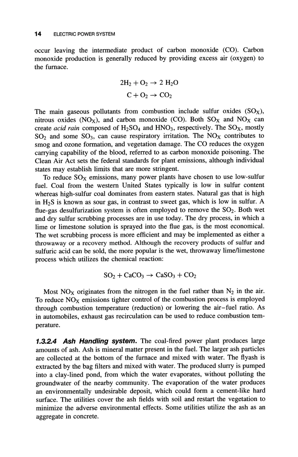
1.3.2.4 Ash Handling system. The coal-fired power plant produces large
amounts of ash. Ash is mineral matter present in the fuel. The larger ash particles
are collected at the bottom of the furnace and mixed with water. The flyash is
extracted by the bag filters and mixed with water. The produced slurry is pumped
into a clay-lined pond, from which the water evaporates, without polluting the
groundwater of the nearby community. The evaporation of the water produces
an environmentally undesirable deposit, which could form a cement-like hard
surface. The utilities cover the ash fields with soil and restart the vegetation to
minimize the adverse environmental effects. Some utilities utilize the ash as an
aggregate in concrete.
FOSSIL POWER PLANTS 15
1.3.3 Turbine
The high-pressure, high-temperature steam drives the turbine. The heat energy
in the steam is converted to mechanical energy. The turbine has a stationary
part and a rotating shaft. Both are equipped with blades. The length of the
turbine blades decreases from the exhaust to the steam entrance. The shaft is
supported by bearings. The steam is supplied through the stationary part of the
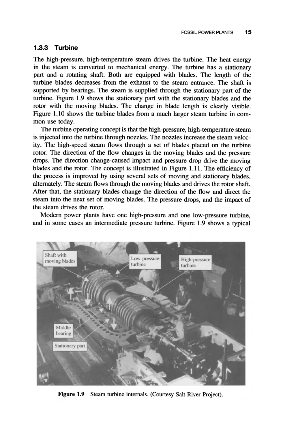
turbine. Figure 1.9 shows the stationary part with the stationary blades and the
rotor with the moving blades. The change in blade length is clearly visible.
Figure 1.10 shows the turbine blades from a much larger steam turbine in com-
mon use today.
The turbine operating concept is that the high-pressure, high-temperature steam
is injected into the turbine through nozzles. The nozzles increase the steam veloc-
ity. The high-speed steam flows through a set of blades placed on the turbine
rotor. The direction of the flow changes in the moving blades and the pressure
drops. The direction change-caused impact and pressure drop drive the moving
blades and the rotor. The concept is illustrated in Figure 1.11. The efficiency of
the process is improved by using several sets of moving and stationary blades,
alternately. The steam flows through the moving blades and drives the rotor shaft.
After that, the stationary blades change the direction of the flow and direct the
steam into the next set of moving blades. The pressure drops, and the impact of
the steam drives the rotor.
Modern power plants have one high-pressure and one low-pressure turbine,
and in some cases an intermediate pressure turbine. Figure 1.9 shows a typical
Shaft with
mo\ ing hlade
Low-pre surc
turbine
High-pre '\urc
turbine
......
,,'" ' '. I I I
.
....
"
. "'
-.
..
.'
. ,
.
1iddlc
bedring
...
Stationary pan .
...
. .
.. ,
. , I
\
Figure 1.9 Steam turbine intemals. (Courtesy Salt River Project).
16 ELECTRIC POWER SYSTEM
i ... --
... t
.
.
--... , ,
\ ..
;
- ...
--.....
..
-
Figure 1.10 Turbine blades in a large unit. (Courtesy Siemens).
N07/le
HI ade
; !
o
A
: :
:
I t I
I I
I I
I I
I I
I I
f\10\ ing Stational) Mo\ in!! Stationary
Blade Blade Blade
I " B '
I I I I
I I
I I I I
A
8A8
8A8
: t :
i'-=./i I I i'-=./i
I I I I I I
I I I I I I
I I I I I I
Figure 1.11 Operating concept of a steam turbine.
unit with two turbines. The right-hand side is the high-pressure turbine; the
left-hand side is the low-pressure turbine. A bearing is placed between the two
units. The steam enters at the right-hand side, drives the high-pressure turbine
and exhausts before the middle bearing. The exhausted steam is reheated and
fed to the low-pressure turbine. The reheated steam enters just behind the middle
FOSSIL POWER PLANTS 17
bearing and drives the low-pressure turbine. The steam exhausts at the end of
the turbine. The arrows indicate the steam entrance and exhaust points.
1.3.4 Generator and Electrical System
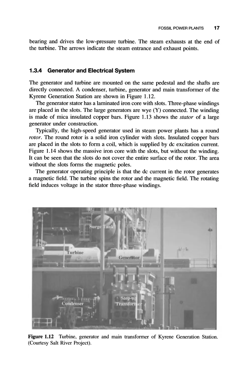
The generator and turbine are mounted on the same pedestal and the shafts are
directly connected. A condenser, turbine, generator and main transformer of the
Kyrene Generation Station are shown in Figure 1.12.
The generator stator has a laminated iron core with slots. Three-phase windings
are placed in the slots. The large generators are wye (Y) connected. The winding
is made of mica insulated copper bars. Figure 1.13 shows the stator of a large
generator under construction.
Typically, the high-speed generator used in steam power plants has a round
rotor. The round rotor is a solid iron cylinder with slots. Insulated copper bars
are placed in the slots to form a coil, which is supplied by dc excitation current.
Figure 1.14 shows the massive iron core with the slots, but without the winding.
It can be seen that the slots do not cover the entire surface of the rotor. The area
without the slots forms the magnetic poles.
The generator operating principle is that the dc current in the rotor generates
a magnetic field. The turbine spins the rotor and the magnetic field. The rotating
field induces voltage in the stator three-phase windings.
. .
:urg' .
...
. -
,..
I -
rurhin
Gl'n 1tor
I
· . el-u
Co d' er
.
. .
I
Figure 1.12 Turbine, generator and main transformer of K yrene Generation Station.
(Courtesy Salt River Project).
18 ELECTRIC POWER SYSTEM
,
I
"
.
.. \ \ \ I
, . \ - \
- "
" J I
"'
..)
I
.
.. L
- . " ' .
. . -
.- .
'>
'. '\ ,
.. ,
. ''\
. \'
#t ".
, .
. " --- to
. .. ,
ft,
'\ . ..
.
.. . . .
\ .... .
Figure 1.13 Synchronous generator stator. (Courtesy Westinghouse Corporation).
'" ......
,
"1 ) "
. . ,
'( .
. \ '
"" :
. .
. .
......
t
,
Figure 1.14 Synchronous generator rotor. (Courtesy Siemens).
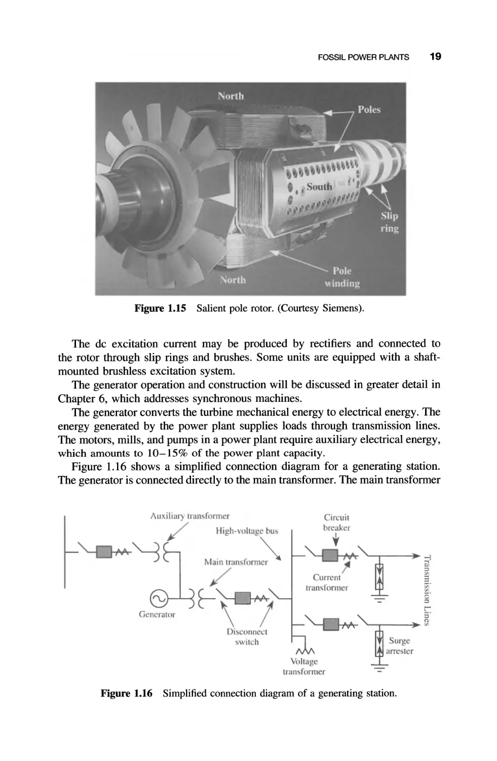
The hydro generators use a salient pole rotor, as shown in Figure 1.15. This
rotor has poles with dc windings. The poles are supplied by dc current through
brushes connected to the slip rings.
High-pressure oil-lubricated bearings support the rotor at both ends. The bear-
ings are insulated at the opposite side of the turbine connection to avoid shaft
currents generated by stray magnetic fields.
The small generators are cooled by air, which is circulated by fans attached to
the rotor. The large generators are hydrogen cooled. The hydrogen is circulated
in a closed loop and cooled by a hydrogen-to-water heat exchanger. The very
large generators are water-cooled. The cooling water is circulated through the
special hollow conductors of the windings.
FOSSIL POWER PLANTS 19
North
Poles
"
,
I
I 'I
. .
....j
. . South
:t "....,.'
.' ." ,
," '
It' I
.
.
, , ,
.' I, '
Slip
ring
North
Pole
\\ inding
Figure 1.15 Salient pole rotor. (Courtesy Siemens).
The dc excitation current may be produced by rectifiers and connected to
the rotor through slip rings and brushes. Some units are equipped with a shaft-
mounted brushless excitation system.
The generator operation and construction will be discussed in greater detail in
Chapter 6, which addresses synchronous machines.
The generator converts the turbine mechanical energy to electrical energy. The
energy generated by the power plant supplies loads through transmission lines.
The motors, mills, and pumps in a power plant require auxiliary electrical energy,
which amounts to 10-15% of the power plant capacity.
Figure 1.16 shows a simplified connection diagram for a generating station.
The generator is connected directly to the main transformer. The main transformer
'-3
Auxiliary tran former
} ligh-\ oltage hu'\
Main lran'fnrm
Circuit
hrea cr
'-.J'
Generator
Current
transfonner
oJ
.F
....
....
.F
.F
,...
:5
c
....
G
tr
Disconnect
\.. itch
Surge
arre,ter
Voltage
transformcr
Figure 1.16 Simplified connection diagram of a generating station.
20 ELECTRIC POWER SYSTEM
supplies the high-voltage bus through a circuit breaker, disconnect switches and
current transformer. An auxiliary transformer is also connected directly to the
generator. The generating station auxiliary power is supplied through this trans-
former. A circuit breaker, disconnect switches and current transformer protect the
auxiliary transformer at the secondary side of the transformer. The use of a circuit
breaker at the generator side is uneconomical in the case of large generators.
The high-voltage bus forms a node point and distributes the generator power
among the transmission lines. The voltage of the bus is monitored using a voltage
transformer.
The two outgoing transmission lines are connected to the bus. The lines are
protected against lightning and switching surge by a surge arrester. Each line is
also protected by a circuit breaker. Two disconnect switches permit the separation
of the circuit breaker in case of circuit breaker fault. The current transformer
measures the line current and activates the protection in the event of a line
fault. The protection relay triggers the circuit breaker, which switches off (opens)
the line. The high-voltage bus configuration in Figure 1.16 is not typical; the
operation of a circuit breaker and other protection components will be discussed
in more detail in Section 1.6.1.
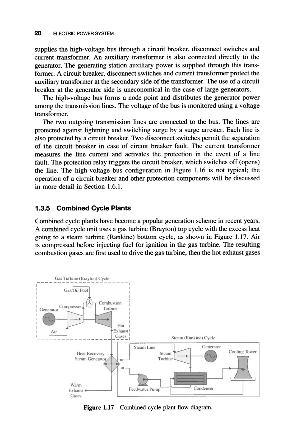
1.3.5 Combined Cycle Plants
Combined cycle plants have become a popular generation scheme in recent years.
A combined cycle unit uses a gas turbine (Brayton) top cycle with the excess heat
going to a steam turbine (Rankine) bottom cycle, as shown in Figure 1.17. Air
is compressed before injecting fuel for ignition in the gas turbine. The resulting
combustion gases are first used to drive the gas turbine, then the hot exhaust gases
G&i' 1 urhinc (Brayton) Cyclc
Ga /Oil fuel
Comhu tion
Turhine
Hot
Air Exhau t
Ga.,c, I
----__________________J
C;te..11U Lin..-
Stc..am (Ranl-..inc) Cycle
Gcncrator
Coolin!! To\\er
I. A
, Con<kn",r I
Heat Reco\ery
Steam Generator
Steam
Turhine
\\'ann
F,hau,t
G&l'C
;\ L{fl
Fccd:;;r Pump
Figure 1.17 Combined cycle plant flow diagram.
NUCLEAR POWER PLANTS 21
are sent to a heat recovery steam generator (HRSG), before release through the
stack. The heat transferred to the HRSG produces steam, which is used to drive a
steam turbine-generator set. Some combined cycle plants use burners to increase
(augment) the Rankine cycle steam quality. The bottom steam cycle employs
condenser cooling, as is normally found in a thermal power plant.
The overall thermal efficiency of combined cycle plants built today is a remark-
able 60%. Combined cycle plants are designed for intermediate load since they
are relatively quick to start. Additional advantages of these plants are that they
can be constructed in a relatively short period (about 2 years), and their use of
natural gas, which is an environmentally good choice (except for greenhouse gas
emission), and a reasonably priced fuel.
The greenhouse effect on global warming has received significant attention
in recent years. Many scientists believe that the increased emission of green-
house gases, such as water vapor, carbon dioxide, nitrous oxide and methane,
is causing the temperature of the Earth to rise. Short-wavelength radiation from
the sun passes through the atmosphere without interference from the greenhouse
gases. The transmitted sunlight is then absorbed by the Earth's surface. Later, the
absorbed energy is re-emitted by the Earth as long-wavelength radiation. This
long-wavelength radiation (unlike the short-wavelength sunlight) is absorbed by
the greenhouse gases (such as CO 2 , which can originate from combustion); thus
heating the Earth's atmosphere.
1.4 NUCLEAR POWER PLANTS
Nuclear power plants are a major part of the electrical energy generation industry.
More than 500 plants are in operation worldwide. The most popular plants (close
to 300) are the pressurized water reactors (PWRs). In addition, there are more
than 100 boiling water reactors (BWRs) and 50 gas-cooled reactors. Further, close
to 50 heavy-water reactors and a few breeder reactors operate around the world.
A nuclear power plant generates electricity in a manner very similar to a
fossil power plant. Typically, nuclear plants provide base energy, running at
practically constant load. Their electric output is around 1000 MW. Concern with
thermal pollution increased with the construction of nuclear plants due to their
large size and lower thermal efficiency (17th 33%) as compared to coal-fired
units (17th 40%), and the fact that all the heat rejection from a nuclear plant
is via the condenser cooling water, whereas a fossil unit also releases excess
heat through the stack. For this reason nuclear plants sought alternative heat-
dissipation techniques such as the tall natural draft cooling towers, with which
nuclear units are so commonly associated.
The advantages of nuclear power are the abundant and relatively cheap fuel,
and the pollution free operation in normal conditions. However, leaks or equip-
ment failure could allow radioactive gas or liquid (water) discharge that might
pose a health hazard to the surrounding communities. An additional unanswered
question is the final storage of the spent fuel, which is radioactive and hazardous.
A similar concern is the decommissioning of old and obsolete plants.
22 ELECTRIC POWER SYSTEM
Decreased energy consumption in the United States after the energy crises of
the 1970s, along with the listed environmental and health concerns, stopped or
slowed the building of new nuclear plants and curtailed the operation of several
existing plants in the United States. These actions resulted in severe financial
losses for several utilities. Nevertheless, several hundred nuclear plants are in
operation and generating large amounts of energy worldwide.
1.4.1 Nuclear Reactor
Most power reactors use enriched uranium as a fuel. The U02 is pressed into
pellets and the pellets are stacked in a Zircaloy-clad rod. These rods are the
fuel elements used in a reactor. Many fuel rods are placed in a square lattice
to construct a fuel assembly, as shown in Figure 1.18. A couple hundred fuel
assemblies are generally needed to fuel the entire reactor core. This reactor core
is housed in a reactor pressure vessel that is composed of steel 8 to 10 inches
thick. The reactor core is filled with fuel and control rods. The atomic reaction
is controlled by the position of the control rods. Figure 1.19 shows the nuclear
reactor vessel where the core is located. The control and fuel rods are arranged
in a pattern carefully calculated during the reactor design.
Most reactors use neutrons in thermal equilibrium «0.1 eV) with a moderator
to sustain the chain reaction, and hence, are called thermal reactors. The fission
reaction emits neutrons at fast energy levels (> 1 MeV). Thermal reactors employ
a moderator such as light water, heavy water, or graphite to slow down the
Spacer
Grids
----
--
/'
"
//
\
'-
.
. ...
. .
. ....
..
... . .
. . ..
.
Nuclear
Fuel
Pellet
..
Cladding
"" .
.
.
.
.
.
.
.
.
. ..
..
Fuel Rod - .. I
GUide Tube -
'-
Instrument Tube -
0.-.... ....
ODIWOC ,,'" Z
Figure 1.18 Nuclear reactor fuel pellet, rod and assembly. (Source: DOE OCRWM).
NUCLEAR POWER PLANTS 23
Control Rod
Dri\e 1cchani m
I i ;
j I..
Re tctor VC :"Id Hcad
(see detailed inlagc)
- ,
41
, ,,.- f
,
Core Barrel
"
,
'.
Control Rod
Drive Shaft
.,.
I - --
7
I
Core Support
I
I I
-- I
- .:. . . I.
- - <>...;.-.. J
- - .....0 :=-.....
f ' e o-o .:.:. .
. 00 eel:J .....
o '- ( e
,\.. e .. e -0"
oi ."
j 1
'"
RCilctor Vc cI
Figure 1.19 Nuclear reactor vessel. (Source: DOE EIA).
neutrons. Such thermal reactors are easier to control than fast (breeder) reactors
and some designs can use natural uranium. In the United States, most nuclear
plants utilize light water reactors (LWRs), which include the PWRs and BWRs.
The nuclear reaction starts if sufficient numbers (a critical mass) of rods are
placed in a confined space. Natural uranium consists of about 0.7% of the isotope
24 ELECTRIC POWER SYSTEM
uranium-235 (U-235) and the remainder (99.3%) is U-238. Uranium-235 readily
undergoes fission by thermal neutrons, whereas U-238 does not. In most cases,
the fuel is enriched to about 3% U-235 to achieve a sustained reaction.
The neutron absorption by the uranium initiates atomic fission. The fission of
the uranium expels v neutrons and releases heat energy (Q).
235U + 1 n -+ ( 236 U ) * -+ AI X + A2X + v 1 n + Q
92 0 92 Zl Z2 0
The freed neutrons (v 2-3 emitted neutrons per fission) sustain the chain reac-
tion; the generated heat is utilized to produce steam. In addition to neutrons
and heat, the nuclear fission produces 2- 3 fission fragments (X). These fission
products are radioactive and have half-lives on the order of a thousand years.
The cooling water enters the reactor, flows through the core and removes the
heat generated by the nuclear fission. Safe reactor operation basically involves
making sure that heat is adequately removed from the core in order to avoid
release of radioactivity from the plant. This can be ensured by maintaining
the U02 fuel temperature below its melting temperature of about 5000°F, and
by keeping the cladding temperature below the point ( 2200°F) at which the
exothermic zirconium-water reaction occurs.
The nuclear reaction is controlled to maintain proper heat generation. The
reaction is regulated using control rods, which can be constructed of neutron-
absorbing material such as boron, silver, cadmium, and indium. The withdrawal
of the control rods increases the reaction rate and heat generation. The insertion
of the control rods reduces the power generation. The reactor is shut down by
inserting all the control rods into the core.
In addition to causing fission, some neutrons undergo parasitic capture by the
uranium-238. The added neutron increases the atomic mass of the U-238, which
can be transformed to plutonium-239 via the following reactions and radioac-
tive decays:
238 u+ In
92 0
239 N p
93
) 2 U 23.5min ) 2 Np+_ e
2.355 day ) 239 PU+ 0 e
94 -1
Pu-239 and other nuclides of higher atomic number than uranium are termed the
transuranics. The transuranics are radioactive and long-lived, having half-lives
of thousands of years.
Nuclear waste is classified as either low-level or high-level waste. Low-level
waste includes clothing, rags, and tools, which are sealed in a drum for ultimate
placement in a dedicated landfill. The high-level waste includes fission products
and transuranic isotopes, and is highly radioactive and must be stored for long
periods. Approximately once every 18 months the reactor is shutdown for refu-
eling, at which point about one-third of the (spent) fuel assemblies are removed.
At present, United States government policy prohibits chemical reprocessing of
spent fuel rods from commercial nuclear power plants. Instead, the spent fuel
NUCLEAR POWER PLANTS 25
assemblies will likely be placed in corrosion-resistant metal canisters, which will
be housed in an underground repository. For the past 20 years, studies have been
conducted to determine whether Yucca Mountain (located 100 miles northwest
of Las Vegas, Nevada) can serve as a suitable geologic repository.
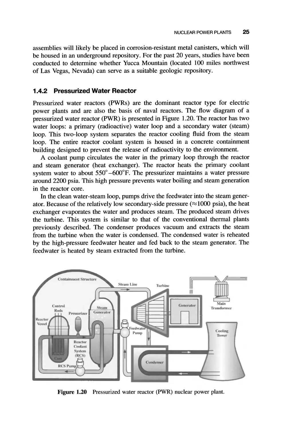
1.4.2 Pressurized Water Reactor
Pressurized water reactors (PWRs) are the dominant reactor type for electric
power plants and are also the basis of naval reactors. The flow diagram of a
pressurized water reactor (PWR) is presented in Figure 1.20. The reactor has two
water loops: a primary (radioactive) water loop and a secondary water (steam)
loop. This two-loop system separates the reactor cooling fluid from the steam
loop. The entire reactor coolant system is housed in a concrete containment
building designed to prevent the release of radioactivity to the environment.
A coolant pump circulates the water in the primary loop through the reactor
and steam generator (heat exchanger). The reactor heats the primary coolant
system water to about 550° -600°F. The pressurizer maintains a water pressure
around 2200 psia. This high pressure prevents water boiling and steam generation
in the reactor core.
In the clean water-steam loop, pumps drive the feedwater into the steam gener-
ator. Because of the relatively low secondary-side pressure ( 1000 psia), the heat
exchanger evaporates the water and produces steam. The produced steam drives
the turbine. This system is similar to that of the conventional thermal plants
previously described. The condenser produces vacuum and extracts the steam
from the turbine when the water is condensed. The condensed water is reheated
by the high-pressure feedwater heater and fed back to the steam generator. The
feedwater is heated by steam extracted from the turbine.
r[l
\hin
I rnn,rnrn1l"r
I'urhine
III
III
("ontn)&
RINI..
I I I
(;cncratur
R...a....nr
, l"......1
..I'T"Uri/l'r
...
('oolin
1U\\Cf
RCS It ump
.--
F,......".... n
I'UIIII' i
t
---
Cundcn..er
Figure 1.20 Pressurized water reactor (PWR) nuclear power plant.
26 ELECTRIC POWER SYSTEM
Cooling pond
"'-..
Cooling to\\'crs
f"..
Reactor
contalnn1cnt
building
TurbioL
g ncn)tur
buildin
....
...
l
I
-
s\\ itch ani
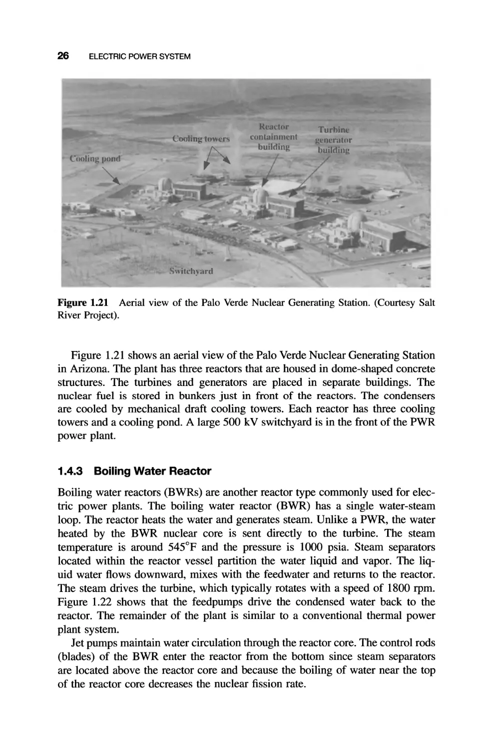
Figure 1.21 Aerial view of the Palo Verde Nuclear Generating Station. (Courtesy Salt
River Project).
Figure 1.21 shows an aerial view of the Palo Verde Nuclear Generating Station
in Arizona. The plant has three reactors that are housed in dome-shaped concrete
structures. The turbines and generators are placed in separate buildings. The
nuclear fuel is stored in bunkers just in front of the reactors. The condensers
are cooled by mechanical draft cooling towers. Each reactor has three cooling
towers and a cooling pond. A large 500 kV switchyard is in the front of the PWR
power plant.
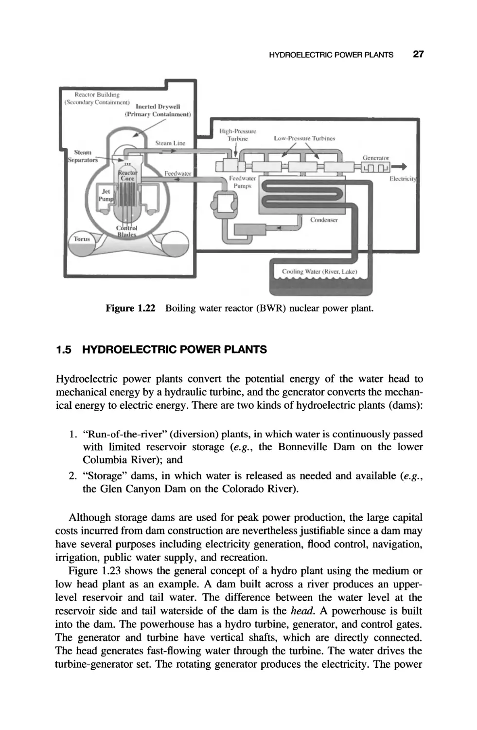
1.4.3 Boiling Water Reactor
Boiling water reactors (BWRs) are another reactor type commonly used for elec-
tric power plants. The boiling water reactor (BWR) has a single water-steam
loop. The reactor heats the water and generates steam. Unlike a PWR, the water
heated by the BWR nuclear core is sent directly to the turbine. The steam
temperature is around 545°F and the pressure is 1000 psia. Steam separators
located within the reactor vessel partition the water liquid and vapor. The liq-
uid water flows downward, mixes with the feedwater and returns to the reactor.
The steam drives the turbine, which typically rotates with a speed of 1800 rpm.
Figure 1.22 shows that the feedpumps drive the condensed water back to the
reactor. The remainder of the plant is similar to a conventional thermal power
plant system.
Jet pumps maintain water circulation through the reactor core. The control rods
(blades) of the BWR enter the reactor from the bottom since steam separators
are located above the reactor core and because the boiling of water near the top
of the reactor core decreases the nuclear fission rate.
HYDROELECTRIC POWER PLANTS 27
Reactor BUilding
(SeC:tmd.11) Conlainrnenl)
Im'rh'd UQ 'H.II
.I-rim..n Cunlalnment)
Stc.tm line
I tm -Pre!'a!'aur Turhinc!'a
Slt'um
"'("paralor.
.1
-....
Rl'3rtU
I Curl
l J{'l"'" 1 1 1 ' 1 1
PumJ- 1
I
Cunl ul
J .ul .
...
Feed" .tter
I.eed"aler
a Pump!.
EIcC:lric:il:
-== Cunllcn-.cr
Tu rU"
Cooling \\alcr (Rj\cr. I ale)
Figure 1.22 Boiling water reactor (BWR) nuclear power plant.
1.5 HYDROELECTRIC POWER PLANTS
Hydroelectric power plants convert the potential energy of the water head to
mechanical energy by a hydraulic turbine, and the generator converts the mechan-
ical energy to electric energy. There are two kinds of hydroelectric plants (dams):
1. "Run-of-the-river" (diversion) plants, in which water is continuously passed
with limited reservoir storage (e.g., the Bonneville Dam on the lower
Columbia River); and
2. "Storage" dams, in which water is released as needed and available (e.g.,
the Glen Canyon Dam on the Colorado River).
Although storage dams are used for peak power production, the large capital
costs incurred from dam construction are nevertheless justifiable since a dam may
have several purposes including electricity generation, flood control, navigation,
irrigation, public water supply, and recreation.
Figure 1.23 shows the general concept of a hydro plant using the medium or
low head plant as an example. A dam built across a river produces an upper-
level reservoir and tail water. The difference between the water level at the
reservoir side and tail waterside of the dam is the head. A powerhouse is built
into the dam. The powerhouse has a hydro turbine, generator, and control gates.
The generator and turbine have vertical shafts, which are directly connected.
The head generates fast-flowing water through the turbine. The water drives the
turbine-generator set. The rotating generator produces the electricity. The power
28 ELECTRIC POWER SYSTEM
Dat11
HC ld water
Turbine and
generator
-------------"
-----------------------i
------------j
-----------
Head
PO\\ cr
house
Re ef\-oir
Tail \\ater
Water
intak
Draft tube
Spillwa}
and darn
Tail \\-ater
Reservoir
Control
gate,
o
o
PO\\ er
h()u e
Figure 1.23 Hydroelectric power plant (medium or low head).
obtained from a hydro pla t is the product of the head (H), water density (p),
and volumetric flow rate (V):
P==HpgV,
(1.3)
where g is gravitational acceleration. The water discharged from the turbine flows
to the tail water reservoir, which frequently is the continuation of the original
river. Control gates regulate the flow through the turbine. In the event of a flood,
the spillway gates open sending overflow across the dam, or diversion gates at
the bottom of the dam may be opened. Both actions allow the direct flow of the
HYDROELECTRIC POWER PLANTS 29
excess water to the tail water reservoir, which eliminates the overloading of the
dam. Additional gates at the water intake and draft tube permit the isolation and
removal of water from the turbine during maintenance.
1.5.1 Low Head Hydro Plants
Figure 1.24 shows the cross-section of a low head powerhouse, with a Kaplan tur-
bine. A large oil-immersed truss bearing supports both the generator and turbine.
The upper, watertight chamber houses the vertical shaft generator. The vertical
shaft Kaplan turbine is like a large propeller with 4-10 blades. The pitch of the
blades is adjustable between 5° to 35° by a hydraulic servomechanism.
The water enters the turbine through gates and is evenly distributed by a spiral
casing surrounding the turbine. The flow is regulated by "wicket gates" and by
the adjustment of the pitch. The water speed in the turbine is around 10-30 ft/s.
The water is discharged from the turbine through an elbow-shaped draft tube that
reduces the water velocity to 1-2 ft/s.
The hydro generator is a salient pole machine. Typically, the machine has 20- 72
poles. These poles are supplied by dc current and they produce the magnetic
field that induces the voltage in the generator. The shaft speed is 100-300 rpm.
Figure 1.25 shows a large hydro generator in the construction phase.
Generator
Wackel Gate
Gate
Figure 1.24 Cross-section of a hydropower house. (Source: D.G. Fink, Standard Hand-
bookfor Electrical Engineers, New York: McGraw-Hill, 1978, with permission).
30 ELECTRIC POWER SYSTEM
.
I
-
.-
o..
r -
-..
1,-
Poles
Stato
1
-".- "
"
Figure 1.25 Large salient pole hydro generator under construction. (Courtesy Toshiba).
A welded spoke wheel supports the pole spider. The poles have a laminated
iron core with dc windings, using stranded copper conductors. Short-circuited
damper bars are built in each pole face.
The stator is laminated iron with slots. A welded steel frame holds the iron
core. A three-phase winding is placed in the stator slots. The turn-to-turn insu-
lation is fiberglass or Dacron glass. The turn-to-ground insulation is epoxy or
polyester resin impregnated mica tape. The larger machines have a braking sys-
tem that rapidly stops the machine when removed from service.
1.5.2 Medium- and High-head Hydro Plants
In addition to the described low-head hydro, medium- and high-head hydro plants
are in operation. The medium-head hydro has similar construction, but uses the
Francis turbine, which has a different blade arrangement, as shown in Figure 1.26.
Figure 1.27 shows the arrangement of a high-head hydro plant. The high-head
hydro uses an impulse turbine. The large head-produced, high water pressure is
converted to a high-velocity water jet, which drives the turbine. The rating of a
high-head hydro plant is generally less than 100 MW.
1.5.3 Pumped Storage Facility
Also related to hydroelectric power is the practice of using pumped storage
facilities as an energy storage device. Pumped storage facilities consist of both
high-elevation and low-elevation reservoirs, as shown in Figure 1.28. The power-
plant chamber of the pumped storage facility houses a reversible hydraulic turbine
HYDROELECTRIC POWER PLANTS 31
i
---- -
(
... "
,
......
\ ' ..
. .
#,
"
--------
Figure 1.26 Wheel of a medium head Francis turbine. (Courtesy Hydro-Quebec).
similar to that used in a dam. The direction of this turbine can be reversed by
supplying the special motor-generator with electricity, such that it becomes a
pump to transfer water to the upper reservoir. Such pumped storage units, like
hydro plants, can provide power on very short notice.
The pumped storage plant consumes electricity during low-demand (night-
time) to pump water from the low-elevation body of water to a high-elevation
reservoir. Then during peak power demands (daytime), the water is allowed to
flow back down and generate electricity before returning to the low-elevation
lake. Of course, more electricity is used to pump the water uphill than is subse-
quently generated in the return downhill. However, overall the pumped storage is
economical because it generates high-cost, on-peak electricity while consuming
32 ELECTRIC POWER SYSTEM
Da.n and
Spilh\ it)
Intake To\u.'r
o
===== .
Pipelin ·
Tunnel
Pipeline
SurJ;l' r clld"
Inta c ro\\er
\ I '
Rock
Tunnel
Hl"&.d
\\'ater
H." .
Ele\ ation
Pipeline
Pell tOl'
Tail
" \\'atcr ./
<.: .6'["1-1 :'"
.." " "
Figure 1.27 High-head hydro power plant (Source: D.G. Fink, Standard Handbookfor
Electrical ngineers, New York: McGraw-Hill, 1978, with permission).
..... .
,,11th, rd
.... 1
.......
.-
.
t Jeo, In
, ,
.n'.
k I "1"
, .. rAn urnwr
u. \ I
( "'m r u ·
H Lrn P.."rrplant
( haunbc-
I ,..." "
I (
I
I
I
! \\ ..I1l-r relt." 'lod
durin lK."alk
'oland
I .
I m \..
I unllC"
-
..
Lw
r
.
\\nter pU'I1JX o d
durin 10\\ dedndl)
.uwnd period
Figure 1.28 Pumped storage facility.
DISTRIBUTION SYSTEM 33
low-cost, off-peak energy. Additionally, the upper reservoir experiences some
evaporative water loss.
1.6 DISTRIBUTION SYSTEM
The electrical network that connects the power plants and load centers together
brings the electricity near to towns and other loads. Figure 1.2 shows that the
high-voltage system has several loops, and in most cases, at least two transmission
lines are connected to each substation or power plant. The sub-transmission lines
supply the distribution stations around the town, as shown in Figure 1.1. The
distribution system supplies the residential and industrial customers.
1.6.1 Substations and Equipment
Substations form the node points of the electric system. Figure 1.29 shows a
typical substation. Their major role is to distribute the electrical energy and
provide protection against faults on the lines and other equipment. Figure 1.1
shows three types of substations that are used:
1. Extra-high voltage substations (500 kV/230 kV);
2. High voltage substations (230 kV/69 kV); and
3. Distribution substations (69 kV/12 kV).
.
.
. ...
....
-... ,
,
.
.
--
, ;::.
t ,
---.........
, -
, ,
#-.
,..--
. \
I
,
, _-a-
.
f I j
.1'
I
.. r- ::::t::J ...
Ii 1 L
.. I -t--. f",....
L "l.
· r-::::I ...
1
-=-I
. 77
.,
,
I.
--
.. a_-
I 1 r
\ I
..,
7
I
Figure 1.29 Aerial view of a three-bay distribution substation. (Courtesy Salt River
Project).
34 ELECTRIC POWER SYSTEM
Supply S
Transmission
line
Circuit breaker
assembly
\ CBAS
o
II
II
Bus 1
1 Disconnect
switch
Current
transformer
Circuit
breaker
1 Disconnect
switch
Voltage
transformer
Circuit breaker
assembly (CBA)
Bus 2
, I
F'II
T3
II Groundin disconnect
sWitch
II
Surge arrester
T2
Transmission lines
Figure 1.30 Concept of high-voltage substation electric circuit with a breaker-and-a-half
configuration.
Although the circuit diagrams of these substations are different, the general circuit
concept and major components are the same. Figure 1.30 presents a concep-
tual diagram for a high-voltage substation. That circuit is frequently called the
"breaker-and-a-half bus scheme". The rationale behind the name is that two lines
have three circuit breakers.
The primary equipment is as follows:
Circuit breaker (CB), which is a large switch that interrupts load and fault
current. The fault current automatically triggers the CB, but the CB can
be operated manually. A circuit breaker has a fixed contact and a moving
contact placed in a housing that is filled with SF 6 (sulfur hexafluoride) gas.
Figure 1.31 shows a simplified contact arrangement. In the closed position,
the moving contact is inside the tubular fixed contact. Strong spring loading
assures low contact resistance in the closed position. The switch is oper-
ated by pulling the moving contact out of the tubular fixed contact. The
opening of the switch generates arcing between the contacts. The simul-
taneous injection of high pressure SF6 blows out the arc. The operating
principle for an actual circuit breaker is demonstrated in Figure 1.32. The
DISTRIBUTION SYSTEM 35
Fixed contact
Switch Closed
Fixed contact
SF 6 injection
Switch Opens
Figure 1.31 Simplified circuit breaker operation.
Slene I "'l"cnc 2 Sccnc 3 Sccne ..
I --(D . .
... II
, -
,
- 3
0- -0
0- I
- 6 - 5
(jy
" 8)
--0 ,.. . . . .
I.
Figure 1.32 SF 6 circuit breaker operation sequence.
circuit breaker has two tubes serving as fixed contacts (marked 1, 2 and
9) placed in a porcelain housing and a moving part with sliding contacts
(3, 8 and 5), which connect the two fixed parts when the breaker is closed
(Scene 1). The breaker is filled with SF 6 gas, which has high dielectric
strength. The opening of the breaker drives the moving part downward
(Scene 2). First, contact 3 separates and the moving contact compresses
the SF 6 gas in chamber 7. This is followed by the separation of the main
contact 5. The opening of contact 5 produces arcing between 4 and 5, and
simultaneously initiates the fast, jet-like flow of the compressed SF 6 , as
36 ELECTRIC POWER SYSTEM
Bus bar
. Current CT
Disconnect 1 Circuit Disconnect
breaker
.
- ......
-
1
- 1:1 1 t
I 1
.
Figure 1.33 Circuit breaker assembly on a 69 kV substation.
shown by the small arrows in Scene 3. The SF 6 jet blows out the arc and
interrupts the current (Scene 4).
The industry uses two types of CBs: live-tank and dead-tank breakers. In
a live-tank breaker, the switch is supported by insulators, and the switch is
placed in a porcelain housing and insulated from the ground. Figure 1.33
shows a live-tank breaker. The switch is in the cross-arm. The vertical
porcelain column insulates the switch and houses the control rods. The
dead-tank breaker has a grounded metal housing. The switch is placed
in this grounded (dead) tank and insulated by oil or SF 6 . Large bushings
connect the electricity to the switch. Figure 1.34 shows a 500 kV SF6 dead-
tank circuit breaker.
Disconnect switch, which provides circuit separation and facilitates circuit
breaker maintenance. The circuit breaker position cannot be determined by
observation. But the lineman must know that the breaker is open for safety
reasons. Also, in the event that CB maintenance is required, a disconnect
switch is needed on each side of the CB to completely isolate the circuit
breaker. A disconnect switch is a large device that provides visible evidence
that the circuit is open, and it can be operated only when the circuit breaker
is open. Figure 1.35 shows a typical disconnect switch, with a vertically
rotating bar, that opens the switch. Figure 1.33 shows disconnect switches
with horizontally moving bars.
Current and voltage transformers, which reduce the current to 5 A, or less,
and the voltage to about 120 V, respectively. The current and potential
transformers (PTs) insulate the instrumentation circuits from the high volt-
age and current. These signals trigger the protection relays, which operate
. I
...
a
:s
-
. ::=.:=
.
....
-
.
..
=
---
... ,
'-
..
..
"--- .;::
L ...
-.. ...
DISTRIBUTION SYSTEM 37
. .
...
.
\
...::::--
, '--
===:::::
--,
...
,.
..
,
Figure 1.34 Dead tank 500 kV SF6 circuit breaker.
.
...
.
or
...
';.
I ---... --
---. .
\.\.
--
[
( n
"
=
.
.,., J
--
, ::.- --
. f
If
--
\
- . .
i "&
..
I
] ,.
--
-
-
.
r
Figure 1.35 Disconnect switch, 500 k V.
1
t
.1
- I
i
.
,
-
-\1 \
38 ELECTRIC POWER SYSTEM
the circuit breaker in case of fault. In addition, the low power quantities
are used for metering and system control.
Surge arresters, which are used for protection against lightning and switching
overvoltages. Figure 1.36 shows a surge arrester. The surge arrester contains
a nonlinear resistor housed in a porcelain tube. A nonlinear resistor has
very high resistance at normal voltage, but the resistance is greatly reduced
when the voltage exceeds a specified level. This diverts lightning current
to ground and protects the substation from overvoltage.
The major component of the substation is the circuit breaker assembly (CBA),
which requires two disconnect switches and one or more current transformers
(CTs) for proper operation. A circuit breaker assembly is shown on the right
side of Figure 1.30 with a single CT. In the main diagram, the simplified box
is used. The two disconnect switches in the circuit breaker assembly permit
maintenance of any circuit breaker. In case of a circuit breaker failure, other
breakers will provide backup to clear the fault. The opening of the two disconnect
switches, after de-energization, permits breaker maintenance to be performed.
The current transformer measures the line current and activates protection in
case of a line fault. The protection triggers the circuit breaker, which opens the
line to stop current flow. Figure 1.33 shows the circuit breaker assembly on a
69 kV substation.
The breaker-and-a-half bus scheme is a redundant system where a fault of any
of the components does not jeopardize operation. Figure 1.30 shows that power
entering through the supply transformer may flow directly through circuit breaker
assembly CBA 5 and supply transmission line T3. However, a part of the power
can flow through CBA 4, Bus 1 and CBA 1 to supply Tl. Transmission line T2
is supplied through CBA 5, CBA 6, Bus 2 and CBA 3, and/or through CBA 4,
Bus 1, CBA 1 and CBA 2.
Example: Circuit Breaker Failure Analysis. It is an interesting exercise to
analyze the operation when one of the components fails. It can be seen that any
CBA can be removed without affecting service integrity.
Normal operation: Referring to Figure 1.30, there are two independent current
paths between the supply (S) and each of the transmission lines (Tl, T2 and T3).
As an example, the supply S can feed T3 directly through CBA 5, or through
the series combination of CBA 4, Bus 1, CBA 1, 2, 3, Bus 2 and CBA 6.
Fault operation: The substation electric circuit of Figure 1.30 is analyzed here
for three cases: (a) short circuit on transmission line Tl, (b) short circuit on Bus
1, and (c) circuit breaker failure of CBA 5.
(a) Short circuit on transmission line T 1: The protective response to a short
circuit on a transmission line is to isolate the affected line using the adjoining
circuit breakers. For instance, a short circuit on line Tl triggers the protection
that opens the two circuit breakers, CBA 1 and CBA 2. In this case, the supply
S feeds T3 directly through CBA 5, and S serves T2 through CBA 5, 6, Bus 2
and CBA 3. Figure 1.37 shows the resultant current paths.
DISTRIBUTION SYSTEM 39
\
--..
-
-..
\ -
.
-
-
"
-
-
-
Figure 1.36 Surge arrester, 69 kV.
(b) Short circuit on Bus 1: Likewise, a short circuit on a bus initiates isolation
of the bus from the remainder of the circuit. A short circuit on Bus 1 triggers the
opening of both CBA 4 and CBA 1. In this case, Tl is supplied through CBA 5,
6, Bus 2, CBA 3 and 2; T2 is supplied through CBA 5, 6, Bus 2 and CBA 3; and
T3 is supplied directly through CBA 5. Figure 1.38 shows the current pathways.
(c) Circuit breaker failure: The two circuit breaker failure modes are fail
open and fail close. If a circuit breaker cannot be closed, it fails in the open
40 ELECTRIC POWER SYSTEM
uppl)
I S
I
I
I
I
T
I
--
I
I
I
I
I
I
,
Tralblnh i(J1l
r I l.i aw
Uu, I
CBA4
\ CBA I
.
CBA5
\ CBA 2
.
-+
: CBA .
I
+ - - Ulb 2
T2t
\ CBA 6
.
T3
Translllis.,iun lines
Figure 1.37 Current paths in the case of a short circuit on transmission line TI.
SUI)I)I
I S
I
I
I
I
r
I
--.,
---t
I
: +
I I
I
,
Transnlissiun
TI I inc
Bus I
CBA..J CBA 1
CRA 5
\ eRA 6
.
Uu, 2
T3
Tnlnsnli sion I inl"'
Figure 1.38 Current paths in the case of Bus 1 fault.
position. Similarly, if the circuit breaker cannot be opened (i. e., current switched
off), then it has failed closed. Below, we analyze CBA 5 for each of the two
failure modes.
Case 1: CBA 5 fails open. If CBA 5 cannot be closed, it has failed in the open
position. Consequently, Tl will be supplied through CBA 4, Bus 1 and CBA 1.
T2 is powered through CBA 4, Bus 1, CBA 1 and 2; and T3 is supplied through
CBA 4, Bus 1, CBA 1, 2, 3, Bus 2 and CBA 6. Figure 1.39 shows the current
paths. It is observed from this scenario that the circuit breakers and busses must
DISTRIBUTION SYSTEM 41
Supply Transmission
I S _____.! ltLin
I I
I I
: CBA4 i
T I
I__
Bus 1
Figure 1.39 Circuit breaker CBA 5 fails in open position.
Feeder I
I
I
rCBA 1
-,
I
\ I CBA 2
o ,
-I
I \ I CBA 3
, 0 ,
CBA5
I
,
I
I
,
, T3
____ 1___
I
T2,
Transmission Lines
Bus 2
Sub-transmission Line
\
o
Re-closing
Circuit Breaker
Feeder 4
Feeder 2
Single-phase
Radial Feeder
Fuse
Single-phase
Radial Feeder
-
-
To Consumer
Service Drop
-
-
Distribution
(Step-down)
Transfomer
-
-
l.
.J
T
Three-phase Four-wire
Main Feeder
Figure 1.40 Concept of radial distribution system.
42 ELECTRIC POWER SYSTEM
be specified to simultaneously carry all three load currents. Specifically in this
case the full supply current passes through both CBA 4 and 1, and Bus 1.
Case 2: CBA 5 fails closed. If CBA 5 fails in closed position (that is, the
circuit breaker cannot be opened), then a short circuit in T3 cannot be isolated
locally because the faulty CBA 5 directly connects the source to the shorted line.
Backup protection at the source (not shown) is required to switch off the supply.
Similarly, if a CBA that is directly connected to a bus fails closed, then a short
circuit on that bus cannot be locally isolated.
1.6.2 Distribution Feeder
The distribution system is a radial system, without loops. Figure 1.40 shows
the concept of a typical distribution system, where a main three-phase feeder
is positioned along a major thoroughfare. The voltage of this primary distribu-
tion system is around 15 kV. In Arizona, the nominal voltage for most urban
distribution is 12.47 kV or 13.8 kV.
The main feeder is protected by a re-closing circuit breaker that switches
off the feeder in case of a fault, and after a few seconds, the breaker re-closes
Line
Fuse cutout
f
,
Surge
arrester
ablf1
Figure 1.41 Overhead line and cable connections.
DISTRIBUTION SYSTEM 43
and restores the energy supply. This is an effective way of protection for over-
head distribution circuits because most faults on an overhead line are tempo-
rary-originating from a weather-related event. However, if the re-closing is
unsuccessful, the breaker opens the line permanently.
Many commercial customers (e.g., grocery stores, office buildings, schools)
are supplied with three-phase power due to heavy loads such as fan motors
and air conditioning. Residential and light commercial customers are supplied
by single-phase sub-feeders, which are protected by fuses. Close to the resi-
dential and light commercial loads, distribution transformers are connected to
the single-phase sub-feeders. Low voltage (120/240 V) secondary circuits, called
consumer service drops, supply the individual customers. The distribution trans-
formers are protected on the primary side by fuses. This fuse operates in case of
transformer fault or short on the service drop cable. The consumer is protected
by circuit breakers on the service panel.
Figure 1.41 shows the interconnection of a distribution line with a distribution
cable. This connection is used to cross busy roads and to supply high-end res-
idential areas. The figure shows the cable termination, the surge arrester that is
12.47 k V
Line
Fuse
cutout
\
Surge
arrester
Transformer
Figure 1.42 Consumer service drop.
44 ELECTRIC POWER SYSTEM
used for overvoltage protection, and the fuse cutout, which is used for overcurrent
protection. The fuse cutout contains a fuse mounted on a pivoted insulator and it
serves as a disconnect switch that can be opened using an isolated rod-commonly
known as a hot stick. A metal conduit attached to the wooden pole protects
the cable.
Figure 1.42 shows a typical consumer service drop, where a step-down trans-
former mounted on the distribution pole supplies an individual house or a group of
homes. For aesthetic purposes, the overhead distribution lines have been replaced
by underground cables in some residential areas. In such cases, the transformer
is placed in a ground-level metal casing, which is placed on a concrete slab, as
shown in Figure 1.43. Figure 1.42 shows a typical single-phase pole mounted
4 4
"
I..
,
"
-J .,
..
.
,.
1 -
. ..
, ..
. ..
. \... .
"
,
Figure 1.43 Ground level transformer in a residential area.
DISTRIBUTION SYSTEM 45
transformer that supplies a few (1-5) houses. The pole-mounted oil-insulated
transformer is protected by a surge arrester and a fuse-cutout. The secondary of
the transformer supplies a 240 V/120 V insulated conductor that is attached to
carrier steel wire leading the electricity to the houses. Such transformers may
supply a 240/120 V low voltage line.
1.6.3 Residential Electrical Connection
A low-voltage secondary feeder supplies individual houses. A distribution trans-
former has a three-wire electrical system, which accommodates both 120 V and
240 V loads. Figure 1.44 shows the electrical connection of a typical house-
hold supply.
The step-down transformer has a neutral and two phase wires. The neutral
is grounded at the transformer secondary side. The three wires are connected to
the kW and kWh meter at the house. The house has a four-wire system, which
consists of three insulated wires and one bare ground wire. The ground wire and
insulated neutral wire are grounded at the house service entrance.
The kW and kWh meters measure and record the kWh energy consumption,
and in some cases the maximum 15-minute kW demand. Figure 1.45 shows a
typical kWh meter and service panel with the main circuit breaker.
The power company is responsible for the system up to the secondary termi-
nals of the meter. The service panel and the house wiring are the homeowner's
responsibility. The service panel is equipped with the main circuit breaker,
which protects the house against short circuit and overload. Lighting and small
appliances are supplied by the 120 V lines, which are also protected by circuit
Primary feeder
12.47 kV
Circuit Neutral wire
Service drop breaker _ _ _ /_ i nSulate d-,
transformer I
II 120 V Lighting
120 V Lighting
kW and kWh
meter
L-_______-.J
Service panel
240 V
Appliances
Ground wire
(bare)
Figure 1.44 Residential electrical connection.
46 ELECTRIC POWER SYSTEM
Figure 1.45 Typical residential kWh meter and service panel.
breakers. In older installations, fuses have been used instead of circuit breakers.
The load is connected between the phase and neutral conductors. The housing of
appliances and lamps is grounded by the ground wire. Larger appliances, such
as the cooking stove and clothes dryer, are supplied by 240 V circuits.
1.7 EXERCISES
1. Draw a sketch and explain the concept of energy transmission. What are
the advantages of the multi-level voltages?
2. What are the typical voltages for sub-transmission, high-voltage, extra-
high-voltage and ultra-high-voltage systems?
3. What are the typical voltages for the distribution system?
PROBLEMS 47
4. What is the role of electric-generating stations?
5. List the types of electric-generating stations.
6. What are the base load and peak load? Illustrate them with a sketch.
7. List the components of a fossil power plant.
8. Describe typical fuel storage, handling and injection systems used in fossil
power plants.
9. Describe the boiler used in a fossil power plant. Draw a sketch showing
the major subsystems.
10. Describe typical water-steam and ash-handling systems used in fossil
power plants.
11. What is the condenser? Draw a sketch.
12. What is an electrostatic precipitator?
13. Describe a typical wet cooling tower. Draw a sketch. What is the function
of the cooling tower?
14. Describe the operating concept of a steam turbine.
15. Draw a simplified connection diagram of a power plant, and identify the
components and their roles.
16. Describe the combined cycle power plant. Draw a sketch.
17. What is the operating principle of nuclear power generation?
18. Describe the concept of a boiling water reactor. Draw a sketch.
19. Describe the concept of a pressurized water reactor. Draw a sketch.
20. Describe the types of hydroelectric power plants and their operating
principles.
21. What is a low-head hydro plant? Draw a sketch.
22. Describe a high-head hydro power plant. Draw a sketch.
23. What is a pumped storage facility?
24. Draw the connection diagram of a high-voltage substation uSIng the
breaker-and-a-half configuration. Identify the components.
25. What is a circuit breaker? Discuss its role and operating principle.
26. What are current and voltage transformers?
27. What is the disconnect switch and its purpose?
28. What is a surge arrester? Why is it important?
29. Draw a diagram of a typical radial distribution system. Describe briefly
its operation.
30. Describe the residential electric connection. Draw the connection diagram.
1.8 PROBLEMS
Problem 1.1
Substations frequently use the connections shown in the one-line diagram of
Figure 1.30. Analyze the circuit operation for the cases of CBA 4 (a) fails open,
and (b) fails close.
48 ELECTRIC POWER SYSTEM
Problem 1.2
An electric power plant is built with a rated output of 800 MWe. In the first year of
operation, the plant operates at an average of 85% of its full power for 10 months,
and then is shutdown for the remaining 2 months. In the second year, the plant
generates an average of 700 MWe over the entire year. (a) Determine the plant
capacity factor for each year. (b) If the total operating and maintenance (O&M)
cost to the utility was equal in the first and second years, and the electricity-
averaged O&M cost in the first year was 15 mills/kW.hr, then what was the
O&M cost in mills/kW.hr for the second year?
Problem 1.3
Determine the condenser heat dissipation requirements in MWth (megawatts ther-
mal) for two different 1000 MWe power plants. The first plant is a coal-fired unit
that has a thermal efficiency of 40% and releases 15% of the heat produced in the
furnace up the stack. The second plant is a nuclear unit with a thermal efficiency
of 33%.
CHAPTER 2
SINGLE-PHASE CIRCUITS
An electric power system is a three-phase system that contains generators, trans-
formers, transmission lines, and loads. Transmission lines and cables are linear
elements. Generators and transformers are also linear devices if iron saturation is
neglected. Loads are generally nonlinear. A typical load in the power system draws
constant power at a constant power factor. The proper operation of electric power
devices requires that the load voltage be kept within :f:5 % of the rated voltage.
Most three-phase loads are balanced, which permits the representation of the
three-phase system by a single-phase circuit. This emphasizes the importance of
the discussion of single-phase circuits in an electric power textbook. Although it is
assumed that the reader is familiar with single-phase circuit analysis techniques,
in this chapter we review the fundamental concepts and establish the nomen-
clature and terminology utilized in this book. After an overview of the basic
principles, we teach the use of PSpice, Mathcad and MATLAB programs for
circuit analysis. The principal analysis concepts are presented through interactive
derivations and numerical solutions using computer tools.
2.1 CIRCUIT ANALYSIS FUNDAMENTALS
2.1.1 Basic Definitions and Nomenclature
The basic electrical quantities include current (I), voltage (V) and power (P).
Voltage is an electromotive force or potential. Voltage is the difference in energy
Electrical Energy Conversion and Transport: An Interactive Computer-Based Approach, by George
G. Karady and Keith E. Holbert
ISBN 0-471-47652-8 Copyright @ 2005 The Institute of Electrical and Electronics Engineers
49
50 SINGLE-PHASE CIRCUITS
: J
Circuit I
Element
.
b
V ab
Figure 2.1 Passive sign convention, current enters the circuit element at the positive
voltage terminal.
level of a unit charge located at each of two points in a circuit, and therefore,
represents the energy required to move the unit charge from one point to the other.
Current is time rate of change of electric charge (q) at a given location, that is,
i (t) = ; , and is measured in amperes (A). Normally we talk about the movement
of positive charges although we know that, in general, for metallic conductors,
current results from electron motion (conventionally positive flow). The sign of
the current indicates its direction of flow relative to some pre-chosen reference
direction. In selecting the current direction, it is useful to follow the passive
sign convention, which designates that current should enter the positive voltage
terminal of a circuit element (see Figure 2.1). If the passive sign convention is
obeyed, then determining whether an element supplies or absorbs power is made
easier. In particular, if power (which is the product of the current and voltage)
is positive, then the element is absorbing power; conversely, if the power is
negative, the circuit element is supplying power; in summary:
P <0
P > 0
Element supplies power
Element absorbs power
The conventions prescribed by the Institute for Electrical and Electronics Engi-
neers (IEEE) are employed in this book (ANSI/IEEE Std 280-1985). The instan-
taneous values of time-varying quantities such as voltage and current are repre-
sented by lowercase letters, for example, v (t) and i (t) . Uppercase letters charac-
teri e values associated with time varying quantities such as the root-mean-square
voltage (V rms ) and average power (P). Bold uppercase letters denote frequency-
dependent variables such as complex power (8) and phasor voltages and currents
(e.g., V rms and I). Figure 2.1 illustrates the equivalency of three designations
for voltage polarity: (1) the use of explicit +/ - labeling, (2) an arrow that points
toward the positive terminal, and (3) the notation Vab for which the first letter
of the subscript indicates the positive terminal and the second letter denotes the
negative terminal.
2.1.2 Voltage and Current Phasors
The time domain functions are used for transient analysis. Single- and three-
phase analyses are more easily performed in the frequency domain using phasor
representation. A phasor is a complex representation of a truly real quantity. A
IMPEDANCE 51
general sinusoidal voltage may be transformed from its time domain expression:
vet) = V M cos(wt + 8)
(2.1 )
to an equivalent phasor expression by merely considering the magnitude (V M )
and phase shift (8) of the original signal, that is, the phasor representation is
v = V M L8
(2.2)
The supply voltage is often selected as the reference with a phase angle of 8 = O.
Engineering calculations utilize the amplitude (rms value) and phase angle of both
voltage and current. The amplitude and phase angle can be calculated using a
polar (or complex) notation.
The root-mean-square (rms) value is calculated from
V rms =
l i T
- v(t)2 dt
T 0
(2.3)
For a sinusoidal signal the magnitude and rms values are related by
VM = v rms J2
(2.4)
Hence, the time-domain voltage equation becomes
vet) = J2v rms COS(wt + 8)
(2.5)
2Jr
where w = 2Jr f = - is the angular frequency in radians per second; f is the
T
cyclic frequency, 60 Hz in the United States, and 50 Hz in Europe and other
parts of the world; and T is the period of the sinusoidal waveform.
Similarly, the current may be represented as
i(t) = 1 M cos(wt + 4J) = J2I rms cos(wt + 4J)
or
I = IML4J = J2IrmsL4J
(2.6)
Often it is necessary to describe the phase shift between current and voltage.
For alternating current (ac) waveforms at the same frequency, vet) is said to lead
i (t) by 8-4J, or equivalently i (t) lags vet) by the same amount. If 8 = 4J, then
the two waveforms are said to be in phase; if 8 i= 4J, then the two waveforms
are out of phase.
2.2 IMPEDANCE
Ohm's Law provides a linear relationship between voltage and current:
V=IZ
(2.7)
where Z is the impedance, having units of ohms, Q. Unlike voltage and current,
impedance is a truly complex quantity that can be expressed in rectangular or
52 SINGLE-PHASE CIRCUITS
polar notation. Impedance consists of a resistive term, R, and an imaginary term,
the reactance, X. The reactance is a function of frequency, which generally makes
the impedance a function of frequency:
Z(w) = R + jX(w)
(2.8)
The relation between the magnitude of the impedance, and resistance and
reactance can be visualized by the impedance triangle shown in Figure 2.2. The
polar representation of the impedance is
Z = IZIL8 = IZle jO = IZI[cos(8) + j sin(8)] = R + j X
and
IZI = ..j R2 + X 2 e = arctan ( )
(2.9)
Addition and subtraction of complex numbers is easiest using rectangular repre-
sentations; whereas phasor (or polar) notation leads to simplified multiplication
and division of complex quantities.
Most calculators and computer software have built-in functions for performing
the complex math associated with phasor and impedances; however, the results
depend upon the user's proper utilization of such engineering tools. As a simple
example, consider the conversion of the impedance Z = - 3 - j 4 Q to a polar
representation using MATLAB. The magnitude is easily found using the absolute
value function (abs)
» Z = -3-4j;
» abs(Z)
ans =
5
An inexperienced user might simply use the atan function to find the angle
» atan(imag(Z)/real(Z» *180/pi
ans =
53.1301
x
R
Figure 2.2 Impedance triangle.
IMPEDANCE 53
But the answer above is incorrect, in that the impedance lies in the third quadrant,
not the first. MATLAB provides a different function, angle, for properly calcu-
lating the angle of a complex variable, but the resultant angle is in radians:
» angle(Z) *180/pi
ans =
-126.8699
The reciprocal of the impedance is the admittance, Y = IjZ. The impedance and
admittance relations for the resistor, capacitor and inductor are given in Table 2.1.
The reactance of an inductor and a capacitor is Xind = wL and X cap = -1/(wC),
respectively.
2.2.1 Series Connection
When M impedances are connected in series, the resulting equivalent impedance is
M
Ze = L Zk
k=l
(2.10)
Example: The equivalent impedance of a circuit with a resistor, inductor and
capacitor connected in series is
1
Ze = ZR + ZL + Zc = R + jwL ind + .
JWC cap
= IZle jO = IZI[cos(8) + j sin(8)]
where
IZI=
R2 + ( WLind _ 1 ) 2
wC cap
8 = arctan
1
wL ind -
wC cap
R
The phase angle (0) is positive in an inductive circuit and negative in a capaci-
tive circuit.
TABLE 2.1 Passive Circuit Elements
Element
Impedance
Admittance
Capacitor (C)
Inductor (L)
Resistor (R)
Zc == 1/(jwC) == -1/(wC)L90°
ZL == jwL == wLL90°
ZR == R == RLO°
Y c == jwC
Y L == 1/(jwL)
Y R == 1/ R
54 SINGLE-PHASE CIRCUITS
...
Figure 2.3 Parallel impedances with equivalent.
2.2.2 Parallel Connection
Circuit elements which share the same two end nodes are said to be in parallel.
When N impedances are connected in parallel (see Figure 2.3), the resulting
equivalent impedance is
1
Ze =
N 1
L Zk
k=l
(2.11 )
In the case of two impedances connected in parallel the above equation can
be simplified as follows:
Ze = 1 1
-+-
Zl Z2
Alternatively, the admittance of a circuit with N components connected in parallel
can be calculated by adding the admittances of the components together.
1
Z l Z2
Zl + Z2
N
Y e = LY k
k=l
(2.12)
Example
Determine the impedance of a circuit with a resistor, inductor and capacitor
connected in parallel. The admittance of a circuit with resistance, inductance and
capacitance connected in parallel is
1 1
Y = - + . + jwC cap
R }wLind
The impedance of this circuit is
1 1
Z--- 1
- Y - 1 . C
R + . L + } w cap
}W ind
1
111
R + 'X + .X
} ind } cap
2.2.3 Mathcad Examples
The practical aspects of series and parallel circuit impedance calculations will
be presented through numerical examples. The analysis of a simple circuit with
IMPEDANCE 55
complex impedances using a hand calculator is a complicated and lengthy pro-
cedure. The circuit analysis process can be simplified by using general-purpose
calculation programs like MATLAB, Mathcad or Mathematica. In this book Math-
cad and MATLAB are used.
This first example is performed using Mathcad. Particular advantages of this
program are that the equations appear as the hand written equations, and the
program calculates and converts the units automatically. In Appendices A and
B, respectively, short tutorials for Mathcad and MATLAB are presented. The
tutorials present the basic know ledge necessary to get started.
Series Connection of Impedances
Utilities can connect a capacitor in series with a transmission line to compensate
the line impedance. This reduces the voltage drop in cases of heavy load on the
line. Figure 2.4 shows the one-line circuit diagram, and Figure 2.5 shows the
equivalent circuit.
The system frequency data are f := 60 Hz ro := 2.n.f
The transmission line resistance and reactance per mile are
Q
Rmi := 0.32
mt
Q
X mi := 0.75
mt
The transmission line length is dline:= 3mi
The transmission line resistance and reactance are
Rline:= i.dline
Rline = 0.96 Q
Xline:= Xmi.dline
Xline = 2.25 Q
E1
Transmission
Line
Capacitor
Figure 2.4 One-line diagram of a transmission line compensated by a capacitor con-
nected in series.
C comp
-1
X line
R line
Zser
--; t--
Figure 2.5 Equivalent circuit of a transmission line compensated with a series capacitor.
56 SINGLE-PHASE CIRCUITS
Note that Mathcad has two equal signs: the first equal sign (:=) is used when a
variable is defined; the second equal sign (=) is used to obtain the value of a
variable. The capacitor value is C comp := 1572 flF
The reactance of the capacitance is
-1
X comp :=
ro,C comp
X comp = -1.687 11
The line resistance and reactance, and the reactance of the capacitor are con-
nected in series. The equivalent impedance of the compensated line is
Zser := j 'X comp + Rline + j 'X 1ine
Zser = 0.96 + 0.563j 11
Parallel Connection of Impedances
Operators connect a capacitor in parallel with motors to improve the power factor.
Figure 2.6 shows the one-line diagram for a motor and capacitor connected in
parallel. The motor is represented by an inductance and resistance connected in
parallel, as shown in Figure 2.7. The values are
X mot := 23 11 ot := 20 11
The compensating capacitor is Ccomp_M := 500 JlF
The reactance of the capacitor is
-1
X comp M := Xcomp_M = -5.30511
- ro'Ccomp_M
Motor
E-
Capacitor
Figure 2.6 One-line diagram of a motor and capacitor connected in parallel.
Ccomp_M T
X mot Rmot
Zpar
Figure 2.7 Equivalent circuit for a motor and capacitor connected in parallel.
IMPEDANCE 57
The three impedances are connected in parallel. The equivalent impedance is
ar :=
1
1
+
ot
1
1
ar = 2.125 - 6.163j Q
+
j ,X mot j 'Xcomp_M
Combined Series and Parallel Connection of Impedances
We assume that the compensated transmission line supplies the motor and capac-
itor load. Figure 2.8 shows the one-line circuit diagram of the combined system,
and Figure 2.9 shows the equivalent circuit, which is a series combination of the
compensated line and motor.
The total impedance of the system can be obtained immediately by adding the
two equivalent circuit impedances together.
Zequ := Zser + ar
Zequ = 3.085 - 5.6j Q
2.2.4 MA TLAB Examples
The impedance calculation of the three series and/or parallel networks used above
in the Mathcad examples is repeated here using MATLAB. For all three examples,
the system cyclic and angular frequency must first be established as shown in
Impedance.m below.
% Impedance.m
f = 60;
wfreq = 2 * pi * f;
% system frequency (Hz)
% angular frequency (rad/sec)
Motor
Transmission
Line
Capacitor
t-
Capacitor
Figure 2.8 Compensated transmission line supplies a motor with capacitor load.
C comp X line R line Zser
-1
Ccomp_M X mot Rmot Zpar
Figure 2.9 Equivalent circuit of the system in Figure 2.8.
58 SINGLE-PHASE CIRCUITS
Series Connection of Impedances
The equivalent impedance of the series circuit of Figure 2.5 is readily seen to be
the summation of the individual component impedances:
1
Zser = ZUne + Zcomp = RUne + j XUne + .
] wC comp
The uncompensated line impedance formed by the series resistor and inductor
is first computed.
9.-
o
1. Series connection of impedances
% establish
Rmi = 0.32;
Xmi = 0.75;
length = 3;
Zline = (Rmi
transmission line parameters
% line resistance (ohm/mile)
% line reactance (ohm/mile)
% line length (miles)
+ j*Xmi) * length % uncompensated line
% impedance (ohms)
Next, the reactance (impedance) of the compensating capacitor is calculated.
% compute impedance of compensating capacitor for
% transmission line
Ccomp = 1572e-6;
Zcomp = 1 / (j*wfreq*Ccomp)
% farads
% ohms
The capacitor impedance is added to the line impedance.
% compute series equivalent impedance of compensated
% line
Zser = Zline + Zcomp
The results as computed by MATLAB are:
Zline =
0.9600 + 2.2500i
Zcomp =
o - 1.6874i
Zser =
0.9600 + 0.5626i
IMPEDANCE 59
Parallel Connection of Impedances
The equivalent impedance of the parallel circuit shown in Figure 2.7 IS also
calculated in a straightforward manner:
1 1 1
- = -+ . +jwC comp M
Zpar Rmot ] X mot -
After setting the motor resistance and reactance, the impedance of the parallel
capacitor is computed.
% 2. Parallel connection of impedances
% establish motor resistance and reactance
Rmot = 20; % ohms
Xmot = 23; % ohms
% compute capacitor reactance
CcompM = 500e-6;
ZcompM = 1 / (j*wfreq*CcompM)
% farads
% ohms
The equivalent parallel impedance of the capacitor, inductor and resistor
is calculated
% combine the parallel motor elements and capacitor
Zpar = 1 / (l/Rmot + l/(j*Xmot) + l/ZcompM) % ohms
The MATLAB computed results are:
ZcompM =
o - 5.3052i
Zpar =
2.1249 - 6.1631i
Combined Series and Parallel Connection of Impedances
The overall equivalent impedance from combining the compensated transmission
line and motor in series (see Figure 2.9) is simply the sum of the their impedances
% 3. Combined series and parallel connection of
% impedances
Zequ = Zser + Zpar % ohms
60 SINGLE-PHASE CIRCUITS
The MATLAB result below matches the answer found using Mathcad.
Zequ =
3.0849 - S.600si
2.2.5 Delta-wye Transformation
A particular configuration of impedances that does not lend itself to the using
series and parallel combination techniques is that of a delta ( ) connection. In
such cases, the delta ( ) connection is converted to a wye (Y) configuration, as
shown in Figure 2.10.
Z l Z2
Za =
Zl + Z2 + Z3
Z l Z3
Zb =
Zl + Z2 + Z3
Z2 Z 3
Zc =
Zl + Z2 + Z3
(2.13)
The above formula is more easily remembered as the impedance next to a par-
ticular Y node is the product of the two delta impedances connected to that node
divided by the sum of the three delta impedances. The reverse transformation (Y
to ) can also be performed:
ZaZb + ZbZc + ZcZa
Zl=
Zc
ZaZb + ZbZc + ZcZa
Z2 =
Zb
ZaZb + ZbZc + ZcZa
Z3 =
Za
(2.14 )
For the balanced case in which all the delta (Z = Zl = Z2 = Z3) and wye
(Zy = Za = Zb = Zc) impedances are equal, the transformation formula reduces
a
b
a
b
c
c
Figure 2.10 Delta-wye impedance transformation.
POWER 61
to simply
ZA == 3Z y
(2.15)
2.3 POWER
The instantaneous power is the product of the instantaneous values of the voltage
and current. The instantaneous power, pet), is
pet) == v(t)i(t) == ,J2v rms cos(wt + 8),J2I rms cos(wt + 4»
(2.16)
U sing the trigonometric identity
cos(a) cos(fJ) == cos(a - fJ) + cos(a + fJ)
the expression for instantaneous power may be rewritten as
pet) == VrmsIrms[cos(8 - 4» + cos(2wt + 8 + 4»]
(2.17)
The first term is a constant, and the second term has a cyclic frequency at twice
the applied frequency. These facts make calculation of the average power, P,
easier, since we simply integrate a constant and a cosine wave over exactly
twice its period (which is equal to zero):
p = (T p(t) dt = Vrms1rms cos(8 - </J)
T 10
The average power, P, is the real power transferred from the generator to the
load impedance. The product VrmsIrms is termed the apparent power and is
expressed in units of volt-amperes as compared to average power, which is
expressed in watts. The real power is also known as the active power.
Another related quantity whose units are volt-amperes is the complex power,
S, which is defined as
(2.18)
S == VrmsI:ms == VrmslrmsL8 - 4>
(2.19)
where * denotes the complex conjugate. Hence, apparent power is the magnitude
of the complex power, ISI == VrmsIrms. The total complex power, like energy, in
a system is conserved although S has no physical significance. The conjugate of
a phasor is formed by merely changing the sign of the phase angle:
1 * - (I j rp ) * - I - jrp - I L
rms - rms e - rms e - rms - 0/
(2.20)
Expanding the expression for complex power yields
S V 1 * 11 j 8 I - j rp
== rms rms == v rms e rms e
== V rms Irms cos( 8 - 4» + j V rms Irms sine 8 - 4»
(2.21 )
== P + jQ
62 SINGLE-PHASE CIRCUITS
The derivation shows that the real part of the complex power is the average
power. The imaginary part of 8 is called the reactive power, Q. The reactive or
quadrature power indicates temporary energy storage rather than any real power
loss in an element. To distinguish Q from P and 8, reactive power is expressed
in units of volts-amperes reactive (VAR).
The reactive power is positive in an inductive load circuit, where the load
phase angle is positive and the current is lagging the voltage;
The reactive power is negative in a capacitive load circuit, where the load
phase angle is negative and the current is leading the voltage.
The relation between the magnitude of the complex or apparent power, and the
real power and reactive power can be visualized by the power triangle shown in
Figure 2.11.
The power factor, pI, is defined as the ratio of average power to apparent power
P P
pf= = - = cos(8 - </J)
VrmsIrms 181
(2.22)
The quality of an electrical load is judged by the power factor (0 < pf < 1).
A low power factor requires more rms current for the same load power, which
results in greater utility transmission losses in the power lines. As an example,
the power companies require most customers to maintain a power factor greater
than 0.8. The power factor angle is e = 8 - </J, and its relationship to some other
parameters is summarized in Table 2.2.
Q
p
Figure 2.11 Power triangle.
TABLE 2.2 Power Factor Angle Relations
Power Factor Angle Current - Voltage (Pi) Load Equivalent Reactive Power
() = -90° i (t) leading vet) Purely Capacitive Q = - Vrms1rms
-90° < () < 0° Equivalent RC Q <0
() = 0° i (t) in phase with vet) Purely Resistive Q =0
0° < () < 90° i (t) lagging vet) Equivalent RL Q > 0
() = 90° Purely Inductive Q = Vrms1rms
POWER 63
Irms = Irms A
V rms = v rms & t
z =IZI
Figure 2.12 General load.
Because the cosine of an angle between -90 0 to +900 ranges from zero to
unity, it is necessary to supplement the actual pf value with a designation as to
whether the current is leading or lagging the voltage as illustrated in Table 2.2.
If V rms and Inns are the voltage and current at the load impedance Z (see
Figure 2.12), then
V L8
Z = nns = rms = rms L8 - 4J = IZIL()
Irms [rms L4J [rms
(2.23)
The load phase angle, (), then describes the amount by which the voltage leads
the current. In this case, the power factor angle is equivalent to the load angle,
that is, () = 8 - 4J. Then in a purely resistive load, the power factor is unity
(Pf = 1); whereas in a purely reactive (capacitive or inductive) load the power
factor is zero (Pf = 0).
If the power factor is unity, then the power is simply the product of the rms
current and voltage
[MVM
P = [rms V rms =
2
(2.24 )
The above formula demonstrates one reason for utilizing the effective (or rms)
values, since they allow us to write an equation for the average power like those
used in dc circuits (i.e., P = [2 R); in fact, that relation is ultimately the basis
for defining the rms value. For a resistor, Ohm's Law can be combined with the
above formula to find the power dissipated in a resistor
V 2
P = [2 R = rms
rms R
(2.25 )
Note that since the resistance is always positive, then the resultant power value
in the above expression must also always be positive. Recall that for P > 0
that power is absorbed by an element, which means that the resistor always
absorbs power.
For ac steady -state circuits, each of the following quantities is conserved:
instantaneous power L Pk(t)
k
real power L P k
k
64 SINGLE-PHASE CIRCUITS
reactive power L Qk
k
complex power L Sk
k
where the summations are over all the circuit elements in the network. Apparent
power is not conserved.
2.4 AC CIRCUITS
The typical linear single-phase ac circuit contains voltage sources and impedances
(resistance, inductance and capacitance). The components may be connected
in series or parallel, or combinations of the two can occur. As an example,
Figure 2.13 shows a simple single-phase circuit. In this circuit, an ac voltage
source generates a sinusoidal ac voltage that drives current through a resistance
and a reactance. An actual generator used in a power system is more complex
than a simple voltage source; however, to a first approximation a generator can
be represented as a simple voltage source.
Figure 2.14 shows the sinusoidal voltage waveform generated by the voltage
source. The voltage direction (or polarity) is indicated on the circuit diagram
of Figure 2.13 by an arrow from g to a. This means during the positive half
cycle the potential of point a is larger than g. The generator current flows from
g to a in the positive half cycle ; The generator current and voltage are in the
same direction. The load current in the positive half cycle flows from b to g;
The load current and voltages are in opposite direction.
The sinusoidal voltage drives a sinusoidal current through the circuit. For a
voltage source with a reference phase shift of zero (8 = 0°), the current equation is
i(t) = hIrms cos(wt - e)
(2.26)
where e = 8 - 4J is the phase shift between the voltage and current waveforms.
The current can be lagging or leading the voltage. The current is lagging (e > 0)
a
i(t)
b
..
L
r vL(t)
v(t) r rv
R
r vR(t)
g
Figure 2.13 Example single-phase circuit.
AC CIRCUITS 65
10
5
v(t) 0
-5
-10
0°
I
60°
120°
180° 240° 300° 360°
T
I
Figure 2.14 Sinusoidal source voltage.
..,
iL(t) lagging
/
ic(t) leading
............... .,..
,.
,.
,.
/'
........
-
....,....
....
,
,
,
""
/"
Time
.,..
,.
.,..,.""
.,..""
.,..
""""
....
I ,_
I .7"",
............
....-
8<0
Figure 2.15 Illustration of leading and lagging current phase shifts.
in an inductive and leading (() < 0) in a capacitive circuit. Figure 2.15 shows the
voltage with lagging and leading currents. As an example, the inductive circuit in
Figure 2.13 generates lagging current. The current will be leading if we replace
the inductor with a capacitor in that circuit.
The rms value of the current is calculated using Ohm's Law, which states that
the current is equal to the voltage divided by the impedance. The rms current is
V rms
Irms = -
Z
(2.27)
where Z is the total impedance of the circuit.
The total impedance is a reduction of the individual impedances in the circuit
into a single equivalent impedance. A simple example for the combination of
impedances is the calculation of the circuit impedance of Figure 2.13. In that
circuit a resistance and inductive reactance are connected in series. The magnitude
of the circuit impedance is calculated as:
IZI = J R2 + Xl nd
(2.28)
66 SINGLE-PHASE CIRCUITS
The phase angle between the resistance and reactance is calculated from
X. d
tan(B) =
R
(2.29)
System Efficiency and Voltage Regulation
A one-line diagram is often used to provide a concise representation of the
network under study. The one-line diagram is a simplified schematic that shows
only the major components and major interconnection(s) between components.
As an example, Figure 2.16 shows a three-phase generator supplying a network
through a transformer. The shorthand notation of the one-line diagram is then
expanded into a circuit schematic for analysis. The one-line connection diagram
of the system shown in Figure 2.16 can be converted to the three-phase circuit
given in Figure 2.17, which shows all the components in each phase. Further,
in the case of a balanced load, the single-phase equivalent ac circuit diagram,
shown on Figure 2.18, could be used for analysis.
The performance of a power system can be quantified in terms of its efficiency
and the voltage drop through the system. The system efficiency is the ratio of
the output, in most cases the load power, and the input, in most cases the supply
power. For the system of Figure 2.16, the system efficiency can be expressed as
. Pnet Pgen - Ploss
efficlency = - =
]>gen ]>gen
(2.30)
Transformer
&----3 t-----O
Generator - Y Network
Figure 2.16 One-line diagram of a simple three-phase system.
Generator
Transformer
I
I
I
_______J
Network
r---------I
ru I
I
I
I
I
I
I
I
-
Figure 2.17 Three-phase connection diagram.
AC CIRCUITS 67
X gen
Xtr
X net
T e-j30°
Figure 2.18 Single-phase equivalent circuit for balanced load.
&1
Transmission
Line
Generator
Load
Figure 2.19 One-line diagram for load served via transmission or feeder line.
R line X line
V 100d t
Figure 2.20 Circuit schematic for load served via transmission or feeder line.
where Pgen and Pnet are the supplied generator power and consumed network
power, respectively, and Ploss is the power loss in the system. An efficiency for
an individual component, such as a transformer or a transmission line, can be
defined in a similar manner.
The power engineer is also concerned with the reduction in voltage through the
system, and ultimately the voltage provided to the customer. Consider the one-
line diagram of Figure 2.19 which shows a generator supplying a load through
a transmission line. The equivalent single-phase circuit is shown in Figure 2.20.
The voltage regulation is defined based upon the input voltage (V gen in the case
of the network of Figure 2.20) being held constant; the voltage regulation is
the difference between the magnitudes of the voltage at the load terminals for
the no-load (Vno-load) and (full) load conditions divided by the load voltage
(V load) magnitude:
IV no-load I - IVloadl
Voltage Regulation = x 100%
IVloadl
(2.31 )
68 SINGLE-PHASE CIRCUITS
The no-load voltage is equal to the generator supply voltage (V gen ) if the load
current is zero. Figure 2.20 shows a single load, if this load is switched off, the
no-load current is zero and the load voltage is equal to the supply voltage. Hence,
the formula for the voltage regulation can be expressed simply as the difference
between the magnitudes of the supply (sending end) and load (receiving end)
voltages divided by the load voltage magnitude:
. IVgenl - IVloadl
Voltage Regulatlon = x 100%
IVloadl
(2.32)
This latter expression for the voltage regulation is frequently applicable in the
examples of this book, and requires a single circuit analysis in contrast to
Equation (2.31), which requires analyses at both loaded and unloaded conditions.
MATLAB Power Factor Example
The electrical network of a utility supplies an industrial load 100 kW, 60 Hz,
480 V (rms) through a feeder (see Figure 2.19). The feeder impedance is 0.15 +
jO.6 ohms. Vary the load pf from 0.6 to 0.9 lagging, and plot the supply real
power versus pf to determine the generation requirements ("cost") for the utility
to serve this industrial customer.
Referring to Figure 2.20, the rms current through the line to the load can be
calculated using
P Load
I Line =
pfVLoad
The real power supplied by the utility is that necessary to serve the load as
well as the real power loss in the transmission line:
PSupply = P Load + RLineIiine
Note that this calculation is independent of the system frequency and whether
the load power factor is leading or lagging.
Begin the MATLAB script file by establishing the system circuit data:
% PowerFactor.m
% Establish the circuit parameters
Pload = 100e3; % watts
Vload = 480; % volts-rms
Rline = 0.15;
% ohms
Next, we vary the power factor as requested using a step size of 0.001, which
will eventually generate about 300 points to be plotted.
AC CIRCUITS 69
% Vary the power factor from 0.6 to 0.9, with steps
% of 0.001
pf = 0.6 : 0.001 : 0.9;
The line-load current and power supplied by the utility are then computed
using the equations above. Note the use of the MATLAB ".I" and "."" element-
by-element division and power operators, respectively.
% Compute a vector of line-load currents for the pf
% values
Iline = Pload ./ (pf * Vload);
% Compute the power supplied by utility for each pf
% value
Psupply = Pload + Rline * Iline. A 2;
MATLAB can then be used to easily plot the results, which are shown in
Figure 2.21.
Figure No. 1
E.1Ie dlt ew [nsert IDols Wn dow tleJp
-loJ 29
UD ,.. lilt A
120
118
116
...:.::
-..-
eo
Q.I
2: 114
::s
(/)
.....
Q)
S:
112
110
10g 55
I .e )
Power .Cost" to Utility for Uncompensated Load
06
0.65
o 7 0 75 0 8
Power Factor (pQ
0.85
09
0.95
Figure 2.21 MATLAB plot of utility supplied power as a function of power factor.
70 SINGLE-PHASE CIRCUITS
% Plot the power supplied v. the power factor
plot (pf, Psupply/1000);
xlabel('Power Factor (pf) ');
ylabel('Power Supplied (kW) ');
title('Power "Cost" to Utility for Uncompensated Load');
The graph shows that if the load has a power factor of 0.6, then the utility
must generate about 118 kW to supply the 100 kW load. Whereas if the load
power factor is raised to 0.9, then the utility need only generate 108 kW to supply
the load.
2.5 BASIC LAWS
2.5.1 Kirchhoff's Current Law
Kirchhoff's current law (KCL) states that the sum of the currents entering any
node is zero. The other KCL formulation is that the current flowing toward the
node is equal to the current flowing away from the node (see Figure 2.22). For
N currents entering a node, KCL is written as
N
Lik(t) = 0
k=l
or
N
LIk = 0
k=l
(2.33)
A network with three nodes is presented in Figure 2.23. The nodal (KCL)
equations for nodes A, Band C are
node A: I A + I CA - lAB = 0
node B: I B + lAB - I BC = 0
node C: Ic + I BC - I CA = 0
2.5.1.1 Current Division. The combination of KCL and Ohm's Law to circuit
elements that are in parallel results in the well-known current divider equation.
1 2
I.
Figure 2.22 Illustration of Kirchhoff's current law.
BASIC LAWS 71
I A
.. A
I B
..
B C
..
Ic
Figure 2.23 Example network for applying KCL nodal equations.
IT
.
1 1 + ZI
1 2 1
. Z2
...
I IN
.
Figure 2.24 Network for applying current division.
Referring to Figure 2.24, the current (I k ) through the parallel impedance Zk is
Ik = h Zpar
Zk
where IT is the total current through all the parallel elements and Zpar is the
equivalent impedance for the N parallel elements. For the special case of only
two elements in parallel (ZI and Z2) the above formula reduces to
(2.34)
Z2
11 = IT
ZI + Z2
(2.35)
where this expression is normally read as the current through one branch is the
total current times the impedance in the other branch divided by the sum of the
two branch impedances.
2.5.1.2 Nodal Analysis. Nodal analysis systematically applies KCL to the
nodes of a circuit in order to solve for the voltages at each node. There are three
basic steps followed in nodal analysis:
1. Choose a reference (ground or neutral) node where the voltage is deemed
zero, and then assign (label) unique voltages to the other nodes.
72 SINGLE-PHASE CIRCUITS
2. Apply KCL to each node other than the reference node while expressing
the currents in terms of the node voltages using Ohm's Law (I = t::,. V jZ).
3. Solve the resulting system of KCL equations for the nodal voltages.
A practical example is two electric distribution networks interconnected through
a transmission line. Figure 2.25(a) shows the one-line diagram (arrangement) of
the system. A shunt capacitor is placed in the middle of the line to improve volt-
age regulation.
Figure 2.25(b) shows the equivalent circuit diagram. Each of the distribution
systems is represented by a voltage source. The magnitudes of the two voltage
sources are equal, but there is a 60° phase difference between them. The voltage
of Source 1 is the reference voltage, with a zero degree (0°) phase angle. Source
2 has a phase shift of 60° with respect to Source 1, that is, V 2 = VI L - 60°.
The transmission line is represented with a resistance and reactance connected
in series. A capacitance is placed at the middle of the line. This requires the
division of the line into two parts: Line 1 and Line 2.
The example here presents the practical application of the KCL equations
method, referred to as nodal analysis. First, a solution is obtained by hand. This
is followed by a computer solution using Mathcad.
Method 1: Hand Solution
The hand solution follows the nodal analysis procedure above as follows:
Step 1: The nodes have already been labeled in Figure 2.25(b). The nodal
voltages for nodes 1 and 2 are simply the source voltages since each source is
directly connected to the neutral (ground) node. The remaining node 3 is assigned
the voltage, V3.
Step 2: Since the voltages at nodes 1 and 2 are already known, it is only
necessary to write a single KCL expression, specifically at node 3:
11 - 13 + 1 2 = 0
Network 1
I I
Line 1 Line 2
C . --L
apacltor I
(a)
Network 2
I I
1 Xl RI 3 R 2 X 2 2
vlt tV 2
Source 1 n Source 2
(b)
Figure 2.25 One-line diagram and equivalent circuit for the interconnection of two elec-
tric distribution networks. (a) One-line diagram; (b) Equivalent circuit.
BASIC LAWS 73
For each current in the KCL expression we now substitute an equivalent Ohm's
Law expression in terms of the node voltages.
VI - V3
R 1 + j XI
V3 V 2 - V3 _ 0
jX cap + R2 + j X 2 -
Step 3: Here there is a single equation to be solved. Algebraic manipulation
leads to an expression for the only unknown nodal voltage, that of V 3:
V 3 =
VI V2
R 1 +jX 1 + R 2 +jX 2
111
Ri + jXi + jX cap + R2 + jX 2
Substituting in the circuit parameter values yields a value for V 3. The values of
the nodal voltages can then be used to find the three currents: 11, 1 2 and 13.
VI - V3
11 =
R 1 +jX 1
1 2 = V 2 - V 3
R 2 + jX 2
13 = V3
j X cap
Method 2: Mathcad Solution
Here we again solve the circuit of Figure 2.25, but using a computer-based nodal
analysis. The reader is encouraged to utilize his/her computer and follow the
calculation using the Mathcad program.
Mathcad Hint: Electrical engineers prefer to use a lowercase j to denote the
imaginary number rather than a lowercase i to avoid confusion with current
i (t). However, Mathcad defaults to using the letter i for the imaginary number.
This can be changed to j in the Display Options tab of the Result Format
dialog box. In this book, we have chosen to follow the standard convention
and use j for the imaginary unit.
The physical circuit data are first defined. The -60 0 phase angle for voltage
source V 2 can be incorporated using the complex exponential, that is, Lf) = e je .
VI := 7.2 kV
V 2 := 7.2.e - j.60 deg kV
ro := 2.1t. 60 Hz
Xl := 11 Q
X 2 := Xl
R I := 4 Q
R 2 := R 1
C cap := 100 W
-1
X cap :=
ro,C cap
74 SINGLE-PHASE CIRCUITS
Immediate results are computed for
V 2 = 3.6 - 6.235j kV
X cap = -26.526 Q
Mathcad has an equation solver that simplifies the circuit analysis. However,
for comparison we will first solve this problem using the equations derived in the
hand calculation above. After this, we use the Mathcad equation solver to demon-
strate the advantages of the computer use for elementary circuit calculations.
Typing and dimensional errors may prohibit Mathcad from performing the
calculations. To reduce such errors, we display the results of intermediate calcu-
lations as we progress through the problem. To do so, we select a guess (seed)
value for the variable; this causes Mathcad to compute a numerical result as
soon as each new equation is entered. The reasonableness of the numerical val-
ues obtained at each step helps to assure us that the equations are solvable and
that we have not erred in typing the formula. In order to verify the equations in
this problem, we select a guess value of V 3 := 7 kV.
Approach #1: The nodal current equation (KCL) for node 3 is
11 - 13 + 1 2 = 0
The currents can be calculated by dividing the voltage difference by the
impedance, that is, Ohm's Law. The voltage difference between node 1 and
3 is VI - V 3. The impedance is R 1 + jX 1. The current is
VI - V 3
11 :=
R 1 + jX 1
11 = 5.839 - 16.058j A
Current 1 2 is calculated similarly. The result is
V 2 - V 3
1 2 :=
R 2 + j X 2
1 2 = -599.921+ 90.938j A
The capacitance current 13 is the voltage V 3 divided by the capacitive impedance.
V 3
13 :=
j X cap
13 = 263.894j A
The numerical values help to assure the validity of the equations, but these are
not the actual current values since V 3 is a guess value. The substitution of the
current values in the nodal equation results in the following equation:
VI - V 3
R 1 + jX 1
V 3
j X cap
V 2 - V 3
+ =0
R 2 + j X 2
BASIC LAWS 75
where V 3 is the unknown in this equation. The rearrangement of the equation
results in
VI [ 1 1 1 ] V2
- V 3 . + + + = 0
R 1 + jX 1 jX cap (R1 + jX 1 ) (R2 + jX 2 ) R 2 + jX 2
The equation is solved for V 3 . The result is
VI V 2
+
R 1 +jX 1 R 2 +jX 2
V 3 := [ 1 1 1 ]
jX cap + (Rl + jX 1 ) + (R2 + jX 2 )
V 3 = 6.381- 4.54j kV
Approach #2 : Another way is to solve the nodal equation is using the Mathcad
Find equation solver. The Mathcad equation solvers are more fully explained in
Appendix A. The use of the Find equation solver requires a guess value for V3,
which was selected before.
Given
VI - V 3
R 1 + jX 1
V 3 V 2 - V 3
+ =0
jX cap R 2 + jX 2
the equation-solver immediately computes the voltage:
Find(V 3 ) = 6.381- 4.54j kV
IV 3 1 =7.831kV
arg(V 3 ) = -35.434 deg
We can see that the two approaches result in the same voltage. The magnitude
operator (II) and arg function are utilized above to change the complex num-
ber expression for V3 into a phasor quantity. The corresponding values of the
currents are
VI - V 3
11 :=
R 1 + jX 1
11 = 388.46+ 66.775j A
1111 = 394.158 A
arg(I 1 ) = 9.754 deg
V 2 - V 3
1 2 :=
R 2 + j X 2
1 2 = -217.3 + 173.771j A
1121 = 278.237 A
arg(I 2 ) = 141.351 deg
V 3
13 :=
j X cap
13 = 171.16+ 240.546j A
1131 = 295.226 A
arg(I 3 ) = 54.566 deg
76 SINGLE-PHASE CIRCUITS
2.5.2 Kirchhoff's Voltage Law
Kirchhoffs voltage law (KVL) states that the sum of the voltages around a loop
is zero. The other formulation is that the supply voltage is equal with the load
voltages or voltage drops in a closed loop. KVL is written as
L Vk(t) = 0
k
or
LVk=O
k
(2.36)
It is imperative that the correct voltage polarity be used in the above formulae
as the loop is traversed. Often the engineer prefers to begin at a voltage source,
which is taken to be a voltage increase (positive voltage), and then follow the
loop using that source as the reference polarity.
Figure 2.26 presents a simple circuit to demonstrate application of KVL loop
equations. In this circuit the voltage source, V s, drives the current I through
the resistance and reactance. The current produces a voltage drop V R across the
resistance and a voltage drop V x across the inductance. KVL states that the sum
of the three voltages is zero. The loop equation is
V s - VR - V x = 0
or
V s = IR + IjX
where V R = I R and V x = I jX are the voltage drops across the resistor and
inductor, respectively.
2.5.2.1 Voltage Division. The combination of KVL and Ohm's Law to circuit
elements that are in series and have the same current flowing through them (i.e.,
in a single loop), results in the well-known voltage divider equation. Referring
to Figure 2.27, the voltage (V k) across the series impedance Zk is
Zk
Vk = V T - z
ser
(2.37)
I
. a
L i V x
b
R i V R
g
Figure 2.26 Simple circuit for demonstration of loop equation.
BASIC LAWS 77
VI V 2
...
VTf
ZN t V N
Figure 2.27 Network for applying voltage division.
where V T is the total voltage across all the series impedance elements and Zser
is the equivalent impedance for the N series elements.
2.5.2.2 Loop Analysis. Loop (or mesh) analysis systematically applies KVL
to the loops of a circuit in order to solve for the currents around each loop.
Similar to nodal analysis, there are three basic steps followed in loop analysis:
1. Identify the loops and assign a current to each mesh or loop.
2. Apply KVL around each loop to obtain an equation in terms of the loop
currents. Note that a loop/mesh current is not a branch current, specifically,
a branch current may be made up of one or more loop currents.
3. Solve the resulting system of KVL equations for the loop currents.
Example: The examples below repeat the analysis of the circuit of Figure 2.25
except that loop analysis is used here. Again, a solution is first obtained by hand,
and then Mathcad is used.
Method 1: Hand Solution
The hand solution follows the loop analysis procedure above as follows:
Step 1 : Figure 2.28 shows that this circuit contains two independent meshes.
We assume two loop currents: the current in Loop 1 is ILl and in Loop 2 is
I L2 . The directions of the loop currents are marked on Figure 2.28. The chosen
directions are advantageous since the loop current directions match the polarity
of the voltage sources.
Step 2: KVL is first applied to the left-hand loop (Loop 1):
VI - ILl (R I + j Xl) - (ILl + I L2 )j X cap = 0
Xl
RI
R 2
X 2
fZ\II
3+
c
Figure 2.28 Circuit for using loop equations.
78 SINGLE-PHASE CIRCUITS
A KVL expression is next written for Loop 2:
V 2 - I L2 (R 2 + jX 2 ) - (I L2 + ILI)jXcap = 0
Step 3: In this example the application of loop analysis results in two coupled
equations, which may be written in a matrix formulation:
[ Rl + j(X 1 + X cap )
j X cap
jX cap ] [ ILl ] _ [ VI ]
R2 + j(X 2 + X cap ) I L2 - V 2
This matrix equation is of the form Z ! = V which has a solution of! = Z -l V .
Method 2: Mathcad Solution
Here we solve the circuit of Figure 2.28 using a Mathcad-based loop analysis.
Again two approaches are taken using Mathcad: (1) following the hand solution
above and (2) using the Mathcad Find equation solver.
Using KVL, the loop equations are
VI - I Lr (R 1 + jX 1 + jX cap ) - IL2-jXcap = 0
V 2 - I L 2"(R 2 + jX 2 + jX cap ) - ILrjXcap = 0
The verification of the validity of the equations requires the selection of guess
values, which are
ILl := 300 A
I L2 := 300 A
Approach #1: First, rearrange the KVL equation for Loop 1 to solve for I L2 .
VI - I L r(R 1 + jX 1 + jX cap )
I L2 := .
J X cap
The numerical result using the guess values is I L2 = -175.593 + 226.195j A
The I L2 is substituted in the second KVL equation:
VI - I L r (R 1 + j Xl + j X cap ) .. .
V 2 - . .(R2 + JX 2 + JX cap ) - ILrJXcap = 0
J X cap
The further rearrangement of that equation results in
(R2 + jX 2 + jX cap ) [ ILf(R 1 + jX 1 + jXcap).(R2 + jX 2 + jX cap ) . ]
V 2 - V r . + . - ILfJXcap = 0
J J
BASIC LAWS 79
Solving for ILl yields
(R2 + jX 2 + jX cap )
V 2 - V r .
J X cap
I '=
U.. X (Rl + jX 1 + jX cap )-(R 2 + jX 2 + jXcap)
J cap - . X
J cap
ILl = 388.46 + 66.775j A
II L1 1 = 394.158 A
arg(I L1 ) = 9.754 deg
The Loop 2 current is
VI - I Lr (R l + jX 1 + jX cap )
I L2 := .
J X cap
I L2 = -217.3 + 173.771j A
II L2 1 = 278.237 A
arg(I L2 ) = 141.351 deg
The capacitance (branch) current 13 is the sum of the two loop currents.
13 := ILl + I L2
13 = 171.16+ 240.546j A
1131 = 295.226 A
arg(1 3 ) = 54.566 deg
Approach #2: The Mathcad equation solver can solve the loop equations
directly. The method is illustrated below. The guess values are
ILl := 300 A
LL2 := 250 A
Given the two KVL expressions already developed
VI - I Lr (R l + jX 1 + jX cap ) - ILZjXcap = 0
V 2 - I LZ (R 2 + jX 2 + jX cap ) - IL1-jXcap = 0
the Mathcad Find equation solver immediately computes
( 388.46+ 66.775j )
Find ( 1 1 ,1 ) = A
L L2 -217.3 + 173.771j
The obtained results are the same as those from the first approach.
2.5.3 Thevenin's Theorem
Thevenin's theorem states that an electric network can be represented by a voltage
source and an impedance connected in series (see Figure 2.29). The voltage of the
80 SINGLE-PHASE CIRCUITS
ZTh
V oc
Figure 2.29 Thevenin equivalent circuit.
source is the open circuit voltage, V oc, of the network. The Thevenin equivalent
impedance (ZTh) is calculated by removing and replacing the voltage sources
in the network by a short circuit and calculating the input impedance across
the terminals.
In a power network the impedance is calculated from the short circuit current,
I short . The short circuit current is computed by the operating utility and is an
available datum. In a power network the short circuit current is usually induc-
tive. Practically, the resistance is often negligible; consequently, the network can
generally be represented by an inductive reactance. The open circuit voltage of
a power network is normally within 5% of the rated line-to-ground (neutral)
voltage, Vln. The Thevenin reactance is
IVlnl
X Net =
I Ishort I
(2.38)
2.5.4 Loads
In an electric power network the typical load consumes constant power at a
constant power factor if the load voltage is within the ::i::5 % limit. The load
current calculation requires the load voltage. The first step is the calculation of
the phase angle from the power factor value. The phase angle is
e Load = ::i:: arccos(p fLoad)
(2.39)
The phase angle (of the complex power) is positive if the load power factor is
lagging, and negative if the power factor is leading. The complex power is
S V 1 * '1 I j8Load
Load = Load Load = Y rms _load rms _load e
(2.40 )
'8 P Load '8
= I SLoad I e J Load = e J Load
pf Load
The real part of the complex power is the real power; the imaginary part is
the reactive power. From Table 2.2, the reactive power is positive if the power
factor is lagging (inductive load) and negative if the power actor is leading
(capacitive load).
APPLICATIONS OF SINGLE-PHASE CIRCUIT ANALYSIS 81
TABLE 2.3 Sign Convention of Exponential
Power Factor
Current, I
Complex Power, S
Leading
(Capacitive)
Lagging
(Inducti ve )
IIle+ j8
positive exponent
IIle- j8
negati ve exponent
ISle- j8
negative exponent
ISle+ j8
positive exponent
Where () == arccos(pf) is the load power factor phase angle.
The load current is the conjugate of the complex power and load voltage ratio:
I _ [ SLoad ] *
Load - V
Load
(2.41)
The three equations above can be combined together to obtain an expression for
the direct calculation of the load current. The result is
I - P Load =F j arccoscpj; )
Load - e Load
V Load pf Load
(2.42)
In this equation the plus (+) sign is used if the power factor is leading and the
minus (-) sign is used if pf is lagging. In other words, the reactive component
of the current is negative if the power factor is lagging (the load is inductive).
The reactive component of the current is positive if the power factor is leading
(the load is capacitive). The sign of the exponential is summarized in Table 2.3.
Industrial, commercial and domestic loads are typically motor and lighting
loads. Motors are a major component of these loads. Consequently, most loads
are inductive and the power factor lagging. However, the use of compensating
capacitors may produce a leading power factor at night when the loads are light.
Another source of leading power factors are the lightly loaded, long transmission
lines, where the line capacitor over compensates for the load inductance.
2.6 APPLICATIONS OF SINGLE-PHASE CIRCUIT ANALYSIS
The practical application of the complex phasor analysis of a single-phase circuit
is presented through three simple numerical examples. The reader is encour-
aged to use a computer and follow the calculation by entering the equations and
evaluating the results. This interactive method of learning will lead to a better
understanding of the concepts.
2.6.1 Analysis of Transmission Line Operation
In the first example, the operation of a transmission line is analyzed in three
different operating conditions:
82 SINGLE-PHASE CIRCUITS
1. No-load (open circuit) condition;
2. Short-circuit condition; and
3. Loaded condition.
The input current, real and reactive power, and the voltage and current at the
recei ving end are calculated for each condition.
The transmission line is represented by a n (pi) circuit and supplied by a
voltage source (V s).
The system frequency data are f := 60 Hz 0) := 2.n.+' 6
The M is introduced into Mathcad to represent the mega prefix: M := 10
The supply voltage is: Vs := 76 kV
The line impedance is: Z line:= (8 + Ij.40) g
The sending end and receiving end capacitances are:
C s := 0.8 JlF
C r := C s
No-load Condition
Figure 2.30 shows the equivalent circuit for an open circuit (unloaded) condi-
tion. Inspection of the equivalent circuit shows that the voltage source supplies
two parallel current paths. The first (right side) path contains X 1ine , R 1ine and C r
connected in series. The second (left) path contains the line capacitance C s .
The impedance of the first path is:
Zcircuit := Zline +
j .0) .C r
1
Zcircuit = 8 - 3275.728j g
The voltage source supplies the first path directly. The current through the
first path is calculated by Ohm's Law.
Vs
Iline_open = 0.06 + 23.2j A
Iline_open :=
Zcircuit
Is_open
--.
X line
R line
V s f
.
lline_open C r
r V copen
Supply
Transmission Line
Open
Circuit
Figure 2.30 Transmission line in an open circuit condition.
APPLICATIONS OF SINGLE-PHASE CIRCUIT ANALYSIS 83
The current through the second path is:
ICs :=
Vs
1
j . (0 . C s
ICs = 22.92j A
The total source current in the open circuit condition is the sum of the two
currents above.
IS_open := ICs + Iline _ open
IS_open = 0.06 + 46.12j A
The generator complex power is the product of the supply voltage and the
source current conjugate, where the complex conjugate operation is denoted by
Mathcad using the overline mark.
Sopen := VS.IS_ open
Sopen = 0 - 3.51j MVA
The result shows that the real power is negligible. The negative reactive power
indicates that the voltage source absorbs reactive power. The passive sign con-
vention is not obeyed at the supply of Figure 2.30 since the current IS_open exits
(rather than enters) from the positive voltage terminal; hence, a negative power
value indicates reactive power is absorbed rather than supplied.
The open circuit voltage on the line end is the line current times the impedance
of the receiving capacitance (C r ). The open circuit voltage is:
1
Vr_open := Iline_open. .
J .ro .C r
Vr_open = 76.93 - 0.19j kV
IVr_openl = 76.93 kV
arg(Vr_open) = -0.14 deg
The supply voltage, V s, is 75 k V. The open-circuit voltage is slightly higher
than the supply voltage. In fact, the open-circuit voltage can be dangerously
high in a long line, where the high voltage can endanger the transmission line
insulation. This is referred to as the Ferranti effect. Power companies load the
line with an inductance, when required, to eliminate the overvoltage in an open
circuit condition.
Short-circuit Condition
Figure 2.31 shows the equivalent circuit in the short circuit condition. It is
assumed that the short circuit occurs at the receiving end of the line. The equiv-
alent circuit shows that the short circuit eliminates the receiving capacitance Cr.
84 SINGLE-PHASE CIRCUITS
IS_short
X line
R 1ine
I short
Supply
Transmission Line
Short
Circuit
Figure 2.31 Transmission line short-circuited.
The line current is the ratio of the supply voltage and line impedance;
Vs
Ishort :=
Zline
Ishort = 0.37 - 1.83j kA
I Ishortl = 1.86 kA
The active (real) part of the short circuit current is small. The large reactive
part is inductive.
Large short circuit currents can produce arcing and may damage line conduc-
tors. Utilities protect the transmission lines with circuit breakers that open the
line automatically when a short circuit occurs. Typically, the short circuit current
is interrupted within 50-200 msec (3-12 cycles).
Using KCL, the supply current is:
IS short := Ishort + ICs
IS_short = 0.37 - 1.8j kA I IS_short I = 1.84 kA
Calculate the complex input power:
Ss short := Vs .IS short
- -
Ss short = 27.77 + 137.1j MVA
Both the real and the reactive powers are significant for the short circuit condition.
Loaded Condition
Loading produces a voltage drop, which varies with the load. To evaluate the
load effect, we load the line and plot the supply voltage versus the load power.
The practical question is the calculation of the load, when the supply voltage
is an established value and a certain load voltage is to be maintained. Here we
compute the load power when the supply voltage is 80 kV, the load voltage is
75 kV, and the pf is 0.75 lagging.
The load data are: Vload := 75 kV pfjoad := 0.75
The load is variable, but we test the calculation by using Pload := 50 MW as
a guess value.
Figure 2.32 shows the equivalent circuit of the loaded line.
APPLICATIONS OF SINGLE-PHASE CIRCUIT ANALYSIS 85
Isup
---.
X line
RUne
V sup f rv
Supply
t V 10ad
Transmission Line
Figure 2.32 Equivalent circuit of the loaded line.
Referring to Equation (2.40), the absolute value of the load complex power
as a function of the variable load is:
( ) Pload
Sload Pload :=
pfjoad
Sload( Pload) = 66.67 MV A
Using the expression from Table 2.3 for a lagging load, the vector value of
the load complex power is:
( ) ( ) j .acos (pfload)
Sload v Pload := Sload Pload .e
Sload_v(Pload) = 50 + 44.1j MVA
Had the load been leading (capacitive), the sign of the above exponential would
have been negative. From Equation (2.41), the load current is:
(p ) ( Sload_v(Pload) )
Iload load := V
load
Iload(Pload) = 666.67 - 587.94j A
Recall that the overline in the above equation is the manner with which Math-
cad designates the complex conjugate operation. The capacitive current at the
receiving end is:
leap _r :=
Vload
1
j . ro . C r
leap_r = 22.62j A
The line current is the sum of the load and receiving-end capacitance currents:
lline( Pload) := leap J + Iloai Pload)
Iline(Pload) = 666.67 - 565.33j A
The required supply voltage is the sum of the load voltage and the voltage
drop on the line impedance:
Vsup(Pload) := Vload + Zline.Iline(Pload) Vsup(Pload) = 102.95 + 22.14j kV
86 SINGLE-PHASE CIRCUITS
The capacitive current at the supply side is the supply voltage divided by the
sending-end capacitive impedance:
( ) Vsup(Pload)
I cap _ s Pload := 1
j . ro . C s
lcap_s(Pl oa d) = -6.68 + 31.05j A
The supply current is the sum of the line current and sending-end capaci-
tive current:
I sup (p load) := I cap _ s ( P load) + I lin P load)
The supply complex power is:
Ssup (Pload) := V sup (Pload) .Isup (Pload)
Ssup(Pload) = 56.11 + 69.62j MVA
The proper operation of the power system requires that the load voltage be
within ::i::5% limits. This entails the calculation of the regulation, which is the
percentage value of the voltage drop. The regulation should be less than 5%. Here
we define the voltage regulation as the difference between the absolute values
of the supply and load voltages divided by the load voltage absolute value. The
regulation versus load is:
Reg( Pload)
._ I V sup (Pload)I - IVloa
· I VI 0 ad!
Reg(Pload) = 40.4%
Note that the more than 40% regulation is unacceptable.
To plot the supply voltage versus load, we vary the load power according to:
Pload:= 0 MW, 1 MW..15 MW
Figure 2.33 shows that the required supply voltage varies linearly with the
load. For the Mathcad plots presented in this book, the units are given as the
denominator of a fraction having the particular variable as the numerator. Specif-
ically in Figure 2.33, the units of P 10ad and V sup are MW and kV, respectively.
A practical question is the determination of the load voltage at a specified
supply voltage. This problem calls for the calculation of the load when the supply
voltage is 80 kV. An approximate value of 10 MW is determined from the plot.
The exact value is calculated by solving
I Vsup(PZoad) I = 80 kV
APPLICATIONS OF SINGLE-PHASE CIRCUIT ANALYSIS 87
P 10ad := 0 MW, 1 MW.. 15 MW
85
80
Iv sup (P1oad)1
kV
75
70 0
5
10
15
P 10ad
MW
Figure 2.33 Supply voltage versus load power.
for P Zoad using the Mathcad root equation solver. A guess value for the equation
solver is Pload := 20 MW and the result is:
root( IVsup(Pload)l- 80 kV,Pload) = 10.01 MW
More information on the use of the Mathcad root equation solver is given in
Appendix A.
2.6.2 Generator Supplies a Constant Impedance Network Through a
Line
Figure 2.34 shows the one-line diagram of a system where a generator supplies
a constant impedance load through a transmission line. The generator can be
represented by a voltage source and impedance. In this example, we neglect the
generator impedance and represent the generator with a voltage source only. A n
circuit represents the line. The load is represented by a resistance and inductive
reactance connected in parallel. The equivalent circuit is shown in Figure 2.35.
The circuit data are given below.
The generator voltage rating and frequency are:
V g := 15kV
tg := 60 Hz
Transmission
Line
rv
Generator
Load
Figure 2.34 Generator supplies an impedance load through a line.
88 SINGLE-PHASE CIRCUITS
Ig
---.
X line
R line
VgI
R L
Generator
Transmission Line
Load
Figure 2.35 Equivalent circuit of the system in Figure 2.34.
The transmission line parameters are:
RUne:= 1.1 Q
Xline:= 6 Q
The load impedance is:
C s := 30
RL := 45 Q
C r := C s
XL := 60 Q
Equivalent Impedance Calculation
If the system frequency is 60 Hz, the capacitive impedances at the sending and
receiving ends of the line are:
1
Zcs = -88.419j Q
Zcr := Zcs
Zcs :=
j .0) .C s
The load is represented by a resistance and reactance connected in parallel. The
equivalent load impedance is:
ZL:=
1
1 1
-+
RL j .XL
ZL = 28.8 + 21.6j Q
The load impedance and the capacitance at the line end are also connected in
parallel. The equivalent impedance is:
Zcr.ZL
ZL Cr :=
- Zcr + ZL
ZL Cr = 42.529 + 10.252j Q
The transmission line impedance is connected in series with the combined
impedance of the load and capacitor. The equivalent impedance is:
Zline L Cr:= Rline + j . Xline + ZL Cr
Zline L Cr= 43.629 + 16.252j Q
The combination of the impedances results in a simplified circuit, shown in
Figure 2.36.
APPLICATIONS OF SINGLE-PHASE CIRCUIT ANALYSIS 89
vgf
lline
C s
Zline_L_ Cr
Generator I
I
Combined
Impedance
Figure 2.36 Simplified equivalent circuit of Figure 2.35.
Current Calculation
The currents in this circuit can be calculated directly using Ohm's Law. Further
circuit simplification is unnecessary. The sending-end capacitor current is:
V g
ICs := -
Zcs
ICs = 169.646j A
The line current is:
V g
Iline :=
Zline L Cr
Iline = 301.916 - 112.466j A
The generator current is the sum of the capacitor and line currents. The
result is:
Ig := ICs + Iline
Ig = 301.916 + 57.18j A
IIgl = 307.283 A
<I> g := arg( Ig)
<t>g = 10.724 deg
Voltage and Voltage Drop Calculation
The next step is the calculation of the load voltage, which is the product of the
line current and the combined impedance of the load and receiving-end capacitor.
Vload := Iline.ZL Cr
Vload = 13.993 - 1.688j kV
IVloa = 14.095 kV
arg( Vload) = -6.878 deg
An alternative method for calculating the load voltage is subtraction of the
voltage drop on the line impedance from the generator voltage:
Vload_alt:= V g - Iline"(Rtine+ j Xline)
Vload a1t= 13.993 -1.688j kV
90 SINGLE-PHASE CIRCUITS
The load current is the ratio of the load voltage and load impedance.
IL:= Vload
ZL
IL = 282.828 - 270.725j A
I ILl = 391.514 A
arg(Id = -43.747 deg
An alternate method for load current calculation is the use of the current
division equation.
Zcs
IL alt:= Iline.
- Zcs + ZL
IL alt = 282.828 - 270.725j A
The proper operation of household and other equipment requires the load
voltage be within about :f:5% of the rated voltage. The standards for electric
utilities specify that the voltage be within :f:5% for 95% of the time, and within
:f:8% for 99% of the time.
The most frequently used method to evaluate the operating conditions is the
calculation of the percentage voltage drop or voltage regulation. The percentage
voltage drop is defined as:
IVgl -IVloa
Voltage_drop:=
IVloa
Voltage_drop= 6.424%
Note that Mathcad automatically converts the fractional voltage drop to a per-
centage value; therefore, the usual 100% multiplier is not needed in the above
formula. The voltage drop in the investigated circuit is slightly more than 5%-it
is not acceptable.
2.6.3 Power Factor Improvement
Consider a factory that operates with a poor (low) power factor. The utility
penalizes the factory operator with a higher electricity rate. The operator can
install a capacitor connected in parallel with the load to improve the power
factor and reduce the power cost. Figure 2.37 shows the system one-line dia-
gram.
The factory load is:
P load := 150 kW
P oad := 0.65 inductive
V load := 7.2 kV
The desired power factor is:
P up := 0.9 (lagging).
APPLICATIONS OF SINGLE-PHASE CIRCUIT ANALYSIS 91
leap
.
Isup
.
E--
'V
Iload
.
Load
Figure 2.37 Power factor improvement by capacitor.
The capacitor does not affect the real power but reduces the reactive power.
Consequently the load current and the desired supply current are calculated using
the given load value and the appropriate power factor. Also the load and supply
voltages are equal. Using Equation (2.42) for a lagging power factor, the load
current is:
0_ P 10ad - j .acos (pfload)
1 10ad .- .e
P oad.Vload
1 10ad = 20.833 - 24.357j A
The desired supply current is:
0_ P10ad - j.acos(pfsup)
I sup .- .e
p up.Vload
I sup = 20.833 - 10.09j A
The capacitance current is the difference of the supply and load currents. The
capacitance current is:
leap := I sup - 1 10ad
leap = 14.267j A
The capacitor-provided reactive power is:
Qeap := V1oad.leap
Qeap = -102.721j kV A
The impedance of the capacitor is:
Z 0= Vload
cap ·
leap
Zeap = -504.667j Q
Assuming 50 Hz frequency, the capacitor needed to improve the power factor is:
(0 := 2.1t .50 Hz
1
C eap := .
J.ro.Z eap
C eap = 6.307 JlF
This capacitor is connected in parallel with the load.
92 SINGLE-PHASE CIRCUITS
2.7 SUMMARY
It has been assumed that the reader was already familiar with much of the basic
circuit analysis laws, conventions and techniques presented in this chapter. The
goal of this chapter has been to review those basics while preparing the reader
to apply computer tools, such as Mathcad and MATLAB, to network analysis. In
addition, several quantities that are possibility new to the reader have been intro-
duced; for example, system efficiency and voltage regulation which are defined
in Equations (2.30) and (2.31), respectively. Further, we note that the engineer
should be prepared to utilize interrelations between real power, reactive power,
complex power, voltage, current and power factor to solve for the unknown vari-
able(s) based on those quantities that are known. Specifically, the reader will find
the following relations to be particularly useful throughout the remainder of this
textbook. For V rms and Inns obeying the passive sign convention, as shown in
Figure 2.38:
S V 1 * T I j 8 I - j ljJ
= nns nns = Yrms e rms e
= Vrms1rms cos(8 -l/J) + jVrms1rms sin(8 -l/J)
(2.43 )
= P + jQ
If that circuit element is an impedance, then
Z = V nns = V rms L8 = V rms L8 - <P = IZIL8
Inns Irms Ll/J Irms
S - V 1 * - T I I :f::.j8 - I S I :f::.j8 - P :f::.j8
Z - rms rms - Yrms rms e - Z e - pie
(2.44 )
(2.45)
where () = ::l::: arccos (Pf) and the proper sign can be determined by referring to
Table 2.4.
Inns = Irms A
V nm = v rms & I
Circuit
Element
Figure 2.38 General circuit element obeying passive sign convention.
TABLE 2.4 Important Interrelations
Power Factor Reacti ve Complex
Load Angle Power Power
Capacitive e < 0° (leading) Q < 0 ISle- jO
Inductive e > 0° (lagging) Q > 0 ISle+ jO
PROBLEMS 93
2.8 EXERCISES
1. What is the rms value of a sinusoidal voltage or current? Present the
equation.
2. Describe the impedance triangle, and present the equations for complex
and polar representation of an impedance consisting of a resistance and
reactance connected in series.
3. Describe the rules for the calculation of an equivalent impedance when
impedances are connected in series and in parallel.
4. How do you calculate the instantaneous power?
5. What is the complex power? What is the unit of measure for com-
plex power?
6. Present the equations for the complex power calculation.
7. What is the active power? What is the unit of real power?
8. What is the reactive power? What is the unit of reactive power?
9. What is the power triangle?
10. What is the power factor? How it is used? Give the basic equations for
the power factor calculation.
11. What is the sign of the reactive power if the current is leading the voltage?
Draw a sketch of the current and voltage waveforms.
12. What is the sign of the reactive power if the current is lagging the voltage?
Draw a sketch of the current and voltage waveforms.
13. Describe Kirchhoff's current law.
14. Describe Kirchhoff's voltage law.
15. Discuss the Thevenin equivalent of a circuit. Illustrate the concept with
a diagram.
16. Present the equations for the current calculation in the case of loads with
lagging and leading power factors.
17. Draw an equivalent circuit for a transmission line. Identify the components.
18. What is the definition of voltage regulation? Present the equation and
describe the meaning of the variables.
19. Discuss the concept of power factor correction.
2.9 PROBLEMS
Problem 2.1
Household lighting voltage is 120 Vrms. Determine the voltage magnitude. What
is range of the rms voltage if the voltage is within :f:5 % of the nominal value.
Problem 2.2
Calculate the impedance of the network shown in Figure 2.39. The 60 Hz network
circuit element values are
94 SINGLE-PHASE CIRCUITS
Branch 1:
Branch 2:
Branch 3:
Branch 4:
RI = 25 Q
R 2 = 25 Q
R3 = 48 Q
C 4 = 25 J-LF
LI =0.1 H
L 2 =0.1 H
C 3 =0.1 J-LF
L4 = 0.3 H
Problem 2.3
A single-phase 3 hp, 240 V pool pump (motor) runs at full load with 92% effi-
ciency and a power factor of 0.73 lagging. Calculate the capacitor needed to
improve power factor to 0.98 lagging.
Problem 2.4
Two voltage sources are connected together through an impedance of Z = 12 +
j21 Q. Determine which source operates as the load and which is the generator.
The voltage sources are:
VI = 14 kVLO°
and
V2 = 13 kVL -12°.
Problem 2.5
The electrical network shown in Figure 2.40 has a voltage source of 140 V and
the values of the impedances are as follows: ZI = 5 - j8 Q, Z2 = 10 + j5 Q,
Z3 = 5 - j5 Q, Z4 = 15 + jiG Q. Determine: (a) the real power absorbed by
each impedance, and (b) the reactive power of each impedance.
Rl
Ll
R 2
L 2
Zeq .
C 4
L4
Figure 2.39 Network for Problem 2.2.
Z2
vrv
Zl
Z3
Z4
Figure 2.40 Electric network for Problem 2.5.
PROBLEMS 95
Problem 2.6
A single-phase voltage source of V s = 220 V L 10° supplies a load impedance of
Z = 100 QL50°. Determine: (a) the resistance and reactance of the load, (b) the
real and reactive power absorbed by the load, and (c) the power factor of the
circuit as viewed from the source, and state whether the circuit is lagging or
leading.
Problem 2.7
Two ideal voltage sources are connected to each other through a feeder with a
combination of impedances, as shown in Figure 2.41. The voltage source values
are VI = 100 V and V 2 = 120 V L - 25°, and the impedances are ZI = 10 Q,
Z2 = 5j Q, Z3 = -25j Q, and Z4 = 3 Q. Determine: (a) the real power of each
voltage source, and state whether the source is supplying or absorbing real power;
(b) the reactive power of each source, and state whether the source is supplying or
absorbing reactive power; and (c) the real and reactive power of the impedances,
and state whether the power is supplied or absorbed. (d) Plot the real power
consumed by the feeder against the power angle, assuming that the angle varies
between 0° to 360°. Find the maximum power consumed. Explain the trend of
the power consumed versus the power angle.
Note: The power angle is the phase angle difference between phasors VI and
V2. In this part of the problem, the phase angle of VI is zero, and replace the
-25° by a variable angle for V2.
Problem 2.8
An industrial plant consists of several single-phase motors. The plant absorbs a
power of 600 kW with a power factor of 0.75 lagging from the substation bus.
The supply voltage is 12.47 kV. (a) Find the required kVAR rating of a capacitor
connected across the load to raise the power factor to 0.95 lagging. (b) Assuming
a synchronous motor rated at 250 hp, with an 80% efficiency is operated from
Z4
Z3
Figure 2.41 Circuit for Problem 2.7.
96 SINGLE-PHASE CIRCUITS
the same bus at rated conditions and a power factor of 0.85 leading, calculate
the resultant supply power factor.
Problem 2.9
A 220 V bus supplies a motor and capacitor. The single-phase motor has the
following rating:
v = 220 V
S = 65 kVA
pf = 0.8 (lagging)
The motor is loaded to its rated capability. The capacitor is connected in
parallel with the motor to obtain a total power factor of 0.99 leading. Draw the
equivalent circuit. Determine the required kVA rating of the capacitor, and the
capacitance value. Plot the pf as a function of capacitance. Find the capacitance
needed to obtain a final pf = 1.
CHAPTER 3
THREE-PHASE CIRCUITS
Practically all electrical energy generation and transmission systems use a three-
phase circuit. The three-phase energy is transported through three or four con-
ductors to large customers. Only the small household and light commercial loads
are supplied by a single phase. The major advantage of the three-phase system is
the efficiency of power transmission. Another advantage is generation of constant
torque for rotating machines. This is particularly important for industries with
large motors. In addition, the three-phase generator efficiency is higher than a
single-phase unit. A three-phase transmission line carries three times the power of
a single-phase line and requires practically the same right-of-way. These advan-
tages resulted in the worldwide use of three-phase circuits for electric power
generation, transmission and distribution.
This chapter presents the concept of the three-phase electric transmission sys-
tem; discusses the wye and delta connections; and the per unit system frequently
used in power engineering. This chapter also presents the calculation of volt-
age, current and power in three-phase wye and delta systems, and discusses
three-phase power measurements.
3.1 THREE-PHASE QUANTITIES
This book primarily addresses balanced three-phase systems. A balanced system
is one in which the three sinusoidal voltages have the same magnitude and
Electrical Energy Conversion and Transport: An Interactive Computer-Based Approach, by George
G. Karady and Keith E. Holbert
ISBN 0-471-47652-8 Copyright @ 2005 The Institute of Electrical and Electronics Engineers
97
98 THREE-PHASE CIRCUITS
frequency, and each is 120° out-of-phase with the other two; that is,
Van(t) = VMcos(wt)
Vbn (t) = VM cos(wt - 120°) (3.1)
V cn (t) = VM cos(wt - 240°) = V M cos(wt + 120°)
When V bn lags Van by 120° and V en lags V bn by 120°, then the system is
said to have a positive phase sequence, or also called an abc phase sequence.
The phase sequence describes the order in which the phase voltages reach their
maximum (peak) values with respect to time. IfV en and V bn lag Van by 120° and
240°, respectively, the system has a negative phase sequence. A positive phase
sequence as shown in Equation (3.1) is used throughout this book.
A balanced three-phase circuit is one in which the loads are such that the
currents produced by the voltages are also balanced
ia (t) = 1 M cos(wt - 0)
ib(t) = 1 M COS(wt - 0 - 120°)
ic(t) = 1 M COS(wt - 0 - 240°)
(3.2)
where the voltage of each phase leads its corresponding current by an angle of o.
The trigonometric identity:
cos(a) + cos(a - 120°) + cos(a + 120°) = 0
(3.3)
can be used with Equations (3.1) and (3.2) to find that both the sum of the
balanced voltages and the sum of the balanced currents equal zero (i.e., Van (t) +
Vbn (t) + V cn (t) = 0 and ia (t) + ib(t) + ic(t) = 0).
Recall that the instantaneous power for a single phase is pet) = i (t)v(t). The
total instantaneous power for three phases is then
VMI M
pet) = PaCt) + Pb(t) + Pc(t) = 3 cos(O) = 3V rms l rms cos(O) (3.4)
2
The instantaneous three-phase power is a constant over time! In similar manner,
the total three-phase complex power is:
ST = SA + SB + Sc = 3S 1
(3.5)
where Sl is the complex power of anyone the three phases in the balanced circuit.
Three-phase circuits employ wye (Y) and delta ( ) connected networks.
Figure 3.1 and Figure 3.2 show the physical arrangements for wye and delta
loads, respectively, to demonstrate the basis for their names. For the case of
identical impedances within each branch of the load, a Y arrangement can be
THREE-PHASE QUANTITIES 99
b I
I
I
1
1
I Load
I
1
I
C I
a
a r-------------
b
C
n
1
1
I Load
n L_______
Figure 3.1 Wye-connected loads.
a
1- - - - - - - - - - - - -,
I Load
I
I
I
1
1
I
I
I
I
1
L___________
a
r-------------
1
b
b
C
1
I
I
I
I
1 Load
L____________.....
Figure 3.2 Delta-connected loads.
C
transformed to a configuration (and vice versa) using the following relation
presented in Section 2.2.5:
ZA = 3Z y
(3.6)
Generators and loads connected in wye and delta configurations are presented
in the following sections. We find four combinations possible: (1) Y-Y, (2) Y- ,
(3) D. - Y, and (4) D. - D.. While analyzing these connections, we shall determine
phase and line values for both voltage and current where phase quantities describe
the values across or through each phase of the source or load.
MA TLAB Example
The MATLAB script below is used to visualize the time-varying voltages and
currents of a balanced three-phase 60 Hz circuit. Consider the case where the
currents lag their corresponding voltages by an angle, ():
va(t) = J2v rms cos(wt)
Vb(t) = J2v rms cos(wt - 120°)
vc(t) = J2v rms cos(wt - 240°)
100 THREE-PHASE CIRCUITS
ia(t) = hIrms cos(wt - 0)
ib(t) = hIrms cos(wt - 120° - 0)
ic(t) = h1rms cos(wt - 240° - 0)
We select an rms voltage (V rms ) of 120 V, an rms current (Irms) of 10 A, and
a phase angle of 0 = 45°. The vector functions available in MATLAB make such
computations and graphing straightforward.
% ThreePhasePower.m
% consider a balanced three-phase system at 60 Hz
freq = 60; w = 2*pi*freq; % Hz and rad/sec
% establish time vector (about 2 cycles long)
t = 0:0.0005:0.04;
% use common
vrms = 120;
irms = 10;
angle = pi/4;
household ac values
% rms voltage (volts)
% rms current (amps)
% angle v leads i
% need to change rms to a magnitude
va vrms*sqrt(2)*cos(w*t);
vb = vrms*sqrt(2)*cos(w*t-2*pi/3);
vc = vrms*sqrt(2) *cos (w*t-4*pi/3) ;
% plot the voltage for each phase
subplot(3,1,1) ;
plot (t, va, 'b: ' , t, vb, 'r- - , , t, vc, 'g' ) ;
ylabel('Voltage (volts) ');
legend ( 'Va' , 'Vb' , 'Vc' ) ;
title(['Three-Phase Balanced System
num2str(freq),' Hz, and V Leads
num2str(angle*180/pi),' deg']);
at ',...
I by ,
, . . .
% change rms to a magnitude, and shift angle
ia = irms*sqrt(2)*cos(w*t-angle);
ib = irms*sqrt(2)*cos(w*t-2*pi/3-angle);
ic = irms*sqrt(2)*cos(w*t-4*pi/3-angle);
% plot the current for each phase
subplot(3,1,2) ;
plot (t, ia, 'b: ' , t, ib, 'r- - , , t, ie, 'g' )
ylabel('Current (amps) ');
legend ( 'la',' Ib' , 'Ie');
WYE-CONNECTED GENERATORS 101
The instantaneous real power in each phase and the total real power are cal-
culated from
PaCt) = ia(t)va(t)
Pb(t) = ib(t)vb(t)
Pc(t) = ic(t)vc(t)
Ptotal(t) = PaCt) + Pb(t) + Pc(t)
using MATLAB.
% compute instantaneous power in each phase
pa = va.*ia / 1000; % kW
pb = vb.*ib / 1000;
pc = vc.*ic / 1000;
% compute total power in all three phases
pt = pa+pb+pc;
% plot the power for each phase, and total power
subplot(3,1,3) ;
plot (t,pa, 'b:' ,t,pb, 'r--' ,t,pc, 'g' ,t,pt, 'k-.')
xlabel('Time (sec) ');
ylabel('Power (kW) ');
legend ( , Pa ' , ' Pb' , ' Pc ' , ' ptotal ' ) ;
The resulting plots from MATLAB are shown in Figure 3.3. Note that the
instantaneous power of each phase varies at a frequency of 120 Hz, thus veri-
fying Equation (2.19). The instantaneous total power is seen to be a constant as
expected. The total power shown in the graph can be verified using Equation (3.4)
Ptotal = 3V rms 1 rms cos(O) = 3(120 V)(10 A) cos(45°) = 2,546 W
The reader is encouraged to vary the phase angle (0) between the current and
voltage from +90° to -90° to study its effect on the instantaneous real powers.
3.2 WYE-CONNECTED GENERATORS
Figure 3.4 shows a three-phase generator connected in a wye (Y) configuration.
The generator can be represented by three voltage sources where the magni-
tudes of the ac source voltages (IVanl, IVbnl, IV en I) are the same. The phase shift
between the voltages is 120°. This system has three phase conductors (a, b and c)
and a grounded neutral (n) conductor. The neutral point of a real generator is not
directly grounded. An impedance to ground is utilized to limit current if a short
circuit occurs. The impedance is sized to limit fault current to 5 A, which is the
threshold for iron damage.
102 THREE-PHASE CIRCUITS
F gure No. 1
Fde Edt I View Insert 100ls Window t!elp
n[j I A/I 1Jt>J3:J
..
Three-Phase Balanced System at 60 Hz, and V Leads I by 45 deg
I - E]] ..!.
, , " - - - - Va
, - Vb
\ ,,' VC I-
I
" ......
.. , ' ""'-....-
.. i-I
I
"""'
I
,JO---"-,
,
I _ I
"......200
U)
o
Q) 0
C)
ro
-
o
> -200
o
20
..
,
,
,
".
"
.. \
..
".... \ ,,'
" ,
.... ,'"
, .... - - ", ----;
,
"
,
"
..
,
..
/
'.
,
I
0.005
0.01
0.015
0.02
0.025
0.03
0.035
0.04
I I
,,-""-.. ,.-- ...... -..-
......" ," ,,- ....../ "
"".. ",,' / "'.. ',,'
.. ' .. "
..)... ..,
" "" ,",",-
""' -' ' '--
--.
U)
c..
E
ro
0-
c:
Q)
'-
'-
::J
(j - 20
o
4
I
I
I
, EJJ ..!.--- la
- Ib
Ic I..
I
,
I
I
I
I
I
0035 0.04
Pa
Pb
Pc
Pt ot a I
0.035 004
0005
001
0.015
002
0025
003
---------------------------
..Y 2 ,...... ............. ,.-.. ,"- ,.-..
" .. ' " " ..
j "", /'\ " ,I ,.\ ',/,-' \(
o 0 .-./ .. - - ' .. .. ' ' ........... ... _ ' "-..,... - ,
a.
-2
o
0.005
0.01
0015 0.02
Time (sec)
0.025
0.03
Figure 3.3 Time-varying voltage, current and power in a balanced three-phase circuit.
The voltage of phase a (Van) is selected as the reference with a phase angle
of . Similar to Equation (3.1), the phasor voltage expressions are:
Van = VpL
V bn = VpL - 120 0
V cn = VpL - 240 0
(3.7)
where V p is the phase voltage between the phase and neutral conductors, and is
called the line-to-neutral voltage. An important property of this balanced voltage
set is:
Van + V bn + V cn = 0
(3.8)
As noted in Chapter 1, the power system voltage is described by the rms value
of the line-to-line voltage. The line-to-line voltage is also termed simply the line
voltage. To find general expressions for the three line-to-line voltages, we employ
KVL. The KVL relation for the n-*a-*b-*n loop is:
Van - V ab - V bn = 0
(3.9)
WYE-CONNECTED GENERATORS 103
fa
.
a
V ab
V ea
V en
b
V bc
Ie
.
('
Figure 3.4 Three-phase wye-connected generator.
We rearrange the above equation and then substitute for V bn in terms of Van to
find that
V ab = Van - V bn
:- Van - VanL -120°
= Van (1 - e-j120o)
= V an .J3"L30°
(3.10)
Consider the line voltage V ab to have magnitude V L and phase angle 1/1
(i.e., V ab = V L L1/1). The relationship between the line-to-neutral and line-to-line
voltages is then
V ab = V an .J3"L30°
V L L1/1 = V p L8.J3"L30°
V L = v P .J3" and 1/1 = 8 + 30°
(3.11)
The line-to-line voltage magnitude is ,J3 times larger than the line-to-neutral
(phase) voltage, and the line voltage leads the corresponding phase voltage by
30°. Figure 3.5 is a comparison of the relative magnitudes of the line and phase
voltages and the phase shift between them.
104 THREE-PHASE CIRCUITS
t := 0, O.lm.s .. 30m.s
200
. . .
, ,
150 ,
.
100 ,
.
,
van(t) 50 ,
.
,
- 0 , .
, .
.
Vab(t) -50 . .
,
-100 ,
-150 , ,
. . . . - .
-200
0 5 10 15 20 25 30
t
ms
Figure 3.5 Comparison of the relative magnitudes of and the phase shift between the
line, Vab(t), and phase, Van (t), voltages.
Similar KVL expressions can be developed for the other two line voltages.
The three line voltages are:
V ab == V an J3L30°
Vbc == V bn J3L30° == V an J3L - 90°
V ca == V cn J3L30° == V an J3L - 210°
(3.12)
We will find that the wye-connected generator with its three line-to-neutral volt-
age sources can be equivalently represented by a delta-connected generator having
three sources equal to the above line voltages, and vice versa.
Mathcad Implementation
A useful exercise is to numerically verify the above equations using Mathcad.
An rms line voltage of 120 V is selected, and the voltage of phase a (Van) is
selected as the reference, with a zero phase angle (8 == 0°):
V an := 120V.e-joO deg
(3.13)
Note that Mathcad has two equal signs: the first equal sign (:==) is used when
a variable is defined; the second equal sign (==) is used to obtain the value of a
variable. Although the phase a voltage source could have been simply entered
as "Van :== 120 V", we have chosen to input the value in this manner to clearly
demonstrate that Van is a phasor quantity.
WYE-CONNECTED GENERATORS
105
._ - j.120 deg
V bn .- Van.e
- j .240 deg
V en := Van.e
The numerical values are:
V an := 120 V
V bn = -60 - 103.923j V
(3.14)
(3.15)
V en = -60 + 103.923j V
The sum of the three voltages is zero, thereby confirming Equation (3.8):
V an + V bn + V en = 0 kV
(3.16)
The line voltage is calculated using the loop equation. The KVL equation for the
n-+a-+b-+n loop is:
V an - V ab - V bn = 0
From this equation the voltage between a and b is:
V ab := V an - V bn
V ab = 180 + 103.923j V IVabl = 207.846 V
Similarly, using KVL, the voltages between bc and ca are:
V be := V bn - V en
V ea := V en - V an
The numerical values are:
V ab = 180 + 103.923j V IVabl = 207.846 V
V be = -207.846j V Ivbcl = 207.846 V
V ea = -180+ 103.923jV I Veal = 207.846 V
(3.17)
(3.18)
arg(Vab) = 30 deg
(3.19)
(3.20)
arg(V ab ) = 30deg
arg( V be) = -90 deg
arg(V ea ) = 150 deg
The obtained numerical values show that the phase angle between the line-
to-line voltages is 120°, and the phase angle between the line-to-neutral and the
line-to-line voltage is 30° (e.g., LV ab - LV an = 30°). The line-to-line voltage
is J3 times larger than the line-to-neutral voltage (e.g., IVabl = J3IV an l). This
relationship is illustrated on the phasor diagram of Figure 3.6. The phasor diagram
clearly shows the 30° phase shift between the line-to-line and line-to-neutral
voltages, and the construction of the line-to-line voltages by the subtraction of
the two line-to-neutral voltages.
106 THREE-PHASE CIRCUITS
Vb.:
Figure 3.6 Phasor diagram of a wye-connected balanced system.
The line-to-line phasor voltages can be also calculated using the following
expressions from Equation (3.12):
V .-. M 3 . V . j .30 deg
ab .- V J an e
V bc := 13 oVbn 0 ej-3 0 deg
V .= r; 3 . V . j.30 deg
ca. V..J en e
Using these equations, the numerical values are calculated:
(3.21 )
(3.22)
(3.23)
V ab = 180 + 103.923j V V bc = -207.846j V
V ca = -180+ 103.923jV
Comparison of the results above shows the validity of the equations, as these
values are the same as those obtained earlier using KVL.
3.3 WYE-CONNECTED LOADS
A wye load can be connected to a wye generator via either a three-wire or a
four-wire system, as shown in Figure 3.7. Most high-voltage transmission lines
use a three-wire grounded system. The loads are connected between the phases
through transformers. The ground current is minimal, preferably zero. In the
distribution level, the four-wire system is frequently used. The neutral wire is
insulated, although it is grounded at the transformer sites.
At the low voltage level, both the three-wire and four-wire systems are used by
industry. The larger industrial complexes use a three-wire 460 V system for larger
WYE-CONNECTED LOADS 107
(a)
(b)
Figure 3.7 Three and four WIre wye-connected systems. (a) Three-wire system;
(b) Four-wire system.
motor loads. The smaller loads are supplied by a 208 V four-wire system, where
the lights and small loads are connected between the phases and the neutral wire,
and the larger loads are connected between the phases and supplied by 208 V.
The motors are supplied by the 208 V three-phase system.
A wye-connected generator can be loaded by three impedances connected in
a wye configuration, as shown in Figure 3.8. Three phase conductors (a, b, c)
connect the load impedances (Za,Zb,Zc) to the sources, and the neutral conductor
connects the neutral point of the sources to the neutral point of the load. The neu-
tral point of the sources is grounded to assure that the potential of the phase con-
ductors to the ground remains constant. This is an important safety consideration.
In actual applications, generators are not generally connected directly to the load;
an exception is shipboard power systems. Loads are connected to the generators
through transformers and transmission lines, which are the subjects of the next
two chapters.
For the four-wire circuit, the source voltages are connected directly to the
load impedances and the neutral conductor provides a return path for each
phase current. Each source line-to-neutral voltage drives a current through the
corresponding impedance. However, in general for a wye-connected load, the
terminology "load voltage" refers to the line-to-line voltage. Figure 3.8 shows
that the current in each phase can be calculated by dividing the appropriate
line-to-neutral voltage by the corresponding load impedance in that phase.
108 THREE-PHASE CIRCUITS
Van
.
V bn
.
a Za
jV ab la
b Zb
V ea jv
Ib
C Ze
Ie
.
10
-
-
n V en
.
Figure 3.8 Three-phase wye-connected generator with an impedance load.
3.3.1 Balanced Wye Load (Four-wire System)
Most three-phase systems operate with a balanced load, where each phase carries
the same load or is loaded with the same impedance. Because the phases do not
affect one another it is sufficient to calculate the current in phase a. The currents
in phase band c have the same amplitude and relative phase angle, but the phase
shift between the currents is 120 0 .
Referring to Figure 3.8 and using KVL applied to phase a yields:
Van-IaZa=O
(3.24 )
The line current in phase a is:
I _ Van
a-
Za
(3.25)
Since Za = Zb = Ze = Zy, the line currents in phases band c are identical in
magnitude to la, but lagging by 120° and 240°, respectively. Using this fact and
applying KCL at the neutral node yields
10 = la + Ib + Ie = 0
(3.26)
The complex power in the load of phase a is:
Sa = Vanl:
(3.27)
The total three-phase complex power is three times the single-phase power above:
ST = 3S a
(3.28)
WYE-CONNECTED LOADS 109
Mathcad Example
The balanced three-phase Y - Y system is represented by a single-phase equivalent
circuit. This circuit carries one-third of the total three-phase power. The circuit is
energized by the line-to-neutral voltage. To illustrate the calculation of the current
in a balanced three-phase system, we assume that the generator of Figure 3.4 is
loaded by a three-phase load of 3 kW with a power factor of 0.8, lagging.
P3ph_Ioad:= 3000 W
P oad := 0.8
Van = 120V
The system is represented by the single-phase equivalent diagram shown in
Figure 3.9. The load in this circuit is the one-third of the three-phase load and
the line-to-neutral voltage energizes the circuit:
0_ P3ph_load
PI ph 0- 3
PI ph = 1000 W
The line current in phase a is
PI ph - j .acos (pf 1oad )
Ia : = . e
V an.p oad
(3.29)
The exponential is negative because pf is lagging. The currents of phases band
c are shifted by 120 0 and 240 0 , respectively.
- J ' .120 de g
Ib := Ia. e .
._ - j .240 deg
Ie .- Ia. e
(3.30)
The numerical current values are:
Ia = 8.333 - 6.25j A
Ib = -9.579 - 4.092jA
Ic = 1.246 + 1 0.342j A
3.3.2 Unbalanced Wye Load (Four-wire System)
An analytical derivation of the line currents in the unbalanced case proceeds in
the same manner as that for the balanced case, except that each phase must be
Ia
p 3ph_Ioad/ 3
Load
pf Load
Figure 3.9 Single-phase equivalent of a three-phase system with a balanced load.
110 THREE-PHASE CIRCUITS
separately analyzed. Assuming that the neutral return line has a zero impedance,
as is implied in Figure 3.8, means that each line current can be determined using
Ohm's Law:
I _ Van
a-
Za
For the unbalanced case
Ib = Vbn
Zb
I _ V en
e-
Ze
(3.31)
10 = Ia + Ib + Ie i= 0
(3.32)
and the total complex power supplied by the generator is:
ST = Sa + Sb + Se = VanI: + VbnI + VenI:
(3.33)
Since the unbalanced case requires the analysis of all three phases, use of a
computer program is highly advantageous to perform such repetitive complex-
valued calculations.
Mathcad Example
This Mathcad example analyzes an unbalanced four-wire Y - Y system to find the
line currents and the total three-phase power. To illustrate this load current cal-
culation, the load in phase a is selected as a resistance and inductance connected
. .
In senese
Za := (10 + j .5).Q
The load in phase b is set as a resistance and capacitance connected in series:
Zb := (12 - j .7).Q
The load in phase c is a pure resistance: Ze := 13 Q
The phase currents are calculated by Ohm's Law:
Van
la := -
Za
Vbn
Ib := -
Zb
V en
Ie := -
Ze
(3.34)
By KCL, the current in the neutral conductor is the sum of the phase currents.
10 := la + Ib + Ie
(3.35)
For line-to-neutral voltages of
Van := 120 V
Vbn = -60 - 103.923j V
V en = -60 + 103.923jV
the numerical results for the line currents are:
la = 9.6 - 4.8jA
Ib = 0.039 - 8.638j A
Ie = -4.615 + 7.994j A
10 = 5.023 - 5.444j A
WYE-CONNECTED LOADS 111
Figure 3.8 and this calculation illustrate that the phase currents do not affect
each other if the neutral conductor impedance is negligible.
The analysis shows that a wye-connected system has two voltages (line-to-
line and line-to-neutral) and a single line-load current (because the line and load
currents are identical) in each phase.
Power Calculation. The generator complex power can be calculated by com-
puting the complex power of each phase and adding them together to obtain the
total three-phase power. The complex power of each phase is calculated by mul-
tiplying the appropriate source voltage with the corresponding current conjugate.
Sa := Van.la
Sb := Vbn.lb
Se := Ven.le (3.36)
As a reminder, Mathcad signifies the complex conjugate operation using an
overline notation. The three-phase complex power is:
S3--p hase := Sa+ Sb+ Se
(3.37)
The corresponding numerical values are:
Sa = 1152 + 576j VA Sb = 895.337 - 522.28j VA Sc = 1107.692 VA
S3-p hase = 3155.029 + 53.72j VA
The first number is the real power; the second number is the reactive power. It
can be seen that phase a carries inductive reactive power (lagging pf). Phase b
carries capacitive reactive power, and in phase c the reactive power is zero.
3.3.3 Wye-connected Three-wire System
Figure 3.10 shows a wye-connected three-wire system. Three wye-connected
sources supply three impedances also connected in a wye. The neutral point
(g) of the generator is grounded. But the supply and load neutral points are
not connected together. This eliminates the direct return path. The unequal line
currents generate a voltage difference (V go) between the neutral point of the
generator and the neutral point (n) of the load impedances.
The system operation is demonstrated through a numerical example. The bal-
anced supply line-to-line voltage is: VL L := 480 V
The three load impedances are: -
Za := (70 + j .60) Q
Zb := (40 - j .50) Q
Zc := (80 + j .30) Q
112 THREE-PHASE CIRCUITS
a
a
Ia
c
b
g
V c
c->
Ib C b
Figure 3.10 Three-wire wye-connected system.
The reference voltage is the line-to-neutral voltage of phase a. The line-to-neutral
voltages are:
480V
Va :=
{3
- J ' .120 de g ._ - J ' .240 de g
Vb := Va.e V c .- Va.e
Va = 277.128 V
Vb = -138.564 - 240j V V c = -138.564 + 240j V
Voltage Difference Between the Neutral Points
The system contains three lines, which are g--+a--+n, g--+b--+n and g--+c--+n. The
currents are calculated from the loop voltage equations (KVL). As an example in
loop g--+a--+n--+g, the difference of the line-to-neutral voltage and the voltage
between the neutral points (V go) drives the current though impedance Za. The
line currents are:
V c - V gn
Ic :=
Zc
(3.38)
The sum of the currents in node point n is zero. The node point equation for
node n is:
Va - V gn
Ia :=
Za
Vb - V gn
Ib :=
Zb
Va-V gn Vb-Vgn Vc-V gn
+ + = 0
Zb Zc
Za
The voltage difference between the neutral points is calculated from this
equation. The voltage difference between the neutral points is:
V gn :=
Va Vb V c
-+-+-
Za Zb Zc
111
-+-+-
Za Zb Zc
(3.39)
DELTA-CONNECTED SYSTEM 113
The numerical result shows that the voltage difference is significant.
V gn = 111.297 - 100.246j V
IVgnl = 149.788 V
The currents are calculated by substituting the obtained voltage difference in
Equation (3.38). The currents are:
Va - V gn
Ia :=
Za
Ia = 2.073 - 0.345j A
IIal = 2.102 A
Vb - V gn
Ib :=
Zb
Ib = -0.733 - 4.411j A
IIbl = 4.471 A
V e - V gn
Ie :=
Ze
Ie = -1.34 + 4.756jA
IIel = 4.941 A
The calculation of the power is similar to the previous case.
The above analysis is for an unbalanced load. We can extend the results to the
case of a balanced load by considering Equation (3.39) when Za == Zb == Ze ==
Zy:
V gn ==
Van V bn V en
-+-+-
Za Zb Ze
111
-+-+-
Za Zb Zc
1
-(Van + V bn + Yen)
Zy
3
Zy
Van + V bn + V en
3
In addition, we know from Equation (3.8) that the sum of the balanced voltage
sources is zero; therefore V gn == 0 for a balanced three-phase circuit.
3.4 DELTA-CONNECTED SYSTEM
Figure 3.11 shows a three-phase generator connected in a delta ( ) arrange-
ment. The voltage between terminals ab, bc and ca are the line-to-line voltages.
For a balanced three-phase system, the magnitudes of these voltages are equal,
and the phase shift between them is 120 0 . The voltage between phase ab is
selected as the reference with a zero phase angle. The delta source (line) volt-
ages are:
V ab == V L L 1/1
V be == V L L 1/1 - 120 0
V ea == V L L1/1- 240 0
(3.40 )
114 THREE-PHASE CIRCUITS
a a
a a Vabt
b t V ab
V ea b V ea
b C tVb< Vb< t
C
c
Figure 3.11 Delta-connected generators and the equivalent wye-connected system.
The delta-connected generator can be converted to an equivalent wye-connected
supply consisting of three voltage sources, as shown in Figure 3.11. The voltages
of the equivalent wye-connected sources are the line-to-neutral voltages, which
are calculated from the line-to-line voltages using the relations below, which are
essentially a restatement of Equation (3.12).
_ Vab -j30°
Van - .f3 e
Vbe _ '30°
Vbn = -e ]
.f3
_ V ea -j30°
V en - .f3 e
(3.41)
The practical use of this conversion is that we can assume either a wye or
a delta connection for the supply depending on the load. In the case of a delta
load, the delta connection is more advantageous, and likewise, in the case of a
wye load, the assumption of a wye-connected source simplifies the calculation.
Most of the time, we assume that the supply is connected in a wye.
In general, the line-to-line voltage is stated as the rated voltage of a three-
phase system. As an example, the 500 kV system, which is used for bulk energy
transmission in most parts of the United States, has a line-to-ground voltage of
500 kV 88 6 . h .. . 50
.f3 = 2 · 7 kV smce t e hne-to-hne voltage 1S the 0 kV.
Mathcad Example
The analysis of the delta-connected system is presented through a numerical
example. The line-to-line voltages with Vab as the reference are:
V ab := 208V
- j .120 deg
V be := Vab.e
._ - j .240deg
V ea .- Vab.e
(3.42)
The numerical values are:
V ab := 208V V be = -104 - 180.133j V
V ea = -104 + 180.133jV
This delta-connected generator will be connected to a balanced load and then an
unbalanced load in the Mathcad examples in the two subsections below.
DELTA-CONNECTED SYSTEM 115
3.4.1 Balanced Delta Load
Figure 3.12 shows a delta-connected load in which the line-to-line (source) volt-
ages are directly applied to the load if the line impedance is negligible. This
implies that the applied vol!ages are independent of each other. Consequently,
the calculation of the current ab is sufficient in the case of a balanced load. The
current in phases bc and ca will have the same amplitude and relative phase
angle as ab, but will be shifted by ::l: 120°.
The current through impedance Zab is computed using Ohm's Law:
I _ Vab
ab--
Zab
To determine the line current la, we employ KCL at node a:
(3.43)
la = lab - lea
(3.44 )
Substituting the Ohm's Law expressions for the phase currents yields:
Ia = V ab _ V ea (3.45)
Zab Zea
For a balanced delta load, Zab = Zbe = Zea = ZA and for a balanced source,
V ea = VabL - 240°, such that
V ab VabL - 240°
la=--
ZA ZA
V
= (1- L -240°)
ZA (3.46)
= lab(1 - e- j240o)
= l ab -J3"L - 30°
The line current is ,J3 times larger than the delta load (phase) current.
a
Ia
e
v ab
v ea
b
v be
b
Ib --+
e
Ie .
Figure 3.12 Delta connected load.
116 THREE-PHASE CIRCUITS
The voltage Vab and current lab for Zab obey the passive sign convention, and
the complex power is:
Sab = Vab l : b
(3.47)
The total three-phase complex power is three times the single-phase power above.
It is important to note that the above analysis is applicable to a delta load
being supplied by either (i) a delta generator with line voltages Vab, V be and
Yea, or (ii) a wye generator with line-to-neutral voltages Van, V bn and Yen.
Mathcad Example
To illustrate the calculation of the line and phase currents in a balanced three-
phase system, we assume that the sources in Figure 3.11 are loaded by a three-
phase load of 3 kW with a power factor of 0.8 lagging.
P3ph_Ioad:= 3000 W
P oad := 0.8
The line-to-line phasor voltage is set to V ab := 208 .e- j.O deg V
Phase ab carries one-third of the total three-phase load and the line-to-line
voltage supplies this load.
P 3ph load
PI ph := 3-
PI ph = IOOOW
(3.48)
The current of phase ab is:
PI ph - j .acos (pfload)
lab := .e
V ab .P oad
(3.49)
The numerical values for the phase current ab are:
lab = 4.808 - 3.606jA
I lab I = 6.01 A
arg(l ab ) = -36.87 deg
The currents of phases bc and ca are shifted by 120 0 and 240 0 , respectively.
- j . 120 deg
I be := lab. e
I be = -5.527 - 2.361j A
- j .240 deg
lea := lab. e
lea = 0.719 + 5.966j A
DELTA-CONNECTED SYSTEM 117
From KCL and referring to Figure 3.12, the line currents are:
la := lab - lea
Ib := I be - lab
Ie := lea - I be
(3.50)
The numerical values for the line currents are:
la = 4.089 - 9.572jA IIal 10.409A arg(Ia} = -66.87 deg
Ib = -10.334 + 1.245jA lIb I = 10.409A arg(Ib} = 173.13 deg
Ie = 6.245 + 8.327j A I lei = 10.409A arg(Ie} = 53.13 deg
Comparison of the line currents shows that their amplitudes are the same in each
phase and the phase shift between them is 120 0 . Comparison of the line and
phase currents shows that the line current is .J3 times the phase current and the
phase shift is - 30 0 , as shown in Figure 3.13. That phasor diagram is, in general,
applicable to all delta-connected balanced systems. This example also shows that
in a delta system we have two currents (phase and line) and one voltage (the
line-to-line voltage).
An alternative method for calculating the line current in a balanced system is
to use Equation (3.46):
I .= ,-; 3 . 1 . - j. 30 deg
a. V.J ab e
(3.51 )
\ tlb
-lea
Figure 3.13 Phasor diagram of a delta-connected balanced system.
118 THREE-PHASE CIRCUITS
The numerical values are:
la = 4.089 - 9.572jA
Ilal = lOA09A
arg( la) = -66.87 deg
Similar formulas are used to calculate the currents in phases band c.
3.4.2 Unbalanced Delta Load
Derivation of the line and phase currents in the case of an unbalanced delta load
proceeds in a similar manner as that of the balanced delta load. Referring to
Figure 3.12, each load (phase) current is directly computed from Ohm's Law:
I _ V ab
ab--
Zab
V be
I be =-
Zbe
V ea
lea=-
Zea
(3.52)
The line currents must be determined from applying KCL at each node of the
delta load:
la = lab - lea
Ib = I be - lab
(3.53)
Ie = lea - I be
For an unbalanced load, we will find that the line currents and load currents
through each phase are different, and that they are not evenly separated by 120 0 .
Mathcad Example
The delta or wye connected source is loaded with three impedances connected
in a delta. The impedances are:
Zab := 23 Q
Zbc := (22 + j .15).Q
Zca := (25 - j .22).Q
The three-phase equivalent circuit of the load in Figure 3.12 shows that
each line-to-line voltage directly energizes the corresponding impedance, which
implies that the current through each impedance can be calculated by dividing
the appropriate line-to-line voltage by the corresponding impedance. The currents
of the impedances are calculated using Ohm's Law. The phase currents are:
V ab
lab := -
Zab
V bc
I b .=-
c.
Zbc
V ca
Ica := - (3.54)
Zca
The numerical values are:
lab = 9.043 A
I be = -7.038-3.389jA
lea = -5.918 + 1.998jA
SUMMARY 119
I lab I = 9.043A arg( lab) = 0 deg
lIbel = 7.812A arg(Ibe) = -154.287 deg
Ileal = 6.246A arg(Iea) = 161.348 deg
The numerical results show that the phase shifts between the phase currents
are not 120 0 as in the case of a balanced load, nor are the current magnitudes
equal.
The currents in the conductors connecting the generator to the loads are the
line currents. The line current can be calculated using KCL. The node point
equation for a is:
I a - I ab + I ea = 0
From this equation the current in line a is:
I a := I ab - I ea
(3.55)
Using the node point equations for nodes band c permits the calculation of the
line currents band c.
Ib := I be - lab
The numerical values are:
la = 14.961 - 1.998jA
Ib = -16.082 - 3.389jA
Ie = 1.12+ 5.387jA
Ie := lea - I bc
(3.56)
IIal = 15.094A
IIbl = 16.435 A
IIel = 5.502A
arg(Ia) = -7.605deg
arg(Ib) = -168.099deg
arg(Ie) = 78.253 deg
In the case of an unbalanced load, the line current magnitudes are different in
each phase and the phase shifts are not 120 0 .
3.5 SUMMARY
The current, voltage and power relationships for a wye-connected source are
summarized in Table 3.1 for the cases of a balanced wye-connected load (see
Figure 3.14) and delta-connected load (see Figure 3.15).
120 THREE-PHASE CIRCUITS
TABLE 3.1 Wye-connected Source with Balanced Load
Per phase
Parameters
Wye-connected Load
Delta-connected Load
Source voltage
Line voltage
Load impedance
Load voltage
Load current
Line current
Load power
(per phase)
Load power
(total)
Van = V p e j8 = V p L8
r;; "30 0 r;; or;;o °
V ab = y3V an e J = y3V an L30 = y3V p L8 + 30 = V L L8 + 30
Zy = ZyLe = Z y L8 - </J
Z = Z Le = 3Z y
Van
Vab
Van
Ian = IyL</J = -
Zy
V p L8
ZyLe
la = ILL</J = Ian
Sy = Vanl: = V p I L L8 - </J
= VLI L Le
ST = 3S y = VLILLe
° Vab
lab = I L</J + 30 =-
ZA
I
= L</J + 30°
la = ILL</J = labL - 30°
SA = Vabl: b = VLI L8 - </J
= VLI L Le
ST = 3SA = VLILLe
V ab = J3 Van L30°
Van
r---------
I
ru
a
Zy
V bn
t V ab
b
Zy
ru
V en
ru
c
Zy
..J
I
I
I Load
L_______
n
Figure 3.14 Balanced wye-wye connection.
3.6 THREE-PHASE POWER MEASUREMENT
Power measurements generally require wattmeters. An analog wattmeter has two
inputs: current and voltage. The current input is connected in series with and
THREE-PHASE POWER MEASUREMENT 121
Van
a
r-------------
I
ru
V bn
z
b
n
ru
Load
z
c
I
I
I
I
I
I
L____________-'
z
V en
ru
Figure 3.15 Balanced wye-delta connection.
the voltage input in parallel with the supply or load. The wattmeter provides
a measurement of the average power (P). In addition, a voltmeter and an amp
meter are used to determine the rms values of the voltage and current (V rms and
I rms ) .
Digital power meters sample the voltage and current waveforms, and a micro-
processor calculates the rms values of the voltage and current. Also, the instanta-
neous voltage and current readings are multiplied to calculate the instantaneous
power. The average value of this product gives the real power (P).
The measured data permit the calculation of the power factor (Pf) and the
apparent power (ISI). The magnitude of the complex power is:
IS I == IVI*I == VrmsIrms
(3.57)
The power factor is:
P
pi = !Sf
(3.58)
The three- and four-wire power measurements described below are valid for
either balanced or unbalanced three-phase systems.
3.6.1 Four-wire System
For a four-wire system, the loads can be connected between the phase conductors,
or between the phase conductors and the neutral. This may result in unbalanced
loading, which requires the measurement of each phase separately, that is, three
wattmeters are required. Figure 3.16 shows the typical measuring system using
analog meters. The measurement system provides a current, a voltage, and a
power reading for each of the three phases. The sum of the measured three
powers gives the total three-phase power.
P T == P A + P B + Pc
(3.59)
122 THREE-PHASE CIRCUITS
Phase B
Phase A
V BN V
Neutral (N)
Phase C
Figure 3.16 Measurement connections for a four-wire, three-phase system.
3.6.2 Three-wire System
In a three-wire system, the loads are connected between the phase conductors. The
sum of the three line currents is zero, which permits the measurement of the three-
phase power with just two wattmeters. Figure 3.17 shows the connection diagram
for a three-wire system. The current of phase A and the voltage between phases A
and B feed one of the wattmeters. The current of phase C and the voltage between
phases C and B supply the other wattmeter. The wattmeter multiplies the voltage
and current values, and determines the average power value.
The reading of the wattmeters can be expressed in complex notation. The
power is the real value of the voltage times the current conjugate. Accordingly,
the reading of the wattmeter that is connected to current A and voltage AB is:
P AB = Re(V ABI ) = Re[(V A - VB)I ] = Re(V AI - VBI )
(3.60 )
I A
Phase A
Phase B
Phase C
Ic
PCB
Figure 3.17 Measurement connections for a three-wire, three-phase system.
MATHCAD EXAMPLES 123
Similarly, the reading of the wattmeter that is connected to current C and voltage
CB is:
PCB = Re(VeBI ) = Re[(V e - VB)I ] = Re(Vel - VBI )
(3.61)
We shall prove that the sum of the two wattmeter readings is the total three-
phase real power:
P T = P AB + PCB
(3.62)
The substitution of the two power values results in
P T = Re(V AI: - V BI:) + Re(V el - V BI )
(3.63)
Simplification of the expression yields
P T = Re[V All + Vel - VB(ll + I )]
(3.64 )
Recall that the sum of the three line currents is zero such that
I B = -(I A + Ie)
(3.65)
Substituting the current formula into the power equation gives:
P T = Re(VAll + Vel + VBI;)
(3.66)
The real value of the components can be separated individually, which results
In:
P T = Re(V AI:) + Re(V BI;) + Re(V el )
= P A + P B + Pc
(3.67)
Consequently, the sum of the two wattmeter readings is the three-phase real
power.
A similar derivation shows that the difference of the two wattmeters is related
to the reactive power. The equation for the total three-phase reactive power is:
QT = -J?,(P AB - PCB)
(3.68)
3.7 MATHCAD EXAMPLES
3.7.1 Analysis of Motor Operation in Delta and Wye Configurations
A three-phase 60 Hz motor rated at 75 hp and 460 V operates with an efficiency
of 0.9 and a power factor of 0.7 lagging. Assuming the motor is connected (1) in
a wye and (2) in a delta, calculate the input power, the complex and reactive
powers, and the motor phase and line currents for both cases. Regardless of the
connection type, the motor voltage is the line-to-line voltage.
124 THREE-PHASE CIRCUITS
The wye and delta connected motor circuits are given in Figure 3.18 and
Figure 3.19, respectively. The motor data are assigned to appropriate variables:
P m := 75hp 11 := 0.9 := 60Hz
V m := 460 . eJ '.Ode g V .f 0 7 (1 · )
Pm:=. agglng
First, we compute the motor input electric power, complex power, and reactive
power, which are independent of the connection type. The input electric power is:
Pm
Pm in := -
- 11
Pm in = 62.142 kW
The real power is measured in watts, but the complex or apparent power is
measured in VA. The reactive power is measured in VAR (volt-ampere reactive).
Unfortunately, Mathcad does not recognize the VAR unit. Consequently, the
VA unit is used in Mathcad as the measure of reactive power. The three-phase
complex and reactive powers are:
".".,.......----..............
"
",.
Ia
. /
/
/
I
I
I
I
\
\
\
\
Motor
......
"-
'"
'"
\
\
\
\
\
,
,
I
c I
/
Ib
.
.
...... "
......------"
Ie
Figure 3.18 Wye-connected three-phase motor.
.
"
,/
/
a
......---.......
- -
Motor ...... "-
'"
,
\
\
\
\
c J
I
I
I
/
Ia
Ib
- .
Ie
.
/
I
I
I
I
\ V ab
\
\
\
,
"'......b
-
/
,/
"
.......-.----
-
Figure 3.19 Delta-connected three-phase motor.
MATHCAD EXAMPLES 125
Pm_in j-aeos(pf m )
Sm in := . e
pf;n
Sm in = 62.142 + 63.397j kVA
Qm _in := Im( Sm _in)
Qm in = 63.397 kV A
The reactive power is positive when the power factor is lagging, consequently,
the exponential is positive.
Delta Connection Currents
The motor has two types of currents: phase (load) and line currents. The line-
to-line voltage drives the load current through the phases. Each phase carries
one-third of the total power. The current through phase ab is:
8m in
lab delta:=
3
V m
lab_delta = 45.03 - 45.94jA
IIab_delt = 64.329A
arg(lab_delta) = -45.573 deg
For a balanced load, the other two delta currents are shifted by 120 0 and 240 0 .
- j-120 deg
Ibe delta := lab delta. e
- -
Ibe delta = -62.3 - 16.027jA
- j-240deg
lea delta := lab delta. e
- -
lea delta = 17.27 + 61.967jA
Referring to Figure 3.19, the line current in phase a for a balanced delta
connection is
la delta:= lab delta - lea delta
- - -
la delta = 27.76 - 107.907j A
IIa_delt = 111.421 A
arg(Ia_deltJ = -75.573 deg
Wye Connection Current
The 460 V line-to-line voltage is the reference; the line-to-neutral voltage is
obtained by division of the line-to-line voltage with J3 and shifting by -30 0
using Equation (3.41).
V m - j-30deg
V m In := - . e
- {3
Vm_I n = 230 - 132.791j V
126 THREE-PHASE CIRCUITS
The line-to-neutral voltages drive the current through the phase windings.
The motor has only one type of current, that is, the phase and line currents are
identical. Each phase winding carries one-third of the power. The line (or phase)
current is:
Sm in
Im_wye :=
3
V m In
Im_wye = 27.76 - 107.907j A
I Im_wyeI = 111.421 A
arg(Im_wye) = -75.573 deg
The motor represents a balanced load; consequently, the voltage difference
between the motor and the supply neutral points is zero. The zero voltage differ-
ence permits the elimination of the neutral conductor.
Comparison of the line current for both the wye and delta connections shows
that the line current is independent of the connection of the motor, but the winding
or phase current is less in a delta connection than a wye. This is an advantage
because the smaller current reduces the winding losses or permits the use of
smaller wire for the delta-connected motor windings.
3.7.2 Two Three-phase Loads Connected in Parallel
A wye-connected grounded source of 480 V supplies two three-phase loads con-
nected in parallel. One load is wye connected and the other is delta connected. The
circuit diagram of the system is shown in Figure 3.20, where the load impedances
are as follows:
"ye Load:
Za := (100 + j .20).Q
Zb := -j .75 Q
Zc := j . 80 Q
Delta Load:
Zab := (150 + j .70).Q
Zbc := (150 + j .70).Q
Zca := 100 Q
a
Ia
..
Ia_ a
..
I a _ y
a
..
c
Ic
t Ic_
b
c
Ib
..
..
I b _ y
..
I c _ y
Figure 3.20 Generator supplies two loads connected in parallel.
MATHCAD EXAMPLES 127
We intend to calculate the wye currents, the delta phase currents, the delta line
currents, the supply currents, the supply complex power, and the power factor.
The first step of the calculation is the determination of the source line-to-
neutral and line-to-line voltages. The line-to-neutral voltage will be used to
calculate the currents of the wye load, and the line-to-line voltage is necessary
for the computation of the current in the delta load.
The line-to-neutral phasor voltages are:
480V
V a := f3
- j-120 deg
Vb:=Va.e
- j-240 deg
V c := Va . e
The corresponding line-to-line voltages are:
Vab:=Va-Vb Vbe:=Vb-Ve
V ea := V e - Va
Vab = 415.692 + 240j V Vbe = -480j V
V ea = -415.692 + 240j V
Wye Load Currents
The wye load currents can be calculated by dividing each line-to-neutral voltage
with the wye impedance for that phase
Va
la wy e := -
- Za
Vb
Ib wye := -
- Zb
V e
Ie wy e := -
- Z
e
la_wye = 2.665 - 0.533jA
Ib_wye = 3.2 - 1.848jA
le_wye = 3 + 1.732jA
Delta Load Currents
The delta load currents can be calculated by dividing each line-to-line voltage
with the corresponding delta impedance:
Vab
lab := -
4tb
Vbe
Ibe := -
Zbe
V ea
lea := -
Zca
lab = 2.889 + O.252jA
Ibe = -1.226 - 2.628j A
lea = -4.157 + 2.4jA
Referring to Figure 3.20 and using KCL, the line currents into the delta
load are:
la delta:= lab - Ica
Ib delta:= Ibc - lab
Ic delta := Ica - Ibc
la delta = 7.046 - 2.148j A Ib delta = -4.115 - 2.88j A Ic delta = -2.931 + 5.028j A
128 THREE-PHASE CIRCUITS
Supply Currents
Each supply current is the sum of the delta load line current and the wye
load current.
I a _ s := la_delta + Ia_wye
Ib _s := Ib _delta + Ib _ wye
Ic_s := Ic_delta + Ic_wye
I c _ s = 0.069 + 6.76j A
I Ic _ s I = 6.76 A
arg( I c _ s ) = 89.412 deg
I a _ s = 9.71 - 2.681jA
I Ia_sl = 10.074A
arg(Ia_s) = -15.435 deg
Ib_s = -0.915 - 4.727j A
I Ib_sl = 4.815 A
arg(Ib_s) = -100.956 deg
Supply Complex Power and Power Factor
The supply complex power is calculated by multiplying each phase voltage by
the supply current conjugate. The power factor is the cosine of the complex
power angle.
Sa s:= Va.Ia s
- -
Sa s = 2.691 + 0.743j kVA
p a := cos( arg( Sa s))
- -
p a = 0.964
Sb s := Vb · Ib s
- -
Sb s = 1.261 - 0.435j kVA
P _b := cos( arg( Sb_s))
p b = 0.945
S e s := V e . Ie s
- -
Se s = 1.613 + 0.953j kVA
P _c := cos( arg( Sc_s))
p e = 0.861
The three-phase supply power is the sum of the phase powers.
Ss_3phase := Sa_s + Sb_s + Se_s
Ss_3phase = 5.565 + 1.261j kVA
3.8 PER UNIT SYSTEM
Most power engineering calculations use the per unit system, where every value
(ohms, amperes, volts, watts, etc.) are divided by a base value and expressed in
per unit values. The base values are not phasors, they represent the magnitudes
PER UNIT SYSTEM 129
only. This simplifies the analyses of the power system. Further simplification is
that the per unit system eliminates the transformers from the network.
The use of the per unit system requires first the selection of base values. The
base power Sbase and base voltage V base for one point in the system are selected.
The corresponding base current and impedance are calculated using Ohm's Law
and the power relations. If Vbase is the line-to-line voltage and Sbase is the three-
phase complex power, the base phase current in a three-phase circuit is:
Sbase
I base =
.J3 V base
(3.69)
The base impedance is
V base
Zbase =
.J3 I base
V ase
Sbase
(3.70)
Per unit values of the power, current, voltage and impedance are calculated
by dividing each value by the corresponding base value. The per unit values are:
IS I
Spu = -
Sbase
III
I pu = -
I base
IVI
V pu =
V base
IZI
Zpu=-
Zbase
(3.71 )
(3.72)
(3.73)
(3.74)
The impedance of a generator or a transformer is frequently given in percent
or per unit. The bases for these quantities are the rated power and voltage. The
per unit impedance values are frequently converted to ohms. For the conversion
of unit impedance to ohms, we substitute Equation (3.70) into Equation (3.74).
The result is:
Z p u = = Sbase IZI
Z V 2
base base
(3.75)
Solving this equation for Z we obtain:
IZI = ZbaseZpu = V ase Zpu
Sbase
(3.76)
The use of the per unit system for circuit calculations is beyond the scope of
this book. However, the conversion of a per unit impedance value to the ohm
value is important because the generator and transformer impedances are given
in percent (%) or per unit. The simplest use of the per unit system requires
130 THREE-PHASE CIRCUITS
the conversion of the per unit impedance values to ohms and solution of the
circuit using the methods described in this chapter. A more efficient method is
to convert all quantities to per unit values and solve the circuit using the per
unit values.
Example
The use of the per unit method is illustrated with a numerical example. A three-
phase generator supplies a load through a transmission line (see Figure 3.21). The
generator terminal and excitation voltages together with the voltage regulation
must be calculated for a given load. The active power, the load voltage and
(lagging) power factor define the load.
6
The generator data are: M := 10
Sg := 50 MVA
V g :=22kV
Xg := 125%
The transmission line impedance is:
The three-phase load data are:
Zline:= (0.42 + j.0.915).Q
P load := 40 MW
pf load := 0.8
V load := 22 kV
The per unit method is applied below using two different approaches.
Approach 1. The generator impedance is converted to ohms, and the circuit is
calculated in the traditional manner. The generator impedance in ohms per phase
is calculated using Equation (3.76).
V 2
g
Xg := Xg'-
Sg
Xg = 12.1 Q
Generator
Transmission Line
Load
Egen
V gen r
Pload/ 3
Figure 3.21 Generator supplies a load through a short transmission line.
PER UNIT SYSTEM 131
The voltage reference given above is the line-to-line voltage at the load. The load
current is obtained from the power per phase and the line-to-neutral voltage:
I load :=
P 10ad - j 'acos(pf 1oad )
.e
V 10ad
3. {3 .pf load
I 10ad = 1.05 - 0.787j kA
where the exponent in the above formula is negative due to the lagging power
factor. The generator excitation voltage is the sum of the load line-to-neutral volt-
age and the voltage drop on the line and generator impedances. The calculation
results in:
V 10ad ( . )
E gen ;::::: {3 + I load ' Zline + ] Xg
Egen = 23.389+ 13.332j kV
The line-to-line value of the excitation voltage is:
{3'1 Egen I = 46.63 kV
arg( Egen) = 29.683 deg
The generator terminal voltage is:
V 10ad
V gen;::::: {3 + I load ' Z line
V gen = 13.863+ 0.63j kV
IVgenl = 13.877 kV
arg(V gen ) = 2.601 deg
The generator line-to-line voltage is:
V gen _ ll :={3'lv gen (
V gen _ ll = 24.036 kV
Note that this generator voltage is higher than the rated value which is an unac-
ceptable condition. The voltage regulation is;
IVgen_ul -IV1oadl
Reg :=
I V10adl
Reg = 9.255%
Note that Mathcad automatically converts the fractional voltage regulation to
a percentage value; therefore, the usual 100% multiplier is not needed in the
above formula.
Approach 2. All parameters are converted to per unit. For this conversion,
base power and voltage values are selected. Traditionally, the base voltage is the
rated voltage of the system, and the base power can be either the generator rated
132 THREE-PHASE CIRCUITS
complex power or a value of 100 MVA, which is traditionally used by power
companies. In this example, we follow utility tradition, and select:
Sbase := 100 MV A
V base := 22 kV
U sing the selected base values, the base current and impedance are calculated
with Equations (3.69) and (3.70):
Sbase
I base :=
3. V base
{3
I base = 2.624 kA
V base
Z .=
base' '3. I
V.J base
Zbase = 4.84 Q
The substitution of the base current into the base impedance equation yields
an alternate expression:
2
V base
Zbase :=
Sbase
Zbase = 4.84 Q
The generator impedance is recalculated using the new base values. First, the
generator impedance in ohms is calculated using Equation (3.76):
y2
g
Xg := "g'-
Sg
Xg=12.1Q
The new per unit value of the generator impedance is the ratio of the generator
impedance in ohms and the new base impedance, Equation (3.74):
Xg
"ge :=
Zbase
"ge = 2.5
The substitution of the base impedance equation (3.76) and the generator
impedance expression above into the above equation results in a practical expres-
sion for the direct recalculation of a per unit impedance to a new base.
y2
g
"g'-
Sg
Xge := 2
V base
ase
Xge = 2.5
PER UNIT SYSTEM 133
The equation is rearranged to obtain a simple form.
2
( Vg ) Sbase
"ge := "g' .
V base Sg
"ge = 2.5
Note: To eliminate errors when using the computer to perform the above
derivation, it is useful to recalculate the generator per unit impedance after each
step. The correct numerical value indicates the validity of the equation.
The per unit value of the line impedance is calculated by dividing the given
line impedance with the base impedance.
Zline
zline :=
Zbase
Zline = 0.087 + 0.189j
The per unit values of the load voltage and power are:
V load
v load :=
V base
Vload = 1
P load
Pload := S
base
Pload = 0.4
The load current is calculated from the per unit values.
. Pload - j.acos(pf 1oad )
110ad := . e
v load' pf load
i 10ad = 0.4 - 0.3j
I i10adl = 0.5
The generator excitation and terminal voltages are:
e g := vload + i1oad.(j"ge + zline)
e g = 1.841 + 1.05j
legl = 2.12
arg( e g ) = 29.683 deg
I egl. V base = 46.63 kV
v g := v load + i load ' zline
v g = 1.091 + 0.05j
Iv gl = 109.255%
arg(v g) = 2.601 deg
V generator := V base '1 v g I
Vgenerator = 24.036 kV
134 THREE-PHASE CIRCUITS
The voltage regulation is
Regulation := Iv g I - 1
Regulation = 9.255%
The two methods result in the same numerical values. The power industry
uses the per unit method (Method 2) for most calculations, because it reduces
the computation time and permits an easy comparison of the results.
3.9 MATLAB EXAMPLES
Two example MATLAB calculations are presented below. The first shows the
effect of a capacitor connected in series with the line; and the second demonstrates
the voltage drop (regulation) calculation on a feeder with multiple loads. The first
example expresses the generator reactance on a per unit (p.u.) basis.
3.9.1 Investigation of the Effect of Capacitive Line Compensation
A wye-connected generator supplies a three-phase delta connected motor through
a short transmission line. A capacitor is connected in series with the transmission
line at the generator side to improve voltage regulation, as shown in the one-line
diagram of Figure 3.22. The system frequency is f = 60 Hz. The motor line-
to-line voltage, power and power factor are V rnot = 208 volts, Prnot = 25 hp, and
pf mot = 0.7 lagging, respectively. The 0.8-mile-Iong transmission line has a per
unit length impedance of 0.2 + jO.6 ohms/mile. The wye-connected generator
parameters are Sg = 100 kVA, Vg_rated = 208 volts, and Xg = 10%.
The major steps of the analysis are:
(a) Draw the equivalent circuit diagram;
(b) Calculate the motor current in the delta, and the transmission line current;
(c) Calculate and plot the voltage regulation as a function of capacitance,
C cap ; and
(d) Determine the capacitance value that is needed to reduce the voltage drop
to 5%.
An equivalent circuit for the system is drawn, as shown in Figure 3.23. The
balanced circuit allows us to perform the calculations below by analyzing a
single phase.
Generator
eti p 3citor
Line
Figure 3.22 Motor supplied through a compensated line.
MATLAB EXAMPLES 135
C cap
I line .
Zline
V rnot
Zline
Figure 3.23 Equivalent circuit for compensated motor.
Matlab Program
First, the circuit values given above are initialized in the MATLAB program.
% LineCompensation.m
%
clear all
% System frequency (Hz and rad/sec)
f = 60; w = 2*pi*f;
% Motor line-to-line
Vmot = 208;
Pmot = 25;
Pmot = Pmot*745.7
PFmot = 0.7;
voltage, power and lagging power factor
% volts
% hp (1 hp = 745.7 W)
% watts
% Transmission line impedance
Zline = (0.2+0.6j) * 0.8; % ohms
% Wye-connected
8g = 100e3;
Vg_rated = 208;
Xg = 0.1;
generator parameters
% VA
% volts
% in p.u.
% Calculate generator reactance from per unit value
Xgen = Xg*Vg_rated A 2/8g; % ohms
136 THREE-PHASE CIRCUITS
The above generator reactance computation uses Equation (3.76) where the
base values are the generator ratings, that is,
vi rated
X gen = - Xg
Sg
The phasor current through a single branch of the motor delta is first computed:
I P mot /3 - j arccos'.... if )
mot = e \Y. mot
pf mot V mot
(3.77)
where the three-phase motor power (Pmot) is divided by 3 to find the single-
phase equivalent value. To calculate the line current (Iune) and the line-to-ground
voltage (V mottn) of the motor, we make prudent use of the equations summarized
in Table 3.1; specifically:
r;; - '30 0
lune = ImotY 3e ]
V _ VmotLO°
motln - ,J"3e j300
(3.78)
where the motor voltage is taken as the reference angle of zero for the system.
% Calculate the motor (delta) current
Imot = (Pmot/3)/(PFmot*Vmot)*exp(-j*(acos(PFmot)))
% Calculate the line current
Iline = Imot*sqrt(3)*exp(-j*30/180*pi)
% Calculate motor line-to-ground voltage
Vmotln = Vmot/(sqrt(3)*exp(j*30/180*pi))
We vary the compensating capacitance and compute the regulation values. We
vary the capacitance C cap from 0.5 mF to 2.5 mF in steps of 0.1 mF to find the
optimum value.
% Initializing for 5% regulation search
found = 0;' % index to where Ccap value is found
% Vary the capacitor values and create an array
Ccap = 0.0005 : 0.0001 : 0.0025; % in farad
for k=l: size(Ccap,2)
MATLABEXAMPLES 137
The combined series impedance of the generator and capacitor reactances and
the line impedance is computed:
1
Zsystem = Zgen + Zcap + Zline = j X gen + . c + Zline
] (J) cap
Using KVL, the voltage across the source in the phase of interest is determined:
V gen = IlineZsystem + V motln
Finally, the relative voltage drop across the system (i.e., from the generator
to the motor) is calculated from
R I . IVgenl - IVmottnl X 100 01. 0
egu atlon = 7(
IV mottnl
% compute impedance from generator to motor
Zsystem = j*Xgen + l/(j*w*Ccap(k)) + Zline; % ohms
% compute generator voltage
Vgen = Iline*Zsystem + Vmotln; % volts
% compute voltage regulation in percent
Regulation(k) = (abs(Vgen)-abs(Vmotln))/abs(Vmotln)*100;
% find the capacitor corresponding to 5% regulation
We search for the capacitance required for a 5% voltage drop, and compute
the system efficiency (8) at that operating point using
Pmot
8=-
Pgen
The power used by the motor is given; the active power supplied by the
generator can be determined from the real part of the complex generator power
Sgen = 3V genI ne
if Regulation(k) < 5 & found == 0
Ccap_5percent_reg = Ccap(k)
% generator three-phase complex
Sgen = 3*Vgen*conj (Iline)
% compute generator real power
pgen = real (Sgen)
% determine system efficiency
efficiency = pmot/pgen*lOO
found = k;
% farads
power
% volt-amps
% watts
% percent
end
end
138 THREE-PHASE CIRCUITS
Finally, we plot the regulation versus compensating capacitance and write the
capacitance needed for 5 % voltage regulation as the plot title.
% Plot the voltage regulation vs. capacitance
plot (Ccap*1000 , Regulation)
xlabel(ICornpensating Capacitor (rnF) I)
ylabel(IRegulation (percent) I)
title([ICapacitance at 5% Voltage Drop is I, ...
nurn2str(Ccap_5percent_reg*1000), I rnFI]);
Matlab Results
MATLAB computes the following numerical results:
» LineCornpensation
Prnot =
1.8643e+004
Irnot =
29.8758 -30.4794i
Iline =
18.4178 -71.5923i
Vrnotln =
1.0400e+002 -6.0044e+001i
Ccap_5percent_reg =
0.0010
Sgen =
2.1266e+004 -1.588ge+004i
pgen =
2.1266e+004
efficiency =
87.6653
The MATLAB plot of the regulation versus the compensating capacitance is
shown in Figure 3.24 along with the minimum capacitance value for a 5% voltage
drop. The graph shows that at first the series capacitor reduces the voltage drop by
compensating for the circuit inductance. The voltage drop reaches a minimum
when the capacitor and circuit (line and generator) reactances are equal (C
1.6 mF). When the capacitor impedance becomes larger than the line impedance,
MATLAB EXAMPLES 139
Figure No. 1 .=J.gJ
Eile d,t I Iew Insert lools Wi ndow tfelp
n[j r I A)'I 1 j9()
Capacitance at 5% Voltage Drop is 1 mF
120
100
80
.........
-
c
Q)
u 60
L-
Q)
c..
c
0
rn 40
C')
Q)
c:::
20
o
-20
05
1 1 5 2
Compensating Capacitor (mF)
2.5
Figure 3.24 MATLAB plot of regulation versus compensation capacitance.
the line is over-compensated and the voltage drop increases. The traditional 5%
regulation at this load requires a compensating capacitor of 1.0 mF.
3.9.2 Three-phase Feeder with Two Loads
A three-phase source (f = 50 Hz) supplies a delta-connected and a wye-connec-
ted load through a feeder as depicted in the one-line diagram of Figure 3.25. The
source is a grounded, wye-connected generator.
Load 1 is delta-connected and is an asymmetrical load:
Phase ab series connected inductance and resistance: Lab = 3.5 H, Rab =
2200 Q;
Line 1
Load 2
wye
Generator
Load 1
delta
Figure 3.25 Three-phase generator supplying two loads.
140 THREE-PHASE CIRCUITS
A
a .. Ia_D t Zline -.-.. tVAN
a a I a _ y
Load 2
30kW
pf = 0.75
- Ic C
Ib ---+-
-.-..
---+- I c _ y
-.-.. Zline
I b _ y
Figure 3.26 Equivalent circuit for three-phase generator supplying two loads.
Phase bc parallel capacitance and inductance: C be = 0.5 I-lF, L be = 6 H;
Phase ca series capacitance and resistance: C ea = 1.0 I-lF, Rea = 1000 Q.
Load 2 is a grounded, wye-connected, symmetrical load:
Vioad2 = 13.8 kV, Pload2 = 30 kW, pfl o ad2 = 0.75 lagging
Line 1 (feeder to Load 2): impedance of 0.45 + jO.65 Q/mi, length = 6 mi
The objective of the calculation is the determination of the required supply
voltage, current and power. The major steps of the calculation are:
1. Draw the three-phase connection diagram and calculate the impedances of
the delta load.
2. Calculate the Load 2 currents (phases a, b, c) and the voltages (phases a,
b, c) at the generator terminal.
3. Calculate the generator line-to-line voltages and delta load currents.
4. Calculate the delta-connected Load 1 line currents, generator currents and
complex power in each phase.
The equivalent circuit diagram is given in Figure 3.26.
Matlab Program
The circuit parameters are set first.
% PhaseCircuit.m
o
clear all
% System frequency (Hz and rad/sec)
f = 50; omega = 2*pi*f;
% Load #1: Delta connected, asymmetrical load
MATLAB EXAMPLES 141
% Phase ab is series inductor and resistor
Lab = 3.5; Rab = 2200; % (H) and (ohm)
% Phase bc is parallel capacitor and inductor
Cbc = 0.5e-6; Lbc = 6; % (F) and (H)
% Phase ca is series capacitor and resistor
Cca = 1.0e-6; Rca = 1000; % (F) and (ohm)
% Load #2: Grounded, wye-connected, symmetrical load
% load voltage (V), power (W), and power factor (inductive)
Vload2 = 13.8e3; Pload2 = 30e3; pf_load2 = 0.75;
% Feeder Data (Line 1 Data)
Zline = (0.45 + j*0.65) * 6; % ohms
% Generator is grounded, wye-connected
Referring to Figure 3.26, the impedance on each leg of the delta load IS
computed:
Zab = Rab + jwLab
1
Zbc =
I/Z Lbe + I/Z cbe
1
Zca = Rea + .
JwC ea
1
1/(jwL be ) + jwC be
% Calculate the impedances of delta load
Zab = Rab + j*omega*Lab
XLbc = omega*Lbc;
XCbc = -l/(omega*Cbc);
Zbc = l/(l/(j*XCbc) + l/(j*XLbc))
Zca = Rca + l/(j*omega*Cca)
Next, the wye load (Load 2) currents and voltage are calculated. The current
in phase A is calculated from the single-phase complex power, which is
Sa = Pload 2/ 3 e j arccos (pfload 2)
p fZoad 2
(3.79)
The line-to-neutral voltage of phase A of the wye load is set as the reference
voltage phase angle of zero. Unlike the previous MATLAB example that had a
balanced load, this problem requires calculation of the individual currents and
voltages of the three phases because Load 1 is not balanced. Load 2 is balanced;
therefore, the other phase currents lag by 120° and 240°. From Chapter 2, we
recall that
( Sa ) *
I a _¥ = VAN
where VAN = V Zoad 2/ ,J3LO°.
142 THREE-PHASE CIRCUITS
% Calculate Load 2 currents
% Compute complex power of Phase A (V*A)
Sa = Pload2*exp(j*acos(pf_load2))/(3.0*pf_load2);
% Compute phase A line-to-neutral voltage (V)
VAN = Vload2/sqrt(3.0);
% Compute phase A current to Load 2
Ia_Y = conj (Sa/VAN)
Ib_Y = Ia_Y*exp(-j*120*pi/180)
Ic Y = Ia_Y*exp(-j*240*pi/180)
The generator terminal voltages (with respect to ground) are computed using
KVL from the source to the wye-connected load neutral, which is grounded as
seen in Figure 3.26.
Vag = V AN + Ia_yZLine
Because the wye load is balanced, the other line-to-neutralload voltages (VBN
and V CN) lag VAN by 120 0 and 240 0 , respectively. The generator line-to-line
voltages are also calculated from Kirchhoff's voltage law.
V ab = Vag - Vbg
V be = V bg - V eg
V ea = V eg - Vag
% Calculate voltages at the generator terminal
Vag = VAN + Ia_Y*Zline
Vbg = VAN*exp(-j*120*pi/180) + Ib Y*Zline
Vcg = VAN*exp(-j*240*pi/180) + Ic Y*Zline
% Calculate the generator line-to-line voltages
Vab = Vag - Vbg
Vbc = Vbg - Vcg
Vca = Vcg - Vag
Since the line-to-line voltages are across the individual delta load impedances,
the current through each delta leg is easily determined with Ohm's Law:
V ab
I ab =-
Zab
V be
I be =-
Zbe
V ea
Iea=-
Zea
The line currents into the delta load are obtained from applying KCL at the
three delta nodes.
Ia D=Iab-Iea
Ib D=Ibe-Iab
Ie D=Iea-Ibe
MATLAB EXAMPLES 143
% Calculate the currents in the delta load
lab = Vab/Zab
Ibc = Vbc/Zbc
Ica = Vca/Zca
% Calculate the delta load line currents
Ia D = lab - Ica
Ib D = Ibc - lab
Ic D = Ica - Ibc
From KCL, the total current from the each source is the sum of the currents
to the two loads.
Ia=Ia n+Ia Y
Ib=Ibn+IbY
Ic=Icn+IcY
Finally, the source-generated complex power is determined for each phase.
Sg_a = VagI:
Sg_b = Vbg I :
Sg_c = VcgI:
% Calculate the generator currents
Ia = Ia D + Ia Y
Ib = Ib D + Ib Y
Ic Ic D + Ic Y
% Calculate the generator complex powers
Sg_a = Vag * conj (Ia)
Sg_b = Vbg * conj (Ib)
Sg_c = Vcg * conj (Ic)
Matlab Results
The MATLAB results from PhaseCircuit.m are:
» PhaseCircuit
Zab =
2.2000e+003 +1.0996e+003i
Zbc =
o +2.6778e+003i
144 THREE-PHASE CIRCUITS
Zca =
1.0000e+003 -3.1831e+003i
Ia Y =
1.2551 - 1.1069i
Ib Y =
-1.5862 - 0.5335i
Ie Y =
0.3311 + 1.6404i
Vag =
7.9751e+003 +1.9063e+000i
Vbg =
-3.985ge+003 -6.9076e+003i
Veg =
-3.9892e+003 +6.9057e+003i
Vab =
1.1961e+004 +6.9095e+003i
Vbe =
3.3018e+000 -1.3813e+004i
Vea =
-1.1964e+004 +6.9038e+003i
lab =
5.6062 + 0.3387i
Ibe =
-5.1584 - 0.0012i
lea =
-3.0488 - 2.8009i
Ia D =
8.6550 + 3.1396i
Ib D =
-10.7646 - 0.3400i
Ie D =
PSPICE EXAMPLE 145
2.1096 - 2.7997i
Ia =
9.9101 + 2.0327i
Ib =
-12.3507 - 0.8735i
Ic =
2.4406 - 1.1593i
Sg_a =
7.9038e+004 -1.6193e+004i
Sg_b =
5.5263e+004 +8.1833e+004i
Sg_c =
-1.7742e+004 +1.2230e+004i
3.10 PSPICE EXAMPLE
A 230 kV high-voltage, 60 Hz, network supplies a 69 kV local network through
four substations. Figure 3.27 shows the one-line diagram of the 69 kV system.
This system supplies three distribution stations, which have constant impedance
loads. An equivalent impedance models the load on each distribution station.
U sing load flow studies, the utility determines the magnitude and phase angle
of voltages at the 69 kV buses: 1,2,3 and 4 of the supplying 230 kV substations.
The utility also provides the short circuit current at the 69 kV bus.
3.10.1 Calculation of Equivalent Circuit Parameters
For the analysis of the 69 kV system, the 230 kV network is represented by
its Thevenin equivalent circuit at each substation. The Thevenin equivalent is
a voltage source and reactance connected in series. The source voltage is the
utility-provided line-to-ground voltage (magnitude and phase angle) at the 69 kV
buses. The equivalent Thevenin impedance of the 230 kV network at the 69 kV
bus is calculated from the utility provided short circuit currents. Furthermore, we
assume that the voltage of the 230 kV system is constant and unaffected by the
69 kV loads.
The voltages at the 69 kV buses are:
ro := 2.1t .60 Hz
6
M := 10
n:= 1..4
146 THREE-PHASE CIRCUITS
Bus 1 Load 1
Line 1
230 kV Bus 2
Network
Line 2
Line 7 230 kV
Network
Load 3
Line 6 Load 2 Line 3
Bus 3
Line 4
230 kV Line 5
Network Bus 4
230 kV
Network
Figure 3.27 One-line diagram of the 69 k V local network.
Substation 1:
Substation 2:
Substation 3:
Substation 4:
VSUbi := 67.5 kV
Vsub.2 := 62 kV
Vsub) := 69 kV
Vsuh4 := 65 kV
o I := 0 deg
B2 := lOdeg
03 := 18deg
04 := 22 deg
The short circuit currents are:
Ish0t1 := 12 kA
I s h0I1.3 := 5 kA
Substation 1:
Substation 3:
Substation 2:
Isho := 7.5 kA
Ishort := 7.5 kA
zJ
Substation 4:
The loads are (all lagging pf):
Load 1:
Load 2:
Load 3:
k := 1.. 3
PI := 67 MW
P2 := 83 MW
P3 := 67 MW
pfl := 0.83
pf2 := 0.76
pf3 := 0.90
The transmission line data are: fi:= 1.. 7
. ) Q
The line impedance per mile is: Zline:= (0.27 + J .0.78 -.
fit
PSPICE EXAMPLE 147
The line lengths are:
dlinel := 15 mi
dline2:= 16 mi
dline3:= 37 mi
dline4 := 9 mi
dlines:= 35 mi
dline6:= 18 mi
dline7:= 18 mi
3.10.1.1 Load Impedance Calculation. The load impedance is a resistance
and inductance connected in parallel. The impedance values are calculated using
the rated nominal voltage of 69 kV.
The resistance in the load impedance is calculated from the given power values.
(69 kV)2
Rl.K:=
Pk
RLI = 71.060
RL2 = 57.3610
RL3 = 71.060
The inductance calculation requires the determination of the reactive power
using the power factor and active power values. The equations are:
<l>k := acos(pfk)
Pk
Qk .=
. tan( <I> k)
(69 kV)2
Xk :=
Qk
Xk
LLk := -
ill
The obtained load inductance values are:
LLI = 126.667 mH
LL2 = 130.118 mH
LL3 = 91.291 mH
3.10.1.2 Calculation of the Thevenin Equivalents. The equivalent
Thevenin reactance is the ratio of the nominal line-to-neutral voltage and the
short circuit current. The phase angle of the short circuit current is assumed as
-90 0 , that is, the active component of the short circuit current is neglected, as
described in Section 2.5.3. In actual circumstances, the resistive component may
not be negligible.
Ls
n
X n
n := 1.. 4
69kV
X n :=
f3 .I short
n
:=-
ill
148 THREE-PHASE CIRCUITS
The inductance values are:
Ls = 8.81 mH
1
Ls = 14.09 mR Ls = 21.13 mH
2 3
Ls = 14.09mH
4
The Thevenin equivalent voltage of the network is the line-to-neutral voltage
of the voltage measured at the 69 kV bus of each substation. PSpice uses the
peak value of the line-to-neutral voltages. This requires the multiplication of the
given voltage values by ,J2/3 .
v subn
Vs .= . 0.
n. [3 V
The source voltage values are:
VSI = 55.114 kV VS2 = 50.623 kV VS3 = 56.338 kV VS4 = 53.072 kV
o 1 := 0 deg
02 := 10deg
03 := 18deg
04 := 22 deg
The line impedance is the product of the specific impedance times the line length:
Zm := Zlinedline
m
Rt]m := Re( Zm)
Lt]m:= Im( Zm)
0)
The numerical values are:
Ltf = (0 31.035 33.104 76.554 18.621 72.415 37.242 37.242) mR
Rtf = (0 4.05 4.32 9.99 2.43 9.45 4.86 4.86) Q
3.10.2 PSpice Analysis of the Circuit
The voltages and currents in this complicated network can be calculated using
PSpice. The student version is suitable for this analysis. Figure 3.28 shows the
equivalent circuit of the system, which was created by the PSpice Schematics
editor. For additional information on PSpice see Appendix D.
The system is analyzed using the AC sweep analysis. You have to double
click on "Analysis set up" and select "AC sweep". After this, double click on
AC sweep. This opens the "AC sweep and Noise analysis" window, where you
should select Total pts = 1, Start Freq: 60 Hz, End Freq: 60 Hz. After this we run
PSpice, which first checks the circuit and generates the "netlist" of components.
This list gives the numerical values of the components and the instructions for
the printing.
PSPICE EXAMPLE 149
1 42 72 kV. 1 58 deg I
Lgi UI Rtl ( ?> Rt2 U1 Lg2
r rY""\... - . T e ,, ..fY"""'\.
8 B mH I 31 mH 4 0'5 . 4 31 33 1 mH 14 09 mH 1
VgI Lt7 3724 mH J 1 ...J.. Vg2
55114 V LLI RtJ ("-) 50623 V
Odeg _ Rt1 48 12661mH j 7106 110deg
o I RL3 71 06. Lt3 76 55 mH 0
III J I {"\ '../v-., I 0
1 I --T 1 . I -f' J
3986 V.704deg .
LL3 91 3 mH { '
Rt6 486 · Rt3 < 2886
LL2 RL2 I
.
US 37 24 mH . J
Lg4 U5 Rt5 1 Rt4 U4
'\... JV"V ' \'Vv-. - . . Yv'\....
V!j4 J-, 1400 mH 1241 mH 945 if ' 243 1862 mH
53012 V \ ;> I I
22 dog .!_ 43 56 IN. 10 94 deg
o
Vg3
'\..,' 56338 V
18d eg
Figure 3.28 Equivalent circuit for the 69 kV local network.
The netlist and the results can be obtained after running the simulation from
"Schematic 69 kV.dat" file by double clicking on "View/Output files". The obtained
netlist and load voltages for the circuit of Figure 3.28 are
* From [PSPICE NETLIST] section of pspiceev.ini:
.lib "nom. lib"
.INC "69kV system. net"
**** INCLUDING "69kV system. net" ****
* Schematics Netlist *
L_Lt1 $N_0001 $N_0002 31mH
R_Rt1 $N_0002 $N_0003 4.05
L_Lt5 $N_0004 $N_0005 72.41mH
R_Rt5 $N_0005 $N_0006 9.45
L_Lt6 $N_0004 $N_0007 37.24mH
L_Lt7 $N_0008 $N_OOOI 37.24mH
L_Lg4 $N_0009 $N_0004 14.09mH
R_Rt2 $N_0003 $N_0010 4.32
L_Lt3 $N_0011 $N_0012 76.55mH
L_Lt2 $N_OOIO $N_0012 33.1mH
R_Rt4 $N_0006 $N_0013 2.43
V_V2g $N_0014 0 DC OV AC 50623V 10deg
V_Vg4 $N_0009 0 DC OV AC 53072V 22deg
V_Vg1 $N_0015 0 DC OV AC 55114V 0
R_RL3 0 $N_0016 71.06
L LL3 0 $N_0016 91.3mH
150 THREE-PHASE CIRCUITS
R RL1
L LL1
L LL2
L_Lg1
L_Lg2
R Rt6
R Rt7
R RL2
R Rt3
L Lt4
V_Vg3
L_Lg3
o $N_0003 71.06
o $N_0003 126.67mH
$N_0006 0 130.11mH
$N_0015 $N_0001 8.8mH
$N_0012 $N_0014 14.09mH
$N_0007 $N_0016 4.86
$N_0016 $N_0008 4.86
$N_0006 0 57.36
$N_0017 $N_0011 28.86
$N_0013 $N_0017 18.62mH
$N_0018 0 DC OV AC 56338V 18deg
$N_0017 $N_0018 21.23mH
. PRINT AC
+ VM ( [$N _ 0003] )
+ VP ( [$N_0003] )
. PRINT AC
+ VM ( [$N_0006] )
+ VP ( [$N _ 0006] )
. PRINT AC
+ VM( [$N_0016])
+ VP ( [$N_0016] )
The results of the calculation are the load voltages. The magnitude (peak
value) and phase angle of the load voltages are
Load 1
Load 2
Load 3
FREQ VM($N_0004) VP($N_0004)
6.000E+Ol 3.986E+04 7.035E+00
FREQ VM($N_0005) VP($N_0005)
6.000E+Ol 4.272E+04 1.580E+00
FREQ VM($N_0003) VP($N_0003)
6.000E+01 4.356E+04 1.094E+01
The obtained voltage values are listed in text boxes in Figure 3.28.
PSpice outputs the frequency (60 Hz), the magnitude of the peak line-to-
neutral voltage and the phase angle in degrees. Multiplying the peak voltage
values by ,J3j2 yields the rms line-to-line voltages. The load voltage values are
Load 1
Load 2
Load 3
48.81 kV
52.32 kV
53.35 kV
A comparison of the supply voltages ( 69 kV) and load voltages show that
the voltage drop is more than 20%, which indicates that this 69 kV network
is overloaded.
PROBLEMS 151
In general, PSpice is suitable for analyzing medium size networks containing
10- 20 voltage sources and lines. The analysis of a large utility network requires
the use of a dedicated load flow program that can handle a network with more
than a thousand buses.
3.11 EXERCISES
1. Describe the ideal three-phase wye-connected generator. Give the equa-
tions for the line-to-line and line-to-neutral voltages.
2. What is an unbalanced four-wire wye-connected system? Draw a sketch.
3. How is the neutral current in a four-wire system calculated?
4. What is the complex power in a four-wire system? Present the equations.
5. Describe a wye-connected balanced load, and show an equivalent circuit.
Present the equations for calculating the current.
6. Describe a delta-connected balanced load, and show an equivalent circuit.
Present the equation for calculating the currents.
7. What is an unbalanced three-wire wye-connected system? Draw a sketch.
8. Calculate the voltage differences between the neutral points in a three-wire
wye-connected system.
9. Describe the three-phase delta-connected generator.
10. Calculate the currents in a delta-connected unbalanced load. Discuss the
phase differences.
11. Discuss the concept of the per unit system.
3.12 PROBLEMS
Problem 3.1
Use complex exponentials to analytically verify the trigonometric relation of
Equation (3.3).
Problem 3.2
A three-phase 5 hp, 208 V motor has an efficiency of 92%, and a power factor
of 0.87 (lagging) when it runs at full power. Calculate the motor phase currents
and line currents if the motor is (a) wye connected, and (b) delta connected.
Problem 3.3
Three impedances are connected in a delta and supplied by a balanced wye-
connected generator with a line voltage of 4200 V. Calculate the line currents.
The 60 Hz system data are:
Branch ab is a resistance Rab == 45 Q and
an inductance Lab == 3.9 H connected in parallel.
152 THREE-PHASE CIRCUITS
Branch bc is a resistance R be = 15 Q and
a capacitance C be = 8 J-LF connected in series.
Branch ca is a resistance Rea = 30 Q and
an inductance L be = 0.2 H connected in series.
Problem 3.4
A three-phase substation bus supplies one wye and one delta connected loads. The
constant impedance loads are connected in parallel. A three-phase feeder with
an impedance per phase of Z = 0.6 + j 1.8 Q connects the loads to a source,
as shown in the one-line diagram of Figure 3.29. The loads draw the following
three-phase power:
PI = 35 kW
8 2 = 30 kVA
pf 1 = 0.90 (leading)
pf 2 = 0.85 (lagging)
wye connected
delta connected
The line-to-line load voltage is 480 V. Determine: (a) the impedance of each
load per phase, (b) the total line current flowing through the feeder, (c) the line-
to-line voltage at the substation bus, and (d) the total three-phase real and reactive
powers supplied by the bus.
Problem 3.5
A delta-connected load and a wye-connected capacitor bank are supplied through
a feeder. The delta-connected load consists of three identical resistive-inductive
impedances of ZD" = 50 QL40° per phase. The source is wye connected and
consists of a three-phase voltage source of 240 V (line-to-line). The feeder has
a conductor impedance of Z = 2 + j2 Q per phase.
Determine:
(a) The current and line-to-line voltage at the load terminals without the capac-
itor bank.
(b) The resulting line-to-line voltage at the load terminals if the wye-connected
capacitor bank is connected in parallel with the load. The capacitor bank
has a reactance of X = -35 Q per phase.
PI Y
8 2 L
Figure 3.29 One-line diagram for Problem 3.4.
PROBLEMS 153
(c) Discuss the effects of the capacitor bank on the voltage at the load ter-
minals.
Problem 3.6
A three-phase generator supplies two three-phase loads. The 2.4 kV genera-
tor is rated at 180 kVA. The per-unit impedance of Load 1 is ZLoadl == 80% +
j75% and for Load 2 is ZLoad2 == 70% + j25% on 200 kVA and 2.5 kV bases.
(a) Draw the equivalent circuit. (b) Determine the ohmic value of the impedances.
(c) Calculate the source current in amperes and in percent if the generator oper-
ating voltage is 3.8 kV (line-to-line) and a reactance of X == 125% is connected
in series with the generator voltage.
Problem 3.7
A three-phase generator is rated 12.5 kV and 800 kVA. The generator oper-
ates with a line voltage of V ab == 12.0 kV. The generator is loaded with three
impedances connected in a delta. The impedances are Zab == 200 + j300 Q,
Zbc == - j250 Q, and Zca == j 150 Q. Calculate the generator and load current
in each phase. Is the generator overloaded?
Problem 3.8
A balanced three-phase source supplies power to three wye-connected loads, as
shown in the single-phase diagram of Figure 3.30. The loads are
Load 1:
Load 2:
Load 3:
8 1 == 38 kVA
8 2 == 30 kVA
Unknown
pf 1 == 0.7 lagging
Pf2 == 0.75 leading
The line voltage at the loads and the line current at the source are 240 V and
150 A, respectively. If the combined power factor at the loads is unity, determine:
(a) the real, apparent, and reactive powers of the unknown load; and (b) the pf
of the unknown load.
IT ·
V U_load
J3
Load 1
Load 2
Load 3
Figure 3.30 Single-phase circuit diagram for Problem 3.8.
154 THREE-PHASE CIRCUITS
Problem 3.9
Verify that the reactive power of a three-wire three-phase system can be calculated
from the two wattmeter measurements using Equation (3.68).
CHAPTER 4
TRANSMISSION LINES AND CABLES
Transmission lines are used to transfer large amounts of power over long dis-
tances. Extra-high voltage ac lines are used for long-distance energy transport,
like the interconnection between Arizona and California or the remote James
Bay hydropower plant with Montreal. For point-to-point power transport, long-
distance bulk energy transfer, high-voltage dc (HVDC) lines are highly effective
because there is no inductive voltage drop. Typical example, HVDC lines are the
Pacific Intertie, which interconnects Los Angeles with Oregon, and the intercon-
nection between France and England using underwater cables. High-voltage ac
lines often connect power plants to a city. Typical examples are the high-voltage
transmission system between the Palo Verde Nuclear Generating Station and
Phoenix, Arizona, and the lines between Hoover Dam and Las Vegas, Nevada.
Within a city, sub-transmission lines connect the distribution substations together,
and distribution lines, originating from the substations, supply the energy to the
residential and commercial customers. In congested cities, some transmission
lines are replaced by underground cables.
In this chapter we describe the construction and components of the transmis-
sion lines. We address the most important environmental effects of the transmis-
sion lines, that is, the electric and magnetic fields. The chapter derives equations
for calculation of transmission line resistance, inductance, and capacitance; intro-
duces equivalent circuit for the line and present analysis methods to evaluate line
performance.
Electrical Energy Conversion and Transport: An Interactive Computer-Based Approach, by George
G. Karady and Keith E. Holbert
ISBN 0-471-47652-8 Copyright @ 2005 The Institute of Electrical and Electronics Engineers
155
156 TRANSMISSION LINES AND CABLES
The transmission lines are categorized according their voltages.
· Extra-high-voltage lines
· Voltage: 345 kV, 500 kV, 765 kV
· Interconnection between systems
· High-voltage lines
. Voltage: 115 kV, 230 kV
· Interconnection between substations, power plants
. Sub-transmission lines
. Voltage: 46 kV, 69 kV
. Interconnection between substations and large industrial customers
. Distribution lines
. Voltage: 2.4 kV to 46 kV, with 15 kV being the most commonly used
. Supplies residential and commercial customers
· High-voltage DC lines
· Voltage: :i:120 kV to :i:600 kV
· Interconnection between regions (e.g., Oregon-California)
4.1 CONSTRUCTION
Figure 4.1 shows a typical extra-high-voltage (EHV) transmission line. The major
components of the line are:
. Three-phase conductors, which carry the electric current;
· Insulators, which support and electrically isolate the conductors;
Insulatnr
Shil"ld cnnduct(J "-..
, /
" //
' 1. /
::
"-
Hundled
l'unductor
(four cnndul.tnrs)
Tower
Grnundin
rod
.' '1
, ,
/
,///
Foun(httion
/// ff /
Figure 4.1 Typical extra high-voltage transmission line.
CONSTRUCTION 157
· Tower, which holds the insulators and conductors;
· Foundation and grounding; and
· Optional shield conductors, which protect against lightning.
Figure 4.2 shows a transmission line corridor with two different high-voltage
transmission lines. The line on the right-hand side uses a steel lattice tower. The
line on the left-hand side is built with a more aesthetically pleasing steel tube
tower. The steel tube tower is constructed of a tapered steel tube equipped with
banded arms. The arms hold the insulators and the conductors. The left-hand line
is built with two-conductor bundles per phase, to reduce the corona effect and
generation of radio and television noise. Grounded shield conductors at the top
of the towers protect each line against lightning.
The siting of new transmission lines is becoming increasingly difficult because
of the environmental effects of the line. Shown in Figure 4.1 is the tower of an
Shield
conuuctor
..
,
In lIlator -
" Pha,c
---+
conductor
I
I
J
To",cr -
.
I
,
..
--- 69 k V Line
4
.
Figure 4.2 Transmission line corridor with two high-voltage lines.
158 TRANSMISSION LINES AND CABLES
EHV line, which is more than 100 ft. tall and the line requires a 200-300-ft-wide
corridor or right-of-way. Figure 4.2 shows that the lines are not an aesthetically
pleasing sight. Most people believe that new lines are necessary as the popula-
tion is growing. However, the public wants the lines be located far from their
house- "not in my backyard".
An additional problem is the public's aversion to electric and magnetic fields
generated by the lines. Although no one has proven any adverse health effects
from these fields, they are considered undesirable in populated areas. These con-
siderations have led to the development of transmission line corridors with several
lines remote from populated areas.
Sub-transmission lines interconnect substations and locally distribute energy
within a city or rural area. These lines are supported with a steel tube or wood
tower. The steel tower has a concrete foundation. Frequently the wood towers are
placed in the ground without a foundation. A single conductor is usually used
in each phase because the lower sub-transmission voltage reduces the corona
generation, although multiple conductors per phase may be used to increase the
current-carrying capability of the line. The conductors are supported by post insu-
lators without a cross-arm, or may be supported by suspension insulators attached
to a cross-arm. Lightning protection might be achieved using one grounded shield
conductor placed on top of the tower. The shield conductor is grounded at each
tower. A plate or vertical tube electrode (ground rod) is used for grounding.
Figure 4.3 shows a typical double-circuit 69 kV sub-transmission line with a
wooden pole. This line carries two three-phase circuits and is located along
major city streets and roadways. Note the 12.47 kV distribution line under the
69 kV line and the communication cables under the 12.47 kV circuit.
Distribution lines supply electricity to the residential and commercial build-
ings. In urban areas, most new construction uses underground cables to distribute
the energy. In rural areas, distribution lines mostly employ a wood tower with
cross-arm( s). Some utilities use concrete towers. The wood is treated with cre-
osote to protect against rotting. A simple concrete block foundation or no foun-
dation is used. Small porcelain or plastic post insulators hold the conductors.
The insulator shaft is grounded, to eliminate leakage current from causing the
wood tower to ignite and burn. A simple steel rod is used for grounding. A
shield conductor is seldom used. Figure 4.4 shows typical 15 kV distribution
line construction.
Figure 4.5 shows a distribution line with a 240 V voltage cable connection
and a pole-mounted transformer that supplies houses in a neighborhood. The
distribution line has four conductors; one of them (second from the right) is the
grounded neutral conductor. A 240/120 V service cable is attached under the dis-
tribution line. The line supplies each transformer through a fuse and a disconnect
switch. The single-phase pole-mounted transformers are installed under the cable
connection. The low voltage 240/120 V line supplies nearby homes. For better
utilization of the tower, telephone and/or cable television lines are often attached
to the pole under the transformer.
CONSTRUCTION 159
Shield
conductor
...
Double circuit
69 kV line
Di tribution line
12.47 kV
--
....
.................
-.........
\\' ooden to\\ er
.......
11 I T .
, l .\1, o.
} - " '
l- t,- . .
t.
..1.-
t .
0, 1
- -
.-1.
,
,..
;. ....
Figure 4.3 Double circuit sub-transmission line.
( undul.tur
In,ul61tur
" nod en crw,'
arm
\\ noden polt:
Figure 4.4 Distribution line construction.
160 TRANSMISSION LINES AND CABLES
.
Insulator
Surge arrester
Fuse cutout
Transformers
240 V/120 V
insulated lioe
Figure 4.5 Distribution line with pole-mounted transformer and service cable
connection.
Figures 4.1-4.5 illustrate that the conductors are suspended on the poles. The
distance between the poles is called the span, and it varies between 100 to
1500 ft., depending on the voltage. A conductor, which is hung between two
points, sags as shown in Figure 4.6. The sag varies with the conductor temper-
ature, wind, and icing conditions. In summer, the sag is significantly larger than
in the winter. The sag determines the distance between the conductors and the
ground. The National Electrical Safety Code 1 specifies the minimum distance,
depending on the line voltage and the use of the land below the line. As an
example, below a 22 kV line the minimum distance must be more than 14.5 ft.
if the land is used for pedestrian traffic.
High wind and icing can damage the conductors, and the lines may clap in
stormy weather. In order to limit line damage, the line is divided into sections,
1 Table 232-1, National Electrical Safety Code, ANSI C2-1997, p. 232Bl.
CONSTRUCTION 161
Tension Tower
/
Span S rt'
____________-. uppo Ing
/ Tower
Insulator
Sag /
------j----- -
I
I
Tension Tower
\
Figure 4.6 Transmission line supporting and tension towers.
as shown in Figure 4.6. A dead end or tension tower terminates the two ends of
each section. Between the tension towers are multiple supporting (or suspension)
towers that carry the conductors. The insulators are in a vertical position at the
supporting towers, and the insulators are aligned with the conductor at the tension
towers. The tension tower carries tangential, transverse and vertical loads. The
supporting tower carries only transverse and vertical loads. The advantage of this
construction is that any storm damage may be limited to one section.
The tension in the conductor depends on the conductor weight, the ambient
temperature, wind, ice, and the sag at the time of installation. During operation,
the maximum tension occurs at wintertime. The sag calculation must consider
the ambient temperature, conductor tensile strength, wind, and ice loading on the
line. The mechanical performance analysis of a transmission line is not discussed
in this book. The reader is advised to study the literature.
In urban areas cables are placed in concrete ducts, which protect the cables, and
simplify maintenance and replacement of faulty cable sections. Figure 4.7 shows
a typical section of an urban distribution cable system installation. The figure
shows the concrete duct banks with low-voltage cables. Manholes, placed in the
STREET MANHOLE
PRIMARY CABLE . . . I .
. . .-1 -
. .' i - -.1
LOW-VOLT ,:A .L. :,;.; ,.:.:..' · I., ''-.11 i !
,J
CONSUMER'S
LOW-VOLTAGE
SWITCHGEAR
Figure 4.7 Cutaway view of an underground secondary grid network. (From Electric
Utility System and Practices, General Electric, 1978, p. 116).
162 TRANSMISSION LINES AND CABLES
street or easement (e.g., front or back yard), divide the cable system into sections.
In the case of a cable fault, the faulty cable is cut, pulled out, and replaced. The
figure shows the transformer and related switchgear placed in a sidewalk vault.
Figure 4.8 shows a concrete duct bank and 13.8 kV cables down a manhole.
A typical connection diagram of a residential cable distribution system is
shown in Figure 4.9. The cable loop supplies the residential transformers. Each
--.
"
"
.
.
Figure 4.8 Typical concrete conduit with cables in a manhole.
Supply 1
Fuse cutout
Cable
Supply 2
Residential transformer
vault or pedestal
Transformer
\l4n
disconnect
switch
Figure 4.9 Connection diagram of a residential open-loop cable distribution system.
COMPONENTS OF THE TRANSMISSION LINES 163
transformer is protected by a fuse. Each end of the looped cable system is con-
nected to the bus of a distribution substation. However, the loop is normally
opened by a disconnect switch. In the case of supply failure (e.g., Supply 1), the
fuse cutout is opened at the Supply 1 side, and the disconnect switch is closed
at the middle of the feeder. Supply 2 now energizes both halves of the cable
loop. The advantage of an open loop system is the elimination of undesirable
loop currents and the minimization of customer outages.
High-voltage 230 kV -69 kV cables are used in large municipalities, such as
New York, to supply urban substations located in the middle of the city. These
cables carry several hundred megawatts of power to supply skyscrapers and other
urban loads.
The material presented in this section gives a general overview of the trans-
mission line types and construction. However, utilities are using different types
of construction and several variations of the described lines exist.
4.2 COMPONENTS OF THE TRANSMISSION LINES
4.2.1 Towers and Foundations
The most frequently used tower types are:
· Lattice tower, used for 220 kV and above;
· Guyed lattice tower, 345 kV and above;
· Tapered steel tube with cross-arm, 230 kV and below;
· Concrete tower, for distribution and sub-transmission; and
· Wood tower, for distribution to 220 kV.
Most of the metal towers are stabilized by a concrete foundation and grounded.
Buried copper rods or plates are used for grounding. The grounding resistance
determines the lightning strike caused overvoltage. Overvoltage occurs when the
voltage is more than 10%-20% greater than the rated voltage. Good grounding
will limit overvoltage.
4.2.2 Conductors
Transmission lines use stranded aluminum conductors. The use of stranded con-
ductor replaces the single solid conductor with several small diameter conductors.
The stranding improves conductor flexibility.
Typical phase conductors are:
· Aluminum Conductor Steel Reinforced (ACSR);
· All Aluminum Conductor (AAC); and
· All Aluminum Alloy Conductor (AAAC).
164 TRANSMISSION LINES AND CABLES
Typical shield conductors are:
· Aluminum-Clad Steel (Alumoweld); and
· Extra-High-Strength Steel.
Most frequently used is ACSR, which has a stranded steel center core and one
to four outside layers of aluminum strands. The cross-section of this conductor is
shown in Figure 4.10. The steel provides mechanical strength and the aluminum
offers a low resistance path for current flow.
Bundled conductors are used for lines above 220 kV to reduce corona and
increase current-carrying capacity. The bundled conductor contains 2, 3, or 4 con-
ductors in each phase. The distance (d) between the conductors is 12-18 inches,
which is maintained by aluminum bars (spacers) placed at 20-50 ft. distances
along a span. Typical bundled conductor arrangements are shown in Figure 4.11.
4.2.3 Insulators
Ball-and-socket type insulators composed of porcelain or toughened glass are
used for most high-voltage lines. These are also referred to as "cap-and-pin"
insulators. The cross-section of a ball-and-socket type insulator is shown in
Figure 4.12.
The porcelain skirt provides insulation between the iron cap and steel pin. The
upper part of the porcelain is smooth, to promote rain washing and cleaning of
the surface. The bottom part is corrugated, which prevents wetting and provides a
longer protected leakage path. Portland cement is used to attach the cap and pin.
Aluminum outer trand,
2 la) cr . 30 cundw:tor,
Steel core strands.
7 condLlctor
Figure 4.10 Aluminum conductor steel reinforced (ACSR) conductor.
,
,I
r
r
I ,
I ,
I 1 ' I
-' ,
f d
r
I ,
1 1111( )- 1
d
1 -< >1
d
1 -< >1
J
Figure 4.11 Typical bundled conductor arrangements.
COMPONENTS OF THE TRANSMISSION LINES 165
Insulator's Head
Compression
Loading
Cement
Locking Key
Expansion Layer
Imbedded Sand
Skirt
Insulating Glass
or Porcelain
Petticoats
Corrosion Sleeve
for DC Insulators
Figure 4.12 Cap-and-pin porcelain insulator.
The ball-and-socket insulators are attached to each other by inserting the ball
in the socket and securing the connection by a locking key. Several insulators
are connected together to form an insulator string. Figure 4.13 shows ball-and-
socket insulators connected together. Strings of insulators are frequently used for
transmission lines. Insulator strings are arranged vertically on support towers and
near horizontally on dead-end (tension) towers. The typical number of insulators
used by utilities in the United States and Canada in lightly polluted areas are:
Line Voltage
69 kV
115 kV
138 kV
230 k V
345 kV
500 kV
765 kV
Number of Insulators
per String
4-6
7-9
8-10
12
18
24
30-35
Porcelain post insulators are often used to support sub-transmission lines.
These insulators replace the cross-arm of the towers, as shown in Figure 4.3. The
post insulator consists of a porcelain column, with weather skirts or corrugation
on the outside surface to increase leakage distance. For indoor use, the outer
surface is corrugated. For outdoor use, a deeper weather shed is used. The end
fitting seals the inner part of the tube, to prevent water penetration.
Growing industrial pollution increased the number of flashovers on porcelain
insulator strings. Flashover occurs when an arc bridges an insulator, thereby
providing a conduction path between the line and ground. This motivated the
development of pollution-resistant non-ceramic ( composite) insulators.
166 TRANSMISSION LINES AND CABLES
.:-----T
I
I
I
I
V)
.
Figure 4.13 Ball-and-socket insulator string. (Source: The Electric Power Enf!:ineerinf!:
Handbook , L. L. Grigsby, Ed., CRC Press, Boca Raton, FL, 2001).
8
o
I
o
0)
.. rI- .",.,..,,- ......
'. .
:!;....
..... .
;
Figure 4.14 Composite insulator. (1) Sheds of alternating diameters prevent bridging
by ice, snow and cascading rain. (2) Fiberglass reinforced resin rod. (3) Injection molded
EPDM rubber weather sheds and rod covering. (4) Forged steel end fitting, galvanized
and joined to rod by swaging process. (Source: Sediver, Inc., York, SC).
Composite insulators are built with mechanical load-bearing fiberglass rods,
which are covered by rubber weather sheds to assure high electrical strength.
Figure 4.14 shows the cross section of a composite insulator.
End fittings connect the insulator to a tower or conductor. The end fitting is a
heavy metal tube with an oval eye, a socket, a ball, a tongue, or a clevis ending.
This galvanized forged steel-end fitting tube is swaged and compressed to the
fiberglass rod. In this rod, the fiberglass is bound with epoxy or polyester resin,
which assures high mechanical strength.
COMPONENTS OF THE TRANSMISSION LINES 167
All high-voltage composite insulators use rubber weather sheds installed on
fiberglass rods. The interface between the weather-shed, fiberglass rod, and the
end fittings is carefully sealed to prevent water penetration. The most serious insu-
lator failure is caused by water penetration to the interface. The most frequently
used materials are silicon rubber, EPDM (ethylene propylene diene monomer)
rubber, and the alloy of the two. The direct molding of the sheds to the fiberglass
rod produces high-quality insulators and is the best approach, although other
methods are used successfully. The rubber contains fillers and additive agents to
prevent discharge-caused tracking and erosion.
The advantages of these non-ceramic insulators are:
· Lightweight, which lowers construction and transportation costs;
. More vandalism resistant;
. Higher strength-to-weight ratio, which allows longer design spans;
. Better contamination performance; and
· Improved transmission line aesthetics, resulting in better public acceptance
of a new line.
The disadvantages are the ultraviolet radiation and surface-discharge-caused
aging of the weather shed. This limits the life. of present-day composite insulators
to 15-20 years.
Post type composite insulators are frequently used on medium- and low-
voltage lines. The typical line post insulator arrangement is shown in Figure 4.15.
This insulator has a fiberglass core covered by a silicon or EPDM rubber weather-
shed. The figure shows the hardware that holds the two phase conductors.
o
o
Figure 4.15 Line post-composite insulator with yoke holding two conductors. (1) is the
clevis ball, (2) is the socket for the clevis, (3) is the yoke plate, and (4) is the suspension
clamp. (Source: Sediver).
168 TRANSMISSION LINES AND CABLES
4.3 CABLES
In many cities and residential areas, transmission lines are opposed because of
environmental and aesthetical concerns in addition to lack of space for large
towers. In these areas, the electrical energy is transported and distributed by
underground cables. The underground cables are insulated conductors that are
buried in the ground or placed in underground concrete cable ducts. Most cables
are placed in concrete ducts, although older installations use directly buried
cables. This has been found to be undesirable because cable life is significantly
reduced.
Figure 4.16 shows a typical, single-phase high-voltage cable with a solid
dielectric. The cable uses a stranded aluminum conductor, which is surrounded
by a semiconducting shield layer that produces a smooth surface and reduces
the stranding-caused electrical field concentration. The cable is insulated by a
cross-linked polyethylene (PEX) dielectric. This is covered by a semiconducting
layer that terminates the electric field. A grounded metal wire forms the outside
shield. This shield is suitable to carry the short-circuit current and serve as a
neutral conductor for low- or medium-voltage cables. Finally, the weather and
water resistant external layer protects the cable. This layer is made out of PVC
(polyvinyl chloride), high-density polyethylene, or rubber. Older high-voltage
cables use paper insulation, saturated with high-pressure oil.
Figure 4.17 shows a three-phase solid dielectric distribution cable used in resi-
dential areas. The cable has three stranded aluminum conductors. Each of them is
surrounded by a semiconducting shield layer. Solid PEX dielectric provides insu-
lation for each conductor. A grounded semiconducting layer covers the conductor
insulation to assure a cylindrical field distribution. Fillers are placed between the
PEX-Insulation
PVC- hcct
Insulalion hieId
Copper crccn
Conductor '\hicld
Conduch)r
.
"
- -- ""
--.
-..
----.
Figure 4.16 Single-phase high-voltage cable with solid dielectric.
TRANSMISSION LINE ELECTRICAL PARAMETERS 169
PVC- heet
/ Copper 'Crccn
PEX-
Filler ln ulation
[n ulation shield
Condul.tor hield
Condw:tor
..
Figure 4.17 Three-phase distribution cable with solid dielectric.
phases to assure a cylindrical cross-section. A grounded copper wire surrounding
the insulated phase conductors forms the outside shield. Finally, the weather and
water-resistant PVC sheet protects the cable from the environment.
4.4 TRANSMISSION LINE ELECTRICAL PARAMETERS
When the transmission lines are energized and carry current, the current produces
a magnetic field, and the charge creates an electric field around the line. The
results of the generated fields are the line inductance and capacitance. In addition,
the conductors have temperature- and frequency-dependent resistance.
4.4.1 Resistance
The calculation of the stranded conductor ac resistance is complicated and the
results are inaccurate. The practical method is the use of conductor tables.
Table 4.1 shows the technical data of ACSR (aluminum conductor steel rein-
forced) conductors. As seen in the first column of the table, the conductors are
named after birds. The table gives the geometry of each conductor, including
the cr<?ss-sections, number of layers, size of the wires, and so forth. These data
are followed by the weight and mechanical strength of the conductors. The dc
resistance is given at 25°C. The ac resistance is given at several different temper-
atures. These data are used to determine the transmission line resistance. From
the last column, the geometric mean radius (GMR) is used for the line inductance
calculation.
For the calculation of the line electrical parameters the conductor diameter,
the GMR and the conductor ac resistance at the appropriate ambient temperature
are needed. The temperature dependence of the resistance has a minor effect on
the voltage drop calculation, but significantly affects the line loss.
N
(IJ
=
....
CJ
=
==
=
U
.-..
.-
.....
QJ
.....
(IJ
=
't
=
==
=
CJ
e
a
.-
e
=
.....
=
'-'
=:
00
u
<
.s
=
Q
.....
=
CJ
.a
..=
CJ
,.-.j
==
170
.-..,
:E
c.:;'-'
.-..,
Q)
-
.
00
s
oJ::
o
'-'
N
::t
o
\0
u
C\$
Q)
u
t::
C\$
00
.
00
Q)
u U
"'Cj
N
oJ::
.-..,
OJ) 00
t:: 0..
'-'
tZ}
15 2
OJ) 0.. 0
. Q) 0
=0
'-' ......-(
I
Q)
Q)
8
C\$
o
d
u
-d.-..,
t:: d
o .
u'-'
-
Q)
£
OJ) tZ}
t::
t::
C\$
S
tZ} ::I
t::
's
::I
<
t::
o
.
u
Q)
tZ}
I
00
00
o
U
.-..,
C'I
s
E8 s
'-'
.-..,
C'I
- S
< S
'-'
< u
'-'
......-( OOO ......-( OO NOO\\O ......-(......-(\O\OO......-(O
\ONO\ OO NO\OOO , OO \O ......-(NO OOO......-(
U
o
o
o
......-(
N\O O\ O\OOO\ N......-( O\N......-(O \O ......-(N
oo......-( ooOOO\\OO\O O\N ......-( OO......-(O\O\ooooO\\O
\O ooooooooOOO\O\O\OOO......-(......-(......-(NNN
......-(......-(......-(......-(......-(......-(......-(......-(......-(......-(
U
o
NNOOO \ON OOO O......-( ......-(\OOO NO\......-(\OO\......-( O\
OO......-( ......-( OO......-( OOO \OONOOOOO\O\
\O ooooooOOO\O\O\OO......-(......-(......-(......-(......-(N
......-(......-(......-(......-(......-(......-(......-(......-(
U
o
o
......-(ON......-( OO OOO\......-( OO......-( N OON O\\O
N OO......-(OO\ OO......-(N \OOO......-( \OOON ......-(......-(O\ ,O\
\O\O\O ooooooooO\O\ooooo......-(
......-(......-(......-(......-(......-(......-(
U
o
N
OO\O \OO\NN......-(N ON......-( OO......-(N\O O OO O
O\......-( \O ON \OOOON \OOO......-( \ON O\O\
\O\O\O\O\O\O ooooooO\O\O\O\oo
......-(......-(
OO \O\OOOOOONN\OO NOOO O\O\ \O
$
......-(
OO N ......-(......-( N ......-( O......-(OO\O O
......-(......-( O......-( N......-(O OO ......-(N
OO\O \O N N N
O\O\\O ......-( NNNO N ......-( ......-( O\ O
......-( NO......-( O\ O ......-( N \OO\N ......-(
N OO O\ OO\O \O N ......-( NO
NNNNNN......-(......-(......-(......-(......-(......-(......-(......-(......-(......-(......-(......-(......-(......-(......-(......-(......-(......-(......-(
N N
\O O \ON\OO\ ......-(\O\O\O......-( O\......-(O
NO OO ......-( O\OOO \O N ......-(......-(O O\O\N
N
OON NN O \ON OON OO NOO\O N
oooO \OO O\O\ON OOOO OO\ ......-( O\\O......-(
O ......-(......-(
N......-(......-(......-(......-(......-(......-(......-(......-(......-(......-(......-(......-(......-(......-(......-(......-(......-(......-(......-(......-(......-(......-(......-(......-(......-(
......-(O\ ......-( O ......-( O\O\
O\ ......-( \O ON OO
OOOOO......-(O\OOONONo\......-(o\
......-( ......-( ......-(......-(......-(......-( ......-(
X X X X X X X X X X X X X
O\O\O\ O\O\O\ O\ O\ O\
......-(......-(......-( ......-(......-(......-( ......-( ......-( ......-(
......-( ......-(
N N
......-(0\......-(
......-( ......-(
X X X
O\
......-(
N NO\ O O\......-(N
O\OO\O OO......-(OON
oooooo o O\
......-( ......-(......-(......-(......-(......-( ......-(
X X X X X X X X X X
O\ O\
......-( ......-(
OOO\ N\O\OONNOO N ......-(\OOO\O O\\ON
......-(......-( O ......-(OO NOOOO OOOON OO......-(OON
ooOO \O OO\OOO\O \O \O
......-(......-(......-(......-(......-(......-(......-(......-(......-(......-(......-(......-(......-(......-(......-(......-(......-(......-(......-(......-(......-(......-(......-(......-(......-(......-(
x x x x x x x x x x x x x x x x x x x x x x x x x X
\O\ON O O
oo oooo
......-( \O......-( OONNOO NN\OO\......-( ......-(O \O N
N OO O\O\O......-(......-( NOOOO OO\\OO\ ......-(\O
N......-(......-(O\O\OOOOoooo \O\O\O\O\O
......-( ......-( ......-( ......-( ......-(
......-(OONN\O\O \O
O O\O\OOO\O\ONNOOOO OO\O\ONNOOOOOO
N......-(OOO\OOOO \O\O\O\O\O\O
......-( ......-( ......-( ......-( ......-(
N \O......-(OOOO......-(......-(......-(......-(NNN O
......-(......-(\O OOO\O\......-(......-( O\O\......-(......-( O
......-(......-( NN......-(......-(......-(......-(OOO\O\O\O\
NNNNN......-(......-(......-(......-(......-(......-(......-(......-(......-(......-(......-(......-(......-(......-(......-(......-(......-(
Q)
"'Cj
o
U
Q)
oJ::
8 .
t3 13 '1
oJ::
u t::
. t::
.
z :E
Q)
£
a C\$ t:: C\$
. Q) - OJ)'
Q) 1:: 0 "'Cj - ...,
.a ::I O a 'a
u U
8
0.. C\$ Q) U
0..Q)::=
oS: c5
OJ)
. a t:: .5
"£ o o
.a.a
U
OJ)
. 5 oJ::
U
t:: t::
::I .
d
-
-
ci
C'f
00
0\
-
<
u
6
.....
<
o
ca
-ci
..;
en
e
o
-ci
'1:1
s::
C"I
;::.
c
...t:)
I:::S
Ir)
r"r)
c
c
Q:::
c
.
.
'-'
.....
::3
.....
......
.....
en
s:=
..c
en
o
u
'B
u
N
TRANSMISSION LINE ELECTRICAL PARAMETERS 171
The "Cardinal" conductors are frequently used on high-voltage lines. As an
example of using Table 4.1, the line parameters for the Cardinal conductor are
extracted. The diameter of this conductor is d = 1.196 in., the GMR is 0.0404 ft.,
and the conductor 60 Hz ac resistance at 25°C is 0.0998 ohm/mile and at 75°C
is 0.1191 ohm/mile. Considering the desert climate in Arizona, the resistance
at 25°C corresponds to winter conditions, if the heating effect of the current is
included. The 75°C value represents summer conditions, including the current
and direct sunshine-caused radiation heating.
4.4.2 Magnetic Field Generated by Transmission Lines
The current in a conductor produces a magnetic field inside and around the con-
ductor. The magnetic flux lines produced by current flowing in an isolated, long
straight, round conductor are concentric circles. Figure 4.18 shows the magnetic
field distribution inside and outside of a conductor. The right-hand rule gives the
field direction. If the thumb of the right hand points in the direction of current
flow, then the fingers of the right hand curl in the magnetic field direction, for
example, clockwise in Figure 4.18.
Both ac and dc lines generate magnetic fields. The intensity of the field is
proportional with the current. The dc current generated magnetic field is constant.
The dc line generated magnetic field has not been seen as a health concern because
it is constant and is much less than the Earth's magnetic field, which is about half
of a gauss. However, ac generated magnetic fields, which vary in time according
to the system frequency, have received concern, although their magnitude is also
much less than the Earth's magnetic field.
The calculation of the line reactance requires computation of both the internal
and external magnetic fields. The evaluation of the environmental effect of the
transmission line involves the calculation of the magnetic field at about 1 m
above the ground. The people working and moving around the line are exposed
to the exterior magnetic field.
I ntcm..ll
field
External
I '- Ikld
,
.) \
,
Ie
\
Conductor
Figure 4.18 Magnetic field generated by a conductor.
172 TRANSMISSION LINES AND CABLES
The relation between the magnetic field and the current that generates the field
is described by Ampere's Law or by Maxwell's first equation. Ampere's Law
states that the integral of the magnetic field intensity vector along a closed path
is equal to the sum of the currents within the closed path. The integral form of
Ampere's Law is given by
LJi = f B.di
(4.1 )
-+
where H is the magnetic field intensity vector measured in amp-tumlm;
Ii is the current( s) that generates the field;
.
dl IS the elementary path length vector; and
--+
H . dl is a scalar ( dot) product.
In the case of current in a long straight, round solid conductor, the magnetic
flux lines are circles, as shown in Figure 4.18 and Figure 4.19. The magnetic
field is constant along a flux line, which simplifies the integration. This case is
shown in Figure 4.19, which illustrates the definitions of the quantities used here.
In this case, the integral is simplified by
{2n {2n
1=10 Hrdlj> = Hr 10 dlj> = 21CrH
(4.2)
The magnetic field intensity can be calculated from the above equation as
I
H=-
2nr
(4.3)
R
Figure 4.19 Application of Ampere's Law for a small cylindrical conductor generated
magnetic field (current flowing out of the page).
TRANSMISSION LINE ELECTRICAL PARAMETERS 173
The field analysis requires the calculation of the magnetic flux density, B,
which in air is the product of the free space permeability (/-Lo) and the magnetic
field intensity. The flux density is:
I
B = /-Lo H = /-Lo-
2nr
The flux density is measured in either tesla (T) or gauss (10 4 gauss = 1 tesla).
The free space permeability is:
(4.4)
7 H
/-Lo = 4n 10- -
m
(4.5)
The magnetic flux is the integral of the flux density on a surface F.
<1>= lBXdF
(4.6)
In this equation, B x dF is a vector (cross) product.
As an example, the flux between the conductor surface at r c and point R in
Figure 4.19 is
1 -+ --:::t. l R I /-Lo ( R )
<I> = B x d ' = /-Lo - dr = I -In -
F rc 2nr 2n rc
(4.7)
This equation assumes the length of the conductor is unity. The magnetic flux is
measured in weber or tesla.m 2 . A weber is a volt.sec and a tesla is a volt.sec per
meter squared.
4.4.2. 1 Magnetic Field Energy Content. The magnetic field is generated
by a current. The maintenance of the magnetic field requires electric energy input.
The magnetic field stores the energy. The instantaneous electric energy input is:
d<l>
dW = e i dt = -idt = i d<l> = i dB F
dt
(4.8)
where B is the flux density;
F is the selected area;
e is the induced voltage; and
i is the current that generates the field.
Using Ampere's Law, i is replaced by the magnetic field intensity H using
i = HI, and B is replaced by the product of magnetic field intensity and the free-
space permeability. After substituting these expressions into the above equation,
we obtain
dW = i dBF = (HI)(/-Lo dH)F = /-Lo H dH(IF) = /-Lo H dH Vol (4.9)
where I is the selected path length.
174 TRANSMISSION LINES AND CABLES
In this equation 1 F = Vol is the volume of the selected area, where the energy
stored by the magnetic field is calculated.
The integration of this equation gives the magnetic field energy in the selected
volume:
1 H2
W = /.Lo H dH Vol = /.LOT Vol
Vvol
(4.10)
This energy storage is temporary in an ac circuit.
4.4.2.2 Single Conductor Generated Magnetic Field. Figure 4.20 shows
the magnetic field gener':lted around a conductor and the magnetic field vector at
an arbitrarily selected point. The conductor coordinates are Xc and y c; the selected
point coordinates are X and y. The current flows into the plane.
The magnetic field intensity (H) outside the conductor is calculated with
Ampere's formula of Equation (4.3):
Ie Ie
H(x y) = - =
, 2n d 2n J (x - xc)2 + (y - Yc)2
(4.11 )
where Ie is the conductor current;
xc, Yc are the conductor center-point coordinates; and
x, y are the coordinates of an arbitrarily selected point.
y
y
x
Figure 4.20 Magnetic field vector (current into the page).
TRANSMISSION LINE ELECTRICAL PARAMETERS 175
From the larger triangle of Figure 4.20, the cosine and sine of 0 are:
cosO =
J (X - Xc)2 + (y - Yc)2
x -xc
. L) Y - Yc
SIn 0 =
J (x - Xc)2 + (y - Yc)2
From the smaller vector triangle, the x and y components of the magnetic
field are:
H ( X y) - l sin ( O ) - I Y - Yc
x, -2nd - c 2n [(x-x c )2+(y_yc)2]
Ic x - Xc
H ( X y) - - cos ( O ) - I
y , -2nd - c 2n [(x-x c )2+(y_yc)2]
The total magnetic field intensity is the vector sum of the X and y components:
( 4.12)
(4.13)
A A
H(x, y) = Hx(x, y)i + Hy(x, y)j
( 4.14)
where i and J are the unit vectors in the x and y directions, respectively. The
corresponding magnitude of the total field is:
IH(x, y)1 = / IHx(x, y)1 2 + IHy(x, yW
( 4.15)
The magnetic flux density (B) is:
B(x, y) = JLoH(x, y)
(4.16)
4.4.2.3 MA TLAB Plot of Magnetic Field Surrounding a Conductor. It
is useful to plot the magnitude of the magnetic field surrounding a conductor
in order to gain a better understanding. First, we create a MATLAB function to
calculate the magnetic field at an arbitrary distance from a single conductor using
Equations (4.12) and (4.13). This function, entitled "hmagfield.m" will also be
used in further examples in this chapter.
function [Hx,Hy] = hmagfield(Icond, xc, yc, x, y)
% Icond
% xc, yc
% x, y
conductor current (phasor)
conductor center coordinates
location for calculation of magnetic field
% compute distance between conductor and calculation point
d2 = (X-XC)A 2 + (Y_YC)A 2 ;
% calculate magnetic field in both x and y directions
Hx = Icond*(y-yc)/(2*pi*d2);
Hy = Icond*(x-xc)/(2*pi*d2);
return
176 TRANSMISSION LINES AND CABLES
Suppose a conductor is located at a height of 70 ft. from ground level and is
carrying 1000 amps. The coordinates are set such that y = 0 is at ground level
and x = 0 is directly below the conductor. The above function is called using
x values along a range of -100 to + 100 ft., and y values from ground level
(y = 0) to a vertical position of 100 ft. Equation (4.15) is used to compute the
magnitude of the magnetic field. We then utilize MATLAB to create a plot of
the intensity of the magnetic field in the vicinity of the conductor. The resulting
plot is shown in Figure 4.21.
%
% MagneticFieldPlot.m
%
conv = 3.281; % conversion from feet to meters
% set the conductor position (ft) and current (A)
xcond = 0; ycond = 70;
Icond = 1000 + OJ;
% create vectors for x and y positions (ft)
x = (-100 : 5 : 100);
y = (0 : 5 : 100);
% compute magnetic field (Aim) at the desired locations
for i = 1:size(x,2)
for j = 1:size(y,2)
[Hx, Hy] = hmagfield(Icond, xcond, ycond, x(i),
y(j));
Hmag(j,i) = sqrt(abs(Hx)A 2 + abs(Hy)A 2 ) * conv;
end
end
% plot the magnetic field magnitude as a function of
% position
mesh(x,y,Hmag)
xlabel('Horizontal position, X (ft) ')
ylabel('Vertical Position, Y (ft) ')
zlabel('Magnetic Field, H (Aim) ')
title([num2str(abs(Icond)) , , Amp Conductor at X=',...
num2str(xcond),', Y=',num2str(ycond) , , ft'])
The reader is advised to expect MATLAB to issue a warning when perform-
ing the above calculations since a computation is performed at the center of the
conductor where the distance is zero, and hence a division by zero occurs. If
necessary, this can be avoided by judiciously creating the x and y vectors to
avoid including the location of the conductor (i.e., omitting x = 0, y = 70), for
example, by substituting the following statements in the above coding.
TRANSMISSION LINE ELECTRICAL PARAMETERS 177
Figure No. 1
Etle d,t Iew !nSPtt Iools Wi ndow tielp
]D -'r I A
I *)
1000 Amp Conductor at X=O, Y=70 ft
. . .
. . . .
. . e.
. . .
.' .'
. .' .
. . .
..-:- ......
120
--100
E
80
I
-
"'C 60
Q)
u...
u 40
Q)
c
rn
20
:2
0
100
. . .
. . .
. . .
...... . ..- . '.
.' ...... . . . . . . . . . i. . . . . . J ' I "l' . . . . . . . . . . '. '.
:::::.. .......!......... .::: C:...... .........::: I........... '.
. . .
. . .
. . . .
,.......:.
. . .
'. ,
. . . .
. . . . .
. . .
'. .
Vertical Position, Y (ft)
o -100
Horizontal Position, X (ft)
Figure 4.21 Magnetic field intensity around a 1000 A conductor. (The magnetic field
strength goes to infinity at the conductor coordinates).
% create vectors for x and y positions (ft)
% while avoiding the conductor location
x = (-98 4: 98);
y = (o : 4: 100);
Further, this entire computation could be accomplished in MATLAB with a
single function call to draw the mesh plot on a 60 x 60 point grid; specifically:
»ezmesh{' 1000*3 .281/ {2*pi*sqrt (x"2+ (y-70) "2)) ',...
[-100,100,0,100])
4.4.2.4 Complex Spatial Vector Mathematics. To understand the Mathcad
and MATLAB computations of magnetic (and later electric) fields around multiple
conductors presented in the next two sections, it is useful to pause and examine
178 TRANSMISSION LINES AND CABLES
the addition of complex spatial vectors such as the magnetic and electric fields
created by ac lines. Consider two complex spatial vectors:
VI = vlxi + VlyJ = (a + jb)i + (c + jd)J
V2 = v 2x i + V2 y J = (e + jf)i + (g + jh)J
(4.17)
(4.18)
To add these two complex vectors together requires that the x-directional and
y-directional complex values be added separately. In particular, the sum of the
above two vectors is:
VT = VI + V2 = (vlxi + VlyJ) + (v 2x i + V2yj)
A A
= [(a + e) + j(b + f)]i + [(c + g) + j(d + h)li
A A
= (p + jq)i + (s + jt)j
( 4.19)
The visualization of the above complex spatial vector requires four-dimensional
space since there are two pairs of real and imaginary values distributed over two
spatial (x and y) coordinates. Because of the difficultly in visualizing the above
complex vectors, it is more convenient to consider only the magnitudes of the x
and y directional vectors. The x and y direction magnitudes (and phase angles)
of the total vector are:
VT = ; p2 + q2 L arctan ( ) i + ; s2 + t 2 L arctan ( ) 1
(4.20)
The overall magnitude of the total vector is:
IVTI = ; (p2 + q2) + (s2 + t 2 ) = JIVTXl 2 + IVTyl2
= J (a + e)2 + (b + f)2 + (c + g)2 + (d + h)2
(4.21)
In similar fashion, the magnitudes of the original complex vectors are:
IVII = J (a 2 + b 2 ) + (c 2 + d 2 )
I V 21 = J (e 2 + f2) + (g2 + h 2 )
(4.22)
From Equations (4.21) and (4.22), we note the following inequality:
IVTI i= J I V I1 2 + I V 21 2
(4.23)
Consequently, the fields cannot be calculated by simply summing the vector
magnitudes, but rather both directional components must be separately added, as
shown in Equation (4.19).
TRANSMISSION LINE ELECTRICAL PARAMETERS 179
4.4.2.5 Three-phase Transmission Line Generated Magnetic Field.
Each phase conductor of a three-phase line generates its own magnetic field. The
total field intensity (H T ) is the sum of the phase-generated magnetic field vectors
(H A , H B , He):
H T = H A +HB +He
( 4.24)
The calculation method is presented with a numerical example in Mathcad.
Figure 4.22 shows the conductor arrangement of a 500 kV transmission line. The
line current is 1500 A, which corresponds to a load of around 1300 MW. The
coordinates of the line conductors are:
XA := -35 ft
:= 0 ft
xc := 35 ft
Y A := 70 ft
YB := Y A
Ye := Y A
The complex line currents are:
I A := 1500 A
- j-120 deg
I B := IA.e
- j.240 deg
Ie := IA.e
The magnetic field is measured in milligauss, which we must explicitly define
-3
in Mathcad as: mG:= 10 .G
The free space permeability is:
-7 H
J..l o := 4.n.10 .-
m
y
A
I
I
c
= 35 ft
= 35 ft
H = 70 ft
Magnetic field
calculated
y = 1 m
x
Figure 4.22 Transmission line conductor arrangement.
180 TRANSMISSION LINES AND CABLES
The magnetic field is normally calculated 1 m above ground level under the
transmission line. The calculation will be tested as the equations are entered by
calculating the field directly under conductor C; the coordinates are:
x:= 35 ft
y := 1 m
The total magnetic field vector (H T ) is computed by first determining the
x and y directional magnetic field components (Hx and Hy) from each of the
phase conductors. The phase current generated, x-directional field components
are calculated from Equation (4.12). The individual results for the three phase
conductors are
Y-YA
HAx(x,y) := I A . [ ]
2.1t. (x - XA)2 + (y - Y A)2
A
HAx(x,y) = -5.588 -
m
Y -YB
HBx(x, y) := lB' [ ]
2.1t. (x - XJ3)2 + (y - YB)2
HBix,y) = 4.603+ 7.973j A
m
Y-Yc
Hcix,y) := IC'
2.1t.[ (x - xci + (y - yc)2]
Hcix,y) = 5.87 - 10.167j A
m
The total x-directional component of the magnetic field is found by summing
the three component values:
HX<x,y) := HAx(x,y) + HBix,y) + Hcix,y)
.A
HX<x, y) = 4.885 - 2.194J -
m
From a practical point of view, the magnitude or absolute value of the field is used
to determine the field intensity. The calculated value is: IHix,y)1 = 5.355
The phase-current-generated, y-directional field components are computed
using Equation (4.13). The results are:
x-xA
HAy(x,y) := I A . [ ]
2 0 1t o (x- XA)2 + (y - Y A)2
A
HAy(x,y) = 5.863 -
m
x- XJ3
HBy(x,y) := lB'
2 0 1t.[ (x _ }2 + (y _ YB)2 ]
HBlx,y) = -2.415- 4.182j A
m
x-xc
HCy(x,y) := IC'
2 0 1t.[ (x- xci + (y - yc)2]
A
HC (x,y) = 0 -
y m
TRANSMISSION LINE ELECTRICAL PARAMETERS 181
The total magnetic field in the y-direction is:
Hy(x, y) := HAy (x, y) + HBy(x, y) + HCy(x, y)
.A
Hy(x,y) = 3.448- 4.182J -
m
and its magnitude is IHy{x,y)1 = 5.421 A
m
The above calculation yields the magnetic field x and y components (Hx and
H y ), which are complex vectors, and which are separated by 90° in space (i.e.,
orthogonal).
The total magnetic field vector (H T ) is calculated by separately performing
a vector addition of the real and imaginary components together (see Equation
(4.19» to obtain the real and imaginary components of the total magnetic field
vector. However, if the magnetic flux density or magnetic field magnitudes are the
only desired quantities, then the magnitude of the magnetic field can be computed
directly from the magnitudes of the x and y components using Equation (4.15).
The magnitude (rms value) of the magnetic field at the selected point is:
ag{x,y):= (lH,.{X,y)1)2 + (Il\r{x, y)1)2
A
ag(x,y) = 7.619 -
m
The magnetic flux density (B) is used to estimate the magnetic field environ-
mental effect. The flux density is:
Bfie1d(X,y) := J.1 o 'H mag (x,y)
-6
fl :== 10
Bfie1d(X,y) == 95.748 mG
Bfie1d(X, y) == 9.575 fl.T
The distribution of the flux density under the transmission line at aim height
is plotted in Figure 4.23 for a range of lateral distances from the line.
The maximum flux density occurs directly below the center (phase B) con-
ductor:
Bmax := Bfield( 0 ft, 1 m)
Bmax= 109.829 mG
At aim height, the flux densities under conductors A and Care:
Bfie1d(XA' 1 m) = 95.748 mG
Bfield( :> 1 m) = 95.748 mG
and at the 100 ft. and 250 ft. edge of the right-of-way they are:
B fie1d (100 ft, 1 m) = 43.135 mG
B fie1d (250 ft, 1 m) = 9.083 mG
182 TRANSMISSION LINES AND CABLES
x : = -300 ft, -299 ft .. 300 ft
120
y := 3.281 ft
80
100
Bfie1d(X,y) 60
mG
40
20
o
-300
-200
-100
o
100
200
300
x
ft
Figure 4.23 Magnetic flux density under the line at 1 m height.
Several studies have investigated the health effects from exposure to mag-
netic fields. A few studies linked long-term exposure to an increased incidence
of cancer and childhood leukemia. 3 Other researchers, including the U.S. Envi-
ronmental Protection Agency4, report no adverse effects from the magnetic
fields. However, public misconceptions have nevertheless compelled utilities
to adopt limits on magnetic fields near power lines. At present, utilities limit
the field to around 100 mG at the edge of the right-of-way and try to keep
it below 10 mG in residential areas close to the line. Figure 4.23 shows that
the magnetic field decreases rapidly with distance. In the present example, the
flux density is less than 10 mG if the distance is more than 250 ft. from the
line center.
4.4.2.6 MATLAS Program for Magnetic Field from Three Phase
Conductors. Here we use the MATLAB function presented in Section 4.4.2.3
to compute and plot the combined magnetic field from three phase conductors in
the geometry of Figure 4.22. First, the line data are established using
3 S. J. London et ale "Exposure to Residential Electric and Magnetic Fields and Risk of Childhood
Leukemia," American Journal of Epidemiology, vol. 131, no. 9 (November 1991), pp. 923-937.
4 U.S. Environmental Protection Agency, "Evaluation of the Potential Carcinogenicity of Electro-
magnetic Fields," EPA/600/6-90/005B, October 1990.
TRANSMISSION LINE ELECTRICAL PARAMETERS 183
o
% MagneticFieldThreePhase.m
o
conv = 3.281; conversion from feet to meters
0
xa = -35; ya = 70; Conductor A position (ft)
0
xb = 0; yb = ya; Conductor B position (ft)
0
xc = -xa; yc = ya; Conductor C position (ft)
0
Ia = 1500 + OJ;
Ib = Ia * exp(-120j*pi/180);
Ic = Ia * exp(-240j*pi/180);
% Phase A current (A)
% Phase B current (A)
% Phase C current (A)
Next, the hmagjield function is repeatedly called for each (x, y) position to
compute the x and y components of the magnetic field generated by each of the
phase conductors. The total magnetic field magnitude is then determined using
Equations (4.24) and (4.15).
% create vectors for x and y positions (ft)
x = (-97.5 5: 97.5);
y = (2.5: 5: 97.5);
% compute magnetic field at the desired locations
for i = 1:size(x,2)
for j = 1:size(y,2)
% magnetic field (A/ft) due to each phase conductor
[Hax, Hay] = hmagfield(Ia, xa, ya, x(i), y(j));
[Hbx, Hby] = hmagfield(Ib, xb, yb, x(i), y(j));
[Hcx, Hcy] = hmagfield(Ic, xc, yc, x(i), y(j));
% overall magnetic field (A/m) in x & y directions
Hx = (Hax + Hbx + Hcx) * conv;
Hy = (Hay + Hby + Hcy) * conv;
% determine magnetic field magnitude (A/m)
Hmag(j,i) = sqrt(abs(Hx)A 2 + abs(Hy)A 2 );
end
end
The results are plotted using the MATLAB code shown below, and are shown
in Figure 4.24.
% plot magnetic field magnitude as a function of position
mesh(x,y,Hmag)
xlabel('Horizontal Position, X (ft) ')
ylabel('Vertical Position, Y (ft) ')
184 TRANSMISSION LINES AND CABLES
zlabel('Magnetic Field, H (Aim) ')
title([num2str(abs(Ia)), ' Amp Three-Phase Line',...
'at height of', num2str(ya), ...
'ft, and spacing of ',num2str(xc), ' ft'])
4.4.3 Inductive Reactance
AC current in the conductor produces a magnetic field inside and outside the
conductor, as shown in Figure 4.18. The magnetic flux lines are concentric circles.
The calculation of the line inductance requires the calculation of the magnetic
flux inside and outside the conductor.
4.4.3.1 External Magnetic Flux. Consider a conductor of radius rc carrying
current Ie, as shown in Figure 4.25. For the calculation of the external flux, we
Figure No. 1
tile dlt iew I Insert 100ls Wi ndow tielp
..dgJ
JD
gjl A)I
Ij!).s
1500 Amp Three-Phase Line at height of 70 ft. and spacing of 35 ft
. I
. . .
250
. .'
..'
. . .
......
[j.. ..
.' I
....... .
I \.. . .
, ..
-.. .
. .
'..
'E200
I_ 150
"'U
Q)
u... 1 00
u
W
c::
50
. .-
,. .. . .
. . .
. '.
. .
,. .:
. . .
..'
. . .
. ..
. . .
o ' .
100
. . .
...
. . .
. .,
100
Vertical Position. Y (ft)
o -100
Horizontal Position. X (ft)
Figure 4.24 Magnetic field intensity around three 1500 A phase conductors.
TRANSMISSION LINE ELECTRICAL PARAMETERS 185
tl\
Figure 4.25 Magnetic flux calculation (current direction into page).
select a magnetic flux line at a radius of x. The magnetic field intensity is calcu-
lated using Ampere's Law. The magnetic field intensity from Equation (4.3) is:
H==l
21TX
( 4.25)
The magnetic flux density from Equation (4.4) is:
Ie
B == JLo H == JLo-
21TX
(4.26)
For the calculation of the magnetic flux density, we select a small tubular
section. The thickness of the section is dx and the length is L. Referring to
Equation (4.7), the external field flux in a tubular element of length L and thick-
ness dx is:
Ic L
d. == JLo- dx
21TX
(4.27)
The flux passing through the plane placed between PI and P 2 is calculated by
integrating the flux density between D I and D2. The magnetic flux is:
i D2 IcL Ic L ( D2 )
.12 == JLo- dx == JLo-ln -
DI 21T X 21T D I
(4.28)
This equation will be used to calculate the phase-conductor generated flux and
inductance.
4.4.3.2 Internal Magnetic Flux. For the calculation of the magnetic field
inside the conductor, a small tubular section is selected, as shown in Figure 4.26.
186 TRANSMISSION LINES AND CABLES
x
""
"
,
,', 1 /
, .........,: -- ,' /
" 1 ,,/
.....---: --,.'"
1
1
1
1
I'"
1
L
..
Figure 4.26 Internal flux in a conductor.
If the current (Ie) is uniformly distributed in the conductor, the current (Ix) within
a circular section is proportional to the ratio of the cross-sectional areas of that
section and the entire conductor:
n x 2 x 2
Ix = -Ie = -Ie
n r 2 r 2
c c
(4.29)
Ampere's Law is applied to the circular section marked by the hatched lines.
The magnetic field intensity is found by substituting Equation (4.29) into (4.3):
Ix x
Hx = - = Ie
2nx 2nr;;
(4.30)
The magnetic flux density is:
x
Bx = JLoH x = JLo 2 Ie
2n r c
(4.31)
The volume of the tubular element of thickness dx and length Lis:
dV = L2nx dx
(4.32)
According to Equation (4.10), the magnetic energy stored in a tubular element
of thickness dx and length Lis:
( ) 2
1 2 JLo lex
dW x = -JLo Hx dV = - 2 L2nxdx
2 2 2nrc
(4.33)
TRANSMISSION LINE ELECTRICAL PARAMETERS 187
The magnetic energy in the conductor is found by integrating the above equation
between 0 and rc. The systematic integration of the expression yields:
1 1 1 i re ( Ix ) 2 12 L i re
W x =- JLoH;dV=- JLo L2nxdx=JLo x 3 dx
2 V 2 0 2nrc 4nrc 0
1 2 L i re 12 L r 4 1 2 L 1
c 3 c c c
W x = JLo- X dx = JLo-- = JLo--
4nr: 0 4nr: 4 2n 8
(4.34)
( 4.35)
The magnetic energy can be expressed either with the internal inductance of
the conductor (Lc) or with the internal flux. The magnetic flux and inductance
relation is:
.int = IeLc
( 4.36)
The general equation for the magnetic energy in an inductor is:
W = !I Lc
( 4.37)
The combination of these two equations gives the energy flux relation:
W x = ! Ic<l>int
( 4.38)
The conductor magnetic flux is calculated from substituting Equation (4.35)
into the above relation:
IeL 1
.int = /La 2n 4
( 4.39)
The interesting conclusion is that the internal flux in a conductor carrying a
current is independent of the radius.
4.4.3.3 Total Conductor Magnetic Flux. The total conductor generated
magnetic flux is the sum of the internal and external fluxes. Equation (4.28)
gives the conductor generated flux passing through the plane placed between two
points PI and P 2 , as shown in Figure 4.27. The distances between the center of
the conductor, and PI and P 2 are DI and D 2 , respectively.
For the determination of the flux between the conductor and an external point,
PI is placed on the conductor surface, as shown in Figure 4.27. In this case, D I is
equal to the conductor radius, rc. The substitution of DI = rc in Equation (4.28)
and replacement of D 2 with D gives a general equation for the external magnetic
fl ux:
IeL D
.ext = /La- 1n -
2n r c
where D is the distance from the center of the conductor;
re is the conductor radius;
Ie is the conductor current; and
L is the conductor length.
( 4.40)
188 TRANSMISSION LINES AND CABLES
dl
Figure 4.27 Flux between the conductor and an external point.
The total conductor generated flux, which is the sum of the internal and exter-
nal fluxes, is:
IcL ( D ) IcL 1 JLoL [ ( D ) 1 ]
.c = JLo-in - + JLo-- = Ic- in - +-
2n rc 2n 4 2n rc 4
(4.41)
Although this formula is suitable for calculations, the equation is modified by
substituting : = in ( e- /4 ) into the above expression. The two natural loga-
rithms are combined together, which results in a simplified formula. A further
simplification is the assumption of an L unit length which gives the flux in weber
per unit length. In the United States Wb/mile is the preferred unit, whereas in
Europe Wblkm is used.
.c JLo [ ( D ) 1 ] JLo ( D ) JLo ( D )
- = Ic- in - + - = Ic- in = Ic- in
L 2n rc 4 2n e- O . 25 r c 2n GMR
(4.42)
where GMR is the geometric mean radius.
The GMR for a solid conductor is GMR = r c e- O . 25 , but for a stranded con-
ductor the GMR values are given in conductor tables. As an example, the GMR
for the Cardinal conductor is 0.0404 ft. from Table 4.1.
Equation (4.42) is used to calculate the flux generated by a conductor. That
equation can be interpreted that the actual conductor is replaced by an ideal
conductor (tube) with a radius of GMR. The magnetic field inside this ideal
conductor tube is zero.
4.4.3.4 Inductance of a Three Phase Line. In the case of a three-phase
line, the current in each phase conductor produces a magnetic field. The field
TRANSMISSION LINE ELECTRICAL PARAMETERS 189
lines are concentric circles around the conductors. Conductor A is exposed to
three fluxes:
1. .AA, the flux generated by the phase A current;
2. . AD, the flux generated by the phase B current; and
3. . AC, the flux generated by the phase C current.
The inductance of a three-phase line for a balanced system is usually referred
to as positive sequence inductance. It is assumed that the line is transposed and the
line currents are balanced. The approach to compute the line inductance is derived
using a numerical example. A three-phase line, built with Cardinal conductors
and arranged as shown in Figure 4.22, has the following geometrical data:
Phase spacing:
D AB := 35ft D BC := DAB
D AC := 2.D AB
Conductor height and GMR: H line:= 70ft
The phasor line currents are:
GMRc := 0.0404 ft
I A := 150o.e - j.O deg A I B := IA.e - j.120 deg
- j.240 deg
IC:= IA.e
The coordinates of a distant point F (see Figure 4.28) are:
D AF := 1000 ft
F:=DAF
D CF := D AF
The length of the line is: L : = 100 mi
The flux linking conductor A is determined by calculation of the flux paths
through the plane between conductor A and an arbitrarily selected distant point
F. The current in conductor A produces a flux of . AA between A and F, as
shown in Figure 4.28. The flux can be calculated with Equation (4.42).
J.l o { DAF 1
<I>AA :=IA'-'l .L
2.n GM
(4.43)
The numerical value is: <I> AA = 488.437 Wb
The current in conductor B creates a flux of . AD between A and F, as shown
in Figure 4.29. The flux can be calculated with Equation (4.28).
J.l o { DBF )
<I>AB:=IB.-.I .L
2.n DAB
(4.44 )
190 TRANSMISSION LINES AND CABLES
c
OAF
Figure 4.28 Phase A produced flux linkage between A and F.
°RI
Figure 4.29 Phase B produced flux linkage between A and F.
The numerical values are:
et> AB = -80.928- 140.171j Wb
let> ABI = 161.855 Wb
Similarly, the current in conductor C generates a flux of . AC between A and
F, as shown in Figure 4.30. The flux is computed using
Jl o { DCF 1
et> AC := IC.-. l L
2.1t D AC
(4.45)
The numerical values are:
et> AC = -64.195+ 111.189j Wb
let> Aci = 128.39 Wb
TRANSMISSION LINE ELECTRICAL PARAMETERS 191
D AL
A:'\ B :C
r--.-----..-------.-
I I
I
I
I
"
I
.'
(I> ,\ f'
/
... Dc..-
Figure 4.30 Phase C produced flux linkage between A and F.
The total flux linkage with conductor A is the sum of the fluxes generated by
the phase currents, that is, the addition of Equations (4.43), (4.44), and (4.45).
f)A = I A Jlo in ( DAF ) L + I B Jlo in ( DBF ) L + Ie Jlo in ( DCF ) L (4.46)
211 GMR 211 DAB 211 D AC
Similar equations describe the flux linkage with conductors Band C.
For balanced conditions, the sum of the three currents is zero, which permits
the elimination of Ie from the above expression. After substitution of Ie = - I A -
I B , simplification results in:
f)A = I A Jlo in ( DAc DAF ) L + I B Jlo in ( DAC DBF ) L
211 GMR D CF 211 DAB DCF
(4.47)
This equation gives the flux linking phase A by calculation of the flux paths
through the plane between conductor A and an arbitrarily selected distant point
F. Moving point F to infinity results in D AF = D BF = D cF . Substitution of these
values yields:
Jl o { DAC 1 Jlo { D AC 1
<I> A := IA.-.l L + IB.-.l L
2.1t GMI\; 2.1t DAB
(4.48)
The numerical value is: 1<1> AI = 344.535 Wb
Similar equations can be derived for phases Band C. Equation (4.48) shows
that if the line is built with unequal conductor spacing, the voltage drop along
the line will be unbalanced even if the currents are balanced. In other words,
if the line is supplied by balanced three-phase voltage, the phase voltages at
the opposite end of the line will be different. Utilities commonly transpose the
conductors to avoid these unbalanced voltages. Figure 4.31 shows the concept
192 TRANSMISSION LINES AND CABLES
A
B
C
C
A
B
B
C
A
Figure 4.31 Transposed three-phase line.
of line transposition. In this example, each phase occupies each position for
one-third of the line length.
The transposition equalizes the line and permits the calculation of the flux
using an average spacing, called the geometric mean distance (GMD). The GMD
is calculated by
GMD:= D AB O D AC Dsc
(4.49)
The corresponding numerical value is: GMD = 13.441 m
If line transposition is employed, then this implies that DAB, D Bc and D AC may
be replaced by the GMD. The substitution of Equation (4.49) into (4.48) elimi-
nates the second term on the right-hand side of Equation (4.48). The simplified
flux equation is:
J...l o f GMD )
<I> A := IA.-.l L
2.n GM
(4.50)
The corresponding numerical value is: <I> A = 337.736 Wb
The inductance of phase A is calculated using the flux-inductance relation
described by Equation (4.36). This equation gives the inductance:
<I> A
LA ind :=-
- I A
(4.51)
The corresponding numerical value is: LA_ind = 0.225 H
Substituting Equation (4.50) into (4.51), provides the unit length inductance as
L . '= J...l o .In( GMD 1
A_Inductance' 20x -1 GM
( 4.52)
The corresponding numerical value is: LA inductance = 2.252 m
- mt
The per phase reactance of the line per unit length is
X A := [ ro. [ 110 oli GMD 1]
2.n 41 GM
(4.53 )
For a system frequency of w = 2Jr 60 Hz, the corresponding numerical value is:
Q
X = 0.849 -
A mi
TRANSMISSION LINE ELECTRICAL PARAMETERS 193
Many high-voltage transmission lines are built with bundled conductors. The
application of bundled conductors reduces the line reactance. The bundled con-
ductors are replaced by an equivalent conductor. The GMR of this conductor
depends on the number of conductors in the bundle and the distance between the
conductors within the bundle. The equivalent GMRs of the bundles are:
Two-conductor bundle: GMR = J d GMRc
Three-conductor bundle: GMR = V d 2 GMRc
Four-conductor bundle: GMR = 1.09 -1 d 3 GMRc
(4.54)
(4.55)
(4.56)
where GMRc is the conductor GMR obtained from the conductor tables, and d
is the distance between the conductors in the bundle.
4.4.4 Capacitance
The conductors of an energized transmission line carry charges. These charges
produce an electric field around the conductors. The capacitance of a long straight,
solid round conductor is calculated in this section.
4.4.4.1 Electric Field Generation. The electric field is generated by electric
charge. Typically, a charged spherical-shaped particle generates radial electric
field vectors, as shown in Figure 4.32. The direction of the field vectors depends
on the polarity of the charge, as shown in the figure. Specifically, for a positive
charge the electric field radiates outward, whereas for a negative charge, the field
is directed toward the charge. Equipotential surfaces are concentric spheres.
-+
The electric flux density, D, on a surface enclosing the charge is determined
by Gauss' Law:
1 -+ ---+
q= F DxdF
(4.57)
Figure 4.32 Electric field generated by spherical-shaped charges (particles).
194 TRANSMISSION LINES AND CABLES
where q is the charge, measured in Coulomb (C) or Ampere-sec;
....
D is the flux density vector measured in C/m 2 ; and
F is the area surface surrounding the charge, measured in m 2 .
The electric field generated by a charge can be calculated in air by dividing
the charge density with the free space permittivity:
....
.... D
E=-
£0
(4.58)
....
where E is the electric field intensity vector, measured by VIm or V/cm; and
£0 is the free space permittivity, measured by Farad/m.
The free-space permittivity is a universal constant. Its value, which can be
used for air, is:
10- 9 F
£0 = --
3611 m
( 4.59)
The integral of the electric field between two points is the voltage or potential
difference. The value of this integral is independent from the route. As an example
using Figure 4.32, the integration along a field line (Path 2) or any other line
(Path 1) gives the same result:
Vab = i b E.dt
( 4.60)
The energizing of a transmission line generates charges on the conductors.
These charges produce electric fields around the line. The potential of earth
ground is considered zero. The integration of the electric field between a point in
the vicinity of the line and the ground gives the space potential of the selected
point. The potential difference between the conductor and ground is called the
line-to-ground voltage, and the voltage difference between two conductors is
called the line-to-line voltage in a three-phase system.
4.4.4.2 Electrical Field Around a Conductor. Figure 4.33 shows an ener-
gized conductor and the radial electric field lines emanating from the conductor.
The field inside the conductor is zero. The constant electric field (potential) lines
are concentric circles (not shown). For the calculation of the electric flux density,
D, we select a constant potential line at a radius of x, as shown in Figure 4.34.
According to Gauss' Law the electric flux density per unit length is:
IDI=JL
211X
(4.61)
where Q is the electric charge per unit length.
TRANSMISSION LINE ELECTRICAL PARAMETERS 195
Conductor with
charge +q
Figure 4.33 Electric field around a conductor.
Path of
integration
P2
>-
Figure 4.34 Electric field and constant potential lines around a charged conductor.
The electric field intensity is the ratio of the flux density and the permittivity:
-+
lEI = = Q .!.
£0 2]'(£0 X
( 4.62)
The permittivity of air can be taken as that for free space. The potential difference
between points PI and P2 is the integral of the electric field along the path. The
potential difference is:
l p2 Q l D2 1 Q ( D )
VI 2 = rEI dx = - dx = In--2
PI 2]'(£0 DI X 2]'(£0 DI
(4.63)
This equation is suitable to calculate the potential difference in the vicinity of a
transmission line conductor.
Matlab Visualization
Computing the electric field in the vicinity of a single conductor becomes a rather
straightforward procedure given the above derivation. Recall that the line-to-
ground voltage, V Zn , for a symmetrical three-phase system is obtained by dividing
196 TRANSMISSION LINES AND CABLES
the line-to-line voltage by ,J3. As the electric field lines extend radially outward
from the conductor, the potential V 1 2 along a straight path from the conductor
to the ground is known to be \tin. The distance (D 2 ) from the conductor to the
ground, however, changes depending on the angle 0 shown in Figure 4.35. To
determine the electric field, first substitute Equation (4.63) into (4.62) to eliminate
charge from the expression, and set x equal to d to correspond to the distance
from the conductor to an arbitrary point (x o , Yo), as shown in Figure 4.35:
-+ V 1n
lEI = ( D2 )
din -
Dl
(4.64)
where Dl is the conductor radius (r e ). The distance from the conductor center to
some arbitrary point (x o , Yo) is:
d = J (xe - xo)2 + (Ye - Yo)2
and the straight-line distance from the conductor through that arbitrary point to
the earth ground is:
D 2 = Ye
cos(O)
Using these expressions, a MATLAB program (shown below) is developed to
compute and plot the electric field intensity near a single 500 kV conductor that is
at a height of 70 ft. Executing the program produces three graphs visualizing the
electric field. Figure 4.36 shows a surface plot of the electric field strength below
the conductor. The equipotential lines surrounding the conductor are shown in
the contour plot of Figure 4.37. MATLAB has the ability to combine the surface
and contour plots into a single graph, which is given in Figure 4.38.
)
.
Q I .\c. Yc
F
DI=r
F
D,
.' ) '
........ 11
I;:
X(,
.'
Ground L \ I
. . X
Figure 4.35 Electric field geometry for single conductor.
TRANSMISSION LINE ELECTRICAL PARAMETERS 197
%
% EFieldSingleConductor.m
%
conv = 3.281; % conversion from meters to feet
epsO = 1e-9/(36*pi);
% permittivity of air (F/m)
% set the conductor position (ft)
xcond = 0; ycond = 70;
rc = 0.147; % conductor radius (ft)
Vline = SOOe3; % line voltage (V)
Vln = Vline/sqrt(3);% line-to-neutral voltage
% create vectors for x and y positions (ft)
x = (-100: S : 100);
y = (0 : S : 60);
% compute electric field (V/m) at the desired locations
for i = 1:size(x,2)
for j = 1:size(y,2)
% compute distance from conductor to selected
% point (m)
d = sqrt((x(i)-xcond)A 2 + (y(j)-ycond)A 2 ) / conv;
% compute the angle normal to ground
theta = atan2(x(i)-xcond,y(j)-ycond);
% compute distance from conductor to ground along
% path (ft)
dist = ycond / cos(theta);
EfieId(j,i) = VIn / (d * log(abs(dist/rc)));
end
end
% plot the electric field magnitude as a function of
% position
mesh(x,y,Efield/1000)
xlabel('Horizontal Position, X (ft) I)
ylabel('Vertical Position, Y (ft) I)
zlabel('Electric Field, E (kV/m) I)
title([num2str(Vline/1000), I kV Line Conductor at X=I,...
num2str(xcond), I, Y=',num2str(ycond), I ft ' ])
figure;
contour(x,y,Efield/1000,20)
xlabel('Horizontal position, X (ft) I)
ylabel('Vertical Position, Y (ft) I)
title( [num2str(Vline/1000), I kV Line Conductor at X=I,...
num2str(xcond), I, Y=I ,num2str(ycond), I ft ' ])
198 TRANSMISSION LINES AND CABLES
figure
contour3(x,y,Efield/1000,20)
surface(x,y,Efield/1000, 'EdgeColor', [.8 .8 .8], ...
'FaceColor', 'none');
xlabel('Horizontal Position, X (ft) ')
ylabel('Vertical Position, Y (ft) ,)
zlabel('Electric Field, E (kV/m) ,)
title([num2str(Vline/1000),' kV Line Conductor at X=', ...
num2str(xcond), " Y=',num2str(ycond),' ft'])
4.4.4.3 Three-phase Transmission Line Generated Electric Field. The
energized conductors of a three-phase transmission line generate an electric field.
The electric field has undesirable environmental effects.
a) The high electric field at the conductor surface produces corona discharges
that generate radio and television (TV) disturbances.
b) The electric field at the ground level may produce small shocks and disturb
people walking under the line.
Figure No. I
EII Qt ew Insert loas Wi ndow ti'P
.::.fQJ
liD III I A)I
I JfJ >=J .,",
500 kV Line Conductor at X=O. Y=70 ft
.' .
..... -.
... ...
. .'
20
..... ...
. .'
.." ..-..
.."OO ... ..
.. .:. ..
.' .
.." .."
'. .
..'
E
3> 15
........
. ..... . . ' ..,
...." ..
...:-.....
.." .."
....:..
.' .
: ......
- ..
.... ..
'!. '.
w
-0 10
Q)
u..
g
u 5
Q)
w
.' .
.. .. ... .. ..
.' .
.0'
. .....:.. ...
o. .
.. .;,..
o
60
.. ......
...-:-
...... ..
..: ..
100
Vertical Position. Y (ft)
o -100
Horizontal Position. X (ft)
Figure 4.36 Electric field strength below a single 500 kV conductor at a height of 70 ft.
TRANSMISSION LINE ELECTRICAL PARAMETERS 199
Figure No.2
Elle dit Iew Insert lools m dow t!elp
.=J.gJ29
nD f;I€i1 A /I
I ;!> )9 .:;
500 kV Line Conductor at X=O. Y=70 ft
60
o
-100 -80 -60 -40 -20 0 20 40
Horizontal Position I X (ft)
50
240
..........
>
-
c
o
. 30
o
Q.
<V
U
1:::
Q) 20
>
10
60
80
100
Figure 4.37 Equipotentiallines below a single 500 k V conductor at a height of 70 ft.
Corona Discharge
When the electric field intensity is above 20-25 kV/cm at the surface of a
conductor, corona discharge is generated. The corona discharge is the electric
breakdown of the air near the conductor. Figure 4.39 shows a typical corona
discharge. In this case, the discharge is originated by a water droplet on the
conductor. Generally, water droplets, dirt and metal protrusions on the conductor
surface increase the local electric field and initiate corona. The high humidity
decreases the breakdown strength of the air surrounding the conductors, which
further increases the intensity of the discharge. The strong corona discharge on a
conductor is visible at night. The corona discharge intensity increases with rain
and wet weather.
Other sources of discharge include polluted insulators in foggy weather, during
which dry-band arcing may occur.
Corona discharge also occurs during fair weather conditions. This occurs
mostly where the hardware holding the conductors has sharp edges and surface
protrusions which increase the electric field and initiate discharge.
200 TRANSMISSION LINES AND CABLES
Figure No. 3
ole dit tew Insert lools Wi ndow tielp
-IDJ
II [j I A /I
)3 I
500 kV Line Conductor at X=O I Y=70 ft
. . :
.' ':
. .
. . .
. . ..- .
20
. . .
. . .
. . .
. .'
. . .:- . . .
E 15
:>
-
. . .
..'
. . . .
.....:.
-!-\
-+-
....
. . .
. . . .
..'
. . .
. . .
. . .
. . .:- .
. . .
. . .
W
-0. 10
Q)
LL
.
u 5
w
. . .
. . .
. . .
" .
. . . . . .
. . .
. . .
! . . .
. iloilo.
. . . . .:.
..........:...
..'
, .
o
60
. . .:. . . . .
: . . .. ___ .. .,: : II . _
...... ................... : ...... ..... ....,. .
.... . . .
........ : '- -- ..' \ . ,' ,.. :
. :....... ... --:-:-- "., ", :,::: .:
..... : ,. . ..' . .' ------- '." '... ......... '. ...
,.", --- . \ ...... . .
... . ',,- ..' ..... i: " "'-..... "....,
.' --- .... ----"" \ .... ... .
-- ..... . ..
----..:. "" .""
. . . . . . . : ':'--.. -:"':":.o.. :.:.:;.,7' '. "
. . ............ '. .........-
::-'. ....... .
..,.. .
.....--
100
. . .
20
Vertical Position I Y (ft)
o -100
Horizontal PositIOn I X (ft)
Figure 4.38 Three-dimensional contour of equipotentiallines superimposed on a surface
plot of the electric field strength from a single 500 kV conductor.
.
o
Figure 4.39 Corona discharge on a wet conductor. (Source: EPRI Transmission Line
Reference Book, Red Book).
TRANSMISSION LINE ELECTRICAL PARAMETERS 201
The electric effect of the corona is high-frequency current pulses, which gener-
ate radio and TV disturbances. These effects cause public protest and complaints.
The power companies eliminate or reduce the TV and radio disturbances by using
bundled conductors, as shown in Figure 4.11.
Electric Field at the Ground Level
The electric field at ground level produces minor disturbances. As an example,
a large ungrounded truck may accumulate charges when parked under or close
to a transmission line. A grounded person (i.e., standing on the ground) receives
minor electric shocks when (s)he touches the truck. This is not dangerous but can
cause an accident if the worker drops equipment because of the minor shock. In
fact, in Japan engineers test the level of annoyance by having people walk under
the line while carrying an umbrella. Soon afterwards, when the person touches
the metallic shaft of the umbrella, he receives a mild shock. If the shock annoys
the participant, then the engineer deems the electric field unacceptable.
Pedestrians under a transmission line may experience a tingling sensation on
their skin and hair repulsion. Typically, these annoying effects occur when the
field at ground level is around 1- 3 k V 1m. The perception level depends on the
person's mood, the weather conditions and so forth.
In the past, power companies received a large number of complaints. Presently,
most utilities keep the electric field under 1 kVlm at the edge of the right-of-
way. The right-of-way of a 500 kV line is around 125 ft. and for a 220 kV line
is about 75-90 ft.
Electric Charge Calculation
The calculation of the transmission line-generated electric field requires the cal-
culation of the rms value charges accumulated on the conductors. That is, we
consider only the magnitude of the electric field and not its time-dependent behav-
ior. The energizing of the conductors generates charges both on the conductors
and in the ground under the conductors. The ground effect is simulated by placing
(mirror) image conductors, as shown in Figure 4.40. The image conductors carry
equivalent negative charges and are placed equidistance below ground level.
Concept of Charge Calculation
An electrical charge generates an electric field. In this electric field the volt-
age difference between two selected points (1 and 2) can be calculated by
Equation (4.63), which is repeated here:
Q ( D2 )
VI 2 == in-
, 2n 8 0 D I
( 4.65)
Figure 4.40 shows that in the case of a three-phase line, six charges (i.e., QA, QB,
Qc and their negatives) produce the electric field.
202 TRANSMISSION LINES AND CABLES
y
Qo= QA i
-- fc
Xl' YI
,Q2=QC
- _.
I X2, Y 2
Xo
Yo
Ground Level
x
-Yo
Xo
X2 , -Y2
- _.
I
-----$--
I
-Qo = -QA
X I , -Y I
-Q2 = -Qc
Figure 4.40 Transmission line arrangement for electric field calculation.
The concept of the charge calculation is initially presented using a simpli-
fied arrangement, which contains only two conductors k and m, as shown in
Figure 4.41. This figure shows the charges and the distances, which are needed
for the analysis. The voltage difference between conductor k and its image con-
ductor is equal to twice the line-to-neutral voltage:
Vk,-k = 2V Zn ,k
(4.66)
Simultaneously, the voltage difference between conductor k and its image
conductor -k can be calculated by the summation of the voltage differences
produced by the charges on the all conductors. In this case the voltage difference
between Qk and its image conductor (- Qk) is generated by charges Qk, - Qk,
Qm, and -Qm:
V k -k = Qk in ( Dkk ) + -Qk in ( 2.- ) + Qm in ( Dkm )
, 2JT 80 r c 2JT 80 Dkk 2JT 80 d km
+ - Qm i ( d km )
2JT80 n Dkm
( 4.67)
TRANSMISSION LINE ELECTRICAL PARAMETERS 203
y
----- -. -
I
-Qk
Qrni
I
Xk
Yk
x
Dkk
-Yk
Xk
Figure 4.41 Simplified line arrangement with two conductors.
The first two terms are identical as well as the last two terms since -In(x) =
In(ljx). This permits the simplification of the equation by combining the first
two and the last two terms together, such that
Vk,-k = 2 [ Qk In ( Dkk ) + Qm In ( D km )]
2TC So r c 2TC So d km
(4.68)
The combination of Equations (4.66) and (4.68) produces an expression for the
charge calculation. After rearrangement the final equation is:
Vln,k = [ 1 In ( Dkk )] Qk + [ 1 In ( D km )] Qm
2TC So r c 2TC So d km
(4.69)
In this equation, the coefficients of the charges are the potential coefficients. A
further simplification is:
VZn,k = Pkk Qk + Pkm Qm
(4.70)
where
1 ( Dkm )
Pkm = In-
2TC So d km
(4.71)
204 TRANSMISSION LINES AND CABLES
where d km = rc when k = m. The voltage difference between conductor m and
its image conductor -m can be calculated with a similar equation:
VZn,m = PmkQk + PmmQm
(4.72)
The two voltage equations form a set of linear equations. The charges on each
conductor can be computed from these coupled equations:
VZn,k = Pkk Qk + Pkm Qm
VZn,m = PmkQk + PmmQm
(4.73)
These equations can be represented in a matrix form:
Vl n = PQ
(4.74)
where Vln is the line-to-ground voltage vector;
Q is the conductor charge vector; and
P is the potential coefficient matrix of
p = [ Pkk
Pmk
Pkm ]
Pmm
Mathcad Conductor Charge Calculation
The electric charge calculation for a three-phase line is presented using a numer-
ical example. The transmission line rated voltage is 500 kV (line-to-line). The
coordinates of the conductors and image conductors are:
Xo := -35 ft
Xl := 0 ft
:= 35ft
Yo := 70 ft
Y I := 70 ft
Y2 :=70ft
The conductor radius and line-to-ground voltage are:
r c : = 1. 7 6 in
500 kV
V In : = ..J3
The dielectric constant (permittivity) of free space ( air) is:
10 -9 F
EO :=
36 . 1t
m
The line-to-ground voltages of phases A, Band C are formed into a vector
representation:
k:=0..2
- j.k.120 deg
V In := V In.e
k
288.675
V In = -144.338- 250j kV
-144.338+ 250j
TRANSMISSION LINE ELECTRICAL PARAMETERS 205
The charge calculation requires the distances between the phase conductors
(positive charges), which are (refer to Figure 4.41)
dk,i:= J (Xk - xi + (Yk - yl
i := 0.. 2
d k k:= fC
,
0.147 35 70
d = 35 0.147 35 ft
70 35 0.147
where the index variable i is used in Mathcad instead of m, to avoid conflicting
with the unit of meters. The distances between the phase conductors and image
conductors (between positive and negative charges) are:
Dk,i:= J (xk -xi + (Y k + yl
140 144.309 156.525
D = 144.309 140 144.309 ft
156.525 144.309 140
The potential coefficients are:
1 l{ Dk,i )
P'- -
k,i'- 2.1(.£' d.
o k,l
76.741 15.844 9.001
fit
P = 15.844 76.741 15.844
J.1F
9.001 15.844 76.741
The voltage-charge relation is described by the previously derived matrix expres-
sion of Equation (4.74). The solution of the matrix equation gives the charges
on the conductor surface:
milli:= 10- 3
- 1
Q := P . Vl n
4.484 + 0.385j
milli C
Q = -2.413 - 4.179j
-1.909 + 4.075j
mt
Mathcad Electric Field Calculation
Before calculating the electric field for a three-phase line, the concept of the
calculation is presented using only one conductor (k) and its image conductor
(-k). Figure 4.42 shows the conductor arrangement. The field is calculated at a
selected point having coordinates xo and YO. The figure shows the two electrical
field vectors Epk and Enk generated by Qk and -Qk, respectively, where the p
and n signify positive and negative charges, respectively. From Figure 4.42 it
can be seen that the vectors are divided into x and y components. The total field
is the vector sum of these components.
For the calculation of three-phase quantities, a variable k = 0, 1, 2 is intro-
duced into the equations. The k = 0 denotes the field generated by phase A, k = 1
signifies the field produced by phase B, and k = 2 represents the field created
206 TRANSMISSION LINES AND CABLES
y
Xk
Yk
----------------l
!
I
Yo - Yk
Enk
Eny
E (x o ' Yo)
fiX
x
-Yk
Yo + Yk
Xk
Xo - Xk
Figure 4.42 Electric field generated by conductor k and its image conductor.
by phase C. The basic equation for the electric field is given by Equation (4.62),
which is repeated here:
Ek = <2I<
2.n .So. Dko
(4.75)
where Qk is the charge per unit length on conductor k; and
Dko is the distance between conductor k and a selected point (0).
The electric field in the vicinity of a three-phase line is generated by the six
charges shown in Figure 4.40. Each charge generates a field vector. The total
field is the sum of the field vectors generated by the six charges, that is,
E T = L Ek + E-k
k
(4.76)
The example presented below calculates the three-phase generated fields. This
calculation uses the rms values of the voltages, charges and field vectors. The time
variation is not considered. The conductor k generated electric field is calculated
at a selected point (0), whose coordinates are:
x 0 := 40 ft
Yo
3ft
TRANSMISSION LINE ELECTRICAL PARAMETERS 207
Field generated by the positive charges on the conductors
Referring to Figure 4.42, the distance between conductor k, with positive
charge, and the selected point is
dis ("o,y 0' k) := J ("0 - "Je)2 + (Yo - Y k)2
dis (xo ' Yo' k) =
100.568 ft
78.032
67.186
The magnitude of the positive charge generated electric field vector is:
Qk
11>("o'Yo,k):= . ( )
2.1t'Eo .dlS "0 ' Yo' k
11>("o'Y o ,k) =
kV
1.636+0.14j
-1.134-1.965j
-1.042+2.226j
m
The field vector's space angle, f/Jp, is:
( YO-Yk )
<I>p( "0, Yo' k) := asin . ( )
dlS "0, Yo' k
q> ("o'Yo,k) =
-41.775 deg
-59.162
-85.732
The x component of the positive field vector is:
EpX(\> ' Yo' k) := Ep( "0 ' Yo' k)'cos ( q>p(\>' Yo' k))
Epx(\>'Yo,k) =
1.22+0.105j
-0.582-1.007j
-0.078+0. 166j
kV
m
The y component of the positive field vector is:
l1>y ("0' Yo' k) := Ep(\> ' Yo' k),sin( q>p( "0 ' Yo' k))
l1>y ("0 ' Yo' k) =
-1.09-0.094j
0.974+1.687j
1.04-2.22j
kV
m
208 TRANSMISSION LINES AND CABLES
Field generated by the negative (image) charges on the conductors
The negative charges generated fields are calculated by similar equations. The
distance between image conductor -k, with negative charge, and the selected
point is:
Dis("o,Y 0 ,k) := J ("0 - \Y + (Y 0 + Y k)2
Dis( ,y 0' k) =
104.661 f1
83.241
73.171
The magnitude of the negative charge generated electric field vector is:
-Q
k
Eh("o'Y o,k) := . ( )
2.1t'E o .DIS ,yo,k
Eh( 'y o,k) =
-1.572-0.135j
1.064+1.842j
0.957 -2.044j
kV
m
From Figure 4.42, the field vector's space angle, <I>n, is:
( YO+Yk J
<l>n("o,Y o,k) := asin . ( )
DIS 'Yo,k
cpn( 'Y o,k) =
44.226 deg
61.28
86.082
The x and y components of the negative field vector are:
Ehx( ' Yo' k) := Eh ( ' Yo' k)- cos ( cp n ( ' Yo' k) )
Ehx( 'Yo,k) =
Ehy( 'Y o,k) := Eh( 'Y o,k)-sin( cpn( 'Y o,k))
-1.126-0.097j
0.511 +0.885j
0.065-0.14j
Eh y ( ' Yo' k) =
-1.096-0.094j
0.933+1.615j
0.955-2.039j
kV
m
kV
m
TRANSMISSION LINE ELECTRICAL PARAMETERS 209
The x and y components of the total electric field are found from the sum of
all the x and y components, respectively, of the conductors and their images.
Ex("o'Y o ):= L(Ppx(xo,yo,k) + Fm("o,yo,k))
k
Ex("o,y 0) = 10.886- 88.095j V
m
Fy("o'y 0) := L(PPy("o,y o,k) + Fny(Xo,y o,k))
k
( ) . kV
Fy xo'Y 0 = 1.715- 1. 144J -
m
The x and y components of the electric field are complex vectors, which are
orthogonal. The total field magnitude can be directly computed from
Elliag("o'y 0) := J (I EJ"o'y 0)1)2 + (I Fy("o'y 0)1)2
kV
Elliag( 'Yo) = 2.063-
m
The total field is plotted at a 3 ft. height, that is, Yo == 3 ft., in Figure 4.43. The
dots show the approximate position of the phase conductors. The figure shows
that the maximum field occurs under the conductors A and C. The field decreases
rapidly by increasing the distance from the conductors. In this case, it can be
seen that the field is negligible beyond 300 ft. from the conductors.
Xu := -300 ft. -299 ft .. )(X) ft
2.5
Conductor Spacing
A
. u.. u .
--
I
0.5
I
I
J
2
Em.tg(xo. )0)
1.5 l-
I
( )
300
- ()() -Ion
n
100
_ -1..... _ .J
2(K) 3(K)
Xu
ft
Figure 4.43 Electric field distribution at 3 ft. from the ground.
210 TRANSMISSION LINES AND CABLES
MA TLAB Program for Electric Field Calculation
The electric and magnetic fields have significant environmental effects, ranging
from the annoyance of pedestrians to the fear of producing leukemia. Using
the equations derived above, a MATLAB program is developed to calculate the
electric fields produced by a three-phase line.
The application of MATLAB is demonstrated by calculating the electric fields
generated by a 345 kV double-circuit transmission line. The tower arrangement
is shown in Figure 4.44. The line current is 1500 A; the conductor diameter is
1.762 in. The coordinates of the phase conductors are
Circuit 1 (right side) x y
Phase Al 14.3 ft 70 ft
Phase B 1 21.3 ft 94 ft
Phase C 1 14.3 ft 118 ft
Circuit 2 (left side) - -
Phase A2 -14.3 ft 70 ft
Phase B2 -21.3 ft 94 ft
Phase C2 -14.3 ft 118 ft
A flowchart for the MATLAB program is shown in Figure 4.45. The MATLAB
program begins with establishing the physical data.
%
% EFieldDoubleCircuitLine.m
%
clear all
conv = 3.281; % conversion from meters to feet
epsO = 1e-9/(36*pi); % permittivity of air (F/m)
% input data
nc = 6; % number of conductors
rc = 1.762 / 12; % conductor radius (ft)
Vline = 345e3; % line voltage (V)
Vln = Vline/sqrt(3);% line-to-neutral voltage
% create vectors for the conductor positions (ft)
xc = [14.3, 21.3, 14.3, -14.3, -21.3, -14.3];
yc = [70, 94, 118, 70, 94, 118];
TRANSMISSION LINE ELECTRICAL PARAMETERS 211
I 15'-19' I
. .
I I
9'
24'-27'
24'-26'
14'3"
76'
Figure 4.44 Tower arrangement of a double circuit 345 kV line. (Source: EPRI Trans-
mission Line Reference Book, Red Book).
Next, the distances from each conductor to the other five conductors and the
six image conductors are computed. From those distances the elements of the
potential coefficients matrix (P) are formed using
1 ( Dkm )
Pkm = in-
27r 80 d km
(4.77)
where D km is the distance from conductor k to image conductor m, and d km is the
distance from conductor k to conductor m. These distances are computed from
D km = J (Xk - xm)2 + (Yk + Ym)2
{ re
d km =
J (Xk - xm)2 + (Yk - Ym)2
(4.78)
k=m
k;f=m
(4.79)
where re is the conductor radius. The voltage vector is formed from the line-to-
ground phasor voltages:
[ '0°
V = Vine- J
II e- j 120°
Y in
'240° ]
Vin e - J . . .
(4.80)
212 TRANSMISSION LINES AND CABLES
Input data:
Voltage, Conductor
diameter and coordinates
Calculate the distances between conductors, d km , and the
distances between conductors and their image conductors, Dkm
Compute the potential coefficients matrix, P, and its inverse
Calculate the charge on each conductor, Qk' by multiplying the
inverse of P with the line-to-ground phasor voltage vector
Calculate the distances between a selected point and the
conductors and their image conductors
Sum the x and y components of the electric fields generated by
each of the conductors and the image conductors
Compute and plot the total electric field magnitude
Figure 4.45 Computer program flowchart to perform electric field calculation.
The charge vector is calculated from the product of the inverted potential coef-
ficient matrix and the above voltage vector, that is, Q = p-l v.
The MATLAB realization of this is:
% create the potential coefficients matrix
for k=l nc
for m = k:nc
% determine distances between conductors k and m
if k == m
dkm = rCi % for k=m, the distance is the
% conductor radius
else
dkm = sqrt((xc(k)-xc(m))A 2 + (yc(k)-yc(m))A 2 ) i
end
% determine distances between conductor k and
% image m
Dkm = sqrt((xc(k)-xc(m))A 2 + (yc(k)+yc(m))A 2 ) i
TRANSMISSION LINE ELECTRICAL PARAMETERS 213
% compute potential coefficient
P(k,m) = log (Dkm/dkm) / (2*pi*epsO) i
P(m,k) = P(k,m) i % symmetric matrix
end
end
% form the line-to-ground voltage vector
vlg = [Vlni Vln*exp(-j*pi*2/3) i Vln*exp(-j*pi*4/3) i
Vlni Vln*exp(-j*pi*2/3) i Vln*exp(-j*pi*4/3)] i
% calculate charges on each conductor
q = inv(p) * vlgi
With the charges on each conductor now known, the electric fields created
by the positive charges on conductor k and the negative charges on its image
conductor are calculated using Equation (4.62). Specifically, the electric field at
point 0 due to conductor k is:
-.. Qk
E ko ==
2n £0 d ko
(4.81)
This electric field is a complex vector quantity that can be broken into its x and
y components using the geometrical relations portrayed in Figure 4.42
-.. '" '"
E ko == Ekx i + Ekyj
= Qk [cos(cPp)i' + sin(cPp)]]
2n £0 dko
(4.82)
where i and j are orthogonal unit vectors. The total electric field is found by sum-
ming the x and y components from all the conductors and their image conductors:
N
Ex == L Ekx + E-kx
k=l
Qk -Qk
== COS(c!Jkp) + COS(<I>kp)
k=l 2n £0 d ko 2n £oDko
( 4.83)
N
= L Qk [ x o -Xk _ Xo -Xk ]
k= 1 2n £0 dio Dfo
N
Ey == L E ky + E_ ky
k=l
214 TRANSMISSION LINES AND CABLES
N
= L <A. sin(q,kp) + -Qk sin (<I>kp)
k=l 2n £0 d ko 2n £ODko
( 4.84)
N
= L Qk [ YO Yk _ YO Yk ]
k=l 2n £0 d ko D ko
The electric field magnitude is computed from x and y field components:
lEI = J IExl 2 + I E y l2
(4.85)
This is accomplished in MATLAB using
% create vectors for x and y positions (ft)
x = (-100: 5: 100);
y = (0 : 5 : 60);
% compute electric field (Vim) at the desired locations
for i = 1:size(x,2)
for j = 1:size(y,2)
Ex = 0; Ey = 0;
for k = l:nc
% compute distance from conductor to selected
% point (ft)
dist = sqrt ( (x (i) -xc (k) ) A 2 + (y (j) -yc (k) ) A 2 ) ;
% compute distance from image conductor to
% location (ft)
D is t = sqrt ( (x ( i) - xc (k) ) A 2 + (y (j ) + yc (k) ) A 2) ;
% calculate x-component electric field
Ex = Ex + q(k)/(2*pi*epsO) * ...
(x(i)-xc(k)) * (1/dist A 2 - 1/Dist A 2);
% calculate y-component electric field
Ey = Ey + q(k)/(2*pi*epsO) *
((y(j)-yc(k))/dist A 2 - (y(j)+yc(k))/Dist A 2);
end
% compute total electric field magnitude (Vim)
Efield(j,i) = sqrt (abs(Ex) A 2 + a bs(Ey)A 2 ) * conv;
end
end
A contour-enhanced surface plot of the results is created in Figure 4.46 using
the MATLAB coding below.
TRANSMISSION LINE ELECTRICAL PARAMETERS 215
% plot the electric field magnitude as a function of
% position
contour3(x,y,Efield/lOOO,20)
surface(x,y,Efield/lOOO, 'EdgeColor', [.8 .8 .8], ...
'FaceColor', 'none');
xlabel('Horizontal Position, X (ft) ')
ylabel('Vertical Position, Y (ft) ')
zlabel('Electric Field, E (kV/m) ')
title([num2str(Vline/lOOO), ...
, kV Three-Phase Double Circuit Transmission Line'])
Figure No.3
Elle dll View Insert lools Wi ndow tielp
.:lQJ
llD
I A
I jt> )9 :
345 kV Three-Phase Double Circuit Transmission Line
. .'
...... . -.
w
....
w . .
w w W
10
.' .
.. . .. .
. w'
............:.....
. . .
2 .:j........:
. .'. .
. .....--.,. .
..... .......::j : ..............:.
: '\ : . . . . '.'
. .
.. .. .. .
. ......
: .. ..
. . .
.. .. . ..
. .
.......... 8
E
:>
c
w 6
-
"'C
Q)
LL. 4
U
'i::
U 2
Q)
w
0
60
.. : .. .. .. ..
. . .
. . .
. . .
: .. .. ..
. . .
.." I -:.. .. .
...... .. -.
. . .
-' .
.. .. .. .
.. .. .. .. ..
. . .
. . .
. . .
. .'
.. .:. .. .. ..
. . .
. . .
.. .. .. .. ..:
.. .. .. .
. . .
..'
. . .. .
.. .. . ..
.. ...-
.. .. .. .." ..
.. ...... .......
.... "' '. .
.. .. .. '"- .. .. ..
: --....- . . . . : "' .... :. .
.1- ""'-.. .. . .. .. .. :..." ..
-.;..' .,...."., --- '. . . . . .:.....:. '- :
.: --.-- . ..' ... '. .
.' .... - - ....... - . -'. '\ ;.»......, .
..' . -c._ ..
.., . . ..:.. ----=-=- -, :... ,..
.' . ----- ------... ': ..,' " "'. ."" .......... '. .
'"........ ..' .' ."""''''':-.- ---- ,,"' "..., '-..' .:: ,. r:.
..' ""-. " _ """- ........ ___ "'................. w....
................... .w..0 . " ::... :............ "' ..."
, ..""- --. :.. ,.. ...... '.----'
40 . " ".. . : ... ...... ...... 100
......:'><,.... '- 50
,.....
.. . .. .. ..
Vertical Position. Y (ft)
o -100
Horizontal Position. X (ft)
Figure 4.46 Three-dimensional contour of potential lines superimposed on a surface
plot of the electric field strength from a three-phase 345 kV double circuit transmission
line.
216 TRANSMISSION LINES AND CABLES
4.4.4.4 Three-phase Line Capacitance. The three-phase line capacitance
for a balanced system is usually referred to positive sequence capacitance, which
neglects the ground effect and assumes that the line is transposed.
Figure 4.47 shows a simplified three-phase transmission line without ground.
The charges (Q) on the conductor surface produce voltage differences between
the conductors. These voltage differences are equal to the line-to-line voltages.
The charge on conductor A produces a voltage difference between conductor
A and B. This voltage difference is calculated by integrating the QA generated
electric field between A and B, which is achieved by the substitution of Dl == rc
and D2 == DAB into Equation (4.63). The voltage difference produced by QA
between A and B is:
QA ( DAB )
V AB A == in-
- 2Jr£o rc
( 4.86)
The charge on conductor B also creates a voltage potential between A and B.
This voltage is computed by integrating the Q B generated electric field between
B and A, which is achieved by the substitution of Dl == DAB and D2 == rc in
Equation (4.63) to yield
QB ( rc )
V AB B == in-
- 2Jr£o DAB
(4.87)
Similarly, the charge on conductor C generates a voltage between A and B.
This voltage difference is determined by integrating the Q c produced electric
field between A and B, which is achieved by the substitution of DI == D Ac and
D2 == DBC in Equation (4.63) to give
Qc ( DBC )
V AB C == in-
- 2Jr£o D AC
( 4.88)
The total voltage between A and B is the sum of the voltages generated by the
three phase conductors. The result of the summation is:
VAB == V AB A + V AB B + VAB c
- - -
== QA in ( DAB ) + QB in ( ) + Qc in ( D BC ) (4.89)
2Jr£o rc 2Jr£o DAB 2Jr£o D AC
QB
B
A
Figure 4.47 Simplified three-phase line.
TRANSMISSION LINE ELECTRICAL PARAMETERS 217
The voltage difference between A and C can be derived using an approach
analogous to the above derivation. The voltage difference between A and Cis:
V AC - QA in ( D Ac ) + QB in ( D Bc ) + Qc in ( )
2Jr£0 rc 2Jr£0 DAB 2Jr£0 D Ac
If the transmission line is transposed, the distances between the conductors are
replaced by an average distance called the GMD (geometric mean distance). The
GMD is calculated by Equation (4.49), which is repeated here:
( 4.90)
GMD == -V DABDBcDAc
(4.91)
The substitution of the GMD yields:
V AB = QA in ( GMD ) + QB in ( rc ) == (QA - QB) in ( GMD ) (4.92)
2Jr£0 rc 2Jr£0 GMD 2Jr£0 rc
V AC = QA in ( GMD ) + Qc in ( rc ) == (QA - Qc) in ( GMD ) (4.93)
2Jr£0 rc 2Jr£0 GMD 2Jr£0 rc
The sum of the two voltages is:
(2QA - QB - Qc) ( GMD ) 3QA ( GMD )
VAB + V AC == in == in
2Jr £0 rc 2Jr £0 rc
( 4.94)
because QA == -QB - Qc for balanced sources.
In a balanced system the relation between the line-to-line and line-to-neutral
voltages is:
V AB == ,J3VANej30° = ,J3V AN (cos30° + j sin 30°) (4.95)
V AC == - V CA == ,J3VANe- j30 ° == ,J3VAN(COS 30° - j sin 30°) (4.96)
The sum of these two voltages is:
r;; ° r;; ,J3
V AB + VAC == 2v3VANcos(30) == 2v3VAN- == 3VAN
2
Combining Equations (4.94) and (4.97) results in the line-to-neutral voltage:
(4.97)
V AB + VAc QA ( GMD )
VAN == == in
3 2Jr £0 r c
(4.98)
The capacitance-to-neutrai per unit length is:
c _ QA _ 2Jr£0
AN - V - ( GMD )
AN in
rc
( 4.99)
218 TRANSMISSION LINES AND CABLES
Many high-voltage transmission lines are built with bundled conductors. The
application of bundled conductors increases the line capacitance. The bundled
conductors are replaced by an equivalent conductor. The radius of this equivalent
conductor depends on the number of conductors in the bundle and the distance
between the conductors within the bundle. The equivalent radii of the bundles are:
Two-conductor bundle: r equ =
Three-conductor bundle: r equ = d 2 rc
Four-conductor bundle: r equ = 1.09 -1 d 3 rc
(4.100)
(4.101)
(4.102)
where rc is the conductor radius, and d is the distance between the conductors
in the bundle. In the case of bundled conductors, the conductor radius rc in
Equation (4.99) is replaced by the appropriate requ.
4.4.5 Equivalent Circuit for a Balanced System
The equivalent transmission line circuits for a balanced system are presented
in this section. These circuits are usually referred to as the positive sequence
transmission line equivalent circuits. The transmission line parameters are the
resistance and reactance of the conductors, and the capacitance to neutral. These
parameters are calculated per unit line length and per phase. The line carries
balanced current and is transposed. This permits the representation of the line by
a single-phase circuit, which corresponds to phase A. The currents and voltages
in phases Band C are shifted by 120 0 and 240 0 , respectively. The single-phase
equivalent circuit carries one-third of the line power and is supplied by the
line-to-neutral voltage.
The parameters are distributed evenly along the line. The line can be divided
into short segments and each segment has a reactance and resistance connected
in series and a capacitance connected in parallel to the ground, as shown in
Figure 4.48. The voltages and currents in a distributed system are calculated by
solving the system differential equations. This is necessary for lines longer than
150-200 miles. The analysis of a long transmission line is beyond the scope of
this book.
A medium-length line can be represented by a n (pi) circuit. In this circuit,
the line resistance and inductance are concentrated in the middle section, and half
of the line capacitance is placed at the beginning and the other half at the end
of the line. Figure 4.49 shows the single-phase equivalent circuit of a medium
Sending
end
1"
1"
1"
Receiving
end
Figure 4.48 Equivalent network for a long transmission line.
NUMERICAL EXAMPLES 219
RUne LUne
1-
I
.
.
1-
I C Line /2
CLine / 2
.
.
Figure 4.49 Equivalent network of a medium-length line.
.
RUne X Une
.
.
--L
.
Figure 4.50 Equivalent network of a short line.
length line. This circuit is used when the line length is 50-150 miles. The use
of the medium length equivalent circuit will be demonstrated through numerical
examples in the following section.
The capacitance of a short line is negligible. This simplifies the equivalent
circuit, as shown in Figure 4.50. This circuit is used when the line length is less
than 50 miles.
4.5 NUMERICAL EXAMPLES
4.5.1 Mathcad Examples
A set of Mathcad examples is presented in this section. The first computation
involves the calculation of transmission line parameters, which are used in the
transmission line operation analysis that follows.
4.5.1.1 Calculation of Transmission Line Parameters. The 500 kV Chol-
la-Saguaro transmission line in Arizona is built with lattice towers supporting a
two-conductor Bluebird bundle in each phase. Figure 4.51 shows the typical
tower arrangement. The line data are:
The rated line voltage is: V 1ine := 500 k V
The line length is: L Line:=206 mi
The operating frequency is: f:= 60 Hz (0 := 2.1t.f
The distance between conductors in the bundle is: d:= 18 in
The number of conductors in each bundle is: n := 2
The distance between the phases is: D:= 32 ft
The Bluebird conductor data are obtained from Table 4.1.
220 TRANSMISSION LINES AND CABLES
I 22'-26' I
. ..
I I
64'-130'
27'
Figure 4.51 Cholla-Saguaro transmission line towef.
The conductor radius is:
1. 762 in
fC :=
2
The GMR is: GMRc := 0.0588 ft
The ac resistance per mile at 75°C is:
Q
R75:= 0.0544 --:
mt
10- 9 F
E '=
O' 361t m
-7 H
J..l o :=4.1t.10 .-
m
The universal constants are:
The GMR of the two-conductor bundle is found using Equation (4.54):
GMR:= d.GM
GMR = 0.091 m
The equivalent radius of the two-conductor bundle is determined from Equa-
tion (4.100):
f equ := d'fC
f equ = 0.101m
Using Equation (4.49), the geometric mean distance (GMD) between the phase
conductors is:
GMD:= D.D.2.D
GMD= 12.289m
NUMERICAL EXAMPLES 221
The line reactance per unit length is calculated by using Equation (4.53). The
reactance is:
110 { GMD )
X L := (0.-1
2.x GMR
Q
XL = 0.596 ---:
mt
The total reactance of the line is:
X Line := XL' LLine
X Line = 122.754 Q
The line operating temperature is determined by the ambient temperature, sun
radiation and the load current produced heating. In Arizona, it is prudent to use
the 75°C (167°F) temperature for the calculation of the conductor ac resistance.
The two conductors in the bundle are connected in parallel. The line resistance
of this two-conductor bundle is:
R75
R Line := -. LLine
n
R Line = 5.603 Q
The line resistance and reactance are connected in series. The overall impedance
of this line is:
ZLine := R Line + j. X Line
ZLine = 5.603 + 122.754j Q
The capacitance-to-ground per unit length is calculated by Equation (4.99).
The capacitance to ground is:
C. '=
Lme o lrl GMD )
l f equ
2.Jt.£
o
nF
CLine = 18.627 --:-
mt
The line performance is studied using a single-phase equivalent circuit. In
this circuit, the line capacitance is divided into two parts. Half of the total line
capacitance is placed on the beginning and the other half at the end of the line,
as shown in Figure 4.52.
.
R Line x Line
-1
XCLI
.
.
l
I XCS
.
Figure 4.52 Diagram of single-phase equivalent line.
222 TRANSMISSION LINES AND CABLES
The capacitive reactance at the supply side is:
Xes :=
-1
CLine
0). . L L '
2 Ine
Xes = -1.383 ill
The capacitive reactance at the load side is the same:
XeL:= Xcs
X CL = -1.383 kQ
The capacitance term may be expressed in terms of its impedance:
Zcs:= j. Xcs
Zcs = -1.383j kQ
ZCL:= j. X CL
ZCL = -1.383j kQ
4.5.1.2 Transmission Line Operation Analysis. The transmission line oper-
ation is analyzed using the circuit shown in Figure 4.53. In this circuit, Network
1 supplies a load or another network (Network 2) through the line. The trans-
mission line is represented by the n (pi) circuit shown in Figure 4.52. The two
networks are represented by their Thevenin equivalent circuits, which contain a
voltage source and reactance connected in series.
The open circuit voltage of a large network is nearly equal to the rated line-
to-neutral voltage. The network reactance is calculated from the short-circuit
current, which can be obtained from the utility operating the network. For this
numerical example, we assume for Network 1 and 2 the following voltage and
short circuit current values:
V net1 := 500 kV
etl short := -j'10 kA
V net2 := V net1
et2 short := -j'15 kA
where the angular reference is the open-circuit line-to-line voltage for each net-
work. It has been assumed above that the short-circuit current is inductive current,
which is a good approximation. Using these values, the network impedances are
calculated with Ohm's Law while converting the line voltage to a line-to-neutral
value. The obtained impedance values are:
V net I
Znetl :=
{3. etl short
Znetl = 28.868j Q
V net2
Znet2 :=
{3. et2 short
Znet2 = 19.245j Q
NUMERICAL EXAMPLES 223
Network 1
Transmission
Line
Network 2
or
Load
Figure 4.53 Circuit for transmission line operation analysis.
Below we will perform three different analyses:
1. Network 1 supplies a load: When the line is connected to a load the objec-
tive of the analysis is to determine the voltage regulation and transmission
efficiency. The voltage regulation should be less than 5%. The transmission
efficiency is the ratio of the real power absorbed by the load and the power
supplied by the source.
2. Transmission line interconnects two networks: When the line is connected
to a second network (Network 2) the goal of the analysis is to determine
the power that can be transferred from one network to the other.
3. Short circuit current calculation: An additional question is the line current
for a short circuit on the line. This short-circuit current is used for setting
protection equipment and selecting circuit breakers.
4.5.1.3 Network 1 Supplies a Load Through the Transmission Line. Fig-
ure 4.54 shows the equivalent circuit of the system. The load is variable, but the
load voltage and power factor are constant. The strategy of this calculation is to
determine the currents and supply voltage as a function of the load.
Network 1 and the transmission line data are calculated in the previous examples
of this section. For the calculation, we select the load voltage equal to the rated
voltage. The selected load (line-to-line) voltage and power factor are:
V L 11:= V line
V L 11 = 500 kV
pf L := 0.8
( lagging)
The load power is variable between 0 MW and 600 MW. However, to test the
equations we select a test load value of: P L :=400 MW
The voltage regulation has to be less than: Reg:= 5%
Znetl
Inetl
--+-
ZLine
I L
--+-
+ IcL t V L _ n Load, P L
vs_nt I cs +
Figure 4.54 Equivalent circuit for a power system (a network supplies a load through
a line).
224 TRANSMISSION LINES AND CABLES
The single-phase equivalent circuit carries one-third of the three-phase power
and is supplied by the line-to-neutral voltage.
P L
P L1 (pd := 3
V L 11
V L n:= -
- {3
The single-phase complex power of the load, if the power factor is lagging, is:
P L1 (P L ) j.acos(pf L )
SL1(P L ) := .e
pf L
SL1(P L ) = 133.333+ 100j MVA
The load current is calculated from the complex power:
( SL1(PL) J
IL(P L ) :=
V L n
I L ( P L ) = 461.88- 346.41j A
where the overline denotes the complex conjugate. The current of the capacitance
at the load (receiving) end is:
V L n
I CL := -
ZCL
I CL = 208.798j A
The equivalent circuit of Figure 4.54 shows that the line current is the sum of
the receiving-end capacitance current and the load current. The line current is:
ILine(PL) := I CL + IL(P L )
ILine(PL) = 461.88- 137.612j A
The next step of the calculation is the determination of the voltage at the
sending end of the line. This voltage is the sum of the load voltage and the
voltage drop in the line impedance:
V s n(P L ):= V L n + ILine(PL)'ZLine
- -
V s n(P L ) = 308.156+ 55.926j kV
If we know the voltage at the sending end of the line, we can calculate the
current through the capacitance at the beginning of the line. The current through
the capacitance is:
V s n(P L )
I CS ( P L ) := -
ZCS
ICS(P L ) = -40.451 + 222.888j A
The equivalent circuit shows that the network current is the sum of the sending-
end (supply side) capacitance and line currents. The Network 1 current is:
I net1 (P L ) := ILine(PL) + ICS(P L )
I net1 (P L ) = 421.429 + 85.276j A
NUMERICAL EXAMPLES 225
Using the equivalent circuit, we calculate the required network operating line-
to- neutral voltage
Vnet1_op (P L ) := VS_n(P L ) + I net1 (P L )'Znet1 Vnet1_op (P L ) = 305.694+ 68.092j kV
IVnet1_op(PL)1 = 313.186 kV arg(Vnet1_op(PL)) = 12.557 deg
The magnitude of the network operating line-to-line voltage is:
Vnet1_11(PL) :={3.IVnet1_op (P L ) I
Vnet1_11(PL) = 542.454 kV
The voltage regulation is calculated here using the absolute value of the supply
and load voltages:
Regu(Pd:= VnetUI(pJ - V L _ II
V L 11
Regu( P L ) = 8.4910/0
The voltage regulation is plotted against the load in Figure 4.55 to estimate
the load value at 5 % regulation. The figure shows that the voltage regulation is
a nearly linear function of the load. The regulation is negative under a load of
about 250 MW. This means that at light loads the load voltage is larger than
the supply voltage. This is the Ferranti effect, which produces overvoltages at
the end of the line in open circuit conditions, when the line receiving-end circuit
breaker interrupts the load. The figure shows that at zero load, the overvoltage
is around 12-13%.
From Figure 4.55 the 5% regulation occurs approximately at a 350 MW load.
The exact value can be calculated using the Mathcad root equation solver. A
guess value for the root finder is: P L : = 400 MW
P L 5%:= root(Regu(P L ) - 5%,P L )
P L 5% = 340.227 MW
The three-phase input complex power is:
SS3(P L ) := 3. V netl _ op (P L ). etl (P L )
SS3(P L ) = 403.904 + 7.883j MVA
The three-phase real power is:
P S3 (P L ) := Re( SS3(P L ))
P S3 (P L ) = 403.904 MW
The system operating (transmission) efficiency is the ratio of the input and
output (load) powers:
P L
effi pJ := ()
P S3 P L
effic(P L ) = 99.0330/0
226 TRANSMISSION LINES AND CABLES
P L := 0,1 MW .. 600 MW
30
20
5
o
Regu(P L )
%
10
-10
-20
o
100
200
300
P L
MIWI
400
500
600
Figure 4.55 Voltage regulation versus load.
The efficiency is plotted against the load in Figure 4.56 to determine the
maximum efficiency. The figure show that the system (line) efficiency in the
50-600 MW range is approximately constant and above 98%. The maximum
efficiency is calculated by the Mathcad Maximize function. A guess value for the
load is P L := 250 MW where the efficiency is maximum.
P L _ max := Maximize(effic,P L )
P L max= 144.659 MW
effi ax:= effic(PL_mJ
efficMax = 99.596%
The high efficiency indicates that the transmission line is an economical tool for
long distance energy transfer.
4.5. 1.4 Transmission Line Interconnects Two Networks. Figure 4.57
shows the equivalent circuit of the system, where a 500 kV transmission line
interconnects Network 1 and Network 2. Both networks are capable of gener-
ating or absorbing real and reactive power. In other words, both networks can
work as a generator or as a load.
Power engineers use various models to approximate the network behavior. The
simplest model is the Thevenin equivalent of the network. In the case of a large
network, a relatively small load has little effect on the voltage; consequently,
the open circuit voltage can be approximated by the network line-to-neutral volt-
age (either the rated or the actual operating value). The Thevenin impedance is
NUMERICAL EXAMPLES 227
P L := 0,1 MW .. 1000 MW
100 r
80
60
effic(P L )
%
40
20
00 200 400 600 800 1000
P L
MIWI
Figure 4.56 Efficiency versus load.
Znetl
Inetl
-.
ZLine
Znet2
Vs_nl I cs +
I
Figure 4.57 Equivalent circuit of a power system where a transmission line intercon-
nects two networks.
approximated by a reactance which is the ratio of the rated line-to-neutral voltage
and the short-circuit current.
We assume that the voltage of Network 1 is equal with the rated voltage and
its phase angle is zero. The Network 2 voltage is 0.95 times the rated voltage
but its phase angle varies between -180 0 and + 180 0 .
The medium-length transmission line is represented by a n circuit and each
network by a voltage source and a reactance. The parameter values were given
in the example of Section 4.5.1.1.
The purpose of this analysis is the determination of the power transfer between
the two networks as the phase angle (8) of Network 2 varies. Particularly impor-
tant is the determination of the maximum transferable power. The maximum
transferable power is called the steady-state stability limit.
228 TRANSMISSION LINES AND CABLES
The phase angle of Network 2 is variable, but for the verification of the
equations, we initially select a phase angle of 0 := -50 deg
The network line-to-neutral voltages are
500 kV
V net1 In:=
- {3
V net1 In = 288.675 kV
. ,0
V net2 In (0) := V net1 In .0.9S.
- -
V net2 In (0) = 176.279- 210.081j kV
The first step of the analysis is the replacement of Network 1 and the transmis-
sion line (to the left of the dashed line in Figure 4.57) by its Thevenin equivalent
circuit. The Thevenin equivalent contains a voltage source and impedance con-
nected in series, as shown in Figure 4.58. The voltage of the source is the open
circuit voltage of the system when Network 2 is removed. The impedance is the
input impedance of the system if the voltage sources are short-circuited.
Open Circuit Voltage Calculation
Figure 4.59 shows the equivalent circuit for the open-circuit voltage calculation.
The line impedance and the capacitance at the line end are connected in series.
The impedance of this branch is:
ZLine CL:= R Line + j. x Line + zCL
ZLine CL = 5.603 - 1259.804j Q
ZThev
Znet2
V net2_ln (0)
Figure 4.58 Thevenin equivalent of the system of Figure 4.57.
Znetl
I netl _ o
.
R Line
X Line
+
t V kopeo
Figure 4.59 Equivalent circuit for open-circuit voltage calculation.
NUMERICAL EXAMPLES 229
This branch is connected in parallel with the capacitance at the beginning of
the line. The network reactance is connected in series with this impedance. The
result of the summation of the system impedance is:
1
1 1
+-
ZLine CL ZCS
+ Znet 1
ZLine CL CS = 1.534- 630.301j Q
- -
ZLine CL CS:=
- -
The Network 1 current is the voltage divided by the calculated impedance:
V net1 In
I net1 ° .- -
- ZLine CL CS
I net1 ° = 1.115 + 457.993j A
IInetl 01 = 457.995 A
arg(Inetl 0) = 89.861 deg
Figure 4.59 shows that the network current is divided between the line and
the sending-end capacitance. The line current is calculated by the current divi-
sion equation:
ZCS
I Line ° := Inet 1 0'
- ZLine CL + ZCS
I Line ° = 1.091 + 239.633j A
IILine_ol = 239.635 A
arg(ILine_o) = 89.739 deg
The open circuit voltage is the voltage drop across the line receiving-end
capacitance.
VL_open := ILine_o,ZCL
IVL_openl = 331.309 kV
V L -.9 en = 331.306- 1.509j kV
arg(VL_open) = -0.261 deg
This voltage is used in the Thevenin equivalent circuit shown in Figure 4.58.
Calculation of the Thevenin Impedance
The equivalent circuit for the Thevenin impedance calculation is shown in Figure
4.60. The Network 1 voltage source has been replaced by a short circuit.
The reactance of Network 1 and the sending-end line capacitance are connected
in parallel. That equivalent parallel impedance is connected in series with the line
impedance. The result of combining these impedances is:
Znet CS Line:=
1
1 1
+-
Znet 1 ZCS
+ ZLine
Znet CS Line = 5.603 + 152.237j Q
230 TRANSMISSION LINES AND CABLES
Znetl
ZLine
ZThev
...
Figure 4.60 Equivalent circuit for Thevenin Impedance calculation.
The equivalent circuit shows that the load capacitance is connected in paral-
lel with the impedance obtained above. Combining these impedances gives the
Thevenin impedance, which is:
ZThev :=
1
1 1
+-
Znet CS Line ZCL
ZThev = 7.075 + 171.042j Q
With the Thevenin impedance and open-circuit voltage found, the equivalent
circuit of Figure 4.58 can be used to calculate the current flowing from Network
1 to Network 2. The current is the voltage difference divided by the sum of the
Thevenin and Network 2 impedances:
( s: ) 0_ V L _ open - Vnet2_ln (s)
I net2 u .-
ZThev + Znet2
et2(8) = 1124.831- 772.876j A
Power Transfer
The direction of real and reactive power transfer can be determined using the
consequences of the passive sign convention. This analysis permits the determi-
nation of which network operates as supplier (generator) and which operates as a
load (absorber) of power. Figure 4.58 shows that the chosen current direction for
I net2 is into the positive voltage terminal of the Network 2 source. Therefore, if
the resultant Network 2 power is positive-valued, then the network is absorbing
power and, conversely, if the power is negative, Network 2 supplies power. The
complex power of Network 2 is
Snet2(8) := 3,V net2 In (8). I net2 (8)
Snet2(8) = 1081.952- 300.192j MVA
The real power of Network 2 is:
p net2(8) := Re(Snet2(8))
p net2(8) = 1081.952 MW
To analyze the direction of power flow, we plot the Network 2 real power versus
the power angle in Figure 4.61. The graph shows that Network 2 power is almost
NUMERICAL EXAMPLES 231
0:= -180 deg, -179 deg.. 180 deg
1500
/ '"
---- --7 ---- - - -. \ --- --- ...--- ---- ---.. ---- ----
V \
\
/ \
/ \
,- \
/
\ /
, /
\
J
\ /
"- I
./
1200
900
600
P net2 (0) 300
MW
0 0
Pope -300
MW
-600
-900
-1200
-1500
-180 -150 -120 -90 -60 -30 0 30 60 90 120 150 180
o
deg
Figure 4.61 Network 2 real power versus power angle.
always positive when the power angle is negative. This means that the power
flows from Network 1 to Network 2 as alluded to in Figure 4.58. The consequence
is that Network 1 is the supplier and Network 2 is the absorber (load) when
8 < O. Figure 4.61 shows that the Network 2 real power is negative when the
power angle is positive. This means that Network 2 is the supplier and Network
1 is the load, when the power angle is positive.
In a similar manner, the reactive power of Network 2 is:
Qnet2 ( b) :== 1m( Snet2 ( b) )
Qnet2(b) == -300.192 MVA
The Network 2 reactive power versus power angle is graphed in Figure 4.62.
The graph shows that Network 2 absorbs reactive power for power angles from
about - 30° to +35°, and for other angles, Network 2 produces reactive power.
Referring to Figure 4.61, the maximum real power transfer occurs around
-90°. The exact value is calculated by the Mathcad Maximize function. The
guess value is ():= -90 deg. The actual angle for maximum power transfer and
the maximum power transfer are:
0max:= Maximiz Pnet2 ' 0)
b max == -88.131 deg
P max := P net2 ( bmax)
Pmax= 1387.431 MW
232 TRANSMISSION LINES AND CABLES
<> := -180 deg, -179 deg .. 180 deg
500
150
i ! i
- - - -1- - - - -j-'" T -. --
i ' I
I I
i I
-200
-550
-900
Qnet2(<»
MVA
o
-1250
-1600
-1950
-2300
-2650 - --.- - -- ----- --- ------ --- - ----- --
-3000
-180 -150 -120 -90 -60 -30 0 30 60 90 120 150 180
<>
deg
Figure 4.62 Network 2 reactive power versus power angle.
The safe operation of the system requires that the transferred power is 15 - 20%
lower than the maximum power. This difference is called the reserve margin. For
safe operation, the power limit for a 20% reserve margin is:
Pope := 0.8' P max
Pope = 1109.945 MW
Note that for the analysis of a real system, the transient stability and the thermal
load conditions must be analyzed to determine the "real" safe operating limit. In
other words, the system may require a larger safety margin.
Figure 4.61 shows that two delta (8) values satisfy the power equation. The
first is approximately -120°, and the second is near -60°. The first value is
the stable operating point, the second is beyond the maximum power and it is
unstable. As an example, if a disturbance increases delta from -120° to -115°, it
produces a power increase, which indicates a stable operating point. Conversely,
an increase of delta from -60° to -55° will reduce the power, which indicates
unstable operation.
For the unstable operating point the guess value from Figure 4.61 is:
o := -60 deg
NUMERICAL EXAMPLES 233
The safe operating limit is:
8 0pe := root(p net2(8) - Pope' 8)
Dope = -51.853 deg
The 8 == -51.9° is an unstable operating point.
For the stable operating point the guess value from Figure 4.61 is:
8:= -120 deg
The safe operating limit is:
8 0pe := root(p net2(8) - Pope' 8)
8 0pe = -124.41 deg
4.5.1.5 Short Circuit Current Calculation. The selection of circuit break-
ers and protection coordination requires calculation of the short circuit current.
Figure 4.63 shows the equivalent circuit for the short circuit current calcula-
tion. The short circuit occurs at the receiving end of the line. The short circuit
eliminates the line end capacitance.
Figure 4.63 shows that the line impedance and the capacitance at the sending
end of the line are connected in parallel. Further, the Network 1 reactance is
connected in series with this impedance. The overall equivalent impedance is:
1
1 1
-+
ZCS ZLine
The Network 1 current is:
Zshort := Znet1 +
Zshort = 6.748 + 163.552j Q
V net1 In
IS short := -
- Zshort
IS short = 72.702- 1762.034j A
The line current due to the short circuit is:
Zcs
I L short := IS short'
- - ZCS + ZLine
I L short = 71.184- 1934.041j A
IlL_short I = 1.935 kA
arg(IL_short) = -87.892 deg
Znetl
Is short
ZLine
+
+ IL_short
Figure 4.63 Equivalent circuit for short-circuit calculation.
234 TRANSMISSION LINES AND CABLES
Network 1
Transmission
Line CB
Network 2
or
Load
Figure 4.64 Circuit breaker (CB) installation at transmission line ends.
This short circuit current, of close to 2 kA, can produce significant ohmic
heating, which may anneal the line conductor if the current is not switched off
within a few cycles. The high current produces mechanical forces between the
conductors, which can also endanger the system, if the line is not adequately
designed. This example demonstrates that the fast interruption of the short cir-
cuit current is necessary to maintain the safety of the electrical system. The
short-circuit current is interrupted by circuit breakers connected in series with
the line. Typically, circuit breakers (CB) are installed at both ends of the line,
as shown in Figure 4.64. A short circuit on the line triggers the operation of
both circuit breakers. The circuit breakers normally interrupt the (shorted) circuit
within 3-8 cycles.
4.5.2 PSpice: Transient Short Circuit Current in Transmission Lines
The most frequent transmission line fault is a lightning-caused insulator flashover
and the follow-on short circuit. The short circuit produces a large current that
heats the conductors and produces mechanical stresses. The calculation of the
short circuit current is important because the resultant values are used for pro-
tection coordination. As discussed in Chapter 1, transmission lines are protected
against short circuits. Generally, circuit breakers are installed at both ends of the
line, as shown in Figure 4.64. In the case of a short circuit, the protection detects
abnormal current or voltage, and activates both circuit breakers. The short circuit
current is normally interrupted after 3 - 8 cycles.
The short-circuit causes transient current. Typically, the current is the highest
in the first cycle and gradually decreases to a steady-state value. The calculation
of the transient short-circuit current is presented in this example. The transient
current calculation requires the solution of the network differential equations.
This can be achieved by using the transient analysis option of the PSpice circuit
simulation program. This calculation is demonstrated using a numerical example.
Figure 4.65(a) shows a network that supplies a transmission line. The equiv-
alent circuit of this system is shown in Figure 4.65(b). The network line-to-line
voltage is 500 kV, which yields a supply line-to-neutral voltage magnitude of
500 kV
Vnetwork = ,J3 = 288.68 kVrms = 408 kV(peak)
The network inductance value, taken from the example of Section 4.5.1.2, is:
Xnetwork 28.868 Q
Lnetwork = = = 0.07657 H
(J) 2n 60 Hz
NUMERICAL EXAMPLES 235
Circuit
N etwork 1 Breaker 1
I HB
Line
Short CircU i
(a)
Circuit
BBl1 wad
Xnetwork
ZUne
Short
Circuit
Zload
(b)
Figure 4.65 Transient short circuit current calculation. (a) Connection diagram;
(b) Equivalent circuit.
The line impedance of 5.603 + j 100.676 Q, obtained from the example of
Section 4.5, is utilized to compute the line inductance
X line
Lline =
(J)
100.676 Q
= 0.26705 H
2Jr 60 Hz
The inductive load is taken to be 266 + j200 Q, which yields a load induc-
tance of 0.5305 H. These circuit component values are used to establish the
PSpice circuit of Figure 4.66. A normally open switch that can be closed at a
user defined time instant represents the short circuit. To perform a transient ac
analysis the VSIN part must be used instead of the normal VAC source. The
switch (U 1) is set to close at 50 msec into the simulation.
Figure 4.67 shows the currents through the line and switch for the 400 msec
simulation. Prior to the switch activation, the line current oscillates between about
F 'Eu=60 Hz
Lnet Rime Lline Rioad
I · ....../""'rV'Y"-.. - · --.f\J'.Ar . - . ..fY"'w-v\.. · - . - · --AJVv- . --,
I 7657 mH 5603 26705 mH ......1 266 .
Vnet
'\... U 1 530 5 mH LloiJd
tClose::O 050 see I
. , 1 Use VSIN part (not VAC) C"..
. ! i
I
-"-
VAMPL=408 kV
Figure 4.66 PSpice circuit diagram for simulation of a transmission line short circuit.
236 TRANSMISSION LINES AND CABLES
TransmlsSIOnI.IneShort. DreAD PSpke AID Demo - [Tr envntH'ouli neShort.dat <ectlve»
] Ee E.dt Irace TQOIs
]iI'" '" _ -1 _ l1l Tr iorLn!Shor t _ .. J
u@ C\ t6'n '" I (I] r t.A IiiiiII I a........ ... III-..cr. ,;(' . -,:: ...... J" n;- Jv ,. 1
T t;::j ... ) _.... r1 ..Ji/:\ -".. , . Y""J ,,<....
JQJ
1iI
. , ,
,
--( 11 I -.t-- - 41
.. ....... ...
I
-r
. , .
:m::_. _:,: 'I_ : \ -1: . :- U :- '- :- \: -1-: - ::f::r.ri _: )i:- -:- --:: :: j
ii'. '. .1 · .
,. ,:, .., I J' I I' · 1
--- - ',' --:r-: -- 'I--l - . T - , - . _. t l .: [l .. +- f -. "-:-1- ,- -
: .. . I -f ... , -- r f --11-
-la . OICA
Os 1 uu.s
D I(llin ) I(X_U1.S1)
20\ S
30o.s
...
Ti
. Tr ,
l!1 CalctAatng blat pori 'Of T ransent AMIyus
Bial pori calctJated
==.mhed
Sinuahon complete
.
j
::J
..:.I
AnalySIS A atch A Dew:es I
FOI press F 1
Tme- 4
- -
(100%- ...... ... ........
Figure 4.67 Results of PSpice simulation.
::1::1 kA, and the switch current is zero. After the switch is closed, line and switch
currents are identical for all practical purposes. The peak current is found using
the Cursor Max function in Probe, and then is shown on the plot of Figure 4.67
using the Mark Label function in Probe. The maximum current of about 5.13 kA
occurs at 58.3 msec into the simulation (i.e., 8.3 msec after the short circuit
occurs). About 8-10 cycles are needed to reach the steady-state short circuit
current value of about 3 kA peak-to-peak. The maximum value of the short
circuit current approaches nearly twice the steady-state short circuit current.
4.5.3 PSpice: Transmission Line Energization
The sudden energizing of a transmission line can produce serious overvoltage at
the end of the line. This phenomenon is investigated using PSpice. The typical
scenario occurs when an out-of-service line is returned to service. Figure 4.68
shows a de-energized transmission line, which is supplied by a network. The
circuit breakers at both ends of the line are open. To return the line into service
the circuit breaker at one end is first closed. This action may cause serious
overvoltage at the open end of the line.
NUMERICAL EXAMPLES 237
Network
Line
Circuit
breaker
Line end CB
open, no load
Figure 4.68 Transmission line energization.
Lsource
Circuit
breaker
R 1ine
Line
Figure 4.69 Equivalent circuit for line energization.
Typically, a transmission line can be represented, with reasonable accuracy, by
an equivalent n network. A longer line is divided into 5-10 mile long sections
and a n circuit models each section. The resultant n circuits are connected
in series. A more accurate method is the representation of a long line with a
distributed circuit. In this example, a ten-mile long line is selected and modeled
by a single n circuit. The electric network, supplying the line, is represented by
its Thevenin equivalent circuit: a voltage source and an impedance connected in
series. Figure 4.69 shows the equivalent circuit.
The system circuit parameters are given as follows. The network Thevenin
equivalent data are:
Vsource = 408.25 kV Rsource = 0.01 Q Lsource = 98.483 mH
The transmission line data are:
L1inc = 15.783 InH R 1inc = 0.254 Q C 1mcl = Clinc2 = 93.292 nF
VI.O
\12 · 10 V
TO · 21 ms
TR · O. ms
PW.201 ms
TF.O ms
PER · 201 ms
1"0
l_50Uf'tt
S _ Circuli breaker
R_sOUft@
lJlnt
RJtnt
VOFF · 0
V l.408 k
FREQ · GO
08 483 mH
001
1 .783 mH
C J....1
03 202 nF
0254
C -'11'1.2
03.201 nF
cr-;:-
Figure 4.70 PSpice model for calculating line energization generated overvoltage.
238 TRANSMISSION LINES AND CABLES
Figure 4.70 shows the PSpice model, which is based on the equivalent circuit of
Figure 4.69.
The circuit breaker is controlled by a pulse generator, which turns on the
supply side breaker after a delay of TD = 21 ms, which corresponds to the
approximate occurrence of the peak value of the supply voltage. The rise time
(TR) and fall time (TF) of the control pulse are arbitrarily set to 0.5 ms. The
pulse width (PW) and period (PER) are selected to be long enough to permit the
evaluation of the damping of the transients. The chosen values are PW = 201 ms
and PER = 201 ms. The source is a sine wave (VSIN), where the bias dc voltage
is assumed to be zero (VOFF = 0 V). The amplitude of the sine wave is Vsource.
The frequency is 60 Hz and the delay angle is zero.
Figure 4.71 shows the simulation results which include the supply voltage
and the voltage at the line end. It can be seen that the line energization produces
a high-frequency transient line voltage, which is superimposed with the 60 Hz
source voltage. The maximum amplitude of the transient voltage is about twice
the peak value of the supply voltage, or 760 kV. This high voltage may damage
insulation. The peak value of the overvoltage depends on the time of energization.
The overvoltage is maximum when the line is energized at the instant of the peak
of the supply voltage, and minimum when it is energized at the zero crossing of
the supply voltage.
The reader is encouraged. to vary the delay time TD and study the effect of
switching time. The attenuation of the high frequency transient voltage is slow.
The reader is encouraged to determine the time constant of the attenuation and
the frequency of the transient voltage.
-1.0tlU
1 n41 16 ns
:J U(R linp:2)
18 ns 20 ns
U (U _ c;om.cp : t )
22 I1S
24 ns
26 ns
28 nc;
311 nc;
fine
Figure 4.71 Line energization generated overvoltage.
EXERCISES 239
4.6 EXERCISES
Transmission Line Construction
1. Identify the components of a transmission line. Draw a sketch of a high-
voltage line.
2. Explain the use of suspension and dead-end towers. How are these struc-
tures arranged to improve transmission line survivability?
3. Draw a double-circuit high-voltage transmission line.
4. Discuss the grounding methods used for transmission lines.
5. Describe the high-voltage conductor structure.
6. Describe the ACSR conductor.
7. Describe the bundled conductor.
8. What is the structure of composite insulators? Draw a sketch.
9. Describe the standard porcelain suspension insulator. Draw a sketch.
10. Describe a post-type porcelain insulator. Draw a sketch.
11. Describe a post-type composite insulator. Draw a sketch.
12. Describe the conductor holder for single and bundled conductors.
Transmission Line Parameters (Resistance, Reactance, Capacitance,
Magnetic and Electric Field)
13. Why is the stranded conductor ac resistance larger than the dc resistance?
14. What data are needed to determine the conductor resistance, and how is
the resistance determined?
15. What is the effect of temperature on the conductor resistance?
16. What are the GMD, the GMR of a single conductor, and the GMR of a
bundled conductor?
17. Draw an equivalent circuit used for transmission line reactance calculation.
18. Describe the procedure used to calculate the reactance of a line.
19. Explain the concept of magnetic field calculation. What are the basic
equations?
20. Explain the environmental effect of magnetic fields.
21. Describe the concept of line capacitance calculation.
22. Explain the method used for calculation of electric charge on the conduc-
tors of a three-phase line.
23. Explain the concept of electric field calculation. Give the basic equations.
240 TRANSMISSION LINES AND CABLES
24. Explain the environmental effects of the electric field.
25. Draw the equivalent circuit for both short- and medium-length transmis-
sion lines.
26. What is the concept of a long transmission line equivalent circuit.
27. What is the no-load voltage of a long line? Is it less or greater than the
supply voltage?
28. What is the definition of the voltage drop or regulation?
29. What is the definition of the line loss?
Corona Discharge and Lightning Protection
30. Describe the concept of corona generation, and list the effects of corona
generation.
31. What is the effect of rain on corona generation?
32. What is the radio and TV interference?
33. Describe the methods used for transmission line lightning protection.
4.7 PROBLEMS
Problem 4.1
Calculate the inductance and reactance of a distribution line. The distance between
phases A and B is 24 in., and between phases Band C is 12 in. The GMR of
the conductor utilized is 0.4 ft.
Problem 4.2
Calculate the capacitance of a distribution line. The distance between phases A
and B is 24 in., and between phases Band C is 12 in. The diameter of the con-
ductor is 1.15 in. Discuss whether the capacitance can be considered negligible.
Problem 4.3
A short three-phase distribution line supplies a balanced load. Calculate the nec-
essary supply voltage and regulation if the load voltage is 13.8 kV line-to-line.
The load is 3 MW with a power factor of 0.82 (lagging). The line length is 12 mi.
The line resistance is 0.12 ohm/mi and the line inductance is 0.35 ohm/mi.
Problem 4.4
A short three-phase distribution line supplies a balanced load. Calculate the load
voltage and regulation if the supply voltage is 13.8 kV (line-to-line). The load is
PROBLEMS 241
3 MW, with a power factor of 0.82 (lagging). The line length is 12 mi. The line
resistance is 0.12 ohm/mi, and the line inductance is 0.35 ohm/mi.
Problem 4.5
A fuel cell, located 15 miles outside a town, supplies the town's three-phase
distribution network. The fuel cell voltage is maintained at 12.47 kV. The local
network voltage is also kept at this level. Calculate the required phase angle
difference between the fuel cell and local network voltage if the fuel cell supplies
15 MW to the network. The line impedance is 0.23 + j 0.45 ohm/mi.
Problem 4.6
Figure 4.72 shows a transmission line tower and the conductor arrangement. The
line is built with three bundled conductors per phase, horizontally arranged, with
a separation of D == 8.5 m between centers of adjacent bundles. The equilateral
spacing between conductors in each bundle is d == 40 cm. The line is constructed
with Bluebird conductors. The line length is 120 km. The supply voltage of the
transmission line is 345 kV at 60 Hz.
Determine: (a) the resistance and inductive reactance of the transmission line
in QIkm; and (b) the capacitance of the line per phase in I-LFaradslkm and capac-
itive admittance in JvL Siemenslkm. (c) Draw the equivalent circuit. (d) If the
transmission line is connected to a balanced three-phase wye-connected load
with impedance of Zy == 10 + j25 ohm per phase, calculate the load current and
load voltage.
Problem 4.7
A three-phase, 60 Hz transmission line is composed of an ACSR conductor with
diameter 0.680 in., GMR of 0.0230 ft, and ac resistance of 0.342 Q/mile at
50° C. The conductors are equilaterally spaced with D == 1.5 m between conductor
centers, as shown in Figure 4.73. The line is 50 km long, and it provides a
voltage of 13.2 kV line-to-line to a 5 MW load connected to its receiving end.
--i U J.-
.
.
.
... ..
. -GJ - -6) -
0 0 0 0
Y I I '-i
dW' u 0 0
""I
I+--- D + -D .1
Figure 4.72 Transmission line tower and conductor arrangement.
242 TRANSMISSION LINES AND CABLES
/0\
j \
I
D
"I
Figure 4.73 Conductor spacing for Problem 4.7.
(a) Find the total impedance of the line. (b) Determine the sending-end voltage,
current, real power, and reactive power for each of the following load condi-
tions: (1) Pll = 0.85 lagging, (2) Pl2 = 1, and (3) Pl3 = 0.91 leading. (c) Plot
the sending voltage (obtained with pll) versus the length of the transmission
line, assuming the length varies from 1 to 50 km.
Problem 4.8
A three-phase, 60 Hz transmission line with a length of 140 mi consists of three
Cardinal conductors per bundle with equilateral spacing of 30 cm between con-
ductors. The bundles are arranged vertically with spacing between centers, as
shown in Figure 4.74 (x = 4.5 m, y = 6.8 m). A source voltage of 500 kV sup-
plies the line. The supply short-circuit duty, which is three times the product of
the line-to-neutral voltage and the short circuit current, is 22,000 MVA.
(a) Determine the total resistance, inductive reactance, and capacitive admit-
tance of the transmission line. (b) Draw the equivalent circuit. (c) Obtain the
Thevenin equivalent circuit as viewed from the load terminals. (d) Plot the
short-circuit current versus distance, assuming that a short circuit may occur
., d 4-
,
------.-- -GJ . -Q .
T ... T'}- I . I
Y - ---_. 0.":1 d-G)d
I
.".
. '" I ....
Y Y
T ------.;;
..
. 0 0
-Jx
...... 1
0
h Y
0 0
0
I.-x-
Figure 4.74 Three-phase transmission line and bundle spacing.
PROBLEMS 243
at any point on the transmission line. If the short circuit occurs at the end of the
line, determine the magnitude of the current. Explain the tendency of the curve.
Problem 4.9
A 230 kV transmission line interconnects two 60 Hz power sources. The follow-
ing data are available:
Source 1: short circuit duty = 12,000 MVA
Source 2: short circuit duty = 19,000 MVA
The transmission line length is 125 mi. There are three Falcon conductors per
bundle with a distance of 14 in. between the conductors. The distance between
phases is 22 ft. using a horizontal, arrangement, as depicted in Figure 4.72.
(a) Find the transmission line and power supply parameters. (b) Make an equiv-
alent circuit drawing. (c) If the absolute values of the Source 1 and Source
2 voltages are equal to the rated voltage, calculate and plot the active power
transferred versus the power angle relation, and determine the maximum power
transferred. The power angle here is defined as the angle between the voltages
of Sources 1 and 2.
Problem 4.10
A three-phase, 50 Hz transmission line is built with two Bluejay conductors per
bundle, as shown in Figure 4.75. The distance between conductors in the bundle
is 15 in. The separation distance between the center points of adjacent phases is
30 ft. The height of the line is 60 ft. The line has a length of 90 mi, and delivers
a maximum of power of 1000 MVA with a power factor of 0.85 lagging to the
load. The voltage at the load terminals is 345 kV.
(a) Determine the total inductance, resistance and capacitance of the transmis-
sion line. (b) Draw the equivalent circuit. (c) Find the required supply voltage
and complex power. (d) Plot the supply voltage and the voltage regulation versus
the load, and determine the load value that causes a voltage regulation of 10%.
T ol
h
j
J.
-+1 d f+
-<Y -<V
D
o 0
+
o 0
D
Figure 4.75 Transmission line tower and conductor arrangement.
244 TRANSMISSION LINES AND CABLES
Problem 4.11
In a manner similar to the MATLAB example presented in Section 4.4.2.6, calcu-
late and plot the total magnetic field intensity generated by a balanced three-phase
500 kV transmission line where the phase conductors are at the same hori-
zontal coordinate, but at different vertical positions (similar to those shown in
Figure 4.74). The phase conductors carrying 1000 A balanced are located at
heights of 80 ft., 110ft. and 140 ft. from ground level.
CHAPTER 5
TRANSFORMERS
At the beginning of the 20 th century, the distance for energy transmission was
limited by the transmission line voltage drop. The invention of the transformer
revolutionized electric energy transmission. The transformer can increase or
decrease the voltage, which correspondingly results in the decrease or increase
of the current.
The generator voltage is limited to 20-26 kV. This voltage is suitable to
transport 5-10 MW of power for a distance of 5-10 miles (8-16 km). The
development of the transformer permitted the increase of the transmission voltage
to a few hundred kV while simultaneously reducing the current, consequently
allowing the transport of large amounts of energy over a few hundred miles.
An important safety feature is that the transformer insulates the primary and
secondary electric circuits and permits the separate grounding of the circuits,
which prevents high-voltage-caused accidents.
This chapter describes the construction of the transformer, analyzes the mag-
netic circuit, develops the transformer equivalent circuit, and presents operation
analysis for both single- and three-phase transformers.
5.1 CONSTRUCTION
Figure 5.1 shows the components of a single-phase transformer. The transformer
has a laminated iron core, and primary and secondary windings. The primary
winding is supplied by ac voltage, which generates an ac magnetic flux in the
Electrical Energy Conversion and Transport: An Interactive Computer-Based Approach, by George
G. Karady and Keith E. Holbert
ISBN 0-471-47652-8 Copyright @ 2005 The Institute of Electrical and Electronics Engineers
245
246 TRANSFORMERS
Primary winding
Secondary \\ indin!!
-- - -
Supply -- --
- --- N p N s - . Load
-- -
-- ---
/
Laminated iron core
Figure 5.1 Basic components of a single-phase transformer.
Primary
Winding
.....
1tlhi-laycr
Laminated ---..
Iron Core
HI
Secondary
I Winding
XI
X.,
-,
\Vinding
Terminal
Figure 5.2 Single-phase transformer arrangement.
iron core. This magnetic flux generates ac voltage in the secondary winding.
The loading of the secondary winding produces current in both the secondary
and primary windings. The magnetic field transports the electric energy from the
primary to the secondary. The voltage and current ratio depends on the turns
ratio (T), which is the ratio of the number of turns in the primary (N p ) and
secondary (Ns) coils:
N p
T=-
N s
(5.1)
In a real transformer, the primary and secondary windings are placed on the
same leg of the core, as shown in Figure 5.2. In this figure, the secondary winding
surrounds the primary winding. This arrangement improves magnetic coupling
and reduces the leakage flux of the windings. Historically, the primary winding
terminals are marked HI and H 2 , and the secondary terminals are denoted as
Xl and X 2 . The practical application of this nomenclature is the determination
of when an ac voltage connected to HI and H 2 is in phase with the voltage
appearing between Xl and X 2 .
CONSTRUCTION 247
H 2
X 2
H 2
Xl
HI
V s
V p
V s
V p
Xl
HI
X 2
o
100
100
V p(t)
V s(t)
V p(t)
V s(t)
o
-100
o
15
20
-100
o
15
20
5
10
t
ms
5
10
t
ms
(a)
(b)
Figure 5.3 Polarity for transformer.
Each transformer coil can be wound either clockwise or counter clockwise.
The winding directions determine the voltage polarity. Figure 5.3 demonstrates
the effect of winding directions on polarity. In Figure 5.3(a) both windings are
wound in the same direction; consequently the secondary and primary voltages
are in phase as shown in the graph. Figure 5.3(b) shows the change of polarity,
in this case the secondary winding is wound in the opposite direction of the
primary, which results in the primary and secondary voltages being reversed. The
transformer polarity is important when transformers are connected in parallel. The
parallel connection requires that the respective secondary and primary voltages
must be equal. Two transformers can be connected in parallel if, in addition to
the turns ratio, the primary and secondary winding polarities are the same in
both transformers. When two windings are connected in series, the voltages are
added if the winding polarities are the same, and the voltages are subtracted if
the polarities oppose each other.
The laminated iron core is built with thin silicon-iron sheets. The silicon-steel
sheets are stacked together to form the core. The sheet material consists of around
3% silicon. The sheets are insulated by a thin varnish layer placed on one side.
This lamination is needed to reduce the eddy currents in the core. The magnetic
flux that generates voltage in the windings produces undesired circulating current
in the core. The lamination blocks and breaks up the current path.
Figure 5.4 shows a small transformer, the E and I shaped lamination and the
winding. The E and I sheets are stacked and insulated screws press the laminated
iron core together.
The winding construction is shown in Figure 5.5. The winding holder is made
out of plastic, or for cheaper units paper is used. The layered winding is built
248 TRANSFORMERS
(a)
Ir un urc
In,uhuiun
St-cnndM)
inJmg
(b)
Figure 5.4 Small transformer construction. (a) Lamination; (b) Iron core winding.
\\ In ,
I fll11dl) :
.
\\ II1Jin :
.
.
.
.
.
,
.
lIollkr
.. .....
.
c tmdar)
\\ II1Jin
:'
..'
. 1 . .,
.. ..
. ...
.,..,
.,..,
.,. .,
. 1 . .,
. ..
. ..,
. ...
:1::'
:1: ::
'.1..'
..
In,uhuiun
Figure 5.5 Winding construction.
CONSTRUCTION 249
. ,
. . .
. .
.
.
,.
.
..
1.
Figure 5.6 Dry-type three-phase distribution transformer (Courtesy Siemens).
with enamel-insulated wires. Thin paper or plastic insulation is placed between
the layers. Similar but thicker insulation containing several layers separates the
primary and secondary windings.
A larger dry-type three-phase distribution transformer is shown in Figure 5.6.
The transformer windings are vacuum dried and dipped in epoxy resin insula-
tion.
Large transformers are oil cooled and insulated. The assembled transformer is
dried and placed in a steel tank. The tank is filled, under vacuum, with heated
transformer oil. The ends of the windings are connected to bushings. The oil cir-
culates through outside radiators for cooling. For increased transformer capacity,
fans may blow air through the radiators and the insulating oil may be pumped
through the radiators. Figure 5.7 shows an oil insulated and cooled transformer.
This transformer is equipped with cooling radiators, which are cooled by forced
ventilation. Cooling fans are installed under the radiators. The oil temperature
and pressure are monitored to assess transformer performance.
Bushings connect the windings to the electrical system. The transformer bush-
ing is a hollow porcelain insulator, as shown in Figure 5.8. The insulator has a
corrugated surface to increase leakage distance and flashover voltage in bad
250 TRANSFORMERS
I
.-
.!.
Bu hing
::' ..." --- ...
I ( ' "t-' -... -
",
'.
...
.........
J
tiI\... 11
" .. "
\
Sted
111- t mk
I ron core
hchind the 'teel
har
,
'f
---
........
,.
1(
-«
'\
rJ .,1 t
'" t' t"
,
n rrrr f\
If
.. :;
I
t .
.
--
\\ inding
. II.
'\."
I ,
.....
"
1"-
.
I
I
I
In ulalion
.
, . '-...
......,.
t \ ....
. .-
. ' Ii
Radiator '-
Figure 5.7 Oil insulated and cooled transformer. (Courtesy Westinghouse)
tv1ctal har
,... r ..----.
' 0 ") 0
I: 0 I l E:xtcrior
porcelain tube
J . " - · -
.-
::rJ
.J
,.,
.:i l ;;11 1
. -'I
:.h -
9f
Flange
! .... ----
Interior
porcelain tuhe
.......
t -o
o 0
l I
Figure 5.8 Porcelain transformer bushing, 15 kV class.
weather. The insulator is filled with transformer oil, which provides insulation.
An aluminum or copper bar is threaded through the porcelain to connect the ends
of the transformer winding to the outside bus. Figure 5.9 shows a large oil-cooled
transformer with its low voltage and high voltage bushings.
MAGNETIC CIRCUITS 251
I
bushin ·
'"
011 t..tnk
Low voltage
b 'hing
---...
\
.
..
. n'
I
. . 0 ·
.
Figure 5.9 Large oil-cooled high-voltage transformer.
5.2 MAGNETIC CIRCUITS
In a transformer, the electric energy is transferred by magnetic coupling from
the primary to the secondary side. This necessitates the study of the magnetic
circuit. For power transformers the typical magnetic circuit contains a laminated
iron core with one or two windings. Iron cores are used for power transformers
because the high permeability of iron reduces the transformer size. The magnetic
property of the iron core is described by the B(H) curve, which gives the flux
density (B) and magnetic field intensity (H) relation, as shown in Figure 5.10.
The quality sheet steel is the best of the four materials graphed in the figure
because its permeability is the largest of the three materials. The quality sheet
steel is a very low carbon steel with silicon and manganese content of 3% or
less. For power transformers silicon steel is the material of exclusive use.
The ac magnetization generates losses in the iron core. These losses cause
heating of the core. The losses are:
1. Hysteresis loss, which is caused by the reorientation, rotation of the dipoles
in the iron in every cycle.
252 TRANSFORMERS
19
18
17
16
15
. 14
.
:J
co 13
gt
12
11
z
0
J= 10
g
c 9
8
7
6
5
1.8
1.11
Quality Sheet Steel
f='
1.4
Ordinar} Sh t Sted
----
C t Steel
12
'j. .
c:
':.J
Q
)(
u::
':.J
!)
c:
0.8
0.6
0.4
O.l
0
0
500
1000
1500
2000
2500
1agnctic Field Intcnsit). II (A-turn/m)
Figure 5.10 B(H) magnetization curves.
29G066 (29 06), 29N145 (29 15), 26N174 (26 19) and 24N208 (24 19)
Typ6c8I Core Los. Value. tn WansfPound BaNd on Epstein Sampfes (ASTM A34J)
Half P..... Hall Crop GlIIIn (except where noa.d) .. eo Hz after Annedng.
II / I J
2 tGC S8 (2 [OD' / VJ /
/ I VII
1/ /j V
II
2- O6 (2 01 ) I 5- 5K. /; /1
J II
J // /
) 'J 29N 45 (: 1 i\
J 'I vii
/ ) /
j J
1/ I j 'I
j 2BN1 '4l Ii'
/ 1/ I II
J ) 1I j
V / I
/ I I
/ 1.1
/ / 7 I I
/ / ..ft,
/ / / V '7 /' .,
V
/ V
./
.... // "/
""....
4
.03 .04
2
4
7 10
.07 .1
.2 .4 .7 1
CORE LOSS (Pc) . WansIPound
Figure 5.11 Magnetization loss curve. (Courtesy Tempel Steel Co.)
2. Eddy current losses, which are due to the currents g nerated by the ac
flux in the iron core. The lamination of the core significantly reduces the
eddy-current losses.
The typical loss curve of silicon-steel is shown in Figure 5.11.
MAGNETIC CIRCUITS 253
5.2.1 Magnetic Circuit Theory
Before performing a complete analysis of a magnetic circuit, this section presents
the governing relationships of a typical magnetic circuit, as shown in Figure 5.12.
The magnetizing current (1m) supplied to the coil winding generates a magnetic
field. Using the right-hand rule, the magnetic flux (<I» is in the clockwise direc-
tion. The magnetic field intensity (H) is related to the current using Ampere's
circuital law:
ImNm = H.e
(5.2)
where N m is the number of turns in the coil winding and.e is the magnetic path
length. The magnetic path length is the average distance traveled by the magnetic
flux. If the permeability (JL) of the core material is known, the magnetic flux
density (B) can be determined using
B = JLH
(5.3)
Permeability is defined as a measure of the ability of a material to carry mag-
netic flux.
The magnetic flux is the product of B and the cross sectional area (A) of the
toroid core material:
<I> = BA
(5.4)
Farady's Law provides a means to relate the induced voltage (E) in the coil
to the magnetic flux
d<l>
E=N m -
dt
(5.5)
E
A
1m
Figure 5.12 Simple toroidal magnetic circuit.
254 TRANSFORMERS
We substitute Equations (5.2) through (5.4) into the above expreSSIon (in
reverse order) to find
_ d(BA) _ d(JLH) _ d ( ImNm ) _ JLAN; dIm
E - N m - AN m - JLAN m - - -
dt dt dt l l dt
(5.6)
The induced voltage is also related to the inductance (L) created by the coiled
winding:
dIm
E=L-
dt
(5.7)
Equating the results of this expression and Equation (5.6) yields an expression
for the inductance of the coil:
L = JLAN
l
(5.8)
Such analysis will be applied to a more involved magnetic circuit in the next
section, and we will find identical results. In addition, we will show that the
energy stored in the coil at any time instant is:
LI 2
Energy = -.!!!:..
2
(5.9)
5.2.2 Magnetic Circuit Analysis
The method for magnetic circuit analysis is presented through a numerical
example using interactive derivation of the equations. The reader is encouraged
to follow the derivation using his/her computer and the Mathcad program. This
significantly enhances learning.
Figure 5.13 shows a magnetic circuit with an iron core equipped with an
excitation winding. AC current supplies the winding, which generates a counter-
clockwise ac magnetic flux <Pm in the iron core.
Magnetic Circuit Data
The dimensions of the iron core are
w := 3 in
h:= w
a := 1 in
b := 1.5a
The circuit is supplied by an rms magnetizing current 1m through a winding
having N m turns:
1m := 2 A
N m := 20
f := 60 Hz
ro:= 2.1t.f
MAGNETIC CIRCUITS 255
1m
(
I
I I
I I
I J
-.-++-
I "
I ,
I,'
a
<Pm
t Vm
N m
h
- -...... - - ./
a
w
Figure 5.13 Iron core magnetic circuit.
The magnetic path is the route traversed by <Pm in the iron core, as shown in
Figure 5.13. The corresponding magnetic path length (L m ), which is that average
distance traveled by the magnetic flux, is:
1m:= 2.(w + a) + 2.(h + a)
1m = 40.64 em
The core cross-section (shown in Figure 5.13) is:
Acore := a.b
2
Aeore = 9.677 cm
Magnetic Field Intensity
The ac current generated magnetic field is evenly distributed within the core
cross-section. The magnetic field intensity is calculated using Ampere's Law:
1m' N m
Hm:=
1m
(5.10)
The numerical value is:
A
Hm = 98.425 -
m
= 1.237 oersted
256 TRANSFORMERS
Magnetic Flux Density
The magnetic flux density is determined from the B(H) curve. Figure 5.14 shows
the magnetization B(H) and relative permeability versus magnetic field inten-
sity curves for the selected iron core. In this figure, the magnetic field strength
(intensity) is in oersted units where 1 oersted = 79.577 A(turn)/m.
The magnetic flux density can be determined from Figure 5.14. The obtained
value is Bm := 1.22 T for Hm = 1.24 Oe..
Instead of determining the magnetic flux density from the B(H) curves, an
alternative method is to calculate the flux density by multiplying the magnetic
field intensity with the permeability of the free space (/Lo) and the relative per-
meability (/Lr). The relative permeability is defined based on the permeability
(/L) of a material in comparison to that of free space
/L
/Lr = -
/Lo
(5.11 )
The relative permeability for steel from Figure 5.14 is approximately
Jl r := 10 4 for Hm = 1.24 Oe. The magnetic flux density is
Bm:= Jlo'Jlr'Hm
(5.12)
where the permeability of free space and air is 110 := 4.1t.1Q- 7. H . The numerical
m
value obtained from the above equation is Bm = 1.237 T.
The small deviation between the two numerical values for Bm is due to the
inaccuracy of reading the values from the graph of Figure 5.14.
M45 Semiprocessed 26 Gage Steel
2 12000
1.8 "
I \ 10000
,.-.. 1.6 I \
I \
"-' I \
...
1.4 I \ .....
8000 -
.....
I \ .D
...
..... I
00 1.2 \ <I)
I 1 ---- (T) I E
<I) \
0 1 I \ 6000 <I)
I \
;:j I \ Q)
- \ :>
0.8 I .....
, ...
I -
u ,
..... I 4000 <I)
... ,
<I) 0.6 I
,
00 I ,
I ,
0.4 ;' "" 2000
,," "
0.2 ,," '......
-" ...........
---
0 --....._--- 0
0.1 1 10 100
Magnetic Field Intensity, H (oersteds)
Figure 5.14 Magnetization B(H) and relative permeability curves of high-quality trans-
former steel sheets.