Second Edition
Logic in Computer Science:
Modelling and reasoning about systems
Solutions to designated exercises
Michael Huth and Mark Ryan
1
2
3 r
4
5 |_
6
p^q
^Q
P
Q
_L
^P
premise
premise
assumption
-K>1,3
-.e4,2
-i 3-5
(xi)
w)
(^2) 1
(2)
m"
.© 1
.-v^X \|
©
(2f (?)
/A /\
(P) (Q) (V) (V)
/^
|0 (3)
Ik = 2;
t = a[l];
s = a[l];
while (k != n+1) {
t = min(t+a[k] , a[k]) ;
s = min(s,t);
k = k+1;
|}

2
© Michael Huth and Mark Ryan, 2004
Please report errors and ommissions to:
MICHAEL HUTH
Department of Computing
Imperial College London, UK
mrh@doc.imperial.ac.uk

Contents
1 Propositional logic 4
2 Predicate logic 35
3 Verification by model checking 56
4 Program verification 75
5 Modal logics and agents 90
6 Binary decision diagrams 102
3

1
Propositional logic
Exercises 1.1 (p.78)
1(a). We chose p to stand for "The sun shines today." and q denotes "The
sun shines tomorrow." The corresponding formula is then
NB: If we had chosen q to denote "The sun does not shine tomorrow."
then the corresponding formula would be
p^q .
1(d). We choose
p : "A request occurs."
q : "The request will eventually be acknowledged."
r : "The requesting process will eventually make progress."
The formula representing the declarative sentence is then
P ~> {qV _,r) •
NB: If we had chosen r to denote "The requesting process won't ever
be able to make progress," the corresponding formula would be
P ~~^ (<1 v r) •
1(h). We choose
r : "Today, it will shine."
s : "Today, it will rain."
The resulting formula is (r V s) A -i(r A s).
4

Propositional logic
5
l(i). The proposition atoms we chose are
p : "Dick met Jane yesterday."
q : "Dick and Jane had a cup of coffee together."
r : "Dick and Jane had a walk in the park."
This results in the formula
p ^ q\/ r
which reads as p —> (q V r) if we recall the binding priorities of our
logical operators.
2(a). ((np)A?)-^r.
2(c). (p->g)->(r->(5V*)).
2(e). (pVg)-^((np)Ar).
2(g). The expression p V q A r is problematic since A and V have the same
binding priorities, so we have to insist on additional brackets in order
to resolve this conflict.
Exercises 1.2 (p.78)
1(a). (Bonus) We prove the validity of (p A q) A r, s A t h q A s by
1 (p A q) A r premise
2
3
4
5
6
1(c) We prove the validity of (p A q) A r h p A (g A r) by
1 (p Aq) Ar premise
2
3
4
5
6
7 p A (q A r) Ai 4, 6
s At
pAq
Q
s
q As
premise
Aei 1
Ae23
Aei 2
Ai4,5
pAq
r
P
Q
q Ar
Aei 1
Ae2 1
Aei 2
Ae22
Ai5,3

6 Propositional logic
1(e). One possible proof of the validity of q —> (p —> r), -ir, g I—>p is
1 q —> (p —> r) premise
2 ^r
3 q
4 p —>> r
5 ->p
1(f). We prove the validity of h (p A g)
1
premise
premise
->el,3
MT4,2
pby
P
assumption
Aei 1
2
3 pAg-)-p-Ml-2
1(h). We prove the validity of p h (p —>> q) —>> g by
1 p premise
2
9
assumption
->e2,l
3 |
4 (p -> g) -> q ->i 2 - 3
l(i). We prove the validity of (p —>► r) A (q —> r) h p A g —>> r by
1
2
3
4
5
6
(p->r)
pAq
P
p —> r
r
A(
g->r)
premise
assumption
Aei 2
Aei 1
->e4,3
pAq
—>i 2 — 5
l(j)- We prove the validity of q —> r h (p —> q) —> (p —> r) by

Propositional logic
7
1
2
3
4
5
6 |
7 (p -»• g) -»• (p
1(1). We prove the validity of p —>■ q, r -
1
q —> r
p^tq
P
Q
\ r
p —>> r
premise
assumption
assumption 1
->e 2, 3
->el,4
^i3-5
p
r
Q
s
> r) ->i 2 - 6
shpVr-» g V s by
premise
premise
2
3
4
5
6
7
8
9
10
11 p\/r^q\/s -M3-10
l(n) We prove the validity of (p V (q —> p)) A q h p by
p V r
P
9
gV5
assumption
assumption 1
->el,4
Vii 5
1 r
5
qW s
qVs
assumption 1
^e 2, 7
Vi28
Ve 3,4 -6,7 -9
(p V (q —> p)) A q premise
q Ae2 1
pV(g->p) Aei 1
P
assumption
1
2
3
4
5
6
7 p Ve 3,4-4,5-6
Note that one could have put line 2 in between lines 5 and 6 with
Q
P
P
assumption
->e5,2

Propositional logic
the corresponding renumbering of pointers. Would the proof above
still be valid if we used rules Ae2 and Aei in the other ordering?
We prove the validity of p —>> g, r^s\~pAr^qAs by
1
2
3
4
5
6
7
8
p^r q
r —> s
p A r
P
Q
r
s
q As
premise
premise
assumption
Aei 3
->el,4
Ae23
->e2,6
Ai5,7
9 p Ar ^ qAs -^i 3 — 8
We prove the validity of p —>► q A r h (p —> q) A (p —> r) by
p —> q A r
premise
1
2
3
4
5
6
7
9 p^r ->i 6 - 8
10 (p -> q) A (p -> r) Ai 5, 9
The reader may wonder why two separate, although almost identical,
arguments have to be given. Our proof rules force this structure (=
assuming p twice) upon us. If we proved q and r in the same box,
then we would be able to show p —> q A r which is our premise and
not what we are after.
p
q A r
Q
p^q
P
q /\r
r
assumption
-►el, 2
Aei 3
->i 2 —4
assumption
->el,6
Ae2 7

Propositional logic
1 (v). We prove the validity of p V (p A q) h p by
1
2
3
4
5 p Ve 1,2-2,3-4
l(x). We prove the validity of p —> (q V r), g —>■ s, r —> s h p
pV
p
(pAq)
premise
assumption
p A
P
Q
assumption
Aei 3
1
2
3
4
5
6
7
8
9
10
11
p —> (q V r) premise
g —>■ s
r —> s
premise
premise
p
q V r
9
1 5
assumption
->el,4
assumption 1
->e 2, 6
1 r
1 5
s
assumption 1
->e 3, 8
Ve 5,6 -7,8 -9
5 by
P
->i 4 - 10

(P A q) V (p A
pAg
P
9
gVr
p A (g V r)
r)
premise
assumption
Aei 2
Ae22
Vii 4
Ai3,5
10 Propositional logic
l(y)- We prove the validity of (p A q) V (p A r) h p A (g V r) by
1
2
3
4
5
6
7
8
9
10
11 |
12 pA(gVr) Ve 1,2-6,7-11
2(a). We prove the validity of -ip —>■ -ig h g —>• p by
1
2
3
4
5 ,
6 q^P -^-i 2 — 5
p A r
P
r
q\/ r
p A (q V r)
assumption
Aei 7
Ae2 7
Vi29
Ai 8,10
-ip —>> -i^
9
-.-.g
-i-ip
P
premise
assumption
-.-d2
MT1,3
-n^e 4

Propositional logic
2(b). We prove the validity of —«p V —«g I—"(p A q) by
11
1
2
3
4
5
6
7
8
9
10
11
12
2(c). We prove the val
1
2
-ip V ■
^P
1 pAg
P
±
^(pA
^Q
1 pAg
^(pA
^q
Q)
q)
^(pAg)
idity of ~<p,p V
^P
pv?
3
4
5
6
7
p
-L
Q
Q
premise
assumption
assumption 1
Aei 3
-.e 4, 2
-ii 3 — 5
assumption
assumption 1
Ae28
-.e 9, 7
-.i 8 — 10
Vel,2-6,7-
q\- q by
premise
premise
assumption
-.e3,l
_Le4
assumption
Ve 2,3-5,6-6
11

12 Propositional logic
2(d). We prove the validity of p V q, ->q V r h p V r by
1
2
3
4
5
6
7
9
10
11
12
13
pVq
-iq V r
pVq
P
| p V r
premise
premise
assumption
copy 1
assumption 1
Vii 5
9
_L
| pVr
^ V r
assumption 1
-.e 7, 3
_Le8
Ve 4, 5 - 6, 7 - 9
p V r
assumption
Vi2 11
pyr Ve 2, 3-10,11-12
Observe how the format of the proof rule Ve forces us to use the copy
rule if we nest two disjunctions as premises we want to eliminate.
2(e). We prove the validity of p —> (q V r), ->q, ->r I—p by
p —> (q V r) premise
1
2
3
4
5
6
7
8
9
10
11
premise
premise
p
q V r
1 q
±
assumption
->el,4
assumption 1
-ie 6, 2
1 r
±
±
assumption 1
-ie 8, 3
Ve 5,6 - 7,8 - 9
^p
ni4-10

Propositional logic
2(f). We prove the validity of -p A ->q I—i(pVg) by
1
2
3
4
5
6
7
8
9 |
10 n(pVg) -.12 — 9
2(g). We prove the validity of p A -.p I—>(r -} q) A (r —)■ q) by
1 p A-ip premise
2 p Aei 1
3 -.p Ae2 1
4 ± ^e 2,3
5 -i(r ->• g) A (r ->■ g) ±e 4
2(i). We prove the validity of -.(-.p V q) h p by
-.p A -ig
pVg
1 P
-■P
±
premise
assumption
assumption 1
Aei 1
-.e3,4
1 9
-■9
±
±
assumption 1
Ae2 1
-.e6,7
Ve 2,3-5,6-8
1
2
3
4
5
6
-.(-ipV
-ip
-ip V q
_L
-i-ip
V
Q)
premise
assumption
Vii 2
-.e3,l
-.i2 — 4
-.-.e 5
Note that lines 5 and 6 could be compressed to one line
application of RAA.
3(d). We prove the validity of I—>p —> (p —> (p —> q)) by

14
Propositional logic
1
2
3
4
5
6
7
-■P
P
1 P
1 9
P^
P~>
9
(p->
?)
assumption
assumption 1
assumption II
-ie 3,1
_Le4
->i 3 - 5
^i2-6
8 -ip -)► (p -> (p -> q)) -^i 1 — 7
Note that all three assumptions/boxes are required by the format of
our —M rule.
3(n). We prove the validity of p A q I—i(-ip V -ig) by
1
2
3
4
5
6
7
8
9
10
pAq
->pV
1 -'P
P
_L
^Q
assumption
assumption
assumption 1
Aei 1
-.e 4,3
1 "^
9
±
_L
-i(-ip
V-o)
assumption 1
Ae2 1
-.e 7,6
Ve 2,3 -5,6 -8
-.i 2 — 9

Propositional logic
We prove the validity of (p —>■ q) V (q —>■ r) by
15
1
2
3
4
5
6
7
8
9
10
11
12
13
qy^q
lemma
q
p
9
p^q
(p^q)y (q
-> r)
assumption
assumption 1
copy 2
->i3-4
Vii 5
assumption
±
r
assumption
-■e8,7
le9
q -> r ->i 8 - 10
(P -> 9) V (q -> r) Vi2 11
(p -> 9) V (g -> r) Ve 1,2-6,7-12
We prove the validity of h ((p —> q) —> q) —> ((</ —> p) —>■ p) by
1
2
3
4
5
6
7
8
9
10
11
12
13
14
(p->q)
q^tp
^p
p
_L
9
p^q
q
p
_L
—1—ijo
(?->p)
-)►
-)►
q
p
assumption
assumption 1
assumption II
assumption III
-■e4,3
le5
-^14 — 6
->el,7
->e2,8
-.e9,3
-.i 3 — 10
-.-. e 11
->i 2 - 12
((p-►«)-►«)-► (fa->p)->p) -M 1 - 13

16 Propositional logic
Let us motivate some of this proof's strategic choices. First, the
opening of assumption boxes in lines 1 and 2 has nothing to do with
strategy; it is simply dictated by the format of the formula we wish to
prove. The assumption of -<p in line 3, however, is a strategic move
with the desire to derive _L in order to get p in the end. Similarly,
the assumption of p in line 4 is such a strategic move which tries to
derive p —> q which can be used to obtain _L.
5(d). We prove the validity of h (p —> q) —> ((-<p —>► q) —> q) by
p^tq
-^p^tq
P
Q
assumption
assumption 1
lemma
assumption 11
->el,4
^P
Q
9
hp -> q)
^q
assumption 11
->e2,6
Ve3,4-5,6-7
^i2-8
10 (p -> q) -> ((->p -> q) -> q) -^i 1 — 9
Exercises 1.3 (p.81)
1(b). The parse tree of p A q is
1(d). The parse tree of p A (-iq —> -<p) is

Propositional logic
17
1(f). The parse tree of -"((-"^ A (p —> r)) A (r —> q)) is

18
Propositional logic
2(a). The list of all subformulas of the formula p
is
H>V(-.-.g-> (pAq)))
P
Q
^P
^q

Propositional logic
19
3(a).
pAq
-■-■g -> (p A q)
-np V (-.-.g-> (pAg))
P^ (npV(nng-> (pA?))).
Note that -ig and -i-ig are two different subformulas.
An example of a parse tree of a propositional logic formula which is
a negation of an implication:
3(c). An example of a parse tree of a formula which is a conjunction of
conjunctions is

20 Propositional logic
4(a). The parse tree of -1(5 —>> (-i(p —>> (q V -"S)))) is

Propositional logic
21
Its list of subformulas is
P
Q
s

22
Propositional logic
-15
q V -is
p —> (qV ~"s)
-.(p-> (?Vn5))
*->("■(?-> (?Vn5)))
"-(5^(-.(p^(gV-.5)))).
5. The logical formula represented by the parse tree in Figure 1.22 is
7(a). The parse tree
does not correspond to a well-formed formula, but its extension
does.
7(b). The parse tree

Propositional logic
23
is inherently ill-formed; i.e. any extension thereof could not
correspond to a well-formed formula. (Why?)
Exercises 1.4 (p.82)
1. The truth table for ^p V q is
p
T
T
F
F
q
T
F
T
F
^P
F
F
T
T
-ip V q
T
F
T
T
and matches the one for p —> q.
2(a). The complete truth table of the formula ((p —> q) —> p) —> p is given
by
p
T
T
F
F
q
T
F
T
F
p^tq
T
F
T
T
(p -> q) -> p
T
T
F
F
{(p->q) ->p) ->p
T
T
T
T
Note that this formula is valid since it always evaluates to T.
2(c). The complete truth table for p V (-i(q A (r —> q))) is
p
T
T
T
F
T
F
F
F
_q_
T
T
F
T
F
T
F
F
r
~Y
F
T
T
F
F
T
F
r —> q
T
T
F
T
T
T
F
T
q A (r -> q)
T
T
F
T
F
T
F
F
^(q/\(r -»g))
F
F
T
F
T
F
T
T
pVHqA(r^q)))
T
T
T
F
T
F
T
T
3(a). The requested truth value of the formula in Figure 1.10 on page 44
computed in a bottom-up fashion:

24
Propositional logic
4(a). We compute the truth value of p
fashion on its parse tree:
(-i<7 V (q —> p)) in a bottom-up

Propositional logic
25
4(b). Similarly, we compute the truth value of -"((-"^ A (p —> r)) A (r —> q))
in a bottom-up fashion on its parse tree:

26
Propositional logic
The formula of the parse tree in Figure 1.10 on page 44 is not valid
since it already evaluates to F for any assigment in which p and q
evaluate to F. However, this formula is satisfiable: for example, if q
and p evaluate to T then q —> ^p renders F and so the entire formula
evaluates to T.

Propositional logic
27
7(c). We prove
.9 ~9 „9 9 n • (n + 1) • (2n + 1) , .
I2 + 22 + 32 + • • • + n2 = ^ J—± - (1.1)
for all natural numbers n > 1 by mathematical induction on n.
1. Base Case: If rc = 1, then the lefthand side of (1.1) equals l2
which is 1; the righthand side equals 1 • (1 + 1) • (2 • 1 + l)/6 =
2 • 3/6 = 1 as well. Thus, equation (1.1) holds for our base
case.
2. Inductive Step: Our induction hypothesis is that (1.1)
holds for n. Our task is to use that information to show
that (1.1) also holds for n + 1. The lefthand side for n + 1
equals l2 + 22 + 32 -\ \-n2 + (n +1)2 which, by our induction
hypothesis, equals
n.(n + l).(2n + l) 2>
6
The righthand side of (1.1) for n + 1 equals
(n + l)-((n + l) + l)-(2(n + l) + l)
6
Thus, we are done if the expressions in (1.2) and (1.3) are
equal. Using our algebra skills acquired in high-school, we
see that both expressions equal
(n + l)-(2n2 + 7n + 6)_
6
7(d). We use mathematical induction to show that 2n > n + 12 for all
natural numbers n > 4. Before we do that we inspect whether we
could improve this statement somehow: if n = 1,2 or 3 then 2n is
smaller than n + 12; e.g. 23 = 8 is smaller than 3 + 12 = 15. Thus,
we can only hope to prove 2n > n + 12 for n > 4; there is no room
for improvement.
1. Base Case: Our base case lets n be 4. Then 2n = 24 = 16
is greater or equal to4 + 12 = 16.
2. Inductive Step: We need to show that 2n+1 > (n + 1) + 12,
where our induction hypothesis assumes that 2n >n + 12.
Thus,
2n+1 = 2 • 2n
> 2 • (n + 12) by our induction hypothesis

28
Propositional logic
= [(n + l) + 12] + (n + ll)
> (n + l) + 12
guarantees that our claim holds for n + 1. Note that the first
step of this computation also uses that multiplication with a
positive number is monotone: x > y implies 2 • x > 2 • y.
8. The Fibonacci numbers are defined by
Fx ^ 1
F2 d^ 1
Fn+1 = Fn + Fn-X for all n> 2. (1.5)
We use mathematical induction to prove that F3n is even for all
n> 1.
1. Base Case: For n = 1, we compute F3.i = F3 = F2 + F\
by (1.5), but the latter is just 1 + 1 = 2 which is even.
2. Inductive Step: Our induction hypothesis assumes that
F3n be even. We need to show that i*3.(n+i) is even as well.
This is a bit tricky as we have to decide on where to apply
the inductive definition of (1.5):
^3-(n+l) = ^3n+3
= ^(3n+2)+l
= ^+2+^+2)-! by (1.5)
= ^(3n+l)+l + ^3n+l
= {F3n+1 + F3n) + F3n+1 unfolding F(3ri+1)+1 with (1.5)
= 2 • F^n+i + F3n.
Since F3n is assumed to be even and since 2 • F%n+\ clearly is
even, we conclude that 2-F3n+i + F3n, and therefore i*3.(n+i),
is even as well.
Note that it was crucial not to unfold F$n+i as well; otherwise,
we would obtain four summands but no inductive argument.
(Why?)
10. Consider the assertion
"The number n2 + bn + 1 is even for all n> 1."
(a) We prove the inductive step of that assertion as follows: we

Propositional logic 29
simply assume that n2 + bn + 1 is even and we need to show that
(n + l)2 + b(n + 1) + 1 is then even as well. But
(n + l)2 + 5(n + 1) + 1 = (n2 + 2n + 1) + (5n + 5) + 1
= (n2 + 5n + 1) + (2n + 6)
must be even since
- n2 + bn + 1 is assumed to be even,
- 2n + 6 = 2 • (n + 3) is always even,
- and the sum of two even numbers is even again.
(b) However, the Base Case fails to hold for this assertion since n2 +
bn + 1 = l2 + 5 • 1 + 1 = 1 + 5 + 1 = 7 is odd if n = 1.
(c) Thus, the assertion is false, for it is simply not true for n = 1.
(d) We use mathematical induction to show that n2 + bn + 1 is odd
for all n > 1.
1. Base Case: If n = 1, then we have already computed that
n2 + bn + 1 = 7 is odd.
2. Inductive Step: Our induction hypothesis assumes
that n2 + bn + 1 is odd. Above we already computed
(n + l)2 + 5(n + 1) + 1 = (n2 + 5n + 1) + (2n + 6) (1.6)
(this computation involves only high-school algebra and has
nothing to do with possible induction hypotheses). Thus,
(n + l)2+5(n + l) + l
must be odd, for
- n2 + bn + 1 is assumed to be odd,
- 2n + 6 is always even,
- and the sum of an odd and an even number is odd.
12(c). We prove that the sequent p —> (q —> r) h p —> (r —> q) is not valid.
Using soundness of our natural deduction calculus with respect to
the truth-table semantics, it suffices to find an assignment of truth
values to p, q and r such that p —> (q —> r) evaluates to T, but
p —> (r —> q) evaluates to F. The latter can only occur if p = T and
q —> r = F. Sop = g = T and r = F is the only choice which can
defeat the claimed validity of this sequent. However, for this choice
we easily compute that p —> (q —> r) evaluates to T as this amounts
to T -> (F -> T) which computes to T.

30
Propositional logic
13(a) Let p denote "France is a country." and q denote "France won the
Euro 2004 Soccer Championships." Then p V q holds in the world
we currently live in, but p A q does not.
13(b) Here one can choose for p and q the same meaning as in item 13(a):
-ip —>> -it? holds as p is true, but ^q —> ^p is false as ^q is true
whereas -ip is false.
17(b) This formula is indeed valid. To make it evaluate to F we need that
both disjuncts evaluate, in particular • —>► p, have to evaluate to F.
This p needs to evaluate to F and -i(p —>► q) needs to evaluate to T.
But the latter contradicts that p is F.
Exercises 1.5 (p.87)
2(a) (Bonus) We have q V (-ip V r) = ^p\/ (q\/ r) = p —> (q\/ r) since V is
associative and implication can be decomposed in this way. Since
= is transitive, we conclude that q V (-ip V r) = p —> (q\/ r).
(b) q A -ir —>> p is not equivalent to p —>► q V r since qA^r^p\fp^
(q\/r)\ for let q and r be F andp be T. Then qA^r^p computes
T, whereas p —> q\/ r computes F.
(c) (Bonus) We have p A ^r —> q = -i(p A -ir) V q = (~^p V -i-ir) V q =
q V (-ip V r) which is the formula in (a). Thus, p A ^r —> q is
equivalent to p —> q V r. Note that this made use of the identity
^((pAip) = ^(pV^ip which is shown in item 10(a) of Exercises 1.13.
(d) We have -iq A ^r —> ^p = ^(^q A -ir) V -ip = (~^^q V -i-ir) V
-ip = q\/ (-ip V r) and, as in the previous item, we conclude that
-i<7 A -ir —> ^p is equivalent to p —> q V r.
6(d)i. To show (p A ((p V rj) = (p, we need to show (p A ((p V rj) \= (p and
(p \= (pA((p\/rj). To see (pA((p\/rf) \= (p, assume that (pA((p\/rj) evaluates
to T. Then (p has to evaluate to T as well. To see (p 1= (p A ((p V 77),
assume that (p evaluates to T. Then (p V 77 evaluates to T as well.
Thus, (p A ((p V 77) evaluates to T, too.
6(e)ii. To show (p V (ip A rj) \= ((p V ip) A ((p V 77), assume that (p V (ip A 77)
evaluates to T.
Case 1: Suppose that (p evaluates to T. Then (p V ip and 0 V 77 evaluate to
T. Therefore, ((p V ip) A ((p V 77) evaluates to T as well.
Case 2: Suppose that ip A 77 evaluates to T. Then both ^ and 77 evaluate to
T. Thus, (pVip and (pV77 evaluate to T. Therefore, ((pVip)A ((pV77)
evaluates to T.

Propositional logic
31
Note that these two cases are exhaustive. (Why?)
To show (0VV>)A(0V7?) \= (/)V(if>Ar)), assume that ((j)V ip) A((j)V rj)
evaluates to T. Then 0 V if) and if) V rj evaluate to T.
Case 1: Suppose that (j) evaluates to F. Then we conclude that ip and rj
have to evaluate to T. Thus, ?p A rj evaluates to T. Therefore,
4> V (if) A rj) evaluates to T.
Case 2: Suppose that (j) evaluates to T. Then 0 V (if) Arj) evaluates to T as
well.
6(g)ii. To show -i(0VVO 1= -"^A-^? assume that -i(0V V0 evaluates to T.
Then (j) V ip evaluates to F. Thus, (j) and ip evaluate to F. So -«/) and
^ip evaluate to T. Therefore, -«/) A ^ip evaluates to T as well.
To show -«/) A ^ip \= -i(0 V ip), assume that -«/) A ^ip evaluates to T.
Then -i0 and ^ip evaluate to T. Thus, (j) and ip evaluate to F. This
entails that (j) V if) evaluate to F. Therefore, -i(0 V if)) evaluates to T.
7(a). The formula (j)\ in CNF which we construct from the truth table
p q
T T
F T
T F
F F
01
F
F
F
T
is
(->p V -ig) A (p V -ig) A (->p V q).
Note how these principal conjuncts correspond to the lines in the
table above, where the (j)\ entry is F: e.g. the third line T | F | F
results in the conjunct (-ip V q).
7(b). The formula <j>2 in CNF based on the truth table
p
T
T
T
T
F
F
F
F
g
T
T
F
F
T
T
F
F
r
~Y
F
T
F
T
F
T
F
02
T
F
F
F
T
F
T
F

32
Propositional logic
is
(-■p V^Vr)A(^VgV^)A(^VgVf)A(pV^Vf)A(pVgVr).
Incidentally, if you are not sure about whether your answer is correct
you can also try to verify it by ensuring that your answer has the
same truth table as the above.
8. We write pseudo-code for a recursive function IMPL_FREE which expects
a (parse tree of a) propositional formula as input and produces an
equivalent formula as output such that the result contains no
implications. Since our logic has five data constructors (= five ways of
building a formula), namely atoms, negation, conjunction,
disjunction, and implication, we have to consider five cases. Only in the case
of implication do we have to do work beyond mere book-keeping:
function IMPL.FREE (0) :
/* computes a formula without implication equivalent to 0 */
begin function
case
0 is an atom: return 0
0 is -i^i: return -nIMPL_FREE (0i)
0 is 0i A 02: return IMPL.FREE (0i) A IMPL.FREE (02)
0 is 0i V 02: return IMPL.FREE (0i) V IMPL.FREE (02)
0 is 0i -> 02: return IMPL.FREE (-.^ V 02)
end case
end function
There are quite a few other solutions possible. For example, we could
have optimized this code in the last case by saying
return -h(IMPL_FREE0i) V (IMPL_FREE02)
which would save us a couple of computation steps. Furthermore, it
is possible to overlap the patterns of the first two cases by returning
0 if 0 is a literal in the first clause. Notice how the two clauses
agree in this case. Such a programming style, while correct, it not
recommended as it makes it harder to read somebody else's code.
9. We use our algorithm IMPL_FREE together with the functions NNF and
CNF to compute CNF(NNF(IMPL_FREE 0)), where 0 is the formula

Propositional logic 33
-i(p —>> (-i(<7 A (-ip —>► g)))). In the solution below we skipped some of
the obvious and tedious intermediate computation steps. Removing
all implications results in:
IMPL.FREE (j) = -nIMPL_FREE (p -> (-.(g A (^p -> q))))
= n(nj)V IMPL.FREE (-.(g A (^p -> g))))
= n(^Vn(^A IMPL.FREE (^p -► g)))
= n(npVn(gA(nnpV?)))
Computing the corresponding negation normalform yields:
NNF -.(-.p V -.(g A (-.^p V g))) = (NNF -.^p) A (NNF -.-.(g A (-.^p V g)))
= (NNFp) A (NNF (g A (-.^p V g)))
= pA (g A (NNF (^pVg)))
= pA(gA((NNF^p) V (NNFg)))
= pA(gA(pVg))
= p A g A (p V g)
which is already in conjunctive normalform so we won't have to call
CNF anymore. Notice that this formula is equivalent to the CNF
pAg.
15(a) The marking algorithm first marks r, g, and u through clauses of the
form T —>► •. Then it marks p through clause r —> p and s through
clause u —> s. The w never gets marked and so p Aq Aw can never
trigger a marking for _L. Thus the algorithm determines that the
formula is satisfiable.
15(g). Applying the marking algorithm to (T —>► q) A (T —>► s) A (w —>
_L) A (p A q A s -> _L) A (v -> s) A (T -> r) A (r -> p), it marks g, s,
and r in the first iteration of the while-loop. In the second iteration,
p gets marked and in the third iteration an inconsistency is found:
(p A q A s —> _L) is a subformula of the original formula and p, g, s
are all marked. Thus, the Horn formula is not satisfiable.
17. (Bonus) Note that Horn formulas are already of the form if>i A ?p2 A... A
ipm, where each ^ is of the form pi A p2 A ... A pik —> qi. We know
that the latter formula is equivalent to —«(pi Ap2 A ... Apik) V g^, i.e.
it is equivalent to ->pi V ->p2 V ... V ~^p%k V g^. Thus, we may convert
any Horn formula into a CNF where each conjuction clause has at

34
Propositional logic
most one positive literal in it. Note that this also covers some special
cases such as T —>► q = -<T V q = IV q = q.
Exercises 1.6 (p.90)
2. We illustrate the arguments for some of these rules.
• For example, if a A-node has to evaluate to T in order for the
overall formula to be satisfiable, then both its arguments have to
evaluate to T in order for the overall formula to be satisfiable.
• If both arguments have to evaluate to T in order for the overall
formula to be satisfiable, then the A-node needs to evaluate to T
as well for the overall formula to be satisfiable.
• If we know that the overall formula can only be satisfiable if an
A-node evaluates to F and one of its arguments evaluates to T,
then we know that the overall formula can only be satisfiable if all
this is true and the other argument evaluates to F.
• Etc.
4. There are many equivalent DAGs one could construct for this. We chose
as a formula -i((p V q) A (p —> r) —> r) which can be translated
as -"(-"p A -ig) A (n(pA -ir) A -ir) into the SAT solver's adequate
fragment. One can then draw the corresponding DAG and will see
that the linear SAT solver computes a satisfiablity witness for which
p and r evaluate to F and q evaluates to T.
11. A semi-formal argument could go like this: the linear solver will
compute all constraints it can infer from the current permanent markings
so the order of evaluation won't matter for it as all constraints will
be found and so it will always detect a contradiction if present. The
cubic solver may test nodes in a different order but if any test
creates a new permanent constraint, the cubic solver will test again
all unconstrained notes so the set of constraints can only increase.
Moreover, a contradiction found by testing in some order will also
be found by testing in some other order as the eventual discovery of
constraints is independent of the order of tests by the argument just
made.

2
Predicate logic
Exercises 2.1 (p. 157)
1. (a) Mx{P{x) ^A{m,x))
(b) 3x(P(x)AA(x,m))
(c) A(m, m)
(d) Vx(S(x) —>■ (3y(L(y)A-iS(x, y)))), or, equivalently, -i3a:(<S'(a;)A
Vy(L(y)^£(z,y))).
(e) \/x(L(x) —> 3y(S(y) A -ni?(y, #))), or, equivalently,
-3y(L(y) A ¥*(£(*) ^5(:r,y))).
(f) Vx(L(x) —> Vy(S(y) —> ^B(y,x))), or, equivalently, yxiy(L(x)/\
S(y)^^B(y,x)).
3. (a) Va;(Red(a;) -)► Inbox(a;))
(b) Vx(lnbox(x) -> Red(x))
(c) Va;(Animal(x) —> (-iCat(#)V-iDog(a;))), or, equivalently, ^3a;(Animal(a;)A
Cat (a;) ADog(a;)).
(d) yx(Pr±ze(x) -> 3y(Boy(y) A (Win(y,a;))))
(e) 3y(Boy(y) A Va;(Prize(x) —> Win(y,a;))) Note carefully the
difference between (d) and (e), which look so similar when
expressed in natural language. Item (d) says that every prize
was won by a boy, possibly a different one for each prize. But
item (e) says it is the same boy that won all the prizes.
Exercises 2.2 (p.158)
l(a)ii. The string f(x^g(y^z)^d) is not a term since / requires two
arguments, not three. Likewise, g requires three arguments, not two.
l(a)iii. >/
1(c). 1. There is only one term of height 1 (without variables); it is
simply d.
35

36
Predicate logic
2. There are two terms of height 2, namely /(d, d) and g(d, d, d).
3. There are quite a few terms of height 3: the root node has
to be / or g. Depending on that choice, we have 2 or 3
arguments. Since the overall term has to have height 3 it
follows that at least one of these arguments has to be a term
of height 2. Thus, we may list all these terms systematically:
. f(dj(d,d))
• f(f(d,d),d)
• f(g(d,d,d),d)
• f(d,g(d,d,d))
• f(f(d,d),f(d,d))
• f{g(d,d,d),g(d,d,d))
• f(f(d,d),g(d,d,d))
. fig(d,d,d),f(d,d))
are all the terms with / as a root. The terms with g as a root
are of the form g(#l, #2, #3), where at least one of the three
arguments has height 2. Thus, g(d^d^d) is not allowed, but
other than that each argument can be d, /(rf, rf), or g(d, d, d).
This gives us 3 • 3 • 3 — 1 = 26 different terms of height 3. The
first ten are
• g(d,d,g(d,d,d))
• g(d,g(d,d,d),d)
• g(g(d,d,d),d,d)
• g(d,dj(d,d))
• g(dj(d,d),d)
• g{f{d,d\d,d)
• 9(dJ(d,d)J(d,d))
• g{d,f{d,d),g{d,d,d))
• g(d,g(d,d,d)J(d,d))
• g(d,g(d,d,d),g(d,d,d))
and you are welcome to write down the remaining 16 terms if
you wish. In conclusion, there are 1 + 2 + 8 + 26 = 37 different
terms already of height less than 4.
3(a). (i) V
(") V
(iii) x; f(m) denotes a term, not a formula.
(iv) x; in predicate logic, we can't nest predicates: the missing
argument in B(?,y) has to be a term, but B(m^x) is a
formula.

Predicate logic 37
(v) x; again, we can't nest predicates (B,S are predicates),
(vi) V
(vii) V
(viii) x; again, we can't nest predicates.
4(a). The parsetree is

38
Predicate logic
bound
bound

Predicate logic
39
4(b). From the parsetree of the previous item we see that all occurrences of
z are free, all occurrences of x are bound, and the leftmost occurrence
of y is free, whereas the other two occurrences of y are bound.
4(d).(i) - (j)[w/x\ is simply (j) again since there are no free occurrences of
x in (j) that could be replaced by w\
— c/)[w/y] is 3x(P(w,z) A Vy(^Q(y,a;) VP(y,z))) since we replace
the sole free occurrence of y with w\
~ <f>[f(x)/y] is 3x(P(f(x),z) AVy(^Q(y,x) V P(y,z))) since we
replace the sole free occurrence of y with /(#);
- <l>\9(y,z)/z] 3x(P(y,g(y,z))AVy(^Q(y,x)VP(y,g(y,z)))) since
we replace all (free) occurrences of z with g(y,z).
(ii) All of them, for there are no free occurrences of x in (j) to begin
with.
(iii) The terms w and g(y,z) are free for y in 0, since the sole free
occurrence of y only has 3 x as a quantifier above it. For that very
reason, f(x) is not free for y in 0, since the x in f(x) would be
captured by 3x in that substitution process.
4(f). Now, the scope of 3x is only the formula P(y,z), since the inner
quantifier Vx binds the x (and overrides the binding of 3x in the
formula -iQ(x,x) \/ P(x,z)).
Exercises 2.3 (p.160)
3(a). A formula (/)=% whose models are exactly those which have three
distinct elements is
3x 3y 3z (((-"(# = y) A -i(x = z)) A ->(y = x))
AVw (((w = x)V{w = y)) V (w = z))).
3(c). As in item 3 above, we may generally construct formulas (j)=n for
each n = 1, 2, 3,... such that the models of (j)=n are exactly those
with n distinct elements. Then a model is finite iff it satisfies (j)=n
for some n > 1. Therefore,
V <t>=n
n>l
would do the trick, but, alas, this conjunction is infinite and not
part of the syntax of predicate logic.

Xo
yo
VyP(^0,y)
P(xo,Vo)
Vv P(xq,v)
Vxel
Vye4
W i 3—5
Predicate logic
We prove the validity of six\/yP{x:y) h Mu^iv P{u,v) by
1 MxMyP(x1 y) assum
2
3
4
5
6 |
7 VwWP(u,v) Vui2-6
We prove the validity of 3x My P(x, y) h Vy 3x P(x, y) by
1 3x\/yP(x,y) assum
2
3
4
5
6
7 |
8 Vy3xP(x,y) Vyi2-7
Note that we have to open a yo-box first, since we mean to show a
formula of the form Vy ip. Then we could open an xo-box to use 3x e.
We prove the validity of 3x (S ->■ Q(x)) \- S -> 3x Q(x) by
yo
Xo
VyP(x0,y)
P(xo,Vo)
3xP(x,y0)
3xP(x,y0)
assum
Vye4
3x i 5
3a;e 1,3—6
1
2
3
4
5
6
7
3a; (5 —> Q(x)) prem
5
^0
5 -► Q(a;o)
Q(^o)
3a; Q (a;)
3ajQ(a;)
assum
assum
^e 4,2
3a;i 5 |
3a;e 1,3—6
S^3xQ(x) ->i 2—7

Predicate logic
9(d). We prove the validity of \/xP(x) -> S h 3x (P(x) -> S)
1
2
3
4
5
6
7
8
9
10
11
12
13
14
15
16
17
18
19
20
21
VxP(x)^S
prem
->3x (P(x) -»• 5)
assum
1 a;o 1
--P(zo)
^o)
-L
5
P(xo) -► ^
3s (P(s) ->
±
—P(s0)
^(^o)
VsP(a;)
S
P(t)
S
P(t) ->• 5
3s (P(s) ->
±
S)
S)
assum
assum
-ie5,4
le6
-^i 5—7
3x i 8
-•e9,2
-.i 4—10
-i-ie 11
Vsi3-12
->el,13
assum
copy 14 |
->i 15-16
3sil7
-ie 18,2
—3s (P(x) -> 5) -.i 2-19
3s (P(s) -> 5) -.-.e 20

42 Predicate logic
9(k). We prove the validity of Mx (P(x) A Q(x)) h Mx P(x) A Mx Q(x) by
Mx(P(x) AQ{x)) prem
So
^0
p(Xo) a g(s0)
i>(*o)
VsP(s)
p(x0) a g(s0)
<2(so)
Vxel
Aei 3
Vxi2-4
Vxe 1
Ae2 7
1
2
3
4
5
6
7
9 VsQOr) Vxi6-8
10 VxP(x) AVxQ(x) Ai5,9
»(1). We prove the validity of Va: P{x) V Va: Q[x) h Vx (P(x) V Q(x)) by
1 sixP{x)\/\/xQ(x) prem
2 I so
3
4
5
6 |
7 yix{P{x)yQ{x)) Van 2-6
>(m). We prove the validity of 3x (P(x) A Q(x)) h 3a:P(a:) A 3xQ(x) by
1 3a; (P(a:) A Q(x)) prem
2
3
4
5
6
7
^0
MxP(x) assum
P(xq) Mxe 3
PWVQW Vii4
V#Q(a;) assum
Q(#o) Va;e3
^o)VQW Vi24
P^VQW Ve 1,3-5, 3-5
Xq
P{x0) A Q(a;o)
P(*o)
3xP(x)
Q(xq)
3xQ(x)
3xP(x) A3xQ(x)
assum
Aei 3
3x i 4
Ae23
3a; i 6
Ai5,7
3xP(x)A3xQ(x) 3xe 1,2-8

3xF(x)
1 x0
F(x0)
F(xQ) V G(x0)
3x (F(x) V G(x))
3x (F(x) V G(x))
assum
assum
Vii 4
3x i 5
3x e 2,3-6
3a;G(a;)
po
G(x0)
F(x0) V G(x0)
3x(F(x)\/G(x))
3x (F(x) V G(x))
assum
assum
Vi24
3x'\ 5
3a;e2,3-6
Predicate logic 43
9(n). We prove the validity of 3a;.F(a;) V 3a; G(x) h 3a; (-F(x) V G(x)) by
1 3a;.F(a;) V 3a; G(a;) prem
2 '
3
4
5
6
7 |
8 3a; (F(x) V G(a;))
9(p). We prove the validity of -Nx^P{x) h 3a;P(a;) by
1
2
3
4
5
6
7
8
9 |
10 3a;P(a;) RAA 2-9
9(q). We prove the validity of six^P(x) I—>3xP(x) by
Ve 1,2-7,2-7
-Nx ~<P(x)
^3xP(x)
prem
assum
1 x° 1
P(xo)
3xP(x)
±
^P(x0)
Va; ^P(x)
±
assum
3a; i 4
->e5,2
-.i 4-6
Va;i3-7
-■e8,l
1
2
3
4
5
6
7
Va; ->P(x) prem
3a;P(a;)
1 x0
P(xo)
^P(xo)
±
±
assum
assum
Vxel
-ie 4,5 |
3a;e 2,3-6
^3xP(x) -ii 2-7

44
Predicate logic
9(r). We prove the validity of ^3x P(x) h Vx ^P(x) by
^3xP(x)
prem
Xq
3xP(x)
±
^P(x0)
assum
3x i 3
-■e4,l
-ii 3—5
1
2
3
4
5
6 |
7 Va;-iP(a:) Va;i2-6
Note that we mean to show Va;-iP(a:), so the a;o-box has to show the
instance ->P(xo) which is achieved via a proof by contradiction.
11(a). We prove the validity of P(b) h Vx ((a; = &)->• P(x)) by
1 P(b) prem
2
3
4
5 |
6 Vz ((x = b) -»• P(a;)) Vxi2-5
11(c). We prove the validity of 3x3y(H(x,y) V i?(y, x)),->3xH(x,x) h
Xo
1 a:0 = &
(xo = &)-»• P(«o)
assum 1
=e 3,1
->i3-4

3x3y-
1
2
3
4
5
6
7
8
9
10
11
12
13
14
15
16
17
18
19
20
21
Predicate logic
i(x = y) by
3x3y{H{x,y)V H{y,x))
->3xH(x,x)
45
prem
prem
Xq
3y{H{x0,y)VH{y,x0))
yo
H(x0,y0) V H(y0,x0)
^o = yo
H(x0,y0)
H(yo,yo)
3xH(x,x)
_L
assum
assum
assum
assum
=e7,8
3j;i9
-.el0,2
H(yo,x0)
H(yo,yo)
3xH(x,x)
_L
_L
^(^o = yo)
3y^(x0 = y)
3x3y^(x = y)
3x3y^(x = y)
assum
=e7,12
3^:113
-.el4,2
Ve 6,8-11,12-
-.i 7-16
3yil7
3^:118
3ye4,5-19
-15
3x3y^(x = y)
3xe 1,3-20

x0
S
VxQ(x)
Q(xo)
S -+ Q{x0)
assum 1
->el,3
Vxe4
^i 3—5
46 Predicate logic
12. We prove the validity of S -> Vx Q{x) h Vx (S -> Q{x)) by
1 S ^VxQ(x) prem
2
3
4
5
6 |
7 Vz (5 -»■ Q(a;)) Vxi2-6
13(a). We show the validity of
VaPfoa^VaVi/V^Pfot,,*) -+P(f(x),y,f(z))) h P(/(a),a,/(a))
by
1 VxP(a,XiX) prem
2 VxVyVz(P(x,y,z) -> P(f(x),yJ(z))) prem
3 P(a,a,a) \fxe 1
4 VyVz(P(a,y,z) -► P(/(a),i/,/(*))) Vxe2
5 Vz(P(a,a,z)->P(/(a),a,/(z))) Vye4
6 P(a,a,a)->P(/(a),a,/(a))
7 PU(a),aJ(a))
13(b). We show the validity of
VxP(a, x, x), Va; Vy W (P(#, y, z)
by
MxMyMz (P(x,y,z) -
P(a,f(a),f(a))
VyVz(P(a,y,z) -> P(f(a),y,f(z)))
Vze5
->e6,3
P(/(:r),y,/(*))) I" 3*P(/(a),*,/(/(a)))
1
2
3
4
5
6
7
P(/(x),y,/(*)))
prem
prem
Va;e 1
Vze2
to(P(a,/(a),z) ->P(/(a),/(a),/(z))) Vye4
P(a, /(a), /(a)) -> P(/(a), /(a), /(/(a))) Vze 5
P(/(a),/(a),/(/(a))) ^e6,3
3zP(/(a),z,/(/(«))) 3zi7

Predicate logic
47
Note that we just had to add one more line to the proof of the
previous item and instantiate x, y and z with f(a) instead of a in
lines 3, 4 and 5, respectively.
13(c). We prove the validity of
Vy Q(6, j/), V* Vy (Q(x, y) -+ Q(s(x),s(y))) h 3z (Q(b, z)AQ(z, s(s(b)))
by
1 VyQ(6,y)
2 Va;Vi/(Q(a;,i/)^Q(5(a;),5(i/)))
3 Vi/(Q(6,i/)^Q(5(6),5(i/)))
4 Q(b,s(b))^Q(s(b),s(s(b)))
5 Q(M&))
6 Q(a(6),a(a(6)))
7 Q(M(&))AQ(s(6),s(s(&))
8 3*(Q(M) AQ(z,s(5(l)))
Exercises 2.4 (p.163)
1. The truth value of Vx^yQ(g(x, y),g(y, y),z) depends only on the values
that valuations assign to its free variables, i.e to the occurrence of
z. We choose A to be the set of integers, gM(a,af) is the result of
subtracting a1 from a, and a triple of integers (a, 6, c) is in QM if,
and only if, c equals the product of a and b. That way g(y,y) is
interpreted as 0 and, consequently, our formula says that 0 equals
the value assigned to z by our valuation. So for l(z) =0 the formula
holds in our model, whereas for V(z) = 1 it is false.
5(a). The formula VxVyBz (R(x,y) —> R(y,z)) is not true in the model
M: for example, we have (6, a) E RM, but there is no m E A with
(a, m) E RM contrary to what the formula claims. Thus, we may
"defeat" this formula by choosing b for x and a for y to construct a
counter-witness to the truth of this formula over the given model.
5(b). The formula VxVy3z (R(x,y) —> R(y,z)) is true in the model M!\
we may list all elements of R in a "cyclic" way as (a, b) (6, c) (c, 6),
the cycle being the last two pairs. Thus, for any choice of x and y
we can find some z so that the implication R(x, y) —t i?(y, z) is true.
6. • We choose a model with A being the set of integers. We define (n, m) E
PM if, and only if, n is less than or equal torn (n <m). Evidently,
prem
prem
Vxe2
Vye3
Vxel
->e4,5
Ai5,6
3xi7

48
Predicate logic
this interpretation of P is reflexive (every integer is less than or
equal to itself) and transitive: n < m and m < k imply n < k.
However, 2 < 3 and 3^2 show that this interpretation cannot be
symmetric.
• We choose as set A the sons of J. S. Bach. We interpret P(x,y)
as ux is a brother of y". Clearly, this relation is transitive and
symmetric, but not reflexive.
• We define A = {a, 6, c} and
pM def ^ a^ ^ b^ ^ ^ ^ c^ ^ b^ ^ a^ ^ ^
Note that this interpretation is reflexive and symmetric. We also
have that (6, a) and (a, c) are in PM. Thus, we would need (6, c) G
PM to secure transitivity of PM. Since this is not the case, we
infer that this interpretation of P is not transitive.
8. To show the semantic entailment Vx P(x) V Vx Q(x) \= Vx (P(x) V Q(x))
let M be any model such that M \= MxP{x) V Mx Q(x). Then M \=
VxP(x) or M 1= Vx Q(x). Thus, either all elements of A are in PM,
or they are all in QM. In any case, every element of A is in the union
PM u qM Therefore, M \= Vx (P(x) V Q(x)) follows.
9(b). To see that <p A rj \= ?p does not imply <p 1= if> and rj \= ?p in general
consider the special case where if) is just (j) again. Then cj) A rj \= (j)
and (j) \= (j) are clearly the case, but we cannot guarantee that rj \= (j)
holds as well. For example, we could pick rj to be 3xP(x) and (j) to
be VxP(x).
11(b). The collection of formulas Vx^S(x, x), Vx3y S(x,y)i Va;Vy Vz ((S(x,y)A
5(y, z)) —t S(x, z)) says that the interpretation of S is irreflexive,
serial (see Chapter 5), and transitive. There are plenty of such relations
around. For example, consider S(x, y) to be interpreted over the
natural numbers as meaning ux is strictly less than y" (x < y). Clearly,
this is irreflexive and transitive. It is also serial since n < n + 1 for
all natural numbers n.
11(d). The collection of formulas 3xS(x,x)i VxVy (S(x,y) —> (x = y))
says that S should be interpreted as equality and that at least one
element is equal to itself. But since the interpretation of equality over
any model is reflexive ((a, a) G =M for all a E A) this is true for all
models which interpret equality in the standard way (and where A
is non-empty, which we assumed in our definition of models).
12(b) This is valid. To prove it, use 3yi with dummy variable yo at the
toplevel and within its box use —H to show (VxP(x)) —> P(yo) and
then close the 3y i box to conclude the desired formula.

Predicate logic
49
12(g) This formula claims that any relation that is serial and anti-symmetric
has no minimal element. Let the model be the set of natural
numbers with where S is interpreted as "less than or equal." Then this
relation is serial and anti-symmetric but 0 is a minimal element. So
this formula is not valid.
Exercises 2.5 (p. 164)
1(b). We interpret the sequent
Vx(P(x) -> R(x)),Vx(Q(x) -> R(x)) h 3x(P(x) A Q(x))
by
P(x) : ux is a cat."
Q(x) : ux is a dog."
R(x) : ux is an animal."
Then \/x(P(x) —> R(x)) and \/x(Q(x) —> R(x)) are obviously true,
but 3x(P(x) A Q(x)) is false, despite recent efforts in microbiology.
1(d). We interpret the sequent Vx3yS(x,y) h 3yVxS(x,y) over the integers
by
S(x, y) : "y equals 2 • x."
Clearly, every x has a y, namely 2 • #, such that S(x, y) holds. But
there is no integer y which equals 2 • x for all choices of x.
1(f). For the sequent 3x (-*P(x) A Q(x)) h "ix (P(x) -> Q(x)) no proof is
possible since we can interpret P and Q over the integers such that
P(x) is saying ux is odd" and Q(x) is saying that ux is even". In
this model we have M \= 3x (^P(x) A Q(x)), e.g. take 2 as a value
of #, but we cannot have M 1= Vx (P(x) —> Q(x)) since not all odd
numbers are even (in fact, none of them are!).
1(g). For the sequent 3x (^P(x) V ^Q(x)) h Mx (P(x) VQ(x)) no proof is
possible since we may interpret P and Q over the same domain of
integers, but now P(x) says that ux is divisible by 2", whereas Q(x)
says that ux is divisible by 3". Then we have M! \= 3x(^P(x) V
^Q(x)) for this model, e.g. take 9 as the value of x; however, we
cannot have M! 1= \lx (P(x)VQ(x)) since not all integers are divisible
by 2 or 3 (e.g. choose x to be 13).

50
Predicate logic
Exercises 2.6 (p.165)
1(a) The formula 3P0 was meant to be the one that specifies unreacha-
bility. Therefore, this does not hold here as si is reachable from 53
through the path s$ —> sq —> s\.
4. There are infinitely many such paths (you are welcome to think about
the degree of infinity here). For example, we can travel from 53 to
so and then cycle between 51 and so for any finite number of times
before we travel from 51 to S2-
5(a) We can specify such a formula by 3P(Va;Vy(P(3;,y) —>► R(x,y))) A
(VarPfoz)) A {VxVy{P{x,y) -► P{y,x))).
5(e) We specify this by saying there is some P which contains exactly all
pairs that have a directed i?-path of length 2 and that is transitive.
So this may read as 3P{^x^y{P{x,y) <& 3z(R(x,z) A R(z,y)))) A
(VxVyVz(P(x,y) AP(y,z) -► P(x,z))).
6. We use an instance of the law of the excluded middle. Either A is in
A or it isn't. If A is in A, then by definition of A it is not in A,
contradiction. If A is not in A, then by definition of A it is actually
of member of -A, a contradiction. So no matter what case, we derive
a contradiction.
8(a) This formula claims that there is a binary relation P with the property
that any P-edge excludes its reverse P-edge and that any i?-edge has
a reverse P-edge. This cannot be in the given model. For example,
there are i?-edges from 51 to so and vice versa so they would imply P-
edges from so to s\ and vice versa, respectively. But this contradicts
the requirement on P-edges, namely that a P-edge from so to s\
excludes the possibility of a P-edge from 51 to sq.
9(b) We can achieve this by using universal second-order logic to quantify
over all transitive relations that contain R and to then make the
desired statement about all such transitive relations: VP(Va;Vy(i?(a;, y) —>►
P(x, j/))) A (VxVyVz(P(x, y) A P(y, z) -+ P(x, z))) -+ (VxP(x, x)).
9(e) The equivalence relation that identifies no two distinct elements is
maximal in this sense and so \/x\/yR(x,y) «->> (x = y) is a correct
encoding in predicate logic.
Exercises 2.7 (p.166)
1(a) Both Person_l and Person_2 are members of cast, but Person_2
loves Person_0 which is alma and the Person_l loves alma and
Person_2. Therefore this is a counterexample to OfLovers as no
person in this graph loves him or herself.

Predicate logic
51
1(c). A model with only two persons is such that one of them has to be
alma and then the other person has to love alma. But the only way to
then get a counterexample is to then have another love relationship
which, necessarily, has to involve self-love.
2(b) fun SevenNodesEachHavingFiveReachableNodes(G : Graph) {
with G {
# nodes = 7
all n : nodes I # n."edges = 5
}
} run SevenNodesEachHavingFiveReachableNodes for 7 but 1 Graph
4(a-e) Here is a file ColoredGraphs . als with a possible solution:
module ColoredGraphs
sig Color {}
sig Node {
color : Color
}
sig AboutColoredGraphs {
nodes : set Node,
edges : nodes -> nodes
}{ edges = ~ edges && all x : nodes, y : x.edges I not x.color = y.color }
fun TwoColorable(g : AboutColoredGraphs) {
with g {
# nodes.color = 2
# nodes >= 3
all x : nodes I some x.edges — to see more interesting graphs
}
} run TwoColorable for 4 but 1 AboutColoredGraphs
fun ThreeColorable(g : AboutColoredGraphs) {
with g {
# nodes.color = 3
# nodes >= 3
all x : nodes I some x.edges
}
} run ThreeColorable for 4 but 1 AboutColoredGraphs

52
Predicate logic
fun FourColorable(g : AboutColoredGraphs) {
with g {
# nodes.color = 4
# nodes >= 3
all x : nodes I some x.edges
}
} run FourColorable for 4 but 1 AboutColoredGraphs
— we cannot specify that a graph is 3-colorable but not
2-colorable, for in order to do this — we need to say ccthere is
a 3-coloring;; that works for this graph and ccall 2-colorings;;
— don;t work; the presence of the existential and universal
quantifiers over relations are — what makes this not expressible
in Alloy or any other tool that attempts to reduce this to — SAT
solving for propositional logic
5(a-f) Here is a file KripkeModels.als with a possible solution:
module KripkeModel sig Prop {}
sig State {
labels : set Prop — those propositions that are true at this state
}
sig StateMachine {
states : set State,
init, final : set states,
next : states -> states
}{ some init }
fun Reaches(m : StateMachine, s : set State) {
with m {
s = init.*next
}
} run Reaches for 3 but 1 StateMachine
fun DeadlockFree(m : StateMachine) {
with m {
init.*next & { x : states I no x.next } in final

Predicate logic 53
}
} run DeadlockFree for 3 but 1 StateMachine
fun Deterministic(m : StateMachine) {
with m {
all x : init.*next I sole x.next
}
} run Deterministic for 3 but 1 StateMachine
fun Reachability(m : StateMachine, p : Prop) {
with m {
some init.*next & { s : states I p in s.labels }
}
} run Reachability for 3 but 1 StateMachine
fun Liveness(m : StateMachine, p : Prop) {
with m {
all x : init.*next I some x.*next & { s : states I p in s.labels }
}
} run Liveness for 3 but 1 StateMachine
assert Implies {
all m : StateMachine, p : Prop I Liveness(m,p) => Reachability(m,p)
} check Implies for 3 but 1 StateMachine
assert Converse {
all m : StateMachine, p : Prop I Reachability(m,p) => Liveness(m,p)
} check Converse for 3 but 1 StateMachine
fun SimulationForFiveDf(m : StateMachine) {
with m {
# states = 3
some x : states I not sole x.next
all x : states I no x.next => x in final
all x,y : states I { p : Prop I p in x.labels } =
{ p : Prop I p in y.labels } => x = y
}
} run SimulationForFiveDf for 3 but 1 StateMachine

54 Predicate logic
6(a) We write a signature for groups along with the necessary constraints
(group axioms):
sig Group {
elements: set Element,
unit: elements,
mult: elements -> elements ->! elements,
inv: elements ->+ elements
}{ all a,b,c: elements I c.((b.(a.mult)).mult) =
(c.(b.mult)).(a.mult)
all a: elements I a = unit. (a.mult) && a = a.(unit.mult)
all a: elements I unit = a.((a.inv).mult) && (a.inv).(a.mult) = unit
}
where elements models G, unit models e, and mult models •.
Please note
• that the three axioms for multiplication are encoded as constraints
attached to the signature; we display multiplication in a "curried"
form);
• the role of ! which ensures that any two group elements have a
unique result of their multiplication; and
• the role of + stating that each element has at least one inverse.
6(b) The following fun-statement generates a group with three elements:
fun AGroup(G: Group) {
# G.elements = 3
} run AGroup for 3 but 1 Group
6(c) We declare
assert Inverse {
all G: Group, e: G.elements I sole e.(G.inv)
} check Inverse for 5 but 1 Group
and no counter-example is found within that scope; sole S denotes
that S contains at most one element. The small-scope hypothesis
therefore suggests that inverses are unique in all finite groups. In
this case, the small-scope hypothesis got it right: inverses are unique
in groups, even in infinite ones.
6(d) i. We declare

Predicate logic
55
fun Commutes (G: Group) {
all a,b: G.elements I a.(b.(G.mult)) = b.(a.(G.mult))
} run Commutes for 3 but 1 Group
assert Commutative {
all G: Group I Commutes(G)
} check Commutative for 5 but 1 Group
ii. Analyzing the assertion above we find no solution. The small-
scope hypothesis therefore suggests that all finite groups are
commutative. This time, the small-scope hypothesis got it wrong!
There are finite groups that are not commutative,
iii. In fact, increasing the scope from 5 to 6 reveals a violation to our
goal. Please run this analysis yourself and inspect the navigable
tree to determine where and how commutativity is broken.
6(e) Yes, the assertions are formulas that make a claim about all groups.
So a counter-example exists iff it exists for a single group. We already
achieved the restriction to one group with the but 1 Group in the
check and run directives.

3
Verification by model checking
Exercises 3.1 (p.245)
2(b). • 93,94,93,92,92,92,...
• No, because the path 93,91,92,92, • • • does not satisfy a U b.
2(e). • 93,94,93,92,92,92,-..
• No, because the path 93,91,92,92, • • • does not satisfy X(a A b).
3. For each equivalence, there are two directions to prove. We prove the
two directions for the first equivalence.
• (jiU^^W^A Ftp. Suppose ir \= 0 U ip. Then take i such that
tt2 \= tp and 7T7 1= 0 for all j < i. These facts are enough to prove
7r 1= 0 W tp and 7r 1= Ftp.
• (^W^AF^^U^. Suppose ty \= 0 W tp A Ftp. Then ty \= Ftp,
from which we derive the existence of i such that tt1 \= ip. Take
the smallest such i. From ir \= 0 W ip, it follows that 7T7 1= 0 for
all j < i. This shows that ir \= (j)\J ip.
5. The subformulas are p^p, r, Fr, 9, ^9, G^9, -ir, 9 W -ir, Fr V G^9,
Fr V G^9 4?Wnr,npU (Fr V G^9 -> 9 W -.r).
8. Add the clauses:
0 is X0i: return XNNF(0i)
0 is -.X0i: return XNNF(^0i)
0 is F0i: return FNNF (0i)
0 is -.F<^i: return GNNF(^0i)
0 is G0i: return GNNF (0i)
0 is -.G^i: return FNNF(^0i)
0 is 0i U 02: return NNF(0i) U NNF(02)
0 is -.(01 U 02): return NNF(^0i) R NNF(^02)
0 is 0i R 02: return NNF(0i) R NNF(02)
0 is -.(0i R 02): return NNF(^0i) U NNF(^02)
56

Verification by model checking
57
(j) is 0i W fo: return NNF(0i) W NNF(02)
0 is -.(01 W 02): return NNF(-.(02 R (01 V 02)))-
Exercises 3.3 (p.247)
1(a). The two states req.busy and Ireq.busy satisfy Fstatus = busy
since they satisfy status = busy. The state req.ready also
satisfies this formula since all its successors (the two states above) satisfy
it. Since the only two states which satisfy req are among the above,
we infer that all states satisfy G(request —>► Fstatus = busy). In
particular, this will be true for all states which are reachable from
some initial state (which is this case amounts to the same thing as
"all states").
3. The hint given in the remark is incorrect as it stands. To make it correct,
we need two additional assumptions:
• The msg.chan. forget and ack.chan. forget are both false;
• The components are composed synchronously (i.e. without the
process keyword).
Under these assumptions and the assumptions about msg.chan. output 1
and mack_chan. output being constant 0, the system is
deterministic.
The first few states are given as follows:
var
s .st
s.messagel
s.message2
r.st
r.ack
r.expected
msg_chan.output1
msg_chan.output2
msg_chan.forget
ack_chan.output
ack_chan.forget
alias
msg_ chan.input1
msg_chan.input2
ack_chan.input
r.messagel
r.message2
s.ack
5Q
sending
0
0
rece
1
0
0
1
0
1
0
jiving
51 52
sending
0
0
receiving
1
0
0
0
0
1
0
Exercises 3.4 (p.247)
1(a). The parsetree is:
®
0

58 Verification by model checking
1(b). The parsetree is:
1(c). The parsetree is:
1(d). The parsetree is:

Verification by model checking
59
2(a). In CTL every F and every G has to be combined with a path quantifier
A or E. For example, AFEGr and AFAGr etc. are such well-
formed CTL formulas.
2(f). The formula AEFr is not in CTL, since we cannot put a path
quantifier A in front of a CTL formula (here: EFr).
2(g). The formula A[(p U q) A (p U r)] is not in CTL, since there is no
clause of the form A[0i A 02] in the grammar of CTL. NB: There is
also no clause of the form A[(0i U 02) A (03 U 04)].
3(c). This is a CTL formula; its parsetree is:
(s
3(e). This is a CTL formula; its parsetree is:

60 Verification by model checking
3(f). For F r A AG q to be a CTL formula it would have to be the case that
Fr is a CTL formula as there is only one clause for constructing
conjunctions, but this is not the case.
4. We list all subformulas of the formula AG (p —> A[p U (-^p A A[-^p U
q])]) by first drawing its parsetree; then it is simple to read off all
subformulas from that tree:

Verification by model checking 61
The list of subformulas is therefore
P
Q
^P
AhpUg]
-p A A[-^p U g]
A[p U -np A A[^p U g]]
p ->► A[p U^A A[^p U g]]
AG (p -> A[p U (-p A A[^p U g])]).
6(b)(i). Since r E i(so), i.e. r is listed "inside" state so, we have At, so N r.
Thus, we infer that M, sq \= ^p -> r, for • -)► T = T.

62
Verification by model checking
6(b)(iii). Since M,sq \= r (see item lb(i)) and since there is an infinite
path so —> so —> so —> • • •, we have M,sq \= EGr. Therefore, we
infer M, so \f ^EG r.
7(a). We have [T] = S since by definition s \= T for all s E S.
7(f). We have s \= (j)\ —> fa if s 1= fa or s \f fa. This immediately renders
[&->&] = (s-M)u[&].
7(g). We already saw that AX0 and -hEX^0 are equivalent. Thus, this
identity is clear.
9. We begin with the modified versions based on G and F. Independent
of the path quantifier A or E, we need to modify F and G to stand
for a strict future, respectively a strict globality. This can be done
by wrapping the respective CTL connective with an EX or an AX
respectively:
new AG fa. AX (AG fa (Why is AG (AX fa incorrect?)
new EG fa. EX (AG fa
new AF fa AX (AF fa
new EG0: EX(EG0).
As for the U connective, we basically want to maintain the nature of
the fa U fa pattern, but what changes is that we ban the extreme
case of having $2 at the first state. Thus, we have to make sure that
01 is true in the current state and conjoin this with the shifted AU,
respectively EU operators:
new AU : 0i A AX (A[0i U 02])
new EU: 0i A EX (E[0i U fa]).
10(b). 1. First, assume that s \= EF^VEF^. Then, without loss
of generality, we may assume that s \= EF 0 (the other case
is shown in the same manner). This means that there is a
future state sn, reachable from 5, such that sn 1= (/). But
then sn 1= (f) V ip follows. But this means that there is a state
reachable from s which satisfies (f) V if). Thus, s 1= EF (0 V if))
follows.
2. Second, assume that s 1= EF (0 V V0- Then there exists a state
5m, reachable from 5, such that sm \= (j) V if). Without loss
of generality, we may assume that sm 1= ip. But then we can
conclude that s \= EF ^>, as Sfn is reachable from s. Therefore,
we also have s \= EF tj) V EF if).
10(c). While we have that s \= (AF0 V AF^) implies s \= AF (0 V ^),
the converse is not true. Therefore, the formulas AF 0 V AF if) and
AF (0VVO are not equivalent. To see that the converse fails, consider

Verification by model checking
63
a model with three states i, s and t such that i —>► 5, i —>► t, 5 —>► 5,
5 —>► t, t —>► 5, and t —>► t are the state transitions. If we think of (j)
and ip to be atoms ^, respectively q, we create labelings L{%) = 0,
L(s) = {p} and L(t) = {#}. Since s and t satisfy p\/ q we have
i 1= AF (p\/ q). However, we do not have i \= AFp V AF q:
• To see i \f AF p we can chose the path i—>t—>t—>t—>t—>'—.
• To see i \f AF q we symmetrically choose the path i —>► 5 —>► 5 —>►
10(e). This is not an equivalence (it would have to be -hAG0 instead of
-iAF (j)). Consider the model from item lc. We have s \= EF -ip since
we have the initial path segment s —> t —> — But we do not have
s 1= -iAFp, for the present is part of the future in CTL.
10(h). Saying that a CTL formula (j) is equivalent to T is just paraphrazing
that (j) is true at all states in all models. (Why?) But this is not the
case for EG (j) —t AG (j). Consider the model of item lc. Clearly, we
have s \= EGp, but we certainly don't have s \= AG p. (What about
T and AG (j> -> EG 0, though?)
11(a). The formula AG (0 A ty) is equivalent to AG0 A AG^ since both
express that 0, as well as if), is true for all states reachable from the
state under consideration.
14. function TRANSLATE (0)
/* translates a CTL formula (j) into an equivalent one from an adequate fragment */
begin
case
0 € Atoms : return 0
sT
s±
return -i±
return J_
s -.01 : return -.TRANSLATE 0
s 0i A 02 : return (TRANSLATE fa) A TRANSLATE 02
s 0i V ^2 : return TRANSLATE (-.01 A -.02)
s 0i -> 02 : return TRANSLATE (-.0 V 02)
s AX 0i : return TRANSLATE -.EX -.01
s EX 0i : return EX TRANSLATE 0i
s A(0i U 02) : return TRANSLATE -(E[^02 U (-0i A -02)] V EG •
s E(0i U 02) : return EfTRANSLATE 0i U TRANSLATE 02]
s EF 0i : return TRANSLATE E[T U 0i]
s EG 0i : return -hAF -.TRANSLATE 0i
s AF 0i : return AF TRANSLATE 0i
s AG 0i : return -hEF -.TRANSLATE 0i
^02)

64
Verification by model checking
end case
end function
You can now prove, by mathematical induction on the height of 0's
parse tree, that the call TRANSLATE cj) terminates and that the
resulting formula has connectives only from the set {_L, -<, A, AF , EU , EX }.
Exercises 3.5 (p.250)
1 (a). The process of translating informal requirements into formal
specifications is subject to various pitfalls. One of them is simply ambiguity.
For example, it is unclear whether "after some finite steps" means
"at least one, but finitely many steps", or whether zero steps are
allowed as well. It may also be debatable what "then" exactly means
in "... then the system enters ... ". We chose to solve this problem
for the case when zero steps are not admissible, mostly since
"followed by" suggests a real state transition to take place. The CTL
formula we came up with is
AG (p -> AX AG (-.g V A[^r U *]))
which in LTL may be expressed as
G(p->XG(n9VnrUt)).
It says: At any state, if p is true, then at any state which one can
reach with at least one state transition from here, either q is false, or r
is false until t becomes true (for all continuations of the computation
path). This is evidently the property we intent to model. Variaous
other "equivalent" solutions can be given.
1(f). The informal specification is ambiguous. Assuming that we mean a
particular path we have to say that there exists some path on which
p is true every second state (this is the global part). We assume that
the informal description meant to set this off such that p is true at
the first (=current), third etc. state. The CTL* formula thus reads
as
E[G(pAXXp)].
Note that this is indeed a CTL* formula and you can check that it
insists on a path so —>► s\ —> S2 —> - - . where so, #2, S4,... an* sa^sfy
P-

Verification by model checking
65
6(b). Notice that the first clause in the grammar for path formulas says that
"every state formula is a path formula as well". This is a casting in
programming terminology. Semantically, it is justified since we can
evaluate a state formula on a given path by simply evaluating it in
the first state of that path. With this convention we can analyze the
meanings of the two given CTL* formulas:
• A state s satisfies AG Fp iff for all paths tt with initial state s
satisfies GFp, i.e. p is true infinitely often on the path ir. Thus,
AG Fp is equivalent to AG (AFp).
• The last observation makes clear why this cannot be equivalent to
AG (EFp), although the former always implies the latter.
Recalling our model of Exercise 3.4, item 1(c), note that i \= AG (EFp),
since every state can reach state s, but that i \f AG (AFp) (e.g.
the path i->t->t->t->...).
6(d). Clearly, AXp V AX AXp implies A[Xp V XXp] at any state and any
model (why?). To see that the other implication fails in general,
consider the model below:
State s satisfies A[XpVXXp] since every path either has to turn left
(Xp) or right (XXp). But state s neither satisfies AXp (turn right),
nor AXAXp (turn left). Thus, it does not satisfy AXp V AX AX p.
7(a) E[FpA(^ U r)] is equivalent to E[q U (pAE[^ U r])]VE[g U (rA EFp)].
7(b) E[Fp A G q] is equivalent to E[q U (p A EG q)].
7(d) A[(p \J q) AGp] is equivalent to A[p U q] A AG p.
7(e) A[Fp —> F q] is equivalent to ^E[Fp A G-ig], which we can then write
as ^E[^ U (p A EG -.g)] which is in CTL. If we allow R in CTL
formulas, it can be written more succinctly as A[q R (p —> AFg)].

66
Verification by model checking
EXERCISES 3.6 (p.251) </>i to 04 refer to the Safety, Liveness, Non-blocking
and No-strict-sequencing properties given on p. 189.
1. • The specification SPEC AG!((prl.st = c) & (pr2.st = c)) holds
since no state in that transition system is of the form ccO or ccl.
This does not require any fairness constraints.
• The specification SPEC AG((prl.st = t) -> AF (prl.st = c))
is true, but depends on the use of fairness constraints. There are
six different states in which prl.st = t holds: ££0, ttl, icO, tnO,
tnl, and tcl. Note that there are transitions from some of these
states to themselves, and a path which just ended up continuously
in any of these states would violate the specification we mean to
verify. This is exactly where fairness needs to come into the
picture.
- The state UO eventually must transition to ctO, since Fairness running
makes process 1 move at some point. Similarly, state ttl must
transition to tcl eventually.
- The states tnO and tnl can remain where they are if process 2
makes a move by deciding to stay in its non-critical mode. But
process 1 will eventually take a move (because of FAIRNESS
running), and these states will then transition to ctO and ctl
respectively.
- The system cannot remain in the states tcO and tcl forever
because process 2 must eventually get selected to run, and the
fairness constraint ! (st = c) means that it must eventually
leave its critical section.
Given the fact that the system can never stay in any of these six
states forever, we see that eventually process 2 enters its critical
section from any such state. (Why?)
• The argument for the specification
SPEC AG((pr2.st = t) -> AF (pr2.st = c))
is symmtric.
• The specification
SPEC EF(prl.st=c &
E[prl.st=c U (!prl.st=c & E[! pr2.st=c U prl.st=c ])])
is true without any fairness assumptions, for it simply states the
possibility of a certain execution pattern and we can read off such
a path which enters c\ twice in a row before it enters C2- Indeed, if

Verification by model checking
67
3.
we remove all fairness constraints (even FAIRNESS running), this
property still holds.
1. AG^(ci Ac2)
AG -(ciA C2)'2(wf
AG
jrf<( a ^ ni™2
^ATG ^(ci A c2) yK_y\
->(ci Ac2) //
f \
--(ci A/£) 1*1*2 )
\ AG -/a /y£j~^
fClt2 J
-"(ci Ac2)
AG^(ci Ac2)
-"(ci Ac2)
Ac2)
AG^t^A^)
v ->(ci A c2j\
—-^/nit2 j
f *ic2 J
-"(ci Ac2)
AG^(ci Ac2)
\ S6 J
[nic2 )
/ -i(ci Ac2)
AG-i(ci Ac2)
No state gets a c\ A c2 label. Therefore, all states get an
—i(ci Ac2) label. Thus, all states get, and keep, an AG —>(ci Ac2)
label.
2. AG(ti ^AFci)

68
Verification by model checking
l:AFci
ti -► AFci
First, we determine all labels for AFci; only states 52 and 54
get such a label. Then we label a state with t\ —>> AF c\ if it
does not have a ti-label, or if it does have an AF ci-label. Note
that a state gets such a label if both cases apply. Indeed, this
procedure does exactly what the truth table of t\ —>> AF c\
would compute if we think of T as "having a label" and F as
"not having a label".
Second, we label all H\ -> AF c\ states" with AG (*i -)►
AFci), but in the next round those labels are deleted for
states so, ^5, &nd sq, causing the deletion of the
remaining such labels in the next round. Thus, no state satisfies
AG(ti ->AFa).
3. AG(m ->EX*i)

Verification by model checking
69
l:AG(ni ->EXti)
m -^EXti
fcin2
m -+EXK
l:AG(m ->EXti)
ni -►EXti
l:AG(m ->EXti)
ni -^EXti
l:AG(ni ->EXti)
m -^EXti
l:AG(m ->EXti)
Similar to the case of t\ —> AF c\ we label states with n\ —>>
EXti if they don't have an ni-label, or if they have an EXti-
label, which we do not show in the figure above. It turns
out that all states get this label. Thus, we have to label all
states with AG (n\ —t EX t\) initially and so all of these labels
survive the next round, i.e. all states get this label for good.
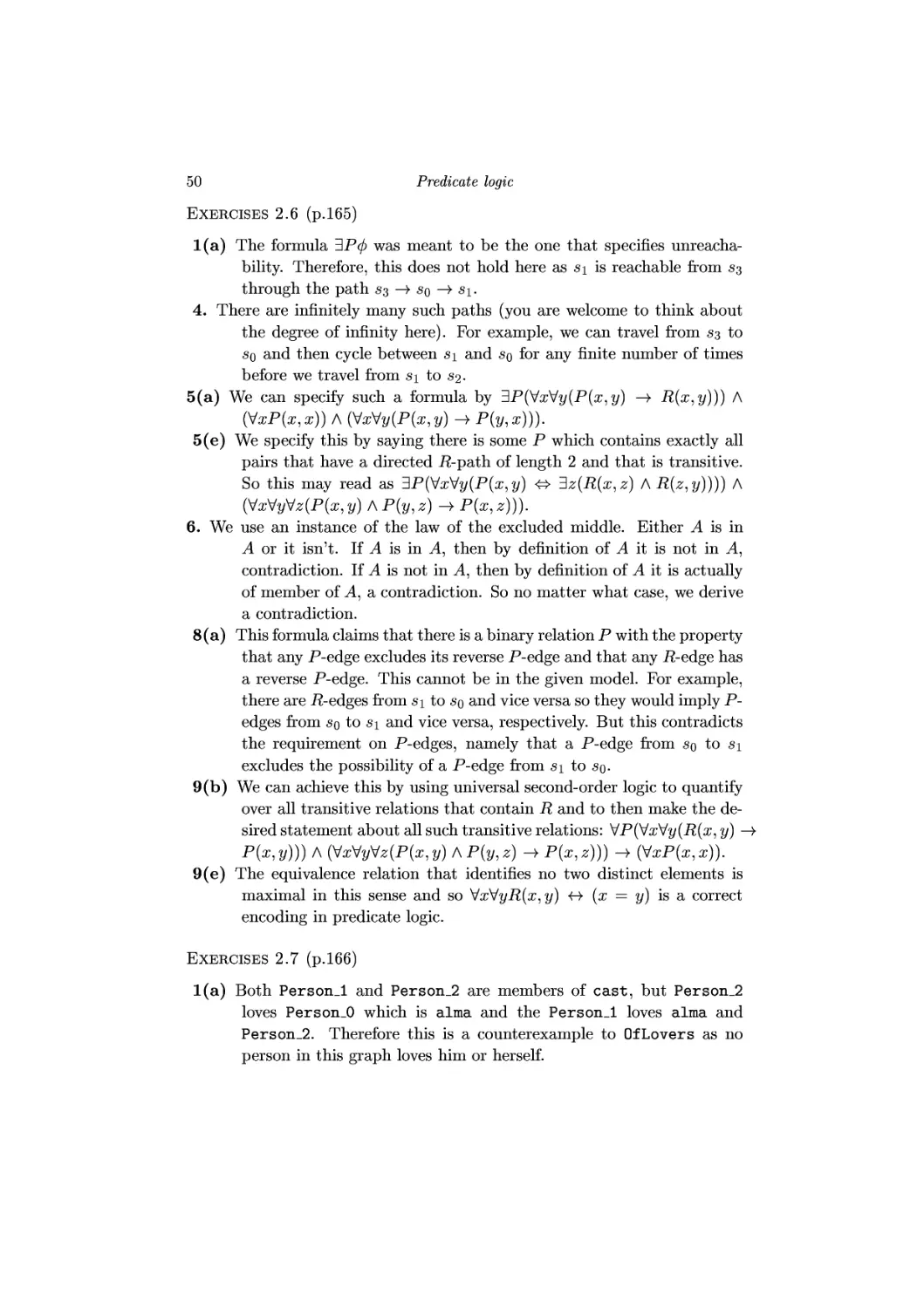
EF (ci A E[ci U (-.ci A E[^c2 U ci])]).

70
Verification by model checking
We write 0i for E[-ic2 U ci]
We write 02 for -ici A 0i.
l:0i
The interative procedure for determining the E[^C2 U ci]
labels takes three rounds. Then we "throw out" those
labeled states which have a c\-label. The resulting labels for
—«ci A E[^C2 U c\] are now the target formula for the next EU
operator:
1:03
02 We write 03 for E[c± U 02]
The iteration for this EU-labeling (^3) requires only two

Verification by model checking
71
rounds. Next, we refine 03 to those states which also
satisfy c\ (label for ^4):
We write 04 for c\ A 03.
We write 0 for EF 04.
which triggers the iterative procedure for EF, which
terminates after four rounds, concluding that all states satisfy
EF (ci A E[ci U (-.ci A E[^c2 U ci])]).
function SATEG (0)
/* determines the set of states satisfying EG (j) */
begin
local var W,X,Y
begin
Y:=SAT(0);
X:=5;
repeat until X = Y
begin
X:=Y;
Y := y fl {s I exists s' such that s —>> s' and s' E Y}
end
return y
end
9. There are lots of ways of scheduling this in a strictly alternating fashion.
We chose a fairly deterministic version:

72
Verification by model checking
Note that the states on the left half, including n\n<i, are the only ones
that satisfy E[^C2 U ci]. Only t\ri2 and niri2 satisfy —«ci A E[^C2 U
ci]. These two are also the only states which satisfy E[ci U —«ci A
E[^C2 U ci]]. Since none of them satisfies ci, there is no state in the
system which satisfies c\ A E[ci U —«ci A E[^C2 U ci]]. Therefore, no
state of that system can satisfy EF {c\ A E[ci U —«ci A E[^C2 U ci]]).
11. • Let (j) be true infinitely often on the computation path sq —> si —>
52 —> — Proof by contradiction: Suppose that the negation of
our claim is true. This means that there exists some n > 0 such
that for all m > n we have sm \f (j). But then <j> could only be true
on finitely many states of that path, namely at most at the states
50, 31, . . . , 3n_i-
• Suppose that for every n > 0 there is some m > n with sm \= (j).
Proof by contradiction: Assume that (j) is only true at finitely many
states on that path. Then there has to be a maximal number no
such that no Sjyi with ui > tiq satisfies (j>. By this is a contradiction
to the assumption above which applied "for all n > 0", so in
particular it applies to that no-
15. All the states are labelled EcGT (i.e., all the states have a fair path
leading from them).
Exercises 3.7 (p.252)
1(a). • The function Hi is monotone: if Y is a subset of Y' then Hi only
removes the elements 1, 4, and 7 from Y and Y1 if applicable.
Since Y CY' this ensures that Hi(Y) C Hi(Y').

Verification by model checking
73
• The function H2 is not montone: e.g. {2} C {2,5}, but #2({2}),
which is {5, 9}, is not a subset of #2({2, 5}), which is {9}.
• The function H$ is monotone since union and intersection are
monotone and the composition of monotone operations is again
monotone.
1(b). We compute the least and greatest fixed-point of H3 with just one
iteration each: it is {2,4} in each of these cases. So why can we say
that this is the only fixed-point of H%!
2(a) Let X C X' and 5 G FX(X). Then 5 G A n F(X) implies 5 G A and
5 G F(X). So in order to show s G ^i(X') = A n F(X') it suffices
to show s G F(Xf). But this follows from 5 G F(X) as X C X' and
since i*1 is monotone.
2(b) Let X C X' and consider 5 G F2(X).
• If 5 G A then 5GiU(Bn F(Xf) = F2{Xf) follows.
• If 5 0 A thensGF2(X) = 4u (B flF(X)) implies 5 G 5nF(X),
but we already saw in item (a) that this implies 5 G Bfl F(X')
and so 5 G A U (B n i^X')) = F2(X') does it.
5. • Let X C X' and 5 G #(X) = [0] n {s0 € £ | 50 -► «i implies si G X}.
Then 5 G [0] is clear. If sf G S with 5 -)► 5', then 5 G #(X)
implies s' G X. Since X C X', we infer from that sr E X'. But
this shows 5 G [0] n {50 G £ | 50 ->> si implies si G X'} = H(X').
• We compute
jy([AG 0]) = [0] n {50 G S I 50 -> 5i implies Sl G [AG 0]}
= [0]n[AXAG0]
= [AG#
• We have already seen that [AG 0] is a fixed point of H. To show
that it is the greatest fixed point, it suffices to show here that any
set X with H(X) = X has to be contained in [AG0]. So let 5o
be an element of such a fixed point X. We need to show that 5o
is in [AG 0] as well. For that we use the fact that
50 G X = H(X) = [0] n {5 G S I 5 -> 5i implies si G X}
to infer that s\ G X for all s\ with 5o —» si- But, since si is
in X, we may apply that same argument to s± E X = H(X) =
[(/)] fl {5 G S I 5 —>► 52 implies 52 G X} and we get 52 G X for all
52 with 5i —>► 52. By mathematical induction, we can therefore
show that sn G X, where sn is any state that is reachable from sq.
Since all states in X satisfy 0, this means that 5 is in [AG 0].

Verification by model checking
(d) The pseudo-code for SATag:
function SATAg (0)
/* determines the set of states satisfying AG (j) */
local var X, Y
begin
Y:= SAT (</>);
X:=0;
repeat until X = Y
begin
X:=Y;
y := Y n {5 E 5 I s -> s' implies s1 E y}
end
return Y
end

4
Program verification
Exercises 4.1 (p.299)
1. This is an open-ended and thought-provoking exercise. For example,
Software Development Environments can improve the reliability of
code by tracking version numbers and ensuring that all modified
code is re-compiled, or linked when necessary. Editors can enhance
the realibility of software by depicting source code through use of
colors and fonts that check the integrity of syntax for the respective
programming language. Programming language constructs may also
improve or worsen the reliability of software. High-level abstractions
and encapsulation principles are generally perceived as aiding the
robustness of software whereas explicit pointer management may
result in efficient but flawed software. Etc.
Exercises 4.2 (p.299)
1. In what circumstances would if B {C\} else {C2} fail to terminate?
(We assume that the program is well-typed.) Our core language is
such that boolean expressions B in themselves cannot diverge, i.e.
they will return a truth value. Thus, this code can only diverge if
C\ or C2 diverge and if the control flow passes execution on to the
respective diverging command C\ or C2. Notice that this program
necessarily diverges if both C\ and C2 diverge.
2. We can express such a for-loop in our core language as
C_l;
while B {
C_3;
C_2;
}
75

76
Program verification
Note that this form first executes the body C3 before it performs the
update operation C2 for the boolean condition B.
Exercises 4.3 (p.300)
1(a) Since l{x) = —2, l(y) = 5, and l(z) = —1 we have / \f x + y < z as
—2 + 5 is not less than —1. Thus / 1= [x + y < z) —> ^(x * y = z) as
the assumption of the implication does not hold.
1(c) We have / 1= (x + y — z) < x * y * z since the expression on the
left evaluates to —2 + 5 — (—1) = 4 and the one on the right to
(-2) • 5 • (-1) = 10.
2. For any 0, if>, and P we have that \=tot{(j)) P {?p) implies Npar|0| P {?p).
For let Ntot|0| P {ip) be the case. Assuming that program P is
executed in a store meeting the precondition <j> we then know that it
will terminate its execution and end up in a final state meeting the
postcondition ip. If we ignore that this secures termination we have
just shown Npar|0| P {if>).
Please remember that you can only understand proofs of {(/)) P {1/))
by reading them in a bottom-up fashion!
5(a). We show \-par{x > 0)y = x + 1; [y > 1) by
(ar>0)
{(x + 1) > 1} Implied
y = x + 1;
[y > 1) Assignment
5(b). We show Hpar([T]) y = x;y = x + x + y;|y = 3-a;|by
(x + x + x = 3 • x) Implied
y = x;
[(x + x + y) = 3 • x) Assignment
y = x + x + y;
[y = 3 • x) Assignment
5(c). We show Hparfj: >l)a=l;y = x;y = y-a; [y > 0 A x > y) by

Program verification 77
[x > 1}
[x — 1> Q /\x> x — 1} Implied
a = 1;
[x — a>OAx>x — a) Assignment
y = x;
{(y — a) > 0 A x > (y — a)) Assignment
y = y - a;
{y > 0 A x > y) Assignment
6(a). There are infinitely many programs which meet these input/output
behaviors. To implement {T) P {y = x + 2) we made a fairly obvious
choice, namely the assignment y = x +2; The proof is
m
{(x + 2) = x + 2) Implied
y = x + 2;
[y = x + 2) Assignment
6(b). There are infinitely many programs which meet these input/output
behaviors. To implement |T| P [z > x + y + 4) we chose a non-
optimal, but still correct, sequence of assignments:
m
{10 > 4} Implied
{x+ (y + 10) > x + y + 4) Implied
u = y + 10;
{(x + u) > x + y + 4) Assignment
z = x + u;
[z > x + y + 4) Assignment
9(c). We show that any instance of the rule If-Statement can be replaced
by a proof in the proof system without this rule:
(B A 0i} d (*l>) (^B A 02} C2 (V)
Implied Implied
((B -> 00 A B) d {t/>) {hB -> 02) A -5) C2 {t/>)
Implied Implied
((B -► 0i) A (-5 -► 02) A B) d {*!>) ((B -► 0i) A (-5 -► 02) A ^B) C2 fa)
If-statement
{(B -> 0i) A (-5 -> 02)| if B {d} else {C2} (V>)

78
Program verification
10. We show Hpar([T) P [z = min(a;,y)|, where mhi(x,y) is the smallest
number of x and y (e.g. min(7,3) = 3) for the code P given below:
m
if x > y {
|T A (x > y)) If-statement
(y = min(x^y)) Implied
z = y;
[z = min(a;, y)) Assignment
} else {
|T A -i(a; > y)) If-statement
[x = min(a;, y) | Implied
z = x;
[z = min(a;, y) | Assignment
}
[z = min(a;, y)) If-statement
If x equals y at runtime then the second branch of the if-statement
gets executed and the value of x will be the result. This is fine
as this value then also equals the value of y. Logically, we cannot
really improve our description of min(a;, y) (in the sense that we could
impose more or less properties on it), but human beings might benefit
from the fact the you draw their attention to special or overlapping
cases of your specification (such as the one where x equals y). (How
do you prove this with the modified proof rule for if-statements?)
11(a). We write code P which satisfies |T| P [z = max(a;,y)| under
partial correctness, where max(a;, y) denotes the larger of x and y:

Program verification 79
m
if x < y {
[~T /\{x <y)) If-statement
[y = max(a;, y)) Implied
z = y;
[z = max(a;, y)} Assignment
} else {
[ T A -■ (a; < y)) If-statement
[x = max(a;,y)} Implied
z = x;
f z = max(a;, y) | Assignment
}
[z = max(a;, y) | If-statement
Notice that we simply took the code and the proof for min and
changed > into < and min into max.
11(b). We seek a program P which satisfies
hpar(T)P(((a; = 5) -> (v = 3)) A ((x = 3) -> (y = 1))}. (4.1)
Again, there are many programs one could write here as a solution.
We chose a fairly natural one. We prove (4.1) as follows:
m
if x = 5 {
(TA(a; = 5)) If-statement
{((x = 5) _> (3 = 3)) A ((x = 3) -> (3 = 1))| Implied
y = 3;
{((x = 5) -> (y = 3)) A ((x = 3) -> (y = 1))| Assignment
} else {
|T A -i(x = 5)| If-statement
(((x = 5) -> (1 = 3)) A {{x = 3) -> (1 = 1))| Implied
y = l;
(((a = 5) -> (y = 3)) A ((x = 3) -► (y = 1))| Assignment
}
(((a = 5) -► (y = 3)) A ((x = 3) -> (y = 1))| If-statement

80
Program verification
Note that the applications of the rule Implied in lines 4 and 9 was
valid since F -> • = T and T -> T = T.
Two other solutions are possible: one could program a "nested"
if-statement which is not really needed since the precondition only
means to distinguish between two values of x, so we may identify its
computation for all values of x other than 5. The second solution is
an optimization: the program
y = x - 2;
also satisfies the required pre- and postconditions. (Why?)
13. We show Hparfa; > 0) Copyl [x = y). First, we note which variables
get updated in the body of the while-statement: y and a. Second,
we compute their values after each iteration for, say, the first four
iterations. Third, upon inspection of these values we suggest y =
x — a as a candidate for an invariant. The proof is
{x>0)
fO = x-x)
a = x;
fO = x - a)
J = 0;
[y = x-a)
while ! (a =
[y = x
y = y +
[y = x
a = a -
[y = x
}
[(y = x - a) A ^^(a = 0)| Partial-while
[y = x) Implied
Note that we never really made use of the precondition x > 0; this
is in contrast to the corresponding proof of total correctness which
additionally secures program termination; then this precondition is
instrumental in securing program correctness.
Implied
Assignment
Assignment
■0) {
— a) Invariant Hyp. A guard
.) = x — (a — 1)| Implied
l;
— (a — 1)| Assignment
l;
— a) Assignment

Program verification
81
14. We show Hparfy > 0) Multil [z = x • y). First, we note which variables
get updated in the body of the while-statement: z and a. Second,
we compute their values after each iteration for, say, the first four
iterations. Third, upon inspection of these values we suggest z = x-a
as a candidate for an invariant. The proof is
fy>0|
(0 = £•()} Implied
a = 0;
fO = x • a) Assignment
z = 0;
[z = x • a) Assignment
while ! (a = y) {
[z = x • a) Invariant Hyp. A guard
[z + x = x • (a + 1)| Implied
z = z + x;
(z = x • (a + 1) | Assignment
a = a + 1;
[z = x • a) Assignment
}
[(z = x • a) A ^^(a = y)| Partial-while
[z = x • y) Implied
Again, we never used the precondition y > 0 for this partial
correctness proof, but it is crucial in securing total correctness later
on.
18. We show Hpar([3; > 0) Downf ac [y = x\). First, we note which variables
get updated in the body of the while-statement: y and a. Second,
we compute their values after each iteration for, say, the first four
iterations. Third, upon inspection of these values we suggest y- (a!) =
x\ as a candidate for an invariant. However, since ^(a > 0) does not
imply a = 0, we need to strengthen this invariant to (y • (a!) =
x\) A(a>0). The proof is

82
Program verification
(x>Q)
{(l-(x\) = ar!) A(ar>0)) Implied
a = x;
|(1 . (a!) = x\) A (a > 0)| Assignment
y = 1;
{{y ' (a0 = ^0 A (a > 0)1 Assignment
while a > 0 {
{(y ' (a!) = #0 A (a > 0) A (a > 0)| Invariant Hyp. A guard
{(y • ((a - 1)! • a) = a;!) A (a - 1 > 0)| Implied
{{{y • a) • ((a - 1)!) = a;!) A (a - 1 > 0)| Implied
y = y * a;
{(y • ((a - 1)!) = x\) A (a - 1 > 0)| Assignment
a = a - 1;
[(y ' (a0 = x\) A (a > 0)| Assignment
}
{(y • (a!) = a!) A (a > 0) A -.(a > 0)| Partial-while
fy = a;!) Implied
Note that we had to strenghten our invariant hypothesis by adding a
conjunct (a > 0). This was needed since -i(a > 0) does not in itself
imply the desired (a = 0) to secure that our invariant implies the
postcondition.
21(a). We simulate the code for each of these arrays in a table which lists

Program verification
83
the values of k, t, and s where "time" runs downwards.
-1
-9
s
-3
-3
-4
6
Notice that the minimal-sum section is unique in this case: it is the
sum of the entire array which is —9, the last value stored in s.
21(c). We proceed as in item 1:
6
-1
-3
-6
-10
1087
-1
-3
-6
-10
-10
Again, there is a unique minimal-sum section: the entire array but
the last entry.

84 Program verification
23. A direct attempt in proving the specification S2 for Min_Sumwould look
like this:
m
Hi] =5(1,1)| Implied
{3i,j {i < j < nAo[l] = S(i,j))) Implied
k = 2;
(3i, j (i < j <n A a[l] = 5(i, j))) Assignment
t = a[l];
(3i, j (i < j <n A a[l] = 5(i, j)) | Assignment
s = a[l];
f 3i, j(i<j<nAs = 5(i, j))) Assignment
while (k != n + 1) {
(3i,j (i < j < n A s = 5(i,j))) Invariant Hyp
|3i, j (i < j <n A min(s,min(£ + a[fe],a[fe])) = S(i,j))) Implied
t = min(t + a[k], a[k]);
f 3i, j (i < j <n A min(5, t) = 5(i, j)) | Assignment
s = min(s,t);
(3i,j (i < j < n A 5 = S(i,j))) Assignment
k = k + 1;
(3i,j (i < j < n A s = 5(i,j))) Assignment
}
{3i, j(i<j<nhs = 5(i, j)) | Partial-while
It looks fine if it were not for the justification of the Implied rule in
the while-loop. Knowing that s is the sum of some section does not
immediately imply that min(.s, min(t + a[fe], a[fe])) is the sum of some
section as well. Evidently, we need to reason that min(t + a[fe], a[k])
is the sum of some section for all values of k that the program is
computing. This proof is similar to the one given above and we omit
it here.
Exercises 4.4 (p.303)
1(a). We prove Htotfa; > 0) Copyl [x = y) as follows: since the while-loop
in Copyl has as guard B the boolean expression -i(a = 0) and,

Program verification
85
since a > 0 is an invariant of the entire program (assuming the
precondition x > 0), we may instantiate the formula 0 < E = Eq
to 0 < a = Eq. Of course, we may reuse the invariant 0j, which is
a + y = x from the partial correctness proof. With these data at
hand we simply have to follow the proof pattern for total correctness
proofs:
(x>0)
{(x + 0 = x) A (x >0)| Implied
a = x;
{(a + 0 = x) A (a > 0)| Assignment
y = 0;
{(a + y = x) A (a > 0)| Assignment
while ! (a = 0) {
{(a + y = x) A ^(a = 0) A (0 < a = i£o)| Invariant Hyp. A guard
{(a- l + y + 1 = x) A (0 < a- 1 < £0)| Implied
y = y + i;
((a — l + y = a;)A(0<a — l< £o)| Assignment
a = a - 1;
[(a + y = x) A (0 < a < E0)) Assignment
}
{(a + y = x) A ^^(a = 0)| Total-while
[x = y) Implied
Note that the Implied in line 9 is valid, since ^(a = 0) and 0 < a = Eq
together imply 0 < a — 1 < Eq.
1(b). We show Htotfy > 0) Multil [z = x * y), where the code for Multil
is
a = 0;
z = 0;
while (a != y) {
z = z + x;
a = a + 1;
}
The boolean guard a != y is equivalent to y - a != 0, so we may
instantiate 0<JE = JE0to0<y — a = Eq. This works out as

86
Program verification
0 <y — a turns out to be an invariant of the entire program. Since we
already showed that [y > 0) Multil [z = x • y) holds under partial
correctness, we may reuse the invariant 0j, which is z = x • a, from
that proof. Now everything is in place for crafting the proof in a
bottom-up fashion:
fy>0|
{(0 = x • 0) A (0 < y - 0)| Implied
a = 0;
[(0 = x • a) A (0 < y — a)) Assignment
z = 0;
[(z = x * a) A (0 < y — a)) Assignment
while (y - a != 0) {
{(z = x • a) A ^(y — a = 0) A (0 < y — a = E0)) Invariant Hyp. A guard
{(z + x = x- (a + 1)) A (0 < y- (a + 1) < E0)) Implied
z = z + x;
((z = x- (a + 1)) A(0<y- (a + l) < E0)) Assignment
a = a + 1;
{(z = x • a) A (0 < y — a < Eq)) Assignment
}
{(z = x • a) A ^^(y — a = 0)| Total-while
(z = x • y) Implied
Again, the use of y > 0 was crucial in justifying line 2; this program
diverges whenever y is negative. Make sure that you understand why
the application of Implied in line 9 is justified.
1(d). In order to prove Htotfa; > 0) Downf ac [y = x\) we may think of the
Boolean guard a > 0 as a ! = 0, for a > 0 turns out to be an
invariant of the entire program. This suggests that 0 < E = Eq is just
0 < a = Eq. We need as full invariant (y • (a!) = x\) A (a > 0) from
the case of partial correctness; the formula y • (a!) = x\ alone will not
do, since we mean to identify ^(a = 0) with a > 0. Thus, the entire
proof may be constructed as follows:

Program verification
87
(x>0)
|(1 * (x\) = a;!) A (x > 0) A (0 < x)) Implied
a = x;
|(1 * (a!) = x\) a (a > 0) A (0 < a)) Assignment
y = 1;
|(y * (a!) = x\) A (a > 0) A (0 < a)| Assignment
while a != 0 {
{(y • (a!) = x\) A (a > 0) A (-.(a = 0) A (0 < a = E0)) Invariant Hyp. A guard
{(y • ((a - 1)! • a) = a;!) A (a > 0) A (0 < a - 1< £0)| Implied
f ((l/ • a) • ((a - 1)!) =x\)A(a>0)A(0<a-KE0)) Implied
y = y * a;
f (y • ((a - 1)!) = a!) A (a > 0) A (0 < a - 1 < E0)) Assignment
a = a - 1;
|(y . (a!) = x\) A (a > 0) A (0 < a < E0)) Assignment
}
{(y • (a!) = x\) A (a > 0) A ^(a = 0)| Total-while
(y = #!} Implied
Note that the a > 0 in line 6 stems from the invariant, whereas the
second a > 0 results from the proof pattern 0 < E.
1(e). We prove Htot([a; > 0) Copy2 [x = y), where Copy2 is the code
y = 0;
while (y != x) {
y = y + i;
}
The boolean expression B is y != x which we can rewrite to the
equivalent expression x - y. Therefore, the precondition x > 0
suggests to instantiate 0 < E = Eq to 0 < x — y = Eq. An invariant
4>i requires that (j>i A (x — y = 0) implies x = y. Since the latter is
already a consequence of x — y = 0, we may simply choose T for (f>j.

Program verification
{x>0)
(TA(i-0>0)| Implied
y = 0;
|T A (a; — y>0)| Assignment
while x - y != 0 {
|T A -i(a; — y = 0) A (0 < a; — y = E0)} Invariant Hyp. A guard
{T A(0<x-(y + l) <E0)} Implied
y = y + l;
(T A (0 < a: - y < E0) } Assignment
}
{T A ->-i(a; - y = 0) | Total-while
[x = y) Implied
Note that we actively made use of the precondition x > 0 and that
this code diverges if x < 0.
Exercises 4.5 (p.304)
1(a).
The method certif y_V may itself call other certifications methods,
e.g. two such methods certify_Vl and certify_V2, and may accept
a cerificate if both calls to VI and V2 judge the certificate to be
valid. Programming by contract is useful as it can specify necessary
or sufficient conditions for accepting certificates.
One may face self-certifying services. For example, if VI calls certif y_V
and that method relies on some method call to VI, then VI could
instrument that method code so as to influence the judgment of V
withing certify.V.
We write a contract for method isGood:
method name : isGood
input : amount of Type int
assumes : access to 'balance'
guarantees : isGood(amount) iff balance >= amount
output : of Type boolean
modifies only : nothing modified
2(b). The method withdraw only modifies balance and accepts amount of
type int. Therefore it suffices to show that it meets its guarantee,
assuming that balance <= 0 is true. If the boolean guard in its body
i(b).
2(a).

Program verification 89
evaluates to false, then balance is not being modified and so
satisfies balance <= 0 by assumption. If the boolean guard evaluates
to true, then the value of amount is negative and isGood(amount)
returns true. By the guarantee of isGood the latter means that the
value of balance is greater or equal to the value of amount. But
then the execution of the assignment for balance ensures that its
new value is greater or equal to zero.

5
Modal logics and agents
Exercises 5.2 (p.350)
l(a)iii. The relation a Ih q holds as state a is labelled with q in the figure.
l(a)iv. The relation a Ih UUq holds iff x Ih Uq holds for all x with R(a, x).
Since e and b are the only instances of x which satisfy R(a,x), we
see that a Ih UUq holds iff e Ih Uq and 6 Ih □</ hold. But none of
this is the case. For example, we have i?(6, e) and e \f q, so 6 \f Uq
follows.
l(a)vi. The relation a Ih DO-ig holds iff e Ih O-ig and b Ih O-ig holds,
since e and 6 are the only x with R(a,x). First, we have e Ih O^g,
since there is some x with R(e,x) and # II ig; choose # to be e.
Second, we also have b Ih O^g, because we may choose again easa;
with i?(6, e) and e II—\q. In conclusion, a Ih DO^g holds.
l(a)x. We have c Ih D_L iff x Ih _L for all x with i?(c,a;). By definition
of Ih, we have x \f _L for all x, so c Ih D_L holds iff there is no x
with R(c,x). Inspecting the figure, this is evidently the case. Thus,
c Ih D_L holds.
l(b)iii. We seek a world which satisfies Op V Og, i.e. a world x such that
there are worlds y and y1 with R(x,y) and R(x,yf) such that y Ih p
and y1 Ih q. If we choose c for x and 6 for y and y', this is clearly
realized. Therefore, c Ih Op V Og follows.
l(b)iv. We have x Ih 0(p V Og) iff there is some y with R(x,y) and y Ih
p V Og. This can be realized. For example, choose x and y to be the
worlds b and c, respectively.
4(b). • We seek a model in which p —> BOq is true. By definition, we
seek a model in which all its worlds satisfy p —> BOq. Certainly,
any model in which no world satisfies p would do. (Why?) More
interestingly, consider the figure below.
90

Modal logics and agents
91
The world b satisfies p —> DOg, since c 1/ p. For the worlds a and
c, we have a Ih p and c Ih p, so we need to secure a Ih DOg and
c Ih DOg. But this can be done, since all three worlds, x, of this
model have an immediate successor state, x\ such that x' Ih q.
(Why does this imply what we require, and what choices of x' for
x would you make?)
• We seek a model in which p —>► UOq is not true. By definition,
we seek a model in which not every world satisfies p —> UOq. The
model in Figure 5.5 of the textbook qualifies, for a \f p —>► UOq.
(Why?)
5(d). The relation x Ih 0(p A q) means that there is a world y with R(x, y)
and y Ih p A q. On the other hand, x Ih Op A Og means that there
are worlds y' and y" with
R(x,yf) and y' Ihp
i2(aM//;) and i//; Ih g.
With that in mind, it is relatively easy to find a model which
distinguishes these two formulas:
Note that a \f 0(p A g), whereas a Ih O^ A Og.

92
Modal logics and agents
5(f).(i) First, we have x Ih 0(p V q) iff there is a world y with R(x, y) and
y\\-p\/q. But then y Ih p or y Ih g.
Case 1: If y Ih p, then x Ih Op, and so x Ih Op V Oq follows.
Case 2: If y Ih g, we argue in the symmetric way: x Ih Og, and so
x Ih Op V Og follows.
(ii) Second, if we have x Ih Op V Og, then we have x Ih Op, or p Ih Og,
not necessarily exclusive.
Case 1: If x Ih Op, then there exists a world y' with R(x, y') and y Ih p.
This implies y' Ih p V g, and so x Ih 0(p V q) follows as R(x, y1).
Case 2: Symmetrically, if # Ih Og, then there exists a world yn with
R(x, yn) and y Ih g. This implies yn Ih p V g, and so a; Ih 0(p V g)
follows as R(x,yff).
6(a). To show that D(0 A ^) ** (D0 A D^) is valid is suffices to show that
x Ih D(0 A V7) implies a; Ih D0 A D^, and vice versa, where a; is any
world of any model. (Why?)
(i) If x Ih D(0 A V7, then i?(a;, y) implies y Ih (f) A ^, and so y Ih 0 and
y Ih ^ follow. Since y is an arbitrary element with i?(a;,y), we
conclude x Ih D0 and a; Ih D^, and so a; Ih D0 A D^ follows.
(ii) Conversely, if a; Ih U(f> A D^, we infer x Ih D0 and a; Ih Hip. If y is
any element with R(x, y), then x Ih D0 implies y Ih 0, and a; Ih Utp
implies y Ih ip. Therefore, y Ih 0 A ip holds. Since y is an arbitrary
element with R(x,y), we infer that x Ih D(0 A ^) holds.
(Why is the argument above still valid if there is no y with R(x, y)?)
6(c). As in item 8(a), it suffices to show that x Ih DT implies x Ih T, and
vice versa, where x is any world of any model.
(i) If x Ih DT, then x Ih T holds, since the latter holds simply by the
definition of Ih.
(ii) If x Ih T, then we have y Ih T for all y with R(x,y), since we have
y Ih T for all worlds y, by definition of Ih. Thus, x Ih DT is proved.
Exercises 5.3 (p.351)
1(a). We interpret the formula {(f) —>► D0) —> (0 —> Ocjj) according to the
interpretations of □ and O in Tables 5.7 and 5.6.
(i) It is necessarily true that 0: The formula says
"If 0's truth implies that 0 is necessarily true, then 0's truth implies
that 0 is possibly true."
This should be valid.

Modal logics and agents
93
(ii) It will always be true that (j)\ The formula says
"If 0's truth implies that 0 is always true, then 0's truth implies that 0
is true sometimes in the future."
This should be valid.
(iii) It ought to be that (j)\ The formula says
"If 0's truth implies that 0 ought to be true, then 0's truth implies that
it is permitted that 0 (is true)."
This may be contested by some, but should generally be valid.
(iv) Agent Q believes that 0: The formula says
"If 0's truth implies that agent Q believes 0, then 0's truth implies that
0 is consistent with Q's beliefs."
This should be valid, provided that agent Q values consistency of
beliefs.
(v) Agent Q knows that 0: The formula says
"If 0's truth implies that agent Q knows that 0, then 0's truth implies
that 0 is true, for all agent Q knows."
This should be valid.
(vi) After any execution of program P, (f) holds: The formula says
"If 0's truth implies that, after any execution of program P, 0 holds,
then 0's truth implies that 0 holds after some execution of program P.
This should clearly be valid.
) We have / 1= -i(P)-i0 iff we have / \f (P)-"0 iff (it is not the case
that some execution beginning in store / terminates in a state
satisfying -i0) iff (all executions beginning in state / terminates in a state
satisfying (f) or don't terminate at all).
). For natural numbers n,ra > 1, we have R(n,m) iff n < m. For
example, 2 < 5, but 5^2.
• R is not reflexive, since n jt n for any n > 1.
• R is not symmetric, since n < m implies m jt n.
• R is serial, since for each n > 1 there is some m, for example
m = n + 1, such that n < m.
• R is transitive, since n < m and m < k clearly imply n < k.
• R is not Euclidean; otherwise n < m and n < k would always
imply m < &, but this is not the case. For example, we have
3 < 11 and 3 < 5, but 11 it 5.
• R is not functional, since, e.g., we have 2 < 4 and 2 < 5 with 4
and 5 being distinct elements.

94
Modal logics and agents
• R is linear, since n > m and n < k always imply that ra and k are
equal, or k < ra, or ra < k.
• R is not total; otherwise, we would have n < ra or ra < n for all
n, ra > 1, but this is not the case when n equals ra.
• R is not an equivalence relation, since we saw above that it is
neither reflexive, nor symmetric.
3(d) This is very similar to the previous solution in its methodology but
some of the cases are a bit trickier.
• To see whether R is reflexive we need to check that for all real
numbers x there are positive numbers a and b such that x = a-x+b.
This cannot be for x = 0 as b has to be positive.
• This relation is transitive. For if a, 6, c, d are positive real numbers
with x = a • y + b and y = c • z + d, then a • c and a • d + b are
positive as well and x = a- c ■ z + (a- d + b).
• This is clearly not functions, e.g. 2 equals 1 • 1 +1 and also equals
2-0.5 + 1.
• Etc.
4. Let R be a reflexive, transitive and Euclidean relation. We need to
show that R is an equivalence relation. Since R is already reflexive
and transitive, it suffices to show that R is symmetric. To that end,
assume that R(a,b). We have to show that R(b,a) holds as well.
Since R is Euclidean, we have that R(x, y) and R(x, z) imply i?(y, z)
for all choices of #, y and z. So if we instantiate this with x = a,
y = b and z = a, then we have R(x,y) by assumption (as R(a, 6)),
but we also have R(x, z) since i? is reflexive (so R(a, a) holds). Using
that R is Euclidean, we obtain i?(y, z) which is i?(6, a) as desired.
Notice that this local argument made no use of the transitivity of R.
(Why and where does the global argument use this transitivity?)
9(a) This is not valid in intuitionistic propositional logic. Consider a model
with three worlds x, y, and z such that L(x) = {}, L(y) = {^}, and
L(z) = {q}. Further, let R(x, y) and R(x, z) be the only non-reflexive
instances of R. Note that L is monotone with respect to R. Then
x \f p —> q since y is accessible by x and p —> q does not hold at y.
Similarly, x \f q —> r since z is accessible from x and does not satisfy
q —> r.
9(f) This is intuitionistically valid. There is an obvious proof that involves
only the proof rules -d and ^e and these proof rules are
intuitionistically valid.

Modal logics and agents
95
11(b). Let Ucj) mean that "agent Q believes 0". Then the formula scheme
Ucj) V D-i0 means
"For any formula 0, agent Q either believes 0, or she believes -i0."
13(a). Reading D0 as "agent Q knows 0", we read R(x,y) as "y could be
the actual world according to agent Q's knowledge at #".
(i) i? should indeed be symmetric. Suppose R(x,y), but not R(y,x).
Then, as far as Q's knowledge at x is concerned, y could be the
actual world, but his knowledge at y rules out the possibility of
x being the actual world. Therefore, at y he knows something
preventing x from being actual; so at x he knows he knows
something preventing x from being actual. Therefore, he (simply)
knows something preventing x being actual, i.e. he knows
something which is false. This contradicts our model of knowledge.
(ii) The totality of R means that for all worlds x and y we have R(x,y)
or R(y, x). But x and y may contain mutually exclusive knowledge
(e.g. agent Q may know all prime ministers of Canada at world
#, but fail to remember some of them at world y). In that case,
neither R(x, y) nor R(y, x) are valid, so R is not total in general.
13(c). Let Ucj) model "always in the future, (f) holds". Note that R(x,y)
here means "y is in the future of x".
• Whether R is reflexive, or not, depends on whether the present is
part of the future (only then is R reflexive).
• R is not symmetric, since there is no symmetry between the past
and the future.
• Assuming that time does not halt, R should be serial: each point
in time, x, has some future point, y.
• R is transitive: if y is in the future of x and z in the future of y,
then z is in the future of x as well.
def
• R is not Euclidean; for example, if x is the year 2005 and y = 2031,
z = 2012, then y and z are in the future of #, but z is not a future
of y.
• Assuming that time goes on without end, R is not functional, for
each point in time will have many distinct future points in time.
• Assuming the ordinary notion of time, namely that future points
are either identical, or one occurs prior to the other, the relation
R is linear.
• Whether R is total, or not, depends on the answer to the question
whether the present is part of the future (only then is R total).
• R is not an equivalence relation since it is not symmetric.

96
Modal logics and agents
16(b). A frame T = (W,R) satisfies D_L iff each world w E W satisfies
this formula. (Why don't we have to consider labelling functions
here?) But w lh D_L holds iff there is no w' with R(w,w'), for _L is
satisfied by no world whatsoever. Thus, D_L corresponds to R being
the empty relation (= no two worlds are related).
16(c). OD0 —>► DO0 corresponds to weakly directed: ifR(x, y) and R(x, z),
then there exists a point u such that R(y,u) and R(z,u). The proof
of this is in similar style to Theorem 5.13.
17. We seek a formula scheme cf) which corresponds to density: for all
x,z E W, there exists some z E W with R(x,y) and R(y,z). We
claim that
Ocj)^ OOcj)
is such a formula scheme.
(i) Let T = (W, i?) be a frame which satisfies Ocf) —>► OO0. Suppose
that i?(a;, z) holds. Let L be any labelling function with respect
to which we have z \\- p, but w \f cf) for any other world. Then
x lh Ocf) as R(x, z). Since the frame satisfies Ocf) —>► OO0 we obtain
that x lh OO0 holds. Thus, there is some y E W with i?(a;, y) and
y lh O0. But the latter can only mean R(y,z) due to the choice
of our labelling function L. Thus, R is dense.
(ii) Let T = (W, i?) be a frame such that R is dense. Let x E W be
given. We need to show that x lh Ocf) —> OOcj) holds for any choice
of labelling function L. This is certainly the case if x \f Ocf). But
if x lh O0, then there has to exist a world, z, such that R(x,z)
and z\\~ cj). By density of i?, R(x, z) implies the existence of some
world y with R(x, y) and i?(y, z). Since z lh 0, the relation i?(y, z)
implies y lh O0. But the latter guarantees x lh OO0 as R(x,y)
holds.
Exercises 5.4 (p.353)

Modal logics and agents 97
1(a). We prove the validity of D(p —>► q) \~k ^P —> ^Q by
□ (p —>► q) prem
Up
! P
p^q
1 _2
Dg
ass
"""De"2""_:
□el
->e 4,3 !
□i 3—5
Dp -)► Dg -M 2-6
1(c). We prove the validity of Hk □(]) 4 g) A D(g 4 r) 4 D(p 4 r) by
n(p-> q) A □(? ~>r)
U(p^q)
B(q^r)
^
P^Q
Q
| q -> r
! | r
! _p —> r
n(p -> r)
ass
Aei 1
Ae2 1
ass 1!
De2
->e6,5
De3
->e8,7
->i 5-9 !
□i4-10
D(p -► q) a D(^ -► 0 -► D(p -► r) -^ i-ii
We left line 4 empty since our macros for producing boxes otherwise
causes the two boxes to overlap; we will use this "hack" in subsequent
examples as well.

98 Modal logics and agents
1(f). We prove the validity of 0(p —>► q) Hk Up —> Oq by
-iD-i(p —» g) prem
Up
1 U^Q
\\\ p^q
i P
Q
! "^
-1
! ^ip^q\
U^(p -> g)
±
-iD-ig
ass
ass 1
ass l!
De 2 ;
->e 5,6 ;
De 3
-ie7,8
->i 5—9 !
Di4-10
-.e 11,1
-.i 3—12
Up -> ^U^q ->i 2-13
2(c). We prove the validity of I~kt45 ODp <B> Dp by proving Hkt45
OUp —> Up and Hkt45 Up ^ OUp separately:
(i) We prove the validity of Hkt45 OUp —> Up by
^u^up
D^D^Dp
ass
5 1
!| -nU^
! u-iUp
| -nD^Dp
■| _L
Up
! JP_
Up
ass 1 i
54 i
De2
-ne5,6 ||
RAA 4-7
T8 !
□i3-9
^U^Up -> Up ->e 1-10

Modal logics and agents
99
Notice that this half of the equivalence did not need axiom 4, so
we actually proved the stronger Hkt5 OUp —> Up.
(ii) We prove the validity of Hkt45 Up ^ OUp by
Up
\j^\jp
^Up
_L
-^U^Up
ass
ass 1
T2
-ie 1,3 |
^i 2—4
Up -> ^u^up —m 1—5
Since this proof also never required the axiom 4, we conclude that
the equivalence between Up and OUp holds already with respect
to KT5.
Exercises 5.5 (p.354)
3(c). KlPWK2q.
3(g). KxK2p.
3(k). (KipAKi^q) V (K2pAK2^q) V- • • V (KnpAKn^q), where the agents
are numbered from 1 to n.
4(d). By definition of E, the relation x Ih E(p V q) holds iff x Ih Ki(p V
q) A K2(p V q) A K%(p V q) is true. For all i = 1,2, 3, we have that
Ri(xz,w) implies w E {xi,x2}. But since x\ \V p\J q and ^2 Ih ^ V g,
we infer that x Ih E(p V g) indeed holds.
4(i). By definition of C, we have xq Ih C^g iff xq Ih E^-ig holds for each
k = 1, 2,..., where Ek is EE...E (k times).
(i) Now #6 ll~ i21-l(7 simply means #6 Ih K\^q A K2^q A K^-^q. The
latter holds since, for i = 1,2, 3, the relation Ri(xQ,w) implies that
w equals #5; and we do have x§ II—\q.
(ii) We have x$ Ih E2^q iff we have x$ Ih KiE^q A K2E^q A K3E^q.
As in (i), we see that this amounts to checking whether x$ satisfies
a certain formula, but this time it is E^q and not -iq. However,
x$ Ih E^q fails to hold. For example, we have ^2(^5,^4), but
#4 \f -iq since #4 Ih q.
Therefore, we infer xq \f E2^q, and from that x$ \f C^q follows.
6. • Let x be any world in any model of KT45. To show x Ih Cq(J) —t
CoCgCJ), it suffices to assume x Ih Cq(J) and show x Ih CqCqcJ). The
latter is shown if we can prove that x Ih E1gCq4> for any / < 1.

100
Modal logics and agents
We make use of the second part of Theorem 5.26. Thus, if y is
any world which is G-reachable from x within / steps, we have to
argue that y Ih Cg^, i.e. y Ih E^cf) for all k > 1. Fix any k > 1. If
z is G-reachable from y within k steps, we are done if z Ih (/). But
since y is G-reachable from x within / steps, we conclude that z is
G-reachable from x within / + k steps. But then our assumption
that x Ih Cg4> implies x Ih E^cj) which renders z Ih (/). Thus,
CG(t> -> CGCg(j) is valid in KT45.
• To show that ^Cg4> —> Cg^Cg4> is valid in KT45, it suffices to
consider an arbitrary world x in an arbitrary model of KT45 such
that x II—^Cg4>> We then only have to show that x Ih Cg^Cg4>
follows. We make crucial use of the second part of Theorem 5.26,
and apply proof by contradiction: Assume that x \f Cg^Cg4>> By
Theorem 5.26, there exists a world y which is G-reachable by x
such that y \f ^Cg4>, i.e. y Ih Cg<J>- Since G is non-empty (what
does ^Cg4> —> Cg^Cg4> mean if G is empty, and why it is then
valid?), we know that the relation
|J Ri (5.1)
ieG
is an equivalence relation (see the discussion in the textbook after
Theorem 5.26). But then x and y are related via this equivalence
relation and one satisfies Cg^, whereas the other one does not.
This is a contradiction. (Why?)
10(c). Again, we prove this via showing two separate implications.
(i) We prove Cp -> KiCp by
Cp
CCp
ECp
KiCp
ass
C4 1
CE2
EKi3
Cp -> KiCp ->i 1-4
(ii) This follows simply by the rule KT.
10(e). The formula scheme -i0 —>► K^K^ means
"If 0 is false, then agent % knows that he does not know 0."

Modal logics and agents 101
Here is a proof:
^
Kit
4>
±
^Ki<j>
Ki-^Kit
ass
ass 1
KT2
-.e 3,11
-.i2—4
Kb 5
-.0 -> K^Ki(j) —>il—6
10(g) • The proof strategy for showing the validity of -^K\-^K\$ —> Ki(/>
is to use proof by contradiction with ^K\(j) as an assumption which
then renders K\-^K\§ by if4 applied to agent 1 and so _L can be
inferred.
• The other direction is reasoned in a similar way: use proof by
contradiction and assume K\-^K\^> which is demoted to ^K\(f) by
KT applied to agent 1 and so _L can be inferred.

6
Binary decision diagrams
Exercises 6.1 (p.398)
3. If we identify p and q with x and y, respectively, then there are infinitely
many boolean formulas f(x,y) in terms of •, +, -, 0 and 1 such that
/ has a truth table corresponding to the one for p —> q. For example,
f(x,y) = x + y
is one such formula and
def
f(x,y) = z + x-y + 0 + z
is yet another.
Exercises 6.2 (p.398)
1. If we swap the dashed and solid lines in the binary decision tree of
Figure 6.2, we obtain the binary decision tree
102

Binary decision diagrams
103
A truth table corresponding to this binary decision tree is
X
T~
0
1
0
y
l
l
0
0
f{x,y)
l
0
0
0
def
A formula with this truth table is f(x, y)=x- y, which corresponds
to "logical and".
The solution depends on
(i) whether we actually impose an ordering on p, q and r as we
construct the binary decision tree;
(ii) and, if so, what ordering we would actually choose.
We choose an ordering, namely the obvious one of up before q before
r". The resulting binary decision tree is
Note that the truth values of 0, read downwards in the table,
correspond to the leaf values of the binary decision tree, if read from the
left to the right.
Exercises 6.3 (p.399)
1. Let B be any BDD. We appeal to Definition 6.3 which also is meant to
apply to BDDs.
(i) In that Definition we see that, in order to evaluate the BDD B as a
boolean function, we take its argument which uniquely determines
a path along B and the result is the value of the leaf node it
reaches. So if we redirect edges to identical leaf nodes, this cannot
change the value computed in this manner.

104
Binary decision diagrams
(ii) Suppose that both outgoing edges of node n point to the same
node m. Then any evaluation path of B which passes through
node n has to pass through node ra, independent of the value of
n's label. Thus, we may savely redirect incoming edges of n to
m without changing the leaf nodes that one could reach on such
paths
(iii) Structurally identical BDDs clearly induce the same boolean
function. So if we redirect all incoming edges of the root node of one
BDD to the root node of an identical one, this cannot change the
value of leaf nodes that are reached by given arguments.
2(a).
X
T~
1
1
0
l
0
0
0
y
l
l
0
i
0
1
0
0
z
~T
0
l
l
0
0
1
0
f(x,y)
l
l
l
l
0
l
0
0
Exercises 6.4 (p.400)
1(a). First, we use the truth table of item 2(a) in Exercises 6.3 to construct
the binary decision tree for it:
Second, we apply the reductions C1-C3 to this tree until a reduced
BDD is found. Two ^-nodes perform a redundant test on 1 and are
themselves redundant non-terminals. Thus, these two nodes may be
replaced with a leaf node for 1. We also remove duplicate terminal
and obtain

Binary decision diagrams
105
Next, we remove the remaining redundant test for one a>node and
get
This BDD is reduced.
3(b). A binary decision tree for f(x,y) = x + y in the ordering [x^y^z] is

106
Binary decision diagrams
We immediately see that all z-nodes are redundant tests, so they
may all be eliminated. Further, the rightmost y-node is a redundant
non-terminal, so we get
which is reduced.
3(d). The binary decision tree for f(x^y^z) =* (x © y) • (x + z) in the
ordering [x,y,z] is
Three z-nodes are redundant tests and we may share two which are
identical. In conjunction with the removal of duplicate terminals,
this gives us
which is reduced.

Binary decision
diagrams
Exercises 6.5 (p.401)
6(a).
Xl
0
0
1
1
0
0
1
1
0
0
1
1
0
0
1
1
X2
0
1
0
1
0
1
0
1
0
1
0
1
0
1
0
1
X3
0
0
0
0
0
0
0
0
X4
~6~
0
0
0
1
1
1
1
0
0
0
0
1
1
1
1
f(xi,
X2,X3,X4)
1
0
0
1
0
1
1
0
0
1
1
0
1
0
0
1
6(b). We proceed as in Chapter 1 (see the discussion after Proposition 1.45):
(Xi +X2+X3 + X4) ' (xi + X2+X3 + X4) '
(Xl + X2+X3 + X4) ' (Xi +X2+X3 + X4) '
(Xi + X2 + X3 + X4) • (Xi + X2 + X3 + X4) •
(Xi + X2 + X3 + X4) • (xi + X2 + X3 + ^4).
6(c). In general, if we consider the even-bit parity function in n variables
(n = 4 in item 6(a) and 6(b)), then the OBDD corresponding to
Figure 6.11 has 2n + 1 nodes. The corresponding conjunctive nor-
malform, however, has 2n~1 many conjuncts, unacceptable for even
moderate values of n.
Exercises 6.6 (p.402)
1(c). TheBDD

108
Binary decision diagrams
#5
is the result of applying the labels to the BDD and
/ #3
#0^ #1-
is the resulting reduced OBDD with unique labels.
Exercises 6.7 (p.402)
5. The expression / —>► (#, h) is a boolean function in three arguments (/,
g and h) which is equivalent to g if / evaluates to 1; otherwise, it is
equivalent to h.
(a) Using +, © and , we may define this as
f-9 + 7-h.
For if / evaluates to 1, the expression is equivalent to 1 • g + 1 • h
which in turn is equivalent to g. Conversely, if / evaluates to 0,
then we get 0 • g + 0 • h which is eqivalent to h.
(b) We set fn = x -> (/i0(n)?/hi(n))-

Binary decision diagrams
109
(c) We use mathematical induction on the maximal number, /n, of
edges we need to reach a leaf node from node n.
— If ln = 1, then the outcoming edges of n point to leaf nodes. So
for fn being x -> (/i0(n),/hi(n)), we have /i0(n),/hi(n) € {0,1}.
Thus, fn is independent of any y, different from #, which occurs
before x in the ordering.
- We assume that the claim holds for all nodes m with lm < k. Let
n be a node such that ln = k+1. Then /i0(n)? ^hi(n) < & follow. By
our induction hypothesis, /i0(n) and /hi(n) are independent from
any y, different from x, which occurs before x in the ordering.
But then fn is also independent of all such y as fn equals x —>
(/lo(n)?/hi(n))»
10(a).(i) Let the boolean formula (/ © g) + c be valid. If c evaluates to
0, then that formula is equivalent to / © g and since the former
is valid, we conclude that / © g is valid as well. By the definition
of © is means that / and g can never evaluate to the same value
for a given argument. Thus, / and g always evaluate to the same
value, i.e. they are equivalent.
(ii) Suppose that / and g are equivalent on all arguments for which
c evaluates to 0. If (/ © g) + c is not valid, then there is some
argument for which is evaluates to 0. But then c evaluates to 0
as well. By our assumption, / and g then evaluate to the same
value, but this contradicts the fact that / © g evaluates to 0.
10(b). We first apply © to Bj [note: the BDD for J] and Bg, yielding:
Reducing, we obtain:

110
Binary decision diagrams
Now apply + to Bc and this BDD, resulting in:
1+0 0+1
0 + 1 1 + 0
We find that this reduces to the constant BDD 1.
Exercises 6.8 (p.404)
1(b). The reduced OBDD for f[l/x] is
1(d). The reduced OBDD for f[0/z] is the one which represents the
function y, since we remove the top z-node and keep the left, reduced,
subOBDD.
2(a). The expression / = x • f[g/x] + x • f[g/x] does it.
2(b). Replacing a node n, labelled with x, with the BDD for g will almost
always be inconsistent with the chosen global variable ordering.

Binary decision diagrams 111
2(c). The expression g —>► (f[l/x],f[0/x\) is equivalent to f[g/x] and can be
implemented via the operator described in item 5(a) of Exercises 6.7.
Exercises 6.9 (p.405)
3(a).(i) Let (j) be satisfiable. Then there is a valuation p such that (j)
evaluates to 1 with respect to p. Since
3x.(j) = (j)[0/x]+(j)[l/x]
we infer that 3x.(j) evaluates to 1 as well under p, for the latter has
to assign 0 or 1 to a;.
(ii) Let 3x.(f) be satisfiable. Then there exists a valuation pf such that
(/>[0/x] + (/>[l/x] evaluates to 1 with respect to pf.
Case 1: If (/>[0/x] computes to 1 under //, then (j) computes to 1 under
pf[x \-> 0], where pf[x \-> 0] behaves like //, but that it assigns 0
to x.
Case 2: If c/>[l/x] computes to 1 under //, then (j) computes to 1 under
p'[x \-> 1], where p'[x \-> 1] behaves like p\ but that it assigns 1
to x.
Since at least one of these cases has to apply (why?), this concludes
the argument.
Exercises 6.11 (p.407)
l.(i) We identify the subset of states {so,s\} with the boolean function
x\- X2 + x\- X2 whose reduced OBDD with the ordering [x\, #2] is
(ii) The set {50,^2} corresponds to x\ • X2 + x\ • X2 whose reduced
OBDD with the ordering [^1,^2] is

112
Binary decision diagrams
Exercises 6.13 (p.408)
1(a). (Bonus) The transition function of this circuit is
(x[ 4-> xi) • 04 ** xi ® x2)>
Notice the this describes a determinstic system. If we start this off
in the state 01, the system evolves as in
Xl
0
1
0
1
0
X2
1
1
0
0
1
at which point it finished a full cycle. Thus, this implements a
counter "modulo 4".
1(b). (Bonus) The CTL model is given by
so
S3
ysx
S2
Exercises 6.14 (p.409)
2.(i) If m = 0, then v^Z.Z = 1 ensures p \= v^Z.Z by the definition of K
(ii) If p 1= vmZ.Z, then we also get p 1= z/m+iZ.Z, for z/m+iZ.Z is
defined to be Z\ymZ.ZjZ\ which is just vmZ.Z again.
(Can you argue that vmZ.Z equals 1 for all m > 0?)

Binary decision diagrams
113
Exercises 6.15 (p.410)
8(a). The function /EX(*iA^2 is defined as 3x'.(f^-fXlA^X2[x := xf] which
equals 3x'.((x[ «->► x\) • (x'2 ** x\ ® X2) • (^ • a^))-
8(c). The function jAG(AF^iA^2) should compute 1 exactly for those
states s which satisfy the CTL formula AG(AF^a;i A -a^). The
latter formula says, at state s, that -^x\ A -1X2 is true infinitely often
on all computation paths that begin in s. But this -^x\ A -1X2 is true
exactly at state 52, this formula is satisfied by all states, for each
infinite path has to pass through 52 infinitely often. Thus, we may
choose as boolean formula without foxed points simply 1.
Exercises 6.16 (p.411)
1. (Bonus) In Equation (6.27), the function /EcG^ is defined in terms of
checkEX and checkEU, but these two patterns are defined in a way
which does not depend in fair (see the Equations (6.25) and (6.26)).