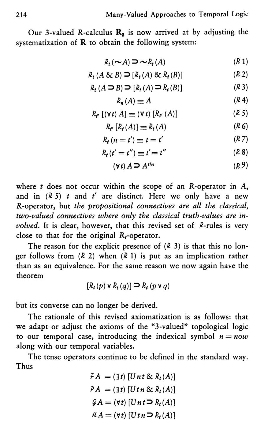
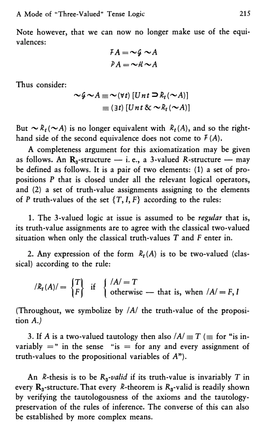
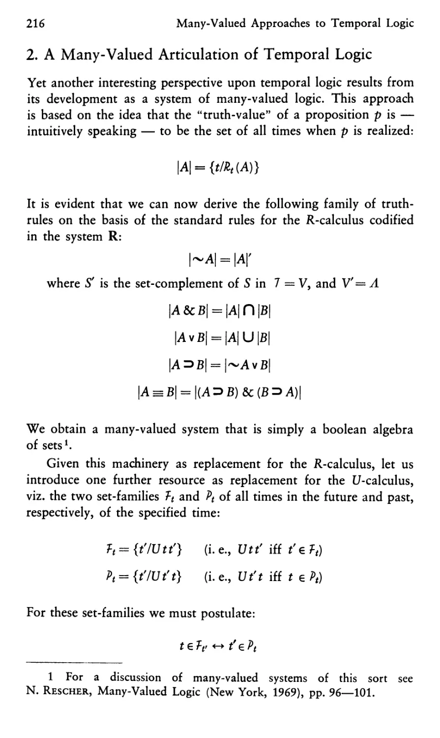
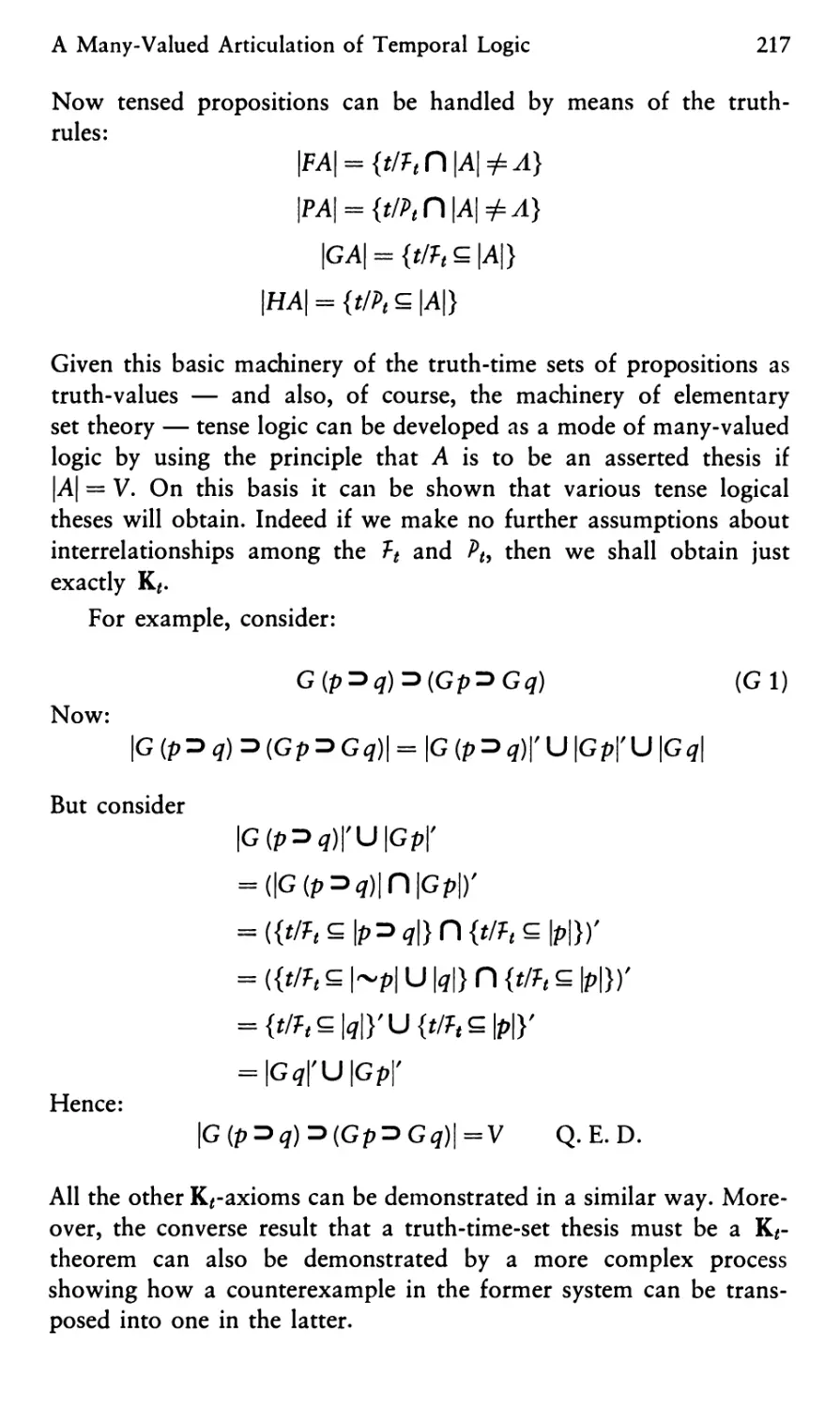
/


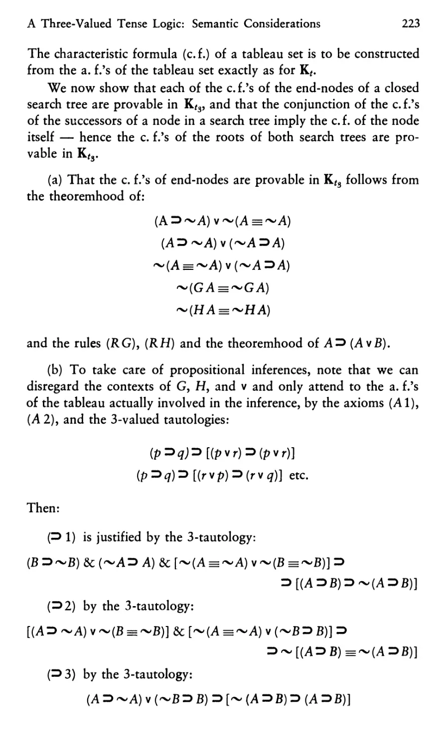
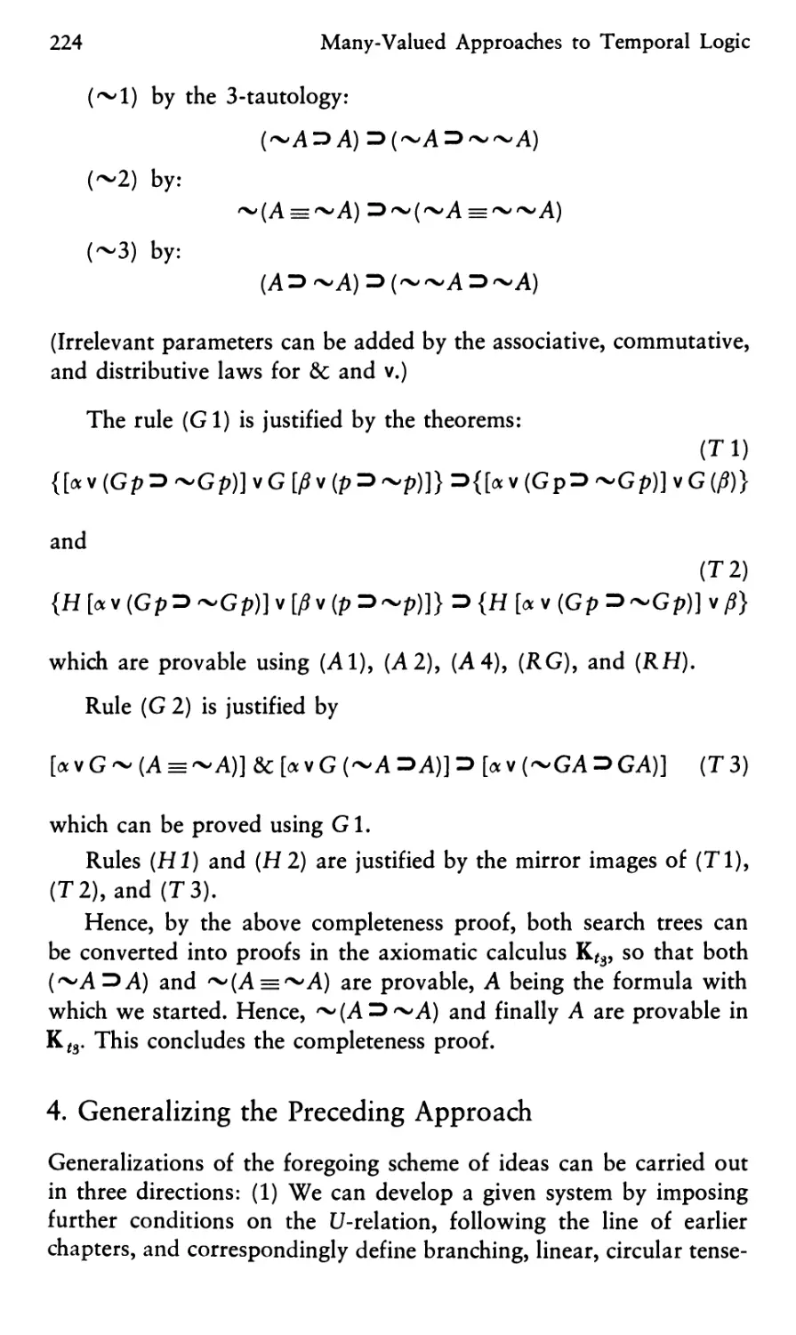

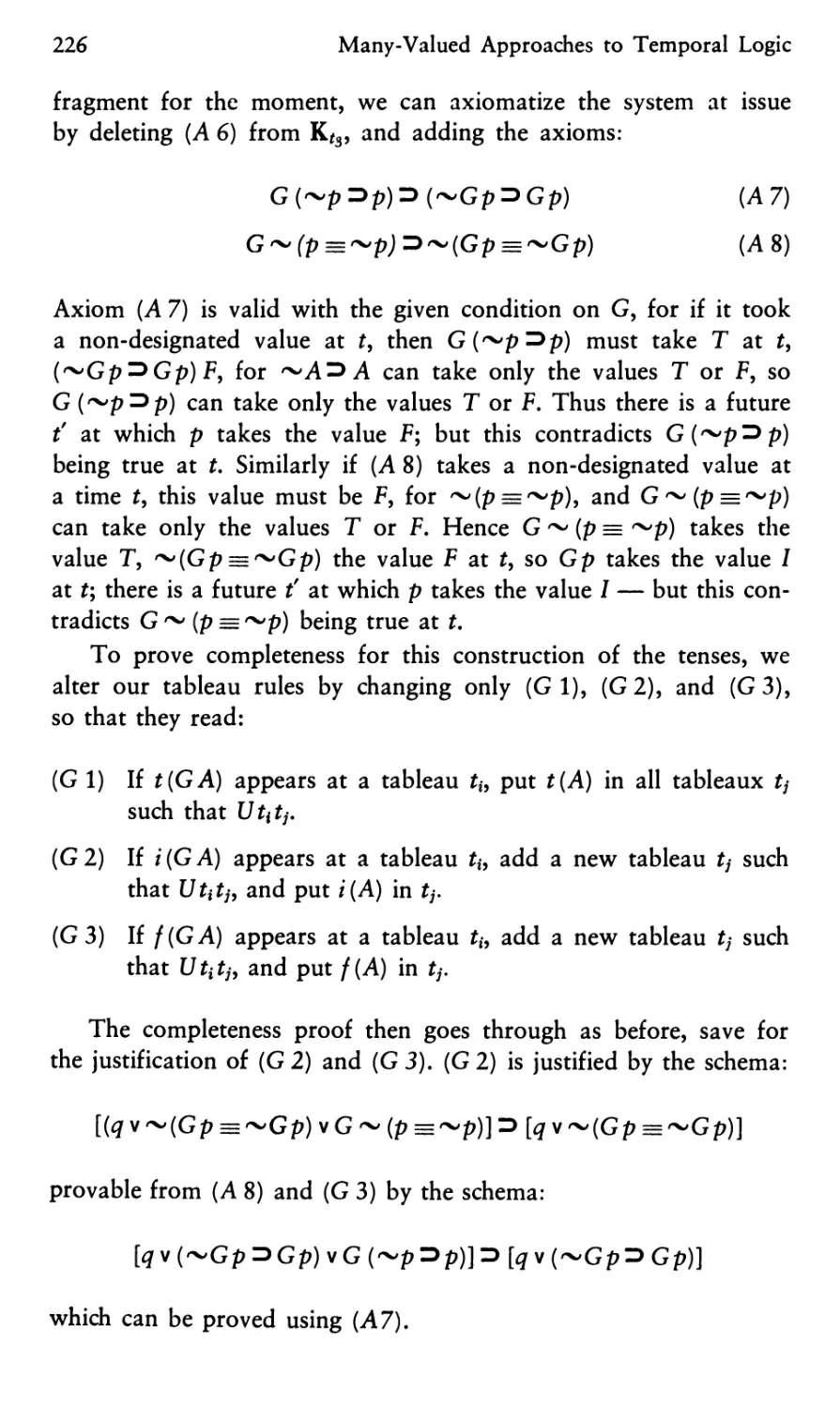


Текст
Library of V T®m>
Exact Philosophy ILd&lT
Editor:
Mario Bunge, Montreal
Co-editors:
Sir Alfred Jules Ayer, Oxford
Rudolf Carnap t, Los Angeles, Calif.
Herbert Feigl, Minneapolis, Minn.
Victor Kraft, Wien
Sir Karl Popper, Penn
Springer-Verlag Wien New York
Library of Exact Philosophy
Nicholas Rescher and
Alasdair Urquhart
Temporal Logic
Springer-Verlag Wien New York 1971
Printing type: Sabon Roman
Composed and printed by Herbert Hiessberger, Pottenstein
Binding work: Karl Scheibe, Wien
Design: Hans Joachim Boning, Wien
ISBN 3 -211- 80995 -3 Springer-Verlag Wien - New York
ISBN 0 -387- 80995 -3 Springer-Verlag New York - Wien
All rights reserved
No part of this book may be translated or reproduced in any form
without written permission from Springer-Verlag
© 1971 by Springer-Verlag/Wien
Library of Congress Catalog Card Number 74-141565
Printed in Austria
Arthur Prior
In Memoriam
General Preface to the LEP
The aim of the Library of Exact Philosophy is to keep alive the
spirit, if not the letter, of the Vienna Circle. It will consequently
adopt high standards of rigor: it will demand the clear statement
of problems, their careful handling with the relevant logical or
mathematical tools, and a critical analysis of the assumptions and
results of every piece of philosophical research.
Like the Vienna Circle, the Library of Exact Philosophy sees in
mathematics and science the wellsprings of contemporary intellectual
culture as well as sources of inspiration for some of the problems
and methods of philosophy. The Library of Exact Philosophy will
also stress the desirability of regarding philosophical research as
a cooperative enterprise carried out with exact tools and with the
purpose of extending, deepening, and systematizing our knowledge
about human knowledge.
But, unlike the Vienna Circle, the Library of Exact Philosophy
will not adopt a school attitude. It will encourage constructive work
done across school frontiers and it will attempt to minimize sterile
quarrels. And it will not restrict the kinds of philosophical problem:
the Library of Exact Philosophy will welcome not only logic,
semantics and epistemology, but also metaphysics, value theory
and ethics as long as they are conceived in a clear and cogent way,
and are in agreement with contemporary science.
Montreal, January 1970
Mario Bunge
Preface
This book is an introduction to temporal logic, a now flourishing
branch of philosophical logic whose origin is of recent date, its main
impetus having been provided by the publication in the late 1950s of
A. N. Prior's pioneering book, Time and Modality (Oxford, The
Clarendon Press, 1957). Virtually all work in the field to around
1966 is surveyed in Prior's elegant treatise Vast, Present and Future
(Oxford, The Clarendon Press, 1967). In consequence, it is no
simple matter to write a comprehensive book on the subject
without merely rehearsing material already dealt with in Prior's works.
We believe, however, that the present book succeeds in this difficult
endeavor because it approaches established materials from wholly
novel points of departure, and is thus able to attain new perspectives
and achieve new results. Its introductory character notwithstanding,
the present work is consequently in substantial measure devoted
to an exposition of new findings and a demonstration of new results.
Parts of the book have been published previously. Chapter II is
a modified version of an article of the same title by N. Rescher
and James Garson in The Journal of Symbolic Logic (vol. 33
[1968], pp. 537—548). And Chapter XIII is a modified version of
the article "Temporally Conditioned Descriptions" by N. Rescher
and John Robison in Ratio, vol. 8 (1966), pp. 46—54. The authors
are grateful to Professors Garson and Robison, and to the editors
of the jounal involved, for their permission to use this materials here.
The authors acknowledge with thanks the conscientious
assistance of Judy Bazy (Mrs. Martin Stanton) and Miss Kathy Walsh
in preparing the difficult typescript.
The authors are very grateful to Dorothy Henle, Arnold van
der Nat, and Zane Parks for assistance in correcting the proofs.
XII
Preface
Shortly after completion of the work we learned of the tragic
death of Arthur Prior. It pleases us that a few days before he
was able to examine the work and approve our intention to dedicate
it to him.
Pittsburgh, Spring, 1971
N. Rescher and A. Urquhart
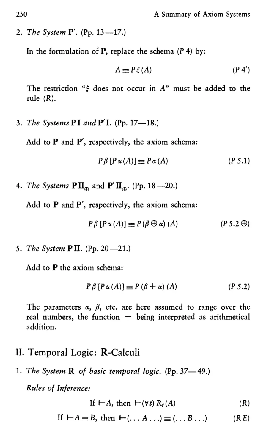
Contents
Foreword on Notation and Prerequisites XVII
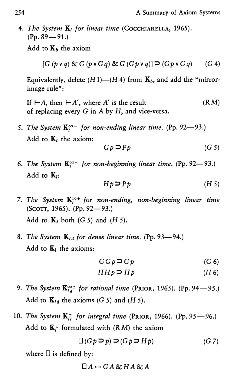
Chapter I
The Background of Temporal Logic 1
Chapter II
Topological Logic 13
1. Introduction 13
2. The P-Operator 13
3. Three Basic Axioms 14
4. The Relation of P-Unqualified to P-Qualified Formulas:
The Preferred Position f: A Fourth Axiom 16
5. The Iteration of P: A Fifth Axiom and the Two Systems PI and PII 17
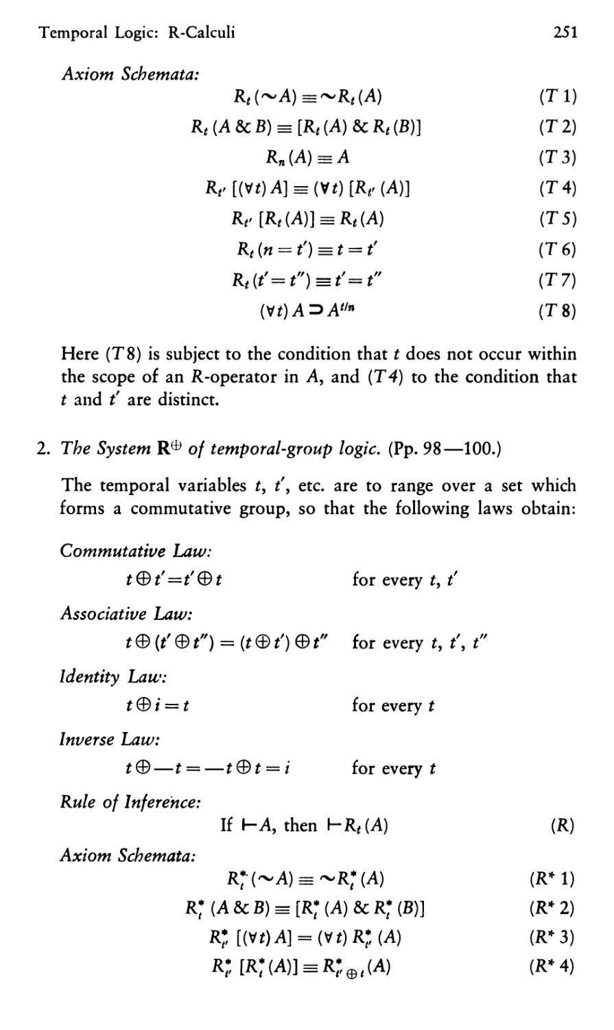
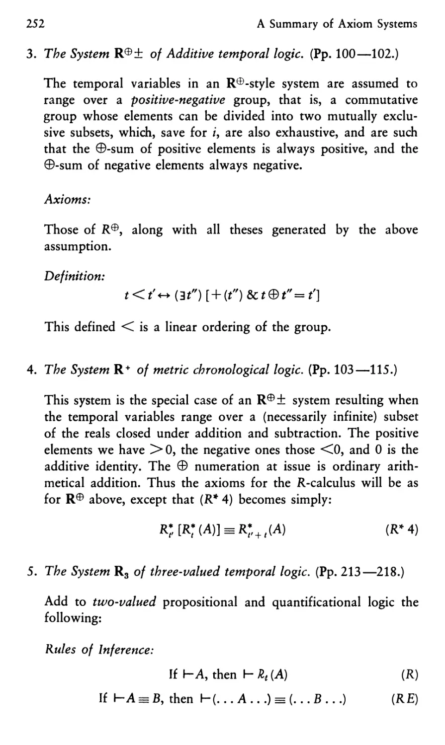
6. The Possible Worlds Interpretation of Topological Logic 21
Chapter III
Fundamental Distinctions for Temporal Logic 23
1. The Temporal Equivocality of IS 23
2. Translating Temporal to Atemporal IS 24
3. Temporally Definite and Indefinite Statements 25
4. The Implicit Ubiquity of "Now" in Tensed Statements 26
5. Dates and Pseudo-Dates 27
6. Times of Assertion 28
7. Two Styles of Chronology 30
Chapter IV
The Basic System R of Temporal Logic 31
1. The Concept of Temporal Realization 31
2. The Temporal Transparency of "Now" 32
3. .Temporal Homogeneity 35
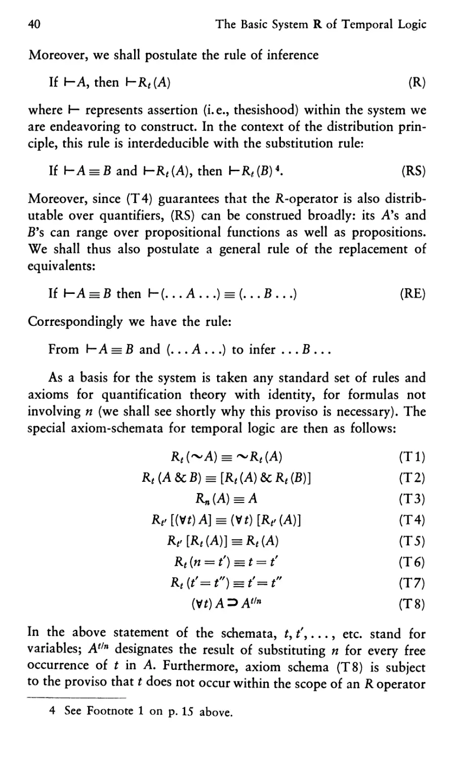
4. Axioms for the Logical Theory of Chronological Propositions 37
5. Temporal and Topological Logic 43
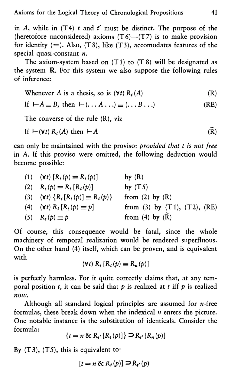
6. The Completeness and Decidability of R 44
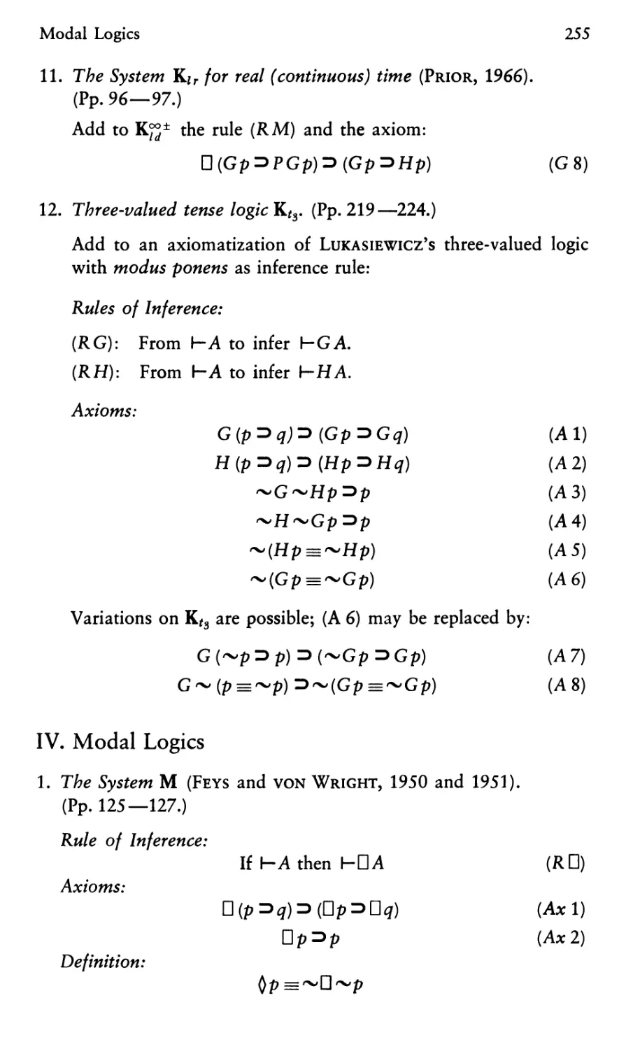
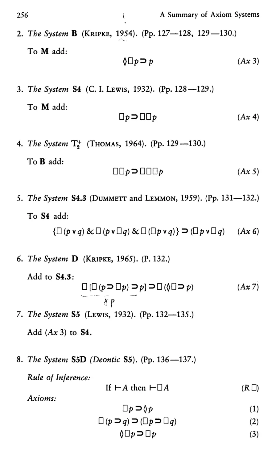
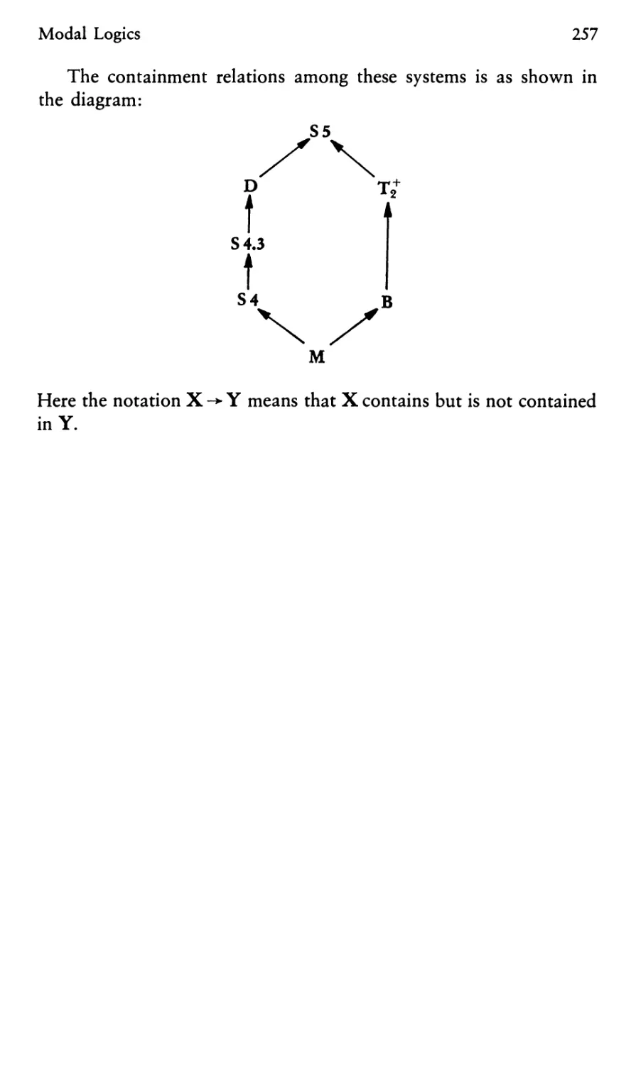
XIV
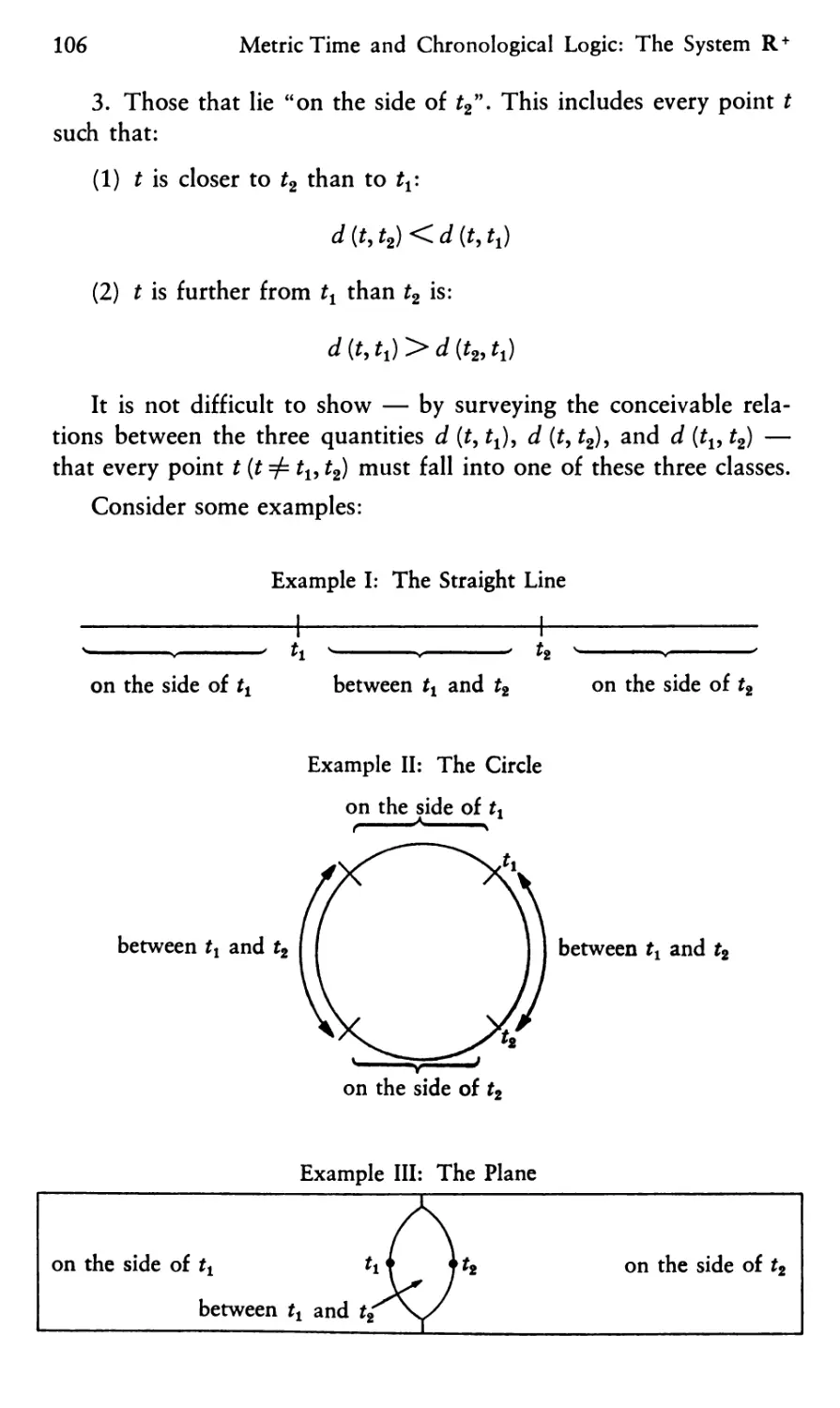
Chapter V
The Introduction of Tense Operators 50
1. Presentness and Precedence 50
2. Tense 52
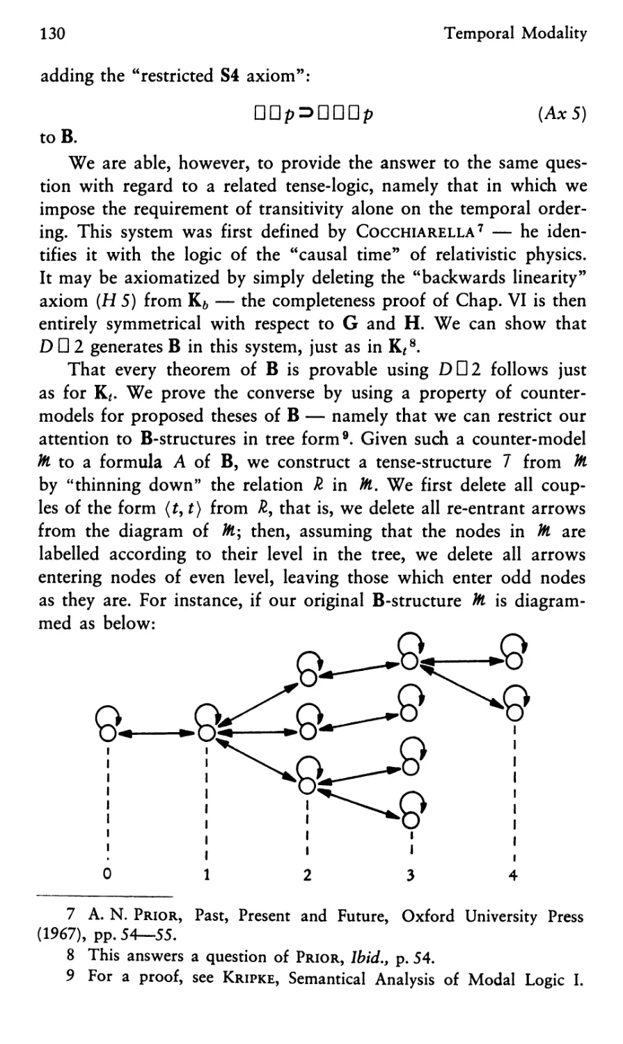
Chapter VI
The System K* of Minimal Tense Logic 55
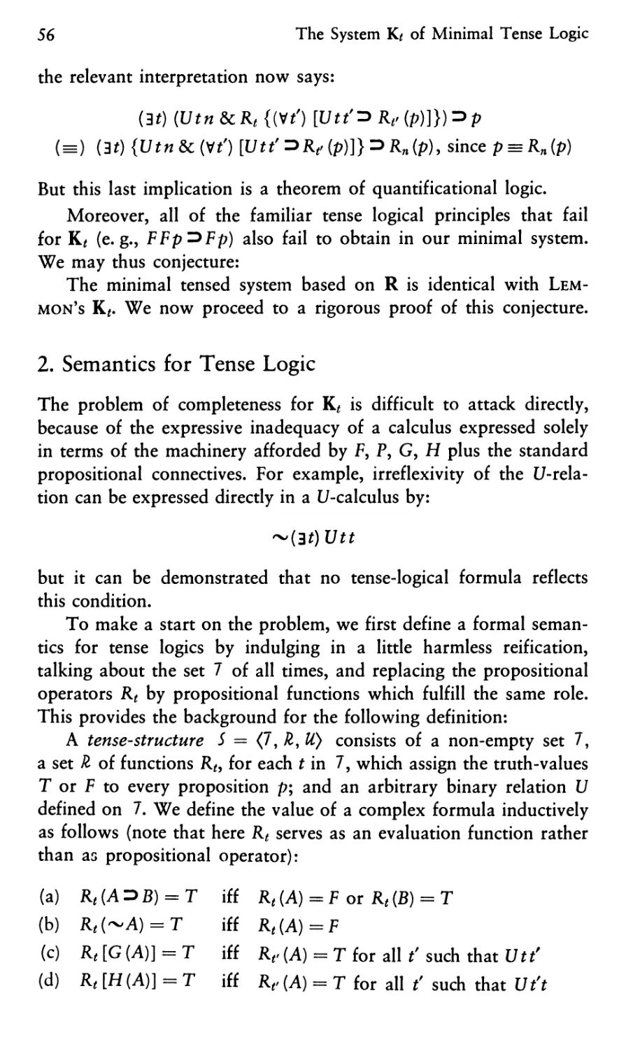
1. The Problem of a Minimal Tense Logic 55
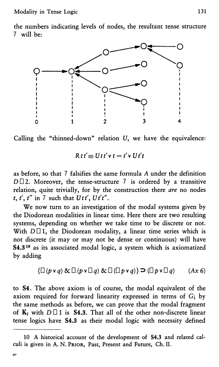
2. Semantics for Tense Logic 56
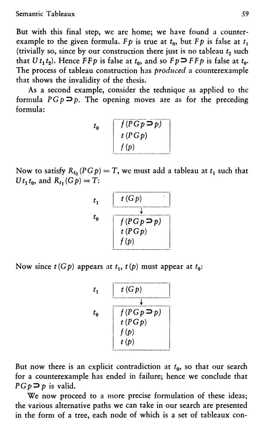
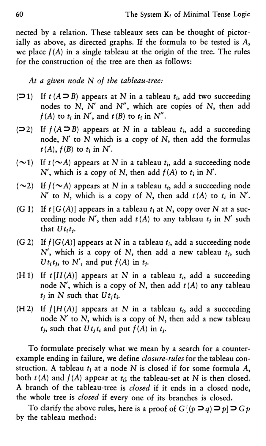
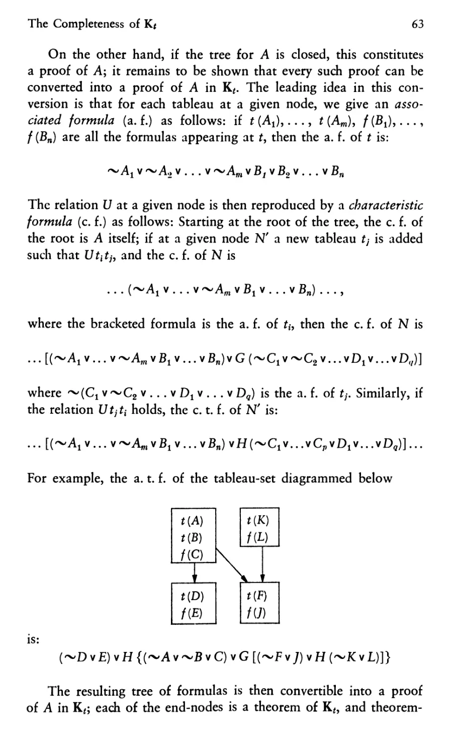
3. Semantic Tableaux 58
4. The Completeness of K* 62
5. Some Corollaries 66
6. Completeness of K* with Respect to R 67
Chapter VII
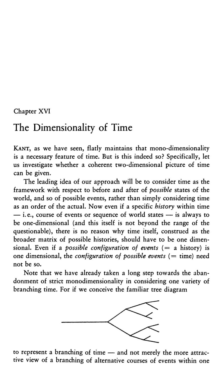
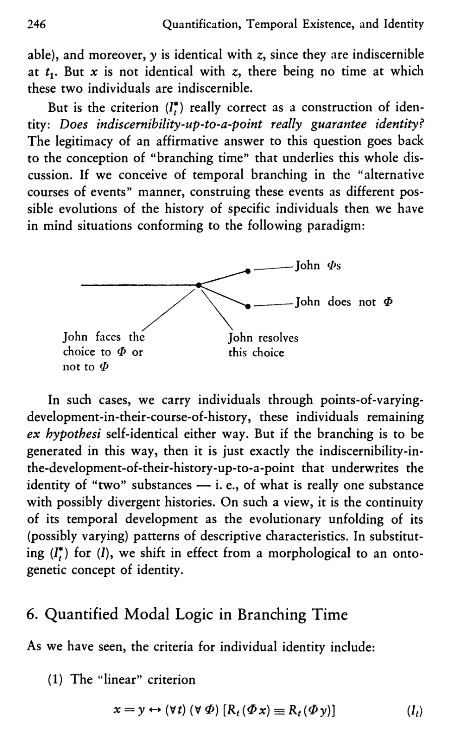
Branching Time: The System Kb 68
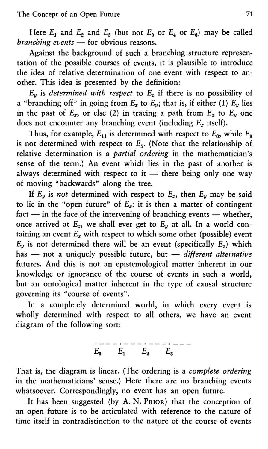
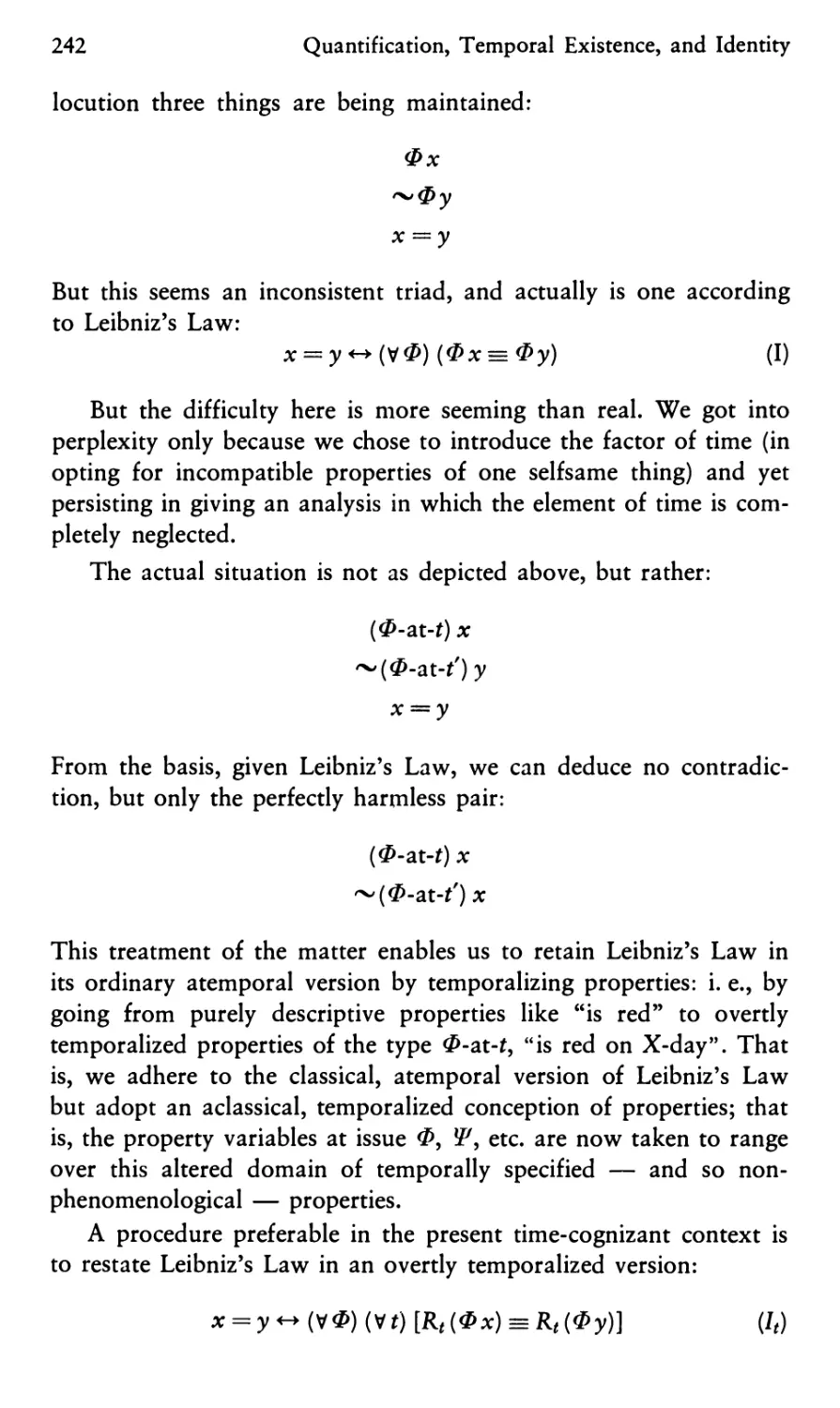
1. Branching Structures 68
2. The Concept of an Open Future 70
3. The Logic of Branching Time 74
4. Axiomatization of Kb 76
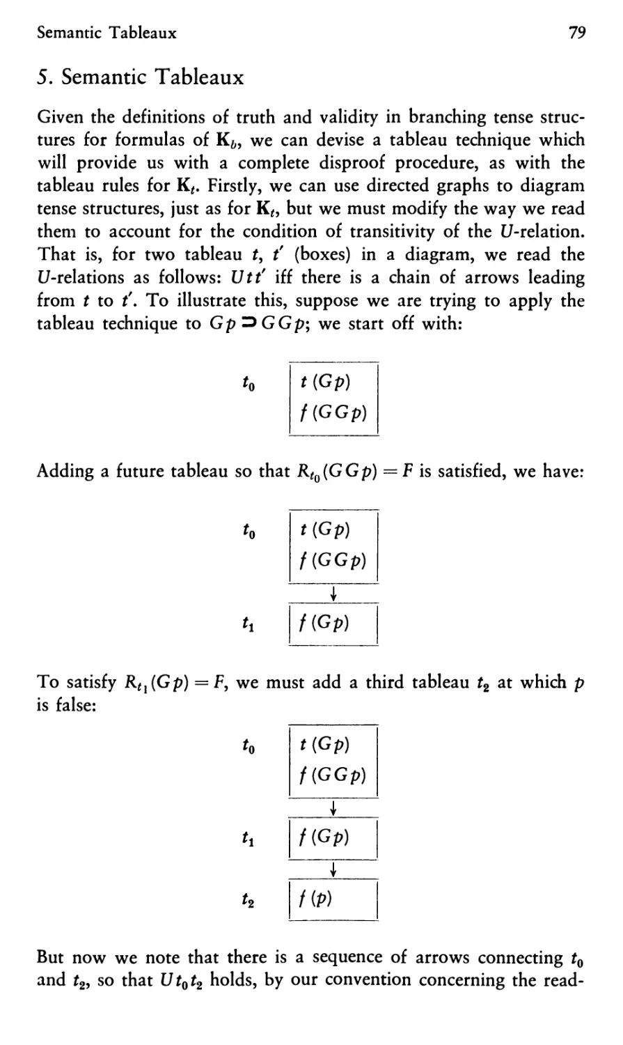
5. Semantic Tableaux 79
6. Systematic Tableaux 81
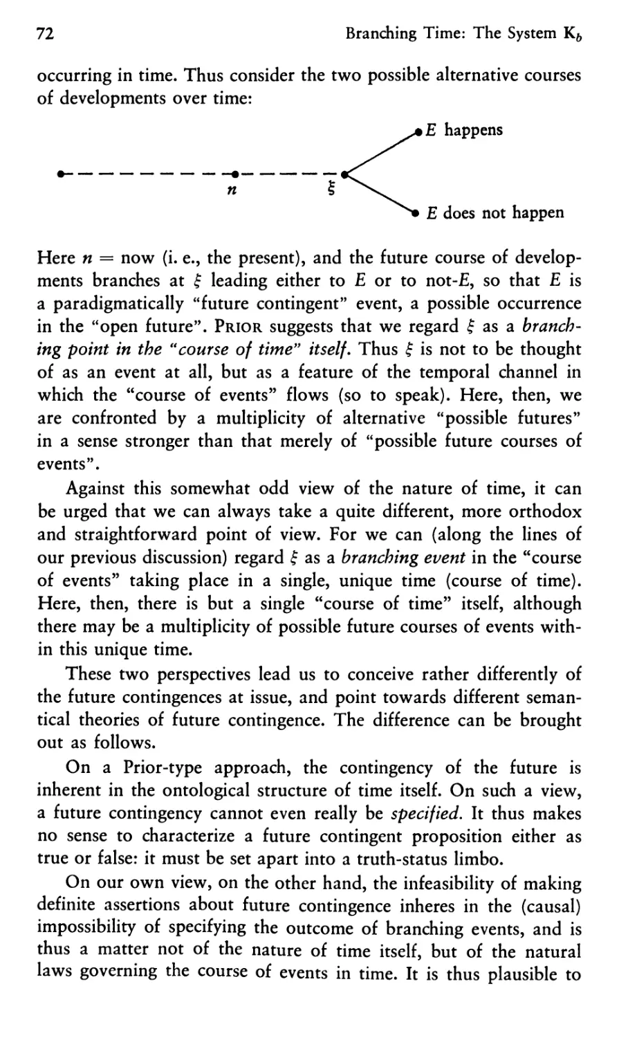
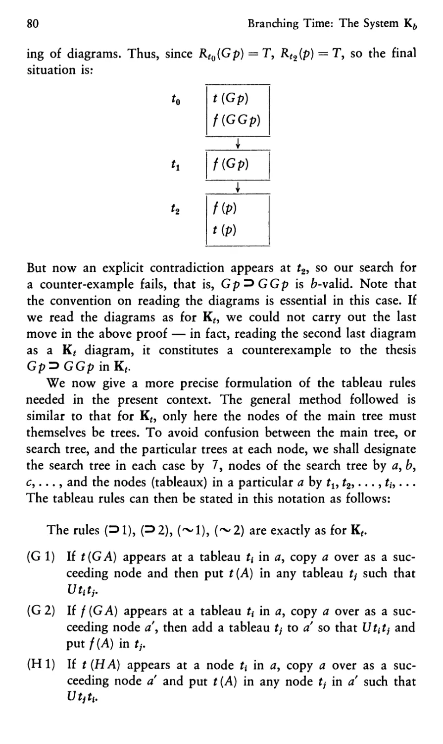
7. Completeness Proof for K& 83
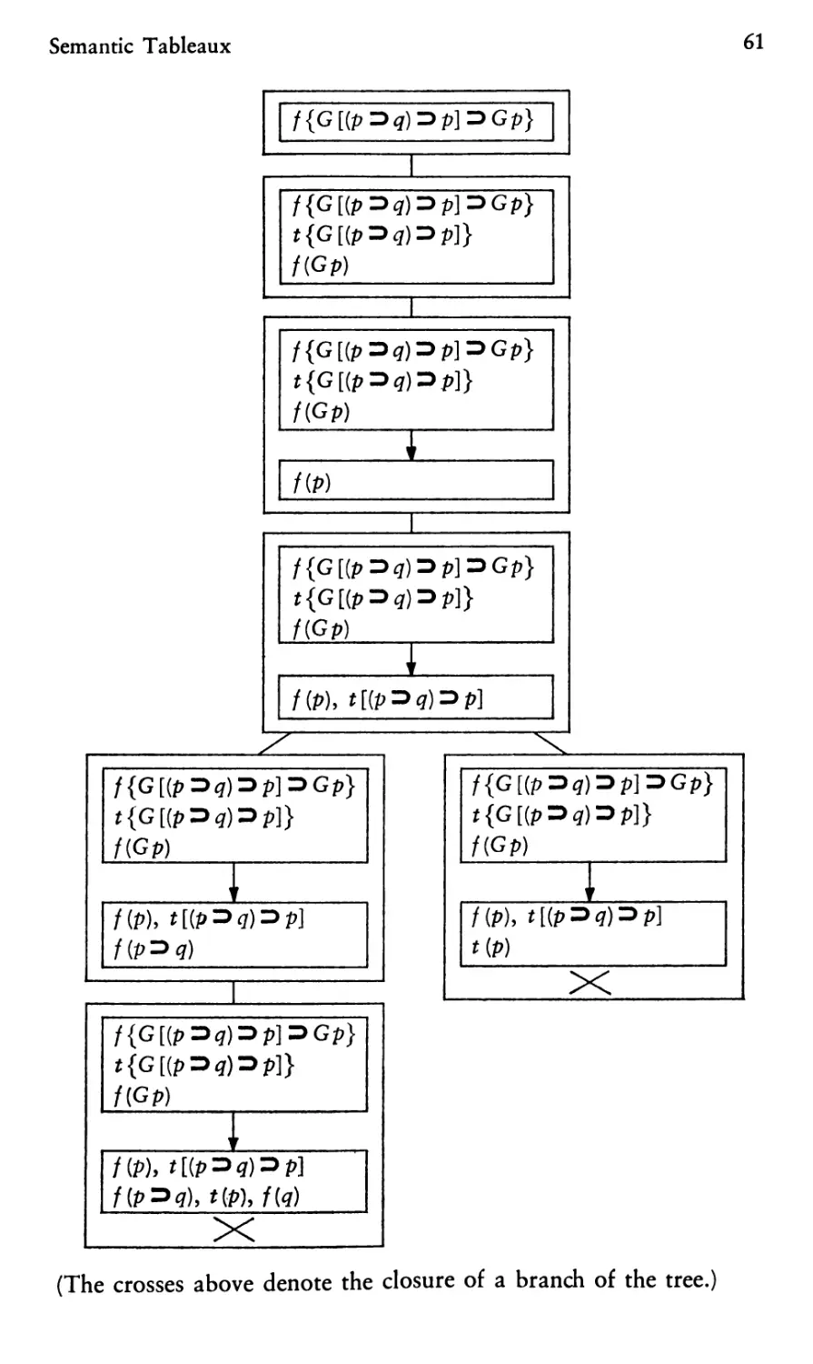
Chapter VIII
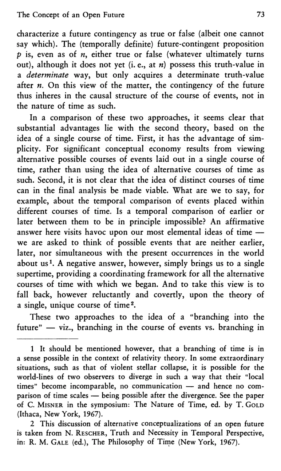
Linear Time: The System K/ and Its Variants 88
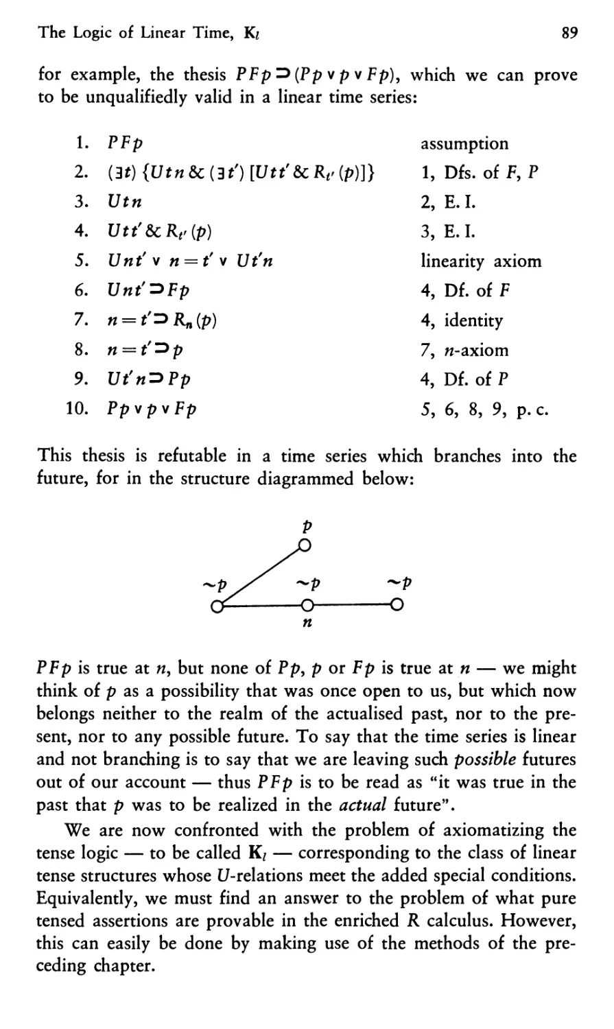
1. The Logic of Linear Time, K/ 88
2. Extensions of K/ 91
Chapter IX
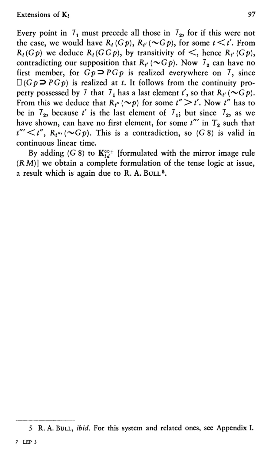
Additive Time: The Systems R® and R®± 98
1. Temporal-Groups and the System R® 98
2. Additive Temporal Logic and the System R® ± 100
Chapter X
Metric Time and Chronological Logic: The System R +
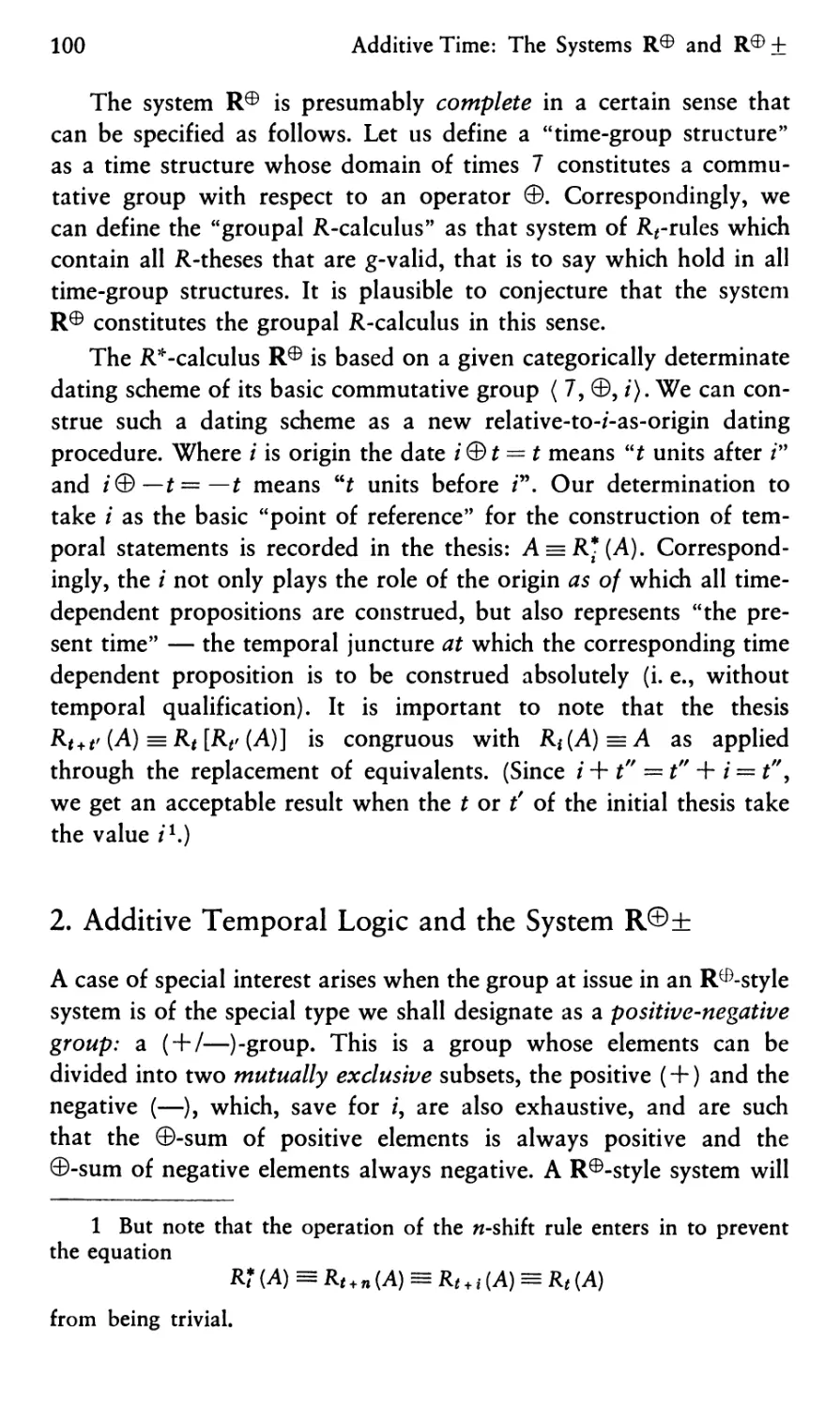
1. The Concept of Metric Time 103
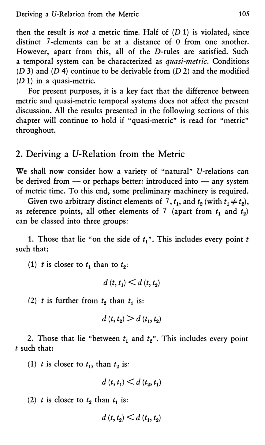
2. Deriving a U-Relation from the Metric 105
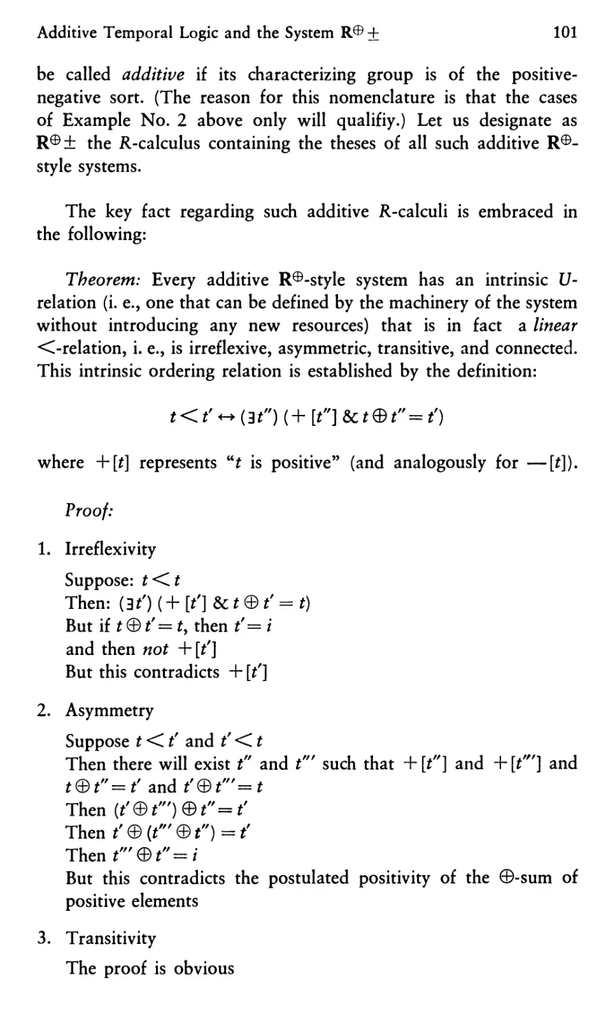
3. The System R+ 109
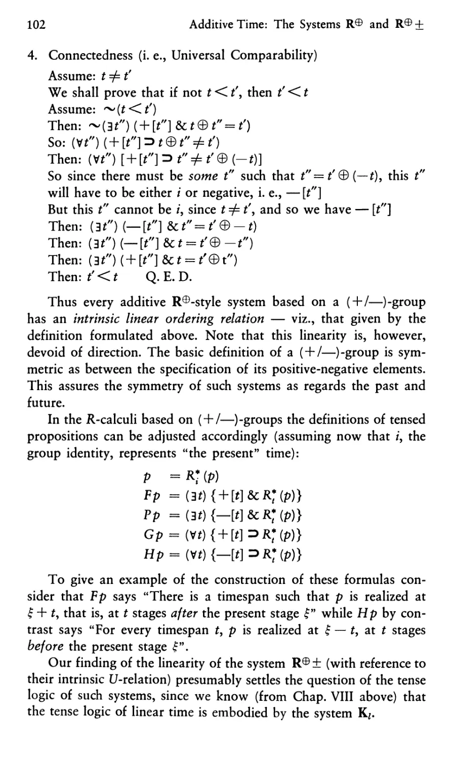
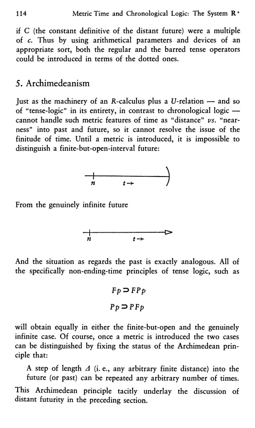
4. "Distance" into Past and Future 110
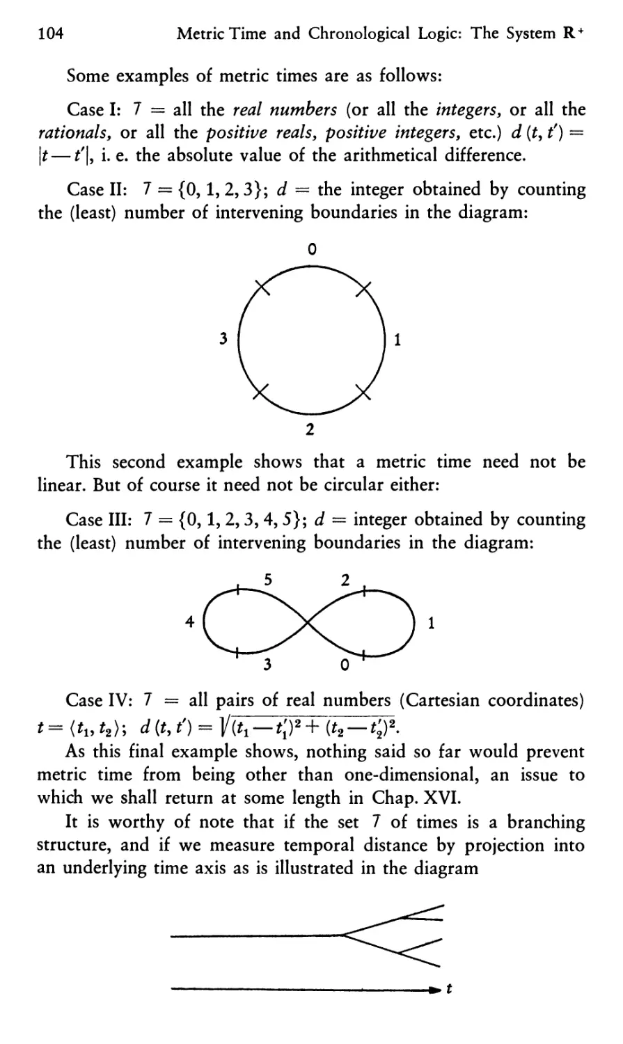
5. Archimedeanism 114
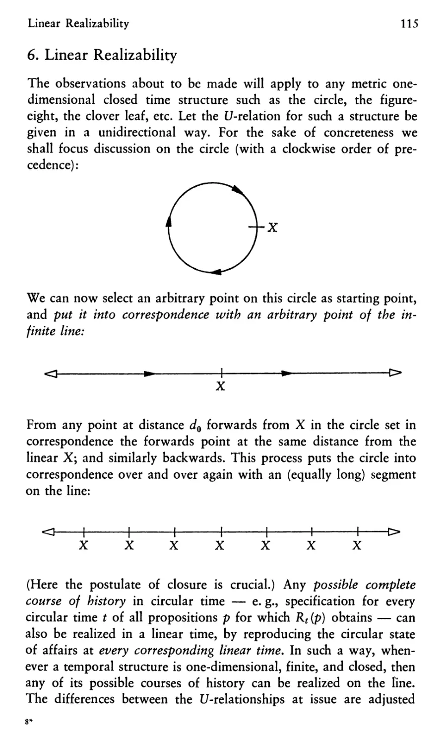
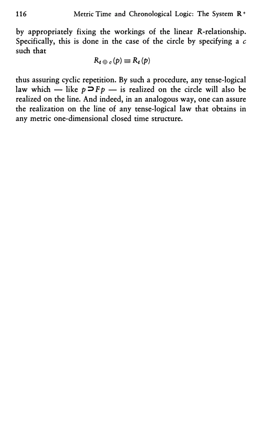
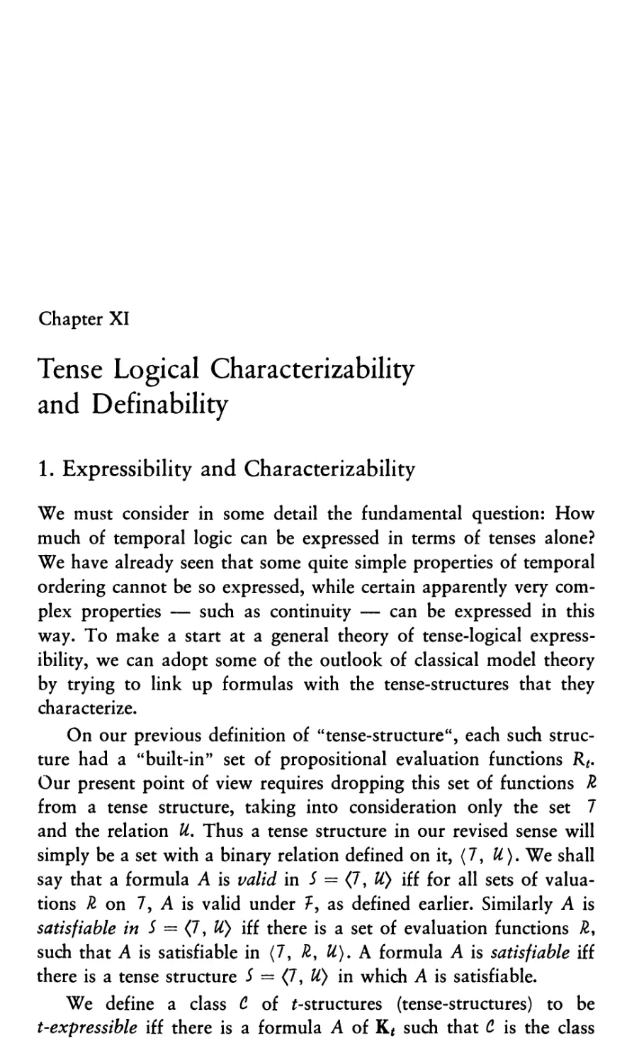
6. Linear Realizability 115
Contents
XV
Chapter XI
Tense Logical Characterizability and Definability 117
1. Expressibility and Characterizability 117
2. Tense-Logical Definability 122
Chapter XII
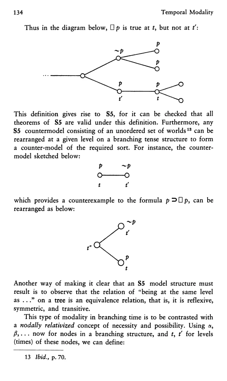
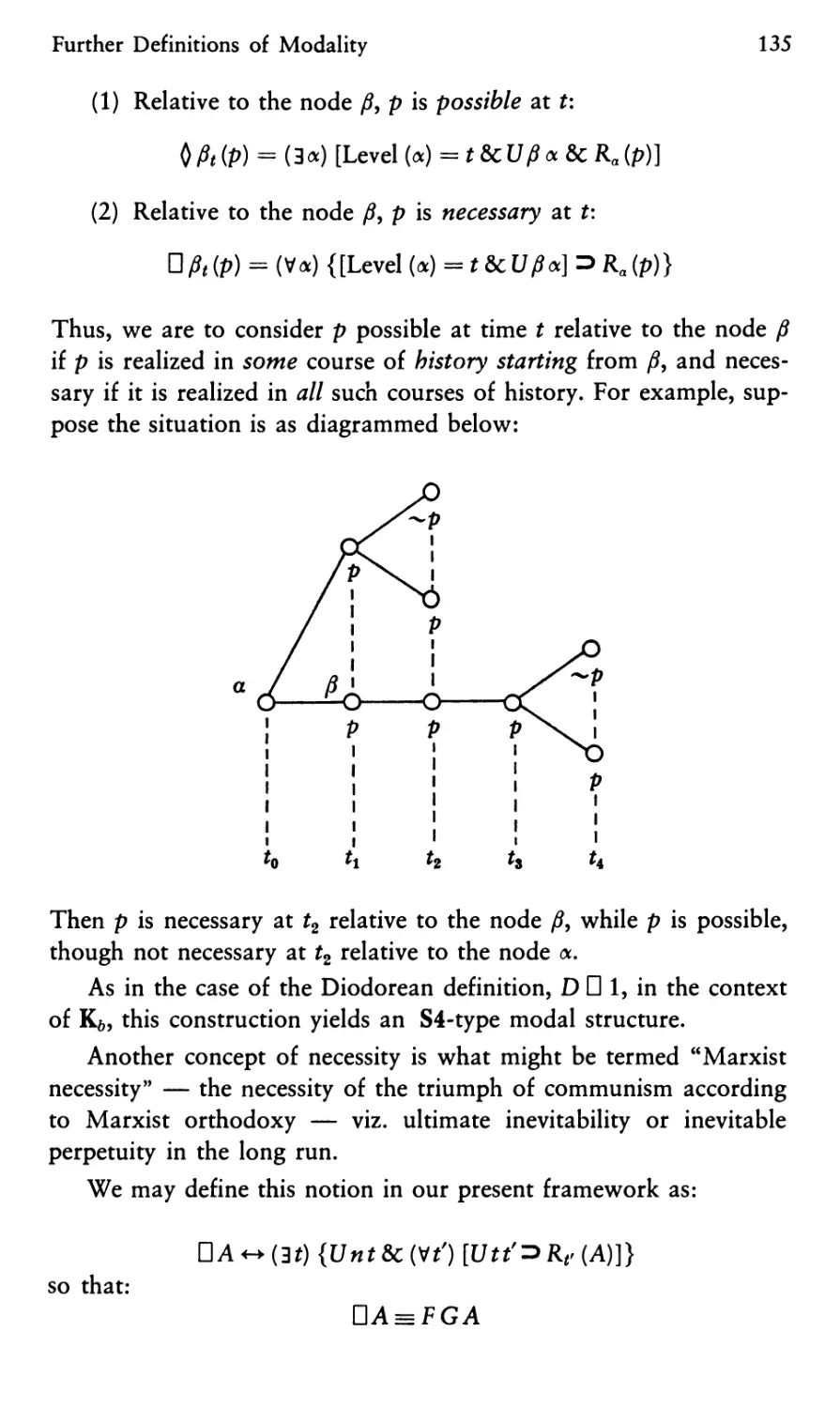
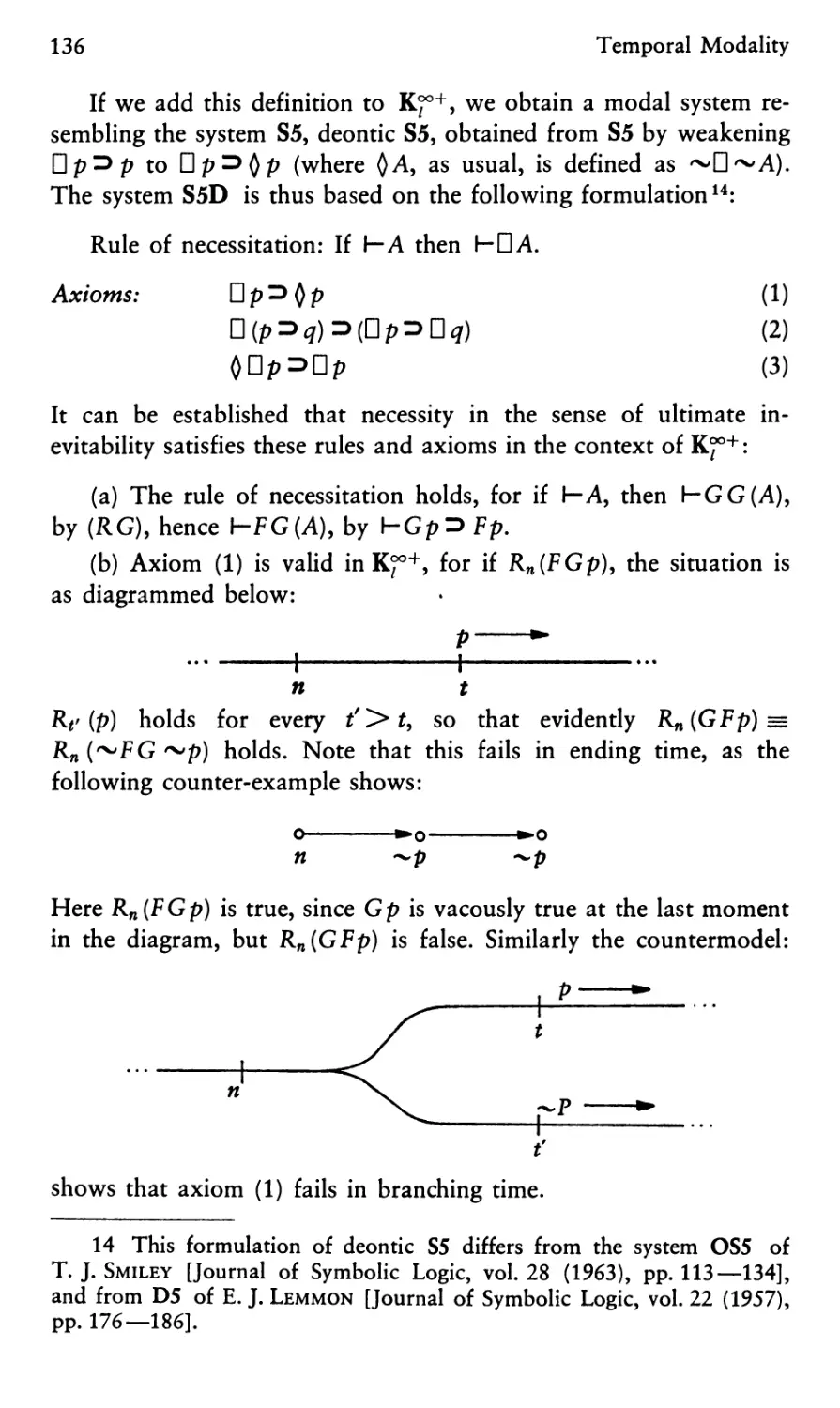
Temporal Modality 125
1. The Tensed Interpretation of Modality 125
2. Modality in Tense Logic 126
3. Further Definitions of Modality 133
Chapter XIII
Temporally Conditioned Descriptions and the Concept
of Temporal Purity 138
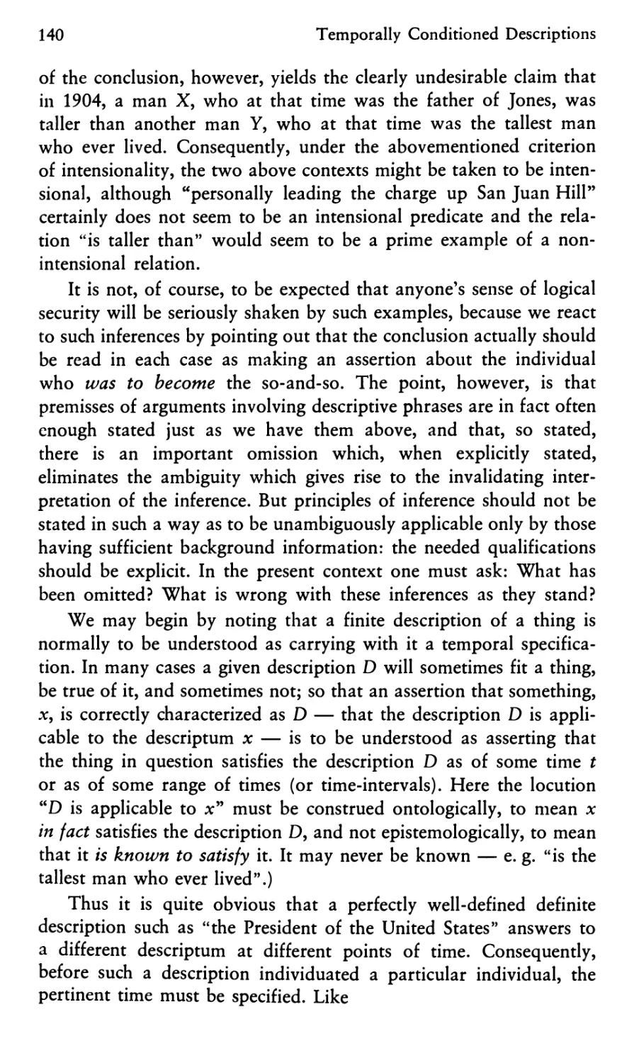
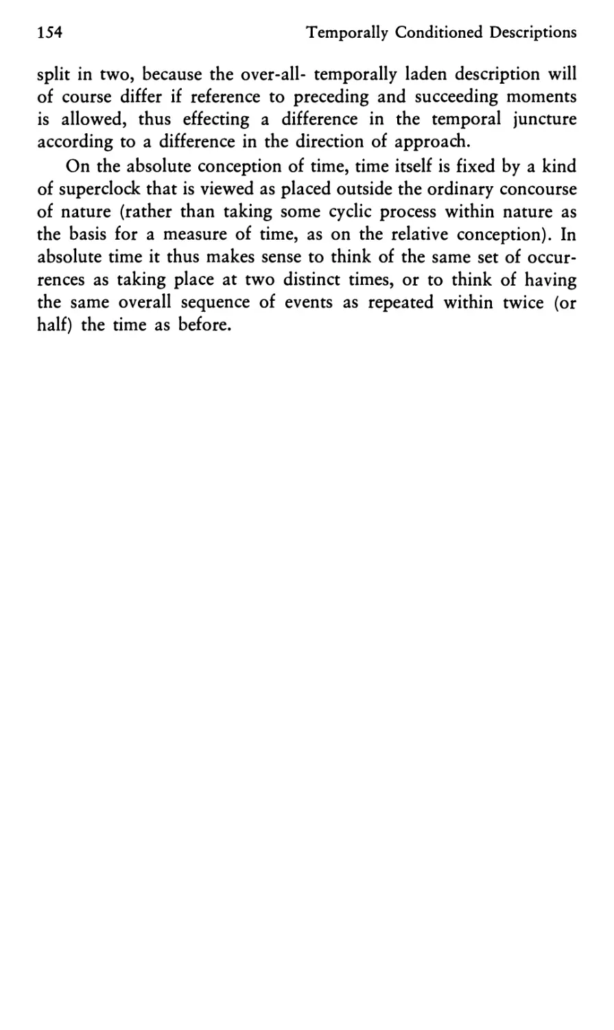
1. Temporally Conditioned Descriptions 138
2. Chronological Purity 144
3. The "Purely Phenomenological" Characterization of the Occurrences
of a Moment 149
4. The Absolute vs. the Relative Conception of Time 151
Chapter XIV
The Theory of Processes 155
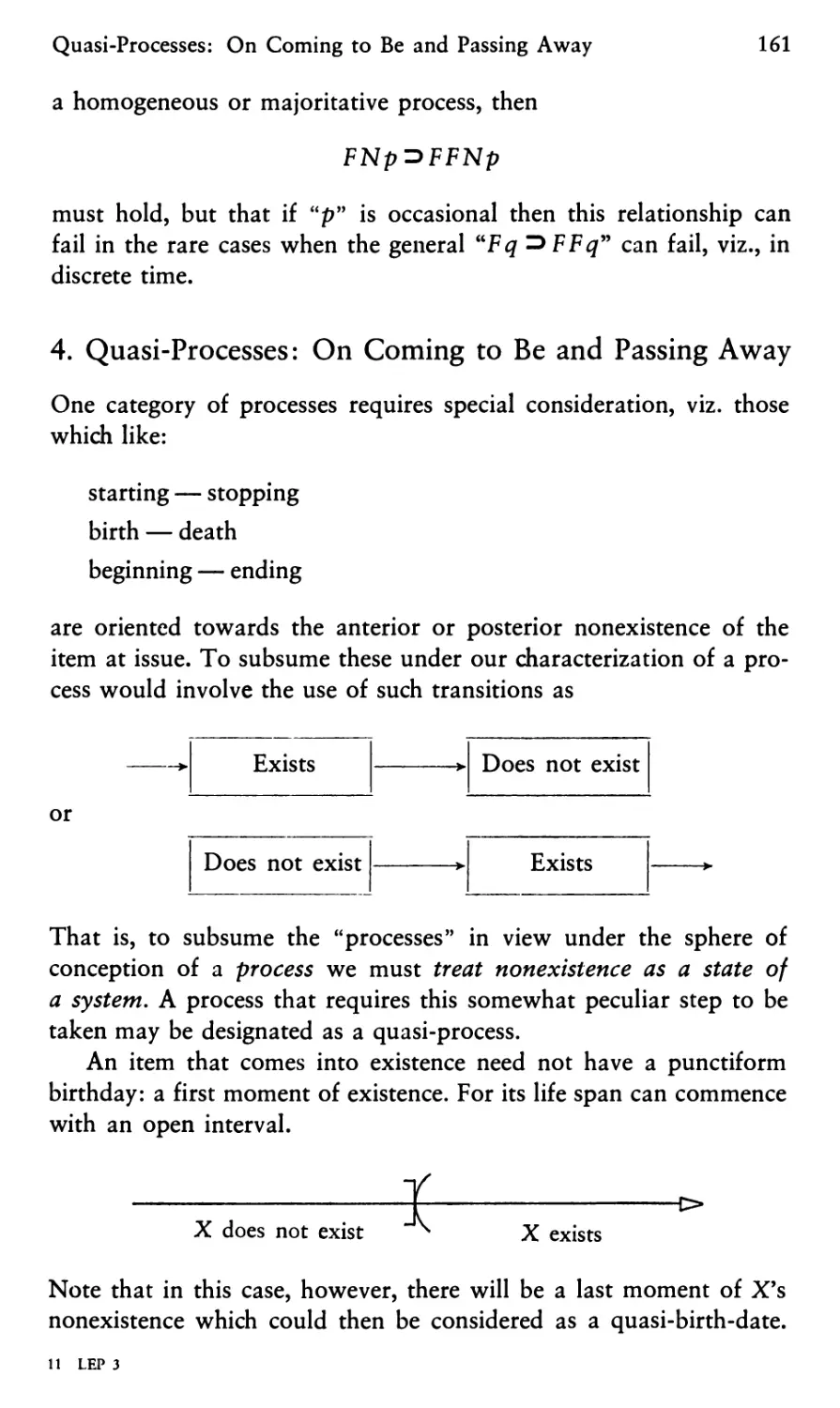
1. What is a Process? 155
2. The Representation of Processes: Process Implications 155
3. Activities and Processes: Some Applicable Distinctions 159
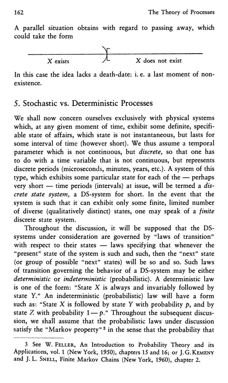
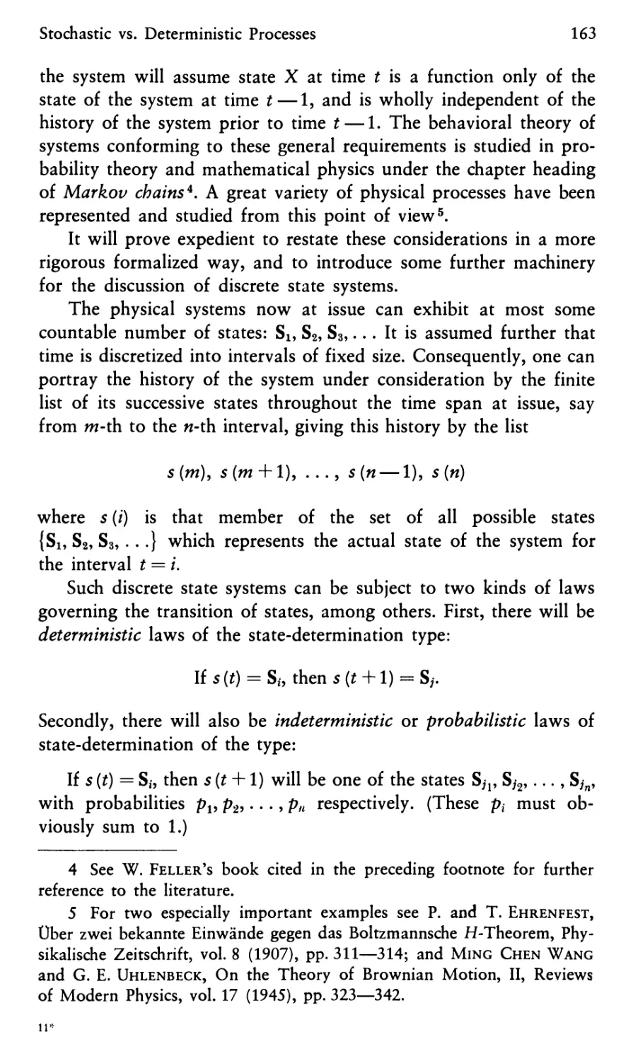
4. Quasi-Processes: On Coming to Be and Passing Away 161
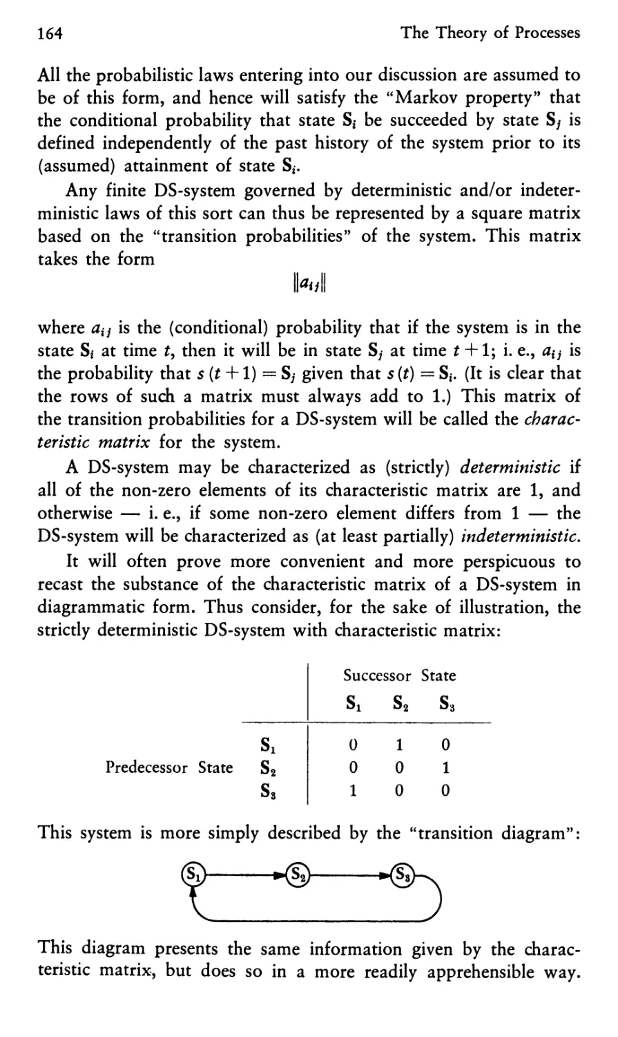
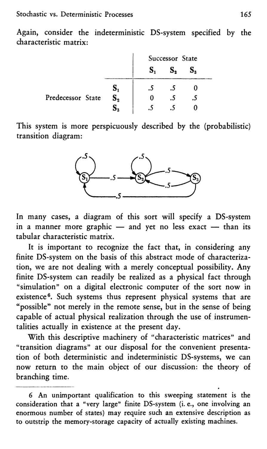
5. Stochastic vs. Deterministic Processes 162
6. Stochastic Processes and Branching Time 166
7. The Structure of Events 167
Chapter XV
The Logic of World States 170
1. The Concept of a World State 170
2. Some Further Perspectives on Instantaneous World States 173
3. The Concept of a World History 179
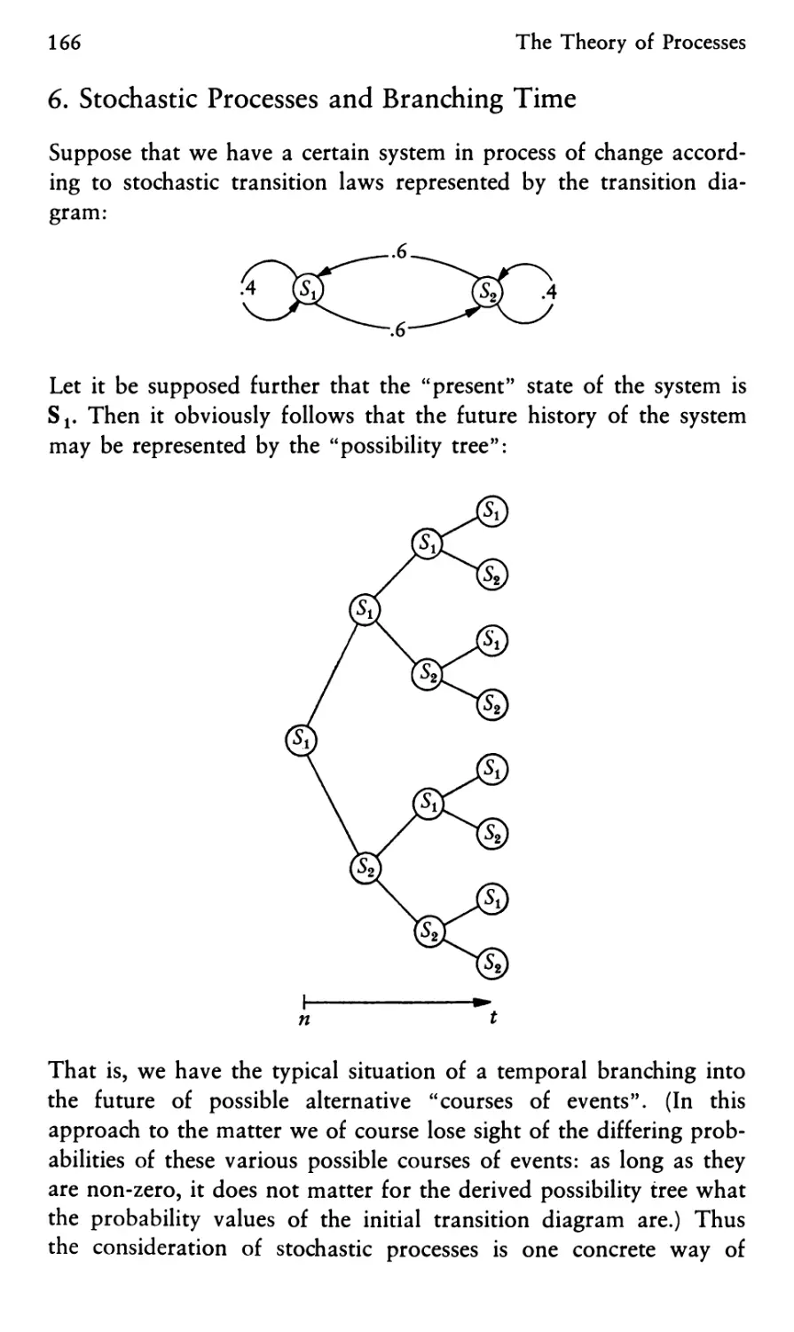
4. Development of R-calculi Within Tense Logic 182
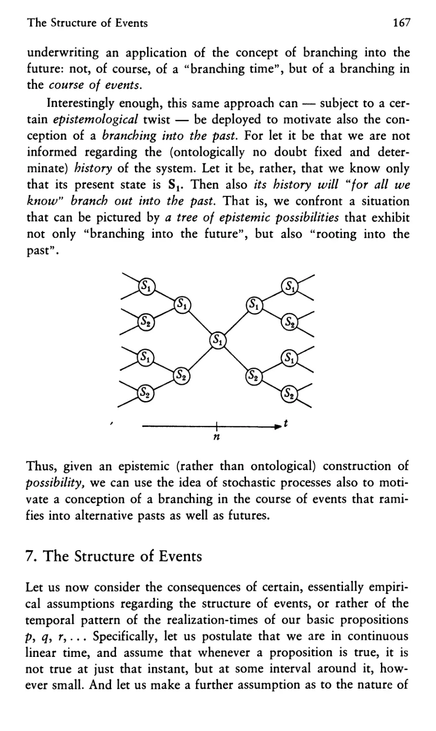
Chapter XVI
The Dimensionality of Time 184
XVI
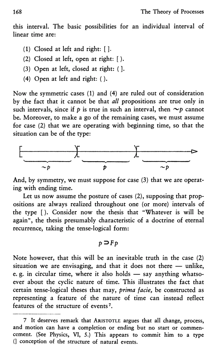
Contents
Chapter XVII
The "Master Argument" of Diodorus
and Temporal Determinism 189
1. The "Master Argument" 189
2. Necessity and Determinism in the Context of the "Master Argument" 195
3. Evading the Deterministic Conclusion of the "Master Argument" 196
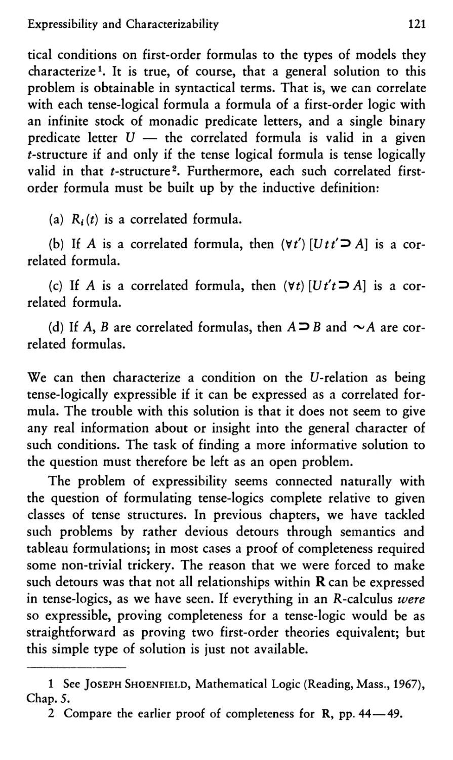
4. The Groundwork of a 3-Valued Conception of Temporal Truth 198
5. Alternative Futures and Future Contingency 200
6. Temporal Determination 203
7. Nomological Necessitation 206
Chapter XVIII
Many-Valued Approaches to Temporal Logic 213
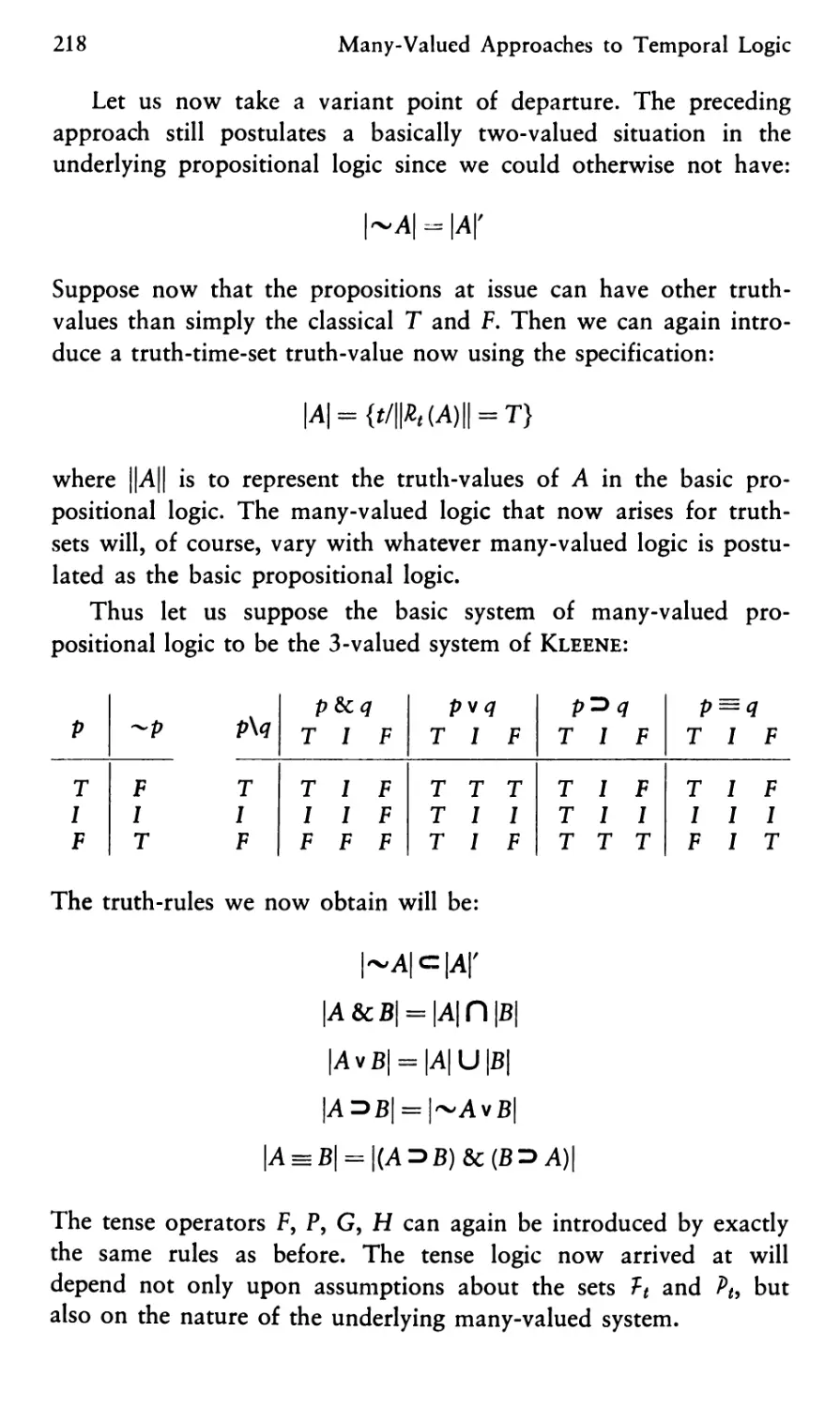
1. A Mode of "Three-Valued" Tense Logic 213
2. A Many-Valued Articulation of Temporal Logic 216
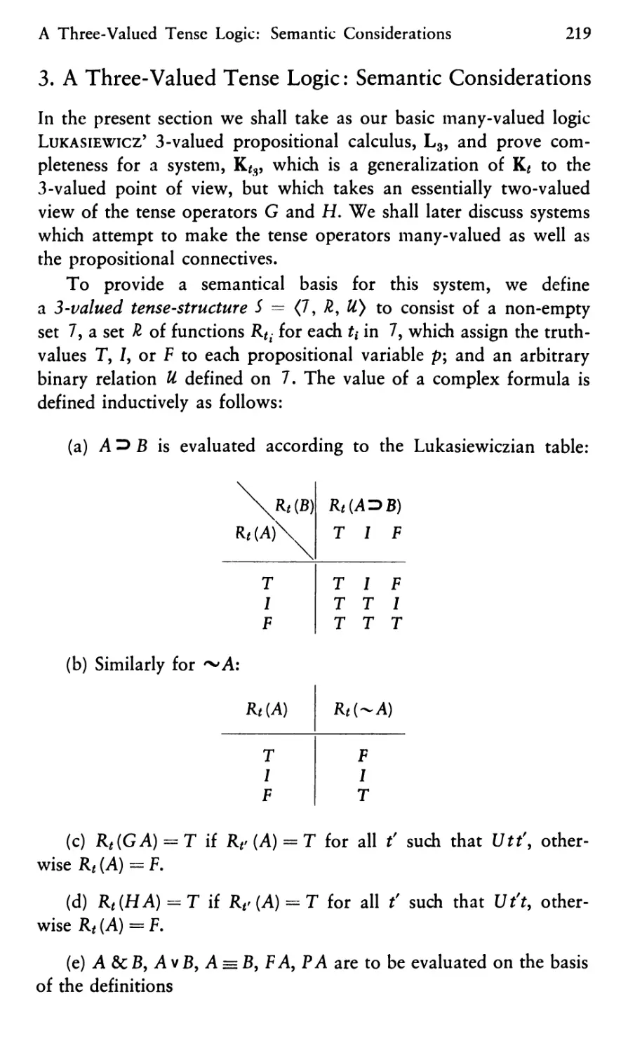
3. A Three-Valued Tense Logic: Semantic Considerations 219
4. Generalizing the Preceding Approach 224
Chapter XIX
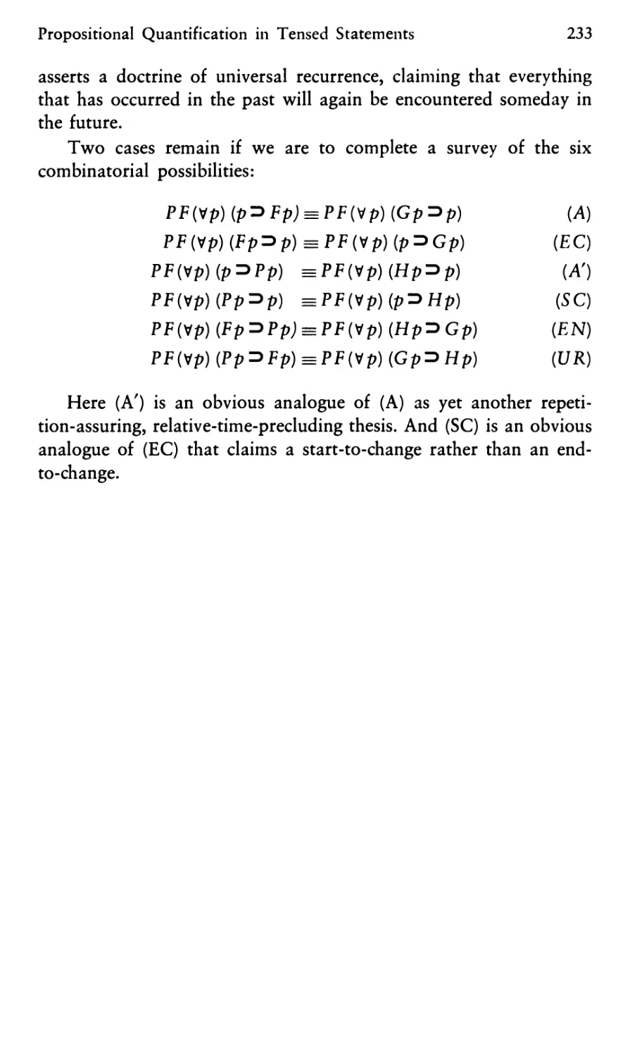
Propositional Quantification in Tensed Statements 228
Chapter XX
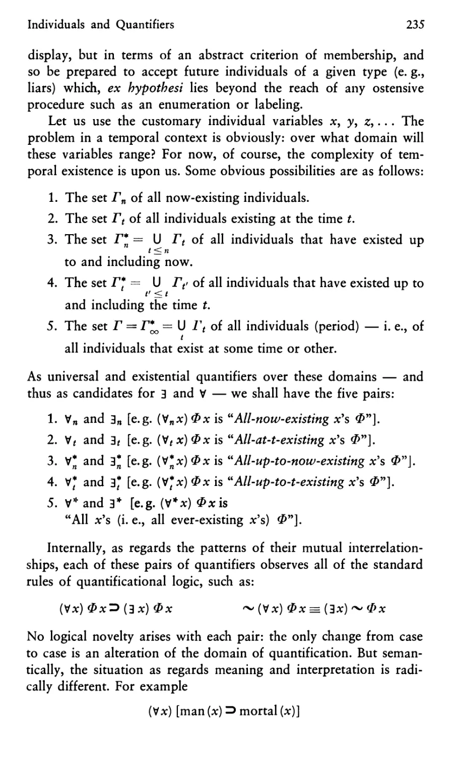
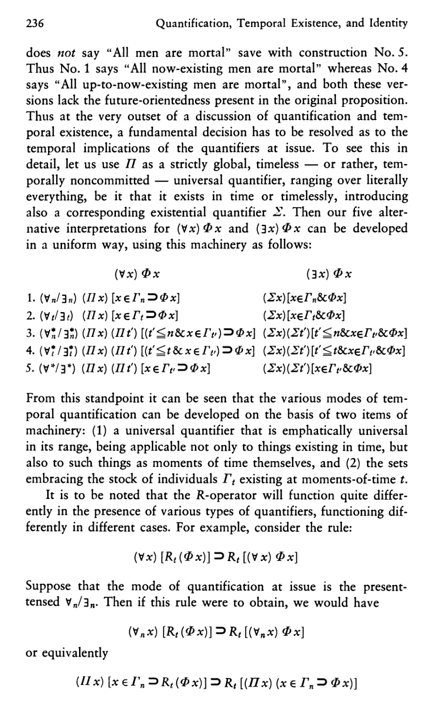
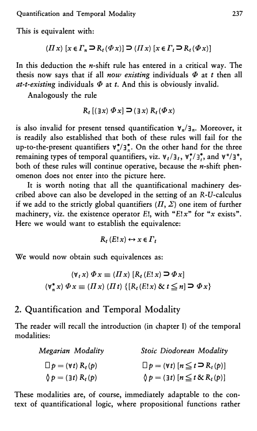
Quantification, Temporal Existence, and Identity 234
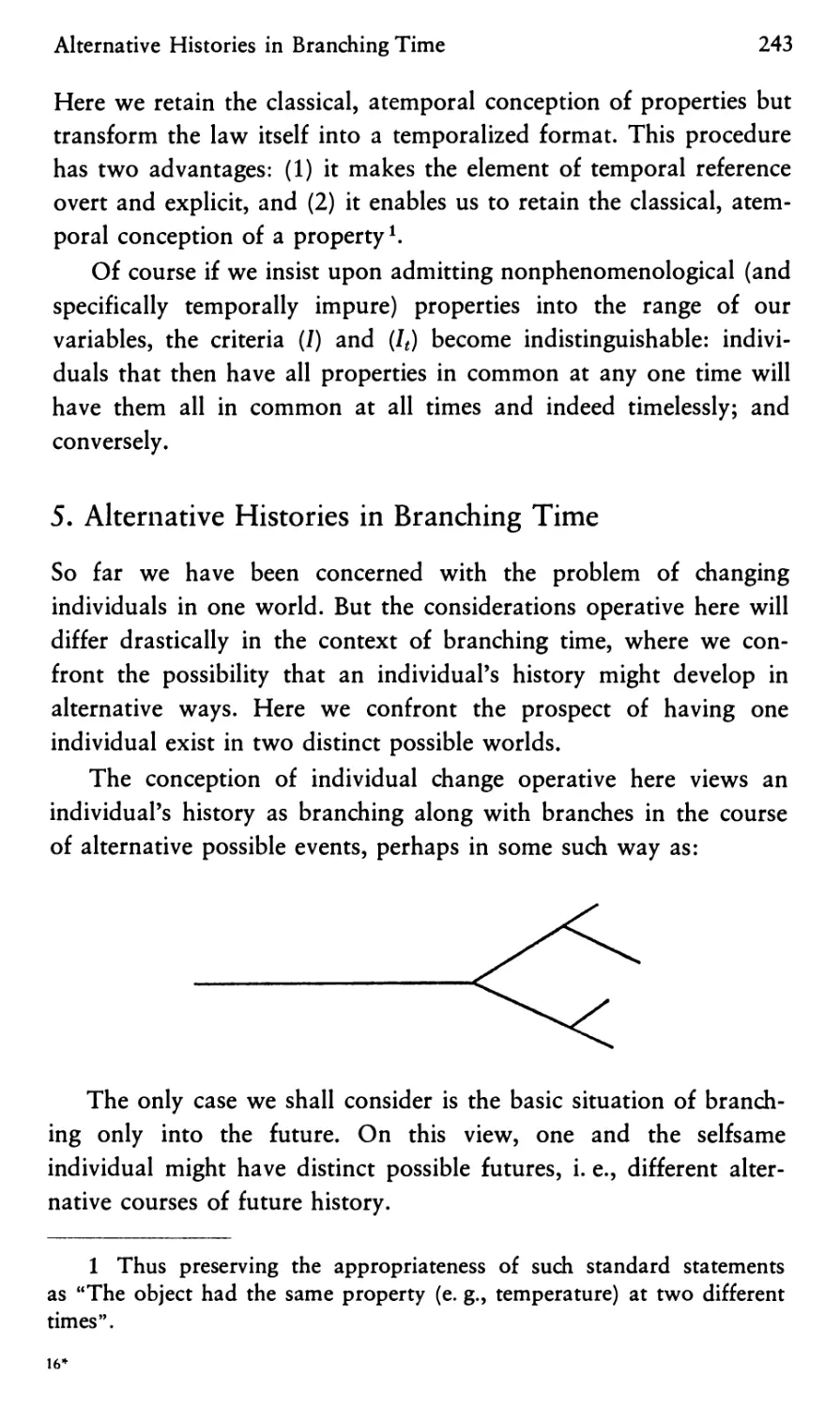
1. Individuals and Quantifiers 234
2. Quantification and Temporal Modality 237
3. Quantified Tense Logic 240
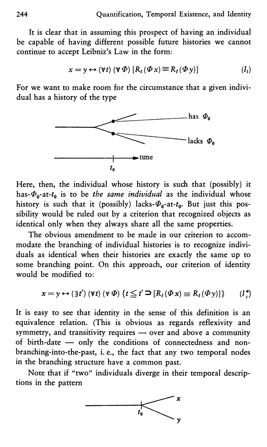
4. Temporal Change, Identity, and Leibniz' Law 241
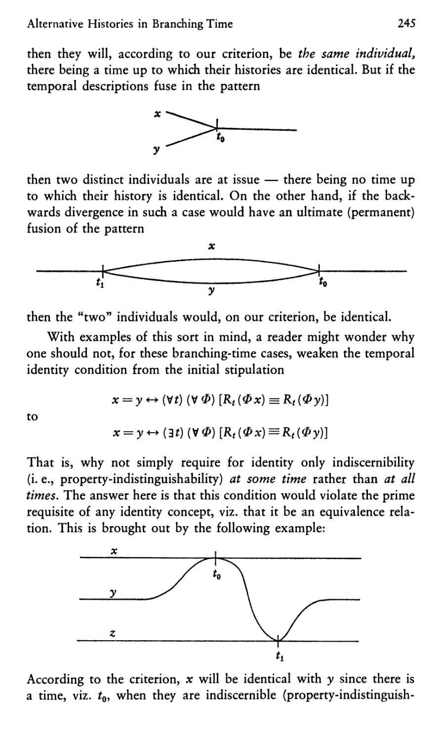
5. Alternative Histories in Branching Time 243
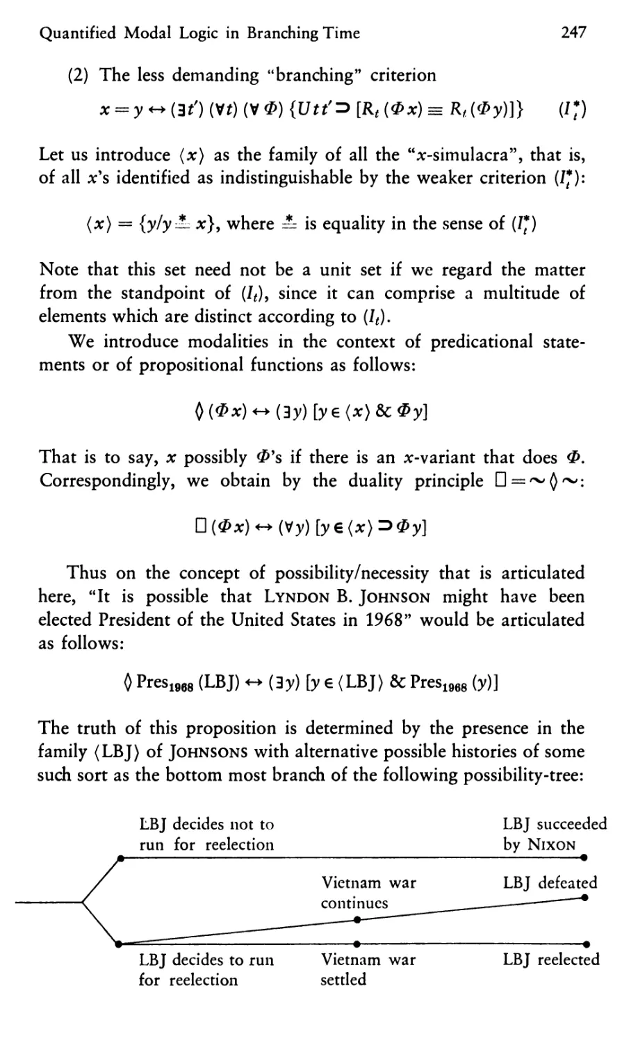
6. Quantified Modal Logic in Branching Time 246
Appendix I
A Summary of Axiom Systems for Topological, Temporal
and Modal Logics 249
Appendix II
The Modal Structure of Tense-Logical Systems 258
Bibliography of Temporal Logic 259
A. Chronological Listing 259
B. Author Listing (Alphabetical) 263
Index of Names 268
Subject Index 270
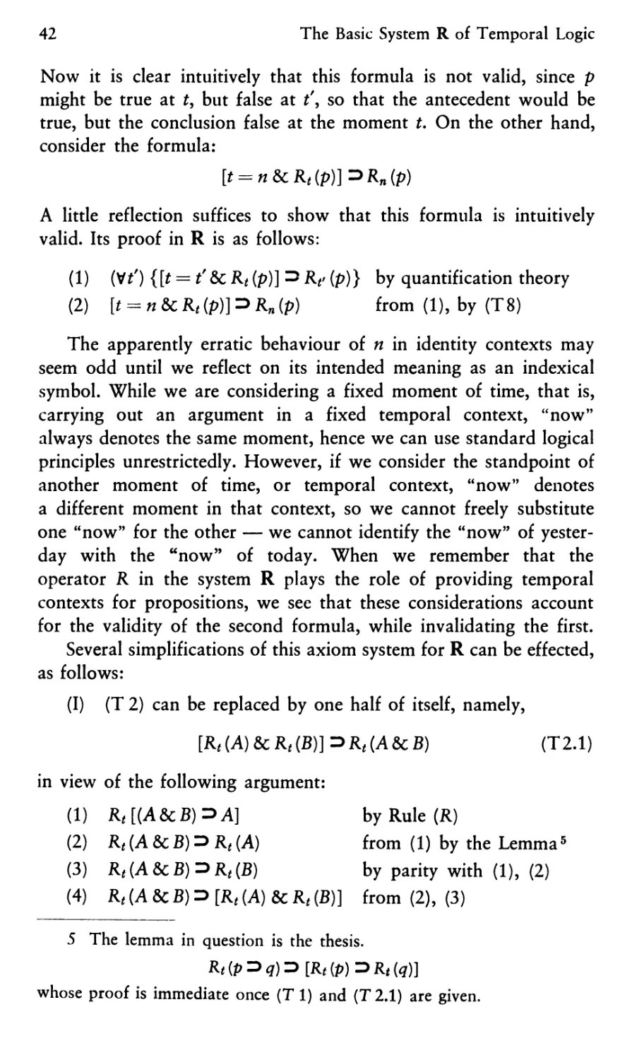
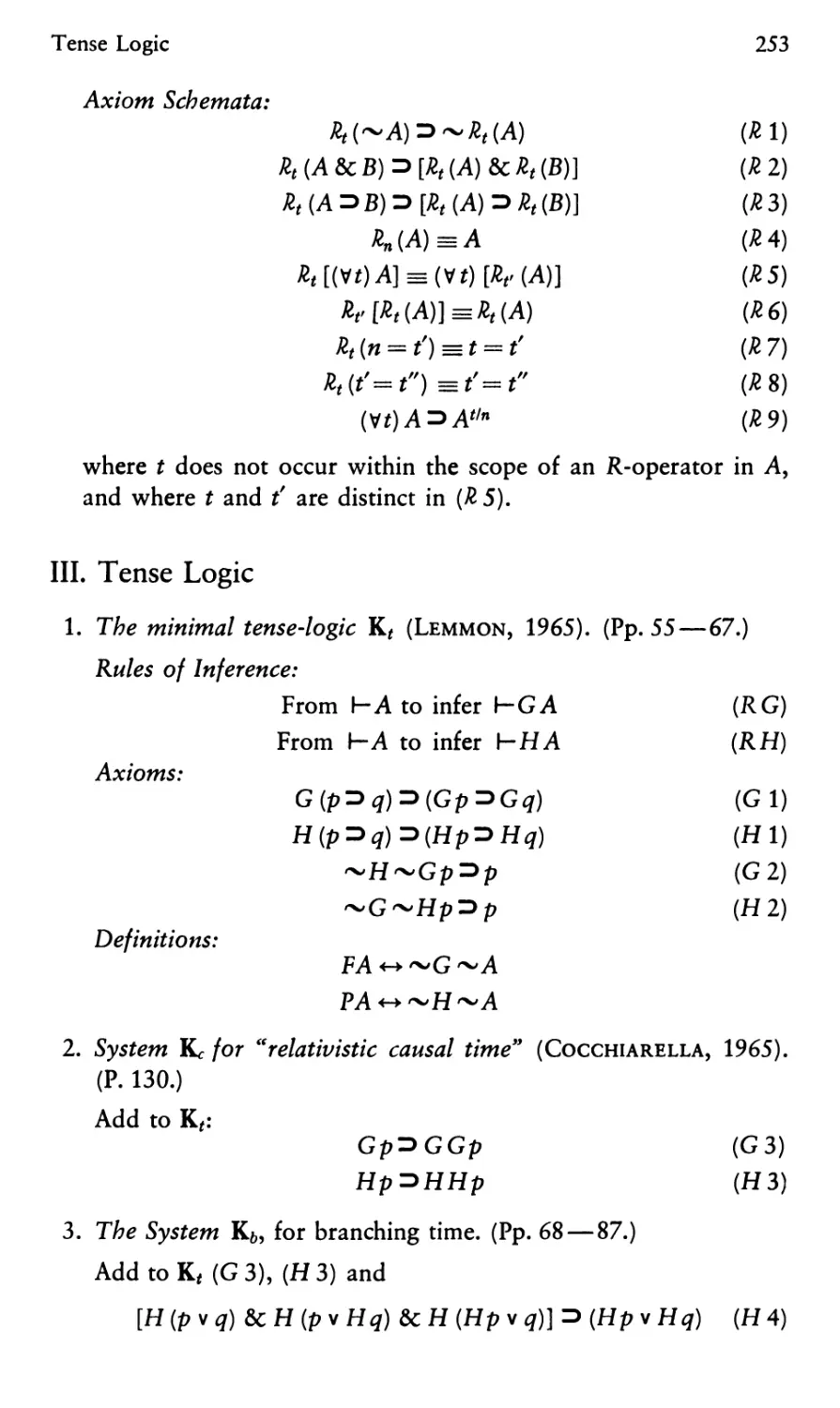
Foreword on Notation and
Prerequisites
This book is relatively self-contained; the reader is assumed only
to have a grasp of the elementary portions of modern symbolic
logic, such as may be obtained from a solid beginning course in
the subject. Beyond this, nothing but the most rudimentary
mathematical background is presupposed; a knowledge of some familiar
modal logics is very helpful, though not essential.
A few preliminary remarks on symbolism and notation are in
order. Our notation for classical logic is by and large of the classical
Principia type (but V is used as explicit universal quantifier).
Assuming that logicians have by now learned the surprisingly far from
simple lesson of the proper use of quotes, we abandon them
altogether and use symbols and formulas autonymously, that is, as
names for themselves. In the metalanguage we employ = for
definitional identity, and -> and <-► for entailment and equivalence,
respectively.
A few concepts of elementary set theory are used. We denote
sets and set-theoretical structures by script letters — A, B, etc. We use
the ideas of elementhood or set-membership (€), of set union and
intersection (U and H), and a mechanism for set formation, with
{x/C(x)} for "the set of all those items x satisfying the condition
that C holds of x".
Within the sphere of tense logical operators we follow A. N.
Prior's symbolism (while abandoning his Polish-style notation, as
indicated).
XVIII
Foreword on Notation and Prerequisites
Throughout, the reference numbers or code-letters for formulas
are placed between parentheses. Systems are always indicated by
boldface: thus Lewis' best-known modal system is symbolized as
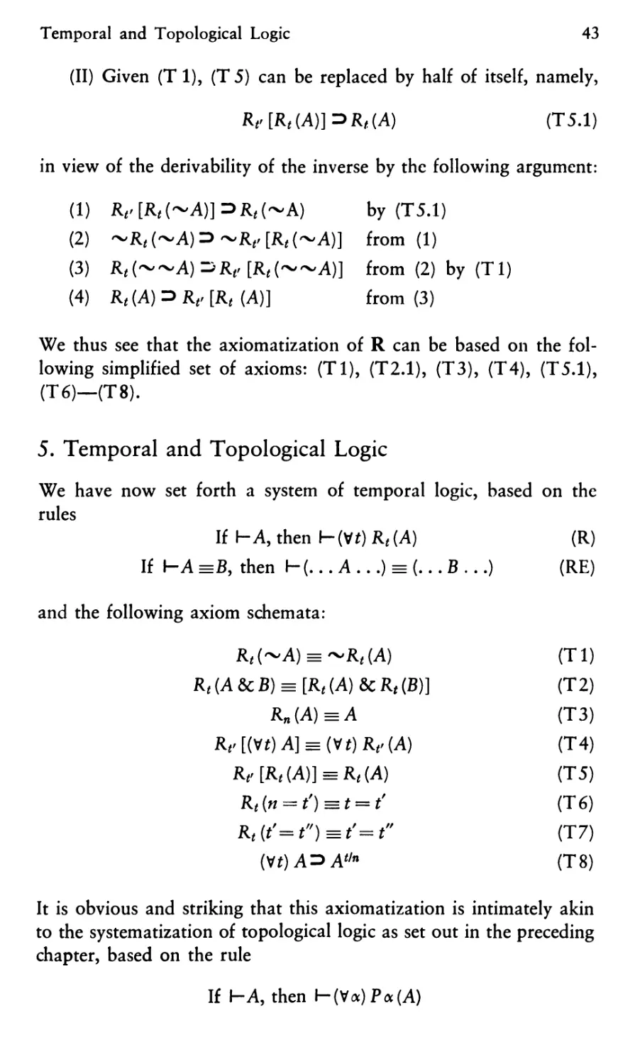
S5 and not S5.
Chapter I
The Background of Temporal Logic
The theory of temporal logic is an integral concern of philosophical
inquiry, and questions of the nature of time and of temporal
concepts have preoccupied philosophers since the inauguration of the
subject. Kant wrote:
"The possibility of apodeictic principles concerning the relations
of time, or of axioms of time in general, is also grounded upon this
a priori necessity [of time as part of the framework of sensory
experience]. [Examples of such apodeictic principles are:] Time has
only one dimension; different times are not simultaneous but
successive ..." *.
It is the primary aim of temporal logic to clarify the content,
to elaborate the consequences, and to elucidate the interrelationships
among the members (and candidate-members) of the family of
"apodeictic principles concerning the relations of time, or the axioms
of time in general". In sharpening our understanding of these
fundamentals, temporal logic provides the philosopher — and indeed
the natural scientist as well — with tools for achieving a better
understanding of the nature of time itself.
Standard logic takes no special cognizance of time-related
propositions. As a result, it handles such propositions clumsily or even
inadequately. "Lightning always precedes thunder" becomes glossed
as the monstrosity "All occurrences-of-lightning are events-preceded-
by-occurrences-of-thunder". "There was a rainstorm yesterday" be-
1 Critique of Pure Reason, A 31/B 47; tr. by N. K. Smith (New York,
1929), p. 75.
2
The Background of Temporal Logic
comes "All days-identical-with-yesterday are days-on-which-a-rain-
storm-occurs". The verbs — as apart from the timeless copula is
or are — are absorbed by artificial noun constructs. There is no
direct way of handling tensed verbs at all. "Socrates is sitting" (with
the tensed "is" that means "is now") at the very best becomes
"All moments-identical-with-the-present are (timelessly) moments-
when-Socrates-is-seated". (Of course the "is" of the second noun
construct continues to be tensed: it clearly cannot be glossed as "has
(timelessly) the property of being seated".)
The object of temporal logic — "tense logic" or "change logic"
as it has also been called by various authors — is to systematize
reasoning with propositions that have a temporalized aspect. Such
propositions generally do not involve the timeless "is" (or "are")
of the mathematicians' "3 is a prime", but rather envisage an
explicitly temporal condition: "Bob is sitting", "Robert was present",
"Mary will have been informed". In this area, we have to do with
statements involving "time talk" in which some essential reference
to the Before-After relationship or the Past-Present-Future
relationship is at issue, and the ideas of succession, change, and constancy
enter in. Temporal logic seeks to provide the linguistic and
inferential apparatus for exact discourse and rigorous reasoning in this
sphere.
It might be argued that time-related discourse of the paradigm of
"It is (now) raining in London" does not really fall within the
purview of logic. Logic, it would be argued, deals with propositions,
and the sentence at issue fails to state a proposition on two grounds:
1. It is not repeatable: the person who asserts it on two different
occasions asserts different things.
2. It is semantically incomplete: it lacks a determinate truth-
value, since its truth-status cannot be settled without extraneous
information (viz. the time of assertion).
But these objections can be met in sufficient measure. Our
statement is certainly repeatable with invariant meaning, not to be sure
on temporally different occasions, but certainly by different
assertory. If X and Y both make the assertion in question concurrently —
perhaps even in quite different languages — it would be entirely
correct to say that both "have said precisely the same thing". (This
shows, incidentally, that it is not the concrete utterances that are at
The Background of Temporal Logic
3
issue here, since the two assertors certainly make distinct utterances.
So something far more propositional than sentence-utterings is at
issue.)
As regards the second objection, while the "incompleteness" at
issue must be admitted, it is surely venial, since it is automatically
removed once we are given a minimum of information regarding the
context of the assertion.
The logical theory of such time-related propositions is of
substantial interest because these explicitly temporal considerations
arise in a wide variety of philosophically relevant contexts. Apart
from their obvious significance for the analysis of tensed discourse,
they are germane to various interests of philosophers of science —
the structure of time,'the analysis of temporal relations (e.g., of
temporal conjunction and contiguity, important for the analysis of
principles of causal inquiry such as Mill's methods), and the
characterization of natural processes, among others. Mediating the linkage
of temporally sequential processes, they come to have a bearing on
the concept of sets of instructions, and so have a bearing upon the
logical theory of commands, thus entering the purview of ethics
through the command theory of moral imperatives. Moreover, they
are of interest to the logician, both in their own right, and because
of their involvement with the theory of modality, via the
chronologized conception of modality along lines to be explained shortly.
Temporal logic thus deserves to be developed (1) because it is
possible and logic cannot defensibly ignore one of its possible
branches, (2) because it is interesting from the logical standpoint
itself, and (3) because it is useful in its philosophical applications.
The early history of temporal quantifiers like "sometimes" and
"always" — and of the theory of temporalized modalities as linked
to them through the mediation of such principles as "What is
sometimes actual is always possible"— remains shrouded in obscurity. We
know that the rudiments of such a theory were actively developed
by the ancient Greeks: the Megarians and the Stoics2, and
Aristotle and the early Peripatetics3. The notions of temporalized modal-
2 See E. Zeller, Die Philosophic der Griechen, Pt. 3, vol. I (5th ed.,
Leipzig, 1923); and Benson Mates, Stoic Logic (Berkeley and Los Angeles,
1953), see esp. pp. 36—41.
3 I. M. Bochenski, La logique de Theophraste (Freiburg, 1947).
4 The Background of Temporal Logic
ity that are at work here are mainly those relating to the "Master
Argument" of Diodorus Cronus4.
There seems to have been a disagreement as to modality between
the Stoics and the Megarians. On the Stoic view:
(1) The actual is that which is actually currently realized now
Opi((Tn(p)
(where n = now, and Tt(p) stands for "p is true at t") or more
generally
Ot(P)UlTt(p)
(2) The possible is that which is realized (i. e., true) at some
present-or-future time
Op iff (lt)[t^n&cTt(p)]
or more generally
0*(P) iff 00[*'^*&TV(p)]
(3) The necessary is that which is realized at every future time
Up iff (Vt)[t^n*Tt(p)]
or more generally
nt(p)i(i(vt')[t'^t=>Tt,(p)]
The Megarians, on the other hand, did not admit the now-
relativization of the modalities of possibility and necessity, retaining
it only for truth (actuality):
(1) The actual is that which is actually realized now
Opi((Tn(p)
4 See Mates, op.cit., pp.38—39. Cf. Jaakko Hintikka, Aristotle
and the "Master Argument" of Diodorus, American Philosophical
Quarterly, vol. 1 (1964), pp. 101—114. And see also N. Rescher, A Version of
the "Master Argument" of Diodorus, The Journal of Philosophy, vol. 63
(1966), pp. 438 —445. We shall deal with the Master Argument in some
detail in chapter XVII.
The Background of Temporal Logic
5
(2) The possible is that which is realized at some (i.e., any) time
Op iff (3*)T«(p)
(3) The necessary is that which is actually realized at all times
Dp iff (v*)T,(p)
Aristotle's position is in line with that of the Stoics5, but
sometimes he appears to side with the Megarians in viewing the necessary
as that which is true all of the time, a position faithfully reflected
in St. Thomas Aquinas' statement that: Et sic quidquid semper est,
non contingenter semper est, sed ex necessitate*.
Yet another variant of the Stoic ideas on temporal modality is
also to be found in Aristotle: a sense of temporalized modality
according to which certain propositional claims are possible prior
to the event, actual then, and necessary thereafter, so that their
modal status is not omnitemporal (as on the Stoic concept), but
changes over time. The modalities here at issue are relativized, so
that we have:
Ot(P) for p is actual at time t
§t(p) for p is possible at time t
D* (p) for p is necessary at time t
Now if p {t0) is a true proposition about what happens contingently
at t0 — so that Tto[p(t0)] is assumed — then:
O* [p(t0)] is true if t = t0 and also whenever t^> t0
§t lp(to)] is true for all t, even those t<Ct0
D*[p(*o)] is true for all £>£0 (or perhaps even t^t0)
Here, then we have temporally relativized modalities that regard the
modal status of what happens at one time from the standpoint of
another time.
5 J. HlNTIKKA, Op. Clt.
6 In: I de Caelo, lect. 26, n. 258. And correspondingly: quod possible
est non esse, quandoque non est (Summa Theolcgica, I A, q. 2, a. 3). Cf.
Guy Jalbert, Necessite et contingence chez saint Thomas d'Aquin et chez
ses predecesseurs (Ottawa, 1961), pp. 204—206, 224—225, and 228.
6
The Background of Temporal Logic
Mention should also be made of the Diodorean concept of
implication (named after the Stoic logician Diodorus Cronus) which (for
example) has it that the conditional "If the sun has risen, it is
daytime" is to be given the temporal construction "All times when the
sun is risen are times when it is daytime"7.
In all of this there is yet no hint of the ramified machinery
of temporalized modalities which we find in Arabic texts — but
which are unquestionably of Greek provenience. For the roots of the
theory as the Arabs were later to treat it we must undoubtedly look
to the Stoic doctrine of predication. The Stoics distinguished between
three types of qualities:
poion (quality)
(i) poiotes (permanent property)
(ii) schesis (enduring state)
(iii) hexis (transient characteristic)
In construing "quality" (to poion) here, we are to work from the top
down, and thus have three possibilities8:
(1) Only group (i): those qualities that are wholly completed
and altogether permanent (apartizontas kai emmonous ont'as).
(2) Groups (i) and (ii): not only the permanent qualities (e.g.,
a man's "being an animal") but the enduring states as well (e.g.,
"being prudent").
(3) Groups (i)—(iii): adding to (2) also strictly transient
qualities (e.g., "walking" or "running").
The distinction between such types of qualities lends itself readily
to temporalization in the interpretation of propositions in which
they are attributed:
A man is an animal all of the time.
A prudent man acts wisely most of the time.
A healthy man walks some of the time.
7 For the Megarian and Stoic theories see N. Rescher, Truth and
Necessity in Temporal Perspective, in idem, Essays in Philosophical
Analysis (Pittsburgh, 1969).
8 I follow E. Zeller, op. cit., pp. 97—99 (especially no. 1 for p. 97);
relying also upon £mile Brehier, La theorie des incorporels dans Pancien
Stoicisme (2nd ed., Paris, 1928), p. 9.
The Background of Temporal Logic
7
The elaboration of such temporalized predications would lend
itself naturally to the development of temporal modalities of the
sort to be found later in Arabic logical texts.
The Aristotelian and Stoic logic of temporal relations was taken
over and developed by medieval Arabic logicans. Thus Avicenna
(d. 980) developed the temporal treatment of implication in the
manner of Diodorus into a general theory of categorical
propositions (of the A, E, I, O type that figures in traditional syllogistic
logic)9. Moreover, Avicenna also developed considerably the Mega-
rian-Stoic theory of temporal modalities. It is worth giving some
brief indication of his theory.
The modal machinery used by Avicenna is of highly intricate
constitution. Modal propositions are classed into thirteen different
sorts. These modal distinctions were in fact drawn on the basis of
complex chronological considerations. The nature of the temporal
modalities at issue can be made clearer with the help of some
symbolism. A, By C, ..., are to be variables standing for categorical
propositions. The contradictory of a proposition A will be
symbolized as ~A. [A] will represent the subject of the proposition A,
and El [A] is to mean that the subject of A exists, i. e., that it is
actually exemplified. (It should be noted that because [A] = [^A],
El [A] will mean the same as El [^A].) C [A] will mean that the
subject of A satisfies the condition C. In addition to the quantity
and the quality of the categorical proposition A, the modal
proposition will bear one of the modal qualifiers, necessary, not
necessary, perpetual, or not perpetual.
There are four basic modal relationships, symbolized as follows,
out of which the thirteen modal propositions are then constructed.
These four are:
1. (A/D/B) meaning "A is necessarily true whenever B is true".
2. (ANtIB) meaning "A is true whenever B is true".
3. (A/3t/B) meaning "A is true at some time that B is true".
4. (A/Q/B) meaning "A is possible at some time that B is true".
9 For a detailed account of this theory see N. Rescuer, Avicenna
on the Logic of "Conditional" Propositions, in: Studies in the History of
Arabic Logic (Pittsburgh, 1963), pp.76—86.
8
The Background of Temporal Logic
Various simple and compound modal propositions were then
developed, the most important of which are as follows. (Here T and
S represent special forms of the condition C.)
1. Absolute necessary
2. Absolute perpetual
3. General conditional
4. General conventional
5. General absolute
6. General possible
7. Special conditional
(3 &C ~5)
8. Special conventional
(4 &c *>5)
9. Non-necessary existential
(5 &C ~6)
10. Non-perpetual existential
(5 &C ~5)
11. Temporal (3' & ^5)
12. Spread (3" &C *>5)
(A/D/El[A])
(AhtlE\[A\)
(A/D/C[A])
(ANtlC[A\)
(A/3t/El[A])
(A/Q/El[A])
(A/D/C[A]) &c (~A/it/E\['
'A])
[ANtlC[A]) &c (^A/3t/E\[^A])
(A/3t/E\[A\) &C (<^A/Q/E![^A])
(A/3t/E\[A\) &C {^A/3t/El[^A])
(A/D/T[A]) &c (~A/3t/El[~A\)
(A/D/S[A]) &c (~A/3t/El[~A\)
13. Special possible (6 &c *>6) (A/Q/E! [A]) &c (^A/Q/E! [<*>A])
By way of illustration, if A is the categorical proposition "All fire
is hot", the Absolute Perpetual modal proposition would read
"When there is fire, then it is necessarily hot". The Non-necessary
Existential proposition would read "When there is fire it is
sometimes hot and (but) it is possible that it not be hot". If A is the
categorical proposition "Some men are not wise" then the Absolute
Perpetual is "When there are men, then there are always some who
are not wise", and the Special Possible is "When there are men,
then possibly some of them are not wise and (but) possibly all are
wise".
The contradictory of a simple modal proposition is obtained
by interchanging A and ^A, □ and Q, Vt and 3t, wherever they
occur, and replacing C [A] in the original by E\ [A] in the negation.
Thus the negation of the General Absolute is (^A/Vt/El [^A]),
that is, an Absolute Perpetual proposition, and the negation of
The Background of Temporal Logic
9
a General Conditional is (^A/ty/El [^A]), that is, a General
Possible proposition.
The negation of a compound proposition is obtained by negating
each of the constituent conjuncts, and putting them into a
disjunction. Thus the negation of the Special Possible is a
disjunction of two Necessary Absolutes, i.e., (^A/D/E! [A]) v (A/D/E! [A]).
The negation of the Special Conditional is the disjunction of
a General Possible and an Absolute Perpetual, i.e., (^A/ty/El [^A])
v(A/v/E![A]).
These brief indications point up the subtlety and complexity of
the theory of temporal modalities developed by the Arabs in the
middle ages. But we cannot pursue this matter here10.
The Latin medievals seem to have taken this up from the Arabs
to a very modest extent. Thus we find in Pseudo-Scotus a
distinction between four types of temporalized "necessity" (conditionale =
conditional, quando = as-long-as, ut nunc = as-of-now, and pro
semper = for all times)11. I would conjecture a correspondence with
the cognate Arabic ideas along something like the following lines:
Pseudo-Scotus Construction al-Qazwini
1. quando (A/D/E! [A]) absolute necessary
2. pro semper (AhtlE\ [A]) absolute perpetual
3. conditionale (A/D/C[A]) general conditional
4. ut nunc12 (A/3t/E\[A]) general absolute
If this conjecture — or anything like it — is correct, the theory of
temporalized modalities also found its way into the Latin scholastics.
While this development could have been mediated (or perhaps
only strengthened) through Arabic materials, it could also have
been indigenous to a purely Latin tradition. Signs of this are
already to be found in Boethius: "ea vero quae ex necessitate aliquid
10 For further information see N. Rescher, Temporal Modalities
in Arabic Logic (Dordrecht, 1967).
11 I. M. Bochenski, Notes historiques sur les propositions modales
(Quebec, 1951), p. 7.
12 We here construe "nunc" not as the now (that is, the now-of-
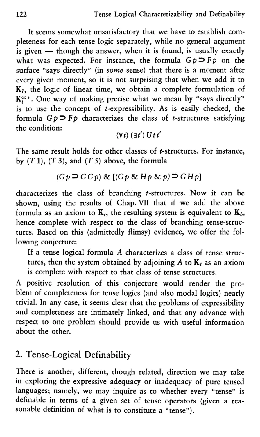
the-present), but as a now (that is, some — i. e., any — instant). This
dual interpretation is standard in the medievals. ,
10 The Background of Temporal Logic
inesse designat tribus dicitur modis; uno quidem quo ei similis est
propositioni quae inesse significat . . . alia vero necessitatis signifi-
catio est, cum hoc modo proponimus 'hominem necesse est cor
habere, dum est atque vivif . .. alia vero necessitatis significatio est
universalis et propria quo absolute praedicat necessitatem ... pos-
sibile autem idem tribus dicitur modis; aut enim quod est, possibile
esse dicitur ... aut quod omni tempore contingere potest, dum ea
res permanet cui aliquid contingere posse proponitur . .. item
possibile est quod absolute omni tempore contingere potest .. . ex his
igitur apparet alias propositiones esse inesse significantes alias neces-
sarias alias contingentes atque possibiles, quarum necessariarum con-
tingentiumque cum sit trina partitio, singulae ex iisdem partitionibus
ad eas quae inesse significant referuntur; restant igitur duae neces-
sariae et duae contingentes quae cum ea quae inesse significat
enumeratae quinque omnes propositionum faciunt differentias;
omnium vero harum propositionum aliae sunt affirmativae aliae nega-
tivae"13. Cognate distinctions are also drawn elsewhere. For
example, in St. Thomas Aquinas and other medieval scholastics we
find a distinction — akin to the modern distinction between logical
and physical necessity — between those relationships which are
perpetual and (in a sense) necessary: (1) by an eternity that is a parte
ante, or (2) by an eternity that is a parte post. Truths of the former
class are necessary by a necessity that turns wholly on the nature
of the essences involved — as men are eternally rational and
equiangular triangles eternally equilateral. Truths of the second class
are necessary by a necessity that devolves from the au fond
contingent arrangements of this world — as men are eternally mortal,
or the northern latitudes eternally cold14. Traces of such an interest
in temporal modalities are to be found as late as William
of Ockham 15.
13 Quoted from C. Prantl, Geschichte der Logik im Abendlande,
vol. I (Leipzig, 1855; photoreprinted, Graz, 1955), p. 703, no. 150.
14 See Guy Jalbert, op. cit., pp. 41, 119—120, 137—138, 141—143.
This work is primarily concerned with possible and necessary existents.
For a detailed treatment of such existents, primarily in Avicenna, but with
some comparisons and contrasts in St. Thomas, can be found in Gerard
Smith, Avicenna and the Possibles, The New Scholasticism, vol. 17 (1943),
pp.340—357.
15 Summa Logicae (ed. P. Boehner), Pt. I, ch. 73, lines 16 — 49;
Pt. II, ch's. 7, 19—22; Pt. Ill, div. i, ch's. 17—19.
The Background of Temporal Logic
11
Central to all of these variant constructions of temporal modality
is thus a conception of statements that will vary in truth-status over
time, pointing towards a corresponding body of logical machinery
to deal with the relations among such time-related propositions.
The logical theory of nonmodal statements (both categorical and
hypothetical) having a tensed copula was treated extensively in
medieval times. The logical writings of such later schoolmen as
Ockham, Albert of Saxony, and John Buridan treated
chronological considerations extensively, inter alia drawing a temporally
grounded distinction between an omnitemporal consequentia sim-
pliciter (or simplex) and a temporal consequentia ut nunc18.
The medieval Latin schoolmen also taught a temporalized theory
of categorical propositions in terms of their doctrine of the
"ampliation" of terms, articulating such rules as the following:
Every term having supposition, as subject, with respect to a verb
of past time, is ampliated to stand for that which exists or for that
which has existed.
Some A was aB = (3x) {[Tn(Ax)vTp(Ax)]&cTp(Bx)}
Every A was a B = (Vx) {[Tn(Ax) vTp(Ax)] =>T„(Bx)}
Every term having supposition, as subject, with respect to a verb
of future time, is ampliated to stand for that which exists or for that
which will exist.
Some AwillbeaB = (ax) {[Tn(Ax)vTf(Ax)]&cTf(Bx)}
Every A will be a B = (Vx) {[Tn(Ax) v Tf{Ax)] => Tf{Bx)}17
Here we take "Tn(g)" to mean "q is true now", "Tp(q)" to mean
"q was true in the past" and "Tf(q)n to mean "q will be true in the
future".
Having dealt at some considerable length with the history of
temporal logic in antiquity and the middle ages, we shall skip almost
entirely over the intervening era up to the post World War II years.
We do so not because these intervening developments lack impor-
16 Some discussions of these matters can be found in E. A. Moody,
Truth and Consequence in Medieval Logic (Amsterdam, 1953), pp.53—57,
73 — 80, 97—100.
17 Ibid., p. 56. I have altered Moody's notation.
12
The Background of Temporal Logic
tance and interest — far from it! — but because they have already
been treated in a most vivid and helpful way in A. N. Prior's book
Past, Present and Future (Oxford, 1967).
A major revival of interest in temporal logic has sprung up since
the later 1940's. The stimulus for this revival can be traced largely
to three sources: the study of historical materials (especially the
studies of Stoic logic by Martha Hurst Kneale and Benson Mates
and the studies of medieval logic by Ernest Moody)18, the logical
analysis of grammatical tenses by Hans Reichenbach 19, and above
all the endeavor by the Polish logician Jerzy Los20 to devise
a system of temporal logic — specifically an R-calculus (cf. Chap. IV
below) — for the analysis of issues in the philosophy of science,
especially Mill's methods of inductive reasoning. Los's ideas were
considerably refined and extended by Arthur N. Prior, and then
further developed by Nicholas Rescher. Under the stimulus and
inspiration of Prior's work, ramifications in various directions have
been explored by many logicians and with the result of making
temporal logic a very active field of current research. However,
independent of Prior (and apparently of Los as well) is the recent
development by G. H. von Wright (1963 and 1965) of a
(substantially weaker) system of a chronological "logic of change"21 which
has been extended in various directions by several logicians. A
comprehensive picture of recent developments can be gleaned from the
bibliography at the end of the book.
18 See especially Martha Hurst Kneale, Implication in the Fourth
Century B.C., Mind, vol.44 (1935), pp. 485—495. Benson Mates, Dio-
dorean Implication, The Philosophical Review, vol.58 (1949), pp.234 —
242; idem, Stoic Logic, op. cit., Ernest Moody, op. cit.
19 Hans Reichenbach, Elements of Symbolic Logic (New York,
1947).
20 Jerzy Los, Podstawy Analizy Metodologicznej Kanonow Milla
(Foundations of the Methodological Analysis of Mill's Canons), Annales
Universitatis Mariae Curie-Sklodowska, Sectio F, vol. 2 (for 1947,
published in 1948), pp. 269—301. See the review of this by Henry Hiz, in:
The Journal of Symbolic Logic, vol. 16 (1951), pp.58—59.
21 The weakness of von Wright's system relative to those of the
Los-Prior-Rescher type is demonstrated in N. Rescher and J. Garson,
A Note on Chronological Logic, Theoria, vol. 33 (1967), pp. 39 — 44.
Chapter II
Topological Logic
1. Introduction
A particularly illuminating view of temporal logic is obtained by
approaching it as a special case of a generic logic of positions. The
purpose of this chapter is to present a very versatile family of logical
systems of positional or topological logic. These systems are to have
a very general nature, capable of reflecting the characteristics of
a wide range of logical systems, including not only temporal logic,
but also what may be called a locative or place logic, and even
a logic of "possible worlds".
2. The P-Operator
Let us add to a system of standard propositional logic the
parametrized operator Pa, where "P*(p)" is to be read and understood
as "the proposition p is realized at the position a". Here a may be
any element of a range of positions. These may be spatial positions
indicated by Cartesian coordinates, or by any positional scheme such
as seat-numbers in a lecture hall. Or again, the positions at issue
may be temporal, with a ranging over the integers (for days or
years) or over the real numbers (for a more refined scheme of
dating).
Once the nature of the parameter a has been specified (as places,
times, or the like), the "propositions" at issue must be construed
as propositional functions of this parameter-type. Thus if the a's
represent times, the p's must be temporally indefinite propositions of
14
Topological Logic
the type "It rained yesterday" and if the <x's represent places, the
p's must be spatially indefinite propositions of the type "It is
raining here". In general, the propositions at issue must be positionally
indefinite in this sense of being able to vary in truth-value.
3. Three Basic Axioms
Regardless of the specific interpretation given the P-operator, the
following two basic axiom schemata obtain:
Pa(<^A)=z^>Pa(A) (PI)
Pa (A&cB)=e [Pa (A) &cPa (B)] (P2)
The axiom (PI) asserts that if not-/? obtains at some position, then it
is not the case that p obtains at that position, and conversely. This
axiom schema embodies a decision to construct topological logic
from a two-valued point of view: the (positionally indefinite)
propositions at issue are to be either true or else false at any given
position — a third possibility ("inapplicable", "neutral",
"indeterminate", or the like) is excluded. (If this condition were dropped
and a third truth-value admitted, the principal connective of (PI)
would have to be changed from an equivalence to an implication
and corresponding changes in the development of the system would
be required.)
Axiom schema (P2) has it that if a conjunction is true at some
position then each of the conjuncts is true at that position, and
conversely.
Since (PI) and (P2) guarantee distributivity of the P-operator
over a set of propositional connectives which is functionally
complete — viz. negation and conjunction — the following principle of
distribution results:
The P-operator distributes itself over all truth (PD)
functional connectives.
We would, moreover, want to stipulate the following rule of
inference:
If HA, then h-Pa(A)
(R)
Three Basic Axioms
15
where h- represents assertion within the system we are endeavoring
to construct. According to this rule, theorems are to be realized at
any and every position whatsoever. Given the principle of distribu-
tivity (PD), this rule is interdeducible with the substitution rule:
If HA = B and \-Px (A), then \-Px (B) K (RS)
To render the machinery of our system sufficiently powerful for
our purpose, we shall want to be in a position to quantify over the
domain of parameter values. For the axiom schemata (PI) and
(P2) we shall thus suppose an initial universal quantifier with
respect to <x, and similarly, we shall suppose every asserted thesis
to be asserted universally with respect to its (otherwise unqualified)
parameters.
Given the usual machinery of quantificational logic the
following further axiom schema seems in order:
(V«)P/»[A(«)]=P/»(V«)[A(«)] (P3)
This axiom schema is readily motivated for at any rate those cases in
which the parameter values at issue are the natural numbers. For
construing universal quantification as potentially infinite
conjunction, we see that the lefthand side of (P3) becomes
PP [A (o)] &P/? [A (1)] &CP/3 [A (2)] & ...
whereas its right-hand side becomes
Pfi[A(0)6cA(l)6cA(2) & ...]
But these two will be equivalent in virtue of (P2).
1 The proof of the interdeducibility of (R) and (RS) is as follows:
(a) Given (RS), (R) is derivable, since we may prove Pa(p^p) [from
the tautology Pa(p)^Pa(p) and (PD)]. Whenever we wish to prove
Pa (T), where T is a truth of the system, we first prove (pi) p) = T and
then apply (RS) to get Px(T).
(b) Given (R), (RS), is derivable, since we have by assumption that
h-(A = B) and can thus prove Pa(A = B) by use of (R). But Pa(A = B)
entails Pa(A)^P<x(B) by (PD) and propositional logic. By assumption
we were able to prove Pa (A), and so we can get Pa (B) by detachment.
16
Topological Logic
The axiom systems we shall consider will all be based upon
the axiom schemata (PI)—(P3) and the rule (R), together with
certain additions. These additions deal with (i) the problem of the
relation of P-unqualified to P-qualified formulas, and (ii) the
problem of iterations of P.
4. The Relation of P-Unqualified to P-Qualified Formulas:
The Preferred Position S: A Fourth Axiom
How, subject to the specified conception of the P-operator, is one
to construe the unqualified formula /?? We certainly do want to
assert the thesis:
(V«)P«(p)Z>p (P4)
In accepting this we accept also its equivalent [in view of (PI)]:
P*(3*)P*(P) (1)
Thus what is true at all positions is true unqualifiedly, and what is
true is true at some position or other. But we would certainly not
want to have also the converse of (1) and assert the equivalence
(V«)P«(p)=p (2)
For this would at once render otiose the introduction of the
P-operator and the whole machinery of differential positions, since the
assertion of a formula would then simply become equivalent to its
assertion at all positions. Performing the substitution of simply p
for Poc(p) within the axioms introduced so far would reduce them
all to tautologies of propositional logic.
We may wish to introduce a "preferred position" (f) within our
parameter range — like "now" for the time, or "here" for the space,
or "at the origin" for some coordinate-scheme — and then to
identify the unqualified or absolute assertion of p with its assertion at
this preferred or actual position (to be presented by the constant f).
This policy is enshrined in the axiom schema:
A = P£(A) (P4')
Our initial thesis (P4) is, of course, an immediate consequence of
this axiom schema (P4'). Thus we may envisage two systems of
The Iteration of P: A Fifth Axiom and the Two Systems PI and PII 17
topological logic depending on whether we choose to adopt (P4)
or to take the added step of adopting (P4'). The system consisting
of (PI), (P2), (P3), and (P4) will be called P; and that consisting
of (PI), (P2), (P3), and (P4') will be called F.
5. The Iteration of ?: A Fifth Axiom and
the Two Systems PI and PII
How is one to construe
pnp«(p)]
and similar formulas in which the P-operator occurs in a nested
manner? One possible policy is to let the innermost operator of itself
be the complete determinant:
Pp[Pa(A)] = Pa(A) (P5.1)
This thesis amounts to assuming a fixed-point coordinate scheme
with a specified origin: If p is true at the fixed position <x, then it
is true everywhere that p is true at a.
The system based on (PI) to (P4) plus (P5.1) will be designated
as PI. This system is thus to be based on the rule (R) — if h-A,
then h-Pa (A) — and the following five axiom schemata:
Pa(~A)==^<Pa(A) (PI)
Pa (A&cB) = [Pa (A) &cPa (B)] (P2)
(V*)PP(A)=Pp[(V*)A] (P3)
(V<x)P<x(A)=>A (P4)
P/3[Pa{A)] = Pa(A) (P5.1)
where in (P3) a and /? are distinct, and in (P4) a is not free in A.
The system which we shall designate as P'l is to be identical with
PI, except for replacing (P4) with the stronger axiom schema (P4'):
P£(A)=A. It should be noted that in both systems the presence
of (P5.1) and (P3) allows us to prove:
(V«) Pa (A) = PP [(V*) Pa (A)] (P3*)
A corresponding result could be obtained with existential
quantifiers. Thus a positional prefix can be suppressed before positionally
18
Topological Logic
definite assertions — those in which the propositional parameter does
not have a free occurrence.
However, in system P' I the whole positional machinery is readily
seen to become superfluous in view of the provability of:
P«(p) = PP(p)=p
To avoid this collapse of the positional machinery in P' I, we must
restrict the rule (R) so that it is only applicable to formulas not
containing occurrences of f. This restriction effectively blocks any proof
of the "collapsing theorem".
A second possible policy is to assume a floating-point coordinate
scheme with a shifting reference point: "P<x(/?)" says that p is true
at a position a units from a shifting "here" (and not a fixed origin!),
so that "P/? [Pa (/?)]" says that Poc(p) is true at a position /? units
from here, where "P<x(/?)" says that p is true at a place <x units
from there. Here we would assume a type of vector addition for
parameter values and stipulate the axiom scheme:
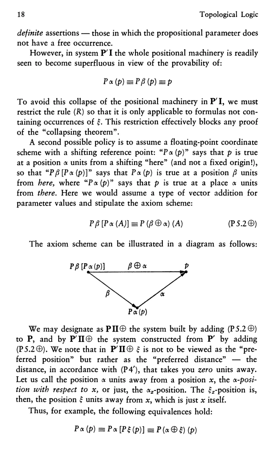
PP[P«{A)]==P(P®«){A) (P5.20)
The axiom scheme can be illustrated in a diagram as follows:
PP[Poc(P)] P®« P
P«(P)
We may designate as PII© the system built by adding (P5.2©)
to P, and by P'H© the system constructed from P' by adding
(P5.2©). We note that in P'H© f is not to be viewed as the
"preferred position" but rather as the "preferred distance" — the
distance, in accordance with (P4'), that takes you zero units away.
Let us call the position a units away from a position x, the a-posi-
tion with respect to x, or just, the opposition. The f^-position is,
then, the position f units away from x> which is just x itself.
Thus, for example, the following equivalences hold:
Pa(/?)=Pa[Pf(p)]=P(a©f)(/>)
The Iteration of P: A Fifth Axiom and the Two Systems PI and PII 19
for, Pa [Pf (/?)] at the position x says that Pf (p) is true at the
^-position which in turn says that p is true at the position f units away
from the ^-position, i. e., at the ^-position. But this is what Poc(p)
says at the position x.
It is interesting that the two systems PII© and P'H© are
equivalent so long as we assume that there is a zero element (@) such
that (V<x) [(*(&©) = a] holds2. Thus, making this assumption, our
choice between (P4) and (P4') becomes irrelevant and we may
consequently omit the prime in the designation of topological systems
which contain (P5.2).
Exactly what further assumptions concerning © should be made
will depend upon the parameter range. If the parameters <x, /?, y
(etc.) range over sets of Cartesian coordinates one can define:
(xl9 y» zt) © (x2, y2, z2) = (xt + x2y yt + y2, zt + z2)
More complicated forms of "addition" could also be introduced,
varying with the structure of the space envisaged or the character
of the coordinates that are used. For instance, we may wish to
develop a system of topological logic which captures the notion that
space is bounded and curves around on itself. Thus by traveling far
enough in a straight line, one expects to return to the point of
departure. We can easily specify an "addition function" which
would reflect this hypothesis about the nature of space. For simpli-
2 Given the weaker thesis
(V«)P«(p)=>p (P4)
we may now prove the stronger:
PO(p)=p (P4')
Half of the proof goes thus:
(V«)[P«B»3P«(«»]
(V«)[P«P9(p)3P«M
(V«)P«[P© <p)^p]
P0(P)=>P
The reverse half goes thus:
(V«)[P«(P) = P«(P)]
(V«)[P«(p)=5P«P0(p)]
(V«)P«[p=>P@(p)]
pzyp0(p)
20
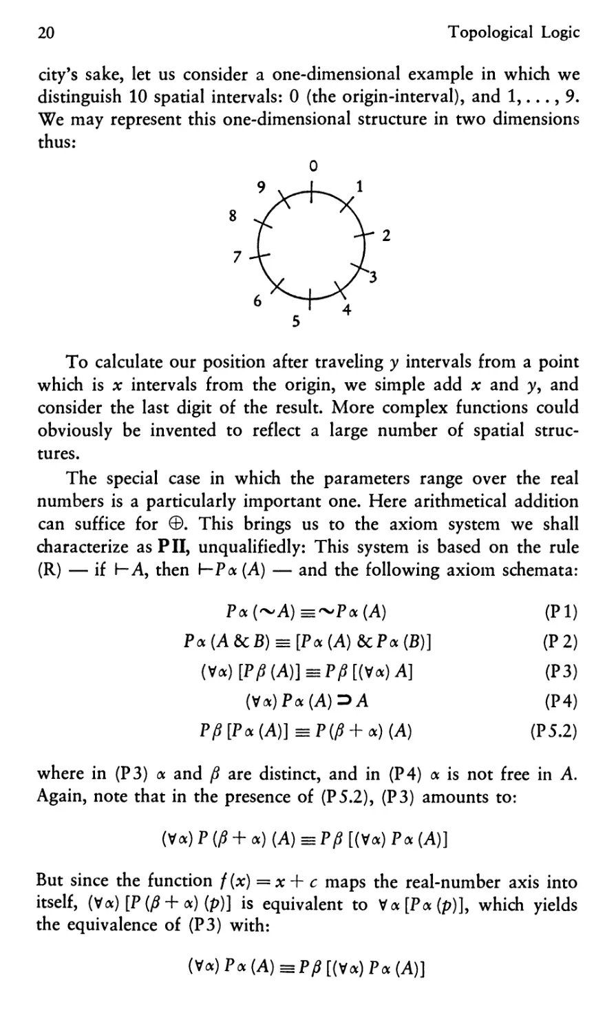
Topological Logic
city's sake, let us consider a one-dimensional example in which we
distinguish 10 spatial intervals: 0 (the origin-interval), and 1,..., 9.
We may represent this one-dimensional structure in two dimensions
thus:
■Q
To calculate our position after traveling y intervals from a point
which is x intervals from the origin, we simple add x and y, and
consider the last digit of the result. More complex functions could
obviously be invented to reflect a large number of spatial
structures.
The special case in which the parameters range over the real
numbers is a particularly important one. Here arithmetical addition
can suffice for ©. This brings us to the axiom system we shall
characterize as PII, unqualifiedly: This system is based on the rule
(R) — if HA, then h-Pa (A) — and the following axiom schemata:
Pa(^A)=^Pa(A) (PI)
Pa (A&cB) = [Pa (A) &cPa (B)] (P 2)
(V«)[P/?(A)] = P/?[(V«)A] (P3)
(Va)Pa{A)^>A (P4)
Pp[P*(A)]=P(fi + «)(A) (P5.2)
where in (P3) a and /? are distinct, and in (P4) a is not free in A.
Again, note that in the presence of (P5.2), (P3) amounts to:
(Va) P (/* + *) (A) = Pfi [(Va) Pa (A)]
But since the function f(x) =x+ c maps the real-number axis into
itself, {V*)[P(P + *)(p)] is equivalent to V<x [Pa (/?)], which yields
the equivalence of (P3) with:
(V*)P*(A)=PIJ[(v<x)P*(A)]
The Possible Worlds Interpretation of Topological Logic 21
We again have it that positionally definite assertions can be asserted
unqualifiedly, regardless of a positional prefix.
When the basic space of positions is finite or denumerable, we
can associate with every (spatially indefinite) proposition its "truth-
vector", viz., the (finite or infinite) series of T's and F's indicating
its truth-status for each of the positions at issue. (If there were, say,
three basic truth-values [T, F, 7], the situation would be analogous,
but more complex.) Regarding each such truth-vector as itself
a "truth-value" we obtain a many-valued system whose truth-tables
are satisfied by the topological system PI in the usual sense that
every thesis of the topological system is a tautology of the many-
valued system. (A formula is a many-valued tautology when it
assumes the [uniquely] "designated" truth-value, viz., that
composed uniformly of T's, for every assignment whatsoever of truth-
values to its propositional variables.) This point of view also
provides the basis for a semantical interpretation of the system at issue.
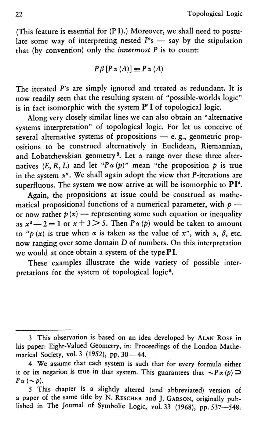
6. The Possible Worlds Interpretation of Topological Logic
Let "P<%(/?)" be construed to mean "the proposition p is true in
possible world No. <x". We are here to think of the possible worlds
as enumerated in a truth-table of the Wittgenstein-Carnap manner:
World No.
1
2
3
4
5
6
7
8
Po
+
+
+
+
—
—
—
—
4o
+
+
—
—
+
+
—
—
h
+
—
+
—
+
—
+
—
Note that here we have (for example) P3(p0v^ro)5 that is, p0v~ro
obtains in possible world No. 3. The key feature of the conception
of possible worlds that is relevant for our purposes is that a
"possible" world is descriptively complete in the sense that with respect
to a possible world any proposition will either be true or else false.
22
Topological Logic
(This feature is essential for (PI).) Moreover, we shall need to
postulate some way of interpreting nested P's — say by the stipulation
that (by convention) only the innermost P is to count:
P(i[P«(A)]^P«(A)
The iterated P's are simply ignored and treated as redundant. It is
now readily seen that the resulting system of "possible-worlds logic"
is in fact isomorphic with the system P'l of topological logic.
Along very closely similar lines we can also obtain an "alternative
systems interpretation" of topological logic. For let us conceive of
several alternative systems of propositions — e. g., geometric
propositions to be construed alternatively in Euclidean, Riemannian,
and Lobatchevskian geometry3. Let <x range over these three
alternatives (E,R>L) and let "P<%(/?)" mean "the proposition p is true
in the system <x". We shall again adopt the view that P-iterations are
superfluous. The system we now arrive at will be isomorphic to PI4.
Again, the propositions at issue could be construed as
mathematical propositional functions of a numerical parameter, with p —
or now rather p (x) — representing some such equation or inequality
as x2 — 2=1 or x + 3 > 5. Then Pot (p) would be taken to amount
to "p (x) is true when <x is taken as the value of x", with <x, /?, etc.
now ranging over some domain D of numbers. On this interpretation
we would at once obtain a system of the type PI.
These examples illustrate the wide variety of possible
interpretations for the system of topological logic5.
3 This observation is based on an idea developed by Alan Rose in
his paper: Eight-Valued Geometry, in: Proceedings of the London
Mathematical Society, vol.3 (1952), pp. 30—44.
4 We assume that each system is such that for every formula either
it or its negation is true in that system. This guarantees that ^Poc (p) 13
Pa(^p).
5 This chapter is a slightly altered (and abbreviated) version of
a paper of the same title by N. Rescher and J. Garson, originally
published in The Journal of Symbolic Logic, vol. 33 (1968), pp. 537—548.
Chapter III
Fundamental Distinctions for Temporal Logic
1. The Temporal Equivocality of IS
Before the actual systematization of the apparatus of temporal logic
is possible, a variety of basic concepts must be clarified and
preliminary issues resolved.
Logicians have frequently dwelt upon the equivocation of "is"
as between the "is of identity" on the one hand, and the "is of
predication" on the other. The temporal equivocation of "is" has,
however, been little heeded. Yet it is quite clear that there are several
very distinct possibilities:
(i) The "atemporal is" that means "is timelessly". ("There is
a prime number.")
(ii) The "is of the present" that means "is now". ("The sun is
setting.")
(iii) The "omnitemporal is" that means "is always". ("Copper is
a conductor of electricity.")
(iv) The "transtemporal is" that means "is throughout the present
period". ("The earth is a planet of the sun.")
In contrast to the atemporal "is" of (i) — let us write it as is —
the uses of "is" at issue in (ii)—(iv) may all be characterized as
temporal. No doubt subtler gradations of meaning could be
discovered, but the four that have been indicated show that "is" is
highly equivocal in that it can bear sharply divergent constructions
from a chronological standpoint.
24
Fundamental Distinctions for Temporal Logic
2. Translating Temporal to Atemporal 75
Supposing the only "is" at our disposal to be the atemporal one (is),
the question arises whether we can still render statements like:
(St) It is (i. e., is now) raining in London.
In making such a translation, how are we to preserve the reference
to now, the present moment? We cannot do this without doing it
by an overt use of dates. It would not do to use:
(52) It is raining in London on July 1, 1966.
Even if it is correct that July 1, 1966 is the present date, these
propositions will not be equivalent. For (SJ, unlike (S2), does not tell
us the date of the occurrence at issue; and (S2), unlike (SJ, does not
tell us what is happeniing in London now. The very best we can do
to render (St) is:
(53) It's raining in London now is a fact.
If we adopt a theory of facts according to which these, unlike events,
are in themselves timeless, and then adopt an overt means of
temporal reference, we can render a statement like (St) by means of the
atemporal "is" in the manner of (S3).
Along these lines, we can use the atemporal "is" as a way of
providing tenseless counterparts to tensed statements — deliberately
emptying the verb-copula of such statements of any reference to the
present. Thus to indicate rainfall in London on January 1, 2000 we
do say "It will rain in London on January 1, 2000" using a future
tense form of "is". But we could say "Its raining in London on
January 1, 2000 is a fact", thus shifting to an atemporal "is".
A similar expedient is of course also possible with respect to the
past. Instead of "Caesar was assassinated in 44 B. C", we could
say "Caesar's assassination in 44 B.C. is a fact". Since facts, unlike
things and events, can — on one plausible construction of the
matter — be taken to be atemporal, such paraphrasing can always
effect the shift from a tensed to an atemporal "is". But this is always
rather a transformation than a translation: something is always lost
in the process — to wit, the temporal placement of the event at
issue with the respect to the time of assertion, i. e., the actual
present. When a tensed copula is used, the statement asserted is itself
made from within the temporal framework; when the atemporal is
Temporally Definite and Indefinite Statements
25
is used, the statement may well be about something that happens
within the temporal framework, but the assertion itself does not
have a stance within the temporal framework. Even when "the same
fact" is viewed, there is a crucial difference in perspective here —
a difference so wide that there is no way to bridge it over.
3. Temporally Definite and Indefinite Statements
We shall say that a statement is temporally definite if its truth or
falsity is independent of the time at which it is asserted. Consider the
statements:
(1) It sometimes rains in London.
(2) It always rains in London.
(3) It's raining in London on all Sundays of 3000 A.D. is a fact.
(4) It's raining in London on January 1, 3000 A.D. is a fact.
These statements are all temporally definite: Their truth or falsity
is entirely unaffected, no matter what answer is given to the
question "When was that statement made (asserted)?". The assertion
of time of the statement has no bearing on its truth-value.
By contrast, consider the statements:
(5) It is now raining in London.
(6) It rained in London yesterday.
(7) It will rain in London sometime next week.
These statements are all temporally indefinite in that their truth or
falsity is not independent of their time of assertion. The answer
given to the question "When was that statement made?" is essential
rather than immaterial to the determination of the truth or falsity
of the statement1.
1 Cf. J. T. Saunders, A Sea Fight Tomorrow?, The Philosophical
Review, vol. 67 (1958), pp. 367—378 (see especially pp. 373—376). A
discussion of "Fugitive Propositions", represented by statements which, like
"It is now snowing", may be said to "express different propositions when
made on different occasions" was set afoot by a paper by A. E. Duncan-
Jones in: Analysis, vol. 10 (1949—50), pp. 21—23. Cf. also a paper of
the same title by P. Nowell Smith, ibid., pp. 100—103, as well as the
illuminating paper on "Tense Usage and Propositions" by Jonathan
Cohen, ibid., vol. 11 (1951), pp. 80—87.
26
Fundamental Distinctions for Temporal Logic
In view of this temporal indefiniteness, some may feel inclined to
deny to (5)—(7) the status of "genuine" statements, on the grounds
that their truth or falsity depends in an essential way upon matters
that are not explicitly contained in the overtly given meaning-content
of the statement itself, so that the proposition expressed by the
statement is left indeterminate — to look at the matter in a somewhat
old-fashioned way. On such a view of the matter, temporally
indefinite statements would be assimilated, say, to pronominally
ambiguous statements such as "His father is tall" or "Their house is
large".
If someone wishes to limit the applicability of the classification-
label "statement" in this way — and consequently to coin some
grouping of "quasi-statements" to include chronologically indefinite
"statements" as well as "proper statements" — there is nothing
whatever to object. (Our entire enterprise could be carried through
in this way at the cost of added complications.) But we shall not
adopt this policy here, and shall speak of both of these types of
declarations as "statements", and shall use the usual statement
variables '/?', 'q\ V, etc., to represent temporally indefinite as well
as temporally definite statements. Our reason for the policy is that
a logic of temporal propositions must be prepared to cope with
both types of statements, and that uniformity of treatment leads to
certain economies, while any possible confusions can be avoided
by a careful heed of the necessary distinctions.
4. The Implicit Ubiquity of "Now" in Tensed Statements
Consider any tensed statement such as:
(1) It is raining in London.
(2) It rained in London yesterday.
(3) It will rain in London next year.
It does not take profound analysis to bring out the equivalence of
these statements to
(1') It is raining in London at the present time.
(2') It has rained in London at some time prior to the present
time.
Dates and Pseudo-Dates
27
(3') It will rain in London at some time in the year after the
one into which the present time falls.
In each case, a reference to "now", the present time, is implicitly
or explicitly present.
It is in fact this reference to the transient present, the now-of-
this-present-time that marks the difference between McTaggart's
B-series of before — concurrently with — after and his B-series of
past-present-future. For if we have the B-series machinery plus
"now", then we obviously can readily generate the A-series
machinery as follows:
past = before now,
present = concurrently with now,
future = after now.
And correspondingly we can move from tenseless to tensed
statements by an analogous device:
It has rained = it rains at some time before now.
It is raining = it rains now.
It will rain = it rains at some time after now.
Here the italicized verb is the detensed version of its ordinary
counterpart.
These considerations point to the crucial fact that a reference —
overt or implicit — to the now-of-the-present constitutes an
invariable and indeed definitive feature of tensed statements.
5. Dates and Pseudo-Dates
It is useful to distinguish between dates and pseudo-dates. A genuine,
definite date is a time-specification that is chronologically stable
(such as "JanuarY 1, 3000" or "The day of Lincoln's assassination").
A pseudo-date is a time specification that is chronologically unstable
(such as "today" or "six weeks ago"). The specification of a date
does not change with the particular occasion of reference whereas
the specification of a pseudo-date does change with this occasion,
because of the tacit reference to the transient present.
28
Fundamental Distinctions for Temporal Logic
6. Times of Assertion
Let us introduce the notation,
\t\-p
to represent the assertion of p at the time t. For example if pt is the
statement "It is raining in London today", and tt is January 1, 1900,
then "l^j I— pi" represents the assertion made on January 1, 1900
that it is raining today — an assertion that is true if and only if
the statement "Its raining in London on January 1, 1900 is a fact"
is true.
When we consider a complex assertion of the type
\t\-p
we note that there are four possibilities:
(1) p is temporally definite and t is a (genuine) date.
(2) p is temporally definite and t is a pseudo-date.
(3) p is temporally indefinite and t is a (genuine) date.
(4) p is temporally indefinite and t is a pseudo-date.
In cases (1) and (2) when p is temporally definite, then (by
definition) "\th-p" and "\t'y-pn are materially equivalent (i.e., have the
same truth-value) for all values of t and t'. The assertion times —
and thus the dating schemes — become irrelevant: the truth-status
of the complexes at issue will hinge simply and solely upon that of
p itself.
Consider an instance of type (3):
(3') |January 1, 2000 I— It rains in London tomorrow.
This complex assertion is materially equivalent with (i. e., has the
same truth-value as) the temporally definite proposition:
(3'') It rains in London on January 2, 2000.
And this situation will, of course, prevail generally in case (3).
The state of affairs in case (4) is analogous. Consider, for
example:
(4') |Yesterday h- It rains in London tomorrow.
Times of Assertion
29
This complex assertion is materially equivalent with the temporally
indefinite proposition:
(4") It rains in London today.
And this situation will, of course, prevail generally in case (4).
The question of the existence of certain logico-chronological
relationships among temporal propositions is a subject of some
interest. For example, let us suppose time to be measured in units
of days, so that the time variable is discretized. Thus let (£+1)
represent "tomorrow", (t — 1) "the day before £-day", and the like.
Let the statements pl9 qu and rt be as follows:
pt: It rains in London today.
qt\ It will rain in London tomorrow.
rt: It rained in London yesterday.
Consider the following assertions:
1*1—Pi (P)
\t—l\-qi (Q)
\t+l\-r± (R)
It is clear that, for any value of t whatsoever, the assertions (P), (Q),
and (R) must (logically) be materially equivalent (i.e., have the same
truth-value). This rather trivial illustration establishes the
far-reaching point — to which we shall have to return below — that the
theory of temporal propositions must be prepared to exhibit the
existence of logical relationships among these propositions of such
a kind that the truth of the assertion of one statement at one time
may be bound up essentially with the truth (or falsity) of the
assertion of some very different statement at another time2.
2 It should be noted that the Tarski criterion of truth
"S" is true if and only if S
cannot be applied to chronologically indefinite statements without due
modification to take account of assertion times. It clearly would not do
to assert
"It is raining in London now" is true if and only if it is raining in
London now,
if the time of assertion of this entire statement differs from that of the
quoted substatement.
30
Fundamental Distinctions for Temporal Logic
7. Two Styles of Chronology
The distinction between dates and pseudo-dates points to the
existence of two very different temporal dating-procedures, depending
upon whether the fundamental reference-point — the "origin" in
mathematical terms — of the chronological scheme is a
chronologically stable date or a chronologically unstable pseudo-date. If
the "origin" is a pseudo-date, say "now" or "today", we shall have
a style of dating all of whose chronological specifiers are pseudo-
dates, e. g., tomorrow, day before yesterday, four days ago, etc. If,
on the other hand the "origin" is a genuine date — or rather,
a concrete, particular event fixing such a date — say the founding
of Rome, or the accession of Alexander, we shall have a style of
dating all of whose dates are also of this chronologically stable type,
e. g., two hundred and fifty years "ah urbe condita". In the one
case we are dealing with a fixed-point origin, and in the other with
a floating-point origin.
The style of chronology that is adopted will of course have
significant implications for the ensuing logic of chronological
propositions. If the style of chronology is based upon pseudo-dates,
all statements to the effect that a certain event occurs or a certain
process takes place at such and such a time will be chronologically
indefinite statements, whereas if the chronology is based upon
genuine dates, such statements will all be chronologically definite.
In this derivative sense we may thus speak of a chronology of
genuine dates as being temporally definite or stable, and one of
pseudo-dates as being temporally indefinite or unstable. In the
former case our temporal order will be that of McTaggart's
B-series (earlier/contemporaneous/later), in the latter, that of his
A-series (past/present/future).
Thus the distinction between a dating schema based on a fixed-
point origin that is chronologically stable and one based on a
floating-point origin — ultimately making reference to a transient now
— is fundamental for temporal logic. The implications of the
introduction of the "now" will make themselves felt at every step along
the way, and will enter pivotally to demarcate the line of separation
of temporal from chronological logic, as we shall now go on to see
in the next chapter.
Chapter IV
The Basic System R of Temporal Logic
1. The Concept of Temporal Realization
Let A be some temporally indefinite statement. Then we can in
general form another statement asserting that A holds (obtains) at
the particular time t. Correspondingly, we introduce the statement-
forming operation R, the operation of temporal realization. We
shall write "Rt(A)" to be read "A is realized at the time £", which
is to represent the explicit statement that A holds (obtains)
specifically at the time t. Thus if tt is 3 p. m. Greenwich time on January 1,
2000, and pt is the (temporally indefinite) statement, "All men are
(i.e., are now) playing chess", then "R, (/?!)" is the statement "It is
the case at 3 p. m. Greenwich time on January 1, 2000 that all men
are (now) playing chess", or equivalently simply, "All men are
playing chess at 3 p. m. Greenwich time on January 1, 2000". Again, if
p2 is the statement "All men will play chess tomorrow", then
llRtl(p2)n is the statement "It is the case at 3 p. m. Greenwich time
on January 1, 2000 that all men will be playing chess tomorrow".
We shall abstract from one possible difficulty that can arise with
this schematism, namely that the time units of p and of t are
incompatible so that "R*(p)" would be senseless. For example if p is
the statement "It has now been raining for exactly one minute",
then we can hardly say that p is the case on a certain day or in
a certain year. We shall simply assume that p and t are compatible
in all cases we are considering.
If t is a proper date (not a pseudo-date), then "R,(/?)" is always
temporally definite. For example, if pt is the temporally indefinite
statement "It is raining in London today", and tt is as specified two
32
The Basic System R of Temporal Logic
paragraphs ago, then "jR.^(Pi)" is the temporally definite statement,
"It is raining in London at 3 p. m. Greenwich time on January 1,
2000". On the other hand, if t2 is a pseudo-date "tomorrow", then
"RttiPi)" is "It is the case tomorrow that it is raining in London
today".
In characterizing Rt{A) we have thus far supposed that A is
a temporally indefinite statement. It will prove convenient to drop
this restriction by means of the following:
Convention
If A is a temporally definite statement, then Rt (A) is to be taken
simply as equivalent with A itself, for any value of t whatsoever
(this now being arbitrary). Thus if A is temporally definite, then A
and (V£) Rt(A) are to be regarded as equivalent.
In short, a temporally definite statement is to be taken as realized
omnitemporally, i. e., at all times whatsoever.
2. The Temporal Transparency of "Now"
Our discussion of temporal realization has to this point left
unresolved the important issue of the iteration of the R-operator.
What are we to make of: "It is the case at the time t that it is the
case at the time t' that /??" Here we shall adopt the S5-like rule
of the vacuousness of iterations, akin to that of the primary system
of topological logic,
Rt,[Rt(p)] = Rt(p)
with one very important proviso. For consider
RARt(P)]
in the special case that t — n (i.e., now). In this special case, it is
obvious that
It is the case at the time t that it is now raining
must be construed as
It is the case at the time t that it is raining.
The Temporal Transparency of "Now"
33
That is to say "now" is temporally transparent: when it occurs
behind a temporal qualifier the reference of "now" shifts from the
now-actually-present to the then-currently-present. Thus it is clear
that our iteration rule must be modified to:
&t' [&t (P)] = \ J i x \ according as t (i. e., the symbol t)
[ Ks (P) J
The special feature of the temporal transparency of "now"
represented in this modified iteration rule is one of the key, characteristic
features of temporal logic.
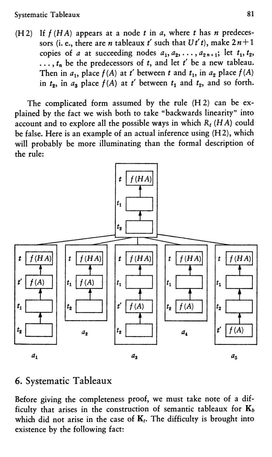
The key feature of the temporal transparency principle is that
"It will be the case tomorrow that it is now the case that /?" is
tantamount to "p tomorrow" and not to "p now". A.N.Prior has
maintained that only the reverse view is correct*, but this legislates a
unique solution of what, at the verbal level, is an equivocal locution that
could be construed either way. How we construe it is a matter not
of linguistic necessity but of logical convenience, and our
transparency view of "now" is, we insist, every bit as workable as fixity-
insisting, Prior's contrary one. Thus the essential upshot, and surely
more natural consequence of the transparency approach is that it
is the case that tomorrow's tomorrow is the day after tomorrow
rather than tomorrow, and yesterday's today is not today but
yesterday.
A second key feature of "now" is its temporal redundancy, as
illustrated in the fact that
It rained in London yesterday
and
It is now true that it rained in London yesterday
are equivalent. This situation is not specific to this example, and we
have it that in general:
K(P) = P
This temporal redundancy of the "now" is fundamental, and is
in fact the source of its temporal transparency. For if
K(P) = P
1 A. N. Prior, Now, Nous, vol. 2 (1968), pp. 101—119 (see especially
pp. 102—103).
is not n
is n
34 The Basic System R of Temporal Logic
then it is obvious that one must have it that
Rt[Rn(p)]=Rt(P)
and not
Rt[Rn(p)] = Rn(p)
as an across-the-board espousal of the unqualified iteration principle
Rt[RAP)] = RAP)
would have it.
But the relationship can also be seen in a converse perspective.
For if we postulate
(Vt){Rt[R„(P)] = Rt(P)}
then we shall consequently have
(Vt)Rt[Rn(p)=P]
And so, if an omnitemporally asserted thesis is to be asserted sim-
pliciter (that is, if we are to have the rule: If h-(V£) Rt(A), then HA),
we must also have it that:
Rn(p)=P
It is, in fact, our intention that the temporal transparency of the
"now" is to obtain in a very general way, so that in general the rule
obtains:
R, (...*...) = (...*...)
provided that n is not governed by some R-operator within the
context (...«...). We shall speak of this as the "w-Shift Rule". It
signalizes the fact that (figuratively speaking) n is temporally
transparent: you see through it to the time that lies behind — when
subject to another temporal qualifier, "now" simply evaporates. This
w-Shift Rule is of fundamental importance for the development of
a temporal logic, for (as we shall see) it makes possible the use of
the Rt machinery for the articulation of genuinely tensed
propositions.
The introduction of "now" with its special features is the key step
in the move from a positional logic in general towards a specifically
Temporal Homogeneity
35
temporal logic. With this step we move from the essentially spatial
situation of a B-series to the specifically temporal situation of an
A-Series. The status of n = "now" is, of course, somewhat peculiar
from the logical standpoint. It is neither fish nor fowl, neither
constant nor variable. It is not a constant, since it does not denote the
same T-element on each occasion of its use, and not a variable,
since it cannot meaningfully be quantified, i. e., a statement like
(V«) [Rn(p)] is not meaningful. This dualistic character of the "now"
is reflected in the w-Shift Rule. If we were to assign n to any
semantical category, it would have to be that of indexicals, i. e., those parts
of speech which denote something uniquely in a given context,
though not the same thing in every context. (Personal pronouns are
examples of other indexical expressions.)
3. Temporal Homogeneity
One of the major ideas regarding time — and one which has very
significant implications for the logic of time — is that of
homogeneity. Time is — or would be — homogeneous if the structure of
the local temporal environment of every temporal position (point
in continuous time, or interval [i. e., atomic or element interval]
in discrete time) is exactly like that of all the others. This idea could
be formulated as follows:
A mode of time is homogeneous iff whenever it is a thesis
that "... t0 ..." obtains for any constant £0, then it is also the
case that "(V£) (... t...)" is a thesis.
This condition thus has it that there are no theses (i. e., time-
logical theses) regarding the structure of time that differentiate
between any one particular temporal position and the rest. The
situation regarding this temporal homogeneity is in this regard
analogous to the requirement that the individuals are not to be
differentiated from one another by purely logical means2.
The condition in view will at once disqualify various modes of
time as not homogeneous. For example, both "beginning time" and
"ending time" will be excluded. For in the former case — and the
2 See Alfred Tarski, Logic, Semantics, Metamathematics (Oxford,
1956), pp.385—386.
36 The Basic System R of Temporal Logic
situation in the latter is wholly analogous — we will have it as
a thesis that:
(a*)~00 (*'<*)
or equivalently
(lt)(Vt')(t^t')
Consider now the time t0 — whose existence we can infer from this
by existential instantiation — that is the "beginning of time", with
respect to which we have the thesis:
(v0(*b^0
It is quite obvious that this thesis cannot be generalized to yield:
Consequently the original thesis would violate the requirement of
temporal homogeneity.
In assigning a privileged position to "now" —the present moment
— in a temporal logic we may well also violate the requirement of
homogeneity, or at any rate would do so if n (now) were admitted
as a constant. For in temporal logic one wants to adopt the stance
that absolute (i. e., temporally unqualified) propositions are to be
construed present-tensedly, so that an absolute proposition is
tantamount to an actual proposition, that is a proposition quoad "now".
Rn(p)=P
But consider its universal generalization with respect to the
"constant" n:
(Vt)[Rt(p)=p]
This has the consequence
(3t)Rt(p)=>p
which is clearly unacceptable as a thesis since it would immediately
generate a contradiction whenever we assume a p0 such that
(3t)Rt(p0) and {3t)Rt(^p0) both obtain. Thus the privileged
character of the now would prevent time from being homogeneous
in the indicated sense if — contrary to reason — n were construed
as a constant.
Axioms for the Logical Theory of Chronological Propositions 37
The homogeneity of time is closely related with the issue of
temporal compression and expansion inherent in the possibility of
obtaining an isomorphic modeling between a long period of time
and a short one. It is this feature of temporal dilation that assures
the possibility of simulating the events of one time-span of "real
time" within a span of synthetic time, so as to contract a sector of
history or stretch it out by "slowing down" or "speeding up" a
sequence of occurrences3. Temporal dilation can occur not only
within continuous linear time but also in circular time, figure-eight
time, and indeed in principle even in a multidimensional time. Note,
however, that it could not occur in discrete linear time, for example,
or in branching time. (These two sentences anticipate issues to be
considered below.) In this context, the question of the dilatability
of time as a whole also arises. Note that if time is linear and infinite
into both the past and future, then time as a whole can be isomor-
phically modeled by a finite interval that is open at both ends. Now
this feature is not realized by circular time or figure-eight time or
indeed by any non-linear one-dimensional time structure.
4. Axioms for the Logical Theory
of Chronological Propositions
We shall now set out to develop the logical theory of chronological
propositions in a systematic, formal way. The machinery we shall
require for this purpose is as follows:
(i) /?, q, r, etc., as propositional variables, ranging over both
temporally definite and indefinite statements.
(ii) t, t\ etc., as variables for periods of elapsed time since the
origin, i. e., as dates or quasi-dates.
(iii) The indexical symbol «, for "now".
(iv) The usual connectives of propositional logic, specifically ~
for negation, &C for conjunction, ^ for material implication, and
= for mutual material implication (material equivalence).
(v) The usual quantifiers, both universal (V) and existential (3).
These will be needed at present to range not over individuals —
3 In this formulation, the words "a sector of history" are important,
because if all of the history of the period were at issue, the issue relative
versus absolute time would be prejudiced.
38 The Basic System R of Temporal Logic
since we are at this point developing only a propositionai, and not
a higher order logic — but only over times (dates).
(vi) An identity predicate such that x = y is to be a meaningful
expression whenever x, y are variables or the indexical symbol n.
(vii) The operator R for chronological realization, as introduced
above.
We shall need, moreover, to presuppose all of the usual logical
principles of quantification theory with identity, for formulas of the
system which do not involve the symbol n. The only novelty is to
be the set of logical rules for the operator R, and the indexical n>
to whose elaboration we now turn.
We shall suppose, to begin with, that the operator R is governed
by the following rules or theses:
(T 1) The negation of a statement is realized at a given time ///
(if and only if) it is not the case that that statement is realized at
that time:
Rt(~p)=~Rt(p) (Tl)
(T 2) A conjunction of two statements is realized at a given time
/'// each of these two statements is realized at that time:
Rt(p&Cq) = [Rt(p)&cRt(q)] (T2)
If a statement is asserted simpliciter, without explicit temporal
qualification this is to be tantamount to its assertion quoad now.
We thus have:
(T3) If a statement is realized currently (i.e., now and at
present) then it obtains unqualifiedly or absolutely:
Rn(P)=P (T3)
It is obvious that this thesis will have the consequence:
(Vt)Rt(p)^p
For any statement p (chronologically definite or not) and any
style of chronology (chronologically definite or not), (Vt)Rt{p) is
a chronologically definite statement (and so for that matter is
(3t)Rt(p)). It thus falls under the Convention of Section 2 above,
with the result that:
Axioms for the Logical Theory of Chronological Propositions 39
Being a chronologically definite proposition {Vt)Rt{p) is such
that a statement asserting its realization at any given time is
equivalent with (Vt)Rt(p) itself:
Rt'[(Vt)Rt{p)] = (Vt)Rt(p)
Now this equivalence would lead us (in the face of (T5) below) to
the result:
The R-operator is interchangeable with a following universal
quantifier:
Rt,[(Vt) Rt(p)] = (Vt) {Rt,[Rt(P)]} (T4)
The thesis (T4) merits further consideration. On the "long
conjunction" interpretation of the universal quantifier it amounts to
Rf [Rtx (P) & Rt2(p) & Rts(p) &...] =
= R* [Rtl (P)] &c Rt, [Rt2 (p)] &c Rt, [Rts(p)] &c...
which is a virtual consequence of (T2). Actually, however, we in
fact want to assert a thesis somewhat stronger than (T4), viz. what
is best formulated by the axiom schema:
R,[(V*)A] = (Vt)R,(A) (T4)
Finally there is — as we saw in Section 3 above — the key
matter of R-iteration:
R, »(/»]-{ ^[according as ({^otn (T5)
Taking these rules as our starting point, we shall now present
an axiomatic theory for the logic of the operation of chronological
realization.
In view of (T 1) and (T2) the situation here is analogous with
that in topological logic in that — since these theses guarantee
distributivity of the R-operator over a functionally complete set of
propositional connectives — we have a principle of distribution:
The R-operator is distributable over all truth-functional
connectives.
40 The Basic System R of Temporal Logic
Moreover, we shall postulate the rule of inference
If HA, then h-R,(A) (R)
where h- represents assertion (i. e., thesishood) within the system we
are endeavoring to construct. In the context of the distribution
principle, this rule is interdeducible with the substitution rule:
If h-A = B and \-Rt (A), then \-Rt (B)4. (RS)
Moreover, since (T4) guarantees that the R-operator is also
distributable over quantifiers, (RS) can be construed broadly: its A's and
B's can range over propositional functions as well as propositions.
We shall thus also postulate a general rule of the replacement of
equivalents:
If HA = B then h-(... A ...) = (... B ...) (RE)
Correspondingly we have the rule:
From I-A = B and (... A ...) to infer ... B ...
As a basis for the system is taken any standard set of rules and
axioms for quantification theory with identity, for formulas not
involving n (we shall see shortly why this proviso is necessary). The
special axiom-schemata for temporal logic are then as follows:
R<(~A) = ~R,(A) (Tl)
Rt(AScB) = [Rt(A)&cRt(B)] (T2)
Rn(A) = A (T3)
RA(Vt)A] = (Vt)[Rt,(A)] (T4)
RARt(A)] = Rt(A) (T5)
Rt{n = t') = t = t' (T6)
Rt{t'=t") = t'=t" (T7)
(W)A=>A"» (T8)
In the above statement of the schemata, t, t',..., etc. stand for
variables; A"n designates the result of substituting n for every free
occurrence of t in A. Furthermore, axiom schema (T8) is subject
to the proviso that t does not occur within the scope of an R operator
4 See Footnote 1 on p. 15 above.
Axioms for the Logical Theory of Chronological Propositions 41
in A, while in (T4) t and t' must be distinct. The purpose of the
(heretofore unconsidered) axioms (T6)—(T7) is to make provision
for identity ( = ). Also, (T8), like (T3), accomodates features of the
special quasi-constant n.
The axiom-system based on (Tl) to (T 8) will be designated as
the system R. For this system we also suppose the following rules
of inference:
Whenever A is a thesis, so is (V*) Rt(A) (R)
If \-A = B, then h-(... A ...) = (... B ...) (RE)
The converse of the rule (R), viz
If t-(Vt)Rt(A) then I-A (R)
can only be maintained with the proviso: provided that t is not free
in A. If this proviso were omitted, the following deduction would
become possible:
(1) (}/t)[Rt(p)sRt(p)] by(R)
(2) Rt(p) = Rt[R,(P)] by(T5)
(3) (v*) {Rt [R, (p)] = Rt (p)} from (2) by (R)
(4) (V*)Ri[R«(p)sp] from (3) by (Tl), (T2), (RE)
(5) Rt(p) = p from (4) by (R)
Of course, this consequence would be fatal, since the whole
machinery of temporal realization would be rendered superfluous.
On the other hand (4) itself, which can be proven, and is equivalent
with
(>/t)Rt[Rt(p) = K(P)]
is perfectly harmless. For it quite correctly claims that, at any
temporal position t, it can be said that p is realized at t iff p is realized
now.
Although all standard logical principles are assumed for w-free
formulas, these break down when the indexical n enters the picture.
One notable instance is the substitution of identicals. Consider the
formula:
{t = n&cRARt(p)]}=>Rt,[Rn(p)]
By (T3), (T5), this is equivalent to:
[t = n&cRt(p)]=>Rt>(p)
42
The Basic System R of Temporal Logic
Now it is clear intuitively that this formula is not valid, since p
might be true at t, but false at t\ so that the antecedent would be
true, but the conclusion false at the moment t. On the other hand,
consider the formula:
[t = n&cRt(p)]*Rn(P)
A little reflection suffices to show that this formula is intuitively
valid. Its proof in R is as follows:
(1) (VO {[t = t' &C Kt (p)] => Rf (p)} by quantification theory
(2) [t = n&cRt(p)]^Rn(p) from (1), by (T8)
The apparently erratic behaviour of n in identity contexts may
seem odd until we reflect on its intended meaning as an indexical
symbol. While we are considering a fixed moment of time, that is,
carrying out an argument in a fixed temporal context, "now"
always denotes the same moment, hence we can use standard logical
principles unrestrictedly. However, if we consider the standpoint of
another moment of time, or temporal context, "now" denotes
a different moment in that context, so we cannot freely substitute
one "now" for the other — we cannot identify the "now" of
yesterday with the "now" of today. When we remember that the
operator R in the system R plays the role of providing temporal
contexts for propositions, we see that these considerations account
for the validity of the second formula, while invalidating the first.
Several simplifications of this axiom system for R can be effected,
as follows:
(I) (T 2) can be replaced by one half of itself, namely,
[Rt (A) &c Rt(B)] ^Rt(A&c B) (T2.1)
in view of the following argument:
(1) Rt[(A&cB)^>A] by Rule (R)
(2) Rt (A&cB)^> Rt (A) from (1) by the Lemma5
(3) Rt(A&cB)^Rt(B) by parity with (1), (2)
(4) Rt (A&cB)=> [Rt (A) & Rt (B)] from (2), (3)
5 The lemma in question is the thesis.
Rt(P^q)^[Rt(P)^Rt(q)]
whose proof is immediate once (T 1) and (T2.1) are given.
Temporal and Topological Logic 43
(II) Given (T 1), (T5) can be replaced by half of itself, namely,
Rt>[Rt(A)]*Rt(A) (T5.1)
in view of the derivability of the inverse by the following argument:
(1) iMiM^A)]=>iM-A) by (T5.1)
(2) ^Rt (<-A) => <-R,> [Rt (-A)] from (1)
(3) Rt(^>^A)ZjRt,[Rt(<^<^A)] from (2) by (Tl)
(4) Rt(A)=>Rt,[Rt(A)] from (3)
We thus see that the axiomatization of R can be based on the
following simplified set of axioms: (Tl), (T2.1), (T3), (T4), (T5.1),
(T6)—(T8).
5. Temporal and Topological Logic
We have now set forth a system of temporal logic, based on the
rules
If h-A, then \-(Vt)Rt(A) (R)
If \-A =B, then h-(... A ...) = (... B ...) (RE)
and the following axiom schemata:
R,(~A) = ~R,(A) (Tl)
Rt(A8cB) = [Rt(A)ScRt(B)] (T2)
R«(A)=A (T3)
R,[(Vt)A] = (Vt)Rt>(A) (T4)
R,[Rt(A)] = Rt(A) (T5)
Rt{n = t') = t = t' (T6)
Rt(t'=t")=t'=t" (T7)
(Vf)A3A"» (T8)
It is obvious and striking that this axiomatization is intimately akin
to the systematization of topological logic as set out in the preceding
chapter, based on the rule
If I-A, then (-(Va)Pa(A)
44
The Basic System R of Temporal Logic
and the axiom schemata:
Pa(^A) = ^Pa{A) (PI)
Pa{A&cB) = [Poc(A)&cPoc(B)] (P2)
(V«)P«{A)=>A (P3)
P/?[(V<x)A] = (V<x)P/?(A) (P4)
P/}[Pa(A)] = Poc{A) (P5)
Indeed, it is now obvious that we have, in effect, developed temporal
logic as a special case of topological logic (with identity), by simply
letting the "positions" at issue be times, i. e., positions in a temporal
framework and introducing special features for the temporal quasi-
constant n for "now". For in bringing n upon the scene in the
manner specified by (T3) we could drop the analogue of (P3), but had
to make an appropriate readjustment in the quantificational rules.
In short, in taking the step from topological to temporal logic the
only changes we have introduced (apart from introducing the
machinery of identity) are those modifications brought about in the wake
of the requirement of accommodating the temporal peculiarities of
the indexical quasi-constant n ("now") and its ramifications.
6. The Completeness and Decidability of R
The temporal calculus R presented in the preceding sections is
complete, that is, it is sufficiently powerful to prove any statement
of temporal logic which we would intuitively regard as true solely
by virtue of the meanings of the terms occurring in it, while of
course no invalid statements are provable.
To prove this for R, we first give a semantics for this system, so
that we have a formal notion of validity to correspond to our
informal concepts. We define a t-structure S = (7, f) to consist of:
(a) a non-empty set 7; we denote elements of 7 by a, b, c, d>.. .
(b) a set of evaluation functions ?, each function / la being
associated with one a in 7, which assign the values T or F to each
propositional variable p(.
The Completeness and Decidability of R
45
Now let [ ] be a function which assigns each variable t a value
a = [t] in 7. Given [ ], we define [ ]a for each a in 7 by:
[t]a = [*], * a variable (and so, different from n)
[n]a = a
Now, given a ^-structure 5, and an assignment function [ ] for S,
we can calculate IAIa the value of A at a under [ ], where A is
a complex formula, by the rules:
(i) /<-A/a = T~/A/a = F.
(ii) /A&cB/a = T<->/A/a = T&c/B/a = T.
(iii) /x = y/fl=T<-*[x]fl=[y]fl,
where x, y are variables, or the indexical n.
(iv) /(Vt)A/a = T<->/A/a = T under [ ]'•*, for all b in 7, where
[ Y>b is a function such that [t] = b> but otherwise agrees
with [ ] in its assignments.
(v) /R*(A)/fl = T~/A/[x]fl = T,
where x is a variable, or the indexical n.
The intended meaning of these formal definitions should be clear
enough — 7 is a set of times, while we have replaced our
proposition-forming operator R by the evaluation functions / /a, so that
intuitively;
/A/a = T iff Ra(A)
We define a formula A of R to be t-valid if for every ^-structure
$ = (7 j ?)> and every assignment [ ] of variables to members of
7,1Ala = T under [ ] for every a in 7.
The completeness theorem we are pursuing now reads:
Th 1: For every formula A of R, I— R A if and only if A is t-valid.
One half of this theorem we can easily prove, namely:
Th 2: If \-R A, then A is t-valid.
46 The Basic System R of Temporal Logic
Proof: We show that all the axioms of R are f-valid, and that
the rules of R preserve f-validity. We shall illustrate this only with
the special axioms of R:
(a) (Tl) is f-valid.
~/A/Wa~F
~/Rt(A)/a = F
*->/~Rt(A)/a = T
(b) (T2) is f-valid.
/R, (A & B)la = T~/A&c BIWa = T
~/A/[<la=T&/B/m<J = T
WR,(A)/8 = T&/R,(B)/„ = T
~/R,(A)&cRt(B)/a = T
(c) (T3) is f-valid.
/R„(A)/a = /A/[B)a
= /A/a
(d) (T4) is f-valid.
/Rr [(V*) A]la = T«-»/(v*) A/ta = T
«-» /A/Ma = T under [ p, for all b in 7
*-» /R, (A)/„ = T under []'>', for all b in 7
<-/(Vt)[R,(A)]/8 = T
(e) (T5) is *-valid.
/R,,[R<(A)]/0 = /R,(A)/(„]a
= /AA<][a
= M/M„
= /R«(A)/a
(f) (T6) is *-valid.
/R, (« = t')la = T W« = *7Wa = T
** Mm. = Mm.
The Completeness and Decidability of R 47
(g) (T7) is *-valid.
/R,(*' = *")/« = T~/S = t"/[t]a= T
(h) (T8) is *-valid.
Suppose that A is a formula in which t does not occur within
the scope of an R operator. Then we can prove by an induction on
the complexity of A that for any ^ in 7, any assignment [ ], the
value IAtlnla under [ ] is the same as IAIa under [ Y>a. Then:
/(VO Ala = T under [ ] -> IAIa = T under [ ]*>*
-+IAtlnl=-T under [ ]
(i) The rule (R) preserves ^-validity.
Suppose A is £-valid, but (V£) Rt(A) is not. Then for some
^-structure Sy some assignment [ ], some a in 7,
/Rt(A)/m = F under [ ]
hence
But then A is not £-valid, contrary to supposition. *
(j) The (RE) preserves ^-validity.
If A = B is t-valid, /AJa = /B/a for any a in any ^-structure S.
Hence, by an induction on the complexity of (... A...),
/(... A .. ,)/fl = /(... B .. .)/„ for any * in S.
This completes the proof of Th2.
We now proceed to a proof of the second half of Thl, namely
Th3: If A is *-valid, \-RA.
Proof: The proof of Th3 proceeds by showing that for every
formula A of R, there is a formula A! of R which is provable in R
if and only if A is, and which, if valid, is provable by quantification
theory alone.
48
The Basic System R of Temporal Logic
Let us say that a formula A of R is in normal form if it contains
no occurrences of propositional variables not in the scope of
R-operators, no occurrences of the symbol w, and all R-operators
in A occur only in part of the form Rt (/?*), where pi is a propositional
variable.
Lemma 1. For every formula A of R, there is a formula A! in
normal form such that A! is valid if A is, and \—R A if \—RA'.
Proof: Starting from A, we proceed to A! by stages:
Stage 1: We first replace any propositional variable pi not in the
scope of an R-operator by Rn (pi). We next eliminate all occurrences
of n in A not within the scope of an R-operator, replacing them
by a variable t which does not occur in A. Let us call the resulting
formula Av Suppose that A1 is provable in R, then (Vf) Ax is
provable in R, hence A is provable in R, by (T8), (T3). Futhermore,
it is clear that if A is valid, so is Av
Stage 2: Starting from the formula Al5 we drive the R-operators
in the formula inwards so that they have the smaller possible scope.
These steps can be justified by (RE), (Tl), (T2), and (T4). In
applying (T4), alphabetic change of bound variables is to be carried
out whenever necessary. If iterations of R-operator appear at any
step in the process, they can be removed by application of (T3),
(T5). The end-result is a formula A2 such that h-RA1 = A2 and in
which R-operators occur only in parts of A2 of the form Rt (x = y)
or Rt{pi).
Now by the use of (T6), (T7) and the theorems
Rt(n = n) = t = t
which are easily demonstrated in R, we can eliminate all occurrences
of R-operators governing identity formulas. The resulting formula,
A', is in normal form. Now if \-RA\ h-RA2y since A! is equivalent
to A2, hence t-RAu so finally h-RA. Furthermore, if A is valid, so
is A', since \-RAl = A'.
Now for any formula A in normal form, let A* be the formula
of pure quantification theory with identity which we obtain by
replacing each part of A of the form R,(ft) by R^), where Ri is
The Completeness and Decidability of R
49
a monadic predicate letter. Assume that A* can be falsified by some
interpretation. That is, we can find a set 7, and an interpretation
of each monadic predicate letter Rt in 7, and an assignment of
variables [ ] to elements of 7 which falsifies A*. Let ft be the subset
of 7 which is the interpretation of the monadic predicate letter R*.
Now consider the ^-structure S = (J, £), where each / la in T is
defined by:
/pi/a = T~h(a)
It is now easily seen that A can be falsified in S under [ ].
Now assume that A is t-valid. Then by Lemma 1, A' is t-valid.
But then A'* is valid. It follows that we can prove A' in R by
imitating the proof of A'* in our basic system of quantification theory with
identity (we know that there must be such a proof by the
completeness theorem for quantification theory). Hence, again by Lemma 1,
This completes the proof of Th3, and so the proof of the
completeness theorem for R.
The completeness theorem provides us with some welcome sub-
sidiary information, namely, the decidability of R, for we have
effectively associated with each formula A of R a formula of
monadic quantification theory with identity which is provable if
and only if A is provable in R. Since monadic quantification theory
with identity is decidable6, we have a mechanical procedure for
determining whether or not A is a theorem of R, for arbitrary A,
i. e., R is decidable. (It might not be going too far to say that R is
simply monadic quantification theory in a somewhat unfamiliar guise.)
This decidability result of course does not carry over to the case in
which we add further predicates (e. g., an arbitrary dyadic
predicate) to R, as we shall do in the next chapter.
6 For a proof, see Alonzo Church, Introduction to Mathematical
Logic (Princeton, 1956), pp. 284—285.
Chapter V
The Introduction of Tense Operators
1. Presentness and Precedence
Two further additions are essential in the move from a topological
logic of generic "places" to a genuinely temporal logic of specific
"times". The first of these — as yet unmentioned — is a
relationship of temporal precedence to establish the series of earlier (prior
or anterior) and later (posterior) times, of before or after (of what
McTaggart calls the B-series). The second — with which we have
already dealt — is the introduction of now, the "present time",
a privileged time with respect to which all anterior times are
determined as past and all posterior ones as future. (The series of past-
present-future comprises what McTaggart calls the A-series and
contrasts with the B-series: If one event is ever earlier than another,
this is an unchanging relationship, while past-present-future
determinations are changing — what was once future will someday be
past.)
For the development of a genuinely temporal logic we must thus
introduce two items of machinery:
(i) the "privileged present", viz., n for "now", and
(ii) the relationship of temporal precedence, viz., Utt' for "the
time t is before (i. e., prior to) the time t'n.
Consider the questions:
(1) Is U irreflexive?
(Vt)~«Utt
Presentness and Precedence
51
(2) Is U asymmetric?
(3) Is 17 transitive?
(Vf) (VO (VO [{Utt'&cUt't")=>Utt"]
(4) Is there a [/-minimum?
(30 (VO [*'=£*=> 17 «']
(5) Is there a [7-maximum?
(6) Is U dense?
Let us designate as a U-calculus a set of rules for the [7-relation
as given in the answer to questions of the indicated type. It is clear
that our system R is vacuous from this standpoint: it stands quite
empty in this regard and awaits the specification of further [7-rules.
The introduction of the special "constant" n is subject in R to
the w-shift principle that n gives way to the subscript of the
innermost Rroperator applicable to it. To get the effect of this w-shift
principle in the augmented (R/[/)-calculus we add as axioms:
Rt(Unt')==Utt'
Rt(Ut'n) = Ut't
Furthermore, since statements concerning relationships of temporal
precedence hold timelessly, we must further add the axiom:
Rt(Ut't") = Ut't"9 provided t'j*n, t"j*n
Given the above three axioms, we can prove by induction on the
complexity of a formula (... n ...) containing the quasi-constant n
that
h-R,(... ;*...) = (...*...)
which is precisely the content of the w-shift principle.
52 The Introduction of Tense Operators
2. Tense
Given the machinery of presentness and precedence, it is an easy
and natural step to introduce these operators into our various
systems of temporal logic.
Operator Construction Definition
Fp "It will be that /?": (3*) [Unt&cKt{p)]
p is future (i. e., p will be realized
at some time in the future)
Pp "It has been that /?": (It) [Utn&cRt(p)]
p is past (i. e., p has been realized
at some time in the past)
Gp "Henceforth always /?": (V*) [Unt => Rt(p)]
p is future-perpetual (i. e., p will
be realized at every time in the
future)
Hp "Heretofore always p»: (V*) [Utn ^ Rt (p)]
p is past-perpetual (i. e., p has
been realized every time in the
past)
Note that on any of these accounts G = ^P^ and H = ^P~
(if we assume two-valuedness for R).
It must be noted carefully at this point that we have to observe
some restrictions on translating tense operators like P, P, G, and H
into the R-calculus, lest the translations be intuitively unacceptable.
For instance, consider the problem of translating FFp. If we proceed
naively in translating FFp into R, we may run into perplexity.
Seemingly FFp amounts to:
(3t)[Unt&cRt(Fp)]
which in turn amounts to:
(2t){Unt6cRt(lt')[Unt'6cRr(p)]}
This is equivalent with:
(3t) {Unt & (30 [Utt' &c Rt (R?(/?))]}
Tense
which amounts to
53
(3t){Unt&c(3t')[Utt'&cRt'(p)]}
But this last formula does not express what we want it to express,
namely that p is true in the future of a future moment: it says that
there is a future and p is realized in the future, and does not say
that there is a future in whose future p is realized. Obviously
something has gone wrong here.
We now give an exact specification of what we mean by a
translation A* of a formula A involving only tense operators and logical
connectives. The translation, A*, in R is to be a formula with no
free time-variables. We define A* by an induction on the number
of connectives and operators in A:
(a) If A is a propositional variable, A* = Rn (A)
(b) [A=>B]* = A*=>B*
(c) [~A\* = ~A*
(d) [G(A)]* = (Vt)[Unt=>Rt(A*)]
(e) [H(A)]*= (Vt)[Utn=>Rt(A*)]
(f) [F(A)]*=(3t)[Unt&cRt(A*)]
(g) [P(A)]*=(2t)[Utn&cRt(A*)]
where Ms a temporal
variable that does not
occur bound in A*
Given these rules governing the rendition in the R-calculi of the
tense operators P, F, G, H, it is easy to see the justification for
designating these as tense operators. Thus, for example, FPp is
a pluperfect qualification of /?, to the effect that this will have been
realized at some point in the future:
[F?p}* = F{(v')[Ut'n&tRAp)}} (g)
= (3t){Unt&cRt(3t')[Ut'n&cRt>(p)]} (f)
EzdWntScdOlRtiUftiScRtRrip)]}
= (2t){Unt&c(3t')[Ut't&cRt>(p)]} w-shift rule
= (3*) (3 0 [Unt&cUt't&CRf (p)]
54
The Introduction of Tense Operators
Here the last formula is exactly the rendition of the pluperfect
statement that p obtains at a time (t') which precedes the future time at
issue (t).
An analogous line of thought can be used to establish the tensed
nature of the other forms of mutual application of the four basic
tense operators (F, P, G, H). Thus the additional machinery of
a U-relation defined among the elements of the set 7 constituting
the domain over which the subscripts of the R-operator can range,
makes it possible to introduce tenses of the familiar sort upon the
stage of discussion.
Chapter VI
The System K/ of Minimal Tense Logic
1. The Problem of a Minimal Tense Logic
We come now to the problem of devising a "tense logic" — that is,
a set of rules governing the mutual logical interrelationships of the
tense operators as defined within the framework of a (R/U)-calculus.
Let us begin here with the question of an irreducibly basic or
minimal tense logic; "minimal" in the sense of involving no assumptions
whatsoever regarding the nature of the [/-relation. This last
condition is imposed to assure "minimality" in the sense of topological
neutrality — i. e., the lack of any specific assumptions about the
structure of time.
The answer to our problem is provided by E. J. Lemmon's
system K*, whose axiomatic basis is as follows:
Axioms
G(p^q)^(Gp^>Gq) (G 1)
H(p^q)Z>(HPZ>Hq) (HI)
^H^Gp^p (G2)
^G^Hp^p (H2)
Rules
If A is a classical tautology then I—A (RT)
If h-A then l-HA (RH)
If h-A then l-GA (RG)
If h-A and M3 B then h-B (RD)
It is readily shown that all this holds for the minimal system we are
seeking. By way of example, let us verify this for (G 2), which, in
56
The System K< of Minimal Tense Logic
the relevant interpretation now says:
(It) (Utn & Rt {(VO [l/«'=> Rt> (/?)]}) ^ p
( = ) (3*){U*«&(V0[U«/3^(P)]}3^(P), since psR^tp)
But this last implication is a theorem of quantificational logic.
Moreover, all of the familiar tense logical principles that fail
for K* (e.g., FFp^Fp) also fail to obtain in our minimal system.
We may thus conjecture:
The minimal tensed system based on R is identical with Lem-
mon's K,. We now proceed to a rigorous proof of this conjecture.
2. Semantics for Tense Logic
The problem of completeness for K^ is difficult to attack directly,
because of the expressive inadequacy of a calculus expressed solely
in terms of the machinery afforded by F, P, G, H plus the standard
propositional connectives. For example, irreflexivity of the
[/-relation can be expressed directly in a [/-calculus by:
*(3t)Utt
but it can be demonstrated that no tense-logical formula reflects
this condition.
To make a start on the problem, we first define a formal
semantics for tense logics by indulging in a little harmless reification,
talking about the set 7 of all times, and replacing the propositional
operators Rt by propositional functions which fulfill the same role.
This provides the background for the following definition:
A tense-structure S = (7, #, U) consists of a non-empty set 7,
a set & of functions Rh for each t in 7, which assign the truth-values
T or F to every proposition p; and an arbitrary binary relation U
defined on 7. We define the value of a complex formula inductively
as follows (note that here Rt serves as an evaluation function rather
than as propositional operator):
(a) Rt(A^B) = T iff Rt(A) = F or Rt(B) = T
(b) Rt(^A) = T iff Rt(A)=F
(c) Rt[G(A)] = T iff iMA) = T for alW such that 17«'
(d) Rt [H (A)] = T iff Rt, (A) = T for all t' such that Ut't
Semantics for Tense Logic
57
We now define truth and validity in tense-structures; a formula
A is true in a tense-structure (7, £, #) iff R*(A) = T for all t in 7,
valid iff it is true in all tense-structures. Thus, for instance, the
formula p^Gp is true in the tense-structure consisting of a single
instant in time t0, but not valid, since Kt0(P ^ Gp) = F in the tense-
structure diagrammed below:
Rt9 (P) = T O O *ti (P) = f
to h
In such a diagram one represents:
1. the elements of 7, here t0 and tu by small circles,
2. the 17-relationships among 7-elements by arrows,
3. the truth-value assignment function by writing the pertinent
evaluations alongside the circle.
To return to our original problem, the minimal tense logic Kt
is intended to correspond to a situation in which we put no
restrictions whatever on our [/-relation. We should therefore expect the
following completeness theorem: a formula A is provable in K* if
and only if it is tense-structurally valid, i. e., true in all
tense-structures. The first half of this equivalence, i. e., that all theorems of K*
are valid in this sense is easily checked.
For instance, let us assume for a reductio argument, that (H 2)
is not t. s. valid (tense-structurally valid). Then there must be a time
t0 in a tense-structure at which KtQ{FHp^>p) = F. Then KtQ(FHp) =
T and Kto (p) = F. From the first equation we deduce that for some
tt such that Ut0t^ Ktx{Hp) =T, hence that Rto(p) =T. But this
contradicts the second equality, so that (H 2) is t. s. valid.
To prove the other half of the equivalence, we shall make use of
the technique of semantic tableaux1.
1 For a very elegant exposition of the technique as applied to
classical logic, the reader should consult Raymond Smullyan (1968) from
whom we have borrowed some of the methods and notation used in the
present chapter. The application of semantic tableaux to modal logics
originates with a series of papers by Saul Kripke (1959, 1963, 1963 a,
1965), and a 1961 paper by Jaakko Hintikka. (For details regarding all
these references see the Bibliography.)
58
The System K* of Minimal Tense Logic
3. Semantic Tableaux
The idea behind the technique of semantic tableaux is simple and
intuitively satisfying — given a formula A, we carry out a systematic
search for a counterexample to A; if all possible lines of search end
in failure there can be no such counterexample to A, so A must be
valid. As an example, suppose we are inquiring as to the validity
of the formula Fp^FFp. We assume that the formula can be
falsified, and so place f(Fp^FFp) in a box (tableau) t0
representing a certain moment of time:
*0 f(Fp^FFp)
Now by the semantic rules for ^, if A ^ B is false at t0, A is true,
and B is false at t0> so we place the corresponding formulas at t0:
*0 f(Fp^FFp)
t(Fp)
f(FFp)
Now since Fp is true at t0, there must be a tableau tt such that
Ut0tt and Rtiip) = T, so we enlarge our tableau model
correspondingly, representing the U-relation as an arrow connecting the
tableaux:
h I f(Fp=>FFp) I
t(Fp)
I f(FFp) |
But now, since f(FFp) appears at t0, Fp must be false at tu so we
carry out the corresponding inference in our tableau model:
t0 f{Fp^FFp)
t(Fp)
| f(FFp)
h I t(p)
fiFp)
Semantic Tableaux
59
But with this final step, we are home; we have found a
counterexample to the given formula. Fp is true at t0, but Fp is false at tt
(trivially so, since by our construction there just is no tableau U such
that Ut1t2). Hence FFp is false at t0, and so Fp^> FFp is false at tQ.
The process of tableau construction has produced a counterexample
that shows the invalidity of the thesis.
As a second example, consider the technique as applied to the
formula PGp^p. The opening moves are as for the preceding
formula:
T(PGp^pJ~\
t(PGp)
f(P)
T, we must add a tableau at tt such that
t(Gp)
f(PGp*p)
t(PGp)
fiP)
Now since t(Gp) appears at tu t(p) must appear at t0:
tt t(Gp)
I
f(PGPo
t(PGp)
ftp)
t(P)
>P)
But now there is an explicit contradiction at f0, so that our search
for a counterexample has ended in failure; hence we conclude that
PGp^p is valid.
We now proceed to a more precise formulation of these ideas;
the various alternative paths we can take in our search are presented
in the form of a tree, each node of which is a set of tableaux con-
'o
Now to satisfy Rto(PGp)
Uttt0, and Rtl(Gp) = T:
h
to
60
The System K< of Minimal Tense Logic
nected by a relation. These tableaux sets can be thought of pictor-
ially as above, as directed graphs. If the formula to be tested is A,
we place / (A) in a single tableau at the origin of the tree. The rules
for the construction of the tree are then as follows:
At a given node N of the tableau-tree:
(^1) If t{A^B) appears at N in a tableau t» add two succeeding
nodes to N, N' and N", which are copies of N, then add
/(A) to ti in N', and t{B) to tt in N".
p2) If f(A^B) appears at N in a tableau th add a succeeding
node, N' to N which is a copy of N, then add the formulas
t{A),f{B) to U in N'.
(^1) If t(^A) appears at N in a tableau £,-, add a succeeding node
N', which is a copy of N, then add /(A) to ^ in N'.
(~2) If f{^A) appears at N in a tableau tiy add a succeeding node
N' to N, which is a copy of N, then add *(A) to ti in N'.
(G 1) If t [G (A)] appears in a tableau £,• at N, copy over N at a
succeeding node N', then add t (A) to any tableau fy in N' such
that U*,*y.
(G 2) If /[G(A)] appears at N in a tableau th add a succeeding node
N', which is a copy of N, then add a new tableau £,-, such
Utith to Nr, and put /(A) in *y.
(HI) If t[H(A)] appears at N in a tableau tiy add a succeeding
node N', which is a copy of N, then add £ (A) to any tableau
fy in N such that Ufy^.
(H2) If f[H(A)] appears at N in a tableau tiy add a succeeding
node N' to N, which is a copy of N, then add a new tableau
th such that Ufyfj and put /(A) in fy.
To formulate precisely what we mean by a search for a
counterexample ending in failure, we define closure-rules for the tableau
construction. A tableau ti at a node N is closed if for some formula A,
both t(A) and /(A) appear at ^; the tableau-set at N is then closed.
A branch of the tableau-tree is closed if it ends in a closed node,
the whole tree is closed if every one of its branches is closed.
To clarify the above rules, here is a proof of G [(/? ^ q) => p] ^ G /?
by the tableau method:
Semantic Tableaux
f{G[(p^q)=>p]Z>Gp}
61
f{G[(p=>q)Z>p]=>Gp}
t{G[(p^q)Z>p)}
f(Gp)
/{G[(p3?)=?]=G?}
t{G[(p^q)*p}}
| f(Gp)
I
[tip)
I
I f{G[(pZ>q)Z>p]Z>Gp}
t{G[(p=>q)Z>p]}
I f(Gp)
| tip), t[(p-=>q)Z>p]
f{G[(pliq)-=>p]-DGp}
t{G[(PZ>q)Z>p]}
f(Gp)
I
f(P), t[(p=>q)=>p)
f(P=>q)
f{G[[pZiq)Z>p]Z>Gp}
t{G[{p-=>q)Z>p\)
f{Gp)
J
f(P),t[(p=>q)Z>p]
flP=>q),t(p),f(q)
X
(The crosses above denote the closure of a branch of the tree.)
1{G[{p-=>q)-=>p]-DGp)
t{G[(p^q)*p}}
f(Gp)
f(P), t[{pZ>q)-Dp]
t(P)
X
62
The System K* of Minimal Tense Logic
4. The Completeness of K/
It is intuitively evident that if we carry out the construction of
a tree for a formula A, then we must reach a stage in the
construction when no further rules can be applied without redundancy. Each
application of a rule results in breaking down the formula to which
it applies into simpler parts.
A rigorous proof can be provided by defining the degree of
a formula as follows:
(a) If A is a propositional variable, Deg (A) = 0
(b) Deg [A^B] = max [Deg(A), Deg(B)]
(c) Deg[<-A]=Deg(A)
(d) Deg [GA] = Deg (A) + 1
(e) Deg [HA] = Deg(A) + 1
The proof is then based on the fact that an application of an
inference rule cannot result in a formula of higher degree than the
one to which the rule was applied 2. Let us call a search tree complete
if no rules can be applied to it without redundancy. Given a
complete tree for a formula A, if the tree is not closed, at least one
branch must be open. Pick the last node N in such a branch; then
define a tense-structure, <7, £, U), where 7 is the set of tableaux
appearing at the node N, U is the relation defined on the set of
tableaux, and for each ^ in 7, Kti is defined by:
**&,) =
T if t (pj) appears in tt
F if / (pj) appears in t{
T or F arbitrarily otherwise
This can be done consistently, since N is not closed. It is now easy
to prove by an induction on the complexity of a formula B at N,
that if t(B) appears in ti9 Rti (B) = T, if f(B) appears in th Rti (B) = F.
Hence, if A was the original formula to be tested, RtQ (A) = F, so A
is falsified in the tense-structure constructed, hence not valid.
2 A proof of a very closely related result is to be found in S. Kripke's
above-mentioned 1963 paper in the section where the decision problem
for the modal system B is discussed.
The Completeness of K*
63
On the other hand, if the tree for A is closed, this constitutes
a proof of A; it remains to be shown that every such proof can be
converted into a proof of A in K*. The leading idea in this
conversion is that for each tableau at a given node, we give an
associated formula (a. f.) as follows: if t {At),.. ., t (Am), / (BJ,. ..,
/ {Bn) are all the formulas appearing at t, then the a. f. of t is:
~At v~A2 v ... v~AmvBivB2v,..vBB
The relation 17 at a given node is then reproduced by a characteristic
formula (c. f.) as follows: Starting at the root of the tree, the c. f. of
the root is A itself; if at a given node N' a new tableau tj is added
such that Utjtj, and the c. f. of N is
.. . (*>At v ... v <^Am v Bt v . .. v Bn) .. .,
where the bracketed formula is the a. f. of t^ then the c. f. of N is
...[(^A1v...v^AmvB1v...vBn)vG(~C1v^C2v...vD1v...vD(/)]
where ^(Ct v ^C2 v . . . v Dx v .. . v Dff) is the a. f. of tj. Similarly, if
the relation Utjti holds, the c. t. f. of N' is:
... [(^A1v...v~AfWvB1v...vBn)vH(^C1v...vCpvD1v...vD<z)]...
For example, the a. t. f. of the tableau-set diagrammed below
is:
t(A)
t(B)
/(Q
f
t(D)
f(E)
\
\
t(K)
\ '
'
t{F)
fU)
(^Dv£)vH{(~Av^BvC)vG[(^Fv;)vH(^KvL)]}
The resulting tree of formulas is then convertible into a proof
of A in K,; each of the end-nodes is a theorem of K,, and theorem-
64
The System K* of Minimal Tense Logic
hood is preserved in passing from a node (nodes) in the tree to its
(their) predecessor(s). Hence the root of the tree, i.e., A is a theorem
ofK,.
We define a //-formula as a formula built up from a. f.'s using
disjunction, H and G; a //-formula in which A appears we denote
by //(A). Obviously, every formula on the tree is a //-formula. Since
the tree is closed, each end-node must be of the form:
// {At v .. . v ^C v,..vAmvB1v...vCv,,.vBn)
and so is a theorem of K* by RT, RG, RH, and the rule:
From A to infer A v B.
We now turn to the justification of the rules of inference. We
show that the conjunction of the c. f.'s of the successors of a given
node N imply the c.f. of N itself. Now each rule of inference can
occur within the context of a //-formula, e. g., the inference
corresponding to the tableau rule (^2) is of the form:
// (^At v ... v ^Am v^CvB1v...vD)
// (- Ax v ... v - A,„ vB1v...v(CDD)v...vBH)
However, we can show inductively using RT and the tense axioms
of K, that if the inferences
A\ , A1,A2
tt and
A 2 A3
are valid, i. e.,
H*, At 3 A2, \-Kt (A, & A2) => A3
then so are the inferences
^ (Al) and ^ (Al)> ^ (Aa)
/* (A2) // (A8)
i.e.,
l-/c//^(A1)=>//(A2)
and
,-^^(A1)&//(A2)3yu(A3)
The Completeness of K*
65
Hence, each rule need only be justified out of //-contexts. The
propositional rules corresponding to our tableau-rules p 1), p2),
(^1), (^2) are easily seen to be valid, using the p. c. (Propositional
Calculus) fragment of K,. All that remains to be justified are the
tensed tableau rules.
Rule G 1: This falls into two halves, depending on the c. f.'s of
N and N'.
(i)
[^A1v...v^G(£)v...v^A^vB1v...vBw]vG(^C1v...v^CjPv^£vD1v...vDq)
[-A1v...v-G(£)v...v-AwvB1v...vBn]vG(-C1v...v-CpvD1v...vD<z)
is justified by the theorem
[{^p v^Gqvr) v G {^s v^qvu)] 3 [(^p v^Gq v r) v G (~5V u)]
which is provable by (G 1) and p. c.
(ii)
H[^A1v...v^G(£)v...v^A^vB1v...vBn]v(^C1v...v^CpV^£vD1v...vDg)
H [-AiV.. .v-G(£)v.. .v-Amvi^v.. .vB„] v(-C^.. .v-CpvDiV...vDQ)
is justified by the theorem
[H (^pv^'Gqvr) v (^sv^qvt)] ^ [H (^/? v^Gq vr) v (^sv*)]
which is provable using G 2 and H 2 as follows:
1. H {^py^Gqy/r) v (^s v ^q v t) Assumption
2. ^H^ip&cGq&C^r) =>[#=> (^sv*)] 1. by p. c.
3. [^H^(/?&G^&^r) &cq] =>(^sv*) 2. by p. c.
4. [^H^(/?&G^&^r)&^H^G^]=>(^svf) 3. by (G2)
5. [^H^{p&cGq&cGq&c^r)]^>{^syt) 4. by (HI)
6. H {'^pv'^'Gqvr) v(^svj) 5. by p. c.
Rtt/e G2;
(^At v ... v ^ Am v Bt v ... v Bn) v G (C)
[-At v ... v - Aw vBlv...vBnvG (C)]
is valid by p. c. alone.
66
The System K* of Minimal Tense Logic
The rules (H 1) and (H2) are justified in a precisely analogous
way, using the mirror-image rules and axioms in the corresponding
places.
This concludes the completeness proof for K*.
5. Some Corollaries
(I) As can be seen by examining the completeness proof, the purely
future-tense fragment of K, is obtainable by deleting all the rules
and axioms involving H. That is, the future-tense fragment of K*
is PC+(Gl) + (RG). The resulting calculus bears a resemblance
to von Wright's modal system M, and in fact, if we define
necessity according to the Diodorean prescription
Dp = (p6cGp)
the resulting modal system is precisely M. The above completeness
proof is easily modified to show this fact directly.
(II) The remark made at the beginning of this chapter, that not
all conditions on the U-relation can be expressed in terms of tense
operators, can be proved by an examination of the tableau
construction. As A. N. Prior remarks (on p. 45 of Past, Present and
Future), it seems that irreflexivity and asymmetry are not "reflected"
in tense-logical theses. On one plausible construal, this observation
amounts to:
A formula is true in all tense-structures iff it is true in all
asymmetrical (a fortiori irreflexive) tense-structures.
One half of this equivalence is of course trivial; the other half
amounts to:
1/ a formula has a t. s. counter-model, it has an asymmetrical
counter-model.
Now this last can be seen to be true from the way our tableau-
sets are constructed; the only models our tableau-rules provide us
with are asymmetrical models, by virtue of the form of rules (G 2)
and (H 2), for whenever the relation U is extended in a model, it is
extended to a new tableau, so that Uuth UtjU are never true
together in any counter-model we may find to our starting formula.
This proof only further emphasizes the expressive weakness of
a tensed calculus as opposed to an R-calculus type — if that fact
needed further emphasis.
Completeness of K* with Respect to R
67
6. Completeness of K/ with Respect to R
Having shown K, complete with respect to the class of
set-theoretically defined tense-structures, we can now use the completeness
result to prove that the theorems of K* are precisely the tense-logical
theses provable in R, that is, that for any formula A of K,, A is
provable in K, if and only if its translation into the language of R, A*,
is provable in the latter system.
To prove the required theorem, we first establish (given the
obvious definitions of truth and validity in tense-structures for
formulas of R):
T 1: For any tense structure S = (J, R, U), and any time t in 7,
Rt (A) = T iff Rt (A*) = T; hence if A* is valid so is A.
Proof: By a straightforward induction on the complexity of A.
T 2: If A is provable in K,, A* is provable in R.
Proof: It is an easy exercise to check that the translation of
every axiom of Kt is provable in R, and that if the correlates of the
premisses of an inference rule are provable in R, so is the correlate
of the conclusion.
T 3: If A* is provable in R, A is provable in K,.
Proof: We first show that all theorems of R are valid in all
tense-structures, so that if A* is provable in R, A* is valid. By (T 1),
A must also be valid. Hence by the preceding completeness proof,
A is provable.
This concludes the completeness proof of K, relative to R.
Chapter VII
Branching Time: The System K^
1. Branching Structures
The concept of a "branching structure" includes the notion of
a "tree", of which it is a generalization. That is, dropping the
conditions of discreteness and rootedness from the concept of a tree,
we define a branching structure to be a set 7 over which a binary
relation 17 (the accessibility relation of temporal posteriority) is
defined, satisfying the conditions
(Vx) (Vy) (V«) [{Uxy & Uyz) => Uxz] [transitivity]
and
(Vx) (Vy) (Vz) [(Uxz & Uyz) => (Uxy v x = y v Uyx)]
[backwards linearity]
Some examples of branching structures are
O
a^
o
Branching Structures
69
Here the points (indicated in the finite case by nodal circles) are 7
-elements and the connecting lines (indicated in the finite case by arrows
and in the infinite case by relative placement from left to right)
represent the U-relation.
For any x in 7, we define the path back from x, Px, as follows:
K = {yly e 7 & Uyx vx = y} (1)
A subset A of 7 is a branch if and only if (1) for every x, y e A,
Px£.d, and also either Px£.Py or Py£lPx\ and furthermore (2) if
xe A and (3y) {Uxy) then (3y) {Uxy &cy eA). Thus, here
(xl9 x2, x4, x5) is a branch, while none of (xu x4, x5), (x2, x3),
(xl9 x2, x3, xA) are branches.
A branching structure is connected if and only if either (1) for
every y there is a x such that Uxy, and for all x, y, there is a z such
that Uzx and Uzy:
(Vy) (3*) (Uxy) & (Vx) (Vy) (3z) (Uz* & Uzy)
or (2) there is a unique 2, the roof, such that:
^(3*) (U*z) &(Vy) (y =£ * =>Uzy)
This condition rules out such branching structures as:
70
Branching Time: The System K^
Lastly, if we require a branching structure 7 to satisfy the
conditions:
(1) ^{3x)Uxx.
(2) 7 is connected in sense (2).
(3) For all x in 7, save the root, there is a unique y such that
Uyz and ^(3z) {Uyz&cUzx),
then 7 is a tree, a type of structure familiar in both mathematical
and logical contexts.
In the case of a tree, we may define the root of the tree to have
level 0, and the successors of a node of level n to have level n +1. In
the case of non-discrete branching structures, we cannot define level
for nodes in the tree by a straight-forward inductive process of this
type; it is necessary to introduce a distance function on branches,
defining two nodes to have the same level if they are at the same
distance from an origin.
We shall make use of the concept of a tree, and of the more
general concept of a branching structure in what follows. A node
in a branching structure is to be thought of in temporal contexts as
an event, while a branch is to be thought of as a possible world
history.
2. The Concept of an Open Future
Considering a "course (sequence) of events", say Ex... E2... £4, we
may view it as one among various possible (i. e., physically possible)
alternatives, including also, say Et... E2... E5 and Et... E3... £6.
Moreover, we can consider all these possible courses as represented
in a tree-like diagram:
_^*- ^a
(time) *■ •-
E0
The Concept of an Open Future
71
Here Et and E2 and £3 (but not E0 or E4 or £6) may be called
branching events — for obvious reasons.
Against the background of such a branching structure
representation of the possible courses of events, it is plausible to introduce
the idea of relative determination of one event with respect to
another. This idea is presented by the definition:
Ey is determined with respect to Ex if there is no possibility of
a "branching off" in going from Ex to Ev; that is, if either (1) Ey lies
in the past of EX9 or else (2) in tracing a path from Ex to Ey one
does not encounter any branching event (including Ex itself).
Thus, for example, En is determined with respect to E6, while E9
is not determined with respect to E5. (Note that the relationship of
relative determination is a partial ordering in the mathematician's
sense of the term.) An event which lies in the past of another is
always determined with respect to it — there being only one way
of moving "backwards" along the tree.
If Ey is not determined with respect to Ex, then Ey may be said
to lie in the "open future" of Ex: it is then a matter of contingent
fact — in the face of the intervening of branching events — whether,
once arrived at Ex, we shall ever get to Ey at all. In a world
containing an event Ex with respect to which some other (possible) event
Ev is not determined there will be an event (specifically Ex) which
has — not a uniquely possible future, but — different alternative
futures. And this is not an epistemological matter inherent in our
knowledge or ignorance of the course of events in such a world,
but an ontological matter inherent in the type of causal structure
governing its "course of events".
In a completely determined world, in which every event is
wholly determined with respect to all others, we have an event
diagram of the following sort:
Ejq hi hj2 £3
That is, the diagram is linear. (The ordering is a complete ordering
in the mathematicians' sense.) Here there are no branching events
whatsoever. Correspondingly, no event has an open future.
It has been suggested (by A. N. Prior) that the conception of
an open future is to be articulated with reference to the nature of
time itself in contradistinction to the nature of the course of events
72 Branching Time: The System Kb
occurring in time. Thus consider the two possible alternative courses
of developments over time:
j*E happens
>• E does not happen
Here n = now (i. e., the present), and the future course of
developments branches at f leading either to E or to not-E, so that E is
a paradigmatically "future contingent" event, a possible occurrence
in the "open future". Prior suggests that we regard f as a
branching point in the "course of time" itself. Thus f is not to be thought
of as an event at all, but as a feature of the temporal channel in
which the "course of events" flows (so to speak). Here, then, we
are confronted by a multiplicity of alternative "possible futures"
in a sense stronger than that merely of "possible future courses of
events".
Against this somewhat odd view of the nature of time, it can
be urged that we can always take a quite different, more orthodox
and straightforward point of view. For we can (along the lines of
our previous discussion) regard f as a branching event in the "course
of events" taking place in a single, unique time (course of time).
Here, then, there is but a single "course of time" itself, although
there may be a multiplicity of possible future courses of events
within this unique time.
These two perspectives lead us to conceive rather differently of
the future contingences at issue, and point towards different
semantical theories of future contingence. The difference can be brought
out as follows.
On a Prior-type approach, the contingency of the future is
inherent in the ontological structure of time itself. On such a view,
a future contingency cannot even really be specified. It thus makes
no sense to characterize a future contingent proposition either as
true or false: it must be set apart into a truth-status limbo.
On our own view, on the other hand, the infeasibility of making
definite assertions about future contingence inheres in the (causal)
impossibility of specifying the outcome of branching events, and is
thus a matter not of the nature of time itself, but of the natural
laws governing the course of events in time. It is thus plausible to
The Concept of an Open Future
73
characterize a future contingency as true or false (albeit one cannot
say which). The (temporally definite) future-contingent proposition
p is, even as of n> either true or false (whatever ultimately turns
out), although it does not yet (i. e., at n) possess this truth-value in
a determinate way, but only acquires a determinate truth-value
after n. On this view of the matter, the contingency of the future
thus inheres in the causal structure of the course of events, not in
the nature of time as such.
In a comparison of these two approaches, it seems clear that
substantial advantages lie with the second theory, based on the
idea of a single course of time. First, it has the advantage of
simplicity. For significant conceptual economy results from viewing
alternative possible courses of events laid out in a single course of
time, rather than using the idea of alternative courses of time as
such. Second, it is not clear that the idea of distinct courses of time
can in the final analysis be made viable. What are we to say, for
example, about the temporal comparison of events placed within
different courses of time. Is a temporal comparison of earlier or
later between them to be in principle impossible? An affirmative
answer here visits havoc upon our most elemental ideas of time —
we are asked to think of possible events that are neither earlier,
later, nor simultaneous with the present occurrences in the world
about us1. A negative answer, however, simply brings us to a single
supertime, providing a coordinating framework for all the alternative
courses of time with which we began. And to take this view is to
fall back, however reluctantly and covertly, upon the theory of
a single, unique course of time2.
These two approaches to the idea of a "branching into the
future" — viz., branching in the course of events vs. branching in
1 It should be mentioned however, that a branching of time is in
a sense possible in the context of relativity theory. In some extraordinary
situations, such as that of violent stellar collapse, it is possible for the
world-lines of two observers to diverge in such a way that their "local
times" become incomparable, no communication — and hence no
comparison of time scales — being possible after the divergence. See the paper
of C. Misner in the symposium: The Nature of Time, ed. by T. Gold
(Ithaca, New York, 1967).
2 This discussion of alternative conceptualizations of an open future
is taken from N. Rescher, Truth and Necessity in Temporal Perspective,
in: R. M. Gale (ed.), The Philosophy of Time (New York, 1967).
74
Branching Time: The System Kb
time itself — are intimately related to the issue of the absolutistic
vs. the relativistic approaches to time. If we approach time rela-
tivistically — so that its moments are determined, indeed defined
by the corresponding clusters of events — then of course a
branching in the course of events is tantamount to a branching in time.
On the other hand, if we view time absolutistically, as affording
a matrix or framework within which events and event-clusters find
their place, then a branching in the course of events carries no
implications whatever regarding any branching of time itself:
a branching in time does not entail the branching of time.
Again, if the "complete description" of the cluster of events at
a moment of time is temporally laden rather than phenomenological,
so that the course of events carries an internal clock, so to speak,
then of course a branching in events carries with it a branching in
time in exactly the way that makes cross-correlations difficult, nay
in principle impossible — along the lines of our earlier discussion.
For there can — in the hypothesized situation — be nothing to
guarantee that the internal clockwork of temporal branch N is
identical with that of temporal branch M so as to underwrite the
probability of cross-correlations.
3. The Logic of Branching Time
Given that our picture of time is as discussed in the previous
section, we can ask the question: What tense logic corresponds to
this picture? We shall read "Utt'"9 here, not as a genuine temporal
ordering ("time t' is later than time J"), but as ut' is a cluster of
events occurring later than t in a course of events beginning with t".
Formally, we can reflect these ideas by imposing the condition
that the 17-relation should order the set of fs so that it is a
branching structure, with 17 the accessibility relation on the structure. The
[7-relation then has the properties we require of it — while we can
take many alternative routes traveling up a tree-like structure, any
backwards path (towards the past) is uniquely determined. This
amounts to imposing the two following conditions on the 17-relation:
(a) (v*) (VO (VO [(Utt'&cUt't")=>Utt"] (transitivity)
(b) (Vt)(Vt')[(UtnZcUt'n)=>(Utt'v t=t'v Ut't)]
(backwards linearity)
The Logic of Branching Time
75
To inquire as to the tense logic corresponding to this picture
of time, we can simply take over previous definitions of
tense-structures which we provided for the completeness proof for K,, adding
the condition that 17 is to order 7 in a branching structure, 17 being
the accessibility relation. Tense structures satisfying this condition
we shall call branching tense structures.
Now if we define b-valid to mean "true in all branching tense
structures", what is the set of formulas that are characteristic of
branching tense structures, or b-valid? A fortiori all theorems of
K* are b-valid, but some added formulas which are not theorems
of K, will be b-valid. Corresponding to the transitivity condition on
17, Gp^GGp is b-valid. For assume that Rn(Gp) holds, i.e., that
Rt(p) holds for all t such that Unt; then for any t' such that Unt\
Rf(Gp) holds, for if Ut't", then 17nt" by transitivity, and hence
Rt»(p). Thus Gp^GGp is b-valid. Similarly Hp=>HHp is b-valid.
Corresponding to the condition of backwards linearity, we find that
the formula:
{H(pvq)&cH{pvHq)&cH{Hpvq)}^>{HpvHq)
is b-valid. To see that this is so, it is easier to consider the logically
equivalent formula:
(^H ~p &c ^H ^q) ^
{~H ^{p&cq)v ^H ^ {p&c ^H ^q) v <^H ^ {^H ^p &cq)}
that is,
(Pp &cPq)=> {P (p &Cq) v P (p &cPq) v P (Pp &c q)}
To see that the last formula is b-valid, assume that for some t, such
that 17 tn> Rt(p) holds, and that for some t' such that Ut'n> Rtf (q)
holds, so that Rn(Pp &cPq) is true. Now since there can only be
one path back from n through t and t\ one of t = t\ Ut't or 17tt'
must be true. Hence we can see that one of the three formulas:
Rt(p&cq)
Rt(p&cPq)
RAPp&cq)
must be realized, since each follows from one of the possible
relations between t and t'.
76
Branching Time: The System Kb
We have thus found formulas of tense logic that express both
transitivity and backwards linearity of the U-relation in branching
tense structures. In fact, we can state something stronger: if we
adjoin the formulas we have just discussed to K* as axioms, we
obtain a complete axiomatization for branching time, which we
shall call Kb. That is, for any formula A, I— KbA if and only if A
is b-valid. We now proceed to a formal proof of this fact, using
techniques similar to those used to prove the completeness of K*.
4. Axiomatization of Kb
To axiomatize K&, we add to Kt three further axioms:
Gp^GGp (G3)
Hp^HHp (H3)
[H(p\rq)&cH(pv Hq) &cH(Hpv q)] 3 (Hp v Hq) (H4)
The rules of inference in Kb are those of K,, namely modus ponens
(detachment) and the rules RG and RH.
Before proceeding to the completeness proof proper, it will be
useful first to prove as a theorem a formula we shall use in the
proof, namely:
{Hp&cp&cGp)=>GHp
That this formula is fo-valid we can see as follows: assume that
Rn{Hp &Cp &cGp) holds. That is, that p is true at every node
(time) accessible from n, and at n itself. Then at any node (time) t
such that Unt, Rt> (p) is true for any t' such that Ut't, since every
such t' is either in the future or past of n. Hence Rt(Hp), so
Rn(GHp).
If Kb is complete, as we stated earlier, the above formula should
be provable, and this in fact turns out to be the case, although the
proof is rather complicated.
We first prove some subsidiary theorems (we abbreviate ^G^
as F, ^H^ as P. Steps in proofs derived by propositional calculus
alone we shall justify by the abbreviation "by p. c." or "p. c").
Tl: p^G^H^p
Proof: 1. 'vG^H'vpS'vp by HI
2. pZ>G^H^p byp.c.
Axiomatization of Kb 77
T2: Gp8cFq=>F(p&cq)
Proof: 1. p => [~ (p &C q) "=> ~ q]
2. G{p=>[~(p&(7J=>~<7]}
3. Gp=>G[~(/?&<7)=>~<7]
4. Gp3[G~(p&(7)3G~<7]
5. Gp3 [~G~<7=>~G~(p&<7)]
6. (Gp&C~G~q)^>~G~{pScq)
7. (Gp&cFq)=>F(p&cq)
T3: F(pvq)^>(FpvFq)
Proof: 1. ~/)3[~ijD~(/?v^)]'
2. G~p => G [~g 3~(p v<j)]
3. G~p=>[G~<7=>G~(pv<j)]
4. (G~p&cG~q)^>G~(pvq)
5. ~ (~G~p v~G~(7) ^ G~ (/? v <j)
6. 'vG~(pv^)3(~G'v/;v~G~^)
7. F{pvq)'=>{FpvFq)
T4: If I- A 3 B, then h- FA 3 FB
Proof: If A=>B is provable, so is ^B^^A, hencel—G [~B^~A],
by RG. Hence l-G~B=>G~A by Gl, so \-~G~A^>
~G~B, that is, I-FA3FB.
T 5: F (Pp & P(?) = [FP (p&Cq)v FP (p & Pq) v FP (Pp & p)]
Proof: 1. (Pp & P<j) =3 [P(p&<7)vP(p&P<7)v ?(?£&<?)]
by HA, p. c.
2. F (Pp ScPq)^ F[P (p &C q) y P (p &C Pq) vP(Pp&C q)]
1, T4
3. F(Pp&P?):MFP(P&<7)vFP(p&:P<7)vFP(P/>&(?)]
T3, p. c.
T6: ~FP(~p8cGp&cHp&cp)
Proof: 1. ~(~p&cGp8cHp&Cp) p. c.
2. GH~(~pScGp&cHp&cp) 1, RG, RH
3. ~~G~~H~(~p2cGp&cHp8>cp) p. c.
4. ~FP(~pStGp&cHp&cp) dfs. of F, P
by p. c.
by RG
by Gl
by Gl
by p. c.
by p. c.
def. of F
p.c.
RG, Gl
2, Gl
p.c.
p.c.
p.c.
def. of F
78 Branching Time: The System Kb
T7: ^FP(P^p&cGp&cHp &cp)
Proof: By the definition of P, \-P^p=^Hp, so T7 can be
proved by the same method as T6.
T8: *> FP [*> p &c P {Gp &c Hp &c p)]
Proof: 1. ^Gp^>^(Gp&cHp &Cp) p. c.
2. H[~Gp=>~(Gp6cHp&cp)] RH
3. H^Gp^>H^{Gp&cHp&cp) HI
4. ^H^{Gp&cHp&Cp)^>^H^Gp p.c.
5. ^H^Gp^p G2
6. <^H<^{Gp&cHp&cp)^>p 4,5
7. ^[^/7&^H^(G/7&:H/7&:p)] p.c
8. ^FP[^p&C^H^(Gp &cHp &cp)] as in steps
2—4 of the
proof of T6
We now give the proof of {Gp &cHp &cp)^ GHp. It will
suffice to derive a contradiction from (Gp&cHp&Cp) and ^GHp.
T9: (Gp&cHp&cp)^GHp
Proof: 1. {Gp&cHp&cp)
2. ^GHp
3. FP^p 2, dfs. off, P
4. GP(Gp&cHp&cp) 1, Tl
5. F[P<^p&:P(G/?&:H/?&;/?)] 3, 4, T2
6. FP [^ /? & (Gp ScHp&c p)]
vFP[^<p&cP (Gp &cHp&c p)]
yFP[P^p&c{Gp&cHp&cp)] 5, T5
assumptions
But in view of T6, T7, T8, we can derive a contradiction from
step 6, so the proof of T 9 is complete.
Semantic Tableaux
79
5. Semantic Tableaux
Given the definitions of truth and validity in branching tense
structures for formulas of K^, we can devise a tableau technique which
will provide us with a complete disproof procedure, as with the
tableau rules for K,. Firstly, we can use directed graphs to diagram
tense structures, just as for K,, but we must modify the way we read
them to account for the condition of transitivity of the U-relation.
That is, for two tableau t> t' (boxes) in a diagram, we read the
U-relations as follows: 13tt' iff there is a chain of arrows leading
from t to t'. To illustrate this, suppose we are trying to apply the
tableau technique to Gp^GGp; we start off with:
*o t (Gp)
f(GGp)
Adding a future tableau so that Rto(GGp) = F is satisfied, we have:
t0 \t(Gp)
\f(GGp)
i
h \f(Gp)
To satisfy Rtl(Gp) = F, we must add a third tableau t2 at which p
is false:
t0 I * (GP) I
\f(GGp) |
h | / (Gp) |
h \f(P) I
But now we note that there is a sequence of arrows connecting t0
and t2, so that UtQt2 holds, by our convention concerning the read-
Branching Time: The System K6
Rt0(Gp) = T, Rti(p) = T, so the final
t(Gp)
f(GGp)
A
tip)
But now an explicit contradiction appears at t2, so our search for
a counter-example fails, that is, Gp^GGp is b-valid. Note that
the convention on reading the diagrams is essential in this case. If
we read the diagrams as for K,, we could not carry out the last
move in the above proof — in fact, reading the second last diagram
as a K, diagram, it constitutes a counterexample to the thesis
Gp=>GGp in K,.
We now give a more precise formulation of the tableau rules
needed in the present context. The general method followed is
similar to that for K,, only here the nodes of the main tree must
themselves be trees. To avoid confusion between the main tree, or
search tree, and the particular trees at each node, we shall designate
the search tree in each case by 7, nodes of the search tree by <z, b,
c,..., and the nodes (tableaux) in a particular a by tu t2,..., th ...
The tableau rules can then be stated in this notation as follows:
The rules (31), (3 2), (^1), (^2) are exactly as for K,.
(G 1) If t(GA) appears at a tableau t\ in #, copy a over as a
succeeding node and then put t(A) in any tableau tj such that
Utit,.
(G2) If f{GA) appears at a tableau t{ in #, copy a over as a
succeeding node a\ then add a tableau tj to a so that Uutj and
put / (A) in tj.
(HI) If t {HA) appears at a node t% in a, copy a over as a
succeeding node a and put t{A) in any node tj in a such that
Utjti.
80
ing of diagrams. Thus, since
situation is:
f(G
f(p)
Systematic Tableaux
81
(H2) If / {HA) appears at a node t in a> where t has n
predecessors (i. e., there are n tableaux t' such that Ut't)> make 2n+l
copies of a at succeeding nodes al9 a2,..., a2n + u let *i> *2>
..., tn be the predecessors of t, and let t' be a new tableau.
Then in au place / (A) at t' between t and tu in a2 place / (A)
in ^25 in ^3 place /(A) at *' between tt and ^2, and so forth.
The complicated form assumed by the rule (H2) can be
explained by the fact we wish both to take "backwards linearity" into
account and to explore all the possible ways in which Rt {HA) could
be false. Here is an example of an actual inference using (H2), which
will probably be more illuminating than the formal description of
the rule:
t
h
f(HA)\
A
t | f(HA)\
A
t'\f(A) |
A
' 1 1 1
A
''1 1
\t
r
k
f(HA)\
t J
f(A) |
A
t I/(HA)
f(A)
r
r
k
/(HA)|
t
A
/(A) |
r
'1
r
/(HA)|
A
t
A
/(A) |
^1
a*
6. Systematic Tableaux
Before giving the completeness proof, we must take note of a
difficulty that arises in the construction of semantic tableaux for Kb
which did not arise in the case of K,. The difficulty is brought into
existence by the following fact:
82
Branching Time: The System Kb
There are formulae of Kb which are not b-valid, hut have no
finite branching counter model.
For consider the formula:
F(Gp)vGp
This formula is not b-valid, for it is falsified on the model:
"w^7 ~+~p ^"p -^p ^~p ^p
O *0 *0 K} *0 KD KD *■
n
At every node (temporal instant) in the model Gp is false, so at n
both Gp and F(Gp) are false. On the other hand, consider an
arbitrary node n in a finite branching tense structure. In any such
structure, either there are no nodes accessible from n, in which case Gp
is (vacuously) true at n, or there is a node t accessible from n which
is an end-node, so that Rt(Gp) holds vacuously, hence Kn[F(Gp)]
holds. In consequence, F(Gp)vGp is true in any finite branching
tense structure.
Any tableau construction for F(Gp)yGp must run on to
infinity. This means that unless we take special precautions, we
cannot be sure that if a tableau construction does not close, it
provides us with a counter model to the formula with which we began.
For example, if we begin with the formula
[F(Gp) vGp] vGq
and perform the tableau construction for it, we can end up with
a construction which does not close, providing us with the model
previously discussed which falsifies F (Gp) v Gp, but if we forget
ever to apply the tableau rules to the formula Gg, the construction
does not produce a counter model for the whole formula.
There are two ways of avoiding this situation: either we can give
a systematic procedure for applying the rules, or find a finite way
of dealing with infinite counter models. We shall take the first way
here, leaving questions of decidability aside.
The systematic procedure involves numbering the formulas in the
search tree, and applying the rules in the order given by the
numbering.
Completeness Proof for K&
83
Step 0: Number the starting formula 1.
Step n: Apply the appropriate tableau rules to all formulas in the
search tree which are numbered n. Any new formulas introduced
by the application of rules are to be given numbers later than any
others occurring on the search tree. Proviso: If the rules (G 1), (H 1)
are applied to a formula of the form t [G{A)] or t [H(A)]y carry
out the inference then add t [G (A)] or t [H (A)] as a formula in the
same tableau with a later numbering than any other formula on the
search tree.
As the reader will find if he experiments with the actual use
of the algorithm given above, the constructions produced by the
method are clumsy and (usually) highly redundant; its sole
advantage lies in the fact that it insures the production of a counter model
if the search tree does not close.
7. Completeness Proof for Kb
If a systematic construction for a formula of Kb does not close, we
are assured of the existence of a counter model. Let <71? Jtl9 U^,
(72, £2> ^2)1 • • • , (73, #3> ^3) ... be the tense structures at each
node in an open branch of the search tree, constructed from the
tableau sets as for K^. Then take the union of all these structures,
<7', £', W), that is:
<7', R\ W) = <Jt U 72 U ...,#! U R2 U ... ,^ U U2 U .. .>
We can verify that (J\ £', U,') is a branching tense structure, and
that it falsifies our starting formula, just as in the case of K, (the
systematic nature of the construction is essential in verifying this).
On the other hand, if the search tree 7 for a formula A closes
the tableau proof can be converted into a proof of A in K^. We
shall devote the rest of the section to showing this fact.
Let 7 be the closed tree for the formula A. For each tableau t{ at
a node a2 the associated formula (a. f.) is
h (At) v h (A2) v ... v h (An)
where Au..., An are all the formulas appearing at tt and h (Aj) is
Aj or ^Aj according to whether /(Ay) or t(Aj) appears at tt. The
6*
84
Branching Time: The System Kb
characteristic formula (c. f.) for a given node a in the search tree 7
is then given by the following two-step procedure. Firstly, let the
a.f. of the starting tableau be A0, and the a.f.'s of the path back to
the origin of the tree at a be Al5 ..., An. Then construct the formula:
B = A0vH[(A1)vH[(A2)vH[(A3)v...vH[(An_1)vH(An)]...]
Secondly, construct the c. f. of the whole tree at a by an induction
on the level of the tableaux in the tree; for tableaux of level zero,
B0 = B. Assume Bn has been constructed. Then if a tableau f< with
a. f. Q has successors tiv..., fy with a. f.'s Qp ..., C^, replace the
occurrence of Q in Bn with:
[QvG(Cil)v...v.G(Qy)]
save where Cijt is one of A0,..., An, in which case it is not added
to the formula. If the highest tableau in the tree has level fe, then the
c. f. of the whole tree is Bk.
We can now prove that for a closed search tree 7, if A is the
c. f. of an end-node in 7, then \—KbA, and if A,- is the c.f. of a node
in 7, and Aiv ..., At. the c.f.'s of its successors, then:
hK4(Afl,8c...&AIy)DA<
Hence, if A was the starting formula, I— k0 A, since each of the c.f.'s
of the end-nodes are theorems, and this property is preserved on
working back down the tree to the origin, so that it holds for the
c. f. of the origin, i. e., \—A.
That each of the c. f.'s of the end-nodes in 7 are theorems
follows from the closure condition for 7, since at least one a. f. in the
c. f. of an end-node must have both C and ~C as disjuncts, for
some formula C. Hence the c. f. of the node is a theorem of Kb by
propositional logic, and the rules (RG) and {RH).
To complete the proof, we need to show that theoremhood is
preserved in passing down 7 to its origin. We prove this for the
propositional rules as for K,, by an induction on the complexity of
the //-formulas. For the tense-rules, the proof is as follows:
(a) (Gl): To justify this rule, we need the notion of a future
associated formula. If tt is a successor of tt in a, then by the con-
Completeness Proof for K& 85
struction given for the c. f. of a> if Ah A* are the a. f.'s of th th then
either
[...vA,:v...vG(Ayv...)]
or
[H(...vAjV...)vA,]
must be a subformula of the c. f. of a; let us call A;- a successor
of At-. Then AA is a future associated formula of Aj if there is
a sequence
A( = Al5 A2,. .. Am = Ak
such that Ai + 1 is a successor of Aj. The schema corresponding to the
tableau rule (G 1) then reads:
If Aj is a future a. f. of (Aj v ^GB), then
h-//[(Aiv-GB),(Aiv-B)]=>//[(Aiv-GB), A,]
By hypothesis, we have a sequence of a. f.'s,
A1 = (A/v-GB), A2,..., Am = Ay
where Ai + 1 is a successor of A*. Hence, by m applications of the
inference scheme used to justify (G 1) and (HI) in Kh we have:
h- // [{At v ^ GB), {Aj v ~B)] => /«[(A^ v ^ GB v ^ GmB), Ay]
Since h-Gp^GGp, h-^GmB ^~GB, for any m, hence:
(Here Gm represents a sequence of m G's.)
(b) (G 2): Justification as for K,.
(c) (HI): (HI) is justified by an argument exactly analogous
to that for (G 1), but using Hp^> HHp at the appropriate place
instead of Gp^>GGp.
(d) (HI): This is the most complicated of the rules requiring
justification in our calculus. The main line of reasoning behind the
following justification is an induction on the number of tableaux
earlier than t, which contains f{HB).
86
Branching Time: The System K6
(i) If t has no predecessors, (H 2) can be justified as for Kt.
(ii) Assume that (H2) can be justified for the case of there
being n tableaux earlier than t. Now in a case where there are n +1
earlier tableaux, let the origin of the tree and its successor on the
path to t be r and r', and their a. f.'s R, R'; furthermore, let the
a. f. of t be (CvHB). Since R' is a successor of R, we have two
alternative cases:
Case 1: [R'vH(R)] is a subformula of the conclusion, that is,
the conclusion has the form:
^{[CvH(B)], [R'vH(R)]}
Now, by our construction in applying {H 2), we have:
\- v([Cv H (B)], {R'v H[Bv H(R)]})
H//{[CvH(B)],[R'vH(BvR)]}
h//([CvH(B)],{R'vH[RvH(B)]})
Call the conjunction of the above three theorems K. Then by H4,
we have
h-J(D/i{[CvH (B)], [Rr v H(R)vH (B)]}
hence h//{[CvH(B)], [R'vH(R)vH(B)]}.
But now we can treat [R'vH(R)] as the a. f. of the origin of
a tree in which there are only n tableaux earlier than t. By inductive
assumption, this is justifiable, hence if K' is the conjunction of all
the 2n + 3 premisses involved:
hK'3/.{[C»H(B)],[R'»H(R)]}
Case 2: [Rv G (R')] is a subformula of the c. f. of the conclusion.
Hence, by our construction for the c. f. of the tree, the entire
conclusion has the form:
RvG{...R'...[CvH(B)]}
Now by assumption, we have:
h-RvH(B)vG{...R'...[CvH(B)]}
I-RvBvG{...R'...[CvH(B)]}
h-RvG(BvG{. ..R'...[CvH(B)]})
Completeness Proof for K& 87
Hence by T9:
h-R v G (H (B) v G {... R'... [C v H (B)]})
Now consider K', the conjunction of all the premisses save the three
given above. They are all of the form:
AvG (Xi)
By inductive hypothesis, if we take all the Xj's as premisses for an
inference involving n earlier tableaux, along with the added premiss
H(B)vG[...R'...(CvH(B))]
we have:
hXj &c ... &C Xi & ... {H(B) v G [... R'... (C v H(B))]} ^
3G[...R'...(CvH(B))]
Hence:
h-JC&(RvG{H(B)vG[...R'...(C vH(B)]}>3
3{RvG[...R'...(CvH(B))]}
So by the above:
(-RvG{...R'...[CvH(B)]}
This concludes the completeness proof for Kb.
Chapter VIII
Linear Time: The System K/ and Its Variants
1. The Logic of Linear Time, K/
The standard picture of time is that of a linear series. This appears
not only in ordinary conceptions but is assumed in a great portion
of physics. The absolute time of Newtonian physics is a
one-dimensional linear continuum; even in relativistic physics the
ordering of "local" time series is linear. In terms of the relation 17 of
temporal precedence, this means that the temporal order in such
conceptions satisfies the requirement both of transitivity:
{Utt'&cUt't")=>Utt"
and connectedness:
Utt' v t = t' v Ut't
To conform to standard usage, we shall use < throughout this
chapter instead of 17, to indicate that the specifically linear case is
involved, so that we can rewrite the above as:
t<t' v t = t' v t'<t
We obtain a temporal logic complete with respect to the linear
conception of time (that is, making no further assumptions as to
whether time is discrete, dense, etc.), by adding the two postulates
given above to R. In this enriched system we can prove some new
assertions turning on the interaction of tense operators. Consider,
The Logic of Linear Time, Ki
89
for example, the thesis PFp^{PpvpvFp), which we can prove
to be unqualifiedly valid in a linear time series:
1.
2.
3.
4.
5.
6.
7.
8.
9.
10.
PFp
(lt){Utn&c(3i
Utn
Utt'8cRt>(p)
Unt' v n = t' v
Unt'=>Fp
n = t'^Kn{p)
n = t'^>p
Ut'n=>Pp
PpvpvFp
t')[Utt'&cRAP)]}
Ut'n
assumption
1, Dfs. of F, P
2, E.I.
3, E. I.
linearity axiom
4, Df. of F
4, identity
7, n-axiom
4, Df. of P
5, 6, 8, 9, p. c.
This thesis is refutable in a time series which branches into the
future, for in the structure diagrammed below:
P
~*~p **~p
-O O
n
PFp is true at «, but none of Pp> p or Fp is true at n — we might
think of p as a possibility that was once open to us, but which now
belongs neither to the realm of the actualised past, nor to the
present, nor to any possible future. To say that the time series is linear
and not branching is to say that we are leaving such possible futures
out of our account — thus PFp is to be read as "it was true in the
past that p was to be realized in the actual future".
We are now confronted with the problem of axiomatizing the
tense logic — to be called K; — corresponding to the class of linear
tense structures whose U-relations meet the added special conditions.
Equivalently, we must find an answer to the problem of what pure
tensed assertions are provable in the enriched R calculus. However,
this can easily be done by making use of the methods of the
preceding chapter.
90
Linear Time: The System Kj and Its Variants
In Kb we have the axiom (H4):
[H{pvq)&cH{pv Hq) &cH{Hpv q)] ID {Hp v Hq)
which expresses backwards linearity. To axiomatize Kt it suffices
to add to Kb the corresponding axiom for forwards linearity:
[G {p v q) & G {p v Gq) 8>cG{Gpv q)] => (G/? v Gq)1 (G4)
Actually, we might just as well have added as an axiom to Kb
the formula
PFp => {Pp v p v F/?)
which we have already noted to be characteristic of linear, non-
branching time. It is an uncomplicated, though rather tedious,
exercise in axiomatics to prove (G 4) from the above formula in the
context of K,.
Completeness of Kt with respect to tense-structures (7, R, <)
where < is a linear ordering of 7, is provable by adapting the
completeness proof for K6, replacing the tableau rule (G 2) by an exact
counterpart of the rule (HI). Just as in our earlier proof {HI)
guaranteed that any countermodels we should find for formulas
would have the property of backwards linearity, so in the present
case the combined use of (H 2) and the new rule (G 2') guarantees
that any countermodels the tableau method turns up shall be linear
both backwards and forwards, as required. The conversion of
a closed search tree into a proof of the starting formula in Kj
proceeds by analogy with the conversion used for Kb.
The resulting axiomatization has a certain inelegance in that the
axioms (G 1)—(G 4), (HI)—(H4) are precisely symmetrical,
corresponding to the symmetrical character of a linear ordering. This
inelegance can be removed by building the symmetry directly in to
the axiomatization in the form of a "mirror-image" rule:
(RM) If I—A, then l—A', where A' is the result of replacing
every G by H, and vice-versa.
1 Kj is equivalent to a system studied by Nino B. Cocchiarella in:
Tense and Modal Logic: A Study in the Topology of Temporal Reference
(Doctoral dissertation, University of California at Los Angeles, 1965).
Extensions of Kj
91
This "mirror-image" rule is not peculiar to the case of linear
time; it is suitable for any tense logic in which the postulates for the
U-relation are symmetrical in the sense that assertions involving
17 remain true when we interchange U and its converse, U. For
instance, if a relation is transitive so is its converse, that is:
[Utt'&LUt't"=>Utt"]'=>[Utt'&LUt't'"=>Utt"]
This interchange of V and #, in the context of tensed assertions,
results in the interchange of G and H, F and P; this is precisely the
content of {RM). We might have used {RM) as a rule of K,, but
it has the defect that is admissible in K,, but not in all extensions
of K,, as is seen by the fact that if fails in Kb. It is thus undesirable
in a way that, for instance, {RG) is not, (RG) being admissible in
in all extensions of K* obtained by restricting the U-relation.
With {RM) we can omit both (RH) and the axioms (HI)—(H4)
from Kj, the remaining axioms being:
Gl: G(/?=>4)=>(G/?=>G<7)
G2: ^H^Gp^p
G3: Gp=>GGp
G4: [G {p v q) &c G {p v Gp) &cG{Gpv q)] 3 (Gp vGq)
We refer to the formulation of Kt with the mirror-image rule as K/.
2. Extensions of K/
The basic linear tense logic K* leaves unanswered many fundamental
natural questions about the structure of time. Is there a first or last
moment in time, or is time infinite in both directions? We might,
for instance, wish to hold that there is a first moment to conform
to the primeval atom theory of cosmogony, while if we are inclined
to a steady state universe we shall take the last option given above.
Further, is there a moment between any two moments, so that <
densely orders the set of temporal instants, or is the ordering
discrete; equivalently, is the ordering like that of the rational numbers
or the integers? The latter alternative, it should be noted, does not
imply that our physics is committed to a discrete time ordering; the
92
Linear Time: The System K/ and Its Variants
context of our temporal discourse might be one in which it is
convenient to talk about time as discrete e.g. in reasoning about digital
computers. Lastly, to reproduce the time of classical physics we have
to add to the condition of density a requirement of continuity, so
that time has the structure of the continuum of real numbers.
A decision on each of the questions above will result in a different
tense logic. We present the resulting variety of systems below.
a) Infinite vs. Ending or Beginning Time
If we wish to express the condition that time must have a stop,
we can make use a formula we discussed in the preceding, i&apter,
namely GpvFGp, for if time has a last moment t, Gp is true for
all p at that moment since the antecedent of
t<t'^Rr(p)
is false for any t\ so the implication is valid; hence, if we have the
misfortune to be in the situation that the present moment is the last,
Gp is true, while if the end of the cosmos is postponed till a future
date, FGp is true. Similarly, the idea that time has a beginning can
be written tense-logically as HpvPHp.
The opposite condition, that of time's having no end can be
expressed as Gp^> Fp, for in a linear structure infinite into the future,
if Gp is true at t> since there is always a t' such t<Ct' and p is
true at t\ Fp is true at t. An analogous argument shows that
Hp^Pp expresses time's backwards infinity. Denoting Gp^Fp
and Hp^Pp by (G 5) and [HS) respectively, there are three
systems which we denote by Kj°+, Kj°~, Kj01, depending on whether
we extend Kt by adding (G 5), (H5), or both2. These axiomatiza-
tions are complete with respect to their intended interpretations. We
shall sketch the completeness proof for K^+ only, as the proof for
the other two systems is exactly similar.
We formulate a new tableau rule:
(R°° + ) To the last tableau in a tableau set add a new (empty)
tableau t' such that Utt\
2 K/° is equivalent to a system formulated by Dana Scott in: The
Logic of Tenses (multilith, Stanford University).
Extensions of Kj
93
We must alter the systematic procedure for the construction of
tableau sets by adding t[G{p^p)] to the starting formula at step
0; this insures that the construction will proceed infinitely if it does
not close. Secondly, we add the requirement that after step n in the
procedure, we apply (R°° + ) to every open end node in the search
tree before proceeding to step n + 1. Let us assume that a tableau
construction using (R°°+) does not close at any stage; it must
proceed indefinitely, since we have to keep reapplying (G 1) to copies
of the formula t[G(p^p)]. Since at every second step we apply
(R°° + ) to every open end node in the search tree, the model we
obtain by taking the union of the partial models on an open
(infinite) branch of the search tree must be infinite into the future.
It must be noted that although each partial model in the branch has
only a finite future, the countermodel we obtain by "adding up" all
these partial models is infinite.
Constructions involving (R°° + ) will produce empty tableaux; we
fix the a. f. of such tableaux as (p &C ~~p). Applications of the rule
R°°+ are then justified in Kj°+ by the theorem schema:
p[DvG(p&c ~p)] => ju (D)
taking D to be the a. f. of the last tableau in application of (R°° + ).
This theorem schema can be proved generally in K™+ by making
use of the theorem ^G (p &~p); this can be proved from G (p^p),
which by {G 5) implies the equivalent formula F{p^p). The rest
of the completeness proof proceeds as before.
b) Density
Density in time we can represent by adding the axioms:
GGp^Gp {G6)
HHp^Hp (H6)
The connection of {G6) with density in time can be seen by looking
at the equivalent formula Fp^FFp; if Fp is true at t, there is a
moment t' in the future of t at which p is true — but if time is dense,
there is a moment t" between t and t' at which Fp is true, hence, FFp
is true at t. The same argument shows (H6) to be valid in dense time
series. We shall call the result of adding (G 6) and (H 6) to Kty Ktd.
94
Linear Time: The System Kj and Its Variants
Completeness of Ktd with respect to the class of dense linear
tense structures can be proved by a similar method to that used in
the preceding section. That is, in the systematic procedure for K^+,
replace applications of (R°° + ) by applications of:
(KD) Between every two tableaux in a tableau set interpolate
a new (empty) tableau,
to every open branch in the search tree. This systematic procedure
will produce only dense counter-models, just as the procedure using
R°°+ produced only forward infinite counter-models. As before, it is
absolutely crucial to distinguish between the partial models arrayed
along an infinite open branch, and the single countermodel obtained
by taking the union of all these partial models. Any such partial
model is of course discrete; density only appears when we "run
together" all the tense structures in the sequence.
In the proof of equivalence of the tableau method to the
axiomatic calculus, we justify applications of {KD) by the theorems:
{A v G [{p &c~p) v G (B)]} =>[AvG (B)]
and
{AvH [(p &c^p) v H(B)]} => [A v H(B)]
taking A and B to be a.f.'s of the tableaux between which a new
tableau is interpolated by an application of (RD). The first of these
theorems is proved in Ktd as follows:
1. A v G [{p &c * p) v G (B)] assumption
2. A v G [*> (p &c *> p) => G (B)] 1, p. c.
3. Av[G~«(p&c<^p)Z>GG{B)] 2, Gl
4. Ay/GG(B) 3, RGy MP
5. AyG(B) 4, G6
The proof of the second theorem is quite analogous. The rest of the
equivalence proof proceeds as for K*.
Density can be combined with any of the preceding principles
concerning infinity of the time series by simply adding the
characteristic axioms. K^+, for instance, is the result of adding (G5) to
Extensions of Kj
95
K/rf(Kj3+ = Kld + K^°+). Completeness for this variety of systems
can be proved by combining the special tableau rules for density
and infinity3.
c) Discreteness
In diametric contrast to the condition of density, we may impose
a discrete ordering on time, so that the ordering of temporal instants
is isomorphic to that of the integers (negative and non-negative),
or of a subset of the integers. For the calculus K^* in which the
structure of time is that of the complete set of the integers, we add
(G5) to K/ [that is, K, with the rule (RM)], as for Kf ±, while to
express the assumption of discreteness we further adjoin the axiom;
U[Gp^p]=>[Gp^Hp] (G7)
where DA is defined as GA&cHA&cA. The validity of {G7) in
a discrete linear tense-structure we can show by reductio; assume
that both D[Gp^>p] and Gp are true at t, but Hp is false. Then
there must be a t' < t at which p is false;
t' t
...o-o-o ...o-o-o-o ...
Now since Rt[D(Gp^>p)], Rt> [Gp =>/?], hence Rt> {^Gp), so there
is a t"*>t' at which p is false; t" cannot be in the future of t since
this would contradict Rt[Gp], nor can it be t itself, for if it were
we could conclude that Rtl^Gp], since Rt[Gp^p]. Hence, t"
must be between t' and t;
t' t" t
...o-o-o...o-o-o...o-o-o-o...
rKt p *** p
We can repeat this argument for f", so there is a t"' between t" and
t .. . and so on ad infinitum. This means that there is an infinity
3 K/J* is equivalent to an axiom system presented by A. N. Prior in:
Postulates for tense-logic, American Philosophical Quarterly, vol.3 (1966);
PP. 1-9.
96
Linear Time: The System K/ and Its Variants
of moments between t' and t, contradicting the assumption of
discreteness, so the reductio is complete. The resulting system with
{G7) is complete for tense-structures with an integral ordering as
has been proved by R. A. Bull4.
d) Continuity
If we divide a densely ordered linear series I into two nonempty
sets St and S2, so that every point in St precedes those in S2, three
possibilities can arise:
(a) Sx has a last member, but S2 no first.
(b) Sx has no last member, but S2 has a first.
(c) St has no last member and S2 no first.
The ordering of I is continuous if the last possibility never arises.
Thus the ordering of the rationals is dense but not continuous, since
the last possibility is realized if S1 = {x : x2 ^ 2}, S2 = {x : x2 ^ 2}.
There is a gap in the ordering of the rationals where the square root
of 2 ought to be, for as can be shown by a classical argument of
number theory, no rational number x satisfies the equation x2 = 2,
though we can approach as close as we like from either side towards
the gap which is occupied by ]/2 in the continuum of real numbers.
In the real continuum this gap is filled in.
The above property of the full linear continuum is reflected in
the axiom:
D (Gp ^PGp) => (Gp 3 Hp) (G8)
Let us suppose that in a continuous linear tense-structure 7,
Rt[U(Gp^PGp)], Rt[GP], ~Rt[HP]. Then we can divide 7
into 7j and 72 according to whether Gp or ^Gp is realized, both
7X and 72 being non-empty:
^Gp Gp
7, 72
4 R. A. Bull, An algebraic study of tense logics with linear time,
The Journal of Symbolic Logic, vol. 33 (1968), pp. 27—38.
Extensions of Kj
97
Every point in 7t must precede all those in 72, for if this were not
the case, we would have Rt (Gp), Rt' (^Gp), for some t<Ct'. From
Rt(Gp) we deduce Rt(GGp)> by transitivity of <, hence Rf(Gp),
contradicting our supposition that Rf (^Gp). Now 72 can have no
first member, for Gp^PGp is realized everywhere on 7, since
D(Gp^PGp) is realized at t. It follows from the continuity
property possessed by 7 that 71 has a last element t\ so that Rf (^Gp).
From this we deduce that Rt" {^p) for some t" > *'. Now t" has to
be in 72, because £' is the last element of 72; but since 72, as we
have shown, can have no first element, for some f in T2 such that
t"'<it", Rtf" {^Gp). This is a contradiction, so (G 8) is valid in
continuous linear time.
By adding (G 8) to K^1 [formulated with the mirror image rule
(RM)] we obtain a complete formulation of the tense logic at issue,
a result which is again due to R. A. Bull5.
5 R. A. Bull, ibid. For this system and related ones, see Appendix I.
7 LEP 3
Chapter IX
Additive Time: The System R® and R®±
1. Temporal-Groups and the System R©
Let us begin, as usual, with the general idea of an R-calculus of the
standard sort described in Chap. III. But let us now make yet another
sort of special assumption regarding the set 7 over which the
temporal variables t, t\ etc. are to range. Specifically, let it be assumed
that this set forms a commutative group in accordance with the
standard
Definition
A commutative group ( 7, ©, /) is constituted by a set of elements
7 which can be combined by a single-valued binary operation ©
that is both commutative and associative, and relative to which 7
contains (1) an element / satisfying the identity law, and (2) for
any element t some element, called its inverse, —t, satisfying the
identity law.
Consequently, for such a group we shall have the following four
laws:
Commutative Law: t®t' = t' ®t for every t, t'
Associative Law: *©(*'© t") = (t © t') © t" for every t, t\ t"
Identity Law: t®i = i®t = t for every t
Inverse Law: t®—t = i for every t
Temporal-Groups and the System R®
99
Some examples of commutative groups are:
No. 1: 7 = the set of all real (or rational) numbers
© = multiplication
—t = lit
i = 1
No. 2: 7 = the set of all integers (or reals, or rationals, or even
integers)
© = addition
—t = — t
i = 0
No. 3: 7 = {0,1,2,3}
© = addition mod (4)
—t = 3— t
i = 0
Now in this setting — that is, with a time-parameter set thit
constitutes such a commutative group — we obtain what may be
characterized as a system of temporal-group logic, R® by stipulating
a new R-style relation R* subject to the postulates:
R*{^A) = ^<R*(A) (R*l)
R* (A&cB) = [R* (A)&cR* (B)] (R*2)
R*(A)=A (R*3)
R* [(V*)A] = (V*)R;, (A) (R*4)
R* [R;(A)] = R'e,(A) (R*5)
R* (/ = *')=* = *' (R»6)
R;(^ = r) = ^ = r (R'7)
(VflAiJA"1 (R5S-8)
Thus in the special case of a temporal-group logic we obtain
an R-calculus that is roughly the same as the standard one, subject
to the proviso that we ignore the indexical symbol n. However,
the "fixed point" value / now plays somewhat the same role as n
[cf. (R*3)], and the fifth iteration axiom is now modified to be of
the form:
r;,[r?(p)] = r;,0/(p)
100
Additive Time: The Systems R® and R® ±
The system R® is presumably complete in a certain sense that
can be specified as follows. Let us define a "time-group structure"
as a time structure whose domain of times 7 constitutes a
commutative group with respect to an operator ©. Correspondingly, we
can define the "groupal R-calculus" as that system of Rrrules which
contain all R-theses that are g-valid, that is to say which hold in all
time-group structures. It is plausible to conjecture that the system
R® constitutes the groupal R-calculus in this sense.
The R*-calculus R® is based on a given categorically determinate
dating scheme of its basic commutative group ( 7, ©, /). We can
construe such a dating scheme as a new relative-to-/-as-origin dating
procedure. Where /' is origin the date i®t = t means "t units after /"
and i® —t= —t means "t units before /". Our determination to
take / as the basic "point of reference" for the construction of
temporal statements is recorded in the thesis: A = R*{A).
Correspondingly, the / not only plays the role of the origin as of which all time-
dependent propositions are construed, but also represents "the
present time" — the temporal juncture at which the corresponding time
dependent proposition is to be construed absolutely (i. e., without
temporal qualification). It is important to note that the thesis
Kt+tf (A) = Rt [Rtf (A)] is congruous with Rt (A) = A as applied
through the replacement of equivalents. (Since /' + t" = t" + / = f",
we get an acceptable result when the t or t' of the initial thesis take
the value i1.)
2. Additive Temporal Logic and the System R©±
A case of special interest arises when the group at issue in an R®-style
system is of the special type we shall designate as a positive-negative
group: a ( + /—)-group. This is a group whose elements can be
divided into two mutually exclusive subsets, the positive (+) and the
negative (—), which, save for /', are also exhaustive, and are such
that the ©-sum of positive elements is always positive and the
©-sum of negative elements always negative. A R®-style system will
1 But note that the operation of the w-shift rule enters in to prevent
the equation
Rf(A) s= Rt + n(A) = Rt + i(A) = Rt(A)
from being trivial.
Additive Temporal Logic and the System R® ±
101
be called additive if its characterizing group is of the positive-
negative sort. (The reason for this nomenclature is that the cases
of Example No. 2 above only will qualifiy.) Let us designate as
R®± the R-calculus containing the theses of all such additive R®-
style systems.
The key fact regarding such additive R-calculi is embraced in
the following:
Theorem: Every additive R®-style system has an intrinsic 17-
relation (i. e., one that can be defined by the machinery of the system
without introducing any new resources) that is in fact a linear
<-relation, i. e., is irreflexive, asymmetric, transitive, and connected.
This intrinsic ordering relation is established by the definition:
t<t' <-> (30 (+ [t"]&Lt®t"W)
where +[t] represents "t is positive" (and analogously for —[t]).
Proof:
1. Irreflexivity
Suppose: t<.t
Then: (at') (+ [*'] & t 0 t' = t)
But if t®t'=t, then t'=i
and then not +[t']
But this contradicts + [t']
2. Asymmetry
Suppose t<it' and t'<it
Then there will exist t" and t'" such that + [*"] and + [*"'] and
t®t"=t and f®t"'=t
Then (t'®t"')®t"=t'
Then*'0(*"'0n=*'
7hent'"®t"=i
But this contradicts the postulated positivity of the ©-sum of
positive elements
3. Transitivity
The proof is obvious
102
Additive Time: The Systems R® and R®±
4. Connectedness (i. e., Universal Comparability)
Assume: t =£ t'
We shall prove that if not t < t\ then t' < £
Assume: ~ (*<*')
Then: ~(30 ( + [*"] &*0 t" = t')
So: (vo (+[*"]3*er=£0
Then: (vO [+[*"] 3 f ±t'® (-t)]
So since there must be some t" such that t"=t'®(—t), this f"
will have to be either / or negative, i. e., —[t"]
But this t" cannot be /, since t =£ t\ and so we have — [t"]
Then: (30 (— [*"] &*" = 10 - t)
Then: (30 (— [*"] &* = t'@ -t")
Then: (30 ( + [*"] &Ct = ^9t")
Then: t'<t Q. E. D.
Thus every additive Re-style system based on a ( + /—)-group
has an intrinsic linear ordering relation — viz., that given by the
definition formulated above. Note that this linearity is, however,
devoid of direction. The basic definition of a ( + /—)-group is
symmetric as between the specification of its positive-negative elements.
This assures the symmetry of such systems as regards the past and
future.
In the R-calculi based on ( + /—)-groups the definitions of tensed
propositions can be adjusted accordingly (assuming now that /, the
group identity, represents "the present" time):
P =*-Up)
Fp =(3*){ + M&R?(p)}
Pp =(3t){-[t]&cR*t(p)}
Gp = (Vt){ + [t]Z>R;(p)}
Hp = (V*){—[*]3R?(p)}
To give an example of the construction of these formulas
consider that Fp says "There is a timespan such that p is realized at
f + t, that is, at t stages after the present stage f" while Hp by
contrast says "For every timespan t> p is realized at f — t> at t stages
before the present stage f".
Our finding of the linearity of the system R®± (with reference to
their intrinsic U-relation) presumably settles the question of the tense
logic of such systems, since we know (from Chap. VIII above) that
the tense logic of linear time is embodied by the system Kt.
Chapter X
Metric Time and Chronological Logic:
The System R+
1. The Concept of Metric Time
Supposing as given an R-calculus of the usual (minimal) sort, we
may suppose further that the set 7 of values of the temporal
variables t, t\ etc. constitutes a metric space (in the sense of Hausdorff).
In such a case the R-system at issue will be said to embody a metric
time. In the present chapter our attention will be directed to systems
of this sort.
The set 7 is said to constitute a metric space if there is a real
valued (binary) function d — called a "distance function" — defined
over all pairs of 7-elements, and satisfying two basic conditions:
<f(*,O = 0iff t = t' (Dl)
d(t,t') + d(t\t")^d(t\t) (D2)
These two basic conditions entail, among others, the following
derivative conditions:
d{tyt')^0 (D3)
d(tyt')=d(t\t) (D4)
When the temporal parameter-set 7 is governed by a metric of
this sort, the system at issue may be characterized as a specifically
chronological logic. For when the "times" at issue are metrized, it
seems clearly appropriate to speak of chronology, with its
implications of the measurement of time.
104 Metric Time and Chronological Logic: The System R +
Some examples of metric times are as follows:
Case I: 7 = all the real numbers (or all the integers, or all the
rationals, or all the positive reals, positive integers, etc.) d {t, t') =
\t —1\ i. e. the absolute value of the arithmetical difference.
Case II: 7 = {0, 1, 2, 3}; d = the integer obtained by counting
the (least) number of intervening boundaries in the diagram:
0
o
2
This second example shows that a metric time need not be
linear. But of course it need not be circular either:
Case III: 7 = {0,1, 2, 3, 4, 5}; d = integer obtained by counting
the (least) number of intervening boundaries in the diagram:
•CXD'
Case IV: 7 = all pairs of real numbers (Cartesian coordinates)
t=(tut2); J(*,0 = V(*1-*1')2+(*2-*;)2.
As this final example shows, nothing said so far would prevent
metric time from being other than one-dimensional, an issue to
which we shall return at some length in Chap. XVI.
It is worthy of note that if the set 7 of times is a branching
structure, and if we measure temporal distance by projection into
an underlying time axis as is illustrated in the diagram
Deriving a U-Relation from the Metric
105
then the result is not a metric time. Half of (D 1) is violated, since
distinct 7-elements can be at a distance of 0 from one another.
However, apart from this, all of the D-rules are satisfied. Such
a temporal system can be characterized as quasi-metric. Conditions
(D 3) and (D 4) continue to be derivable from (D 2) and the modified
(D 1) in a quasi-metric.
For present purposes, it is a key fact that the difference between
metric and quasi-metric temporal systems does not affect the present
discussion. All the results presented in the following sections of this
chapter will continue to hold if "quasi-metric" is read for "metric"
throughout.
2. Deriving a U-Relation from the Metric
We shall now consider how a variety of "natural" [/-relations can
be derived from — or perhaps better: introduced into — any system
of metric time. To this end, some preliminary machinery is required.
Given two arbitrary distinct elements of 7, tu and t2 (with tt =£ t2),
as reference points, all other elements of 7 (apart from tt and t2)
can be classed into three groups:
1. Those that lie "on the side of ttf\ This includes every point t
such that:
(1) t is closer to tt than to t2:
d{t,t1)<d{t,t2)
12) t is further from t2 than tt is:
d(t,t2)>d(tlyt2)
2. Those that lie "between tt and t2". This includes every point
t such that:
(1) t is closer to tu than U is:
(2) t is closer to t2 than tt is:
d(t,t2)<d(tut2)
106 Metric Time and Chronological Logic: The System R +
3. Those that lie "on the side of t2". This includes every point t
such that:
(1) t is closer to t2 than to tt:
d(t,t2)<d(t,tt)
(2) t is further from tt than t2 is:
d(t9t1)>d(tt,t1)
It is not difficult to show — by surveying the conceivable
relations between the three quantities d {t, tt), d (t, t2), and d (tl912) —
that every point t (t =£ tu t2) must fall into one of these three classes.
Consider some examples:
Example I: The Straight Line
1 1
on the side of tx between tx and t2 on the side of t2
Example II: The Circle
on the side of U
A. x
between tx and 12 I I 1 I between tx and t2
on the side of U
Example III: The Plane
on the side of tt ^i f f h on the side of t2
between tt and t2'
Deriving a U-Relation from the Metric 107
Given this threefold grouping of points in a metric space, we
can now proceed to define an induced U-relation, as follows.
Two 7-elements, tt and t2, are selected arbitrarily. The one (tt)
to fix the origin, the other {t2) to fix the "direction" of time — as
increasing (i. e., growing later) from tt to t2. A corresponding
U-relation is then introduced according to the rule:
Utt' obtains if
1. Both t and t' are on the side of tu and
d(t,t1)>d(t\t1)
2. Both t and t' are on the side of t2, and
d(t9tt)<d(t\t2)
3. Both t and t' are between tt and t2, and
d(t,t1)<d(t\t1)
4. t is on the side of tt and t' is not.
5. t is between tt and t2 and t' is on the side of t2.
6. And in no other case does Utt' obtain.
It is readily demonstrated that the U-relation introduced in this
way will have the following features:
(1) Irreflexivity.
It is obvious that we cannot have l/££.
(2) Asymmetry.
If Utt' then we cannot have Ut't.
(3) Transitivity.
This is somewhat more difficult to establish, and makes
essential use of the metric character of d.
(4) Nonconnectedness (i. e., a failure of universal
connectedness). We do not in general have that if t^t' then either
Utt' or Ut't. For consider Case III above (the plane) or
Case II (the circle).
108 Metric Time and Chronological Logic: The System R +
The failure of (4) means that in the tense logic of this induced
U-relation, the standard formulas representing linearity fail.
Consider the "backwards linearity" axiom:
{Pp & Pq) 3 [P (p &C q) v P (Pp &C q) v P {p & Pq)]
This is falsified by the non-linear model:
p&c-^p
h
u
Now we can consider this as a model with a U-relation induced
by a distance function if we let d (ts> tt) = d (£4, tt) = d (tu t2) = 1
and d (t3, t2) = d (£4, t2) = 2. (The specification of d {ts, t4) does not
matter.) Then it is easily seen that U*tt' (where 17* is the relation
induced by this metric) if and only if Utt' in the original model.
Hence the "backwards linearity" formula fails in general for metric
U-relations. And a similar argument applies to "forward linearity".
The formulas Gp^ GGp and Hp^HHp of course are valid
in this interpretation, since any U-relation induced by a metric is
transitive, as was shown above. Further, if we impose the condition
that t1=%=t2, i. e. that 7 contains at least two elements, then
F {p v ^p) v P (p v ^p) must also be valid, for then any time t in
such a tense structure must have at least one time either in its past
or in its future.
It is to be noted that in the case of specific metric 7-structures
we may begin with a fixed intrinsic U-relation — such as, in the
case of the circle,
t, = n
The System R+
109
with Utt' for arbitrary t and t' — which is altogether different from
the U-relationship that would be derived according to the specified
procedure with which we have been concerned. In such a case, of
course, a tense logic different from the induced S5 system implicit
in our procedure could well be obtained (and indeed would be
forthcoming in the case of circular time).
3. The System R+
The system R+ results when three assumptions are made regarding
an R-calculus, viz.
(1) That it is a system of the type R®±.
(2) That the set 7 of values of the temporal variables constitutes
a metric space.
(3) The ( + /—)-group and the metric are so related that
d{t®t\i) =
d {t, i) + d (t\ i) if t and t' are alike in posi-
tivity/negativity
\d{t, i) — d(t\i)\ if t and t' differ in posi-
tivity/negativity
In consequence, the formal rules for the resulting R-calculus are
exactly as for R® ±.
In such a system one can correlate an arbitrary element t of 7
with a unique real number,
(t)=±d(t,i)
where /' is the identity of the additive group and + or — is selected
according as +[t] or —[t]. That is, (t) is essentially a distance
vector as of the origin / specifying the direction and numerical
magnitude of the "temporal step" involved in moving from the origin of t
in a linear time-axis representation. Condition (3) above assures that
we shall then have
{t®t') = {t) + {t')
where + now represents ordinary arithmetical addition. Thus an R+
system will be such that its "times" t, t\ etc. can in effect be repre-
110
Metric Time and Chronological Logic: The System R +
sented by numbers that are to be combined arithmetically. In taking
this step we utilize the underlying isomorphism to "identify" any
7-element t with its correlated real number index {t): in each case
the number {t) associated with a 7-element t is to be simply t
itself. The three prime realization of this type of system will be
obtained from:
(1) 7 = the integers (positive, negative and zero).
(2) 7 = all the rational numbers.
(3) 7 = all the real numbers1.
Throughout / = 0, and whether t is a positive or negative 7-element
will be determined in the arithmetically natural way.
In view of the isomorphism at issue, we may identify t with (£),
and let © be ordinary addition. Correspondingly, the R-calculus at
issue for R+ will be exactly as for R® above, except that (R* 5) is
to be replaced by:
R^m^R^tiA) (r*5)
Here an iteration of the R-relation simply leads to subscript
addition.
A salient feature of the system R+ is that the U-relation derived
from its metric by the procedure of the preceding section will
coincide with the natural metric of the real number axis from which its
7-elements are drawn. In this regard the present (essentially linear)
case differs from that of the circle where, as we saw in section 2,
the derived U-relation does not yield the "natural" ordering of
points on a circle.
4. "Distance" into Past and Future
In the context of metric time it becomes possible to deal with the
ideas at issue in familiar talk about the "remote" or the
"proximate", the "near" or the "distant", the "immediate" or the "ulti-
1 But these, of course, are not the only realizations: any (necessarily
infinite) subset of the reals that is closed under addition and subtraction
will do, e. g.:
"Distance" into Past and Future 111
mate", past or future. For these purposes, two pieces of machinery
must be assumed:
1. A U-relation of temporal precedence: Utt'.
2. A metric: d(t,t').
It deserves note that when both a metric and a U-relationship
are given separately, there need not, in general, be any relationship
between them — they are essentially independent of one another.
Consider some plausible candidate rules of relationship:
(1) If 17**', then <f (*, *') ¥= 0.
(2) If Utt' and Ut't" then d (t, t') < d (t, t").
None of these rules will obtain in general. Thus (1) and (2) both
hold on the line but fail on the circle.
The metric and the ordering can be combined into the single,
unified but complex relationship "t precedes t' by the distance k":
Uh(t9t') ++Utt' &cd (t,t') = k
To implement the idea of a "near" and a "distant" future or past
we specify two constants c and C and correspondingly define:
t closely precedes t'
Utt'++Utt'&cd(t,t')<c
t distantly precedes t'
Utt'++Utt'6cd(t,t')>C
Along analogous lines we can also define:
(1) p is realized at some time in the near future of t:
Pt(p) = (lt')[Utt'&cRt>(p)]
(2) p is realized (at some time) in the remote future of t:
Ft(p) = (3t')[Utt'&cRt,(p)]
112 Metric Time and Chronological Logic: The System R +
(3) p is realized at all times in the near future of t:
Gt(p) = (Vt')[Utt'=>Rt>(p)]
(4) p is realized at all times in the remote future of t:
Gt(p) = (Vt')[Utt'^Rt,(p)]
There will, of course, be unrelativized (i. e. present-tense)
counterparts to all these, obtained by setting t — n.
The tense logic of these new operators is of considerable interest.
Let us examine first the principles of our earlier minimal tense logic,
K/. It is easily checked that all theorems of this system hold if the
tense operators in them are replaced by their barred or dotted
counterparts. For example, the reader can easily verify that
G(pZ>q)Z>(GpZ>Gq)
and
PGpZ>p
obtain. On the other hand, we certainly do not have
?Gp-=>p
or
PGp=>p
Furthermore, tense logical principles obtaining in various classes of
tense structures may not carry over to the new tense operators. For
example, in any transitive tense structure, the formula
FFp=> Fp
is valid, but the corresponding formula
FFp-=>Fp
is not valid — what is in the near future of the near future may
well be in the remote future. A more surprising result is that in the
remote future of the remote future is not necessarily in the remote
future. Thus
FFpZ>Fp
"Distance" into Past and Future
113
can fail on the circle, and will, for example, do so when the
constant C that specifies the distant future is 5A of a diameter. (Two
forward steps of 5Ath diameter each will carry us to within well
less than 5Ath diameter of our starting point.)
More interestingly, the use of the distance function prevents the
collapse of past and future into one another which occurs in the
case of circular time. Here we shall in general have
Fp = Pp
but we do not have
Pp = Pp
That is, p may occur in the near future in the cosmic cycle, but not
in the near past. The rather complex question of the axiomatization
of systems involving these tense operators is left as an open question.
It is noteworthy that if we were to be given, to begin with,
a systematization of F, P, G, H, it would be possible to introduce
F, P, G, H by means of definitions of the form
F*(p) = F(F(F(...(F(p))...)
k times
together with modest amount of arithmetical machinery. Let us
consider specifically the case of P. We begin with the recursive
definitions:
rnP) = FP
r^p) = P(p) &~ ri(p) = FFp &~ Fp
r»(/7) = p(p)&~r»-i(p)
The intuitive idea behind these definitions is that rn(p) means
"p is realized within the n-th c-step into the future" (c being the
constant definitive of the near future). Now we may define:
FP = (3k)r><(p)
Moreover, we could also define
Fp = (3k)[k>C&cr"(p)]
114 Metric Time and Chronological Logic: The System R +
if C (the constant definitive of the distant future) were a multiple
of c. Thus by using arithmetical parameters and devices of an
appropriate sort, both the regular and the barred tense operators
could be introduced in terms of the dotted ones.
5. Archimedeanism
Just as the machinery of an R-calculus plus a U-relation — and so
of "tense-logic" in its entirety, in contrast to chronological logic —
cannot handle such metric features of time as "distance" vs.
"nearness" into past and future, so it cannot resolve the issue of the
finitude of time. Until a metric is introduced, it is impossible to
distinguish a finite-but-open-interval future:
H )
From the genuinely infinite future
n t->
And the situation as regards the past is exactly analogous. All of
the specifically non-ending-time principles of tense logic, such as
Fp=>FPp
Pp^PFp
will obtain equally in either the finite-but-open and the genuinely
infinite case. Of course, once a metric is introduced the two cases
can be distinguished by fixing the status of the Archimedean
principle that:
A step of length A (i. e., any arbitrary finite distance) into the
future (or past) can be repeated any arbitrary number of times.
This Archimedean principle tacitly underlay the discussion of
distant futurity in the preceding section.
Linear Realizability
115
6. Linear Realizability
The observations about to be made will apply to any metric one-
dimensional closed time structure such as the circle, the figure-
eight, the clover leaf, etc. Let the U-relation for such a structure be
given in a unidirectional way. For the sake of concreteness we
shall focus discussion on the circle (with a clockwise order of
precedence):
o
We can now select an arbitrary point on this circle as starting point,
and put it into correspondence with an arbitrary point of the in-
finite line:
<1 » 1 » O
X
From any point at distance d0 forwards from X in the circle set in
correspondence the forwards point at the same distance from the
linear X; and similarly backwards. This process puts the circle into
correspondence over and over again with an (equally long) segment
on the line:
<3 1 1 1 1 1 1 1 D>
X X X X X X X
(Here the postulate of closure is crucial.) Any possible complete
course of history in circular time — e. g., specification for every
circular time t of all propositions p for which Rt (p) obtains — can
also be realized in a linear time, by reproducing the circular state
of affairs at every corresponding linear time. In such a way,
whenever a temporal structure is one-dimensional, finite, and closed, then
any of its possible courses of history can be realized on the fine.
The differences between the [/-relationships at issue are adjusted
116 Metric Time and Chronological Logic: The System R +
by appropriately fixing the workings of the linear R-relationship.
Specifically, this is done in the case of the circle by specifying a c
such that
Rt®c(p) = Rt(p)
thus assuring cyclic repetition. By such a procedure, any tense-logical
law which — like p^Fp — is realized on the circle will also be
realized on the line. And indeed, in an analogous way, one can assure
the realization on the line of any tense-logical law that obtains in
any metric one-dimensional closed time structure.
Chapter XI
Tense Logical Characterizability
and Definability
1. Expressibility and Characterizability
We must consider in some detail the fundamental question: How
much of temporal logic can be expressed in terms of tenses alone?
We have already seen that some quite simple properties of temporal
ordering cannot be so expressed, while certain apparently very
complex properties — such as continuity — can be expressed in this
way. To make a start at a general theory of tense-logical
expressibility, we can adopt some of the outlook of classical model theory
by trying to link up formulas with the tense-structures that they
characterize.
On our previous definition of "tense-structure", each such
structure had a "built-in" set of propositional evaluation functions Rt.
Our present point of view requires dropping this set of functions R
from a tense structure, taking into consideration only the set 7
and the relation U. Thus a tense structure in our revised sense will
simply be a set with a binary relation defined on it, (7, U). We shall
say that a formula A is valid in S = (I, U) iff for all sets of
valuations H on 7, A is valid under £, as defined earlier. Similarly A is
satisftable in S = (7, U) iff there is a set of evaluation functions £,
such that A is satisfiable in (7, £, U). A formula A is satisfiable iff
there is a tense structure S = (7, U) in which A is satisfiable.
We define a class C of ^-structures (tense-structures) to be
t-expressible iff there is a formula A of Kt such that C is the class
118
Tense Logical Characterizability and Definability
of ^-structures in which A is valid; we shall say that A characterizes
C if the above condition holds.
It is in order to offer some positive results on expressibility.
(T 1) The class of transitive tense structures is a ^-expressible
class.
Proof: The formula Gp^> GGp characterizes this class, for firstly
it is valid in all transitive ^-structures. Furthermore, if a ^-structure
fails to be transitive there are t0> tu t2 such that Ut0tly Utlt2> but
not Ut0t2. Assigning Rt3(p) = T to all t3 such that Ut0t3, and
Rt2(P)= F gives a countermodel to Gp^GGp, since then
Rto(Gp ^GGp) =F, so that this formula is not valid in any non-
transitive ^-structure.
(T 2) The class of symmetric ^-structures is a ^-expressible class.
Proof: The formula FGp^p characterizes this class, for firstly
it is valid in all symmetric ^-structures; also, if a ^-structure is not
symmetric there are nodes £0, tt such that Ut0tly not Utlt0. Assign
the value T to p at all nodes t2 (if any) such that Ut^ but give p
the value F in t0. Then FGp has the value T in £0, p the value F, so
this assignment falsifies FGp^p.
(T3) The class of backwards linear ^-structures is a ^-expressible
class.
Proof: The formula {Gp&cHp&Cp)^>GHp characterizes this
class, for it is valid in all backwards linear ^-structures. Conversely,
assume we are given a ^-structure which does not satisfy the
condition of backwards linearity. Then the situation must be as
diagrammed below:
Now assign Rto (p) = Rtl (p) = T, and in general Rt (p) = T for any t
such that Ut0t or Utt09 while Rt2(p) = F.
Then Rt0{Gp&cHp&cp) = T, RtQ{GHp) = F, so that the given
formula is falsifiable in any ^-structure not in the appropriate class.
Expressibility and Characterizability
119
(T4) The class of forward linear ^-structures is a ^-expressible
class.
Proof: The formula (Gp &cHp &cp)^ HGp can be shown to
characterize the class by an argument analogous to that used to
prove (T3).
(T5) The class of ^-expressible ^-structures is closed under set-
theoretical intersection (although not under union).
Proof: Assume that A characterizes A., and B characterizes B.
Then it is easily seen that A&cB characterizes A H B.
On the other hand:
(T6) The class of ^-expressible ^-structures is not closed under
complementation.
Proof: As we have seen, the class of symmetric ^-structures is
a ^-expressible class. However, the complement of this class, that
of the non-symmetric ^-structures, is not ^-expressible. For assume
there were a formula A which characterized this class. Then in any
symmetric ^-structure, A can be assigned the truth-value F. For
instance, it can be assigned F in the structure:
But then A is also assigned F in the structure:
o -o
h h h
which contradicts our original assumption.
This last theorem is a consequence of a more general theorem,
{T7), which states that connectedness of a tense structure cannot
be expressed in terms of a tensed formula. (A ^-structure is con-
120 Tense Logical Characterizability and Definability
nected if every node is accessible from every other by a chain of
arrows, or reversed arrows.
{T7) The class of connected ^-structures is not ^-expressible.
Proof: Assume there were a formula A characterizing this class.
Then A could be assigned the truth-value F in the structure:
9 9
Assume Rto (A) = F; then Rto (A) = F also in the structure
9
h
which we obtain by deleting tv This contradicts our assumption that
A characterizes the class of connected structures.
The import of (T 7) is that we have no way of saying in terms
of tense-logical laws alone that the time series is unique.
It should be noted in this connection that while it may not be
possible to characterize a class of ^-structures satisfying a given
condition, it may be possible to pick out the class satisfying this
condition from a restricted class of ^-structures. Thus a class may
not be ^-expressible, but may well be ^-expressible relative to a
subclass of the class of all ^-structures. To give a quite trivial example:
we have already seen that the class of non-symmetric ^-structures
is not ^-expressible. However, the class of symmetric,
non-symmetric ^-structures (that is, the null class) is ^-expressible, for it is
characterized by the formula p & ~p.
The findings regarding £-expressibility presented thus far are
rather meager in that they deal only with the question of the
£-expressibility of various particular classes. It would be very
satisfactory if a general theory of expressibility were obtainable. It does
not seem unlikely that such a theory could be formulated, in view
of the successes of classical model theory in relating purely syntac-
Expressibility and Characterizability
121
tical conditions on first-order formulas to the types of models they
characterize1. It is true, of course, that a general solution to this
problem is obtainable in syntactical terms. That is, we can correlate
with each tense-logical formula a formula of a first-order logic with
an infinite stock of monadic predicate letters, and a single binary
predicate letter U — the correlated formula is valid in a given
^-structure if and only if the tense logical formula is tense logically
valid in that ^-structure2. Furthermore, each such correlated first-
order formula must be built up by the inductive definition:
(a) Ri(t) is a correlated formula.
(b) If A is a correlated formula, then (Vt') [Utt'^ A] is a
correlated formula.
(c) If A is a correlated formula, then (V£) [Ut't^ A] is a
correlated formula.
(d) If A, B are correlated formulas, then A^B and ~A are
correlated formulas.
We can then characterize a condition on the [/-relation as being
tense-logically expressible if it can be expressed as a correlated
formula. The trouble with this solution is that it does not seem to give
any real information about or insight into the general character of
such conditions. The task of finding a more informative solution to
the question must therefore be left as an open problem.
The problem of expressibility seems connected naturally with
the question of formulating tense-logics complete relative to given
classes of tense structures. In previous chapters, we have tackled
such problems by rather devious detours through semantics and
tableau formulations; in most cases a proof of completeness required
some non-trivial trickery. The reason that we were forced to make
such detours was that not all relationships within R can be expressed
in tense-logics, as we have seen. If everything in an R-calculus were
so expressible, proving completeness for a tense-logic would be as
straightforward as proving two first-order theories equivalent; but
this simple type of solution is just not available.
1 See Joseph Shoenfield, Mathematical Logic (Reading, Mass., 1967),
Chap. 5.
2 Compare the earlier proof of completeness for R, pp. 44—49.
122
Tense Logical Characterizability and Definability
It seems somewhat unsatisfactory that we have to establish
completeness for each tense logic separately, while no general argument
is given — though the answer, when it is found, is usually exactly
what was expected. For instance, the formula Gp^Fp on the
surface "says directly" (in some sense) that there is a moment after
every given moment, so it is not surprising that when we add it to
K/, the logic of linear time, we obtain a complete formulation of
Kj°+ . One way of making precise what we mean by "says directly"
is to use the concept of £-expressibility. As is easily checked, the
formula Gp^Fp characterizes the class of ^-structures satisfying
the condition:
(V*)(30U«'
The same result holds for other classes of ^-structures. For instance,
by (Tl), (T3), and (T5) above, the formula
{Gp ^GGp)&c [(Gp &cHp&cp)^> GHp]
characterizes the class of branching ^-structures. Now it can be
shown, using the results of Chap. VII that if we add the above
formula as an axiom to K,, the resulting system is equivalent to Kb,
hence complete with respect to the class of branching
tense-structures. Based on this (admittedly flimsy) evidence, we offer the
following conjecture:
If a tense logical formula A characterizes a class of tense
structures, then the system obtained by adjoining A to K, as an axiom
is complete with respect to that class of tense structures.
A positive resolution of this conjecture would render the
problem of completeness for tense logics (and also modal logics) nearly
trivial. In any case, it seems clear that the problems of expressibility
and completeness are intimately linked, and that any advance with
respect to one problem should provide us with useful information
about the other.
2. Tense-Logical Definability
There is another, different, though related, direction we may take
in exploring the expressive adequacy or inadequacy of pure tensed
languages; namely, we may inquire as to whether every "tense" is
definable in terms of a given set of tense operators (given a
reasonable definition of what is to constitute a "tense").
Tense-Logical Definability
123
Let us consider the corresponding problem for classical logic.
Here the question, which is known as the problem of "functional
completeness", has some well-known solutions. If we define a
"truth-functional statement" to be a statement involving prop-
ositional variables whose truth-value can be given as a function
of the truth-values of the variables appearing in it (that is, we can
draw up a truth-table for it), then we can prove that every such
statement can be expressed in terms of conjunction and negation
alone. We can equally define all such truth-functions in terms of
disjunction and negation, or in terms of the Sheffer stroke operation
— there are an unlimited number of such solutions.
To give a well-defined meaning to the corresponding problem in
the case of temporal logic, we must provide a definition fulfilling
the same role as that of "truth-functional statement" in classical
logic. We therefore define a "tense" to be a function <P of
propositions /?!,..., pn, whose truth conditions are given by an equivalence
of the form:
Rt [* (P» • • •, Pn)] «-> Am
where A[t] is a formula of R, with t its sole free variable. Thus for
instance, the function T defined by:
Rt [I1 (PuP*)] ~ 00 {Utt'Sc (30 [U*V& R,» (pt &cp2)]}
is a tense, which can be seen to be definable in terms of F, P, G, H
and truth functions, since
r(p1,p2)++FP(p1&cp2)
Can every such "tense" be so defined in terms of F, P, G, H and
truth-functional connectives? The answer to this question is negative,
as was discovered by Hans Kamp3. He defined two binary tenses
by the equivalences:
pSq «-> (3t) {Utn &C Rt (q) & (VO [{Utt' & Ut'n) => Rt> (p)]}
pTq<->(3t){Unt&cRt(q)&c(Vt')[(Unt'&cUt't)=>Rtr(p)]}
3 On Tense Logic and the Theory of Order (Ph. D. thesis, University
of California at Los Angeles, 1968). See the discussion of Kamp's work in:
A. N. Prior, Past, Present and Future (Oxford, 1967).
124 Tense Logical Characterizability and Definability
These may be read respectively as "p since q" and "p till q" — thus
we may write the sentence:
"I have been convalescing since my operation" as
"(I am convalescing) S (I undergo an operation)".
Kamp showed that S and T are not definable in terms of any
"one-place" tenses such as F or P. On the other hand, both F and P
are definable in terms of S and T, since it is easily seen that:
F/?<-> {pv^p)Tp
Pp++ (pv^p)Sp
More generally, Kamp has shown that if we make the assumptions
that time is linear, dense and infinite both ways, every "tense", as
previously defined, can be expressed in terms of S and T4.
4 Ibid.
Chapter XII
Temporal Modality
1. The Tensed Interpretation of Modality
In classical antiquity, Diodorus Cronus defined the necessary as
that which is and always will be the case, and correspondingly,
defined the possible as that which is or will be the case1. Using our
standard notation for necessity and possibility, we can express these
definitions in a tense calculus by:
DDl: DA<->A&GA
DOl: $A++AvFA
It will be seen that these definitions underwrite the usual negation-
duality between □ and Q, i. e., the equivalence:
§A <->^D^ A
A different interpretation of modality within tense logic is
possible by means of the Aristotelian/Megarian construction of modality
which takes the past into consideration as well as the future,
defining necessity by:
DD2: DA<->A&cGA&cHA
and possibility correspondingly by:
DQ2: §A<r+AvFAv PA
1 For more information on Diodorus Cronus and the context in
which the definition was formulated, see Ch. XVII below.
126
Temporal Modality
The methods used for the investigation of tensed calculi in the
preceding chapters provide us with techniques for a precise analysis
of the consequences of the two definitions of modality. The modal
logic arising from such definitions will, of course, depend on our
assumptions about the structure of time. As we shall see in the
following sections, the result is, in many cases, one of the familiar
modal logics which were conceived entirely independently of
of a temporal interpretation of modality.
2. Modality in Tense Logic
We shall first investigate the effect of adding DDl or DDl to
the various tense logics we have already developed, and sketch
arguments to identify the modal fragments of the resulting systems 2.
Adding DDl, the Diodorean definition of necessity, to K*,
results in the well-known system M of von Wright and Feys, which
is axiomatized by adding to the two-valued propositional calculus
the rule:
(RD): HA->h-DA
and the axioms:
Dp^p (Axl)
D(pDl/)D(Dp3D(j) (Axl)
That every theorem of M is provable in K, with D □ 1 is easily
shown. The first axiom, for instance, is simply
(Gp&cp)Z>p
which follows by propositional logic alone, the second, given DDl,
can be written out as:
[G (/? =><?)&(/? => q)] =>[(Gp&cp)=>(Gq&C q)]
2 For a comprehensive treatment of modal logic the reader should
consult G. E. Hughes and M. J. Cresswell, Introduction to Modal Logic
(London, Methuen and Co., 1968).
Modality in Tense Logic
127
which
1.
2.
3.
4.
5.
6.
7.
can be proved
G(/>=>4)
p^q
Gp&cp
Gp^Gq
Gq
<7
Gq&cq
as follows:
assumption
assumption
assumption
1, axiom Gl
3, 4, M. P.
2, 3, M. P.
5, 6
The rule of necessitation, that is,
HA->h-A&GA
follows from the rule (KG).
The converse, that M is precisely the modal fragment of this
calculus, can be seen by a modification of the completeness proof
for Kt. Noting that DDl gives us:
Op=(Vt)[(Untvn = t)^Rt(p)]
we can replace G in the tableau rules by □, altering (G 1) so that
if t(DA) appears in a tableau t, we put A in t itself as well as in
every t' such that Utt'. The completeness proof for the future tense
fragment of K, then goes through word for word, replacing G at the
appropriate places by □, save that a slight modification in the
justification for (G 1) is necessary, involving an essential use of the
axiom (Axl). Namely, if (^DAvB) is the a.f. of a tableau to which
the rule (□ 1) was applied, we must justify the schematic inference:
(^DAv^AvB)z>(^DAvB)
which however follows easily from (Axl).
Adding the second definition of necessity, D □ 2, to K*, results
in a different, but familiar, system of modal logic, the so-called
"Brouwerian" system B3. It is axiomatized by adding the axiom
QDp^p (Ax 3)
to M. To show that the modal fragment of K, with DDl is B,
we shall proceed indirectly by using an independent completeness
3 Ibid., pp.57—59, 74f., 257f.
128
Temporal Modality
proof for B. We can define a modal structure hi = <5, Ry 7> in
a way similar to that in which we defined a tense structure4,
defining:
Rt(Op) = (Vt)[Tnt^Rt(p)]
If we define a B-structure as a modal structure in which the relation
7 is reflexive and symmetric then the following completeness
theorem holds:
I— BA iff A is valid in all B-structures5.
Now all theorems of B are provable in K^, given DD2. (Ax 3),
in primitive notation, is:
[{p &cGp&cHp)vF{p&cGp&c Hp) vP{p&cGp&c Hp)] => p
It can be seen that p follows trivially from the first of the disjuncts;
the second disjunct entails FHp, from which p follows by (H2),
while if the third disjunct holds, PGp is true, from which p follows
by(G2).
We now turn to the reverse containment, showing that B is
exactly the modal fragment of K, with modality interpreted in terms
of D □ 2. Assume that a modal statement A is not provable in B.
Then by the above completeness theorem, there is a B-structure Hi
in which A is falsified. Now consider hi as a tense structure, with
U = 7. Since 7 is reflexive and symmetric, it follows that
Tab = (Tab va = bvTba)
so that the same structure will still falsify A under the new
definition of modality, DD2. Hence A is not a theorem of K*, by the
completeness theorem for K*. It follows by contraposition that any
purely modal theorem provable in K, + D □ 2 is also provable in B.
Proceeding to Kb, the modal fragment of this system which
results from adopting D □ 1 is the well-known modal logic S4,
4 Formally speaking, tense-structures are identical with modal
structures — but the distinction is heuristically useful.
5 For a proof, see Saul Kripke, Semantical Analysis of Modal
Logic I, Normal Propositional Calculi, Zeitschrift fur Mathematische Logik
und Grundlagen der Mathematik, vol. 9 (1963), pp. 67—96.
Modality in Tense Logic
129
which results from M by adding the axiom
Dp^nnp (Ax 4)
The proof of this proceeds by an argument entirely analogous to
that used to show that M results from D □ 1 in K,. The
characteristic axiom of S4 which in its unabbreviated form is (Gp&Cp)^
[G{Gp &cp) &cGp &Cp] can be proved from (G 3) in Kb9 so that
every theorem of S4 is provable in the modal fragment of Kb + D D 1
follows by the same modification of the completeness proof for Kb
as we already made in the completeness proof of K*.
Exactly what modal logic results from adding D □ 2 to Kb is an
open question. The system in question certainly contains B, by the
considerations we adduced for K, + D □ 2, but it also contains
theorems which do not belong toB, for instance the S4-like theorem
DDp^DDDp. That this is provable in K& + D□ 2 can be seen
from the fact that if D D p is true at any time in a branching tense-
structure, p is true at every time in that structure, so D D D p is true
at the initial time. However, it is not a theorem of B, as the B-struc-
ture diagrammed below provides a counter model to the formula:
t(DDp) P P P -P
/ (□ D □ p) O—^O—*>0 "O
Although stronger than B, this modal fragment of Kb is weaker than
S5, since Dp 3 □ Dp is refuted at n in the diagram below:
p
The most plausible conjecture would seem to be that it is T^,
a system investigated by Ivo Thomas6, which is axiomatized by
6 In his paper: Modal Systems in the neighborhood of T, Notre
Dame Journal of Formal Logic, vol. 5 (1965), pp. 59—61.
9 LEP 3
130
Temporal Modality
adding the "restricted S4 axiom":
DDp^DDDp
(Ax 5)
toB.
We are able, however, to provide the answer to the same
question with regard to a related tense-logic, namely that in which we
impose the requirement of transitivity alone on the temporal
ordering. This system was first defined by Cocchiarella7 — he
identifies it with the logic of the "causal time" of relativistic physics.
It may be axiomatized by simply deleting the "backwards linearity"
axiom (H 5) from Kb — the completeness proof of Chap. VI is then
entirely symmetrical with respect to G and H. We can show that
D D 2 generates B in this system, just as in K,8.
That every theorem of B is provable using DD2 follows just
as for K/. We prove the converse by using a property of counter-
models for proposed theses of B — namely that we can restrict our
attention to B-structures in tree form9. Given such a counter-model
hi to a formula A of B, we construct a tense-structure 7 from hi
by "thinning down" the relation R in hi. We first delete all
couples of the form (t,t) from £, that is, we delete all re-entrant arrows
from the diagram of ht; then, assuming that the nodes in hi are
labelled according to their level in the tree, we delete all arrows
entering nodes of even level, leaving those which enter odd nodes
as they are. For instance, if our original B-structure hi is
diagrammed as below:
©
9_Qs^9
1
7 A. N. Prior, Past, Present and Future, Oxford University Press
(1967), pp.54—55.
8 This answers a question of Prior, Ibid., p. 54.
9 For a proof, see Kripke, Semantical Analysis of Modal Logic I.
Modality in Tense Logic
131
the numbers indicating levels of nodes, the resultant tense structure
7 will be:
0 12 3 4
Calling the "thinned-down" relation U, we have the equivalence:
Rtt'=Utt'vt = t'\/Ut't
as before, so that 7 falsifies the same formula A under the definition
DD2. Moreover, the tense-structure 7 is ordered by a transitive
relation, quite trivially, for by the construction there are no nodes
*, t\ t" in 7 such that Utt\ Ut't".
We now turn to an investigation of the modal systems given by
the Diodorean modalities in linear time. Here there are two resulting
systems, depending on whether we take time to be discrete or not.
With DDl, the Diodorean modality, a linear time series which is
not discrete (it may or may not be dense or continuous) will have
S4.310 as its associated modal logic, a system which is axiomatized
by adding
{D(pyq)&cD(pyDq)&cD(Dpyq)}^>(DpyDq) (Ax 6)
to S4. The above axiom is of course, the modal equivalent of the
axiom required for forward linearity expressed in terms of G; by
the same methods as before, we can prove that the modal fragment
of K/ with D D 1 is S4.3. That all of the other non-discrete linear
tense logics have S4.3 as their modal logic with necessity defined
10 A historical account of the development of S4.3 and related
calculi is given in A. N. Prior, Past, Present and Future, Ch. II.
132
Temporal Modality
in the Diodorean fashion can be seen by examining the completeness
proofs given for them in Chapter VII. In the case of the tense logic
like Kj°+ where time is assumed to be infinite into the future, if we
alter the completeness proof as before, changing G's to D's
throughout, then the axiom which was used to justify the tableau rule
accounting for forward infinity, namely Gp^Fp, becomes Dp 3 Qp,
which is provable in S4.3, indeed in M. Similarly, in the
completeness proof for a tense-logic assuming density in the time series, the
axiom used to justify the density rule in tableau construction,
GGp^Gp, becomes D□ p 3Dp in the corresponding modal proof,
which requires no additional axioms. Further, continuity generates
no additional special modal theorems.
We have already observed that if we limit ourselves to the
language of pure tensed statements alone, some conditions on the
[/-relation which are statable in an R-calculus can no longer be
characterized. Limiting ourselves to purely modal statements is
a still further step towards the obliteration of distinctions. As we
have seen, forward infinity, density and continuity all fail to be
reflected in any characteristic modal theses if we adopt DDl.
Furthermore, if we adopt D D 2, even transitivity, which is reflected
if we use DDl, does not generate any special modal theorems. It
should be noted, however, that there is a certain assymmetry with
regard to time's infinity. Although the assumption that time is
infinite to the future results in no added modal theorems, if we assume
that time is not infinite into the future, we shall have to add QDp
as an axiom to S4.3 (compare the discussion of ending time in
Chapter VII). 7*
The assumption that time is Unear and discrete results in a modal
logic stronger than S4.3, namely the system D, which is axiomatized
by adding:
D[D(p3Dp)=>p]=>D(0Dp3p) (Ax7)
to S4.311. We can prove (Ax 6) in Ku on the basis of DDl, using
the axiom (G 7).
The question as to the modal logics generated by D D 2 in linear
time is much less interesting since it will be S5, no matter what the
11 A proof of this is to be found in R. A. Bull, An Algebraic Study
of Diodorean Modal Systems, Journal of Symbolic Logic, vol.33 (1968),
pp. 27—38.
Further Definitions of Modality
133
structure of the linear time series at issue. This is so because for
any time t in linear tense-structure,
Rt(Dp) = Rt(p&cGp&cHp) = (Vt')Rt,(p)
and the latter definition of modality will result in S5 independently
of any conditions about relations defined on the set 712.
The last remark incidentally demonstrates that if we define
0p<-> {Vt)Rt(p) in any tense structure, we have a definition of
modality which is independent of U, and will result in an S5 modal
fragment in every case.
In a circular time-series, the two definitions of modality collapse
into one another, since
Gp = Hp = (Gp &cp) = (Gp &cHp &cp)
in such a tense-structure. In this case, as for linear time, Rt (D p) =
(VO Rt(p), so that again S5 will result from either definition.
3. Further Definitions of Modality
In the preceding section, we have concentrated on two natural
definitions of modality, defined in terms of our earlier tense
operators. This represents only a small fraction of the wealth of
possibilities for the construction of modalities in the framework of
chronological logic. In the present section we mention some further
possibilities along these lines.
We have already mentioned that necessity can be defined as
omnitemporality [D/?<-+ (V£) Rt(p)] independently of the U-relation.
Another possibility along these lines is to adopt the
interpretation in branching tense-structures given in Chapter VI, redefining
"D p holds at t" to mean "p would have held at t no matter what
the course of history". Formally, t, which is a date in our
underlying linear time scheme, can be defined as a level in a branching
tense-structure, so that the definition can be rewritten:
DO3. In a branching tense-structure Dp is true at a node t if
and only if p is true at every node of the same level as t.
12 Kripke, op. cit.y p. 70.
134 Temporal Modality
Thus in the diagram below, □ p is true at t, but not at t'\
P
This definition gives rise to S5, for it can be checked that all
theorems of S5 are valid under this definition. Furthermore, any
S5 countermodel consisting of an unordered set of worlds13 can be
rearranged at a given level on a branching tense structure to form
a counter-model of the required sort. For instance, the counter-
model sketched below:
P
O
t
-P
-O
t'
which provides a counterexample to the formula p^Dp, can be
rearranged as below:
Another way of making it clear that an S5 model structure must
result is to observe that the relation of "being at the same level
as ..." on a tree is an equivalence relation, that is, it is reflexive,
symmetric, and transitive.
This type of modality in branching time is to be contrasted with
a nodally relativized concept of necessity and possibility. Using <x,
/?,... now for nodes in a branching structure, and t, t' for levels
(times) of these nodes, we can define:
13 lbid.t p. 70.
Further Definitions of Modality 135
(1) Relative to the node fi, p is possible at t:
0 fit(P) = (3«) [Level (a) = t &CUfia &c Ra(p)]
(2) Relative to the node fi, p is necessary at t:
Ufit{p) = (V«) {[Level (<x) = t&cUfia]=> Ra(p)}
Thus, we are to consider p possible at time t relative to the node fi
if p is realized in some course of history starting from fi, and
necessary if it is realized in all such courses of history. For example,
suppose the situation is as diagrammed below:
Then p is necessary at t2 relative to the node fi, while p is possible,
though not necessary at t2 relative to the node <x.
As in the case of the Diodorean definition, D D 1, in the context
of Kb, this construction yields an S4-type modal structure.
Another concept of necessity is what might be termed "Marxist
necessity" — the necessity of the triumph of communism according
to Marxist orthodoxy — viz. ultimate inevitability or inevitable
perpetuity in the long run.
We may define this notion in our present framework as:
DA «-> (it) {Unt&c (VO [Utt'z* Rt> (A)]}
so that:
DA=FGA
136
Temporal Modality
If we add this definition to Kj50*, we obtain a modal system
resembling the system S5, deontic S5, obtained from S5 by weakening
Dp^>p to Dp^Qp (where QA, as usual, is defined as ~D~A).
The system S5D is thus based on the following formulation14:
Rule of necessitation: If h-A then h-DA.
Axioms: Up^typ (1)
U(p*q)*(Up-DUq) (2)
0Dp=>D/> (3)
It can be established that necessity in the sense of ultimate
inevitability satisfies these rules and axioms in the context of Kj0"*":
(a) The rule of necessitation holds, for if h-A, then I—GG(A),
by (RG), hence h-FG{A), by h-G/>=> Fp.
(b) Axiom (1) is valid in Kj°+, for if Rn(FGp), the situation is
as diagrammed below:
P +*
n t
Rf {p) holds for every t'>t, so that evidently Rn(GFp)==
Rn(^FG ~"p) holds. Note that this fails in ending time, as the
following counter-example shows:
n ~~p ^p
Here Rn(FGp) is true, since Gp is vacously true at the last moment
in the diagram, but Rn(GFp) is false. Similarly the countermodel:
■f£
t'
shows that axiom (1) fails in branching time.
14 This formulation of deontic S5 differs from the system OS5 of
T.J. Smiley [Journal of Symbolic Logic, vol.28 (1963), pp. 113—134],
and from D5 of E. J. Lemmon [Journal of Symbolic Logic, vol. 22 (1957),
pp. 176—186].
Further Definitions of Modality
137
(c) Axiom (2) is valid in non-ending linear time, as is easily
checked. A countermodel similar to the last given shows that this,
too, fails if time is allowed to branch into the future.
(d) Axiom (3) is valid in K~4, for if GFFGp, then GFGp (by
transitivity), hence FFGp (by non-endingness), hence FGp (again
by transitivity).
The reverse problem — namely whether the modal fragment
of Kj°+ is exactly S5D — is left as an open question.
There is a considerable interest, from a temporal point of view,
in modal logics based on many-valued calculi. The motivation for
such systems is the philosophical view that propositions about things
which do not yet exist are neither true nor false, not being "statable"
at all. The system Q, defined by Prior in Time and Modality,
embodies this idea. Here propositions can take the values 1, 0, or 2,
where 1 and 0 are the classical truth values true and false, while the
value 2 is assigned to any proposition which is not "statable" at
that time (e. g. a proposition about Lyndon Baine Johnson when
the time is April 1, 1673). In this system, which has been axiomatized
by R. A. Bull 15, such standard modal equivalences as
~D/7 = () ^p
fail.
A large variety of tense logics as well as modal logics can be
considered by basing systems not on classical two-valued proposi-
tional calculus, but on any standard many-valued logic. A more
detailed consideration of these matters will be found in
Chapter XVIII below.
15 See A. N. Prior, Time and Modality, Oxford University Press
(1957) and R.A. Bull, An Axiomatization of Prior's Modal Calculus Q,
Notre Dame Journal of Formal Logic, vol.5 (1964), pp.211—214.
Chapter XIII
Temporally Conditioned Descriptions
and the Concept of Temporal Purity
1. Temporally Conditioned Descriptions
It is a commonplace fact that an event, state of affairs, or object
is never to be described only by means of some one single and
unique description: there must inevitably be a multiplicity of distinct
descriptions (both definite and indefinite descriptions) which
describe or single out the same thing. Given a pair of definite
descriptions Dt and D2 such that what is referred to by the description Dt
— the descriptum of Dt — is the same as or identical with the des-
criptum of D2, it is well known that such an inference as the
following fails:
Smith believes that —Dt—; therefore,
Smith believes that —D2—.
The intensionality of such epistemic sentences — involving
imputations of knowledge, belief, and the like — is shown by the failure
of substitution inferences of this sort. The failure or unacceptability
of an inference from a proposition Au together with the proposition
that Dt = D2, to a proposition A2 which is exactly like Ax except
that A2 contains an occurrence of D2 at some or all places where Ax
contains an occurrence of Du is often taken as a defining
characteristic of an intensional context, and to show that such an inference
fails is sufficient to show that the context is intensional.
Temporally Conditioned Descriptions 139
Let us now turn to a consideration of the way in which
inference-patterns of the type
—D,—
—Dt—
function in temporal (rather than epistemic) contexts. Consider the
following two inferences:
(1) In 1898, the eldest son of Martha Roosevelt personally led the
charge up San Juan Hill.
The eldest son of Martha Roosevelt is identical with the 26th
U. S. President.
In 1898, the 26th U. S. President personally led the charge up
San Juan Hill.
(2) In 1904, the father of Jones was taller than the son of Smith.
The son of Smith is identical with the tallest man who ever
lived.
In 1904, the father of Jones was taller than the tallest man who
ever lived.
In each of these two arguments, the first premiss and the
conclusion are of exactly the same form (the one being obtained from the
other by simply replacing one description by an identically referring
one), but a perfectly legitimate way of reading the first premiss turns
out to be uncomfortably ambiguous when applied to the conclusion,
in that a seemingly plausible reading of the conclusion yields an
invalid argument. In (1), for example, we may read the first premiss
as claiming that in 1898, the eldest son of Martha Roosevelt, and
therefore a son of Martha Roosevelt, personally led the charge up
San Juan Hill. But may we read the conclusion as claiming that in
1898, the 26th U. S. President, and therefore a U. S. President,
personally led the charge up San Juan Hill? Or, in (2) a straightforward
way of reading the first premiss yields the claim that in 1904, a man
X, who at that time was the father of Jones, was taller than another
man Y, who at that time was the son of Smith. A similar reading
140
Temporally Conditioned Descriptions
of the conclusion, however, yields the clearly undesirable claim that
in 1904, a man X, who at that time was the father of Jones, was
taller than another man Y, who at that time was the tallest man
who ever lived. Consequently, under the abovementioned criterion
of intensionality, the two above contexts might be taken to be inten-
sional, although "personally leading the charge up San Juan Hill"
certainly does not seem to be an intensional predicate and the
relation "is taller than" would seem to be a prime example of a non-
intensional relation.
It is not, of course, to be expected that anyone's sense of logical
security will be seriously shaken by such examples, because we react
to such inferences by pointing out that the conclusion actually should
be read in each case as making an assertion about the individual
who was to become the so-and-so. The point, however, is that
premisses of arguments involving descriptive phrases are in fact often
enough stated just as we have them above, and that, so stated,
there is an important omission which, when explicitly stated,
eliminates the ambiguity which gives rise to the invalidating
interpretation of the inference. But principles of inference should not be
stated in such a way as to be unambiguously applicable only by those
having sufficient background information: the needed qualifications
should be explicit. In the present context one must ask: What has
been omitted? What is wrong with these inferences as they stand?
We may begin by noting that a finite description of a thing is
normally to be understood as carrying with it a temporal
specification. In many cases a given description D will sometimes fit a thing,
be true of it, and sometimes not; so that an assertion that something,
x, is correctly characterized as D — that the description D is
applicable to the descriptum x — is to be understood as asserting that
the thing in question satisfies the description D as of some time t
or as of some range of times (or time-intervals). Here the locution
"D is applicable to x" must be construed ontologically, to mean x
in fact satisfies the description D, and not epistemologically, to mean
that it is known to satisfy it. It may never be known — e. g. "is the
tallest man who ever lived".)
Thus it is quite obvious that a perfectly well-defined definite
description such as "the President of the United States" answers to
a different descriptum at different points of time. Consequently,
before such a description individuated a particular individual, the
pertinent time must be specified. Like
Temporally Conditioned Descriptions 141
(1) is sitting (Socrates)
and
(2) is the President of the U. S. (George Washington)
so also
(3) is a native Virginian (the President of the U.S.)
will be a temporally indefinite proposition. But the reason varies
with the case, for (1) and (2) apply a temporally unstable predicate
to a temporally stable subject, while (3) applies a temporally stable
predicate to a temporally unstable subject.
Thus given a description D, let us represent its descriptum by
(D). Given this construction of the matter, it at once follows that
Rt(Dx) = Rt(x = (D))
is to be a logical truth. Correspondingly, we can let (D/t) be the
descriptum of D at t, so that
Rt[D((D/t))]
is also to be a logical truth. But of course since Rt (Dx) and Ry {Dx)
are not, in general, equivalent, we may well have it that:
(D/t) j= (D/t')
Thus the inferences
Rt[<P(D/t')] Rt[<P(D/t')]
Rt[$(Dlt")] Rt»[<P(D/t')]
will correspondingly collapse, carrying down in their wake such
arguments as those considered at the outset of this section. In brief,
only if t = t' will a substitution of identical inference of the type
MX = Y]
Ri'[g(X)]
R*[*(Y)]
be valid.
142
Temporally Conditioned Descriptions
A significant and useful distinction can be drawn between
terminating and non-terminating descriptions. By the inauguration date
of a description we mean the time at which the description first
becomes applicable to its descriptum. By the termination date of
a description we mean the time at which that description ceases to
be applicable to its (erstwhile) descriptum1. Terminating
descriptions are those which when once they have become applicable to
their descripta, as of some inauguration date, need not apply to
them at all times thereafter, for example "the tallest man in the
room", "the only son of Smith", or "the husband of Mary". Non-
terminating descriptions are those which of their very nature must
apply to a thing at all times subsequent to their inauguration dates,
for example "the first man to return from a visit to the moon",
"the eldest son of Smith", or "the 23rd U. S. President".
Consequently, we must be careful that we do not introduce
within the scope of an already indicated temporal designation some
description of a thing which does not apply to that thing under
that temporal designation. The thesis "What is once true of a thing
is always true of it" is a truism or a gross error, all depending on
its interpretation. To see this, let us elucidate the idea of a
description's "becoming applicable to" a thing. Some symbolic machinery
is useful here. A tensed statement such as "R. M. Nixon is (now)
the President of the U. S." will of course be true if asserted at some
times and false at others. Let us introduce this idea of an assertion
time explicitly, so that
represents the (tensed) statement that p is (currently) the case viewed
as asserted at the time t. We of course have the principle that if
1 We must recognize, of course, that a given description may apply
to an individual at all times during an interval tx — ty and at all times
during a later time interval tu — tv, while not applying to the individual
at any time during the intermediate time interval ty — tu. For such cases,
as might be exemplified by the case of the indefinite description "President
of the U. S." as applied to Grover Cleveland, one might usefully introduce
the conception of an application era for a given description and refer to
inauguration and termination dates of the description with reference to
a description for each such application era. Thus, the inauguration dates
of "President of the U. S." as applied to Cleveland would be, for the
first application era of this description, 1885, and 1893 for its second
application era.
Temporally Conditioned Descriptions 143
"Dx" is a temporally conditioned description, and if
(1) \t\-Dx
represents a truth, then we must have it that so does
(2) If'HDjc-at-f
for other assertion times t\ Specifically, it must then be that
(3) \tt-Dx-at-t
represents a truth. But we are certainly not warranted in moving
from (1) to (2) to
(4) |*'HDx-at-*'
Thus, if "Jones is the youngest man in the department" is true in
or as of 1965, then at any time at all, say 1980, "Jones is the
youngest man in the department in 1965" is true at that time, i.e.,
1980. Of course, we do not have that "Jones is the youngest man
in the departement in 1980" is true in 1980.
A description D "begins to be applicable" to its descriptum x at
the inauguration date t in the precise sense that t0 is the earliest
value of t for which
\t h- D now applies to x
represents a truth. Thus, given that George Washington became
the first U. S. President in 1789, we have that the inauguration date
of the description "the first U. S. President" as applied to George
Washington is the earliest time viz., 1789, at which an assertion of
the form
George Washington is (now)2 the first U. S. President would
be true.
In general, we might say that given a context of the form
at time t, —Dx—, i. e. \t I— . .. Dt...
and
Dt is identical with D2, i. e. Dt = D2
2 It is important that the copula here be the tensed "is-of-the-present"
rather than the tenseless "is".
144
Temporally Conditioned Descriptions
we can infer
at time t, —D2—, i. e. \t h- ... D2 . ..
only if the identity-premise holds as of time t, that is, only if the
individual that satisfies as of t the description Dt also satisfies as of
this same time the description D2.
It is interesting to note that there is in ordinary usage what might
be termed a "was to become" operator, applicable to all
non-terminating descriptions, which we shall symbolize as 'W. Given that a
time t0 is the inauguration date of a non-terminating description D
as applied to a descriptum X, we have that for every time prior to
t0, X may — if extant at all — be described as W(D), viz. as "the
individual which was to become D". That is, if "X = D" is true as
of the inauguration date t0, then:
(Vt){[t<t0&cEt\X]=>Rt[X=W(D)]}
Here "Et! X" abbreviates "X exists at time t".
2. Chronological Purity
We turn now to a related problem, moving from the definite
description of things to that of events and states of things. Since Hume's
day it has often been claimed that there are no necessary
connections in nature and that no happening logically entails anything about
past or future happenings. Of course, we believe and expect on the
basis of present and past occurrences that certain events will occur,
but this belief or expectation rests on extra-logical grounds: we
cannot say that any number of present and past occurrences logically
entail that some event will occur in the future.
But just how is one to understand this temporal independence
claim that the occurrence of a particular event E at some time t does
not entail the occurrence of some other event E* at some other time
t ± At} Since events are not the kinds of things between which
entailment relations hold, this is presumably to be taken as asserting
that no proposition asserting that an event E occurs at a time t
entails a proposition asserting that another event E* occurs at a time
t±At.
Chronological Purity
145
This question sets the stage for a second sort of difficulty. That
a certain event occurs at a time t may be expressed by a proposition
of the form
(1) the event E occurs at t
where "the event E" is a descriptive phrase used to refer to the event
in question. Now let us suppose that in fact the event E is an event,
and in particular the so-and-so event, which as a matter of fact
precedes the occurrence of another event E* by a time-period K, so
that we might also truly refer to the event E by means of "the
so-and-so event preceding the occurrence of the event E* by K".
Then, a second way of expressing that this event E occurs at t will
be by means of a proposition of the form
(2) the so-and-so event preceding the occurrence of the event E*
by K occurs at t.
However, (2) entails
(3) the event E* occurs at t + K
and this means that a proposition asserting the occurrence of a
present event does entail a proposition asserting the occurrence of
a future event, or, more simply put, that a certain present event
(i. e. the so-and-so event preceding the event E* by K) entails
a future event (i. e. the event E*).
Perhaps an example will help make the point clearer. On
January 20th, 1961, a noteworthy political event occurred in
Washington, an event which may be referred to as "the inauguration of
JFK". Thus, the proposition
(A) the inauguration of JFK occurred on January 20th, 1961
is true.
Now, this same event might also be truly referred to by means
of "the inauguration preceding the (first) inauguration of LBJ by
four years", so that
(B) the inauguration preceding the inauguration of LBJ by four
years occurred on January 20th, 1961
10 LEP 3
146
Temporally Conditioned Descriptions
is also true. But, now, we also have that
(C) If the inauguration preceding the inauguration of LBJ by
four years occurred on January 20th, 1961, then the
inauguration of LBJ occurred on January 20th, 1965
is true. Consequently, we have that a proposition asserting that
something occurred in 1961 logically entails a proposition asserting
that something else occurred in 1965; the occurrence of a certain
1965 event is entailed by the occurrence of a certain 1961 event.
One might conclude from the foregoing that it is simply wrong
to deny the existence of necessary connections in nature. It might
even be argued that every pair of natural events or states are
necessarily connected, in that any given event or state stands in some
relation to any other event or state and may therefore be truly
described in terms of that relation, with the result that the
occurrence of the one (so described) entails the occurrence of the other.
This, however, is not the moral we propose to draw. Rather, we
take the preceding as indicating the need for some set of criteria
for determining the admissibility of event or state descriptions with
respect to significant inferences involving those descriptions. It seems
clear that the occasion might arise when we would be quite willing
to admit, or even insist on, the use of a description of the sort given
in (B) above as a means of referring to the Kennedy inauguration
in 1961, e. g. in an historical discussion. But, it seems equally clear
that for purposes of determining the "consequences" (in any
interesting sense) of a given event or state, such descriptions as (B) are quite
unacceptable. In discussions pertaining to the "implications" or
"consequences" of a given event or state of things, care must be
taken not to trivialize the discussion by building into the description
of the event or state information which itself entails the consequence
in question.
Perhaps the following observations may suggest a basis for
formulating such criteria. With respect to a given event or state of
things X, we may distinguish in a rough way between various sorts
of descriptions that might be given of X. Broadly speaking, there are
those descriptions which refer to occurrences earlier or later than X
and there are those which do not. Those descriptions which make
essential reference to something earlier than X we shall term
retrospective (with respect to X). For example, describing a buffalo hunt
Chronological Purity
147
as "the first great buffalo hunt" or the collapse of a building as "the
unexpected collapse of the building" or a contract as "a precedent-
breaking agreement" would all count as retrospective descriptions.
Those descriptions which make essential reference to something
later than X we shall term prospective (with respect to X). As
examples of this sort we might mention such descriptions as "the
last great buffalo hunt", "the beginning of the end", or "the
catastrophic assassination of the monarch". Those descriptions which
are neither prospective with respect to X nor retrospective with
respect to X we shall term temporally pure (with respect to X). This
would include such descriptions as "the buffalo hunt" or "the
collapse of the building". Finally, those descriptions which are both
prospective with respect to X and retrospective with respect to X
we shall term circumspective (with respect to X). Here we have as
examples such descriptions as "the fatal collision of the first two
automobiles produced in 1965".
We have thus far explained the idea of "temporal purity" by
example rather than formula. But just what is it that renders the
description of a day as a "rainy day" as temporally pure but that of
"a predecessor of a rainy day" as temporally impure? The answer
is seemingly simple: To characterize X-day as rainy (1) makes no
essential reference to what happens on days other than X-day, (2)
makes a claim whose truth can be determined solely on the basis of
genuinely contemporary information, and (3) entails no nontrivial
consequences regarding earlier or later happenings. So far so good
— but the difficulty at issue is simply glossed over by the words
that have been stressed. To settle whether X-day is rainy is not
feasible without settling whether (X—1) day is the predecessor of
a rainy day, and therefore does "make reference to happenings on
other days" and "can be determined by noncontemporary
information" and "does have consequences regarding earlier happenings".
To be sure these interrelations are all harmless (inessential, non-
genuine, trivial); but just why is this so? Can an adequate formula
be given? We think it can — as follows. A given event (e. g., some
particular performance of Hamlet or a given period of time (e. g.,
some particular day) is described purely when the description of the
event (period) is (1) compatible with the supposition that there are
no occurrences whatsoever falling outside the time-span in question,
and (2) compatible with the supposition that the description in
question could be applicable (to something) at every comparable
148
Temporally Conditioned Descriptions
time-span3. In just this way the characterization of a day "a hot
day" is chronologically pure, whereas its characterization as "the
predecessor of a hot day" is not. Again, the description is
chronologically prospective when the attribution to a given event or
period is incompatible with the "annihilation assumption" that there
are no future events at all — to say of a given day that it is the
predecessor of a hot day is thus chronologically prospective because
it is incompatible with the assumption that there are no events at
all on days later than the day initially at issue. An analogous
"creation assumption" can serve as basis for the definition of
"chronologically retrospective" descriptions.
These classifications are not without their difficulties and
obscurities. In describing an event as "the shooting of that large tiger"
we claim that the tiger in question is large — and large in the
reference class at any rate of previous tigers, if not of tigers in
general, and not simply contemporary tigers. The retrospective claim
"Most previously examined tigers are smaller than that one" would
certainly be warranted. However, this sort of prior reference
involved in descriptions of the "large tiger" type is to be regarded as
"built into a knowledge of the language", and should not count as
rendering the event-description in question chronologically
retrospective.
While these classifications are admittedly rough and in need
of further precision, they would appear to suffice for our present
purpose of suggesting a principle of admissibility for the descriptions
of events and states to be used in any discussion of their
consequences" or "implications". It would seem to be a sound rule that
only chronologically pure descriptions are to be admitted in such
contexts. But it should be noted that such an apparently necessary
restriction would not provide a sufficient condition for generally
excluding unwanted inference. We may always describe an event
or state in terms of its relationships to contemporary or simultaneous
elements and still get unacceptable results, even though we use only
chronologically pure descriptions4. For example, we might describe
3 We are indebted to E. L. Gettier for noting the insufficiency of
the first condition alone, since it by itself countenances as "temporally
pure" the description of a certain episode as the first buffalo hunt.
4 It would also be of interest to consider (as we shall not do here)
the topic of spatially pure and impure descriptions.
The "Purely Phenomenological" Characterization
149
the inauguration of Kennedy as "the presidential inauguration
simultaneous with the birth of John Jones", in which case the occurrence
of this event, so described, would entail the birth of John Jones —
a clearly unwanted result5.
3. The "Purely Phenomenological" Characterization
of the Occurrences of a Moment
Suppose that
(1) Pi = (today) it is a rainy day
and
(2) p2 = (today) it is the day after a rainy day.
Then we shall obviously have, as a logical truth, the equivalence:
Rt(Pi) = Ri^(Pt)
It is clear that equivalences of this general sort can invariably be
used to transpose a statement about the occurrences at any one
temporal juncture into (logically) equivalent statements about the
occurrences of any other temporal juncture.
These considerations have profound implications for the idea
of a "complete description" of the occurrences of a moment. For
we are brought back — albeit now in a logically trivial way — to
the idealist dictum that, due to the logical interconnection of things,
a complete knowledge of the state of the world at one moment
would involve a complete knowledge of all its states at all times.
Of course, we throw the game away with the concession of logical
triviality in the superloading of the "completeness" of complete
description of a momentary state.
Consider again the propositions (or quasi-propositions) (1) and
(2) above. It is clear that pt involves a chronologically pure descrip-
5 The preceeding portion of this chapter is a slightly modified version
of an article Temporally Conditioned Descriptions, by Nicholas Rescher
and John Robison, initially published in Ratio, vol. 8 (1966), pp.46—54.
The authors acknowledge with gratitude the benefit they have received in
writing that paper from discussions with Kurt Baier, Richard M. Gale,
and Edmund L. Gettier.
150
Temporally Conditioned Descriptions
tion of the day at issue, whereas (2) does not. And this is the key
point. Let us characterize a description of something as temporally
phenomenological when it is given in terms of this descriptum's
then-and-there atttributes-of-the-moment, in such a way as to
preclude any extraneous references to temporally relational
characteristics, such as those at issue with impure characterizations.
Perhaps the best known predicate that is not temporally
phenomenological is Nelson Goodman's "grue", defined as the color that:
is observed prior to the time t0 and is green or is not observed
prior to t0 and is blue.
The predicate clearly fails to be temporally phenomenological: to
know whether an observed object is grue we must relate the time
of observation to the extraneous t0; again if two objects which,
considered on the basis of their color photographs, are to all appearances
indistinguishable, one can be grue and the other not depending upon
the relation to t0 of the time at which their pictures were taken6.
Thus the "fair" way to construe the complete description of the
occurrences at a given time is in phenomenological terms: by means
of temporally pure descriptions alone. And given the complete
description of a state of the world in these terms, no nontrivial
information whatsoever — i. e. information in terms of temporally pure
characterizations — follows about the state of the world at any
other time. We are now back to the situation envisaged in Hume's
thesis that even complete knowledge of a state of affairs at one time
provides no logical basis for any inference regarding matters at any
other time.
It will be useful to introduce the "dotted variables"
P, q, r, .. .
for propositions of the specifically (temporally) phenomenological
sort, so that all of the predicates (and the nouns) occurring in them
6 Goodman, in one passage concedes that "'Grue'... [is such that]
instances of application before t cannot match those after t in colour,
while this does not hold for 'green'". (Positionality and Pictures, in
P. A. Nidditch [ed.], The Philosophy of Science [London, 1968], p. 163.)
He takes no account of the apparent result that this invalidates grue's
claims to represent a single color — according to the standard concept
of individuation for colors.
The Absolute vs. the Relative Conception of Time 151
are temporally pure. If pt and p2 are elementary propositions (i. e.,
contain no connectives), then a truth of the type
(V*)[JMPi)3R« + *(P*)]
can never be a logical truth, but must represent an empirical
generalization.
Note also that the R-operator will always carry a proposition
outside of the dotted range. Thus
Rt(P)
cannot fall within the range of the dotted propositions unless t = n.
Correspondingly, if a thesis were asserted for dotted variables above,
say
\-(...p...)
we could be precluded inferring the thesis:
*-[... Rt(p)...]
The use of dotted variables correspondingly effects a sharp
restriction on substitutions, in that the substitution of formulas involving
Rt for dotted variables would be precluded. Only such a restriction
could salvage the acceptability of such a thesis as:
t-(vt)(vt'){t^t'z>[Rt(p)E\=Rt,(p)]}
4. The Absolute vs. the Relative Conception of Time
We have, to begin with, the idea of "events" as occurrences that
take place within time. And we have the idea of the series of times
as constituting a matrix within which events happen. The question
of absolute vs. relative time revolves about the relationship between
times and events. The relativist position may be stated as follows:
Everyone grants that at a "moment of time" there is some cluster
of occurrent events. But the key fact is that this cluster of then-
occurrent events determines and defines that moment of time as the
moment it is. It is thus in principle inconceivable —that is, it is
literally impossible — that the same events should occur at two
152
Temporally Conditioned Descriptions
distinct moments of time. For a moment of time is just constituted
— or at any rate individuated — by the cluster of events that
comprise it. Events are logically prior to times because events
constitute times.
By contrast, the absolutist position can be stated as follows:
A "moment of time" is a content-indifferent container of events:
it is no more defined or made up by the events it comprises than
a box is defined or made up by its contents. It is perfectly possible
that the same cluster of events should occur at distinct times even
as the same paragraph can occur on two pages of a book. Times
are not individuated by events, events may be differentiated by
times. Times are logically prior to events because events can only
be differentiated and identified with reference to times.
This is not just a "purely theoretical" divergence without
practical consequences. The relativist must rule out such time
structures as:
And the difference is made graphic in case of a cyclic cosmology:
o
The absolutist can speak of "eternal recurrence": we go through
everything in exactly the same way again and again and again in
a cosmic history that is infinite in both directions (temporally
forward and backward). The relativist confronted by the same picture
has to say that we have a finite history that we pass through just
once. In relative time the same set of events just could not happen
at two distinct times.
The Absolute vs. the Relative Conception of Time 153
The idea, basic to the distinction between an absolutistic and a
relativistic conception of moments of time, of a "complete inventory of
the then-occurrent events" needs further exploration. One key issue
is: Are "clock events" — that is events characterized by statements
of the type: "The clock now reads Y-year D-day M-minute" — to
be comprised in this "complete inventory"? A second key issue is:
Are events of the "chronologically impure" sort — i. e., those
characterized by statements of the sort "The present post dates by x days
an occurrence of type A" — comprised in the inventory. Everything
hinges on the answer to these questions. If the "jevents of the
moment" are given in a strictly phenomenological way, by purely
descriptive machinery exclusive of the reference to other times
implicit in clock events and in chronologically impure
characterizations, then it is clear that this cluster of events — being wholly
repeatable — cannot in principle suffice for the unique individuation
of a moment. On the other hand, if events are presented in
a temporally laden way, and not strictly phenomenologically, then
a "complete inventory" of this clearly can suffice to define a unique
moment of time (e. g., as the moment that occurs after an interval
of such-and-such duration after a unique reference event taken as
origin). Thus the temporally laden characterization of the events
of a moment corresponds to the relativistic idea that a moment of
time is uniquely specified by the cluster of then-occurrent events.
On the other hand, the purely phenomenological characterization of
the events of a moment corresponds to the absolutistic idea that the
events of a moment are context-neutral so far as their temporal
setting is concerned, and could in principle recur repeatedly at other
moments of time.
Thus on a strictly phenomenological characterization of the
"events of a moment" we would clearly have a figure eight time of
the essentially cyclic pattern
CXD
and with a cross-over point that can be attained from two distinct
directions and with unending repetitions. But if temporal junctures
are individuated nonphenomenologically, the cross-over point is
154
Temporally Conditioned Descriptions
split in two, because the over-all- temporally laden description will
of course differ if reference to preceding and succeeding moments
is allowed, thus effecting a difference in the temporal juncture
according to a difference in the direction of approach.
On the absolute conception of time, time itself is fixed by a kind
of superclock that is viewed as placed outside the ordinary concourse
of nature (rather than taking some cyclic process within nature as
the basis for a measure of time, as on the relative conception). In
absolute time it thus makes sense to think of the same set of
occurrences as taking place at two distinct times, or to think of having
the same overall sequence of events as repeated within twice (or
half) the time as before.
Chapter XIV
The Theory of Processes
1. What is a Process?
Some relatively unproblematic examples of processes are: the baking
of a cake, the drying up of a pool of water, the flowering of a cherry
tree, the reciting of Hiawatha, and a performance of Beethoven's
9th. The consideration of examples of this sort leads to the
recognition that a process embodies a temporally sequential, coordinated
series of stages linked together in a cohesive unit. The stages at issue
here can be viewed as the transient states within an ongoing system
of changes, or rather of state-types since they, as well as the entire
process at issue, must be repeatable, in principle at any rate. Thus
while John's growing up from his babyhood to his adulthood is
indeed to be viewed as process, this is so because it is a concrete
instance of the generic phenomenon of a boy's growing up from
infancy to adulthood. In accordance with this line of thought a
process may thus be defined as: A programmed sequence (temporal
sequence) of repeatable state-types. A process, in short, is a generic
history.
2. The Representation of Processes: Process Implications
Consider the (chronologically indefinite) statements:
pt: Today is Monday
qt: Today is Tuesday
156 The Theory of Processes
Here we have it that, whenever pt is realized on any given date, qt
will have to be realized the next day. That is, if our dating
parameter t is based upon the discrete sequence of days, we shall have:
This example provides the backdrop for introducing the concept of
what we shall term process-implication, a concept formalized by the
definition:
p\cY+qiot (Vt)[Rt(p)=>Rt + c(q)V
A few examples of rules that obviously hold for this relationship
are as follows:
(1) p\0\+p
(2) (p\c\-+q)^(~q\-c\-+~p)
(3) [(P \c\-+ q) & (q \d\+ r)] ^(p\c + d\-+ r)
Process implications give information in input-output form. They
say: Given an input state of type 1 an output state of type 2 will
result after a specified lapse of time. They take a generic process of
the sort
State St
State S2
State St
1 The time at issue being given as an arithmetical series of days:
... (D —l)-day, D-day, (D + l)-day
we might as well let D-day = 0-day, and determine our days as the series
of integers:
...,-2,-1,0, +1, +2,...
This being so, we can now work with the machinery of R+.
2 This definition is formulated in terms of R+-machinery. To
formulate it for the general case of R, we would have to alter it to
Pl/WK* for (V0[fc(«=>R/(«)(*)]
where / is some generalized time function [which cannot, of course, in
general assume the simple arithmetic form f(t) = t+ c\.
The Representation of Processes: Process Implications
157
and fix it within a temporal setting in a manner best illustrated by
the diagram
©
©
k-interval Ax—J
©
k- interval zf2"~H
t2 = tx + At ts = t2 + Az
In terms of this machinery of process implication we can
introduce the idea of a "propositional process family" as follows:
The set of propositions P = {pl9 p2,. . ., pn} constitutes a
propositional process family with respect to the propositional operator
0 and the temporal function / — for short, P is a ($,/)-process
family — if:
(vp) (peP=> (v*) {Rt(p) =>R/(,) [#(/>)]}>
An example is in order. Let P consist of the propositions:
[1] = Today is Sunday.
[2] = Today is Monday.
[3] = Today is Tuesday.
[4] = Today is Wednesday.
[5] = Today is Thursday.
[6] = Today is Friday.
[7] = Today is Saturday.
Let
/(*) = *+!
it being understood that t is to be measured in days. Finally let $
be given by the rule:
$[/] = [(/+!) mod7]
That is, 0 [i] is simply the next day after [i] day in sequence of
days of the week. Given these specifications, a ($,/)-process in the
158
The Theory of Processes
sense of the preceding definition is determined, this process being
just exactly "the succession of days of the week".
This concept of a temporally conditioned implication is clearly
applicable and useful in the description of processes. Suppose, for
example, that we have a physical system whose behavior is
characterized by the following "transition diagram":
j® i JSt i
This diagram is to be interpreted as follows: When the system has
been in state St for two time-periods, it goes into state S2; when it
has been in state S2 for two time-periods, it goes into state S3; when
it has been in state S3 for one time-period, it goes into state St. The
diagram is exactly like a computer program that "tells the system
how to behave".
From this description of the system we obtain such
process-implications as:
s,|ih-s,
While these implications do not characterize the behavior of the
system fully, it is easy to modify the description of the system in
such a way that we can characterize its behaviour completely by
means of process-implications. For whenever the state Si is one that
repeats for n time-periods (as, e. g., St repeats twice in the example),
we can obtain n states: SiQ, Siu ..., Si (W_d, where the system is
in state S,y if it (1) is in state S*, and (2) has been in state Si for
exactly / time-periods. Our system thus becomes:
The characterization of the behavior of the system is completely
reproduced by the following five process-implications (each corres-
Activities and Processes: Some Applicable Distinctions
159
ponding to one of the arrows of the transition diagram):
S2l\l\-+S3
Ss |1K*io
Clearly, these process-implications provide exactly the same
information given by the transition-diagrams that characterize the
behavior of the system under discussion.
It is important, however, to note these 5,-y states are not pheno-
menological: they cannot be identified in terms of chronologically
pure descriptions. To recognize that the system is in one of these
states at a given time we require more than a knowledge of
its then and there overt characteristics: we must also know
something about its previous history. When characterizing a state
as nonphenomenological we use this term "state" in a somewhat
remote sense and "by courtesy only". For such a
nonphenomenological "state" of a system is a condition of it for the obtaining of
which at a given time no amount of contemporaneous, then-and-
there information could possibly suffice. But with regard to systems
given in the manner indicated above we need to have more than
phenomenological data to deal with the system in terms of process
implications. All we know phenomenologically is that the system
is (say) "in St" but this does not suffice for a determination of its
behavior, since for that purpose we also need to know whence the
system came to be "in Sx".
In any event, the concept of process-implication affords machinery
by means of which the logical theory of the concept of process can
be elucidated.
3. Activities and Processes: Some Applicable Distinctions
Many or most types of human activities can be characterized as
processes of suitable sorts; walking, reading, eating, etc. With a view to
classification of such activities and processes, it is interesting to
distinguish different types of temporal patterns involved.
160
The Theory of Processes
Suppose that a particular process or activity takes place in
a certain interval of time. Then this process or activity can be:
(1) Homogeneous: that is, it can go on at all times throughout
this interval. Bathing oneself or flying a plane or riding a horse are
homogeneous processes: the man who engages in these activities
throughout a period of time will engage in them during all sub-
periods.
(2) Majoritative: that is, it can go on at most times throughout
the interval (but not invariably all such times). Writing a letter, for
example, or working on a mathematical problem, or doing a
crossword puzzle are activities that represent processes of this sort. One
can be said correctly to have spent a certain hour at these activities
without having spent every second of that hour at them.
(3) Occasional: that is, it can go on at some times throughout
the interval (but not necessarily at most times). Examples: growing
up or drinking wine or conversing on the telephone.
(4) Wholistic: that is, it relates to the structure of the interval
as a whole, with the result that if the process consumes a certain
period it cannot possibly transpire during any subperiod thereof.
Examples are reciting Hiawatha (i. e., not a part but the whole
thing) or baking a cake or flying from New York to Los Angeles.
Let "/?" represent a process or activity, and let "Np" mean "p
is going on 'now', i. e. during some suitably sized interval that
includes n (= the present instant)". Then note that in the case of
a homogeneous process we must have
but that this implication fails for majoritative and occasional
processes. Moreover, for wholistic processes we even have:
Np^^Rn(p)
Moreover note than
Np^>^N^p
will hold for homogeneous and majoritative processes, but not for
occasional ones. It also deserves remark that whenever "p" is
Quasi-Processes: On Coming to Be and Passing Away 161
a homogeneous or majoritative process, then
FNp=>FFNp
must hold, but that if "p" is occasional then this relationship can
fail in the rare cases when the general "Fq ^>FFq" can fail, viz., in
discrete time.
4. Quasi-Processes: On Coming to Be and Passing Away
One category of processes requires special consideration, viz. those
which like:
starting — stopping
birth — death
beginning — ending
are oriented towards the anterior or posterior nonexistence of the
item at issue. To subsume these under our characterization of a
process would involve the use of such transitions as
Exists
Does not exist
or
Does not exist
Exists
That is, to subsume the "processes" in view under the sphere of
conception of a process we must treat nonexistence as a state of
a system, A process that requires this somewhat peculiar step to be
taken may be designated as a quasi-process.
An item that comes into existence need not have a punctiform
birthday: a first moment of existence. For its life span can commence
with an open interval.
X does not exist ^ X exists
Note that in this case, however, there will be a last moment of X's
nonexistence which could then be considered as a quasi-birth-date.
11 LEP 3
162
The Theory of Processes
A parallel situation obtains with regard to passing away, which
could take the form
X exists A- X does not exist
In this case the idea lacks a death-date: i. e. a last moment of
nonexistence.
5. Stochastic vs. Deterministic Processes
We shall now concern ourselves exclusively with physical systems
which, at any given moment of time, exhibit some definite,
specifiable state of affairs, which state is not instantaneous, but lasts for
some interval of time (however short). We thus assume a temporal
parameter which is not continuous, but discrete, so that one has
to do with a time variable that is not continuous, but represents
discrete periods (microseconds, minutes, years, etc.). A system of this
type, which exhibits some particular state for each of the — perhaps
very short — time periods (intervals) at issue, will be termed a
discrete state system, a DS-system for short. In the event that the
system is such that it can exhibit only some finite, limited number
of diverse (qualitatively distinct) states, one may speak of a finite
discrete state system.
Throughout the discussion, it will be supposed that the DS-
systems under consideration are governed by "laws of transition"
with respect to their states — laws specifying that whenever the
"present" state of the system is such and such, then the "next" state
(or group of possible "next" states) will be so and so. Such laws
of transition governing the behavior of a DS-system may be either
deterministic or indeterministic (probabilistic). A deterministic law
is one of the form: "State X is always and invariably followed by
state Y." An indeterministic (probabilistic) law will have a form
such as: "State X is followed by state Y with probability p, and by
state Z with probability 1 — p." Throughout the subsequent
discussion, we shall assume that the probabilistic laws under discussion
satisfy the "Markov property"3 in the sense that the probability that
3 See W. Feller, An Introduction to Probability Theory and its
Applications, vol. 1 (New York, 1950), chapters 15 and 16; or J.G.Kemeny
and J. L. Snell, Finite Markov Chains (New York, 1960), chapter 2.
Stochastic vs. Deterministic Processes
163
the system will assume state X at time Ms a function only of the
state of the system at time t—1, and is wholly independent of the
history of the system prior to time t— 1. The behavioral theory of
systems conforming to these general requirements is studied in
probability theory and mathematical physics under the chapter heading
of Markov chains*. A great variety of physical processes have been
represented and studied from this point of view5.
It will prove expedient to restate these considerations in a more
rigorous formalized way, and to introduce some further machinery
for the discussion of discrete state systems.
The physical systems now at issue can exhibit at most some
countable number of states: Si, S2, S3,.. . It is assumed further that
time is discretized into intervals of fixed size. Consequently, one can
portray the history of the system under consideration by the finite
list of its successive states throughout the time span at issue, say
from ra-th to the w-th interval, giving this history by the list
s(ra), s(m + l), ..., s(n— 1), s(n)
where s (i) is that member of the set of all possible states
{Si, S2, S3, . . .} which represents the actual state of the system for
the interval t = i.
Such discrete state systems can be subject to two kinds of laws
governing the transition of states, among others. First, there will be
deterministic laws of the state-determination type:
If 5(0 = S,, thens(* + l) = S;-.
Secondly, there will also be indeterministic or probabilistic laws of
state-determination of the type:
If s (t) = Si, then s (t +1) will be one of the states S;p S,-2,..., S,-n,
with probabilities pl9 p2,.. ., pn respectively. (These pi must
obviously sum to 1.)
4 See W. Feller's book cited in the preceding footnote for further
reference to the literature.
5 For two especially important examples see P. and T. Ehrenfest,
Ober zwei bekannte Einwande gegen das Boltzmannsche H-Theorem, Phy-
sikalische Zeitschrift, vol. 8 (1907), pp. 311—314; and Ming Chen Wang
and G. E. Uhlenbeck, On the Theory of Brownian Motion, II, Reviews
of Modern Physics, vol. 17 (1945), pp. 323—342.
n*
164
The Theory of Processes
All the probabilistic laws entering into our discussion are assumed to
be of this form, and hence will satisfy the "Markov property" that
the conditional probability that state S$ be succeeded by state Sy is
defined independently of the past history of the system prior to its
(assumed) attainment of state S,-.
Any finite DS-system governed by deterministic and/or indeter-
ministic laws of this sort can thus be represented by a square matrix
based on the "transition probabilities" of the system. This matrix
takes the form
where a{i is the (conditional) probability that if the system is in the
state Si at time t, then it will be in state S; at time t + 1; i. e., a{j is
the probability that s (t +1) = S;- given that s (t) = S*. (It is clear that
the rows of such a matrix must always add to 1.) This matrix of
the transition probabilities for a DS-system will be called the
characteristic matrix for the system.
A DS-system may be characterized as (strictly) deterministic if
all of the non-zero elements of its characteristic matrix are 1, and
otherwise — i. e., if some non-zero element differs from 1 — the
DS-system will be characterized as (at least partially) indeterministic.
It will often prove more convenient and more perspicuous to
recast the substance of the characteristic matrix of a DS-system in
diagrammatic form. Thus consider, for the sake of illustration, the
strictly deterministic DS-system with characteristic matrix:
Sx
s2
s3
Successor State
Si
0
0
1
5*2 ^3
1 0
0 1
0 0
Predecessor State
This system is more simply described by the "transition diagram"
(Si) *($v *v^)
This diagram presents the same information given by the
characteristic matrix, but does so in a more readily apprehensible way.
Stochastic vs. Deterministic Processes
165
Again, consider the indeterministic DS-system specified by the
characteristic matrix:
Si
s2
S3
Successor
Si
.5
0
.5
s2
.5
.5
.5
State
s3
0
.5
0
This system is more perspicuously described by the (probabilistic)
transition diagram:
In many cases, a diagram of this sort will specify a DS-system
in a manner more graphic — and yet no less exact — than its
tabular characteristic matrix.
It is important to recognize the fact that, in considering any
finite DS-system on the basis of this abstract mode of
characterization, we are not dealing with a merely conceptual possibility. Any
finite DS-system can readily be realized as a physical fact through
"simulation" on a digital electronic computer of the sort now in
existence6. Such systems thus represent physical systems that are
"possible" not merely in the remote sense, but in the sense of being
capable of actual physical realization through the use of
instrumentalities actually in existence at the present day.
With this descriptive machinery of "characteristic matrices" and
"transition diagrams" at our disposal for the convenient
presentation of both deterministic and indeterministic DS-systems, we can
now return to the main object of our discussion: the theory of
branching time.
6 An unimportant qualification to this sweeping statement is the
consideration that a "very large" finite DS-system (i. e., one involving an
enormous number of states) may require such an extensive description as
to outstrip the memory-storage capacity of actually existing machines.
166 The Theory of Processes
6. Stochastic Processes and Branching Time
Suppose that we have a certain system in process of change
according to stochastic transition laws represented by the transition
diagram:
0O0
Let it be supposed further that the "present" state of the system is
Sx. Then it obviously follows that the future history of the system
may be represented by the "possibility tree":
That is, we have the typical situation of a temporal branching into
the future of possible alternative "courses of events". (In this
approach to the matter we of course lose sight of the differing
probabilities of these various possible courses of events: as long as they
are non-zero, it does not matter for the derived possibility tree what
the probability values of the initial transition diagram are.) Thus
the consideration of stochastic processes is one concrete way of
The Structure of Events
167
underwriting an application of the concept of branching into the
future: not, of course, of a "branching time", but of a branching in
the course of events.
Interestingly enough, this same approach can — subject to a
certain epistemological twist — be deployed to motivate also the
conception of a branching into the past. For let it be that we are not
informed regarding the (ontologically no doubt fixed and
determinate) history of the system. Let it be, rather, that we know only
that its present state is Sx. Then also its history will "for all we
know" branch out into the past. That is, we confront a situation
that can be pictured by a tree of epistemic possibilities that exhibit
not only "branching into the future", but also "rooting into the
past".
n
Thus, given an epistemic (rather than ontological) construction of
possibility, we can use the idea of stochastic processes also to
motivate a conception of a branching in the course of events that
ramifies into alternative pasts as well as futures.
7. The Structure of Events
Let us now consider the consequences of certain, essentially
empirical assumptions regarding the structure of events, or rather of the
temporal pattern of the realization-times of our basic propositions
p, q, r,... Specifically, let us postulate that we are in continuous
linear time, and assume that whenever a proposition is true, it is
not true at just that instant, but at some interval around it,
however small. And let us make a further assumption as to the nature of
168
The Theory of Processes
this interval. The basic possibilities for an individual interval of
linear time are:
(1) Closed at left and right: [ ].
(2) Closed at left, open at right: [).
(3) Open at left, closed at right: (].
(4) Open at left and right: ().
Now the symmetric cases (1) and (4) are ruled out of consideration
by the fact that it cannot be that all propositions are true only in
such intervals, since if p is true in such an interval, then ~p cannot
be. Moreover, to make a go of the remaining cases, we must assume
for case (2) that we are operating with beginning time, so that the
situation can be of the type:
E I i
<^,p p ~^p
And, by symmetry, we must suppose for case (3) that we are
operating with ending time.
Let us now assume the posture of cases (2), supposing that
propositions are always realized throughout one (or more) intervals of
the type [). Consider now the thesis that "Whatever is will be
again", the thesis presumably characteristic of a doctrine of eternal
recurrence, taking the tense-logical form:
p^Vp
Note however, that this will be an inevitable truth in the case (2)
situation we are envisaging, and that it does not there — unlike,
e. g. in circular time, where it also holds — say anything
whatsoever about the cyclic nature of time. This illustrates the fact that
certain tense-logical theses that may, prima facie, be constructed as
representing a feature of the nature of time can instead reflect
features of the structure of events7.
7 It deserves remark that Aristotle argues that all change, process,
and motion can have a completion or ending but no start or
commencement. (See Physics, VI, 5.) This appears to commit him to a type
(] conception of the structure of natural events.
The Structure of Events
169
An interesting case in point is the thesis
(p&Gp)-=>PGp
which, according to Prior8, is characteristic of discrete time. It is
noteworthy that this thesis obtains in continuous time in a type (3)
situation, where propositions must always hold in intervals of the
type (]. Thus under a suitable assumption as to the structure of
events, it is perfectly possible for this "discrete time" thesis to obtain
in continuous time.
In assuming that the temporal structure of event-occurrence (or
proposition-realization) is, say, of the case (2) type, we are making
an assumption regarding the temporal pattern of events in general.
We claim that the generic realization-history of any proposition
consists in one (or more) intervals of the form [ ). This conforms
the present discussion to the characterization of processes given
above, but does so at the extremely general level of all-occurrences-
in-general, so that in such cases we are dealing with the process-
structure of process itself.
8 Past, Present, and Future (op. cit.), p. 59,
Chapter XV
The Logic of World States
1. The Concept of a World State
We have already had occasion to consider whether certain
conditions on the U-relation are or are not expressible in terms of tense
operators alone. For example, we have seen in the context of the
completeness proof for Kt, that irreflexivity of U is not so
expressible1. We shall now present some further results along these lines,
using a calculus of "world states" which gives some hope that the
R-calculi can be developed within pure tense calculi.
The Calculus of World States stems from an idea of C. A.
Meredith's, that if we use the propositional constant w to represent the
conjunction of all truths in the actual world, we can add axioms
containing w to any standard system of modal logic, say S52. The
w-governing axioms in question are as follows:
w (Wl)
pZ>U{w-=>p) (W2)
~Uw (W3)
That is, "the world" is the case, "the world" is everything that is the
case, and "the world" is not necessary3. It should be noted that if
1 Below, pp. 55 —56, and especially p. 66.
2 For a presentation of Meredith's findings, see A. N. Prior, Past,
Present and Future (Oxford, 1967), pp. 77—79.
3 Compare the opening sentences of L. Wittgenstein's Tractatus
Logico Philosophicus (London, 1922).
The Concept of a World State 171
the modal logic to which we append these three postulates is
formulated with a rule of necessitation,
from h- A to infer h- □ A (h- □)
then one must restrict applications of this rule in the extended
calculus to formulas A in which w does not occur, for otherwise Uw
would immediately be provable from (Wl) by (I— □), contradicting
(W3). Given a rule of substitution, however, we can apply any of
the standard modal principles to all propositions containing w.
A similar restriction must be built into the rule:
from KA3B, to infer h-DA^DB (D=>)
For since
h-w
we obtain by propositional logic that
1—^3 w
so that, specifically
Applying the rule (□ ^), this yields:
V-U{p'=>p)'=>Uw
But by the duly restricted version of (h- □) we have
HD(/>=>p)
so that we obtain
which generates a contradiction.
Note that we can weaken (Wl) to:
0"/ (Wl.l)
Proof: 1. ^w^\3{w^>^w) by W 2
2. ^w^U^w from 1, by modal logic
3. ^U^w^w from 2, by p. c.
172
The Logic of World States
Secondly, (W 2) can be replaced by:
()(w&cp)=>p (W2.1)
Proof: 1. §{w&Lp)'=>p W2.1
2. Q(w&c ^p) ^ ~p 1, Substitution
3 -wpD-vJ (w&C^p) 2, Contraposition
4. pD(M/3p) 3, DN, D = ^0^
We can thus replace (Wl)—(W3) by the pair of assertions:
(1) "The world" is contingent:
(2) "The world" is compossibility-complete: anything compatible
with "the world" is actually the case:
§(w&cp)^p
From the standpoint of the Ontological Argument, (2) is particularly
interesting, since it licenses the transition from possibility to actuality
and violates the medieval precept de posse ad esse non valet con-
sequentia. This appears most sharply in an already noted
consequence of (2) or of (W 3), viz.:
Q tt/3 w
These findings about "the world" are of special interest in
a Leibnizian context. For Leibniz certainly accepts our principles of
contingency and completeness, and his ideas on possibility and
necessity are essentially those which result in an S5-system of
modality when formalized, for he appears to accept the S5-idea that the
realm of the possible is fixed by purely logical considerations, so
that what is possible is necessarily possible. The net effect of this is
that Leibniz must (as he appears to do), distinguish between two
modes of "demonstrable assertion", viz.,
Some Further Perspectives on Instantaneous World States 173
(1) A mode of contingent demonstrability with respect to which
the rule:
If H A then h-DA
fails.
(2) A mode of necessary demonstrability with respect to which
this rule obtains.
Leibniz, as is well known, insists that even the contingent is
demonstrable, albeit by a characteristic (infinistic) process of
demonstration.
2. Some Further Perspectives on Instantaneous
World States
We can generalize Meredith's idea to temporal logic by postulating
a temporally restricted "world-proposition" for every time. Thus
consider allowing the formation of infinitely long conjunctions in
R4. And now let
w = wn = conj {p/K(P)}
where conj (X) is the conjunction of all the propositions in X. Also,
in general, let
wt = con] {p/Rt(p)}
The use of dotted variables in these definitions is essential. For we
want wt to be "the world" at t. But if we load into it such
temporally impure components as
pt was the case kx time-units ago,
p2 will be the case k2 time-units hence,
then wt will be a complete history of the world, and not a
"snapshot" of the world-state at t, contrary to our intention.
4 Anyone with a distaste for such non-constructive objects as infinitely
long formulas will be comforted to note that the development could just
as well have been carried through in terms of sets of propositions.
174 The Logic of World States
Let us make two assumptions governing wt. The first of these is
(A 1) No two distinct times are phenomenologically indiscernible:
for any pairs of times t and t' there will be some p true at
the one time but not the other:
(Vt)(Vtr){t±f = (3p)[Rt&)tC~Rr{p)]}
This is equivalent with
(V*) (VO {(Vp) [R,(P)=>MP)] =>* = *'}
which amounts to
(V*) (VO [conj (p/R,(p)} = conj {p/Rt(p)} =>* = *']
This amounts to
(Vf)(vO [w* = "V =>* = *']
or correspondingly
(VO (VO [t±t"=>wt=\=wt>]
The second of our assumptions is essentially trivial:
(A 2) There are at least two distinct times:
In the context of (Al) this entails:
0*)(30(w*=l="'*')
It will be useful to establish that (A 1) has the consequences:
R? (wt) =t = t'
The backwards half of this follows immediately from the definition
of wt. It remains to show:
Rt, (wt) ^t = t'
Some Further Perspectives on Instantaneous World States 175
Assume:
R? (wt)
Then:
Rt'[conj{p/Rt(p)}]
Then:
(Vt)[Rt,(p) = Rt(p)]
But then t' = t by (A 1).
Recall now the three basic wt axioms:
b(wt&cp)=>Rt(p)
Let us again suppose the Megarian construction of possibility:
$A^(3t)Rt(A)
Then:
(l') OORfto)
(2') OOM^w*)
(30 (V')Rt,{wt&p)^Rt(p)
Note now that (1') and (2') are both guaranteed by our two
assumptions (Al) and (A 2). For let tt and t2 be the two distinct
times that must exist according to (A 2). Then by (Al):
(3p)[Rtx(p)^^^t2(p)]
Now since tt exists, so does {p/Rtl(p)} and hence so does
conj {plRtx (?)}> so that (1') is assured. Moreover, since (A2)
guarantees {p/Rt2{p)} ¥= {pl^t\ (?)}> we have that wt2i=Wtl, and this
assures (2'). Moreover, suppose:
(lt')Rt>(wt6cp)
Let the time at issue be tt. Then
and so
Rtl(wt)6cRtl{p)
176
The Logic of World States
But the first half of this conjunction guarantees that tt = £, so the
second half leads to the sought-for result:
Rt(P)
Thus (3') is also guaranteed.
It is thus established that, in the context of the Megarian
construction of modality, assumption (Al) — together with the
essentially trivial (A 2) — guarantees the axioms for the "world" in the
sense of Meredith, when this is based on the definition:
wt = con] {p/Rtip)}
Another way of looking at these matters is to consider the
problem of "phenomenological chronometry" — the idea that
"instants" are only abstractions from events, so that instants can
only be distinguished on the basis of events occurring at these
instants. In practice, the standard events which serve to distinguish
one moment from another are positions or states of an isolated
dynamical system or "clock". Thus we can distinguish 12 o'clock
today from one o'clock today by the event statements giving the
positions of the hands of the standard clock. We can incorporate
these ideas in a chronological calculus if we assume that there is
a subclass of propositions which express such statements.
A "clock event" as we shall understand it is an event that
uniquely fixes a time, i. e., assuming the occurrence of that event,
a particular unique time will be determined. The "clock-event
postulate" is the stipulation that for every moment of time there
is a clock-event, i. e., an event-realization proposition that is realized
at that time, and at that time alone:
Clock-Event Postulate
(Vt)(ip)(Vt')[R,(p) = t = t'] (C)
We shall write Ct (p) to indicate that p is a clock-event proposition
for the time t, i. e.:
Ct(p)<r>W)[Rf(p) = t'=t]
Some Further Perspectives on Instantaneous World States 177
Thus the clock axiom amounts to a universal existence principle for
clock-event propositions:
(Vt)(ip)Ct(p)
We shall obviously have such rules as:
Ct(p)&cCt(q)*Ct(p&cq)
C,(p)=>R,(p)
It is crucial to distinguish between ^Ct(p) and Ct(^p). The
former amounts to
~(vO[^ft»)st = n
or, equivalently
ornate)+'=n
The second, on the other hand, comes to
(vt')[JM~P)st = fl
or, equivalently
which entails the above, but is not entailed by it.
It is worth noting that, on the relative conception of time, the
clock-event postulate could be strengthened to:
(V*)(3P)(V0 [MP) = *==*'] (Q
The use of a dotted variable here is indicating as usual that the
proposition in question is temporally pure or purely phenomeno-
logical. In this form the axiom leads to the consequence
(v*)(3p)Q(p)
which clearly expresses the central tenet of a theory of relative
time that times are to be individuated phenomenologically on the
basis of the events occurring "at" them.
Closely allied to the clock-event postulate is a chronometric
axiom dealing with the proposition C(t) for: "The clock now reads
12 LEP 3
178 The Logic of World States
time t." We shall specify this by a contextual rather than direct
definition
Rt> [C (t)] <-> t = t'
More fully, the C-operator is embodied in the full statement of a
certain chronometric axiom:
(Vt)(Vt'){Rf[C(t)]=t = t'}
The question of the existence of this C-operator amounts to the
acceptability of:
(Vt)(VlT)(3p)[Rrtt>) = t = f]
But this is an immediate consequence of the clock-event postulate.
Our first finding regarding the C-operator is embodied in the
theorem:
Rf[C(t)&cp] = [t = t'&cRt(p)]
Proof:
Rt,[C(t)&cp] = [Rt>[C(t)]&cRt(p)]
= [t = t'&cRt>(p)]
Consider once again the Megarian omnitemporal temporal
modalities:
DA<->{Vt)Rt(A)
0A~(3*)R,(A)
We now can establish the theorem:
0 [C (*)&*>] s R«(p)
Proof:
nc(t)&cp)
= (3t')Rt,[C(t)&cp)
= (lt'){Rt,[C(t)]&cR,(p)}
= (lt')[t = t'&cRt>(p))
= Rt(P)
Thus any proposition that is temporally compatible (in the Megarian
manner) with C (t) must be realized at t, and conversely.
The Concept of a World History
179
Again, we can also establish the theorem:
Proof:
()C(t)&c()~C(t)
= (30R^[CW]&(30Rr[-cw]
= (30(* = 0&(30~R*'[C(*)]
= (3t/)(t = t/)&C(3t/)(ti=t/)
We have thus established (relative to the Megarian modalities)
the two propositions:
(1) b[C(t)8cp] = Rt(p)
(2) 0CW&0~C(f)
Recall now the axioms for Meridith's "world" viz.:
(a) §w&c§~w
(b) Q(w&cp)=>p
It is now obvious that if we take the special case of t = w, then
C(t) = C (n) will play exactly the role of Meredith's wy since (2)
yields (a) and (1) now comes to:
()[C(n)&cp]=Rn(p)=p
And in fact it is possible to go beyond this when we temporalize
iv to obtain wt (with wn = w), subject to the rules:
(i) Qwt&cQ^Wt
(ii) ()(wt&cp)Z>Rt(p)
For it is readily shown along lines parallel to the preceding that
C(t) plays just exactly the role of this temporally relativized world
operator wt.
3. The Concept of a World History
Extending the idea of a "world state" wt as an all-embracing
proposition that presents a "complete picture of the world at the time V\
let us introduce the idea of a "world history" Wt that presents
180
The Logic of World States
a "complete history of the world up to and including the time t".
Here clearly we shall have at least: Wt ^ wt.
Assuming the clock postulate — so that different times t^t'
have different world states wt^wt'— it follows now that different
times have different world histories {Wt^Wt')- Now /'/ we assume
that time is linear, then clearly:
\- W,=> Wf or hW^W, for all t, t' (L)
This axiom assures that one of the following three conditions must
obtain:
(1) I-Wt => Wf and hWr => Wh so that t = t'
(2) h-W,=> Wt> and H Wt>-=>Wt> H for not-H)
(3) H Wt => Wv and hWr => W,
We are thus able to introduce a (linear) [/-relation with universal
comparability by the stipulation that corresponding to these three
eventualities it is to be the case that:
(1) * = *'
(2) t'<t
(3) t<t'
From the conditions governing Wt, it will follow that this
[/-relation < is:
(i) irreflexive
It is manifestly impossible that t < t, i. e., that h- (Wt ^ Wt)
and not \-(Wt^>Wt).
(ii) asymmetric
If t<Ct\ then not t'<it, since (3) manifestly precludes (2).
(iii) transitive
Assume t<t' and *'<*". Then
(a) -iWt^Wy and hWpW,
(b) -iWs^Wt" and hWr3Wr.
The Concept of a World History 181
But these entail
(C) h-\y>=>W,.
Now assume that also
(d) l-W,=>Wr.
Then (b) and (d) entail h-Wt^Wt', contradicting (a). Hence,
we conclude
(e) -iWt^Wf.
This together with (c) entails
(f) H wt" => Wt and H W, => Wt».
But this is
(g) t<t" QED.
Hence the [/-relation introduced by the specified definition in terms
of the world histories Wt is linear if the basic linearity principle (L)
obtains.
From this finding, it at once follows that:
If we adjoin a world-history operator Wt to an R-calculus
subject only to the linearity condition
h- Wt => Wt> or H Wf => W„ for all *, *'
together with the obvious condition that
If \-Wt = Wt>, then t = t'
then the induced [/-relation < will be irreflexive, transitive, and
asymmetric with the consequence that the resulting system of
temporal modalities must have an S4.3 structure.
What we have done above is to extract a [/-relation in an
R-calculus from a given linear Wt operator. Given a linear
[/-relation, the direction of definition can be reversed, using the obviously
appropriate definitions:
wt = con) {p/Rt(p)}
Wt = conj {wtr/Ut'tvt=t'}
182
The Logic of World States
With this way of introducing Wt it is again essential (for reasons
canvassed on p. 173 above) that the variables in the definition of
wt be dotted.
4. Development of R-calculi Within Tense Logic
The discussion of "phenomenological chronometry" in the previous
section leads on naturally to a further idea, namely that we should
simply identify an instant with the set of propositions true at that
instant. Now if we add this postulation of a logic of instantaneous
world states to Kh it would be both philosophically and logically
satisfying if we could develop the minimal R-calculus R within K*
as thus augmented. This would be logically satisfactory because it
would show that K* is capable of expressing our basic intuitions
about time in spite of its apparent expressive weakness, and
philosophically satisfactory because it would be a formal expression of
McTaggart's dictum that the "A series" (the series of past, present,
future) is presupposed by the "B series" (the series of earlier and
later).
This can indeed be done, but not quite in the form suggested
above. What we need to carry out the required construction is to
add to Kt not only the special "world-state" axioms:
t)wt&c^wt (wl)
()(wt&cp)=>p (wl)
but also (1) a set of modal axioms which will give us an S5 modal
structure, and (2) axioms to make quantification over world-state
propositions possible, as well as (3) the additional special axioms:
(3wt)wt (w3)
Up-=>Gp (m/4)
Up-=>Hp (w5)
Then if we define
Dl: Rt(A)++0(wt*p)
D2: Utt'<->0{wt^Fwr)
Development of R-calculi Within Tense Logic
183
not only are all theorems of R provable in this system of modal
tense logic, but our old definition of F, P, G, and H now become
theorems in this system5.
This is a pleasing result as far as it goes, but unfortunately it
does not seem possible to proceed any farther in reducing R to K^,
for no definition of an S5 modality in terms of Krmachinery alone
seems possible. Prior considers introducing the "recursive
definitions"
Un + 1p = HUnp&cGDnp
np = (Vn)Dnp
into the calculus6. However, strictly speaking, these are not
definitions at all, since there is simply no way of eliminating □ in favor
of G's and H's in such context as D p ^ p — though of course we
can eliminate it from such contexts as:
[]2344 p 3/7
Worse still, even if we take the above as axioms (which is their true
logical status), we would be required to add number theory to the
object language of K* to prove such S5 theorems as Dp^DD/?7.
Thus we cannot eliminate □ in favor of tense operators by
"recursive definitions".
It should be remarked however, that an S5 modality is
definable in any linear tense logic, as we saw in Chapter X. In the specific
case of such a system then, the reduction of an R-calculus to a tense
logic can be carried out.
5 For details, see Prior, op. cit., pp. 88—92, 187—197, and Paper XI
in: Prior, Papers on Time and Tense (Oxford, 1968).
6 Past, Present and Future, op. cit., p. 192.
7 To see why this is so, see the proof given of the thesis in question
on p. 130 of A. N. Prior, Papers on Time and Tense, op. cit.
Chapter XVI
The Dimensionality of Time
Kant, as we have seen, flatly maintains that mono-dimensionality
is a necessary feature of time. But is this indeed so? Specifically, let
us investigate whether a coherent two-dimensional picture of time
can be given.
The leading idea of our approach will be to consider time as the
framework with respect to before and after of possible states of the
world, and so of possible events, rather than simply considering time
as an order of the actual. Now even if a specific history within time
— i. e., course of events or sequence of world states — is always to
be one-dimensional (and this itself is not beyond the range of the
questionable), there is no reason why time itself, construed as the
broader matrix of possible histories, should have to be one
dimensional. Even if a possible configuration of events (= a history) is
one dimensional, the configuration of possible events (= time) need
not be so.
Note that we have already taken a long step towards the
abandonment of strict monodimensionality in considering one variety of
branching time. For if we conceive the familiar tree diagram
to represent a branching of time — and not merely the more
attractive view of a branching of alternative courses of events within one
The Dimensionality of Time
185
basic underlying linear time-framework — we encounter a lapse in
the strict comparability that characterizes one-dimensional time. It
is as though our clocks divided like amoeba at the branch points and
proceded to behave differently — or, rather, and even worse,
incomparably — along the different branches. (Note, however, that a given
potentially actual "history" — i.e., one specific path within the tree
— will now always have to be one dimensional1). The lack of
mono-dimensionality towards the future can be overcome by a
"hidden variable" type of theory — once a given future state is postulated
(i. e., given or assumed) the entire future up to that state is rendered
one-dimensional.
Supposing the basically discretized case, let us take as the basic
temporal relationship with which we shall at present be dealing the
relation of temporal succession — i. e., of coming "immediately
after". Consider now a diagram — let us call it a "state-space"
diagram — construed on the following principles:
a position = a state of the "world" or of a system within it;
nextness = temporal contiguity;
nextness in a specified direction = temporal precedence or
succession.
On this basis, a history comes to be an appropriately construed path
in such a diagram, together with a specified direction along this path
(representative of earlier and later).
To give concrete exemplification to these ideas, consider the
(indeterministic) state transition system:
1 Consider the "history" of an individual or of the "whole world"
itself. In its temporal aspect any possibly-actual history must clearly be
one-dimensional. But the actually-possible history of an individual or of
the world itself can ramify into alternatives, and so break outside of the
one-dimensional range. Exactly this prospect underlay one of the
approaches to "branching time" that was considered in Chapter VII above.
186
The Dimensionality of Time
With respect to this system, the following sequences of events
qualify as possible histories:
h^l . . . Oj, O3, i34, i3i, O3, O4, i3i, S2 . . •
h2: . . . 1S1, o3, o4, iSj, o2 . . .
/73: . . . Oj, 02, ^4, Oj, 025 ^4» "15 "3 " " "
/74I . . . Oj, 025 ^4» ^1» "3 " " "
Given these different configurations of events we can introduce (1)
a zone-axis, i. e., an (arbitrary) ordering of individual histories, and
(2) a distance-axis to specify a position within a given zone. Now,
to answer the question "What time is it?" — posed in an categorical
rather than zone-relative way — one must specify both a zone-
coordinate and also a position within that zone. (We may assume
here that the first displayed occurrence of 'S^ in the listed sequences
corresponds to the origin in our coordinate system.) Again, in
answer to the question "How many time-units elapsed between the
initial occurrence of St and the next occurrence of S2?" one must
take note of the fact that in ht this distance is greater than in h3.
If we assume that initial (here unspecified) segment of each of
the hi sequences are precisely the same, then we can present these
different histories in a familiar tree-diagram by combining hx and h2
into one branch D, splitting at the first ^-position from the origin,
then similarly combining h3 and hA into D', and finally combining
D and D' into a branch D". Each position in such a (basically two-
dimensional) tree diagram has a wedge-shaped region of possibility
ramifying in tree-like manner off to its right.
This approach lays the basis for a conception of time that is
two-dimensional in the following sense: (i) it is nonlinear, and
involves a view of time according to which distinct times may fail to
be comparable as to their relative position in an ordering of earlier/
later, and (ii) the natural identification of temporal junctures is not
achieved in terms of a one-parameter schematism such as the "time
axis" of real numbers, but requires specification of two (or
conceivably more) parameter values, as with Cartesian coordinates.
Consider now a more complex version of the same basic picture
given above. Possible states of the world are now to be represented
by points on the Cartesian plane. A "wedge of relative possibility" is
The Dimensionality of Time 187
determined by (1) an angle (of <180°), and (2) an orientation.
Some examples are:
This wedge is to represent transition-accessibility: the states (points)
lying within the possibility wedge of a given state (point) are all
possible relative to it.
The idea is that our vision into the future is imperfect in
discernment as between alternatives, and grows fuzzier as we move
further and further into the future. We must now think of the states
at issue as completely specified, and not as phenomenologically given,
and thus repeatable elsewhere. Now for any two states S0 and St (or
rather times t0 and tu since these are now assumed to be uniquely
correlated), we have the principle:
l)tt' iff t' lies in t\ wedge of possibility.
This gives the following trichotomy:
1. Utt\ i.e., t is earlier than t'.
2. Ut't, i.e., t' is earlier than t.
3. Neither Utt' nor Ut't, i.e., t and t' are quasi-simultaneous
(neither being earlier or later than the other).
In general, once a wedge of possibility is specified then we obtain
the following graphic representation of the temporal situation over
the plane of possibilities.
quasi-simultaneous
time
wedge of possibility
reference-point
in time
188
The Dimensionality of Time
This situation is closely akin to the Minkowskian picture of
relativistic time. There we change from the present picture where the
"wedge of accessibility" represents relative possibility — i. e.,
transition accessibility to various possible alternative states of the world
— to one where it represents causal accessibility to various actual
alternative positions in the world. Just as time itself can on our
approach be looked upon as two-dimensional with respect to the
factors of succession and causal alternativeness, so relativistic time
is two-dimensional with respect to succession and spatial
alternativeness. In the one case, the time-order represents different possibility-
linkages associated with a change of state, in the other it represents
different causality-linkages associated with a change of position. But
on either perspective we can succeed in building up a coherent two-
dimensional picture of time. Only when time is conceived of as an
order of actual events is there warrant for viewing it as in principle
one-dimensional; the case is quite otherwise, when we form an
enlarged picture of time as an order of possible events.
Chapter XVII
The "Master Argument" of Diodorus
and Temporal Determinism
1. The "Master Argument"
Regardless of any doctrinal views of the matter, it is clear that with
respect to a wide spectrum of propositions we are not in a position
to say whether they are true or false. (E. g., "The President of the
U.S.A. in the year 2010 will have been trained as a physician.")
And this is most graphically the case in those matters with respect
to which we ourselves deliberate regarding our line of conduct.
(E. g., "Smith will do A" in a context in which Smith is endeavoring
to decide whether to do A or B.) In such cases, the temptation may
come upon us to hold not simply that one cannot yet say whether the
statement at issue is true or false, but to hold that the statement does
not yet have any truth-value whatever. Although the points at issue
may seem to involve only matters of abstract logic, this appearance
is deceptive, for important philosophical doctrines are critically
involved. Consider the argument:
(1) All propositions have a truth-value, and these truth-values do
not change over time1.
(2) Therefore, propositions about my actions tomorrow were
already true (or false) yesterday, and consequently.
1 We rule out such assertions as "It rained in London yesterday"
which may be true at some times and false at others, because they involve
a shifting time-indicator (today, yesterday) rather than a definite date. The
propositions at issue must thus be taken as temporally definite.
190 The "Master Argument" of Diodorus and Temporal Determinism
(3) My deliberations and decisions today can have no influence
upon my actions tomorrow.
This line of reasoning grounds the philosophical doctrine of fatalism
— i. e., (3), — upon the seemingly harmless theory of time and
truth represented by (1).
The philosophical discussion revolving about this conception of
propositions about future contingents as at first not having a truth-
value, but acquiring one later on, was inaugurated by Aristotle's
treatise De Interpretatione (On Interpretation). Considerations of
just this fatalism-indicating sort led Aristotle, eager to preserve
a doctrine of human freedom with a meaningful role for deliberation
and choice, to explore the logical issues revolving about the
concepts of truth and futurity, and to hold (according to many
interpreters) that it is necessary for propositions about the past-and-
present to be necessarily true now, but that propositions about the
future will, when contingent matters are at issue, now lack a truth-
status and be neither true nor false2. But perhaps the most
celebrated controversy about temporal truth and necessity in
antiquity revolves about the Master Argument of the Stoic logician
Diodorus Cronus.
The fullest single account of the Master Argument of Diodorus
Cronus to have come down to us is that of Epictetus:
The Master Argument seems to have been formulated with
some such starting points as this. There is an incompatibility
between the following three propositions:
(1) Everything that is past and true is necessary.
(2) The impossible does not follow (from? after?) the possible.
(3) What neither is nor will be is possible.
Seeing this incompatibility, Diodorus used the plausibility of the
two propositions to establish the thesis that nothing is possible which
neither is nor will be true3:
2 The varying interpretations of Aristotle's position are discussed in
detail in N. Rescher, Essays in Philosophical Analysis (Pittsburgh, 1969);
see chapter 13, Truth and Necessity in Temporal Perspective.
3 Dissertationes, ed. H. Schenkl, vol. II (Leipzig, 1898), chap. 19,
frag. 1.
The "Master Argument"
191
The upshot of Diodorus' argument is thus to lead us to the
startling conclusion that every possibility whatsoever is realized in
the present and/or future.
It is strikingly clear that the argument proceeds within a
framework of temporalized modalities: That which once was merely
possible is now actually true and will henceforth be strictly necessary.
This tensed way of looking at the matter of modality is clearly
central to the argument.
Let us now attempt to apply some formal machinery for the
logic of temporal modalities to the reconstruction of the Master
Argument. Specifically, let us write
Tt(p) for "p is actual — that is, actually true — at the time t".
Pt(p) for "p is possible at the time t".
Nt(p) for "p is necessary at the time t".
We assume here the usual negation duality between possibility and
necessity:
Nt(A) =^Pt(^A) and equivalently Pt{A) = ^Nt{^A)
Moreover, let us assume a linear time ordering <.
To begin with consider the first premiss: Everything that is past
and true is (now) necessary. The most plausible construction of this
thesis appears to be:
(«){[T((?)&«»pN,(?)} (1)
The generalized version of this premiss would be: What is past and
true is necessary thereafter, or symbolically:
(V*) (VO {[Tt(p) &*<*']=> Nr(p)} (la)
These principles are straightforwardly in line with any theory of
temporalized modalities that implements the medieval dictum: unum-
quodque, quando est, oportet esse ("Anything, when it is, is
necessary" construed here as "Anything, when once it is, is henceforth
necessary").
192 The "Master Argument" of Diodorus and Temporal Determinism
Consider now the second premiss: The impossible does not
follow (from? after?) the possible. We propose to follow Zeller in
giving an essentially temporal reading to the verb "follow" (akolou-
thein): "The impossible does not follow after the possible" — that
is, what is once possible does not later become impossible, but
rather is possible at all later times:
(v*)(vO([P<(P)&'<n=>MP)} (2)
A straightforwardly equivalent version of this principle is
(vt)(vt'){[~Pt,(p)&ct<t']=>~Pt(p)}
in other words: What is impossible at one time was never possible
before. Either way, the premiss thus construed is clearly the
possibility-conservation principle which says: the once possible is always
possible thereafter4.
The third premiss asserts: What neither is nor will be is possible.
It is clear from other contexts that this is to be construed as
"Something that neither is nor will be true is nonetheless possible". This is
plausibly to be interpreted as:
Pn(Po) & (V*) [n ^ *=> ~T,(p0)] for some pQ (3)
The Master Argument was claimed to show that (1)—(3) are
mutually incompatible, so that if we accept (1) and (2) — as,
according to Diodorus, we ought — then we must also accept
the denial of (3), and subscribe in general to the thesis:
Pn(P)=>(1t)[n£t&cTt(p)]
4 Note that this premiss has consequences with markedly
deterministic overtones. For, by the duality-relationship between P and N, viz.,
the equivalence of N with ^P^, (2) is equivalent (via a uniform
substitution of "^p" for '/?') to
(V0(vO{[N^(/7)&f<n=>N,(p)>
that is, the thesis that: What is necessary at a time was always necessary
theretofore.
The "Master Argument"
193
For just exactly this is the Diodorean thesis that every (present)
possibility must be realized at some present-or-future time5.
How is the incompatibility of (1)—(3) to be demonstrated? This
now becomes the focal issue in our elucidation of the Master
Argument. Before embarking on a proposed reconstruction, two
preparatory maneuvers are in order.
Consider again premiss (1), or rather its generalized counterpart:
(Vt)(vO{[T,(p)&*<fl3N,(p)} (la)
This is patently equivalent to:
(V*)(vO{[~N,,(p) &*<*'] =>~T<(p)} (A)
5 Strengthening this thesis to an equivalence
Pn(P) = (lt)[n^t&cTt(p)]
we note that it is, in turn, equivalent to
^Pn(p) = (Vt)[n^tZ>^Tt(p)]
i. e., with the Diodorean dictum that: The impossible is that which neither
is, nor will be true. This, in turn, is equivalent (by uniform substitution
of "^p" for '/?') to
-Pw (-P) = (VO [n<,f=>^Tt (-/>)]
But, given the duality relationship of P and N (viz., the equivalence of N
with ^P^), and postulating the equivalence of T with ^T^ (see below),
this principle is seen to come to:
N(p) = (Vt)[n^tZ>Tt(p)]
Just this is the Diodorean dictum that: The necessary is that which is and
always will be true. Our prime source for these "Diodorean dicta" is
Boethius' statement:
Diodorus defines the possible as that which either is or will be (quod
aut est aut erit), the impossible as that which, being [now] false, will not
be true (quod cum falsum sit, non erit verum), the necessary as that which,
being [now] true, will not be false (quod cum verum sit, non erit falsum),
the non-necessary as that which either is already or will be false (aut
jam est aut erit falsum). (Commentarii in librum Aristotelis Peri hermenias,
Secunda Editio, ed. by Karl Meiser (Leipzig, 1880), p. 234.)
For a discussion of the passage see W. and M. Kneale, The
Development of Logic (Oxford, 1962), pp. 117—118.
13 LEP 3
194 The "Master Argument" of Diodorus and Temporal Determinism
Making the uniform substitution of "~p" for '/?' we obtain:
(V*) (VO {[~Nr(~p) &Ct<t'] 1>^Tt(^p)} (B)
In view of the usual duality principle relating necessity and
possibility we obtain:
(V*) (VO {[Pt>(p)&Ct<t'] =>~T,(~/>)} (C)
This completes our first maneuver.
The second maneuver is to assume the general applicability of
the Law of the Excluded Middle6. We thus postulate the thesis that,
at any arbitrary time, any given proposition is true, or else its
contradictory is true:
(*t)[Tt(p)*Tt(~p)]
In the face of this thesis, (C) at once leads to the (eminently
problematic) result that what is possible at a time is true at all prior
times:
(V*)(vO{[M/>)&*<n^T,(/>)} (D)
We are now in a position to present in short compass the reduc-
tio ad absurdum reasoning of the Master Argument. The starting
point is provided by the three premisses (let us restate them):
(Vt)(*t'){[Tt{p)&ct<t']-=>NAP)} (la)
(V*) (V t') {[Pt (p)&Ct< t'] => P, (p)} (2)
Pn (p9) & (V*) [n ^ t = ~T, (p0)] for some p0 (3)
The purportedly immanent contradiction is now
straightforwardly derivable. Let tt and t2 be times such that: n < tt < t2. We
now reason as follows
(a) P«(p0) by (3)
(b) ~T,, (p0) by (3)
(c) Pt2(p0) from (a) by (2)
(d) Ttl(p0) from (c) by (la) via (D)
6 Actually, when we speak here (and below) in traditional
terminology of the "Law of the Excluded Middle" we refer to what many
writers (e. g., the Kneales) nowadays call the Law of Bivalence.
Necessity and Determinism in the Context of the "Master Argument" 195
The fact that (b) and (d) are mutual contradictories yields the
sought-for absurdity.
This completes our exposition of the reconstructed Master
Argument.
2. Necessity and Determinism in the Context
of the "Master Argument"
It remains to take note of one striking feature of this
reconstruction, a feature that relates to the "logical determinism" espoused by
the Stoics in antiquity. This turns on the pivotal second premiss,
which — as we remarked above — leads to the consequence:
(y/t)(Vf){\Ne(p)6ct<t>]=>Nt(p)} (2a)
This, in effect, says that what is necessary at any time must be
necessary at all earlier times. But consider this thesis in the context
of the (plausible) premiss (1) asserting that what is true at a time is
necessary at all later times. From (2a) and (la) — together with
the obvious principle (VfJ [Nt{p)^ Tt(p)] — we at once obtain the
unpalatably deterministic thesis:
Tf(p)*(Vt)Nt(p)
The result is the conclusion that the only truths are those which
are necessary at all times: i. e., that all that is true — and indeed
all that is possible — is also necessary (in the Aristotelian
chronological sense of this term).
The materials of our reconstruction of the Master Argument —
the two premisses (la) and (2a) accepted by Diodorus —are thus
patently sufficient by themselves to lead us volens nolens to the
well-known determinism of the Megarians and Stoics, as attributed
by Cicero preeminently to Diodorus himself:
This is a view that you, Chrysippos, will not allow at all, and
this is the very point about which you are specially at issue with
Diodorus. He says that only what either is true or will be true is
a possibility, and whatever will be, he says, must necessarily happen
and whatever will not be, according to him cannot possibly happen.
You say that the things which will not be are also possible — for
196 The "Master Argument" of Diodorus and Temporal Determinism
instance it is possible for this jewel to be broken even if it never
will be7.
Our construction of the Master Argument of Diodorus Cronus
thus not only is adequate to the purposes envisaged by Diodorus,
but involves ingredients from which there follows, as an inexorable
consequence, a deterministic position of just the sort he in fact
espoused.
3. Evading the Deterministic Conclusion
of the "Master Argument"
What juncture of the argument offers the most vulnerable spot for
avoiding the deterministic conclusion inherent in the materials of
our reconstructed Master Argument?
Apparently at the point of its (essential) reliance upon (2), the
possibility-persistence principle to the effect that what is once
possible is ever possible thereafter. Our principle of chronological
determinism was obtained solely from the two premisses (1) and (2).
Now (1) — and also (la) — is relatively immune from criticism
because it is essentially an innocuous definitional principle as to the
sort of chronological necessity that is to be at issue in these
discussions8. But (2), the claim that no possibilities are ever lost by being
foreclosed by the subsequent course of history is the obvious
candidate for rejection. The thesis at issue bears all the earmarks of
a singular metaphysical doctrine. Certainly it has little to
recommend it from the angle of common human experience, lost
possibilities being a striking feature of the historical process.
This rejection of the possibility-conservation principle (2) was
not, of course, the path of Diodorus himself. He resolved the incom-
7 Cicero, De Fato, 13 (H. Rackham); our italics.
8 I say "relatively immune" because (la) is equivalent — in the
presence of the Law of the Excluded Middle and the duality relationship
betwecen P and N — to
(Vt) (Vt') {[Ft(p) &ct'<t]Z> T(, (p)} (1 b)
that is, the only thing possible at a given time is that which is true at
all previous times. But perhaps the onus for this implausible consequence
is best put on the duality principle at issue (the equivalence of N with
Evading the Deterministic Conclusion of the "Master Argument" 197
patibility of the triad by abandoning (3) as we have seen, retaining
(1) and (2), and thus opting for a logical determinism.
In this context, it is of interest to consider the Law of the
Excluded Middle as formulated above in the context of a
chronologically relativized concept of truth:
(V*)[T,(/;)vT, (-/>)] (EM)
The truth-status of the proposition with respect to the time-of-
reference t must be the decisive consideration9. We obviously will
not want to be faced with the situation that both "p-at-t" and
"not-p-at-t".
It appears the most convenient exit from the sphere of necessita-
tion within which our reconstruction of the Master Argument has
unfolded is provided by the path credited to Aristotle by a
substantial sector of the tradition: the denial of the applicability of the Law
of the Excluded Middle10 in the context of a temporally relativized
conception of truth11.
9 For reasons already indicated, our reconstruction of the Master
Argument departs in this regard from that of Kneale, where it is
maintained that "Diodorus' definitions of the modal notions are based on the
assumption that truth-values change" (op. cit., p. 121). The truth-value of
the temporally indefinite statement "It rains in Athens today" will indeed
change, but if this statement is made on January 1, 1966, then the truth
value of its temporally definite propositional counterpart "It rains in
Athens on January 1, 1966" will not change over time. What can change
with time t is not the truth-value of the absolute proposition, p-at-t\ but
that of its temporally-modalized necessary, or possible or actual
counterparts, Nt (p-at-O, or ?t (p-at-t') or Tt (p-at-O-
10 It has, however, been argued elsewhere that Aristotle's basic
discussion in chapter 9 of De Interpretatione need not be interpreted in this
manner. See chapter 5 of Studies in the History of Arabic Logic
(Pittsburgh, 1963).
11 The working out of the line of thought of sections 1—3 benefited
by discussions with Anne (Mrs. Michael) Pelon. This material is a
revised version of an article entitled "A Version of the 'Master Argument'
of Diodorus", wich appeared in: The Journal of Philosophy, vol. 63 (1966),
pp.438 — 445. The present revision has profited from a point of criticism
in Herbert Guerry's paper "Rescher's Master Argument", ibid., vol. 64
(1967), pp.310—312.
198 The "Master Argument" of Diodorus and Temporal Determinism
4. The Groundwork of a 3-Valued Conception
of Temporal Truth
By abandoning the law of the Excluded Middle we would be able to
maintain "Tj(X-at-£0)" whenever t^t0, but reject both this and
"Tt (not: X-at-£0)" whenever t<Ct0, avoiding the deterministic
consequences at issue and making room for a version of the doctrine of
"future contingency". The rationale for this rejection of (EM) would
presumably be provided by a three-valued system of chronological
logic in which a contingent proposition p that "becomes true" at t0
is indeterminate in truth-status prior to that time, i. e., is such that
both of the following obtain:
T(0(p)&c~Tt0(~p)
t<t0=>[~Tt(p)&c~Tt(~p)]
Prior to the time at which the contingent proposition first "becomes
true" both it and its negation fail to have the truth-value truth —
or for that matter also that of falsity of which we have not spoken
here. On this approach chronologically dependent propositions
acquire a truth-value in the course of time.
The rejection of the Principle of Excluded Middle — or rather of
Bivalence — for a temporalized conception of truth as mooted in
the preceding section needs to be developed more fully.
The basic ideas here operative are as follows:
(1) That we are dealing with propositions of the type p (t),
q(t),. . . , that are temporally definite propositions with a time of
reference t.
(2) That at a given time t\ such a proposition p(t) may be
definitely true or definitely false or neither of these, thus occupying
a truth-status that is indeterminate or neutral. Thus, representing the
truth-value of a proposition p at the time t by \p\h then we may have
\p (t)\t> =T or \p(t)\t> = F or \p(t)\,=L
(3) The behaviour of truth-values over time is to conform to the
rules:
(i) If \p{t)\r = T (or F), then there is no time t" for which
\p(t)\t»=F (or T, respectively), although there may perhaps be
The Groundwork of a 3-Valued Conception of Temporal Truth 199
a time t" for which \p{t)\t" = I. This is to say that the temporally
perspectival truth-status of a (temporally definite) proposition can
never change from one classical truth-value to the other.
(ii) Once the temporally perspectival truth-status of a
(temporally definite) proposition assumes a classical truth-value T or F at
one time, it retains this value at all subsequent times:
If \p(t)\t, = F and t">t\ then \p(t)\r = F
If \p (t)\r = T and t" > t\ then \p {t)\r = T
(iii) As of its time of reference, every (temporally definite)
proposition has acquired a classical truth-value, and thus:
\p(t)\t±I (i. e., is T or F)
Now let us introduce temporalized necessity (and impossibility)
according to the rules:
T,(p) = (\p\t=T)
N, (p) = (VO [^P T> (p)} = (VO [t' ^ t=> \p\, = T]
Consider once more, from this standpoint, the premisses of the
Master Argument, viz.:
(y/t)(y/f){[Tt(p)8ct<t>]=Nr(p)} (l)
(Vt)(vO{[N,,(~p) &*<*'] =>N,(~p)} (2)
Pn (Po) & (V*) [« ^ t => ~T, (p0)], for some p0 (3)
It is clear that (1) is a consequence of (ii) stipulated above.
Moreover, if we define
Pt(p)<-+~Nt(~p)
then
Pt(p) = (3t')[t'^t&C~Ttr(~P)]
and (3) is also, then, a consequence of (i)—(iii). However, (2) must
now be rejected, for the following reason: let the proposition p(t')
bear neither T nor F at some time t, t <C t\ and let it further be that
p{t') acquires the value F at t'. Then we have contrary to (2):
[Nt>(~p)6ct<t'] & ~Nt(~p)
200 The "Master Argument" of Diodorus and Temporal Determinism
Once again (2) appears as the weak spot among the premisses of the
Master Argument.
This 3-valued conception of temporal truth points towards
a many-valued approach to temporal logic that will be explored in
greater detail in the following chapter.
5. Alternative Futures and Future Contingency
There are three major historical positions with respect to the place
of contingency in the course of events whose successive occurrence
marks the passage of time. These may be denominated — for
reasons both of historical suggestiveness and referential convenience —
as the Stoic, the Epicurean, and the Leibnizian positions.
The Stoic position is rooted in a deterministic metaphysic: all
events are fully and completely determined on the basis of earlier
events by the operative laws of nature. There just are no alternative
futures. Once the course of events has reached a certain temporal
juncture, the inexorable workings of the laws of nature fully
determine the entire course of events that is future with respect to this
juncture. There is no place at all for contingency in nature.
The Epicurean position roots in an indeterministic metaphysic:
the course of events is determined not fully but only partially. The
chain of natural determinism is broken by certain C-events (chance
occurrences in inanimate nature and human choices in the animate
realm). Such C-events are strictly contingent — situations in which
they occur might well have been different, even assuming the
selfsame course of antecedent history. Thus even in medias res, after the
course of natural history reaches a certain temporal juncture,
distinctly alternative futures with respect to this juncture are
possible, depending upon which way such indeterministic C-event-
situations happen to eventuate.
The Leibnizian position represents a complex and ingenious
halfway house between these two. It roots in a creationist
metaphysic. For Leibniz, the creator God chooses an all-inclusive course
of universal history by selecting one (completely specific) possible
world of actualization: as a home-movie fan might select one given
film-reel for projection. Antecedently to the completion of such
a selection, alternative futures are possible even when an otherwise
identical course of past history is given. But once a selection is
made, the entire course of history is completely determined, so that
Alternative Futures and Future Contingency
201
the future of any given event within this course is completely fixed.
A parte ante with respect to the divine selection of one among the
possible worlds for actualization, there are genuine alternatives, and
there is thus room for a certain contingency in the course of events.
But a parte post with respect to the divine creation choice, there is
no question of alternatives and thus no room for contingency. At
the theological level of God's creation-choice, Leibniz is a radical
Epicurean: here every event is a C-event. But with respect to the
position in medias res after God's selection of one possible world
for actualization, Leibniz is a thoroughgoing Stoic.
A pictorial representation can help to clarify the difference
among the three conceptions. Let us represent the world as an
infinite tree branching toward the future, whose branch points
(nodes) represent junctures (events of a certain sort, viz. C-events)
at which one among different alternatives come to be realized:
The actual course of world history will be one among the
branches of such a tree. Given any node, a possible future (with
respect to that node) will be determined by any branch that includes
this node, and will consist in all the parts of the branch that do not
precede the node.
Now with respect to this mode of representation, three distinct
modes of futurity can be conceived:
(1) Future actuality or simple futurity (F). A proposition will
obtain in this mode if it is true in one certain — viz. the actual —
possible future.
(2) Future possibility. A proposition will obtain in this mode if
it is true in some (any one) possible future.
202 The "Master Argument" of Diodorus and Temporal Determinism
(3) Future necessity or inevitable futurity. A proposition will
obtain in this mode if it is true in each and every possible future.
Now the Stoic position is that it makes no sense to consider
modes (2) and (3) in contrast with (1): the actual future is the only
possible future. And since there is only one possible future — the
actual one — the three modes of futurity simply coincide, so that
the distinction between them is unwarranted and otiose, a
distinction without a difference.
By contrast, the Epicurean position is that mode (1) is improper
and illegitimate. We cannot defensibly speak of "the actual future"
of any juncture because — with respect to that juncture — that
future is wholly undefined and so indeterminable. And (unless world
history comes to an end) there is not and will never be a way of
specifying any one branch as "the actual" one. Thus to employ
a notion of futurity based on the conception of the actual branch
is illegitimate. However, the idea of alternatively possible futures is
legitimate, and with it (2) and (3) become the viable, and the only
viable modes of futurity.
The Leibnizian position is balanced between these two on the
edge of a distinction. The conception that underlies it is the
distinction between a pre-creation perspective and a post-creation
perspective. When God chooses to realize one possible world, the entire
history of that world (and thus all of what is to the past, present,
and future of any juncture within it) must be regarded as
specified. Thus from a post-creation point of view, given God's creation-
selection, it is perfectly proper to speak of "the actual future", and
indeed that future is (for the chosen world) the only possible future.
We consequently have it that a parte post, after the creation choice,
the Stoic, deterministic view of the matter is correct. On the other
hand, from the pre-creation perspective, where there is as yet no
question of an "actual world" with its history — and thus no actual
present with its actual future whatsoever — the correct view of the
matter is the Epicurean, possibilistic one. Only with respect to what
is "prior" to God's creation choice does it make sense, so Leibniz
would have it, to speak of there being "alternatives". Thus in his
system it is here and here alone that there is room for contingency:
Leibniz emphatically rejects the in medias res contingency of the
Epicureans.
Temporal Determination
203
6. Temporal Determination
Let us introduce a modality of the "temporal determination" of
propositions subject to three guiding intuitions:
(A) If a statement is realized at a given time, its realization at
that time is "determined" for all subsequent times: i. e., all realized
statements are postdetermined.
(B) If a statement's realization is determined at some prior time,
then that statement will have to be realized in due course.
(C) If a statement is necessary, its realization at any given time
is "determined" at any time whatsoever. (Thus, in particular, the
realization at a given time of a necessary statement is always
predetermined.)
To implement this idea we shall introduce an operator Dh
subject to rules now to be specified, with the intended interpretation
that Dt [Rt> (p)] is to state that "p's realization at the time t' is
determined (to be true) at the time t". This operator is to be subject
to the basic principle that:
Dt [Ry (A)] is to obtain iff one of the following three conditions
holds:
(i) t'^t and Rt>(A).
(ii) t < t' and there is a statement B such that R( (B) obtains
and moreover R? (A) follows from Rt(B).
(iii) (V*)R,(A).
Note that (A)—(C) follow at once from (i)—(iii), respectively.
In the wake of the basic principle, it can be established that Dt
will have to be governed by the following rules12:
Dt (X & Y) = [Dt (X) &c Dt (Y)] (D 0.1)
Dt (X => Y) => [Dt (X) => Dt (Y)] (D 0.2)
Dt(~X)^~Dt(X) (D0.3)
(through not necessarily conversely)
12 Throughout, X, Y, Z,... will be assumed to represent propositions
of the form Rt(A).
204 The "Master Argument" of Diodorus and Temporal Determinism
D,(X)3X (Dl)
(V*)R,(A)=>D,[R,(A)] (Dl)
[Rv (A) & t'£ t] => D, [R, (A)]13 (D 3)
All of these rules are relatively self-explanatory. The (D 0.x)
theses are just what we would expect of any concept of determinate
truth. (D 1) asserts that what is true determinately is true simpliciter;
so that determinate truth implies truth. (D 2) asserts that the omni-
temporally true is true in the mode of temporal determination
always, i. e., at any time whatsoever. Finally, (D 3) asserts that what is
true at a certain time is true determinately thereafter, a thesis which
exactly implements the conception of temporal determination with
which we are now concerned.
We can also introduce the idea of predetermination, to be
represented by D*, by the definition:
D*[Rt(p)] «- 00 {(*'<*) &D, [Rt(p)]}
These two concepts of temporal determination Dt and of
predetermination D* are intended to capture the Aristotelian idea that
statements are sometimes, but not invariably determined as definitely
true (e. g., always ex post facto). What is to be avoided is a
determination that is complete and all-embracing, and so provides a
possible basis for fatalism, since if everything — including all of
our own choices and actions — is predetermined, there seems little
point in our deliberations, since their outcome will always be
"a foregone conclusion". Technically, this amounts to avoiding the
deterministic thesis that the realization of a state of affairs is
invariably such that it was predetermined. The consequence to be
avoided is represented by the thesis:
Rt{p)^D*[Rt(p)} (D*)
It is thus an unhappy, indeed shocking, development that A. N. Prior
was able to demonstrate14 that it is an unavoidable theorem. Given
13 A minor modification in (D3), and correspondingly in (i) above,
will shortly be shown to be necessary.
14 Professor Prior conveyed his (unpublished) findings in
correspondence.
Temporal Determination 205
our standard rules for the system R, so that in postulating a concept
of temporal determination subject to the rules (D 0)—(D 3) one
unwittingly follows Diodorus and his Stoic brethren into an all-
embracing determinism.
Prior's proof of (D*) goes essentially as follows. Assume t is
an arbitrary time =f=n. Select an arbitrary t'<it, and another
arbitrary t" < t'.
(1) Rt(p)=>Rt»[Rt(p)] since t±n
(2) Rt(p)=>Dt,{Rr[Rt(p)]} (1), (D3)
(3) Rt(p)=>Dt,[Rt(p)] (2)
(4) Rt(p) =>(30 W<t) &cDt, [Rt(p)]} (3)
(D*) Rt(p)=>D*[Rt(p)] (4),
by definition
The assumption here that t =£ n is trivial, since, of course, a moment
ago the present n was not "now" but "then", and if the occurrences
at that "then" were predetermined, so are those of this "now".
Since (D 3) is the only one of the D-principles used in this
derivation it is clear that this must be modified if the catastrophic
consequence (D*) is to be avoided. And it is not difficult to see
intuitively what sort of modification of (D 3) is needed. Consider once
again:
[Rt,(A)&ct'^t]=>Dt[Rt,(A)]
But now let:
A = "there is to be rain three days hence".
t' — three days before D-day.
t = two days before D-day.
Then
Rr (A) = it rains on D-day
And now by (D 3), since t' ^ t> we have:
It is determined on (D — 2)-day that it rains on D-day.
This result of (D 3) is obviously unacceptable, and it is almost
equally obvious that the source of the difficulty lies in the temporal
206 The "Master Argument" of Diodorus and Temporal Determinism
impurity of A, in that A does not make a strictly phenomenological
contention whose assertion at given time makes (in an appropriate
sense) claims only about what transpires at that time.
Correspondingly, the appropriate repair in our systematization of the operator
of temporal determination Dt is to add to (D 3) a suitable proviso,
as follows:
[Rt> (A) &ct'£t]=>Dt [Rt, (A)] (D 3)
provided that A is temporally pure (i. e., conveys a strictly
phenomenological statement so that, if asserted with respect to a time,
it makes a claim strictly as to what goes on then and there)15.
This quite intuitive restriction blocks the critical second step of
Prior's argument as stated above16. This discussion will have
served to illustrate the fact that the adequate treatment of the
concepts of determination and predetermination in the framework of a
rigorous logical system of chronological logic is by no means trivial,
but is indeed a rather subtle matter. The devising of a set of rules
of chronological logic capable of establishing — in a precise and
rigorous way — a judicious line between occasional and pervasive
determination is by no means as simple as one might expect it to
be on first thought17.
7. Nomological Necessitation
As in Chapter XV above, let us define wt as a complete description
of the world at t (but genuinely — i. e., temporally purely — at £),
and Wt as a complete history of the world up to t:
wt = conj {Rt(p)lp is true at t}
W« = conj {wflt'^t}
15 A, that is, should be a dotted letter in the manner of our previous
convention. Note that this would preclude A from taking the form Rt (B)
where t =^= n.
16 The restriction on the sort of substitutions to be made in the
deterministic principles represents what Prior calls the "Ockhamist
Solution" to the problem of determinism-evasion. See: Past, Present and Future
(op. cit.), pp. 122—125.
17 For further considerations relating to these issues see N. Rescher,
Truth and Necessity in Temporal Perspective, in: R. M. Gale (ed.), The
Philosophy of Time (New York, 1967).
Nomological Necessitation 207
We also need to deploy the idea of a corpus of the "laws of nature":
L = conj {pip is a "law of nature"}
Correspondingly we can introduce a conception of nomological
entailment:
p=$q<r+(p&cL)^q
Given this machinery we define the concept of nomological
necessitation as follows:
Nt(p)~Wt=*Rt(p)
That is, p is "nomologically necessary at tn if a complete
description of the history of the world to t, together with the "laws of
nature", suffices as evidential basis for the deduction of p at t. It
should be noted that if Nt'[Rt(p)] is to obtain when t'<Ct, then
there must be some condition obtaining at t' — as embodied in W^,
the then world history — that assures p's realization at t, given the
"laws of nature".
By virtue of the definitions of the world histories Wt we
immediately obtain such theorems as
Rt(p)=>Nt[Rt(p)]
[Rt(P)&ct^t')^>NAp)
{Nt,[Rt(P)]&ct'^t"}=>Nt»[Rt(P)]
The definition of the operator of nomological necessitation is such
that, regardless of how we decide to specify the "corpus of laws" L
(consistent with W*), we obtain the implications:
Nt (A&cB) = [Nt (A) & Nt (B)] (N 0.1)
N, (A => B) => \Nt (A) => Nt (B)] (N 0.2)
N,(~A)3<VN,(A) (N0.3)
(though not necessarily conversely)
Nt(A)^A (Nl)
t-A=>Nt(A) (N2)
Rt(A)=>Nt,[Rt(A)] (N3)
wherever t ^ t' (provided A is temporally pure)
208 The "Master Argument" of Diodorus and Temporal Determinism
Thus Nt conforms exactly to all the rules for temporal
determinism specified in the preceding section. That is, the operation of
nomological necessitation as introduced above provides a model
that also realizes the concept of temporal determinism at issue.
Again, the three key theses that revolve about the Master
Argument are:
(i) Everything that is past and true is necessary:
(Vt)(Vt'){[Rt(p)&ct<t']=>Nt,(P)}
(ii) The impossible does not follow after the possible:
(*t)(Vt'){\Nf(~p)&ct<t']=>Nt(~p)}
(iii) Not: What neither is nor will be is possible
{-R,(p)&(vO[Kf3^(j))]}DN«(^)
All of these follow from the rules for the operator Nt of
nomological necessitation. That (i) and (ii) follow is by now obvious;
the only open issue is the question of (iii). Consider now the
following line of reasoning:
(1) ~Ri(P)&c(*t')[t<t' = ~Rt>(p)]
(2) Rt(^p) from (1)
(3) Wt&cL^>Rt{~p) from (2) and def. of Wt
(4) Nt{~p) from (3) and def. of N
This completes our demonstration that the pivotal theses of the
Master Argument all follow as theorems from the proposed
construction of "necessity" as nomological necessitation.
In a 1966 paper, Storrs McCall18 attempted to characterize
the ancient and medieval conception of temporal truth (of which he
gave an accurate and well-documented presentation) by means of
a family of rules for "tenseless dated propositions", referring to
18 Storrs McCall, Temporal Flux, American Philosophical
Quarterly, vol. 3 (1966), pp. 270—281. Compare the summary of McCall's
discussion in A. N. Prior, Past, Present and Future (Oxford, 1967), pp. 135—
136.
Nomological Necessitation 209
a fixed time-of-reference, but themselves asserted at different times.
Introducing the symbolism
p (t) = the proposition p refers to the time t
\A\t = the truth-value of the proposition A if asserted
at the time t
we may state McCall's truth-rules specifying under what
circumstances |p(£)|r is to bear the truth value T as follows:
(1) \p(t)\t = Tiiip(t).
(2) If |p(f)|f = T and t'<it, then "some condition sufficient to
make p (t) true at t" is to obtain at t'.
(3) If |pW|r = T and t'<t" then \p{t)\t»= T.
(4) Under no other circumstances does |p(f)|*' = T.
Now if we translate McCall's conditions by means of the
following dictionary
McCalls Expression Reconstruction
P(t) Rt(p)
\A\t = T Nt(A)
and use the obvious logical symbolism we obtain
(10 Rt(p)*Nt[Rt(p)].
(2r) If Nf [Rt(p)] and *'< t then Wt> assures conditions sufficient
to render Rt (p) true at t.
(30 {N, [R*(P)] 6cf<n=Nr [Rt(p)l
(4r) N,/ [Rtip)] will not obtain under other circumstances.
Thus McCall's conditions for temporal truth, duly reinterpreted,
all conform to the workings of our concept of nomological
necessitation: all his rules for temporal truth become provable theorems on
this reinterpretation.
To return to the issue of contingency in its Aristotelian setting,
it would seem that the advantages lie on the side of the medieval
construction of the argument of chapter 9 of his De interpretatione
14 LEP 3
210 The "Master Argument" of Diodorus and Temporal Determinism
which does not deny to propositions about the future contingents
a truth-status as such, but only denies that this truth-status is
determinate. Good sense can be made of what is at issue here in a
relatively simple and straightforward way. For we can say that a
proposition A is determinately true (or false) at a given time t, with
respect to a set L of presumed natural laws if it is possible, in
principle, to deduce A (or ~i4, respectively) from the body of
information consisting of:
(1) the standard machinery of logic and mathematics;
(2) the set of natural laws L, and
(3) a complete history of the world up to and including the
time t19.
If, with respect to these data, we can settle the question of the truth
or falsity of p, then we may say that p has a determinate truth-value
as of the time t. Determinate truth thus comes to be identified with
nomological necessitation.
The philosophical motivation of this definition is clearly set forth
in an illuminating passage by C. S. Peirce:
"A certain event either will happen or it will not. There is nothing
now in existence to constitute the truth of its being about to happen,
or of its being not about to happen, unless it be certain
circumstances to which only a law or uniformity can lend efficacy. But
that law or uniformity, the nominalists say, has no real being, it is
only a mental representation. If so, neither the being about to
happen nor the being about not to happen has any reality at present
... If, however, we admit that the law has a real being, and of the
mode of being of an individual, but even more real, then the future
necessary consequent of a present state of things is as real and true
as the present state of things itself"20.
In the wake of this definition, all propositions regarding the
present and past must be determinately true or false. Some
propositions, however, will be genuinely of the future contingent type,
19 This complete history must be "complete" only with respect to
descriptive terms which are "chronologically pure" (e. g., "it is raining
now") rather than "chronologically impure" ("it is now three days before
a rainy day"). On the problems at issue here see chapter XIII below.
20 C. S. Peirce, Collected Papers, ed. by C. Hartshorne and
P. Weiss, vol. VI (Cambridge, Mass., 1960), p. 368.
Nomological Necessitation
211
namely those which do not have a determinate truth-value, so that
it is in principle impossible to say now how matters "will turn out"
with respect to them.
This approach does not deny a truth-value (of the standard T,
F sort) to propositions — not even to future-contingent ones. For
what we are proposing to do is to construe the present assertion of
future-oriented proposition, for example,
Ttoday (A-tomorrow)
as tantamount to a future assertion of a present-oriented proposition,
viz.,
Ttomorrow (A-today)
Our semantical perspective is to let the issue of the truth or falsity
of a chronological perspective hinge entirely upon how matters turn
out at the time at issue, so that the allocation of a truth-status to
future-contingents is perfectly innocuous, because it prejudges
nothing. No suggestion is intended that the truth-status a future-
contingent proposition certainly has at times prior to the time of
reference can be specified at these earlier times without any reference
to "how matters turn out".
This approach preserves intact the standard group of logical and
semantical concepts that cluster about the notions of truth and
falsity. At the same time, it averts consequences of a necessitarian and
fatalistic kind. The truth-status of a future-contingent proposition is
made to hinge upon what happens at the future time: there is
no suggestion that its having a truth-value, and an (ultimately)
knowable one, in any way fixes beforehand or predetermines what
that truth-value is to be. This view of the matter as based on the
medieval interpretation of Aristotle — it seems to us — is not only
tenable in itself, but possessed of significant advantages over the
alternative semantical bases of theory of the temporal aspects of the
concept of truth.
The doctrine advanced above should be formulated in sharper
perspective. In the final analysis, a proposition of the form
T,0 (A) = "It is true at time t0 that A" (t0 a definite date)
is apposite (i. e., possibly appropriate) only when A is temporally
indefinite and is futile and redundant when A is temporally definite.
14*
212 The "Master Argument" of Diodorus and Temporal Determinism
For a temporally definite proposition can only be true or false,
and cannot properly be so at such-and-such a time: the truth status
of a temporally definite proposition just is what it is as of its time
of reference, there is just no occasion for any further temporal
qualification. To say that A is true now that Caesar crossed the
Rubicon is as silly as to say this is true here.
However, while the truth-status of a temporally definite
proposition is not a function of time, the determinability of that truth-
status of course will be, and so the situation changes completely
when — with the medievals — we speak of determinate or
determinable truth. For if the universe contains chance processes in its
inert sector or contingently free actions in the organic sphere then
there will be propositions whose truth-status is for ontological
reasons undeterminable prior to the event. And even in a
deterministic universe, if only partial information is to count as in
principle accessible regarding its states, then there will be propositions
whose truth-status is for ontological reasons comparably
undeterminable. On either basis the step from truth or falsity pure and
simple to determinable truth or falsity lays the foundation for a
conception of truth-standing that is quite legitimately a function of time.
Chapter XVIII
Many-Valued Approaches to Temporal Logic
1. A Mode of "Three-Valued" Tense Logic
All the tense logics we have dealt with so far have been two-valued
in a fairly definite sense, that is, they are all based on the classical
propositional calculus. In terms of model theory, this is reflected
in the way we evaluate the propositional connectives ~, ^, v, = in
tense structures — the truth-values of complex formulas built with
these connectives are calculated at each moment in a tense-structure
according to the classical, two-valued prescription.
One can easily generalize this semantical machinery to
encompass a many-valued point of view by replacing the classical
evaluations at each node in a tense-structure by those of any
standard many-valued logic. This still leaves open the question of how
the tense operators are to be treated in this context — we may
take a two-valued or many-valued view of these. The present
chapter presents various applications of these ideas.
Let us begin with a "half-way-house" approach to the
development of three-valued temporal logic. This approach is to obtain
a new R-calculus R3 by modifying the standard R-calculus subject
to the idea that an absolute (i. e., not R-qualified) proposition need
no longer simply take a classical truth-value (T or F) at a given
node, but may be indeterminate as well, so that ^Kt{p) no longer
entails Rt(^p). Now an absolute proposition may be undefined
(indeterminate), becoming so only with a temporal specification.
214
Many-Valued Approaches to Temporal Logic
Our 3-valued R-calculus R3 is now arrived at by adjusting the
systematization of R to obtain the following system:
Rt(~A)=>~Rt(A) (HI)
Rt(A&cB)^[Rt(A)&cRt(B)] (R2)
Rt(A=>B)=>[Rt(A)=>Rt(B)] (R3)
Rn(A) = A (R4)
Rr[(Vt)A] = (Vt)[Rt,(A)] (R5)
Rt,[Rt(A)]=Rt(A) (R6)
Rt(n = t') = t = t' (R7)
^(^ = r) = ^=r (RS)
(Vt)A^>At/n (R9)
where t does not occur within the scope of an R-operator in A,
and in (R 5) t and t' are distinct. Here we only have a new
R-operator, but the propositional connectives are all the classical,
two-valued connectives where only the classical truth-values are
involved. It is clear, however, that this revised set of #-rules is very
close to that for the original Rroperator.
The reason for the explicit presence of (R 3) is that this no
longer follows from (R 2) when (£1) is put as an implication rather
than as an equivalence. For the same reason we now again have the
theorem
[*t(p)vRt(q)]=>Rt(pvq)
but its converse can no longer be derived.
The rationale of this revised axiomatization is as follows: that
we adapt or adjust the axioms of the "3-valued" topological logic
to our temporal case, introducing the indexical symbol n = now
along with our temporal variables.
The tense operators continue to be defined in the standard way.
Thus
M =(3t)[Unt&cRt(A)]
PA =(3t)[Utn&cRt(A)]
ZA = (Vt)[Unf=>Rt(A)}
HA = {Vt)[Utn^Rt(A)]
A Mode of "Three-Valued" Tense Logic
215
Note however, that we can now no longer make use of the
equivalences:
PA = ~U~A
Thus consider:
~$~A = ~(Vf) [Unt^Rt(^A)]
= (lt)[Unt&c~Jtt(~A)]
But ~#*(~A) is no longer equivalent with #*(A), and so the right-
hand side of the second equivalence does not come to T (A).
A completeness argument for this axiomatization may be given
as follows. An Restructure — i. e., a 3-valued R-structure — may
be defined as follows. It is a pair of two elements: (1) a set of
propositions P that is closed under all the relevant logical operators,
and (2) a set of truth-value assignments assigning to the elements
of P truth-values of the set {T, /, F} according to the rules:
1. The 3-valued logic at issue is assumed to be regular that is,
its truth-value assignments are to agree with the classical two-valued
situation when only the classical truth-values T and F enter in.
2. Any expression of the form %t(A) is to be two-valued
(classical) according to the rule:
/R(A)/= iT\ if j M/ = T
(FJ | otherwise — that is, when /A/ = F, /
(Throughout, we symbolize by IAI the truth-value of the
proposition A.)
3. If A is a two-valued tautology then also IAI = T (= for "is
invariably = " in the sense "is = for any and every assignment of
truth-values to the propositional variables of A").
An ^-thesis is to be R3-valid if its truth-value is invariably T in
every R3-structure. That every ^-theorem is R3-valid is readily shown
by verifying the tautologousness of the axioms and the tautology-
preservation of the rules of inference. The converse of this can also
be established by more complex means.
216
Many-Valued Approaches to Temporal Logic
2. A Many-Valued Articulation of Temporal Logic
Yet another interesting perspective upon temporal logic results from
its development as a system of many-valued logic. This approach
is based on the idea that the "truth-value" of a proposition p is —
intuitively speaking — to be the set of all times when p is realized:
\A\ = {t/Rt(A)}
It is evident that we can now derive the following family of truth-
rules on the basis of the standard rules for the R-calculus codified
in the system R:
l~A| = |A|'
where S' is the set-complement of S in 7 = V, and V' = A
|A&B| = |A|n|B|
|AvB| = |A|U|B|
|A3fi| = |^AvB|
|A = B| = |(A3B)&:(B3A)|
We obtain a many-valued system that is simply a boolean algebra
of sets1.
Given this machinery as replacement for the R-calculus, let us
introduce one further resource as replacement for the U-calculus,
viz. the two set-families T-t and Pt of all times in the future and past,
respectively, of the specified time:
h = {t'/Utt'} (i.e., Utt' iff t'eh)
Pt = {t'IUt't) (i.e., Ut't iff t e?t)
For these set-families we must postulate:
teh «-> t'ePt
1 For a discussion of many-valued systems of this sort see
N. Rescher, Many-Valued Logic (New York, 1969), pp. 96—101.
A Many-Valued Articulation of Temporal Logic
217
Now tensed propositions can be handled by means of the truth-
rules:
\FA\ = {t/hn\A\±A}
\PA\ = {t/Ptn\A\j=A}
\GA\ = {t/h^\A\}
\HA\ = {t/PtQ\A\}
Given this basic machinery of the truth-time sets of propositions as
truth-values — and also, of course, the machinery of elementary
set theory — tense logic can be developed as a mode of many-valued
logic by using the principle that A is to be an asserted thesis if
|A| = V. On this basis it can be shown that various tense logical
theses will obtain. Indeed if we make no further assumptions about
interrelationships among the ft and Pt, then we shall obtain just
exactly K*.
For example, consider:
G(p=>q)=>(Gp^Gq) (G 1)
Now:
\G(p^q)=>(Gp=>Gq)\ = \G(p=>q)\'U\Gp\'U\Gq\
But consider
\G(p = q)\'U\Gp\'
= (\G(p=>q)\n\Gp\)'
= ({t/h^\p^q\}n{t/h^\p\}Y
= ({t/h^\~p\U\q\}ri{t/h^\p\}Y
= {t/?t^\q\yu{t/h^\p\y
= \Gq\'V\Gp\'
Hence:
\G (p => q) => (Gp 3 Gq)\ = V Q. E. D.
All the other Kraxioms can be demonstrated in a similar way.
Moreover, the converse result that a truth-time-set thesis must be a Kr
theorem can also be demonstrated by a more complex process
showing how a counterexample in the former system can be
transposed into one in the latter.
218
Many-Valued Approaches to Temporal Logic
Let us now take a variant point of departure. The preceding
approach still postulates a basically two-valued situation in the
underlying propositional logic since we could otherwise not have:
MiH^r
Suppose now that the propositions at issue can have other truth-
values than simply the classical T and F. Then we can again
introduce a truth-time-set truth-value now using the specification:
\A\ = {tl\\Rt{A)\\ = T)
where ||A|| is to represent the truth-values of A in the basic pro-
positional logic. The many-valued logic that now arises for truth-
sets will, of course, vary with whatever many-valued logic is
postulated as the basic propositional logic.
Thus let us suppose the basic system of many-valued pro-
positional logic to be the 3-valued system of Kleene:
p\1
T
1
F
p&cq
T I F
T I F
1 1 F
F F F
pvq
T I F
T T T
T I I
T 1 F
pZ>q
T I F
T I F
T 1 1
T T T
p = q
T I F
T 1 F
I 1 1
F 1 T
P
T
1
F
^P
F
I
T
The truth-rules we now obtain will be:
|-A|c=|A|'
\A6cB\ = \A\n\B\
|AvB| = |A|U|B|
|A^B| = |~AvB|
|A = B| = |(A=>B)&(B=>A)|
The tense operators F, P, G, H can again be introduced by exactly
the same rules as before. The tense logic now arrived at will
depend not only upon assumptions about the sets Tt and ?«, but
also on the nature of the underlying many-valued system.
A Three-Valued Tense Logic: Semantic Considerations
219
3. A Three-Valued Tense Logic: Semantic Considerations
In the present section we shall take as our basic many-valued logic
Lukasiewicz' 3-valued propositional calculus, L3, and prove
completeness for a system, K^, which is a generalization of K* to the
3-valued point of view, but which takes an essentially two-valued
view of the tense operators G and H. We shall later discuss systems
which attempt to make the tense operators many-valued as well as
the propositional connectives.
To provide a semantical basis for this system, we define
a 3-valued tense-structure S = (I, R, U) to consist of a non-empty
set 7, a set R of functions Rt • for each £,• in 7, which assign the truth-
values T, /, or F to each propositional variable p; and an arbitrary
binary relation U defined on 7. The value of a complex formula is
defined inductively as follows:
(a) A ^ B is evaluated according to the Lukasiewiczian table:
\Ri(B)
R«(A)\
T
I
F
Rt(A^B)
T I F
T I F
T T 1
T T T
(b) Similarly for ~A:
Rt(A)
T
1
F
Rt(^A)
F
1
T
(c) Rt(GA) = T if Rr(A) = T for all t' such that Utt\
otherwise Rt {A) = F.
(d) Rt{HA) = T if Rr (A) = T for all t' such that Ut't,
otherwise Rt (A) = F.
(e) A &c B, A v B, A = B, F A, P A are to be evaluated on the basis
of the definitions
220
Many-Valued Approaches to Temporal Logic
AvB = (A^B)^B
A&cB = ~(^>Av^>B)
A = B = (A^B)&c(B^A)
FA=^>G^>A
PA = ~H~A
The assumption of two-valuedness built into (c) and (d) should be
noted — a formula governed by a tense-operator can only take the
classical value T or F.
We may define a formula A to be valid in a 3-valued
tense-structure S iff Rt(A) = T for all t in 7. This definition generates a
minimal 3-valued tense logic, as in the classical case, which we call K*3.
It is axiomatized by adding to any axiomatization of Lukasiewicz'
logic with modus ponens the rules:
From h-A to infer l-GA (RG)
From h-A to infer h-HA (RH)
and the axioms:
G(p^q)^{Gp^Gq) (A 1)
H(pZ>q)Z>(Hp^Hq) (A 2)
^G^Hp-=>p (A3)
~H~Gp^p (A4)
~{Hp = ~Hp) {A 5)
~(Gp = ~Gp) (A 6)
The only axioms here that require comment are (A 5) and (A 6)
which say — in effect — that Gp and Hp can only take the values
T or F, as required by the semantic conditions.
It can be checked that all of the theorems of Kt5 are valid in all 3-
valued ^-structures. We shall verify (A 4) as an example. Assume that
Rt(^H^Gp) = T; then for some t' such that Ut't, Rf (Gp) = T,
so by the condition (c), Rt{p) = T. Rti^H^Gp) =1 is impossible,
and HRt(^H^Gp) = F, then Rt{^H^Gp^ p) = T by the truth-
table for ^. Hence (A 4) is valid.
To prove the converse, that if A is valid in all 3-valued
^-structures, then A is provable in K*3, we generalize the completeness
proof of chapter IV. The general outline of the argument is very
similar and in places identical to that of chapter IV, and the reader
A Three-Valued Tense Logic: Semantic Considerations
221
should refer back to the relevant parts of chapter IV to fill in the
argument sketched below.
Semantic Tableaux
To develop a tableau construction for a formula A, put i(A) in
a tableau by itself, and f(A) in a second2. Then continue the
construction as follows:
pi) If t (A ^>B) appears in a tableau t{ in a tableau set, copy over
the whole tableau set at three succeeding nodes in the search
tree. Put t(B) at tt in the first, f(A) at *,- in the second, and
*(A), i{B) at t{ in the third.
p 2) If / (A ^> B) appears at a tableau t{ in a tableau set, copy over
the whole set at two succeeding nodes in the search tree,
then put t(A), i(B) at t% in the first, /(A), f{B) in tt in the
second.
P3) If f(A^B) appears at t{ in a tableau set in the search tree,
copy over the whole set at a succeeding node in the search
tree, and then put t(A), /(B) in t\ in the new set.
(~1) If t(^A) appears at tiy copy over the set at a succeeding node
in the search tree, then put / (A) at U in the new set.
(^2) If i(^A) appears at th copy over the set at a succeeding
node, putting i(A) at t\ in the new set.
(~3) If /(~A) appears at tiy copy over the whole tableau-set
containing tu then put t(A) at t{ in the new set.
(G 1) If t(GA) appears at £,-, copy over the whole tableau-set
containing %, then put t(A) in every tableau tj such that Utitj.
(G2) If f(GA) appears at ti9 copy over the whole tableau set
containing ti at two succeeding nodes, then add a new tableau tj
such that Utitj to each node, putting i(A) at tj in the first,
/ (A) at tj in the second.
The rules (HI) and (HI) correspond exactly to (G 1) and (G2).
A tableau set is closed if any of the combinations {*(A),/(A)},
{t(A), /(A)}, {/(A),/(A)} appears at a tableau in the set or if
2 Thus it is not sufficient, as in the classical case, to prove that
a formula cannot take the value F; to be valid A must also be incapable
of taking the value 7.
222
Many-Valued Approaches to Temporal Logic
i(GA), i(HA) appear at a tableau in the set. A branch of a search
tree closes if the last node in it is a closed tableau set. A search tree
closes if all its branches close. Thus, a proof of G(p^ p) goes:
|»[G«Op)] |
x
f[G{p*P)] | 1
i
i(P=>P) 1
tip)
HP) 1
X
f[G<pZ>p)]
^^^
| UG{p-=>p)] | 1
1
1 HP*P) 1 1
1
| | f[G(p=>p)] | |
♦
1 1 HP^P) 1 1
HP)
\ f(P) \
\ x 1
| f[G(p-=>p)] | 1
*
1 fiP^P) \ 1
1
1 | f[G(p-=>p)] | 1
*
1 1 /*=*rt 1
1 /(?) 1
1 X 1
As in chapter IV, we can make our tableau method systematic, or
better, prove that any construction for a formula of K*3 will
terminate in a finite number of steps. Then if a branch in either of the
search trees does not close, we can construct a countermodel to the
original, exactly as for K*. On the other hand, if both search trees
do close, we can convert the resulting tableau proof into a proof of
the original formula in K,3.
The starting formula we shall denote by A. The conversion we
carry out as follows: at each node of a search tree, we give an
associated formula (a. f.) for each tableau by the rule —
if t (At), ..., * (A,), i (Bt),..., i (B,), / (Q), ..., / (Cm)
appear at a tableau ff- in a tableau set, then the a.f. of t\ is:
(At =>~AX) v ... v (Ak =>~AA.) v (Bi = ^B1) v ... v {Bi = ~Bi) v
K3CJV...VK3CJ
A Three-Valued Tense Logic: Semantic Considerations 223
The characteristic formula (c.f.) of a tableau set is to be constructed
from the a. f.'s of the tableau set exactly as for K,.
We now show that each of the c.f.'s of the end-nodes of a closed
search tree are provable in K,3, and that the conjunction of the c. f.'s
of the successors of a node in a search tree imply the c. f. of the node
itself — hence the c. f.'s of the roots of both search trees are
provable in Kj3.
(a) That the c. f.'s of end-nodes are provable in K*3 follows from
the theoremhood of:
(A 3 ^A) v ^(A = ^A)
(A=>^A)v(^A=>A)
^{A = ^A) v (^A^>A)
~(GA = ~GA)
~(HA = ~HA)
and the rules (RG), (RH) and the theoremhood of A3 (A vB).
(b) To take care of propositional inferences, note that we can
disregard the contexts of G, H, and v and only attend to the a. f.'s
of the tableau actually involved in the inference, by the axioms (Al),
(A 2), and the 3-valued tautologies:
(p=q)*[(p*r) = (p*r)]
(P'=>q)'=>[(rvp)'=>{ryiq)] etc.
Then:
ip 1) is justified by the 3-tautology:
{B^o-B) &c (^A=> A) & [~(A = ~A) v<^(B = ~B)] =>
=>[(A=>B)Z>~(A=>B)]
(3 2) by the 3-tautology:
[(A=> ~A) v ~(B = ~B)] & [~(A = ~A) v {~B^>B)] =>
=>^[(A3B)=^(A=>B)]
(3 3) by the 3-tautology:
(A => ~A) v (~B => B) => [~ (A => B) => (A =>B)]
224 Many-Valued Approaches to Temporal Logic
(~1) by the 3-tautology:
(~ A => A) => (~ A => ~ ~ A)
(~2) by:
^(A = ^A) z><^>(<^>A = '^"^'A)
(~3) by:
(A3 ~A) => I'wAD^A)
(Irrelevant parameters can be added by the associative, commutative,
and distributive laws for & and v.)
The rule (Gl) is justified by the theorems:
(Tl)
{[av(G/7=>^G/7)]vG[/?v(/7=>^p)]}Z){[av(Gp=>^G/7)]vG(^)}
and
{Tl)
{H [a v (Gp-=> ~Gp)] v [/J v (p =>~/?)]} => {H [a v (Gp =>~G/?)] v £}
which are provable using (Al), (A 2), (A 4), (RG), and (RH).
Rule (G 2) is justified by
[avG^(A = ^A)]&[avG(^A=>A)]=>[av(^GA=>GA)] (T3)
which can be proved using G1.
Rules (HI) and {HI) are justified by the mirror images of (Tl),
(T2), and (T3).
Hence, by the above completeness proof, both search trees can
be converted into proofs in the axiomatic calculus K*3, so that both
(^A^>A) and ^(A = ^A) are provable, A being the formula with
which we started. Hence, ^{A^>^A) and finally A are provable in
K,3. This concludes the completeness proof.
4. Generalizing the Preceding Approach
Generalizations of the foregoing scheme of ideas can be carried out
in three directions: (1) We can develop a given system by imposing
further conditions on the U-relation, following the line of earlier
chapters, and correspondingly define branching, linear, circular tense-
Generalizing the Preceding Approach
225
structures in the 3-valued, just as in the 2-valued case. (2) We can
alter our semantic evaluations of the tense operators to correspond
to varying ideas as to what such operators should mean in the
context of a many-valued logic. (3) We can alter the basic logic used
in our system to any reasonably well behaved many-valued (even
infinite-valued) logic. Here only the first two of these developments
will be considered.
Taking the semantical conditions of the previous sections as a
basis what logics do we obtain by adding restrictions on the
[/-relation? The answer turns out to be rather uninteresting, in that the
extensions of K,3 are obtained in just the same way as the
extensions of Kf. Thus if we require U to be transitive, we must add
Gp^ GGp and Hp^HHp as axioms. From these we can prove
(Gn^>^>Gnp)=>{Gp=>^>Gp) and {Hnp=>~Hnp) => (Hp ~Hp)
as theorems, and the completeness proof relative to 3-valued
transitive tense-structure then goes through just as in the 3-valued case.
For backwards linearity, as in branching structures, we add
[H(pvq)&cH(pvHq)&cH(Hpvq)]^>(HpvHq)
just as for Kb. Thus the adoption of a 3-valued point of view in
a sense makes no difference to our previous findings: we obtain the
corresponding families of systems by adjoining to our minimal
3-valued tense logic the same postulates as we adjoin to K* to obtain
the two-valued family.
A somewhat more interesting generalization, from our present
viewpoint, is to alter the basic semantic conditions on the tense
operators; in contrast to the situation in systems based on two-
valued logic, we have several plausible ways to construe these
operators. For instance, it would conform more to the spirit of the
present enterprise if one allowed tensed statements to take
non-classical truth-values — our previous construction does not satisfy this
condition. A construction which does can be explained as follows:
let us order our three values, writing 0 for F, V2 for /, 1 for T, then
define:
Rt(Gp) = min {Rr (p)/Utt'}
That is, Gp takes the "worst possible" value out of the set of future
values of p. This new definition will of course change the set of
theorems of our tense calculus. Considering only the future tense
15 LEP 3
226
Many-Valued Approaches to Temporal Logic
fragment for the moment, we can axiomatize the system at issue
by deleting (A 6) from K*3, and adding the axioms:
G(~p=>p)^>(~Gp^Gp) {A7)
G^>(p = ^>p)^>~(Gp = <^>Gp) (A 8)
Axiom (A 7) is valid with the given condition on G, for if it took
a non-designated value at f, then G (^pz>p) must take T at t,
{^Gp^>Gp)F, for ^A^> A can take only the values T or F, so
G (~»p^p) can take only the values T or F. Thus there is a future
t' at which p takes the value F; but this contradicts G (^p^ p)
being true at t. Similarly if (A 8) takes a non-designated value at
a time t, this value must be F, for ^{p = ^p), and G~ (p=^p)
can take only the values T or F. Hence G ~ (/? = ~p) takes the
value T, ^(Gp^^Gp) the value F at t, so Gp takes the value /
at £; there is a future *' at which p takes the value / — but this
contradicts G ~ (p = ^p) being true at t.
To prove completeness for this construction of the tenses, we
alter our tableau rules by changing only (G 1), (G 2), and (G 3),
so that they read:
(G 1) If t(GA) appears at a tableau ti9 put t(A) in all tableaux tj
such that Ufjfy.
(G2) If i(GA) appears at a tableau tiy add a new tableau tj such
that 17***/, and put i(A) in *,-.
(G 3) If f(GA) appears at a tableau *f, add a new tableau *,- such
that Utitj, and put /(A) in tj.
The completeness proof then goes through as before, save for
the justification of (G 2) and (G 3). (G 2) is justified by the schema:
[(q v~(Gp = ~Gp) vG~ (p =^p)] => [q v^>(Gp = ~Gp)]
provable from (A 8) and (G 3) by the schema:
[qv (~Gp^Gp) vG (~p^>p)]^> [q v (~Gp^> Gp)]
which can be proved using {A7).
Generalizing the Preceding Approach
227
Another possible generalization is to define G by the conditions:
Rt(Gp)
F if for all t' such that Utt", Rt> (p) = F
T if for all t' such that Utt\ Rt> (p) = T
/ otherwise
The idea behind this definition is that F is to be read somewhat as
"definitely false", / as "perhaps false, perhaps true", so that if we
are in a situation where there are two possible courses of history
open to us in the future, one in which p is false and one in which
p is true, Gp takes the "intermediate" value /.
The three definitions of G can be summarized in the "truth-
table" below:
p Gp Gp Gp
A
{T}
«
W
{T,l}
{T,F}
{'>*}
{T,I,F}
T
T
F
F
F
F
F
F
T
T
I
F
1
F
F
F
T
T
I
F
I
I
I
1
(Here the entry made under the leftmost column corresponds to
the set {Rt(p)/Unt}, so that, e.g., the first entry is to be read
{Rt(p)/Unt} = A.)
If we take the past-tense operators H and P into consideration
as well as G and F, we can define a large variety of systems by
combining different constructions of the operators. Thus, we might
wish to express the philosophical viewpoint that though
propositions about the future may be dubious or undecided, and so can take
the value /, propositions about the past are either true or false, so
that ^(Pp = ^Pp)y for instance, is a law of tense-logic. In this case
the appropriate choice would be to combine the first construction
for the case of H with the second construction for G, which gives
us what we want, namely that ^(Pp =^P/7) is a law of this tense
calculus, but ^(Fp=^Fp) is not.
15*
Chapter XIX
Propositional Quantification
in Tensed Statements
It is interesting to consider the use of propositional quantifiers in
tensed contexts, since this device substantially augments the sphere
of statable tense-logical theses. For in the absence of a device for
explicit propositional quantification, we can only assert theses that
have a tacit initial string of universal quantifiers, as, for example,
F (pv^p)
amounts to
(Vp)F(pv~p)
A thesis of the variant form
F(y/p)[...p...]
could not be stated. For
F(y/p)0(p) (1)
of course says something quite different from
(Vp)F$(p) (2)
In construing the universal quantifier as a "long conjunction", the
former amounts to
F[0{p1)Sc0(pt)Sc$(pt)6c...]
d')
Propositional Quantification in Tensed Statements
229
whereas the latter amounts to:
F$(Pl)&cF<P(p2)&cF<P(ps)lic... (2')
But of course while we do indeed have the implication
F(p&cq)^>(Fp&cFq)
we do not have the converse implication
(Fp&cFq)=>F(p&cq)
since the future times when p and q are realized to validate the
antecedent will in general be different leaving the consequent unvali-
dated. (Concretely, suppose that both pt and ^pt are realized at
different future junctures.)
Let us examine some interesting tense-logical theses that can be
stated with propositional quantifiers. Throughout this discussion we
shall suppose (1) a linear time, so that the [/-relation underlying the
tense-logical operators F, P, G, H is linear, and also (2) the non-
endingness of this linear time into both past and future, so that PFA
says that A obtains at some time or other, i. e., PFA = PA v A v FA.
Consider the thesis:
There is a future time such that everything that happens then will
happen again in the future:
F(Vp)(p*Fp)
Let the time at issue be t0. Since each and every proposition realized
at t0 is also to be realized at some still more future time (say tt), it is
clear that the conjunction of all t0 occurrences will also be realized
at tu so everything that happens at t0 will be repeated at tt. The
thesis at issue thus assures that there are distinct future times such
that everything happening at the one also happens at the other.
Since in linear time anything said about the future is transformed
into a corresponding assertion about time in general by prefixing
PF we have a representation of the thesis:
230 Propositional Quantification in Tensed Statements
There are distinct times such that everything that happens at the
one also happens at the other
PFF(Vp)(p^Fp)
or, assuming density, simply
PF(vp)(p=>Fp) (A)
This asserts that at some point in time it occurs that everything that
is then the case will be realized again at some future juncture1. This
is in fact a time-is-absolute thesis, for it has the consequence that
time cannot be relative, distinct times being indiscernible from the
standpoint of propositional realizations.
Consider now the thesis — an obvious cognate of the above:
F(vp)(Fp*p)
This patently amounts to:
There is a future time such that anything that is the case in its
future is the case then-and-there.
This thesis, or its equivalent
F(*p)(p=>Gp)
is clearly an end-of-change-in-the-future principle, stating that there
is a future time where all change comes to an end, viz. anything the
case then is the case evermore. This can be generalized by prefixing
PF to obtain
PFF(Vp){Fp=>p)
or again, assuming density, simply to
PF(Vp)(Fp=>p)
PF(Vp)(p=>Gp)
1 Note that (A) is equivalent to
PF(Vp)(GpZ>p)
that is, to the thesis that at some point in time, everything that is always
going to be the case is the case then-and-there.
(EC)
Propositional Quantification in Tensed Statements 231
It is interesting to compare this with the thesis that "time must
have a stop". This end-of-time thesis can be formulated as:
(*P)FGp (ET)
Since this thesis begins with a universal propositional quantifier
unlike those we have been considering so far — it can be stated
in basic tense logic. Note now (ET) unpacks into
(Vp)(lt)(t>n6cRt{(Vt')[t'>n*Rf(p)]})
which is equivalent with
(Vp)(3t){t>n&C(Vt')[t'>t=>Rt>(p)]}
and this is equivalent with
(3t){t>n&C(Vt')[t'>t^(Vp)Rt>(p)]}
which entails (by a reductio-style argument)
(3*) [*>w&~00 (*'>*)]
This says that there is a future time after which there is no time at
all, obviously just the claim of an end-of-time2.
The fact that (EC) (or its variants) does not entail (ET) (or its
variants) is rightly construed by Prior3 to militate against the
dictum of McTaggart that "there could be no time if nothing
changed"4. But the case would be wholly otherwise if we took
a relative view of time, postulating:
t±S = (3p)[Rt(p)6c~Rt>(p)] (RT)
For now consider:
PF{vp){pZ>Gp) (EC)
2 This discussion of the theses (EC) and (ET) should be compared
with A. N. Prior, Time and Change, Ratio, vol. 10 (1968), pp. 173—177.
3 Ibid.
4 J. M. E. McTaggart, The Nature of Existence (two vols.,
Cambridge, 1921, 1927), vol. I, p. 11.
232 Propositional Quantification in Tensed Statements
According to this, there is a time tt such that:
(Vt) (Vp)[Rix(p) 6ct>tt*Rt(p)] (1)
Assume now that:
(lt)(t>tl) (2)
Let this time whose existence (2) assures be t2 so that t2 > tv Then
by (1):
(VP)[Rtl(p)=>Rt2(p)] (3)
But in view of (RT) this leads to tt = £2, which contradicts the
assumptions (2). Hence not-(2), that is:
~(3*)*>*i
Thus (EC) does entail an end-to-time consequence in the face of
the relativity thesis (RT).
Again, consider the thesis:
There is going to be a time after which everything that happens
at any time has already happened at some point in the past:
F(Vp)(Fp*Pp)
This thesis claims the existence in the future of a "deja-vu point"
after which everything is but a reencountering of a past situation.
This can once more be generalized by prefixing PF to obtain
?FF(Vp)(Fp*=>?p)
or, assuming density, simply
PF(Vp)(Fp=>Pp) (EN)
This is an end-of-novelty thesis that asserts the existence of a
universal deja-vu point which — unlike the preceding version — it
simply fails to position specifically in the future.
The converse of this thesis, viz.
PF(vp)(PpZ>Fp) (UR)
Propositional Quantification in Tensed Statements
233
asserts a doctrine of universal recurrence, claiming that everything
that has occurred in the past will again be encountered someday in
the future.
Two cases remain if we are to complete a survey of the six
combinatorial possibilities:
PF(vp)(pZ>Fp) = PF(Vp)(Gp=>p) (A)
PF(Vp)(FpZ>p) = PF(Vp)(p=>Gp) (EC)
PF(*p)(p-=>Pp) =PF{Vp)(Hp-=>p) (A')
PF(vp)(Pp=>p) = PF(Vp)(p=>Hp) (SC)
PF(Vp)(Fp^Pp) = PF(Vp)(Hp=>Gp) (EN)
PF(Vp)(Pp^Fp)=PF(Vp)(Gp=>Hp) (UR)
Here (A') is an obvious analogue of (A) as yet another
repetition-assuring, relative-time-precluding thesis. And (SC) is an obvious
analogue of (EC) that claims a start-to-change rather than an end-
to-change.
Chapter XX
Quantification, Temporal Existence, and Identity
1. Individuals and Quantifiers
The preceding chapters have dealt primarily with propositional logic:
quantifiers have entered not in the standard way with respect to
individuals, but only with respect to the realization-time
pertaining to certain propositions. We must now turn to the usual arena
of quantification theory, viz., quantifiers over individuals and their
application to transform propositional functions into propositions.
Things — the "real things" of the physical world — of course
exist within the temporal framework, be they tables, clouds, men,
palm trees, or pyramids. All such things have a history: they come
into being, they pass away, and they change during the course of
their lifespan. So much rudimentary metaphysics is needed to guide
the logician.
For the sake of reference and discussion we must thus be able
to consider, for an arbitrary time t, the stock of then-existing
individuals. Of course there is the problem of how such a set can be
"given". If we are overly rigorous nominalists about it, and refuse to
countenance sets that are not given by lists that exhaustively
enumerate their membership, we shall certainly never get the discussion
off the ground. Surely past (and present) things are too numerous
for practicable enumeration, and perhaps, unless we take a very
finistic view of the universe, such enumeration may well even be
impossible in principle. Worse yet, there is the problem of listing
future individuals. Let us, for reasons such as this, eschew a rigorous
nominalism, in the context of the present discussion, and be
prepared to accept collections that are given, not by an extensionalistic
Individuals and Quantifiers 235
display, but in terms of an abstract criterion of membership, and
so be prepared to accept future individuals of a given type (e. g.,
liars) which, ex hypothesi lies beyond the reach of any ostensive
procedure such as an enumeration or labeling.
Let us use the customary individual variables x, y, z,.. . The
problem in a temporal context is obviously: over what domain will
these variables range? For now, of course, the complexity of
temporal existence is upon us. Some obvious possibilities are as follows:
1. The set rn of all now-existing individuals.
2. The set Tt of all individuals existing at the time t.
3. The set T*n = U Tt of all individuals that have existed up
t < n
to and including now.
4. The set r* = U Ft> of all individuals that have existed up to
and including the time t.
5. The set T = r^ = U Tt of all individuals (period) — i. e., of
t
all individuals that exist at some time or other.
As universal and existential quantifiers over these domains — and
thus as candidates for 3 and V — we shall have the five pairs:
1. Vn and 3n [e.g. (Vnx)<Px is "All-now-existing x's $"].
2. V, and 3* [e.g. (V,*)$xis "All-at-t-existing x's $"].
3. V* and 3* [e.g. (V*x) <Px is "All-up-to-now-existing x's $"J.
4. V* and 3* [e.g. (V*x) <Px is "All-up-to-t-existing x's $"].
5. V* and 3* [e.g. (V*x) #*is
"All x's (i. e., all ever-existing x's) $"].
Internally, as regards the patterns of their mutual
interrelationships, each of these pairs of quantifiers observes all of the standard
rules of quantificational logic, such as:
(V*) <Px^> (3x)<Px ~(Vx)<Px=(3x)~<I>x
No logical novelty arises with each pair: the only change from case
to case is an alteration of the domain of quantification. But seman-
tically, the situation as regards meaning and interpretation is
radically different. For example
(Vx) [man (x) 3 mortal (x)]
236
Quantification, Temporal Existence, and Identity
does not say "All men are mortal" save with construction No. 5.
Thus No. 1 says "All now-existing men are mortal" whereas No. 4
says "All up-to-now-existing men are mortal", and both these
versions lack the future-orientedness present in the original proposition.
Thus at the very outset of a discussion of quantification and
temporal existence, a fundamental decision has to be resolved as to the
temporal implications of the quantifiers at issue. To see this in
detail, let us use 77 as a strictly global, timeless — or rather,
temporally noncommitted — universal quantifier, ranging over literally
everything, be it that it exists in time or timelessly, introducing
also a corresponding existential quantifier 2\ Then our five
alternative interpretations for (Vx)&x and (3x)<Px can be developed
in a uniform way, using this machinery as follows:
(Vx)$x {3x)0x
1. (V»/3») (77*) [xeFn^&x] (Zx)[xern&C&x]
2. (vtlit) (nx)[xert^<Px] (Zx)[xzrt&$x}
3. (VS/3S) (77x) (770 [(*'^«&*€/V)3**] (2x)(2t')[t'£n8cxer»8c$x]
4. (V?/37) (77x) (770 [(*'^*&*e/V)3#*] (2x)(2t')[t'£t6cxert.&c0x]
5. (V*/3*) (77*) (770 [*€/V3**] {2x){2t')[xert>&cQx]
From this standpoint it can be seen that the various modes of
temporal quantification can be developed on the basis of two items of
machinery: (1) a universal quantifier that is emphatically universal
in its range, being applicable not only to things existing in time, but
also to such things as moments of time themselves, and (2) the sets
embracing the stock of individuals Tt existing at moments-of-time t.
It is to be noted that the R-operator will function quite
differently in the presence of various types of quantifiers, functioning
differently in different cases. For example, consider the rule:
(V*)[R«(**)]3R,[(V*)**]
Suppose that the mode of quantification at issue is the present-
tensed Vn/3n- Then if this rule were to obtain, we would have
(Vnx)[Rt(&x)]=>Rt[(Vnx)0x]
or equivalently
(IIx) [x e I\ 3 Rt (&X)] => Rt [(77*) (x e rn => 0X)]
Quantification and Temporal Modality
237
This is equivalent with:
(77*) [xern^Ri(0x)]^(IIx)[xeri^Rt(0x)]
In this deduction the w-shift rule has entered in a critical way. The
thesis now says that if all now existing individuals $ at t then all
at-t-existing individuals $ at t. And this is obviously invalid.
Analogously the rule
R*[(lx)0x]^(3x)Ri(0x)
is also invalid for present tensed quantification Vn/3n. Moreover, it
is readily also established that both of these rules will fail for the
up-to-the-present quantifiers V*/3*. On the other hand for the three
remaining types of temporal quantifiers, viz. Vf/3*, V*/3*, and V*/3*,
both of these rules will continue operative, because the w-shift
phenomenon does not enter into the picture here.
It is worth noting that all the quantificational machinery
described above can also be developed in the setting of an R-U-calculus
if we add to the strictly global quantifiers (77, H) one item of further
machinery, viz. the existence operator £!, with "Elx" for ux exists".
Here we would want to establish the equivalence:
Rt(E\x)<->xert
We would now obtain such equivalences as:
(V, x) <Px = (77*) [Rt {El x) 3 0X]
(V*x)<Z>x = (77x)(770 {[Rt(Elx)&ct^n]^0x]
2. Quantification and Temporal Modality
The reader will recall the introduction (in chapter I) of the temporal
modalities:
Megarian Modality Stoic Diodorean Modality
Dp = (Vt)Rt(p) np = (*t)[n£t = Rt(p)]
()P = (3t)Rt(p) §P = (lt)[n^t&cRt(p)]
These modalities are, of course, immediately adaptable to the
context of quantificational logic, where propositional functions rather
238
Quantification, Temporal Existence, and Identity
than propositions are at issue. But the logical rules that obtain in
the resulting quantified modal logic will depend upon our specific
choice of the mode of temporal quantification at issue. This point
needs to be developed at some length.
A quantified modal logic must enable us to construe and conjure
with the following eight expressions:
(1) U(\/x)$x
(2) (V*)D<Z>*
(3) (3*)D<Z>*
(4) Q(3*)<2>*
(5) 0(V*)3>*
(6) (Vx) 0 &x
(7) 0(3x)<Px
(8) 0*)v#*
Now on the two constructions of quantification that we have in
view, these eight formulas will be construed as follows:
Temporal Construction
Original
Megarian Version Stoic/Diodorean Version
1. D(Vx)*x [Vt)Rt[{ytx)0x] (\/t){n£tZ>Rt[(Vx)<Px]}
? = (Vt)(Vx)R«(tfx) } = (Vt)(Vx)[n£t=>Rt(<Px)]
2. (V*)D<2>* (Vx)(Vt)Rt(0x) {Vx)(vt)[n^t=>Rt(0x)]
3. (3x)D0x (ax) (vt) *<(**) (3x)(V*)[«^t = Rt(*x)]
4. n(3x)0x (v*)R«[(3x)*x] (Vt){n^tZ>R,[(3x)$x]}
? = (V0(3x)R«(*x) ?=MV*){n£*3(3x)[R«(#x)]}
5. Q(Vx)*x (3*)R«[(Vx)*x] (3t){n£t &C Rt[(\fx)0x]}
} = (3t){Vx)Rt{0x) } = (3t)(\/x)[n£t & Rt(<Px)]
6. (V*)v0* (Vx)(3t)Rt(&x) (\/x)(lt)[n£t &c Rt(<Px)]
7. 0(3*)<2>* (3*)R«[(3x)*x] (lt){n£t & R*[(3x)*x]}
? = (30(3x)R«(*x) ? = (30(3x)[«^t & Rt(<Px)]
8. (3*)v0x (3x)(3t)R«(**) (3x)(3t)[«^t & R«(*x)]
Note here that the ?-indicated equivalences turn on the availability
of the rule
Rt[(yfx)$x] = (Vx)Rt(0x)
Quantification and Temporal Modality
239
or equivalently
Ri[(3x)0x] = (3x)R4(0x)
And given such an equivalence we would consequently obtain (on
both constructions of modality):
D(Vx)<Px=(Vx)[]<Px
§(Vx)<Px^(Vx)§<Px
§(lx)<Px=(3x)§<Px
(3x)D<Px^D(3x)0x
But if the indicated equivalences are not forthcoming — and, as we
have seen, they do not obtain on the present tensed now-referential
construction of the quantifiers (viz. Vn/3n and V*/3*) — then the
four listed principles of modal quantificational logic will not obtain.
This remark, incidentally, settles the question of the acceptability
of the "Barcan formulas":
()(3x)<Px^(lx)§<Px
(V*)D<Z>x3D(Vx)<Z>x
For, in line with the preceding discussion, the acceptability of these
formulas rests on the availability of the equivalence
Rt[(Vx)0x] = (Vx)Rt(0x)
or its cognate, and thus hinges on the present-tensedness of the
quantifiers. In other words, in these cases the acceptability of the
modal commutation principles:
M{Qx)<Px = {Qx)M&x
(M being a modality and Q a quantifier) is seen to hinge on the
availability of the quantifier commutation principles
Rt[(Qx)0x] = (Qx)Ri(0x)
This fact should not be surprising since we are, in effect developing
modality as a mode of quantification.
240
Quantification, Temporal Existence, and Identity
3. Quantified Tense Logic
To set about constructing a version of K, with individual variables
— let us call it QK, — we add to the language of K, the universal
quantifier and the existence predicate introduced in the preceding
section — E\x for "x exists". The universal quantifier is to range
over the set F of all individuals that may exist at some time or other.
In those cases — such as Kb or K* — where the time series is not
specified to be linear, we must include in r all individuals existing
in all possible courses of history.
These added items of formal machinery enable us to define the
restricted quantifiers in terms of the unrestricted quantifier:
(VS*)A=(V*)[E!*3A]
(V*x)A = (V*)H[E!*3A]&(Vnx)A
The restricted quantifiers differ substantially from the unrestricted
quantifier in that they do not interchange with tense operators. Thus
the formulas
(Vx)G<Px = G(Vx)<Px
and
(Vx)H<Px = H(Vx)&x
are valid for the unrestricted quantifier, but not for either of the
restricted quantifiers. For example, (V„x) G&x^ G (Vnx) <Px is
falsified at t1 in the model:
- o o*
E\ a E\ a, 0a
^E\b E\by^<Pb
The same model also falsifies (V^)G$x^G(V*^i
Furthermore, even some standard principles of quantificational logic fail
for the restricted quantifiers, notably the principle of universal
instantiation. Neither of the formulas
(Vnx) 0x^0y
(V» Qx^&y
Temporal Change, Identity, and Leibniz' Law
241
is logically valid. The reason for this is that we do not require there
to be any existent individuals at a given moment of time. At a
moment when no individuals are in existence, (Vnx) <Px is vacuously
true, while <Py might well be false at that moment.
To axiomatize this system, we simply adjoin the axioms and
rules of K, to any complete set of axioms and rules for
quantification theory (including the existence predicate E! x among the
primitive symbols). Completeness may be proved for QK, by adapting
the earlier tableau technique; this is achieved by adding to the
tableau formulation of K* rules to deal with quantified statements:
(V 1) If t [(Vx) A] appears in a tableau U in a tableau set, and y is
an individual variable, copy over the whole set at a
succeeding node in the search tree, then put t [Axly] at U in the
new set.
(V 2) If / [(Vx) A] appears in a tableau *,- in a tableau set, copy over
the whole set at a succeeding node in the search tree, then
put / [Axly] at U in the new set, where y is the first individual
variable which does not occur in the old set.
Completeness of QK, can be established using this tableau
formulation by an extension of the argument used to establish
completeness for Kf. Completeness arguments for QK&, QK1? etc., can
be given along the same lines.
4. Temporal Change, Identity, and Leibniz' Law
The concept that something changes requires that this something be
the same thing at two different temporal junctures. There can be no
change without sameness: the sameness of the thing with different
(incompatible) properties at different times — this is the very essence
of change. The changes and constancies that one self-identical thing
displays in the course of time constitutes its history, which can be
presented by a temporalized description series specifying its state at
all times throughout the period of its existence.
The key locution in a discussion of change goes as follows: the
thing which at time t has the property 0 is the same thing as the
thing that at time t' lacks the property 0. In the context of this
16 LEP 3
242
Quantification, Temporal Existence, and Identity
locution three things are being maintained:
x = y
But this seems an inconsistent triad, and actually is one according
to Leibniz's Law:
x = y++(V<P) (<Px = <Py) (I)
But the difficulty here is more seeming than real. We got into
perplexity only because we chose to introduce the factor of time (in
opting for incompatible properties of one selfsame thing) and yet
persisting in giving an analysis in which the element of time is
completely neglected.
The actual situation is not as depicted above, but rather:
(0-at-t) x
^(<P-at-t')y
x = y
From the basis, given Leibniz's Law, we can deduce no
contradiction, but only the perfectly harmless pair:
(0-at-t) x
~(#-at-0*
This treatment of the matter enables us to retain Leibniz's Law in
its ordinary atemporal version by temporalizing properties: i. e., by
going from purely descriptive properties like "is red" to overtly
temporalized properties of the type <P-at-t, "is red on X-day". That
is, we adhere to the classical, atemporal version of Leibniz's Law
but adopt an aclassical, temporalized conception of properties; that
is, the property variables at issue 0, *P, etc. are now taken to range
over this altered domain of temporally specified — and so non-
phenomenological — properties.
A procedure preferable in the present time-cognizant context is
to restate Leibniz's Law in an overtly temporalized version:
x = y~(V0)(Vt)[Ri(0x) = R4(0y)] (/,)
Alternative Histories in Branching Time
243
Here we retain the classical, atemporal conception of properties but
transform the law itself into a temporalized format. This procedure
has two advantages: (1) it makes the element of temporal reference
overt and explicit, and (2) it enables us to retain the classical,
atemporal conception of a property1.
Of course if we insist upon admitting nonphenomenological (and
specifically temporally impure) properties into the range of our
variables, the criteria (/) and (It) become indistinguishable:
individuals that then have all properties in common at any one time will
have them all in common at all times and indeed tunelessly; and
conversely.
5. Alternative Histories in Branching Time
So far we have been concerned with the problem of changing
individuals in one world. But the considerations operative here will
differ drastically in the context of branching time, where we
confront the possibility that an individual's history might develop in
alternative ways. Here we confront the prospect of having one
individual exist in two distinct possible worlds.
The conception of individual change operative here views an
individual's history as branching along with branches in the course
of alternative possible events, perhaps in some such way as:
—<■
The only case we shall consider is the basic situation of
branching only into the future. On this view, one and the selfsame
individual might have distinct possible futures, i. e., different
alternative courses of future history.
1 Thus preserving the appropriateness of such standard statements
as "The object had the same property (e. g., temperature) at two different
times".
16*
244 Quantification, Temporal Existence, and Identity
It is clear that in assuming this prospect of having an individual
be capable of having different possible future histories we cannot
continue to accept Leibniz's Law in the form:
x = y<r>(Vt)(y/0)[Rt(0x) = Rt(0y)] (It)
For we want to make room for the circumstance that a given
individual has a history of the type
has $0
lacks 0O
1 ►time
'o
Here, then, the individual whose history is such that (possibly) it
has-$0-at-£0 is to be the same individual as the individual whose
history is such that it (possibly) lacks-$0-at-£0. But just this
possibility would be ruled out by a criterion that recognized objects as
identical only when they always share all the same properties.
The obvious amendment to be made in our criterion to
accommodate the branching of individual histories is to recognize
individuals as identical when their histories are exactly the same up to
some branching point. On this approach, our criterion of identity
would be modified to:
x = y~(lt')(Vt)(V<P){t^t'=>[Rt(<Px) = Rt(0y)]} (/,*)
It is easy to see that identity in the sense of this definition is an
equivalence relation. (This is obvious as regards reflexivity and
symmetry, and transitivity requires — over and above a community
of birth-date — only the conditions of connectedness and non-
branching-into-the-past, i. e., the fact that any two temporal nodes
in the branching structure have a common past.
Note that if "two" individuals diverge in their temporal
descriptions in the pattern
Alternative Histories in Branching Time
245
then they will, according to our criterion, be the same individual,
there being a time up to which their histories are identical. But if the
temporal descriptions fuse in the pattern
then two distinct individuals are at issue — there being no time up
to which their history is identical. On the other hand, if the
backwards divergence in such a case would have an ultimate (permanent)
fusion of the pattern
then the "two" individuals would, on our criterion, be identical.
With examples of this sort in mind, a reader might wonder why
one should not, for these branching-time cases, weaken the temporal
identity condition from the initial stipulation
to
x = y~(Vt)(V$)[Rt(<Px) = Rt(<Py)]
x = y~(3t)(V0)[Rt(0x) = Rt(0y)]
That is, why not simply require for identity only indiscernibility
(i. e., property-indistinguishability) at some time rather than at all
times. The answer here is that this condition would violate the prime
requisite of any identity concept, viz. that it be an equivalence
relation. This is brought out by the following example:
According to the criterion, x will be identical with y since there is
a time, viz. t0, when they are indiscernible (property-indistinguish-
246
Quantification, Temporal Existence, and Identity
able), and moreover, y is identical with z, since they are indiscernible
at tv But x is not identical with z, there being no time at which
these two individuals are indiscernible.
But is the criterion (/*) really correct as a construction of
identity: Does indiscernibility-up-to-a-point really guarantee identity?
The legitimacy of an affirmative answer to this question goes back
to the conception of "branching time" that underlies this whole
discussion. If we conceive of temporal branching in the "alternative
courses of events" manner, construing these events as different
possible evolutions of the history of specific individuals then we have
in mind situations conforming to the following paradigm:
John 0s
John does not 0
John faces the John resolves
choice to 0 or this choice
not to <I>
In such cases, we carry individuals through points-of-varying-
development-in-their-course-of-history, these individuals remaining
ex hypothesi self-identical either way. But if the branching is to be
generated in this way, then it is just exactly the indiscernibility-in-
the-development-of-their-history-up-to-a-point that underwrites the
identity of "two" substances — i. e., of what is really one substance
with possibly divergent histories. On such a view, it is the continuity
of its temporal development as the evolutionary unfolding of its
(possibly varying) patterns of descriptive characteristics. In
substituting (/*) for (/), we shift in effect from a morphological to an
ontogenetic concept of identity.
6. Quantified Modal Logic in Branching Time
As we have seen, the criteria for individual identity include:
(1) The "linear" criterion
* = y ~ (Vf) (V 0) [Rt (0X) = Rt (0y)] (lt)
Quantified Modal Logic in Branching Time 247
(2) The less demanding "branching" criterion
* = y~(3O(V*)(V*){U«'3[lM**)=R/(0y)]} (/,*)
Let us introduce (x) as the family of all the "^-simulacra", that is,
of all x's identified as indistinguishable by the weaker criterion (/*):
(x) = {y/y -lz x}, where ~ is equality in the sense of (/*)
Note that this set need not be a unit set if we regard the matter
from the standpoint of (It), since it can comprise a multitude of
elements which are distinct according to (It).
We introduce modalities in the context of predicational
statements or of propositional functions as follows:
0 (#*)<-* (By) \ye(x)&c$y]
That is to say, x possibly $'s if there is an ^-variant that does 0.
Correspondingly, we obtain by the duality principle D = ~ Q ~:
D(<P*)«->(Vy)[y e(x)^0y]
Thus on the concept of possibility/necessity that is articulated
here, "It is possible that Lyndon B. Johnson might have been
elected President of the United States in 1968" would be articulated
as follows:
0 Pres1968 (LBJ) «-> (3y) \y € (LBJ) &c Pres19fl8 (y)]
The truth of this proposition is determined by the presence in the
family (LBJ) of Johnsons with alternative possible histories of some
such sort as the bottom most branch of the following possibility-tree:
LBJ decides not to LBJ succeeded
run for reelection by Nixon
/ : "
/ Vietnam war LBJ defeated
( continues —■ *
\ ■-— " • •
LBJ decides to run Vietnam war LBJ reelected
for reelection settled
248 Quantification, Temporal Existence, and Identity
In line with the specified equivalences, we have:
O[Rt($x)]~(3y)[ye(x)&cRt(0y)]
n[Rt(0x)]~(y)\ye(x)*Rt(0y)]
By the way of comparison, we have:
Rttt(*x)]~Rt{ly)\ye(x)&c0y]}
(?)~(3y)[y€<*)&R,(#y)]
Rt[n(0x)]~Ri{(Vy)\ye(x) = 0y]}
(})<r>(Vy)\ye(x)*Rt(0y)]
Where the equivalences prefixed by (?) depend upon the quantifier-
commutation principle:
Rt[(Qx)<Px] = (Qx)Rt<Px
We have set forth in Sect. 1 above the factors in which the
availability of this principle turns — viz. whether the quantifiers be
construed present-tensedly or not.
It is of interest to examine certain of the standard theses of
quantified modal logic subject to the line of interpretation of modal-
ized predications represented by the preceding constructions.
Consider, for example, the standard thesis:
§(Vx)$x^(Vx)()<Px
This now becomes:
0 (Vx) $x3(vx) (3y) [y €(x) &c<Py]
That is v1 (V x) <Px is to be true only if some ^-simulacrum of every x
has #. Again consider the thesis:
D(Vx)<Px^(Vx)n<Px
This now becomes:
□ (Vx) #X=> (Vx) (Vy) b € (X) 3 0y]
That is, D (V x) <Px is to be true only if every x-simulacrum of every
x has 0.
Once the conception of x-simulacra is given, the differences in
the import of various modally quantified propositions can thus be
brought out straightforwardly in purely quantificational terms.
Appendix I
A Summary of Axiom Systems
for Topological, Temporal, and Modal Logic
Except in the special case of many-valued temporal logics, a
standard system of propositional and quantificational logic is
presupposed throughout, with modus ponens as rule of inference, and also
the rule of substitution unless the use of axiom schemata render its
presence superfluous. In the case of the R-calculi standard
quantificational axioms and rules are assumed only for formulas not
involving the indexical n.
I. Topological Logic
(All the systems of topological logic summarized below are due to
Rescher and Garson, 1968.)
1. The System P. (Pp. 13—17.)
Rule of Inference:
If I-A, then h-P<x(A) (R)
Axiom Schemata:
Pa(~A)==~Pa{A) (PI)
P*(A&cB) = [P*(A)&cP*(B)] (P2)
(V«)P/?(A) = P/?[(V«)A] (P3)
(Va)P<x(A)3A (P4)
In (P3) a and ft must be distinct, and in (P4) a must not be free
in A.
250 A Summary of Axiom Systems
2. The System P'. (Pp. 13—17.)
In the formulation of P, replace the schema (P 4) by:
A = P$(A) (P4')
The restriction "f does not occur in A" must be added to the
rule (R).
3. The Systems PI and FI. (Pp. 17—18.)
Add to P and P\ respectively, the axiom schema:
Pp[P<x(A)]==P<x(A) (P5.1)
4. The Systems PIIe and PTI^ (Pp. 18—20.)
Add to P and P', respectively, the axiom schema:
P/?[P«(A)] = P(/?0<x)(A) (P5.2 0)
5. The System PII. (Pp. 20—21.)
Add to P the axiom schema:
P/?[P<*(A)] = P(/? + <*)(A) (P5.2)
The parameters <%, ft, etc. are here assumed to range over the
real numbers, the function + being interpreted as arithmetical
addition.
II. Temporal Logic: R-Calculi
1. The System R of basic temporal logic. (Pp. 37—49.)
Rules of Inference:
If I-A, then t-(Vt)Rt(A) (R)
If KA = B, then h-(... A ...) = (... B ...) (RE)
Temporal Logic: R-Calculi
251
Axiom Schemata:
Rt(~A)=~Rt(A)
Rt(A8cB) = [Rt(A)&cRt(B)]
Rt,[(Vt)A] = (Vt)[Rt.(A)}
Rt,[Rt(A)] = Rt(A)
Rt (n = t')=t = t'
R((f'=f")=f'=f"
(V*)A=>A"»
(Tl)
(T2)
(T3)
(T4)
(T5)
(T6)
(T7)
(T8)
Here (T8) is subject to the condition that t does not occur within
the scope of an R-operator in A, and (T4) to the condition that
t and t' are distinct.
2. T/7e System R© o/ temporal-group logic. (Pp. 98—100.)
The temporal variables f, t', etc. are to range over a set which
forms a commutative group, so that the following laws obtain:
Commutative Law:
t@t'=t'©t for every t, t'
Associative Law:
t®{t'® t") = (t® t') 01" for every t, t', t"
Identity Law:
t®i = t for every t
Inverse Law:
t®—t = —t®t = i for every t
Rule of Inference:
If h-A, then h-R,(A)
Axiom Schemata:
r;-(~a) = ~r;(A)
r:(a&cb) = [r;(A)&cr;(B)}
R:,[(Vt)A] = (Vt)R;,(A)
r;[r;(A)] = K®M)
(R)
(R*l)
(R*2)
(R*3)
(R*4)
252
A Summary of Axiom Systems
3. The System R®± of Additive temporal logic. (Pp. 100—102.)
The temporal variables in an R®-style system are assumed to
range over a positive-negative group, that is, a commutative
group whose elements can be divided into two mutually
exclusive subsets, which, save for /, are also exhaustive, and are such
that the ©-sum of positive elements is always positive, and the
©-sum of negative elements always negative.
Axioms:
Those of R®, along with all theses generated by the above
assumption.
Definition:
t<t'++(it")[+(t")&:t®t"=t'}
This defined < is a linear ordering of the group.
4. The System R+ of metric chronological logic. (Pp. 103—115.)
This system is the special case of an R®± system resulting when
the temporal variables range over a (necessarily infinite) subset
of the reals closed under addition and subtraction. The positive
elements we have >0, the negative ones those <C0, and 0 is the
additive identity. The © numeration at issue is ordinary
arithmetical addition. Thus the axioms for the R-calculus will be as
for R® above, except that (R* 4) becomes simply:
r;[r;(A)] = r* + i(A) (rm)
5. The System R3 of three-valued temporal logic. (Pp. 213—218.)
Add to two-valued propositional and quantificational logic the
following:
Rules of Inference:
If h-A, then r-£*(A) (R)
If h-A = B, then H(... A ...) = (... B ...) (RE)
Tense Logic
253
Axiom Schemata:
£,(~A)3~£,(A) (HI)
Rt(A&cB)=>[Rt(A)&cRt(B)] (Rl)
Rt(A=>B)Z)[Rt(A)-=>Rt(B)] (R3)
R„(A)=A (R4)
Rt[(Vt)A] = (vt)[Rt,(A)] (R5)
Rt,[Rt(A)]=Rt(A) (R6)
Rt(n = t') = t = t' (R7)
(Vf)A=>A"B (R9)
where t does not occur within the scope of an R-operator in A,
and where t and t' are distinct in (R 5).
III. Tense Logic
1. The minimal tense-logic Kt (Lemmon, 1965). (Pp.55—67.)
Rules of Inference:
From I-A to infer \-GA (RG)
From \-A to infer I-HA (RH)
Axioms:
Definitions:
G(pZ>q)Z>(Gp=>Gq) (G 1)
H(p-=>q)Z>{HPZ>Hq) (HI)
^H^Gp~=>p (G2)
~G~Hp-=>p (HI)
FA <->• ~G ~A
PA<->~H~A
2. System Kc for "relativistic causal time" (Cocchiarella, 1965).
(P. 130.)
Add to K,:
Gp-=>GGp (G3)
Hp-=>HHp (H3)
3. The System Kb, for branching time. (Pp. 68—87.)
Add to K, (G 3), (H 3) and
[H(pvq)&cH(pv Hq) ScH(Hpv q)] ^ (Hp vHq) (H 4)
254 A Summary of Axiom Systems
4. The System Kt for linear time (Cocchiarella, 1965).
(Pp. 89—91.)
Add to Kb the axiom
[G(p\rq)&cG(pvGq)&cG(Gpvq)]^>(GpvGq) (G 4)
Equivalently, delete (HI)—(H4) from Kfe, and add the "mirror-
image rule":
If I-A, then h-A', where A' is the result (RM)
of replacing every G in A by H, and vice-versa.
5. The System K™+ for non-ending linear time. (Pp. 92—93.)
Add to K/ the axiom:
Gp-=>Fp (G5)
6. The System Kj°~ for non-beginning linear time. (Pp. 92—93.)
Add to Kr.
Hp-DPp (H5)
7. The System Kj0* for non-ending, non-beginning linear time
(Scott, 1965). (Pp. 92—93.)
Add to Kt both (G 5) and (H 5).
8. The System Ktd for dense linear time. (Pp. 93—94.)
Add to Kj the axioms:
GGp^Gp (G6)
HHp-DHp (H6)
9. The System K™/ for rational time (Prior, 1965). (Pp. 94—95.)
Add to Kid the axioms (G 5) and (H 5).
10. The System K± for integral time (Prior, 1966). (Pp. 95—96.)
Add to K^ formulated with (RM) the axiom
D(Gp3p)3(G/7=>Hp) (G7)
where D is defined by:
QA^GA&cHA&cA
Modal Logics
255
11. The System Ktr for real (continuous) time (Prior, 1966).
(Pp. 96—97.)
Add to K^* the rule (RM) and the axiom:
D (Gp ^PGp)^> (Gp^Hp) (G 8)
12. Three-valued tense logic Ktr (Pp.219—224.)
Add to an axiomatization of Lukasiewicz's three-valued logic
with modus ponens as inference rule:
Rules of Inference:
(RG): From h-A to infer hGA.
(RH): From h-A to infer h-HA.
Axioms:
G(p-=>q)Z>(Gp^Gq)
H(p=>q)Z>(Hp*Hq)
~G~Hp=>p
~H~Gp^p
~(Hp = ~Hp)
~(Gp = ~Gp)
Variations on K<3 are possible; (A 6) may be replaced by:
G (~p => p) => (~Gp => Gp)
G~(p = ~p) =>~(Gp = ~Gp)
(Al)
(A 2)
(A3)
(A 4)
(A 5)
(A 6)
(A7)
(A 8)
IV. Modal Logics
1. Tfo System M (Feys and von Wright, 1950 and 1951).
(Pp. 125—127.)
Rule of Inference:
If I-A then h-DA (RD)
Axioms:
U(p-=>q)-=>(Up-=>Uq) (Axl)
Up*=>p (Axl)
Definition:
(^p=^Q^p
256 ( A Summary of Axiom Systems
2. The System B (Kripke, 1954). (Pp. 127—128, 129—130.)
To M add:
0Dp=>p (Ax 3)
3. The System S4 (C. I. Lewis, 1932). (Pp. 128—129.)
To M add:
Dp=>DDp (Ax 4)
4. The System T+ (Thomas, 1964). (Pp. 129—130.)
To B add:
nnpz>onop (Axs)
5. The System S4.3 (Dummett and Lemmon, 1959). (Pp. 131—132.)
To S4 add:
{D(pvq)&cU(pvDq)&cU(Dpvq)}^(DpvDq) (Ax 6)
6. The System D (Kripke, 1965). (P. 132.)
Add to S4.3:
D[D(p=Dp)^p]^D(OD=>P) (Ax7)
7. The System S5 (Lewis, 1932). (Pp. 132—135.)
Add (Ax 3) to S4.
8. The System S5D (Deontic S5). (Pp. 136—137.)
Rule of Inference:
If I-A then h-D A (RD)
Axioms:
Dpr>0p (1)
D(p=>^)=>(Dp=>D^) (2)
QUp^np (3)
Modal Logics
257
The containment relations among these systems is as shown in
the diagram:
S5
D
t
S4.3
t
S4
T2+
1
B
M
Here the notation X -» Y means that X contains but is not contained
inY.
Appendix II
The Modal Structure of Tense-Logical Systems
System
Modal Systems Resulting
from Definitions of Necessity
Stoic Style T [; ' Megarian Style C P .
UA = A&cGA DA = HA&A&GA
K,
K6
(K^Kr.K^.KJ
*r
K,
M
S4
S4.3
D
S4
B
T,+ (? — conjecture)
S5
S5
B
Bibliography of Temporal Logic
A. Chronological Listing
Findlay (1941). J. N. Findlay: Time: A Treatment of Some Puzzles,
Australasian Journal of Psychology and Philosophy, vol. 19 (1941),
pp. 216—235. Reprinted in A. G. N. Flew's Logic and Language,
1st series (Oxford, 1961).
Los (1947). Jerzy Los: Podstawy analizy metodologicznej kanonow
Milla (Foundations of the methodological analysis of Mill's canons),
Annales Universitatis Mariae Curie-Sklodowska, vol. 2 (1947), pp.
269—301. Reviewed by Henry Hiz in: The Journal of Symbolic
Logic, vol.16 (1951), pp.58—59.
Reichenbach (1947). Hans Reichenbach: Elements of Symbolic Logic
(New York, 1947).
Moody (1953). Ernest A. Moody: Truth and Consequence in Medieval
Logic (Amsterdam, 1953).
Prior (1955). A. N. Prior: Diodorean Modalities, The Philosophical
Quarterly, vol. 5 (1955), pp. 202—213. Reviewed by Benson Mates
in: The Journal of Symbolic Logic, vol. 21 (1956), pp. 199—200.
Prior (1956). A. N. Prior: The Consequences of Actions, Proceedings
of the Aristotelian Society, supplementary vol. 30 (1956), pp. 91—99.
Reprinted in: Prior (1968 b).
Prior (1957). A. N. Prior: Time and Modality (Oxford, 1957).
Reviewed by P. T. Geach in: Cambridge Review, vol.78 (1957), pp.543 —
545; by J. F. T. in: Oxford Magazine, November 7, 1957, p. 98; by
C. A. V. in: Rivista di Filosofia, vol.48 (1957), pp. 226—227; by
O.Becker in: Philosophische Rundschau, vol.6 (1958), pp.54 — 60;
by R. Blanche in: Revue Philosophique de la France et de PEtranger,
vol.83 (1958), pp. 114—115; by L.J.Cohen in: The Philosophical
Quarterly, vol. 8 (1958), pp. 266—271; by C. L. Hamblin in:
Australasian Journal of Philosophy, vol. 36 (1958), pp. 232—234; by K. J. J.
Hintikka in: The Philosophical Review, vol. 67 (1958), pp. 401—404;
17a LEP 3
260
Bibliography of Temporal Logic
by A. Bharati in: Zeitschrift fur philosophische Forschung, vol. 13
(1959), pp. 477—479; by R. Feys in: Revue Philosophique de Louvain,
vol.57 (1959), pp. 268—271; by C. Lejewski in: Philosophy, vol.34
(1959), pp. 56—59; by R. M. Martin in: Mind, vol. 68 (1959),
pp. 272—275; by S. Kanger in: The Journal of Symbolic Logic,
vol. 25 (1960), pp. 342—343.
Prior (1958 a). A. N. Prior: Diodorus and Modal Logic: A Correction,
The Philosophical Quarterly, vol. 8 (1958), pp. 226—230.
Prior (1958 b). A. N. Prior: The Syntax of Time Distributions,
Franciscan Studies, vol. 18 (1958), pp. 105—120. Reviewed by S. Kanger in:
The Journal of Symbolic Logic, vol.27 (1962), p. 114.
Becker (1960). Oskar Becker: Zur Rekonstruktion des Kyrieuon Logos
des Diodorus Kronos, Erkenntnis und Verantwortung: Festschrift fur
Theodor Litt, ed. by J. Derbolav and F. Nicolin (Dusseldorf, 1960).
Prior (1960). A. N. Prior: Identifiable Individuals, Review of
Metaphysics, vol.13 (1960), pp. 684 —696. Reprinted in: Prior (1968b).
Stahl (1961). Gerold Stahl: Temps et existence, Revue philosophique,
vol.20 (1961), pp.501—507.
Prior (1962 a). A. N. Prior: Tense-Logic and the Continuity of Time,
Studia Logica, vol. 13 (1962), pp. 133—151.
Prior (1962b). A. N. Prior: The Formalities of Omniscience,
Philosophy, vol.37 (1962), pp. 114—129. Reprinted in: Prior (1968b).
Prior (1962 c). A. N. Prior: Possible Worlds, The Philosophical
Quarterly, vol. 12 (1962), pp. 36—43.
Prior (1962 d). A. N. Prior: Changes in Events and Changes in Things,
presented as a Lindley Lecture (University of Kansas, 1962). Reprinted
in: Prior (1968 b). Reviewed by Gillian Romney in: Philosophical
Books, vol.3 (1962), pp. 16—17.
Prior (1962 e). A. N. Prior: Limited Indeterminism, Review of
Metaphysics, vol. 16 (1962), pp.55 — 61. Reprinted in: Prior (1968b).
Harries (1963). Theodore E. Harries: The Theory of Branching
Processes (Berlin—Gottingen—Heidelberg, 1963).
Rescher (1963). Nicholas Rescher: Avicenna on the Logic of
"Conditional" Propositions, Notre Dame Journal of Formal Logic, vol. 4
(1963), pp.48—58. Reprinted in: Studies in the History of Arabic
Logic (Pittsburgh, 1963).
von Wright (1963). Georg Henrik von Wright: Norm and Action
(New York, 1963).
Anscombe (1964). G. E. M. Anscombe: Before and After, The
Philosophical Review, vol.73 (1964), pp. 3—24.
Hintikka (1964). Jaakko Hintikka: Aristotle and the "Master
Argument" of Diodorus, American Philosophical Quarterly, vol. 1 (1964),
pp. 101—114.
Chronological Listing
261
Blanche (1965). Robert Blanche: Sur Interpretation du Kyrieuon
logos, Revue Philosophique de la France et de PEtranger, vol. 15
(1965), pp. 133—149.
Bull (1965). R. A. Bull: An Algebraic Study of Diodorean Modal
Systems, The Journal of Symbolic Logic, vol.30 (1965), pp.58 — 64.
Cocchiarella (1965). Nino B. Cocchiarella: Tense and Modal Logic:
A Study in the Topology of Temporal Reference (Ph. D. thesis,
University of California at Los Angeles, 1965).
Geach (1965). Peter T. Geach: Some Problems about Time,
Proceedings of the British Academy, vol.51 (1965), pp. 321—336.
Hamblin (1965). C. L. Hamblin: The Logic of Tenses (mimeograph,
1965, University of New South Wales).
Lehrer and Taylor (1965). Keith Lehrer and Richard Taylor:
Time, Truth, and Modalities, Mind, vol. 74 (1965), pp. 390—398.
Prior (1965/66). A. N. Prior: Time, Existence and Identity, Proceedings
of the Aristotelian Society, vol. 65 (1965/66), pp. 183—192. Reprinted
in: Prior (1968 b).
Scott (1965). Dana Scott: The Logic of Tenses (multilith, 1965,
Stanford University).
Taylor (1965). See Lehrer and Taylor (1965).
von Wright (1965). Georg Henrik von Wright: And Next, Acta Phi-
losophica Fennica, fasc. 18 (1965), pp. 293—304.
Aqvist (1966). Lennart Aqvist: "Next" and "Ought": Alternative
Foundations for von Wright's Tense Logic with an Application to
Deontic Logic, Logique et Analyse, voL 9 (1966), pp.231—251.
Clifford (1966). John E. Clifford: Tense Logic and the Logic of
Change, Logique et Analyse, vol.9 (1966), pp. 210—230.
Cocchiarella (1966a). Nino B. Cocchiarella: Modality Within Tense
Logic, abstract in: The Journal of Symbolic Logic, vol. 31 (1966),
pp. 690 —691.
Cocchiarella (1966 b). Nino B. Cocchiarella: A Completeness
Theorem for Tense Logic, abstract in: The Journal of Symbolic Logic,
vol. 31 (1966), pp. 689 — 690.
Cocchiarella (1966 c). Nino B. Cocchiarella: A Logic of Actual and
Possible Objects, abstract in: The Journal of Symbolic Logic, vol. 31
(1966), pp.688 —691.
Luce (1966). David R. Luce: A Calculus of "Before", Theoria, vol. 32
(1966), pp.24—44.
Makinson (1966). D. C. Makinson: There are Infinitely many
Diodorean Modal Functions, The Journal of Symbolic Logic, vol. 31 (1966),
pp.406—408.
Prior (1966). A. N. Prior: Postulates for Tense Logic, American
Philosophical Quarterly, vol.3 (1966), pp. 153—161.
17a*
262
Bibliography of Temporal Logic
Rescher (1966a). Nicholas Rescher: On the Logic of Chronological
Propositions, Mind, vol. 75 (1966), pp. 75—96. Reprinted in:
N. Rescher (1969).
Rescher (1966 b). Nicholas Rescher: Temporal Modalities in Arabic
Logic (Dordrecht, 1966).
Rescher (1966c). Nicholas Rescher: The Logic of Commands
(London, 1966).
Rescher and Robison (1966d). Nicholas Rescher and John Robison:
Temporally Conditioned Descriptions, Ratio, vol. 8 (1966), pp. 46—54.
Robison (1966). See Rescher and Robison (1966d).
von Wright (1966). Georg Henrik von Wright: And Then, Commen-
tationes Physio-Mathematicae, vol. 32 (1966).
Garson and Rescher (1967). See Rescher and Garson (1967 b).
Prior (1967 a). A. N. Prior: Past, Present and Future (Oxford, 1967).
Reviewed by B. Rundle in: Oxford Magazine, Michaelmas 4 (1967);
by G. Kung in: Philosophical Studies, vol. 17 (1968), pp. 237—245;
by S. McCall in: Dialogue, vol. 6 (1968), pp. 618—621; by R. A.
Bull in: Mathematical Reviews, vol. 36 (1968), p. 10; by C. Williams
in: Ratio, vol. 11 (1969), pp. 145—158. This contains a comprehensive
list of errata in both books.
Prior (1967 b). A. N. Prior: Stratified Metric Tense Logic, Theoria,
vol.33 (1967), pp. 28—38. Reprinted in: Prior (1968b).
Prior (1967c). On Spurious Egocentricity, Philosophy, vol.42 (1967),
pp. 336—336. Reprinted in: Prior (1968b).
Rescher (1967 a). Nicholas Rescher: Truth and Necessity in
Temporal Perspective, in: R. M. Gale (ed.), The Philosophy of Time (New
York, 1967).
Rescher and Garson (1967 b). Nicholas Rescher and James Garson:
A Note on Chronological Logic, Theoria, vol. 33 (1967), pp. 39—44.
Segerberg (1967). K. Segerberg: On the Logic of Tomorrow, Theoria,
vol.33 (1967), pp.45—52.
von Wright (1967a). Georg Henrik von Wright: Quelques remarques
sur la logique du temps et les systemes modales, Scientia, vol. 61
(1967), pp. 1—8.
von Wright (1967b). Georg Henrik von Wright: The Logic of Action
— A Sketch, The Logic of Decision and Action, ed. N. Rescher
(Pittsburgh, 1967), pp. 121—136.
Bull (1968). R. A. Bull: An Algebraic Study of Tense Logics with
Linear Time, The Journal of Symbolic Logic, vol. 33 (1968),
pp. 27—38.
Gale (1968). Richard Gale: The Language of Time (London, 1968).
Reviewed by A. N. Prior in: Mind, vol.78 (1969), pp. 453—460.
Chronological Listing
263
Garson and Rescher (1968). See Rescher and Garson (1968 b).
Hamblin (1968). C. L. Hamblin: Starting and Stopping (privately
circulated typescript, 1968).
Kamp (1968). Hans Kamp: On Tense Logic and the Theory of Order
(Ph. D. thesis, University of California at Los Angeles, 1968).
McCall (1968 a). Storrs McCall: Time and the Physical Modalities
(unpublished dittograph, 1968).
McCall (1968 b). Storrs McCall: On What It Means to be Future
(abstract), Journal of Symbolic Logic, vol. 33 (1968), p. 640.
Prior (1968 a). A. N. Prior: Time and Change, Ratio, vol.10 (1968),
pp. 173—177.
Prior (1968 b). A. N. Prior: Papers on Time and Tense (Oxford, 1968).
Reviewed by G. Kung in: Philosophical Studies, vol. 17 (1968),
pp.237—245; by B. Rundle in: Oxford Magazine, Trinity 4 (1968);
by S. Blackburn in: British Journal of Philosophy of Science, vol. 19
(1969), pp. 371—373.
Prior (1968 c). A. N. Prior: Now, Nous, vol.2 (1968), pp. 101—119.
Prior (1968 d). A. N. Prior: The Logic of Tenses, Akten des XIV. Inter-
nationalen Kongresses fur Philosophic, vol.11 (1968), pp.638 — 640.
Prior (1968e). A. N. Prior: Egocentric Logic, Nous, vol.2 (1968),
pp. 191—207.
Prior (1968f). A. N. Prior: Fugitive Truth, Analysis, vol.29 (1968),
pp. 5 — 8.
Prior (1968 g). A. N. Prior: 'Now' Corrected and Condensed, Nous,
vol. 2 (1968), pp. 411—412.
Prior (1968 h). A. N. Prior: Modal Logic and the Logic of Applicability,
Theoria, vol. 24 (1968), pp. 183—202.
Rescher (1968 a). Nicholas Rescher: Topics in Philosophical Logic
(Dordrecht, Holland: 1968), chap. XII.
Rescher and Garson (1968 b). Nicholas Rescher and J. Garson:
Topological Logic, Journal of Symbolic Logic, vol. 33 (1968),
pp. 537—548.
von Wright (1968 a): Georg Henrik von Wright: Time, Change and
Contradiction, A. S. Eddington Memorial Lecture No. 22 (1 November
1968), Cambridge, 1968.
von Wright (1968 b). Georg Henrik von Wright: Always, Theoria,
vol.34 (1968), pp.208—221.
von Wright (1968 c). Georg Henrik von Wright: An Essay in Deon-
tic Logic and the General Theory of Action, Acta Philosophica Fen-
nica, vol. 21 (1968).
Bull (1969). R. A. Bull: Note on a Paper on Tense Logic, Journal of
Symbolic Logic, vol.34 (1969), pp. 215—218.
264
Bibliography of Temporal Logic
Gabbay (1969). Dov Gabbay: Model Theory for Tense Logics
(Jerusalem, 1969; Scientific Report No. 1 of the Applied Logic Branch of the
Hebrew University; Multilithed).
Massey (1969). Gerald J. Massey: Tense Logic! Why Bother? Nous,
vol. 3 (1969), pp. 17—32.
Prior (1969). A. N. Prior: Tensed Propositions As Predicates, American
Philosophical Quarterly, vol. 6 (1969), pp. 290—297.
Rescher (1969). Nicholas Rescher: Topics in Philosophical Logic
(Dordrecht, 1969).
B. Author Listing (Alphabetical)
Anscombe, G. E. M.
(1964) Before and After
Aqvist, Lennart
(1966) "Next" and "Ought": Alternative Foundations for von
Wright's Tense Logic with an Application to Deontic Logic
Becker, Oskar
(1960) Zur Rekonstruktion des Kyrieuon Logos des Diodorus
Kronos
Blanche, Robert
(1965) Sur Interpretation du Kyrieuon logos
Bull, R. A.
(1965) An Algebraic Study of Diodorean Modal Systems
(1968) An Algebraic Study of Tense Logics with Linear Time
(1969) Notes on a Paper on Tense Logic
Clifford, John E.
(1966) Tense Logic and the Logic of Change
COCCHIARELLA, NlNO B.
(1965) Tense and Modal Logic: A Study in the Topology of
Temporal Reference
(1966 a) Modality Within Tense Logic
(1966 b) A Completeness Theorem for Tense Logic
(1966 c) A Logic of Actual and Possible Objects
Findlay, J. N.
(1941) Time: A Treatment of Some Puzzles
Gabbay, Dov
(1969) Model Theory for Tense Logics
Gale, Richard
(1968) The Language of Time
Author Listing
265
Garson, James
(1967) A Note on Chronological Logic (With Nicholas Rescher)
(1968) Topological Logic (With Nicholas Rescher)
Geach, Peter T.
(1965) Some Problems about Time
Hamblin, C. L.
(1965) The Logic of Tenses
(1968) Starting and Stopping
Harries, Theodore E.
(1963) The Theory of Branching Processes
HlNTIKKA, JAAKKO
(1964) Aristotle and the "Master Argument" of Diodorus
Kamp, Hans
(1968) On Tense Logic and the Theory of Order
Lehrer, Keith
(1965) Time, Truth, and Modalities (With Richard Taylor)
Los', Jerzy
(1947) Podstawy analizy metodologicznej kanonow Milla
(Foundations of the methodological analysis of Mill's canons)
Luce, David R.
(1966) A Calculus of "Before"
Makinson, D. C.
(1966) There are Infinitely many Diodorean Modal Functions
Massey, Gerald J.
(1969) Tense Logic! Why Bother?
McCall, Storrs
(1968 a) Time and the Physical Modalities
(1968 b) On What It Means to be Future
Moody, Ernest A.
(1953) Truth and Consequence in Medieval Logic
Prior, A. N.
(1955) Diodorean Modalities
(1956) The Consequences of Actions
(1957) Time and Modality
(1958a) Diodorus and Modal Logic: A Correction
(1958 b) The Syntax of Time Distinctions
(1960) Identifiable Individuals
(1962 a) Tense-Logic and the Continuity of Time
(1962 b) The Formalities of Omniscience
266
Bibliography of Temporal Logic
(1962 c) Possible Worlds
(1962d) Changes in Events and Changes in Things
(1962e) Limited Indeterminism
(1965/66)Time, Existence and Identity
(1966) Postulates for Tense Logic
(1967 a) Past, Present and Future
(1967 b) Stratified Metric Tense Logic
(1967 c) On Spurious Egocentricity
(1968 a) Time and Change
(1968 b) Papers on Time and Tense
(1968 c) Now
(1968 d) The Logic of Tenses
(1968 e) Egocentric Logic
(1968f) Fugitive Truth
(1968 g) 'Now' Corrected and Condensed
(1968 h) Modal Logic and the Logic of Applicability
(1969) Tensed Propositions as Predicates
Reichenbach, Hans
(1947) Elements of Symbolic Logic
Rescher, Nicholas
(1963) Avicenna on the Logic of "Conditional" Propositions
(1966 a) On the Logic of Chronological Propositions
(1966 b) Temporal Modalities in Arabic Logic
(1966 c) The Logic of Commands
(1966d) Temporally Conditioned Descriptions (With John Robison)
(1967 a) Truth and Necessity in Temporal Perspective
(1967 b) A Note on Chronological Logic (With James Garson)
(1968 a) Topics in Philosophical Logic
(1968 b) Topological Logic (With James Garson)
(1969) Topics in Philosophical Logic
Robison, John
(1966) Temporally Conditioned Descriptions
(With Nicholas Rescher)
Scott, Dana
(1965) The Logic of Tenses
Segerberg, K.
(1967) On the Logic of Tomorrow
Stahl, Gerold
(1961) Temps et existence
Taylor, Richard
(1965) Time, Truth, and Modalities (With Keith Lehrer)
Author Listing
267
von Wright, Georg Henrik
(1963) Norm and Action
(1965) And Next
(1966) And Then
(1967 a) Quelques remarques sur la logique du temps et les systemes
modales
(1967 b) The Logic of Action — A Sketch
(1968 a) Time, Change and Contradiction
(1968 b) Always
(1968 c) An Essay on Deontic Logic and the General Theory of Action
Index of Names
(Exclusive of Bibliography)
Albert of Saxony 11
Aquinas, St. Thomas 5, 10
Aristotle 3, 5, 168, 190, 197, 211
Avicenna 7, 10
Baier, Kurt 149
Bochenski, I. M. 3, 9
Boethius 9, 193
Brehier, Emile 6
Bull, R. A. 96, 97, 132, 137
Buridan, John 11
Carnap, Rudolf 21
Chrysippos 195
Church, Alonzo 49
Cicero 195, 196
Cocchiarella, Nino B. 90, 130, 253
Cohen, Jonathan 25
Cresswell, M. J. 126
Diodorus Cronus 4, 6, 7, 125, 190,
193, 195, 196, 205
Dummett, Michael 256
Duncan-Jones, A. E. 25
Ehrenfest, P. T. 163
Epictetus 190
Feller, William 162, 163
Feys, Robert 126, 255
Fitch, Frederick 256
Gale, Richard M. 149
Garson, James 12, 22, 249
Gettier, E. L. 148, 149
Goodman, Nelson 150
Guerry, Herbert 197
Hintikka, Jaakko 4, 5, 57
Hiz, Henry 12
Hughes, G.E. 126
Jalbert, Guy 5, 10
Johnson, Lyndon B. 247
Kamp, Hans 123, 124
Kant, Immanuel 1, 184
Kemeny, J. G. 162
Kleene, S. C. 218
Kneale, Martha Hurst 12, 193,
194, 197
Kneale, William 193, 194, 197
Kripke, Saul 57, 62, 128, 130,
133, 256
Leibniz, G. W. 172, 173, 176,
200, 202
Lemmon, E. J. 55, 253, 256
Lewis, C. I. 256
Los, Jerzy 12
Lukasiewicz, Jan 219, 220, 255
Mates, Benson 3, 4, 12
Index of Names
269
McCall, Storrs 208, 209
McTaggart, J. M. E. 27, 30, 50,
182, 231
Meredith, C. A. 170, 173, 179
Minkowski, Hermann 187
Misner, J. W. 73
Moody, E. A. 11, 12
Ockham, William 10, 11
Peirce, C. S. 210
Pelon, Ann 197
Prantl, Carl 10
Prior, A. N. 12, 33, 66, 71, 72, 95,
123, 130, 131, 137, 169, 170,
183, 204, 206, 208, 231, 254, 255
Reichenbach, Hans 12
Rescher, Nicholas 4, 6, 7, 9, 12,
22, 73, 149, 190, 206, 249
Robison, John 149
Rose, Alan 22
Saunders, J. T. 25
Scott, Dana 92, 254
Shoenfield, Joseph 121
Smith, Gerard 10
Smith, P. Nowell 25
Smullyan, Raymond 57
Snell, J. L. 162
Tarski, Alfred 35
Thomas, Ivo 129, 256
Uhlenbeck, G. E. 163
von Wright, G. H. 12, 66, 126, 255
Wang, Ming Chen 163
Wittgenstein, Ludwig 21, 170
Zeller, Eduard 3, 6, 192
Subject Index
absolute time 151—154
Arabic theory of temporal modality
7—9
archimedian principle 114
associated formula 63, 83, 222
asymmetry 51
backwards linearity 68
beginning time 92—93
branch 69
branching points 71
branching structure 68
branching structure, connected 69
branching tense structures 75
branching time 70—74, 74—87
B-structure 215
fc-validity (branching) 75
connectedness 88, 101
continuity 96
continuous linear structure 96
continuous time 96 — 97
correlated formula 121
dates 27
degree of a formula 62
dense linear structure 94
dense time 93 — 95
density 51
descriptions, phenomenological
149—151
determination, relative 71
determination, temporal 203—206
determinism and determination
71, 195—197
deterministic state systems
162—167
dimensionality of time 184—188
discrete linear structure 95
discrete state systems 162
discrete time 95 — 96, 132
distance function 103
distance-in-time 110—114
duality 191, 192 n., 193 n.
ending time 92—93
evaluation function 44, 56, 117,
215, 219
excluded middle 194
expressibility 117—122
calculus 51
causal time 130
characteristic formula 63, 84, 223
characterizability 117—122
chronological purity 144—149
chronology 103
Clock event postulate 176
closure rules 60
commutative group 98
completeness proofs 44, 62, 67, 83,
90, 92, 94, 96, 97, 100, 128, 129,
130, 132, 215, 222, 226, 240
compression, temporal 37
connected branching structure 69
Subject Index
271
expressive incompleteness 66,
122—124
future associated formula 85
future contingency 200—202
group, commutative 98
group, positive-negative 100
history 184
history of temporal logic 1—12
homogeneous time 35
identity 241—248
inauguration date 142
incompleteness, expressive 66,
122—124
indeterministic state systems
162—167
infinite linear structure 92
infinite time 92—93
instantaneous world state 173
intensionality 138—140
intrinsic linear ordering 102
irreflexivity 50
is (the copula) 23—24
Leibniz' law 241—246
level 69
linear ordering, intrinsic 102
linear readability 115—116
linear structure 90
linear structure, continuous 96
linear structure, dense 94
linear structure, discrete 95
linear structure, infinite 92
linear time 88 — 91, 132
linearity, backwards 68
many-valued temporal logic
213—227
master arguments 188—212
maximum 51
medieval theory of temporal
modality 9—12
Megarian theory of temporal
modality 4—5
metric 103, 105
metric space 103
metric time 103—116
minimal tense logic 55, 79 — 81
minimum 51
Minkowskian relativistic time 187
mirror-image rule 90
modal structure 128
modality and quantification
237—239
modality, nodally relativized
134—135
modality, temporal 3—12,
125—137
w-shift rule 34, 51
nearness-in-time 110—114
necessity, tensed 125
nodally relativized modality
134—135
node 59 — 60
nomological necessitation 207
normal form 48
now (the present) 26—27
open future 70—74
path 69
phenomenological descriptions
149—151
positive-negative group 100
possibility, relative 186
possible-world interpretation 21—22
precedence, temporal 50
process 155
process implications 155—159
propositional quantification
228—233
pseudo-dates 27
purity, chronological 144—149
quantification and modality
237—239
272
Subject Index
quantification, propositional
228—233
quantification, restricted 235—237
quantified tense logic 240—241
quasi-process 161
realizability, linear 115—116
realization, temporal 31—32
redundancy, temporal 33
relative determination 71
relative possibility 186
relative time 151—154
relativistic time 187
restricted quantification 235—237
root 69
R3-structure 215
invalidity 215
satisfiability 117
semantic tableaux 58 — 61,
79 — 83, 92—93, 94, 221—222,
226
simulacrum 247—248
Stoic theory of temporal modality
4—7
structure (i. e., tense structure)
44, 56, 117
structure, branching 68, 75 — 83
structure, B-structure 128
structure, linear 90
structure, linear, continuous 96
structure, linear, dense 94
structure, linear, discrete 95
structure, linear, infinite 92
structure, modal 128
structure, R8-structure 215
structure, three-valued 219
succession, temporal 185
systems of temporal logic
249—258
tableaux-tree 59 — 60
temporal change 241—248
temporal compression 37
temporal determination 203—206
temporal logic, many-valued
213—227
temporal logic, systems of
249—258
temporal modality 3—12,
125—137
temporal modality, Arabic theory of
7—9
temporal modality, medieval theory
of 9—12
temporal modality, Megarian
theory of 4—5
temporal modality, Stoic theory of
4—7
temporal precedence 50
temporal realization 31—32
temporal redundancy 33
temporal succession 185
temporal transparency (of now)
32—34
temporal truth, three valued
conception of 198—200
temporally conditioned descriptions
138—144
temporally definite statements
25—26
tense-expressive completeness 66,
122—124
tense logic, minimal 55, 79—81
tense logic, quantified 240—241
tense operators 52—54
tense structure validity 57
tense structures, branching 75
tense structures, three-valued 219
tensed necessity 125
termination date 142
three-valued conception of temporal
truth 198—200
three-valued evaluation functions
219
three-valued tense logic 213—215
three-valued tense structures 219
three-valued validity 220
time, absolute 151—154
time, branching 70—74, 74 — 87
Subject Index
273
time, causal 130
time, continuous 96— 97
time, dense 93—95
time, dimensionality of 184—'.
time, discrete 95 — 96, 132
time, ending 92—93
time, homogeneous 35
time, infinite 92—93
time, linear 88 — 91, 132
time, relativistic 187
topological logic 13—22
transition laws 162
tree 70
^-validity 45
U-relation 50—51, 105
validity 117
validity, ^-validity 75
validity, R3-validity 215
validity, tense-structured 57
validity, three-valued 220
validity, ^-validity 45
world history 179
world state 170—184
world state, instantaneous 173