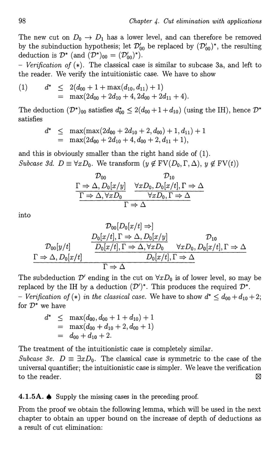
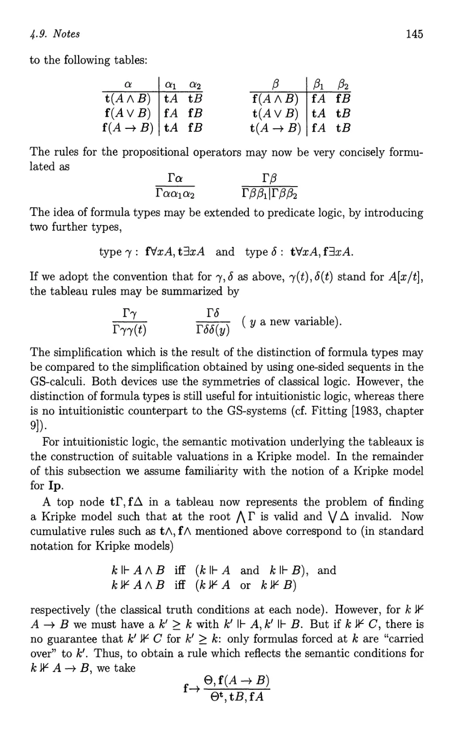
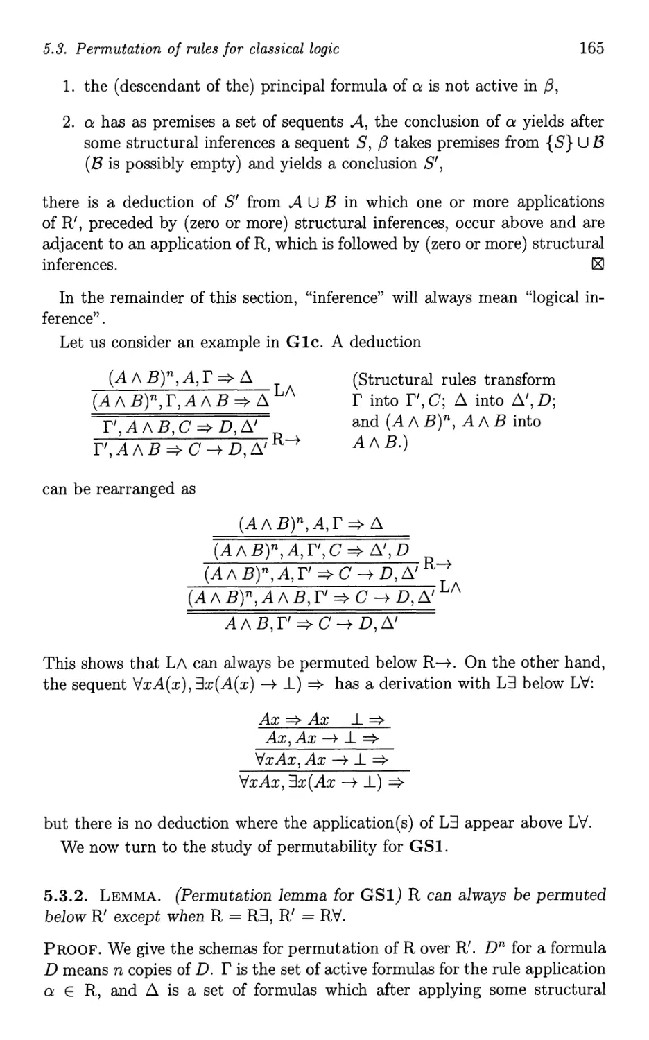
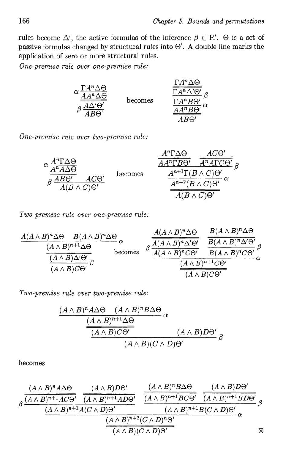
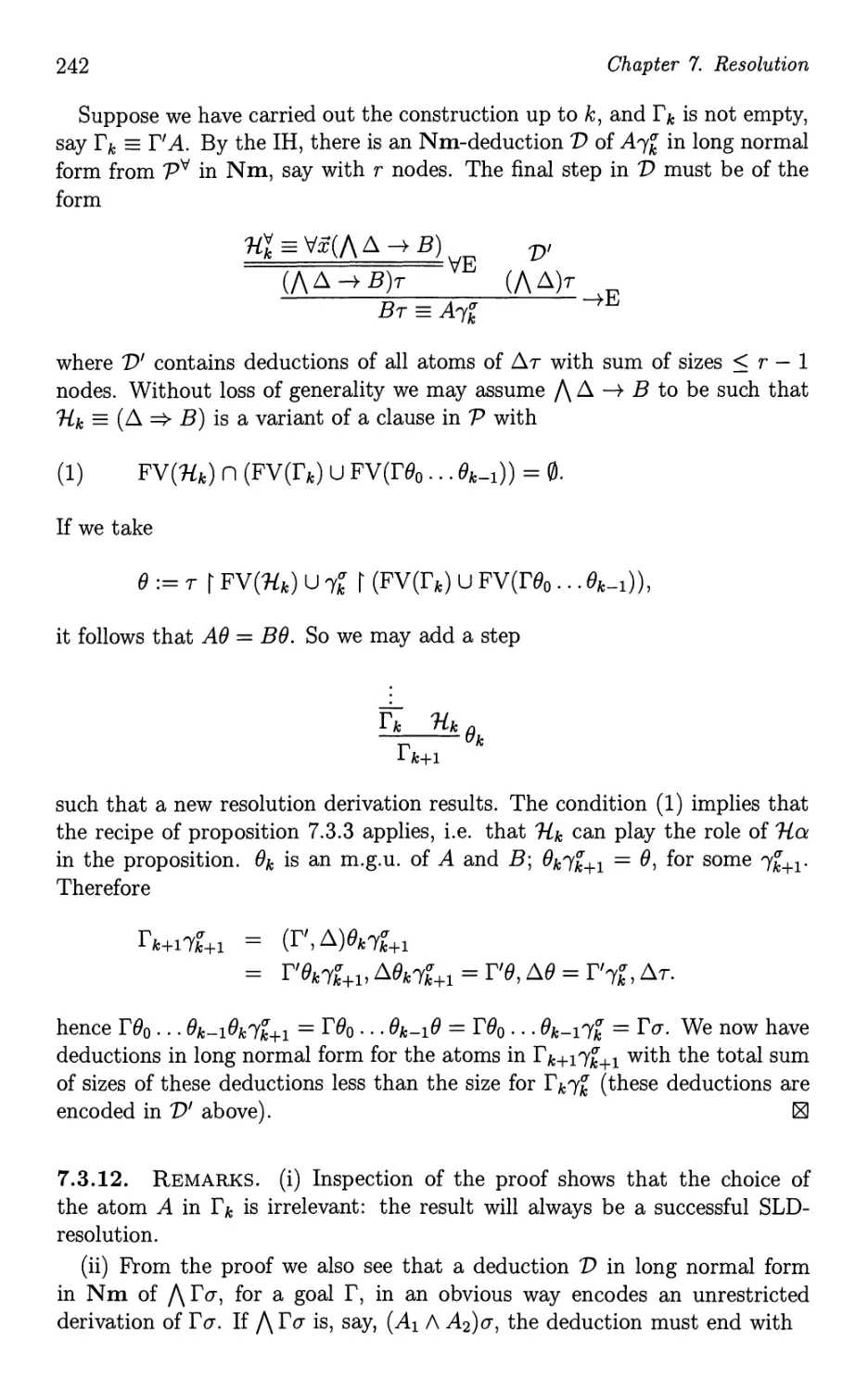
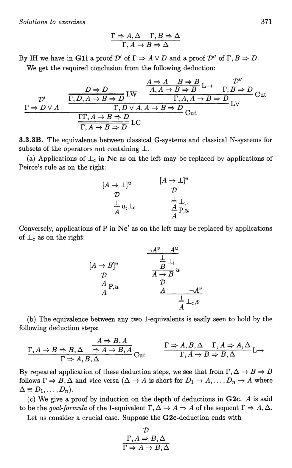
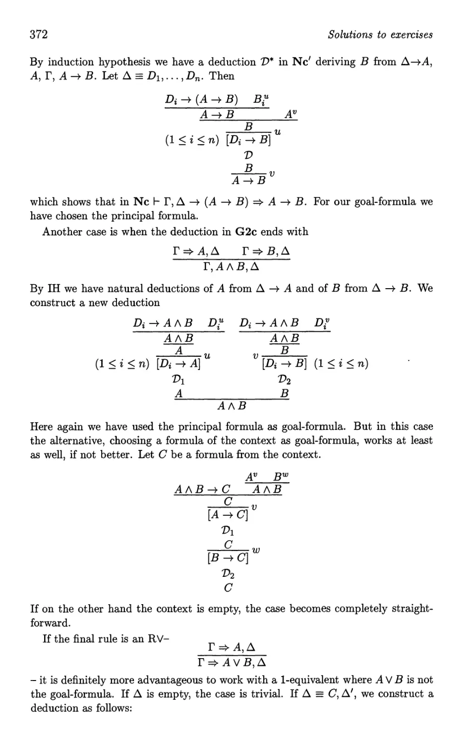
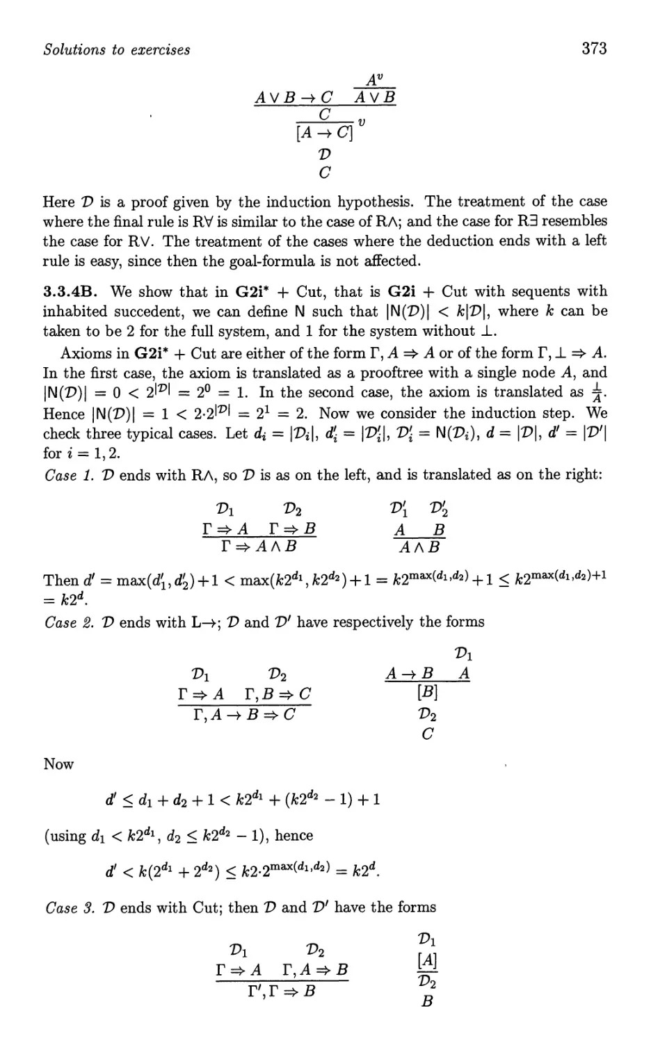
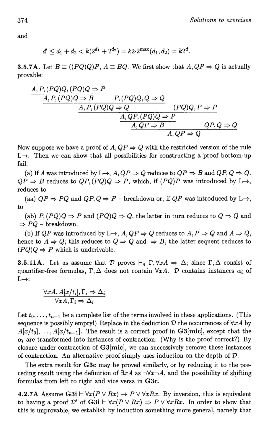
/

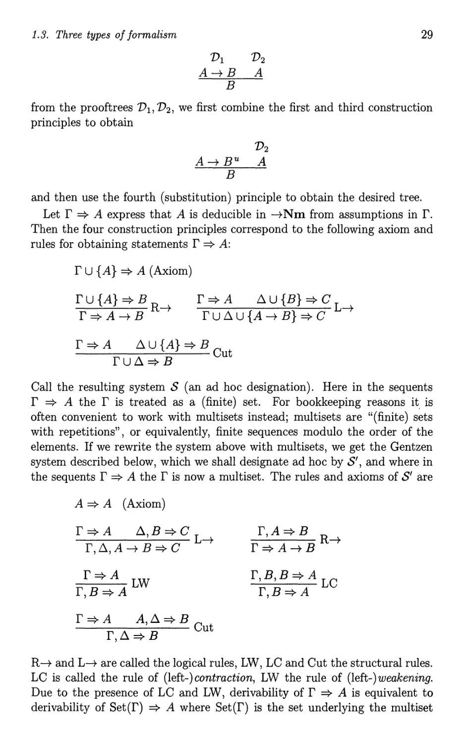

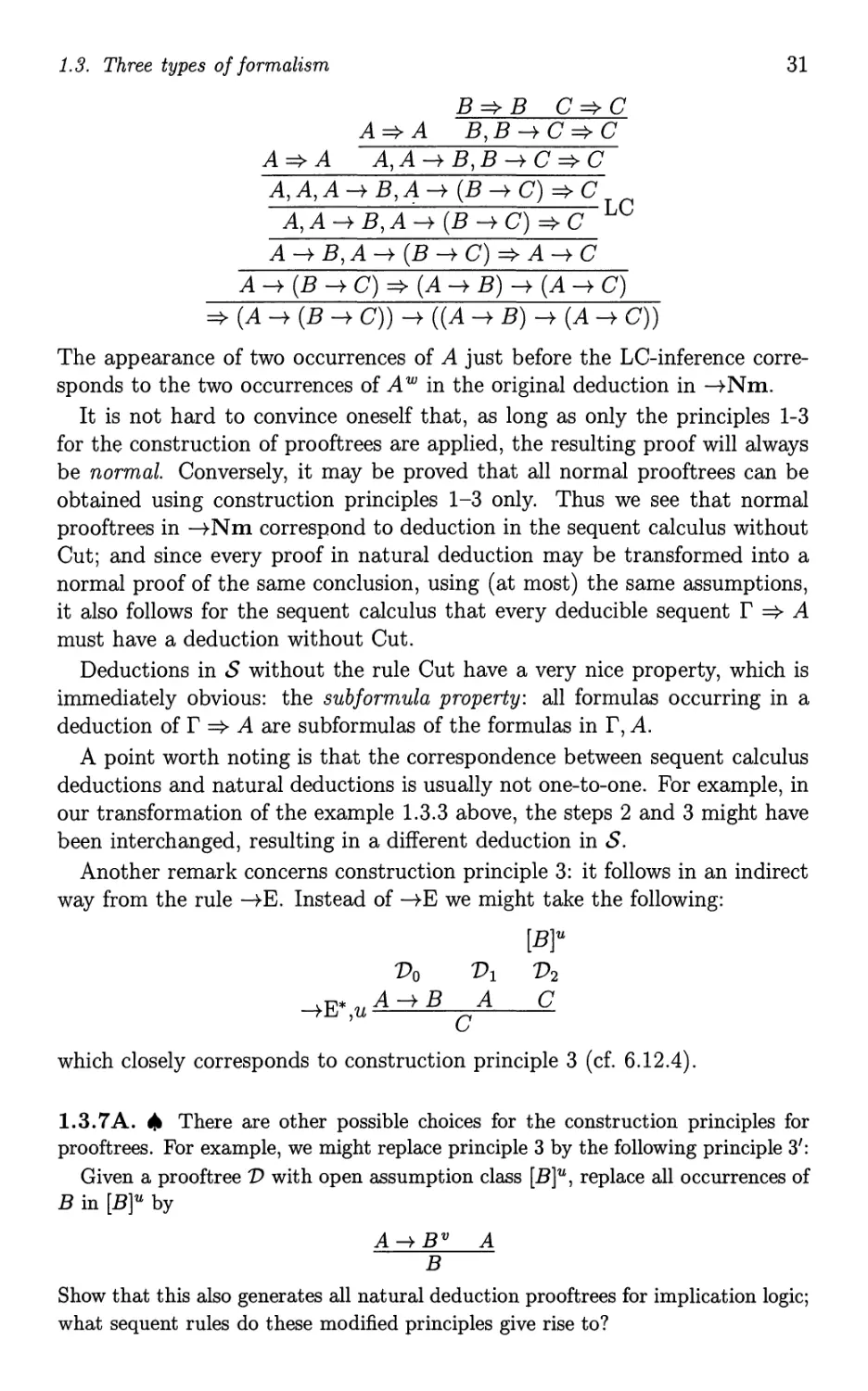

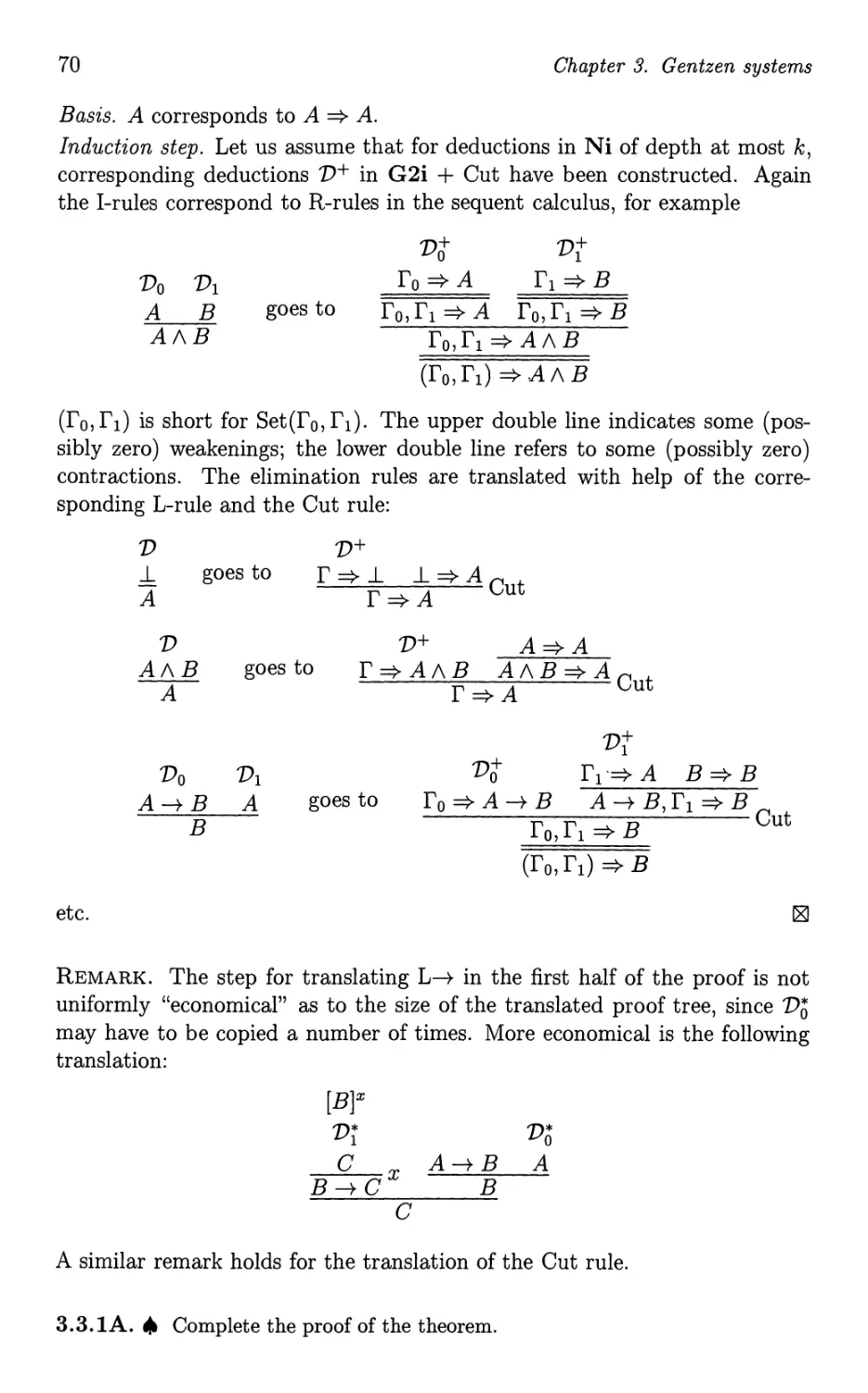

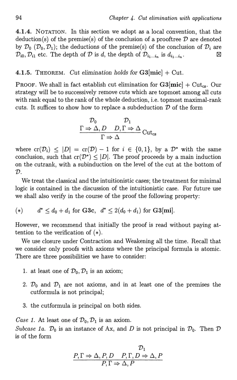
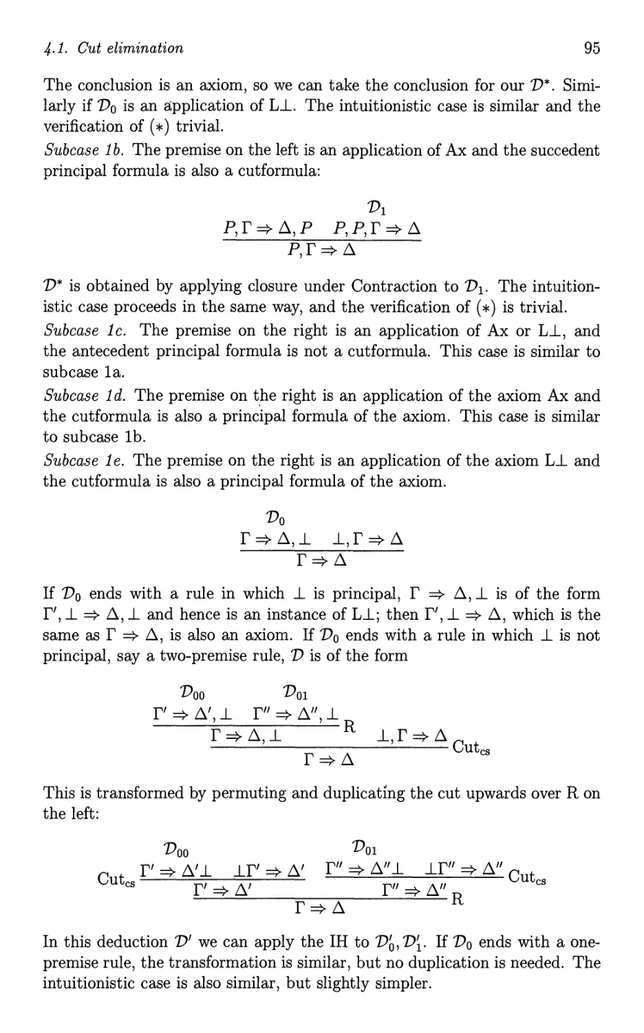
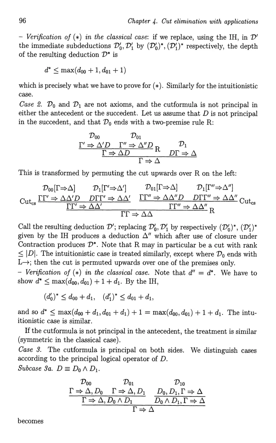


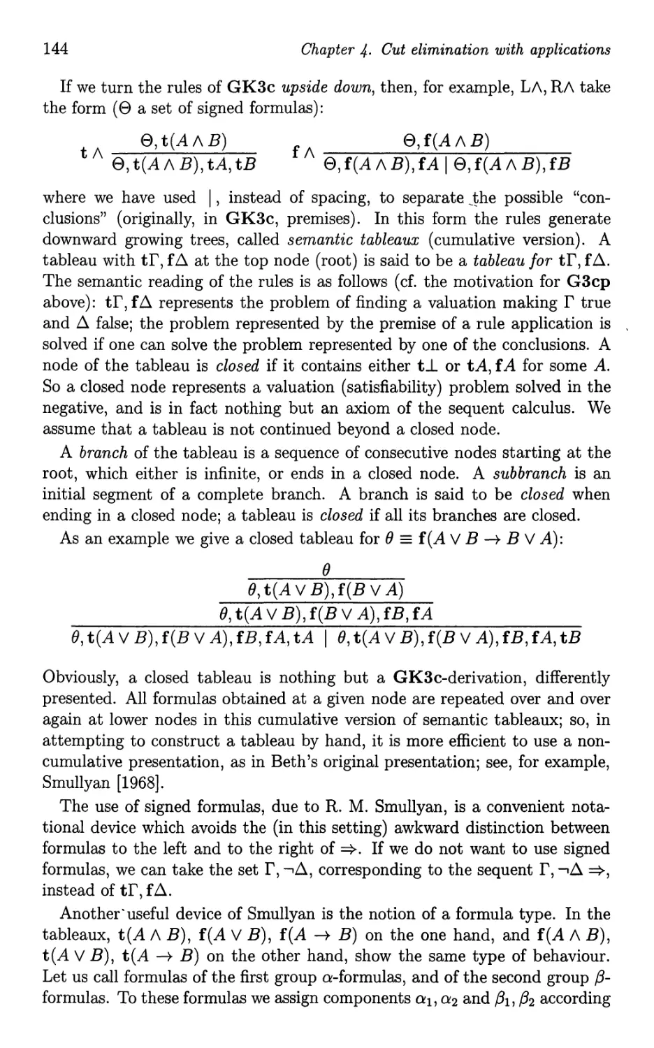
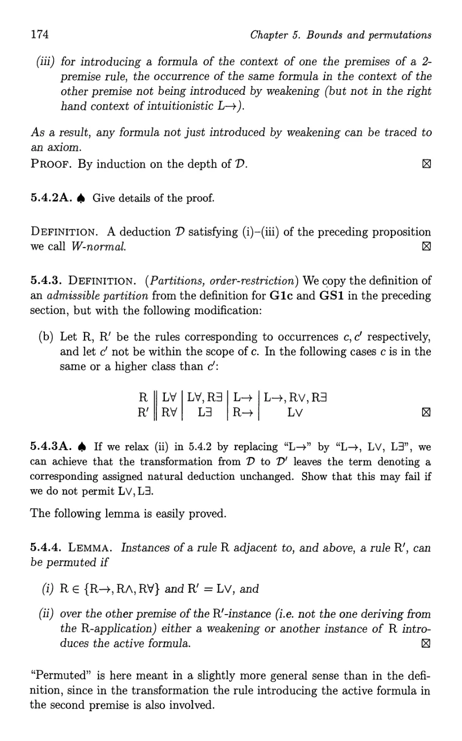

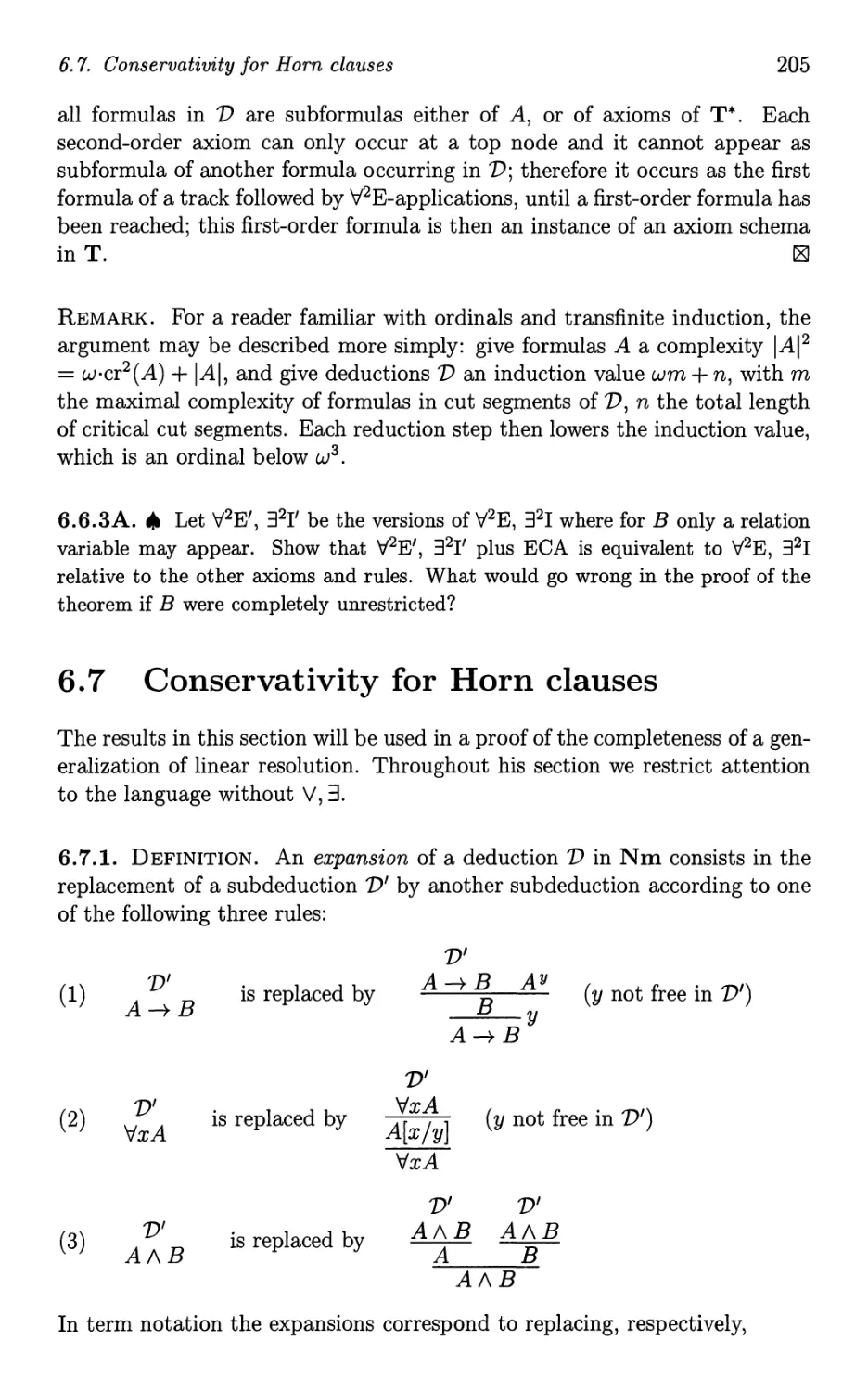
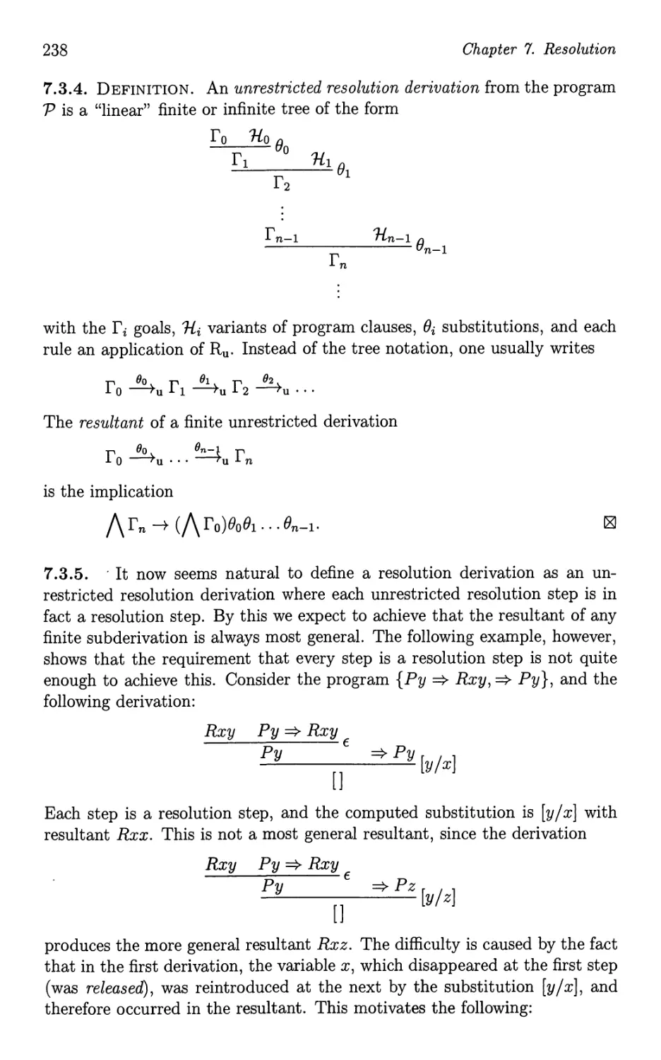
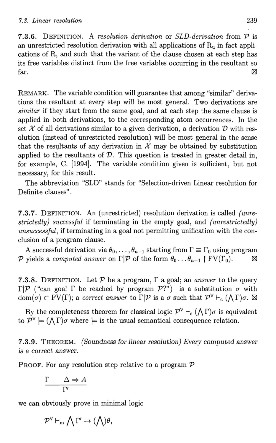
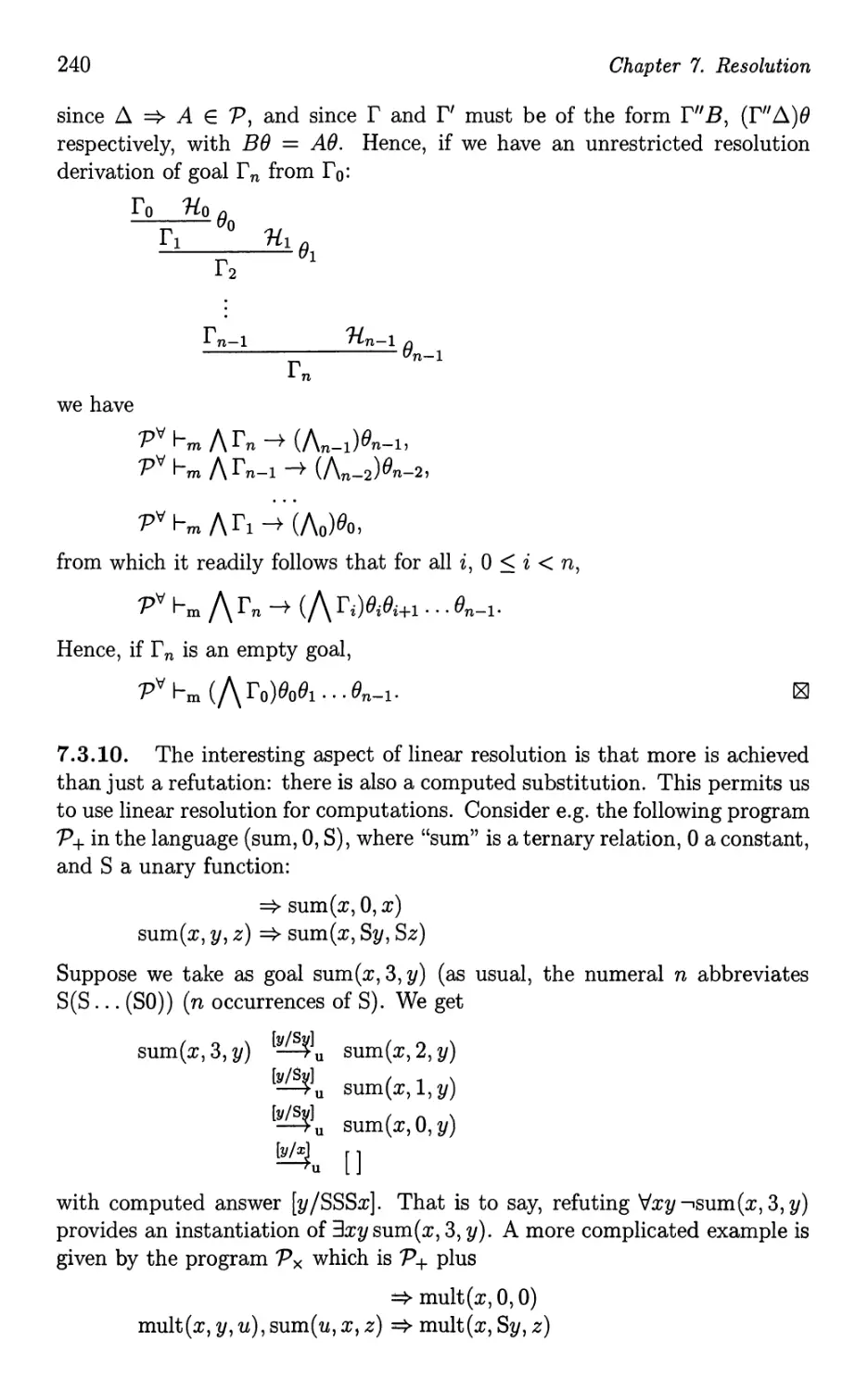
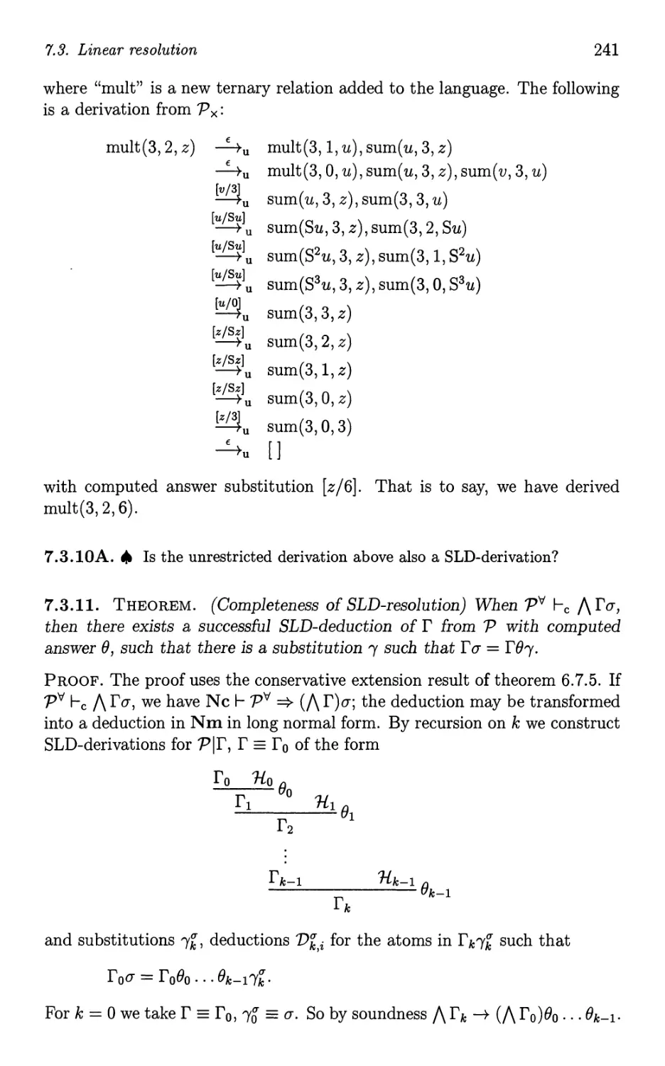
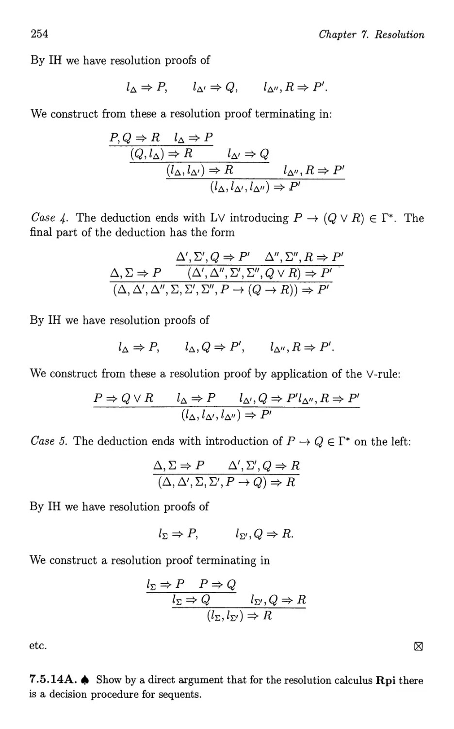
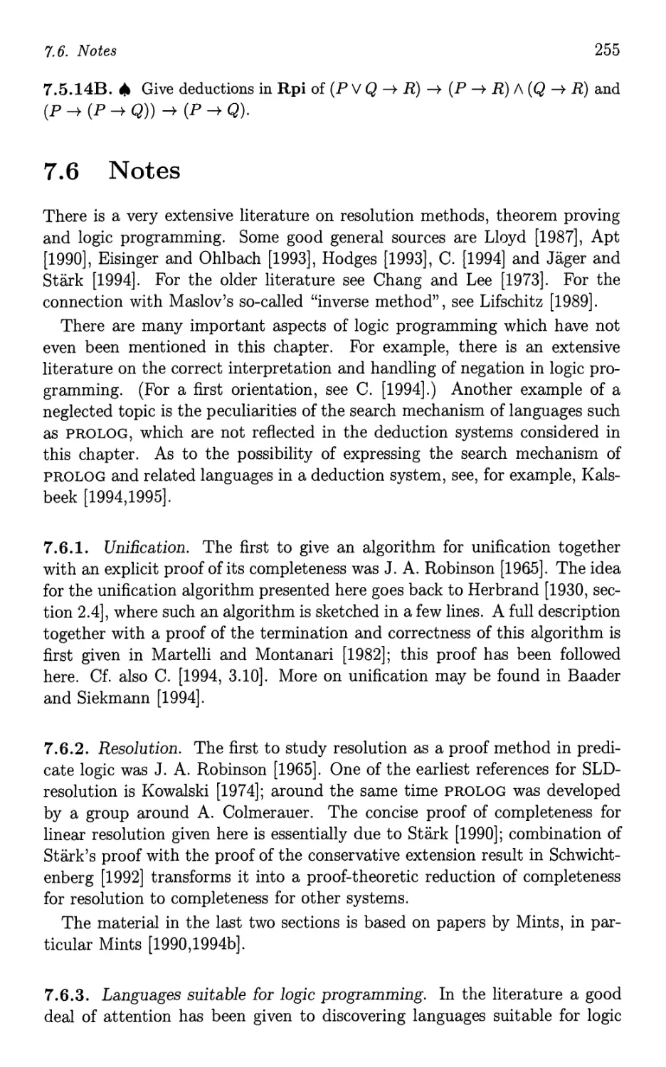
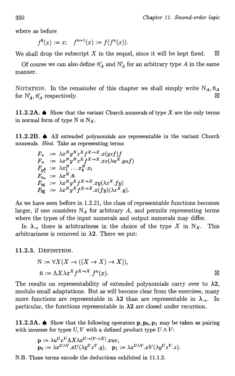


Текст
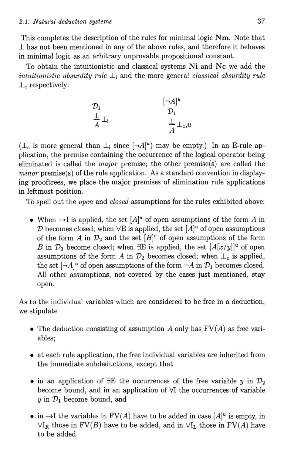
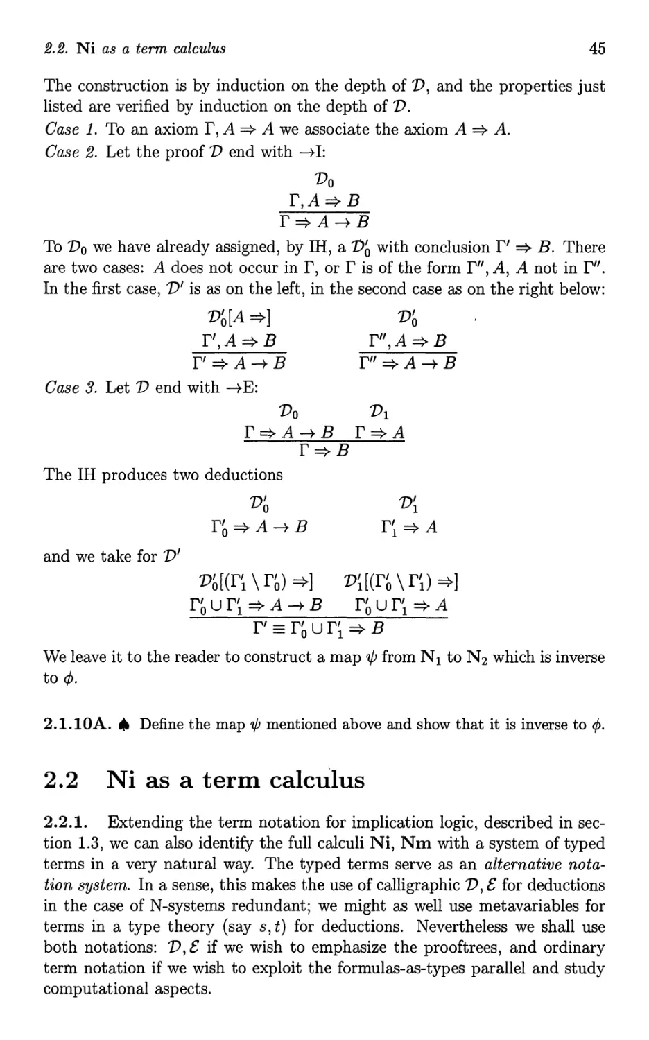
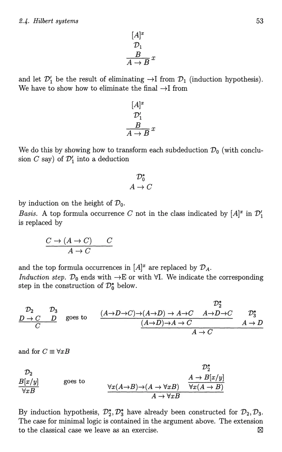
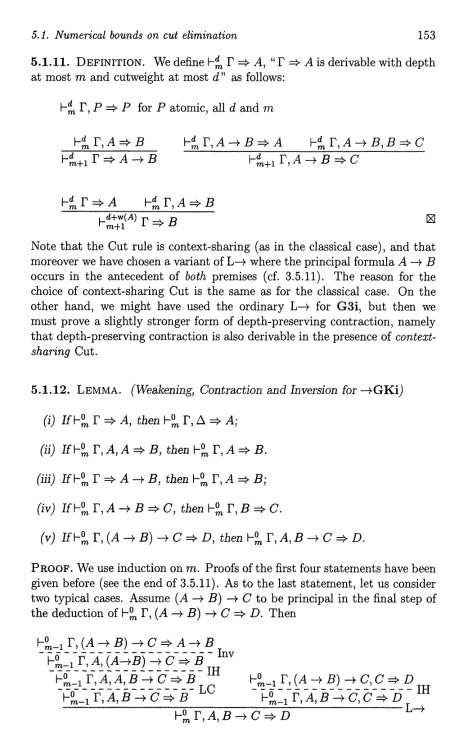
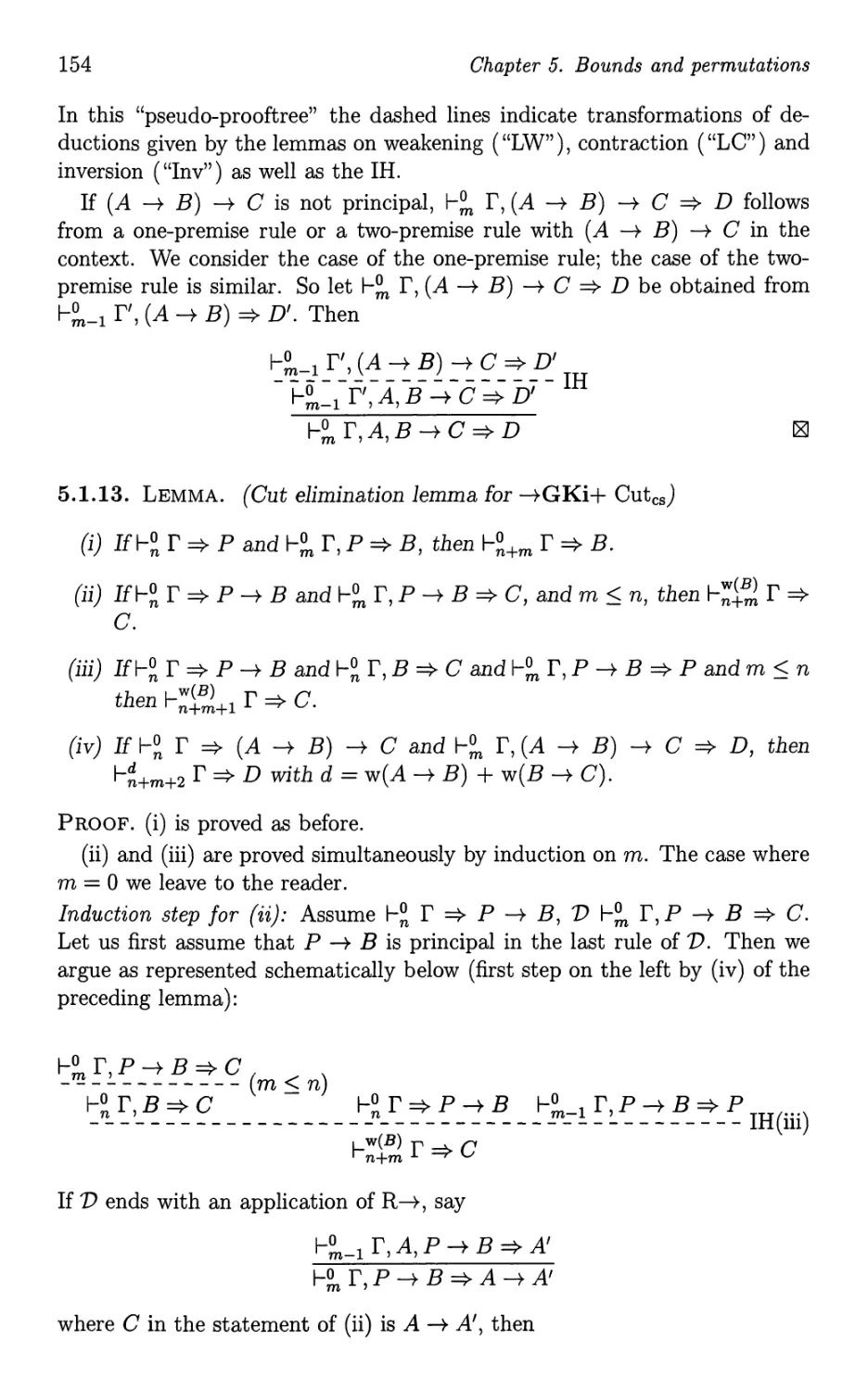
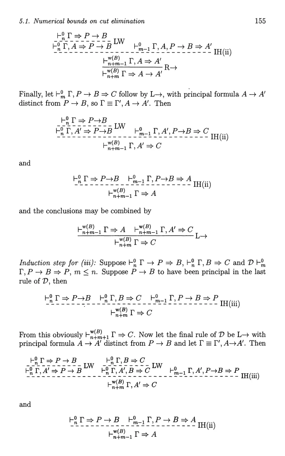
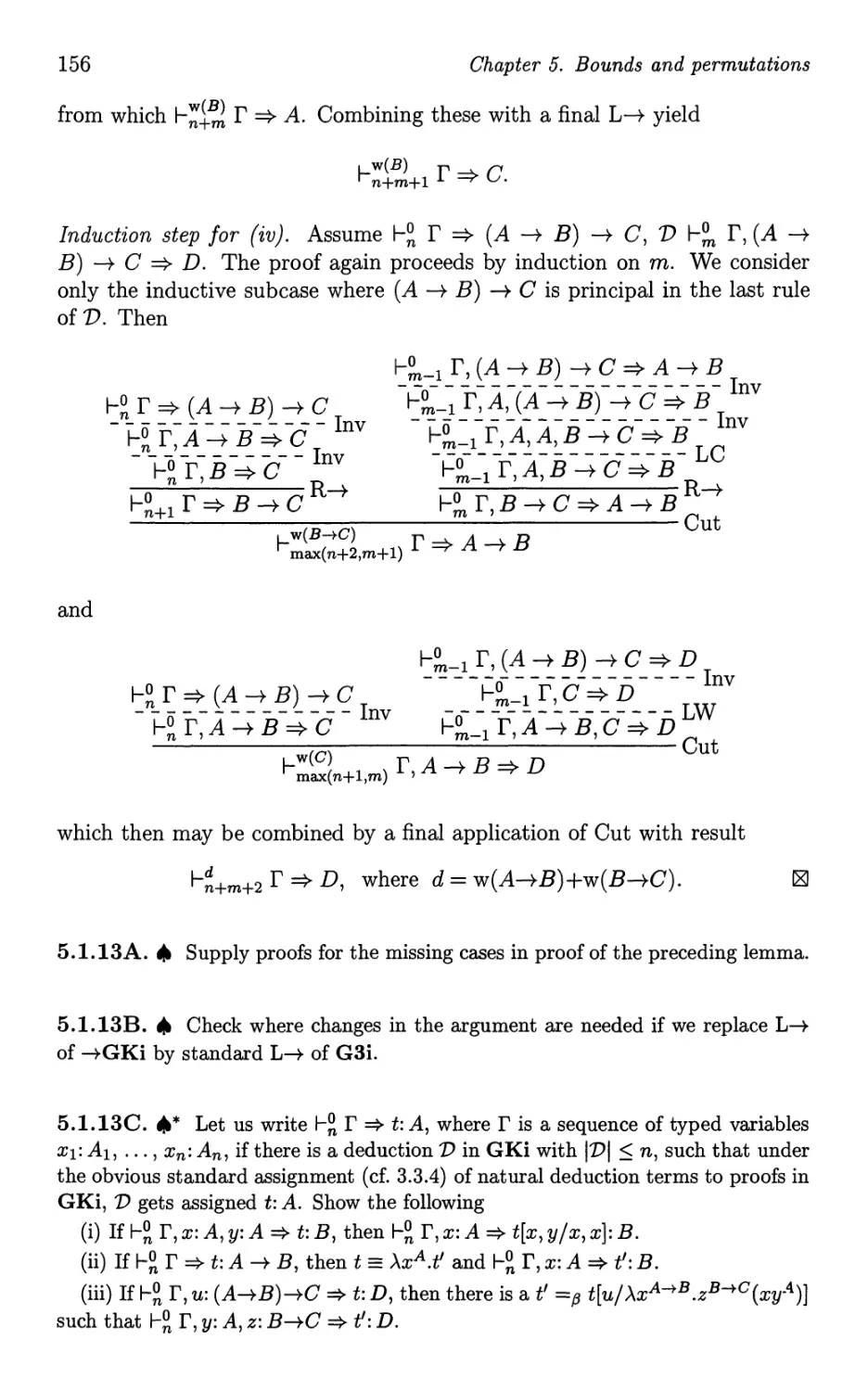
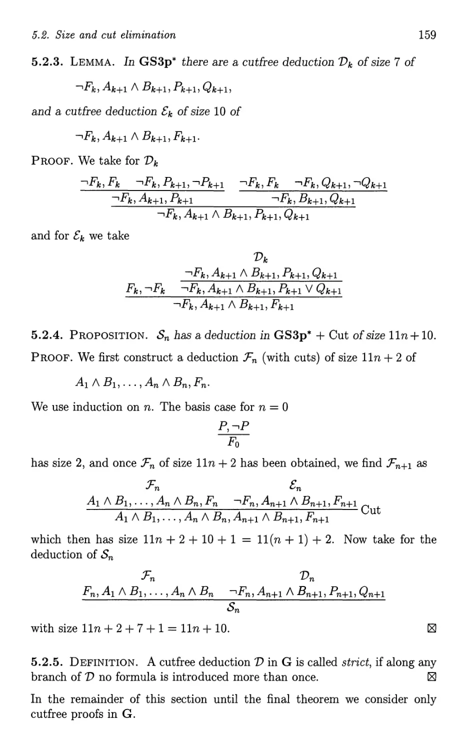
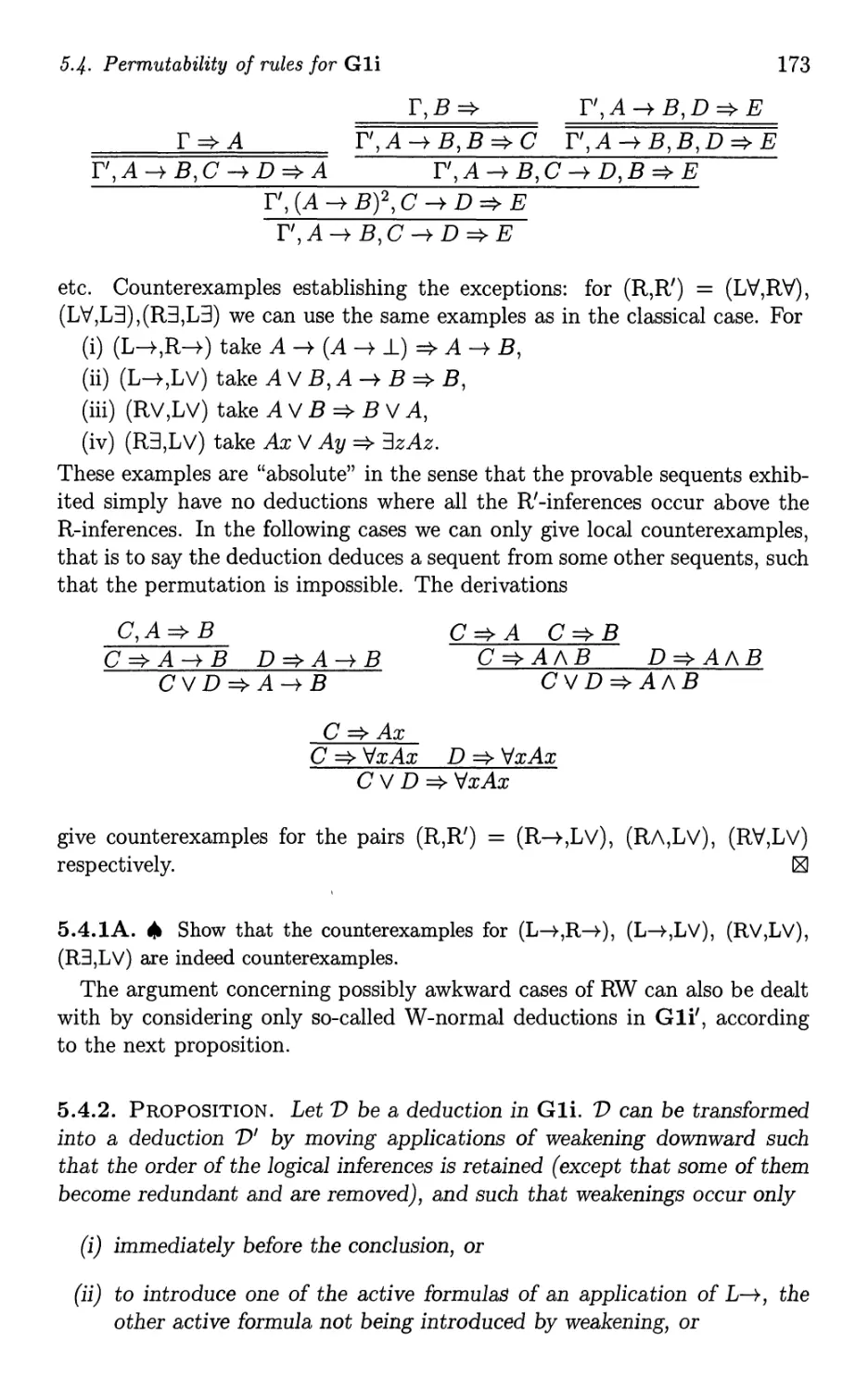
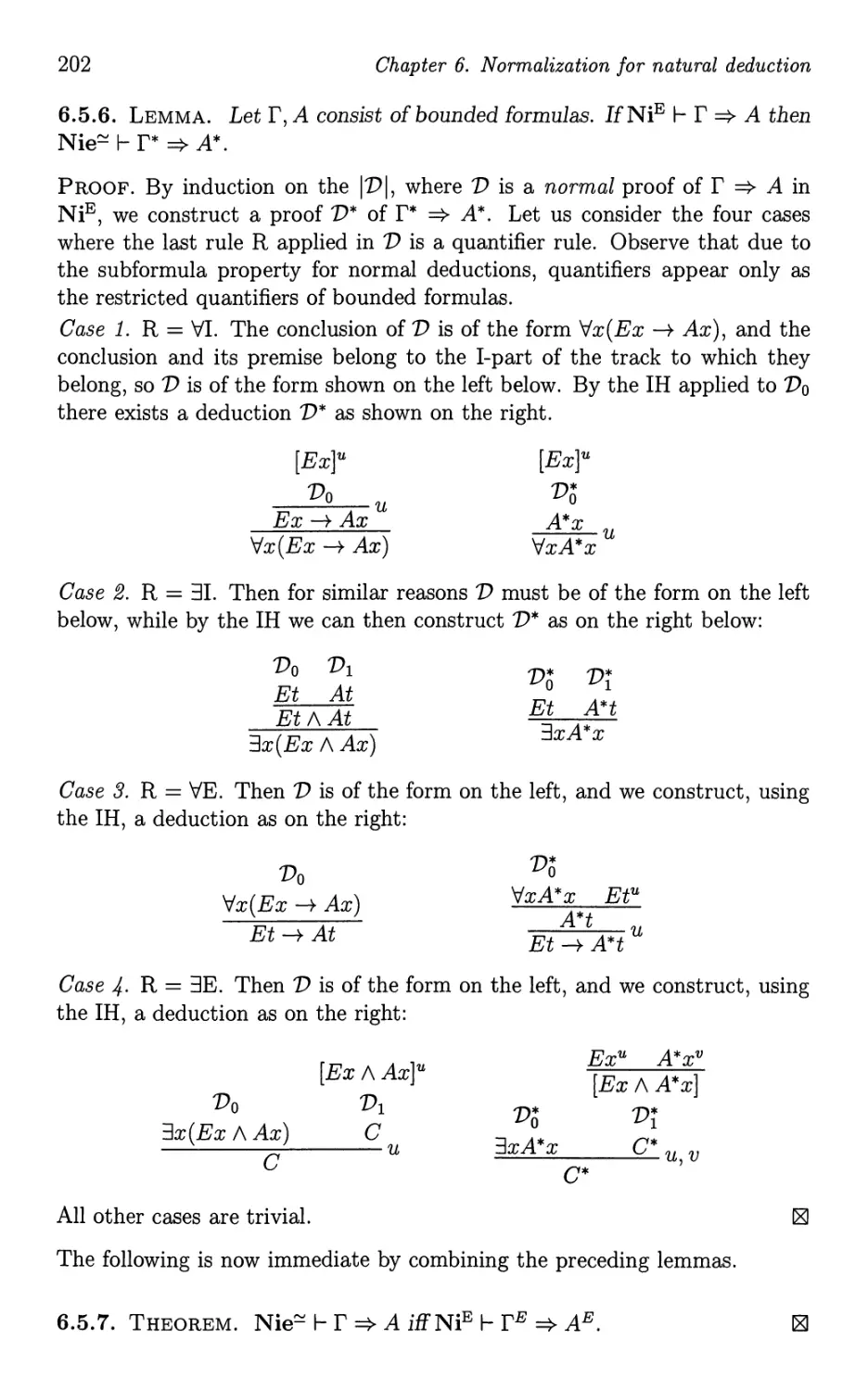
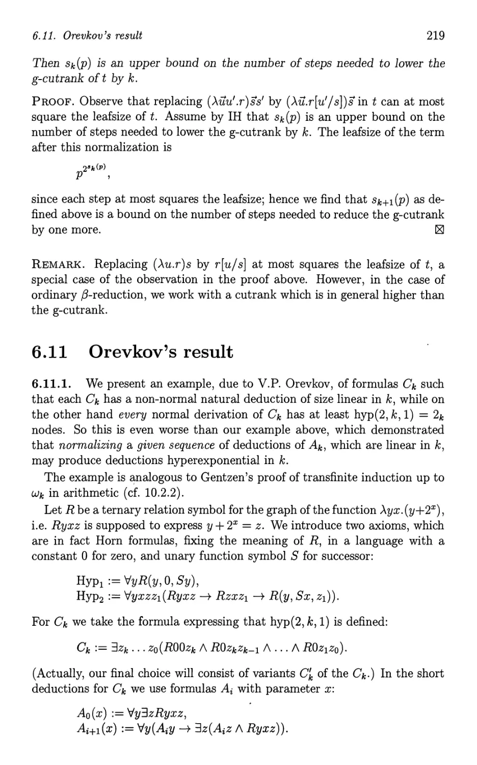
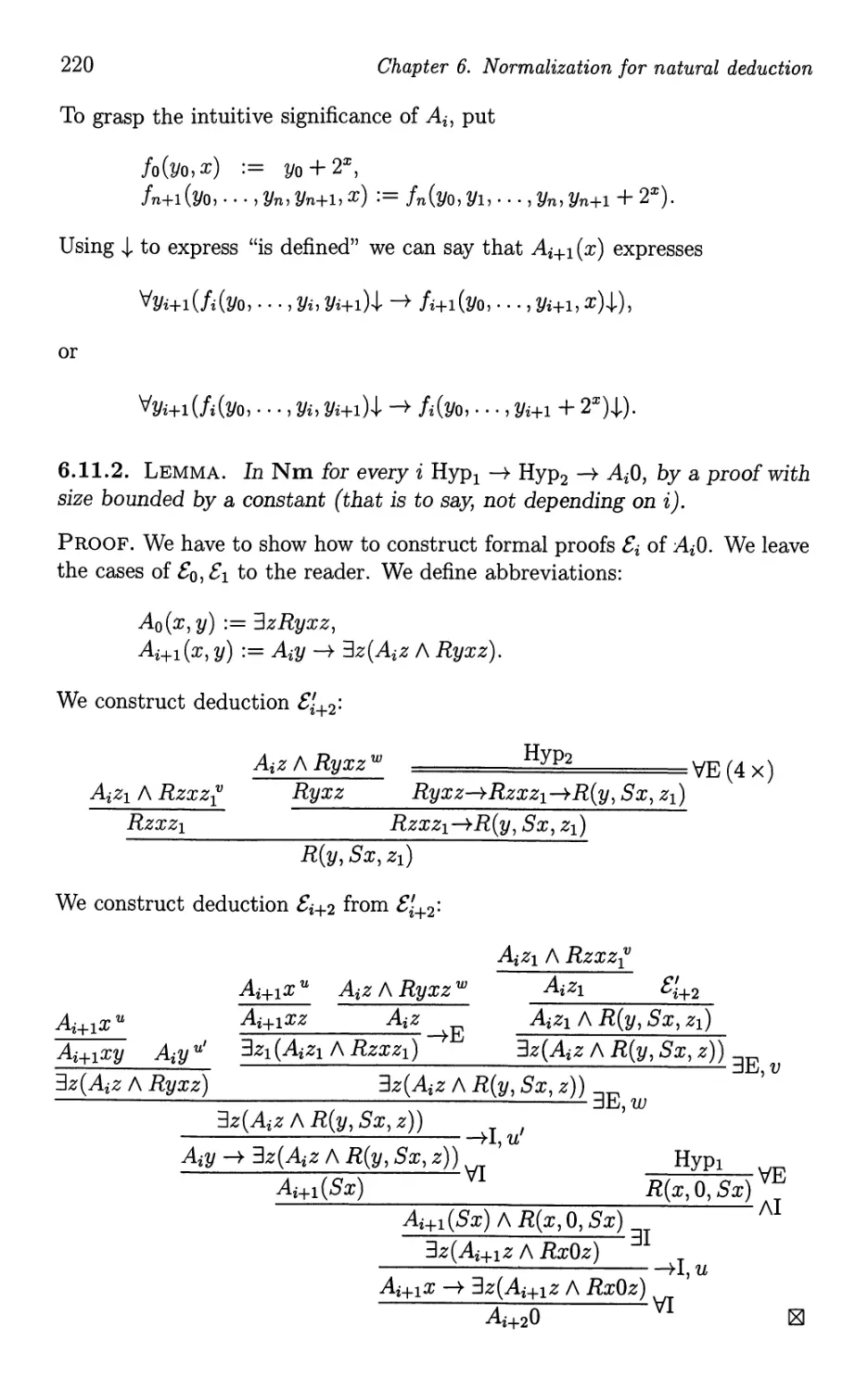
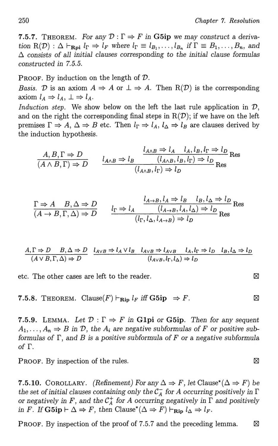
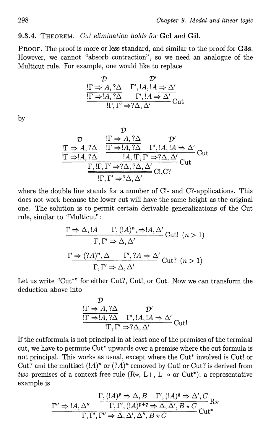
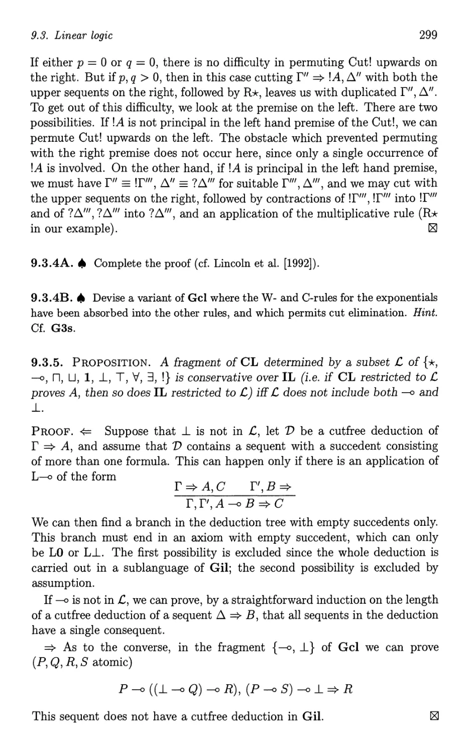
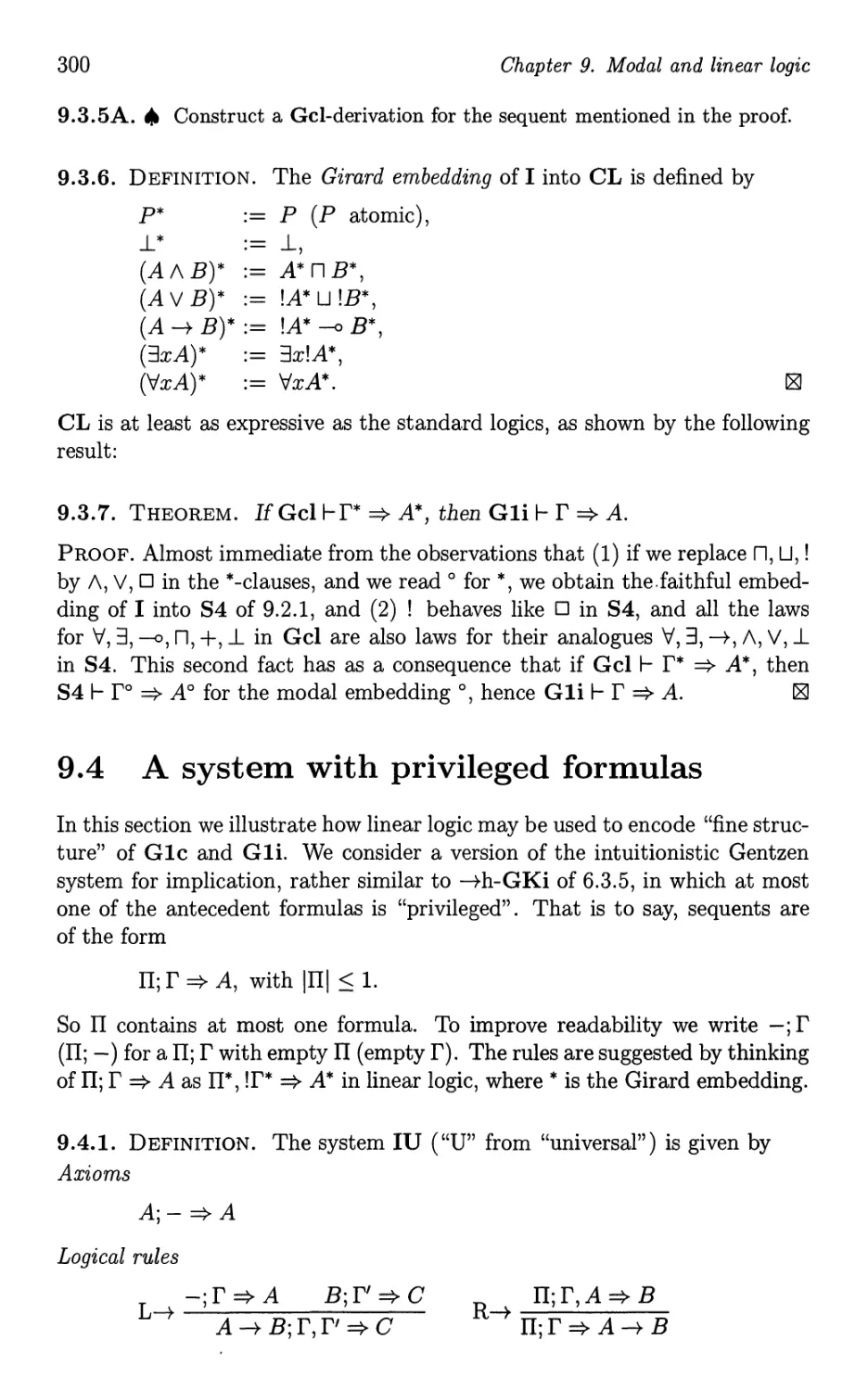
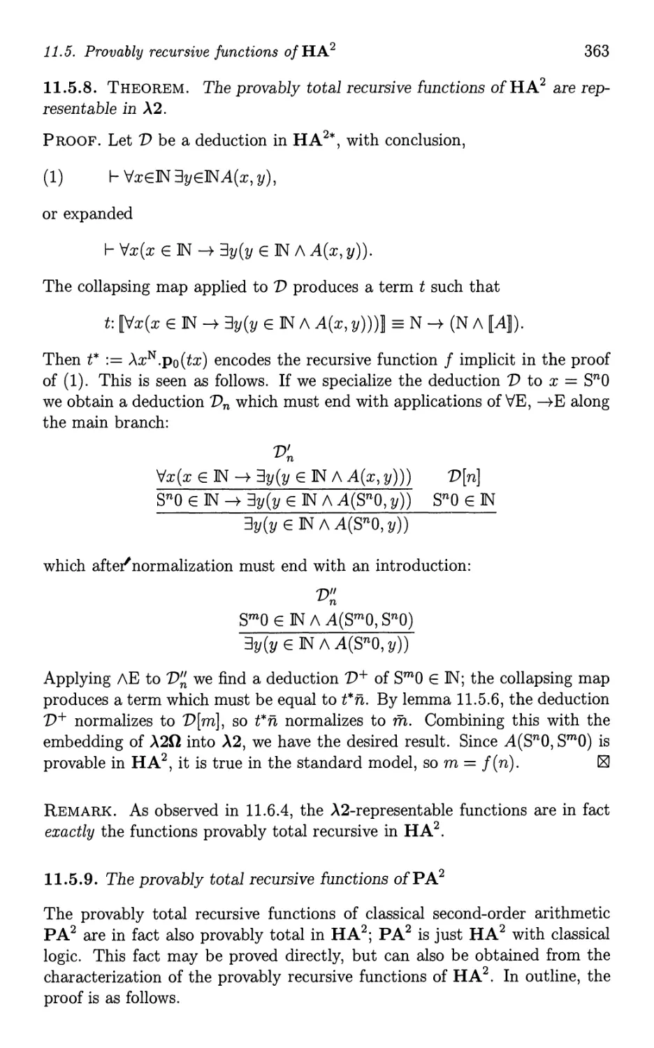
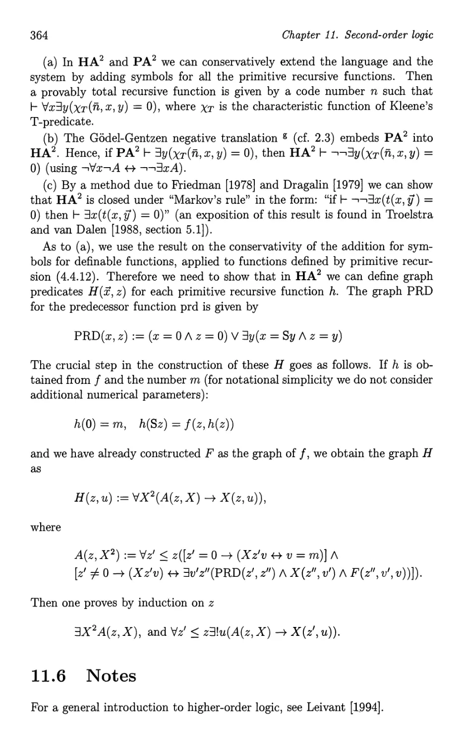
Basic Proof
Theory
Seconcl Eclition
A. S. Troelstra and
H. Schwichtenberg
Basic Proof Theory
Second Edition
A.S. Troelstra
University of Amsterdam
H. Schwichtenberg
University of Munich
IIII
IIIII CAMBRIDGE
::: UNIVERSITY PRESS
PUBLISHED BY THE PRESS SYNDICATE OF THE UNIVERSITY OF CAMBRIDGE
The Pitt Building, Trumpington Street, Cambridge, United Kingdom
CAMBRIDGE UNIVERSITY PRESS
The Edinburgh Building, Cambridge CB2 2RU, UK http://www.cup.cam.ac.uk
40 West 20th Street, New York, NY 10011-4211, USA http://www.cup.org
10 Stamford Road, Oakleigh, Melbourne 3166, Australia
Ruiz de Alarcon 13, 28014 Madrid, Spain
@ Cambridge University Press 1996, 2000
This book is in copyright. Subject to statutory exception
and to the provisions of relevant collective licensing agreements,
no reproduction of any part may take place without
the written permission of Cambridge University Press.
First published 1996
Second edition 2000
Printed in the United Kingdom at the University Press, Cambridge
Typeset by the author in Computer Modern 10/13pt, in I¥IEjX2e [EPC]
A catalogue record of this book is available from the British Library
Library of Congress Cataloguing in Publication data
ISBN 0 521 77911 1 paperback
Contents
Preface .
IX
1 Introduction 1
1.1 Preliminaries 2
1.2 Sim pIe type theories 10
1.3 Three types of formalism . . 22
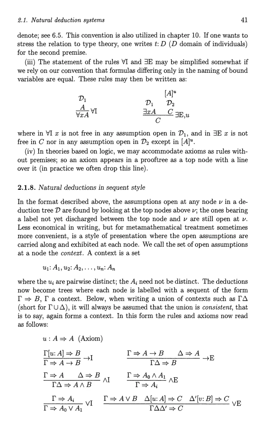
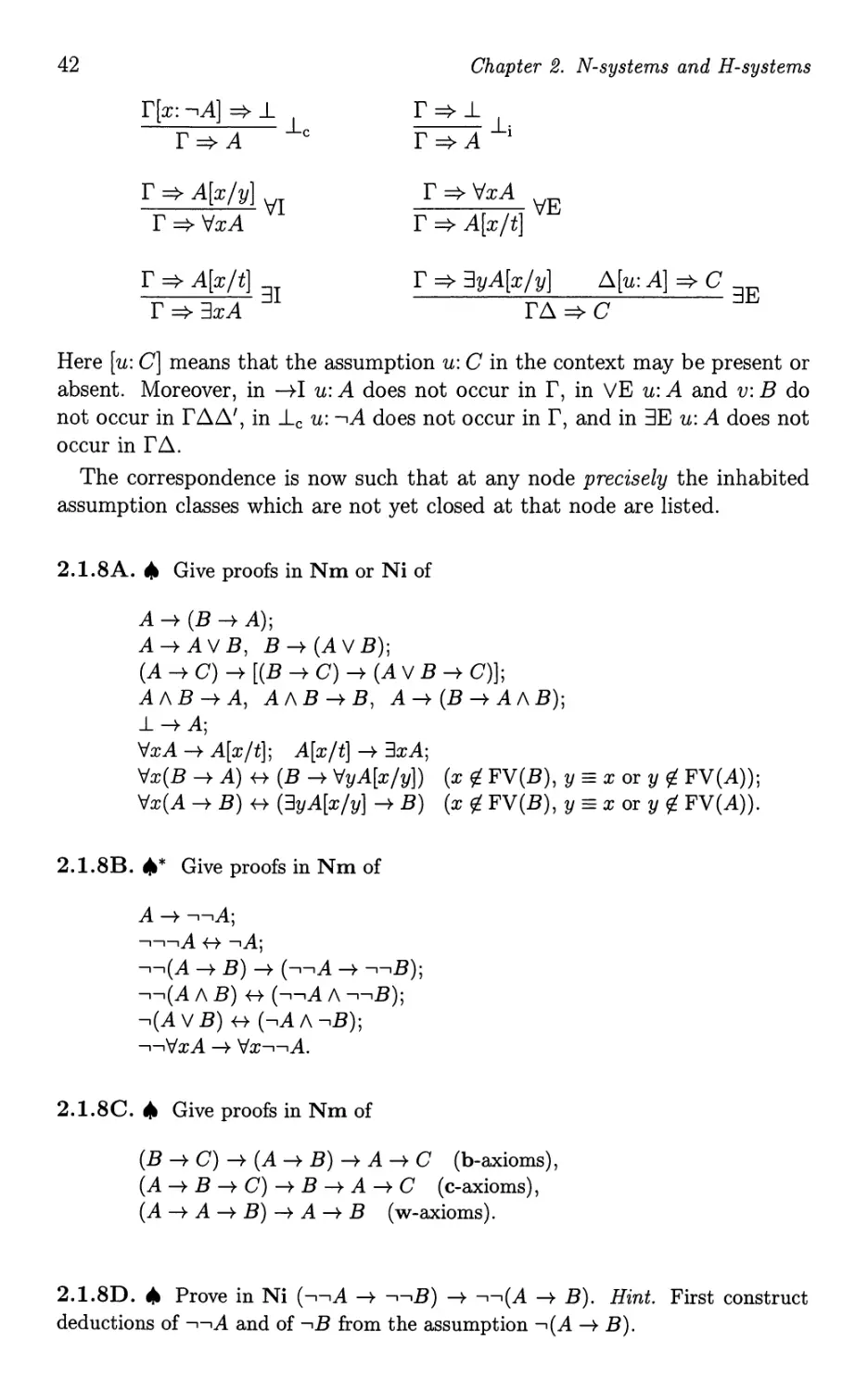
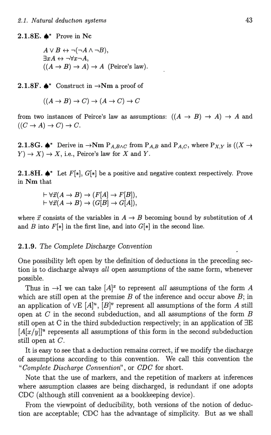
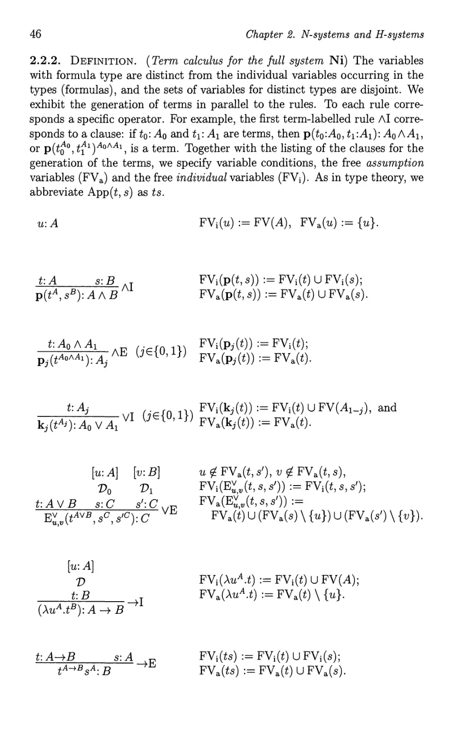
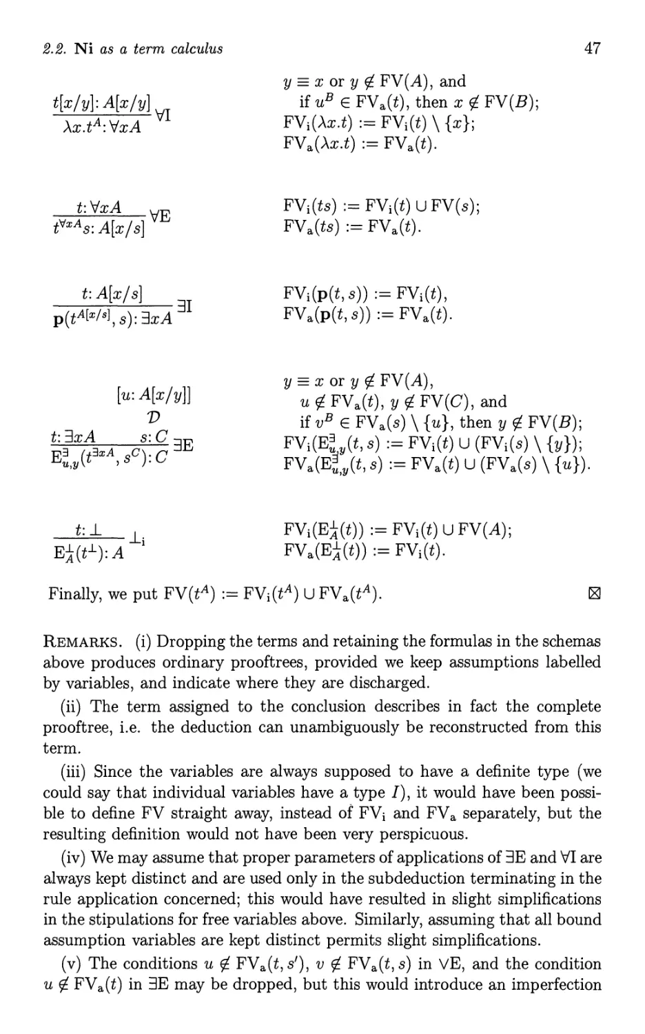
2 N-systems and H-systems 35
2.1 Natural deduction systems 35
2.2 Ni as a term calculus. 45
2.3 The relation between C, I and M 48
2.4 Hilbert systems 51
2.5 Notes . 55
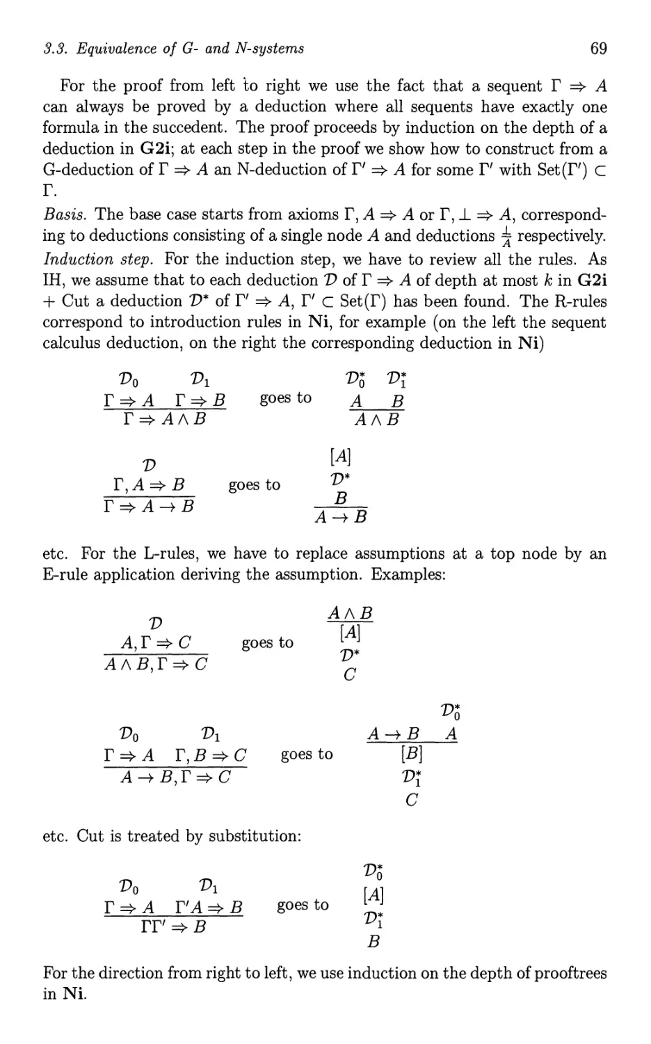
3 Gentzen systems 60
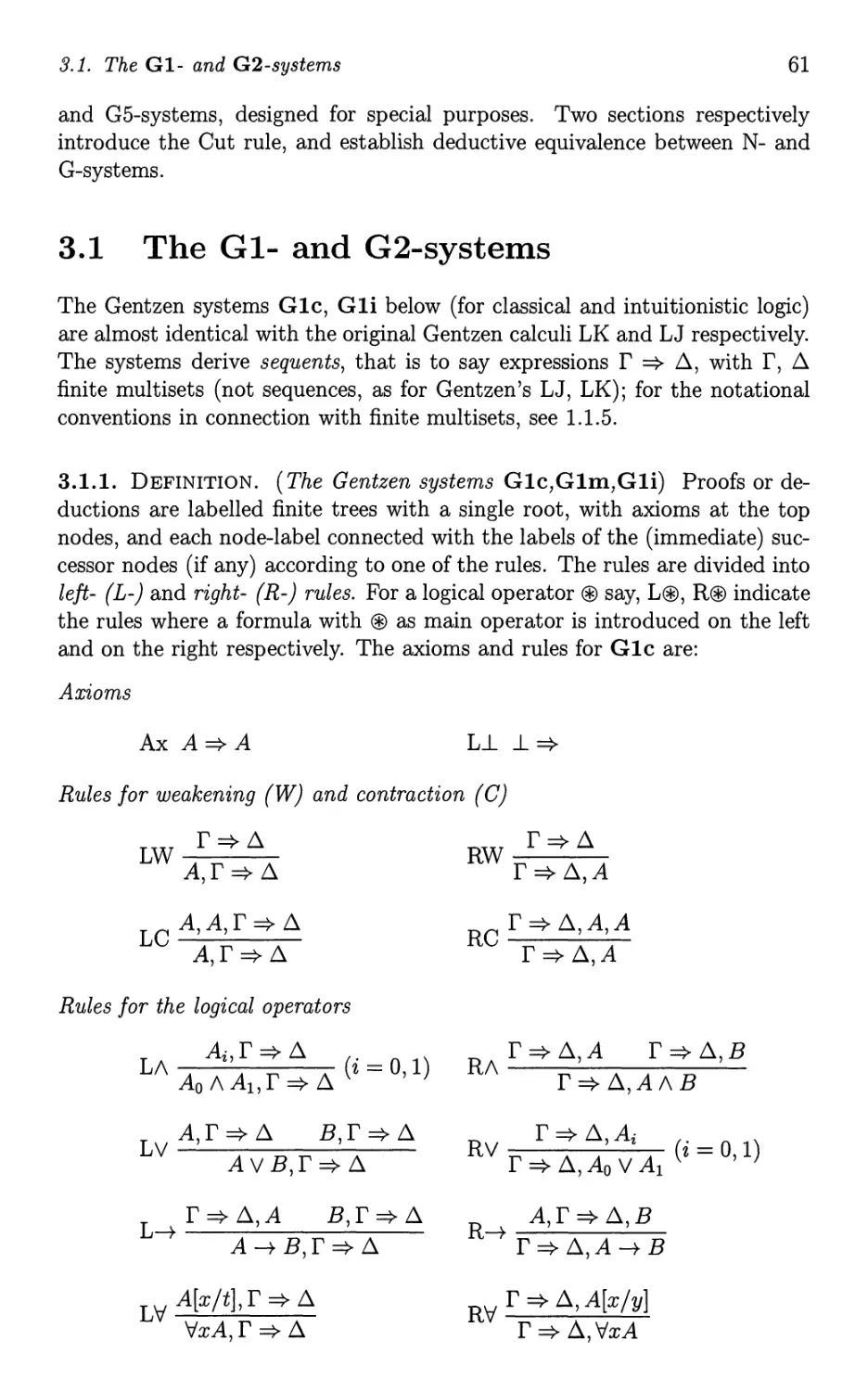
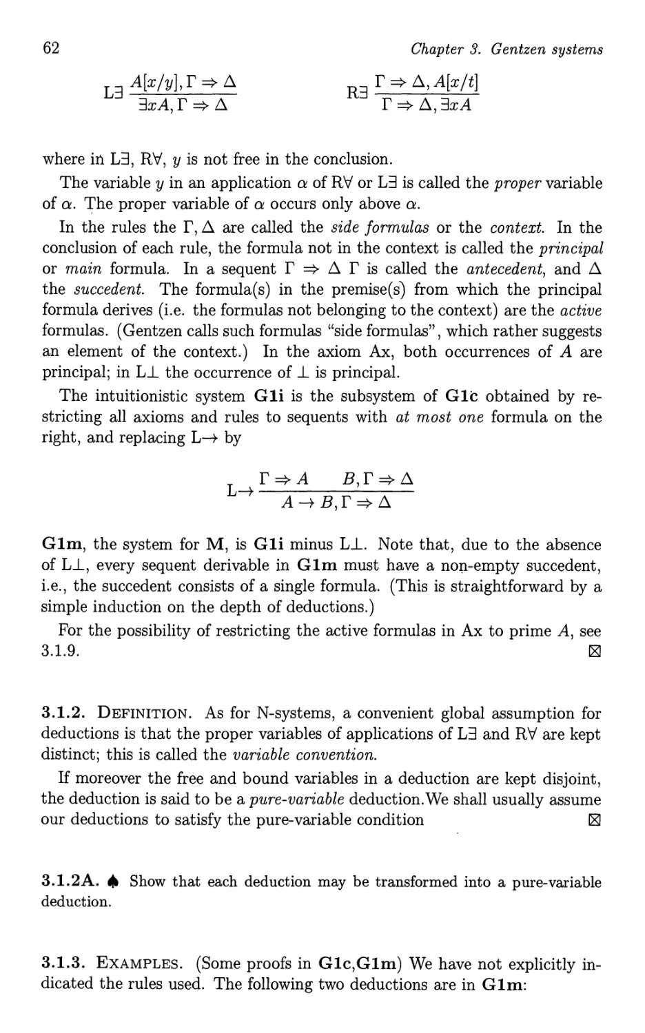
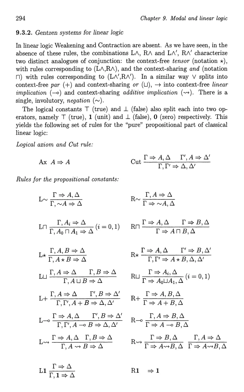
3.1 The G1- and G2-systems 61
3.2 The Cut rule 66
3.3 Equivalence of G- and N-systems 68
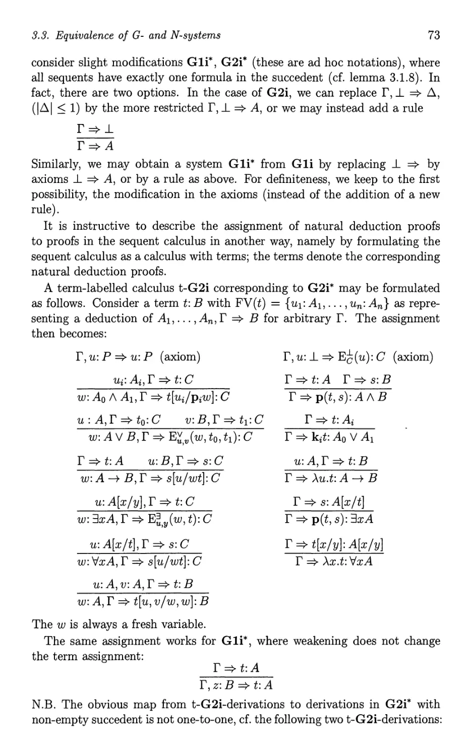
3.4 Systems with local rules 75
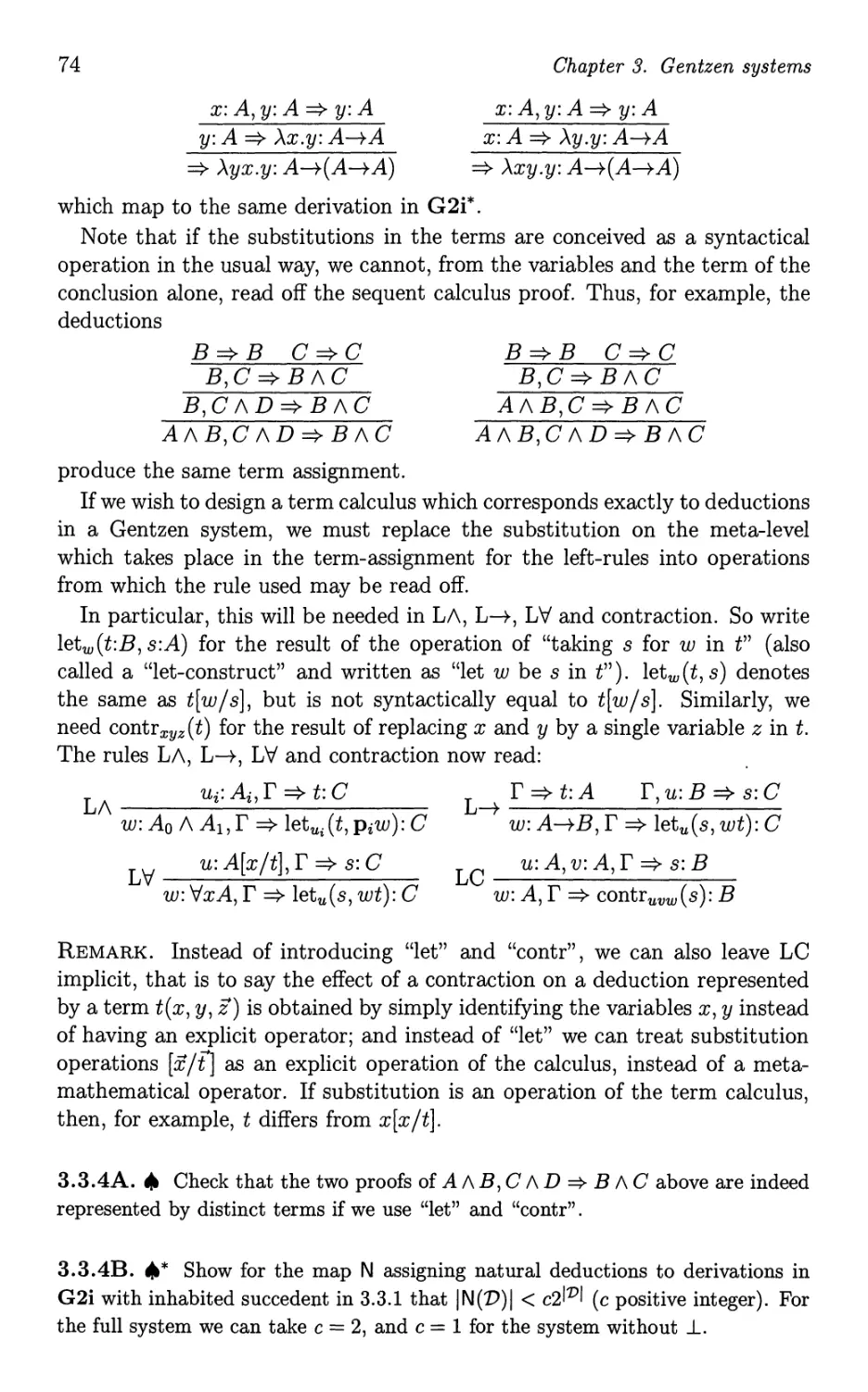
3.5 Absorbing the structural rules 77
3.6 The one-sided systems for C . 85
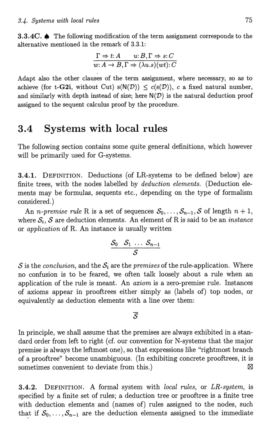
3.7 Notes . 87
4 Cut elimination with applications 92
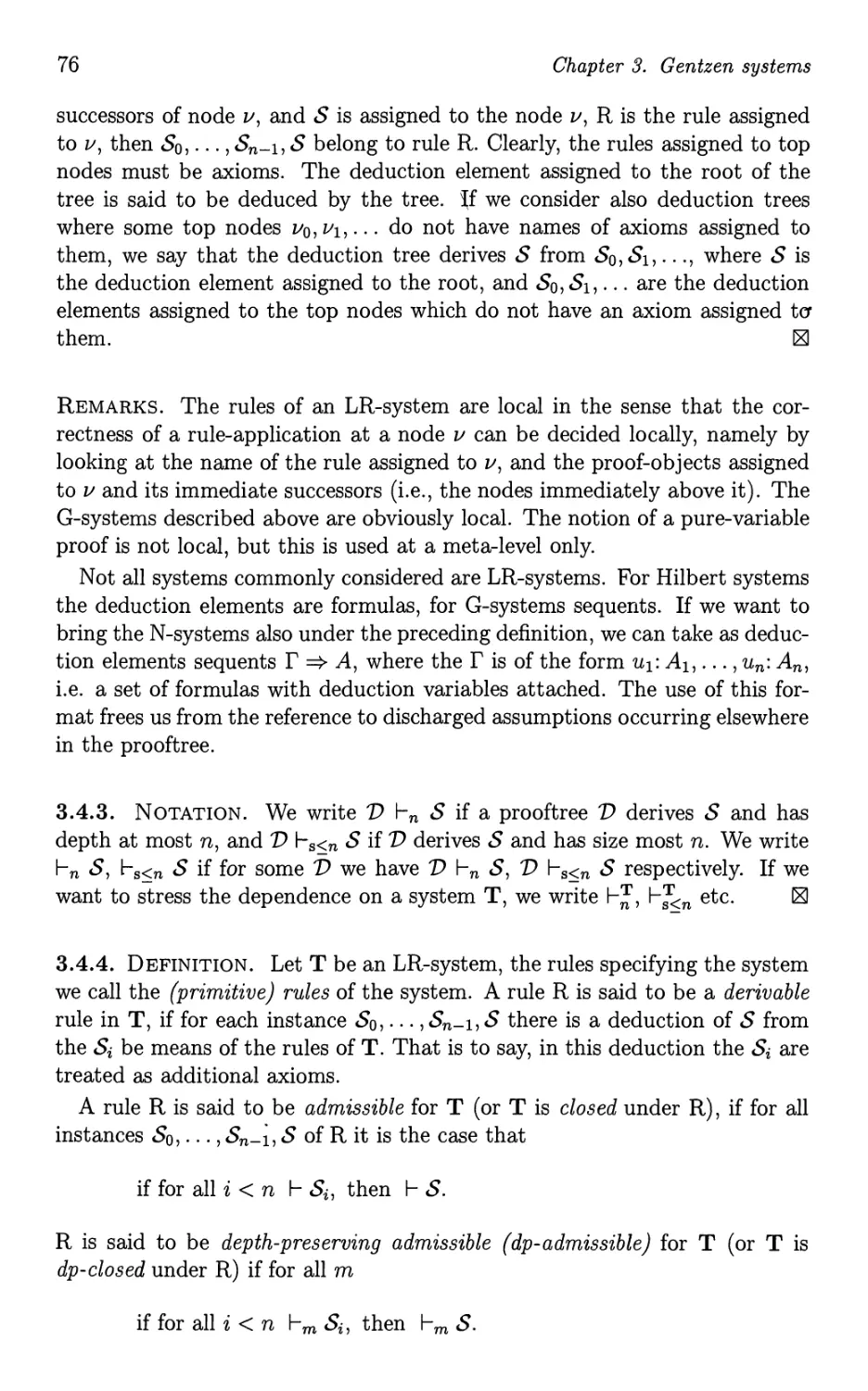
4.1 Cut elimination 92
4.2 Applications of cutfree systems 105
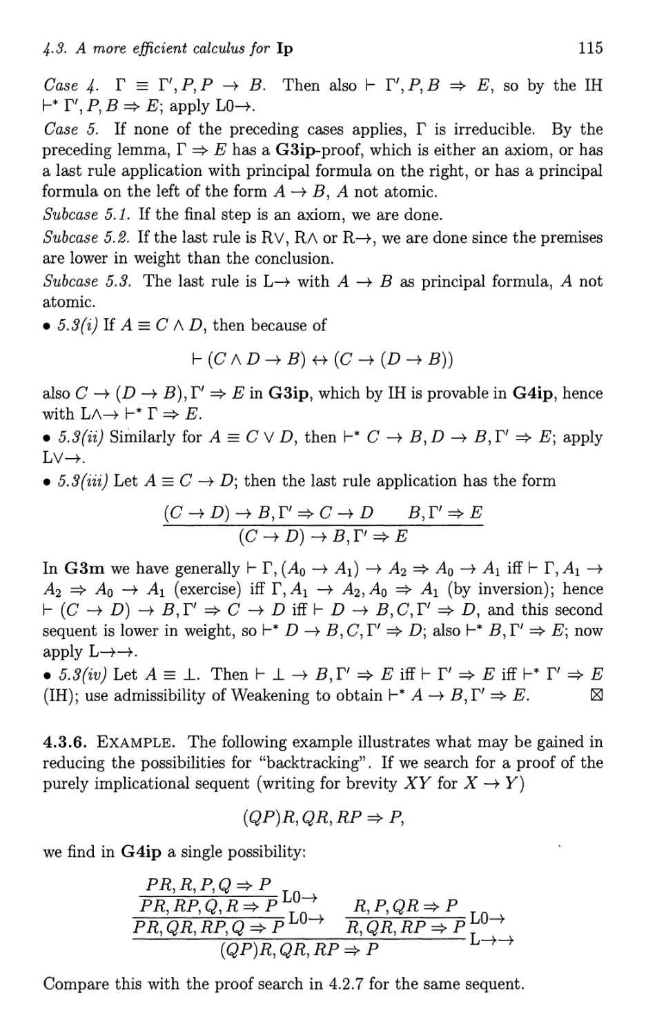
4.3 A more efficient calculus for Ip 112
4.4 Interpolation and definable functions 116
4.5 Extensions of G1-systems 126
4.6 Extensions of G3-systems 130
4.7 Logic with equality 134
v
VI
Contents
4.8 The theory of apartness
4. 9 Notes............
136
139
5 Bounds and permutations
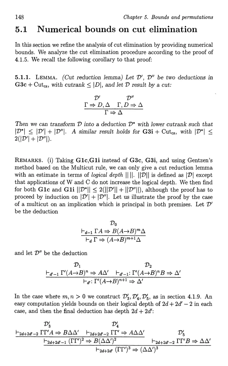
5.1 Numerical bounds on cut elimination
5.2 Size and cut elimination . . . . . . . .
5.3 Permutation of rules for classical logic .
5.4 Permutability of rules for G Ii . . . . . .
5.5 Notes....................
147
148
157
164
171
176
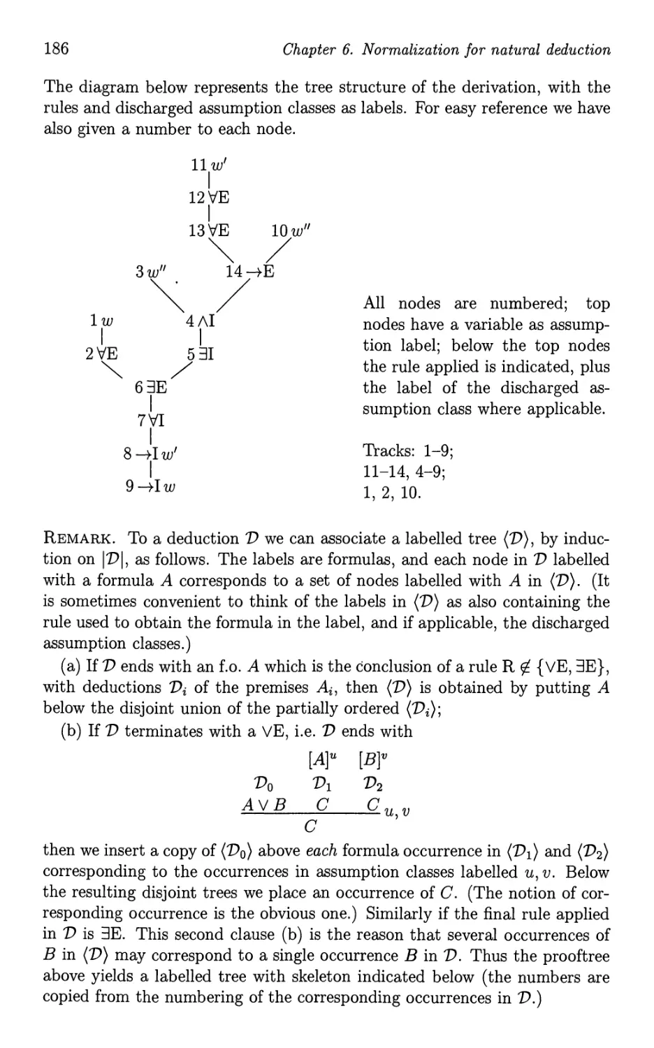
6 Normalization for natural deduction
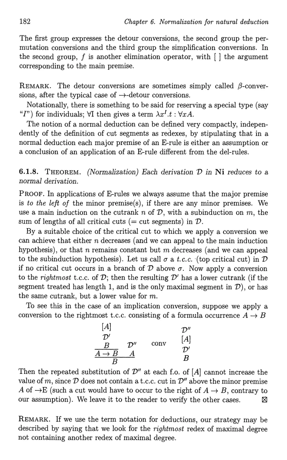
6.1 Conversions and normalization. . . .
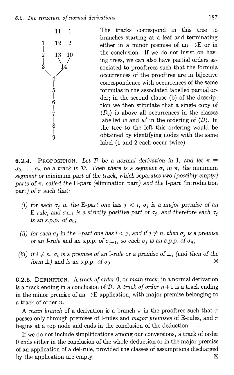
6.2 The structure of normal derivations . . .
6.3 Normality in G-systems and N-systems
6.4 Extensions with simple rules . . . . . . .
6.5 E-Iogic and ordinary logic . . . . . . . .
6.6 Conservativity of predicative classes .
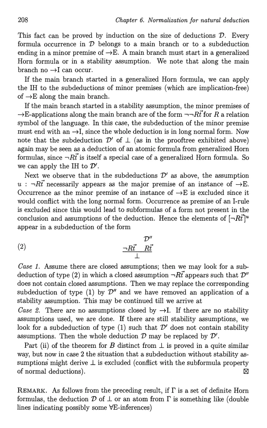
6.7 Conservativity for Horn clauses . . . . .
6.8 Strong normalization for -+Nm and A-t
6.9 Hyperexponential bounds ....
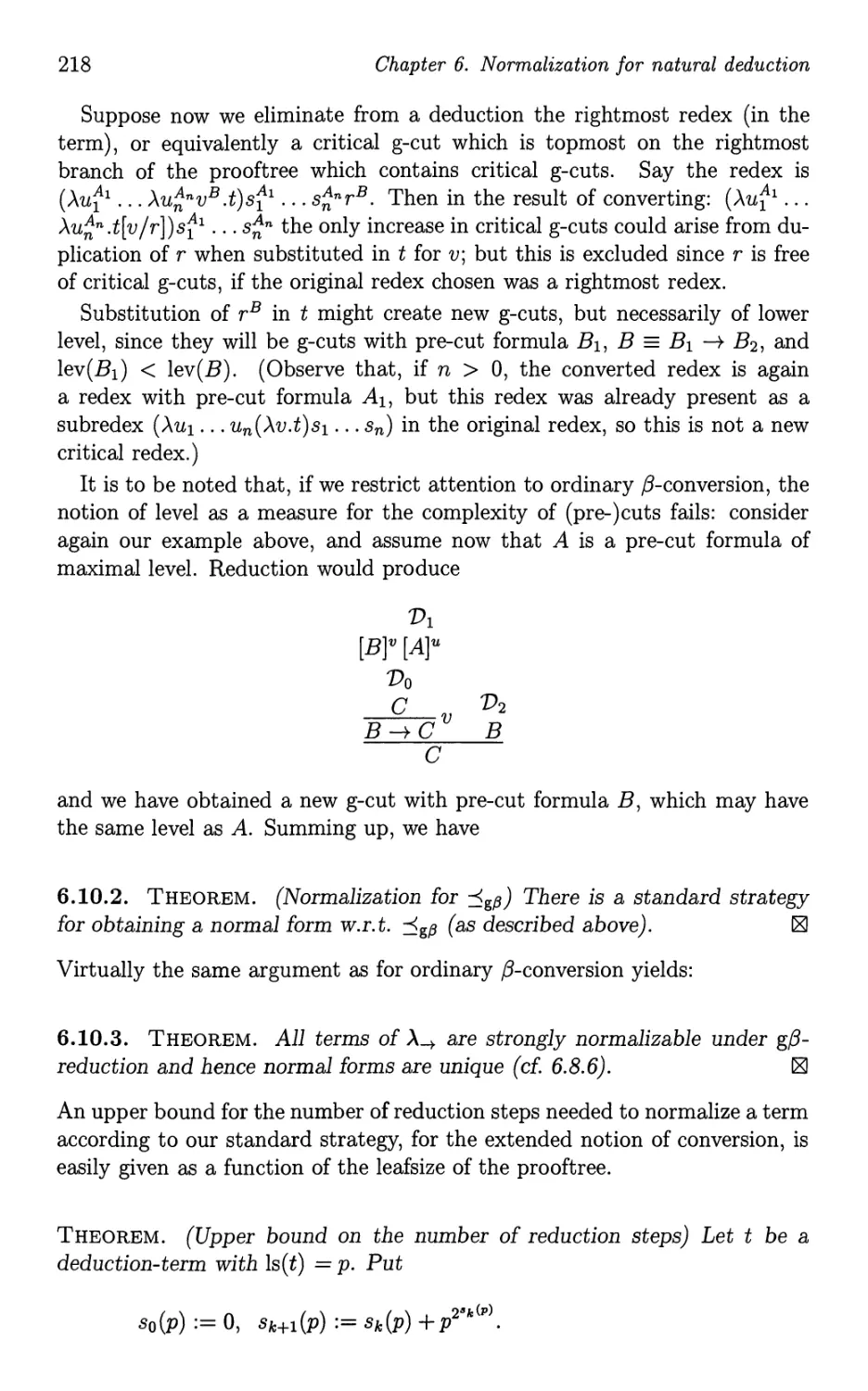
6.10 A digression: a stronger conversion
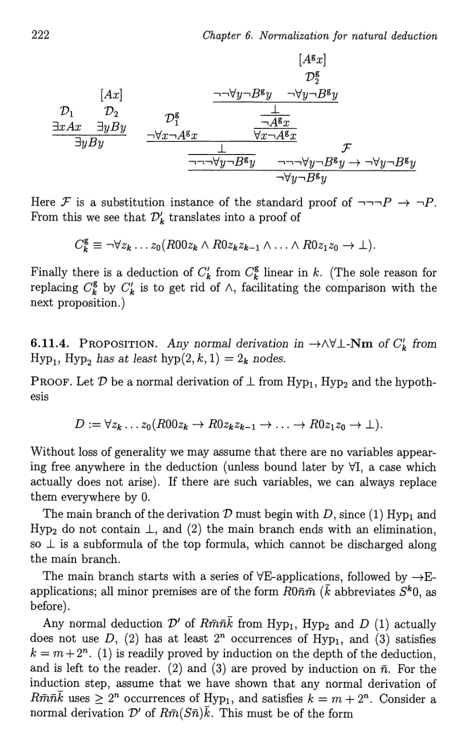
6.11 Orevkov's result . . . . . .
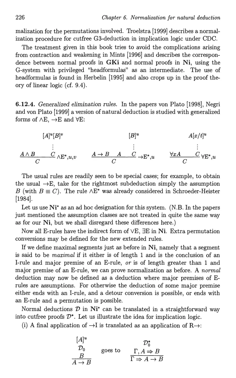
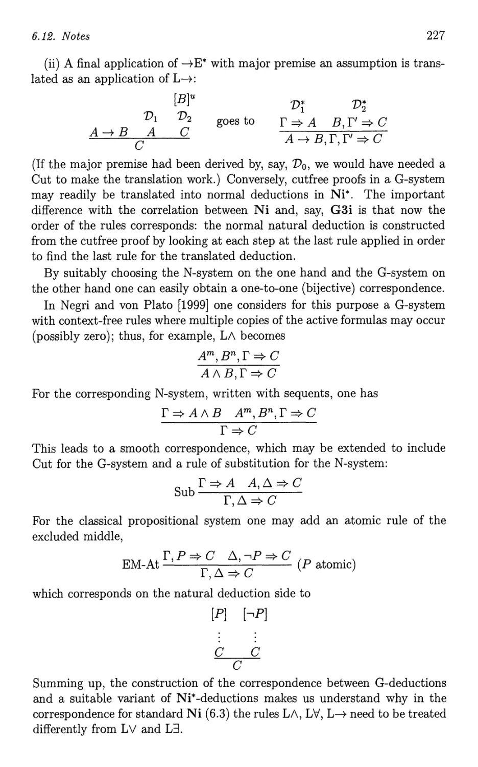
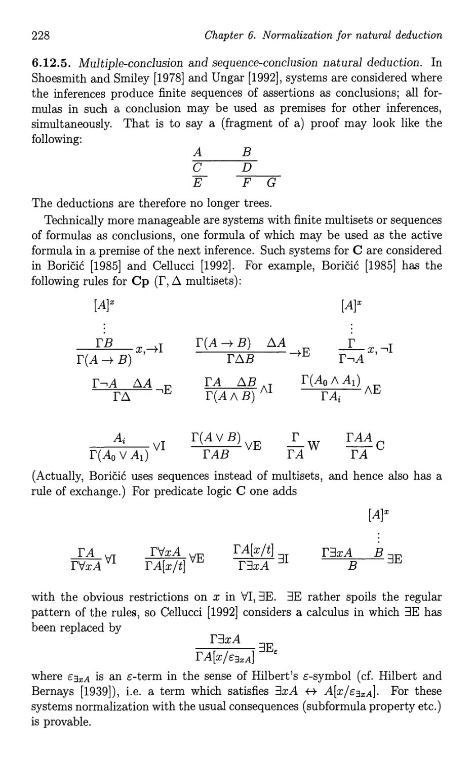
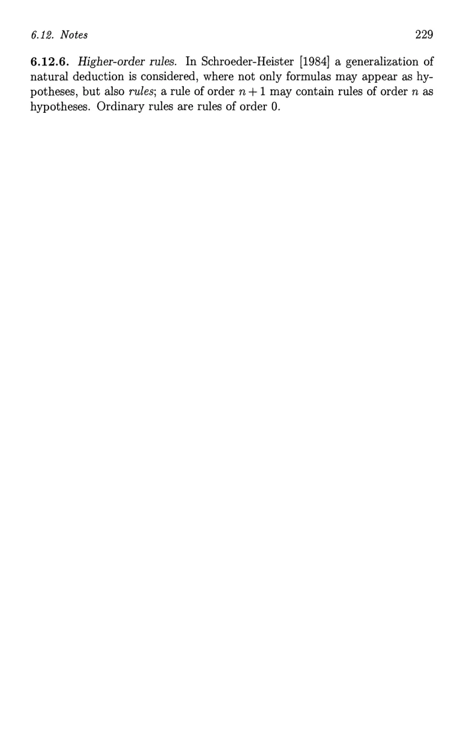
6 .12 Notes . ..... . .
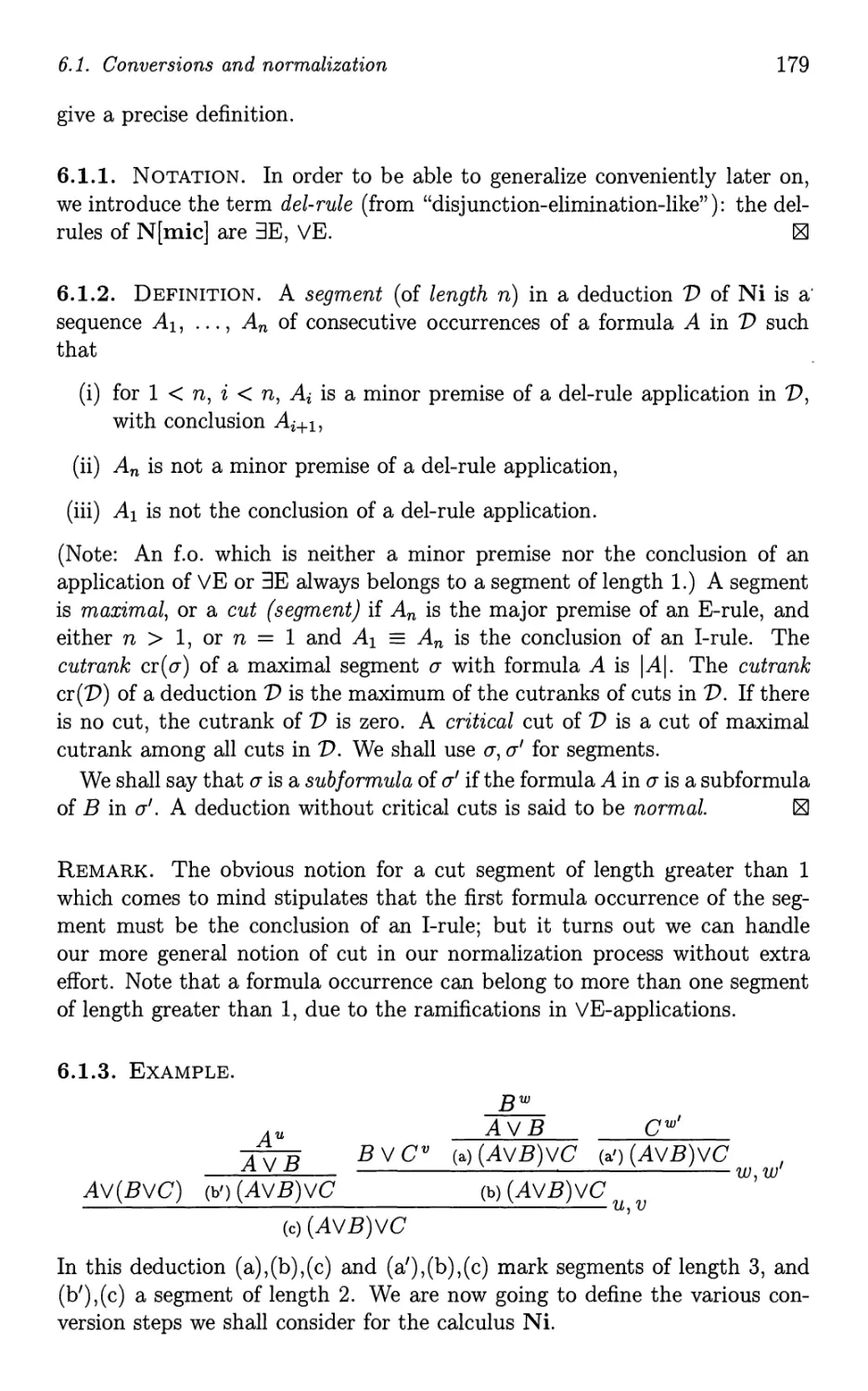
178
178
184
189
197
199
203
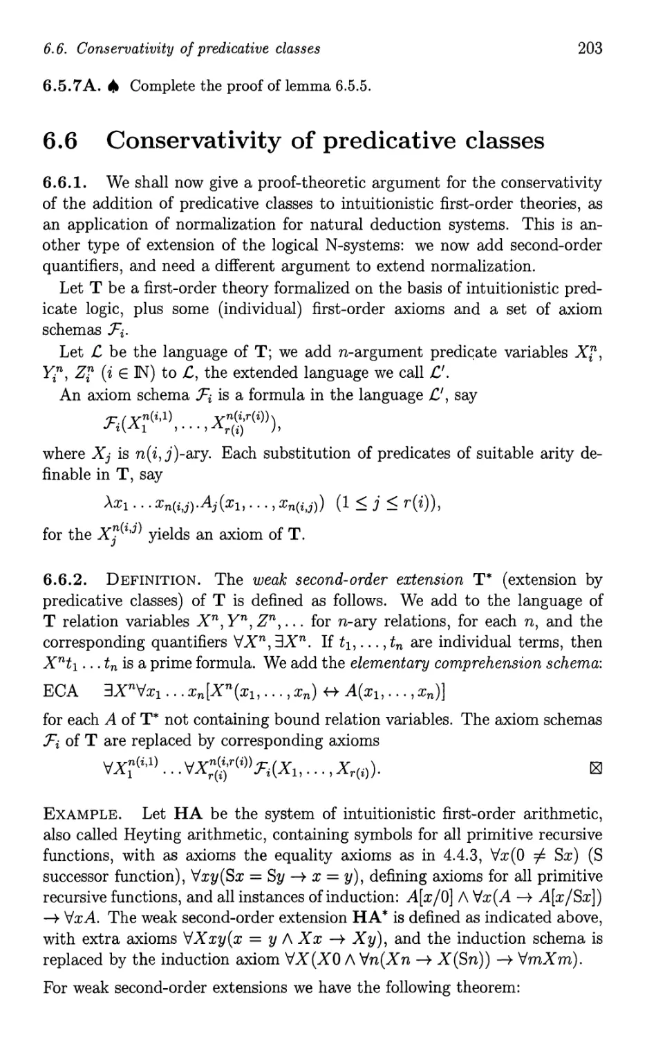
205
210
215
217
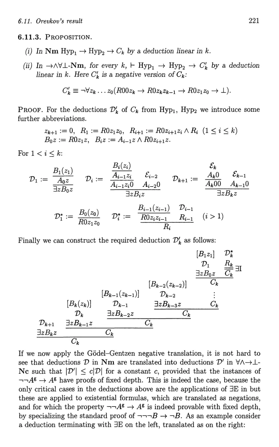
219
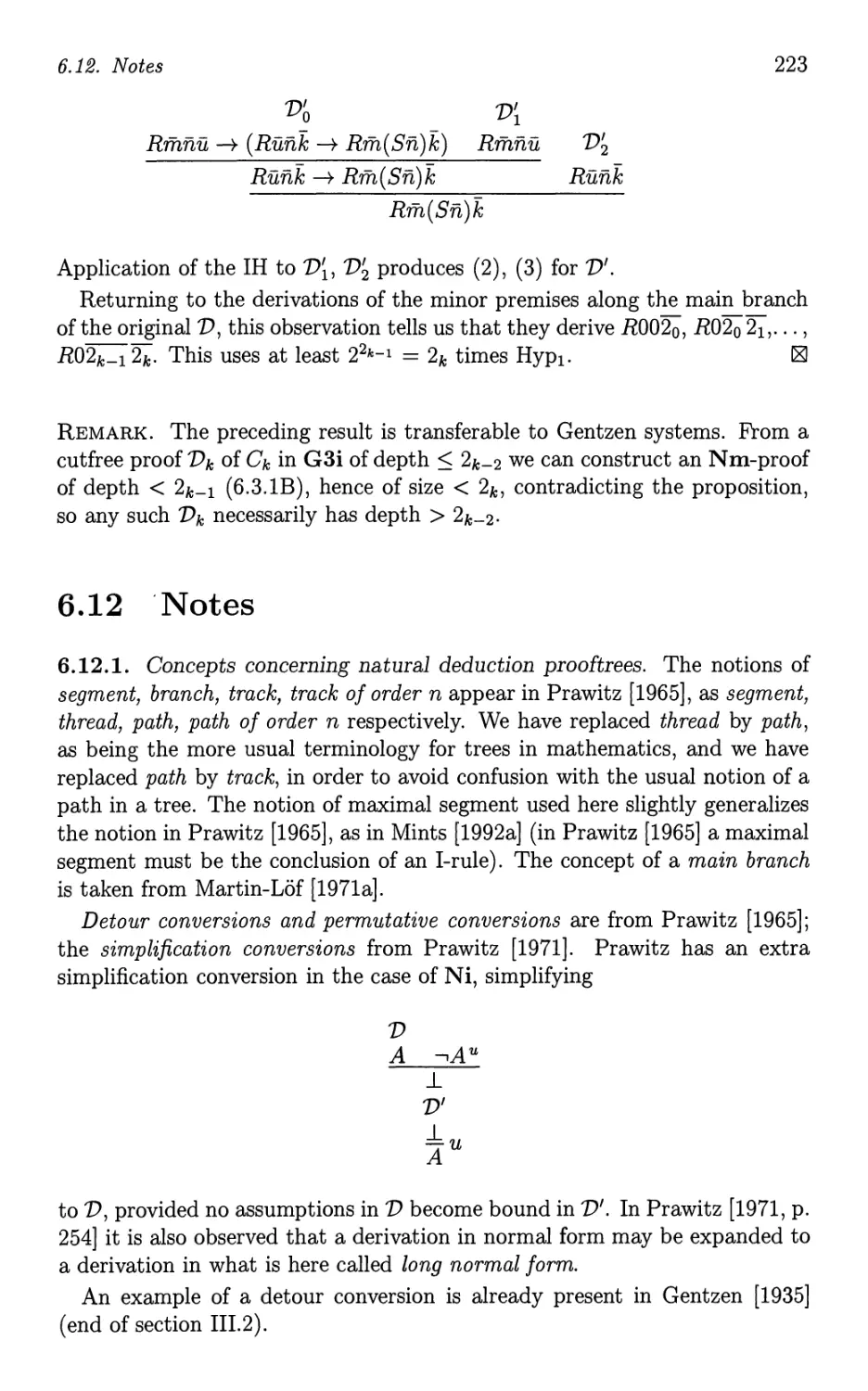
223
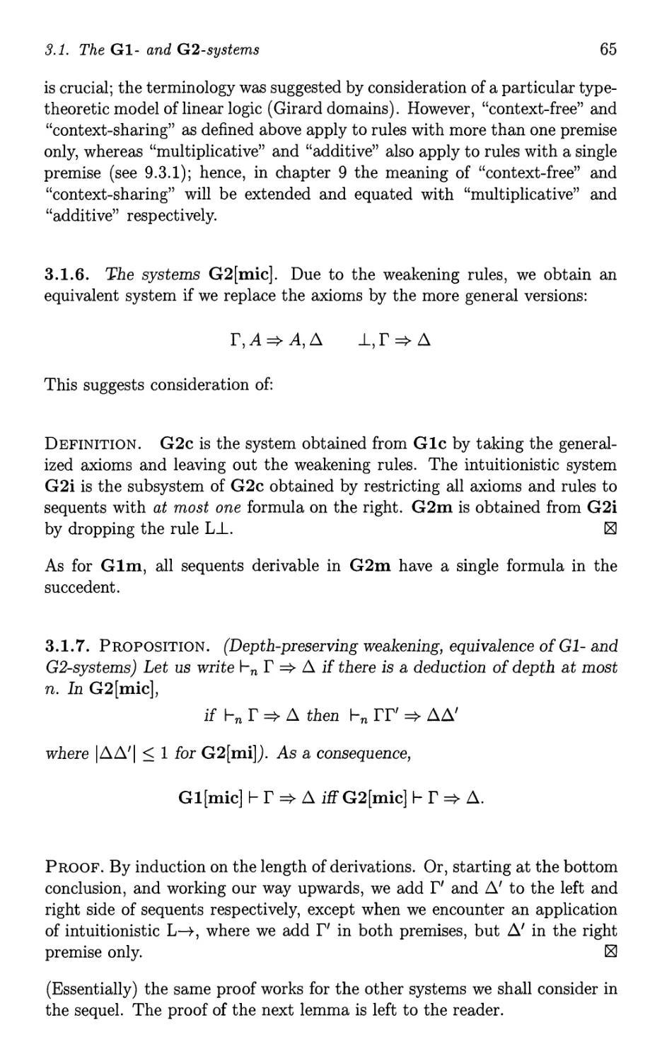
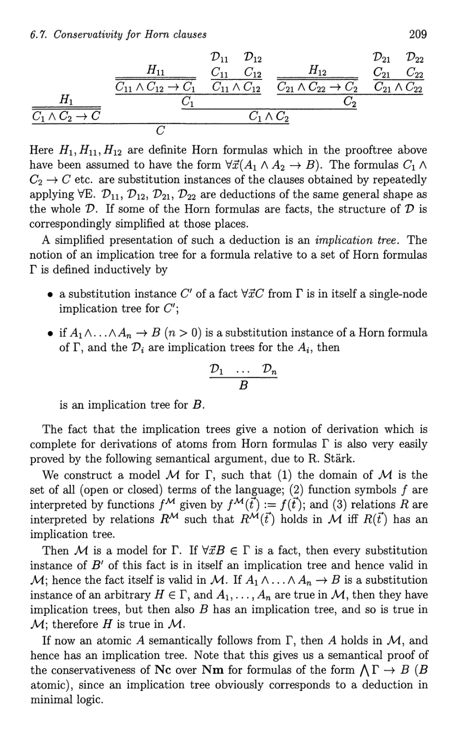
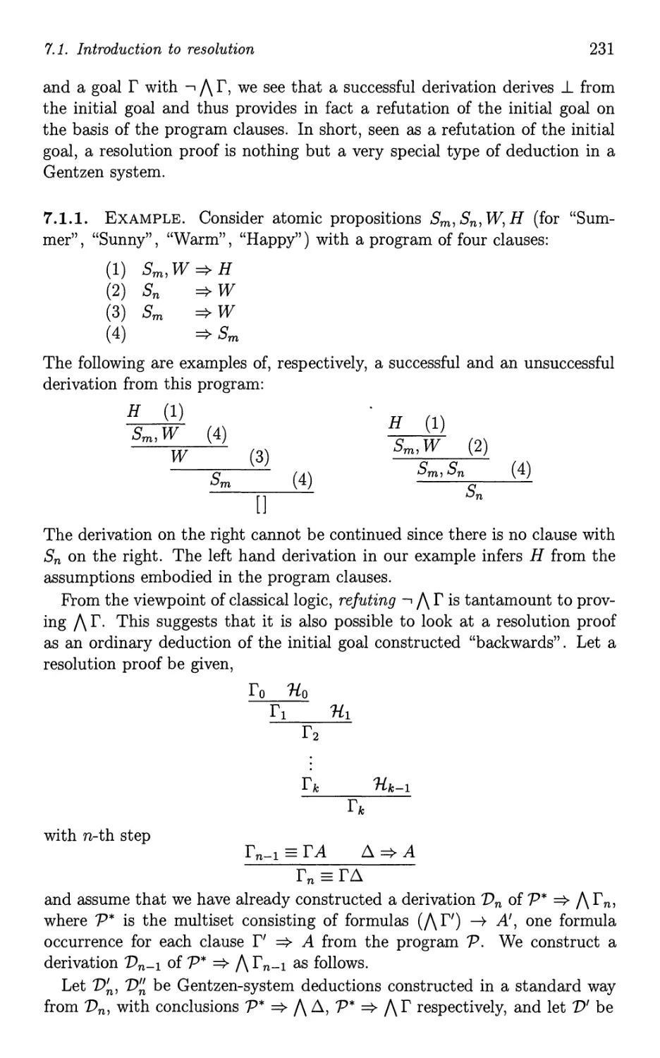
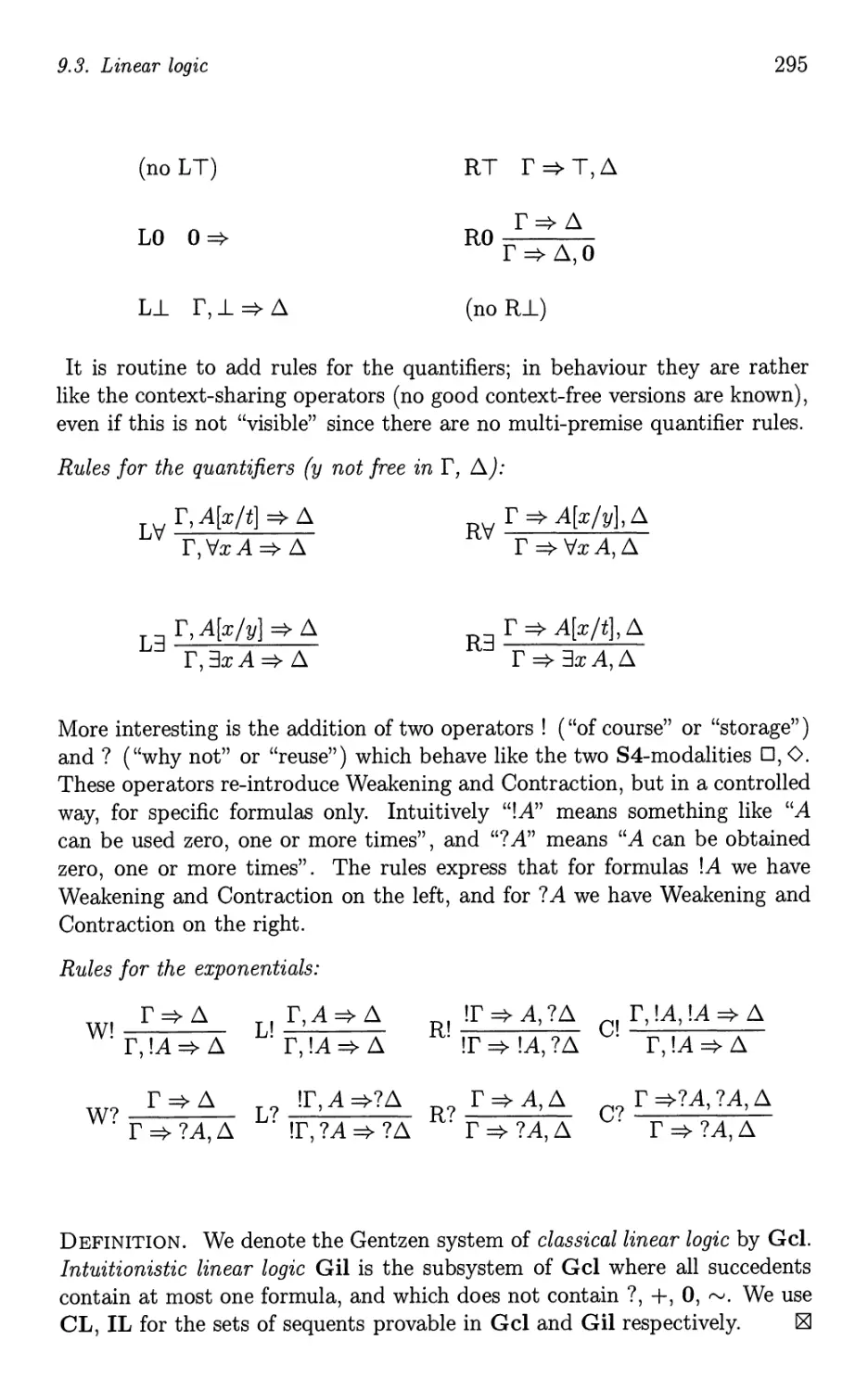
7 Resolution
7.1 Introduction to resolution
7.2 Unification........
7.3 Linear resolution . . . .
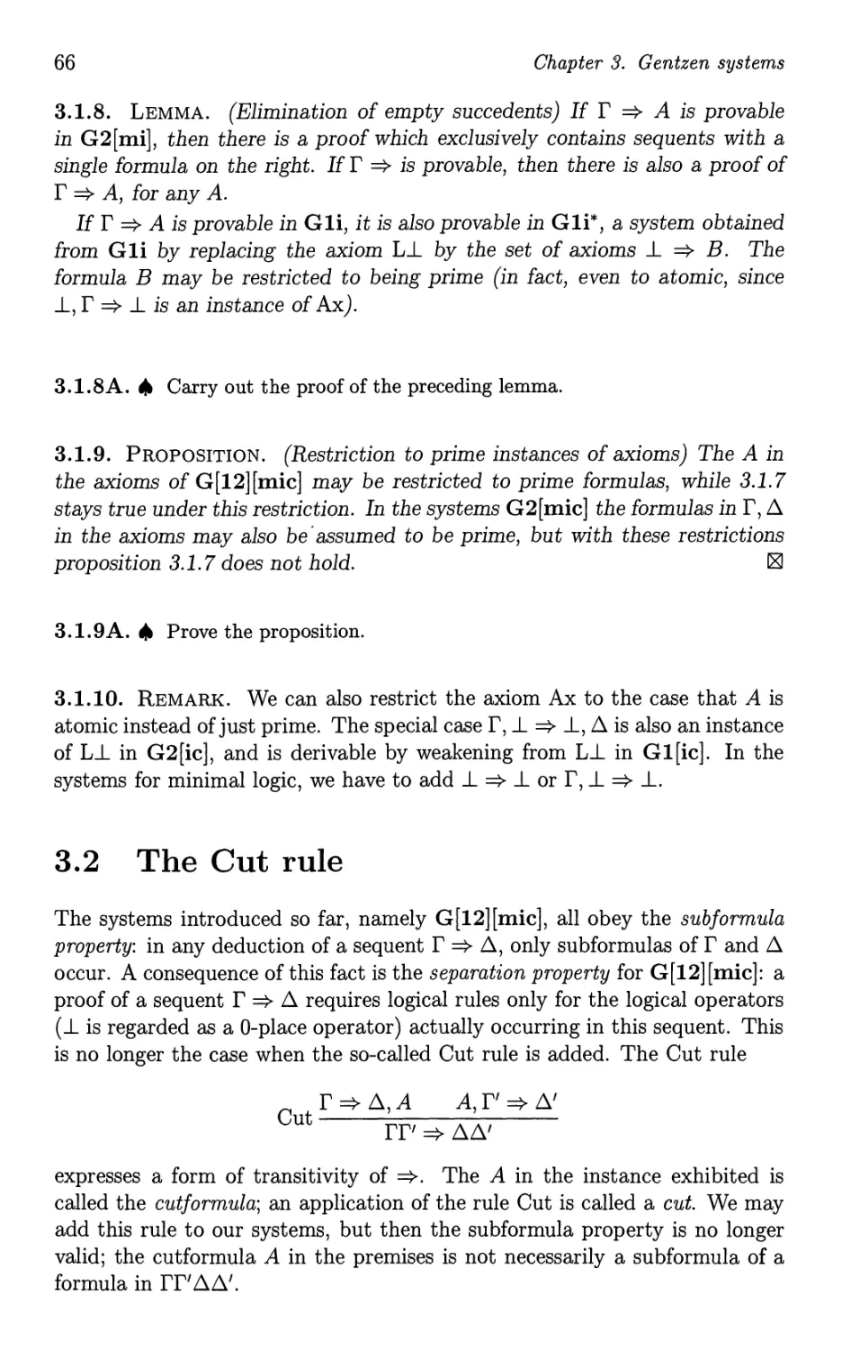
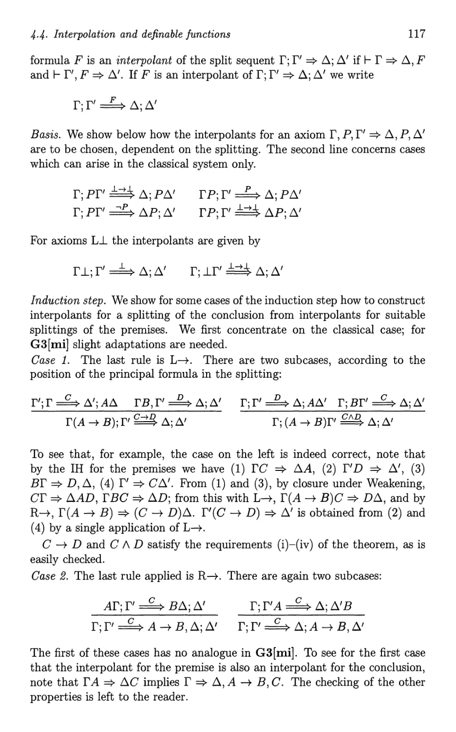
7.4 From Gentzen system to resolution
7.5 Resolution for Ip
7. 6 Notes.....
230
230
232
236
243
246
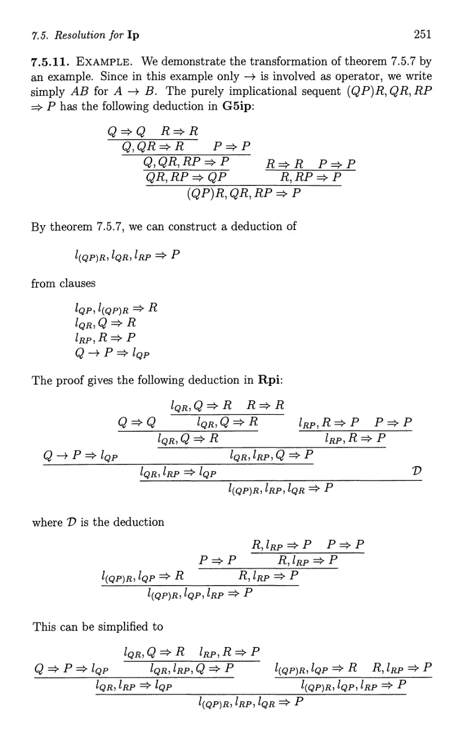
255
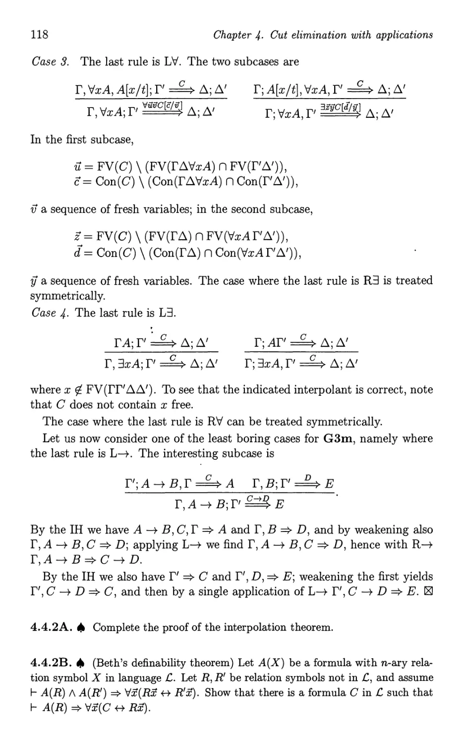
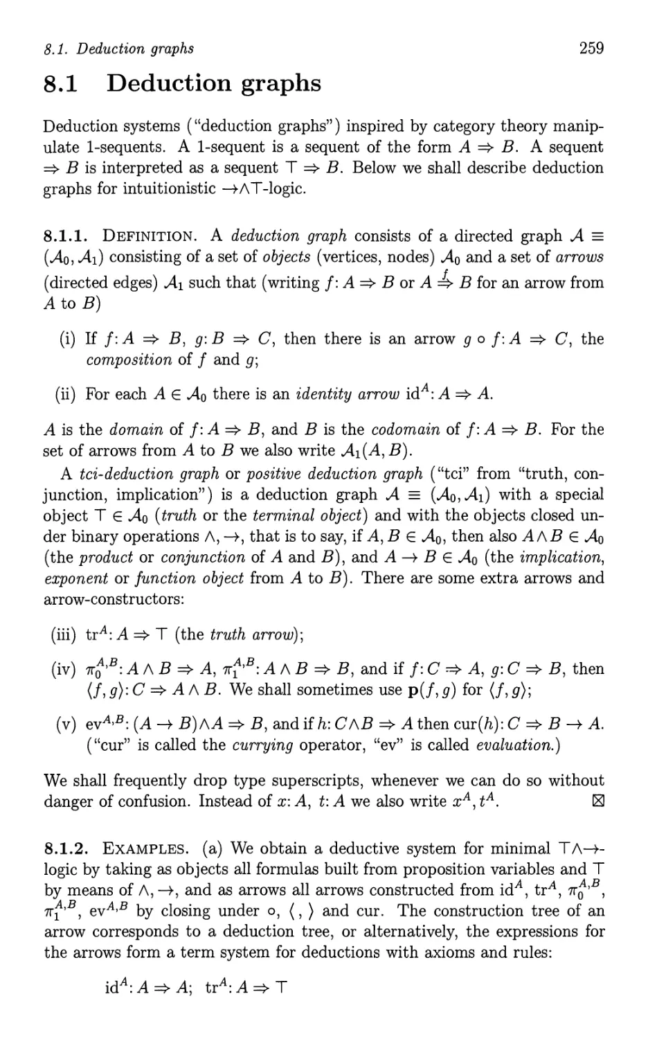
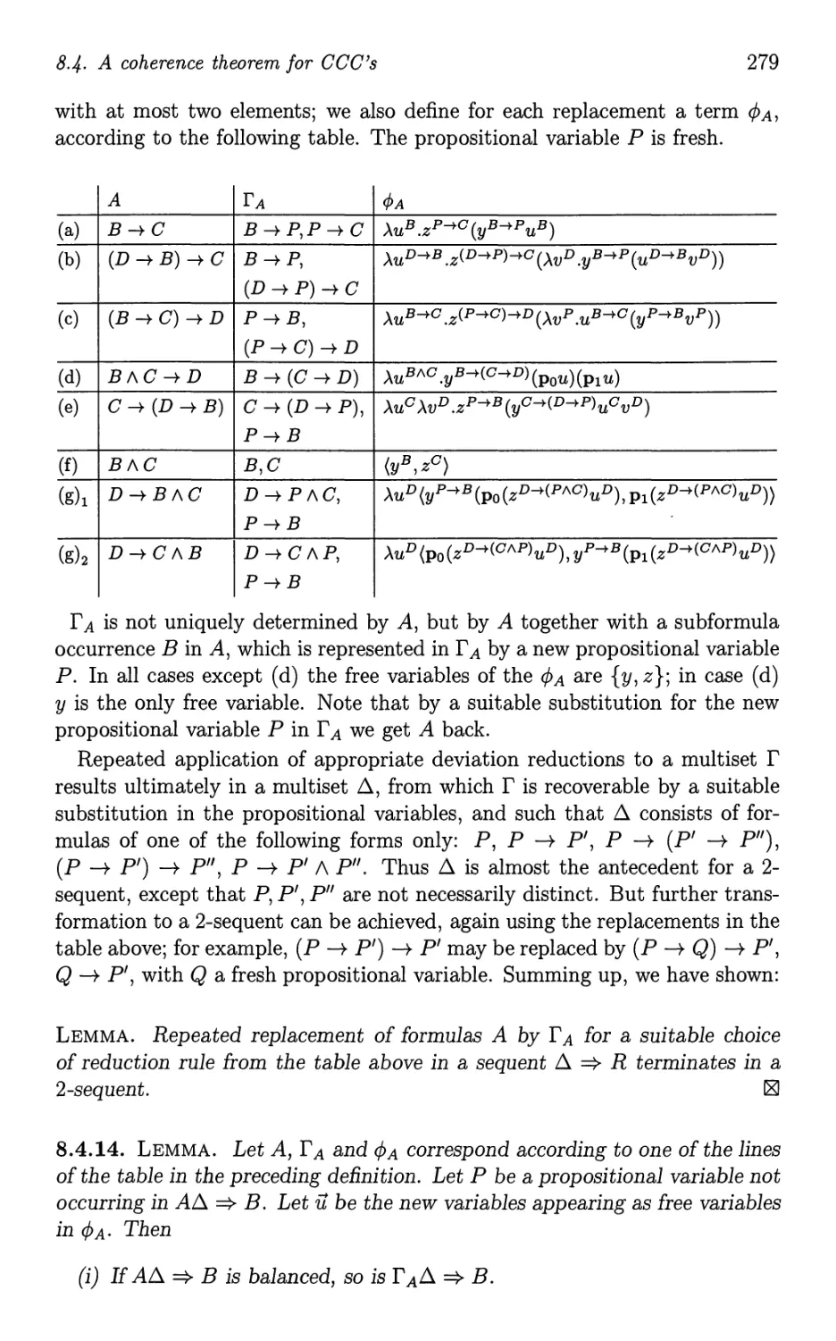
8 Categorical logic
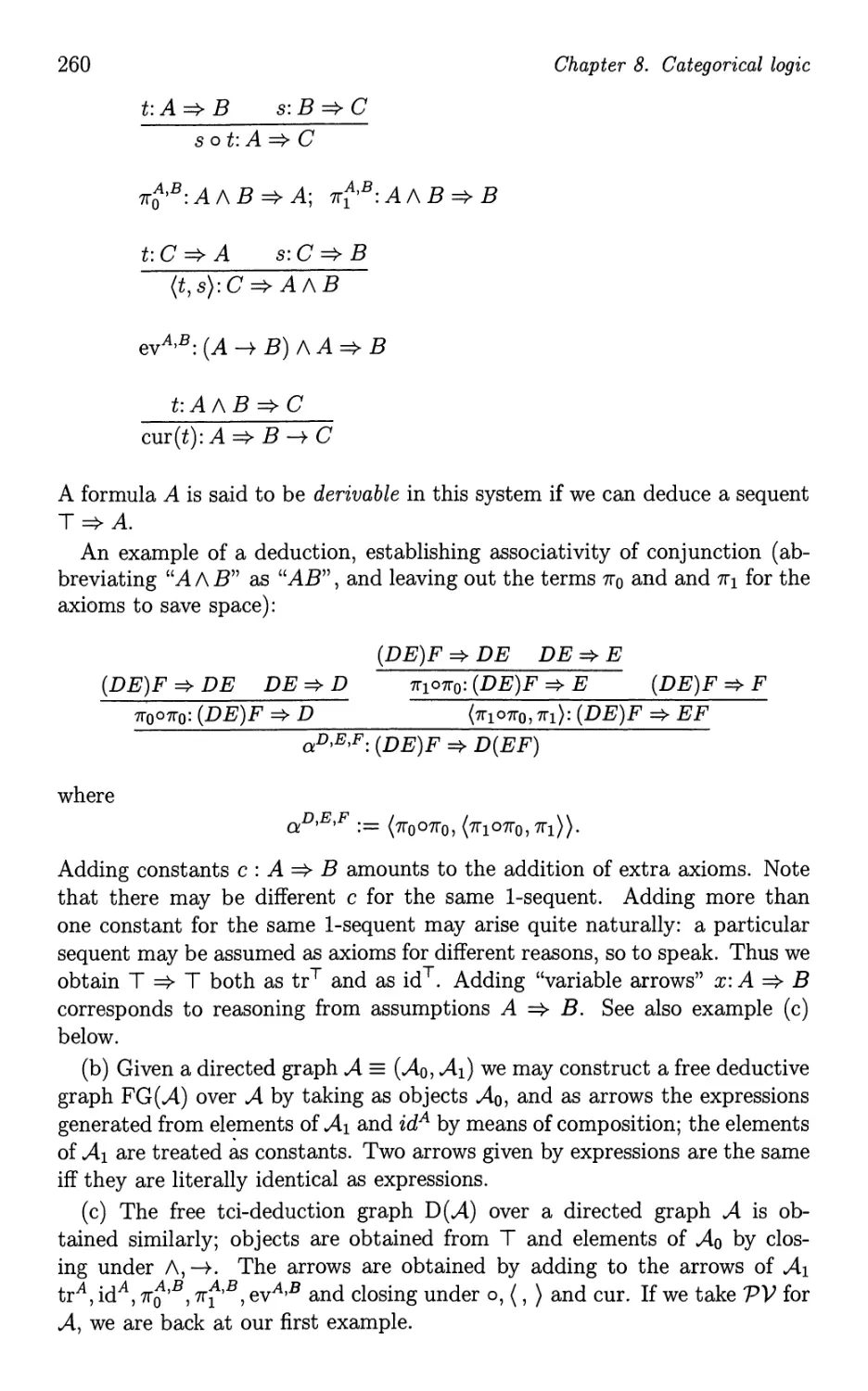
8.1 Deduction graphs . . . . . . . . .
8.2 Lambda terms and combinators
8.3 Decidability of equality. ....
8.4 A coherence theorem for CCC's
8.5 Notes................
258
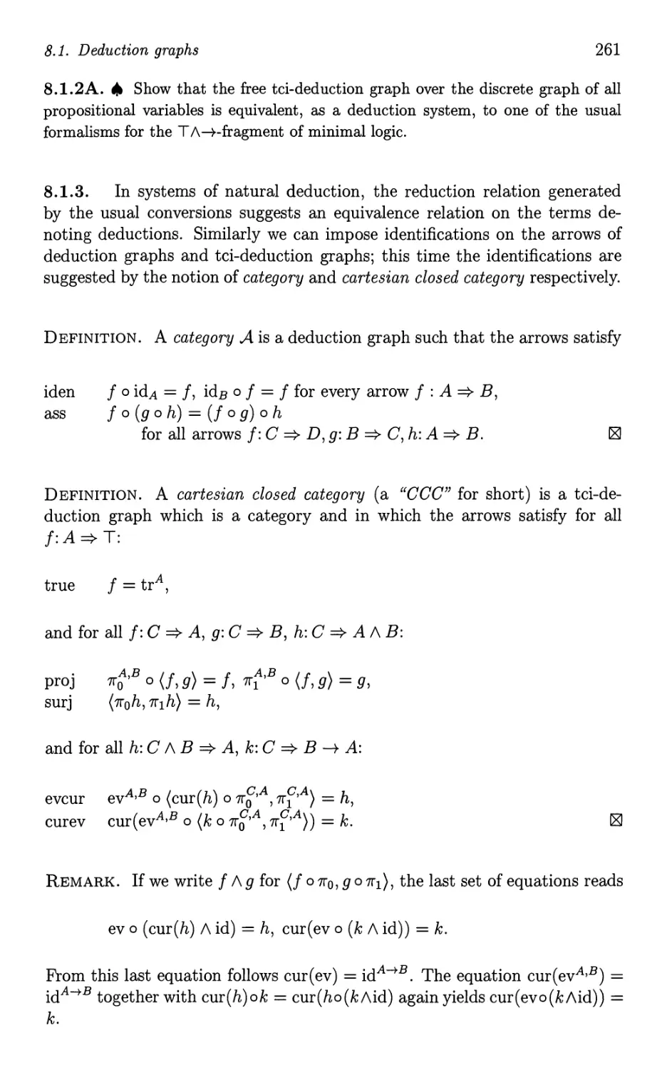
259
264
271
274
281
9 Modal and linear logic
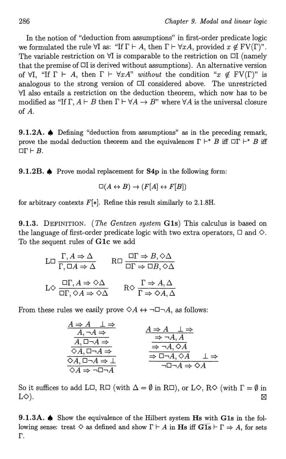
9.1 The modal logic 84 .
283
. 284
Contents
9.2 Embedding intuitionistic logic into S4
9.3 Linear logic . . . . . . . . . . . . .
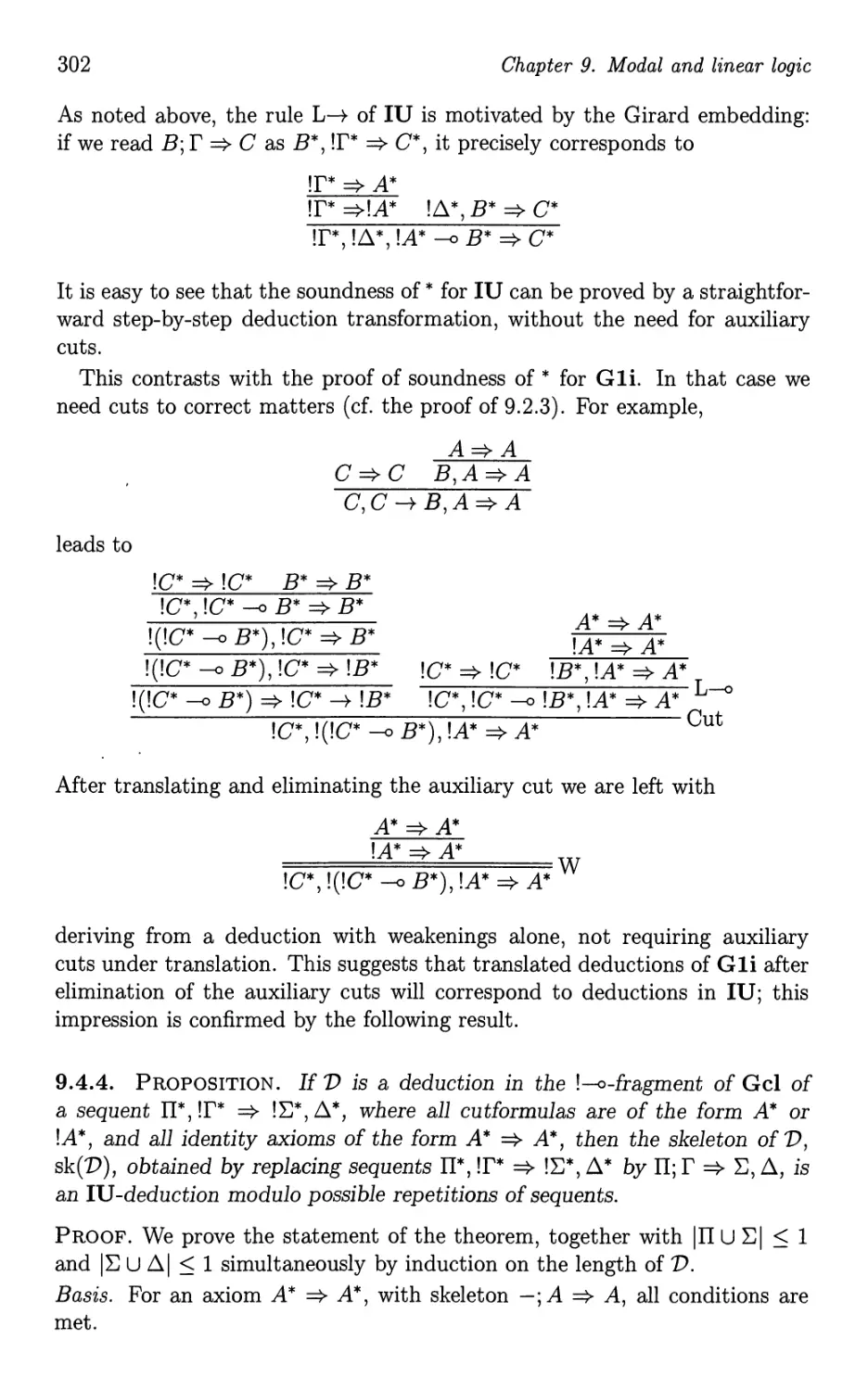
9.4 A system with privileged formulas.
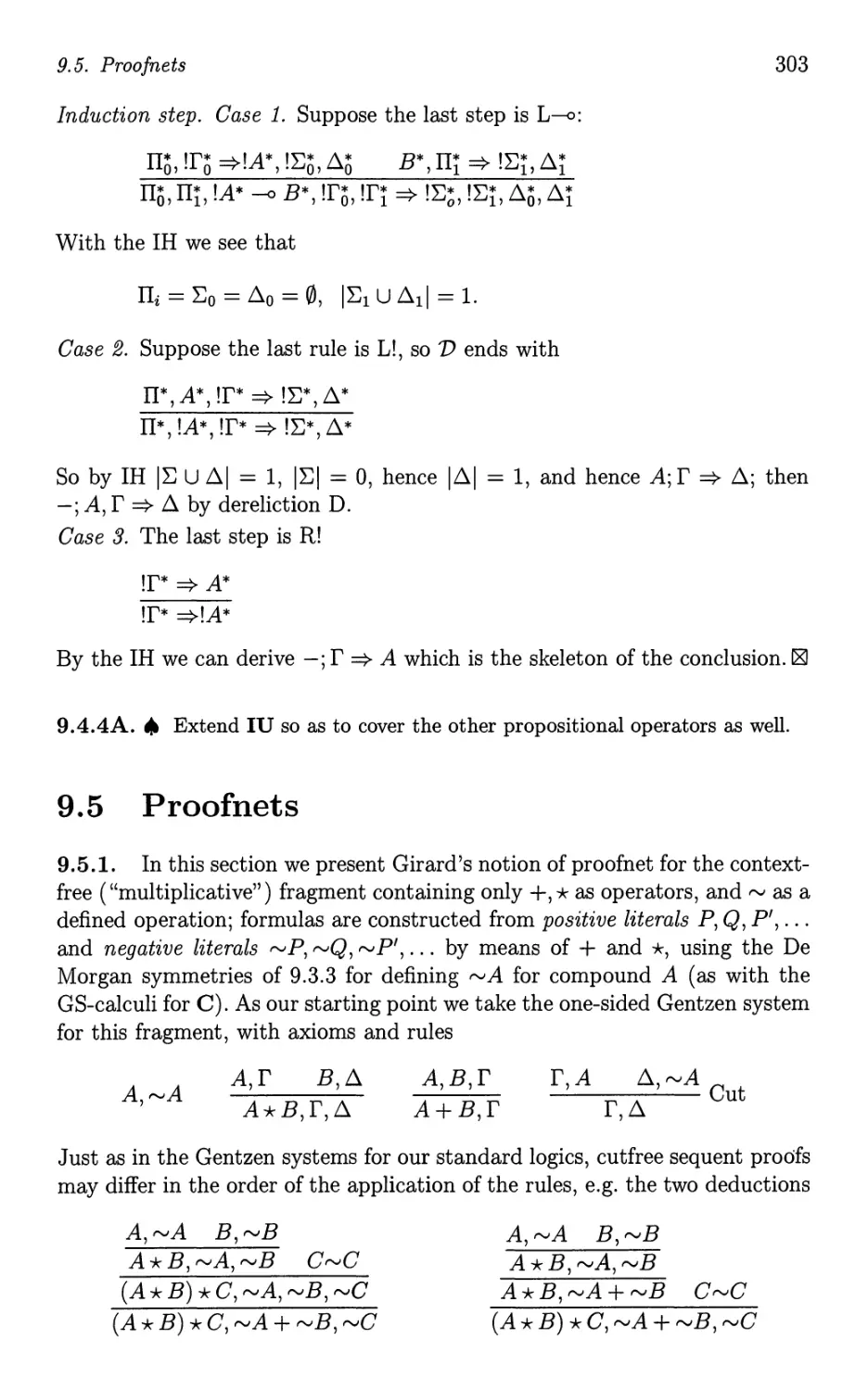
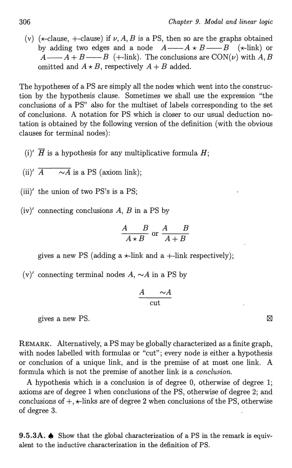
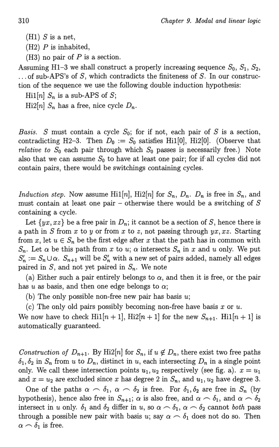
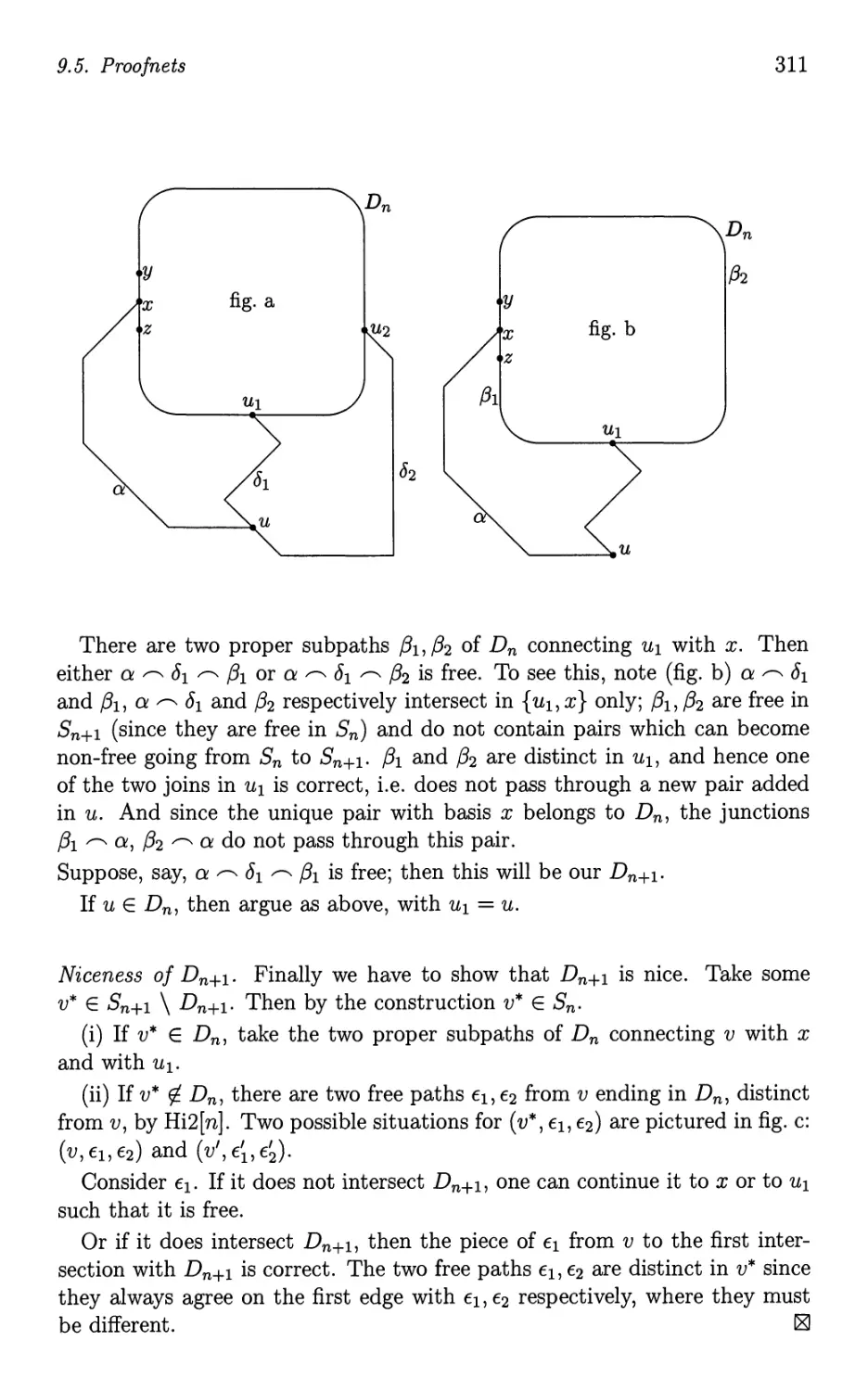
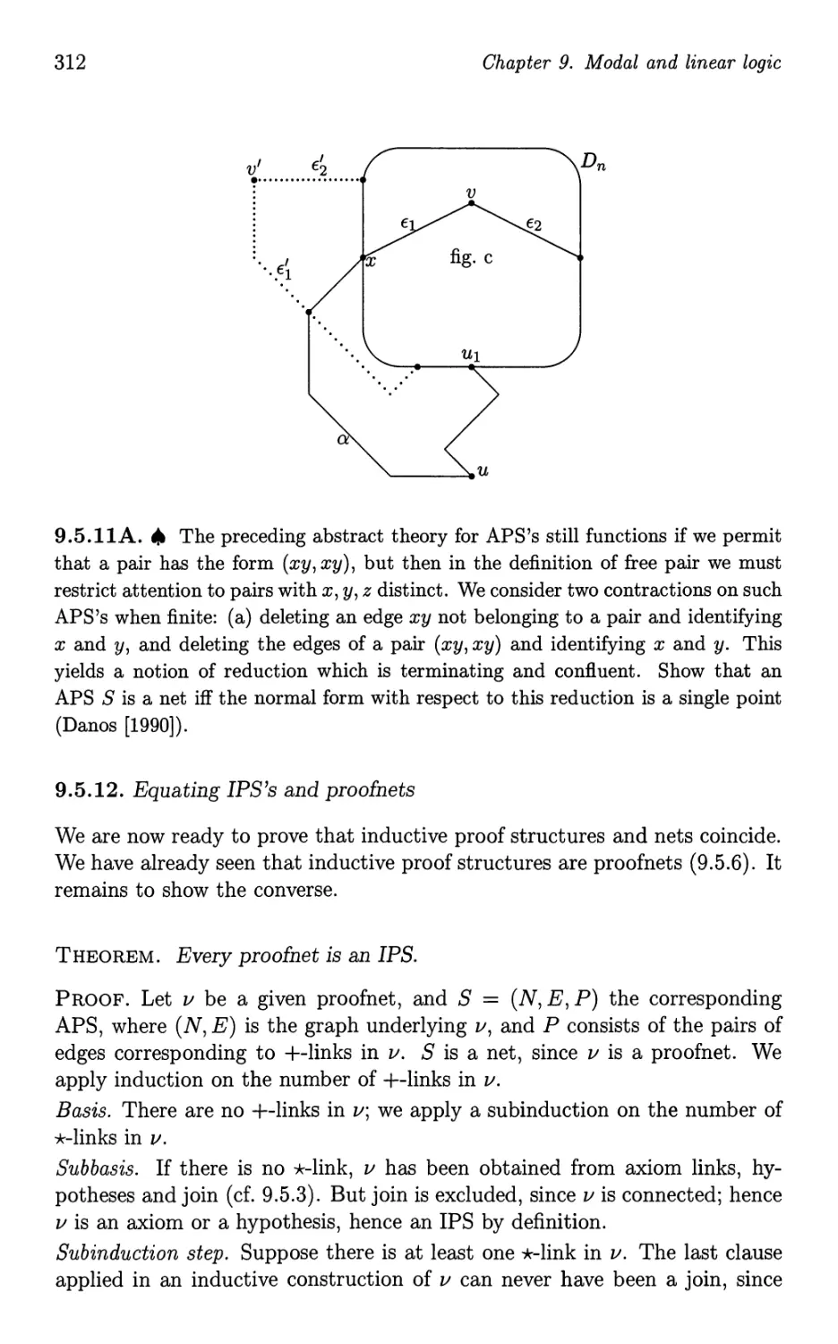
9.5 Proofnets
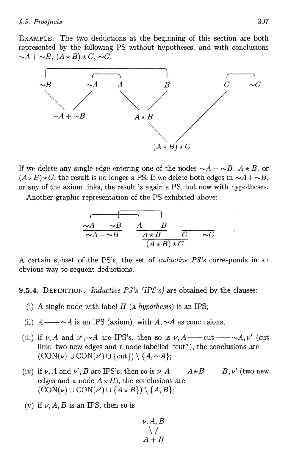
9.6 Notes.............
10 Proof theory of arithmetic
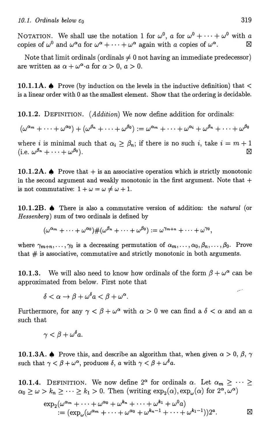
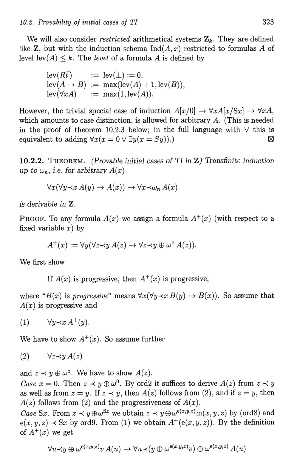
10.1 Ordinals below co . . . . . . . . . . .
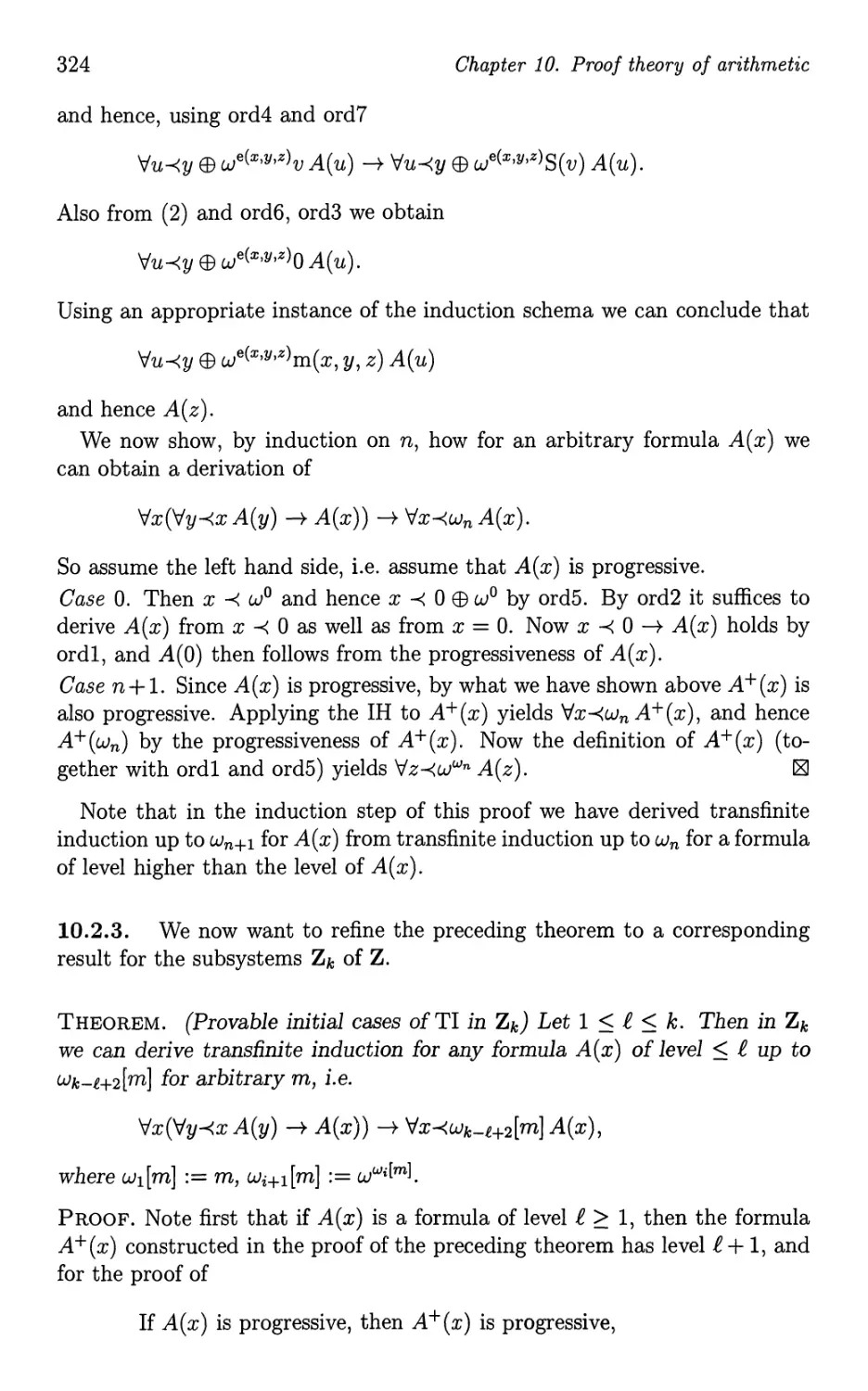
10. 2 Provability of initial cases of TI . . .
10.3 Normalization with the omega rule
10.4 Unprovable initial cases of TI . . . .
10.5 TI for non-standard orderings
10.6 Notes. . . . . . . . . . . . . . .
11 Second-order logic
11.1 Intui tionistic second-order logic
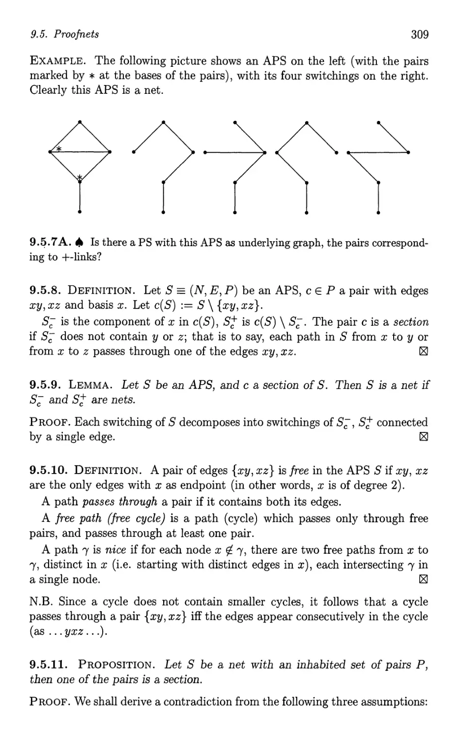
11.2 I p2 and A2 ...............
11.3 Strong normalization for N i 2 . .
11.4 Encoding of A2 n into A2 .......
11.5 Provably recursive functions of HA 2
11. 6 Notes. . . . . . . . . . . . . . . . . . .
Solutions to selected exercises
Bibliography
Symbols and notations
Index
VB
288
292
300
303
. . . . 313
317
318
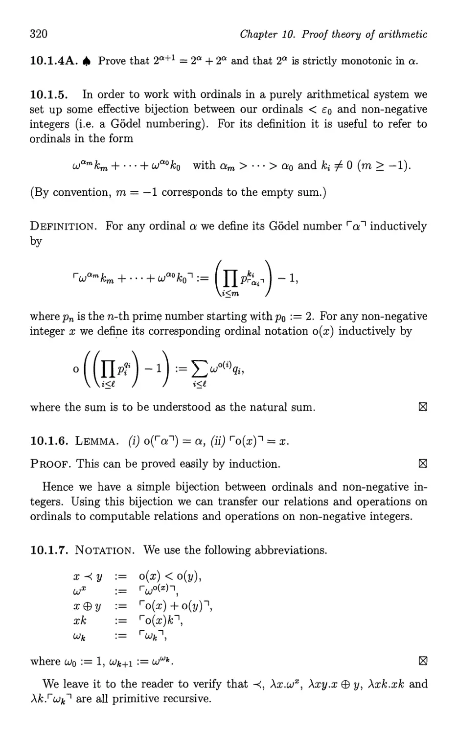
321
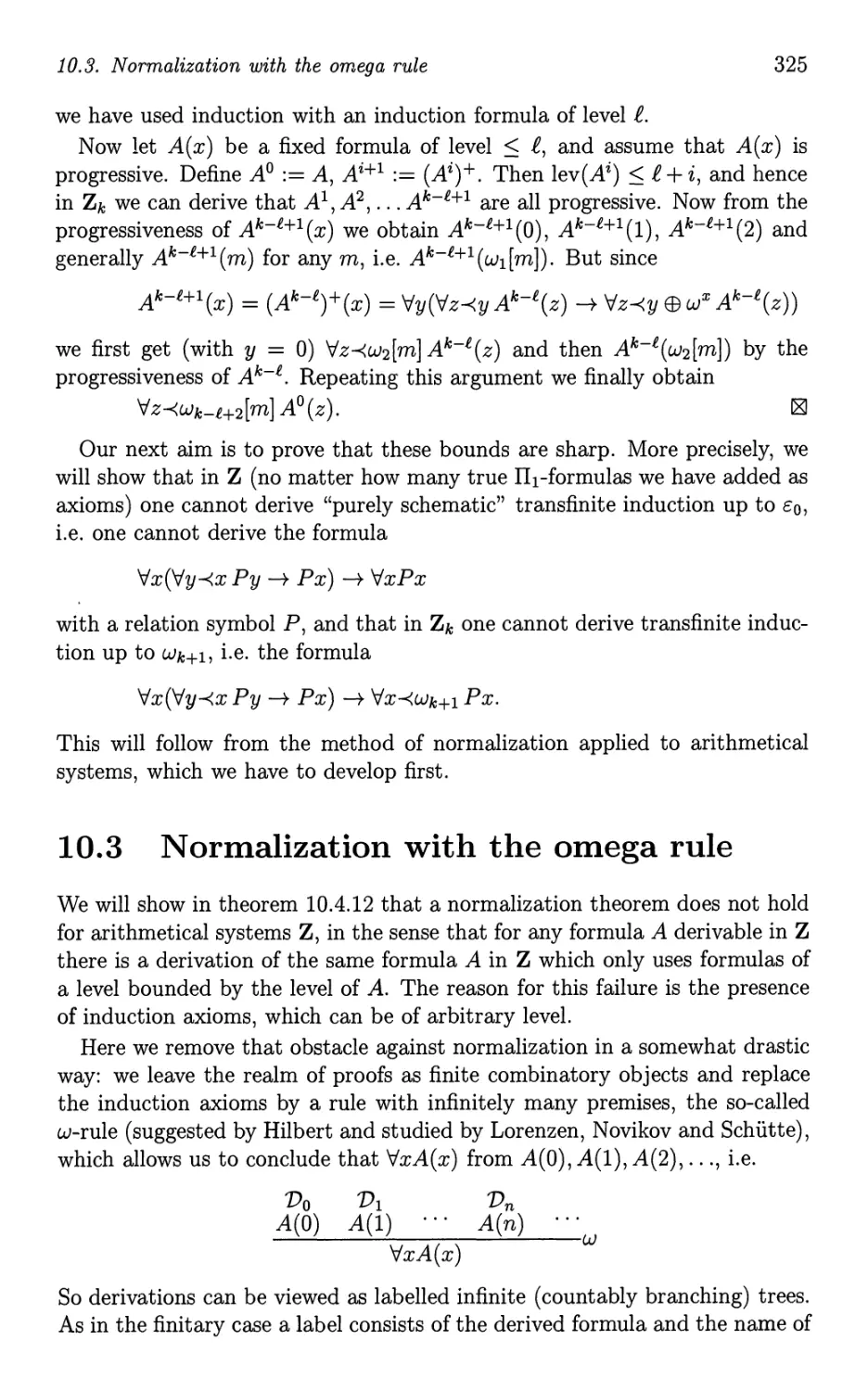
325
330
337
342
345
345
. . . . . . 349
351
. . . 357
. . . . . 358
364
367
379
404
408
Preface
Preface to the first edition
The discovery of the set-theoretic paradoxes around the turn of the century,
and the resulting uncertainties and doubts concerning the use of high-level
abstractions among mathematicians, led D. Hilbert to the formulation of his
programme: to prove the consistency ofaxiomatizations of the essential parts
of mathematics by methods which might be considered as evident and reliable
because of their elementary combinatorial ("finitistic") character.
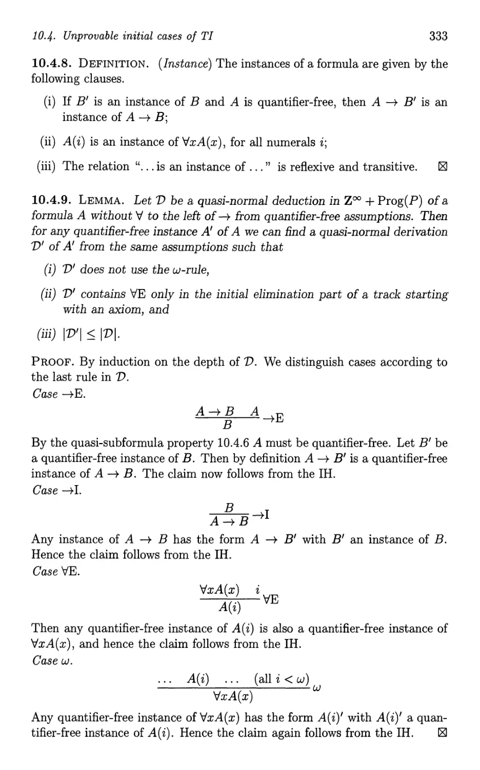
Although, by G6del's incompleteness results, Hilbert's programme could
not be carried out as originally envisaged, for a long time variations of
Hilbert's programme have been the driving force behind the development of
proof theory. Since the programme called for a complete formalization of the
relevant parts of mathematics, including the logical steps in mathematical ar-
guments, interest in proofs as combinatorial structures in their own right was
awakened. This is the subject of structural proof theory; its true beginnings
may be dated from the publication of the landmark-paper Gentzen [1935].
Nowadays there are more reasons, besides Hilbert's programme, for study-
ing structural proof theory. For example, automated theorem proving implies
an interest in proofs as combinatorial structures; and in logic programming,
formal deductions are used in computing.
There are several monographs on proof theory (Schutte [1960,1977], Takeuti
[1987], Pohlers [1989]) inspired by Hilbert's programme and the questions
this engendered, such as "measuring" the strength of subsystems of analy-
sis in terms of provable instances of transfinite induction for definable well-
orderings (mo
e precisely, ordinal notations). Pohlers [1989] is particularly
recommended as an introduction to this branch of proof theory.
Girard [1987b] presents a wider panorama of proof theory, and is not easy
reading for the beginner, though recommended for the more experienced.
The present text attempts to fill a lacuna in the literature, a gap which
exists between introductory books such as Heindorf [1994], and textbooks
on mathematical logic (such as the classic Kleene [1952a], or the recent van
Dalen [1994]) on the one hand, and the more advanced monographs mentioned
above on the other hand.
Our text concentrates on the structural proof theory of first-order logic and
IX
x
Preface
its applications, and compares different styles of formalization at some length.
A glimpse of the proof theory of first-order arithmetic and second-order logic
is also provided, illustrating techniques in relatively simple situations which
are applied elsewhere to far more complex systems.
As preliminary knowledge on the part of the reader we assume some fa-
miliarity with first-order logic as may be obtained from, for example, van
Dalen [1994]. A slight knowledge of elementary recursion theory is also help-
ful, although not necessary except for a few passages. Locally, other prelimi-
nary knowledge will be assumed, but this will be noted explicitly.
Several short courses may be based on a suitable selection of the material.
For example, chapters 1, 2, 6 and 10 develop the theory of natural deduc-
tion and lead to a proof of the "classical" result of Gentzen on the relation
between the ordinal co and first-order arithmetic. A course based on the
first five chapters concentrates on Gentzen systems and cut elimination with
( elementary) applications.
There are many interconnections between the present text and Hindley
[1997]; the latter concentrates on type-assignment systems (systems of rules
for assigning types to untyped lambda terms) which are not treated here. In
our text we only consider theories with "rigid typing", where each term and
all of its subterms carry along a fixed type. Hindley's book may be regarded
as a companion volume providing a treatment of dedu.ctions as they appear
in type-assignment systems.
We have been warned by colleagues from computer science that references
to sources more than five years old will make a text look outdated. For readers
inclined to agree with this we recommend contemplation of the following
platitudes: (1) a more recent treatment of a topic is not automatically an
improvement over earlier treatments; (2) if a subject is worthwhile, it will
in due time acquire a history going back more than five years; (3) results of
lasting interest do exist; (4) limiting the horizon to five years entails a serious
lack of historical perspective.
Numbered exercises are scattered throughout the text. These are immedi-
ately recognizable as such, since they have been set in smaller type and have
been marked with the symbol ..
Many of these exercises are of a routine character ("complete the proof of
this lemma"). We believe that (a) such exercises are very helpful in famil-
iarizing the student with the material, and (b) listing these routine exercises
explicitly makes it easy for a course leader to assign definite tasks to the
students.
At the end of each chapter, except the first, there is a section called "Notes".
There we have collected historical credits and suggestions for further reading;
also we mention other work related to the topic of the chapter. These notes
do not pretend to give a history of the subject, but may be of help in gaining
some historical perspective, and point the way to the sources. There is no
Preface
Xl
attempt at completeness; with the subject rapidly expanding this has become
well-nigh impossible.
The references in the index to names of persons concern in the majority of
cases a citation of a publication. In case of publications with more than one
author, only the first author's name is indexed. Occurrences of author names
in the bibliography have not been indexed. There is a separate list, where
symbols and notations of more than local significance have been indexed.
The text started as a set of course notes for part of a course "Introduction
to Constructivism and Proof Theory" for graduate students at the University
of Amsterdam. When the first author decided to expand these notes into a
book, he felt that at least some of the classical results on the proof theory
of first-order arithmetic ought to be included; hence the second author was
asked to become coauthor, and more particularly, to provide a chapter on
the proof theory of first-order arithmetic. The second author's contribution
did not restrict itself to this; many of his suggestions for improvement and
inclusion of further results have been adopted, and a lot of material from his
course notes and papers has found its way into the text.
We are indebted for comments and information to K. R. Apt, J. F. A. K. van
Benthem, H. C. Doets, J. R. Hindley, G. E. Mints, V. Sanchez, S. V. Solovjov,
A. Weiermann; the text was prepared with the help of some useful Latex
macros for the typesetting of proof trees by S. Buss and for the typesetting of
ordinary trees by D. Roorda. M. Behrend of the Cambridge University Press
very carefully annotated the near-final version of the text, expunging many
blemishes and improving typographical consistency.
Amsterdam/Munchen
Spring 1996
A. S. Troelstra
H. Schwichtenberg
Preface to the second edition
In preparing this revised edition we used the opportunity to correct many
errata in the first edition. Moreover certain sections were rewritten and some
new material inserted, especially in chapters 3-6. The principal changes are
the following.
Chapter 1: section 1.3 has been largely rewritten. Chapter 2: the material
in 2.1.10 is new. Chapter 3: more prominence has been given to a Kleene-style
variant of the G3-systems (3.5.11), and multi-succedent versions of G3[mi]
are defined in the body of the text (3.5.10). A general definition of systems
with local rules (3.4) is also new. Chapter 4: the proof of cut elimination
for G3-systems (4.1.5) has been completely rewritten, and a sketch of cut
elimination for the systems m-G3[mi] has been added (4.1.10). There are new
sections on cut elimination for extensions of G3-systems, with applications
to predicate logic with equality and the intuitionistic theory of apartness.
Chapter 5: a result on the growth of size of proofs in propositional logic
Xll
Preface
under cut elimination (5.2) has been included. Chapter 6: extensions of N-
systems with extra rules, with an application to E-Iogic, are new; the section
on E-Iogic replaces an inadequate treatment of the same results in chapter
4 of the first edition. Chapter 11: a new proof of strong normalization. for
A2. New are also the "Solutions to selected exercises"; these are intended
as a help to those readers who study the text on their own. Exercises for
which a (partial) solution is provided are marked with *. The updating of
the bibliography primarily concerns the parts of the text which have been
revised.
In a review of the first edition it has been noted that complexity-theoretic
aspects are largely absent. We felt that this area is so vast that it would
require a separate monograph of its own, to be written by an expert in the
area. Another complaint was that our account was lacking in motivation and
philosophical background. This has not been remedied in the present edition,
although a few words of extra explanation have been added here and there.
A typically philosophical problem we did not deal with is the question: when
are two proofs to be considered equal? We doubt, however, whether this
question will ever have a simple answer; it may well be that there are many
answers, depending on aims and points of view.
One terminological change deserves to be noted: we changed "contraction"
(in the sense of a step in transforming terms of type theory and proofs in natu-
ral deduction), into "conversion". Similarly, "contracts to" and "contractum"
have been replaced by "converts to" and "conversum" repectively. On the
other hand "contraction" as the name of a structural rule in Gentzen systems
is maintained. See under the remarks at the end of 1.2.5 for a motivation.
We are again indebted to many people for comments and corrections, in par-
ticular H. van Ditmarsch, L. Gordeev, J. R. Hindley, R. Matthes, G. E. Mints,
and the students in our classes. Special thanks are due to Sara Negri, who
unselfishly offere to read carefully a large part of the text; in this she has
been assisted by Ian von Plato. Their comments led to many improvements.
For the remaining defects of the text the authors bear sole responsibility.
A msterdam/Munchen
March 2000
A. S. Troelstra
H. Schwichtenberg
Chapter 1
Introduction
Proof theory may be roughly divided into two parts: structural proof theory
and interpretational proof theory. Structural proof theory is based on a com-
binatorial analysis of the structure of formal proofs; the central methods are
cut elimination and normalization.
In interpretational proof theory, the tools are (often semantically moti-
vated) syntactical translations of one formal theory into another. We shall
encounter examples of such translations in this book, such as the G6del-
Gentzen embedding of classical logic into minimal logic (2.3), and the modal
embedding of intuitionistic logic into the modal logic S4 (9.2). Other well-
known examples from the literature are the formalized version of Kleene's
realizability for intuitionistic arithmetic and G6del's Dialectica interpretation
(see, for example, Troelstra [1973]).
The present text is concerned with the more basic parts of structural proof
theory. In the first part of this text (chapters 2-7) we study several formal-
izations of standard logics. "Standard logics", in this text, means minimal,
intuitionistic and classical first-order predicate logic. Chapter 8 describes
the connection between cartesian closed categories and minimal conjunction-
implication logic; this serves as an example of the applications of proof theory
in category theory. Chapter 9 illustrates the extension to other logics (namely
the modal logic S4 and linear logic) of the techniques introduced before in
the study of standard logics. The final two chapters deal with first-order
arithmetic and second-order logic respectively.
The first section of this chapter contains notational conventions and def-
initions, to be consulted only when needed, so a quick scan of the contents
will suffice to begin with. The second section presents a concise introduction
to simple type theory, with rigid typing; the parallel between (extensions of)
simple type theory and systems of natural deduction, under the catch-phrase
"formulas-as-types", is an important theme in the sequel. Then follows a
brief informal introduction to the three principal types of formalism we shall
encounter later on, the N-, H- and G-systems, or Natural deduction, Hilbert
systems, and Gentzen systems respectively. Formal definitions of these sys-
tems will be given in chapters 2 and 3.
1
2 Chapter 1. Introduction
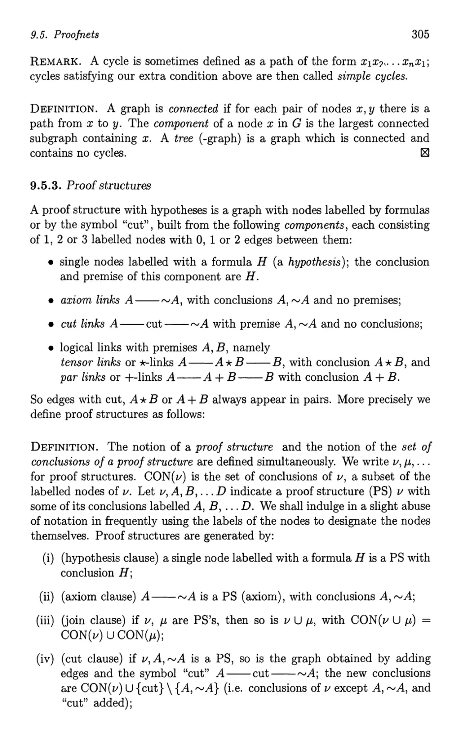
1.1 PreliITlinaries
The material in this section consists primarily of definitions and notational
conventions, and may be skipped until needed.
Some very general abbreviations are "iff" for "if and only if", "IH" for "in-
duction hypothesis", "w.l.o.g." for "without loss of generality". To indicate
literal identity of two expressions, we use = . (In dealing with expressions
with bound variables, this is taken to be literal identity modulo renaming of
bound variables; see 1.1.2 below.)
The symbol [gI is used to mark the end of proofs, definitions, stipulations
of notational conventions.
IN is used for the natural numbers, zero included. Set-theoretic notations
such as E, C are standard.
1.1.1. The language of first-order predicate logic
The standard language considered contains V, /\, -+, -1-, "1,3 as primitive logi-
cal operators (-1- being the degenerate case of a zero-place logical operator, Le.
a logical constant), countably infinite supplies of individual variables, n-place
relation symbols for all n E IN, symbols for n-ary functions for all n E IN.
O-place relation symbols are also called proposition letters or proposition vari-
ables; O-argument function symbols are also called (individual) constants.
The language will not, unless stated otherwise, contain = as a primitive.
Atomic formulas are formulas of the form Rt 1 . . . tn, R a relation symbol,
t 1 , . . . , t n individiual terms, .1 is not regarded as atomic. For formulas which
are either atomic or -1- we use the term prime formula
We use certain categories of letters, possibly with sub- or superscripts or
primed, as metavariables for certain syntactical categories (locally different
conventions may be introduced):
. x, y, z, u, v, w for individual variables;
. f, g, h for arbitrary function symbols;
. c, d for individual constants;
. t, s, r for arbitrary terms;
. P, Q for atomic formulas;
. R for relation symbols of the language;
. A, B, C, D, E, F for arbitrary formulas in the language.
1.1. Preliminaries
3
NOTATION. For the countable set of proposition variables we write PV. We
introduce abbreviations:
A +-+ B :== (A -+ B) /\ (B -+ A),
-,A :== A -+ .1,
T :== .1 -+ .i.
In this text, T ("truth") is sometimes added as a primitive. If r is a finite
sequence AI,. . . , An of formulas, /\ r is the iterated conjunction (... (AI /\
A 2 ) /\ . . . An), and V r the iterated disjunction (. . . (AI V A 2 ) V . . . An). If r
is empty, we identify V r with .1, and /\ r with T. 181
NOTATION. (Saving on parentheses) In writing formulas we save on paren-
theses by assuming that 'i, 3, -, bind more strongly than V, /\, and that in
turn V, /\ bind more strongly than -+, +-+. Outermost parentheses are also
usually dropped. Thus A /\ -,B -+ C is read as ((A /\ (-,B)) -+ C). In the
case of iterated implications we sometimes use the short notation
Al -+ A 2 -+ ... An-l -+ An for Al -+ (A2 -+ ... (An-l -+ An).. .).
We also save on parentheses by writing e.g. Rxyz, Rt o t 1 t 2 instead of R(x, y, z),
R(t o , tI, t 2 ), where R is some predicate letter. Similarly for a unary function
symbol with a (typographically) simple argument, so f x for f (x), etc. In this
case no confusion will arise. But readability requires that we write in full
R(fx, gy, hz), instead of Rfxgyhz. 181
1.1.2. Substitution, free and bound variables
Expressions £, £' which differ only in the names of bound variables will be
regarded by us as identical. This is sometimes expressed by saying that £
and £' are a-equivalent. In other words, we are only interested in certain
equivalence classes of (the concrete representations of) expressions, expres-
sions "modulo renaming of bound variables". There are methods of finding
unique representatives for such equivalence classes, for example the namefree
terms of de Bruijn [1972]. See also Barendregt [1984, Appendix C].
For the human reader such representations are less convenient, so we shall
stick to the use of bound variables. But it should be realized that the issues of
handling bound variables, renaming procedures and substitution are essential
and non-trivial when it comes to implementing algorithms.
In the definition of "substitution of expression £' for variable x in expression
£" , either one requires that no variable free in £' becomes bound by a variable-
binding operator in £, when the free occurrences of x are replaced by £' (also
expressed by saying that there must be no "clashes of variables" ), "£' is free
for x in £", or the substitution operation is taken to involve a systematic
renaming operation for the bound variables, avoiding clashes. Having stated
4
Chapter 1. Introduction
that we are only interested in expressions modulo renaming bound variables,
we can without loss of generality assume that substitution is always possible.
Also, it is never a real restriction to assume that distinct quantifier occur-
rences are followed by distinct variables, and that the sets of bound and free
variables of a formula are disjoint.
NOTATION. "FV" is used for the (set of) free variables of an expression; so
FV(t) is the set of variables free in the term t, FV(A) the set of variables free
in formula A etc.
6'[x/t] denotes the result of substituting the term t for the variable x in the
expression 6'. Similarly, 6'[x/tl is the result of simultaneously substituting
the terms t == t l , . . . , t n for the variables x == Xl, . . . , X n respectively.
For substitutions of predicates for predicate variables (predicate symbols)
we 'use essentially the same notational conventions. If in a formula A, con-
taining an n-ary relation variable X n , X n is to be replaced by a formula
B, seen as an n-ary predicate of n of its variables x = Xl, . . . , X n , we write
A[X n / Ax.B] for the formula which is obtained from A by replacing every
occurrence Xntby B[x/f] (neither individual variables nor relation variables
of tlx B are allowed to become bound when substituting).
Note that B may contain other free variables besides x, and that the "Ax"
is needed to indicate which terms are substituted for which variables.
Locally we shall adopt the following convention. In an argument, once a
formula has been introduced as A(x), Le., A with a designated free variable
x, we write A(t) for A[x/t], and similarly with more variables. 181
1.1.3. Subformulas
DEFINITION. (Gentzen subformula) Unless stated otherwise, the notion of
subformula we use will be that of a subformula in the sense of Gentzen.
(Gentzen) subformulas of A are defined by
(i) A is a subformula of A;
(ii) if B 0 C is a subformula of A then so are B, C, for 0 == V, /\,-+;
(iii) if VxB or 3xB is a subft>rmula of A, then so is B[x/t], for all t free for
X in B.
If we replace the third clause by:
(iii)' if tlxB or 3xB is a subformula of A then so is B,
we obtain the notion of literal subformula.
181
1.1. Preliminaries
5
DEFINITION. The notions of positive, negative, strictly positive subformula
are defined in a similar style:
(i) A is a positive and a stricly positive subformula of itself;
(ii) if B 1\ C or B V C is a positive [negative, strictly positive] subformula
of A, then so are B, C;
(iii) if tlxB or 3xB is a positive [negative, strictly positive] subformula of A,
then so is B[x/t] for any t free for x in B;
(iv) if B -+ C is a positive [negative] subformula of A, then B is a negative
[positive] subformula of A, and C is a positive [negative] subformula of
A;
(v) if B -+ C is a strictly positive subformula of A then so is C.
A strictly positive subformula of A is also called a strictly positive part (s.p.p.)
of A. Note that the set of subformulas of A is the union of the positive and
the negative subformulas of A.
Literal positive, negative, strictly positive subformulas may be defined in
the obvious way by restricting the clause for quantifiers. [gI
EXAMPLE. (P -+ Q) -+ R V tlxR'(x) has as s.p.p.'s the whole formula,
RVtlxR'(x), R, tlxR'(x), R'(t). The positive subformulas are the s.p.p.'s and
in addition P; the negative subformulas are P -+ Q, Q.
1.1.4. Contexts and formula occurrences
Formula occurrences (f.o.'s) will play an even more important role than the
formulas themselves. An f.o. is nothing but a formula with a position in
another structure (proof tree, sequent, a larger formula etc.). If no confusion
is to be feared, we shall permit ourselves a certain "abus de langage" and talk
about formulas when really f.o.'s are meant.
The notion of a (sub ) formula occurrence in a formula or sequent is intu-
itively obvious, but for formal proofs of metamathematical properties it is
sometimes necessary to use a rigorous formal definition. This may be given
via the notion of a context. Roughly speaking, a context is nothing but a for-
mula with an occurrence of a special propositional variable, a "placeholder".
Alternatively, a context is sometimes described as a formula with a hole in it.
DEFINITION. We define positive (P) and negative (formula-)contexts (N)
simultaneously by an inductive definition given by the three clauses (i)-(iii)
below. The symbol "*" in clause (i) functions as a special proposition letter
(not in the language of predicate logic), a placeholder so to speak.
6
Chapter 1. Introduction
(i) * E P;
and if B+ E P, B- E N, and A is any formula, then
( ii ) A I\ B+ B+ I\ A AVB+ B+VA A-+B+ B--+A tlxB+ 3xB+ E p.
, , , , , " ,
(iii) AI\B-, B-I\A, AVB-, B-VA, A-+B-, B+-+A, tlxB-, 3xB- E N.
The set of formula contexts is the union of P and N. Note that a context
contains always only a single occurrence of *. We may think of a context as
a formula in the language extended by *, in 'which * occurs only once. In a
positive [negative] context, * is a positive [negative] subformula. Below we
give a formal definition of (sub)formula occurrence via the notion of context.
For arbitrary contexts we sometimes write F[*], G[*], ... . Then F[A],
G[A], ... are the formulas obtained by replacing * by A (literally, without
renaming variables).
The notion of context may be generalized to a context with several place-
holders *1,. . . , *n, which are treated as extra proposition variables, each of
which may occur only once in the context.
The strictly positive contexts SP are defined by
(iv) * ESP; and if B ESP, then
(v) AI\B, B 1\ A, A VB, BV A, A -+ B, tlxB, 3xB ESP.
An alternative style of presentation of this definition is
P == * I A 1\ PIP 1\ A I A V PIP V A I A -+ PIN -+ A I tlxP I 3xP,
N == A 1\ N I N 1\ A I A V N I N V A I A -+ NIP -+ A I tlxN I 3xN,
SP == * I A 1\ SP I SP 1\ A I A V SP I SP V A I A -+ SP I tlxSP 1 3 xSP.
A formula occurrence (f. o. for short) in a formula B is a literal subformula
A together with a context indicating the place where A occurs (so B may be
obtained by replacing * in the context by A). In the obvious way we can now
define positive, strictly positive and negative occurrence.
1.1.5. Finite multisets
Finite multisets, i.e. "sets with multiplicity", or to put it otherwise, finite
sequences modulo the ordering, will play an important role in this text.
NOTATION. If is a multiset, we use I I for the number of its elements. For
the multiset union of r and we write r u or in certain situations simply
r, or even r (namely when writing sequents, which will be introduced
later). The notation r, A or r A then designates a multiset which is the union
of r and the singleton multiset containing only A.
1.1. Preliminaries
7
If "c" is some unary operator and r = AI,. . . , An is a finite multiset of
formulas, we write cr for the multiset cA 1 , . . . , cAn.
Finite sets may be regarded as special cases of finite multisets: a multiset
where each element occurs with multiplicity one represents a finite set. For
the set underlying a multiset r, we write Set(r); this multiset contains the
formulas of r with multiplicity one.
NOTATION. We shall use the notations /\ r, V r also in case r is a multiset.
/\ r, V r are then the conjunction, respectively disjunction of r' for some
sequence r' corresponding to r. /\ r, V r are then well-defined modulo logical
equivalence, as long as in our logic /\, V obey the laws of symmetry and
associativity. 181
DEFINITION. The notions of (positive, negative) formula occurrence may be
defined for sequents, i.e.? expressions of the form r =} , with r, finite
multisets, as (positive, negative) formula occurrences in the corresponding
formulas /\ r -+ V .
1.1.6. Deducibility and deduction from hypotheses, conservativity
NOTATION. In our formalisms, we derive either formulas or sequents (as
introduced in the preceding definition). For sequents derived in a formalism
S we write
S r =} or s r =} ,
and for formulas derived in S
S A or s A.
If we want to indicate that a deduction V derives r =} , we can write
V s r =} (or V r =} if S is evident).
For formalisms based on sequents, S A will coincide with S =} A
(sequent r =} A with r empty).
If a formula A is derivable from a finite multiset r of hypotheses or as-
sumptions, we write
r s A.
In systems with sequents this is equivalent to S r =} A. (N.B. In the
literature r A is sometimes given a slightly different definition for which
the deduction theorem does not hold; cf. remark in 9.1.2. Moreover, some
authors use instead of our sequent-arrow =}.)
A theory is a set of sentences (closed formulas); with each formalism is
associated a theory of deducible sentences. Since for the theories associated
8
Chapter 1. Introduction
with the formalisms in this book, it is always true that the set of deducible
formulas and the set of pairs {(r, A) I r r A} are uniquely determined by
the theory, we shall also speak of formulas belonging to a theory, and use the
expression "A is ded uci ble from r in a theory" .
In particular, we write
r r m A,
r ri A,
r rc A
for deducibility in our standard logical theories M, I, C respectively (cf. the
next subsection). [gI
DEFINITION. A system S is conservative over a system S' C S, if for formulas
A in the language of S' we have that if S r A, then S' r A. For systems with
sequents, conservativity similarly means: if r r =} A in S, with r =} A in
the language of S', then r r =} A in S'. Similarly for theories. [gI
1.1.7. Names for theories and systems
Where we are only interested in the logics as theories, Le. as sets of theorems,
we use M, I and C for minimal, intuitionistic and classical predicate calculus
respectively; Mp, Ip and Cp are the corresponding propositional systems. If
we are interested only in formulas constructed from a set of operators A say,
we write A-S or AS for the system S restricted to formulas with operators
from A. Thus -+/\-M is M restricted to formulas in /\, -+ only.
On the other hand, where the notion of formal deduction is under investiga-
tion, we have to distinguish between the various formalisms characterizing the
same theory. In choosing designations, we use some mnemonic conventions:
. We use "N" "H" "G" for "Natural Deduction" "Hilbert S y stem"
, , ,
and "Gentzen system" respectively. "GS" (from "Gentzen-Sch utte" )
is used as a designation for a group of calculi with one-sided sequents
(always classical).
. We use "c" for "classical" "i" for "intuitionistic" "m" for "minimal"
, , ,
"s" for "S4", "p" for "propositional", "e" for "E-Iogic". If p is absent,
the system includes quantifiers. The superscript "2" is used for second-
order systems.
. Variants may be designated by additions of extra boldface capitals,
numbers, superscripts such as "*" etc. Thus, for example, G 1c is close
to the original sequent calculus LK of Gentzen (and G1i to Gentzen's
LJ), G 2c is a variant with weakening absorbed into the logical rules,
G3c a system with weakening and contraction absorbed into the rules,
GK (from Gentzen-Kleene) refers to Gentzen systems very close to the
system G3 of Kleene, etc.
1.1. Preliminaries
9
. In order to indicate several formal systems at once, without writing
down the exhaustive list, we use the following type of abbreviation:
S[abc] refers to Sa, Sb, Sc; S[ab][cd] refers to Sac, Sbc, Sad, Sbd,
etc.; [mic] stands for "m, or i or c"; [mi] for "m or i"; [123] for "1,
2 or 3", etc. In such contracted statements an obvious parallelism is
maintained, e.g. "G[123]c satisfies A iff G[123]i satisfies B" is read as:
"G1c (respectively G2c, G3c) satisfies A iff G1i (respectively G2i,
G3i) satisfies B" .
1.1.8. Finite trees
DEFINITION. (Terminology for trees) Trees are partially ordered sets (X, < )
with a lowest element and all sets {y : y < x} for x E X linearly ordered.
The elements of X are called the nodes of the tree; branches are maximal
linearly ordered subsets of X (Le. subsets which cannot be extended further).
Trees are supposed to grow upwards; the single node at the bottom is called
the root or bottom node of the tree. If a branch of a tree is finite, it ends in a
leaf or top node of the tree. If n, m are nodes of a tree with partial ordering
-<, and n -< m, then m is a successor of n, n a predecessor of m. If n -< m
and there are no nodes properly between nand m, then n is an immediate
predecessor of m, and m an immediate successor of n.
A tree is said to be k-branching (strictly k-branching), if each node has at
most k (exactly k) immediate successors.
We also consider labelled trees, with a function assigning objects (e.g. for-
mulas) to the nodes. The terminology for trees is also applied to labelled
trees. [gI
1.1.9. DEFINITION. The length or size of a finite tree is the number of nodes
in the tree. We write s(T) for the size of T.
The depth (of a tree) or height (of a tree) ITI of a tree T is the maximum
length of the branches in the tree, \vhere the length of a branch is the number
of nodes in the branch minus 1.
The leafsize Is(T) of a tree T is the number of top nodes of the tree.
For future use we note: Let T be a tree which is at most k-branching, Le.
each node has at most k (k > 1) immediate successors. Then
s(T) < k IT1 + 1 , Is(T) < s(T).
For strictly 2- branching trees s (T) == 2ls (T) - 1.
Formulas may also be regarded as (labelled) trees. The definitions of size
and depth specialized to formulas yield the following definition.
10
Chapter 1. Introduction
DEFINITION. The depth IAI of a formula A is the maximum length of a
branch in its construction tree. In other words, we define recursively IPI == 0
for atomic P, 1.11 == 0, IA 0 BI == max(IAI, IBI) + 1 for binary operators 0,
I 0 AI == IAI + 1 for unary operators o.
The size or length s (A) of a formula A is the number of occurrences of logical
symbols and atomic formulas (parentheses not counted) in A: s(P) == 1 for
P atomic, s(.1) == 0, s(A 0 B) == s(A) + s(B) + 1 for binary operators 0, s( oA)
== s ( A) + 1 for unary operators o. 181
For formulas we therefore have
s(A) < 2IAI+l.
1.2 SiITlple type theories
This section briefly describes typed combinatory logic and typed lambda cal-
culus, and may be skipped by readers already familiar with simple type the-
ories. For more detailed information on type theories, see Barendregt [1992],
Hindley [1997]. Below, we consider only formalisms with rigid typing, Le.
systems where every term and all subterms of a term carry a fixed type.
Hindley [1997] deals with systems of type assignment, where untyped terms
are assigned types according to certain rules. The untyped terms may pos-
sess many different types, or no type at all. There are many parallels between
rigidly typed systems and type-assignment systems, but in the theory of type
assignment there is a host of new questions, sometimes very subtle, to study.
But theories of type assignment fall outside the scope of this book.
1.2.1. DEFINITION. (The set of simple types) The set of simple types T-t
is constructed from a countable set of type variables Po, PI, P 2 , . .. by means
of a type-forming operation (function-type constructor) -+. In other words,
simple types are generated by two clauses:
(i) type variables belong to T-t;
(ii) if A, B E T-t, then (A -+ B) E T-t.
A type of the form A -+ B is called a function type. "Generated" means that
nothing belongs to T-t except on the basis of (i) and (ii). Since the types
have the form of propositional formulas, we can use the same abbreviations
in writing types as in writing formulas (cf. 1.1.1). 181
Intuitively, types denote special sets. We may think of the type variables
as standing for arbitrary, unspecified sets, and given types A, B, the type
A -+ B is a set of functions from A to B.
1.2. Simple type theories
11
1.2.2.. DEFINITION. (Terms of the simply typed lambda calculus A-t) All
terms appear with a type; for terms of type A we use t A , sA, r A , possibly with
extra sub- or superscripts. The terms are generated by the following three
clauses:
(i) For each A E T-t there is a count ably infinite supply of variables of
type A; for arbitrary variables of type A we use u A , vA, w A , x A , yA, zA
(possibly with extra sub- or superscripts);
(ii) if tA-tB, sA are terms of types A -+ B, A, then App( tA-tB, sA)B is a
term of type B;
(iii) if t B is a term of type Band x A a variable of type A, then (AX A .tB)A-tB
is a term of type A -+ B. 181
NOTATION. For App( tA-tB, sA)B we usually write simply (tA-tB sA)B .
There is a good deal of redundancy in the typing of terms; provided the
types of x, t, s are known, the types of (AX.t), (ts) are known and need
not be indicated by a superscript. In general, we shall omit type-indications
whenever possible without creating confusion. When writing ts it is always
assumed that this is a meaningful application, and hence that for suitable
A, B the term t has type A -+ B, s type A.
If the type of the whole term is omitted, we usually simplify (ts) by
dropping the outer parentheses and writing simply ts. The abbreviation
t 1 t 2 ...t n is defined by recursion on n as (tlt2...tn-l)tn, i.e. t 1 t 2 ...t n is
(. . . (( t 1 t 2 ) t 3 . . .) t n ) .
For AXl.(AX2'(." (AXn.t).. .)) we write AXIX2', .xn.t. Application binds
more strongly than AX., so AX. tt' is Ax. ( tt'), not (AX. t) t' .
A frequently used alternative notation for x A , t B is x: A, t: B respectively.
The notations t A and t: A are used interchangeably and may occur mixed;
readability determines the choice. 181
EXAMPLES. k1,B:= AxAyB .x A , S1,B,C:= AXA-t(B-tC)yA-tB zA .xz(yz).
1.2.3. DEFINITION. The set FV(t) of variables free in t is specified by:
FV(x A ) := x A ,
FV(ts) := FV(t) U FV(s),
FV(Ax.t) := FV(t) \ {x}.
181
1.2.4. DEFINITION. (Substitution) The operation of substitution of a term
s for a variable x in a term t (notation t[x/ s]) may be defined by recursion
12
Chapter 1. Introduction
on the complexity of t, as follows.
x[x/ s] :== s,
y[x/ s] :== y for y =I- x,
(t 1 t 2 )[X/ s] :== t 1 [x/ s]t 2 [x/ s],
(AX.t)[X/ s] :== AX.t,
(Ay.t)[X/ s] :== Ay.t[X/ s] for y =I- x; w.l.o.g. y tt FV(s).
A similar definition may be given for simultaneous substitution t[x/s]. 181
LEMMA. (Substitution lemma) If x =I- y, x tt FV(t 2 ), then
t[x /t 1 ][y /t 2 ] t[y /t 2 ][x /t 1 [y /t 2 ]].
PROOF. By induction on the depth of t.
181
1.2.5. DEFINITION. (Conversion, reduction, normal form) Let T be a set
of terms, and let conv be a binary relation on T, written in infix notation:
t conv s. If t conv s, we say that t converts to s; t i called a redex or
convertible term, and s the conversum of t. The replacement of a redex by
its conversum is called a conversion. We write t >-1 s (t reduces in one step
to s) if s is obtained from t by replacement of (an occurrence of) a redex
t' of t by a conversum t" of t', Le. by a single conversion. The relation >-
("properly reduces to") is the transitive closure of >-1 and >- ("reduces to") is
the reflexive and transitive closure of >-1, The relation >- is said to be the
notion of reduction generated by cont. -<1, -<, -< are the relations converse to
>-1, >-, >- respectively.
With the notion of reduction generated by conv we associate a relation on
T called conversion equality: t ==conv s (t is equal by conversion to s) if there
is a sequence to," . . , t n with to = t, t n - s, and ti -< t i + 1 or t i >- ti+l for each
i, 0 < i < n. The subscript "conv" is usually omitted when clear from the
context.
A term t is in normal form, or t is normal, if t does not contain a redex. t
has a normal form if there is a normal s such that t >- s.
A reduction sequence is a (finite or infinite) sequence of pairs (to, 8 0 ), (tI, 8 1 ),
( t 2 , 8 2 ), . . . with 8 i an (occurrence of a) redex in t i and t i >- t i + 1 by conversion
of 8 i , for all i. This may be written as
dO d1 d2
to >-1 t 1 >-1 t 2 >-1 . . . .
We often omit the 8 i , simply writing to >-1 t 1 >-1 t 2 . . . .
Finite reduction sequences are partially ordered under the initial part re-
lation ("sequence (j is an initial part of sequence r"); the collection of finite
reduction sequences starting from a term t forms a tree, the reduction tree
1.2. Simple type theories
13
of t. The branches of this tree may be identified with the collection of all
infinite and all terminating finite reduction sequences.
A term is strongly norm izing (is SN) if its reduction tree is finite. 181
REMARKS. (i) As to the terminology, in the literature on lambda calculus
and combinatory logic, writers use mostly "contraction", "contracts", "con-
tractum", instead of "conversion", "converts", "conversum". In the lambda
calculus literature "conversion" is used for a more general notion: there t
converts to s if t and s can be shown to be equal by reduction steps (go-
ing in both directions). On the other hand, there is a tradition, deriving
from Prawitz [1965], of using "conversion" instead of "contraction" for the
corresponding notion applied to natural deductions.
Moreover, "contraction" is also widely used in the literature on Gentzen
systems (to be discussed later) for a specific deduction rule, whereas the
notion of "conversion" of the lambda calculus literature is hardly used here.
Therefore after prolonged hesitation we have chosen the terminology adopted
here.
(ii) Usually it is more convenient to think of the reduction tree of a term
t as a tree with its nodes labelled with terms; t is put at the root, and if s
6
is the label of the node v, there is, for each pair (s', 8) such that s >-1 s', an
immediate successor v' to v, with label s'.
Instead of the notion defined above, we may also consider a less refined
notion of reduction sequence by disregarding the redexes; that is to say, we
identify sequences
60 61 62 , fO , f1 , f2
to >-1 t 1 >-1 t 2 >-1 . . . and to >-1 t 1 >-1 t 2 >-1 . . .
if ti == t for all i. The notion of reduction tree is then changed accordingly.
The arguments in this book using reduction sequences hold with both notions
of reduction sequence.
NOTATION. We shall distinguish different conversion relations by subscripts;
so we have, for example, cont,8, cont,817 (to be defined below). Similarly for
the associated relations of one-step reduction: >-,8,1, >-,8, >- ,8, etc. We write
==,8 instead of =cont,8 etc. 181
1.2.6. EXAMPLES. For us, the most important reduction is the one induced
by tJ-conversion:
(AXA.tB)sA cont,8 tB[xA / sA].
7]-conversion is given by
AX A .tx cont 17 t
(x tt FV ( t ) ) .
14
Chapter 1. Introduction
tJ1J-conversion cont,81J is cont,8 U cont1J'
It is to be noted that in defining >-,8,1, >- ,81J,1 conversion of redexes occur-
ring within the scope of a A-abstraction operator is permitted. However,
no free variables may become bound when executing the substitution in a
tJ-conversion. An example of a reduction sequence is the following:
(AXyZ.XZ(YZ)) (AUV. u) (AU'V' .u') >-,8,1
(AYZ.(AUV.U)Z(YZ))(AU'V'.u') >-,8,1
(AYZ.(AV.Z)(YZ))(AU'V'.u') >-,8,1
(AYZ.Z)(AU'V'.u') >-,8,1
AZ.z.
Relative to cont,81J conversion of different redexes may yield the same result:
(AX.yX)Z >-1 yz either by converting the tJ-redex (AX.yX)Z or by converting
the 1J-redex AX.YX. So here the crude and the more refined notion of reduction
sequence, mentioned above, differ.
DEFINITION. A relation R is said to be confluent, or to have the Church-
Rosser property (CR), if, whenever to Rt 1 and to Rt 2 , then there is a t 3 such
that t 1 R t 3 and t 2 R t 3 . A relation R is said to be weakly confluent, or to
have the weak Church-Rosser property (WCR), if, whenever to R t 1 , to R t 2
then there is a t 3 such that t 1 R* t 3 , t 2 R* t 3 , where R* is the reflexive and
transitive closure of R. [gI
1.2.7. THEOREM. For a confluent reduction relation >- the normal forms
of terms are unique. Furthermore, if >- is a confluent reduction relation we
have: t == t' iff there is a term t" such that t >- t" and t' >- t".
PROOF. The first claim is obvious. The second claim is proved as follows.
If t == t' (for the equality induced by >- ), then by definition there is a chain
t = to, t 1 ,..., t n t', such that for all i < n ti >- t i + 1 or t i + 1 >- tie The
existence of the required t" is now established by induction on n. Consider
the step from n to n + 1. By induction hypothesis there is an s such that
to >- s, t n >- s. If t n + 1 >- tn, take t" == s; if t n >- t n + 1 , use the confluence to
find a t" such that s >- t" and t n + 1 >- t". [gI
1.2.8. THEOREM. (Newman's lemma) Let >- be the transitive and reflexive
closure of >-1, and let >-1 be weakly confluent. Then the normal form w.r. t.
>-1 of a strongly normalizing t is unique. Moreover, if all terms are strongly
normalizing w.r. t. >-1, then the relation >- is confluent.
PROOF. Assume WCR, and let us write s E UN to indicate that s has a
unique normal form. If a term is strongly normalizing, then so are all terms
occurring in its reduction tree. In order to show that a strongly normalizing t
has a unique normal form (and hence satisfies CR), we argue by contradiction.
1.2. Simple type theories
15
We show that if t E SN, t ft UN, then we can find a t 1 -< t with t 1 ft UN.
Repeating this construction leads to an infinite sequence t >- t 1 >- t 2 >- ...
contradicting the strong normalizability of t.
So let t E SN, t ft UN. Then there are two reduction sequences t >-1 t >-
t >- . . . >-1 t' and t >-1 t >-1 t >- . . . >-1 t" with t', t" distinct normal terms.
Then either t == t , or t =/:. t . In the first case we can take t 1 :== t == t .
In the second case, by WCR we can find a t* such that t* -< t , t ; t E SN,
hence t* >- till for some normal till. Since t' =/:. till or t" =/:. till, either t ft UN
or t ft UN; so take t 1 :== t if t' =/:. till, t 1 :== t otherwise. The final statement
of the theorem follows immediately. 181
1.2.9. DEFINITION. The simple typed lambda calculus A-+ is the calculus of
,B-reduction and ,B-equality on the set of terms of A-t defined in 1.2.2. More
explicitly, A-t has the term system as described, with the following axioms
and rules for -< (is -< /3) and == (is ==/3):
t >- t (AX A .tB)sA >- tB[xA/ sA]
tts
rt >- r s
tts
tr >- sr
t>-s
AX.t >- AX.S
tts str
t >- r
t t s
t==s
t==s
s==t
t==s s==r
t==r
The extensional simple typed lambda calculus A'I/-t is the calculus of ,B'f]-
reduction and ,B'f]-equality ==(317 and the set of terms A-t; in addition to the
axioms and rules already stated for the calculus A-t there is the axiom
AX. tx >- t (x ft FV ( t ) ) .
181
1.2.10. LEMMA. (Substitutivity of >- (3 and >- (317) For >- either >- /3 or >- /317 we
have
if s >- s' then s [y / s"] >- s' [y / s"] .
PROOF. By induction on the depth of a proof of s >- s'. It suffices to check
the crucial basis step, where s is (AX.t)t', and s' is t[x/t']: (AX.t)t'[y/s"] ==
(Ax.(t[y/s"Dt'[y/s"] == t[y/s"][x/t'[y/s"]] == t[x/t'][yjs"] using (1.2.4). Here it
is assumed that x =1= y, x ft FV (s") (if not, rename x). 181
1.2.11. PROPOSITION. >-(3,1 and >-/317,1 are weakly confluent.
PROOF. By distinguishing cases. If the conversions leading from t to t' and
from t to t" concern disjoint redexes, then till is simply obtained by converting
both redexes. More interesting are the cases where the redexes are nested.
16
Chapter 1. Introduction
If t = . . . (Ax. s ) s/ . . ., t/ = . . . s [x / s/] . . ., and t" = . . . (Ax. s ) s" . . ., s/ >-1 s",
then till = . . . s [x / s"] . . ., and t/ >- till in as many steps as there are occurrences
of x in s, t" >- till in a single step.
If t = . . . (Ax. s) s/ . . ., t/ = . . . s [x / s/] . . ., and t" = . . . (Ax. s") s/ . . ., S >-1 s",
then till _ . . . s" [x / s/] . . . . Here we have to use the fact that if s >- S", then
s[x/ s/] >- s"[x/ s/], Le. the compatibility of reduction with substitution.
The cases involving 1]-conversion we leave to the reader. [gI
1.2.12. THEOREM. The terms of A-t, A'I/-+ are strongly normalizing for >- {3
and >- {3'TJ respectively, and hence the (3- and (31]-normal forms are unique.
PROOF. For >- {3 and >- {3'TJ see sections 6.8 and 8.3 respectively. [gI
From the preceding theorem it follows that the reduction relations are con-
fluent. This can also be proved directly, without relying on strong normal-
ization, by the following method, due to W. W. Tait and P. Martin-L6f (see
Barendregt [1984,3.2]) which also applies to the untyped lambda calculus.
The idea is to prove confluence for a relation >- p which intuitively corre-
sponds to conversion of a finite set of redexes such that in case of nesting the
inner red exes are converted before the outer ones.
1.2.13. DEFINITION. >- p on A-+ is generated by the axiom and rules
(id) x >- p x
t >- t/
(Amon) -p
Ax.t >- p Ax.t'
( ) t >- P t/ S >- P s/
appmon
. ts >- t/ s/
-p
t >- t/ s >-. s/
((3par) -p -p
(Ax.t)s >- p t/[x/ s/]
We need some lemmas.
t >- t/
(71par) A -p I (x f/- FV(t))
x.tx >- p t
[gI
1.2.14. LEMMA. (Substitutivity of >- p) If t >- p t/, S >- p s/, then t[x/ s] >- p
t/ [x / s/] .
PROOF. By induction on Itl. Assume, without loss of generality, x tJ. FV(s).
We consider one case and leave others to the reader. Let t = (Ay.t 1 )t 2 and
assume (induction hypothesis):
if t 1 >- p t and s >- p s/, then t 1 [x / s] >- p t [x / s/],
if t 2 >- p t and s >- p s/, then t2[X/ s] >- p t [x/ s/].
Then
t >- p t [y /t ], and
t[x/ s] = (Ay.t 1 [x/ sDt 2 [x/ s] >- p t [x/ s/][y/t [x/ s/]]
by the IH, and by 1.2.4 this last expression is (t [y / t ]) [x / s/] .
[gI
1.2. Simple type theories
17
1.2.15. LEMMA. >- p is confluent.
PROOF. By induction on It I we show: for all t/, t", if t >- p t/, t" then there is
a till such that t/, t" >- P till.
Case 1. If t >- p t/, t" by application of the same clause in the definition of >- p,
the claim follows immediately from the IH, using 1.2.14 in the case of {3par.
Case 2. Let
t = AX.tox >- p AX.t x, where to >- p t (Amon), and
t >- p t , where to >- p t (1Jpar).
Apply the IH to to >- p t , t to find t / such that t , t P t /. We can then
take till = t /.
Case 3. Let
t = AX.(AX.to)X >- p AX.t , where to >- p t ({3par, Amon), and
t >- p t , where AX.t o >- p t (17par).
Then AX.to >- p AX.t ; since IAx.t 1 < Itl, the IH applies and there is t / such
that AX.t ,t >- p t /. Then we can put till = tWo
Case 4. Let
t = (AX.tO)t 1 >- p (AX.t )t ,
where to >- p t , t 1 >- p t (Amon, appmon), and
t >- p t [x/t ], where to >- p t , t 1 >- p t ({3par).
B y the IH we find till till such that
0' 1
t/ t" >- till t/ t" >- till .
0' 0 -p 0' l' 1 -p l'
then
(Ax.t )t >- p t /[x/t /] ({3par) and
t [x/t ] >- p t /[x/t /] (substitutivity of >- p).
Take till = t / [x / t /] .
Case 5. Let
t = (AX. to x) t 1 >- p t t ,
where to >- p t , t 1 >- p t , x tt FV(t o ) (17par, appmon), and
t >- p t [x/t ], where tox >- p t , t 1 >- p t ({3par).
Also tox >- p t x. Apply the IH to tox (which is possible since Itoxl < It I) to
find till with
o
t/ X t" >- till
o , 0 -p 0'
18
Chapter 1. Introduction
and apply the IH to t 1 to find t ' such that
t' t" >- till
l' 1 -p l'
Then
t tl - (t x)[x/t ] >- p (t 'x)[x/t '] = t 'tt and
t [x /t ] >- p t ' [x /t ']
(both by substitutivity of >- p).
[8]
1.2.16. THEOREM. (3- and (3'TJ-reduction are confluent.
PROOF. The reflexive closure of >-1 for (3'TJ-reduction is contained in >- p, and
>- is therefore the transitive closure of >- p. Write t >- p,n t' if there is a chain
t - to >- p t 1 >- p t 2 >- p . . . >- p t n - t'. Then we show by induction on n + m,
using the preceding lemma, that if t >- p,n t', t >- p,m t" then there is a till such
that t' >- till t" >- till . [8]
_p,m , _p,n
1.2.17. Typed combinatory logic
We now turn to the description of (simple) typed combinatory logic, which is
an analogue of A-+ without bound variables.
DEFINITION. (Terms of typed combinatory logic CL-t) The terms are induc-
tively defined as in the case of A-t, but now with the clauses
(i) For each A E T-t there is a count ably infinite supply of variables of
type A; for arbitrary variables of type A we use u A , vA, w A , x A , yA, zA
(possibly with extra sub- or superscripts)
(ii) for all A, B, C E T there are constant terms
kA,B E A -+ (B -+ A),
sA,B,C E (A -+ (B -+ C)) -+ ((A -+ B) -+ (A -+ C));
(iii) if tA-tB, sA are terms of the types shown, then App(t A -+ B , sA)B is a
term of type B.
Conventions for notation remain as before. Free variables are defined as in
A-t, but of course we put FV(k) = FV(s) = 0. [8]
1.2. Simple type theories
19
DEFINITION. The weak reduction relation >- w on the terms of CL-t is gen-
erated by a conversion relation cont w consisting of the following pairs:
kA,BxAyB cont w x, SA,B,CxA-+(B-+C)yA-tBzA cont w xz(yz).
In other words, CL-t is the term system defined above with the following
axioms and rules for >- w and =w (abbreviated to >- , =):
t >- t
kxy >- x
sxyz >- xz(yz)
t t s
rt >- r s
tts
tr >- sr
t>-s str
t >- r
tts
t==s
t=s
s=t
t==s s==r
t=r
1.2.18. THEOREM. The weak reduction relation in CL-t is confluent and
strongly normalizing, so normal forms are unique.
PROOF. Similar to the proof for A-t, but easier (cf. 6.8.6).
1.2.19. The effect of lambda-abstraction can be achieved to some extent in
CL-t, as shown by the following theorem.
THEOREM. To each term t in CL-t there is another term A*XA.t such that
(i) x A 5t FV(A*x A .t),
(ii) (A*XA.t)sA >-w t[xA/sA].
PROOF.We define A*XA.t by recursion on the construction of t:
A*XA.X :== sA,A-tA,AkA,A-+AkA,A,
A*XA.yB :== kB,AyB for y =f=. x,
A*xA.tr-+Ct :== sA,B,C(A*X.t 1 )(A*X.t 2 ).
The properties stated in the theorem are now easily verified by induction on
the complexity of t.
COROLLARY. CL-+ is combinatorially complete, i.e. for every applicative
combination t of k, s and variables Xl, X2, . . . , X n there is a closed term s
such that in CL-t r- SXl . . . X n ==w t, in fact even CL-t r- SX1 . . . X n >- w t.
20
Chapter 1. Introduction
REMARK. Note that the defined abstraction operator A*X fails to have an
important property of AX: it is not true that, if t = t', then A*X.t = A*X.t'.
Counterexample (dropping all type indications): kxk = X, but A*x.kxk =
s(s(kk) (skk)) (kk), A*X.X = skk. The latter two terms are both in weak
normal form, but distinct; hence by the theorem of the uniqueness of normal
form, they cannot be proved to be equal in CL-t.
1.2.19A.. Consider the following variant )..°x.t of )..*x.t: )..°x.x := skk, )..°x.t :=
kt if x (j. FV(t), )..°x.tx := t if x (j. FV(t), )..°x.ts := s()..°x.t) ()..°x.s) if the preceding
clauses do not apply. Show that this alternative defined abstraction operator has
the properties mentioned in the theorem above, and in addition
( iii ) ).. ° x. tx >- w t if x (j. t,
(iv) ()..°x.t)[y/s] = )..°x.t[y/s] if y t x, x (j. FV(s).
Show by examples that )..*x.t does not have these properties in general. Also, verify
that it is still not true that if t = t', then )..° x. t = )..° x. t' .
1.2.20. Computational content
In the remainder of this section we shall show that there is some "compu-
tational content" in simple type theory: for a suitable representation of the
natural numbers we can represent certain number-theoretic functions. This
will be utilized in 6.9.2 and 11.2.2.
DEFINITION. The Church numerals of type A are tJ-normal terms nA of type
(A -+ A) -+ (A -+ A), n E IN, defined by
nA := AfA-+AAXA.fn(x),
where fO(x) := X, fn+1(x) := f(fn(x)). N A is the set of all the nA . 181
N.B. If we want to use tJ1J-normal terms, we must use AfA-+A.f instead of
Afx.fx for lA.
DEFINITION. A function f: INk -+ IN is said to be A-representable if there is
a term F of A-t such that (abbreviating nA as n )
,
F n l . . . nk = f (nl . . . nk)
for all nl, . . . , nk E IN, ni = ( ni ) A .
181
1.2. Simple type theories
21
DEFINITION. Polynomials, extended polynomials
(i) The n-argument projections pi are given by pi (Xl, . . . , X n ) = Xi, the
unary constant functions C m by cm(x) = m, and sg, sg are unary func-
tions which satisfy sg(Sn) == 1, sg(O) = 0, sg (Sn) == 0, sg (O) = 1, where
S is the successor function.
(ii) The n-argument function f is the composition of m-argument g, n-
argument hI, ..., h m if f satisfies f(x) == g(hl(x),. . ., hm(x)).
(iii) The polynomials in n variables are generated from pi, C m , addition and
multiplication by closure under composition. The extended polynomials
are generated from p1, C m , sg, sg , addition and multiplication by closure
under composition. [gI
1.2.20A.. Show that all terms in ,B-normal form of type (P --+ P) --+ (P --+ P),
P a propositional variable, are either of the form np or of the form )..fP-tP.f.
1.2.21. THEOREM. All extended polynomials are representable in A-+.
PROOF. Abbreviate IN A as N. Take as representing terms for addition, mul-
tiplication, projections, constant functions, sg, sg :
F+ := AxNyN fA-+AzA.xf(yfz),
Fx :== AxNyN fA-+A.x(yf),
Fpf :== Axf . . . xr .Xi,
Fen :== AX N . n ,
Fsg :== AX N fA-+AzA .X(AuA.f z)z,
Fsg :== AX N fA-+AzA .X(AU A .z)(f z).
It is easy to verify that F +, F x represent addition and multiplication respec-
tively; by showing that
( nA fA-+A) 0 ( mA fA-+A) =={3 (n + m)A(fA-tA), nA 0 m A ={3 ( nm )A,
where fog :== Az.f(g(z)). The proof that the representable functions are
closed under com posi tion is left to the reader. [gI
A proof of the converse of this theorem (in the case where A is a proposition
variable) may be found in Schwichtenberg [1976].
REMARK. Extended polynomials are of course majorized (bounded above)
by polynomials.
However, if we permit ourselves the use of Church numerals of different
types, and in particular liberalize the notion of representation of a function
22
Chapter 1. Introduction
by permitting numerals of different types for the input and the output, we
can represent more than extended polynomials. In particular we can express
exponentiation
nA -tA m A == (mn)A (n > 0).
1.2.21A.. Complete the proof of the theorem and verify the remark.
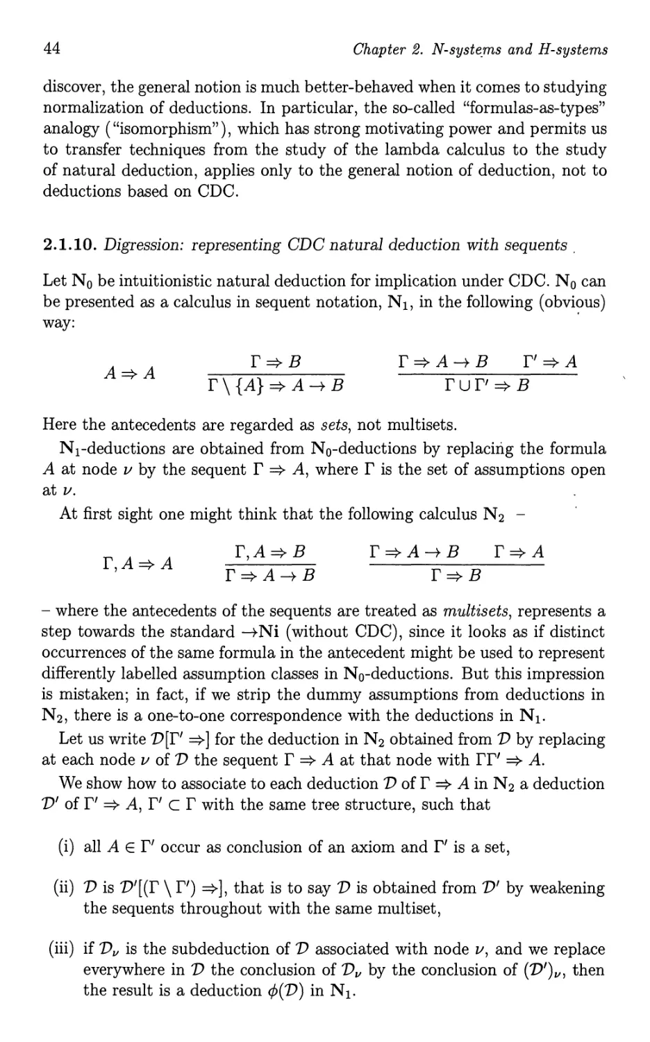
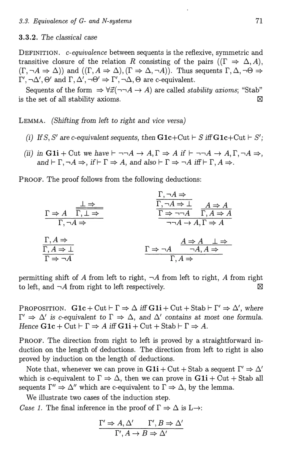
1.3 Three types of forITlalisITl
The greater part of this text deals with the theory of the "standard" logics,
that is minimal, intuitionistic and classical logic. In this section we introduce
the three styles of formalization: natural deduction, Gentzen systems and
Hilbert systems. (On the names and history of these types of formalism,
see the notes to chapters 2 and 3.) The first two will play a leading role in
the sequel; the Hilbert systems are well known and widely used in logic, but
less important from the viewpoint of structural proof theory. Each of these
formalization styles will be illustrated for implication logic.
Deductions will be presented as trees; the nodes will be labelled with for-
mulas (in the case of natural deduction and Hilbert systems) or with sequents
(for the Gentzen system); the labels at the immediate successors of a node v
are the premises of a rule application, the label at v the conclusion. At the
root of the tree we find the conclusion of the whole deduction.
The word proof will as a rule be reserved for the meta-level; for formal
arguments we preferably use deduction or derivation. But prooftree will mean
the same as deduction tree or derivation tree, and a "natural deduction proof"
will be a formal deduction in one of the systems of natural deduction. Rules
are schemas; an instance of a rule is also called a rule-application or inference.
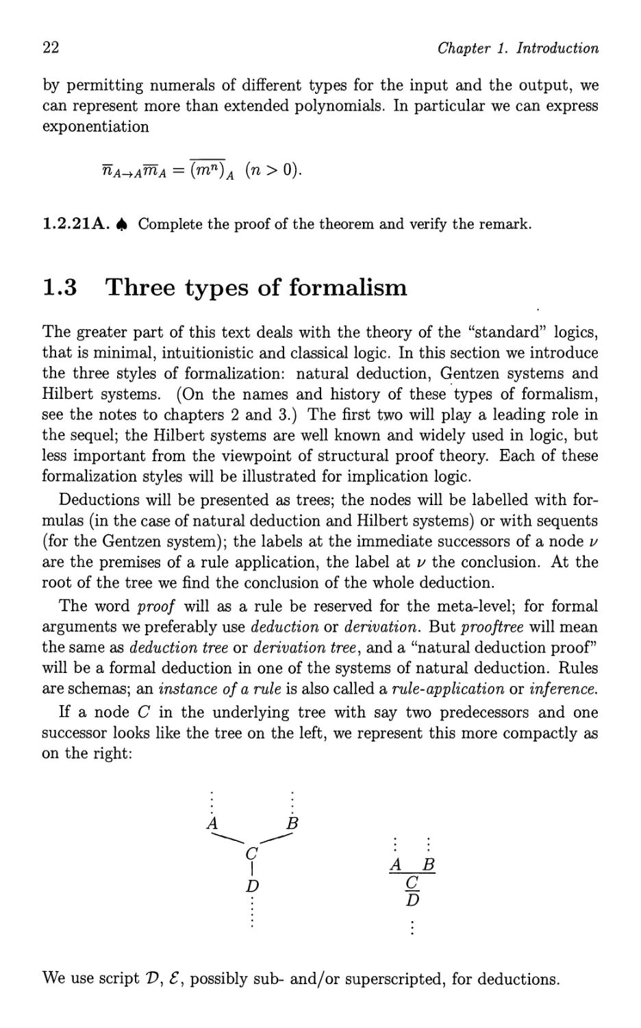
If a node C in the underlying tree with say two predecessors and one
successor looks like the tree on the left, we represent this more compactly as
on the right:
A B
----
C
I
D
A B
C
D
We use script V, [;, possibly sub- and/or superscripted, for deductions.
1.3. Three types of formalism
23
1.3.1. The BHK-interpretation
Minimal logic and intuitionistic logic differ only in the treatment of nega-
tion, or (equivalently) falsehood, and minimal implication logic is the same
as intuitionistic implication logic. The informal interpretation underlying in-
tuitionistic logic is the so-called Brouwer-Heyting-Kolmogorov interpretation
(BHK-interpretation for short); this interpretation tells us what it means to
prove a compound statement such as A -+ B in terms of what it means to
prove the components A and B (cf. classical logic, where the truthvalue of
A -+ B is defined relative to the truthvalues of A and B). As primitive notions
in the BHK-interpretation there appear "construction" and "(constructive,
informal) proof". These notions are admittedly imprecise, but nevertheless
one may convincingly argue that the usual laws of intuitionistic logic hold for
them, and that, for our understanding of these primitives, certain principles
of classical logic are not valid for the interpretation. We here reproduce the
clause for implication only:
A construction p proves A -+ B if p transforms any possible proof q of
A into a proof p(q) of B.
A logical law of implication logic, according to the BHK-interpretation, is a
formula for which we can give a proof, no matter how we interpret the atomic
formulas. A rule is valid for this interpretation if we know how to construct
a proof for the conclusion, given proofs of the premises.
The following two rules for -+ are obviously valid on the basis of the BHK-
interpretation:
( a) If, starting from a hypothetical (unspecified) proof u of A, we can find
a proof t( u) of B, then we have in fact given a proof of A -+ B (without
the assumption that u proves A). This proof may be denoted by AU.t(U).
(b) Given a proof t of A -+ B, and a proof s of A, we can apply t to s
to obtain a proof of B. For this proof we may write App(t, s) or ts (t
applied to s).
1.3.2. A natural deduction system for minimal implication logic
Characteristic for natural deduction is the use of assumptions which may
be closed at some later step in the deduction. Assumptions are formula
occurrences appearing at the top nodes (leaves) of the proof tree; they may
be open or closed. Assumptions are provided with markers (a type of label).
Any kind of symbol may be used for the markers, but below we suppose the
markers to be certain symbols for variables, such as u, v, w, possibly sub- or
superscripted.
The assumptions in a deduction which are occurrences of the same formula
with the same marker form together an assumption class. The notations
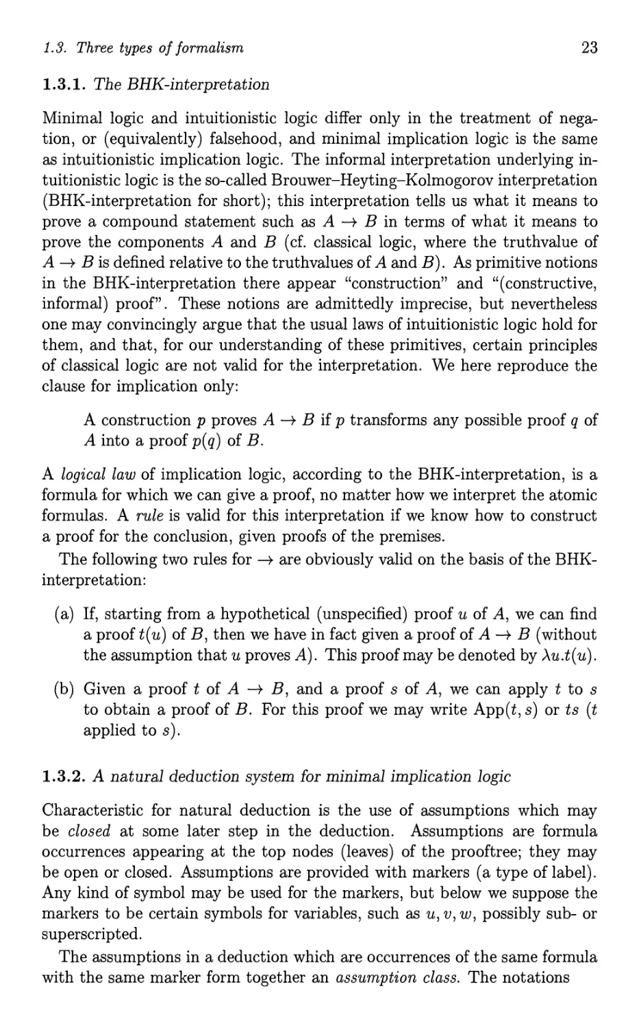
24 Chapter 1. Introduction
[A]U AU V' V'
[A] A
V V
V V
B B
B B
have the following meaning, from left to right: (1) a deduction V with con-
clusion B and a set [A] of open assumptions, consisting of all occurrences of
the formula A at top nodes of the proof tree V with marker u (note: both B
and the [A] are part of V, and we do not talk about the multiset [A]U since
we are dealing with formula occurrences); (2) a deduction V with conclusion
B and a single assumption of the form A marked u occurring at some top
node; (3) deduction V with a deduction V', with conclusion A, substituted
for the assumptions [A]U of V; (4) the same, but now for a single assumption
occurrence A in V. Under (3) the formula A shown is the conclusion of V'
as well as the formula in an assumption class of V.
In cases (3) and (4) this metamathematical notation may be considered
imprecise, since we have not indicated the label of A before substitution. But
in practice this will not cause confusion. Note that the marker u disappears
by the substitution: only topformulas bear markers.
We now consider a system -+Nm for the minimal theory of implication.
Proof trees are constructed according to the following principles.
A single formula occurrence A labelled with a marker is a single-node
proof tree, representing a deduction with conclusion A from open assumption
A.
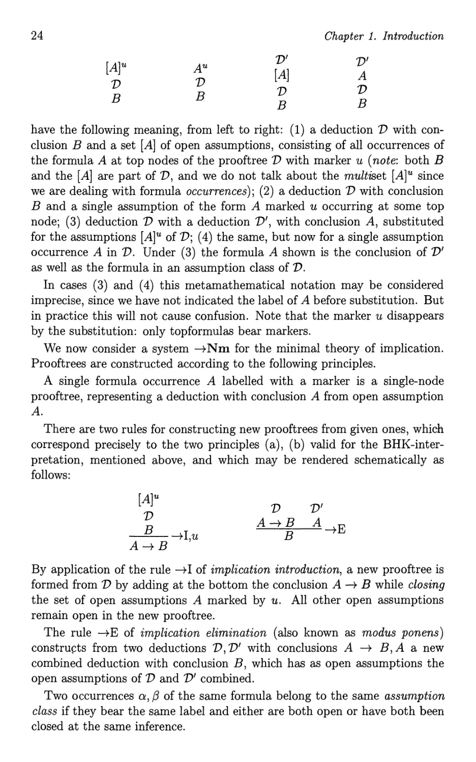
There are two rules for constructing new proof trees from given ones, which
correspond precisely to the two principles (a), (b) valid for the BHK-inter-
pretation, mentioned above, and which may be rendered schematically as
follows:
[A]U
V
B -+1 u
A-+B '
V
A-+B
B
V'
A-+ E
By application of the rule -+1 of implication introduction, a new proof tree is
formed from V by adding at the bottom the conclusion A -+ B while closing
the set of open assumptions A marked by u. All other open assumptions
remain open in the new proof tree.
The rule -+ E of implication elimination (also known as modus ponens)
constru ts from two deductions V, V' with conclusions A -+ B, A a new
combined deduction with conclusion B, which has as open assumptions the
open assumptions of V and V' combined.
Two occurrences a, /3 of the same formula belong to the same assumption
class if they bear the same label and either are both open or have both been
closed at the same inference.
1.3. Three types of formalism
25
It should be noted that in the rule -+1 the "degenerate case", where [A]U
is empty, is permitted; thus for example the following is a correct deduction:
AU
v
B-+A u
A -+ (B -+ A)
At the first inference an empty class of occurrences is discharged; we have
assigned this "invisible class" a label v, for reasons of uniformity of treatment,
but obviously the choice of label is unimportant as long as it differs from all
other labels in use; in practice the label at the inference may be omitted in
such caseS.
In applying the rule -+1, we do not assume that [A] consists of all open as-
sumptions of the form A occurring above the inference. Consider for example
the following two distinct (inefficient) deductions of A-+(A-+A):
AU
A-+A v AW
A u
A-+A w
A -+ (A -+ A)
AU
A-+A u AV
A v
A-+A w
A -+ (A -+ A)
The formula tree in these deductions is the same, but the pattern of closing as-
sumptions differs. In the second deduction all assumptions of the given form
which are still open before application of an inference -+1 are closed simulta-
neously. Deductions which have this property are said to obey the Complete
Discharge Convention; we shall briefly return to this in 2.1.9. But, no matter
how natural this convention may seem if one is interested in deducible formu-
las, for deductions as combinatorial structures it is an undesirable restriction,
as we shall see later.
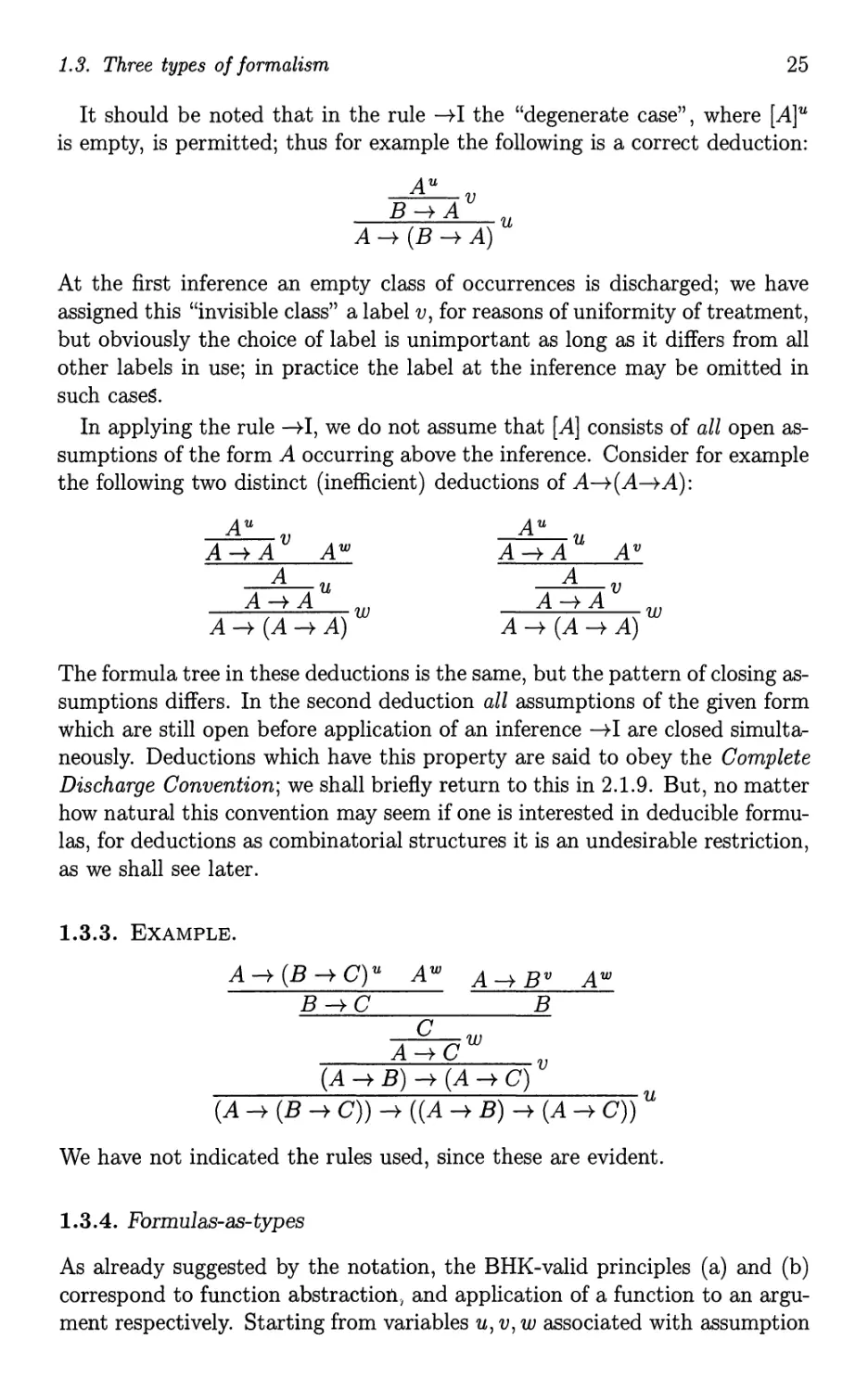
1.3.3. EXAMPLE.
A -+ (B -+ C) U A W
B-+C
A -+ BV
B
AW
C w
A-+C v
(A -+ B) -+ (A -+ C)
u
(A -+ (B -+ C)) -+ ((A -+ B) -+ (A -+ C))
We have not indicated the rules used, since these are evident.
1.3.4. Formulas-as-types
As already suggested by the notation, the BHK-valid principles (a) and (b)
correspond to function abstractioIl 1 and application of a function to an argu-
ment respectively. Starting from variables u, v, w associated with assumption
26
Chapter 1. Introduction
formulas, these two principles precisely generate the terms of simple type
theory A-t.
Transferring these ideas to the formal rules constructing proof trees, we
see that parallel to the construction of the proof tree, we may write next
to each formula occurrence the term describing the proof obtained in the
sub deduction with this occurrence as conclusion.
(i) To assumptions A correspond variables of type A; more precisely, for-
mulas with the same marker get the same variable. If we have already used
variable symbols as markers, we can use these same variables for the corre-
spondence.
(ii) For the rules -+1 and -+E the assignment of terms to the conclusion,
constructed from term( s) for the premise( s), is shown below.
[u: A]
V
t: B u
AUA.t B : A -+ B
V V'
t:A -+ B s:A
(tA-tB sA): B
Thus there is a very close relationship between A-+ and -+Nm, which at
first comes as a surprise. In fact, the terms of A-t are nothing else but
an alternative notation system for deductions in -+Nm. That is to say, if
we consider just the term assigned to the conclusion of a deduction, and
assuming not only the whole term to carry its type, but also all its subterms,
the proof tree may be unambiguously reconstructed from this term. This is
the basic observation of the formulas-as-types isomorphism, an observation
which has proved very fruitful, since it is capable of being extended to many
more complicated logical systems on the one haqd, and more complicated
type theories on the other hand, and permits us to lift results and methods
of type theory to logic and vice versa.
By way of illustration, we repeat our previous example, but now at each
node of the proof tree we also exhibit the corresponding terms. We have not
shown the types of subterms, since these follow readily from the construction
of the tree. We have dropped the superscript markers at the assumptions,
as well as the repetition of markers at the line where an assumption class is
discharged, since these are now redundant.
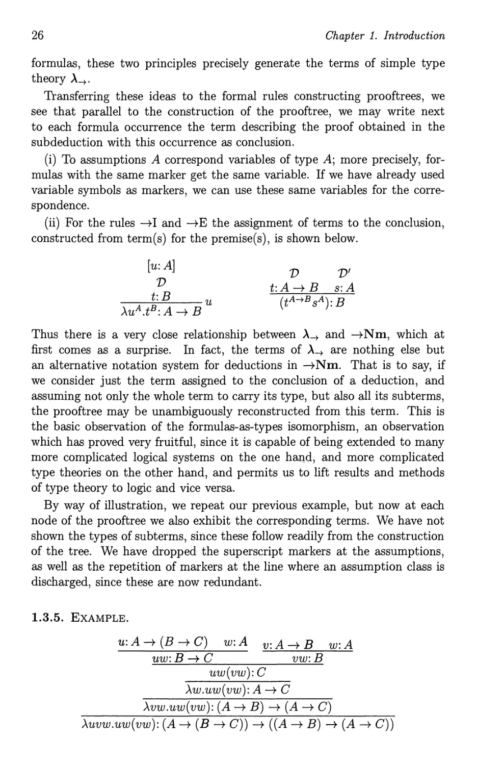
1.3.5. EXAMPLE.
u: A -+ (B -+ C) w: A v: A -+ B w: A
uw:B-+C vw:B
uw(vw): C
AW.UW(vw): A -+ C
AVW.UW(vw): (A -+ B) -+ (A -+ C)
AUVW.UW(vw): (A -+ (B -+ C)) -+ ((A -+ B) -+ (A -+ C))
1.3. Three types of formalism
27
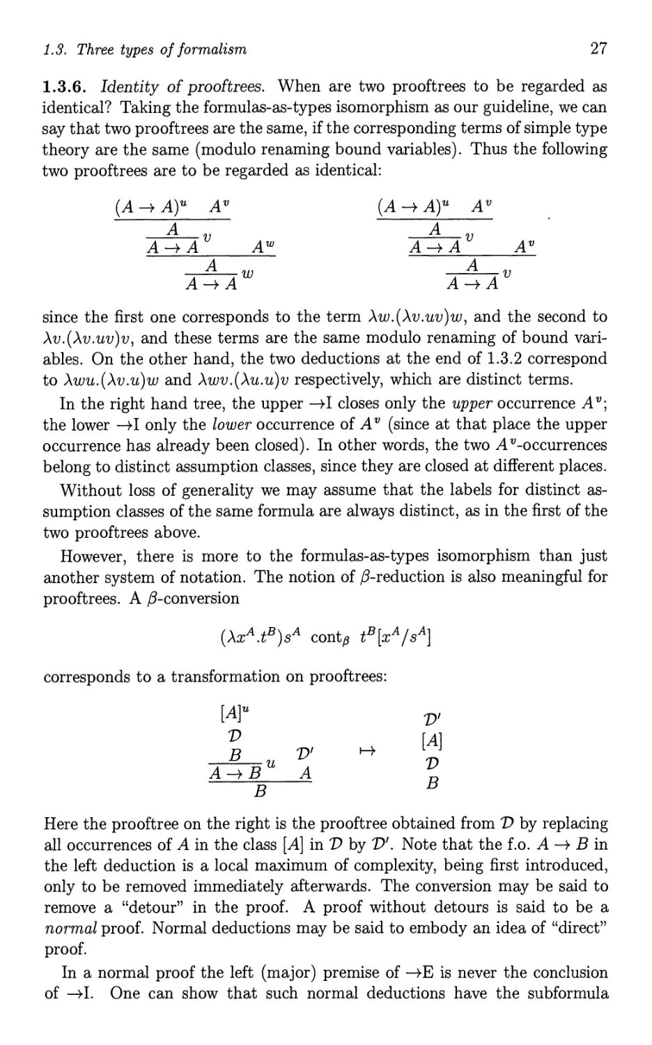
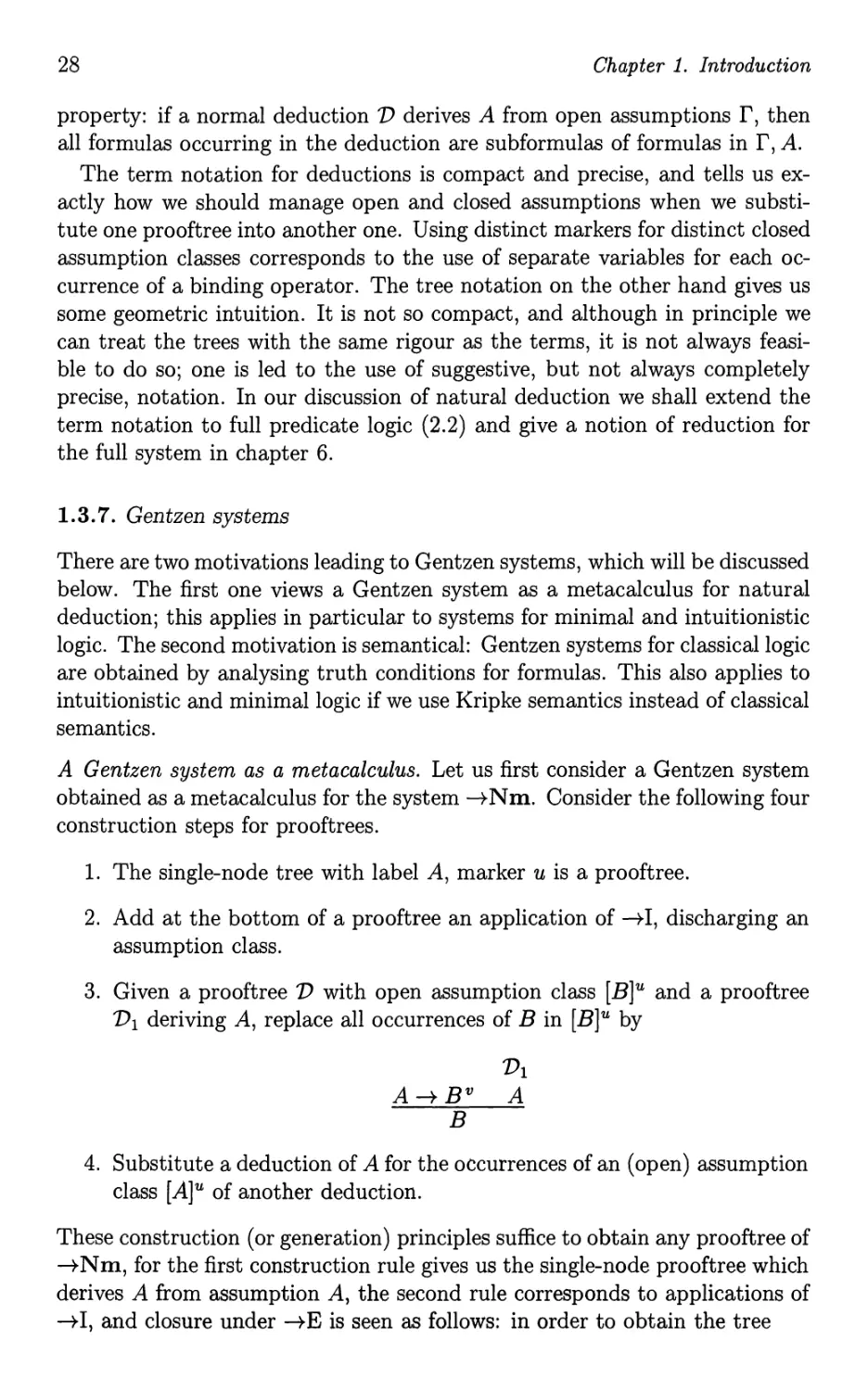
1.3.6. Identity of proof trees. When are two proof trees to be regarded as
identical? Taking the formulas-as-types isomorphism as our guideline, we can
say that two proof trees are the same, if the corresponding terms of simple type
theory are the same (modulo renaming bound variables). Thus the following
two proof trees are to be regarded as identical:
(A -+ A)U AV
A
A-+A v AW
A
A-+A w
(A -+ A)U AV
A
A-+A v AV
A
A-+A v
since the first one corresponds to the term AW.(AV.UV)W, and the second to
AV.(AV.UV)V, and these terms are the same modulo renaming of bound vari-
ables. On the other hand, the two deductions at the end of 1.3.2 correspond
to AWU.(AV.U)W and AWV.(AU.U)V respectively, which are distinct terms.
In the right hand tree, the upper -+1 closes only the upper occurrence A v;
the lower -+1 only the lower occurrence of A v (since at that place the upper
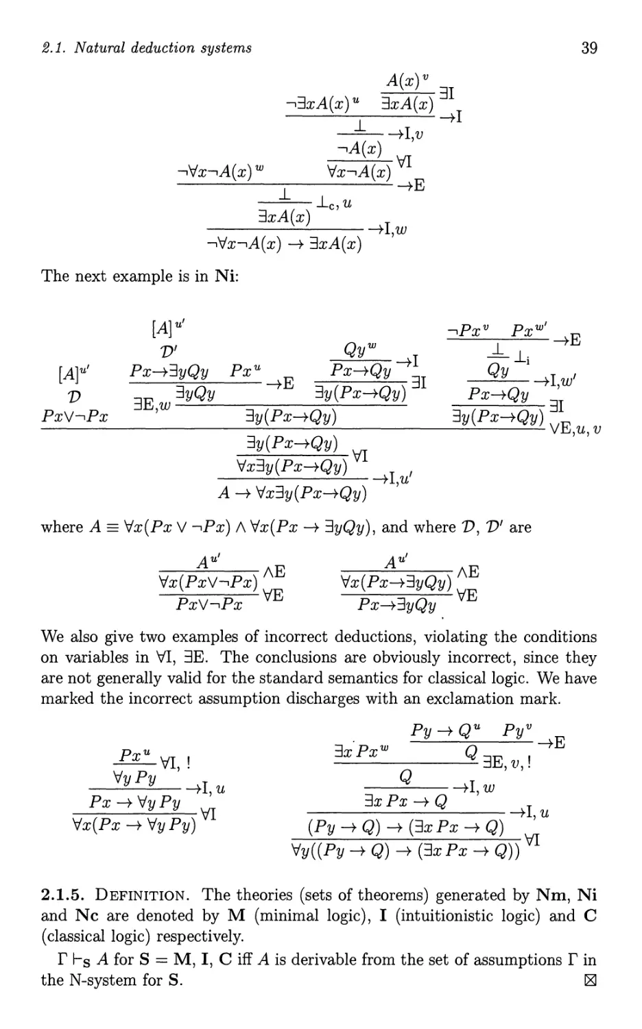
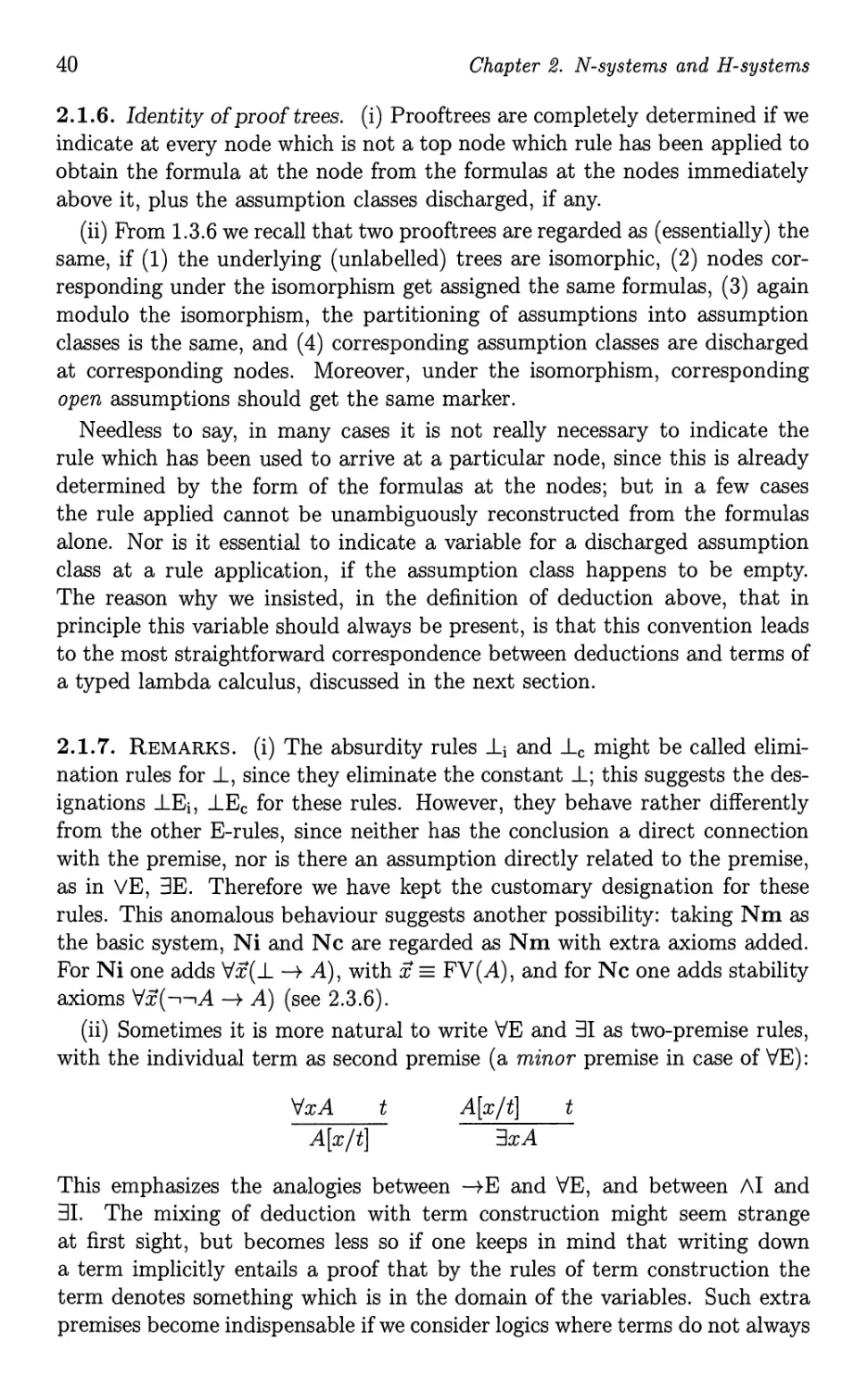
occurrence has already been closed). In other words, the two A v -occurrences
belong to distinct assumption classes, since they are closed at different places.
Without loss of generality we may assume that the labels for distinct as-
sumption classes of the same formula are always distinct, as in the first of the
two proof trees above.
However, there is more to the formulas-as-types isomorphism than just
another system of notation. The notion of f3-reduction is also meaningful for
proof trees. A /3-conversion
(AX A .tB)sA cont,B t B [x A / sA]
corresponds to a transformation on proof trees :
[A]U
V
B V'
A-+B u A
B
V'
[A]
V
B
Here the proof tree on the right is the proof tree obtained from V by replacing
all occurrences of A in the class [A] in V by V'. Note that the f.o. A -+ B in
the left deduction is a local maximum of complexity, being first introduced,
only to be removed immediately afterwards. The conversion may be said to
remove a "detour" in the proof. A proof without detours is said to be a
normal proof. Normal deductions may be said to embody an idea of "direct"
proof.
In a normal proof the left (major) premise of -+E is never the conclusion
of -+1. One can show that such normal deductions have the subformula
28
Chapter 1. Introduction
property: if a normal deduction V derives A from open assumptions r, then
all formulas occurring in the deduction are subformulas of formulas in r, A.
The term notation for deductions is compact and precise, and tells us ex-
actly how we should manage open and closed assumptions when we substi-
tute one proof tree into another one. Using distinct markers for distinct closed
assumption classes corresponds to the use of separate variables for each oc-
currence of a binding operator. The tree notation on the other hand gives us
some geometric intuition. It is not so compact, and although in principle we
can treat the trees with the same rigour as the terms, it is not always feasi-
ble to do so; one is led to the use of suggestive, but not always completely
precise, notation. In our discussion of natural deduction we shall extend the
term notation to full predicate logic (2.2) and give a notion of reduction for
the full system in chapter 6.
1.3.7. Gentzen systems
There are two motivations leading to Gentzen systems, which will be discussed
below. The first one views a Gentzen system as a metacalculus for natural
deduction; this applies in particular to systems for minimal and intuitionistic
logic. The second motivation is semantical: Gentzen systems for classical logic
are obtained by analysing truth conditions for formulas. This also applies to
intuitionistic and minimal logic if we use Kripke semantics instead of classical
semantics.
A Gentzen system as a metacalculus. Let us first consider a Gentzen system
obtained as a metacalculus for the system -+Nm. Consider the following four
construction steps for proof trees.
1. The single-node tree with label A, marker u is a proof tree.
2. Add at the bottom of a proof tree an application of -+1, discharging an
assumption class.
3. Given a proof tree V with open assumption class [B]U and a proof tree
VI deriving A, replace all occurrences of B in [B]U by
VI
A -+ BV A
B
4. Substitute a deduction of A for the occurrences of an (open) assumption
class [A]U of another deduction.
These construction (or generation) principles suffice to obtain any proof tree of
-+Nm, for the first construction rule gives us the single-node proof tree which
derives A from assumption A, the second rule corresponds to applications of
-+ I, and closure under -+ E is seen as follows: in order to obtain the tree
1.3. Three types of formalism 29
1)1 1)2
A-+B A
B
from the proof trees 1)1, 1)2, we first combine the first and third construction
principles to obtain
1)2
A -+ BU A
B
and then use the fourth (substitution) principle to obtain the desired tree.
Let r ::::} A express that A is deducible in -+Nm from assumptions in r.
Then the four construction principles correspond to the following axiom and
rules for obtaining statements r ::::} A:
r U {A} ::::} A (Axiom)
r ::::} A U {B} ::::} C L-+
r U U {A -+ B} ::::} C
r ::::} A U {A} ::::} B C
r U ::::} B ut
r U {A} ::::} B R-+
r::::}A-+B
Call the resulting system S (an ad hoc designation). Here in the sequents
r ::::} A the r is treated as a (finite) set. For bookkeeping reasons it. is
often convenient to work with multisets instead; multisets are "(finite) sets
with repetitions", or equivalently, finite sequences modulo the order of the
elements. If we rewrite the system above with multisets, we get the Gentzen
system described below, which we shall designate ad hoc by S/, and where in
the sequents r ::::} A the r is now a multiset. The rules and axioms of S/ are
A ::::} A (Axiom)
r ::::} A , B ::::} C L-+
r, ,A-+B::::}C
r,A::::}B R-+
r::::}A-+B
r ::::} A LW
r,B::::}A
r ::::} A A, ::::} B C
r, ::::} B ut
r, B, B ::::} A LC
r, B ::::} A
R-+ and L-+ are called the logical rules, LW, LC and Cut the structural rules.
LC is called the rule of (left-) contraction, LW the rule of (left-) weakening.
Due to the presence of LC and LW, derivability of r ::::} A is equivalent to
derivability of Set(r) ::::} A where Set(r) is the set underlying the multiset
30
Chapter 1. Introduction
r. We have simplified the axiom, since some applications of LW produce
r, A =} A from A =} A.
If one uses sequences instead of sets, in order to retain equivalence of deriv-
ability of r =} A and derivability of Set(r) =} A, an extra rule of exchange
then has to be added:
r,A,B, =} C LE
r,B,A, =} C
EXAMPLE. (Of a deduction in Sand S')
A =} A B =} B L-+
A-+B,A=}B
R-+
A =} (A -+ B) -+ B R-+
=} A -+ ((A -+ B) -+ B)
The natural deduction of (A -+ (B -+ C)) -+ ((A -7 B) -+ (A -+ C)),
which we gave earlier in example 1.3.3 may be obtained by repeated use of
the generation principles 1-3 (not 4) as follows:
3:A -+ (B -+ C)U 3:Aw
1: B -+ C
2:A-+BV 2:Aw
1: B
o:C w
4: A -+ C v
5: (A -+ B) -+ (A -+ C)
u
6: (A -+ (B -+ C)) -+ ((A -+ B) -+ (A C))
In the displayed tree, the numbers 0-6 indicate the seven steps in the construc-
tion of the tree. The number 0 corresponds to an application of construction
principle 1, the numbers 4-6 to applications of principle 2, the numbers 1 and
3 to applications of principle 3, and number 2 to an application of principle
3 in the construction of the subtree with conclusion B. We can now readily
transform this into a sequent deduction in S:
B =} B C =} C (0)
A=}A B,B-+C=}C (l)
A =} A A, A -+ B, B -+ C =} C (2)
A, A -+ B,A -+ (B -+ C) =} C( 3)
A -+ B,A -+ (B -+ C) =} A -+ C(4)
A -+ (B -+ C) =} (A -+ B) -+ (A -+ C) (5)
=} (A -+ (B -+ C)) -+ ((A -+ B) -+ (A -+ C)) (6)
where the lines 1-6 correspond to the steps 1-6 above; the only axiom appli-
cation appearing as a right premise for L-+, namely C =} C, corresponds to
step o.
Only a slight change is necessary to formulate the deduction in the calculus
with multisets:
1.3. Three types of formalism
31
B B C C
A A B,B-+C C
A A A,A -+ B,B -+ C C
A, A, A -+ B,A -+ (B -+ C) C
. LC
A, A -+ B, A -+ (B -+ C) C
A -+ B, A -+ (B -+ C) A -+ C
A -+ (B -+ C) (A -+ B) -+ (A -+ C)
(A -+ (B -+ C)) -+ ((A -+ B) -+ (A -+ C))
The appearance of two occurrences of A just before the LC-inference corre-
sponds to the two occurrences of A W in the original deduction in -+Nm.
It is not hard to convince oneself that, as long as only the principles 1-3
for the construction of proof trees are applied, the resulting proof will always
be normal. Conversely, it may be proved that all normal proof trees can be
obtained using construction principles 1-3 only. Thus we see that normal
proof trees in -+Nm correspond to deduction in the sequent calculus without
Cut; and since every proof in natural deduction may be transformed into a
normal proof of the same conclusion, using (at most) the same assumptions,
it also follows for the sequent calculus that every deducible sequent r A
must have a deduction without Cut.
Deductions in S without the rule Cut have a very nice property, which is
immediately obvious: the subformula property: all formulas occurring in a
deduction of r A are subformulas of the formulas in r, A.
A point worth noting is that the correspondence between sequent calculus
deductions and natural deductions is usually not one-to-one. For example, in
our transformation of the example 1.3.3 above, the steps 2 and 3 might have
been interchanged, resulting in a different deduction in S.
Another remark concerns construction principle 3: it follows in an indirect
way from the rule -+E. Instead of -+E we might take the following:
[B]U
V o VI V 2
-+ E* u A -+ B A C
, C
which closely corresponds to construction principle 3 (cf. 6.12.4).
1.3.7 A. . There are other possible choices for the construction principles for
proof trees. For example, we might replace principle 3 by the following principle 3':
Given a proof tree V with open assumption class [B]U, replace all occurrences of
B in [B]U by
A --+ B V A
B
Show that this also generates all natural deduction proof trees for implication logic;
what sequent rules do these modified principles give rise to?
32
Chapter 1. Introduction
1.3. 7B.. Show that the following proof tree requires an application of construc-
tion principle 4:
A-+A-+B AU
A-+B AU
B
A-+B u AV
B
1.3.8. Semantical motivation of Gentzen systems
For classical logic, we may arrive in a very natural way at a Gentzen system
by semantical considerations. Here we use sequents r =} , with r and
finite sets; the intuitive interpretation is that r =} is valid iff /\ r -+ V
is true. Now suppose we want to find out if there is a valuation making all of
r true and all of false. We can break down this problem by means of two
rules, one for reducing A -+ B on the left, another for reducing A -+ B on
the right:
r =} A, r, B =} L-+
r, A-+B =}
r,A=}B, R-+
r =} A-+B,
The problem of finding the required solution for the sequent at the bottom is
equivalent to finding the solution(s) for (each of) the sequent(s) at the upper
line. Thus starting at the bottom, we may work our way upwards; along each
branch, the possibility of applying the rules stops, if all components have been
reduced to atoms. If all branches terminate in sequents of the form r/, P =}
P, /, there is no valuation for the sequent r =} making r true and false.
Taking sequents r/, P =} P, / as axioms, the search tree for the valuation
has then in fact become a derivation of the sequent r =} from axioms and
L-+, R-+. This very simple argument constitutes also a completeness proof
for classical propositional logic, relative to a Gentzen system without Cut.
This idea for a completeness proof may also be adapted (in a not entirely
trivial way) to intuitionistic and minimal logic, with Kripke semantics as the
intended semantics.
The reader may be inclined to ask, why consider Gentzen systems at all?
They do look more involved than natural deduction. There are two reasons
for this. First of all, for certain logics Gentzen systems may be justified by
semantical arguments in cases where it is not obvious how to construct an
appropriate natural deduction system. Secondly, given the fact that there is
a special interest in systems with the subformula property (on which many
elementary proof-theoretic applications rest), we note that the condition of
normality, guaranteeing the subformula property for natural deduction, is a
global property of the deduction involving the order in which the rules are
applied, whereas for Gentzen systems this is simply achieved by excluding
the Cut rule.
1.3. Three types of formalism
33
1.3.9. A Hilbert system
A third type of formalism, extensively used in the logical literature, is the
Hilbert system. Here there is a notion of deduction from assumptions, as for
natural deductions, but assumptions are never closed. In Hilbert systems, the
number of rules is reduced at the expense of introducing formulas as axioms.
In most systems of this type, modus ponens (-+E) is in fact the only rule for
propositional logic.
The Hilbert system -+Hm for minimal implication logic has as axioms all
formulas of the forms:
.-.
A -+ (B -+ A) (k-axioms),
(A -+ (B -+ C)) -+ ((A -+ B) -+ (A -+ C)) (s-axioms),
for arbitrary A, Band C, and has -+E as the only rule. A deduction of B
from assumptions r is then a tree with formulas from r and axioms at the
top nodes, and the conclusion B at the root. (Usually, one finds K and S
instead of k and s in the literature, since K and S are standard notations
in combinatory logic. However, in modal logic one also encounters an axiom
schema K, and we wish to avoid confusion.)
EXAMPLE. A deduction V A of A --+ A:
[A--+((A--+A)--+A)] --+ [(A--+(A--+A))--+(A--+A)] A--+((A--+A)--+A)
(A--+(A--+A)) --+ (A--+A) A--+(A--+A)
A--+A
Deductions in Hilbert systems are often presented in linear format. Thus,
in the case of implication logic, we may define a deduction of a formula A
as a sequence AI, A 2 ,. . . , An such that A An' and moreover for each k
(1 < k < n) either Ak is an axiom, or there are Ai, Aj with i, j < k such that
Aj = Ai -+ Ak' For example, the proof tree above may be represented by the
following sequence:
(1)
(2)
(3)
(4)
(5)
[A-+((A-+A)-+A)] -+ [(A-+(A-+A))-+(A-+A)]
A-+((A-+A)-+A)
(A-+(A-+A)) -+ (A-+A)
A -+ (A -+ A)
A-+A
s-axlom
k-axiom
(1), (2)
k-axiom
(3), (4)
In fact, it is also possible to present natural deduction proofs and Gentzen
system deductions in such a linear form. Where the primary aim is to discuss
the actual construction of deductions, this is common practice in the literature
on natural deduction. The disadvantage of the tree format, when compared
with the linear format, is that the width of proof trees for somewhat more
complicated deductions soon makes it impracticable to exhibit them. On the
34
Chapter 1. Introduction
other hand, as we shall see, the tree format for natural deductions has decided
advantages for meta-theoretical considerations, since it provides an element
of geometrical intuition.
There is also a formulas-as-types isomorphism for -+Hm, but this time the
corresponding term system is CL-t, where the constants k and s represent
the axioms (cf. 1.2.17)
kA,B : A -+ (B -+ A),
SA,B,C : (A -+ (B -+ C)) -+ ((A -+ B) -+ (A -+ C)),
and application corresponds to -+E as for natural deduction.
EXAMPLES. We write AB as an abbreviation for A -+ B.
kB(CB),A: (B(CB))(A(B(CB))) kB,c : B(CB)
kB(CB),AkB,C : A(B(CB))
The proof tree exhibited before, establishing A -+ A, corresponds to a term
SA,A-tA,AkA,A-tAkA,A.
The notion of weak reduction of course transfers from terms of CL-t to -+ Hm,
but is of far less interest than tJ-reduction for -+Nm. However, the construc-
tion of an "abstraction-surrogate" ;\*x in 1.2.19 plays a role in proving the
equivalence (w.r.t. derivable formulas) between systems of natural deduction
and Hilbert systems, since it corresponds to a deduction theorem (see 2.4.2),
and thereby provides us with a method for translating natural deduction
proofs into Hilbert system proofs.
Chapter 2
N -systems and H -systems
Until we come to chapter 9, we shall concentrate on our three standard logics:
classical logic C, intuitionistic logic I and minimal logic M. The informal in-
terpretation (semantics) for C needs no explanation here. The logic I was
originally motivated by L. E. J. Brouwer's philosophy of mathematics (more
information in Troelstra and van Dalen [1988, chapter 1]); the informal inter-
pretation of the intuitionistic logical operators, in terms of the primitive no-
tions of "construction" and "constructive proof" , is known as the "Brouwer-
Heyting-Kolmogorov interpretation" (see 1.3.1, 2.5.1). Minimal logic M is a
minor variant of I, obtained by rejection of the principle "from a falsehood
follows whatever you like" (Latin: "ex falso sequitur quodlibet", hence the
principle is often elliptically referred to as "ex falso"), so that, in M, the
logical symbol for falsehood .1. behaves like some unprovable propositional
constant, not playing a role in the axioms or rules.
This chapter opens with a precise description of N-systems for the full
first-order language with proofs in the form of deduction trees, assumptions
appearing at top nodes. After that we present in detail' .the corresponding
term system for the intuitionistic N-system, an extension of simple type the-
ory. Once a precise formalism has been specified, we are ready for a section on
the G6del-Gentzen embedding of classical logic into minimal logic. This sec-
tion gives some insight into the relations between C on the one hand and M,
I on the other hand. Finally we introduce Hilbert systems for our standard
logics and prove their deductive equivalence to the corresponding N-systems.
2.1 Natural deduction systeITls
We use script V, £, possibly sub- and/or superscripted, for deductions,"and
adopt the notational conventions for proof trees with assumptions' and con-
clusion adopted at the beginning of 1.3.2.
2.1.1. DEFINITION. (The systems Nm, Ni, Nc) Assumptions are formula
occurrences always appearing at the top of a branch (assumptions are "leaves"
35
36
Chapter 2. N-systems and H-systems
of the tree), and are supposed to be labelled by markers (e.g. natural numbers,
or variable symbols). The set of assumptions of the same form with the
same marker forms an assumption class. Distinct formulas must have distinct
markers. We permit empty assumption classes!
Assumptions may be closed; assumption classes are always closed "en bloc" ,
that is to say, at each inference, either all assumptions in a class are closed,
or they are all left open. Closure is indicated by repeating the marker ( s) of
the class( es) at the inference.
For ease in the exposition, we shall reserve u, v, w for assumption markers,
and x, y, z for individual variables.
Deductions in the system of natural deduction are generated as follows.
Basis. The single-node tree with label A (Le. a single occurrence of A) is a
(natural) deduction from the open assumption A; there are no closed assump-
tions.
Inductive step. Let Vb V 2 , Va be deductions. A (natural) deduction V may
be constructed according to one of the rules below. The classes [A]U, [B]V,
[-.A]U below contain open assumptions of the deductions of the premises of
the final inference, but are closed in the whole deduction.
For /\, V, -+, "I, 3 we have introduction rules (I-rules) and elimination rules
(E-rules).
VI V 2 VI VI
A B A /\ B /\E A /\ B /\E
A /\ B /\1 A R B L
[A]U VI V 2
VI
A-+B A-+ E
B -+1 u B
A-+B '
VI
A vI
AVB R
VI
B VI
AVB L
VI
AVB
[A]U
V 2
C
C
[B]V
Va
C
VE, u, v
VI
A[x/y]
'ixA "II
In VI: y = x or y (j. FV(A),
and y not free in any assump-
tion open in VI.
VI
"Ix A
A[x/t] \IE
VI
A[x/t]
3xA 31
VI
3xA
C
[A [x/y]]U
V 2
C 3Eu
,
In 3E: y = x or y (j. FV(A),
and y not free in C nor in any
assumption open in V 2 except
in [A [x / y]] U .
2.1. Natural deduction systems
37
This completes the description of the rules for minimal logic Nm. Note that
-L has not been mentioned in any of the above rules, and therefore it behaves
in minimal logic as an arbitrary unprovable propositional constant.
To obtain the intuitionistic and classical systems Ni and Nc we add the
intuitionistic absurdity rule -L i and the more general classical absurdity rule
-Lc respectively:
VI
-L
--L.
A 1
[-,A]U
VI
-L
- -Lc,u
A
(-Lc is more general than -L i since [-,A]U) may be empty.) In an E-rule ap-
plication, the premise containing the occurrence of the logical operator being
eliminated is called the major premise; the other premise(s) are called the
minor premise(s) of the rule application. As a standard convention in display-
ing proof trees, we place the major premises of elimination rule applications
in leftmost position.
To spell out the open and closed assumptions for the rules exhibited above:
. When -+1 is applied, the set [A]U of open assumptions of the form A in
V becomes closed; when VE is applied, the set [A]U of open assumptions
of the form A in V 2 and the set [B]V of open assumptions of the form
B in V 3 become closed; when 3E is applied, the set [A[x/y]]U of open
assumptions of the form A in V 2 becomes closed; when -Lc is applied,
the set [-,A]U of open assumptions of the form -,A in VI becomes closed.
All other assumptions, not covered by the cases just mentioned, stay
open.
As to the individual variables which are considered to be free in a deduction,
we stipulate
. The deduction consisting of assumption A only has FV(A) as free vari-
abl es;
. at each rule application, the free individual variables are inherited from
the immediate subdeductions, except that
. in an application of 3E the occurrences of the free variable y in V 2
become bound, and in an application of 'VI the occurrences of variable
y in VI become bound, and
.: in -+1 the variables in FV(A) have to be added in case [A]U is empty, in
VIR those in FV(B) have to be added, and in VI L those in FV(A) have
to be added.
38
Chapter 2. N-systems and H-systems
The individual variable becoming bound in an application a of 'VI or 3E is
said to be the proper variable of a.
Instead of closed (assumption) one also finds in the literature the terminol-
ogy eliminated or cancelled or discharged. Because of the correspondence of
closed assumptions with bound variables in the term calculus (to be explained
in detail in the next section) we also sometimes use "bound" for "closed". If
A is among the open assumptions of a deduction 1) with conclusion B, the
conclusion B in V is said to depend on A in V. From now on we regard
"assumption of V" and "open assumption of V' as synonymous.
2.1.2. DEFINITION. A convenient global assumption in the presentation of
a deduction is the variable convention. A deduction is said to satisfy the
variable convention if the proper variables of the applications of 3E and 'VI
are kept distinct. That is to say, the proper variable of an application a of
3E or 'VI occurs in the deduction only above a.
If moreover the bound and free variables are kept distinct, the deduction
is said to be a pure-variable deduction. Henceforth we shall usually assume
that the pure-variable condition is satisfied.
2.1.3. REMARKS. (i) Since in our notation for proof trees, [A]U refers to
all assumptions A labelled u, it is tacitly understood that in VE the label u
occurs in V 2 only, and v in V 3 only. Similarly, in 3E the marker u occurs
in V 2 only. This restriction may be relaxed, at the expense of a much more
clumsy formulation of 3E and VE.
(ii) The rules of (extensions of) natural deduction systems are often pre-
sented in a more informal style. Instead of using inductive clauses "If V o ,
VI, . . . are correct deductions, then so is V" as we did above, we can also de-
scribe the rules by exhibiting premises and assumptions to be discharged (if
any), where the deductions between assumptions and premises are indicated
by vertical dots. Thus -+E and VE are given by the schemas
[A]U [B]V
A -+ B A -+E
B
AVB C
C
C
VE,u, v
2.1.4. EXAMPLES. The first example is in the classical system Nc:
2.1. Natural deduction systems
39
A(x) v
:H
-,3xA(x)U 3xA(x)
-+1
-L -+1 v
,
-,A( x)
'VI
-,'Vx-,A(x) W 'Vx-,A(x)
-L -+E
-L u
3xA(x) c,
-+I,w
-,'Vx-,A(x) -+ 3xA(x)
The next example is in Ni:
QyW
Px u Px-+Qy -+ I
-+E 3y(Px-+Qy)
3y(Px-+Qy)
3y(Px-+Qy) VI
'Vx3y(Px-+Qy) I
-+I,u
A -+ 'Vx3y(Px-+Qy)
where A 'Vx(Px V -,Px) 1\ 'Vx(Px -+ 3yQy), and where V, V' are
[A ]U'
V
PxV-,Px
[ A] u'
V'
Px-+3yQy
3E,w 3yQy
,
-,Px V PX W
1- -+E
--L i
Qy -+1 w'
,
Px-+Qy
31
3y(Px-+Qy) E
V , u, v
AU'
I\E
'Vx(PxV-'Px)
'VE
PxV-,Px
AU'
I\E
'Vx(Px-+3yQy)
'VE
Px-+3yQy
We also give two examples of incorrect deductions, violating the conditions
on variables in 'VI, 3E. The conclusions are obviously incorrect, since they
are not generally valid for the standard semantics for classical logic. We have
marked the incorrect assumption discharges with an exclamation mark.
Px U 'VI, !
'Vy Py I
-+ , u
Px -+ 'Vy Py 'VI
'Vx(Px -+ 'Vy Py)
Py -+ QU Pyv
3x Px w Q -+E
3E, v, !
Q -+1 w
,
3x Px -+ Q I
-+ , u
(Py -+ Q) -+ (3x Px -+ Q)
Vy((Py -+ Q) -+ (3x Px -+ Q)) VI
2.1.5. DEFINITION. The theories (sets of theorems) generated by Nm, Ni
and Nc are denoted by M (minimal logic), I (intuitionistic logic) and C
(classical logic) respectively.
r r-s A for S == M, I, C iff A is derivable from the set of assumptions r in
the N-system for S.
40
Chapter 2. N-systems and H-systems
2.1.6. Identity of proof trees. (i) Proof trees are completely determined if we
indicate at every node which is not a top node which rule has been applied to
obtain the formula at the node from the formulas at the nodes immediately
above it, plus the assumption classes discharged, if any.
(ii) From 1.3.6 we recall that two proof trees are regarded as (essentially) the
same, if (1) the underlying (unlabelled) trees are isomorphic, (2) nodes cor-
responding under the isomorphism get assigned the same formulas, (3) again
modulo the isomorphism, the partitioning of assumptions into assumption
classes is the same, and (4) corresponding assumption classes are discharged
at corresponding nodes. Moreover, under the isomorphism, corresponding
open assumptions should get the same marker.
Needless to say, in many cases it is not really necessary to indicate the
rule which has been used to arrive at a particular node, since this is already
determined by the form of the formulas at the nodes; but in a few cases
the rule applied cannot be unambiguously reconstructed from the formulas
alone. Nor is it essential to indicate a variable for a discharged assumption
class at a rule application, if the assumption class happens to be empty.
The reason why we insisted, in the definition of deduction above, that in
principle this variable should always be present, is that this convention leads
to the most straightforward correspondence between deductions and terms of
a typed lambda calculus, discussed in the next section.
2.1.7. REMARKS. (i) The absurdity rules 1.. i and 1..e might be called elimi-
nation rules for 1.., since they eliminate the constant 1..; this suggests the des-
ignations 1..E i , 1..Ee for these rules. However, they behave rather differently
from the other E-rules, since neither has the conclusion a direct connection
with the premise, nor is there an assumption directly related to the premise,
as in VE, 3E. Therefore we have kept the customary designation for these
rules. This anomalous behaviour suggests another possibility: taking Nm as
the basic system, Ni and Nc are regarded as Nm with extra axioms added.
For Ni one adds 'v'x(1.. -+ A), with x = FV(A), and for Nc one adds stability
axioms 'v'i( I-,A -+ A) (see 2.3.6).
(ii) Sometimes it is more natural to write 'v'E and :U as two-premise rules,
with the individual term as second premise (a minor premise in case of 'v'E):
'v'xA t
A[x/t]
A[x/t] t
3xA
This emphasizes the analogies between -+E and 'v'E, and between /\1 and
31. The mixing of deduction with term construction might seem strange
at first sight, but becomes less so if one keeps in mind that writing down
a term implicitly entails a proof that by the rules of term construction the
term denotes something which is in the domain of the variables. Such extra
premises become indispensable if we consider logics where terms do not always
2.1. Natural deduction systems
41
denote; see 6.5. This convention is also utilized in chapter 10. If one wants to
stress the relation to type theory, one writes t: D (D domain of individuals)
for the second premise.
(iii) The statement of the rules 'VI and 3E may be simplified somewhat if
we rely on our convention that formulas differing only in the naming of bound
variables are equal. These rules may then be written as:
VI
A
'V x A 'VI
VI
3xA
C
[A]U
V 2
C 3Eu
,
where in 'VI x is not free in any assumption open in VI, and in 3E x is not
free in C nor in any assumption open in V 2 except in [A]u.
(iv) In theories based on logic, we may accommodate axioms as rules with-
out premises; so an axiom appears in a proof tree as a top node with a line
over it (in practice we often drop this line).
2.1.8. Natural deductions in sequent style
In the format described above, the assumptions open at any node v in a de-
duction tree V are found by looking at the top nodes above v; the ones bearing
a label not yet discharged between the top node and v are still open at v.
Less economical in writing, but for metamathematical treatment sometimes
more convenient, is a style of presentation where the open assumptions are
carried along and exhibited at each node. We call the set of open assumptions
at a node the context. A context is a set
U1: AI, U2: A 2 , . . . , Un: An
where the Ui are pairwise distinct; the Ai need not be distinct. The deductions
now become trees where each node is labelled with a sequent of the form
r =} B, r a context. Below, when writing a union of contexts such as r
(short for r u ), it will always be assumed that the union is consistent, that
is to say, again forms a context. In this form the rules and axioms now read
as follows:
U : A =} A (Axiom)
r[u: A] =} B -+1
r=}A-+B
r =} A =} B /\1
r =}A/\B
r=}A-+B =}A E
r =}B -+
r =} Ao /\ Al /\E
r =} Ai
r =} Ai VI
r =} Ao V Al
r =} A V B [u: A] =} C /[v: B] =} C vE
r / =} C
42
Chapter 2. N-systems and H-systems
r[x: -,A] =} 1.. 1..
r=}A C
r =} 1.. 1...
r=}A 1
r =} A[x/y] 'VI
r =} 'VxA
r =} 'VxA VE
r =} A[x/t]
r =} 3yA[x/y] [u: A] =} 0 3E
r =} 0
r =} A[x/t] 31
r =} 3xA
Here [u: 0] means that the assumption u: 0 in the context may be present or
absent. Moreover, in -+1 u: A does not occur in r, in VE u: A and v: B do
not occur in r ', in 1..c u: -,A does not occur in r, and in 3E u: A does not
occur in r .
The correspondence is now such that at any node precisely the inhabited
assumption classes which are not yet closed at that node are listed.
2.1.8A.. Give proofs in Nm or Ni of
A -+ (B -+ A);
A-+AVB, B-+(AVB);
(A -+ C) -+ [(B -+ C) -+ (A V B -+ C)];
A 1\ B -+ A, A 1\ B -+ B, A -+ (B -+ A 1\ B);
..1 -+ A;
VxA -+ A[x/t]; A[x/t] -+ 3xA;
Vx(B -+ A) ++ (B -+ VyA[x/y]) (x (j. FV(B), y = x or y (j. FV(A));
Vx(A -+ B) ++ (3yA[x/y] -+ B) (x (j. FV(B), y = x or y (j. FV(A)).
2.1.8B..* Give proofs in Nm of
A -+ -,-,A;
-,-,-,A ++ -,A;
-,-,(A -+ B) -+ (-,-,A -+ -,-,B);
-,-,(A 1\ B) ++ (-,-,A 1\ -,-,B);
-,(A V B) ++ (-,A 1\ -,B);
-,-,VxA -+ Vx-,-,A.
2.1.8C.. Give proofs in Nm of
(B -+ C) -+ (A -+ B) -+ A -+ C (b-axioms),
(A -+ B -+ C) -+ B -+ A -+ C (c-axioms),
(A -+ A -+ B) -+ A -+ B (w-axioms).
2.1.8D. . Prove in Ni (-,-,A -+ -,-,B) -+ -,-,(A -+ B). Hint. First construct
deductions of -,-,A and of -,B from the assumption -,(A -+ B).
2.1. Natural deduct'lon systems
43
2.1.8E..r.* Prove in Nc
A V B ++ -,( -,A !\ -,B),
3xA ++ -,Vx-,A,
((A --+ B) --+ A) --+ A (Peirce's law).
2.1. 8F. .r. * Construct in --+ N m a proof of
((A --+ B) --+ C) --+ (A --+ C) --+ C
from two instances of Peirce's law as assumptions: ((A --+ B) --+ A) --+ A and
( (C --+ A) --+ C) --+ C.
2.1.8G..r.* Derive in --+Nm P A,BAC from P A,B and P A,C, where PX,y is ((X--+
Y) --+ X) --+ X, Le., Peirce's law for X and Y.
2.1.8H..r.* Let F[*], G[*] be a positive and negative context respectively. Prove
in Nm that
r- Vx(A --+ B) --+ (F[A] --+ F[B]),
r- Vx(A --+ B) --+ (G[B] --+ G[A]),
wher x consists of the variables in A --+ B becoming bound by substitution of A
and B into F[*] in the first line, and into G[*] in the second line.
2.1.9. The Complete Discharge Convention
One possibility left open by the definition of deductions in the preceding sec-
tion is to discharge always all open assumptions of the same form, whenever
possible.
Thus in -+1 we can take [A]X to represent all assumptions of the form A
which are still open at the premise B of the inference and occur above B; in
an application of VE [A]U, [B]V represent all assumptions of the form A still
open at C in the second subdeduction, and all assumptions of the form B
still open at C in the third sub deduction respectively; in an application of ::IE
[A[x/y]]U represents all assumptions of this form in the second sub deduction
still open at C.
It is easy to see that a deduction remains correct, if we modify the discharge
of assumptions according to this convention. We call this convention the
"Complete Discharge Convention", or CDC for short.
Note that the use of markers, and the repetition of markers at inferences
where assumption classes are being discharged, is redundant if one adopts
CDC (although still convenient as a bookkeeping device).
From the viewpoint of deducibility, both versions of the notion of deduc-
tion are acceptable; CDC has the advantage of simplicity. But as we shall
44
Chapter 2. N-syste_ms and H-systems
discover, the general notion is much better-behaved when it comes to studying
normalization of deductions. In particular, the so-called "formulas-as-types"
analogy ("isomorphism"), which has strong motivating power and permits us
to transfer techniques from the study of the lambda calculus to the study
of natural deduction, applies only to the general notion of deduction, not to
deductions based on CDC.
2.1.10. Digression: representing CDC natural deduction with sequents ,
Let No be intuitionistic natural deduction for implication under CDC. No can
be presented as a calculus in sequent notation, N 1, in the following (obvi?us)
way:
A=}A
r=}B
r\{A}=}A-+B
r =} A -+ B r/ =} A
r u r/ =} B
Here the antecedents are regarded as sets, not multisets.
N 1 -deductions are obtained from No-deductions by replacing the formula
A at node lJ by the sequent r =} A, where r is the set of assumptions open
at lJ.
At first sight one might think that the following calculus N 2 -
r, A =} A
r, A =} B
r=}A-+B
r=}A-+B r=}A
r=}B
- where the antecedents of the sequents are treated as multisets, represents a
step towards the standard -+Ni (without CDC), since it looks as if distinct
occurrences of the same formula in the antecedent might be used to represent
differently labelled assumption classes in No-deductions. But this impression
is mistaken; in fact, if we strip the dummy assumptions from deductions in
N 2 , there is a one-to-one correspondence with the deductions in N 1 .
Let us write V[r/ =}] for the deduction in N 2 obtained from V by replacing
at each node lJ of V the sequent r =} A at that node with rr/ =} A.
We show how to associate to each deduction V of r =} A in N 2 a deduction
V/ of r/ =} A, r/ c r with the same tree structure, such that
(i) all A E r/ occur as conclusion of an axiom and r/ is a set,
(ii) V is v/[(r \ r/) =}], that is to say V is obtained from V/ by weakening
the sequents throughout with the same multiset,
(iii) if V v is the sub deduction of V associated with node lJ, and we replace
everywhere in V the conclusion of V v by the conclusion of (V/)v, then
the result is a deduction cjJ(V) in N 1.
2.2.
i as a ternn calculus
45
The construction is by induction on the depth of V, and the properties just
listed are verified by induction on the depth of V.
Case 1. To an axiom r, A =} A we associate the axiom A =} A.
Case 2. Let the proof Vend with -+1:
V o
r, A =} B
r=}A-+B
To 1)0 we have already assigned, by IH, a V
with conclusion r' =} B. There
are two cases: A does not occur in r, or r is of the form r", A, A not in r".
In the first case, V' is as on the left, in the second case as on the right below:
V
[A =}] 1J
r',A=}B r",A=}B
r'=}A-+B r"=}A-+B
Case 3. Let V end with -+E:
V o VI
r
A-+B r=}A
r=}B
The IH produces two deductions
V'
o
r
=} A -+ B
1)'
1
r
=} A
and we take for V'
v
[(r
\ r
) =}] V
[(r
\ r
) =}]
r' Ur' =}A-+B r' ur'
A
o 1 0 1 -r'"
r' = r
u r
=} B
We leave it to the reader to construct a map 'lj; from N 1 to N 2 which is inverse
to cp.
2.1.10A. . Define the map 'l/J mentioned above and show that it is inverse to 4J.
2.2 Ni as a terlll calculus
2.2.1. Extending the term notation for implication logic, described in sec-
tion 1.3, we can also identify the full calculi Ni, Nm with a system of typed
terms in a very natural way. The typed terms serve as an alternative nota-
tion system. In a sense, this makes the use of calligraphic V, E for deductions
in the case of N-systems redundant; we might as well use metavariables for
terms in a type theory (say s, t) for deductions. Nevertheless we shall use
both notations: V, E if we wish to emphasize the proof trees, and ordinary
term notation if we wish to exploit the formulas-as-types parallel and study
computational aspects.
46
Chapter 2. N-systems and H-systems
2.2.2. DEFINITION. (Term calculus for the full system Ni) The variables
with formula type are distinct from the individual variables occurring in the
types (formulas), and the sets of variables for distinct types are disjoint. We
exhibit the generation of terms in parallel to the rules. To each rule corre-
sponds a specific operator. For example, the first term-labelled rule /\1 corre-
sponds to a clause: if to: Ao and t 1 : Al are terms, then p(to:Ao, t 1 :A I ): Ao/\AI'
or p( t O , t1 1 )Ao/\Al, is a term. Together with the listing of the clauses for the
generation of the terms, we specify variable conditions, the free assumption
variables (FV a ) and the free individual variables (FV i ). As in type theory, we
abbreviate App(t, s) as ts.
u: A
FVi(u) := FV(A), FVa(u):= {u}.
t: A s: B /\1
p(t A , SB): A /\ B
FVi(p(t, s)) := FVi(t) U FVi(s);
FVa(p(t, S)) := FVa(t) U FV a(S).
t: Ao /\ Al E (jE{O, I}) FV i (Pj(t)) := FVi(t);
pj(t AoAA1 ): Aj /\ FVa(pj (t)) := FVa(t).
t: Aj (jE{O, I}) FVi(kj(t)) : . FVi(t) U FV(A I _ j ), and
kj(t Aj ): Ao V Al VI FVa(kj(t)) .- FVa(t).
[u: A] [v: B]
V o VI
t:A VB s:C s':C
EV ( t AVB sC s'C ) . C VE
u, v " .
u 5t FV a ( t, s'), v 5t FV a ( t, s ) ,
FVi(E v(t, s, s')) := FVi(t, s, s');
,
FVa(E ,v(t, s, s')) :=
FV a (t) U (FV a (s) \ { u } ) U (FV a (s') \ {v} ).
[u: A]
V
t: B -+ I
(AUA.t B ): A -+ B
FVi(AuA.t) := FVi(t) U FV(A);
FV a(AU A .t) := FVa(t) \ {u}.
t: A-+B s: A -+E
tA-tB sA: B
FVi(ts) := FVi(t) U FVi(s);
FVa(ts) := FVa(t) U FVa(s).
2.2. i as a ternn calculus
47
t[x/y]: A[x/y]
VI
Ax.t A : VxA
y - x or y ft FV(A), and
if u B E FVa(t), then x ft FV(B);
FVi(AX.t) :== FVi(t) \ {x};
FV a ( AX. t) : == FV a ( t ) .
t: VxA VE
ttJxA s : A[x/ s]
FVi(ts) :== FVi(t) U FV(s);
FV a ( ts) : == FV a ( t) .
t:A[x/s]
:U
p(tA[x/s], S): 3xA
FV i (p ( t, S)) : == FV i ( t ) ,
FV a (p ( t, S)) : == FV a ( t ) .
[u: A[x/y]]
V
t: 3xA s: C 3E
E ,y(t3XA, Sc): C
y x or y ft FV(A),
u ft FVa(t), y ft FV(C), and
if vB E FVa(s) \ {u}, then y ft FV(B);
FVi(E y(t, s) :== FVi(t) U (FVi(s) \ {y});
FVa(E ,y(t, s) :== FVa(t) U (FVa(s) \ {u}).
t: -L -L i
E1(t-L): A
FV i (E1(t)) :== FVi(t) U FV(A);
FV a (E1(t)) :== FVi(t).
Finally, we put FV(t A ) :== FVi(tA) U FVa(t A ).
REMARKS. (i) Dropping the terms and retaining the formulas in the schemas
above produces ordinary proof trees, provided we keep assumptions labelled
by variables, and indicate where they are discharged.
(ii) The term assigned to the conclusion describes in fact the complete
proof tree, Le. the deduction can unambiguously be reconstructed from this
term.
(iii) Since the variables are always supposed to have a definite type (we
could say that individual variables have a type I), it would have been possi-
ble to define FV straight away, instead of FV i and FV a separately, but the
resulting definition would not have been very perspicuous.
(iv) We may assume that proper parameters of applications of 3E and VI are
always kept distinct and are used only in the sub deduction terminating in the
rule application concerned; this would have resulted in slight simplifications
in the stipulations for free variables above. Similarly, assuming that all bound
assumption variables are kept distinct permits slight simplifications.
(v) The conditions u ft FVa(t, s'), v ft FVa(t, s) in VE, and the condition
u ft FVa(t) in 3E may be dropped, but this would introduce an imperfection
48
Chapter 2. N-systems and H-systems
in the correlation between deduction trees as described earlier in 2.1.1 and the
term calculus. The conditions just mentioned correspond to the conditions
in 2.1.1 that the u in VE occurs in V 2 only etc.
(vi) There is considerable redundancy in the typing of terms and subterms,
and in practice we shall drop types whenever we can do so without creating
confusion.
(vii) Instead of the use of subscripted variables for the operators, we can use
alternative notations, such as E 3 (t, (y, z)s), EV(t, (y)s, (z)s'). Here variables
are bound by "()" , so as not to cause confusion with the A which is associated
with -+1 and VI.
(viii) As noted before; in the rules VE and 31 the term s may appear as
a second premise; in certain situations this is a natural thing to do (analogy
with type theories).
(ix) Extra axioms may be represented by addition of constants of the ap-
propriate types.
2.2.2A..r.* Give proofs in Nm of (A V B --+ C) --+ ((A --+ C)I\(B --+ C)) (A, B, C
arbitrary), and of "Ix(Rx --+ R'y) --+ (3xRx --+ R'y) (R, R' unary relation symbols)
and label the nodes with the appropriate terms; compute FV a and FVi for the
terms assigned to the conclusions.
2.3 The relation between C, I and M
In this section we discuss some embeddings of C into M or I, via the so-called
"negative translation". This translation exists in a number of variants.
2.3.1. DEFINITION. A formula A in a first-order language is said to belong
to the negative fragment (or "A is negative") if atomic formulas P occur only
negated (Le. in a context P -+ 1..) in A, and A does not contain V, 3. 181
2.3.2. LEMMA. For A negative, M
A H -,-,A.
PROOF. As seen by inspection of exercise 2.1.8B, the following are all provable
in N m:
A -+ -,-,A, -,-,-,A H -,A;
-,-,(A A B) -+ -,-,A A -,-,B;
-,-,(A -+ B) -+ (-,-,A -+ -,-,B), (-,-,A -+ -,-,B) H (A -+ -,-,B);
-,-,VxA -+ 'v'x-,-,A.
Using these implications, we establish the lemma by induction on the depth
of A; A has one of the forms -,p (P atomic), 1.., B A C, B -+ C, 'v'xA.
Consider e.g. the case A = B -+ C. Then -,-,A = -,-,(B -+ C) which implies
(B -"-7 -,-,C), and by IH (B
C); this finally yields -,-,(B
C). We leave
the other cases to the reader. I8J
2.3. The relation between C, I and M
49
2.3.2A.. Do the remaining cases.
2.3.3. DEFINITION. For all formulas of predicate logic the (Godel-Gentzen)
negative translation g is defined inductively by
(i) pg := liP for atomic P;
(ii) -L g := -L;
(iii) (A /\ B)g := Ag /\ Bg;
(iv) (A -+ B)g := Ag -+ Bg;
(v) (V'xA)g := V'xAg;
(vi) (A V B)g := I( lAg /\ ,Bg);
(vii) (3xA)g := ,V'x,Ag.
Inessential variants are obtained by dropping clause (ii) and applying the
first clause to -L as well, or by adding a process of systematically replacing
III by I. [gI
2.3.4. THEOREM. For all A
(i) C AHAg;
(ii) r c A <=> r g m Ag,
where r g := {Bg : B E r}.
PROOF. The proof shows by induction on the length of deductions in N c that
whenever r r- A, then r g Ag. The rules for V,3 are in Nc derivable from
the other rules, if we use the classical definitions A V B := I( ,A /\ ,B), 3xA
:= ,V'x,A. So we may restrict attention to Nc for the language /\ V'-+-L.
All applications of rules, except applications of -Lc, translate into applica-
tions of the corresponding rules of N m, e.g.
[A]X
V
B
A-+B x
[Ag]X
translates as vg
Bg
x
(A -+ B)g
For the translation of -Lc we need lemma 2.3.2:
VA
"Ag -+ Ag
Ag
where V A is a standard proof of "Ag -+ Ag as given by lemma 2.3.2. [gI
[-,A]X
V
-L x
A
translates as
[,Ag]X
vg
-L -+1 x
,
"A g
2.3.5. COROLLARY. For negative A, C A iffM A, i.e. C is conservative
over M w.r.t. negative formulas.
50
Chapter 2. N-systems and H-systems
2.3.5A.. Derive the rules for defined V, 3 from the other rules in Ne.
In a very similar way we obtain the following:
2.3.6. THEOREM. Let r, A be formulas without V, 3, and let Nc r- r =} A.
Then there is a proof of M r- r, =} A where consists of assumptions
'Vx (....Rx -+ Rx), R a relation symbol occurring in r, A. (Such assumptions
are called stability assumptions.)
PROOF. Since V,3 are classically definable, we may assume that the whole
proof of N c r- r =} A is carried out in the language without V, 3. For this
fragment, all instances of 1..c are reducible to instances with atomic conclu-
sion relative to the rules of N m (exercise). For the rest, the proof proceeds
straightforwardly by induction on the length of classical deductions in the
language without V, 3. 181
2.3.6A. . Show that in Ni all instances of ..li are derivable from the instances
of ..li with atomic conclusion. Show that in Ne, for the language without V, 3,
all instances of ..lc are derivable from instances ..lc with atomic conclusion. (For a
hint, see 6.1.11.)
2.3.7. Other versions of the negative translation
One of the best known variants is Kolmogorov's negative translation k. Ak
is obtained by simultaneously inserting double negations in front of all sub-
formulas of A, including A itself, but excepting 1.., which is left unchanged.
Inductively we may define k by:
pk := ....p for P atomic;
1.. k := 1..;
(A 0 B)k := ....(Ak 0 Bk) for 0 E {/\, V, -+};
(QxA)k := ....(Qx)Ak for Q E {'V,3}.
Another variant A q ( Kuroda's negative translation) ("q" from "quantifier")
is obtained as follows: insert II after each occurrence of 'V, and in front of
the whole formula.
2.3.8. PROPOSITION. M r- Ag H A k ,
I r- Ag H Aq.
2.3.8A..* Prove the proposition.
COROLLARY. For formulas A not containing 'V, C r- ,A iff I r- ,A.
PROOF. Let C r- lA, then C r- lAg, hence M r- lAg. Now (,A)g _ lAg,
and by the proposition I r- (,A)g H (,A)q. But (,A)q = ""lA, and
I r- ,,,,A -+ ..A. 181
2.4. Hilbert systems
51
2.4 Hilbert systeITls
Hilbert systems, H-systems for short, are very convenient in proofs of many
metamathematical properties established by induction on lengths of deduc-
tions. But the main theme of this text contains cutfree and normalizable
systems, so we shall not return to Hilbert systems after this section, which
is mainly devoted to a proof of equivalence of Hilbert systems with other
systems studied here.
By a Hilbert system we mean an axiomatization with axioms and as sole
rules -+E and 'VI; so there are no rules which close hypotheses (= assump-
tions). In a more liberal concept of Hilbert formalism one can permit other
rules besides or instead of -+ E and 'VI, provided that no rule closes assump-
tions. (For example, we could allow a rule: from A, B derive A 1\ B.)
2.4.1. DEFINITION. (Hilbert systems Hc, Hm, Hi for C, M and I) The
axioms for Hm are
A -+ (B -+ A), (A -+ (B -+ C)) -+ ((A -+ B) -+ (A -+ C));
A -+ A V B, B -+ A V B;
(A -+ C) -+ ((B -+ C) -+ (A V B -+ C));
AI\B-+A, AI\B-+B, A-+(B-+(AI\B));
'VxA -+ A[x/t], A[x/t] -+ 3xA;
'Vx(B -+ A) -+ (B -+ 'VyA[x/y]) (x tt FV(B), y - x or y tt FV(A));
'Vx(A -+ B) -+ (3yA[x/y] -+ B) (x tt FV(B), y x or y tt FV(A)).
Hi has in addition the axiom 1. -+ A, and Hc is Hi plus an additional axiom
schema -,-,A -+ A (law of double negation). Instead of the law of double
negation, one can also take the law of the excluded middle A V -,A.
Rules for deductions from a set of assumptions r:
Ass If A E r, then r r- A.
-+E If rr-A-+B, rr-A, then rr-B;
'VI If r r- A, then r r- 'VyA[x/y], (x tt FV(r), y = x or y tt FV(A)).
-+E is also known as Modus Ponens (MP), and 'VI as the rule of Generalization
(G).
Deductions from assumptions r may be exhibited as proof trees, where ax-
ioms and assumptions from r appear at the top nodes, and lower nodes are
formed either by the single-premise rule 'VI or by the two-premise rule -+E.
As observed already in 1.3.9, quite often the notion of deduction is presented
in linear format, as follows:
AI,. . . , An is said to be a deduction of A from r, if An = A, and each Ai
is either an element of r, or an instance of a logical axiom, or follows from
Aj, j < i, by 'VI, or follows from Aj and Ak with j and k < i, by -+E. 181
52
Chapter 2. N-systems and H-systems
2.4.2. THEOREM. H[mic] and N[mic] are equivalent, i.e. r A in H[mic]
iff r ::::} A in N[mic].
PROOF. We concentrate on the intuitionistic case. The direction from left to
right is straightforward: we only have to check that all axioms of Hi are in
fact derivable in Ni (exercise 2.1.8A, example 1.3.3); the rules -+E, 'VI are
also available in Ni.
Now as to the direction from right to left. First we show how to transform
a deduction in Ni into a deduction in the intermediate system with axioms of
Hi and rules -+1, 'VI and -+E only, by induction on the height of deductions.
There are as many cases as there are rules. On the left hand side we show
a derivation of height k + 1 terminating in /\1, VE, 3E; on the right we
indicate the transformation into a deduction with axioms and -+1 and -+E
only. By induction hypothesis, VI, V 2 , V 3 have already been transformed into
Vi, V , V respectively.
VI V 2
A B
A!\B
V'
1
A -t (B -t (A !\ B)) A
B-t(A!\B)
A!\B
V'
2
B
[A]
VI V 2
AVB C
C
[B]
V 3 h
t--+
C
[A]
V
C
(A-tC)-t((B-tC)-t(AVB-tC)) A -t C
(B-tC)-t(AVB-tC)
AVB-tC
[B]
V'
3
C
B-tC
V
AVB
C
Vx(A-tC)-t(3xA-tC)
3xA -t C
[A [x/y]]
V'
2
C
A[x/y]-tC
V'x(A-tC)
C
V'
1
3xA
VI
3xA
C
[A[x/y]]
V 2
C
h
t--+
In the second proof tree it is tacitly assumed that x tt FV( C); if this is not
the case, we must do some renaming of variables. Alternatively, we may rely
on our convention that formulas and proof trees are identified if differing only
in the names or'bound variables. The remaining cases are left as an exercise.
Now we shall show, by induction on the height of a deduction in the in-
termediate system, how to remove all applications of -+1. First we recall
that A -+ A can be proved in Hi by the standard deduction V A exhibited in
subsection 1.3.9.
Consider any deduction V with axioms, open hypotheses and the rules -+1
and -+E. Suppose Vends with -+1, say V is of the form
2.4. Hilbert systems
53
[A]X
VI
B
A-+B X
and let V be the result of eliminating -+1 from VI (induction hypothesis).
We have to show how to eliminate the final -+1 from
[A]X
V'
1
B
A-+B X
We do this by showing how to transform each subdeduction V o (with conclu-
sion C say) of V into a deduction
V*
o
A-+C
by induction on the height of V o .
Basis. A top formula occurrence C not in the class indicated by [A]X in V
is replaced by
C -+ (A -+ C) C
A-+C
and the top formula occurrences in [A]X are replaced by VA.
Induction step. V o ends with -+E or with VI. We indicate the corresponding
step in the construction of V o below.
V2
D-1-C
C
V 3
D goes to
V*
2
(A-1-D-1-C)-1-(A-1-D) -1- A-1-C A-1-D-1-C
(A-1-D)-1-A -1- C
A-1-C
V*
3
A-1-D
and for C = VxB
V2
B[x / y]
VxB
goes to
Vx(A-1-B)-1-(A -1- VxB)
A -1- VxB
V*
2
A -1- B[x/y]
Vx(A -1- B)
By induction hypothesis, V , V; have already been constructed for V 2 , V 3 .
The case for minimal logic is contained in the argument above. The extension
to the classical case we leave as an exercise. [gI
54
Chapter 2. N-systems and H-systems
REMARKS. (i) This argument may also be read as showing that Hi itself is
closed under -+1, Le. it shows how to construct a proof of r A -+ B from
a proof of r, A B. This is called the deduction theorem for Hi.
(ii) The compactness of term notation is well illustrated by the following
example. Suppose we want to show that the rule VE can be replaced by
instances of the axiom (A-+C) -+ (B-+C) -+ (A V B -+ C). Let so(x A ): C,
Sl(yB): C, t: AVB be given, and let d be a constant for the axiom. Then
d(AxA.s )(AyB.sf)tAVB: C takes the place of the voluminous proof tree oc-
curring at the relevant place in the argument above.
(iii) If we concentrate on implication logic, we see that the method of
eliminating an open assumption A, in the proof of the deduction theorem, is
exactly the same, step for step, as the definition of the abstraction operator
A*X A in combinatory logic (1.2.19). Consider, for example, the induction step
in this construction. By induction hypothesis, we have constructed on the
proof tree side deductions of r A -+ (C -+ D), corresponding to a term
A*XA.t C -+ D , and of r A -+ C, corresponding to a term A*XA.S C . The
deduction of A -+ D constructed from this corresponds to
SA,C,D: (A(CD))((AC)(AD)) A*XA.tC-tD: A(CD)
S(A*XA.t): (AC) (AD) A*XA.S C : AC
S ( A * x . t) ( A * x . s): AD
where -+ has been dropped, that is to say, EF is short for E -+ F.
2.4.2A. . Do the remaining cases of the transformation of a natural deduction
in the intermediate system.
2.4.2B.. Show the equivalence of He and Ne.
2.4.2C. . Show that Hi with I as primitive operator may be axiomatized by
replacing the axiom schema ..1 --+ A by A --+ (,A --+ B) and (A --+ B) --+ (,B --+
IA).
2.4.2D. .* An alternative axiomatization for --+Hm is obtained by taking as
rule modus ponens, and as axiom schemas A --+ B --+ A, (A --+ A --+ B) --+ A --+ B
(contraction), (A --+ B --+ C) --+ (B --+ A --+ C) (permutation), (A --+ B) --+
(C --+ A) --+ (C -+ B) (when combined with permutation this is just transitivity of
implication). Prove the equivalence.
2.4.2E. . Show that a Hilbert system for V--+!\M is obtained by taking as the
only rule --+E, and as axioms ViF, where F is a formula of one of the following
forms: A --+ B --+ A; (A --+ B --+ C) --+ (A --+ B) --+ A --+ C; A --+ B --+ A !\ B;
Ao !\ Al --+ Ai (i E {O, I}); B --+ VyB (y (j. FV(B)); Vy(B[x/y] --+ C[x/y]) --+
2.5. Notes
55
VxB --+ VxC (y (j. FV(Vx(B --+ C)); VxA --+ A[x/t]. Can you extend this to full
M?
2.4.2F.. Show that the following axiom schemas and rules yield a Hilbert system
for Ip: (1) A --+ A, (2) if A, A --+ B then B, (3) if A --+ Band B --+ C then A --+ C,
( 4) A 1\ B --+ A, A 1\ B --+ B, (5) A --+ A VB, B --+ A VB, (6) if A --+ C, B --+ C
then A V B --+ C, (7) if A --+ B, A --+ C then A --+ B 1\ C, (8) if A 1\ B --+ C
then A --+ (B --+ C), (9) if A --+ (B --+ C) then A 1\ B --+ C, (10) ..1 --+ A. This is
an example of a Hilbert system for propositional logic with more rules than just
modus ponens. (Spector [1962], Thoelstra [1973].)
2.5 Notes
2.5.1. The Brouwer-Heyting-Kolmogorov interpretation. This interpreta-
tion (BHK-interpretation for short) of intuitionistic logic explains what it
means to prove a logically compound statement in terms of what it means to
prove its components; the explanations use the notions of construction and
constructive proof as unexplained primitive notions. For atomic formulas the
notion of proof is supposed to be given. For propositional logic the clauses of
BHK are
. P proves A 1\ B iff P is a pair (Po, PI) and Po proves A, PI proves B,
. P proves A V B iff P is either of the form (O,PI), and PI proves A, or of
the form (1, PI) and PI proves B,
. P proves A -+ B iff P is a construction transforming any proof c of A
into a proof p(c) of B,
. 1.. is a proposition without proof.
It will be clear that A V -,A (that is to say, A V (A -+ 1..)) is not generally
valid in this interpretation, since the validity of A V -,A would mean that for
every proposition A we can either prove A or refute A, that is to say we can
either prove A or give a construction which obtains a contradiction from any
alleged proof of A. (The only way of making A V -,A generally valid would
be to give "proof" and "construction" a non-standard, obviously unintended
interpretation.) More information on the BHK-interpretation and its history
may be found in Troelstra and van Dalen [1988, 1.3, 1.5.3], Troelstra [1983,
1990] .
For predicate logic we may add clauses:
. P proves ('v'xED)A if P is a construction such that for all d E D, p(d)
proves A[x/d],
56
Chapter 2. N-systems and H-systems
. p proves (3xED)A if p is of the form (d,p') with d an element of D, and
p/ a proof of A[xjd].
2.5.2. Natural deduction. Gentzen [1935] introduced natural deduction sys-
tems N J and NK for intuitionistic and classical logic respectively. N J is like
Ni, except that -, is treated as a primitive with two rules
[A]U
V
1..
- -,1 u
-,A '
VI V 2
A -,A E
1.. -,
which reduce to instances of -+1, -+ E if -,A is defined. Gentzen's NK is
obtained from NJ by adding axioms A V -,A. Gentzen was not the first to
introduce this type of formalism; before him, Jaskowski [1934] gave such a
formalism (in linear, not in tree format) for classical logic (cf. Curry [1963, p.
249]).
Gentzen's examples, and his description of the handling of open and closed
assumptions, may be interpreted as referring to the N-systems as described
here, but are also compatible with CDC. In the latter case, however, Gentzen's
marking of discharged assumptions would be redundant. On the other hand,
Gentzen's examples are all compatible with CDC.
Subsection 2.1.10 improves the discussion of Troelstra [1999, p. 99], where
the system N 3 is misstated; N 1 as defined here is the correct version.
In Curry [1950,1963] natural deduction is treated in the same manner as
done by Gentzen. For classical systems he considers several formulations,
taking as his basic one the intuitionistic system with a rule already considered
by Gentzen:
-,-,A
A
However, in the absence of negation Curry includes for the classical systems
the Peirce rule P:
[A -+ B]U
V
A pu
A'
Beth [1962b,1962a] also considers natural deduction for C with the Peirce
rule. Our Nm, Ni and Nc coincide with the systems for M, I and C in
Prawitz [1965] respectively, except that Prawitz adopts CDC as his standard
convention. The more liberal convention concerning the closure of open as-
sumptions is also described by Prawitz, but actually used by him only in his
discussion of the normalization for a natural deduction system for the modal
logic S4.
2.5. Notes
57
Many different presentation styles for systems of natural deduction are
considered in the literature. For example, Jaskowski [1934] and Smullyan
[1965,1966] present the proofs in linear style, with nested "boxes"; when a
new assumption is introduced, all formulas derived under that assumption
are placed in a rectangular box, which is closed when the assumption is dis-
charged. See also Prawitz [1965, appendix C].
Although natural deduction systems were not the exclusive discovery of
Gentzen, they certainly became widely known and used as a result of Gentzen
[1935]. However, we have reserved the name "Gentzen system" for the cal-
culi with l'eft- and right-introduction rules (discussed in the next chapter),
since not only are they exclusively due to Gentzen, but it was also for these
formalisms, not for the N-systems, that Gentzen formulated a basic meta-
mathematical result, namely cut elimination. The words used by Gentzen
in the preamble to Gentzen [1935] indicate that he had something like nor-
malization for NJ, but not for NK; however, he did not present his proof for
NJ.
2.5.3. Hilbert systems. Kleene [1952a] uses the term "Hilbert-type system";
this was apparently suggested by Gentzen [1935], who speaks of "einem dem
Hilbertschen Formalismus angeglichenen Kalkiil". Papers and books such
as Hilbert [1926,1928], Hilbert and Ackermann [1928], Hilbert and Bernays
[1934] have made such formalisms widely known, but they date from long
before Hilbert; already Frege [1879] introduced a formalism of this kind (if
one disregards the enormous notational differences). We have simplified the
term "Hilbert-type system" to "Hilbert system". There is one aspect in which
our system differs from the systems used by Hilbert and Frege: they stated
the axioms, not as schemas, but with proposition variables and/or relation
variables for A, B, C, and added a substitution rule. As far as we know, von
Neumann [1927] was the first to use axiom schemas. Extensive historical
notes may be found in Church [1956, section 29].
Many different Hilbert systems for I and C appear in the literature. Our
systems are fairly close to the formalisms used in Kleene [1952a]. The axioms
for implication in exercise 2.4.2D are the ones adopted by Hilbert [1928].
Kolmogorov [1925] gave a Hilbert system for minimal logic for the fragment
I, -+, V, 3. The name "minimal calculus" (German: Minimalkalkiil) or
"minimal logic" was coined by Johansson [1937], who was the first to give a
formalization w.r.t. all operators in the form of a Gentzen system.
Glivenko [1929] contains a partial axiomatization for the intuitionistic logic
of -+, A, V, I. The first (Hilbert-type) axiomatization for the full system I is
in Heyting [1930a,1930b]. Heyting [1930b] attempts unsuccessfully to use a
formal substitution operator, and makes an incompletely realized attempt to
take "partial terms" into account, Le. terms which need not always denote
something. Heyting's propositional rule "If A, B, then A A B" was shown to
58
Chapter 2. N-systems and H-systems
be redundant by Bernays (see his letter to Heyting, reproduced in Troelstra
[1990]). Bernays also considered the problem of formalizing intuitionistic
logic, and noted that a suitable formalism could be obtained by dropping
-,-,A -+ A from Hilbert's formalism, but these results were not published.
The deduction theorem, which is crucial to our proof of equivalence of nat-
ural deduction and Hilbert systems, was discovered several times indepen-
dently. The first published proof appears to be the one by Herbrand [1930]
(already announced in .Herbrand [1928]). Tarski [1956, p.32, footnote] claims
earlier, unpublished discovery in 1921. For more historical information see
Curry [1963, p. 249].
2.5.4. Rule of detachment. Interesting variants of Hilbert systems for propo-
sitionallogics are systems based on the so-called Condensed Detachment rule
(CD). These systems are based on axioms and the rule
CD A -+ B C
cd(A -+ B, C)
where cd(A -+ B, C) is defined as follows. Let PV(F) be the set of proposi-
tional variables in F. If A and C have a common substitution instance, let
D == AO'l == CO'2 (0'1,0'2 substitutions defined on (part of) the propositional
variables of A and C respectively) be a most general common substitution
instance such that PV(D) n (PV(B) \ PV(A)) == 0; then take cd (A -+ B, C)
to be BO'l' (There is an algorithm for finding a most general common substi-
tution instance, namely the unification algorithm discussed in 7.2.11, where
-+ is treated as a binary function constant. ) It can be shown that, for exam-
ple, -+-M is complete for the system based on the axioms obtained from the
schemas k, s (1.3.9) and b, c, w (2.1.8C) by choosing distinct propositional
variables P, Q, R for A, B, C, plus the rule CD. For more information on this
see Hindley and Meredith [1990], Hindley [1997, chapter 6].
2.5.5. Negative translation. See Kolmogorov [1925], G6del [1933b], Gentzen
[1933a], Kuroda [1951]. More on the negative translation and its variants,
as well as stronger conservativity results for C relative to I and M, may be
found in Troelstra and van Dalen [1988, section 2.3].
2.5.6. Formulas-as-types. For intuitionistic implication logic, the idea is
clearly present in Curry and Feys [1958, sections 9E-F]; in embryonic form
already in Curry [1942, p. 60, footnote 28]; the first hint is perhaps found
in Curry [1934, p. 588]. The idea was not elaborated and/or exploited by
Curry, possibly for the following two reasons: the parallel presents itself less
forcefully in the setting of type-assignment systems than in the case of type
theories with rigid typing, and, related to this, the parallel did not seem
2.5. Notes
59
relevant to the problems Curry was working on. In any case it is a fact that
the parallel is not even mentioned in Curry [1963].
In Howard [1980] (informally circulating since 1969), the parallel is made
explicit for all the logical operators (with some credit to P. Martin-L6f). N.
G. de Bruijn has been developing a language AUTO MATH for the writing
and checking of mathematical proofs since 1967; he independently arrived at
formulas-as-types to deal with logic in his language. The logical community
at large became only slowly aware of this work. There is now an excellent
account in Nederpelt et al. [1994], with an introduction and reproduction
of the more important papers on AUTOMATH, many of which had not been
widely accessible before.
Chapter 3
Gentzen systems
Gentzen [1935] introduced his calculi LK, LJ as formalisms more amenable to
metamathematical treatment than natural deduction. For these systems he
developed the technique of cut elimination. Even if nowadays normalization
as an "equivalent" technique is widely used, there are still many reasons to
study calculi in the style of LK and LJ (henceforth to be caned Gentzen
calculi or Gentzen systems, or simply G-systems):
. Where normal natural deductions are characterized by a restriction on
the form of the proof - more precisely, a restriction on the order in
which certain rules may succeed each other - cut free Gentzen systems
are simply characterized by the absence of the Cut rule.
. Certain results are more easily obtained for cutfree proofs in G-systems
than for normal proofs in N-systems.
. The treatment of classical logic in Gentzen systems is more elegant than
in N -systems.
The Gentzen systems for M, I and C have many variants. There is no reason
for the reader to get confused by this fact. Firstly, we wish to stress that in
dealing with Gentzen systems, no particular variant is to be preferred over
all the others; one should choose a variant suited to the purpose at hand.
Secondly, there is some method in the apparent confusion.
As our basic system we present in the first section below a slightly modified
form of Gentzen's or
ginal calculi LJ and LK for intuitionistic and classical
logic respectively: the G I-calculi. In these calculi the roles of the logical rules
and the so-called structural rules are kept distinct.
It is possible to absorb the structural rules into the logical rules; this leads
to the formulation of the G3-calculi (section 3.5) with the G2-calculi (not very
important in their own right) as an intermediate step. Finally we formulate
(section 3.6) for classical logic the Gentzen-Schutte systems (GS-systems),
exploiting the De Morgan dualities. The use of one-sided sequents practically
halves the number of rules. In later chapters we shall encounter the G4-
60
3.1. The Gl- and G2-systems
61
and G5-systems, designed for special purposes. Two sections respectively
introduce the Cut rule, and establish deductive equivalence between N- and
G-systems.
3.1 The G 1- and G2-systellls
The Gentzen systems G 1c, G Ii below (for classical and intuitionistic logic)
are almost identical with the original Gentzen calculi LK and LJ respectively.
The systems derive sequents, that is to say expressions r ::::}
, with r,
finite multisets (not sequences, as for Gentzen's LJ, LK); for the notational
conventions in connection with finite multisets, see 1.1.5.
3.1.1. DEFINITION. (The Gentzen systems G1c,Glm,G1i) Proofs or de-
ductions are labelled finite trees with a single root, with axioms at the top
nodes, and each node-label connected with the labels of the (immediate) suc-
cessor nodes (if any) according to one of the rules. The rules are divided into
left- (L-) and right- (R-) rules. For a logical operator @ say, L@, R@ indicate
the rules where a formula with @ as main operator is introduced on the left
and on the right respectively. The axioms and rules for G1c are:
Axioms
Ax A::::} A
L 1.. 1..::::}
Rules for weakening (W) and contraction (C)
LW r::::}
A, r ::::}
LC A, A, r ::::}
A, r ::::}
RW r::::}
r ::::}
, A
RC r ::::}
, A, A
r ::::}
, A
Rules for the logical operators
Ai, r ::::}
( . )
LA A A r
2 == 0, 1
o AI, ::::}
RA r ::::}
, A r ::::}
, B
r ::::}
, A A B
LV A,r::::}
B,r::::}
AVB,r::::}
L-+ r ::::}
, A B, r ::::}
A-+B,r::::}
r ::::}
, Ai ( . )
Rv r
A A 2==0,1
::::} , OV 1
R-+ A, r ::::}
, B
r ::::}
, A -+ B
LV' A[x It], r ::::}
V'xA, r ::::}
RV' r ::::}
, A[xly]
r ::::}
, V'xA
62
Chapter 3. Gentzen systems
L3 A[x/y], r =}
3xA, r =}
R3 r =} , A[x/t]
r =} ,3xA
where in L3, R'v', y is not free in the conclusion.
The variable y in an application a of R'v' or L3 is called the proper variable
of a. he proper variable of a occurs only above a.
In the rules the r, are called the side formulas or the context. In the
conclusion of each rule, the formula not in the context is called the principal
or main formula. In a sequent r =} r is called the antecedent, and
the succedent. The formula ( s) in the premise ( s) from which the principal
formula derives (i.e. the formulas not belonging to the context) are the active
formulas. (Gentzen calls such formulas "side formulas" , which rather suggests
an element of the context.) In the axiom Ax, both occurrences of A are
principal; in L-L the occurrence of -L is principal.
The intuitionistic system G Ii is the subsystem of G Ie obtained by re-
stricting all axioms and rules to sequents with at most one formula on the
right, and replacing L-+ by
L-+ r =} A B, r =}
A-+B,r=}
G1m, the system for M, is G1i minus L-L. Note that, due to the absence
of L-L, every sequent derivable in G1m must have a nop-empty succedent,
i.e., the succedent consists of a single formula. (This is straightforward by a
simple induction on the depth of deductions.)
For the possibility of restricting the active formulas in Ax to prime A, see
3.1.9.
3.1.2. DEFINITION. As for N-systems, a convenient global assumption for
deductions is that the proper variables of applications of L3 and R'v' are kept
distinct; this is called the variable convention.
If moreover the free and bound variables in a deduction are kept disjoint,
the deduction is said to be a pure-variable deduction. We shall usually assume
our deductions to satisfy the pure-variable condition
3.1.2A. . Show that each deduction may be transformed into a pure-variable
ded uction.
3.1.3. EXAMPLES. (Some proofs in G1c,G1m) We have not explicitly in-
dicated the rules used. The following two deductions are in G1m:
3.1. The Gl- and G2-systems
63
B B A A
AI\B B AI\B A
AI\B BI\A
(A 1\ B) -+ (B 1\ A)
B B
A A A, B B
A A A, A -+ B B
A, A -+ (A -+ B) B
A -+ (A -+ B) A -+ B
(A -+ (A -+ B)) -+ (A -+ B)
The fact that more than one formula may occur on the right enters essentially
into certain classical proofs, for example the following two deductions in G1c
(the left deduction derives Peirce's Law, in the right deduction x tt FV(B)):
Ax Ax
Ax Ax,B B B
Ax, Ax -+ B B,Ax B
Ax,3x(Ax -+ B) B Ax -+ B
'v'xAx, 3x(Ax -+ B) B 3x(Ax -+ B)
('v'xAx -+ B) 3x(Ax -+ B)
P P
P P, Q
P,P -+ Q P P
(P -+ Q) -+ P P
((P -+ Q) -+ P) -+ P
It not difficult to see that there are no proofs of the conclusions if we admit
only sequents with at most one formula on the right.
The use of the contraction rule in the following two deductions (the left
one is a deduction in G1m, the right one is a deduction both in G1c and
G1i) cannot be avoided:
p=>p ..1=>..1
p => P V -,p p, ..1 => ..1
p, (p V -,P) --+ ..1 => ..1
(P V -,P) --+ ..1 => -,p ..1 => ..1
(P V -,P) --+ ..1 => P V -,P (P V -,P) --+ ..1, ..1 => ..1
(P V -,P) --+ ..1, (P V -,P) --+ ..1 => ..1 LO
(P V -,P) --+ ..1 => ..1
=> ((P V -,P) --+ ..i) --+ ..1
..1=>
P => P P, ..1 =>
P, P --+ ..1 =>
P 1\ -,P, -,p =>
P 1\ -,P, P 1\ -,P =>
P 1\ -,P => LC
P 1\ -,p => ..1
3.1.3A.. Prove in Glm A => A for arbitrary A from atomic instances P => P.
3.1.3B.. Give sequent calculus proofs in Glm of
A 1\ B --+ A, A 1\ B --+ B, A --+ (B --+ (A 1\ B)),
A --+ A V B, B --+ A V B,
(A V B --+ C) --+ ((A --+ C) 1\ (B --+ C)),
A --+ (B --+ A),
(A --+ (B --+ C)) --+ ((A --+ B) --+ (A --+ C)),
VxA --+ A[x/t], A[x/t] --+ 3xA.
3.1.3C..* Prove in Gli that (-,-,A --+ -,-,B) --+ -,-,(A --+ B).
64
Chapter 3. Gentzen systems
3.1.3D..r.* Give sequent calculus proofs in Gle of
(A -+ 3xB) -+ 3x(A -+ B) (x (j. FV(A))
3x(Ax -+ \/yAy),
(A -+ B) V (B -+ A).
3.1.4. NOTATION. Some notational conventions in exhibiting deductions in
sequent calculi:
. Double lines indicate some (possibly zero) applications of structural
rul es.
. In proof trees the union of finite multisets r, r/ , r", . .. of formulas is
indicated simply by juxtaposition: rr/r", or the multisets are separated
by commas for greater readability: r, r/, r". The union of a multiset r
with a singleton multiset {A} is written r A or r, A.
. In proof trees An stands for a multiset consisting of n copies of A; so A 0
is the empty multiset. 181
3.1.5. REMARK. Context-sharing and contextfree rules. In the two-premise
rules, the contexts in both premises are the same (exception: succedent of in-
tuitionistic L-+, because of the restriction to at most one formula in the succe-
dent). Rules with such a treatment of contexts are called context-sharing.
But because of the presence of the structural rules of contraction and weak-
ening, equivalent systems are obtained if some or all of these context-sharing
rules are replaced by context-independent (non-sharing, context-free) versions,
where the contexts of both premises are simply joined together. For example,
the context-independent versions of L-+ and R/\ are
r ::::} A, r/, B ::::} /
r, r/ , A -+ B ::::} , /
r ::::} A, r/ ::::} B, /
r, r/ ::::} A /\ B, , /
To see that the two versions of say R/\ are equivalent, consider
r ::::} A r/ ::::} B /
W W
rr/ ::::} A ' rr/ ::::} B /
rr/ ::::} (A /\ B) '
r ::::} A r ::::} B
rr ::::} (A /\ B)
C
r ::::} (A /\ B)
If we replace in G 1c the rule L-+ by its non-sharing version, the intuition-
istic version may be obtained by simply restricting attention to sequents with
at most one formula on the right everywhere.
For "non-sharing" and "sharing" sometimes the terms multiplicative and
additive respectively are used. This terminology derives from linear logic,
where the distinction between sharing and non-sharing versions of the rules
3.1. The Gl- and G2-systems
65
is crucial; the terminology was suggested by consideration of a particular type-
theoretic model of linear logic (Girard domains). However, "context-free" and
"context-sharing" as defined above apply to rules with more than one premise
only, whereas "multiplicative" and "additive" also apply to rules with a single
premise (see 9.3.1); hence, in chapter 9 the meaning of "context-free" and
"context-sharing" will be extended and equated with "multiplicative" and
"additive" respectively.
3.1.6. The systems G2[mic]. Due to the weakening rules, we obtain an
equivalent system if we replace the axioms by the more general versions:
r, A =} A,
-1-, r =}
This suggests consideration of:
DEFINITION. G 2c is the system obtained from G 1c by taking the general-
ized axioms and leaving out the weakening rules. The intuitionistic system
G2i is the subsystem of G2c obtained by restricting all axioms and rules to
sequents with at most one formula on the right. G2m is obtained from G2i
by dropping the rule L-1-. 181
As for Glm, all sequents derivable in G2m have a single formula in the
succedent.
3.1.7. PROPOSITION. (Depth-preserving weakening, equivalence ofGl- and
G2-systems) Let us write n r =} if there is a deduction of depth at most
n. In G2[mic],
if n r =} then n rr' =} '
where I 'I < 1 for G2[mi]). As a consequence,
G1[mic] r =} iff G2[mic] r =} .
PROOF. By induction on the length of derivations. Or, starting at the bottom
conclusion, and working our way upwards, we add r' and ' to the left and
right side of sequents respectively, except when we encounter an application
of intuitionistic L-+, where we add r' in both premises, but ' in the right
premise only. 181
(Essentially) the same proof works for the other systems we shall consider in
the sequel. The proof of the next lemma is left to the reader.
66
Chapter 3. Gentzen systems
3.1.8. LEMMA. (Elimination of empty succedents) If r =} A is provable
in G2[mi], then there is a proof which exclusively contains sequents with a
single formula on the right. If r =} is provable, then there is also a proof of
r =} A, for any A.
If r =} A is provable in G Ii, it is also provable in G 1i*, a system obtained
from G Ii by replacing the axiom L-L by the set of axioms -L =} B. The
formula B may be restricted to being prime (in fact, even to atomic, since
-L, r =} -L is an instance of Ax).
3.1.8A.. Carry out the proof of the preceding lemma.
3.1.9. PROPOSITION. (Restriction to prime instances of axioms) The A in
the axioms of G[12][mic] may be restricted to prime formulas, while 3.1.7
stays true under this restriction. In the systems G2[mic] the formulas in r,
in the axioms may also be' assumed to be prime, but with these restrictions
proposition 3.1.7 does not hold. 181
3.1.9A.. Prove the proposition.
3.1.10. REMARK. We can also restrict the axiom Ax to the case that A is
atomic instead of just prime. The special case r, -L =} -L,
is also an instance
of L-L in G2[ic], and is derivable by weakening from L-L in G1[ic]. In the
systems for minimal logic, we have to add -L =} -L or r, -L =} -L.
3.2 The Cut rule
The systems introduced so far, namely G[12][mic], all obey the subformula
property: in any deduction of a sequent r =}
, only subformulas of r and
occur. A consequence of this fact is the separation property for G[12] [mic]: a
proof of a sequent r =}
requires logical rules only for the logical operators
(-L is regarded as a O-place operator) actually occurring in this sequent. This
is no longer the case when the so-called Cut rule is added. The Cut rule
C r =}
, A A, r' =}
'
ut rr' =}
,
expresses a form of transitivity of =}. The A in the instance exhibited is
called the cutformula; an application of the rule Cut is called a cut. We may
add this rule to our systems, but then the subformula property is no longer
valid; the cutformula A in the premises is not necessarily a subformula of a
formula in rr'
' .
3.2. The Cut rule
67
There is also a context-sharing version of the Cut rule, also called additive
Cut (left classical, right intuitionistic):
C r =} A Ar =}
ut cs r =}
C r=}A Ar=}B
ut cs r =} B
It is easy to see that due to the presence of weakening and contraction the
addition of Cut cs is equivalent to the addition of Cut.
Do new formulas become derivable by adding Cut? The answer is: not if we
treat formulas modulo renaming of bound variables. The following example
shows that the possibility of renaming bound variables is essential in predicate
logic: without renaming bound variables, we cannot derive tlxtly(RyI\Qx) =}
Qy (R, Q unary relation variables) in G1c or G2c without Cut. To see this,
note that such a proof, say in G2c, ought to have the following structure:
Qt =} Qy
Rs 1\ Qt =} Qy
tly(Ry 1\ Qt) =} Qy
tlxtly(Ry 1\ Qx).=} Qy
The top can only be an axiom if t _ y, but this is a forbidden substitution:
t is not free for x in tly(Ry 1\ Qx). Note that introducing contractions would
not help in finding a proof. On the other hand, with Cut we can give a proof:
Qz =} Qz
Ry 1\ Qz =} Qz
Vy(Ry 1\ Qz) =} Qz
tlxtly(Ry 1\ Qx) =} Qz Qy =} Qy
tlxtly(Ry 1\ Qx) =} tlzQz tlzQz =} Qy
Cut
tlxtly(Ry 1\ Qx) =} Qy
The impossibility of finding a cutfree proof is obviously connected with the
fact that the variables can occur both free and bound in the same sequent.
As will be shown later, if we permit renaming so as to keep bound and free
variables disjoint, the addition of the Cut rule becomes conservative.
3.2.1. THEOREM. (Closure under Cut) Any sequent r =} in which no
variable occurs both free and bound, and which is provable in G[12][mic] +
Cut, is also provable in G[12][mic].
The proof will be postponed till section 4.1. We note that we can restrict
attention to so-called pure-variable deductions, defined in 3.1.2.
3.2.1A..r.* We form a calculus m-Gli from Gle by changing R--+, RV to
r, A => B
r=>A--+B,
r => A[x/y]
r => VxA,
68
Chapter 3. Gentzen systems
Equivalent to m-Gli is the variant m-GIi' with for R--+, RV
r,A * B
r*A--+B
r * A[x/y]
r * VxA
Show that the resulting calculi are equivalent to G Ii in the sense that G Ii r- r *
V
iff m-Gli r- r *
iff m-GIi' r- r *
(where V denotes iterated disjunction;
the empty disjunction is identified with ..l). What restriction on R--+, RV in G2c
produces equivalence to G2i and GIi? Hint. Use closure under Cut for Gli.
3.2.1B. . If m-Gli r- r *
, I
I > 1, and r does not contain V, then m-Gli
r- r * A for some A E
. Prove this fact (Dragalin [1979]).
3.2.1 C.. As a generalization of the preceding exercise, prove the following. Let
r not contain V,3. If m-Gli r- r *
/, I
/I > 1,
containing existential
formulas, then m-Gli r- r * A for some A E
/ or m-Gli I- r * A[x/t] for some
3xA E
(Dragalin [1979]).
3.3 Equivalence of G- and N-systeITls
In this section we establish the equivalence between the N-systems and the
corresponding G-systems. Let us write N[mic]
r =} A iff there is a context
r* = UI: AI,. . ., un: An, such that r = AI"." An, and N[mic]
r* =} A
in the sequential notation variant (cf. 2.1.8); in other words,
r =} A in
an N-system if there is a proof tree deriving A using the open assumptions in
r; the multiplicity of a formula B in r is equal to the number of inhabited
assumption classes with distinct labels containing occurrences of B.
Observe that the N-systems are closed under contraction and weakening;
that is to say, if
rBB =} C then
rB =} C, and if
r =} C then
r B =} C. Contraction is achieved by identifying the labels for two dis-
tinct assumption classes containing the same formula B. Weakening may be
achieved as follows. Let V derive A from assumptions r. Then the deduction
(x a "fresh" label)
V
A BX
AI\B
A
derives A from r, B.
3.3.1. THEOREM. G[12][mi] + Cut
r =} A iffN[mi]
r =} A.
PROOF. We give the proof for G2i + Cut, Ni. The result for G2m is
contained in that for G2i. Moreover, G1[mi] is equivalent to G2[mi], and
by the closure under Cut, also G1[mi] + Cut is equivalent to G2[mi] + Cut.
3.3. Equivalence of G- and N-systems
69
For the proof from left to right we use the fact that a sequent f =} A
can always be proved by a deduction where all sequents have exactly one
formula in the succedent. The proof proceeds by induction on the depth of a
deduction in G2i; at each step in the proof we show how to construct from a
G-deduction of f =} A an N-deduction of f' =} A for some f' with Set(f/) C
f.
Basis. The base case starts from axioms f, A =} A or f, -L =} A, correspond-
ing to deductions consisting of a single node A and deductions respectively.
Induction step. For the induction step, we have to review all the rules. As
IH, we assume that to each deduction V of f =} A of depth at most k in G2i
+ Cut a deduction V* of f' =} A, f' C Set (f) has been found. The R-rules
correspond to introduction rules in Ni, for example (on the left the sequent
calculus deduction, on the right the corresponding deduction in Ni)
V o VI
f=}A f=}B
f=}AI\B
goes to
V* V*
o 1
A B
AI\B
V
f, A =} B
f=}A-+B
goes to
[A]
V*
B
A-+B
etc. For the L-rules, we have to replace assumptions at a top node by an
E-rule application deriving the assumption. Examples:
V
A, f =} C
AI\B,f=}C
goes to
AI\B
[A]
V*
C
V o VI
f=}A f,B=}C
A-+B,f=}C
goes to
V*
o
A-+B A
[B]
V*
1
C
etc. Cut is treated by substitution:
V o VI
f =} A f' A =} B
ff' =} B
goes to
V*
o
[A]
V*
1
B
For the direction from right to left, we use induction on the depth of proof trees
in Ni.
70
Chapter 3. Gentzen systems
Basis. A corresponds to A =} A.
Induction step. Let us assume that for deductions in Ni of depth at most k,
corresponding deductions V+ in G2i + Cut have been constructed. Again
the I-rules correspond to R-rules in the sequent calculus, for example
vt vi
fo=}A f 1 =}B
fo,f1=}A fo,f1=}B
fo,fl=}AI\B
(fo, f l ) =} A 1\ B
V o VI
A B
AI\B
goes to
(fo, f l ) is short for Set(fo, f 1 ). The upper double line indicates some (pos-
sibly zero) weakenings; the lower double line refers to some (possibly zero)
contractions. The elimination rules are translated with help of the corre-
sponding L-rule and the Cut rule:
V
AI\B
A
goes to
V+
f=}-L -L=}A C t
f=}A u
V+ A =} A
f=}AI\B AI\B=}A C t
f=}A u
V
-L
A
goes to
vi
vt f 1 '=} A B =} B
fo=}A-+B A-+B,fl=}B C
ut
fo,f1=}B
(fo, f l ) =} B
V o VI
A-+B A
B
goes to
etc.
REMARK. The step for translating L-+ in the first half of the proof is not
uniformly "economical" as to the size of the translated proof tree, since V o
may have to be copied a number of times. More economical is the following
translation:
[B]X
V*
1
C
B-+C x
C
A-+B
B
V*
o
A
A similar remark holds for the translation of the Cut rule.
3.3.1A.. Complete the proof of the theorem.
3.3. Equivalence of G- and N-systems
71
3.3.2. The classical case
DEFINITION. c-equivalence between sequents is the reflexive, symmetric and
transitive closure of the relation R consisting of the pairs ((r =} , A),
(r,-,A =} )) and ((r,A =} ),(r =} ,-,A)). Thus sequents r, ,-,8 =}
r', -, ', 8' and r, ', -,8' =} r', -, , 8 are c-equivalent.
Sequents of the form =} 'i i( -,-,A -+ A) are called stability axioms; "Stab"
is the set of all stability axioms. 181
LEMMA. (Shifting from left to right and vice versa)
(1) If S, S' are c-equivalent sequents, then G 1c+Cut r- S iffG 1c+Cut r- S';
(1i) in G1i + Cut we have r- -,-,A -+ A, r =} A if r- -,-,A -+ A, r, -,A =},
and r- r, -,A =}, ifr- r =} A, and also r- r =} -,A iffr- r, A =}.
PROOF. The proof follows from the following deductions:
1..=}
r =} A r,1.. =}
r, -,A =}
r, -,A =}
r, -,A =} 1.. A =} A
r =} -,-,A r, A =} A
-,-,A -+ A, r =} A
r, A =}
r,A =} 1..
r =} -,A
A=}A 1..=}
r =} -,A -,A, A =}
r, A =}
permitting shift of A from left to right, -,A from left to right, A from right
to left, and -,A from right to left respectively. 181
PROPOSITION. G 1c + Cut r- r =} iff G Ii + Cut + Stab r- r' =} ', where
r' =} ' is c-equivalent to r =} , and ' contains at most one formula.
Hence G1c + Cut r- r =} A iff G1i + Cut + Stab r- r =} A.
PROOF. The direction from right to left is proved by a straightforward in-
duction on the length of deductions. The direction from left to right is also
proved by induction on the length of deductions.
Note that, whenever we can prove in G1i + Cut + Stab a sequent r' =} '
which is c-equivalent to r =} , then we can prove in G Ii + Cut + Stab all
sequents r" =} " which are c-equiva ent to r =} , by the lemma.
We illustrate two cases of the induction step.
Case 1. The final inference in the proof of r =} is L-+:
r' =} A ' r' B =} '
, ,
r' , A -+ B =} ,
72
Chapter 3. Gentzen systems
By the induction hypothesis we have deductions in G Ii + Cut + Stab of
r', -,8:.' =} A and r', B, -,8:.' =}; apply L-+ and find r', -,8:.' , A -+ B=}.
Case 2. Let the final inference be Rv:
r =} A, 8:.
r=}AVB,8:.'
By the induction hypothesis we have in G Ii + Cut + Stab a proof of r, -,8:. =}
A, from which we obtain a proof of r, -, =} A V B. [gI
REMARK. Inspection of the proof shows that in transforming a deduction V
in G1c + Cut into a deduction in G1i + Cut + Stab, we need only instances
of =} Vi( ,-,A -+ A) for formulas A occurring in V.
3.3.3. THEOREM. G[12]c + Cut r- r =} A
iff Nc r- r =} A.
[gI
REMARK. The proof and the statement of this theorem also apply to all
X-fragments of C for which {-+, -1-} C X C {-+, -1-, /\, V, V, 3}. For fragments
containing -+, but not -1-, we must proceed differently. A method which
applies to these fragments is given in Curry [1950], cf. exercise 3.3.3B below.
3.3.3A.. Complete the proof of the proposition and theorem.
3.3.3B..* (a) For N-systems, let us write r- r * A if A can be deduced from
assumptions in r. Let N c' be N c with -Lc replaced by the Peirce rule P, defined
in 2.5.2. Show Nc r- r * A iff Nc' r r =} A.
In the following two parts of the exercise we extend the equivalence between
N-systems and G-systems to fragments X such that {--+} C X C {--+, V, /\, V, 3}.
Let G be X-G2c + Cut.
(b) If S = r * A, , then a sequent S* = r, --+ A * A is called a I-equivalent
of Sj Ll --+ A abbreviates B 1 --+ A, B 2 --+ A, . . . , Bn --+ A for = Bl, B 2 , . . . , Bn.
Show that any two I-equivalents S*, S** of a sequent S are provably equivalent in
G.
(c) Show that G r r * A iff X-Nc' r- r * A. Hint. For the proof from left to
right, show by induction on the depth of deductions in G, that whenever G r- S,
then for some I-equivalent S* of S, Nc' r- S* (Curry [1950]).
3.3.3C.. Prove equivalence of Gli with the Hilbert system Hi directly, that is
to say, not via the equivalence of G Ii with natural deduction.
3.3.4. From Gentzen systems to term-labelled calculi
In the discussion of term assignments for intuitionistic sequent calculi, the
versions where empty succedents are possible are less convenient. Hence we
3.3. Equivalence of G- and N-systems
73
consider slight modifications G1i*, G2i* (these are ad hoc notations), where
all sequents have exactly one formula in the succedent (cf. lemma 3.1.8). In
fact, there are two options. In the case of G2i, we can replace r,1- =} ,
(I I < 1) by the more restricted r, 1- =} A, or we may instead add a rule
r=}1-
r=}A
Similarly, we may obtain a system G1i* from G1i by replacing 1- =} by
axioms 1- =} A, or by a rule as above. For definiteness, we keep to the first
possibility, the modification in the axioms (instead of the addition of a new
rul e ) .
It is instructive to describe the assignment of natural deduction proofs
to proofs in the sequent calculus in another way, namely by formulating the
sequent calculus as a calculus with terms; the terms denote the corresponding
natural deduction proofs.
A term-labelled calculus t-G2i corresponding to G2i* may be formulated
as follows. Consider a term t: B with FV(t) = {U1: AI, . . . , Un: An} as repre-
senting a deduction of AI, . . . , An, r =} B for arbitrary r. The assignment
then becomes:
r, u: P =} u: P (axiom)
Ui: Ai, r =} t: C
w: Ao /\ AI, r =} t[Ui/PiW]: C
u: A,r =} to:C v:B,r =} tl:C
w: A V B, r =} E v( w, to, t l ): C
,
r =} t:A u:B,r =} s:C
w: A -+ B, r =} s[u/wt]: C
u: A[x/y], r =} t: C
w: 3xA, r =} E ,y(w, t): C
u: A[x/t], r =} s: C
w: 'v'xA, r =} s[u/wt]: C
u: A, v: A, r =} t: B
w: A, r =} t[u, v/w, w]: B
r, u: 1- =} E ( u): C (axiom)
r =} t: A r =} s: B
r=}p(t,s):A/\B
r =} t: Ai
r =} kit: Ao V Al
u: A, r =} t: B
r =} Au.t: A -+ B
r =} s: A[x/t]
r =} p(t, s): 3xA
r =} t[x/y]: A[x/y]
r =} Ax.t: 'v'xA
The w is always a fresh variable.
The same assignment works for G 1i*, where weakening does not change
the term assignment:
r =} t: A
r, z: B =} t: A
N.B. The obvious map from t-G2i-derivations to derivations in G2i* with
non-empty succedent is not one-to-one, cf. the following two t-G2i-derivations:
74
Chapter 3. Gentzen systems
x: A, y: A =} y: A
y: A =} AX.y: A-+A
=} AyX.y: A-+(A-+A)
x: A, y: A =} y: A
x: A =} AY.y: A-+A
=} AXY.y: A-+(A-+A)
which map to the same derivation in G 2i* .
Note that if the substitutions in the terms are conceived as a syntactical
operation in the usual way, we cannot, from the variables and the term of the
conclusion alone, read off the sequent calculus proof. Thus, for example, the
deductions
B=}B C=}C
B,C=}B/\C
B,C/\D=}B/\C
A /\ B, C /\ D =} B /\ C
B=}B C=}C
B,C=}B/\C
A/\B,C=}B/\C
A /\ B, C /\ D =} B /\ C
produce the same term assignment.
If we wish to design a term calculus which corresponds exactly to deductions
in a Gentzen system, we must replace the substitution on the meta-level
which takes place in the term-assignment for the left-rules into operations
from which the rule used may be read off.
In particular, this will be needed in L/\, L-+, LV' and contraction. So write
letw(t:B, s:A) for the result of the operation of "taking s for w in t" (also
called a "let-construct" and written as "let w be s in t"). let w (t, s) denotes
the same as t [w Is]' but is not syntactically equal to t [w Is] . Similar ly, we
need contr xyz (t) for the result of replacing x and y by a single variable z in t.
The rules L/\, L-+, LV' and contraction now read:
L/\ Ui:Ai,r=}t:C L-+ r=}t:A r,u:B=}s:C
w: Ao /\ AI, r =} letui(t, PiW): C w: A-+B, r =} letu(s, wt): C
LV' u: A[xlt], r =} s: C LC u: A, v: A, r =} s: B
w: V'xA, r =} letu(s, wt): C w: A, r =} contruvw(s): B
REMARK. Instead of introducing "let" and "contr", we can also leave LC
implicit, that is to say the effect of a contraction on a deduction represented
by a term t(x, y, z) is obtained by simply identifying the variables x, y instead
of having an explicit operator; and instead of "let" we can treat substitution
-+
operations [x It] as an explicit operation of the calculus, instead of a meta-
mathematical operator. If substitution is an operation of the term calculus,
then, for example, t differs from x[xlt].
3.3.4A..r. Check that the two proofs of A 1\ B, C 1\ D * B 1\ C above are indeed
represented by distinct terms if we use "let" and "contr".
3.3.4B. .r.* Show for the map N assigning natural deductions to derivations in
G2i with inhabited succedent in 3.3.1 that IN(V)I < c2 1v1 (c positive integer). For
the full system we can take c = 2, and c = 1 for the system without ..l.
3.4. Systems with local rules
75
3.3.4C.. The following modification of the term assignment corresponds to the
alternative mentioned in the remark of 3.3.1:
r ::::} t: A u: B, r ::::} s: C
w: A --+ B, r ::::} ('xu.s) (wt): C
Adapt also the other clauses of the term assignment, where necessary, so as to
achieve (for t-G2i, without Cut) s(N(V)) < c(s(V)), c a fixed natural number,
and similarly with depth instead of size; here N(V) is the natural deduction proof
assigned to the sequent calculus proof by the procedure.
3.4 SysteITlS with local rules
The following section contains some quite general definitions, which however
will be primarily used for G-systems.
3.4.1. DEFINITION. Deductions (of LR-systems to be defined below) are
finite trees, with the nodes labelled by deduction elements. (Deduction ele-
ments may be formulas, sequents etc., depending on the type of formalism
considered. )
An n-premise rule R is a set of sequences So, . . . , Sn-l, S of length n + 1,
where Si, S are deduction elements. An element of R is said to be an instance
or application of R. An instance is usually written
So Sl... Sn-l
S
S is the conclusion, and the Si are the premises of the rule-application. Where
no confusion is to be feared, we often talk loosely about a rule when an
application of the rule is meant. An axiom is a zero-premise rule. Instances
of axioms appear in proof trees either simply as (labels of) top nodes, or
equivalently as deduction elements with a line over them:
S
In principle, we shall assume that the premises are always exhibited in a stan-
dard order from left to right (cf. our convention for N-systems that the major
premise is always the leftmost one), so that expressions like "rightmost branch
of a proof tree" become unambiguous. (In exhibiting concrete proof trees, it is
sometimes convenient to deviate from this.) [gI
3.4.2. DEFINITION. A formal system with local rules, or LR-system, is
specified by a finite set of rules; a deduction tree or proof tree is a finite tree
with deduction elements and (names of) rules assigned to the nodes, such
that if So, . . . , Sn-1 are the deduction elements assigned to the immediate
76
Chapter 3. Gentzen systems
successors of node v, and S is assigned to the node v, R is the rule assigned
to v, then So, . . . , Sn-I, S belong to rule R. Clearly, the rules assigned to top
nodes must be axioms. The deduction element assigned to the root of the
tree is said to be deduced by the tree. f we consider also deduction trees
where some top nodes Vo, VI, . .. do not have names of axioms assigned to
them, we say that the deduction tree derives S from So, Sl, . . ., where S is
the deduction element assigned to the root, and So, Sl, . . . are the deduction
elements assigned to the top nodes which do not have an axiom assigned t(j
them.
REMARKS. The rules of an LR-system are local in the sense that the cor-
rectness of a rule-application at a node v can be decided locally, namely by
looking at the name of the rule assigned to v, and the proof-objects assigned
to v and its immediate successors (Le., the nodes immediately above it). The
G-systems described above are obviously local. The notion of a pure-variable
proof is not local, but this is used at a meta-level only.
Not all systems commonly considered are LR-systems. For Hilbert systems
the deduction elements are formulas, for G-systems sequents. If we want to
bring the N-systems also under the preceding definition, we can take as deduc-
tion elements sequents r =} A, where the r is of the form Ul: AI, . . . , Un: An,
Le. a set of formulas with deduction variables attached. The use of this for-
mat frees us from the reference to discharged assumptions occurring elsewhere
in the proof tree.
3.4.3. NOTATION. We write V r- n S if a proof tree V derives S and has
depth at most n, and V r-s n S if V derives S and has size most n. We write
r- n S, l-s<n S if for some V we have V r- n S, V r-s<n S respectively. If we
want to stress the dependence on a system T, we write r-;, r- ;<n etc. [gI
3.4.4. DEFINITION. Let T be an LR-system, the rules specifying the system
we call the (primitive) rules of the system. A rule R is said to be a derivable
rule in T, if for each instance So, . . . , Sn-I, S there is a deduction of S from
the Si be means of the rules of T. That is to say, in this deduction the Si are
treated as additional axioms.
A rule R is said to be admissible for T (or T is closed under R), if for all
instances So, . . . , Sn- , S of R it is the case that
if for all i < n r- Si, then r- S.
R is said to be depth-preserving admissible (dp-admissible) for T (or T is
dp-closed under R) if for all m
if for all i < n r- m Si, then r- m S.
3.5. Absorbing the structural rules
77
An n-premise rule R of T is said to be i-invertible for T [i-dp-invertible for
T] if the rule
R = {(S, Si) : (So,..., Sn-b S) E R}
is admissible [dp-admissible]. R is invertible [dp-invertible] if R is i-invertible
[i-dp-invertible] for all 0 < i < n.
For two-premise rules, we may also use left-invertible, right-invertible for
O-invertible and I-invertible respectively. 181
3.5 Absorbing the structural rules
We now consider Gentzen systems in which not only weakening but also
contraction has been "absorbed" into the rules and axioms: the family of G3-
systems. This has advantages in an upside down search procedure for proofs
of a given sequent. (See also 4.2.7.)
A number of results in this section involve the notion of depth of a proof;
but the proofs go through if we use the notion of size of a proof instead.
3.5.1. DEFINITION. (The Gentzen systems G3c, G3m, G3i) The system
G3c is specified by the following axioms and rules:
Ax P, r ::::}
, P (P atomic)
LA A, B, r ::::}
AAB,r::::}
Lv A, r ::::}
B, r ::::}
AVB,r::::}
L-+ r ::::}
, A B, r ::::}
A-+B,r::::}
LV' V'xA, A[x/t], r ::::}
V'xA, r ::::}
L3 A[x/y], r ::::}
3xA, r ::::}
L-1- -1-, r ::::}
RA r ::::}
, A r ::::}
, B
r ::::} il, A A B
Rv r::::}
, A, B
r ::::}
, A V B
R-+ A, r ::::}
, B
r::::}
,A -+ B
RV' r ::::}
, A[x/y]
r ::::}
, V'xA
R3 r ::::}
, A[x/t], 3xA
r ::::}
, 3xA
where in RV', L3 the y is not free in the conclusion.
The intuitionistic version G3i of G3c has the following form:
Ax P, r ::::} P (P atomic)
L-1- -1-, r =} A
78
Chapter 3. Gentzen systems
L/\ A,B,r =} c
A/\B,r=}C
R/\ r =} A r =} B
r=}A/\B
LV A,r=}c B,r=}C
AVB,r=}C
R V r ::::} Ai (i = 0, 1)
r =} Ao V Al
L-+ A -+ B, r =} A B, r =} C
A-+B,r=}C
R-+ A,r =} B
r=}A-+B
LV' V'xA, A[x/t], r =} C
V'xA, r =} C
RV' r =} A[x/y]
r =} V'xA
L3 A[x/y], r =} C
3xA,r =} C
R3 r =} A[x/t]
r =} 3xA
where in L3 and RV' the y is not free in the conclusion.
G3m is G3i with L1.. left out, and 1.., r =} 1.. added (to compensate for
this missing instance of Ax). Alternatively, one can let the P in Ax range over
prime, instead of atomic formulas; then G3m is simply a restriction of G3i.
Sequents derivable in G3m always have a single formula in the succedent
(just as for G1m and G2m).
The concepts of principal and active formula occurrence in an inference
are copied from the systems G1[mic]; but note that in, for example, an
application of LV', only the occurrence of V'xA in the conclusion is principal.
3.5.1A.. Show that A ::::} A is derivable in G3[mic] for arbitrary A. Show that
in Ax, L..l in G3cp all formulas in r may be taken to be atomic. What goes
wrong for full G3c? And for G3ip?
3.5.1B.. Give a proof of Peirce's law ((A --+ B) --+ A) --+ A in the system G3c.
3.5.2. LEMMA. (Substitution of terms) For the systems G[123][mic], if
V r- r =} , then V[x/t] r- r[x/t] =} [x/t], provided t is free for x in
r * and does not contain variables used as proper parameters of L3,
RV'. The substitution does not change the size, depth or logical depth of the
proof. Hence, by renaming proper parameters ofL3, RV': ifr- n r =} then
r- n r[x/t] =} [x/t] provided t is free for x in r, .
PROOF. By induction on the depth of proofs.
3.5. Absorbing the structural rules
79
3.5.3. LEMMA. (dp-admissibility of weakening) G3[mic] is closed under
weakening. That is to say, if r- is deducibility in G3c, then
If r- n r =} then r- n r, r' =} , '
where I 'I < 1 for G3[mi].
N.B. This lemma is not true if we insist that in Ax, L-L all formulas of r,
are atomic.
3.5.4. PROPOSITION. (Inversion lemma) Let r- be deducibility in G3c.
(i) Ifr- n A /\ B, r =} then r- n A, B, r =} .
(ii) If r-: n r ===> , A V B then r- n r =} , A, B.
(iii) If r- n Ao V AI, r =} then r- n Ai, r =} (i E {O, I}).
(iv) Ifr- n r =} , Ao /\ Al then r- n r =} , Ai (i E {O, I}).
(v) Ifr- n r =} A -+ B, then r- n r,A =} B, .
(vi) Ifr- n r, A -+ B =} then r- n r =} , A and r- n r, B =} .
(vii) If r- n r =} , 'v'xA then r- n r =} , A[x/y], for any y such that y tt
FV(r, , A).
(viii) If r- n 3xA, r =} then r- n A[x/y], r =} , for any y such that y tt
FV(r, , A).
The properties above, with the exception of (ii) and (vi), also hold for G3[mi],
under the intuitionistic restriction on sequents. For G3[mi] one half of (vi)
remains provable:
(vi) Ifr- n r, A -+ B =} C then r- n r, B =} C.
PROOF. The proposition is proved by induction on n. As a typical example,
we prove (vi) for G3c. Assume (vi) to have been proved for n, and all r, .
Let r-n+1 A -+ B, r =} by a deduction V. If V is an axiom, then A -+ B
is not principal, and r, B =} as well as r =} , A are axioms. If V is not
an axiom and A -+ B is not principal, we apply the IH to the premise(s) and
then use the same rule to obtain deductions of r =} A, and B, r =} .
If on the other hand A -+ B is principal, the deduction ends with
r=} ,A B,r=}
A-+B,r=}
and we can take the immediate sub deduction of premises. Similarly in the
case of G3i, where only the second premise counts, if A -+ B is principal.
80
Chapter 3. Gentzen systems
3.5.4A.. Complete the proof of the inversion lemma.
3.5.5. PROPOSITION. (dp-admissibility of contraction) Let be deducibility
in G3c. Then we have for all A, r,
(i) If n A, A, r ::::} , then n A, r ::::} .
(ii) If n r ::::} , A, A, then n r ::::} , A.
The first property, under the intuitionistic restriction, also holds for G3[mi].
PROOF. By induction on n. We consider the first assertion; the second is
treated symmetrically. Let V be a deduction of length n + 1 of A, A, r ::::} .
If A is not principal in the last rule applied in V, apply IH to the premise.
If A is principal in the last rule applied, we distinguish cases.
Case 1. The last rule applied is LA:
n A, B, A A B, r =>
n+l A A B, A A B, r ::::}
Apply the inversion lemma to the premise and find a proof of
n A, B, A, B, r ::::}
and use IH twice.
Case 2. The last rule applied is L3. Then
n r, A[x/y], 3xA ::::}
n+l r, 3xA, 3xA ::::}
By the inversion lemma, there is a y/ such that for some V/
V/ r- n r, A[x/y], A[x/y'] ::::} ,
and y, y/ tt FV(r ), y/ tt FV(A[x/y]), y tt FV(A[x/y'], y ;t y/. Using the
substitution lemma we may conclude that
n r, A[x/ z], A[x/ z] ::::}
where z is a fresh variable not occurring free in r, . Then we apply the
induction hypothesis w.r.t. A[x/ z] and find n r, A[x/ z] ::::} .
Case.3. The last rule applied is LV:
n A, A V B, r ::::} n B, A V B, r ::::}
n+l A V B,A V B,r::::}
We use the inversion lemma and apply the induction hypothesis.
3.5. A bsorbing the structural rules
81
Case 4. The last rule applied is L-+:
nA-+B,r=> ,A nA-+B,B,r=>
n+l A -+ B,A -+ B,r =>
By the inversion lemma applied to the first premise, n r => A, A, , and
applied to the second premise n r, B, B => . We then use the IH and
obtain n r => A, and n r, B => , from which n+l r, A -+ B ::::} .
In the case of G3i the treatment is slightly different, but we leave this to
the reader (the occurrence of A -+ B in the left premise of L-+ makes up for
the missing h-alf of the inversion lemma in this case).
Case 5. The last rule applied is LV. Immediate. 181
,3.5.6. REMARKS. (i) If A -+ B is omitted in the left premise of L-+ of G3i,
the proof of the preceding proposition breaks down at Case 4. A counterex-
ample in the implication fragment is provided by the sequent (P, Q E PV)
(((P-+Q)-+Q)-+P)-+Q, Q-+P => Q
We leave it to the reader to check this.
(ii) The inversion lemma may be stated as follows. In G3c, if n r, A ::::}
(respectively n r ::::} A, ) then there is a proof of depth < n + 1 with A as
principal formula, if A is composite, but not of the form 'v'xA' (respectively
composite, but not of the form 3xA'); an appropriate adaptation holds for
G3i.
It is possible to improve on the result for G3c as follows: we may take
','depth < n" instead of "depth < n + 1", provided we restrict attention to
proofs where all axioms Ax, L.L are such that the formulas in r are atomic
or 'v'-formulas, and the formulas in are atomic or 3-formulas. But we
have to pay a price for this: for this class of proofs, the weakening operation
transforming a proof of r ::::} into a proof of r, r/ ::::} , / cannot be done
while preserving the depth (a corresponding observation for G[12][mic] was
made in proposition 3.1.9).
(iii) If we drop the restriction on Ax, that is if we consider G3[mic] + GAx,
where GAx is the axiom schema r, A ::::} A, without restrictions on the A,
we can still formulate a version of the inversion lemma which is sometimes
useful. For example, for G3c + GAx we have the following version of (vi)
of the inversion lemma (3.5.4): if 1) n r, A -+ B ::::} and A -+ B is not
principal in an axiom in V, then n r ::::} A, and n r, B => .
3.5.7. PROPOSITION. The dp-admissibility of weakening and contraction,
dp-closure under substitution of terms and the dp-inversion lemma hold for
G3[mic] + Cutes.
PROOF. The proof for G3[rnic] readily extends. 181
82
Chapter 3. Gentzen systems
3.5.7 A..r.* Show that the example under (i) of the preceding remarks is indeed
provable in G3i, but unprovable in G3i if A -+ B is omitted in the rule L-+.
3.5.7B..r. Show that we can establish the stronger variant of the inversion lemma
under the appropriate restriction on the axioms, as described above.
3.5.8. PROPOSITION. In G3[ic], if n r =} -L, , then n r =} A, .
PROOF. By induction on n. Let V be a proof of length n of r =} -L, . If
V is an axiom, then either -L occurs in r, so then r =} A, is an axiom; or
some P occurs in both r and , and again r =} A, is an axiom. If V is not
an axiom, we apply the IH to the premise(s) that the occurrence of -L derives
from. [gI
3.5.9. PROPOSITION. (Equivalence) G1c r =} iff G3c I- r =} , and
G1[mi] I- r =} A iffG3[mi] r =} A.
PROOF. Straightforward by closure of G3[ic] under weakening and contrac-
tion. In both directions the proofs proceed by induction on the depth of
deductions. [gI
REMARK. As a corollary to the proof one obtains that
If G1[mic] I-n r =} then G3[mic] I-n r =} .
But the converse does not hold: for P E PV, P V IP has a proof of depth 2
in G3c, but not in G1c. Shortest proofs in G1c, G3c respectively are shown
below:
P=}P
P =} P, -L
=} P, P -+ -L
=} P VIP, P -+ -L
=} P VIP, P V IP
=} P V IP
P =} P, -L
=} P, P -+ -L
=} P V IP
3.5.10. Intuitionistic multi-succedent systems
The systems in the following definition are used in 4.1.10 and some of the
exercises only, so the definition may be skipped until needed.
DEFINITION. In 3.2.1A we already encountered a multi-succedent version of
the system G3i. We may also define a multi-succedent version m-G3i of G3i,
in which we keep as close as possible to G3c, permitting whenever possible
3.5. Absorbing the structural rules
83
a multiset in the succedent. The system m-G3i is obtained from G3c by
restricting R-+ and RV' to
R-+ r, A =} B
r=}A-+B,
RV' r =} A[x/y]
r =} V'xA,
where in RV' x tt FV(r), y x or y tt FV(A, r), and L-+ is modified into
L-+ r, A -+ B =} A, r, B =}
r,A-+B=}
The system m-G3m is obtained from m-G3i by omitting the axiom L-1-, but
then one has to add r, -1- =} -1-, as an instance of Ax.
A slight variant of m-G3i, m-G3i', has a left premise in L-+ of the form
r, A -+ B =} A (no ). [8]
The substitution lemma (3.5.2), the lemma on dp-admissibility of weak-
ening (3.5.3), a suitable version of inversion (3.5.4) and dp-admissibility of
contraction (3.5.5) are valid also for m-G3[mi].
Intuitionistic multi-succedent systems arise quite naturally in semantical
investigations (cf. 4.9.1).
REMARK. We do not know of a designation of this type of system, that
is completely satisfactory in the sense that it is mnemonically' convenient,
consistent, and not cumbersome. The classical systems are always "multi-
succedent" , so there we drop the prefix m-. Also, in a publication where only
multi-succedent G-systems are discussed, the prefix m- is redundant.
3.5.10A. . Check that the substitution lemma, dp-admissibility of weakening,
and contraction and a suitable version of inversion are valid for m-G3[mi].
3.5.11. Kleene-style G3-systems
The systems G3[mic] are inspired by Dragalin; the system closest to Dra-
galin's system for intuitionistic logic is m-G3i. Kleene's original systems of
the G3-family differ in one important respect from G3[mic]: they are strictly
cumulative, that is to say, if in the classical case r =} is the conclusion of
an application of a rule of the system, then r =} appears as a subsequent
of the premises of the application; and in the intuitionistic case, if r =} A
is the conclusion of a rule-application, then r appears as a sub-multiset of
the antecedents of the premises of the application. In other words, in the
intuitionistic and minimal cases the antecedent can only increase when going
from the conclusion to one of the premises, and in the classical case both the
antecedent and the succedent can only increase.
Going downwards form premises to conclusion, any formula "introduced"
on the left or on the right (classical case only) is already present in the
84
Chapter 3. Gentzen systems
premises; the active formula(s) in the antecedent and the succedent (in the
classical case) are, so to speak, absorbed into the conclusion.
DEFINITION. (The systems GK[mic]) The rules for GKi are almost the
same as for Kleene's system G3 in Kleene [1952a]. The subscript i appearing
in some of the rules may be 0 or 1.
Ax P, r =} P (P atomic)
LA Ai, Ao A AI, r =} c
Ao A A!, r =} c
L-1- -1-, r =} A
RA r =} A r =} B
r=}AAB
LV Ao, Ao V AI, r =} c A!, Ao V A!, r =} C
Ao V AI, r =} C
Rv r =} Ai
r =} Ao V Al
L-+ A -+ B, r =} A A -+ B, B, r =} C
A-+B,r=}C
LV' V'xA, A[x/t], r =} C
V'xA, r =} C
L3 3xA, A[x/y], r =} C
3xA,r =} C
R-+ A, r =} B
r=}A-+B
RV' r =} A[x/y]
r =} V'xA
R3 r =} A[x/t]
r =} 3xA
where in L3 and RV' the y is not free in the conclusion. The corresponding
system GKm is obtained by dropping L-1-, and adding -1-, r =} -1-.
The classical system GKc is obtained by extending the cumulativeness of
the rules in a symmetric way to the succedent, and generalizing the axioms
and rules to arbitrary contexts on the right. Thus we have
RA r =} , Ao, Ao A Al r =} , A!, Ao A Al
r =} , Ao A Al
R-+ A,r =} ,B,A -+ B
r =} , A -+ B
etc.
Rv r =} , Ai, Ao V Al
r =} , Ao V Al
RV' r =} , A [x/y], V'xA
r =} , V'xA
The proof of dp-closure. under contraction for these systems is virtually trivial;
there is no need to appeal to an inversion lemma. But dp-inversion lemmas
for the left rules become trivial (with the exception of left-inversion for L-+),
since each premise is a left-weakening of the conclusion.
3.5.11A..r.* Prove the following simple form of Herbrand's theorem for G3[mic]:
ifr, and A are quantifier-free, and I-n r, V'xA => , then there are tI,... , t m such
that I-n r, A[X/tI]," . , A[x/t m ] => . For G3c we also have: if I-n r => , 3xA
then for suitable tl,... , t m I-n r => , A[X/tI], ..., A[x/t m ].
3.6. The one-sided systems for C
85
3.5.11B. . Describe an assignment N of natural deductions to G3i-deductions
in such a way that, for a suitable constant c E 1N, I N (V)! < clV! (cf. exercise
3.3.4C). In fact, we can take c = 8.
3.5.11C.. Check that an assignment G of proofs in G3i + Cut to proofs in Ni
can be given such that s(G(V)) < c(s(V)) for some c E 1N (in fact we can take
c = 5), and similarly with depth instead of size.
3.5.11D.. Prove that m-G3i r- r =}
iff G3i r- r =} V
. (m-G3i was defined
in 3.5.10.)
3.5.11E. . Show that if m-G3i r- r =}
for non-empty
, and r does not
contain V, then for some A E
, m-G3i r- r =} A (m-G3i as in the preceding
exercise) .
3.5.11F. . Formulate and prove lemmas on dp-invertibility of the rules of the
systems GK[mic].
3.6 The one-sided systellls for C
The symmetry present in classical logic permits the formulation of one-sided
Gentzen systems, the Gentzen-Schutte systems; one may think of the se-
quents of such a calculus as obtained by replacing a two-sided sequent r ::::}
by a one-sided sequent::::} -,f,
(with intuitive interpretation the disjunction
of the formulas in -,f,
), and if we restrict attention to one-sided sequents
throughout, the symbol ::::} is redundant. Each of the systems G[123]c has
its one-sided counterpart GS[123]. One may also think of "GS" as standing
for "Gentzen-symmetric", since the symmetries of classical logic given by the
De Morgan duality have been built in.
In order to achieve this, we need a different treatment of negation. We
shall assume that formulas are constructed from positive literals P, pI, P",
R( to, . . . , t n ), R( 80, . . . ,8m) etc., as well as negative literals -,P, -,p l , -,P",
-,R(t o , . . . , tn), . . . by means of v, A, V, 3. Both types of literals are treated as
primitives.
3.6.1. DEFINITION. Negation -, satisfies -,-,p = P for literals P, and is
defined for compound formulas by De Morgan duality:
(i) -,(A A B) := (-,A V -,B);
(ii) -,(A V B) := (-,A A -,B);
(iii) -,VxA:= 3x-'A;
86
Chapter 3. Gentzen systems
(iv) -,3xA:= 'v'xIA.
3.6.2. DEFINITION. The one-sided calculus GS1 (corresponding to G 1c)
has the following rules and axioms:
Ax P,-'P
f
RW f A
,
RC f,A,A
f,A
f,A
RVL r, A V B
f,B
RVR r, A V B
R/\ f,A f,B
f, A /\ B
R'v' f, A[x/y]
f, 'v'xA
R3 f, A[x/t]
f,3xA
under the obvious restrictions on y and t.
In the calculus GS2 corresponding to G2c the axiom is generalized to
f, P, IP
and the rule W is dropped. Finally, in the calculus GS3, corresponding to
G3c, the axioms are generalized to f, P, IP (P atomic), the rules Wand C
are dropped and R V, R3 are replaced by
RV f,A,B
f, A V B
R3 f, A[x/t], 3xA
f, 3xA
The Cut rule takes the form
C f, A , IA
ut f
,
The letter "R" in the designation of the rules may be omitted, but we have
kept it since all the R-rules of the one-sided calculi are just the R-rules of the
systems G[123]c for sequents of the form =} .
3.6.2A.. Prove an inversion lemma for GS3:
(i) If r- n r, A V B then r- n r, A, Bj
(ii) If r- n r, A 1\ B then r- n r, A and r- n r, Bj
(iii) Ifr- n r, VxA then r- n r, A[x/y] (y not free in r, and also y = x or y (j. FV(A)).
3.6.2B.. Use the inversion lemma to prove closure of GS3 under contraction.
3.7. Notes
87
3.7 Notes
3.7.1. General. Some papers covering to some extent the same ground as our
chapters 1-6 are Gallier [1993], Bibel and Eder [1993]. For an introduction
to Gentzen's work, see M. E. Szabo's introduction to Gentzen [1969].
3.7.2. Gentzen systems; the calculi G 1c, G Ii. Gentzen gave formulations
for classical and intuitionistic logic; but, as already mentioned in the preceding
chapter, Johansson [1937] was the first to give a Gentzen system for minimal
logic.
Gentzen's original formulation LK differs from the subsystem G1c in the
following respects:
(i) Instead of a primitive constant -L, Gentzen uses a negation operator -,
with rules
L-, f =}
,A
-,A, f =}
R-, A,f=}
f =}
, -,A
(ii) In Gentzen's system, sequences instead of multisets were used; accord-
ingly there were exchange or permutation rules (cf. 1.3.7):
LE f,A,B,f' =}
f,B,A,f' =}
RE f =}
,A,B,
'
f =}
, B, A,
,
(iii) For L-+, Gentzen used the non-sharing version.
(iv) Gentzen defined his systems so as to include the Cut rule, whereas we
have preferred to take the systems without Cut rule as basic.
LK is equivalent to G1c which may be seen as follows. If we define -L :==
A /\ -,A for some fixed A, we can derive -L =} in Gentzen's system:
A=}A L
A, -,A =} -,
L/\
A /\ -,A, -,A =}
L/\
A /\ -,A, A /\ -,A =}
A /\ -,A =} LC
Conversely, defining -,A :== A -+ -L as usual, we obtain in G1c the rules for
L-, and R -, as a special case of L-+ and by an application of RW followed by
R-+ respectively.
Kleene [1952b] gives the rules for Glc and G1i as in this text. G1[ic]
+ Multicut (where "Multicut" is a generalization of the Cut rule, defined in
4.1.9) is nearly identical with the G2-systems in Kleene [1952a].
88
Chapter 3. Gentzen systems
3.7.3. The calculi G[23][mic]. As explained in the introduction to this chap-
ter, the calculi G 2 [mic] serve only as a stepping stone to the more interesting
systems G3[mic].
The systems G3[mic] as presented here are inspired by Dragalin [1979], but
are not quite identical with Dragalin's systems. The form of the rules LA and
RA was first used in a sequent calculus for classical logic by Ketonen [1944].
Our G3c corresponds indeed to Dragalin's classical G-system, except that
Dragalin has -, as an additional primitive. Dragalin's intuitionistic G-system
corresponds most closely to m-G3i, with -, as an additional primitive. In a
letter to H. A. J. M. Schellinx, dated 22-11-1990, Dragalin points out that
instead of the form of L-+ in the intuitionistic system proposed in his book,
the following form is preferable:
A -+ B, r ::::} A, B, r ::::}
A-+B,r::::}
One of the advantages mentioned by Dragalin is dp-invertibility of this rule
with respect to both premises.
The differences between our systems GK[mic] and the G3...systems formu-
lated in Kleene [1952a] are the following.
(i) In Kleene's systems, -, is primitive, not 1...
(ii) The rule LA has in Kleene's intuitionistic system the form
LA r, Ao, A!, Ao A Al ::::} B
r, Ao A AI::::} B
and similarly for Rv and LA in the classical system.
(iii) Kleene wished to interpret these rules so that for every instance of a
rule
r 1 ::::} 1 ... r n ::::} n
r
any instance
r ::::} ... r ::::}
r/
with Set(r i ) = Set(r ), Set(r) = Set(r/), Set( i) = Set( ) and Set( ) =
Set( /), is also an application of the rule.
In other words, by the convention under (iii) the premises and conclusions
of the rl!les may be read as finite sets, with r A short for r u U {A}, etc.
It is perhaps worth pointing out that this means for, say, LA that if we
write the premise as A, B, A A B, r with A, B, A A B tJ. r, then the conclusion
may be any of the following:
AAB,r A,AAB,r B,AAB,r A,B,AAB,r.
3.7. Notes
89
(The last possibility is actually redundant, since it results in repetition of
the premise.) Our reason for deviating from Kleene as mentioned under (ii)
above arises from the fact that the version presented here is in the case of
GKi better suited for describing the correspondence between normal natural
deductions and normal sequent calculus proofs, to be discussed later.
Pfenning [1994] has recently described a computer implementation of cut
elimination for Kleene's G3-systems combined with context-sharing Cutes.
The semantic tableaux of Beth [1955], and the model sets of Hintikka [1955]
are closely connected with G3-systems. See also 4.9.7.
Hudelmaier [1998, p.25-50] introduces a generalized version of the notion
of a multi-succedent G3-type system; for the systems falling under this defi-
nition, cut elimination is proved.
3.7.4. Equivalence of G-systems and N-systems. The construction in 3.3.1
of G-deductions with Cut from N-deductions is already found in Gentzen
[1935]. The construction of a normal N-deduction from a cutfree G-deduction
is outlined in Prawitz [1965, App. A,32]. As to the assignment of cutfree G-
deductions to normal N-deductions, see section 6.3.
3.7.5. Gentzen systems with terms. The assignment of typed terms to the
sequents in a sequent calculus proof is something which might be said to be
already present, for the case of implication logic, in Curry and Feys [1958,
section 9F2], and follows from proofs showing how to construct a natural
deduction from a sequent calculus proof, when combined with the formulas-
as-types idea.
For a bijective correspondence between deductions in a suitable Gentzen
system and a term calculus, less trivial than the one indicated at the end of
3.3.4, see, for example, Herbelin [1995].
Vestergaard [1998b,1998a] studies implicational G3-systems where the de-
ductions are represented as terms, as in the paper by Herbelin mentioned
above; the Cut rule is interpreted as an explicit substitution operator. The
steps of the cut elimination procedure (the process of cut elimination is dis-
cussed in the first part of the next chapter) recursively evaluate the sub-
stitution operator. Vestergaard's results seem to indicate that -+GKm is
computationally better behaved than -+G3m; for (his version of) the latter
calculus Vestergaard presents an infinite sequence of deductions which (intu-
itively) represent distinct deductions but are mapped to the same deduction
under cut elimination. Recent work by Grabmayer [1999] indicates that the
results are highly sensitive to the precise formulation of the rules and the cut
elimination strategy.
3.7.6. Inversion lemmas. Ketonen [1944] showed the invertibility of the
propositional rules of his Gentzen system (using Cut, without preservation
90
Chapter 3. Gentzen systems
of depth). An inversion lemma of the type used in our text first appears
in Schutte [1950b], for a calculus with one-sided sequents. Schutte does not
explicitly state preservation of depth, but this is obvious from his proof, and
in particular, he does not use Cut for showing invertibility. Curry [1963] con-
tains inversion lemmas in practically the same form as considered here, with
explicit reference to preservation of (logical) depth and (logical) size.
Related to the inversion lemmas is the so-called "inversion principle" for
natural deduction. This principle is formulated by Prawitz [1965] as follows:
the conclusion of an elimination does not state anything more than what
must already have been obtained if the major premise had been obtained by
an introduction. This goes back to Gentzen [1935,35]: "The introductions [of
M] represent, as it were, the 'definitions' of the symbols concerned, and the
eliminations are no more, in the final analysis, than the consequences of these
definitions." The term "inversion principle" was coined by Lorenzen [1950].
3.7.7. The one-sided systems. Gentzen systems with one-sided sequents for
theories based on classical logic were first used by Schutte [1950b]. Schutte
has negation for all formulas as a primitive and writes iterated disjunctions
instead of multisets. The idea of taking negation for compound formulas as
defined is found in Tait [1968]. Tait uses sets of formulas instead of multisets.
Because of these further simplifications some authors call the GS-calculi "Tait
calculi" .
In the paper Rasiowa and Sikorski [1960] a system similar to GS3 is found;
however, negation is a primitive, and there are extra rules for negated state-
ments. For example, -,(A V B) is inferred from -,A and -,B. In addition there
is a rule inferring -,-,A from A. The inspiration for this calculus, which is
halfway between the calculi of Schutte and Tait, derives from the ideas of
Kanger and Beth, in other words, from semantic tableaux.
3.7.8. Varying Gentzen systems. In the literature there is a wide variety of
"enrichments" of the usual Gentzen systems as described in this chapter. We
give some examples.
(a) Gentzen systems with head formulas. Sequents take the form r; r/ =}
; /; the formulas in r are treated differently form the formulas in r/ / .
An example is given in 6.3.5, where sequents of the form II; r =} A with
IIII < 1 are considered. In this example, if II; r =} A has been obtained
by a left rule, IIII = 1 and the formula in II is principal. See also 9.4 and
Girard [1993].
(b) Gentzen systems with labelled formulas. Extra information may be
added to the formulas in sequents; the term-labelled calculus described in
3.3.4 is an example.
( c) Hypersequents are finite sequences of ordinary sequents:
r 1 =} l I r 2 =} 21...1 r n =} n.
3. 7. Notes
91
Hypersequents were first introduced in Pottinger [1983] for the proof-theoretic
treatment of certain modal logics, and have been extensively used and studied
in a series of papers by Avron [1991,1996,1998]. They can be used to give cut-
free formulations not only of certain modal logics, but also for substructural
and intermediate logics. (In substructural logics the structural rules of weak-
ening and contraction are not generally valid, intermediate logics are theories
in the language of propositional logic or first-order predicate logic, which are
contained in classical logic and contain intuitionistic logic.) An interesting ex-
ample of an intermediate logic permitting a cutfree hypersequent formulation
is the logic LC, introduced in Dummett [1959]; a Hilbert-type axiomatization
for LC is obtained by adding axioms of the form (A -+ B) V (B -+ A) to
Hip.
The hypersequent formulation CLC of LC (Avron [1991]) uses sequents
with a single formula in the succedent, and
r 1 =} All . . . I r n =} An
is interpreted as
(/\ r 1 -+ AI) V . . . V (/\ r n -+ An).
A typical rule of GLC is the "commutation rule" showing interaction between
various sequents in a hypersequent:
I I r l =} Al I 2 I r 2 =} A 2 I
I I 2 I r 1 =} A 2 I 2 =} Al I I
where I 2, , are hypersequents. (If I 2, , are empty, r l - AI,
r 2 = A 2 , this immediately yields (AI -+ A 2 ) V (A 2 -+ AI) on the interpreta-
tion. )
(d) Labelled sequents. Instead of labeling formula occurrences, we may
also label the sequents themselves. An example is Mints [1997], where the
sequents in hypersequents are labelled with finite sequences of natural num-
bers. Mints uses this device for a cutfree formulation of certain propositional
modal logics. The indexing is directly related to the Kripke semantics for the
logics considered.
(e) Display Logic. This is a very general scheme for Gentzen-like systems,
introduced by Belnap [1982], where the comma in ordinary sequents has been
replaced by a number of structural operations. Mints [1997] relates Display
Logic to his hypersequents of indexed sequents, and Wansing [1998] shows
how formulations based on hypersequents may be translated into formalisms
based on display sequents. See furthermore Belnap [1990], Wansing [1994].
Chapter 4
Cut elimination with applications
The "applications of cut elimination" in the title of this chapter may perhaps
be described more appropriately as "applications of cutfree systems", since
the applications are obtained by analyzing the structure of cutfree proofs;
and in order to prove that the various cut free systems are adequate for our
standard logics all we need to know is that these systems are closed under
Cut (that is to say, Cut is a an admissible rule). Nevertheless there are
good reasons to be interested in the process of cut elimination, as opposed
to semantical proofs of closure under Cut. True, the usual semantical proofs
establish not only closure under Cut, but also completeness for the semantics
considered. On the other hand, the proof of cut elimination for G3c is at
least as efficient as the semantical proof (although G3cp permits a very fast
semantical proof of closure under Cut), and in the case of logics with a more
complicated semantics (such as intuitionistic logic, and the modal logic S4
in chapter 9) often more efficient. For linear logic in section 9.3, so far no
semantical proof of closure under Cut has been published. Other reasons for
being interested in the process of cut elimination will be found in certain
results in sections 5.1 and 6.9, which describe bounds on the increase in size
of deductions under cut elimination and normalization respectively.
4.1 Cut elilllination
As mentioned before, "Cut" is the rule
r ::::}
, A A, r' ::::}
'
r r' ::::}
,
, ,
Closure under Cut just says that the Cut rule is admissible: if
r ::::}
A and
Af' ::::}
' in the system considered, then also
ff' ::::}
'. This in itself
does not give us an algorithm for constructing a deduction of ff' ::::}
' from
given deductions of f ::::}
A and Af' ::::}
'. In the systems studied here
the deductions are recursively enumerable. So, if we know that the system is
closed under Cut, there exists, trivially, an uninteresting algorithm for finding
92
4.1. Cut elimination
93
a deduction of ff' =} 8:.8:.' given the fact that f =} A and Af' =} 8:.' are
deducible: just search through all deductions until one arrives at a deduction
for ff' =} 8:.8:.'. For such a trivial algorithm we cannot find a bound on the
depth of the cut free proof in terms of the depth of the original proof.
We shall say that cut elimination holds, for system S + Cut, if there is
a "non-trivial" algorithm for transforming a deduction in S + Cut into a
deduction with the same conclusion in S. In our proofs such a non-trivial
algorithm is based on certain local transformation steps, such as permuting
rules upward over other rules, or replacing a cut on a compound formula A
by some cuts on (A and) its immediate subformulas, and on certain simple
global transformations on subdeductions, as for example the transformations
implicit in the inversion lemma and closure under Contraction for G3[mic].
4.1.1. DEFINITION. The level of a cut is defined as the sum of the depths of
the deductions of the premises; the rank of a cut on A is IAI + 1. The cutrank
of a deduction V, cr(V), is the maximum of the ranks of the cutformulas
occurring in V. [gI
4.1.2. NOTATION. For the deduction V* with conclusion f,f' =} 8:.,8:.'
obtained by applying dp-admissible Weakening to V with conclusion f =} 8:.
we write V[f'=}8:.']. We say in this case that V has been weakened with
f' =} 8:.'; similarly for individual sequents.
In intuitionistic and minimal systems with at most one formula in the succe-
dent this is usually weakening with sequents f =} (Le., empty succedent); in
this case V[f =} ] may be abbreviated as V[f]. [gI
4.1.3. LEMMA. For all systems closed under dp-weakening, proof trees with
instances of Cut may be transformed in a proof tree with instances of con-
textsharing Cut cs , defined in 3.2; the transformation preserves depth. Hence
eliminability of Cut is a consequence of eliminability of Cutes.
PROOF. If T is a system closed under dp-admissible Weakening, then so is
T + Cutes: if we weaken premises and conclusion of an instance of Cutes with
the same sequent, the result is again an instance of Cut cs .
Let V be a proof tree containing instances of Cut and Cutes; take a top-
most instance a of Cut, conclusion of a sub deduction V', and with premises
f =} A, 8:. and f', A =} 8:.', derived by V o , VI respectively. Then V o [r'=}8:.'],
V I [f=}8:.] have conclusions ff' =} A8:.8:.' and ff'A =} 8:. ' respectively; now
apply Cutes to to thes deductions to obtain the original conclusion of V';
replace V' by the transformed deduction. Thus we may successively replace
all instances of Cut by instances of Cutes. [gI
94
Chapter 4. Cut elimination with applications
4.1.4. NOTATION. In this section we adopt as a local convention, that the
deduction (s) of the premise( s) of the conclusion of a proof tree V are denoted
by V o (V o , VI); the deductions of the premise(s) of the conclusion of Vi are
V iO , ViI etc. The depth of V is d, the depth of V i1 ... in is d i1 ... in . 181
4.1.5. THEOREM. Cut elimination holds for G3[mic] + Cut.
PROOF. We shall in fact establish cut elimination for G3[mic] + Cut cs . Our
strategy will be to successively remove cuts which are topmost among all cuts
with rank equal to the rank of the whole deductio.n, Le. topmost maximal-rank
cuts. It suffices to show how to replace a sub deduction V of the form
V o VI
r =} , D D, r =} C
ut cs
r=}
where cr(V i ) < IDI = cr(V) - 1 for i E {O, I}, by a V* with the same
conclusion, such that cr(V*) < IDI. The proof proceeds by a main induction
on the cutrank, with a subinduction on the level of the cut at the bottom of
V.
We treat the classical and the intuitionistic cases; the treatment for minimal
logic is contained in the discussion of the intuitionistic case. For future use
we shall also verify in the course of the proof the following property:
(*) d* < do + d 1 for G3c, d* < 2(d o + d 1 ) for G3[mi].
However, we recommend that initially the proof is read without paying at-
tention to the verification of (*).
We use closure under Contraction and Weakening all the time. Recall that
we consider only proofs with axioms where the principal formula is atomic.
There are three possibilities we have to consider:
1. at least one of V o , VI is an axiom;
2. V o and VI are not axioms, and in at least one of the premises the
cutformula is not principal;
3. the cut formula is principal on both sides.
Case 1. At least one of V o , VI is an axiom.
Subcase la. V o is an instance of Ax, and D is not principal in V o . Then V
is of the form
VI
p,r =} ,P,D p,r,D =} ,P
P, r =} , P
4.1. Cut elimination
95
The conclusion is an axiom, so we can take the conclusion for our V*. Simi-
larly if V o is an application of L-L. The intuitionistic case is similar and the
verification of (*) trivial.
Subcase lb. The premise on the left is an application of Ax and the succedent
principal formula is also a cutformula:
VI
P, r =} , P P, P, r =}
P, r =}
V* is obtained by applying closure under Contraction to VI. The intuition-
istic case proceeds in the same way, and the verification of (*) is trivial.
Subcase 1 c. The premise on the right is an application of Ax or L-L, and
the antecedent principal formula is not a cutformula. This case is similar to
subcase 1a.
Subcase 1 d. The premise on t,he right is an application of the axiom Ax and
the cutformula is also a principal formula of the axiom. This case is similar
to subcase lb.
Subcase 1 e. The premise on the right is an application of the axiom L-L and
the cutformula is also a principal formula of the axiom.
V o
r =} , -L -L, r =}
r=}
If V o ends with a rule in which -L is principal, r =} , -L is of the form
r', -L =} , -L and hence is an instance of L-L; then r', -L =} , which is the
same as r =} , is also an axiom. If V o ends with a rule in which -L is not
principal, say a two-premise rule, V is of the form
V oo VOl
r' =} ' -L r" =} " -L
r =? , 1.. ' R
r=}
-L, r =} C
ut cs
This is transformed by permuting and duplicatIng the cut upwards over R on
the left:
V oo
r' =} ' -L -Lr' =} '
Cut cs r' =} '
VOl
r" =} "-L -Lr" =} "
Cut
r" =} " R cs
r=}
In this deduction V' we can apply the IH to V , V . If V o ends with a one-
premise rule, the transformation is similar, but no duplication is needed. The
intuitionistic case is also similar, but slightly simpler.
96
Chapter 4. Cut elimination with appl'ications
- Verification of (*) in the classical case: if we replace, using the IH, in V'
the immediate subdeductions Vb, V by (Vb)*, (V )* respectively, the depth
of the resulting deduction V* is
d* < max(d oo + 1, dOl + 1)
which is precisely what we have to prove for (*). Similarly for the intuitionistic
case.
Case 2. V o and VI are not axioms, and the cutformula is not principal in
either the antecedent or the succedent. Let us assume that D is not principal
in the succedent, and that V o ends with a two-premise rule R:
V OO VOl
r' =} 8:.' D r" =} 8:." D
r =} 8:.D R
r:::}8:.
VI
Dr =} 8:.
This is transformed by permuting the cut upwards over R on the left:
VOO[r=} ] VI [r'=}8:.']
rr' =} 8:. ' D Drr' =} 8:.8:.'
Cut cs rr' :::} '
VOl [r=} 8:.] VI [r" =} 8:."]
rr" =} 8:.8:." D Drr" =} 8:. "
Cut
rr" =} " cs
R
rr =} 8:.8:.
Call the resulting deduction V'; replacing Vb, V by respectively (Vb)*, (V )*
given by the IH produces a deduction " which after use of closure under
Contraction produces V*. Note that R may in particular be a cut with rank
< IDI. The intuitionistic case is treated similarly, except where V o ends with
L-+; then the cut is permuted upwards over one of the premises only.
- Verification of (*) in the classical case. Note that d" = d*. We have to
show d* < max(d oo , dOl) + 1 + d l . By the IH,
(d )* < d oo + d l , (d )* < dOl + db
and so d* < max(d oo + db dOl + d l ) + 1 = max(d oo , dOl) + 1 + d l . The intu-
i tionistic case is similar.
If the cutformula is not principal in the antecedent, the treatment is similar
(symmetric in the classical case).
Case 3. The cutformula is principal on both sides. We distinguish cases
according to the principal logical operator of D.
Subcase 3a. D = Do A DI'
V oo VOl V IO
r :::} , Do r =} , DI Do, Db r :::}
r :::} , Do A DI Do A D I , r :::}
r:::}
becomes
4.1. Cut elimination
97
VOl
r =} , DI
VOO[DI=}] V IO
Dlr =} , Do Do, Db r =}
Db r =}
r=}
and similarly in the intuitionistic case.
- Verification of ( * ). We have to show
d* < max(d oo , dOl) + 1 + d lO + 1 == max(d oo + 1, dOl + 1) + d lO + 1.
In fact inspection of the constructed V* shows
d* max(d Ob max(d oo , d lO ) + 1) + 1
max(d OI , d oo + 1, d lO + 1) + 1
< max(d oo + 1, dOl + 1) + d lO + 1.
Subcase 3b. D - Do V DI' The treatment in the classical case is symmetric
to the preceding case; the intuitionistic case is somewhat simpler.
Subcase 3c. D = Do -+ DI' The deduction in G3c has the form
V oo V 10 VII
r,Do =} DI, r =} Do, r,D I =}
r =} Do -+ D I , r, Do -+ DI =}
r=}
This is transformed into a deduction V':
V IO
r, =} Do,
V oo VII [D o =}]
r, Do =} Db r, Do, DI =}
r, Do =}
r=}
The new cut on Do -+ DI is of a lower level than the original one, so by the
subinduction hypothesis we can remove this cut. In the intuitionistic case we
have
V oo
r, Do =} DI
r =} Do -+ DI
V IO VII
r, Do -+ D 1 =} Do r, DI =} A
r, Do -+ DI =} A
r=}A
which is replaced by
V oo
rDo =} DI V IO
r =} Do-+DI r, Do-+DI =} Do C
ut cs
r =} Do
r =} DI
V oo
r Do =} DI C t
u cs
r=}A
VII
r DI =} A C t
u cs
98
Chapter 4. Cut elimination with applications
The new cut on Do -+ D 1 has a lower level, and can therefore be removed
by the subinduction hypothesis; let Vbo be replaced by (Vbo)*, the resulting
deduction is 1)* (and (V*)oo = (Vbo)*)'
- Verification of (*). The classical case is similar to subcase 3a, and left to
the reader. We verify the intuitionistic case. We have to show
(1) d* < 2(d oo + 1 + max(d 10 , d 11 ) + 1)
= max(2d oo + 2d 10 + 4, 2d oo + 2d 11 + 4).
The deduction (V*)oo satisfies d oo < 2(d oo + 1 +d 10 ) (using the IH), hence V*
satisfies
d* < max(max(2d oo + 2d 10 + 2, d oo ) + 1, d 11 ) + 1
= max(2d oo + 2d 10 + 4, d oo + 2, d 11 + 1),
and this is obviously smaller than the right hand side of (1).
Subcase 3d. D tlxDo. We transform (y tt FV(D o , r, ), y tt FV(t))
V oo V 10
r =} , Do [x/y] VxDo, Do [x/t], r =}
r =} , VxDo tlxDo, r =}
r=}
into
V oo [y It]
r =} , Do [x/t]
Voo[Do[x/t] =}]
Do [x/t], r =} , Do [x/y] V 10
Do [x/t], r =} , tlxDo tlxDo, Do [x/t], r =}
Do [x/t], r =}
r=}
The sub deduction V' ending in the cut on tlxDo is of lower level, so may be
replaced by the IH by a deduction (V')*. This produces the required 1)*.
- Verification of (*) in the classical case. We have to show d* < d oo + d 10 + 2;
for V* we have
d* < max(d oo , d oo + 1 + d 10 ) + 1
= max(d oo + d 10 + 2, d oo + 1)
= d oo + d 10 + 2.
The treatment of the intuitionistic case is completely similar.
Subcase 3e. D 3xDo. The classical case is symmetric to the case of the
universal quantifier; the intuitionistic case is simpler. We leave the verification
to the reader. [gI
4.1.5A.. Supply the missing cases in the preceding proof.
From the proof we obtain the following lemma, which will be used in the next
chapter to obtain an upper bound on the increase of depth of deductions as
a result of cut elimination:
4.1. Cut elimination
99
4.1.6. COROLLARY. (Cut reduction lemma) Let V', V" be two deductions
in G3c + Cutes, with cutrank < IDI, and let V result by a cut:
V' V"
r=}D, r,D=}
r=}
Then we can transform V into a deduction V* with lower cutrank and the
same conclusion such that IV* I < IV' I + IV" I. A similar result holds for
G3i + Cutes, with IV*I < 2(IV'1 + IV"\).
4.1.7. REMARK. The cut elimination procedure as described above does not
produce unique results: there is indeterminacy at certain steps. In particular
when both cutformulas are non-principal, we can move a cut upwards on the
right or on the left. By way of illustration, consider the following deduction:
P', P, Q =} P, R, P'VQ' PI\Q, R, P' =} P', Q', P
P' P I\ Q =} P R P'V Q ' P I\ Q R P' P'V Q ' P
, , , , , --r ,
P', PI\Q =} P, P'VQ'
The cutformula R is not principal on either side. So we can permute the cut
upwards on the right or on the left. Permuting upwards on the left yields
P, Q, P I\Q , R, P' =} P', Q' , P
PI\Q, P, Q, P' =} P, R, P'VQ' P, Q, PI\Q, R, P' =} P'VQ', P
PI\Q,P',P,Q =} P,P'VQ'
PI\Q,P',PI\Q =} P,P'VQ'
Now we have to apply closure under Contraction to get the required conclu-
sion; following the method of transformation of the deductionR in the proof
of dp-closure under Contraction (3.5.5) the result is
P, Q, R, P' =} P', Q' , P
P,Q,P' =} P,R,P'vQ' P,Q,R,P' =} P'VQ',P
P' P Q =} P P'V Q '
" ,
P', PI\Q =} P, P'VQ'
The remaining cut is now simply removed by noting that the conclusion of
the cut is an axiom (subcase la in the proof of 4.1.5):
P' P Q =} P P'V Q '
" ,
P', P I\Q =} P, P'VQ'
If we start, symmetrically, permuting the cut upwards on the right, we end
up with
P' PI\ Q =} P P' Q '
, , ,
P', PI\Q =} P, P'VQ'
100
Chapter 4. Cut elimination with applications
These two results represent obviously different proofs.
Another source of indeterminacy in the cut elimination process appears in
case 3, where in the subcases which reduce a cut of degree n + 1 of level k
into two cuts of degree n (and possibly a cut of degree n + 1 and level less
than k); one has to choose an order in which the cuts of degree n are applied.
4.1.8. Variations
The most commonly used strategy in proofs of cut elimination is the removal
of topmost cuts; that is to say, we show how to replace a sub deduction V of
the form
V o VI
r =} , D D, r =}
r=}
where V o , VI are cutfree, with a cutfree proof V* with the same conclusion.
The preceding proof can almost be copied for this strategy. We have to
distinguish the same main cases, and the same subcases in case 3.
In permuting cuts upwards, as in subcase Ie and case 2, permuting over a
cut of lower rank does not occur. In the sub cases of case 3, we have to appeal
not only to the subinduction hypothesis, but to the main IH as well. Take
for example the proof tree obtained in subcase 3d after transformation. We
first appeal to the subinduction hypothesis to remove the cut on 'ixDo, and
then to the IH to remove all cuts of lower degree.
In the proof above, we have removed instances of Cut cs . Under the strat-
egy of removing topmost cuts, we can also directly remove instances of Cut;
the details are rather similar to those presented in the proof above, but the
appeals to closure under Contraction appear at other places. For example, in
the subcase 3d we now have:
Voo[y] V IO
r =} , Do [xjy] 'ixDo, Do [xjt], r' =} '
r =} , 'ixDo 'ixDo, r' =} '
r r' =} '
, ,
into
Voo[y]
r =} , Do [xjy] V IO
r =} , 'ixDo 'ixDo, Do [xjt], r' =} '
Do [xjt], r, r' =} , '
rrr' =} '
We remove the cuts by appeal to IH and sub-IH, and finally have to apply
closure under Contraction. On the other hand, in the treatment of case 2 the
appeal to dp-closure under Contraction is not any longer necessary.
Voo[y jt]
r =} , Do [xjt]
4.1. Cut elimination
101
The strategy of removal of topmost maximal-rank cuts does not work with
Cut, since we cannot guarantee dp-closure under Contraction for the system
with Cut.
4.1.9. Gentzen's method of cut elimination
There is another method, going back to Gentzen, which applies to G[12][mic],
not directly, but via a slight modification of these systems, and which works
as follows.
If we try to prove cut elimination directly for G 2 [mic], by (essentially) the
same method as used above for G3[mic], we encounter difficulties with the
Contraction rule. We should like to transform a deduction
V"
V' f',A,A=}B
f =} A f' , A =} B C LC
f,f'=} B ut
into
V' V"
V' f =} A f', A, A =} B C
f=}A f ,f',A=}B C ut
f, f, f' =} B ut
f, f' ::::} B LC
but this does not give a reduction in the height of the subtrees above the
lowest new cut. The solution is to replace Cut by a derivable generalization
of the Cut rule:
Multicut f =} ,An Am,f' =} ' (n,m> 0)
f,f' =} B, , '
where Ak, k E IN, stands for k copies of A. Multicut, also called "Mix", can
then be eliminated from this modified calculus in the same way as Cut was
eliminable from the G3-systems.
Rank and level of a Multicut application (a multicut) are defined as rank
and level of a cut. We can apply either the strategy of removing topmost
cuts, or the strategy of removing topmost maximal-rank cuts.
Under both strategies we use an induction on the rank of the multicut,
with a subinduction on the level of the multicut, in showing how to get rid
of a multicut of rank k + 1 applied to two proofs with cutrank 0 (on the first
strategy) or less than k + 1 (on the second strategy). In the example above,
the upper deduction is simply replaced by
V"
f =} A f',A,A =} B
f, f' =} B Multicut
102
Chapter 4. Cut elimination with applications
Instructive is the following case, the most complicated one: let V be obtained
by a multicut on the following two cutfree deductions:
V oo
fA =} B(A-+B)m
f::::} (A-tB)m+l R-t
V 10 VII
f'(A-+B)n =} A ' f'(A-+B)n B =} '
f'(A-tB)n+1 ::::} ' L-t
In the case where m, n > 0 we construct Va, Vb, V c :
V a -
Vb
V c
V 10 VII
V OO f'(A-+B)n =} A ' f'(A-+B)n B =} '
fA =} B(A-+B)m f'(A-+B)n+l =} '
ff'A =} B '
V oo
fA=} B(A-+B)m V 10
f =} (A-+B)m+l f'(A-+B)n =} A '
ff' =} A '
V oo
fA=}B(A-+B)m VII
f =} (A-+B)m+l f'(A-+B)nB =} '
ff' B =} '
In each of these deductions the multicut on A -+ B has a lower level than
in V. Therefore we can construct by the IH their transforms V , V , V of
cutrank < IA -+ BI and combine these in
V' V'
a b
ff' A =} B ' ff' =} A ' V
fff'f' =} B ' ' ff' B =} '
(ff')3 =} ( ')3
ff' =} ' C
The multicuts are now all of lower rank.
4.1.9A.. Show also for the other cases how to reduce the rank of an application
of Multicut when the cutformula is principal in both premises.
4.1.9B. . Argue that Gentzen's cut elimination procedure applies equally well
to the system G2i* mentioned in 3.3.4. (One can save a few cases in the argument
if the A in the axioms r,..l ::::} A is restricted to be prime.) What happens to this
argument if, instead of the axioms r,..l ::::} A, we adopt the rule "If r ::::} ..1, then
r ::::} A"?
4.1. Cut elimination
103
4.1.10. Cut-elimination for m-G3i
The proofs of cut elimination for G3i can be adapted to m-G3i. We shall
not carry this out in detail, but instead provide a sketch.
LEMMA.
(i) In m-G3i the following rule is depth-preserving admissible:
r =} -1-,
r=}
(ii) LV, LA, L3, RV, RA, R3 are invertible in m-G3i.
(iii) m-G3i is closed under depth-preserving left- and right-contraction.
THEOREM. Cut is eliminable from deductions in m-G3i + Cut.
PROOF. We follow the standard strategy of removing topmost cuts; so we
have to show how to remove a cut applied to two cut free deductions of the
premises. The main case distinctions are:
1. one of the premises of the cut is an axiom;
2. case 1 does not apply, and the left premise of the cutis obtained by a
rule application for which the cutformula is not principal;
3. cases 1 and 2 do not apply, and the right premise of the cut is obtained
by an application of rule R for which the cutformula is not principal;
4. the cutformula is principal in both premises.
The asymmetry between cases 2 and 3 is caused by the rules R-+ and R'v'
which deviate from the general pattern. The only new element, when com-
pared with the proof for G3i, occurs under case 3, in particular where the
rule R is R-+ or RV. For example, if R is R-+, the proof ends with
A,r',C =} D
r =} , A A, r' =} C -+ D, '
r=}C-+D, , '
Since we are in case 3 and cases 1 and 2 do not apply, A is principal on the left.
If the left premise is obtained by R-+, or R'v', say R-+, with A Al -+ A 2 ,
the proof ends
r,A 1 =} A 2
r =} , A
Then we transform the end of the proof simply into
104
Chapter 4. Cut elimination with applications
f,A 1 =}A 2
f =} A, A, f/, C =} D
f,f/,C=}D
f,f' =} C -+ D, , '
However, if the left premise has been obtained by one of the invertible rules
RV, R/\, R3, we use inversion. For example, let RV be the rule for the left
premise, so the deduction ends with
f=} ,A,B AVB,f/,C=}D
f=} ,AVB AVB,f/=}C-+D, '
f,f' =} , /,C -+ D
we replace this by
YJ!_,! ,9_ _I! (Inv)
A, f/, C =* D Y_ ,! ,9_ _I! (Inv)
f=} ,A,B A,f/=}C-+D, ' B,f/,C=}D
f,f' =} , /,B,C -+ D B,f' =} C -+ D, '
f/f/f =} / / , C -+ D
Here the dotted line indicates an application of Inversion to transform a
proof with conclusion as above the line into a proof of no greater depth with
conclusion as below the line. [gI
4.1.10A.. Prove the lemma.
4.1.10B.. Adapt the proof of cut elimination for m-G3i to elimination of Cut cs .
4.1.10C.. Check that Cut or Cutes is also eliminable from m-G3i' plus Cut or
Cut cs .
4.1.11. Semantic motivation for G3cp
In the introduction we described for the case of implication logic a very natural
way of arriving at a cut free sequent calculus for G3cp. We extend this here
to all of G3cp.
In testing the truth of a sequent f =} , we try to give a valuation such
that /\ f becomes true and V becomes false, in other words, the valuation
should make all formulas in f true and all formulas in false.
In order to make f =} , A -+ B false, we try to make f, A true and ,B
false, Le. we try to find a refuting valuation for the sequent f, A =} , B.
In order to make f, A -+ B =} false, we try to make either f true and
, A false, or f, B true and false. In other words, we try to find a refuting
valuation either for f =} , A or for f, B =} .
4.2. Applications of cut elimination
105
Thus at each step we reduce the problem of finding a refuting valuation to
corresponding problems for less complex sequents. In the end we arrive at
r =}
with r =}
consisting of atomic formulas only. These have refuting
valuations if they are not axioms.
Our rules for reducing the problem of finding a refuting valuation for a
sequent correspond to the following rules read upside down:
P, r =}
, P
-1-, r =}
r,A,B =}
r,A;\B=}
r =}
, A r =}
, B
r =}
, A 1\ B
A, r =}
B, r =}
AvB,r=}
r =}
,A,B
r =}
, A V B
r=}
,A B,r=}
r,A -+ B =}
A,r =}
,B
r =}
, A -+ B
These rules are precisely the propositional part of G3c. If we start "bot-
tom upwards", the different branches of the refutation search tree represent
different possibilities for finding a refutation. This gives us the following:
THEOREM. (Completeness for G3cp) A sequent r =}
is formally derivable
by the rules listed above iff there is no refuting valuation. [gI
This idea may be extended to predicate logic G3c. Since Cut.is obviously
valid semantically, one thus finds a proof of closure under Cut by semantical
means; but the proof does not provide a specific algorithm of cut elimination.
See also 4.9.7.
4.2 Applications of cutfree systellls
From the existence of cutfree formalizations of predicate logic one easily ob-
tains a number of interesting properties.
Below, positive and negative occurrences of formulas in r =}
are defined
as positive and negative occurrences in the classical sense in /\ r -+
, where
/\ is used for iterated conjunction.
4.2.1. PROPOSITION. (Subformula property, preservation of signs in deduc-
tions) Let V be a cutfree deduction of a sequent r =}
in G[mic][123].
Then for any sequent r' =}
' in V we have
(i) the formulas ofr' occur positively in r, or negatively in
;
106
Chapter 4. Cut elimination with applications
(ii) the formulas of 8:.' occur either positively in 8:., or negatively in r;
moreover, for G1[mic],
(iii) if a formula A occurs only positively [negatively] in r =} 8:., then A is
introduced in V by a right [left] rule.
PROOF. Immediate by inspection of the rules.
[8]
An appropriate formulation of the third property for systems G[23] [mic]
requires more care, since formulas may now also enter as context in an axiom.
COROLLARY. (Separation property) Any provable sequent r =} A always has
a proof using only the logical rules and/or axioms for the logical operators
occurring in r =} A.
4.2.1A. . Show that the separation property holds for Ni, and that it holds
for Hi in the following form: let X be any subset of {/\, V, --+,..1, \7', 3} containing
--+; show that the X-fragment of Hi can be axiomatized by the axioms and rules
involving operators from X only. Hint. Combine the equivalence proofs of 2.4.2
and 3.3 with the subformula property for G3i.
4.2.1B.. Show that the separation property holds for Ne in the form: if r --+ A
is provable in Ne, then it has a proof using only axioms/rules for logical operators
occurring in r --+ A, and possibly ..1c. Extend the separation theorem to He for
fragments containing at least --+,..1. (For the case of --+He see 4.9.2, 6.2.7C, 2.1.8F.)
4.2.2. THEOREM. (Relation between M and I) Let P be a fixed proposition
letter, not occurring in r, A. For arbitrary B not containing P let B* .-
B[-L/P], and put r* :== {B* : B E r}. Then (with the notation of 1.1.6)
r m A iff r* i A * .
PROOF. If r m A, then r* m A* (since -L behaves as an arbitrary propo-
sition letter P in minimal logic), hence r* i A * . Conversely, if r* i A * ,
we can show r* =} A* by a cutfree proof in one of the intuitionistic systems;
by the separation property for cutfree systems, the proof does not use the
-L -axiom, so r* m A *, hence r m A. [gI
4.2.3. THEOREM. (Disjunction property under hypotheses) In M and I, if
r does not contain a disjunction as s.p.p. (== strictly positive part, defined in
1.1.4), then, ifr A V B, it follows that r A or r B.
PROOF. Suppose r i A V B, then we have a proof V in G3i of r =} A V B,
where r does not contain a disjunction as strictly positive part.
4.2. Applications of cut elimination
107
A sequent f' =} A V B in 1) such that f' does not contain a s.p.p. which
is disjunctive, and where A V B is not principal, has exactly one premise of
the form f" =} A V B where f" has no disjunctive or existential s.p.p. 's.
(Only LV can cause two premises with A V B in the succedent, but then f'
would contain a disjunction, hence a disjunctive s. p. p.) Therefore there is a
sequence
fo =} A V B, f 1 =} A V B, . . . , f n =} A V B
in 1) such that A V B is principal in the first sequent, f i =} A V B is the
premise of fi+1 =} A V B (0 < i < n) and f n =} A V B is the conclusion.
Note that fo =} A V B cannot be an axiom (except when 1.. E fo, in
which case the matter is trivial), because of the restriction to atomic principal
formulas in axioms. Therefore fo =} A V B is preceded by fo =} A or fo =} B,
say the first; replacing in all f i =} A V B the occurrence of A V B by A and
dropping the repetition of fo =} A results in a correct deduction.
There is a similar theorem for the existential quantifier:
4.2.4. THEOREM. (Explicit definability under hypotheses) In M or I
(i) if f does not contain an existential s.p.p., and f r- 3xA, then there are
terms t 1 , t 2 ,. . ., t n such that f r- A(t 1 ) V . . . V A(t n ),
(ii) if f contains neither a disjunctive s.p.p., nor an existential s.p.p., and
f r- 3xA, then there is a term t such that f r- A(t).
REMARK. Rasiowa-Harrop formulas (in the literature also called Harrop
formulas) are formulas for which no s.p.p. is a disjunction or an existential
formula. For f consisting of Rasiowa-Harrop formulas 4.2.3 and 4.2.4 both
hold.
4.2.4A. . Prove theorem 4.2.4.
4.2.4B.. Reformulate the arguments of theorem 4.2.3,4.2.4 as proofs by induc-
tion on the depth of deductions.
4.2.4C.. (Alternative method for proving the disjunction property) The method
of the "Aczel slash" provides an alternative route to a proof of: if r r-i A VB, then
r r-i A or r r-i B, for suitable r. We describe the method for propositional logic
only. Let r be a set of sentences; riA is defined by induction on the depth of A by
(i) riP := r r- P for P atomic;
(ii) rlA!\ B := riA and riB;
(iii) riA V B := riA or riB;
108
Chapter 4. Cut elimination with applications
(iv) riA -+ B := (If riA then riB) and r r- A -+ B.
By induction on the depth of A one can prove that, if riA, then r r- A. By
induction on the length of proofs in Hi one can show that, if one assumes riG for
all G E rand r r- A, then riA. Deduce from this that if riG for all G E r, and
r r- A VB, then r r- A or r r- B. Show finally that if no formula in r contains
a disjunction as a strictly positive subformula, then riG for all GEr. Conclude
from this: if r-i -,A,-+ B V G, then r-i -,A -+ B or r-i -,A -+ G.
4.2.5. THEOREM. (Herbrand's theorem) A prenex formula B, say
B 'ix3x''iy3y'... A(x, x', y, y',.. .),
A quantifier-free, is provable in GS1, iff there is a disjunction of substitution
instances of A of the form
n
D - V A(Xi, t i , Yi, Si,. . .),
i=O
such that D is provable propositionally and B can be obtained from the se-
quent A(xo, to, Yo, So,. . .),..., A(x n , tn, Yn, Sn,...) by structural and quantifier
rul es.
PROOF. For a detailed proof and a more precise statement see 5.3.7. The
idea of the proof is as follows. Suppose B has a proof in GS1, then we can
rearrange the proof in such a way that all quantifier-inferences come below
all propositional inferences. For example, a succession of two rules as on the
left may be rearranged as on the right (x tt FV (r B)):
A,B,r
'ixA,B,r
'ixA, B V C, r
A,B,r
A, B V C, r
'ixA, B V C, r
where, in case x E FV(C), we have to rename the variable x in A in the infer-
ences on the right. Ultimately we find a propositional sequent which is the last
sequent of the propositional part and the first sequent of the quantifier part;
this sequent must then consist of a multiset of formulas A (Xi, t i , Yi, Si, . . .). [gI
4.2.5A. . Give complete details of the permutation argument in the proof of
Herbrand's theorem.
4.2.6. THEOREM. Ip is decidable.
PROOF. Let r =} A be a propositional sequent. We can construct a search
tree, for "bottom-up" proof search in the system G3ip.
More generally, in order to describe the search tree we note that
4.2. Applications of cut elimination
109
(i) Each node of the search tree represents the problem of proving (simul-
taneously) a finite set of sequents r 1 =} A!, . . . , r n =} An.
(ii) A predecessor of a problem is obtained by replacing a r i =} Ai by
r' =} A' or by a pair r' =} A', r" =} A" such that
r' =} A'
r. A.
-r
or
r' =} A' r" =} A"
r i =} Ai
is a rule application of G3i.
We regard two problems {r 1 =} A!, ..., r n =} An} and { I =} BI, ...,
n =} Bm} as equivalent, if to each r i =} Ai there is a j =} Bj such that
Set(r i ) == Set( j) and Ai = Bj. If along a branch of the search tree we meet
with an axiom, the branch ends there; and if along a branch a repetition
of a problem occurs, that is to say we encounter a problem equivalent to a
problem occurring lower down the branch, the branch is cut off at the repeated
problem. '\
(iii) Because of the subformula property, there are only finitely many prob-
lems. This puts a bound on the depth of the search tree. 181
REMARK. The proof that such a decision method works is still easier for
Kleene's original calculus G3, or for GKi, defined in 3.5.11.
4.2.7. EXAMPLE. The following example illustrates the method. In order to
shorten the verifications a bit, we note in advance that sequents of the forms
r,A I -+ A 2 ,A 2 -+ A3,... , A n - I -+ An =} Al -+ An
r, AI, Al -+ A 2 , . . . , An-I -+ An =} An
are derivable. Below, P, Q, R E PV. We drop -+ to keep formulas short. Let
us now attempt in G3i a backward search for a proof of the sequent
(1) (QP)R,QR,RP =} P
We add "y, t" to indicate derivability and underivability, respectively. (N .B.
We may conclude underivability if a sequent is obviously classically falsifi-
able.) "Indifferent" after a sequent indicates that the derivability for this
sequent does not matter since the branch in the search tree breaks off already
for other reasons.
(a) Apply L-+ with principal formula RP; this requires proofs of
(2) (QP)R,QR,RP=}R,
(QP)R, QR, P =} P y.
110
Chapter 4. Cut elimination with applications
Since the second sequent is an axiom, the problem reduces to (2). We continue
the search with (2) first.
(aa) Apply in (2) L-+ with principal formula RP; we find
(QP)R,QR,RP R and
(QP)R, QR, P R (indifferent),
so this operation is useless, since we are back at (2).
(ab) Apply L-+ with Q R principal:
(3) (QP)R,QR,RP Q,
(QP)R,RP,R R J.
We continue with (3).
(aba) Apply L-+, with RP principal, to (3):
(QP)R, QR, RP R (repetition),
(QP)R, QR, P Q (indifferent),
so this track breaks down.
(abb) Apply L-+, with QR principal, to (3):
(QP)R,QR,RP Q (repetition),
(QP)R, R, RP Q t,
so this track also breaks down.
(abc) Apply L-+, with (QP)R principal to (3):
(QP)R, QR, RP QP J,
R,QR,RP Q t,
again breakdown. We return to (2).
(ac) Apply L-+, with (QP)R principal, to (2):
(QP)R,QR,RP QP J,
QR,RP,R R J,
so this track leads to a derivation. We have now investigated all possibilities
for (2).
4.2. Applicatzons of cut elimination
111
(b) Apply L-+, with QR principal, to (1):
(4) (QP)R,QR,RP Q,
(QP)R, R, RP P J.
(4) is identical with (3), so this track fails.
(c) Apply L-+, with (QP)R principal, to (1):
(QP)R, QR, RP QP J,
QR,RP,R QPJ,
so this leads to a derivation. All in all, we have found two roads leading to a
deduction, all others failed.
4.2.7 A..r.* Show proof-theoretically that IlL Vx(PV Rx) --+ PVVxRx (P E PV,
R a unary relation symbol) . You may use classical unsatisfiability as a shortcut to
see that a sequent cannot be derivable.
4.2.7B. .r.* Apply the decision procedure for Ip to the following sequents: ::::}
(P --+ Q) V (Q --+ P), ::::} ((P --+ Q) --+ P) --+ P, ::::} ,P V lIP, [((P --+ Q) --+
Q) --+ P] --+ Q, Q --+ P ::::} Q (P, Q, R E PV).
4.2.7C. .r. Prove the following lemma for the calculi Gl[mic]: a provable se-
quent always has a proof in which the multiplicity of any formula in antecedent or
succedent is at most 2. Derive from this a decision method for Ip based on G Ii.
Let Gl[mic]O be the calculi obtained from Gl[mic] by replacing L--+ by the
original version of Gentzen:
r ::::} , A B, r' ::::} ,
A --+ B, r, r' ::::} , '
Show that the statement above also holds for Gl[mic]O if we read 'at most 3' for
'at most 2' (Gentzen [1935]).
4.2.7D..r.* Let us call a proof in Gl[mic]O (see the preceding exercise) restricted
if in all applications of L--+
r ::::} , A B, r' ::::} ,
A --+ B, r, r' ::::} , '
A --+ B does not occur in r'. Show that every [cutfree] proof of a sequent r ::::}
can be transformed into a [cutfree] restricted proof of r ::::} (Dosen [1987]).
112
Chapter 4. Cut elimination with applications
4.2.7E. . Use the preceding result to show that every sequent r =>
provable
in Gl[mic]O, with multiplicity of formulas in r and in
at most 2, has also a
deduction in which all sequents have multiplicity at most 2 for all formulas in
antecedent and succedent (Dosen [1987]).
4.2. 7F. .* Let C be a formula of I not containing --+, and let r = {AI --+
BI, . . . , An --+ Bn}. Prove that if r r- C, then r r- Ai for some i < n (Prawitz
[1965]).
4.2.7G. . Show the decidability of prenex formulas in I for languages without
function symbols and equality.
4.2.7H. . Show that the following derived rule holds for intuitionistic logic: If
I r- (A --+ B) -+ C V D, then I r (..4 --+ B) --+ C or I r- (A --+ B) -+ D or
I r- (A --+ B) --+ A.
Generalize the preceding rule to: If E = /\i(A i --+ Bi) and I r- E --+ C V D, then
I r- E --+ C or I r- E --+ D or I r- E --+ Ai for some i.
4.3 A more efficient calculus for Ip
The fact that in the calculus G3i in the rule L-+ the formula A -+ B in-
troduced in the conclusion has to be present also in the left premise makes
the bottom-up proof search inefficient; the same implication may have to be
treated many times. Splitting L-+ into four special cases, such that for a
suitable measure the premises are strictly less complex than the conclusion,
produces a much more efficient decision algorithm.
4.3.1. DEFINITION. The Gentzen system G4ip has the axioms and rules of
G3ip, except that L-+ is replaced by four special cases (P E PV):
LO-+ P, B, r => E
P --> B, P, r => E
L/\-+ C
(D -+ B),r => E
C/\D-+B,r=>E
L C-+B,D-+B,r=>E
V-+
C V D -+ B, r => E
L D -+ B, C, r => D B, r => E
-+-+
(C-+D)-+B,r=>E
Note that all rules are invertible, except L-+-+, Rv.
l8I
4.3. A more efficient calculus for Ip
113
4.3.1A. . Observe that we do not have the subformula property in the strict
sense for this new calculus; can you formulate a reasonable substitute?
It is not hard to obtain an upper bound on the length of branches in a
bottom-up search for a deduction, once we define an appropriate measure.
4.3.2. DEFINITION. We assign to propositional formulas A a weight w(A)
as follows:
1. w(F) = w(-1-) := 2 for P E PV,
2. w(A /\ B) := w(A)(l + w(B)),
3. w(A V B) := 1 + w(A) + w(B),
4. w(A -+ B) := 1 + w(A)w(B).
For sequents r ::::} we put
w(r::::} ):= L{w(B): B E r }
where each w(B) occurs as a term in the sum with the multiplicity of B in
r .
Now observe that for each rule of the calculus G4ip, the weight each of the
premises is lower than the conclusion. So all branches in a bottom-up search
tree for a proof of the sequent r =} A have length at most w(r ::::} A). We
now turn to the proof of equivalence between G4ip and G3ip.
The idea of the proof is to show, by induction on the weight of a sequent,
that if G3ip r ::::} A, then G4ip r ::::} A. If G3ip r ::::} A and we can
find one or two sequents (S, S/ say) from which r ::::} A would follow in G4ip
by an invertible rule, the sequents S, S/ are also derivable in G3ip and have
lower weight, so the IH applies.
If none of the invertible rules of G4ip is applicable, we must look at the
last rule applied in the G3ip-proof. Except for one "awkward" case, we can
then always show in a straightforward way that there are sequents of lower
weight provable in G3ip, which by a rule of G4ip yield r =} A. However, by
lemma 4.3.4 we can show that we may restrict attention to proofs in G3ip
in which the awkward case does not arise.
4.3.3. DEFINITION. (Irreducible, awkward, easy) A multiset r is called
irreducible if r neither contains a pair P, P -+ B (P E PV), nor -1-, nor a
formula C /\ D, nor a formula C V D. A sequent r ::::} A is irreducible iff r
is irreducible. A proof is awkward if the principal formula of the final step
occurs on the left and is critical, that is to say of the form P -+ B, otherwise
it is easy.
114
Chapter 4. Cut elimination with applications
4.3.4. LEMMA. A provable irreducible sequent has an easy proof in G3ip.
PROOF. We argue by contradiction. Assume that there are provable irre-
ducible sequents without easy proofs. Among all the awkward proofs of such
sequents, we select a proof V of such a sequent with a leftmost branch of
minimal length. Let r =} C be the conclusion of that proof. r =} C -
P -+ B, r' =} C with P tt r', since r is irreducible. Hence V has the form
V' V"
P -+ B, r' =} P B, r' =} C
P -+ B, r' =} C
V' cannot be an axiom since P tt r'. P -+ B, r' =} P is also irreducible, and
not all possible deductions of this sequent can be awkward, for then V" would
be an awkward proof with a leftmost branch shorter than the leftmost branch
of V, which is excluded by assumption. Hence P -+ B, r' =} P must have
an easy proof VIII and end with an application of a left rule; r - P -+ B, r'
is irreducible, so the last rule applied must have been L-+ with principal
formula D -+ E, D not atomic (since VIII was easy), Le. if we replace V' by
VIII we get a deduction of the form
V o VI
P -+ B, D -+ E, r" =} DE, P -+ B, r" =} P V"
P -+ B, D -+ E, r" =} P B, D -+ E, r" =} C
P -+ B, D -+ E, r" =} C
where r' D -+ E, r". We permute the application of rules and obtain
VI V"
V o E, P -+ B, r" =} P B, D -+ E, r" =} C
P -+ B, D -+ E, r" =} DE, P -+ B, r" =} C
P -+ B, D -+ E, r" =} C
The new proof is easy.
[8]
4.3.5. THEOREM. G3ip and G4ip are equivalent.
PROOF. Let , * be derivability in G3ip and G4ip respectively. The rules
of G4ip are derivable in G3ip, so G4ip c G3ip.
For the converse, consider any G3ip-proof of a propositional sequent r =}
E; we show by induction on the weight of the sequent that we can find a
G4ip-proof of the same sequent.
Case 1. If -L E r we are done.
Case 2. Let r = r', A 1\ B =} E; then also r', A, B =} E, and r', A, B has
lower weight than r, so * r', A, B =} E.
Case 3. r A VB, r': similarly.
4.3. A more efficient calculus for Ip
115
Case 4. f - f', P, P -+ B. Then also r f', P, B =} E, so by the IH
r* f', P, B =} E; apply LO-+.
Case 5. If none of the preceding cases applies, f is irreducible. By the
preceding lemma, f =} E has a G3ip-proof, which is either an axiom, or has
a last rule application with principal formula on the right, or has a principal
formula on the left of the form A -+ B, A not atomic.
Subcase 5.1. If the final step is an axiom, we are done.
Subcase 5.2. If the last rule is R V, R/\ or R-+, we are done since the premises
are lower in weight than the conclusion.
Subcase 5.3. The last rule is L-+ with A -+ B as principal formula, A not
atomic.
. 5.3{i} If A = C /\ D, then because of
r (C /\ D -+ B) +-+ (C -+ (D -+ B))
also C -+ (D -+ B), f' =} E in G3ip, which by IH is provable in G4ip, hence
with L/\-+ r* f =} E.
. 5.3{ii} Similarly for A C V D, then r* C -+ B, D -+ B, f' =} E; apply
LV-+.
. 5.3 {iii} Let A C -+ D; then the last rule application has the form
(C -+ D) -+ B, f' =} C -+ DB, f' =} E
(C -+ D) -+ B,f' =} E
In G3m we have generally r f, (Ao -+ AI) -+ A 2 =} Ao -+ Al iff r f, Al -+
A 2 =} Ao -+ Al (exercise) iff f, Al -+ A 2 , Ao =} Al (by inversion); hence
r (C -+ D) -+ B, f' =} C -+ D iff r D -+ B, C, f' =} D, and this second
sequent is lower in weight, so r* D -+ B, C, f' =} D; also r* B, f' =} E; now
apply L-+-+.
. 5.3{iv} Let A - 1... Then r 1.. -+ B, f' =} E iff r f' =} E iff r* f' =} E
(IH); use admissibility of Weakening to obtain r* A -+ B, f' =} E. 181
4.3.6. EXAMPLE. The following example illustrates what may be gained in
reducing the possibilities for "backtracking". If we search for a proof of the
purely implicational sequent (writing for brevity XY for X -+ Y)
(QP)R,QR,RP =} P,
we find in G4ip a single possibility:
P R, R, P, Q =} P L
0-+
P R, RP, Q, R =} P R, P, Q R =} P
P R, QR, RP, Q =} P LO-+ R, QR, RP =} P LO-+
(QP)R,QR,RP P L-+-+
Compare this with the proof search in 4.2.7 for the same sequent.
116
Chapter 4. Cut elimination with applications
4.3.6A..r.* Test the following formulas for derivability in Ip: A = ("P --+ P)
--+ ,P V "P, A --+ (("P --+ P) V (,P V "P)) and [((P --+ R) --+ R) --+
((Q --+ R) --+ R)] --+ (((P --+ Q) --+ R) --+ R).
4.3.6B..r. Prove that in G3m r- r, (Ao --+ AI) --+ A 2 ::::} Ao --+ Al iff r- r, Al --+
A 2 ::::} Ao --+ AI.
4.4 Interpolation and definable functions
The interpolation theorem is a central result in first-order logic; therefore
we have reserved a separate section for it. An important corollary of the
interpolation theorem, historically preceding it, is Beth's definability theorem
(4.4.2B) .
4.4.1. NOTATION. In this section we adopt the following notation. Rel+ (f),
Rel- (f) are the sets of relation symbols occurring positively, respectively
negatively in f. We put Rel(f) := Rel+(f) U Rel-(f). Con(f) is the set of
individual constants occurring in f.
4.4.2. Interpolation theorem for M, I, C
An interpolant for a derivable implication
A -+ B is a formula F such
that
A -+ F,
F -+ B, and such that F satisfies certain additional
conditions. For example, for propositional logic, one requires that F contains
propositional variables occurring in both A and B only. For sequents f =}
,
the obvious notion of interpolant would be a formula F satisfying additional
conditions such that
f =} F,
F =}
. However, in order to construct
interpolants by induction on the depth of derivations of sequents, we need a
more general notion of interpolant, as in the following theorem.
THEOREM. Suppose G3[mic]
ff' =}
' (with I
'I < 1 and
= 0 for
G3[mi]); then there is an interpolation formula (interpolant) F such that
(1) G3[mic]
f =}
F, G3[mic]
f'F =}
';
(ii) Reli(F) c Reli(f,-,
) n Reli(-,f',
') fori E {+,-};
(iii) Con(F) C Con(f, -,
) n Con( -,f',
');
(iv) FV(F) C FV(f, -,
) n FV(-,f',
').
PROOF. By induction on the depth of cut free deductions in G3[mic]. A split
sequent is an expression f; f' =}
;
' such that ff' =}
' is a sequent. A
4.4. Interpolation and definable functions
117
formula F is an interpolant of the split sequent f; f' =} ; / if f =} , F
and f/, F =} /. If F is an interpolant of f; f' =} ; / we write
f.f' . /
, ,
Basis. We show below how the interpolants for an axiom f, P, f' =} , P, /
are to be chosen, dependent on the splitting. The second line concerns cases
which can arise in the classical system only.
f. Pf' -L--t . P /
, ,
f. Pf' p. /
, ,
p
fP' f' . P /
, ---r ,
f p. f' -L-+-} p. /
, ,
For axioms L-L the interpolants are given by
f-L.f' . /
, ,
f' -Lf' -L-+-} . /
, ,
Induction step. We show for some cases of the induction step how to construct
interpolants for a splitting of the conclusion from interpolants for suitable
splittings of the premises. We first concentrate on the classical case; for
G3[mi] slight adaptations are needed.
Case 1. The last rule is L-+. There are two subcases, according to the
position of the principal formula in the splitting:
C D
r/r===> /A rB r/--\.. ' /
, , , --r ,
r(A -+ B); r/ C-+ ; /
D C
r. r/ --\.. . A ' r. Br' ===> . /
, --r , , ,
CAD
r; (A -+ B)r' ===> ; /
To see that, for example, the case on the left is indeed correct, note that
by the IH for the premises we have (1) fC =} A, (2) f'D =} /, (3)
Bf =} D, , (4) f' =} C /. From (1) and (3), by closure under Weakening,
Cf =} AD, fBC =} D; from this with L-+, f(A -+ B)C =} D , and by
R-+, f(A -+ B) =} (C -+ D) . f/(C -+ D) =} / is obtained from (2) and
( 4) by a single application of L-+.
C -+ D and CAD satisfy the requirements (i)-(iv) of the theorem, as is
easily checked.
Case 2. The last rule applied is R-+. There are again two subcases:
C
Af' f' B ' /
, ---r ,
C
f' f' A -+ B . /
, ---r "
C
f' f' A ---;. . / B
, ,
C
f. f' ===> . A -+ B /
, , ,
The first of these cases has no analogue in G3[mi]. To see for the first case
that the interpolant for the premise is also an interpolant for the conclusion,
note that fA=} C implies f =} , A -+ B, C. The checking of the other
properties is left to the reader.
118
Chapter 4. Cut elimination with applications
Case 3. The last rule is L'v'. The two subcases are
C
r 'v'xA A [ x / t ] . r' ====> . '
, " ,
r w A . r ' 'v'uvc[C/v I A. A'
, vx , : u, u
c
r. A [ x / t ] VxA r' ====> . '
, " ,
r . w A r ' 3zyC[d/y I A. A'
, vx , : u, u
In the first subcase,
if = FV(C) \ (FV(r 'v'xA) n FV(r' ')),
c= Con(C) \ (Con(r 'v'xA) n Con(r' ')),
if a sequence of fresh variables; in the second subcase,
z= FV(C) \ (FV(r ) n FV('v'xAr' ')),
J = Con(C) \ (Con(r ) n Con('v'xAr' ')),
y a sequence of fresh variables. The case where the last rule is R3 is treated
symmetrically.
Case 4. The last rule is L3.
,
rA'r' ' '
, ,
c
r 3xA' r' ---;. . ,
" ,
C
r. Ar' ====> . '
, ,
C
r. 3xA r' . ,
, , ---r ,
where x tt FV(rr' '). To see that the indicated interpolant is correct, note
that C does not contain x free.
The case where the last rule is R'v' can be treated symmetrically.
Let us now consider one of the least boring cases for G3m, namely where
the last rule is L-+. The interesting subcase is
C D
r', A -+ B r ---;. ArB' r' E
" , , ---r
r,A -+ B;r' E
By the IH we have A -+ B, C, r =} A and r, B =} D, and by weakening also
r, A -+ B, C =} D; applying L-+ we find r, A -+ B, C =} D, hence with R-+
r, A -+ B =} C -+ D.
By the IH we also have r' =} C and r', D, =} E; weakening the first yields
r' , C -+ D =} C, and then by a single application of L-+ r', C -+ D =} E. 181
4.4.2A.. Complete the proof of the interpolation theorem.
4.4.2B.. (Beth's definability theorem) Let A(X) be a formula with n-ary rela-
tion symbol X in language £. Let R, R' be relation symbols not in £, and assume
r- A(R) 1\ A(R') ::::} Vx(Rx f-t R'x). Show that there is a formula C in £ such that
r- A(R) ::::} Vx( C f-t Rx).
4.4. Interpolation and definable functions
119
Interpolation with equality and function symbols
We shall now show how the interpolation theorem for logic with equality and
function symbols may be obtained by a reduction to the case of pure predicate
logic.
4.4.3. DEFINITION. We introduce the following notations:
Eqo tlX(X == x) 1\ tlxy(X == y -+ y == x) 1\ tlxyZ(X == Y 1\ Y == z -+ x == Z),
Eq(/) tlxx' (x == x' -+ Ix == Ix'),
Eq(R) tlxx' (x == x' 1\ Rx -+ Rx').
For a given language let Eq be the set consisting of Eqo, Eq (I) for all func-
tion symbols I, and Eq (R) for all relation symbols R of the language. We put
Eq ( R 1, . . . , Rn) Eq ( R 1 ), . . . , Eq ( Rn), and Eq (II, . . . , In) = Eq (11 ), . . . , Eq (In) .
For notational simplicity we shall assume below that our language has only
finitely many relation symbols and function symbols. This permits us to
regard Eq as a finite set, but is not essential to the argument.
We write Eq(A), Eq(r) for Eq with the function symbols and relation sym-
bols restricted to those occurring in a formula A or a multiset r. Let
3!y Ay :== 3y(Ay 1\ tlz(Az -+ z == y)).
If F i is a predicate variable of arity p( i) + 1, for 1 < i < n, then
Fn(F i ) :== tlx3!y Fi(x, y) 1\ Eq(F i ),
Fn(F 1 ,.. ., Fn) :== Fn(F I ),.. ., Fn(Fn)
Let us assume that to each n-ary function symbol Ii in A there is associated
the n + l-ary relation symbol F i , F i not occurring in A. Then F n (A) consists
of all Fn(F i ) for the Ii occurring in A. Similarly for Fn(r), r a multiset.
4.4.4. DEFINITION. Let 11, . . . , In be a fixed set of function symbols of the
language, and F I , . . . , Fn be a corresponding set of predicate symbols, such
that the arity of F i is equal to the arity of Ii plus one. Relative to this set of
function symbols we define for each term t of the language a predicate t*(x)
(x tt FV(t)) by the clauses:
(i) y*(x) :== (x == y);
(ii) li(t l ,..., tp)*(x) :== tlXI . . . x p (ti(X1) 1\ . . .1\ t;(x p ) -+ FiXI . . . xpx);
(iii) g(t1,..., tp)*(x) :== tlX1 . . . xp(ti(XI) 1\ . . . 1\ t;(x p ) -+ g(Xl, . . . , x p ) == x),
for all function symbols 9 distinct from the Ii.
We associate, relative to the same set of function symbols, to each formula A
-+
not containing F a formula A*, by the clauses:
120
Chapter 4. Cut elimination with applications
(iv) (t l = t 2 )* := 'v'XIX2(ti(Xl) A t;(X2) -+ Xl = X2);
(v) (Rt l ... t p )* := 'v'Xl . . . xp(ti(Xl) A . . . A t;(x p ) -+ RXI . . . x p );
(vi) * is a homomorphism w.r.t. logical operators.
Finally, for any formula A we let AO be the formula obtained from A by
replacing everywhere subformulas of the form Fit l . . . tpt by fitl . . . t p = t. 181
Note that (x = x/)* is equivalent to x = x', and that (fi(X))*(Y) is equivalent
to Fi(x, y).
Up till 4.4.12, we may take the discussion to refer to a fixed set 11, . . . , In
of function symbols, with corresponding relation symbols F l , . . . , Fn; we shall
...,
sometimes abbreviate Fn(F) as Fn.
4.4.5. LEMMA. In G3[mic] we have
(1) Eq, r =} iff Eq(r ), r => A, r =* ;
...,
(ii) if Eq, Fn(F), r =* , then Eq, ro =* 0 .
Combining (i) and (ii) produces
..., ...,
(iii) if Eq \ Eq(/), Fn(F), r =} , then Eq, ro => o.
PROOF. The first statement is proved by replacing in the proof of Eq, r =*
all occurrences I t l . . . t n of n-ary function symbols I not occurring in r =>
by t l , which amounts to interpreting I by the first projection function
(from an n-tuple to the first component), and replacing all predicate symbols
not occurring in r =* by T = .1. -+.1.. This makes the corresponding
equality axioms trivially true; the result will be a derivation of a sequent
Eq(r ), , r =* , where is a set of derivable formulas which may be
removed with Cut. .
The proof of the second statement is easy: if we replace formulas Fitl . . . tnt
...,
by litl . . . t n = t throughout, Fn(F) becomes provable. 181
4.4.6. LEMMA. The following sequents are provable in G3m:
Eq => (x = t) +-+ t*O(x),
Eq => (A H A*O),
where t is arbitrary, and does not contain x, and A is any formula not con-
taining FI, . . . , Fn.
PROOF. The first assertion is proved by induction on the complexity of t, the
second statement by induction on the logical complexity of A, with the first
assertion used in the basis case. 181
4.4. Interpolation and definable functions
121
4.4.7. LEMMA. For any term t, G3m Eq, Fn(F) ::::} 3!x(t*(x)).
PROOF. By induction on the construction of t. We consider the case t =
fi(t 1 , · . . , t p ); other cases are similar or simpler. To keep the notation simple,
let p = 1. By the IH,
Eq, F n, ti (y), t; (z) ::::} y = z, so
Eq, Fn, ti(Y), t;(z), F(y, u) ::::} F(z, u).
Now t*(z) = Vy(ti(Y) -+ Fyz), hence
,
Eq, F n, t (y), F (y, u) => t* ( u).
Fn contains Vx3!yFxy, hence
Eq, Fn, t (y) ::::} 3ut* (u).
We can also prove
Eq, t (y), t*(z), t*(u) =} z = u,
which suffices for the statement to be proved.
4.4.8. LEMMA. Let t, s(y) be terms, A(y)* a formula not containing F 1 , . . .,
Fn. Then we can prove in G3m:
Eq, Fn, t*(x) ::::} s(x)*(z) H s(t)*(z),
Eq, Fn, t* (x) ::::} A( x)* H A( t)* (z).
PROOF. The first statement is proved by induction on the complexity of s,
the second statement by induction on the logical complexity of A, using the
first statement in the basis case.
As a typical example of the inductive step in the proof of the first state-
ment, let s(x) = g(SI(X),..., sp(x)) (g not one of the Ii). Then s(t) =
g( SI (t), . . . , sp (t)). By the IH
Eq, Fn, t(x)* ::::} Si(t)*(y) H Si(X)*(Y) (1 < i < p).
Assume now t* (x) and
g(SI(t),..., sp(t))*(y) = VYl... Yn(/\iSi(t)*(Yi) -+ Y = g(yl,..., yp)).
Using the IH, the displayed assumption is equivalent to
VYI .. . Yn(/\iSi(X)*(Yi) -+ Y = g(yl,. .., yp)),
Le. to g(SI(X),..., sp(x))*(y).
122
Chapter 4. Cut elimination with applications
4.4.9. LEMMA. Let A(x) be a formula not containing a relation symbol
-+
from F. Then we can prove in G3m:
-+ -+
r- Eq, Fn(F), 'v'xA(x) * =} A(t)*; r- Eq, Fn(F), A(t)* =} 3xA(x)*.
PROOF. Immediate by lemmas 4.4.7, 4.4.8.
-+
4.4.10. LEMMA. Let r =} not contain relation symbols from F. Then we
have in G3[mic]:
if r- Eq, r =} then r- Eq, F n, r* =} * .
-+ -+
Hence, by 4.4.5, if r- Eq, r :::} , then r- Eq \ Fn(f), Fn(F), r* =} *.
PROOF. The easiest way to establish this result is to use the equivalence of
sequent calculi with Hilbert-type systems; so it suffices to establish for H[mic]
that
If Eq r- A then Eq, Fn r- A*.
The proof is by induction on the depth of derivation of Eq r- A in the H-
system.
Basis. If A is an element of Eq, other than Eq(fi), the assertion of the theorem
is trivial. If A Eq (fi), A * becomes equivalent to
Vxx' (x == X' -+ fiX == fiX')*,
which is equivalent to
'v'xx'(X == X' -+ 'v'yy'(FiXY 1\ Fix'y' -+ y == y')),
which follows from Fn(F i ).
If A is a propositional axiom, or a quantifier axiom of one of the following
two types (x tt FV(B), y = x or y tt FV(A)):
'v'x(B -+ A) -+ (B -+ 'v'yA[x/y]) or
'v'x(A -+ B) -+ (3yA[x/y] -+ B),
then A* is an axiom of the same form. If A is one of the axioms
Vx A -+ A[x/t], A[x/t] -+ 3x A,
the statement of the theorem follows from the lemma 4.4.9.
Induction step. It s readily seen that application of -+E or 'v'I permutes with
application of * .
4.4. Interpolation and definable functions
123
4.4.11. THEOREM. (Interpolation theorem for languages with functions and
equality) For G[123][mic], if r- Eq, A =} B, then there is an interpolating
formula C such that
(i) r- Eq, A =} C, r- Eq, C =} B;
(1i) all free variables, individual constants, function constants, predicate
letters (not counting ==) in C occur both in A and in B.
PROOF. Assume
r- Eq,A =} B
then by 4.4.5, (i)
r- Eq(A), Eq(B), A =} B.
Applying 4.4.10 and 4.4.5(i) we find that
r- Eq-(A), Fn(A), Eq-(B), Fn(B), A* =} B*,
where Eq-(A) == Eq(A) \ (I), Eq-(B) == Eq(B) \ (I). Hence
r- (/\Eq- (A) 1\ /\Fn(A) 1\ A*) =} (/\Eq- (B) 1\ /\Fn(B) -+ B*),
hence by the interpolation theorem for predicate logic without function sym-
bols and equality, for some D
r- /\Eq- (A) 1\ /\Fn(A) 1\ A* =} D,
r- D =} /\Eq-(A) 1\ /\Fn(A) 1\ A* -+ B*,
that is to say
r- Eq-(A), Fn(A),A* =} D and r- Eq-(B), Fn(B),D =} B*.
Then apply the mapping 0 and let C = DO, then by 4.4.5:
r- Eq(A), A =} C, r- Eq(B), C =} B.
Condition (ii) for C readily follows from the corresponding condition satisfied
by D.
As a by-product of the preceding arguments (in particular 4.4.10) we obtain
the following theorem on definable functions.
124
Chapter 4. Cut elimination with applications
4.4.12. THEOREM. (Conservativity of definable functions) Let T be a first-
order theory in a language £, based 0rt C, I or M. Let T r- 'v'x3!yA(x, y) (x
of length n). Let I be a new function symbol not in £. Then T + 'v'xA(x, Ix)
is conservative over T w.r. t. £ (i.e. no new formulas in £ become provable
when adding 'v'xA(x, Ix) to T).
PROOF. Let fo be a finite set of non-logical axioms of T, such that fo r-
'v'x3!yA(i, y). Consider the mapping * of 4.4.4 with I for 11, . . . , In, and F
for F 1 ,. . . , Fn. If r- f 1 =} B in T, with f 1 a finite subset of T, f 1 in language
£U{/}, B in £, then by 4.4.10 in the original T with F added to the language
r- fI, Fn(F) =} B (since f 1 is not affected by *). But if we substitute A(x, y)
for F, Fn(F) is provable relative to £ from fo, hence r- fofl =} B in £, i.e.
Tr-B.
REMARK. The result extends to certain theories T axiomatized by axioms
and axiom schemas, in which predicates appear as param ters. Let T r-
'v'x3!yA(x, y), let I be a new function symbol not in the language £ of T, and
let T* be T with the axiom schemas extended to predicates in the language
£ U {I}. If now the new instances of the axiom schemas translate under
* (substituting A for F) into theorems of T, the result still holds. This
generalization applies, for example, to first-order arithmetic, with induction as
an axiom schema; the translation * transforms induction into other instances
of induction.
Interpolation in many-sorted predicate logic
4.4.13. Many-sorted predicate logic is a straightforward extension of or-
dinary first-order predicate logic. Instead of a single sort of variables, there
is now a collection of sorts J, and for each sort j E J there is a countable
collection of variables of sort j; the logical operators are as before. We think
of the collection of sorts as a collection of domains variables of sort j range
over a domain D j .
Furthermore the language contains relation symbols, constants, and func-
tion symbols as before. In the standard version, the sorts of the arguments
of an n-ary relation symbol of the language are specified, and the sorts of
arguments and value of the function symbols is specified.
Only marginally different is a version where for the relation symbols the
sort of the arguments is left open, so that Rt 1 . . ..t n is a well-formed formula
regardless of the sorts of the terms tl, . . . , tn.
Here we restrict attention to many-sorted languages with relation symbols,
equality and constants, but no function symbbis; the sort of the arguments
of a relation symbol is left open.
4.4. Interpolation and definable functions
125
4.4.14. DEFINITION. A quantifier occurrence a in A is essentially universal
[essentially existential], if a is either a positive occurrence of tI of [3] or
a negative occurrence of 3 [of \7]. A quantifier occurrence a in a sequent
r =} is essentially universal [essentially existential] if the corresponding
occurrence in /\ r -+ V is essentially universal [essentially existential].
Let Un (A) be the collection of sorts such that A contains an essentially
universal quantifier over that sort, and Ex(A) the collection of sorts such that
A contains an essentially existential quantifier over that sort; and similarly
for sequents. [gI
Inspection of our proof of the interpolation theorem shows that essentially
universal quantifiers in the interpolant derive from essentially universal quan-
tifiers in =} r and that essentially existential quantifiers derive from es-
sentially existential quantifiers in r/ =} /. So an interpolant C to A =} B
contains an essentially universal [existential] quantifier if A [if B] contains an
essentially universal [existential] quantifier.
This observation straightforwardly extends to many-sorted predicate logic,
so that one obtains
4.4.15. THEOREM. (Interpolation for many-sorted predicate logic without
function symbols) If r- A -+ B, there exists an interpolant C satisfying all
the conditions of theorem 4.4.11 and in addition
Sort(C) C Sort(A) n Sort(B),
Un(C) c Un (A), Ex(C) c Ex(B).
PROOF. For many-sorted languages without equality and without function
symbols, we can check by looking at the induction steps of the argument for
theorem 4.4.2 that an interpolant satisfying the conditions of the theorem
may be found; this is then extended to the language with equality by taking
from the argument for 4.4.11 what is needed for equality only. We leave the
details as an exercise. [gI
4.4.15A.. Prove the interpolation theorem for many-sorted logic.
4.4.16. Persistence. We sketch an application of the preceding interpolation
theorem to the model theory of classical logic.
A first-order sentence A is said to be persistent, if the truth of A in a model
is preserved under model-extension. Let us consider, for simplicity, a language
.( with a single binary relation symbol R. For variables in .( we use x, y, z.
Persistence of a sentence A means that for any two models M = (D, R) and
M' = (D/, R/) such that
D c D/, R' n (D x D) = R,
126
Chapter 4. Cut elimination with applications
we have
If MFA then M' F A.
This may also be expressed by looking at two-sorted structures satisfying
(*) M* - (D,D',R,R') with D CD', R' n (D x D) = R.
We extend £ to a two-sorted language £' by adding a new sort of variables
x' , y' , z' and a new predicate symbol R'. In this language the persistence of
A in £, may be expressed as
r- Ext 1\ A -+ A',
where Ext is the formula 'v'x3y'(x = y') 1\ 'v'xy(R(x, y) +-+ R'(x, y)), expressing
the conditions on the two-sorted structure in (*). A' is obtained from A by
replacing quantifiers of £ by quantifiers of the new sort, and replacing R by
R'. By interpolation, we can find a formula F such that
Ext 1\ A -+ F', F' -+ A'.
Since Ext is not essentially universal w.r.t. the new sort of variables, F'
contains only variables of the new sort and all quantifiers are essentially ex-
istential. From this we see that for F obtained from F' by replacing R' by R
and new quantifiers by old quantifiers, that r- F +-+ A. So A is equivalent to
a formula in which contains only essentially existential quantifiers.
It is not hard to prove the converse: if all quantifiers
n A are essentially
existential, then A is persistent. The obvious proof proceeds by formula
induction, so we need an extension of the notion of persistence to formulas.
-+
A formula A with FV(A) = x is persistent if for all sequences of elements d
from D of the same length as x we have
-+ -+
If M F A[xjd] then M' F A[xjd].
4.5 Extensions of G I-systeITls
This section is devoted to some (mild) generalizations of cut elimination, with
some applications.
4.5.1. Systems with axioms
Extra (non-logical) axioms may be viewed as rules without premises; hence
an application of an axiom A in a proof tree may be indicated by a top node
labelled with A with a line over it.
It is possible to generalize the cut elimination theorem to systems with
axioms in the form of extra sequents ("non-logical axioms"). In the case of
the systems Gl[mic] we again use Gentzen's method with the derived rule
of Multicut (4.1.9). The statement is as follows:
4.5. Extensions of G I-systems
127
PROPOSITION. (Reduction to cuts on axioms) Let V be any deduction in
G 1 [mic] + Cut from a set of axioms closed under substitution (i.e. ifr =}
is an axiom, then so is r[x/t] =} [x/t]).
Then there is also a deduction containing only cuts with one of the premises
a non-logical axiom.
If the non-logical axioms consist of atomic formulas only, there is a deduc-
tion where all cuts occur in subdeductions built from non-logical axioms with
Cut. Alternatively, if the non-logical axioms contain atomic formulas only
and are closed under Cut, we can assert the existence of a cutfree proof.
PROOF. The cut elimination argument works as before, provided we count as
zero the rank of a cut between axioms removing their principal formulas. [gI
In particular, when the axioms contain only atoms, and possibly -1-, we con-
clude that a deduction of r =} A with cuts only in sub deductions constructed
from non-logical axioms and Cut, contains only subformulas of r =} A, atoms
occurring in non-logical axioms, and -1- (if it occurs in a non-logical axiom).
Below we present two examples; but in order to present the second example,
we must first define primitive recursive arithmetic.
4.5.1A.. Prove the proposition by carefully checking where Gentzen's proof of
cut elimination (cf. 4.1.9) needs to be adapted.
4.5.2. Primitive recursive arithmetic PRA
This subsection is needed as background for the second example in the next
subsection, and may be skipped by readers already familiar with one of the
usual formalizations of primitive recursive arithmetic, a formalism first intro-
duced by Skolem [1923]. For more information, see e.g. Troelstra and van
Dalen [1988, 3.2, 3.10.2], where also further references may be found. PRA
is based on Cp, with equality between natural numbers and function sym-
bols for all primitive recursive functions. Specifically, there are the following
-+
equality axioms (in which t, t/, t", t, 8 are arbitrary (sequences of) terms):
t- t
- ,
t == t" 1\ t/ == t" -+ t == t/
,
t == s -+ I(t) = 1(8),
for all function symbols 1 of the language. For the functions we have as
aXIoms
o =1= SO, St = Ss -+ t == s,
and defining axioms for all primitive recursive functions. For example, for
addition 1+ we have axioms (t, s arbitrary terms)
1+(t,O) = t, 1+(t,Ss) == S(/+(t,s)).
128
Chapter 4. Cut elimination with applications
Finally, we have a quantifier-free rule of induction:
If r r- A(O) and r r- A(x) -+ A(Sx), then r r- A(t),
for quantifier-free A (x) and r not containing x free.
REMARKS. (i) If we define -L as SO == 0, the axiom SO =1= 0 becomes re-
dundant: define by recursion a "definition-by-cases" function cjJ satisfying
cjJtsO == t, cjJts(Sr) == s, then 0 == SO -+ t == cjJtsO == cjJts(SO) == s, Le.
o == SO -+ t == s, and from this, by induction on IAI, 0 == SO -+ A, for
all formulas A.
(ii) The axiom St == Ss -+ t == s is in fact a consequence of the presence
of the primitive recursive predecessor function prd satisfying prd(St) == t,
prd(O) == O. For if St == Ss, then t == prd(St) == prd(Ss) == s.
(iii) The axioms may be formulated with variables, e.g. x == z 1\ Y == z -+
x == y, and the induction rule with conclusion r r- A(x), provided we add a
substitution rule:
If r(x) r- A(x), then r(t) r- A(t).
(iv) The equality axioms for the primitive recursive functions are in fact
provable from t == s -+ St == Ss and induction; the proof is long and tedious
and left to the reader.
(v) If we base PRA on Ip instead of Cp, then decidability of equality,
and hence by formula induction, A V -,A for all A, is provable (Troelstra and
van Dalen [1988,3.2]), hence this theory coincides with the theory based on
classical logic.
(vi) PRA can be formulated as a calculus of term equations, without
even propositional logic (the addition of propositional logic is conservative;
references in Troelstra and van Dalen [1988, 3.10.2]).
4.5.3. EXAMPLES. Example 1. Logic with equality may be axiomatized by
adding the following sequents as axioms:
=:}t==t
t == s, A[x/t] ::::} A[x/ s] (A atomic)
Example 2. Primitive recursive arithmetic may be axiomatized by adding to
the axiomatic sequents of example 1 the following:
St == Ss ::::} t == s. 0 = St::::} .
. , ,
::::} t = s for any defining equation t = s
of a primitive recursive function;
t < 0 ::::}, s < t ::::} s < St, s = t ::::} s < St;
s < St ::::} s < t, s == t, ::::} s < t, u = t, t < s;
R(t 1 ,..., tn) ::::} fR(t 1 ,..., tn) == 0;
fR(t 1 , . . . , tn) = 0 ::::} R(t 1 , . . . , tn).
4.5. Extensions of Gl-systems
129
For any primitive recursive relation P there is among the primitive recursive
functions a function tp, such that tp(y, z) := min [u < y 1\ -,P(Su, z)], that
is to say, tp(y, z) is the least U < Y such that -,P(Su, z) if existing, and y
otherwise. tp is characterized by the equations (dropping the parameters z
for notational simplicity):
tp(O) := 0,
{ t p (y) if t p (y) < y,
tp(Sy):= Stp(y) if tp(y) = Y 1\ P(Sy),
tp(y) if tp(y) = Y 1\ -,P(Sy).
These equations can easily be brought in the standard form of a primitive
recursive definition. We can express induction w.r.t. P by the sequents:
P(O,Z) =} P(tp(u,Z),Z),P(u,Z)
P(O, Z), P(Stp(u, Z), Z) =} P(u, Z).
To see that the first sequent holds, observe that if P(O, z), then either tp(u, z)
< u, and then P(tp(u, z), z), while -,P(Stp(u, z), z), or tp(u, z) = u, and
then P(u, z). Also, by the preceding, if P(O, z) and P(Stp(u, z), z), then
tp(u, z) < U is excluded, hence tp(u, z) = U and then P(u, z); this explains
the second sequent.
We want to show that the following induction rule (x not free in r) is
derivable: if r- r =} P(O), r- r, Px =} P(Sx), then r- r =} Px. By Cut we get
r =} P(tp(x)), P(x) and r, P(Stp(x)) =} P(x). Then
r =} P(tp(x)), P(x) r, P(tp(x)) =} P(Stp(x))
r, P(Stp(x)) =} P(x) r, r =} P(x), P(Stp(x))
r, r, r =} P(x), P(x)
and then r =} P(x) by closure under Contraction. Application of the gener-
alized cut elimination to the systems of these examples yields the following
proposition (also easily proved model-theoretically).
4.5.4. PROPOSITION.
(i) Predicate logic with equality is conservative over the propositional part
of predicate logic with equality;
(1i) PRA with full predicate logic is conservative over PRA with proposi-
tionallogic only. 181
130
Chapter 4. Cut elimination with applications
REMARK. We also obtain an alternative proof of: if r =}
is a sequent not
containing ==, which is provable in predicate logic with ==, then in fact r =}
is also provable without the axiom sequents for equality (cf. 4.7).
4.6 Extensions of G3-systeITls
Here we shall consider additional non-logical axioms and rules for G3-systems.
We concentrate on the intuitionistic case, that is to say, extensions of G3i.
The case of G3c can be dealt with similarly.
We consider additional rules of four types
4.6.1. DEFINITION. Let r be an arbitrary multiset, A an arbitrary formula,
-+ -+ -+
P = PI,. . . , Pn, pI, Q = QI" . . , Qk-I, Q' atomic formulas. (If k == 0, Q is
taken to be empty.) We list four types of rules below, where the formulas in
-+ -+
Q, Q' represent active formulas in the premises, and P, P' are principal in the
conclusion.
-+ I -+ I
RUl(P,P) r,p=}p
-+ -+
RU2(P) r, P =} A
-+
R U 3(P; Q) r, P, Qi =? ! (l
i
k-l)
r, P =} A
R (Q -+ Q ' P ) r, Q =} Q'
U4 " r=}p
If we want to deal with extensions of G3c, the treatment of antecedent and
succedent must become symmetric.
-+
REMARK. Addition of RU2 (P) to G3i + Cut cs is equivalent to addition of
-+ -+-+
r, P =} -1-, as follows by cutting r, P =} -1- with r, P, -1- =} A.
-+ -+
Addition of RU3(P, Q) to G3i + Cut cs is equivalent to the addition of
(1) r,p=}VQ.
-+
-+
To see that (1) justifies RU3(P; Q), let V derive r, P, V Q =} A from sequents
r, P, Qi =} A by repeated use of Lv. Then the rule is justified by
V
-+
r,p=}VQ r ,p,VQ=}A C
ut
r, P =} A
4.6. Extensions of G3-systems
131
Conversely, we obtain (1) by deriving from the axioms r, P, Qi =} Qi by
-+
repeated Rv the sequent r, P, Qi =} V Q; then the rule yields r, P =} V Q.
RU2 may be seen as a degenerate case of RU3 where the number of premises
IS zero.
Addition of RU4 ( Q, Q' , P) is equivalent to the addition of
(2) r, /\ Q -+ Q' =} P.
-+
For if r, Q =} Q' then by LA and R-+ we find r =} /\ Q -+ Q', and Cut cs
with (2) yields r =} P. Conversely,
-+ -+
r, /\ Q -+ Q', Q =} Qi (1 < i < k)
RA
r, /\ Q -+ Q', Q =} /\ Q r, Q, Q' =} Q'
-+ L-+
r,!\ Q --: Q', Q Q' RU4(Q, Q', P)
r, /\ Q -+ Q' =} P
Finally, the addition of RUI (P, P') is equivalent to the addition of RU3(P; P')
by the following one-step deductions:
C r, P =} P' r, P, P' =} A
u t cs
r, P =} A
-+
R r, P, P' =} P'
U3
r, P =} P'
4.6.1A.. Assuming dp-closure under LO and LW, show that a generalization of
RU3 to a rule with several active formulas in the premises, for example
r,p,QI,Q2=>A r,p,Q3,Q4=>A
r, P => A
is equivalent to a finite set of rules of type RU3.
4.6.2. DEFINITION. A basic cut is a cut with atomic cutformula principal
in the conclusions of instances of RUi (1 < i < 4). 181
4.6.3. DEFINITION. A set of rules X is closed under substitution, if for every
instance a of a rule from X, the inference obtained by applying a substitution
[x/ to each of the premises and the conclusion of a, is again an instance of
a rule from X.
A set of rules X is closed under (left- )contraction, if contraction on the
conclusion of an instance of X yields the conclusion of another instance of X.
A G3i-system is a system of sequents formulated in a first-order language,
containing the axioms and rules of G3i, and in addition (1) a collection
of rules of types RUi (1 < i < 4) which is closed under substitution and
Contraction plus (2) basic context-sharing cuts. 181
132
Chapter 4. Cut elimination with applications
LEMMA. Let S be any G3i-system. Then
(i) The inversion lemma of G3i extends to S.
(1i) Sand S + Cut cs are dp-closed under left-weakening and left-contraction,
and under the rule: if r- n f =} 1.. then r- n r =} A (a variant of right-
weakening) .
PROOF. (i) The proof for G3i also applies to S, since all the principal formulas
in the additional rules are atomic.
(ii) Routine extension for the proofs for G3i. 181
4.6.4. THEOREM. (Cut elimination for G3i-systems) Context-sharing cuts,
except possibly basic cuts, may be eliminated from proofs in S + Cut cs .
PROOF. The proof for G3i extends to G3i-systems, since it remains true that
whenever at least one of the cutformula occurrences (say a) in a cut is not a
principal formula, then either the a belongs to the context of an axiom, and
the whole cut is redundant, or a occurs in the conclusion of a rule, and the
cut may be permuted upwards on that side where a occurs. The new extra
axioms and rules, and the basic cuts, may be dealt with just as the other
rules and axioms. Finally note that the new rules can never participate in a
cut where both cutformula occurrences are principal unless the cut is basic,
since the principal formulas of the logical rules are never atomic.
Let us check on the slight modifications in some of the cases.
Subcase la. V o is a non-logical axiom, and D is not principal. So V must be
of the form
VI
C f,P=}D(Ru2) D,f,P=}A
utes
fP=}A
Now the conclusion is an instance of the same non-logical axiom.
Subcase lb. V o is a non-logical axiom and D is p!incipal. Then V is of the
form
VI
f, P =} P' (RUI) pI, f, P =} A C
ut
f, P =} A
If P' is context on the right, we can permute the cut upwards on the right.
If P' is also principal on the right, then either VI is an instance of Ax, so A
is pI, and the conclusion coincides with V o , or VI is a non-logical rule, and
then we have a basic cut.
Subcase le. VI is a non-logical axiom, and D is not principal in VI' Then
we have
4.6. Extensions of G3-systems
133
1)0
-+ -+
f,P =} D D,f,P =} P' (RU1)
-+
f, P =} P'
and the conclusion is again an instance of RUl; similarly if 1)1 is an instance
of RU2.
Subcase 1 d. 1) is a non-logical axiom, say of type RUb and D is principal in
-+
1)1. Let P* - PI, . . . , P n - 1 . Then V is of the form
V o
-+ -+
f, P* =} Po Po, f, P* =} P' (RUl)
-+
f P* =} P'
,
We may assume that V o is not an axiom (otherwise one of the earlier subcases
applies); now we may permute the cut upwards on the left. This is routine,
except in the case where Po is principal; but then we have an instance of a
RU4-rule, and the cut is a basic cut.
Case 2. Neither V o nor VI is an axiom, and D is not principal either on the
left or on the right. Then we can permute upwards as before, for example
V Oi
-+
f, P, Qi =} D ... (0 ::; i < k)
-+
f, P =} D
VI
-+
f,P,D=}A
-+
f, P =} A
becomes
V Oi
V 1 [Qi =}]
-+ -+
f,P,Qi=}D f,P,Qi,D=}A
-+
r, P,::i ::::} A (0 < i < k)
f, P =} A
Since we used "economical" thinning in this case, no appeal to closure under
Contraction is needed.
Case 3. This can at most yield basic cuts in the new situations. [gI
COROLLARY. If the additional axioms and rules in S have their principal
formulas on the left only (i.e., are of the types RU2, RU3), then cut elimination
results in a cutfree proof (no basic cuts left).
4.6.4A.. Show that rules of the four types in 4.6.1 are sufficient to eliminate all
logically compound principal and active quantifier-free formulas from extra axioms.
Hint. A logically compound quantifier-free formula may be replaced by a set of
atomic formulas linked together by suitable axioms; for example, if we have asso-
ciated to Band C the atomic formulas PB and Pc respectively, we can associate
with B --+ C a new atomic formula PB-+C with additional axioms PB-tC, PB ::::} Pc,
and PB --+ Pc ::::} PB-tC.
134
Chapter 4. Cut elimination with applications
4.6.4B.. Formulate an adequate set of rule-types similar to 4.6.1 for the classical
case.
4.6.4C.. Give details of the cut elimination proof.
4. 7 Logic with equality
4.7.1. DEFINITION. The theory of equality may be axiomatized by adding
to G3[mic] the rules
R f t == t, r =}
e r=}
R t == s, P[x/ s], P[x/t], r =}
ep
t == s, P[x/t], r =}
where P is atomic. Let us call these theories G3[mic]=. By the remarks
above, these theories are closed under Cut, Weakening and Contraction, pro-
vided the extra rules are themselves closed under Contraction. Duplication
can happen in Rep if P = x == s; in this case Rep concludes t == s, t == s, r =}
from t == s, t == s, s == s, r =}
. But if we contract the instances of t == s
in premise and conclusion, the result is in fact an instance of Ref. [gI
In order to prove equivalence with the extension of G1[mic] with axiomatic
sequents for equality given before, we prove
4.7.2. LEMMA. In G3[mic]= the fqllowing rules are admissible for all A:
( ' ) L == A[ / ] A[ / ] ( " ) t == s, A[x/ s], A[x/t], r =}
1 Its, x t =} x s 11 == A[ / ] r A
t s, x t, =} L..l
PROOF. (i) is proved by induction on the depth of A. The most complicated
induction step is where
(x) = B(x) -+ C(x). In G3[mi]= this case is
handled by the following deduction:
_ _
_ _8 2-1!
_l!
I!l2 - - W
s == t, t == t, t == s, Bt =} Bs R
ep
s == t, t == t, Bt =} B s
s == t, Bt =} Bs Ref s == t, Cs =} Ct (IH)
s - -t
Bs-
-Cs,Bt
Bs W s -- t-CsBt
Ct W
L-+
s == t, Bs -+ Cs, Bt =} Ct
R-+
s == t, Bs -+ Cs =} Bt -+ Ct
In G3c= the lower weakening on the left is left out. The other cases are left
to the reader. (ii) is readily derivable from (i) and closure under Cut and
Contraction. [gI
4.7.2A.. Supply the missing details in the preceding proof.
4. 7. Logic with equality
135
4.7.3. DEFINITION. Let us introduce a name for the following contracted
instance of Rep:
R * s = t, t = t, f =}
ep
s = t, f =}
This is at the same time an instance of Ref, but in the next lemma we shall
show how to remove Ref from deductions (except possibly Rep*). [gI
LEMMA.
(i) Iff =} is equality-free and derivable in G3[mic] + Ref + Rep* + Rep,
all sequents f' =} ' in the proof have no equality in '.
(ii) Iff =} is equality-free, and derivable in G3[mic] + Ref + Rep* + Rep,
Ref can be eliminated from the proof.
PROOF. (i) If somewhere in the deduction of an equality-free f =} there
appears a f' =} ' containing = in a formula A of ', A can only become
active in a logical rule, but will then appear as a subformula of the conclusion.
(ii) We show how to eliminate a Ref-application appearing as the last in-
ference in a deduction V containing no other applications of Ref. The proof
is by induction on the depth of V. Let
s = s f' =} '
,
f' =} ,
be the bottom inference of V; if s = s is not principal, we can permute the
application of Ref upwards over the preceding rule and apply the IH. If s = s
is principal, it is principal in Rep or Rep*:
s = s, P[x/ s], P[x/ s], f" =} ' R
ep
s = s, P[x/ s], f" =} '
P[x/ s] =} '
or
s = s, s = s, f' =} ' R *
ep
s = s f' =} '
,
f' =} '
In both cases we can apply dp-closure under Contraction to the derivation of
the topline, apply Ref and apply the IH to the resulting deduction. [gI
4.7.4. THEOREM. G3[mic]= is conservative over G3[mic].
PROOF. Immediate from the preceding lemma: once an equality appears on
the left, in a deduction without Ref, equalities remain present on the left,
whereas the appearance of an equality on the right is excluded by the first
half of the lemma. [gI
136 Chapter 4. Cut elimination with applications
4.8 The theory of apartness
4.8.1. Apartness is intended as a positive version of inequality. Thus, for
example, in the intuitionistic theory of real numbers, two numbers are apart
if the distance between them exceeds a positive rational number. The pure
theory of apartness AP has besides equality a single primitive binary relation,
# ; a simple description is to say that it can be formalized on the basis of Ni
with the following axioms added:
REFL
SYM
TRA
#EQ
API
AP2
AP3
tlx(x = x),
tlxy(x = y -+ Y = x),
tlxyz(x = Y 1\ Y = z -+ x = z),
tlxyx(x # y 1\ x = x' 1\ Y = y' -+ x' # y'),
tlxy(-,x # y -+ x = y),
tI x ( -,x # x),
tlxyz(x#y -+ x#z V y#z).
In this theory we can prove that -,t # s H t = s. This permits us to consider
instead of AP an equivalent theory ApI, formulated with a single binary
relation #, where equality is simply defined as
t = s := -,t # s.
The only extra axioms are now AP2 and AP3.
From AP3 one easily proves in AP' the equality axiom # EQ for #. To
see this, note that if x # y, x = x', then by the definition of equality -,(x # x'),
and since by AP3 applied to x # y we find x # x'V x' # y, and the first disjunct
is excluded, we have x' # y, etc.
We can reformulate AP' as a G3i-system AP-G3i as follows: there are an
extra axiom of type RU2 and an extra rule of type RU3:
#1 f,t#t=}A
#2 t#s, t#r,r::::} A t#s,s#r,r::::} A
t#s,f=}A
We define t = s := -,t # s. As an immediate consequence of the fact that the
principal formulas appear on the left only, we have
4.8.2. THEOREM. Cutes is completely eliminable from AP-G3i (i.e. we need
not even basic cu ts) .
4.8. The theory of apartness
137
4.8.3. COROLLARY. A cutfree deduction of r =} A in AP-G3i contains
only subformulas ofr, A and atomic formulas. [gI
We now want to characterize the equality fragment of the theory of apartness.
We introduce "approximations" to apartness as a sequence of inequalities of
ever increasing strength:
(#0 s := -d = s; t #n+l s := tlx(t #n x V s #n x).
DEFINITION. The theory EQAP consists of the pure theory of equality
(REFL, SYM, TRA) with in addition the following axioms for all n E IN:
INEQn It #n+l s =} t = s. [gI
It follows that
For all n, It #n s ++ t = s.
4.8.4. DEFINITION. We extend the notions of positive and negative context
as follows. A positive sequent-context S+[*] is of the form r, N =} A or of
the form r =} P, where N, P are negative and positive formula contexts
respectively. Similarly for a negative sequent-context S- [*], with the roles of
N, P interchanged. [gI
The proof of the following lemma is immediate.
LEMMA. Let S+[*], S-[*] be a positive and a negative sequent-context re-
spectively. Then
if r- S+[t #n+l s], then r- S+[t #n s],
if r- S-[t #n s], then r- S-[t #n+l s].
4.8.5. DEFINITION. Let r ::::} A be a sequent in the language of AP-G3i.
Then (r ::::} A)n is obtained from r =} A by replacing all positive occurrences
of # by =1=, and all negative occurrences by #n. For (r =} A)n we also write
r n =} An. [gI
By repeated use of the lemma we have that if r- (r =} A)n then r- (r =} A)n+l,
for all n E IN. Note that if all occurrences of # in r =} A occur under a
negation (Le., r =} A is a statement in equality theory), then (r =} A)n holds
in EQAP iff r =} A is provable in EQAP, since It #n s ++ t = s -+ It # s.
4.8.6. THEOREM. Let r =} A be a sequent in the language of pure equality
which has been proved in AP-G3i by a deduction V. Then we can effectively
transform V into a deduction V* in EQAP ofr m =} Am for a suitable m.
138
Chapter 4. Cut elimination with applications
PROOF. We show by induction on the depth of deductions V in AP-G3i with
conclusion r =} A that we can transform V into vn in EQAP with conclusion
(r =} A)n for a suitable n. For definiteness we shall assume EQAP to be
axiomatized with in a system based on G3i with Cut cs , and logical axioms
with principal formulas of arbitrary complexity. Furthermore below p will
always be max(n, m).
Case 1. V is an axiom. For any axiom V, V O is provable in EQAP.
Case 2. Vends with an application of # 2 and is of the form
VI V 2
t # s, t # r, r =} A t # s, s # r, r =} A
t#s,r=}A
Remember that t #p+1 s == t1z(t #P z V s #P == z). Then we can take for the
transformed V
vn vm
1 2
t #n S, t #n r, r n =} An t #m s, s #m r, r m =} Am
-------------- ---------------
t # p s t # p r r p =} AP t # p s s # p r r p =} AP
" " LV
t #P S, t #P r V s #P r, r p =} AP
--------------------
t #p+I s, t #P r V s #P r, r p =} AP
t #p+I s, rp =} AP Ltl
-------------
t #p+1 s, r p + I =} AP+I
The transitions marked by the dashed lines are justified by the preceding
lemma, since r n ' =} An' (n' > n) is obtained from r n =} An by replacing a
number of negative occurrences of #n by #n' .
Case 3. Vends with a logical rule, for example a two-premise rule
VI V 2
r I =}A I r 2 =}A 2
r=}A
Using the induction hypothesis for VI, V 2 , we see that we can take for the
transform of V
Vr Vr
r l =} Al r 2 =} A 2
----- ------
ri =} Ai r =} A
r p =} AP
For single-premise rules the transformation is even simpler.
4.8.7. THEOREM. The equality fragment of APP is EQAP.
PROOF. A formula in the language of equality is expressed in the language
with only # as a formula where all atomic formulas t # s occur negated. Let
r =} A be such a statement, derived in APP. By the preceding proposition
we then obtain a proof of r n =} An for some n in EQAP. But since -d #n s
B -d # s, this is in EQAP equivalent to r =} A.
4.9. Notes
139
4.9 Notes
4.9.1. The Cut rule. The Cut rule is a special case of a rule considered in
papers by Hertz, ,e.g. Hertz [1929]; Gentzen [1933b] introduces Cut. The proof
of cut elimination in subsection 4.1.5 follows the pattern of Dragalin [1979].
The calculus in 4.1.11 is precisely the propositional part of the calculus of
Ketonen [1944].
It was recently shown that the introduction of Multicut in establishing
cut elimination for Gl-systems (4.1.9) can be avoided; see von Plato [1999],
Borisavljevic [1999].
A detailed proof of cut elimination for m-G3i is found in Dyckhoff [1996].
In studying the computational behaviour of the cut elimination process, it
makes sense to have both context-free and context-sharing logical rules within
the same system (cf. refconrules), see J oinet et al. [1998], Danos et al. [1999].
Strong cut elimination means that Cut can be eliminated, regardless of
the order in which the elementary steps of the process are carried out (the
order may be subject to certain restrictions though). Strong cut elimination
is treated in Dragalin [1979], Tahhan Bittar [1999], Grabmayer [1999].
The considerations in 4.1.11 may be extended to classical predicate logic,
and used to give a perspicuous completeness proof relative to a cutfree sys-
tem, thereby at one stroke establishing completeness and closure under Cut
(not cut elimination). This was discovered in the fifties by several people
independently: Beth [1955], Hintikka [1955], Schutte [1956], Kanger [1957].
For more recent expositions see, for example, Kleene [1967], Heindorf [1994],
Socher-Ambrosius [1994]. The basic idea of all these proofs is to attempt,
for any given sequent, to construct systematically cutfree proofs "bottom-
up"; from the failure of the attempts to find a proof a counterexample to the
sequent may be read off. It was Beth who introduced the name "semantic
tableau" for such an upside-down Gentzen system; cf. 4.9.7.
This idea is also applicable to intuitionistic logic, using Beth models (Beth
[1956,1959]) or Kripke models (Kripke [1965], Fitting [1969]), and to modal
logics, using Kripke's semantics for modal logic (cf. Fitting [1983]). See 4.9.7
below. Beth was probably the first to use multi-succedent systems for intu-
itionistic logic, namely in his semantic researches just mentioned.
4.9.2. Separation theorem. Wajsberg [1938] proved the separation theorem
for Hip; however, Wajsberg's proof is not completely correct; see Bezhan-
ishvili [1987] and the references given there. In exercise 4.2.1B a proof of the
separation property is sketched for all fragments of Hc except for the frag-
ments not containing negation, such as the implicative fragment. In order
to extend the sep--QJ11tion theorem to this case, we consider the variant of Hc
with -,-,A -+ A replaced by Peirce's law. Then the axioms k, s (1.3.9) and
Peirce's law axiomatize -+Hc. This result is due to P. Bernays, and is not
140
Chapter 4. Cut elimination with applications
hard to prove by a semantical argument. For other axiomatizations of -:+Hc
see Curry [1963, p.250].
Below we give a short semantical proof of Bernays' result, communicated
to us by J. F. A. K. van Benthem. The argument consists in the construction
of a Henkin set not containing a given unprovable formula A, Le. a maximal
consistent set of formulas not containing A; the required properties are proved
with the help of the result of exercise 2.1.8F.
Suppose .fL A. Then, using a countable axiom of choice, we can find a
maximal set X of formulas such that X .fL A (enumerate all formulas as
Fo, F 1 , F 2 ,. . ., put Xo == 0, Xn+1 == X n if X n U {Fn} r- A, Xn+l == X n U {Fn}
otherwise, and let X == UnEIN X n ). It is easy to see that X is deductively
closed, that is to say, if X r- B then B EX. For all B, C
(*)
B -+ C E X iff B tt X or C EX.
For the direction from left to right, let B -+ C E X; if B E X then by
deductive closure C EX. Hence the right hand side of (*) holds. For the
direction from right to left, we argue by contraposition. Case 1. Assume
C E X. Then X r- B -+ C, hence X r- A; contradiction, hence C tt X.
Case 2. Assume B tt X. Then X, B r- A (maximality), hence X r- B -+ A
(deduction theorem); also by the deduction theorem X r- (B -+ C) -+ A.
Hence with 2.1.8F X r- A; again contradiction, so B E X.
By (*) we can now define a valuation Vx (propositional model) from X, for
which we can prove for all formulas G: G E X iff vx(G) == true.
We have not found a really simple syntactical proof of the separation the-
orem for -+Hc. A syntactical proof may be obtained from the result in
Curry [1963, p.227, corollary 2.3]; another syntactical proof is outlined in
exercise 6.2.7C.
4.9.3. Other applications. 4.2.2 was proved in Malmnas and Prawitz [1969],
and 4.2.3, 4.2.4 were proved in Prawitz [1965] (in all three cases by using N-
formalisms). Buss and Mints [1999] study the disjunction property and the
explicit definability property from the viewpoint of complexity theory. The
proof of 4.2.6 corresponds to Kleene's decision method for the system G3 in
Kleene [1952a].
The notion of a Rasiowa-Harrop formula was discovered independently by
H. Rasiowa and R.. Harrop (Rasiowa [1954,1955], Harrop [1956,1960]). For
more information on the "Aczel slash" of exercise 4.2.4C (Aczel [1968]) and
similar relations, see the references in Troelstra [1992b].
Another type of application of cut elimination, not treated here, concerns
certain axiomatization problems for intuitionistic theories, such as the ax-
iomatization of the j-free fragment of the theory of a single Skolem function
with axiom VxR(x, jx), R a relation symbol, see Mints [1999]. For other
examples, see Motohashi [1984a], Uesu [1984].
4.9. Notes
141
4.9.4. The Gentzen system G4ip. This calculus, with its splitting of L-+,
was recently discovered independently by Dyckhoff [1992] and Hudelmaier
[1989,1992]. Here we have combined the notion of weight as defined by Hudel-
maier with Dyckhoff's clever proof of equivalence with the ordinary calculus.
Long before these recent publications, a decision algorithm based on the same
or very similar ideas appeared in a paper by Vorob'ev [1964]; but in that pa-
per the present formalism is not immediately recognizable. Remarks on the
history of this calculus may be found in Dyckhoff's paper.
In Dyckhoff and Negri [1999], a direct proof, without reference to G3i,
of the closure of G4ip under Weakening, Contraction and Cut is presented.
Such a proof is more suitable for generalization to predicate logic and to
systems with extra rules, since induction on the weight of sequents may break
down when rules are added. However, the proof is somewhat longer than the
"quick and dirty" proof presented here.
A very interesting application of the system G4ip is found in a paper by
Pitts [1992]. In particular, Pitts uses G4ip to show that in Ip there exist
minimal and maximal interpolants (an interpolant M of A ::::} B is said to
be minimal if for all other interpolants C we have M ::::} C; similarly for
maximal interpolants). The corresponding property of Cp is trivial. Since
Pitts [1992] several semantical proofs of this result has been given; see for
example Visser [1996].
4.9.5. Interpolation theorem. This was originally proved by Craig [1957a]
for C without function symbols or equality, and in Craig [1957b] extended
to C with equality. Craig's method is proof-theoretic, using a special modifi-
cation of the sequent calculus. The theorem was inspired by the definability
theorem of Beth [1953]. Craig's theorem turned out to have a model-theoretic
counterpart, namely the consistency theorem of A. Robinson [1956].
The refinement taking into account positive and negative occurrences is
due to Lyndon [1959]; Lyndon's method is algebraic-model-theoretic. The
example 3x(x = e A -.Rx) ::::} -.Re shows that we cannot extend the Lyndon
refinement to constants or function symbols in the presence of equality (e
occurs positively on the left, negatively on the right, but has to occur in
every interpolant).
Schutte [1962] proved the interpolation theorem for I, using the method
of "split sequents", which he apparently learned from Maehara and Takeuti
[1961], but which according to Takeuti [1987] is originally due to Maehara
[1960].
Nagashima [1966] extended the interpolation theorem to both C and I with
function symbols, but without equality, using as an intermediate the theories
with equality present. Inspection of his proof shows that with very slight
adaptations it also works for languages with function symbols and equality.
Kleene [1967] also proved interpolation for languages with equality and func-
142
Chapter 4. Cut elimination with applications
tion symbols by essentially the same method. Our exposition of interpolation
for languages with functions and equality combines features of both proofs.
Felscher [1976] gives an essentially different proof for languages with func-
tion symbols but without equality (this paper also contains further historical
references) .
Oberschelp [1968] proved, by model-theoretic reasoning, for classical logic
with equality, but without function symbols or constants, interpolation w.r.t.
positive and negative occurrences of relation symbols plus the following con-
dition on occurrences of == in the interpolant: if == has a positive [negative]
occurrence in the interpolant C of A =} B (Le., A =} C, C =} B) then ==
has a positive occurrence in A [negative occurrence in B]. As noted by Ober-
schelp, we cannot expect a symmetric interpolation condition for ==, as shown
by the sequents x == y =} Rx V -.Ry and Rx 1\ -.Ry =} x =1= y. Fujiwara [1978]
extended this to interpolation w.r.t. functions, positive and negative occur-
rences of relations, and the extra condition for ==. Motohashi [1984b] gave a
syntactic proof of this result and moreover extended Oberschelp's result (Le.
without the interpolation condition for functions) to intuitionistic logic.
Schulte-M6nting [1976] gives a proof of the interpolation theorem which
yields more fine-structure: one can say something about the complexity of
terms and predicates in the interpolant.
For a model-theoretic proof of interpolation for C with functions and con-
stants, but no ==, see, for example, Kreisel and Krivine [1972]. There is an
extensive literature on interpolation for extensions of first-order logic, most
of it using model-theoretic methods.
The interpolation theorem for many-sorted languages, with the applica-
tion to the characterization of persistent sentences (4.4.13-4.4.16), is due to
Feferman [1968].
A syntactic proof of the eliminability of symbols for definable functions is
already in Hilbert and Bernays [1934] (elimination of the t-operator). Cf.
also Schutte [1951], Kleene [1952a]. For our standard logics there are very
easy semantical proofs of these results, using classical or Kripke models.
4.9.6. Generalizations with applications. Perhaps Ketonen [1944] may be
said to be an early analysis of cutfree proofs in Gentzen calculi with axioms;
but he considers the form of cutfree derivations in the pure calculus where
axioms are present in the antecedent of the sequents derived. Schutte [1950b]
considers for his one-sided sequent calculus derivations enriched with sequents
of atomic formulas as axioms, and proves a generalized cut elimination the-
orem for such extensions. A proof for a context-free variant of the standard
Gentzen formalism LK is given in Sanchis [1971]. Schutte and Sanchis require
the axioms to be closed under Cut; whereas Girard [1987b]) does not require
closure of the set of axioms under Cut.
The examples of this generalized cut elimination theorem are given as they
4.9. Notes
143
appear in Girard [1987b].
The possibility of completely eliminating cuts for G3[mic] extended with
suitable rules was first noticed in Negri [1999] for the intuitionistic theory of
apartness, and is treated in greater generality in Negri and von Plato [1998].
Among the applications are predicate logic with equality, the intuitionistic
theory of apartness just mentioned, and the intuitionistic theory of partial
order.
The paper N agashima [1966] axiomatizes intuitionistic and classical logic
with equality by the addition of the two rules
t == t, r =}
r=}
r =} , A(s) A(t), r' =} '
s == t r r' =} ,
, , ,
to Gentzen'.s systems LJ and LK. Nagashima states cut elimination for these
extensions, and a corresponding subformula property: each formula in a cut-
free proof in one of these extensions is either a prime formula or a subformula
of a formula in the conclusion. from this he then derives the conservativity
of the extensions over pure predicate logic without equality. This result is
an essential ingredient of N agashima's proof of the interpolation theorem for
languages with functions but without equality.
The proof of this conservativity result presented in 4.7 is due to J. von Plato
and S. Negri.
The characterization of the equality fragment of the predicate-logical theory
of apartness in 4.8 is due to van Dalen and Statman [1979]. They obtained
this result by normalization of an extension of natural deduction. The present
simpler proof occurred to us after studying Negri [1999].
The latter paper also contains the interesting result that the propositional
theory of apartness is conservative over the theory of pure equality plus the
stability axiom (i.e., "t == s -+ t == s; Negri [1999] defines equality as the
negation of apartness, which automatically ensures stability).
4.9.7. Semantic tableaux. Semantic tableaux may be described as a par-
ticular style of presentation of a certain type of Gentzen calculus - in fact,
Kleene's G3-calculi mentioned in 3.5.11. In the literature, the details of the
presentation vary.
The motivation of semantic tableaux, however, is in the semantics, not in
the proof theory - in the spirit of the semantic motivation for G3cp in 4.1.11.
They have been widely used in completeness proofs, especially for modal
logics. For classical logic, there is a detailed treatment in Smullyan [1968];
for intuitionistic and modal logics, see Fitting [1969,1983,1988].
Let us describe a cumulative version of semantic tableaux for Cp, starting
from G K3c. Signs are symbols t, f, and we use s, s' , S1, . .. for arbitrary
signs. Signed formulas are expressions sA, A a formula. We encode a sequent
r =} , with r, finite sets, as the set of signed formulas tr, f .
144
Chapter 4. Cut elimination with applications
If we turn the rules of GK3c upside down, then, for example, LA, RA take
the form (8 a set of signed formulas):
8, t(A A B)
tA
8, t(A A B), tA, tB
f A 8, f(A A B)
8, f(A A B), fA I 8, f(A A B), fB
where we have used I, instead of spacing, to separate _the possible "con-
clusions" (originally, in GK3c, premises). In this form the rules generate
downward growing trees, called semantic tableaux (cumulative version). A
tableau with tf, f at the top node (root) is said to be a tableau for tf, f .
The semantic reading of the rules is as follows (cf. the motivation for G3cp
above): tf, f represents the problem of finding a valuation making f true
and false; the problem represented by the premise of a rule application is ,
solved if one can solve the problem represented by one of the conclusions. A
node of the tableau is closed if it contains either tl. or tA, fA for some A.
So a closed node represents a valuation (satisfiability) problem solved in the
negative, and is in fact nothing but an axiom of the sequent calculus. We
assume that a tableau is not continued beyond a closed node.
A branch of the tableau is a sequence of consecutive nodes starting at the
root, which either is infinite, or ends in a closed node. A subbranch is an
initial segment of a complete branch. A branch is said to be closed when
ending in a closed node; a tableau is closed if all its branches are closed.
As an example we give a closed tableau for 0 = f(A V B -+ B V A):
o
0, t(A V B), f(B V A)
0, t(A V B), f(B V A), fB, fA
0, t(A V B), f(B V A), fB, fA, tA I 0, t(A V B), f(B V A), fB, fA, tB
Obviously, a closed tableau is nothing but a GK3c-derivation, differently
presented. All formulas obtained at a given node are repeated over and over
again at lower nodes in this cumulative version of semantic tableaux; so, in
attempting to construct a tableau by hand, it is more efficient to use a non-
cumulative presentation, as in Beth's original presentation; see, for example,
Smullyan [1968].
The use of signed formulas, due to R. M. Smullyan, is a convenient nota-
tional device which avoids the (in this setting) awkward distinction between
formulas to the left and to the right of ::::}. If we do not want to use signed
formulas, we can take the set f, -, , corresponding to the sequent f, I ::::},
instead of tf, f .
Another'useful device of Smullyan is the notion of a formula type. In the
tableaux, t(A A B), f(A V B), f(A -+ B) on the one hand, and f(A A B),
t(A V B), t(A -+ B) on the other hand, show the same type of behaviour.
Let us call formulas of the first group a-formulas, and of the second group (3-
formulas. To these formulas we assign components aI, a2 and (31, (32 according
4.9. Notes 145
to the following tables:
a al a2 (3 (31 (32
t(A A B) tA tB f(A A B) fA fB
f(A V B) fA fB t(A V B) tA tB
f(A -+ B) tA fB t(A -+ B) fA tB
The rules for the propositional operators may now be very concisely formu-
lated as
fa f(3
faa1a2 f(3(31If(3(32
The idea of formula types may be extended to predicate logic, by introducing
two further types,
type "I: f'v'xA, t3xA and type 8: tVxA, f3xA.
If we adopt the convention that for "1,8 as above, "I(t), 8(t) stand for A[x/t],
the tableau rules may be summarized by
f"l
f"l"l(t)
r y) (y a new variable).
The simplification which is the result of the distinction of formula types may
be compared to the simplification obtained by using one-sided sequents in the
GS-calculi. Both devices use the symmetries of classical logic. However, the
distinction of formula types is still useful for intuitionistic logic, whereas there
is no intuitionistic counterpart to the GS-systems (cf. Fitting [1983, chapter
9]).
For intuitionistic logic, the semantic motivation underlying the tableaux is
the construction of suitable valuations in a Kripke model. In the remainder
of this subsection we assume familiarity with the notion of a Kripke model
for Ip.
A top node tf, f in a tableau now represents the problem of finding
a Kripke model such that at the root 1\ f is valid and V invalid. Now
cumulative rules such as tA, fA mentioned above correspond to (in standard
notation for Kripke models)
k II- A A B iff (k II- A and k II- B), and
k AAB iff (k A or k B)
respectively (the classical truth conditions at each node). However, for k
A -+ B we must have a k' > k with k' II- A, k' II- B. But if k C, there is
no guarantee that k' C for k' > k: only formulas forced at k are "carried
over" to k'. Thus, to obtain a rule which reflects the semantic conditions for
k A -+ B, we take
f-+ 8, f(A -+ B)
e t tB fA
, ,
146
Chapter 4. Cut elimination with applications
with e t :== {to: to EO}. Putting k H- tA iff k H- A, k H- fA iff k A,
this rule may be read as: in order to force e, f(A -+ B) at k, we must find
another node k' > k, k' forcing e t , f B, tA. So f -+ is not strictly cumulative
any more. Of course, if we interpret this rule as a rule of a Gentzen system,
we find
r, A =} B
r=}A-+B,
exactly as in the calculi m-G1i in 3.2.1A and m-G3i in 3.5.11D, but for the
fact that rand r, A, etc. are interpreted as sets, not as multisets. Thus we
see that multiple-conclusion Gentzen systems for I appear naturally in the
context of semantic tableaux.
Chapter 5
Bounds and permutations
This chapter is devoted to two topics: the rate of growth of deductions under
the process of cut elimination, and permutation of rules.
It is not hard to show that there is a hyperexponential upper bound on
the rate of growth of the depth of deductions under cut elimination. For
propositional logic much better bounds are possible, using a clever strategy
for cut elimination. This contrasts with the situation for normalization in the
case of N-systems (chapter 6), where propositional logic is as bad as predicate
logic in this respect.
In contrast to the case of normalization for N-systems, it is not easy to
extract direct computational content from the process of cut elimination for
G-systems, since as a rule the process is non-deterministic, that is to say the
final result is not a uniquely defined "value". Recent proof-theoretical studies
concerning linear logic (9.3) lead to a more or less satisfactory analysis of the
computational content in cut elimination for C (and I); in these studies linear
logic serves to impose a "fine structure" on sequent deductions in classical
and linear logic (some references are in 9.6.5).
We also show that in a GS-system for Cp with Cut there are sequences of
deduction with proofs linearly increasing in size, while the size of their cutfree
proofs has exponentially increasing lower boun9.s.
These results indicate that the use of "indirect proof" , Le. deductions that
involve some form of Cut play an essential role in formalized versions of proofs
of theorems from mathematical practice, since otherwise the length of proofs
would readily become unmanageable. .
The second topic of this chapter is the permutation of rules. Permutation
of rules permits further standardization of cut free deductions, and in par-
ticular one can establish with their help a (version of) Herbrand's theorem.
Permutation arguments also play a role in the theory of logic programming;
see 7.6.3.
147
148 Chapter 5. Bounds and permutations
5.1 NUlllerical bounds on cut elilllination
In this section we refine the analysis of cut elimination by providing numerical
bounds. We analyze the cut elimination procedure according to the proof of
4.1.5. We recall the following corollary to that proof:
5.1.1. LEMMA. (Cut reduction lemma) Let V', V" be two deductions in
G3c + Cutes, with cutrank < IDI, and let V result by a cut:
V/ V"
r=>D,
r,D=>
r=>
Then we can transform V into a deduction V* with lower cutrank such that
IV*I < IV/I + IV"I. A similar result holds for G3i + Cutes, with IV*I <
2(IV/1 + IV"I).
REMARKS. (i) Taking G1c,G1i instead of G3c, G3i, and using Gentzen's
method based on the Multicut rule, we can only give a cut reduction lemma
with an estimate in terms of logical depth 1111. IIVII is defined as IV I except
that applications of Wand C do not increase the logical depth. We then find
for both G1c and G1i IIV*II < 2(IIV/11 + IIV"II), although the proof has to
proceed by induction on IV/I + IV"I. Let us illustrate the proof by the case
of a multicut on an implication which is principal in both premises. Let V/
be the deduction
V o
d-l rA => B(A-+B)m
d r => (A-+B)m+l
and let V" be the deduction
VI V 2
d'-l r/(A-+B)n => A
'
d'-l: r/(A-+B)n B =>
/
d': r/(A-+B)n+l =>
/
In the case whete m, n > 0 we construct V
, V
, V
, as in section 4.1.9. An
easy computation yields bounds on their logical depth of 2d + 2d' - 2 in each
case, and then the final deduction has depth 2d + 2d/:
V/ V/
3 4
2d+2d'-2 rr'A => B
'
2d+2d'-2 rr/ => A
' V
2d+2d'-1 (rr/)2 => B(
/)2
2d+2d'-2 rr'B
D.
/
2d+2d' (rr/)3 => (
/)3
5.1. Numerical bounds on cut elimination
149
etc.
(ii) In the absence of the -+-rules, we can use the estimate IIV*II < (IIV/II+
IIV" II). We can also use this estimate in the case of G 1c, if we split R-+ into
r,A=} r=}B,
R-+o r ::::} A -+ B,,6. R-+ 1 r ::::} A -+ B,,6.
5.1.2. NOTATION. Let "hyp" be the hyperexponentialfunction defined by
hyp(x, 0, z) = z, hyp(x, By, z) = xhyp(x,y,z)
We abbreviate
21 := hyp(2, k, i), 2k:= hyp(2, k, 1),
and similarly for 4t, 4k.
5.1.3. THEOREM. (Hyperexponential bounds on cut elimination) To each V
in G3[mic] + Cut of cutrank k there is a cutfree V* with the same conclusion,
obtained by eliminating cuts from V, such that
IV*I < 2fl (for G3c + Cut), IV*I < 4fl (for G3[mi] + Cut).
PROOF. We show by induction on IVI that, whenever cr(V) > 0, then there
is a V* with cr(V*) < cr(V), IV*I < 2 1v1 (for G3c) or IV*I < 4 1v1 (for G3i).
If V does not end with a cut, or ends with a cut of rank less than cr(V),
we can apply the IH to the immediate subdeduction(s) of the premise(s), and
find (in the case of G3c)
IV*I = IVol + 1 < 2 1vo1 + 1 < 2 1v1 (I-premise rule),
IV*I = max(IVol, IVil) + 1 < max(2 IVo1 , 2 1V11 ) + 1 <
2 1vo1 + 2 1v11 < 2 max (I V ol,l v 11)+1 = 2 1v1 (2-premise rule).
There remains the case where Vends with a cut on A, IAI + 1 = cr(V). Then
we can apply the reduction lemma.
5.1.4. The inversion-rule strategy
It follows from known results (see, for example, the remark at the end of
6.11.1) that hyperexponential bounds are unavoidable in the case of predicate
logic, in the sense that no bounded iteration of exponentiation can provide
bounds for cut elimination.
On the other hand, if we restrict attention to propositional logic, consider-
able improvements in the estimate are possible, by using a different strategy
for eliminating cuts. This points to an essential difference between normaliza-
tion for natural deduction and cut elimination by the inversion-rule strategy.
More about this in 6.9. Before explaining this strategy for the case of classical
implication logic, we first give a definition:
150
Chapter 5. Bounds and permutations
DEFINITION. The cutlength cl(V) of a deduction V is the maximum value of
L {s( A) : A occurrence of cutformula in a}
taken over all branches a of the proof tree.
The strategy works as follows. We first show how to replace a deduction
ending with a single cut on A (Le. the deductions of the premises of the
cut are cutfree) by a deduction of the same sequent, such that the cutlength
decreases, Le the cutlength of the new deduction is less than s(A).
If the deduction ends with a cut on a prime formula, we use essentially the
same transformations as in Gentzen's procedure; and if the cutformula is not
atomic, we use inversion lemmas which permit us to replace the cut by cuts
of lower rank. The Cut rule we use is context-sharing (for the reason behind
this choice, see the remarks in the next section).
Then we define a transformation "Red" on arbitrary ded-uctions by recur-
sion on the construction of the deduction; this operator removes all uppermost
cuts, Le. all cuts without cuts above them.
NOTATION. Let us write V r =} if V proves r =} with depth < n,
cutlength < d. r =} if such a V exists.
5.1.5. The rules of -+G3c plus context-sharing Cutes can be stated as
r, P =} P, for P atomic, all d and m
r, A =} B,
+1 r =} A -+ B,
r =} A, r, B =}
+1 r,A -+ B =}
In addition we have Cutes:
r =} A, r, A =}
d+deg(A) r =}
m+l
As already noted, the Cut rule is context-sharing. The reason for this is that
with ordinary Cut, the transformations of deductions of r =} used yield
deductions of sequents r/ =} / where contraction would be needed to get
r =} back; and we have depth-preserving closure under contraction for
deductions without Cut, but not when ordinary context-free Cut is present.
By the use of Cutes the need for contraction is avoided (moreover, depth-
preserving contraction is derivable for the system with Cutes).
We need the following results:
5.1. Numerical bounds on cut elimination
151
5.1.6. LEMMA. (Weakening, Contraction, Inversion lemma for -+G3c)
(i) Ifr r =} then r r,A =} :
( ii ) if r O rr'r' =} ' ' then r O rr' =} ,.
n n'
(iii) ifr r, A -+ B =} then r r =} A, , r r, B =} ;
(iv) ifr r =} A -+ B, then r r,A =} B, .
PROOF. This has been established before.
5.1.7. LEMMA. (Cut elimination lemma for -+G3c)
(i) If r?n r =} P, and r r, P =} then r +m r =} ;
(ii) ifr r =} A -+ B, and r r,A -+ B =} then r J+S(B) r =} .
PROOF. (i) Let two cutfree deductions
V'
r =} P,
V"
r, P =}
be given. We prove (i) by induction on n + m.
Basis. n + m = O. V', V" are axioms. If P is not principal in either V' or
V", then also r =} is an axiom, so r r =} . If P is principal in V' and
V", then r = r', P and r' P =} P , and V" becomes r' P P =} . One of the
occurrences of P in V" is not principal, so r' P =} is also an axiom, hence
again r r =} .
Induction step. If n + m = k + 1, then at least one of V', V" is not an axiom,
say V'. If V' ends with L-+, then r = r',A-+B, and we have deductions
V o r?n-I r' =} AP , VI r?n-1 r'B =} P ; by the inversion lemma, we also
have deductions V 2 r r' P =} A , V 3 r r' P B =} . Combining V o with
V 2 , VI with V 3 , the IH yields r +m-1 r' =} A , r +m-I r' B =} ; with L-+
it follows that r +m r'A-+B =} . The case where V' ends with R-+ is even
simpler.
As to (ii), let V' r r =} A-+B, and V" r r, A-+B =} . By the
inversion lemma there are V o r r, A =} B, , VI r r =} A, , V 2 r
r, B =} ; then
V*
1
C r rA =} B r r =} AB
ut cs ( )
r S A r =} B r O r B =}
n+I n C t
u cs
rs(A)+s(B) r =}
n+2
V o
V 2
where Vi is obtained by weakening all sequents in VI on the right with B
(weakening lemma).
152
Chapter 5. Bounds and permutations
5.1.8. THEOREM. (Numerical bounds on cut elimination, classical case)
(1) In -+G3c + Cutcs, if r ::::} , then I r ::::} ;
(1i) for each V in -+G3c + Cutcs there is a cutfree V* with the same
conclusion, obtained by eliminating cuts from V, such that
IV*I < (IVI + 1)2cl(V);
(iii) for each V in -+G3c + Cutcs there is a cutfree V* with the same
conclusion, obtained by eliminating cuts from V, such that
IV*I < (IVI + 1)2(IVI+I)2 Cr ('D).
PROOF. (i) We define a transformation Red on deductions V as follows.
(1) V is an axiom: Red(V) := V.
(2) V is obtained from cutfree V o , VI by a cut. By the cut elimination
lemma we construct a new deduction Red(V) with cl(Red(V)) < cl(V). Also
IRed(V) I < 21VI + 1 which may be seen by inspection (n + 2 < n + (n + 1)
since n > 0).
(3) V is obtained from other deductions V o , or from V o , VI, by a logical
rule or a cut which is not a top cut. Then Red(V) is obtained by applying
the same rule to Red(V o ), or to Red(V o ), Red(V I ).
(ii) follows from (i) by iteration. As to (iii), let V r ::::} . Then cl(V)
< p( n + 1) where p is the maximum size of cutformulas in V; p < 2cr(V), hence
cl(V) < 2 cr (V)(IVI + 1).
r8I
5.1.9. The inversion-rule strategy for intuitionistic implication logic
In principle, the same strategy works for intuitionistic --+GKi + Cutcs, but
we now have much more work to do since we do not have such strong inversion
properties as in the classical case.
5.1.10. DEFINITION. Let the weight w(A) of a formula A be defined as in
4.3.2. We define the cutweight cw(V) of a deduction V as the maximum of
L {w(A) : A occurrence of cutformula in a},
a ranging over the branches of V. r8I
The notion of weight has the property
w(A -+ B) + w(B -+ C) < w((A -+ B) -+ C)
since, if (j = w(A), b = w(B), c = w(C), we have 1 +ab+ 1 + bc = 2 + (a+ c)b
< 2 + abc (since a, b, c > 2) < 1 + c + abc = 1 + (1 + ab )c. Moreover we recall
that
w( A) < 2 s (A) < 22IAI+l.
5.1. Numerical bounds on cut elimination
153
5.1.11. DEFINITION. We define f::::} A, "f::::} A is derivable with depth
at most m and cutweight at most d" as follows:
f, P ::::} P for P atomic, all d and m
f, A ::::} B
+1 f ::::} A -+ B
f, A -+ B ::::} A f, A -+ B, B ::::} C
+1 f, A -+ B ::::} C
f ::::} A f, A ::::} B
d+w(A) f ::::} B
m+l
Note that the Cut rule is context-sharing (as in the classical case), and that
moreover we have chosen a variant of L-+ where the principal formula A -+ B
occurs in the antecedent of both premises (cf. 3.5.11). The reason for the
choice of context-sharing Cut is the same as for the classical case. On the
other hand, we might have used the ordinary L-+ for G3i, but then we
must prove a slightly stronger form of depth-preserving contraction, namely
that depth-preserving contraction is also derivable in the presence of context-
sharing Cut.
5.1.12. LEMMA. (Weakening, Contraction and Inversion for -+GKi)
(i) If f ::::} A, then f, ::::} A;
(ii) If f, A, A ::::} B, then f, A ::::} B.
(iii) If f ::::} A -+ B, then f, A ::::} B;
(iv) If f, A -+ B ::::} C, then f, B ::::} C.
(v) If f, (A -+ B) -+ C ::::} D, then f, A, B -+ C ::::} D.
PROOF. We use induction on m. Proofs of the first four statements have been
given before (see the end of 3.5.11). As to the last statement, let us consider
two typical cases. Assume (A -+ B) -+ C to be principal in the final step of
the deduction of f, (A -+ B) -+ C ::::} D. Then
-1 f, (A -+ B) -+ C ::::} A -+ B
---------------------fuv
-1 f, A, (A-+B) -+ C ::::} B
-------------------IH
-1 f, A, A, B -+ C ::::} B -1 f, (A -+ B) -+ C, C ::::} D
-----------------LC -------------------IH
-1 f, A, B -+ C ::::} B -1 f, A, B -+ C, C ::::} D
o A L-+
I-mf, ,B-+C::::}D
154
Chapter 5. Bounds and permutations
In this "pseudo- proof tree" the dashed lines indicate transformations of de-
ductions given by the lemmas on weakening ("LW"), contraction ("LC") and
inversion ("Inv") as well as the IH.
If (A -+ B) -+ C is not principal, r- r, (A -+ B) -+ C =} D follows
from a one-premise rule or a two-premise rule with (A -+ B) -+ C in the
context. We consider the case of the one-premise rule; the case of the two-
premise rule is similar. So let r- r, (A -+ B) -+ C =} D be obtained from
r- -l r', (A -+ B) =} D'. Then
r- -l r', (A -+ B) -+ C =} D'
------------------IH
r- -l r', A, B -+ C =} D'
r- r, A, B -+ C =} D
5.1.13. LEMMA. (Cut elimination lemma for -+GKi+ Cutes)
(i) Ifr- r =} P and r- r, P =} B, then r- +m r =} B.
(ii) Ifr- r =} P -+ B and r- r, P -+ B =} C, and m < n, then r- r =}
C.
(iii) Ifr- r =} P -+ B and r- r, B =} C and r- r, P -+ B =} P and m < n
then r-: +l r =} C.
(iv) If r- r =} (A -+ B) -+ C and r- r, (A -+ B) -+ C =} D, then
r- +m+2 r =} D with d = w(A -+ B) + w(B -+ C).
PROOF. (i) is proved as before.
(ii) and (iii) are proved simultaneously by induction on m. The case where
m = 0 we leave to the reader.
Induction step for (ii): Assume r- r =} P -+ B, V r- r, P -+ B =} C.
Let us first assume that P -+ B is principal in the last rule of V. Then we
argue as represented schematically below (first step on the left by (iv) of the
preceding lemma):
T --: [3_ - ( m < n )
o - 0 0
r- n r, B =} C r- n r =} P -+ B r- m-l r, P -+ B =} P ...
- - - - - - - - - - - - - - - - - - - - - - - - - - - - - - - - - - - - - - - - - - - IH ( 111)
r-w(B) r =} C
n+m
If Vends with an application of R-+, say
r- _l r, A, P -+ B =} A'
r- r, P -+ B =} A -+ A'
where C in the statement of (ii) is A -+ A', then
5.1. Numerical bounds on cut elimination
155
r- r P -+ B
- - - - - - - - - - - LW
r- r,A P -+ B r- _l r,A,p -+ B A' ..
- - - - - - - - - - - - - - - - - - - - - - - - - - - - - - - IH (ll )
r-w(B) r A A'
n+m-l , R-+
r-w(B) r A -+ A'
n+m
Finally, let r- r, P -+ B C follow by L-+, with principal formula A -+ A'
distinct from P -+ B, so r _ r / , A -+ A'. Then
r- r P-+B
- - - - - - - - - - - LW
r- r,A/ p-+B r- _lr,A',p-+B C..
- - - - - - - - - - - - - - - - - - - - - - - - - - - - - - IH (11)
r-w(B) r A' C
n+m-l ,
and
r- r P-+B r- 1 r, P-+B A
- - - - - - - - - - - - -- - - - - - - - - - - IH (ii )
r-w(B) r A
n+m-l
and the conclusions may be combined by
r-w(B) r A r-w(B) r A' C
n+m-l n+m-l , L-+
r-w(B) r C
n+m
Induction step for (iii): Suppose r- r -+ P B, r- r, B C and V r-
r, P -+ B P, m < n. Suppose P -+ B to have been principal in the last
rule of V, then
r- r P-+B r- r, B C r- _l r, P -+ B P ...
- - - - - - - -: - - - - - - - - - - - - - - - - - - - - - - - - - - IH ( III )
r-w(B) r C
n+m
From this obviously r- i +l r C. Now let the final rule of V be L-+ with
principal formula A -+ A' distinct from P -+ B and let r = r / , A-+A ' . Then
r- r => P --+ B r- r, B => C
- - - - - - - - - - - LW - - - - - - - - - LW
r- r, A' => P --+ B r- r, A' , B => C r -l r, A' , P --+ B => P ...
- - - - - - - - - - - - - - - - - - - - - - - - - - - - - - - - - - - - - - - - - - IH (Ill)
r-w(B) r A' => C
n+m ,
and
r- r P -+ B r- 1 r, P -+ B A
- - - - - - - - - - - - - -- - - - - - - - - - - - IH (ii)
r-w(B) r A
n+m-l
156
Chapter 5. Bounds and permutations
from which r ::::} A. Combining these with a final L-+ yield
Lw(B) r C
I n+m+l ::::} .
Induction step for (iv). Assume r ::::} (A -+ B) -+ C, V r, (A -+
B) -+ C ::::} D. The proof again proceeds by induction on m. We consider
only the inductive subcase where (A -+ B) -+ C is principal in the last rule
of V. Then
-1 r, (A -+ B) -+ C ::::} A -+ B
---------------------Inv
r ::::} (A -+ B) -+ C -l r, A, (A -+ B) -+ C ::::} B
--------------fuv -------------------Inv
r, A -+ B ::::} C -l r, A, A, B -+ C ::::} B
-----------Inv -----------------LC
r, B ::::} C -l r, A, B -+ C ::::} B
o R-+ 0 R-+
n+l r::::} B -+ C m r,B -+ C::::} A -+ B
w(B-+C) Cut
max(n+2,m+l) r ::::} A -+ B
and
-l r, (A -+ B) -+ C ::::} D
------------------Inv
r ::::} (A -+ B) -+ C -l r, C ::::} D
- - - - - - - - - - - - - - Inv - - - - - - - - - - - - - - - LW
r, A -+ B ::::} C -l r, A -+ B, C ::::} D
(C) Cut
:ax(n+l,m) r, A -+ B ::::} D
which then may be combined by a final application of Cut with result
+m+2 r ::::} D, where d = w(A-+B)+w(B-+C).
5.1.13A.. Supply proofs for the missing cases in proof of the preceding lemma.
5.1.13B. . Check where changes in the argument are needed if we replace L
of GKi by standard L of G3i.
5.1.13C..* Let us write I- r => t: A, where r is a sequence of typed variables
Xl: AI, . . . , X n : An, if there is a deduction V in G Ki with IVI < n, such that under
the obvious standard assignment (cf. 3.3.4) of natural deduction terms to proofs in
GKi, V gets assigned t: A. Show the following
(i) If I- r, x: A, y: A => t: B, then I- r, x: A => t[x, y/x, x]: B.
(ii) If I- r => t: A B, then t = AXA.t' and I- f, x: A => t': B.
(iii) Ifl- r,u: (A B) C => t:D, then there is a t' ={3 t[U/AxA-+B.zB-+C(xyA))
such that I- r, y: A, z: B C => t': D.
5.2. Size and cut elimination
157
5.1.14. THEOREM. For deductions in -+G3i + Cutcs as described, we have
(1) If r-
+1 r =} A then r-
n+l r =} A;
(1i) for all V there is a cutfree V* with the same conclusion, obtained by
eliminating cuts, such that
IV*I < (IVI + 1)2 cw (V).
(iii) For all V there is a cutfree V* with the same conclusion, obtained by
eliminating cuts, such that
IV' I < (IVI + 1 )2(l v l+l)22 Cr (V) .
PROOF. It suffices to prove the theorem for -+GKi. This is because deduc-
tions in -+G3i plus context-sharing Cut are easily transformed by dp-closure
under weakening into deductions in GKi plus Cutcs, preserving depth and the
measure for cuts. On cutfree deductions of the variant we can apply an inverse
transformation with the help of dp-admissible weakening and contraction.
(i), (ii) are proved as in the classical case: we define an operator Red on
deductions V which removes all top cuts from V in such a way that the
cutweight (instead of the cutlength, as in the classical case) is reduced. The
crucial case is the treatment of a top cut; for this we use the cut elimination
lemma, (i), (ii) and (iv).
As to the proof of (iii),
IV*I < 2 cW (V) (IVI + 1) < 2 m (IV)I+l)(IVI + 1),
where m is the maximum weight of cutformulas in V, say m = w(A). We
observe that w(A) < 2 s (A) < 22cr1VI. 181
5.2 Size and cut eliITlination
In this section we present an example of an infinite sequence (Sn)n of sequents,
with deductions in GS3p + Cut of size linear in n, while any cutfree proof
of Sn in GS3p has size > 2 n . In fact, the result will be slightly stronger than
just stated, since we shall consider a version of GS3p with the logical axiom
generalized to principal formulas of arbitrary logical complexity:
r, A,-,A
We call this version GS3p*.
The result will entail a corresponding result for G3p[mi], also with the ax-
ioms generalized. As an auxiliary system we shall use the following "strictly
158
Chapter 5. Bounds and permutations
increasing" system G for classical propositional logic (which combines fea-
tures of GK- and GS-formalisms):
Ax r, A,-,A
Rv r,A,B,A vB
r, A V B
R/\ r, A /\ B, A r, A /\ B, B
r, A /\ B
In what follows we use the notations s n' <n which have been introduced
in 3.4.3. The following lemma is easily established, and its proof left as an
exerCIse.
5.2.1. LEMMA. If GS3p* s n r then G s n r.
5.2.2. DEFINITION. We define a sequent Sn for each positive n as follows:
Sn := Tn, Pn+l, Qn+l,
where
Tn := Al /\ B I , . . . , An+1 /\ B n + l ;
Fo := (P V -,P), Fn+I:= (Fn /\ (Pn+1 V Qn+I));
An+1 := Fn /\ -,P n + l , Bn+I:= Fn /\ -,Qn+l.
For use later on we also define the following abbreviations for i < n:
Tn,i := Al /\ B I , . . . , A i - I /\ Bi-l, Ai+1 /\ B i + l , . . . , An+1 /\ B n + l ,
Sn,i := Tn,i, -,P i , P n + l , Qn+1
It is not hard to see that Sn must be valid for all n: note that Sn+1 is equivalent
to -,(A I /\ B I ) /\. . . /\ -,(An+1 /\ B n + l ) -+ P n + 1 V Qn+l, and that .(AI /\ B I ) is
equivalent to PI VQI, -,(Ai/\B i ) is equivalent to !\1<k<i(PiVQi) -+ P i + 1 VQi+l.
The validity follows more formally from the arguments below.
To simplify the proofs of the next few lemmas, we observe that if we can
produce a derivation using instead of R/\ the more general rule
r r' A r' r" B
" "
r r' r" A /\ B
, , ,
which generalizes both the context-sharing and the context-free versions of
R/\, there is a derivation of the same size in GS3p*: simply use the closure
under weakening to transform a proof using the hybrid rule into a proof using
only the context-sharing R/\.
5.2. Size and cut elimination
159
5.2.3. LEMMA. In GS3p* there are a cutfree deduction V k of size 7 of
-,F k , Ak+l /\ B k + 1 , P k + b Qk+b
and a cutfree deduction £k of size 10 of
-,F k , Ak+l/\ Bk+b Fk+l'
PROOF. We take for V k
-,F k , Fk -,F k , Pk+ 1, -,Pk+ 1 -,F k , Fk -,F k , Q k+ 1, -,Q k+ 1
-,F k , Ak+l' P k + l -,F k , Bk+l' Qk+l
-,F k , Ak+l/\ Bk+1, P k +1, Qk+l
and for £k we take
V k
-,F k , Ak+l/\ B k +1, P k + b Qk+l
F k , -,F k -,F k , Ak+l/\ B k + l , P k + l V Qk+1
-,Fk, Ak+l/\ Bk+b Fk+l
5.2.4. PROPOSITION. Sn has a deduction in GS3p* + Cut of size 11n + 10.
PROOF. We first construct a deduction Fn (with cuts) of size 11n + 2 of
Al /\ B 1, . . . , An /\ Bn, F n .
We use induction on n. The basis case for n = 0
P, -,P
Fo
has size 2, and once Fn of size 11n + 2 has been obtained, we find Fn+l as
Fn En
Al/\ B l , . . . , An /\ Bn, Fn -,Fn, An+l/\ B n + l , Fn+l
A C
Al/\ B l , . . ., n /\ Bn, An+l/\ B n + l , Fn+l
which then has size 11n + 2 + 10 + 1
deduction of Sn
11(n + 1) + 2. Now take for the
V n
-,Fn, An+l/\ B n + l , P n + b Qn+l
Sn
with size 11n + 2 + 7 + 1 = 11n + 10.
Fn
F n, Al /\ B 1, . . . , An /\ Bn
5.2.5. DEFINITION. A cut free deduction V in G is called strict, if along any
branch of V no formula is introduced more than once.
In the remainder of this section until the final theorem we consider only
cutfree proofs in G.
160
Chapter 5. Bounds and permutations
5.2.6. LEMMA. If V is a [strict) cutfree derivation of f, A, A with s(V) < n,
there is also a [strict) cutfree derivation V' of f, A with s(V ' ) < n.
PROOF. Straightforward by induction on the size of V; since the conclusion
in the rules of G is always contained in the premise(s), we can delete an
occurrence of A throughout the deduction; strictness is not affected by this
operation. [gI
5.2.7. LEMMA. (Inversion in G) Let V s n f, A, and A not be principal in
an axiom, then
(i) if A = B 1\ C then there are deductions V' s n f, A and V" s n f, B,
(ii) if A - B V C then there is a deduction V' s n f, A, B.
Strictness is preserved in the construction of V', V" from V.
PROOF. Assume V s n f, A 1\ B, where A 1\ B is not principal in axioms of
V. We use induction on the size ofV. If V is an axiom, AI\B is not principal,
so f, A and f, B are again axioms. If the last rule in V introduces A 1\ B, V
has immediate sub deductions V A, VB deriving f, A 1\ B, A and f, A 1\ B, B
respectively.
Apply the induction hypothesis to V A, this yields a proof of f, A, A; then
appeal to closure under contraction, etc.
If Vends with another rule, not introducing A 1\ B, we apply the induction
hypothesis to the immediate subderivation(s).
Case (ii) of the lemma is proved similarly. [gI
5.2.8. LEMMA. If V n f, there is a strict V' such that V' s n f.
PROOF. We show how to reduce the number of violations of strictness in V.
If V is not strict, there are a formula A and a branch (J' in V such that A is
introduced at least twice along (J'. Let us consider the two lowest introductions
a and (3 of A in (J', and assume A = B 1\ C (the case A = B V C is similar
but simpler). If (J' passes through the left premise of the lowest introduction
of a (the case of the right premise is symmetric), V has the form
V 2 £2
f 2 ,BI\C,B,B f 2 ,BI\C,B,C (3
f 2 ,BI\C,B
VI
fl, B 1\ C, B
f 1 ,BI\C
V o
f
£1
fl, B 1\ C, C
a
with (J' passing through f 2 , B 1\ C, Band f 1 , B 1\ C, B, and no introductions
of B 1\ C along (J' in VI and V o . By closure under contraction we find from
5.2. Size and cut elimination
161
V 2 a V such that
V S S(V2) f 2 , B /\ C, B.
Now replace the sub deduction with conclusion f 2 , B /\ C, B in V by V .
The resulting proof has fewer violations of strictness and is smaller than V.
Repeating this we finally arrive at a strict proof V/ with s(V/) < s(V). 181
5.2.9. DEFINITION. If a formula A is not principal in the axioms of a
deduction V, and A is nowhere introduced in V, we say that A is passive. 181
The following lemma is immediate.
LEMMA. If V s n f, A with A passive in V, then V[-A]s s n f, where
V[-A] is the deduction obtained by deleting one occurrence of A from all
sequents in V.
If a strict Vends with an introduction of A, and A is not principal in any
axiom of V, then A is passive in the immediate subdeductions ofV.
5.2.10. LEMMA. In any deduction of Sn, Sn,i the formulas Ak /\ Bk' Ak' Bk'
Fk' P k V Qk cannot occur as principal formula in an axiom.
PROOF. Each of the subformulas listed has only positive occurrences in the
sequent Sn, Sn,i, which means that everywhere in the deduction they can only
occur positively. 181
5.2.11. LEMMA. Let 1 < i < n. If s n Sn+1,i then s n Sn.
PROOF. The rules and axioms in a cutfree deduction of Sn+l,i can use only
subformulas of Sn+l,i. On multisets of subformulas of Sn+l,i we define, for a
fixed i, 1 < i < n + 1, a mapping * which is essentially nothing else but the
erasing of Pi, -, , Qi everywhere. For the empty multiset A we put
A* := A,
and for the singleton-multisets, which we identify with formulas, we put
L* := A if L E {Pi, Qi, -, }, L* := L for other literals L;
( V Qi)* := A, * is the identity on other disjunctions,
Fk := Fk for k < i, Ft := F i - I , Fk+1 := Fk /\ (P k V Qk) for k > i;
Ak := F k - I /\ -,P k , Bk := F k - I /\ -,Qk (k =1= i);
(A k /\ B k )* := Ak /\ Bk (k =1= i).
Finally, for multisets of arbitrary size we put
(f, A) * : = f*, A * .
162
Chapter 5. Bounds and permutations
Assume to be a strict cutfree deduction such that V s<n Sn i. We trans-
- ,
form V into a deduction V*; we do this by defining * on sub deductions of V,
using recursion on the depth of V.
(i) Any sub deduction with one or more of , Qi, -, , V Qi in the conclu-
sion is mapped under * to the empty deduction. Observe that introductions
of Pi V Qi, and axioms with , -, as principal formulas can occur in V only
above introductions of F i , hence they will be discarded.
(ii) Axioms r not having Pi or Qi as principal formula are translated into
axioms r*.
(iii) Sub deductions of the form
Vi V 2 V [-Fi*]
, F i , F i - l , F i , Pi V Qi are replaced by
F" *,Ft-l
, i
Note that the whole sub deduction on the right is deleted by the process, in
keeping with the fact that such sub deductions are mapped to the empty de-
duction. In VI the formula Fi is passive, since VI is part of a strict deduction
and Fi cannot be principal in an axiom (5.2.9). This property is preserved
under *.
(iv) In all other cases
PI V 2
/ /I is translated as
V* V*
I 2
/* /I*
*
and
VI V
/ is translated as /*
*
The resulting structure is a correct deduction, since axioms, when not dis-
carded, are translated into axioms, and applications of rules are translated
into correct applications of rules. We end up with a deduction of
AI/\ B 1 , . . . , A i - l /\ B i - b Ai+l/\ B;+l, . . . , A +2 /\ B:+ 2 , -,Pn+2' -,Qn+2.
By renaming propositional variables P k + l r-+ P k , Qk+l r-+ Qk (k > i), leaving
the rest invariant, we obtain a deduction of size < n of Sn+l' [gI
5.2.12. PROPOSITION. If V is a cutfree derivation of Sn, then s(V) > 2n+1
for all n > o.
PROOF. Since So = AI/\ B I , PI, QI is not an axiom, any proof of this sequent
must have size > 2.
5.2. Size and cut elimination
163
Assume now the statement of the theorem to have been proved for Sn. Let
V be a strict cutfree proof of Sn+l, Le. of
Al 1\ Bb . . . , An+2 1\ Bn+2' P n + 2 , Qn+2.
V must necessarily end with the introduction of Ai 1\ B i for some i. We
distinguish two cases.
Case 1. Vends with the introduction of An+2 1\ B n + 2 , so there are V A, VB
such that
V A s m Tn, A n + 2 , P n + 2 , Qn+2, VB s m' Tn, Bn+2' P n + 2 , Qn+2,
S(V) = m + m' + 1.
In V A the formula An+2 cannot be principal in an axiom (lemma 5.2.10) hence
by lemma 5.2.7
m Tn, Fn+b P n + 2 , Qn+2.
Since P n + 2 , Qn+2 do occur only once in this sequent, they cannot be principal
in axioms, hence s m Tn, Fn+b Le. s m Tn, Fn 1\ (Pn+l V Qn+l); since Fn
and Pn+1 V Qn+l cannot be principal in axioms, we find, again by lemma
5.2.7, that there must be a deduction showing s m Tn, P n +l, Qn+l. Since
Tn, P n +l, Qn+l is Sn, we find by induction hypothesis 2n+l < m, and similarly
we find 2n+l < m', so s(V) > 2n+2.
Case 2. Vends with the introduction of Ai 1\ B i , 't < n. Then there are
V A, VB such that
V A s m Tn+l,i, Ai, P n + 2 , Qn+2, VB s<m' Tn+l,i, B i , P n + 2 , Qn+2,
S(V) = m + m' + 1.
Since Ai cannot be principal in an axiom, we find by lemma 5.2.7
s<m Tn+l i, .P i , P n + 2 , Qn+2, Le., s<m Sn+l i.
- , - ,
With an appeal to lemma 5.2.11, we see that s<m Sn, hence 2n+l < m.
Similarly 2n+l < m' by consideration of VB, hence -again s(V) > 2n+2. [gI
5.2.13. THEOREM. In GS3p* + Cut there is a sequence (Sn)n with de-
ductions V n of s(V n ) linear in n, while any proof of Sn in GS3p* has size
> 2 n ; a corresponding result holds for G3[mi]*, i.e. G3[mi] with the axiom
generalized to A =} A for arbitrary A.
PROOF. The statement for the classical system is immediate form what has
been proved before. To prove the statement for the intuitionistic systems,
we use a lemma. Let AC be the standard translation of A into negation-
normal form, that is to say, we first replace subformulas B -+ C by ,B V C
and then push negations inward until they appear in front of prime formulas
164
Chapter 5. Bounds and permutations
only; finally we delete occurrences of ". For sequents we put (r => A)C :=
(.r)C, AC. Then one easily checks by induction on size of deductions that if
(*) G3m
s<n r => A then GS3p*
s
n (r => A)c.
Now we define
S
:=
=> Pn+l V Qn+l,
where
rr'/ '- A ' V B ' A ' V B ' .
'n' - 1 l' . . ., n+ 1 n+ 1 ,
Fo := (P -+ P), Fn+l:= (Fn 1\ (Pn+l V Qn+l));
A
+l := Fn -+ P n + b B
+l:= Fn -+ 9n+l'
Noting that (S
)C = Sn, we see that the result follows from (*) and the result
for the classical systen1. [gI
5.2.13A. . Prove lemma 5.2.1.
5.2.13B. . The deductions in 5.2.4 are easily transformed into deductions in
GS3p (with axioms with atomic principal formulas only). Determine the size of
the deductions of Sn in GS3p.
5.2.13C. . Describe cutfree proofs V n for S
(as defined in 5.2.13) in G3m*
such that the depth of V n is linearly bounded in n.
5.3 Perlllutation of rules for classical logic
S. C. Kleene has analyzed in detail for the calculi G1c and G1i when two
successively applied rules of the sequent calculus may be reversed in the order
of their application. A similar analysis applies to GS1. In this section we
want to give the analysis for GS1 and G1c; the next section will deal with
G1i.
But first of all we need a precise definition of the notion of permutability
of rules.
5.3.1. DEFINITION. (Permutability of rules in Gentzen systems) Let us
call two logical inferences adjacent if they are separated by applications of
structural rules only.
Rule R is said to be permutable below (or permutable down over) rule R/,
if the following holds: for all inferences a E R, (3 E R/, a adjacent to (3, and
above (3, such that
5.3. Permutation of rules for classical logic
165
1. the (descendant of the) principal formula of a is not active in f3,
2. a has as premises a set of sequents A, the conclusion of a yields after
some structural inferences a sequent S, f3 takes premises from {S} U B
(B is possibly empty) and yields a conclusion S',
there is a deduction of S' from A U B in which one or more applications
of R', preceded by (zero or more) structural inferences, occur above and are
adjacent to an application of R, which is followed by (zero or more) structural
inferences. [gI
In the remainder of this section, "inference" will always mean "logical in-
ference" .
Let us consider an example in G1c. A deduction
(A A B)n,A,f =}
(A /\ B)n, r, A /\ B ::::} L/\
f' , A A B, C =} D, ' R
f', A A B =} C -+ D, ' -+
(Structural rules transform
f into f' C' into ' D'
, , , ,
and (A A B)n, A A B into
AAB.)
can be rearranged as
(AAB)n,A,f=}
(A A B)n, A, f', C =} ', D
(A /\ B)n, A, r' ::::} C -+ D, ' R -+
(A /\ B)n, A /\ B, r' ::::} C -+ D, ' L/\
A A B, f' =} C -+ D, '
This shows that LA can always be permuted below R-+. On the other hand,
the sequent V'xA(x), 3x(A(x) -+ 1..) =} has a derivation with L3 below LV':
Ax =} Ax 1.. =}
Ax, Ax -+ 1.. =}
V'xAx, Ax -+ 1.. =}
V'xAx, 3x(Ax -+ 1..) =}
but there is no deduction where the application(s) of L3 appear above LV'.
We now turn to the study of permutability for GS1.
5.3.2. LEMMA. (Permutation lemma for GS1) R can always be permuted
below R' except when R = R3, R' = RV'.
PROOF. We give the schemas for permutation of Rover R'. Dn for a formula
D means n copies of D. f is the set of active formulas for the rule application
a E R, and is a set of formulas which after applying some structural
166
Chapter 5. Bounds and permutations
rules become b:.', the active formulas of the inference (3 E R'. 8 is a set of
passive formulas changed by structural rules into 8'. A double line marks the
application of zero or more structural rules.
One-premise rule over one-premise rule:
rAn b:.8
a AAn 8
Ab:.' 8'
(3 AB8'
becomes
rAn b:.8
rAn b:.'8'
rAnBe' /3
AAn B8' a
AB8'
One-premise rule over two-premise rule:
A n rb:.8
a An Ab:.8
(3 AB8' AC8'
A(B 1\ C)8'
becomes
A n rb:.8 AC8'
AAnr B8' An ArC8' (3
An+lr(B 1\ C)8'
a
An+2(B 1\ C)8'
A(B 1\ C)8'
Two-premise rule over one-premise rule:
A(A!\B)n 8 B(A!\B)n 8
A(A!\ B)n '8' B(A!\ B)n '8'
(3 A(A 1\ B)nC8' B(A 1\ B)nC8' (3
a
(A !\ B)n+lC8'
(A !\ B)C8'
A(A!\ B)n 8 B(A!\ B)n 8
a
(A!\ B)n+l 8
becomes
(A !\ B) '8'
(3
(A !\ B)C8'
Two-premise rule over two-premise rule:
(A 1\ B)n Ab:.8 (A 1\ B)n Bb:.8
a
(A 1\ B)n+l b:.8
(A 1\ B)C8' (A 1\ B)D8'
(3
(A 1\ B)(C 1\ D)8'
becomes
(A !\ B)n A 8 (A !\ B)D8' (A !\ B)n B 8 (A !\ B)D8'
(A !\ B)n+l AC8' (A !\ B)n+l AD8' (A !\ B)n+l BC8' (A !\ B)n+l BD8'
(3 (A 1\ B)n+l A( C 1\ D)8' (A 1\ B)n+1 B( C 1\ D)8' (3
a
(A!\ B)n+2(C !\ D)n8'
(A!\ B)(C !\ D)8'
5.3. Permutation of rules for classical logic
167
5.3.3. DEFINITION. (Partitions, order-restriction) Let V be a deduction of
a sequent S. Let C 1 , . . . , C n be a partition of all occurrences of logical symbols
in S into classes; a class C i is said to be higher than C j iff i < j. The partition
is admissible if it satisfies the following two conditions:
(a) If c is a symbol occurrence within the scope of another symbol occur-
rence c', then c and c' are either in the same class or c is in a higher
class than c'.
(b) If a c , f3c' are the rules corresponding to occurrences c, c' respectively,
c' is not wi thin the scope of c, c is an occurrence of 3, and c' is an
occurrence of 'i, then c is in the same or a higher class than c'.
We shall say that V satisfies the order-restriction (corresponding to the given
admissible partition) if in any branch of V no inference a occurs above an
inference 13 if a corresponds to a symbol occurrence in a lower class than the
symbol occurrence corresponding to 13.
5.3.4. LEMMA. (Bottom-violation) Let V be a deduction in which at most
the final logical inference a has an inference 13 above it which belongs to a
lower class than a. Then we can rearrange V to obtain V' with the same
conclusion, without violation of the order-restriction, and with all logical
inferences in V' corresponding to logical inferences in V. If V appears as a
subdeduction of a pure-variable deduction V o , it can be arranged that the
replacement of V by V' results in a Vb with the pure-variable property.
PROOF. Let the grade g(V) of V be the number of inferences 13' above a
violating the order-restriction. Apply induction on the grade. In case g(V) =
o we are done. So let g(V) = n+ 1, and let 13 be the lowest inference violating
the restriction relative to a; then 13 must be adjacent to a, and a, 13 introduce
distinct formulas which do not overlap (Le. neither is a subformula of the
other). Now we can permute 13 below a. The only situation where this is not
possible is are precisely the ones not causing violation of the order-restriction
(part (b) of the admissibility condition).
5.3.5. THEOREM. (Ordering theorem for GS1) Let V be a deduction in
GS1 and let an order-restriction relative to a partition of the occurrences of
logical symbols in the conclusion of V be given. Then we can transform V
into a deduction of the same sequent satisfying the order-restriction.
PROOF. Let the degree d(V) of 1) be the number of logical inferences a c such
that there is a logical inference f3c l violating the order-restriction. For degree
o we are done; so let d(V) = n + 1. We look for an uppermost a c with
a violating inference above it; we apply the bottom-violation lemma to the
sub deduction ending with ac. This reduces the degree.
168
Chapter 5. Bounds and permutations
5.3.6. THEOREM. Let A be a prenex formula obtained as the conclusion of
a deduction V in GS1. We can rearrange V to obtain a deduction V' such
that all quantifier-inferences come below the propositional inferences in any
branch of V' .
PROOF. We can distribute the symbols in A into two classes: C 1 contains
all propositional operators, C 2 all quantifiers. This gives rise to an order-
restriction meeting (a) and (b) of the definition. 181
5.3.7. THEOREM. (Herbrand's theorem) Let us consider predicate logic
without equality. A prenex formula B, say
B = 'ix3x''iy3y'... A(x, x', y, y',.. .),
with A quantifier-free, is provable in GS1, iff there is a sequent r consisting
of substitution instances of A of the form A(Xi, t i , Yi, Si, . . .) such that r is
provable propositionally and B can be obtained from r by structural and
quantifier rules only.
PROOF. A proof was already sketched in 4.2.5. We can now obtain a proof as
a corollary to the ordering theorem. Applying the ordering theorem for GS1,
we can achieve that all quantifier rules are applied below all propositional
rules in the derivation of B. So the final part of the deduction derives the
formula B from the sequent corresponding to the disjunction D using only
R'i, R3 and contractions (there is obviously no need for weakenings). 181
REMARK. If the prenex formula B is of the form 3x'iyA(x, y), A quantifier-
free, r may be assumed to have the following form:
A ( to, Yo), . . . , A ( t i , Yi), . . . , A ( tn, Yn)
where the t i are such that Yi tt FV (t j ) for i > j. This is because the first
logical inference must be R'i, to be applied to an A(t i , Yi) such that Yi does
not occur in tj for any j. So let us assume i = n. By the ordering theorem,
we may assume without loss of generality that this is followed (if necessary
preceded by some contractions) by R3 on 'iyA(t n , y), producing 3x'iyA. Then
the next step must be R'i again, applied to some Yj, say Yn-l, such that Yj
does not occur in any t p for p < n, etc.
A similar analysis applies to the more complicated case of B = 'ix3y'iz
A(x, Y, z), A quantifier-free; in this case r may be assumed to have the form
(*)
A(xo, to, zo),. . . , A(Xi, t i , Zi),. . . , A(x n , tn, Zn),
where Zi tt FV(tj) for j < i. Without loss of generality we may assume that
in the t n no variables occur except the Xi and the Yj.
5.3. Permutation of rules for classical logic
169
5.3. 7 A.. Prove that the conditions on r are necessary and sufficient to guarantee
that V x3yV z A can be derived from (*).
5.3.7B.. Let r be the sequent
A(tO(XI), Xo, So, Yo), A(tl (X2), x!, SI(YO), YI),
A(t2(X3), X2, S2(YI), Y2), A(t3, X3, S3(Y2), Y3),
with A quantifier-free. All Xi, Yj occurring in the tk, Sk are shown. Derive from r the
prenex formula 3uVx3vVyA(u, X, v, y). (This example shows that the dependence
of the terms on the variables in the Herbrand disjunction can become complicated
for the case of more than two quantifier alternations.)
We turn now to the formulation of the ordering theorem for G1c. The
proof runs largely parallel to the proof for the one-sided calculus GS1. The
definition of partitions and ordering condition are practically the same as for
GS1, except that the second condition (b) in the definition of admissible
partition has to be adapted:
5.3.8. DEFINITION. (Partitions, order-restriction) The definition runs as
before except that the second restriction in the definition of admissible par-
tition is modified as follows:
(b) If a c , (3c' are the rules corresponding to occurrences c, c/ respectively, d
is not within the scope of c, a c is an occurrence of LV' or R3, and (3c' is
an occurrence of L3 or R V', then c is in the same or a higher class than
d.
5.3.9. NOTATION. We may think of a sequent A!,..., An =} BI,..., Bm
as a multiset of signed formulas tAl, ..., tAn, fB I ,. . ., fBn' We write for
sequents simply S, S/, T, T', U, U/,. . .. If S := r =} , S/ := r/ =} /, then
S S/ := rr/ =} /. We write s, s/ for arbitrary signs from {t, f}. So sA may
stand for tA or fA.
The use of signs can be avoided in the classical context (e.g. by using one-
sided sequents), but is especially useful in the intuitionistic case.
REMARK. Since in /\ Ai -+ V Bj the Ai occur negatively and the Bj posi-
tively, it might seem more natural to use +, - for f, t. But f, t are customary
(and natural) in semantic tableau theory (4.9.7), and we have adopted the
same notation here.
170
Chapter 5. Bounds and permutations
5.3.10. LEMMA. (Local permutation lemma for G1c) In the calculus G1c
rule R is always permutable below R' in pure variable deductions except when
R E {LV, R3}, R' E {L3, RV}.
PROOF. In the following general transformation schemas involving two-
premise rules we adopt as notational conventions: sA, s' B are principal in
R, R' respectively; the letter S is reserved for sequents of active formulas in
R, the letter T for sequents of active formulas in R'; the letter U refers to
passive sequents. Indices 1,2 refer to first and second premise; primes serve
to indicate the effect of structural rules, e.g. U' follows from U by structural
rul es.
The schemas are quite similar to the permutation schemas for GS1. The
principal reason for exhibiting them in full is that we want to be able to refer
to them in the case of G1i in the next section.
One-premise rule over one-premise rule:
S(sA)nTU
(sA)(sA)nTU R
(sA)T'U' ,
(sA)(s'B)U' R
becomes
S(sA)nTU
S(sA)nT'U' ,
S(sA)n(s'B)U' R
(sA)(sA)n(s' B)U' R
(sA)(s'B)U'
Two-premise rule over one-premise rule:
Sl (sA)nTU S2(sA)nTU
(sA)(sA)nTU R
(sA)T'U'
(sA)(s' B)U' R'
becomes
Sl(sA)nTU S2(sA)nTU
Sl(sA)nT'U' S2(sA)nT'U'
Sl(sA)n(s' B)U' R' S2(sA)n(s' B)U' R'
(sA)(sA)n(s' B)U' R
(sA)(s' B)U'
One-premise rule over two-premise rule:
S(sA)nTIU
(sA)(sA)nT1U R
becomes
(sA)T{U' (sA)T2U'
(sA)(s' B)U' R'
S(sA)nTIU (sA)T2 U '
S(sA)(sA)nTIU' S(sA) (sA)nT2U' ,
S(sA)(sA)n(s' B)U' R
(sA)(sA)(sA)n(s' B)U' R
(sA)(s' B)U'
Two-premise rule over two-premise rule:
Sl(sA)nT 1 U S2(sA)nT 1 U
(sA) (sA)nT1U R
(sA)T{U' (sA)T 2 U' ,
(sA) (s'B)U' R
5.4. Permutability of rules for G Ii
171
becomes
Sl(sA)nTIU (sA)T2U' S2(sA)nTIU (sA)T2 U '
Sl(sA)(sA)nT{U' Sl(sA)(sA)nT2U' S2(sA) (sA)nT{U' S2(sA) (sA)nT2U'
Sl(sA)(sA)n(s'B)U' R' S2(sA)(sA)n(s'B)U' R'
(sA)(sA)(sA)n(s' B)U' R
(sA)(s' B)U'
In the case of quantifier rules being involved, we have to check whether the
conditions on variables remain satisfied after transformation. This turns out
to be the case except in the cases listed above. For example, if R = RV', R' =
LV', the variable condition on the given piece of deduction requires that TU
does not contain the proper parameter y of the R-inference free; this remains
correct since new variables introduced by weakening in U' must be distinct
from y in a pure variable deduction. The counterexamples are:
(i) LV' over RV': V'xAx =} V'x(Ax V B),
(ii) LV' over L3: V'xAx, 3x(Ax -+ -1-) =} ,
(iii) R3 over L3: 3x(Ax 1\ B) =} 3xAx,
(iv) R3 over RV': =} 3xAx, V'x(Ax -+ -1-).
The second example has been discussed before. [gI
5.3.10A. . Show that the counterexamples in the preceding proof are indeed
counterexamples.
REMARK. All these examples are "absolute" , that is to say in each case there
is a deduction of the provable sequent with Rover R', but no deduction where
all occurrences of R' are over R, separated by structural rules only. Giving
relative counterexamples, where the given sequent can be derived from some
other given sequents with Rover R', but not with R' over R, is easier. The
following describes an application of the permutation theorem for G 1c.
We can now prove a "bottom-violation lemma" and an "ordering theorem"
exactly as for GS 1.
5.3.11. THEOREM. The ordering theorem holds for G1c (ef. 5.3.5). [gI
5.4 PerITlutability of rules for G Ii
As in the preceding section, "inference" is short for "logical inference"
application of a logical rule. Permutability o( rules has already been defined
in 5.3.1.
172
Chapter 5. Bounds and permutations
5.4.1. LEMMA. (Local permutation lemma) In pure-variable deductions in
G Ii, R is permutable below R' except in the following so-called forbidden
cases:
R LV' LV', R3 L-+ R-+, L-+, R/\, RV, RV', R3
R' RV' L3 R-+ LV
PROOF. Observe first of all that certain combinations of rules need not be
considered, due to the intuitionistic restriction on sequents. In particular,
permutation of a right rule below another right rule is not possible, since the
definition of permutability of rules will never apply: the principal formulas
concerned are nested. For the rest, the proof in this case follows the general
pattern of the proof in the classical case, but now we have to check the
intuitionistic restriction on the succedent, and moreover must pay special
attention to the L-+ rule since the appears only in the second premise.
Let us check the intuitionistic restriction for the case of a 2-premise rule over
a I-premise rule. Let us first observe that in the transformations indicated for
the classical case, the structural rules leading from U to U' may be postponed,
in the transformation, till after the application of R shown.
Difficulties can arise, if among the structural rules applied below R in the
given deduction there is an application of RW serving to introduce a positive
formula serving as an active formula for the next R'-application. (If the RW
concerns U, the discussion is usually simpler.) If this is the case, sA = -A,
(T 1 U)+ = A. This application may become incorrect after transformation if
8 1 or 8 2 contains a positive formula, which is only possible if R = L-+, when
8 1 consists of a positive active formula. The following R'-inference can be
RV', R3, Rv (for L-+ over R-+ nothing is claimed).
Let us consider the case of R' = R V. Then we transform as follows.
f=}A f,B=}
f,A-+B=}
f',A-+B=}C
f' , A -+ B =} C V D
becomes
f, B =}
f, B =} C
f =} A f, B =} C V D
f, A -+ B =} C V D
f',A-+B=}CVD
A similar analysis applies for a 2- premise rule over a 2- premise rule. Consider
e.g. L-+ over L-+ with an essential RW in between.
f =} A f,B =}
f,A -+ B =}
f' , A -+ B =} C f' , A --7 B, D =} E
f',A -+ B,C -+ D =} E
becomes
5.4. Permutability of rules for G Ii
173
r, B => r/ , A -+ B, D => E
r => A r/ , A -+ B, B => C r/ , A -+ B, B, D => E
r/ , A -+ B, C --7 D => A r/ , A -+ B, C -+ D, B => E
r/, (A -+ B) 2 , C -+ D => E
r/,A -+ B,C -+ D => E
etc. Counterexamples establishing the exceptions: for (R,R/) = (LV,RV),
(LV,L3),(R3,L3) we can use the same examples as in the classical case. For
(i) (L-+,R-+) take A -+ (A -+ 1..) => A -+ B,
(ii) (L-+,LV) take A V B, A -+ B => B,
(iii) (RV,LV) take A vB=> B V A,
(iv) (R3,LV) take Ax V Ay => 3zAz.
These examples are "absolute" in the sense that the provable sequents exhib-
ited simply have no deductions where all the R/-inferences occur above the
R-inferences. In the following cases we can only give local counterexamples,
that is to say the deduction deduces a sequent from some other sequents, such
that the permutation is impossible. The derivations
C, A => B
C=>A-+B D=>A-+B
CVD=>A-+B
C => A C => B
C=>AAB D=>AAB
CVD=>AAB
C => Ax
C => VxAx D => VxAx
C V D => VxAx
give counterexamples for the pairs (R,R/) = (R-+,LV), (RA,LV), (RV,LV)
respectively. [gI
5.4.1A. . Show that the counterexamples for (L--+,R--+), (L--+,LV), (RV,LV),
(R3,L V) are indeed counterexamples.
The argument concerning possibly awkward cases of RW can also be dealt
with by considering only so-called W-normal deductions in Gli/, according
to the next proposition.
5.4.2. PROPOSITION. Let V be a deduction in G Ii. V can be transformed
into a deduction V/ by moving applications of weakening downward such
that the order of the logical inferences is retained (except that some of them
become redundant and are removed), and such that weakenings occur only
(i) immediately before the conclusion, or
(ii) to introduce one of the active formulaS of an application of L-+, the
other active formula not being introduced by weakening, or
174
Chapter 5. Bounds and permutations
(iii) for introducing a formula of the context of one the premises of a 2-
premise rule, the occurrence of the same formula in the context of the
other premise not being introduced by weakening (but not in the right
hand context of intui tionistic L-+).
As a result, any formula not just introduced by weakening can be traced to
an aXIom.
PROOF. By induction on the depth of V.
5.4.2A.. Give details of the proof.
DEFINITION. A deduction V satisfying (i)-(iii) of the preceding proposition
we call W-normal.
5.4.3. DEFINITION. (Partitions, order-restriction) We c.opy the definition of
an admissible partition from the definition for G1c and GS1 in the preceding
section, but with the following modification:
(b) Let R, R' be the rules corresponding to occurrences c, c' respectively,
and let c' not be within the scope of c. In the following cases c is in the
same or a higher class than c':
R LV' LV', R3 L-+ L-+, RV, R3
R' RV' L3 R-+ LV
5.4.3A. . If we relax (ii) in 5.4.2 by replacing "L--+" by "L--+, LV, L3", we
can achieve that the transformation from V to V' leaves the term denoting a
corresponding assigned natural deduction unchanged. Show that this may fail if
we do not permit LV,L3.
The following lemma is easily proved.
5.4.4. LEMMA. Instances of a rule R adjacent to, and above, a rule R', can
be permuted if
(i) R E {R-+, R/\, RV'} and R' = LV, and
(ii) over the other premise of the R' -instance (i.e. not the one deriving from
the R-application) either a weakening or another instance of R intro-
duces the active formula.
"Permuted" is here meant in a slightly more general sense than in the defi-
nition, since in the transformation the rule introducing the active formula in
the second premise is also involved.
5.4. Permutability of rules for G Ii
175
5.4.4A. . Prove the lemma.
5.4.5. LEMMA. (Bottom-violation lemma) Let V be a W-normal deduction
in which only the lowest inference violates the order-restriction relative to a
given partition. Then V can be rearranged so that the order-restriction is
met, and the resulting deduction is W-normal.
PROOF. Let V be given; we assume all instances of the axioms to be atomic,
and V W-normal. Let a be the last inference in V; a violates the order-
restriction w.r.t. a partition C 1 , . . . , C k . Then there is an inference f3 adjacent
to a violating the order-restriction. As before we let the grade of V be the
total number of inferences violating the order-restriction relative to the lowest
inference. We show how to reduce the grade by considering cases.
Case 1. The grade can be reduced by permuting f3 below a according to
the local permutation lemma, except when f3 E {R-+, R'v', R/\} and a E LV.
(Note that the other exceptions mentioned in the local permutation lemma
cannot play a role since these cannot produce a violation by the conditions
on admissible partitions.)
Case 2. f3 E R/\, R'v', R-+, a E LV, and the principal formula A of f3 in the
other premise of a introduced by weakening; we can then reduce the grade
by applying the special permutation lemma.
Case 3. f3 E R/\, R'v', R-+, a E LV, and the principal formula A of f3 in the
second premise of a not introduced by weakening. We have two subcases.
Subcase 3.1. A is also a principal formula in the second premise of a, and has
therefore been introduced by an inference f3' of the same type as f3, necessarily
belonging to the same class of the partition; then by the special permutation
lemma we can reduce the grade.
Subcase 3.2. A is not a principal formula in the second premise, and the
inference f3' above the second premise adjacent to a must in fact be a left-
rule application. Since A was not introduced by weakening, it follows from
W-normality that there is above f3' an inference "y of the same rule as the rule
of f3, introducing A in the second premise of a; then "y and f3 belong to the
same class and it follows that f3' also violates the order-restriction, since a is
the only inference with respect to which violations occur. But then we can
apply the local permutation lemma w.r.t. f3' and a. [gI
We now get as before
5.4.6. THEOREM. The ordering theorem with order-restriction as defined
above holds for G1i (cf. 5.3.5). [gI
5.4.6A.. (Herbrand's theorem for negations of prenex formulas in the language
without = and function symbols) Let B be a prenex formula
\,J-+ :J-+\,J-+:J-+ A( -+ -+ -+ -+ )
VXO:JYOVXl:JYl... XO, Yo, Xl, Yl,... ,
176
Chapter 5. Bounds and permutations
A quantifier-free, and assume I I- ,B. Then we can find a finite conjunction 0
of substitution instances of A such that I I- ,0 and ,B is provable from ,0. In
particular, if B = 3x\/y3z A(x, y, Z) with A quantifier-free, the members of the
conjunction are of the form A(Xi, t;, ii), where we may assume the t
to consist of
variables in {xo, . . . xn, zo" . . , ii-I} (Kreisel [1958]).
5.4.6B.. For Gli we define two classes of formulas simultaneously:
g = At I g /\ g I \/xg I 3xg I V --+ g
D = At I g --+ At I \/xV I V /\ V
where At is the set of atomic formulas, excluding.1.. V is called the set of hereditary
Rasiowa-Harrop formulas. Use the ordering theorem for Gli to show that if a
sequent r => G with reV, G Egis derivable in Gli, there is a deduction such
that (i) all sequents occurring in the deduction are of of the form r' => G' with
r' c V, G' E g, and (ii) if the succedent formula G' is non-atomic, it is a principal
formula.
Try to give a simple direct proof of this theorem, not relying on the ordering
theorem. Note that (a) if we add T as a primitive with axioms r => T, we can add
a clause g = T I ... , and that (b) actually the conditions mentioned in the local
permutation lemma already suffice.
5.5 Notes
5.5.1. Bounds on cut elimination. Tait [1968] explicitly states the hyper-
exponential bound on the depth of deductions for a one-sided Gentzen system
for classical logic. Girard [1987b] presents a detailed proof of the hyper-
exponential growth under cut elimination for Gentzen's system; the proof is
also given, with a slight emendation, in Gallier [1993]. Here we have lifted
the argument to G3-systems, thereby removing the need for distinguishing
between "depth" and "logical depth" of deductions.
Curry's proof (Curry [1963]) of cut elimination for G1i plus Peirce's rule
is analysed in Felscher [1975], who showed that Curry's procedure cannot be
formalized in primitive recursive arithmetic; Gordeev [1987] showed that a
different strategy, using appropriate inversion lemmas for a suitable system
with Peirce's rule, produces the same hyperexponential estimates as in the
case of the standard Gentzen systems. The better bounds for Ip obtained by ,
the inversion-rule strategy have been found by Hudelmaier [1989,1992]; the
expositi0!1 here is indebted to Schwichtenberg [1991], and hence indirectly to
unpublished notes by Buchholz. See also Hudelmaier [1993].
The result in 5.2 is a slightly modified version of the presentation in Fitting
[1996], which in its turn originated in a proof in Statman [1978], as simplified
by S. Buss and G. Takeuti.
5.5. Notes
177
An area which we have not touched upon in this book is complexity the-
ory for propositional and predicate logic. For an illuminating survey, see
Urquhart [1995]. From this it will be seen that seemingly slight modifications
in systems, which seem irrelevant from a general theoretical (metamathemat-
ical) point of view, may result in quite different behaviour from the viewpoint
of complexity theory.
5.5.2. Permutation of rules. The results in the sections on permutation of
rules are entirely based on Kleene [1952b]. In our exposition we have at one
point simplified Kleene's argument for the intuitionistic case. Curry [1952b]
discusses permutation of rules in classical Gentzen systems.
Already the proof of the "verscharfter Hauptsatz" (sharpened Hauptsatz)
in Gentzen [1935] contains a permutation argument. The sharpened Haupt-
satz states that a cutfree deduction in classical logic may always be arranged
in such a way that the propositional inferences precede all quantifier infer-
ences; the quantifier part of the deduction is linear, the last sequent of the
propositional part is called the midsequent, and hence the sharpened Haupt-
satz is also known as the midsequent theorem. Obviously the midsequent
theorem contains a version of Herbrand's theorem; in other respects Her-
brand stated a more general result, not only for formulas' in prenex normal
form (cf. the Introductory Note to Herbrand [1930] in van Heijenoort [1967],
where also corrections to Herbrand [1930] are discussed).
Clearly, a Herbrand disjunction contains more information than the prenex
formula derived from it. This suggests that it might be profitable to look for
Herbrand disjunctions in mathematical proofs; if we are lucky, we can extract
from the terms appearing in the disjunction explicit information, such as
bounds on the size or number of realizations of existential quantifiers. An
example of such a "Herbrand analysis" is given in Luckhardt [1989]. Such
analyses are not applications of Herbrand's theorem as such, since (1) we
want more precise information than is provided by Herbrand's theorem in its
original form, and (2) interesting proofs for analysis will go beyond pure logic.
Chapter 6
Normalization for natural deduction
We now embark on a more thorough study of natural deduction, normaliza-
tion and the structure of normal derivations. We describe a simple normal-
ization strategy w.r.t. a specific set of conversions which transforms every
deduction in Ni into a deduction in normal form; moreover, for -+Nm we .
prove that deductions are in fact strongly normalizable, i.e. every sequence of
normalization steps terminates in a normal deduction, which is in fact unique.
As in the case of cut elimination, there is a hyperexponential upper bound
on the rate of growth under normalization. From a suitable example we
also easily obtain a hyperexponential lower bound. This still leaves open
the possibility that each theorem might have at least some cut free deduction
of "modest" length; but this possibility is excluded by an example, due to
Orevkov, of a sequence of statements Cn, n E IN, with deductions linearly
bounded by n, for which the minimum depth of arbitrary normal proofs has
a hyperexponential lower bound.
This points to the very important role of indirect proof in mathematical
reasoning: without indirect reasoning, exemplified by non-normal proofs, we
cannot present proofs of manageable size for the C n .
6.1 Conversions and norlllalization
In this and the next section we shall study the process of normalization for
Ni, which corresponds to cut elimination for intuitionistic sequent calculi.
We shall assume, unless stated otherwise, that applications of -Li have
atomic conclusions in the deductions we consider.
As mentioned already in section 1.3.4, normalizations aim at removing local
maxima of complexity, i.e. formula occurrences which are first introduced and
immediately afterwards eliminated. However, an introduced formula may be
used as a minor premise of an application of vE or 3E, then stay the same
throughout a sequence of applications of these rules, being eliminated at
the end. This also constitutes a local maximum, which we should like to
eliminate; for that we need the so-called permutation conversions. First we
178
6.1. Conversions and normalization
179
give a precise definition.
6.1.1. NOTATION. In order to be able to generalize conveniently later on,
we introduce the term del-rule (from "disjunction-elimination-like"): the del-
rules of N[mic] are 3E, vE.
6.1.2. DEFINITION. A segment (of length n) in a deduction V of Ni is a'
sequence AI, ..., An of consecutive occurrences of a formula A in V such
that
(i) for 1 < n, i < n, Ai is a minor premise of a del-rule application in V,
with conclusion A i + I ,
(ii) An is not a minor premise of a del-rule application,
(iii) Al is not the conclusion of a del-rule application.
(Note: An f.o. which is neither a minor premise nor the conclusion of an
application of vE or 3E always belongs to a segment of length 1.) A segment
is maximal, or a cut (segment) if An is the major premise of an E-rule, and
either n > 1, or n = 1 and Al = An is the conclusion of an I-rule. The
cutrank cr(a) of a maximal segment a with formula A is IAI. The cutrank
cr(V) of a deduction V is the maximum of the cutranks of cuts in V. If there
is no cut, the cutrank of V is zero. A critical cut of V is a cut of maximal
cutrank among all cuts in V. We shall use a, a ' for segments.
We shall say that a is a subformula of a ' if the formula A in a is a subformula
of B in a ' . A deduction without critical cuts is said to be normal. [gI
REMARK. The obvious notion for a cut segment of length greater than 1
which comes to mind stipulates that the first formula occurrence of the seg-
ment must be the conclusion of an I-rule; but it turns out we can handle
our more general notion of cut in our normalization process without extra
effort. Note that a formula occurrence can belong to more than one segment
of length greater than 1, due to the ramifications in VE-applications.
6.1.3. EXAMPLE.
AU
AvB
AV(BVC) (b') (AVB)VC
(c) (AVB)VC
In this deduction (a),(b),(c) and (a/),(b),(c) mark segments of length 3, and
(b/),(c) a segment of length 2. We are now going to define the various con-
version steps we shall consider for the calculus Ni.
BVCV
BW
A V B C w'
(a)(AVB)VC (a')(AVB)VC I
W,W
(b) (AVB)VC
U,V
180
Chapter 6. Normalization for natural deduction
6.1 g4. Detour conversions
We first show how to remove cuts of length 1. We write "conv" for "converts
to".
A-conversion:
VI V 2
Al A 2 V. for i E {I, 2}.
conv 1-
Al A A 2 A.
1-
A.
1-
V - conversion:
V [AI]U [ A 2 ]V V
A. VI V 2 [Ai] for i E {1,2}.
1, conv
Al V A 2 C C uv Vi
, C
C
-+-conversion:
[A]U VI
V [A]
B VI conv
A-+B u A V
B B
V -conversion:
V
A V [xlt]
VyA[xly] con v
A[xlt]
A[xlt]
3-conversion:
V [A]U V
A[y It] V' conv [A[y It]]
3xA[ylx] C V'[y It]
C u C
6.1.5. Permutation conversions
In order to remove cuts of length> 1, we permute E-rules upwards over minor
premises of VE, 3E.
V -perm conversion:
D
V'
E- rule
conv
V
AVB
VI
C V'
D
D
V 2
C V'
D
V VI V 2
AVB C C
C
6.1. Conversions and normalization
181
3-perm conversion:
D
V"
E- rule
conv
V
3xA
D
V/
C V"
D
V
3xA
C
V/
C
6.1.6. Simplification conversions
Applications of VE with major premise Al V A 2 , where at least one of [AI], [A 2 ]
is empty in the deduction of the first or second minor premise, are redundant;
we accordingly introduce simplifying conversions. Similarly, an application
of 3E with major premise 3xA, where the assumption class [A[x/y]] in the
derivation of the minor premise is empty, is redundant. Redundant applica-
tions of VE or 3E can be removed by the following conversions:
V VI V 2
Al V A 2 C C
C
conv
Vi
C
where no assumptions are discharged by VE in Vi, and
V V/
3xA C
C
conv
V/
C
where no assumptions of V/ are discharged at the final rule application.
The simplification for VE introduces a non-deterministic element if both dis-
charged assumption classes [Ai] are empty.
6.1.7. Term notation. In term notation the conversions take the following
compact form:
PiP(t o , t l ) conv t i (i E {O, I}),
E oul (kit, to, t l ) conv tdUi/ t ],
(AUA.t)sA conv t[u/ s],
(AX.t)S conv t[x/ s],
E y (p ( t, s ), t/) conv t/ [ u, y / t, s];
f[E v(t, to, t l )] conv E v(t, f[t o ], f[t l ]),
f [E y ( t, s)] conv E y ( t, f [ s ]) ;
E oul (t, to, t l ) conv t i (Ui not free in t i ),
E y (t, t/) conv t/ (u, y not free in t/).
182
Chapter 6. Normalization for natural deduction
The first group expresses the detour conversions, the second group the per-
mutation conversions and the third group the simplification conversions. In
the second group, f is another elimination operator, with [ ] the argument
corresponding to the main premise.
REMARK. The detour conversions are sometimes simply called (3-conver-
sions, after the typical case of -+-detour conversions.
N otationally, there is something to be said for reserving a special type (say
"1") for individuals; 'VI then gives a term Ax!.t : 'VxA.
The notion of a normal deduction can be de ned very compactly, indepen-
dently of the definition of cut segments as redexes, by stipulating that in a
normal deduction each major premise of an E-rule is either an assumption or
a conclusion of an application of an E-rule different from the del-rules.
6.1.8. THEOREM. (Normalization) Each derivation V in Ni reduces to a
normal derivation.
PROOF. In applications of E-rules we always assume that the major premise
is to the left of the minor premise(s), if there are any minor premises. We
use a main induction on the cutrank n of V, with a subinduction on m, the
sum of lengths of all critical cuts (= cut segments) in V.
By a suitable choice of the critical cut to which we apply a conversion we
can achieve that either n decreases (and we can appeal to the main induction
hypothesis), or that n remains constant but m decreases (and we can appeal
to the subinduction hypothesis). Let us call a a t.e.c. -(top critical cut) in V
if no critical cut occurs in a branch of V above a. Now apply a conversion
to the rightmost t.c.c. of V; then the resulting V' has a lower cutrank (if the
segment treated has length 1, and is the only maximal segment in V), or has
the same cutrank, but a lower value for m.
To see this in the case of an implication conversion, suppose we apply a
conversion to the rightmost t.C.c. consisting of a formula occurrence A -+ B
[A]
V'
B V"
A-+B A
B
Then the repeated substitution of V" at each f.o. of [A] cannot increase the
value of m, since V does not contain a t.c.c. cut in V" above the minor premise
A of -+E (such a cut would have to occur to the right of A -+ B, contrary to
our assumption). We leave it to the reader to verify the other cases. 181
V"
conv
[A]
V'
B
REMARK. If we use the term notation for deductions, our strategy may be
described by saying that we look for the rightmost redex of maximal degree
not containing another redex of maximal degree.
6.1. Conversions and normalization
183
It is worth noting that this strategy also produces normal deductions if
we assume that our deductions obey the Complete Discharge Convention (cf.
2.1.9).
6.1.8A.. Do the remaining cases of the proof of the theorem.
6.1.8B. . If we permit in Ni non-atomic applications of ..li, a local maximum
of complexity may arise if the conclusion of ..li is the major premise of an elim-
ination rule. Devise extra conversions to remove such maxima and extend the
normalization theorem.
6.1.9. REMARK. The term notation also suggests the possibility of a more
general concept of conversion, namely (restricting attention to -+Nm)
(Axy.t)sr conv g,8 (Axt[y jr])s.
We call this generalized be,ta-conversion (gtJ-conversion). Consideration of
this conversion has advantages when computing bounds on the number of
reduction steps needed to reach normal form. For this more general notion
of conversion, essentially the same strategy leads to normal forms (see 6.10).
It is worth noting that the following theorem holds:
6.1.10. THEOREM. Deductions in Ni are strongly normalizing w.r.t. the
conversions listed, that is all reduction sequences terminate (every strategy
produces normal forms).
We do not prove this for the full system here; for references, see 6.12.2.
The important case of -+-logic will be treated in section 6.8, with some ex-
tensions indicated in the exercises. Strong normalization also holds w.r.t.
gtJ-conversion, by essentially the same method. See also section 8.3.
6.1.11. REMARK. The system Nc is not as well-behaved w.r.t. to normaliza-
tion as Ni. In particular, no obvious "formulas-as-types" parallel is available.
Nevertheless, as shown by Prawitz, a form of normalization for Nc w.r.t. the
-L/\-+'v'-language is possible, by observing that -Lc for this language may be
restricted to instances with atomic conclusions. For example, the left tree
below may be transformed into the tree on the right hand side:
(B -+ C) U B v
C -,c w
-L u
[-,(B -+ C)]
V
-L w
C
B-+C v
[-,(B -+ C)] U
V
-L
B-+C u
184
Chapter 6. Normalization for natural deduction
I
6.1.11A.. Extend normalization to ..l!\--+V-Nc. Hint. Use the preceding remark
and the result of exercise 2.3.6A (Prawitz [1965]).
6.2 The structure of norITlal derivations
6.2.1. Normal deductions in implication logic
By way of introduction, let us first consider the structure of normal derivations
in -+ N m. Let V be a normal derivation in -+ N m. A sequence of f.o.'s
Ao, . . . , An such that (1) Ao' is a top formula (leaf) of the proof tree, and (2)
for 0 < i < n, Ai+1 is immediately below Ai, and (3) Ai is not the minor
premise of an -+ E-application, is called a track of the deduction tree V. A
track of order 0 ends in the conclusion of V; a track of order n + 1 ends in
the minor premise of an -+E-application with major premise belonging to a
track of order n.
Since by normality E-rules cannot have the conclusion of an -+I-application
as their major premise, the E-rules have to precede the I-rules in a track, so the
following is obvious: a track may be divided into an E-part, say Ao, . . . , Ai-I,
a minimal formula Ai, and an I-part A i + l , . . . , An. In the E-part all rules are
E-rules; in the I-part all rules are I-rules; Ai is the conclusion of an E-rule a!ld,
if i < n, a premise of an I-rule. It is also easy to see that each f.o. of V belongs
to some track. Tracks are pieces of branches of the tree with successive f.o.'s
in the subformula relationship: either Ai+1 is a subformula of Ai or vice versa.
As a result, all formulas in a track Ao, . . . , .J4 n are subformulas of Ao or of An;
and from this, by induction on the order of tracks, we see that every formula
in V is a subformula either of an open assumption or of the conclusion.
. 1 The tree to the left illustrates the
structure of a normal derivation
i i in -+ N m. A dotted line connects
. 1.. ......... . 1.. ......... a minor premise of -+ E with its
conclusion; a solid line connects a
i................ ( major) premise with the conclu-
. 1 .. .... ............ sion' f Th l e d P I arts of b t r h an t Ches k ma th de
up 0 so i ines are e rac s; e
r unramified parts are always the I-
. part of a track. The tree shown
I has tracks of order 0-2. The only
. 1 track of order 2 consists of three
. nodes.
The notion of track and the analysis given can readily be extended to -+/\"1-1--
Ni. In the -+"1 -1--fragment there is always a unique track of order 0, but as
soon as /\ is added to the language, there may be several tracks of order 0 in
a normal derivation.
6.2. The structure of normal derivations
185
However, if we want to generalize this type of analysis to the full system, we
encounter a difficulty with the rules VE, 3E. The conclusion of an application
of VE or 3E is not necessarily a subformula of the major premise. Hence
restricting attention to pieces of branches of the proof tree does not lead to a
satisfactory analysis of the form of normal deductions. The subformulas of a
major premise A V B or 3xA of an E-rule application do not appear in the
conclusion, but among the assumptions being discharged by the application.
This suggests the definition of track below.
The general notion of a track has been devised so as to retain the subformula
property in case one passes through the major premise of an application of a
del-rule. In a track, when arriving at an Ai which is the major premise of an
application a of a del-rule, we take for Ai+l a hypothesis discharged bya.
6.2.2. DEFINITION. A track of a derivation V is a sequence of f.o.'s Ao, . . . , An
such that
(i) Ao is a top f.o. in V not discharged by an application of del-rule;
(ii) Ai for i < n.is not the minor premise of an instance of -+E, and either
(a) Ai is not the major premise of an instance of a del-rule and Ai+l
is directly below Ai, or
(b) Ai is the major premise of an instance a of a del-rule and Ai+l is
an assumption discharged by a;
(iii) An is either
(a) the minor premise of an instance of -+E, or
(b) the conclusion of V, or
(c) the major premise of an instance a of a del-rule in case there are
no assumptions discharged by a. [gI
6.2.3. EXAMPLE. Consider the following derivation:
tlxy(Pxy -+ Pyx)W l
tiE
tly(Puy -+ Pyu)
tiE
Puv -+ Pvu
P w" P
uv vu /\1
tlx3yP xy W tiE Puv /\ Pvu 31
3yPuy 3y(Puy 1\ Pyu) 3E,w"
3y(Puy /\ Pyu)
tlI
tlx3y(Pxy /\ Pyx)
-+ I w'
tlxy(Pxy -+ Pyx) -+ tlx3y(Pxy /\ Pyx)
-+Iw
tlx3yPxy -+ [tlxy(Pxy -+ Pyx) -+ tlx3y(Pxy /\ Pyx)]
P w"
uv -+E
186
Chapter 6. Normalization for natural deduction
The diagram below represents the tree structure of the derivation, with the
rules and discharged assumption classes as labels. For easy reference we have
also given a number to each node.
1w
I
2 'VE
11 w'
I
12 'VE
I
13 'VE 10 w"
"" /
3 w" 14-+E
"\/
4 /\1
I
5 31
/
63E
I
7 'VI
I
8 -+1 w'
I
9 -+1 w
All nodes are numbered; top
nodes have a variable as assump-
tion label; below the top nodes
the rule applied is indicated, plus
the label of the discharged as-
sumption class where applicable.
Tracks: 1-9;
11-14 4-9'
, ,
1, 2, 10.
REMARK. To a deduction V we can associate a labelled tree (V), by induc-
tion on lVI, as follows. The labels are formulas, and each node in V labelled
with a formula A corresponds to a set of nodes labelled with A in (V). (It
is sometimes convenient to think of the labels in (V) as also containing the
rule used to obtain the formula in the label, and if applicable, the discharged
assumption classes.)
(a) If Vends with an f.o. A which is the conclusion of a rule R tt {VE, 3E},
with deductions Vi of the premises Ai, then (V) is obtained by putting A
below the disjoint union of the partially ordered (Vi);
(b) If V terminates with aVE, Le. Vends with
[A]U
VI
C
C
then we insert a copy of (V o ) above each formula occurrence in (VI) and (V 2 )
corresponding to the occurrences in assumption classes labelled u, v. Below
the resulting disjoint trees we place an occurrence of C. (The notion of cor-
responding occurrence is the obvious one.) Similarly if the final rule applied
in V is 3E. This second clause (b) is the reason that several occurrences of
B in (V) may correspond to a single occurrence B in V. Thus the proof tree
above yields a labelled tree with skeleton indicated below (the numbers are
copied from the numbering of the corresponding occurrences in V.)
V o
AVB
[B]V
V 2
C uv
,
6.2. The structure of normal derivations
187
11 1
I I
1 12 2
I I I
2 13 10
I \ /
3 14
"'/
4
I
5
I
6
I
7
I
8
I
9
The tracks correspond in this tree to
branches starting at a leaf and terminating
either in a minor premise of an -+E or in
the conclusion. If we do not insist on hav-
ing trees, we can also have partial orders as-
sociated to proof trees such that the formula
occurrences of the proof tree are in bijective
correspondence with occurrences of the same
formulas in the associated labelled partial or-
der; in the second clause (b) of the descrip-
tion we then stipulate that a single copy of
(V o ) is above all occurrences in the classes
labelled wand w' in the ordering of (V). In
the tree to the left this ordering would be
obtained by identifying nodes with the same
label (1 and 2 each occur twice).
6.2.4. PROPOSITION. Let V be a normal derivation in I, and let 7r
0"0, . . . ,O"n be a track in V. Then there is a segment O"i in 7r, the minimum
segment or minimum part of the track, which separates two (possibly empty)
parts of 7r, called the E-part (elimination part) and the I-part (introduction
part) of 7r such that:
(i) for each O"j in the E-part one has j < i, O"j is a major premise of an
E-rule, and O'j+l is a strictly positive part of O"j, and therefore each O"j
is an s.p.p. of 0"0;
(ii) for each O'j in the I-part one has i < j, and if j =1= n, then O"j is a premise
of an I-rule and an s.p.p. of O"j+b so each O"j is an s.p.p. of an;
(iii) if i =1= n, O"i is a premise of an I-rule or a premise of -1- i (and then of the
form -1-) and is an s.p.p. of 0"0. 181
6.2.5. DEFINITION. A track of order 0, or main track, in a normal derivation
is a track ending in a conclusion of V. A track of order n + 1 is a track ending
in the minor premise of an -+E-application, with major premise belonging to
a track of order n.
A main branch of a derivation is a branch 7r in the proof tree such that 7r
passes only through premises of I-rules and major premises of E-rules, and 7r
begins at a top node and ends in the conclusion of the deduction.
If we do not include simplifications among our conversions, a track of order
o ends either in the cOIf elusion of the whole deduction or in the major premise
of an application of a del-rule, provided the classes of assumptions discharged
by the application are empty. 181
188
Chapter 6. Normalization for natural deduction
REMARK. If we search for a main branch going upwards from the conclusion,
the branch to be followed is unique as long as we do not encounter an /\1-
application.
6.2.6. PROPOSITION. In a normal derivation each formula occurrence be-
longs to some track.
PROOF. By induction on the height of normal deductions. For example,
suppose Vends with an VE-application:
VI
Al V Al
[ AI]U
V 2
c
C
[ A 2 ]V
V 3
c
U,V
C in V 2 belongs to a track 7r (induction hypothesis); either this does not start
in [AI]U, and then 7r, C is a track in V which ends in the conciusion; or 7r
starts in [AI]U, and then there is a track 7r/ in VI (induction hypothesis) such
that 7r/, 7r, C is a track in Vending in the conclusion. The other cases are left
to the reader.
REMARK. In the case discussed in the proof, we can explicitly describe all
tracks of V, they are of the following four types:
(a) tracks of order> 0 in VI, or tracks of order> 0 in V i + 1 not beginning
in [Ai], or
(b) of the form 7r1, 7r2 with 7r1 a track of order 0 in VI and 7r2 a track of
order> 0 in V i + 1 beginning in [Ai], or
(c) of the form 7r1, 7r2, C with 7r1 is a track of order 0 in VI, 7r2 a track of
order 0 in V i + 1 beginning in [Ai], or
(d) of the form 7ri, C, with 7ri is a track of order 0 in 1J i + 1 not beginning in
[ Ai] .
6.2.7. THEOREM. (Subformula property) Let V be a normal deduction in I
for r A. Then each formula in V is a subformula of a formula in r U,{A}.
PROOF. We prove this for tracks of order n, by induction on n.
6.2.7 A.. Give full details of the proof of the subformula property.
6. 3. Normality in G-systems and N-systems
189
6.2.7B.. For ..l!\--+V-Ne (cf. 6.1.11) the following subformula property holds: if
V derives A from r, and V is normal with atomic instances of ..lc only, then every
formula in V is either a subformula of A, r or the negation of an atomic formula
in A, r. Prove this fact (Prawitz [1965]).
6.2.7C. . Prove the separation theorem for --+He (cf. 4.9.2) via the following
steps.
(i) If A is an implication formula derivable in He, it is derivable, say by a
deduction V, in --+..lNe with ..li, ..lc restricted to atomic conclusions.
(ii) Replace in V the instances of ..lc by uses of P Q,l.., where P X,y is Peirce's
Law, Le., ((X --+ Y) --+ X) --+ X, and where Q E PV. The result is a derivation V'
in --+..lNi of A from PQi,l.. (1 < i < n) with Qi E PV.
(iii) Let PI, . . . , Pm be the conclusions of instances of ..li occurring in V', and let
B = Ai Pi. Replace..l everywhere by B; by interpolating some steps, the instances
of ..li are transformed into a sequence of !\E-applications. The result is a proof V"
in --+!\Nm from assumptions PQi,B (1 < i < n).
(iv) Use exercise 2.1.8G to transform this into a derivation of A from PQi,Pj
(1 < i < n, 1 < j < m). By the subformula property for Nm, this reduces to
a normal deduction in --+Nm; from this we readily construct a proof in Hm plus
assumptions P Qi,Pj' hence a proof in He.
6.2.7D. . Prove the following proposition. Let V be a deduction of A in Ni
without open assumptions, which is normal w.r.t. detour conversions. If A is not
atomic, Vends with an I-rule. Hence if Ni I- A VB, it follows that either Ni I- A
or Ni I- B (Prawitz [1965]). Hint. Consider a main branch in V.
6.2.7E. . Prove theorems 4.2.3, 4.2.4 using normalization instead of cut elimi-
nation (Prawitz [1965]).
6.3 NorITlality in G-systeITls and N-systellls
This section is not needed in the remainder of this chapter and may be
skipped. In this section we study the relationship between normal natu-
ral deductions and cut free G-proofs. We first present a simple construction
of G-proofs from normal N-proofs; this motivates the study of the class of
so-called normal cut free G-proofs.
As noted before (3.3.4), several cutfree G-deductions may correspond to
a single normal N-deduction. However, by imposing the extra condition of
normality plus some less crucial conditions, we can achieve, for the right choice
of G-system, a one-to-one correspondence between normal Ni-deductions and
normal G-deductions. For our G-system we choose a term-labelled version of
GKi.
190
Chapter 6. Normalization for natural deduction
6.3.1. Constructing normal cutfree G-proofs from normal N-proofs. As a
preliminary warming-up for the more precise results later in the section, we
describe first a simple construction of cutfree G-proofs from normal proofs
in Ni. The argument takes no account of assumption markers, and applies
therefore also to Ni under CDC. On the other hand, the construction is largely
insensitive to the precise G-system for which we want cutfree deductions.
Below we present the argument for G Ii; for other systems small adaptations
are necessary.
Let us write G r ::::} D if G1i r =} D, and r N D if there is a normal
natural deduction proof of D from assumptions in r.
THEOREM. G r =} D iffr N D.
PROOF. We show by induction on the depth of normal N-deductions that if
r N D, then G r =} D.
Case 1. Suppose that V consists of the assumption A; this is translated as
the axiom A =} A.
Case 2. Let V be a normal derivation for r N D, and suppose that the
final step in V is an I-rule application. Let [; be the deduction(s) in the
sequent calculus corresponding by induction hypothesis to the immediate
subdeduction(s) of V; apply to [; the corresponding R-rule. For example,
if Vends with
[A]
V'
B
A-+B
we have by induction hypothesis a deduction showing G r, A =} B (use
weakening on the conclusion of [; to introduce A on the left if necessary,
hence by R-+ we have G1i r ::::} A -+ B.
Case 3. The conclusion of V is the result of an E-rule application, or of -L i .
We note beforehand, that if a main branch ending with an E-rule contains an
application a of VE or 3E, then a is the sole application of one of these rules
and moreover it is the final rule applied in the main branch; for suppose not,
then V is not normal, since in this case the uppermost occurrence (3 (which
may, or may not coincide with a) of an application of vE or 3E is followed
by an E-rule, and it is possible to apply a permutation conversion.
Let r be the main branch of V. r is unique, since the I-part of r is empty
(multiple main branches can only occur as a result of /\1). r does not contain
a minor premise, hence no assumption can be discharged along r.
Thus the first f.o. 0 of r belongs to r and is a major premise of an E-rule.
Suppose e.g. 0 = 0 1 -+ O 2 . Then V has the form
6.3. Normality in G-systems and N-systems 191
V'
C 1 -+ C 2 C 1
(C 2 )
V"
A
where (C 2 ) refers to a single occurrence in V". The f.o. C 1 cannot depend on
other assumptions besides the ones on which A depends, since no assumptions
are discharged in r, which passes through the f.o. C 2 .
Thus, if V establishes r, C 1 -+ C 2 N A, then V' establishes r N C 1 , and
V" shows r, C 2 N A. By the induction hypothesis,
G r =} C 1 ,
G r, C 2 =} A.
and therefore by -+L:
G C 1 -+ C 2 , r ::::} A.
To consider yet another subcase, suppose now that C = C 1 V C 2 . Then V
has the form
[C 1 ]U
VI
C 1 V C 2 A
A
[ C 2 ]V
V 2
Auv
,
deriving A from C 1 V C 2 , r. Then
[C 1 ]
VI
A
and
[C 2 ]
V 2
A
are correct normal derivations of smaller depth and therefore by the induction
hypothesis
G r, C 1 =} A, G r, C 2 =} A
Then the VL rule gives us a deduction showing G r, C 1 V C 2 =} A. The
other cases are left to the reader. [gI
REMARK. If we adapt the argument to the construction of proofs in G3i,
then either we have to generalize the axioms to r, A =} A for arbitrary A, or
we must in the basis case use standard proofs of the axioms for compound A.
The argument also yields a quick proof of the subformula property for
normal deductions, requiring a partial analysis of their structure only: the
cutfree Gentzen proof constructed contains formulas from the original N-
deduction only, and for Gentzen proofs the subformula property is immediate.
6.3.1A.. Let V be a normal deduction in Ni, and let G(V) be the corresponding
deduction in GKi constructed in the proof of the theorem above. Then IG(V)I <
IVI.
192
Chapter 6. Normalization for natural deduction
6.3.1B.. Show that for deductions in G3i + Cut or GKi + Cut (with atomic
A in L..1) we can find a normal proof N(V) in Ni such that IN(V)I < c2 1v1 for a
positive integer c. For the full system we can take c = 2, for the system without ..1
it suffices to take c = 1 (cf. 3.3.4B).
6.3.2. If we analyse the construction in the proof of the prec ding theo-
rem, we discover that we do not obtain arbitrary cut free proofs, but in fact
proofs satisfying an extra property: whenever we encounter an application of
L-+, LA or LV', the antecedent active formula in (one of) the premise(s) is
itself principal. We call deductions obeying this condition normal deductions.
The question rises, whether there is perhaps a one-to-one correspondence be-
tween normal natural deductions and normal cut free G-proofs? Before we
can answer this quewstion however, we first have to be more precise as to
the systems we want to compare. For the N-systems the choice is canonical:
standard Ni, which is isomorphic to a calculus of typed terms. On the side
of the G-systems, we choose a term-labelled version of GKi.
6.3.3. NOTATION. Below we use u, v for deduction variables (with formula
type), x, y for individual variables. If we wish to emphasize that a term is a
deduction term, we use d, e. [gI
6.3.4. DEFINITION. The system t-GKi with term labels is given by the
following rules (i = 0,1).
Ax r, u: P u: P
Ll.. r,u:l.. E-L(u):A
LA r, u: Ao A AI, v: Ai t ( u, v): B
r, u: Ao A Al t( u, PiU): B
RA r to: Ao r t I : Al
r p(t o , t I ): Ao A Al
L-+ r, u: Ao-+A1 s(u): Ao f, u: Ao-+AI, v: Al t(u, v): B
r, u: Ao-+AI t(u, us( u)): B
R-+ r, u: A t: B
r Au.t: A-+B
LV r,u:AoVA1,v:A o *to(u,v):C r,u: AoVAl,w: Al * t1(u,w):C
r, u: AoVA I E ,w(u, to(u, v), t 1 (u, w)): C
Rv r t: Ai
r ki(t): Ao V Al
LV' r, u: V'xA, v: A[x/t] s(u, v): B
r, u: V'xA s(u, ut): B
RV' r t: A
r Ax.t: V'xA
6. 3. Normality in G-systems and N-systems
193
L3 f, u: 3xA(x), v: A(y) =} s(u, v, y): B
f, u: 3xA(x) =} E ,y(u, s(u, v, y)): B
R3 f =} s: A[x/t]
f =} p(t, s): 3xA
The variable restrictions on the rules are as usual: in R'v' x tt FV(f, 'v'xA), in
L3 x tt FV(f, 3xA, B).
By dropping all the term-labels from the formulas we obtain the system
G Ki.
6.3.5. DEFINITION. (Normal and pruned deductions) A deduction V in GKi
or t-G Ki is normal, if the active antecedent formula in any application of L'v',
LA, L-+ is itself principal, and in the applications of L-L only atomic A are
used.
A deduction V of f =} t: A in t-GKi is said to be pruned, if all deduction
variables of f actually occur free in t. A deduction of f =} A in GKi is
pruned if f is a set (a multiset where every formula has multiplicity 1) and V
cannot be written as V'[f' =}] for inhabited f'. (The notation V'[f' =}] was
explained in 4.1.2.)
The restriction to atomic A in applications of L-L in the definition of normality
is needed because we had a corresponding restriction on -L i in Ni.
One easily sees that every deduction in GKi of f =} A or in t-GKi of
f =} t: A may be pruned to deductions of f' =} A or f' =} t: A respectively,
with f' c f; the original deduction is obtained from the pruned deduction by
a global weakening. The two notions of "pruned" do not fully correspond: if
we have in the antecedent of the conclusion of a pruned deduction in t-GKi
x: B, y: B, with x, y distinct, then stripping of the terms produces a deduction
in GKi with in the conclusion multiple occurrences of B in the antecedent,
so some further pruning is then needed.
DEFINITION. The system h-GKi with head formulas is specified as follows.
Sequents are of the form II; f =} A with IIII < 1. To improve readability, we
often write - for an empty II.
Ax P; f =} P
L-L -L; f =} A
LA Ai; Ao A A!, f =} B
Ao A AI; f =} B
RA II; f =} Ao II; f =} Al
II; f =} Ao A Al
L-+ -; f, Ao-+AI =} Ao AI; f, Ao-+AI =} B
Ao-+AI; f =} B
R-+ II; f, Ao =} Al
II; f =} Ao-+A1
LV -;f,AoV.l41, A o =} C -;f,AoVAI,AI =} C
AoVA I ; f =} C
Rv II;f =} Ai
II; f =} Ao V Al
194
LV' A[x/t]; r, V'xA ::::} B
V'xA; r ::::} B
Chapter 6. Normalization for natural deduction
RV' II; r ::::} A
II; r ::::} V'xA
L3 A[x/y]; r, 3xA ::::} B
3xA; r ::::} B
D A; r ::::} B
-; A, r ::::} B
R3 II;f::::} A[x/t]
II; r ::::} 3xA
In RV' x tt FV(IIr), in L3 y tt FV(r, 3xA, B); P atomic; and i == 0 or i == 1.
The formula in front of the semicolon, if present, is called the head formula.
The names of the rules are given as usual; "D" stands for dereliction (since
A loses its status of head formula).
We may also formulate a combination ht-GKi in the obvious way. [gI
Dropping in a deduction V in h-GKi the semicolons, and deleting the repe-
titions resulting from D, results in a normal deduction in GKi. Conversely,
a normal deduction in G Ki can straightforwardly be transformed into a de-
duction in h-GKi. The proof that every sequent derivable in GKi also has
a normal proof may be established either by proving closure under Cut of
h-GKi, or via the correspondence, to be established below, of normal deriva-
tions in GKi with normal derivations in Ni.
6.3.6. LEMMA. (Contraction for h-GKi)
(i) If n A; r, A ::::} B then n A; r ::::} B, and
(ii) if n II; r, A, A ::::} B then r- n II; f, A ::::} B.
6.3.7. THEOREM. (Cut elimination for h-GKi) The system with head for-
mulas is closed under the rules of Head-cut (Cuth) and Mid-cut (Cut m ):
II.r ::::} A A' r' ::::} B
Cuth ' II' rr' ::::} 'B
,
C -; r ::::} A II; r', A ::::} B
u t m II' rr' ::::} B
,
PROOF. The proof follows the standard proof of Cut elimination for the
system GKi without term labels. [gI
6.3.8. THEOREM. The systems GKi and h-GKi are equivalent:
GKi r ::::} A iff h-GKi -; r ::::} A.
PROOF. The direction from right to left is trivial, as observed before. The
other direction is proved by induction on the depth of deductions in GKi,
6. 3. Normality in G-systems and N-systems
195
using closure under Cut of h-GKi. We consider a typical case. Suppose the
proof in GKi ends with
A-+B, r =} A A-+B, B, r =} C
A-+B, r =} C
Then by the IH we have deductions in h-GKi of
-; A-+B, r =} A and -; A-+B, B, r ::::} C.
Then we obtain a proof of -; A-+B, r =} C with the help of Cut as follows:
A; A-+B =} A
-; A, A-+B =} A B; A, A-+B ::::} B
A-+B; A =} B
-; A-+B, A ::::} B -; A-+B, B, r =} C C
-;A-+B,r=}A -;(A-+B)2,A,r=}C ut
-; (A-+ B)3, r 2 ::::} c Cut
where X n is short for n copies of X. The desired conclusion follows by closure
under contraction. If A or B are not atomic, we have to insert at the top
standard deductions for A; A-+B ::::} A or B, A-+B =} B respectively. 181
6.3.9. The correspondence between pruned normal proofs in t-GKi and
normal proofs in Ni. Instead of using the conventional notation Po and PI
for the projections, we find it more convenient for the arguments below to
switch notation and to introduce two constants 0 and 1 such that Pot = to,
PIt = t1. Then successive application of L-+, LA, LV' results in a term of the
form uto . . . tn-I where each t i is either a deduction term or an individual term
or one of 0, 1, corresponding to L-+ , LV' and LA-applications respectively.
The deduction variable u is called the head-variable.
6.3.10. LEMMA. The term t in a proof in t-GKi of r ::::} t: A represents a
normal natural deduction.
PROOF. We only have to check that the applications of rules cannot introduce
terms of the following form:
p( -, - )-, (AU.- )-, (AX.- )-, E ,w(ki-' -, -), E ,y(p( -, -), -),
E ,v(( - )-, -, -), E ,y(( - )-; -), E ,v(E, -, -), E ,y(E, -)
where the - stand for arbitrary terms or 0 or 1 (at least when this makes sense
syntactically) . The different occurrences of - do not necessarily represent
the same expression. The E stands for a term of the form E v( -, -, -) or
,
E ,y( -, -).
It is straightforward to carry out the check. 181
196
Chapter 6. Normalization for natural deduction
6.3.11. PROPOSITION. To a normal term t, representing a normal deduction
in Ni and deriving A from r, corresponds a unique pruned normal deduction
vt in t-GKi deriving r =} t: A.
PROOF. By induction on the size of t.
Case 1. If t begins with an I-operator, that is to say, if t has one of the
following forms:
p ( do, d 1 ), P ( 8, d), AU. d, AX. d, k i d
then the last rule applied in t is AI, :H, -+1, 'VI, AI, respectively, and V t ends
with a corresponding application of RA, R3, R-+, R'V, RA. For example, if t
ends with AI, V t has the form
v6 Vi
r=}do:Ao r=}d1:A 1
r =} p(d o , d 1 ): Ao A Al
and we can apply the IH to do and d 1 .
Case 2. Case 1 does not apply. Then t has one of the following forms:
to, E 1,v2(to, t 1 , t 2 ), E ,y(to, tl), E-L(t o )
where to = uc, and c is a (possibly empty) string 80,81 . . . 8 n -1 such that each
8i is either a deduction term, or an individual term, or one of 0, 1. U is called
the head-variable of t. Note that the fact that t is normal, and that case 1
does not apply, precludes that to begins with an introduction operator (Le.,
one of p, AX, AV, k i ), or that t is of the form E 1,v2(to, tI, t 2 ) or E ,y(to, t 1 ),
while to begins with an elimination operator.
Subcase 2a. t = U or t = E 1,v2(u; tI, t 2 ) or t = E ,y(u, t 1 ) or t = E-L(u). Then
V t is an axiom Ax, or ends with LV, or ends with L3, or is an axiom L-L
respectively, and the IH may be applied to t 1 , t 2 .
Subcase 2b. If t = to or t = E ,v(to, tI, t 2 ) or t = E ,y(to, t 1 ) or t = E-L(t o ),
and to is not a variable, then to = ut/c. If t = to, put e(v) = Vc; if t =
E O,Vl(tO,tl,t2)' l t e(v) = E O,Vl(vc,tl>t2), and ift = E ,yYO,tl)' put e(v) =
EW,y(vc, t 1 ), and If t = E-L(to), put e(v) = E-L(vc). Then eIther
2b.l. t/ is 0 or 1, V t ends with an LA-application
u: Ao A A!, v: Ai, r =} e( u, vc): B .
u: Ao A A!, r =} e(u, uic) ,
where i stands for 0 or 1, we may apply the IH to e(u,vc); or
2b.2. If t/ is a deduction term, V t ends with a L-+-application
u: Ao-+Al, r =} d/: Ao u: Ao-+A1' , v: AIr =} e( u, vc): B
u: Ao-+AI, r =} e( u, ut/c): B
and we can apply the IH to d', e( u, vc), or
6.4. Extensions with simple rules
197
2b.3. If t/ is an individual term, V t ends with LV':
u: V'xA, v: A[x It'] =} e( u, vc): B
u: V'xA =} e( u, ut/c): B
and we can apply the IH to e(u, vc).
6.3.12. THEOREM. There is a bijective correspondence between pruned
normal deductions in t-GKi and normal deductions in Ni.
PROOF. Immediate from the preceding arguments.
In fact, there is an effective procedure for transforming a non-normal de-
duction into a normal t-GKi-deduction by permuting rules; as shown by
Schwichtenberg, even strong normalization holds for this process. See 3.7.4.
If we relax the restriction to atomic conclusions on -Li in N i, then we may
also relax the restriction on L-L in normal proofs.
6.4 Extensions with silllple rules
The extensions considered are extensions of N[mi] with rules involving only
atomic premises, conclusions, and discharged assumptions. These extensions
are the counterpart for N-systems of the extensions of G-systems considered
in 4.5.
We recall that we shall assume restriction of -Li to instances with atomic
conclusions throughout.
6.4.1. DEFINITION. Let N* be any system obtained from N[mi] by adding
rules Rulel(Po"." P n - b Q) of Type Ia or Rulel(P O ,"', Pn, -L) of Type Ib-
-1
resp.
Q
-L
- or Rulel(Ro,. . . , Rn; Po,. . ., Pn, Q) of Type Ic-
[ R i ] Ui
Pi
Q
U I, . . . , Un
- or rules Rule2(QI," ., Qm; PI"'.' Pn) of type 11-
[ Pi] Ui
QI . . . Qm
C
c
U I, . . . , Un
198
Chapter 6. Normalization for natural deduction
The Qj are the major premises, the premises C are the minor premises. The
Pi, Qj, Rk are all atomic. The formula C in rules of type II is arbitrary.
We also require that the set of additional rules is closed under substitution
of terms for individual variables, that is if we make in premises, assumptions
and conclusion of one of the additional rules a substitution [i It ], then the
result is another rule of the same type.
In these extended systems the del-rules are the rules VE, 3E and the type-II
rul es . [gI
REMARKS. Note that addition of a rule of type II is equivalent to the addition
of an axiom
QI /\ . . . /\ Qm -+ PI V . . . V Pn
or a rule
QI /\ . . . /\ Qm
PI V . . . V Pm
as may be easily checked by the reader.
Combination of two rules Rulel(P, Q) and Rulel(Q, R) produces a deduc-
tion containing
(*)
P
Q
R
This corresponds in G-systems to a basic Cut on Q. By our conventions the
occurrence of Q is not counted as a cutformula in N-systems.
6.4.2. Conversions are now extended with permutative conversions and
simplifications involving rules of type II. The notion of a maximal segment
may be defined as before with our new notion of del-rule, and we can prove
normalization.
LEMMA. Each derivation in a system Ni* can be transformed into a normal
derivation with the same conclusion.
PROOF. The proof follows the same strategy as before, namely removing a
cut of maximal complexity which is topmost in the rightmost branch of the
deduction containing such cuts. IZI
The definition of track is as before, but with our new notion of del-rule.
6.5. E-logic and ordinary logic
199
THEOREM. Let V be a normal derivation in N*, and let 7r be a track in
V. Then 7r may be divided into three parts: an E-part ao, . . . , ai-1 (possibly
empty), a minimal part ai, . . . , ak, and an I-part ak+!" . . , an (possibly empty)
such that
(i) for each aj in the E-part one has j < i, aj is a major premise of an
E-rule, and aj+l is a strictly positive part of aj, and therefore each aj
is an s.p.p. of ao,
(ii) for each aj in the I-part one has k < j, and if j =1= n, then aj is a premise
of an I-rule and an s.p.p. of aj+l, so each aj is an s.p.p. of an,
(iii) for i < j < k the segment aj is a premise of a type-I rule or the major
premise of a type-II rule, and for i < j < k the segment aj is the
conclusion of a type-I rule or an assumption discharged by a type-II
rul e,
(iv) if k =1= n, ak is also a premise of an I-rule or of -Li.
LEMMA. In a normal deduction in a system Ni* each f.o. belongs to a track.
THEOREM. Let V be a normal deduction of A from assumptions r in a
system Ni*. Then each formula in V is either a subformula of r, A or an
atomic formula occurring in one of the additional rules.
6.4.2A.. Check the proof of lemma and theorem.
6.5 E-logic and ordinary logic
E-Iogic is an adaptation of first-order predicate logic which accommodates
possibly empty domains and possible non-denoting (undefined) terms. Such
terms may arise, for example, in the theory of partial functions. This is
achieved by adding a special unary predicate E, the existence predicate. Et
means "t denotes" or "t is defined" .
Two notions of equality play a role: strict equality ==, where t == s means
that t and s are both defined and equal, and weak equality
; s
t means that
s is defined iff t is defined, and if one of these is defined, they are equal. In
this section we want to compare a version of E-Iogic with modified quantifier
rules with ordinary logic with some special axioms for E added.
This section makes use of the results of the preceding section on extensions
of N-systems.
200
Chapter 6. Normalization for natural deduction
6.5.1. DEFINITION. Let Nie be the system obtained from Ni by adding a
special unary predicate E, and modifying the quantifier rules of Ni as follows:
[Ey]U
V
VI A[x/y] u
'v'xA
V o VI
'v'E 'v' x A Et
At
V o VI
A[x/t] Et
:U :3xA
V o
:3E :3xA
C
[A[x/y]]U [Ey]V
VI
C uv
,
with the usual variable restrictions.
Nie is obtained from Nie by adding a predicate for weak equality with
aXIoms:
(a1) t t,
(a2) s t /\ A(s) -+ A(t) (A atomic),
(a3) (Es V Et -+ s t) -+ s t,
(a4) E(ft l ... tn) -+ Et i (1 < i < n),
( a5) Rt l ... t n -+ Et i (1 < i < n)
(R a relation symbol, f a function symbol of the language). The correspond-
ing theory is designated by Ie.
Ni E is obtained from Ni by adding a unary predicate E and equality =,
with extra axioms and rules
Et
-
t=t
At t = s .
As (A atomIc)
Rt 1 . . . t n to = t l E(ftl . . . tn)
Et i Etj Et i
where j E {O, I}, 1 < i < n, R is a predicate letter and f a function symbol
of the language. The last three rules are called the strictness rules. [gI
6.5.2. DEFINITION. We define the following map from formulas of Nie to
formulas of Ni E :
(Et)E := Et,
( )E := ,
(to t 1 )E := Et o V Et l -+ to = tI,
(Rto . . . tn_I)E := Rto . . . tn-I,
(A 0 B)E := AE 0 BE for 0 E {/\, V, -+},
('v'xA)E := 'v'x[Ex -+ AE],
(:3xA)E := :3x[Ex /\ AE].
[gI
6.5. E-logic and ordinary logic
201
6.5.3. DEFINITION. Let .us call a formula of Ni E bounded if all quantified
subformulas of A are of the form 'Vx(Ex -+ B) or 3x(Ex /\ Bx). We define
a mapping * from the bounded formulas of Ni E to the formulas of Nie as
follows:'
(Et)* := Et,
(JL)* := JL,
(s = t) * : = s t /\ E s /\ Et,
(Rto. . . t n - l )* := Rt o . . . tn-I,
(AoB)* :=A*oB* for oE{/\,V,-+},
('Vx(Ex -+ A))* := 'VxA*,
(3x(Ex /\ A))* := 3xA*.
6.5.4. LEMMA. Nie r- A H (AE)*.
PROOF. By induction on the complexity of A. The most interesting case is
that of prime formulas to t l :
((to tl)E)* - (Et o V Et l -+ to = t 1 )*
- Eto V Et 1 -+ (to t l /\ Et o /\ Et l )
H (EtoVEtl -+ to t l ) /\ (EtoVEt l -+ Eto/\Et l ).
The first half of this conjunction is by axiom (a3) equivalent to to t l , and
the second part is derivable from to t l with the help of (a2).
6.5.5. LEMMA. If Nie r- r =} A, then Ni E r- r E =} AE.
PROOF. By induction on the depth of proofs in Nie . The more interesting
cases concern the axioms. Let us consider the axiom
s t /\ A[x/ s] -+ A[x/t],
for A atomic. For example, let A = r r'. Assume
A[x/ s]E = Er[x/ s] V Er'[x/ s] -+ r[x/ s] = r'[x/ s],
(s t)E = Es V Et -+ s = t,
Er[x/t] V Er'[x/t].
We have to show r[x/t] = r'[x/t]. Because of the strictness of function sym-
bols, if x actually occurs in r, Er[x/t] V Er'[x/t] implies Et. With the second
assumption this yields s = t and Es. By induction on the complexity of r"
one proves for all r":
s = t --+ r"[x / s] = r"[x It],
hence in particular r[x/ s] = r[x/t], r'[x/ s] = r'[x/t], and so by strictness
Er[x/ s] V Er'[x/ s]. Therefore r[x/ s] = r'[x/ s] (first assumption), so r[x/t] =
r' [x / t]. The rest of the proof is left to the reader.
202
Chapter 6. Normalization for natural deduction
6.5.6. LEMMA. Let r, A consist of bounded formulas. IfNi E r =} A then
Nie r- r* =} A*.
PROOF. By induction on the lVI, where V is a normal proof of r =} A in
N iE, we construct a proof V* of r* =} A * . Let us consider the four cases
where the last rule R applied in V is a quantifier rule. Observe that due to
the subformula property for normal deductions, quantifiers appear only as
the restricted quantifiers of bounded formulas.
Case 1. R = V'I. The conclusion of V is of the form V'x(Ex -+ Ax), and the
conclusion and its premise belong to the I-part of the track to which they
belong, so V is of the form shown on the left below. By the IH applied to V o
there exists a deduction V* as shown on the right.
[Ex]U
V o
u
Ex -+ Ax
V'x(Ex -+ Ax)
[Ex]U
V*
o
A*x
u
V'xA*x
Case 2. R = :H. Then for similar reasons V must be of the form on the left
below, while by the IH we can then construct V* as on the right below:
V o VI
Et At
Et 1\ At
3x(Ex 1\ Ax)
V* V*
o 1
Et A*t
3xA*x
Case 3. R = V'E. Then V is of the form on the left, and we construct, using
the IH, a deduction as on the right:
V*
o
V'xA*x Et U
A*t
u
Et -+ A*t
Case 4. R = 3E. Then V is of the form on the left, and we construct, using
the IH, a deduction as on the right:
V o
V'x(Ex -+ Ax)
Et -+ At
V o
3x(Ex 1\ Ax)
C
[Ex 1\ Ax]U
VI
C
U
V*
o
3xA*x
C*
Ex U A*x v
[Ex 1\ A*x]
V*
1
C* U v
,
All other cases are trivial.
The following is now immediate by combining the preceding lemmas.
6.5.7. THEOREM. Nie r =} A iffNi E r E =} AE.
6.6. Conservativity of predicative classes
203
6.5.7 A.. Complete the proof of lemma 6.5.5.
6.6 Conservativity of predicative classes
6.6.1. We shall now give a proof-theoretic argument for the conservativity
of the addition of predicative classes to intuitionistic first-order theories, as
an application of normalization for natural deduction systems. This is an-
other type of extension of the logical N-systems: we now add second-order
quantifiers, and need a different argument to extend normalization.
Let T be a first-order theory formalized on the basis of intuitionistic pred-
icate logic, plus some (individual) first-order axioms and a set of axiom
schemas F i .
Let £ be the language of T; we add n-argument prediGate variables Xi,
n, Zi (i E IN) to £, the extended language we call £'.
An axiom schema
is a formula in the language £', say
:F, ( Xn(i,l) Xn(i,r(i)) )
z 1 , . . ., r (i) ,
where X j is n( i, j)-ary. Each substitution of predicates of suitable arity de-
finable in T, say
AX1 . . . Xn(i,j).Aj(x1,. . ., Xn(i,j)) (1 < j < r(i)),
for the Xj(i,j) yields an axiom of T.
6.6.2. DEFINITION. The weak second-order extension T* (extension by
predicative classes) of T is defined as follows. We add to the language of
T relation variables xn, yn, zn, . . . for n-ary relations, for each n, and the
corresponding quantifiers tI xn , 3xn. If t 1 , . . . , t n are individual terms, then
X n t 1 . . . t n is a prime formula. We add the elementary comprehension schema:
ECA 3xntlxl . . . xn[Xn(Xl, . . . , x n ) H A(Xl, . . . , x n )]
for each A of T* not containing bound relation variables. The axiom schemas
F i of T are replaced by corresponding axioms
W X n (i,l) W X n(i,r(i)) 'L (X X ) 1":71
VI' . . v r(i) Ji 1, . . ., r(i). LQJ
EXAMPLE. Let HA be the system of intuitionistic first-order arithmetic,
also called Heyting arithmetic, containing symbols for all primitive recursive
functions, with as axioms the equality axioms as in 4.4.3, tlx(O =1= Sx) (S
successor function), tlxy(Sx = Sy -+ x = y), defining axioms for all primitive
recursive functions, and all instances of induction: A[x/O] 1\ tlx(A -+ A[x/Sx])
-+ tlxA. The weak second-order extension HA * is defined as indicated above,
with extra axioms tlXxy(x = y 1\ Xx -+ Xy), and the induction schema is
replaced by the induction axiom tlX(XO 1\ tln(Xn -+ X(Sn)) -+ tlmXm).
For weak second-order extensions we have the following theorem:
204
Chapter 6. Normalization for natural deduction
6.6.3. THEOREM. T* is a conservative extension of T.
PROOF. We make use of a mild extension of the normalization theorem for
Ni. The axiom schema ECA can be dispensed with at the cost of introducing
second-order quantifier rules of the following forms:
A[X n jyn] 2
'v' x n A 'v' I
'v'XnA
A[Xn / Ax.B] 1y'2E
[A[Xn jyn]]u
A[X n j Ax.B] 2
3Xn A 3 I
3X n A
C
c u 3 2 E
,
Here A[X n j AXI . . . xn.B] is the formula obtained from A by replacing each
prime formula of the form Xnt l t 2 . . . t n by B[ Xl, . . . , xn!t l , . . . , t n ].
In 'v'2I, yn does not occur in assumptions on which the formula occurrence
A(yn) depends; in 3 2 E yn does not occur free in assumptions on which C
depends, except A[X n jyn], nor does yn occur free in C. B does not contain
bound predicate variables.
To the conversions we add conversions for the second-order quantifiers, and
permutative conversions for 3 2 E (and if desired simplifications as well).
The 2-complexity c 2 (A) of A is the number of second-order quantifiers in
A. The 2-cutrank of V, cr 2 (V), is the maximum of the 2-complexities of
formulas in maximal segments. The l-cutrank of V, crl(V), is the maximum
of IAI for all cut formulas with c 2 (A) == cr 2 (V). A critical cut is a maximal
segment a with A E a and IAI == crl(V), c 2 (A) == cr 2 (V). The cutlength of
V, cl(V) is the total number of cutformulas A in critical cuts.
A t.c.c. (topmost critical cut) is now defined as before. The notion of
subformula is extended by stipulating that A(AXI . . . xn.B) is a subformula of
'v'X n A(X n ), 3X n A(X n ), for any B not containing bound relation variables.
With this notion of subformula we prove normalization and give an analysis
of the structure of tracks as before, and obtain the subformula property. The
normalization proof uses a nested induction: a main induction on cr 2 (V),
with a subinduction on crl(V), and a sub-subinduction on cl(V). At each
reduction step either cr 2 (V) is lowered, or crl(V) is lowered and cr 2 (V) stays
the same, or cl(V) is lowered and crl(V) and cr 2 (V) stay the same.
Alternatively, one may describe this as an induction on the lexicograph-
ically ordered triples (cr 2 (V), crl(V), cl(V)). The induction hypothesis is
then that for all V/ with (cr 2 (V/), crl(V/), cl(V')) < (cr 2 (V), crl(V), cl(V))
the transformation into a normal deduction has already been achieved.
Now let A be a formula in the language of T such that T* I- A, and let V
be a normal derivation in T* with conclusion A. By the subformula property
6.7. Conservativity for Horn clauses
205
all formulas in V are subformulas either of A, or of axioms of T*. Each
second-order axiom can only occur at a top node and it cannot appear as
subformula of another formula occurring in V; therefore it occurs as the first
formula of a track followed by V' 2 E-applications, until a first-order formula has
been reached; this first-order formula is then an instance of an axiom schema
in T. 181
REMARK. For a reader familiar with ordinals and transfinite induction, the
argument may be described more simply: give formulas A a complexity IAI2
= w.cr 2 (A) + IAI, and give deductions V an induction value wm + n, with m
the maximal complexity of formulas in cut segments of V, n the total length
of critical cut segments. Each reduction step then lowers the induction value,
which is an ordinal below w 3 .
6.6.3A. . Let V 2 E / , 3 2 1' be the versions of V 2 E, 3 2 1 where for B only a relation
variable may appear. Show that V 2 E / , 3 2 1' plus EOA is equivalent to V 2 E, 3 2 1
relative to the other axioms and rules. What would go wrong in the proof of the
theorem if B were completely unrestricted?
6.7 Conservativity for Horn clauses
The results in this section will be used in a proof of the completeness of a gen-
eralization of linear resolution. Throughout his section we restrict attention
to the language without V,3.
6.7.1. DEFINITION. An expansion of a deduction V in Nm consists in the
replacement of a sub deduction V' by another sub deduction according to one
of the following three rules:
V'
(1) V' is replaced by A-+B AY (y not free in V')
A-+B B
y
A-+B
V'
(2) V' is replaced by V'xA (y not free in V')
V'xA A[x/y]
V'xA
V' V'
(3) V' is replaced by AI\B AI\B
AI\B A B
AI\B
In term notation the expansions correspond to replacing, respectively,
206
Chapter 6. Normalization for natural deduction
(1) t A -+ B by Au A .tA-+Bu (u tt FV(t)),
(2) t'VxA by Ay.t'VxA y (y tt FV(t)),
(3) tA!\B by p(Pot, PIt).
Cases (1) and (2) are often called 1]-expansions; this term is sometimes ex-
tended to case (3). The term "expansion" has been chosen since the inverse
replacements (right hand side replaced by left hand side) are usually called
in the terminology of the A-calculus contractions; in .particular the inverses of
(1) and (2) are called 1]-contractions (in this book we have used "conversion"
instead of "contraction" however).
Expansions may create new redexes. Therefore we want to allow them only
in positions where no new redexes are created. We define:
6.7.2. DEFINITION. (Minimal position, long normal form) A formula oc-
currence A is said to be in end position in a deduction V, if A is either the
conclusion of V, or the minor premise of an application of -+E. A formula
occurrence A is said to be in minimal position, if either
. A is the conclusion of an E-rule application and a premise of an I-rule
application or
. A is in end position and the conclusion of an E-rule application.
A deduction is in long normal form if V is in normal form and no expansions
at minimal positions are possible.
REMARKS. (i) The expansion of an occurrence at a minimal position of a
normal deduction does not create new redexes. Clearly, the minimal part of
a path in a deduction in long normal form always consists of a single atomic
formula. In order to construct, starting from a given deduction, a deduction
in long normal form with the same conclusion, we first normalize, then apply
expanSIons.
(ii) A deduction in long normal form is comparable to a sequent calculus
deduction with the axioms f, A =} A, or A =} A restricted to atomic A. The
construction of a deduction in -+Nm from a deduction in a Gentzen system,
with atomic instances of the axioms only, as in 3.3 produces a deduction in
long normal form. Conversely, the construction in 6.3 produces a deduction
with atomic instances of the axioms from a deduction in long normal form.
6.7.3. LEMMA. Let V be a normal deduction. There is a terminating
sequence of expansions transforming V into a deduction in long normal form.
6.7. Conservativity for Horn clauses
207
PROOF. Let ed(V), the expansion degree, of V be the sum of the sizes of
formulas in minimal position. Assume V to be normal. Now search for
an occurrence A of a compound formula in minimal position, such that no
formula occurrence of this kind occurs above A. Then an expansion of V at
A decreases the expansion degree of the deduction. [gI
REMARKS. (i) The depth of the long normal form V' of V constructed ac-
cording to the recipe above is at most 31VI.
(ii) the transition to long normal form corresponds in Gentzen systems to
the replacement of axioms with non-atomic active formulas by deductions of
these axioms from axioms with atomic active formulas (cf. 3.1.3A).
6.7.4. DEFINITION. A generalized Horn formula is a formula of the form
'v'i(Ao /\ .. . /\ An-l -+ B)
where B is atomic and Ao, . . . , An-l are formulas without -+. A generalized
Horn formula is called definite if B is atomic, not equal to -1-. If the Ai are
atomic, we have Horn formulas, definite Horn formulas respectively. A fact
is a Horn formula with n == 0, that is to say, a fact is of the form 'v'iB. [gI
6.7.5. THEOREM.
(i) Let Nc r- r =} -1-, where r is a set of generalized Horn formulas. Then
Nm r- r =} -1-, by a deduction not involving -+1.
(ii) Let Nc r- r =} B, where B is atomic, and r is a set of definite general-
ized Horn formulas. Then Nm r- r =} B, by a deduction not involving
-+1.
(iii) If we drop the "generalized" from the preceding two statements, the
deduction in N m may be assumed to contain applications of /\1 and
E-rules only.
PROOF. Given Nc r- r =} -1-, there is by theorem 2.3.6 a deduction in Nm
of r, =} -1-, where is a set of stability assumptions 'v'i( -,-,Ri -+ Ri). By
lemma 6.7.3 we may assume V to be in long normal form.
Closure of assumptions in an Nm-deduction V in long normal form of
r, =} A, r a set of generalized Horn formulas, a set of stability assump-
tions, A -+-free, can only occur in sub deductions of the following form (the
double line stands for 0 or more 'v'E-applications):
[ -,Rt]u
V'
-1- -+1 u
'
-,-,Rt -+E
(1)
'v'i( -,-,Ri -+ Rx)
"""* 'v'E
-,-,Rt -+ Rt
Rt
208
Chapter 6. Normalization for natural deduction
This fact can be proved by induction on the size of deductions V. Every
formula occurrence in V belongs to a main branch or to a sub deduction
ending in a minor premise of -+E. A main branch must start in a generalized
Horn formula or in a stability assumption. We note that along the main
branch no -+1 can occur.
If the main branch started in a generalized Horn formula, we can apply
the IH to the sub deductions of minor premises (which are implication-free)
of -+E along the main branch.
If the main branch started in a stability assumption, the minor premises of
-+ E-applications along the main branch are of the form -,-,Rt for R a relation
symbol of the language. In this case, the sub deduction of the minor premise
must end with an -+1, since the whole deduction is in long normal form. Now
note that the subdeduction V' of -L (as in the proof tree exhibited above)
again may be seen as a deduction of an atomic formula from generalized Horn
formulas, since -,Rt is itself a special case of a generalized Horn formula. So
we can apply the IH to V'.
Next we observe that in the sub deductions V' as above, the assumption
u : -,Rt necessarily appears as the major premise of an instance of -+E.
Occurrence as the minor premise of an instance of -+E is excluded since it
would conflict with the long normal form. Occurrence as premise of an I-rule
is excluded since this would lead to subformulas of a form not present in the
conclusion and assumptions of the deduction. Hence the elements of [-,Rt]u
appear in a sub deduction of the form
V"
-,Rt Rt
-L
Case 1. Assume there are closed assumptions; then we may look for a sub-
deduction of type (2) in which a closed assumption -,Rt appears such that V"
does not contain closed assumptions. Then we may replace the corresponding
sub deduction of type (1) by V" and we have removed an application of a
stability assumption. This may be continued till we arrive at
Case 2. There are no assumptions closed by -+1. If there are no stability
assumptions used, we are done. If there are still stability assumptions, we
look for a sub deduction of type (1) such that V' does not contain stability
assumptions. Then the whole deduction V may be replaced by V'.
Part (ii) of the theorem for B distinct from -L is proved in a quite similar
way, but now in case 2 the situation that a sub deduction without stability as-
sumptions might derive -L is excluded (conflict with the subformula property
of normal deductions). 181
(2)
REMARK. As follows from the preceding result, if r is a set of definite Horn
formulas, the deduction V of -L or an atom from r is something like (double
lines indicating possibly some 'iE-inferences)
6. 7. Conservativity for Horn clauses
209
HI
C 1 /\ C 2 -+ C
H 11
C 11 /\ C 12 -+ C 1
C 1
VII V 12
C 11 C 12
C 11 /\ C 12
H 12
C 21 /\ C 22 -+ C 2
C 2
V 21 V 22
C 21 C 22
C 21 /\ C 22
C 1 /\ C 2
C
Here HI, H 11 , H 12 are definite Horn formulas which in the proof tree above
have been assumed to have the form 'Vi(A 1 /\ A 2 -+ B). The formulas C 1 /\
C 2 -+ C etc. are substitution instances of the clauses obtained by repeatedly
applying'VE. VII, V 12 , V 21 , V 22 are deductions of the same general shape as
the whole V. If some of the Horn formulas are facts, the structure of V is
correspondingly simplified at those places.
A simplified presentation of such a deduction is an implication tree. The
notion of an implication tree for a formula relative to a set of Horn formulas
r is defined inductively by
. a substitution instance C/ of a fact 'ViC from r is in itself a single-node
implication tree for C/;
. if A 1 /\. . ./\A n -t B (n > 0) is a substitution instance of a Horn formula
of r, and the Vi are implication trees for the Ai, then
VI V n
B
is an implication tree for B.
The fact that the implication trees give a notion of derivation which is
complete for derivations of atoms from Horn formulas r is also very easily
proved by the following semantical argument, due to R. Stark.
We construct a model M for r, such that (1) the domain of M is the
set of all (open or closed) terms of the language; (2) function symbols fare
interpreted by functions f M given by f M (i) : == f (i); and (3) relations Rare
interpreted by relations RM such that RM(t) holds in M iff R(t) has an
implication tree.
Then M is a model for r. If'ViB E r is a fact, then every substitution
instance of B' of this fact is in itself an implication tree and hence valid in
M; hence the fact itself is valid in M. If A 1 /\ . . ./\ An -+ B is a substitution
instance of an arbitrary HEr, and AI, . . ., An are true in M, then they have
implication trees, but then also B has an implication tree, and so is true in
M; therefore H is true in M.
If now an atomic A semantically follows from r, then A holds in M, and
hence has an implication tree. Note that this gives us a semantical proof of
the conservativeness of Nc over Nm for formulas of the form /\ r -+ B (B
atomic), since an implication tree obviously corresponds to a deduction in
minimal logic.
210 Chapter 6. Normalization for natural deduction
6.8 Strong norlllalization for -+NITl and A-+
Strong normalization is a useful property to have: suppose we have a mapping
q; from a term system S to a term system S' such that a reduction step in S
translates under q; into one or more reduction steps in S'. Then from strong
normalization for S' we may infer strong normalization for S. Normalization
as a rule is not enough for such a transfer, unless we can indicate for S a
strategy which translates under q; into a strategy for normalizing in S'. In
preparation for strong normalization of intuitionistic second-order logic, we
prove strong normalization for intuitionistic implication logic.
6.8.1. DEFINITION. SN(t):= t is strongly normalizing.
A term t is non-introduced if t is not of the form AX. s. More generally, in
term calculi a term t is non-introduced if the principal operator of t is not an
operator corresponding to an introduction rule for the type of t.
So if conjunction is added to the type-forming operations, and pairing with
inverses to the constant terms, non-introduced terms are the terms not of
the form AX.s or pts. In the present case, we might also have used the term
non-abstract for non-introduced. [gI
6.8.2. DEFINITION. For each formula A we define by induction on the depth
of A a "computability" predicate of type A, CompA, applicable to terms of
type A, as follows:
Compx(t) := SN(t) (X a propositional variable),
CompA-+B(t) := 'v's(CompA(s) -+ CompB(ts)).
[gI
6.8.3. LEMMA. The following three properties hold for Comp A :r.
Cl IfCompA(t), then SN(t).
C2 If Comp A (t) and t >- t', then Comp A (t').
C3 1ft is non-introduced, then'v't'-<ltCompA(t') implies CompA(t).
As a corollary of 03:
C4 1ft is non-introduced and normal, then ComPA(t).
PROOF. We establish Cl-3 simultaneously by induction on IAI.
Basis. A - X. C1, C2 are immediate. As to C3, for a non-introduced t such
that 'v't' -< 1 t Comp A (t'), any reduction path starting from t passes through a
t' -<1 t, t' E SN by Cl, so t E SN.
Induction step. A = B -+ C.
6.8. Strong normalization
211
Cl. Suppose t E CompB-tC, and let x be a variable of type B. By C4, as a
consequence of C3 for B, we have x E CompB, hence tx E Compc' Clearly
the reduction tree of t is embedded in the reduction tree for tx, hence SN ( t) ,
since SN(tx) by C1 for C.
C2. Let t E ComPB-tC, t' -< t, s E ComPB' Then ts E Compc, ts >- t's, so
Compc(t's) by C2 for C; s is arbitrary, so t' E CompB-+C'
C3. Let t be non-introduced, and assume tit' -<1 t(CompB-+C(t')). Let s E
CompB, then by induction hypothesis SN(s); let hs be the number of nodes
in the reduction tree. We prove ts E Comp with a subinduction on hs. If
ts >-1 t", then either
. t" = t's, t >-1 t'; by assumption for B -+ C, CompB-+C(t'), hence
Compc(t's); or
. t" = ts', S >-1 s'; by C2 Comp B (s'), and hs' < hs, so by the subinduction
hypothesis for s', ts' E Compc.
There are no other possibilities, since t is non-introduced; therefore, using
C3 for ts, we find that ts E Compc. This holds for all s E CompB so
t E CompB-+C' [gI
6.8.4. LEMMA. tis E CompA(CompB(t[x/S])) implies CompA-tB(AX.t).
PROOF. Assume tlsECompA(t[x/S] E CompB); we have to show (AX.t)S E
CompB for all s E CompA' We use induction on hs + ht, the sum of the
sizes of the reduction trees of sand t. (Note that ht is well-defined since our
assumptions imply CompB(t), using CompA(x) for variable x, and by Cl of
the preceding lemma SN(t).) (AX.t)S is non-introduced; if (AX.t)S >-1 t", then
either
. t" = (AX.t)S' with s >-1 s', then by C2 s' E Comp and by induction
hypothesis t" E Comp B follows; or
. t" = (AX.t')S with t >-1 t', then by C2 t' E Comp and by induction
hypothesis t" E CompB; or
. t" = t[x/ s], and CompB(t") holds by assumption.
Now apply C3.
[gI
6.8.5. THEOREM. All terms of A-+ are strongly computable under substitu-
tion, that is to say if FV(t) C {Xl: AI,.. . , x n : An}, Si E CompAi (1 < i < n),
t: B then
CompB(t[x1,' . ., x n / SI,. . . , snD.
212
Chapter 6. Normalization for natural deduction
As a corollary, all terms are computable and therefore strongly normalizable.
PROOF. By induction on the construction oft. Let r* = r[xl,' . ., Xn/ 8 1' . . ., sn]
for all terms r.
Case 1. t is a variable: immediate.
Case 2. t = t 1 t2, Then t* = ttt 2 ; by induction hypothesis Comp A-+B(tt),
CompA(t 2 ). Then CompB(t*) by definition of CompA-+B'
Case 3. t = AyB.t1C. Let FV(t 1 ) C {y,xl:AI,... ,Xn:An}, 8 E CompB,
8i E CompAi' Then by induction hypothesis, t1[y,Xl,... ,Xn/8, 81,..., 8n] E
Com Pc, Le. ti[Y/8] E Compc. By the preceding lemma Ay.tt E CompB-tc.18I
We now immediately obtain
6.8.6. THEOREM. All terms of A-+ (deductions of -+Nm) are strongly nor-
malizable under f3-reduction. 181
Uniqueness of normal form is either proved directly, or readily follows from
Newman's lemma (1.2.8). Strong normalizability for CL-+ may be proved
by the same method as used above for A-t, or can be reduced to strong
normalization for A-+ by the obvious embedding of terms of CL-+ into A-+
(cf. the next subsection).
6.8.7. As a simple example of a reduction of strong normalization for a
system of terms S to strong normalization for S' via a mapping of terms
which translates a one-step reduction in S into one or more reduction steps
in S', we take for S the term calculus A'v'-+, and for S' the calculus A-t. The
reduction map 'ljJ is defined on formulas as follows:
'ljJ(Rtl . . . tn) := R* (R* E PV),
'ljJ( A -+ B) := 'ljJA -+ 'ljJB,
'ljJ(tlxA) := (Q -+ Q) -+ A (Q E PV distinct from the R*).
R* is a propositional variable assigned to the relation letter R. We extend 'l/J
to deductions by assigning to a singleton tree "A" the singleton tree "'ljJA",
and extending the definition of 'ljJ as a homomorphism relative to tlI, tiE, Le.
[A]
V
B
A -+ B -+1
$,
['ljJA]
'ljJV
'ljJB
'ljJ(A -+ B) -+1
etc. For tlI, tiE we translate
V
A tlI
tlyA[x/y]
$,
'ljJV
'ljJA
(Q -+ Q) -+ 'ljJA -+1
6.8. Strong normalization
213
V
'v'xA
A[x/t] \IE
;4
'ljJV
(Q -+ Q) -+ 'ljJA
'ljJA
Q
Q-+Q
-+E
Checking that this has the desired effect we leave as an exercise.
6.8.7 A. . Show that the embedding 'ljJ just defined has the required properties
for reducing strong normalization for --t'v' to strong normalization for --t. The
embedding'ljJ has the property that if r => A is provable, then so is 'ljJ(r) => 'ljJ(A).
This property is not needed for the reduction; show that 'ljJ may be somewhat
simplified if this property is not required.
6.8.7B. . Assuming strong normalization for -+v, show how to obtain strong
normalization for -+'v'V3'
6.8.7C..* Extend the proof of strong normalization via computability to --t/\,
the term calculus for intuitionistic --+I\-logic, putting
ComPA/\B := CompA(pot) and ComPB(p1 t ).
The new detour-conversions are of course Pi(P(to, tl)) cont ti (i = 0,1). Show
that lemma 6.8.3 extends to this case, and prove an extra lemma: if t E Comp A'
s E CompB, then pts E ComPA/\B; then prove the strong normalization theorem.
6.8.7D.. Extend the uniqueness of normal form (modulo the renaming of bound
variables) to the full calculus Ni, relative to detour- and permutative conversions.
Including simplification conversions may spoil uniqueness of normal form; why?
6.8.8. Failure of strong normalization under CDC
The following example, due to R. Statman, shows that strong normalization
fails for natural deduction under the CDC. Let Vo(P, Q) be the deduction
P
Q-+P
Q
P-+Q
Q
P
Q-+P
P
Q
P
and let V n + 1 (Q, P) be
Q
P-+Q
Vn(P, Q)
Q
214
Chapter 6. Normalization for natural deduction
Note that Vn(P, Q) has conclusion P.
Let p2n = P, Q2n = Q, p2n+1 - Q, Q2n+1 P. Vn(P, Q) has the form
p
Q-+P
Q
P-+Q
Q
p
Q-+P
P
Q
P
pn
We now start with a deduction £:
VO(QO, pO)
pO
After one reduction step at the cut shown we obtain a deduction containing
as a subdeduction:
VO(PO,QO)
pO
QO -+ pO
VI ( QI , pI)
pI
By induction on n we can prove that after the n-th reduction step we have
obtained a deduction containing a sub deduction
V O (Pl, QI)
pI
QI -+ pI
vn(pn, Qn)
pn
Qn -+ pn
pn
where no assumption open in this sub deduction is cancelled in the remainder
of the deduction. Applying a normalization step to the Qn -+ pn shown
produces a deduction with as sub deduction
V n + I (Qn, pn)
Qn
V n + I (Qn, pn)
pn -+ Qn
pn
Qn -+ pn
V n + I (Qn, pn)
pn
Qn
with no assumption open in this sub deduction discharged in the remainder
of the deduction. This sub deduction is equal to
V n + 1 (Qn, pn)
pn -+ Qn
v n + 2 (pn, Qn)
Qn
6.9. Hyperexponential bounds
215
which may be rewritten as
V ( pn+l Q n+1 )
n+l ,
Qn+l -+ pn+1
V (Q n+l pn+l )
n+2 ,
pn+l
As a result, the sequence of reduction steps indicated produces deductions
forever increasing in size and depth.
6.9 Hyperexponential bounds
6.9.1. Hyperexponential upper bounds on the growth of deductions. It is not
difficult to estimate the growth of the depth of a deduction on normalizing,
by analogy with the result in 5.1. For deductions V in -+Nm, the cutrank
cr(V) of V is simply the maximum of IAI for all cutformulas A in V.
LEMMA. Let V be a deduction in -+Nm with cutrank < k. Then there is a
deduction V* -< V with cr(V) < k such that IV*I < 2 1 1)1.
PROOF. By induction on IVI; the details are left as an exercise.
From this lemma we obtain immediately
THEOREM. To each V in -+Nm there is a normal V* -< V with IV*I < 2
)
(which is equal to hyp(2, cr(V), IV!)).
6.9.1A. . Provide details of the proof of the lemma.
6.9.2. Hyperexponentiallower bounds on the growth of deductions. We can
easily show, by considering a particular example, that no elementary function
(Le. a primitive recursive function defined with recursions bounded by some
finitely iterated exponentiation) can give a universal bound on the increase
of the length of a deduction under normalization.
6.9.3. DEFINITION. Let X be a fixed proposition variable, and define the
iterated types by
OX :== X, (k + l)X :== kX -+ kX.
The Church numerals of type kX are defined by (cf. 1.2.20)
nk X : == AykX -+kX x kX . yn (x).
Below we shall abbreviate nkX as IT:.
216
Chapter 6. Normalization for natural deduction
Recall that, if we put
t 0 s : = AX. t ( s ( x ) ) ,
then
Ir(y) 0 Ii:(y) ={3 Ir+m(y), Ir 0 Ii: ={3 Ir m , Ii:rlIr ={3 Ir m (m > 0).
The following deduction, logically trivial, represents the Church numeral 3 A :
f:A-+A x:A
f:A-+A fx:A
f:A-+A f 2 x:A
f 3 x: A
Ax.f3 x : A -+ A
3 A : (A -+ A) -+ (A -+ A)
Note that the deduction corresponding to nA has depth n + 2.
6.9.4. THEOREM. We write vnf for the normal form of V in -+Nm. There
is no fixed k such that we always have Ivnf I < 2fl.
PROOF. Consider the following special deduction term Tn:
.- 1 2 1 2 1 2 - 1 2 n
r n'- n-l n-2'" 0 -{3 0 .
The depth of the left hand side is easily seen to be n + 3, while on the right
the depth is 2n + 2. 181
However, a still stronger result is possible; in 6.11.1 we shall exhibit a
sequence of formulas (types) C k with non-normal deductions of a size linear
in k, such that every normal deduction of Ok contains at least 2k nodes.
From the theorem above plus earlier results, it follows that the "inversion-
rule strategy" of 5.1.9 cannot possibly correspond to normalization. To see
this, we observe:
(a) A deduction V in -+Nm may be transformed into a deduction G(V) in
G3i* + Cutes such that
IG(V)I < clVI,
for a positive constant c, and the cutrank of G(V) is bounded by the maximum
depth of formulas in V. The proof is the same as for G3i + Cut (3.5.11C).
(b) For a derivation V in -+ G3i* + Cutes we can find a cutfree deduction
V* with bounds on IV*I as in 5.1.14.
(c) For a deduction V in -+G3i* + Cutes we can construct a translation to
a proof N(V) in -+Nm such that
IN(V)I < 2 1v1
6.10. A stronger conversion
217
(cf. 6.3.1B). Moreover, if V is cutfree, then N(V) is normal.
( d) Suppose that we apply ( a), (b), (c) successively to the deductions r n in
the proof of the theorem. The maximal depth of formulas in r n is easily seen
to be n + 1, hence G(r n ) has cutrank at most n + 2. It is then readily seen
that IN(G(rn)*)1 is bounded by 2
+3 for a fixed k.
(e) We finally observe that the mapping N under (a) is inverse to Gunder
(c) in the sense that NG(V) and V have the same normal form. Therefore,
for sufficiently large n, the normal form of N(G(r n )*) cannot coincide with
the normal form of r n.
6.10 A digression: a stronger conversion
6.10.1. The following generalization of tJ-conversion, already mentioned in
6.1.9, is more readily suggested by the term notation than by deduction trees:
(Auv.t)sr cont (Au.t[v/r])s (gtJ-conversion).
The normal forms w.r.t. this notion of conversion however are the same as for
tJ-conversion. For the purposes of illustration, let us also exhibit an instance
of this conversion in tree form:
[B]V[A]U
V o
t: C v
AV.t: B -+ C u VI cont
AUV.t: A -+ (B -+ C) s: A V 2
(AUV.t)S: B -+ C r: B
(Auv.t)sr: C
V 2
[B]V [A]U
V o
t[v/r]: C VI
u
Au.t[v/r]: A -+ C s: A
(AU.t[V /r])s: C
This more general notion of reduction permits us to count the complexity of
formulas in a more economical way, namely by the notion of (implication-)
level.
DEFINITION. Let -< g{3 be the reduction relation w.r.t. this more general con-
version. A g-cut is simply a redex w.r.t. the generalized notion of conversion.
For implication formulas A we define the levellev(A) by
lev(P) := 0 (P atomic), lev(A -+ B) := max(lev(A) + 1, lev(B)).
In a redex (AUvB.t)sr B we call B the pre-cut formula. The l-rank (level-rank)
of a redex will be the level of its pre-cut formula plus 1. We write Icr(V) for
the maximum of the I-ranks of g-cuts (redexes) in V.
A critical g-cut (critical redex) of a deduction V is a cut with pre-cut
formula of maximal level among all pre-cut formulas of the deduction. [gI
218
Chapter 6. Normalization for natural deduction
Suppose now we eliminate from a deduction the rightmost redex (in the
term), or equivalently a critical g-cut which is topmost on the rightmost
branch of the proof tree which contains critical g-cuts. Say the redex is
(AU l . . . AU nvB .t)S l . . . s nrB. Then in the result of converting: (AU l...
Au n .t[v /r])s11 . . . s n the only increase in critical g-cuts could arise from du-
plication of r when substituted in t for v; but this is excluded since r is free
of critical g-cuts, if the original redex chosen was a rightmost redex.
Substitution of r B in t might create new g-cuts, but necessarily of lower
level, since they will be g-cuts with pre-cut formula B I , B = BI -+ B 2 , and
lev(B 1 ) < lev(B). (Observe that, if n > 0, the converted redex is again
a redex with pre-cut formula AI, but this redex was already present as a
subredex (AUI. . . Un(AV.t)SI . . . sn) in the original redex, so this is not a new
critical redex.)
It is to be noted that, if we restrict attention to ordinary tJ-conversion, the
notion of level as a measure for the complexity of (pre- )cuts fails: consider
again our example above, and assume now that A is a pre-cut formula of
maximal level. Reduction would produce
VI
[B]V [A]U
V o
C V 2
B-+C v B
C
and we have obtained a new g-cut with pre-cut formula B, which may have
the same level as A. Summing up, we have
6.10.2. THEOREM. (Normalization for -< gj3) There is a standard strategy
for obtaining a normal form w.r. t. -< gj3 (as described above). [gI
Virtually the same argument as for ordinary tJ-conversion yields:
6.10.3. THEOREM. All terms of A-+ are strongly normalizable under gtJ-
reduction and hence normal forms are unique (cf. 6.8.6). [gI
An upper bound for the number of reduction steps needed to normalize a term
according to our standard strategy, for the extended notion of conversion, is
easily given as a function of the leafsize of the proof tree.
THEOREM. (Upper bound on the number of reduction steps) Let t be a
deduction-term with ls(t) = p. Put
So (p) := 0, Sk+l (p) := Sk (p) + p2 8 k{P) .
6.11. Orevkov's result
219
Then Sk (p) is an upper bound on the number of steps needed to lower the
g-cutrank oft by k.
PROOF. Observe that replacing (AUU/ .r)ss/ by (Au.r[u/ / s])s in t can at most
square the leafsize of t. Assume by IH that Sk (p) is an upper bound on the
number of steps needed to lower the g-cutrank by k. The leafsize of the term
after this normalization is
2 8 k(p)
P ,
since each step at most squares the leafsize; hence we find that Sk+l (p) as de-
fined above is a bound on the number of steps needed to reduce the g-cutrank
by one more. [gI
REMARK. Replacing (Au.r)s by r[u/s] at most squares the leafsize of t, a
special case of the observation in the proof above. However, in the case of
ordinary tJ-reduction, we work with a cutrank which is in general higher than
the g-cutrank.
6.11
Orevkov's result
6.11.1. We present an example, due to V.P. Orevkov, of formulas C k such
that each C k has a non-normal natural deduction of size linear in k, while on
the other hand every normal derivation of C k has at least hyp(2, k, 1) = 2k
nodes. So this is even worse than our example above, which demonstrated
that normalizing a given sequence of deductions of A k , which are linear in k,
may produce deductions hyperexponential in k.
The example is
nalogous to Gentzen's proof of transfinite induction up to
Wk in arithmetic (cf. 10.2.2).
Let R be a ternary relation symbol for the graph of the function Ayx.(y+2 X ),
Le. Ryxz is supposed to express y + 2 x = z. We introduce two axioms, which
are in fact Horn formulas, fixing the meaning of R, in a language with a
constant 0 for zero, and unary function symbol B for successor:
HYPI := 'VyR(y, 0, By),
HYP2 := 'Vyxzzl(Ryxz -+ RZXZl -+ R(y, Bx, Zl)).
For C k we take the formula expressing that hyp(2, k, 1) is defined:
C k := 3z k . . . zo(ROOz k /\ ROZkZ k - l /\ . . . /\ ROz1z O ).
(Actually, our final choice will consist of variants C
of the C k .) In the short
deductions for C k we use formulas Ai with parameter x:
Ao(x) := 'Vy3zRyxz,
Ai+l(X) := 'Vy(AiY -+ 3z(A i z /\ Ryxz)).
220
Chapter 6. Normalization for natural deduction
To grasp the intuitive significance of Ai, put
fo(Yo, x) := Yo + 2 x ,
fn+1 (Yo, . . . , Yn, Yn+b x) := fn(Yo, Yb . . . , Yn, Yn+1 + 2 X ).
Using t to express "is defined" we can say that Ai+1(X) expresses
'VYi+1(fi(YO,... ,Yi,Yi+1)t -+ fi+1(YO,... , Yi+bx)t),
or
'VYi+1 (fi(Yo, . . . , Yi, Yi+1)t -+ fi(YO, . . . , Yi+1 + 2 X )t).
6.11.2. LEMMA. In Nm for every i HYP1 -+ HYP2 -+ AiO, by a proof with
size bounded by a constant (that is to say; not depending on i).
PROOF. We have to show how to construct formal proofs E i of AiO. We leave
the cases of Eo, £1 to the reader. We define abbreviations:
Ao(x, y) := 3zRyxz,
Ai+1 (x, y) := Aiy -+ 3z(A i z A Ryxz).
We construct deduction E1+2:
Aiz 1 A Rzxzt
RZXZ1
Aiz A Ryxz W
Ryxz
HYP2 'IE (4 x )
RyxZ-+RzxZ1-+R(y, Sx, Zl)
RZXZ1-+R(y, Sx, Zl)
R(y, Sx, Zl)
We construct deduction Ei+2 from E1+2:
Aiz 1 A Rzxzt
Ai+1X U Aiz A Ryxz W Aiz 1 E1+2
Ai+1X U Ai+1XZ Aiz -+E Aiz 1 A R(y, Sx, Zl)
Ai+lXY Aiy U' 3z 1 (AZI /\ RZXZl) 3z(A i z /\ R(y, Sx, z)) 3E, v
3z(Az /\ Ryxz) 3z(A i z /\ R(y, Sx, z)) 3E, W
3z(A i z A R(y, Sx, z)) I I
-+ , U
Aiy -+ 3z(Az /\ R(y, Sx, z)) VI
Ai+1(SX)
HYP1 'VE
R(x, 0, Sx)
AI
Ai+1(SX) A R(x, 0, Sx)
31
3z(Ai+1Z A RxOz) I
-+ , U
Ai+1X -+ 3z(A i + 1 Z A RxOz)
VI
A i + 2 0
r8I
6.11. Orevkov's result
221
6.11.3. PROPOSITION.
(1) In Nm HYPI -+ HYP2 -+ C k by a deduction linear in k.
(1i) In -+/\V'1..-Nm, for every k, HYPI -+ HYP2 -+ C by a deduction
linear in k. Here C is a negative version of Ck:
C = ,V'Zk . . . zo(ROOz k -+ ROZkZk-1 -+ ROzIz O -+ 1..).
PROOF. For the deductions V of C k from HYPI, HYP2 we introduce some
further abbreviations.
Zk+1 := 0, R I := ROzIz O , R i + I := ROZi+IZ i /\ (1 < i < k)
Boz := ROzIz, Biz:= Ai-IZ /\ ROZi+IZ.
For 1 < i < k:
BI (ZI)
V I := Aoz
3zBoz
Vi :=
B i ( Zi)
Ai-IZ i £i-2
Ai-IZiO A i - 2 0
3zB i z
B i - I (Zi-I)
V '= RO
. ZiZi-1
V k + 1 :=
£k
AkO £k-I
AkOO Ak-IO
3zB k z
Vi:= Bo(zo)
ROzIz O
V i - I
-I
(i > 1)
Finally we can construct the required deduction V as follows:
[BIz I ]
VI
3zBoz
C k
V*
k
R
k 31
C k
V k + 1
3zB k z
[Bk(Zk)]
V k
3zB k - I Z
[B k - I (Zk-I)]
V k - I
3zBk_2z
[B k - 2 (Zk-2)]
Vk-2
3zBk-3 z
C k
C k
C k
C k
C k
If we now apply the G6del-Gentzen negative translation, it is not hard to
see that deductions V in Nm are translated into deductions V/ in 'v'/\-+1..-
Nc such that IV/I < clVI for a constant c, provided that the instances of
"Ag -+ Ag have proofs of fixed depth. This is indeed the case, because the
only critical cases in the deductions above are the applications of 3E in but
these are applied to existential formulas, which are translated as negations,
and for which the property "Ag -+ Ag is indeed provable with fixed depth,
by specializing the standard proof of ",B -+ ,B. As an example consider
a deduction terminating with 3E on the left, translated as on the right:
222
Chapter 6. Normalization for natural deduction
[Ax]
VI V 2
3xAx 3yBy
3yBy
vg
I
-,'ix-,Agx
[Agx]
V
-,-,'iy-,Bgy -,'iy-,Bgy
-1-
-,Agx
'ix-,Agx
-1-
-,-,-,'iy-,Bgy
:F
-,-,-,'iy-,Bgy -+ -,'iy-,Bgy
-,'iy-,Bgy
Here :F is a substitution instance of the standard proof of -,-,-,p -+ -,P.
From this we see that V translates into a proof of
Cf - -,'iz k . . . zo(ROOz k /\ ROZkZ k - l /\ . . . /\ ROzIz O -+ -1-).
Finally there is a deduction of C from Cf linear in k. (T e sole reason for
replacing ct by C is to get rid of /\, facilitating the comparison with the
next proposition.)
6.11.4. PROPOSITION. Any normal derivation in -+/\'i-1--Nm of C from
HYPI, HYP2 has at least hyp(2, k, 1) = 2k nodes.
PROOF. Let V be a normal derivation of -1- from HYPI, HYP2 and the hypoth-
eSIS
D := 'iz k . . . zo(ROOz k -+ ROZkZ k - 1 -+ . . . -+ ROzIz O -+ -1-).
Without loss of generality we may assume that there are no variables appear-
ing free anywhere in the deduction (unless bound later by 'iI, a case which
actually does not arise). If there are such variables, we can always replace
them everywhere by o.
The main branch of the derivation V must begin with D, since (1) HYPI and
HYP2 do not contain -1-, and (2) the main branch ends with an elimination,
so -1- is a subformula of the top formula, which cannot be discharged along
the main branch.
The main branch starts with a series of 'iE-applications, followed by -+E-
applications; all minor premises are of the form ROnm (k abbreviates SkO, as
before) .
Any normal deduction V' of Rmnk from HYPI, HYP2 and D (1) actually
does not use D, (2) has at least 2 n occurrences of HYPI, and (3) satisfies
k = m + 2 n . (1) is readily proved by induction on the depth of the deduction,
and is left to the reader. (2) and (3) are proved by induction on n. For the
induction step, assume that we have shown that any normal derivation of
Rmnk uses > 2 n occurrences of HYPI, and satisfies k = m + 2 n . Consider a
normal derivation V' of Rm(Sn)k. This must be of the form
6.12. Notes
223
V' "nl
o 1/1
Rmnu -+ (Runk -+ Rm(Sn)k) Rmnu
Runk -+ Rm(Sn)k
Rm(Sn)k
V'
2
Runk
Application of the IH to V
, V
produces (2), (3) for V'.
Returning to the derivations of the minor premises along the main branch
of the original V, this observation tells us that they derive R00 2 0 , R0 2 0 2 1 " . . ,
R0 2 k - 1 2 k . This uses at least 2 2k - 1 == 2k times HYP1. [gI
REMARK. The preceding result is transferable to Gentzen systems. From a
cut free proof V k of Ok in G3i of depth < 2k-2 we can construct an Nm-proof
of depth < 2k-1 (6.3.1B), hence of size < 2 k , contradicting the proposition,
so any such V k necessarily has depth> 2k-2'
6.12 'Notes
6.12.1. Concepts concerning natural deduction proof trees. The notions of
segment, branch, track, track of order n appear in Prawitz [1965], as segment,
thread, path, path of order n respectively. We have replaced thread by path,
as being the more usual terminology for trees in mathematics, and we have
replaced path by track, in order to avoid confusion with the usual notion of a
path in a tree. The notion of maximal segment used here slightly generalizes
the notion in Prawitz [1965], as in Mints [1992a] (in Prawitz [1965] a maximal
segment must be the conclusion of an I-rule). The concept of a main branch
is taken from Martin-L6f [1971a].
Detour conversions and permutative conversions are from Prawitz [1965];
the simplification conversions from Prawitz [1971]. Prawitz has an extra
simplification conversion in the case of Ni, simplifying
V
A .AU
l..
V'
l.. u
A
to V, provided no assumptions in V become bound in V'. In Prawitz [1971, p.
254] it is also observed that a derivation in normal form may be expanded to
a derivation in what is here called long normal form.
An example of a detour conversion is already present in Gentzen [1935]
(end of section 111.2).
224
Chapter 6. Normalization for natural deduction
6.12.2. Normalization and its applications. The proof of the normalization
theorem follows Prawitz [1965]; this proof is in fact a straightforward exten-
sion of a very early (1942!) unpublished proof by A. M. Turing of normaliza-
tion in simply typed lambda calculus (i.e. implication logic); see Gandy [1980].
The next proof known to us is in Curry and Feys [1958, theorem 9 in section
9F], where normalization is obtained via cut elimination. For normalization
of Nc see Prawitz [1965], Smullyan [1965], Stalmarck [1991], Andou [1995]
and the references given in these papers. In the case of Andou [1995] it is
essential that -, is a primitive with rules -,1, -,E.
Extensions (section 6.4) with rules of type Ia are discussed in Prawitz
[1971]. There is also a brief discussion of extensions of N-systems in Negri
and von Plato [1998]; in that paper rules of type II are introduced.
The result in 6.5, relating E-Iogic to ordinary logic with some special ax-
ioms, is due to Scott [1979], who gave a semantic proof, but the idea of the
present proof is due to G. R. Renardel de Lavalette (unpublished). There is
a variant of E-Iogic where free variables stand for "existing" objects, the do-
mains are always inhabited, but where terms need not be always defined: the
logic of partial terms (LPT), called E+ -logic in Troelstra and van Dalen [1988].
As to the conservative extension of predicative classes (6.6.3), the corre-
sponding result for classical theories is wellknown; a result of this type appears
for example in Takeuti [1978]. A similar result for a theory based on intu-
itionistic logic, namely the conservativeness of EMo f over HA, is proved in
Beeson [1985, p. 322] by means of Kripke models. The present proof is taken
from Troelstra and van Dalen [1988, chapter 10].
Between 1965 and 1970 there appeared many proofs (cf. Troelstra [1973,
2.2.35]) of the fact that the terms of suitable term calculi for the primitive
recursive functionals of G6del [1958] could be brought into normal form, and
hence the numerical terms evaluated. Usually these proofs implicitly estab-
lish normalization for A-t. There is little or no attention given to strong
normalization; exceptions are Sanchis [1967] (for a theory with combinators)
and Howard [1970] (for lambda abstraction). But in most other cases the
proofs might have been adapted to strong normalization without difficulty.
For example, in Tait [1967], where the method using computability predi-
cates is introduced, normalization for a system of terms with combinators
and recursors is proved, but not strong normalization, although it is easy to
adapt Tait's proof to strong normalization for a system of terms with lambda
abstraction (see, for example, Troelstra [1973, section 2.2]). The proof of
Diller [1970] can also be adapted so as to obtain a proof of strong normal-
ization fqr simple type theory, etc. Strong normalization was firmly put on
the map by Prawitz [1971], who proved strong normalization for a natural-
deduction version of intuitionistic second-order logic, using Girard's extension
of Tait's method. In this text we followed the Tait method, adapted to strong
normalization.
6.12. Notes
225
For the proof of strong normalization for the full system, see Prawitz [1971],
For an exposition, one may also look at Troelstra [1973, Chapter 4] (disregard-
ing everything which concerns arithmetic).
Another method for proving strong normalization, by assigning suitable
functionals to terms or derivations, is introduced in Gandy [1980]. Gandy
did not treat permutative conversions; this step is taken in van de Pol and
Schwichtenberg [1995].
A new elegant approach to proofs of normalization and strong normaliza-
tion for systems of typed terms or typable terms, especially for A2 and its
extensions, is described in Matthes [1998]. In Joachimski and Matthes [1999]
these methods are applied to a lambda calculus with sumtypes, where per-
mutative conversions are also treated; these methods obviously also apply to
strong normalization for Ni.
The conservative extension result in 6.7.5 is taken from Schwichtenberg
[1992] .
As to the failure of strong normalization under CDC, see also Leivant [1979].
The result in 6.9.4 and the generalization of tJ-conversion are taken from
Schwichtenberg [1991]. The presentation of Orevkov's result in 6.11.1 is a
slight modification of an exposition by Schwichtenberg, which in turn is an
adaptation to N-systems of Orevkov [1979]. Orevkov's result is an adaptation
of a result in Statman [1978] for languages containing function symbols. Other
papers of Orevkov dealing with bounds are Orevkov [1984,1987].
6.12.3. Comparing G-systems with N-systems. (Continued from 3.7.4.) The
natural map N from cutfree G-deductions to normal N-deductions, originally
due to Prawitz [1965], is many-to-one, not one-to-one. Prawitz also described
an inverse, G cf , assigning a cutfree G-proof to a normal N-proof; this is the
argument in 6.3.1 (Prawitz [1965, App.A 33]). The images under G cf in fact
not only are cutfree, but satisfy some extra conditions; they are so-called
normal G-deductions, as in 6.3.5. This insight, with credit to Curry, is present
in Howard [1980, section 5] which was written in 1969.
The precise notion of normality differs for the various G-systems, but in any
case the antecedent active formulas in applications of L-+, LA and L'i have to
be principal themselves. Zucker [1974] showed that in the negative fragment
of LJ + Cut (that is to say, the fragment of -+ A 'i 1..) two deductions have the
same image under N, if they are interreducible using permutations of rules
and reductions of cuts. Pottinger [1977] extends Zucker's work. Mints [1996]
proves normalization of cut free proofs by permutation of rules, sharpening
the notion of normality so as to obtain a one-to-one correspondence between
normal natural deductions and normal proofs in a system which is practically
identical with G1i (the treatment needs to be supplemented for contraction).
Dyckhoff and Pinto [1999] prove a result similar to the result of Zucker
[1974] but for a cut free calculus. Schwichtenberg [1999] proves strong nor-
226
Chapter 6. Normalization for natural deduction
malization for the permutations involved. Troelstra [1999] describes a normal-
ization procedure for cut free G3-deduction in implication logic under CDC.
The treatment given in this book tries to avoid the complications arising
from contraction and weakening in Mints [1996] and describes the correspon-
dence between normal proofs in GKi and normal proofs in Ni, using the
G-system with privileged "headformulas" as an intermediate. The use of
headformulas is found in Herbelin [1995] and also crops up in the proof the-
ory of linear logic (cf. 9.4).
6.12.4. Generalized elimination rules. In the papers von Plato [1998], Negri
and von Plato [1999] a version of natural deduction is studied with generalized
forms of /\E, -+ E and 'v'E:
[A]U[B]V
[B]U
A[x/t]U
AI\B
C
C I\E* u v
, ,
A--+B A
C
C --+E* u
,
VxA
C
C VE* u
,
The usual rules are readily seen to be special cases; for example, to obtain
the usual -+E, take for the rightmost sub deduction simply the assumption
B (with B _ C). The rule /\E* was already considered in Schroeder-Heister
[1984].
Let us use Ni* as an ad hoc designation for this system. (N.B. In the papers
just mentioned the assumption classes are not treated in quite the same way
as for our Ni, but we shall disregard these differences here.)
Now all E-rules have the indirect form of VE, 3E in Ni. Extra permutation
conversions may be defined for the new extended rules.
If we define maximal segments just as before in Ni, namely that a segment
is said to be maximal if it either is of length 1 and is the conclusion of an
I-rule and major premise of an E-rule, or is of length greater than 1 and
major premise of an E-rule, we can prove normalization as before. A normal
deduction may now be defined as a deduction where major premises of E-
rules are assumptions. For otherwise the deduction of some major premise
either ends with an I-rule, and a detour conversion is possible, or ends with
an E-rule and a permutation is possible.
Normal deductions V in Ni* can be translated in a straightforward way
into cutfree proofs V*. Let us illustrate the idea for implication logic.
(i) A final application of -+1 is translated as an application of R-+:
[A]U
V o
B
A-+B
goes to
V*
o
r,A B
r A-+B
6.12. Notes
227
(ii) A final application of -+E* with major premise an assumption is trans-
lated as an application of L-+:
[B]U
VI V 2
A-+B A C
C
goes to
V* V*
1 2
f=}A B,f'=}C
A -+ B,f,f' =} C
(If the major premise had been derived by, say, V o , we would have needed a
Cut to make the translation work.) Conversely, cutfree proofs in a G-system
may readily be translated into normal deductions in Ni*. The important
difference with the correlation between Ni and, say, G3i is that now the
order of the rules corresponds: the normal natural deduction is constructed
from the cutfree proof by looking at each step at the last rule applied in order
to find the last rule for the translated deduction.
By suitably choosing the N-system on the one hand and the G-system on
the other hand one can easily obtain a one-to-one (bijective) correspondence.
In Negri and von Plato [1999] one considers for this purpose a G-system
with context-free rules where multiple copies of the active formulas may occur
(possibly zero); thus, for example, LA becomes
Am Bn f =} C
, ,
AAB,f=}C
For the corresponding N-system, written with sequents, one has
f =} A A B Am, Bn, f =} C
f=}C
This leads to a smooth correspondence, which may be extended to include
Cut for the G-system and a rule of substitution for the N-system:
Sub f =} A A, =} C
f, =} C
For the classical propositional system one may add an atomic rule of the
excluded middle,
EM A f, P =} C , IP =} C (P . )
- t f, =} C atomIC
which corresponds on the natural deduction side to
[P] [IP]
C C
C
Summing up, the construction of the correspondence between G-deductions
and a suitable variant of Ni* -deductions makes us understand why in the
correspondence for standard Ni (6.3) the rules LA, LV', L-+ need to be treated
differently from LV and L:3.
228
Chapter 6. Normalization for natural deduction
6.12.5. Multiple-conclusion and sequence-conclusion natural deduction. In
Shoesmith and Smiley [1978] and Ungar [1992], systems are considered where
the inferences produce finite sequences of assertions as conclusions; all for-
mulas in such a conclusion may be used as premises for other inferences,
simultaneously. That is to say a (fragment of a) proof may look like the
following:
A B
C D
E F G
The deductions are therefore no longer trees.
Technically more manageable are systems with finite multisets or sequences
of formulas as conclusions, one formula of which may be used as the active
formula in a premise of the next inference. Such systems for C are considered
in Boricic [1985] and Cellucci [1992]. For example, Boricic [1985] has the
following rules for Cp (f, multisets):
[A]X
[A]X
f B x -+1
f(A -+ B) ,
f-,A A E
f -,
f(A -+ B)
f B
fA B
f(A 1\ B) 1\1
A
-+E
f
- x -,1
f-,A '
f(Ao 1\ AI)
fA i I\E
Ai VI
f(Ao V AI)
f(A V B) E
fAB V
f
fA W
fAA C
fA
(Actually, Boricic uses sequences instead of mul tisets, and hence also has a
rule of exchange.) For predicate logic C one adds
[A]X
fA
f'V x A 'VI
f'VxA
r A [xjt] \IE
f A[x/t]
f3xA :U
f3xA B 3E
B
with the obvious restrictions on x in 'VI,3E. 3E rather spoils the regular
pattern of the rules, so Cellucci [1992] considers a calculus in which 3E has
been replaced by
f3xA 3E
f A[X/c3xA] e
where C3xA is an c-term in the sense of Hilbert's c-symbol (cf. Hilbert and
Bernays [1939]), Le. a term which satisfies 3xA H A[X/c3xA]' For these
systems normalization with the usual consequences (subformula property etc.)
is provable.
6.12. Notes
229
6.12.6. Higher-order rules. In Schroeder-Heister [1984] a generalization of
natural deduction is considered, where not only formulas may appear as hy-
potheses, but also rules; a rule of order n + 1 may contain rules of order n as
hypotheses. Ordinary rules are rules of order o.
Chapter 7
Resolution
In this chapter we study another form of inference, which forms the keystone
of logic programming and certain theorem-proving systems. We do not aim at
giving a complete introduction to the theory of logic programming; rather, we
want to show how resolution is connected with other formalisms and to pro-
vide a proof-theoretic road to the completeness theorem for SLD-resolution.
The first three sections deal with propositional resolution, unification and
resolution in predicate logic. The last two sections illustrate for Cp and Ip
how deductions in a suitably chosen variant of the Gentzen systems can be
directly translated into deductions based on resolution, which often permits
us to lift strategies for proof search in Gentzen systems to resolution-based
systems. The extension of these methods to predicate logic is more or less
straightforward.
7.1 Introduction to resolution
Propositional linear resolution is a "baby example" of resolution methods,
which is not of much interest in itself, but may serve as an introduction to
the subject.
We consider programs consisting of finitely many sequents (clauses) of the
form r =} P, P a propositional variable and r a finite multiset of propositional
variables ("definite clauses", "Horn clauses" or "Horn sequents"). A goal or
query r is a finite (possibly empty) set of propositional variables, and may be
identified with the sequent r =}. [] is the empty goal. The so-called (linear)
resolution rule is in the propositional case just an instance of Cut:
r,A =}
=} A
r,
=}
A resolution derivation consists of a sequence of such instances of Cut, where
the right premise is a rule from the given program. A successful derivation,
starting from an initial goal r, is a finite derivation tree ending in the empty
goal. Identifying a program clause 1l -
=} A with the formula (!\
) -+ A,
230
7.1. Introduction to resolution
231
and a goal r with -, /\ r, we see that a successful derivation derives -L from
the initial goal and thus provides in fact a refutation of the initial goal on
the basis of the program clauses. In short, seen as a refutation of the initial
goal, a resolution proof is nothing but a very special type of deduction in a
Gentzen system.
7.1.1. EXAMPLE. Consider atomic propositions 8m, 8n, W, H (for "Sum-
mer", "Sunny", "Warm", "Happy") with a program of four clauses:
(1) 8m,W H
(2) 8n W
(3) 8m W
(4) 8m
The following are examples of, respectively, a successful and an unsuccessful
derivation from this program:
H (1)
8m, W (4)
W (3)
8m (4)
[ ]
H (1)
8m, W (2)
8m,8n (4)
8n
The derivation on the right cannot be continued since there is no clause with
8n on the right. The left hand derivation in our example infers H from the
assumptions embodied in the program clauses.
From the viewpoint of classical logic, refuting -, /\ r is tantamount to prov-
ing /\ r. This suggests that it is also possible to look at a resolution proof
as an ordinary deduction of the initial goal constructed "backwards". Let a
resolution proof be given,
r 0 1-l0
r 1 1-l 1
r 2
r k 1-lk-l
r k
with n-th step
r n - 1 = rA A
r n = r
and assume that we have already constructed a derivation V n of P* /\ r n,
where P* is the multiset consisting of formulas (/\ r/) -+ A', one formula
occurrence for each clause r/ A from the program P. We construct a
derivation V n - 1 of P* /\ r n-l as follows.
Let V , V be Gentzen-system deductions constructed in a standard way
from V n , with conclusions P* /\ , P* /\ r respectively, and let V/ be
232
Chapter 7. Resolution
/\
==r- /\
A ==r- A
P* ==r- /\
-+ A /\
-+ A, A
==r- A
P* , /\
==r- A
From this we construct V n - l :
V
V'
V
P* ==r- /\
P* , /\
==r- A
P* ==r- /\ r P* ==r- A
P* ==r- /\ r 1\ A
Another point worth noting is the following. Assume we have derived the
empty sequent (goal) from an initial goal ro and a set of program clauses P.
We may regard the program clauses as axioms. Then the generalized form
of the cut elimination theorem (cf. 4.5.1) tells us that an arbitrary classical
Gentzen system deduction can be transformed into a deduction where all cut
formulas occur in an axiom. Hence this may be read as a resolution proof;
Le. we have obtained a completeness theorem.
7.2 Unification
The present section contains some results on substitution operations needed
in what follows.
7.2.1. NOTATION. A substitution is a mapping, say a, of variables to terms
such that the domain of a, dom( a) = {x : ax =1= x}, is finite. We may
therefore represent a substitution by [XI/t l ,..., xn/tn], with all Xi distinct,
and Xi =1= ti for 1 < i < n. An equivalent notation is [Xl,' . . , Xn/tl, . . . , t n ].
€ is the identical substitution, with empty domain. In many arguments we
treat [XI/t l ,..., xn/tn] as a set of ordered pairs {(Xl, t l ),..., (xn, tn)}'
For a substitution a = [XI/t l ,... ,xn/tn], ranv(a) := FV({t l ,..., tn}). (We
do not use "ran" as the abbreviation, since this suggests the range of a func-
tion in the usual sense.) a is said to be a variable substitution if ax is a
variable for all x.
For an arbitrary quantifier-free expression 8 and substitution a, 8a is
obtained by replacing every variable in 8 by its a-image. 8a is called an
instance (induced by a) of 8.
If a, 'T are substitutions, a'T, the composition of a and 'T, is the substitution
defined by
X ( a'T) = (xa)'T for all variables x.
7.2. Unification
233
REMARK. Note that substitutions do not commute: [x/y][y/z] is distinct
from [y / z][x/y].
Composition of substitutions may be defined in a more direct way by saying
that if r, a are substitutions given by
r = [XI/t l ,... ,xn/tn], a = [YI/SI,... ,Ym/sm],
then the substitution ra is the sequence p found by deleting from
[XI/t l a, . . . , xn/tn a , YI/ Sl, . . . , Ym/ sm]
the Xi/tia for which tia = Xi, and the Yj/Sj for which Yj E {x!,'" ,x n }.
To see this, note that, for each variable x, (xa)r is the same as xp, where
p is defined as above from a and r. (One considers three cases: X = Xi,
X tt {Xl,'" ,Xn,Yl,... ,Ym}, and X = Yj but X tt {Xl,'" ,X n }.)
7.2.1A.. Elaborate the preceding remark.
7.2.2. LEMMA. Let 0, a, r be substitutions. Then:
(i) a = r iffta = tr for all terms t iff xa = xr for all variables X;
(ii) rE = Er = r;
(iii) (tr)a = t( 'Ta) for all terms t;
(iv) O(ar) = (Oa)r.
PROOF. (ii) is obvious, (i) and (iii) are proved by a routine induction on
terms, and (iv) is an immediate consequence of (i) and (iii). 181
REMARK. (iv) permits us to write Oar (without parentheses) for the com-
position of 0, a, r.
7.2.2A.. Prove (i) and (iii) of the preceding lemma.
7.2.3. DEFINITION. A variable-permutation is a substitution a with inverse
a-I such that aa- l = a-1a = E. If 8 is a quantifier-free expression and a is
a variable-permutation, then 8a is called a variant of 8.
a < r iff there is a 0 such that a = rO. a and r are said to be equivalent
(notation a rv r) if a < rand 'T < a. 181
234
Chapter 7. Resolution
7.2.4. LEMMA. For equivalent a, r there is a permutation 0 such that aO =
r, rO- 1 = a.
PROOF. Let a, r be equivalent; then there are p, p' such that a = rp, r = ap',
and hence ap' p = a, rpp' = 'T. p' must be injective on A = U{FV(xa) :
x variable}, and map variables to variables, since p' p is the identity on A. It
is now easy to construct a variable-permutation 0 which coincides with p' on
A.
7.2.4A.. Complete the proof of the lemma.
7.2.5. NOTATION. We call the expression t s an equivalence. We use
E, E', . .. for finite multisets of equivalences {t 1 Sl,"', t n sn}. The
inconsistent multiset of equivalences is {-L}.
7.2.6. DEFINITION. A substitution a unifies E or a is a unifier of E, if, for
each t s in E, ta sa. No substitution unifies {-L}.
a is a relevant unifier of E, if dom(a) c FV(E), ranv(a) c FV(E).
a is called a most general unifier (m. g. u. for short) if a is a unifier of E,
and for every other unifier r of E we have r < a.
a is a unifier (most general unifier) of two atoms P( t 1 , . . . , t m ) ,Q( Sl, . . . , sn)
if P Q and n = m, and a is a unifier (most general unifier) of {t 1
S1, . . . , t m sm}'
REMARK. If a, a' are m.g. U.'s of an expression 8, and is t a term in 8, then
ta and ta' are variants (since a = a'O, a' = aO', this follows by lemma 7.2.4).
EXAMPLE. {gx fy} has no unifier. {gx gfy, fy f gz} has a unifier
[xl fgz, ylgz]; this is an m.g.u., as we shall see.
7.2.7. DEFINITION. A substitution 0 is idempotent if 00 = O.
LEMMA. 0 idempotent iff dom(O) n ranv(O) = 0.
PROOF. Let x E dom(O) n ranv(O), and yO = t with x E FV(t), then y(OO) =
(yO)O = to =1= t = yO. Hence 00 =1= O.
Conversely, if dom(O) n ranv(O) = 0, then, for all variables x, FV(xO) n
dom(O) = 0. Hence (xO)O = xO; therefore by (iii) 00 = O.
7.2.8. LEMMA. Let 0 be a unifier of 8. Then 0 is an idempotent m.g.u. iff
a = Oa for all unifiers of 8.
PROOF. Let a be unifier of 8. Since 0 is an m.g. U., we have a = O'T for
some substitution r. Hence a = Or = OOr (idempotency) = Oa. The other
direction is immediate, since 0 itself is one of the a.
7.2. Unificatzon
235
7.2.9. DEFINITION. Let E [>7 E' be defined by the following clauses:
(a) {t x } U E [> € {x t} U E if t is not a variable;
(b) {x x}UE[>€E;
( c) {f ( S 1, . . . , S n) f ( t 1, . . . , t n )} U E [> € {S 1 t 1, . . . , Sn t n } U E, and
{f (SI, .. . , sn) g( t1, .. . , t m )} U E [> € {1..}, if f =I- g;
(d) {x t, SI t 1 , . . . , Sn tn}[>[x/t]
{SI[X/t] t 1 [x/ S], . . . sn[x/t] tn[x/t]}, if x tt FV(t), and
{x t} U E [> € {1..}, if x E FV ( t) and t =I- x.
7.2.10. LEMMA. Let E [>p E'. Then
(i) If a unifies E', then pa unifies E.
(1i) If a unifies E, then a == pa, and a also unifies E'.
PROOF. By case distinction according to the definition of E [> p E'. The only
interesting case is the first part of (d) of the definition.
(i) If a' is a unifier of E', then [x /t]a' is a unifier of E.
(ii) Let a be a unifier of E. Then xa == ta, hence [x/t]a == a (since both
substitutions agree on all variables), and also Si[x/t]a == Sia == tia == ti[x/t]a.
Hence a is also a unifier of E'.
7.2.11. THEOREM. (Unification) Let E 1 be a finite multiset of equivalences.
Then a sequence E 1 [> Pl E 2 [> P2 E3 . .. always terminates in an En which is
either the empty set or the inconsistent set. In the first case, PIP2P3 . . . Pn is
an idempotent and relevant most general unifier of E 1 ; in the second case, a
most general unifier does not exist.
PROOF. (i) The sequence E 1 , E 2 , E 3 , . . . terminates. To see this, we assign to
a set of equivalences E a triple (nl, n2, n3) where nl is the number of variables
in E, n2 the total number of occurrences of function symbols in E, and n3 the
total number of equations of the form t == x in E, where t is not a variable.
Case (a) of the definition of [>p lowers n3, while nl, n2 remain the same; in
cases (b), (c) n2 is lowered and nl is not increased; in case (d) nl is lowered.
If the last En+l == O, then by (i) of the lemma PI . . . Pn is a unifier of E 1 .
If () is a unifier of E 1 , then () == PI . . . Pn (). This is proved by induction on n,
using (ii) of the preceding lemma.
If En+l == {1..}, E is not unifiable. .
EXAMPLE. If we apply the algorithm to E 1 == {gx gfy, fy f gz}, we
obtain E 1 [>€ {x fy,fy fgz} [>€ {x fy,y gz} [>[x/fY] {y gz}
[>[y/gz] _0, producing an m.g.u. [x, y/ f gz, gz].
236
Chapter 7. Resolution
NOTATION. We write mgu(E) for a most general unifier according to the
algorithm. 181
7.2.11A. . Decide whether the following sets of equivalences are unifiable, and
if this is the case, find an m.g.u.: {f(fx) :::::: gyz,hx:::::: fz}, {f(x,gx) :::::: f(y,y)},
{f(hx, hv) :::::: f(h(gu), h(fuw)}, {h(x, gx, y) :::::: h(z, u, gu)} (f, g, h function sym-
bols) .
7.3 Linear resolution
As in the preceding section, we have a fixed first-order language .( which is
kept constant throughout the section.
7.3.1. DEFINITION. A Horn clause is a sequent of the form AI,. . . , An =} B
with the Ai and B atomic; a definite Horn clause is a Horn .clause with B =1= -1-.
We use 1-l, possibly sub- or superscripted, for Horn clauses. If 1-l = (r =} B)
is a Horn clause, let 1-l'V be a corresponding formula t1i(/\ r -+ B) where
x = FV(r =} B).
A definite program consists of a finite set of definite Horn clauses. We use
the letter P for programs. p'V = {1-l'V : 1l E P}.
A goal or query r is a finite set of atomic formulas A!, . . . , An, Ai =1= -1-; a
corresponding goal formula is /\ r = Al 1\ . . . 1\ An. We use r, possibly sub-
or superscripted, for goals. The empty goal is denoted by [ ]. 181
REMARK. If we think of r and the antecedent of a Horn clause as multisets,
the formulas /\ rand 1-l'V are not determined uniquely, but only up to logical
equivalence. This will not affect the discussion below.
Definite Horn clauses AI, . . . , An =} B are in the logic programming liter-
ature usually written as B : - AI, . . . , An.
7.3.2. DEFINITION. The unrestricted resolution rule Ru derives a goal r'
from a goal r and program P via a substitution () (r' is derived unrestrictedly
from rand P via ()) if r =
, A, if there is a variant 1-l' =
' =} B of a
clause 1-l in P; () is a unifier of A and B, and r' = (
,
')(). We can write
r 1-l'
r' Ru, ()
or, not specifying the variant 1-l', we may also write
r'
u r
7.3. Linear resolution
237
In a still more precise notation, we may append the clause and/or the pro-
gram. The implication
/\ (r') -+ /\ (rO)
is called the resultant of the Ru-inference; if r' is empty, we also identify the
resultant with roo
The resolution rule R is the special case of Ru where the resultant is most
general among all possible resultants of unrestricted resolution with respect
to the same program clause and the same atom occurrence in the goal r,
that is to say, if /\ r' -+ /\ ro' is another resultant relative to the same
rule and selected atom occurrence, then there is a substitution (J' such that
(/\ r' -+ /\ rO)(J' = /\ r' -+ /\ ro'. We use
r' r
for a resolution step.
r8I
REMARK. It readily follows that r' in a resolution step is unique modulo
equivalence. For a resolution step it is not sufficient to require that we have
an Ru-application with 0 an m.g.u. of A and B, as may be seen from the
following example. Consider a program {Dy => Az} and an instance of Ru:
Cy, Ax Dy * Az Ru,[z/x]
Cy, Dy
with resultant Cy A Dy -+ Cy A Ax. A more general resultant is Cy A Du -+
Cy A Ax, obtained from
Cy, Ax Du * Az Ru,[z/x]
Cy, Du
Given the possibility of an unrestricted resolution step w.r.t. a partial goal,
selection of atom in the goal, and rule from the program, a recipe for finding a
resolution step for the same choice of rule and atom is given by the following:
7.3.3. PROPOSITION. Let r, A be a goal, 1-l a rule from the program P, and
let there exist an unrestricted resolution step w.r. t. 1-l and atom A in the goal.
Then a resolution step for the same goal, and same choice of atom and rule, is
obtained by taking a variable-permutation a such that FV(1-la) nFV(r) = 0,
and then constructing an m.g. u. 0 of A and B, where 1-la = ( => B).
7.3.3A.. Prove the proposition.
238
Chapter 7. Resolution
7.3.4. DEFINITION. An unrestricted resolution derivation from the program
P is a "linear" finite or infinite tree of the form
r 0 1-l0 ()
r l 0 1-l
I ()I
r 2
r n - I
r n
1-l n - 1 ()
n-I
with the r i goals, 1-l i variants of program clauses, (}i substitutions, and each
rule an application of Ru. Instead of the tree notation, one usually writes
r oo r 01 r 02
o ----=-+ u I ----=-+ u 2 -=-+ U . . .
The resultant of a finite unrestricted derivation
00 On- r
r 0 -=-+u . . . u n
is the implication
/\ r n -+ (/\ rO)()O(}1 . . . (}n-I.
7.3.5. . It now seems natural to define a resolution derivation as an un-
restricted resolution derivation where each unrestricted resolution step is in
fact a resolution step. By this we expect to achieve that the resultant of any
finite subderivation is always most general. The following example, however,
shows that the requirement that every step is a resolution step is not quite
enough to achieve this. Consider the program {Py =} Rxy, =} Py}, and the
following derivation:
Rxy
Py =} Rxy
Py €
[ ]
=? Py [y/x]
Each step is a resolution step, and the computed substitution is [y/x] with
resultant Rxx. This is not a most general resultant, since the derivation
Rxy
Py =} Rxy
Py €
[ ]
=? Pz [y/z]
produces the more general resultant Rxz. The difficulty is caused by the fact
that in the first derivation, the variable x, which disappeared at the first step
(was released), was reintroduced at the next by the substitution [y/x], and
therefore occurred in the resultant. This motivates the following:
7.3. Linear resolution
239
7.3.6. DEFINITION. A resolution derivation or SLD-derivation from P is
an unrestricted resolution derivation with all applications of Ru in fact appli-
cations of R, and such that the variant of the clause chosen at each step has
its free variables distinct from the free variables occurring in the resultant so
fur.
REMARK. The variable condition will guarantee that among "similar" deriva-
tions the resultant at every step will be most general. Two derivations are
similar if they start from the same goal, and at each step the same clause is
applied in both derivations, to the corresponding atom occurrences. In the
set X of all derivations similar to a given derivation, a derivation V with res-
olution (instead of unrestricted resolution) will be most general in the sense
that the res ltants of any derivation in X may be obtained by substitution
applied to the resultants of V. This question is treated in greater detail in,
for example, C. [1994]. The variable condition given is sufficient, but not
necessary, for this result.
The abbreviation "SLD" stands for "Selection-driven Linear resolution for
Definite clauses" .
7.3.7. DEFINITION. An (unrestricted) resolution derivation is called (unre-
strictedly) successful if terminating in the empty goal, and (un restrictedly)
unsuccessful, if terminating in a goal not permitting unification with the con-
clusion of a program clause.
A successful derivation via (}o, . . . , (}n-l starting from r = rousing program
P yields a computed answer on riP of the form (}o . . . (}n-l f FV(ro).
7.3.8. DEFINITION. Let P be a program, r a goal; an answer to the query
riP ("can goal r be reached by program P?") is a substitution a with
dom(a) c FV(r); a correct answer to riP is a a such that p'V c (!\ r)a.
By the completeness theorem for classical logic p'V c (!\ r)a is equivalent
to p'V F (!\ r)a where F is the usual semantical consequence relation.
7.3.9. THEOREM. (Soundness for linear resolution) Every computed answer
is a correct answer.
PROOF. For any resolution step relative to a program P
r =}A
r/
we can obviously prove in minimal logic
p'V r m !\ r/ -+ (!\)(),
240
Chapter 7. Resolution
since ::::} A E P, and since rand r/ must be of the form r" B , (r" ) ()
respectively, with B(} = At). Hence, if we have an unrestricted resolution
derivation of goal r n from ro:
ro 1-l0 ()
r l 0 1-l
I (}I
r 2
r n
1-ln-1 ()
n-I
rn-I
we have
p'V m 1\ r n -+ (I\n-I)(}n-l,
p'V m 1\ r n-I -+ (I\n-2)(}n-2,
p'v' m 1\ r I -+ (I\o)(}o,
from which it readily follows that for all i, 0 < i < n,
p'V m /\ r n -+ (/\ ri)(}i(}i+1 . . . (}n-I.
Hence, if r n is an empty goal,
p'V m (/\ rO)(}O(}1 . . . (}n-I'
7.3.10. The interesting aspect of linear resolution is that more is achieved
than just a refutation: there is also a computed substitution. This permits us
to use linear resolution for computations. Consider e.g. the following program
P + in the language (sum, 0, S), where "sum" is a ternary relation, 0 a constant,
and S a unary function:
::::} sum(x, 0, x)
sum(x, y, z) ::::} sum(x, Sy, Sz)
Suppose we take as goal sum(x, 3, y) (as usual, the numeral n abbreviates
S (S . . . (SO)) (n occurrences of S). We get
sum(x, 3, y) [ y/Sj] u sum(x, 2, y)
[ y/Sj] u sum(x, 1, y)
[ y/Sj] u sum(x, 0, y)
u []
with computed answer [yjSSSx]. That is to say, refuting Vxy -,sum(x, 3, y)
provides an instantiation of 3xy sum(x, 3, y). A more complicated example is
given by the program Px which is P + plus
:::} mult(x, 0, 0)
mult(x, y, u), sum(u, x, z) => mult(x, Sy, z)
7.3. Linear resolution
241
where "mult" is a new ternary relation added to the language. The following
is a derivation from P x:
mult(3, 2, z)
€
-7u
€
-7u
[v j3 u
[ujSu]
u
[ujSu]
u
[ujSu]
u
[ujO} u
[z/sz]
u
[zjSz]
u
[zjSz]
u
[zj3 u
€
-7u
mult(3, 1, u), sum( u, 3, z)
mult(3, 0, u), sum(u, 3, z), sum(v, 3, u)
surn(u,3,z),surn(3,3,u)
sum(Su, 3, z), sum(3, 2, Su)
surn(S2 u ,3,z),surn(3,1,S2 u )
surn(S3 u ,3,z),surn(3,0,S3 u )
sum(3, 3, z)
sum(3, 2, z)
sum(3, 1, z)
sum(3, 0, z)
sum(3, 0, 3)
[ ]
with computed answer substitution [z/6]. That is to say, we have derived
mult(3, 2, 6).
7.3.10A.. Is the unrestricted derivation above also a SLD-derivation?
7.3.11. THEOREM. (Completeness of SLD-resolution) When p'V c /\ fa,
then there exists a successful SLD-deduction of f from P with computed
answer 0, such that there is a substitution 'Y such that fa = fO'Y.
PROOF. The proof uses the conservative extension result of theorem 6.7.5. If
p'V c /\ fa, we have Nc p'V ::::} (/\ f)a; the deduction may be transformed
into a deduction in Nm in long normal form. By recursion on k we construct
SLD-derivations for Plf, f = fo of the form
fo 1-l0 0
f l 0 1-l
I OI
f 2
f k - I
1-lk-1 0
k-I
f k
and substitutions 'Yk' deductions 'Dk,i for the atoms in fk'Yk such that
foa=foOo...Ok-I'Yk'
For k = 0 we take f = fo, 'Yo = a. So by soundness /\ f k -+ (/\ fo)Oo . . . Ok-I'
242
Chapter 7. Resolution
Suppose we have carried out the construction up to k, and f k is not empty,
say f k = f' A. By the IH, there is an Nm-deduction V of A1'k in long normal
form from p'V in Nm, say with r nodes. The final step in V must be of the
form
1-lZ == t1i(!\ -+ B)
(/\ -+ B)r \IE
Br - A1'k
V'
(/\ )r
-+E
where V' contains deductions of all atoms of r with sum of sizes < r - 1
nodes. Without loss of generality we may assume /\ -+ B to be such that
1-l k ( =} B) is a variant of a clause in P with
(1) FV(1-l k ) n (FV(f k ) U FV(fO o ... Ok-I)) = 0.
If we take
o := r f FV(1-l k ) U 1'k f (FV(f k ) U FV(fO o . . . Ok-I)),
it follows that AO = BO. So we may add a step
f k 1-lk Ok
fk+l
such that a new resolution derivation results. The condition (1) implies that
the recipe of proposition 7.3.3 applies, Le. that 1-lk can play the role of 1-la
in the proposition. Ok is an m.g.u. of A and B; OkTk+1 = 0, for some 1'k+I'
Therefore
fk+ITk+1
(f', )Ok1'k+1
f'Ok1'k+I' Ok1'k+1 = f'O, O = f'Tk' r.
hence fOo . . .0k-IOk1'k+1 = fOo . . . Ok-IO = fOo . . . Ok-I1'k = fa. We now have
deductions in long normal form for the atoms in fk+I1'k+1 with the total sum
of sizes of these deductions less than the size for f k 1'k (these deductions are
encoded in V' above). 181
7.3.12. REMARKS. (i) Inspection of the proof shows that the choice of
the atom A in f k is irrelevant: the result will always be a successful SLD-
resolution.
(ii) From the proof we also see that a deduction V in long normal form
in Nm of /\ fa, for a goal f, in an obvious way encodes an unrestricted
derivation of fa. If /\ fa is, say, (A I /\ A 2 )a, the deduction must end with
7.4. From Gentzen system to resolution
243
Vx(!\
-+ B)
(!\
-+ B)<r' 'v'E
B a'
V' Vy(!\
' -+ B')
(!\
)<r' (!\
' -+ B')<r" 'v'E
B' a"
Ba' /\ B' a" = (AI /\ A 2 )a
V"
(!\
')a"
Without loss of generality we can assume x n y = 0, Al a = B a', A 2 a = B' a" ,
which translates into the beginning of an unrestricted derivation
Al,A2
=} B
,
Ba'
a' a
' =} B'
, II
a
' a"
a'
,
which can be continued using V', V" in the same manner.
7.4 FrOITl Gentzen systeITl to resolution
In this section P, Q, R will be positive literals.
7.4.1. At the end of section 7.1 we indicated how in propositional logic
cut free deductions of an empty goal could be read as resolution derivations,
with "linear resolution" , Le. all program clauses were of the form f =} P, f
consisting of proposition letters only, or in one-sided notation =} If, P. So
the program clauses in linear resolution contain a single positive literal.
A more general form of propositional resolution is just Cut on literals:
f,P
,IP
f
We shall now describe a very simple method of transforming cutfree deduc-
tions of a Gentzen-Schiitte system GS5p for Cp into a sytem based on gen-
eral resolution. This method applies to program clauses of the form f =}
(or in the form of a one-sided sequent, If,
).
The principal reason for discussing this very simple case is that it can serve
as an introduction to the more complicated case of intuitionistic propositional
logic, to be treated in the next section.
7.4.2. DEFINITION. The axioms and rules of GS5p are
Ax P, IP R/\ f,A
,B
(f,
,A/\B)
RVI f,A,B RV2 f,A RV3 f,B
(f,AVB) (f,AVB) (f,AVB)
244
Chapter 7. Resolution
Here (r) is the set corresponding to the multiset r. The system is not yet
closed under weakening; if we add weakening
r
RW r
,
we can always transform deductions such that weakening occurs only imme-
diately before the final conclusion. 181
7.4.2A. . Show that in GS5p plus RW the applications of RW can always be
moved to the bottom of the deduction. Show that GS5p + RW is equivalent to,
say, GSlp.
7.4.3. DEFINITION. A clause formula is a disjunction of literals (... (L 1 V
. . .) V Ln). We identify clause formulas which differ only in the order of the
literals, and shall assume L 1 ,. . . , Ln to be a set; this justifies the notation
without parentheses: L 1 V . . . V Ln. A clause is a finit'e set {L 1 ,.. . , Ln} of
literals. The number n of elements of the disjunction in a clause formula [the
number of elements in the clause] is called the length of the clause formula
[clause]. 181
We might dispense with the separate syntactical category of clauses; but the
distinction is convenient in discussing the connection between resolution and
Gentzen system deductions in standard notation.
7.4.4. DEFINITION. (The resolution system Rcp) In this system clauses are
derived from sets of clauses using the following axiom and rule:
R ,P, r P,
r,
Axiom P, ,P
As before, "R" is called the resolution rule (but is in fact Cut on proposition
letters).
7.4.5. PROPOSITION. For each formula F constructed from literals using
V, A, there is a set of clause formulas Clause(F) and a proposition letter lF
such that in 'Cp F is derivable iff the sequent Clause(F) ::::} lF is derivable in
a Gentzen system for Cpo
PROOF. Let F be an arbitrary formula constructed from positive and negative
literals by means of V, /\. With each subformula A of F we associate a
propositional variable lA, the label of A. For atomic formulas P we assume
P = lp. For A = B A C, B V C, ,P we let A* = lB Ale, lB V le, ,lp. Then
(1) lAHA*
7.4. From Gentzen system to resolution
245
for all subformulas A of F guarantees that lA ++ A for all subformulas A of
F. The equivalences (1) may be expressed by a set of clause formulas f F of
length < 3 as follows: for each subformula A let CA C1 U C A , where
C !\e := {-,lB V -,lc V IB!\c}, CB!\c:= {-,lB!\c V lB, -,lB!\e V lc}
C vc := {IBvc V -,IB, IBvc V -,le}, C BVC := {lB V Ie V -,lBvc}
C p = C p := {lp V lIP}
The formulas in C1 correspond to A* -+ lA (with positive occurrence of lA),
and the formulas in C A to IA -+ A* (with negative occurrence of IA). If we
replace in f F =} l F all labels by the corresponding subformulas, all formulas
in f become true, hence F holds if f F =} IF holds. The converse is obvious.
NOTATION. If = AI"", An, we write l for lAu' .., IAn'
7.4.6. THEOREM. There is a mapping R which transforms any deduction
V of F I , . . . , Fn in GS5p into a resolution proof R(V) of lFl' . . . , IFn from C
:= U{Cla(F i ) : 1 < i < n}, where Cla(F) is the set of clauses corresponding
to Clause( F) .
PROOF. The deduction in GS5p has at its nodes (multi)sets of subformulas
of F I , . . . , Fn. We show by induction on the depth of the deduction that if the
multiset has been derived, then in the resolution calculus we can derive l
from the clauses in C as axioms.
Case 1. An axiom P, -,p translates into
lIP, lp (input) lp, -,lp
lp, lIP
where "(input)" means that the clause is an axiom clause from C.
Case 2. If the final rule in V is R VI, as on the left, we add to the derivation
in Rp existing by IH the part shown on the right:
lAY B, -,lA (input) (lr, lA, lB)
lAY B, -,IB (input) (lAV B, IB, lr)
(IAVB, IAVB, lr)
f, A, B
(f,A V B)
The cases of RV2, RV3 are simpler and left to the reader.
Case 3. Similarly if the last rule is R/\:
IA!\B, -,IA, -,IB (input) lr, IA
(lA!\B, -,lB, lr) l , IB
(lA!\B, lr, l )
f, A , B
(f, , A /\ B)
246
Chapter 7. Resolution
7.4.6A. . What goes wrong in the argument above if GS5p has RVl, but not
R V 2, R V 3? What is the reason behind the choice of a context-free version of R/\ ?
7.4.7. COROLLARY. The calculus Rcp is complete for Cp (in the sense that
there is a transformation of a formula F into a problem of deriving a letter
lp from a set of clauses, such that the the latter deduction is possible in Rcp
iff F was derivable in Cp).
7.4.8. REMARK. In dealing with predicate logic, a standard procedure is
to use "Skolemization": formulas are brought into- prenex form, and existen-
tial quantifiers are eliminated by the introduction of new function symbols
("Skolem functions"). But there is also a method, due to N. Zamov, which
avoids the process of prenexing and Skolemizing, and which is briefly sketched
here.
In predicate logic, literals are atomic formulas or their negations, and initial
clauses are disjunctions of literals L 1 V . . . V Ln (n > 2), or existentially
quantified disjunctions of literals 3y(L1 V . . . V Ln) (n > 2). Clauses are
simply disjunctions of literals (n arbitrary). (We make no distinction between
clauses and clause formulas in this description.)
In the spirit of proposition 7.4.5 one can show that there is a finite set Clap
of initial clauses such that a formula F holds if the universal closure of Clap
is inconsistent.
Resolution appears in two versions, namely as ordinary resolution
L V C -,L' V C'
R
(C V C')a
with a an m.g. u. of the literals L, L', and 3-resolution
3y(L V C) -,L' V C'
R3 (G V G')a
where a is an m.g.u. of L, L' not containing the assignment yjt, and such
that (C V C')a does not contain y.
7.5 Resolution for Ip
In this section P, Q, R'E PV.
7.5.1. We now apply the ideas of the preceding section in the more compli-
cated context of Ip. We start by introducing yet another variant of the intu-
itionistic Gentzen system, the system G5ip. The antecedents of sequents are
multisets. There is no weakening rule, but weakening has been built into some
7.5. Resolution for Ip
247
of the logical rules. There is also no separate contraction rule, but most of the
rules have contraction built explicitly into the conclusion. This is indicated by
putting parentheses around the multiset of the antecedent; thus in the conclu-
sions of the rules below, an expression like (f, f/, . . . , A, A', . . .) indicates the
multiset obtained by taking the multiset union of f, f/,..., {A}, {A'},... and
contracting whenever possible, i.e. all formulas in the union are contracted to
multiplicity one. In other words, (f) will be Set (f). Note that sets are repre-
sentable as multisets in which every formula has multiplicity one. The rules
below are such that in a deduction every multiset occurring in the antecedent
of a sequent is in fact a set.
DEFINITION. (The Gentzen systems G5ip, G5i) The system G5ip is given
by axioms and rules:
Axioms
Ax A=}A
Ll.. l.. =} A
Rules for the logical operators
L f,Ao=}C
/\1
(f, Ao /\ AI) =} C
L f,Al=}C
/\2
(f, Ao /\ AI) =} C
L f,Ao,Al =} C
/\3
(f, Ao /\ AI) =} C
R/\ f=}A =}B
(f, ) =} A /\ B
LV A,f=}C B, =}C f=}A i ( . )
(A B r ) c RVi r A A = 0, 1
V ,,=} =} oV 1
L-+ f =} A B , =} C
(f, , A -+ B) =} C
R A, f =} B f =} B
-+1 f =} A-+B R-+ 2 f =} A-+B
The system can be extended to a system G5i for predicate logic by adding
LV' A[x/t], f =} B
(V'xA, f) =} B
RV' f =} A[x/y]
f =} V'xA
L3 A[x/y], f =} B
(3xA, f) =} B
R3 f =} A[x/t]
f =} 3xA
where in L3, RV' y tt FV(f, ), and also y = x or y tt FV(A). However, we
shall not discuss predicate logic in the remainder of this section. [gI
G5i has the following property.
248
Chapter 7. Resolution
7.5.2. PROPOSITION. If we add the Weakening rule
r=}B
LW A, r ::::} B
then any derivation in G5i + LW can be transformed into a derivation where
the only application of weakening appears just before the conclusion; the
ordering of the subtree of the proof tree consisting only of nodes where a
logical rule is applied, with the names of the rules attached to these nodes as
labels, remains the same under this transformation.
PROOF. The proof is straightforward, by "pushing down" applications of LW.
The fact that there are several variants of certain rules, such as R-+ and L/\,
which incorporate an element of weakening, makes this possible. [gI
7.5.3. PROPOSITION. The system G5ip is equivalent to the system G1pi
in the following sense: if r =} A is provable in G5ip, then it is also provable
in G1pi, and ifr =} A is provable in G1pi, then r' ::!} A is provable in G5ip
for some r' c r. [8J
7.5.4. DEFINITION, An intuitiQnistic clause is a sequent of one of the fol-
lowing forms (PI, . . . , Pn treated as a set):
(P-+Q)=}R, P=}(QVR), PI,...,Pn=}Q
(P, Q, R, PI, . . . , Pn atomic). A clause is initial if it is of the first, second or
third type with n < 2. n = 0 is possible for clauses.
An intuitionistic clause formula is of the form
(P -+ Q) -+ R, P -+ (Q V R), PI -+ (P 2 -+ ... (Pn -7 Q) ...).
In the third case there corresponds more than one clause formula to a clause
(because of permutations of the ). I2J
7.5.5. THEOREM. Let F be an arbitrary propositional formula, and suppose
that we have associated with each subformu1a A of F a propositional variable
lA (the label of A). Then there is a set Clause(F) of initial clause formulas
involving only labels of subformu1as of F such that
=} F iff Clause(F) =} lp.
PROOF. For atomic formulas A we may take lA = A. For compound A of the
forms B V C, B /\ C, B -+ C we let A* be lB V lc, lB /\ lc, lB lc respectively.
The set of equivalences of the form
lA H A*
7.5. Resolution for Ip
249
fixes the relationship between the formulas and their labels, and entails
lA HA
for all subformulas A of F. We express A* -+ IA (where the label of A appears
positively) by a set of clause formulas C1, and lA -+ A* (where IA appears
negatively) by a set of clause formulas CA'
C AD = {IB,lD -+ IBAD} C"BAD = {IBAD -+ lB,lBAD -+ ID}
C VD = {lB -+ lBVD, lD --+ lBvD} C"BvD = {IBvD -+ IB V lD}
Ct-+D = {(IB -+ lD) -+ lB-tD} C"B-+D = {lB-tD -+ (IB -+ lD)}.
Now take for Clause(F) the collection
U{C1 U C A : A non-atomic subformula of F}.
Then we have: if Clause(F) =} IF, then =} F, for if we substitute A for the
lA everywhere, all the formulas of Clause(F) become true and IF becomes
F. Conversely, if =} F, the Clause(F) entails F H IF, so Clause(F) =} IF
follows.
REMARK. The theorem can be extended to sequents =} F in a straight-
forward way.
7.5.6. DEFINITION. (The resolution calculus Rip)
Axioms
P =} P,
-L =} P (A atomic).
Inference rules
r (P -+ Q) =} R , [P] =} Q
-+ =}R
([ P] indicates that P may be present or not).
r P=}QVR
V
=} P / , Q =} S
( / //) =} S
// R =} S
,
Res ::::} P P, / =} Q
( Ll/) =} Q
with P, Q, R, S propositional variables.
250
Chapter 7. Resolution
7.5.7. THEOREM. For any V : r =} F in G5ip we may construct a deriva-
tion R(V) : r-Rpi lr =} lp where lr IBl' . . . , lBn if r = B I , . . . , Bn, and
consists of all initial clauses corresponding to the initial clause formulas
constructed in 7.5.5.
PROOF. By induction on the length of V.
Basis. V is an axiom A =} A or 1.. =} A. Then R(V) is the corresponding
axiom lA =} lA, 1.. =} IA.
Induction step. We show below on the left the last rule application in V,
and on the right the corresponding final steps in R(V); if we have on the left
premises r =} A, =} B etc. Then lr =} lA, l =} IB are clauses derived by
the induction hypothesis.
A,B,r =} D
(A /\ B, r) =} D
lA!\B =} lA lA, lB, lr =} In
Res
lA!\B =} lB (lA!\B, lB, lr) =} In
Res
(lA!\B, lr) =} In
r=}A B, =}D
(A -+ B,r, ) =} D
lA-tB, lA =} lB lB, l =} In
Res
lr =} lA (lA-tB, lA, l ) =} In
Res
(lr, l , lA-tB) =} In
A, r => D B,ll => D lAVB => lA V lB lAVB => lAVB lA, lr => In lB, If),. => In
(A V B, r, 1l) => D (lAvB, lr, If),.) => In
etc. The other cases are left to the reader.
7.5.8. THEOREM. Clause(F) r-Rip lp iffG5ip =} F.
7.5.9. LEMMA. Let V : r =} F in G1pi or G5ip. Then for any sequent
AI,. . . , An =} B in V, the Ai are negative subformulas of F or positive sub-
formulas of r, and B is a positive subformula of F or a negative subformula
of r.
PROOF. By inspection of the rules.
7.5.10. COROLLARY. (Refinement) For any =} F, let Clause*( =} F) be
the set of initial clauses containing only the C A for A occurring positively in r
or negatively in F, and the C1 for A occurring negatively in r and positively
in F. IfG5ip r- =} F, then Clause*( =} F) r-Rip l =} lp.
PROOF. By inspection of the proof of 7.5.7 and the preceding lemma.
7.5. Resolution for Ip
251
7.5.11. EXAMPLE. We demonstrate the transformation of theorem 7.5.7 by
an example. Since in this example only -+ is involved as operator, we write
simply AB for A -+ B. The purely implicational sequent (QP)R, QR, RP
=* P has the following deduction in G5ip:
Q=*Q R=*R
Q,QR=*R P=*P
Q, QR, RP =* P R =* R P =* P
QR,RP =* QP R,RP =* P
(QP)R, QR, RP =* P
By theorem 7.5.7, we can construct a deduction of
l(Qp)R, lQR, lRP =* P
from clauses
lQP, l(QP)R =* R
lQR, Q =* R
lRP, R =* P
Q -+ P =* lQP
The proof gives the following deduction in Rpi:
lQR, Q =* R R =* R
Q =* Q lQR, Q =* R
lQR, Q =* R
lRP, R =* P P =* P
lRP,R =* P
Q -+ P =* lQp lQR, lRP, Q =* P
lQR, lRP =* lQP V
l(QP)R, lRP, lQR =* P
where V is the deduction
R, lRP =* P P =* P
P =* P R, lRP =* P
l(QP)R, lQP =* R R, lRP =* P
l(QP)R, lQP, lRP =* P
This can be simplified to
lQR, Q =* R lRP, R =* P
Q =* P =* lQP lQR, lRP, Q =* P
lQR, lRP =* lQp
l(QP)R, lQP =* R R, lRP =* P
l(QP)R, lQP, lRP =* P
l(Qp)R, lRP, lQR =* P
252
Chapter 7. Resolution
7.5.12. Permutability of rules
We recall the definition 5.3.1 of the permutability of rules in Gentzen systems.
LEMMA. In G5ip the following permutation properties hold:
(1) R-+ permutes over LV, L-+;
(1i) LV permutes over L-+, R-+, LV;
(iii) L-+ permutes over L-+, R-+.
PROOF. By checking the various cases.
From now on, we consider deductions in G5ip with atomic instances of the
axioms only.
7.5.13. LEMMA. Let V be a (cutfree) deduction in G5ip of a sequent of
the form r =} P, P atomic, r a set of initial clause formulas. Then V can be
transformed into a deduction V' such that the following three conditions are
met.
(1) An £'0. P -+ Q is principal in the succedent if it is at the same time an
active formula of an L-+ application.
(1i) An £'0. P -+ Q V R is principal in the antecedent, and the active occur-
rence of Q V R in one of the premises is itself principal.
(iii) An £.0. P -+ (Q -+ R) is principal in the antecedent, and the active
occurrence of Q -+ R is itself principal.
PROOF. We note that because of the subformula property, every succedent
formula must be of the form Q or Q -+ R, and an antecedent formula has
one of the following forms: Q, Q -+ R, Q V R, Q -+ (R -+ S), (Q -+ R) -+ S,
Q -+ R V S; formulas of the last three forms belong to r.
We now extensively use permutability of rules, as follows.
Step 1. We permute any application of R-+ introducing a formula Q -+ R
downward over LV, L-+ until we reach an L-+ application with Q -+ R as
active formula. It is easy to see that each permutation of this kind decreases
the number of occurrences of implications in the succedents of the deduction.
Note that premises of applications of L-+ with Q -+ R or Q V R as active
formula on the left will have an atomic formula as succedent.
Step 2. If the deduction does not yet meet the second or third condition,
there will be applications of L-+ with an active formula occurrence of the
form Q -+ R or Q V R on the left such that this active occurrence is not the
principal formula of an application of L-+ or LV. Such an occurrence and
7.5. Resolution for Ip
253
its ancestors we call "offending occurrences". We apply induction w.r.t. the
number of offending occurrences of Q -+ R or Q V R. We search for a topmost
application of this kind, and permute it upwards over the preceding two rules
(L-+, L-+ or LV, L-+ or R-+, L-+) corresponding to an application of L-+
meeting condition (i), (ii) or (iii). The number of offending occurrences of
the offending active formula Q V R or Q -+ R will diminish by this procedure.
The final result will be a deduction meeting all requirements. [gI
7.5.13A.. Check the cases of Step 2 in detaiL
7.5.14. THEOREM. G5ip f* =} P ifff Rpi P.
PROOF. The direction from right to left is straightforward. Conversely, let
us assume G5ip f* =} P. We may assume this to have been proved by
a cutfree deduction V in standard form according to the preceding lemma.
Each sequent occurring in V will be of the form
E, =} A
where E c f*. We prove by induction on the depth of V that l =} lA is
derivable in Rip from f.
Case 1. V is an axiom; trivial.
Case 2. Suppose the deduction ends with L-+ introducing (P -+ Q) -+ R E
f*. Then the final part of the deduction has the form
E, , [P] =} Q
E =} P -+ Q R ' E' =} P'
, , ,
((P -+ Q) -+ R, E, E' , ') =} P'
with (P -+ Q) -+ R E f*. By IH we have resolution proofs of
lr, [P] =} Q,
R, l , =} P'.
We construct a resolution proof terminating in
P -+ Q =} lp-+Q l , [P] =} Q
l =} lp--tQ
lp-+Q =} R
l =} R
R, l , =} P'
(l , l ,) =} P'
Case 3. The deduction ends with L-+, introducing P -+ (Q -+ R) E f*; then
the final part of the deduction has the form
E' t1' =} Q E" " R =} P'
, , ,
E =} P ( E' E" ' " Q) -+ R =} P'
, , , , ,
( p -+ (Q -+ R ) E E' E" ' II ) =} P'
, , , , , ,
254
Chapter 7. Resolution
By IH we have resolution proofs of
I =} P,
I , =} Q,
l " , R =} P'.
We construct from these a resolution proof terminating in:
P, Q =} R I =} P
(Q,I ) =} R I , =} Q
(I , I ,) =} R I ", R =} P'
(l , l " l ,,) =} p'
Case 4. The deduction ends with LV introducing P -+ (Q V R) E f*. The
final part of the deduction has the form
' E' Q =} p' 8:." E" R =} P'
, , , ,
8:. E =} P ( 8:.' 8:." E' E" Q V R ) =} P'
, , , , ,
( 8:. 8:.' 8:." E E' E" P -+ (Q -+ R ) ) =} P'
, , " , ,
By IH we have resolution proofs of
l =} P,
I , Q =} P',
I ", R =} P'.
We construct from these a resolution proof by application of the V-rule:
P=}QVR
l =} P I " Q =} P'l ", R =} P'
(l , I " l ,,) =} P'
Case 5. The deduction ends with introduction of P -+ Q E f* on the left:
8:., E =} P 8:.', E', Q =} R
(8:.,8:.', E, E', P -+ Q) =} R
By IH we have resolution proofs of
lE =} P,
l E' , Q =} R.
We construct a resolution proof terminating in
lE =} P P =} Q
IE =} Q lE', Q =} R
(l E, l E') =} R
etc.
7.5.14A.. Show by a direct argument that for the resolution calculus Rpi there
is a decision procedure for sequents.
7.6. Notes
255
7.5.14B.. Give deductions in Rpi of (P V Q -+ R) -+ (P -+ R) 1\ (Q -+ R) and
(P -+ (P -+ Q)) -+ (P -+ Q).
7.6 Notes
There is a very extensive literature on resolution methods, theorem proving
and logic programming. Some good general sources are Lloyd [1987], Apt
[1990], Eisinger and Ohlbach [1993], Hodges [1993], C. [1994] and Jager and
Stark [1994]. For the older literature see Chang and Lee [1973]. For the
connection with Maslov's so-called "inverse method" , see Lifschitz [1989].
There are many important aspects of logic programming which have not
even been mentioned in this chapter. For example, there is an extensive
literature on the correct interpretation and handling of negation in logic pro-
gramming. (For a first orientation, see C. [1994].) Another example of a
neglected topic is the peculiarities of the search mechanism of languages such
as PROLOG, which are not reflected in the deduction systems considered in
this chapter. As to the possibility of expressing the search mechanism of
PROLOG and related languages in a deduction system, see, for example, Kals-
beek [1994,1995].
7.6.1. Unification. The first to give an algorithm for unification together
with an explicit proof of its completeness was J. A. Robinson [1965]. The idea
for the unification algorithm presented here goes back to Herbrand [1930, sec-
tion 2.4], where such an algorithm is sketched in a few lines. A full description
together with a proof of the termination and correctness of this algorithm is
first given in Martelli and Montanari [1982]; this proof has been followed
here. Cf. also C. [1994, 3.10]. More on unification may be found in Baader
and Siekmann [1994].
7.6.2. Resolution. The first to study resolution as a proof method in predi-
cate logic was J. A. Robinson [1965]. One of the earliest references for SLD-
resolution is Kowalski [1974]; around the same time PROLOG was developed
by a group around A. Colmerauer. The concise proof of completeness for
linear resolution given here is essentially due to Stark [1990]; combination of
Stark's proof with the proof of the conservative extension result in Schwicht-
enberg [1992] transforms it into a proof-theoretic reduction of completeness
for resolution to completeness for other systems.
The material in the last two sections is based on papers by Mints, in par-
ticular Mints [1990,1994b].
7.6.3. Languages suitable for logic programming. In the literature a good
deal of attention has been given to discovering languages suitable for logic
256
Chapter 7. Resolution
programming, and of greater expressive power than is provided by programs
consisting of definite clauses and goals which are conjunctions of atoms.
Generalization is possible in several ways. For example, one may enlarge
the classes of formulas which are used as goals and clauses of programs,
while keeping the notion of derivability standard, that is to say, classical.
A further generalization consists in considering also ihtuitionistic or minimal
derivability. A more radical move is the consideration of logical languages
wi th more or different logical operators, such as the languages of higher-order
logic and of linear logic.
A good example of such an investigation is Miller et al. [1991]. The idea in
this paper is to look for logical languages for which the "operational seman-
tics" (which provides the computational meaning and which is similar to the
BHK-interpretation of intuitionistic logic (2.5.1)) coincides with provability.
Let G be a goal formula, r be a program, specified as a finite set of formulas,
and let r r- 0 G express that our search mechanism succeeds with program r
for goal G. Then one requires for r-o: r r-o T, r r-o G 1 /\ G 2 iff r r-o G 1 and
r r-o G 2 , r r-o G 1 V G 2 iff r r-o G 1 or r r-o G 2 , r r-o D -+ G iff r U {D} r-o G,
r r-o 3xA iff r r-o A[x/t] for some term t, r r-o 'v'xA iff r r-o A[x/y] for some
variable y, not free in r or 'v'xA, and free for x in A. As a formalization of
r- 0 one can take the notion of uniform provability in a Gentzen system. A
deduction is said to be uniform if, whenever in the course of the deduction
r =} G is proved for a non-atomic goal G, the last step of the deduction
consists in the application of the right-introduction rule for the principal
operator in G.
One now looks for triples (F, g, r-) with V, F formula classes, and r- a
notion of derivability in a Gentzen system such that for reF, G E gone
has r r-o G iff there is a uniform deduction of r =} G iff r- r =} G. Such
triples are called abstract programming languages in Miller et al. [1991].
A simple example is obtained by taking for r- classical provability (say in
G1c), for 9 the class inductively characterized by
Q = T I At I Q /\ gig V 9 I 3xQ,
where At is the class of atomic formulas, and for F the class characterized by
V = At I 9 -+ At I F /\ ! I 'v'xF.
The proof that this triple is an abstract programming language involves
showing that whenever a sequent of the right form is provable, it has a uniform
deduction; the argument uses the permutability of certain rules in the Gentzen
system (cf. 5.4.6B). Permutation arguments are also an important ingredient
of the papers mentioned below.
In Harland [1994], Hodas and Miller [1994], Miller [1994], and Pym and
Harland [1994] suitable (fragments of) linear logic are used as formalisms for
7. 6. Notes
257
logic programming (references to related work iu Hodas and Miller [1994]).
For examples of programming in such languages see Andreoli and Pareschi
[1991] and Hodas and Miller [1994].
Andreoli [1992] shows how by choosing an appropriate formalization of
linear logic one can greatly restrict the search space for deductions.
Chapter 8
Categorical logic
For this chapter preliminary knowledge of some basic notions of category
theory (as may be found, for example, in Mac Lane [1971], Blyth [1986],
McLarty [1992], Poigne [1992]) will facilitate understanding, but is not nec-
essary, since our treatment is self-contained. Familiarity with chapter 6 is
assumed.
In this chapter we introduce another type of formal system, inspired by
notions from category theory. The proofs in formalisms of this type may
be denoted by terms; the introduction of a suitable equivalence relation be-
tween these terms makes it possible to interpret them as arrows in a suitable
category.
In particular, we shall consider a system for minimal -+1\ T -logic connected
with a special cartesian closed category, namely the free cartesian closed
category over a countable discrete graph, to be denoted by CCC(PV). In
this category we have a decision problem: when are two arrows from A to B
the same?
This problem will be solved by establishing a correspondence between the
arrows of CCC(PV) and the terms of the extensional typed lambda calculus.
For this calculus we can prove strong normalization, and the decision problem
is thereby reduced to computing and comparing normal forms of terms of the
lambda calculus.
Another interesting application of this correspondence will be a proof of
a certain "coherence theorem" for CCC(PV). (A coherence theorem is a
theorem of the form: "between two objects satisfying certain conditions there
is at most one arrow".) The correspondence between lambda terms modulo
/31J-equality and arrows in CCC(PV) will enable us to use proof-theoretic
methods.
In this chapter P, pI, P", Q, R E PV.
258
8.1. Deduction graphs
259
8.1 Deduction graphs
Deduction systems ("deduction graphs") inspired by category theory manip-
ulate 1-sequents. A I-sequent is a sequent of the form A =} B. A sequent
=} B is interpreted as a sequent T =} B. Below we shall describe deduction
graphs for intuitionistic -+/\ T -logic.
8.1.1. DEFINITION. A deduction graph consists of a directed graph A =
(Ao, AI) consisting of a set of objects (vertices, nodes) Ao and a set of arrows
(directed edges) Al such that (writing f: A =} B or A 4 B for an arrow from
A to B)
(i) If f: A =} B, g: B =} C, then there is an arrow g 0 f: A =} C, the
composition of f and g;
(ii) For each A E Ao there is an identity arrow id A : A =} A.
A is the domain of f: A =} B, and B is the codomain of f: A =} B. For the
set of arrows from A to B we also write AI(A, B).
A tci-deduction graph or positive deduction graph ("tci" from "truth, con-
junction, implication") is a deduction graph A - (Ao, AI) with a special
object T E Ao (truth or the terminal object) and with the objects closed un-
der binary operations /\, -+, that is to say, if A, B E Ao, then also A /\ B E Ao
(the product or conjunction of A and B), and A -+ B E Ao (the implication,
exponent or function object from A to B). There are some extra arrows and
arrow-constructors:
(iii) tr A : A =} T (the truth arrow);
(iv) 1r
,B: A /\ B =} A, 1rt,B: A 1\ B =} B, and if f: C :::} A, g: C =} B, then
(f,g): C =} A /\ B. We shall sometimes use p(f,g) for (f,g);
(v) evA,B: (A -+ B)/\A =} B, and if h: C/\B =} A then cur(h): C =} B -+ A.
("cur" is called the currying operator, "ev" is called evaluation.)
We shall frequently drop type superscripts, whenever we can do so without
danger of confusion. Instead of x: A, t: A we also write x A , t A . [gI
8.1.2. EXAMPLES. (a) We obtain a deductive system for minimal T /\-+-
logic by taking as objects all formulas built from proposition variables and T
by means of /\, -+, and as arrows all arrows constructed from idA, tr A , 1r
,B,
1r
,B, evA,B by closing under 0, (, ) and cur. The construction tree of an
arrow corresponds to a deduction tree, or alternatively, the expressions for
the arrows form a term system for deductions with axioms and rules:
id A : A =} A; tr A : A =} T
260
Chapter 8. Categorical logic
t: A =} B s: B =} C
sot: A =} C
1r ,B: A /\ B =} A; 1r ,B: A /\ B =} B
t: C =} A s: C =} B
(t,s):C=}A/\B
evA,B: (A -+ B) /\ A =} B
t: A /\ B =} C
cur(t): A =} B -+ C
A formula A is said to be derivable in this system if we can deduce a sequent
T =} A.
An example of a deduction, establishing associativity of conjunction (ab-
breviating "A /\ B" as "AB", and leaving out the terms 1ro and and 1r1 for the
axioms to save space):
(DE)F => DE DE => E
(DE)F => DE DE => D 7r107rO: (DE)F => E (DE)F => F
7r007ro: (DE)F => D (7r1 07ro, 7r1): (DE)F => EF
aD,E,F: (DE)F =} D(EF)
where
aD,E,F := ( 1r 0 01r O, ( 1r 1 01ro, 1r1))'
Adding constants c : A =} B amounts to the addition of extra axioms. Note
that there may be different c for the same I-sequent. Adding more than
one constant for the same I-sequent may arise quite naturally: a particular
sequent may be assumed as axioms for different reasons, so to speak. Thus we
obtain T =} T both as tr T and as id T. Adding "variable arrows" x: A =} B
corresponds to reasoning from assumptions A =} B. See also example (c)
below.
(b) Given a directed graph A = (Ao, AI) we may construct a free deductive
graph FG(A) over A by taking as objects Ao, and as arrows the expressions
generated from elements of Al and id A by means of composition; the elements
of Al are treated as constants. Two arrows given by expressions are the same
iff they are literally identical as expressions.
(c) The free tci-deduction graph D(A) over a directed graph A is ob-
tained similarly; objects are obtained from T and elements of Ao by clos-
ing under /\, -+. The arrows are obtained by adding to the arrows of Al
tr A , idA, 1r ,B , 1rt,B , evA,B and closing under 0, ( , ) and cur. If we take PV for
A, we are back at our first example.
8.1. Deduction graphs
261
8.1.2A. . Show that the free tci-deduction graph over the discrete graph of all
propositional variables is equivalent, as a deduction system, to one of the usual
formalisms for the T !\--+-fragment of minimal logic.
8.1.3. In systems of natural deduction, the reduction relation generated
by the usual conversions suggests an equivalence relation on the terms de-
noting deductions. Similarly we can impose identifications on the arrows of
deduction graphs and tci-deduction graphs; this time the identifications are
suggested by the notion of category and cartesian closed category respectively.
DEFINITION. A category A is a deduction graph such that the arrows satisfy
iden
ass
1 0 id A = I, idB 01 = 1 for every arrow 1 : A =} B,
1 0 (g 0 h) = (log) 0 h
for all arrows I: C =} D, g: B =} C, h: A =} B.
DEFINITION. A cartesian closed category (a ((GGG" for short) is a tci-de-
duct ion graph which is a category and in which the arrows satisfy for all
I:A=}T:
true 1 = tr A ,
and for all I: C =} A, g: C =} B, h: C =} A 1\ B:
pro] 1r ,B 0 (I, g) = I, 1rt,B 0 (I, g) = g,
sur] (1r O h,1r 1 h) = h,
and for all h: C 1\ B =} A, k: C =} B -+ A:
evcur evA,B 0 (cur(h) 0 1rf,A, 1rf,A) = h,
curev cur( evA,B 0 (k 0 1rf,A, 1rf,A)) = k.
REMARK. If we write 1 1\ 9 for (/ 0 1r0, go 1rl), the last set of equations reads
ev 0 (cur(h) 1\ id) = h, cur( ev 0 (k 1\ id)) = k.
From this last equation follows cur(ev) = id A -+ B . The equation cur(evA,B) =
idA-tB together with cur(h)ok = cur(ho(kl\id) again yields cur(evo(kl\id)) =
k.
262
Chapter 8. Categorical logic
8.1.4. EXAMPLES. (a) There are numerous examples of categories; they
abound in mathematics. A very important example is the category Set, with
as 0 b j ects all sets, and as arrows from A to B all set-theoretic mappings
from A to B. Composition is the usual function composition, and id A is the
identity mapping on A. Set is made into a CCC by choosing a singleton set
as terminal object, say {0}. It is then obvious what to take for tr A , since
there is no choice; for the product A 1\ B we choose a fixed representation of
the cartesian product, say {(a, 0) : a E A} U {(b, 1) : b E B} where 0 == 0,
1 == {0}, and (x, y) is the set-theoretic ordered pair of x and y. A -+ B is
the set of all functions from A to B. We leave it as an exercise to complete
the definition. Note that in this example elements of a set A are in bijective
correspondence with the arrows f : T =} A, and that there is a bijective
correspondence between the arrows from A to B and the elements of the
object A -+ B.
(b) Given a directed graph A - (Ao, AI), we obtain a fr e category over A,
Cat (A), by taking as objects the objects of A, and as arrows the equivalence
classes of arrows in the free deduction graph over A. That is to say the
equality between arrows is the least equivalence satisfying
t 0 (s 0 r) (t 0 s) 0 r, t 0 id t, id 0 t t,
and congruence:
if t t', s s' then t 0 s t' 0 s'.
In other words, equality between arrows can be proved from the axioms t 0
(s 0 r) == (t 0 s) 0 r, t 0 id == t, id 0 t == t, t == t, by means of the rules
t == t' t' == t"
t == t"
t == t'
t' == t
t == t' s == s'
t 0 s == t' 0 s'
Similarly we construct the free CCC(A) over A, by first constructing the free
tci-deduction graph and then imposing as equivalence on arrows the least
equivalence relation satisfying
t 0 (s 0 r) (t 0 s) 0 r, t 0 id t, id 0 t t,
f tr A for all f : A =} T,
7ro 0 (t, s) t, 7r1 0 (t, s) S, (7ro 0 t, 7r1 0 t) t,
ev 0 (cur(s) 0 7ro, 7r1) s, cur(ev 0 (t 0 7ro, 7r1)) t,
and the congruences
if t t', s s' then t 0 s t' 0 s',
if t t', s s' then (t, s) (t', s'),
if t t' then cur(t) cur(t').
8.1. Deduction graphs
263
Again this can be reformulated as: equality = between arrows can be proved
from axioms t = t, (-7ro 0 t, 7r1 0 t) = t, . .. by means of the rules
t = t' t' = t"
t = t"
t = t'
t' = t
t = t' s = s'
(t, s) = (t', s') , etc.
An important special case of this construction is CCC(PV), where PV, the
collection of proposition variables, is interpreted as a discrete category with
no arrows and with PV as its objects.
8.1.4A.. Complete the definition of Set as a CCC.
REMARK. Free categories, graphs and CCC's may also be defined by cer-
tain universal properties, or via the left adjoint of a forgetful functor; but
since we concentrate here on he proof-theoretic aspects, while minimizing
the category-theoretic apparatus, we have chosen to define the free objects
by an explicit construction; cf. Lambek and Scott [1986, section 1.4].
8.1.5. LEMMA. The following identities hold in any eee and will be fre-
quently used later on:
(I, g) 0 h == (1 0 h,g 0 h),
ev(cur(/), g) = 1 (id, g),
cur(/) 0 g' = cur(1 0 (g' 0 7ro, 7r1) ),
where I: A 1\ B =} C, g: A =} B, g': A' =} A.
8.1.5A.. Prove this lemma.
8.1.6. DEFINITION. Two objects A, B in a category A - (Ao, AI) are
isomorphic, if there are arrows 1 : A =} B, g : B =} A such that g 0 1 = idA,
log == id B . We write A B for "A and B are isomorphic" .
One readily sees that if A A', B B', then there is a bijective cor-
respondence between the arrows from A to B and the arrows from A' to
B'.
For example, the isomorphism A -+ T T holds in every CCC. This is
verified as follows: trA-tT : A -+ T =} T and cur(tr T/\A) : T =} A -+ Tare
inverse to each other; trA-tT 0 1 = tr T = id T for every 1 : T =} A -+ T;
and cur( tr T /\A) 0 trA-t T = cur( tr T /\A 0 (tr A -+ T 1\ id A )) = cur( tr(A-t T)/\A) =
cur(evA-+T,A) == id A -+ T . We shall have occasion to use this isomorphism,
together with others mentioned in 8.1.6A below.
264
Chapter 8. Categorical logic
8.1.6A. . Show that in any eee the following isomorphisms hold: A 1\ B
B 1\ A, T 1\ A
A, (A 1\ B) 1\ 0
A 1\ (B 1\ 0), T --+ A
A, A --+ T
T,
(0 --+ A 1\ B)
(0 --+ A) 1\ (0 --+ B), (B 1\ 0 --+ A)
B --+ (0 --+ A).
We note the following:
8.1.7. PROPOSITION. (One-to-Qne correspondence between Al (A, B) and
AI(T,A -+ B)) In any tci-deduction. graph there are operators r -, and rv
such that for I : A =} B, 9 : T =} A -+ B:
r 1-' : T =} A -+ B, grv: A =} B.
Moreover, in a eee they satisfy:
r I-'rv = I, r grv-, = g.
PROOF. Take
r/-':= cur(1 07r{,A), grv:= evA,B 0 (g 0 trA,id A ).
8.1.7 A.. Verify the required properties for r ., and rv as defined.
8.2 Lalllbda terlUs and cornbinators
In this section we construct a one-to-one correspondence between the arrows
of the free cartesian closed category over a countable discrete graph CCC(PV)
and the closed terms of the extensional typed l
mbda calculus with function
types and product types, A'I/-+!\' This is the term calculus for -+/\-Ni with
two extra conversions, namely 1J-conversion and surjectivity of pairing, in
proof tree form
V
A -+ B A x cont V
B A-+B
x A-+B
v V
Al /\ A 2 Al /\ A 2 cont V
Al A 2 Al /\ A 2
Al /\ A 2
We have already encountered the inverses of these transformations (so-called
expansions) in section 6.7.
8.2.1. DEFINITION. (The calculus A'I/-t/\T) We introduce an extension of
A-t with product types (conjunction types) and a type of truth T. The
type structure T-t/\ T corresponds with the objects of the free cartesian closed
category CCC(PV) over the countable discrete graph PV:
(i) T E T, P E T-+/\T for all fJ E PV.
8.2. Lambda terms and combinators
265
(ii) If A, B E T-tA T, then (A -+ B), (A A B) E T-tA T.
Terms are given by the clauses:
(iii) There is a countably infinite supply of variables of each type;
(iv) *: T;
(v) if t: Ao A AI, then Pit: Ai (i E {O, I} );
(vi) if t: A -+ B, s: A, then ts: B;
(vii) if t: A, s: B, then p(t, s): A A B; for p(t, s) we also write (t, s).
Axioms and rules for /31J-reduction are
true
/3con
1Jcon
pro]
sur]
t T >- *
- ,
(AX A .tB)sA >- tB[x/ s],
AX A . tx >- t (x 5t FV ( t ) ) ,
Pi (to, t I ) >- t i (i E {O, I}),
(Pot, PIt) >- t.
Ih addition we have
(refi) t >- t
t>-s
(repl) -
t[x/r] >- s[x/r]
where x in "repl" denotes any occurrence, free or bound, of the variable x.
The rule repl may be split into special cases:
t t t' s t s'
P ( t, s) >- P ( t' , s')
t t t' s t s'
ts >- t's'
t t t'
AX.t >- AX.t'
t >- t'
Pit Pit' (i E {O, I})
Below we shall prove strong normalization for A'I/-t/\, extending the proof of
section 6.8 for A-+; by Newman's lemma (1.2.8) uniqueness of normal form
readily follows.
8.2.2. NOTATION. Below we shall very often drop 0 in the notation for
composition, and simply write tt' for tot', whenever this can be done without
impairing readability.
DEFINITION. An expression denoting an arrow in CCC(PV) is called a com-
binator. An A-combinator is a combinator in CCC(PV) constructed without
ev, cur.
266
Chapter 8. Categorical logic
8.2.3. THEOREM. Let A, B be conjunctions of propositional variables and
T, such that no propositional variable occurs twice in A and such that each
variable in B occurs in A. Then there is a unique /\-combinator
AB: A =} B.
Moreover, if A and B have the same variables, and also in B no variable
occurs twice, then AB is an isomorphism with inverse BA'
PROOF. We use a main induction on the depth IBI of B. If B = Bo /\ B I , we
put AB := ( ABo, AB1)' For the basis case, B is either T or a propositional
variable. If B is T, take AT := tr A . If B is aPE PV, then B occurs as a
component of A and may be extracted by repeated use of Po, Pl' This may
be shown by a subinduction on IAI: suppose A - Ao /\ AI, then P occurs in
Ai for i = 0 or i = 1; take AP := AiP7ri'
The uniqueness of the /\-combinator from A to B may be shown as fol-
lows. Again, the main induction is on IBI. Suppose (3: A =} B is another
/\-combinator. If B = Bo /\ B I , then 7ri 0 AB : A =} B i . By the IH it follows
that 7ri 0 AB = 7ri 0 (3, but then AB = ( 7r o 0 AB, 7r1 0 AB) = ( 7r o 0 (3, 7r1 0 (3)
= (3.
So we are left with the case of B prime. B = T is trivial; so consider
B - P for some variable P. We may assume that (3 is written in such a way
that no associative regrouping (3' of (3 (i.e. (3' obtained from (3 by repeated
use of the associativity for arrow composition) contains a subterm of one of
the forms 7ri 0 (t, s), id 0 t, t 0 id. Let (3 be written as (... (tOt l ) . . . tn) such
that no ti is of the form t' 0 t". t n cannot be of the form (t', t"), for then B
could not be a variable, since this would require somewhere a projection 7ri
to appear in front of some (s', S") (use induction on n).
So either n = 1 and then (3 = id = AB, or n > 1, and then t n = 7ro or 7r1,
depending on whether, if A = Ao /\ AI, P occurs in Ao or in AI. Suppose
t n 7ro, then (. . . (tOt l ) . . . tn-I) is an /\-combinator of Ao =} P; now apply the
IH, and it follows that (. . . (tOt l ) . . . tn-I) = AoP, hence (3 = AoP 07ro = AP'
8.2.4. DEFINITION. Let
8 = X I: A 1, . . . , X n : An, 8' = YI: B I, . . . , Ym: Bm
be lists of typed variables such that in 8 all variables are distinct, and such
that all variables in 8' occur in 8. Put
8 := (.. . (P I /\ P 2 ) .. . P n ), 8':= (.. . (QI/\ Q2) . .. Qn)
such that Qj = Pi iff Yj = Xi' By theorem 8.2.3 there is a unique /\-combinator
E>E>/ Now define (388 1 as the combinator obtained by replacing Pi by Ai in
the types of the components of E>E>/. Furthermore put, for any list 8:
8.2. Lambda terms and combinators
267
8 0 : == (.. . (( T /\ AI) /\ A 2 ) .. . /\ An).
The following lemma is then readily checked.
8.2.5. LEMMA. Let 8,8' be as above, 8" a permutation of8.
(i) /3e,8 == id; /3e,8" /3e" ,8 == id; /3e" ,e ' == /3e,e l (3e",e;
(ii) /38x,e l x == (/38,e l1r o, 1r l) if x tt e8';
(iii) /3e'I!,e l == /3e,e' 0 1rt, where in 8w each variable occurs exactly once,
and where 1rt is a string of operators 1ro of the appropriate types, of a
length equal to the length of w;
(iv) /3e,e l 'I! == 1rt 0 /3e,e', where each variable in 8'w also occurs in 8, and
where 1rt is a string of operators 1ro of the appropriate types, of a length
equal to the length of W .
8.2.5A.. Prove the lemma.
8.2.6. DEFINITION. (Mapping'T from arrows in CCC(PV) to typed terms)
The mapping 'T assigns a typed term tB[xA] to each arrow from A to B in the
CCC(PV). 'T(t) has at most one free variable. We write Ty(t) to indicate that
y is the letter chosen to represent the variable free in the expression T (t).
'Tx (id A ) :== x A ,
'T x ( t r A ) : == *,
( A,B ) . == P . x A!\B
. 2 ,
'Tx( (t, s)) :== ('Txt, 'Txs) - p(Txt, 'Txs),
'Tx (evA,B) :== (Pox(A-tB)!\A) (PIX(A-tB)!\A),
'Tx (cur( tA!\B-tC)) :== AZ B . (AyA!\B . 'Tyt) (x A , zB),
'Tx(t 0 s) :== (Ay.'Tyt)'Txs.
One should think of the variable x in 'Tx (t) as being bound, i.e. what re-
ally matters is AX.'Tx(t). However, the use of Ax.'Tx(t) is less convenient in
computations.
8.2.7. DEFINITION. (Mapping a from typed terms to arrows) Let t B be a
typed lambda term with its free variables contained in a list 8. By induction
on It I we define a combinator ae(t B ) : 8 0 =} B.
268
a exAe' (x A )
ae (t A -+ B sA)
ae((t,s))
ae (AX A .t B )
ae (PitA!\B)
ae(*)
Chapter 8. Categorical logic
:= [3y TexAe' ,x A ,
: = evA, B ( a e t, a e s) ,
:= (ae t , ae s ),
:= cur(aexA(tB)) (w.l.o.g. x A tt 8),
:= 1riae(t) (i E {O, I}),
:= tr eo .
8.2.8. LEMMA. (T preserves equality between combinators) For terms t, s
denoting arrows in CCC(PV) such that t = s we have Tx(t) = Tx(S).
PROOF. The proof is by induction on the depth of a proof tree for t = s. We
have to verify the statement for instances of the axioms, and show that the
property is transmitted by the rules. The latter is straightforward. For the
basis case of the axioms, we shall verify two complicated cases.
Case 1. The axiom evcur. Let t: A 1\ B =} C.
TX(ev(cur(t)1rO,1rI)) = (def. of T)
(Ay.Ty(ev)) (Tx(cur(t)1ro), T x 1rI) = (def. of T)
(AY.POY(PIY)) (Tx(cur(t)1ro), T x 1rI) = ([3con, proj)
(Tx(cur(t)1ro))(T x 1rl) = (def. of T)
(Ay.Ty(cur(t))Tx1ro)(PlXA!\B) = (def. of T)
(Ay A AZ B . ((AuA!\B .Tu(t)) (yA, zB))) (PoxA!\B) (PIxA!\B) = ([3con)
(AUA!\B'Tut) (PoX, PIX) = (surj)
(AuA!\B .Tut)xA!\B = ([3con) Tut.
Case 2. The axiom curev.
Tx (cur( ev(t1ro, 1rI))) = (def. of T)
AZ B . (AyA!\B .Ty( ev( t1r o, 1rI) )(x A , zB), abbreviated (*).
We observe that
Ty (ev(t1ro, 1rI)) = (def. of T)
AU(B-+C)!\B .Tu( eV)Ty( (t1ro, 1rI)) = (def. of T)
(AU(B-tC)!\B.(pOU) (PIU)) (Ty(t1rO)' Ty1rI) = ([3con, proj)
Ty( t1r O)Ty1rI = (def. of T) (AXA.Txt) (PoyA!\B) (PIyA!\B).
Therefore
Tx( cur( ev( t1r o, 1rI))) = (*) =
AzB.(AyA!\B.(AXA.Txt)(pOY)(PIy))(xA, zB) = ([3con, proj)
AzB.(AXA.Txt)xAzB = ([3con) AzB.Tx(t)zB = (1Jcon) Txt.
8.2. Lambda terms and combinators
269
8.2.8A.. Complete the proof.
8.2.9. LEMMA. Let 8,8/ be lists of typed variables without repetitions,
such that all variables of 8 are in E)/, and FV (t) is contained in 8. Then
a e' ( t) = a e ( t ) ,By T 8' ,y T e .
PROOF. By induction on Itl. We check one case. Let t = AXA.S. Then
ae' (t) = cur( ae'xA (s)) = (IH)
cur ( a ex A ( s ) ,ByTe' xA ,y T exA) = ( 8.1.5 )
cur(aexA(s))((,ByTe',yTe)7ro,7rl) = (8.1.5)
cur(aexA(S)),ByTe',yTf) = ae(AXA.S),ByTe',yTe (def. of 0"). 181
8.2.9A.. Complete the proof of the lemma.
8.2.10. LEMMA. (ae respects ,B-conversion)
ae( (AX A .tB)sA) = ae(tE[xA/ sA]).
PROOF. The proof proceeds by induction on Itl. We first note that
ae( (AX A .tB)sA) = ev(cur(ae(t B )), ae s ) = ae(t) (id, ae s ).
Hence we only need to show
aex(t), = ae(t[x/ sD where, := (id, ae(s)).
If x is not free in t, then t[x/ s] - t, and aex, == ae7ro(id, ae(s)) = ae(t) =
ae(t[x/ s]). So we may concentrate on cases where x actually Occurs free in t.
We check the most complicated case of the induction step, and leave the
other cases to the reader.
Case 1. Let t = AyD.t/.
aex(t), = (def. of a)
cur ( a exy ( t/) ), = (8.1.5)
cur( aexy (t/) (, 7r o, 7rl)) =
(since ,BzTexy,ZTeyx = ((7ro7ro, 7rl), 7rl7rO), and 8.2.9)
cur( aeyx (t/) ( ( 7r o 7r o, 7rl), 7rl7rO) ) (, 7r o, 7rl)'
Now
270
Chapter 8. Categorical logic
a eyx ( t') ( ( 7r 0 7r 0, 7r 1 ), 7r 1 7r 0) ( ,7r 0, 7r 1) == ( 8.1. 5)
aeyx(t') (( 7r o 7r o, 7r1)(,7rO, 7r1), 7rl7rO(,7rO, 7rl)) == (8.1.5, proj)
aeyx (t') ( ( 7r 0 7r 0 (, 7r o, 7rl), 7rl (, 7r o, 7rl) ), 7rl ,7ro) == (proj)
aeyx (t') ( ( 7r o, 7r o, 7rl), 7rl,7rO) == (def. of ,)
aeyx(t') ( ( 7r o(id, ae s )7ro, 7rl), 7rl (id, aes)7ro) == (proj)
aeyx (t') ( ( 7r o, 7rl)' ae (s )7ro) == (surj)
aeyx (t') (id, ae (s ) 7r o) == (since ae (s )7ro == aey (s) and 8.2.5)
aeyx(t') (id, aey(s)) == (by IH) aey(t'[x/s]),. hence
ae (t[x / s]) == cur( aeyt'[x / s]) == ae( t) [x / s]. [8]
8.2.10A.. Do the remaining cases in the proof of the lemma.
8.2.11. LEMMA. (a preserves /3'TJ-equality) If for lambda terms t, t' we have
t == t', then for all appropriate 8, O'et == ae t '.
PROOF. We prove this by induction on the depth of a deduction of t == t'.
Preservation under the rules is easy; we also have to check that the property
holds for axioms. For example, if x tJ: FV(t),
ae(>..x.tx) == (def. of a) cur(aex(tx) == (def. of a)
cur(ev(aex t , aex x )) == (8.2.9) cur(ev((aet)7ro, 7rl)) == (8.1.5) ae t .
Also ae( (>..x.t)s) == ae(t[x/ s]) by lemma 8.2.10. Other cases are left to the
reader. [8]
8.2.12. LEMMA. (ax is inverse to'T x modulo a projection)
axA('Tx(t)) == t7ri,A.
PROOF. By induction on Itl. We check two difficult cases of the induction
step and leave the others to the reader.
Case 1. Let t cur(s), s: A 1\ B =} C.
ax'Tx(cur(s)) == (def. of'T)
ax(>..zB.(>..yA-tB.'TyS) (x A , zB)) == (def. of a)
cur(axz(>..yA-+B.'Tys)(xA,zB))) == (def. of a)
cur(ev(axz(>..yA-+B.'Tys), axz(x A , zB))) == (def. of a)
cur( ev( cur( axzy'Tys), (7rl7rO, 7rl)) ).
Now observe that
axzy('Tys) == (8.2.9) (ay'Tys)(7ro7r07rO,7rl) == (IH)
S7rl ( 7r o 7r o 7r o, 7rl) == (proj) S7rl.
8.3. Decidability of equality
271
Hence
cur( ev(cur( O"xzyTyS), (7rl'7ro, 7rl))) ==
cur ( ev ( cur ( S7r 1), (7r 1 7r 0, 7r 1) )) == ( 8.1.5)
cur( S7rl (id, (7rl7rO, 7rl) )) == (proj)
cur( s( 7rl7rO, 7rl)) == (8.1.5) cur( S )7rl'
Case 2. Let t = S 0 s', s: C =} B, s': A =} C.
0" xA (Tx (ss')) == (def. of T)
O"xA((Ayc.TyS)TxS') == (def. of 0")
evC,B(O"x(AY.TyS),O"xTxS') == (def. of 0")
evC,B(cur(O"XyTyS),O"xTxS'), abbreviated (*).
Observe that
O"xyTyS == (8.2.9) C7 y T y S(7r07rO,7rl) == (IH)
( T /\A,C ) ( . ) T/\A,C
S7rl 7r07r0, 7r 1 == pro] S7r 1 ,
hence (*) is
evC,B(cur(O"xyTyS),O"xTxS') == (8.1.5)
ev C ,B(cur(s7ri/\A,C, S'7ri/\A,C) == (8.1.5)
evC,B(cur(s), s')7ri/\A,C == (8.1.5) so s' 07ri/\A,C.
8.2.12A.. Complete the proof.
8.2.13. THEOREM. For combinators t, s, t == S iffTx(t) == Tx(S).
PROOF. If t == S then Tx(t) == Tx(S) by lemma 8.2.8. If for two combinators
t, s: A =} B we have Tx(t) == Tx(S), we have by lemma 8.2.11 O"x(Tx(t)) ==
O"x(Tx(S)), hence t7rl == S7rl: T /\ A =} B (lemma 8.2.12). Therefore t
t7rl (tr A , id A ) == S7rl (tr A , id A ) == S.
8.3 Decidability of equality
We consider here the question of decidability of equality between combina-
tors. First of all, we note that we can restrict attention to the case where A
and B are objects of CCC(PV) which do not contain T. To see this, one ob-
serves that any object B constructed from PV, T by means of /\, -+ is either
isomorphic to T or to an object B' not containing T. This follows from the
isomorphisms (cf. 8.1. 6A) :
T /\ A
A /\ T
A; A -+ T
T; T -+ A
A.
272
Chapter 8. Categorical logic
By the results of the preceding section, the problem is equivalent to comparing
closed terms in A'I/-+/\. By proving strong normalization and uniqueness of
normal form for A'I/-4/\ we obtain decidability between the lambda terms, hence
between the combinators. (In the calculus AfJ-+/\ T uniqueness of normal form
fails, see 8.3.6C.)
8.3.1. We extend the results of section 6.8 in a straightforward way; the
method uses a predicate "Camp" as before. We use -+, 'i and /\ also on the
metalevel, as in the following definition.
DEFINITION. For each formula (type) A in the /\-+-fragment we define the
computability predicate CompA, by induction on the complexity of A; for
prime A and A = B -+ C the definition is as before (6.8.2), for A = B /\ C
we put
CompB/\C(t) :=
SN(t) /\ 'it/t"(t >- p(t/, t") -+ CompB(t/) /\ Compc(t")).
8.3.2. LEMMA. The properties CI-4 of lemma 6.8.3 remain valid for CompA.
PROOF. The proof proceeds by induction on the complexity of A, as before.
We have to consider one extra case for the induction step, namely where
A = B /\ C.
Cl is trivial in this case, since included in the definition.
C2. If t >- t*, then obviously CompB/\C(t*) since SN(t*) follows from SN(t)
and if t* >- p( t/, t"), then also t >- p( t/, t").
C3. Assume 'it1 -<1 t(CompB/\C(t 1 )), and t non-introduced, that is to say
not of the form p(t/, t"). It is obvious from the assumption that SN(t). As-
sume t >- p(t/, t") in n steps. n = 0 is excluded since t is non-introduced;
so there is a t 1 such that t >-1 t 1 >- p(t/, t"); it now follows that CompB(t/),
Compc(t").
For the induction step where A = B -+ C, we have to take 1J-conversion
into account, but this does not change the proof. 181
8.3.3. LEMMA. 'is E CompA(CompB(t[xjS]) -+ CompA-+B(AX.t)).
PROOF. We extend the proof of lemma 6.8.4. There is only one extra case if
(AX.t)S >-1 t", namely
. t = t/ x, t" = t/ S.
But also in this caSe CompB(t") by the assumption.
r8I
8.3. Decidability of equality
273
8.3.4. LEMMA. CompB(t) 1\ Compc(t') -+ CompB!\C(p(t, t')).
PROOF. p( t, t') is strongly normalizable. For consider any reduction sequence
of p (t, t'):
t " -- (t t ' ) t " t " t "
= p, >-1 0 >-1 1 >-1 2'"
If there is no step in the sequence where
(1) t = p(t n , t ) = p(Pot +I' Pot +I) >-1 t +1
occurs, the reduction sequence is essentially a combination of reduction se-
quences of t and t' and hence bounded in length by ht + h t ,. If on the other
hand there is a first step as in (1), then the length of the reduction sequence
is bounded by ht + ht' + 1, since the reduction tree of t is embedded in the
red uction tree of t.
Now assume p(t, t') >- p(s, s'). Then either this reduction is obtained by
reducing t to sand t' to s', and then ComPB(s), Compc(s') follow; or the
reduction sequence proceeds as
p( t, t') >- p(Pot" , PIt") >- t" >- p( s, s'),
where t >- Pot", t' >- PIt". But in this case, also t >- Pot" t pop(s, s') >-1 s,
t' >- Pot" >- PIP(S, s') >-1 s', and therefore CompB(s), Compc(s').
8.3.5. THEOREM. All terms of A'I/-t!\ are strongly computable under substi-
tution, and hence strongly normalizable.
PROOF. The proof extends the proof of section 6.8 by considering some extra
cases.
Case 4. t .,.-- Pot'. We have to show that for any substitution * with com-
putable terms, t* is computable. t* = po(t'*), and by the induction hypothe-
sis t'* is computable. So it suffices to show that whenever CompB!\C(s), then
ComPB(POs) for arbitrary s of type B 1\ C. This is done by induction on hs.
Since pos is non'l"introduced, it suffices to prove CompB(t) for all t -<1 POSe If
t -<1 Pos, then either
. t = po(s') with s' -<1 s; then CompB(t) by induction hypothesis, or
. s = p(s', s"), t __ s'; CompB(t) is now immediate from ComPB!\C(s).
Case 5. t = PIt' is treated symmetrically.
Case 6. t = p(t o , t l ). We have to show that for a substitution * with com-
putable terms, t* = p(t(j, ti) is computable; but this now follows immediately
from the induction hypothesis plus lemma 8.3.4. 181
274
Chapter 8. Categorical logic
8.3.6. PROPOSITION. >-1 is weakly confluent and hence normal forms in
A'I/-t/\ are unique.
PROOF. The proof of this fact proceeds as for A-t (cf. 1.2.11).
8.3.6A. . Prove the confluence of terms in
'TJ-t!\.
8.3.6B. . Show that in >"'TJ-1-/\ long normal forms (cf. 6.7.2) are unique. Hint.
Show by induction on the complexity of t that if t, s are expanded normal and
t >- s, then t = s.
8.3.6C.. Give an example showing failure of confluence in
'TJ-1-/\T. Hint. Con-
sider p(Pot, PIt) with Pot or PIt of type T, or AXA.tx with tx of type T, x (j. FV(t).
8.4 A coherence theoreITl for CCC's
Coherence theorems are theorems of the following type: given a free category
C of a certain type (here cartesian closed) and objects A, B of C satisfying
suitable conditions, there is exactly one combinator from A to B (modulo
equality of arrows in a category of the given type). In this section we prove
a coherence theorem for CCC(PV); the proof is based on Mints [1992e].
8.4.1. NOTATION. In this section we write
r =} A if A is deducible
from open assumptions r in /\-+-Nm (cf. 2.1.8). In term notation we write
x: r =} t: A, or sometimes more compactly t[x: r]: A or t[xr]: A. We write
[x: B], if: r =} A, or [xB], if: r =} A to indicate that the assumption x B may
be either present or absent.
8.4.2. DEFINITION. A /\-+-formula A is balanced if no propositional variable
occurring in A has more than one occurrence with the same sign (so there
are at most two occurrences of any propositional variable, and if there are
two, they have opposite signs). A sequent r =} A is balanced if the formula
/\ r -+ A is balanced.
The theorem which we shall prove is
8.4.3. THEOREM. (Coherence theorem) Let A,B be objects ofCCC(PV)
not containing T. If A =} B is balanced, there is at most one combinator in
CCC(PV) from A to B.
The theorem is obviously false if we drop the condition of balance: in A there
are two distinct arrows f, 9 : Po /\ Po =} Po /\ Po, namely idPo/\Po = (7rO,7rl),
and (7r1, 7ro). The theorem will first be proved for so-called 2-sequents.
8.4. A coherence theorem for CCC's
275
8.4.4. DEFINITION. A 2-sequent is a sequent of the form r =} R, where
each formula in r has one of the following forms:
P -+ pI, (P -+ PI) -+ P", P" -+ (P -+ PI), p" -+ P 1\ P'
for distinct P, pI, P" E PV.
8.4.5. PROPOSITION. Let x: r =} t: R be a (3'TJ-normal deduction term for a
2-sequent. Then t has one of the following forms:
(a) x R ,
xP-t( Q-tR)t P t Q
1 2,
(b)
(c)
(d)
xQ-tRt Q
1 ,
X(P-+Q)-+RyP-+Q,
(e) x(P-tQ)-tR(AyP.t ),
(f) x(P-tQ)-tR(yP' -t(P-tQ)tf') ,
(g) po(xP-tR/\Qtf) or PI (xP-tQ/\Rtf) ,
where t I , t 2 are again normal.
PROOF. If t is not a variable (case (a)), t represents a deduction ending
in an E-rule; a main branch must therefore begin in an open assumption,
corresponding to a variable. Since r =} R is a 2-sequent, we have the following
possibilities. In the first three cases we assume that the final rule is -+ E.
(1) The open assumption is of the form xP-t(Q-tR); this yields case (b).
(2) The open assumption is of the form xP-tR (case (c)).
(3) The open assumption is of the form x(P-tQ)-tR, and t has the form
x(P-tQ)-tRt -tQ. to may either be a variable (case (d)), or end with -+1 (case
(e)), or end with an E-rule. In the third subcase, the main branch of to must
start in an open assumption, Le. a variable yP' -t(P-t Q ); this yields case (f) of
the proposition.
(4) Now assume that the final E-rule is I\E. The open assumption is of the
form P -+ R 1\ Q or P -+ Q 1\ R; this yields case (g).
8.4.6. LEMMA. If r =} R, R E PV is derivable, then R has a positive
occurrence among the formulas of r.
PROOF. r =} R is intuitionistically true, hence classically true; if R has no
positive occurrences in r, we can take a valuation v with v(R) = .l, v(Q) = T
for all Q distinct from R; this would make r true and R false.
276
Chapter 8. Categorical logic
8.4.7. LEMMA, Let x: r =} t: R be a {3'f]-normal deduction term for a 2-
sequent. Then any propositional variable occurring negatively in r also occurs
positively in r.
PROOF. By induction on It I , using proposition 8.4.5 to distinguish cases. We
shaUleave most of the cases to the reader.
Case (b). t = xP--t(Q-1-R)tft , t l ,t 2 also normal. For negative occurrences of
propositional variables in the sequents corresponding to t l , t 2 we can therefore
apply the IH. Q in the type of x is a negative occurrence; but y: r' =} t 2 : Q
plus the preceding lemma shows that r' c r necessarily contains a positive
occurrence of Q. [gI
8.4.7 A.. Do the remaining cases of the proof.
8.4.8. DEFINITION. Let S : r =} R be a balanced 2-sequent. An S-sequent
is a sequent r' => Q where r' c r, Q occurs positively in S, and is a list
of propositional variables such that if P E then a formula (P -+ PI) -+ P 2
occurs in r.
8.4.9. LEMMA. Let S : r => R be a balanced 2-sequent, and let A E r be a
formula with a strictly positive occurrence of R. Then all positive occurrences
of R in the antecedent of any S-sequent are in a single occurrence of A.
PROOF. Strictly positive occurrence of R in A, A occurring in the antecedent
of a 2-sequent, means that A has one of the forms P -+ R, P' -+ (P -+ R),
P -+ R /\ P', P -+ P' /\ R. We argue by contradiction. Let r' => Q be an
S-sequent containing a positive occurrence of R not in A.
The occurrence cannot be in r', because then S would be unbalanced, since
r' c r. Also, the occurrence can not be in , because then r would contain
(R -+ PI) -+ P 2 for certain PI, P 2 , again making S unbalanced. 181
8.4.10. DEFINITION. An occurrence A E r, r => R a 2-sequent, is called
redundant in the sequent if A contains a negative occurrence of R (so A is of
one of the forms R -+ P 2 , PI --t (R -+ P 2 ), (PI -+ R) -+ P 2 , R -+ (PI -+ P 2 ),
R -+ P I /\ P 2 ). [gI
8.4.11. LEMMA. Let S be a balanced 2-sequent, r => R an S-sequent,
x: r => t: R a normal deduction term. Then r contains no redundant ele-
ments.
PROOF. We use induction on Itl, arguing by cases according to 8.4.5.
Case (a). t = x R . r = R has no negative occurrences, hence no redundant
members.
8.4. A coherence theorem for cCC's
277
Case (b). t = xP-+(Q-tR)tft . Then [xP-+(Q-+R)], y: r 1 ::::} t 1 : P and
[xP-t(Q-tR)], £: r 2 ::::} t 2 : Q represent deductions of S-sequents, hence x must
be absent, by the IH. P -+ (Q -+ R) contains a strictly positive occurrence
of R, so the preceding lemma applies and we see that r 1, r 2 contain no pos-
itive occurrences of R. And thus by lemma 8.4.7 there is also no negative
occurrence of R.
The other cases are left to the reader. [gI
8.4.11A. . Do the remaining cases of the proof.
8.4.12. PROPOSITION. (Coherence for 2-sequents) Let r ::::} R be a bal-
anced 2-sequent, x: r' ::::} t: R, y: r" ::::} s: R normal deduction terms such that
f', r" c r , (x: r') U (y: r") = £: r for suitable z. Then r' = r" = rand
t = s.
PROOF. By induction on It I + Isi. Assume It I > Isi. We use a case distinction
according to proposition 8.4.5.
Case (a). t is a variable; then t = x R = s.
Case (b). Suppose t = xP-+(Q-+R)tft . The term s' cannot have one of
the other forms, since this would yield that there were two distinct positive
occurrences of R in r. Therefore s = XP-+(Q-+R) sf s . Furthermore
[XP-+(Q-+R)], Yl: r ::::} t 1 : P,
[xP-t(Q-+R)], £1: r * SI: P,
[XP-+(Q-+R)], Y2: r ::::} t2: Q,
[xP-+(Q-+R)], £2: r ::::} S2: Q.
P -+ (Q -+ R), r ::::} P is a (r' ::::} R)-sequent. In this sequent P -+ (Q -+ R)
is redundant, since it contains a negative occurrence of P. Then Yl: r =}
tl: P, and similarly
Y2: r =} t 2 : Q, £1: r ::::} SI: P, £2: r =} 82: Q.
It follows that Yl: r U £1: r and Y2: r U £2: r are again balanced, and we
can apply the induction hypothesis.
Cases (c) and (d). Similar, and left to the reader.
Case (e). t = x(P-+Q)-+R(AyP.t ). The possibility that s falls under one of
the cases (a)-( c), (g) is readily excluded. For (e) we can argue as in case (b)
above, using the IH. The possibilities (d) and (f) can both be excluded; since
the argument is similar in both cases, we restrict ourselves to (f). So we have
s = x(P-+Q)-+R (yP' -+(P-+Q) (s')P').
The terms t and s correspond to deductions
tl: Q
x: (P -t Q) -t R )..y.tl: P -t Q
t = X()..y.tl): R
z : P' -t (P -t Q) s': P'
x: (P -t Q) -t R zs': P -t Q
s = x(zs'): R
278
Chapter 8. Categorical logic
s': P' is a normal deduction of
[(P -+ Q) -+ R], [P' -+ (P -+ Q)], r =} P'.
z: P' -+ (P -+ Q) is redundant, hence absent in s'. But then x: (P -+ Q) -+ R
is also absent, since Q is a negative occurrence in r, while another positive
occurrence outside R' -+ (P -+ Q) ought to be present but cannot be present
since this would make r =} R unbalanced.
Among the assumptions of t 1 there must be positive occurrences of Q; also
r c {(P -+ Q) -+ R, P' -+ (P -+ Q),r } U {(P -+ Q) -+ R, r }.
But then these must coincide with P' -+ (P -+ Q) in r (otherwise there
would be two positive occurrences of Q in r); and since Q is strictly positive
in P' -+ (P -+ Q), this is the only occurrence in r . This would give as the
only possibility for t 1
z: P' -+ (P -+ Q) t 2 : P'
zt 2 : P -+ Q t 3 : P
t 1 ( zt 2)t 3 : Q
But again from the balancedness of r' =} R it follows that apart from the
occurrence of P in (P -+ Q) -+ R there can be no other positive occurrence
of P in r . Hence t 3 : P must be the bound assumption variable yP, which
contradicts the 1}-normality of t (for if t 3 is not a variable, the main branch
of the sub deduction of t3: P must contain another positive occurrence of P).
The cases (f) and (g) are left to the reader. 181
8.4.12A.. Do the remaining cases of the proof.
8.4.13. Reduction to 2-sequents. Let us assign to a formula a "deviation"
which measures the deviation of the formula from a form which is acceptable
as antecedent formula in a 2-sequent:
dev(B -+ e) := IBI + lei, dev(B /\ e) := IBI + lei + 1.
For a multiset r, let n be the maximum of the deviations of formulas in r,
and let m be the number of formula occurrences in r with deviation n. If we
replace, in a multiset with formulas of deviation> 0, a formula A of maximum
deviation by one or two formulas r A according to a suitably chosen line in
the table below, either n is lowered, or n stays the same and m is lowered.
DEFINITION. (Deviation reductions) A formula A which has a logical form
not permitted in the antecedent of a 2-sequent may be replaced by a set r A
8.4. A coherence theorem for CCC's
279
with at most two elements; we also define for each replacement a term CPA,
according to the following table. The propositional variable P is fresh.
A fA <I> A
(a) B-+G B -+ P,P -+ G AU B .zP-+C (yB-+P u B )
(b) (D -+ B) -+ G B -+ P, Au D -+ B .z{D-+P)-+C (AV D .yB-+P (uD-+Bv D ))
(D -+ P) -+ G
(c) (B -+ G) -+ D P -+ B, AU B -+ C .z{P-+C)-+D (AV P .u B -+ C (yP-+Bv P ))
(P -+ G) -+ D
(d) BI\G-+D B -+ (G -+ D) AU BAC .yB-+{C-+D) (Pou) (PI u)
(e) G -+ (D -+ B) G -+ (D -+ P), AU C AV D .zP-+B (yC-+{D-+P)uCv D )
P-+B
(f) BI\G B,G (yB, zC)
(g)1 D-+BI\G D -+ P 1\ G, AU D (yP-+B (po (zD-+{PAC)U D ), PI (zD-+{PAC)U D ))
P-+B
(g)2 D-+GI\B D -+ G 1\ P, AU D (Po (zD-+{CAP)U D ), yP-+B (PI (zD-+{CAP)U D ))
P-+B
r A is not uniquely determined by A, but by A together with a subformula
occurrence B in A, which is represented in r A by a new propositional variable
P. In all cases except (d) the free variables of the CPA are {y, z }; in case (d)
y is the only free variable. Note that by a suitable substitution for the new
propositional variable P in r A we get A back.
Repeated application of appropriate deviation reductions to a multiset r
results ultimately in a multiset , from which r is recoverable by a suitable
substitution in the propositional variables, and such that consists of for-
mulas of one of the following forms only: P, P -+ pI, P -+ (PI -+ P"),
(P -+ PI) -+ P", P -+ P' 1\ P". Thus is almost the antecedent for a 2-
sequent, except that P, pI, P" are not necessarily distinct. But further trans-
formation to a 2-sequent can be achieved, again using the replacements in the
table above; for example, (P -+ PI) -+ P' may be replaced by (P -+ Q) -+ pI,
Q -+ pI, with Q a fresh propositional variable. Summing up, we have shown:
LEMMA. Repeated replacement of formulas A by r A for a suitable choice
of reduction rule from the table above in a sequent =} R terminates in a
2-sequent. [gI
8.4.14. LEMMA. Let A, r A and CPA correspond according to one of the lines
of the table in the preceding definition. Let P be a propositional variable not
occurring in A =} B. Let i1 be the new variables appearing as free variables
in CPA. Then
(1) If A =} B is balanced, so is r A =} B.
280
Chapter 8. Categorical logic
(ii) If x: A, y: ::::} t: B, then u: r A, y: ::::} t[X/4>A]: B.
(iii) If x: A, y: ::::} t: B and x: A, y: ::::} s: B, then t =/31/ s iff t[x / 4> A] =/31/
s[x/4>AL and x is j3'f]-equal to some substitution instance of 4>A[P/E] for
a suitable formula E.
Here 4>A[PjE] is obtained from 4>A by substituting in the the types of all vari-
ables (free and bound) of 4>A the formula E for the proposition variable P.
In fact, it will turn out that for E we can always take B as appearing in the
table of the preceding definition.
PROOF. (i) by direct verification. (ii) is obtained by combining u: r A (here
u are the free variables of 4> A) with x: A, y: ::::} t: B (using closure under
substitution for proof trees in N-systems).
(iii) Assume x: A, y: ::::} t: B and x: A, y: ::::} s: B. Suppose first t = 1/ s.
Then t[X/4>A] =/31/ S[X/4>A] holds because j3'f]-conversion is compatible with
substitution.
Conversely, suppose t[X/4>A] =/31/ S[X/4>A]' Choose a substitution of a for-
mula E for the propositional variable P in 4>A such that A becomes logically
equivalent to the conjunction of r A [PjE] (in fact, for E we can always take B
in the table of the preceding definition), and a substitution [it/f] in 4>A[PjE]'
such that 4>A[PjE][u/f] =/31/ x. Then this shows that t =/31/ s. The appropri-
ate substitution [u/f] is defined according to the cases of the table in the
foregoing definition.
Case (a). 4>A[PjB] = AUB.zB-+C(yB-+Bu B ). Substitution [y, Z/AVA.V, xA-+B].
Case (b). 4>A[PjB] ::;: AuD-+B.z(D-+B)-+C(AVD.yB-+B(uD-+BvB)).
Substitution [y, Z/AWB.W, x(D-+B)--tC].
Case (c). Similar to the preceding case, and left to the reader.
Case (d). There is no propositional substitution.
Substitution [y / AV B AW c .xB!\C-+D p ( vB, w C )].
Case (e). Substitution [y, z/xC-+(D-+B), AWB.W].
Case (f). Substitution [y, z/PoxB!\C, Pl xB !\C].
Case (g)I' Substitution [y, z/ AWB.W, xD-+C!\B] for y, z.
Case (g)2. Similar to the preceding case.
8.4.14A.. Check the missing details.
8.4.15. LEMMA. For any sequent ::::} B, with = AI,. . . , An, there are a
2-sequent r ::::} R, a sequence of terms s = sl, . . . , Sn and a term r, in variables
u: r, such that
(i) If x: ::::} t: B, then u: r ::::} r( t[x/ 3]): R.
(ii) If x: =} t: B, x: =} t/: B, then t =/31/ S iff r(t[1/s]) =/31/ r(t'[1/sD.
8.5. Notes
281
(iii) If
=> B is balanced, so is r => R.
PROOF. We 'consider the sequent
B -+ R => R (R a fresh propositional
variable). If x:
=> t: B then x:
, v: B -+ R => vt: R. Conversely, if
x:
, v: B --+ R => vt: R, we can substitute B for P, AW B .w B for v, and
we get x:
=> t: B back, using the fact that AW B . w B : B -+ B and the fact
that the deduction terms are closed under substitution. Now repeatedly ap-
ply the preceding lemma to x:
, v: B -+ R =* t: R until we have found a
2-sequent as in the statement of the lemma of 8.4.13.
8.4.16. Proof of the coherence theorem. This is now almost immediate: an
arbitrary combinator from A to B in CCC(PV) with A -+ B balanced is
representable by a lambda term; this may be seen as deduction term of a
sequent. Lambda terms for balanced r => B are in bijective correspondence
with arrows for a suitable 2-sequent by the preceding lemma, and for arrows
between 2-sequents the coherence theorem was proved in proposition 8.4.12.
8.5 Notes
8.5.1. The presentation in the first section is inspired by Lambek and Scott
[1986], but in the next section, in the treatment of the correspondence between
terms in the AfJ-calculus and arrows in the free cartesian closed category we
have followed Mints [1992b]. The treatment of strong normalization for typed
A'I/-+/\ extends the earlier proof for A-+. The first proof of the extension was
due to de Vrijer [1987]; a proof by a quite different method, reducing the -+A-
case to the implication case, is given in Troelstra [1986], see also Troelstra
and van Dalen [1988, 9.2.16].
8.5.2. Coherence for CCC's. Mints [1979] indicated a short proof of the co-
herence theorem for cartesian closed categories for objects constructed with -+
alone; Babaev and Solovjov [1979] proved by a different method the coherence
theorem for -+A-objects. Mints [1992d] then observed that the properties of
the depth-reducing transformations (our lemmas 8.4.14, 8.4.15) established
in Solovjov [1979] could be used to give a simplified proof (similar to his proof
for the -+-case) for this result. The depth-reducing transformation as such
was already known to Wajsberg [1938], and to Rose [1953]. Our treatment
follows Mints [1992d], with a correction in proposition 8.4.12. (The correction
was formulated after exchanges between Mints, Solovjov and the authors.)
There are obvious connections between these results and certain results on
so-called BCK-Iogic. In particular, it follows from the -+A-coherence theorem
that for balanced implications -+ A- I is conservative over the corresponding
fragment of BCK-Iogic. See, for example, Jaskowski [1963], Hirokawa [1992],
282
Chapter 8. Categorical logic
Hindley [1993]. In the direction of simple type theory, this "ramifies" into
theorems counting the number of different deductions of a formula (type).
8.5.3. Other coherence theorems. There is a host of coherence theorems for
various kinds of categories; some use, as for the result sketched here, proof-
theoretical methods, by reduction to a logical language (usually a fragment of
the typed lambda calculus), for example Mints [1977], Babaev and Solovjov
[1990]; others use very different methods, for example, Joyal and Street [1991].
In Kelly and Mac Lane [1971] the presentation of a coherence result for
closed categories is entirely in terms of categories. However, inspired by
Lambek [1968,1969], the proof uses an essential ingredient from proof theory,
namely cut elimination (cf. Kelly and Mac Lane [1971, p. 101]). The results of
Kelly and Mac Lane [1971] are extended and strengthened in Voreadou [1977]
and Solovjov [1997].
Lambek [1968,1969,1972] systematically explores the relationships between
certain types of categories and certain deductive systems, in the spirit of our
first section in this chapter. The first of these papers deals with categories
corresponding to the so-called Lambek calculus, the second paper deals with
closed categories, and the third paper with cartesian closed categories; it
contains a sketch of the connection between extensional typed combinatory
logic (which is equivalent to A'I/) and arrows in the free CCC(PV). A different
treatment was given in Lambek [1974], Lambek and Scott [1986].
The link between (a suitable equivalence relation on) natural deduction
proofs and arrows in free cartesian closed categories was made more precise
in Mann [1975].
Curien [1985,1986] also investigated the connection between the typed
lambda calculus and CCC's; in these publications an intermediate system
has been interpolated between extensional AfJ and the categorical combina-
tors. Hardin [1989] investigates Church-Rosser properties for (fragments of)
these calculi.
Chapter 9
Modal and linear logic
Another possible title for this chapter might have been "some non-standard
logics" , since its principal aim is to illustrate how the methods we introduced
for the standard logics M, I and C are applicable in different settings as well.
For the illustrations we have chosen two logics which are of considerable
interest in their own right: the wellknown modal logic S4, and linear logic.
For a long time modal logic used to be a fairly remote corner of logic. In
recent times the interest in modal and tense logics has increased considerably,
because of their usefulness in artificial intelligence and computer science. For
example, modal logics have been used (1) in modelling epistemic notions such
as belief and knowledge, (2) in the modelling of the behaviour of programs,
(3) in the theory of non-monotonic reasoning.
The language of modal logics is an extension of the language of first-order
predicate logic by one or more propositional operators, modal operators or
modalities. Nowadays modal logics are extremely diverse: several primitive
modalities, binary and ternary operators, intuitionistic logic as basis, etc. We
have chosen 84 as our example, since it has a fairly well-investigated proof
theory and provides us with the classic example of a modal embedding result:
intuitionistic logic can be faithfully embedded into S4 via a so-called modal
translation, a result presented in section 9.2.
Linear logic is one of the most interesting examples of what are often called
"substructural logics" - logics which in their Gentzen systems do not have all
the structural rules of Weakening, Exchange and Contraction. Linear logic
has connections with S4 and is useful in analyzing the "fine-structure" of
deductions in C and I. In section 9.3 we introduce linear logic as a sequent
calculus Gcl and sketch a proof of cut elimination, and demonstrate its ex-
pressive power by showing that intuitionistic linear logic can be faithfully
embedded in Gcl. The next section shows for the case of intuitionistic impli-
cation logic how linear logic may be used to obtain some fine-structure in our
standard logics. Finally we leave the domain of Gentzen-system techniques
and discuss the simplest case of proofnets for linear logic, which brings graph-
theoretic notions into play (section 9.5). Proofnets have been devised so as to
exploit as fully as possible the symmetries present in (classical) linear logic.
283
284 Chapter 9. Modal and linear-togic
9.1 The ITlodal logic 84
The modal theory S4 discussed in this section includes quantifiers; for its
propositional part we write S4p. The language of S4 is obtained by adding
to the language of first-order predicate logic a unary propositional operator
D. DA may be read as "necessarily A" or "box A". The dual of 0 is 0; 0 A
is pronounced as "possibly A" or "diamond A"; 0 A may be defined in S4 as
,D,A.
9.1.1. DEFINITION. (Hilbert system Hs for the modal logic 84) A Hilbert
system for S4 is obtained by adding to the axiom schemas and rules for
classical logic Hc the schemas
DA -+ A (T-axioms)
D(A -+ B) -+ (DA -+ DB) (K-axioms, or normality axioms)
DA -+ DDA (4-axioms)
and the necessitation rule:
01 If
A then
DA.
The notion of a deduction from a set of assumptions r may be defined as
follows.
The sequence AI, . . . , An is a deduction of r
A (A from assumptions r)
if A = An' and for all Ai either
1. Ai E r, or
2. there are j, k < i such that Ak = Aj -+ Ai, or
3. Ai = VxAj, j < i, x not free in r, or
4. Ai ........ DAj, j < i, and there is a subsequence of AI, . . . , Aj which is a
derivation of
Aj.
An alternative formulation of a "deduction from assumptions" is as follows:
a deduction is a tree constructed starting from (r,
sets of formulas)
r
A (A E r)
A (A axiom)
by means of rules.
r
A
r,Bf-A W
A 01
DA
r
A -+ B r
A -+E
rr-B
rr-A
r
VxA VI (x tt FV(r))
9.1. The modal logic 84
285
REMARK. Instead of -+E, DIone usually talks about "modus ponens" and
"necessitation" (or "rule N") when discussing Hilbert systems. The designa-
tion "axiom K" or "K-axiom" ("K" from "Kripke") is standard in the litera-
ture on modal logics. "Axiom K" is also used in the literature for the axiom
(schema) A -+ (B -+ A), because of the connection with the combinator
called K (in standard notation for combinatory logic) via the formulas-as-
types parallel. In order to avoid confusion we have used in this text k for the
combinator, and k-axiom for an axiom of the form A -+ (B -+ A).
9.1.2. LEMMA. The deduction theorem
If r, A B then r A -+ B
and the generalization of 01
If OBI,' . ., DBn A then OBI, . . . , DBn DA
are derived rules in Hs.
PROOF. We leave the proof of the deduction theorem to the reader. The
generalization of the necessitation rule is proved by induction on n. Suppose
we have already derived for all Dr of length n that Dr A ::::} Dr DA.
Now let Dr, DA B. Then
Dr DA -+ B (deduction theorem)
Dr D(DA -+ B) (induction hypothesis)
Dr DDA -+ DB (normality axiom, modus ponens)
Dr DA -+ DB (4-axiom, transitivity of -+).
Hence with modus ponens and Dr, DA DA we find Dr, DA DB. 181
REMARK. One often finds in the literature the notion of a deduction from
assumptions formulated without restriction on the rule 01, Le.
r A
r DA
Let us write 1-* for the notion of deducibility with this more liberal rule of
necessitation. For * we can prove only a "modal deduction theorem" , namely
If r, A * B, then r * DA -+ B.
In fact,
r * B iff Dr * B iff Dr B.
Of course, the generalized 01 of the preceding lemma is now trivial. We
have chosen the definition in 9.1.1, because it is more convenient in proving
equivalences with Gentzen systems and systems of natural deduction.
286
Chapter 9. Modal and linear logic
In the notion of "deduction from assumptions" in first-order predicate logic
we formulated the rule VI as: "If f A, then f VxA, provided x tt FV(f)".
The variable restriction on VI is comparable to the restriction on 01 (namely
that the premise of 01 is derived without assumptions). An alternative version
of VI, "If f A, then f VxA" without the condition "x tt FV(f)" is
analogous to the strong version of 01 considered above. The unrestricted
VI also entails a restriction on the deduction theorem, which now has to be
modified as "If f, A B then f V A -+ B" where V A is the universal closure
of A.
9.1.2A. . Defining "deduction from assumptions" as in the preceding remark,
prove the modal deduction theorem and the equivalences r r-* B iff Dr r-* B iff
Dr r- B.
9.1.2B.. Prove modal replacement for S4p in the following form:
O(A ++ B) --+ (F[A] ++ F[B])
for arbitrary contexts F[*]. Refine this result similarly to 2.1.8H.
9.1.3. DEFINITION. (The Gentzen system GIs) This calculus is based on
the language of first-order predicate logic with two extra operators, 0 and O.
To the sequent rules of G1c we add
LO f, A =}
f, OA =}
RD Of =} B, O
Of =} DB, O
LO Of, A =} O
of, OA =} O
RO f =} A,
r =} OA,
From these rules we easily prove 0 A H -,o-,A, as follows:
A=}A -L=}
A, -,A =}
A, O-,A =}
o A, O-,A =}
o A, O-,A =} -L
o A =} -,O-,A
A=}A -L=}
=} -,A, A
=} -,A, 0 A
=} o-,A, 0 A -L =}
-,O-,A =} 0 A
So it suffices to add LO, RO (with = 0 in RO), or LO, RO (with f = 0 in
LO ) . [8J
9.1.3A. . Show the equivalence of the Hilbert system Hs with GIs in the fol-
lowing sense: treat 0 as defined and show r r- A in Hs iff GIS r- r ::::} A, for sets
r.
9.1. The modal logic 84
287
9.1.3B.. Formulate a one-sided sequent calculus for 84.
9.1.4. DEFINITION. (The Gentzen system G3s) A version of the sequent
calculus where Weakening and Contraction have been built into the other
rules is obtained by extending G3c with the following rules:
LO f,A, OA =}
f, OA =}
LO Of, A =} O
f', Of, OA =} O , '
RO Of =} A, O
f', Of =} OA, O , '
RO f =} A, OA,
f =} OA,
In order to retain the symmetry both 0 and 0 have been adopted as primi-
ti ves.
9.1.4A.. Prove that Contraction is derivable for G3s.
9.1.5. THEOREM. Cut elimination holds for G3s, GIs.
PROOF. For G3s, we can follow the model of the proof for G3c. Let us
consider the case where the cut formula OA is principal in both premises of
the Cut rule, so the deduction with a critical cut as last inference terminates
In
VI
Of' -+ A O '
,
f" Of' =} OA O ' " f OA =}
, " ,
f f" Of' " O '
" --r, ,
V 2
f, A, OA =}
This is transformed into
VI
Of' =} A, O ' V 2
V I f" Of' =} OA O ' " f A OA =}
, " " C
Of' =} A O ' f" f Of' A =} O ' " ut
, "", C
f f" Of' Of' =} O ' O ' " ut
, " ",
The extra cut is of lower degree, and the rank of the sub deduction ending
in the cut of maximal degree is lower than in the original deduction. By
the induction hypothesis we know how to eliminate cuts from this deduction;
then we use closure under Contraction to obtain a cutfree deduction of the
original conclusion.
Cut elimination for G Is does not work directly, but via introduction of the
"Multicut" rule, as in 4.1.9.
288
Chapter 9. Modal and linear logic
9.1.5A. . Complete the proof of the theorem and describe cut elimination for
G Is with the help of "M ulticut" .
9.1.5B.. Formulate a G3-type system for the logic K, defined as 84, but with
only K-axioms, no T- and 4-axioms. Prove a cut elimination theorem for this
system.
9.2 EITlbedding intuitionistic logic into 84
9.2.1. DEFINITION. (The modal embedding)
The embedding exists in sev-
eral variants. We describe a variant 0, and a more familiar variant o. The
definition is by induction on the depth of formulas (P atomic, not -L):
po '_ P po DP
-L 0 .- -L -L 0 '- -L
(A /\ B)O .- AO /\ BO (A /\ B)LI .- AD /\ B O
(A V B)O .- DAo V DBO (A V B)O .- AD V B O
(A -+ B)o:== DAo -+ BO (A -+ B)o:== D(A O -+ B O )
(3xA)0 .- 3xDAo (3xA)0._ 3xA o
(V'xA) ° .- V'xA ° (V'xA) ° := DV'xA ° r8I
9.2.2. PROPOSITION. The two versions of the modal embedding are equiv-
alent in the following sense: 84
DA ° HA D and hence S4
oro => A ° iff
S4
r O =} AD. r8I
9.2.2A.. Prove oAo ++ AD by induction on the depth of A.
9.2.3. THEOREM. The embeddings ° and ° are sound, i.e. preserve de-
ducibility.
PROOF. It is completely straightforward to show, by induction on the length
of a deduction in G3i, that if G3i
r =} A, then G3s
r O =} AD. We
consider two typical cases of the induction step, namely where the last rule
in the G3i-deduction is L-+, R-+ respectively.
L-+: the deduction terminates with
r,A-+B=}A r,B=}C
r, A -+ B =} C
which is transformed into
r O B O =} CO
,
r O , D(A O -+ B O ) =} AD fa, D(A O
-BB)
EO
cf o
r o , D(A O -+ B O ), AD -+ B O =} Co
r o , D(A O -+ B O ) =} CO
9.2. Embedding intuitionistic logic into 84
289
The transition marked by the dashed line is justified by a weakening trans-
formation applied to the proof of r O , B O =} Co.
R-+: We use as a lemma, that DA D ++ A D for all A (proof by induction on
IAI). The deduction in G3i terminates in
r, A =} B
r=}A-+B
which is transformed into
r O A D =} B O
,
r O =} A D -+ B O
Cuts
oro =} AD -+ B O
oro =} D(A O -+ B O )
Cuts
r o =} O(A O -+ B O )
where the "Cuts" are cuts with standard deductions of OC O =} Co, Co =}
OC o (C E r).
So apart from these cuts, the transformation of deductions is straightfor-
ward. A direct proof of soundness for 0 requires more complicated cuts. [gI
9.2.3A.. Complete the proof.
9.2.4. More interesting is the proof of faithfulness of the embeddings. We
prove the faithfulness of 0 via a number of lemmas.
DEFINITION. Let F be the fragment of S4 based on /\, V, -+, -1-, O. We
assign to each deduction V in the F-fragment of G3s a grade p(V) which
counts the applications of rules in V other than R--.+, R/\, R'v'. More precisely,
the assignment may be read off from the following schemas, where p, p' are
grades assigned to the premises, and the expression to the left of the conclu-
sion gives the grade of the conclusion, expressed in terms of the grade(s) of
the premises.
p(V) = 0 for an axiom V
p:r=}
p + 1 ; f' ::::} /:).1 for LA, RV, LD, RD, LV
p:r,A=> p':r,B=} p:r=} ,A p':r,B=}
p + p' + 1 : r, A vB=} p + p' + 1 : r, A -+ B =}
p : r, A =} B, p : r =} A[x/y], 'v'xA,
p : r =} A -+ B, p : r =} 'v'xA,
p : r =} A, p' : r =} B,
p + p' : r =} A /\ B,
290
Chapter 9. Modal and linear logic
9.2.5. LEMMA. (Inversion lemma) Let n r =} mean that r =} can be
proved by a G3s-derivation V with p(V) < n, where the axioms have only
atomic principal formulas. Then
(i) n r =} A -+ B, iff n r, A =} B, ;
(ii) n r =} A /\ B, iff n r =} A, and n r =} B, ;
(iii) n r =} 'v'xA, iff n r =} A[x/y], (y not free in r, , 'v'xA).
From this it follows that a cutfree derivation V of r =} in the F-fragment
may be assumed to consist of derivations of a number of sequents r i =} i,
with all formulas in i atomic, disjunctions, existential or modal, followed by
applications of R/\, R-+ and R'v' only. 181
9.2. 5A.. Prove the inversion lemma.
9.2.6. DEFINITION. A formula C is primitive if C is either atomic, or a
disjunction, or starts with an existential quantifier. 181
LEMMA. Let ° be the embedding of 9.2.1. Suppose we have derivations of
ei ther
(a) Dro, o =} DAo, or
(b) oro, ° =} DA ° , BO (BO primitive).
Then there are derivations of these sequents where any sequent with more
than one formula in the succedent has one of the following two forms:
(i) DEo, o =} D8°,Ao with 181 > 1, AO primitive, or
(ii) DEo, ° =} 08°, with 181 > 2.
PROOF. We apply induction on p(V). If p(V) = 0, V is necessarily an axiom
and the result is trivial.
Suppose p(V) > O. If a sequent of type (a) is the consequence of a right
rule, the rule must be RD; in this case = 0, IAI = 1, hence the deduction
ends with
oro =} AO
oro =} DAo
The premise has been obtained by application of R/\, R-+ and R'v' from de-
ductions Vi of Dri =} Ai, Ai primitive. Now apply the induction hypothesis
to the Vi.
9.2. Embedding intuitionistzc logic into 84
291
If a sequent of type (b) is the conclusion of a right rule, the rule must
be Rv or R3. Consider the case where the rule is Rv. Then the final rule
application is
oro =} OA ° DBO DBO
, 0' 1
oro =} DA ° DBO V DBO
'01
We can then apply the IH to the premise. Similarly if the last rule applied
was R3.
Now assume that a sequent of type (a) or (b) was obtained by a left rule,
for example
o oro =} OAo DAo o oro BO DAo
, , ,, --r
o oro DAo -+ Bo =} DAo
, ,
Then we can apply the IH. Other cases are left to the reader.
9.2.7. DEFINITION. Let (a), (b), (i), (ii) be as in the preceding lemma.
Standard derivations are cutfree derivations with conclusions of type ( a) or
(b) and each sequent with more than one formula in the succedent of types
(i) or (ii) only.
LEMMA. If G3s oro =} A 0 , then there is a cutfree derivation such that
all its applications of R-+, R'v' have at most one formula in the succedent.
PROOF. By the inversion lemma, oro =} AO can be obtained from deductions
Vi of ori =} Ai with Ai primitive, using only R-+, R/\, R'v', and by the
preceding lemma the Vi may be assumed to be standard. So if we have
somewhere an application of R-+ or R'v' with more than one formula in the
succedent of the conclusion, the conclusion must be of one of the forms (i), (ii)
in the statement of the preceding lemma, which is obviously impossible.
9.2.8. THEOREM. (Faithfulness of the modal embedding)
G3s oro =} AO iff G3s r D =} AD iff Ip 1\ r -+ A.
PROOF. The first equivalence has already been established, so it suffices to
show that if oro =} AO then Ip /\ r -+ A. Now delete all modalities in
a standard derivation of oro =} AO; then we find a derivation in a classical
sequent calculus in which all applications of R-+ and R'v' have one formula in
the succedent; it is easy to see that then all derivable sequents are intuition-
istically valid, by checking that, whenever r =} occurs in such a deduction,
then r =} V is provable in Ip (cf. 3.2.1A).
292 Chapter 9. Modal and linear logic
9.3 Linear logic
There are several possible reasons for studying logics which are, relative to our
standard logics, "substructural", that is to say, when formulated as Gentzen
systems, do not have all the structural rules.
For example, in systems of relevance logic, one studies notions of formal
proof where in the proof of an implication the premise has to be used in an
essential way (the premise has to be relevant to the conclusion). In such
a logic we cannot have Weakening, since Weakening permits us to conclude
B -+ A from A; B does not enter into the argument at all. On the other
hand, Contraction is retained.
In the calculus of Lambek [1958], designed to model certain features of the
syntax of natural language, not only Weakening and Contraction are absent,
but Exchange as well. Therefore the Lambek calculus has two analogues
of implication, AI B and A \B. The rules for these operators are (r,
,
/
sequences, antecedents of sequents always inhabited)
r ::::} A
B
' ::::} C
L\ b.r(A\B)A' =* c
r ::::} A
B
/ ::::} C
L/ b.(A/ B)rb.' =* C
R\ Ar =* B
r ::::} A \B
R/ r A =* B
r ::::} AI B
In so-called BCK-Iogic, Weakening and Exchange are permitted, but Con-
traction is excluded (see, for example, Ono and Komori [1985]).
If we think of formulas, not as representing propositions, but as types of
information, and each occurrence of a formula A as representing a bit of
information of type A, we naturally may want to keep track of the use of
information; and then several occurrences of A are not equivalent to a single
occurrence. These considerations lead to linear logic, introduced in Girard
[1987a]. In the Gentzen system for linear logic we have neither Weakening
nor Contraction, but Exchange is implicitly assumed since in the sequents
r ::::}
considered the r,
are multisets, not sequences.
From the viewpoint of structural proof theory, the most interesting aspect
of linear logic is that it can be used to obtain more insight into the systems
for the standard logics. This is illustrated in a simple case (intuitionistic
implication logic) in the next section. See in addition the literature mentioned
in the notes
9.3.1. Conjunction
In order to set the stage, we consider the rules for conjunction. For both the
left and the right rule two obvious possibilities present themselves:
r, Ai ::::}
( . ) L A / r, Ao, AI::::}
LA r A A
'l = 0,1 1\ A A
, 0 AI::::} r, 0 AI::::}
9.3. Linear logic
293
RA r Ao, r AI,
r Ao A AI,
RA/ ro Ao, d rI AI, I
ro, r l Ao A AI, o, I
In the absence of the rules Wand C, we have to consider four possible com-
binations: (LA,RA), (LA/,RA), (LA,RA/), (LA/,RA/). However, the second
and the third combination yield undesirable results: versions of Weakening
and/or Contraction become derivable. For example, combining LA' with RA
permits us to derive Contraction by one application of the Cut rule:
A A A A r,A,A
A AAA r,AAA
r,A
Therefore only the first and the fourth combination remain. It is easy to see
that for each of these combinations the crucial step in cut elimination, where
the cut formula has been active in both premises, is possible:
r Ao, r AI, r/,A o /
r Ao A AI, r/, Ao A Al / C
r,r/ , / ut
becomes
r Ao, r/, Ao / C
r r/ / ut
, ,
and
r Ao, r/ AI, / r", Ao, Al "
r, r/ Ao A AI, , / r", Ao A Al " C
r r/ r" / " ut
" "
becomes
r Ao, r", Ao, Al /
r' A / r r" A " Cut
, , , 1 , C
r r/ r" / " ut
" "
"Context-free" or "context-sharing" becomes visible only in the case of rules
with several premises. But a secondary criterion is whether rules "mesh
together" in proving cut elimination. That is why LA' is to be regarded as
"context-free": its natural counterpart RA' is context-free.
9.3.1A. . Investigate the consequences of the second and third combinations of
conjunction rules in more detail; can you get full Weakening and Contraction?
294
Chapter 9. Modal and linear logic
9.3.2. Gentzen systems for linear logic
In linear logic Weakening and Contraction are absent. As we have seen, in the
absence of these rules, the combinations LA, RA and LA', RA' characterize
two distinct analogues of conjunction: the context-free tensor (notation *),
with rules corresponding to (LA,RA), and the context-sharing and (notation
n) with rules corresponding to (LA' ,RA'). In a similar way V splits into
context-free par (+) and context-sharing or (U), -+ into context-free linear
implication (-<» and context-sharing additive implication (-v-+). There is a
single, involutory, negation (rv).
The logical constants T (true) and -L (false) also split each into two op-
erators, namely T (true), 1 (unit) and -L (false), 0 (zero) respectively. This
yields the following set of rules for the "pure" propositional part of classical
linear logic:
Logical axiom and Cut rule:
Ax A=}A
Rules for the propositional constants:
Lrv r =} A,
r, rvA =}
Ln r, Ai ::::} (i = 0 1)
r, Ao n Al =} '
L* r,A,B =}
r,A*B=}
Lu r, A =} r, B =}
r,AUB=}
L r, A =} r', B =} '
+ r,r',A+B=} , '
L-<> r =} A, r',B =} '
r,r',A -<> B =} , '
L r =} A, r, B =}
r,A -v-+ B =}
L1 r =}
r,l =}
C r =} A, r' , A =} '
ut
r r' =} ,
, ,
Rrv r, A =}
r =} rvA,
Rn r =} A, r =} B,
r=}AnB,
R* r =} A, r' =} B, '
r,r'=}A*B, , '
R r =} Ai, ( . )
U r A A 't == 0, 1
=} oU b
R+ r =} A, B,
r=}A+B,
R-<> r,A=}B,
r=}A-<>B,
R-v-+ r =} B, r, A =}
r =} A-v-+B, r =} A-v-+B,
R1 =} 1
9.3. Linear logic
295
(no L T)
RT r T,
LO O
RO r
r , 0
Ll.. r, l..
(no Rl..)
It is routine to add rules for the quantifiers; in behaviour they are rather
like the context-sharing operators (no good context-free versions are known),
even if this is not "visible" since there are no multi-premise quantifier rules.
Rules for the quantifiers (y not free in r, ):
LV' r, A[x/t]
r, V'x A
RV' r A[x/y],
r V'x A,
L3 r, A[x/y]
r, 3x A
R3 r A[x/t],
r 3xA,
More interesting is the addition of two operators ! ("of course" or "storage")
and? ("why not" or "reuse") which behave like the two S4-modalities 0, <>.
These operators re-introduce Weakening and Contraction, but in a controlled
way, for specific formulas only. Intuitively "!A" means something like "A
can be used zero, one or more times", and "? A" means "A can be obtained
zero, one or more times". The rules express that for formulas !A we have
Weakening and Contraction on the left, and for? A we have Weakening and
Contraction on the right.
Rules for the exponentials:
W ' r
. r,!A
L' r,A
. r,!A
R' !r A, ? C' r, !A, !A
. !r !A, ? . r, !A
W ? r L? !r, A ? R ? r A,
. r ? A, '!r, ? A ? . r ? A,
C? r ? A, ? A,
. r ? A,
DEFINITION. We denote the Gentzen system of classical linear logic by Gcl.
Intuitionistic linear logic Gil is the subsystem of Gcl where all succedents
contain at most one formula, and which does not contain?, +, 0, i"'.J. We use
CL, IL for the sets of sequents provable in Gcl and Gil respectively.
296
Chapter 9. Modal and linear logic
EXAMPLES. We give two examples of deductions in Gil:
A=}A B=}B
AnB=}A AnB=}B
!(A n B) =} A !(A n B) => B
!(A n B) =}!A !(A n B) =} !B
!(A n B), !(A n B) =} !A * !B
!(AnB)=}!A*!B C!
A=}A C=}C B=}B 9*C
A -0 C, A =} C B -0 C, B :::> ()
(A -0 C) n (B -<> C), A =} C (;1-<> C) n (B -<> C), 13 =} C
(A -0 C) n (B -<> C), Au B =} C
(A'-<> C) n (B -<> C) =} (A U B) -0 C
=} (A -<> C) n (B C) -0 ((A U B) -<> C)
9.3.3. De Morgan dualities
There is a great deal of redundancy in the very symmetric calculus Gcl: there
is a set of "De Morgan dualities" which permits the elimination of many
constants. Using A -{::} B as abbreviC;1tion for " A => B and B =} A",
we have
A*B -{::} f'J(f'JA + f'JB), A+B -{::} f'J( A * f'JB),
AnB -{::} f'J(f'JA U f'JB), AuB -{::} f'J( f'JA n B),
A-<>B -{::} rvA + B, A-v-+B {:} f'JA U B,
'v'xA -{::} f'J3xf'J A, 3xA -{::} 'v'xf'JA
,
!A -{::} f'J? f'JA ? A -{::} f'J! A.
. ,
The operators *, +, nand U are associative and commutative modulo <:=?, and
further nand U are idempotent modulo -{::}. The constants 0,1,1.. and T
behave as neutral elements w.r.t. +, *, U and n respectively n.e. A * 1 {;:} A,
A U 1.. -{::} A, etc.).
Exploiting the symmetries of the classical calculus, we can introduce a
system GScl which has one-sided sequents only, just like the GS-systems for
ordinary classical logic (9.3.3G).
9.3.3A.. Prove in Gel the De Morgan dualities listed above.
9.3.3B.. Prove in Gel for the relevant operators the associativity, idempotency,
commutativity, and neutral-element properties. Which of these properties also hold
in Gil?
9.3.3C.. Prove in Gil !A*!B => !(AnB) and (AUB)*C => (A*C) U (B*C).
Show that (A U B) n C (A n C) U (B n C) is not derivable in Gel.
9.3. Linear logic
297
9.3.3D.. A natural deduction system for -oIL is given by the axioms and rules
(1) A => A, (2) If r, A => B then r ::::} A -0 B, (3) If r => A -0 B and ::::} A
then r ::::} B (r, finite multisets). Prove equivalence with Gil.
9.3.3E.. Show that a Hilbert system for -oIL is obtained by taking the axiom
schemas (A -0 B) -0 ((B "'-<) C) -0 (A -0 C)) and [A -0 (B -0 C)] -0 [B -0
(A -0 C)], with modus ponens as deduction rule ('Iroelstra [1992a]). Hint. Use
the preceding exercise, and derive a deduction theorem for the Hilbert system.
9.3.3F. .. The positive (P) and negative (N) contexts in the language of linear
logic are defined as for the language of ordinary first-order logic, that is to say that
'P *IAnPIPnAIA*PIP*AIA+PIP+AIAUP
I P U A I A --<> PIN -0 A I A PIN A I f'JN
N - AnNINnAIA*NIN*AIA+NIN+AIAuN
I N u A I A -0 NIP -0 A I A NIP A I f'Jp
Let F[ *], G[ *] be a positive and a negative context respectively, and let z be a list
of variables free in B or C but bound in F[B] or F[C]; similarly, let i1 be a list
of variables free in B or C but bound in G[B] or G[C]. Prove that in Gel, Gil
without exponentials !, ? ('Iroelstra [1992a,3.10])
r- 1 r1 Vz(B -<) C) =} F[B] -0 F[C],
r- 1 n Vi1(B -0 C) => G[C] -0 G[B].
In the full theories we only have
If r- (B ---<> C) then r- F[B] -0 F[C] and G[C] -0 G[B].
9.3.3G. . Write down a system GSci with one-sided sequents for CL, similar
to the GS-systems for C.
9.3.3H.. (Approximation theorem, Girard [1987a]) Prove the following result.
Let
!nA := (1 n A) * .. . (n times) . .. * (1 n A)
? n A : = (0 u A) + . . . (n times ) . .. + (0 U A).
Suppose that we have shown GScl r- r (GSci as in the preceding exercise), and
assume each occurrence a of ! in r to have been assigned a label n(a) E 1N' \ {O}.
Then we can assign to each occurrence (3 of ? a label n({3) E IN \ {O} such that if
r' is obtained from r by replacing every occurrence a of ! and every occurrence
(3 of ? by !n(a), ? n(/3) respectively, then in GScl without !, ? we have r- r'. Hint.
Use induction on the depth of deductions, starting from atomic instances of the
axioms, and use the monotonicity laws of exercise 9.3.3F.
298
Chapter 9. Modal and linear logic
9.3.4. THEOREM. Cut elimination holds for Gcl and Gil.
PROOF. The proof is more or less standard, and similar to the proof for G3s.
However, we cannot "absorb contraction", so we need an analogue of the
Multicut rule. For example, one would like to replace
V V'
!f =} A, ? f', !A, !A =} '
! f =}! A, ? f', !A =} '
!f, f' =}? , ' Cut
by
V
V !f =} A, ? V'
!f =} A, ? !f =} !A, ? f', !A, !A =} '
'f 'A? 'A 'f f' ? ' Cut
. =? 'riff' ? '; 1:1 ' , Cut
,., =} . ,. , C!, C?
!f, f' =}? , '
where the double line stands for a number of C!- and C?-applications. This
does not work because the lower cut will have the same height as the original
one. The solution is to permit certain derivable generalizations of the Cut
rule, similar to "Multicut":
f =} ,!A f, (!A)n, =}!A, ' C , ( )
ut. n > 1
f f' =} '
, ,
f =} (?A)n,
f', ? A =} ' C ? ( )
ute n > 1
f f' =} '
, ,
Let us write "Cut*" for either Cut?, Cut!, or Cut. Now we can transform the
deduction above into
V
!f =} A, ? V'
!f =}!A, ? f', !A, !A =} '
!f, f' =}? , ' Cut!
If the cutformula is not principal in at least one of the premises of the terminal
cut, we have to permute Cut* upwards over a premise where the cut formula is
not principal. This works as usual, except where the Cut* involved is Cut! or
Cut? and the multiset (!A)n or (? A)n removed by Cut! or Cut? is derived from
two premises of a context-free rule (R*, L+, L-o or Cut*); a representative
example is
f, (!A)P =} , B f', (!A)q =} ', C
f" =? !A,I:1" f,f', (!A)p+q =? 1:1,I:1',B*C R*
f f' f" =} ' " B * C Cut*
" ",
9.3. Linear logic
299
If either p == 0 or q == 0, there is no difficulty in permuting Cut! upwards on
the right. But if p, q > 0, then in this case cutting f" =} !A, 8:." with both the
upper sequents on the right, followed by R*, leaves us with duplicated f", 8:.".
To get out of this difficulty, we look at the premise on the left. There are two
possibilities. If!A is not principal in the left hand premise of the Cut!, we can
permute Cut! upwards on the left. The obstacle which prevented permuting
with the right premise does not occur here, since only a single occurrence of
!A is involved. On the other hand, if !A is principal in the left hand premise,
we must have f" - !f"', 8:." _ ? 8:.'" for suitable f"', 8:."', and we may cut with
the upper sequents on the right, followed by contractions of !f"', !f'" into !f'"
and of ? 8:."', ? 8:.'" into? 8:."', and an application of the multiplicative rule (R*
in our example). [gI
9.3.4A.. Complete the proof (cf. Lincoln et al. [1992]).
9.3.4B.. Devise a variant of Gel where the W- and C-rules for the exponentials
have been absorbed into the other rules, and which permits cut elimination. Hint.
Cf. G3s.
9.3.5. PROPOSITION. A fragment of CL determined by a subset £ of {*,
-0, n, U, 1, -1-, T, "1,3, !} is conservative over IL (i.e. if CL restricted to.(
proves A, then so does IL restricted to £) iff £ does not include both -0 and
-1-.
PROOF. {::: Suppose that -1- is not in £, let V be a cutfree deduction of
f =} A, and assume that V contains a sequent with a succedent consisting
of more than one formula. This can happen only if there is an application of
L-o of the form
f =} A,C f/,B =}
f, f' , A -0 B =} C
We can then find a branch in the deduction tree with empty succedents only.
This branch must end in an axiom with empty succedent, which can only
be LO or L-1-. The first possibility is excluded since the whole deduction is
carried out in a sublanguage of Gil; the second possibility is excluded by
assumption.
If -0 is not in £, we can prove, by a straightforward induction on the length
of a cutfree deduction of a sequent 8:. =} B, that all sequents in the deduction
have a single consequent.
=} As to the converse, in the fragment {-o, -1-} of Gcl we can prove
(P, Q, R, S atomic)
P -0 ((-1- -0 Q) -0 R), (P -0 S) -0 -1- =} R
This sequent does not have a cut free deduction in Gil.
[8]
300
Chapter 9. Modal and linear logic
9.3.5A.. Construct a Gel-derivation for the sequent mentioned in the proof.
9.3.6. DEFINITION. The Girard embedding of I into CL is defined by
P* .- P (P atomic),
-1-* .- -1-,
(A /\ B)* .- A* n B*
,
(A V B)* .- !A * U !B*,
(A -+ B)* := !A * -0 B*,
(3xA)* .- 3x!A* ,
(V'xA) * .- V'xA* .
CL is at least as expressive as the standa.rd logics, as shown by the following
resul t:
9.3.7. THEOREM. IfGcl
r*=}A*, thenG1i
r=}A.
PROOF. Almost immediate from the observations that (1) if we replace n, U,!
by /\, V, 0 in the * -clauses, and we read ° for *, we obtain the .faithful embed-
ding of I into S4 of 9.2.1, and (2) ! behaves like 0 in S4, and all the laws
for V', 3, -0, n, +, -1- in Gcl are also laws for their analogues V', 3, -+, /\, V,-1-
in S4. This second fact has as a consequence that if Gcl
r* =} A*, then
S4
r o =} A ° for the modal embedding 0, hence G Ii
r =} A.
9.4 A systelll with privileged forlllulas
In this section we illustrate how linear logic may be used to encode "fine struc-
ture" of G1c and G1i. We consider a version of the intuitionistic Gentzen
system for implication, rather similar to -+h-GKi of 6.3.5, in which at most
one of the antecedent formulas is "privileged". That is to say, sequents are
of the form
II; r =} A, with III I < 1.
So II contains at most one formula. To improve readability we write -; r
(II; - ) for a II; r with empty II (empty r). The rules are suggested by thinking
of II; r =} A as II*, !r* =} A * in linear logic, where * is the Girard embedding.
9.4.1. DEFINITION. The system IU ("U" from "universal") is given by
Axioms
A. - =} A
,
Logical rules
-.r =} A B.r' =} C
L-+ ' ,
A -+ B. r r' =} C
, ,
R--.t II; r, A =} B
II; r =} A -+ B
9.4. A system with privileged formulas
301
Structural rules
LW II; r ::::} A LC II; r, B, B ::::} A
II;r,B::::} A II;r,B::::} A
D B; r ::::} A
-'B r::::} A
, ,
r8I
REMARK. An equivalent system is obtained by taking the context-sharing
version of L-+. Observe also that A -+ B can never be introduced by L-+, if B
has been introduced by Weakening or Contraction. Thus deleting semicolons
in all sequents of an IU-proof, we have, modulo some repetitions caused by
D, a restricted kind of intuitionistic deduction.
9.4.2. PROPOSITION. The system IU is closed under the rules "Headcut"
(Cuth) and "Midcut" (Cut m ):
II. r ::::} A A. r/ => B -; r ::::} A II; A, r/ ::::} B
Cuth ' II' r r/ ::::}' B Cut m II' r r/ ::::} B r8I
, , , ,
9.4.2A.. Show that IU is closed under Cuth and Cut m .
9.4.3. THEOREM. If Gli r ::::} A then IU -; r => A.
PROOF. By induction on the length of deductions V of r ::::} A in G1i.
Problems can arise only when the last rule in V is L-+ or LV. So suppose 1)
to end with
r ::::} A r, B ::::} C
r,A-+B::::}C
By IH we have in IU
-; r ::::} A and -; r, B ::::} C
So we cannot apply L-+ directly, since this would require a premise B; r ::::} c.
However, we can derive -; A -+ B, A ::::} B:
A. - ::::} A
,
-' A ::::} A B' - ::::} B
, ,
A -+ B; A ::::} B
,
-; A -+ B, A ::::} B
and then we may construct a derivation with the help of cuts
-;r::::}A -;A,A-+B::::}B C
ut m
-; r, A -+ B ::::} B -; r, B :::} C Cut m
-; r, r, A -+ B => C
;r,A-+B=}C LC 181
302
Chapter 9. Modal and linear logic
As noted above, the rule L-+ of IU is motivated by the Girard embedding:
if we read B; f =} C as B*, !f* =} C*, it precisely corresponds to
!f* =} A*
!f* =}!A* ! *, B* =} C*
!f*, ! * , !A * -0 B* =} C*
It is easy to see that the soundness of * for IU can be proved by a straightfor-
ward step-by-step deduction transformation, without the need for auxiliary
cuts.
This contrasts with the proof of soundness of * for G1i. In that case we
need cuts to correct matters (cf. the proof of 9.2.3). For example,
A=}A
C=}C B,A=}A
C, C -+ B, A =} A
leads to
!C* =} !C* B* =} B*
!C* , !C* -0 B* =} B*
A* =} A*
!(!C* -0 B*), !C* =} B* !A* =} A*
!(!C* -0 B*), !C* =} !B* !C* =} !C* !B*, !A* =} A*
! ( !C* -0 B* ) =} !C* -+ !B* !C* , !C* -0 !B* !A* =} A* L-o
, Cut
!C*, !(!C* -0 B*), !A* =} A*
After translating and eliminating the auxiliary cut we are left with
A* =} A*
!A* =} A*
!C*, !(!C* -0 B*), !A* ::::} A* W
deriving from a deduction with weakenings alone, not requIrIng auxiliary
cuts under translation. This suggests that translated deductions of G Ii after
elimination of the auxiliary cuts will correspond to deductions in IU; this
impression is confirmed by the following result.
9.4.4. PROPOSITION. If V is a deduction in the !-o-fragment of Gcl of
a sequent II*,!f* =} !E*, *, where all cutformulas are of the form A* or
!A *, and all identity axioms of the form A * =} A *, then the skeleton of V,
sk(V), obtained by replacing sequents II*, !f* =} !E*, * by II; f =} E, , is
an IU-deduction modulo possible repetitions of sequents.
PROOF. We prove the statement of the theorem, together with III U EI < 1
and IE U I < 1 simultaneously by induction on the length of V.
Basis. For an axiom A* =} A*, with skeleton -; A =} A, all conditions are
met.
9.5. Proofnets
303
Induction step. Case 1. Suppose the last step is L--o:
II * ' f *
' A * ,
* A * B * II *
,
* A *
0" 0 -r . , . L.J o, U o , 1 -r . L.J l, u l
II * II * ' A * --0 B * ' f * ' f *
,
* ,
* A * A *
0, 1" ,. 0" 1 -r .L.J o , .L.Jl, uo, ul
With the IH we see that
IIi == Eo ==
o == 0, lEI U
11 == 1.
Case 2. Suppose the last rule is L!, so Vends with
II* , A * , !f* =} !E*,
*
II*, !A*, !f* =} !E*,
*
So by IH IE U
I == 1, lEI == 0, hence I
I == 1, and hence A; f =}
; then
-; A, f =}
by dereliction D.
Case 3. The last step is R!
!f* =} A*
!f* =}!A*
By the IH we can derive -; f =} A which is the skeleton of the conclusion. 181
9.4.4A.. Extend IU so as to cover the other propositional operators as well.
9.5 Proofnets
9.5.1. In this section we present Girard's notion of proofnet for the context-
free ("multiplicative") fragment containing only +, * as operators, and rv as a
defined operation; formulas are constructed from positive literals P, Q, P', . . .
and negative literals rvp, rvQ, rvP',. .. by means of + and *, using the De
Morgan symmetries of 9.3.3 for defining rvA for compound A (as with the
GS-calculi for C). As our starting point we take the one-sided Gentzen system
for this fragment, with axioms and rules
A '"'-J A
,
A,f B,
A*B,f,
A,B,f
A+B,f
f,A
,rvA
f
Cut
,
Just as in the Gentzen systems for our standard logics, cutfree sequent proofs
may differ in the order of the application of the rules, e.g. the two deductions
A rvA B rvB
, ,
A * B rvA rvB CrvC
, ,
( A * B ) * C rvA rvB rvC
, , ,
(A * B) * C, rvA + rvB, rvC
A rvA B rvB
, ,
A*B rvA rvB
, ,
A * B, rvA + rvB CrvC
(A * B) * C, rvA + rvB, rvC
304
Chapter 9. Modal and linear logic
represent "essentially" the same proof: only the order of the application of
the rules differs. The proofs also exhibit a lot of redundancy inasmuch as
the inactive formulas are copied many times. There is also a good deal of
non-determinism in the process of cut elimination, due to the possibilities for
permuting cut upwards either to the left or to the right.
Proofnets were introduced by Girard [1987a] in order to remove such re-
dundancies and the non-determinism in cut elimination, and to find a unique
representative for equivalent deductions in Gcl. In the same manner as Ni
improves upon G Ii, proofnets improve on Gcl. For the full calculus Gcl
proofnets are complicated, but for the +*-fragment there is a simple and sat-
isfying theory. Proofnets are labelled graphs, and therefore we define in the
next subsection some graph-theoretic notions for later use.
9.5.2. Notions from graph theory
DEFINITION. A graph is a pair G = (X, R), where X is a set, and R is an
irreflexive symmetric binary relation on X (R irreflexive means Vx-,Rxx, and
R symmetric means Vxy(Rxy -+ Ryx)). The elements of X are the nodes or
vertices of the graph, and the pairs in R are the edges of the graph. (X', R')
is a subgraph of (X, R) if X' c X and R' C R.
We shall use lower case letters x, y, z, . . . for nodes; an edge (x, y) is simply
written as xy or yx.
A node is of order k if it belongs to exactly k different edges. 181
In the usual way finite graphs may be represented as diagrams with the nodes
as black dots; dots x, yare connected by a line segment if Rxy. For example
the picture below is a graph with five nodes and seven edges (so the crossing
of the two diagonal lines does not count as a node).
DEFINITION. A path XIX2',. X n in a graph G is a sequence of nodes Xl, X2,
. . . , X n with n > 1, and XiXi+1 an edge for 1 < i < n. A path XIX2 . . . X n is
said to be a path from Xl to Xn. A subpath of a path XIX2. . . X n is a path
XiXi+IXi+2. . . Xj with 1 < i < j < n.
A cycle is a path of the form Xl X2 . . . XnXI, such that for no i 1= j Xi = X j
(so a cycle cannot contain a proper subpath which is a cycle).
For the concatenation Xl . . . XnXn+1 . . . X m of paths a = Xl . . · X n and (3 =
X n + I . . . X m we write a ,-.... /3. 181
9.5. Proofnets
305
REMARK. A cycle is sometimes defined as a path of the form XIX?,. . . XnXI;
cycles satisfying our extra condition above are then called simple cycles.
DEFINITION. A graph is connected if for each pair of nodes X, y there is a
path from X to y. The component of a node X in G is the largest connected
subgraph containing x. A tree (-graph) is a graph which is connected and
contains no cycles. 181
9.5.3. Proof structures
A proof structure with hypotheses is a graph with nodes labelled by formulas
or by the symbol "cut", built from the following components, each consisting
of 1, 2 or 3 labelled nodes with 0, 1 or 2 edges between them:
. single nodes labelled with a formula H (a hypothesis); the conclusion
and premise of this component are H.
. axiom links A-rvA, with conclusions A, rvA and no premises;
. cut links A-cut-rvA with premise A,rvA and no conclusions;
. logical links with premises A, B, namely
tensor links or *-links A-A*B-B, with conclusion A*B, and
par links or +-links A A + B-B with conclusion A + B.
So edges with cut, A * B or A + B always appear in pairs. More precisely we
define proof structures as follows:
DEFINITION. The notion of a proof structure and the notion of the set of
conclusions of a proof structure are defined simultaneously. We write lJ, J..L, . . .
for proof structures. CON(lJ) is the set of conclusions of lJ, a subset of the
labelled nodes of lJ. Let lJ, A, B, . . . D indicate a proof structure (PS) lJ with
some of its conclusions labelled A, B, . . . D. We shall indulge in a slight abuse
of notation in frequently using the labels of the nodes to designate the nodes
themselves. Proof structures are generated by:
(i) (hypothesis clause) a single node labelled with a formula H is a PS with
conclusion H;
(ii) (axiom clause) A-rvA is a PS (axiom), with conclusions A, rvA;
(iii) (join clause) if lJ, J..L are PS's, then so is lJ U J..L, with CON (v U J..L)
CON(lJ) U CON(J..L);
(iv) (cut clause) if II, A, rvA is a PS, so is the graph obtained by adding
edges and the symbol "cut" A-cut-rvA; the new conclusions
are CON(lJ) U {cut} \ {A, rvA} (Le. conclusions of lJ except A, rvA, and
"cut" added);
306
Chapter 9. Modal and linear logic
(v) (*-clause, +-clause) if v, A, B is a PS, then so are the graphs obtained
by adding two edges and a node A-A * B-B (*-link) or
A-A + B -B (+-link). The conclusions are CON (v) with A, B
omitted and A * B, respectively A + B added.
The hypotheses of a PS are simply all the nodes which went into the construc-
tion by the hypothesis clause. Sometimes we shall use the expression "the
conclusions of a PS" also for the multiset of labels corresponding to the set
of conclusions. A notation for PS which is closer to our usual deduction no-
tation is obtained by the following version of the definition (with the obvious
clauses for terminal nodes):
(i)' H is a hypothesis for any multiplicative formula H;
(ii)' A
rvA is a PS (axiom link);
(iii)' the union of two PS's is a PS;
(iv)' connecting conclusions A, B in a PS by
A B A B
A * B or A + B
gives a new PS (adding a *-link and a +-link respectively);
(v)' connecting terminal nodes A, rvA in a PS by
A rvA
cut
gives a new PS.
REMARK. Alternatively, a PS may be globally characterized as a finite graph,
with nodes labelled with formulas or "cut"; every node is either a hypothesis
or conclusion of a unique link, and is the premise of at most one link. A
formula which is not the premise of another link is a conclusion.
A hypothesis which is a conclusion is of degree 0, otherwise of degree 1;
axioms are of degree 1 when conclusions of the PS, otherwise of degree 2; and
conclusions of +, *-links are of degree 2 when conclusions of the PS, otherwise
of degree 3.
9.5.3A.. Show that the global characterization of a PS in the remark is equiv-
alent to the inductive characterization in the definition of PS.
9.5. Proofnets
307
EXAMPLE. The two deductions at the beginning of this section are both
represented by the following PS without hypotheses, and with conclusions
rvA + rvB, (A * B) * C, rvC.
r
1
A B
/
A*B
(A*B)*C
(
C
rvB
(
rvA
)
)
rvC
/
rvA + rvB
If we delete any single edge entering one of the nodes rv A + rv B, A * B, or
(A * B) * C, the result is no longer a PS. If we delete both edges in rv A + rv B,
or any of the axiom links, the result is again a PS, but now with hypotheses.
Another graphic representation of the PS exhibited above:
( r
rvA rvB
rvA + rvB
1
A B
A*B C
(A*B)*C
)
rvC
A certain subset of the PS's, the set of inductive PS's corresponds in an
obvious way to sequent deductions.
9.5.4. DEFINITION. Inductive PS's (IPS's) are obtained by the clauses:
(i) A single node with label H (a hypothesis) is an IPS;
(ii) A-rvA is an IPS (axiom), with A, rvA as conclusions;
(iii) if v,A and v',rvA are IPS's, then so is v,A-cut-rvA,v' (cut
link: two new edges and a node labelled "cut"), the conclusions are
(CON(v) U CON(v') U {cut}) \ {A, rvA};
(iv) if v, A and v/, B are IPS's, then so is v, A-A * B -B, v/ (two new
edges and a node A * B), the conclusions are
(CON(v) U CON(v') U {A * B}) \ {A, B};
(v) if v, A, B is an IPS, then so is
v, A, B
\/
A+B
308
Chapter 9. Modal and linear logic
(two new edges and a node A + B), conclusions as in the corresponding
clause of the preceding definition. 181
N.B. The example above of a PS is in fact an IPS. An IPS can usually be
generated in many different ways from the clauses (i )-( v) .
LEMMA. The multiset r is derivable in the sequent calculus iff r is the
multiset of conclusions of an IPS without hypotheses. 181
The proof of the lemma is straightforward and left to the reader. We are now
looking for an intrinsic, graph-theoretic criterion which singles out the IPS's
from among the PS's.
9.5.5. DEFINITION. A switching of a PS is a graph obtained by omitting
one of the two edges of every +-link of the PS. We call a PS a proofnet if
every switching is a tree. 181
We shall now establish that a PS is a proofnet iff it is an IPS. One side is
easy:
9.5.6. LEMMA. Each IPS is a proofnet.
181
9.5.6A.. Prove the lemma by induction on the generation of an IPS.
In order to to prove the converse we move to a more abstract setting and
prove a graph-theoretic theorem. In this connection it is useful to observe
that we need not consider proofnets with cut links: if we replace in a PS a
cut link A-cut-rvA by a *-link, A-A*rvA-rvA, the result is
again a PS which is a proofnet iff the original PS was a proofnet.
9.5.7. Abstract proof structures
DEFINITION. An abstract proof structure (APS) S = (N, E, P) is a triple
with (N, E) a finite graph, P set of pairs (xy, xz) of edges with y =1= z; x is
the basis of the pair. A node can be the basis of at most one pair in P. An
element of P is said to be a pair of S. The graph terminology introduced
above is also applied, with the obvious meaning, to an APS.
A sub-APS (N',E',P') of an APS (N,E,P) is an APS with (N',E') a
subgraph of (N, E), and such that P' is P restricted to E x E.
A switching of an APS (N, E, P) is a subgraph (N, E') of (N, E) such E'
is obtained by omitting one edge from each pair of the APS. (So if the APS
has n pairs, there are 2 n switchings).
An APS is a net, if all its switchings are trees. 181
9.5. Proofnets
309
EXAMPLE. The following picture shows an APS on the left (with the pairs
marked by * at the bases of the pairs), with its four switchings on the right.
Clearly this APS is a net.
9.q. 7 A.. Is there a PS with this APS as underlying graph, the pairs correspond-
ing to +-links?
9.5.8. DEFINITION. Let 3 = (N, E, P) be an APS, c E P a pair with edges
xy, xz and basis x. Let c(3) :== 3 \ {xy, xz}.
3; is the component of x in c( 3), 3: is c( 3) \ 3-;. The pair c is a section
if 3-; does not contain y or z; that is to say, each path in 3 from x to y or
from x to z passes through one of the edges xy, xz. [gI
9.5.9. LEMMA. Let 3 be an APS, and c a section of 3. Then 3 is a net if
3-; and 3: are nets.
PROOF. Each switching of 3 decomposes into switchings of 3-;, 3: connected
by a single edge. [gI
9.5.10. DEFINITION. A pair of edges {xy, xz} is free in the APS 3 if xy, xz
are the only edges with x as endpoint (in other words, x is of degree 2).
A path passes through a pair if it contains both its edges.
A free path (free cycle) is a path (cycle) which passes only through free
pairs, and passes through at least one pair.
A path 'Y is nice if for each node x tt 'Y, there are two free paths from x to
'Y, distinct in x (Le. starting with distinct edges in x), each intersecting 'Y in
a single node. [gI
N.B. Since a cycle does not contain smaller cycles, it follows that a cycle
passes through a pair {xy, xz} iff the edges appear consecutively in the cycle
(as . . . yxz . . .).
9.5.11. PROPOSITION. Let 3 be a net with an inhabited set of pairs P,
then one of the pairs is a section.
PROOF. We shall derive a contradiction from the following three assumptions:
310
Chapter 9. Modal and linear logic
(HI) 8 is a net,
(H2) P is inhabited,
(H3) no pair of P is a section.
Assuming HI-3 we shall construct a properly increasing sequence 8 0 , 8 1 , 8 2 ,
. . . of sub-APS's of 8, which contradicts the finiteness of 8. In our construc-
tion of the sequence we use the following double induction hypothesis:
Hi1[n] 8n is a sub-APS of 8;
Hi2[n] 8n has a free, nice cycle Dn.
Basis. 8 must contain a cycle 8 0 ; for if not, each pair of 8 is a section,
contradicting H2-3. Then Do := 8 0 satisfies Hi1[0], Hi2[0]. (Observe that
relative to 8 0 each pair through which 8 0 passes is necessarily free.) Note
also that we can assume 8 0 to have at least one pair; for if all cycles did not
contain pairs, there would be switchings containing cycles.
Induction step. Now assume Hil[n], Hi2[n] for 8n, Dn. Dn is free in 8n, and
must contain at least one pair - otherwise there would be a switching of 8
containing a cycle.
Let {yx, xz} be a free pair in Dn; it cannot be a section of 8, hence there is
a path in 8 from x to y or from x to z, not passing through yx, xz. Starting
from x, let u E 8n be the first edge after x that the path has in common with
8n. Let a be this path from x to u; a intersects 8n in x and u only. We put
8 := 8n U a. 8n+1 will be 8 with a new set of pairs added, namely all edges
paired in 8, and not yet paired in 8n. We note
(a) Either such a pair entirely belongs to a, and then it is free, or the pair
has u as basis, and then one edge belongs to a;
(b) The only possible non-free new pair has basis u;
(c) The only old pairs possibly becoming non-free have basis x or u.
We now have to check Hil[n + 1], Hi2[n + 1] for the new 8 n + 1 . Hi1[n + 1] is
automatically guaranteed.
Construction of Dn+1' By Hi2[n] for 8n, if u tt Dn, there exist two free paths
61, 62 in 8n from u to Dn, distinct in u, each intersecting Dn in a single point
only. We call these intersection points U1, U2 respectively (see fig. a). x = U1
and x = U2 are excluded since x has degree 2 in 8n, and U1, U2 have degree 3.
One of the paths a ,-... 61, a ,-... 62 is free. For 61, 62 are free in 8n (by
hypothesis), hence also free in 8 n + 1 ; a is also free, and a ,-... 61, and a ,-... 62
intersect in u only. 61 and 62 differ in u, so a ,-... 61, a ,-... 62 cannot both pass
through a possible new pair with basis u; say a ,-... 61 does not do so. Then
a ,-... 61 is free.
9.5. Proofnets
311
Dn
Dn
y
{32
fig. a
y
U1
fig. b
{31
82
There are two proper subpaths (31, (32 of Dn connecting U1 with x. Then
either a ,-... 61 ,-... (31 or a ,-... 61 ,-... (32 is free. To see this, note (fig. b) a ,-... 61
and (31, a ,-... 61 and (32 respectively intersect in {U1, x} only; (31, (32 are free in
Sn+1 (since they are free in Sn) and do not contain pairs which can become
non-free going from Sn to Sn+1. (31 and (32 are distinct in U1, and hence one
of the two joins in U1 is correct, Le. does not pass through a new pair added
in u. And since the unique pair with basis x belongs to Dn, the junctions
(31 ,-... a, (32 ,-... a do not pass through this pair.
Suppose, say, a ,-... 61 ,-... (31 is free; then this will be our Dn+1'
If U E Dn, then argue as above, with U1 = U.
Niceness of Dn+1' Finally we have to show that Dn+1 is nice. Take some
v* E Sn+1 \ Dn+1' Then by the construction v* E Sn.
(i) If v* E Dn, take the two proper subpaths of Dn connecting v with x
and with U1.
(ii) If v* tt Dn, there are two free paths t1, t2 from vending in Dn, distinct
from v, by Hi2[n]. Two possible situations for (v*, t1, t2) are pictured in fig. c:
(v, t1, t2) and (v', t , t ).
Consider t1' If it does not intersect D n + 1 , one can continue it to x or to U1
such that it is free.
Or if it does intersect Dn+1, then the piece of t1 from v to the first inter-
section with Dn+1 is correct. The two free paths t1, t2 are distinct in v* since
they always agree on the first edge with t1, t2 respectively, where they must
be different. 181
312
Chapter 9. Modal and linear logic
. I
. . .f 1
fig. c
I
v' f2
.. . . . . . . . . . . . . . . . . . .
Ul
9.5.11A. . The preceding abstract theory for APS's still functions if we permit
that a pair has the form (xy, xy), but then in the definition of free pair we must
restrict attention to pairs with x, y, z distinct. We consider two contractions on such
APS's when finite: (a) deleting an edge xy not belonging to a pair and identifying
x and y, and deleting the edges of a pair (xy, xy) and identifying x and y. This
yields a notion of reduction which is terminating and confluent. Show that an
APS S is a net iff the normal form with respect to this reduction is a single point
(Danos [1990]).
9.5.12. Equating IPS's and proofnets
We are now ready to prove that inductive proof structures and nets coincide.
We have already seen that inductive proof structures are proofnets (9.5.6). It
remains to show the converse.
THEOREM. Every proofnet is an IPS.
PROOF. Let lJ be a given proofnet, and S = (N, E, P) the corresponding
APS, where (N, E) is the graph underlying lJ, and P consists of the pairs of
edges corresponding to +-links in lJ. S is a net, since lJ is a proofnet. We
apply induction on the number of +-links in lJ.
Basis. There are no +-links in lJ; we apply a subinduction on the number of
*-links in II.
Sub basis. If there is no *-link, lJ has been obtained from axiom links, hy-
potheses and join (cf. 9.5.3). But join is excluded, since lJ is connected; hence
lJ is an axiom or a hypothesis, hence an IPS by definition.
Subinduction step. Suppose there is at least one *-link in lJ. The last clause
applied in an inductive construction of lJ can never have been a join, since
9.6. Notes
313
this would conflict with v being connected. So let the last clause applied in
an inductive construction of v be a tensor clause, with conclusion A * Band
premises A, B, and let v A, vB be the components of A and B in v after deletion
of the tensor link. VA, VB are connected (if not, v would not be connected),
are disjoint (otherwise v would contain a cycle) and together with the tensor
link make up all of v (otherwise v would not be connected). Hence, by IH,
V A, vB are IPS's, and so is v.
Induction step. v has +-links, so 3 has pairs. Hence we can find a pair c
in 3 which is a section. Then 3-; and 3: are nets. The proof structure v:
corresponding to 3: has conclusions A, B and is an IPS by the IH; add a +-
link to obtain an IPS v* with conclusion A + B. 3-; corresponds to v-; which
has A + B as hypothesis and which is also an IPS by the IH; substituting v*
for the hypothesis A + B in v-; yields v as an IPS. 181
COROLLARY. A PS v is an IPS iff v is a proofnet.
[8]
9.6 Notes
For a general introduction to modal logics, the reader may consult, for ex-
ample, Bull and Segerberg [1984], Hughes and Cresswell [1968], Fitting [1983,
1993], Mints [1992d].
9.6.1. The modal logic S4. The first axiomatization of 84 is due to C. 1.
Lewis (in Lewis and Langford [1932]), but the Hilbert system given here is
due to G6del [1933a]. For some background information on this paper see the
"Introductory Note to 1933f' in G6del [1986].
An early reference for a Gentzen system for 84 with a proof of cut elimina-
tion is Curry [1952a]. A form of G3s with 0 as the only primitive modality
appears in Kanger [1957].
Some examples of modal logics which in many respects can be treated in
the same way as 84 are the following sublogics of S4 (cf. the definition of
S4 in 9.1.1), based on the same classical basis and the same deduction rules
as S4, but with only some of the modal axioms: K (K-axioms only), K4
(K- and 4-axioms only), T (K- and T-axioms). These systems are examples
of normal modal logics, Le. they have a modal-logic Kripke semantics of the
standard type.
In Mints [1990,1994b] resolution calculi for S4 and some closely related
logics are developed, in the spirit of sections 7.4, 7.5.
9.6.2. Interpolation for modal logics. Fitting [1983] and Rautenberg [1983]
contain proofs of interpolation for many modal formalisms. In Fitting [1983,
3.9, 7.13] it is shown that in S4 (and some closely related modal logics such
314
Chapter 9. Modal and linear logic
as K, K4, T) one can impose an additional condition on the interpolant of
A-+B.
In order to define this extra condition, let us extend the notion of positive
and negative formula occurrence by adding to the clauses for positive and
negative contexts in 1.1.4: DB+, OB+ E P and DB-, OB- E N. A formula
is said to be of D-type (O-type) if all occurrences of 0 occur positively (neg-
atively) and all occurrences of 0 occur negatively (positively). Then we can
require for the interpolant C of A -+ B
(i) if B is of O-type, then C is of O-type;
(ii) if A is of D-type, then C is of D-type;
(iii) if A is of D-type and B is of O-type, then C is non-modal, that is to
say contains neither 0 nor D.
9.6.3. Modal embedding of I into S4. There are many, slightly different,
embeddings of I into S4. G6del [1933a] proved correctness and conjectured
faithfulness for a particular embedding and a slight variant of this, in the case
of Ip and S4p.
The original motivation in G6del [1933a] for the embedding was provided
by reading DA as "A is (intuitionistically) provable", where "provable" is
not to be read as "formally provable in a specific recursively axiomatizable
system" (as G6del was careful to point out), but rather as "provable by any
intuitionistically acceptable argument" , or "provable in the sense of the BHK-
interpretation" (2.5.1).
For some variant embeddings, see McKinsey and Tarski [1948], Maehara
[1954]. The 0 mapping is copied from the Girard embedding (9.3.6, Girard
[1987a]) of intuitionistic logic into classical linear logic. For 0 (the mapping
used by Rasiowa and Sikorski [1953,1963], but for the fact that we have
1.. instead of -, as a primitive) the proof of faithfulness is somewhat easier
to give. The proof of faithfulness given here is an adaptation of the proof
by Schellinx [1991] of faithfulness for the original Girard embedding of I
into classical linear logic. Our proof is rather similar to the argument in
Maehara [1954]; as in Maehara's proof, a sequent calculus for I with finite
multisets in the succedent plays a role (cf. exercise 3.2.1A).
A very elegant alternative method for proving faithfulness is found in Flagg
and Friedman [1986]; this method works not only for predicate logic, but also
for other formalisms based on intuitionistic logic on the one hand, and S4 on
the other hand (for example, intuitionistic arithmetic and so-called epistemic
arithmetic; proof-theoretic arguments for the faithfulness of the embedding
in this case had been given before in Goodman [1984] and Mints [1978].
It should be pointed out, however, that S4 is by no means the strongest
system for which such an embedding works (cf. again the Introductory Note
to 1933/ in G6del [1986]).
9.6. Notes
315
9.6.4. Semantic tableaux for modal logics. Semantic tableaux (cf. 4.9.7)
have been widely used in the study of modal logics (for example, see Fitting
[1983,1988], Gore [1992] to obtain completeness proofs relative to a suitable
Kripke semantics. These proofs as a rule then establish completeness for a
cut free sequent calculus, with closure under Cut as a by-product.
Direct proofs of cut elimination by a Gentzen-type algorithm are less nu-
merous (e.g. Curry [1952a], Valentini [1986]).
Just as for intuitionistic logic, semantic tableaus for modal logics cannot
have all rules strictly cumulative. Thus we have for the modalities in S4 the
rul es
8, tA 8, fA
8*,tOA 8*,fDA
where 8* := {tDA : tDA E 8} U {fOA : fOA E 8}. More flexibility is
achieved by considering tableaus with indexed sequents, also called "prefixed
tableau systems" (Fitting [1983, chapter 8]); the idea for such systems (but
without the indices explicitly appearing) goes back to Kripke [1963]. The
indices correspond to "worlds" in the Kripke semantics for the logic under
consideration.
Mints [1994a] gives a cut elimination algorithm for a whole group of such
systems. He also shows that there is a close relationship between these sequent
calculi with indexed sequents, and systems (Wan sing [1994]) in the display-
logic style of Belnap [1982]. N- and G- systems with a linearly ordered set of
"levels" are considered in Martini and Masini [1993], Masini [1992,1993].
9.6.5. Linear logic. For a first introduction beyond the present text, the
reader may consult Troelstra [1992a]. Full bibliographical information on
linear logic may be found in electronic form under http://www.es . emu. edu/
-earsten/linearbib/linearbib.html.
The system of linear logic in its present form was introduced by Girard
[1987a]. As already noted in the preamble of section 9.3, this was not the
first study of Gentzen systems in which (some of) the structural rules had
been dropped; see Dosen [1993] and the references given there. The novel
idea of Girard was to reintroduce Weakening and Contraction in a controlled
form by means of the exponential operators (namely!, ?).
Some of our symbols for linear logic deviate from the ones used in Girard
[1987a] and many other papers on linear logic: we use n, U, *, +, -1-, 0, rv for
Girard's &, EB, Q9, p, 0, -1-, 1.. (note the interchange between 0, -1-); -v-+ does not
appear in Girard's paper; the other symbols coincide. p is also printed as an
upside-down &. For the easons behind our choice of notation, see Troelstra
[1992a,2.7].
The embeddability of I into Gcl is stated in Girard [1987a] and completely
proved in Schellinx [1991]. A one-sided version of G3s is embedded into
classical linear logic Gcl in Martini and Masini [1994]. Combining this with
316
Chapter 9. Modal and linear logic
the embedding of I into 84 yields another proof of the embeddability of I into
Gcl. The results in 9.4 are taken from Schellinx [1994]. For much farther-
reaching results in this direction, see Danos et al. [1997,1995].
Interpolation for fragments of CL is treated in Roorda [1994]. For resolu-
tion calculi for linear logic, see Mints [1993].
Natural deduction formulations of IL are discussed in Benton et al. [1992],
Mints [1995], Ronchi della Rocca and Roversi [1994], Troelstra [1995].
Proofnets were introduced in Girard [1987a]. The original criterion for
a proof structure to be a proofnet was formulated as the so-called "longtrip
condition". It is not hard to see that this criterion is equivalent to the switch-
ing criterion as given here (the terminology of "switching" was suggested by
the notion of a longtrip). Later Girard [1991] gave a much simpler proof,
also covering the case of quantifiers, reproduced (without the quantifiers) in
Troelstra [1992a, chapter 17]. Another proof, of independent interest, was
given in the thesis of Danos [1990]; this is the proof presented here. For yet
another proof see Metayer [1994]. An important early paper on proofnets is
Danos and Regnier [1989]. In the meantime, the concept of proofnets has
been extended (without the "boxes" of Girard [1987a]) to cover quantifiers
and context-sharing operators n, U as well (Girard [1996]).
Basic logic of Sambin et al. [1997], Sambin and Faggian [1998] goes one
step beyond linear logic; here also the role of the contexts is isolated. Among
the extensions of basic logic we find linear logic and quantum logic, and the
cut elimination procedure for basic logic extends to these systems.
9.6.6. Computational content of classical logic. For a long time the quest
after a form of "computational content" in classical logic, comparable to the
computational content in I provided by the formulas-as-types parallel, seemed
hopeless. But recently the picture has changed. See for example Danos et
al. [1997], Joinet et al. [1998], Danos et al. [1999], where methods for "con-
structivizing" classical logic, in the sense just referred to, are being studied
via a classification of possible methods for embedding Gentzen's system LK
into linear logic.
Chapter 10
Proof theory of arithmetic
This chapter presents an example of the type of proof theory inspired by
Hilbert's programme and the G6del incompleteness theorems. The principal
goal will be to offer an example of a true mathematically meaningful prin-
ciple not derivable in first-order arithmetic. Some experience with formal
proofs in arithmetic and the first elements of recursion theory will facilitate
understanding for the reader, even if most sections (the last two excepted)
are essentially self-contained.
The main tool for proving theorems in arithmetic is clearly the induction
schema
Ind(A, x)
A[x/O] -+ 'v'x(A -+ A[x/Sx]) -+ 'v'xA.
Here A is an arbitrary formula. An equivalent form of this schema is "cumu-
lative" induction
Ind(A, x)* 'v'y<x (A[x/y] -+ A) -+ 'v'xA.
Ind(A, x) and Ind(A, x)* refer to the standard ordering of the natural num-
bers. Now it is tempting to try to strengthen arithmetic by allowing more
general induction schemas, e.g. with respect to the lexicographical ordering
of IN x IN. More generally, we might pick an arbitrary well-ordering <J over
IN, Le. a linear ordering without infinite descending sequences. Then the
following schema of transfinite induction holds.
TL:::) ( A, x) 'v' x ('v' y <J x A [x / y] -+ A) -+ 'v' x A.
This can be read as follows. Suppose the property A(x) is "progressive", Le.
from the validity of A(y) for all y<Jx we can always conclude that A(x) holds.
Then A (x) holds for all x.
To see the validity of this schema consider the set of all x such that A(x)
does not hold. If this set is not empty, then by the well-foundedness of <J
it must contain a smallest element Xo. But by the choice of Xo we have
'v'y<Jxo A(y) and hence a contradiction against the assumed progressiveness
of A(x).
317
318
Chapter 10. Proof theory of arithmetic
One might wonder whether this schema of transfinite induction actually
strengthens arithmetic. We will prove here a classic result of Gentzen [1943]
which in a sense answers this question completely. However, in order to state
the result we have to be more explicit about the well-orderings used. This is
done in the following section 10.1.
10.1
Ordinals below co
From elementary set theory we know that there are particular well-ordered
sets called ordinals such that any well-ordered set is isomorphic to an ordi-
nal, and the ordinals themselves form a well-ordered class. Here we restrict
ourselves to a countable set of relatively small ordinals, traditionally called
ordinals below co. Moreover, we equip these ordinals with an extra structure
(a kind of algebra). It is then customary to speak of ordinal notations. These
ordinal notations can be introduced without any set theory i
a purely formal,
combinatorial way. Our treatment is based on the Cantor normal form for
ordinals; for detailed information we refer to Bachmann [1955]. We also in-
troduce some elementary relations and operations for such ordina.lp.otations,
which will be used later. For brevity we from now on use the word "ordinal"
instead of "ordinal notation" .
10.1.1. DEFINITION. We define the two notions a is an ordinal and a < {3
for ordinals a, {3 simultaneously by induction:
. Ifam,...,ao are ordinals, m > -1 and am > ... > ao (where a > {3
means a > (3 or a = (3), then
warn + . . . + Wao
is an ordinal. Note that the empty sum denoted by 0 is allowed here.
. If warn + . . . + wao and w/3n + . . . + w/3o are ordinals, then
warn + . . . + Wao < W/3n + . . . + W/3o
iff there is an i > 0 such that am-i < {3n-i, a m -i+I = {3n-i+b . . . , am =
{3n, or else m < n and am = {3n, . . . , ao = (3n-m.
For proofs by induction on ordinals it is convenient to introduce the notion
of level of an ordinal by the stipulations (a) if a is the empty sum 0, level ( a)
= 0, and (b) if a = warn + . .. + wao with am > ... > ao, then level(a) =
level ( am) + 1. 181
For ordinals of level k, Wk < a < Wk+l, where Wo = 0, WI = W, Wk+I = W Wk .
10.1. Ordinals below cO
319
NOTATION. We shall use the notation 1 for W O , a for W O + . . . + W O with a
copies of W O and waa for w a + . . . + w a again with a copies of w a . [gI
Note that limit ordinals (ordinals =1= 0 not having an immediate predecessor)
are written as a + wO'..a for a > 0, a > O.
10.1.lA.. Prove (by induction on the levels in the inductive definition) that <
is a linear order with 0 as the smallest element. Show that the ordering is decidable.
10.1.2. DEFINITION. (Addition) We now define addition for ordinals:
(warn + . . . + w ao ) + (w/3n + . . . + w/30) : = warn + . . . + w ai + w/3n + . . . + w/3o
where i is minimal such that ai > (3n; if there is no such i, take i = m + 1
(Le. w/3n + . . . + w/3o). [gI
10.1.2A.. Prove that + is an associative operation which is strictly monotonic
in the second argument and weakly monotonic in the first argument. Note that +
is not commutative: 1 + w = w =1= w + 1.
10.1. 2B. . There is also a commutative version of addition: the natural (or
H essenberg) sum of two ordinals is defined by
(warn + . . . + w ao )#(w/3 n + . . . + w/30) := w1'rn+n + . . . + w1'O,
where l'm+n, . . . ,1'0 is a decreasing permutation of am, . . . , ao, {3n, . . . , {30. Prove
that # is associative, commutative and strictly monotonic in both arguments.
10.1.3. We will also need to know how ordinals of the form (3 + w a can be
approximated from below. First note that
.' .
8 < a -+ (3 + WO a < (3 + w a .
Furthermore, for any 'Y < (3 + w a with a > 0 we can find a 8 < a and an a
such that
, < (3 + WO a.
10.1.3A.. Prove this, and describe an algorithm that, when given a > 0, {3, l'
such that l' < {3 + w a , produces 8, a with l' < {3 + wOa.
10.1.4. DEFINITION. We now define 2 a for ordinals a. Let am > ... >
ao > w > k n > ... > k 1 > O. Then (writing eXP2(a),expw(a) for 2 a ,w a )
eXP2 (warn + . . . + w ao + w kn + . . . + w k1 + W O a )
:= (expw(wam +... + wao + Wkn-1 +... + w k1 - 1 ))2 a . [gI
320
Chapter 10. Proof theory of arithmetic
10.1.4A.. Prove that 2 a + 1 = 2 a + 2 a and that 2 a is strictly monotonic in a.
10.1.5. In order to work with ordinals in a purely arithmetical system we
set up some effective bijection between our ordinals < co and non-negative
integers (i.e. a G6del numbering). For its definition it is useful to refer to
ordinals in the form
warn k m + . . . + w ao ko with am > . . . > ao and k i =1= 0 (m > -1).
(By convention, m == -1 corresponds to the empty sum.)
DEFINITION. For any ordinal a we define its G6del number r a ' inductively
by
r warn k m + . . . + w ao ko' :== ( n P i" ) - 1,
l,<m
where Pn is the n-th prime number starting with Po :== 2. For any non-negative
integer x we defi?e its corresponding ordinal notation o( x) inductively by
o ( ( IIp{i ) -1 ) :== LWO(i)qi,
i .f, i l
where the sum is to be understood as the natural sum.
10.1.6. LEMMA. (i) o(r a ,) == a, (ii) r o(x)' == x.
PROOF. This can be proved easily by induction.
Hence we have a simple bijection between ordinals and non-negative in-
tegers. Using this bijection we can transfer our relations and operations on
ordinals to computable relations and operations on non-negative integers.
10.1.7. NOTATION. We use the following abbreviations.
x-<y
W X
.- o(X) < o(y),
.- r wo(x),
,
.- ro(x) + o(Y)',
.- ro(x)k',
.- r Wk "
xEBy
xk
wk
where Wo :== 1, Wk+1 :== W Wk .
We leave it to the reader to verify that -<, AX.W x , AXY.X EB y, Axk.xk and
Ak. r Wk' are all primitive recursive.
10.2. Provability of initial cases of TI
321
10.2
Provability of initial cases of TI
We now derive initial cases of the principle of transfinite induction in arith-
metic, Le. of
TI
a(P)
tlx(tly-<x Py -+ Px) -+ tlx-<a Px
for some number a and a predicate symbol P, where -< is the standard order
of order type co defined in the preceding section. In section 10.4 we will
see that our results here are optimal in the sense that for our full system of
ordinals < co the principle
TI
(P)
tlx(tly-<x Py -+ Px) -+ tlxPx
of transfinite induction is underivable. All these results are due to Gentzen
[1943].
10.2.1. DEFINITION. By an arithmetical system Z we mean a theory based
on minimal logic tI-+-L-M (including equality axioms) with the following
properties. The language of Z consists of a fixed (possibly countably infinite)
supply of function and relation constants which are assumed to denote fixed
functions and relations on the non-negative integers for which a computation
procedure is known. Among the function constants there must be a constant
S for the successor function and 0 for (the O-place function) zero. Among
the relation constants there must be a constant = for equality and -< for the
ordering of type co of the natural numbers, as introduced in section 10.1.
In order to formulate the general principle of transfinite induction we also
assume that a unary relation symbol P is present, which acts like a free set
variable.
Terms are built up from object variables x, y, z by means of f(t 1 , . . . , t m ),
where f is a function constant. We identify closed terms which have the same
value; this is a convenient way to express in our formal systems the assumption
that for each function constant a computation procedure is known. Terms of
the form S(S(. . . S(O) . . .)) are called numerals. We use the notation SnO or
n or (only in this chapter) even n for them. Formulas are built up from -L
and atomic formulas R( t 1 , . . . , t m ), with R a relation constant or a relation
symbol, by means of A -+ Band tlxA. Recall that we abbreviate A -+ -L by
,A.
The axioms of Z will always include the Peano axioms, Le. the universal
closures of
PAI
PA2
Ind(A, x)
Sx = Sy -+ x = y,
Sx = 0 -+ A,
A[x/O] -+ tlx(A -+ A[x/Sx]) -+ tlxA,
322
Chapter 10. Proof theory of arithmetic
with A an arbitrary formula. We express our assumption that for any relation
constant R a decision procedure is known by adding the axiom Rii whenever
Rii is true, and -,Rfi whenever Rii is false. Concerning -< we require irreflex-
ivity and transitivity for -< as axioms, and also - following Schutte - the
universal closures of
ordl
ord2
ord3
ord4
ord5
ord6
ord7
ord8
ord9
x -< 0 -+ A,
z -< y EB W O -+ (z -< y -+ A) -+ (z = y -+ A) -+ A,
x EB 0 = x,
x EB (y EB z) = (x EB y) EB z,
OEBx=x,
wXO = 0
,
WX(Sy) = wXy EB w X ,
z -< yEBw sx -+ z -< yEBwe(x,y,z)m(x,y,z),
z -< y EB w Sx -+ e(x, y, z) -< Sx,
where EB, AXY.WXy, e and m denote the appropriate function constants and
A is any formula. (The reader should check that e, m can be taken to b'e
primitive recursive.) These axioms are formal counterparts to the properties
of the ordinal notations observed in the preceding section; for example, ord8
correponds to the remark in 10.1.3. We also allow an arbitrary supply of true
formulas 'v'iA with A quantifier-free and without P as axioms. Such formulas
are called ill-formulas (in the literature also il -formulas).
Moreover, we may also add an ex-falso-quodlibet schema or even a stability
schema for A:
Efq l.. -+ A,
Stab -,-,A -+ A.
Addition of Efq leads to an intuitionistic arithmetical system (the 'v'-+l..-
fragment of a version of Heyting arithmetic HA, cf. 6.6.2) and addition of
Stab to a classical arithmetical system (a version of Peano arithmetic P A;
see 10.5). Note that in our 'v'-+ l..-fragment of minimal logic these schemas
are derivable from their instances
EfqR 'v'i (l.. -+ Ri),
Stab R 'v'i( -,-,Ri -+ Ri),
with R a relation constant or the special relation symbol P. The proof uses
theorem 2.3.6 and the first half of exercise 2.3.6A. Note also that when the
stability schema is present, we can replace PA2, ord1 and ord2 by their more
familiar classical versions
PA2 C Sx =1= 0,
ord1 C x -I< 0,
ord2 c z -< y EB W O -+ z =1= y -+ z -< y.
10.2. Provability of initial cases of TI
323
We will also consider restricted arithmetical systems Zk. They are defined
like Z, but with the induction schema Ind(A, x) restricted to formulas A of
levellev(A) < k. The level of a formula A is defined by
lev(Rt)
lev(A -+ B) .-
lev ('v'xA)
. - lev ( -L) : = 0,
max(lev(A) + 1, lev (B)),
.- max(l, lev(A)).
However, the trivial special case of induction A[xjO] -+ 'v'xA[xjSx] -+ 'v'xA,
which amounts to case distinction, is allowed for arbitrary A. (This is needed
in the proof of theorem 10.2.3 below; in the full language with V this is
equivalent to adding 'v'x(x = 0 V 3y(x = By)).) 181
10.2.2. THEOREM. (Provable initial cases of TI in Z) Transfinite induction
up to w n , i.e. for arbitrary A(x)
'v'x('v'y-<x A(y) -+ A(x)) -+ 'v'x-<w n A(x)
is derivable in Z.
PROOF. To any formula A(x) we assign a formula A+(x) (with respect to a
fixed variable x) by
A+(x) := 'v'y('v'z-<y A(z) -+ 'v'z-<y EB W X A(z)).
We first show
If A(x) is progressive, then A+(x) is progressive,
where "B(x) is progressive" means 'v'x('v'y-<x B(y) -+ B(x)). So assume that
A( x) is progressive and
(1) 'v'y-<x A+(y).
We have to show A + (x). So assume further
(2) Vz-<y A(z)
and z -< y EB w X . We have to show A(z).
Case x = O. Then z -< y EB woo By ord2 it suffices to derive A(z) from z -< y
as well as from z = y. If z -< y, then A(z) follows from (2), and if z = y, then
A(z) follows from (2) and the progressiveness of A(x).
Case Sx. From z -< yEBw sx we obtain z -< yEBwe(x,y,z)m(x, y, z) by (ord8) and
e(x, y, z) -< Sx by ord9. From (1) we obtain A+ (e(x, y, z)). By the definition
of A+(x) we get
'v'u-<y EB we(x,y,z)v A( u) -+ 'v'u-< (y EB we(x,y,z)v) EB we(x,y,z) A( u)
324
Chapter 10. Proof theory of arithmetic
and hence, using ord4 and ord7
t!u-<y E9 we(x,y,z)v A( u) -+ t!u-<y E9 we(x,y,z)S( v) A( u).
Also from (2) and ord6, ord3 we obtain
t!u-<y E9 we(x,y,z)O A( u).
Using an appropriate instance of the induction schema we can conclude that
t!u-<y E9 we(x,y,z)m(x, y, z) A(u)
and hence A(z).
We now show, by induction on n, how for an arbitrary formula A(x) we
can obtain a derivation of
t!x(t!y-<x A(y) -+ A(x)) -+ t!x-<w n A(x).
So assume the left hand side, Le. assume that A(x) is progressive.
Case O. Then x -< W O and hence x -< 0 E9 W O by ord5. By ord2 it suffices to
derive A(x) from x -< 0 as well as from x = o. Now x -< 0 -+ A(x) holds by
ordl, and A(O) then follows from the progressiveness of A(x).
Case n+ 1. Since A(x) is progressive, by what we have shown above A+(x) is
also progressive. Applying the IH to A + (x) yields t!x-<w n A + (x), and hence
A+(w n ) by the progressiveness of A+(x). Now the definition of A+(x) (to-
gether with ord1 and ord5) yields t!z-<W Wn A(z). 181
Note that in the induction step of this proof we have derived transfinite
induction up to Wn+1 for A(x) from transfinite induction up to W n for a formula
of level higher than the level of A( x).
10.2.3. We now want to refine the preceding theorem to a corresponding
result for the subsystems Zk of Z.
THEOREM. (Provable initial cases of TI in Zk) Let 1 < f, < k. Then in Zk
we can derive transfinite induction for any formula A(x) of level < f, up to
Wk-l+2[m] for arbitrary m, i.e.
t!x(t!y-<x A(y) -+ A(x)) -+ t!X-<Wk-l+2[m] A(x),
where WI [m] := m, Wi+l [m] := wWi[m].
PROOF. Note first that if A(x) is a formula of level f, > 1, then the formula
A + (x) constructed in the proof of the preceding theorem has level f, + 1, and
for the proof of
If A(x) is progressive, then A+(x) is progressive,
10. 3. Normalization with the omega rule
325
we have used induction with an induction formula of level f.
Now let A(x) be a fixed formula of level < f, and assume that A(x) is
progressive. Define AO := A, Ai+1 := (A i )+. Then lev(A i ) < f + i, and hence
in Zk we can derive that AI, A2, . . . Ak-l+l are all progressive. Now from the
progressiveness of Ak-l+l(X) we obtain Ak-l+l(O), Ak-l+l(l), Ak-l+I(2) and
generally Ak-l+l(m) for any m, Le. Ak-l+l(wl[mD. But since
Ak-l+I(X) = (Ak-l)+(x) = tly(tlz-<y Ak-l(z) -+ tlz-<y EB W X Ak-l(z))
we first get (with y = 0) tlz-<w2[m] Ak-l(z) and then Ak-l(w2[m]) by the
progressiveness of Ak-l. Repeating this argument we finally obtain
tlZ-<Wk-l+2[m] AO(z). 181
Our next aim is to prove that these bounds are sharp. More precisely, we
will show that in Z (no matter how many true III-formulas we have added as
axioms) one cannot derive "purely schematic" transfinite induction up to co,
Le. one cannot derive the formula
tlx(tly-<x Py -+ Px) -+ tlxPx
with a relation symbol P, and that in Zk one cannot derive transfinite induc-
tion up to Wk+l, Le. the formula
tlx(tly-<x Py -+ Px) -+ tlX-<Wk+l Px.
This will follow from the method of normalization applied to arithmetical
systems, which we have to develop first.
10.3
N orlllalization with the olllega rule
We will show in theorem 10.4.12 that a normalization theorem does not hold
for arithmetical systems Z, in the sense that for any formula A derivable in Z
there is a derivation of the same formula A in Z which only uses formulas of
a level bounded by the level of A. The reason for this failure is the presence
of induction axioms, which can be of arbitrary level.
Here we remove that obstacle against normalization in a somewhat drastic
way: we leave the realm of proofs as finite combinatory objects and replace
the induction axioms by a rule with infinitely many premises, the so-called
w-rule (suggested by Hilbert and studied by Lorenzen, Novikov and Schutte),
which allows us to conclude that tlxA(x) from A(O), A(l), A(2), . . ., Le.
V o
A(O)
VI
A(l)
tlxA(x)
V n
A(n)
w
So derivations can be viewed as labelled infinite (countably branching) trees.
As in the finitary case a label consists of the derived formula and the name of
326
Chapter 10. Proof theory of arithmetic
the rule applied. Since we define derivations inductively, any such derivation
tree must be well-founded, Le. must not contain an infinite descending path.
Clearly this w-rule can also be used to replace the rule \fI. As a consequence
we do not need to consider free individual variables.
It is plain that any derivation in an arithmetical system Z can be trans-
lated into an infinitary derivation with the w-rule; this wiJI be carried out
in lemma 10.3.5 below. The resulting infinitary derivation has a noteworthy
property: in any application of the w-rule the cutranks of the infinitely many
immediate subderivations V n are bounded, and also their sets of free assump-
tion variables are bounded by a finite set. Here the cutrank of a derivation is
as usual the least number > the level of any subderivation obtained by -+1 as
the main premise of -+E or by the w-rule as the main premise of \fE, where
the level of a derivation is the level of its type as a term, Le. of the formula
it derives. Clearly a derivation is called normal iff its cutrank is zero, and
we will prove below that any (possibly infinite) derivation of finite cutrank
can be transformed into a derivation of cutrank zero. The resulting normal
derivation will continue to be infinite, so the result may seem useless at first
sight. However, we will be able to bound the depth of the resulting derivation
in an informative way, and this will enable us in 10.4 to obtain the desired
results on unprovable initial cases of transfinite induction. Let us now carry
out this programme.
N.B. The standard definition of cutrank in predicate logic measures the
depth of formulas; here one uses the level, as in section 6.10.
10.3.1. DEFINITION. We introduce the systems Zoo of w-arithmetic as fol-
lows. Zoo has the same language and - apart from the induction axioms -
the same axioms as Z. Derivations in Zoo are infinite objects. It is useful to
employ a term notation for these, and we temporarily use d, e, f to denote
such (infinitary) derivation terms. For the term corresponding to the deduc-
tion obtained by applying the w-rule to d i , i E IN we write (di)i<w' However,
for our purposes here it suffices to only consider derivations whose depth is
bounded below co. [gI
In the present chapter we will also regard the term t in \fE as a "minor
premise", as mentioned in 2.1.6, remark (v). The notion of a track (see 6.2.2)
is adapted accordingly.
DEFINITION. We define the notion "d is a derivation of depth < a" (written
Idl < a) inductively as follows (i ranges over numerals).
(A) Any assumption variable u A with A a closed formula and any axiom
ax A is a derivation of depth < a, for any a.
(-+1) If dB is a derivation of depth < ao < a, then (AU A .dB)A-+B is a
derivation of depth < a.
10. 3. Normalization with the omega rule
327
(-+E) If dA-tB and e A are derivations of depths < ai < a (i=1,2), then
(dA-tB eA)B is a derivation of depth < a.
(w) For all A(x), if dt(i) are derivations of depths < ai < a (i < w),
then ((dt(i))i<w)'-VXA is a derivation of depth < a.
('v'E) For all A(x), if d"lxA is a derivation of depth < ao < a, then, for all
i, (d"lxAi)A(i) is a derivation of depth < a. 181
NOTATION. We will use Idl to denote the least a such that Idl < a. 181
Note that in ('v'E) it suffices to use numerals as minor premises. The reason
is that we only need to consider closed terms, and any such term is in our
setup identified with a numeral.
10.3.2. DEFINITION. The cutrank cr(d) of a derivation d is defined by
cr ( u A) .- cr( ax A ) := 0,
cr( Au.d) .- cr( d),
cr( dA-tB e A ) .- { max (lev ( A -+ B), cr( d), cr( e)) if d = Au.d',
max(cr(d), cr(e)) otherwise,
cr( (d i ) i<w) .- SUPi<w cr( d i ),
cr(d"lxAj) .- { max(lev(VxA),cr(d)) if d = (di)i<w,
cr ( d) otherwise. 181
Clearly cr( d) E IN U {w} for all d. For our purposes it will suffice to consider
only derivations with finite cutranks (Le. with cr( d) E IN) and with finitely
many free assumption variables.
10.3.3. LEMMA. If d is a derivation of depth < a, with free assumption
variables among u, il and of cutrank cr(d) = k, and e is a derivation of depth
< (3, with free assumption variables among il and of cutrank cr(e) = R,
then d[u/e] is a derivation with free assumption variables among il, of depth
Id[u/e] I < (3 + a and of cutrank cr(d[u/eD < max(lev(e), k, R).
PROOF. Straightforward induction on the depth of d.
181
10.3.3A.. Give the proof in some detail.
10.3.4. Using this lemma we can now embed our systems Zk (Le. arithmetic
with induction restricted to formulas of level < k) and hence Z into Zoo. In
this embedding we refer to the number nI(d) of nested applications of the
induction schema within a Zk-derivation d.
328
Chapter 10. Proof theory of arithmetic
DEFINITION. The nesting of applications of induction in d, nI (d), is defined
by induction on d, as follows.
nI(u) .- nI(ax) :== 0 (axioms and assumption variables),
nI (Ind) .- 1,
nI (Ind de) .- max(nI(d),nI(e) + 1),
n I ( de ) .- max(nI(d),nI(e)), if d is not of the form Indd o ,
nI(Au.d) .- nI( d) (case of -+1).
nI(Ax.d) .- nI (d) (case of 'VI).
nI(dt) .- nI( d) (case of 'VE).
10.3.5. LEMMA. Let a Zk-derivation in long normal form (see 6.7.2) be
given with < m nested applications of the induction schema, i.e. of
Ind(A, x) A[xIO] -+ 'Vx(A -+ A[xISx]) -+ 'VxA.
all with lev(A) < k. We consider subderivations dB not of the form Ind t or
Ind td o . For every such subderivation and closed substitution instance Ba of
B we construct (dr:)Bu in Zoo with free assumption variables u Cu for u C free
assumption of d, such that Idr:1 < w m + 1 and cr(dr:) < k, and moreover such
that d is obtained by -+1 iff dr: is, and d is obtained by 'VI or of the form
Ind tdoe iff dr: is obtained by the w-rule.
PROOF. By recursion on such subderivations d.
Case u C or ax. Take u Cu or ax.
Case Ind tde'. Since the deduction is in long normal form, e' == Axv.e. By IH
we have dr: and er:. (Note that neither d nor e can have one of the forbidden
forms Ind { and Ind td o , since both are in long normal form). Write er:(t, j)
for er: [x, v It, j], and let
(Ind td(Axv.e))C: :== (dC:, eC:(O, dC:), eC:(l, eC:(O, dC:)),.. .).
By IH ler:1 < wm-1.p and Idr:1 < wm.q for some p, q < w. By lemma 10.3.3
we obtain
ler: (0, dr:) I < wm.q + wm-1.p,
ler:(l, er:(O, dr:)) I < wm.q + w m - 1 .2p
and so on, and hence
I(Indd(Axv.e))C:1 < wm.(q + 1).
Concerning the cutrank we have by IH cr(dr:), cr(er:) < k. Therefore
cr(er:(O, dr:)) < max(lev(A(O)), cr(dr:), cr(er:)) < k,
cr(er:(l, er:(O, dr:))) < max(lev(A(I)), k, cr(er:)) == k,
10. 3. Normalization with the omega rule
329
and so on, and hence
cr( (Ind d( Axv.e) ) ) < k.
Case AU c .d B . By IH, we have (de:)Bu with possibly free assumptions u Cu .
Take (Au.d)e: := AU cu . de: .
Case de, with d not of the form Ind r or Ind td o . By IH we have de: and ee:.
Since de is sub derivation of a normal derivation we know that d and hence
also de: is not obtained by -+1. Therefore (de) e: : = de: ee: is normal and
cr( de:ee:) = max( cr( de:), cr( ee:)) < k. Also we clearly have Ide:ee: I < w m + 1 .
Case (Ax.d)'r/xB(x). By IH for every i and substitution instance B( i)a we have
de:i' Take (Ax.d)e: := (de:i)i<w'
, ,
Case (dt)B[x/t]. By IH, we have (de:) ('r/xB)u. Since dt is a subderivation of a
normal derivation, d is not obtained by 'VI, hence d is not obtained by the
w-rule. Therefore we may take (dt)e: := de:i, where i is the numeral with the
same value as ta. [gI
10.3.6. DEFINITION. A derivation is called convertible or a redex if it is of
the form (Au.d)e or else (di)i<wj, which can be converted into d[u/e] or d j ,
respectively. A derivation is called normal if it does not contain a convertible
subderivation. Note that a derivation is normal iff it is of cutrank O.
Call a derivation a simple application if it is of the form dod 1 . . . d m with
do an assumption variable or an axiom. [gI
10.3.7. We want to define an operation which by repeated conversions
transforms a given derivation into a normal one with the same end formula
and no additional free assumption variables. The usual methods to achieve
such a task have to be adapted properly in order to deal with the new situation
of infinitary derivations. Here we give a particularly simple argument due to
Tait [1965].
LEMMA. For any derivation d A of depth < a and cutrank k + 1 we can find a
derivation (dk)A with free assumption variables contained in those of d, which
has depth < 2 a and cutrank < k.
PROOF. By induction on a. The only case which requires some argument is
when the derivation is of the form de with Idl < al < a and lei < a2 < a, but
is not a simple application. We first consider the subcase where d k = Au.d 1 (u)
and lev(d) = k + 1. Then lev(e) < k by the definition of level (recall that
the level of a derivation was defined to be the level of the formula it derives),
and hence d1[u/e k ] has cutrank < k by lemma 10.3.3. Furthermore, also by
lemma 10.3.3, d 1 [u/ e k ] has depth < 2 a2 + 2 a1 < 2 max (a 2 ,ad+ 1 < 2 a . Hence we
can take (de)k to be d1[u/e k ].
330
Chapter 10. Proof theory of arithmetic
In the subcase where d k == (di)i<w, lev(d) == k + 1 and e k == j we can take
(de)k to be d j , since clearly d j has cutrank < k and depth < 20:. If we are not
in the above subcases, we can simply take (de)k to be dke k . This derivation
clearly has depth < 20:. Also it has cutrank < k, which can be seen as follows.
If lev(d) < k + 1 we are done. But lev (d) > k + 2 is impossible, since we have
assumed that de is not a simple application. In order to see this, note that
if de is not a simple application, it must be of the form dod 1 . . . dne with do
not an assumption variable or axiom and do not itself of the form d'd"; then
do must end with an introduction -+1 or w, hence there is a cut of a degree
exceeding k + 1, which is excluded by assumption. [gI
10.3.7 A.. Complete the proof.
As an immediate consequence we obtain
10.3.8. THEOREM. (Normalization for ZOO) For any derivation d A of depth
< a and cutrank < k we can find a normal derivation (d*)A with free assump-
tion variables contained in those of d, which has depth < 2/:, where 20 :== a,
2 0: . == 2 2
1'\71
m+ 1 . . LQJ
As in section 6.2 we can now analyze the structure of normal derivations
in Zoo. In particular we obtain
10.3.9. THEOREM. (Subformula property for ZOO) Let V be a normal de-
duction in Zoo for r r- A. Then each formula in V is a subformula of a formula
inrU{A}.
PROOF. We prove this for tracks (see 6.2.2) of order n, by induction on n. [gI
10.3.9A.. Complete the proof.
10.4
Unprovable initial cases of TI
We now apply the technique of normalization for arithmetic with the w-rule
to obtain a proof that transfinite induction up to co is underivable in Z, Le.
a proof of
Z If t/x(t/y-<x Py -+ Px) -+ t/xPx
with a relation symbol P, and that transfinite induction up to Wk+l is unde-
rivable in Zk, i.e. a proof of
Zk If Vx(t/y-<x Py -+ Px) -+ t/X-<Wk+l Px.
10.4. Unprovable initial cases of TI
331
It clearly suffices to prove this for arithmetical systems based on classical
logic. Hence we may assume that we have used only the classical versions
PA2 c , ordl c and ord2 C of the axioms from section 10.2.
Our proof is based on an idea of Schutte, which consists in adding a so-
called progression rule to the infinitary systems. This rule allows us to con-
clude Pj (where j is any numeral) from all Pi for i -< j.
10.4.1. DEFINITION. More precisely, we define the notion of a derivation in
Zoo + Prog(P) of depth < a by the inductive clauses of definition 10.3.1 and
the additional clause Prog( P):
(Prog) If for all i -< j we have derivations dfi of depths < ai < a, then
(dfi)f j is a derivation of depth < a.
We also define cr( (di)i-<j) := SUPi-<j cr(d i ). 181
Since this progression rule only deals with derivations of atomic formulas, it
does not affect the cutranks of derivations. Hence the proof of normalization
for Zoo carries over unchanged to Zoo + Prog(P). In particular we have
10.4.2. LEMMA. For any derivation d A in Zoo + Prog(P) of depth < a
and cutrank < k + 1 we can find a derivation (dk)A in Zoo + Prog(P) with
free assumption variables contained in those of d, which has depth < 20: and
cutrank < k. 181
10.4.3. We now show that from the progression rule for P we can easily
derive the progressiveness of P.
LEMMA. We have a normal derivation
Prog(P) with depth 5.
PROOF.
. tly-:j Py . tiE
Z -< J -+ pz i -< j
Pi -+E
of tlx(tly-<x Py -+ Px) In Zoo +
Pj
tI . P P . -+1
y-<J y -+ J
tlx(tly-<x Py -+ Px)
(all i -< j) P
rog
(all j)
w
181
10.4.4. The crucial observation now is that a normal derivation of pr {3'
must essentially have a depth of at least {3. However, to obtain the right esti-
mates for the subsystems Zk we cannot apply lemma 10.4.2 down to cutrank
o (i.e. to normal form) but must stop at cutrank 1. Such derivations, Le.
those of cutrank < 1, will be called quasi-normal; they can also be analyzed
easily.
332
Chapter 10. Proof theory of arithmetic
10.4.5. We begin by showing that a quasi-normal derivation of a quantifier-
free formula can always be transformed without increasing its cutrank or its
depth into a quasi-normal derivation of the same formula which
1. does not use the w-rule, and
2. contains 'v'E only in the initial part of a track starting with an axiom.
Recall that our axioms are of the form 'v'iA with A quantifier-free.
DEFINITION. (Quasi-subformula) The quasi-subformulas of a formula A are
given by the following clauses.
(i) A, Bare quasi-subformulas of A -+ B;
(ii) A(i) is a quasi-subformula of'v'xA(x), for all numerals i;
(iii) if A is a quasi-subformula of B, and C is an atomic formula, then C -+ A
and 'v'xA are quasi-subformulas of B;
( . ) ". . b I f ". fl . d t . t . I t .
IV . . . IS a quasl-su lormu a 0 ... IS a re eXlve an ransl lve re a Ion.
EXAMPLE. Q -+ 'v'x(P -+ A), P, Q atomic, is a quasi-subformula of A -+ B.
We now transfer the subformula property for normal derivations (theo-
rem 10.3.9) to a quasi-subformula property for quasi-normal derivations.
10.4.6. THEOREM. (Quasi-subformula property) Let V be a quasi-normal
deduction in Zoo + Prog(P) for r A. Then each formula in V is a quasi-
subformula of a formula in r U {A}.
PROOF. We prove this for tracks of order n, by induction on n.
10.4.6A.. Prove this in detail.
10.4.7. COROLLARY. Let V be a quasi-normal deduction in Zoo+Prog(P) of
a formula 'v'iA with A" quantifier-free from quantifier-free assumptions. Then
any track in V of positive order ends with a quantifier-free formula.
PROOF. If not, then the major premise of the -+E whose minor premise is
the offending end formula of the track, would contain a quantifier to the left
of -+. This contradicts theorem 10.4.6.
Our next aim is to eliminate the w-rule. For this we need the notion of an
instance of a formula.
10.4. Unprovable initial cases of TI
333
10.4.8. DEFINITION. (Instance) The instances of a formula are given by the
following clauses.
(i) If B' is an instance of B and A is quantifier-free, then A -+ B' is an
instance of A -+ B;
(ii) A( i) is an instance of VxA(x), for all numerals i;
(iii) The relation "... is an instance of . . ." is reflexive and transitive. [gI
10.4.9. LEMMA. Let V be a quasi-normal deduction in Zoo + Prog(P) of a
formula A without V to the left of -+ from quantifier-free assumptions. Then
for any quantifier-free instance A' of A we can find a quasi-normal derivation
V/ of A' from the same assumptions such that
(i) V/ does not use the w-rule,
(ii) V/ contains VE only in the initial elimination part of a track starting
with an axiom, and
(iii) IV/I < IVI.
PROOF. By induction on the depth of V. We distinguish cases according to
the last rule in V.
Case -+E.
A -+ B A -+E
B
By the quasi-subformula property 10.4.6 A must be quantifier-free. Let B' be
a quantifier-free instance of B. Then by definition A -+ B' is a quantifier-free
instance of A -+ B. The claim now follows from the IH.
Case -+1.
B
A -+ B -+ I
Any instance of A -+ B has the form A -+ B' with B' an instance of B.
Hence the claim follows from the IH.
Case VE.
VxA(x)
A(i)
Then any quantifier-free instance of A( i) is also a quantifier-free instance of
VxA(x), and hence the claim follows from the IH.
Case w.
't
VE
A ( i) . . . (all i < w)
w
VxA(x)
Any quantifier-free instance of VxA(x) has the form A( i)' with A( i)' a quan-
tifier-free instance of A(i). Hence the claim again follows from the IH. [gI
334
Chapter 10. Proof theory of arithmetic
10.4.9A.. Do the remaining cases.
DEFINITION. A derivation d in Zoo + Prog(P) is called a po., -,P{3-refutation
if a and {3 are disjoint and d derives a formula A -+ B := Al -+ . . . -+ Ak -+ B
with A and the free assumptions in d among pr aI', . . . , pr am " -,pr {31', . . .,
-,pr {3n ' or true quantifier-free formulas without P, and B a false quantifier-
free formula without P or else among pr {31', . . . , pr {3n '. [gI
(So, classically, a pa, -,p {3-refutation shows Ai pr ai' -+ V j pr {3j '.)
10.4.10. LEMMA. Let d be a quasi-normal po., -,P{3-refutation. Then
min({3) < Idl + lh( a'),
where a' is the sublist of a consisting of all ai < min({3), and lh( a') denotes
the length of the list a'.
PROOF. By induction on Idl. By lemma 10.4.9 we may assume that d does not
contain the w-rule, and contains 'v'E only in a context where leading universal
quantifiers of an axiom are removed. We distinguish cases according to the
last rule in d.
Case -+1. By our definition of refutations the claim follows immediately from
the IH.
Case -+E. Then d = fC-+(A-tB)e C . If C is a true quantifier-free formula
without P or of the form pr,' with, < min({3), the claim follows from the
IH for f:
min({3) < If I + lh(a') + 1 < Idl + lh(a').
If C is a false quantifier-free formula without P or of the form pr,' with
min({3) < " the claim follows from the IH for e:
min({3) < lei + lh(a') + 1 < Idl + lh(a').
It remains to consider the case when C is a quantifier-free implication involv-
ing P. Then lev(C) > 1, hence lev(C -+ (A -+ B)) > 2 and therefore (since
cr(d) < 1) f must be a simple application (10.3.6) starting with an axiom.
Now our only axioms involving Pare Eqp: 'v'x, y(x = y -+ Px -+ Py) and
Stab p : 'v'x( -,-,Px -+ Px), and of these only Stab p has the right form. Hence
f = Stab p r ,' and therefore e: -,-,pr, '. Now from lev( -,-,pr, ,) = 2, the
assumption cr(e) < 1 and again the form of our axioms involving P, it follows
that e must end with -+1, Le. e = AU--,pr')''''.e . So we have
[u: -,pr, ,]
eo
1-
-,-,pr, '
f
-,-,pr,' -+ pr, '
pr,'
10.4. Unprovable initial cases of TI
335
The claim now follows from the IH for eo.
Case'v'E. By assumption we then are in the initial part of a track starting
with an axiom. Since d is a Pa, -,PtJ-refutation, that axiom must contain
P. It cannot be the equality axiom Eqp: 'v'x, y(x = y -+ Px -+ Py), since
r 'Y' = r 8' -+ pr'Y' -+ pr 8' can never be (whether 'Y = 8 or 'Y =1= 8) the
end formula of a Pa, -,PtJ-refutation. For the same reason it can not be the
stability axiom Stab p : 'v'x(-'-,Px -+ Px). Hence the case 'v'E cannot occur.
Case Prog(P). Then d = (dfr6-'): -'. By assumption on d, 'Y is in ff. We
may assume 'Y = tJi := min(tJ), for otherwise the premise deduction d/3i: pr tJi'
would be a quasi-normal Pa, -,PtJ-refutation, to which we could apply the
IH.
-+
If there are no Q.j < 'Y, the argument is simple: every d 6 is a Pa, --,PtJ, -,P8-
refutation, 'so by IH, since also no Q.j < 8,
min(,B,8) = 8 < Id 6 1,
hence 'Y = min(tJ) < Idl.
To deal with the situation that some Q.j are less than 'Y, we observe that
there can be at most finitely many Q.j immediately preceding 'Y; so let c be
the least ordinal such that
'v' 8 (c < 8 < 'Y -+ 8 E a).
Then c,c + 1,...,c + k -1 E a, c + k = 'Y. c is either a successor or a limit.
If c = c' + 1, it follows by the IH that since del is a Pa, -,PtJ, -'P(c - 1)-
refutation,
c - 1 < Ide-II + lh(a') - k,
where a' is the sequence of Q.j < 'Y. Hence c < Idl + lh(a') - k, and so
'Y < I d I = lh ( &') .
If c is a limit, there is a sequence (8 f (n))n with limit c, and with all Q.j < c
below 8 f(O), and so by IH
8 f(n) < Idf(n) I + lh( a') - k,
and hence c < Idf(n) I + lh( a') - k, so 'Y < Idl + lh( a').
10.4.11. THEOREM. Transfinite induction up to co is underivable in Z, i.e.
Z ry' 'v'x('v'y-<x Py -+ Px) -+ 'v'xPx
with a relation symbol P, and for k > 3 transfinite induction up to Wk+I is
underivable in Zk, i.e.
Zk ry' Vx('v'y-<x Py -+ Px) -+ 'v'X-<Wk+I Px.
336
Chapter 10. Proof theory of arithmetic
PROOF. We restrict ourselves to the second part. So assume that transfinite
induction up to Wk+l is derivable in Zk. Then by the embedding of Zk into
Zoo (lemma 10.3.5) and the normal derivability of the progressiveness of P
in Zoo + Prog(P) with finite depth (lemma 10.4.3) we can conclude that
t!X-<Wk+l Px is derivable in Zoo + Prog(P) with depth < w m + 1 and cutrank
< k. (Note that here we need k > 3, since the formula expressing transfinite
induction up to Wk+l has level 3). Now k - 1 applications of lemma 10.4.2
yield a derivation of the same formula t!X-<Wk+l Px in Zoo + Prog(P) with
depth 'Y < 2'k=t 1 < Wk+l and cutrank < 1.
Hence there is also a quasi-normal derivation of pr'Y+3' in Zoo + Prog(P)
with depth 'Y + 2 and cutrank < 1, of the form
V
t!X-<Wk+l PX
r'Y + 3' -< Wk+l -+ pr'Y + 3'
pr'Y + 3'
V'
r'Y + 3' -< Wk+l
where V'is a deduction of finite depth (it may even be an axiom, depending
on the precise choice of axioms for Z); this contradicts lemma 10.4.10. r8I
10.4.12. Normalization for arithmetic is impossible
The normalization theorem for first-order logic applied to one of our arith-
metical systems Z is not particularly useful since we may have used in our
derivation induction axioms of arbitrary complexity. Hence it is tempting to
first eliminate the induction schema in favour of an induction rule allowing
us to conclude t!xA(x) from a derivation of A(O) and a derivation of A(Sx)
with an additional assumption A(x) to be cancelled at this point (note that
this rule is equivalent to the induction schema), and then to try to normalize
the resulting derivation in the new system Z with the induction rule. We will
apply theorems 10.4.11 and 10.2.2 to show that even a very weak form of the
normalization theorem cannot hold in Z with the induction rule.
THEOREM. The following weak form of a normalization theorem for Z with
the induction rule is false: "For any derivation dB with free assumption vari-
-
ables among u A for formulas A, B of level < f, there is a derivation (d*)B,
with free assumption variables contained in those of d, which contains only
formulas of level < k, where k depends on f, only."
PROOF. Assume that such a normalization theorem holds. Consider the
formula
t!x(t!y-<x Py -+ Px) -+ t!X-<W n +l Px
expressing transfinite induction up to W n +l, which is of level 3. By theo-
rem 10.2.2 it is derivable in Z. Now from our assumption it follows that there
10.5. TI for non-standard orderings
337
exists a derivation of this formula containing only formulas of level < k, for
some k independent of n. Hence Zk derives transfinite induction up to W n +l
for any n. But this clearly contradicts theorem 10.4.11. 181
10.5
TI for non-standard orderings
The results proved up to now in this chapter all refer to the standard definition
of a well-ordering -< of order type co in section 10.1. We now consider the
question whether these results can be transferred to orderings defined in a
less standard way. It will turn out that all our attempts in this direction fail.
The results in this section require classical logic, but apart from that are
to a large extent independent of the particular formulation of an arithmetical
system. However, in 10.5.4 it will be convenient to be more specific about
the function constants allowed. Therefore we assume that we have constants
for all primitive recursive functions; clearly it then suffices to have a single
relation constant = for equality. As non-logical axioms we take the defining
equations for all primitive recursive functions (and of course the equality
axioms) plus the Peano axioms PAl, PA2 c and the induction schema from
10.2.1. The resulting formalism is called Peano arithmetic PA.
10.5.1. We first consider the schema TI<](A, x), where <J is a primitive
recursive (non-standard) definition of a well-ordering of order type < co. By
means of a counterexample we will see that in general TI<](A, x) is unprovable
in P A, even if the ordering defined by <J is the standard ordering < of the
natural numbers.
Let 'v'xA(x) be an arbitrary universal formula of arithmetic. We may as-
sume that x < yI\A(y) -+ A(x) is provable; otherwise take 'v'z<x A(z) instead
of A(x). Depending on A we define an ordering <A by
{ n < m and A ( n ) , or
n < m'-
A .- m < nand -,A(n).
Then n <A m or m <A n whenever n =1= m. To see this, suppose n < m.
Then in case A(n) we have n <A m, and in case -,A(n) we also have -,A(m)
by our assumption on A, hence m <A n.
If 'v'xA( x) is true, <A defines the standard ordering < of IN. Otherwise there
is a minimal k such that -,A(k) holds; the ordering may then be visualized as
(1) 0,1,2,3, . . ., k - 1, . . . k + 3, k + 2, k + 1, k,
Le. the initial segment [0, k - 1] ordered by <, followed by the segment (w, k]
ordered by>. So the linear ordering <A is a well-ordering iff'v'xA(x) holds.
We now show that we can formally derive 'v'xA(x) from an instance of
transfinite induction on <A within P A, or more precisely
(2) PA+TI<A(A,x)
'v'xA.
338
Chapter 10. Proof theory of arithmetic
To prove (2), recall that TI<A (A, x) is
tI Y (ti x < A Y A ( x) -+ A (y )) -+ tI xA ( x) .
It clearly suffices to prove the premise tly(tlx<AyA(x) -+ A(y)). So let y be
given and assume
(3) tlX<AY A(x).
We have to show A(y). So assume -,A(y). Then k < y for the minimal k
such that -,A(k). Because of the form (1) of the ordering <A we can conclude
that y is in the non-well-founded part of <A, hence y + 1 <A y. Therefore
A(y + 1) by (3), contradicting -,A(k) and k < y < y + 1.
Note that if A is quantifier-free, then the ordering <A is primitive recursive
(and the above argument may be recast in minimal logic). Now since there
is a true formula tlx(fx = 0) with f primitive recursive that-is unprovable in
P A (e.g. the formula expressing the consistency of P A), we have
PROPOSITION. There is a primitive recursive definition <J of the standard or-
dering of IN such that P A does not derive the schema TI<J (A, x) of transfinite
induction with respect to <J. [gI
10.5.2. We now ask ourselves whether PA TI<](A, x) for an ordering <J
and all arithmetical A implies that <J defines a well-ordering of order type
less than co. The answer is no, in a strong sense: it is not even true that such
a <J must be well-founded, even if we require it to be primitive recursive. We
now prove this by means of a counterexample. The idea for this example is
based on the properties of an implicit truth function for arithmetic. As a first
step we need Tarski's classic result on the undefinability of a truth predicate
for arithmetic.
For the rest of this chapter we presuppose some familiarity with G6del
numberings of arithmetic. We shall assume that a standard numbering for
terms, formulas and formal proofs of classical first-order arithmetic P A has
been given.
We use P for some standard primitive recursive bijective coding of pairs of
natural numbers onto the natural numbers, with inverses Po, Pl.
Furthermore there is some coding of finite sequences from IN into IN, such
that the primitive recursive extraction function AXY.(X)y given by
( n ) = { x y if y < u,
y 0 otherwise,
for an n coding the sequence (xo, Xl, . . . , Xu-I)' and a primitive recurSIve
length function lth such that
lth(n) = u.
For the G6del number of an expression £ we write r£l.
10.5. T I for non-standard orderings
339
10.5.3. THEOREM. (Undefinability of a truth predicate for PA) A truth
predicate for arithmetic is a predicate T such that T(r AI) H A is true for all
arithmetical sentences A. There is no arithmetically definable truth predicate
for arithmetic.
PROOF. Let Sub z be the arithmetical operation such that
Subz(rt ' , r AI) = r A[Z/t]',
where z is a fixed variable, t a term, and [zit] indicates substitution of t for
the variable z. Assume now T to be arithmetically definable.
S(x, y) := T(Subz(r x ',y)),
where 0 := 0, n + 1 := S n . Then we have
S( n , r AI) H A[z/ n] .
To see this, note
S( n , r A')HS(n, r A')HT(Subz(r n I, r A '))HT(r A[z/ n] ')++A[z/ n] .
Now a contradiction follows. Let
A := .S(z, z), and n = r AI.
Then
S( n , n ) +-+ S( n , r AI) H A[z/ n] = .S( n , n ).
10.5.4. Implicit truth function
Let f be the characteristic function of the truth predicate for arithmetical
sentences, Le. for sentences A:
f(rA')=OHA.
(For definiteness, we may assume fn to be any value, say 0, on n which are
not the G6del number of a formula). f is not arithmetically definable, as we
have seen, but in any case it must satisfy a number of conditions with respect
to the logical operators:
(i) f (r 81 = 82 I) = 0 H Val(r 81 I) = Val(r 82 I),
(ii) f(c(r A',rB')) = 0 H f(r AI) = Ol\f(rB') = 0, where c(r A',rB') =
rAI\B',
(iii) f(n(r AI)) = 0 H f(r AI) = 1, where n(r AI) = r .A',
(iv) f (r'v'ViA( Vi) I) = 0 H 'v'n(f (Sub vi (r n I, r A I)) = 0),
where Val is a function computing the value of the closed terms. The con-
ditions (i)-(iv) completely determine f on the set Sent of G6del numbers of
sentences.
340
Chapter 10. Proof theory of arithmetic
LEMMA. f satisfies a rrg-condition of the form
'Vx3yR(x, y, f),
where R is a primitive recursive predicate.
PROOF. We recast the conditions above. For the components (n)i of n, when
n is viewed as the code of a finite sequence, we write ni in this proof. For
definiteness, we assume that if n E Sent, then no describes the main operator
of a formula given as a G6del number: no = 0 for r A' = n prime, no = 1,2,3
for conjunctions, negations, and universal quantifiers respectively. From (i)-
(iv) we obtain
'VnESent((fn = 0 -+ {(no = 0 -+ Val(nl) = Val(n2)) A
(no = 1 -+ fnl =: 0 A fn2 = 0) A
(no = 2 -+ fnl # 0) A
(no = 3 -+ 'Vm(f(Sub(nl, n2, m)) = O))}) A
(fn # 0 -+ {(no = 0 -+ Val(nl) # Val(n2)) A
(no = 1 -+ fnl # 0 V fn2 # 0) A
(no = 2 -+ fnl = 0) A
(no = 3 -+ 3m'(f(Sub(nl,n2,m')) # O))})).
Here Sub(nl, n2, m) = Sub vn2 (r m " nl) and if no = 3, n codes r'Vv n2 B'. Note
that Val(nl) = Val(n2) can be written in the form 3kQ(nl, n2, k) with primi-
tive recursive Q. Intuitively, Q( nl, n2, k) says that k codes two terminating
computations yielding the values of the closed terms coded by nl, n2, and
that the values are equal. Similarly, Val(nl) # Val(n2) can be written as
3k'Q'(nl, n2, k').
By moving the quantifiers 'Vm, 3m', 3k, 3k' outwards we obtain a quanti-
fier-free formula R preceded by 'Vn'Vm3m'3k3k', and the truth of the lemma
is now obvious. . [gI
10.5.4A. . Describe the construction of Q mentioned in the proof.
10.5.5. REMARK. At this point one can conclude easily that Beth's defin-
ability theorem 4.4.2B and hence also the interpolation theorem 4.4.2 cannot
hold for Peano arithmetic PA. To see this, note that as in 10.5.4 one can
give an implicit. definition of the truth predicate T for arithmetic (here for
definiteness we assume that Tn is false for n which are not the G6del number
of a formula), in the form A(P) := 'Vx3yR(x, y, P) with a unary predicate
symbol P and a primitive recursive predicate R. Clearly P is uniquely deter-
mined by A(P), Le. A(P) A A(Q) -+ 'Vx(Px H Qx) is derivable in PA. Now
if Beth's theorem would hold, then there would be a formula C not involving
P such that A(P) -+ 'Vx(C H Px) in derivable in PA and hence true in the
standard model. This contradicts Tarski's undefinability theorem 10.5.3.
10.5. TI for non-standard orderings
341
10.5.6. DEFINITION. Let f'x := minyR(x, Y, f), where f is the characteris-
tic function of the truth predicate, and R is as above. 181
Note that VxR(x, f'x, f) holds. Let (f', f) be the encoding of f' and f into
a single sequence; this sequence is obviously not arithmetical, but satisfies
the lI -condition just mentioned.
10.5.7. We now want to argue that any pair f', f satisfying VxR(x, f'x, f)
is such that f is the characteristic function of the truth predicate for arith-
metical sentences. To see this, observe that from VxR(x, f'x, f) we obtain
Vx3yR(x, y, f) and hence the condition given in the proof of the lemma in
10.5.4. But as already noted. this determines f on the set Sent of G6del
numbers of sentences.
10.5.8. Let us now make use of this insight to produce the counterexample
we are aiming at. As a first step we will rewrite VxR(x, f'x, f) in the form
VxQ( ax ), or more precisely construct a primitive recursive predicate Q such
that { (f', f) I VxR(x, f'x, f) } = { a I Q( ax ) }.
The first step consists in replacing each subterm ft in R(x, f'x, f) by PI(at)
and f'x by po(ax), yielding the form VxRI(x, a). We now argue that this
can be rewritten as
VXVXI . . . VXn(XI = at l A . . · A X n = at n -+ R 2 (x, Xl,' . ., x n ))
where t l , . . . , t n are terms without a. This can be proved easily by induc-
tion on the number of nestings of a; e.g. Vx(a(ax) = 0) is rewritten as
VX'VXI VX2(XI = ax A X2 = aXI -+ X2 = 0). Now this can be further rewritten
as
VyVx, Xl, . . . , x n , yl, . . . , Yn < y (YI = t 1 A.. . A Yn = t n A
Xl = aYI A... A X n = aYn -+ R 2 (x,XI,... ,x n )).
Finally aYi can be replaced by ( aY )Yi and Y by lth( ay ). This yields the form
VxQ( ax ) with a primitive recursive Q.
10.5.9. DEFINITION. Let a be a variable ranging over functions in IN -+ IN.
With any lIt-sentence Va3x-,Q( ax ) we associate a tree
Tr Q : { ax I Vy < x Q( ay ) }.
The converse of the partial ordering <J on Tr Q (initial segment ordering of
finite sequences) can be extended to a linear ordering <J* (the Brouwer-Kleene
ordering of Tr Q ) by defining the converse
ax [>* (3 y if either ( ax <J (3y ) or
( a z = (3 z and az > (3z for some z < X, y). 181
342
Chapter 10. Proof theory of arithmetic
10.5.10. LEMMA. If Tr Q is well-founded under the converse of <J, then <J*
is a well-ordering.
PROOF. Consider any infinite sequence within Tr Q
- *- *- *
aoxo I> alXI I> a2X2 I> ...;
from this we find an increasing sequence in <J, within Tr Q, that is to say, an
infinite sequence a in Tr Q . For aO we can take (assuming Xo > 0)
aO ==
im aiO.
z-+oo
This limit is determined, since a lxl is either a prolongation of ao xo, or a oz ==
a lZ and alz < aoz; so either aoO == alO or alO < aoO; the value of ai at 0
can go down at most finitely often, then aiO remains fixed. And so on for
aI, a2 etc. [gI
10.5.11. THEOREM. The Brouwer-Kleene ordering <J* of the lIt-sentence
'v'a3x-.Q(ax), Q as in 10.5.8, is primitive recursive, not well-founded, but
well-founded w.r. t. all arithmetical sequences. It follows that TI<]* (A, x) holds
for any arithmetical formula A( x), i.e.
'v' y ('v' x <J * Y A ( x) -+ A (y )) -+ 'v' x A ( x) .
PROOF. If the Brouwer-Kleene ordering <J* were well-founded, it would mean
that there was no truth definition; in other words, the encoding of arithmetical
truth (f', f) provides an infinite sequence on the Brouwer-Kleene ordering.
On the other hand, we have observed in 10.5.7 that any a == (f', f) satis-
fying'v'xQ(ax) and hence 'v'xR(x, f'X, f) is such that f is the characteristic
function of the truth predicate for arithmetical sentences. Hence there is no
arithmetically definable such a, Le. <J* is arithmetically well-founded.
Finally let A(x) be any arithmetical formula and assume that TI<]* (A, x)
does not hold. Then the premise 'v'y('v'x<J*yA(x) -+ A(y)) is true but the
conclusion 'v'xA(x) is false, hence -.A(xo) for some Xo. From the premise for
Xo we obtain an Xl <J* Xo such that -.A(XI), then an X2 <J* Xl such that -.A(X2),
and so on. If we pick the smallest Xo such that -.A( xo), then the smallest
Xl <J* Xo such that -.A(XI) and so on, we obtain an arithmetically definable
sequence xo, Xl, X2, . . . such that Xi+l <J* Xi for all i, contradicting our previous
observation. [gI
10.6
Notes
Some important general references on the branch of proof theory generated
by (modifications of) Hilbert's programme (cf. remarks in the preface) are
10.6. Notes
343
Schutte [1960], Kreisel [1977], Schutte [1977], Takeuti [1987], Girard [1987b],
Pohlers [1989], Buchholz et al. [1981]. Girard [1987b] covers more than just
proof theory in the Hilbert programme tradition. In the appendices to Takeuti
[1987] some leading proof-theorists have given their views on proof theory.
10.6.1. Gentzen's consistency proofs. The proof in Gentzen [1936] starts
from a formalism for arithmetic based on natural deduction. Gentzen defines
a notion of "reduction step" for deductions, which preserves correctness. If
no reduction step is possible, the conclusion must be a sequent the truth of
which is immediately decidable. He then assigns ordinal notations less than co
to derivations and shows that suitable reduction steps lower the ordinal (no-
tation) assigned to a derivation, ultimately producing a derivation to which
no reduction step is applicable. A fully reduced derivation of 1 = 2 is impos-
sible, and from this it may be concluded that arithmetic is consistent. In fact,
Gentzen's argument uses TI (A, x) for a quantifier-free A in his consistency
proof .
Originally Gentzen had a different version of the proof, not based on trans-
finite induction, but on a notion of "reduction rule" instead. A reduction rule
is something like a strategy for reducing derivations to correct derivations.
Objections raised to this proof because of a supposed use of Brouwer's fan the-
orem induced Gentzen to short circuit this discussion by using transfinite in-
duction instead. On this early version of Gentzen's proof, see Bernays [1970].
Gentzen's first proof is not easy to follow, and in Gentzen [1938] he presents
a second version, based on a "Gentzen system" (as it is called in this book),
which is more perspicuous, even if the formalism of arithmetic itself is some-
what less natural.
Finally, in Gentzen [1943], he proved the initial cases of transfinite induc-
tion along -< (10.2.2) and gave a direct proof of the underivability of TI (P)
for a predicate letter P (10.4.11).
Schutte [1950a] showed that Gentzen's consistency proofs could be made
more perspicuous using an infinitary proof system with w-rule (such as Z in
our exposition), and embedding standard arithmetic in the infinitary system.
Our exposition in section 10.4 takes Gentzen [1943] as point of departure,
but incorporates Schutte's idea of using an infinitary system. Moreover, the
logical basis is an N-system; for a similar exposition based on a Gentzen
system, see Schwichtenberg [1977].
Gentzen's results on transfinite induction provided the first example of a
true, mathematically meaningful statement not provable in first-order arith-
metic, in contrast to the original incompleteness result of G6del, where the
unprovable statement was entirely motivated by metamathematical consid-
erations. Still, transfinite induction up to co might be regarded as esoteric.
The first example of a purely combinatorial statement, of "straightforwardly
mathematical character" was found by Paris [1978]; see also Harrington and
344
Chapter 10. Proof theory of arithmetic
Paris [1977]. After the first result of this type, many more followed; examples
with references may be found in Takeuti [1987, section 12], Buchholz and
Wainer [1987], Gallier [1991], Friedman and Sheard [1995].
10.6.2. Subsystems ofZ. Refinements of Gentzen's theorem 10.2.2 on prov-
able and 10.4.11 on unprovable initial cases on TI in Z to corresponding results
for the subsystems Zk were first obtained by Mints [1971] and Parsons [1973].
10.6.3. Continuous cut elimination. An important version of cut elimina-
tion for infinitary systems is continuous cut elimination, due to Mints [1975].
Provided one permits a "repetition rule" (which simply repeats the premise
as the conclusion), cut elimination may be defined. as a continuous operation
(in the usual tree topology) on proof trees.
This technique has been successfully applied in, for example, Gordeev
[1988] and Buchholz [1991]. Buchholz obtains a neat proof of the uniform
reflection principle by this method. The uniform reflection principle may be
stated as
ProofPA(r A(x)' -+ A(x)) (FV(A) c {x}),
where Proofs is the standard arithmetized proof predicate for system S, and
r A(x)' is the G6del number of A(8 X O) as a function of x, Le. r A(x)' is
represented by a term containing at most x free.
For continuous normalization of infinite terms, see Schwichtenberg [1998].
10.6.4. TI for non-standard orderings. Both counterexamples in the text
are due to Kreisel. The first one, in 10.5.1, was given by Kreisel in lectures
on proof theory at UCLA (Kreisel [1968]). It is also mentioned in Kreisel
[1977]. The second one, leading to theorem 10.5.11, is from Kreisel [1953].
In fact, we can find a primitive recursive ordering which is not well-founded,
but well-founded w.r.t. all hyperarithmetical sequences. This follows from
the characterization of nt-predicates as ELHyp-predicates given by Kleene
[1955, Theorem XXVI].
This should be contrasted with the result of Friedman and Scedrov [1986]
showing that matters for intuitionistic first-order arithmetic HA are different.
The remark on the failure of interpolation for arithmetic (10.5.5) we owe
to G.E. Mints, who considers it to be folklore.
Chapter 11
Second-order logic
11.1
Intuitionistic second-order logic
There exists a close connection between intuitionistic second-order logic and
the so-called polymorphic lambda calculus A2. A2 is an extension of A-+
permitting abstraction over type variables, and under the formulas-as-types
paradigm it may be regarded as isomorphic to the natural deduction system
for intuitionistic second-order propositional logic -+'v'2Ni p 2, that is to say,
-+Nmp extended with quantification over propositions. A2 is an important
component of various type systems studied in computer science.
In this chapter we show how strong normalization for intuitionistic second-
order predicate logic may be reduced to normalization for N mp2, and we
present a proof of strong normalization for -+'v'2Ni p 2 (= A2). Next we show
that intuitionistic second-order arithmetic HA 2 (formal intuitionistic anal-
ysis) can be represented in intuitionistic second-order logic, and show that
every recursive function which is provably total in HA 2 can be represented by
a term of A2. From the formal deduction establishing totality of the function
being considered, one can read off an algorithm, encoded by a term of A2, for
computing the function.
11.1.1. Description ofNi 2
To the first-order language, second-order quantifiers 'v' X n , 3X n are added. If
we wish to distinguish the symbols for second-order quantification from those
for first-order quantification, we write 'v'2, 3 2 . The additional quantifier rules
are given by
vyn A[
n jyn] 'PI
'v' x n A 'v'2E
A[X n / AX! . . . xn.B]
A[X n / AX! . . . Xn. B ] 2
3Xn A 3 I
3X n A
C
[A[Xn /yn]]u
V
C u 3 2 E
,
345
...
346
Chapter 11. Second-order logic
where
. in 'v'21 A does not depend on open hypotheses containing xn free, and
yn is free for xn in A;
. A[X n / AXI . . . xn.B] is obtained from A by replacing each occurrence of
a subformula Xnt 1 ... t n in A by B[Xl"" ,xn/t 1 ,..., tn];
. in 3 2 E yn does not occur free in assumptions on which C depends exept
A[xn /yn], nor does yn occur free in C.
These rules are the same as in 6.6.3, except that the restriction on B has
been dropped.
11.1.2. Restriction to the language with -+, 'v', 'v'2
There is a good deal of redundancy in the operators of second-order logic,
since we can define -1-, /\, V, 3,3 2 from -+, 'v', 'v'2 as follows. In the definitions
below X O is not free in A, B.
-1- .- ('v' XO)XO,
A/\B .- 'v'XO((A -+ (B -+ X)) -+ X),
AVB .- 'v'XO((A -+ X) -+ ((B -+ X) -+ X)),
3yA .- 'v'XO('v'y(A -+ X) -+ X),
3ynA .- 'v'XO('v'yn(A -+ X) -+ X)).
Under these definitions, the usual introduction and elimination rules for the
defined operators become derived rules in the fragment based on -+, 'v', 'v'2o
For example, the following deductions show that /\1, /\E L are derivable.
A-+(B-+XO) U A
B -+ X O B
X O
u
(A-+(B-+XO))-7X o
VXO((A-+(B-+X))-+X)
'v' X O ((A-+(B-+X))-+ X)
(A-+(B-+A))-+A
A
AU
B-+A u
A-+(B-+A)
and the proof of /\E R is similar to the proof of /\ELo Note that the distinction
between minimal and intuitionistic logic disappears in second-order logic.
Henceforth we shall assume 1 2 to be formulated with primitives -+, V, V 2
only, unless expressly indicated otherwise.
11.1.2A.. Derive the rules for the other defined operators.
11.1. Intuitionistic second-order logic
347
11.1.3. Normal deductions and normalization for Ni 2
We can formulate notions of conversion, reduction and normal form in the
same way as for Ni. In particular, to the detour conversions of the -+"1-
fragment of Ni we add 'i 2 -detour conversions:
V
A
'iyn A[x n /yn]
A[X n / Ax.B]
cont
V[X n / Ax.B]
A[X n / Ax.B]
Since we restrict attention to the -+'i'i 2 -language, there is no need for con-
sidering permutative conversions and immediate simplifications. But it is
of interest to note that the detour conversions for the operators /\, V, -1-, 3, 3 2
correspond under the definitions to transformations of proof trees which result
from -+'i'i 2 -detour conversions. On the other hand, permutative conversions
correspond after translation under the definitions to transformations not gen-
erated by the -+ "I 'i 2 -detour conversions.
11.1.4. PROPOSITION. Strong normalization w.r.t. detour conversions of
Ni 2 in the full language is reducible to strong normalization w.r. t. detour
conversions for the -+"1 'i 2 -fragment of Ni 2 .
11.1.4A.. Prove the preceding proposition in detail.
11.1.4B.. Give an example of a permutation conversion in the full second-order
language which does not translate into a series of conversions relative to --+, "land
"1 2 .
There is no meaningful subformula property for second-order logic. Any
A[X n / Ax.B] ought to count as a subformula of "I x n A, but the logical com-
plexity of the subformula may be very much larger than the complexity of
"I X n A. This is also the reason why it does not seem to be worthwhile to
strive for normalization relative to the full language, including permutative
converSIons.
Nevertheless, some useful conclusions can be drawn from the fact that a
derivation can be brought into normal form.
For one thing, a normal derivation of a first-order formula (Le. a formula
without "12) does not contain second-order quantifiers. Another example is
given by the following (cf. 6.2.7D):
11.1.5. PROPOSITION. A normal derivation without open assumptions ends
with an introduction.
PROOF. Let V be a normal derivation without open assumptions. Assume
that. Vends with an elimination rule. Follow a main branch (defined as in
348
Chapter 11. Second-order logic
6.2.5) starting from the conclusion. We pass through eliminations only; at
the top we find a formula which cannot be an open assumption (there are
none, by hypothesis), but also cannot be discharged by I since there are no
introductions below this formula; contradiction. 181
11.1.6. PROPOSITION. Let V be a normal derivation in Ni 2 of Av B without
open hypotheses, i.e. V derives VXO((A -+ X) (B X) --t X). Then
Ni2 AorNi2I-B.
PROOF. First proof. There is an immediate proof from the preceding propo-
sition, if we consider normal deduction w.r.t. the full language, so that V
appears as a primi ive.
However, it is instructive to see how we have to argue if V is defined and
we are reasoning about the -+VV 2 -fragment.
Second proof. Let us follow the main branch (defined as in 6.2.5) of V,
going upwards from the conclusion.
If the final rule applied in V is an E-rule, then the main branch passes
through eliminations only and its topmost formula must be an open assump-
tion, which is impossible. So the final rule applied is \121. The immediate
sub deduction VI of V therefore terminates with (A-+X) -+ (B-+X) -7 X
and has no open assumptions. Again, the final rule of VI must have been an
introduction, so the premise (B -+ X) -+ X is the conclusion of a subdeduc-
tion V 2 from open assumptions of the form A -+ X.
Case 1. A -+ X does actually occur as the top formula of the main branch.
Then the first rule applied to A -+ X has to be an elimination rule, otherwise
A -+ X or V X (A -+ X) would have to occur as a subformula of the conclusion
in the strict sense. We see that this is impossible, if we keep in mind that X
does not occur in A or B. So -+ E is applied at the top -
V'
A-+X A
X
- and then introductions must follow in the main branch. V' may use A -+
X, B -+ X as open "assumptions. But if in V' we replace the X everywhere by
A VB, these assumptions become derivable and we have found a deduction
fot A.
Case 2. If there is no formula A --+ X at the top of the main branch, it must
be the case that the final rule of V 2 is an introduction discharging B -+ X
at the top of the main branch and possibly other places. The argument is
similar to the preceding case, and we find a deduction of B. 181
11.2. I p 2 and .A2
349
11.2 I p 2 and A2
11.2.1. Ni 2 and polymorphic lambda calculus
In a more or less routine fashion we can reformulate Ni 2 as a calculus of
typed terms. We shall not give here the description for the full calculus,
but only for intuitionistic second-order propositional logic I p 2. In I p 2 only
propositional variables X O , yo, Zo, . . . occur; we drop the superscript o. As in
the full system, 1., A, V, 3, 3 2 are definable.
The new clauses describing the formation of terms for deductions in propo-
sitional Ni 2 are given by
t: A
AX.t: (VX)A
t: (VX)A
t('vX)AB: A[Xj B]
There is an obvious condition to be met in the case of V 2 I: t may not contain
free individual variables with a type in which X occurs free. We have added
new operators of type abstraction, AX, and type application (application of
a term to a type (= formula). The resulting calculus of typed terms is also
known as the polymorphic lambda calculus or system F (Girard [1971,1972])
or A2.
Henceforth term will be used for first-order terms; for second-order terms
we use type or formula.
The conversions for -+ and V 2 correspond in term notation to
(AXA.tB)(SA) cont t[xAjsA]: B
(AX.t A : (VX)B)A cont t[XjA]: B[XjA]
Observe that we do not have application on the level of types: instead of
having ((VX)A)B convert to A[XjB], we simply identify ((VX)A)B with
A[XjB], so that we can in fact dispense with the notation ((VX)A)B.
For this system we shall prove strong normalization and uniqueness of
normal form in the next section. The remainder of this section is devoted to
computational aspects of A2, in preparation for section 11.5.
11.2.2. Computational content
DEFINITION. Let X be a fixed propositional variable in A-*. We put
N
:= X -+ «(X -+ X) -+ X).
This is the type of (variant) natural numbers over X. The so-called (variant)
Church numerals are terms of type N
in normal form:
n
:= AX X fX-+X.fn(x) : N
,
350
Chapter 11. Second-order logic
where as before
fO(x) := x; fn+I(X):= f(fn(x)).
We shall drop the subscript X in the sequel, since it will be kept fixed. 181
Of course we can also define n and N for an arbitrary type A in the same
manner.
NOTATION. In the remainder of this chapter we shall simply write N A , nA
for N , n respectively. 181
11.2.2A.. Show that the variant Church numerals of type X are the only terms
in normal form of type N = Nx.
11.2.2B. . All extended polynomials are representable in the variant Church
numerals. Hint. Take as representing terms
F+ .- AX N yN zX fX-+x .x(yzf)f
Fx .- AxNyN zX fX-+X.XZ(AUX.yuf)
Fp .- AX{\' . .. x .Xi
FC n .- AX N .n
Fsg .- AX N yX fX-+x .XY(AZ X .fy)
Fsg .- AX N yX fX-+x .X(fY)(AZX .y).
As we have seen before in 1.2.21, the class of representable functions becomes
larger, if one considers N A for arbitrary A, and permits representing terms
where the types of the input numerals and output numerals may differ.
In A-+ there is arbitrariness in the choice of the type X in N x. This
arbitrariness is removed in A2. There we put:
11.2.3. DEFINITION.
N := t1X(X -+ ((X -+ X) -+ X)),
n:= AXAX x fX-+X.fn(x).
181
The results on represent ability of extended polynomials carryover to A2,
modulo small adaptations. But as will become clear from the exercises, many
more functions are representable in A2 than are representable in A-+. In
particular, the functions representable in A2 are closed under recursion.
11.2.3A.. Show that the following operators P, Po, PI may be taken as pairing
with inverses for types U, V with a defined product type U /\ V:
P := AU U v V AXAXU-+(V-+X) .xuv,
Po := AXU!\V.XU(Ayu zV. y ), PI:= AXU!\V.XV(AyU zV. z ).
N.B. These terms encode the deductions exhibited in 11.1.2.
11.3. Strong normalization for Ni 2
351
11.2.3B. . Let S = AZ N AXAXXyX-+X.y(zXxy), It = AX.AU X fX-+x zN.zXuf.
Show that
ItXu X fX-txQ = u,
ItXu X fX-+x (St) = f(ltXu X fX-tXt).
11.2.3C. . Define with the help of pairing and the iterator of the preceding
exercise a recursor Rec such that
Rec Xu x fX-t(N-tX)Q = u X ,
RecXu x fX-t(N-+X) ( Sn ) = f(Recufn)n.
11.3
Strong norITlalization for Ni 2
We first show that strong normalization for full second-order logic can be
reduced to strong normalization for propositional Ni 2 or A2.
11.3.1. PROPOSITION. Strong normalization for Ni 2 is a consequence of
strong normalization for propositional Ni 2 .
PROOF. We define a mapping cjJ from formulas and deductions of Ni 2 to
formulas and deductions of propositional Ni 2 , as follows.
cjJ(Xnt 1 . . . t n ) :== X*
where X* is some propositional variable bijectively associated with the rela-
tion variable xn, and for compound formulas we put
cjJ(A -+ B) :== cjJA -+ cjJB,
cjJ('V x n A) :== 'V X* cjJA,
cjJ('VxA) :== 'Vx* cjJA, x* not free in cjJA.
Here x* is a propositional variable associated to the individual variable x.
Deductions are translated as follows. We write :4. for "cjJ maps to" .
. The single-node proof tree "A" is translated into the single-node proof tree
"cjJ A" .
. For proof trees of depth greater than one, we define inductively
1)
B
A -+ B -+1
:4.
cjJV
cjJB
cjJA -+ cjJB -+1
V
A-+B
B
V/
A-+ E
:4.
cjJV
cjJA -+ cjJB
cjJB
cjJV/
cjJA -+E
352
Chapter 11. Second-order logic
cjJV
cjJ(A[X n ]) 2
cjJ('VY* A[x n Iyn]) 'V I
cjJV
'VX*cjJ(A) 2
cjJ(A) [X* I cjJB] 'V E
cjJV
cjJ (A [x]) 2
'Vy*cjJ(A[x]) 'V I
cjJV
'Vx*cjJA 2
cjJA 'V E
Note that for all individual variables x and terms t
V
A[x n ] 2
'Vyn A[x n Iyn] 'V I
V
'VxnA 2
A[xn I Ax.B] 'V E
V
A[x]
'VI
'VyA[xly]
V
'VxA
A[xjt] 'IE
cjJA = cjJ(A[i In).
Furthermore,
V >-1 V/ ::::} cjJV >- cjJ(V/).
11.3.2. In contrast to the situation for A-+, the propositional variables
in Ni 2 cannot simply be regarded as formulas of minimal complexity, since
in the course of the normalization process quite complex formulas may be
substituted for these variables. The notion of computability for A2 has to
reflect this; the idea is to assign "variable computability predicates" to the
propositional variables. A "computability candidate" has to satisfy certain
requirements. A straightforward generalization of 6.8.3 (on which the proof
of strong normalization of A2 in Girard et al. [1988] is based) is obtained by
defining the notion of a computability candidate as follows.
DEFINITION. A term t is called non-introduced if t is not of the form AX.s or
AX.s. A set of terms X, all of the same type A, is a computability candidate
(a c. c.) (of type A) iff
CCI If t E X then SN(t);
CC2 If t E X and t >- t/ then t/ E X;
CC3 If t is non-introduced, and 'Vt/ -<It(t/ E X) then t E X.
As a corollary of CC3 we find
CC4 If t : A is non-introduced and normal, then t E X.
Instead of this definition, obtained by transferring the properties CI-3 in 6.8.3
from computability predicates for function types to c.c. 's, we use the slightly
different notion of a saturated set which is convenient for generalizations.
11.3. Strong normalization for Ni 2
353
11.3.3. Saturated sets. To motivate our definition of saturated sets we first
collect some properties of the set SN of strongly normalizable terms. In this
section, f will be used for a sequence of first- and second-order terms (types).
We say that fis in SN, if the first-order terms of f are in SN.
LEMMA.
(i) If f E SN, then for any variable x of the appropriate type xf E SN.
(ii) 1ft E SN, then AX.t E SN.
(iii) Ift[x/r]fE SN and r E SN, then (Ax.t)rfE SN.
(iv) 1ft E SN, then AX.t E SN.
(v) Ift[X/B]fE SN, then (AX.t)BfE SN.
PROOF. (i) Immediate, since every reduction step must take place in a mem-
ber of €.
(ii), (iv) are treated similarly.
(iii) (cf. lemma 6.8.4) Assume t[x/r]f E SN and r E SN; we have to show
(Ax.t)rf E SN. We use induction on h r + h g + ht, the sum of the sizes of the
reduction trees of r, f and t. If (Ax.t)rf>-1 t", then either
. t" = (Ax.t)r'fwith r >-1 r', and by induction hypothesis t" E SN; or
. t" = (Ax.t)r€' with ci >-1 c , and by induction hypothesis t" E SN; or
. t" = (Ax.t')rfwith t >-1 t', and by induction hypothesis t" E SN; or
. t" = t[x/r]f, and t" E SN holds by assumption.
(v) is treated similarly. 181
Parts (i), (iii) and (v) yield non-introduced terms. We call a set A of
strongly normalizable terms of type A saturated if it is closed under (i), (iii)
and (v):
DEFINITION. A set A of terms is said to be saturated of type A (notation
A: A) if A consists of terms of type A such that
Sat-1 If tEA, then t E SN.
Sat-2 If f E SN, then for any variable x of the appropriate type xf E A.
Sat-3 If t[x/r]f E A and r E SN, then (Ax.t)rf E A.
Sat-4 If t[X/ B]f E A, then (AX.t)Bf E A.
181
So in particular the set SN A of strongly normalizable terms of type A is
saturated.
354
Chapter 11. Second-order logic
11.3.4. DEFINITION. The following definition of a predicate of strong com-
putability "Comp" extends the definition given before for predicate logic.
-* -*
Let A be a formula with FV(A) c X, and let B = BI" . . , Bn be a sequence
-*
of formulas of the same length, and let B = BI"'" Bn be a sequence of
-* -*
saturated sets with B i : B i . We define Comp A[X / B] (computability under
-* -*
assignment of B to X) as follows:
-* -*
(i) Compxi[X/B] := B i ,
-* -* -* -* -* -*
(ii) CompB-tc[X/B] := {tESN: 'v'sECompB[X/B](ts E Compc[X/B])},
-* -* -* -*
(iii) Comp ('v'y)c[X /B] := { tESN : 'v'D'v'D: D(tD E Compc[X, Y/B, D]) }
(D ranging over types). 181
NOTATION. In order to save on notation, we shall use in the remainder of this
-* -*
section a standard abbreviation: we write Comp for Compn[X/B], where
B i : B i are saturated sets (1 < i < m), fixed in each proof. So Comp [Y/C]
-* -*
stands for Compn[X, Y/B, C] etc. 181
-* -*
11.3.5. LEMMA. CompA is a saturated set of type A[X/B].
PROOF. We have to show Sat-I-4 with Comp for A, i.e.
(i) If r E ComPA then r E SN.
(ii) If € E SN then X€ E CompA.
(iii) If r[x/s]€E CompA and s E SN, then (Ax.r)S€E ComPA'
(iv) If r[Y/C]€E CompA then (AY.r)C€E CompA'
(i) follows from the definition of CompA and the fact that every saturated
set is a subset of SN.
(ii) is proved by induction on the depth of A. So assume € E SN. Note
that this implies X€ E SN, by the properties of SN.
Case (ii)l. A = Xi. By Sat-2forB i we find X€E B i , and hence x€E CompXi'
Case (ii) 2. A = Al -+ A 2 . We have to show X€ E CompAl-+A20 Assume
S E CompAl; we then have to show XES E CompA2' Since S E SN by (i), we
find that XES E CompA2 (using (ii) for A 2 ).
Case (ii) 3. A = ('v'Y)A I . We have to show that X€ E Comp('v'Y)Al' So let
C: C be a saturated set, then we must show that X€C E CompAl[Y/C], But
this is a consequence of (ii) for AI'
(iii) is proved by induction on the depth of A. We assume S E SN, r[x/ s]€ E
CompA' Note that this implies (Ax.r)S€E SN, by the properties of SN.
Case (iii)l. A = Xi. We have to show (Ax.r)S€ E B i . But S E SN, so this
follows from Sat-3.
Case (iii)2. A = Al -+ A 2 . Let t E CompAl' Then we must show (Ax.r)S€t E
CompA2' By IH for A 2 it suffices to show that r[x/s]€t E CompA2' which
holds by definition of Compo
11.3. Strong normalization for Ni 2
355
Case (iii) 3. A = (VY)AI' Let C: C be a saturated set. We must show
(Ax.r)sfC E Comp l [YjC]. By the IH for Al it suffices to show that r[xj s]fC E
Comp l [Y jC], which holds by definition.
(iv) is again proved by induction on the depth of A. Let r[YjC]fE Comp .
Note that this implies (AY.r)CfE SN, by the properties of SN.
Cases (iv)l and (iv) 2. Left to the reader.
Case (iv) 3. A = (VZ)A I . Let D: D be a saturated set. We must show
(AY.r)CfD E Comp l[ZjD]. By the IH it suffices to show r[YjC]fD E
Comp l[ZjD], which is trivial.
11.3.5A. . Supply the proofs of the missing cases for (iv) in the proof of the
preceding lemma.
11.3.6. LEMMA. Let B: B be a sequence of saturated sets as before. Then
Comp A [YjC][X jB] == CompA[X, YjB, Compc[X jB]].
(The right side is well-defined by the preceding lemma.)
PROOF. By induction on the complexity of A. Let A = V Z.B. Then
Comp('v'ZB)[YjC] :==
{tESN : VDVD:D(tD E Comp [Yjc][ZjD])} ==
{tESN: VDVD:D(tD E Comp [Y,ZjCompc,D])} ==
Comp [YjCompc]'
We leave the other cases to the reader.
11.3.6A.. Complete the proof of the preceding lemma.
11.3.7. THEOREM. Let t[XI: A!, . . . , x n : An]: C, and assume that the free
second-order variables of {t,AI,... ,An} are contained in {X!,... ,X m }.
For 1 < i < m, 1 < j < n let B i : B i be saturated sets, Sj: Aj[X j B],
Sj E CompAj[XjB]. Then
t[XjB][1js] E Compc[XjB].
PROOF. Let us write t* for t[XjB][ijs]. We prove the statement of the
theorem by induction on t.
Case 1. t = Xfi. Immediate, since Si E Comp j by assumption.
Case 2. t = rs. By IH, r*, s* are strongly computable, hence so is r* s*.
356
Chapter 11. Second-order logic
Case 3. t = r('v'Z)AC: A[ZIC]. By IH r* E Comp('v'Z)A. By the definition of
Comp*, lemma 11.3.5 and lemma 11.3.6
-* -*
r*C[XIB] E Comp [ZIComp ] = Comp [z/C].
Case 4. t = Az C1 .r C2 . We have to show that Azcdx/B].r* E Comp 1 C2. So
assume s E Comp l' Then we have to show (Az.r*)s E Comp 2' By Sat-3 it
suffices to show that r*[xl s] E Comp 2 (for Comp 2 is saturated by lemma
11.3.5). But this follows by IH from
-*
r*[xl s] = r[X I B][i, xis, s].
Case 5. t = AZ. r. t* is of the form AZ. r*. We have to show t* E Comp('v'Z)Al'
So let C: C. Then we have to show (AZ.r*)C E Comp l [ZIC]. By Sat-4 we
need only to show r*[ZIC] E Comp h[ZIC], which follows by IH. 181
COROLLARY. All terms of A2 belong to SN, hence they are'strongly normal-
izable. 181
11.3.8. An auxiliary system
In section 11.5 we should like to map deductions and formulas of second-
order arithmetic to terms and types of A2, in such a way that the notion of
reducibility is preserved, and second-order propositions go to the correspond-
ing type. For this it is necessary that (V X)X is mapped to an inhabited
type of '\2; but since the type (VX)X is uninhabited in '\2, we introduce the
auxiliary system '\2{). In the next section we shall show that in '\2{) precisely
the same recursive functions are representable as in '\2; this is proved by a
suitable encoding of '\2{) into '\2.
DEFINITION. Let A2{) be obtained from '\2 by adding a constant n: V X.X.
There are no conversion rules involving n. 181
THEOREM.
(i) The terms in '\2{) are strongly normalizable.
(ii) Normal forms in '\2 and '\2{) are unique.
(iii) If we include conjunction as a type-forming operator, strong normaliza-
tion and uniqueness of normal form remain valid for '\2 and '\2{).
PROOF. (i) As for '\2, adding some cases where necessary.
(ii) By extending the proof of weak confluence in 1.2.11. The rest of the
proof is left to the reader. 181
11.4. Encoding of
2{1 into
2
357
11.3.8A.. Supply the missing details in the proof of the preceding theorem.
11.4 Encoding of A2 n into A2
11.4.1. PROPOSITION. Let t: N -+ N be a [closed] term in A2{). Then there
is a [closed] term t' in A2 such that tn >- m ::::} t'n >- m.
PROOF. For the proof we define (1) an encoding ° of types and terms of A2U
into A2, for which it can be proved that if t >-1 t', then to >- (t')O, and (2)
maps W, C such that Wn >- n°, Cn° >- n. From this the t' in the statement of
the theorem is obtained as AZN.C(to(Wz)). Once the right definitions for 0, W,
C have been given, the proofs become straightforward inductive arguments,
which are left almost entirely to the reader.
We define the encoding map ° on types by
XO := X,
(A -+ B)O := AO -+ BO,
('v' X. A) ° : = 'v' X (X -+ A 0 ) .
It follows that
(A[Xj B])O = AO[Xj BO].
In order to define the encoding of terms, we assume that there is associated to
each type variable X a "fresh" individual variable x of type X, not occurring
free in the terms to be encoded. The correspondence between the X and the
associated xX is assumed to be one-to-one. Below, in the definition of the
encoding, we shall use the tacit convention that the type variables Xi, X, Y
have Xi, X, Y associated to them.
For A with FV(A) = {Xb..., X p }, we define a term TA: AO with free
variables Xl: XI, . . ., x p : Xp, Xl, . . ., X p as follows:
TXi .- Xi: Xi
TB-+e := AY: BO .Te (y tt FV( Te))
T"IX.B := AXAxx.TB.
For closed A, T A : A ° is closed. For example,
T("IX)X = AXAxx.x:'v'X(X -+ X).
We now extend ° to terms, and associate to each tEA, with free variables
XI, . . . , Xp, Yl: AI, ..., Yq: Aq a term to: AO with free variables XI,. . . , Xp,
Xl: XI, . . . , X p : Xp, Yl: AI" . . , Yq: A
, as follows:
ifA = Ai then (Yi: Ai)O .- y., AO.
. ,
if A = B-+C then (AY: B.t: C)O .- AY: BO .to: Co;
((t: B-+A)(s: B))O .- (to: BO -+ A 0) (so: BO);
if A = ('v'X)B then (AX.t: 'v' X.B)O .- AX AX: X.tO: BO;
if A = B[XjC] then (( t: ('v' X)B)C)O .- (to: (('v' X)B)O)COTe;
if A = ('v' X)X then n° .- T"IX.X = AX AX: X.x.
358
Chapter 11. Second-order logic
Then one verifies commutativity with substitution:
(i) (t[y: AI s: A])O = to[y: AO I so: A°],
(ii) rA[XjB] = rA[XI BO][x: BO IrB: B°], and
(iii) (t[XI B])O = to [XI BO][x: BO IrB: BO]
by induction on t, A and t respectively, and uses this in verifying
if t >-1 t/ then to >- (t/)o.
For example, we have as one step in the induction for (ii):
r('v'Y)C[XjB] = AYAYY'rC[XjB] -
AYAyY.(rc[XIBO][x:BolrB:BO]) =
(AYAyY.(rc)) [XI BO][x: BO IrB: BO] =
r('v'y)c[XI BO][x: BO IrB: BO].
Further, we note that
N° = tlX(X -+ (X -+ ((X -+ X) -+ X)))
(n)O = AXAxXyXZX-tX.zny.
We can define operators W ("weaken") and C ("contract") such that
W - >- -0 C -o >- -
n _ n, n _ n;
simply take
W := AU N AX AXxyx zX-tx.uXxz,
C := AuN°AXAyXZx-tx.uXyyz.
For the term t/ of the proposition we may now take
t/ := AZN.C(to(Wz)).
11.4.1A.. Fill in the missing details of this proof.
11.5 Provably recursive functions of HA 2
11.5.1. DEFINITION. lntuitionistic second-order arithmetic HA 2 (alterna-
tive notation HAS) is obtained taking the language of pure second-order
logic, with a single individual constant 0 (zero), a single function constant S
(successor), and a binary predicate symbol = for equality between individ-
uals, with the axioms and rules of intuitionistic second-order logic, and the
following axioms for equality and successor:
tlx(x = x),
tlX 1 t1xy(x = y 1\ Xx -+ Xy),
tlxy(Sx = Sy -+ x = y),
tlx( -,Sx = 0), i.e. tlx(Sx = 0 -+ (ti XO)X),
11.5. Provably recursive functions of HA 2
359
and the induction axiom:
tlXI(XO /\ tlx(Xx -+ X(Sx)) -+ tlyXy).
Note that the second equality axiom implies
tlxy(x = y -+ y = x);
tlxyz(x = Y /\ x = z -+ y = z);
tlxy(x = y -+ Sx = Sy).
(For the first, take Xz = (z = x), then x = y /\ Xx -+ Xy yields x = y /\
x = x -+ y = x, and since x = x holds, x = y -+ y = x; for the second take
Xx (x = z); for the third, take Xz = (Sx = Sz)). 181
11.5.2. DEFINITION. A subsystem HA 2* based on 1 2 and equivalent to HA 2
is the following. The language consists of 0, S, = as before, but we define a
predicate IN by
x E IN = INx := tlXI(XO -+ (tlx(Xx -+ X(Sx)) -+ Xx)).
As axioms we include
tlx(x = x), tlxyz(x = y -+ (x = z -+ Y = z)),
tlxy(Sx = Sy -+ x = y), tlxy(x = y -+ Sx = Sy),
tlx(Sx = 0 -+ (tlXO)X).
The standard model of HA 2 * (and of HA2) has IN and the powersets of INk
as domains of individuals and k-place relations respectively; 0, S, = get their
usual interpretation. 181
11.5.3. DEFINITION. xn E Ext := tlxE INtiYE IN (x = y /\ Xx -+ XV), where
x E IN stands for Xl E IN, . . . , X n E IN etc. 181
So "X E Ext" means that X behaves as an "extensional predicate" w.r.t.
IN, or, perhaps more appropriately, satisfies replacement w.r.t. elements of
IN . Note that IN E Ext.
11.5.4. DEFINITION. (Interpretation of HA 2 in HA2*) Formulas of HA 2
can now be interpreted in HA 2*, by relativization of all individual variables
to IN, and all relation variables to Ext; so tlx, 3x go to tlXEIN, 3xEIN, and
tlxn,3xn to tlXnEExt, 3X n EExt; with respect to the other logical operators
the embedding is a homomorphism. 181
From now on we take as a matter of convenience the language based on
-+, /\, tI, tl 2 , 3; from the results in 11.1.4 we know that we have strong normal-
ization w.r.t. detour conversions for this language.
360
Chapter 11. Second-order logic
11.5.4A.. Verify that the embedding of the definition (call it 'ljJ) indeed satisfies
for all closed A of HA2: HA 2 I- A => HA 2 * I- 'ljJ(A).
11.5.5. DEFINITION. (Normal deduction V[n] of SnO E IN in HA2*) For
V[O] we take
o E Xl
-+1
Vy(y E X -+ Sy E X) -+ 0 E X -+1,1
o E X -+ (Vy(y E X -+ Sy E X) -+ 0 E X) 2
OEIN VI
and for V[n] if n > 0:
[0 E X]2
Vy(y E X -+ Sy E X)l V n - l
VE
sn-Io E X -+ SnO E X sn-Io E X
SnO E X -+E
-+1,1
Vy(y E X -+ Sy E X) -+ sno E X -+1,2
o E X -+ Vy(y E X -+ Sy E X) -+ SnO E X 2
Sno E IN V I
where V n - l is either 0 E X (for n = 1) or is of the form
Vy(y E X -+ Sy E X)
VE
sn- 2 0 E X -+ sn-Io E X
sn-Io E X
[0 E X]
V n - 2
sn- 2 0 E X
r8I
It is easy to see that V[n] translates under the collapsing map into n of A2.
11.5.6. LEMMA. V[n] is the unique normal deduction ofSnO E IN.
PROOF. Let V be a normal deduction of SnO E IN. V cannot end with an
E-rule. For assume V to end with an E-rule; if we follow a main branch
from the conclusion upwards, the branch must start in a purely first-order
axiom, such as Vx(x = x), or in Vx(Sx = 0 -+ (VXO)X). From a purely first-
order axiom we can never arrive at the conclusion alone, passing through
eliminations only. Elimination starting from Vx-,Sx = 0 must begin with
Vx(Sx = 0 -+ (VX)X)
St = 0 -+ (VX)X
(VX)X
V'
St = 0
11.5. Provably recursive functions of HA 2
361
However, no open assumptions of V' can be discharged lower down; so V'
must deduce St = 0 from the axioms. But in the standard model St = 0 is
false (here we rely on the consistency of the system).
Therefore the deduction ends with an introduction, with sub deduction VI
of the premise 0 E X -+ C'iy(y E X -+ Sy E X) -+ SnO E X). Again, the
final step of VI must be an introduction, and the premise of the conclusion
of VI is Vy(y E X -+ Sy E X) -+ SnO E X, which is the conclusion of
sub deduction V 2 from assumptions 0 EX. V 2 cannot end with an E-rule;
for if it did, a main branch of V 2 would have to terminate either in 0 E X or
in an axiom. The axioms are excluded as possibilities for the same reasons
as before (assign IN to the variable X in the "standard model" part of the
argument). To 0 E X no elimination rule is applicable. So the final step of
V 2 is an I-rule, and the immediate subdeduction V 3 of V 2 derives SnO E X
from assumptions 0 E X and Vy(y E X -+ Sy E X). The last rule of V 3 must
be an elimination rule, and the main branch must terminate in 0 E X or in
Vy(y E X -+ Sy E X). If it terminates in 0 E X and n = 0, we are done.
Terminating in 0 E X while n =1= 0 is impossible. So assume the main branch
to start in Vy(y E X -+ Sy EX):
Vy(y E X -+ Sy E X)
t E X -+ St E X
St E X
V"
t E X
but then (St E X) = (SnO E X) etc.
11.5.7. DEFINITION. We define a collapsing map [ ] from formulas and
deductions of HA 2* to formulas and deductions of A20. Let M be a fixed
inhabited type of A20, e.g. M = V X (X -+ X), containing T = AX Ax .x x . To
the relation variables xn we let bijectively correspond propositional (type-)
variables X*. For formulas we take
[t = s] .- M,
[X t l . . . tn] .- X*
,
[A -+ B] .- [A] -+ [B],
[VxA] .- [A],
[3xA] .- [A],
[vxn A] .- VX*[A].
Observe that
[A[x/t]] = [A], [t E IN] = N.
The definition is extended to deductions as follows. We have not before in-
troduced a complete term calculus for HA 2*, but the notations below will be
362
Chapter 11. Second-order logic
self-explanatory. The definition proceeds by induction on construction of de-
duction terms, or what is the same, by induction on the length of deductions.
First the basis case, assumptions and axioms:
Xi : Ai
Vx(x = x)
Vxyz(x = y -+ (x = z -+ y = z))
Vxy(Sx = Sy -+ x = y)
Vxy(x = y -+ Sx = Sy)
Vx(Sx = 0 -+ VX.X)
H- Xi: [Ai],
H- T: M,
...-.+ AxMyM.TM: M -+ M -+ M,
...-.+ AyM .TM: M -+ M,
H- AyM.T M : M -+ M,
...-.+ AZ M .0: M -+ (V X)X.
For the rules we put
AXA.t B : A -+ B H- AX[A].[t][B]: [A -+ B],
tA-tB sA: B H- [t][A-tB] [S][A]: [B],
AXI.t: VxA H- [t]: [VX I A] (note [Vx I A] _ [A[x/y]]),
t'v'yIA[xjY]SI: A[x/s] ...-.+ [t]: [A] (note [A] = [VyA[x/y]]),
p(to, t [xjto]): 3xA ...-.+ [tll [A] (note [A[x/to]] = [A]),
E ,z(t3XA, s(y, zA[x jy ])): C ...-.+ [s(y, ZA[x jy ])] [z/[t][A]]: [C].
For the next two cases observe that [A[X/AX.C]] - [A][X* /[C]].
Axn.t A : vxn A ...-.+ AX*.[t][A]: 'v'X*[A],
t'v'xnA(AX.B): A[xn/AX.B] ...-.+ [t]'v'x*[A][Bl [A][X* /[B]].
For the A-rules we need on the right hand side defined operators:
pA,B := AxAyB AX AzA-t(B-tX) .zxy,
p ,B := AuA/\B.uA(AxAyB.x), p ,B:= AuA/\B.uB(AxAyB.y).
Then
p(t A , SB): A A B ...-.+ p([t][A], [S][B]): [A A B],
etc.
PROPOSITION. The collapsing map preserves reductions: iEV reduces to V',
then the collapse of V reduces to the collapse of V' .
11.5.7 A.. Verify this.
11.5. Provably recursive functions of HA 2
363
11.5.8. THEOREM. The provably total recursive functions ofHA 2 are rep-
resentable in A2.
PROOF. Let V be a deduction in HA 2*, with conclusion,
(1)
\fxEIN 3YEINA(x, y),
or expanded
r- \fx(x E IN -+ 3y(y E IN 1\ A(x, y)).
The collapsing map applied to V produces a term t such that
t: [\fx(x E IN -+ 3y(y E IN 1\ A(x, y)))] = N -+ (N 1\ [A]).
Then t* :== AX N .Po (tx) encodes the recursive function f implicit in the proof
of (1). This is seen as follows. If we specialize the deduction V to x == SnO
we obtain a deduction V n which must end with applications of \fE, -+E along
the main branch:
V'
n
\fx(x E IN -+ 3y(y E IN I\A(x,y)))
SnO E IN -+ 3y(y E IN 1\ A(SnO, y))
3y(y E IN 1\ A(SnO,y))
V[n]
SnO E IN
which after' normalization must end with an introduction:
V"
n
SmO E IN 1\ A(SmO, SnO)
3y(y E IN 1\ A(SnO, y))
Applying I\E to V
we find a deduction V+ of SmO E IN; the collapsing map
produces a term which must be equal to t*fi. By lemma 11.5.6, the deduction
V+ normalizes to V[m], so t*fi normalizes to m. Combining this with the
embedding of A2{) into A2, we have the desired result. Since A(SnO, SmO) is
provable in HA 2 , it is true in the standard model, so m == f (n). 181
REMARK. As observed in 11.6.4, the A2-representable functions are in fact
exactly the functions provably total recursive in HA 2 .
11.5.9. The provably total recursive functions ofPA 2
The provably total recursive functions of classical second-order arithmetic
P A 2 are in fact also provably total in HA2; P A 2 is just HA 2 with classical
logic. This fact may be proved directly, but can also be obtained from the
characterization of the provably recursive functions of HA 2 . In outline, the
proof is as follows.
364
Chapter 11. Second-order logic
(a) In HA 2 and PA 2 we can conservatively extend the language and the
system by adding symbols for all the primitive recursive functions. Then
a provably total recursive function is given by a code number n such that
'v'X3Y(XT(n, x, y) = 0), where XT is the characteristic function of Kleene's
T-predicate.
(b) The G6del-Gentzen negative translation g (cf. 2.3) embeds PA 2 into
HA 2 . Hence, if PA 2
3Y(XT(n, x, y) = 0), then HA 2 r- -,-,3Y(XT(n, x, y) =
0) (using -,'v'x-,A H -,-,3xA).
(c) By a method due to Friedman [1978] and Dragalin [1979] we can show
that HA 2 is closed under "Markov's rule" in the form: "if
-,.....,3x(t(x, 17) =
0) then
3x(t(x,17) = 0)" (an exposition of this result is found in Troelstra
and van Dalen [1988, section 5.1]).
As to (a), we use the result on the conservativity of the addition for sym-
bols for definable functions, applied to functions defined by primitive recur-
sion (4.4.12). Therefore we need to show that in HA 2 we can define graph
predicates H(x, z) for each primitive recursive function h. The graph PRD
for the predecessor function prd is given by
PRD(x, z) := (x = 0 /\ z = 0) V 3y(x = Sy /\ z = y)
The crucial step in the construction of these H goes as follows. If h is ob-
tained from f and the number m (for notational simplicity we do not consider
additional numerical parameters):
h(O) == m, h(Sz) = f(z, h(z))
and we have already constructed F as the graph of f, we obtain the graph H
as
H(z, u) := 'v'X 2 (A(z, X) -+ X(z, u)),
where
A ( z, X2) : = 'v' z/ < z ([ z/ = 0 -+ (X z/ v H v = m)] /\
[z/ =1= 0 -+ (Xz/v) H 3v'z"(PRD(z', z") /\ X(z", v') /\ F(z", v', v))]).
Then one proves by induction on z
3X 2 A(z, X), and'v'z' < z3!u(A(z, X) -+ X(z/, u)).
11.6 Notes
For a general introduction to higher-order logic, see Leivant [1_994].
11. 6. Notes
365
11.6.1. Takeuti's conjecture. Closure under Cut for second-order classical
logic, known as "Takeuti's Conjecture", was first proved by Tait [1966] by a
semantical argument, using classical metamathematical reasoning; this was
extended to higher-order logic by Takahashi [1967].
Prawitz [1967] also gave a proof, extended to higher-order logic in Prawitz
[1968], along the same lines as Takahashi's proof. Takahashi [1970] deals with
type theory with extensionality.
Prawitz [1970] uses Beth models to obtain closure under Cut for a cut free
system of intuitionistic second-order logic (cf. 4.9.1).
11.6.2. Normalization and strong normalization for A2. Girard [1971] was
the first to prove a normalization theorem for a system of terms correspond-
ing to intuitionistic second-order logic in /\, -+, "I, "1 2 ,3 2 , based on his idea of
"reducibility candidates" as a kind of variable computability predicate, as a
method for extending the method of computability predicates of Tait [1967]
to higher-order systems. Martin-L6f [1971b] proves normalization (not strong
normalization) for HA 2 with -+, "I, "1 2 in the form of deduction trees (not
terms), using Girard's idea. Prawitz [1971], also inspired by Girard [1971],
contains a proof of strong normalization, for intuitionistic first- and second-
order logic, covering also permutation conversions for V,3. (Prawitz [1981]
is a supplement, in particular for classical second-order logic.) Girard [1972]
also proves strong normalization. Girard [1971] is also the first place where
A2 is defined (called system "F" by Girard). Not much later, A2 was redis-
covered by Reynolds [1974]. (Strong) normalization for A2 and the associated
logical systems has been re-proved many times, always in essence by the same
method (for example, Osswald [1973], Tait [1975]). A smooth version is given
in the recent Girard et al. [1988]; but the proof presented here is based on
Matthes [1998], where the result has been generalized considerably.
The method of computability predicates by Tait, with its extension by
Girard, has a semantical flavour; see, for example, Hyland and Ong [1993],
Altenkirch [1993] and Gallier [1995].
As to the significance of cut elimination and normalization for second- and
higher-order logic, see Kreisel and Takeuti [1974], Girard [1976], Pappinghaus
[1983].
11.6.3. A2 as a type theory has been further strengthened, for example
in the "calculus of constructions" of Coquand and Huet [1988], but then the
formulas-as-types parallel cannot any longer be viewed as an isomorphism.
See for this aspect Geuvers [1993,1994]. For some information on extensions
of A2 see Barendregt [1992]. An elegant normalization proof for the calculus
of constructions is found in Geuvers and Nederhof [1991].
The characterization of the provable recursive functions of HA 2 as the
functions representable in A2 is due to Girard [1971,1972]; the proof given
366
Chapter 11. Second-order logic
here follows Girard et al. [1988].
Leivant [1990] gave a proof of this characterization for classical second-order
arithmetic, by another, more semantically inspired method.
11.6.4. A converse theorem. All A2-representable functions are in fact prov-
ably recursive in HA 2 . The idea for the proof is based on (1) arithmetizing
the syntax of A2, and (2) observing that the proof of strong normalization
for any given closed term t of A2 can in fact be carried out in HA 2 itself, and
in particular that we can prove
HA 2 V'n3!mRed(rtfi', r m ,),
where r s' is the code of the A2-term s, and Red( t, t') expresses that the
term with code t reduces to the term with code t'. The proof is carried
out in Girard [1972]. For a proof with similar details, see, for example, the
formalization of normalization of Ni 2 in Troelstra [1973, section 4.4].
Solutions to selected exercises
2.1.8B.
-,(A -t B) U
-Lw'
-,-,A -t -,-,B v -,-,A
-,-,B
-,A w' A W
..l
B
A-tB w
BW"
-,(A -t B)U A -t B
w"
-,B
..l U
-,-,(A -t B)
v
(-,-,A -t -,-,B) -t -,-,(A -t B)
2.1.8E.
AW
-,(A v B) v A v B
w
-,A
B W '
-,(A v B) v A v B
w'
-,B
-,( -,A !\ -,B) U
-,A !\ -,B
..l
..le, v
AVB u
-,( -,A !\ -,B) -t A v B
The other half of the equivalence is easier and holds even intuitionistically.
-,AV
(A -t B) -t A W
A
-,AV AU
..l
- ..l.
B 1
A-tB U
..l
- ..le, v
A w
((A-tB)-tA)-tA
367
368
Solutions to exercises
2.1.8F. Write PX,Y for ((X -+ Y) -+ X) -+ X.
PAB
,
G-+AW
A /I
w
(A -+ B) -+ A
A
(A -+ B) -+ GU
G
A -+ B W "
A -+ GV
G w
(G-+A)-+G
G v
(A -+ G) -+ G
u
((A -+ B) -+ G) -+ (A -+ G) -+ G
2.1.8G.
PC,A
A -+ B U
B
A W A -+ GV
G
BI\G w
A-+BI\G
AW
(A -+ (B 1\ G)) -+ A w'
A u
(A -+ B) -+ A
A v
(A -+ G) -+ A
A ,
w
P A,B!\C
2.1.8H. Proof by induction on the complexity of contexts. We do two cases.
Let G[*] = F[*] -+ G.
PAB
,
PAC
,
F[B] -+ GU
G w
F[A] -+ G
u
(F[B] -+ G) -+ F[A] -+ G
v
Vx(A -+ B) -+ (F[B] -+ G) -+ F[A] -+ G
Let F[*] = VyF'[*], then
IH Vx(A -+ B) v
F[A] -+ F[B]
F[B]
F[A] W
Vyx(A -+ B) U
IH Vx(A -+ B) VyF'[A] v
F'[A] -+ F'[B] F'[A]
F'[B]
VyF'[B]
v
VyF'[A] -+ VF'[B]
u
Vyx(A -+ B) -+ VyF'[A] -+ VF'[B]
2.2.2A. The proof tree is exhibited with at each node
term: type I FV a( term) I FVi (term)
Types of subterms have been omitted.
Solutions to exercises
369
v: "Ix(Rx --+ R'y) 1 v 1 y
vx:Rx --+ R'y 1 v 1 x,y w:Rx I w I x
u:3xRx I u 10 vxw:R'y 1 V,w 1 x,y
w
E x(u, vxw): R'y I u, v I y
, u
Au.E x(u, vxw): 3xRx --+ R'y I v I y
, v
Avu.E ,x(u, vxw): "Ix(Rx --+ R'y) --+ (3xRx --+ R'y) I 0 1 y
2.3.8A. For the equivalence I I- Ag ++ Aq let A* be obtained from A by inserting
-,-, after each "I, so Aq = -,-,A*. Then prove by induction on the depth of A that
-,-,(A* ++ Ag).
2.4.2D. Let us call the alternative system H/, and let us introduce abbreviations
for the axioms mentioned: kA,B (cf. 1.3.6), wA,B (contraction), eA,B,C (permuta-
tion) and tA,B,C (near-transitivity).
We may prove the equivalence to --+Hi either directly, by giving a derivation of
the axiom schema s in H/, or by paralleling the proof that --+ Hi is equivalent to
--+ Ni. For the latter strategy, we have to derive A --+ A, and to show closure under
--+1. The first is easy: take (A --+ A --+ A) --+ A --+ A as instance of the contraction
axiom, and detach the premise as an instance of k.
To show closure under --+1, suppose we have derived in H'
Vo VI
A--+B A
B
where Vo, VI use assumptions from r, O. By the induction hypothesis there are
vo, Vi deriving 0 --+ (A --+ B) and C --+ A respectively from r. We combine these
in a new proof
V*
o
eC,A,B 0 --+ A --+ B
tA,C-*B,C A --+ 0 --+ B
(0 --+ A) --+ (0 --+ C --+ B)
wC,B 0 --+ 0 --+ B
O--+B
V*
1
C--+A
3.1.3C.
...L=>
A => A A, ..1 => B --+ B
-,A, A => A, B => B ...L => ..L
-,A, A => B ..1 =} ...L B => A --+ B B, ...L => ...L
-, A :::} A --+ B -,A, ..1 => ...L -, (A --+ B), B => ...L ...L => ...L
-,(A --+ B),-,A =>...L -,(A --+ B) => -,B -,(A --+ B),...L =>...L
.(A --+ B) => -,-,A -,(A --+ B), -,-,B => ...L
-,-,A --+ -"B, -,( A --+ B) => ...L
-,-,A --+ -,-,B => -,-,(A --+ B)
=> -,-,A --+ -,-,B --+ -,-,(A --+ B)
370
Solutions to exercises
3.1.3D.
B*B
A * B A, B * B
A, A * B B * A --+ B
* A, A --+ B B * 3x(A --+ B)
* A, 3x(A --+ B) 3xB * 3x(A --+ B)
A --+ 3xB * 3x(A --+ B)
Ax, Az * Az, VyAy
Ax * Az, Az--+VyAy
Ax * Az, 3x(Ax--+VyAy)
Ax * VyAy, 3x(Ax--+VyAy)
* Ax--+VyAy, 3x(Ax--+VyAy)
* 3x(Ax--+VyAy), 3x(Ax--+VyAy)
* 3x(Ax--+VyAy)
3.2.IA. For the proof of equivalence we have to appeal to closure under Cut for
G Ii. The easy direction is
A,B*A,B
A * B, B--+A
* A--+B,B--+A
A--+B, (A --+ B) V (B --+ A)
(A--+B) V (B--+A), (A--+B) V (B--+A)
(A--+B) V (B--+A)
If Gli r- r * V then m-Gli r- r * .
The proof is perfectly straightforward, by an induction on the depth of deductions
in G Ii, provided we prove simultaneously
If Gli r- r * then m-Gli r- r * .
In the induction step, it helps to distinguish cases according to whether contains
zero, one or more formulas. The difficult direction is to show
(*) If m-Gli r- r * then Gli r- r * V .
Using closure of Gli under Cut we first establish that
Gli r- (A V B) V C * A V (B V C),
Gli r- A V (B V C) * (A V B) V C,
Gli r- A V B * B V A.
This permits us to disregard bracketing and order of the formulas in forming r *
V . Now the proof proceeds by induction on the depth of deductions in m-Gli.
We treat some crucial cases in the proof of (*).
The last step in the proof in m-Gli was R/\:
r * , A r * , B
r * , A /\ B
Let D be V . By induction hypothesis we have deductions of
\
Gli r- r * D V A and Gli r- r * D V B
Hence we have
Gli r- r * (D V A) /\ (D V B)
We now prove Gli r- (D V A) /\ (D V B) * D V (A /\ B), and apply Cut.
Suppose now the last step in the proof in m-G Ii was L--+:
Solutions to exercises
371
r * A, r,B *
r,A--+B*
By IH we have in Gli a proof V' of r * A V D and a proof V" of r, B * D.
We get the required conclusion from the following deduction:
A * A B * B V"
L--+
D * D LW A, A --+ B * B r, B * D
r D A --+ B * Dr, A, A --+ B * D Cut
LV
r, D V A, A --+ B * D C
rr, A --+ B * D ut
LC
r,A--+B*D
V'
r*DvA
3.3.3B. The equivalence between classical G-systems and classical N-systems for
subsets of the operators not containing -1.
(a) Applications of -1c in Nc as on the left may be replaced by applications of
Peirce's rule as on the right:
[A --+ -1]U
V
...L
A ...L /
-P/u
A '
Conversely, applications of P in N c ' as on the left may be replaced by applications
of ...Lc as on the right:
[A --+ ...L]U
V
...L
- u,-1 c
A
[A --+ B]U
V
A pu
A'
-,AV AU
...L -1.
B 1
A--+B U
V
A -,Av
...L
- ...Lc, v
A
(b) The equivalence between any two I-equivalents is easily seen to hold by the
following deduction steps:
A * B,A
r,A --+ B * B, * A --+ B,A
r * A,B, Cut
r * A,B, r,A * A,
L--+
r,A --+ B * B,
By repeated application of these deduction steps, we see that from r, --+ B * B
follows r * B, and vice versa ( --+ A is short for Dl --+ A, . . . , Dn --+ A where
= Dl, . . . , Dn).
(c) We give a proof by induction on the depth of deductions in G2c. A is said
to be the goal-formula of the I-equivalent r, --+ A * A of the sequent r_ * A, .
Let us consider a crucial case. Suppose the G2c-deduction ends with
V
r,A*B,
r*A--+B,
372
Solutions to exercises
By induction hypothesis we have a deduction V* in Nc' deriving B from --+A,
A, r, A --+ B. Let = Db . . . , Dn. Then
Di --+ (A --+ B) B i u
A --+ B AV
B u
(1 < i < n) [Di --+ B]
V
B
A--+B v
which shows that in Nc I- r, --+ (A --+ B) => A --+ B. For our goal-formula we
have chosen the principal formula.
Another case is when the deduction in G2c ends with
r => A, r => B,
r,A/\B,
By IH we have natural deductions of A from --+ A and of B from --+ B. We
construct a new deduction
Di --+ A /\ B Diu
A/\B
A u
(1 < i < n) [Di --+ A]
VI
A
D i --+ A /\ B
A/\B
v B
[Di --+ B]
V2
B
DJl
(1 < i < n)
A/\B
Here again we have used the principal formula as goal-formula. But in this case
the alternative, choosing a formula of the context as goal-formula, works at least
as well, if not better. Let 0 be a formula from the context.
AV BW
A/\B--+O A/\B
C
[A --+ 0] v
VI
C
[B --+ 0] w
V 2
o
If on the other hand the context is empty, the case becomes completely straight-
forward.
If the final rule is an R V-
r => A,
r=>AVB,
- it is definitely more advantageous to work with a I-equivalent where A V B is not
the goal-formula. If is empty, the case is trivial. If = 0, /, we construct a
ded uction as follows:
Solutions to exercises
373
A V
AVB-+C AVB
C
[A -+ C] v
V
C
Here V is a proof given by the induction hypothesis. The treatment of the case
where the final rule is RV is similar to the case of R/\; and the case for R3 resembles
the case for RV. The treatment of the cases where the deduction ends with a left
rule is easy, since then the goal-formula is not affected.
3.3.4B. We show that in G2i* + Cut, that is G2i + Cut with sequents with
inhabited succedent, we can define N such that IN(V)I < klVI, where k can be
taken to be 2 for the full system, and 1 for the system without ..i.
Axioms in G2i* + Cut are either of the form r, A A or of the form r, ..1 =} A.
In the first case, the axiom is translated as a proof tree with a single node A, and
I N (V) I = 0 < 21 v I = 2 0 = 1. In the second case, the axiom is translated as * .
Hence IN(V)I = 1 < 2.2 1v1 = 2 1 = 2. Now we consider the induction step. We
check three typical cases. Let di = lVii, d = IV I, V = N(Vi), d = lVI, d' = IV'I
for i = 1, 2.
Case 1. Vends with R/\, so V is as on the left, and is translated as on the right:
VI V2
r=}A r=}B
r=}A/\B
V' V'
1 2
A B
A/\B
Then d' = max(d ,d )+1 < max(k2 d1 ,k2 d2 )+1 = k2 max (dl,d2) +1 < k2 max (dl,d2)+1
= k2 d .
Case 2. Vends with L-+; V and V' have respectively the forms
VI V 2
r=}A r,B=}C
r,A-+B=}C
VI
A-+B A
[B]
V 2
C
Now
d' < d 1 + d2 + 1 < k2 d1 + (k2 d2 - 1) + 1
(using d 1 < k2 d1 , d2 < k2 d2 - 1), hence
d' < k(2 d1 + 2 d2 ) < k2.2 max (dl,d2) = k2 d .
Case 3. Vends with Cut; then V and V' have the forms
VI V 2
r=}A r,A=}B
r',r =} B
VI
[A]
V 2
B
374
Solutions to exercises
and
d' < d 1 + d 2 < k(2 d1 + 2 d2 ) = k2.2 max (dl, d 2 ) = k2 d .
3.5.7 A. Let B = ((PQ)Q)P, A = BQ. We first show that A, QP ::::} Q is actually
provable:
A, P, (PQ)Q, (PQ)Q ::::} P
A, P, (PQ)Q ::::} B P, (PQ)Q, Q ::::} Q
A, P, (PQ)Q ::::} Q (PQ)Q, P ::::} P
A, QP, (PQ)Q ::::} P
A, QP ::::} B QP, Q ::::} Q
A, QP ::::} Q
Now suppose we have a proof of A, QP ::::} Q with the restricted version of the rule
L--+. Then we can show that all possibilities for constructing a proof bottom-up
fail.
(a) If A was introduced by L--+, A, QP ::::} Q reduces to QP ::::} Band QP, Q ::::} Q.
QP ::::} B reduces to QP, (PQ)Q ::::} P, which, if (PQ)P was introduced by L--+,
reduces to
(aa) QP ::::} PQ and QP, Q ::::} P - breakdown or, if QP was introduced by L--+,
to
(ab) P, (PQ)Q ::::} P and (PQ)Q ::::} Q, the latter in turn reduces to Q ::::} Q and
::::} PQ - breakdown.
(b) If QP was introduced by L--+, A, QP ::::} Q reduces to A, P ::::} Q and A ::::} Q,
hence to A ::::} Q; this reduces to Q ::::} Q and ::::} B, the latter sequent reduces to
(PQ)Q ::::} P which is underivable.
3.5.11A. Let us assume that V proves r- n r, VxA ::::} ; since r, consist of
quantifier-free formulas, r, does not contain VxA. V contains instances ai of
L--+:
VxA, A[X/ti], r i ::::} i
VxA, ri ::::} i
Let to, . . . , tn-l be a complete list of the terms involved in these applications. (This
sequence is possibly empty!) Replace in the deduction V the occurrences ofVxA by
A[x/to], . .. , A[X/tn-l]' The result is a correct proof in G3[mic], except that the
ai are transformed into instances of contraction. (Why is the proof correct?) By
closure under contraction of G3[mic], we can successively remove these instances
of contraction. An alternative proof simply uses induction on the depth of V.
The extra result for G3c may be proved similarly, or by reducing it to the pre-
ceding result using the definition of 3xA as -,Vx-,A, and the possibility of t'J ifting
formulas from left to right and vice versa in G3c.
4.2.7 A Assume G3i r- Vx(P V Rx) --+ P V VxRx. By inversion, this is equivalent
to having a proof V' of G3i r- Vx(P V Rx) ::::} P V VxRx. In order to show that
this is unprovable, we establish by induction something more general, namely that
Solutions to exercises
375
there is no deduction V" for Vx(P V Rx), Rto, Rtl, .. . , Rtn-l ::::} P VVxRx. This
is proved by induction on the depth of V". Let us abbreviate the antecedent of
the conclusion of V" as n' If the last rule applied in V" is R V, it would mean
that n ::::} P or n ::::} VxRx ought to be provable; but neither of these is even
classically valid. If the last rule applied in V" is LV, it means that we have a proof
VIII of depth less than IV"I showing n, PV Rt n ::::} PVVxRx, which by the inversion
lemma means that there is a proof of no greater depth of n, P, Rt n ::::} P V VxRx.
This is impossible by the induction hypothesis.
4.2.7B The only somewhat awkward case is the test for the sequent BQ, QP ::::} Q
with B = ((PQ)Q)P. (We have dropped --+ in the notation, since the sequent is
purely implicational.) We put A = BQ. The application of the algorithm leads
in principle to many branches in the search tree, which all yield failure because of
repetition of sequents. However, after some experimenting with branches, we may
note the following.
Suppose we concentrate in the search tree on the left premises of applications
of L--+, and forget about the right premises. Moreover, we always apply in reverse
R--+, whenever possible. Then
A, r ::::} 0 yields A, r, (PQ)Q --+ P,
Q P, r ::::} 0 yields Q P, r ::::} Q,
(PQ)Q, r ::::} 0 yields (PQ)Q, r, P ::::} Q.
Hence, after repeatedly treating the initial sequent by L--+, always followed when
applicable by R--+, we always find a sequent r ::::} A with A equal to P or Q, and
r as a set a subset of A, (PQ)Q, QP, P.
Modulo contraction, applying L--+ (followed by R--+ when applicable) always
again yields one of these sequents, so all branches produce repetitions. (Actually,
the reader may note that the sequent considered is not even classically provable,
by finding a suitable falsifying valuation.)
4.2.7D. Let Gli[mic]O be the system obtained from Gli[mic] by replacing L--+ by
its context-free version (as in Gentzen's original system). Suppose a deduction V
in Gli[mic]O establishes I-n B, A --+ B, r ::::} ; then we readily see by induction on
n that there is also a deduction V' establishing I-n B, r ::::} , and V' is restricted
if V is restricted. This suffices to prove the property by induction on the depth of
proofs.
4.2.7F. Let V be a deduction in G3i with IVI < n ofr::::} O. V cannot be an
axiom. We apply induction on the depth of V. If the final rule in V was a right
rule, the premises are of the form r ::::} 0' and the induction hypothesis applies. If
the last rule applied in V is an application of L--+ (there is no other possibility),
the final step is of the form
r ::::} Ai r', Bi ::::} 0
r' , Ai --+ Bi ::::} 0
where r = r', Ai --+ Bi, and the result follows.
376
Solutions to exercises
4.3.6A. We discuss the last formula of the exercise, abbreviated by not writing
many implication arrows to:
(a) (PR)R -1- (QR)R =* (PQ)R -1- R.
Let us write A for (PR)R -1- (QR)R. We shall always tacitly reduce any problem by
use of the invertible rule R-1-. As a shortcut we also observe that (for all B, C, D, r)
DB, B, r =* C is derivable iff B, r =* C is derivable. Our initial problem is replaced
by (R-1-):
(b) A, (PQ)R =* R.
(1) First treat in (b) (PQ)R. This reduces with L-1--1- to
A, QR, P =* PQ and R -1- R (Axiom)
We then apply L-1--1- to A and obtain from the first problem:
R -1- (QR)R, PR, QR, P =* Q and (QR)R, QR =* R.
We continue with the first and apply LO-1-:
R-1-(QR)R, P, R, QR =* Q.
Again with LO-1-
R, (QR)R, P, QR =* Q.
This is equivalent to P, R =* Q which is obviously underivable.
(2) Now treat in (b) first (PQ)R by L-1--1-:
R-1-(QR)R, QR, PR, P =* Q and R-1-P(QR)R, R, PR =* R (Axiom).
Apply LO-1- to the first of these formulas, then
R -1- (QR)R,QR,P,R =* Q.
Again with LO-1-
(QR)R, QR, P, R =* Q.
which is equivalent to P, R =* Q which is underivable.
Hence the formula to be tested is underlvable.
5.1.13C. The proofs of properties (i) and (ii) are more or less routine and left to
the reader; we concentrate on the proof of (iii). Let us write I-n for I- . Assume
we have
I-n+l r, u: (A-1-B)-1-C ==> t: D.
Solutions to exercises
377
Let the final step in the deduction be an application of L--+, with (A--+B)--+C as
principal formula. Then there are premises:
r- n r, u: (A--+B)--+C =} 80: A--+B,
r- n r, u: (A--+B)--+C, W: C =} to: D.
By the inversion property (ii), the first line yields
r- n r, u: (A--+B)--+C, Yo: A =} 81: B,
where 80 = AY .81. By the IH applied to this result, we find
r- n r,z:B--+C,y:A,Yo:A =} 82: B ,
where
82 ={3 81[U/AXA-+B.z(xy)].
From now on we write a for the substitution [u/ Ax A -+ B .z(xy)]. Apply the contrac-
tion property (i):
(*) r- n r, z: B--+C, y: A =} 82[YO/Y]: B.
Put
83 = 82[YO/Y], 84 = 81 [yo/y],
and note that 82[YO/y] ={3 81[YO/y], Le., 83 ={3 84 a . Also, applying the IH to the
other premise,
(**) r- n r, z: B--+C, y: A, w: C =} t1: D,
where t1 ={3 toa. Combining (*) and (**) we find
r-n+1 r,z: B--+C,y:A =} t1[W/ Z8 3]:D.
Since, with an appeal to the substitution lemma 1.2.4,
t1[W/ z8 4 a ] ={3 toa[w/ z8 4 a ] = to[w/ z8 4]a,
we can take in this case t' = to[w / Z84]. The other cases of the induction step are
easier.
6.8.7C. The proof of C1 and C2 of lemma 6.8.3 for the extra case is easy; only C3
asks some extra attention. Assume
(\It' -< 1 t) Comp A!\B (t').
We have to show ComPA!\B(t), that is to say ComPA(pot), CompB(p1t); for this
it suffices to show
(\It" -<lPot)Comp A (t"), (\It'" -<lP1 t)Comp B (t"').
378
Solutions to exercises
Case 1. The term t is not of the form ptotl' Then if t" -<1 Pot, t" = Pot', t' -<1 t,
and by hypothesis CompA/\B(t'), hence ComPA(pot'), Le., CompA(t"); similarly
CompB(t"') for all tIll -<1 PIt.
Case 2. If t is of the form ptot!, and t" -<1 Pot, t" is either of the form PO(ptbtl)
with tb -<1 to, or of the form Po(ptoti) with ti -<1 t!, or is equal to to. In the first
subcase, since by assumption CompA/\B(ptbtl), also ComPA(po(ptbtl))' In the
second subcase, CompA/\B(ptoti), hence CompA(po(ptoti)). In the third subcase,
we conclude that CompA(to), since as before we have CompA(po(ptbtl)) for all
tb -< to, and since C2 holds for A, it also follows that Comp A (tb). etc. In the same
way we establish in this case (Vt'" -<lplt)CompB(t"').
But note that a better result may be obtained by strengthening the property
defining Comp A/\B, see 8.3.1.
Bibliography
S. ABRAMSKY, D. M. GABBAY, AND T. S. E. MAIBAUM
[1992] eds., Handbook of Logic in Computer Science, Vol. 1. Background: Math-
ematical Structures, Clarendon Press, Oxford. Editor of the volume
D. M. Gabbay.
P. H. G. ACZEL
[1968] Saturated intuitionistic theories, in Contributions to Mathematical Logic,
H. A. Schmidt, K. Schutte, and H.-J. Thiele, eds., Studies in Logic and
the Foundations of Mathematics, North-Holland Pub!. Co., Amsterdam,
1-11.
T. ALTENKIRCH
[1993] Constructions, Inductive Types and Strong Normalization, PhD thesis,
The University of Edinburgh, Department of Computer Science, Edin-
burgh.
Y. ANDOU
[1995] A normalization-procedure for the first-order natural deduction with full
logical symbols, Tsukuba Journal of Mathematics, 19, 153-162.
J.-M. ANDREOLI
[1992] Logic programming with focusing proofs in linear logic, Journal of Logic
and Computation, 2, 297-347.
J.-M. ANDREOLI AND R. PARES CHI
[1991] Linear objects: logical processes with built-in inheritance, New Genera-
tiqn Computing, 9, 445-473.
K. R. APT
[1990] Logic programming, in Handbook of Theoretical Computer Science, Vol-
ume B. Formal Methods and Semantics, J. v. Leeuwen, ed., Elsevier
Pub!. Co., 493-574.
A. AVRON
[1991] Hypersequents, logical consequence and intermediate logic for concur-
rency, Annals of Mathematics and Artificial Intelligence, 4, 225-248.
[1996] The method of hypersequents in the proof theory of propositional non-
classical logics, in Logic: from Foundations to Applications. European
Logic Colloquium, Clarendon Press, Oxford, 1-32.
[1998] Two types of multiple-conclusion systems, Logic Journal of the IGPL
Interest Group in Pure and Applied Logics, 6, 695-717.
379
380
Bibliography
F. BAADER AND J. SIEKMANN
[1994] Unification theory, in Gabbay et ale [1994J, 41-125.
A. A. BABAEV AND S. V. SOLOVJOV
[1979] A coherence theorem for canonical maps in CCC's (Russian, with En-
glish summary), Zapiski Nauchnykh Seminarov Leningradskogo Otde-
leniya Ordena Lenina Matematicheskogo Instituta imeni V. A. Steklova
Akademii Nauk SSSR (LOMI), 88, 3-29. Translation in Journal of So-
viet Mathematics, 20 (1982), 2263-2279.
[1990] On conditions of full coherence in biclosed categories: a new applica-
tion of proof theory, in COLOG-88, P. Martin-Lof and G. E. Mints,
eds., Lecture Notes in Computer Science 417, Springer-Verlag, Berlin,
Heidelberg, New York, 3-8.
H. BACHMANN
[1955] Transfinite Zahlen, Springer-Verlag, Berlin, Heidelberg, New York. 2nd,
revised edition 1967.
H. P. BARENDREGT
[1984] The Lambda Calculus, North-Holland Pub!. Co., Amsterdam. 2nd edi-
tion.
[1992] Lambda calculi with types, in Handbook of Logic in Computer Science,
Vol. 2, S. Abramsky, D. M. Gabbay, and T. S. E. Maibaum, eds., Oxford
University Press, Oxford, 118-309.
M. J. BEESON
[1985] Foundations of Constructive Mathematics, Springer-Verlag, Berlin, Hei-
delberg, New York.
N. D. BELNAP
[1982] Display logic, Journal of Philosophical Logic, 11, 375-417.
[1990] Linear logic displayed, The Notre Dame Journal of Formal Logic, 31,
14-25. .
N. BENTON, G. BIERMAN, J. M. E. HYLAND, AND V. C. V. DE PAIVA
[1992] Term assignment for intuitionistic linear logic, Tech. Rep. 262, Computer
Laboratory, University of Cambridge.
P. BERNAYS
[1970] On the original Gentzen consistency proof for number theory, in Myhill
et ale [1970J, 409-417.
E. W. BETH
[1953] On Padoa's method in the theory of definition, Indagationes Mathemat-
icae, 15, 330-339.
[1955] Semantic entailment and formal derivability, Mededelingen der Konink-
lijke Nederlandse Akademie van Wetenschappen (Amsterdam), Afdeling
Letterkunde. Nieuwe Reeks, 18, 309-342.
[1956] Semantic construction of intuitionistic logic, Mededelingen der Konink-
lijke Nederlandse Akademie van Wetenschappen (Amsterdam), Afdeling
Letterkunde. Nieuwe Reeks, 19, 357-388.
Bibliography
381
[1959]
The Foundations of Mathematics, Studies in Logic and the Foundations
of Mathematics, North-Holland Publ. Co., Amsterdam. 2nd edition,
1965.
Formal Methods, D. Reidel Publ. Co., Dordrecht, Netherlands.
Umformung einer abgeschlossenen deduktiven oder semantischen Tafel
in eine natiirliche Ableitung auf Grund der derivativen bzw. klassischen
Implikationslogik, in Logik und Logikkalkiil, M. Kasbauer and F. von
Kutschera, eds., Verlag Karl Alber, Freiburg i. Br.jMiinchen, Germany,
49-55.
[1962a]
[1962b]
M. N. BEZHANISHVILI
[1987] Notes on Wajsberg's proof of the separation theorem, in Initiatives in
Logic, J. Srzednicki, ed., Martinus Nijhoff, Dordrecht, Netherlands, etc.,
116-128.
W. BIBEL AND E. EDER
[1993] Methods and calculi for deduction, in Gabbay et ale [1993J, 68-182.
T. S. BLYTH
[1986] Categories, Longman, London.
B. R. BORIcnc
[1985] On sequence-conclusion natural deduction systems, Journal of Philo-
sophical Logic, 14, 359-377.
M. BORISAVLJEVIC
[1999] A cut-elimination proof in intuitionistic predicate logic, Annals of Pure
and Applied Logic, 99, 105-136.
N. G. DE BRUIJN
[1972] Lambda-calculus notation with nameless dummies, a tool for automatic
formula manipulation, Indagationes Mathematicae, 34, 381-392.
W. BUCHHOLZ
[1991] Notation systems for infinitary derivations, Archive for Mathematical
Logic, 30, 277-296.
W. BUCHHOLZ, S. FEFERMAN, W. POHLERS, AND W. SIEG
I
[1981] Iterated Inductive Definitions and Subsystems of Analysis: Recent Proof-
Theoretical Studies, Lecture Notes in Mathematics 897, Springer-Verlag,
Berlin, Heidelberg, New York.
W. BUCHHOLZ AND S. S. WAINER
[1987] Provably computable functions and the fast growing hierarchy, in Logic
and Combinatorics. Proceedings of a Summer Research Conference held
August 4-10, 1985, S. G. Simpson, ed., Contemporary Mathematics 65,
American Mathematical Society, Providence, RI, 179-198.
R. A. BULL AND K. SEGERBERG
[1984] Basic modal logic, in Handbook of Philosophical logic II. Extensions of
Classical Logic, D. Gabbay and F. Guenthner, eds., Reidel, Dordrecht,
Netherlands, 1-88.
382
Bibliography
S. Buss AND G. E. MINTS
[1999] The complexity of the disjunction and existential properties in intuition-
istic logic, Annals of Pure and Applied Logic, 99, 93-104.
D. H. C.
[1994] From Logic to Logic Programming, MIT Press, Cambridge, MA.
C. CELLUCCI
[1992] Existential instantiation and normalization in sequent natural deduc-
tion, Annals of Pure and Applied Logic, 58, 111-148.
C.-L. CHANG AND R. C.-T. LEE
[1973] Symbolic Logic and Mechanical Theorem Proving, Academic Press, New
York.
A. CHURCH
[1956] Introduction to Mathematical Logic. Part I, Princeton University Press,
Princeton, N J. 2nd edition.
T. COQUAND AND G. HUET
[1988] The calculus of constructions, Information and Computation, 76, 95-
120.
W. CRAIG
[1957a] Linear reasoning. A new form of the Herbrand-Gentzen theorem, The
Journal of Symbolic Logic, 22, 250-268.
[1957b] Three uses of the Herbrand-Gentzen theorem in relating model theory
and proof theory, The Journal of Symbolic Logic, 22, 269-285.
P.-L. CURIEN
[1985] Typed categorical combinatory logic, in Automata, Languages and Pro-
gramming (ICALP 85), W. Brauer, ed., Lecture Notes in Computer
Science 194, Springer-Verlag, Berlin, Heidelberg, New York, 130-139.
[1986] Categorical Combinators, Sequential Algorithms and Functional Pro-
gramming, Pitman, London, and John Wiley and Sons, New York.
H. B. CURRY
[1934] Functionality in combinatory logic, Proceedings of the National Academy
of the U.S.A., 20, 584-590.
[1942] The combinatory foundations of mathematical logic, The Journal of
Symbolic Logic, 7, 49-64.
[1950] A Theory of Formal Deducibility, Notre Dame Mathematical Lectures
6, The University of Notre Dame Press, Notre Dame, IN.
[1952a] The elimination theorem when modality is present, The Journal of Sym-
bolic Logic, 17, 249-265.
[1952b] The permutability of rules in the classical inferential calculus, The Jour-
n l of Symbolic Logic, 17, 245-248.
[1963] Foundations of Mathematical Logic, McGraw-Hill, New York. Also pub-
lished by Dover, New York 1977.
H. B. CURRY AND R. FEYS
[1958] Combinatory Logic I, Studies in Logic and the Foundations of Mathe-
matics, North-Holland Pub!. Co., Amsterdam. 2nd edition 1968.
Bibliography
383
D. VAN DALEN
[1994] Logic and Structure, Springer-Verlag, Berlin, Heidelberg, New York. 3rd
edition.
D. VAN DALEN AND R. STATMAN
[1979] Equality in the presence of apartness, in Essays on Mathematical Logic.
Proceedings of the Fourth Scandinavian Logic Symposium and of the 1st
Soviet-Finnish Logic Conference, J. Hintikka, 1. Niiniluoto, and E. Saari-
nen, eds., Reidel, Dordrecht, Netherlands, 95-116.
V. DANOS
[1990] La logique lineaire appliquee a l' etude de divers processus de normali-
sation (principalement du )..-calcul), PhD thesis, Universite Paris VII,
Juin.
V. DANOS, J.-B. JOINET, AND H. A. J. M. SCHELLINX
[1995] On the linear decoration of intuitionistic derivations, Archive for Math-
ematical Logic, 33, 387-412. Slightly revised and condensed version of a
technical report from 1993 with the same title.
[1997] A new deconstructive logic: classical, logic, The Journal of Symbolic
Logic, 62, 755-807. l.\. 11\ t (,"'.
[1999] Computational isomorphisms in classical logic. To appear in Theoretical
Computer Science.
V. DANOS AND L. REGNIER
[1989] The structure of multiplicatives, Archive for Mathematical Logic, 28,
181-203.
J. DILLER
[1970] Zur Berechenbarkeit primitiv-rekursiver Funktionale endlicher Typen,
in Contributions to Mathematical Logic, H. A. Schmidt, K. Schutte, and
H.-J. Thiele, eds., North-Holland Pub!. Co., Amsterdam, 109-120.
K. DOSEN
[1987] A note on Gentzen's decision procedure for intuitionistic propositional
logic, Zeitschrift fur Mathematische Logik und Grundlagen der Mathe-
matik, 33, 453-456.
[1993] A historical introduction to substructural logics, in Substructural Logics,
K. D6sen and P. Schroeder-Heister, eds., Clarendon Press, Oxford, 1-30.
A. G. DRAGALIN
[1979] Mathematical Intuitionism. Introduction to Proof Theory (Russian),
Nauka, Moscow. Translated as Volume 67 in the series Translations of
Mathematical Monographs, under the title Mathematical Intuitionism.
American Mathematical Society, Providence, RI, 1988.
M. A. E. DUMMETT
[1959] A propositional calculus with denumerable matrix, The Journal of Sym-
bolic Logic, 24, 97-106.
R. DYCKHOFF
[1992] Contraction-free sequent calculi for intuitionistic logic, The Journal of
Symbolic Logic, 57, 795-807.
384 Bibliography
[1996] Dragalin's proof of cut-admissibility for the intuitionistic sequent cal-
culi G3i and G3i/, Tech. Rep. CS-96-9, Computer Science Division,
St Andrews University.
R. DYCKHOFF AND S. NEGRI
[1999] Admissibility of structural rules for contraction-free systems of intuition-
istic logic, The Journal of Symbolic Logic, 64, to appear.
R. DYCKHOFF AND L. PINTO
[1999] Permutability of proofs in intuitionistic sequent calculi, Theoretical
Computer Science, 212, 141-155.
N. EISINGER AND H. J. OHLBACH
[1993] Deduction systems based on resolution, in Gabbay et ale [1993J, 184-271.
S. FEFERMAN
[1968] Lectures on proof theory, in Proceedings of the Summer School in Logic,
M. H. Lob, ed., Lecture Notes in Mathematics 70, Springer-Verlag,
Berlin, Heidelberg, New York, 1-107.
W. FELSCHER
[1975] Kombinatorische Konstruktionen mit Beweisen und Schnittelimination,
in ISILC Proof Theory Symposin, Kiel1974, J. Diller and G. H. Muller,
eds., Springer-Verlag, Berlin, Heidelberg, New York, 119-151.
[1976] On interpolation when function symbols are present, Archiv fur Mathe-
matische Logik und Grundlagenforschung, 17, 145-157.
J. E. FENSTAD
[1971] ed., Proceedings of the Second Scandinavian Logic Symposium, North-
Holland Pub!. Co., Amsterdam.
M. D. FITTING
[1969] Intuitionistic Logic, Model Theory and Forcing, North-Holland Pub!.
Co., Amsterdam.
[1983] Proof Methods for Modal and Intuitionistic Logics, Reidel, Dordrecht,
Netherlands.
[1988] First-order modal tableaux, Journal of Automated Reasoning, 4, 191-
213.
[1993] Basic modal logic, in Gabbay et al. [1993J, 365-448.
[1996] First- Order Logic and Automated Theorem Proving, Springer-Verlag,
Berlin, Heidelberg, New York. 2nd edition.
R. C. FLAGG AND H. M. FRIEDMAN
[1986] Epistemic and intuitionistic formal systems, Annals of Pure and Applied
Logic, 32, 53-60.
G. FREGE
[1879] Begriffschrift, eine der arithmetischen nachgebildete Formelsprache des
reinen Denkens, Louis Nebert, Halle. Reprinted in: Ignacio Angelelli
(ed.) Begriffschrift und andere A ufsiitze, Olms, Hildesheim 1964. Trans-
lation in van Heijenoort [1967], 5-82.
Bibliography
385
H. M. FRIEDMAN
[1978] Classically and intuitionistically provable functions, in Higher Set The-
ory, G. H. Muller and D. S. Scott, eds., Lecture Notes in Mathematics,
Springer-Verlag, Berlin, Heidelberg, New York, 21-27.
H. M. FRIEDMAN AND A. SCEDROV
[1986] I tuitionistically provable recursive well-orderings, Annals of Pure and
Applied Logic, 30, 165-171.
H. M. FRIEDMAN AND M. SHEARD
[1995] Elementary descent recursion and proof theory, Annals of Pure and Ap-
plied Logic, 71, 1-45.
T. FUJIWARA
[1978] A generalization of the Lyndon-Keisler theorem on homomorphism and
its application to interpolation theorem, Journal of the Mathematical
Society of Japan, 30, 278-302.
D. M. GABBAY, C. J. HOGGER, AND J. A. ROBINSON
[1993] eds., Handbook of Logic in Artificial Intelligence and Logic Programming.
Vol. 1, Logical Foundations, Clarendon Press, Oxford.
[1994] eds., Handbook of Logic in Artificial Intelligence and Logic Programming.
Vol. 2, Deduction Methodologies, Clarendon Press, Oxford.
J. GALLIER
[1991] What's so special about Kruskal's theorem and the ordinal '"Yo? A survey
of some results in proof theory, A nnals of Pure and Applied Logic, 53,
199-260.
[1993] Constructive Logics. Part I: a tutorial on proof systems and typed A-
calculi, Theoretical Computer Science, 110, 249-339.
[1995] Proving properties of typed lambda-terms using realizability, covers and
sheaves, Theoretical Computer Science, 142, 299-368.
R. O. GANDY
[1980] An early proof of normalization by A. M. Turing, in Seldin and Hindley
[1980J, 453-455.
G. G ENTZEN
[1933a] Uber das Verhaltnis zwischen intuitionistischer und klassischer Logik.
Originally to appear in the Mathematische Annalen, reached the stage
of galley proofs but was withdrawn. It was finally published in Archiv
fur Mathematische Logik und Grundlagenforschung, 16 (1974), 119-132.
Translation in Gentzen [1969], 53-67.
[1933b] Uber die Existenz unabhangiger Axiomensysteme zu unendlichen Satz-
systemen, Mathematische Annalen, 107, 329-350.
[1935] Untersuchungen uber das logische Schliessen I, II, Mathematische Zeit-
schrift, 39, 176-210, 405-431. Translation in Gentzen [1969], 68-131.
[1936] Die Widerspruchsfreiheit der reinen Zahlentheorie, Mathematische An-
nalen, 112, 493-565. Translation in Gentzen [1969], 132-170.
[1938] Neue Fassung des Widerspruchsfreiheitsbeweises fur die reine Zahlen-
theorie, Forschungen zur Logik und zur Grundlegung der exakten Wis-
senschaften. Neue Reihe, 4, 19-44. Translation in Gentzen [1969], 252-
286.
386 Bibliography
[1943] Beweisbarkeit und Unbeweisbarkeit yon Anfangsfallen der transfiniten
Induktion in der reinen Zahlentheorie, Mathematische Annalen, 119,
140-161. Translation in Gentzen [1969], 287-311.
[1969] The Collected Papers of Gerhard Gentzen, North-Holland Publ. Co.,
Amsterdam. English translation of Gentzen's papers, edited and intro-
duced by M. E. Szabo.
H. G EUVERS
[1993] Logics and Type Systems, PhD thesis, Katholieke Universiteit Nijmegen.
[1994] Conservativity between logics and typed 'x-calculi, in Types for Proofs
and Programs, H. Barendregt and T. Nipkow, eds., Lecture Notes in
Computer Science 806, Springer-Verlag, Berlin, Heidelberg, New York,
79-107.
H. GEUVERS AND M. J. NEDERHOF
[1991] A modular proof of strong normalization for the calculus of construc-
tions, Journal of Functional Programming, 1, 155-189.
J.-Y. GIRARD
[1971] Une extension de l'interpretation de G6del a l'analyse, et son application
a l'elimination des coupures dans l'analyse et la theorie des types, in
Fenstad [1971), 63-92.
[1972] Interpretation fonctionelle et elimination des coupures de l'arithmetique
d'ordre superieur, PhD thesis, Universite Paris VII.
[1976] Three-valued logic and cut elimination: the actual meaning of Takeuti's
conjecture, Dissertationes M athematicae, 136.
Linear logic, Theoretical Computer Science, 50, 1-102.
Proof Theory and Logical Complexity, Bibliopolis, Napoli.
Quantifiers in linear logic II, in Nuovi problemi della logica e della
filosofia della scienza, Volume II, G. Corsi and G. Sambin, eds., CLUEB,
Bologna (Italy). Proceedings of the conference with the same name,
Viareggio, 8-13 gennaio 1990.
[1993] On the unity of logic, Annals of Pure and Applied Logic, 59, 201-217.
[1996] Proof-nets: the parallel syntax for proof theory, in Logic and Algebra.
Papers from the International Conference in memory of Roberto Magari,
held in Pontignano, April 26-30, 1994, A. Ursini and P. Aglian6, eds.,
Lecture Notes in Pure and Applied Mathematics 180, Marcel Dekker
Inc., New York, 97-124.
J.-Y. GIRARD, Y. LAFONT, AND P. TAYLOR
[1988] Proofs and Types, Cambridge Tracts in Theoretical Computer Science
7, Cambridge University Press, Cambridge, UK.
[1987a]
[1987b]
[1991]
V. GLIVENKO
[1929] Sur quelques points de la logique de M. Brouwer, Academie Royale de
Belgique. Bulletins de la Classe des Sciences, serie 5, 15, 183-188.
K. GODEL
[1933a] Eine Interpretation des intuitionistischen Aussagenkalkiils, Ergebnisse
eines mathematischen K olloquiums, 4, 39-40. Also, with translation, in
G6del [1986], 300-303.
Bibliography
387
[1933b]
[1958]
Zur intuitionistischen Arithmetik und Zahlentheorie, Ergebnisse eines
mathematischen K olloquiums, 4, 34-38. Also, with translation, in G6del
[1986], pp. 286-295.
Uber eine bisher noch nicht benutzte Erweiterung des finiten Stand-
punktes, Dialectica, 12, 280-287. Also, with translation, in G6del [1990],
240-251.
Collected Works, Volume I, Oxford University Press, Oxford.
Collected Works, Volume II, Oxford University Press, Oxford.
[1986]
[1990]
N. D. GOODMAN
[1984] Epistemic arithmetic is a conservative extension of intuitionistic arith-
metic, The Journal of Symbolic Logic, 192-203.
L. GORDEEV
[1987] On Cut elimination in the presence of Peirce rule, Archiv fur Mathema-
tische Logik und Grundlagenforschung, 26, 147-164.
[1988] Proof-theoretic analysis: weak systems of functions and classes, Annals
of Pure and Applied Logic, 38, 1-121.
R. P. GORE
[1992] Cut-free sequent and tableau systems for propositional normal modal
logics, Tech. Rep. 257, Computer Laboratory, University of Cambridge.
C. A. GRABMAYER
[1999] Cut-elimination in the implicative fragment --+G3mi of an intuitionis-
tic G3- Gentzen system and its Computational Meaning, Master's thesis,
Institute for Logic, Language and Computation, University of Amster-
dam.
T. HARDIN
[1989] Confluence results for the pure strong categorical logic, Theoretical Com-
puter Science, 65, 291-342.
J. A. HARLAND
[1994] A proof-theoretic analysis of goal-directed provability, Journal of Logic
and Computation, 4, 69-88.
L. A. HARRINGTON AND J. B. PARIS
[1977] A mathematical incompleteness in Peano arithmetic, in Handbook of
Mathematical Logic, J. Barwise, ed., North-Holland Publ. Co., Amster-
dam, 1133-1142.
R. HARROP
[1956] On disjunctions and existential statements in intuitionistic systems of
logic, Mathematische Annalen, 132, 347-361.
[1960] Concerning formulas of the type A --+ B V C, A --+ (Ex)B(x) in intu-
itionistic formal systems, The Journal of Symbolic Logic, 25, 27-32.
J. VAN HEIJENOORT
[1967] ed., From Frege to Godel. A Source Book in Mathematical Logic 1879-
1931, Harvard University Press, Cambridge, MA. Reprinted 1970.
388
Bibliography
L. HEINDORF
[1994] Elementare Beweistheorie, BI- Wissenschaftsverlag, Mannheim, Ger-
many.
H. HERBELIN
[1995] A A-calculus structure isomorphic to Gentzen-style sequent calculus
structure, in Computer Science Logic. 8th Workshop, CSL '94. Kaz-
imierz, Poland, September 1994, L. Pacholski and J. Tiuryn, eds., Lec-
ture Notes in Computer Science 933, Springer-Verlag, Berlin, Heidel-
berg, New York, 61-75.
J. HERBRAND
[1928] Sur la theorie de la demonstration, Academie des Sciences de Paris.
Comptes Rendus Hebdomadaires des Seances, 186, 1274-1276. Also in
Herbrand [1968].
[1930] Recherches sur la theorie de la demonstration, Societe des Sciences et des
Lettres de Varsovie. Comptes Rendus des Sciences. Classe III: Sciences
Mathematiques et Physiques, 33. Also in Herbrand [1968].
[1968] Ecrits Logiques, Presses U niversitaires de France, Paris. Translated as
Logical Writings, Harvard University Press, Cambridge" MA, 1971.
P. HERTZ
[1929] Uber Axiomensysteme fur beliebige Satzsysteme, Mathematische An-
nalen, 101, 457-514.
A. HEYTING
[1930a] Die formalen Regeln der intuitionistischen Logik, Sitzungsbe.richte der
Preussischen Akademie von Wissenschaften. Physikalisch-mathemat-
ische Klasse, 42-56.
[1930b] Die formalen Regeln der intuitionistischen Mathematik II, Sitzungs-
berichte der Preussischen Akademie von Wissenschaften. Physikalisch-
mathematische Klasse, 57-71.
D. HILBERT
[1926] Uber das Unendliche, Mathematische Annalen, 95, 161-190.
[1928] Die Grundlagen der Mathematik, Abhandlungen aus dem mathematisch-
en Seminar der H amburgischen Universitiit, 6, 65-85.
D. HILBERT AND W. ACKERMANN
[1928] Grundzuge der theoretischen Logik, Springer-Verlag, Berlin, Heidelberg,
New York.
D. HILBERT AND P. BERNAYS
[1934] Grundlagen der Mathematik, Bd. I, Springer-Verlag, Berlin, Heidelberg,
New York. 2nd edition 1968.
[1939] Grundlagen der Mathematik, Bd. II, Springer-Verlag, Berlin, Heidel-
berg, New York. 2nd edition 1970.
J. R. HINDLEY
[1993] BCK- and BCI-Iogics, condensed detachment and the 2-property, Notre
Dame Journal of Formal Logic, 34, 231-250.
[1997] Basic Simple Type Theory, Cambridge University Press, Cambridge,
UK.
Bibliography
389
J. R. HINDLEY AND D. MEREDITH
[1990] Principal type-schemes and condensed detachment, The Journal of Sym-
bolic Logic, 55, 90-105.
K. J. J. HINTIKKA
[1955] Form and content in quantification theory. Two papers on symbolic logic,
Acta Philosophica Fennica, 8, 7-55.
S. HIROKAWA
[1992] Balanced formulas, BCK-minimal formulas and their proofs, in Logical
Foundations of Computer Science (LFCS'92), A. Nerode and M. Tait-
slin, eds., Lecture Notes in Computer Science 620, Springer-Verlag,
Berlin, Heidelberg, New York, 198-208.
J. HODAS AND D. MILLER
[1994] Logic programming in a fragment of intuitionistic linear logic, Informa-
tion and Computation, 110, 327-365.
W. HODGES
[1993] Logical features of Horn clauses, in Gabbay et al. [1993J, 449-518.
W. A. HOWARD
[1970] Assignment of ordinals to terms for primitive recursive functionals of
finite type, in Myhill et ale [1970J, 443-458.
[1980] The formulae-as-types notion of construction, in Seldin and Hindley
[1980J, 480-490. Circulated as preprint since 1969.
J. HUDELMAIER
[1989] Bounds for Cut Elimination in Intuitionistic Propositional Logic, PhD
thesis, Eberhard-Karls Universitat, Tiibingen, Germany.
[1992] Bounds for cut elimination in intuitionistic propositional logic, Archive
for Mathematical Logic, 31, 331-354.
[1993] An O( n log n )-space decision procedure for intuitionistic propositional
logic, Journal of Logic and Computation, 3, 63-75.
[1998] Semantische Sequenzenkalkiile, habilitationsschrift, Fakultat fiir Infor-
matik der Eber hard- Karls- U niversitat Tii bingen, Germany.
G. E. HUGHES AND M. J. CRESSWELL
[1968] An Introduction to Modal Logic, Methuen, London.
J. M. E. HYLAND AND C. L. ONG
[1993] Modified realizability semantics and strong normalization proofs, in
Typed Lambda Calculi and Applications, M. Bezem and J. Groote, eds.,
Springer Lecture Notes in Computer Science 664, 179-194.
G. JAGER AND R. F. STARK
[1994] A proof-theoretic framework for logic programming. Draft for a chapter
in the Handbook of Proof Theory, edited by S. Buss, to be published by
North-Holland Pub!. Co.
S. J ASKOWSKI
[1934] On the rules of supposition in formal logic (Polish), Studia Logica (old
series), 1, 5-32. Translation in Polish Logic 1920-39, S. McCall, ed.,
Clarendon Press, Oxford, 1967, 232-258.
390
Bibliography
[1963] Uber Tautologieen, in welchen keine Variabele mehr als zweimal vor-
kommt, Zeitschrijt fur Mathematische Logik und Grundlagen der Math-
ematik, 9, 231-250.
F. JOACHIMSKI AND R. MATTHES
[1999] Short proofs of nornalization for the simply-typed A-calculus, permuta-
tive conversions and G6del's T. Submitted.
1. JOHANSSON
[1937] Der Minimalkalkiil, ein reduzierter intuitionistischer Formalismus, Com-
positio Mathematica, 4, 119-136.
J.-B. JOINET, H. A. J. M. SCHELLINX, AND L. TORTORA DE FALCO
[1998] Linear decorations, simulations and normalization, Tech. Rep. Preprint
nr.1067, Mathematisch Instituut, Universiteit Utrecht. Submitted.
A. JOYAL AND R. STREET
[1991] The geometry of tensor calculus 1, Advances in Mathematics, 88, 55-112.
M. B. KALSBEEK
[1994] Gentzen systems for logic programming styles, Tech. Rep. CT-94-12,
Institute for Logic, Language and Computation, University of Amster-
dam.
[1995] Meta-Logics for Logic Programming, PhD thesis, Universiteit van Ams-
terdam.
S. KANGER
[1957] Provability in Logic, Acta Universitatis Stockholmiensis. Stockholm
Studies in Philosophy, vol. 1, Almqvist and Wikse.1l, Stockholm.
G. M. KELLY
[1964] On Mac Lane's conditions for coherence of natural associativities, com-
mutativities etc., Journal of Algebra, 1, 397-402.
[1972a] An abstract approach to coherence, in Mac Lane [1972J, 106-147.
[1972b] A cut-elimination theorem, in Mac Lane [1972J, 196-213.
G. M. KELLY AND S. MAC LANE
[1971] Coherence in closed categories, Journal of Pure and Applied Algebra, 1,
97-140.
O. KETONEN
[1944] Untersuchungen zum Pradikatenkalkiil, Annales Academiae Scientiarum
Fennicae, sere A, 1. M athematica-physica, 23. A detailed review by
P. Bernays is in The Journal of Symbolic Logic, 10 (1945), 127-130.
S. C. KLEENE
[1952a] Introduction to Metamathematics, North-Holland Publ. Co., Amster-
dam.
[1952b] Permutability of inferences in Gentzen's calculi LK and LJ, Memoirs of
the American Mathematical Society, 10, 1-26.
[1955] Hierarchies of number-theoretic predicates, Bulletin of the American
Mathematical Society, 61, 193-213. Additions and corrections in Pro-
ceedings of the American Mathematical Society 8 (1957), p. 1006.
Bibliography
391
[1967] Mathematical Logic, Wiley and Sons, New York.
A. N. KOLMOGOROV
[1925] On the principle of the excluded middle (Russian), Matematicheskij
Sbornik. Akademiya Nauk SSSR i Moskovskoe Matematicheskoe Obshch-
estvo, 32, 646-667. Translation in van Heijenoort [1967], 414-437.
R. A. KOWALSKI
[1974] Predicate logic as a programming language, in Information Processing
74. Proceedings of the IFIP congress 74, J. L. Rosenfeld, ed., North-
Holland Pub!. Co., Amsterdam, 569-574.
G. KREISEL
[1953] A variant to Hilbert's theory of the foundations of arithmetic, British
Journal for the Philosophy of Science, 4, 107-127.
[1958] Elementary completeness properties of intuitionistic logic with a note
on negations of prenex formulae, The Journal of Symbolic Logic, 23,
317-330.
[1968] Notes concerning the elements of proof theory. Course notes of a course
on proof theory at V.C.L.A., 1967-1968.
[1977] Wie die Beweistheorie zu ihren Ordinalzahlen kam und kommt, Jahres-
bericht der Deutschen M athematiker- Vereinigung, 78, 177-223.
G. KREISEL AND J.-L. KRIVINE
[1972] Modelltheorie, Springer-Verlag, Berlin, Heidelberg, New York.
G. KREISEL AND G. TAKEUTI
[1974] Formally self-referential propositions for cut free classical analysis and
related systems, Dissertationes Mathematicae, 118.
S. A. KRIPKE
[1963] Semantical analysis of modal logic I, Zeitschrift fur Mathematische Logik
und Grundlagen der Mathematik, 9, 67-96.
[1965] Semantical analysis of intuitionistic logic I, in Formal Systems and Re-
cursive Functions, J. N. Crossley and M. A. E. Dummett, eds., Studies
in Logic and the Foundations of Mathematics, North-Holland Pub!. Co.,
Amsterdam, 92-130.
S. KURODA
[1951] Intuitionistische Untersuchungen der formalistischen Logik, Nagoya
Mathematical Journal, 2, 35-47.
J. LAMBEK
[1958] The mathematics of sentence structure, The American Mathematical
Monthly, 65, 154-170.
[1968] Deductive systems and categories I: syntactic calculi and residuated cat-
egories, Mathematical Systems Theory, 2, 287-318.
[1969] Deductive systems and categories II: standard constructions and closed
categories, in Category Theory, Homology Theory and their Applications,
P. J. Hilton, ed., Lecture Notes in Mathematics 86, Springer-Verlag,
Berlin, Heidelberg, New York, 76-122.
392 Bibliography
[1972] Deductive systems and categories III: cartesian closed categories, intu-
itionist propositional calculus, and combinatory logic, in Toposes, Alge-
braic Geometry and Logic, F. W. Lawvere, ed., Lecture Notes in Math-
ematics 27 4, Springer-Verlag, Berlin, Heidelberg, New York, 57-82.
[1974] Functional completeness of cartesian categories, Annals of Pure and Ap-
plied Logic, 6, 259-292.
J. LAMBEK AND P. J. SCOTT
[1986] Introduction to Higher-Order Categorical Logic, Cambridge Vniversity
Press, Cambridge, UK.
D. LEIVANT
[1979] Assumption classes in natural deduction, Zeitschrift fur M athematische
Logik und Grundlagen der Mathematik, 25, 1-4.
[1990] Contracting proofs to programs, in Logic and Computer Science,
P. Odifreddi, ed., Academic Press, New York, 279-327.
[1994] Higher-order logic, in Gabbay et al. [19941, 229-321.
C. 1. LEWIS AND C. H. LANGFORD
[1932] Symbolic Logic, Appleton-Century-Crofts, New York. Reprinted Dover
Publications, New York, 1951, 1959.
V. A. LIFSCHITZ
[1989] What is the inverse method?, Journal of Automated Reasoning, 5, 1-23.
P. LINCOLN, J. MITCHELL, A. SCEDROV, AND N. SHANKAR
[1992] Decision problems for propositional linear logic, Annals of Pure and
Applied Logic, 56, 239-311.
J. W. LLOYD
[1987] Foundations of Logic Programming, Springer-Verlag, Berlin, Heidelberg,
New York.
P. LORENZEN
[1950] Konstruktive Begriindung der Mathematik, Mathematische Zeitschrift,
53, 162-202.
H. LUCKHARDT
[1989] Herbrand-Analysen zweier Beweise des Satzes von Roth: Polynomiale
Anzahlschranken, The Journal of Symbolic Logic, 54, 234-263.
R. C. LYNDON
[1959] An interpolation theorem in the predicate calculus, Pacific Journal of
Mathematics, 9, 129-142.
S. MAC LANE
[1963] Natural associativity and commutativity, Rice University Studies, 49,
28-46.
[1971] Categories for the Working Mathematician, Springer-Verlag, Berlin, Hei-
delberg, New York.
[1972] ed., Coherence in Categories, Springer-Verlag, Berlin, Heidelberg, New
York.
Bibliography
393
[1976] Topology and logic as a source of algebra, Bulletin of the American
Mathematical Society, 82, 1-40.
[1982] Why commutative diagrams coincide with equivalence proofs, Contem-
porary Mathematics, 13, 387-401.
S. MAEHARA
[1954] Eine Darstellung der intuitionistische Logik in der klassischen, Nagoya
Mathematical Journal, 7, 45-64.
[1960] On the interpolation theorem of Craig (Japanese), Sugaku, 12, 235-237.
Not seen by us.
S. MAEHARA AND G. TAKEUTI
[1961] A formal system of first-order predicate calculus with infinitely long
expressions, Journal of the Mathematical Society of Japan, 13, 357-370.
P. E. MALMNAS AND D. PRAWITZ
[1969] A survey of some connections between classical, intuitionistic and
minimal logic, in C0ntributions to Mathematical Logic, H. Schmidt,
K. Schutte, and H. Thiele, eds., North-Holland Publ. Co., Amsterdam,
215-229.
C. R. MANN
[1975] The connection between equivalence of proofs and Cartesian closed cat-
egories, Proceedings of the London Mathematical Society. Third series,
31, 289-310.
A. MARTELLI AND U. MONTANARI
[1982] An efficient unification algorithm, ACM Transactions on Programming
Languages and Systems, 4, 258-282.
P. MARTIN-LoF
[1971a] Hauptsatz for the intuitionistic theory of iterated inductive definitions,
in Proceedings of the Second Scandinavian Logic Symposium, J. Fenstad,
ed., North-Holland Pub!. Co., Amsterdam, 179-216.
[1971b] Hauptsatz for the theory of species, in Proceedings of the Second Scan-
dinavian Logic Symposium, J. Fenstad, ed., North-Holland Publ. Co.,
Amsterdam, 217-233.
S. MARTINI AND A. MASINI
[1993] A computational interpretation of modal proofs, Tech. Rep. TR-27/93,
Dipartimento di Informatica, Universita di Pisa.
[1994] A modal view of linear logic, The Journal of Symbolic Logic, 59,888-899.
A. MASINI
[1992] 2-Sequent calculus: a proof theory of modalities, Annals of Pure and
A pplied Logic, 58, 229-246.
[1993] 2-Sequent calculus: intuitionism and natural deduction, Journal of Lan-
guage and Computation, 3, 533-562.
R. MATTHES
[1998] Extensions of System F by Iteration and Primitive Recursion on Mono-
tone Inductive Types, PhD thesis, Mathematisches Institut der Univer-
sitat M unchen, Germany.
394
Bibliography
J. C. C. McKINSEY AND A. TARSKI
[1948] Some theorems about the sentential calculi of Lewis and Heyting, The
Journal of Symbolic Logic, 13, 1-15.
C. McLARTY
[1992] Elementary Categories, Elementary Toposes, Oxford Logic Guides 21,
Clarendon Press, Oxford.
F. METAYER
[1994] Homology of proof nets, Archive for Mathematical Logic, 33, 169-188.
D. MILLER
[1994] A multiple-conclusion meta-logic, in Proceedings. Ninth Annual Sympo-
sium on Logic in Computer Science. July 1994, Paris, S. Abramsky, ed.,
IEEE Computer Society.Press, Los Alamitos, California, 272-281.
D. MILLER, G. NADATHUR, F. PFENNING, AND A. SCEDROV
[1991] Uniform proofs as a foundation for logic programming, Annals of Pure
and Applied Logic, 51, 125-157.
G. E. MINTS
[1971] Exact estimates of the provability of transfinite induction in the ini-
tial segments of arithmetic (Russian), Zapiski N auchnykh S eminarov
Leningradskogo Otdeleniya Ordena Lenina M atematicheskogo Instituta
imeni V. A. Steklova Akademii Nauk SSSR (LOMI), 20,134-144. Trans-
lation in Journal of Soviet Mathematics, 1 (1973), 85-91.
[1975] Finite investigations of infinite derivations (Russian), Zapiski Nauchnykh
S eminarov Leningradskogo Otdeleniya Ordena Lenina M atematicheskogo
Instituta imeni V. A. Steklova Akademii Nauk SSSR (LOMI), 49, 67-
122. Translation in Journal of Soviet Mathematics, 10 (1978), 548-596.
[1977] Closed categories and the theories of proofs(Russian), Zapiski Nauch-
nykh S eminarov Leningradskogo Otdeleniya Ordena Lenina M atematich-
eskogo Instituta imeni V. A. Steklova Akademii Nauk SSSR (LOMI), 68,
83-114. Translation in Journal of Soviet Mathematics, 15 (1981),45-62;
also revised translation in Mints [1992c], 183-212.
[1978] On Novikov's hypothesis (Russian). Photocopied proceedings. Transla-
tion in Mints [1992c], 147-151.
[1979] A coherence theorem for for cartesian closed categories (abstract), I The
Journal of Symbolic Logic, 44, 453-454.
[1990] Gentzen-type systems and resolution rules. Part 1. Propositional logic, in
Colog-88, G. E. Mints and P. Martin-Lof, eds., Lecture Notes in Math-
ematics 417, Springer-Verlag, Berlin, Heidelberg, New York, 198-231.
[1992a] Normalization of natural deduction and the effectivity of classical exis-
tence, in Mints [1992c), 123-146. This is a translation of the Russian
original in Logicheskij Vyvod (Logical Inference). Proceedings of the All-
Union Symposium on the Theory of Logical inference, V. A. Smirnov,
ed., Nauka, Moskva, 1979, 245-265.
[1992b] Proof theory and category theory, in Mints [1992c), Bibliopolis, Napoli,
and North-Holland Publ. Co., Amsterdam, 157-182.
[1992c] Selected Papers in Proof Theory, North-Holland Publ. Co., Amsterdam;
Bibliopolis, Napoli.
Bibliography
395
[1992d] A Short Introduction to Modal Logic, CSLI Lecture Notes 30, Center for
the Study of Language and Information, Stanford, California.
[1992e] A simple proof of the coherence theorem for CCC, in Mints [1992c),
Bibliopolis, Napoli, and North-Holland Publ. Co., Amsterdam, 213-220.
[1993] Resolution calculus for the first order linear logic, Journal of Logic, Lan-
guage and Information, 2, 59-83.
[1994a] Cut-elimination and normal forms of sequent derivations, Tech. Rep.
CSLI-94-193, CSLI, Stanford. Contains: Normal forms for sequent
derivations; Indexed systems of sequents and cut-elimination; Normal-
ization as an epsilon substitution process.
[1994b] Gentzen-type systems and resolution rule. Part II. Predicate Logic, in
Logic Colloquium '90, J. Oikkonen and J. Vaananen, eds., Lecture Notes
in Logic 2, Springer-Verlag, Berlin, Heidelberg, New York, 163-190.
[1994c] Resolution strategies for intuitionistic logic, in Constraint Programming,
B. Mayoh, E. Tyugu, and J. Penjam, eds., Springer-Verlag, Berlin, Hei-
delberg, New York, 289-312.
[1995] Natural deduction in intuitionistic linear logic. Manuscript dated May
19, 1995.
[1996] Normal forms for sequent derivations, in Kreiseliana, P. Odifreddi, ed.,
A.K. Peters, Wellesley, MA., 469-492.
[1997] Indexed systems and cut-elimination, Journal of Philosophical Logic, 26,
671-696.
[1999] Axiomatization of a Skolem function in intuitionistic logic, in Formaliz-
ing the Dynamics of Information, M. Faller, S. Kaufmann, and M. Pauly,
eds., CSLI, Stanford, CA. To appear.
N. MOTOHASHI
[1984a] Approximation theory of uniqueness conditions by existence conditions,
Fundamenta Mathematicae, 120, 127-142.
[1984b] Equality and Lyndon's interpolation theorem, The Journal of Symbolic
Logic, 49, 123-128.
J. MYHILL, A. KINO, AND R. E. VESLEY
[1970] eds., Intuitionism and Proof Theory, North-Holland Publ. Co., Amster-
dam.
T. NAGASHIMA
[1966] An extension of the Craig-Schutte interpolation theorem, Annals of the
Japan Association for the Philosophy of Science, 3, 12-18.
R. P. NEDERPELT, J. H. GEUVERS, AND R. C. DE VRIJER
[1994] eds., Selected Papers on Automath, North-Holland Publ. Co., Amster-
dam.
S. NEGRI
[1999] Sequent calculus proof theory of intuitionistic apartness and order rela-
tions, Archive for Mathematical Logic, 38, 521-547.
S. NEGRI AND J. VaN PLATO
[1998] Cut elimination in the presence of axioms, The Bulletin of Symbolic
Logic, 4, 418-435.
396 Bibliography
[1999] Sequent calculus in natural deduction style. Manuscript.
J. VON NEUMANN
[1927] Zur Hilbertschen Beweistheorie, Mathematische Zeitschrijt, 26, 1-46.
M. H. A. NEWMAN
[1942] On theories with a combinatorial definition of "equivalence", Annals of
Mathematics, 2nd series, 43, 223-243.
A. OBERSCHELP
[1968] On the Craig-Lyndon interpolation theorem, The Journal of Symbolic
Logic, 33, 271-274.
H. ONO AND Y. KOMORI
[1985] Logics without the contraction rule, The Journal of Symbolic Logic, 50,
169-201.
v. P. OREVKOV
[1979] Lower bounds for the lengthening of proofs after cut-elimination (Rus-
sian), Zapiski Nauchnykh Seminarov Leningradskogo Otdeleniya Ordena
Lenina Matematicheskogo Instituta imeni V. A. Steklova Akademii Nauk
SSSR (LOMI), 88, 137-162, 242-243. Translation Journal of Soviet
Mathematics, 20 (1982), 2337-2350.
[1984] Upper bounds for the lengthening of proofs after cut-elimination (Rus-
sian), Zapiski Nauchnykh Seminarov Leningradskogo Otdeleniya Ordenq,
Lenina Matematicheskogo Instituta imeni V. A. Steklova Akademi'i Nauk
SSSR (LOMI), 137, 87-98. Translation Journal of Soviet Mathematics,
34 (1986), 1810-1819.
[1987] Applications of Cut elimination to obtain estimates of proof lengths,
Doklady Akademii Nauk SSSR, 296, 539-542. Translation Soviet Math-
ematics Doklady, 36 (1988), 292-295.
H. OSSWALD
[1973] Ein syntaktischer Beweis fur die ZuverUissigkeit der Schnittregel im
Kalkul von Schutte fur die intuitionistische Typenlogik, M anuscripta
Mathematica, 8, 243-249.
P. PAPPINGHAUS
[1983] Completeness properties of classical theories of finite type and the nor-
mal form theorem, Dissertationes M athematicae, 207.
J. B. PARIS
[1978] Some independence results for Peano arithmetic, The Journal of Sym-
bolic Logic, 43, 725-731.
C. PARSONS
[1973] Transfinite induction in subsystems of number theory (abstract), The
Journal of Symbolic Logic, 38, 544-545.
F. PFENNING
[1994] A structural proof of cut elimination and its representation in a logical
framework, Tech. Rep. CMU-CS-94-218, School of Computer Science,
Carnegie- Mellon University.
Bibliography
397
A. M. PITTS
[1992] On an interpretation of second-order quantification in first-order intu-
itionistic propositional logic, The Journal of Symbolic Logic, 57, 33-52.
J. VON PLATO
[1998] Structure of derivations in natural deduction. Manuscript.
[1999] A proof of Gentzen's Hauptsatz without multicut. To' appear in the
Archive for Mathematical Logic.
W. POHLERS
[1989] Proof Theory. An Introduction, Lecture Notes in Mathematics 1407,
Springer- Verlag, Berlin, Heidelberg, New York.
A. POIGNE
[1992] Basic category theory, in Abramsky et ale [1992}, 413-640.
J. C. VAN DE POL AND H. SCHWICHTENBERG
[1995] Strict functionals for termination proofs, in Proceedings of the Second
International Conference on Typed Lambda Calculi and Applications,
Edinburgh, Scotland, M. Dezani-Ciancaglini and G. Plotkin, eds., Lec-
ture Notes in Computer Science 902, Springer-Verlag, Berlin, Heidel-
berg, New York, 350-364.
G. POTTINGER
[1977] Normalization as a homomorphic image of cut-elimination, Annals of
Mathematical Logic, 12, 323-357.
[1983] Uniform, cut-free formulations of T, 84 and 85, The Journal of Symbolic
Logic, 48, 900.
D. PRAWITZ
[1965] Natural Deduction. A Proof- Theoretical Study, Almquist and Wiksell,
Stockholm.
[1967] Completeness and Hauptsatz for second-order logic, Theoria, 33, 246-
253.
[1968] Hauptsatz for higher-order logic, The Journal of Symbolic Logic, 33,
452-457.
[1970] Some results for intuitionistic logic with second-order quantification
rules, in Myhill et ale [1970}, 259-269.
[1971] Ideas and results in proof theory, in Proceedings of the Second Scandi-
navian Logic Symposium, J. E. Fenstad, ed., North-Holland Pub!. Co.,
Amsterdam, 235-307.
[1981] Validity and normalizability of proofs in 1st and 2nd order classical and
intuitionistic logic, in Atti de Congresso Nazionale di Logica, S. Bernini,
ed., Bibliopolis, Napoli, 11-36.
D. J. PYM AND J. A. HARLAND
[1994] A uniform proof-theoretic investigation of logic programming, Journal
of Logic and Computation, 4, 175-207.
H. RASIOWA
[1954] Constructive theories, Bulletin de l'Academie Polonaise des Sciences.
Serie des Sciences Mathematiques, Astronomiques et Physiques, 2, 121-
124.
398 Bibliography
[1955] Algebraic models of axiomatic theories, Fundamentae Mathematicae, 41,
291-310.
H. RASIOWA AND R. SIKORSKI
[1953] Algebraic treatment of the notion of satisfiability, Fundamentae Mathe-
maticae, 40, 62-95.
[1960] On the Gentzen theorem, Fundamentae Mathematicae, 48, 57-69.
[1963] The Mathematics of Metamathematics, PAN, Warszawa.
W. RAUTENBERG
[1983] Modal tableau calculi, Journal of Philosophical Logic, 12, 403-423.
J. C. REYNOLDS
[1974] Towards a theory of type structure, in Programming Symposium, Pro-
ceedings. Colloque sur La Programmation, B. Robinet, ed., Lecture Notes
in Computer Science 19, Springer-Verlag, Berlin, Heidelberg, New York,
408-425.
A. ROBINSON
[1956] A result on consistency and its application to the theory of definition,
Indagationes Mathematicae, 15, 330-339.
J. A. ROBINSON
[1965] A machine-oriented logic based on the resolution principle, Journal of
the Association for Computing Machinery, 12, 23-41.
S. RONCHI DELLA ROCCA AND L. ROVERS I
[1994] Lambda-calculus and intuitionistic linear logic, tech. rep., Department
of Computer Science, Universita di Torino, Torino, Italy.
D. ROORDA
[1994] Interpolation in fragments of classical linear logic, The Journal of Sym-
bolic Logic, 419-444.
G. F. ROSE
[1953] Propositional calculus and realizability, Transactions of the American
mathematical Society, 175, 1-19.
G. SAMBIN, G. BATTILOTTI, AND C. FAGGIAN
[1997] Basic logic: reflection, symmetry, visibility. To appear.
G. SAMBIN AND C. FAGGIAN
[1998] From basic logic to quantum logics with cut-elimination, International
Journal of Theoretical Physics, 37, 31-37.
L. E. SANCHIS
[1967] Functionals defined by recursion, The Notre Dame Journal of Formal
Logic, 8, 161-174.
[1971] A generalization of the Gentzen Hauptsatz, The Notre Dame Journal of
Formal Logic, 12, 499-504.
H. A. J. M. SCHELLINX
[1991] Some syntactical observations on linear logic, Journal of Logic and Com-
putation, 1, 537-559.
Bibliography
399
[1994] The Noble Art of Linear Decorating, PhD thesis, Universiteit van Ams-
terdam.
P. SCHROEDER-HEISTER
[1984] A natural extension of natural deduction, The Journal of Symbolic Logic,
49, 1284-1300.
J. SCHULTE-MoNTING
[1976] Interpolation formulas for predicates and terms which carry their own
history, Archiv fur Mathematische Logik und Grundlagenforschung, 17,
159-170.
K. SCHUTTE
[1950a] Beweistheoretische Erfassung der unendliche Induktion in der Zahlen-
theorie, Mathematische Annalen, 122, 369-389.
[1950b] Schlussweisen-Kalkiile der Pradikatenlogik, Mathematische Annalen,
122, 47-65.
[1951] Die Eliminierbarkeit d s bestimmten Artikels, Mathematische Annalen,
123, 166-186.
[1956] Ein System des verkniipfenden Schliessens, Archiv fur Mathematische
Logik und Grundlagenforschung, 2, 34-67.
[1960] Beweistheorie, Springer-Verlag, Berlin, Heidelberg, New York.
[1962] Der Interpolationssatz der intuitionistischen Pradikatenlogik, M athema-
tische Annalen, 148, 192-200.
[1977] Proof Theory, Springer-Verlag, Berlin, Heidelberg, New York.
H. SCHWICHTENBERG
[1976] Definierbare Funktionen im A-Kalkiil mit Typen, Archiv fur Mathema-
tische Logik und Grundlagenforschung, 17, 113-114.
[1977] Proof theory: some applications of cut-elimination, in Handbook of
Mathematical Logic, J. Barwise, ed., North-Holland Publ. Co., Ams-
terdam, 867-895.
[1991] Normalization, in Logic, Algebra and Computation, F. Brauer, ed.,
Springer- Verlag, Berlin, Heidelberg, New York, 201-235.
[1992] Minimal from classical proofs, in Computer Science Logic. 5th
Workshop, CSL'91. Berne, Switzerland, October 1991. Proceedings,
E. Borger, G. Jager, H. Kleine Biining, and M. Richter, eds., Lecture
Notes in Computer Science 626, Springer-Verlag, Berlin, Heidelberg,
New York, 326-328.
[1998] Finite notations for infinite terms, Annals of Pure and Applied Logic,
94, 201-222.
[1999] Termination of permutative conversions in intuitionistic Gentzen calculi,
Theoretical Computer Science, 212, 247-260.
D. S. SCOTT
[1979] Identity and existence in intuitionistic logic, in Applications of Sheaves,
M. P. Fourman, C. J. Mulvey, and D. S. Scott, eds., Lecture Notes in
Mathematics 753, Springer-Verlag, Berlin, Heidelberg, New York, 660-
669.
400
Bibliography
J. P. SELDIN AND J. R. HINDLEY
[1980] eds., To H. B. Curry: Essays on Combinatory logic, Lambda Calculus
and Formalism, Academic Press, New York.
D. J. SHOESMITH AND T. J. SMILEY
[1978] Multiple-Conclusion Logic, Cambridge University Press, Cambridge,
UK.
T. SKOLEM
[1923] Begriindung der elementaren Arithmetik durch die rekurrierende
denkweise ohne Anwendung scheinbarer Veranderlichen mit unendlichen
Ausdehnungsbereich, Videnskaps Selskapet i Kristiania, Skrifter Utgit
(1), 6, 1-38. Translation van Heijenoort [1967], 303-333.
R. M. SMULLYAN
[1965] Analytic natural deduction, The Journal of Symbolic Logic, 30, 123-139.
[1966] Trees and nest structures, The Journal of Symbolic Logic, 31, 303-321.
[1968] First-order Logic, Springer-Verlag, Berlin, Heidelberg, New York.
R. SOCHER-AMBROSIUS
[1994] Deduktionssysteme, BI- Wissenschaftsverlag, Mannheim, Germany.
S. V. SOLOVJOV
[1979] Derivation of equivalence of proofs under reduction of formula depth
(Russian, with English summary), Zapiski Nauchnykh Seminarov
Leningradskogo Otdeleniya Ordena Lenina M atematicheskogo Instituta
imeni V. A. Steklova Akademii Nauk SSSR (LOMI), 88, 197-207. Trans-
lation Journal of Soviet Mathematics, 20 (1982), 2370-2376.
[1997] Proof of a conjecture of S. Mac Lane, Annals of Pure and Applied Logic,
90, 101-162.
C. SPECTOR
[1962] Provably recursive functions of analysis: a consistency proof of analysis
by an extension of principles formulated in current intuitionistic mathe-
matics, in Recursive Function Theory, J. C. E. Dekker, ed., Symposia in
Pure Mathematics V, American Mathematical Society, Providence, RI,
1-27.
G. STALMARCK
[1991] Normalization theorems for full first order classical natural deduction,
The Journal of Symbolic Logic, 56, 129-149.
R. F. STARK
[1990] A direct proof for the completeness of SLD-resolution, in Computer
Science Logic, Selected Papers from CSL '89, E. Borger, H. Kleine
Biining, and M. M. Richter, eds., Lecture Notes in Computer Science
440, Springer-Verlag, Berlin, Heidelberg, New York, 382-383.
R. STATMAN
[1978] Bounds for proof-search and speed-up in the predicate calculus, Annals
of Pure and Applied Logic, 15, 225-287.
Bibliography
401
E. TAHHAN BITTAR
[1999] Strong normalization proofs for cut elimination in Gentzen's sequent
calculi, Banach Center Publications, 46, 179-225. The title of the vol-
ume is Logic, Algebra, and Computer Science, published by the Polish
Academy of Sciences, Warszawa.
W. W. TAIT
[1965] Infinitely long terms of transfinite type, in Formal Systems and Recur-
sive Functions, J. N. Crossley and M. A. E. Dummett, eds., Studies in
Logic and the Foundations of Mathematics, North-Holland Pub!. Co.,
Amsterdam, 176-185.
[1966] A nonconstructive proof of Gentzen's Hauptsatz for second-order predi-
cate logic, Bulletin of the American Mathematical Society, 72, 980-988.
[1967] Intensional interpretation of functionals of finite type, I, The Journal of
Symbolic Logic, 32, 198-212.
[1968] Normal derivability in classical logic, in The Syntax and Semantics of
Infinitary Languages, K. J. Barwise, ed., Lecture Notes in Mathematics
72, Springer-Verlag, Berlin, Heidelberg, New York, 204-236.
[1975] A realizability interpretation of the theory of species, in Proceedings of
Logic Colloquium, R. J. Parikh, ed., Lecture Notes in Mathematics 453,
Springer-Verlag, Berlin, Heidelberg, New York, 240-251.
M. TAKAHASHI
[1967] A proof of cut-elimination in simple type theory, Journal of the Mathe-
matical Society of Japan, 19, 399-410.
[1970] A system of simple type theory of Gentzen style with inference on ex-
tensionality and the cut-elimination in it, Commentarii M athematici
Universitatis Sancti Pauli, 18, 129-147.
G. TAKEUTI
[1978] Two Applications of Logic to Mathematics, Princeton University Press,
Princeton N J.
[1987] Proof Theory. 2nd edition, North-Holland Pub!. Co., Amsterdam.
A. TARSKI
[1956] Logic, Semantics, Metamathematics. Papers from 1923 to 1938, Claren-
don Press, Oxford, UK.
A. S. TROELSTRA
[1973] Metamathematical Investigation of Intuitionistic Arithmetic and Analy-
sis. Chapters 1-4, Lecture Notes in Mathematics 344, Springer-Verlag,
Berlin, Heidelberg, New York.
[1983] Logic in the writings of Brouwer and Heyting, in Atti del Convegno Inter-
nazionale di Storia della Logica, San Gimignano, 4-8 dicembre 982,
V. M. Abrusci, E. Casari, and M. Mugnai, eds., Cooperativa Libraria
Universitaria Editrice Bologna, Bologna, Italy, 193-210.
[1986] Strong normalization for typed terms with surjective pairing, The Notre
Dame Journal of Formal Logic, 27, 547-550.
[1990] On the early history of intuitionistic logic, in Mathematical Logic, P. P.
Petkov, ed., Plenum Press, New York, 3-27. Proceedings of the Heyting
'88 Summer School and Conference on Mathematical Logic, September
13-23, 1988 in Chaika, Bulgaria.
402 Bibliography
[1992a] Lectures on Linear Logic, CSLI-Lecture Notes 29, Center for the Study
of Language and Information, Stanford, California.
[1992b] Realizability, Tech. Rep. ML-92-09, Institute for Logic, Language and
Computation, University of Amsterdam. A revised version is to appear
in Handbook of Proof Theory, S. Buss, ed., North-Holland Pub!. Co.,
Amsterdam.
[1995] Natural deduction for intuitionistic logic, Annals of Pure and Applied
Logic, 73, 79-108.
[1999] Marginalia on sequent calculi, Studia Logica, 62, 291-303.
A. S. TROELSTRA AND D. VAN DALEN
[1988] Constructivism in Mathematics, Studies in Logic and the Foundations
of Mathematics, North-Holland Pub!. Co., Amsterdam. Two vols.
T. UESU
[1984] An axiomatization of the apartness fragment of the theory DLO+ of
dense linear order, in Logic Colloquium '84, Lecture Notes in Mathe-
matics 1104, Springer-Verlag, Berlin, Heidelberg, New York, 453-475.
A. M. UNGAR
[1992] Normalization, Cut-Elimination, and the Theory of Proofs, Center for
the Study of Language and Information, Stanford, California. CSLI-
Lecture Notes 28.
A. URQUHART
[1995] The complexity of propositional proofs, The Bulletin of Symbolic Logic,
1, 425-467.
S . VALENTINI
[1986] A syntactic proof of cut-elimination of GLlin, Zeitschrift fur Mathemat-
ische Logik und Grundlagen der Mathematik, 32, 137-144.
R. VESTERGAARD
[1998a] A computational anomaly in the Troelstra-Schwichtenberg G3i(m) sys-
tem. Manuscript.
[1998b] The cut rule and explicit substitutions (author's cut), Tech. Rep. TR-
1998-9, Department of Computer Science, University of Glasgow.
A. VISSER
[1996] Uniform interpolation and layered bisimulation, in Godel '96 (Brno,
1996), Lecture Notes in Logic 6, Springer-Verlag, Berlin, Heidelberg,
New York, 139-164.
R. VOREADOU
[1977] Coherence and non-commutative diagrams in closed categories, Memoirs
of the A merican Mathematical Society, 182.
N. N. VOROB'EV
[1964] A new algorithm for derivability in a constructive propositional calcu-
lus (Russian), Trudy Ordena Matematicheskogo Instituta imeni V. A.
Steklova. Akademiya Nauk SSSR, 72, 195-227. Translation in American
Mathematical Society Translations. Series 2, 94 (1970), 37-71.
Bibliography
403
R. C. DE VRIJER
[1987] Surjective Pairing and Strong Normalization: two Themes in Lambda
Calculus, PhD thesis, University of Amsterdam.
M. W AJSBERG
[1938] Untersuchungen iiber den Aussagenkalkiil von A. Heyting, Wiadomosci
Matematyczne, 46, 45-101. Translation in Wajsberg [1977], 132-171.
[1977] Logical Works, Zaklad Narodowy Imiena Ossolinskich., Wydawnictwo
Polskiej Akademii Nauk. Wroclaw, Poland. Edited by S. J. Surma.
H. WANSING
[1994] Sequent calculi for normal modal propositional logics, Journal of Logic
and Computation, 4, 125-142.
[1998] Translation of hypersequents into display sequents, Journal of the IGPL
Interest Group in Pure and Applied Logics, 6, 719-733.
J. 1. ZUCKER
[1974] The correspondence between cut-elimination and normalization I, II,
Annals of Mathematical Logic, 7, 1-156.
Symbols and notations
Below we list symbols and notations which either appear in the text more
than just locally, or are important for other reasons. The more important
notations and conventions in use throughout the book are found in section
1.1. For conventions on proof trees, see 1.3.2, 3.1.4, 4.1.2.
Logical operators
/\, V,-+
\1,3
-', ++
-L
T
=}
0,0
/\,V
n, U, *, +, -0,
f"oJ,O,l
, ?
., .
Substitution
[[x/t]
[[x/f]
A[X n / Ax.B]
A(t)
F[*], F[A]
2
2, 345
3
2, 294
3, 294
7
284
3, 7
294
294
295
4, 11
4, 11
4
4
6
(primitive propositional operators)
( quantifiers)
(defined operators)
( falsity)
(truth)
(sequent arrow)
(necessary, possible)
(iterated conjunction and disjunction)
(binary linear logic operators)
(negation, zero, unit of linear logic)
(modalities of linear logic)
(substitution in expression)
(simultaneous substitution)
(second-order substitution)
(convention on substitution)
(context, substitution in context)
Measures on trees and formulas
ITI
s(T)
Is (T)
IAI
s(A)
w(A)
9
9
9
10
10
113
(depth of a tree T)
(size of a tree T)
(leafsize of a tree T)
(depth of a formula A)
(size of a formula A)
(weight of a formula A)
404
Symbols and notations
405
lev (A)
217, 323 (level of a formula A)
Theories. Theories, Le. sets of theorems, are characterized by the formalisms
generating them. For general conventions in the designation of theories, see
1.1.7.
AP
C
CL
EQAP
Turnstile symbols
, s
c, i, m
n,
s n, ; n
d
n
7
8
76
76
150, 153
136
39
295
137
HA
HA 2
I
Ie
( deducibility)
(deducibility in C, I, M)
(deducibility with depth < n)
(deducibility with size < n)
(deducibility with 'rank' d and depth < n)
203
358
39
200
IL
I p 2
M
PA
PRA
S4
322,337
127
284
295
349
39
Formalisms. For general conventions in the designation of formalisms, see
1.1.7.
AP-G3i 136 G4ip 112 Hs 284
G1[mic] 61 G5i 247 IV 300
m-G Ii 68 Gcl 295 N[mic] 35
GIs 286 Gil 295 Ni 2 345
G2[mic] 65 GK[mic] 84 Nie, Nie 200
G3[mic] 77 h-GKi 193 Rcp 244
G3[mic]== 134 t-GKi 192 Rip 249
m-G3[mi] 82 GS[123] 86 Z 321
G3s 287 GS5p 243 Zn 323
H[mic] 51
Type systems. Designations of the principal type systems:
A-+ 15 AfJ-+/\ T 264 A2{}
AfJ-+ 15 A2 349 CL-+
356
18
Terms and constants of type formalisms
App
t l t 2 . . . t n
AX
AU
AX 1 X 2 . . . X n . t
k, s
11, 47
11
11, 47
46
11
11, 18
( application operator)
(iterated application of t l , t 2 , . . .)
(abstraction on variable x)
(abstraction on assumption variable u)
(iterated lambda-abstraction on t)
( combinators)
406
p(t,s),(t,s)
Po, PI
ko, k 1
E y
E 3 '
y,z
E*
46, 47
46
46
46
47
47
Symbols and notations
(pair of t,S)
(unpairing functions, left and right)
(injections, left and right)
(disjunction elimination operator)
(existence elimination operator)
(operator corresponding to ..li)
Rules and axioms. Let t E {/\, V, -+, V, 3}, t E {/\, V, -+, V, 3,0,0, W, C}.
tI, tE
..li ,..lc
01
Ax,L..l
Rt, Lt
\;121 V 2 E 3 2 1 3 2 E
, , ,
Cut
Cu t cs
R,Ru
Ind
TI
36-37
37
284
204, 345
66,86
67
236
317
317
Reductions and conversions
(introduction and elimination rules)
(absurdity rules)
(neccessitation rule)
axioms; see the respective G-systems.
see the respective G-systems.
(second-order quantifier-rules)
(context-free Cut rule)
( context-sharing Cut)
(resolution, unrestricted resolution)
(induction schema)
(transfinite induction)
In chapter 10 -<, -< , >-, >- are used for orderings of the natural numbers, in
particular for the standard ordering of ordertype co.
>-, >- , >-1 12
-<, -< ,-<1 12
-< 320
>-{3, >- {3, >-{3,I, >-{3TJ etc. 13
={3 15
={3TJ 15
>- w, =='w 19
>-g{3, >- g{3, 217
Translations and embeddings
g
k
49
50
50
288
300
q
o 0
,
*
(reduction, general)
( converse reduction)
(in chapter 10: standard well-ordering)
(,B-reduction, etc.)
(,B-equality)
(,B 1]-equali ty )
(weak reduction, equality)
(generalized ,B-reduction)
(G6del-Gentzen negative translation)
(Kolmogorov's negative translation)
(Kuroda's negative translation)
(modal embeddings)
(Girard's embedding)
Symbols and notations 407
Resolution (chapter 7)
dom, ranv 232 (domain and variable-range)
1-[, 1-[',. . . 236 (metavariables for Horn clauses)
P, P',. . . 236 (metavariables for programs)
1-[\;/, p'V, 236 ( universal closures)
[ ] 236 (empty goal)
R,R u 236 (resolution rules)
r' u r 237 (unrestricted resolution step)
r' r 237 (resol ution step)
riP 239 (computed answer)
Categorical logic (chapter 8)
f 259 (notation for arrows)
f:A=>B, A=>B
gof 259 (composition of f and g)
A/\B,A-+B 259 (product and exponent objects)
id A 259 (identity arrow)
A,B A,B 259 (pro j ection arrows)
7r o , 7r 1
(f,g) 259 (pairing of arrows)
T 259 (terminal 0 b j ect )
tr A 259 ( tru th arrow)
evA,B 259 (evaluation arrow)
cur 259 (currying operator)
CCC(PV) 263 (free category over PV)
f""o.J 263 (isomorphism of objects)
Other notations
rgJ
IN
PV
FV
I I
r U , r
Set (r)
hyp( t, t', t")
21,41,2 k ,4 k
nA,N A
n,N
Comp
2
2
2
2
4,46
6
6
7
149
149
20
350
210
( end-of- proof symbol)
(literal identity)
(natural numbers)
(propositional variables)
(free variables)
(number of elements in multiset)
(join of multisets)
(set associated with multiset r)
(hyperexponentiation)
(abbreviations for hyperexponentiation)
(Church numerals on basis A)
(second-order Church numerals)
(computability predicate)
Index
abstraction, 11
type, 349
absurdity rule
classical, 37
intuitionistic, 37
active formula, 62, 78
Aczel, 140
Aczel slash, 107, 140
adjacent inferences, 164
admissible rule, 76
dp-, 76
Altenkirch, 365
Andou, 224
Andreoli, 257
answer, 239
computed, 239
correct, 239
antecedent, 62
application, 11
simple, 329
type, 349
approximation theorem, 297
APS, 308
Apt, 255
arithmetic
Heyting, 203
intuitionist ie, 203
Peano, 322
primitive recursive, 127-129
arithmetical system, 321
classical, 322
intuitionist ie, 322
restricted, 323
arrow, 259
identity, 259
truth, 259
variable, 260
assumption
bound, 38
408
cancelled, 38
closed, 37
discharged, 38
eliminated, 38
open, 37
stability, 50
assumption class, 23, 36
assumption variable, 46
atomic formula, 2
atomic instances of axioms, 66
AUTO MATH, 59
A vron, 91
axIom
b- c- w- 42
, , ,
k-, s-, 33
4-, 284
K-, 284
normality, 284
T-, 284
axiom link, 305
Baader, 255
Babaev, 281, 282
Bachmann, 318
balanced formula, 274
Barendregt, 3, 10, 16, 365
basic logic, 316
BCK-Iogic, 292
Beeson, 224
Belnap, 91, 315
Benthem, van, 140
Benton, 316
Bernays, 139, 343
Beth, 89, 90, 139, 141
Beth's definability theorem, 118, 340
Bezhanishvili, 139
BHK-interpretation, 55
Bibel, 87
Blyth, 258
Index
Borisavljevic, 139
Boricic, 228
bottom-violation lemma, 167, 175
bound assumption, 38
branch, 9
main, 187
branching
k- 9
,
Brouwer, 35
Brouwer- Heyting- Kolmogorov interpre-
tation, 55
Brouwer-Kleene ordering, 341
Bruijn, de, 3, 59
Buchholz, 176, 343, 344
Bull, 313
Buss, 140, 176
cancelled assumption, 38
candidate
computability, 352
cartesian closed category, 261
category, 261
cartesian closed, 261
free, 262
free cartesian closed, 262
c.c., 352
CCC, 261
free, 262
CDC, 43
Cellucci, 228
Chang, 255
Church, 57
Church numeral, 20, 349
Church-Rosser property, 14
weak, 14
class
predicative, 203
clause, 244
initial, 246
intuitionistic, 248
clause formula, 244
intuitionistic, 248
closed
d p-, 76
closure (under a rule), 76
codomain of an arrow, 259
coherence theorem, 274, 281-282
409
collapsing map, 361
Colmerauer, 255
combinator, 265
1\-, 265
combinatory logic
typed, 18
complete discharge convention, 43
completeness
combinatorial, 20
semantic, 105
completeness for linear resolution, 241
completeness of resolution calculus, 246
complexity theory, 177
composition of arrows, 259
composition of substitutions, 232
comprehension
elementary, 203
computability candidate, 352
computability predicate, 210, 272
conclusion of a link, 305
conclusion of a proof structure, 305,
306
confluent, 14
weakly, 14 \
conjunction (object), 259
conservative, 8
conservativity of definable functions,
124, 142
consistency (of contexts), 41
constructions
calculus of, 365
context, 6, 41, 62
negative, 5
positive, 5
strictly positive, 6
context-free, 64
context- independent, 64
context-sharing, 64
contraction, 61, 194
dp-admissible, 80
convention
variable, 38
conversion, 12
{3-, 13
{3"1-, 14
"1-, 13
1\-, 180
410
V-, 180
V-perm, 180
-+-, 180
V-, 180
3-, 180
3-perm, 181
detour, 180, 347
g(3-, 183, 217
generalized (3-, 183, 217
permutation, 180
simplification, 181
conversion equality, 12
conversum, 12
convertible, 12
Coquand, 365
CR, 14
Craig, 141
critical cut, 179
Curien, 282
Curry, 56, 58-59, 89, 90, 140, 176,
177, 224, 313, 315
currying operator, 259
Cut, 66
additive, 67
closure under, 67, 92-102
context-sharing, 67
cut, 66, 179
critical, 1 79
critical g-, 217
g-, 217
cut elimination, 92-102, 287, 298
continuous, 344
generalizations of, 126
numerical bounds on, 148-157
cut link, 305
cut reduction lemma, 148
Cut rule, 66, 139
cutformula, 66
cutlevel, 93
cutrank, 93, 179, 327
Dalen, van, ix, x, 143
Danos, 139, 312, 316
De Morgan duality, 85, 296
decidability of Ip, 108
ded uction, 22
natural, 23
Index
normal, 1 79
pure-variable, 38, 62
deduction from hypotheses, 7
deduction graph, 259
positive, 259
tci-, 259
ded uction theorem, 58
modal, 285
deduction tree, 75
deduction variable, see assumption vari-
able
definability
explicit, 107
definability theorem
Beth's, 118, 340
del- rule, 1 79
del-rules, 198
depth (of a formula), 10
depth of a tree, 9
dereliction, 194
derivable rule, 76
derivation, 22
convertible, 329
normal, 329
quasi-normal, 331
detachment rule, 58
deviation reduction, 278
Diller, 224
discharged assumption, 38
disjunction property, 106, 107
Doets, 239, 255
domain of an arrow, 259
domain of a substitution, 232
Dosen, 111
Dosen, 315
double negation law, 51
dp-admissible rule, 76
dp-closed, 76
dp-invertible, 77
Dragalin, 68, 88, 139, 364
duality
De Morgan, 85, 296
Dummett, 91
Dyckhoff, 139, 141, 225
E-Iogic, 199
E-part, 187, 199
Index
E-rule, 36
Eisinger, 255
eliminated assumption, 38
elimination
cut, see cut elimination
eli ination of empty succedent, 66
elimination part, 187, 199
elimination rule, 36
embedding
Girard, 300
modal, 288, 314
equality
conversion, 12
equivalent substitutions, 233
evaluation ( arrow), 259
ex-falso-quodlibet schema, 322
exchange rule, 87
excluded middle
law of, 51
expansion, 205
explicit definability, 107
exponent object, 259
extensions (of G I-systems), 126
extensions (of G3-systems), 130
extensions (of N-systems), 197
fact, 207
faithfulness of modal embedding, 291
Felscher, 142, 176
Fitting, 139, 143, 145, 176, 313, 315
Flagg, 314
f.o., 6
formula
active, 62, 78
atomic, 2
balanced, 274
cut, 66
goal, 236
Harrop, see Rasiowa-Harrop
hereditary Harrop, see hereditary
Rasiowa- Harrop
hereditary Rasiowa-Harrop, 176
interpolation, 116
main, 62
negative, 48
IIl-, 322
prime, 2
411
principal, 62, 78
Rasiowa-Harrop, 107, 140
side, 62
formula clause, 244
formula occurrence, 6, 7
negative, 6, 7
positive, 6, 7
strictly positive, 6
formulas-as-types, 25, 58, 365
fragment
negative, 48
free (for a variable), 3
free cartesian closed category, 262
free category, 262
free cce, 262
Frege, 57
Friedman, 344, 364
Fujiwara, 142
function object, 259
G (rule), 51
g-cut, 217
critical, 217
G-system, 60
multi-succedent, 82
Gallier, 87, 176, 344, 365
Gandy, 224, 225
Generalization rule, 51
Gentzen, ix, 56-58, 60, 87, 89, 90, 111,
139, 177, 318, 321, 343
Gentzen system, 60, 61, 65, 77, 87, 88,
112, 141, 247, 286, 287, 294,
295
Gentzen's method of cut elimination,
101
Gentzen-Schiitte system, 85
Geuvers, 365
Girard, ix, 90, 142, 143, 176, 292, 297,
304, 314-316, 343, 349, 352,
365, 366
Girard embedding, 300
Glivenko, 57
goal, 236
goal formula, 236
G6del, 58, 224, 313, 314
Goodman, 314
Gordeev, 176, 344
412
Gore, 315
Grabmayer, 89, 139
graph
deduction, 259
positive deduction, 259
tci-ded uction, 259
H -system, 51
Hardin, 282
Harland, 256
Harrington, 344
Harrop, 140
Harrop formula, see Rasiowa-Harrop
hereditary, see Rasiowa-Harrop
head formula, 194
head-cut, 194
Headcut rule, 301
height of a tree, 9
Heijenoort, van, 177
Heindorf, ix, 139
Herbelin, 89, 226
Herbrand, 58,177,255
Herbrand's theorem, 108, 168, 175
Hertz, 139
Heyting, 57, 58
Hilbert, ix, 57, 142
Hilbert system, 51, 57, 284, 297
Hindley, x, 10, 58, 282
Hintikka, 89, 139
Hirokawa, 281
Hodas, 256, 257
Hodges, 255
Horn clause, 236
definite, 236
Horn formula, 207
definite, 207
definite generalized, 207
generalized, 207
Howard, 59, 224, 225
Hudelmaier, 89, 141, 176
Hughes, 313
Hyland, 365
hyperexponential function, 149
hypothesis of a proof structure, 305
I-part, 187, 199
I-rule, 36
Index
idempotent substitution, 234
identity
literal, 2
identity arrow, 259
iff, 2
IH,2
implication
linear, 294
implication (object), 259
ind uction
transfinite, 317
instance of a formula, 332
interpolant, 116
interpolation, 116-123, 141-142, 313,
316, 340
interpolation formula, 116
introduction part, 187, 199
introduction rule, 36
intuitionistic logic, 57
inversion lemma, 79, 89, 290
inversion principle, 90 .
inversion-rule strategy, 149-157
invertible, 77
dp-, 77
left, 77
right, 77
IPS, 307
isomorphism (of 0 b j ects ), 263
Jaeger, 255
Jaskowski, 56, 57, 281
Joachimski, 225
Johansson, 57, 87
Joinet, 139, 316
Joyal, 282
K -axiom, 284
Kalsbeek, 255
Kanger, 90, 139, 313
Ketonen, 88, 89, 139, 142
Kleene, ix, 57, 84, 87, 139-142, 177,
344
Kleene's systems, 83
Kolmogorov, 57, 58
Kowalski, 255
Kreisel, 142, 176, 343, 344, 365
Kripke, 139, 315
Index
413
Kuroda, 58
literal, 246
negative, 85
positive, 85
Lloyd, 255
local permutation lemma, 170, 172
local rule, 75
Lorenzen, 90
Luckhardt, 177
Lyndon, 141
I-rank, 217
L- rule, 61
lambda calculus
extensional simple typed, 15
polymorphic, 349
simple typed, 15
Lambek, 263, 282, 292
Lambek calculus, 292
law of double negation, 51
law of the excluded middle, 51
leaf, 9
leafsize, 9
left rule, 61
Leivant, 225, 364, 366
lemma
bottom-violation, 167, 175
cut reduction, 99, 148
inversion, 79, 89, 290
local permutation, 170, 172
Newman's, 14
substitution, 12
length of a branch, 9
length of a clause (formula), 244
length of a formula, 10
length of a segment, 179
length of a tree, 9
letter
proposition, 2
level
implication, 217
level (of a cut), 93
level of a derivation, 326
level of a formula, 217, 323
level of an ordinal, 318
level-rank, 217
Lewis, 313
Lincoln, 299
linear implication, 294
linear logic, 315
classical, 295
intuitionistic, 295
linear resolution
completeness for, 241
soundness for, 239
link, 305
m.g.a., 234
m.g. u., 234
Mac Lane, 258
11aehara, 141, 314
main formula, 62
major premise, 37
Malmnas, 140
Mann, 282
marker, 36
Martelli, 255
Martin-Lof, 16, 223, 365
Martini, 315
Matthes, 225, 365
maximal segment, 179
McKinsey, 314
McLarty, 258
Metayer, 316
mid-cut, 194
Midcut rule, 301
midsequent theorem, 177
Miller, 256
minimal logic, 57
minimal part, 199
minimum part, 187
minor premise, 37
Mints, 91, 140, 223, 226, 255, 274,
281, 282, 313-316, 344
modal embedding, 288, 314
modal logic, 313
Modus Ponens, 51
most general unifier, 234
Motohashi, 140, 142
11P, 51
multi-succedent G-system, 82
multicut, 101
M ulticut rule, 101
414
multiple-conclusion natural deduction,
228
multiset, 6
N-system, 35
Nagashima, 141, 143
natural deduction, 23, 56
multiple-conclusion, 228
term calculus for, 46
natural deduction in sequent style, 41
natural deduction system, 35
necessitation rule, 284
Nederpelt, 59
negative formula, 48
negative fragment, 48
negative literal, 85
negative translation, 48, 58
G6del-Gentzen, 49
Kolmogorov's, 50
Kuroda's, 50
Negri, 143, 224, 226
Neumann, 57
Newman, 14
Newman's lemma, 14
node, 9
bottom, 9
top, 9
non-introduced, 210, 352
non-sharing, 64
normal, 193, 347
normal deduction, 179
normal form, 12
unique, 274
normality axiom, 284
normalization, 182, 218, 224, 347
bounds on, 215-216, 219-223
strong, 183, 210, 218, 273, 347,
351, 365
normalizing
strongly, 13
numeral, 321
Oberschelp, 142
object, 259
function, 259
one-sided system, 85, 90
Ono, 292
Index
order of a track, 187
order-restriction, 167, 169
ordering theorem, 167, 171, 175
ordinal, 318
ordinal notation, 318
Orevkov, 225
Osswald, 365
Pappinghaus, 365
par, 294
par link, 305
parentheses, 3
Paris, 343
Parsons, 344
part
elimination, 187, 199
introduction, 187, 199
minimal, 199
minimum, 187
strictly positive, 5
partition
admissible, 167, 169, 174
Peano arithmetic, 337
Peano axioms, 321
Peirce rule, 56
Peirce's law, 43
permutable rules, 164, 252
permutation
variable-, 233
permutation conversion, 180
permutation rule, 87
permuting below, 164
Pfenning, 89
Pitts, 141
Plato, von, 139, 143, 226
Pohlers, ix, 343
Poigne, 258
Pol, van de, 225
polymorphic lambda calculus, 349
polynomial, 21
extended, 21
positive deduction graph, 259
positive literal, 85
Pottinger, 91, 225
Prawitz, 13, 56, 57, 89, 90, 112, 140,
189, 223-225, 365
pre-cut formula, 217
Index
predecessor, 9
immediate, 9
predicative class, 203
premIse
major, 37
minor, 37
premise of a link, 305
prime formula, 2
primitive recursive arithmetic, 127-129
primitive rule, 76
principal formula, 62, 78
product (object), 259
program
definite, 236
progression rule, 331
progressive, 323
proof, 22
proof structure, 305
abstract, 308
inductive, 307
proofnet, 308, 316
prooftree, 22, 75
proper variable, 62
pruning, 193
PS, 305
inductive, 307
pure- variable deduction, 38, 62
Pym, 256
quantum logic, 316
query, 236
R-rule, 61
rank (of a cut), 93
Rasiowa, 90, 140, 314
Rasiowa-Harrop formula, 107
hereditary, 1 76
Rautenberg, 313
recursive functions
provably total, 363
redex, 12, 329
critical, 217
reduction, 12
deviation, 278
generated, 12
one-step, 12
proper, 12
415
weak, 19
reduction of strong normalization, 212
reduction sequence, 12
reduction tree, 12
redundant, 276
relevant unifier, 234
renaming, 3
Renardel de Lavalette, 224
representable, 20
resolution, 255
resolution calculus, 249, 316
resolution derivation, 239
unrestricted, 238
resolution rule, 237, 244
unrestricted, 236
resolution system, 244
resultant, 237
Reynolds; 365
right rule, 61
Robinson, 141, 255
Ronchi della Rocca, 316
Roorda, 316
root, 9
Rose, 281
rule
admissible, 76
Cut, 66, 139
del-, 179
derivable, 76
detachment, 58
exchange, 87
left, 61
local, 75
Multicut, 101
Peirce, 56
permutation, 87
primitive, 76
progression, 331
right, 61
rule P, 56
Sambin, 316
Sanchis, 142, 224
Schellinx, 314-316
Schroeder-Heister, 226, 229
Schulte-Monting, 142
Schutte, 90
416
Schutte, 90, 139, 141, 142, 343
Schwichtenberg, 21, 176, 225, 255, 343
Schutte, ix
Scott, 224
second-order arithmetic
intuitionistic, 358
second-order extension
weak, 203
segment, 179
maximal, 179
minimum, 187
semantic tableau, 89, 143-146, 314
separation, 66, 106, 139, 189
sequence
reduction, 12
sequent, 7
2-, 275
sharpened Hauptsatz, 177
Shoesmith, 228
side formula, 62
simple type, 10
simplification conversion, 181
SIze
leaf-, 9
size of a formula, 10
size of a tree, 9
Skolem, 127
slash
Aczel, 107, 140
SLD-derivation, 239
SLD-resolution
completeness for, 241
soundness for, 239
Smullyan, 57, 143, 224
SN, 13
Socher-Ambrosius, 139
Solovjov, 281, 282
soundness for linear resolution, 239
s.p.p., 5
stability, 50
stability axiom, 71
stability schema, 322
Stalmarck, 224
Stark, 255
Statman, 176
strictly positive part, 5
Index
strong normalization, 183, 210, 218,
273
reduction of, 212
strongly normalizing, 13
subformula, 4
literal, 4
negative, 5
positive, 5
strictly positive, 5
subformula (segment), 179
subformula property, 66, 105, 188
substitution, 3, 4, 11, 232
idempotent, 234
identical, 232
rule, 57
variable, 232
substitutivity, 15, 16
succedent, 62
successful, 239
unrestrictedly, 239
successor, 9
immediate, 9
sum
Hessenberg, 319
natural, 319
switching, 308
system
G-, 60
Gentzen, 60
H- 51
,
Hilbert, 51, 57
LR-, 75
N- 35
,
system F, 349
Szabo, 87
T -axiom, 284
tableau
semantic, 89, 143-146, 314
Tahhan Bittar, 139
Tait, 16, 90, 176, 224, 329, 365
Tait calculus, 90
Takahashi, 365
Takeuti, ix, 141, 176, 224, 343, 344
Takeuti's conjecture, 365
Tarski, 58
tci-deduction graph, 259
Index
tensor, 294
tensor link, 305
term calculus for Ni, 46
term-labelled calculus for t-G 2i, 73
theorem
approximation, 297
Beth's definability, 118, 340
coherence, 274, 281-282
ded uction, 58
Herbrand's, 108, 168, 175
interpolation, 116, 123, 125, 340
midsequent, 177
modal deduction, 285
ordering, 167, 171, 175
separation, 106, 139, 189
track, 185
main, 187
tree, 9
deduction, 22, 75
derivation, 22
labelled, 9
reduction, 12
Troelstra, 1, 35, 55, 58, 127, 128, 140,
224-226, 281, 297, 315, 316,
364, 366
truth arrow, 259
truth function, 339
truth predicate, 339
Turing, 224
type
function, 10
simple, 10
type abstraction, 349
type application, 349
Uesu, 140
Ungar, 228
unification, 235, 255
unifier, 234
most general, 234
relevant, 234
unsuccessful, 239
unrestrictedly, 239
Urquhart, 177
Valentini, 315
variable
417
assumption, 46
free, 4, 11
proper, 38, 62
proposition, 2, 3
type, 10
variable arrow, 260
variable convention, 38, 62
variable substitution, 232
variable-permutation, 233
variant, 233
Vestergaard, 89
Visser, 141
Voreadou, 282
Vorob'ev, 141
Vrijer, de, 281
Wajsberg, 139, 281
Wansing, 91, 315
WCR, 14
weak second-order extension, 203
weakening, 61
depth-preserving, 65
weight, 113
w .1.o.g., 2
Zucker, 225
I r II
This introduction to the basic ideas of structural
proof theory contains a thorough discussion
and comparison of various types of
formalization of first-order logic. Examples are
given of several areas of application, namely the
metamathematics of pure first-order logic
(intuitionistic as well as classical); the theory of
logic programming; category theory; modal
logic; linear logic; first-order arithmetic and
second-order logic.
In each case the aim is to illustrate the methods
in relatively simple situations and then apply them
elsewhere in much more complex settings. There
are numerous exercises throughout the text.
In general, the only prerequisite is a standard
course in first-order logic, making the book ideal
for graduate students and beginning researchers
in mathematical logic, theoretical computer
science and artificial intelligence.
For the new edition, many sections have been
rewritten to improve darity, new sections have
been added on cut elimination, and solutions to
selected exercises have been included.
Cambridge Tracts in Theoretical
Computer Science
Editorial Board
S. Abramsky, Department of Computer Science,
University of Edinburgh
P.H. Aczel, Department of Computer Science,
University of Manchester
J.W. de Bakker, Centrum voor Wiskunde en
Informatica, Amsterdam
Y. Gurevich, Microsoft Research
J.V. Tucker, Department of Mathematics and Computer
Science, University College of Swansea
; f .